retour d’expériences sur la recherche reproductible 3-4...
TRANSCRIPT
Retour d’expéRiences sur la Recherche Reproductible3-4 décembre 2015, Orléans
Cas d’études de calculs parallèles numériquement reproductibles
Philippe Langlois, Chemseddine Chohra, Rafife Nheili
DALI, Université de Perpignan Via DomitiaLIRMM, UMR 5506 CNRS - Université de Montpellier
1 / 47
Acknowledgment
Christophe Denis, EDF R&D, Clamart and CMLA, CachanJean-Michel Hervouet, LNE, EDR R&D, Chatou
2 / 47
Reproducibility failure of one industrial simulation code
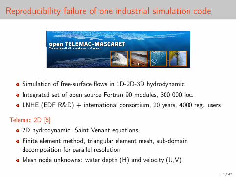
Simulation of free-surface flows in 1D-2D-3D hydrodynamic
Integrated set of open source Fortran 90 modules, 300 000 loc.
LNHE (EDF R&D) + international consortium, 20 years, 4000 reg. users
Telemac 2D [5]
2D hydrodynamic: Saint Venant equations
Finite element method, triangular element mesh, sub-domaindecomposition for parallel resolution
Mesh node unknowns: water depth (H) and velocity (U,V)
3 / 47

The Malpasset dam break: a reproducible simulation?
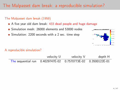
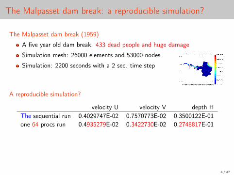
The Malpasset dam break (1959)
A five year old dam break: 433 dead people and huge damage
Simulation mesh: 26000 elements and 53000 nodes
Simulation: 2200 seconds with a 2 sec. time step
4 / 47
The Malpasset dam break: a reproducible simulation?
The Malpasset dam break (1959)
A five year old dam break: 433 dead people and huge damage
Simulation mesh: 26000 elements and 53000 nodes
Simulation: 2200 seconds with a 2 sec. time step
A reproducible simulation?
velocity U velocity V depth HThe sequential run 0.4029747E-02 0.7570773E-02 0.3500122E-01
4 / 47
The Malpasset dam break: a reproducible simulation?
The Malpasset dam break (1959)
A five year old dam break: 433 dead people and huge damage
Simulation mesh: 26000 elements and 53000 nodes
Simulation: 2200 seconds with a 2 sec. time step
A reproducible simulation?
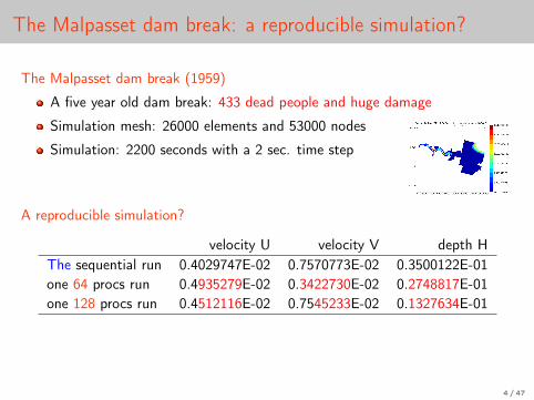
velocity U velocity V depth HThe sequential run 0.4029747E-02 0.7570773E-02 0.3500122E-01one 64 procs run 0.4935279E-02 0.3422730E-02 0.2748817E-01
4 / 47
The Malpasset dam break: a reproducible simulation?
The Malpasset dam break (1959)
A five year old dam break: 433 dead people and huge damage
Simulation mesh: 26000 elements and 53000 nodes
Simulation: 2200 seconds with a 2 sec. time step
A reproducible simulation?
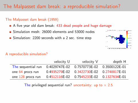
velocity U velocity V depth HThe sequential run 0.4029747E-02 0.7570773E-02 0.3500122E-01one 64 procs run 0.4935279E-02 0.3422730E-02 0.2748817E-01one 128 procs run 0.4512116E-02 0.7545233E-02 0.1327634E-01
4 / 47
The Malpasset dam break: a reproducible simulation?
The Malpasset dam break (1959)
A five year old dam break: 433 dead people and huge damage
Simulation mesh: 26000 elements and 53000 nodes
Simulation: 2200 seconds with a 2 sec. time step
A reproducible simulation?
velocity U velocity V depth HThe sequential run 0.4029747E-02 0.7570773E-02 0.3500122E-01one 64 procs run 0.4935279E-02 0.3422730E-02 0.2748817E-01one 128 procs run 0.4512116E-02 0.7545233E-02 0.1327634E-01
The privileged sequential run? uncertainty: up to × 2.5
4 / 47
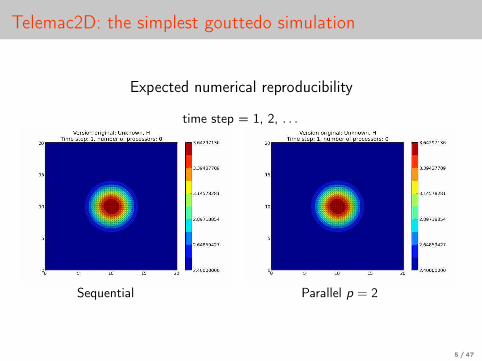
Telemac2D: the simplest gouttedo simulation
Expected numerical reproducibility
time step = 1, 2, . . .
Sequential Parallel p = 2
5 / 47
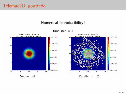
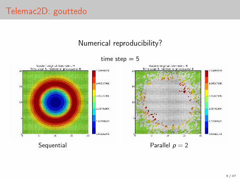
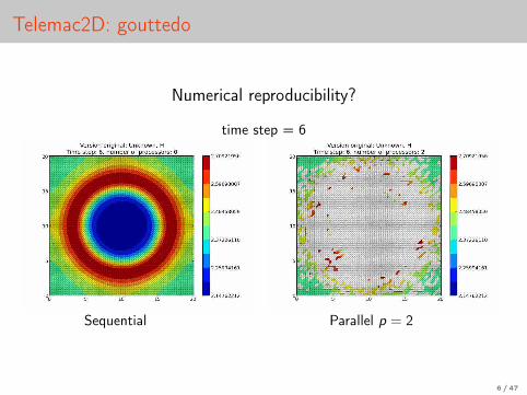
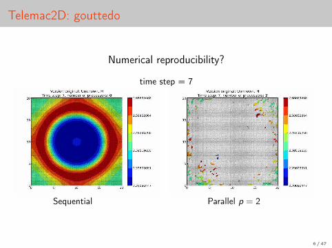
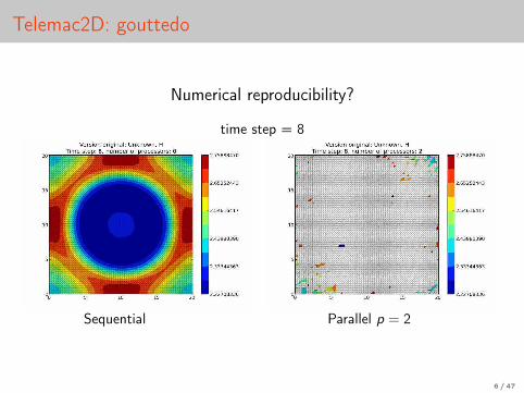
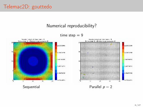
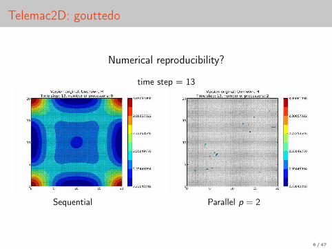
Telemac2D: gouttedo
Numerical reproducibility?
time step = 1
Sequential Parallel p = 2
6 / 47
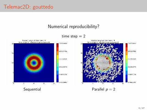
Telemac2D: gouttedo
Numerical reproducibility?
time step = 2
Sequential Parallel p = 2
6 / 47
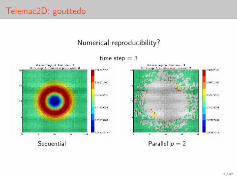
Telemac2D: gouttedo
Numerical reproducibility?
time step = 3
Sequential Parallel p = 2
6 / 47
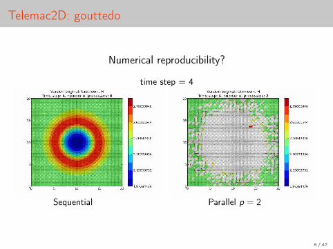
Telemac2D: gouttedo
Numerical reproducibility?
time step = 4
Sequential Parallel p = 2
6 / 47
Telemac2D: gouttedo
Numerical reproducibility?
time step = 5
Sequential Parallel p = 2
6 / 47
Telemac2D: gouttedo
Numerical reproducibility?
time step = 6
Sequential Parallel p = 2
6 / 47
Telemac2D: gouttedo
Numerical reproducibility?
time step = 7
Sequential Parallel p = 2
6 / 47
Telemac2D: gouttedo
Numerical reproducibility?
time step = 8
Sequential Parallel p = 2
6 / 47
Telemac2D: gouttedo
Numerical reproducibility?
time step = 9
Sequential Parallel p = 2
6 / 47
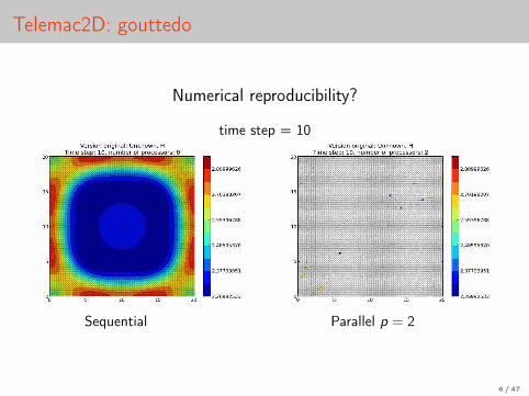
Telemac2D: gouttedo
Numerical reproducibility?
time step = 10
Sequential Parallel p = 2
6 / 47
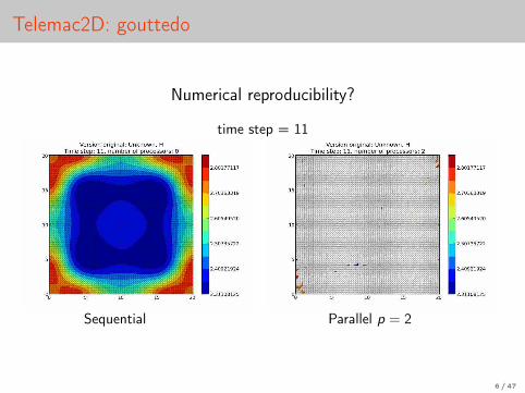
Telemac2D: gouttedo
Numerical reproducibility?
time step = 11
Sequential Parallel p = 2
6 / 47
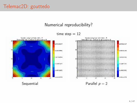
Telemac2D: gouttedo
Numerical reproducibility?
time step = 12
Sequential Parallel p = 2
6 / 47
Telemac2D: gouttedo
Numerical reproducibility?
time step = 13
Sequential Parallel p = 2
6 / 47
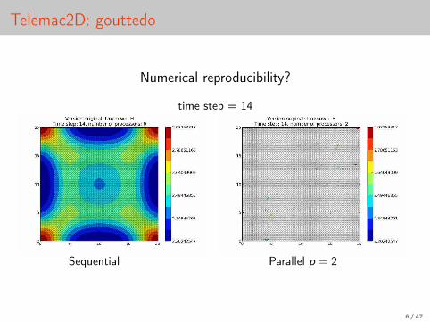
Telemac2D: gouttedo
Numerical reproducibility?
time step = 14
Sequential Parallel p = 2
6 / 47
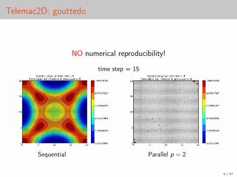
Telemac2D: gouttedo
Numerical reproducibility?
NO numerical reproducibility!
time step = 15
Sequential Parallel p = 2
6 / 47
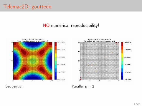
Telemac2D: gouttedo
NO numerical reproducibility!
Sequential Parallel p = 2
7 / 47
Numerical Reproducibility
1 Motivations
2 Basic ingredients
3 Recovering reproducibility in a finite element resolution
4 Efficient and reproducible BLAS 1
5 Conclusion and work in progress
8 / 47
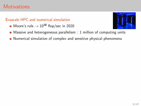
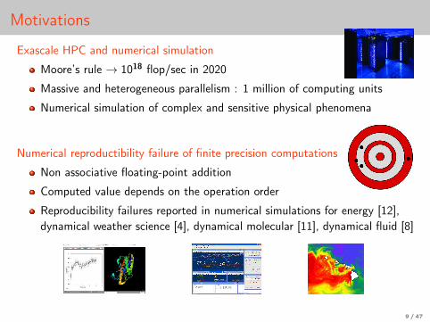
Motivations
Exascale HPC and numerical simulation
Moore’s rule → 1018 flop/sec in 2020
Massive and heterogeneous parallelism : 1 million of computing units
Numerical simulation of complex and sensitive physical phenomena
Numerical reproductibility failure of finite precision computations
Non associative floating-point addition
Computed value depends on the operation order
Reproducibility failures reported in numerical simulations for energy [12],dynamical weather science [4], dynamical molecular [11], dynamical fluid [8]
9 / 47
Reproducibility failure (1)
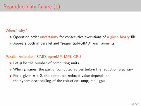
When? why?
Operation order uncertainty for consecutive executions of a given binary file
Appears both in parallel and “sequential+SIMD” environments
Parallel reduction: SIMD, openMP, MPI, GPU
Let p be the number of computing units
When p varies, the partial computed values before the reduction also vary
For a given p > 2, the computed reduced value depends onthe dynamic scheduling of the reduction: omp, mpi, gpu
10 / 47
Reproducibility failure (1)
When? why?
Operation order uncertainty for consecutive executions of a given binary file
Appears both in parallel and “sequential+SIMD” environments
Parallel reduction: SIMD, openMP, MPI, GPU
Let p be the number of computing units
When p varies, the partial computed values before the reduction also vary
For a given p > 2, the computed reduced value depends onthe dynamic scheduling of the reduction: omp, mpi, gpu
10 / 47
Reproducibility failure (2)
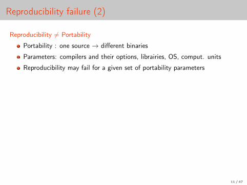
Reproducibility 6= Portability
Portability : one source → different binaries
Parameters: compilers and their options, librairies, OS, comput. units
Reproducibility may fail for a given set of portability parameters
Reproducibility 6= Accuracy
Reproducibility: bitwise identical results for every p-parallel run, p ≥ 1
Full accuracy = unit roundoff accuracy = bitwise exact result
Improving accuracy up to correct rounding ⇒ reproducibility
Reproducibility
Pros: numerical debug, validation, legal agreements
Cons: numerical debug, stochastic arithmetic
11 / 47
Reproducibility failure (2)
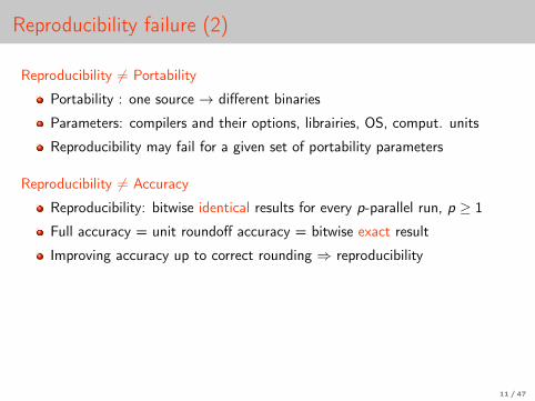
Reproducibility 6= Portability
Portability : one source → different binaries
Parameters: compilers and their options, librairies, OS, comput. units
Reproducibility may fail for a given set of portability parameters
Reproducibility 6= Accuracy
Reproducibility: bitwise identical results for every p-parallel run, p ≥ 1
Full accuracy = unit roundoff accuracy = bitwise exact result
Improving accuracy up to correct rounding ⇒ reproducibility
Reproducibility
Pros: numerical debug, validation, legal agreements
Cons: numerical debug, stochastic arithmetic
11 / 47
Reproducibility failure (2)
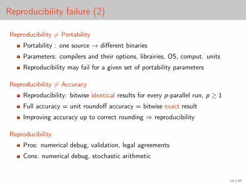
Reproducibility 6= Portability
Portability : one source → different binaries
Parameters: compilers and their options, librairies, OS, comput. units
Reproducibility may fail for a given set of portability parameters
Reproducibility 6= Accuracy
Reproducibility: bitwise identical results for every p-parallel run, p ≥ 1
Full accuracy = unit roundoff accuracy = bitwise exact result
Improving accuracy up to correct rounding ⇒ reproducibility
Reproducibility
Pros: numerical debug, validation, legal agreements
Cons: numerical debug, stochastic arithmetic
11 / 47
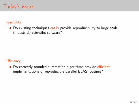
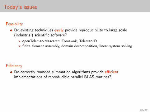
Today’s issues
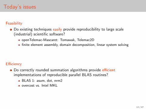
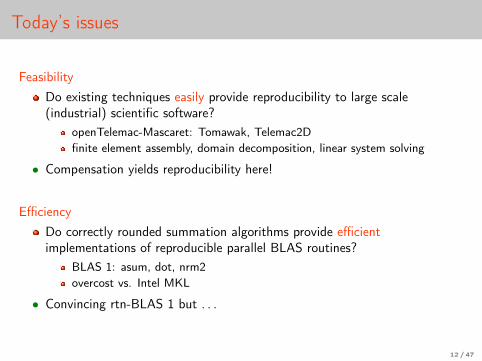
FeasibilityDo existing techniques easily provide reproducibility to large scale(industrial) scientific software?
openTelemac-Mascaret: Tomawak, Telemac2Dfinite element assembly, domain decomposition, linear system solving
• Compensation yields reproducibility here!
EfficiencyDo correctly rounded summation algorithms provide efficientimplementations of reproducible parallel BLAS routines?
BLAS 1: asum, dot, nrm2overcost vs. Intel MKL
• Convincing rtn-BLAS 1 but . . .
12 / 47
Today’s issues
FeasibilityDo existing techniques easily provide reproducibility to large scale(industrial) scientific software?
openTelemac-Mascaret: Tomawak, Telemac2Dfinite element assembly, domain decomposition, linear system solving
• Compensation yields reproducibility here!
EfficiencyDo correctly rounded summation algorithms provide efficientimplementations of reproducible parallel BLAS routines?
BLAS 1: asum, dot, nrm2overcost vs. Intel MKL
• Convincing rtn-BLAS 1 but . . .
12 / 47
Basic ingredients
1 Motivations
2 Basic ingredientsFinite element assembly: sequential and parallel casesSources of non reproducibility in Telemac2DCompensation
3 Recovering reproducibility in a finite element resolutionReproducible parallel FE assemblyReproducible conjugate gradient
4 Efficient and reproducible BLAS 1
5 Conclusion and work in progress
13 / 47
Basic ingredients
1 Motivations
2 Basic ingredientsFinite element assembly: sequential and parallel casesSources of non reproducibility in Telemac2DCompensation
3 Recovering reproducibility in a finite element resolutionReproducible parallel FE assemblyReproducible conjugate gradient
4 Efficient and reproducible BLAS 1
5 Conclusion and work in progress
14 / 47
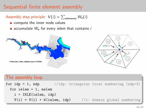
Sequential finite element assembly
Assembly step principle: V (i) =∑
elements We(i)compute the inner node valuesaccumulate We for every ielem that contains i
!"
!"#$$#
%&#
"!#
"#&# '
'#()*+,'-#
+#*+#
The assembly loopfor idp = 1, ndp //idp: triangular local numbering (ndp=3)for ielem = 1, nelemi = IKLE(ielem, idp)
<–- LOOP INDEX INDIRECTION
V(i) = V(i) + W(ielem, idp) //i: domain global numbering
15 / 47
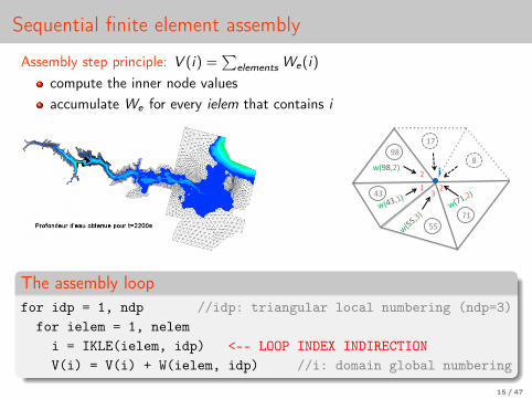
Sequential finite element assembly
Assembly step principle: V (i) =∑
elements We(i)compute the inner node valuesaccumulate We for every ielem that contains i
!"
!"#$$#
%&#
"!#
"#&# '
'#()*+,'-#
+#*+#
The assembly loopfor idp = 1, ndp //idp: triangular local numbering (ndp=3)for ielem = 1, nelemi = IKLE(ielem, idp) <–- LOOP INDEX INDIRECTIONV(i) = V(i) + W(ielem, idp) //i: domain global numbering
15 / 47
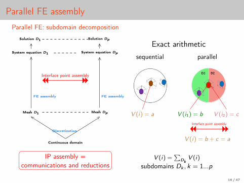
Parallel FE assembly
Parallel FE: subdomain decomposition
Solution D1
System equation D1
Mesh D1
Solution Dp
System equation Dp
Mesh Dp
Continuous domain
Interface point assembly
Discretization
FE assembly FE assembly
IP assembly =communications and reductions
Exact arithmeticsequential parallel
V (i) =∑
DkV (i)
subdomains Dk , k = 1...p
V (i) = a V (i1) = b V (i2) = c
V (i) = b + c = a
Interface point assembly
16 / 47
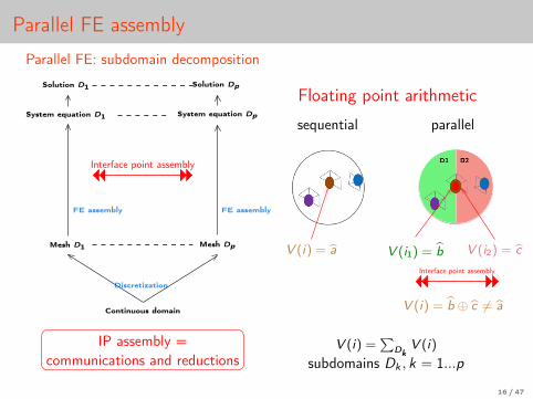
Parallel FE assembly
Parallel FE: subdomain decomposition
Solution D1
System equation D1
Mesh D1
Solution Dp
System equation Dp
Mesh Dp
Continuous domain
Interface point assembly
Discretization
FE assembly FE assembly
IP assembly =communications and reductions
Floating point arithmetic
sequential parallel
V (i) =∑
DkV (i)
subdomains Dk , k = 1...p
V (i) = a V (i1) = b V (i2) = c
V (i) = b ⊕ c 6= a
Interface point assembly
16 / 47
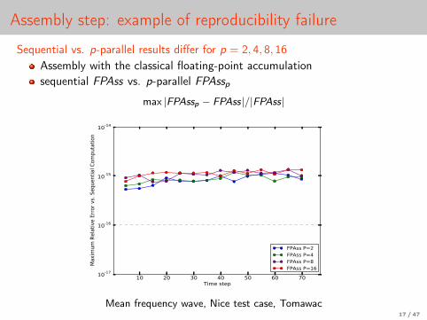
Assembly step: example of reproducibility failure
Sequential vs. p-parallel results differ for p = 2, 4, 8, 16Assembly with the classical floating-point accumulationsequential FPAss vs. p-parallel FPAssp
max |FPAssp − FPAss|/|FPAss|
10 20 30 40 50 60 70Time step
10-17
10-16
10-15
10-14
Maxi
mum
Rel
ativ
e Er
ror v
s. Se
quen
tial C
ompu
tatio
n
FPAss P=2FPAss P=4FPAss P=8FPAss P=16
Mean frequency wave, Nice test case, Tomawac17 / 47
Basic ingredients
1 Motivations
2 Basic ingredientsFinite element assembly: sequential and parallel casesSources of non reproducibility in Telemac2DCompensation
3 Recovering reproducibility in a finite element resolutionReproducible parallel FE assemblyReproducible conjugate gradient
4 Efficient and reproducible BLAS 1
5 Conclusion and work in progress
18 / 47
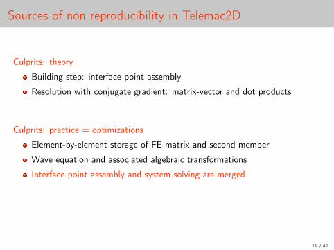
Sources of non reproducibility in Telemac2D
Culprits: theory
Building step: interface point assembly
Resolution with conjugate gradient: matrix-vector and dot products
Culprits: practice = optimizations
Element-by-element storage of FE matrix and second member
Wave equation and associated algebraic transformations
Interface point assembly and system solving are merged
19 / 47
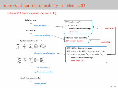
Sources of non reproducibility in Telemac2D
Telemac2D finite element method (FE)
Solution U,V
wave equation
conjugate gradient
Solution H
Interface node assembly:
AM1 in each iteration
CV 2 = Bu − AuhH,
CV 3 = Bv − AvhH.
Interface node assembly:
CV 2,CV 3
System equation Ay = b
AM2,AM3 : diagonal matrices,
AM1 = Ahh − AhuAM2−1Auh − AhvAM3−1Avh,
CV 1 = Bh − AhuAM2−1Bu − AhvAM3−1Bv ,
Interface node assembly:
AM2,AM3,CV 1
Ahh Ahu AhvAuh Auu 0Avh 0 Avv
H
UV
=
BhBuBv
algebraic transformation
AM1 0 00 AM2 00 0 AM3
HUV
=
CV1CV2CV3
Mesh (elements, nodes)
Continuous domain
Discretization
FE assembly +
algebraic computation
H
AM1,CV1
AM2,AM3
20 / 47
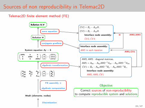
Sources of non reproducibility in Telemac2D
Telemac2D finite element method (FE)
Solution U,V
Interface node assembly:
AM1 in each iteration
CV 2 = Bu − AuhH,
CV 3 = Bv − AvhH.
Interface node assembly:
CV 2,CV 3
wave equation
conjugate gradient
Solution U,V
Solution H
ObjectiveCorrect sources of non-reproducibility
to compute reproducible system and solutions
System equation Ay = b
AM2,AM3 : diagonal matrices,
AM1 = Ahh − AhuAM2−1Auh − AhvAM3−1Avh,
CV 1 = Bh − AhuAM2−1Bu − AhvAM3−1Bv ,
Interface node assembly:
AM2,AM3,CV 1
Ahh Ahu AhvAuh Auu 0Avh 0 Avv
H
UV
=
BhBuBv
algebraic transformation
AM1 0 00 AM2 00 0 AM3
HUV
=
CV1CV2CV3
Mesh (elements, nodes)
Continuous domain
Discretization
FE assembly +
algebraic computation
H
AM1,CV1
AM2,AM3
20 / 47
Basic ingredients
1 Motivations
2 Basic ingredientsFinite element assembly: sequential and parallel casesSources of non reproducibility in Telemac2DCompensation
3 Recovering reproducibility in a finite element resolutionReproducible parallel FE assemblyReproducible conjugate gradient
4 Efficient and reproducible BLAS 1
5 Conclusion and work in progress
21 / 47
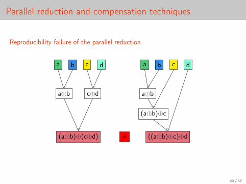
Parallel reduction and compensation techniques
Reproducibility failure of the parallel reduction
a b c d
a⊕b c⊕d
(a⊕b)⊕(c⊕d)
a b c d
a⊕b
(a⊕b)⊕c
((a⊕b)⊕c)⊕d6=
22 / 47
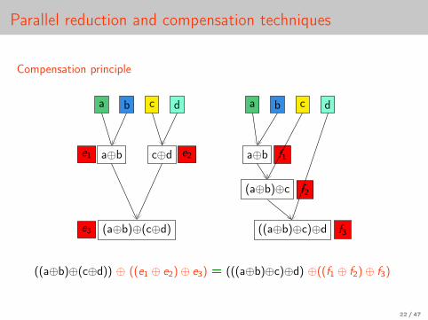
Parallel reduction and compensation techniques
Compensation principle
a b c d
a⊕be1 c⊕d e2
(a⊕b)⊕(c⊕d)e3
a b c d
a⊕b f1
(a⊕b)⊕c f2
((a⊕b)⊕c)⊕d f3
((a⊕b)⊕(c⊕d)) ⊕ ((e1 ⊕ e2)⊕ e3) = (((a⊕b)⊕c)⊕d) ⊕((f1 ⊕ f2)⊕ f3)
22 / 47
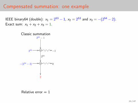
Compensated summation: one example
IEEE binary64 (double): x1 = 253 − 1, x2 = 253 and x3 = −(254 − 2).Exact sum: x1 + x2 + x3 = 1.
Classic summation
254
−1
0
253 − 1
253
−(254 − 2)
2
Relative error = 1
Compensation of the rounding errors
254
0
−1
253 − 1
253
−(254 − 2)
1
2
−1
The exact result is computed
23 / 47
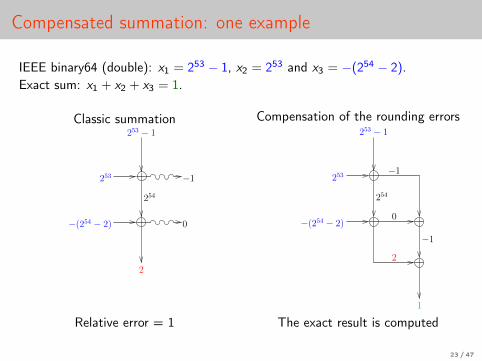
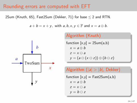
Rounding errors are computed with EFT
2Sum (Knuth, 65), Fast2Sum (Dekker, 71) for base ≤ 2 and RTN.
a + b = x + y , with a, b, x , y ∈ F and x = a⊕ b.
Algorithm (Knuth)
function [x,y] = 2Sum(a,b)x = a⊕ bz = x ay = (a (x z))⊕ (b z)
Algorithm (|a| > |b|, Dekker)function [x,y] = Fast2Sum(a,b)
x = a⊕ bz = x ay = b z
24 / 47

Other existing techniques
Existing techniques to recover numerical reproducibility in summation
Accurate compensated summation [6]
Demmel-Nguyen’s reproducible sums [3]
Integer convertion [7]
25 / 47
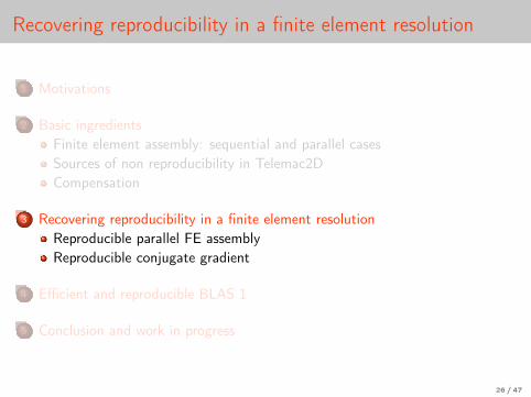
Recovering reproducibility in a finite element resolution
1 Motivations
2 Basic ingredientsFinite element assembly: sequential and parallel casesSources of non reproducibility in Telemac2DCompensation
3 Recovering reproducibility in a finite element resolutionReproducible parallel FE assemblyReproducible conjugate gradient
4 Efficient and reproducible BLAS 1
5 Conclusion and work in progress
26 / 47
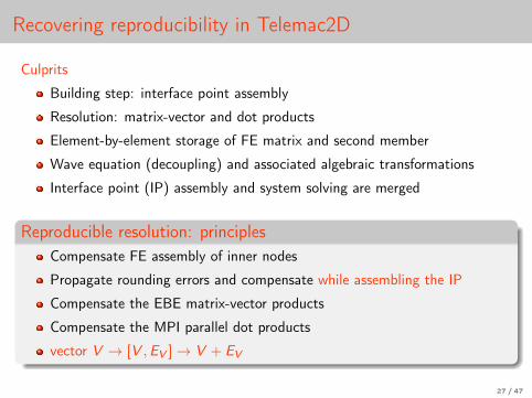
Recovering reproducibility in Telemac2D
Culprits
Building step: interface point assembly
Resolution: matrix-vector and dot products
Element-by-element storage of FE matrix and second member
Wave equation (decoupling) and associated algebraic transformations
Interface point (IP) assembly and system solving are merged
Reproducible resolution: principlesCompensate FE assembly of inner nodes
Propagate rounding errors and compensate while assembling the IP
Compensate the EBE matrix-vector products
Compensate the MPI parallel dot products
vector V → [V ,EV ]→ V + EV
27 / 47
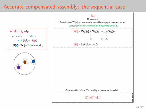
Accurate compensated assembly: the sequential case!"
!!!
"#$%!&! ! '%!
(#$%!&! )*! + ! '
"#$%&"#$%*(#$%
) + '
,(!-../0123!45'67$186$5'! %!957!/:/73!'5;/!0/.<!$!1/25'=$'=!65!/2/0/'6!/ /'!!
450>86-6$5'!-';!-??8082-6$5'!59!758';$'=!/7757.!
450>/'.-6$5'!59!6</!,(!-../0123!957!/:/73!0/.<!'5;/!@!
28 / 47
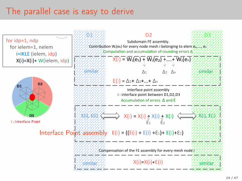
The parallel case is easy to derive
!"
!"#
$$#
%&#
'(#
"#&#
)#)#
*+'(,)-#
.#/#0123#+!",)-#
4+.-/4+.-5*+!",)-#
678#.9:/",#;9:####678#.<=<>/",#;<=<>#########./0123#+.<=<>,#.9:-############4+.-/4+.-5#?+.<=<>,#.9:-##
@3#A7;B8.CDE7;#B7#.;;<8#;79<F##
.9:/)#.<=<>/!"#
!"!!#$!%!
!!!!!
"#$%!&!"#$%!'!"#$%!'!"#$%!!!!!(#$%!&!##(#$%!'!(#$%!')*%'!(#$%')+%!!!!!!
"#$%!&!,-#./%!'!,-#.0%!'12'!,-#.3%!!!(#$%!&!4*'!4+'1'!43!
"#$%&"#$%'(#$%!
4*! 4+! 43!
)*! )+!
!56789:;$3!<(!;==.:7>?2!!@93AB$76C93!,-#.D%!E9B!.F.B?!398.!:.=G!$!7.>93H$3H!A9!.>.:!./I12I!.3!!
@9:J6A;C93!;38!;KK6:6>;C93!9E!B9638$3H!.BB9B=!4!!
L3A.BE;K.!J9$3A!;==.:7>?!!$!M!$3A.BE;K.!J9$3A!7.AN..3!O*IO+IOP!
QKK6:6>;C93!9E!.BB9B=!!4!;38!)!!
@9:J.3=;C93!9E!AG.!<(!;==.:7>?!E9B!.F.B?!:.=G!398.!$!
"#$%I!(#$%!"#$%I!(#$%!
=$:$>;B!
=$:$>;B! =$:$>;B!
=$:$>;B!
Interface Point assembly
29 / 47
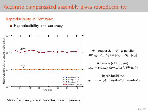
Accurate compensated assembly gives reproducibility
Reproducibility in Tomawac
Reproducibility and accuracy
10 20 30 40 50 60 70Time step
10-17
10-16
10-15
10-14
Maxi
mum
Rel
ativ
e Er
ror v
s. Se
quen
tial C
ompu
tatio
n
CompAss P=2CompAss P=4CompAss P=8CompAss P=16
CompAss P=2CompAss P=4CompAss P=8CompAss P=16
acc
rep
Mean frequency wave, Nice test case, Tomawac
As : sequential, Ap : p-parallelmaxrel (A1,A2) = |A1 − A2|/|A2|
Accuracy (of FPSum):acc = maxrel (CompAssp ,FPAsss)
Reproducibility:rep = maxrel (CompAssp ,CompAsss)
30 / 47
Recovering reproducibility in a finite element resolution
1 Motivations
2 Basic ingredientsFinite element assembly: sequential and parallel casesSources of non reproducibility in Telemac2DCompensation
3 Recovering reproducibility in a finite element resolutionReproducible parallel FE assemblyReproducible conjugate gradient
4 Efficient and reproducible BLAS 1
5 Conclusion and work in progress
31 / 47
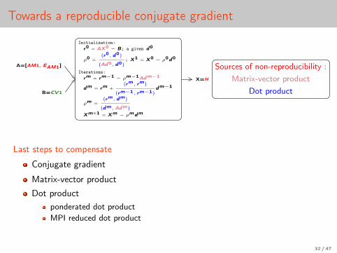
Towards a reproducible conjugate gradient
Initialization:r0 = AX0 − B; a given d0
ρ0 =(r0, d0)
(Ad0, d0); X1 = X0 − ρ0d0
Iterations:rm = rm−1 − ρm−1Adm−1
dm = rm +(rm, rm )
(rm−1, rm−1)dm−1
ρm =(rm, dm )
(dm,Adm )
Xm+1 = Xm − ρmdm
A=[AM1, EAM1]
B=CV1
X=H
Sources of non-reproducibility :Matrix-vector product
Dot product
Last steps to compensate
Conjugate gradient
Matrix-vector productDot product
ponderated dot productMPI reduced dot product
32 / 47
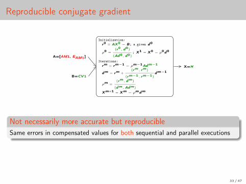
Reproducible conjugate gradient
Initialization:r0 = AX0 − B; a given d0
ρ0 =(r0, d0)
(Ad0, d0); X1 = X0 − ρ0d0
Iterations:rm = rm−1 − ρm−1Adm−1
dm = rm +(rm, rm )
(rm−1, rm−1)dm−1
ρm =(rm, dm )
(dm,Adm )
Xm+1 = Xm − ρmdm
A=[AM1, EAM1]
B=CV1
X=H
Not necessarily more accurate but reproducibleSame errors in compensated values for both sequential and parallel executions
33 / 47
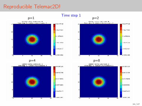
Reproducible Telemac2D!Time step 1
p=1 p=2
p=4 p=8
34 / 47
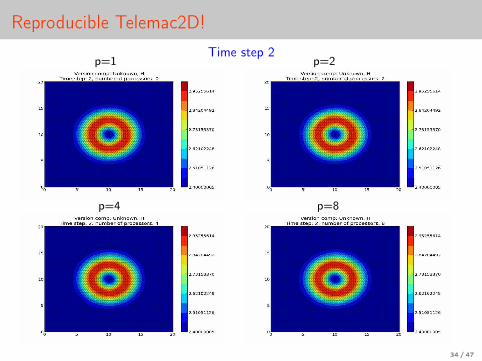
Reproducible Telemac2D!Time step 2
p=1 p=2
p=4 p=8
34 / 47
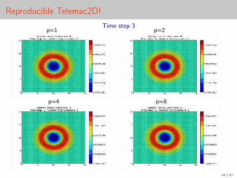
Reproducible Telemac2D!Time step 3
p=1 p=2
p=4 p=8
34 / 47
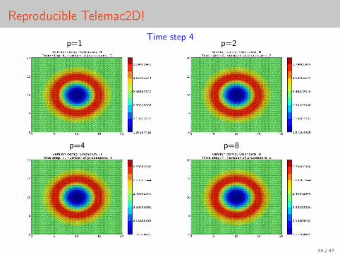
Reproducible Telemac2D!Time step 4
p=1 p=2
p=4 p=8
34 / 47
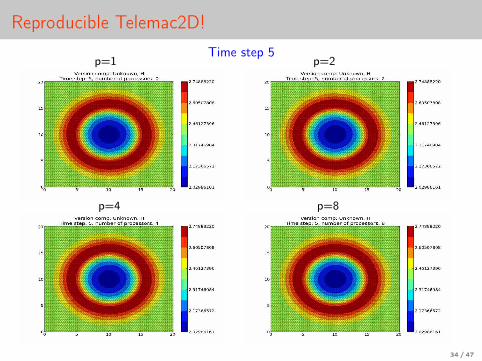
Reproducible Telemac2D!Time step 5
p=1 p=2
p=4 p=8
34 / 47
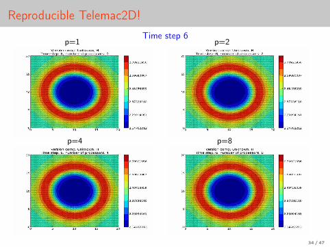
Reproducible Telemac2D!Time step 6
p=1 p=2
p=4 p=8
34 / 47
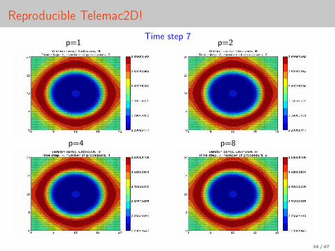
Reproducible Telemac2D!Time step 7
p=1 p=2
p=4 p=8
34 / 47
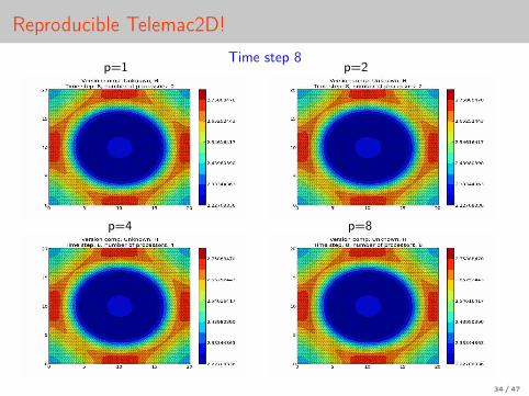
Reproducible Telemac2D!Time step 8
p=1 p=2
p=4 p=8
34 / 47
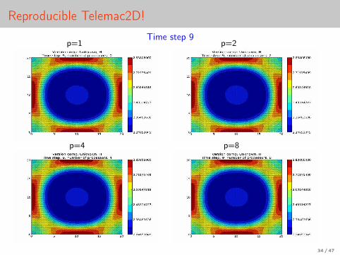
Reproducible Telemac2D!Time step 9
p=1 p=2
p=4 p=8
34 / 47
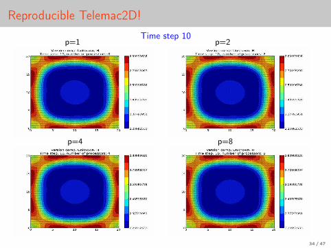
Reproducible Telemac2D!Time step 10
p=1 p=2
p=4 p=8
34 / 47
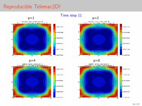
Reproducible Telemac2D!Time step 11
p=1 p=2
p=4 p=8
34 / 47
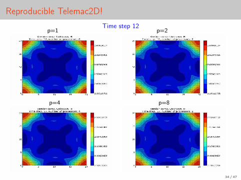
Reproducible Telemac2D!Time step 12
p=1 p=2
p=4 p=8
34 / 47
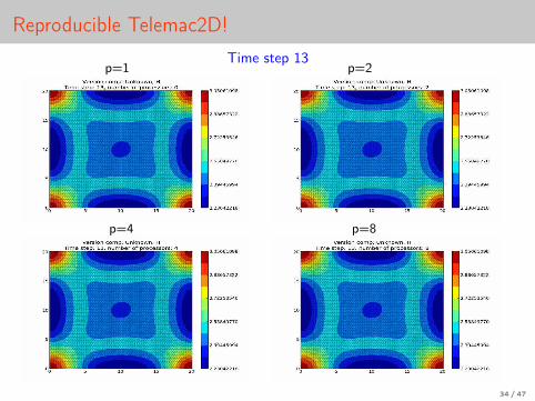
Reproducible Telemac2D!Time step 13
p=1 p=2
p=4 p=8
34 / 47
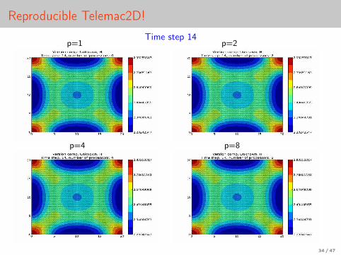
Reproducible Telemac2D!Time step 14
p=1 p=2
p=4 p=8
34 / 47
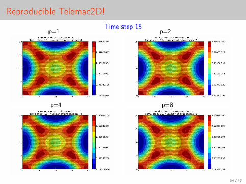
Reproducible Telemac2D!Time step 15
p=1 p=2
p=4 p=8
34 / 47
Efficient and reproducible BLAS 1
1 Motivations
2 Basic ingredientsFinite element assembly: sequential and parallel casesSources of non reproducibility in Telemac2DCompensation
3 Recovering reproducibility in a finite element resolutionReproducible parallel FE assemblyReproducible conjugate gradient
4 Efficient and reproducible BLAS 1
5 Conclusion and work in progress
35 / 47
Numerical reproducibility for the BLAS
BLAS + correctly rounded sums
Dot product of length n → sum of length 2n
A correctly rounded result is reproducible
A large panel of algorithms for faithful or correctly rounded sums
Motivation
How to benefit from these CR sums for reproducible BLAS?
Is the over-cost acceptable in practice for reproducible BLAS?
Current results
BLAS 1 : asum, dot, norm2
openMP for shared memory
Hybrid openMP-MPI for shared+distributed memory
36 / 47
Overview I
Our methodology
1 Optimization and choice of the best sequential CR sums2 Deriving parallel CR sums3 Application to reproducible BLAS-1 routines
The starting point: sequential summation algorithms
Accurate: Sum-K [6]
Faithful: AccSum [10], FastAccSum [9]
Correctly rounded (in RtN): iFastSum, HybridSum [14], OnlineExactsum [15]
37 / 47
Overview IIReproducible parallel BLAS-1: algorithmic choice
Rasum: parallel Sum K as in [13] with K = 2 for n ≤ 107.
Rdot: FastAccSum (small n) or modified OnLineExact (large n)
Rnrm2: Rdot+IEEE sqrt → reproducible only
All details in [1]Efficiency of Reproducible Level 1 BLAS,C. Chohra, Ph. L., D. Parello.SCAN 2014 Post-Conference ProceedingsLecture Notes of Computer Science (2015).http://hal-lirmm.ccsd.cnrs.fr/lirmm-01101723
38 / 47
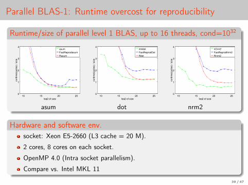
Parallel BLAS-1: Runtime overcost for reproducibility
Runtime/size of parallel level 1 BLAS, up to 16 threads, cond=1032
10 15 20 250
1
2
3
4
log2 of size
runtim
e(c
ycle
s)
/ siz
e
asum
FastReprodasum
Rasum
10 15 20 250
1
2
3
4
log2 of size
runtim
e(c
ycle
s)
/ siz
e
mkldot
FastReprodDot
Rdot
10 15 20 250
1
2
3
4
log2 of size
runtim
e(c
ycle
s)
/ siz
e
nOrm2
FastReprodNrm2
Rnrm2
asum dot nrm2
Hardware and software env.socket: Xeon E5-2660 (L3 cache = 20 M).
2 cores, 8 cores on each socket.
OpenMP 4.0 (Intra socket parallelism).
Compare vs. Intel MKL 11
39 / 47
Parallel BLAS-1: Scalability
Hardware and software env.OCCIGEN: 26th supercomputer in top500 list.
4212 cores, 12 cores on each socket.
OpenMP 4.0 (Intra socket parallelism).
OpenMPI (Inter socket communications).
40 / 47
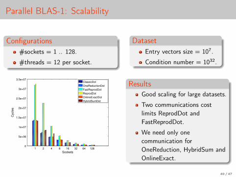
Parallel BLAS-1: Scalability
Configurations#sockets = 1 .. 128.
#threads = 12 per socket.
DatasetEntry vectors size = 107.
Condition number = 1032.
1 2 4 8 16 32 64 1280
5e+06
1e+07
1.5e+07
2e+07
2.5e+07
3e+07
3.5e+07
Sockets
Cycle
s
ClassicDot
OneReductionDot
FastReprodDot
ReprodDot
OnlineExactDot
HybridSumDot
ResultsGood scaling for large datasets.
Two communications costlimits ReprodDot andFastReprodDot.
We need only onecommunication forOneReduction, HybridSum andOnlineExact.
40 / 47
Time to conclude
1 Motivations
2 Basic ingredientsFinite element assembly: sequential and parallel casesSources of non reproducibility in Telemac2DCompensation
3 Recovering reproducibility in a finite element resolutionReproducible parallel FE assemblyReproducible conjugate gradient
4 Efficient and reproducible BLAS 1
5 Conclusion and work in progress
41 / 47
To conclude
Feasibility ?Do existing techniques easily provide reproducibility
to large scale industrial scientific software?
Efficiency ?Do correctly rounded summation algorithms provide
efficient implementations of reproducible parallel BLAS routines?
42 / 47
Conclusion I
Numerical reproducibility
How to remain confident facing the complexity of today’s computationalsystems? and tomorrow?
Sources: floating-point peculiarities and parallel reduction, data alignment,operator choices, compiler optimizations
Feasability
Existing techniques are efficient enough and more or less easy to apply
More precision, less errors or even exact computation
Reproducibility at the large scale: the openTelemac case
Complex, large and real simulations are tractable
Difficult to automatize but easier to pass the methodology on to softwaredeveloppers
Next step for Telemac 2D: more complex physical and numerical issues
43 / 47
Conclusion IIEfficiency
Convincing reproducible BLAS level 1
Hybrid openMP+MPI and scalability “in the large”
Current step: Intel MIC (Xeon Phi)
Next steps: BLAS-2, optimistic but BLAS-3, no future!
Numerical reproducibilty: cons/pros
Non reproducibility reveals bugs or numerical problems!
just return 1 ... it is reproducible indeed!
Reproducibility is one factor towards numerical quality . . . as theorems,experiments, tools that yields error bounds, stability conditions, accuracy
Reproducibility for the validation steps, not for the actual/operating mode
Sequential → parallel implementation: reproducibility = no more bug. . . both implementations can be wrong!
44 / 47
Références I
C. Chohra, P. Langlois, and D. Parello.Efficiency of Reproducible Level 1 BLAS.In SCAN 2014 Post-Conference Proceedings, Lecture Notes of Computer Science, pages 1–10,July 2015.
J. M. Corden and D. Kreitzer.Consistency of Floating-Point Results using the Intel Compiler or Why doesn’t my applicationalways give the same answer?Intel Corporation, Aug. 2014.
J. W. Demmel and H. D. Nguyen.Fast reproducible floating-point summation.In Proc. 21th IEEE Symposium on Computer Arithmetic. Austin, Texas, USA, 2013.
Y. He and C. Ding.Using accurate arithmetics to improve numerical reproducibility and stability in parallelapplications.J. Supercomput., 18:259–277, 2001.
J.-M. Hervouet.Hydrodynamics of free surface flows: Modelling with the finite element method.John Wiley & Sons, 2007.
T. Ogita, S. M. Rump, and S. Oishi.Accurate sum and dot product.SIAM J. Sci. Comput., 26(6):1955–1988, 2005.
45 / 47
Références II
Open TELEMAC-MASCARET. v.7.0, Release notes.www.opentelemac.org, 2014.
R. W. Robey, J. M. Robey, and R. Aulwes.In search of numerical consistency in parallel programming.Parallel Comput., 37(4-5):217–229, 2011.
S. M. Rump.Ultimately fast accurate summation.SIAM J. Sci. Comput., 31(5):3466–3502, 2009.
S. M. Rump, T. Ogita, and S. Oishi.Accurate floating-point summation – part I: Faithful rounding.SIAM J. Sci. Comput., 31(1):189–224, 2008.
M. Taufer, O. Padron, P. Saponaro, and S. Patel.Improving numerical reproducibility and stability in large-scale numerical simulations on gpus.In IPDPS, pages 1–9. IEEE, 2010.
O. Villa, D. G. Chavarría-Miranda, V. Gurumoorthi, A. Márquez, and S. Krishnamoorthy.Effects of floating-point non-associativity on numerical computations on massively multithreadedsystems.In CUG 2009 Proceedings, pages 1–11, 2009.
46 / 47
Références III
N. Yamanaka, T. Ogita, S. Rump, and S. Oishi.A parallel algorithm for accurate dot product.Parallel Comput., 34(6–8):392 – 410, 2008.
Y.-K. Zhu and W. B. Hayes.Correct rounding and hybrid approach to exact floating-point summation.SIAM J. Sci. Comput., 31(4):2981–3001, 2009.
Y.-K. Zhu and W. B. Hayes.Algorithm 908: Online exact summation of floating-point streams.ACM Trans. Math. Software, 37(3):37:1–37:13, Sept. 2010.
47 / 47