complexité du calcul de bases de gröbner pour les systèmes ... · complexité du calcul de bases...
TRANSCRIPT
Complexité du calcul de bases de Gröbnerpour les systèmes quasi-homogènes
Jean-Charles Faugère1 Mohab Safey El Din1,2
Thibaut Verron1,3
1Université Pierre et Marie Curie, Paris 6, FranceINRIA Paris-Rocquencourt, Équipe POLSYS
Laboratoire d’Informatique de Paris 6, UMR CNRS 7606
2Institut Universitaire de France
3École Normale Supérieure, Paris
16 mai 2013
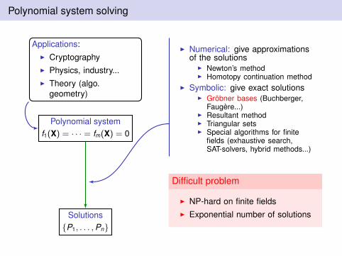
Polynomial system solving
Polynomial systemf1(X) = · · · = fm(X) = 0
Solutions{P1, . . . ,Pn}
Applications:I CryptographyI Physics, industry...I Theory (algo.
geometry)
I Numerical: give approximationsof the solutions
I Newton’s methodI Homotopy continuation method
I Symbolic: give exact solutionsI Gröbner bases (Buchberger,
Faugère...)I Resultant methodI Triangular setsI Special algorithms for finite
fields (exhaustive search,SAT-solvers, hybrid methods...)
Difficult problem
I NP-hard on finite fieldsI Exponential number of solutions
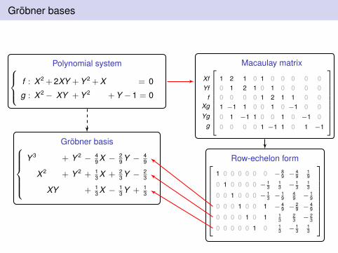
Gröbner bases
Polynomial system
f : X 2 +2XY +Y 2 +X = 0
g : X 2− XY +Y 2 +Y −1 = 0
Gröbner basis
Y 3 + Y 2 − 49 X − 2
9 Y − 49
X 2 + Y 2 + 13 X + 2
3 Y − 23
XY + 13 X − 1
3 Y + 13
Macaulay matrix
1 2 1 0 1 0 0 0 0 00 1 2 1 0 1 0 0 0 00 0 0 0 1 2 1 1 0 01 −1 1 0 0 1 0 −1 0 00 1 −1 1 0 0 1 0 −1 00 0 0 0 1 −1 1 0 1 −1
XfYf
fXg
Ygg
Row-echelon form
1 0 0 0 0 0 0 − 89 − 4
919
0 1 0 0 0 0 − 13
13 − 1
313
0 0 1 0 0 0 − 13 − 1
949 − 1
9
0 0 0 1 0 0 1 − 49 − 2
9 − 49
0 0 0 0 1 0 1 13
23 − 2
3
0 0 0 0 0 1 0 13 − 1
313
ProblematicStructured systems→ Can we exploit it?
Successfully studied structures
I Bihomogeneous (Dickenstein,Emiris, Faugère, Safey,Spaenlehauer...)
I Group symmetries (Colin,Faugère, Gattermann,Rahmany, Svartz...)
I Quasi-homogeneous?
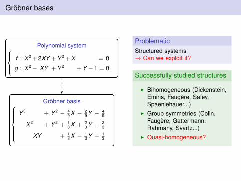

Quasi-homogeneous systems
Definition
System of weights: W = (w1, . . . ,wn) ∈ Nn
Weighted degree: degW (Xα11 . . .Xαn
n ) =∑n
i=1 wiαi
Quasi-homogeneous polynomial: poly. containing only monomials of same W -degree
e.g. X 2 + XY 2 + Y 4 for W = (2, 1)
I Homogeneous systems are W -homogeneous with weights (1, . . . , 1).
Applications
Physical system
Volume= Area×Height
Weight 3 Weight 2 Weight 1
Polynomial inversion
X = T 2 + U2
Y = T 3 − TU2
Z = T + 2U
P(X ,Y ,Z ) = 0
Weight 2
Weight 3Weight 1
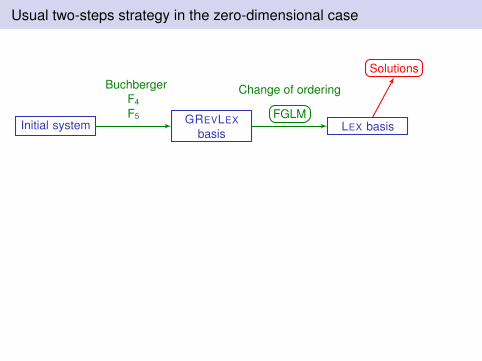
Usual two-steps strategy in the zero-dimensional case
Initial system GREVLEXbasis
LEX basis
F5
BuchbergerF4
F5 FGLM
Change of ordering
Solutions
ComplexityNumber of solutionsof the system
Highest degreereached by the comput.
Size of the built matrices
GoalUnder generic assumptions, complexity polynomial in the number of solutions
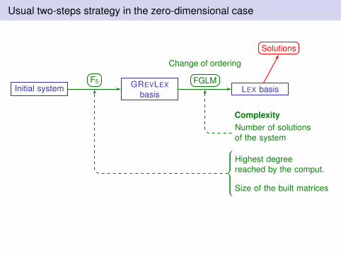
Usual two-steps strategy in the zero-dimensional case
Initial system GREVLEXbasis
LEX basisF5
BuchbergerF4
F5
FGLM
Change of ordering
Solutions
ComplexityNumber of solutionsof the system
Highest degreereached by the comput.
Size of the built matrices
GoalUnder generic assumptions, complexity polynomial in the number of solutions
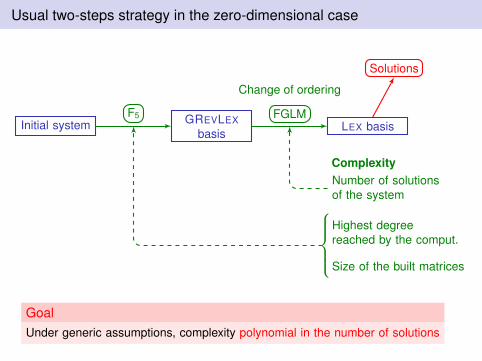
Usual two-steps strategy in the zero-dimensional case
Initial system GREVLEXbasis
LEX basisF5
BuchbergerF4
F5
FGLM
Change of ordering
Solutions
ComplexityNumber of solutionsof the system
Highest degreereached by the comput.
Size of the built matrices
GoalUnder generic assumptions, complexity polynomial in the number of solutions
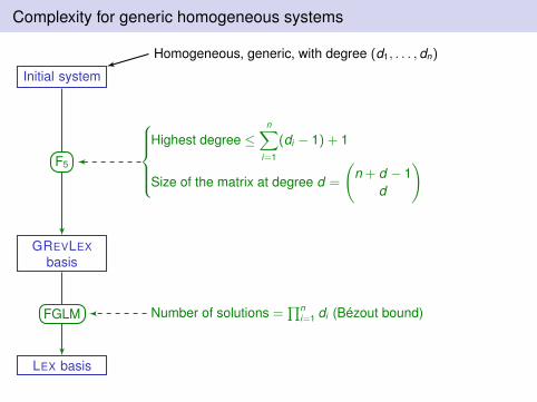
Complexity for generic homogeneous systems
Initial system
GREVLEXbasis
LEX basis
F5
FGLM
Homogeneous, generic, with degree (d1, . . . , dn)
Highest degree ≤n∑
i=1
(di − 1) + 1
Size of the matrix at degree d =
(n + d − 1
d
)
Number of solutions =∏n
i=1 di (Bézout bound)

Main results: strategy and complexity results
Initial system
Modifiedsystem
W -GREVLEXbasis of F
LEX basis
F5
FGLM
Homogeneous, with degree (d1, . . . , dn)
W -Homogeneous, generic,with W -degree (d1, . . . , dn)
W = (w1, . . . ,wn)
Highest W -degree
≤n∑
i=1
(di − 1) + 1−n∑
i=1
(wi − 1) + max{wj} − 1
≤n∑
i=1
(di − wi) + max{wj}
Size of the matrix at W -degree d ' 1∏ni=1 wi
(n + d − 1
d
)
Number of solutions =
∏ni=1 di∏ni=1 wi
(weighted Bézout bound)
Roadmap
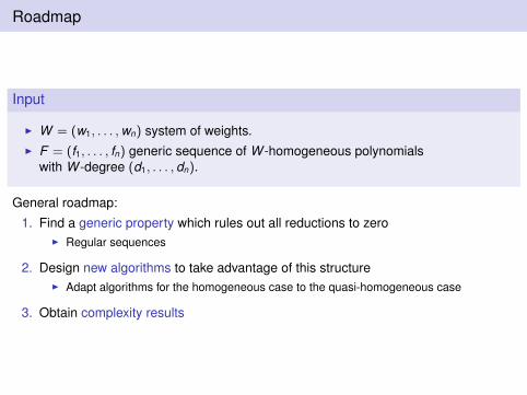
Input
I W = (w1, . . . ,wn) system of weights.I F = (f1, . . . , fn) generic sequence of W -homogeneous polynomials
with W -degree (d1, . . . , dn).
General roadmap:
1. Find a generic property which rules out all reductions to zeroI Regular sequences
2. Design new algorithms to take advantage of this structureI Adapt algorithms for the homogeneous case to the quasi-homogeneous case
3. Obtain complexity results
Regular sequences
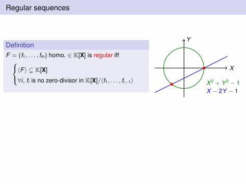
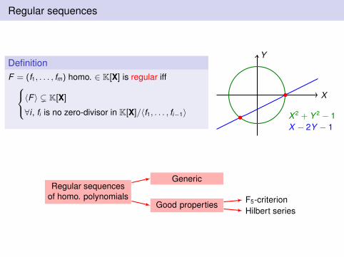
DefinitionF = (f1, . . . , fm) homo. ∈ K[X] is regular iff〈F 〉 ( K[X]
∀i , fi is no zero-divisor in K[X]/〈f1, . . . , fi−1〉
X
Y
X 2 + Y 2 − 1X − 2Y − 1
Regular sequencesof homo. polynomials
Generic
Good properties F5-criterionHilbert series
Result (Faugère, Safey, V.)
Regular sequences
DefinitionF = (f1, . . . , fm) homo. ∈ K[X] is regular iff〈F 〉 ( K[X]
∀i , fi is no zero-divisor in K[X]/〈f1, . . . , fi−1〉
X
Y
X 2 + Y 2 − 1X − 2Y − 1
Regular sequencesof homo. polynomials
Generic
Good properties F5-criterionHilbert series
Result (Faugère, Safey, V.)

Regular sequences
DefinitionF = (f1, . . . , fm) quasi-homo. ∈ K[X] is regular iff〈F 〉 ( K[X]
∀i , fi is no zero-divisor in K[X]/〈f1, . . . , fi−1〉
X
Y
X 2 + Y 2 − 1X − 2Y − 1
Regular sequencesof quasi-homo. polynomials
Generic if 6= ∅
Good properties F5-criterionHilbert series
Result (Faugère, Safey, V.)
From quasi-homogeneous to homogeneous
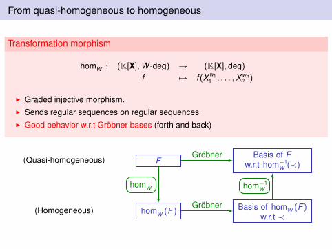
Transformation morphism
homW : (K[X],W -deg) → (K[X], deg)f 7→ f (X w1
1 , . . . ,X wnn )
I Graded injective morphism.I Sends regular sequences on regular sequencesI Good behavior w.r.t Gröbner bases (forth and back)
(Quasi-homogeneous) FBasis of F
w.r.t hom−1W (≺)
(Homogeneous) homW (F ) Basis of homW (F )w.r.t ≺
Gröbner
Gröbner
homW hom−1W

Adapting the algorithms
Detailed strategy
I F5 algorithm on the homogenized systemI FGLM algorithm on the quasi-homogeneous system
F W -GREVLEXbasis of F
homW (F )
GREVLEXbasis of
homW (F )
F5
homWhom−1
W

Adapting the algorithms
Detailed strategy
I F5 algorithm on the homogenized systemI FGLM algorithm on the quasi-homogeneous system
F W -GREVLEXbasis of F
∏ni=1 di∏ni=1 wi
solutions
homW (F )
GREVLEXbasis of
homW (F )
∏ni=1 di solutions
F5
homWhom−1
W
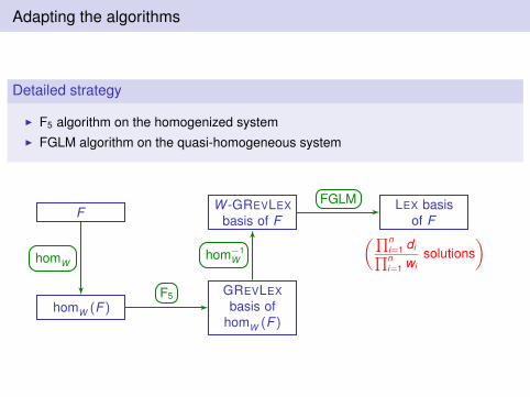
Adapting the algorithms
Detailed strategy
I F5 algorithm on the homogenized systemI FGLM algorithm on the quasi-homogeneous system
F W -GREVLEXbasis of F
LEX basisof F
homW (F )
GREVLEXbasis of
homW (F )
F5
FGLM
homWhom−1
W
(∏ni=1 di∏ni=1 wi
solutions)
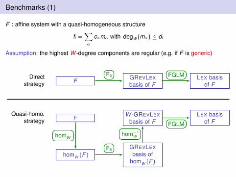
Benchmarks (1)
F : affine system with a quasi-homogeneous structure
fi =∑
α
cαmα with degW (mα) ≤ di
Assumption: the highest W -degree components are regular (e.g. if F is generic)
Directstrategy F GREVLEX
basis of FLEX basis
of F
Quasi-homo.strategy F W -GREVLEX
basis of FLEX basis
of F
homW (F )
GREVLEXbasis of
homW (F )
F5
FGLM
homWhom−1
W
F5 FGLM
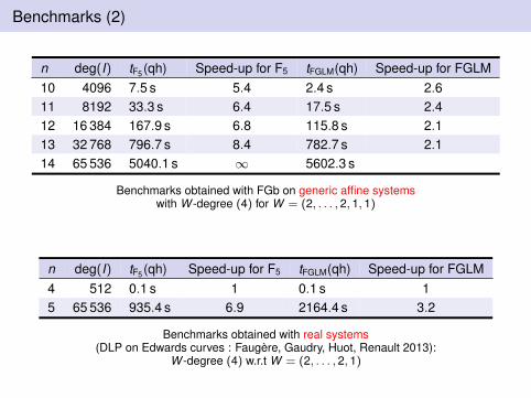
Benchmarks (2)
n deg(I) tF5 (qh) Speed-up for F5 tFGLM(qh) Speed-up for FGLM10 4096 7.5 s 5.4 2.4 s 2.611 8192 33.3 s 6.4 17.5 s 2.412 16 384 167.9 s 6.8 115.8 s 2.113 32 768 796.7 s 8.4 782.7 s 2.114 65 536 5040.1 s ∞ 5602.3 s
Benchmarks obtained with FGb on generic affine systemswith W -degree (4) for W = (2, . . . , 2, 1, 1)
n deg(I) tF5 (qh) Speed-up for F5 tFGLM(qh) Speed-up for FGLM4 512 0.1 s 1 0.1 s 15 65 536 935.4 s 6.9 2164.4 s 3.2
Benchmarks obtained with real systems(DLP on Edwards curves : Faugère, Gaudry, Huot, Renault 2013):
W -degree (4) w.r.t W = (2, . . . , 2, 1)
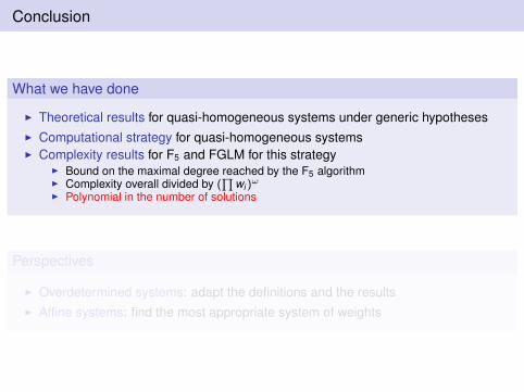
Conclusion
What we have done
I Theoretical results for quasi-homogeneous systems under generic hypothesesI Computational strategy for quasi-homogeneous systemsI Complexity results for F5 and FGLM for this strategy
I Bound on the maximal degree reached by the F5 algorithmI Complexity overall divided by (
∏wi )
ω
I Polynomial in the number of solutions
Perspectives
I Overdetermined systems: adapt the definitions and the resultsI Affine systems: find the most appropriate system of weights

One last word
Thank you for your attention!