representation of type 4 wind turbine …¨yekamara.pdf · universitÉ de montrÉal representation...

UNIVERSITÉ DE MONTRÉAL

REPRESENTATION OF TYPE 4 WIND TURBINE GENERATOR FOR

STEADY STATE SHORT-CIRCUIT CALCULATIONS

WOULÈYE KAMARA

DÉPARTEMENT DE GÉNIE ÉLECTRIQUE

ÉCOLE POLYTECHNIQUE DE MONTRÉAL

MÉMOIRE PRÉSENTÉ EN VUE DE L’OBTENTION

DU DIPLÔME DE MAÎTRISE ÈS SCIENCES APPLIQUÉES

(GÉNIE ÉLECTRIQUE)

DÉCEMBRE 2013

© Woulèye Kamara, 2013.

UNIVERSITÉ DE MONTRÉAL

ÉCOLE POLYTECHNIQUE DE MONTRÉAL

Ce mémoire intitulé:

REPRESENTATION OF TYPE 4 WIND TURBINE GENERATOR FOR STEADY STATE

SHORT-CIRCUIT CALCULATIONS

présenté par : KAMARA Woulèye

en vue de l’obtention du diplôme de : Maîtrise ès sciences appliquées

a été dûment accepté par le jury d’examen constitué de :

M. SAYDY Lahcen, Ph.D., président

M. MAHSEREDJIAN Jean, Ph.D., membre et directeur de recherche

M. SOUMARÉ Saidou, M.Sc.A., membre et codirecteur de recherche

M. KOCAR Ilhan, Ph.D., membre

iii

ACKNOWLEDGEMENTS

I would like to express my gratitude to all the people who contributed to any extent to the

fulfillment of this master thesis.

First, I would like to thank my research director, Professor Jean Mahseredjian for his valuable

guidance and constant support. He has early believed in the benefits of this research project and has

encouraged me since then.

I also wish to thank to my co-director and colleague, Saidou Soumare, for proposing this

research topic and for his constant support in the realization of this research project. His advices

and encouragements have contributed to the fulfillment of this project.

I would like to specially thank my manager, Marc Coursol, General Director of CYME

International T&D, for the support that he has provided me throughout these years, for his

guidance and for always encouraging me to undertake new challenges.

I am very grateful to my colleagues, Assane Gueye, Jean Sébastien Lacroix, Patrick

Jacques. This research wouldn’t have been the same without their valuable contribution and

feedback.

I am dedicating this work to my parents Nafissatou and Sadibou Kamara, and to my sister,

Khadijatou Kamara who have never stopped believing in me, and have provided me endless love and

support.

iv

RÉSUMÉ

Plusieurs impacts techniques sont associés à l'interconnexion des éoliennes au réseau électrique.

Parmi eux, l'augmentation du niveau de court-circuit du réseau ainsi que son impact sur la

coordination de protection a longtemps représenté un frein majeur à l'interconnexion de nouvelles

centrales éoliennes au réseau, particulièrement pour les réseaux à moyenne tension [1].

Compte tenu de l’intérêt grandissant pour les énergies renouvelables, les logiciels de calcul de

court-circuit utilisés à des fins de planification doivent permettre de mieux évaluer l'impact des

centrales éoliennes sur le niveau de court-circuit du réseau auquel elles sont connectées.

Malheureusement, très peu ont développé des modèles d’éoliennes à couplage électronique direct

dans le domaine fréquentiel qui estiment adéquatement leur contribution au courant de défaut.

La principale contribution de ce travail de recherche est le développement d'un modèle simple et

précis d’éolienne à couplage électronique direct pour les calculs de court-circuit en régime

permanent. Le modèle développé reproduit le comportement réel de l'éolienne en cas de défaut en

modélisant adéquatement l'effet du convertisseur. Les données utilisées pour le modèle sont

facilement accessibles aux ingénieurs de planification.

L’autre contribution de ce travail de recherche est le développement d'un algorithme de court-

circuit adapté pour prendre en charge le modèle d’éoliennes à couplage électronique direct

proposé. Un algorithme de court-circuit basé sur l'analyse-nodale-augmentée modifiée (MANA)

est résolu de manière itérative. L'algorithme est implémenté avec succès dans CYME, un logiciel

commercial d'analyse des réseaux. Il permet de reproduire la contribution de l’éolienne au

courant de défaut du réseau, y compris pour des réseaux complexes et débalancés.

L’étude détaillée du comportement d’une éolienne à couplage électronique direct à l'aide du

logiciel de transitoire électromagnétique EMTP-RV démontre que le modèle proposé reproduit

fidèlement le comportement réel de l'éolienne en court-circuit.

Le modèle proposé est ensuite implémenté dans le logiciel CYME 7.0 et validé pour différents

scénarios en utilisant le réseau de distribution 25 kV de Fortis Alberta. La contribution au courant

de défaut obtenue à partir du modèle proposé est comparée à celle obtenue à partir des modèles

actuels de CYME.

v

La validation montre que le modèle proposé permet de déterminer le courant de défaut de

l’éolienne à couplage électronique direct avec une meilleure précision que les modèles actuels de

CYME 7.0. En outre, la performance et la robustesse de l'algorithme de court-circuit développé

permettent d’analyser de grands réseaux débalancés, qui intègrent des éoliennes à couplage

électronique direct.

vi

ABSTRACT

Various technical impacts are associated to the interconnection of wind turbine generators to the

grid. Among them, the increase of short-circuit levels along with its effect on the settings of

protecting relays has long acted as an important inhibiting factor for the interconnection of new

wind power plants to the grid. This is especially true at the medium voltage level where networks

operate close to their short-circuit design value [1]. As renewable energies are progressively

replacing traditional power generation sources, short-circuit studies need to adequately assess the

impact of newly interconnected wind power plants on the fault level of the network.

For planning and design purposes, short-circuit studies are usually performed using steady-state

short-circuit programs. Unfortunately, very few have developed models of wind turbine

generators that accurately estimate their fault contribution in the phase domain. In particular, no

commercial fault-flow analysis program specifically addresses the modeling of inverter-based

wind turbine generators which behavior is based on the inverter’s characteristics rather than the

generator’s.

The main contribution of this research work is the development of a simplified and yet accurate

model of full-scale converter based wind turbine generator, also called Type 4 wind turbine

generator, for steady-state short-circuit calculations. The model reproduces the real behavior of

the Type 4 wind turbine generator under fault conditions by correctly accounting for the effect of

the full-scale converter. The data used for the model is easily accessible to planning engineers.

An additional contribution of this research work is the development of a short-circuit algorithm

adapted to support the proposed model of Type 4 wind-turbine generator. Short-circuit algorithm

based on modified-augmented-nodal analysis (MANA) is solved iteratively to accommodate the

proposed model. The algorithm is successfully implemented in CYME 7.0, a commercial

distribution system analysis program, to perform short-circuit calculations in multiphase complex

unbalanced systems.

Detailed study of the behavior of Type 4 wind turbine generator using electromagnetic type

programs like EMTP-RV has assessed that the proposed model closely reproduces the real

behavior of the wind turbine generator under steady-state fault conditions. The proposed model is

then implemented in CYME 7.0 and validated for different fault scenarios using the Fortis

Alberta 25 kV distribution system as benchmark. The fault contribution obtained from the

vii

proposed model is compared against the one obtained from the previous model implemented in

CYME 7.0. The validation test cases show that the proposed model estimates the fault

contribution of the wind turbine generator with better precision than the former models. Besides,

the performance and robustness of the short-circuit algorithm developed allow handling

unbalanced networks with inverter interfaced wind turbine generators as it is based on the

MANA formulation.

viii

TABLE OF CONTENTS

ACKNOWLEDGEMENTS .......................................................................................................... III

RÉSUMÉ ....................................................................................................................................... IV

ABSTRACT .................................................................................................................................. VI

TABLE OF CONTENTS ........................................................................................................... VIII

LIST OF TABLES ........................................................................................................................ XI

LIST OF FIGURES ......................................................................................................................XII

LIST OF NOTATIONS AND ABBREVIATIONS................................................................... XIV

CHAPITRE 1 INTRODUCTION ............................................................................................... 1

1.1 Background ...................................................................................................................... 1

1.2 Problem definition ............................................................................................................ 2

1.3 Objective and methodology ............................................................................................. 2

1.3.1 Objective ...................................................................................................................... 2

1.3.2 Methodology ................................................................................................................ 3

1.4 Report outline ................................................................................................................... 3

1.5 Original contribution ........................................................................................................ 4

CHAPITRE 2 DESCRIPTION OF TYPE 4 WTG ..................................................................... 5

2.1 Principles of energy conversion ....................................................................................... 5

2.2 Wind turbine control philosophies ................................................................................... 7

2.2.1 Passive stall control ...................................................................................................... 7

2.2.2 Pitch control ................................................................................................................. 8

2.3 Generator-converter description ....................................................................................... 8

2.4 Fault-ride through ............................................................................................................. 9

ix

2.4.1 Low voltage ride-through requirements ..................................................................... 10

2.4.2 Active power restoration ............................................................................................ 13

2.4.3 Reactive current injection for voltage support ........................................................... 13

CHAPITRE 3 DETAILED STUDY OF TYPE 4 WTG UNDER FAULT CONDITIONS .... 15

3.1 Description of the study network ................................................................................... 15

3.2 Fault contribution of Type 4 WTG under various fault conditions................................ 17

3.2.1 Three-phase fault (LLL) ............................................................................................. 17

3.2.2 Single line-to-ground fault (LG) ................................................................................ 21

CHAPITRE 4 SHORT-CIRCUIT ANALYSIS IN NETWORKS WITH TYPE 4 WTG ........ 25

4.1 Purpose of short-circuit studies ...................................................................................... 25

4.2 Literature review ............................................................................................................ 26

CHAPITRE 5 SHORT-CIRCUIT MANA MODEL FOR TYPE 4 WTG ............................... 32

5.1 Newton MANA method ................................................................................................. 33

5.2 Sub-transient model ........................................................................................................ 37

5.2.1 Controlled generator model ........................................................................................ 37

5.2.2 Current limiting constraint ......................................................................................... 41

5.3 Transient model .............................................................................................................. 43

5.4 Short-circuit algorithm ................................................................................................... 47

5.4.1 Short-circuit calculation methods ............................................................................... 47

5.4.2 MANA shunt fault models ......................................................................................... 48

5.4.3 Fault flow algorithm ................................................................................................... 51

CHAPITRE 6 MODEL VALIDATION ................................................................................... 58

6.1 Validation of the new model against detailed EMTP model ......................................... 58

6.1.1 Description of the study network ............................................................................... 58

x

6.1.2 Results and discussion ................................................................................................ 59

6.2 Comparison of the new model with the models in CYME 7.0 ...................................... 62

6.2.1 Description of the study network ............................................................................... 62

6.3 Fault contribution of Type 4 WTG under various fault conditions................................ 63

6.3.1 Three-phase fault at various locations ........................................................................ 63

6.3.2 Line-to-ground fault at various locations ................................................................... 66

CONCLUSION ............................................................................................................................. 69

xi

LIST OF TABLES

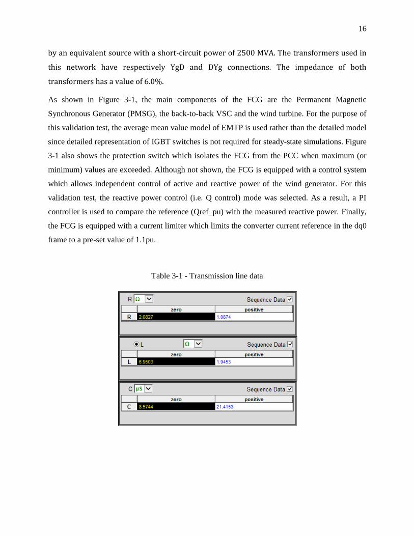
Table 3-1 - Transmission line data ................................................................................................. 16

xii

LIST OF FIGURES

Figure 2-1 : Cp coefficient as a function of λ and pitch angle in degrees [5]. .................................. 6

Figure 2-2 : Topology of Type 4 wind turbine generator [5] ........................................................... 9

Figure 2-3 : Minimum FRT requirements according to the E.ON grid code [10] ......................... 11

Figure 2-4 : Minimum FRT requirements according to Hydro-Québec grid code [32] ................ 12

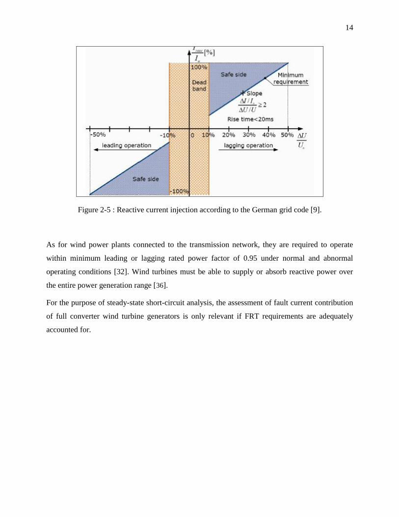
Figure 2-5 : Reactive current injection according to the German grid code [9]. ........................... 14

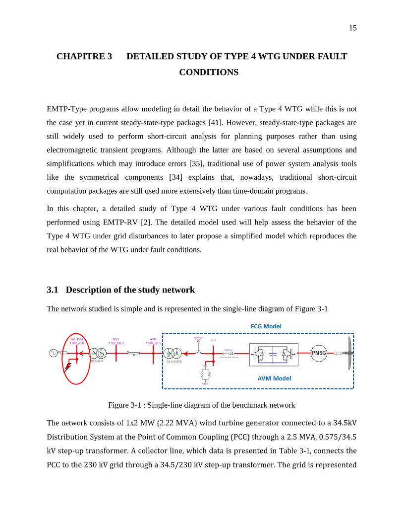
Figure 3-1 : Single-line diagram of the benchmark network ......................................................... 15

Figure 3-2 : Voltage at HV-AVM bus (PCC) for a LLL fault ....................................................... 18

Figure 3-3 : Fault current of the FCG (measured at the HV-AVM bus ) for a LLL fault.............. 18

Figure 3-4 : VSC current in the dq0 frame for a LLL fault ........................................................... 19

Figure 3-5 : Sequence currents of the FCG (at the HV-AVM bus) for a LLL fault ...................... 19

Figure 3-6 : Fault current of the FCG (at the LV side of its transformer) for a LLL fault ............ 20

Figure 3-7 : Sequence currents of the FCG (at the LV side of its transformer) for a LLL fault .... 21

Figure 3-8 : Voltage at HV-AVM bus (PCC) for a LG fault ......................................................... 21

Figure 3-9: Fault current of the FCG (measured at the HV-AVM bus ) for a LG fault................. 22

Figure 3-10 : VSC current in the dq0 frame for a LG fault ........................................................... 22

Figure 3-11 : Sequence currents of the FCG (measured at the HV-AVM bus) for a LG fault ...... 23

Figure 3-12 : Fault current of the FCG (at the LV side of its transformer) for a LG fault ............ 24

Figure 3-13 : Sequence currents of the FCG (at the LV side of its transformer) for a LG fault .... 24

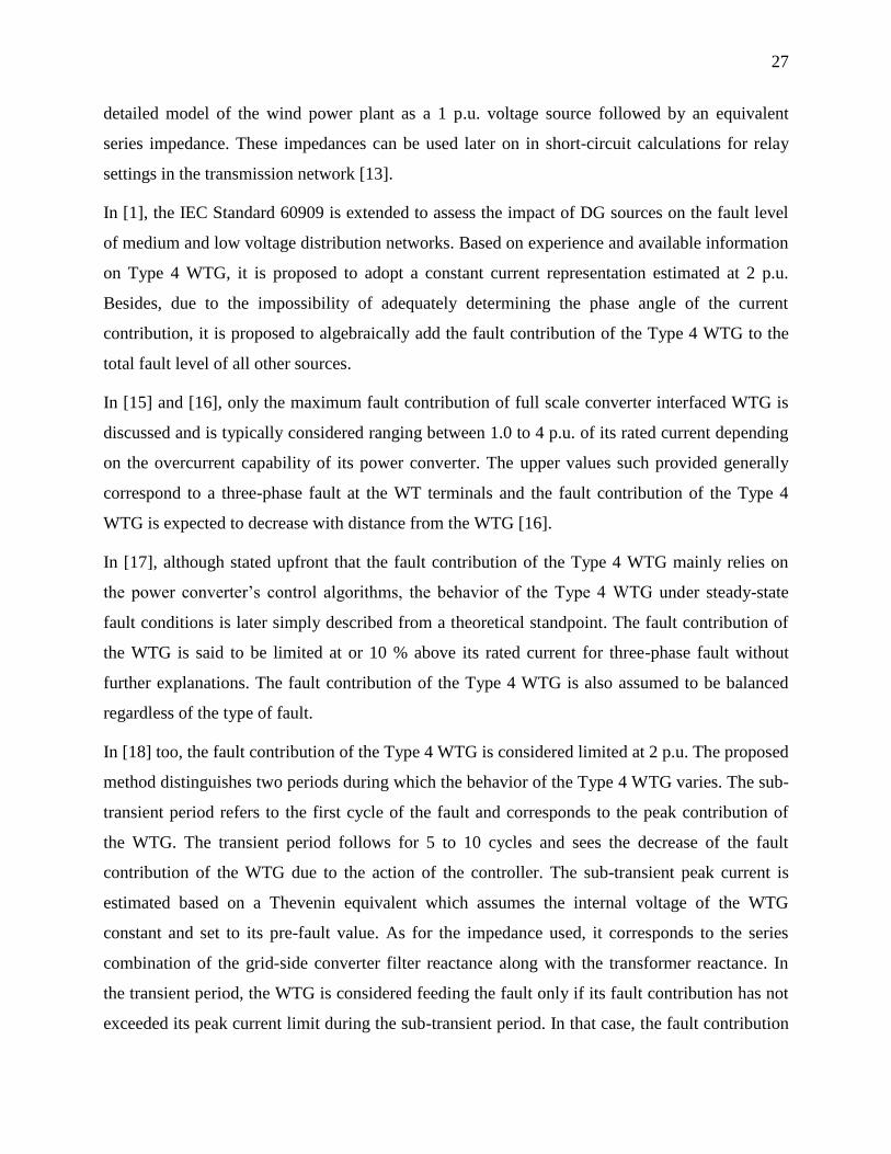
Figure 4-1 : Full converter based WTG model in CYME 7.0 ........................................................ 30

Figure 5-1 : Reactive current injection according to the German code [10]. ................................. 44

Figure 5-2 : Shunt Fault Representation with Impedance [33] ...................................................... 49

Figure 5-3 : MANA LG Fault Model ............................................................................................. 49

xiii

Figure 5-4 : MANA LLL Fault Model [33] ................................................................................... 50

Figure 5-5 : Initialization of the fault-flow algorithm. ................................................................... 54

Figure 5-6 : Fault-flow algorithm................................................................................................... 56

Figure 5-7 : Algorithm to check the WTG maximum fault contribution. ...................................... 57

Figure 6-1: Single-line diagram of the benchmark network .......................................................... 58

Figure 6-2 : Fault contribution of the FCG for a LG fault ............................................................. 59

Figure 6-3 : Fault contribution of the FCG for a LG fault ............................................................. 61

Figure 6-4: Equivalent representation of Fortis Alberta 25 kV distribution system. ..................... 62

Figure 6-5: Fault contribution of Type 4 WTG for LLL fault – Pdes = 436.5 kW ........................ 64

Figure 6-6 : Fault contribution of Type 4 WTG for LLL fault – Pdes = 150 kW .......................... 66

Figure 6-7 : Fault contribution of Type 4 WTG for LG fault – Pdes = 436.5 kW ......................... 67

Figure 6-8 : Fault contribution of Type 4 WTG for LG fault – Pdes = 150 kW ............................ 68

xiv

LIST OF NOTATIONS AND ABBREVIATIONS

FCG Full converter generator

FRT Fault ride-through

HV High voltage

LRT Low voltage ride-through

MANA Modified augmented nodal analysis

MV Medium voltage

PCC Point of common coupling

PWM Pulse width modulation

VSC Voltage source converter

WT Wind turbine

WTG Wind turbine generator

1

CHAPITRE 1 INTRODUCTION

Equation Chapter (Next) Section 1

This thesis presents a new model of full converter based wind generator for steady-state short-

circuit calculations. This chapter brings light to the reasons that motivated the need to develop

models of full converter based wind turbine generators, also named Type 4 WTG. It describes the

objectives of this research work and the methodology used to achieve them. The chapter also

provides a report outline and emphasizes the original contribution of the research work.

1.1 Background

Short-circuit studies are important to assess the impact of newly interconnected wind power

plants on the fault level of the system. When extending the generating capabilities of existing

networks, it is not uncommon that utilities worldwide choose to interconnect wind power plants

to an existing network since the price of oil has become unsustainable and the interest in

renewable energies is consistently increasing. Throughout the last decades, power utilities have

shown a major interest in distributed resources like wind power, solar panels, fuel cells, etc.

Among these resources, wind power stands out as the fastest growing source of renewable energy

worldwide with an average growth rate of 25.7% in ten years [14]. Actually, the penetration level

of wind energy conversion systems (WECS) has reached a point where it is important to assess

their impact on electrical networks. Their fault contribution has long been ignored since wind

turbine generators were supposed to disconnect after a fault. However, with the increased

penetration level of wind power, utilities are forced to revise their grid code requirements and

wind generators are now expected to support the grid voltage during a fault. For this reason, their

contribution to the fault level of the network can no longer be disregarded.

Therefore, in order to keep guarantying the safe and reliable operation of networks dominated

with grid-connected inverters, power analysis programs should closely reproduce the real

behavior of wind turbines, especially during abnormal operating conditions.

2

1.2 Problem definition

Electromagnetic Transient type programs like EMTP-RV [2] already provide accurate models of

WECS to estimate their contribution under abnormal conditions. However, these models are

fairly complex and require data which may not be accessible to distribution and planning

engineers. In particular, details of the inverter are often held closely by manufacturer. The same

is true for stability-type programs like CYMSTAB [42]. As a consequence, steady-state short-

circuit programs are widely used to perform short-circuit studies of electrical networks.

Steady-state short-circuit programs are based on standards, namely IEC 60909 [3] and IEEE

C37.010 [12], IEEE C37.5 [4], etc.., when it comes to modeling equipment for short-circuit

analysis purposes. Although the analytical equations provided by the actual standards have been

revised to cover the modeling of most representative distributed generation sources, they still do

not include the fault contribution of electronically coupled wind turbine generators with adequate

accuracy. In the literature as well ([21], [24], [25]), few models accurately reproduce the effect of

the grid side converter on the fault contribution of the wind generator. Most of these models also

ignore the fault ride-through requirements of wind generators which, in many national grid codes,

have become essential to effectively assess their fault contribution. With the fast progress of grid-

connected inverter based generators, it is therefore clear that the need to model them accurately is

crucial to better assess their contribution to the short-circuit level of electrical networks.

1.3 Objective and methodology

1.3.1 Objective

The purpose of this research work is to develop a simplified model of full converter based wind

turbine generator for steady-state short-circuit analysis. The proposed model should accurately

account for the effect of the grid side converter and use data easily accessible to planning

engineers. Moreover, it should be sensitive to applicable fault ride through requirements. Finally,

traditional short-circuit algorithms must be adapted to support the proposed model of wind

turbine generator and closely reproduce its fault current contribution under steady-state abnormal

operating conditions. In this research work, the modeling of the DFIG has not been addressed

since the current models in CYME 7.0 are adequate enough and correctly represent the crowbar

protection.

3

1.3.2 Methodology

To achieve the objectives previously set, an exhaustive literature review of the methodologies

available to represent a full converter based wind turbine generator under steady-state fault

conditions, is carried out first. Then, a detailed analysis of the Type 4 WTG under fault

conditions is performed using the detailed models in the electromagnetic type program EMTP-

RV. Based on the observed behavior, a simplified model of full converter based wind turbine

generator is developed, accounting for the effect of the grid side converter. In accordance with

the objectives set, the model uses accessible data and allows estimating the fault contribution of

the wind generator in accordance with the fault ride through requirements set by applicable grid

codes. The proposed model also accounts for the control strategy applied to the wind turbine

generator prior to the fault. The model developed is afterwards adapted to an iterative short-

circuit calculations algorithm based on the modified-augmented-nodal analysis (MANA)

approach [28]. Finally, the model is validated for different fault scenarios using the Fortis Alberta

25 kV distribution system as benchmark. Results obtained are validated against the results

provided by the former models developed in CYME 7.0. Validation test cases assess that the

model and algorithm developed closely reproduce the fault contribution of the Type 4 WTG

during fault conditions.

1.4 Report outline

The present thesis is organized into six chapters.

Chapter 1 introduces the reasons that motivated the need to accurately assess the fault

contribution of a full converter based wind generator. It also describes the objectives of the

research work along with the methodology used to achieve them.

Chapter 2 describes in details the components of a Type 4 WTG. It also reviews the FRT

requirements specific to national grid codes.

Chapter 3 assesses the behavior of a Type 4 WTG under fault conditions through an extensive

analysis performed using the detailed models implemented in EMTP-RV.

Chapter 4 explains the purpose of short-circuit studies and reviews the different models of Type 4

WTG proposed in literature, highlighting their scopes and limitations.

4

Chapter 5 presents the model of Type 4 WTG and the algorithm developed to estimate the

steady-state fault contribution of a wind turbine generator. Effect of fault ride-through

requirements and pre-fault control strategies are also taken into account in the proposed model.

Chapter 6 presents the test cases used to validate the proposed model and algorithm along with

the results of the comparison performed between the proposed model and the models

implemented in CYME 7.0, a commercial program for distribution networks analysis.

1.5 Original contribution

The main contribution of this research work is the development of accurate but yet simple models

of Type 4 WTG for steady-state short-circuit calculations. The modelaccounts for the pre-fault

control operating set-points and the applicable fault ride through requirements. Hence, it

accurately reproduces the effect of the grid side converter on the generator’s fault current

contribution. The other main contribution of this research work consists in adapting a MANA

based algorithm presented in [28] to support the proposed model of Type 4 WTG for short-circuit

analysis and accurately assess the impact of these types of generators on the fault current level of

networks to which they are connected.

5

CHAPITRE 2 DESCRIPTION OF TYPE 4 WTG


2.1 Principles of energy conversion

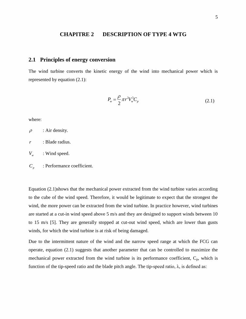
The wind turbine converts the kinetic energy of the wind into mechanical power which is

represented by equation (2.1):

2 3

2w w pP r V C

(2.1)

where:

: Air density.

r : Blade radius.

wV : Wind speed.

pC : Performance coefficient.

Equation (2.1)shows that the mechanical power extracted from the wind turbine varies according

to the cube of the wind speed. Therefore, it would be legitimate to expect that the strongest the

wind, the more power can be extracted from the wind turbine. In practice however, wind turbines

are started at a cut-in wind speed above 5 m/s and they are designed to support winds between 10

to 15 m/s [5]. They are generally stopped at cut-out wind speed, which are lower than gusts

winds, for which the wind turbine is at risk of being damaged.

Due to the intermittent nature of the wind and the narrow speed range at which the FCG can

operate, equation (2.1) suggests that another parameter that can be controlled to maximize the

mechanical power extracted from the wind turbine is its performance coefficient, Cp, which is

function of the tip-speed ratio and the blade pitch angle. The tip-speed ratio, λ, is defined as:

6

t

w

r

V

(2.2)

where:

t : Turbine rotational speed.

As for the blade pitch angle, it can be controlled through different strategies described hereafter.

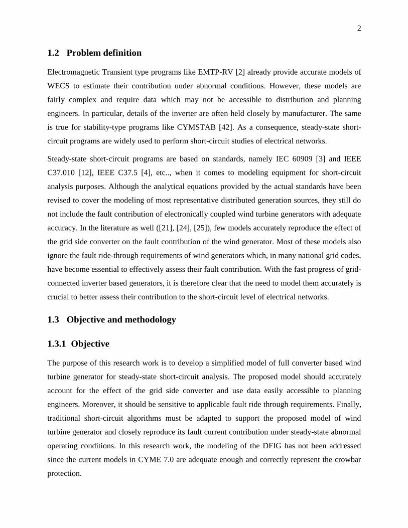
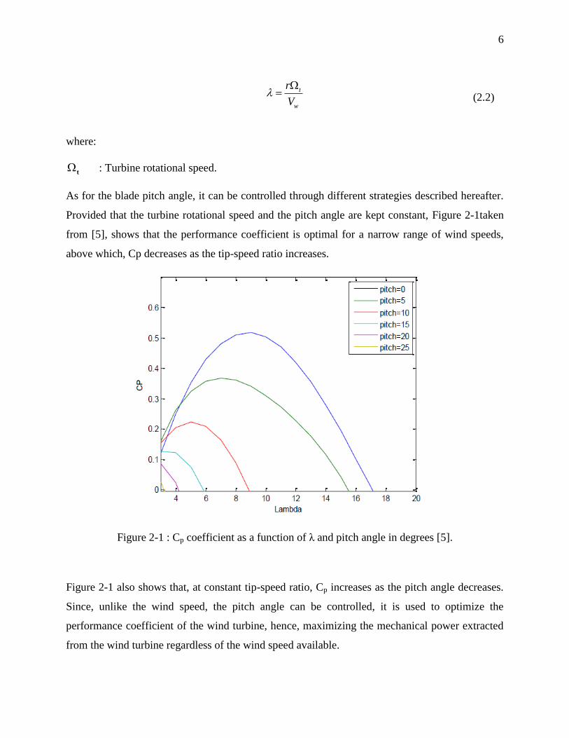
Provided that the turbine rotational speed and the pitch angle are kept constant, Figure 2-1taken

from [5], shows that the performance coefficient is optimal for a narrow range of wind speeds,

above which, Cp decreases as the tip-speed ratio increases.

Figure 2-1 : Cp coefficient as a function of λ and pitch angle in degrees [5].

Figure 2-1 also shows that, at constant tip-speed ratio, Cp increases as the pitch angle decreases.

Since, unlike the wind speed, the pitch angle can be controlled, it is used to optimize the

performance coefficient of the wind turbine, hence, maximizing the mechanical power extracted

from the wind turbine regardless of the wind speed available.

7

Theoretically, due to the effect of the wind turbine on the wind velocity, wind turbines can

capture at most 59% of the wind power available. This is called the Betz’s limit [43]. In practice

however, only 40 to 50% of the wind power is extracted by current wind turbines.

2.2 Wind turbine control philosophies

For a given wind speed, it is clear from equation (2.1) that the only parameter that allows

controlling the power extracted from the wind turbine is the performance coefficient Cp. Based on

this principle, various active or passive control strategies are developed in order to optimize the

power extracted from the wind turbine at given wind speeds.

In particular, at high wind speeds (before the cut-out speed), wind turbines employ these control

strategies to waste part of the excess energy of the wind in order to keep producing energy

without damaging the turbine.

The main control strategies currently used for power regulation are described hereafter.

2.2.1 Passive stall control

The blades of passive stall controlled wind turbines are aerodynamically designed to produce

turbulence beyond a specific wind speed, gradually increasing the angle of attack of the blades

until leading the blades to stall. At high wind speeds, this mechanism allows limiting the

mechanical power produced by the wind turbine to protect it from possible damages without the

need for active controls. In this type of control, the pitch angle is fixed, hence the low

maintenance cost associated to less mechanically moving elements compared to pitch regulated

wind turbines. However, the drawback of this power regulation strategy is that, above nominal

wind speed, it leads to a drop below nominal power. Besides, a significant disadvantage of stall-

regulated wind turbines is the voltage flicker produced as a result of the sensitivity of the turbine

torque to any slight change in the wind speed. This is true especially when the wind turbine is

connected to a weak power system [5].

8

2.2.2 Pitch control

Pitch controlled wind turbines are equipped with a closed-loop rotor speed controller which

regulates the pitch angle of the rotor blades to optimize the mechanical power delivered by the

wind turbine according to the wind speed variations [6]. As a result, depending on the wind

speed, the rotor blades are either pitched toward the wind to maximize the wind energy capture or

turned out of the wind to protect the wind turbine from excessive mechanical stress. During

normal operation for which the wind speed ranges from start-up to nominal wind speed, the pitch

angle is adjusted to optimize Cp, thus, optimize the power output of the turbine. At high winds,

unlike stall controlled wind turbines for which the power output drops with wind speed, the

blades of pitch regulated wind turbines are adjusted to allow maintaining a constant nominal

power output [5].

2.3 Generator-converter description

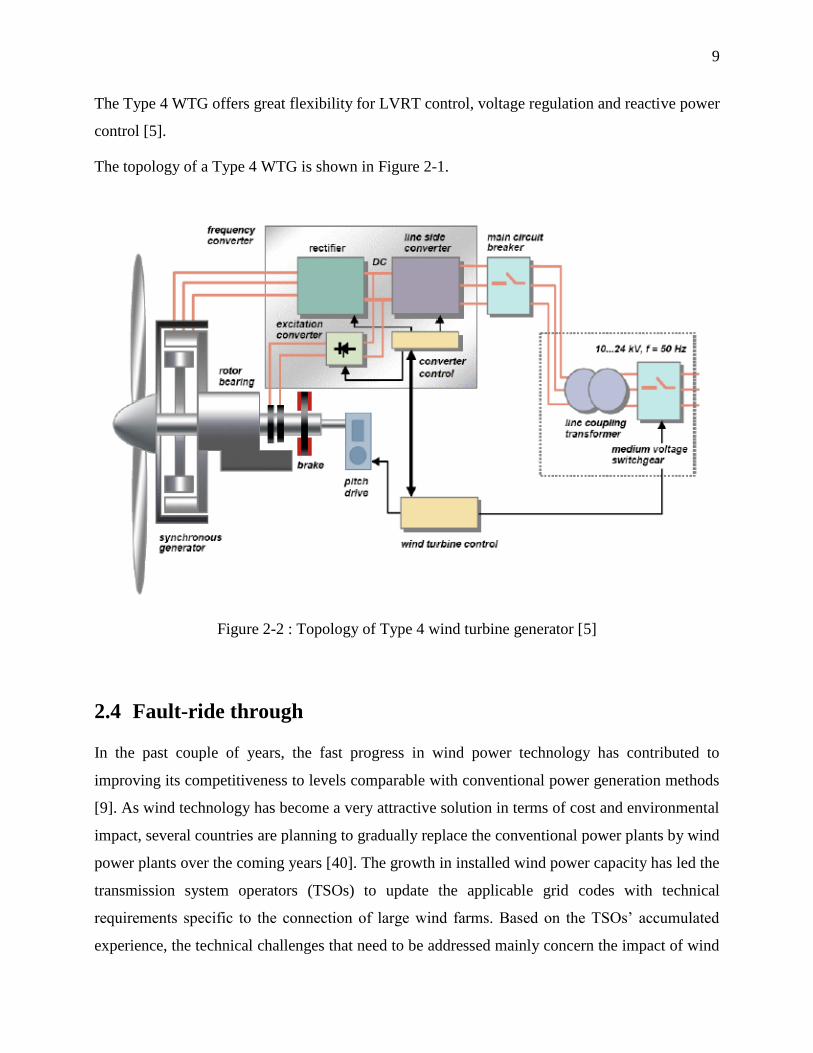
A type 4 WTG is composed of a variable-speed wind turbine generator which stator is connected

to the grid via a full scale back-to-back converter. A permanent magnet generator is generally

used in this type of configuration. However, a wound rotor generator or an induction generator

can be used as well.

The full scale frequency converter is composed of back-to-back voltage source converters: an

AC-to-DC rectifier and a DC-to-AC inverter. It allows operating the wind turbine within a wide

range of frequencies which vary according to the prevailing wind conditions. In particular, the

purpose of the grid-side converter is not only to convert the operating frequency of the WTG to

the grid frequency but also to decouple the grid from the WTG. Hence, during grid disturbances,

the mechanical dynamic of the WTG is isolated from the grid transient dynamic [17], allowing

more effective management of mechanical loads [26].

The power converter allows controlling the real and reactive powers independently, within the

margin of the maximum converter’s current. In practice, the power converter is designed with an

overload capability of 10% above rated current [17]. The active power control allows optimizing

the performance of the WTG for various prevailing wind conditions whereas the reactive power

control is used for voltage regulation at the PCC or at a more distant node [10], [17].

9

The Type 4 WTG offers great flexibility for LVRT control, voltage regulation and reactive power

control [5].

The topology of a Type 4 WTG is shown in Figure 2-1.

Figure 2-2 : Topology of Type 4 wind turbine generator [5]

2.4 Fault-ride through

In the past couple of years, the fast progress in wind power technology has contributed to

improving its competitiveness to levels comparable with conventional power generation methods

[9]. As wind technology has become a very attractive solution in terms of cost and environmental

impact, several countries are planning to gradually replace the conventional power plants by wind

power plants over the coming years [40]. The growth in installed wind power capacity has led the

transmission system operators (TSOs) to update the applicable grid codes with technical

requirements specific to the connection of large wind farms. Based on the TSOs’ accumulated

experience, the technical challenges that need to be addressed mainly concern the impact of wind

10

power plants on grid stability, power quality and their behavior during fault situations. In the

latter case, grid codes require wind power plants to remain connected during and after a fault to

ensure fast restoration of the active power to the pre-fault levels right after fault clearance [10].

Besides, in countries with high wind power penetration levels, wind farms are expected to

contribute to power system voltage and frequency control like conventional power plants [10]. As

a result, many new grid codes require the wind turbine to inject reactive current into the grid to

provide voltage support during grid disturbances and avoid the loss of stability in networks [37],

[39], [32].

This section will provide a brief review of the common grid code requirements developed for

wind power plants interconnection to the grid in Germany and in Canada as they are among the

most demanding. For the purpose of this dissertation, we will limit our discussion to the

requirements related to the behavior of wind turbines during fault situations, that is to say the

requirements in terms of fault ride-through capability, active power regulation as well as voltage

regulation capabilities.

2.4.1 Low voltage ride-through requirements

Depending on the type and location of the fault affecting the grid, various buses may be affected

by voltage dips or voltage rises in one or more phases. LVRT requirements, also known as fault-

ride-through (FRT) requirements refer to the ability of wind turbines to remain connected to the

grid for a specified duration while withstanding voltage dips down to a given percentage of the

nominal voltage [9], [10]. This capability is defined as a voltage against time characteristic which

indicates the minimum voltage dips that the wind turbine should withstand without disconnecting

from the grid.

As shown in Figure 2-3 and Figure 2-4, the FRT curve varies depending on the protection

philosophy and the power system characteristics specific to each country or region. Besides,

depending on the grid code, the prescribed voltage dip may either be symmetric or correspond to

the maximum voltage drop of all phases [10].

11

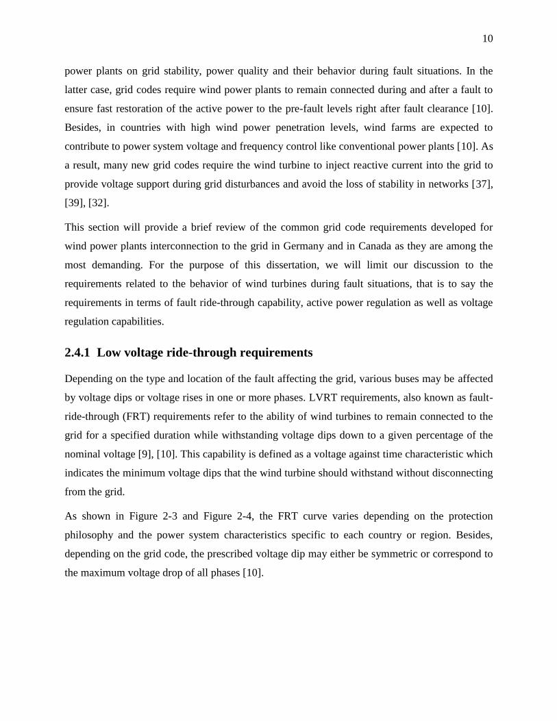
Figure 2-3 : Minimum FRT requirements according to the E.ON grid code [10]

In Germany, as shown in Figure 2-3, wind generators are required to stay connected to the grid

for voltages within the limit lines 1 and 2 whereas they should be disconnected from the grid if

the voltage at the low voltage side of the generator transformer drops below the limit line 2.

According to the minimum FRT requirements of the E.ON grid code depicted in Figure 2-3, wind

generators should withstand voltage drops down to 0% of the nominal voltage at the point of

common coupling (PCC) for durations up to 150 ms. The maximum voltage dip duration is 1.5 s.

After this time, the automatic protection system must disconnect the wind generators depending

on the voltage sag at the low voltage side of their respective transformers.

12

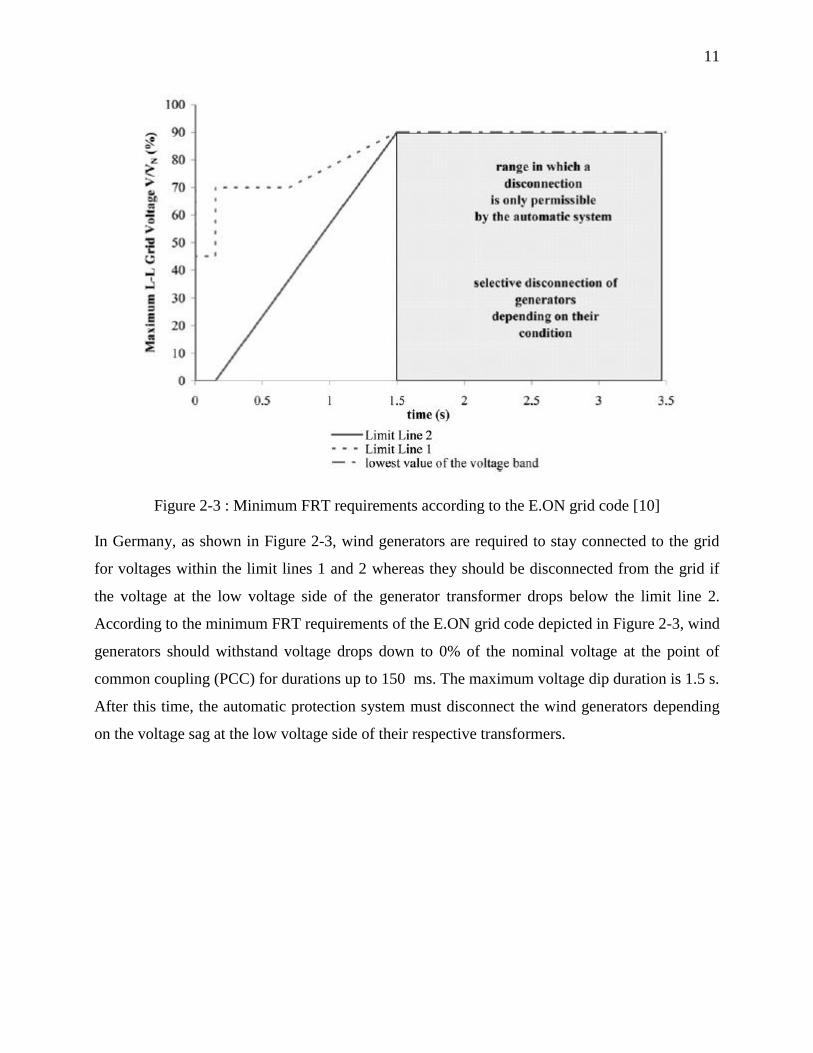
Figure 2-4 : Minimum FRT requirements according to Hydro-Québec grid code [32]

In the province of Quebec, as shown in Figure 2-4, wind generators are required to stay

connected to the grid for voltages above the red line whereas disconnection is allowed if the

positive sequence voltage at the high voltage side of the switchyard drops below the red line.

According to the minimum FRT requirements of the Hydro-Québec grid code, wind generators

should withstand voltage drops down to 0% of the nominal voltage for durations up to 150 ms.

Wind generators must stay connected to the grid for voltage dips at the high voltage side of the

switchyard within 0.75 to 0.85 p.u. which last less than 2 s and voltage dips within 0.85 to 0.9

p.u. which last less than 30 s They must always remain in service for voltage dips greater or equal

to 0.9 p.u [32]. For a particular FRT curve, the wind turbine must remain connected to the grid

for voltage dips above the limit line whereas the wind turbine should be disconnected from the

grid for voltage dips below the limit line. In this respect, grid codes of Germany and the province

of Quebec appear to be among the more restrictive grid codes as they require wind farms to

withstand voltage dips down to 0%. The duration of the prescribed voltage dip depends on the

response time of the protection system. According to the latest E.ON grid code [37], wind power

plants must withstand maximum voltage dips down to 0% of the nominal voltage for durations up

to 150 ms (7.5 cycles). On the other hand, the wind farms connected to Hydro-Québec

transmission system via power converters are required to remain operational throughout the

13

entire voltage range except for voltage levels greater than 1.25 p.u [36]. The minimum time

periods during which the wind farms must remain in operation during voltage dips is specified in

Figure 2-4.

The E.ON grid code [37] addresses LVRT requirements for symmetrical voltage dips only

whereas Hydro-Quebec specifies FRT requirements for both three-phase and unsymmetrical

faults affecting the transmission network. It also provides additional requirements for remote

symmetrical and unsymmetrical faults cleared by slow protective devices (up to 45 cycles) [36],

[10], [32].

2.4.2 Active power restoration

Most grid codes include provisional requirements to ensure fast restoration of the active and

reactive power to the pre-fault levels right after fault clearance [10]. The German grid code

requires the pre-fault active power to be completely restored 5 s after fault clearance [10]. As for

Hydro-Quebec, no specific requirement has been set up regarding the restoration of active power

in-feed [32].

2.4.3 Reactive current injection for voltage support

In networks with significant wind penetration, wind turbine generators are expected to support

and fast restore the grid voltage in the same way as conventional generators by injecting

additional reactive current into the network during disturbances [10]. In Germany, the required

reactive current injection must start one cycle after the fault is detected, for voltage drops or rises

larger than 10% of the WT nominal voltage (5% in case of offshore wind farms). The minimum

reactive current injection is defined in Figure 2-5.

14

Figure 2-5 : Reactive current injection according to the German grid code [9].

As for wind power plants connected to the transmission network, they are required to operate

within minimum leading or lagging rated power factor of 0.95 under normal and abnormal

operating conditions [32]. Wind turbines must be able to supply or absorb reactive power over

the entire power generation range [36].

For the purpose of steady-state short-circuit analysis, the assessment of fault current contribution

of full converter wind turbine generators is only relevant if FRT requirements are adequately

accounted for.

15

CHAPITRE 3 DETAILED STUDY OF TYPE 4 WTG UNDER FAULT

CONDITIONS

Equation Chapter 3 Section 1

EMTP-Type programs allow modeling in detail the behavior of a Type 4 WTG while this is not

the case yet in current steady-state-type packages [41]. However, steady-state-type packages are

still widely used to perform short-circuit analysis for planning purposes rather than using

electromagnetic transient programs. Although the latter are based on several assumptions and

simplifications which may introduce errors [35], traditional use of power system analysis tools

like the symmetrical components [34] explains that, nowadays, traditional short-circuit

computation packages are still used more extensively than time-domain programs.

In this chapter, a detailed study of Type 4 WTG under various fault conditions has been

performed using EMTP-RV [2]. The detailed model used will help assess the behavior of the

Type 4 WTG under grid disturbances to later propose a simplified model which reproduces the

real behavior of the WTG under fault conditions.

3.1 Description of the study network

The network studied is simple and is represented in the single-line diagram of Figure 3-1

Figure 3-1 : Single-line diagram of the benchmark network

The network consists of 1x2 MW (2.22 MVA) wind turbine generator connected to a 34.5kV

Distribution System at the Point of Common Coupling (PCC) through a 2.5 MVA, 0.575/34.5

kV step-up transformer. A collector line, which data is presented in Table 3-1, connects the

PCC to the 230 kV grid through a 34.5/230 kV step-up transformer. The grid is represented

16

by an equivalent source with a short-circuit power of 2500 MVA. The transformers used in

this network have respectively YgD and DYg connections. The impedance of both

transformers has a value of 6.0%.

As shown in Figure 3-1, the main components of the FCG are the Permanent Magnetic

Synchronous Generator (PMSG), the back-to-back VSC and the wind turbine. For the purpose of

this validation test, the average mean value model of EMTP is used rather than the detailed model

since detailed representation of IGBT switches is not required for steady-state simulations. Figure

3-1 also shows the protection switch which isolates the FCG from the PCC when maximum (or

minimum) values are exceeded. Although not shown, the FCG is equipped with a control system

which allows independent control of active and reactive power of the wind generator. For this

validation test, the reactive power control (i.e. Q control) mode was selected. As a result, a PI

controller is used to compare the reference (Qref_pu) with the measured reactive power. Finally,

the FCG is equipped with a current limiter which limits the converter current reference in the dq0

frame to a pre-set value of 1.1pu.

Table 3-1 - Transmission line data

17

3.2 Fault contribution of Type 4 WTG under various fault conditions

Three phase (LLL) fault and single line-to-ground (LG) fault are respectively applied at the HV-

AVM bus which is also considered to be the point of common coupling (PCC) of the wind

turbine to the grid. Their effect on the full converter based WTG along with the fault contribution

of the WTG are discussed hereafter. In particular, currents injected into the HV-AVM bus are

monitored, along with the current injected into the AVM bus, measured at the LV side of the

FCG’s step-up transformer. This is to have, later on, a good basis of comparison between the

current contribution of the detailed model of FCG in EMTP-RV and the contribution of the

proposed model. Actually, in EMTP-RV, the wind power plant model includes not only the FCG,

but also its step up transformer, the collector line and the step-up transformer which connects the

FCG to the grid. Consequently, the fault contribution of the FCG corresponds to the current

injected to the grid, into the HV-AVM bus. In CYME 7.0 however, the FCG model doesn’t

include either the step-up transformers or the collector line. As a result, the fault contribution of

the FCG corresponds to the current injected at the LV side of the FCG step-up transformer. Since

the objective of this research work is to integrate the proposed model in CYME 7.0, the same

approach as currently used in CYME 7.0 is followed and the FCG is modeled such to reproduce

its fault contribution at the LV side of its step-up transformer. Other types of equipment

pertaining to the wind power plant are modeled separately. Therefore, although one should be

interested by the fault contribution of the FCG at the HV-AVM bus, as it is the case in EMTP-

RV, later, for validation purposes, the current at the LV side of the FCG’s step-up transformer

will be considered as the fault contribution of the FCG to the grid. As a result, this current will be

analyzed as well in this study.

3.2.1 Three-phase fault (LLL)

A three-phase fault is applied at the PCC at 1.0 s and is cleared after 1.15 s. As illustrated in

Figure 3-2, the voltage at the PCC rapidly drops to 0 p.u. as a result of the LLL fault and is

restored as soon as the fault is cleared.

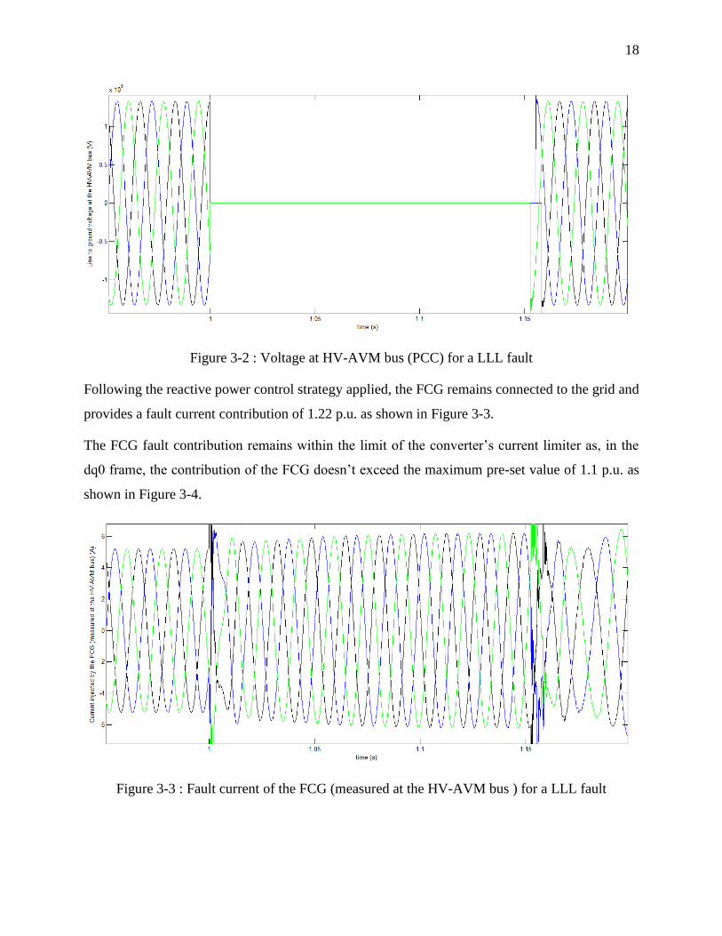
18

Figure 3-2 : Voltage at HV-AVM bus (PCC) for a LLL fault

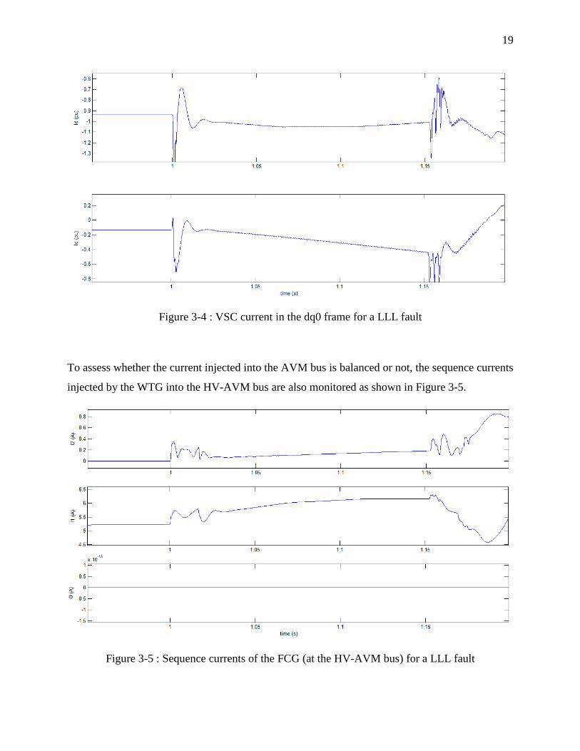
Following the reactive power control strategy applied, the FCG remains connected to the grid and

provides a fault current contribution of 1.22 p.u. as shown in Figure 3-3.

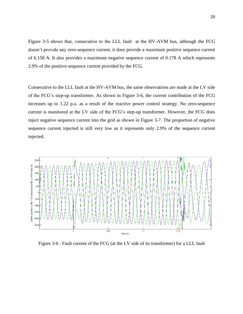
The FCG fault contribution remains within the limit of the converter’s current limiter as, in the

dq0 frame, the contribution of the FCG doesn’t exceed the maximum pre-set value of 1.1 p.u. as

shown in Figure 3-4.

Figure 3-3 : Fault current of the FCG (measured at the HV-AVM bus ) for a LLL fault

19

Figure 3-4 : VSC current in the dq0 frame for a LLL fault

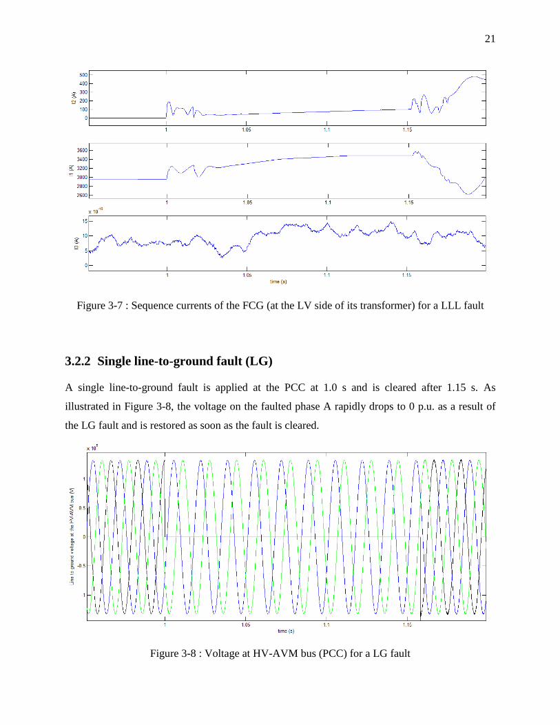
To assess whether the current injected into the AVM bus is balanced or not, the sequence currents

injected by the WTG into the HV-AVM bus are also monitored as shown in Figure 3-5.

Figure 3-5 : Sequence currents of the FCG (at the HV-AVM bus) for a LLL fault

20

Figure 3-5 shows that, consecutive to the LLL fault at the HV-AVM bus, although the FCG

doesn’t provide any zero-sequence current, it does provide a maximum positive sequence current

of 6.158 A. It also provides a maximum negative sequence current of 0.178 A which represents

2.9% of the positive-sequence current provided by the FCG.

Consecutive to the LLL fault at the HV-AVM bus, the same observations are made at the LV side

of the FCG’s step-up transformer. As shown in Figure 3-6, the current contribution of the FCG

increases up to 1.22 p.u. as a result of the reactive power control strategy. No zero-sequence

current is monitored at the LV side of the FCG’s step-up transformer. However, the FCG does

inject negative sequence current into the grid as shown in Figure 3-7. The proportion of negative

sequence current injected is still very low as it represents only 2.9% of the sequence current

injected.

Figure 3-6 : Fault current of the FCG (at the LV side of its transformer) for a LLL fault

21

Figure 3-7 : Sequence currents of the FCG (at the LV side of its transformer) for a LLL fault

3.2.2 Single line-to-ground fault (LG)

A single line-to-ground fault is applied at the PCC at 1.0 s and is cleared after 1.15 s. As

illustrated in Figure 3-8, the voltage on the faulted phase A rapidly drops to 0 p.u. as a result of

the LG fault and is restored as soon as the fault is cleared.

Figure 3-8 : Voltage at HV-AVM bus (PCC) for a LG fault

22

Following the reactive power control strategy applied, the FCG remains connected to the grid and

provides a fault current contribution of 1.23 p.u. as shown in Figure 3-9.

Figure 3-9: Fault current of the FCG (measured at the HV-AVM bus ) for a LG fault

Like for the LLL fault, the FCG fault contribution remains within the limit of the converter’s

current limiter as, in the dq0 frame, the contribution of the FCG doesn’t exceed the maximum

pre-set value of 1.1 p.u. as shown in Figure 3-10.

Figure 3-10 : VSC current in the dq0 frame for a LG fault

23

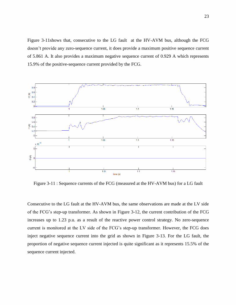
Figure 3-11shows that, consecutive to the LG fault at the HV-AVM bus, although the FCG

doesn’t provide any zero-sequence current, it does provide a maximum positive sequence current

of 5.861 A. It also provides a maximum negative sequence current of 0.929 A which represents

15.9% of the positive-sequence current provided by the FCG.

Figure 3-11 : Sequence currents of the FCG (measured at the HV-AVM bus) for a LG fault

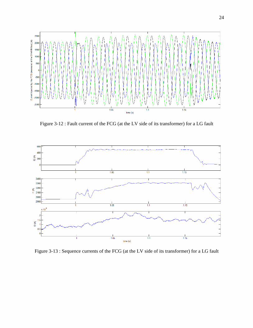
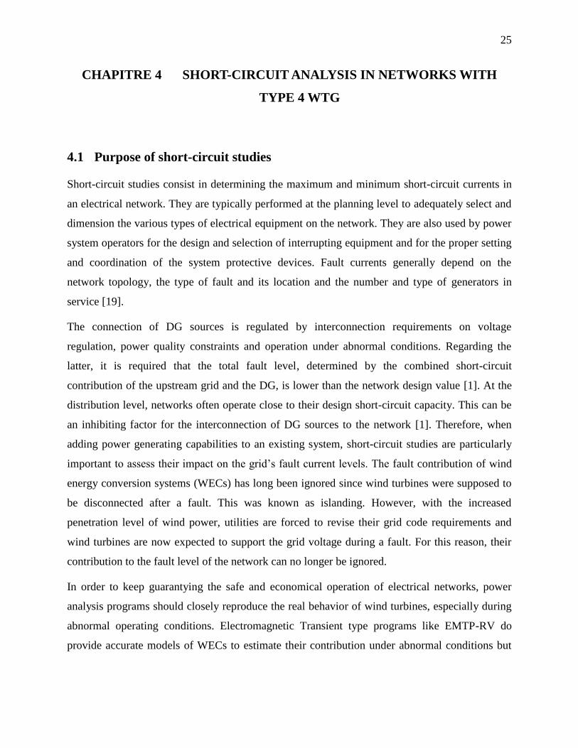
Consecutive to the LG fault at the HV-AVM bus, the same observations are made at the LV side

of the FCG’s step-up transformer. As shown in Figure 3-12, the current contribution of the FCG

increases up to 1.23 p.u. as a result of the reactive power control strategy. No zero-sequence

current is monitored at the LV side of the FCG’s step-up transformer. However, the FCG does

inject negative sequence current into the grid as shown in Figure 3-13. For the LG fault, the

proportion of negative sequence current injected is quite significant as it represents 15.5% of the

sequence current injected.

24

Figure 3-12 : Fault current of the FCG (at the LV side of its transformer) for a LG fault

Figure 3-13 : Sequence currents of the FCG (at the LV side of its transformer) for a LG fault

25

CHAPITRE 4 SHORT-CIRCUIT ANALYSIS IN NETWORKS WITH

TYPE 4 WTG


4.1 Purpose of short-circuit studies

Short-circuit studies consist in determining the maximum and minimum short-circuit currents in

an electrical network. They are typically performed at the planning level to adequately select and

dimension the various types of electrical equipment on the network. They are also used by power

system operators for the design and selection of interrupting equipment and for the proper setting

and coordination of the system protective devices. Fault currents generally depend on the

network topology, the type of fault and its location and the number and type of generators in

service [19].

The connection of DG sources is regulated by interconnection requirements on voltage

regulation, power quality constraints and operation under abnormal conditions. Regarding the

latter, it is required that the total fault level, determined by the combined short-circuit

contribution of the upstream grid and the DG, is lower than the network design value [1]. At the

distribution level, networks often operate close to their design short-circuit capacity. This can be

an inhibiting factor for the interconnection of DG sources to the network [1]. Therefore, when

adding power generating capabilities to an existing system, short-circuit studies are particularly

important to assess their impact on the grid’s fault current levels. The fault contribution of wind

energy conversion systems (WECs) has long been ignored since wind turbines were supposed to

be disconnected after a fault. This was known as islanding. However, with the increased

penetration level of wind power, utilities are forced to revise their grid code requirements and

wind turbines are now expected to support the grid voltage during a fault. For this reason, their

contribution to the fault level of the network can no longer be ignored.

In order to keep guarantying the safe and economical operation of electrical networks, power

analysis programs should closely reproduce the real behavior of wind turbines, especially during

abnormal operating conditions. Electromagnetic Transient type programs like EMTP-RV do

provide accurate models of WECs to estimate their contribution under abnormal conditions but

26

traditional short-circuit computation packages are still more widely used to perform short-circuit

studies of electrical networks.

Standard calculation methods like IEC 60909 [3] have been developed to calculate the fault

contribution of various grid elements. However, they are not applicable to full scale converter

based WTG as their fault contribution don’t depend on the electrical characteristic of the

generator. The latter is indeed completely decoupled from the grid. Hence, the fault contribution

of full converter based DG sources rather depends on the type of interface with the grid, the

voltage before the fault, the operating mode, the technology used, etc.

4.2 Literature review

With the increased penetration level of wind power plants interfaced with the grid via full scale

frequency converters and the progression of FRT requirements in several countries, recent studies

have shown that the fault current contribution of WTG cannot be disregarded anymore. In some

cases for instance, plants contribution to the short-circuit level at the substation HV bus after the

installation of DG units has appeared to be as high as six or more times the rated turbine current

[13].

For this reason, valuable effort has already been provided in modeling the behavior of inverter

interfaced wind power plants and their effect on the design short-circuit level of distribution

networks. However, when addressing the modeling of Type 4 WTG, many frequency domain

short-circuit packages don’t model adequately the effect of the full scale frequency converter on

the fault contribution of the WTG [41]. Besides, traditional short-circuit analysis methods are

barely adapted to determine the fault current contribution of Type 4 WTG ([3], [4], [12]).

Actually, no standard addresses the modeling of full scale converter based WTG. The standard on

DG interconnection [11] simply states that the fault current of ECG usually ranges within 1.2 to

1.5 p.u. without further explanations. As for [3] it doesn’t provide any guideline on the modeling

of Type 4 WTG.

In short-circuit analysis, sources are conventionally represented by an ideal voltage source behind

an impedance. This is the case for synchronous generators, induction generators and motors. As a

result, an approach presented in [12] proposes using the E/Z simplified method to represent the

27

detailed model of the wind power plant as a 1 p.u. voltage source followed by an equivalent

series impedance. These impedances can be used later on in short-circuit calculations for relay

settings in the transmission network [13].

In [1], the IEC Standard 60909 is extended to assess the impact of DG sources on the fault level

of medium and low voltage distribution networks. Based on experience and available information

on Type 4 WTG, it is proposed to adopt a constant current representation estimated at 2 p.u.

Besides, due to the impossibility of adequately determining the phase angle of the current

contribution, it is proposed to algebraically add the fault contribution of the Type 4 WTG to the

total fault level of all other sources.

In [15] and [16], only the maximum fault contribution of full scale converter interfaced WTG is

discussed and is typically considered ranging between 1.0 to 4 p.u. of its rated current depending

on the overcurrent capability of its power converter. The upper values such provided generally

correspond to a three-phase fault at the WT terminals and the fault contribution of the Type 4

WTG is expected to decrease with distance from the WTG [16].

In [17], although stated upfront that the fault contribution of the Type 4 WTG mainly relies on

the power converter’s control algorithms, the behavior of the Type 4 WTG under steady-state

fault conditions is later simply described from a theoretical standpoint. The fault contribution of

the WTG is said to be limited at or 10 % above its rated current for three-phase fault without

further explanations. The fault contribution of the Type 4 WTG is also assumed to be balanced

regardless of the type of fault.

In [18] too, the fault contribution of the Type 4 WTG is considered limited at 2 p.u. The proposed

method distinguishes two periods during which the behavior of the Type 4 WTG varies. The sub-

transient period refers to the first cycle of the fault and corresponds to the peak contribution of

the WTG. The transient period follows for 5 to 10 cycles and sees the decrease of the fault

contribution of the WTG due to the action of the controller. The sub-transient peak current is

estimated based on a Thevenin equivalent which assumes the internal voltage of the WTG

constant and set to its pre-fault value. As for the impedance used, it corresponds to the series

combination of the grid-side converter filter reactance along with the transformer reactance. In

the transient period, the WTG is considered feeding the fault only if its fault contribution has not

exceeded its peak current limit during the sub-transient period. In that case, the fault contribution

28

of the Type 4 WTG is updated dynamically according to the feeder fault response by adjusting

the internal voltage of the WTG equivalent model.

A model specific to ENERCON WECs but applicable to any full scale converter based WTG is

presented in [19]. To fit the standard steady-state short-circuit calculation methods, the WTG is

modeled as a voltage source behind impedance rather than a controlled current source. The

equivalent model is developed in sequence domain and is based on the worst case scenario,

considered to be the injection of the WTG maximum current at a phase angle of 90 degree. The

equivalent positive sequence impedance of the WTG is determined accordingly and considered as

purely reactive. As for the negative and zero sequence impedances, they are considered as infinite

to reproduce a balanced fault current injection. The value of the internal voltage of the WTG is

constant and set at the value of the low voltage terminal of the WTG after occurrence of the fault.

Besides, unlike in [9], the value of the maximum fault contribution is specific to the WTG.

In [20], it is stated that, for the purpose of steady-state short-circuit analysis, the fault

contribution of full scale converter based WTG is assumed similar in sub-transient, transient and

steady-state fault conditions. Instead, the fault contribution of electronically coupled WTG is said

to depend on the distance to fault from the WTG. As a result, it is proposed to adopt two distinct

models to assess the fault contribution of the WTG: a current source set to the maximum fault

contribution for close faults and a constant PQ source for remote faults. Problem in implementing

such a model remains as it is hard to differentiate a remote from a near fault.

In [21], an extended Gauss-Seidel load-flow based approach is proposed to assess the fault

contribution of grid-connected inverter dominated networks. The inverter-based WTG are

modeled as current constrained PQ nodes behind a coupling reactance during the sub-transient

and transient periods. Additionally, when the low pass filter on the grid-side fails to sufficiently

attenuate the negative sequence component caused by unbalanced fault conditions, the WTG is

modeled as a constant positive sequence current source in parallel with the filter capacitor. As

soon as the fault contribution of an inverter exceeds the converter’s threshold, its model is

switched to a current source set to a pre-defined value, typically 2 p.u.

The modeling of Siemens Type 4 WTG is specifically addressed in [22]. The WTG is considered

providing balanced currents even for unbalanced types of faults. The article discusses only the

maximum contribution of the Siemens Type 4 WTG and also distinguishes two time periods for

29

which the fault contribution of the WTG differs. In the first period lasting half a cycle, the current

contribution of the WTG is limited to 2.5 p.u. whereas in the second period, the current injected

to the grid is limited to a required FRT value, namely 2% lagging reactive current increase for

every 1% drop in positive sequence voltage 90% of nominal voltage. This results in a typical

fault contribution between 1.1 to 1.2 pu.

In [23], the contribution of Type 4 WTG is assumed not to exceed 1.5 p.u. Besides, it is assessed

that the impact of Type 4 WTG depends not only on the size of the machine but also on its

location as, when located at the end of the line, they barely affect the feeder breaker fault duty.

Another interesting contribution from [9] proposes modeling wind turbines with full rating power

converters as a Thevenin equivalent which is iteratively adjusted by a general routine to fit the

model with the expected FRT behavior specified in the German grid code. The interest of this

method is that the proposed model of Type 4 WTG doesn’t require using proprietary data from

specific WT manufacturers. However, the method appears to be tedious to implement and its

convergence is not guaranteed for all network topologies.

When it comes to variable speed wind turbine generators, the Joint Working Group on Wind

Plant Short Circuit Contribution co-chaired by R. Walling [25] not only estimates that the

complex behavior of Type 4 wind turbine generators cannot be represented by a simple Thevenin

equivalent but also recommends adapting short-circuit algorithms to accurately represent the

short-circuit current contribution of wind turbine generators. In [24] and [25], the short-circuit

behavior of Type 4 WTG is compared to a limited current source which magnitude depends on

the time period that is considered. Indeed, to better evaluate the behavior of Type 4 WTG under

fault conditions, it is recommended to consider two distinct time periods between which the

behavior of the Type 4 WTG changes. In the first one to two cycles after occurrence of the fault,

the fault contribution of the WTG mainly depends on the pre-fault operating conditions and the

fault contribution of the WTG ranges between a minimum value corresponding to the pre-fault

load current to a maximum fault contribution that can go up to 2 to 3 p.u. After detection of the

fault, the fault contribution of the WTG mainly depends either on the applicable FRT

requirements or on the control strategy implemented by the WT manufacturers. In such case, the

fault contribution of the WTG can range between zero amps to a maximum of 1.5 p.u.; depending

on the overcurrent design capability of the converter. The article only provides recommendations

30

but doesn’t provide any model for the representation of Type 4 WTG for short-circuit analysis. It

is however mentioned that in case current sources cannot be modeled directly in the short-circuit

analysis method chosen, an equivalent voltage behind impedance model must be adopted and

adjusted iteratively to match the desired fault contribution. This is hardly applicable unless the

WTG is assumed to always contribute up to its maximum value regardless of the type of fault and

location.

As for the models currently implemented in commercial short-circuit analysis software tools [41],

they don’t appropriately handle either the short-circuit contribution of Type 4 WTG. In the

general multiphase network representation adopted by CYME to perform short-circuit analysis,

electronically coupled generators are treated the same way as induction generators, that is, a

voltage source followed by a sub-transient impedance ''Z . Like for induction generators, the

equivalent voltage source representing the ECG is considered ungrounded, i.e. with infinite zero-

sequence impedance. Hence, ECGs are modeled as delta connected induction generators. As for

''Z , it is derived from the maximum three-phase fault contribution of the inverter, which

corresponds to a percentage of the rated current of the WTG. The detailed model of ECG as

implemented in CYME 7.0 is shown below:

Figure 4-1 : Full converter based WTG model in CYME 7.0

The value of Eequ depends on the pre-fault voltage. If short-circuit calculations start at nominal

value:

equ NOME V (2.3)

where:

31

NOMV : Line-to-neutral rated voltage of the WTG.

If short-circuit calculations start at load flow solution:

1 .equ LF wecs LFE V Z I (2.4)

where:

LFV : Magnitude of line-to-neutral pre-fault voltage of the WTG (p.u.).

LFI : Pre-fault line current of the WTG (p.u.).

1wecsZ : Sub-transient impedance of the WTG (p.u.).

On the other hand, in CYME 7.0, regardless of the pre-fault conditions assumed, the sub-transient

impedance ''Z is always calculated as:

_ max

1'' 1wecs

wecs

Z Z jI

(2.5)

where:

_ maxwecsI : Maximum three-phase fault contribution of the full converter WTG (expressed in

p.u. based on the converter rated current).

The impedance ''Z represents the direct sequence impedance as a full converter WTG only injects

direct sequence current into the grid. The negative and zero sequence impedances of the WTG are

both considered as infinite.

It is obvious from equation (2.5) that when short circuit starts at load flow solution, the impedance of

the WTG is not calculated correctly since it assumes that the equivalent source is at 1 pu instead of its

real value. Hence, according to equation (2.4), Eequ is not calculated correctly either.

32

CHAPITRE 5 SHORT-CIRCUIT MANA MODEL FOR TYPE 4 WTG


The fault contribution of Type 4 WTG strongly relies on the control strategy applied before the

fault and on the FRT capabilities either set by applicable grid codes or implemented by a specific

manufacturer.

In [26], two time periods are distinguished to adequately estimate the contribution of a Type 4

WTG under fault operating conditions: during fault detection (1 to 2 grid cycles) and after fault

detection.

During the first two cycles following the occurrence of a fault, the WTG tends to behave

according to its operating control mode. It provides only direct sequence currents under both

balanced and unbalanced conditions; except in some specific cases [27]. However, its fault

contribution is limited by the overload capacity of the converter which is typically 110 to 150%

of the rated current. Therefore, when the converter is saturated, the WTG behaves as a current

source providing the maximum fault contribution.

After fault detection, the fault contribution of the Type 4 WTG is determined either by the

applicable grid codes or by the inverter control strategy implemented by a specific manufacturer.

Several grid codes require the WTG to stay connected to the grid under abnormal conditions and

also to provide voltage support by injecting a pre-specified amount of reactive current. Hence,

after fault detection, the Type 4 WTG behaves like a voltage controlled current source, injecting

only balanced current under any operating conditions.

Based on the observed behavior of the Type 4 WTG under steady-state fault conditions, two

models are proposed in this dissertation to assess its fault current contribution in phase domain.

The two models reproduce the behavior of the WTG respectively under sub-transient and

transient abnormal operating conditions. They are afterwards implemented in an iterative short-

circuit algorithm using the MANA approach. As previously stated, these models depend not only

on the control strategy applied prior to the fault but also on the FRT capabilities of the WTG.

The multiphase MANA formulation presented in [28] is adopted to represent adequately the

constraint equations of the WTG. Besides, due to the iterative nature of the proposed short-circuit

33

model, a fault flow algorithm based on Newton’s method is adopted to perform short-circuit

calculations on networks with inverter connected WTG.

5.1 Newton MANA method

Based on the expansion in Taylor series of a matrix function f(x) around a given solution xj, the

Newton method allows solving non-linear matrix equations like f(x) = 0 by reformulating them

as:

. -j j jJ x f (2.6)

where:

jJ : Jacobian matrix at iteration j.

jf : Mismatch vector at iteration j.

jx : Computed error at iteration j.

jx is used to update the solution vector x such that:

1.j j jx x x (2.7)

In [28], a Newton-based solution approach is adopted to accommodate controlled devices. In this

method, controlled devices are modeled according to their constraint equations. The method

consists in using the MANA approach to build an augmented Jacobian matrix which is iteratively

updated until matching the constraints set for each controlled device.

The resulting generic matrix equation at given iteration j is given by:

34

jj

j

nn c IL IG

n xr d

L LI x L

G GI GE L GI

GPQ GPQI G GPQ

GPV G GPV

GSL GSL

fY A A A 0

ΔV fA A 0 0 0

J 0 J 0 0 ΔI f

Y 0 0 B B ΔI f

J 0 0 J 0 ΔI f

J 0 0 0 0 ΔE f

J 0 0 0 0 f

(2.8)

where:

nY : Classical nodal admittance matrix.

rA : Voltage coefficient matrix for non-linear devices without controls.

cA : Current coefficient matrix for non-linear devices without controls.

dA : Adjacency matrix of infinite impedance type devices

LJ : Voltage coefficient matrix for PQ loads.

LIJ : Current coefficient matrix for PQ loads.

GY : Internal admittance matrix of generators.

GIB : Current coefficient matrix for generators.

GEB : Internal voltages coefficient matrix for generators.

GPQJ : Voltage coefficient matrix for PQ controlled generators.

GPQIJ : Current coefficient matrix for PQ controlled generators.

GPVJ : Voltage coefficient matrix for PV controlled generators.

GSLJ : Voltage coefficient matrix for slack-type buses.

35

In their detailed form, sub-matrices cA , rA and dA presented in equation (2.8) published in [28]

and [44] are respectively written as presented below:

c c c cA V D S (2.9)

T T

r c c c cA V D S A (2.10)

d dA S (2.11)

where:

cV : Voltage sources adjacency matrix.

cD : Dependency functions matrix.

cS : Adjacency matrix of zero impedance type devices.

dS : Adjacency matrix of infinite impedance type devices

In equation (2.8), jf is the mismatch vector presented in its detailed form. It represents the

mismatch between the desired value of the variable under constraint and its value at iteration j.

As for the computed error at iteration j, jx , presented in its detailed form in equation (2.8), it

corresponds to the error affecting the unknown variables computed between two consecutive

iterations. These variables are:

nV : Nodes voltages.

xI : Vector containing sources currents, transformers secondary currents and switch currents.

LI : PQ-loads currents.

GI : Generators currents.

36

GE : Generators internal voltages.

In the Newton formulation presented in equation (2.8), complex elements of each sub matrix are

separated into real and imaginary parts such that the matrix equation (2.8) is only filled with real

numbers.

The MANA approach used in [28] to build the Jacobian matrix allows adopting a systematic and

yet efficient method to integrate into the Jacobian such arbitrary equations like constraint

equations as it allows partitioning the latter into matrices which contain all the devices without

controls and the remaining block matrices which represent the controlled devices. Devices

without controls are modeled as in the classical MANA formulation throughout sub-matricesnY ,

cA , rA and dA . As for controlled devices, they are represented in the Jacobian according to their

control type.

As shown in equation(2.8), the constraint equations for a given controlled device p are integrated

in the Jacobian through voltage and current coefficient sub-matrices, which can be generally

labeled as p

J and pI

J . Subscript p can be replaced by subscripts L or G, respectively for load

and generator. Using the Newton’s method, these block matrices, along with the corresponding

mismatch vectorp

f , are updated at each iteration j until the constraint equation defined in (2.12)

is minimized.

j j j j j

p pI pJ .ΔV +J .ΔI = -f (2.12)

Load currents ( LI ) and generator currents ( GI ) are derived respectively from the computed

errors LΔI and GΔI . They are included in the Kirchhoff Law’s equations of the Jacobian,

through the sub-matrices ILA and IGA .

37

5.2 Sub-transient model

Under normal operating conditions, the full scale converter of a Type 4 WTG is generally

controlled either to deliver constant output power (PQ) or to achieve voltage regulation (PV)

within the converter’s design limits. When a fault occurs, the Type 4 WTG tries to maintain the

constraints imposed by the control strategy set prior to the fault. Hence, under low voltage

conditions, the current contribution of the WTG can increase up to the maximum current limit of

the power converter. As a result, during the first two cycles after occurrence of a fault, before the

fault is detected, the Type 4 WTG is modeled as a current limited generator, controlled in PQ or

in PV.

5.2.1 Controlled generator model

In the Newton MANA method presented in [28] and described hereinabove, all power generating

devices are represented in the Jacobian as sets of constraint equations derived from their control

settings. Each phase is modeled separately which yields 6 by 6 coefficient matrices for three-

phase generators. Besides, additional terms ( GIB , GEB and GY ) are added in the Jacobian to

account for generators’ current constraint equations.

In the literature and in most commercial short-circuit analysis programs, the Type 4 WTG is

generally represented as a voltage source behind impedance under abnormal conditions. The

challenge in representing the Type 4 WTG as a Thevenin equivalent resides in the fact that the

voltage angle and/or the impedance need to be iteratively adjusted to achieve the desired fault

contribution [9], [26]. In the sub-transient operating mode, one doesn’t know in advance the fault

contribution of the WTG as it depends on several factors such as the pre-fault operating

conditions and control operating set points. Therefore, as stated in [26], modeling the Type 4

WTG as a Thevenin equivalent wouldn’t reproduce the real behavior of the WTG under fault

conditions. Since the Thevenin equivalent model of the Type 4 WTG doesn’t comply with the PQ

controlled generator model limited in current, the Type 4 WTG cannot be represented as

suggested in [28]. Instead, it is proposed to represent the full converter based WTG uniquely as a

set of constraints derived according to its pre-fault control type, using matrices pJ and pI

J . This

representation is even extended to all type of controlled generators in [29], where it is assessed

that for load flow calculations purposes, the Jacobian terms GIB , GEB and GY are redundant as

38

long as the generators’ control settings are adequately taken into account in the Jacobian through

matrices p

J and pI

J .

The same load-flow representation of constraints equations than presented in [28] is used for the

purpose of modeling the Type 4 WTG under steady-state short-circuit operating conditions. It is

important to clarify that, although the same load-flow representation of constraints equations as

in [28] is used, a load flow is not run prior to the short-circuit calculations. The proposed model

only accounts for the control mode that was set for the FCG prior to the fault. Short-circuit

calculation is done with same traditional assumptions considering pre-fault voltage at 1 pu.

Although not accurate, this is done to comply with the assumptions followed in CYME 7.0

Hence, for a PQ controlled WTG labeled as p and connected at an arbitrary node k, its constraint

equations at a given iteration j are formulated as:

.

.

j

des p pj

des p p

P real V conj I

Q imag V conj I

GPQf (2.13)

where:

desP : Desired (by-phase) active power of WTG p.

desQ : Desired (by-phase) reactive power of WTG p.

pI : Line current of WTG p connected to arbitrary node k.

pV : Voltage of WTG p connected to arbitrary node k.

In this dissertation, it is assumed that the WTG is a three-phase device connected in Y/Yg

configuration. Hence, pV always refers to the line-to-neutral voltage of a WTG p.

Besides, the desired active and reactive power for each phase, Pdes and Qdes, are expressed as

follows:

39

3

desdes

SP real

(2.14)

3

desdes

SQ imag

(2.15)

where:

desS : Desired three-phase apparent power.

Formulation of the mismatch vector GPQf at iteration j as expressed in equation (2.13) can be

rewritten as:

j

R R I I

des p p p pj

I R R I

des p p p p

P V I V I

Q V I V I

GPQ

f (2.16)

where:

R : Subscript which stands for the real part of the complex variable.

I : Subscript which stands for the imaginary part of the complex variable.

Equation (2.16) populates the Jacobian terms GPQJ and GPQI

J which stand respectively for the

voltage and current coefficient sub-matrices for the PQ controlled WTG. They are expressed as:

j

R I

p pj

I R

p p

jR I

p pj

I R

p p

I I

I I

V V

V V

GPQ

GPQI

J

J

(2.17)

40

For PV controlled generators, the voltage control is applied only on its magnitude and yields the

mismatch vector GPVf at iteration j, expressed as:

2 2

jR R I I

des p p p pj

R I

des p p

P V I V I

V V V

GPVf (2.18)

where:

desP : Desired (by-phase) active power of WTG p.

desV : Desired (by-phase) voltage of WTG p.

pV : Voltage of WTG p connected to arbitrary node k.


Therefore, for a PV controlled generator labeled as p and connected to arbitrary node k, equation

(2.18) yields the Jacobian term GPVJ which stands for the voltage coefficient sub-matrix in

equation (2.8). GPVJ is expressed as:

1 1

2 2 2 22 2

jR I

p p

j

R I R R I I

p p p p p p

I I

V V V V V V

GPVJ (2.19)

Besides, according to the mismatch equation(2.18), the active power control yields additional

Jacobian terms which represent the real and imaginary derivative of the generator’s current GI .

These terms can be regrouped in a sub-matrix JGPVI expressed as:

41

0 0

jR I

j km kmV V

GPVIJ (2.20)

To stay consistent with the generic matrix formulation presented in [28] and shown in equation

(2.8), the elements of sub-matrix GPVIJ should substitute the term

GPQIJ provided that the Q row

of the PQ control sub-matrix GPQ

J is replaced by the coefficients derived from the voltage

constraint equation presented in (2.19).

5.2.2 Current limiting constraint

In the sub-transient operating mode, the maximum fault contribution of the Type 4 WTG is

limited by the overload capability of the converter to which it is connected to. This is to protect

the power converter from excessive fault currents that would damage the IGBT switches.

Therefore, at each iteration j, the fault current contribution provided by the sub-transient WTG

model, WTGI , is compared to the loading limits of the converter, _ maxVSCI . If WTGI exceeds _ maxVSCI ,

the controlled generator model of the WTG is changed for a constant current source which value

corresponds to the converter’s threshold, VSC_thI . VSC_thI is defined as :

_ VSC_th _ maxIWTG rated VSCI I (2.21)

where:

_WTG ratedI : Magnitude of rated current of the WTG.

VSC_thI : Threshold current of the WTG’s converter.

_ maxVSCI : Maximum current carrying capability of the WTG’s converter (input data).

In this dissertation, the worst case scenario is considered, where:

42

VSC_th _ maxI VSCI (2.22)

Typically, the maximum current carrying capability of the converter is set between 110% to

150% of the WTG rated current, depending on the cooling capabilities and the rating of the

converter [25]. The magnitude of the converter’s rated current, WTG_ratedI , is defined in

equation(2.23) :

WTG_ratedI

3.

NOM

NOM

S

V (2.23)

where:

NOMV : Line-to-line rated voltage of the WTG.

NOMS : Three-phase rated power of the WTG.

As for the angle of the converter’s rated current, it is defined as:

WTG_rated

1

I cos ( )NOMPF (2.24)

Where:

NOMPF : Power factor of the WTG at nominal value.

With the WTG modeled as an ideal current source, the mismatch vector If is expressed as:

( ) ( )

( ) ( )

j

des pj

des p

real I real I

imag I imag I

I

f (2.25)

where:

43

des _ maxI VSCI (2.26)

Equation (2.25) yields the Jacobian term IJ which stands for the current coefficient sub-matrix

for the current source. It is expressed as:

1 0

0 1

j

j

IJ (2.27)

When the Type 4 WTG reaches the threshold of the converter and is modeled as a current source,

the sub-matrix IJ replaces the term GPQI

J in the generic matrix equation (2.8). Besides, the term

GPQJ is null as, according to the mismatch vector shown in equation (2.25), there is no Jacobian

term which represents the derivative of the PCC voltage.

5.3 Transient model

The Type 4 WTG can generally detect a default within 1 to 2 grid cycles after it occurs [25].

After fault detection, the Type 4 WTG operates in transient mode and its behavior changes. The

WTG acts like a voltage dependent current source and, in practice, its fault contribution depends

not only on the FRT requirements set by applicable grid codes but also on the inverter control

strategy specific to each manufacturer.

With the increased wind penetration level in several countries, the wind turbine is required to

remain connected to the grid during abnormal operating conditions to avoid affecting the grid

stability. However, the amount of current to be injected by the WTG during fault ride through is

not standardized yet and remains specific to each country. The fault current injection of the WTG

can range from zero, i.e. no current injection, to the maximum current carrying capability of the

converter [25]. In the absence of specific FRT requirements from national grid codes or utilities,

WT manufacturers adopt their own control strategy to optimize the operation of the WTG. Since

FRT specifications vary significantly among WTG manufacturers and so do they among national

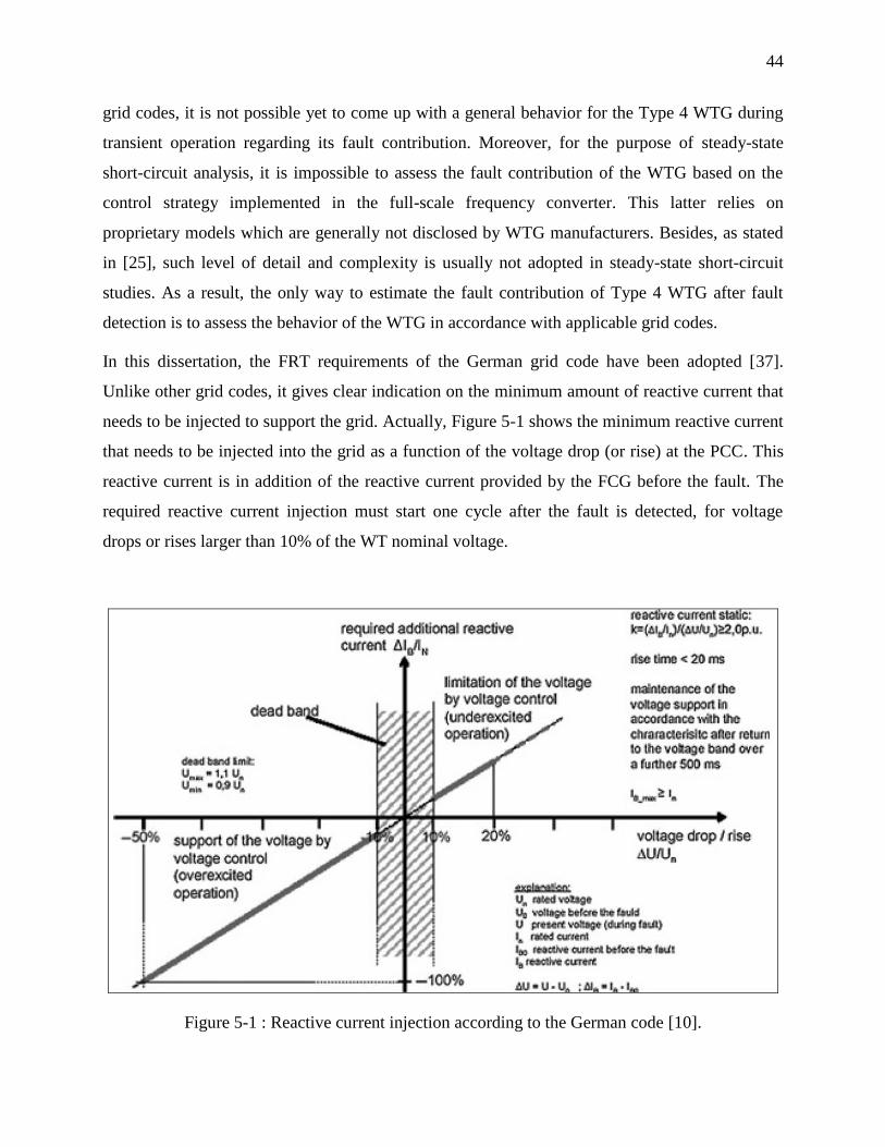
44

grid codes, it is not possible yet to come up with a general behavior for the Type 4 WTG during

transient operation regarding its fault contribution. Moreover, for the purpose of steady-state

short-circuit analysis, it is impossible to assess the fault contribution of the WTG based on the

control strategy implemented in the full-scale frequency converter. This latter relies on

proprietary models which are generally not disclosed by WTG manufacturers. Besides, as stated

in [25], such level of detail and complexity is usually not adopted in steady-state short-circuit

studies. As a result, the only way to estimate the fault contribution of Type 4 WTG after fault

detection is to assess the behavior of the WTG in accordance with applicable grid codes.

In this dissertation, the FRT requirements of the German grid code have been adopted [37].

Unlike other grid codes, it gives clear indication on the minimum amount of reactive current that

needs to be injected to support the grid. Actually, Figure 5-1 shows the minimum reactive current

that needs to be injected into the grid as a function of the voltage drop (or rise) at the PCC. This

reactive current is in addition of the reactive current provided by the FCG before the fault. The

required reactive current injection must start one cycle after the fault is detected, for voltage

drops or rises larger than 10% of the WT nominal voltage.

Figure 5-1 : Reactive current injection according to the German code [10].

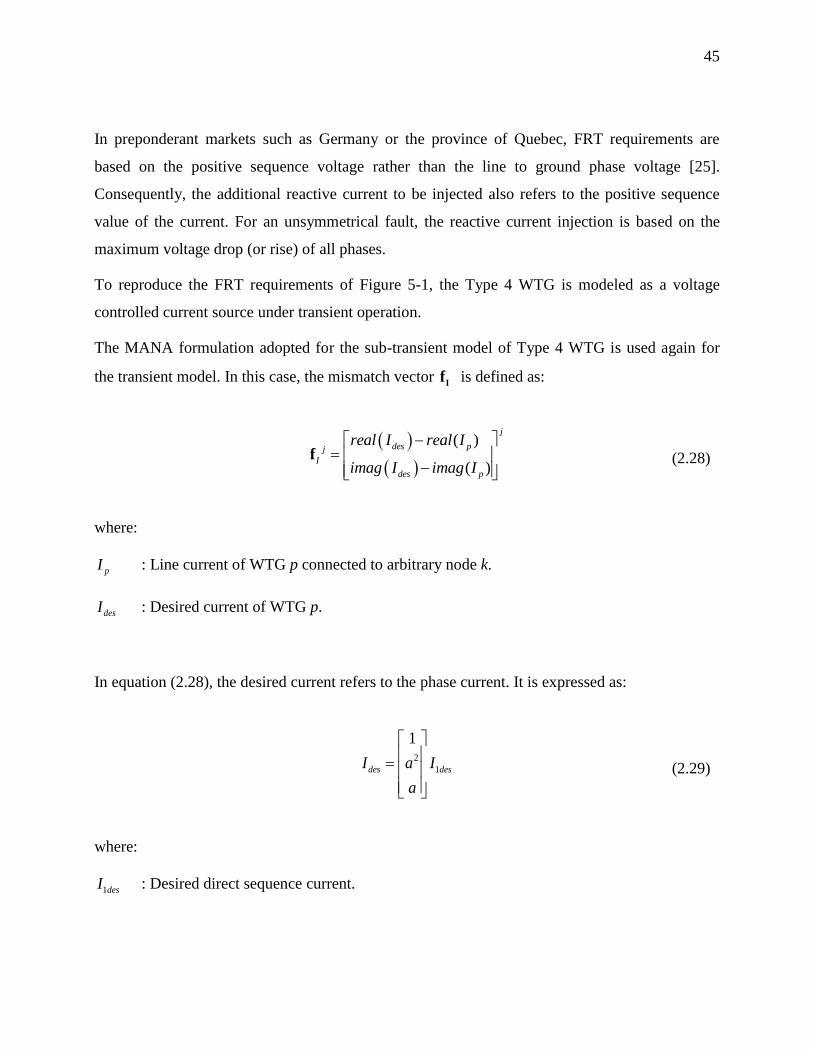
45

In preponderant markets such as Germany or the province of Quebec, FRT requirements are

based on the positive sequence voltage rather than the line to ground phase voltage [25].

Consequently, the additional reactive current to be injected also refers to the positive sequence

value of the current. For an unsymmetrical fault, the reactive current injection is based on the

maximum voltage drop (or rise) of all phases.

To reproduce the FRT requirements of Figure 5-1, the Type 4 WTG is modeled as a voltage

controlled current source under transient operation.

The MANA formulation adopted for the sub-transient model of Type 4 WTG is used again for

the transient model. In this case, the mismatch vector If is defined as:

( )

( )

j

des pj

I

des p

real I real I

imag I imag I

f (2.28)

where:


desI : Desired current of WTG p.

In equation (2.28), the desired current refers to the phase current. It is expressed as:

2

1

1

des desI a I

a

(2.29)

where:

1desI : Desired direct sequence current.

46

1 1 1des P des Q desI I jI (2.30)

In equation (2.30), the desired direct sequence reactive current 1Q desI is defined, in compliance

with Figure 5-1, as:

1 10 1Q des Q Q FRTI I I (2.31)

Where:

10QI : Pre-fault direct sequence reactive current of WTG.

1Q FRTI : Additional direct sequence reactive current required from WTG.

According to the German grid code, 1Q FRTI is determined as in Figure 5-1. It is function of the

drop (or rise) of the PCC voltage during fault with respect to the PCC pre-fault voltage. As

previously stated, in the German grid code, the voltage refers to the positive sequence voltage.

As for 1P desI , it generally depends on the proprietary models of WT manufacturers. Like stated in

[25], most grid codes do not provide specific requirements regarding the active current injection

during fault. An interesting alternative to determine the required active current injection is

proposed in [9] and is consequently adopted in this dissertation with a slight but important

difference. The worst case scenario is considered in the transient operating mode. Therefore, the

WTG is assumed to contribute up to its maximum fault contribution rather than contributing up

to the WTG’s rated current. Hence, the desired active direct sequence current, 1P desI , is defined

as:

2 2

1 _ max 1P des VSC Q desI I I (2.32)

47

This assumption is reasonable as long as the available wind power exceeds the WTG output

power during the fault [31] and all WTG connected to a common full-scale frequency converter

are considered in operation.

Equation (2.28) yields the Jacobian term IJ which stands for the current coefficient sub-matrix

for the current source. At a given iteration j, it is expressed as:

1 0

0 1

j

j

IJ (2.33)

The sub-matrix IJ is then integrated in the generic matrix equation (2.8).

In the province of Quebec, Hydro-Québec requires both synchronous and asynchronous

generators connected to the grid to supply (or absorb) the reactive power corresponding to an

overexcited (or underexcited) rated power factor equal to or less than 0.95 [32]. Such FRT

requirement would be easy to implement in the multiphase MANA formulation adopted. Indeed,

one could deduct the desired active and reactive current to be injected in the grid considering the

maximum power factor, i.e. 0.95, and the maximum fault contribution.

5.4 Short-circuit algorithm

5.4.1 Short-circuit calculation methods

Short-circuit analysis is performed using either sequence network representation or detailed

multiphase representation. Traditionally, the symmetrical component formulation was preferred

as it provided a convenient and trivial way of representing unsymmetrical faults in a balanced

system in accordance with Fortescue’s theorem. The nodal admittance matrix method (YBus), the

nodal impedance matrix method (ZBus) and the classical nodal analysis method are other methods

that can be used for formulating network equations for short-circuit calculations. However, they

present significant limitations regarding the modeling of complex transformer connections,

ungrounded voltage sources, ideal current sources and zero impedance devices [33].

48

The modified-augmented-nodal-analysis (MANA), presented in [28] as the most general

approach available in literature, overcomes all the shortcomings aforementioned and follows a

formulation method of network equations which allows handling arbitrary network topologies

along with various component models. Nowadays, with the proliferation of fast computers with

large core memory, it is more advantageous to use actual multiphase representation since it

provides more accurate modeling capabilities. Yet, thanks to modern sparse matrix techniques,

the method can be easily implemented without compromise on the solution’s performance; even

for large distribution systems [34]. As a result, the method proves to be very well adapted to

model North American distribution networks which are inherently unbalanced and are

characterized by their single and double phase laterals topology. Moreover, the necessity to

address new modeling challenges like the connection of distributed generation to the distribution

system or the detailed modeling of unusual transformer topologies further justifies the benefits of

using a phase domain analysis approach [34]. While sequence network representation requires

special treatment of unusual configurations and could possibly lead to significant errors in short-

circuit studies, the generic multiphase formulation provides a general approach to handle

arbitrary network topologies and accurately model various devices [28], [34], [35].

Due to the nature of the proposed models of Type 4 WTG, the MANA formulation is used in this

dissertation as it is the only short-circuit method which allows representing ideal current sources

directly. Besides, the MANA formulation [28] [44] has proven to be the most systematic and

efficient approach to model controlled devices by accommodating arbitrary equations like

constraint equations.

5.4.2 MANA shunt fault models

In the MANA formulation, faults are represented by ideal switches. As presented in [33], only

sub-matrices cS and dS from equations (2.9) and (2.11) are modified to insert fault equations,

thus avoiding manipulating the existing network or renumbering the Jacobian matrix. Fault

impedances fZ and gZ are also taken into account in these sub-matrices. The most common

types of faults are represented in Figure 5-2 which is taken from [33].

49

Figure 5-2 : Shunt Fault Representation with Impedance [33]

The formulation of matrices Sc and Sd depends on the type of fault that is represented. For

example, the MANA model of a single line-to-ground (LG) fault is represented in Figure 5-3 and

yields equation (2.34) [33].

Vx Zg Isw1 ---->

+

SW1

+

Figure 5-3 : MANA LG Fault Model

1 0x g SWV Z I (2.34)

where:

xV : Fault voltage on phase x.

gZ : Fault impedance.

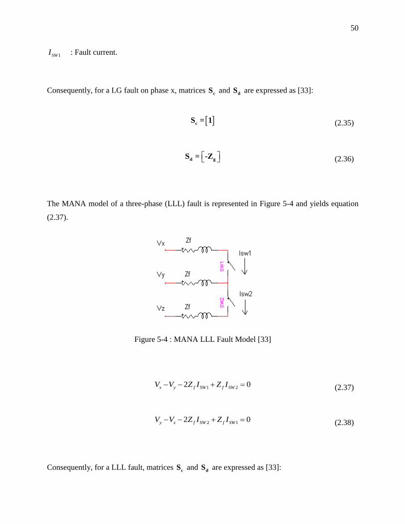
50

1SWI : Fault current.

Consequently, for a LG fault on phase x, matrices cS and

dS are expressed as [33]:

cS = 1 (2.35)

d gS = -Z (2.36)

The MANA model of a three-phase (LLL) fault is represented in Figure 5-4 and yields equation

(2.37).

Figure 5-4 : MANA LLL Fault Model [33]

1 22 0x y f SW f SWV V Z I Z I (2.37)

2 12 0y z f SW f SWV V Z I Z I (2.38)

Consequently, for a LLL fault, matrices cS and dS are expressed as [33]:

51

1 0

1 1

0 1

cS = (2.39)

-2

-2

f f

f f

Z Z

Z Z

dS (2.40)

Detailed representation of other types of fault can be found in [33].

5.4.3 Fault flow algorithm

5.4.3.1 Short-circuit calculations assumptions

In the proposed MANA-based fault flow algorithm, all devices other than the Type 4 WTG are

modeled as linear devices based on the short-circuit MANA representation, as detailed in [33]. In

particular, all generators except inverter connected generators are modeled as voltage source

behind impedance. The value of the impedance can be the sub-transient, transient or steady-state

value depending on the period studied.

Besides, same assumptions as in traditional short-circuit analysis are made to have the same basis

of comparison later on, when comparing the existing short-circuit models of Type 4 WTG with

the proposed one. As a result, loads, shunt capacitors and line charging effects are neglected, pre-

fault voltages are considered nominal and transformers are set at nominal tap.

Since loads are neglected, the generic matrix equation (2.8) yields:

jj

n nn c IG

r d x x

G GI G G

ΔV fY A A

A A 0 ΔI f

J 0 J ΔI f

(2.41)

52

Although it has been chosen to neglect loads, shunt capacitors and line charging effects, it is

important to mention that the Jacobian matrix formulation proposed in [28] allows accurately

representing these elements for short-circuit calculations purposes. Therefore, for more precision,

they could be modeled in the Jacobian matrix in equation (2.41). In such case, loads would be

modeled as constant impedances rather than being modeled according to their PQ constraint

equations. As for pre-fault voltages, they can also be considered at load-flow value instead of

nominal value for more precision.

5.4.3.2 Initialization of fault flow algorithm

Since the solution of the matrix equation (2.41) is found based on the Newton method, suitable

initialization of the algorithm is crucial to guarantee the convergence and performance of the

method. For this reason, the proposed fault flow algorithm is initialized with the Fixed-Point

MANA method presented in [28]. All devices are represented as linear devices. They are

modeled according to their MANA short-circuit model detailed specifically for each equipment

in [33]. As for the Type 4 WTG, it is proposed to model it as a three-phase voltage source behind

constant impedance. Each phase is modeled separately and yields equations (2.42) and (2.43)

below:

_WTG NOM LNE V (2.42)

_

_

NOM LN

WTG

VSC th

VZ

I (2.43)

where:

_NOM LNV : Nominal line-to-neutral voltage of the WTG (V).

_VSC thI : Threshold current of the WTG’s converter defined as in equation (2.22) (A).

53

The matrix equation (2.44) is then solved in a single iteration of the fixed point method as

proposed in [29]. As explained hereinabove, faults are represented by ideal switches and

represented in sub-matrices cA ,

rA and dA .

n nn c

r d x x

ΔV fY A

A A ΔI f

(2.44)

In its compact form, matrix equation (2.44) yields:

AX = b

(2.45)

The mismatch between the linear solution obtained from the fixed-point solution and the sought

final solution will depend on the control operating set-points and the distance-to-fault of the

WTG. By modeling the Type 4 WTG according to its maximum fault contribution at the

initialization step, the solution of the fixed-point algorithm is very close to the final solution for

faults close to the WTG. As for remote faults, more iterations are necessary to reach the final

solution. Besides, since all devices other than the Type 4 WTG are modeled appropriately, the

fixed point allows obtaining a solution very close to the final one in a single iteration. Figure 5-5

shows the initialization routine described and adapted from [29].

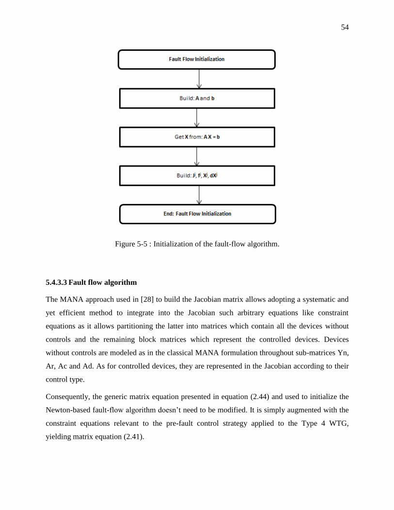
54

Figure 5-5 : Initialization of the fault-flow algorithm.

5.4.3.3 Fault flow algorithm

The MANA approach used in [28] to build the Jacobian matrix allows adopting a systematic and

yet efficient method to integrate into the Jacobian such arbitrary equations like constraint

equations as it allows partitioning the latter into matrices which contain all the devices without

controls and the remaining block matrices which represent the controlled devices. Devices

without controls are modeled as in the classical MANA formulation throughout sub-matrices Yn,

Ar, Ac and Ad. As for controlled devices, they are represented in the Jacobian according to their

control type.

Consequently, the generic matrix equation presented in equation (2.44) and used to initialize the

Newton-based fault-flow algorithm doesn’t need to be modified. It is simply augmented with the

constraint equations relevant to the pre-fault control strategy applied to the Type 4 WTG,

yielding matrix equation (2.41).

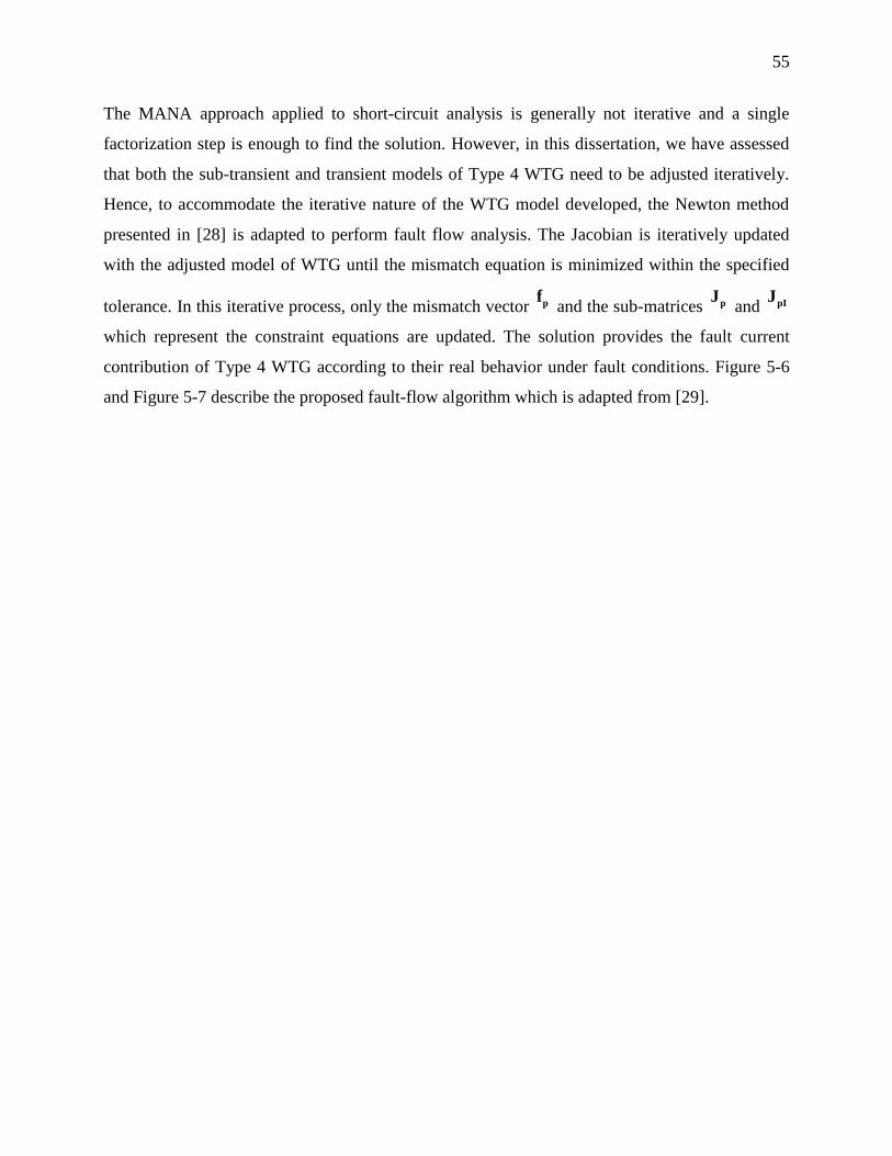
55

The MANA approach applied to short-circuit analysis is generally not iterative and a single

factorization step is enough to find the solution. However, in this dissertation, we have assessed

that both the sub-transient and transient models of Type 4 WTG need to be adjusted iteratively.

Hence, to accommodate the iterative nature of the WTG model developed, the Newton method

presented in [28] is adapted to perform fault flow analysis. The Jacobian is iteratively updated

with the adjusted model of WTG until the mismatch equation is minimized within the specified

tolerance. In this iterative process, only the mismatch vector pf

and the sub-matrices pJ

and pIJ

which represent the constraint equations are updated. The solution provides the fault current

contribution of Type 4 WTG according to their real behavior under fault conditions. Figure 5-6

and Figure 5-7 describe the proposed fault-flow algorithm which is adapted from [29].

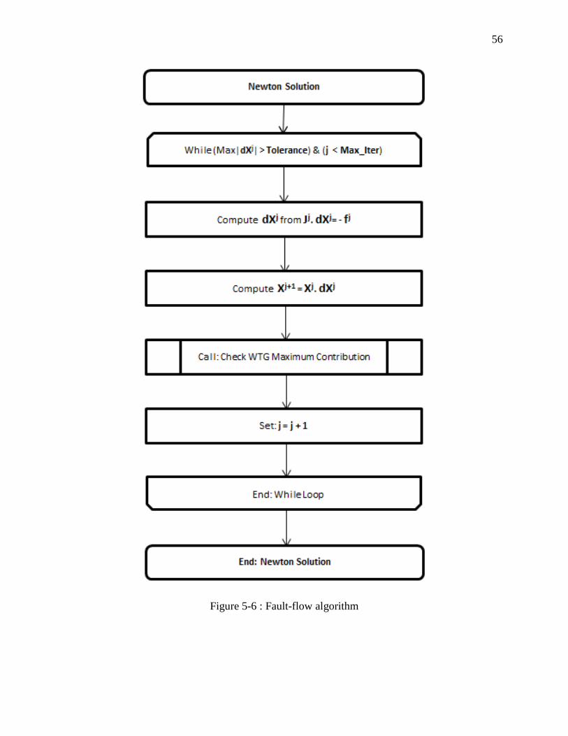
56

Figure 5-6 : Fault-flow algorithm

57

Figure 5-7 : Algorithm to check the WTG maximum fault contribution.

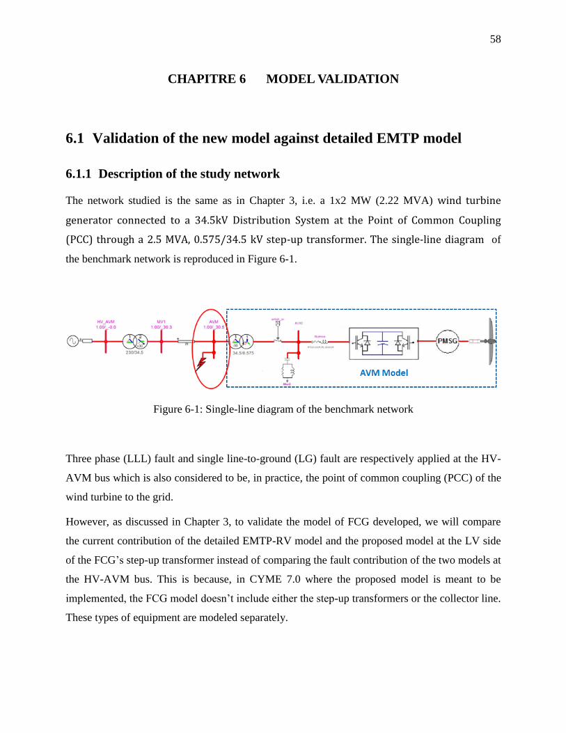
58

CHAPITRE 6 MODEL VALIDATION


6.1 Validation of the new model against detailed EMTP model

6.1.1 Description of the study network

The network studied is the same as in Chapter 3, i.e. a 1x2 MW (2.22 MVA) wind turbine

generator connected to a 34.5kV Distribution System at the Point of Common Coupling

(PCC) through a 2.5 MVA, 0.575/34.5 kV step-up transformer. The single-line diagram of

the benchmark network is reproduced in Figure 6-1.

Figure 6-1: Single-line diagram of the benchmark network

Three phase (LLL) fault and single line-to-ground (LG) fault are respectively applied at the HV-

AVM bus which is also considered to be, in practice, the point of common coupling (PCC) of the

wind turbine to the grid.

However, as discussed in Chapter 3, to validate the model of FCG developed, we will compare

the current contribution of the detailed EMTP-RV model and the proposed model at the LV side

of the FCG’s step-up transformer instead of comparing the fault contribution of the two models at

the HV-AVM bus. This is because, in CYME 7.0 where the proposed model is meant to be

implemented, the FCG model doesn’t include either the step-up transformers or the collector line.

These types of equipment are modeled separately.

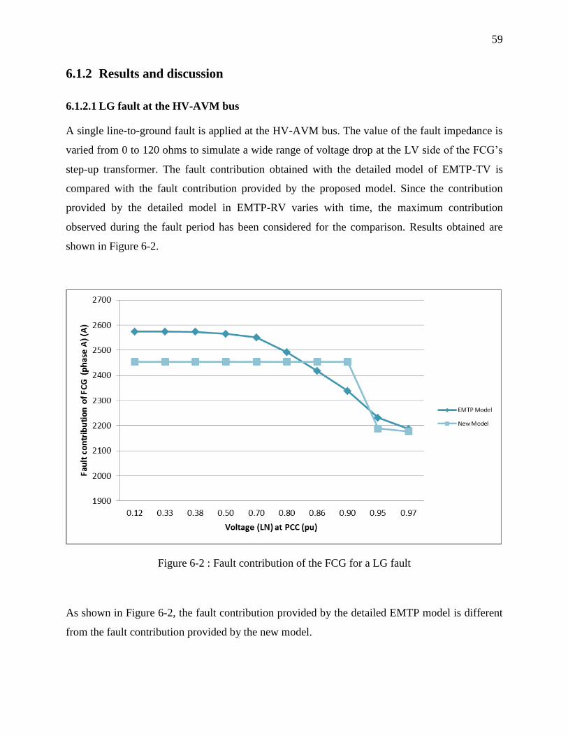
59

6.1.2 Results and discussion

6.1.2.1 LG fault at the HV-AVM bus

A single line-to-ground fault is applied at the HV-AVM bus. The value of the fault impedance is

varied from 0 to 120 ohms to simulate a wide range of voltage drop at the LV side of the FCG’s

step-up transformer. The fault contribution obtained with the detailed model of EMTP-TV is

compared with the fault contribution provided by the proposed model. Since the contribution

provided by the detailed model in EMTP-RV varies with time, the maximum contribution

observed during the fault period has been considered for the comparison. Results obtained are

shown in Figure 6-2.

Figure 6-2 : Fault contribution of the FCG for a LG fault

As shown in Figure 6-2, the fault contribution provided by the detailed EMTP model is different

from the fault contribution provided by the new model.

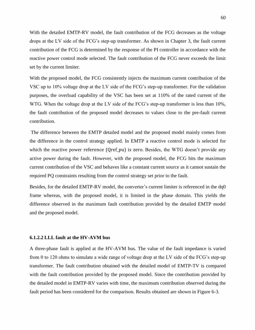
60

With the detailed EMTP-RV model, the fault contribution of the FCG decreases as the voltage

drops at the LV side of the FCG’s step-up transformer. As shown in Chapter 3, the fault current

contribution of the FCG is determined by the response of the PI controller in accordance with the

reactive power control mode selected. The fault contribution of the FCG never exceeds the limit

set by the current limiter.

With the proposed model, the FCG consistently injects the maximum current contribution of the

VSC up to 10% voltage drop at the LV side of the FCG’s step-up transformer. For the validation

purposes, the overload capability of the VSC has been set at 110% of the rated current of the

WTG. When the voltage drop at the LV side of the FCG’s step-up transformer is less than 10%,

the fault contribution of the proposed model decreases to values close to the pre-fault current

contribution.

The difference between the EMTP detailed model and the proposed model mainly comes from

the difference in the control strategy applied. In EMTP a reactive control mode is selected for

which the reactive power reference (Qref_pu) is zero. Besides, the WTG doesn’t provide any

active power during the fault. However, with the proposed model, the FCG hits the maximum

current contribution of the VSC and behaves like a constant current source as it cannot sustain the

required PQ constraints resulting from the control strategy set prior to the fault.

Besides, for the detailed EMTP-RV model, the converter’s current limiter is referenced in the dq0

frame whereas, with the proposed model, it is limited in the phase domain. This yields the

difference observed in the maximum fault contribution provided by the detailed EMTP model

and the proposed model.

6.1.2.2 LLL fault at the HV-AVM bus

A three-phase fault is applied at the HV-AVM bus. The value of the fault impedance is varied

from 0 to 120 ohms to simulate a wide range of voltage drop at the LV side of the FCG’s step-up

transformer. The fault contribution obtained with the detailed model of EMTP-TV is compared

with the fault contribution provided by the proposed model. Since the contribution provided by

the detailed model in EMTP-RV varies with time, the maximum contribution observed during the

fault period has been considered for the comparison. Results obtained are shown in Figure 6-3.

61

Figure 6-3 : Fault contribution of the FCG for a LG fault

Like for the LG fault, Figure 6-3 shows that the fault contribution provided by the detailed EMTP

model is different from the fault contribution provided by the new model.

With the detailed EMTP-RV model, the fault contribution of the FCG decreases as the voltage

drops at the LV side of the FCG’s step-up transformer. Once again, the fault current contribution

of the FCG is determined by the response of the PI controller in accordance with the reactive

power control mode selected. The fault contribution of the detailed EMTP-RV model is also

limited under the pre-set value of the converter’s current limiter.

With the proposed model, the FCG consistently injects the maximum current contribution of the

VSC, i.e. 110% of the rated current of the WTG, regardless of the voltage drop at the LV side of

the FCG’s step-up transformer. It therefore behaves like a constant current source.

Similarly to what was observed for the LLL fault, the difference between the EMTP detailed

model and the proposed model mainly comes from the difference in the control strategy applied

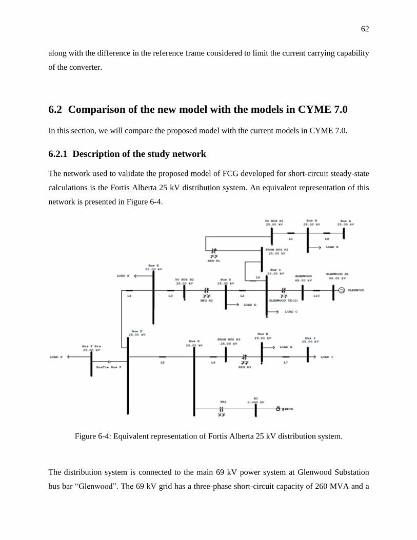
62

along with the difference in the reference frame considered to limit the current carrying capability

of the converter.

6.2 Comparison of the new model with the models in CYME 7.0

In this section, we will compare the proposed model with the current models in CYME 7.0.

6.2.1 Description of the study network

The network used to validate the proposed model of FCG developed for short-circuit steady-state

calculations is the Fortis Alberta 25 kV distribution system. An equivalent representation of this

network is presented in Figure 6-4.

Figure 6-4: Equivalent representation of Fortis Alberta 25 kV distribution system.

The distribution system is connected to the main 69 kV power system at Glenwood Substation

bus bar “Glenwood”. The 69 kV grid has a three-phase short-circuit capacity of 260 MVA and a

63

single-phase short-circuit capacity of 181 MVA. Its X1/R1 ratio is 1.602 and its X0/R0 ratio is

3.069.

A FCG of 436.5 kW, 0.24 kV is connected to bus bar 147-0. Its converter is designed with an

overload capability of 20% above rated, hence 1260.07 A. Loads are connected to bus bars B, C, D,

E, F, H and I. Their contribution is however neglected in the short-circuit analysis.

6.3 Fault contribution of Type 4 WTG under various fault conditions

This section discusses the results obtained for LLLG and LG faults, applied respectively at

different buses, for different pre-fault conditions and assuming that the WTG operates in fixed

generation mode prior to the fault. For each scenario, the WTG fault contribution obtained with

the proposed model is compared with results from CYME, considering both a nominal pre-fault

voltage (column CYME NOMINAL in the tables below) and a pre-fault voltage (column CYME

LOAD FLOW in the tables below) computed from the load flow solution.

6.3.1 Three-phase fault at various locations

6.3.1.1 Desired active generation: 436.5 kW

A three-phase fault is applied at different buses of the distribution network. Prior to the fault, the

Type 4 WTG operates in fixed generation mode and its desired active generation is set to 436.5

kW, which corresponds to the rated power of the generator. Figure 6-5 shows the resultant fault

contribution of the WTG.

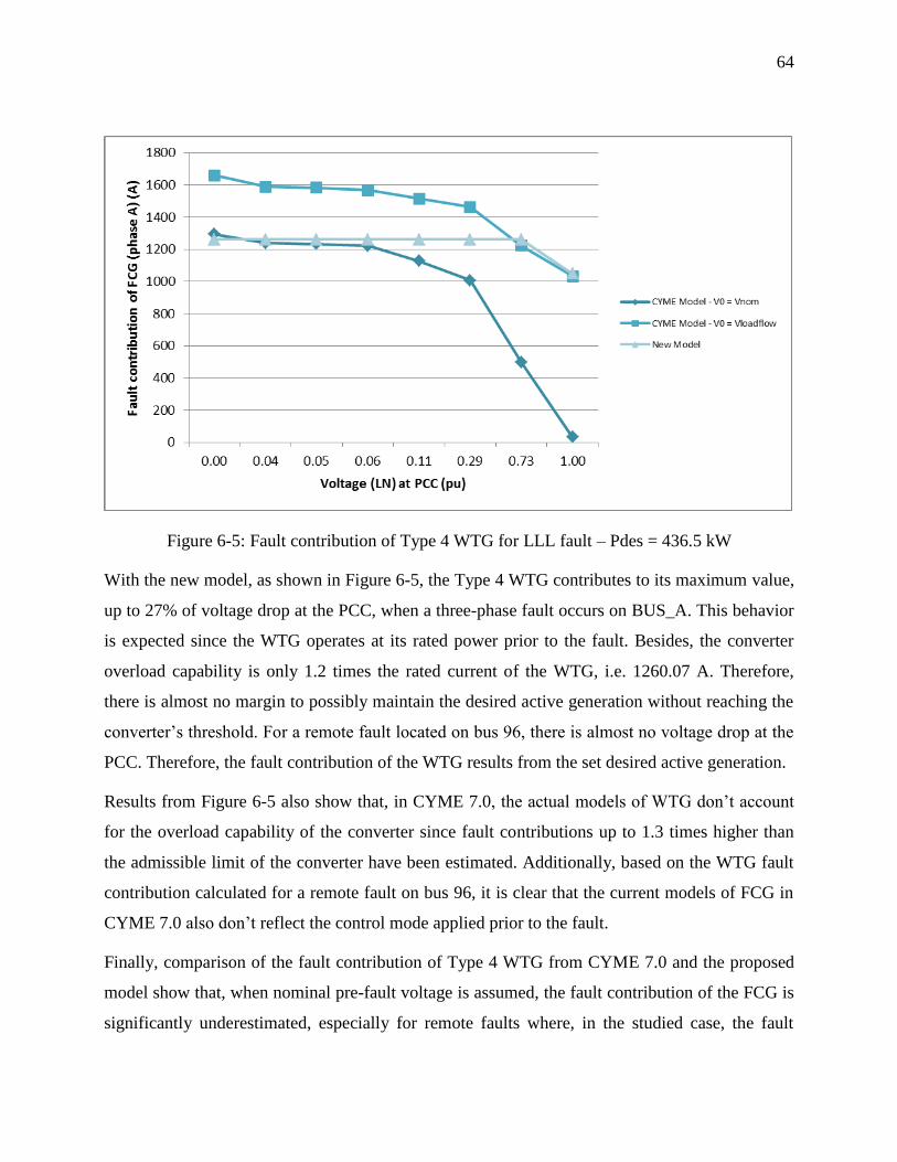
64

Figure 6-5: Fault contribution of Type 4 WTG for LLL fault – Pdes = 436.5 kW

With the new model, as shown in Figure 6-5, the Type 4 WTG contributes to its maximum value,

up to 27% of voltage drop at the PCC, when a three-phase fault occurs on BUS_A. This behavior

is expected since the WTG operates at its rated power prior to the fault. Besides, the converter

overload capability is only 1.2 times the rated current of the WTG, i.e. 1260.07 A. Therefore,

there is almost no margin to possibly maintain the desired active generation without reaching the

converter’s threshold. For a remote fault located on bus 96, there is almost no voltage drop at the

PCC. Therefore, the fault contribution of the WTG results from the set desired active generation.

Results from Figure 6-5 also show that, in CYME 7.0, the actual models of WTG don’t account

for the overload capability of the converter since fault contributions up to 1.3 times higher than

the admissible limit of the converter have been estimated. Additionally, based on the WTG fault

contribution calculated for a remote fault on bus 96, it is clear that the current models of FCG in

CYME 7.0 also don’t reflect the control mode applied prior to the fault.

Finally, comparison of the fault contribution of Type 4 WTG from CYME 7.0 and the proposed

model show that, when nominal pre-fault voltage is assumed, the fault contribution of the FCG is

significantly underestimated, especially for remote faults where, in the studied case, the fault

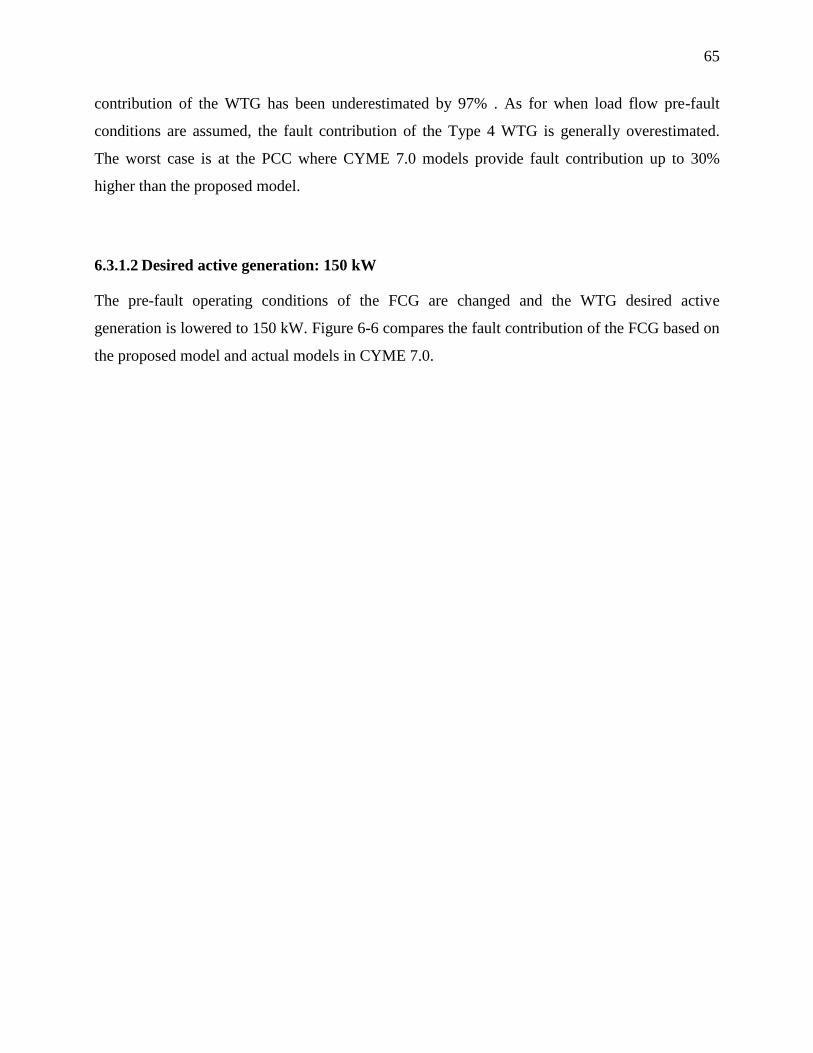
65

contribution of the WTG has been underestimated by 97% . As for when load flow pre-fault

conditions are assumed, the fault contribution of the Type 4 WTG is generally overestimated.

The worst case is at the PCC where CYME 7.0 models provide fault contribution up to 30%

higher than the proposed model.

6.3.1.2 Desired active generation: 150 kW

The pre-fault operating conditions of the FCG are changed and the WTG desired active

generation is lowered to 150 kW. Figure 6-6 compares the fault contribution of the FCG based on

the proposed model and actual models in CYME 7.0.

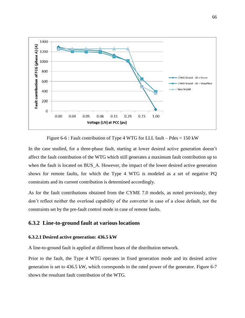
66

Figure 6-6 : Fault contribution of Type 4 WTG for LLL fault – Pdes = 150 kW

In the case studied, for a three-phase fault, starting at lower desired active generation doesn’t

affect the fault contribution of the WTG which still generates a maximum fault contribution up to

when the fault is located on BUS_A. However, the impact of the lower desired active generation

shows for remote faults, for which the Type 4 WTG is modeled as a set of negative PQ

constraints and its current contribution is determined accordingly.

As for the fault contributions obtained from the CYME 7.0 models, as noted previously, they

don’t reflect neither the overload capability of the converter in case of a close default, nor the

constraints set by the pre-fault control mode in case of remote faults.

6.3.2 Line-to-ground fault at various locations

6.3.2.1 Desired active generation: 436.5 kW

A line-to-ground fault is applied at different buses of the distribution network.

Prior to the fault, the Type 4 WTG operates in fixed generation mode and its desired active

generation is set to 436.5 kW, which corresponds to the rated power of the generator. Figure 6-7

shows the resultant fault contribution of the WTG.

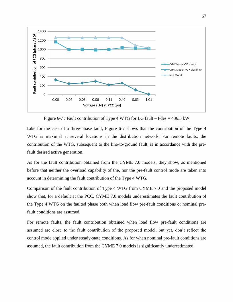
67

Figure 6-7 : Fault contribution of Type 4 WTG for LG fault – Pdes = 436.5 kW

Like for the case of a three-phase fault, Figure 6-7 shows that the contribution of the Type 4

WTG is maximal at several locations in the distribution network. For remote faults, the

contribution of the WTG, subsequent to the line-to-ground fault, is in accordance with the pre-

fault desired active generation.

As for the fault contribution obtained from the CYME 7.0 models, they show, as mentioned

before that neither the overload capability of the, nor the pre-fault control mode are taken into

account in determining the fault contribution of the Type 4 WTG.

Comparison of the fault contribution of Type 4 WTG from CYME 7.0 and the proposed model

show that, for a default at the PCC, CYME 7.0 models underestimates the fault contribution of

the Type 4 WTG on the faulted phase both when load flow pre-fault conditions or nominal pre-

fault conditions are assumed.

For remote faults, the fault contribution obtained when load flow pre-fault conditions are

assumed are close to the fault contribution of the proposed model, but yet, don’t reflect the

control mode applied under steady-state conditions. As for when nominal pre-fault conditions are

assumed, the fault contribution from the CYME 7.0 models is significantly underestimated.

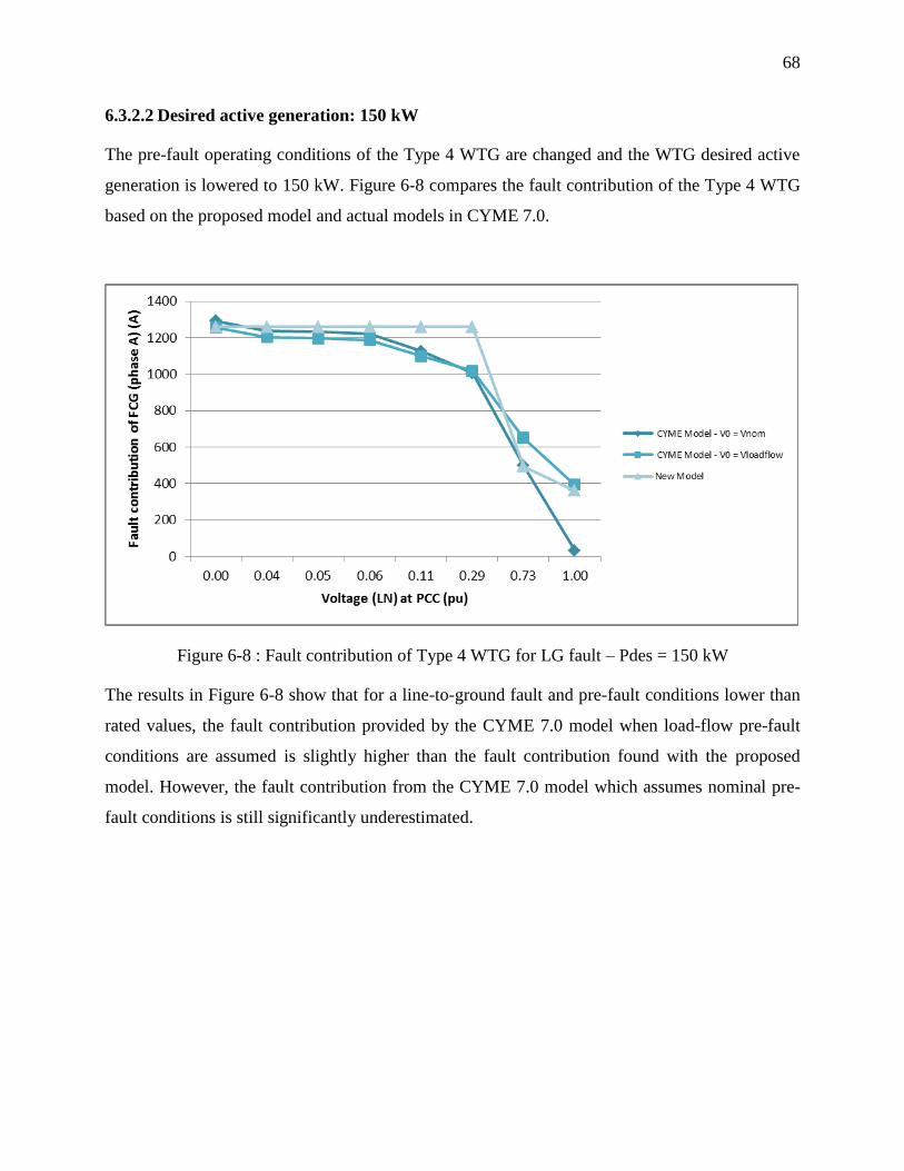
68

6.3.2.2 Desired active generation: 150 kW

The pre-fault operating conditions of the Type 4 WTG are changed and the WTG desired active

generation is lowered to 150 kW. Figure 6-8 compares the fault contribution of the Type 4 WTG

based on the proposed model and actual models in CYME 7.0.

Figure 6-8 : Fault contribution of Type 4 WTG for LG fault – Pdes = 150 kW

The results in Figure 6-8 show that for a line-to-ground fault and pre-fault conditions lower than

rated values, the fault contribution provided by the CYME 7.0 model when load-flow pre-fault

conditions are assumed is slightly higher than the fault contribution found with the proposed

model. However, the fault contribution from the CYME 7.0 model which assumes nominal pre-

fault conditions is still significantly underestimated.

69

CONCLUSION

Actual representation of FCG in commercial short-circuit analysis software tools doesn’t

reproduce their real behavior under steady-state fault conditions. Actually, most packages don’t

allow direct representation of current sources since they use sequence network representation to

perform short-circuit calculations [38]. As a result, Type 4 WTG is modeled as a voltage source

behind impedance which is iteratively adjusted to match the fault current contribution of the

WTG. This model is not appropriate, especially in sub-transient operating mode for which one

cannot determine in advance the fault contribution of the WTG. In CYME [41], the value of this

impedance is fixed and is derived from a three-phase bolted fault at the WTG terminals. As a

result, at nominal pre-fault voltage, the mismatch between the WTG’s fault current contribution

computed by CYME and the WTG’s real fault contribution increases with the distance from PCC

to fault. Besides, in CYME, the Type 4 WTG is assumed to inject only reactive current into the

grid whereas, in practice, the currents injected by a Type 4 WTG have real and reactive

components as determined by the applicable grid code minimum LVRT requirements [26].

The purpose of this research work was to provide a simple model of Type 4 WTG which closely

reproduces its real behavior under fault conditions. However, comparison with the detailed

EMTP model shows that the proposed model doesn’t provide the same fault contribution than the

detailed EMTP model under similar fault conditions. The difference observed between the two

models mainly results from the difference in the control strategy applied during the fault.

Actually, in EMTP, the FCG is controlled to stop delivering active power during the fault and to

either inject reactive power into the grid (Q control) or also support the grid voltage (Q+Vac

control). However, with the proposed model, the fault contribution of the FCG depends on the

control strategy set prior to the fault and the FCG tends to behave like a constant current source

as a result of the voltage drop at the LV side of the FCG’s step-up transformer. On the other

hand, for remote faults, the proposed model operates close to its pre-fault values. Besides, the

difference observed between the two models is also due to the difference in the reference frame

in which the converter’s current is limited. In EMTP, the converter’s current is limited in the dq0

frame whereas, for the proposed model, the current is limited in the phase domain. This yields

different maximum fault contributions for the two models.

70

Compared to the current models in CYME 7.0, the proposed model accounts for the overload

capability of the converter along with the pre-fault operating conditions and control operating set

points as recommended in [25] by the Joint Working Group on Wind Plant Short Circuit

Contribution. Besides, no proprietary data is required to model the Type 4 WTG with the

proposed model. The only data relative to the converter is its overload design capability which is

typically expressed based on the rated power of the WTG. Based on the comparison with CYME

current models, the proposed model reproduces better the behavior recommended by the Joint

Working Group on Wind Plant Short Circuit Contribution in [25].

As pointed out in [25], proposing a general model of FCG for short-circuit analysis purposes is

very difficult as it depends on parameters such as the control strategy implemented which is

specific to the WTG manufacturers and the FRT requirements which are specific to either the

applicable grid code or the utility. In this respect, the proposed equivalent model of FCG can be

considered acceptable as, in most cases, it provides the maximum fault contribution and is

therefore on the safe side.

The other contribution of this research work is the development of an iterative fault flow

algorithm for the treatment of WTG for short-circuit analysis purposes, based on the Newton

MANA method published in [28]. The approach is original as short-circuit algorithms are not

iterative by nature. Hence, they are not adapted to accommodate inverter based WTG which

behavior is different from traditional generators. The fault-flow algorithm developed provides a

simple and yet efficient way of modeling Type 4 WTG thanks to a dynamic Jacobian approach.

The performance of the method can be considered acceptable as the algorithm is initialized close

to the final solution with a single iteration of the fixed-point method.

This research works sets the groundwork for modeling the Type 4 WTG for short-circuit analysis

purposes. However, further work needs to be done to explain the differences with the detailed

model in EMTP-RV and to improve the proposed frequency domain model of full converter

based wind turbine generators. Besides, it would be interesting to possibly extend the model to

other full converter based DG units (micro turbines, photovoltaic panels).

71

BIBLIOGRAPHIE

1. T. N. Boutsika and S. A. Papathanassiou, Short-circuit calculations in networks with

distributed generation. Elsevier, 2007: p. 1182 - 1191.

2. EMTP-RV. 2011 [On Line]. Available: http://www.emtp.com

3. IEC60909, Short-circuit currents in three-phase a.c. systems. 2001.

4. IEEEC37.5, Guide for Calculation of Fault Currents for Application of AC High-Voltage

Circuit Breakers Rated on a Total Current Basis.

5. L. D. Bellomo, Comparative Modelling of Wind Parks for Slow and Fast Transients, in

Electrical Engineering. 2010, Ecole Polytechnique de Montreal: Montreal.

6. M. Garcia-Sanz, M. Barreras and P. Vital, Power Regulation Strategies for Wind

Turbines, in Advances in Wind Energy Conversion Technology, Springer, Editor. 2011:

Berlin. p. 159-176.

7. J. Peralta, S. Dennetière and J. Mahseredjian, Dynamic Performance of Average-value

Models for VSC-HVDC Transmission Systems, in Power and Energy Society General

Meeting IEEE. 2012: San Diego, CA. p. 1 - 8.

8. N. Flourentzou, V. G. Agelidis and G. D. Demetriades, VSC-Based HVDC Power

Transmission Systems: An Overview. Power Electronics, IEEE Transactions 24(3): p. 592

- 602.

9. M. Valentini, V. Akhmatov, F. Iov and J. Thisted, Fault Current Contribution from VSC-

based Wind Turbines to the Grid. The Second International Symposium on Electrical and

Electronics Engineering, 2008.

10. M. Tsili and S. Papathanassiou, A review of grid code technical requirements for wind

farms. IET Renewable Power Generation, 2009. 3(3): p. 308-332.

11. IEEE, IEEE Application Guide for IEEE Std 1547.2, IEEE Standard for Interconnecting

Distributed Resources with Electric Power Systems. 2008.

12. IEEEC37.010, IEEE Application Guide for AC High-Voltage Circuit Breakers Rated on a

Symmetrical Current Basis. 1999.

13. N. Samaan, R. Zavadil, J. C. Smith and J. Conto, Modeling of Wind Power Plants for

Short Circuit Analysis in the Transmission Network, in Transmission and Distribution

Conference and Exposition. 2008: Chicago, IL. p. 1 - 7.

14. (WWEA), W.W.E.A. World Wind Energy Association. February 2012; Available from:

http://www.wwindea.org/home/index.php.

15. P. Karaliolios, A. Ishchenko, E. Coster, J. Myrzik and W. Kling, Overview of Short-

Circuit Contribution of Various Distributed Generators on the Distribution Network, in

Universities Power Engineering Conference, UPEC 2008. 43rd International. 2008:

Padova. p. 1 - 6.

http://www.emtp.com/

http://www.wwindea.org/home/index.php

72

16. T. Ackermann and V. Knyazkin, Interaction between Distributed Generation and the

Distribution Network: Operation Aspects, in Transmission and Distribution Conference

and Exhibition 2002. 2002, IEEE/PES: Asia Pacific. p. 1357 - 1362.

17. E. Muljadi, V. Gevorgian, N. Samaan, J. Li and S. Pasupulati, Short Circuit Current

Contribution For Different Wind Turbine Generator Types, in Power and Energy Society

General Meeting. 2010, IEEE: Minneapolis, MN. p. 1 - 8.

18. M. E. Baran and I. El-Markaby, Fault Analysis on Distribution Feeders With Distributed

Generators. IEEE Transactions on Power Systems 2005. 20: p. 1757-1764.

19. M. Fischer and A. Mendonça, Representation of Variable Speed Full Conversion Wind

Energy Converters for Steady State Short-Circuit Calculations, in Power and Energy

Society General Meeting, 2011 IEEE. 2011: San Diego, CA. p. 1 - 7.

20. I. Kocar, J. S. Lacroix and F. Therrien, General and Simplified Computation of Fault

Flow and Contribution of Distributed Sources in Unbalanced Distribution Networks, in

Power and Energy Society General Meeting. 2012, IEEE: San Diego, CA. p. 1 - 8.

21. C. A. Plet, M. Graovac, T. C. Green and R. Iravani, Fault Response of Grid-Connected

Inverter Dominated Networks, in Power and Energy Society General Meeting. 2010,

IEEE: Minneapolis, MN. p. 1 - 8.

22. R. J. Nelson and H. Ma, Short-Circuit Contributions of Full-Converter Wind Turbines, in

Power and Energy Society General Meeting. 2011, IEEE: San Diego, CA. p. 1 - 4.

23. D. Turcotte and F. Katiraei, Fault Contribution of Grid-Connected Inverters, in Electrical

Power & Energy Conference (EPEC). 2009, IEEE: Montreal, QC. p. 1 - 5.

24. R. A. Walling and M. L. Reichard, Short Circuit Behavior of Wind Turbine Generators,

in Protective Relay Engineers, 2009 62nd Annual Conference. 2009: Austin, TX. p. 492 -

502.

25. R. Walling, R. Harley, D. Miller and G. Henneberg, Fault Current Contributions from

Wind Plants.

26. R. A. Walling, E. Gursoy and B. English, Current Contributions from Type 3 and Type 4

Wind Turbine Generators During Faults, in PES General Meeting. 2011: Detroit, MI.

27. A. Yazdani and R. Iravani, A Unified Dynamic Model and Control for the Voltage-

Sourced Converter Under Unbalanced Grid Conditions. IEEE Transactions on Power

Delivery, 2006. 21(3): p. 1620-1629.

28. I. Kocar, J. Mahseredjian, U. Karaagac, G. Soykan and O. Saad, Multiphase Load-Flow

Solution for Large Scale Distribution Systems using MANA. Power Delivery, IEEE

Transactions, 2013. PP(99): p. 1.

29. A. Gueye, CYME 7.1 Load-Flow MANA Solver. 2013.

30. M. Z. Kamh and R. Iravani, A Unified Three-Phase Power-Flow Analysis Model For

Electronically-Coupled Distributed Energy Resources. Power Delivery, IEEE

Transactions, 2011. 26(2): p. 899 - 909.

31. M. Valentini, Fault Current Contribution from VSC-based Wind Turbines to the Grid, in

Institute of Energy Technology. 2008, Aalborg University: Denmark. p. 134.

73

32. TransEnergie, H.Q., Transmission Provider Technical Requirement For the Connection

of Power Plants To The Connection of Power Plants To The Hydro-Quebec Transmission

System. 2009.

33. J. S. Lacroix, Multiphase Short-Circuit Analysis Solver In Phase Domain Using A

Modified-Augmented-Nodal Analysis Approach. 2012, Ecole Polytechnique: Montréal.

34. R. C. Dugan, A Perspective On Transformer Modeling for Distribution Svstem Analvsis,

in Power Engineering Society General Meeting. 2003. p. 114-119.

35. J. Peralta, F. de León and J. Mahseredjian, Assessment of Errors Introduced by Common

Assumptions Made in Power System Studies, in Power and Energy Society General

Meeting. 2011: San Diego, CA. p. 1-8.

36. S. Bernard, D. Beaulieu and G. Trudel, Hydro-Québec grid code for wind farm

interconnection, in Power

Engineering Society General Meeting. 2005, IEEE. p. 1248 - 1252.

37. Gmbh, E.O.N., Grid code - high and extra high voltage. 2006: Bayreuth, Germany

38. 32.0, P., PSSE Program Operation Manual, June 2009

39. REE, Requisitos de repuesta frente a huecos de tension de las instalaciones de

produccion de regimen especial, November 2005, Spain

40. I. Erlich, W. Winter and A. Dittrich, Advanced Grid Requirements for the Integration of

Wind Turbines into the German Transmission System. IEEE Power Engineering Society

General Meeting 2006.

41. CYME Software, 2013 [On Line]. Available: http://www.cyme.com

42. CYMSTAB Software, 2013 [On Line]. Available: http://www.cyme.com

43. Wind Turbine Blade Aerodynamics, [Online]. Available:

http://www.gurit.com/files/documents/2_aerodynamics.pdf

44. J. Mahseredjian, S. Dennetière, L. Dubé, B. Khodabakhchian and L. Gérin-Lajoie, On a

new approach for the simulation of transients in power systems, in 6th

International

Conference on Power System Transients, 2007, p. 1514-1520.

http://www.cyme.com/

http://www.cyme.com/

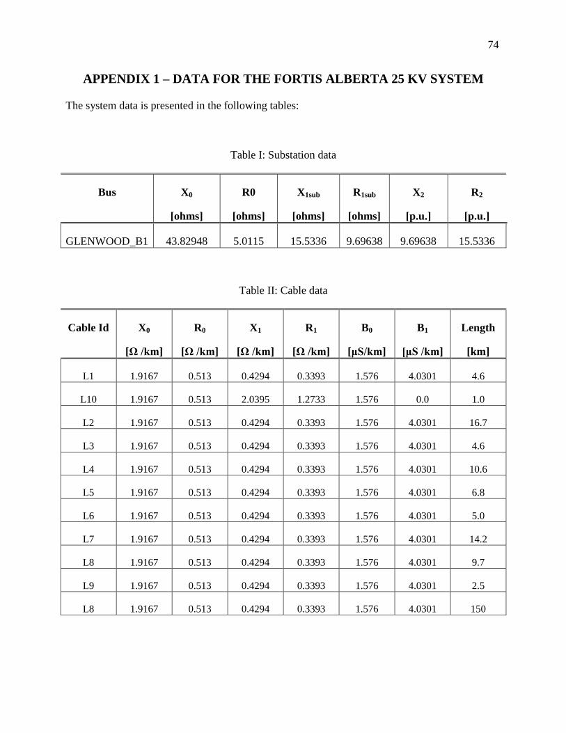
74

APPENDIX 1 – DATA FOR THE FORTIS ALBERTA 25 KV SYSTEM

The system data is presented in the following tables:

Table I: Substation data

Bus X0

[ohms]

R0

[ohms]

X1sub

[ohms]

R1sub

[ohms]

X2

[p.u.]

R2

[p.u.]

GLENWOOD_B1 43.82948 5.0115 15.5336 9.69638 9.69638 15.5336

Table II: Cable data

Cable Id X0

[Ω /km]

R0

[Ω /km]

X1

[Ω /km]

R1

[Ω /km]

B0

[μS/km]

B1

[μS /km]

Length

[km]

L1 1.9167 0.513 0.4294 0.3393 1.576 4.0301 4.6

L10 1.9167 0.513 2.0395 1.2733 1.576 0.0 1.0

L2 1.9167 0.513 0.4294 0.3393 1.576 4.0301 16.7

L3 1.9167 0.513 0.4294 0.3393 1.576 4.0301 4.6

L4 1.9167 0.513 0.4294 0.3393 1.576 4.0301 10.6

L5 1.9167 0.513 0.4294 0.3393 1.576 4.0301 6.8

L6 1.9167 0.513 0.4294 0.3393 1.576 4.0301 5.0

L7 1.9167 0.513 0.4294 0.3393 1.576 4.0301 14.2

L8 1.9167 0.513 0.4294 0.3393 1.576 4.0301 9.7

L9 1.9167 0.513 0.4294 0.3393 1.576 4.0301 2.5

L8 1.9167 0.513 0.4294 0.3393 1.576 4.0301 150

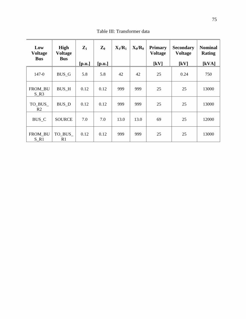
75

Table III: Transformer data

Low

Voltage

Bus

High

Voltage

Bus

Z1

[p.u.]

Z0

[p.u.]

X1/R1 X0/R0 Primary

Voltage

[kV]

Secondary

Voltage

[kV]

Nominal

Rating

[kVA]

147-0 BUS_G 5.8 5.8 42 42 25 0.24 750

FROM_BU

S_R3

BUS_H 0.12 0.12 999 999 25 25 13000

TO_BUS_

R2

BUS_D 0.12 0.12 999 999 25 25 13000

BUS_C SOURCE 7.0 7.0 13.0 13.0 69 25 12000

FROM_BU

S_R1

TO_BUS_

R1

0.12 0.12 999 999 25 25 13000

representation of type 4 wind turbine …¨yekamara.pdf · universitÉ de montrÉal representation...

Documents