met a heuristics
TRANSCRIPT

MetaheuristiquesStrategies pour l’optimisationde la production de biens et de services
Marc Sevaux


Numero d’ordre : 04/03
HABILITATION A DIRIGER DES RECHERCHES
Preparee au Laboratoire d’Automatique, de Mecanique d’informatiqueIndustrielles et Humaines du CNRS (UMR CNRS 8530)dans l’equipe Systemes de Production
Marc Sevaux
MetaheuristiquesStrategies pour l’optimisationde la production de biens et de services
Soutenue le 1er Juillet 2004 devant le jury compose de :
President Prof. Christian PrinsRapporteurs Prof. Michel Gourgand
Prof. Jin-Kao HaoProf. Eric Taillard
Examinateurs Prof. Stephane Dauzere-PeresProf. Bernard Grabot
Directeur Prof. Christian Tahon

Table des matieres
Remerciements 5
I Curriculum Vitæ 7
1 Informations generales 91.1 Etat Civil . . . . . . . . . . . . . . . . . . . . . . . . . . . . . . . . . . 91.2 Fonction actuelle . . . . . . . . . . . . . . . . . . . . . . . . . . . . . 91.3 Prime d’encadrement doctorale et de recherche . . . . . . . . . . . . 91.4 Parcours et formation . . . . . . . . . . . . . . . . . . . . . . . . . . . 10
2 Enseignement 122.1 Enseignements a l’UVHC . . . . . . . . . . . . . . . . . . . . . . . . 122.2 Enseignements avant l’integration a l’UVHC . . . . . . . . . . . . . 152.3 Encadrements pedagogiques . . . . . . . . . . . . . . . . . . . . . . 162.4 Administration de l’enseignement . . . . . . . . . . . . . . . . . . . 18
3 Supervision de travaux d’etudiants 2e et 3e cycle 203.1 Theses de doctorat . . . . . . . . . . . . . . . . . . . . . . . . . . . . 203.2 Memoires de DEA . . . . . . . . . . . . . . . . . . . . . . . . . . . . . 213.3 Projets de DESS . . . . . . . . . . . . . . . . . . . . . . . . . . . . . . 223.4 Projets IUP GEII . . . . . . . . . . . . . . . . . . . . . . . . . . . . . . 23
4 Administration et animation de la recherche 244.1 Animation de la recherche . . . . . . . . . . . . . . . . . . . . . . . . 244.2 Organisation de manifestations a Valenciennes . . . . . . . . . . . . 254.3 Organisation de manifestations en dehors de Valenciennes . . . . . 254.4 Organisation / president de sessions . . . . . . . . . . . . . . . . . . 26
5 Visibilite, rayonnement et autres activites 275.1 Collaborations . . . . . . . . . . . . . . . . . . . . . . . . . . . . . . . 275.2 Appartenance a des societes et des groupes de recherche . . . . . . 285.3 Fonction d’edition . . . . . . . . . . . . . . . . . . . . . . . . . . . . . 305.4 Evaluation de la recherche . . . . . . . . . . . . . . . . . . . . . . . . 31
6 Contrats, projets et financements 336.1 Contrats industriels . . . . . . . . . . . . . . . . . . . . . . . . . . . . 336.2 Projets de recherche . . . . . . . . . . . . . . . . . . . . . . . . . . . . 346.3 Financements obtenus . . . . . . . . . . . . . . . . . . . . . . . . . . 35
1

Table des matieres
7 Thematiques de recherche 367.1 Planification de la production . . . . . . . . . . . . . . . . . . . . . . 387.2 Ordonnancement . . . . . . . . . . . . . . . . . . . . . . . . . . . . . 397.3 Tournees de vehicules . . . . . . . . . . . . . . . . . . . . . . . . . . 427.4 Autres approches ou problematiques . . . . . . . . . . . . . . . . . . 43
8 Liste des publications 48
II Synthese scientifique 55
1 Introduction generale 571.1 Pourquoi les metaheuristiques ? . . . . . . . . . . . . . . . . . . . . . 571.2 Intensification et diversification . . . . . . . . . . . . . . . . . . . . . 571.3 Techniques de resolution pratique . . . . . . . . . . . . . . . . . . . 58
2 Methodes de recherche locale 592.1 Methodes de descente . . . . . . . . . . . . . . . . . . . . . . . . . . 602.2 Recuit simule . . . . . . . . . . . . . . . . . . . . . . . . . . . . . . . 622.3 Recherche tabou . . . . . . . . . . . . . . . . . . . . . . . . . . . . . . 642.4 Recherche a voisinages variables . . . . . . . . . . . . . . . . . . . . 662.5 GRASP . . . . . . . . . . . . . . . . . . . . . . . . . . . . . . . . . . . 672.6 Iterated local search . . . . . . . . . . . . . . . . . . . . . . . . . . . . 682.7 Guided local search . . . . . . . . . . . . . . . . . . . . . . . . . . . . 692.8 Applications . . . . . . . . . . . . . . . . . . . . . . . . . . . . . . . . 70
3 Metaheuristiques a base de population 713.1 Algorithmes genetiques . . . . . . . . . . . . . . . . . . . . . . . . . 723.2 Algorithmes de colonies de fourmis . . . . . . . . . . . . . . . . . . 753.3 Applications . . . . . . . . . . . . . . . . . . . . . . . . . . . . . . . . 76
4 Metaheuristiques avancees 794.1 Algorithmes memetiques . . . . . . . . . . . . . . . . . . . . . . . . 794.2 Scatter search . . . . . . . . . . . . . . . . . . . . . . . . . . . . . . . 814.3 GA|PM . . . . . . . . . . . . . . . . . . . . . . . . . . . . . . . . . . . 824.4 Applications . . . . . . . . . . . . . . . . . . . . . . . . . . . . . . . . 84
5 Complements 895.1 Reglages automatiques des parametres . . . . . . . . . . . . . . . . 905.2 Robustesse . . . . . . . . . . . . . . . . . . . . . . . . . . . . . . . . . 915.3 Optimisation multiobjectif . . . . . . . . . . . . . . . . . . . . . . . . 925.4 Optimisation continue . . . . . . . . . . . . . . . . . . . . . . . . . . 93
6 Conclusions 93
2
Table des matieres
7 Perspectives de recherche 96
References 99
III Selection de publications 109
1 European Journal of Operational Research (2003) 111
2 4OR (2004 a paraıtre) 112
3 Journal of Heuristics (2004 soumis) 112
4 Computers and Operations Research (2004 a paraıtre) 113
5 Naval Research Logistics (2003) 113
3

4

Remerciements
La redaction de ce manuscrit est l’aboutissement de plusieurs annees de tra-vail. Ce travail lui-meme n’aurait pu etre mene sans l’aide de plusieurs personnesauxquelles je souhaite exprimer ma gratitude.
Avant tout, je remercie les rapporteurs de cette dissertation, Michel Gourgand,Jin-Kao Hao et Eric Taillard, qui ont surement passe de longues heures a relire etcorriger ce document. Que les autres membres du jury soient aussi remercies.
Mes remerciements vont a la direction du LAMIH pour son accueil, et aussia l’ensemble de l’equipe “Systemes de Production” et sa bonne ambiance, ainsiqu’a Christian Tahon, son responsable, pour m’avoir fait confiance et donne unegrande liberte d’action ces dernieres annees.
Je tiens a exprimer ma gratitude tout particulierement a Christian Prins, qui aete mon professeur il y a de nombreuses annees et qui a eveille en moi le gout etla passion de la recherche. Je lui suis aussi reconnaissant pour les nombreuses dis-cussions productives, pour cette collaboration que nous avons entamee depuis lafin de ma these et enfin, pour avoir transforme au fil des annees notre partenariaten amitie sincere.
Que Stephane Dauzere-Peres, mon directeur de these soit aussi remercie cha-leureusement ; sous sa direction de 1996 a 1998, j’ai pu comprendre et apprendrele metier de chercheur et une certaine ethique de la recherche. Son amitie a heu-reusement depasse cette periode.
Je remercie aussi les professeurs qui m’ont enseignes la recherche operationnelleavec passion, Eric Pinson, Philippe Chretienne, Jacques Carlier et Claude Bergeainsi que les personnes qui ont su m’aider quand j’en avais besoin, Philippe Tho-min, Alain Gibaud, tout particlierement Xavier Gandibleux et bien d’autres.
Je garde une place de choix pour Kenneth Sorensen, pour tout ce que nousavons cree et partage ensemble, pour notre amitie ; le groupe EU/ME n’etant quela partie emergee de l’iceberg...
Enfin je tiens a terminer cette preface en remerciant de tout cœur mon epouseSandrine et mes enfants, Victoria, Francois et Jean pour leur patience pendantmes nombreuses absences et pour leur amour sans limite.
Marc SevauxValenciennes, Mai 2004
5

6

Premiere partie
Curriculum Vitæ

8

1 Informations generales
1.1 Etat Civil
NOM, Prenom SEVAUX, MarcDate et lieude naissance
Ne le 25 mai 1969 a Brest (29)
Nationalite FrancaiseEtat civil Marie, trois enfants
Service militaire effectue en 1995-1996, en tant qu’officier du corps tech-nique et administratif du service de sante des armees.
1.2 Fonction actuelle
Poste Maıtre de conferences (classe normale)en 61e section du CNU
Adresseprofessionnelle
Universite de Valenciennes et du Hainaut-CambresisUMR CNRS 8530, LAMIH / SPLe Mont Houy, Batiment Jonas 2F-59313 Valenciennes Cedex 9France
Telephone 03 27 51 13 26Fax 03 27 51 13 10Email [email protected]
Url http ://www.univ-valenciennes.fr/sp/sevaux/
Facultede rattachement
Institut universitaire de technologieDepartement Organisation et Genie de la Production(OGP)delocalise a Cambrai
Laboratoirede rattachement
LAMIH/SP : Laboratoire d’Automatique, de Mecanique,d’Informatique industrielles et Humaines – UMR CNRS8530 – Equipe Systemes de Production
1.3 Prime d’encadrement doctorale et de recherche
Titulaire de la prime d’encadrement doctorale et de recherche (PEDR)depuis 2003.
9

1 Informations generales
1.4 Parcours et formation
Depuis Sept. 99 Maıtre de conferences en 61e section a l’universite de Valen-ciennes et du Hainaut-Cambresis. Titulaire d’un poste a l’Institut Univer-sitaire de Technologie, au departement Organisation et Genie de la Produc-tion, delocalise a Cambrai.
Dec. 98 – Aout 99 Ingenieur de recherche (contrat a duree determinee de 9 mois)au departement Automatique et Productique de l’Ecole des Mines de Nantes.Charge de la redaction d’un cahier des charges pour la creation d’une plate-forme logistique (voir section 6.2).
1996 – 1998 Universite Pierre et Marie Curie, ParisDoctorat de l’Universite Pierre et Marie Curie (Paris VI).
Specialite Informatique et Recherche Operationnelle.Laboratoired’accueil
Ecole des Mines de Nantes,departement Automatique et Productique.
Soutenance le 11 Decembre 1998 a l’universite Pierre et Marie Curie(Paris VI).
Sujet Etude de deux problemes d’optimisationen planification et ordonnancement.
President du Jury P. Chretienne (Professeur, Universite P. et M. Curie, Pa-ris).
Rapporteurs Y. Crama (Professeur, Universite de Liege, Belgique),J.B. Lasserre (Directeur de Recherche, LAAS/CNRS,Toulouse)
Examinateurs M.-C. Portmann (Professeur, Ecole des Mines deNancy), C. Prins, (Maıtre Assistant, HDR, Ecole desMines de Nantes), S. Dauzere-Peres (Maıtre Assistant,HDR, Ecole des Mines de Nantes, Directeur de these).
Etude de deux problemes d’optimisation en planification et ordonnance-ment (probleme de planification de la production en temps continu et pro-bleme general d’ordonnancement a une machine). Resolution par l’utilisa-tion de techniques de recherche operationnelle. Validation par le develop-pement de logiciels prototypes.
10

1.4 Parcours et formation
1994 – 1995 Universite Pierre et Marie Curie, ParisDiplome d’Etudes Approfondies de l’Universite Pierre et Marie Curie (Pa-ris VI).
Specialite Informatique et Recherche OperationnelleMention BienResponsable Ph. Chretienne (Professeur, Universite Pierre et Marie
Curie, Paris)Sujet de DEA Les problemes d’ordonnancement avec delais de com-
municationEncadrement C. Picouleau (Maıtre de Conferences, CNAM, Paris).
1992 – 1994 Institut de Mathematiques Appliquees (IMA), AngersDiplomesobtenus
DEUG, Licence, Maıtrise
Specialite Mathematiques Appliquees et Sciences Sociales
11

2 Enseignement
2 Enseignement
2.1 Enseignements a l’UVHC
Recapitulatif des heures enseignees a l’UVHC
Le tableau ci-dessous resume les heures d’enseignement depuis le recrute-ment a l’universite de Valenciennes et du Hainaut-Cambresis. Le descriptif desmatieres enseignees est presente apres le tableau. Dans ce tableau, sont reprisesles heures de cours magistraux (CM), de travaux diriges (TD) et de travaux pra-tiques (TP), ainsi que l’equivalence en heures TD (EqTD). L’IUT permet aussi decomptabiliser certaines heures pour des taches administratives (Responsabilitedes projets, Relations internationales), ainsi que des heures pour l’encadrementdes stages et des projets.
Annee 2003-2004 Niveau CM TD TP EqTDRecherche Operationnelle IUT 2 et APPC 20h 2×40h – 110hInformatique IUT 1 15h 2×20h 62.5hResponsabilite de relations Internationales 10h 6.67hHeures de stages et projets entrant dans le decompte du service 13hTotal annee 2003-2004 192.17h
Annee 2002-2003 Niveau CM TD TP EqTDRecherche Operationnelle IUT 2 et APPC 20h 2×40h – 110hInformatique IUT 1 15h 2×14h 12h 58.5hMathematiques de la decision ISTV Master Info. 1 12h – – 18hResponsabilite des projets 15h 10hHeures de stages et projets entrant dans le decompte du service 29hTotal annee 2002-2003 225.5h
Annee 2001-2002 Niveau CM TD TP EqTDRecherche Operationnelle IUT 2 et APPC 20h 2×40h – 110hInformatique IUT 1 15h 1×24h 20h 59.83hProgrammation lineaire EIGIP 2 – 1×18h – 18hResponsabilite des projets 15h 10hHeures de stages et projets entrant dans le decompte du service 19.5hTotal annee 2001-2002 217.33h
Annee 2000-2001 Niveau CM TD TP EqTDRecherche Operationnelle IUT 2 et APPC 20h 3×40h – 150hInformatique IUT 1 – 1×25h – 25hProgrammation lineaire EIGIP 2 – 1×18h – 18hHeures de stages et projets entrant dans le decompte du service 27hTotal annee 2000-2001 220h
Annee 1999-2000 Niveau CM TD TP EqTDQualite IUT 1 30h 1×30h – 75hRecherche Operationnelle IUT 2 – 1×40h – 40hInformatique IUT 1 – 1×25h 2×25h 58.3hHeures de stages et projets entrant dans le decompte du service 19.5hTotal annee 1999-2000 192.83h
12

2.1 Enseignements a l’UVHC
Descriptif des interventions a l’UVHC
La ligne “# heures” correspond aux heures affectees a ce module pour lesetudiants. Pour les heures d’intervention me concernant, se reporter au tableau.
M17 – Algebre et recherche operationnelle# heures CM 20h, TD 40h.Public IUT OGP 2 et APPCLieu IUT OGP CambraiAnnee(s) depuis 1999Responsabilite responsable du module depuis 2000
– Objectifs du cours : Donner a l’etudiant les principaux outils de la re-cherche operationnelle pour lui permettre d’optimiser les fonctions deproduction et de logistique principales en entreprise. Acquerir les con-nais sances de base en algebre pour une poursuite d’etude eventuelle.
– Contenu du cours : Algebre lineaire (bases de l’algebre, inversion de ma-trices) ; introduction a la recherche operationnelle (historique, princi-pales definitions et termes de la recherche operationnelle) ; theorie desgraphes ; algorithmique des graphes (plus courts chemins, flot maxi-mum, problemes de transport) ; notions de programmation lineaire(modelisa tion mathematique, proprietes et theorie de la programma-tion lineaire) ; resolution graphique et algebrique ; applications indus-trielles de la recherche operationnelle (gestion de production, ordon-nancement, MRP, logistique) ; cas particuliers de la programmation li-neaire (matrice de contraintes totalement unimodulaires) ; langages demodelisation ( apprentissage par l’exemple, principaux modeles ren-contres en industrie de production, resolution de cas industriels avecXpress-IVE de Dash Associates) ; mise en place d’un challenge depuis2001 pour les eleves avec points de bonification pour les meilleursresultats obtenus.
– Notation : une note de TD refletant le travail pratique en continu, un de-voir maison, deux devoirs surveilles d’une heure, un devoir final dedeux heures.
M9 – Informatique# heures CM 15h, TD 24h, TP 20h.Public IUT OGP 1Lieu IUT OGP CambraiAnnee(s) depuis 1999Responsabilite responsable du module depuis 2001
– Objectifs du cours : Donner aux etudiants les moyens d’utiliser l’informa-tique de maniere avancee. Enseigner les bases de la programmationstructuree.
– Contenu du cours : Introduction a l’informatique et a la bureautique (trai-tement de texte, tableur) ; introduction a la programmation structuree
13
2 Enseignement
(arbres programmatiques, langage structure de 4e generation, conceptsde base, expressions, instructions, instructions conditionnelles, boucles,fonctions, procedures) ; construction de macros evoluees en VBA ; con-ception objet ; algorithmique generale ; mise en place de projets infor-matiques (depuis 2001) pour la construction d’application VBA com-pletes et utiles a un technicien OGP (un projet guide, un projet libre) ;liaison entre les programmes et les feuilles de calcul Excel (recuperationde donnees, ecriture dans des feuilles de calcul, manipulation des ob-jets Excel en VBA).
– Notation : deux devoirs surveilles d’une heure, un interrogation indivi-duelle sur ordinateur, deux notes de projets.
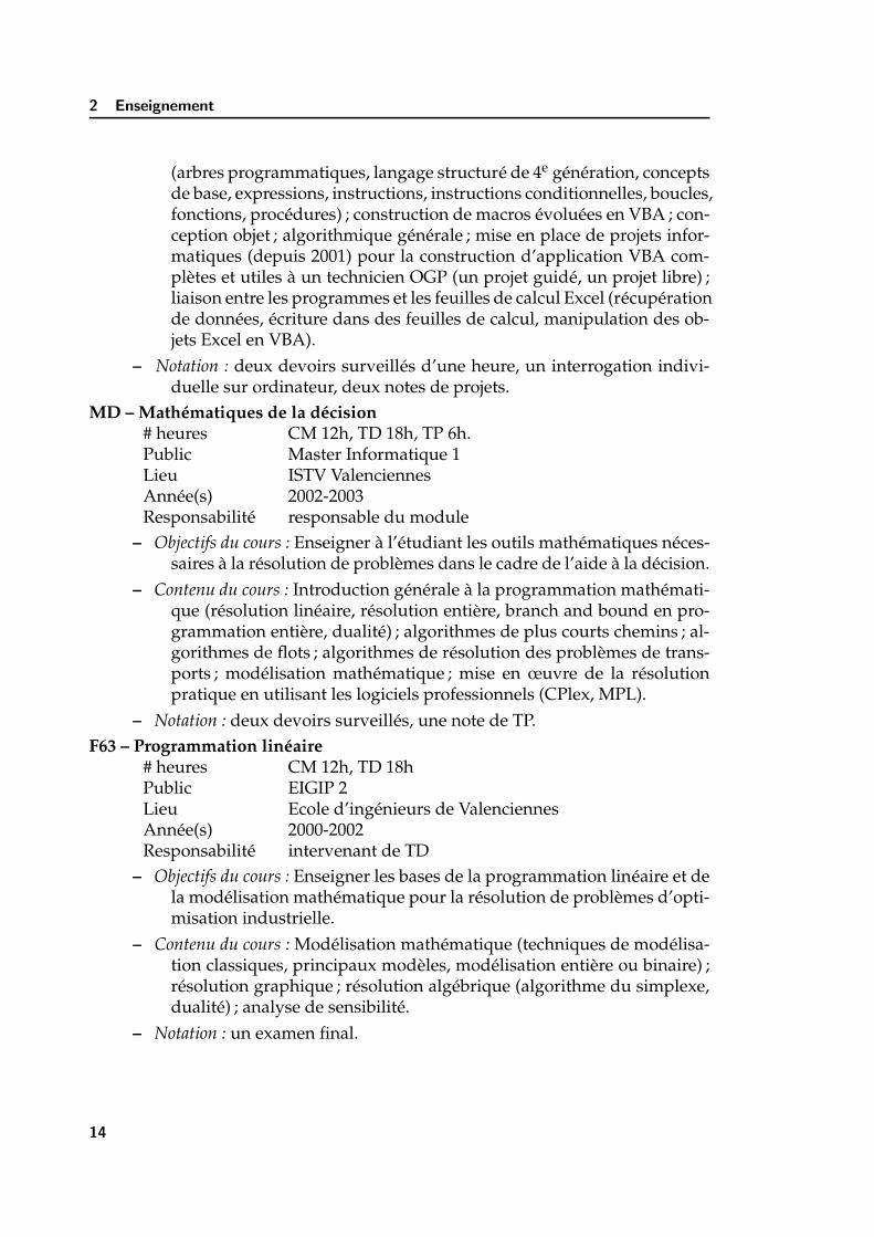
MD – Mathematiques de la decision# heures CM 12h, TD 18h, TP 6h.Public Master Informatique 1Lieu ISTV ValenciennesAnnee(s) 2002-2003Responsabilite responsable du module
– Objectifs du cours : Enseigner a l’etudiant les outils mathematiques neces-saires a la resolution de problemes dans le cadre de l’aide a la decision.
– Contenu du cours : Introduction generale a la programmation mathemati-que (resolution lineaire, resolution entiere, branch and bound en pro-grammation entiere, dualite) ; algorithmes de plus courts chemins ; al-gorithmes de flots ; algorithmes de resolution des problemes de trans-ports ; modelisation mathematique ; mise en œuvre de la resolutionpratique en utilisant les logiciels professionnels (CPlex, MPL).
– Notation : deux devoirs surveilles, une note de TP.F63 – Programmation lineaire
# heures CM 12h, TD 18hPublic EIGIP 2Lieu Ecole d’ingenieurs de ValenciennesAnnee(s) 2000-2002Responsabilite intervenant de TD
– Objectifs du cours : Enseigner les bases de la programmation lineaire et dela modelisation mathematique pour la resolution de problemes d’opti-misation industrielle.
– Contenu du cours : Modelisation mathematique (techniques de modelisa-tion classiques, principaux modeles, modelisation entiere ou binaire) ;resolution graphique ; resolution algebrique (algorithme du simplexe,dualite) ; analyse de sensibilite.
– Notation : un examen final.
14

2.2 Enseignements avant l’integration a l’UVHC
M11 – Qualite# heures CM 30h, TD 30hPublic IUT OGP 1Lieu IUT OGP CambraiAnnee(s) 1999-2000Responsabilite responsable du module
– Objectifs du cours : Donner aux etudiants les bases de la qualite en entre-prise et les outils necessaires a son application industrielle.
– Contenu du cours : Introduction a la qualite (historique, definitions) ; rap-pels statistiques (moyenne, ecart-type, variance, histogramme) ; demar-che qualite en entreprise ; normes ISO ; outils mathematiques de laqualite.
– Notation : deux devoirs d’une heure, un devoir final de deux heures, unenote de TD.
2.2 Enseignements avant l’integration a l’UVHC
La formation pedagogique acquise depuis plusieurs annees n’a pas debutea l’universite de Valenciennes, mais remonte aux annees 1992-1993. Depuis, uncertain nombre de matieres ont ete enseignees pour des public divers. La ligne “#heures” correspond ici aux heures que j’ai effectue.
Programmation lineaire# heures TD 35h, TP 52.5hPublic Eleves ingenieurs (Bac+3 et Bac +4)Lieu Ecole des Mines de NantesAnnee(s) 1997-1999Responsabilite charge de travaux dirigesContenu Methode du simplexe ; application a des problemesdu monde in-dustriel ; utilisa-tion de logicielscommerciaux.
Gestion de la production# heures TD 27.5hPublic Eleves ingenieurs (Bac +4)Lieu Ecole des Mines de NantesAnnee(s) 1997-1999Responsabilite charge de travaux dirigesContenu Gestion des stocks ; MRP ; planification des capacites.
15

2 Enseignement
Mathematiques# heures 120hPublic CAP coiffure 1 et 2Lieu Institut technique des etudes et des carrieres a AngersAnnee(s) 1993-1994Responsabilite enseignantContenu Notions elementaires de mathematiques ; fractions ;
pourcentages ; bases de la comptabilite.
Physique# heures 60hPublic CAP coiffure 1 et 2Lieu Institut technique des etudes et des carrieres a AngersAnnee(s) 1993-1994Responsabilite enseignantContenu Notions de base en electricite ; dangers du courant
electrique ; applications pratiques en salon de coiffure.
Chimie# heures 60hPublic CAP coiffure 1 et 2Lieu Institut technique des etudes et des carrieres a AngersAnnee(s) 1993-1994Responsabilite enseignantContenu Principes d’une reaction chimique ; application au traite-
ment des cheveux.
Informatique# heures TD 60hPublic DEUG 1Lieu Institut de mathematiques appliquees a AngersAnnee(s) 1992-1993Responsabilite charge de travaux dirigesContenu Initiation a la programmation ; algorithmique.
2.3 Encadrements pedagogiques
Encadrements a l’UVHC
2003-2004
IUT-OGP 1 1 Projet : Developpement des relations avec les anciens etudiants del’IUT-OGP, constitution d’un annuaire internet (8 etudiants).
IUT-OGP 2 1 Projet : Responsable du lancement du jeu d’entreprise FirStrat -Stra&Logic (40 etudiants).
IUT-OGP 2 2 Stages : Sujets en cours.
16

2.3 Encadrements pedagogiques
2002-2003
IUT-OGP 1 1 Projet : Developpement des relations avec les anciens etudiants del’IUT-OGP (8 etudiants).
IUT-OGP 2 2 Projets : Entreprise Blankaert Moto, assistance au choix d’une moto(3 etudiants), UVHC, gestion des dechets (2 etudiants).
IUT-OGP 2 2 Stages : 1. et 2. Campack SA, organisation d’une ligne de produc-tion de bouteilles de lait pendant sa mise en exploitation.
2001-2002
IUT-OGP 1 1 Projet : Realisation d’un annuaire des anciens eleves de l’IUT OGPde Cambrai (6 etudiants).
IUT-OGP 2 1 Projet : Entreprise Former - Reorganisation d’un atelier de frappe afroid (6 etudiants).
IUT-OGP 2 3 Stages : 1. Babyliss SA, gestion des stocks pour le centre logistique,2. Ygnis industrie, gestion de production, 3. SA Textiles Miersmann et Fils,optimisation de production.
2000-2001
IUT-OGP APPC 2 Projets : 1. Societe Amival, mise en place d’une ligne de pro-duction alimentaire (4 etudiants), 2. Societe Carolus Acier, amenagementd’un atelier de fabrication (4 etudiants).
IUT-OGP 2 2 Stages : 1. Entreprise Bohain Textile, gestion de production, 2. SocieteSobotex, redaction d’un cahier des charges pour un logiciel d’ordonnance-ment.
1999-2000
IUT-OGP 2 3 Stages : 1. Usine d’embouteillage de Saint-Amand-les-eaux, normesqualite, 2. Vieux-Conde estampages, gestion et suivi de production, 3. Mal-lez imprimerie, suivi de production.
IUT-OGP 1 1 Projet : mise en place d’une demarche qualite au sein du departe-ment OGP pour le suivi de la scolarite d’un eleve (7 etudiants).
Encadrements avant l’integration a l’UVHC
– Encadrement de mini-projets (decouverte d’un outil specifique de RO), elevesingenieurs de derniere annee de l’Ecole des Mines de Nantes (1997-1999).
– Encadrement de stages a l’etranger des eleves de troisieme annee (niveaumaıtrise) de l’Ecole des Mines de Nantes (1996-1999).
– Encadrement de projets transversaux en informatique sur le theme de laplanification et de l’ordonnancement d’ateliers (1998-1999).
17
2 Enseignement
2.4 Administration de l’enseignement
Elu au conseil restreint de l’IUT – depuis 2003
Le conseil restreint de l’IUT supervise l’attribution des postes d’enseignants-chercheurs, d’enseignants et d’attaches temporaires d’enseignement et de recher-che au sein de l’IUT tout entier. Cette attribution se fait sur proposition des dif-ferentes commissions de specialistes et mon intervention concerne les metiers dusecteur secondaire.
Responsable des relations internationales – depuis 2003
La direction de l’IUT a decide de motiver les departements pour relancer lesrelations internationales. Trois axes sont privilegies : 1) les echanges d’etudiants,2) les echanges d’enseignants et 3) le developpement d’axes de recherche en col-laboration avec l’etranger. La mission du responsable des relations internatio-nales est de promouvoir ces echanges et d’assister les differents intervenants dudepartement dans leurs demarches vers l’etranger en accord avec le directeur dedepartement et la direction de l’IUT.
Responsable de l’organisation des projets – 2001-2003
Axes sur la communication en premiere annee a l’IUT, ces projets ont pour butde faire travailler un groupe d’eleves autour d’un theme particulier et par la suitede presenter le resultat de leurs travaux devant leurs collegues et professeurs. Ilsacquierent ainsi une capacite a organiser le travail d’un groupe et presenter untravail. Une seconde partie du projet consiste a proposer un produit innovant etson processus de fabrication pour participer au concours national des OGP. Lesmeilleures propositions seront etendues dans le cadre du projet de 2e annee.Les etudiants de deuxieme annee vont en debut d’annee realiser un projet engroupe au sein d’une entreprise. Ils seront mis face a des industriels a qui ilsdoivent rendre des comptes. Ces projets portent principalement sur la redactionde procedures qualite et sur la reorganisation generale d’ateliers, le developpe-ment de modules informatiques, l’etude de logiciels de GPAO pour une implan-tation sur site, etc. Depuis 2004, les projets en entreprise sont progressivementremplaces par la participation au concours national OGP (creation d’un produitinnovant et de son processus de production) et par la semaine du jeu d’entreprise.
Organisation des visites en entreprise – 1999-2001
Permettre aux eleves de connaıtre differents types d’entreprises et d’environ-nements de travail est un des buts de ces visites. Un questionnaire etudie en fonc-tion de chaque entreprise nous permet de voir comment les eleves apprehendentleur futur cadre de travail industriel et eventuellement d’adapter certaines partiesde la formation. Il s’agit d’environ 4 a 5 visites par an.
18

2.4 Administration de l’enseignement
Recrutement, admission, jury
Participation aux jurys d’admission en DEA AISIH (2001-2003).Participation au recrutement des eleves EIGIP (2000-2002).Participation aux jurys d’attribution du DUT (depuis 2000).Participation aux jurys de passage en IUT 2 (depuis 1999).
19

3 Supervision de travaux d’etudiants 2e et 3e cycle
3 Supervision de travaux d’etudiants 2e et 3e cycle
3.1 Theses de doctorat
Co-direction de These europeenne (2003-2006)
Frederic BEUGNIES a debute une these (bourse ministere) en septembre 2003sur l’Optimisation multiobjectif de problemes de routage dans les reseaux informatiques.Encadrement : Dir. de these X. Gandibleux (UVHC), Co-encadrant M. Sevaux(UVHC). Autres encadrants : S. RANDRIAMASY (Alcatel).
Frederic BEUGNIES poursuit son travail de DEA sur l’etude de deux problemesd’optimisation dans le cas de l’exploitation de reseaux informatiques. Ces travauxentrent dans le cadre d’une collaboration entre le LAMIH et ALCATEL.Les questions posees relevent de deux problemes d’optimisation dans les graphes.Dans un premier temps, il s’agit d’etudier des algorithmes dans un cadre temps-reel et dans une seconde partie de faire de la gestion previsionnelle de trafic. Bienque ces deux approches portent sur des problemes de caracteristiques distinctes(la nature, la dimension, les contraintes, etc), elles se rejoignent dans le sens oul’optimisation finale ne devra pas se faire sur un seul objectif, mais sur plusieursa la fois.
Co-direction de These (2003-2006)
Karim BOUAMRANE a debute en Mars 2003 une these sur le theme Systemed’aide a la regulation d’un reseau de transport bi-modal. Encadrement : Dir. de these :Ch. Tahon (UVHC). Co-encadrant : M. Sevaux (UVHC).
Karim BOUAMRANE s’integre dans le cadre d’un projet cooperatif SART (Sys-teme d’Aide a la Regulation de Transport, anciennement projet COMPACT, voirsection 6). Dans ce projet, un certain nombre de modules permettant la regulationdu transport sont deja operationnels et ont ete developpes par les differents parte-naires du projet. Le travail devolu lors de cette these concerne la proposition et lamise en place operationnelle du systeme d’aide proprement dit par le biais d’unmoniteur d’activation. Un simulateur est integre a l’application pour simuler lecomportement du reseau de transport avant l’implantation du SART.
Co-direction de These (2000-2004)
Yann LE QUERE a debute en mai 2000 une these (en contrat Cifre avec laSNCF) sur le theme de la planification reactive des taches de maintenance pour lesTGV. Directeur de These : Ch. Tahon. Co-encadrants : M. Sevaux (UVHC) et D.Trentesaux (UVHC). Superviseurs industriels : G. Martin (SNCF) et E. Blervacque(SNCF). Soutenance : 30 juin 2004. Jury : B. Grabot, M. Gourgand (Rapporteurs),
20
3.2 Memoires de DEA
M.-J. Huguet, A. Thomas (Examinateurs).
Face a l’accroissement du trafic ferroviaire tant au niveau du fret que des pas-sagers, il est important de diminuer les temps d’immobilisation lors des tachesde maintenance des TGV. Pourtant les taches de maintenance sont complexes etsouvent incertaines. L’etude s’interesse alors a proposer une methode consistanta mesurer l’impact d’une structure de decision et des activites decisionnelles surun ordonnancement reactif.Cette these a donne lieu a la publication d’un article en revue [9], une communica-tion au GRP [45], une conference internationale avec actes [20], une presentationaux journees doctorales d’automatique [16] et a la soumission d’un autre articlepour publication [33]. Un contrat d’accompagnement de la these sur trois ans aete signe avec la SNCF pour un montant de 160 kF.
3.2 Memoires de DEA
DEA AISIH (2003-2004)
Changhong BIAN a realise un stage de DEA au sein de notre equipe. Le sujetetait l’etude d’un probleme d’ordonnancement juste-a-temps sur une machine.Les outils developpes pour cette etude se basent sur des heuristiques pour lacreation de solutions initiales dans des algorithmes genetiques qui sont implantespar la suite. Les algorithmes genetiques s’appuient sur un codage binaire parti-culierement adapte a ce probleme.
DEA AISIH (2003-2004)
Yan QIU a realise un stage de DEA au sein de notre equipe. Le sujet etaitl’Application d’un algorithme genetique pour un probleme de CAO (ce sujet a ete co-encadre avec Yves Mineur).Dans ce travail, il s’agissait de mettre en œuvre un algorithme genetique permet-tant de resoudre un probleme d’optimisation continu rencontre dans le cadre dela modelisation de formes geometriques en CAO. Un algorithme genetique dejaoperationnel a ete fourni comme base d’etude et le travail a consiste a proposerdes ameliorations importantes.
DEA AISIH (2002-2003)
Johann SAINT MARS, etudiant en DEA a realise un stage au sein de notreequipe. Le sujet etait l’etude d’un probleme d’ordonnancement a une machine avecminimisation du retard pondere.Dans ce travail, une approche par programmation lineaire a ete privilegiee. Enfaisant appel aux outils commerciaux et aux modeles les plus recents pour ceprobleme, l’etudiant a evalue les resultats trouves et les a compare aux meilleursresultats des heuristiques connues.
21

3 Supervision de travaux d’etudiants 2e et 3e cycle
DEA AISIH (2000-2001)
Christophe TILLEUL, etudiant en DEA a realise un stage au sein de notreequipe. Le sujet etait l’etude d’un probleme d’ordonnancement bicritere a une ma-chine (ce sujet a ete co-encadre avec X. Gandibleux).Les problemes d’ordonnancement sont le plus souvent tres delicats a resoudrelorsqu’ils sontNP-complets. Dans le cas bi-critere, la difficulte augmente encore.L’objectif de ce travail a ete de resoudre efficacement le probleme d’ordonnance-ment a une machine avec dates de disponibilite pour les criteres de minimisationdu nombre de taches en retard et le retard total de ces taches.
3.3 Projets de DESS
DESS ICHM (2003-2004)
Chris BAUCHOT et Sebastien LEGENDRE ont realise au sein de notre equipeun projet de DESS ICHM. Le sujet est la proposition d’une interface permettant lamanipulation et l’edition de graphes (ce sujet a ete co-encadre avec P. Thomin).Suite a la publication du livre “Algorithmes de graphes” [1], la construction d’uneinterface graphique pour manipuler les graphes et executer les differents algo-rithmes developpes dans le livre est devenue indispensable. Une nouvelle versionde ce livre sera proposee en C++ prochainement. L’interface a ete developpee enQT et est toujours operationnelle.
DESS CCI (2002-2003)
Shiva ROUHOLAMINI et Rachid HARMAOUI, etudiants en DESS “Connais-sances Complementaires en Informatique” ont realise un projet au sein de notreequipe. Le sujet traite etait l’etude d’un probleme d’ordonnancement juste a temps.Dans ce stage, une approche par heuristiques constitue le cœur du travail de-mande. Les etudiants ont pu developper un certain nombres d’heuristiques et lesresultats ont ete compares aux heuristiques classiques connues pour ce probleme.
DESS ICHM (1999-2000)
Laurent HULIN a effectue son projet dans notre equipe. Le sujet est la Proposi-tion d’une interface permettant la manipulation de references bibliographiques (ce sujeta ete co-encadre avec P. Thomin).Il avait pour but de developper une interface qui permette d’effectuer des re-cherches de references bibliographiques a partir de fichiers au format BibTEX.L’outil a ete developpe en php.
22

3.4 Projets IUP GEII
3.4 Projets IUP GEII
IUP GEII (2003-2004)
Yohan COLIN et Nicolas KOWALSKI ont effectue un projet dans notre equipe.Le sujet est l’Optimisation de tournees de vehicules.Le but du projet est d’utiliser les outils de la suite “Optimisation” d’ILOG pourresoudre le probleme de tournees de vehicules dans sa version academique. Unecomparaison a ete menee entre les resultats du logiciel commercial et les meilleuressolutions connues de la litterature.
IUP GEII (2001-2002)
Sebastien LECHARDEUR et Johan SAINT MARS ont effectue un projet dansnotre equipe. Le sujet est Ordonnancement a une machine : une approche genetique (cesujet a ete co-encadre avec P. Thomin).Le critere a optimiser est la retard pondere total dans le cas ou les taches sontsoumises a des dates de disponibilite. L’issue de ce projet a permis de presenterune communication a IFORS’2002 [42].
IUP GEII (2001-2002)
Mathieu LEGEZYNSKI et Stephane DEBACKER effectuent un projet dansnotre equipe. Le sujet est Ordonnancement a une machine : une approche par recherchedispersee (ce sujet a ete co-encadre avec P. Thomin).Les deux binomes travaillent en parallele sur un meme probleme d’ordonnance-ment mais avec deux approches differentes. L’approche par recherche disperseeest plus difficile a mettre en œuvre mais a donne de meilleurs resultats.
23

4 Administration et animation de la recherche
4 Administration et animation de la recherche
4.1 Animation de la recherche
Sur le plan international
Creation et pilotage du groupe EU/ME (EURO Working Group – European chap-ter on Metaheuristics). Groupe europeen de recherche sur le theme des metaheu-ristiques (cree a la suite d’une ecole d’hiver, avec K. Sorensen – Universite d’An-vers, Belgique et C. Wynants – Universite libre de Bruxelles, Belgique). Ce groupecompte aujourd’hui 750 membres de 65 nationalites differentes, avec un potentielencore eleve. Le but de ce groupe, cree en mars 2000, est de donner l’opportuniteaux chercheurs et industriels de se rencontrer et partager leur experience de l’uti-lisation et du developpement des metaheuristiques. D’autres renseignements surle groupe se trouvent a l’adresse suivante :http://webhost.ua.ac.be/eume/
Parmi les taches effectuees dans ce cadre, on retrouve– l’administration du groupe proprement dite (gestion des membres, organi-
sation d’assemblees generales, etc),– la co-gestion du site web du groupe (mailing list, forum de discussion, in-
formations sur les conferences, etc),– les relations avec EURO, l’organisme de tutelle (participation a des reunions
generales, redaction de rapports d’activites),– la gestion du budget,– l’organisation d’une manifestation internationale annuelle (depuis 2001).
Au niveau du laboratoire
Creation et animation (de 2000 a 2002) des seminaires du LAMIH permettant atoutes les equipes de proposer des presentations d’intervenants locaux ou exte-rieurs. Ces seminaires ont lieu sur un rythme regulier (2 fois par mois environ).Ce travail a ete realise en collaboration avec plusieurs membres d’autres equipesdu LAMIH. Depuis 2002, la direction du laboratoire a confie cette tache a sonsecretariat.
Au niveau de l’equipe
Charge de la collecte des informations (publications et activites de recherche etd’encadrement) pour la mise a jour du rapport d’activite.Mise en place et gestion des rapports de recherche internes a l’equipe. Ces rap-ports permettent de diffuser l’information et prendre date pour une publicationqui est soumise a une revue mais pas encore acceptee.
24
4.2 Organisation de manifestations a Valenciennes
4.2 Organisation de manifestations a Valenciennes
Congres International francophone PENTOMDates : 27-29 mars 2003Organisateur : LAMIH/SPPresident du CO : O. SenechalTheme : Performance et nouvelles technologies en maintenanceParticipants : 115
Congres International IFIP FEATSDates : 12-14 juin 2001Organisateur : LAMIH/SPPresident du CO : D. DeneuxTheme : Modelisation avancee par features dans la conception produitParticipants : 80
Reunion du groupe BermudesDates : 2 fevrier 2001Organisateurs : X. Gandibleux et M. SevauxTheme : Ordonnancement dans les ateliers flexiblesParticipants : 40
Journees GRPDates : 27-28 octobre 2000Organisateur : LAMIH/SPPresident du CO : D. TrentesauxTheme : ProductiqueParticipants : 80
4.3 Organisation de manifestations en dehors de Valenciennes
3e Joint meeting EU/MEDates : 18-19 decembre 2003Lieu : Universite d’Anvers (Belgique)Organisateurs : EU/ME et l’universite d’AnversComite d’organisation : W. Dullaert, M. Sevaux, K. Sorensen, J. SpringaelTheme : Applications reelles des metaheuristiquesParticipants : 60Site web : http ://webhost.ua.ac.be/eume/workshops/reallife.html
2e Joint meeting EU/MEDates : 4-5 novembre 2002Lieu : Paris, Carre des sciencesOrganisateurs : EU/ME et le groupe francais PM2O (programmation ma-thematique multi-objectif)Comite d’organisation : X. Gandibleux, M. Sevaux, K. Sorensen, V. T’KindtTheme : Les metaheuristiques multi-objectifs
25
4 Administration et animation de la recherche
Participants : 60Site web : http ://webhost.ua.ac.be/eume/workshops/momh.html
1er Joint meeting EU/MEDates : 28 novembre 2001Lieu : City university, London (UK)Organisateurs : EU/ME et UK Local search groupComite d’organisation : C. Glass, C. Potts, M. Sevaux, K. SorensenTheme : MetaheuristiquesParticipants : 30Financement : obtenu pour 3 jeunes chercheurs aupres d’EURO
4.4 Organisation / president de sessions
Organisation d’un cluster de sessionsConference : INFORMS Denver Colorado 2004Dates : 24-27 octobre 2004Theme principal : metaheuristiquesSessions : Tabu and scatter search, Genetic algorithms, Hybrid search.
Organisation de session inviteeConference : MIC’2001, PortoDates : 16-20 juillet 2001Theme : ordonnancement et metaheuristiques.
President de session2004 : EURO XX (semi-plenary session)2003 : MIC 2003, EMO 20032002 : PMS 2002, ROADEF 20022001 : MIC 2001, MOSIM 2001, ORBEL 2001.
26

5 Visibilite, rayonnement et autres activites
5.1 Collaborations
Universite polytechnique de Hong-KongCorrespondant : C. OguzTheme : Approches hybrides pour le flow-shop multi-stagesVisites : M. Sevaux a Hong-Kong (11-21 mai 2004 et 4-16 mars 2003). C.Oguz a Valenciennes (22-29 mai 2004 et 12-27 juillet 2003)Description : Cette collaboration a lieu dans le cadre d’un programme d’ac-tion integre (voir section 6.3). C. Oguz et moi-meme travaillons sur desproblemes d’ordonnancement de type flow-shop avec de nouvelles approchesintegrant les metaheuristiques et les techniques de type propagation de con-traintes.
Universite d’Anvers (Belgique)Correspondant : K. SorensenTheme : Metaheuristiques ; RobustesseVisites : En moyenne trois par an depuis 2000 ; accueil de K. Sorensen enmoyenne trois fois par an depuis 2001.Description : Developpement de nouvelles metaheuristiques hybrides [31]et de methodes pour l’ordonnancement robuste [18]. Redaction de deux ar-ticles en commun [7, 31]. Gestion du groupe EU/ME et mise en place d’unnouveau projet [37]. Presentation lors d’un seminaire [56].
Universite de Clermont-ferrandCorrespondants : G. Fleury et P. LacommeTheme : Ordonnancement stochastiqueDescription : Presentation en commun d’un article sur le probleme de l’or-donnancement stochastique [14].
Universite de Technologie de Troyes et de Clermont-ferrandCorrespondants : C. Prins (UTT) et P. Lacomme (UBP)Theme : Tournees sur arcs ; algorithmes de graphesVisites : deux en 2002 et deux en 2003Description : Redaction en commun d’un article sur le probleme des tourneessur arcs multiobjectifs [17]. Redaction d’un livre [1].
Ecole des Mines de NantesCorrespondant : S. Dauzere-PeresTheme : Ordonnancement a machines paralleles et a une machineVisites : M. Sevaux a Nantes (4-9 fevrier 2002 et 17-21 avril 2001)Description : Developpement de nouveaux algorithmes pour la resolutiond’un probleme a machines paralleles [19]. Poursuite des travaux engagesprecedemment et redaction de plusieurs articles en commun [5, 8, 10, 35].
27
5 Visibilite, rayonnement et autres activites
Ecole des Mines de Nantes et Univ. de Technologie de TroyesCorrespondants : C. Gueret (EMN) et C. Prins (UTT)Theme : Programmation lineaireDescription : Collaboration et co-ecriture du livre Programmation Lineaire etde sa traduction [2, 3].
Massachusetts Institute of TechnologyCorrespondant : S.B. GershwinTheme : Planification de la production en temps continu ; determination depolitiques de controleVisites : M. Sevaux au MIT (15 avril-17 mai 1997)Description : Redaction d’un article en commun [10].
Institut de Math. Appliquees et Univ. de Technologie de CompiegneCorrespondants : P. Baptiste (UTC), L. Peridy (IMA), E. Pinson (IMA) et D.Rivreau (IMA)Theme : Ordonnancement a une machineDescription : Collaboration dans le cadre de l’etude des problemes d’ordon-nancement a une machine. Partage d’informations et de jeux de donnees.Partage des resultats. Presentation conjointe des resultats lors d’une journeedu Gotha [59].
5.2 Appartenance a des societes et des groupes de recherche
Societes nationales et internationales
SOGESCI-B.V.W.BDescription : societe belge de Recherche OperationnelleAdhesion : depuis 2001Activites : participation aux manifestations nationales [46].
EU/MEDescription : EURO working group, European chapter on metaheuristicsAdhesion : depuis 2000Activites : administration du groupe (voir section 4.1), presentation lors desmanifestations [37, 38, 40].
ROADeFDescription : societe francaise de Recherche Operationnelle et d’Aide a laDecisionAdhesion : depuis 1998Activites : participation et presentations [39, 43, 47, 48] lors des manifesta-tions nationales et regionales, participation aux assemblees generales, ac-tion aupres de la societe pour les ecoles d’ete et d’hiver d’EURO.
28
5.2 Appartenance a des societes et des groupes de recherche
INFORMSDescription : Institute For Operations Research and the Management ScienceAdhesion : depuis 1996Activites : Organisation d’un cluster au congres INFORMS 2004. Presentationdes travaux au congres INFORMS 1998 [49].
Groupes Nationaux
GDR MACS/STPDescription : Groupe de recherche du CNRS en Modelisation Analyse etConduite des Systemes, pole Sciences et Techniques de la ProductionAdhesion : depuis 2003 (creation du GDR en 2003)Activites : Participation aux manifestations nationales. Presentation au themeORT [53].
Club EEADescription : Club des enseignants et des chercheurs en electronique, elec-trotechnique et automatique.Adhesion : depuis 2003
GRPDescription : Groupe de Recherche en ProductiqueAdhesion : de 2000 a 2003Activites : Presentation de travaux aux manifestations nationales [41, 44,45], participation a l’organisation d’une manifestation a Valenciennes.
PM2ODescription : Groupe de travail de la ROADEF en Programmation Mathe-matique Multi-ObjectifAdhesion : depuis 2000Activites : participation aux reunions du groupe, organisation d’une mani-festation conjointe avec EU/ME. Presentations [40, 54].
BermudesDescription : Groupe de recherche en ordonnancement d’ateliers flexiblesAdhesion : depuis 1999Activites : participation et presentation [63] aux manifestations nationales,organisation d’une reunion Bermudes a Valenciennes (avec X. Gandibleux).
GOThADescription : Groupe de recherche en Ordonnancement Theorique et Ap-pliqueAdhesion : depuis 1996Activites : participation et presentation [59, 65, 66] a de nombreuses reunionsdu groupe (en particulier dans le theme flexibilite), redaction d’un chapitrede livre [32].
29

5 Visibilite, rayonnement et autres activites
Groupes Regionaux
GRAISyHMDescription : Groupe de Recherche en Automatique, Informatique des Sys-temes Homme-Machine, theme commande et pilotageAdhesion : depuis 2000 Activites : participation et presentation [62] auxreunions du groupe.
5.3 Fonction d’edition
Editeur associe de IJCI
Depuis 2004, membre du comite editorial de la revue International Journal ofComputational Intelligence. Le but de cette revue internationale est de developperdes systemes qui reproduisent l’analyse, la resolution des problemes et les fa-cultes d’apprentissage du cerveau. Ces systemes apportent les avantages de laconnaissance et de l’intelligence pour la resolution des problemes complexes. Lesdomaines couverts par le journal incluent : les outils intelligents generiques (tech-niques et algorithmes), des applications (utilisant des techniques intelligentes) etdes technologies intelligentes naissantes.
Editeur associe de IJSP
Depuis 2004, membre du comite editorial de la revue International Journal ofSignal Processing. Le but de la revue IJSP est de prendre en compte tous les as-pects de la theorie et de la pratique du traitement du signal. La politique de larevue est une diffusion rapide des connaissances et des experiences aupres desingenieurs et des scientifiques travaillant dans la recherche, le developpement oul’application pratique du traitement du signal.
Numero Special EJOR
Suite au 3e Joint EU/ME workshop en collaboration avec l’universite d’An-vers, un numero special de la revue European Journal of Operational Research est enpreparation. Ce numero special porte sur le theme de l’application des metaheu-ristiques. Date limite de soumission : 7 avril 2004, fin previsionnelle du processusde relecture : octobre 2004.
Edition d’un livre
Suite au 2e Joint EU/ME workshop “MOMH”, il a ete decide de publier dansun livre, une selection d’articles soumis a un processus de relecture de type revueinternationale. Cet ouvrage est publie comme “Lecture Notes in Economics andMathematical Systems” [4]. Taux de selection : 36%
30

5.4 Evaluation de la recherche
5.4 Evaluation de la recherche
Rapporteur de revues internationales
Regulier pour les revues et chapitres de livres– European Journal of Operational Research – EJOR– Kluwer (chapitres de livre)– Journal of Heuristics– Annals of Operations Research– IEEE System Man and Cybernetics – IEEE-SMC– Engineering Applications of Artificial Intelligence – EAAI
Occasionnel pour les revues et chapitres de livres– Quaterly Journal of the Belgian, French and Italian Operations Research
Societies – 4OR– International Journal of Modelling and Simulation– IEEE Transactions on Robotics and Automation – IEEE TRA– Information Systems and Operational Research – INFOR– Robotics and Computer Integrated Manufacturing– IIE Transactions– Decision Support Systems– Rairo - Operations Research– Journal Europeen des Systemes Automatises – JESA– Hermes (chapitre de livre)
Comites scientifiques
MIC’2005 Metaheuristics International ConferenceLieu : Vienne, AutricheDates : Ete 2005Charge : Appel a communications, relecture d’articles soumis.
PENTOM’2005 PErformance et Nouvelles TechnOlogies en MaintenanceLieu : Rabat, MarocDates : Paques 2005Charge : Appel a communications, relecture d’articles soumis.
FRANCORO 2004 Conference Francophone Intl. de Recherche OperationnelleLieu : Fribourg, SuisseDates : 18-21 aout 2004Charge : Appel a communications, relecture d’articles soumis.
EURO’2004 EURO ConferenceLieu : Rhodes Island, GreceDates : 4-7 juillet 2004Charge : Appel a communications, organisation des “medals and awards”,recherche de conferenciers invites.
31

5 Visibilite, rayonnement et autres activites
ISS’2004 International Symposium on SchedulingLieu : Yumebutai, JapanDates : 24-26 Mai 2004Charge : Appel a communications, relecture d’articles soumis.
MIC’2003 Metaheuristics International ConferenceLieu : Kyoto, JaponDates : 25-28 aout 2003Charge : Appel a communications, relecture d’articles soumis.
ESI XXI EURO Summer InstituteLieu : Neringa, LithuaniaDate : 25 juillet-7 aout 2003Charge : Choix de candidat francais.
PENTOM’2003 PErformance et Nouvelles TechnOlogies en MaintenanceLieu : ValenciennesDates : 27-29 mars 2003Charge : Relecture d’articles soumis.
MIC’2001 Metaheuristics International ConferenceLieu : Porto, PortugalDates : 16-20 juillet 2001Charge : Appel a communications, relecture d’articles soumis.
Jury de theses
Comite d’accompagnement de la these de N. Souaı (Faculte polytechnique deMons, Belgique), Problemes de “crew scheduling” pour les campagnes aeriennes,soutenance prevue en 2006.
Examinateur de la these de K. Sorensen (Universite d’Anvers, Belgique), Robust-ness in optimization, soutenue le 13 juin 2003.
Examinateur de la these de W. Ramdane-Chrerif (Universite de technologie deTroyes), Problemes de tournees de vehicules sur arcs soutenue le 12 decembre2002.
Commission de specialistes
Membre elu titulaire de la commission de specialistes en 61e section depuis 2004.
Membre elu suppleant de la commission de specialistes en 61e section en 2003.
32
6 Contrats industriels, projets de recherche et finan-
cements
6.1 Contrats industriels
Contrat Alcatel - Anvers/Marcoussis
Contrat international – 12 mois – 2003-2004Co-responsable scientifique, correspondant pour le LAMIH dans le cadre decette collaboration : M. Sevaux (LAMIH/SP) – 4 participants.
Une clause de confidentialite a ete signee pour ce projet. Les activites meneeslors de cette collaboration et les montants importants engages ne pourront etredevoiles que lorsque le contrat sera termine et la clause de confidentialite levee.Par contre, au fur et a mesure de l’avancement certaines parties de l’activite pour-ront etre rendues publiques avec l’accord d’Alcatel. Elles seront alors mentionneesdans ce paragraphe et des que possible brevetees et publiees.
These Cifre SNCF
Contrat regional – 24.2ke (160kF) – 36 mois – 2000/2003Responsable scientifique : C. Tahon (LAMIH/SP) – 4 participants.
Convention CIFRE avec l’EIMM (Etablissement Industriel de Maintenance duMAteriel) d’Hellemmes. Deux personnes de la SNCF sont impliquees dans lesuivi du projet. Une description plus detaillee du sujet de these se trouve dansla section 3.1.
Centre Hospitalier de Valenciennes
Contrat local – 48ke – 36 mois – 2000/2003Responsable scientifique : C. Tahon (LAMIH/SP) – 4 participants.
Ce contrat entre notre equipe et le Centre Hospitalier de Valenciennes avait pourobjectif de realiser une etude complementaire du schema directeur pour les fluxlogistiques en vue de la construction d’un nouveau batiment. En fait, avant memede prendre en compte la realisation du nouveau batiment, nous avons du tra-vailler sur des modifications internes structurelles (construction d’une nouvelleblanchisserie, deplacement des cuisines). Ce travail a debute au debut de l’annee2000 et pour une duree de 3 ans. Pour cette etude, la simulation a ete l’outil detravail privilegie.
33

6 Contrats, projets et financements
6.2 Projets de recherche
Projet Cooperatif – SART (Phase 2, COMPACT)
Contrat regional – 139ke (Part labo 42.7ke) – 18 mois – 2003/2004Responsable scientifique : S. Hayat (INRETS) – 30 participants.
Dans cette seconde phase, le probleme de transport multi-modal est directementaborde et des propositions de modelisation et de resolution sont faıtes pour pro-poser un systeme d’aide a la regulation du trafic d’un reseau de transport multi-modal (bimodal tramway/bus). Valenciennes et la Semurval, societe exploitantles transports en commun de Valenciennes sont les principaux acteurs de ce pro-jet. La construction future du tramway fait que la realisation de ce projet devientindispensable pour nos partenaires. C’est dans ce cadre que s’inscrit en partie lathese en co-tutelle de Karim Bouamrane (voir section 3.1). Presentation lors d’unseminaire [62].
Projet Cooperatif – Phase 1, MOST/TACT
Contrat regional – 150ke (Part labo 27.4ke) – 18 mois – 2001/2002Responsable scientifique : C. Tahon (LAMIH/SP) – 30 participants.
Methodologies pour l’Optimisation dans les Systemes de Transport et de Tele-communications / Technologies Avancees dans le domaine de la Communicationet des Transports Terrestres. Dans le cadre du CPER 2000-2006, le GRRT Nord-Pas de Calais a obtenu le financement pour le projet cooperatif. Il s’agit dans unpremier volet de ce projet de developper des outils en commun pour la resolutionde problemes lies aux transports mais pas exclusivement. Presentation lors d’unseminaire [62].
Projet S.M.I.L.E.
Projet interne EMN – 2 mois – 1999Responsable scientifique : P. Dejax (EMN/AUTO) – 2 participants.
Redaction du cahier des charges du projet de developpement d’une plate formed’essais d’un Systeme de Modelisation et d’Integration de la Logistique d’Entre-prise. Ce projet vise a permettre aux entreprises le suivi de la chaıne logistiqueavec un module specifique pour le suivi en temps reel des camions de collecte oude livraison ou l’adaptation aux perturbations du reseau routier est instantanee.
34
6.3 Financements obtenus
6.3 Financements obtenus
Financements obtenus pour deplacements
Dans le cadre du support d’activites scientifiques, le ministere des affairesetrangeres peut venir en aide aux laboratoires et aux chercheurs pour financerdes deplacements :
Aout 2003 Financement individuel (850e) pour la conference MIC’2003 au Ja-pon. Presentation d’un article [15].
Juillet 1999 Financement d’equipe (530e – P. Castagliola, C. Prins et M. Sevaux)pour la conference IEPM’99 en Ecosse. Presentation d’un article [25].
Programme d’action integre - Hong-Kong
Projet international d’echange bilateral – 8ke – 24 mois – 2003-2004Responsable scientifique : M. Sevaux (LAMIH/SP) – 3 participants.
Ce programme d’echange avec Hong-Kong, developpe de maniere individuelleau laboratoire est le debut d’une collaboration avec Ceyda Oguz. Le theme re-tenu est le developpement de methodes de resolution pour des problemes d’or-donnancement avec l’integration des techniques de propagation de contraintesdans les metaheuristiques ou dans la programmation lineaire. Ce programme estfinance par l’Egide sous la forme d’un programme d’action integre Procore. Vi-sites : M. Sevaux a Hong-Kong (11-21 mai 2004 et 4-16 mars 2003). C. Oguz aValenciennes (22-29 mai 2004 et 12-27 juillet 2003)
Projet national prospectif – Jemstic
Contrat national – 13ke – 12 mois – 2002Responsable scientifique : D. Trentesaux (LAMIH/SP) – 6 participants.
Conception de systemes cooperatifs pour l’aide au pilotage distribue du cyclede vie des systemes de production de biens et de services. Il s’agit de savoir ici,si l’action de cooperation est benefique, toujours, parfois, ou peu souvent pourl’ensemble des partenaires et aussi de mesurer l’impact de la cooperation sur lesmodes de fonctionnement de chacun des acteurs.
35
7 Thematiques de recherche
7 Thematiques de recherche
Les differents themes de recherche decrits ci-dessous sont le fruit de plusieursperiodes de travail. On notera les periodes DEA (1994-1995), these (1996-1998),apres-these (1998-1999) et MDC (depuis 1999). Chaque theme aborde reprend dansun cartouche la periode de travail dans laquelle les recherches ont ete effectuees etles resultats obtenus en terme de publication et de visibilite du theme (chaque pu-blication n’est citee que dans un seul cadre, meme si certains sujets se recoupent).La figure 1 reprend les thematiques de recherche menees depuis la these. Danscette meme figure, on retrouve aussi les outils necessaires a la resolution desproblemes.
Introduction
Le contexte industriel de plus en plus competitif oblige les entreprises a sanscesse ameliorer leur productivite tant au niveau des biens que des services. Dansce cadre, on retrouve classiquement les differents niveaux de decision strategique,tactique et operationnel. Pour la production de biens, on s’interesse a deux aspectscorrespondants a deux niveaux de decision : la planification de production (ni-veau tactique) et l’ordonnancement (niveau operationnel). Pour les services, ons’interesse plus specifiquement aux tournees de vehicules.
Le probleme de planification est aborde dans un premier temps sous un anglenouveau, mettant en avant la notion d’horizon continu (par opposition au clas-sique horizon discretise). Basee sur cette modelisation, la determination de poli-tiques de controles est abordee avant de terminer par un domaine en plein essort,la planification reactive.
Les problemes d’ordonnancement, plus academiques dans leur presentation,concernent l’objectif particulier de la minimisation du nombre de jobs en retard.Ce type d’objectif est resolu pour les problemes a une machine et a machinesparalleles avec des dates de disponibilite. Le nombre de jobs en retard peut etrepondere ou non. Par la suite, on s’interesse au probleme a une machine, sansdoute le plus difficile a resoudre (toute relaxation donne aussi un probleme NP-difficile au sens fort). Il s’agit du probleme de la minimisation du retard ponderetotal avec dates de disponibilite sur une machine unique. Enfin, sont abordes desproblemes de robustesse indispensables pour les industriels soucieux d’appliquerces methodes dans le cas operationnel.
Les tournees de vehicules attirent l’attention des chercheurs depuis de nom-breuses annees et pourtant il reste encore des possibilites pour ameliorer les me-thodes existantes et en proposer de nouvelles encore plus performantes. Les tour-nees de vehicules sur arcs representent un interet particulier car on retrouve cesproblemes dans la realite avec par exemple le salage des routes en cas de verglas,l’entretien des bordures des routes, la distribution de courrier et la collecte desordures menageres par exemple. On s’interesse alors a l’optimisation bi-objectifde ce probleme. Le cas mono-objectif est aussi resolu de maniere tres efficace
36

� � � � � � � � � � � � � � � � � � � � � � � � � � � � � � � � � � � � � � � � � � � � � � � � � � � � � � � � � � � � � � � � � � � � � � � � � � � � � � � � � � � � � � � � � � � � � � � � �
� � � � � � � � � � � � � � � � � � � � � � � � � � � � � � � � � � � � � � � � � � � � � � � � � � � � � � � � � � � � � � � � � � � � � � � � � � � � � � � � � � � � � � � � � � � � � � � � �
� � � � � � � � � � � � � � � � � � � � � � � � � � � � � � � � � � � � � � � � � � � � � � � � � � � � � � � � � � � � � � � � � � � � � � � � � � � � � � � � � � � � � � � � � � � � � � � � �
� � � � � � � � � � � � � � � � � � � � � � � � � � � � � � � � � � � � � � � � � � � � � � � � � � � � � � � � � � � � � � � � � � � � � � � � � � � � � � � � � � � � � � � � � � � � � � � � �
� � � � � � � � � � � � � � � � � � � � � � � � � � � � � �
� � � � � � � � � � � � � � � � � � � � � � � � � � � � � �
� � � � � � � � � � � � � � � � � � � � � � � � � � � � � �
� � � � � � � � � � � � � � � � � � � � � � � � � � � � � �
� � � � � � � � � � � � � � � � � � � � � � � � � � � � � �
� � � � � � � � � � � � � � � � � � � � � � � � � � � � � �� � � � � � � � � � � � � � � � � � � � � � � � � � � � � � � � � � � � � � � � � � � �� � � � � � � � � � � � � � � � � � � � � � � � � � � � � � � � � � � � � � � � � � � �� � � � � � � � � � � � � � � � � � � � � � � � � � � � � � � � � � � � � � � � � � � �� � � � � � � � � � � � � � � � � � � � � � � � � � � � � � � � � � � � � � � � � � � �� � � � � � � � � � � � � � � � � � � � � � � � � � � � � � � � � � � � � � � � � � � �
� � � � � � � � � � � � � � � � � � � � � � � � � � � � � � � � � � � � � � � � � � � �� � � � � � � � � � � � � � � � � � � � � � � � � � � � � � � � � � � � � � � � � � � �� � � � � � � � � � � � � � � � � � � � � � � � � � � � � � � � � � � � � � � � � � � �� � � � � � � � � � � � � � � � � � � � � � � � � � � � � � � � � � � � � � � � � � � �� � � � � � � � � � � � � � � � � � � � � � � � � � � � � � � � � � � � � � � � � � � �
� � � � � � � � � � � � � � � �
� � � � � � � � � � � � � � � �
� � � � � � � � � � � � � � � �
� � � � � � � � � � � � � � � �
Bi−objective CARP
CARP
Robust VRP
Reactive PlanningProduction Planning
Control Policies
Robust scheduling
1−Machine # Late Jobs //−Machine Weighted # Late Jobs
1−Machine Weighted # Late Jobs 1−Machine TWT
Linear and integer programming
Graphs algorithms
Metaheuristics
Heuristics
1997
2003
2004
1996
1998
1999
2000
2002
2001
FIG. 1 – Problemes et outils abordes
37

7 Thematiques de recherche
donnant aujourd’hui sur des jeux de tests de la litterature les meilleurs resultats.Quand le probleme de tournees de vehicules est a resoudre non plus sur les arcs,mais sur les nœuds du reseau, on s’interesse alors a produire des solutions ro-bustes.
7.1 Planification de la production
Planification de la production en temps continu
Periode : 1996–1998.Resultats : un article publie en revue [11],
une conference avec actes [28],une conference sans actes [51] etdeux seminaires [64, 65].
La planification de production se resout habituellement en discretisant un ho-rizon de planification. Pourtant dans le cas de la production “gros volumes”, ilest souvent preferable de conserver l’horizon intact et de considerer un problemede planification de la production en temps continu [11]. Dans ce cas, la demande (ha-bituellement exprimee en quantites) est remplacee par des taux de demande etla production est alors exprimee elle aussi sous forme de taux [67]. Les taux dedemande sont supposes connus et constants par morceaux. L’horizon de pla-nification est separe en periodes ou la demande est constante, et les periodespeuvent avoir des longueurs differentes. La capacite de production etant parfoisinsuffisante la rupture est autorisee. Ainsi, dans d’autres periodes, il est parfoisnecessaire de produire plus que les demandes courantes. Il faut donc determinercombien produire en plus, et pendant combien de temps.
Pour reduire encore les couts, on autorise les taux de production a changer ad’autres instants que ceux ou la demande change. Ces dates, ainsi que les fins deperiodes, seront appelees temps de changement [51]. Ainsi, il faut determiner ala fois les taux de production et les temps de changement. Parce que ce doubleprobleme est trop difficile a resoudre simultanement, une procedure iterative adeux etapes est proposee.
Dans un premier temps, avec des temps de changement fixes, les taux deproduction optimaux sont determines a l’aide d’un modele de programmationlineaire. Dans une seconde etape, avec des taux de production fixes, les tempsde changement redondants sont elimines, et de nouveaux instants sont ajoutes al’aide de regles. La procedure itere entre les deux etapes jusqu’a ce qu’il n’y aitplus d’amelioration significative (voir [11, 64, 65, 67]).
Une extension permettant de traiter la demande discrete dans le cas ou l’onconserve le modele en temps continu a aussi ete developpee [27, 67].
38
7.2 Ordonnancement
Determination de politiques de controle
Periode : 1997–1999.Resultats : une conference avec actes [25].
Dans le cas particulier ou la demande est constante au cours du temps (surun intervalle de temps reduit par exemple), il peut etre interessant de determiner,partant d’un etat des stocks quelconque, comment se ramener a un etat station-naire, i.e., determiner une politique de controle. De tels resultats sont particu-lierement utiles pour un responsable de production dans le cadre de l’aide a ladecision. Pour le cas simple, reduit a une seule machine, une preuve d’optima-lite de la politique developpee est donnee [25]. Des que plusieurs machines sontmises en jeu, des conditions particulieres sont indispensables pour que cette po-litique reste optimale. Les precedents travaux ont permis de trouver des contre-exemples dans le cas general [67]. L’utilisation des travaux de la planification entemps continu a permis de valider les preuves et les contre-exemples.
Planification reactive
Periode : 2000–2003.Resultats : un article publie en revue [9],
deux conferences avec actes [16, 20] etdeux conferences sans actes [43, 45].
Dans le cadre de la these Cifre de Yann Le Quere au sein de l’etablissement in-dustriel de la maintenance du materiel ferroviaire de la SNCF, l’etude s’interesse aproposer une methode consistant a mesurer l’impact d’une structure de decisionet des activites decisionnelles sur un ordonnancement reactif. Un modele per-mettant d’integrer les aleas possibles sur les taches est developpe. Il permet deprendre en compte non-seulement ces aleas [20, 43, 45], mais aussi les delaisde communication entre les differents centres de decision [9]. Une approche parreseaux de petri [16] est associee a des techniques de propagation de contraintes.
7.2 Ordonnancement
Minimisation du nombre de jobs en retard sur une machine
Periode : 1997–1999.Resultats : un article accepte [5],
deux conferences avec actes [27, 29],deux conferences sans actes [48, 49] etun seminaire [66].
Sur l’ensemble des problemes d’ordonnancement, les problemes a une ma-chine ont ete les premiers etudies, pour leur apparente simplicite. Malheureu-sement, la plupart des problemes generaux d’ordonnancement a une machine
39

7 Thematiques de recherche
sont NP-complets. Tout au long de cette etude, c’est le probleme general d’or-donnancement a une machine dans lequel l’objectif est de minimiser le nombrede taches en retard ou le nombre de taches ponderees en retard, qui sera etudie[67]. Pour ce probleme, l’objectif etait de proposer une methode de resolutionexacte. A travers une nouvelle notion de sequence maıtre [67] des formulationsmathematiques ont ete proposees [27] et ont permis de resoudre efficacement leprobleme en derivant des bornes inferieures par relaxation Lagrangienne [49]. Unnouveau cas particulier polynomial [27] a ete detecte et peut etre resolu optimale-ment en O(n log n). De ces resultats, une methode arborescente efficace a permisd’obtenir les meilleurs resultats au moment de leur publication [5, 29, 48].
Minimisation du nombre pondere de jobs en retard sur une machine
Periode : 1997–2002.Resultats : deux articles publies en revue [8, 10],
participation a une ecole d’hiver [24],deux conferences avec actes [23, 26],deux conferences sans actes [47, 50]trois seminaires [59, 60, 63] etun article en re-ecriture [35].
L’etude du probleme precedent apporte de nombreux elements de reponsepour le probleme de la minimisation du nombre pondere de taches en retard pourl’ordonnancement a une machine. Pour la plupart, les methodes utilisees dans lecas non-pondere ont ete etendues au cas pondere [10, 26, 35, 50, 59]. L’ajout depoids a chacun des jobs permet meme d’ameliorer certaines techniques et no-tamment la resolution par relaxation Lagrangienne [10, 60, 63]. Les algorithmesgenetiques [8, 23, 24, 26] ont aussi permis a resoudre un certain nombre d’ins-tances qui resistaient aux autres approches.
Minimisation du retard pondere total sur une machine
Periode : 2002–2003.Resultats : une conference sans actes [42].
En continuant a etudier les problemes d’ordonnancement a une machine, ons’interesse desormais a la minimisation du retard pondere total. Dans le cas ge-neral (avec des dates de disponibilite des taches differentes), le probleme estextremement complexe, puisque toutes les reductions simples conduisent a dessous problemes qui sont toujours NP-difficiles au sens fort. Une approche parmetaheuristiques donne des resultats parfois competitifs par rapport aux meil-leurs resultats connus [42].
40

7.2 Ordonnancement
Minimisation du nombre pondere de jobs en retard sur machines paralleles
Periode : 1999–2003.Resultats : trois conferences avec actes [19, 21, 22],
une conference sans actes [46],deux seminaires [61, 62] etun article en re-ecriture [34].
Le critere de la minimisation du nombre pondere de jobs en retard est main-tenant etudie sur un environnement a machines paralleles. Ce probleme devientalors beaucoup plus complique que celui a une machine. Les reductions a dessous problemes voisins restent difficiles. On ne peut donc pas calculer facile-ment des bornes sur le probleme. Plusieurs solutions approchees sont donneespar des heuristiques et des metaheuristiques [46, 61, 62]. Une approche basee surla methode taboue [22] dans laquelle plusieurs raffinements sont proposes donnedes resultats tres competitifs. Une exploration plus large des metaheuristiques etdes heuristiques de ce probleme [21] permet de donner de tres bons resultats, jus-qu’a 100 jobs et 6 machines [34]. Une relaxation Lagrangienne (celle du problemea une machine) est etendue au cas machines paralleles et semble particulierementbien s’adapter [19] pour les problemes de taille raisonnable.
Construction d’ordonnancements robustes
Periode : 2001–2003.Resultats : un article accepte en revue [7],
deux conferences avec actes [14, 18],une conference sans actes [39] etun seminaire [57] etun article soumis [33].
Dans l’industrie automobile, la plupart des sous-traitants se sont installes aproximite des usines d’assemblage. Ils delivrent les pieces pretes a monter plu-sieurs fois par jour selon les directives de l’usine d’assemblage (basees sur lacar sequence). Malheureusement, il arrive que les sous-traitants ne puissent li-vrer a temps. On se propose alors de calculer un ordonnancement des piecesa assembler sachant que les dates de debut au plus tot sont sujettes a modifi-cation [18]. L’objectif ici est un indicateur de performance, la minimisation dunombre pondere de taches en retard. Le probleme etudie est 1|rj|∑ wjUj ou lesrj peuvent varier. Une approche par algorithme genetique [7] est proposee. Achaque iteration du GA, on evalue une serie de fonctions dont les rj ont ete mo-difies aleatoirement. Le resultat est un ordonnancement plus robuste qui peutabsorber des variations des rj. Ce type d’algorithmes genetiques modifies permetde proposer des solutions plus generales pour des problemes ou l’approche sta-tistique n’est pas envisageable [33, 57]. Durant la these de Yann Le Quere, uneproblematique d’ordonnancement a contraintes de ressource ou les durees destaches sont variables a pu etre resolue [14, 39].
41
7 Thematiques de recherche
Ordonnancement avec delais de communication
Periode : 1994–1995.Resultats : un rapport de DEA [68].
Le probleme etudie est habituellement denote UET-UCT. Le but du stage deDEA [68] etait de donner des elements de reponse (en terme d’optimisation) pourle probleme considere. Dans un premier temps, le cas general a ete presente avecune modelisation par programmation lineaire en nombres entiers. Des bornesinferieures et superieures ont ete etablies. Deux cas particuliers sont aussi presen-tes : - le cas reduit a deux processeurs et - le cas ou le graphe des precedences estune arborescence. Par la suite, plusieurs algorithmes ont ete etablis et implementesen langage ADA pour resoudre le probleme par heuristiques.
7.3 Tournees de vehicules
Optimisation multi-objectif en tournees de vehicules sur arcs
Periode : 2001–2003.Resultats : un article accepte en revue [6],
une conference avec actes [17],une conference sans actes [40] etun seminaire [54].
La collecte des dechets en milieu urbain est une des nombreuses applicationsdu capacitated arc routing problem. Une approche multi-objectif est proposee poura la fois reduire la duree totale des tournees mais aussi equilibrer l’ensemble destournees [40, 54]. Ces travaux permettent de proposer des resultats sur les ins-tances classiques [17] et ont prouve leur interet [6]. Les problemes multi-objectifssont bien souvent difficiles a resoudre et les metaheuristiques peuvent apporterune reponse a ces problemes [4].
Metaheuristiques avancees pour les tournees de vehicules sur arcs
Periode : 2003–2004.Resultats : une conference avec actes [13] et
deux seminaires [52, 53].
Le probleme de tournees de vehicules sur arcs dans sa forme academique estdeja largement etudie [52]. Pourtant les derniers developpements des algorithmesa base de population ont permis de trouver encore des ameliorations [53]. Les der-niers resultats [13] sont aujourd’hui les plus performants. Ils sont meme meilleursque les resultats precedemment publies sur un ensemble de donnees tests de lalitterature a la fois en terme d’ecart a la meilleure solution et en temps de calcul.Dans ce cas precis, sur la base d’un algorithme genetique, une technique de ges-tion fine de la population a ete rajoutee dans l’algorithme et permet de gerer unepopulation plus petite et de meilleure qualite.
42

7.4 Autres approches ou problematiques
Robustesse en tournees de vehicules
Periode : 2001–2003.Resultats : une conference avec actes [12].
Les problemes de tournees de vehicules, largement etudies dans la commu-naute scientifique, sont maintenant biens resolus par de nombreuses techniques.Pourtant, toutes ces methodes se basent sur une hypothese tres forte : la connais-sance a priori exacte des donnees sur lesquelles s’appuie la problematique. Toutesces methodes peuvent alors voir leurs performances s’effondrer si les donneesvarient, ne serait-ce qu’infimement. Dans cette etude, on s’interesse a resoudre leprobleme permettant de proposer des solutions qui resteraient satisfaisantes pourle decideur meme apres variation. Encore une fois, ce sont les metaheuristiquesqui permettent de resoudre le probleme en y incluant un cycle de simulation [12].
7.4 Autres approches ou problematiques
Optimisation en conception CAO
Periode : 2003–2004.Resultats : une conference sans actes [38] et
un article soumis [30].
Encore une fois, les metaheuristiques peuvent etre d’un grand secours, memedans le domaine de l’optimisation continue. Dans le cas de la conception CAOen automobile, il est indispensable de pouvoir reconstituer des courbes a partirde series de points mesures sur un prototype. En definissant une fonction objectifparticuliere et adaptee au probleme considere, on cherche a optimiser un certainnombre de parametres constituant les courbes modelisant la forme du prototype.Le nombre de parametres est important et necessite un reglage minutieux difficilea trouver manuellement. Un algorithme genetique “continu” permet de faire unerecherche efficace de ces parametres et de trouver des configurations inattendueset pertinentes. Ces resultats ont ete presentes lors d’une conference [38] et ontdonne lieu a la soumission d’un article en revue [30].
Optimisation multiobjectif
Periode : 2003–2004.Resultats : un livre edite [4].
La programmation mathematique multiobjectif est un vaste domaine cou-vrant entre autre l’optimisation d’un probleme donne en tenant compte de plu-sieurs criteres a la fois. Il ne s’agit pas de classer les criteres entre eux, mais bienau contraire de proposer des solutions de compromis lorsque les criteres sont an-tagonistes.
Avec l’aide du groupe francais PM20, EU/ME a organise en France deux jourssur l’optimisation multiobjectif par metaheuristiques. Cette manifestation a reuni
43

7 Thematiques de recherche
60 chercheurs du monde entier. Lors de celle-ci, quatre sessions plenieres ont per-mis aux jeunes chercheurs de trouver ou retrouver un certain nombre d’informa-tions indispensables pour leurs recherches. Une selection d’articles soumis a unprocessus de relecture de type revue internationale a ete publie dans un “LectureNotes in Economics and Mathematical Systems” [4].
Metaheuristiques
Periode : 1999–2004.Resultats : une conference avec actes [15],
deux conferences sans actes [41, 44] ettrois seminaires [55, 56, 58],un article soumis [31] etun chapitre en preparation [32].
Ce theme transversal est etudie a travers des problemes d’optimisation et enparticulier des problemes d’ordonnancement [41, 44]. La presentation de syn-theses importantes lors de seminaires invites [55, 56, 58] permet de mettre enevidence l’information sur ces methodes aujourd’hui incontournables pour laresolution des problemes d’optimisation. En s’appuyant sur l’experience acquisepar l’etude de nombreux problemes d’optimisation, on est a meme aujourd’huide pouvoir proposer de nouvelles methodes d’optimisation qui permettent depalier a certaines des lacunes des metaheuristiques “classiques”. en particulier,la gestion de la population est un point critique et ce dernier est partiellementresolu dans une nouvelle methode hybride appelee GA|PM [31]. De plus, pourdes problemes de robustesse ou de flexibilite, les metaheuristiques offrent unepossibilite rapide et simple de resolution des problemes. Un chapitre dans unouvrage collectif est en preparation sur ce theme [32].
Un livre de reference sur les metaheuristiques, cette fois-ci en Anglais, est enpreparation. Cet ouvrage va regrouper a la fois les developpements theoriquesnecessaires a la comprehension des metaheuristiques et des programmes per-mettant au lecteur de comprendre et d’appliquer rapidement les methodes surses propres problemes. Les etudiants de troisieme cycle et post-doctorants sont lepublic de ce livre qui sera co-ecrit avec C. Prins et K. Sorensen.
Programmation lineaire
Periode : 1996–2003.Resultats : deux livres [2, 3].
La programmation lineaire est une branche de l’optimisation permettant deresoudre de nombreux problemes economiques et industriels. L’apparition de lo-giciels puissants permet, aujourd’hui, de mettre cet outil a la disposition d’unlarge public.
44

7.4 Autres approches ou problematiques
Ce livre, le premier du genre en francais [3], met l’accent sur la demarchede modelisation, appliquee ensuite a la resolution de 65 problemes concrets re-groupes par discipline en onze chapitres. A cote de problemes industriels clas-siques (comme le transport ou l’ordonnancement), vous y trouverez des champsd’application moins connus ou plus recents, comme l’economie, la gestion dupersonnel ou le secteur public.
Chaque chapitre est consacre a un domaine d’applications, et comporte sixproblemes concrets et suffisamment compliques pour ne pas etre traitables a lamain. A partir du descriptif de chaque cas, vous apprendrez, pas a pas, a construireun modele de programmation lineaire que vous pourrez resoudre et modifiergrace au puissant logiciel Xpress fourni sur le CD-Rom d’accompagnement. Descomplements a la fin de chaque chapitre et une bibliographie tres complete per-mettront aux curieux d’en savoir plus. Loin d’etre un recueil d’exercices corriges,ce livre est en fait auto-contenu grace a deux chapitres de cours sur les basestheoriques de la programmation lineaire et a un chapitre sur les logiciels dumarche et les ressources web. Une version en Anglais de ce livre existe [2].
Algorithmes de graphes
Periode : 2003–2004.Resultats : un livre [1].
Les graphes et leurs algorithmes sont des outils mathematiques utilises pourmodeliser et resoudre des problemes complexes dans des domaines aussi variesque l’optimisation (production industrielle, aide a la decision), la conception dereseaux (electriques, routiers, telecoms) ou la modelisation de systemes evolutifs(economie, automatique). Cet ouvrage va permettre a tous de mettre en œuvredes algorithmes plus ou moins complexes pour resoudre de tels problemes. Celivre est une version completement refondue de l’ouvrage ”Algorithmes de gra-phes avec programmes en Pascal”, de Christian Prins, publie aux editions Ey-rolles en 1994, epuise et non-reedite depuis plusieurs annees.
L’objet de ce livre est de rendre ces techniques fondees sur la theorie desgraphes accessibles a des non-mathematiciens et de montrer comment les mettreen œuvre dans des cas concrets. Une premiere partie introduit les notions d’op-timisation combinatoire et de complexite des algorithmes, et donne un large pa-norama des methodes existantes, des plus classiques aux plus recentes (recuit si-mule, tabou). La seconde partie traite des differents problemes de graphes : che-mins optimaux, flots, tournees, coloration, etc. Les algorithmes, soigneusementjustifies, sont accompagnes de programmes en pseudo-code et en langage Delphi(Pascal objet), ainsi que d’exemples d’applications commentees [1].
Un nouveau livre sur ce meme theme est en preparation mais cette fois-ci enutilisant le langage C++ qui offre une plus grande souplesse dans la manipu-lation des structures de donnees. Cet ouvrage sera ecrit avec un nouvel auteur,specialiste en C++, Philippe Thomin.
45

7 Thematiques de recherche
Ontologies pour la recherche operationnelle
Periode : 2003–2004.Resultats : une conference sans actes [37].
Definie comme “la speculation de l’etre en tant qu’etre”, l’ontologie peut etreplus simplement decrite comme une representation formelle de parties impor-tantes de notre monde. Avant tout considere comme un concept philosophique,les ontologies sont utilisees de maniere croissante comme des outils pour partagerle savoir et l’information.
L’interet croissant pour le langage XML (eXtensible Markup Language) pourdecrire l’information d’un tres grand nombre de domaines varies (mathematique,chimie, physique, informatique, etc.) n’a fait que developper l’interet pour lesontologies. En recherche operationnelle, de nombreux jeux de donnees (ou ins-tances) de problemes standards sont couramment utilises pour tester la perfor-mance des algorithmes d’optimisation crees par les chercheurs. Une des plusgrandes collection de ces problemes est la OR-Library. Mais cette collection n’estpas unique. Ces instances sont des sources d’informations tres fortement struc-turees qui sont tres souvent echangees entre les chercheurs. A notre avis, l’echangede ces donnees pourrait etre grandement facilite en appliquant certains des resul-tats de la litterature sur les ontologies.
Le but de ce projet est de developper et d’implementer une nouvelle versionde la OR-Library qui aurait les caracteristiques suivantes :
– Les jeux de donnees sont en format XML. Pour chaque probleme, un schemaXML du jeu de donnees correspondant est fourni. Les instances peuventetre facilement validees et on y accede en utilisant des interpreteurs XML.Ces interpreteurs XML sont disponibles partout et peuvent facilement etreinclus dans les programmes des algorithmes.
– Les instances peuvent etre stockees dans la bibliotheque de facon decen-tralisee. Chaque chercheur qui cree un nouveau jeu de donnees pour unprobleme specifique peut charger/stocker ces donnees. Les jeux de donneesainsi charges peuvent etre valides en les comparant au schema XML duprobleme.
– De nouveaux problemes peuvent etre proposes en soumettant un fichierde schema XML correspondant au nouveau probleme. Pour une nouvellesoumission, une demande de commentaires (RFC : request for comments)est envoye a la communaute. Quand le nouveau probleme est accepte parla communaute des chercheurs, le schema XML et les donnees peuvent etreajoutees a la bibliotheque.
– Les solutions et les valeurs des fonctions objectifs pour chaque instancesont inclus dans la bibliotheque. Saisir ces donnees se fait aussi de manieredecentralisee. Avec peu d’efforts, les chercheurs peuvent partager les resul-tats des developpements recents avec l’ensemble de la communaute. Lescomparaisons entre les differentes techniques de resolution est ainsi facilite.
En atteignant nos objectifs, il sera facile de convaincre la communaute de ve-
46

7.4 Autres approches ou problematiques
nir ”alimenter” notre bibliotheque et d’eviter l’eparpillement des collections dedonnees comme on a pu le constater ces cinq dernieres annees. Une presentationde ce nouveau domaine de recherche a ete proposee lors du 3e EU/ME joint work-shop, [37].
47
8 Liste des publications
*Attention les auteurs sont toujours classes par ordre alphabetique sauf sil’implication d’un ou plusieurs d’entre eux est plus forte.
Livres (auteur)
[1] P. Lacomme, C. Prins, and M. Sevaux. Algorithmes de graphes. Eyrolles, 2003.ISBN 2-212-11385-4, 425 pages (in French).
[2] C. Gueret, C. Prins, and M. Sevaux. Applications of optimisation with Xpress-MP. Dash optimization, 2002. ISBN 0-9543503-0-8, Translated by S. Heipke.
[3] C. Gueret, C. Prins, and M. Sevaux. Programmation lineaire. Eyrolles, 2000.ISBN 2-212-09202-4, 365 pages (in French).
Livres (editeur)
[4] X. Gandibleux, M. Sevaux, K. Sorensen, and V. T’Kindt, editors. Meta-heuristics for multi-objective optimisation, volume 535 of LNEMS. Springer,2004. ISBN 3-540-20637-X, 230 pages.
Revues Internationales
[5] S. Dauzere-Peres and M. Sevaux. An exact method to minimize the numberof tardy jobs in single machine scheduling. Journal of Scheduling, 2004. InPress.
[6] P. Lacomme, C. Prins, and M. Sevaux. A genetic algorithm for a bi-objectivecapacitated arc routing problem. Computers and Operations Research, 2004. InPress.
[7] M. Sevaux and K. Sorensen. A genetic algorithm for robust schedules in ajust-in-time environment. 4OR – Quaterly journal of the Belgian, French andItalian Operations Research Societies, 2(2) :129–147, 2004.
[8] M. Sevaux and S. Dauzere-Peres. Genetic algorithms to minimize the weigh-ted number of late jobs on a single machine. European Journal of OperationalResearch, 151(2) :296– 306, 2003.
[9] Y. Le Quere, M. Sevaux, C. Tahon, and D. Trentesaux. Reactive schedulingof complex system maintenance in a cooperative environment with commu-nication times. IEEE-SMC, 33(2) :225–234, 2003.
48

[10] S. Dauzere-Peres and M. Sevaux. Using lagrangean relaxation to minimizethe weighted number of late jobs. Naval Research Logistics, 50(3) :273–288,2003.
[11] S. Dauzere-Peres, S.B. Gershwin, and M. Sevaux. Models and solving proce-dures for continuous-time production planning. IIE Transactions, 32(2) :93–103, 2000.
Conferences avec actes
[12] K. Sorensen and M. Sevaux. Robust and flexible vehicle routing in practicalsituations. In Proceedings of 5th triennial symposium on transportation analysis,TRISTAN V, Le Gosier, Guadeloupe, France, 13-18 June 2004. To appear.
[13] C. Prins, M. Sevaux, and K. Sorensen. A genetic algorithm with populationmanagement (GA|PM) for the carp. In Proceedings of 5th trienal symposiumon transportation analysis, TRISTAN V, Le Gosier, Guadeloupe, France, 13-18June 2004. To appear.
[14] G. Fleury, Lacomme P, and M. Sevaux. Stochastic maintenance schedulingproblem. In Proceedings of ninth international workshop on project managementand scheduling, PMS 2004, pages 405–409, Nancy, France, 26-28 April 2004.
[15] K. Sorensen and M. Sevaux. GA|PM : genetic algorithms with populationmanagement for permutation problems. In Proceedings of 5th MetaheuristicsInternational Conference, MIC 2003, pages 69/1–7, Kyoto, Japan, 25-28 August2003.
[16] Y. Le Quere, M. Sevaux, C. Tahon, and D. Trentesaux. Modele de cooperationd’un processus de re-ordonnancement distribue. In Proceedings of the Auto-matic control doctoral days (Journees doctorales d’automatique), pages 401–406,LAMIH, Valenciennes, France, 25-27 June 2003. ISBN 2-905725-53-2.
[17] P. Lacomme, C. Prins, and M. Sevaux. Mutliple objective capacitated arcrouting problem. In Proceedings of 2nd International Conference on EvolutionaryMulti-Criterion Optimization, EMO’2003, pages 550–564, Faro, Portugal, 8-11April 2003. LNCS 2632.
[18] M. Sevaux and K. Sorensen. Genetic algorithm for robust schedules. InProceedings of 8th International Workshop on Project Management and Scheduling,PMS’2002, Valencia, Spain, April, 3-5 2002.
[19] S. Dauzere-Peres and M. Sevaux. Lagrangean relaxation for minimizing theweithed number of late jobs on parallel machines. In Proceedings of 8th Inter-national Workshop on Project Management and Scheduling, PMS’2002, Valencia,Spain, April, 3-5 2002.
49
[20] Y. Le Quere, M. Sevaux, D. Trentesaux, and C. Tahon. Planification reactivedes operations de maintien et d’actualisation reglementaire et technologiquedes systemes complexes. In Proceedings of the International Conference on Com-puter aided Maintenance, Rabat, Morocco, November, 7-8 2001.
[21] M. Sevaux and P. Thomin. Heuristics and metaheuristics for parallel ma-chine scheduling : a computational evaluation. In Proceedings of 4th Meta-heuristics International Conference, MIC 2001, pages 411–415, Porto, Portugal,July, 16-20 2001.
[22] M. Sevaux and P. Thomin. Recherche taboue amelioree pour l’ordonnan-cement sur machines paralleles. In Actes de la 3ieme conference Francophonede MOdelisation et de SIMulation, MOSIM’01, pages 829–833, Troyes, France,April, 25-27 2001.
[23] M. Sevaux and S. Dauzere-Peres. A genetic algorithm to minimize theweighted number of late jobs on a single machine. In Proceedings of 7th In-ternational Workshop on Project Management and Scheduling, PMS’2000, pages242–244, Osnabruk, Germany, April, 17-19 2000.
[24] M. Sevaux and S. Dauzere-Peres. Building a genetic algorithm for a singlemachine scheduling problem. In Proceedings of the 18th EURO Winter Insti-tute, ESWI XVIII, Lac Noir, Switzerland, March, 4-18 2000.
[25] S. Dauzere-Peres and M. Sevaux. Using lagrangean relaxation to minimizethe (weighted) number of late jobs. In National contribution for the 15th triennalconference, IFORS’99, Beijin, P.R. of China, August, 16-20 1999.
[26] S. Dauzere-Peres and M. Sevaux. Control policies for some continuous-timeproduction scheduling problems. In Proceedings of the International Conferenceon Industrial Engineering and Production Management, IEPM’99.
[27] S. Dauzere-Peres and M. Sevaux. Handling discrete demand in continuous-time production planning. In Proceedings of the 9th symposium of the Interna-tional Federation of Automatic Control on Information Control in Manufacturing,INCOM’98, pages 467–472.
[28] S. Dauzere-Peres and M. Sevaux. Various mathematical programming for-mulations for a general one machine sequencing problem. In Proceedingsof the 4eme Journees Nationales sur la Resolution Pratique des Problemes NP-Complets, JNPC’98, pages 63–68.
[29] S. Dauzere-Peres and M. Sevaux. A branch and bound method to mini-mize the number of late jobs on a single machine. In Proceedings of the 6thInternational Workshop on Project Management and Scheduling, PMS’98, pages193–196.
50
Articles en cours de revision, soumis ou en re- ecriture
[30] M. Sevaux and Y. Mineur. Continuous optimisation by GA for a curve fittingproblem in autmobile industry. Technical report, University of Valenciennes,CNRS UMR 8530, LAMIH/SP, 2004. Submitted.
[31] K. Sorensen and M. Sevaux. GA|PM : genetic algorithms with populationmanagement. Technical report, University of Valenciennes, CNRS UMR8530, LAMIH/SP, 2004. Submitted.
[32] M. Sevaux, K. Sorensen, and Y. Le Quere. Flexibilite et robustesse en ordonnan-cement, chapitre Metaheuristiques pour la planification et l’ordonnancementrobuste, pages 91–110. Hermes, 2004. Under revision.
[33] M. Sevaux and Y. Le Quere. Solving a robust maintenance scheduling pro-blem at the F rench railway company. Technical Report LAMIH/SP-2003-3,University of Valenciennes, CNRS UMR 8530, LAMIH/SP, April 2003. Un-der revision.
[34] M. Sevaux and P. Thomin. Heuristics and metaheursitics for a parallelmachine scheduling problem : a computational evaluation. Technical Re-port LAMIH/SP-2001-2, University of Valenciennes, CNRS UMR 8530, LA-MIH/SP, November 2001. Under revision.
[35] S. Dauzere-Peres and M. Sevaux. An efficient formulation for minimizingthe number of late jobs in single-machine scheduling. Technical Report98/9/AUTO, Ecole des Mines de Nantes, July 1998. Under revision.
Conferences sans actes
[36] C. Prins, M. Sevaux, and K. Sorensen. Genetic algorithms with populationmanagement : an application to arc routing. In Optimization, Lisboa, Portu-gal, 27-27 July 2004.
[37] K. Ven, K. Sorensen, M. Sevaux and J. Vereist. Lib-OR – Library of OR datasets. In 3rd Joint EU/ME workshop with the university of Antwerp on Real-lifeapplication of metaheuritics, Antwerp, Belgium, Dec. 18-19 2003.
[38] Y. Mineur and M. Sevaux. Curve fitting for styling application by geneticalgorithm. In 3rd Joint EU/ME workshop with the university of Antwerp on Real-life application of metaheuritics, Antwerp, Belgium, Dec. 18-19 2003.
[39] Y. Le Quere and M. Sevaux. Approche robuste pour un probleme acontraintes de ressources. In 5ieme conference nationale de la societe francaisede recherche operationnelle, ROADEF’2003, Feb. 26-28 2003.
51

[40] P. Lacomme, C. Prins, and M. Sevaux. Multiobjective capacitated arc routingproblem. In 2nd Joint EU/ME workshop with the french PM2O group ( MOMHWorkshop) on multi-objective metaheuristics, Paris, France, Nov. 4-5 2002.
[41] M. Sevaux. Les methodes de recherche a population. In Groupe de Rechercheen Productique - Organisation et Gestion de Production, Oct. 24-25 2002.
[42] M. Sevaux and P. Thomin. Scatter search and ga : a one machine schedulingproblem comparison. In The sixteenth triennial conference of international fe-deration of operational research societies, IFORS’2002, Edinburgh, UK, Jul. 6-132002.
[43] Y. Le Quere, M. Sevaux, D. Trentesaux, and C. Tahon. Resolution d’unprobleme industriel de maintenance des TGV a la SNCF. In 4ieme conferencenationale de la societe francaise de recherche operationnelle, ROADEF’2002, Paris,France, Feb. 20-22 2002.
[44] M. Sevaux. Les methodes de recherche a voisinage. In Groupe de Recherche enProductique - Organisation et Gestion de Production, Nov. 8-9 2001.
[45] Y. Le Quere, D. Trentesaux, M. Sevaux, and C. Tahon. Gestion reactive desoperations de maintien et d’actualisation reglementaire et technologiquesdes systemes complexes. In Groupe de Recherche en Productique – Organisationet Gesion de Production, Montpellier, France, Mar. 29-30 2001.
[46] M. Sevaux and P. Thomin. Efficient heuristic and tabu search for parallelmachine scheduling. In ORBEL Conference, Antwerp, Belgium, Jan. 29-302001.
[47] M. Sevaux and S. Dauzere-Peres. Un algorithme genetique pour minimiserle nombre pondere de jobs en retard sur une machine. In 3ieme conference na-tionale de la societe francaise de recherche operationnelle, ROADEF’2000, Nantes,France, Jan. 26-28 2000.
[48] S. Dauzere-Peres and M. Sevaux. Une methode arborescente amelioree pourla minimisation du nombre de jobs en retard. In 2ieme conference nationale dela societe francaise de recherche operationnelle, ROADEF’2000, Autrans, France,Jan. 13-15 2000.
[49] S. Dauzere-Peres and M. Sevaux. On minimizing late jobs in single machinescheduling. In INFORMS/Cors’98, Montreal, Canada, Apr. 26-29 1998.
[50] S. Dauzere-Peres and M. Sevaux. Using lagrangean relaxation to minimizethe weighted number of late jobs in one machine sequencing with releasedates. In Symposium on Combinatorial Optimization, CO’98, Brussels, Belgium,Apr. 15-17 1998.
52

[51] S. Dauzere-Peres, S.B. Gershwin, and M. Sevaux. Modeling and solving pro-cedures of continuous-time production planning problems. In 8th AnnualMeeting of the Production and Operations Management Society, POM-97, MiamiBeach, Florida, USA, Apr. 12-15 1997.
Seminaires
[52] M. Sevaux. A genetic algorithm with population management GA|PM forthe CARP. Invited seminar, The Hong-Kong Polytechnic University, Depart-ment of Logistics, 14 May 2004.
[53] M. Sevaux. Production de biens et services : application en ordonnancementet transport. Seminaire invite, GDR MACS/STP groupe ORT (in French), 13February 2004.
[54] M. Sevaux. Advances in mutliple objective capacitated arc routing problem.Invited seminar, University of Valenciennes, French research group on mul-tiple objective mathematical programming, 15 May 2003.
[55] M. Sevaux. Population metaheuristics. Invited seminar, The Hong-KongPolytechnic University, Department of Management, 14 March 2003.
[56] M. Sevaux. Metaheuristics : a quick overview. Invited seminar, Universityof Antwerp, Faculty of Applied Economic Sciences, 7 February 2003.
[57] M. Sevaux. Metaheuristiques pour la resolution robuste de probl emes d’op-timisation combinatoire. Seminaire invite, Mathematiques Appliquees deBordeaux (in French), 14 November 2002.
[58] M. Sevaux. Les methodes de recherche a voisinage. Seminaire invite, FacultePolytechnique de Mons, groupe Image (in French), 6 March 2002.
[59] M. Sevaux and D. Rivreau. Single machine scheduling : minimizing the[weighted] number of late jobs, a review. Seminaire invite, Groupe de Re-cherche en Ordonnancement Theorique et Applique, GOThA (in French), 28September 2001.
[60] M. Sevaux. Single machine scheduling : Minimizing the [weighted] num-ber of late jobs. Invited seminar, Universite Libre de Bruxelles - Service desMathematiques de la Gestion, 10 May 2001.
[61] M. Sevaux and Ph. Thomin. Parallel machine scheduling : a metaheuristiccomputational evaluation. Seminaire invite, Institut de Recherche en Com-munication et Cybernetique de Nantes, IRCCyN (in French), 19 April 2001.
[62] M. Sevaux and P. Thomin. Parallel machine scheduling : a (meta)heuristiccomputational evaluation. Seminaire invite, Groupe MOST (in French), 5April 2001.
53

[63] M. Sevaux. Ordonnancement a une machine par relaxation lagrangienne.Seminaire invite, Groupe de Recherche Bermudes (in French), 11 June 1999.
[64] S. Dauzere-Peres and M. Sevaux. Modeling and solving procedures ofcontinuous-time production planning problems. Invited seminar, Massa-chusetts Institute of Technology, Cambridge, MA, USA, 23 April 1997.
[65] S. Dauzere-Peres and M. Sevaux. Modeles et procedures de resolution pourla planification en temps continu. Seminaire invite, Groupe de Recherche enOrdonnancement Theorique et Applique, GOThA (in French), 19 December1997.
[66] S. Dauzere-Peres and M. Sevaux. Minimisation du nombre de jobs dans leprobleme d’ordonnancement a une machine. Seminaire invite, Groupe deRecherche en Ordonnancement Theorique et Applique, GOThA (in French),19 December 1997.
These de doctorat
[67] M. Sevaux. Etude de deux problemes d’optimisation en planification et ordonnan-cement (On Two Optimization Problems in Production Planning and Scheduling).These de doctorat, Universite Pierre et Marie Curie (Jussieu, Paris VI), 1998.Ecole des Mines de Nantes.
Rapport de DEA
[68] M. Sevaux. Ordonnancement avec delais de communication. Rapport deDEA, Universite Pierre et Marie Curie (Jussieu, Paris VI), 1995.
54

Deuxieme partie
Synthese scientifique

56
1 Introduction generale
Presenter les differents problemes abordes aux cours des annees precedentesn’aurait qu’un interet limite pour une telle synthese. Dans ce document, nousavons volontairement choisi de presenter les metaheuristiques utilises pour laresolution de nombreux problemes d’optimisation. Ces outils seront mis en avantet rassembles par categories. Mais avant tout, cette synthese a pour modeste am-bition de proposer un panorama general des plus importantes metaheuristiquesd’aujourd’hui qui permettent de resoudre un probleme d’optimisation combina-toire. La conclusion proposera ce que pourraient etre, selon nous, les caracteristi-ques d’une bonne metaheuristique.
1.1 Pourquoi les metaheuristiques ?
Depuis toujours, les chercheurs ont tente de resoudre les problemesNP-diffi-ciles le plus efficacement possible. Pendant longtemps, la recherche s’est orienteevers la proposition d’algorithmes exacts pour des cas particuliers polynomiaux.Ensuite, l’apparition des heuristiques a permis de trouver des solutions en generalde bonne qualite pour resoudre les problemes. En meme temps, les methodes detype “separation et evaluation” ont aide a resoudre des problemes de maniereoptimale, mais souvent pour des instances de petite taille.
Lorsque les premieres metaheuristiques apparaissent, beaucoup de chercheursse sont lances dans l’utilisation de ces methodes. Cela a conduit a une avancee im-portante pour la resolution pratique de nombreux problemes. Cela a aussi cree unengouement pour le developpement meme de ces methodes. Il existe des equipesentieres qui ne travaillent qu’au developpement des metaheuristiques.
Il faut aussi reconnaıtre que c’est un formidable outil pour la resolution effi-cace des problemes poses.
1.2 Intensification et diversification
Toutes les metaheuristiques s’appuient sur un equilibre entre l’intensificationde la recherche et la diversification de celle-ci. D’un cote, l’intensification permetde rechercher des solutions de plus grande qualite en s’appuyant sur les solutionsdeja trouvees et de l’autre, la diversification met en place des strategies qui per-mettent d’explorer un plus grand espace de solutions et d’echapper a des minimalocaux.
Ne pas preserver cet equilibre conduit a une convergence trop rapide versdes minima locaux (manque de diversification) ou a une exploration trop longue(manque d’intensification). Cette vision est bien sur simpliste mais malheureuse-ment on l’observe trop souvent encore aujourd’hui. Il existe de nombreux articles
57

1 Introduction generale
soumis a publication qui se trouvent rejetes par les arbitres pour ces raisons.
Dans les sections qui vont suivre, nous avons essaye, de presenter chaquemetaheuristique de facon uniforme. D’abord, nous rappelons, quand c’est pos-sible, les papiers ou la methode a ete introduite la premiere fois. Une descrip-tion textuelle de l’algorithme est propose avec ses particularites. Parfois, il existedes articles plus recents que les articles d’origine qui presentent soit une vuesynthetique soit un tutorial detaille et que nous citons. Ensuite, nous donnonsune presentation algorithmique de chaque metaheuristique, avant de montrerquels sont les facteurs d’intensification et de diversification de chacune de cesmethodes.
1.3 Techniques de resolution pratique
Nous nous placons ici dans le contexte particulier d’un chercheur faisant facea un probleme d’optimisation pour lequel les methodes exactes ont atteint leurslimites. Nous introduisons alors un ensemble d’outils qui permettront de trouverdes solutions et de les ameliorer. Pour chacune des sections ci-dessous, un cer-tain nombre de methodes sont presentees. Il est impensable de deconnecter lesmethodes des applications pour lesquelles elles ont ete dessinees. Chacune dessections propose donc une partie “Applications” mettant en œuvre les methodesproposees sur des problemes que nous avons rencontres pendant nos recherches.Dans cette partie application, nous presenterons a la fois quelques references im-portantes de la litterature et nos propres travaux.
Face a un probleme d’optimisation, l’etape la plus importante est sans doutel’etape de la modelisation (c’est a dire passer d’un probleme reel a une formu-lation mathematique de ce probleme). C’est aussi l’etape la plus difficile a en-seigner car la plupart du temps, c’est l’experience qui permet de definir un bonmodele. Dans notre cas, une fois ce modele etablit (et la preuve que le problemeappartient a la classe des problemes NP-difficiles obtenue), nous essayons dele transformer en un probleme de programmation mathematique que nous al-lons tenter de resoudre en utilisant un logiciel commercial (pour des exemples detelles modelisations et resolutions, voir Gueret et al. [53, 54]). Utiliser la program-mation mathematique permet aussi d’obtenir des bornes sur le probleme et sansdoute de mieux apprehender sa difficulte propre.
Une fois obtenues des bornes et eventuellement quelques solutions par heuris-tique , on peut commencer a mettre en œuvre des metaheuristiques. Pour ameliorerdes solutions initiales, on peut utiliser des techniques de recherche locale. Lesmethodes de recherche locale, des plus simples aux plus compliquees sont unatout majeur et certaines d’entre elles sont decrites dans la section 2. On y trou-vera les methodes de descente, de recuit simule, de recherche tabou, de recherchea voisinage variable, de GRASP, d’iterated local search, de guided local search.
58

Dans la section 3, les methodes a base de population de solutions les plussimples sont detaillees. Elles presentent un avantage indeniable, mettre en placeun parallelisme intrinseque et explorer un espace de solutions tres vaste. Les al-gorithmes genetiques et les colonies de fourmis sont presentes dans cette sec-tion. Pour diverses raisons, nous n’avons pas eu l’occasion de tester les coloniesde fourmis, seule une application en ordonnancement utilisant des algorithmesgenetiques sera detaillee.
Ces methodes a population, dans leur version de base, ont souvent du mal atrouver des solutions competitives avec d’autres techniques. La section 4 presentedes ameliorations indispensables a la reussite de telles approches. En ajoutant destechniques de recherche locale aux algorithmes genetiques, on obtient les algo-rithmes memetiques. A cote, le scatter search, technique innovante, sera presenteet teste. Le dernier point concerne un nouvel algorithme (GA|PM) presentant descaracteristiques tres interessantes pour l’optimisation.
La section 5 presente des complements interessants. Il s’agit soit de travauxsupplementaires que nous avons mene sur les metaheuristiques, soit des utili-sations des metaheuristiques pour d’autres propos. Des techniques de reglagesautomatiques de parametres sont proposees, et des resolutions en robustesse, op-timisation multiobjectif et optimisation continue sont presentees.
Dans la conclusion (section 6), nous mettons en avant, selon nous, les bonnescaracteristiques que devrait posseder une metaheuristique aujourd’hui et surtoutquelques mises en garde importantes pour la conception de ces methodes.
La section 7 expose les champs d’application qui nous interessent particulie-rement aujourd’hui et que nous souhaitons traiter dans un futur proche. En pa-rallele a ces applications, il nous apparaıt indispensable de pouvoir proposer desthemes de recherche sur le plus long terme. D’un cote, une collaboration indus-trielle pourrait deboucher rapidement sur une these dans le domaine de l’optimi-sation du trafic dans les reseaux de telecommunications. De plus, nous souhaite-rions voir avancer un travail de grande envergure sur la proposition d’une vueunifiee des metaheuristiques a population.
2 Methodes de recherche locale
Les methodes de recherche locale ou metaheuristiques a base de voisinagess’appuient toutes sur un meme principe. A partir d’une solution unique x0, con-sideree comme point de depart (et calculee par exemple par une heuristique cons-tructive), la recherche consiste a passer d’une solution a une solution voisine pardeplacements successifs. L’ensemble des solutions que l’on peut atteindre a par-tir d’une solution x est appele voisinage N (x) de cette solution. Determiner unesolution voisine de x depend bien entendu du probleme traite.
59
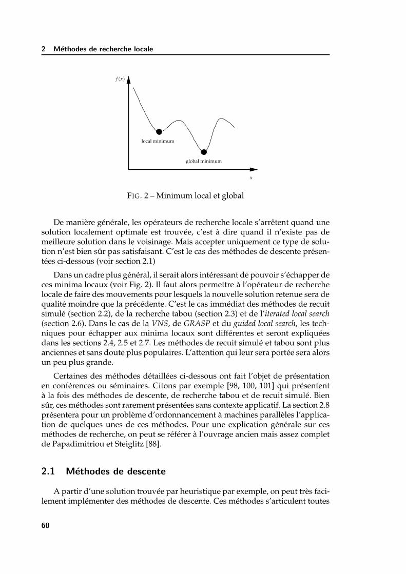
2 Methodes de recherche locale
local minimum
x
global minimum
f (x)
FIG. 2 – Minimum local et global
De maniere generale, les operateurs de recherche locale s’arretent quand unesolution localement optimale est trouvee, c’est a dire quand il n’existe pas demeilleure solution dans le voisinage. Mais accepter uniquement ce type de solu-tion n’est bien sur pas satisfaisant. C’est le cas des methodes de descente presen-tees ci-dessous (voir section 2.1)
Dans un cadre plus general, il serait alors interessant de pouvoir s’echapper deces minima locaux (voir Fig. 2). Il faut alors permettre a l’operateur de recherchelocale de faire des mouvements pour lesquels la nouvelle solution retenue sera dequalite moindre que la precedente. C’est le cas immediat des methodes de recuitsimule (section 2.2), de la recherche tabou (section 2.3) et de l’iterated local search(section 2.6). Dans le cas de la VNS, de GRASP et du guided local search, les tech-niques pour echapper aux minima locaux sont differentes et seront expliqueesdans les sections 2.4, 2.5 et 2.7. Les methodes de recuit simule et tabou sont plusanciennes et sans doute plus populaires. L’attention qui leur sera portee sera alorsun peu plus grande.
Certaines des methodes detaillees ci-dessous ont fait l’objet de presentationen conferences ou seminaires. Citons par exemple [98, 100, 101] qui presententa la fois des methodes de descente, de recherche tabou et de recuit simule. Biensur, ces methodes sont rarement presentees sans contexte applicatif. La section 2.8presentera pour un probleme d’ordonnancement a machines paralleles l’applica-tion de quelques unes de ces methodes. Pour une explication generale sur cesmethodes de recherche, on peut se referer a l’ouvrage ancien mais assez completde Papadimitriou et Steiglitz [88].
2.1 Methodes de descente
A partir d’une solution trouvee par heuristique par exemple, on peut tres faci-lement implementer des methodes de descente. Ces methodes s’articulent toutes
60
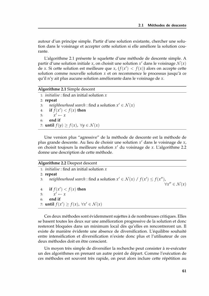
2.1 Methodes de descente
autour d’un principe simple. Partir d’une solution existante, chercher une solu-tion dans le voisinage et accepter cette solution si elle ameliore la solution cou-rante.
L’algorithme 2.1 presente le squelette d’une methode de descente simple. Apartir d’une solution initiale x, on choisit une solution x′ dans le voisinage N (x)de x. Si cette solution est meilleure que x, ( f (x′) < f (x)) alors on accepte cettesolution comme nouvelle solution x et on recommence le processus jusqu’a cequ’il n’y ait plus aucune solution ameliorante dans le voisinage de x.
Algorithme 2.1 Simple descent1: initialise : find an initial solution x2: repeat3: neighbourhood search : find a solution x′ ∈ N (x)4: if f (x′) < f (x) then5: x′ ← x6: end if7: until f (y) ≥ f (x), ∀y ∈ N (x)
Une version plus “agressive” de la methode de descente est la methode deplus grande descente. Au lieu de choisir une solution x′ dans le voisinage de x,on choisit toujours la meilleure solution x′ du voisinage de x. L’algorithme 2.2donne une description de cette methode.
Algorithme 2.2 Deepest descent1: initialise : find an initial solution x2: repeat3: neighbourhood search : find a solution x′ ∈ N (x) / f (x′) ≤ f (x′′),
∀x′′ ∈ N (x)4: if f (x′) < f (x) then5: x′ ← x6: end if7: until f (x′) ≥ f (x), ∀x′ ∈ N (x)
Ces deux methodes sont evidemment sujettes a de nombreuses critiques. Ellesse basent toutes les deux sur une amelioration progressive de la solution et doncresteront bloquees dans un minimum local des qu’elles en rencontreront un. Ilexiste de maniere evidente une absence de diversification. L’equilibre souhaiteentre intensification et diversification n’existe donc plus et l’utilisateur de cesdeux methodes doit en etre conscient.
Un moyen tres simple de diversifier la recherche peut consister a re-executerun des algorithmes en prenant un autre point de depart. Comme l’execution deces methodes est souvent tres rapide, on peut alors inclure cette repetition au
61

2 Methodes de recherche locale
sein d’une boucle generale. On obtient alors un algorithme de type “Multi-startdescent” decrit par l’algorithme 2.3.
Algorithme 2.3 Multistart descent1: initialise : find an initial solution x, k ← 1, f (B) ← +∞
2: repeat3: Starting point : choose an initial solution x0 at random4: x ← result of Simple Descent or Deepest Descent5: if f (x) < f (B) then6: B ← x7: end if8: k ← k + 19: until stopping criterion satisfied
Dans la section 2.8, nous verrons que cette derniere methode peut dans cer-tains cas etre particulierement efficace. De maniere evidente, la diversification esttotalement absente des algorithmes 2.1 et 2.2. En ne conservant que l’aspect in-tensification, la convergence est souvent trop rapide (plus encore avec la versionDeepest descent) et on se trouve tres rapidement bloque dans un optimum local.Les resultats communement admis indiquent que ces techniques conduisent engeneral a des solutions en moyenne a 20% de l’optimum. Dans le cas de l’algo-rithme 2.3, la diversification est simplement inseree par le choix aleatoire d’unesolution de depart. Cette simple technique peut s’averer payante dans certainscas (voir section 2.8).
2.2 Recuit simule
La methode du recuit simule a ete introduite en 1983 par Kirkpatrick et al.[64]. Cette methode originale est basee sur les travaux bien anterieurs de Metro-polis et al. [81]. Cette methode que l’on pourrait considerer comme la premieremetaheuristique “grand public” a recu l’attention de nombreux travaux et prin-cipalement de nombreuses applications.
Le principe de fonctionnement s’inspire d’un processus d’amelioration de laqualite d’un metal solide par recherche d’un etat d’energie minimum correspon-dant a une structure stable de ce metal. L’etat optimal correspondrait a une struc-ture moleculaire reguliere parfaite. En partant d’une temperature elevee ou lemetal serait liquide, on refroidit le metal progressivement en tentant de trouverle meilleur equilibre thermodynamique. Chaque niveau de temperature est main-tenu jusqu’a obtention d’un equilibre. Dans ces phases de temperature constante,on peut passer par des etats intermediaires du metal non satisfaisants, mais con-duisant a la longue a des etats meilleurs.
L’analogie avec une methode d’optimisation est trouvee en associant une so-
62

2.2 Recuit simule
lution a un etat du metal, son equilibre thermodynamique est la valeur de la fonc-tion objectif de cette solution. Passer d’un etat du metal a un autre correspond apasser d’une solution a une solution voisine.
Pour passer a une solution voisine, il faut respecter l’une des deux conditions :– soit le mouvement ameliore la qualite de la solution precedente, i.e. en mi-
nimisation la variation de cout est negative (∆C < 0),– soit le mouvement deteriore la qualite de la solution precedente et la proba-
bilite p d’accepter un tel mouvement est inferieure a une valeur dependantde la temperature courante t (p < e−∆C/t).
Le schema de refroidissement de la temperature est une des parties les plusdifficiles a regler dans ce cas. Ces schemas sont cruciaux pour l’obtention d’uneimplementation efficace. Sans etre exhaustif, on rencontre habituellement troisgrandes classes de schemas : la reduction par paliers, la reduction continue, Lundyet Mees [78] (ou la temperature est reduite a chaque iteration) et la reduction non-monotone, Connolly [15] (ou des augmentations de temperature sont possibles).Pour d’autres schemas de refroidissement de temperature et une large discussion,on peut se reporter a plusieurs articles, dont les travaux de Aarts et Korst [1], deCollins et al. [14] et de Van Laarhoven et Aarts [125] par exemple. La convergencedu recuit simule vers un optimum global, en choisissant le schema adapte, a puetre prouvee (voir [1, 55, 125]).
La popularite du recuit simule a ete incontestable pendant des annees. D’abordcette methode est facile a implementer et elle a permis de resoudre de nom-breux problemes NP-difficiles [9, 126]. Parmi les bibliographies et articles desynthese interessants, on peut citer Koulamas et al. [65] et Collins et al. [14]. Unexcellent tutorial recent pourra guider les chercheurs dans leurs premiers pasavec cette methode [90]. En attendant, l’algorithme 2.4 presente les principalescaracteristiques d’un recuit simule.
Algorithme 2.4 Basic simulated annealing1: initialise : find an initial solution x, fix an annealing schedule T , set initial
temperature t2: repeat3: neighbourhood search : find a solution x′ ∈ N (x)4: determine ∆C = f (x′)− f (x)5: draw p ∼ U (0, 1)6: if ∆C < 0 or e−∆C/t
> p then7: x′ ← x8: end if9: update temperature t according to T
10: until stopping criterion satisfied
Dans cet algorithme, l’equilibre entre intensification et diversification est res-pecte. L’intensification peut se faire par l’intermediaire des etapes des lignes 3, 6
63

2 Methodes de recherche locale
et 9 de l’algorithme 2.4. A la ligne 3, on effectue une recherche des voisins et cecipeut etre fait par une recherche locale. De plus, a la ligne 6, on accepte tous lesmouvements strictement ameliorants comme dans une methode de descente. Leschema de refroidissement de la temperature reduit lui-aussi la probabilite d’ac-cepter des mouvements non-ameliorants et intensifie la recherche. Par ailleurs, ladiversification est obtenue en autorisant des mouvements non-ameliorants souscondition de probabilite (ligne 6) ou en choisissant un schema T (ligne 9) permet-tant l’augmentation de temperature, donc en augmentant la probabilite d’accep-tation de solutions plus diverses.
2.3 Recherche tabou
Dans un article presente par Glover [37] en 1986, on voit apparaıtre pour lapremiere fois, a la fois le terme tabu search et metaheuristique. A la meme epoque,Hansen [56] presente une methode similaire, mais dont le nom n’a pas marqueautant que tabou. En fait, les premices de la methode ont ete presentes initiale-ment a la fin des annees 1970 par Glover [36]. Pourtant ce sont les deux articlesde reference de Glover [38, 39] qui vont contribuer de maniere importante a lapopularite de cette methode. Pour certains chercheurs, elle apparaıt meme plussatisfaisante sur le plan scientifique que le recuit simule, car la partie “aleatoire”de la methode a disparu.
Contrairement au recuit simule qui ne genere qu’une seule solution x′ “alea-toirement” dans le voisinage N (x) de la solution courante x, la methode tabou,dans sa forme la plus simple, examine le voisinageN (x) de la solution courante x.La nouvelle solution x′ est la meilleure solution de ce voisinage (dont l’evaluationest parfois moins bonne que x elle-meme). Pour eviter de cycler, une liste tabou(qui a donne le nom a la methode) est tenue a jour et interdit de revenir a dessolutions deja explorees. Dans une version plus avancee de la methode tabou,on peut voir dans cette recherche une modification temporaire de la structure devoisinage de la solution x permettant de quitter des optima locaux. Le voisinageN ∗(x) integrant ces modifications de structure est regit par l’utilisation de struc-tures de memoire specifiques. Il s’agit de memoire a court terme ou de memoirea long terme.
La memoire a court terme correspond a la mise en place d’une liste tabou.La liste contient les quelques dernieres solutions qui ont ete recemment visitees.Le nouveau voisinage N ∗(x) exclut donc toutes les solutions de la liste tabou.Lorsque la structure de donnee correspondant aux solutions est trop complexeou occupe une grande place memoire, il est courant de ne garder dans la listetabou que des informations soit sur les caracteristiques des solutions, soit sur lesmouvements. Ce type de memoire a court terme est aussi appele recency-basedmemory. En conservant des caracteristiques des solutions ou des mouvements, ilest possible alors qu’une solution de bien meilleure qualite ait un statut tabou.
64
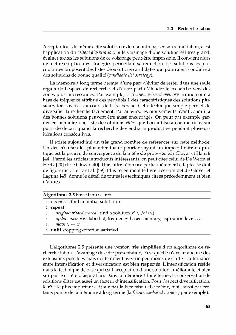
2.3 Recherche tabou
Accepter tout de meme cette solution revient a outrepasser son statut tabou, c’estl’application du critere d’aspiration. Si le voisinage d’une solution est tres grand,evaluer toutes les solutions de ce voisinage peut-etre impossible. Il convient alorsde mettre en place des strategies permettant sa reduction. Les solutions les pluscourantes proposent des listes de solutions candidates qui pourraient conduire ades solutions de bonne qualite (candidate list strategy).
La memoire a long terme permet d’une part d’eviter de rester dans une seuleregion de l’espace de recherche et d’autre part d’etendre la recherche vers deszones plus interessantes. Par exemple, la frequency-based memory ou memoire abase de frequence attribue des penalites a des caracteristiques des solutions plu-sieurs fois visitees au cours de la recherche. Cette technique simple permet dediversifier la recherche facilement. Par ailleurs, les mouvements ayant conduit ades bonnes solutions peuvent etre aussi encourages. On peut par exemple gar-der en memoire une liste de solutions elites que l’on utilisera comme nouveaupoint de depart quand la recherche deviendra improductive pendant plusieursiterations consecutives.
Il existe aujourd’hui un tres grand nombre de references sur cette methode.Un des resultats les plus attendus et pourtant ayant un impact limite en pra-tique est la preuve de convergence de la methode proposee par Glover et Hanafi[44]. Parmi les articles introductifs interessants, on peut citer celui de De Werra etHertz [20] et de Glover [40]. Une autre reference particulierement adaptee se doitde figurer ici, Hertz et al. [59]. Plus recemment le livre tres complet de Glover etLaguna [45] donne le detail de toutes les techniques citees precedemment et biend’autres.
Algorithme 2.5 Basic tabu search1: initialise : find an initial solution x2: repeat3: neighbourhood search : find a solution x′ ∈ N ∗(x)4: update memory : tabu list, frequency-based memory, aspiration level, . . .5: move x ← x′
6: until stopping criterion satisfied
L’algorithme 2.5 presente une version tres simplifiee d’un algorithme de re-cherche tabou. L’avantage de cette presentation, c’est qu’elle n’exclut aucune desextensions possibles mais evidemment avec un peu moins de clarte. L’alternanceentre intensification et diversification est bien respectee. L’intensification residedans la technique de base qui est l’acceptation d’une solution ameliorante et biensur par le critere d’aspiration. Dans la memoire a long terme, la conservation desolutions elites est aussi un facteur d’intensification. Pour l’aspect diversification,le role le plus important est joue par la liste tabou elle-meme, mais aussi par cer-tains points de la memoire a long terme (la frequency-based memory par exemple).
65

2 Methodes de recherche locale
2.4 Recherche a voisinages variables
La recherche a voisinages variables est une methode recente et pourtant tressimple, basee sur la performance des methodes de descente. Introduite par Mla-denovic et Hansen [85], la methode propose simplement d’utiliser plusieurs voi-sinages successifs quand on se trouve bloque dans un minimum local.
Avant tout, il est necessaire de definir un ensemble de kmax voisinages, denotespar Nk=1...kmax (et de preference tels que Nk ⊂ Nk+1). On choisit une solution dedepart x par heuristique. Ensuite, a partir d’une solution initiale x′ choisie dansle premier voisinage N (x) de x, on applique une methode de descente (ou uneautre methode de recherche locale) jusqu’a arriver dans un minimum local (ouque la recherche locale s’arrete). Si la solution trouvee x′′ est meilleure que x alorson recentre la recherche en repartant du premier voisinage, sinon on passe auvoisinage suivant (qui a priori est plus grand). La recherche s’arrete quand tousles voisinages ne sont plus capables d’ameliorer la solution.
Le point crucial dans une VNS, c’est bien evidement la constitution des voisi-nages de plus en plus grands et inclus les uns dans les autres. Une bonne structurede voisinage –ceci etant vrai pour toute recherche locale– conduit generalement ade bons resultats ou au moins a une recherche efficace.
Cette methode recente interesse de plus en plus de chercheurs et est promisea un bel avenir. Le nombre de papiers utilisant cette methode est en tres forteaugmentation dans les congres. La methode est decrite en detail par Hansen etMladenovic [57] et un squelette general de cette methode est propose dans l’algo-rithme 2.6.
Algorithme 2.6 Basic variable neighbourhood search1: initialise : find an initial solution x, k← 12: repeat3: shake : generate a point x′ at random from the neighbourhood Nk(x)4: local search : apply a local search procedure starting from the solution x ′ to
find a solution x′′
5: if x′′ is better than x then6: x ← x′′ and k ← 1 (centre the search around x′′ and search again with a
small neighbourhood)7: else8: k ← k + 1 (enlarge the neighbourhood)9: end if
10: until k = kmax
Dans l’algorithme 2.6, la diversification est geree par deux techniques. Lapremiere consiste a choisir dans le voisinage courant une solution aleatoirement(etape shake) et la seconde c’est le changement de voisinage lui-meme qui agrandit
66
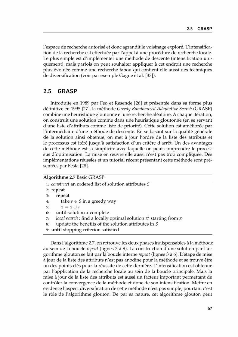
2.5 GRASP
l’espace de recherche autorise et donc agrandit le voisinage explore. L’intensifica-tion de la recherche est effectuee par l’appel a une procedure de recherche locale.Le plus simple est d’implementer une methode de descente (intensification uni-quement), mais parfois on peut souhaiter appliquer a cet endroit une rechercheplus evoluee comme une recherche tabou qui contient elle aussi des techniquesde diversification (voir par exemple Gagne et al. [33]).
2.5 GRASP
Introduite en 1989 par Feo et Resende [26] et presentee dans sa forme plusdefinitive en 1995 [27], la methode Greedy Randomized Adaptative Search (GRASP)combine une heuristique gloutonne et une recherche aleatoire. A chaque iteration,on construit une solution comme dans une heuristique gloutonne (en se servantd’une liste d’attributs comme liste de priorite). Cette solution est amelioree parl’intermediaire d’une methode de descente. En se basant sur la qualite generalede la solution ainsi obtenue, on met a jour l’ordre de la liste des attributs etle processus est itere jusqu’a satisfaction d’un critere d’arret. Un des avantagesde cette methode est la simplicite avec laquelle on peut comprendre le proces-sus d’optimisation. La mise en œuvre elle aussi n’est pas trop compliquee. Desimplementations reussies et un tutorial recent presentant cette methode sont pre-sentees par Festa [28].
Algorithme 2.7 Basic GRASP1: construct an ordered list of solution attributes S2: repeat3: repeat4: take s ∈ S in a greedy way5: x = x ∪ s6: until solution x complete7: local search : find a locally optimal solution x′ starting from x8: update the benefits of the solution attributes in S9: until stopping criterion satisfied
Dans l’algorithme 2.7, on retrouve les deux phases indispensables a la methodeau sein de la boucle repeat (lignes 2 a 9). La construction d’une solution par l’al-gorithme glouton se fait par la boucle interne repeat (lignes 3 a 6). L’etape de misea jour de la liste des attributs n’est pas anodine pour la methode et se trouve etreun des points cles pour la reussite de cette derniere. L’intensification est obtenuepar l’application de la recherche locale au sein de la boucle principale. Mais lamise a jour de la liste des attributs est aussi un facteur important permettant decontroler la convergence de la methode et donc de son intensification. Mettre enevidence l’aspect diversification de cette methode n’est pas simple, pourtant c’estle role de l’algorithme glouton. De par sa nature, cet algorithme glouton peut
67
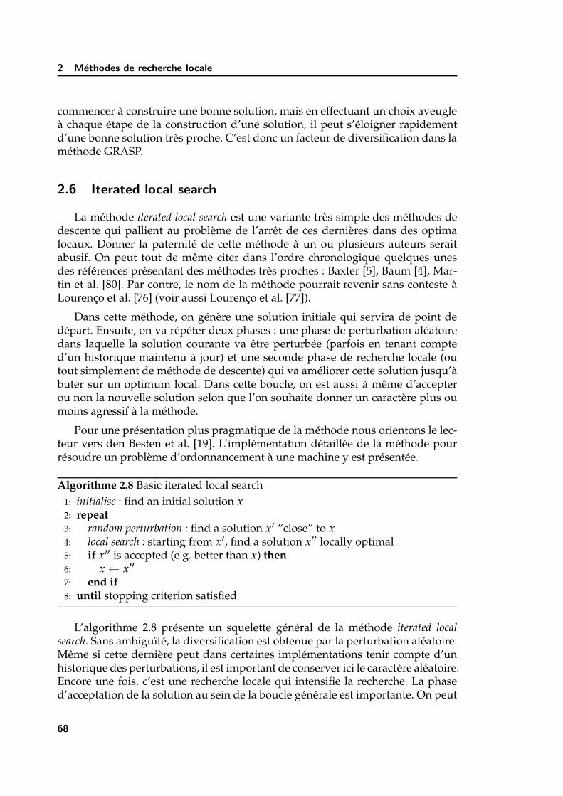
2 Methodes de recherche locale
commencer a construire une bonne solution, mais en effectuant un choix aveuglea chaque etape de la construction d’une solution, il peut s’eloigner rapidementd’une bonne solution tres proche. C’est donc un facteur de diversification dans lamethode GRASP.
2.6 Iterated local search
La methode iterated local search est une variante tres simple des methodes dedescente qui pallient au probleme de l’arret de ces dernieres dans des optimalocaux. Donner la paternite de cette methode a un ou plusieurs auteurs seraitabusif. On peut tout de meme citer dans l’ordre chronologique quelques unesdes references presentant des methodes tres proches : Baxter [5], Baum [4], Mar-tin et al. [80]. Par contre, le nom de la methode pourrait revenir sans conteste aLourenco et al. [76] (voir aussi Lourenco et al. [77]).
Dans cette methode, on genere une solution initiale qui servira de point dedepart. Ensuite, on va repeter deux phases : une phase de perturbation aleatoiredans laquelle la solution courante va etre perturbee (parfois en tenant compted’un historique maintenu a jour) et une seconde phase de recherche locale (outout simplement de methode de descente) qui va ameliorer cette solution jusqu’abuter sur un optimum local. Dans cette boucle, on est aussi a meme d’accepterou non la nouvelle solution selon que l’on souhaite donner un caractere plus oumoins agressif a la methode.
Pour une presentation plus pragmatique de la methode nous orientons le lec-teur vers den Besten et al. [19]. L’implementation detaillee de la methode pourresoudre un probleme d’ordonnancement a une machine y est presentee.
Algorithme 2.8 Basic iterated local search1: initialise : find an initial solution x2: repeat3: random perturbation : find a solution x′ “close” to x4: local search : starting from x′, find a solution x′′ locally optimal5: if x′′ is accepted (e.g. better than x) then6: x ← x′′
7: end if8: until stopping criterion satisfied
L’algorithme 2.8 presente un squelette general de la methode iterated localsearch. Sans ambiguıte, la diversification est obtenue par la perturbation aleatoire.Meme si cette derniere peut dans certaines implementations tenir compte d’unhistorique des perturbations, il est important de conserver ici le caractere aleatoire.Encore une fois, c’est une recherche locale qui intensifie la recherche. La phased’acceptation de la solution au sein de la boucle generale est importante. On peut
68

2.7 Guided local search
par exemple accepter une solution si elle ameliore strictement la solution cou-rante. Mais on peut aussi accepter seulement si elle ameliore la meilleure solutiontrouvee, ou pourquoi pas, si elle ne degrade pas la meilleure solution trouvee deplus d’un certain pourcentage. Comme on le voit, on peut adapter cette methodefacilement et ajouter des facteurs d’intensification ou de diversification a cet en-droit.
2.7 Guided local search
Presentee pour la premiere fois dans un rapport de recherche de Voudouriset Tsang [128], la guided local search (ou recherche locale guidee) est une varianteassez elaboree d’une methode de descente classique.
La methode de base est simple. Elle consiste a modifier la fonction a optimiseren ajoutant des penalites. La recherche locale est appliquee alors sur cette fonctionmodifiee. La solution trouvee (qui se trouve etre un optimum local) sert a calculerles nouvelles penalites. Pour cela, on calcule l’utilite de chacun des attributs de lasolution et on augmente les penalites associees aux attributs de valeur maximale.Ces etapes successives sont repetees jusqu’a ce qu’un critere d’arret soit valide.
L’article initial de Voudouris et Tsang [129], soumis en octobre 1995 n’a ete pu-blie qu’en 1999 et presente de nombreuses ameliorations de l’algorithme 2.9. Pourune presentation tres approfondie, la these de Voudouris [127] est le document leplus complet.
Algorithme 2.9 Basic guided local search1: initialise : find an initial solution x, set penalties to 02: repeat3: cost function : augment the original cost function of x with penalties4: local search : apply a local search procedure to find a solution x′ locally op-
timal (based on the augmented cost function)5: update penalties : by computing utility expressions6: x ← x′
7: until stopping criterion satisfied
Dans l’algorithme 2.9, nous avons volontairement simplifie la presentationpour ne pas surcharger la lecture et la comprehension. L’intensification de la re-cherche est fait directement par l’appel a la recherche locale au sein de la boucleprincipale. Les expressions d’utilites des differents attributs d’une solution servent,pour celles qui sont a leur maximum, a penaliser la fonction de cout. Ce qui veutdire que l’on va forcer la recherche a s’effectuer dans d’autres directions que cellesqui semblaient prometteuses lors des precedentes recherches. Cette mise a jourdes fonctions de penalite est donc un facteur de diversification de la recherche.
69
2 Methodes de recherche locale
2.8 Applications
Applications de la litteratureComme il a ete mentionne precedemment, il existe assez peu de references quine presentent que des methodes de descente. Pourtant, certains ouvrages pluscomplet ou depassant ce cadre sont interessants (voir par exemple Blum et Roli[8] ou Johnson et al. [63]). Il existe enormement d’applications utilisant le recuitsimule. On peut citer des articles importants de Van Laarhoven et Aarts [125] oude Vidal [126] et la bibliographie commentee de Collins et al. [14] qui reference untres grand nombre d’applications. Pour la recherche tabou, on ne compte plus lesarticles se referant a cette methode. On peut citer un numero special de Gloveret al. [47] presentant plusieurs articles sur le sujet. La methode GRASP est deplus en plus populaire. Il existe un site web http://www.graspheuristic.org
qui est maintenu a jour et reference plusieurs centaines d’articles. Regulierementune bibliographie commentee de GRASP est publiee (voir Festa et Resende [29]).La methode Iterated local search, un peu ignoree au debut, sans doute pour sonapparente simplicite, commence a prendre place au sein de toutes ces methodes(voir Paquete et Stutzle [89]). Du cote du Guided local search, c’est le meme constat.Les applications se multiplient et la methode prouve son efficacite dans plusieursdomaines (voir Beullens et al. [7] ou Voudouris et Tsang [129]).
Ordonnancement sur machines parallelesDe notre cote, nous avons aborde plusieurs de ces methodes pour un problemed’ordonnancement sur machines paralleles. Un ensemble de n jobs (j = 1 . . . n)doit etre sequence sur m machines paralleles. Chaque job doit etre execute sur unedes machines et ne peut demarrer avant sa date de debut au plus tot, rj (releasedate). Le temps d’execution de ce job est de pj unites de temps (processing time).Une date echue, dj (due date) et un poids, wj (weight) sont donnes pour chaquejob. Si le job se termine apres sa date echue, on dit qu’il est en retard, sinon lejob est termine a temps. Le critere retenu est la minimisation de la somme despoids des jobs en retard min ∑ wjUj. Ce probleme est note Pm|rj|∑ wjUj dansla litterature [51]. Meme reduit a deux machines, ce probleme est NP-difficile[35]. Ce probleme et les resultats presentes plus loin sont extraits des differentespresentations du probleme (voir par exemple [113–118]).
Le tableau 1 est directement extrait de [115]. Nous comparons ici les methodesen utilisant toujours le meme voisinage. Dans ce cas-ci, il s’agit d’echanger un jobactuellement en retard par un ou plusieurs jobs en avance (voir Sevaux et Tho-min [115]). Sans entrer dans des details, les lignes notees EMP, BWS, BNO, BRSrepresentent differents points de depart des heuristiques (sans objet pour la me-thode multi-start).
Sans tirer des conclusions generales, on constate dans le tableau 1 que le pointde depart a peu d’impact sur la qualite d’une solution obtenue par methode de
70

TAB. 1 – Resultats extraits de Sevaux et Thomin [115].Initial Optimum First Gap to Avg. CPU Max. CPUHeuristics hits (%) pos. (%) opt. (%) time (s) time (s)Deepest descent heuristicsEMP 45 33 21.5 0.02 0.12BWS 49 35 19.6 < .01 < .01BNO 44 31 20.3 < .01 < .01BRS 44 31 20.3 < .01 < .01Multistart deepest descent heuristicMD 78 63 3.9 4.58 41.1Simulated annealingEMP 70 55 6.72 9.10 60.3BWS 70 54 6.59 7.68 53.2BNO 71 56 6.03 9.01 64.9BRS 70 55 5.98 8.87 63.3Tabu searchEMP 89 79 1.94 10.63 101.9BWS 88 76 2.00 9.42 112.0BNO 88 80 1.89 10.17 93.7BRS 88 79 1.95 10.16 107.5
descente et que les solutions se trouvent en moyenne a 20% de l’optimum. En uti-lisant le meme voisinage, et pour une configuration particuliere des parametresde recuit simule et recherche tabou, les ecarts a l’optimum sont respectivementde 6% et 2% environ. Par contre, ce qui est tres surprenant, c’est que la methodemulti-start obtient de tres bons resultats avec un ecart de 4%. Faut-il pour au-tant renoncer a implementer un recuit simule ? Certainement pas. Comme il a etesignale, le reglage des parametres est fixe et en faisant varier ces derniers on de-vrait pouvoir atteindre des resultats meilleurs. Ce qui est important a retirer decette experience, c’est que meme si l’implementation des methodes de descentedonne des resultats mediocres, en passant a une simple methode multi-start onobtient des solutions tres satisfaisantes avec des temps de calcul raisonnables etsurtout un temps d’implementation minimum (le plus dur etant deja fait dansl’ecriture du voisinage lui-meme). Donc, passer ensuite a une methode plus com-plexe comme le recuit simule ou la recherche tabou est un pas supplementaire afranchir pour peu qu’on en ait le temps.
3 Metaheuristiques a base de population
Les methodes de recherche a population, comme leur nom l’indique, travaillentsur une population de solutions et non pas sur une solution unique. On peut
71

3 Metaheuristiques a base de population
trouver d’autres noms generiques pour ces methodes, le plus en vogue etantsans doute evolutionary algorithms (voir Michalewicz [82]). Le principe general detoutes ces methodes consiste a combiner des solutions entre elles pour en formerde nouvelles en essayant d’heriter des “bonnes” caracteristiques des solutionsparents. Un tel processus est repete jusqu’a ce qu’un critere d’arret soit satisfait(nombre de generations maximum, nombre de generations sans ameliorations,temps maximum, borne atteinte, etc). Parmi ces algorithmes a population, on re-trouve deux grandes classes qui sont les algorithmes genetiques et les coloniesde fourmis. Les algorithmes genetiques ont beaucoup fait parler d’eux et de-puis longtemps. Les colonies de fourmis sont des techniques plus recentes, maisl’auteur a su faire parler de la methode et interesser non- seulement les cher-cheurs, mais aussi les grandes instances decisionnaires comme la commission eu-ropeenne par exemple. Il existe bien d’autres techniques que nous aurions pudecrire ici comme le Genetic programming de Koza [67] par exemple. Nous aver-tissons aussi ici le lecteur, que les prises de position sur differents points sontcelles de l’auteur de cette synthese et n’engage que lui. Elles sont pour la plupartdiscutables...
3.1 Algorithmes genetiques
Propose dans les annees 1975 par Holland [61], les algorithmes genetiquesdoivent leur popularite a Goldberg [49]. Avant la parution de son livre qui estune des references les plus citees dans le domaine de l’informatique, on a puvoir un certain nombre d’autres presentations, citons Goldberg [48], Holland [62],Schwefel [97]. Le sujet connaıt une tres grande popularite. Il existe aujourd’huiplusieurs milliers de references sur le sujet et le nombre de conferences dedieesau domaine (que ce soit sur les techniques elles-memes ou sur les applications)ne fait qu’augmenter.
De maniere generale, les algorithmes genetiques utilisent un meme principe.Une population d’individus (correspondants a des solutions) evoluent en memetemps comme dans l’evolution naturelle en biologie. Pour chacun des individus,on mesure sa faculte d’adaptation au milieu exterieur par le fitness. Les algo-rithmes genetiques s’appuient alors sur trois fonctionnalites :
la selection qui permet de favoriser les individus qui ont un meilleur fitness (pournous le fitness sera la plus souvent la valeur de la fonction objectif de la so-lution associee a l’individu).
le croisement qui combine deux solutions parents pour former un ou deux en-fants (offspring) en essayant de conserver les “bonnes” caracteristiques dessolutions parents.
la mutation qui permet d’ajouter de la diversite a la population en mutant cer-taines caracteristiques (genes) d’une solution.
72

3.1 Algorithmes genetiques
La representation des solutions (le codage) est un point critique de la reussited’un algorithme genetique. Il faut bien sur qu’il s’adapte le mieux possible auprobleme et a l’evaluation d’une solution. Le codage phenotypique ou codagedirect correspond en general a une representation de la solution tres proche dela realite. L’evaluation d’une solution representee ainsi est en general immediate.On peut aussi utiliser un codage indirect (codage genotypique) qui est souventplus eloigne de la realite et qui necessite un algorithme de decodage pour recons-tituer une solution valide. Pour ce dernier codage, il existe aujourd’hui beaucoupde travaux et notamment des operateurs de croisement et de mutation en quan-tite.
En effectuant une recherche sur internet, on trouve plusieurs milliers de pagesweb repondant a la requete genetic algorithms. Donner une bonne reference est in-dispensable. Nous renvoyons donc le lecteur vers deux livres importants, Hauptet Haupt [58], Mitchel [84] et vers un bon article introductif qui a le merite d’etreen francais, Fleurent et Ferland [30] et qui explique avec suffisamment de detailsune implementation parmi d’autres. Comme pour d’autres algorithmes, la preuvede convergence est apportee par Cerf [12]. Meme si l’interet pratique de cettepreuve est limite, il est toujours plus satisfaisant de savoir que la methode convergesous certaines conditions.
Nous presentons deux versions possibles d’algorithme genetique. L’algorithme3.1 propose une version qualifiee en Anglais par population replacement (ou algo-rithme generationnel) tandis que l’algorithme 3.2 est une version incrementale.La difference entre les deux reside dans la gestion de la population.
Dans le premier cas (algorithme 3.1), on cree une seconde population en pa-rallele a la premiere, puis on insere des individus obtenus par croisement et muta-tion des individus de la population precedente. Des qu’une nouvelle populationest formee, elle remplace la population precedente et le processus recommence.Un des points importants a prendre en compte est la perte possible du meilleurindividu ou meme de la solution optimale lors du remplacement de la popu-lation. Il faudra donc prevoir un mecanisme permettant d’eviter cela. Dans cetalgorithme, la selection est faite ici en effectuant un tirage aleatoire biaise parla valeur du fitness des individus (par exemple par la methode de ranking deReeves [95]). Comme dans les systemes d’evolution naturels, le croisement et lamutation se font sous conditions de probabilite.
Dans la seconde version de l’algorithme genetique (algorithme 3.2), on creeun nouvel individu par croisement et mutation et il remplace un individu exis-tant dans la population courante. Ma preference va a la seconde methode quipermet (potentiellement) d’exploiter immediatement tout nouvel individu cree al’iteration precedente. Dans cet algorithme, nous choisissons la methode de tour-noi binaire (ou roulette wheel) pour la selection. Le croisement est fait a chaqueiteration et la mutation sous conditions (par exemple avec une faible probabilitemais en respectant un critere d’aspiration). Pour le choix de l’individu a rem-
73
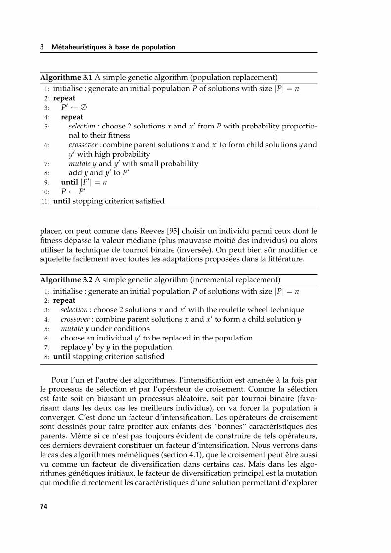
3 Metaheuristiques a base de population
Algorithme 3.1 A simple genetic algorithm (population replacement)1: initialise : generate an initial population P of solutions with size |P| = n2: repeat3: P′ ← ∅
4: repeat5: selection : choose 2 solutions x and x′ from P with probability proportio-
nal to their fitness6: crossover : combine parent solutions x and x′ to form child solutions y and
y′ with high probability7: mutate y and y′ with small probability8: add y and y′ to P′
9: until |P′| = n10: P ← P′
11: until stopping criterion satisfied
placer, on peut comme dans Reeves [95] choisir un individu parmi ceux dont lefitness depasse la valeur mediane (plus mauvaise moitie des individus) ou alorsutiliser la technique de tournoi binaire (inversee). On peut bien sur modifier cesquelette facilement avec toutes les adaptations proposees dans la litterature.
Algorithme 3.2 A simple genetic algorithm (incremental replacement)1: initialise : generate an initial population P of solutions with size |P| = n2: repeat3: selection : choose 2 solutions x and x′ with the roulette wheel technique4: crossover : combine parent solutions x and x′ to form a child solution y5: mutate y under conditions6: choose an individual y′ to be replaced in the population7: replace y′ by y in the population8: until stopping criterion satisfied
Pour l’un et l’autre des algorithmes, l’intensification est amenee a la fois parle processus de selection et par l’operateur de croisement. Comme la selectionest faite soit en biaisant un processus aleatoire, soit par tournoi binaire (favo-risant dans les deux cas les meilleurs individus), on va forcer la population aconverger. C’est donc un facteur d’intensification. Les operateurs de croisementsont dessines pour faire profiter aux enfants des “bonnes” caracteristiques desparents. Meme si ce n’est pas toujours evident de construire de tels operateurs,ces derniers devraient constituer un facteur d’intensification. Nous verrons dansle cas des algorithmes memetiques (section 4.1), que le croisement peut etre aussivu comme un facteur de diversification dans certains cas. Mais dans les algo-rithmes genetiques initiaux, le facteur de diversification principal est la mutationqui modifie directement les caracteristiques d’une solution permettant d’explorer
74

3.2 Algorithmes de colonies de fourmis
de nouveaux espaces de solutions.
3.2 Algorithmes de colonies de fourmis
Les algorithmes a base de colonies de fourmis ont ete introduits par Dorigoet al. [24] et dans la these de [21]. Une des applications principales de la methodeoriginale etait le probleme du voyageur de commerce et depuis elle a considera-blement evolue.
Cette nouvelle metaheuristique imite le comportement de fourmis cherchantde la nourriture. A chaque fois qu’une fourmi se deplace, elle laisse sur la trace deson passage une odeur (la pheromone). Comme la fourmi est rarement une explo-ratrice isolee, avec plusieurs de ses congeneres, elle explore une region en quetede nourriture. Face a un obstacle, le groupe des fourmis explore les deux cotesde l’obstacle et se retrouvent, puis elles reviennent au nid avec de la nourriture.Les autres fourmis qui veulent obtenir de la nourriture elles aussi vont emprun-ter le meme chemin. Si celui-ci se separe face a l’obstacle, les fourmis vont alorsemprunter preferablement le chemin sur lequel la pheromone sera la plus forte.Mais la pheromone etant une odeur elle s’evapore. Si peu de fourmis empruntentune trace, il est possible que ce chemin ne soit plus valable au bout d’un mo-ment, il en est de meme si des fourmis exploratrices empruntent un chemin pluslong (pour le contournement de l’obstacle par exemple). Par contre, si le cheminest fortement emprunte, chaque nouvelle fourmi qui passe redepose un peu depheromone et renforce ainsi la trace, donnant alors a ce chemin une plus grandeprobabilite d’etre emprunte.
On peut alors comprendre l’application directe du probleme du voyageurde commerce. Chaque fourmi constitue un tour en empruntant des aretes dugraphes, puis au bout d’un moment les aretes qui conduisent a une bonne so-lution deviendront les plus empruntees jusqu’a obtention d’une tres bonne so-lution. Meme si le principe est simple, on peut voir apparaıtre des difficultescomme, la quantite de pheromone a deposer, le coefficient d’evaporation, la de-finition du choix biaise, etc. La metaheuristique telle qu’elle est decrite schemati-quement ci- dessous est detaillee par Dorigo et al. [23] et Dorigo et Di Caro [22].Bien que cette methode soit plutot recente, elle a suscite de nombreux articles en“tournees de vehicules”, peut-etre par son exotisme ou parce qu’il est plus facilede publier avec une nouvelle methode moins connue.
Si on regarde en detail l’algorithme 3.3, on pourrait le comparer a l’algorithmeGRASP (voir section 2.5) dans lequel on ferait entrer en jeu plusieurs solutionssimultanement. Chaque fourmi est associee a un algorithme glouton biaise ou lespheromones sont associees aux attributs de GRASP. Pour parfaire la comparaison,il manque la recherche locale de GRASP qui n’est pas presente ici, mais que l’oncommence a voir apparaıtre dans des exposes en conference.
75

3 Metaheuristiques a base de population
Algorithme 3.3 Basic ant colony optimisation1: initialise : create an initial population of ants2: repeat3: for each ant do4: construct a solution based on the construction procedure, biased by the
pheromone trails5: update the pheromone trails based on the quality of the solutions found6: end for7: until stopping criterion satisfied
Les facteurs d’intensification et de diversification sont plus difficiles a cer-ner. Neanmoins, le choix d’un nouvel attribut se fait aleatoirement (meme s’ilest biaise) c’est donc un facteur de diversification. L’intensification se retrouvedans les parametres de depot et d’evaporation qui concentrent plus ou moins lesteneurs en pheromone des attributs de la solution.
3.3 Applications
Pour des presentations generales de methodes a population qui incluent desapplications (principalement en ordonnancement), nous renvoyons le lecteur verscertains de nos travaux et presentations [99, 102].
Applications de la litteratureQue dire des applications des algorithmes a population. Elles sont de plus enplus nombreuses, et de plus en plus evoluees. Du cote des techniques de coloniesde fourmis, le sujet est encore un peu jeune pour proposer plusieurs articles desynthese sur differents travaux. On peut tout de meme citer les articles de Do-rigo et al. [23] et Dorigo et Di Caro [22]. Pour les algorithmes genetiques, on peutciter en premier lieu une bibliographie proposee par Alander [2] qui recense desimplementations. Ce rapport comporte quelques 850 references d’implementationsdes algorithmes genetiques. Le plus impressionnant, c’est que le nombre d’ar-ticles sur les algorithmes genetiques est d’environ 1000 par an depuis 1995 avecplus d’une centaine d’articles sur des implementations chaque annee. La differenceentre ces deux chiffres montre qu’il y a encore un potentiel tres interessant pourde nouvelles applications (voir aussi De Jong [18]). Un site web particulierementinteressant presente des articles et implementations http://www-illigal.ge.
uiuc.edu.
En dehors des ouvrages generaux comme [49, 94] et de tous les autres, onpeut mettre en avant une tres bonne introduction aux problemes resolus par lesalgorithmes genetiques presentee par Reeves [96]. Cet article reference des appli-cations dans tous les domaines de la recherche operationnelle et en particulier de
76

3.3 Applications
l’optimisation combinatoire.
Ordonnancement a une machineDe notre cote, nous avons mene depuis 1999 un certain nombre de travaux sur lesalgorithmes genetiques. Par exemple, dans Sevaux et Dauzere-Peres [107], nousproposons une etude assez detaillee d’un algorithme genetique classique pourlequel nous avons essaye d’appliquer differentes variantes. Le probleme concerneest la minimisation du nombre de jobs en retard sur une machine. Un ensemblede n jobs (j = 1 . . . n) doit etre sequence sur une machine unique ou la preemptionn’est pas autorisee. Chaque job ne peut demarrer avant sa date de debut au plustot, rj (release date). Le temps d’execution de ce job est de pj unites de temps(processing time). Une date echue, dj (due date) et un poids, wj (weight) sontdonnes pour chaque job. Si le job se termine apres sa date echue, on dit qu’il est enretard, sinon le job est termine a temps. Le critere retenu est la minimisation de lasomme des poids des jobs en retard min ∑ wjUj. Ce probleme est note 1|rj|∑ wjUjdans la litterature [51] et NP-difficile au sens fort [75].
Dans cette etude, pour un meme codage indirect, nous etudions l’impact dedifferents moteurs de decodage de la solution, de plusieurs operateurs de croi-sement et de mutation. Ces resultats sont compares avec des solutions obtenuespar la relaxation Lagrangienne de Dauzere-Peres et Sevaux [17]. Cette etude estle fruit de plusieurs experiences (voir [103, 104, 106]).
TAB. 2 – Comparaison pour le moteur “List”, extrait de [105]Best Indiv. Average Indiv. Cpu Time Av. Nb. of
Mean St-Dev Mean St-Dev (in sec.) IterationsOX + Swap 4.52 5.53 4.84 5.83 11.30 39309.04
+ BigSwap 4.46 5.46 4.80 5.78 12.79 43156.70+ Shift 4.53 5.51 4.86 5.81 11.05 37542.16
LOX + Swap 4.53 5.57 4.66 5.68 6.64 23407.71+ BigSwap 3.83 4.90 4.01 5.05 15.40 55058.94+ Shift 4.23 5.29 4.39 5.43 10.76 37850.51
PMX+ Swap 4.31 5.41 4.48 5.56 7.37 25536.58+ BigSwap 3.99 5.09 4.22 5.29 10.68 37171.44+ Shift 4.00 5.09 4.31 5.36 9.95 34677.41
X1 + Swap 4.81 5.76 4.91 5.85 1.99 14335.95+ BigSwap 1.01 1.09 1.44 1.58 10.66 78381.29+ Shift 4.64 5.58 4.73 5.67 2.42 18533.48
La table 2 (resp. 3 et 4) presente les resultats des differentes combinaisonsd’operateurs de croisement et de mutation obtenus pour un moteur de decodaged’un individu de type “List” (resp. de type “Sans delais”, et “FIFO”). Les quatreoperateurs de croisement sont OX, LOX, PMX et X1 et les trois operateurs de
77

3 Metaheuristiques a base de population
TAB. 3 – Comparaison pour le moteur “ND”, extrait de [105]Best Indiv. Average Indiv. Cpu Time Av. Nb. of
Mean St-Dev Mean St-Dev (in sec.) IterationsOX + Swap 1.58 1.13 2.11 1.55 44.90 26464.21
+ BigSwap 1.48 1.03 2.05 1.49 51.10 29443.37+ Shift 1.53 1.07 2.08 1.51 46.64 26837.89
LOX + Swap 1.45 1.04 1.72 1.22 37.56 20468.35+ BigSwap 1.07 0.82 1.46 1.08 57.18 29790.79+ Shift 1.18 0.87 1.54 1.10 50.12 26661.19
PMX+ Swap 1.21 0.93 1.54 1.16 41.34 22046.54+ BigSwap 0.89 0.72 1.33 1.00 61.65 31927.69+ Shift 0.88 0.73 1.45 1.12 58.99 32960.50
X1 + Swap 2.11 1.57 2.30 1.72 11.28 14065.76+ BigSwap 1.29 0.99 1.58 1.17 26.94 33426.13+ Shift 1.63 1.15 1.84 1.30 20.28 23572.64
TAB. 4 – Comparaison pour le moteur “Fifo”, extrait de [105]Best Indiv. Average Indiv. Cpu Time Av. Nb. of
Mean St-Dev Mean St-Dev (in sec.) IterationsOX + Swap 1.02 1.01 1.52 1.38 42.61 31572.30
+ BigSwap 0.91 0.91 1.41 1.27 46.81 34969.10+ Shift 0.98 0.95 1.49 1.32 42.02 31391.71
LOX + Swap 1.12 1.10 1.23 1.17 24.92 18061.56+ BigSwap 0.72 0.75 0.88 0.86 38.62 28357.40+ Shift 0.83 0.82 0.98 0.93 33.85 24807.48
PMX+ Swap 0.93 0.97 1.06 1.05 27.91 20047.78+ BigSwap 0.69 0.74 0.86 0.85 38.65 27862.21+ Shift 0.69 0.74 0.95 0.95 35.90 27528.53
X1 + Swap 1.76 1.66 1.86 1.73 7.48 13791.81+ BigSwap 0.74 0.75 0.84 0.83 17.68 32800.92+ Shift 1.17 1.02 1.25 1.08 13.03 22752.71
78
mutation sont Swap (ou API, Adjacent Pairwise Interchange), BigSwap (ou GPI,General Pairwise Interchange) ou Shift (insertion d’un gene puis decalage) (pourplus de details, voir [105]). Les mesures sont faites par rapport aux solutions op-timales des problemes. Les chiffres de ces tableaux sont les moyennes constateessur 1000 instances. Les mesures sont effectuees en comparant les ecarts (en moyen-ne et ecart-type) du meilleur individu et de l’individu moyen (colonnes “Best In-div.” et “Average Indiv.”). Les temps CPU et nombres moyens d’iterations sontdonnes a titre indicatif.
De ces tables, on a pu mettre en evidence un avantage certain a un moteur dedecodage, un operateur de croisement et un operateur de mutation. En regardantle critere de performance relative, le moteur de type “List” n’est pas satisfaisantquelque soient les operateurs retenus. Le moteur ND de type “Sans delais” donnede bons resultats quand il est associe a l’operateur de croisement PMX et pasavec l’operateur de mutation “Swap”. Le moteur de type “Fifo” donne de bonsresultats avec les operateurs de croisement PMX, LOX et X1 et les operateurs demutation “BigSwap” et “Shift”. Pour la suite de l’etude nous avions retenu lemoteur “Fifo”, l’operateur de croisement PMX et l’operateur de mutation “Shift”.
4 Metaheuristiques avancees
Pour aller plus loin dans la recherche de solutions, il faut avant tout pouvoirdetecter de nouvelles solutions. Les algorithmes a base de population presententun interet particulier : le parallelisme intrinseque. En ajoutant de nouveaux com-posants a ces algorithmes, on peut alors construire des algorithmes “hybrides”.L’une des faiblesses d’un algorithme genetique comme la vitesse de convergencetrop lente peut, par exemple, etre compensee par l’ajout d’une methode de re-cherche locale. C’est le cas des algorithmes memetiques de Moscato [86] presentessection 4.1. Il est clair que sans l’aide des recherches locales les methodes a popu-lation n’arrivent pas a fournir des solutions tres satisfaisantes. De meme, sans lagestion efficace d’une population de solutions, il est difficile pour une recherchelocale de parcourir efficacement l’espace des solutions souvent tres vaste. Uneautre des caracteristiques importantes est de pouvoir limiter la taille de la po-pulation. C’est le cas du “scatter search” de Glover [42] et du nouvel algorithmeGA|PM initialement propose par Sorensen [121]. Une taxonomie des methodesdites hybrides est proposee dans Talbi [124].
4.1 Algorithmes memetiques
Moscato [86] introduit en 89 pour la premiere fois les algorithmes memetiques.On rencontre aussi le nom d’algorithmes genetiques hybrides (trop vague a notregout) ou celui de genetic local search (a ne pas confondre avec guided local search).
79

4 Metaheuristiques avancees
Quelque soit le nom qu’on lui donne, l’idee principale de cette technique est derendre plus agressif un algorithme genetique par l’ajout d’une recherche localeen plus de la mutation.
Une des observations generales provenant de l’implementation d’un algo-rithme genetique basique est souvent la faible vitesse de convergence de l’algo-rithme. L’idee de Moscato est donc d’ajouter une recherche locale – qui peut etreune methode de descente ou une recherche locale plus evoluee (recuit simule ourecherche tabou par exemple). Cette recherche locale sera appliquee a tout nouvelindividu obtenu au cours de la recherche.
Il est evident que cette simple modification entraıne de profonds changementsdans le comportement de l’algorithme lui-meme. Apres avoir cree un nouvel in-dividu a partir de deux parents selectionnes, on applique une recherche locale etsous certaines conditions on applique un operateur de mutation a cet individu.Les conditions peuvent etre une certaine probabilite. Il est aussi possible d’ajouterun critere d’aspiration ou d’autres techniques plus evoluees a cet endroit.
Pour une introduction aux algorithmes memetiques, il est souvent plus fa-cile de se reporter a la page web maintenue a jour par P. Moscato http://www.
densis.fee.unicamp.br/~moscato qui presente les papiers de reference de cettemethode. Nous suggerons aussi au lecteur de consulter Moscato [87].
Algorithme 4.1 A simple memetic algorithm (incremental replacement)1: initialise : generate an initial population P of solutions with size |P| = n2: apply a local search procedure on each solution of P3: repeat4: selection : choose 2 solutions x and x′ with the roulette wheel technique5: crossover : combine parent solutions x and x′ to form a child solution y6: local search : apply a local search procedure on y under conditions7: mutation : apply a mutation operator on y under conditions8: choose an individual y′ to be replaced in the population9: replace y′ by y in the population
10: until stopping criterion satisfied
Nous proposons une version incrementale de l’algorithme memetique (voiralgorithme 4.1). La structure est tres proche de l’algorithme 3.2. Dans cet algo-rithme on conserve la mutation a cote de la recherche locale, mais on pourraiteffectuer l’un ou l’autre, ou les deux, systematiquement ou sous condition de pro-babilite. Les possibilites sont infinies. C’est ce qui complique sans doute la miseau point de ces methodes.
L’intensification dans cet algorithme est produite de toute evidence par l’ap-plication nouvelle de la recherche locale. L’operateur de mutation assure la diver-sification de la methode. Par ailleurs, il existe des comportements pas toujourssouhaitables. On constate par exemple que lorsque l’on choisit un codage indirect
80

4.2 Scatter search
de la solution, il n’est pas toujours facile de trouver des operateurs de croisementefficaces qui permettent d’heriter des bonnes caracteristiques des parents. Unepetite etude statistique menee sur la qualite des parents et de leurs enfants tend aprouver que la diversification pourrait etre aussi amenee par l’operateur de croi-sement lui-meme [92]. Pourtant son but initial dans l’algorithme genetique estbien d’intensifier la recherche. Nous nous demandons alors, si la diversificationn’est pas amenee simplement par l’ajout de nouvelles solutions de depart dansune recherche locale (un peu comme dans un multi-start, sauf que les solutionsinitiales ne sont pas aleatoires, mais resultant de l’operateur de croisement).
4.2 Scatter search
L’origine de la methode ou du moins la premiere publication que l’on trouvecomportant ce nom est due a Glover [41]. Mais le travail conjoint de Fred Glover,Manuel Laguna et Raphael Martı a permis d’obtenir une methode plus claire etplus sophistiquee, et qui garde un caractere generique indeniable [46].
Cette methode fait evoluer une population de solutions et s’appuie sur leprincipe suivant. Une population de solutions (assez importante au depart) estgeneree (en essayant de proposer des solutions diverses les unes des autres) etchaque individu est ameliore par l’application d’une recherche locale. De cette po-pulation on extrait un ensemble de reference (Reference set, R) contenant les meilleuressolutions de la population initiale. Ensuite ces solutions sont combinees entreelles (et avec les nouvelles solutions generees) puis ameliorees jusqu’a ce qu’il n’yait plus de nouvelles solutions generees par combinaison. Ensuite une moitie dela population est regeneree (remplacee par des solutions diverses) et le processusrecommence jusqu’a satisfaction d’un critere d’arret.
Un des points importants, c’est la mesure de la diversite des solutions. Cettemesure doit etre prise dans l’espace des solutions (et non dans l’espace des ob-jectifs) et elle doit refleter la difference entre deux solutions. Ce type de mesuresera utilise dans la metaheuristique GA|PM de la section 4.3. Pour plus de detailssur les mesures que l’on peut utiliser, voir la these de Sorensen [121] et Sorensen[120].
La particularite de cette methode est l’acharnement a epuiser les ressourcespar combinaison. Ceci se traduit par une sorte d’exploration systematique de toutun voisinage possible et bien sur par un temps d’execution parfois prohibitif.Par la suite, on remplace une partie de la population et on recommence. Cettetechnique de restart est presente dans d’autres algorithmes hybrides (voir section4.4). Nous renvoyons vers les publications suivantes pour plus de details sur lamethode elle-meme et sur des particularites d’implementation [42, 43, 46].
L’algorithme 4.2 presente un squelette du scatter search. Volontairement nousavons utilise une notation ensembliste plus claire a nos yeux. Dans cet algorithme,
81

4 Metaheuristiques avancees
Algorithme 4.2 Basic scatter search1: initialise : generate an initial improved population2: Select a diverse subset R (Reference set)3: while stopping criterion is not satisfied do4: A ← R5: while A 6= ∅ do6: combine solutions (B ← R× A)7: improve solutions of B8: update R (keep best solutions from R ∪ B)9: A ← B− R
10: end while11: Remove half of the worst solutions in R12: Add new diverse solutions in R13: end while
l’idee generale des auteurs est de garder a chaque iteration (celles de la boucleexterne) un ensemble de reference qui soit a la fois compose de bonnes solutionset de solutions diverses. Les facteurs d’intensification se retrouvent alors dansl’application systematique d’une methode de recherche locale (lignes 1 et 7) ainsique dans la combinaison repetee des solutions (boucle des lignes 5 a 10) et dansla mise a jour de R (ligne 8). Le choix des sous ensembles diverses (ligne 2) etle remplacement d’une partie de la population a chaque etape (ligne 12) sont lesfacteurs de diversification du scatter search.
4.3 GA|PM
En partant des observations faites sur la plupart des metaheuristiques prece-dentes, y compris des plus sophistiquees, plusieurs caracteristiques importantessont apparues a Sorensen [121]. Nous le rejoignons sur la plupart des points. Enpremier lieu, une recherche locale est indispensable. De meme, il est importantde mesurer (comme dans le scatter search) la diversite des solutions. Par ailleurs,l’exploration systematique n’est pas toujours necessaire. De ces constatations,Sorensen [121] a propose cette nouvelle metaheuristique appelee GA|PM (geneticalgorithm with population management – algorithme genetique avec gestion dela population).
Le fonctionnement est assez simple et est base sur un algorithme genetique (icidans sa version incrementale). Nous supposons que nous savons comparer deuxindividus entre eux et mesurer leur dissemblance. Nous pouvons donc mesurerla similarite entre un individu et la population existante. Au depart, on genereune population initiale de petite taille et on choisit un parametre ∆ fixant le ni-veau de dissemblance des solutions entre elles. Ensuite, on procede comme dansun algorithme genetique, on choisit deux individus que l’on croise pour obtenir
82

4.3 GA|PM
deux enfants. Pour chacun on applique une recherche locale de facon a obtenirdes optima locaux. S’ils ne repondent pas au critere de diversite, on applique unoperateur de mutation sur ces individus jusqu’a satisfaction de ce critere. Ensuitesous condition, on les insere dans la population a la place d’un autre individu.A chaque iteration le parametre ∆ gerant la diversite est mis a jour (suivant plu-sieurs schemas – voir [121, 122]).
Ce qui fait sans doute que cette methode donne de tres bons resultats, c’estqu’elle combine les avantages du scatter search et d’un algorithme memetique.D’un cote elle applique une recherche locale a toutes les nouvelles solutions et del’autre, elle maintient une population de petite taille et diversifiee. A la differencedu scatter search, la diversite est controlee precisement. L’autre avantage, c’estl’evolution du parametre de diversite ∆ (comme dans les schemas de refroidisse-ment de temperature du recuit simule) qui permet a tout moment d’augmenterou de reduire la diversite des individus dans la population. Pour une introductiongenerale de cette methode precisant des details importants, consultez Sorensen etSevaux [122].
Algorithme 4.3 GA|PM outline1: initialise population P2: set population diversity parameter ∆
3: repeat4: select : p1 and p2 from P5: crossover : p1 ⊗ p2 → c1, c26: local search : on c1 and c27: for each child c do8: while dP(c) < ∆ do9: mutate c
10: end while11: if c satisfies conditions for addition then12: remove solution : P ← P\b13: add solution : P ← P ∪ c14: end if15: end for16: update diversity parameter ∆
17: until stopping criterion satisfied
L’algorithme 4.3 presente un cadre general de l’algorithme GA|PM qui peutsans doute etre ameliore pour chacun des problemes que l’on souhaite traiter.Dans cet algorithme le facteur d’intensification principal est l’appel a la recherchelocale. Concernant la diversification, c’est la boucle (lignes 8 a 10) imposant uncertain niveau de diversite qui joue ce role. La manipulation du parametre ∆ peutetre interpretee dans les deux sens. Si on diminue ∆, on autorise l’integration desolutions moins diverses, donc on intensifie la recherche, dans le cas contraire, on
83

4 Metaheuristiques avancees
force les individus a etre de plus en plus eloignes entre eux, on diversifie donc larecherche. Ce qu’il serait interessant de mesurer ici, c’est le nombre d’iterations dela boucle des lignes 8 a 10 pour voir si la recherche locale concentre les individusdans une meme region. Cela permettrait sans doute un ajustement plus precis de∆ au cours de la recherche.
4.4 Applications
Applications de la litteratureLes algorithmes memetiques sont plus anciens et sans doute plus faciles a imple-menter (il suffit de combiner le code d’un algorithme genetique et d’une recherchelocale). On trouve naturellement plusieurs centaines d’applications. Pour des ap-plications interessantes, nous renvoyons le lecteur vers http://www.densis.fee.unicamp.br/~moscato/.
La scatter search plus recente commence a avoir les faveurs des chercheurs.Le retard pris dans l’utilisation de la methode provient tres certainement du faitque les papiers originaux etaient peu clairs sur certaines parties de l’algorithmelui-meme. Il existe aujourd’hui un certain nombre d’articles acceptes ou de rap-ports de recherche qui presente des applications tres interessantes (voir http:
//www-bus.colorado.edu/faculty/laguna/scattersearch.html).
Ordonnancement a une machineAu debut de l’annee 2001, nous avons commence a travailler a la comparaisondes algorithmes memetiques et du scatter search. Peu apres, les auteurs du scat-ter search ont propose une serie d’articles de meme type (voir Campos et al.[10], Martı et al. [79]). De notre cote, nous avons travaille sur un probleme d’or-donnancement a une machine ou l’objectif est la minimisation du retard totalpondere, Sevaux et Thomin [119]. Un ensemble de n jobs (j = 1 . . . n) doit etresequence sur une machine unique ou la preemption n’est pas autorisee. Chaquejob ne peut demarrer avant sa date de debut au plus tot, rj (release date). Le tempsd’execution de ce job est de pj unites de temps (processing time). Une date echue,dj (due date) et un poids, wj (weight) sont donnes pour chaque job. Si le job setermine apres sa date echue, on dit qu’il est en retard et l’on minimise la sommedes retards ponderes. Ce probleme est note 1|rj|∑ wjTj dans la litterature [51] etNP-complet au sens fort. C’est sans doute l’un des problemes a une machine lesplus difficiles. La reduction au probleme sans les poids, 1|rj|∑ Tj estNP-completau sens fort [35]. Si on conserve les poids, mais que les jobs sont tous disponiblesa l’instant 0, le probleme 1| |∑ wjTj est aussi NP-complet au sens fort [74]. Il fautarriver au probleme 1| |∑ Tj pour rencontrer un probleme NP-complet au sensordinaire, [25].
Dans notre etude, nous souhaitons comparer un algorithme memetique (noteMA ici et GA dans l’article d’origine) et un scatter search (note SS). Nous avons
84

4.4 Applications
utilise deux jeux tests, ceux provenant de la OR-Library (ORLIB) et ceux que nousavons cree (ODD). Les instances ODD sont tirees de Sevaux et Sorensen [111].Pour chacun des exemples, le critere d’arret des algorithmes est 10 minutes ou10000 iterations sans amelioration du meilleur individu de la population. Tousles autres parametres sont detailles dans Sevaux et Thomin [119]. Les tables 5 et 6presentent les resultats de cette etude. L’algorithme memetique est toujours limitepar le nombre d’iterations tandis que le scatter search atteint toujours la limite detemps. Les colonnes 2 et 3 des tables presentent donc soit le temps total utilise(MA) soit le nombre d’iterations avant arret (SS). La colonne MA = SS indiquele nombre de fois ou les deux methodes trouvent le meme resultat, et la colonneMA > SS le nombre de fois ou le scatter search obtient de meilleurs resultats(strictement) ; l’inverse ne se produit jamais.
TAB. 5 – Resultats sur ORLIB extraits de Sevaux et Thomin [119]Instances CPU MA it. SS MA = SS MA > SS Sol.ORLIB 40 3.89s 4836 119 6 125ORLIB 50 8.16s 2349 0 125 125ORLIB 100∗ 58.36s 2 42 62 54
∗Time limit = 120s
Dans la table 6 deux colonnes supplementaires “MA best” et “SS best” in-diquent a quel instant dans la recherche les meilleures solutions ont ete trouvees.
TAB. 6 – Resultats sur ODD extraits de Sevaux et Thomin [119]Inst. CPU MA it. SS MA best SS best MA = SS MA > SSODD 20∗ 13.34s 8610 0.4s 0.0s 17 0ODD 40 5.60s 1253 0.6s 3.1s 17 3ODD 60 21.21s 291 4.6s 19.1s 15 5ODD 80 62.68s 99 9.2s 248.9s 9 11ODD 100 111.16s 43 33.6s 289.0s 9 10
∗SS cannot generate 10 diverse solutions for 3 instances
Ce qu’on peut conclure de ces resultats c’est la superiorite du scatter search,avec des parametres identiques a l’algorithme genetique hybride. Il est impossible degeneraliser sur un seul exemple et conclure qu’on ne devrait utiliser que le scat-ter search est faux. La difficulte d’implementation est tout de meme plus grandepour SS et les bons resultats sont obtenus avec un plus grand delai. Par contre onpeut tout de meme penser que mesurer la diversite de la population est un pointimportant dans la resolution.
Lors de l’ecriture de Sorensen et Sevaux [122], pour prouver le bon fonctionne-ment de GA|PM, nous avons effectue une comparaison entre le meme algorithmememetique (MA) et le GA|PM. Dans l’article d’origine l’algorithme memetiqueest note HGA. Les temps CPU ont ete volontairement limites a une minute. Les
85

4 Metaheuristiques avancees
tables 7 et 8 presentent les resultats de cette etude.
Pour chaque groupe d’instances de la OR-Library (table 7), on retrouve lenombre de solutions optimales (ou meilleures solutions connues) retrouvees parchaque methode ainsi que le nombre de fois ou la methode arrive en premiereposition seule. L’ecart moyen constate entre la solution trouvee et la solution opti-male (ou meilleure solution) ainsi que le nombre moyen et maximum d’iterationsest reporte.
TAB. 7 – Resultats sur ORLIB extraits de Sorensen et Sevaux [122]
ORLib40 resultsMethod Opt. First Avg. Gap Iterationsused sol. pos. (in %) Avg. MaxGAPM 125 4 0.000 5682 8961MA 121 0 0.284 327763 470984
ORLib50 resultsMethod Opt. First Av. Gap Iterationsused sol. pos. (in %) Aver. MaxGAPM 123 11 0.002 3334 5298MA 113 0 0.595 196024 287802
ORLib100 resultsMethod Best. First Av. Gap Iterationsused sol. pos. (in %) Aver. MaxGAPM 94 27 0.276 1030 1480MA 85 16 2.110 34164 56521
Dans la table 8, on retrouve les memes informations presentees de manieredifferentes (a l’exception des optima qui ne sont pas connus ici, l’ecart est doncmesure par rapport a la meilleure solution connue).
TAB. 8 – Resultats sur ODD extraits de Sorensen et Sevaux [122]GAPM results MA results
Set of First Avg. gap Avg. First Avg. gap Avg.inst. pos. (in %) iter. pos. (in %) iter.ODD20 0 0.000 32375 0 0.000 952757ODD40 0 0.000 4142 0 0.000 258526ODD60 6 0.088 1685 1 0.251 88106ODD80 6 0.003 1153 1 0.083 39040ODD100 8 0.064 844 4 0.118 19854Global 20 0.057 8040 6 0.148 271657
86
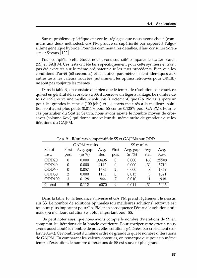
4.4 Applications
Sur ce probleme specifique et avec les reglages que nous avons choisi (com-muns aux deux methodes), GA|PM prouve sa superiorite par rapport a l’algo-rithme genetique hybride. Pour des commentaires detailles, il faut consulter Soren-sen et Sevaux [122].
Pour completer cette etude, nous avons souhaite comparer le scatter search(SS) et GA|PM. Ces tests ont ete faits specifiquement pour cette synthese et n’ontpas ete executes sur le meme ordinateur que les tests precedents. Bien que lesconditions d’arret (60 secondes) et les autres parametres soient identiques auxautres tests, les valeurs trouvees (notamment les optima retrouves pour ORLIB)ne sont pas toujours les memes.
Dans la table 9, on constate que bien que le temps de resolution soit court, cequi est en general defavorable au SS, il conserve un leger avantage. Le nombre defois ou SS trouve une meilleure solution (strictement) que GA|PM est superieurpour les grandes instances (100 jobs) et les ecarts mesures a la meilleure solu-tion sont aussi plus petits (0.011% pour SS contre 0.128% pour GA|PM). Pour lecas particulier du Scatter Search, nous avons ajoute le nombre moyen de cros-sover (colonne Xov.) qui donne une valeur du meme ordre de grandeur que lesiterations du GA|PM.
TAB. 9 – Resultats comparatif de SS et GA|PMs sur ODD
GAPM results SS resultsSet of First Avg. gap Avg. First Avg. gap Avg. Avg.inst. pos. (in %) iter. pos. (in %) iter. Xov.ODD20 0 0.000 33496 0 0.000 168 25509ODD40 0 0.000 4142 0 0.000 31 5710ODD60 0 0.057 1685 2 0.000 8 1859ODD80 2 0.000 1153 0 0.013 3 1021ODD100 3 0.128 844 7 0.010 1 938Global 5 0.112 6070 9 0.011 31 5405
Dans la table 10, la tendance s’inverse et GA|PM prend legerement le dessussur SS. Le nombre de solutions optimales (ou meilleures solutions) retrouve esttoujours plus important pour GA|PM et en consequence l’ecart a la solution opti-male (ou meilleure solution) est plus important pour SS.
On peut noter aussi que nous avons compte le nombre d’iterations de SS encomptant les iterations de la boucle exterieure. Pour corriger cette erreur, nousavons aussi ajoute le nombre de nouvelles solutions generees par croisement (co-lonne Xov.). Ce nombre est du meme ordre de grandeur que le nombre d’iterationsde GA|PM. En comparant les valeurs obtenues, on remarque que pour un memetemps d’execution, le nombre d’iterations de SS est souvent plus grand.
87
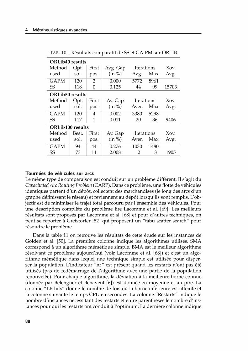
4 Metaheuristiques avancees
TAB. 10 – Resultats comparatif de SS et GA|PM sur ORLIB
ORLib40 resultsMethod Opt. First Avg. Gap Iterations Xov.used sol. pos. (in %) Avg. Max Avg.GAPM 120 2 0.000 5772 8961SS 118 0 0.125 44 99 15703
ORLib50 resultsMethod Opt. First Av. Gap Iterations Xov.used sol. pos. (in %) Aver. Max Avg.GAPM 120 4 0.002 3380 5298SS 117 1 0.011 20 36 9406
ORLib100 resultsMethod Best. First Av. Gap Iterations Xov.used sol. pos. (in %) Aver. Max Avg.GAPM 94 44 0.276 1030 1480SS 73 11 2.008 2 3 1905
Tournees de vehicules sur arcsLe meme type de comparaison est conduit sur un probleme different. Il s’agit duCapacitated Arc Routing Problem (CARP). Dans ce probleme, une flotte de vehiculesidentiques partent d’un depot, collectent des marchandises (le long des arcs d’ungraphe definissant le reseau) et reviennent au depot lorsqu’ils sont remplis. L’ob-jectif est de minimiser le trajet total parcouru par l’ensemble des vehicules. Pourune description complete du probleme lire Lacomme et al. [69]. Les meilleursresultats sont proposes par Lacomme et al. [68] et pour d’autres techniques, onpeut se reporter a Greistorfer [52] qui proposent un “tabu scatter search” pourresoudre le probleme.
Dans la table 11 on retrouve les resultats de cette etude sur les instances deGolden et al. [50]. La premiere colonne indique les algorithmes utilises. SMAcorrespond a un algorithme memetique simple. BMA est le meilleur algorithmeresolvant ce probleme aujourd’hui (voir Lacomme et al. [68]) et c’est un algo-rithme memetique dans lequel une technique simple est utilisee pour disper-ser la population. L’indicateur “nr” est present quand les restarts n’ont pas eteutilises (pas de redemarrage de l’algorithme avec une partie de la populationrenouvelee). Pour chaque algorithme, la deviation a la meilleure borne connue(donnee par Belenguer et Benavent [6]) est donnee en moyenne et au pire. Lacolonne “LB hits” donne le nombre de fois ou la borne inferieure est atteinte etla colonne suivante le temps CPU en secondes. La colonne “Restarts” indique lenombre d’instances necessitant des restarts et entre parentheses le nombre d’ins-tances pour qui les restarts ont conduit a l’optimum. La derniere colonne indique
88

le nombre moyen de croisement effectues.
TAB. 11 – Resultats du CARP extraits de Prins et al. [93]Algorithm Dev. LB Worst LB hits Av. time Restarts Av. Xovers
SMA 0.65 4.07 15 0.37 0 2750.5BMA-nr 0.33 2.23 18 0.95 0 3013.1GAPM-nr 0.24 2.23 20 0.90 0 880.9BMA 0.17 2.23 21 4.79 5(3) 9960.2GA|PM 0.17 2.23 21 1.59 3(1) 1968.9
SMA est tres rapide mais donne des resultats loin des meilleurs. Sans lesrestarts, GA|PM est bien meilleur que BMA en terme d’ecart et en nombre desolutions optimales retrouvees. Si on autorise les restarts, le meme nombre desolutions optimales est trouve, mais GA|PM garde un avantage en temps deresolution. Le nombre d’instances pour lesquelles les restarts sont necessaires estmoins important. C’est donc la meilleure methode resolvant ces instances aujour-d’hui.
5 Complements
Il existe bien d’autres methodes qui auraient pu figurer dans ce document.Nous les avons volontairement ou non ecartes. D’un cote, certaines de ces me-thodes n’ont pas prouve leur efficacite et d’autres peuvent se trouver etre descas particuliers des methodes deja presentees. Pour toutes les methodes que nousavons oublie et pour les auteurs qui auraient souhaite avoir leur place dans ce do-cument de synthese, nous presentons nos plus plates excuses. Avant de conclure,nous pensons qu’il est important de mettre en avant des points relatifs aux me-taheuristiques que nous avons abordes au cours des dernieres annees et qui sontpour certains un nouveau domaine d’investigation ou pour d’autres un champd’application et de recherche a part entiere.
Ci-dessous, nous soulevons un certain nombre de particularites et de ques-tions qui nous paraissent interessantes et auxquelles nous tenterons de repondredans la conclusion de cette synthese.
Codage d’une solutionL’implementation de chacune des metaheuristiques des sections precedentes peutparfois poser des problemes. En premier lieu, et quelque soit la methode utilisee,le codage de la solution est le point crucial de la reussite de l’approche. Par uncodage approprie, qu’il soit direct ou indirect, on manipule plus ou moins facile-ment les solutions de notre probleme, on est plus ou moins rapidement capable
89

5 Complements
d’evaluer la qualite d’une solution et on peut extraire plus ou moins d’informa-tions interessantes sur l’espace des solutions.
VoisinageEn ce qui concerne les methodes de recherche locale, la definition d’un bon voi-sinage est particulierement sensible. Il est par exemple tres important de savoirsi le voisinage est connexe ou non. Et s’il ne l’est pas, comment etre certain de nepas passer a cote de la solution optimale ? La taille du voisinage en lui-meme estun critere interessant. Si le voisinage est petit, on va pouvoir l’explorer tout en-tier, mais on aura besoin d’enormement d’iterations pour explorer un espace dessolutions le plus large possible. Si le voisinage est grand, le nombre d’iterationsnecessaire sera sans doute plus petit, mais le temps necessaire pour parcourir cevoisinage peut etre exponentiel...
Operateurs de croisement et de mutationPour les methodes a population (a l’exception des colonies de fourmis), les ope-rateurs de croisement et de mutation sont toujours difficiles a choisir. Il existeheureusement dans beaucoup de domaines (comme par exemple en ordonnan-cement, Caux et al. [11], Portmann [91]) des etudes sur les differents operateurset leur performance en fonction du codage et du probleme lui-meme. Une ca-racteristique importante d’un operateur de croisement est qu’il devrait “en prin-cipe” produire un enfant au moins aussi bon que les parents.
Mesure de la diversiteUne autre question importante a nos yeux et indispensable pour le scatter searchet le GA|PM est la definition d’une mesure de distance entre individus. Celle-cidoit etre capable de refleter une similitude ou une difference entre deux indivi-dus. On pourra alors en deduire la distance d’un individu a la population touteentiere. En fonction du probleme, du codage des individus et de la distance re-tenue, l’evaluation peut-etre plus ou moins couteuse en temps de calcul. Maisparfois il peut-etre bon de passer du temps pour calculer cette distance si elleconduit au final a une meilleure diversite de la population. Certaines distances,principalement pour les codages de type permutation, sont decrites dans Camposet al. [10], Sorensen [120], Sorensen et Sevaux [122].
5.1 Reglages automatiques des parametres
Passer de la theorie a la pratique est souvent difficile. L’implementation detoutes ces metaheuristiques pose des problemes insoupconnables. Un des sou-cis, et sans doute pas le moindre, est la competence informatique des chercheursoperationnels. Savoir programmer dans un langage informatique de 4e generation
90

5.2 Robustesse
(quel qu’il soit) est tres important. Si on suppose que cette competence est acquise,alors un autre probleme va surgir : le reglage des parametres.
Prenons quelques exemples. Pour le recuit simule, il faut trouver la temperaturede depart, et le schema de variation de cette temperature au cours des iterations.Pour la recherche tabou, la longueur de la liste tabou est importante. Trop grande,celle-ci conduit a un blocage ou dans le pire des cas tous les voisins d’une solutionsont tabous ; trop petite, celle-ci ne peut eviter les cyclages et la methode parcoureles memes solutions indefiniment.
Nous proposons dans Sevaux et Thomin [115, 119] la mise en place de tech-niques de reglages automatiques de ces parametres. Pour le recuit simule, notreexperience est plutot defavorable. Le but recherche etait d’initialiser automatique-ment la temperature de depart pour donner environ une chance sur deux a unesolution degradante d’etre acceptee. Malheureusement, les liens avec le schemade refroidissement de la temperature sont trop forts et ce reglage automatiquedans certains cas nous a decu. Pour la recherche tabou, nous sommes plus enthou-siastes. Dans la methode presentee par Sevaux et Thomin [115], une detection au-tomatique de cyclage est effectuee en permanence et en cas de detection, la lon-gueur de la liste est augmentee de la longueur du cycle. Ensuite la longueur estprogressivement diminuee pour eviter de conserver des elements non-necessairesqui augmentent le temps de calcul de la verification du statut tabou. Cette methodes’apparente un peu a la recherche tabou reactive proposee par Battiti et Tecchiolli[3].
5.2 Robustesse
La recherche de solutions robustes a un probleme d’optimisation semble etreun challenge recent pour les chercheurs. Longtemps laisse aux statisticiens oustochasticiens, ce domaine est en train de voir sa popularite augmenter dans lacommunaute de la recherche operationnelle, Sevaux et Sorensen [110].
Quand le probleme est deterministe c-a-d. que les donnees sont connues etfiables a 100%, la plupart du temps le probleme sous-jacent est un probleme d’op-timisationNP-difficile. Il n’existe alors pas d’algorithme efficace pour le resoudreoptimalement. Les metaheuristiques deviennent un outil de resolution privilegiegarantissant a la fois un temps de developpement reduit et l’obtention d’une so-lution de bonne qualite. Meme si les metaheuristiques et particulierement lesalgorithmes genetiques sont appliques souvent et avec succes pour traiter desproblemes, leur application en environnement incertain est tres limitee. Nousaffirmons que les metaheuristiques peuvent etre tres facilement adaptees auxnecessites d’un probleme stochastique. L’utilisation de metaheuristiques pource type d’optimisation presente un certain nombre d’avantages (voir Sevaux etSorensen [111], Sevaux et al. [112]). Le besoin pour l’optimisation robuste parmetaheuristiques a ete reconnu dans le livre majeur sur l’optimisation robuste
91

5 Complements
[66], quand les auteurs enoncent page 354 ¡¡ We believe that considerable more effortshould be spent on the systematic development of [...] metaheuristic frameworks, whichwith minimal adjustment effort can be applied to a large class of robust optimisation pro-blem [...] ¿¿.
On trouve dans la litterature un nombre impressionnant d’articles utilisantles metaheuristiques pour resoudre des problemes d’ordonnancement. Parmi lestechniques les plus prisees, on retrouve en tete les algorithmes genetiques et la re-cherche tabou. L’article de Reeves [96] presente une liste non-exhaustive d’appli-cations des algorithmes genetiques dans la plupart des domaines de l’optimisa-tion combinatoire. Pour la robustesse en ordonnancement, nous avons tente d’ap-porter un certain nombre de reponses en utilisant le cadre general propose parSorensen [121] et que nous avons applique a un probleme d’ordonnancement Se-vaux et Le Quere [108], Sevaux et al. [112]. En utilisant des particularites stochas-tiques de notre probleme, on peut integrer ces dernieres a une metaheuristique.On obtient alors une metaheuristique “stochastique” hybride qui semble parti-culierement bien s’adapter au probleme Fleury et al. [32].
Dans la gamme des problemes de tournees de vehicules, nous tentons d’ap-pliquer encore une fois le cadre general de Sorensen [121]. Ce type d’approchesemble etre satisfaisant pour la resolution des differentes variantes stochastiquesdu probleme VRP (VRP avec temps de parcours stochastiques). Cette fois-ci nousnous appuyons sur un algorithme de type GA|PM que nous avons adapte pourobtenir des solutions robustes, Sorensen et Sevaux [123]. Cette technique, memesi elle apporte des solutions satisfaisantes, doit etre couplee avec une evaluationstochastique assez precise de la robustesse d’une solution comme dans Fleuryet al. [31].
5.3 Optimisation multiobjectif
Plus brievement, nous souhaitons mettre en avant un domaine nouveau pournous, mais dont la communaute, plutot constituee d’informaticiens, s’est ouverteau monde de la recherche operationnelle recemment. C’est sans doute grace auxefforts permanents de plusieurs personnes, comme Xavier Gandibleux, qui n’ontpas hesite pas a s’investir enormement sur cette thematique fort interessante (voirGandibleux [34]).
La resolution de tournees de vehicules sur arcs est un probleme dont les appli-cations sont particulierement importantes pour les industriels. La premiere appli-cation que nous souhaitons resoudre est la collecte de dechets en milieu urbain.Apres plusieurs conversations avec des industriels, il est apparu que l’objectifclassiquement traite (la minimisation de la duree totale des tournees) n’etait pastoujours l’objectif prioritaire. Dans certains cas, obtenir a la fois des durees to-tales minimales et un equilibre entre les tournees s’averait plus interessant dansla realite. Nous avons traite ce probleme en appliquant une variante de NSGA-II
92

5.4 Optimisation continue
(un algorithme genetique dedie a la resolution de problemes multiobjectifs) et lesresultats obtenus sont tres satisfaisants (voir Lacomme et al. [72, 73]).
5.4 Optimisation continue
La derniere application que nous souhaitons presenter sort totalement ducadre de l’optimisation combinatoire. La conception assistee par ordinateur en“design” automobile est partout.
Le procede de creation d’un vehicule prototype est tres particulier. Dans unpremier temps, un modele est concu sur ordinateur. A partir de ce modele, le desi-gner va fabriquer une maquette qu’il va re-modeler manuellement jusqu’a obtenirla forme desiree. Cette etape est indispensable car il est impossible au designerde se rendre compte du resultat sur un ecran d’ordinateur. Une fois la maquetteobtenue dans sa version definitive, par un procede de reverse engineering, on me-sure des quantites de points sur la maquette et on approxime ces points par denouvelles courbes.
Trouver les parametres de ces courbes est extremement difficile et les reglagesmanuels sont souvent impossibles a reproduire plusieurs fois a l’identique. AvecY. Mineur, nous avons mis au point un algorithme genetique continu (base surles travaux de Chelouah et Siarry [13]) qui permet d’offrir une aide en CAO pourl’obtention de ces parametres. L’ensemble des resultats est presente dans Mineuret Sevaux [83] et dans Sevaux et Mineur [109].
6 Conclusions
Apres ce tour d’horizon assez vaste sur les metaheuristiques et un regard surles differentes applications que nous avons pu traiter, sommes-nous aujourd’huicapable de definir une metaheuristique universelle ? Probablement pas ! Serait-cealors un constat d’echec ? Pas plus !
Ce que nous allons proposer c’est plutot des indications sur les caracteristiquesd’une bonne metaheuristique a notre sens. Voici donc des elements importants anos yeux :
Population Les methodes a population ont un avantage certain, celui du pa-rallelisme intrinseque qu’elles induisent. Travailler sur un ensemble de so-lutions qui partagent des informations, c’est explorer un plus grand es-pace des solutions. De plus, l’echange d’informations entre les individusde differentes regions de l’espace des solutions est souvent benefique.
Codage Le codage retenu pour la representation de la solution est un point clecomme on a pu le voir. Il peut etre direct ou indirect (phenotypique ougenotypique comme diraient les promoteurs des algorithmes genetiques).
93

6 Conclusions
De notre point de vue et experience, un codage indirect est souvent plus fa-cile a manipuler (du point de vue de la structure informatique des donnees)mais necessite un algorithme d’evaluation de la solution. C’est au concep-teur de la methode de trouver un juste equilibre entre les deux. D’experience,un algorithme d’evaluation d’un individu de la population en O(n2) resteraisonnable. A noter que l’on obtient de tres bons resultats quand l’evaluationpeut etre optimale.
Cooperation Les individus doivent etre capables d’echanger des informationsentre eux par croisement par exemple. Le croisement est souvent fait enprenant les individus deux a deux, mais comme le propose le scatter search,ce n’est pas une obligation et plusieurs individus peuvent cooperer pourfournir de nouvelles solutions. L’ideal serait de pouvoir recuperer syste-matiquement les bonnes caracteristiques des parents pour les transmettreaux enfants. Mais quelles sont ces bonnes caracteristiques, souvent on ne lesait pas. Un point que soulignent Hertz et Widmer [60] et sur lequel noussommes d’accord, c’est que si l’on croise deux parents identiques, il sembleraisonnable d’obtenir un enfant qui soit identique aux deux parents. Cettepropriete n’est malheureusement pas toujours respectee.
Recherche locale Ajouter une recherche locale est aujourd’hui indispensable. Lesmethodes qui n’en sont pas dotees ne sont pas competitives en terme dequalite de solutions proposees. Par contre, si le codage retenu est indirect,la recherche locale doit se faire en tenant compte de la solution elle-meme.Un bon exemple pourrait etre celui de l’algorithme memetique de Lacommeet al. [69]. Le codage retenu est une permutation, mais la recherche locale esteffectuee en prenant des voisinages classiques en “tournees de vehicules”.Un mauvais exemple est celui de l’algorithme genetique propose dans [119]ou le codage d’une solution est une permutation (comme souvent en or-donnancement) et la recherche locale se fait en utilisant le voisinage gene-ral pairwise interchange (GPI) qui consiste a echanger deux elements de lapermutation sans integrer des proprietes importantes du probleme. Cetteerreur n’a pas ete reproduite dans [115].
Diversite controlee Mesurer la diversite entre les solutions est particulierementimportant. Quand cela est integre a un mecanisme de controle de la diver-site, la metaheuristique peut se concentrer sur les individus divers et ne paseffectuer d’exploration inutile. Le controle de la diversite est un facteur toutaussi important. Il permet en fonction de l’ensemble des individus de lapopulation de plus ou moins diversifier et de plus ou moins intensifier larecherche.
Restarts Les observations des techniques de “restart” implementees, et notam-ment celles que nous avons teste dans Prins et al. [93], montrent qu’il estparfois envisageable de re-generer une partie de la population. En effet,apres plusieurs generations, une partie de la population tend a etre tres per-formante, tandis qu’une autre partie se retrouve sans potentiel interessant
94

pour des croisements futurs. En remplacant une partie de cette population(la moins bonne de preference) on donne un sang neuf a la population et onpeut ainsi parfois ameliorer les meilleures solutions.
Aleatoire Les plus grandes decouvertes du monde l’ont ete pour certaines d’entreelles par le fait du hasard. Se priver de tout facteur aleatoire implique qu’ilfaut remplacer cette part de chance par une enumeration complete, que cesoit au niveau de la selection des individus ou par exemple des points decroisement d’un operateur de croisement. Par certains cotes, c’est ce quefait le scatter search, mais au prix toujours d’un temps de calcul souventimportant.
Si ces caracteristiques sont les bonnes, alors l’algorithme GA|PM y repondquasiment en totalite et c’est desormais le seul que nous devrions utiliser. Non,surtout pas ! Ce serait sans doute une grave erreur. Ce que nous n’avons pas prisen compte dans les caracteristiques ci-dessus, c’est 1) le probleme lui-meme et 2)le but de la resolution.
– Le probleme en lui-meme est un point fondamental dans la resolution. Ilpeut etre plus ou moins simple a coder, a comprendre et a resoudre. Il peutexister des specificites a ce probleme, comme des cas particuliers polyno-miaux sur lesquels s’appuyer. Par exemple, pour un probleme d’ordonnan-cement juste-a-temps, si on connaıt les jobs en avance et ceux en retard, souscertaines conditions on peut evaluer optimalement cette configuration. Duprobleme et de ses caracteristiques, on va pouvoir choisir le codage le plusapproprie, l’evaluation la meilleure, etc.
– Le but de la resolution est primordial et souvent ignore. Dans le contexteacademique, on cherche a fournir le plus souvent la meilleure solution auprix d’une implementation parfois difficile avec des temps de calculs sou-vent longs et le resultat est l’amelioration des meilleures solutions mais desfois de quelques pour cents uniquement. Si on s’adresse a un industriel, lanotion de solution optimale lui echappe souvent ou lui est indifferente. Il abesoin de savoir si l’implementation va etre robuste, combien de temps onva passer dessus, bref, si l’investissement en vaut la peine. Est-ce necessairede trouver la solution optimale a un probleme industriel auparavant resolumanuellement et dont une solution obtenue par simple heuristique amelioreun rendement de plus de 50% ? Martin Grotschel lors du Euro Winter Ins-titute en Mars 2000 rapportait que pour un probleme de transport de per-sonnes handicapes (dial-a-ride problem) il avait trouve la solution optimaleen quelques semaines de travail mais avait mis plus de cinq ans a la faireappliquer pour ne pas modifier en profondeur le travail des conducteurs dujour au lendemain.
De toute notre experience, le seul imperatif qui ressort c’est qu’il faut es-sayer. En conference, dans les presentations sur les metaheuristiques, les ques-tions simples comme “Mais pourquoi n’avez-vous pas utilise la methode X plutotque la methode Y ?” ont heureusement pratiquement disparu. Un seul mot d’ordre
95

7 Perspectives de recherche
a cela, il faut essayer. On ne peut assurement pas repondre a une question de-mandant le resultat d’une autre metaheuristique sans l’avoir implemente et testeauparavant.
7 Perspectives de recherche
Un bon indicateur des perspectives de recherche est le nombre de publicationsen cours ou en preparation [16, 108, 109, 112, 115, 122]. Pour certaines d’entreelles, le sujet est bien abouti et sera sans doute termine apres la publication d’unarticle en revue. Pour d’autres, il y a encore beaucoup a faire.
Nous allons ici lister les themes en cours d’etude ou qui presentent un interetparticulier et qui seront privilegies dans l’avenir.
Resolution de problemes multiobjectifsCe nouveau type de problemes, aborde sur le cas particulier du CARP [70,72], a permis de montrer les lacunes des methodes existantes. On peut parexemple voir que beaucoup d’algorithmes genetiques multiobjectifs ont desfonctionnements simplistes et que ce qui existe pour les problemes mono-objectif pourrait etre transpose ici. Un exemple simple, les conditions d’arretdes algorithmes multiobjectifs ne sont pas encore ou sont peu traitees.
Developpement de methodes robustesLes problemes rencontres en industrie ont rarement des donnees fiables.Pourtant, toutes les methodes d’optimisation travaillent sur des donneesfixees et connues a l’avance. Les premiers travaux [108, 110, 112] en ordon-nancement sont prometteurs mais une meilleure integration des donnees etparticulierement au niveau statistique permettrait de proposer des methodesplus fiables, et moins consommatrices de temps de calcul. Ce sujet est dejabien avance Fleury et al. [32].
Problemes dans les graphesAvec C. Prins et P. Lacomme, nous avons mis en projet de renover les ap-proches algorithmiques sur les graphes en proposant d’importantes biblio-theques “open source” orientees objet permettant d’utiliser ces algorithmesdans la resolution de problemes plus complexes. Ce travail est partiellementaccompli dans Lacomme et al. [71]. Une version C++ utilisant la STL, plusgenerique, est aussi prevue en collaboration avec P. Thomin. Elle fera l’objetd’un second tome de ce livre.
Programmation lineaireCe theme de predilection tient toujours une place importante. On a noteque dans certains cas, l’espace des solutions est trop grand pour etre traiteavec un logiciel commercial. Une technique de coupes ou de decompositionpourrait alors etre envisagee. Mais pourquoi ne pas utiliser la propagation
96
de contraintes pour reduire cet espace de solutions ? De plus, l’integrationde metaheuristiques permettrait aussi de guider les algorithmes de pro-grammation lineaire vers des solutions prometteuses et pourrait accelererla recherche. La collaboration avec C. Oguz sur les problemes de type flow-shop hybrides nous permettra de mieux cerner ces possibilites prochaine-ment.
Mais en plus des themes ci-dessus, il y a deux autres domaines qui retiennentplus particulierement notre attention.
En premier lieu, la collaboration avec Alcatel que nous menons en ce mo-ment (conjointement avec Xavier Gandibleux) nous a entraıne sur un terrain par-ticulierement interessant. Le sujet est l’optimisation du trafic dans les reseaux detelecommunications. Une clause de confidentialite nous engage a ne pas devoilerle cœur du travail que nous menons, mais c’est un domaine nouveau pour nous etparticulierement interessant. Le contrat d’un an que nous avons signe avec notrepartenaire industriel sera tres probablement renouvele et la charge de travail etantimportante, il me parait indispensable d’engager une these sur ce domaine. Lesmoyens financiers obtenus lors de cette collaboration sont importants et pour-raient permettre de proposer a un jeune chercheur brillant un contrat de thesepour realiser cette etude avec nous.
Alcatel est un des organismes a la pointe du progres dans le domaine etudie,il entend le rester et sait qu’il a besoin d’etendre ses collaborations avec le mondeacademique. Le soucis de confidentialite d’une telle entreprise est legitime. Onne peut defendre des interets industriels forts sans se proteger de la concurrence.Pourtant, Alcatel connaıt aussi les necessites et les imperatifs de publication denotre communaute. Ainsi, lors d’autres contrats, Xavier Gandibleux a pu apresdepot d’un brevet dont il est co-auteur avec Alcatel publier le resultat de ses tra-vaux. Engager une these sur un tel sujet, meme sensible, n’est donc pas incom-patible avec les devoirs d’un encadrant vis a vis de son doctorant (en terme decommunications et de publications).
Le dernier point qui nous anime et qui constituerait un prolongement naturelde cette synthese concerne les metaheuristiques evidemment.
Dans la suite logique de cette composition, et en collaboration avec C. Prinset K. Sorensen, nous allons preparer un ouvrage recensant les principales meta-heuristiques comme ici, mais en mettant l’accent sur l’aspect implementation quinous parait indispensable et indissociable des methodes elles-memes. A l’issuede ce travail, certains problemes ou particularites des metaheuristiques devraientnous apparaıtre plus clairement encore.
En faisant cet inventaire ici, nous avons pu mettre en avant ce que pourraientetre les bonnes caracteristiques d’une metaheuristique. De notre point de vue, ilreste encore beaucoup de chemin a parcourir avant d’etre en mesure de proposerune metaheuristique universelle. Pourtant, c’est notre but aujourd’hui : propo-
97

7 Perspectives de recherche
ser une methode suffisamment generique pour resoudre le plus grand nombrede problemes et pas trop generique pour que les parametres a regler ne soientpas trop nombreux avant que l’on puisse atteindre un degre d’efficacite suffisant.Un deuxieme pas a franchir ensuite sera de proposer, en plus du cadre generald’une metaheuristique, un code source generique et en acces libre et sous licencepublique, qui permettra a tous d’utiliser les metaheuristiques sans avoir a refairedes implementations lourdes et qui consomment beaucoup de temps et d’energie.Realiser tout ceci ne pourra se faire sans l’aide de plusieurs participants et notam-ment des jeunes chercheurs dont la curiosite et l’esprit vif sont les meilleurs atoutspour une plein reussite.
Ce projet important que nous suggerons ne va pas balayer tous les bons resul-tats de ces dernieres annees sur le sujet, mais au contraire s’appuiera dessus pouressayer de proposer une vision unifiee des metaheuristiques. Si ce but, peut-etreidyllique, n’est pas facile a atteindre, au moins aurons-nous apporte une briquesupplementaire a l’edifice...
98

References
[1] E.H.L. Aarts et J. Korst. Simulated Annealing and Boltzmann Machines. JohnWiley, Chichester, 1989.
[2] J.T. Alander. An indexed bibliography of genetic algorithm implemen-tations. Technical Report 94-1-IMPLE, Dept. of Information technologyand production economics, University of Vaasa, Finland, July, 23 1999.ftp.uwasa.fi.
[3] R. Battiti et G. Tecchiolli. The reactive tabu search. ORSA Journal on Compu-ting, 6 :126–140, 1994.
[4] E.B. Baum. Iterated descent : A better algorithm for local search in combi-natorial optimization problems. Technical report, Caltech, Pasadena, CA,1986.
[5] J. Baxter. Local optima avoidance in depot location. Journal of the OperationalResearch Society, 32 :815–819, 1981.
[6] J.M. Belenguer et E. Benavent. A cutting plane algorithm for the Capacita-ted Arc Routing Problem. Computers and Operations Research, 30(5) :705–728,2003.
[7] P. Beullens, L. Muyldermans, D. Cattrysse, et D. Van Oudheusden. A gui-ded local search heuristic for the capacitated arc routing problem. EuropeanJournal of Operational Research, 147 :629–643, 2003.
[8] C. Blum et A. Roli. Metaheuristics in combinatorial optimization : Over-view and conceptual comparison. ACM Computing surveys, 35(3) :268–308,2003.
[9] E. Bonomi et J.L. Lutton. The N-city travelling salesman problem, statisti-cal mechanics and the metropolis algorithm. SIAM Review, 25(4) :551–568,1984.
[10] V. Campos, M. Laguna, et R. Martı. Context-independent scatter and tabusearch for permutation problems, Unpublished manuscript, 2002. URLhttp://leeds.colorado.edu/Faculty/Laguna/publications.htm.
[11] C. Caux, H. Pierreval, et M.C. Portmann. Les algorithmes genetiques et leurapplication aux problemes d’ordonnancement. In Actes des Journees d’etudeOrdonnancement et Entreprise : Applications Concretes et Outils pour le Futur,pages 5–45, Toulouse, 1994. CNRS.
[12] R. Cerf. Une theorie asymptotique des algorithmes genetiques. PhD thesis, Uni-versite de Montpellier II, France, 1994.
99
References
[13] R. Chelouah et P. Siarry. A continuous genetic agorithm designed for theglobal optimization of multimodal functions. Journal of Heuristics, 6 :191–213, 2000.
[14] N.E. Collins, R.W. Eglese, et B.L. Golden. Simulated annealing : An annota-ted bibliography. American Journal of Mathematical and Management Sciences,8 :209–307, 1988.
[15] D. Connolly. An improved annealing scheme for the qap. European Journalof Operational Research, 46 :93–100, 1990.
[16] S. Dauzere-Peres et M. Sevaux. An efficient formulation for minimizingthe number of late jobs in single-machine scheduling. Technical Report98/9/AUTO, Ecole des Mines de Nantes, July 1998. Submitted.
[17] S. Dauzere-Peres et M. Sevaux. Using lagrangean relaxation to minimizethe weighted number of late jobs. Naval Research Logistics, 50(3) :273–288,2003.
[18] K.A. De Jong. Genetic algorithms : A 25 year perspective. In J.M. Murata,R.J. Marks II, et C.J. Robinson, editors, Computational intelligence-imitatinglife, pages 125–134. IEEE Press, New York, 1994.
[19] M.L. den Besten, T. Stutzle, et M. Dorigo. Design of iterated local searchalgorithms : An example application to the single machine total weightedtardiness problem. In Proceedings of EvoStim’01, Lecture Notes in ComputerScience, pages 441–452, Springer, Berlin, 2001.
[20] D. De Werra et A. Hertz. Tabu search techniques : A tutorial and an appli-cation to neural networks. OR Spektrum, 11 :131–141, 1989.
[21] M. Dorigo. Optimization, Learning and Natural Algorithms. PhD thesis, Poli-tecnico di Milano, Italy, 1992.
[22] M. Dorigo et G. Di Caro. The ant colony optimization meta-heuristic. InD. Corne, M. Dorigo, et F. Glover, editors, New Ideas in Optimization, pages11–32, London, 1999. McGraw Hill.
[23] M. Dorigo, G. Di Caro, et L.M. Gambardella. Ant algorithms for discreteoptimization. Artificial Life, 5 :137–172, 1999.
[24] M. Dorigo, V. Maniezzo, et A. Colorni. Positive feedback as a search stra-tegy. Technical Report 91-016, Politecnico di Milano, Italy, 1991.
[25] J. Du et J.Y.T. Leung. Minimizing total tardiness on one machine is NP-hard. Mathematics of Operations Research, 15(3) :483–495, 1990.
[26] T.A. Feo et M.G.C. Resende. A probabilistic heuristic for a computationallydifficult set covering problem. Operations Research Letters, 8 :67–71, 1989.
100

References
[27] T.A. Feo et M.G.C. Resende. Greedy randomized adaptive search proce-dures. Journal of Global Optimization, 6 :109–133, 1995.
[28] P. Festa. Greedy randomized adaptative search procedures. AIRO News, 7(4) :7–11, 2003.
[29] P. Festa et M. Resende. GRASP : An annotated bibliography. In C. Ribeiro etP. Hansen, editors, Essays and surveys in metaheuristics, pages 3–21. KluwerAcademic Publishers, Boston, 2002.
[30] C. Fleurent et J.A. Ferland. Algorithmes genetiques hybrides pour l’optimi-sation combinatoire. RAIRO Recherche Operationnelle, 30(4) :373–398, 1996.
[31] G. Fleury, P. Lacomme, et C. Prins. Evolutionary algorithms for stochas-tic arc routing problems. In G. Raidl, S. Cagnoni, J. Branke, D.W. Corne,R. Drechsler, Y. Jin, C.G. Johnson, P. Machado, E. Marchiori, F. Rothlauf,G.D. Smith, et G. Squillero, editors, Applications of Evolutionary Computing,Proceedings of EvoWorkshops 2004, volume 3005, pages 501–512, Coimbra,Portugal, 5-7 April 2004. Springer-Verlag.
[32] G. Fleury, Lacomme P, et M. Sevaux. Stochastic maintenance schedulingproblem. In Proceedings of ninth international conference on project managementand scheduling, PMS 2004, pages 405–409, Nancy, France, 26-28 April 2004.
[33] C. Gagne, M. Gravel, et W.L. Price. A new hybrid tabu-vns metaheuris-tic for solving multiple objective scheduling problem. In Proceedings of 5thMetaheuristic International Conference, MIC 2003, pages 22.1–7, Kyoto, Japan,25-28 August 2003.
[34] X. Gandibleux. Optimisation multiobjectif : problemes combinatoire,resolutions exactes et approchees, applications. Habilitation a diriger lesrecherches, Universite Valenciennes, France, 12 December 2003.
[35] M.R. Garey et D.S. Johnson. Computers and Intractability : A Guide to Theoryof NP-Completeness. Freeman, San Franscisco, 1979.
[36] F. Glover. Heuristics for integer programming using surrogate constraints.Decision Sciences, 8 :156–166, 1977.
[37] F. Glover. Future paths for integer programming and links to artificial in-telligence. Computers and Operations Research, 13 :533–549, 1986.
[38] F. Glover. Tabu search – part I. ORSA Journal on Computing, 1 :190–206, 1989.
[39] F. Glover. Tabu search – part II. ORSA Journal on Computing, 2 :4–32, 1990.
[40] F. Glover. Tabu search : A tutorial. Interface, 20(1) :74–94, 1990. Special issueon the practice of mathematical programming.
101
References
[41] F. Glover. Genetic algorithms and scatter search - unsuspected potentials.Statistics and Computing, 4 :131–140, 1994.
[42] F. Glover. A Template for Scatter Search and Path Relinking, volume 1363 ofLecture Notes in Computer Science, pages 1–53. Springer, Springer, Berlin,1997.
[43] F. Glover. A template for scatter search and path relinking. In J.-K. Hao,E. Lutton, E. Ronald, M. Schoenauer, et D. Snyers, editors, Artificial Evolu-tion, volume 1363 of Lecture Notes in Computer Science, pages 13–54, Sprin-ger, Berlin, 1998. Springer.
[44] F. Glover et S. Hanafi. Tabu search and finite convergence. Discrete AppliedMathematics, 119 :3–36, 2002.
[45] F. Glover et M. Laguna. Tabu Search. Kluwer, Boston, 1999.
[46] F. Glover, M. Laguna, et R. Martı. Fundamentals of scatter search and pathrelinking. Control and Cybernetics, 39(3) :653–684, 2000.
[47] F. Glover, M. Laguna, E. Taillard, et D. De Werra, editors. Tabu search, vo-lume 41. Annals of Operations Research, 1993.
[48] D. Goldberg. Genetic algorithms with sharing for multimodal function op-timization. In Proceedings of the Second International Conference on GeneticAlgorithms, pages 41–49, 1987.
[49] D.E. Goldberg. Genetic Algorithms in Search, Optimization and Machine Lear-ning. Addison Wesley, 1989.
[50] B.L. Golden, J.S. DeArmon, et E.K. Baker. Computational experiments withalgorithms for a class of routing problems. Computers and Operations Re-search, 10(1) :47–59, 1983.
[51] R.L. Graham, E.L. Lawler, J.K. Lenstra, et A.H.G. Rinnooy Kan. Optimi-zation and approximation in deterministic sequencing and scheduling : Asurvey. Annals of Discrete Mathematics, 5 :287–326, 1979.
[52] P. Greistorfer. A tabu-scatter search metaheuristic for the arc routing pro-blem. Computers and Industrial Engineering, 44(2) :249–266, 2003.
[53] C. Gueret, C. Prins, et M. Sevaux. Programmation lineaire. Eyrolles, 2000.ISBN 2-212-09202-4, 365 pages (in French).
[54] C. Gueret, C. Prins, et M. Sevaux. Applications of optimisation with Xpress-MP. Dash optimization, 2002. ISBN 0-9543503-0-8, Translated by S. Heipke.
[55] B. Hajek. Cooling schedules for optimal annealing. Mathematics of Opera-tions Research, 13 :311–329, 1988.
102

References
[56] P. Hansen. The steepest ascent mildest descent heuristic for combinatorialprogramming. In Congress on Numerical Methods in Combinatorial Optimiza-tion, Capri, Italy, 1986.
[57] P. Hansen et N. Mladenovic. An introduction to variable neighbourhoodsearch. In S. Voß, S. Martello, I.H. Osman, et C. Roucairol, editors, Meta-Heuristics : Advances and Trends in Local Search Paradigms for Optimization,pages 433–458, Kluwer, Boston, 1999.
[58] R.L. Haupt et S.E. Haupt. Practical genetic algorithm. John Wiley & Sons,New York, 1998.
[59] A. Hertz, E. Taillard, et D. de Werra. Local search in combinatorial optimization,chapter A tutorial on tabu search, pages 121–136. J. Wiley & Sons Ltd, NewYork, 1997.
[60] A. Hertz et M. Widmer. Guidelines for the use of meta-heuristics in combi-natorial optimization. European Journal of Operational Research, 151 :247–252,2003.
[61] J.H. Holland. Adaptation in natural and artificial systems. Technical report,University of Michigan, Ann Arbor, 1975.
[62] J.H. Holland, editor. Adaptation in natural and artificial systems : An introduc-tory analysis with applications to biology, control, and artificial intelligence. MITPress/Bradford books, Cambridge, MA, 1992. 2nd edition.
[63] D. Johnson, C.H. Papadimitriou, et M. Yannakakis. How easy is localsearch ? Journal of conputer and system sciences, 17 :79–100, 1988.
[64] S. Kirkpatrick, C.D. Gelatt, et M.P. Vecchi. Optimization by simulated an-nealing. Science, 220 :671–680, 1983.
[65] C. Koulamas, S.R. Antony, et R. Jaen. A survey of simulated annealingapplications to operations research problems. Omega, 22 :41–56, 1994.
[66] P. Kouvelis et G. Yu. Robust Discrete Optimisation and its Applications, vo-lume 14 of Nonconvex Optimization and its Applications. Kluwer AcademicPublishers, Dordrecht, 1997.
[67] J.R. Koza. Genetic Programming. MIT Press, Cambridge, MA, 1992.
[68] P. Lacomme, C. Prins, et W. Ramdane-Cherif. Competitive memetic algo-rithms for arc routing problems. Annals of Operations Research, 2004. Toappear.
[69] P. Lacomme, C. Prins, et W. Ramdane-Cherif. A genetic algorithm for theCapacitated Arc Routing Problem and its extensions. In E.J.W. Boers et al.,editor, Applications of evolutionnary computing–EvoWorkshops 2001, LectureNotes in Computer Science 2037, pages 473–483. Springer, 2001.
103

References
[70] P. Lacomme, C. Prins, et M. Sevaux. Multiobjective capacitated arc rou-ting problem. In 2nd Joint EU/ME workshop with the french PM2O group(MOMH Workshop) on multi-objective metaheuristics, Paris, France, 4-5 No-vember 2002.
[71] P. Lacomme, C. Prins, et M. Sevaux. Algorithmes de graphes. Eyrolles, 2003.ISBN 2-212-11385-4, 425 pages (in French).
[72] P. Lacomme, C. Prins, et M. Sevaux. Mutliple objective capacitated arc rou-ting problem. In Proceedings of 2nd International Conference on EvolutionaryMulti-Criterion Optimization, EMO’2003, pages 550–564, Faro, Portugal, 8-11April 2003. LNCS 2632.
[73] P. Lacomme, C. Prins, et M. Sevaux. A genetic algorithm for a bi-objectivecapacitated arc routing problem. Computers and Operations Research, 2004.In Press.
[74] E.L. Lawler. A psedopolynomial time algorithm for sequencing jobs to mi-nimize total atrdiness. Annas of discrete mathematics, 1 :331–342, 1977.
[75] J.K. Lenstra, A.H.G. Rinnooy Kan, et P. Brucker. Complexity of machinescheduling problems. Annals of Discrete Mathematics, 1 :343–362, 1977.
[76] H.R. Lourenco, O. Martin, et T. Stutzle. Iterated local search. Technicalreport, Technical University of Darmstadt, Germany, 2000. Preprint.
[77] H.R. Lourenco, O. Martin, et T. Stutzle. Iterated local search. In F. Glover etG. Kochenberger, editors, Handbook of Metaheuristics, pages 321–353. KluwerAcademic Publishers, Nowell, MA, 2002.
[78] S. Lundy et A. Mees. Convergence of an annealing algorithm. Mathematicalprogramming, 34 :111–124, 1986.
[79] R. Martı, M. Laguna, et V. Campos. Scatter search vs. genetic algorithms :An experimental evaluation with permutation problems. In C. Rego etB. Alidaee, editors, Adaptive Memory and Evolution : Tabu Search and ScatterSearch, 2002. To appear.
[80] O. Martin, S.W. Otto, et E.W. Felten. Large-step Markov chains for the tra-veling salesman problem. Complex Systems, 5 :299–326, 1991.
[81] N. Metropolis, A. Rosenbluth, M. Rosenbluth, A. Teller, et E. Teller. Equa-tion of state calculations by fast computing machines. Journal of ChemicalPhysics, 21 :1087–1092, 1953.
[82] Z. Michalewicz. Genetic Algorithms + Data Structures = Evolution Programs.Springer, Berlin, 1999.
104

References
[83] Y. Mineur et M. Sevaux. Curve fitting for styling application by geneticalgorithm. In 3rd Joint EU/ME workshop with the university of Antwerp on Real-life application of metaheuritics, Antwerp, Belgium, 18-19 December 2003.
[84] M. Mitchel. An introduction to genetic algorithms. MIT Press, Cambridge,MA, 1998.
[85] N. Mladenovic et P. Hansen. Variable neighbourhood decompositionsearch. Computers and Operations Research, 24 :1097–1100, 1997.
[86] P. Moscato. On evolution, search, optimization, genetic algorithms andmartial arts : Towards memetic algorithms. Technical Report C3P 826, Cal-tech Concurrent Computation Program, 1989.
[87] P. Moscato. Memetic algorithms : A short introduction. In D. Corne qndM. Dorigo et F. Glover, editors, New ideas in optimization, pages 219–234.McGraw-Hill, New York, 1999.
[88] C.H. Papadimitriou et K. Steiglitz. Combinatorial optimization – algorithmsand complexity. Prentice-Hall, Upper Saddle River, New Jersey, 1982.
[89] L. Paquete et T. Stutzle. An experimental investigation of iterated localsearch for coloring graphs. In S. Cagnoni, J. Gottlieb, E. Hart, M. Midden-dorf, et G. Raidl, editors, Applications of Evolutionary Computing, Proceedingsof EvoWorkshops2002 : EvoCOP, EvoIASP, EvoSTim, volume 2279, pages 121–130, Kinsale, Ireland, 2002. Springer-Verlag.
[90] M. Pirlot et R.V. Vidal. Simulated annealing : A tutorial. Control & Cyberne-tics, 25 :9–31, 1996.
[91] M.-C. Portmann. Genetic algorithm and scheduling : a state of the art andsome propositions. In Proceedings of the workshop on production planning andcontrol, pages I–XIV, Mons, Belgium, 1996.
[92] M.-C. Portmann. The quality of offsprings after crossover. Private commu-nication, 2000.
[93] C. Prins, M. Sevaux, et K. Sorensen. A genetic algorithm with populationmanagement (GA|PM) for the carp. In Proceedings of 5th trienal symposiumon transportation analysis, TRISTAN V, Le Gosier, Guadeloupe, France, 13-18June 2004. To appear.
[94] C.R. Reeves. Modern heuristics techniques for combinatorial problems. JohnWiley & Sons, New York, 1993.
[95] C.R. Reeves. A genetic algorithm for flowshop sequencing. Computers andOperations Research, 22 :5–13, 1995.
105

References
[96] C.R. Reeves. Genetic algorithms for the operations researcher. INFORMSJournal on Computing, 9 :231–250, 1997.
[97] H.-P. Schwefel. Evolution strategies : A family of non-linear optimizationtechniques based on imitating some principles of organic evolution. Annalsof Operations Research, 1 :165–167, 1984.
[98] M. Sevaux. Les methodes de recherche a voisinage. In Groupe de Rechercheen Productique – Organisation et Gesion de Production, Toulouse, France, 8-9November 2001.
[99] M. Sevaux. Les methodes de recherche a population. In Groupe de Rechercheen Productique - Organisation et Gestion de Production, Tarbes, France, 24-25October 2002.
[100] M. Sevaux. Les methodes de recherche a voisinage. Seminaire invite, Fa-culte Polytechnique de Mons, groupe Image (in French), 6 March 2002.
[101] M. Sevaux. Metaheuristics : a quick overview. Invited seminar, Universityof Antwerp, Faculty of Applied Economic Sciences, 7 February 2003.
[102] M. Sevaux. Population metaheuristics. Invited seminar, The Hong-KongPolytechnic University, Department of Management, 14 March 2003.
[103] M. Sevaux et S. Dauzere-Peres. Building a genetic algorithm for a singlemachine scheduling problem. In Proceedings of the 18th EURO Winter Insti-tute, ESWI XVIII, Lac Noir, Switzerland, 4-18 March 2000.
[104] M. Sevaux et S. Dauzere-Peres. A genetic algorithm to minimize the weigh-ted number of late jobs on a single machine. In Proceedings of 7th Internatio-nal Workshop on Project Management and Scheduling, PMS’2000, pages 242–244, Osnabruk, Germany, 17-19 April 2000.
[105] M. Sevaux et S. Dauzere-Peres. Genetic algorithms to minimize the weigh-ted number of late jobs on a single machine. Technical Report LAMIH/SP-2000-51, Laboratory for Automation Mechanical engineering Informationsciences and Human-machine systems, 2000.
[106] M. Sevaux et S. Dauzere-Peres. Un algorithme genetique pour minimiser lenombre pondere de jobs en retard sur une machine. In 3ieme conference na-tionale de la societe francaise de recherche operationnelle, ROADEF’2000, Nantes,France, 26-28 January 2000.
[107] M. Sevaux et S. Dauzere-Peres. Genetic algorithms to minimize the weigh-ted number of late jobs on a single machine. European Journal of OperationalResearch, 151(2) :296–306, 2003.
106

References
[108] M. Sevaux et Y. Le Quere. Solving a robust maintenance scheduling pro-blem at the French railway company. Technical Report LAMIH/SP-2003-3,University of Valenciennes, CNRS UMR 8530, LAMIH/SP, April 2003. Sub-mitted.
[109] M. Sevaux et Y. Mineur. Continuous optimisation by GA for a curve fit-ting problem in autmobile industry. Technical report, University of Valen-ciennes, CNRS UMR 8530, LAMIH/SP, 2004. Submitted.
[110] M. Sevaux et K. Sorensen. Genetic algorithm for robust schedules. In Pro-ceedings of 8th International Workshop on Project Management and Scheduling,PMS’2002, pages 330–333, Valencia, Spain, 3-5 April 2002. ISBN 84-921190-5-5.
[111] M. Sevaux et K. Sorensen. A genetic algorithm for robust schedules in ajust-in-time environment with ready times and due dates. 4OR – Quaterlyjournal of the Belgian, French and Italian Operations Research Societies, 2(2) :129–147, 2004.
[112] M. Sevaux, K. Sorensen, et Y. Le Quere. Flexibilite et robustesse en ordonnance-ment, chapter Metaheuristiques pour la planification et l’ordonnancementrobuste, pages 91–110. Hermes, 2004. To appear.
[113] M. Sevaux et P. Thomin. Efficient heuristic and tabu search for parallel ma-chine scheduling. In ORBEL Conference, Antwerp, Belgium, 29-30 January2001.
[114] M. Sevaux et P. Thomin. Heuristics and metaheuristics for parallel ma-chine scheduling : a computational evaluation. In Proceedings of 4th Meta-heuristics International Conference, MIC 2001, pages 411–415, Porto, Portugal,16-20 July 2001.
[115] M. Sevaux et P. Thomin. Heuristics and metaheursitics for a parallel ma-chine scheduling problem : a computational evaluation. Technical Re-port LAMIH/SP-2001-2, University of Valenciennes, CNRS UMR 8530, LA-MIH/SP, November 2001. Submitted.
[116] M. Sevaux et P. Thomin. Parallel machine scheduling : a metaheuristic com-putational evaluation. Seminaire invite, Institut de Recherche en Commu-nication et Cybernetique de Nantes, IRCCyN (in French), 19 April 2001.
[117] M. Sevaux et P. Thomin. Parallel machine scheduling : a (meta)heuristiccomputational evaluation. Seminaire invite, Groupe MOST (in French), 5April 2001.
[118] M. Sevaux et P. Thomin. Recherche taboue amelioree pour l’ordon-nancement sur machines paralleles. In Actes de la 3ieme conference internatio-nale francophone de MOdelisation et de SIMulation, MOSIM’01, pages 829–833,Troyes, France, 25-27 April 2001. ISBN 1-56555-212-1.
107

References
[119] M. Sevaux et P. Thomin. Scatter search and ga : a one machine schedulingproblem comparison. In The sixteenth triennial conference of international fede-ration of operational research societies, IFORS’2002, Edinburgh, UK, 6-13 July2002.
[120] K. Sorensen. Distance measures based on the edit distance for permutation-type representations. In A. Barry, editor, Proceedings of the Workshop on Ana-lysis and Design of Representations and Operators (ADoRo), GECCO Conference,pages 15–21, Chicago, 2003.
[121] K. Sorensen. A framework for robust and flexible optimisation using metaheu-ristics with application in supply chain design. PhD thesis, University of Ant-werp, 2003.
[122] K. Sorensen et M. Sevaux. GA|PM : genetic algorithms with populationmanagement. Technical report, University of Valenciennes, CNRS UMR8530, LAMIH/SP, 2004. Submitted.
[123] K. Sorensen et M. Sevaux. Robust and flexible vehicle routing in practicalsituations. In Proceedings of 5th triennial symposium on transportation analysis,TRISTAN V, Le Gosier, Guadeloupe, France, 13-18 June 2004. To appear.
[124] E.G. Talbi. A taxonomy of hybrid metaheuristics. Journal of Heuristics, 8 :541–564, 2002.
[125] P.J.M. Van Laarhoven et E.H.L. Aarts. Simulated Annealing : Theory and Ap-plications. Kluwer Academic Publishers, Boston, 1987.
[126] R.V. Vidal, editor. Applied simulated annealing, volume 396 of LNEMS.Springer-Verlag, Berlin, 1993.
[127] C. Voudouris. Guided local search for combinatorial optimization problems. PhDthesis, Dept. of Computer Science, University of Essex, Colcherster, UK,1997.
[128] C. Voudouris et E. Tsang. Guided local search. Technical Report TR CSM-247, University of Essex, UK, 1995.
[129] C. Voudouris et E. Tsang. Guided local search and its application to thetravelling salesman problem. European Journal of Operational Research, 113 :469–499, 1999.
108

Troisieme partie
Selection de publications

110

Selection de publications
Description des publications
Pour conclure ce document, nous proposons ici quelques publications. A l’ex-ception d’une seule [3], toutes les references sont publiees [1, 5] ou a paraıtre [2, 4].Elles sont a notre sens representatives de notre activite recente.
Concernant les metaheuristiques proprement dites, [1] presente l’etude deplusieurs operateurs d’un algorithme genetique. Le probleme traite est celui del’ordonnancement a une machine. [2] propose un algorithme genetique adaptepour resoudre le meme probleme d’ordonnancement dans le cas ou les donneessont incertaines. L’utilisation des metaheursitiques pour resoudre un problemebi-critere de tournees de vehicules sur arcs est presente dans [4].
Un travail de plus grande envergure presente dans [3] propose la descriptiond’une nouvelle metaheuristique qui gere de maniere precise la population. Memesi cet article n’est pas encore accepte, il merite d’etre presente car il se trouve etreune nouvelle source de travail et une nouvelle piste importante de recherche.
Enfin, nous souhaitions presenter un travail deconnecte des metaheuristiques[5] mais qui nous tient a cœur particulierement. La resolution par relaxation La-grangienne d’un probleme d’ordonnancement a une machine. Ce article est lapour rappeler qu’il n’existe pas que les metaheuristiques et qu’il est important depouvoir proposer des techniques de resolution alternatives (ou pourquoi pas destechniques a hybrider avec les metaheuristiques).
1 European Journal of Operational Research (2003)
[1] M. Sevaux and S. Dauzere-Peres. Genetic algorithms to minimize the weigh-ted number of late jobs on a single machine. European Journal of OperationalResearch, 151(2) :296–306, 2003.
Abstract : The general one-machine scheduling problem is stron-gly NP-Hard when the objective is to minimize the weightednumber of late jobs. Few methods exist to solve this problem. Inan other paper, we developed a Lagrangean relaxation algorithmwhich gives good results on many instances. However, there isstill room for improvement, and a metaheuristic might lead to bet-ter results. In this paper, we decided to use a Genetic Algorithm(GA). Although a GA is somewhat easy to implement, many va-riations exist, and we tested some of them to design the best GAfor our problem. Three different engines to evaluate the fitness of achromosome are considered, together with four types of crossoveroperators and three types of mutation operators. An improved GAis also proposed by applying local search on solutions determined
111

from the chromosome by the engine. Numerical experiments ondifferent tests of instances are reported. They show that startingfrom an initial population already containing a good solution isvery effective.
2 4OR – Quaterly journal of the Belgian, French and ItalianOperations Research Societies (2004 a paraıtre)
[2] M. Sevaux and K. Sorensen. A genetic algorithm for robust schedules in ajust-in-time environment with ready times and due dates. 4OR – Quaterlyjournal of the Belgian, French and Italian Operations Research Societies, 2004. InPress.
Abstract : Computing a schedule for a given single machine pro-blem is often difficult for irregular criteria, but when the data areuncertain, the problem is much more complicated. In this paper,we modify a genetic algorithm to compute robust schedules whenrelease dates are subject to small variations. Two types of robust-ness are distinguished : quality robustness or robustness in the ob-jective function space and solution robustness or robustness in thesolution space. The modified genetic algorithm is applied to a just-in-time scheduling problem, a common problem in several indus-tries.
3 Journal of Heuristics (2004 soumis)
[3] K. Sorensen and M. Sevaux. GA|PM : genetic algorithms with populationmanagement. Technical report, University of Valenciennes, CNRS UMR8530, LAMIH/SP, 2004. Submitted.
Abstract : We present a new type of evolutionary algorithms cal-led genetic algorithms with population management or GA|PM .The main distinguishing feature of GA|PM is the use of distancemeasures to control the diversity of a small population. Combi-ned with a local search procedure to ensure the high quality ofindividual solutions in the population, population managementstrategies can be developed to avoid slow or premature conver-gence and achieve excellent performance. The new algorithm istested on two problems : the multidimensional knapsack problemand the weighted tardiness single machine scheduling problem.On both problems, population management is shown to be able toimprove the performance of an evolutionary algorithm.
112

4 Computers and Operations Research (2004 a paraıtre)
[4] P. Lacomme, C. Prins, and M. Sevaux. A genetic algorithm for a bi-objectivecapacitated arc routing problem. Computers and Operations Research, 2004. InPress.
Abstract : The Capacitated Arc Routing Problem (CARP) is a veryhard vehicle routing problem for which the objective — in its clas-sical form — is the minimisation of the total cost of the routes.In addition, one can seek to minimize also the cost of the longesttrip. In this paper, a multi-objective genetic algorithm is presentedfor this more realistic CARP. Inspired by the second version of theNon-dominated Sorted Genetic Algorithm framework, the proce-dure is improved by using good constructive heuristics to seedthe initial population and by including a local search procedure.The new framework and its different flavour is appraised on threesets of classical CARP instances comprising 81 files. Yet designedfor a bi-objective problem, the best versions are competitive withstate-of-the-art metaheuristics for the single objective CARP, bothin terms of solution quality and computational efficiency : indeed,they retrieve a majority of proven optima and improve two best-known solutions.
5 Naval Research Logistics (2003)
[5] S. Dauzere-Peres and M. Sevaux. Using lagrangean relaxation to minimizethe weighted number of late jobs. Naval Research Logistics, 50(3) :273–288,2003.
Abstract : This paper tackles the general single machine schedu-ling problem, where jobs have different release and due dates andthe objective is to minimize the weighted number of late jobs. Thenotion of master sequence is first introduced, i.e., a sequence thatcontains at least an optimal sequence of jobs on time. This mas-ter sequence is used to derive an original mixed-integer linear pro-gramming. By relaxing some constraints, it is possible to proposea Lagrangean relaxation algorithm which gives both a lower andupper bound. Although the duality gap becomes larger with thenumber of jobs, it is possible to solve problems of more than 100jobs, and some computational results are presented.
113

114
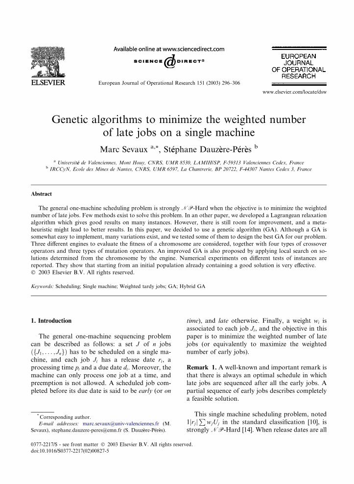
European Journal of Operational Research 151 (2003) 296–306
www.elsevier.com/locate/dsw
Genetic algorithms to minimize the weighted numberof late jobs on a single machine
Marc Sevaux a,*, St�eephane Dauz�eere-P�eer�ees b
a Universit�ee de Valenciennes, Mont Houy, CNRS, UMR 8530, LAMIH/SP, F-59313 Valenciennes Cedex, Franceb IRCCyN, Ecole des Mines de Nantes, CNRS, UMR 6597, La Chantrerie, BP 20722, F-44307 Nantes Cedex 3, France
Abstract
The general one-machine scheduling problem is strongly NP-Hard when the objective is to minimize the weighted
number of late jobs. Few methods exist to solve this problem. In an other paper, we developed a Lagrangean relaxation
algorithm which gives good results on many instances. However, there is still room for improvement, and a meta-
heuristic might lead to better results. In this paper, we decided to use a genetic algorithm (GA). Although a GA is
somewhat easy to implement, many variations exist, and we tested some of them to design the best GA for our problem.
Three different engines to evaluate the fitness of a chromosome are considered, together with four types of crossover
operators and three types of mutation operators. An improved GA is also proposed by applying local search on so-
lutions determined from the chromosome by the engine. Numerical experiments on different tests of instances are
reported. They show that starting from an initial population already containing a good solution is very effective.
� 2003 Elsevier B.V. All rights reserved.
Keywords: Scheduling; Single machine; Weighted tardy jobs; GA; Hybrid GA
1. Introduction
The general one-machine sequencing problem
can be described as follows: a set J of n jobs
ðfJ1; . . . ; JngÞ has to be scheduled on a single ma-
chine, and each job Ji has a release date ri, aprocessing time pi and a due date di. Moreover, the
machine can only process one job at a time, and
preemption is not allowed. A scheduled job com-
pleted before its due date is said to be early (or on
* Corresponding author.
E-mail addresses: [email protected] (M.
Sevaux), [email protected] (S. Dauz�eere-P�eer�ees).
0377-2217/$ - see front matter � 2003 Elsevier B.V. All rights reserv
doi:10.1016/S0377-2217(02)00827-5
time), and late otherwise. Finally, a weight wi is
associated to each job Ji, and the objective in this
paper is to minimize the weighted number of late
jobs (or equivalently to maximize the weighted
number of early jobs).
Remark 1. A well-known and important remark is
that there is always an optimal schedule in which
late jobs are sequenced after all the early jobs. A
partial sequence of early jobs describes completely
a feasible solution.
This single machine scheduling problem, noted
1jrjjP
wjUj in the standard classification [10], isstrongly NP-Hard [14]. When release dates are all
ed.

M. Sevaux, S. Dauz�eere-P�eer�ees / European Journal of Operational Research 151 (2003) 296–306 297
equal to zero ð1kP
wjUjÞ, the problem is still
NP-Hard. When all weights are equal ð1jrjjPUjÞ, the problem remainsNP-Hard, but can be
solved by an Oðn log nÞ algorithm if all release
dates are equal ð1kP
UjÞ [15]. If release and duedates are similarly ordered ðri < rj ) di 6 dj,8ðJi; JjÞÞ Kise et al. [12] gave an Oðn2Þ algorithm
and Lawler [13] an Oðn log nÞ algorithm for the
same special case.
However, some exact approaches have recently
been proposed for the problem 1jrjjP
Uj [2,6]. For
1kP
wjUj, Lawler [13] showed that Moore�s al-
gorithm ([15]) could be applied when process-ing times and weights are agreeable ðpi < pj )wi Pwj, 8ðJi; JjÞÞ. Finally, branch-and-bound pro-
cedures have been developed to solve the case
where all release dates are equal ð1kP
wjUjÞ[21,17].
A new and efficient Lagrangean relaxation al-
gorithm (LRA) has been presented by P�eeridy et al.
[16] and their lower bound will be used in thecomputational experiments. In a recent work,
Dauz�eere-P�eer�ees and Sevaux [7] developed a
Lagrangean relaxation heuristic to solve the
problem in the general case. Because the Lagran-
gean relaxation heuristic gives at the same time a
feasible solution (an upper bound) and a lower
bound, a measure of the quality of a solution can
be given for each instance. The same heuristiccan be used to solve the problem when weights are
equal and thus has been compared to optimal so-
lutions given by a branch-and-bound algorithm [6].
Because we used generic parameters for the LRA
(the parameters are the same for all the randomly
generated instances), in some test problems, the
gap between the solution and the lower bound is
rather large and can be reduced.This paper studies different classical genetic al-
gorithm (GA) techniques, combines them and
presents the first hybrid genetic algorithm (HGA)
that solves efficiently the NP-Hard problem
1jrjjP
wjUj. An initial solution given by a LRA is
used as a good starting point but, when the size of
the instances increases, the HGA solution almost
always improves the best solution found so far.This suggests that the HGA is very efficient for
large size instances.
Section 2 introduces some general consider-
ations about GA. Section 3 is devoted to finding a
good combination for the engine, and the cross-
over and mutation operators. The genetic local
search (GLS) is presented in Section 4 and nu-merical experiments are reported in Section 5.
2. Genetic algorithms
The basic concepts of GAs, introduced by
Holland [11], have been successfully applied to
solve many combinatorial optimization problems.We refer the reader to a recent feature article from
Reeves [20] for an extensive description of GAs in
operations research.
2.1. General considerations
A GA tries to mimic the genetic behavior of a
species. The biggest difference with other meta-heuristics (like Tabu search (TS) or simulated an-
nealing (SA)) is that GA maintains a population of
solutions rather than a unique current solution.
Solutions are coded as finite-length strings called
chromosomes and a measure of their adaptation
(the fitness) is computed by an engine. Starting
from an existing population, each iteration gener-
ates new chromosomes by applying operators (likecrossover and mutation) to two ‘‘randomly’’ chosen
parents. The main advantage of a GA is its in-
trinsic parallelism, which allows the exploration of
a larger solution space than in TS or SA. With an
appropriate design, GAs can give very good re-
sults.
2.2. Chromosome encoding
In [18], Portmann describes how GAs can be
applied to scheduling problems, and some very
interesting hints for building a specific GA can be
found.
Often, when a GA is implemented to solve a
one-machine scheduling problem, the representa-
tion of a chromosome is a permutation of the jobs‘‘J1; J2; . . . ; Jn’’. This representation is easy to
handle and has been adopted for our study.

298 M. Sevaux, S. Dauz�eere-P�eer�ees / European Journal of Operational Research 151 (2003) 296–306
2.3. Population management
Starting from an initial population of size m,two ways of managing the population are usuallyconsidered: either a new population of size m is
generated and replaces the previous population, or
only one offspring is generated and replaces one
chromosome in the existing population. The for-
mer method is named population replacement andthe latter incremental replacement.
In population replacement, it may happen that
the best chromosome in the initial population, i.e.,the best current solution for our problem, is no
longer in the new population, and thus will not be
used again by the crossover operator. This is the
reason why most researchers prefer incremental
replacement, also called elitism or populationoverlaps [8]. In the sequel, only incremental re-
placement will be considered.
2.4. Reproduction mechanism
At every iteration, the selection of the two
parents is done according to a simple ranking
mechanism [19] which gives more chances to
chromosomes with high fitness values to be used
for reproduction. The population is sorted in as-
cending order of fitness values (ascending order ofthe objective function), so the best individual is
ranked first. The selection of the first parent is
made using the probability distribution 2ðmþ1� kÞ=ðmðmþ 1ÞÞ where k is the kth chromosome
in the ascending order of fitness values, and m the
size of the population. Using this technique, the
median chromosome ðmþ 1Þ=2 has the probability1=m of being selected, while the best individual hasthe probability 2=ðmþ 1Þ (roughly twice the me-
dian). The second parent is randomly selected with
an uniform distribution.
A crossover operator is applied on the two
parents and a new offspring is generated. Nor-
mally, two offspring are created but only one is
kept in the algorithm. To keep the size of the
population constant, the new offspring should re-place another individual in the existing population.
In our procedure, an individual is randomly
chosen after the median and replaced by the new
offspring. Afterwards, the population is sorted
again according to the fitness values.
3. Designing a genetic algorithm
3.1. Fitness
For a given chromosome (i.e., a permutation of
the n jobs), a feasible solution, corresponding to
the sum of the weights of the late jobs, has to be
computed, i.e., a feasible schedule has to be de-
termined. This is called the engine. Three engines,denoted by ‘‘list’’, ‘‘non-delay (ND)’’ and ‘‘Fifo’’
have been tested. Since a chromosome is a per-
mutation of n jobs, an engine is nothing else than a
list algorithm.
The list engine is very simple. Jobs are taken in
the order of the chromosome and sequenced con-
secutively when on time. A job which is late if
sequenced at the current position is noted late, andwill be sequenced after the jobs on time (see Re-
mark 1). Note that, if a job has been sequenced at
time t and has left an idle period before t, the list
engine will never schedule a job in this idle period.
This engine builds semi-active schedules, i.e., in
which jobs are sequenced as soon as possible
without changing the order of the jobs on the
machine. Baker [1] named this engine the semi-active schedule generator. The evaluation function
runs in OðnÞ.The ND engine builds non-delay schedules as
the Baker�s non-delay schedule generator [1]. The
idea is to sequence a job each time it is possible
with no delay. When more than one job can be
sequenced at the same time, the order given by the
chromosome determines the jobs that will be se-quenced first. Jobs that cannot be scheduled on
time are sequenced after all the early jobs. This
engine might exclude the optimal solution. This
engine is actually a modification of the Giffler al-
gorithm, originally designed for problems without
release dates and regular criteria (see [9]). The
complexity of the ND engine is Oðn2Þ.The Fifo engine builds active schedules and is
equivalent to the strict order generator proposed
first by Carlier [4]. A list L of idle periods where

M. Sevaux, S. Dauz�eere-P�eer�ees / European Journal of Operational Research 151 (2003) 296–306 299
jobs can be scheduled is maintained. At the be-
ginning, the list L is the interval ½0;þ1½. Each job
in the chromosome is sequenced at the earliest
time, and the list L of idle periods is updated. Jobs
that can no longer be sequenced are late and de-layed after the jobs on time. Once a job is se-
quenced on time, its starting time is fixed and the
job cannot be moved in the remainder of the al-
gorithm, i.e., push and pull operations are not al-
lowed with this engine. The complexity of the
engine is Oðn2Þ.
3.2. Crossover
To determine the best GA for our problem,
four types of crossover operators have been tested.
Those operators are commonly used in GAs and
particularly in scheduling problems: ‘‘OX’’,
‘‘LOX’’, ‘‘PMX’’ (two-point crossover operators)
and ‘‘X1’’ (or ‘‘1X’’) (one-point crossover opera-
tor) (see [18]).In the following, two parent chromosomes with
seven jobs are used, and Table 1 illustrates the
outcome of each two-point crossover operator.
For the two-point crossover operators, the first
point is between positions 2 and 3 and the second
point between positions 5 and 6. These operators
create two offspring but only one is kept.
For OX, LOX and PMX crossover operators,two crossover points are randomly chosen. In the
OX and LOX operators, the partial sequence of
the first parent between these two points are cop-
ied into the new offspring. In the OX operator, the
second parent is scanned from the index of the
second crossover point and filled up with the jobs
that are not already in the offspring, starting after
the second crossover point. The LOX operator fillsup the offspring in the same manner but starts in
the offspring from index 0.
Table 1
Results of the two-point crossover operators
Parent 1 1 2 3 4 5 6 7
Parent 2 4 3 7 6 2 5 1
Offspring OX 6 2 3 4 5 1 7
Offspring LOX 7 6 3 4 5 2 1
Offspring PMX 6 7 3 4 5 2 1
The PMX operator (partial matching crossover)
creates a matching between the two parents. In the
example, job J7 is replaced by job J3 or the opposite,J4 by J6 and J5 by J2. Parent 2 is scanned from the
index 0 and, whenever possible, a job is replaced byits matching. In the offspring, the first job of parent
2, J4, is replaced by J6, job J3 by J7, J7 by J3, etc.The X1 operator (one-point crossover) is a
particular case of the LOX operator where the first
crossover point is the index 0.
3.3. Mutation
The selection process combined with the cross-
over operators help the population to converge.
However, after many iterations in the algorithm,
the population could be composed of local optima
and needs some diversity to reach new points in
the solution space. This is the role of the mutation
operators. In this paper, three types of mutation
operators are evaluated. The ‘‘swap’’ operatorpermutes two contiguous elements. The ‘‘big
swap’’ operator permutes two randomly chosen
elements of the chromosome. The ‘‘shift’’ operator
takes an element and inserts it after a partial se-
quence which is then left-shifted.
3.4. Other parameters
For our study, the number of individuals in the
population is set to m ¼ 5þ n=5, and the mutationrate to 0.25 (i.e., on average, only 1 out of 4
chromosomes is mutated). Two chromosomes are
identical if the permutation of the n jobs is the
same. Two completely different chromosomes can
have two identical fitness values. This is why we
decided to allow a maximum of three clones (threeidentical fitness values in the population).
Due to Remark 1, in any solution, late jobs are
always scheduled after the jobs on time. It is pos-
sible to keep that ‘‘order’’ by reordering the
chromosome after the evaluation. Early jobs are
scheduled first and late jobs after in the order of
the evaluated chromosome. This feature (called
reorder) will be taken into account for the combi-nation of parameters.
For the stopping conditions, the maximum
number of iterations grows with the number of

300 M. Sevaux, S. Dauz�eere-P�eer�ees / European Journal of Operational Research 151 (2003) 296–306
jobs (size of the instance) ItMax ¼ 50� n� m,and the maximum number of iterations without
improvement is ItMax/10.
3.5. Choosing a combination of parameters
To run one version of the GA, an engine, a
crossover operator and a mutation operator have
to be chosen. Optionally, we can reorder a chro-
mosome after its evaluation according to two
partial sequences of early and late jobs. Three
engines, four crossover operators and three mu-
tation operators and the reorder option are avail-able. Combining these parameters leads to 72
differents possible test runs.
To choose the best combination of parameters,
we have generated a set of 1000, 100-job problems
whose optimal solutions were known. The devia-
tion from the optimal solution has been measured
for each instance and used to determine the best
operators and parameters.The best combination is obtained when the re-
ordering of a chromosome occurs at the end of its
evaluation, associated with the X1 crossover op-
erator that keeps a partial sequence of early jobs.
The best engine is the Fifo engine, and the muta-
tion operator big swap gives the best results.
The ‘‘ND’’ engine builds non-delay schedules,
and for an irregular criteria it can exclude theoptimal solution. Nevertheless, on average, this
engine gives good results. Since our objective is to
reach the optimal solution and not give a good
result, we will not keep it for the final version of
the GA. The list engine is too simple and cannot
improve the sequences of early jobs even if there is
a large idle period at the beginning. The Fifo en-
gine fills up these idle periods when it is possible,but can be improved again.
Of course, these crossover operators could be
used in a GA with different probabilities. For ex-
ample, the ND engine or the Fifo engine could be
chosen with probability 1/2, improving on average
the solution (ND engine) and not excluding the
optimal solution (Fifo engine). This is a topic for
future investigations.When the reorder parameter is active, the early
jobs are always sequenced first. The X1 crossover
operator keeps a partial sequence starting from the
beginning of the chromosome i.e., a partial se-
quence of early jobs. This is one of the reasons why
this combination works well.
The big swap mutation operator could be re-
placed by the shift mutation operator since theresults are quite equivalent. The swap mutation
operator does not perturbate enough the chro-
mosome to escape from local optima.
4. Genetic local search
GAs are general search techniques. Sometimesa chromosome may lead to a solution very close to
an optimal solution but, due to the myopic search
of the GA, will not find this optimal solution. An
hybrid genetic algorithm (HGA) would help in this
case, i.e., a technique that combines at the same
time a GA and another improvement method in-
side the GA.
4.1. Local improvement
The GLS chosen here, is a simple method that
improves each chromosome of the GA. The
structure of the GLS developed for our study is the
following:
Step 1 Initialization: create an initial populationof size m.Step 2 Improvement (1): apply a local search to
improve each chromosome of the initial popula-
tion (each chromosome is now a local opti-
mum).
Step 3 Recombination: using genetic operators
(crossover, mutation) create an offspring.
Step 4 Improvement (2): apply a local search toimprove the offspring.
Step 5 Replacement: replace a randomly chosen
individual in the population by the new off-
spring.
Step 6 Stop: if stopping conditions are not met
go to Step 3.
Performing the local search in Steps 2 and 4
requires the definition of a neighborhood struc-
ture, and a strategy to search this neighborhood.
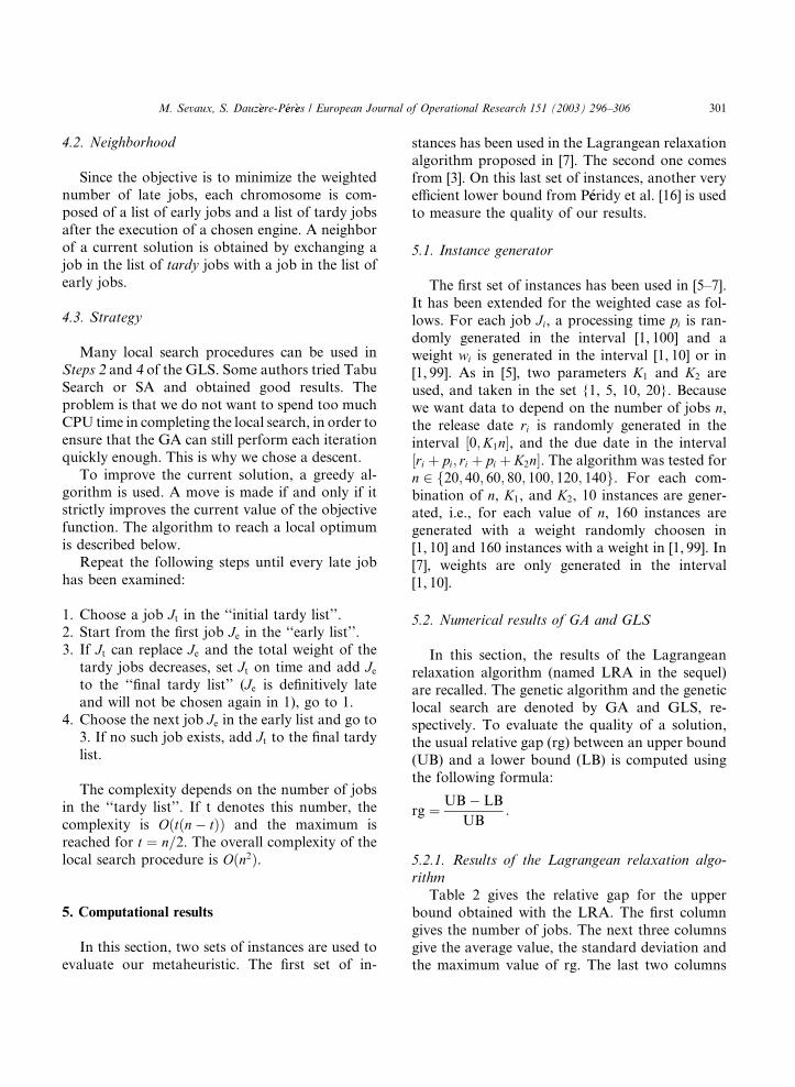
M. Sevaux, S. Dauz�eere-P�eer�ees / European Journal of Operational Research 151 (2003) 296–306 301
4.2. Neighborhood
Since the objective is to minimize the weighted
number of late jobs, each chromosome is com-posed of a list of early jobs and a list of tardy jobs
after the execution of a chosen engine. A neighbor
of a current solution is obtained by exchanging a
job in the list of tardy jobs with a job in the list of
early jobs.
4.3. Strategy
Many local search procedures can be used in
Steps 2 and 4 of the GLS. Some authors tried Tabu
Search or SA and obtained good results. The
problem is that we do not want to spend too much
CPU time in completing the local search, in order to
ensure that the GA can still perform each iteration
quickly enough. This is why we chose a descent.
To improve the current solution, a greedy al-gorithm is used. A move is made if and only if it
strictly improves the current value of the objective
function. The algorithm to reach a local optimum
is described below.
Repeat the following steps until every late job
has been examined:
1. Choose a job Jt in the ‘‘initial tardy list’’.2. Start from the first job Je in the ‘‘early list’’.
3. If Jt can replace Je and the total weight of the
tardy jobs decreases, set Jt on time and add Jeto the ‘‘final tardy list’’ (Je is definitively late
and will not be chosen again in 1), go to 1.4. Choose the next job Je in the early list and go to
3. If no such job exists, add Jt to the final tardy
list.
The complexity depends on the number of jobs
in the ‘‘tardy list’’. If t denotes this number, the
complexity is Oðtðn� tÞÞ and the maximum is
reached for t ¼ n=2. The overall complexity of the
local search procedure is Oðn2Þ.
5. Computational results
In this section, two sets of instances are used to
evaluate our metaheuristic. The first set of in-
stances has been used in the Lagrangean relaxation
algorithm proposed in [7]. The second one comes
from [3]. On this last set of instances, another very
efficient lower bound from P�eeridy et al. [16] is used
to measure the quality of our results.
5.1. Instance generator
The first set of instances has been used in [5–7].
It has been extended for the weighted case as fol-
lows. For each job Ji, a processing time pi is ran-domly generated in the interval [1, 100] and a
weight wi is generated in the interval [1, 10] or in[1, 99]. As in [5], two parameters K1 and K2 are
used, and taken in the set {1, 5, 10, 20}. Because
we want data to depend on the number of jobs n,the release date ri is randomly generated in the
interval ½0;K1n�, and the due date in the interval
½ri þ pi; ri þ pi þ K2n�. The algorithm was tested for
n 2 f20; 40; 60; 80; 100; 120; 140g. For each com-
bination of n, K1, and K2, 10 instances are gener-ated, i.e., for each value of n, 160 instances are
generated with a weight randomly choosen in
[1, 10] and 160 instances with a weight in [1, 99]. In
[7], weights are only generated in the interval
[1, 10].
5.2. Numerical results of GA and GLS
In this section, the results of the Lagrangean
relaxation algorithm (named LRA in the sequel)
are recalled. The genetic algorithm and the genetic
local search are denoted by GA and GLS, re-spectively. To evaluate the quality of a solution,
the usual relative gap (rg) between an upper bound
(UB) and a lower bound (LB) is computed using
the following formula:
rg ¼ UB� LB
UB:
5.2.1. Results of the Lagrangean relaxation algo-
rithm
Table 2 gives the relative gap for the upper
bound obtained with the LRA. The first column
gives the number of jobs. The next three columns
give the average value, the standard deviation and
the maximum value of rg. The last two columns
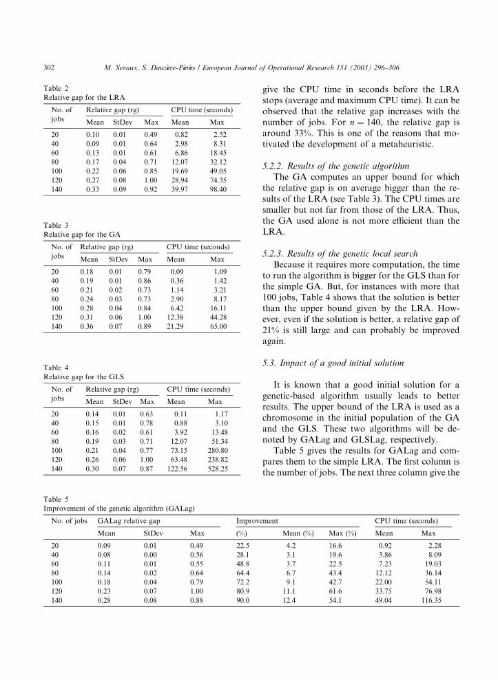
Table 2
Relative gap for the LRA
No. of
jobs
Relative gap (rg) CPU time (seconds)
Mean StDev Max Mean Max
20 0.10 0.01 0.49 0.82 2.52
40 0.09 0.01 0.64 2.98 8.31
60 0.13 0.01 0.61 6.86 18.45
80 0.17 0.04 0.71 12.07 32.12
100 0.22 0.06 0.85 19.69 49.05
120 0.27 0.08 1.00 28.94 74.35
140 0.33 0.09 0.92 39.97 98.40
Table 4
Relative gap for the GLS
No. of
jobs
Relative gap (rg) CPU time (seconds)
Mean StDev Max Mean Max
20 0.14 0.01 0.63 0.11 1.17
40 0.15 0.01 0.78 0.88 3.10
60 0.16 0.02 0.61 3.92 13.48
80 0.19 0.03 0.71 12.07 51.34
100 0.21 0.04 0.77 73.15 280.80
120 0.26 0.06 1.00 63.48 238.82
140 0.30 0.07 0.87 122.56 528.25
Table 3
Relative gap for the GA
No. of
jobs
Relative gap (rg) CPU time (seconds)
Mean StDev Max Mean Max
20 0.18 0.01 0.79 0.09 1.09
40 0.19 0.01 0.86 0.36 1.42
60 0.21 0.02 0.73 1.14 3.21
80 0.24 0.03 0.73 2.90 8.17
100 0.28 0.04 0.84 6.42 16.11
120 0.31 0.06 1.00 12.38 44.28
140 0.36 0.07 0.89 21.29 65.00
Table 5
Improvement of the genetic algorithm (GALag)
No. of jobs GALag relative gap Improve
Mean StDev Max (%)
20 0.09 0.01 0.49 22.5
40 0.08 0.00 0.56 28.1
60 0.11 0.01 0.55 48.8
80 0.14 0.02 0.64 64.4
100 0.18 0.04 0.79 72.2
120 0.23 0.07 1.00 80.9
140 0.28 0.08 0.88 90.0
302 M. Sevaux, S. Dauz�eere-P�eer�ees / European Journal of Operational Research 151 (2003) 296–306
give the CPU time in seconds before the LRA
stops (average and maximum CPU time). It can be
observed that the relative gap increases with the
number of jobs. For n ¼ 140, the relative gap is
around 33%. This is one of the reasons that mo-tivated the development of a metaheuristic.
5.2.2. Results of the genetic algorithm
The GA computes an upper bound for which
the relative gap is on average bigger than the re-
sults of the LRA (see Table 3). The CPU times are
smaller but not far from those of the LRA. Thus,
the GA used alone is not more efficient than theLRA.
5.2.3. Results of the genetic local search
Because it requires more computation, the time
to run the algorithm is bigger for the GLS than for
the simple GA. But, for instances with more that
100 jobs, Table 4 shows that the solution is better
than the upper bound given by the LRA. How-ever, even if the solution is better, a relative gap of
21% is still large and can probably be improved
again.
5.3. Impact of a good initial solution
It is known that a good initial solution for a
genetic-based algorithm usually leads to betterresults. The upper bound of the LRA is used as a
chromosome in the initial population of the GA
and the GLS. These two algorithms will be de-
noted by GALag and GLSLag, respectively.
Table 5 gives the results for GALag and com-
pares them to the simple LRA. The first column is
the number of jobs. The next three column give the
ment CPU time (seconds)
Mean (%) Max (%) Mean Max
4.2 16.6 0.92 2.28
3.1 19.6 3.86 8.09
3.7 22.5 7.23 19.03
6.7 43.4 12.12 36.14
9.1 42.7 22.00 54.11
11.1 61.6 33.75 76.98
12.4 54.1 49.04 116.35

Table 6
Improvement of the genetic local search (GLSLag)
No. of jobs GLSLag relative gap Improvement CPU time (seconds)
Mean StDev Max (%) Mean (%) Max (%) Mean Max
20 0.09 0.01 0.49 18.8 4.5 16.6 0.86 2.57
40 0.08 0.00 0.64 24.4 2.7 10.7 3.26 8.61
60 0.11 0.01 0.54 46.3 3.8 20.2 8.21 20.80
80 0.14 0.02 0.64 63.8 6.9 39.3 16.30 50.45
100 0.18 0.04 0.78 74.4 9.2 42.6 30.12 80.65
120 0.23 0.07 1.00 82.5 11.3 54.2 51.45 174.88
140 0.27 0.08 0.87 90.6 13.4 52.9 87.18 237.69
Table 7
Comparison of the algorithms ðn ¼ 10; . . . ; 50ÞAlgorithm LRA GA GLS GALag GLSLag
n ¼ 10
Dev. from LBLag (%) 10.3 29.4 32.6 10.3 10.3
Dev. from LBPer (%) 1.7 22.0 24.9 1.6 1.6
Optimum found (%) 91.1 52.2 53.3 93.3 93.3
# of time LRA is strictly improved (%) 2.2 2.2
Average CPU time (seconds) 0.32 0.02 0.02 0.33 0.33
Maximum CPU time (seconds) 0.61 0.09 0.05 0.63 0.63
n ¼ 20
Dev. from LBLag (%) 12.2 27.5 25.0 11.8 11.6
Dev. from LBPer (%) 4.2 20.7 18.0 3.7 3.6
Optimum found (%) 61.1 11.1 17.8 66.7 65.6
# of time LRA is strictly improved (%) 10.0 8.9
Average CPU time (seconds) 1.05 0.08 0.10 1.12 1.10
Maximum CPU time (seconds) 2.12 0.14 1.08 2.15 2.16
n ¼ 30
Dev. from LBLag (%) 12.8 26.6 22.4 12.3 12.4
Dev. from LBPer (%) 3.2 18.5 13.8 2.6 2.7
Optimum found (%) 46.7 5.6 12.2 54.4 54.4
# of time LRA is strictly improved (%) 15.6 13.3
Average CPU time (seconds) 1.84 0.17 0.27 1.92 1.93
Maximum CPU time (seconds) 4.66 0.36 0.78 4.71 4.83
n ¼ 40
Dev. from LBLag (%) 9.4 23.7 20.9 9.2 9.2
Dev. from LBPer (%) 2.1 17.3 13.4 1.8 1.8
Optimum found (%) 41.1 5.6 10.0 46.7 44.4
# of time LRA is strictly improved (%) 8.9 10.0
Average CPU time (seconds) 2.66 0.34 0.67 2.70 2.84
Maximum CPU time (seconds) 7.93 1.24 1.79 7.19 8.50
n ¼ 50
Dev. from LBLag (%) 11.1 25.6 19.5 10.7 10.6
Dev. from LBPer (%) 3.2 18.6 12.1 2.7 2.6
Optimum found (%) 35.6 2.2 4.4 40.0 37.8
# of time LRA is strictly improved (%) 21.1 16.7
Average CPU time (seconds) 3.07 0.66 1.38 3.37 3.47
Maximum CPU time (seconds) 7.64 1.27 3.80 7.75 8.16
M. Sevaux, S. Dauz�eere-P�eer�ees / European Journal of Operational Research 151 (2003) 296–306 303

304 M. Sevaux, S. Dauz�eere-P�eer�ees / European Journal of Operational Research 151 (2003) 296–306
relative gap (as in Tables 3 and 4). The three col-
umns ‘‘improvement’’ give the number of time (in
%) GALag improves the initial solution of LRA,
the average and maximum value of the improve-
ment ððUBLRA �UBGALagÞ=UBLRAÞ. The last twocolumns give the average and maximum CPU time
in seconds (time for the LRAþGA).
Table 6 gives the same results for GLSLag and
compares them to the ones of LRA. GLSLag gives
the best results on these tests (the solution is the
best almost 90% of the time) except for the CPU
time (however still reasonable). The general be-
Table 8
Comparison of algorithms ðn ¼ 60; . . . ; 100ÞAlgorithm LRA G
n ¼ 60
Dev. from LBLag (%) 10.8 2
Dev. from LBPer (%) 3.7 1
Optimum found (%) 24.4
# of time LRA is strictly improved (%)
Average CPU time (seconds) 4.00
Maximum CPU time (seconds) 15.38
n ¼ 70
Dev. from LBLag (%) 10.6 2
Dev. from LBPer (%) 3.8 1
Optimum found (%) 23.3
# of time LRA is strictly improved (%)
Average CPU time (seconds) 4.23
Maximum CPU time (seconds) 11.42
n ¼ 80
Dev. from LBLag (%) 10.3 2
Dev. from LBPer (%) 3.8 1
Optimum found (%) 25.6
# of time LRA is strictly improved (%)
Average CPU time (seconds) 4.84
Maximum CPU time (seconds) 14.48
n ¼ 90
Dev. from LBLag (%) 10.2 2
Dev. from LBPer (%) 3.5 1
Optimum found (%) 23.3
# of time LRA is strictly improved (%)
Average CPU time (seconds) 5.89
Maximum CPU time (seconds) 17.00 1
n ¼ 100
Dev. from LBLag (%) 10.9 2
Dev. from LBPer (%) 4.1 1
Optimum found (%) 20.0
# of time LRA is strictly improved (%)
Average CPU time (seconds) 6.05
Maximum CPU time (seconds) 15.83 1
havior shows that if GLSLag is stopped too early,
GALag may give better results because more it-
erations can be done in the same amount of time.
However, even when small CPU times are allowed,
GLSLag almost always dominates GALag. For aspecific 100-job instance, GALag performs 14853
iterations in 11.59 seconds and the best solution is
2143. GLSLag performs only 3555 iterations in
18.14 seconds and the best solution is 2091. GA-
Lag obtains a better solution than GLSLag before
a time limit of 2.56 seconds, but is surpassed by
GLSLag afterwards. This is not as obvious in the
A GLS GALag GLSLag
3.4 21.7 10.2 10.2
7.0 12.2 2.9 2.9
4.4 7.8 32.2 36.7
26.7 27.7
1.19 2.46 4.35 4.80
2.71 8.22 11.62 16.97
3.7 20.9 9.7 9.8
7.6 12.3 2.9 3.0
2.2 4.4 32.2 31.1
40.0 36.7
2.01 3.66 5.02 5.39
5.15 10.59 11.41 13.03
3.6 22.4 9.6 9.6
7.6 12.2 2.7 2.8
1.1 2.2 26.7 28.9
32.2 28.9
3.22 5.87 5.98 6.66
6.99 17.11 16.40 19.86
3.8 22.3 9.3 9.4
7.8 12.0 2.6 2.6
1.1 4.4 27.8 28.9
42.2 36.7
4.49 10.17 7.34 8.91
0.57 29.60 17.45 23.14
3.9 18.0 10.0 10.1
7.7 11.4 3.0 3.1
1.1 2.2 24.4 23.3
47.8 38.9
7.94 13.64 8.66 10.27
7.07 32.41 19.08 23.79

M. Sevaux, S. Dauz�eere-P�eer�ees / European Journal of Operational Research 151 (2003) 296–306 305
results of the following section (see Tables 7 and 8)
on a different set of instances.
Although GLSLag gives the best results, the
relative gap for n ¼ 100 is still large (18%). For
n ¼ 140, the gap is above 25%. This is probablydue to the fact that the lower bounds obtained by
Lagrangean relaxation are not good enough. Re-
call that general parameters are used for LRA for
every instance.
5.4. Comparison with a better lower bound
P�eeridy et al. [16] developed a very efficient lowerbound (denoted LBPer) also using Lagrangean
relaxation, but very differently than in [7]. The
authors sent us the results on a set of instances
generated in a very different way than our set (see
Baptiste et al. [3]), the main difference being that
jobs are more constrained (smaller time windows)
in these instances. We ran the different versions of
the genetic-based algorithms and compared ourresults to the lower bound.
The size of these test problems ranges from
n ¼ 10 to 100. Table 7 gives the results for in-
stances with sizes varying from n ¼ 10 to 50, and
Table 8 from n ¼ 60 to 100. They show that the
duality gap is much smaller with a better lower
bound, and that our solutions are thus closer to
optimality than what our set of instances indi-cated. However, the average deviation from the
lower bound is close to 3% for problems of more
than 50 jobs, which is still too large to conclude
definitely on the quality of our solution proce-
dures.
6. Conclusion
This paper presents a first metaheuristic for a
NP-Hard one-machine scheduling problem. A
GA has been designed testing various engines and
several crossover operators. Consistent improve-
ments have been obtained on several tests of in-
stances, although very good solutions were already
provided by a LRA. However, on our test of in-stances, we do not know whether large gaps be-
tween upper and lower bounds are mostly due to
the duality gap, or to the fact that better solutions
can be determined, i.e., if our solutions are close to
optimality or not. This question could be partially
answered by using the lower bound proposed in
[16], although duality gaps are still too large to
conclude on the second set of instances.Hence, our future research aims at designing an
exact approach for this problem, which could be
used to better evaluate the effectiveness of our
metaheuristic.
Acknowledgements
The authors would like to thank C. Prins for the
very useful hints and private conversations that
motivated this paper. The authors are also grateful
to A. Hertz and M. Laguna for their enlighten-ment, to P. Thomin for his help in the implemen-
tation of part of the code, and to two anonymous
referees for their helpful comments.
References
[1] K.R. Baker, Introduction to Sequencing and Scheduling,
John Wiley, New York, USA, 1974.
[2] P. Baptiste, C. Le Pape, L. P�eeridy, Global constraints for
partial CSPs: A case study of resource and due-date
constraints, 4th International Conference on Principles and
Practices of Constraint Programming, Pisa, Italy, 1998.
[3] P. Baptiste, A. Jouglet, C. Le Pape, W. Nuijten, A
constraint-based approach to minimize the weighted num-
ber of late jobs on parallel machines. Research report 2000/
228, UMR, CNRS 6599, Heudiasyc, France, 2000.
[4] J. Carlier, Probl�eemes d�ordonnancement �aa contraintes de
resources: Algorithmes et complexit�ees, Th�eese d�Etat, Uni-
versit�ee de Paris 6, 28 mai 1984.
[5] S. Dauz�eere-P�eer�ees, Minimizing late jobs in the general one
machine scheduling problem, European Journal of Oper-
ational Research 81 (1995) 134–142.
[6] S. Dauz�eere-P�eer�ees, M. Sevaux, An exact method to mini-
mize the number of tardy jobs in single machine schedul-
ing, Research report 99/6/AUTO, Ecole des Mines de
Nantes, France, 1999.
[7] S. Dauz�eere-P�eer�ees, M. Sevaux, Using Lagrangean relax-
ation to minimize the (weighted) number of late jobs on a
single machine, Research report 99/8/AUTO, Ecole des
Mines de Nantes, France, 1999.
[8] L. Davis (Ed.), Handbook of Genetic Algorithms, Van
Nostrand Reinhold, New York, 1991.
[9] S. French, Sequencing and Scheduling: An Introduction to
the Mathematics of the Job–Shop, Ellis-Horwood, 1990.

306 M. Sevaux, S. Dauz�eere-P�eer�ees / European Journal of Operational Research 151 (2003) 296–306
[10] R.L. Graham, E.L. Lawler, J.K. Lenstra, A.H.G. Rinnooy
Kan, Optimization and approximation in deterministic
sequencing and scheduling: A survey, Annals of Discrete
Mathematics 5 (1979) 287–326.
[11] J.H. Holland, Adaptation in Natural and Artificial Sys-
tems, The University of Michigan Press, Ann Arbor, MI,
1975.
[12] H. Kise, T. Ibaraki, H. Mine, A solvable case of the one-
machine scheduling problem with ready and due times,
Operations Research 26 (1) (1978) 121–126.
[13] E.L. Lawler, Knapsack-like scheduling problems, the
Moore–Hodgson algorithm and the �tower of sets� prop-erty, Mathematical Computer Modelling 20 (2) (1994) 91–
106.
[14] J.K. Lenstra, A.H.G. Rinnooy Kan, P. Brucker, Com-
plexity of machine scheduling problems, Annals of Discrete
Mathematics 1 (1977) 343–362.
[15] J.M. Moore, A n job, one machine sequencing algorithm
for minimizing the number of late jobs, Management
Science 15 (1) (1968) 102–109.
[16] L. P�eeridy, E. Pinson, D. Rivreau, Total cost single-machine
scheduling problem with arbitrary release dates, Proceed-
ings of the Workshop on Project Management and
Scheduling, Osnabr€uuck, Germany, April 17–19, 2000, pp.
233–235.
[17] C.N. Potts, L.N. Van Wassenhove, Algorithms for sched-
uling a single machine to minimize the weighted number of
late jobs, Management Science 34 (7) (1988) 834–858.
[18] M.C. Portmann, Genetic algorithms and scheduling: A
state of the art and some propositions, Proceedings of the
Workshop on Production Planning and Control, Mons,
Belgium, September 9–11, 1996, I–XIV.
[19] C.R. Reeves, A genetic algorithm for flowshop sequencing,
Computers and Operations Research 22 (1) (1995) 5–13.
[20] C.R. Reeves, Genetic algorithms for the operations
researcher, INFORMS Journal on Computing 9 (3)
(1997) 231–250.
[21] F.J. Villarreal, R.L. Bulfin, Scheduling a single machine to
minimize the weighted number of tardy jobs, IIE Trans-
actions 15 (1983) 337–343.

DOI: 10.1007/s10288-003-0028-0
4OR (2004) Regular Paper
A genetic algorithm for robust schedulesin a one-machine environment with ready timesand due dates
Marc Sevaux1 and Kenneth Sörensen2
1 Université de Valenciennes, Le Mont Houy , 59313 Valenciennes, France(e-mail: [email protected])
2 Universiteit Antwerpen, Middelheimlaan 1, 2020 Antwerp, Belgium(e-mail: [email protected])
Received: 19 December 2002 / Accepted: 2 July 2003
Abstract. Computing a schedule for a single machine problem is often difficult, butwhen the data are uncertain, the problem is much more complicated. In this paper,we modify a genetic algorithm to compute robust schedules when release datesare subject to small variations. Two types of robustness are distinguished: qualityrobustness or robustness in the objective function space and solution robustness orrobustness in the solution space. We show that the modified genetic algorithm canfind solutions that are robust with respect to both types of robustness. Moreover, therisk associated with a specific solution can be easily evaluated. The modified geneticalgorithm is applied to a just-in-time scheduling problem, a common problem inmany industries.
Key words: Quality robustness, solution robustness, single machine scheduling,weighted number of late jobs, genetic algorithm
Mathematics Subject Classification: 90B99
1 Introduction
Scheduling problems are generally computationally difficult problems and the prob-lem described in this paper is no exception. The problem becomes even more dif-ficult when some of the data are stochastic (Daveand Beck 2000; Herroelen and
Correspondence to: K. Sörensen
4OR Quarterly Journal of the Belgian, Frenchand Italian Operations Research Societies
© Springer-Verlag 2004

2 M Sevaux and K. Sörensen
Leus 2002). Genetic algorithms – and metaheuristics in general – have been foundto provide good approximations of the optimal solution with a relatively smallcomputational effort (Portmann 1996). Although the literature on applications ofmetaheuristics (and genetic algorithms in particular) to scheduling problems is verylarge, the number of applications to problems with a stochastic component is rathersmall, see, e.g., (Kouvelis and Yu 1997).
One way to deal with stochastic problem data is to find solutions that are robust.We distinguish two types of robustness.Quality robustness is a property of a solutionwhose quality, measured by the objective function value, does not deviate muchfrom optimality when small changes in the problem data occur.
The second type of robustness is solution robustness and can be described asrobustness in the solution space. When changes in the problem data occur, thedecision maker might be forced to re-optimise the problem. In this case, the qualityof the solution is guaranteed by the optimisation procedure. In some situationshowever a solution is preferred that is “close” (in the solution space, not the objectivefunction space) to the solution currently used. Many manufacturers operate witha production schedule that repeats itself on a regular basis (e.g., daily or weekly).When, e.g., a new job needs to be scheduled, the problem is re-optimised, but thenew production schedule should be as similar as possible to the one currently used.This type of robustness stresses the importance of solution stability. The two typesof robustness are not entirely equivalent in the sense that quality robustness is aproperty of a solution that is insensitive to changes in the problem data before thesechanges occur, whereas solution robustness refers to the stability of a solution afterchanges have occurred.
The object of the single machine scheduling problem considered in this paperis to determine the order in which a given set of jobs should be executed on amachine. Each job has a certain release date and cannot be scheduled before thisdate. Also, each job has a certain processing time and a due date, before which itshould be finished. Jobs that are not finished before their due date are called late.The objective of the problem considered in this paper is to minimise the numberof late jobs. A genetic algorithm for this problem was developed by Sevaux andDauzère-Pérès (2002).
When a problem has stochastic parameters, the objective function value itselfbecomes stochastic. The objective of a stochastic problem has several dimensions.Some decision makers prefer a solution that has a high quality on average, othersmight prefer one that hedges against the worst possible situation. However, mostdecision makers like to minimise the risk of ending up with a bad solution, withoutnecessarily choosing an extremely conservative solution. In this paper, we modifythe GA proposed by Sevaux and Dauzère-Pérès (2002) to be able to deal withstochastic release dates and show that this GA is able to find solutions that areboth quality robust and solution robust. The proposed approach can be labelled asampling method, in that it uses sampling to estimate the robustness of a solution.We show that this approach is very flexible in that – although our GA is only used for

A genetic algorithm for robust schedules 3
problems with stochastic release dates – other types of stochastic problem data canbe easily incorporated. Simultaneously, the risk preference of the decision makercan be modelled and a solution can be found that minimises the estimated numberof late jobs and the risk that this solution entails. Solution robustness is obtainedby measuring the distance (in the solution space) to a given base-line solution.This distance measure is based on the edit distance. Minimising the distance toa baseline solution and simultaneously maximising the quality of a solution isobviously difficult. We show in this paper that both objectives can be achievedsimultaneously by letting the GA search for high-quality solutions and measuringthe distance of each solution encountered to the baseline solution. In a second stage,a solution can be chosen that provides a good trade-off.
This paper is structured as follows.After the literature review, the single machinescheduling problem is formulated. Section 4 introduces a genetic algorithm for thedeterministic single machine scheduling problem. In Sect. 5, this GA is modifiedfor the computation of schedules that are both quality robust and solution robust.Section 6 describes how the modified genetic algorithm can be used to find robustproduction sequences in a just-in-time environment. Section 7 reports on somecomputational results.
2 Literature review
Single machine scheduling problems have been successfully tackled using ge-netic algorithms. Genetic algorithms – pioneered by Holland (1975) and Goldberg(1989), as well as many others—use a Darwinian metaphor to find good solutionsfor difficult optimisation problems. A review of genetic algorithms can be found inReeves (1993, 1997). For a review of applications of genetic algorithms to schedul-ing problems we refer to Portmann (1996).
This paper describes a simple GA, developed by Sevaux and Dauzère-Pérès(2002), that finds good solutions to the deterministic scheduling problem describedabove.
Although the literature on deterministic scheduling is several orders of mag-nitude larger, there is a significant body of work on scheduling under uncertainty.Two very recent literature surveys are Herroelen and Leus (2002) and Davenportand Beck (2000). Herroelen and Leus (2002) divide research on scheduling withuncertainty into six categories. In reactive scheduling, procedures are developedto re-optimise the schedule when disruptive events occur. Stochastic scheduling isthe application of stochastic programming with recourse to scheduling problems.GERT network scheduling is used for problems with stochastic evolution structureand feedback. Scheduling under fuzziness recommends the use of fuzzy numbersfor, e.g., project duration instead of stochastic variables.Proactive (robust) schedul-ing attempts to develop a schedule, the quality of which is relatively insensitiveto a changing environment. Herroelen and Leus (2002) also discuss some recentadvances in sensitivity analysis for project scheduling. The method developed in
4 M Sevaux and K. Sörensen
this paper can be categorised under the heading robust scheduling. Davenport andBeck (2000) distinguish between proactive and reactive approaches. Proactive ap-proaches include the insertion of redundancy (typically extra buffer time) into theschedule, the use of probabilistic techniques to determine robust schedules and thecreation of multiple schedules to deal with contingencies.
Although genetic algorithms and meta-heuristics in general have been often andsuccessfully applied to tackle deterministic scheduling problems, their applicationto scheduling under uncertainty is very limited. In this paper, we argue that meta-heuristics can very easily be adapted to the requirements of a stochastic problemformulation. Using meta-heuristics for this type of optimisation problem has severaladvantages that will be discussed later. That there is a need for robust meta-heuristicoptimisation is recognised in the influential book “Robust discrete optimisation”(Kouvelis andYu 1997), when the authors say on p. 354: “We believe that consider-able more effort should be spent in systematic development of [ . . . ] metaheuristicframeworks, which with minimal adjustment effort can be applied to a large class ofrobust optimisation problems [ . . . ]”. Previous work on robust genetic algorithmscan be found in Tsutsui et al. (1996); Tsutsui and Ghosh (1997); Tsutsui and Jain(1998); Tsutsui (1999); Branke (1998, 2001), but the applications of this work arelimited to the robust optimisation of continuous mathematical functions.
A genetic algorithm for robust job shop schedules is developed by Leon et al.(1994b). This algorithm uses an objective function that includes some measure ofrobustness. In their problem, the authors assume that machine operations can bedisrupted and that the disrupted operations are restarted immediately after the endof the disruption period (a right-shift reactive policy). Robustness is defined as afunction of the schedule delay, i.e., the difference between the actual makespan andthe projected makespan. A number of different measures, specifically developed toestimate this measure of robustness is developed. Leon et al. (1993, 1994b) describean approach in which recovering from disruptions is modelled as a game playedagainst nature.
Hart and Ross (1999a, b) have recently developed artificial immune systems asa tool for scheduling under uncertainty. The author’s goal is to develop off line anumber of partial schedules that can be used as building blocks to quickly composea good schedule when unexpected events occur. The underlying assumption isthat such events (such as machine breakdowns) and the desired reaction of thescheduling system, are to some extend predictable. The partial schedules found bythis GA therefore constitute a specific piece of domain knowledge, that can be usedwhen disruptions occur.
Jensen (2001) introduces several novel ideas. In neighbourhood-based robust-ness, the basic idea of which is that if a small set of schedules close to the prescheduleis known to be of good quality before an unexpected event occurs, then perhapsone of these schedules provide a good solution in case an unforeseen event occurs.Co-evolution is a term to describe genetic algorithms in which a population of ro-bust solutions and a population of problem instances evolve simultaneously. At the

A genetic algorithm for robust schedules 5
Table 1. Single machine scheduling problem notation
Description Symbol RemarksNumber of jobs n
Release date rjProcessing time pjDue date djWeight wj
Starting time tj rj ≤ tjCompletion time Cj Cj = tj + pjLateness status Uj Uj = 1 iff Cj > dj and 0 otherwise
end, the first population contains the most robust solutions and the second one themost difficult problem instances. The first population might contain, e.g., a set ofschedules and the second a set of machine breakdowns.
3 Single machine scheduling problem formulation
The objective of the scheduling problem in this paper is to schedule a given setof jobs on a single machine without preemption. Every job has a release datethat represents the time at which production or assembly of the batch can beginat the earliest. The processing times of the jobs are known, as well as their duedates. Depending on its importance, a weight is attached to every job. A job iscalled late if its completion time is greater than its due date. The objective is tofind a schedule of jobs that minimises the total weighted number of late jobs. Latejobs are arbitrarily moved to the end of the schedule, as the amount of lateness isconsidered unimportant. Table 1 clarifies the notation used.
The problem in this paper is denoted as 1|rj | ∑wjUj in the standard classifica-tion. The problem is NP-hard in the strong sense (Lenstra et al. 1977). For the staticcase, previous work on this problem can be found in Sevaux and Dauzère-Pérès(2002), Dauzère-Pérès (1995), Dauzère-Pérès and Sevaux (2003), Dauzère-Pérèsand Sevaux (2001), Baptiste (1999) and Baptiste et al. (2003).
Although all parameters of the problem can be made stochastic, we only modelthe case of stochastic release dates. We will show however, that other stochasticparameters can easily be entered into the problem formulation and solved by themodified GA.
4 A genetic algorithm for a single machine scheduling problem
Algorithm 1 gives a schematic representation of the GA used in the rest of the paper.In this GA, a solution is encoded as a permutation of the n jobs. An initial
population is created by randomly generating permutations of jobs. The size of thepopulationN is computed by the formulaN = 5+n/5 wheren is the number of jobs

6 M Sevaux and K. Sörensen
Algorithm 1 Basic incremental genetic algorithm1: Generate an initial population2: while stopping conditions are not met do3: Select two individuals4: Crossover the two individuals5: Mutate offspring under probability6: Evaluate offspring7: Insert offspring under conditions8: Remove an individual under conditions9: end while
10: Report results
of the selected instance. The main loop of the GA is stopped after a fixed numberof iterations without improvement of the best solution or after a certain maximumnumber of iterations. The maximum number of iterations ItMax is computed byItMax = 50∗n∗N and the maximum number of iterations without improvementis ItMaxwoImp = ItMax/10.
Two parent solutions are drawn from the population. The former is chosenaccording to a ranking selection method which give a higher probability to thebest individuals (Reeves 1993) and the latter is randomly chosen. The populationis sorted in ascending order of fitness values (ascending order of the objectivefunction), so the best individual is ranked first. If N denotes the size of the pop-ulation, the selection of the first parent is made using the probability distribution2(N + 1 − k)/(N(N + 1)) where k is the kth chromosome in the ascending orderof fitness values. Using this technique, the median chromosome (N + 1)/2 hasthe probability 1/N of being selected, while the best individual has the probability2/(N + 1) (approximatively twice the median). The second parent is randomlyselected with an uniform distribution.
The crossover operator is a one-point crossover operator X1. A crossover pointis randomly chosen. The first part of parent P1 is copied into the offspring. The restof the chromosome is filled by reading the information of the second parent P2.The jobs that are not already in the offspring are copied, preserving the permutationproperty. See Fig. 1.
P1
P2 O1
1 2 3 4 5 6 7
4 3 7 6 2 5 1 1 2 3 4 7 6 5
Crossover point
Fig. 1. Crossover operator X1

A genetic algorithm for robust schedules 7
A general pairwise interchangemutation operator permutes two jobs randomlychosen in the chromosome. See Fig. 2. This mutation is done under a probabilityPm. For the deterministic case, we chose Pm = 0.25.
1 2 3 4 5 6 7 1 5 3 4 2 6 7
Fig. 2. Mutation operator GPI
After mutation, the solution is evaluated. The fitness value of a solution is equalto the sum of the weights of the late jobs, i.e.,
f (x) =n∑
j=1
wjUj , (1)
where Uj is defined as in Table 1.The genetic algorithm uses incremental replacement, i.e., the population size
remains the same throughout the run. A new offspring is inserted if it improvesat least the worst solution in the population. When a new solution is inserted, asolution randomly chosen from the worst half of the population, is discarded.
In Sevaux and Dauzère-Pérès (2002) different variations of this simple geneticalgorithm, combined with a local search technique are compared to and found to besuperior over other methods. The GA used in this paper does not attempt to locallyimprove solutions using a local search operator. Experimental results show that,when using the GA to find robust solutions, the use of a local search improvementoperator tends to overemphasise solution quality. Finding robust solutions requiresthe exploration of a diverse set of solutions, covering a portion of the search spacethat is as large as possible. Adding a local search operator at this step will intensifythe search and the solutions will have some jobs tightly sequenced so that any mod-ification in the release date will cause an important modification of the optimisationfunction. For our study, the local search operator will not be used.
5 A genetic algorithm for robust schedules
In the following, we describe how the genetic algorithm for the deterministicscheduling problem can be modified so that it finds solutions that are quality robustand/or solution robust. As in Sörenesen (2001), this is done by replacing the fitnessfunction of the GA by a so-called robust evaluation function. When we want tomake the distinction, the fitness function for the deterministic problem is referredto as the ordinary evaluation function.
8 M Sevaux and K. Sörensen
5.1 Quality robustness
Let x be a solution of the problem (a permutation of the jobs). The quality of x iscomputed by an evaluation function f (x). When we want to indicate that f hasparameters, we write f (x, P ), where P is the set of problem data. In our case, Prepresents the characteristics of the jobs (rj , pj , dj , wj ). To allow the GA to findrobust solutions, the evaluation function f (x) is replaced by a robust evaluationfunction f ∗(x). The robust evaluation function for quality robust solutions adheresto the following principles (Sörensen 2001):
Principle 1 : Each solution is implemented on a modified set of characteristicsSi(P ). S is a sampling function, that takes a random sample from the stochasticelements of P . Si(P ) is the i-th set of sampled parameters of P . We call theimplementation of a solution on a modified set of characteristics a derivedsolution.
Principle 2 : Several evaluations of a solution x on a sample of P are combinedinto a new evaluation function. An evaluation of a derived solution is called aderived evaluation. This new function is the robust evaluation function f ∗(x).
A possible form of a robust evaluation function is a weighted average of m
derived evaluations:
f ∗(x) = 1
m
m∑i=1
cif (x, Si(P )) (2)
where ci is a weight associated to this derived evaluation according to its importanceand m is the number of derived solutions to evaluate.
A more conservative robust evaluation function examines the worst-case per-formance of a solution across all derived evaluations:
f ∗(x) = maxi=1...m
f (x, Si(P ))
if f has to be minimised. In this paper, we only use the robust evaluation functionof Eq. (2).
For the scheduling problem considered in this paper, we assume the release datesto be stochastic. The robust evaluation function evaluates each solution severaltimes, each time on a new random instantiation of the release dates. The samepermutation of the jobs is kept but the release dates are modified. Afterwards, theengine which computes the objective function value of the permutation is calledand executed with this new instantiation of the problem. The derived evaluations arecombined into a single robustness measure as indicated. This implies that a standardevaluation has to be performed several times for each solution, which increases thecomputational time. The advantage of this approach however is that the standardevaluation function does not have to be modified. The implementation of a robustevaluation function is therefore very easy and only requires a standard evaluation

A genetic algorithm for robust schedules 9
function to be available and a metaheuristic already running for problems with staticdata. The only change made is to the evaluation step of Algorithm 1, rendering thisway of finding robust solutions extremely easy to implement and very flexible.
5.2 Solution robustness
Solution robustness is a property of a solution that is similar to a given baselinesolution x0, i.e. for which the distance to the baseline solution (as measured bysome distance function) is small. Of course, solution robustness cannot be usedas the only objective, since solution quality or quality robustness should alwaysbe taken into account. The need for solution robustness therefore automaticallytransforms the problem into a multi-objective one and a solution should be foundthat simultaneously has a high quality (robustness) and a small distance to thebaseline solution. In our framework, solution robustness is obtained by measuringthe distance between the baseline solution and each solution generated by the GA.It is assumed that the GA visits a sufficiently diverse set of solutions, so that atleast a fraction of them will be solution robust. A solution is then chosen using amulti-objective decision making process – taking into account the decision maker’spreferences for solution robustness and quality (robustness).
Edit distance. First developed in the context of correcting binary codes transmit-ted across a faulty channel (Levenshtein 1966), the edit distance is a measure of thesimilarity between two strings, composed of characters of a finite alphabet �. Anextra null-character � is also defined to signify the absence of a character. Threeelementary edit operations are defined (x, y ∈ �): insertion (� → x), deletion(x → �) and substitution (x → y). An edit transformation between strings s andt is a set of elementary edit transformations that transform s into t .
Simplifying, the edit distance d(s, t) can be defined as the number of editoperations that is required to transform a source string s into a target string t1
A straightforward dynamic programming algorithm to compute the edit distanceis due to Wagner and Fischer (1974). The time complexity of this algorithm isO(|s| × |t |) where |s| and |t | are the lengths of strings s and t respectively. Moreefficient algorithms have been developed (e.g. by Ukkonen 1985), but these arebeyond the scope of this paper. Under some conditions (Wagner and Fischer 1974),the edit distance is ametric, i.e. it satisfies the conditions that (∀s, t, u): d(s, t) ≥ 0,d(s, t) = 0 ⇔ s = t , d(s, t) = d(t, s), and d(s, t) ≤ d(s, u) + d(u, t).
1 In a more general formulation of the edit distance, a distance function γ (x, y) ≥ 0 is defined thatdetermines the non-negative real-valued cost of transforming character x into character y (x, y ∈ �∪�).The cost of an edit transformation is defined as the sum of the costs of the elementary edit operations itcontains.The edit distanced(s, t)now is defined as the minimum-cost edit transformation that transformss into t .

10 M Sevaux and K. Sörensen
Distance between two schedules. If all jobs of the scheduling problem are repre-sented by a different character, a schedule can be represented as a string of jobs.The distance between two solutions can be calculated by the edit distance and in-terpreted as the number of “changes” that have to be made to the first schedule toturn it in to the second one. A “change” can be either an insertion of a job into theschedule, a deletion of a job or the substitution of a job by another one.
A sensible distance measure should accurately reflect the “similarity” betweentwo schedules. The meaning of this concept is highly dependent on the specificsituation. Although the edit distance provides a relatively natural way of measuringthe similarity between two schedules (the number of changes required to transformschedule s into schedule t), other distance measures could be developed, e.g., basedon the actual starting times of the jobs.
5.3 Incorporating risk preference
The function f ∗(x) estimates the average performance or the worst case perfor-mance of a solution, given that some of the parameters of the problem are stochastic.Clearly, the worst case performance measure will lead to solutions that are moreconservative. Solutions found using this form of the robust evaluation function willhedge only against the worst possible incidence, independent of the probabilitythat this scenario will occur. This type of robust evaluation function can be used byextremely risk-averse decision makers.
A more subtle manner to incorporate the risk preference of the decision maker,is to include into the robust evaluation function an estimate of the probability thatthe quality of a solution will deviate from its expected value. A possible measureis the standard deviation of the quality of a given solution over all samples:
σ ∗(x) =√√√√ 1
m − 1
m∑i=1
[f (x, Si(P )) − f ∗(x)]2.
The two measures can be integrated in a multi-objective decision making ap-proach. A possible way is to find the solution that minimises f ∗(x) + γ σ ∗(x),where γ is a parameter indicating the risk-averseness of the decision maker. Amore advanced way is to retain all efficient solutions and choose one according toa multi-objective decision making method.
6 Application to just-in-time scheduling
6.1 Just-in-time scheduling
Many manufacturing companies have switched (at least partially) to a just-in-timepolicy over the last two decades. In this philosophy, suppliers are required to deliver

A genetic algorithm for robust schedules 11
their raw materials or semi-finished products to the manufacturer’s plant right ontime for these parts or materials to be taken into production (Christopher 1998). Thesuppliers are required to locate a supply hub (e.g., a warehouse) close to the man-ufacturer’s production facility and deliver parts or materials to the manufacturingplant several times a day, at the request of the manufacturer. Based on the produc-tion sequence, i.e., the order in which the different product batches are be producedin the manufacturing plant, release dates and amounts to deliver of the parts ormaterials are fixed by the schedulers in the manufacturing plant and communicatedto the suppliers. The production sequence determines when the production of eachbatch begins, and consequently which batches will be finished on time and whichnot.
Just-in-time delivery promises several advantages, the most important onesbeing reduced costs and shorter lead times. A negative side-effect from the use ofjust-in-time however, is the fact that any delay in the delivery by the suppliers willpostpone the production of a batch which will lead to longer and unpredictable leadtimes of the finished product and increase the number of late deliveries. Althoughmanufacturing companies and their suppliers are working hard to reduce the delayof parts or materials, unexpected events can have a significant effect on them. Thisin turn will negatively influence the number of production batches that are finishedon time.
While manufacturers are trying hard to reduce the number of late deliveries ofparts and materials as well as the amount of time with which they are delayed, somefactors remain beyond their control. Traffic jams, truck breakdowns, strikes etc.,are factors that may delay delivery, but are very difficult to control. To deal withthese types of unexpected events, a manufacturing company can attempt to design arobust production sequence.A quality robust production sequence can be defined asa production sequence, the quality of which is relatively insensitive to perturbationsin the input data. The quality of a certain schedule can be measured by variousquality measures, e.g. by counting the number of batches that are finished on time.A solution robust production sequence may be defined as a production sequencethat is “close” to a base-line production sequence that is currently in use by themanufacturer. As already mentioned, changing the production sequence drasticallywhen unexpected events occur may increase the quality but might cause a largedisruption in the regular production routine. This in turn may lead to productionerrors, and other undesirable effects.
6.2 Modelling a just-in-time production systemas a scheduling problem
A just-in-time production environment can be modelled as a scheduling problem,in which each of the production batches is represented by a job that has to bescheduled on a single machine. Solving the problem yields a production sequence
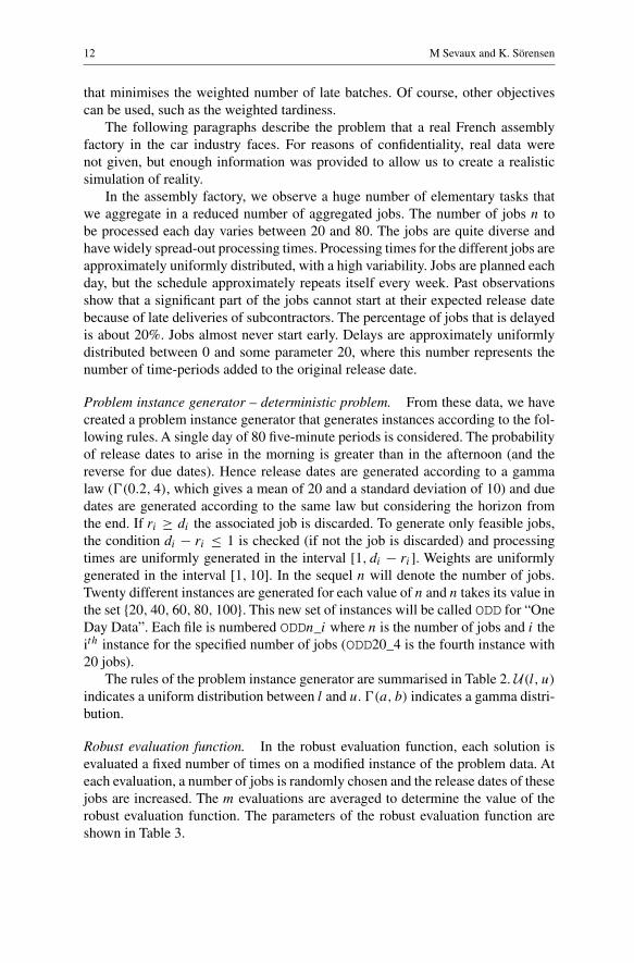
12 M Sevaux and K. Sörensen
that minimises the weighted number of late batches. Of course, other objectivescan be used, such as the weighted tardiness.
The following paragraphs describe the problem that a real French assemblyfactory in the car industry faces. For reasons of confidentiality, real data werenot given, but enough information was provided to allow us to create a realisticsimulation of reality.
In the assembly factory, we observe a huge number of elementary tasks thatwe aggregate in a reduced number of aggregated jobs. The number of jobs n tobe processed each day varies between 20 and 80. The jobs are quite diverse andhave widely spread-out processing times. Processing times for the different jobs areapproximately uniformly distributed, with a high variability. Jobs are planned eachday, but the schedule approximately repeats itself every week. Past observationsshow that a significant part of the jobs cannot start at their expected release datebecause of late deliveries of subcontractors. The percentage of jobs that is delayedis about 20%. Jobs almost never start early. Delays are approximately uniformlydistributed between 0 and some parameter 20, where this number represents thenumber of time-periods added to the original release date.
Problem instance generator – deterministic problem. From these data, we havecreated a problem instance generator that generates instances according to the fol-lowing rules. A single day of 80 five-minute periods is considered. The probabilityof release dates to arise in the morning is greater than in the afternoon (and thereverse for due dates). Hence release dates are generated according to a gammalaw ("(0.2, 4), which gives a mean of 20 and a standard deviation of 10) and duedates are generated according to the same law but considering the horizon fromthe end. If ri ≥ di the associated job is discarded. To generate only feasible jobs,the condition di − ri ≤ 1 is checked (if not the job is discarded) and processingtimes are uniformly generated in the interval [1, di − ri]. Weights are uniformlygenerated in the interval [1, 10]. In the sequel n will denote the number of jobs.Twenty different instances are generated for each value of n and n takes its value inthe set {20, 40, 60, 80, 100}. This new set of instances will be called ODD for “OneDay Data”. Each file is numbered ODDn_i where n is the number of jobs and i theith instance for the specified number of jobs (ODD20_4 is the fourth instance with20 jobs).
The rules of the problem instance generator are summarised in Table 2. U(l, u)
indicates a uniform distribution between l and u. "(a, b) indicates a gamma distri-bution.
Robust evaluation function. In the robust evaluation function, each solution isevaluated a fixed number of times on a modified instance of the problem data. Ateach evaluation, a number of jobs is randomly chosen and the release dates of thesejobs are increased. The m evaluations are averaged to determine the value of therobust evaluation function. The parameters of the robust evaluation function areshown in Table 3.
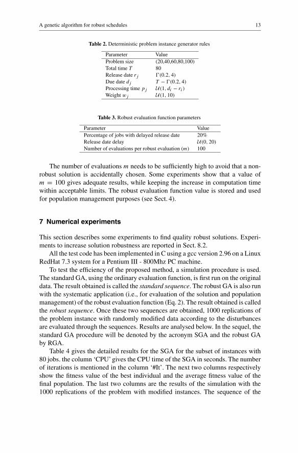
A genetic algorithm for robust schedules 13
Table 2. Deterministic problem instance generator rules
Parameter ValueProblem size (20,40,60,80,100)Total time T 80Release date rj "(0.2, 4)Due date dj T − "(0.2, 4)Processing time pj U(1, di − ri )
Weight wj U(1, 10)
Table 3. Robust evaluation function parameters
Parameter ValuePercentage of jobs with delayed release date 20%Release date delay U(0, 20)Number of evaluations per robust evaluation (m) 100
The number of evaluations m needs to be sufficiently high to avoid that a non-robust solution is accidentally chosen. Some experiments show that a value ofm = 100 gives adequate results, while keeping the increase in computation timewithin acceptable limits. The robust evaluation function value is stored and usedfor population management purposes (see Sect. 4).
7 Numerical experiments
This section describes some experiments to find quality robust solutions. Experi-ments to increase solution robustness are reported in Sect. 8.2.
All the test code has been implemented in C using a gcc version 2.96 on a LinuxRedHat 7.3 system for a Pentium III - 800Mhz PC machine.
To test the efficiency of the proposed method, a simulation procedure is used.The standard GA, using the ordinary evaluation function, is first run on the originaldata. The result obtained is called the standard sequence. The robust GA is also runwith the systematic application (i.e., for evaluation of the solution and populationmanagement) of the robust evaluation function (Eq. 2). The result obtained is calledthe robust sequence. Once these two sequences are obtained, 1000 replications ofthe problem instance with randomly modified data according to the disturbancesare evaluated through the sequences. Results are analysed below. In the sequel, thestandard GA procedure will be denoted by the acronym SGA and the robust GAby RGA.
Table 4 gives the detailed results for the SGA for the subset of instances with80 jobs. the column ‘CPU’ gives the CPU time of the SGA in seconds. The numberof iterations is mentioned in the column ‘#It’. The next two columns respectivelyshow the fitness value of the best individual and the average fitness value of thefinal population. The last two columns are the results of the simulation with the1000 replications of the problem with modified instances. The sequence of the
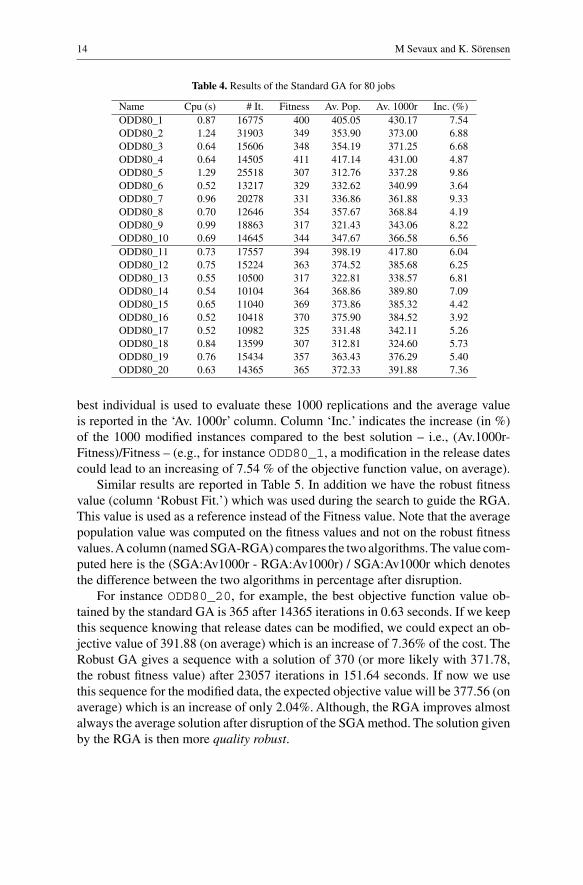
14 M Sevaux and K. Sörensen
Table 4. Results of the Standard GA for 80 jobs
Name Cpu (s) # It. Fitness Av. Pop. Av. 1000r Inc. (%)ODD80_1 0.87 16775 400 405.05 430.17 7.54ODD80_2 1.24 31903 349 353.90 373.00 6.88ODD80_3 0.64 15606 348 354.19 371.25 6.68ODD80_4 0.64 14505 411 417.14 431.00 4.87ODD80_5 1.29 25518 307 312.76 337.28 9.86ODD80_6 0.52 13217 329 332.62 340.99 3.64ODD80_7 0.96 20278 331 336.86 361.88 9.33ODD80_8 0.70 12646 354 357.67 368.84 4.19ODD80_9 0.99 18863 317 321.43 343.06 8.22ODD80_10 0.69 14645 344 347.67 366.58 6.56ODD80_11 0.73 17557 394 398.19 417.80 6.04ODD80_12 0.75 15224 363 374.52 385.68 6.25ODD80_13 0.55 10500 317 322.81 338.57 6.81ODD80_14 0.54 10104 364 368.86 389.80 7.09ODD80_15 0.65 11040 369 373.86 385.32 4.42ODD80_16 0.52 10418 370 375.90 384.52 3.92ODD80_17 0.52 10982 325 331.48 342.11 5.26ODD80_18 0.84 13599 307 312.81 324.60 5.73ODD80_19 0.76 15434 357 363.43 376.29 5.40ODD80_20 0.63 14365 365 372.33 391.88 7.36
best individual is used to evaluate these 1000 replications and the average valueis reported in the ‘Av. 1000r’ column. Column ‘Inc.’ indicates the increase (in %)of the 1000 modified instances compared to the best solution – i.e., (Av.1000r-Fitness)/Fitness – (e.g., for instance ODD80_1, a modification in the release datescould lead to an increasing of 7.54 % of the objective function value, on average).
Similar results are reported in Table 5. In addition we have the robust fitnessvalue (column ‘Robust Fit.’) which was used during the search to guide the RGA.This value is used as a reference instead of the Fitness value. Note that the averagepopulation value was computed on the fitness values and not on the robust fitnessvalues.A column (named SGA-RGA) compares the two algorithms. The value com-puted here is the (SGA:Av1000r - RGA:Av1000r) / SGA:Av1000r which denotesthe difference between the two algorithms in percentage after disruption.
For instance ODD80_20, for example, the best objective function value ob-tained by the standard GA is 365 after 14365 iterations in 0.63 seconds. If we keepthis sequence knowing that release dates can be modified, we could expect an ob-jective value of 391.88 (on average) which is an increase of 7.36% of the cost. TheRobust GA gives a sequence with a solution of 370 (or more likely with 371.78,the robust fitness value) after 23057 iterations in 151.64 seconds. If now we usethis sequence for the modified data, the expected objective value will be 377.56 (onaverage) which is an increase of only 2.04%. Although, the RGA improves almostalways the average solution after disruption of the SGA method. The solution givenby the RGA is then more quality robust.

A genetic algorithm for robust schedules 15
Table 5. Results of the Robust GA for 80 jobs
Name Cpu (s) # It. Fitness Robust Fit. Av. Pop Av. 1000r Inc. (%) SGA-RGA (%)ODD80_1 158.33 22058 406 406.36 411.76 417.60 2.86 2.92ODD80_2 72.52 9956 357 358.91 361.90 366.73 2.72 1.68ODD80_3 108.76 15687 369 363.37 365.62 374.23 1.42 −0.80ODD80_4 152.49 20818 429 422.61 424.57 426.65 −0.55 1.01ODD80_5 224.35 29705 310 314.94 317.48 328.88 6.09 2.49ODD80_6 100.98 15109 327 328.24 335.24 335.49 2.60 1.61ODD80_7 147.44 20249 342 345.39 344.33 358.54 4.83 0.92ODD80_8 96.03 11853 358 360.67 363.67 365.09 1.98 1.02ODD80_9 120.26 14271 325 327.12 330.67 337.71 3.91 1.56ODD80_10 126.65 16910 353 355.95 359.57 358.47 1.55 2.21ODD80_11 119.67 15989 403 408.82 414.05 419.97 4.21 −0.52ODD80_12 94.76 13801 369 371.24 375.29 377.26 2.24 2.18ODD80_13 62.12 8559 341 333.90 337.33 340.49 −0.15 −0.57ODD80_14 85.73 12212 381 378.84 379.76 383.52 0.66 1.61ODD80_15 146.25 16869 373 377.04 382.81 378.48 1.47 1.78ODD80_16 106.09 14472 377 370.44 377.38 380.52 0.93 1.04ODD80_17 144.83 19637 329 329.30 332.00 333.23 1.28 2.60ODD80_18 120.86 15289 313 316.72 315.86 321.17 2.61 1.06ODD80_19 158.79 21159 364 363.40 363.81 368.20 1.16 2.15ODD80_20 151.64 23057 370 371.78 376.43 377.56 2.04 3.65
Table 6. Global SGA and RGA results (deviation and CPU time)
Number Gap to best solution Gap (in %) CPU time (s)of jobs Std GA (%) Rob GA (%) SGA-RGA Std GA Rob GA
20 11.95 3.84 2.88 0.03 1.7340 8.47 2.89 1.61 0.13 10.2760 7.35 3.08 0.89 0.36 45.8180 6.30 2.19 1.48 0.75 124.93100 5.32 2.01 0.47 1.53 215.69
Table 6 gives the summarised results for the whole set of instances from 20 to100 jobs. The columns “Gap to the best solution” indicates the average value inpercentage between the sequence found by any method and the results after the 1000replications of modified instances (e.g., for n = 80, the average value of column“Inc.” in Table 4 and 5). The middle column “Gap SGA-RGA” is the average valueof the column SGA-RGA of Table 5 and measures the improvement of the RGAover the SGA after disruption.
The results confirm that it is always better to take the stochastic nature of some ofthe data into account when determining a schedule. On average, modifications of theproblem data have a much smaller effect on the objective function value of solutionsfound by the RGA. However, since the computation of the robust evaluation functionrequires the ordinary evaluation function to be used 100 times, CPU times are muchlarger for the RGA. A possible strategy to lower the computational effort is to usethe robust evaluation function only when the standard evaluation of a solution is

16 M Sevaux and K. Sörensen
70
75
80
85
90
95
100
0 10 20 30 40 50 60
Rob
uste
valu
atio
nf
∗ (x)
Standard deviation σ∗(x)
Initial solutions
rs
rsrs
rsrs
rs
rs
rsrs
rs All solutions
+
+
++
+
++
++ ++ +
+
+ ++ ++ ++ +
+
+
++
++++
++
+ ++++
++
+ ++++ +
+
+ ++
+
+
++
++
+
+
+ ++
++
+ ++
++
+
+++ +
+++++ +
+++++
++
++
+ +++
++
++ ++
++++
++
+
++
+++
++ ++
+ ++++
+ +++
+
++++
+
+++
++++ + +
++
+
+++++
++ +
+++++ +
++++
++
++ +++
++ +
+
+ + ++
+ +++
++++
+
+++
+
+
++
++ +
+
+++ ++ +
++++++
++ +
++++
++++ ++
++ ++ ++
++
+ ++
+ ++ +++ +
+ ++
+ +++++
++
++
++++
+++
+ ++++
+ ++
+
+ +++++
++++ + +
+++
++ +++
++
+ ++
+
+++ ++
+++
++
+++
++ +
++ +
++ +
++++
++
++
+ +++
+
++++
+
+++
++++
+++++
++
+
+++++ ++
++
++ + ++ +
+++
++ ++
++++
++ + ++
+
++
++ +++++
+
++
++
++
+
++
++++ +++
++++ +++
++ +
+ +
+++
++++
++
++
++ +++
++++
++++
+
++
+++
+++
++
+
+++++ ++
++
++
++
+++
++++
++ +
+
++ +
++
++++
+ ++ ++++
+++++
++ +
++++
+
++++
+++ +++++
++ ++++
+
+++ ++ ++
+++ ++ ++
+++
+
+++
+ +++ +
+
+
+++++++++
++
++
++++
++
+
+ +++
++
++
++ +
++++++++++ + ++
+ +++++
+
+++
++++++
++ +++++++
++++
+
++
++ +++ +++
+ +++ ++
+ ++ ++
++
+ ++++++++
+++
+++
+++
++ ++++
+ +++
+++ ++++
+
++
++ ++
+ +++++++
++
++++ +
+ +++
+
++
+
+++
+
++ +++ +++
++ ++
++
++
+ ++ +++++ + + +++ ++++ +
+ + + ++
++
+
++
+++
+++ +++++ ++ ++
++ + + ++++
+++
+ +++ + + + ++
+
++
+++ ++ + +++++ +++
+
++++
+
+
+ + ++++++ +
+
+
+++
+ +++ +++
+
++
++
++
+
+ +
+
+ +++
+
+
+++ ++++ ++
+
++
+
++++ ++ ++ +++
++ + ++++ +
+++++
+++ + +++
+
+
Fig. 3. Standard deviation of the robust value – all solutions
better than a certain threshold. We did not implement such strategies here since thecomputational times recorded for the RGA are still very reasonable.
8 Helping the decision maker
8.1 Risk analysis
As mentioned in Sect. 5.3, choosing a robust solution is not an easy task and canbe done through a multiple objective decision making process. In Fig. 3, for a 20job instance, we plot all the solutions (including the initial solutions) in the space“Standard Deviation of the robust value / Robust Value”. The initial solutions arespread out in the space and all the other solutions seem to converge toward a goodrobust fitness value (to the bottom of the graph). At the same time, the standarddeviation of the solutions decreases meaning that the solution are more and morerobust. Figure 4 shows only the non-dominated solutions (Pareto solutions) thatcan be suggested to the decision maker.
8.2 Solution robustness
To obtain solutions that are solution robust, the edit distance between a base-linesolution and all the solutions found by the RGA is measured. We assume that the
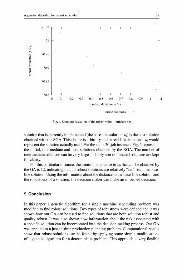
A genetic algorithm for robust schedules 17
70.8
70.85
70.9
70.95
71
71.05
0 0.1 0.2 0.3 0.4 0.5 0.6 0.7 0.8 0.9 1 1.1
Rob
uste
valu
atio
nf
∗ (x)
Standard deviation σ∗(x)
Pareto solutions
rs
rs
rs
rs
rs
rs
Fig. 4. Standard deviation of the robust value – efficient set
solution that is currently implemented (the base-line solution x0) is the best solutionobtained with the SGA. This choice is arbitrary and in real-life situations, x0 wouldrepresent the solution actually used. For the same 20-job instance, Fig. 5 representsthe initial, intermediate and final solutions obtained by the RGA. The number ofintermediate solutions can be very large and only non-dominated solutions are keptfor clarity.
For this particular instance, the minimum distance to x0 that can be obtained bythe GA is 12, indicating that all robust solutions are relatively “far” from the base-line solution. Using the information about the distance to the base-line solution andthe robustness of a solution, the decision maker can make an informed decision.
9 Conclusion
In this paper, a genetic algorithm for a single machine scheduling problem wasmodified to find robust solutions. Two types of robustness were defined and it wasshown how our GA can be used to find solutions that are both solution robust andquality robust. It was also shown how information about the risk associated witha specific solution can be incorporated into the decision making process. Our GAwas applied to a just-in-time production planning problem. Computational resultsshow that robust solutions can be found by applying some simple modificationsof a genetic algorithm for a deterministic problem. This approach is very flexible
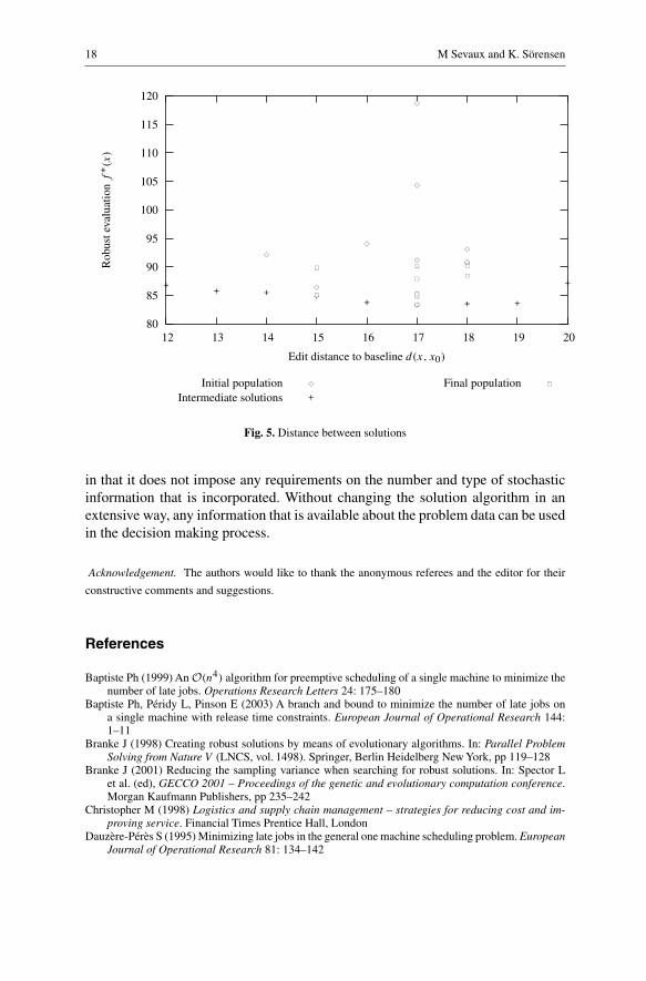
18 M Sevaux and K. Sörensen
80
85
90
95
100
105
110
115
120
12 13 14 15 16 17 18 19 20
Rob
uste
valu
atio
nf
∗ (x)
Edit distance to baseline d(x, x0)
Initial population
rs
rsrsrs
rs
rs
rs
rs
rs
rs
Intermediate solutions
++ + +
+ + + +
+
+Final population
rs
rsrs rs
rsrs
rs rs rs
rs
Fig. 5. Distance between solutions
in that it does not impose any requirements on the number and type of stochasticinformation that is incorporated. Without changing the solution algorithm in anextensive way, any information that is available about the problem data can be usedin the decision making process.
Acknowledgement. The authors would like to thank the anonymous referees and the editor for their
constructive comments and suggestions.
References
Baptiste Ph (1999) An O(n4) algorithm for preemptive scheduling of a single machine to minimize thenumber of late jobs. Operations Research Letters 24: 175–180
Baptiste Ph, Péridy L, Pinson E (2003) A branch and bound to minimize the number of late jobs ona single machine with release time constraints. European Journal of Operational Research 144:1–11
Branke J (1998) Creating robust solutions by means of evolutionary algorithms. In: Parallel ProblemSolving from Nature V (LNCS, vol. 1498). Springer, Berlin Heidelberg New York, pp 119–128
Branke J (2001) Reducing the sampling variance when searching for robust solutions. In: Spector Let al. (ed), GECCO 2001 – Proceedings of the genetic and evolutionary computation conference.Morgan Kaufmann Publishers, pp 235–242
Christopher M (1998) Logistics and supply chain management – strategies for reducing cost and im-proving service. Financial Times Prentice Hall, London
Dauzère-Pérès S (1995) Minimizing late jobs in the general one machine scheduling problem. EuropeanJournal of Operational Research 81: 134–142
A genetic algorithm for robust schedules 19
Dauzère-Pérès S, Sevaux M (2003) Using lagrangean relaxation to minimize the weighted number oflate jobs. Naval Research Logistics 50 (3): 273–288
Dauzère-Pérès S, Sevaux M (2001) An exact method to minimize the number of late jobs in singlemachine scheduling. Technical report, Ecole des Mines de Nantes, France, submitted
Davenport AJ, Beck JC (2000) A survey of techniques for scheduling with uncertainty. Unpubl.manuscript
Goldberg DE (1989)Genetic algorithms in search, optimization andmachine learning.Addison Wesley,♣ ((insert publ.’s place))
Hart E, Ross P (1999a) The evolution and analysis of a potential antibody library for job-shop scheduling.In: Corne D, Dorigo M, Glover F (eds) New ideas in optimization. London, McGraw Hill, pp 185–202
Hart E, Ross P (1999b) An immune system approach to scheduling in changing environments. In:GECCO 99. Proceedings of the genetic and evolutionary computation conference. Morgan Kauf-mann publishers, ♣, pp 1559–1566
Herroelen W, Leus R (2002) Project scheduling under uncertainty – survey and research potentials.Invited paper to be published in the special issue of EJOR containing selected papers from PMS2002
Holland JH (1975)Adaptation in natural and artificial systems. Technical report, University of Michigan,Ann Arbor
Jensen MT Robust and flexible scheduling with evolutionary computation. PhD thesis, University ofAarhus, Dept. of Computer Science, Denmark
Kouvelis P, Yu G (1997) Robust discrete optimisation and its applications. (Nonconvex Optimizationand its Applications, vol. 14). Kluwer Academic Publishers, Dordrecht
Lenstra JK, Rinnooy Kan AHG , Brucker P (1977) Complexity of machine scheduling problems.Annalsof Discrete Mathematics 1: 343–362
LeonVJ,Wu SD, Storer RH (1993) Robust scheduling and game-theoretic control for short-term schedul-ing of job-shops. In: Fandel G, Gulledge T, Jones A (eds) Operations research in production plan-ning and control. Springer, Berlin Heidelberg New York, pp 321–335
Leon VJ, Wu SD, Storer RH (1994a) A game-theoretic control approach for job shops in the presenceof disruptions. International Journal of Production Research 32 (6): 1451–1476
Leon VJ, Wu SD, Storer RH (1994b) Robustness measures and robust scheduling for job shops. IIETransactions 26: 32–43
Levenshtein VI (1966) Binary codes capable of correcting deletions, insertions, and reversals. SovietPhysics – Doklady 10: 707–710
Portmann MC (1996) Genetic algorithm and scheduling: a state of the art and some propositions. In:Proceedings of the workshop on production planning and control. Mons, Belgium, pp I–XIV
Reeves CR (ed) (1993) Modern heuristic techniques for combinatorial problems. Wiley, New YorkReeves CR (1997) Genetic algorithms for the operations researcher. Informs Journal on Computing 9
(3): 231–250Sevaux M, Dauzère-Pérès S (2002) Genetic algorithms to minimize the weighted number of late jobs
on a single machine. European Journal of Operational Research (forthcoming)Sörensen K (2001) Tabu searching for robust solutions. In: Proceedings of the 4th metaheuristics
international conference. Porto, Portugal, pp 707–712Tsutsui S (1999) A comparative study on the effects of adding perturbations to phenotypic parameters
in genetic algorithms with a robust solution searching scheme. In: Proceedings of the 1999 IEEEsystems, man, and cybernetics conference (SMC’99 Tokyo). pp III–585–591
Tsutsui S, Ghosh A (1997) Genetic algorithms with a robust solution searching scheme. IEEE Transac-tions on Evolutionary Computation 1: 201–208
Tsutsui S, Ghosh A, Fujimoto Y (1996) A robust solution searching scheme in genetic search. In: VoigtHM, Ebeling W, Rechenberg I, Schwefel HP (eds) Parallel problem solving from nature – PPSNIV, vol. 10. Springer, Berlin Heidelberg New York, pp 543–552,
Tsutsui S, Jain JC (1998) Properties of robust solution searching in multi-dimensional space with geneticalgorithms. In: Proceedings of the 2nd International Conference on knowledge-based electronicsystems (KES-98).
Ukkonen E (1985) Finding approximate patterns in strings. Journal of Algorithms 6: 132–137Wagner RA, Fischer MJ (1974) The string-to-string correction problem. Journal of theACM 21: 168–173

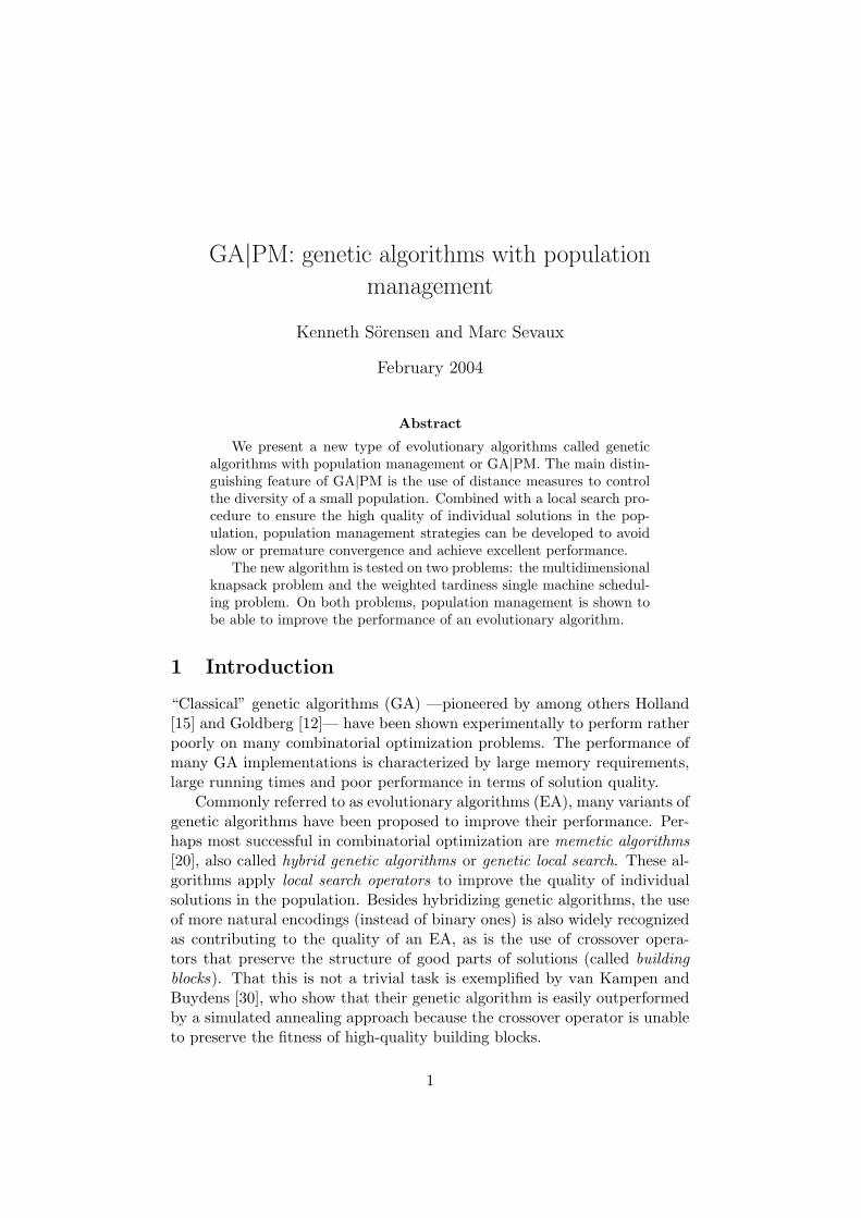
GA|PM: genetic algorithms with population
management
Kenneth Sorensen and Marc Sevaux
February 2004
Abstract
We present a new type of evolutionary algorithms called geneticalgorithms with population management or GA|PM. The main distin-guishing feature of GA|PM is the use of distance measures to controlthe diversity of a small population. Combined with a local search pro-cedure to ensure the high quality of individual solutions in the pop-ulation, population management strategies can be developed to avoidslow or premature convergence and achieve excellent performance.
The new algorithm is tested on two problems: the multidimensionalknapsack problem and the weighted tardiness single machine schedul-ing problem. On both problems, population management is shown tobe able to improve the performance of an evolutionary algorithm.
1 Introduction
“Classical” genetic algorithms (GA) —pioneered by among others Holland[15] and Goldberg [12]— have been shown experimentally to perform ratherpoorly on many combinatorial optimization problems. The performance ofmany GA implementations is characterized by large memory requirements,large running times and poor performance in terms of solution quality.
Commonly referred to as evolutionary algorithms (EA), many variants ofgenetic algorithms have been proposed to improve their performance. Per-haps most successful in combinatorial optimization are memetic algorithms[20], also called hybrid genetic algorithms or genetic local search. These al-gorithms apply local search operators to improve the quality of individualsolutions in the population. Besides hybridizing genetic algorithms, the useof more natural encodings (instead of binary ones) is also widely recognizedas contributing to the quality of an EA, as is the use of crossover opera-tors that preserve the structure of good parts of solutions (called buildingblocks). That this is not a trivial task is exemplified by van Kampen andBuydens [30], who show that their genetic algorithm is easily outperformedby a simulated annealing approach because the crossover operator is unableto preserve the fitness of high-quality building blocks.
1

Nevertheless, even EA with all these improvements may still fall victimto either slow or premature convergence. Many researchers agree that thequality of a metaheuristic optimization approach is largely a result of theinterplay between intensification and diversification strategies (see e.g. Fer-land et al. [7], Laguna et al. [16]). One of the main motivations for thispaper is the observation that the design of evolutionary algorithms makesit particularly difficult to control the balance between intensification anddiversification. As Hertz and Widmer [14] point out, preserving the diver-sity of the population of an evolutionary algorithm is necessary. AlthoughEA have the operators to increase or decrease the diversity of the popula-tion, most lack the means to control this diversification. On the one hand,crossover and mutation operators tend to diversify the population by intro-ducing new or recombining existing genetic material. As a result of too muchdiversification, some EA exhibit extremely slow convergence. On the otherhand, the hybridization (local search) operators tend to focus the search inspecific regions. This may even lead to so-called premature convergence: atotal loss of diversity in the population.
This problem is tackled by a new class of evolutionary algorithms that wepropose: GA|PM or genetic algorithms with population management [28].Population management works by measuring and controlling the diversity ofa small population of high-quality solutions, and makes ample use of distancemeasures. The distance measure to use depends on the representation of asolution. For binary problems, the Hamming distance can be used. Forpermutation problems, several distance measures have been proposed in theliterature, e.g. [2, 25, 26]. The distance measures used in this paper arebased on the edit distance (see e.g. Wagner and Fischer [31]), that is wellknown and easily adaptable to a large number of combinatorial problems[27].
Working with a small population (Greistorfer and Voß [13] call it a pool)is an idea that is incorporated in a number of metaheuristic approaches, buta common framework for creating and maintaining such a population has notyet been established. Scatter search and path relinking [9] are approachesthat work by combining solutions from a small set of high-quality (calledelite) solutions. As mentioned, memetic algorithms [20] combine geneticalgorithms with local search to obtain a small population of high- qualitysolutions. Some work on standard genetic algorithms using a small popula-tion is due to Reeves [23].
GA|PM show some resemblance to memetic algorithms [20] but theydiffer from them in that GA|PM use population management. Other ap-proaches that use a small population of high quality solutions include scattersearch and path relinking [9]. GA|PM offer the advantage of being closerto classical EA in terms of algorithm structure and therefore considerablyeasier to implement. The use of distance measure for GA design has beenproposed for maintaining a diverse population [19] or to locate a set of dif-
2
ferent solutions of a multimodal problem such as in crowding [18] or fitnesssharing [11]. GA|PM differ from these approaches in that they maintain asmall population of locally improved solutions and use adaptive populationmanagement strategies.
The rest of this paper is structured as follows. Section 2 describes the ba-sic structure of a GA|PM and discusses how distance measures can be usedto control the diversity of a population. Some possible population manage-ment strategies are also discussed. In section 3, the algorithm is tested on themultidimensional knapsack problem and the total weighted tardiness single-machine scheduling problems. For both problems, we compare the GA|PMto a hybrid evolutionary algorithm without population management. Al-though the population management improves the performance of the EAin a big way in both cases, we should remark that the main goal of theseapplications was to show the effectiveness of population management, notto create solution methods that could compete with the best-performingapproaches. That GA|PM can be used to create first-class optimizationmethods, is currently being shown in ongoing research. In Sorensen [28], aGA|PM for the vehicle routing problem (VRP) is shown to produce resultscompetitive to the best-known approaches. In Prins et al. [22], a GA|PMis developed for the capacitated arc routing problem (CARP). To date, thisGA|PM is the best-known approach for this problem.
2 GA|PM
This section describes the new genetic algorithm with population manage-ment. Its main distinguishing features are
• a small population (typically 10 to 30 solutions),
• a local improvement operator (e.g. a local search, or simple tabu searchprocedure),
• population management to control the diversity of the population.
2.1 Algorithm overview
A genetic algorithm with population management is structured much like astandard genetic algorithm, but differs in the use of population managementand local search. An outline is given in algorithm 1.
Initially, a small population is built randomly or using initial heuristics.From this population, two parent solutions are selected and subjected to thecrossover operator, forming one or two new offspring solutions. These solu-tions are improved by a local search operator and added to the population,after being subjected to population management.
3

Algorithm 1 GA|PM outline
1: initialize population P2: set population diversity parameter ∆3: repeat
4: select: p1 and p2 from P5: crossover: p1 ⊗ p2 → o1, o2
6: local search: improve o1 and o2
7: for each offspring o do
8: while o does not satisfy conditions for addition (input function)do
9: mutate o10: end while
11: remove solution: P ← P\b12: add solution: P ← P ∪ o13: end for
14: update diversity parameter ∆15: until stopping criterion satisfied
2.2 Population management
Population management controls the diversity of a small population of high-quality solutions. It uses an input function that determines whether anoffspring solution is added to the population or not. In GA|PM, this inputfunction takes the following two factors into account:
• the quality of the solution, and
• the diversity of the population after addition of the solution, or —inother words— the contribution that the solution makes to the diversityof the population; this is measured as the “distance” of the solutionto the population, see section 2.2.2.
2.2.1 Distance measures
To evaluate whether a candidate solution sufficiently diversifies the popula-tion, a distance measure d is used that determines for each pair of solutionstheir relative distance (or similarity). The distance should be measuredin the solution space and not —as is commonly done— in the objectivefunction space. Distance measures cannot be developed independent of theproblem or even the representation (encoding) of the solution. For binaryrepresentations, the Hamming distance can be used. For solutions that areencoded as vectors of real numbers, some form of the Minkowsky-r-distance1
1d(~x, ~y) =
nX
i=1
|xi − xj |r
! 1
r
4
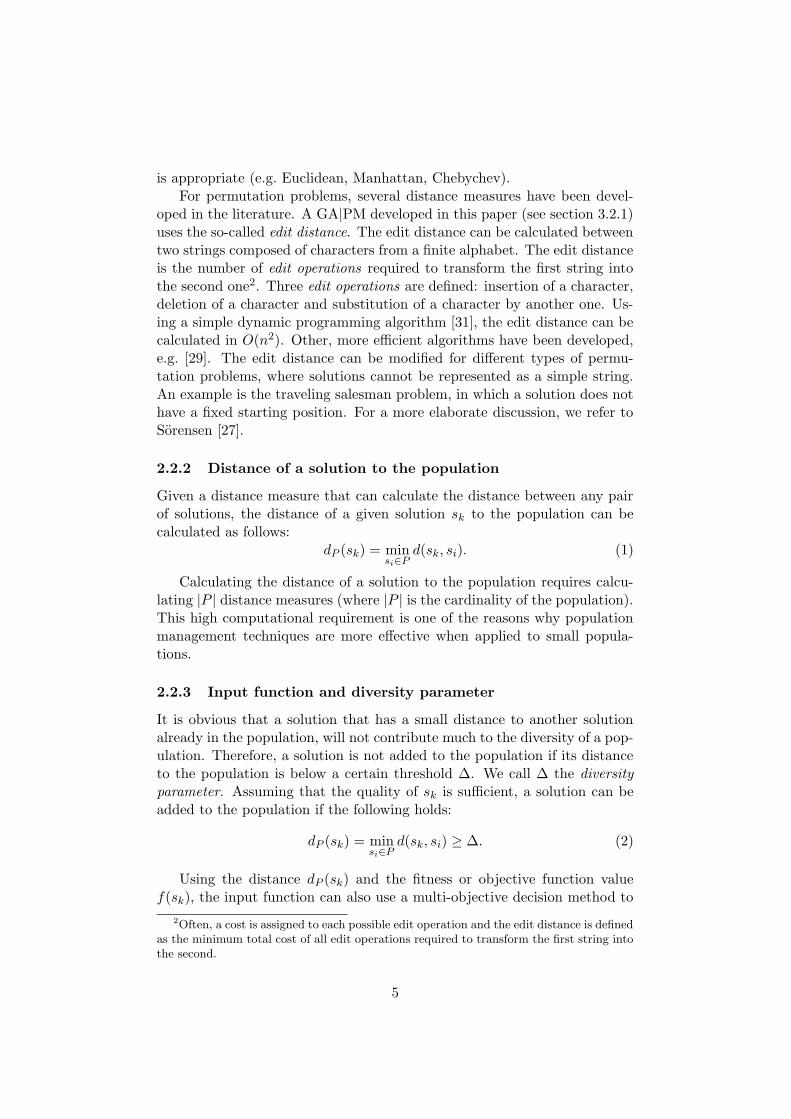
is appropriate (e.g. Euclidean, Manhattan, Chebychev).For permutation problems, several distance measures have been devel-
oped in the literature. A GA|PM developed in this paper (see section 3.2.1)uses the so-called edit distance. The edit distance can be calculated betweentwo strings composed of characters from a finite alphabet. The edit distanceis the number of edit operations required to transform the first string intothe second one2. Three edit operations are defined: insertion of a character,deletion of a character and substitution of a character by another one. Us-ing a simple dynamic programming algorithm [31], the edit distance can becalculated in O(n2). Other, more efficient algorithms have been developed,e.g. [29]. The edit distance can be modified for different types of permu-tation problems, where solutions cannot be represented as a simple string.An example is the traveling salesman problem, in which a solution does nothave a fixed starting position. For a more elaborate discussion, we refer toSorensen [27].
2.2.2 Distance of a solution to the population
Given a distance measure that can calculate the distance between any pairof solutions, the distance of a given solution sk to the population can becalculated as follows:
dP (sk) = minsi∈P
d(sk, si). (1)
Calculating the distance of a solution to the population requires calcu-lating |P | distance measures (where |P | is the cardinality of the population).This high computational requirement is one of the reasons why populationmanagement techniques are more effective when applied to small popula-tions.
2.2.3 Input function and diversity parameter
It is obvious that a solution that has a small distance to another solutionalready in the population, will not contribute much to the diversity of a pop-ulation. Therefore, a solution is not added to the population if its distanceto the population is below a certain threshold ∆. We call ∆ the diversityparameter. Assuming that the quality of sk is sufficient, a solution can beadded to the population if the following holds:
dP (sk) = minsi∈P
d(sk, si) ≥ ∆. (2)
Using the distance dP (sk) and the fitness or objective function valuef(sk), the input function can also use a multi-objective decision method to
2Often, a cost is assigned to each possible edit operation and the edit distance is definedas the minimum total cost of all edit operations required to transform the first string intothe second.
5

determine whether sk should be added to the population or not. A verysimple way of doing this (assuming that f should be minimized) is to calcu-late f(sk) + λdP (sk). If this value does not exceed a certain threshold, thesolution is added, otherwise it is discarded. λ is a parameter that determinesthe relative importance of the diversity with respect to the solution quality.Of course, more elaborate multi-objective decision methods can be used.
If the local search procedure is effective enough to always ensure thequality of solutions it produces, a solution can be added if eq. (2) holds,without taking the objective function value of the solution into account.
As shown in algorithm 1, a solution that does not have a sufficiently largedistance to the population, is randomly mutated until it does. Of course,other strategies are possible, such as simply discarding the solution.
2.2.4 Population management strategies
Using the diversity parameter ∆, the diversity of the population can becontrolled as higher values for ∆ will increase the diversity of the populationwhile lower values will decrease it. A high value of ∆ will allow only solutionsthat have a large distance to all solutions in the population and will lead—perhaps after a few iterations— to a population that consists of verydifferent solutions. A low value of ∆ will allow solutions in the populationthat are relatively similar to solutions already in the population. This willresult in a less diverse population.
Several population management strategies can be proposed, using onlythe diversity parameter ∆. The following lists several potential strategies inincreasing order of complexity.
Strategy 1: ∆ is set to a constant level. This strategy prevents populationconvergence, and introduces a constant level of diversification into thepopulation.
Strategy 2: ∆ is set to a high level in the beginning of the algorithm.The value of ∆ is decreased steadily throughout the working of thealgorithm, allowing increased intensification near the end of the run.
Strategy 3: A closely related alternative strategy is to create a few goodsolutions (low ∆) in the beginning of the algorithm and allow morediversification near the end. A variant of this strategy is used in theexperiments.
Strategy 4: ∆ is set to a high level in the beginning of the algorithm. Itis steadily decreased as better solutions are found. When no improve-ment of the best solution is found for a set number of iterations, thediversity is increased by increasing ∆, thus introducing new geneticmaterial in the population. After this, ∆ is steadily decreased again,
6
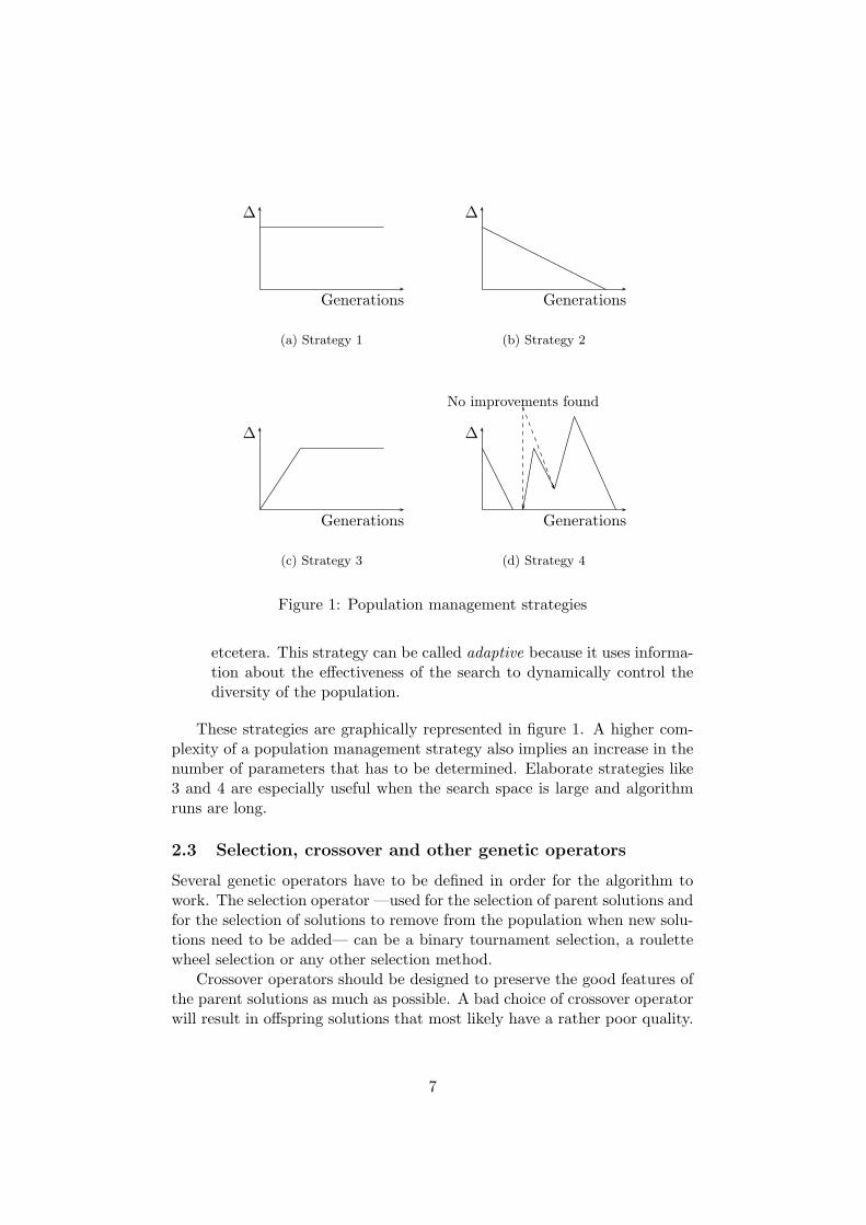
Generations
∆
(a) Strategy 1
Generations
∆
(b) Strategy 2
Generations
∆
(c) Strategy 3
Generations
∆
No improvements found
(d) Strategy 4
Figure 1: Population management strategies
etcetera. This strategy can be called adaptive because it uses informa-tion about the effectiveness of the search to dynamically control thediversity of the population.
These strategies are graphically represented in figure 1. A higher com-plexity of a population management strategy also implies an increase in thenumber of parameters that has to be determined. Elaborate strategies like3 and 4 are especially useful when the search space is large and algorithmruns are long.
2.3 Selection, crossover and other genetic operators
Several genetic operators have to be defined in order for the algorithm towork. The selection operator —used for the selection of parent solutions andfor the selection of solutions to remove from the population when new solu-tions need to be added— can be a binary tournament selection, a roulettewheel selection or any other selection method.
Crossover operators should be designed to preserve the good features ofthe parent solutions as much as possible. A bad choice of crossover operatorwill result in offspring solutions that most likely have a rather poor quality.
7

For the design of efficient selection and crossover operators, we refer tothe specialized literature. See e.g. Reeves [24] for a discussion.
2.4 Intensification
A local search procedure is necessary to maintain a population of high-quality solutions. This local search procedure should be able to quicklyimprove the quality of a solution produced by the crossover operator, with-out diversifying it into other regions of the search space. Neighbourhood-search methods like simple tabu search approaches are particularly usefulfor this purpose.
3 Experiments
In this section, we apply the principles of GA|PM to two problems: themultidimensional knapsack problem and the total weighted tardiness sin-gle machine scheduling problem. We should note that in none of the twoproblems, it is our intention to compete with the best approaches in theliterature as this would involve developing specialized crossover operatorsand advanced local search operators and would distract the attention fromthe main point: the population management of GA|PM. Instead, we fo-cus on the population management and compare the GA|PM we develop tocomparable EA that lack population management.
3.1 The multidimensional knapsack problem
The NP-hard 0/1 multidimensional knapsack problem (MKP01) is a pure0/1 integer programming problem. Given a set of n items each having anassociated profit ci, the objective of this problem is to select the subset ofitems that maximizes the total profit, while satisfying a set of knapsackconstraints. For each knapsack j, each item i has a given weight aij and thesum of the weights of the chosen items is not allowed to exceed the knapsackcapacity bj . More formally, the MKP01 can be stated as follows:
max
n∑
i=1
cixi
s.t.m∑
i=1
aijxi ≤ bj ∀j ∈ [1,m]
xi ∈ 0, 1 ∀i ∈ [1, n]
(3)
Several approaches have been proposed for this problem, including ge-netic algorithms [3] and tabu search [6, 10].
8
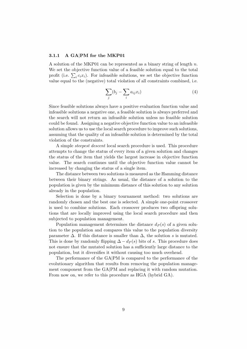
3.1.1 A GA|PM for the MKP01
A solution of the MKP01 can be represented as a binary string of length n.We set the objective function value of a feasible solution equal to the totalprofit (i.e.
∑i cixi). For infeasible solutions, we set the objective function
value equal to the (negative) total violation of all constraints combined, i.e.
∑
j
(bj −∑
i
aijxi) (4)
Since feasible solutions always have a positive evaluation function value andinfeasible solutions a negative one, a feasible solution is always preferred andthe search will not return an infeasible solution unless no feasible solutioncould be found. Assigning a negative objective function value to an infeasiblesolution allows us to use the local search procedure to improve such solutions,assuming that the quality of an infeasible solution is determined by the totalviolation of the constraints.
A simple steepest descent local search procedure is used. This procedureattempts to change the status of every item of a given solution and changesthe status of the item that yields the largest increase in objective functionvalue. The search continues until the objective function value cannot beincreased by changing the status of a single item.
The distance between two solutions is measured as the Hamming distancebetween their binary strings. As usual, the distance of a solution to thepopulation is given by the minimum distance of this solution to any solutionalready in the population.
Selection is done by a binary tournament method: two solutions arerandomly chosen and the best one is selected. A simple one-point crossoveris used to combine solutions. Each crossover produces two offspring solu-tions that are locally improved using the local search procedure and thensubjected to population management.
Population management determines the distance dP (s) of a given solu-tion to the population and compares this value to the population diversityparameter ∆. If this distance is smaller than ∆, the solution s is mutated.This is done by randomly flipping ∆− dP (s) bits of s. This procedure doesnot ensure that the mutated solution has a sufficiently large distance to thepopulation, but it diversifies it without causing too much overhead.
The performance of the GA|PM is compared to the performance of theevolutionary algorithm that results from removing the population manage-ment component from the GA|PM and replacing it with random mutation.From now on, we refer to this procedure as HGA (hybrid GA).
9

3.1.2 Experiments
The GA|PM is tested on 48 well-known test problems available from the ORlibrary3.
A first experiment uses the simplest population management for theGA|PM, i.e. ∆ = 1. A second experiment uses more advanced populationmanagement (a variant of strategy 3 in figure 1) with
∆ =current iteration
maximum iterations×n
5,
where n is the number of items. This strategy sets ∆ to 0 in the beginningof the algorithm and linearly increases it to a maximum of n/5.
A population of 10 is used in all experiments. The HGA uses a 10%random mutation rate. Each algorithm is awarded 10000 generations tofind the optimal solution. Time is measured when the optimal solution isfound or at the end of the 10000 generations when it is not found. Eachexperiment is repeated 5 times.
3.1.3 Numerical comparison
Results show that the GA|PM outperforms the HGA. The average qualityover the 5 runs of the solutions produced by the GA|PM is better in allcases. In 46 out of 55 cases (84%), the worst solution found by the GA|PMis better than the best solution found by the HGA. More detailed resultscan be found in table 1.
Nr. opt. Min. 1 opt. Avg. it. Avg. CPU
GA|PM strategy 1 3.84 87.27% 3537 6.43GA|PM strategy 3 3.73 92.59% 3879 10.00
HGA 0.51 25.45% 9206 9.38
Table 1: Comparison GA|PM and HGA for the multidimensional knapsackproblem
This table should be read as follows. “Nr. opt.” is the average numberof times the optimal solution was found over the 5 runs, “Min. 1 opt.” is theaverage percentage of instances for which the optimal solution was found atleast in one of the 5 runs, “Avg. it.” is the average number of iterations,and “Avg. CPU (s)” is the average time required in seconds.
As can be seen, the GA|PM performs much better than the HGA withoutpopulation management. The average time per iteration is somewhat higher,but the solutions found are much better and the GA|PM therefore performsless iterations. The more advanced population management increases theaverage number of iterations required and also the average CPU time. It
3http://www.ms.ic.ac.uk/jeb/pub/mknap2.txt
10

does however improve the robustness of the algorithm in that the optimalsolution is now found in over 92% of the problem instances.
3.2 The total weighted tardiness single machine scheduling
problem
A set of n jobs has to be sequenced on a single machine. Preemption is notallowed. Jobs are not available before a release date rj and are processedfor pj units of time. For each job, a due date dj and a weight wj is given.If Cj denotes the completion time of job j, the tardiness is defined by Tj =max(0, Cj − dj). The objective is to minimize the total weighted tardiness(1|rj |
∑wjTj). This problem is NP-Hard in a strong sense.
The total weighted tardiness problem with release dates is probably oneof the most difficult one machine scheduling problem. If all the weights areequal to one (1|rj |
∑Tj) the problem is NP-Hard in a strong sense [8]. For
different weights and the release dates all equal to zero (1| |∑
wjTj), theproblem is also NP-Hard in a strong sense [17].
Recent approaches on the 1| |∑
wjTj problem are proposed in the lit-erature. In [5], a comparison between simulated annealing, tabu search andgenetic algorithms is discussed and in [4] the iterated dynasearch algorithmis presented and shown to yield the best solutions. Results are reported inthe OR-Library. A recent constraint-based approach [1] can solve probleminstances with up to 40 jobs.
3.2.1 A GA|PM for the total weighted tardiness problem
In this section, we develop a simple GA|PM for the total weighted tardi-ness problem and compare it to a similar hybrid GA that lacks populationmanagement. To perform a fair comparison between the two approaches,common components are used for the HGA and GA|PM algorithms.
The selection process used is a binary tournament selection, the crossoveroperator is the standard LOX operator [21] and the mutation operator is theGPI (general pairwise interchange). The local search procedure is also basedon the GPI and a steepest descent algorithm is applied. The algorithm isstopped after 60 seconds of CPU time.
For the numerical experiments, we use a variation of strategy 3. Thedistance measure used is the edit distance discussed in section 2.2.1. In theimplementation, ∆ is measured in percentage (result of the distance measuredivided by the maximum distance value). At the initialization step, ∆ isfixed to 1%. Every 15 iterations, ∆ is multiplied by a growth factor (1.05).When an upper limit of 50% is reached, ∆ is not increased anymore, sincethis would not allow the algorithm to find a new solution that is acceptedduring the search.
11

In the HGA, not all solutions are subjected to local search as this almostalways induces premature convergence. Instead, the local search rate pls isset to 10%, the mutation rate pm is fixed to 10%. The size of the populationis set to 25. For the GA|PM, the size of the population is only 10 individuals.
3.2.2 Numerical comparison
Results are reported in different tables. Table 2 summarizes the resultsfor the ODD instances (these instances can be obtained by email request).Optimal solutions are not known for this set. The first column indicates theset of instances (ODD20 is the ODD instances with 20 jobs), the followingthree columns provides the results for the GA|PMmethod and the next threecolumns, the results for the HGA method. Note that for a fair comparison,the same amount of time (60s) has been given to the GA|PM and the HGA.
GAPM results HGA resultsSet of First Avg. gap Avg. First Avg. gap Avg.inst. pos. (in %) iter. pos. (in %) iter.
ODD20 0 0.000 32375 0 0.000 952757ODD40 0 0.000 4142 0 0.000 258526ODD60 6 0.088 1685 1 0.251 88106ODD80 6 0.003 1153 1 0.083 39040ODD100 8 0.064 844 4 0.118 19854
Global 20 0.057 8040 6 0.148 271657
Table 2: Numerical results for ODD instances, CPU time = 60s
For each of the methods, the first column gives the number of timesthe method reports the best solution (among the two methods), the secondcolumn is the average deviation from the best solution. The last columngives the average number of iterations done in 60 seconds.
The OR-Library instances are generated for the 1| |∑
wjTj problem andcan be solved by our approach. Optimal values of solutions are available for124 and 115 out of 125 of the 40 and 50 job problem instances, respectively.When the optimal solution is unknown, best solutions provided by [5] areused instead (by extension they are also called optimal solutions).
12

ORLib40 results
Method Opt. First Avg. Gap Iterationsused sol. pos. (in %) Avg. Max
GAPM 125 4 0.000 5682 8961HGA 121 0 0.284 327763 470984
ORLib50 results
Method Opt. First Av. Gap Iterationsused sol. pos. (in %) Aver. Max
GAPM 123 11 0.002 3334 5298HGA 113 0 0.595 196024 287802
ORLib100 results
Method Best. First Av. Gap Iterationsused sol. pos. (in %) Aver. Max
GAPM 94 27 0.276 1030 1480HGA 85 16 2.110 34164 56521
Table 3: Numerical results for OR-Library instances, CPU time = 60s
In table 3 the column “Opt. sol.” (“Best sol.” for 100 job instances)counts the number of times the algorithm find the optimal solution (or bestknown). The rest of the columns is identical to the previous table exceptthat the deviation is measured from the optimal solution. The maximumnumber of iterations is added too. Again, the same amount of time has beenallocated to the two methods for a fair comparison.
These results show that the GA|PM approach performs better than theHGA approach, even though it operates on a smaller population. For theOR-Library instances, more optimal solutions are found and the approachis ranked first in more cases. Moreover, the deviation from the optimal (orbest known) solution is always smaller with the proposed method. Whenwe use the same stopping conditions (fixed number of iterations withoutimprovement of the best solution) the difference between the two algorithmsis even greater, but the GA|PM requires more time.
4 Conclusions
It is commonly known that the performance of an evolutionary algorithm(and any metaheuristic) on a hard combinatorial optimization problem de-pends in a big way on the balance between intensification and diversification.Although all evolutionary algorithms possess the necessary operators for in-tensification and diversification, many EA implementations lack a mecha-nism to control the balance between these two factors. This paper intro-duced a new class of evolutionary algorithms, GA|PM or genetic algorithmswith population management, that addresses this issue. GA|PM are hy-brid evolutionary algorithms that —like scatter search— operate on a smallpopulation of high-quality individuals. The main distinguishing feature of
13
a GA|PM is the application of population management strategies to controlthe diversity of the population. We discussed how such strategies can beeasily implemented by controlling the value of only a single parameter, thepopulation diversity parameter ∆.
The proposed approach was tested by applying it to two different com-binatorial problems: the multidimensional knapsack problem (a pure 0/1integer programming problem) and the total weighted tardiness single ma-chine scheduling problem, a difficult permutation problem. We discussedthat different problems require different distance measures and proposedto use the edit distance for permutation problems. For binary problems,the Hamming distance was used. Numerical comparison showed that theGA|PM outperformed very similar hybrid genetic algorithms without pop-ulation management (but with random mutation instead).
References
[1] P. Baptiste, A. Jouglet, and J. Carlier. A branch-and-bound procedureto minimize total tardiness on one machine with arbitrary release dates.European Journal of Operational Research, 2004. To appear.
[2] V. Campos, M. Laguna, and R. Martı. Context-independent scatter andtabu search for permutation problems. INFORMS Journal on Comput-ing, to appear, 2003. URL http://leeds.colorado.edu/Faculty/
Laguna/publications.htm.
[3] P.C. Chu and J.E. Beasley. A genetic algorithm for the multidimen-sional knapsack problem. Journal of Heuristic, 4:63–86, 1998.
[4] R. Congram, C.N. Potts, and S. van de Velde. An iterated dynasearchalgorithm for the single-machine total weighted tardiness schedulignproblem. Informs journal on computing, 14(1):52–67, 2002.
[5] H.A.J. Crauwels, C.N. Potts, and L.N. Van Wassenhove. Local searchheuristics for the single machine total weighted tardiness schedulingproblem. Informs Journal of Computing, 10(3):341–350, 1998.
[6] F. Dammeyer and S. Voß. Dynamic tabu list management using thereverse elimination method. Annals of Operations Research, 41:31–46,1993.
[7] J.A. Ferland, S. Ichoua, A. Lavoie, and E. Gagne. Scheduling using tabusearch methods with intensification and diversification. Computers andOperations Research, 28:1075–1092, 2001.
[8] M.R. Garey and D.S. Johnson. Computers and intractability: a guideto theory of np-completeness. Freeman, San Franscisco, USA, 1979.
14

[9] F. Glover. A template for scatter search and path relinking. In J.-K. Hao, E. Lutton, E. Ronald, M. Schoenauer, and D. Snyers, editors,Artificial Evolution, volume 1363 of Lecture Notes in Computer Science,pages 13–54, Springer, Berlin, 1998.
[10] F. Glover and G.A. Kochenberger. Critical event tabu search for themultidimensional knapsack problem. In I.H. Osman and J.P. Kelly,editors, Metaheuristics: The Theory and Applications, pages 407–427.Kluwer Academic Publishers, Boston, 1996.
[11] D. Goldberg. Genetic algorithms with sharing for multimodal functionoptimization. In Proceedings of the Second International Conference onGenetic Algorithms, pages 41–49, 1987.
[12] D.E. Goldberg. Genetic Algorithms in search, Optimization and Ma-chine Learning. Addison Wesley, 1989.
[13] P. Greistorfer and S. Voß. Controlled pool maintenance in combinato-rial optimization. In C. Rego and B. Alidaee, editors, Adaptive Memoryand Evolution: Tabu Search and Scatter Search. Kluwer Academic Pub-lishers, Boston, To appear.
[14] A. Hertz and M. Widmer. Guidelines for the use of meta-heuristics incombinatorial optimization. European Journal of Operational Research,151(2):247–252, 2003.
[15] J.H. Holland. Adaptation in natural and artificial systems. Technicalreport, University of Michigan, Ann Arbor, 1975.
[16] M. Laguna, R. Martı, and V. Campos. Intensification and diversifica-tion with elite tabu search solutions for the linear ordering problem.Computers and Operations Research, 26:1217–1230, 1999.
[17] E.L. Lawler. A ’pseudo-polynomial’ algorithm for sequencing jobs tominimize total tardiness. Annals of Discrete Mathematics, 1:331–342,1977.
[18] S.W. Mahfoud. Crowding and preselection revisited. In R. Manner andB. Manderick, editors, Parallel Problem Solving from Nature, pages 27–36, Elsevier, Amsterdam, 1992.
[19] M. Mauldin. Maintaining diversity in genetic search. In Proceedings ofthe National Conference on Artificial Intelligence, pages 247–250, 1984.
[20] P. Moscato. On evolution, search, optimization, genetic algorithms andmartial arts: Towards memetic algorithms. Technical Report C3P 826,Caltech Concurrent Computation Program, 1989.
15

[21] M-C. Portmann. Genetic algorithm and scheduling: a state of the artand some propositions. In Proceedings of the workshop on productionplanning and control, pages I–XIV, Mons, Belgium, 1996.
[22] C. Prins, M. Sevaux, and K. Srensen. A genetic algorithm with pop-ulation management for the CARP. In Proceedings of TRISTAN V,Guadaloupe, 2004.
[23] C.R. Reeves. Using genetic algorithms with small populations. InS. Forrest, editor, Proceedings of the 5th International Conference onGenetic Algorithms, pages 92–99, Morgan Kaufman, San Mateo, 1993.Morgan Kaufmann.
[24] C.R. Reeves. Genetic algorithms for the operations researcher. IN-FORMS Journal on Computing, 9:231–250, 1997.
[25] S. Ronald. Distance functions for order-based encodings. In D. Fogel,editor, Proceedings of the IEEE Conference on Evolutionary Computa-tion, pages 641–646, IEEE Press, New York, 1997.
[26] S. Ronald. More distance functions for order-based encodings. In Pro-ceedings of the IEEE Conference on Evolutionary Computation, pages558–563, IEEE Press, New York, 1998.
[27] K. Sorensen. Distance measures based on the edit distance forpermutation-type representations. In A. Barry, editor, Proceedings ofthe Workshop on Analysis and Design of Representations and Operators(ADoRo), GECCO Conference, pages 15–21, Chicago, 2003.
[28] K. Sorensen. A framework for robust and flexible optimisation usingmetaheuristics with applications in supply chain design. PhD thesis,University of Antwerp, 2003.
[29] E. Ukkonen. Finding approximate patterns in strings. Journal of Al-gorithms, 6:132–137, 1985.
[30] A.H.C. van Kampen and L.M.C. Buydens. The ineffectiveness of recom-bination in a genetic algorithm for the structure elucidation of a hep-tapetide in torsion angle space. A comparison to simulated annealing.Chemometrics and Intelligent Laboratory Systems, 36:141–152, 1997.
[31] R.A. Wagner and M.J. Fischer. The string-to-string correction problem.Journal of the Association for Computing Machinery, 21:168–173, 1974.
16

A genetic algorithm for a
bi-objective capacitated arc routing problem
P. Lacomme1, C. Prins2 and M. Sevaux3∗
1Universite Blaise Pascal, LIMOS, Campus Universitaire des Cezeaux, BP 10125, F-63177 Aubiere Cedex, France
2Universite de Technologie de Troyes, LOSI, 12 Rue Marie Curie, BP 2060, F-10010 Troyes Cedex, France
3Universite de Valenciennes, LAMIH/SP, Le Mont Houy, F-59313 Valenciennes Cedex 9, France
June 2003
Abstract
The Capacitated Arc Routing Problem (CARP) is a very hard vehicle routing problemfor which the objective – in its classical form – is the minimisation of the total cost ofthe routes. In addition, one can seek to minimize also the cost of the longest trip. Inthis paper, a multi-objective genetic algorithm is presented for this more realistic CARP.Inspired by the second version of the Non-dominated Sorted Genetic Algorithm frame-work (NSGA-II), the procedure is improved by using good constructive heuristics to seedthe initial population and by including a local search procedure. The new framework andits different flavours are appraised on three sets of classical CARP instances comprising81 files. Yet designed for a bi-objective problem, the best versions are competitive withstate-of-the-art metaheuristics for the single objective CARP, both in terms of solutionquality and computational efficiency: indeed, they retrieve a majority of proven optimaand improve two best-known solutions.
Keywords: Capacitated Arc Routing Problem; Multi-objective optimization; Meta-heuristic; Genetic algorithm.
1 Introduction: the CARP and its bi-objective version
The Capacitated Arc Routing Problem (CARP) in its undirected version is defined as follows.Let G = (V, E) be an undirected graph with a set V of n nodes and a set E of m edges. Afleet of identical vehicles of capacity W is based at a depot node s. The number of vehiclesis either fixed or left as a decision variable. A subset of τ edges, denoted as required edgesor tasks, require service by a vehicle. All edges can be traversed any number of times. Eachedge (i, j) has a traversal cost cij and a demand qij . All costs and demands are integers. Thegoal is to determine a set of vehicle trips (routes) of minimum total cost, such that each tripstarts and ends at the depot, each required edge is serviced by one single trip, and the totaldemand handled by any vehicle does not exceed W .
∗Corresponding author. Tel: +33-327-51-1326, fax: +33-327-51-1310.E-mail address: [email protected] (M. Sevaux)
1

Since the CARP is NP-hard, large scale instances must be solved in practice with heuris-tics. Among fast constructive methods, one can cite for instance Path-Scanning [1], Augment-Merge [2] and Ulusoy’s splitting technique [3]. Available metaheuristics include tabu searchalgorithms [4,5], a tabu search combined with scatter search components [6], a variable neigh-borhood search [7], a guided local search [8], and hybrid genetic algorithms [9, 10]. All theseheuristics can be evaluated thanks to tight lower bounds [11,12].
CARP problems are raised by operations on street networks, e.g. urban waste collection,snow plowing, sweeping, gritting, etc. Economically speaking, the most important applicationcertainly is municipal refuse collection. In that case, nodes in G correspond to crossroads,while edges in E model street segments that connect crossroads. The demands are amountsof waste to be collected. The costs correspond either to distances or durations.
The single objective CARP only deals with minimizing the total cost of the trips. In fact,most waste management companies are also interested in balancing the trips. For instance,in Troyes (France), all trucks leave the depot at 6 am and waste collection must be completedas soon as possible to assign the crews to other tasks, e.g. sorting the waste at a recyclingfacility. Hence, the company wishes to solve a bi-objective version of the CARP, in whichboth the total duration of the trips and the duration of the longest trip (corresponding tothe makespan in scheduling theory) are to be minimized. A multiobjective genetic algorithm(MOGA) for this bi-objective CARP is investigated in this paper which extends preliminaryresults presented at the EMO 2003 conference [13]. As the two objectives are conflicting, thefleet size (equal to the number of trips) is not imposed, in order to get smaller makespanvalues. This is not a problem because fleet size is naturally bounded above by τ (when eachtrip contains one single task).
For a complete introduction to multi-objective optimisation, we refer the reader to a recentannotated bibliography [18] which provides a suitable entry point for general definitions andgood references. Concerning the MOGAs, two books are entirely devoted to these algorithms[19,20].
In the last decade, there has been a growing interest in multi-objective vehicle routing,but all published papers deal with node routing problems, e.g. [14–17]. Moreover, apart fromthe total cost of the trips, they only consider additional objectives such as minimizing timewindow violations or balancing vehicle loads, but not makespan. To the best of our knowledge,this paper presents the first study devoted to a multi-objective arc routing problem and withone objective related to the makespan. It is organized as follows. Section 2 recalls a generalframework of multi-objective genetic algorithm, called NSGA-II, and describes how to adapt itfor the bi-objective CARP. The inclusion of a local search procedure is discussed in Section 3.Numerical experiments are conducted in Section 4. Section 5 brings some concluding remarks.
2 A genetic algorithm for the bi-objective CARP
Today, several MOGA frameworks are available in literature and selecting the best one for agiven MOOP is not obvious. A recent survey [21] and two comparative studies [22,23] try toprovide guidelines for selection but these papers consider unconstrained problems, continuousobjective functions, and specific sets of benchmarks. It is very difficult to draw conclusionsfor constrained combinatorial optimization problems.
Our choice for the bi-objective CARP finally turned to a MOGA framework called NSGA-II (Non-Dominated Sorting GA) and designed by Deb [20,24]. The reasons are: a) its modular
2

and flexible structure, b) the possibility of upgrading a single-objective GA to NSGA-II(the encoding of chromosomes and crossover operators can be recycled) and c) its successfulapplications to a wide range of problems. The first subsection is necessary to introduce thenon-trivial framework of NSGA-II, while correcting minor bugs and typos from [20,24]. Theadaptation to the bi-objective CARP is described in the second subsection.
2.1 The NSGA-II framework
Non-dominated sorting algorithm The NSGA-II algorithm computes successive genera-tions on a population of solutions partitioned into non-dominated fronts. The non-dominatedset is identified and constitutes the non-dominated front of level 1 or front 1. This set istemporarily disregarded from the population. The non-dominated set of the remaining popu-lation gives the non-dominated front of level 2, and so on. This process called non-dominatedsorting is repeated until the partition is complete, see the left part of Figure 1 for an example.
rank 1
rank 2
rank 3
rank 4
f1 f1
f2 f2
R(1)
R(k+1)
R(k)R(k−1)
R(nr)
Figure 1: Non-dominated sorting (left) and crowding distances (right)
The method is detailed in Algorithm 1. The population is implemented as a table pop ofns solutions and pop(i) denotes the ith solution. The partition is a vector front of ns lists ofsolutions indexes, i.e. i ∈ front(k) means that solution pop(i) is currently assigned to the frontof level k. Dominance between two solutions x and y is computed by the dom(x, y) booleanfunction. nb better(i) counts the solutions which dominate solution pop(i) and set worse(i)is the set of solutions dominated by pop(i).
The non-dominated sorting algorithm returns the number of fronts nf, the partitionfront(1), front(2), . . . , front(nf ) and a vector rank in which rank(i) denotes the index of thefront that stores solution pop(i). A first phase computes in O(nc ·ns2) nb better and set worsevalues, a second one in O(ns2) assigns solutions to their respective fronts and computes nfand rank. The overall complexity is then O(nc · ns2).
Crowded tournament operator In NSGA-II, each solution is assigned a fitness equal toits non-domination level (1 being the best level). Thus, minimization of the fitness is assumed.Each generation generates new solutions by selecting parent-solutions and applying crossoverand mutation operators. Each parent is selected using binary tournament : two solutions arerandomly selected from the population and the fittest one (with the smallest rank) is kept.
This classical selection technique is modified as follows in NSGA-II: when two solutionsbelong to the same front, the tournament prefers the most isolated one, using a crowdingdistance described below. The crowding distance margin(i) of a solution pop(i) is a kind of
3

Algorithm 1 procedure non dominated sort(pop,ns,front,nf,rank)
1: front(1) ← ∅2: for i ← 1 to ns do
3: nb better(i) ← 04: set worse(i) ← ∅5: for j ← 1 to ns do
6: if dom(pop(i),pop(j)) then
7: add j to set worse(i)8: else if dom(pop(j),pop(i)) then
9: nb better(i) ← nb better(i)+110: end if
11: end for
12: if nb better(i) = 0 then
13: add i to front(1)14: end if
15: end for
16: nf ← 117: loop
18: for all i in front(nf) do
19: rank(i) ← nf20: for all j in set worse(i) do
21: nb better(j) ← nb better(j)-122: if nb better(j) = 0 then
23: add j to front(nf+1)24: end if
25: end for
26: end for
27: exit when front(nf+1) = ∅28: nf ← nf+129: end loop
measure of the search space around it which is not occupied by any other solution in thepopulation. The winner of a tournament between two solutions pop(i) and pop(j) can thenbe computed thanks to a crowded tournament operator, implemented as a boolean functionbetter(i, j) which returns true if rank(i) < rank(j) or (rank(i) = rank(j)) and (margin(i) >margin(j)). The idea is to favor the best solutions, while keeping the fronts well scattered toprevent clusters of solutions.
To simplify, consider nc = 2 criteria like in the bi-objective CARP and a front R of nrsolutions. Let fmin
c and fmaxc be the minimum and maximum values of criterion fc in R,
c = 1, 2. Sort R in increasing values of the first criterion and let R(k) be the kth solution inthe sorted front. The crowding distance of R(k) is defined as follows for 1 < k < nr :
margin(R(k)) =f1(R(k) + 1)− f1(R(k)− 1)
fmax1− fmin
1
+f2(R(k)− 1)− f2(R(k) + 1)
fmax2− fmin
2
(1)
For k = 1 or k = nr , margin(R(k)) = ∞. The goal of this convention is to favour the
4

two extreme points of the front, to try to enlarge it. The right part of Figure 1 depicts thecomputation of margins. The margin of R(k) is nothing but half of the perimeter of therectangle indicated by dashed lines.
Generation of new solutions The computation of new solutions at each iteration ofNSGA-II can be implemented as a procedure add children, specified by Algorithm 2. Thevector rank computed by the non dominated sorting procedure and the vector of crowdingdistances margin are required for the crowded tournament operator. The procedure createsns offsprings which are added at the end of pop, thus doubling its size. Any crossover ormutation operator can be used, depending on the problem at hand.
Algorithm 2 procedure add children(pop,ns,rank,margin)
1: input ns ← ns2: for ns ← input ns to 2×input ns do
3: draw two distinct parents P1, P2 using the crowded tournament operator4: combine P1 and P2, using a crossover operator, to get one new solution S5: mutate S with a fixed probability6: pop(ns) ← S7: end for
NSGA-II overall structure The general structure of NSGA-II is given in Algorithm 3. Aninitial population pop of ns random solutions is built by the first pop procedure and sorted bynon-domination, using Algorithm 1. The procedure get margins computes for each solutionpop(i) its crowding distance margin(i). Then, each iteration of the main loop starts bycalling add children, to create ns children which are added at the end of pop, see Algorithm 2.Finally, the resulting population with 2 · ns solutions is reduced to a new population newpopby keeping the ns best solutions. To do this, fronts and margins must be updated, usingnon dominated sort and get margins. Starting from the front of level 1, complete fronts arethen transferred to newpop as long as possible. The first front front(i) which could not beaccomodated fully is truncated by keeping its most widely spread solutions. This is achievedby arranging its solutions in descending order of the crowding distance values, thanks to themargin sort procedure, and by copying the best solutions until newpop contains exactly nssolutions. Finally, pop receives the contents of newpop for the next iteration of the GA.
2.2 GA components for the bi-objective CARP
This section describes the required components to instanciate the NSGA-II framework forour bi-objective CARP. The representation of solutions as chromosomes and their evaluationcome from a GA [10] which is currently one of the most effective solution methods for thesingle objective CARP. Therefore, only a short description is provided here: the reader isinvited to refer to [9] or [10] for more details.
2.2.1 Chromosome representation and evaluation
A chromosome is an ordered list of the τ tasks, in which each task may appear as one of its twodirections. Implicit shortest paths are assumed between successive tasks. The chromosome
5

Algorithm 3 procedure nsga2()
1: first pop(pop,ns)2: non dominated sort(pop,ns,front,nf,rank)3: get margins(pop,ns,front,nf,margin)4: repeat
5: add children(pop,ns,rank,margin)6: non dominated sort(pop,ns,front,nf,rank)7: get margins(pop,ns,front,nf,margin)8: newpop ← ∅9: i ← 1
10: while |newpop|+|front(i)| ≤ ns do
11: add front(i) to newpop12: i ← i+113: end while
14: missing ← ns-|newpop|15: if missing 6= 0 then
16: margin sort(front,i,margin)17: for j ← 1 to missing do
18: add the j-th solution of front(i) to newpop19: end for
20: end if
21: pop ← newpop22: until stopping criterion
does not include trip delimiters and can be viewed as a giant tour for a vehicle with infinitecapacity. An O(τ 2) procedure Split described in [10] is used to derive a least total costCARP solution (subject to the given sequence), by splitting the chromosome (giant tour)into capacity-feasible tours. This technique is based on the computation of a shortest path inan auxiliary graph, in which each arc models one possible feasible tour that can be extractedfrom the giant tour. The makespan (second objective) corresponds to the maximum durationof the trips computed by Split.
In practice, each chromosome is stored in pop as a record with three fields: the sequence oftasks and the values computed by Split for the total cost and the makespan. The associatedsolution with its detailed trips is not stored because it is required only at the end of the GA,to print the results. It can be extracted at that time by calling Split again.
Following GA terminology, each of our chromosomes represents the genotype of a solution,i.e. one abstraction of a solution instead of the solution itself. The actual solution (phenotype)is materialized by a evaluation/decoding procedure, here Split. The reader may be surprisedby the priority given by Split to the total cost over the makespan. Indeed, it is possible toadapt Split to minimize makespan [10] or even to minimize total cost, subject to an upperbound on the makespan. In fact, all these evaluations are pertinent because they returna non-dominated solution among the possible interpretations of the same chromosome. Anexample of non-pertinent evaluation is to scan the chromosome, starting from the first task,and to create a new trip each time the current task does not fit vehicle capacity. Clearly, suchan evaluation “wastes” the chromosome because it is dominated by Split.
A version of Split that minimizes total cost was adopted because no good rule is available
6
to choose amongst pertinent evaluations. Giving priority in that way to the total cost hasno negative impact on the overall performance of the GA. Indeed, the aim of a decodingprocedure in general is to define a mapping from the set of chromosomes into the set ofsolutions and to assign reproducible values to the two objectives, but not to optimize in someway. Optimizing is the role of the search mechanism of the GA, with its selections that favourthe fittest parents for reproduction.
2.2.2 Initial population and clone management
Most published MOGAs start from an initial population pop made of ns random chromosomes,but including a few good solutions always accelerates the convergence. The procedure first popin Algorithm 3 uses three such solutions computed by classical CARP heuristics, namelyPath-Scanning [1], Augment-Merge [2] and Ulusoy’s heuristic [3]. Each heuristic solution isconverted into a chromosome by concatenating its trips. The chromosome is then re-evaluatedby Split because the resulting solution sometimes dominates the heuristic solution.
Although this is not part of the NSGA-II framework, a sufficient condition is used toprevent identical solutions (clones): in the initial population and in the subsequent iterationsof the GA, there can be at most one solution with two given values of the objectives, i.e. twosolutions cannot occupy the same point in the graphical representation of the fronts (rememberthat all costs are integers). This technique was included to avoid a progressive colonizationof the population by clones (typically 20 to 30% after 100 iterations).
2.2.3 Crossover operators
The advantage of chromosomes without trip delimiters is to allow the use of classical crossoversdesigned for permutation chromosomes, like the Linear Order Crossover (LOX) and the OrderCrossover (OX). Like the single-objective CARP studied in [10], the OX crossover gave thebest results after some preliminary testing. This crossover must be slightly adapted becausethe chromosomes are not exactly permutations: each required edge may appear as one of itstwo directions. Implementation details can be found in [10].
Hence, the crossover used in the add children procedure of Algorithm 2 is in fact OX.One of the two children is selected at random and is evaluated by Split. It is added to poponly if no solution exists with the same objective values, else it is discarded. Because of suchrejections, more than ns crossovers may be required to double the size of pop: the FOR loopof Algorithm 2 must be replaced by a REPEAT . . . UNTIL ns = 2× input ns.
2.2.4 Stopping conditions
There is no standard technique to define reliable stopping conditions for stopping a MOGA.In combinatorial optimization and in the single-objective case, metaheuristics can be stoppedafter a fixed number of iterations without improving the current best solution, or by using avariance criterion. The ways of extending these criteria to several objectives still raise endlessdiscussions in the MOO community. The underlying problem, discussed in the numericalexperiments of Section 4, is to define a pertinent comparison between the final sets of efficientsolutions computed by two different algorithms on the same instance. For this study, theMOGA is simply stopped after a fixed number of iterations. More sophisticated stoppingcriteria had no noticeable effect on the final results.
7

3 Local search procedures
In single-objective optimization, it is well known that a standard GA must be hybridizedwith a local search procedure to be able to compete with state-of-the-art metaheuristics liketabu search. Such GAs, called memetic algorithms by Moscato [25], have raised a growinginterest in the last decade: for instance, a dedicated conference (WOMA) is now entirelydevoted to them. Hybridization is still rarely used in multi-objective optimization, and onlya few authors like Jaszkiewicz [26] start investigating this area. Several difficulties are raised,for instance: a) the notion of local search must be clarified when several objectives must beoptimized, b) several locations are possible in the existing MOGA frameworks for calling alocal search, and c) the local search must not disturb the search mechanism of the MOGA, forinstance by concentrating the solutions into small clusters. This section describes the movesand the general structure of our local search procedure, the criteria used to accept a move,and the possible ways of integrating local search in the MOGA.
3.1 Moves tested and general structure
Our local search procedures work on the individual routes, not on the sequence of tasks definedby a chromosome. Hence, the input chromosome is first converted into a set of routes. Themoves include the removal of one or two consecutive tasks from a route, with reinsertion atanother position, and 2-opt moves. All moves may involve one or two routes and the twotraversal directions of an edge are tested in the reinsertions. Each iteration of the local searchscans all these moves in O(τ 2) to find the first improving move (the criteria for deciding ifthere is an improvement are discussed in the next subsection). The whole local search stopswhen no more improvement can be found. The trips are then concatenated into a chromosome(giant tour), which is reevaluated by Split.
3.2 Acceptance criteria for a move
Four acceptance criteria accept(S, S ′) were tested to accept a move that transforms the in-cumbent solution S into a neighbor solution S ′. This has lead to four local search procedurescalled LS1 to LS4. In what follows, f1(S) and f2(S) respectively denote the total cost andthe makespan of solution S and w1 is a real number in [0, 1].
LS1: accept(S, S ′) = f1(S′)− f1(S) < 0;
LS2: accept(S, S ′) = f2(S′)− f2(S) < 0;
LS3: accept(S, S ′) = ((f1(S′)− f1(S) ≤ 0) and (f2(S
′)− f2(S) < 0))or ((f1(S
′)− f1(S) < 0) and (f2(S′)− f2(S) ≤ 0));
LS4: accept(S, S ′) = w1 · (f1(S′)− f1(S)) + (1− w1) · (f2(S
′)− f2(S) < 0.
LS1 performs its descent on the total cost, LS2 on the makespan, while LS3 accepts thenew solution if and only if it dominates the current one. The last local search is a weightedsum method which scalarizes the two objectives into a single objective, by multiplying eachobjective by a user-supplied weight. In these four versions, no normalization of the objectivesis required because the total duration of the trips and the makespan are commensurable andof the same order of magnitude.
8
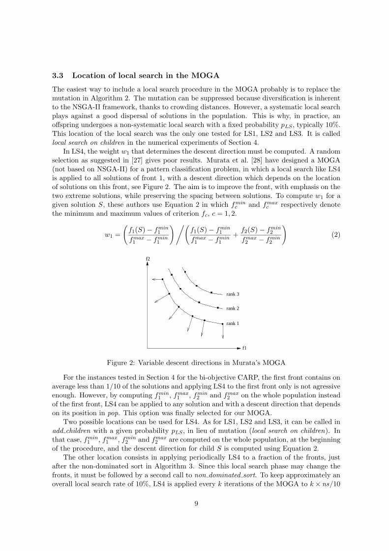
3.3 Location of local search in the MOGA
The easiest way to include a local search procedure in the MOGA probably is to replace themutation in Algorithm 2. The mutation can be suppressed because diversification is inherentto the NSGA-II framework, thanks to crowding distances. However, a systematic local searchplays against a good dispersal of solutions in the population. This is why, in practice, anoffspring undergoes a non-systematic local search with a fixed probability pLS , typically 10%.This location of the local search was the only one tested for LS1, LS2 and LS3. It is calledlocal search on children in the numerical experiments of Section 4.
In LS4, the weight w1 that determines the descent direction must be computed. A randomselection as suggested in [27] gives poor results. Murata et al. [28] have designed a MOGA(not based on NSGA-II) for a pattern classification problem, in which a local search like LS4is applied to all solutions of front 1, with a descent direction which depends on the locationof solutions on this front, see Figure 2. The aim is to improve the front, with emphasis on thetwo extreme solutions, while preserving the spacing between solutions. To compute w1 for agiven solution S, these authors use Equation 2 in which fmin
c and fmaxc respectively denote
the minimum and maximum values of criterion fc, c = 1, 2.
w1 =
(
f1(S)− fmin1
fmax1− fmin
1
)/(
f1(S)− fmin1
fmax1− fmin
1
+f2(S)− fmin
2
fmax2− fmin
2
)
(2)
rank 1
rank 2
rank 3
f1
f2
Figure 2: Variable descent directions in Murata’s MOGA
For the instances tested in Section 4 for the bi-objective CARP, the first front contains onaverage less than 1/10 of the solutions and applying LS4 to the first front only is not agressiveenough. However, by computing fmin
1 , fmax1 , fmin
2 and fmax2 on the whole population instead
of the first front, LS4 can be applied to any solution and with a descent direction that dependson its position in pop. This option was finally selected for our MOGA.
Two possible locations can be used for LS4. As for LS1, LS2 and LS3, it can be called inadd children with a given probability pLS , in lieu of mutation (local search on children). Inthat case, fmin
1 , fmax1 , fmin
2 and fmax2 are computed on the whole population, at the beginning
of the procedure, and the descent direction for child S is computed using Equation 2.The other location consists in applying periodically LS4 to a fraction of the fronts, just
after the non-dominated sort in Algorithm 3. Since this local search phase may change thefronts, it must be followed by a second call to non dominated sort. To keep approximately anoverall local search rate of 10%, LS4 is applied every k iterations of the MOGA to k× ns/10
9

solutions of pop, for instance 10% of solutions every iteration or 20% every two iterations. Infact, better results were obtained by applying LS4 to all solutions every k = 10 iterations,probably because of a better oscillation between diversification and intensification. We callthis way of including LS4 periodic local search.
4 Computational experiments
All developpements were done in Delphi 7 (Borland r©) and tested on a Pentium IV laptopcomputer clocked at 1.8 GHz under Windows 2000. The following subsections describe theinstances used, the MOGA versions selected, the evaluation criteria, the results, and twographical examples.
4.1 Instances tested
The computational evaluation is based on three sets of standard CARP instances which areused by most authors working on the single-objective CARP [4–12]. The first set correspondsto the 23 gdb files from Golden, DeArmon and Baker [1], with 7 to 27 nodes and 11 to 55edges, all required. The original set contains 25 files but two instances (gdb8 and gdb9) areinconsistent and never used. The second set gathers the 34 val files proposed by Belenguerand Benavent in [12], which have 24 to 50 nodes and 34 to 97 edges, all required. The lastset provides the 24 egl instances generated by Belenguer and Benavent [12], by perturbingthe demands in three rural networks supplied by Eglese. These egl files are bigger (77 to 140nodes, 98 to 190 edges) and in some instances not all edges are required. All these files canbe downloaded from the internet, at address http://www.uv.es/~belengue/carp.html.
4.2 Test protocol and parameters
A preliminary testing phase was required to fix the population size, the crossover (OX orLOX), the number of iterations and to evaluate the impact of good heuristic solutions in theinitial population. This has lead to the following features which are shared by all MOGAversions in the sequel: a population of ns = 60 solutions with three good initial solutions, theOX crossover and 100 to 200 iterations corresponding to 6,000 to 12,000 crossovers. Path-Scanning [1], Augment-Merge [2] and Ulusoy’s heuristic [3] were selected to provide goodinitial solutions. They can be discarded without changing the quality of final solutions, butin that case the MOGA converges more slowly, in 300 to 400 iterations.
A basic version of the MOGA without local search, called MO1, was selected as a referencealgorithm. Eight other versions listed in Table 1 were prepared for comparison. They differfrom MO1 by the number of iterations and the kind of local search.
4.3 Evaluation criteria
Comparing two different algorithms for solving the same problem is a central issue in multi-objective optimization, especially when the final choices of the decision maker are unknown.Several criteria were published, either to evaluate the quality of front 1 at the end of onegiven algorithm, or to provide a relative comparison between the final fronts computed bytwo algorithms.
10

Table 1: MOGA versions testedVersion Iterations LS type LS location
MO1 100 None IrrelevantMO2 100 1 On children, rate 10%MO3 100 2 On children, rate 10%MO4 100 3 On children, rate 10%MO5 200 3 On children, rate 10%MO6 100 4 On children, rate 10%MO7 200 4 On children, rate 10%MO8 100 4 Periodic, every 10 iterationsMO9 200 4 Periodic, every 10 iterations
This study uses a simple measure proposed by Riise [29] to compare two fronts. Givena front F to be evaluated and a reference front R (defined by MO1 in our case), a kind ofdistance is measured between each solution of F and its projection onto the extrapolatedreference front. This extrapolated front is a piecewise continuous line (in the bi-objectivecase) going through each solution and extended beyond the two extreme solutions, like inFigure 3. These distances are multiplied by −1 when the solution to compare is below theextrapolated front, like d4 in the figure. The proposed measure µ(F, R) is the sum of thesigned distances between the solutions of F and their respective projections on the referencefront, e.g. µ = d1 + d2 + d3 − d4 in the figure.
front to compare
reference front
extrapolatedfront
f1
f2
d3
d2
d1
d4
Figure 3: Examples of distances to the extrapolated front
Hence, for one given instance, a version of the MOGA with a final front F outperformsMO1 with its final front R if µ(F, R) < 0. Since µ depends on the number of solutions in F , anormalized measure µ(F, R) = µ(F, R)/|F | will be also used. The measure µ is a bit arbitraryand of course subject to criticism. For example, how can we measure the difference betweentwo fronts, when one is well spread while the other displays several gaps between clusters ofsolutions? Nevertheless, its merit is to exist and to help us rank the tested protocols. Becauseof no a-priori knowledge of the solutions which lie on the efficient front, such measures shouldbe completed by a visual inspection.
Very recently, some authors coming from the combinatorial optimization community like
11

Jaszkiewicz [27] have claimed that the authors of multi-objective metaheuristics should proveto be competitive to single objective metaheuristics in terms of quality of solutions andcomputational efficiency. Since several metaheuristics are available for the single objectiveCARP [4–10], they can be used to evaluate the total cost of the leftmost solution of front 1,thus completing the measures µ and µ. Two metaheuristics were selected for that purpose inour computational evaluation: CARPET, the most efficient tabu search algorithm, designedby Hertz et al. [5], and the memetic algorithm (MA) proposed by Lacomme et al. [10].
Our tables of results compare also the leftmost and rightmost solutions with two lowerbounds. The lower bound LB1 for the total cost is the one proposed by Belenguer andBenavent [12]. Concerning makespan, a trivial lower bound LB2 corresponds to the longesttrip, when each trip performs one single task: LB2 = max{Dsi + cij +Djs | [i, j] ∈ E}, wheres is the depot node and Dij the cost of a shortest path from node i to node j in G.
4.4 Results
4.4.1 Format of tables
For each set of benchmarks, the next subsections present one synthetic table with the resultsobtained by CARPET, the MA and each MOGA version, see Table 2 for instance. This tableindicates for each algorithm the following average values: the number of solutions in the finalset of non-dominated solutions F , the deviation Dev LB1 of the leftmost solution to the lowerbound on the total cost LB1, the number of times LB1 hits this bound is reached (numberof proven optima), the deviation Dev LB2 of the rightmost solution to the makespan lowerbound LB2, the number of proven optimal makespans LB2 hits, the measure µ for a referencefront provided by MO1, the normalized measure µ and the CPU time in seconds on a 1.8GHz Pentium-IV PC. For CARPET and the MA, the only applicable columns are Dev LB1,LB1 hits and the running time. These fields are in boldface when a MOGA is at least asgood as a single objective metaheuristic.
For each synthetic table, the results of the best MOGA version in terms of µ are listedinstance by instance in a detailed table given in the Appendix, see Table 5 for instance. Thethree first columns indicate the instance name, the number of nodes n and the number ofedges m. The number of tasks τ is cited only for egl files, because it is always equal to thenumber of edges in the other benchmarks. These columns are followed by the total cost andthe running time achieved by CARPET (listed in [5], except the egl files whose solution valuesare given in [12], but without running times) and by the memetic algorithm [10].
In order to have a fair comparison with the MOGAs, the solution values are given for thestandard setting of parameters of these metaheuristics and the running times are scaled forthe 1.8 GHz PC used in this study. The MA in [10] was executed on a 1 GHz Pentium-IIIPC and its running times are here multiplied by 0.555. CARPET was tested on a 195 MHzSilicon Graphics Indigo-2 workstation which is 5.43 times slower than the Pentium-III. Hence,the execution times provided by Hertz et al. are multiplied by 0.555/5.43 = 0.1022 in ourstudy. The best-known solution values (total cost) found by CARPET and the MA withvarious settings of parameters are given in the BKS column.
The eight remaining columns concern the MOGA: the number of efficient solutions |F |,
the total costs and makespans for the leftmost and rightmost solutions (f left1
, f left2
, f right1
and f right2
), the running time in seconds and the measures µ and µ. Each detailed table endswith three lines that provide for each column its average value (deviation to a bound, running
12
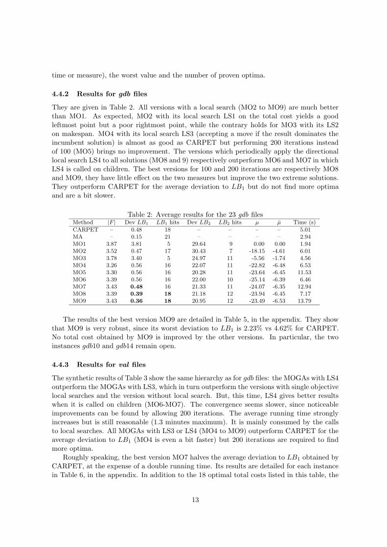
time or measure), the worst value and the number of proven optima.
4.4.2 Results for gdb files
They are given in Table 2. All versions with a local search (MO2 to MO9) are much betterthan MO1. As expected, MO2 with its local search LS1 on the total cost yields a goodleftmost point but a poor rightmost point, while the contrary holds for MO3 with its LS2on makespan. MO4 with its local search LS3 (accepting a move if the result dominates theincumbent solution) is almost as good as CARPET but performing 200 iterations insteadof 100 (MO5) brings no improvement. The versions which periodically apply the directionallocal search LS4 to all solutions (MO8 and 9) respectively outperform MO6 and MO7 in whichLS4 is called on children. The best versions for 100 and 200 iterations are respectively MO8and MO9, they have little effect on the two measures but improve the two extreme solutions.They outperform CARPET for the average deviation to LB1 but do not find more optimaand are a bit slower.
Table 2: Average results for the 23 gdb filesMethod |F | Dev LB1 LB1 hits Dev LB2 LB2 hits µ µ Time (s)
CARPET – 0.48 18 – – – – 5.01MA – 0.15 21 – – – – 2.94MO1 3.87 3.81 5 29.64 9 0.00 0.00 1.94MO2 3.52 0.47 17 30.43 7 -18.15 -4.61 6.01MO3 3.78 3.40 5 24.97 11 -5.56 -1.74 4.56MO4 3.26 0.56 16 22.07 11 -22.82 -6.48 6.53MO5 3.30 0.56 16 20.28 11 -23.64 -6.45 11.53MO6 3.39 0.56 16 22.00 10 -25.14 -6.39 6.46MO7 3.43 0.48 16 21.33 11 -24.07 -6.35 12.94MO8 3.39 0.39 18 21.18 12 -23.94 -6.45 7.17MO9 3.43 0.36 18 20.95 12 -23.49 -6.53 13.79
The results of the best version MO9 are detailed in Table 5, in the appendix. They showthat MO9 is very robust, since its worst deviation to LB1 is 2.23% vs 4.62% for CARPET.No total cost obtained by MO9 is improved by the other versions. In particular, the twoinstances gdb10 and gdb14 remain open.
4.4.3 Results for val files
The synthetic results of Table 3 show the same hierarchy as for gdb files: the MOGAs with LS4outperform the MOGAs with LS3, which in turn outperform the versions with single objectivelocal searches and the version without local search. But, this time, LS4 gives better resultswhen it is called on children (MO6-MO7). The convergence seems slower, since noticeableimprovements can be found by allowing 200 iterations. The average running time stronglyincreases but is still reasonable (1.3 minutes maximum). It is mainly consumed by the callsto local searches. All MOGAs with LS3 or LS4 (MO4 to MO9) outperform CARPET for theaverage deviation to LB1 (MO4 is even a bit faster) but 200 iterations are required to findmore optima.
Roughly speaking, the best version MO7 halves the average deviation to LB1 obtained byCARPET, at the expense of a double running time. Its results are detailed for each instancein Table 6, in the appendix. In addition to the 18 optimal total costs listed in this table, the
13

Table 3: Average results for the 34 val filesMethod |F | Dev LB1 LB1 hits Dev LB2 LB2 hits µ µ Time (s)
CARPET – 1.90 15 – – – – 35.48MA – 0.61 22 – – – – 21.31MO1 5.91 8.52 1 37.73 5 0.00 0.00 3.21MO2 4.76 1.23 17 32.06 5 -85.43 -16.18 27.80MO3 6.06 7.99 3 30.90 7 -7.33 -2.31 11.74MO4 4.88 1.36 15 21.65 8 -109.05 -20.87 32.50MO5 5.29 1.01 19 20.59 9 -125.98 -21.37 65.20MO6 5.00 1.16 15 21.50 10 -113.07 -21.30 38.20MO7 5.24 0.99 18 19.62 10 -121.70 -21.85 76.17MO8 5.09 1.33 16 20.19 10 -114.11 -20.61 44.53MO9 5.32 1.13 17 19.43 10 -124.03 -21.51 83.06
other versions have found optima for the following instances: val2b (259), val2c (457) andval10c (446). Moreover, they improve MO7 for val4d (536 vs 539), val5d (593 vs 595) andval9d (397 vs 399). Unfortunately, no open instance is broken and best-known solutions arenot improved.
4.4.4 Results for egl files
The lower bound LB1 proposed by Belenguer and Benavent is never tight on the egl files.This is why the number of optimal total costs is replaced in Table 4 by the number of best-known solutions retrieved or (in brackets) improved (column BKS ). All MOGAs except MO1and MO3 outperform CARPET in terms of average deviation to the lower bound on the totalcost and retrieve some best-known solutions (CARPET: 0). MO9 is even able to improvetwo best-known solutions, namely egl-e3-c (10349 vs 10369) and egl-s3-b (14004 vs 14028).Contrary to gdb and val files, the MOGAs reach the optimal makespan for a majority ofinstances and become faster than the memetic algorithm. In particular, the last MOGA findsall optimal makespans except one. Average running times are still acceptable: less than 5minutes. For the detailed results in appendix (Table 7), we preferred to select MO9 withthe lowest deviation to LB1 and its two improved instances, rather than MO5 which has aslightly better measure µ.
Table 4: Average results for the 24 egl filesMethod |F | Dev LB1 BKS Dev LB2 LB2 hits µ µ Time (s)
CARPET – 4.74 0 – – – – UnknownMA – 2.47 19 – – – – 292.77MOGA1 5.83 13.24 0(0) 1.87 15 0.00 0.00 2.77MOGA2 5.29 4.24 1(0) 0.94 16 -1234.01 -256.65 158.61MOGA3 6.67 13.32 0(0) 0.17 20 -63.93 -15.98 35.80MOGA4 5.21 4.47 0(0) 0.27 19 -1333.52 -335.11 148.50MOGA5 6.00 3.84 1(0) 0.10 21 -1586.62 -360.97 263.49MOGA6 5.33 4.47 1(0) 0.08 22 -1435.73 -324.27 153.48MOGA7 5.83 4.00 1(0) 0.07 22 -1573.80 -302.97 290.55MOGA8 5.96 4.11 1(0) 0.06 22 -1592.01 -344.66 159.01MOGA9 5.79 3.69 2(2) 0.05 23 -1531.94 -350.76 268.99
BKS gives the number of best-known solutions retrieved or (in brackets) improved by the MOGA.
14

4.5 Graphical examples
Graphical representations are well suited to visualize the behavior of bi-objective optimizationmethods. The kind of progression performed by our MOGAs is illustrated in Figure 4. Thegraphic represents in the objective space the random initial solutions (symbol +), the threegood heuristic solutions (symbol ×) and the final population (symbol +×) computed by MO9on the egl-e3-a instance (77 nodes, 98 edges and 87 tasks). Remember that MO9 is the versionwhich performs 200 iterations and applies LS4 to all solutions, every 10 iterations.
500
1000
1500
2000
2500
3000
3500
4000
6000 8000 10000 12000 14000 16000 18000 20000
Mak
espa
n
Total cost
Initial PopulationInitial heuristicsFinal population
Figure 4: Convergence of MO9 on instance egl-e3-a
One can notice that the initial heuristic solutions are already quite close to the finalpopulation. As already mentioned, adding such solutions is very useful to accelerate thesearch. Figure 5 provides a magnified representation of the final population. A dashed lineis used to emphasize efficient solutions.
The impact of the other key-component, the local search procedure, can be illustratedon the same instance by comparing the efficient set computed by the basic version MO1 (nolocal search, 100 iterations) with the one obtained by the best version MO9 (periodic localsearch LS4, 200 iterations). See Figure 5. Even if the total number of iterations is increasedfor MO1, the results are only slightly improved. As for single objective GAs, hybridizationwith local search is necessary to obtain efficient MOGAs. Here for instance, MO9 decreasesthe best total cost by 10.55% (from 6659 to 5956) and the best makespan by 10.97% (from921 to 820). Moreover, more efficient solutions are obtained and they are better spread, thusproviding the decision maker with a wider choice.
5 Concluding remarks
In industry, most decision makers wish to take several criteria into account and the bi-objectiveCARP addressed in this article is a typical example. The combinatorial optimization commu-nity can help research in multi-objective optimization, by bringing a rich toolbox, very efficientalgorithms, and a stricter methodology to evaluate and compare different algorithms.
15
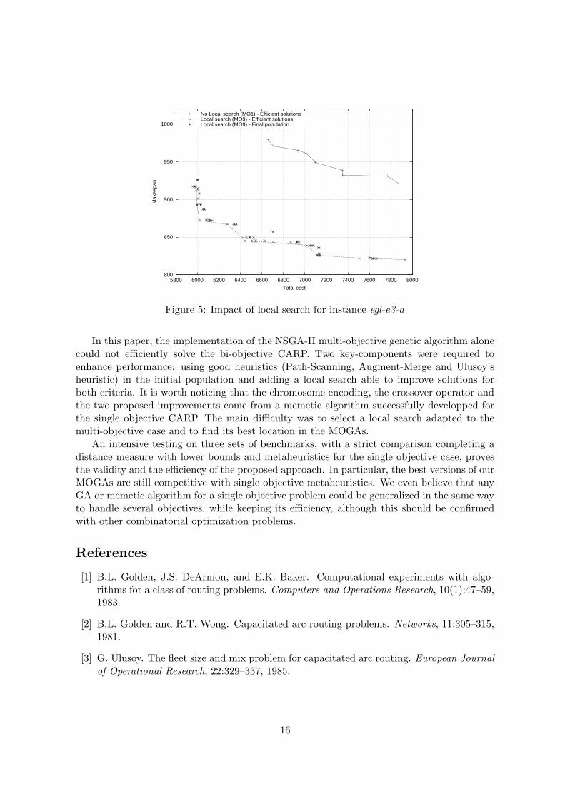
800
850
900
950
1000
5800 6000 6200 6400 6600 6800 7000 7200 7400 7600 7800 8000
Mak
espa
n
Total cost
No Local search (MO1) - Efficient solutionsLocal search (MO9) - Efficient solutionsLocal search (MO9) - Final population
Figure 5: Impact of local search for instance egl-e3-a
In this paper, the implementation of the NSGA-II multi-objective genetic algorithm alonecould not efficiently solve the bi-objective CARP. Two key-components were required toenhance performance: using good heuristics (Path-Scanning, Augment-Merge and Ulusoy’sheuristic) in the initial population and adding a local search able to improve solutions forboth criteria. It is worth noticing that the chromosome encoding, the crossover operator andthe two proposed improvements come from a memetic algorithm successfully developped forthe single objective CARP. The main difficulty was to select a local search adapted to themulti-objective case and to find its best location in the MOGAs.
An intensive testing on three sets of benchmarks, with a strict comparison completing adistance measure with lower bounds and metaheuristics for the single objective case, provesthe validity and the efficiency of the proposed approach. In particular, the best versions of ourMOGAs are still competitive with single objective metaheuristics. We even believe that anyGA or memetic algorithm for a single objective problem could be generalized in the same wayto handle several objectives, while keeping its efficiency, although this should be confirmedwith other combinatorial optimization problems.
References
[1] B.L. Golden, J.S. DeArmon, and E.K. Baker. Computational experiments with algo-rithms for a class of routing problems. Computers and Operations Research, 10(1):47–59,1983.
[2] B.L. Golden and R.T. Wong. Capacitated arc routing problems. Networks, 11:305–315,1981.
[3] G. Ulusoy. The fleet size and mix problem for capacitated arc routing. European Journalof Operational Research, 22:329–337, 1985.
16

[4] J.M. Belenguer, E. Benavent, and F. Cognata. Un metaheuristico para el problemade rutas por arcos con capacidades. In Proceedings of the 23th national SEIO meeting,Valencia, Spain, 1997.
[5] A. Hertz, G. Laporte, and M. Mittaz. A tabu search heuristic for the Capacitated ArcRouting Problem. Operations Research, 48(1):129–135, 2000.
[6] P. Greistorfer. A tabu-scatter search metaheuristic for the arc routing problem. Com-puters and Industrial Engineering, 44(2):249–266, 2003.
[7] A. Hertz and M. Mittaz. A variable neighborhood descent algorithm for the undirectedCapacitated Arc Routing Problem. Transportation Science, 35(4):425–434, 2001.
[8] P. Beullens, L. Muyldermans, D. Cattrysse, and D. Van Oudheusden. A guided localsearch heuristic for the Capacitated Arc Routing Problem. European Journal Of Opera-tional Research, 147(3):629–643, 2003.
[9] P. Lacomme, C. Prins, and W. Ramdane-Cherif. A genetic algorithm for the CapacitatedArc Routing Problem and its extensions. In E.J.W. Boers et al., editor, Applications ofevolutionnary computing, volume 2037 of Lecture Notes in Computer Science, pages 473–483. Springer, 2001.
[10] P. Lacomme, C. Prins, and W. Ramdane-Cherif. Competitive memetic algorithms forarc routing problems. Technical Report LOSI-2001-01, Laboratory for Industrial SystemsOptimization, Universite de Technologie de Troyes, France, 2001. To appear in Annalsof Operations Research.
[11] A. Amberg and S. Voß. A hierarchical relaxations lower bound for the Capacitated ArcRouting Problem. In R.H. Sprague (Hrsg.), editor, Proceedings of the 35th Annual HawaiiInternational Conference on Systems Sciences, pages DTIST02:1–10, Piscataway, 2002.IEEE.
[12] J.M. Belenguer and E. Benavent. A cutting plane algorithm for the Capacitated ArcRouting Problem. Computers and Operations Research, 30(5):705–728, 2003.
[13] P. Lacomme, C. Prins, and M. Sevaux. Multi-objective Capacitated Arc Routing Prob-lem. In C.M. Fonseca et al., editor, Evolutionary multi-criterion optimization (Proceed-ings of EMO 2003, Faro, Portugal), volume 2632 of Lecture Notes in Computer Science,pages 550–564. Springer, 2003.
[14] Y.B. Park and C.P. Koelling. An interactive computerized algorithm for multicriteriavehicle routing problems. Computers and Industrial Engineering, 16:477–490, 1989.
[15] A. Corberan, E. Fernandez, M. Laguna, and R. Martı. Heuristic solutions to the problemof routing school buses with multiple objectives. Journal of the Operational ResearchSociety, 53(4):427–435, 2002.
[16] S.C. Hong and Y.B. Park. A heuristic for bi-objective vehicle routing problem with timewindows constraints. International Journal of Production Economics, 62:249–258, 1999.
17

[17] W. Sessomboon, K. Watanabe, T. Irohara, and K. Yoshimoto. A study on multi-objectivevehicle routing problem considering customer satisfaction with due-time (the creation ofpareto optimal solutions by hybrid genetic algorithm). Transaction of the Japan Societyof Mechanical Engineers, 1998.
[18] M. Ehrgott and X. Gandibleux. Multiobjective Combinatorial Optimization, M. Ehrgottand X. Gandibleux (eds) , volume 52 of International Series in Operations Research andManagement Science, pages 369–444. Kluwer, 2002.
[19] C.A. Coello Coello, D.A. Van Veldhuizen, and G.B. Lamont. Evolutionary algorithmsfor solving multi-objective problems. Kluwer, New York, 2002.
[20] K. Deb. Multi-objective optimization using evolutionary algorithms. Wiley, Chichester,UK, 2001.
[21] C.A. Coello Coello. An updated survey of GA-based multiobjective optimization tech-niques. ACM Computing Surveys, 32(2):109–143, 2000.
[22] K. Deb. Multi-objective genetic algorithms: problem difficulties and construction of testproblems. Evolutionary Computation, 7(3):205–230, 1999.
[23] E. Zitzler, K. Deb, and L. Thiele. Comparison of multiobjective evolutionary algorithms:empirical results. Evolutionary Computation, 8(2):173–195, 2000.
[24] K. Deb, A. Pratap, S. Agarwal, and T. Meyarivan. A fast and elitist multi-objective ge-netic algorithm: NSGA-II. IEEE Transactions on Evolutionary Computation, 6(2):182–197, 2002.
[25] P. Moscato. New ideas in optimization D. Corne, M. Dorigo and F. Glover (eds), chapterMemetic algorithms: a short introduction, pages 219–234. McGraw-Hill, Maidenhead,UK, 1999.
[26] A. Jaszkiewicz. Genetic local search for multiple objective combinatorial optimization.European Journal of Operational Research, 137(1):50–71, 2001.
[27] A. Jaszkiewicz. Do multiple objective metaheuristics deliver on their promises? a com-putational experiment on the set covering problem. IEEE Transactions on EvolutionaryComputation, 7(2):133–143, 2003.
[28] T. Murata, H. Nozawa, H. Ishibuchi, and M. Gen. Modification of local search direc-tions for non-dominated solutions in cellular multiobjective genetic algorithms for patternclassification problems. In C.M. Fonseca et al., editor, Evolutionary multi-criterion op-timization (Proceedings of EMO 2003, Faro, Portugal), volume 2632 of Lecture Notes inComputer Science, pages 593–607. Springer, 2003.
[29] A. Riise. Comparing genetic algorithms and tabu search for multi-objective optimization.In Abstract conference proceedings, page 29, Edinburgh, UK, July 2002. IFORS.
18
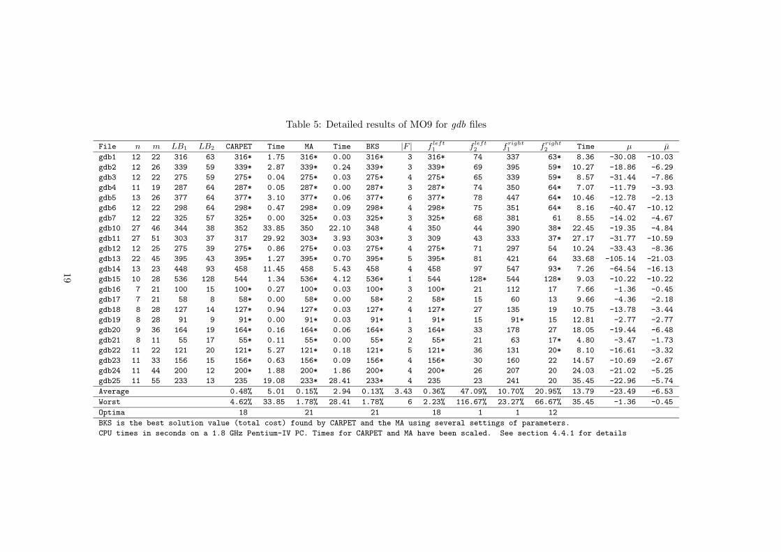
Table 5: Detailed results of MO9 for gdb files
File n m LB1 LB2 CARPET Time MA Time BKS |F | fleft1
fleft2
fright1
fright2
Time µ µ
gdb1 12 22 316 63 316* 1.75 316* 0.00 316* 3 316* 74 337 63* 8.36 -30.08 -10.03
gdb2 12 26 339 59 339* 2.87 339* 0.24 339* 3 339* 69 395 59* 10.27 -18.86 -6.29
gdb3 12 22 275 59 275* 0.04 275* 0.03 275* 4 275* 65 339 59* 8.57 -31.44 -7.86
gdb4 11 19 287 64 287* 0.05 287* 0.00 287* 3 287* 74 350 64* 7.07 -11.79 -3.93
gdb5 13 26 377 64 377* 3.10 377* 0.06 377* 6 377* 78 447 64* 10.46 -12.78 -2.13
gdb6 12 22 298 64 298* 0.47 298* 0.09 298* 4 298* 75 351 64* 8.16 -40.47 -10.12
gdb7 12 22 325 57 325* 0.00 325* 0.03 325* 3 325* 68 381 61 8.55 -14.02 -4.67
gdb10 27 46 344 38 352 33.85 350 22.10 348 4 350 44 390 38* 22.45 -19.35 -4.84
gdb11 27 51 303 37 317 29.92 303* 3.93 303* 3 309 43 333 37* 27.17 -31.77 -10.59
gdb12 12 25 275 39 275* 0.86 275* 0.03 275* 4 275* 71 297 54 10.24 -33.43 -8.36
gdb13 22 45 395 43 395* 1.27 395* 0.70 395* 5 395* 81 421 64 33.68 -105.14 -21.03
gdb14 13 23 448 93 458 11.45 458 5.43 458 4 458 97 547 93* 7.26 -64.54 -16.13
gdb15 10 28 536 128 544 1.34 536* 4.12 536* 1 544 128* 544 128* 9.03 -10.22 -10.22
gdb16 7 21 100 15 100* 0.27 100* 0.03 100* 3 100* 21 112 17 7.66 -1.36 -0.45
gdb17 7 21 58 8 58* 0.00 58* 0.00 58* 2 58* 15 60 13 9.66 -4.36 -2.18
gdb18 8 28 127 14 127* 0.94 127* 0.03 127* 4 127* 27 135 19 10.75 -13.78 -3.44
gdb19 8 28 91 9 91* 0.00 91* 0.03 91* 1 91* 15 91* 15 12.81 -2.77 -2.77
gdb20 9 36 164 19 164* 0.16 164* 0.06 164* 3 164* 33 178 27 18.05 -19.44 -6.48
gdb21 8 11 55 17 55* 0.11 55* 0.00 55* 2 55* 21 63 17* 4.80 -3.47 -1.73
gdb22 11 22 121 20 121* 5.27 121* 0.18 121* 5 121* 36 131 20* 8.10 -16.61 -3.32
gdb23 11 33 156 15 156* 0.63 156* 0.09 156* 4 156* 30 160 22 14.57 -10.69 -2.67
gdb24 11 44 200 12 200* 1.88 200* 1.86 200* 4 200* 26 207 20 24.03 -21.02 -5.25
gdb25 11 55 233 13 235 19.08 233* 28.41 233* 4 235 23 241 20 35.45 -22.96 -5.74
Average 0.48% 5.01 0.15% 2.94 0.13% 3.43 0.36% 47.09% 10.70% 20.95% 13.79 -23.49 -6.53
Worst 4.62% 33.85 1.78% 28.41 1.78% 6 2.23% 116.67% 23.27% 66.67% 35.45 -1.36 -0.45
Optima 18 21 21 18 1 1 12
BKS is the best solution value (total cost) found by CARPET and the MA using several settings of parameters.
CPU times in seconds on a 1.8 GHz Pentium-IV PC. Times for CARPET and MA have been scaled. See section 4.4.1 for details
19

Table 6: Detailed results of MO7 for val files
File n m LB1 LB2 CARPET Time MA Time BKS |F | fleft1
fleft2
fright1
fright2
Time µ µ
val1a 24 39 173 40 173* 0.02 173* 0.00 173* 1 173* 58 173* 58 20.82 -21.08 -21.08
val1b 24 39 173 40 173* 9.26 173* 8.02 173* 6 173* 61 204 42 21.39 -46.67 -7.78
val1c 24 39 235 40 245 93.20 245 28.67 245 2 245 41 248 40* 14.25 -60.72 -30.36
val2a 24 34 227 71 227* 0.17 227* 0.05 227* 6 227* 114 270 90 15.92 -39.62 -6.60
val2b 24 34 259 71 260 13.02 259* 0.22 259* 5 260 101 306 78 15.83 -26.45 -5.29
val2c 24 34 455 71 494 31.66 457 21.76 457 1 463 71* 463 71* 9.49 -7.69 -7.69
val3a 24 35 81 27 81* 0.77 81* 0.05 81* 4 81* 41 88 31 16.40 -40.05 -10.01
val3b 24 35 87 27 87* 2.79 87* 0.00 87* 4 87* 32 105 27* 14.88 -23.83 -5.96
val3c 24 35 137 27 138 41.66 138 28.23 138 1 138 27* 138 27* 10.39 -14.00 -14.00
val4a 41 69 400 80 400* 28.32 400* 0.72 400* 4 400* 134 446 92 89.86 -187.06 -46.77
val4b 41 69 412 80 416 75.66 412* 1.21 412* 9 412* 105 468 83 79.25 -402.04 -44.67
val4c 41 69 428 80 453 70.06 428* 19.11 428* 10 430 99 482 80* 73.68 -474.05 -47.40
val4d 41 69 520 80 556 233.56 541 103.26 530 1 539 80* 539 80* 50.42 -24.43 -24.43
val5a 34 65 423 72 423* 3.80 423* 1.86 423* 4 423* 141 474 96 72.75 -143.50 -35.88
val5b 34 65 446 72 448 41.40 446* 1.04 446* 8 446* 112 506 86 73.83 -151.41 -18.93
val5c 34 65 469 72 476 53.27 474 101.01 474 9 474 96 541 80 67.82 -189.67 -21.07
val5d 34 65 571 72 607 224.11 581 90.74 581 4 595 81 686 72* 51.83 -44.57 -11.14
val6a 31 50 223 45 223* 3.89 223* 0.17 223* 5 223* 75 259 56 37.08 -33.93 -6.79
val6b 31 50 231 45 241 26.94 233 67.34 233 7 233 68 263 50 34.93 -50.39 -7.20
val6c 31 50 311 45 329 85.18 317 52.23 317 5 317 55 329 45* 21.88 6.48 1.30
val7a 40 66 279 39 279* 6.59 279* 1.97 279* 3 279* 85 289 59 72.00 -44.27 -14.76
val7b 40 66 283 39 283* 0.02 283* 0.44 283* 4 283* 58 299 51 79.89 -81.59 -20.40
val7c 40 66 333 39 343 121.44 334 101.17 334 5 335 50 352 40 61.00 -9.03 -1.81
val8a 30 63 386 67 386* 3.84 386* 0.66 386* 7 386* 129 429 87 70.02 -172.40 -24.63
val8b 30 63 395 67 401 81.46 395* 9.95 395* 9 395* 100 455 79 66.16 -227.49 -25.28
val8c 30 63 517 67 533 147.40 527 71.46 527 7 545 74 610 67* 43.29 -180.52 -25.79
val9a 50 92 323 44 323* 28.51 323* 18.29 323* 3 326 82 333 68 171.97 -109.49 -36.50
val9b 50 92 326 44 329 59.89 326* 29.39 326* 3 326* 82 340 58 170.31 -108.22 -36.07
val9c 50 92 332 44 332* 56.44 332* 71.19 332* 12 332* 69 389 51 175.60 -330.71 -27.56
val9d 50 92 382 44 409 353.28 391 211.13 391 6 399 50 434 44* 134.13 -106.55 -17.76
val10a 50 97 428 47 428* 5.52 428* 25.48 428* 5 428* 143 449 91 203.20 -203.37 -40.67
val10b 50 97 436 47 436* 18.43 436* 4.67 436* 5 436* 111 459 77 194.28 -175.23 -35.05
val10c 50 97 446 47 451 93.47 446* 17.30 446* 7 448 93 498 66 205.89 -169.32 -24.19
val10d 50 97 524 47 544 156.31 530 215.04 528 6 537 61 595 54 149.31 -245.01 -40.83
Average 1.90% 63.87 0.61% 38.35 0.54% 5.24 0.99% 52.68% 10.69% 19.62% 76.17 -121.70 -21.85
Worst 8.57% 353.28 4.26% 215.04 4.26% 12 5.42% 204.26% 20.69% 93.62% 205.89 6.48 1.30
Optima 15 22 22 18 3 1 10
BKS is the best solution value (total cost) found by CARPET and the MA using several settings of parameters.
CPU times in seconds on a 1.8 GHz Pentium-IV PC. Times for CARPET and MA have been scaled. See section 4.4.1 for details.
20
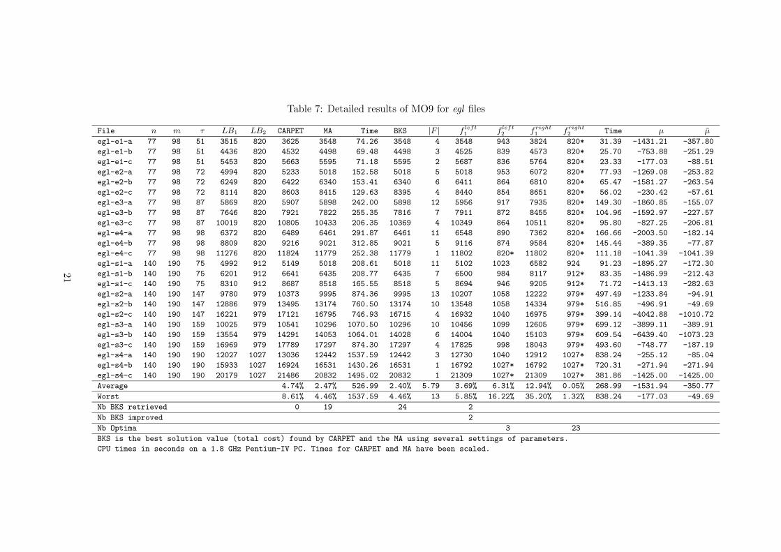
Table 7: Detailed results of MO9 for egl files
File n m τ LB1 LB2 CARPET MA Time BKS |F | fleft1
fleft2
fright1
fright2
Time µ µ
egl-e1-a 77 98 51 3515 820 3625 3548 74.26 3548 4 3548 943 3824 820* 31.39 -1431.21 -357.80
egl-e1-b 77 98 51 4436 820 4532 4498 69.48 4498 3 4525 839 4573 820* 25.70 -753.88 -251.29
egl-e1-c 77 98 51 5453 820 5663 5595 71.18 5595 2 5687 836 5764 820* 23.33 -177.03 -88.51
egl-e2-a 77 98 72 4994 820 5233 5018 152.58 5018 5 5018 953 6072 820* 77.93 -1269.08 -253.82
egl-e2-b 77 98 72 6249 820 6422 6340 153.41 6340 6 6411 864 6810 820* 65.47 -1581.27 -263.54
egl-e2-c 77 98 72 8114 820 8603 8415 129.63 8395 4 8440 854 8651 820* 56.02 -230.42 -57.61
egl-e3-a 77 98 87 5869 820 5907 5898 242.00 5898 12 5956 917 7935 820* 149.30 -1860.85 -155.07
egl-e3-b 77 98 87 7646 820 7921 7822 255.35 7816 7 7911 872 8455 820* 104.96 -1592.97 -227.57
egl-e3-c 77 98 87 10019 820 10805 10433 206.35 10369 4 10349 864 10511 820* 95.80 -827.25 -206.81
egl-e4-a 77 98 98 6372 820 6489 6461 291.87 6461 11 6548 890 7362 820* 166.66 -2003.50 -182.14
egl-e4-b 77 98 98 8809 820 9216 9021 312.85 9021 5 9116 874 9584 820* 145.44 -389.35 -77.87
egl-e4-c 77 98 98 11276 820 11824 11779 252.38 11779 1 11802 820* 11802 820* 111.18 -1041.39 -1041.39
egl-s1-a 140 190 75 4992 912 5149 5018 208.61 5018 11 5102 1023 6582 924 91.23 -1895.27 -172.30
egl-s1-b 140 190 75 6201 912 6641 6435 208.77 6435 7 6500 984 8117 912* 83.35 -1486.99 -212.43
egl-s1-c 140 190 75 8310 912 8687 8518 165.55 8518 5 8694 946 9205 912* 71.72 -1413.13 -282.63
egl-s2-a 140 190 147 9780 979 10373 9995 874.36 9995 13 10207 1058 12222 979* 497.49 -1233.84 -94.91
egl-s2-b 140 190 147 12886 979 13495 13174 760.50 13174 10 13548 1058 14334 979* 516.85 -496.91 -49.69
egl-s2-c 140 190 147 16221 979 17121 16795 746.93 16715 4 16932 1040 16975 979* 399.14 -4042.88 -1010.72
egl-s3-a 140 190 159 10025 979 10541 10296 1070.50 10296 10 10456 1099 12605 979* 699.12 -3899.11 -389.91
egl-s3-b 140 190 159 13554 979 14291 14053 1064.01 14028 6 14004 1040 15103 979* 609.54 -6439.40 -1073.23
egl-s3-c 140 190 159 16969 979 17789 17297 874.30 17297 4 17825 998 18043 979* 493.60 -748.77 -187.19
egl-s4-a 140 190 190 12027 1027 13036 12442 1537.59 12442 3 12730 1040 12912 1027* 838.24 -255.12 -85.04
egl-s4-b 140 190 190 15933 1027 16924 16531 1430.26 16531 1 16792 1027* 16792 1027* 720.31 -271.94 -271.94
egl-s4-c 140 190 190 20179 1027 21486 20832 1495.02 20832 1 21309 1027* 21309 1027* 381.86 -1425.00 -1425.00
Average 4.74% 2.47% 526.99 2.40% 5.79 3.69% 6.31% 12.94% 0.05% 268.99 -1531.94 -350.77
Worst 8.61% 4.46% 1537.59 4.46% 13 5.85% 16.22% 35.20% 1.32% 838.24 -177.03 -49.69
Nb BKS retrieved 0 19 24 2
Nb BKS improved 2
Nb Optima 3 23
BKS is the best solution value (total cost) found by CARPET and the MA using several settings of parameters.
CPU times in seconds on a 1.8 GHz Pentium-IV PC. Times for CARPET and MA have been scaled.
21


Using Lagrangean Relaxation to Minimize the WeightedNumber of Late Jobs on a Single Machine
Stephane Dauzere-Peres,1,* Marc Sevaux2,†
1 IRCCyN/Ecole des Mines de Nantes, La Chantrerie, BP 20722,F-44307 Nantes Cedex 03, France
2 Universite de Valenciennes, LAMIH/SP, Le Mont-Houy,F-59313 Valenciennes Cedex, France
Received 30 April 2001; revised 21 February 2002; accepted 15 July 2002
DOI 10.1002/nav.10056
Abstract: This paper tackles the general single machine scheduling problem, where jobs havedifferent release and due dates and the objective is to minimize the weighted number of late jobs.The notion of master sequence is first introduced, i.e., a sequence that contains at least an optimalsequence of jobs on time. This master sequence is used to derive an original mixed-integer linearprogramming formulation. By relaxing some constraints, a Lagrangean relaxation algorithm isdesigned which gives both lower and upper bounds. The special case where jobs haveequal weights is analyzed. Computational results are presented and, although the duality gapbecomes larger with the number of jobs, it is possible to solve problems of more than 100 jobs.© 2002 Wiley Periodicals, Inc. Naval Research Logistics 50: 273–288, 2003.
1. INTRODUCTION
A set of n jobs { J1, . . . , Jn}, subject to release dates ri and due dates di, have to bescheduled on a single machine. The processing time of jobs on the machine is denoted by pi, anda weight wi is associated with each job. The machine can only process one job at a time. Ascheduled job completed before its due date is said to be early or on time, and late otherwise.Let Ui be equal to 1 if job Ji is late in a schedule, and to 0 otherwise. The objective is tominimize the weighted number of late jobs, or equivalently to maximize the weighted numberof early jobs. A well-known and important remark is that there is always an optimal schedulein which late jobs are sequenced after all the early jobs.
This single-machine scheduling problem, noted 1�rj�¥ wjUj in the standard classification, isstrongly ��-hard [8]. When all weights are equal (1�rj�¥ Uj), the problem remains ��-Hard,but becomes polynomially solvable if all release dates are equal (1�¥ Uj) [9] (O(n log n)), or
* This paper was written while this author was invited professor at the Department of Finance andManagement Science, Norwegian School of Economics and Business Administration, Helleveien 30,N-5035 Bergen-Sandviken, Norway.
† This research was performed while this author was at Ecole des Mines de Nantes.Correspondence to: S. Dauzere-Peres
© 2002 Wiley Periodicals, Inc.

if release and due dates are similarly ordered (ri � rj f di � dj @( Ji, Jj)) [6] (O(n2)), [7](O(n log n)). However, some exact approaches have recently been proposed for this problem[1, 5]. Lawler [7] showed that the Moore’s algorithm [9] could be applied when processing timesand weights are agreeable, i.e., pi � pj f wi � wj @( Ji, Jj). Finally, branch-and-boundprocedures have been developed to solve the case where all release dates are equal (1�¥ wjUj)in [12] and [11]. To our knowledge, no algorithm has been proposed to solve the generalproblem 1�rj� ¥ wjUj.
In this paper, based on the notion of master sequence, i.e., a sequence from which an optimalsequence can be extracted, a new mixed-integer linear programming formulation is introduced.Using this formulation, a Lagrangean relaxation algorithm is derived. Lagrangean relaxation isa powerful optimization tool from which heuristic iterative algorithms can be designed, whereboth upper and lower bounds are determined at every iteration. It is thus possible to alwaysknow the maximum gap between the best solution found and the optimal solution, and stop thealgorithm when this gap is small enough. One condition that is often associated with theefficiency of Lagrangean relaxation approaches is to relax as few constraints as possible, inorder to obtain good bounds when solving the relaxed problem. This is why our formulationcompares very favorably to other known ones (see [4] for a study of classical formulations forthis problem). Only one constraint type, coupling variables of different jobs, needs to be relaxedto obtain an easily solvable problem, which can be solved independently for each job. This isnot the case for other formulations, including discrete-time formulations, which often havemany coupling constraints.
The master sequence is introduced in Section 2, and the resulting mixed-integer linearprogramming formulation is given and discussed in Section 3. Section 4 shows how the size ofthe master sequence, and thus the size of the model, can be reduced. Section 5 presents theLagrangean relaxation algorithm, and Section 6 several improvements of the algorithm. Thenonweighted case is analyzed in more details in Section 7. Numerical results on a large set oftest instances are given and discussed in Section 8. Finally, some conclusions and perspectivesare drawn in Section 9.
2. THE MASTER SEQUENCE
In the remainder of this paper, because we are only interested in sequencing jobs on time (latejobs can be set after the jobs on time), the sequence of jobs will often mean the sequence of earlyjobs. Many results in this paper are based on the following theorem.
THEOREM 1: There is always an optimal sequence of jobs on time that solves the problem1�rj� ¥ wjUj, in which every job Jj is sequenced just after a job Ji such that either condition (1)di � dj, or (2) di � dj and rk � rj @Jk sequenced before Jj, holds.
PROOF: First, note that conditions (1) or (2) being satisfied is equivalent to condition (3),di � dj and ?Jk sequenced before Jj such that rk � rj, not being satisfied.
The proof goes by showing that, by construction, it is possible to change any optimalsequence into an optimal sequence that satisfies conditions (1) or (2).
Suppose that we have a sequence in which some (or all) ready jobs do not satisfy one of theconditions. Starting from the beginning of the sequence, find the first pair of jobs ( Ji, Jj) in thesequence that does not satisfy the two conditions, i.e., for which condition (3) holds. If ti andtj denote the start times of the two jobs, the latter condition ensures that, after interchanging the
274 Naval Research Logistics, Vol. 50 (2003)

two jobs, Jj can start at ti (since ?Jk sequenced before Jj such that rj � rk � ti). Hence, Ji willend at the same time as Jj before the interchange (ti � pi � pj), and thus will still be on time(since ti � pi � pj � dj � di).
The interchange must be repeated if Jj and the new job just before it do not satisfy conditions(1) or (2), until one of these conditions is satisfied for Jj and the job just before it, or Jj issequenced first.
The procedure is repeated for all jobs until the conditions are satisfied for all jobs. Becauseonce a job has been moved, it will never go back again, one knows that the procedure will notbe repeated more than n times, i.e., takes a finite amount of time. �
We will denote by � the subset of sequences in which jobs satisfy the conditions in Theorem1. In the sequel, we will only be interested in sequences in �, since we know that it alwayscontains an optimal sequence.
THEOREM 2: If, in a sequence of �, job Jj is after jobs Ji such that rj � ri, then there isat least one job Ji such that di � dj.
PROOF: By contradiction, if all jobs Jk before Jj such that rk � ri verify dk � dj, thenneither of the conditions (1) and (2) is satisfied. Thus, the sequence is not in �. �
COROLLARY 1: Consider a job Jj. If, for every job Ji such that rj � ri, condition dj � di
holds, then, in every sequence of � (i.e., in an optimal sequence), job Jj is sequenced before alljobs Ji.
COROLLARY 2: Consider a job Ji. If, for every job Jj such that dj � di, condition rj � ri
holds, then, in every sequence of � (i.e., in an optimal sequence), job Ji is sequenced after alljobs Jj.
We want to show that it is possible to derive what will be called a master sequence,denoted by �, which “contains” every sequence in �. A master sequence is a sequence inwhich each job may appear several times. A sequence in � is “created” from the mastersequence by selecting at most one position for each job. The largest possible master sequenceis ( J1, J2, . . . , Jn, J1, J2, . . . , Jn, . . . , J1, J2, . . . , Jn), where ( J1, J2, . . . , Jn) is repeatedn times, and thus has n2 positions (this number is reduced in the sequel). Corollary 1 implies thatthere is only one position for Jj in the master sequence, and Corollary 2 that there is only oneposition for Ji.
THEOREM 3: In a master sequence, if ri � rj and di � dj, then there is a position for Ji
before Jj and a position for Ji after Jj.
PROOF: Because ri � rj, Condition (2) in Theorem 1 is satisfied for the pair of jobs ( Ji, Jj),and because di � dj, Condition (1) is satisfied for the pair ( Jj, Ji). Hence, there is a positionin the master sequence for Ji before and after Jj. �
Hence, there must be a position in a master sequence for Ji after every job Jj such that ri �
rj and di � dj. This shows that there will be at mostn�n � 1�
2 positions in the master sequence.
275Dauzere-Peres and Sevaux: Lagrangean Relaxation for Minimizing Late Jobs

COROLLARY 3: If, for every job Jj such that ri � rj, the condition di � dj holds, then thereis only one position for job Ji in the master sequence.
Corollary 3 shows that, when release and due dates are similarly ordered (as in Kise, Ibaraki,and Mine [6]), the master sequence will be the sequence of jobs in increasing order of theirrelease dates (or due dates if some jobs have equal release dates). In the nonweighted case (wi �1, @Ji), the problem is then polynomially solvable using the algorithm proposed in [6] (inO(n2)) or in [7] (in O(n log n)).
An interesting and important property of the master sequence is a kind of transitivity property.If job Ji is set before and after Jj in the master sequence because either Condition (1) or (2) ofTheorem 1 holds, and if Jj is set before and after Jk in the master sequence because eitherCondition (1) or (2) holds, then either Condition (1) or (2) of Theorem 1 holds and Ji is setbefore, and after Jk in the master sequence.
EXAMPLE 1: Let us consider a 5-job problem with the data of Table 1.Considering sequences in �, by Corollary 1, one knows that J1 is set before all jobs
(conditions r1 � ri and d1 � di are satisfied for every job Ji � J1), and all jobs are set beforeJ5 (conditions ri � r5 and di � d5 are satisfied for every job Ji � J5). Hence, in the mastersequence �, job J1 will be set first and job J5 last.
The master sequence has the following form:
� � �J1, J2, J3, J2, J4, J3, J2, J5�.
Every sequence of jobs in � can be constructed from �. In this example, there are numeroussequences or early jobs (more than 40). For instance, the subset of sequences containing 5 jobsis:
��J1, J2, J3, J4, J5�, �J1, J2, J4, J3, J5�, �J1, J3, J2, J4, J5�, �J1, J3, J4, J2, J5�, �J1, J4, J3, J2, J5�
One can check that each of these sequences is included in �.
The algorithm to create the master sequence � is sketched below. We suppose that the jobsare preordered in nondecreasing order of their release dates, and J� denotes the set of jobs alreadysequenced. In Step 3, jobs that are already in the master sequence (set J� ) and have a positionafter the new job Ji in � (i.e., satisfying the conditions of Theorem 3) are added in nondecreasingorder of their due dates. Hence, to speed up the algorithm, jobs added to J� in Step 2 are orderedin nondecreasing order of their due dates.
Table 1. Data for a 5-job problem.
Jobs J1 J2 J3 J4 J5
ri 0 5 8 12 14pi 8 6 5 6 10di 16 26 24 22 32
276 Naval Research Logistics, Vol. 50 (2003)
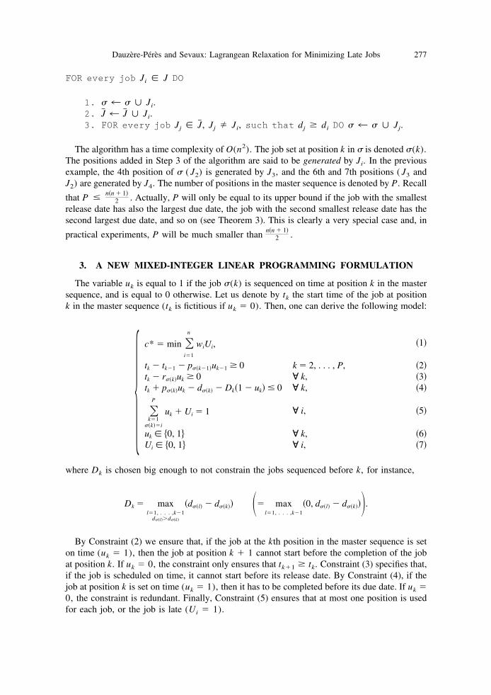
FOR every job Ji � J DO
1. � 4 � � Ji.2. J� 4 J� � Ji.3. FOR every job Jj � J� , Jj � Ji, such that dj � di DO � 4 � � Jj.
The algorithm has a time complexity of O(n2). The job set at position k in � is denoted �(k).The positions added in Step 3 of the algorithm are said to be generated by Ji. In the previousexample, the 4th position of � ( J2) is generated by J3, and the 6th and 7th positions ( J3 andJ2) are generated by J4. The number of positions in the master sequence is denoted by P. Recall
that P �n�n � 1�
2 . Actually, P will only be equal to its upper bound if the job with the smallestrelease date has also the largest due date, the job with the second smallest release date has thesecond largest due date, and so on (see Theorem 3). This is clearly a very special case and, in
practical experiments, P will be much smaller than n�n � 1�2 .
3. A NEW MIXED-INTEGER LINEAR PROGRAMMING FORMULATION
The variable uk is equal to 1 if the job �(k) is sequenced on time at position k in the mastersequence, and is equal to 0 otherwise. Let us denote by tk the start time of the job at positionk in the master sequence (tk is fictitious if uk � 0). Then, one can derive the following model:
�c* � min �
i�1
n
wiUi, �1�
tk � tk1 � p��k1�uk1 � 0 k � 2, . . . , P, �2�tk � r��k�uk � 0 � k, �3�tk � p��k�uk � d��k� � Dk�1 � uk� � 0 � k, �4�
�k�1
��k��i
P
uk � Ui � 1 � i, �5�
uk � �0, 1 � k, �6�Ui � �0, 1 � i, �7�
where Dk is chosen big enough to not constrain the jobs sequenced before k, for instance,
Dk � maxl�1, . . . ,k1
d��l��d��k�
�d��l� � d��k�� �� maxl�1, . . . ,k1
�0, d��l� � d��k���.
By Constraint (2) we ensure that, if the job at the kth position in the master sequence is seton time (uk � 1), then the job at position k � 1 cannot start before the completion of the jobat position k. If uk � 0, the constraint only ensures that tk�1 � tk. Constraint (3) specifies that,if the job is scheduled on time, it cannot start before its release date. By Constraint (4), if thejob at position k is set on time (uk � 1), then it has to be completed before its due date. If uk �0, the constraint is redundant. Finally, Constraint (5) ensures that at most one position is usedfor each job, or the job is late (Ui � 1).
277Dauzere-Peres and Sevaux: Lagrangean Relaxation for Minimizing Late Jobs

In the previous model, it is possible to replace Constraint (3) by tk r�(k) � 0 [orequivalently to remove uk from Constraint (3)]. The new constraint is numbered (3�). Theorem4 will prove the validity of the resulting model.
In the nonweighted case (wj � 1, @Jj), if Constraint (4) is replaced by tk � p�(k)uk d�(k) � 0 [or equivalently Dk � 0 in Constraint (4)], then the resulting formulation stillprovides an optimal solution to the problem. The new constraint is numbered (4�). Although thenonweighted case will be analyzed in more details in Section 7, the following theorem isintroduced here because it is also useful for the weighted case.
THEOREM 4: In the nonweighted case, there is always an optimal sequence of � thatsatisfies Constraints (2), (3�), (4�), and (5)–(7).
PROOF: The proof goes by showing that the only case where there is a problem is when Jj
can be sequenced before and after Ji in the master sequence, and rj � ri and dj � di, and Ji
is not sequenced in the optimal sequence. It can be shown that Constraints (2), (3�), and (4�)prevent job Jj to start between di pj [Constraint (4�)] and ri [Constraint (3�)]. This is only aproblem if di pj � ri. If this is the case, then pi � pj (since Ji is not late if started at its releasedate ri). Hence, in an optimal solution where Jj starts in the interval [di pj, ri], i.e., ends inthe interval [di, ri � pj], Jj can be replaced by Ji, and the sequence will remain optimal sinceJi starts after ri and ends before di. �
The proof of Theorem 4 is based on equal weight for jobs. In the weighted case, followingthe proof of Theorem 4, Dk can be chosen as follows:
Dk � maxl�1, . . . ,k1
�0, r��l� � d��k��
Hence, the case where di pj � ri, discussed in the proof of Theorem 4, is avoided. Innumerical experiments, Dk is very often equal to zero.
4. REDUCING THE MASTER SEQUENCE
Because the size of the model is directly linked to the length of the master sequence, it isdesirable to remove as many positions as possible from �. Not only solution procedures will bemore efficient, but the model will be tighter and will give better lower bounds by Lagrangeanrelaxation.
By Constraints (2) and (3), tk � maxl�1, . . . ,k1 r�(l ). Hence, the first reduction will be doneby removing positions k such that maxl�1, . . . ,k1 r�(l ) � p�(k) � d�(k).
Several dominance rules are proposed in [5] for the nonweighted case. However, if parameterDk is changed according to Theorem 4, all of them do not apply. This is because, in the resultingformulation, when job Jj is before and after Ji in the master sequence and Ji is late, the positionof Jj after Ji might need to be occupied in an optimal solution. One could show that this is notthe case with the initial formulation. Our preliminary numerical experiments showed thatreducing parameter Dk was more important than using the lost dominance rules.
We will describe here the dominance rules that still apply to our formulation, and which havebeen modified for the weighted case (see [5] for details).
In the master sequence, if Conditions (1) ri � rj, (2) ri � pi � rj � pj, (3) ri � pi � pj �dj, (4) rj � pj � pi � di, (5) di pi � dj pj, and (6) wj � wi hold, then Jj dominates
278 Naval Research Logistics, Vol. 50 (2003)

Ji and all positions of job Ji can be removed from the master sequence. Because of Conditions(3) and (4), only one of the two jobs can be scheduled on time. In an optimal solution, eitherboth jobs are late, or it is always possible to find a solution in which job Jj is on time and thetotal weight of late jobs is as small as a solution with job Ji on time.
Another dominance rule is based on the fact that if there is a position l and a job Jj [ Jj ��(l )] such that Conditions (1) r�(l ) � p�(l ) � rj � pj, (2) p�(l ) � pj, (3) r�(l ) � p�(l ) � pj �dj, (4) rj � pj � p�(l ) � d�(l ), (5) d�(l ) p�(l ) � dj pj, and (6) w�(l ) � wj are satisfied,then Jj dominates position l, and thus the latter can be removed. This is because, if there is anoptimal solution in which position l is occupied (i.e., job J�(l ) is on time), then, by Condition(3), Jj is late. The solution can be changed to another optimal solution in which J�(l ) is replacedby Jj.
5. A LAGRANGEAN RELAXATION ALGORITHM
Following Theorem 4 and the remarks in Section 3, the mixed-integer linear programmingformulation is now
�c* � min �
i�1
n
wiUi, �8�
tk � tk1 � p��k1�uk1 � 0 k � 2, . . . , P, �9�tk � r��k� � 0 � k, �10�tk � p��k�uk � d��k� � Dk�1 � uk� � 0 � k, �11�
�k�1
��k��i
P
uk � Ui � 1 � i, �12�
uk � �0, 1 � k, �13�Ui � �0, 1 � i. �14�
By relaxing Constraint (9) using Lagrangean multipliers �k (k � 2, . . . , P), the modelbecomes
�max�k�0
mintk,uk,Ui
��i�1
n
wiUi � �k�2
P
�k�tk � tk1 � p��k1�uk1��, �15�
tk � r��k� � 0 � k, �10�tk � p��k�uk � d��k� � Dk�1 � uk� � 0 � k, �11�
�k�1
��k��i
P
uk � Ui � 1 � i, �12�
uk � �0, 1 � k, �13�Ui � �0, 1 � i. �14�
To use Lagrangean relaxation, one needs to solve the above model for given values of �k (k �2, . . . , P). The objective function can be written:
279Dauzere-Peres and Sevaux: Lagrangean Relaxation for Minimizing Late Jobs
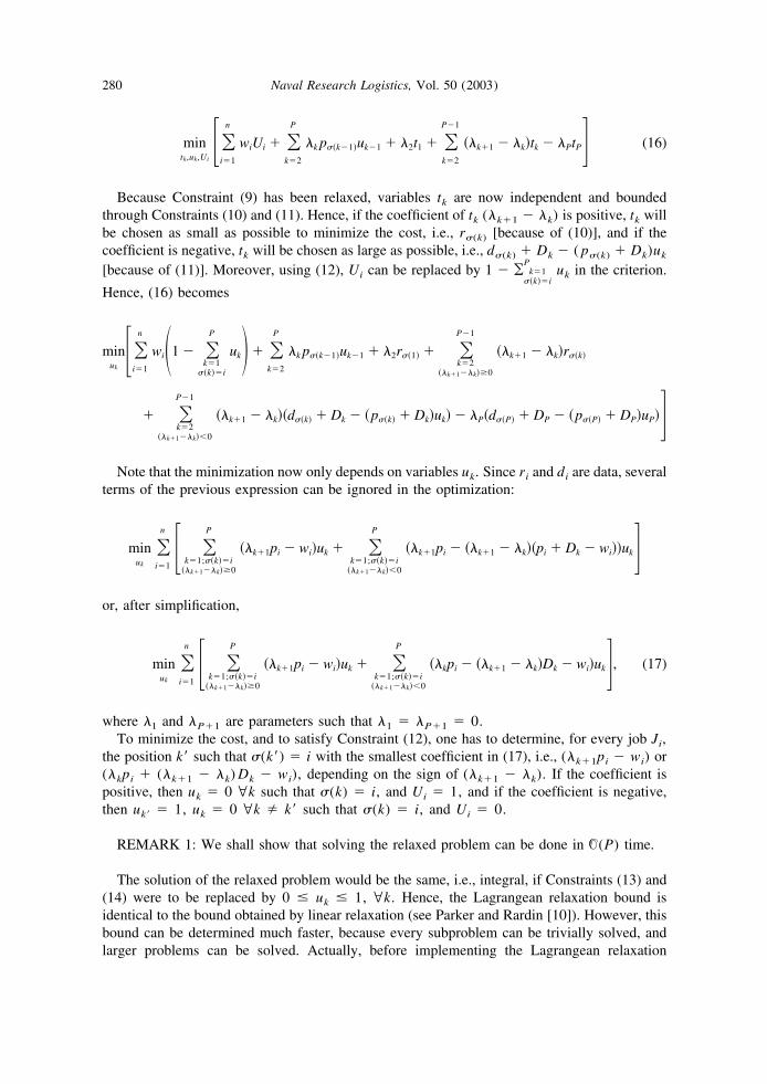
mintk,uk,Ui
��i�1
n
wiUi � �k�2
P
�k p��k1�uk1 � �2t1 � �k�2
P1
��k�1 � �k�tk � �PtP� (16)
Because Constraint (9) has been relaxed, variables tk are now independent and boundedthrough Constraints (10) and (11). Hence, if the coefficient of tk (�k�1 �k) is positive, tk willbe chosen as small as possible to minimize the cost, i.e., r�(k) [because of (10)], and if thecoefficient is negative, tk will be chosen as large as possible, i.e., d�(k) � Dk ( p�(k) � Dk)uk
[because of (11)]. Moreover, using (12), Ui can be replaced by 1 ¥ k�1��k��i
Puk in the criterion.
Hence, (16) becomes
minuk��
i�1
n
wi�1 � �k�1
��k��i
P
uk� � �k�2
P
�k p��k1�uk1 � �2r��1� � �k�2
��k�1�k��0
P1
��k�1 � �k�r��k�
� �k�2
��k�1�k��0
P1
��k�1 � �k��d��k� � Dk � �p��k� � Dk�uk� � �P�d��P� � DP � �p��P� � DP�uP��Note that the minimization now only depends on variables uk. Since ri and di are data, several
terms of the previous expression can be ignored in the optimization:
minuk
�i�1
n � �k�1;��k��i
��k�1�k��0
P
��k�1pi � wi�uk � �k�1;��k��i
��k�1�k��0
P
��k�1pi � ��k�1 � �k��pi � Dk � wi��uk�or, after simplification,
minuk
�i�1
n � �k�1;��k��i
��k�1�k��0
P
��k�1pi � wi�uk � �k�1;��k��i
��k�1�k��0
P
��kpi � ��k�1 � �k�Dk � wi�uk�, (17)
where �1 and �P�1 are parameters such that �1 � �P�1 � 0.To minimize the cost, and to satisfy Constraint (12), one has to determine, for every job Ji,
the position k� such that �(k�) � i with the smallest coefficient in (17), i.e., (�k�1pi wi) or(�kpi � (�k�1 �k) Dk wi), depending on the sign of (�k�1 �k). If the coefficient ispositive, then uk � 0 @k such that �(k) � i, and Ui � 1, and if the coefficient is negative,then uk� � 1, uk � 0 @k � k� such that �(k) � i, and Ui � 0.
REMARK 1: We shall show that solving the relaxed problem can be done in �(P) time.
The solution of the relaxed problem would be the same, i.e., integral, if Constraints (13) and(14) were to be replaced by 0 � uk � 1, @k. Hence, the Lagrangean relaxation bound isidentical to the bound obtained by linear relaxation (see Parker and Rardin [10]). However, thisbound can be determined much faster, because every subproblem can be trivially solved, andlarger problems can be solved. Actually, before implementing the Lagrangean relaxation
280 Naval Research Logistics, Vol. 50 (2003)
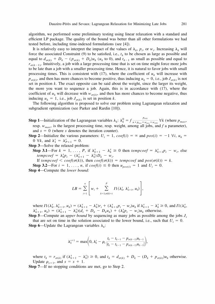
algorithm, we performed some preliminary testing using linear relaxation with a standard andefficient LP package. The quality of the bound was better than all other formulations we hadtested before, including time-indexed formulations (see [4]).
It is relatively easy to interpret the impact of the values of �k, pi, or wi. Increasing �k willforce the associated Constraint (9) to be satisfied, i.e., tk to be chosen as large as possible andequal to d�(k) � Dk ( p�(k) � Dk)uk (uk to 0), and tk1 as small as possible and equal tor�(k1). Intuitively, a job with a large processing time that is set on time might force more jobsto be late than a job with a smaller processing time. Hence, it is natural to favor jobs with smallprocessing times. This is consistent with (17), where the coefficient of uk will increase withp�(k), and then has more chances to become positive, thus inducing uk � 0, i.e., job J�(k) is notset in position k. The exact opposite can be said about the weight, since the larger its weight,the more you want to sequence a job. Again, this is in accordance with (17), where thecoefficient of uk will decrease with w�(k), and then has more chances to become negative, thusinducing uk � 1, i.e., job J�(k) is set in position k.
The following algorithm is proposed to solve our problem using Lagrangean relaxation andsubgradient optimization (see Parker and Rardin [10]).
Step 1—Initialization of the Lagrangean variables �k: �k0 � f
p��k�
n � pmax � wmax � w��k�@k (where pmax,
resp. wmax, is the largest processing time, resp. weight, among all jobs, and f a parameter),and s � 0 (where s denotes the iteration counter).
Step 2—Initialize the various parameters: Ui � 1, coef(i) � � and pos(i) � 1 @i, uk �0 @k, and �1
s � �P�1s � 0.
Step 3—Solve the relaxed problem:Step 3.1—For k � 1, . . . , P, if �k�1
s �ks � 0 then tempcoef � �k�1
s pi wi, elsetempcoef � �k
spi (�k�1s �k
s) Dk wi.If tempcoef � coef(�(k)), then coef(�(k)) � tempcoef and pos(�(k)) � k.
Step 3.2—For i � 1, . . . , n, if coef(i) � 0 then upos(i) � 1 and Ui � 0.Step 4—Compute the lower bound:
LB � �i�1
n �wi � �k�1;��k��i
P
I1��ks, �k�1
s , uk�� ,
where I1(�ks , �k�1
s , uk) � (�k�1s �k
s)ri � (�k�1s pi wi)uk if �k�1
s �ks � 0, and I1(�k
s ,�k�1
s , uk) � (�k�1s �k
s)(di � Dk Dkuk) � (�kspi wi)uk otherwise.
Step 5—Compute an upper bound by sequencing as many jobs as possible among the jobs Ji
that are set on time in the solution associated to the lower bound, i.e., such that Ui � 0.Step 6—Update the Lagrangean variables �k:
�ks�1 � max�0, �k
s � s
tk � tk1 � p��k1�uk1
�tk � tk1 � p��k1�uk1��,
where tk � r�(k) if (�k�1s �k
s) � 0, and tk � d�(k) � Dk (Dk � p�(k))uk otherwise.Update s�1, and s � s � 1.
Step 7—If no stopping conditions are met, go to Step 2.
281Dauzere-Peres and Sevaux: Lagrangean Relaxation for Minimizing Late Jobs

We use a simple and fast greedy algorithm to determine the upper bound in Step 5. From k �1 to k � P, job J�(k) is added to the sequence of early jobs if uk � 1 and J�(k) is on time. Thefinishing time of the current sequence is updated each time a new job is added.
Various parameters have to be initialized and adjusted to ensure the best convergence of thealgorithm for different types of instances. After sd iterations without improvement, the param-eter s is decreased by a factor of 100 (1 red)%. Various stopping conditions arechecked: Maximum number of iterations IterMax, step smaller than or equal to min, and ofcourse if the optimum is found, i.e., the lower and upper bounds are equal. The parameters couldbe adjusted to improve the results on some instances, but we have decided to use genericparameters instead. After some preliminary testing, we chose the following values: f � 0.4,0 � 1.6, sd � 40, and red � 0.9. For the stopping conditions, we used IterMax �100,000 and min � 105. Actually, in our numerical experiments, the number of iterations isnever larger than 20,000.
As already shown, every relaxed problem in Step 3 is solved very quickly, in �(P) time where
P is not larger than n�n � 1�2 . Hence, many iterations can be performed, even for large instances.
6. IMPROVING THE ALGORITHM
Several improvements are proposed. The first one is based on a rewriting of the formulation.In the model, because of Constraint (9), Constraint (10) can be rewritten as
tk � rrk � 0 � k,
where rrk � maxl�1, . . . ,k r�(l ) are release dates per position. To include this change in thealgorithm, it suffices to replace r�(k) by rrk.
A similar rewriting can be performed for Constraint (11) when Dk � 0 @k, as follows:
tk � p��k�uk � ddk � 0,
where ddk � minl�k, . . . ,P;Dk�0d�(l ) are due dates per position. This rewriting can be done forall positions in the nonweighted case since Dk � 0 @k.
Although they do not improve the lower bound obtained by linear relaxation, and thus byLagrangean relaxation, these changes often considerably speed up the algorithm by betterupdating the Lagrangean multipliers in Step 6. This is because the positions for a job are betterdifferentiated whereas, in the original formulation, they all have similar Constraints (10). Hence,the algorithm will more quickly choose the best position(s) for a job, and will require lessiterations to converge to the lower bound.
Another improvement uses the following property to tighten Constraint (9) in the model.
THEOREM 5: Let Ji and Jj be two jobs in a master sequence. If a position k of Ji is generatedby Jj, then there is an optimal schedule in which k is either not occupied or occupied and suchthat tk � dj pi.
PROOF: We want to prove that if, in an optimal schedule S, the position k of Ji generatedby Jj is occupied and tk � dj pi, then this schedule can be transformed into an equivalentoptimal schedule S� in which Ji is sequenced before Jj (i.e., position k is not occupied).
282 Naval Research Logistics, Vol. 50 (2003)

Since a position of Ji is generated by Jj, we know that ri � rj and di � dj. Hence, movingJi before Jj will just shift Jj and the jobs between Jj and Ji in S by pi and, because tk � dj pi in S, the completion time of the shifted jobs will not be larger than dj. By definition of themaster sequence, and because position k is generated by Jj (see the end of Section 2 for thedefinition of a generated position), the due dates of the jobs between Jj and Ji in S are larger thanor equal to dj. Thus, the schedule S� is feasible. �
Following Theorem 5, Constraints (10) can be tightened (the added term is positive) forgenerated positions k (i.e., such that rrk � r�(k)) as follows:
tk � rrk � RRkuk � 0 � k
where RRk � max(0, d�(l ) p�(k) rrk), and l is the position that generated position k (i.e.,r�(k) � r�(l ) and d�(k) � d�(l )).
The relaxed problem in the Lagrangian relaxation changes accordingly by adding the newterm in the objective function, and by considering the coefficient (�k�1pi � (�k�1 �k) RRk wi) when (�k�1 �k) is positive. Strengthening the constraints helps to improvethe quality of the lower bound. Moreover, it also accelerates the algorithm by again betterdifferentiating the positions.
7. THE NONWEIGHTED CASE
The mixed-integer linear programming model defined in Section 3 can be enhanced for thenonweighted case, i.e., wi � 1 @i following Theorem 4 in Section 3. The new model is givenbelow:
�c* � min �
i�1
n
Ui, �18�
tk � tk1 � p��k1�uk1 � 0 k � 2, . . . , P, �19�tk � r��k� � 0 � k, �20�tk � p��k�uk � d��k� � 0 � k, �21�
�k�1
��k��i
P
uk � Ui � 1 � i, �22�
uk � �0, 1 � k, �23�Ui � �0, 1 � i. �24�
Because wi � 1 @Ji and Dk � 0, @k, the objective function (17) can equivalently be writtenas
minuk
�i�1
n �k�1;
��k��i
P
�max��k, �k�1�pi � 1�uk. (25)
283Dauzere-Peres and Sevaux: Lagrangean Relaxation for Minimizing Late Jobs

REMARK 2: In the nonweighted case, for a given job Ji, finding the position k�, �(k�) �i, with the smallest coefficient in (17) is equivalent to finding the position with the smallestcoefficient �k�1 or �k, depending on the sign of (�k�1 �k).
In the Lagrangean relaxation algorithm described in Section 5, the following steps aremodified:
Step 3.1—For k � 1, . . . , P, if �k�1s �k
s � 0, then tempcoef � �k�1s pi 1; else
tempcoef � �kspi 1.
If tempcoef � coef(�(k)), then coef(�(k)) � tempcoef and pos(�(k)) � k.Step 4—Compute the lower bound:
LB � n � �i�1
n �k�1;��k��i
P
I2��ks, �k�1
s , uk�
where I2(�ks , �k�1
s , uk) � (�k�1s �k
s)ri � (�k�1s pi 1)uk if �k�1
s �ks � 0, and I2(�k
s ,�k�1
s , uk) � (�k�1s �k
s)(di piuk) � (�kspi 1)uk otherwise.
Moreover, Kise, Ibaraki, and Mine’s algorithm [6] can be used to compute the upper boundassociated with the current value of the multipliers �s in Step 5. This is because, when thesequence in which jobs can be sequenced is fixed, i.e., for a given permutation of the jobs, theoptimal sequence of early jobs can be found using Kise et al.’s algorithm. In our case, the setof jobs from which jobs have to be sequenced is the set of jobs Ji such that Ui � 1, and thefixed sequence is given by the positions k such that uk � 1.
It is better to adjust the parameters for the algorithm when wi � 1, @i. After multiple trials,we decided to use the following for all tested instances: f � 0.4, 0 � 0.6, sd � 40, andred � 0.9. The same parameters are kept for the stopping conditions (IterMax � 100,000and min � 105).
8. COMPUTATIONAL RESULTS
Many test problems were generated to evaluate our algorithm. For each value of n, thenumber of jobs, 160 instances were randomly generated. The test program, written in C, was runon a SUN UltraSparc workstation.
The Lagrangean relaxation algorithm was first compared with solutions obtained by using thenew formulation in the state of the art mixed-integer linear programming (MIP) solver ILOG-CPLEX. However, even for “small” size problems of 80 jobs, very large CPU times wereobserved with the MIP solver in many cases. For example, on a given instance, the search wasstopped after 19 hours with the optimal solution, but its optimality was not proved. If theaccuracy level is reduced to the one of the Lagrangean relaxation algorithm (see results in thesequel), the CPU time of the MIP solver decreases but remains very large.
Random generator. For each job Ji, a processing time pi is randomly generated from theuniform distribution [1, 100] and a weight wi is generated from the uniform distribution [1, 10].As in [3], two parameters K1 and K2 are used, and taken in the set {1, 5, 10, 20}. Because wewant data to depend on the number of jobs n, the release date ri is randomly generated from the
284 Naval Research Logistics, Vol. 50 (2003)

uniform distribution [0, K1n], and the due date from the uniform distribution [ri � pi, ri �pi � K2n]. The algorithm was tested for n � {20, 40, 60, 80, 100, 120, 140}. For eachcombination of n, K1, and K2, 10 instances are generated, i.e., 160 instances for each value of n.
Results of the nonweighted case. The Lagrangean relaxation algorithm was first run on the 1�rj�¥ Uj problem. In Table 2, results are reported for each value of n. The optimum is consideredto be found when lower and upper bounds are equal. For n � 60, 25 out of 160 instances areoptimally solved, i.e., 15.6%. The CPU time necessary to find the best bounds is also reported.For n � 80, the mean CPU time is less than 1 minute. To evaluate the efficiency of both bounds,the gap between the upper and lower bounds is also measured and reported in the last fourcolumns of the table. This gap is expressed in number of jobs and in percentage in the lastcolumn. For n � 100, the average gap is 3.46 jobs. The standard deviation and maximum gapare also given in the table.
The results are good, and the average duality gap remains stable when n increases. Rememberthat we decided to use the same parameters for our algorithm for every test instance, indepen-dently of n, K1, or K2. The algorithm does not perform so well when the master sequence islong. Looking at Theorem 3, this happens when there are many pairs of jobs ( Ji, Jj) such thatri � rj and di � dj. This is the case when K2 is large, and even more when K1 is also small.The same analysis holds for the CPU time, since the time to solve the relaxed problem at every
Table 3. Sensitivity of the results to parameter K2.
No. ofjobs
Valueof K2
Length of � CPU time (s) Gap Gap (%)meanMean St dev Mean St dev Mean St dev
n � 100 1 97.38 21.40 18.77 7.20 2.70 1.68 2.705 667.65 225.48 63.13 21.99 1.57 0.84 1.57
10 1161.12 313.23 104.58 30.35 3.00 1.20 3.0020 1677.60 303.77 156.18 37.74 6.55 2.29 6.55
n � 120 1 148.05 34.45 28.21 14.55 2.70 2.04 2.255 1002.65 341.77 94.84 32.98 2.17 0.93 1.81
10 1716.35 462.34 154.90 40.73 3.80 1.32 3.1720 2459.25 436.33 230.08 60.36 7.40 3.31 6.17
n � 140 1 214.90 65.15 41.90 21.76 2.67 1.93 1.915 1439.20 517.32 139.62 52.36 2.42 1.06 1.73
10 2412.40 677.09 226.25 66.99 4.25 2.12 3.0420 3357.38 606.50 328.48 80.37 8.90 3.65 6.36
Table 2. Results of the nonweighted case.
No. ofjobs
Optimum CPU time (s) Gap Gap (%)meanNo. (%) Mean St dev Max Mean St dev Max
n � 20 88 55.0% 2.67 1.55 8.06 0.53 0.66 3 2.65n � 40 60 37.5% 11.26 8.80 42.73 0.87 0.87 4 2.18n � 60 25 15.6% 29.55 20.60 106.43 1.93 1.64 9 3.21n � 80 11 6.9% 54.32 35.95 143.96 2.76 2.05 10 3.45n � 100 2 1.3% 85.66 57.45 230.73 3.46 2.45 11 3.46n � 120 2 1.3% 127.01 84.87 350.26 4.02 2.92 16 3.35n � 140 1 0.6% 184.07 121.45 497.96 4.56 3.52 15 3.26
285Dauzere-Peres and Sevaux: Lagrangean Relaxation for Minimizing Late Jobs
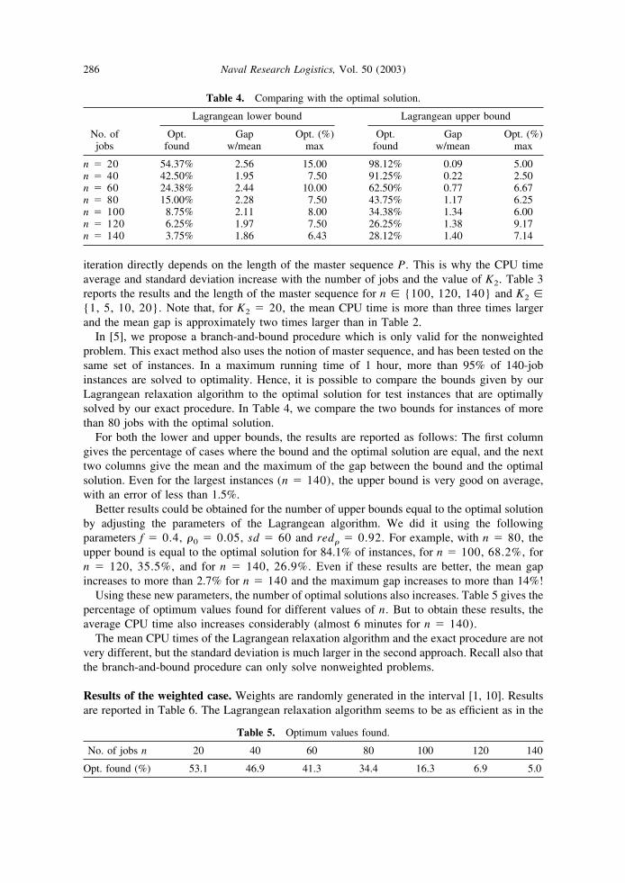
iteration directly depends on the length of the master sequence P. This is why the CPU timeaverage and standard deviation increase with the number of jobs and the value of K2. Table 3reports the results and the length of the master sequence for n � {100, 120, 140} and K2 �{1, 5, 10, 20}. Note that, for K2 � 20, the mean CPU time is more than three times largerand the mean gap is approximately two times larger than in Table 2.
In [5], we propose a branch-and-bound procedure which is only valid for the nonweightedproblem. This exact method also uses the notion of master sequence, and has been tested on thesame set of instances. In a maximum running time of 1 hour, more than 95% of 140-jobinstances are solved to optimality. Hence, it is possible to compare the bounds given by ourLagrangean relaxation algorithm to the optimal solution for test instances that are optimallysolved by our exact procedure. In Table 4, we compare the two bounds for instances of morethan 80 jobs with the optimal solution.
For both the lower and upper bounds, the results are reported as follows: The first columngives the percentage of cases where the bound and the optimal solution are equal, and the nexttwo columns give the mean and the maximum of the gap between the bound and the optimalsolution. Even for the largest instances (n � 140), the upper bound is very good on average,with an error of less than 1.5%.
Better results could be obtained for the number of upper bounds equal to the optimal solutionby adjusting the parameters of the Lagrangean algorithm. We did it using the followingparameters f � 0.4, 0 � 0.05, sd � 60 and red � 0.92. For example, with n � 80, theupper bound is equal to the optimal solution for 84.1% of instances, for n � 100, 68.2%, forn � 120, 35.5%, and for n � 140, 26.9%. Even if these results are better, the mean gapincreases to more than 2.7% for n � 140 and the maximum gap increases to more than 14%!
Using these new parameters, the number of optimal solutions also increases. Table 5 gives thepercentage of optimum values found for different values of n. But to obtain these results, theaverage CPU time also increases considerably (almost 6 minutes for n � 140).
The mean CPU times of the Lagrangean relaxation algorithm and the exact procedure are notvery different, but the standard deviation is much larger in the second approach. Recall also thatthe branch-and-bound procedure can only solve nonweighted problems.
Results of the weighted case. Weights are randomly generated in the interval [1, 10]. Resultsare reported in Table 6. The Lagrangean relaxation algorithm seems to be as efficient as in the
Table 4. Comparing with the optimal solution.
No. ofjobs
Lagrangean lower bound Lagrangean upper bound
Opt.found
Gapw/mean
Opt. (%)max
Opt.found
Gapw/mean
Opt. (%)max
n � 20 54.37% 2.56 15.00 98.12% 0.09 5.00n � 40 42.50% 1.95 7.50 91.25% 0.22 2.50n � 60 24.38% 2.44 10.00 62.50% 0.77 6.67n � 80 15.00% 2.28 7.50 43.75% 1.17 6.25n � 100 8.75% 2.11 8.00 34.38% 1.34 6.00n � 120 6.25% 1.97 7.50 26.25% 1.38 9.17n � 140 3.75% 1.86 6.43 28.12% 1.40 7.14
Table 5. Optimum values found.
No. of jobs n 20 40 60 80 100 120 140
Opt. found (%) 53.1 46.9 41.3 34.4 16.3 6.9 5.0
286 Naval Research Logistics, Vol. 50 (2003)

nonweighted case. CPU times are close because the parameters sd and red are the same andcontrol the convergence of the algorithm.
Again, the last column of Table 6 gives the gap between the two bounds expressed in %. Onecan notice that the gap remains very stable when the number of jobs increases. This gap can alsobe compared to the one given in Table 2 and is very similar. The table equivalent to Table 3 isnot given in the weighted case, since it is very similar.
As in the nonweighted case, better results could be obtained by adjusting the parameters ofthe Lagrangean algorithm. We did it again for n � 140, K1 � 1, and K2 � 20. The averageduality gap for the 10 instances reduces from 8.7% (max � 16.65%), when using the genericparameters ( f � 0.4, 0 � 1.6, sd � 40 and red � 0.9), to only 2.07% (max � 4.19%)by modifying 0 and sd (0 � 2.6 and sd � 80). To obtain these results, the average CPU timeincreases to 751.09 seconds vs. 383.32 seconds with the previous parameters.
Other instances. Different ranges for weights and processing times have been considered togenerate other instances. The generic parameters used in the previous set of instances have tobe adjusted. Since the weights have a direct influence on the value of the objective function, theinitial step 0 in the subgradient search should be chosen accordingly. After many tests, wedecided to use 0 � wmax/8.
Instances of 100 jobs are generated and solved using the previous parameters. Table 7presents the resulting gaps, and each line corresponds to 160 test problems. The results are verysimilar to the ones obtained on the previous instances. All average gaps remain below 3%.
9. CONCLUSION
This paper considers a single-machine scheduling problem in which the objective is tominimize the weighted number of late jobs. Based on the definition of the master sequence, a
Table 6. Results of the weighted case.
No. ofjobs
CPU time (s) Gap Gap (%)meanMean St dev Max Mean St dev Max
n � 20 4.18 2.28 12.46 4.46 3.54 20 4.07n � 40 13.20 8.58 37.88 7.65 7.65 31 3.36n � 60 30.66 20.39 83.28 10.26 6.37 41 3.09n � 80 56.49 38.79 184.43 11.40 7.31 36 2.56n � 100 86.21 58.83 231.57 14.82 8.78 47 2.70n � 120 130.96 90.47 378.59 18.17 11.49 72 2.74n � 140 184.66 130.34 496.85 29.18 21.46 127 3.82
Table 7. Results with different ranges.
Rangeof pi
Rangeof wi
Gap Gap (%)meanMean St dev Max
[1, 100] [1,10] 13.76 9.12 48 2.51[1,99] 133.12 79.39 424 2.66
[25, 75] [1,10] 14.53 10.23 61 2.63[1,99] 144.86 92.07 486 2.92
[1, 500] [1,10] 12.68 5.49 30 2.30[1,99] 135.06 60.52 322 2.73
287Dauzere-Peres and Sevaux: Lagrangean Relaxation for Minimizing Late Jobs
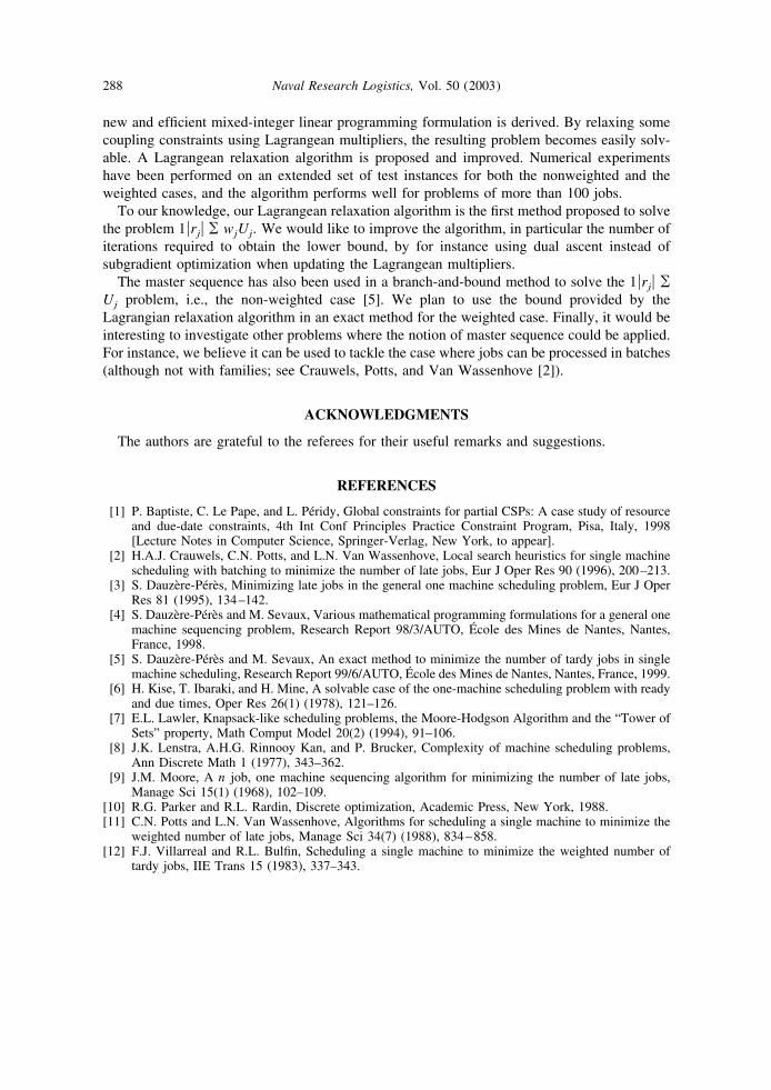
new and efficient mixed-integer linear programming formulation is derived. By relaxing somecoupling constraints using Lagrangean multipliers, the resulting problem becomes easily solv-able. A Lagrangean relaxation algorithm is proposed and improved. Numerical experimentshave been performed on an extended set of test instances for both the nonweighted and theweighted cases, and the algorithm performs well for problems of more than 100 jobs.
To our knowledge, our Lagrangean relaxation algorithm is the first method proposed to solvethe problem 1�rj� ¥ wjUj. We would like to improve the algorithm, in particular the number ofiterations required to obtain the lower bound, by for instance using dual ascent instead ofsubgradient optimization when updating the Lagrangean multipliers.
The master sequence has also been used in a branch-and-bound method to solve the 1�rj� ¥Uj problem, i.e., the non-weighted case [5]. We plan to use the bound provided by theLagrangian relaxation algorithm in an exact method for the weighted case. Finally, it would beinteresting to investigate other problems where the notion of master sequence could be applied.For instance, we believe it can be used to tackle the case where jobs can be processed in batches(although not with families; see Crauwels, Potts, and Van Wassenhove [2]).
ACKNOWLEDGMENTS
The authors are grateful to the referees for their useful remarks and suggestions.
REFERENCES
[1] P. Baptiste, C. Le Pape, and L. Peridy, Global constraints for partial CSPs: A case study of resourceand due-date constraints, 4th Int Conf Principles Practice Constraint Program, Pisa, Italy, 1998[Lecture Notes in Computer Science, Springer-Verlag, New York, to appear].
[2] H.A.J. Crauwels, C.N. Potts, and L.N. Van Wassenhove, Local search heuristics for single machinescheduling with batching to minimize the number of late jobs, Eur J Oper Res 90 (1996), 200–213.
[3] S. Dauzere-Peres, Minimizing late jobs in the general one machine scheduling problem, Eur J OperRes 81 (1995), 134–142.
[4] S. Dauzere-Peres and M. Sevaux, Various mathematical programming formulations for a general onemachine sequencing problem, Research Report 98/3/AUTO, Ecole des Mines de Nantes, Nantes,France, 1998.
[5] S. Dauzere-Peres and M. Sevaux, An exact method to minimize the number of tardy jobs in singlemachine scheduling, Research Report 99/6/AUTO, Ecole des Mines de Nantes, Nantes, France, 1999.
[6] H. Kise, T. Ibaraki, and H. Mine, A solvable case of the one-machine scheduling problem with readyand due times, Oper Res 26(1) (1978), 121–126.
[7] E.L. Lawler, Knapsack-like scheduling problems, the Moore-Hodgson Algorithm and the “Tower ofSets” property, Math Comput Model 20(2) (1994), 91–106.
[8] J.K. Lenstra, A.H.G. Rinnooy Kan, and P. Brucker, Complexity of machine scheduling problems,Ann Discrete Math 1 (1977), 343–362.
[9] J.M. Moore, A n job, one machine sequencing algorithm for minimizing the number of late jobs,Manage Sci 15(1) (1968), 102–109.
[10] R.G. Parker and R.L. Rardin, Discrete optimization, Academic Press, New York, 1988.[11] C.N. Potts and L.N. Van Wassenhove, Algorithms for scheduling a single machine to minimize the
weighted number of late jobs, Manage Sci 34(7) (1988), 834–858.[12] F.J. Villarreal and R.L. Bulfin, Scheduling a single machine to minimize the weighted number of
tardy jobs, IIE Trans 15 (1983), 337–343.
288 Naval Research Logistics, Vol. 50 (2003)


METAHEURISTIQUES :STRATEGIES POUR L’OPTIMISATION DE LA PRODUCTION DE BIENS ET DE SERVICES
Resoudre des problemes d’optimisation est un point cle dans l’amelioration constante dela productivite des entreprises. Quand les methodes traditionnelles echouent, il devientalors naturel de se tourner vers des techniques de resolution approchee.
Les metaheuristiques jouent, aujourd’hui, un role primordial dans la resolution desproblemes d’optimisation. Ces techniques sont devenues, en quelques annees, des outilsincoutournables et performants. Dans cette synthese, nous presentons un panorama desmetaheuristiques classiques (methodes de descente, recuit simule, recherche tabou, algo-rithmes genetiques), de certaines moins connues (recherche a voisinages variables, GRASP,iterated local search, guided local search, colonies de fourmis) et de techniques avancees (al-gorithmes memetiques, scatter search, GA|PM).
Pour toutes ces methodes, nous analysons les facteurs d’intensification et de diversi-fication presents, les particularites de chacune d’elle et notre retour d’experience sur lesapplications que nous avons traites. De cette analyse, nous pouvons proposer ce que sont,selon nous, les caracteristiques indispensables a une bonne metaheuristique.
METAHEURISTICS :STRATEGIES FOR THE OPTIMISATION OF THE PRODUCTION OF GOODS AND SERVICES
Solving optimisation problems is a key point in the constant improving of productivity inthe industries. When traditional methods fail, it is natural to look towards some approxi-mate resolution methods.
Metaheuristics play, today, an important role in solving optmisation problems. Thosetechniques became, in few years, necessary and powerful tools. In this synthesis, we presentan overview of the classical metaheuristics (descent methods, simulated annealing, tabusearch, genetic algorithms), some less known (variable neighbourhood search, GRASP, ite-rated local search, guided local search, ant colonies) and some advanced techniques (me-metic algorithms, scatter search, GA|PM).
For all of these methods, we analyse intensification and diversification factors, specificfeatures of each of them and our experiment on various applications we dealt with. Fromthis analysis, we suggest what are, from our point of view, the necessary caracteristics of agood metaheuristic.
Marc Sevaux, Mai [email protected]