inférence statistique pour certains modèles prédateur-proie
TRANSCRIPT
UNIVERSITÉ DU QUÉBEC À MONTRÉAL
INFÉRENCE STATISTIQUE POUR CERTAINS MODÈLES /
PREDATEUR-PROIE
MÉMOIRE
PRÉSENTÉ
COMME EXIGENCE PARTIELLE
DE LA MAÎTRISE EN MATHÉMATIQUES
PAR
ASHKAN ZAHEDI
MAI 2008

UNIVERSITÉ DU QUÉBEC À MONTRÉAL
STATISTICAL INFERENCE FOR SOME PREDATOR-PREY
MODELS
THESIS
PRESENTEDIN
PARTIAL FULFILMENT OF THE REQUIREMENTS
FOR THE MASTERS IN MATHEMATICS
BY
ASHKAN ZAHEDl
MAY 2008

UNIVERSITÉ DU QUÉBEC À MONTRÉAL Service des bibliothèques
Avertissement
La diffusion de ce mémoire se fait dans le respect des droits de son auteur, qui a signé le formulaire Autorisation de reproduire et de diffuser un travail de recherche de cycles supérieurs (SDU-522 - Rév.ü1-2üü6). Cette autorisation stipule que «conformément à l'article 11 du Règlement no 8 des études de cycles supérieurs, [l'auteur] concède à l'Université du Québec à Montréal une licence non exclusive d'utilisation et de publication de la totalité ou d'une partie importante de [son] travail de recherche pour des fins pédagogiques et non commerciales. Plus précisément, [l'auteur] autorise l'Université du Québec à Montréal à reproduire, diffuser, prêter, distribuer ou vendre des copies de [son] travail de recherche à des fins non commerciales sur quelque support que ce soit, y compris l'Internet. Cette licence et cette autorisation n'entraînent pas une renonciation de [la] part [de l'auteur] à [ses] droits moraux ni à [ses] droits de propriété intellectuelle. Sauf entente contraire, [l'auteur] conserve la liberté de diffuser et de commercialiser ou non ce travail dont [il] possède un exemplaire.»

ACKNOWLEDGMENTS
It is a great pleasure for me to thank Professor Sorana Froda who supervised my
thesis work. 1 would like to express my deepest appreciation to her for her patience.
Professor Froda provided a great help to me to understand and work on this subject.
1 am deeply grateful ta Professor René Ferland and Professor Fabrice Larribe for their
invaluable support thraughout my degree.
1 would also like to thank Ms. Manon Gauthier and Ms. Gisèle Legault, for their
assistance.
ln particular, 1 wish to express my warm regards to Alexandru Stanculescu, Martin
Caberlin and Sarah Vahey for offering me very helpful remarks about the draft.

TABLE OF CONTENTS
LIST OF FIGURES
LIST OF TABLES .
RÉSUMÉ
RÉSUMÉ
INTRODUCTION
CHAPTER l MOTIVATION FROM ECOLOGY
1.1 Mathematical Ecology
1.2 Models .
1. 2.1 Lotka-Volterra System .
1.2.2 Holling System
1.2.3 Hanski System
1.2.4 Arditi System.
1.3 Concluding Remarks .
CHAPTER II DETERMINISTIC ANALYSIS
2.1 Dynamical systems . . . .
2.2 Analysis of the Equilibria in Each Model .
2.2.1 Lotka-Volterra Model
2.2.2 Holling Model
2.2.3 Hanski Model .
2.2.4 Arditi Model
2.3 Final Comments ..
CHAPTER III STOCHASTIC MODELS AND STATISTICAL INFERENCE
3.1 Stochastic Models .
3.1.1 Lotka-Volterra Model
v
vii
xi
xiii
1
3
3
4
5
7
13
14
15
17
17
26
27
29
33
37
41
45
46
47
IV
3.1.2 Holling Model
3.1.3 Hanski Model .
3.1.4 Arditi Model .
3.2 Estimation and Testing
3.2.1 General Aigorithm
3.2.2 Estimation of ([2 .
3.2.3 Estimates for each model
3.2.4 Testing and Comparison of Models .
CHAPTER IV APPLICATIONS: SIMULATIONS AND DATA ANALYSIS
4.1 Description of the Simulation Study
4.1.1 Estimation
4.1.2 Testing
4.1.3 Results
4.2 Data Analysis .
4.3 Discussion ..
BIBLIOGRAPHY
48
50
51
52
52
53
54
59
63
63
66
67
68
72
73
77
LIST OF FIGURES
1.1 Type l functional response . 9
1.2 Type II functional response 10
1.3 Type III functional iesponse . 11
2.1 Classification of equilibria, linear systems - p: trace, q: determinant
(figure courtesy of Kot, 2001) 20
2.2 Example of limit cycle 21
2.3 2-loop cycle .... 22
2.4 Stable equilibrium 26
2.5 A stable solution for Holling Model: The model parameters are ex = 0.1;
K = 250; (3 = 0.05; w = 40; "( := 0.7; 8 = 0.5. . . . . . . . . . . . . . .. 33
2.6 Limit cycle for the Hanski Model: the model parameters are ex = 5.4;
K = 50; (3 = 600; w = 5; "( = 2.8; f-L = 100. . . . . . . . . . . . . . . . .. 37
2.7 A stable solution for Arditi Model: The model parameters are ex = 0.065;
K = 150; (3 = 0.12; w = 1.3; "( = 0.060; 8 = 0.024. . . . . . . . . . . . .. 42
4.1 Holling Model: Logarithm of (a) the predator and (b) the prey population
sizes when 02 = 0.01. The model parameters are ex = 0.1; K = 250;
(3 = 0.05; w = 40; "( := 0.7; 8 = 0.5 . 65
4.2 Observed population sizes: (a) Mink (b) Muskrat . 72

LIST OF TABLES
4.1 Estimates of the parameters for a 2 = 0.0005 and a 2 = 0.001 69
4.2 Estimates of the parameters for a 2 = 0.005 and a 2 = 0.01 . 70
4.3 Testing: How often the predator isocline is accepted as a vertical line . 71
4.4 Results of testing on the mink-muskrat data set. . . . . . . . . . . . . 73

RÉSUMÉ
On propose une méthode stochastique qui s'applique à des systèmes non linéaires
d'équations différentielles qui modélisent l'interaction de deux espèces; le but est d'établir
si un système déterministe particulier peut s'ajuster à des données qui présentent un
comportement oscillatoire. L'existence d'un cycle limite est essentielle pour l'implantation
de notre méthode. Cette procédure se base sur l'estimation des isoclines du système, en
utilisant le fait que les isoclines traversent les solutions du système à des points maxi
mum et minimum. Ensuite, nous proposons des tests qui permettent de comparer trois
modèles: Holling (1959), Hanski et al. (1991), and Arditi et al. (2004). Finalement, on
utilise des données simulées pour illustrer et étudier les propriétés de notre méthode, et
nouS appliquons la procédure à un ensemble de données bien connu.
Mots-clés: systèmes prédateur-proie, équations différentielles ordinaires, plan des phases,
isoclines, modèle stochastique, régression linéaire, estimation par moindres carrés, test
de t, test de Wilcoxon.

ABSTRACT
We propose a stochastic method applicable to two species nonlinear systems of differential equations; the purpose is to determine whether a particular deterministic model can be fitted to a given data set that exhibits oscillatory behavior. Existence of a limit cycle solution is crucial for implementing our method. This method is based on estimating the coefficients of the isoclines of the given system, based on the fact that the isoclines intercept the solutions of the system at their local minima and maxima. Next, we introduce several testing methods which allow to compare three models: Holling (1959), Hanski et al. (1991), and Arditi et al. (2004). Finally, we use simulated data to illustrate and study the properties of our method, and we apply the procedure to a well-known data set.
Key words: predator-prey systems, ordinary differential equations, phase plane, nullisoclines, stochastic model, linear regression, least squares estimation, t-test, Wilcoxon test.

INTRODUCTION
In the 1920s, Lotka (1925) and Volterra (1926) introduced a two dimensional non
linear system of differential equations as a continuous-time model which could explain
the behavior of a two-species population of predator and prey. Since then, the construc
tion and study of deterministic models for general population dynamics of predator-prey
systems has become a central subject in mathematical ecology. Besides Lotka-Volterra,
other classical approaches use what is known as Holling type l, II and III functionals
for modeling the interaction. For the classical references in this area we refer to Kot
(2001).
Animal populations change by migration, birth and death. As seen in nature, either the
predator or prey population, or bath, can become extinct or coexist in a state of equilib
rium. Moreover, extinction or equilibrium can be reached by oscillations. Furthermore,
classical prey-predator models such as Lotka-Volterra, or Holling (1959) cannot express
coexistence of the prey with its predator at a population level much lower than the
maximum possible population size. This is known as the paradox of biological control.
Indeed, the original models were mainly aiming to determine the effect of the prey
population on the number of prey consumed by each predator over time. These models
hardly discussed the effect of the predator population on the predator-prey interactions.
Arditi et al. (2004) were those who first recognized that adding the effect of the preda
tor population on the predator-prey interaction can solve the problem of coexistence at
lower population levels. They proposed several such predator-dependent models.
In this thesis we introduce sorne of these models, namely those which had a major im
pact on the development of the mathematical theory of predator-prey interactions. We
review the ecology of these models and we explain the interpretation of their parameters.
We present sorne elements of the theory of dynamical systems in non-technical terms,
as well as their links to mathematical ecology of predator-prey interactions. We point

2
out how the qualitative analysis of dynamical systems helps us explain the behavior of
the solutions to the predator-prey population systems of ordinary differential equations
(ODEs).
Further, at the core of this work, we introduce a new stochastic model, which adds
observational error to the solutions of the ODEs. An important part of the thesis deals
specifically with statistical inference, namely estimating the parameters, as weB as a
comparison of models based on simple tests. In the end, we conduct simulation studies
. to illustrate our method, and check empirically the properties of our estimators and
tests. We also apply the testing and estimation procedure to a real data set.
The thesis is organized as follows. In Chapter 1, we introduce the Lotka-Volterra, the
Holling, the Hanski and the Arditi models, and explain their specifie contribution to
ecological modeling of predator-prey interactions. Chapter 2 is devoted to the deter
ministic analysis, where we study the four mentioned models separately. In Chapter 3,
we propose and study our stochastic models. Moreover, we develop the estimation and
testing procedures specifie to our models. Finally, we devote Chapter 4 to simulation,
in order to perform an empirical study of our inference methodology, as well as a short
data analysis.

CHAPTER 1
MOTIVATION FROM ECOLOGY
1.1 Mathematical Ecology
In ecology, there is a long tradition of modeling population sizes of interacting
species by functions which are the solutions to a deterministic system of ordinary dif
ferential equations (ODE). Such functions are positive and often are either periodic or
quasi-periodic; see Froda and Colavita (2005). Depending on the coefficients of a given
ODE, the solution can carry on different behaviors such as admitting a limit cycle, stable
node, etc. Due to the natural behavior of the predator and the prey, these systems of
ten bear oscillatory behavior. Despite the abundance of such deterministic models, they
are rarely used in quantitative studies, but appear mainly in the qualitative analysis.
Time series models or stochastic differential equations, for discrete and continuous time
models, respectively, are commonly used in order to assess the quantitative behavior.
For more comments see Froda and Nkurunziza (2007).
As far as the historical background goes the story is as follows: During the First World
War, there was an increase in the predatory fish population and a decrease in the prey
fish population in the aftermath of a complete cease on fishery in the Adriatic sea, which
led Volterra (1926) to formulate a mathematical model to describe the predator-prey
population dynamics (Kot, 2001). In order to explain a mechanism by which predators
regulate their prey, Volterra constructed a mathematical model that describes temporal
changes in prey and predator abundances. He made several restrictive assumptions such
as: (i) the predator-prey population levels are large enough to be considered as contin

4
uous rather than discrete variables; (ii) the prey and the predator are both well-mixed
in the environment; (iii) the populations are closed in the sense that there is no im
migration or emigration; (iv) the population dynamics is completely deterministic, i.e.
no random events are considered; (v) the prey population grows exponentially in the
absence of predator; (vi) the predator rate consumption of prey is a linear function of
prey and vice versa; (vii) the predator population declines exponentially in the absence
of prey. Furthermore, Volterra (1926) introduced a two dimensional first order system
of ordinary differential equations where solutions represent the prey and the predator
population sizes, respectively.
Due to the simplicity of this model, sorne of the major basic facts in ecology were ig
nored in the system. For instance, the proposed parametrization supposes that the
population of the prey will grow exponentially in the absence of predator. This model
is also present in the Lotka (1925) work and therefore, is referred to the Lotka-Volterra
model.
Later on, other researchers partially recovered this problem of the classical Lotka
Volterra model by introducing new terms to the system. One of the major contributions
was made by Holling (1959). For our presentation we retain Holling's approach as well
as the models proposed by Hanski et al. (1991) and Arditi et al. (2004).
In short, all these authors propose adding new parameters in order for avoiding expo
nential growth of the prey population in the absence of predator. In the new cases, the
population of prey increases asymptotically instead of exponentially. They also pro
posed modified equations describing the growth of the predator population by including
nonlinear terms in order to get around certain problems.
In this chapter, we describe each of these models in terms of their ecological interpre
tation.
1.2 Models
In this section, we introduce three systems of differential equations for the predator
prey interactions known as Holling (Holling, 1959), Hanski (Hanski et al., 1991) and

5
Arditi (Arditi et al., 2004), along with the classical Lotka-Volterra model as presented
in Hirsch and Smale (1974). Our main emphasis is on the proposed parameterizations
and their ecological meaning.
In what fol1ows, let x == Xt denote the size of the prey population, and y == Yt denote
the size of the predator population at time t. Sorne authors refer to Xt and Yt as the
prey and predator density, respectively.
1.2.1 Lotka-Volterra System
As stated before, one of the original two-species biological models is called Lotka
Volterra (Hirsch and Smale, 1974). The model includes two equations, one which de
scribes how the size of the prey population changes over time and the second one which
describes how the predator population size changes over time. This model is often
described by
{ 1~ : (a - (3y)x,
Iljf - hx - 8)y. (1.1 )
The parameters appearing in system (1.1) are defined as follows:
a : the natural growth (birth) rate of prey in the absence of the predator per capita,
(3 : the death rate per encounter of prey due to predation or predation rate coefficient,
1 : the reproduction rate of predators per one prey eaten,
8 : the natural death (decline) rate of the predator in the absence of prey.
Let us look more closely at each equation of system (1.1).
The prey equation is defined by
dx dt = ax - {3xy. (1.2)
Thus, by letting {3 = 0 i.e. when there is no predation, we can see that the prey is
assumed to have an unlimited food supply to reproduce exponentially; this exponential
growth is represented in equation (1.2) by the term ax. The rate of decrease due to
predation is assumed to be proportional to the rate at which the predators and the prey
meet; this is represented in equation (1.2) by -{3xy. If either x or y is zero then there
can be no predation. Finally, equation (1.2) can be interpreted as follows: the change

6
in the prey population size is due to its own growth minus the rate at which it is preyed
upon.
Further, the predator equation is given by
dydt = "(xy - oy. (1.3)
By letting "( = 0 in equation (1.3), oy represents the natural death of the predators
which is an exponential decay as opposed to the exponential growth of prey. On the
other hand, in this equation, "(xy represents the growth of the predator population and
is due to predation. (Note the similarity to the predation rate in equation (1.2); how
ever, a different constant is used as the rate at which the predator population grows
is not necessarily equal to the rate at which the predator consumes the prey). Hence,
equation (1.3) represents the change in the predator population size as the growth of
the predator population due to predation, minus natural death.
The system of equations (1.1) admits periodic solutions which do not have a simple,
analytic expression in terms of the usual trigonometric functions (Hirsch and Smale,
1974). However, later on we will see that an approximate linearized solution yields a
simple harmonie motion with the population of predators following that of prey by 90°.
In the Lotka-Volterra system, the predator population grows when there are plenty of
prey but, ultimately surpass their food supply and decline. As the predator population
reaches a lower level, the prey population can increase again. These dynamics continue
in a growth-decline cycle (Kot, 2001).
The prey average population size over one period is oh. Therefore, it depends only on
the parameters which describe population growth and death of predatorj at the same
time, the predator average size over one period is 0:/ (3 and therefore, depends only on
the prey growth and death population parameters (Kot, 2001). Moreover, increasing
the prey growth per capita rate 0:, which is sometimes called enrichment in the eco
logical literature, does not change the prey average size, but it increases the predator
average size (Kot, 2001).
Can this model explain the question about the observed changes in predator and prey
fish abundances during the First World War mentioned before?

7
Volterra (1926) hypothesized that fishery reduces the prey per capita growth rate a
and increases the predator mortality rate 8, while the interaction rates {3 and 'Y do
not change (Volterra, 1926). Thus, ceasing fishery should lead to an increase in a and
decrease in 8 and thus induce a decrease in the average prey fish population 8l'Y and
to an increase in the average predator fish population al{3, which is exactly what was
observed during the First World War.
1.2.2 Holling System
Holling system was introduced in Holling (1959). Before presenting it, we explain
a modification of the Lotka-Volterra model known as the competitive Lotka-Volterra
system (Hirsch, 1990). The competitive Lotka-Volterra equations are a simple model of ,
the population dynamics of species competing for some common resource. The form is
similar to the classical Lotka-Volterra equations (1.1).
Before introducing this new type of model, let us introduce the logistic population model
for one species which is common in ecology,
dx x dt = ax(1 - K)'
where x is the size of the population at a given time, a is inherent per-capita growth
rate, and K is the carrying capacity (Kot, 2001).
Definition 1.2.1 The equilibrium maximum of the population of an organism is known
as the ecosystem 's carrying capacity for that organism.
In non technical terms, the carrying capacity is the asymptotic limit for the population
size of an organism. Moreover, as population size increases, birth rates often decrease
and death rates typically increase. The difference between the birth rate and the death
rate is called natural increase. The carrying capaci ty could support a positive natural
increase, or could require a negative natural increase. Carrying capacity is thus the

8
number of individuaIs an environment can support without significant negative impacts
to the given organism and its environment. A factor that keeps population size at an
equilibrium is known as a regulating factor.
In the logistic model dx x dt = e:tx(l - K)'
below carrying capacity K, populations asymptotically increase until they reach their
asymptote, which is the horizontalline at height K in this case. The carrying capacity
of an environment may vary for different species and may change over time due to a
variety of factors including food availability, water supply, environmental conditions,
and living space (Kot, 2001).
Holling (1959) studied predation of small mammals on pine sawflies, and found that
predation rates increased with increasing prey population size. This was resulted from
two effects:
(i) each predator increased its consumption rate when exposed to a higher prey popu
lation, and
(ii) predator population increases with the increasing prey population. So he proposed
what is known as the Holling system.
Holling system is very similar to the competitive Lotka-Volterra model. Given two
populations, x and y, with logistic dynamics, the Lotka-Volterra formulation adds an
additional term to account for the species' interactions. Thus the competitive Lotka-
Volterra equations are
~~ = e:tx(l - K) - {3xy, (1.4)
{ ~ = ,xy - 8y - 8y2.
In the Lotka-Volterra model (1.1), the prey population can increase indefinitely in the
absence of predator, i. e. if {3 = O. Moreover, if the initial value slightly changes the
trajectory (Xt, Yt) in the plane will dramatically change i.e. the amplitudes of Xt and
Yt are very different. So this system is unstable in a certain sense (Hirsch and Smale,
1974). To correct these problems, introducing additional terms to the model (1.1)
seems necessary. Holling (1959) proposed adding a nonlinear term to the original Lotka
Volterra prey equation and set logistic growth for prey in the absence of predator, as in
9
system (1.4). His next major contribution to the theory of predator-prey interactions
was to replace j3xy by f(x)y, i.e. to add different predator functional responses f(x)
to the prey equation. There are three major types of functional responses proposed by
Holling (Kot, 2001):
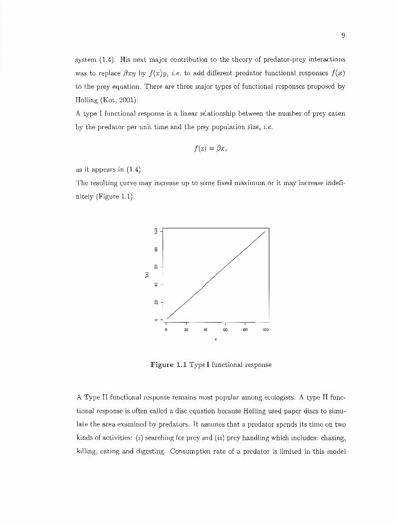
A type 1 functional response is a linear relationship between the number of prey eaten
by the predator pel' unit time and the prey population size, i. e.
f(x) = j3x,
as it appears in (1.4).
The resulting curve may increase up to sorne fixed maximum or it may increase indefi
nitely (Figure 1.1).
0
~
0.,
g x ""
0...
0 N
0
0 20 40 60 80 100
Figure 1.1 Type 1 functional response
A Type II functional response remains most popular among ecologists. A type II func
tional response is often called a disc equation because Holling used paper discs to simu
late the area examined by predators. It assumes that a predator spends its time on two
kinds of activities: (i) searching for prey and (ii) prey handling which includes: chasing,
killing, eating and digesting. Consumption rate of a predator is limited in this model

10
because even if prey are sa abundant that no time is needed for search, a predator still
needs ta spend time on prey handling. The type II functional response is
f(x) =~, w > O. w+x
One can see that for x approaching to 00, f(x) tends to {3. This means that a type
II functional response remains bounded unlike a type 1 functional response, {3x. Since
f(w) = ~, w is referred to as half-capturing saturation constant.
This function indicates the number of prey killed by one predator at various prey pop
ulation sizes and is a typical shape of functional response for many predator species.
At low prey population sizes, predators spend most of their time on search, whereas at
high prey population sizes, predators spend most of their time on prey handling (Figure
1.2).
~
"!
q
6'"
6'".... 6
"! 0
0 6
0 20 40 60 80 100
Figure 1.2 Type II functional response
A type III functional response occurs in predators which increase their search activity
with increasing prey population size. For example, many predators respond to chem
icals emitted by prey and increase their activity. Predator mortality increases first as

11
prey population size increases, and then declines (Figure 1.3).
A type III functional response is the only type of functional response that allows prey
mortality to increase with increasing prey population size. In this thesis, we only review
0 <Xl
0 <0
è 0 '<t
0 N
0
0 20 40 60 80 100
Figure 1.3 Type III functional response
a Holling model where the functional response is of type II. Holling (1959) explained
the following disc equation for the functional response term,
f(x) =~, x+w
where {3 is the maximum predator attack rate and w is the prey population size where
the attack is half-saturated. Therefore, Holling suggested the ODE system (1959)
dx - (1 _ ~) _ J1ELdt - (Xx K x + w' (1.5)
{ ~ = 2~~ -oy,
where x and y are the prey and predator population sizes, respectively.
In the equations (1.5) the parameters are defined as follows:
K: carrying capacity of the prey population;
{3: capturing rate, or search rate for predators, i. e. how effective the predators are;
w: half-capturing saturation constant;
12
T conservation rate (predator birth rate);
8: predators rate of death.
Further, we look at each equation separately. The prey equation is given by
dx x f3xy - = ax(l- -) - --. (1.6)dt K x+w
The prey is assumed to have an unlimited food supply, and to reproduce asymptotically
unless subject to predation, i. e. in the absence of predation, f3 = O. This asymptotic
growth is represented by ax(1 - K) in equation (1.6). The rate of predation upon prey
is assumed to be proportional to the rate at which predator and prey meet. This is
represented by !!~t. If either x or y is zero then there can be no predation.
With these two terms, equation (1.6) can be interpreted as the change in the size of
the prey population given by its own asymptotic growth minus the rate at which it
is preyed upon. Finally, note that for very large carrying capacity, K ----t 00, the first
term in equation (1.6) is identical to the first term in the classical Lotka-Volterra prey
equation (1.1).
Further, consider the predator equation
dy = ,xy _ 8y. (1.7)dt x+w
In this equation, ,xy represents the growth of the predator population due to prex+w
dation. (Note that the coefficient, is not necessarily equal to the coefficient f3.) In
equation (1.7), 8y represents the natural death of the predators which is an exponential
decay as in the classical Lotka-Volterra system (1.1). Renee, equation (1.7) represents
the change in the predator population as the growth of the predator population, minus
natural death.
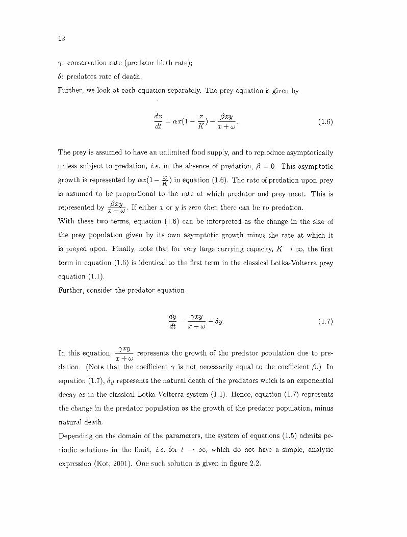
Depending on the domain of the parameters, the system of equations (1.5) admits pe
riodic solutions in the limit, i.e. for t 00, which do not have a simple, analytic ----t
expression (Kot, 2001). One such solution is given in figure 2.2.
13
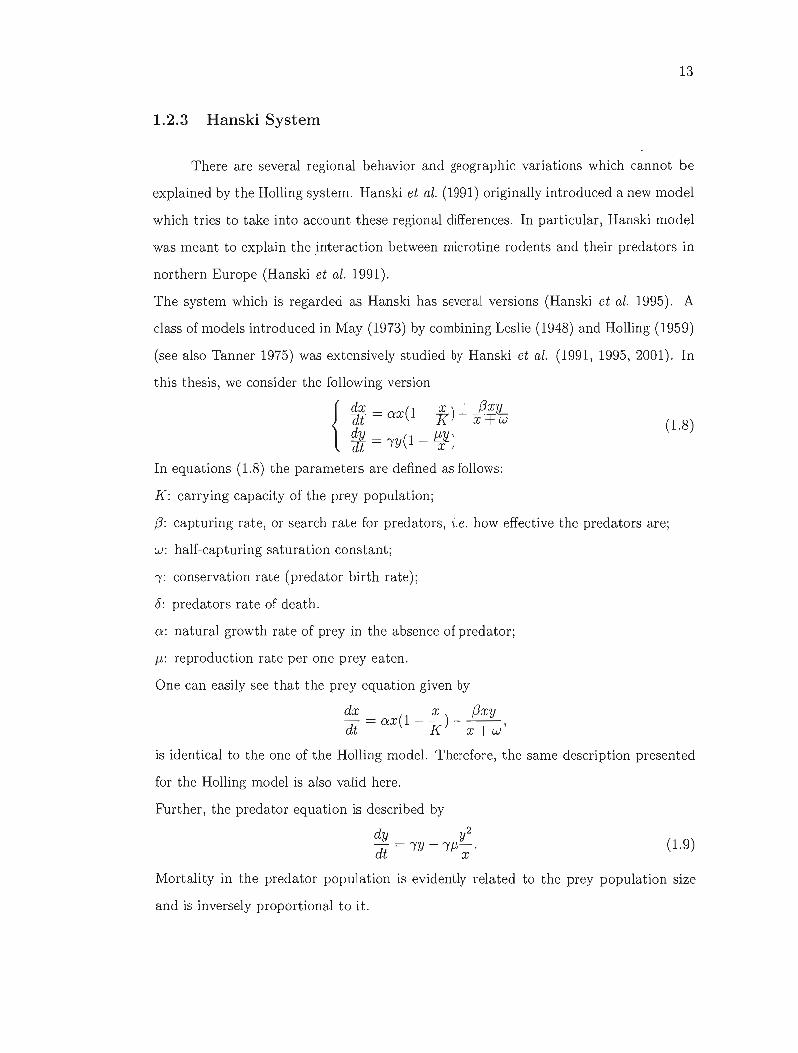
1.2.3 Hanski System
There are several regional behavior and geographic variations which cannat be
explained by the Holling system. Hanski et al. (1991) originally introduced a new model
which tries ta take into account these regional differences. In particular, Hanski model
was meant ta explain the interaction between microtine l'adents and their predators in
northern Europe (Hanski et al. 1991).
The system which is regarded as Hanski has several versions (Hanski et al. 1995). A
class of models introduced in May (1973) by combining Leslie (1948) and Holling (1959)
(see also Tanner 1975) was extensively studied by Hanski et al. (1991, 1995, 2001). In
this thesis, we consider the following version
dx _ (1 X)' JÈJLaI - ax - K - x + w (1.8)
{ 1lf = "fY( 1 - I!l-) In equations (1.8) the parameters are defined as follows:
K: carrying capacity of the prey population;
(3: capturing rate, or search rate for predators, i.e. how effective the predators are;
w: half-capturing saturation constant;
T conservation rate (predator birth rate);
0: predators rate of death.
a: natural growth rate of prey in the absence of predator;
J.L: reproduction rate per one prey eaten.
One can easily see that the prey equation given by
dx x (3xy dt = ax(l - K) - x + w)
is identical to the one of the Holling model. Therefore, the same description presented
for the Holling model is also valid here.
Further, the predator equation is described by
dy y2 - = "fY - "flt-· (1.9)dt x
Mortality in the predator population is evidently related ta the prey population size
and is inversely proportional to it.

14
For specifie types of predators, this model seems more appropriate than standard models
such as Lotka-Volterra (Hanski 1999). However, this model holds a major shortcoming:
the system is not well-defined when the environment does not contain any prey since
the denominator of the predator equation (1.9) becomes zero, whereas in other models
this problem does not occur. In other words, there is no way to quantify the behavior
of the predator population in the absence of prey. One such solution is given in figure
2.3.
1.2.4 Arditi System
Although the inclusion of a more complex functional response f(x) in the Holling
and Hanski predator equation is intuitively appealing, there are sorne notable problems
with this approach (Arditi and Ginzburg 1989). To overcome the problems, it was
suggested that the functional response should be expressed in terms of the ratio of
prey to predators (Jost and Arditi, 2001). Therefore, they defined the model as follows
(Arditi et al. 2004)
dx _ (1 _ -L) _ {3xyaI - ax K x + wy , (1.10)
{ 1JJ. - 'FY _dt - x + wy r5y.
or equivalently,
dx = ax(l _ X) _ {3(xjy)yaI K (x/y)+w'
{ 1JJ. = '"'f(x/y)y - r5ydt (x/y)+w .
We can note immediately the similarity with the Holling system where f(x) = x %w is
replaced by f(x, y) = (jx)y) and depends on the ratio x/y. Otherwise, the equationsx y +w .
can be interpreted in a similar fashion.
Namely, the prey equation is defined as
dx x f3xy - = ax(l - K) - , (1.11)dt x + wy
where the production of prey in the absence of predators is described by ax(l - K)' whereas x ~Xwy is the functional response (number of prey eaten per predator unit per
unit time.)
15
Besides, the predator equation becomes
dy '"'jxy ~ Jy. (1.12) dt x+ wy
Natural mortality of prey is considered to be negligible compared to mortality due to
predation. The constant '"'j is the trophic efficiency, i. e. the ratio of predator population
size level to the prey population size level, and predators are assumed to die with a
constant death rate J.
1.3 Concluding Remarks
In this chapter, four general predator-prey mathematical models, classical Lotka
Volterra, Holling, Hanski, and Arditi were briefly introduced. The Lotka-Volterra model
assumes that the prey consumption rate of the predator is directly proportional to the
prey abundance. This means that predator feeding is limited only by the amount of
prey in the environment. While this may be realistic at low levels of prey population
sizes, it is certainly an unrealistic assumption at high level of prey population sizes
where predators are limited e.g. by time and digestive constraints. The need for a more
realistic description of predator feeding came from an experimental work performed
by Gause on predator-prey interactions (Kot, 2001). It was observed that to explain
his experimental observations, the linear functional dependencies of the Lotka-Volterra
model must be replaced by nonlinear functions.
Further, we introduced one of the original nonlinear models known as Holling. It in
corporates the l'ole of carrying capacity as an asymptote to the prey population size,
which controls its maximum in the absence of predator. Moreover, a more complex
functional response in the predator-prey interaction was introduced as a key step in
improving the classical Lotka-Volterra model. Many questions in predator-prey theory
revolve around the functional response. ln the classical Lotka-Volterra model, the func
tional response is reduced to the form f3x, while in the Holling model, the functional
response becomes x ~w' Neither of these models explains searching for food efficiency
since they do not actually depend on the predator population; they are of the form
16
f = f(x). However, it was observed (Arditi et al. 2004) that changing the functional
response to f(x y) = fJ(x/y) explains the searching efficiency more accurately. , (x/y) +w Moreover, a model by Hanski was introduced where the prey equation is identical to
the one of Holling. Therefore, the same problem related ta the functional response
which appearing in the Holling model exists here as weIl. We also explained, another
disadvantage in the Hanski predator equation regarding the situation where there is no
prey in the environment.
In the next chapter, we proceed to performing an analysis of the dynamics on these four
models.

CHAPTER II
DETERMINISTIC ANALYSIS
We start this chapter by studying the dynamical systems corresponding to equa
tions (1.1), (1.5), (1.8), and (1.10). We introduce the concepts of equilibria and study
their stability. This is motivated by the usual assumption that sorne equilibria indicate
population extinction, while others correspond the averages of population sizes. Later
in this chapter, we review the qualitative analysis of the aforementioned models with
respect to their solution behavior. This includes identifying the equilibrium points and
their stability.
We keep the technicalities to a minimum as we want to introduce only the elements of
the qualitative analysis which are useful in the statistical development of Chapters 3 and
4. It should be mentioned that the concepts introduced in this chapter are presented
mainly informally. We simply give the main ideas behind this type of analysis. For an
extensive work on this issue one can refer to Hirsch and Smale (1974), Hirsch, Smale
and Devaney (2004) and Kot (2001).
2.1 Dynamical systems
In this section, we introduce sorne key topics in dynamical systems, which are
essential in the study of the behavior of the solutions of systems of ordinary differential
equations (ODE) and, in particular, the predator-prey popul~l.tion models. We limit
ourselves to planar systems only. (See figure 2.1 for the linear case.)
Let F(x,y) and G(x,y) be continuous real functions 'with continuous derivatives. An

18
autonomous planar system is given by
~f = F(x, y), (2.1 ) { 011- ( )dt - G x,y ,
with the initial value (xa, Ya). From now on, we limit ourselves tü two dimensional
systems of equations which represent a predator-prey system as a special case. A planar
system can be either linear or nonlinear. An autonomous linear planar system is a
system where F and Gare linear functions, i. e.
F(x,y)=ax+b,
{ G(x,y) = ex + d.
In this chapter, we look at the long term behavior of certain collection of solutions,
i. e. namely for t ----t 00, and compare these behaviors via the qualitative analysis of the
systems. This collection of representative solution curves (Xt, Yt) of the system (2.1) in
JR2 is called a phase plane (Hirsch, Smale and Devaney, 2004, p. 41).
Definition 2.1.1 Equlibrium (Hirsch and Smale 1914) p. 22)
Population equilibrium is an event when neither of the prey or predator population levels
is changing. For the planar system (2.1) this occurs when both F(x*,y*) = G(x*,y*) =
o.
In this case, a solution reaching to (x*,y*) stays forever at (x*,y*).
The equilibrium point (x*,y*) is called non-trivial if (x*,y*) of. (0,0).
We are interested in studying the behavior of the solution around the equilibria of the
planar system since equilibria play an important role in the theory of ODEs. There are
different types of equilibria. However, we mention only those which play a role in our
case. For an extensive study of equilibria, one can refer to Hirsch, Smale and Devaney
(2004) p. 174.
An equilibrium is called stable if close by solutions stay close by for ail future times.
Stable focus is an example of a stable equilibrium where the solution stays near by the
equilibrium if it is already near by (Figures 1.1 and 2.4). Moreover, a stable equilibrium
19
is asymptoticaUy stable if the solution approaches the equilibrium in the long term.
A classical example of an asymptoticaUy stable equilibrium is a sink (or stable node) ,
where the solution tends to the equilibrium in aU directions and stays at the equilibrium
for aU times. An equilibrium that is not stable is caUed unstable. A common example
of an unstable equilibrium is a source (or an unstable node) where the solution tends
away from the equilibrium in aH directions. A center is an unstable equilibrium where
with a smaH perturbation it can either turn into a sink or a source. Another example
of an unstable equilibrium is a saddle. Depending what direction the solution takes it
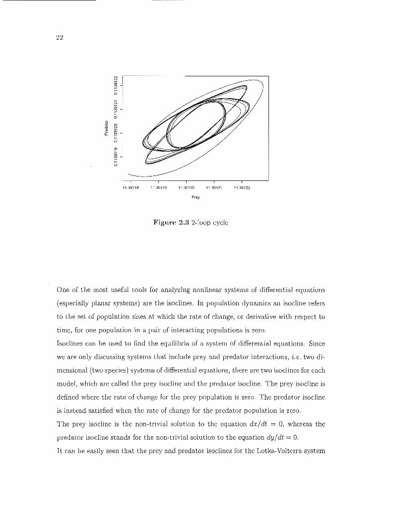
could either converge to the saddle or diverge from it. Figure 2.1 indicates the six types
of equilibrium points which occur in planar linear system.
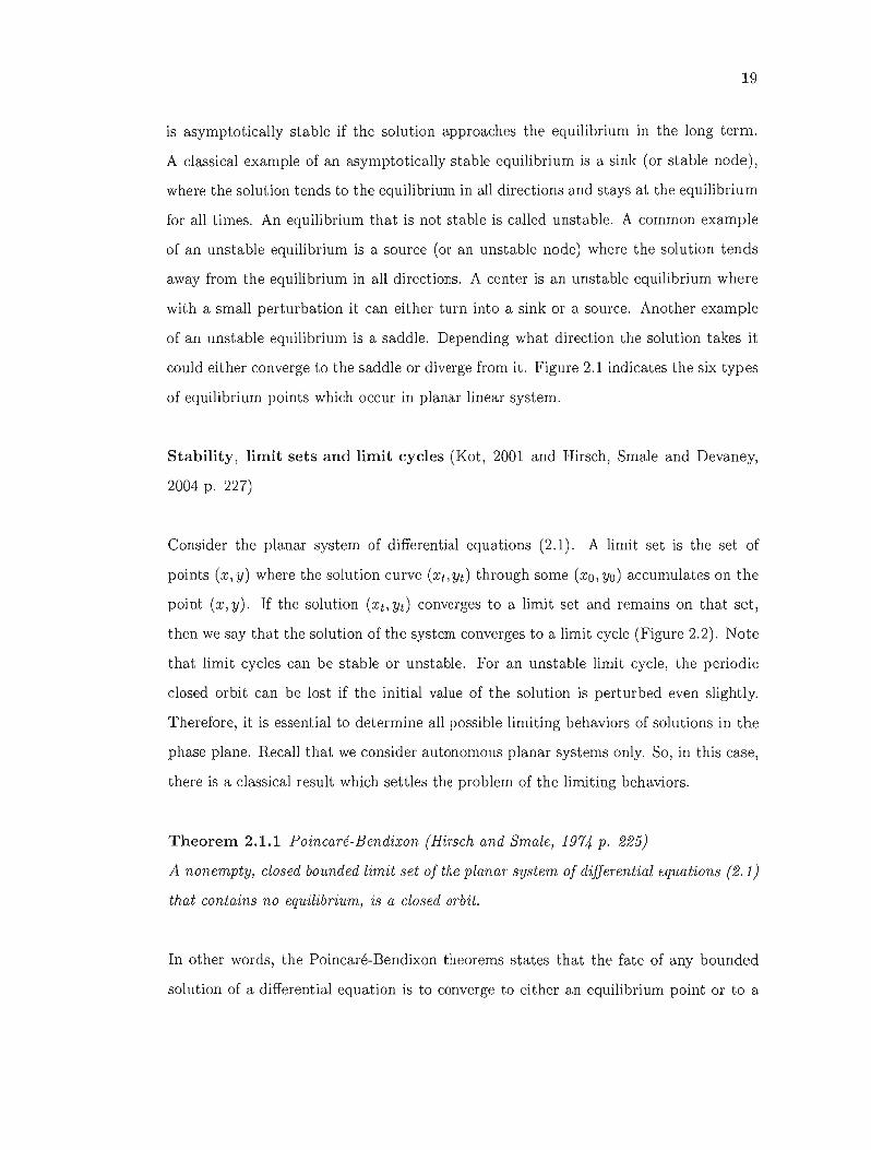
Stability, limit sets and limit cycles (Kot, 2001 and Hirsch, Smale and Devaney,
2004 p. 227)
Consider the planar system of differential equations (2.1). A limit set is the set of
points (x,y) where the solution curve (Xt,Yt) through sorne (xo,Yo) accumulates on the
point (x, y). If the solution (Xt, Yt) converges to a limit set and remains on that set,
then we say that the solution of the system converges to a limit cycle (Figure 2.2). Note
that limit cycles can be stable or unstable. For an unstable limit cycle, the periodic
closed orbit can be lost if the initial value of the solution is perturbed even slightly.
Therefore, it is essential to determine aH possible limiting behaviors of solutions in the
phase plane. Recall that we consider autonomous planar systems only. So, in this case,
there is a classical result which settles the problem of the limiting behaviors.
Theorem 2.1.1 Poincaré-Bendixon (Hirsch and Smale, 1914 p. 225)
A nonempty, closed bounded limit set of the planar system of differential equations (2.1)
that contains no equilibrium, is a closed orbit.
In other words, the Poincaré-Bendixon theorems states that the fate of any bounded
solution of a differential equation is to converge to either an equilibrium point or to a

20
p
-
Sadd le point
Saddle point
Unstable /' /' ~ node /' /' " p2 = 4q
/'
/ /
/
/ Unsk1ble focus 1
Center
+ .L _
\ , , , Stable focus
Stable node
q
p
/
q
Figure 2.1 Classification of equilibria, linear systems - p: trace, q: determinant (figure
courtesy of Kot, 2001)
limit cycle. Limit cycles can be interpreted as closed orbit attractors: there is an open
set 0 of initial values (xo, Yo) such that ail solution starting in 0 will eventually lie on
the limit cycle.
Consider the planar system of differential equations (2.1). As we said earlier, this sys
21
o o
"
o o M
o o N
o o
50 100 150 200
Prey
Figure 2.2 Example of limit cycle
tem can represent a predator-prey population dynamical system. Given the fact that
in ail discussed models the solutions stay in bounded regions, we can conclude that the
solutions to Lotka-Volterra, Holling, Hanski, and Arditi systems ail converge tO.either
equilibrium points or to limit cycles.
Limit cycles may, in practice, lead to extinction due ta environmental impacts (Hanski
et al. 1995). A large limit cycle that periodically brings either population close to zero
implies high probability of its extinction, if we consider possible external impacts that
are not taken into account by the model (Berezovskaya et al. 2001). The importance of
the existence of a limit cycle solution is in its periodic behavior.
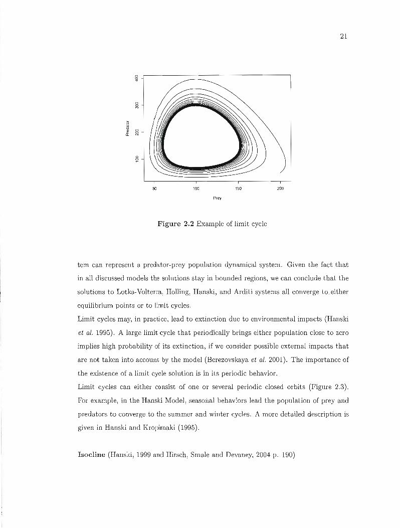
Limit cycles can either consist of one or several periodic clQsed orbits (Figure 2.3).
For example, in the Hanski Model, seasonal behaviors lead the population of prey and
predators to converge to the summer and winter cycles. A more detailed description is
given in Hanski and Kropimaki (1995).
Isocline (Hanski, 1999 and Hirsch, Smale and Devaney, 2004 p. 190)
22
11.39118 11.39119 11.39120 11.39121 11.39122
Prey
Figure 2.3 2-100p cycle
One of the most useful tools for analyzing nonlinear systems of differential equations
(especially planaI' systems) are the isoclines. In population dynamics an isocline refers
to the set of population sizes at which the rate of change, or derivative with respect to
time, for one population in a pair of interacting populations is zero.
Isoclines can be used to find the equilibria of a system of differential equations. Since
we are only discussing systems that include prey and predator interactions, i. e. two di
mensional (two species) systems of differential equations, there are two isoclines for each
model, which are called the prey isocline and the predator isocline. The prey isocline is
defl:ned where the rate of change for the prey population is zero. The predator isocline
is instead satisfied when the rate of change for the predator population is zero.
The prey isocline is the non-trivial solution to the equation dx/dt = 0, whereas the
predator isocline stands for the non-trivial solution to the equation dy/dt = O.
It can be easily seen that the prey and predator isoclines for the Lotka-Volterra system

23
are respectively the horizontal, the vertical lines, given by
o x ==-.
"'(
The prey isoclines for the Holling and Hanski systems are identical to each other, since
the prey equations for both models are identical. We can see that the prey isocline has
the quadratic form CI'
Y= Kj3(K-x)(x+w).
The Holling predator isocline is a vertical line
wo x = "'(-0'
whereas the Hanski predator isocline is a line passing through the origin
1 y= -x.
f.k
The prey isocline for Arditi model is given by
Cl'x(l K) y = j3 (1 x ) ,
-CI'W - K
while the Arditi predator isocline is a line passing through the origin given by
("'( - 0) y = wo x ..
In order to study the stability of equilibria and eventually find the limit cycles, we start
by considering the linearized systems.
Linearization (Hirsch and Smale, 1974)
1inearization makes it possible to use tools for studying linear systems in order to
analyze the behavior of a nonlinear function near a given point, which in our case is an
equilibrium point. The stability of an equilibrium point can be determined by perform
ing a linearization using partial derivatives about that equilibrium point.
Consider the system introduced in (2.1) and let (xt, Yt) denote a solution. The lin
earization of a function is the first order term of its Taylor expansion around the point

24
of interest e.g. the equilibrium point (x*, y*). The corresponding linearized system can
be written as
du = BF (x* y*)u + BF (x* y*)vdt au' av"
{ dv = Be (x* y*)u + Be (x* y*)vdt au' av"
where (u, v) is the new coordinate and F (x* ,y*) = e(x* ,y*) = O. The above linear
system of differential equations can be rewritten in the following matrix form
( ~~) (9j;(x*) *(y*)) (u) ~~ ~(x*) 9f/;(y*) v
Finding a detailed behavior of a nonlinear system is a case by case study. Still, the
study of the linearization of a nonlinear system can give us ideas about the behavior of
the nonlinear system.
In stability analysis, one can use the eigenvalues of the Jacobian matrix evaluated at
an equilibrium point to de termine the nature of that equilibrium. We can obtain the
eigenvalues of the Jacobian matrix by solving the characteristic equation.
det(J - M) = 0,
where J is 2 x 2 Jacobian matrix. Therefore, the characteristic equation is a polynomial
equation of degree 2 which therefore has the roots À! and À 2 given by
À _ T± VT2 - 4D 1,2 - 2 '
where D and T are the determinant and the trace of Jacobian matrix J evaluated at
the equilibrium point (x*, y*).
We say that an equilibrium point (x*, y*) of a nonlinear system is hyperbolic if all of
the eigenvalues of the Jacobian matrix J evaluated at (x*, y*) have nonzero real parts.
Such equilibria are either stable or unstable (Hirsch and Smale, 1974 p. 187). Moreover,
in a neighborhood of such equilibria, the nonlinear system has a similar behavior to the
linearized one (Hirsch, Smale and Devaney, 2004 p. 168).
For non hyperbolic equilibria, not much can be derived from the linearized system, but
there are other criteria for stability. For an extensive presentation of this issue, one can

25
refer to Hirsch, Smale and Devaney (2004) p. 194.
Clearly, we are in the non-hyperbolic case if and only if one of the following conditions
is s satisfied: (i) T = 0 and D > 0; (ii) D = O. In case (i) the equilibrium is a center
(for a linearized system) if D > O. The nonlinear system may have or may not have a
center in this case.
In what follows we check the signs of D and T in the hyperbolic case. Based on the
Routh-Hurwitz stability criterion (Kot, 2001 p. 90 and Hirsch and Smale, 1974 p. 190),
we have the following classification for the stability of hyperbolic equilibria:
(i) D > 0 and T < 0, i. e. both real parts of the eigenvalues of the characteristic equation
are negative. We then have a sink which, as mentioned before, is an asymptotically sta
ble equilibrium. Therefore, the solutions starting nearby the equilibrium tend towards
it.
(ii) D > 0 and T > 0, i. e. both real parts of the eigenvalues of the characteristic
equation are positive. In this case, the equilibrium is a source, which is an unstable
equilibrium and the solutions tend away from it; therefore, this leaves open the possi
bility that there are solutions which spiral to a limit cycle; necessarily, as a corollary to
the Poincaré-Bendixon theorem, this limit cycle must surround the equilibrium (Hirsch,
Smale and Devaney, 2004 p. 229).
(iii) D < 0, i. e. the real part of one of the eigenvalues of the characteristic equation is
positive and the other eigenvalue has a negative real part. We then have a saddle. In
this case, the solutions tend toward the equilibrium along sorne curves of initial values,
while along sorne other curves of initial values, the solutions tend away from the equi
librium, so a saddle is a highly unstable equilibrium.
In this thesis we are interested in systems of differential equations which admit limit
cycles. However, there is no general criterion for the existence of a limit cycle for aH
cases. According to Hirsch, Smale and Devaney (2004) p. 217, one can summarize
the behavior of planar systems as follows: a closed and bounded limit set other than
a closed orbit is made up of equilibria and solutions joining them. A consequence of
the Poincaré-Bendixon theorem is that if a closed and bounded limit set in the plane
contains no equilibria, then it must be a closed orbit.

26
0
"'
0 '<t
(; 1ii "0
~ 0 a. <'l
0 N
;'
20 40 60 so
Prey
Figure 2.4 Stable equilibrium
2.2 Analysis of the Equilibria in Each Model
In this section, we use the dynamical systems and the theory stated in the previous
section, to analyze the behavior of the equilibria of each predator-prey model introduced
earlier. The goal is to identify sufficient conditions for the stability of the equilibria.
Each model is discussed separately. It is important to note that any time we talk about
stability, we mean stability of the equilibria, and therefore, the Routh-Hurwitz criterion
is an appropriate tool to apply.
Let us note that our purpose is to give sorne elementary proofs. Otherwise, qualitative
analyses exist in the literature, but they are very involved. Indeed, even for older models,
full proofs were developed quite recently, with sophisticated mathematical tools For
example, the model of Lotka and Volterra was fully studied in Hirsch and Smale (1974),
and a brief qualitative analysis of Holling's model can be found in Kot (2001). Hanski's
model is studied numerically in Wollkind (1988) and Hanski et al. (1991), and a detailed
phase portrait is done in Gasull et al. (1997) and Saez and Gonzales-Olivares (1999).
27
Qualitative analyses of Arditi's model are given in Jost et al. (1999) and Berezovskaya
et al. (2001).
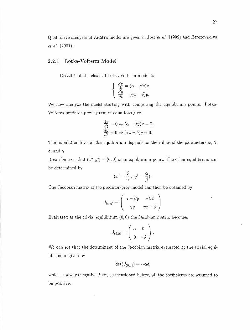
2.2.1 Lotka-Volterra Madel
Recall that the classical Lotka-Volterra model is
~~ = (a - {Jy)x,
{ 1t = bx - 8)y.
We now analyze the model starting with computing the equilibrium points. Lotka
Volterra predator-prey system of equations give
~~ = 0 {:} (a - {Jy)x = 0,
~ = 0 {:} bx - 8)y = O.
The population level at this equilibrium depends on the values of the parameters a, {J,
8, and "f.
It can be seen that (x*, y*) = (0,0) is an equilibrium point. The other equilibrium can
be determined by
* 8 * a)(x=1;y=~·
The Jacobian matrix of t.he predator-prey model can then be obtained by
a-{Jy -(Jx)J(x,y) =
( "fY "fX - 8
Evaluated at the trivial equilibrium (0,0) the Jacobian matrix becomes
J(O,O) = ao(
We can see that the determinant of the Jacobian matrix evaluated at the trivial equi
librium is given by
det(J(o,O)) = -a8,
which is always negative since, as mentioned before, aU the coefficients are assumed to
be positive.

28
Moreover, the trace of the Jacobian matrix evaluated at the equilibrium (0,0) is
1r( J(O,O)) = a - 6.
Note that according to the Routh-Hurwitz criterion, since det J(O,O) < 0, no matter
what the sign of the trace of the Jacobian is, the trivial equilibrium is a saddle point.
This means that if both population levels are at zero, then they will continue to be so,
indefinitely. For more details refer to Kot (2001). However, the trivial equilibrium does
not interest us. Therefore, we now study the stability of the non-trivial equilibrium
point.
Evaluated at the non-trivial equilibrium (x*, y*), the Jacobian matrix J becomes
0 -~) ( W- 0
The determinant of the Jacobian matrix evaluated at the non-trivial equilibrium (x*, y*)
is given by
which is always positive.
Moreover, the trace of the Jacobian matrix evaluated at the non-trivial equilibrium
(x*, y*) is
Therefore, according to the Routh-Hurwitz criterion, the non-trivial equilibrium is a
center for the linearized system. Moreover, Hirsch and Smale (1974) show that it is
also a center for the non-linear system. Thus, this second equilibrium point represents
a fixed point at which both populations sustain their current behavior, indefinitely. In
other words, the solutions are periodic and cycle around this equilibrium point.
The equilibrium point at the origin is a saddle point, and hence unstable, but we will
find that the extinction of both species simultaneously is difficult to happen in the
Lotka-Volterra model. In fact, this can only occur if the prey is artificially completely
eradicated, causing the predator to die out of starvation. If the predator is eliminated,
the prey population grows without bound in this simple model.
29
The Lotka-Volterra model shows that: (i) predators can control exponentially growing
prey populations; (ii) both prey and predators can coexist indefinitely; (iii) the indef
inite coexistence does not occur at equilibrium population, but along a population cycle.
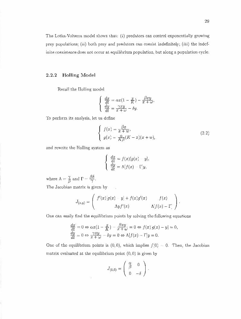
2.2.2 Holling Model
Recall the Holling model
dx _ (1 _ X) _ JÈJL dt - ax K x +W'
{ 1:1L-~_>:dt - x+w uy.
To perform its analysis, let us define
_ (Jx()fx -x+w'
(2.2){ g(x) = K(3(K - x)(x + 'W),
and rewrite the Holling system as
~~ = f(x)[g(x) - y],
{ 1t = A[j(x) - rJy,
where A = ~ and r = ~<5.
The Jacobian matrix is given by
l' (x ) [g (x) - y] + f (x )gl (X ) - f (x) )
J(x,y) = ( Ay1'(x) A[j(x) - r]
One can easily find the equilibrium points by solving the following equations
~~. = 0 <=} ax(l - K) - !~~ = 0 <=} f(x)[g(x) - y] = 0,
1t = 0 <=} 2~~ - <5y = 0 <=} A[j(x) - fly = O.
One of the equilibrium points is (0,0), which implies f(O) = O. Then, the Jacobian
matrix evaluated at the equilibrium point (0,0) is given by
J(O,O) = (~ 0)o -<5 .

30
Since det J(O,O) < 0, no matter what the sign of the trace would be, according to the
Routh-Hurwitz criterion, this trivial equilibrium point is a saddle point.
Other equilibria can be determined by solving the system
x* f3 * 0(1 - X) - ---{Z1l- = 0 x +w ' (2.3)]x* __
x * + w 0 - 0,
which gives one point of coordinates
o"(w(K"( - Ko - ow)x* =~. y* (2.4)
"( - 0' Kf3h - 0)2
Moreover, it can be easily seen that
j(x*) = ~x* = of3 = f. (2.5) x +w "(
Note that j(x*) and x* cannot be O. On the other hand, equations (2.2) and (2.3) imply
that
j(x*)(g(x*) - y*) = O.
Therefore, we must have
g(x*) = y*. (2.6)
The Jacobian matrix J evaluated at the equilibrium (2.4) is obtained by
J x' • = ( j'(x*)[g(x*) - y*] + j(x*)g'(x*) - j(x*) ). ( ,y) Ay* j'(x*) A(J(x*) _ r) (2.7)
Therefore, from (2.5), (2.6) and (2.7) it follows that the Jacobian matrix J evaluated
at the second equilibrium point (x*, y*) is
J x' * = (j(x*)g,(x*) -Of) (2.8) ( ,y) Ay* j'(x*)
Further, we apply the Routh-Hurwitz criterion, i.e. we study the signs of det(J(x*,y*))
and Tr(J(x',y*)) to discuss the stability of this equilibrium, (x*, y*).
From (2.8) we see that
Tr(J(x*,y*)) = j(x*)g'(x*),

31
and
det(J(x',y')) = Ary* j'(x*).
In order to obtain the sign of the determinant of the Jacobian matrix evaluated at this
equilibrium (x*, y*) we determine the derivative of j from (2.2) and we ob tain
'( ) (3wj x = 2 > O. (x + w)
Moreover, note that rA> O. Therefore, det(J(x*,y')) > 0 if and only if g(x*) = y* > O.
Let us assume that
"f - 0 > O.
Therefore, equation (2.4) gives the following inequality as a sufficient condition for
y* = g(x*) > 0,
K h - 0) - OW > 0,
or equivalently,
K 0 ->-- (2.9) w "f - 0'
which is, consequently, a necessary and sufficient condition for the determinant of the
Jacobian matrix evaluated at the second equilibrium to be positive.
Moreover, from (2.2),
g(x) = :(3[-x2 +(K-w)X+KW],
which implies that
Rence, it can be seen that at the equilibrium point (2.4)
'( *) a [-20w W ]9 x = 73 K ("f - 0) - K + 1 .
Note that Tr(J(x',y')) > 0 if and only if g'(x*) > 0, since j(x*) > O.
A simple calculation shows that g'(x*) > 0 if and only if
K("( - 0) - wh +0) > O.

32
Since we assume that
"( - fJ > O.
We obtain K "( fJ ->--+--. w "(-fJ "(-fJ
Renee, a sufficient condition for the existence of an unstable equilibrium is
and K "( fJ ->--+--. w "(-fJ "(-fJ
Moreover, Tr(J(x*,y*)) < 0 if and only if g/(x*) < 0 or equivalently,
and K "( fJ-<--+--. w "(-fJ "(-fJ
This condition, along with inequality (2.9) de termines the following sufficient condition
for the stability of the solution.
fJ K "( fJ --<-<--+-"(-fJ w "(-fJ "(-fJ'
when
Additionally, if K fJ -<-w "(-fJ
then J(x* ,y*) < O.
This indicates that (x*, y*) is a saddle point. Finally,
K fJ "(-=--+-w "(-fJ "(-fJ
given that "( > fJ implies that J(x*,y*) > 0 and Tr(J(x*,y*)) = 0, which indicates that
the equilibrium (x*, y*) is a center for the linearized system. To conclude, we found
a sufficient condition for existence of an unstable equilibrium, which is not a saddle.
Therefore, by theorem 2.1.1, the limit sets could be limit cycles around the equilibrium
(x*, y*) when the parameters satisfy the above condition.

33
o o...
o o M
o o N
o o
50 100 150 200
Prey
Figure 2.5 A stable solution for Holling Madel: The model parameters are a = 0.1;
K = 250; f3 = 0.05; w = 40; 'Y := 0.7; 0 = 0.5.
2.2.3 Hanski Model
Recall that the Hanski model was defined by
dx _ (1 _ .L.) _ PELdt - ax K x+w'
{ éL - (_ l!:Jl.)dt - 'YY 1 X'
The equilibrium points can be obtained by solving
dx - 0 (1 x ) PEL - 0dt - Ç::} ax - K - x + w - , (2.10)
1;}f = 0 Ç::} 'Yy(l -l!j) = o.
It can be seen that (0,0) is an equilibrium point for the Hanski model. However, like
in the Holling case, we are only interested in the non-trivial equilibria. The equation
corresponding ta the prey in (2.10) implies that such an equilibrium satisfies
* y* = ~(1- ~)(x* +w), (2.11)

34
whilst the predator equation in (2.10) can be reduced to
1y* = -x* (2.12)
fJ,
Therefore, one can determine the non-trivial equilibrium points by intersecting the two
isoclines, and obtain
and
Note that the term inside the square root is always non-negative. Rence, aU the equi
librium points are real-valued. Moreover, we are only interested in the equilibrium in
the first quadrant of the phase place, i.e. we look for (x*, y*) > (0,0). Therefore, the
only admissible solution is
* _ (KafJ, -'- afJ,w - K,B) + J(KafJ, - afJ,w - K (3)2 + 4œ2fJ,2 Kw. x - 2ag ,
(2.13)y* _ (KafJ, - afJ,W - K(3) + J(KafJ, - afJ,w - K(3)2 + 4œ2fJ,2Kw
- 2afJ,2
Further, define the function
g(x) = _{3_. (2.14)x+w
The derivative of 9 with respect to x is given by
1 {3 1 2 (2.15)9 (x) = - (x+w)2 = -~g (x).
Therefore, it can be seen that at the non-trivial equilibrium (x*, y*)
I( *) (3 1 2( *)9 X = - = --g x . (2.16)(x+w)2 {3
According to the Routh-Rurwitz criterion, an unstable equilibrium (x*, y*) occurs when
both the determinant and the trace of the Jacobian matrix J evaluated at the equilib
rium (x*, y*) are positive. Moreover, the equilibrium point is asymptoticaUy stable if

35
the Jacobian matrix J evaluated at the equilibrium (x*, y*) is positive and the trace of
J evaluated at (x*, y*) is negative. The Jacobiau matrix is given by
_ ( a - 2ax/ K - yg(x) - xyg'(x) -xg(x) ) ~~- .
1.1/'I y2/x2 "1 - 2"1J.1-Y/x
The Jacobian J evaluated at (x*, y*) using (2.11) is given by
a - 2ax* / K - x*g(x*)/ J.1- - (x*)2 g'(x*)/ J.1- -x*g(x*)) J(x*,y*) = (2.17)
( "I/J.1- -"1
From(2.17), the determinant of J evaluated at (x*, y*), by using (2.17), is determined
by
det(J(x*,y*)) = -a"l + 2~ x* + 2~X*9(X*) - 13: (x*)2 g2(x*). (2.18)
On the other hand, by inserting y. obtained from (2.12) into (2.11) we can write
* x*g(x*) = aJ.1-(1- ~). (2.19)
Further, insert (2.19) into equation (2.18). We obtain
Finally, after reducing the terms we can see that
(2.20)
It remains to check the sign of det (J(x* ,y*))' First, we prove that x* < K. Indeed we
can see that
(aJ.1-K - aJ.1-w - f3K)2 + 4a2J.1-2 wK < (aJ.1-K + aJ.1-w + ,6K)2 {::>
(aJ.1-K - aJ.1-w - f3K) + -J(aJ.1-K - aJ.1-wf3K)2 + 4a2J.1-2 wK < 2aJ.1-K ,
which is valid if and only if
x· < K.
Therefore, we have x·
D < (1 - _)2 < 1K .

36
Now we return to signs of the determinant. The determinant of the Jacobian matrix
evaluated at the non-trivial equilibrium (2.13) is positive if
O'.IJ1- - >0{3 ,
according to (2.20). Therefore, a sufficient condition for the determinant to be positive
is given by
{3 > O'.IJ-. (2.21 )
We now evaluate the trace of the Jacobian (2.17).
x' y' 20'. * 1 * ( *) 1 ( *) 2 *)1 (Tr(J) = 0'. - -x - -x 9 x - - x 9 x - "(. (2.22) ,. K IJ- IJ-
We can simplify the above equation by using (2.16) and (2.19). It can be then seen that
2 * O'.IJ- x 2 0'.*Tr(Jx',y') = T(l- K) - K X - "(.
We previously showed that X* 2
(1 - -) < 1K .
Therefore, the following inequality satisfies
0'.2IJ- 0'.Tr(J • •) < - - -x* - "V
X ,y (3 K /.
If we assume that equation (2.21) is satisfied, then not only, as shown before, is the
determinant positive but also
0'. x*Tr(J • • ) < 0'. - -x* - {::> Tr(J • •) < 0'.(1 - -) - "V"VX ,y K / X ,y K / ,
which implies that
Therefore, the trace of the Jacobian matrix evaluated at the non-trivial equilibrium
(2.13) is negative if
O'.IJ- < {3 and 0'. < "(. (2.23)
Condition (2.23) is sufficient for the asymptotic stability of the equilibrium point (2.13),
since the first condition in (2.23) guarantees that the determinant is posit.ive. In other
cases, e.g. when either O'.IJ- > {3 or 0'. > "(, and the equilibrium is unstable, limit cycles
can occur.

37
11.39118 11.39119 11.39120 11.39121 11.39122
Prey
Figure 2.6 Limit cycle for the Hanski Model: the model parameters are a 5.4;
K = 50; (3 = 600; w = 5; 1 = 2.8; J-L = 100.
2.2.4 Arditi Model
Recall that the Arditi model was introduced as
dx _ (1 _ ~) _ j3xydt - ax k x + wy'
{ 1:JL _ ]xy r dt - x + wy - uy.
In this model, the equilibrium points (x*, y*) can be obtained by
dx - 0 (1 - 2;.) _ (3xy - 0dt - {:} ax k x + wy - ,
(2.24)dx _ 0 ]xy _ r - 0dt - {:} x +wy uy - .
It can be seen that (0,0) is an equilibrium point. However, just like in the Hanski
model, Arditi predator-prey population system does not hoId 0 as population size for
either the prey or the predator since the denominator of bath the prey and the predator
equations become O.
The non-trivial equilibrium points occur when
x* (3y*a(1- -) - = 0 (2.25)
K x* + wy*

38
and ,x*
----8=0. x* + wy*
The later equality implies that
(2.26)
The non-trivial equilibrium points can be derived by solving (2.25) and(2.26). For
example, we insert first y* from (2.26) into (2.25) and solve for X*. The values are given
by
x* = K[l- tw(1- 4)], (2.27)
{ y* = !SG -1)[1- !(1- 4)]·
Define the ratio
R = h - 8) = 1- ~ , (2.28), , and note that
1 ,
1- R J' Moreover, one can easily see that
R --,--------,--=
(1- R) ,-8, y* - x - =w-.
8 8 x*
Additionally, we define
g(x,y) = xy
. , x+wy
(2.29)
and we rewrite (2.24) as
ax(l k) {Jg(x, y) = 0,
{ ,g(x,y) 8y = O.
The first partial derivatives of g(x 1 y) with respect to x and y are
w gx(x, y)
(x/y + w)2' 1
(1 + wY/X)2'
Using equation (2.26) and (2.28) we can evaluate the above derivatives at the equilibrium
point (2.27) and obtain
gx(x*,y*) = ~2 (2.30)
{ gy(x*,y*) = (1- R)2.

39
Therefore, we can see that the Jacobian matrix of the system is
. J = ( 0: - 20:x/K - ;3gx(x, y) -;3gy(x, y) ).
19x(X,y) 19y(X,y) - 0
The determinant of the J acobian matrix evaluated at the equilibrium point (x', y') is
given by
Let now define 1
Z = "6 det(J(x*,y*»)·
Then by using (2.27) and (2.28), we can see that
;3R] 20:1 [ ;3R]. ;3' 0:1.Z = -0: + 20: [1 - - - - 1 - - 9 + 9 + -g ,yo:w 0 o:w x oy
where g; = g(x',y') and g; = g(x·,y·). Finally, by substituting 9; and g; from (2.30)
we can write ;3
Z = (0: - -R)R. (2.31) W
Note that sign(det(J(x*,y*»)) = sign(Z), since 0 > O.
Moreover, the trace of the Jacobian matrix evaluated at the non-trivial equilibrium
(2.28) is
) 20:';3 • • J:Tr (J(x* ,y*) = 0: - K x - gx + 19y - u.
Then we can use (2.27) and (2.30) to obtain
Tr(J(x* *») = 0: - 20:(1 -l..-R) - ~R2 + 0[1(1- R)2 - 1].,y o:w W 0
Therefore, 2;3 ;3 2
Tr(l(x* *») = -0: + -R- -R - oR. (2.32),y W W
We study the stability of the equilibrium (x', y') by discussing all possible cases for the
signs of the determinant (2.31) and the trace (2.32).
Suppose first that 1 < 0, or equivalently, R < O. Hence, equation (2.31) imp!ies that

40
det(J(x*,y*)) < O. Therefore, no matter what the sign of Tr(J(x*,y*)) would be, the equi
librium (x*, y*) is a saddle.
, Alternatively, suppose that "1 > 0, or equivalently, R> O. Then, there are two possibil
ities: the first case is f3 f3 h - 0)
a--R<OÇ::}a--. 0 <O. w w
In this case, equation (2.31) implies that det(J(x*,y*)) < 0, which means that the equi
librium (x*, y*) is a saddle point.
We can therefore conclude that the equilibrium is a saddle point if
a f3either "1 < 0 or 0 < < - (2.33)
1-(0/"1) w'
since a > 0 and 1 - ~ > O.
The other case is when
a - ~R > 0, w
or equivalently,
f30< -R < a, (2.34) w
which implies that det(J(x*,y*)) > O.
Suppose (2.34) holds. From (2.32) we can obtain the inequality
Tr(J(x* 1*)) < ~R(I- R - OW) = ~oR(~ - ~). ,y w f3 w "1 f3
Therefore, Tr(J(x*,y*)) < 0 if (~ - ~) < 0 since we assumed that R > O. Hence, a
sufficient condition for the asymptotical stability of the equilibrium is
f3o< "1 and - < "1, w
or equivalently, by (2.33) f3 a
o< "1 and ~ < 1 - (0/"1)
Finally, given that 0 < "1 and (2.34) are satisfied, we propose looking for a sufficient
condition for the equilibrium to be unstable.
Since R < 1, we have
2f3 f3 2 l:R2Tr(J(x* *) ) > -a + -R - -R - u , ~ w w

41
Then after reducing the terms, we have
(3 Tr(J(x*,y*)) > -a - 0 + ~R(2 - R),
In arder to have an unstable equilibrium, according to the Routh-Hurwitz criterion, we
must have Tr(J(x*,y*)) > 0 and det(1(x*,y*)) > O. We have shown that for
{3R0< - < a,
w
and
Î - 0> 0,
the determinant of the Jacobian matrix evaluated at the equilibrium (x', y*) is positive.
In order tohave Tr(J(x* ,y*)) > 0 it suffices to require that
(3 -a - 0 + - R(2 - R) > 0,
w
or equivalently,
~R> a+o. w 2-R
Further, replace R from (2.28) and use (2.34) to reduce the above relations.
a+o <!l< a <=}
(1 + oh)(1 - oh) W 1 - oh
2~f < gT<a.
In other words, a+o {3 a+et.oh
-,---::-;--:-:---=-:-:- < - < -:---::-;-.,...-;--'---'-~-:-(1 + Oh)(l - oh) W (1 - Oh)(l + oh)'
is a sufficient condition for the equilibrium point (x*, y*) to be unstable. Note that this
condition cannot be satisfied if a < Î.
The complete analysis of this system is done in Berezovskaya et al. (2001). In fact,
these authors find a domain in (a,{3,o'Î,w,K) where the system admits a limit cycle.
2.3 Final Comments
In this chapter, the dynamical systems of four general predator-prey mathematical
models known as classical Lotka-Volterra, Holling, Hanski, and Arditi were studied.

42
22.180 22.185 22.190 22.195 22.200 22.205
Prey
Figure 2.7 A stable solution for Arditi Model: The model parameters are ex = 0.065;
K = 150; (3 = 0.12; w = 1.3; 'Y = 0.060; 15 = 0.024.
According to the Poincaré-Bendixon theorem we know that each system solution can
possibly converge to a limit cycle or an equilibrium.
The complete analysis of these systems goes beyond the scope of this thesis. What we
can provide here are the equations of the isoclines and of the non-trivial equilibria which
are at the core of our inference method. Moreover, the linearized analysis allows us to
point out subdomains of the parameters where limit cycles can accur. These are the
subdomains that mainly interest us. A final issue concerns the following concept.
Definition 2.3.1 Suppose (xt,Yt) is a periodic solution to a dynamical system (2.1).
The prey extremum is the set of all points (x, fi) where (x, fi) E {(Xt, Yt)} and x is the
maximum or minimum value of Xt in some period.
The predator extremum is the set of all points (x, fi) where (x, fi) E {(Xt, Yt)} and fi is
the maximum or minimum value of Yt in some period.

43
Since the prey extremum takes place if dx/dt = 0, one can conclude that the prey isocline
lies on the prey extremum. Moreover, since the predator extremum occurs if dy/dt = 0,
it can be seen that the predator isocline lies on the predator extremum. Furthermore, for
ail four models discussed in this thesis, the prey and predator extremum sets exist and
are non-empty. Furthermore, suppose that for a fixed s, (x s,Ys) belongs to the prey
extremum set of the periodic solution (Xt, Yt) with period T. Then (xs+T> YS+T) also
belongs to the prey extremum. The same argument is also valid for any point belonging
to the predator extremum set. Therefore, knowing only one point of the predator
prey extremum sets and the period of a given solution, one can obtain the predator
prey extremum sets. In the next chapter, we will show how to use the predator-prey
extremum sets to estimate the predator-prey isoclines.

CHAPTER III
STüCHASTIC MüDELS AND STATISTICAL INFERENCE
In the previous chapter we showed that the prey and the predator isoclines lie
on the prey and the predator extremum sets, respectively. Therefore, if we consider to
have a model with its respective extremum sets, we can use linear model techniques
such as Ordinary Least Squares (OLS) to estimate the coefficients of the corresponding
isoclines. On the other hand, by using different fittlng tests such as the F-test, the
t-test or the Wilcoxon test, one can compare the models through their isoclines. The
key point in this comparison is that the prey and the predator isoclines of the four dis
cussed models are different from each other: the predator-prey isoclines of the classical
Lotka-Volterra model are a vertical line and a horizontal line, respectivelYi as for the
Holling model, the predator-prey isoclines pair is a vertical line and a quadratic curve,
respectively; whereas the Hanski predator-prey isolines are a straight line with a posi
tive slope and a quadratic curve, respectivelYi and finally, the predator-prey isoclines of
the Arditi model are different from the others. These differences couId help us identify
the model which can be fitted to a given pair of extremum sets, and further, predict a
solution that corresponds to a given data set.
We start this chapter by proposing and studying the properties of four discussed stochas
tic models. Further on, we demonstrate how to estimate the coefficients of the isoclines.
In the end, by using various types of testing techniques, we suggest a procedure for
choosing a specific model.

46
3.1 Stochastic Models
Suppose 2! is the set of pairs of the predator-prey population sizes observed at
time t, t > O. Furthermore, suppose that Xt and Yt represent the maximum and the
minimum prey and predator population sizes at each period. It turns out that we can
estimate the parameters fairly easily if we consider the model
log X t = log Xt + EX,t, (3.1 )
{ log Yt = log Yt + EY,t,
where X t and Yt are the observed prey and predator population sizes in 2!, respectively.
The measurement errors EX,t and EY,t are assumed to be independent standard normal
random variables that are symmetrically distributed around zero, i.e. EX,t '" N(O, al)
and EY,t '" N(O, a~). The assumption that the errors with expectation zero act additively
on the logarithm of the population sizes conceptually makes sense since Xt and Yt are
both intrinsically positive. Therelore, logxt and logYt which appeared in (3.1) are in
fact deterministic functions which correspond to the expectations of the observations
logXt and logYt , respectively. Moreover, from (3.1) one obtains
E[Xt] = xtE[exp(EX,t)], (3.2)
{ E[yt] = YtE[exp(EY,t)].
Let Xt == x, Yt == y, X t == X and Yt == Y. Note that E[exp(Ex)] and E[exp(EY)] are the
respective moment generating functions of EX and Ey evaluated at k = 1. It is known
that
100 1 (x f-L)2yI2; exp( - 2) exp(x)dx
-00 ax 21T 2aX 2a
exp(f-L + ;).
Given that f-L = 0 one can conclude that
E[exp(EX,t)] = exp(al/2). (3.3)
Similarly we have
E[exp(EY,t)] = exp(a~/2). (3.4)
47
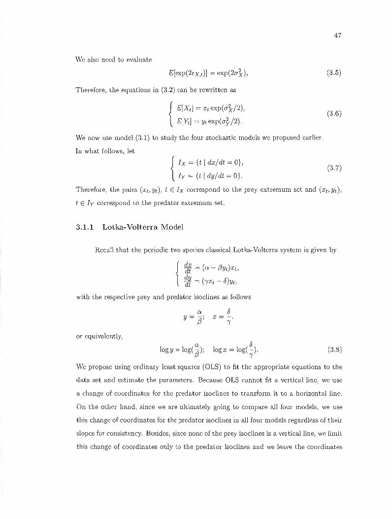
We also need to evaluate
E[exp(2Ex,t)] = exp(2o}), (3.5)
Therefore, the equations in (3.2) can be rewritten as
E[Xtl = Xt exp (a;"/2) , (3.6)
{ E[yt] = Ytexp(a~/2).
We now use model (3.1) to study the four stochastic models we proposed earlier.
In what follows, let
Ix = {t dx/dt = O},1
(3.7){ Iy = {t 1 dy/dt = O}.
Therefore, the pairs (Xt, Yt), t E Ix correspond to the prey extremum set and (Xt, Yt),
t E I y correspond to the predator extremum set.
3.1.1 Lotka-Volterra Model
Recall that the periodic two species classical Lotka-Volterra system is given by
with the respective prey and predator isoclines as follows
6 X -- .-
"(
or equivalently, 6
logx = log( -). (3.8) "(
We propose using ordinary least squares (OLS) to fit the appropriate equations to the
data set and estimate the parameters. Because OLS cannot fit a vertical line, we use
a change of coordinat~s for the predator isoclines to transform it to a horizontal line.
On the other hand, since we are ultimately going to compare ail four models, we use
this change of coordinates for the predator isoclines in ail four models regardless of their
slopes for consistency. Besides, since none of the prey isoclines is a verticalline, we limit
this change of coordinates only to the predator isoclines and we leave the coordinates

48
of the prey isoclines unchanged.
Let (x, i)) = (y, x). By rewriting the predator isocline in (3.8) in the new coordinates
(x, i)), we obtain
log i) = log( ~ ). 'Y
Consider now the random counterparts of the linear functions in (3.8) and the above
equation
log(~) -logyt, tE Ix,
- 8logyt -log(;y), tE ly,
where Ix and ly were defined in (3.7).
The expected values of these variations can be obtained by
log( ~) - E[log yt], t E Ix,
E[logYtJ -log(~), tE ly.
Then under model (3.1) we have
{
E[log~] = no,
E[logyt] = Ao,
tE Ix,
tE ly, (3.9)
where, by using equations (3.8), we obtain
(3.10)
and 8
Ao = log( -). (3.11) 'Y
The above equations are satisfied since
tE Ix, (3.12)
tE ly.
3.1.2 Holling Model
Recall the periodic two species Holling system
dx _ (1 _ X) _ JÈJLdt - cxx K x + w'
{ 1JL-~-8dt - x +w y,

49
with the respective prey and predator isoclines as follows
ex 2 K7J (K - w ) - exw - 0,- Ct xy + K73 x 7J (3.13)
{ x - I5w = O. ~
Let (x,ij) = (y, x). By rewriting the predator isocline in (3.13) in the new coordinates,
we obtain _ wl5
logy - log(--,) = O. (3.14)'Y-v
Therefore, consider the random counterparts of the functions in (3.13) and (3.14)
yt + K(3Xl- K(3(K - w)Xt -~, tE Ix,
log Yi -log~, tE ly,'Y-v
where Ix and ly are defined in (3.7). The expected values of these random perturbations
are given by
E[ytJ + K(3E[X1J - K(3(K - w)E[Xtl-7' tE Ix,
E[log Yi] -log /r:: 8' tE ly.
Then, under model (3.1), there exist new parameters Do, Dl, D2 and Ao such that
E[ytJ ~ D2 E[Xl] +DlE[Xtl + Do, tE Ix, (3.15)
{ E[log yt] = Ao, tE Iy .
In fact, (3.3), (3.4) and (3.5) along with (3.13) and (3.14) imply that in order to obtain
(3,15), one needs to set
D2 = -K!3exp((-4a~ +a~)/2),
Dl = K(3 (K - cu) exp((a~ - a~ )/2), (3.16)
Do = 7T exp(a} /2),
and
I5wAo = log(--,). (3.17)
'Y-v

50
3.1.3 Hanski Model
Recall the two species Hanski system
dx _ (1 _ X) _ Jh:JL ([[ - CiX K x + w'
{ ~ = 'Yy(l - Hj),
with the respective prey and predator isoclines as follows
y + !(3x2 - ~(K - w)x - ~ = 0,
(3.18){ y - /ix = O.
Let (x,i)) = (y,x). By rewriting the predator isocline in (3.18) in the new coordinate,
we obtain
log i) - log x + log IL = O. (3.19)
Now consider the random counterparts of the functions in the left hand side of (3.18)
and (3.19)
yt + K(3Xl- K(3(K - w)Xt -~, tE Ix,
log ft -logXt -logIL, tE Iy,
where Ix and Iy are defined in (3.7). The expected values ofthese random perturbations
are
E[yt] + K(3E[X[] - K(3(K -w)E[Xt ] -~, tE Ix,
E[log ft] - E[log Xt ] - log IL, tEly.
Then, under model (3.1), there exist new parameters no, nI, n 2 and Ao such that
E[yt] ~ n 2E[xlJ + njE[Xt ] + no, tE Ix, _ _ (3.20)
{ E[logyt] = AlE[logXt ] + Ao, tE I y .
By using (3.3), (3.4) and (3.5) along with (3.23), we see that (3.20) is satisfied when
n 2 = - K(3 exp( (-4al + a~ )/2),
nI = K(3(K - w) exp((a~ - al )/2), (3.21)
no = ~ exp(a~/2),
and
(3.22)

51
3.1.4 Arditi Model
Recall the two species Ardi ti system
dx _ (1 x ) (3xyaI - QX - K - x + wy ,
{ 1!Y.. - "(xy - bdt - x + wy y,
with the respective prey and predator isoclines as follows
Qx(l - ~) y - K x = 0,
(3 - Qw(l - K) (3.23)
1 "(:;/y =x - O.
Let (x, y) = (y, x). By rewriting the predator isocline in (3.23) in the new coordinate
we obtain
log y - log x+ log( wb ,) = O. 'Y-u
We rewrite the prey isocline obtained in (3.23) as
Q 2 QW y + x -
Q
x + xy = O.K((3 - QW) (3 - QW K((3 - QW)
Now consider the random counterparts of the functions in the last two equations
yt + K((3 ~ QW)X;- (3 -QQW Xt + K((3Q:: QW)Xtyt, tE Ix, - - wblogyt -logXt -log( ~), tE Iy.
'Y- u
Since we assumed that X t and yt are independent random variables, the expected values
of the random perturbations appearing above are given by
E[yt] + K((3 ~ QW) E[X;] - (3 _QQwE[Xtl + K((3Q:: QW) E[Xt]E[yt], tE Ix,
E[logYt] - E[logXtl-log('YW!(5)' tE Iy.
Then, under model (3.1), there exist new parameters no, nl , n2 and Aosuch that
E[yt] ~ n 2 E[X;] - ~lE[Xt] + noE[Xt]E[yt] = 0, tE Ix, { E[logyt] - A1E[10gXt] - Ao = 0, tE Iy ,
or equivalently,
{ tE Ix, (3.24)
tE Iy.

52
By using (3.3), (3.4) and (3.5) along with (3.18) and (3.19), we see that (3.24) is satisfied
when
n2 = - K(f3 ~ ŒW) exp(( -4a} + a~ )/2),
ni = (3 _ŒŒW exp((a~ - a} )/2), (3.25)
no = K(f3Œ::: ŒW) exp(a~/2),
and
(3.26)
3.2 Estimation and Testing
3.2.1 General Algorithm
As we mentioned previously, the prey and the predator extremum sets exist and
are non-empty. Moreover, it is known that there exist periodic solutions in the limit
to the Lotka-Volterra, Holling, Hanski, and Arditi models for sorne parameter domain.
Therefore, approximately, the prey isocline intersects the solution to the ordinary dif
ferential equations (ODE) at the maximum and the minimum prey population sizes in
each period. Similarly, the predator isocline intersects the ODE solution at the points
where the predator population obtains its maximum and minimum values. This prop
erty is fundamental in our proposai for estimating the parameters of the models, and
consequently, for predicting the population sizes of the prey and the predator at future
times.
In ail four discussed models, we propose the following step-wise algorithm:
Step 1: Estimate a2 = a~ = a~.
Step 2: Estimate the coefficients of equations (3.9), (3.15) and (3.24).
Step 3: Estimate separate ratios ~, t as weil as K and w.
The idea behind the proposai is the following: let y = u(x) and y = v(x) be the prey
and the predator isoclines for a given system of differential equations, respectively. We
denote the prey and the predator extremum sets by P and Q, respectively. Note that
y = u(x) and y = v(x) intersect at an equilibrium point (x*, y*). Therefore, the first

53
two equations which could be used to estimate the parameters are
Y* = u(x*); Y* = v(x*).
Moreover by fitting the prey isocline equation to the set of the prey extremum, P,
one can derive the third equation to estimate the parameters. The fourth parameter
estimate equation can be obtained by fitting the predator isocline equation to the set
of the predator extremum, Q. In this chapter, we apply this method to each of the
models, separately.
3.2.2 Estimation of (J2
Before we proceed with the model inferences, we show how to use the periodic
property of the predator-prey solution in order to estimate the variance and the coeffi
cients of the predator and the prey isoclines.
Let assume that the observed data is close to a limit cycle solution. Therefore, the
solution is periodic. Now consider
P min = {logxt 1 Xt EPand Xt is the local minimum in each period},
Pmax = {log Xt Xt EPand Xt is the local maximum in each period}. 1
and
Qmin = {logYt Yt E Q and Yt is the local minimum in each period}, 1
Qmax = {log Yt 1 Yt E Q and Xt is the local maximum in each period}.
Therefore, we have
E[logXtJ = logxt == logxt,min, where Xt,min E P min ,
E[log Xt] = log Xt == log Xt,max, where Xt,max E Pmax .
and
E[logYiJ = logYt == logYt,min, where Yt,min E Qmin,
E[log Yi] = log Yt == log Yt,max, where Yt,max E Qmax.
Moreover, the variables logXt, where logxt E Pmin or logxt E Pmax and logYi, where
Yt E Qmin or Yt E Qmax are i.i.d and of the same variance (J2.

54
We now define F and Qas the sets of the estimated prey and predator extremum for a
given set of observations Qi. The estimated variance can obtained by
lÎ'maxl (1 X -1X)2 lÎ'minl ( --)2&2 = ~{'"' og i - og i '"' log Xi -logXi
4 L.." ~ + L.." ~ i=l IPmaxl - 1 i=l IPminl- 1
I~xl (log Yi -log Yi)2 I~I (log Yi -log y i )2} + L.." ~ +L.." ~ , (3.27)
i=l IQmaxl - 1 i=l IQminl- 1
where 1Fmax1and \Fminl denote the cardinality of Fmax and Fmin , respectively obtained
from the data set Qi. We assume that \Fmaxl > 1 and IFminl > 1. Additionally, log Xi
and log Yi are the average of the prey and the predator population sizes on the set of
observed extrema Qi. Another possibility is to use a pooled estimator of variance.
We now return to the model estimates using the estimated variance obtained in this
section.
3.2.3 Estimates for each model
Lotka-Volterra
In order to estimate the parameters of the Lotka-Volterra model, we consider the
prey and the predator extremum sets F and Q obtained from the data set Qi which
admits the Lotka-Volterra system. Then, according to the previous arguments, the
Lotka-Volterra prey isocline must be fitted in F. Suppose the first equation in (3.9),
which corresponds to the prey isocline, is fitted to the set F. We have the relation
E[log Yi] = Do, tE Ix· (3.28)
Then equation (3.10) implies the following relation among the estimates
(3.29)
Additionally, the Lotka-Volterra predator isocline must be fitted in set Q. Therefore,
the second relation among the estimates can be obtained by (3.11).
~ cS Ao = log (-), (3.30)
"(

55
assuming that the second equation (3.9), which corresponds to the predator isocline, is
given by
E[Yi] = Ao, tE ly. (3.31)
Therefore one can estimate the parameters ~ and 4by
(3.32)
A complete solution to estimating a, (3, 'Y and fJ cannot be obtained at this stage, but a
different perspective is given in Froda and Colavita (2005) and Froda and Nkurunziza
(2007) where all the parameters are estimated.
Holling Model
To estimate the parameters of the Holling model, we consider the prey and the
predator extremum sets ft and Qobtained from a data set Q( which admits the Holling
system. Then, according to arguments similar to the ones of the previous case, the prey
isocline of the Holling system must be fitted in ft. Suppose the first equation in (3.15),
which corresponds to the prey isocline, is fitted to the set ft. We have a relation among
the parameters.
(3.33)
Then by (3.16) the following relations must be satisfied for the parameter estimates.
D2 = (~) exp(( -4ô"~ + ô"~ )/2), , ---Dl = (K/3(K -(J))exp((ô"~ - ô"~)/2), (3.34)
Do = (Qj) exp(â~/2),
where Do, nI and D2 are obtained by minimizing in Do, Dl and D2 the distance
I)yt - D2 X( - DIXt - DO)2.
P
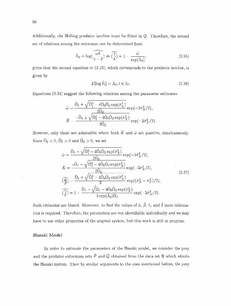
56
Additionally, the Holling predator isocline must be fitted in Q. Therefore, the second
set of relations among the estimates can be determined from
-----. , wO --::y W Ao = log(--.\) {:} h-) = 1 + " (3.35)
'Y - u u exp(Ao)
given that the second equation in (3.15), which corresponds to the predator isocline, is
given by
E[!og Yi] = Ao, tE I y . (3.36)
Equations (3.34) suggest the following relations among the parameter estimates.
However, only those are admissible where both k and ware positive, simultaneously.
Since D2 < 0, Dl > 0 and Do > 0, we set
Such estimates are biased. Moreover, to find the values of &, {3, i, and <5 more informa
tion is required. Therefore, the parameters are not identifiable individually and we may
have to use other properties of the original system, but this work is still in progress.
Hanski Model
In order to estimate the parameters of the Hanski model, we consider the prey
and the predator extremum sets ft and Qobtained from the data set 21. which admits
the Hanski system. Then by similar arguments to the ones mentioned before, the prey
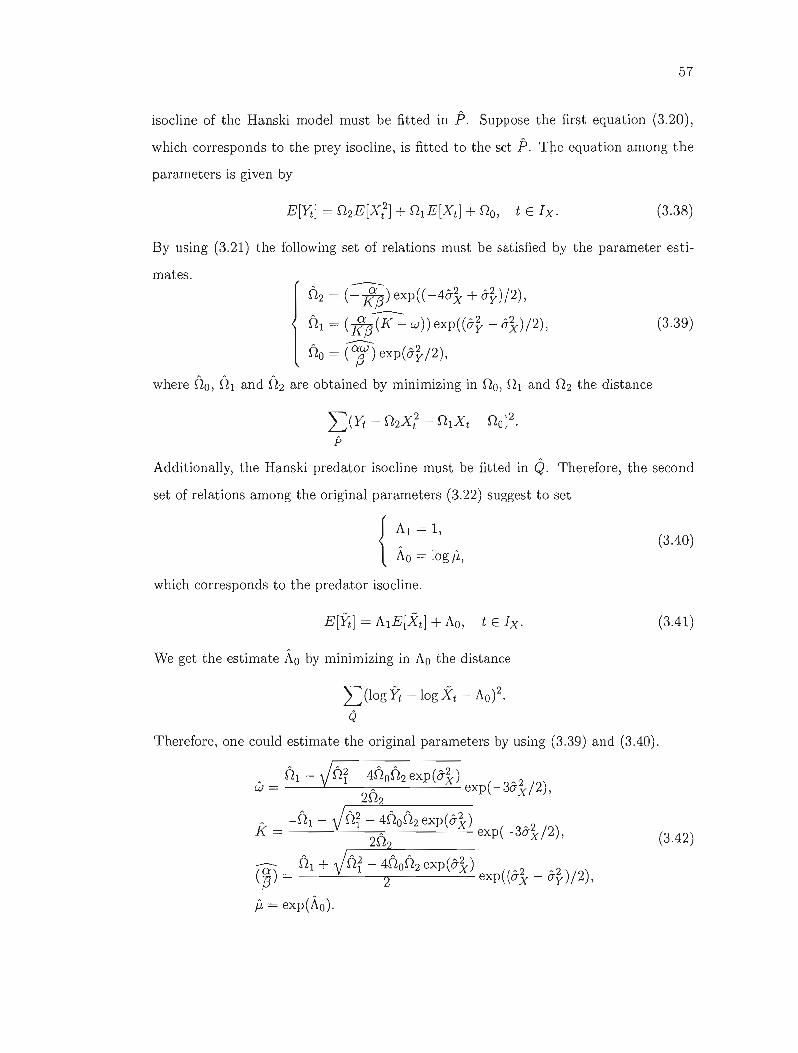
57
isocline of the Hanski model must be fitted in? Suppose the first equation (3.20),
which corresponds to the prey isocline, is fitted to the S€t ? The equation among the
parameters is given by
(3.38)
By using (3.21) the following set of relations must be satisfied by the parameter esti
mates.
n 2 = (~) exp(( -4ô} + â~ )/2),
nI = (K$(l{:.w))exP((â~ -â~)/2), (3.39)
no = ~ exp(â~/2),
where no, nI and n2 are obtained by minimizing in no, nI and n 2 the distance
'l)yt - n2xl- nlxt - nof p
Additionally, the Hanski predator isocline must be fitted in Q. Therefore, the second
set of relations among the original parameters (3.22) suggest to set
1\1 = 1, (3.40)
{ 1\0 = log /-l,
which corresponds to the predator isocline.
(3.41)
We get the estimate Âo by minimizing in 1\0 the distance
L(log Yi -log Xt - 1\of Q
Therefore, one could estimate the original parameters by using (3.39) and (3.40) .
• nl-Jni-4non2exp(âk) ~2 w= • exp(-3ax/2),
2n2
(3.42)
a nI + Jni - 4nOn2exp(â~) ~2 ,2($)= 2 exp((ax- ay)/2),
il = exp(Âo).

--
58
Such estimates are biased. Moreover, to find the values of â: and ~ more information is
required. Therefore, the parameters are not identifiable individually and we may have
to use other properties of the original system, but this work is still in progress.
Arditi Model
To estimate the parameters of the Arditi model, we consider the prey and the
predator extremum sets P and Qobtained from the data set 2! which admits the Arditi
system. Then, similar to the previous arguments, the prey isocline of the Arditi model
must be fitted in P. Suppose that the first equation (3.24), which corresponds to the
prey isocline, is fitted to the set p.'
E[yt] = D2E[Xi] + DIE[Xtl. (3.43)1 + DoE[Xt ]
In view of (3.25), the following set of relations must be satisfied by the parameter
estimates.
(3.44)
where no, nI and n 2 are obtained by minimizing in Do, Dl and !l2 the distance
Additionally, the Arditi predator isocline must be fitted in Q. Therefore, the set of
relations among the original parameters in (3.26) suggest the second set of relations
among the estimates
A w8 Ao = log((-.\)), (3.45)
'Y - u
given that the second equation in (3.24), which corresponds to the predator isocline, is
given by
(3.46)

59
To obtain Âo it suffices to minimize in /\.0 the distance
2:(logYt -logXt - /\.0)2.
Q
Finally, one could estimate the parameters by using (3.44) and (3.45) which gives
w= -D-o- exp( -2â~), n2
k = _~I exp(-3â~/2), n2 (3.47)
~ = -D-o- exp( -2â~) + -J- exp((â~ - â~ )/2),n2 nI m= 1 - D. D.O(Â) exp( -2ô"~),
2 exp 0
Such estimates are biased. Moreover, to find the values of &, 4, i, and 3more informa
tion is required. Therefore, the parameters are not identifiable individually and we may
have to use other properties of the original system, but this work is still in progress.
3.2.4 Testing and Comparison of Models
Conversely, we would like to find out which model can be best fitted to a given
data set 0.. We first construct the predator extremum Q. After change of coordinates on
the predator isoclines and applying the logarithmic transformations, the Lotka-Volterra,
Holling, Hanski, and Arditi predator isoclines are respectively
logy = log 4, logy = log /~(5'
(3.48) log y = log J.L + logx,
logy = log ~ + log X.'Y- o
Since the original variables are all positive, the above equations are well-defined.
Considering the stochastic model (3.1) one obtains
log X t = log Yt + éY,t,
{ log Yt = log Xt + éX,t.

60
Therefore, if t E I y the following relations among the expected values of (log Xt, log Yi) = (log Yi, log Xt) are satisfied.
E[logytl = log 4, E[logytl = log~,
'Y-a (3.49) E[log Yi] = E[log Xtl + log IL,
E[logYiJ = E[logXtl +log~.'Y-a
Note that aU four isoclines are straight lines. The first two equations in (3.49) are
horizontallines while the last two ones have slopes equal to 1. Therefore, a straight line
y = 1\1x + 1\0 (3.50)
is fitted to the predator extremum Q.
It must be noted that the usual linear models tests are conditional on the observed
explanatory variables.
Further, we propose to apply a step-wise procedure to find out which model can be
fitted.
Consider the following hypothesis testing problem:
Ho : 1\1 = 0 against Hl : 1\1 i- O. (3.51)
If the null hypothesis in (3.51) is not rejected, we can accept the Holling model as an
appropriate model to fit the population sizes of the predator and prey. On the other
hand, if the nuU hypothesis (3.51) is rejected, we could proceed to testing
Ho : 1\1 = 1 against Hl : 1\1 i- 1. (3.52)
If the nuU hypothesis in (3.52) is not rejected, we could resort to the prey isoclines to
discriminate between the Hanski and the Arditi models. RecaU that the Hanski prey
isocline is a quadratic curve. Therefore a quadratic curve
(3.53)
is fitted to the prey extremum P. We apply the hypothesis testing
Ho : D2 = 0 against Hl : D2 i- O. (3.54)

61
on the quadratic slope in (3.54). If the null hypothesis in (3.52) is rejected, we could
accept the Hanski model. However, not rejecting the null hypothesis (3.54) does not
imply that the Arditi model can be fitted and therefore, further analysis is required.
Since the Holling model is one the most fundamental two species predator-prey sys
tem, the emphasize is on this model. Besides, other models are also tested against it.
However, in this thesis, we only apply the testing method to find out wether or not the
Holling model could explain the data set. This will be shown in the next chapter.
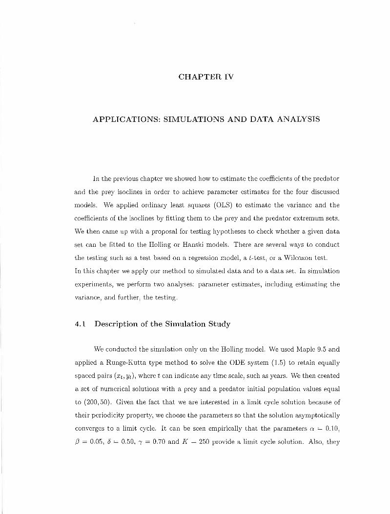
CHAPTERIV
APPLICATIONS: SIMULATIONS AND DATA ANALYSIS
In the previous chapter we showed how to estimate the coefficients of the predator
and the prey isoclines in order to achieve parameter estimates for the four discussed
models. We applied ordinary least squares (OLS) to estimate the variance and the
coefficients of the isoclines by fitting them to the prey and the predator extremum sets.
We then came up with a proposaI for testing hypotheses to check whether a given data
set can be fitted to the Holling or Hanski models. There are several ways to conduct
the testing such as a test based on a regression model, a t-test, or a Wilcoxon test.
In this chapter we apply our method to simulated data and to a data set. In simulation
experiments, we perform two analyses: parameter estimates, including estimating the
variance, and further, the testing.
4.1 Description of the Simulation Study
We conducted the simulation only on the Holling model. We used Maple 9.5 and
applied a Runge-Kutta type method to solve the ODE system (1.5) to retain equally
spaced pairs (xt, Yt), where t can indicate any time scale, such as years. We then created
a set of numerical solutions with a prey and a predator initial population values equal
to (200,50). Given the fact that we are interested in a limit cycle solution because of
their periodicity property, we choose the parameters so that the solution asymptotically
converges to a limit cycle. It can be seen empirically that the parameters ex = 0.10,
f3 = 0.05, (j = 0.50, 'Y = 0.70 and K = 250 provide a limit cycle solution. AIso, they

64
satisfy our sufficient condition for the existence an of unstable equilibrium and therefore,
the solution does not tend to the non-trivial point which is
* ow * cY."{w(K"{ - Ko - ow)x =--'
"( - 0' y = K{3b - 0)2
Unfortunately, a too small data set cannot provide us with good estimates and testing
results; the larger the data set is the more precise the results are. However, since the
data sets used for simulation should refiect real data sets, we have no choice but to cre
ate a data set with a reasonable size in order to conduct our simulation studies. Most
real data sets collected in nature show an approximate 10-year cycle in the predator
prey population interactions (Froda and Colavita, 2005). This means that each prey
and predator local minimum (maximum) observations appear after almost 10 yearly
observations following the previous prey and predator local minimum (maximum) ob
servations. In fact, our method for finding the local extrema is independent on the
cycle length of the solutions. Therefore, we are not concerned if there are too many or
too little observation pairs in each period. On the other hand, the number of cycles
that the data set contains has to be realistic. For instance, in the Mink-Muskrat data
set, which we will introduce in the next section, there are about 12 extrema points for
each species since there a:'e 64 couples of observations. Given that the period is about
10 years, the number of extrema for each species is roughly 12. This results in having
about 24 observation pairs in both prey and predator extremum sets (Figure 4.2). We
created a data set that contains approximately 25 observation pairs in each prey and
predator extremum sets. The number of deterministic pairs created is 2000 (Figure 4.1).
All 2000 deterministic pairs are perturbed by adding random errors, EX and Ey, and
each simulation is repeated 5000 times. The extrema obtained from the first 1000 pairs
are chosen to estimate the parameters, where the extrema obtained from the last 1000
pairs are chosen to estimate the variance and for the testing procedure. The reason we
choose two separate sets of observation pairs will be explained shortly after this. Note
that taking a large number of deterministic pairs, e.g. 1000 is useful only for getting
more precise choice of extremum sets.
As we discussed in Chapter 3, EX and Ey are assumed to be independent. For simplic
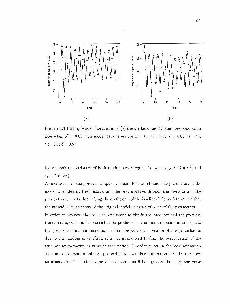
65
0 <ri '".,; ,
'" IlIj>
J .,;
<Il <Il., ., 0 tN N .,; ~ J 'inin
c: 0 c: ~ ~ n ,Q .,; 0
ni ~ "5 "5 a. a. a. a. 0
'".. 0
'"..'0 '0 E E ,5 .c oc: ~
CIl Clri> ..0
0 0 ..J ..J 0..
..;'"
0 20 40 60 80 100 0 20 40 60 80 100
lime Time
(a) (b)
Figure 4.1 Holling Model: Logarithm of (a) the predator and (b) the prey population
sizes when (J2 = 0.01. The model parameters are ex = 0.1; K = 250; /3 = 0.05; w = 40;
1 := 0.7; cl = 0.5.
ity, we took the variances of both random errors equal, i.e. we set EX N(O, (J2) andrv
€y rv N(O, 0-2 ).
As mentioned in the previous chapter, the core tool to estimate the parameters of the
model is to identify the predator and the prey isoclines through the predator and the
prey extremum sets. Identifying the coefficients of the isoclines help us determine either
the iIl;dividual parameters of the original model or ratios of sorne of the parameters.
In order to evaluate the isoclines, one needs to obtain the predator and the prey ex
tremum sets, which in fact consist of the predator local minimum-maximum values, and
the prey local minimum-maximum values, respectively. Because of the perturbation
due to the random error effect, it is not guaranteed to find the perturbation of the
true minimum-maximum value at each period. In order to retain the local minimum
maximum observation pairs we proceed as follows. For illustration consider the prey:
an observation is selected as prey local maximum if it is greater than: (a) the mean

66
value of all population sizes of observed preys and (b) the population sizes of the seven
preceding and the seven succeeding prey observations. Moreover, an observation is se
lected as prey local minimum if it is smaller than: (a) the mean value of all population
sizes of observed preys and (b) the population sizes of the seven preceding and the seven
succeeding preys. Number seven is chosen because there is an approximate 20-year
cycle (if t indicates years) in the prey and the predator populations. The same proce
dure applies to the perturbation of predators. Note that in practice, one could rely on
visual interpretation or other empirical methods and does not necessarily need to use
'an algorithm' for choosing the elements of extremum sets. The algorithm was needed
because we repeated the simulation a great number of times.
Figure 4.1 illustrates a numerical solution to the Holling model corresponding to the
given parameters. We chose 1/10 of the points on the numerical solutions from each
cycle in order to avoid having cluttered graphs.
4.1.1 Estimation
Suppose P and Q denote the prey and the predator extremum sets, respectively.
Since the inference is done on a logarithmic scale, we use relatively small values for
the variance of the random errors. The following four variances were chosen to run the
simulations: (J2 = 0.01, (J2 = 0.005, (J2 = 0.001 and (J2 = 0.0005. As we mentioned
earlier in this section, in order to estimate the variances, observations must be taken
from a closed loop. That is because periodicity property of a closed loop is crucial
to estimate the variance (see section 3.2.2). That is why we choose the extrema of
the last 1000 observation pairs to estimate the variance. Since the chosen parameters
create a numerical solution which asymptotically converges to a limit cycle, we can take
the observations that are on the closed loop. We use equation (3.27) to estimate the
variance from the extremum sets.
Unlike the variance, the parameters are better estimated if the observations are not on
the closed loop part of the numerical solution. This is because the further the elements
of the prey (and the predator) extremum sets are from each other in the phase plane the

67
less the random error affects the shape of the isocline curves. That is why the extrema
of the first 1000 observations pairs are chosen to estimate the parameters. We apply
ordinary least squares (OLS) to fit a verticalline to Q and a quadratic curve to P since
according to equations (3.33) and (3.36), a verticalline and a quadratic curve must be
fitted to the predator extremum and the prey extremum sets, respectively. Then, at
each simulation, we estimate the coefficients Ao, Al, Do, Dl, D2 , and further, evaluate
w, K, ®and mby using (3.37). The results are given in tables 4.1 and 4.2 and are
discussed in section 4.1.3.
4.1.2 Testing
Finally, the last part of the simulation is devoted to testing. We apply the 2
sided regression slope test, the 2-sided t-test and the 2-sided Wilcoxon test to find out
whether or not a verticalline can be fitted to Q. Since yt is not normally distributed,
these tests do not work on a quadratic equation. The regression slope test was described
in Chapter 3. The t-test and the Wilcoxon test are applied when we compare 2-samples
and further we explain why these tests could work in our case.
If we want to use the fact that both Xt and Yt are periodic with the same period T,
the observations must be taken from the closed loop. Therefore, the same pairs of
observations used to estimate the variance can be used, i.e. the extrema of the last 1000
observation pairs.
For simplicity let Ut = log X t and lit = log yt. We use the change of coordinate defined
in Chapter 3 and we obtain Ût = log Xt and Vi = ft. We obtain
~t = ~t + Eu,t,
{ lit = Vt + Ev,t,
where in our models, at times t where the deterministic Ut has a maximum or minimum
value. We have the relation
lit = a + bUt + Ev,t·
Since Ut is periodic, the deterministic values Ut take only two values at the times we
consider (maximum and minimum); the values of the corresponding Vt also repeat them
68
selves. So we actually confront two hypotheses:
b= 0: E[Vt] are the same for aIl t > 0 versus b= 1: E[iltl are different for maxima and
minima of Ut. By using (4.1), we can write
b = 0 => vt = a + Et,
{ b = 1 => vt = a + Üt + Ev,t.
Since E[Ütl lies on the extrema ü max and Ümin, under the b = 1 hypothesis, Vt is from
two populations of different means, a +umax and a + Umin' Then we can simply perform
a 2-sample t-test which should accept the null-hypothesis of i.i.d data sets which give
an almost 0 estimated slope.
Another case of 2-sample testing is the Wilcoxon-Mann-Whitney test which does not
assume normality for the errors.
The results of the tests are shown in table 4.3.
4.1.3 Results
In this section we provide the results obtained from simulation. Tables 4.1 and
4.2 are devoted to parameter estimates; we can see how the parameter estimates change
with an increase in &2. The estimates of 0-2 , Ao and Al are excellent for the whole range
2of 0- values. The estimates of Do, Dl and D2 are generally good but maybe less 50 for
0-2 = 0.01. On the other hand, the estimates of the individual parameters w, K, ~ and
'if are greatly affected by the small bias in the coefficients Do, Dl, D2 and Ao. Therefore,
even if the isoclines coefficient estimates have small relative bias, the estimates of the
parameters of the system can have large relative bias.
It can be observed that the tests performed with the 2-sided regression slope test are
excellent. However, we can see that the Wilcoxon test overestimates acceptance error,
while the t-test underestimates. The somewhat surprising results on the t-test may
be artifacts of the automatic procedure for choosing extrema in the simulation loops.
Small experiments where the data were obtained by perturbing the numerical solution
at exact times of maximum-minimum values gave very good results, i.e. very close to
the nominal Cl: values.

69
Table 4.1 Estimates of the parameters for (J2 = 0.0005 and (J2 = 0.001
Parameter Real value Mean QI Median Q3 Relative Bias
(J2 0.0005 0.0004 0.0004 0.0004 0.0005 0.2
[b -0.008 -0.0066 -0.0084 -0.0062 -0.0044 0.175
Dl 1.68 1.4097 0.8961 1.3159 1.8228 0.1609
Do 80.02 70.6486 45.9361 75.0602 100.1619 0.1171
Al 0 0.0001 0 a 0 N.A.
Ao 4.6052 4.6059 4.5968 4.6062 4.6155 -0.0001
w 40 68.5987 22.9157 46.7337 79.6355 -0.715
K 250 275.7349 239.3305 259.0887 285.2832 -0.1029
ex 73 2 1.654 1.246 1.6113 2.0189 0.173
t 1.4 1.6851 1.2273 1.4664 1.7979 -0.2036
(J2 0.001 0.0008 0.0007 0.0008 0.001 0.2
D2 -0.008 -0.006 -0.0077 -0.0056 -0.0036 0.25
Dl 1.68 1.28 0.7342 1.1895 1.6995 0.2342
Do 80.04 77.1728 52.3258 82.1294 109.0825 0.0358
Al 0 0.0001 0 0 0 N.A.
Ao 4.6052 6.606 4.5951 4.6061 4.6171 0.0004
w 40 169.3726 27.2548 54.9277 99.6829 -3.2343
K 250 295.0879 246.4028 269.112 304.0179 -0.1804
ex 73 2 1.5378 1.0918 1.4949 1.9084 0.2311
t 1.4 2.688 1.271 1.5473 1.9991 -0.92

70
Table 4.2 Estimates of the parameters for (J"2 = 0.005 and (J"2 = 0.01
Parameter Real value Mean QI Median Q3 Relative Bias
(J"2 0.005 0.0041 0.0032 0.0039 0.0048 0.18
D2 -0.0079 -0.0043 -0.0059 -0.0036 -0.0019 0.4557
Dl 1.68 0.9692 0.3731 0.797 1.363 0.4231
Do 80.2003 94.3709 69.2848 103.9421 129.6153 -0.1767
Al 0 -0.0003 0 0 0 N.A.
Ao 4.6052 4.6105 4.5928 4.6094 4.6262 0.0011
w 40 164.0656 42.4329 91.1289 180.4262 -3.1016
K 250 354.7479 271.155 311.4028 382.1624 -0.419
Cl:
-:B 2 1.2281 0.7141 1.1285 1.6278 0.386
t 1.4 2.638 1.4187 1.9073 2.7762 -0.8843
(J"2 0.01 0.0104 0.0074 0.0092 0.0115 -0.04
D2 -0.0079 -0.0036 -0.0049 -0.0029 -0.0014 0.5443
Dl 1.68 0.8362 0.3023 0.6628 1.1806 0.5023
Do 80.401 101.1914 78.8744 110.1739 132.0744 -0.2586
Al 0 0 0 0 0 N.A.
Ao 4.6052 4.6139 4.5944 4.6138 4.6336 -0.0019
w 40 169.0691 54.0566 110.9176 217.5539 -3.2267
K 250 412.8353 289.6489 341.5827 435.4674 -0.6513
Cl:
-:B 2 1.0934 0.5993 0.9969 1.4541 0.4533
* 1.4 2.6656 1.5381 2.095 3.1609 -0.904

71
Table 4.3 Testing: How often the predator isocline is accepted as a vertical line
Type of Testing Percentage of Acceptance
a 2 = 0.0005
2-sided Regression 0.9484
2-sided t-test 0.8209
2-sided Wilcoxon 1
a 2 = 0.001
2-sided Regression 0.9507
2-sided t-test 0.8588
2-sided Wilcoxon 1
a 2 = 0.005
2-sided Regression 0.9602
2-sided t-test 0.8914
2-sided Wilcoxon 1
2a = 0.01
2-sided Regression 0.9704
2-sided t-test 0.8884
2-sided Wilcoxon 1

72
4.2 Data Analysis
In this section we apply our method to the Canadian mink-muskrat data, the
Hudson's Bay Company Records of fur-sales and trappings collected between 1850 and
1911 (Figure 4.2). The data set we are using here is reported in Brockwell and Davis
(1991) pp. 557-558. There are several comments on the predator-prey relationship
between the species listed in the Husdon-Bay data set (Bulmer, 1974). It appears that
the muskrat cycle is due to predation by mink (Bulmer, 1974). As such, a mink-muskrat
couple is a predator-prey pair which seems to satisfy the requirement that the prey
muskrat is the main source of food for the predator mink. There exists an approximate
10-year cycle of the prey and the predator population (see Froda and Colavita, 2005).
The results of testing on the mink-muskrat data set are given in table 4.4. The p-value
o '" +.,
... '"
o +.,
N.~ Q) '" ~
'" 'in c§ ;g .Q
rn + rn:; ., :; g. a.
"'-ID tr. ... o +.,
Cl; +
'" N
1850 1860 1870 1880 1890 1900 1910 1850 1860 1870 1880 1890 1000 1910
Year Year
(a) (b)
Figure 4.2 Observed population sizes: (a) Mink (b) Muskrat
corresponding to the predator isocline slope is greater that 0.873. Therefore, we do
not reject the hypothesis test that the slope is O. In other words, the Holling model
could be fitted to the mink-muskrat data set. The result is also in agreement with a
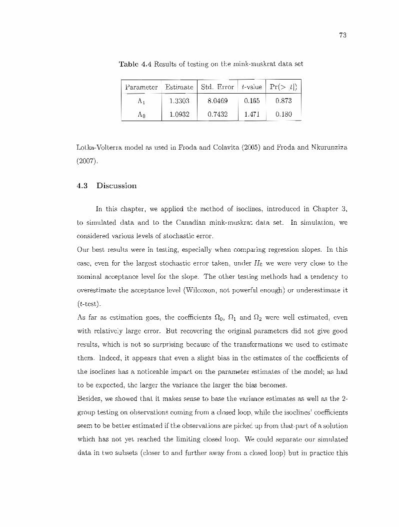
73
Table 4.4 Results of testing on the mink-muskrat data set
Parameter Estimate Std. Error t-value Pr(> Itl)
Al 1.3303 8.0469 0.165 0.873
Ao 1.0932 0.7432 1.471 0.180
Lotka-Volterra model as used in Froda and Colavita (2005) and Froda and Nkurunziza
(2007).
4.3 Discussion
In this chapter, we applied the method of isoclines, introduced in Chapter 3,
to simulated data and to the Canadian mink-muskrat data set. In simulation, we
considered various levels of stochastic error.
Our best results were in testing, especially when comparing regression slopes. In this
case, even for the largest stochastic error taken, under Ho we were very close to the
nominal acceptance level for the slope. The other testing methods had a tendency to
overestimate the acceptance level (Wilcoxon, not powerful enough) or underestimate it
(t-test) .
As far as estimation goes, the coefficients no, ni and n2 were well estimated, even
with relatively large error. But recovering the original parameters did not give good
results, which is not so surprising because of the transformations we used to estimate
them. Indeed, it appears that even a slight bias in the estimates of the coefficients of
the isoclines has a noticeable impact on the parameter estimates of the model; as had
to be expected, the larger the variance the larger the bias becomes.
Besides, we showed that it makes sense to base the variance estimates as well as the 2
group testing on observations coming from a closed loop, while the isoclines' coefficients
seem to be better estimated if the observations are picked up from that part of a solution
which has not yet reached the limiting closed loop. We could separate our simulated
data in two subsets (closer to and further away from a closed loop) but in practice this

74
may be a problem because of scarcity of available data; this is another question that
should be addressed in the future.
FinaUy, as seen earlier, we are not yet able to estimate aU the parameters of the model
individually, and we limited ourselves to estimate the ratios ®and m. These ratios
are important in themselves, since they express in a certain way how birth and death
rates compare for each species. By emulating Froda and Colavita (2005) and Froda and
Nkurunziza (2007), we expect that by relying on periodicity properties of the solution
we should be able to develop a method which could estimate the four parameters a, (3,
oand r individuaUy, and eventuaUy make predictions based on these models.

CONCLUSION
In this thesis we describe sorne important deterministic models for predator-prey
interactions, namely Lotka-Volterra, Holling (1959), Hanski (1991) and Arditi (2004).
We explain the interpretation of their parameters, and present a brief analysis of their
qualitative properties, from the dynamical systems point of view. Further, at the core
of this work, we introduce a new stochastic model, which adds observational error to
the solutions of the ODEs.
An important part of the thesis deals specifically with statistical inference, namely es
timating the parameters, as well as a comparison of models based on simple tests. In
the end, we conduct simulation studies to illustrate our method, and check empirically
the properties of our estimators and tests (we compute relative bias and quartiles). We
also apply the testing and estimation procedure to a real data set. These results are
presented in Chapter 4.
The main idea behind our method is to estimate or to test the coefficients of the model
isoclines. F\lfther, the original parameters can be estimated from the estimated coeffi
cients. For now, we proposed a simple method to achieve this final estimation, but we
consider perfecting it in future. Indeed, while our results in testing seem good, espe
cially when comparing regression slopes, the estimation needs more refinement.
Although the isoclines' coefficients Do, Dl and D2 were well estimated, even with rel
atively large errors, transforming them to recover the original parameters did not give
us good results. This is not so surprising, given that the transformations we used are
not so-called invariant. Therefore, we may consider a maximum likelihood approach, or
resorting to periodicity properties of the solution to be able to develop a method which
could improve present estimates, and also allow us to estimate the four parameters· (x,
{J, 6, 'Y individually. Estimating the individual parameters is crucial in order to predict
the population sizes of the species in future time. Other famous authors, like Froda

76
and Colavita (2005) and Froda and Nkurunziza (2007), have relied on periodicity to
estimate the Lotka-Volterra parameters from its Hamiltonian.
Another possibility is to try to make use of two more equations III order to find a
unique set of solutions for the system of equations (3.37) and (3.47), corresponding to
the Holling and the Arditi models, respectively. Note that we work in the phase plane.
Therefore, one might be able to obtain an extra equation among the parameters of the
model from a relation between the center of mass of the system and the equilibrium
point of the solution. The mass center, as well as the asymptotically stable equilibrium
of a limit cycle solution always lie inside the closed loop. We know that the location of
an equilibrium point is where the isoclines intersect. But, detecting the location of the
mass center without knowing the values of all the individual parameters is a challenge.
Sorne nonparametric procedure may prove of help. On the other hand, when it cornes
to the Hanski model, only one extra equation is needed to enable us to find a unique
solution for the equation (3.42). The periodicity property still seems a valid method to
implement in this case.
To conclude: we feel that the proposed testing procedure is very promising, but the
estimation method needs to be further developed.

BIBLIOGRAPHY
Abrams, P. A. and Ginzburg, 1. 2000. The nature of predation: prey dependent, ratio dependent or neither? TREE, 15, 337-341.
Akçakaya, R., Arditi, Rand Ginzburg, L. 1995. Ratio-dependent predation: an abstraction that works. Ecology, 76, 995-1004.
Albrecht, F., Gatzke, H., Haddad A. and Wax, N. 1974. The dynamics of two interacting populations. J. Math. Anal. Appl., 46, 658-670.
Arditi, R, Callios, J., Tyutyunov, Y. and Jost, C. 2004. Does mutual interference always stabilize predator-prey dynamics? A comparison of models. C.R. Biologies, 327, 1037-1057.
Arditi, Rand Ginzbrug, 1.R 1989. Coupling in predator-prey dynamics: ratiodependence. Journal of Theoretical Biology, 139, 311-326.
Berezovskaya, F., Karev, G. and Ardi ti, R 2001. Parametric analysis of the ratiodependent predator-prey mode!. Journal of Mathematical Biology, 43, 221-246.
Brockwell, P.J. and Davis, RA. 1991. Time Series: Theory and Methods. 2nd edition, Springer-Verlag, New York.
Bulmer, M.G. 1974. A statistical analysis of the 10-year cycle in Canada. The Journal of Animal Ecology, 43,701-718.
Froda, S. and Colavita, G. 2005. Estimating predator-prey systems via ordinary differential equations with closed orbits. Australian and New Zealand Journal of Statistics, 42, 235-254.
Froda S. and Nkurunziza S. 2007. Prediction of predator-prey populations modeled by perturbed ODEs. Journal of Mathematical Biology, 54, 407-451.
Fuller, W. 1987. Measurement error models. John Wiley, New York.
Gasull, A., Kooij, RE., and Torregrosa, J. 1997. Limit cycles in the Holling-Tanner mode!. Publicacions Matemàtiques, 41, 149-167.
Getz, W.M. 1984. Population dynamics: a unified approach. 1. Theor. Biol., IDS, 623643.
Ginzburg, L. 1998. Assuming reproduction to be a function of consumption raises sorne doubts about sorne popular predator-prey models. Ecology, 67, 325-327.

78
Hanski, 1. 1999. Metapopulation Ecology. Oxford University Press, New York.
Hanski, 1., Hansson, 1., and Henttonen, H. 1991. Specialist predators, generalist predators, and the microtine rodent cycle. The Journal of Animal Ecology, 60, 353-367.
Hanski, 1., and Korpimaki, E. 1995. Mi'crotine rodent dynamics in northern Europe: parameterized models for the predator-prey interaction. Ecology (JSTOR), 76, 840-850.
Hanski, 1., Henttonen, H., Korpimaki, E., Oksanen, 1. and Turchin, P. 2001. Smallrodent dynamics and predation. Ecology, 82, 1505-1520.
Hirsch, M. W. 1990. Systems of differential equations which are competitive or Cooperative: IV. Structural stability in three dimensional systems. SIAM Journal of M athematical A nalysis, 21, 1225-1234.
Hirsch, M. W. and Smale, S. 1974. Differential Equations, Dynamical Systems, and Linear Algebra. Elsevier Science (Academic Press), The United States of America.
Hirsch, M. W., Smale, S., Devaney, R. 1. 2004. Differential Equations, Dynamical Systems, and An Inroduction to Chaos. Elsevier Science (Academic Press), The United States of America.
Holling, C. S. 1959. The components of predation as revealed by study of small mammal predation of the European pine swafly. Canadian Entomologist, 91, 293-320.
Holling, C. S. 1965. The functional response of predators to prey density and its role in mimicry and population regulation. Memoirs of the Entomological Society of Canada, 45, 1-60.
Jost, C., Arino, O. and Arditi, R. 1999. About deterministic extinction III ratiodependent predator-prey models. Bull. Math. Biol., 61, 19-32.
Jost, C. and Ellner, S.P. 2000. Testing for predator dependence in predator-prey dynamics: a non-parametric approach. Proc. R. Soc. Lond. B, 267, 1611-1620.
Jost, C. and Arditi, R. 2001. From pattern to process: identifying predator-prey interactions. Population Ecology, 43, 229-243.
Kolmogorov, A.N. 1936. Sulla teoria di Volterra della lotta per l'esistenza. G. dell'Inst. Italiano per l'Attuari, 7, 74-80.
Kot, M. 2001. Elements of Mathematical Ecology. Cambridge University Press, The United Kingdom.
Lehmann, E.1. 1975. Nonparametrics: statistical methods based on ranks. Holden Day, San Francisco.
Leslie, P.H. 1948. Sorne further notes on the use of matrices in population mathematics.

79
Biometrika, 35, 213-245.
Lotka, A. J. 1925. Elements of Physical Biology. Baltimore: Williams and Wilkins.
May, R.M. 1973. Stability and complexity in model ecosystems. Princeton University Press, Princeton, New Jersey.
O'Donoghue, M., Boutin, S., Krebs, C.T., Zuleta, G., Murray, D.L. and Hofer, E.J. 1998. Functional responses of coyotes and lynx to the snowshoe hare cycle. Pop. Ecology, 43, 229-243.
Renshaw, E. 1991. Modeling Biological Populations in Space and Time. Cambridge University Press, The United Kingdom.
Rosenzweig, M.L. and MacArthur, R.H. 1963. Graphical representation and stability conditions of predator-prey interactions. Am. Nat., 97, 29-223.
Saez, E. and Gonzales-Oliveres, E. 1999. Dynamics of a predator-prey mode!. SIAM J. Appl. Math., 59, 1867-1878.
Skalski, G.T. and Gilliam, J.F. 2001. Functional responses with predator interference: viable alternatives to the Holling type II mode!. Ecology, 82, 3083-3092.
Tanner, J.T. 1975. The stability and the intrinsic growth rates of prey and predator populations. Ecology, 56, 855-867.
Volterra, V. 1926. Fluctuations in the abundance of a species considered mathematically. Nature, 118, 558-560.