Empirical Analyses of FinancialMarkets and Population Aging

Inauguraldissertation

zur Erlangung des akademischen Grades

eines Doktors der Wirtschaftswissenschaften

der Universitat Mannheim

vorgelegt von

Barbara Berkel

im Sommersemester 2006

Referent: Prof. Axel Borsch-Supan, Ph.D.Korreferent: Prof. Michael Haliassos, Ph.D.Abteilungssprecher: Prof. Dr. Enno MammenTag der mundlichen Prufung: 9. November 2006

Acknowledgements

First and foremost, I would like to thank my supervisor Axel Borsch-Supan for hisencouragement and support. I have gained valuable insights on how to undertakeempirical economic research from his comments and discussions. Axel Borsch-Supanhas co-authored two of the papers in this dissertation. I would also like to thankMichael Haliassos for being the second reviewer of this dissertation. He has providedme with many helpful comments at early stages of my work on international capitalflows.

I am indebted to my other co-authors, Alexander Ludwig and Joachim Win-ter. They provided me with valuable insights on macroeconomic theory and econo-metrics. I benefited from discussions with David Wise and Mike Hurd about themodeling of retirement entry decisions. With many detailed discussions, commentsor suggestions Florian Heiss, Stefan Hoderlein, Dirk Kruger, Melanie Luhrmann,Anette Reil-Held, Daniel Schunk and Matthias Weiss helped improve my work ondifferent chapters of this dissertation.

Many thanks also go to all current and former colleagues at the Mannheim Re-search Institute for the Economics of Aging (MEA) and especially to Isabella Nohe,Petra Worms-Lickteig and Brunhild Griesbach who all contributed to a stimulatingatmosphere that made me enjoy my work a lot.

I gratefully acknowledge financial support from the Land Baden-Wurttemberg,the Gesamtverband der Deutschen Versicherungswirtschaft (GDV), the Volkswagen-Stiftung and the Heidelberger Buro fur Familienfragen und soziale Sicherheit.

Last but not least, I would like to thank my family and my husband Sebastianfor their encouragement and support during the years of my dissertation.

i

Contents

1 Introduction 1

2 Births, Economic Growth and Population Aging 7

2.1 Introduction . . . . . . . . . . . . . . . . . . . . . . . . . . . . . . . . 7

2.2 Demographic and Workforce Projections . . . . . . . . . . . . . . . . 9

2.3 A Model of the German Economy . . . . . . . . . . . . . . . . . . . . 13

2.3.1 The Model Structure . . . . . . . . . . . . . . . . . . . . . . . 14

2.3.2 Criticisms . . . . . . . . . . . . . . . . . . . . . . . . . . . . . 16

2.4 The Impact of Demographic Change on the German Economy . . . . 17

2.4.1 Exogenous Productivity Growth . . . . . . . . . . . . . . . . . 17

2.4.2 Endogenous Productivity Growth . . . . . . . . . . . . . . . . 18

2.5 Conclusions . . . . . . . . . . . . . . . . . . . . . . . . . . . . . . . . 22

3 Institutional Determinants of International Equity Portfolios 24

3.1 Introduction . . . . . . . . . . . . . . . . . . . . . . . . . . . . . . . . 24

3.2 Empirical Approach . . . . . . . . . . . . . . . . . . . . . . . . . . . . 26

3.2.1 Econometric Specification . . . . . . . . . . . . . . . . . . . . 27

3.2.2 Variables of Interest . . . . . . . . . . . . . . . . . . . . . . . 28

3.2.3 Data . . . . . . . . . . . . . . . . . . . . . . . . . . . . . . . . 31

3.2.4 Estimation Issues . . . . . . . . . . . . . . . . . . . . . . . . . 33

3.3 International Equity Portfolios: Composition and Determinants . . . 34

3.3.1 Bilateral Friendship Bias versus Bilateral Home Bias . . . . . 35

3.3.2 Determinants of International Equity Portfolios . . . . . . . . 35

3.4 Conclusion . . . . . . . . . . . . . . . . . . . . . . . . . . . . . . . . . 46

3.5 Outlook . . . . . . . . . . . . . . . . . . . . . . . . . . . . . . . . . . 47

3.6 Appendix A . . . . . . . . . . . . . . . . . . . . . . . . . . . . . . . . 52

3.7 Appendix B . . . . . . . . . . . . . . . . . . . . . . . . . . . . . . . . 54

ii

4 The EMU and German Cross-Border Portfolio Flows 55

4.1 Introduction . . . . . . . . . . . . . . . . . . . . . . . . . . . . . . . . 55

4.2 Related Literature . . . . . . . . . . . . . . . . . . . . . . . . . . . . 57

4.3 Data and Methodology . . . . . . . . . . . . . . . . . . . . . . . . . . 59

4.3.1 A Gravity Model of Bilateral Asset Trade - Empirical Framework 59

4.3.2 Data and Descriptive Statistics . . . . . . . . . . . . . . . . . 61

4.4 Empirical Results . . . . . . . . . . . . . . . . . . . . . . . . . . . . . 64

4.4.1 German Portfolio Investment and the EMU . . . . . . . . . . 64

4.4.2 Accounting for European Financial Integration . . . . . . . . . 69

4.4.3 Do Countries Respond Differently to the EMU? . . . . . . . . 74

4.5 Conclusion . . . . . . . . . . . . . . . . . . . . . . . . . . . . . . . . . 77

4.6 Appendix . . . . . . . . . . . . . . . . . . . . . . . . . . . . . . . . . 79

4.6.1 Appendix A - Countries by Regions . . . . . . . . . . . . . . . 79

4.6.2 Appendix B - Summary Statistics . . . . . . . . . . . . . . . . 80

4.6.3 Appendix C - Further Robustness Checks . . . . . . . . . . . 80

5 Retirement Age, Retirement Entry Decisions and Pension Reforms 87

5.1 Pension Reforms and Retirement Decisions in Germany . . . . . . . . 87

5.1.1 Introduction . . . . . . . . . . . . . . . . . . . . . . . . . . . . 87

5.1.2 The German Public Pension System . . . . . . . . . . . . . . 89

5.1.3 Pension Reform Scenarios . . . . . . . . . . . . . . . . . . . . 93

5.1.4 Econometric Model . . . . . . . . . . . . . . . . . . . . . . . . 97

5.1.5 Simulations of Reform Variants . . . . . . . . . . . . . . . . . 105

5.1.6 Summary and Conclusions . . . . . . . . . . . . . . . . . . . . 110

5.1.7 Appendix . . . . . . . . . . . . . . . . . . . . . . . . . . . . . 112

5.2 Retirement Age and Preretirement in German Administrative Data . 113

5.2.1 Introduction . . . . . . . . . . . . . . . . . . . . . . . . . . . . 113

5.2.2 Early Retirement, Partial Retirement and Preretirement . . . 114

5.2.3 The Data and Sample . . . . . . . . . . . . . . . . . . . . . . 117

5.2.4 Characteristics of the Official and Effective Retirement Age . . 124

5.2.5 Conclusion and Outlook . . . . . . . . . . . . . . . . . . . . . 131

5.2.6 Appendix . . . . . . . . . . . . . . . . . . . . . . . . . . . . . 133

Bibliography 138

iii

List of Figures

2.1 Projections of population and number of children . . . . . . . . . . . 11

2.2 Working age population and number of pensioners . . . . . . . . . . . 12

2.3 Old-age dependency ratio . . . . . . . . . . . . . . . . . . . . . . . . 12

2.4 Direct and indirect contribution rate to the public pension system . . 19

2.5 GNI per capita growth - exogenous growth . . . . . . . . . . . . . . 19

2.6 GNI per capita - exogenous growth . . . . . . . . . . . . . . . . . . . 20

2.7 GNI per capita growth rate - exogenous & endogenous growth . . . . 21

2.8 GNI per capita - exogenous & endogenous growth . . . . . . . . . . . 21

4.1 Estimated coefficients . . . . . . . . . . . . . . . . . . . . . . . . . . . 68

5.1 Statutory retirement age . . . . . . . . . . . . . . . . . . . . . . . . . 90

5.2 Predicted distribution of retirement ages, men . . . . . . . . . . . . . 108

5.3 Predicted distribution of retirement ages, women . . . . . . . . . . . 109

5.4 Pathways into retirement . . . . . . . . . . . . . . . . . . . . . . . . . 116

5.5 Distribution of retirement entry age in 2003 . . . . . . . . . . . . . . 122

iv

List of Tables

2.1 Fertility rate projections . . . . . . . . . . . . . . . . . . . . . . . . . 10

3.1 Home bias in equities in 2001 . . . . . . . . . . . . . . . . . . . . . . 25

3.2 Countries and regions . . . . . . . . . . . . . . . . . . . . . . . . . . . 32

3.3 Probit estimates of missing values in 2001 . . . . . . . . . . . . . . . 34

3.4 Equity portfolio shares invested within the EMU (in percent) . . . . . 36

3.5 Main regression results, 1997 . . . . . . . . . . . . . . . . . . . . . . . 38

3.6 Main regression results, 2001 . . . . . . . . . . . . . . . . . . . . . . . 39

3.7 The market portfolio share for different regions . . . . . . . . . . . . 42

3.8 The float portfolio share for different regions . . . . . . . . . . . . . . 43

3.9 Regression results for within-EMU investments . . . . . . . . . . . . . 45

3.10 Variable descriptions and data sources . . . . . . . . . . . . . . . . . 52

4.1 Variable definitions and sources . . . . . . . . . . . . . . . . . . . . . 62

4.2 Descriptive statistics . . . . . . . . . . . . . . . . . . . . . . . . . . . 63

4.3 Basic regression results I . . . . . . . . . . . . . . . . . . . . . . . . . 66

4.4 Basic regression results II . . . . . . . . . . . . . . . . . . . . . . . . 67

4.5 Accounting for European financial integration I . . . . . . . . . . . . 71

4.6 Accounting for European financial integration II . . . . . . . . . . . . 72

4.7 Accounting for European financial integration III . . . . . . . . . . . 73

4.8 Heterogenous country responses . . . . . . . . . . . . . . . . . . . . . 76

4.9 Countries by regions . . . . . . . . . . . . . . . . . . . . . . . . . . . 79

4.10 Summary statistics . . . . . . . . . . . . . . . . . . . . . . . . . . . . 80

4.11 Regression results for sub-samples . . . . . . . . . . . . . . . . . . . . 82

4.12 Additional robustness checks I . . . . . . . . . . . . . . . . . . . . . . 83

4.13 Additional robustness checks II . . . . . . . . . . . . . . . . . . . . . 84

4.14 Additional robustness checks III . . . . . . . . . . . . . . . . . . . . . 85

4.15 Regression and F-tests of Figure 4.1 . . . . . . . . . . . . . . . . . . . 86

v

5.1 Adjustment of public pensions by retirement age . . . . . . . . . . . . 91

5.2 Regression output . . . . . . . . . . . . . . . . . . . . . . . . . . . . . 104

5.3 The impact of different reform options on retirement age . . . . . . . 106

5.4 Descriptive statistics of variables used in Table 5.2 . . . . . . . . . . . 112

5.5 Insurance status before official retirement . . . . . . . . . . . . . . . . 120

5.6 Characteristics of the official retirement age I . . . . . . . . . . . . . 125

5.7 Characteristics of the official retirement age II . . . . . . . . . . . . . 128

5.8 Characteristics of the effective retirement age . . . . . . . . . . . . . 129

5.9 Variable definitions . . . . . . . . . . . . . . . . . . . . . . . . . . . . 133

5.10 Summary statistics . . . . . . . . . . . . . . . . . . . . . . . . . . . . 135

vi

Chapter 1

Introduction

Population aging has become a major challenge to a growing number of countriesaround the world. It describes a shift in a country’s age distribution towards theelderly. Two main developments are responsible for this phenomenon: a decreasein fertility rates and an increase in life expectancy. The demographic shift towardsaging societies has started in more developed countries and by now also affectsdeveloping countries. It will remain an important challenge throughout the 21stcentury in many countries, though the level, intensity and timing will differ. Thisdissertation consists of a set of empirical papers that address this important topicfrom different angles.

The shift in a country’s demographic age structure has profound and far-reachingconsequences on economic conditions within and between countries. Most obviously,it strains the financial situation of social security systems, as a rising number ofpensioners has to be supported by a shrinking workforce. Compared to the effectsof population aging on social security systems, the effects on the economy as a wholeare less widely discussed: markets for goods and services as well as labor and capitalmarkets are also affected.

The demand for goods and services varies over the life cycle. A shift in theage structure, therefore, results in changing patterns of demand and consumption(Luhrmann 2005). At the macroeconomic level these changes are likely to triggersector shifts in production and, thus, labor markets (Borsch-Supan 2003b). The sizeand structure of the effects on domestic production and labor markets depend on acountry’s international trading activities and the sectoral mobility of employees.

Production and labor markets are also affected by demographic change throughlabor productivity. In an aging economy the productivity of older workers gainsin importance: In Germany, for example, the share of workers older than 55 yearswill double from 12 percent today to almost a quarter of the total workforce in2035. However, the age profile of productivity at an aggregate level is not yet verywell understood (Borsch-Supan, Duzgun and Weiss 2005). For projections of theeffects of population aging on macroeconomic measures such as economic growth

1

this is a key issue. Chapter 2 underlines the importance of labor productivity andhuman capital when simulating future economic growth depending on stagnating orincreasing fertility rates using an Overlapping Generations (OLG) model.

In an aging economy, the labor force not only becomes older but also smaller. Asa consequence, capital is abundant relative to labor. Cross-country differences in thetiming and level of the aging process induce international capital flows (Luhrmann2003), because younger countries have lower capital-labor ratios and higher asset re-turns. A phenomenon that is widely discussed in this context and that has attractedmuch attention in the popular and academic press is the so-called “asset-meltdown”.Several voices have pushed forward the argument that high savings of the baby-boomcohorts not only contributed to the rise in stock prices in the 1990s but might in thefuture also be responsible for a large decline in asset values when selling financialassets for their retirement consumption: an “asset-meltdown” (Siegel 1998). Whenthe baby-boomers reach retirement within thirty years from now, they will start towithdraw their financial assets in order to finance consumption. This puts pressureon asset prices as subsequent cohorts, the baby busters, are much smaller and theirdemand of financial assets is correspondingly lower. The question of whether thiscauses a substantial “asset-meltdown” has led to divergent answers in the academicliterature (Brooks (2002), Poterba (2001) and (2004)). Using an Overlapping Gen-erations (OLG) model, Borsch-Supan, Ludwig and Winter (2007) show that wellfunctioning capital markets channel capital from aging into younger countries suchthat a decline in asset returns is dampened. The extent of capital mobility is adecisive factor for the amount of such demographically induced capital flows. For abetter understanding it is, therefore, necessary to further empirically explore vari-ous institutional factors that impede perfect capital mobility. In this dissertation, Iinvestigate the relevance of institutional capital market frictions for cross-border in-vestments and the historical experiment of the formation of the European Economicand Monetary Union (EMU) as an example of increased financial market integrationand capital mobility (Chapters 3 and 4).

As mentioned above, the most obvious and most widely discussed effect of de-mographic change is on the social security system. In many developed countriespension systems are of the pay-as-you-go (PAYG) type. PAYG systems are char-acterized by contributors in the current labor force paying for the current retiredgenerations. In aging populations the number of contributors in the workforce sub-stantially decreases relative to the number of pensioners. This already tense financialsituation is often aggravated by governments offering generous early retirement andpreretirement pathways (Gruber and Wise 1999, 2004a and 2004b).

These developments have prompted many countries to reform their pension sys-tems in two main respects. First, a shift towards (partially) funded pension systemsis undertaken which allows for lower replacement rates, i.e., the average net pub-lic pension income relative to average net labor income. As a consequence, peoplehave to substitute private and company pension plans for public old-age provisions.

2

Second, the PAYG system itself is modified by reducing incentives to retire earlyand by increasing the statutory retirement entry age. This dampens the decreasein the number of contributors relative to beneficiaries depending on how responsivepeople are towards new pension rules. Such reforms do not only have positive effectson the financial situation of the pension system but, as discussed above, also haveimportant consequences for labor and capital markets by changing the relative sizeof the workforce. Chapter 5 examines the long-term implications of various reformoptions on retirement entry decisions and the actual retirement age of older workersin Germany. In particular, the effects of an increased statutory retirement age andof the introduction of adjustment costs for early retirement are examined.

The above mentioned issues are not exhaustive but present an overview of themost important economic effects of population aging. The present dissertation con-sists of empirical research papers that touch some of these issues. Selective questionsof the causes and consequences as well as potential policy responses to populationaging are analyzed. Each of the Chapters 2 to 4 is a self-contained paper with itsown introduction and appendix. Chapter 5 contains two papers that are closelyrelated to one another. However, each of them can be read independently. Thisimplies that a few of the arguments and little parts of the literature reviews arerepeated.

Chapter 2 is based on a paper by Berkel, Borsch-Supan, Ludwig and Winter(2004) and undertakes a thought experiment concerning the roots of populationaging, namely demographics itself. The paper poses the intuitive question of whetheran increase in a country’s fertility rate could dampen the consequences of populationaging. While the popular notion - “if we have too many elderly we need morechildren in order to compensate for this” - seems plausible at first, the results ofeconomic theory are ambiguous. On the one hand, a higher fertility rate can havethe effect of reducing the tax and social security burden imposed by the agingprocess. Additional positive effects arise if a higher fertility rate increases a society’shuman capital. On the other hand, children entail costs, in particular for theireducation. It is impossible to quantify the complex interaction between birth ratesand economic growth ex-post empirically, because the aging process is historicallyunique and there is no example of a complete aging process yet. Therefore, an OLGmodel for Germany is employed that structurally maps the complex interactionsbetween the aging process and macroeconomic variables such as per capita economicgrowth over a period of more than a generation. The results are differentiated:Higher fertility rates only result in higher per capita gross national income if theadditional children born are also better educated and trained. Consequently, theformation of human capital and not a higher fertility rate itself is decisive for long-term growth. Moreover, it takes a very long transitional period until a higher fertilityrate results in a larger and better-educated labor force that contributes to socialsecurity. Therefore, reforms of the social security system still have the highestpriority because this is the only way to solve the problems of an aging baby-boomer

3

generation in the short and medium term - meaning the time until the baby-boomersretire.

While Chapter 2 maps the interactive consequences of population aging on rel-evant macroeconomic measures in a general equilibrium simulation model, the re-maining chapters are based on empirical methods. They elaborate in more detailon single issues that are directly or indirectly related to population aging: On theone hand, capital market frictions and the extent of capital mobility are explored.On the other hand, effects of social security reforms on the distribution of actualretirement entry age are investigated.

Chapter 3 is based on Berkel (2004) and examines which institutional capitalmarket frictions impede perfect capital mobility. Despite large potential gains, in-ternational equity investment is less diversified across countries than predicted bythe international version of the traditional capital asset pricing model (ICAPM).According to the ICAPM, individuals should hold equities from around the world inaccordance to the countries’ world market capitalizations. However, empirical factsreveal that international portfolios are largely home biased. Using data on bilat-eral equity portfolio holdings for 38 countries, the paper compares the theoreticallypredicted share of foreign assets at the country level as predicted by the ICAPMunder perfect capital mobility to the actual shares observed in the data. The differ-ence between these two values is then taken to investigate the relevance of differentcapital market frictions: financial market development, information asymmetriesand direct barriers such as capital controls. Two important findings are reported:First, besides a home bias in equities for most country pairs, a ‘friendship bias’ canbe observed for some country pairs, which are mostly located in the EU. This re-sult already suggests that information and familiarity links between countries playan important role. Second, indirect barriers such as the degree of financial mar-ket development and especially information asymmetries have strong explanatorypower. In contrast, direct barriers such as capital flow restrictions have no signifi-cant impact, which might be due to low data quality, though. Based on this work,identified capital market frictions can be incorporated in OLG models in order tosimulate demographically induced capital flows. Corresponding approaches on howto implement capital market frictions are also shortly sketched in this chapter.

Whereas Chapter 3 gives a broad overview on various capital market frictions,Chapter 4 investigates the importance of a single event, namely the formation ofa currency union. The paper analyzes the effect of European financial integration,especially of the EMU, on gross portfolio flows between Germany and 47 countriesfrom 1987 to 2002. A gravity model of bilateral asset trade is estimated. Theresults reveal that there is substantially more portfolio trade between Germany andcountries also participating in the EMU. This effect evolves smoothly over time. Inparticular in 2002, cross-border portfolio flows between Germany and EMU countriesare significantly larger compared to flows between Germany and Denmark, the UK,and Sweden which are part of the EU-15 but not of the Euro area. Moreover,

4

the paper investigates whether economic changes intertwined with the formationof the EMU can explain part of its effect on portfolio investment. Changes inexchange rate volatility, financial market development and increased real economicintegration among EMU countries have significant effects on German gross portfolioflows, but they can not account for the positive effect on German gross portfolioflows due to the formation of the EMU. Finally, heterogeneous country responsesto this event are revealed. The EMU effect on gross portfolio flows is larger forcountries with more developed banking and equity markets and for country pairswith more correlated business cycles. The analyses in Chapters 3 and 4 show thatthe assumption of perfect capital mobility is less problematic within EMU countriescompared to within and between other regions.

Chapter 5 is motivated by the question of how different pension reform optionsaffect retirement entry decisions of older workers. The first part of the chapter isbased on Berkel and Borsch-Supan (2004) and focuses on the changes in pensionlegislation since 1992 and the reform options discussed by the German Social Secu-rity Reform Commission installed in 2002 (“Rurup Kommission”). Theses optionsinclude shifts in the adjustment factors of early retirement and an increase in thestatutory retirement age from age 65 to 67. The aim of the paper is to provide aneconometric estimate of the long-term impact of these reform options on retiremententry decisions in Germany. In a first step, a structural model is estimated whichrelates the actual retirement decisions of older workers in the data to the relevantpension rules. In a second step, pension reform rules are changed and future re-tirement decisions are simulated based on the estimated coefficients of the model.The simulations show that the early retirement adjustment factors introduced by the1992 pension reform will raise the average effective retirement age for men by almosttwo years. The two-year increase in all relevant age limits proposed by the “RurupKommission” would raise the retirement age of men by another eight months. Theresults show that these reform options offer major potential for postponing the ef-fective age of retirement and for regaining financial sustainability of the GermanPAYG public pension system. The analysis employs survey-based data of the Ger-man Socio-Economic Panel (GSOEP) and relies on the individual retirement entryage as self-defined by the interview respondents.

The second part of Chapter 5 discusses the identification of preretirement andits characteristics in administrative data of individuals’ retirement entries in 2003published by the German Pension Insurance (“Deutsche Rentenversicherung”). Ad-ministrative data is very valuable because large samples and detailed information onpension claims and labor-market status before retirement are provided. In this data- in contrast to the GSOEP data mentioned above - retirement entry age is definedas the age when receiving old-age pension payments for the first time. This classifi-cation does not cover preretirement, which refers to retirement entries before earlyretirement, i.e., before age 60 or 63. Identifying and characterizing preretirementis an important exercise in this context since preretirement cases are in the center

5

of interest in recent German pension and labor-market reform initiatives. The dataunderlines that preretirement is frequently used in Germany: 40 percent of all menand women in the sample preretire. On average they stay 2.4 years in preretirementbefore taking one of the regular retirement plans. Furthermore, differences betweenindividual determinants of the retirement age for those choosing preretirement pro-grams as opposed to regular public pension plans are discussed. Once sufficientlylong time series data will be available in the future, deeper analyses of the effectsof pension and labor-market reforms on retirement entries, especially preretirement,can be undertaken based on the insights gained in this paper.

To summarize, this dissertation elaborates on different topics relevant for a bet-ter understanding of the economic consequences of population aging. It investigatesthe impact of demographic change on economic growth, the determinants of interna-tional investment - relevant inter alia for predicting future demographically inducedcapital flows - and evaluates potential reforms of the German pension system.

6

Chapter 2

Births, Economic Growth andPopulation Aging

2.1 Introduction1

The gradually accelerating demographic change is one of the key factors shapingthe future development of our society. In an aging population a shrinking workingage population is accompanied by a rising number of pensioners. In the future thismeans that the financial burden of supporting ever more pensioners will fall on everfewer shoulders and will exercise increasing pressure on social security systems andon the economy as a whole.

To date discussion has focused primarily on the consequences of aging, and onthe financing and design of the public pension system. However, it would also makesense to investigate the causes of the aging phenomenon, focusing in particular onthe continuing decrease of the fertility rate. The obvious question to ask is whetherthe aging problem can be solved by raising the fertility rate?

Economic theory is unable to provide an unambiguous answer to this question.Neo-classical growth theory postulates a negative long-term relationship betweenthe rate of growth of a homogeneous population and per capita production as theper capita output of one additional worker falls when a country’s labor force grows(Solow 1956). However, this comparative static model does not do justice to thecomplex relationships pertaining between the population structure and overall eco-nomic development. In the short and medium term - and particularly during aperiod of demographic change - the connection between fertility rate and economicgrowth is not clear cut at all. Whether changes in population growth hinder, pro-mote, or have no impact at all on economic growth has long been debated between

1This is a joint paper with Axel Borsch-Supan, Alexander Ludwig and Joachim Winter. AGerman version has been published in Perspektiven der Wirtschaftspolitik (2004), 5(1), pp. 71-90.

7

economists and demographers without reaching any conclusive answer.2

The key aspects of economic theory which need to be included in any consider-ation of this issue can be outlined very briefly. A higher fertility rate can have theeffect of reducing the tax and social security contribution burden imposed by theaging process. A higher fertility rate may also increase a society’s human capitalwhich in turn has a positive impact on growth (Lucas (1988), Romer (1986)). On theother hand, children also entail short-term costs (particularly for their education)which must be paid for by society (Cutler et al. (1990), Weil (1999)). However, inreality the detailed workings of these mechanisms are highly complex.

All in all, these opposing effects make it very difficult to arrive at a theory whichadequately explains the impact of higher birth rates on economic growth in anaging society and a quantitative analysis is therefore required. It seems appropriateto perform an empirical ex-post analysis in order to determine the influence of ahigher fertility rate on economic growth. However, for a number of reasons thisapproach would not generate satisfactory results:

(1) The aging process is historically unique. The aging society is a late 20th cen-tury phenomenon. History can provide no examples of any society or economywhich has completed an aging process of this nature.

(2) The observable time frame for the current aging process is not long enough tobe able to analyze past developments to demonstrate the impact of changedfertility rates on economic growth in Germany. The aging process is the out-come of the lower fertility rates prevalent since the beginning of the 1970s andtherefore only stretches back one generation. What is more, as children firstneed to be raised, educated and trained before they can join the labor forceand contribute to gross national income (GNI), it takes 20 to 25 years beforethe impact of changes in the fertility rate becomes apparent in terms of overalleconomic output.

(3) The interactions between the fertility rate and economic growth are extremelycomplex and for this reason it is unlikely that they will be adequately explainedby drawing on developments in the relatively recent past alone.

For these reasons the interaction of fertility rates and economic growth can bemore effectively studied using a macroeconomic simulation model. It is capableof structurally mapping the complex interactions between the aging process andmacroeconomic variables such as per capita economic growth over a period of morethan one generation. The model can simulate various fertility rates and calculatetheir impact on economic growth in the period 2000 to 2100. This long period oftime is necessary in order to encompass both short-term and extremely long-termdevelopments. In order to register the full impact of a change in the fertility rate it

2A review can be found in Bloom, Canning and Sevilla (2001).

8

must be monitored for a period equivalent to at least the entire lifespan of a singleindividual.3

The simulation model used in this study4 consists of three related components: ademographic projection, a workforce projection and a macroeconomic model basedon these two forecasts. In order to analyze the overall economic impact of a changein the fertility rate, the demographic projection entail three fertility scenarios. Theinitial scenario is based on the assumption that the current fertility rate in Germanyof around 1.36 children per woman remains unchanged. This initial scenario is thencontrasted with an increase in the fertility rate to 1.8 children per woman. A fertil-ity rate of this magnitude currently applies in France (1.8), in some Scandinaviancountries (Denmark 1.65, Norway 1.70) and the United States (1.93). Also a po-tential further fall in the fertility rate to 1.1 children per woman is examined. Thisis roughly the rate to be found in some Southern European countries (Spain 1.13or Italy 1.20) and many Eastern European countries (e.g. Bulgaria 1.10, the CzechRepublic 1.16). The workforce projection is based on the demographic projectionand on assumptions regarding the future age and gender-specific composition of theworkforce. The demographic and workforce projections - which are presented inSection 2.2 - provide the exogenous data for the macroeconomic simulation model.

The description of the macroeconomic simulation model - a multi-country modelwith overlapping generations - is presented in Section 2.3 and provides the relevantmacroeconomic variables such as German GNI and growth rates. The results arediscussed in Section 2.4.

2.2 Demographic and Workforce Projections

The starting point of the simulations are demographic projections that differ withrespect to various forecast rates of birth that feed back into the workforce projectionsand the macroeconomic model. The demographic model for Germany is the productof an extrapolation differentiated according to age and sex. Although this study onlyinvestigates variations in fertility rates, our model is actually capable of combiningvarious fertility, mortality and migration scenarios.

In the reference scenario the fertility rate of 1.4 children per woman,5 which hasremained more or less unchanged over the last two decades, is extrapolated to the

3Guest and McDonald (2002) also use a simulation model to study a similar issue and considerthe influence of a falling fertility rate on the standard of living in Australia.

4A comprehensive and detailed explanation of the method adopted can be found in the studyundertaken for the Heidelberg Office of Family Affairs and Social Security (“Heidelberger Buro furFamilienfragen und soziale Sicherheit”) (Borsch-Supan, Berkel, Ludwig and Winter 2002).

5The fertility rate refers to the total fertility rate (TFR). TFR is defined as the average numberof children that would be born to a woman by the time she ended childbearing if she were to passthrough all her childbearing years conforming to the age-specific fertility rates (ASFR) of a givenyear. Both TFR and ASFR are employed in our demographic projections.

9

future for Western Germany (Table 2.1). It is also assumed that the fertility rate of1.15 per woman in Eastern Germany will continue to adjust to the rate in WesternGermany until 2015. The scenario of a constant fertility rate is then comparedwith the alternative scenarios in other European countries referred to briefly in theintroduction. On the one hand it is assumed that the fertility rate will increase from1.4 to 1.8 children per woman by 2015. In the other scenario the fertility rate dropsroughly symmetrically to 1.1 children per woman. Both scenarios help to illustratethe range of effects of variations in the fertility rate on economic growth.6

Table 2.1: Fertility rate projections

decreasing constant increasing

West East West East West East

1999 1.4 1.14 1.4 1.14 1.4 1.14

2015 1.1 1.1 1.4 1.4 1.8 1.82100 1.1 1.1 1.4 1.4 1.8 1.8

Source: Statistisches Bundesamt (2001) for the year 1999.The values for 2015 and 2100 are based upon our fertilityscenarios.

The assumptions regarding life expectancy and labor force projections in Ger-many are based on the medium forecast scenario of Birg and Borsch-Supan (1999).These variables initially differ in Western and Eastern Germany but subsequentlyconverge over time. The demographic projections diverge from the forecasts by Birgand Borsch-Supan (1999) with regard to the migration figures. In the present paperthe ratio of immigrants to the overall German population established in 1999 is ex-trapolated. Demographic changes can consequently be unambiguously assigned todifferences in fertility scenarios.

As international capital flows are allowed for in the macroeconomic simulationmodel and therefore other countries are modeled as well, demographic and laborforce projections are also needed for those other countries, namely EU countries.They are taken from the United Nations projections (UN 2000) and the OECDLabor Force Statistics (OECD 1999).

At a constant fertility rate of 1.4 children per woman Germany’s current popu-lation of around 82 million would be almost halved in 100 years (Figure 2.1 a). A30 per cent higher fertility rate of 1.8 children per woman would significantly slowdown the contraction of the population but would not be enough to stabilize it as

6In addition to these scenarios of rapidly increasing or falling fertility rates in the period upto 2015, also more gradual changes in the period up to 2030 have been studied. The differencesbetween these two alternatives and the variants presented here are negligible in the medium term;cf. Borsch-Supan, Berkel, Ludwig and Winter (2002).

10

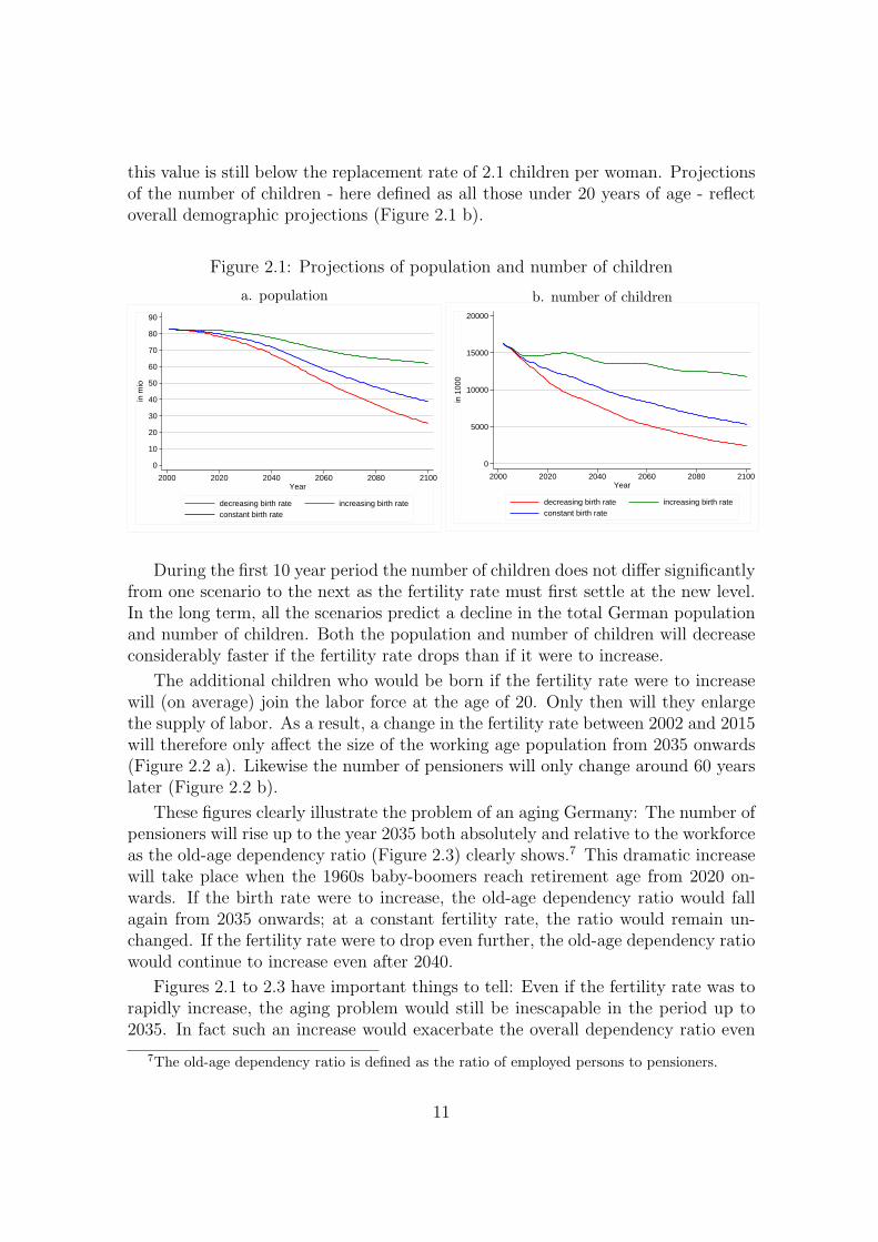
this value is still below the replacement rate of 2.1 children per woman. Projectionsof the number of children - here defined as all those under 20 years of age - reflectoverall demographic projections (Figure 2.1 b).

Figure 2.1: Projections of population and number of children

a. population

0

10

20

30

40

50

60

70

80

90

in m

io

2000 2020 2040 2060 2080 2100Year

decreasing birth rate increasing birth rateconstant birth rate

b. number of children

0

5000

10000

15000

20000

in 1

000

2000 2020 2040 2060 2080 2100Year

decreasing birth rate increasing birth rateconstant birth rate

During the first 10 year period the number of children does not differ significantlyfrom one scenario to the next as the fertility rate must first settle at the new level.In the long term, all the scenarios predict a decline in the total German populationand number of children. Both the population and number of children will decreaseconsiderably faster if the fertility rate drops than if it were to increase.

The additional children who would be born if the fertility rate were to increasewill (on average) join the labor force at the age of 20. Only then will they enlargethe supply of labor. As a result, a change in the fertility rate between 2002 and 2015will therefore only affect the size of the working age population from 2035 onwards(Figure 2.2 a). Likewise the number of pensioners will only change around 60 yearslater (Figure 2.2 b).

These figures clearly illustrate the problem of an aging Germany: The number ofpensioners will rise up to the year 2035 both absolutely and relative to the workforceas the old-age dependency ratio (Figure 2.3) clearly shows.7 This dramatic increasewill take place when the 1960s baby-boomers reach retirement age from 2020 on-wards. If the birth rate were to increase, the old-age dependency ratio would fallagain from 2035 onwards; at a constant fertility rate, the ratio would remain un-changed. If the fertility rate were to drop even further, the old-age dependency ratiowould continue to increase even after 2040.

Figures 2.1 to 2.3 have important things to tell: Even if the fertility rate was torapidly increase, the aging problem would still be inescapable in the period up to2035. In fact such an increase would exacerbate the overall dependency ratio even

7The old-age dependency ratio is defined as the ratio of employed persons to pensioners.

11

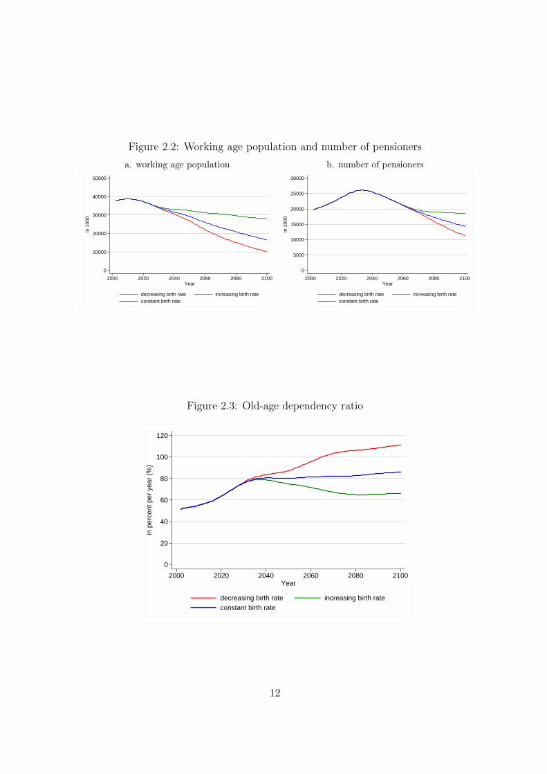
Figure 2.2: Working age population and number of pensioners

a. working age population

0

10000

20000

30000

40000

50000

in 1

000

2000 2020 2040 2060 2080 2100Year

decreasing birth rate increasing birth rateconstant birth rate

b. number of pensioners

0

5000

10000

15000

20000

25000

30000

in 1

000

2000 2020 2040 2060 2080 2100Year

decreasing birth rate increasing birth rateconstant birth rate

Figure 2.3: Old-age dependency ratio

0

20

40

60

80

100

120

in p

erce

nt p

er y

ear

(%)

2000 2020 2040 2060 2080 2100Year

decreasing birth rate increasing birth rateconstant birth rate

12

further in the short term as the increased number of children would also have to besupported by the working age population. This means that in the long term positiveeffects on the economy as a whole can only be expected after an initial aging summitis reached around 2035.

2.3 A Model of the German Economy

Within the focus of this study the effects of demographic change on the economy as awhole are of outstanding importance. Therefore the demographic scenarios outlinedin Section 2.2 are embedded in a model of the German economy. The workforceprojections of the previous section provide the labor supply of the future. In themodel this variable is a central determinant of the object of our study: per capitaGNI and its growth.

An Overlapping Generations (OLG) model is employed which is particularlysuitable for examining demographic changes. The concept of an OLG model wasoriginally devised by Samuelson (1958) and Diamond (1965). The variant presentedin the following expands the model proposed by Auerbach and Kotlikoff (1987)8

to include several countries and thus accounts for the impact of international cap-ital markets and goods on national economies (Borsch-Supan, Ludwig and Winter(2003b); Ludwig (2002)).9

It is assumed that perfect capital markets exist between the countries consideredand that capital can flow freely over national borders. As the following observationsexamine the economic development of Germany in the context of its interactionswith economic developments in other EU countries, the assumption of perfect capitalmobility approximates to reality fairly well, especially since the introduction of theeuro has finally eliminated exchange rate risks in the eurozone.10 The more regionswhich are considered, the less realistic is the assumption of perfect capital markets,however.11

8Cf. Chapter 3 in Auerbach and Kotlikoff (1987).9Models of overlapping generations are a favorite method of studying the impact of population

aging on the economy; refer to Kotlikoff, Smetters and Walliser (1999, 2001), De Nardi, Imrohorogluand Sargent (1999) and Altig et al. (2001) for the USA; Miles and Iben (2000) for the UnitedKingdom and Fehr (2000) and Hirte (2002) for Germany.

10Chapter 3 indicates that the degree of international diversification in the eurozone and withinthe EU-15 countries is relatively advanced compared to other regions. As Chapter 4 shows, the de-gree of capital flows with Germany has increased in light of the European Economic and MonetaryUnion (EMU).

11In contrast to the flows of capital and goods that are determined endogenously in the model,migration is determined exogenously by the demographic model.

13

2.3.1 The Model Structure

In the model the economy has three sectors: the household sector, the productionsector and the (rudimentary) state sector. The most interesting aspect of the statesector is in the context of the present paper the pay-as-you-go (PAYG) retirementinsurance system.

In the household sector, households maximize their consumption and have per-fect foresight regarding the utility they derive from their consumption over theirlifetime. The key notion in this model is consumption smoothing: Households dis-tribute their consumption as evenly as possible over their lifetime. As older familymembers no longer receive earnings from paid work and the public PAYG pensionis lower than the pensioner’s final wage income, households build up savings duringworking life to avoid a dramatic reduction in consumption after retirement. Dueto population aging the public PAYG pension will be much more modest in the fu-ture and will consequently reinforce the need to make private provision for old-age.This effect is mapped in the model by corresponding forecasts of contribution andreplacement rates for the public pension system (see also the discussion of the statesector below).12

In order to accommodate the long-term demographic development of the pop-ulation structure, two characteristic stages in individual’s lives are distinguished:working life and retirement. The proportion of the working age population and theretirement entry age at a specific point in time are defined along sex and cohortlines in the labor force projection. The number of people currently working or inretirement varies according to the demographic projections on the basis of variousfertility rates.13 The model is therefore capable of mapping in detail the influence ofdemographic changes on the labor supply, the demand for goods and consequentlyon the production sector.

Children do not yet receive earnings from paid work, nor are they recipients ofstate transfers on a scale comparable with public pensions. On the contrary, theirconsumption, education and training are financed by their parents. Children aretherefore not modeled as independent decision makers. Parents do, however, takeaccount of the consumption of their children when making their own consumptionand savings decisions. The budget restrictions of all households are extended inorder to take account of the consumption of children. The statistical number ofchildren are assigned to households according to the age-specific fertility rates oftheir female members. The consumption of each child is modeled as a mark-upto the consumption of each adult family member. The consumption of children,expressed in units of parental consumption, produces a scaling factor of 0.36. One

12Other motives for savings, such as a planned bequest or insurance against longevity risks orunforeseeable events are not taken into account in our model.

13Other influencing factors are the labor force participation of women and overall rates of un-employment. The figures are based on the projections of Birg and Borsch-Supan (1999).

14

child’s consumption is thus equal to 36 per cent of the consumption of an adult.14

In monetary terms this is equivalent to around 309 euros a month.

This may appear to be a rather pecuniary view of children. Empirically, however,quantifiable monetary parameters provide the only reliable variables to draw on. Wehave therefore refrained from any attempt to model the utility of children or theirconsumption.15

The production sector consists of one representative company per country. GNIas well as the wage and interest rates are determined on the basis of the specified useof production factors labor and capital as well as a specific technology. Initially it isassumed that the productivity of the factors grows exogenously at a constant rate.Alternatively, it is also examined - in stylized form - the influence of endogenousgrowth. It is assumed that a society’s average human capital increases the youngerits working population is. Human capital in turn determines the productivity whichthen endogenously specifies the overall growth in the model.16 According to thishypothesis, productivity growth in an economy increases as the average age of theworking population falls.17

We restrict our focus to this stylized model of endogenous growth, even thoughthe structure of human capital is much more complicated in reality. It is more orless impossible to take account of all the factors that influence economic growth insuch a model. Although endogenous growth can be modeled theoretically along the“learning by doing” lines suggested by Romer (1986) and implemented by Fougereand Merette (1999), for example, or according to the “learning and doing” approachproposed by Lucas (1988), it is not possible, however, to calibrate these theoreticalmodels reliably with quantitative parameters.

The organization of pension and all other social security systems is the function ofthe state sector. These tasks include collecting pension, unemployment, health andlong-term care insurance contributions as well as income tax, whereby income tax isused in the model to finance state subsidies to the pension system and general stateconsumption. No other government spending is modeled. The replacement rateprovided by the PAYG-funded public pension system is exogenous and is based ondata from the Federal Ministry of Labor. The contribution rate is derived from the

14These calculations are based on 1993 income and consumption survey (EVS) data on theconsumption of children and adults as presented for various types of households in Hertel (1998).

15In an otherwise very similar approach, Kotlikoff and Walliser (2001) take account of the con-sumption of children in the utility of their parents whereby the weighting issue remains controversial(refer also to Brooks (2002)). Barro and Becker (1988) model the “quality” of children in termsof their human capital - however, this approach is also contentious and difficult to implement in aconcrete simulation model.

16Whether a larger and/or younger population has a positive or negative impact on the produc-tivity of an economy is controversial. See, for example, Becker, Edward and Murphy (1999).

17Instead of making human capital dependent on the average age of the working population, thenumber of children can also be used to determine a society’s future human capital. There is verylittle qualitative difference in the results, however.

15

budget equation of the public pension system and federal subsidies. The transitionto a partly-funded pension system is not explicitly modeled in the following butresults from the household savings behavior described above.18

In the model’s ideal capital market, international capital flows into countriesoffering higher interest rates until interest rates differentials are equalized again. Ascapital market imperfections do not exist, both the interest rate and the net wagerate are identical in all the countries considered. The interest rate not only deter-mines the amount of capital accumulated in the domestic market, it also determinesthe amount of capital invested outside of that country and consequently the amountof capital which flows between all the countries under consideration. This relation-ship is used to solve the model by iterating the computations until all markets inall countries are cleared.

2.3.2 Criticisms

Any model of reality inevitably entails a large degree of simplification. While fu-ture demographic developments are mapped in detail and account is taken of thelinkages between national capital markets which are of great importance to Ger-many, a number of aspects which are not of key importance in this study have beenexcluded:19

(1) Variables such as the labor supply or family planning decisions are determinedexogenously from demographic and workforce projections. Potential feedbackeffects between the decision of a woman or couple to have a child and thelabor supplied by that woman or the effects on these variables by the socialinsurance systems are thus not taken into account.20

(2) The model takes no account of market frictions on the domestic labor market orany capital market imperfections, such as credit restrictions. The assumptionof perfect capital markets is not very restrictive for the mapping of capitalflows within the EU, though.

(3) It is assumed that households act on the basis of foresight and that the fu-ture holds no uncertainties. At the individual level such uncertainties wouldinclude the risk implicit in longevity against which individuals would build

18See also Borsch-Supan, Heiss, Ludwig and Winter (2003a) on the introduction of a fundedpension system.

19See also the overview in Kotlikoff (1998).20Sinn (1998), Barro and Becker (1988) as well as Cigno (1991) point to the negative effects

which social insurance systems can have on decisions to have children and the formation of humancapital. See also Fernandez-Villaverde (2001) for the relationship between technological progressand population growth. See Tamuara (2000) for an overview of the theoretical literature on familyplanning.

16

up precautionary savings. At the aggregate level risk on financial markets isignored.

In our view these simplifications do not have a substantial influence on the keyfindings as they only have a secondary and indirect impact on the relationshipbetween fertility rates and economic growth which is of actual interest in this study.21

2.4 The Impact of Demographic Change on the

German Economy

How would the German economy develop if the fertility rate were to rise to 1.8children per woman? Or, what would be the consequences if fertility rates wereto continue to fall even lower? In order to answer these questions the analysisconcentrates in particular on the impact of demographic changes on the level of percapita GNI and its growth. It is thereby initially assumed that technological progressis independent of population structure. The findings of this initial model are thencompared with a scenario in which - as described in Section 2.3.1 - productivity islinked to the population structure.

2.4.1 Exogenous Productivity Growth

As the demographic and workforce projections in Section 2.2 show, in the first 20-year period following an increase in the fertility rate there are more children whohave not yet joined the working population and who need to be supported andeducated by society. This development is also reflected in economic growth. Moreresources are required for children and this dampens capital accumulation to someextent and in turn affects production. This means that an increase in the fertilityrate will initially slow down growth. Apart from this affect, there is a fall in allper capita figures simply because GNI now needs to be distributed among a largernumber of people, i.e., shared with additional children.

These initial losses in growth are only overcome once the children are educatedand trained and have joined the working population at the age of 20 - at the earliestfrom the year 2035 onwards. However, this is also precisely the time at which theaging problem and the crisis in the public health and pension systems will peak.22

This means that not even a dramatic increase in fertility rates to 1.8 children perwoman would substantially alleviate the short-term aging problem.

After this transitional period the positive impact of increasing fertility ratesbecome obvious: Because more children now join the labor force, the working age

21Estimating the scale of these effects is current ongoing work.22The consequences of the aging process for the social security system in Germany is a much

discussed issue. See Birg (2001), p. 170-194, and Borsch-Supan (2002).

17

population grows faster than the rest of the population. The age burden now fallson more shoulders. This is clearly demonstrated by the way the contribution rate23

to the pension system changes over time (Figure 2.4). The contribution rate isidentical for all scenarios until the aging problem reaches its zenith in the period2035 to 2040. If the fertility rate increases the contribution rate will be 5 percentagepoints lower in the year 2060 than it would be in the initial scenario of a constantbirth rate. A higher supply of labor and a lower contribution rate, both induced bya rising fertility rate, will result in temporarily significantly higher per capita GNIgrowth between 2035 and 2080 compared to the reference scenario (Figure 2.5).

This positive effect will lessen over the longer term, however. A larger employedlabor force in the years 2035 to 2060 leads to higher growth as the size of theworking age population grows faster relative to the population as a whole. Whatis more, the older members of the population - the baby-boom generation - willbegin dying during this period. After 2075 the first wave of workers resulting froma higher fertility rate will reach retirement age. This means that, in the scenario ofan increasing fertility rate, the number of pensioners will drop less rapidly (Figure2.2 b) and the old-age dependency ratio will again increase slightly until it levelsout around the year 2100 (Figure 2.3). Under these conditions the opposite effectbecomes more important again whereby additional numbers of workers make a lessthan proportional contribution to production.24 By the end of the present century,and assuming constant technological progress, per capita rates of growth will moreor less converge again. The positive per capita growth effect of a higher fertility ratewill thus die away in the long run.

The impact of a higher fertility rate on levels of per capita GNI is similar (Figure2.6). In fact it is difficult to even visually distinguish the different scenarios in Figure2.6. However, a closer look reveals the same qualitative impact that has already beenobserved for economic growth. In the case of an increasing fertility rate per capitaGNI is lower than in the comparative scenario at first. However, the initial negativeeffect lasts longer as the initial losses in GNI growth first need to be catched up.A weakly positive effect on the level of per capita GNI will only become apparentfrom 2080 onwards.

2.4.2 Endogenous Productivity Growth as a Result ofHuman Capital Accumulation

The rather sobering results generated under the assumption of exogenous growthpresented in Section 2.4.1 do not apply, however, if account is taken of the pos-

23The total contribution rate is the sum of the direct contribution rate and indirect subsidies tothe public pension system financed from general taxation; cf. for example Borsch-Supan, Heiss,Ludwig and Winter (2003a).

24This argument goes back to Solow (1956), cf. Section 2.1 above and, for a more detailedtreatment, Cutler et al. (1990).

18

Figure 2.4: Direct and indirect contribution rate to the public pension system

15

25

35

45

55in

per

cent

per

yea

r (%

)

2000 2020 2040 2060 2080 2100Year

decreasing birth rate increasing birth rateconstant birth rate

Figure 2.5: GNI per capita growth - exogenous growth

0

.5

1

1.5

2

2.5

3

in p

erce

nt p

er y

ear

(%)

2000 2020 2040 2060 2080 2100Year

decreasing birth rate increasing birth rateconstant birth rate

sibility that children born in the future may be better educated and trained andconsequently accelerate the pace of technical progress. In order to illustrate thiseffect a variant of the simulation model is used in this section which allows for en-dogenous growth. As described in Section 2.3.1, the stylized assumption is made

19

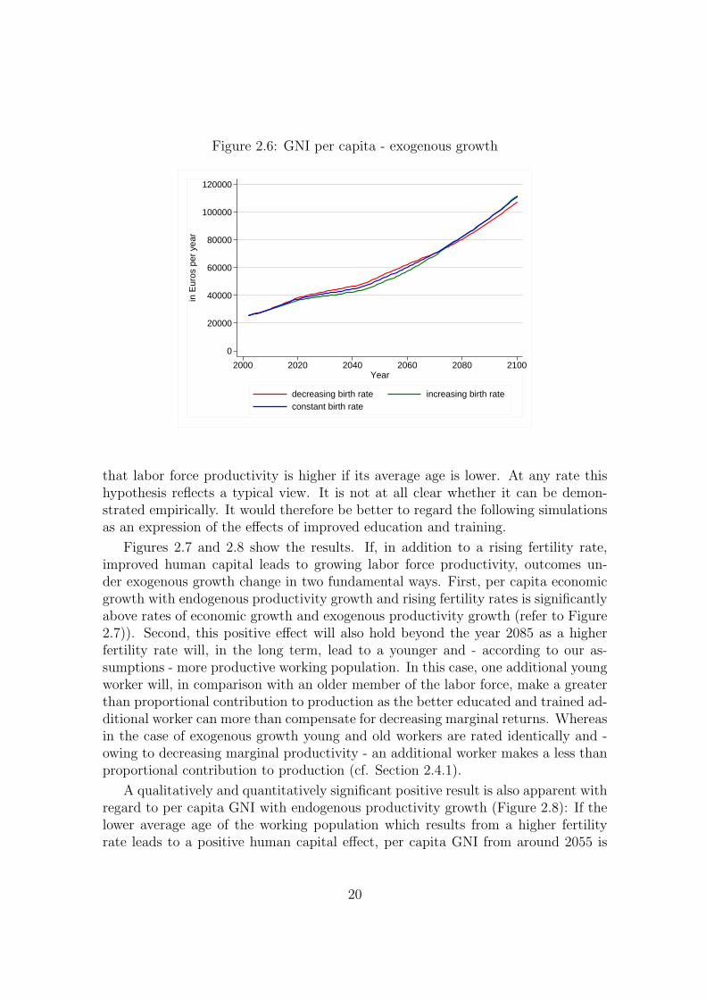
Figure 2.6: GNI per capita - exogenous growth

0

20000

40000

60000

80000

100000

120000in

Eur

os p

er y

ear

2000 2020 2040 2060 2080 2100Year

decreasing birth rate increasing birth rateconstant birth rate

that labor force productivity is higher if its average age is lower. At any rate thishypothesis reflects a typical view. It is not at all clear whether it can be demon-strated empirically. It would therefore be better to regard the following simulationsas an expression of the effects of improved education and training.

Figures 2.7 and 2.8 show the results. If, in addition to a rising fertility rate,improved human capital leads to growing labor force productivity, outcomes un-der exogenous growth change in two fundamental ways. First, per capita economicgrowth with endogenous productivity growth and rising fertility rates is significantlyabove rates of economic growth and exogenous productivity growth (refer to Figure2.7)). Second, this positive effect will also hold beyond the year 2085 as a higherfertility rate will, in the long term, lead to a younger and - according to our as-sumptions - more productive working population. In this case, one additional youngworker will, in comparison with an older member of the labor force, make a greaterthan proportional contribution to production as the better educated and trained ad-ditional worker can more than compensate for decreasing marginal returns. Whereasin the case of exogenous growth young and old workers are rated identically and -owing to decreasing marginal productivity - an additional worker makes a less thanproportional contribution to production (cf. Section 2.4.1).

A qualitatively and quantitatively significant positive result is also apparent withregard to per capita GNI with endogenous productivity growth (Figure 2.8): If thelower average age of the working population which results from a higher fertilityrate leads to a positive human capital effect, per capita GNI from around 2055 is

20

Figure 2.7: GNI per capita growth rate - exogenous & endogenous growth

0

.5

1

1.5

2

2.5

3

in p

erce

nt p

er y

ear

(%)

2000 2020 2040 2060 2080 2100Year

decreasing birth rate− exogenous growth

decreasing birth rate− endogenous growth

increasing birth rate− exogenous growth

increasing birth rate− endogenous growth

constant birth rate

Figure 2.8: GNI per capita - exogenous & endogenous growth

0

50000

100000

150000

200000

in E

uros

per

yea

r

2000 2020 2040 2060 2080 2100Year

decreasing birth rate− exogenous growth

decreasing birth rate− endogenous growth

increasing birth rate− exogenous growth

increasing birth rate− endogenous growth

constant birth rate

21

substantially higher than under conditions of exogenous growth and a rising fertilityrate. In this case it is also decisive that this effect persists beyond the year 2085.What is more, the positive effect is not only larger and permanent, but also occursaround five years earlier.

These results clearly demonstrate that the education and training of children andyoung people will play a key role in managing the process of demographic change.

2.5 Conclusions

Could a higher fertility rate help to dampen the effects of aging? Economic theoryoffers inconclusive guidance, even if the idea that “if we have too many old people,we need more children to balance the effects out”, appears plausible enough. Thequantitative study discussed here also comes to more differentiated conclusions: Along-term boost in per capita gross national income will only result from a higherfertility rate if the additional children born are also better educated and trained.This means that the formation of human capital and not a higher fertility rate itselfis decisive for long-term growth.

The three most important economic policy conclusions consequently relate tothe formation of human capital, the role of tax financed family transfers (“Familien-lastenausgleich”) and the priority of further reforms of our social security systems:

(1) An aging Germany needs better trained and educated - and consequentlyhighly productive - children. Following international comparative studies -such as studies of educational standards like the “TIMMS Study” or the “PISAStudy” in which Germany scored conspicuously poorly - there is a need for far-reaching reforms in Germany’s vocational and continuing professional train-ing sector. In a period of demographic change the engine of future growth- training and education in the context of the family, school, university, andcontinuing professional training - merits special attention and support.

(2) As the number of newborn children has very little influence on per capita GNI,there are no particularly obvious reasons on economic grounds for encouraginghigher fertility rates. If higher fertility rates are desirable, the correspondingrationale will have to be obtained from other scientific disciplines. The studyconsidered here does, however, generalize on the basis of the problems of cur-rent tax financed family transfers. It would be beyond the scope of this paperto discuss whether such transfers are adequate. However, this paper does sup-port the conclusion that all that economists can really call for is compensationfor the burdens borne by families which simultaneously represent benefits forothers. The mere existence of more children does not in itself present a long-term solution to the demographic-driven problems of the future.

22

(3) A higher fertility rate does not represent an alternative to a reform of thesocial security system aimed at solving the immediate aging problem which,if no reform is forthcoming, results in a crisis in the public pension and healthsystems in the period between 2020 and 2040. This also applies if the impactof human capital is taken into account. The transition period after whicha higher fertility rate would result in a larger and better trained labor forceable to pay contributions to the pension and other social insurance systemsis far too long. Further reforms of our social security systems must have toppriority. Specifically, further pension reforms are needed which go well beyondthe steps taken by the “Riester reform” and which tackle the problems whichwill arise after 2015. Furthermore, a reform of the health system, which evenfaces more pressing problems, is needed.

Investments in human capital and reforms of social security systems are invest-ments in the future which initially impose painful costs. However, it would be futileto hope for a painless cure to the problems associated with demographic change. Thehappy circumstance that we are living longer on average at the same time involvesthe need to finance this longevity. The financing burden must be mainly borne bythe generation which will itself enjoy a longer life. The option of postponing urgentsocial reforms and shifting the burden to later (and possibly larger) generations will,as this paper has demonstrated, ultimately prove to be an economic nonstarter.

23

Chapter 3

Institutional Determinants ofInternational Equity Portfolios -A Country-Level Analysis

3.1 Introduction

Despite large potential gains, international equity investment is less diversified acrosscountries than predicted by the international version of the traditional capital assetpricing model (ICAPM) based on Sharpe (1964), Lintner (1965) and Mossin (1966).According to the ICAPM, individuals should hold equities from countries aroundthe world in proportion to their market capitalizations. However, empirical factsreveal that international portfolios are heavily biased towards domestic assets. Thisphenomenon − known as the ‘home bias puzzle’ − is one of the most strikingempirical results in international economics. Table 3.1 shows that in 2001 U.S.investors hold almost 90 percent of their portfolios in domestic equity compared toa world market capitalization of U.S. equity of only 50 percent. For some countriesthis bias is even more pronounced, for example 67.8 percent compared to 3.9 percentfor Germany and 85.9 percent compared to 1.25 percent for Spain. If one considersthe European Monetary Union (EMU) as one large financial unit, the home biasphenomenon is also very noticeable: Investors hold 80.9 percent whereas marketcapitalization of the euro area amounts to 15.2 percent.

This phenomenon has already attracted a large body of theoretical and empiricalresearch. Lewis (1995, 1999) and Karolyi and Stulz (2003) provide extensive reviewsof the recent international economics and finance literature. However, the puzzleis not yet fully resolved. This is partly due to the lack of data on cross-borderholdings, especially of large cross-country panel data and of data with a reasonablylong time series dimension. Therefore, most existing studies dealing with the homebias phenomenon are limited to data on U.S. foreign equity holdings or on countries’

24

Table 3.1: Home bias in equities in 2001

% of equity assets share of world

in domestic equities market capitalization

US 89.22 50.64

Japan 89.50 8.26UK 74.73 8.13Germany 67.81 3.93France 79.80 4.31Spain 85.94 1.25

EMU 80.93 15.19

Sources: Foreign equity investments from the IMF’s CPIS, marketcapitalizations from WDI (2002) and FIBV, own calculations.

total foreign equity holdings not subdivided into country pairs. In contrast, thispaper employs a more comprehensive data set, the Coordinated Portfolio InvestmentSurvey (CPIS) of the International Monetary Fund (IMF), that allows to shed newlight on bilateral equity holdings between countries for 1997 and 2001 as well as ontheir institutional determinants.1

An important assumption of the traditional version of the ICAPM is that thereare no barriers to international investment. Based on the ICAPM, the theoreticallypredicted share of foreign assets at the country level is calculated in this paper andcompared to the actual share observed in the data. The difference between these twovalues is then taken to investigate the relevance of different capital market frictions.This empirical approach is based on Ahearne, Griever and Warnock (2004) andEdison and Warnock (2004).

The present paper contributes to the existing literature in two aspects. First,it extends the analysis of the home bias in equities to a large cross section of 38countries whereas Ahearne, Griever and Warnock (2004) and Edison and Warnock(2004) look at U.S. holdings of foreign equities alone.2 The home bias phenomenonis described and characterized at the bilateral country level. An interesting findingis thereby - as far as known to the author - for the first time revealed: a phe-nomenon that I call bilateral ‘friendship bias’ for several European country pairs.

1As opposed to institutional explanations, individual investor behavior such as familiarity, prob-ability judgments and social identity have also been considered in the literature to explain partof this phenomenon. The distinction between institutional and behavioral explanations was firstsuggested by French and Poterba (1991).

2Ahearne, Griever and Warnock (2004) employ country-level data for 1994 and 1997; Edisonand Warnock (2004) use security-level data for U.S. firms for 1994 and 1997.

25

Second, Ahearne, Griever and Warnock (2004) and Edison and Warnock (2004) fo-cus on information frictions as one important explanation of the home bias, whichthey proxy by firms’ cross listings. In contrast, the present paper takes variousinstitutional frictions to investment into account such as information asymmetries,financial market development and capital controls.3 Especially the impact of finan-cial development is investigated more closely. It is proxied by the development ofthe equity market and, alternatively, of the banking sector. Financial developmentof both the home and the foreign country are considered and differences betweenthem examined. Moreover, the analysis accounts for closely-held shares that cannotbe freely traded (Dahlquist et al. 2003).

The results provide new insights into the relevance of capital market frictions forforeign equity holdings using a large cross section of country pairs. The degree of eq-uity market development of the country invested in plays a significant positive role,whereas the development of the banking sector in the investor’s country is positivelylinked to portfolio shares of foreign equity investment. Information advantages mea-sured by geographical proximity as well as by the existence of a common legal originor, alternatively, of a common historical colonial relationship have great explanatorypower. The existence of capital controls has no significant impact on the share offoreign equity investment, which, however, might be due to low data quality.

Section 3.2 describes the econometric specification and discusses the measuresof capital market frictions employed in the empirical analysis. Descriptive statisticsof portfolio compositions across countries and estimation results are presented inSection 3.3 and concluded in Section 3.4. Based on the insights of the presentpaper, Section 3.5 gives an outlook on how to implement capital market frictionsinto an Overlapping Generations (OLG) simulation model.

3.2 Empirical Approach

The empirical approach is based on the idea of comparing the portfolio share of for-eign equities predicted by the International Capital Asset Pricing Model (ICAPM)to the empirical share in a world with capital market frictions. The discrepancybetween these two measures is then explained by direct and indirect barriers tointernational investment at the country level. After explaining the economic speci-fication in more detail, the variables of interest and the data are described. Finally,arising estimation issues are discussed.

3Frictions caused by non-tradable goods are not considered in this paper. Lewis (1999) testsimplications of models assuming complete markets and non-tradable goods. She shows that thesemodels are not able to explain the home bias. Baxter and Jermann (1997) show that whennon-traded human capital is taken into account, the international diversification puzzle is evenaggravated.

26

3.2.1 Econometric Specification

In order to set up an empirical model, two different classes of theoretical capitalasset pricing models are considered: first, the traditional version of the ICAPMwithout capital market frictions and, second, an ICAPM with barriers to interna-tional investment.4

The first class of models goes back to Sharpe (1964), Lintner (1965) and Mossin(1966). The traditional version of the ICAPM is built on the assumption that in-vestment and consumption opportunity sets do not differ across countries. Investorsare the same with respect to risk-aversion and information. These models assumeperfect markets. The fact that countries use different currencies has no significantimplications for portfolio choice and asset pricing. There are no taxes, no tariffs, noinformation asymmetries, no restrictions on short-sales and no barriers to interna-tional investment. One convenient property of this traditional version of the ICAPMis that it has simple and clear implications for investors’ asset holdings: Investorshold the world market portfolio share of risky assets irrespective of their country ofresidence i. It follows that the portfolio share of country i invested into country j,W ∗

j , can be expressed as:

W ∗j,t =

MCAPj,t

MCAPworld,t

,∀i,

where MCAPj,t denotes market capitalization of country j in period t andMCAPworld,t world market capitalization in period t. This market portfolio shareserves as the benchmark case of portfolio holdings to which the actual portfolio sharethat can be observed in the data is compared.

The second class of models by Black (1974), Stulz (1981), Merton (1987) andCooper and Kaplanis (1994) relaxes the assumption of perfect markets.5 Thesemodels include frictions that are typically modeled as a deadweight cost or a taxon expected returns in the foreign country. Those costs can be interpreted as costscaused by capital controls, taxes, information costs or transaction costs. Thesemodels only provide for testable implications of single model parameters, however,and do not allow to deduct an estimation equation of portfolio shares and varioustypes of capital market frictions. Therefore, a reduced form approach is employedin the subsequent empirical analysis that combines - against the background of theabove mentioned two classes of CAPM models with and without frictions - themarket portfolio share, W ∗

j,t, investment costs, Ci,t, Cj,t and Cij,t, and observedportfolio shares, W act

ij,t :

4See Stulz (1995) for a detailed review of the capital asset pricing literature and a systematicdiscussion of different models.

5Deviations from the optimal portfolios in the case of the traditional ICAPM mentioned abovecan also arise due to deviations from purchasing power parity such as in the model by Adler andDumas (1981). However, Cooper and Kaplanis (1994) show empirically that large parts of thehome bias in equity puzzle cannot be explained by this model.

27

W actij,t = α0,t + α1,tW

∗j,t + C ′

i,tβ1,t + C ′j,tβ2,t + C ′

ij,tβ3,t + Z ′ij,tγt + εij,t.

The optimal share of investment in the ICAPM with perfect markets, W ∗j,t, enters

the right hand side.6 Ci,t, Cj,t and Cij,t are vectors of measures for capital marketfrictions referring to the country of origin i, the country of destination j or thecountry pair ij.7 These vectors consist of variables that take account of investmentcosts due to indirect or direct barriers to investment. They are in the center of in-terest and discussed in more detail in the following section. The vector Zij,t includesadditional covariates that proxy investment opportunities and diversification con-siderations. They are also discussed in more detail in the next section. Moreover,a constant, α0,t, and a nuisance term, εij,t, are included. εij,t captures all the fac-tors affecting actual portfolio shares other than measured by the above mentionedexplanatory variables.

3.2.2 Variables of Interest

Information Frictions

Asymmetric information is regarded as a key factor of explaining the empirical ev-idence on foreign asset holdings and international capital flows. Martin and Rey(2004) construct a gravity model where transaction costs and costs caused by in-formation asymmetries between two countries are proxied by geographical distance.The model implies that gross bilateral asset flows will be greater the smaller thedistance. Di Giovanni (2005), Portes and Rey (2005) and Ghosh and Wolf (2000)use this gravity model to explain cross-border capital flows between countries.8 InPortes and Rey (2005), information frictions are also captured by using variablesmeasuring directly the degree of asymmetry between domestic and foreign investorssuch as the volume of telephone traffic and the number of bank branch subsidiariesas well as an index of insider trading. They find that for a large cross section ofcountries the geographical component dominates in explaining the volume and di-rection of international capital flows. Geographical distance does not only play animportant role for investment at the cross-country level but also within countries:Using firm level data, Coval and Moskowitz (1999) and Huberman (2001) provideevidence that U.S. investors have strong preferences for geographically proximateinvestments.

6Thus, the effect of W ∗j,t on W act

ij,t is left unrestricted. In a restricted version one could regresscapital market frictions on W act

ij,t −W ∗j,t.

7Country of origin denotes the investor’s country of residence, whereas the country of destinationis the country invested in, i.e., the issuers country of residence.

8Portes and Rey (2005) investigate international equity flows, Di Giovanni (2005) cross-borderM&A activity and Ghosh and Wolf (2000) FDI, bank lending, portfolio debt and portfolio equity.

28

Information advantages do not only arise due to geographical proximity but alsodue to similarity of institutions and legal structures. Legal rights of investors differvery much across countries. A large part of this variation is accounted for by legalorigin. This applies especially to commercial laws for the financing of firms and forinvestment but also to law enforcement (La Porta et al. 1997, 1998). Thus a commonlegal origin indicates a lower level of information asymmetries. It is distinguishedbetween German, French and Scandinavian civil law families, the English commonlaw, and the Socialist law family.

The similarity of institutions can also be proxied by the fact that two countriesshare a common colonial background. Colonialism explains the building of insti-tutions for several, although not all, countries (Acemoglu, Johnson and Robinson2002). The institutions are often very similar to those of the former colonizers.Thus, information advantages exist between former colonies and their colonizers.

The following variables are included to mirror information frictions:9 the log-arithm of distance between country i and country j, logdistanceij, and a dummyvariable equal to one if a country pair has a common legal origin, samelegorij. Al-ternatively, a dummy variable equal to one if two countries share a common colonialbackground is used, colonyij.

10

Financial Market Development

In larger and more liquid markets prices are supposed to be more informative. Onereason is that larger markets encourage arbitrage through liquidity, the existence ofmore and better substitutes to use as hedges for trading against mispriced securitiesand reduced transaction costs (Beck, Demirguk-Kunt and Levine (2001) and Wurgler(2000)).

A common proxy for financial development such as the size and depth of thedomestic capital market is the amount of private credit provided by the bankingsector relative to GDP which is included in the subsequent regression analysis forthe home and foreign country, logdcrediti,t and logdcreditj,t respectively.11 Thebanking sector plays an important role for private investment in many emergingeconomies as well as in continental Europe and Japan. It represents the overalldevelopment of the private banking sector - more specifically the development of itsfinancial institutions that conduct and channel international equity investments -

9Section 3.2.3 and Table 3.10 in Appendix A include descriptions of all employed variables,their sources and exact calculations.

10In the trade literature, a dummy variable that denotes whether two countries have a commonlanguage is often employed in order to proxy information advantages. Note that in this sample allcountry pairs that have a common colonial background at the same time share a common languageand vice versa.

11See for example Chinn and Ito (2006) and Di Giovanni (2005). As a comparable measureM2 to GDP is often used. However, this variable is only available for a much smaller number ofcountries.

29

and the amount of liquidity available in the economy.

In order to capture an additional angle of financial development, stock mar-ket capitalization of country i and j relative to GDP is considered, logmcapi,t andlogmcapj,t. It directly addresses the influence of growing equity markets on in-ternational investments which experienced a substantial growth in industrializedeconomies as well as in new markets of transitional and emerging countries in the1990s.

Finally, a variable is employed that measures the actual liquidity in the equitymarket, i.e., it takes account of equity shares by large controlling shareholders thatcan not be freely traded. Especially in countries with poor investor protectionmany firms are controlled by large shareholders such that only a fraction of theshares issued by firms can be freely traded in these countries and held by foreigninvestors. La Porta et al. (1998) provide evidence that the size and breadth ofcapital markets is largely influenced by investor protection and the quality of thelegal environment. Dahlquist et al. (2003) investigate the impact of equity sharesheld by large shareholders on U.S. foreign investment. They show that a country’sshare in U.S. equity portfolios is negatively related to the share of equities heldby large shareholders in that country. In the subsequent regression analysis ofthe present paper the float portfolio share calculated by Dahlquist et al. (2003),W float

j,t , is used as a proxy for investor rights and the liquidity of the market. Thefloat portfolio share is the market capitalization of a country excluding closely-heldshares by controlling shareholders.

Direct Barriers

Direct barriers such as capital controls that have an immediate impact on net invest-ment returns and, therefore, on the investment decision are also considered. Albeithaving been reduced to a great extent throughout the 1990s, capital controls arestill existent today. The crucial question is whether controls that are in place arein fact effective.12 Although there have been attempts to determine measures of theeffectiveness of capital controls, these are only available for a very small number ofcountries or years.13

Given the large cross-country data sample that is employed in the present paper,a financial openness measure is used that was for the first time provided by Grilliand Milesi-Ferretti (1995) based on the IMF’s Annual Report on Exchange Arrange-ments and Exchange Restrictions (AREAER), restricti,t and restrictj,t. It does notaccount for the effectiveness of capital controls but only states whether restrictionson capital flows are in place or not.

12For a detailed description of different types of capital controls and their effectiveness see Edisonet al. (2002) and Neely (1999); for different country experiences see Ariyoshi et al. (2000).

13See, e.g., Edison et al. (2002) for a comprehensive overview of capital control measures.

30

Additional Covariates

Two different variables are considered that mirror diversification and investmentopportunities. First, a correlation variable that is equal to the monthly returncorrelation in the four years preceding year t is added, rcorrij,t. If diversificationmotives matter for investors’ investment decisions, countries hold a higher portfolioshare of those foreign assets whose stock returns are only weakly correlated withdomestic stock returns.

Second, GDP growth for the country of destination is included, gdpgrowthj,t.Again this variable is averaged across the four years preceding year t in order toavoid business cycle effects.14 High GDP growth in the foreign country j mirrorsprofitable investment opportunities that emerge in booming economies. This isan implication of standard growth theory. Emerging countries in South-east Asiain the 1990s that experienced booming economies and large capital inflows at thesame time constitute a well-known example of this relationship.

3.2.3 Data

So far, reliable bilateral holdings data has hardly been available except for the resultsof some smaller surveys of residents’ portfolio holdings such as for the U.S. in 1994and 1997. The present work is based on cross-country equity holdings obtained fromthe Coordinated Portfolio Investment Survey (CPIS) of the International MonetaryFund (IMF). For the first time this data set includes comparable portfolio holdingsdata from as many countries around the world as possible. The survey has beenundertaken in 1997 with 29 countries only. Since 2001 yearly waves are undertakenincluding 64 countries. Data for 1997 and 2001 is used in this study. The availabilityof several other variables limits the number of countries in the present sample to 38in 2001. Table 3.2 lists all countries by regions.

The CPIS data refers to end of year numbers and includes, among other things,information on gross bilateral foreign equity holdings, securities and, for some coun-tries, separately reported liabilities. Foreign equity holdings entail cross-border in-vestment from all sectors: monetary authorities, general government, banks andother financial intermediaries, nonprofit organizations, and households.15 The great-est difficulty consists in capturing cross-border investments by households. The IMFprovides the definitions and concepts,16 whereas the data is organized by domesticstatistical institutions as each country should take account of its own particular fi-nancial structure and circumstances. There are some differences in reporting equity

14Alternatively, seven and ten year averages have been considered. However, results do notchange.

15Note that equity investment that establishes a direct investment relationship is excluded fromthe CPIS. See the definition in the IMF’s Balance of Payments Manual, fifth edition (BPM5) andthe IMF’s Coordinated Portfolio Investment Survey Guide.

16These have to be in conformity with the BPM5.

31

holdings between the 1997 and 2001 waves. In 1997 the distinction between unavail-able and zero was not made. Therefore, the two years are treated separately in theestimations.

The CPIS data is used in order to calculate actual portfolio shares of countryj’s assets held in country i. Note that country i refers to the residence of theholder of the security and country j refers to the residence of the issuer of thesecurity. Appendix B explains in detail how W act

ij,t is calculated from the observationsof bilateral cross-country portfolio holdings.

Information on countries’ total market capitalizations is taken from the WorldDevelopment Indicators (WDI, 2002) and the International Federation of Stock Ex-changes (FIBV).17 An alternative measure of market capitalizations, the liquidityadjusted float portfolio share, can be found in Dahlquist et al. (2003). Data onGDP growth is obtained from WDI (2002).

Table 3.2: Countries and regions

South America South-east Asia Northern Europe

Argentina Indonesia DenmarkBrazil Malaysia FinlandChile Philippines Ireland

Colombia Singapore NorwayVenezuela Thailand Sweden

United Kingdom

North America Oceania Western EuropeCanada Australia Austria

United States New Zealand BelgiumFrance

West Asia Eastern Europe GermanyIsrael Hungary Netherlands

Turkey Poland Switzerland

East Asia Southern Europe Northern AfricaHong Kong Greece Egypt

Japan ItalyKorea, Rep. Of Portugal

Spain

17The availability of stock market measures limits the amount of countries in the present sampleto 38.

32

In order to measure information frictions, the physical distance between coun-tries’ capital cities and alternatively the fact of two countries sharing a commonborder is used. Moreover, a dummy variable is added that is equal to one if twocountries have a common colonial background. All data are based on the CIA fact-book18 and are obtained from Frankel, Stein and Wei (1995). A dummy variable,based on La Porta et al. (1998), is included that is equal to one if both countriesbelong to the same legal family. The amount of domestic credit provided by thebanking sector relative to GDP, obtained from WDI (2002), is used to proxy thedegree of financial market development.

Capital controls are taken account of by using an updated index by Grilli andMilesi-Ferretti (1995) based on the IMF’s AREAER. The capital control data refersto the home country as well as to the country of destination. Unfortunately, the datadoes not allow a clear separation of restrictions on inflows or outflows. Thus, thesame indicator, restricti,t and restrictj,t respectively, is included for both countries.

In 1997 as well as in 2000/01 there have been several banking crises, for examplein Thailand, Malaysia and Turkey. This is taken into account by a dummy variablethat is equal to one if a banking crisis as documented in Caprio and Klingebiel(2003) happened in the relevant or precedent year.

In order to calculate return correlations rcorrij,t, standard national stock marketindices by Morgan Stanley Capital International (MSCI) are used.19 The regionalclassification of the countries is shown in Table 3.2. It is based on the UN geograph-ical region division20 and used to construct region dummies.

For more detailed information on variable definitions and sources refer to Table3.10 in Appendix A.

3.2.4 Estimation Issues

In several cases reported investments are zero. These corner solution outcomes arelikely due to an investor’s optimization in a world with investment barriers whichresults in an optimal outcome of zero foreign equity holdings. Consequently, W act

ij,t iszero. For all other observations the dependent variable is positive and continuous.Therefore, a corner solution model is estimated. In the context of this study, partialeffects of W ∗

j,t, Ci,t, Cj,t and Cij,t on E(W actij,t |W ∗

j,t, Ci,t, Cj,t, Cij,t) are of interest. Notethat these marginal effects refer to the full sample including zero and positive values.They are obtained by estimating a Tobit model censored at zero and by calculatingaverage adjustment factors for the coefficients of the Tobit regression. All tables inthis paper report these marginal effects instead of estimated coefficients.21

18See www.cia.gov/cia/publications/factbook/.19For all available countries the gross index including dividend payments in U.S. dollars is used.20See http://unstats.un.org/unsd/methods/m49/m49region.htm.21See Wooldridge (2002), Chap. 16 pp. 521-524, for the derivation of the adjustment factor.

33

The corner solution model can be applied to the CPIS data for 2001, but notimmediately to the 1997 wave, because - as mentioned in Section 3.2.3 - in 1997zeros refer to both true zeros and missing values. In order to provide comparabilityacross regressions for each year and to validate a Tobit estimation approach for the1997 data, missing values are imputed by using the information of the 2001 wave: AProbit model fitting the probability of a missing or a zero entry given the explanatoryvariables mentioned above is estimated for 2001. The estimation output is reportedin Table 3.3. The estimated coefficients are used to estimate the probability of azero or missing value for 1997. If the probability of a missing is larger than one half,the reported zero is changed into a missing value.

Table 3.3: Probit estimates of missing values in 2001

W ∗j,t 0.02 rcorrij,t -0.186

(0.93) (0.64)logdistanceij -0.067 gdpgrowthij -1.405

(0.66) (0.20)samelegorij 0.681 bankcrisisi -0.523

(4.10)*** (3.26)***logdcrediti,t -0.223 bankcrisisj -0.095

(2.40)** (0.56)logdcreditj,t 0.043 constant 2.049

(0.42) (1.78)*restricti,t -0.094 No. of obs. 433

(0.93) LL -239.46restrictj,t -0.061 adj. R2 0.08

(0.68)

Notes: The dependent variable is equal to one if there exists amissing value and equal to zero if there is a zero value in 2001.Absolute values of t statistics are reported in parentheses. Allregressions include region dummies for country i and j in order toaccount for region-specific fixed effects.

3.3 International Equity Portfolios: Composition

and Determinants

In a first step, descriptive statistics of the composition of international equity port-folios and the extent of the home bias at the aggregate country level are presented.It serves to give a first comparison of bilateral portfolio shares in the data and op-timal portfolio shares as predicted by the traditional version of the ICAPM under

34

the assumption of perfect capital markets. In a second step, multivariate analysisare undertaken as described in Section 3.2.1. The results provide insights into thedeterminants of international equity portfolios.

3.3.1 Bilateral Friendship Bias versus Bilateral Home Bias

For all countries around the world with existing stock markets, a home bias inequities with respect to total home versus foreign investment can be observed. Table3.1 in Section 3.1 presents an overview of this home bias for some selected countries.

In contrast to a home bias referring to total home versus foreign investment,one can also observe a home bias at the bilateral country pair level. A bilateralhome bias indicates that investors hold - compared to the traditional version of theInternational Capital Asset Pricing Model (ICAPM) - too little of their portfolio inforeign equities of a given country. For the U.S. this bilateral home bias is existentfor all country pairs and has been amply discussed in the literature (e.g. Tesar andWerner (1995), and Ahearne, Griever and Warnock (2004)). However, for certaincountry pairs, especially within the EMU, one can observe a bilateral ‘friendshipbias’. It states that the actual equity portfolio share, W act

ij,t , is larger than the onepredicted by the ICAPM under the assumption of perfect capital markets, W ∗

j,t.Table 3.4 documents the predicted and the actual shares. Bold numbers refer tocountry pairs with a bilateral friendship bias.

In most cases within the EMU this relationship is reciprocal, i.e., it is observedfor the country pair Austria-Germany and at the same time for the country pairGermany-Austria. The number of country pairs with a friendship bias has increasedsubstantially from 1997 to 2001. Moreover, the friendship bias has been persistentover the years: for almost all country pairs with a friendship bias in 1997 one canalso observe a friendship bias in 2001. The fact that most country pairs with afriendship bias in the present data sample are part of the EMU might indicate thatthis phenomenon is related to the large extent of enhanced financial integrationand development within the EMU. Also historical and cultural linkages might bean explanation. The results of the multivariate analysis that are discussed in thefollowing section will shed light on the actual determinants of international portfolioholdings.

3.3.2 Determinants of International Equity Portfolios

Main estimation results for the years 1997 and 2001 are summarized in Tables 3.5and 3.6. In the first specification, market capitalization of country j, W ∗

j,t, is the onlyexplanatory variable entering the regression. Subsequently, the introduced proxiesfor capital market frictions are added one after the other.22

22Further robustness checks have been undertaken by excluding single countries from the samplein order to test whether major financial centers such as the U.K., Ireland and the U.S. drive the

35

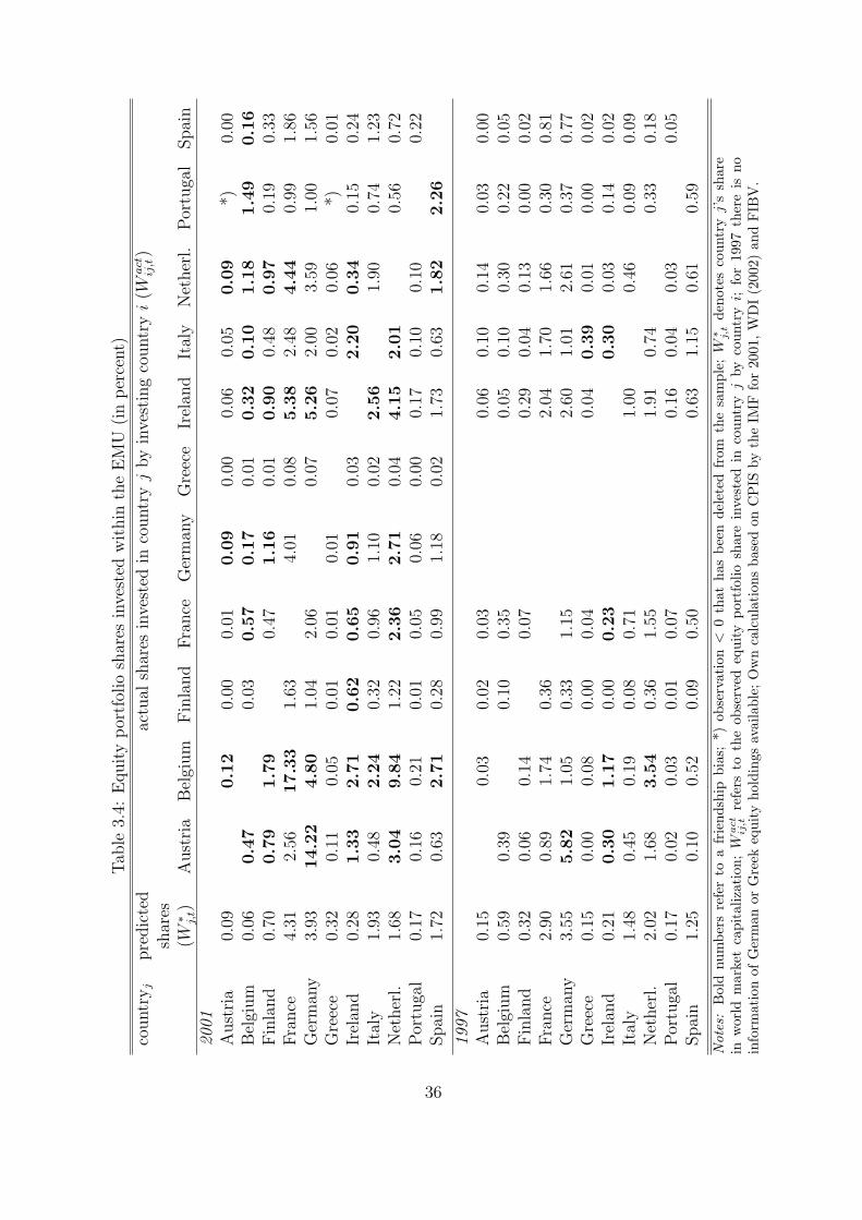
Tab

le3.

4:E

quity

por

tfol

iosh

ares

inve

sted

wit

hin

the

EM

U(i

nper

cent)

countr

yj

pre

dic

ted

actu

alsh

ares

inve

sted

inco

untr

yj

by

inve

stin

gco

untr

yi

(Wact

ij,t)

shar

es(W

∗ j,t)

Aust

ria

Bel

gium

Fin

land

Fra

nce

Ger

man

yG

reec

eIr

elan

dIt

aly

Net

her

l.Por

tuga

lSpai

n

2001

Aust

ria

0.09

0.1

20.

000.

010.0

90.

000.

060.

050.0

9*)

0.00

Bel

gium

0.06

0.4

70.

030.5

70.1

70.

010.3

20.1

01.1

81.4

90.1

6Fin

land

0.70

0.7

91.7

90.

471.1

60.

010.9

00.

480.9

70.

190.

33Fra

nce

4.31

2.56

17.3

31.

634.

010.

085.3

82.

484.4

40.

991.

86G

erm

any

3.93

14.2

24.8

01.

042.

060.

075.2

62.

003.

591.

001.

56G

reec

e0.

320.

110.

050.

010.

010.

010.

070.

020.

06*)

0.01

Irel

and

0.28

1.3

32.7

10.6

20.6

50.9

10.

032.2

00.3

40.

150.

24It

aly

1.93

0.48

2.2

40.

320.

961.

100.

022.5

61.

900.

741.

23N

ether

l.1.

683.0

49.8

41.

222.3

62.7

10.

044.1

52.0

10.

560.

72Por

tuga

l0.

170.

160.

210.

010.

050.

060.

000.

170.

100.

100.

22Spai

n1.

720.

632.7

10.

280.

991.

180.

021.

730.

631.8

22.2

6

1997

Aust

ria

0.15

0.03

0.02

0.03

0.06

0.10

0.14

0.03

0.00

Bel

gium

0.59

0.39

0.10

0.35

0.05

0.10

0.30

0.22

0.05

Fin

land

0.32

0.06

0.14

0.07

0.29

0.04

0.13

0.00

0.02

Fra

nce

2.90

0.89

1.74

0.36

2.04

1.70

1.66

0.30

0.81

Ger

man

y3.

555.8

21.

050.

331.

152.

601.

012.

610.

370.

77G

reec

e0.

150.

000.

080.

000.

040.

040.3

90.

010.

000.

02Ir

elan

d0.

210.3

01.1

70.

000.2

30.3

00.

030.

140.

02It

aly

1.48

0.45

0.19

0.08

0.71

1.00

0.46

0.09

0.09

Net

her

l.2.

021.

683.5

40.

361.

551.

910.

740.

330.

18Por

tuga

l0.

170.

020.

030.

010.

070.

160.

040.

030.

05Spai

n1.

250.

100.

520.

090.

500.

631.

150.

610.

59

Not

es:

Bol

dnu

mbe

rsre

fer

toa

frie

ndsh

ipbi

as;

*)ob

serv

atio

n<

0th

atha

sbe

ende

lete

dfr

omth

esa

mpl

e;W∗ j,t

deno

tes

coun

try

j’s

shar

ein

wor

ldm

arke

tca

pita

lizat

ion;

Wact

ij,t

refe

rsto

the

obse

rved

equi

typo

rtfo

liosh

are

inve

sted

inco

untr

yj

byco

untr

yi;

for

1997

ther

eis

noin

form

atio

nof

Ger

man

orG

reek

equi

tyho

ldin

gsav

aila

ble;

Ow

nca

lcul

atio

nsba

sed

onC

PIS

byth

eIM

Ffo

r20

01,W

DI

(200

2)an

dFIB

V.

36

The marginal effect of W ∗j,t on actual portfolio shares is highly significant but

very low in size, namely equal to 0.05 in 1997 and 0.09 in 2001. The size does notchange in the subsequent regressions when additional variables enter. Noticeable,for a large cross section of countries the market portfolio share, W ∗

j,t, which - in thetraditional ICAPM under the assumption of perfect capital markets - just equalsthe portfolio share invested in country j for each country i, does hardly explain theactual share of foreign investment in country j, W act

ij,t .

Information Asymmetries

Differences in accounting standards, disclosure requirements and regulatory environ-ments across countries lead to information asymmetries between local and foreigninvestors. Foreign investors have to translate and interpret this information in lightof the relevant legal conventions and business culture which leads to additional costs.

Information frictions proxied by logdistanceij and samelegorij have highly signif-icant and large coefficients. A one percent increase in geographical distance betweentwo countries leads on average to a decrease in the portfolio share of equity holdingsof about 0.16 percentage points in 1997 and 0.29 in 2001 (Tables 3.5 and 3.6, speci-fication (2)). If both countries have the same legal origin, the share of foreign equityholdings is on average about 0.24 higher in 1997 and even larger in 2001, namelyequal to 0.43. When colonyij is used instead of samelegorij (specification (3)), theeffect is even larger: If both countries have a common colonial background, themarginal effect amounts to 0.40 in 1997 and in 2001 to 0.62.23 Overall, the resultsemphasize the importance of information frictions as determinants of internationalequity portfolios.

Financial Market Development

The second group of indirect capital market frictions refers to the degree of finan-cial market development. Two alternative measures of financial development areconsidered: the relative size of the banking sector and the relative size of the eq-uity market. They proxy different angles of financial market development but arepositively correlated with each other. Moreover, the float portfolio share, W float

j,t , isincluded instead of the market portfolio share, W ∗

j,t, in order to exclude non-liquidequity shares.

Financial development of the banking sector in the source country i as well as inthe country of destination j is proxied by the corresponding ratios of private credit

results. These additional regressions are not reported in the following, because results did notchange. However, they can be obtained from the author upon request.

23Likewise, logdistanceij can be interchanged with a dummy variable equal to one if two countriesare part of the same region or share a common border. The results can be obtained from the authersupon request.

37

Tab

le3.

5:M

ain

regr

essi

onre

sult

s,19

97

(1)

(2)

(3)

(4)

(5)

(6)

(7)

(8)

W∗ j,t

0.04

90.

049

0.04

90.

047

0.04

70.

047

0.04

7

[14.

51]*

**[1

5.25

]***

[15.

45]*

**[1

4.66

]***

[14.

62]*

**[1

4.64

]***

[14.

74]*

**lo

gdis

tance

ij-0

.156

-0.1

53-0

.163

-0.1

64-0

.165

-0.1

63-0

.175

[6.2

6]**

*[6

.20]

***

[6.5

6]**

*[6

.56]

***

[6.6

3]**

*[6

.47]

***

[7.0

2]**

*sa

mel

egor

ij0.

251

0.23

50.

232

0.23

70.

237

0.22

3[5

.59]

***

[5.2

2]**

*[5

.13]

***

[5.2

7]**

*[5

.27]

***

[5.0

2]**

*co

lony i

j0.

404

[6.8

8]**

*lo

gdcr

edit

i,t

0.23

90.

240

0.18

90.

194

0.11

6[3

.43]

***

[3.4

3]**

*[2

.55]

**[2

.60]

***

[1.5

4]lo

gdcr

edit

j,t

0.07

20.

076

0.07

10.

081

0.07

[1.0

9][1

.15]

[1.0

8][1

.18]

[1.0

4]lo

gm

cap i

,t0.

064

0.06

40.

038

0.03

00.

034

[1.4

4][1

.43]

[0.8

1][0

.60]

[0.6

9]lo

gm

cap j

,t0.

078

0.07

70.

084

0.07

40.

088

[2.0

1]**

[1.9

7]**

[2.0

7]**

[1.6

4][1

.98]

**

Wflo

at

j,t

0.03

8[1

4.38

]***

rest

rict

i,t

0.10

60.

106

0.09

1[1

.87]

*[1

.86]

*[1

.62]

rest

rict

j,t

-0.0

17-0

.019

-0.0

19[0

.50]

[0.5

5][0

.55]

rcor

r ij,

t0.

057

-0.0

09[0

.53]

[0.0

8]gdpg

row

thj,

t0.

066

[5.5

0]**

*N

o.of

obs.

900

900

900

900

900

900

900

900

adjm

.fa

ctor

0.51

0.5

0.5

0.5

0.5

0.5

0.5

0.5

adj.

R2

0.17

0.2

0.21

0.21

0.21

0.22

0.22

0.23

Not

es:

Dep

ende

ntva

riab

lefo

ral

lsp

ecifi

cati

ons:

Wact

ij,t

;Tob

ites

tim

atio

nof

aco

rner

solu

tion

mod

el.

Rep

orte

dco

effici

ents

are

mar

gina

leff

ects

corr

ecte

dby

anad

just

men

tfa

ctor

asre

port

edin

Sect

ion

3.2.

4.A

bsol

ute

valu

esof

tst

atis

tics

are

repo

rted

inpa

rent

hese

s.R

egio

ndu

mm

ies

for

the

coun

try

ofor

igin

and

the

coun

try

ofde

stin

atio

n,du

mm

ies

for

bank

ing

cris

esin

the

coun

try

ofor

igin

and

the

coun

try

ofde

stin

atio

n,as

wel

las

aco

nsta

ntar

ein

clud

edbu

tno

tre

port

ed.

38

Tab

le3.

6:M

ain

regr

essi

onre

sult

s,20

01

(1)

(2)

(3)

(4)

(5)

(6)

(7)

(8)

W∗ j,t

0.08

70.

087

0.08

60.

085

0.08

50.

085

0.08

4

[13.

88]*

**[1

4.29

]***

[14.

40]*

**[1

3.45

]***

[13.

42]*

**[1

3.42

]***

[13.

67]*

**lo

gdis

tance

ij-0

.285

-0.2

71-0

.292

-0.2

92-0

.292

-0.2

77-0

.288

[5.4

5]**

*[5

.26]

***

[5.6

1]**

*[5

.59]

***

[5.6

1]**

*[4

.64]

***

[4.9

8]**

*sa

mel

egor

ij0.

432

0.43

50.

431

0.43

60.

441

0.39

1[4

.36]

***

[4.4

2]**

*[4

.37]

***

[4.4

3]**

*[4

.46]

***

[4.0

8]**

*co

lony i

j0.

620

[4.8

9]**

*lo

gdcr

edit

i,t

0.24

10.

240

0.24

40.

248

0.29

9[1

.77]

*[1

.76]

*[1

.78]

*[1

.81]

*[2

.25]

**lo

gdcr

edit

j,t

-0.0

140.

009

-0.0

18-0

.013

-0.0

10[0

.11]

[0.0

8][0

.14]

[0.1

0][0

.08]

logm

cap i

,t-0

.149

-0.1

49-0

.149

-0.1

56-0

.212

[2.4

0]**

[2.4

0]**

[2.3

9]**

[2.4

4]**

[3.3

8]**

*lo

gm

cap j

,t0.

166

0.17

20.

165

0.15

80.

158

[2.6

4]**

*[2

.72]

***

[2.6

2]**

*[2

.44]

**[2

.52]

**

Wflo

at

j,t

0.06

9[1

3.24

]***

rest

rict

i,t

0.01

70.

020

-0.0

02[0

.19]

[0.2

2][0

.02]

rest

rict

j,t

-0.0

12-0

.007

-0.0

08[0

.14]

[0.0

8][0

.10]

rcor

r ij,

t0.

050

0.04

6[0

.49]

[0.4

6]gdpg

row

thj,

t0.

145

[5.6

2]**

*N

o.of

obs.

899

899

899

899

899

899

899

899

adjm

.fa

ctor

0.55

0.55

0.54

0.55

0.55

0.55

0.55

0.54

adj.

R2

0.1

0.11

0.11

0.12

0.12

0.12

0.12

0.12

Not

es:

see

Tab

le3.

5.

39

provided by the financial sector relative to GDP, logdcrediti,t and logdcreditj,t. Forboth years only the coefficient for country i is significant and has a positive sign24

(specification (4)). A one percent increase in private credit relative to GDP in thehome country i is associated with an increase in foreign portfolio shares of about0.24 percentage points in 1997 and 2001. The positive effect indicates that moreand better banking institutions and more liquidity in the banking sector at home -proxied by private credit relative to GDP in country i - are associated with moreinvestments in foreign markets.

Stock market capitalization in country i, logmcapi,t, has no effect in 1997 anda negative effect in 2001.25 The latter is in line with the consideration that moredeveloped equity markets offer more diversification possibilities at home such thatinvestors are less inclined to invest abroad. The negative marginal effect in 2001amounts to 0.15. In contrast, stock market capitalization in country j, logmcapj,t

has a positive and significant marginal effect on foreign portfolio shares which isequal to 0.08 in 1997 and 0.17 in 2001. Based on these results, investors seem to bemore inclined to hold equity shares in such economies. The more developed equitymarkets in the foreign country j, the more informative are prices and investmentopportunities.

All in all, the results suggest the following relationship between financial marketdevelopment and foreign portfolio shares: Both, the relative size of the bankingsector in the investor’s country and the relative size of the stock market in theissuer’s country are positively linked to foreign portfolio shares.

The effect of the float compared to the market portfolio share is slightly smallerin both years (specification (5)). In the full sample the float portfolio share doesnot seem to capture any further liquidity effects and thus does not provide anyadditional explanatory power compared to the market portfolio share, W ∗

j,t.

Capital Controls

If capital controls on incoming capital are in place, the share of foreign equityinvestment into that country should be lower. Again a negative effect is expected ifcapital controls on outgoing capital are in place. Unfortunately, the AREAER datadoes not allow to distinguish between incoming and outgoing capital controls. Theresults in Tables 3.5 and 3.6 show that capital controls have hardly any significantimpact. Exceptions are specifications (6) and (7) in 1997. The existence of controlsyields a weak positive effect that is significant at the 10 percent level only, meaning

24If stock market capitalization is excluded from specification (4), logdcreditj,t has a positiveand significant effect on actual portfolio shares. Due to the fact that logdcreditj,t and marketcapitalization, logmcapj,t, are positively correlated, the effect is attributed to logmcapj,t ratherthan logdcreditj,t once both variables enter the regression.

25Note that the negative sign is not influenced by the alternative financial market developmentmeasure logdcrediti,t and still present in a regression without logdcrediti,t and logdcreditj,t.

40

that the existence of controls in the country of origin, i, is associated with a highershare of foreign equity. This result is mainly driven by Chile that experiencedhigh shares of foreign equity holdings and capital controls in 1997.26 Once Chileis excluded from the sample, the coefficient on restricti,t turns negative in 1997.27

Moreover, the effect vanishes in the full sample when GDP growth is added.

Investment Opportunities and Diversification

In addition, variables mirroring investors’ investment opportunities and diversifi-cation, i.e., GDP growth and return correlations respectively, are included in theregression analysis.

As specifications (7) and (8) (Tables 3.5 and 3.6) show, return correlations,rcorrij,t, have no significant impact. A negative effect would be consistent with adiversification motive. The tendency to find either a positive relationship or none atall is in line with other empirical studies, e.g., Portes and Rey (2005) and Aviat andCoeurdacier (2004). The finding might be driven by the common positive impactthat financial integration has on portfolio shares and return correlations at the sametime. According to this argument, return correlations measure the effect of increasedfinancial integration instead of measuring diversification opportunities. One possiblesolution to this measurement problem would be to instrument current stock marketcorrelation. Coeurdacier and Guibaud (2005) show that when using stock returncorrelation over the period of 1950-1975 as an instrument, a diversification motivecan be identified. As such data is not present for the country sample used in thispaper, this approach cannot be undertaken, however.

GDP growth is included for the country of destination. In booming economiesthat experience high GDP growth rates more promising investment opportunitiesare likely to be existent. In line with this consideration, GDP growth in country jhas a significantly positive impact in both years: A one percentage point increase inGDP growth leads to an increase in foreign equity holdings of about 0.07 percentagepoints in 1997 and 0.15 in 2001 (specification (8)).

Market and Float Portfolio Shares in Different Geographical Regions

The results in Tables 3.5 and 3.6 show that coefficients on the market and floatportfolio shares are very low. The float portfolio denotes the market portfolio sharecorrected for non-tradable shares held by large shareholders. – Do these two findingschange when the impact of W ∗

j,t on W actij,t is analyzed for different regions and countries

separately?

The size of the marginal effects of W ∗j,t and W float

j,t differs significantly across

26See De Gregorio, Edwards and Valdes (2000) on the Chilean experience of capital controls inthe 1990s.

27These results are not reported but can be obtained from the author upon request.

41

Table 3.7: The market portfolio share for different regions

1997 2001

(9) (10) (9) (10)

W ∗j,t 0.131 0.108 0.205 0.180

[3.55]*** [9.37]*** [3.29]*** [7.21]***(W ∗

j,t) ∗ samerica 0.167 0.068[0.63] [0.09]

(W ∗j,t) ∗ namerica -0.090 -0.127

[2.42]** [2.03]**(W ∗

j,t) ∗ easia -0.051 -0.050[1.05] [0.49]

(W ∗j,t) ∗ seasia -0.147 -0.976

[0.33] [0.86](W ∗

j,t) ∗ wasia -0.503 0.211[0.19] [0.01]

(W ∗j,t) ∗ seurope 0.048 -0.325

[0.48] [0.23](W ∗

j,t) ∗ neurope -0.014 -0.017[0.37] [0.26]

(W ∗j,t) ∗ oceania 0.074 0.101

[0.53] [0.38](W ∗

j,t) ∗ eeurope -0.505 1.801[0.03] [0.24]

(W ∗j,t) ∗ U.S. -0.063 -0.096

[5.61]*** [4.01]***(W ∗

j,t) ∗ EMU 0.001 0.119[0.01] [1.78]*

No. of obs. 900 900 899 899adjm. factor 0.49 0.49 0.54 0.54adj. R2 0.24 0.24 0.13 0.13

Notes: see Table 3.5. In addition, the following variables are included but not re-ported: logdistanceij , samelegorij , logdcrediti,t, logdcreditj,t, logmcapi,t, logmcapj,t, restricti,t,restrictj,t, rcorrij,t and gdpgrowthj,t.

42

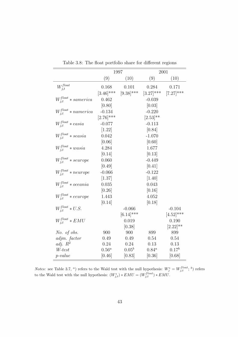
Table 3.8: The float portfolio share for different regions

1997 2001

(9) (10) (9) (10)

W floatj,t 0.168 0.101 0.284 0.171

[3.46]*** [9.38]*** [3.27]*** [7.27]***

W floatj,t ∗ samerica 0.462 -0.039

[0.80] [0.03]

W floatj,t ∗ namerica -0.134 -0.220

[2.76]*** [2.53]**

W floatj,t ∗ easia -0.077 -0.113

[1.22] [0.84]

W floatj,t ∗ seasia 0.042 -1.070

[0.06] [0.60]

W floatj,t ∗ wasia 4.284 1.677

[0.14] [0.13]

W floatj,t ∗ seurope 0.060 -0.449

[0.49] [0.41]

W floatj,t ∗ neurope -0.066 -0.122

[1.37] [1.40]

W floatj,t ∗ oceania 0.035 0.043

[0.26] [0.16]

W floatj,t ∗ eeurope 1.443 4.052

[0.14] [0.18]

W floatj,t ∗ U.S. -0.066 -0.104

[6.14]*** [4.52]***

W floatj,t ∗ EMU 0.019 0.190

[0.38] [2.22]**No. of obs. 900 900 899 899adjm. factor 0.49 0.49 0.54 0.54adj. R2 0.24 0.24 0.13 0.13W-test 0.56a 0.05b 0.84a 0.17b

p-value [0.46] [0.83] [0.36] [0.68]

Notes: see Table 3.7, a) refers to the Wald test with the null hypothesis: W ∗j = W float

j,t ; b) refersto the Wald test with the null hypothesis: (W ∗

j,t) ∗ EMU = (W floatj,t ) ∗ EMU .

43

regions. Tables 3.7 and 3.8 present regressions including region dummies or coun-try dummies interacted with the market and the float portfolio share respectively.Compared to the reference region Western Europe, the marginal effect of the marketportfolio share is significantly smaller for North America (Table 3.7, specification(9)). The same picture applies to the float portfolio (Table 3.8, specification (9)).In contrast, there is no significant difference between Western Europe and all otherregions. Note that the marginal effect of W ∗

j,t - which corresponds to the referenceregion Western Europe - is larger compared to the full sample results in Tables 3.5and 3.6: A one percentage point increase in the market portfolio share is associatedwith an increase in the portfolio share of 0.13 percentage points in 1997 and 0.21 in2001.

The coefficient on the float portfolio is now larger than the one on the marketportfolio share for Western Europe in 1997 and 2001 (specification (9), Table 3.8)and the EMU in 2001 (specification (10), Table 3.8). But as the Wald tests report,the null hypothesis of the coefficients on W ∗

j,t and W floatj,t being equal cannot be

rejected, neither for Western Europe nor for the EMU (Table 3.8).28 These resultsindicate that the float portfolio does not add any explanatory power, neither tothe full sample nor to single regions.29 The two proxies for financial developmentmight already account for the liquidity effect measured by the float portfolio. In thenext paragraph this interpretation is further underlined with regression results in asample with EMU countries only.

The EMU

As the EMU forms a relatively well integrated financial region, regressions are runseparately for this group of countries in order to see whether the above mentioneddeterminants have different effects on portfolio shares.

Within the EMU an increase of W ∗j,t by one percentage point leads to an increase

of the portfolio share by 25 percentage points whereas a similar increase of W floatj,t

leads to a portfolio share that is 33 percentage points higher in 1997 (Table 3.9,specifications (11) and (12)). For 2001 the average partial effects are 37 and 48percentage points respectively. The results show a much larger effect on actualportfolio shares compared to the full sample or other regions. However, W float

j,t isnot significantly larger than W ∗

j,t (see Wald test in specification (12), Table 3.9).

If W floatj,t and the residual value of the market portfolio share, i.e., the difference

between the market and the float portfolio share, W diffj,t , enter the regression at

the same time, both are separately insignificant but jointly significant (specification(13)). This changes once the proxy for equity market development in country j,

28The coefficient corresponding to EMU is the sum of the coefficients of W ∗j,t and of (W ∗

j,t)∗EMU .29This stands in contrast to Dahlquist et al. (2003) who show that the coefficient on W float

j,t

is larger than on W ∗j,t. However, they do not include any other proxies for financial market

development in their regressions.

44

Tab

le3.

9:R

egre

ssio

nre

sult

sfo

rw

ithin

-EM

Uin

vest

men

ts

1997

2001

(11)

(12)

(13)

(14)

(11)

(12)

(13)

(14)

W∗ j,t

0.25

00.

365

[5.0

2]**

*[3

.38]

***

Wflo

at

j,t

0.32

70.

183

0.34

20.

484

0.14

80.

875

[4.9

3]**

*[1

.04]

[2.3

8]**

[3.3

1]**

*[0

.34]

[2.6

3]**

Wdif

fj,

t0.

453

0.01

00.

978

-0.7

25[0

.89]

[0.0

2][0

.81]

[0.7

2]lo

gdis

tance

ij-0

.356

-0.3

59-0

.355

-0.3

58-1

.249

-1.2

42-1

.269

-1.0

67[3

.67]

***

[3.6

9]**

*[3

.66]

***

[3.6

3]**

*[5

.32]

***

[5.2

6]**

*[5

.34]

***

[4.6

5]**

*sa

mel

egor

ij0.

173

0.16

10.

183

0.16

40.

775

0.74

70.

829

0.55

0[1

.47]

[1.3

6][1

.53]

[1.3

5][2

.51]

**[2

.40]

**[2

.54]

**[1

.73]

*lo

gdcr

edit

i,t

0.20

20.

210

0.19

50.

225

-0.5

45-0

.539

-0.5

62-0

.407

[0.8

3][0

.85]

[0.8

0][0

.91]

[1.1

4][1

.12]

[1.1

7][0

.82]

logdcr

edit

j,t

0.25

20.

285

0.23

00.

266

-0.0

180.

051

-0.1

270.

277

[1.0

4][1

.18]

[0.9

3][1

.07]

[0.0

3][0

.09]

[0.2

2][0

.47]

logm

cap i

,t-0

.110

-0.1

22-0

.103

-0.1

83-0

.662

-0.6

67-0

.655

-0.7

62[0

.85]

[0.9

3][0

.78]

[1.4

9][3

.79]

***

[3.8

1]**

*[3

.74]

***

[4.2

8]**

*lo

gm

cap j

,t0.

215

0.17

00.

253

0.45

80.

422

0.52

9[1

.60]

[1.2

5][1

.54]

[2.6

3]**

[2.3

4]**

[2.3

8]**

rcor

r ij,

t-0

.629

-0.5

75-0

.670

-0.3

64-0

.622

-0.6

00-0

.652

-0.3

80[1

.83]

*[1

.68]

*[1

.87]

*[1

.21]

[1.6

3][1

.57]

[1.6

9]*

[0.9

9]gdpg

row

thj,

t0.

056

0.05

50.

058

0.05

20.

207

0.20

70.

210

0.19

1[2

.25]

**[2

.17]

**[2

.29]

**[2

.04]

**[3

.00]

***

[2.9

8]**

*[3

.04]

***

[2.6

6]**

*N

o.of

obs.

8181

8181

8989

8989

adj.

fact

or0.

730.

730.

730.

730.

720.

720.

720.

73ad

j.R

20.

300.

300.

300.

290.

180.

170.

180.

16W

-tes

t1.

3612

.69a

0.66

5.85

a

p-va

lue

0.25

0.00

a0.

420.

00a

Not

es:

see

Tab

le5.

1;th

eW

ald

test

refe

rsto

the

null

hypo

thes

is:

W∗ j

=W

flo

at

j,t

;a)

The

Wal

dte

stre

fers

toth

enu

llhy

poth

esis

:W

flo

at

j,t

=W

dif

fj,

t=

0.

45

logmcapj,t, is left out of the regression (specification (14)). In this case, only thefloat portfolio share is significant. This shows that for the EMU sub-sample thefloat portfolio share indeed seems to capture some liquidity effects of total equityshares traded at stock exchanges if these effects are not accounted for separately byequity market development, namely logmcapj,t.

Information frictions are still existent as shown by the large size of the coeffi-cients of logdistanceij and samelegorij. However, the coefficient of samelegorij isnot significant in 1997. Banking sector development, measured as private creditprovided by the financial sector, is not significant in any of the years whereas stockmarket development matters in 2001, again with a negative effect for country i and apositive effect for country j. This result might point at the fact that banking sectordevelopments within the EMU are fairly similar whereas differences in equity marketdevelopment are still existent such that it matters for foreign portfolio shares.30

Diversification considerations seem to be existent in the EMU sample for bothyears: If returns are negatively correlated across countries, portfolio shares arehigher. GDP growth opportunities in the country of destination, j, matters.

Overall, results for the EMU countries show that information frictions are veryimportant. Results with respect to financial market development are mixed acrossyears. Clearly, banking sector development does not matter in this sample as varia-tion across EMU countries is very small. Moreover, the diversification considerationscome out more clearly and the market portfolio share has a much larger impact com-pared to the full sample results.

3.4 Conclusion

This paper employs the IMF’s Coordinated Portfolio Investment Survey, in orderto investigate institutional determinants of international equity portfolios. Whilea bilateral home bias in equities can be observed for most country pairs includingthe U.S., the data reveal a bilateral ‘friendship bias’ for several other country pairs,mostly countries within the same geographical region, in particular within the EMU.

The empirical approach of the estimation analysis is based on the difference be-tween actual equity portfolio shares and the ones predicted by the ICAPM underthe assumption of perfect capital markets. This difference is used to investigatethe relevance of institutional capital market frictions, such as information asymme-tries, financial market development, and capital controls for portfolio holdings atthe aggregate country level.

Financial market development is looked at from two different angles: equity mar-ket development and development of the banking sector. The results reveal that the

30Baele et al. (2004) and Adam et al. (2002) find that the equity market is less integrated amongEMU countries than other market segments, which supports this interpretation.

46

degree of equity market development in the foreign country plays a significant posi-tive role for foreign portfolio shares. At the same time, the development of the homebanking sector is positively linked to foreign portfolio shares. For holding foreignportfolio shares, it is advantageous to have well developed home financial institu-tions that organize and channel these investments efficiently. Liquidity constraintsdue to controlling shareholders are taken into account by using an alternative floatportfolio instead of the market portfolio share. However, the float portfolio sharehas no additional explanatory power given all other covariates. The impact of fi-nancial market development is substantial, but less important, i.e., less significant,across specifications compared to the impact of information advantages. The latterare proxied by geographical proximity and the existence of a common legal originor, alternatively, by the existence of a common colonial background. In contrast,capital controls do not play any significant role in determining equity portfolios.

In addition, variables mirroring investors’ investment opportunities such as re-turn correlations and GDP growth are included in the regression analysis. As inother empirical studies, no relation between stock market return correlations andforeign portfolio shares can be revealed. Only within the EMU a weakly significantcoefficient is found that is in line with portfolio diversification considerations. GDPgrowth in the foreign country is positively associated with foreign portfolio shares,which is in line with the observation that booming economies offer more promisinginvestment opportunities.

The findings in this paper motivate future research that incorporates capital mar-ket frictions into models that simulate international investment and capital flows.Models that take this direction and explain (part of) the home bias can be found e.g.in Baxter and Jermann (1997), Obstfeld and Rogoff (2000), Heathcote and Perri(2004) or Coeurdacier (2005). However, these papers focus only on non-tradablegoods or costs associated with goods trade whereas the degree of financial marketdevelopment, information frictions or direct barriers to investment are not consid-ered.

3.5 Outlook

As part of a broader research agenda of population aging, it is of interest to incor-porate capital market frictions into an Overlapping Generations (OLG) model asemployed in Chapter 2 in order to project demographically induced capital flowsmore realistically. So far, the model in Chapter 2 assumes perfect capital mobil-ity. In the following, three different approaches of how to consider capital marketfrictions in an OLG model framework are sketched. They combine the insights ofthis paper with different modeling approaches. The first approach is a very directand straight forward way of implementing capital market frictions by introducingexogenous mark-ups on returns to capital. In the second approach adjustment costs

47

of investment are modeled that depend on financial market development. The thirdapproach introduces risk to the, so far, deterministic OLG model in Chapter 2.

Exogenous Mark-ups on Returns to Capital

In a first approach, an exogenous mark-up to the return on financial investmentis introduced. This mark-up can be modeled as a proportional tax, τi,t, on grossreturns to investment that is specific to each country i and year t. The dynamicmaximization problem of the representative firm in the production sector then looksas follows:31

maxKi,t,Li,t,Ii,t

T∑t=0

(1

1 + ri,t(1− τi,t)

)t

[Yi,t − Ii,t − wi,tLi,t] (3.1)

subject to

Yi,t = F (Ki,t, Li,t) and (3.2)

Ii,t = Ki,t+1 −Ki,t(1− δi), (3.3)

where Ki,t, Li,t and Ii,t refer to the capital stock, the labor supply and investmentsin country i in year t; ri,t and wi,t denote returns on financial investments andwages. The tax, τi,t, is proportional to gross returns of financial investment, ri,t,and enters the maximization problem through the discount factor, 1

1+ri,t(1−τi,t), as

the representative firm considers net returns when discounting all future profits.

The maximization problem results in the following first order condition withrespect to capital:

rni,t = ri,t(1− τi,t) = (FKi,t

− δi), (3.4)

where rni,t denotes net returns to financial investment and FKi,t

refers to the marginalproduct of capital. This first order condition describes the relationship between netreturns, mark-ups, gross returns and the marginal product of capital in a straightforward way: Net returns on financial investment equal the marginal product ofphysical investment less depreciation and less the proportional tax. Market clearingon international capital markets and the assumption of perfect capital mobilityrequire that in equilibrium net returns are the same across all countries: rn

i,t = rnt .

The mark-up, τi,t, can be calculated exogenously on the basis of observable taxeson capital as well as capital controls and plugged into the model. De Gregorio,Edwards and Valdes (2000) calculate such mark-ups for Chile. As pointed out inthe present paper it is difficult to find quantitative information on capital controls

31One could also state this maximization problem in a static way. However, as for the secondapproach the dynamic maximization problem is needed, it is also used here. Note also that aconstant interest rate overall periods is assumed here.

48

or on capital taxes including bilateral tax treaties for a large number of countriesthat could be used for such an undertaking.

There are further capital market frictions that have not been directly addressedin the present paper such as country or currency risks that can also be included insuch an approach. Country risks emerge due to political or economic risks and maylead to country defaults. The dummy for banking crises in the present paper showsthat such risks affect international investment (see Table 3.3). Moreover, exchangerate risks play a role in investors’ decisions. Such risks are not existent amongcountries that form a currency union. The next chapter provides empirical evidenceon how German cross-border portfolio investment increases with countries that arealso part of the EMU. In addition to taxes, these risks can also be transformed intorisk premia mark-ups of expected returns to capital. Frankel (1992) and Favero,Giavazzi and Spaventa (1997) show how interest rate differentials can be decomposedinto currency and default risk premia. These premia can then be included in themark-up τi,t.

Modeling Adjustment Costs of Investment

In a second approach that can be combined with the first one, proportional adjust-ment costs to investment can be introduced that depend on the degree of financialmarket development. Convex adjustment costs that are proportional to investmentcan be added to the model.32 They change the firm’s maximization problem in thefollowing way:

maxKi,t,Li,t,Ii,t

T∑t=0

(1

1 + ri,t

)t

[Yi,t − Ii,t − C(Ii,t, Ki,t)− wi,tLi,t] (3.5)

subject to

Yi,t = F (Ki,t, Li,t) and (3.6)

Ii,t = Ki,t+1 −Ki,t(1− δi) and (3.7)

C(Ii,t, Ki,t) =Ψi,t

2

I2i,t

Ki,t

, (3.8)

where Ψi,t is an adjustment cost function that is described in more detail below.The maximization problem yields the following first order condition with respect tocapital:

32Borsch-Supan, Ludwig and Winter (2007) model a fixed adjustment factor to investment basedon Hayashi (1982). The approach described in the following extends this idea in order to specifythese adjustment costs in more detail such that they vary across countries and time.

49

ri,t =FKi,t

+ (1− δi)∆qi,t +Ψi,t

2(

Ii,t

Ki,t)2

qi,t−1

− δi, (3.9)

with qi,t = 1 + Ψi,tIi,t

Ki,tas the Lagrangian factor of the net investment equation 3.8.

It equals the total marginal costs of investment. The first order condition yields thearbitrage condition for the rate of return on financial and physical investment, whichis now augmented by the introduction of adjustment costs on investment. The rateof return on financial investment has to be equal to the marginal cost of one unit ofphysical investment at price qi,t−1 in each country.33 If Ψi,t = 0, then equation 3.9reduces to equation 3.4.

International investment depends positively on the degree of financial marketdevelopment.34 As discussed in Section 3.2.2, it can be proxied by the size of thecapital market. The adjustment cost function,Ψi,t, can therefore be described as afunction of the capital output ratio:

Ψi,t = αKi,t

Yi,t

, (3.10)

The parameter α has to be calibrated such that the current account to outputratios in the data are matched. As costs should decrease with increased financialdevelopment α is expected to be positive.

Implementing Risk

Instead of exogenously implementing currency and default risks as, for example,suggested in the first approach risk can be generated by using a stochastic insteadof a deterministic growth model. Default risk depends on a country’s debt level. Ina stochastic model, this risk can be modeled as shocks to interest rates.35 Theseshocks depend on the level of debt and lead to a risk premium on returns as describedin Turnovsky (1999):36

33The right hand side of equation 3.9 describes the marginal product of capital plus capital gainson non-depreciated capital plus the reduction in marginal adjustment costs minus depreciation.

34Moreover, the present paper indicates that international investment depends positively oninformation advantages that can be proxied by geographical proximity or the fact that two countrieshave a common legal origin. However, these measures are both country pair specific and cantherefore not be implemented in a multi-country OLG setting where all determinants are specificto the home country only. Country pair specific frictions can only be modeled as adjustment coststo investment in a three-country model with three different production sectors. Alternatively, thenotion of a home bias can be introduced via individuals’ preferences that depend on informationadvantages and familiarity. They can be proxied by geographical proximity or a common legalorigin between two countries.

35See for example Backus, Kydland and Kehoe (1994) who built a stochastic growth model.As opposed to this approach, they implement shocks to aggregate productivity and governmentpurchases of goods and services.

36Refer to p. 42ff. Note that Turnovsky’s set-up refers to a deterministic model.

50

ri,t(di,t) = r∗i,t + w(di,t); w′ > 0 (3.11)

where di,t is a country’s debt level; w(di,t) is the country specific risk premium ineach period t that increases with the stock of debt issued by that country. The riskpremium makes foreign borrowing more costly and generates an upward-slopingsupply curve of debt. In addition to default risk, exchange rate risk comes intoplay when goods or capital are traded internationally. This risk can be modeled asshocks to interest rates and goods prices. These shocks and their persistence dependon exchange rate determinants, i.e., economic fundamentals such as prices, interestrates, debt and output.

These three approaches of implementing capital market frictions can be dividedinto two different categories: Frictions can be further specified within the model(second and third approach) or modeled as exogenous mark-ups to interest ratesas described in the first approach. The latter approach is more straight forward toimplement in an already existing model. Moreover, no additional parameters haveto be calibrated within the OLG model. However, this way of implementing frictionsis more vulnerable to the Lucas-critique. Taxes, capital controls as well as exchangerate and country risks are very likely to change in the future, especially in light of theglobalization process and the tendency to form regions that are financially integratedsuch as further enlargements of the EMU. Therefore, an endogenous determinationof capital market frictions within an OLG model is more consistent with long runfuture projections of international capital flows.

51

3.6 Appendix A

Table 3.10: Variable descriptions and data sources

Variable Description and Source

W actij,t actual portfolio share of country j’s assets in country i’s portfolio

Sources: Coordinated Portfolio Investment Survey (CPIS), IMF;International Federation of Stock Exchanges (FIBV),WDI (2002) and own calculations (see Appendix B)

W ∗j,t country j’s stock market capitalization relative to total world

market capitalization (“market portfolio share”) as described inSection 3.2Source: International Federation of Stock Exchanges (FIBV),WDI (2002)

W floatj,t corresponds to W ∗

j,t excluding shares by controlling shareholders(“float portfolio share”)Source: Dahlquist, Pinkowitz, Stulz and Williamson (2003)

for 1997, the ratio of W ∗j,t and W float

j,t in 1997 is used toimpute the values for 2001

logdistanceij logarithm of physical distance between country i’s and j’s capitalsSource: Frankel, Stein and Wei (1995)(www.nber.org/ wei/data/fsw1995/fsw1995.zip)

colonyij dummy equal to one if both countries share a common colonialpast, otherwise it is zeroSource: Frankel, Stein and Wei (1995)(www.nber.org/ wei/data/fsw1995/fsw1995.zip), updated withinformation by the original data source, CIA factbook(www.cia.gov/cia/publications/factbook/)

samelegorij dummy equal to one if both countries share a common legal origin;it is distinguished between German, French, Scandinavian civil lawfamilies, the English common law and the Socialist law familySource: La Porta, de Silanes, Shleifer and Vishney (1998).

logdcrediti,t, logarithm of domestic private credit provided by the banking sectorlogdcreditj,t relative to GDP

Source: WDI (2002)

logmcapi,t, logarithm of stock market capitalization relative to GDPlogmcapj,t Sources: International Federation of Stock Exchanges (FIBV),

WDI (2002)

Table continues on the next page.

52

restricti,t, index of capital flow restrictions which takes the values zero, one, tworestrictj,t or three, depending on whether none, one, two or three of the

following restrictions are in place: (i) multiple exchange rates,(ii) capital account restrictions, and/or (iii) current accountrestrictions are in place; (iii) is only added if (ii) existsa

Source: based on an update of Grilli and Milesi-Ferretti (1995)b

gdpgrowthj,t yearly GDP growth in country j averaged across four yearspreceding year t, i.e., referring to the averages in years 1993-1996for 1997 and 1997-2000 for 2001Source: WDI (2002)

rcorrij,t return correlations of country i’s and country j’s monthly stockmarket indices in the four preceding yearsSource: standard national stock market indices, www.msci.com

samerica dummy variable equal to one if country j is in South Americac

namerica dummy variable equal to one if country j is in North Americac

easia dummy variable equal to one if country j is in East Asiac

seasia dummy variable equal to one if country j is in South East Asiac

wasia dummy variable equal to one if country j is in West Asiac

seurope dummy variable equal to one if country j is in Southern Europec

neurope dummy variable equal to one if country j is in Northern Europec

oceania dummy variable equal to one if country j is in Oceaniac

eeurope dummy variable equal to one if country j is in Eastern Europec

U.S. dummy variable equal to one if country j is the U.S.EMU dummy variable equal to one if country j is in the EMU

a) Restrictions on current account have been included because current account transactions canbe used to (partially) evade restrictions on capital transactions (if these are in place); b) I wouldlike to thank Axel Dreher for sharing his update. c) For the subdivision of countries into regionssee Table 3.2.

53

3.7 Appendix B

The actual portfolio share, W actij,t , can be calculated as foreign equity holdings of

country i in country j, equaij, relative to country j’s total holdings of foreign as

well as domestic equities, equatotj,t =

∑Ni=1 equaji,t:

W actij,t =

equaij,t

equatotj,t

(3.12)

As equatotj,t is not directly available from the CPIS data,37 country j’s total equity

holdings are calculated as follows:

equaj,t = MCAPj,t −N∑

i=1,i 6=j

equlji,t +N∑

i=1,i6=j

equaji,t (3.13)

where∑N

i=1,i 6=j equlji,t denotes the sum of all equity liabilities of the rest of the world

held in country j and∑N

i=1,i6=j equaji,t all foreign assets of country i held in the restof the world.

37The data includes only foreign equity securities and no domestic securities, equajj,t.

54

Chapter 4

European Financial Integrationand German Cross-BorderPortfolio Transactions

4.1 Introduction

The formation of the European Economic and Monetary Union (EMU) has beenthe most important development affecting European financial markets in the lasttwo decades. Starting in 1990, twelve participating countries committed themselvesto remove all obstacles to financial integration.1 Finally, eleven countries gave uptheir national currencies on January 1, 1999, Greece following in 2001, therebyeliminating any exchange rate risk among themselves. In order to analyze thisprocess, three main questions are addressed in this paper: (1) How large is the effectof European financial integration and the EMU on German cross-border portfolioflows?2 More specifically: Are portfolio transactions between Germany and EMUcountries significantly larger over time compared to trade with Denmark, the UKand Sweden that have not introduced the Euro? (2) What kind of reforms orunderlying country characteristics can explain (part of) this effect? (3) Are thereheterogeneous responses to increased European financial market integration withrespect to portfolio investment?

These research questions are of interest because learning more about the under-lying factors and driving forces of financial integration helps to understand deter-minants of international asset trade. In the last two decades, the volume of capitalflows has increased dramatically. In light of economic globalization, financial marketintegration is very likely to further increase over time and across countries. Espe-

1Austria, Belgium, Finland, France, Germany, Italy, Luxembourg, Netherlands in 1990; Ireland,Portugal and Spain in 1993, and Greece in 1998.

2Portfolio flows include equity, mutual funds, bonds and money market papers.

55

cially the investigation of question (3) sheds light on changes in German asset tradewith European countries in the course of future enlargements of the EMU.

Several studies empirically investigate the impact of European financial integra-tion on stock market returns using time-series methods (Baele (2005), Bartram,Taylor and Wang (2005), Fratzscher (2002)). There is also a growing literature onthe effects of the EMU on the real economy, e.g., on goods trade (Rose and vanWincoop (2001) and Micco, Stein and Ordonez (2003)) and business cycles (e.g.,Boewer and Guillemineau (2006)). In contrast, the present paper investigates therole of European financial integration and the EMU on German cross-border port-folio flows. The estimates are based on a gravity model of asset trade a la Martinand Rey (2004) using annual data on gross portfolio flows between Germany and47 countries for the period of 1987 to 2002. As shown in the literature, the gravityframework has performed very well in explaining volumes of bilateral cross-borderasset trade in earlier studies.3 So far, it has not yet been employed to analyze theeffects of European financial integration and the EMU.

Based on this approach and data, the present paper empirically describes thedifferences of German portfolio flows to and from EMU countries compared to theother trading partners. Gross flows mirror the volume of assets transacted on fi-nancial markets. If frictions are present ceteris paribus less asset trading is takingplace. In this respect, gross flows may point at the degree of segmentation betweenmarkets. However, this measure does not have any implications for diversificationacross countries. The data set used refers to cross-border portfolio flows with Ger-many only. Panel data on bilateral portfolio flows within a broader set of countriesis not yet publicly available. As Germany is economically the largest country withinthe EMU and accounted for 19 percent of total portfolio investment within the EMUin 2002,4 it is a promising starting point to analyze the effects of European financialmarket integration.

Referring to the questions posed in the beginning, the following results are re-vealed in the present paper: First, there is substantially more portfolio trade betweenGermany and countries also participating in stage one and three of the EMU. In-vestigations over time show that trade with the Euro area has become more andmore important. For 2002 cross-border portfolio flows between Germany and EMUcountries are significantly larger compared to flows between Germany and Denmark,the UK, and Sweden which are part of the EU-15 but not of the Euro area.5 Sec-ond, developments intertwined with the formation of the EMU such as changes inexchange rate volatility, financial market development and increased real economicintegration among EMU countries have an impact on German portfolio flows. How-

3See, e.g., Buch (2005), Portes and Rey (2005), Portes, Rey and Oh (2001).4This number is based on the Coordinated Portfolio Investment Survey (CPIS) issued by the

IMF.5Note that the sample employed in the present paper ends in 2002. It includes observations for

the years 1987-2002.

56

ever, these factors are not able to explain the effect of the EMU on German portfoliotransactions in the framework employed in this paper. Third, the EMU effect ongross portfolio flows is larger for countries with more developed banking and equitymarkets, and for countries with more correlated business cycles. Whether countriesare more market-based or more bank-based or whether countries are geographicallyfurther away from Germany does ceteris paribus not lead to different country re-sponses.

The paper is organized as follows: Section 4.2 reviews important results of theliterature on financial market integration in Europe. In Section 4.3 the estimationapproach based on a gravity model of bilateral asset trade and the data are described.Section 4.4 summarizes and discusses the empirical results which are concluded inSection 4.5.

4.2 Financial Market Integration in Europe -

Related Literature

A number of recent papers give a broad overview of the degree of capital marketintegration in Europe by using different price and quantity measures of financialintegration. Baele et al. (2004) present a comprehensive assessment of these mea-sures and find a rising degree of equity market integration over time in Europe.A comparison of the European equity market with other market segments revealsthat while the money market has almost fully converged after the introduction ofthe single currency, important barriers to international investment still remain inthe equity market. The markets for government and corporate bonds as well as thecredit market lie in between these two extremes. Despite being characterized by dif-ferent levels of integration, all sectors have shown a marked increase in integration,underlining the hypothesis that monetary unions facilitate cross-border asset flows(Baele et al. (2004), Adam et al. (2002)).

A more indirect measure of financial market integration looks at investmentsavings correlations as pioneered by Feldstein and Horioka (1980). In a world ofperfect capital markets the two macroeconomic variables should be independent ofeach other. Empirically, this is not the case - a phenomenon that is well know in theliterature as the so called Feldstein-Horioka puzzle. Blanchard and Giavazzi (2002)show that the correlation between domestic saving and investment has declined overtime, especially in the Euro area, suggesting higher integration in financial markets.

While the above mentioned studies give a broad and general overview of financialintegration in the Euro area, other papers more specifically look at certain marketsegments. Pagano and von Thadden (2004) focus on the impact that the monetaryunion has on the markets for Euro area sovereign and private bonds. They find thatprimary and secondary bond markets have become increasingly integrated and thatbond yields have converged dramatically during the formation of the EMU. Still

57

existing small yield differentials reflect differences in fundamental risk rather thanpersistent market segmentation. In this respect, the sequence of policy actions in thewake of the EMU removed most remaining obstacles in this market and, therefore,facilitated a huge improvement of bond market integration.

Baele (2005), Bartram, Taylor and Wang (2005) and Fratzscher (2002) focus onEuropean equity markets. They investigate the degree of financial integration withinEurope by analyzing stock market returns across countries using high frequency dataand time-series methods. Baele (2005) investigates the effect of globalization andregional integration on the intensity by which global and regional market shocksare transmitted to local equity markets. He finds that the interdependence of 13European equity markets with the US, and especially within European countriesincreased over the 1980s and 1990s. According to his findings, equity market devel-opment, trade integration and price stability enhance the extent of interdependencewithin European equity markets. Bartram, Taylor and Wang (2005) conjecture thatthe degree of dependence between equity markets of countries within the Euro areaincreased in late 1997 or early 1998 after the Euro membership had been determinedand announced. Similarly, Fratzscher (2002) suggests that European equity marketshave become more integrated since 1996. He also shows that reduced exchange rateuncertainty as well as monetary policy convergence of interest rates and inflationrates have been the central driving forces behind the financial integration process inEurope.

From a microeconomic perspective, Guiso, Haliassos and Japelli (2003) find thathouseholds’ equity market participation has increased. They analyze the currentstate of equity ownership in several European countries. However, considerablecountry-specific differences remain, which they explain by different levels of partici-pation costs in the Euro area. This finding suggests that there are still a number ofbarriers existent that need to be overcome before full integration of European equitymarkets will be realized.

As shown in the cited papers, financial market integration altogether increasedsubstantially in Europe over the last two decades. Different levels of integrationamong financial market segments exist, though, in which still some institutional,legal and fiscal barriers remain. Integration of European equity markets increasedespecially in the late 1990s, but is still lower compared to other segments.

58

4.3 Data and Methodology

4.3.1 A Gravity Model of Bilateral Asset Trade - EmpiricalFramework

Martin and Rey (2004) propose a theory of asset trade based on a general equilibriummodel from which a gravity equation emerges.6 The resulting gravity equation andits intuition are similar to gravity equations in the literature on international trade indifferentiated goods. The model is characterized by three key assumptions: (i) assetsare imperfect substitutes, (ii) cross-border asset trade entails transaction and/orinformation costs, (iii) the supply of assets is endogenous. The model is made up ofrisk-averse agents that develop an optimal number of Arrow-Debreu projects. Theprojects correspond to different assets, which are traded on the market. Prices aredetermined by aggregate demand at home and in foreign countries. Agents set upmore risky projects if asset prices are higher. Consequently, a country’s marketcapitalization evolves endogenously. The model’s main implication is that grossflows of asset trade between two countries depend inversely on transaction and/orinformation costs and proportionally on market sizes. The equation for transactionsbetween country i and country j, Tij, that is the sum of purchases and sales, takes,in logarithms, the following form:

log(Tij) = a0 + a1log(MiMj) + a2log(τij). (4.1)

Mi and Mj are measures for the economic masses of country i and j. τij denotestransaction and/or information costs that occur with asset trade. The model byMartin and Rey (2004) implies that a1 > 0 and a2 < 0; a0 is a constant.

In empirical work, the model has proven to work very well.7 As noted in Martinand Rey (2000) and Portes and Rey (2005), who are the first to use the present modelfor empirical work, one major limitation of the model, however, is its static nature.However, no dynamic theoretical models that are able to replicate the transactionvolumes observed in financial data are available so far.

When going to the data, economic masses of country i and j are generally mea-sured by GDP per capita.8 In order to leave coefficients unrestricted, GDP and

6An empirical gravity model equation also emerges from a model by Obstfeld and Rogoff (2000)that introduces transaction costs solely in the goods market. Thereby it generates substantialamounts of home bias. See Lane and Milesi-Ferretti (2004) for an N-country extension of theObstfeld and Rogoff (2000) model.

7E.g. Buch (2005) applies a gravity model to bank lending data, Portes and Rey (2005) tocross-border portfolio investment, Di Giovanni (2005) to M&A activity and Portes, Rey and Oh(2001) to corporate, government bonds and equities.

8Alternatively, stock market capitalization relative to GDP is used to measure market size (e.g.Portes and Rey (2005)). However, as the data employed in this paper does not only entail equity

59

population size of country i and j enter the regression in separate terms. Transac-tion or information costs, τij, are measured by two variables: geographical distancebetween country i and j, distanceij, and the percentage of foreigners of nationalityi or j living in Germany, foreignerij,t.

9 As Portes and Rey (2005) have shown, geo-graphical distance between two countries is a very good proxy for information costs.The variable foreignerij,t depicts a proxy of familiarity and network effects betweencountries. It is an inverse measure of τij and expected to have a positive influenceon transactions through lower information costs, i.e., β6 > 0. It complements thedistance proxy of information asymmetries in so far as that it varies not only acrosscountry pairs but also over time. This is in line with French and Poterba (1991),who stress the importance of cultural familiarity as an explanation for internationalinvestment.

To summarize, the basic estimation equation becomes:

log(Tij,t) = β0 + β1log(gdpi,t) + β2log(gdpj,t) + β3log(popi,t)

+ β4log(popj,t) + β5log(distanceij,t) + β6log(foreignerij,t)

+N∑

n=7

βnZnij,t + εij,t, (4.2)

where i denotes the source or transacting country, j the country invested in and ttime. The dependent variable, Tij,t, is defined as country i’s transactions of countryj’s portfolio investment. As derived from the theoretical model, the dependent vari-able and all explaining variables mentioned above enter in logarithms.10 Additionalvariables, Zn

ij,t, are included that account for time and country-fixed effects: a fullset of time dummies, dummies for financial centers as well as a dummy variable de-scribing whether a banking crisis is present in country i or country j in the relevantor precedent year (crisisi,t and crisisj,t). β0 is a constant and εij,t is an error term,which captures all factors that have not explicitly been accounted for. In order toaccount for heteroscedasticity, the error term is assumed to be distributed N(0, σ2

ij).

The basic specification of the gravity model described above is subsequently aug-mented in the following regression analysis in order to analyze different hypothesesconcerning the course of European integration and its underlying driving forces.The estimation strategy is as follows: First, effects of the formation of the EMUare identified by adding dummy variables that stand for the starting point of theEMU in 1990 and the final fixation of exchange rates in 1999. Moreover, German

but also bonds, a country’s GDP and population size are used as scaling variables. Anyhow, theuse of stock market capitalization leads to qualitatively similar results.

9This variable always refers to foreigners living in Germany. Data on the percentage of Germansliving in foreign countries is unfortunately very difficult to obtain.

10When taking the model to the data, reported zero transactions are replaced by very smallvalues, namely 500 US Dollar. Note that the smallest reported positive transaction volume amountsto about 7 million US Dollar.

60

asset trade with EMU countries is investigated over time in comparison to tradewith EU-15 countries that are not part of the Euro area, namely Denmark, the UKand Sweden. Second, variables that proxy financial reforms or changes and real eco-nomic integration are added in order to account for (part of) the EMU effect. Third,heterogeneous responses to increased European financial market integration are in-vestigated by adding interaction effects with variables that measure financial marketdevelopment and structure, information costs and business cycle synchronization.

In order to measure the impact of financial market integration - which is a con-tinuous process over time - the time-series dimension is of interest. Therefore, notonly standard pooled ordinary least squares (POLS) estimates but also fixed effectsestimations are undertaken.11 In this respect, the static nature of the model is alimiting assumption. Still, countries’ market sizes proxied by GDP and populationsize are likely to explain asset transactions between countries also over time, giventhat shocks, new information and structural changes within countries lead to contin-ued shifts in overall portfolio composition. However, in order to test the robustnessof the estimation equation, additional regressions are undertaken: GDP growth incountry i and country j are used as additional scaling variables.12 The underlyinghypothesis is that not the size of the market in levels generates asset demand butthat changes in the size of the market lead to adjustments in international assetportfolios. This consideration is in line with the traditional Capital Asset PricingModel (CAPM) by Sharpe (1964), Lintner (1965) and Mossin (1966) which statesthat portfolio shares should correspond to assets’ market shares.

4.3.2 Data and Descriptive Statistics

This study investigates German cross-border portfolio investment. The dependentvariable, Tij,t, includes the amount of foreign purchases and sales of German portfolioassets - with i referring to the foreign transacting country and j to German assets -as well as the amount of German sales and purchases of foreign portfolio investment- in this case i refers to Germany and j to assets of the foreign country. The datain use was provided by the Deutsche Bundesbank. Portfolio investments are partof the balance of payments and include equity, mutual funds, bonds and notes aswell as money-market papers.13 The data is available for 47 countries from 1987to 2002.14 The period covers the three stages of the formation of the EMU from1990 to 1999. Further financial and macroeconomic variables are necessary for theempirical analysis. Table 4.1 summarizes their definitions and sources. Summarystatistics for all variables are provided in Appendix B.

11See Cheng and Wall (2005) for a comparison of different panel estimation methods for theestimation of bilateral goods trade.

12Results of these regressions and further robustness checks can be found in Appendix C).13See Deutsche Bundesbank, Monthly Reports, www.bundesbank.de/volkswirtschaft/vo.php.14For a list of countries see Table 4.9 in Appendix A.

61

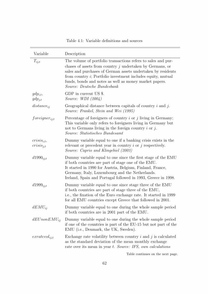
Table 4.1: Variable definitions and sources

Variable Description

Tij,t The volume of portfolio transactions refers to sales and pur-

chases of assets from country j undertaken by Germans, orsales and purchases of German assets undertaken by residentsfrom country i; Portfolio investment includes equity, mutualfunds, bonds and notes as well as money market papers.Source: Deutsche Bundesbank

gdpi,t, GDP in current US $.gdpj,t Source: WDI (2004)

distanceij Geographical distance between capitals of country i and j.Source: Frankel, Stein and Wei (1995)

foreignerij,t Percentage of foreigners of country i or j living in Germany;This variable only refers to foreigners living in Germany butnot to Germans living in the foreign country i or j.Source: Statistisches Bundesamt

crisisi,t, Dummy variable equal to one if a banking crisis exists in thecrisisj,t relevant or precedent year in country i or j respectively.

Source: Caprio and Klingebiel (2003)

d1990ij,t Dummy variable equal to one since the first stage of the EMUif both countries are part of stage one of the EMU.It started in 1990 for Austria, Belgium, Finland, France,Germany, Italy, Luxembourg and the Netherlands.Ireland, Spain and Portugal followed in 1993, Greece in 1998.

d1999ij,t Dummy variable equal to one since stage three of the EMUif both countries are part of stage three of the EMU,i.e., the fixation of the Euro exchange rate. It started in 1999for all EMU countries except Greece that followed in 2001.

dEMUij Dummy variable equal to one during the whole sample periodif both countries are in 2001 part of the EMU.

dEUnonEMUij Dummy variable equal to one during the whole sample periodif one of the countries is part of the EU-15 but not part of theEMU (i.e., Denmark, the UK, Sweden).

exratevolij,t Exchange rate volatility between country i and j is calculatedas the standard deviation of the mean monthly exchangerate over its mean in year t. Source: IFS, own calculations

Table continues on the next page.

62

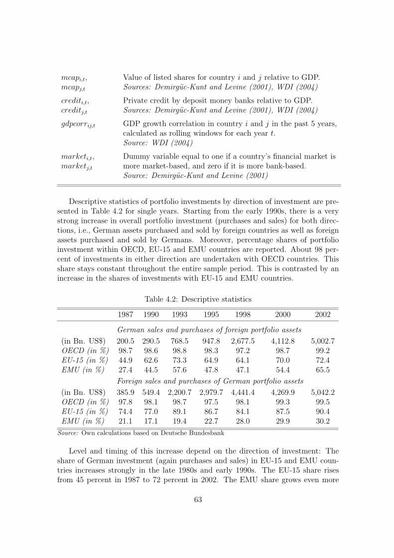
mcapi,t, Value of listed shares for country i and j relative to GDP.mcapj,t Sources: Demirguc-Kunt and Levine (2001), WDI (2004)

crediti,t, Private credit by deposit money banks relative to GDP.creditj,t Sources: Demirguc-Kunt and Levine (2001), WDI (2004)

gdpcorrij,t GDP growth correlation in country i and j in the past 5 years,calculated as rolling windows for each year t.Source: WDI (2004)

marketi,t, Dummy variable equal to one if a country’s financial market ismarketj,t more market-based, and zero if it is more bank-based.

Source: Demirguc-Kunt and Levine (2001)

Descriptive statistics of portfolio investments by direction of investment are pre-sented in Table 4.2 for single years. Starting from the early 1990s, there is a verystrong increase in overall portfolio investment (purchases and sales) for both direc-tions, i.e., German assets purchased and sold by foreign countries as well as foreignassets purchased and sold by Germans. Moreover, percentage shares of portfolioinvestment within OECD, EU-15 and EMU countries are reported. About 98 per-cent of investments in either direction are undertaken with OECD countries. Thisshare stays constant throughout the entire sample period. This is contrasted by anincrease in the shares of investments with EU-15 and EMU countries.

Table 4.2: Descriptive statistics

1987 1990 1993 1995 1998 2000 2002

German sales and purchases of foreign portfolio assets

(in Bn. US$) 200.5 290.5 768.5 947.8 2,677.5 4,112.8 5,002.7OECD (in %) 98.7 98.6 98.8 98.3 97.2 98.7 99.2EU-15 (in %) 44.9 62.6 73.3 64.9 64.1 70.0 72.4EMU (in %) 27.4 44.5 57.6 47.8 47.1 54.4 65.5

Foreign sales and purchases of German portfolio assets

(in Bn. US$) 385.9 549.4 2,200.7 2,979.7 4,441.4 4,269.9 5,042.2OECD (in %) 97.8 98.1 98.7 97.5 98.1 99.3 99.5EU-15 (in %) 74.4 77.0 89.1 86.7 84.1 87.5 90.4EMU (in %) 21.1 17.1 19.4 22.7 28.0 29.9 30.2

Source: Own calculations based on Deutsche Bundesbank

Level and timing of this increase depend on the direction of investment: Theshare of German investment (again purchases and sales) in EU-15 and EMU coun-tries increases strongly in the late 1980s and early 1990s. The EU-15 share risesfrom 45 percent in 1987 to 72 percent in 2002. The EMU share grows even more

63

strongly, namely from 27 percent to 66 percent. A slightly different pattern arisesfor the other direction: Investment in German portfolio assets by EU-15 countries isalso rising mainly in the early 1990s but less significantly: from 74 percent in 1987to 90 percent in 2002. Investments undertaken by EMU countries increase later, inthe mid-1990s, and both less dramatically, from 21 percent in 1987 to 30 percent in2002.

Overall, the main difference between the two directions is due to a large share offoreign investment in German portfolio assets by EU-15 countries whereas the shareof German sales and purchases of EMU and EU-15 portfolio assets is relatively low.This is partly driven by a large share of German portfolio assets purchased andsold by the UK due to its importance as a leading financial center. The empiricalanalysis accounts for this fact by including financial center dummies15.

4.4 Empirical Results

First, the impact of European financial integration on German portfolio investmentis investigated in general. Second, potential underlying forces driving European in-tegration are explicitly taken into account. It is very likely that countries’ responsesto European financial integration differ. This issue is addressed in the last part ofthis section. Additional robustness checks can be found in Appendix C.

4.4.1 German Portfolio Investment and the EMU

The standard gravity regression equation described in Section 4.3.1 is used to identifythe effect of European financial integration on portfolio investment. The effectis modeled by different dummy variables that mirror the formation of the EMUor, more generally, EMU membership. The effect of EU-15 versus EMU financialintegration is disentangled and further robustness checks are undertaken.

The Formation of the EMU

To start with, results of the standard gravity model are compared with results inthe existing literature. The coefficients of the first column in Table 4.3 are based onpooled OLS estimates with White-heteroscedasticity robust standard errors. Speci-fication (1) includes the scaling variables, the percentage of foreigners and distance.Additional year dummies, dummies for financial centers, and dummies for financialcrises in the transacting country i or the country invested in, country j, are added

15Financial centers are Hong Kong, Ireland, Luxembourg, UK, Singapore and Switzerland. Foreach of these countries separate dummies enter that refer to country i and j.

64

in all specifications but not explicitly reported.16

The results are consistent with earlier estimates of gravity models in the liter-ature.17 The distance coefficient is - as expected - negative and ranges in absolutesize between 0.34 and 0.43. Portes and Rey (2005) report a coefficient around mi-nus 0.6 estimating bilateral portfolio flows between 14 countries from 1989 to 1996.Buch (2005) considers assets and liabilities of commercial banks from five countries(France, Germany, Italy, UK and the US) for 1983 and 1999 and estimates a dis-tance coefficient between minus 0.3 and 1.25 depending on the respective estimationsample.

The estimated coefficients of the remaining variables in specification (1) are inline with the theoretical considerations mentioned in Section 4.3.1: The coefficientsof the scaling variables, gdpi,t, gdpj,t, popi,t and popj,t have the expected positive andnegative effects. The percentage of people of the respective foreign country livingin Germany, foreignerij,t, is associated with a positive effect on transactions. Thisresult suggests that familiarity between two countries plays a role.

In addition to the scaling variables and proxies for information costs, specifica-tions (2) to (5) include dummy variables for stage one or three of the EMU. Foreach specification, two estimates are reported: pooled OLS and country pair fixedeffects.18 Fixed effects capture omitted variables that are specific and constant incross sectional units. Most of these effects are not random but deterministicallyassociated with certain historical, political or geographical facts (Egger 2000). Thepooled OLS estimator captures both the effect over time and the cross sectionaleffect of higher trade with EMU countries.

In the fixed effects model the coefficients on GDP and population size are notalways significant and, in case of population size, yield different signs compared tothe pooled OLS estimation. This may have different reasons: First, the inclusionof country pair fixed effects and year dummies may already account for a largepart of the variation of these variables. Second, in the fixed effects estimationGDP and population size rather seem to influence portfolio transactions in the samedirection whereas in the pooled OLS regression they do not. Third, as the sub-sample estimates in Table 4.11, Appendix C, show, effects are not as homogeneousacross sub-samples as in the pooled OLS case and might therefore be even lesssignificant in the aggregate full sample.

In specification (2) to (5), Table 4.3, the dummies for stage one and three of theEMU are highly significant. Based on these results, Germany experiences higher

16In order to take German reunification into account an additional dummy variable is consid-ered. As the effect turns out to be insignificant, specifications without this additional dummy arepresented in the following.

17Note that the R2 amounts to 74 percent, which shows that the model performs very well inexplaining the variation in the data.

18Separate country pair fixed effects for each direction are considered, i.e., country pair ij isdistinguished from country pair ji.

65

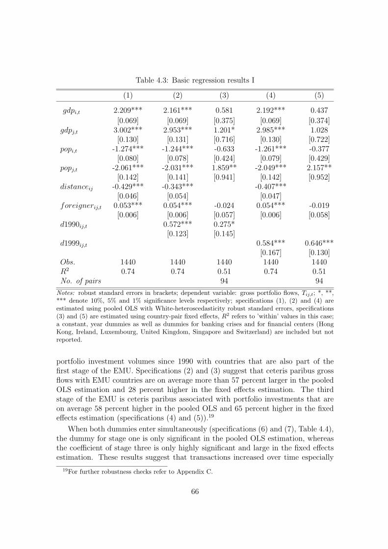
Table 4.3: Basic regression results I

(1) (2) (3) (4) (5)

gdpi,t 2.209*** 2.161*** 0.581 2.192*** 0.437

[0.069] [0.069] [0.375] [0.069] [0.374]gdpj,t 3.002*** 2.953*** 1.201* 2.985*** 1.028

[0.130] [0.131] [0.716] [0.130] [0.722]popi,t -1.274*** -1.244*** -0.633 -1.261*** -0.377

[0.080] [0.078] [0.424] [0.079] [0.429]popj,t -2.061*** -2.031*** 1.859** -2.049*** 2.157**

[0.142] [0.141] [0.941] [0.142] [0.952]distanceij -0.429*** -0.343*** -0.407***

[0.046] [0.054] [0.047]foreignerij,t 0.053*** 0.054*** -0.024 0.054*** -0.019

[0.006] [0.006] [0.057] [0.006] [0.058]d1990ij,t 0.572*** 0.275*

[0.123] [0.145]d1999ij,t 0.584*** 0.646***

[0.167] [0.130]Obs. 1440 1440 1440 1440 1440R2 0.74 0.74 0.51 0.74 0.51No. of pairs 94 94

Notes: robust standard errors in brackets; dependent variable: gross portfolio flows, Tij,t; *, **,*** denote 10%, 5% and 1% significance levels respectively; specifications (1), (2) and (4) areestimated using pooled OLS with White-heteroscedasticity robust standard errors, specifications(3) and (5) are estimated using country-pair fixed effects, R2 refers to ’within’ values in this case;a constant, year dummies as well as dummies for banking crises and for financial centers (HongKong, Ireland, Luxembourg, United Kingdom, Singapore and Switzerland) are included but notreported.

portfolio investment volumes since 1990 with countries that are also part of thefirst stage of the EMU. Specifications (2) and (3) suggest that ceteris paribus grossflows with EMU countries are on average more than 57 percent larger in the pooledOLS estimation and 28 percent higher in the fixed effects estimation. The thirdstage of the EMU is ceteris paribus associated with portfolio investments that areon average 58 percent higher in the pooled OLS and 65 percent higher in the fixedeffects estimation (specifications (4) and (5)).19

When both dummies enter simultaneously (specifications (6) and (7), Table 4.4),the dummy for stage one is only significant in the pooled OLS estimation, whereasthe coefficient of stage three is only highly significant and large in the fixed effectsestimation. These results suggest that transactions increased over time especially

19For further robustness checks refer to Appendix C.

66

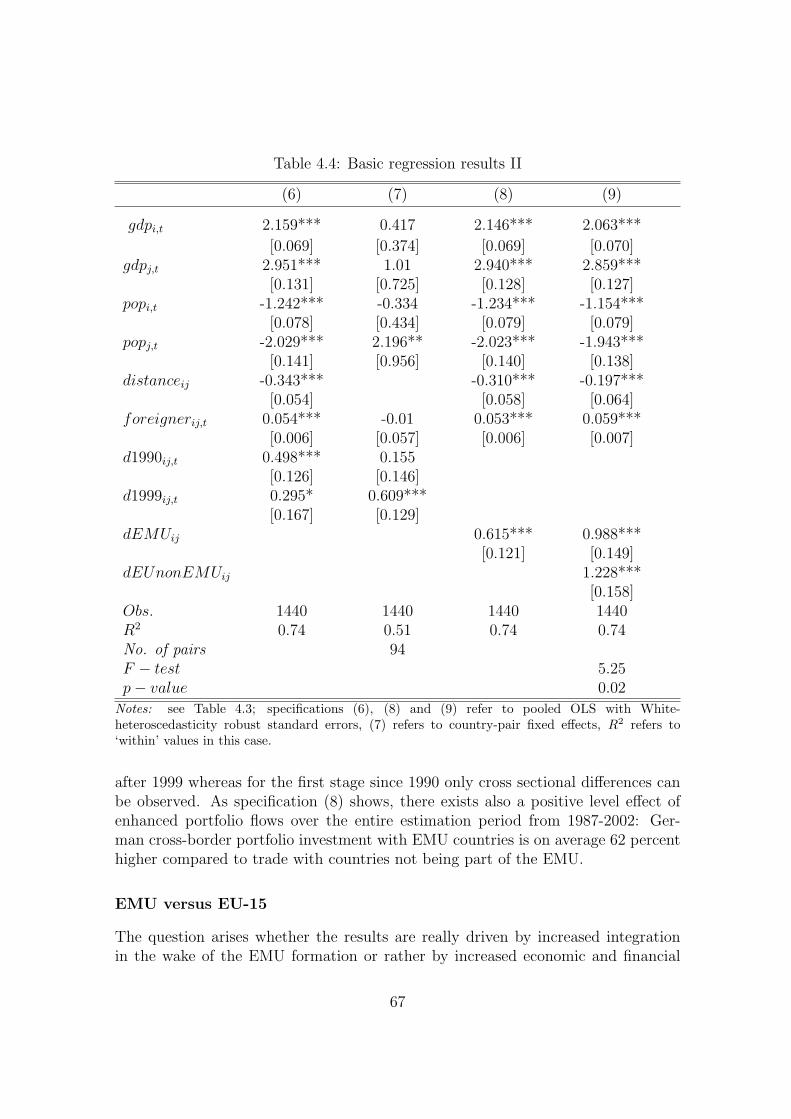
Table 4.4: Basic regression results II

(6) (7) (8) (9)

gdpi,t 2.159*** 0.417 2.146*** 2.063***

[0.069] [0.374] [0.069] [0.070]gdpj,t 2.951*** 1.01 2.940*** 2.859***

[0.131] [0.725] [0.128] [0.127]popi,t -1.242*** -0.334 -1.234*** -1.154***

[0.078] [0.434] [0.079] [0.079]popj,t -2.029*** 2.196** -2.023*** -1.943***

[0.141] [0.956] [0.140] [0.138]distanceij -0.343*** -0.310*** -0.197***

[0.054] [0.058] [0.064]foreignerij,t 0.054*** -0.01 0.053*** 0.059***

[0.006] [0.057] [0.006] [0.007]d1990ij,t 0.498*** 0.155

[0.126] [0.146]d1999ij,t 0.295* 0.609***

[0.167] [0.129]dEMUij 0.615*** 0.988***

[0.121] [0.149]dEUnonEMUij 1.228***

[0.158]Obs. 1440 1440 1440 1440R2 0.74 0.51 0.74 0.74No. of pairs 94F − test 5.25p− value 0.02

Notes: see Table 4.3; specifications (6), (8) and (9) refer to pooled OLS with White-heteroscedasticity robust standard errors, (7) refers to country-pair fixed effects, R2 refers to‘within’ values in this case.

after 1999 whereas for the first stage since 1990 only cross sectional differences canbe observed. As specification (8) shows, there exists also a positive level effect ofenhanced portfolio flows over the entire estimation period from 1987-2002: Ger-man cross-border portfolio investment with EMU countries is on average 62 percenthigher compared to trade with countries not being part of the EMU.

EMU versus EU-15

The question arises whether the results are really driven by increased integrationin the wake of the EMU formation or rather by increased economic and financial

67

integration within all EU-15 countries. Therefore, an additional dummy for EU-15countries that are not part of the EMU, namely Denmark, the UK and Sweden, isconsidered in the regression analysis, dEUnonEMUij.

When both the EMU dummy, dEMUij, and dEUnonEMUij enter simultane-ously the regression equation, the coefficient of dEUnonEMUij is larger comparedto the EMU dummy (specification (9)). The hypothesis of both coefficients beingequal can be rejected at the 5 percent level, though not at the one percent level.20

On average across the whole time period under consideration, transactions betweenGermany and Denmark, the UK and Sweden respectively tend to be larger comparedto trade with EMU countries.

Next, these effects are estimated separately for each year. Interaction termsbetween the EMU dummy variable and year dummies as well as the dummy variablefor EU-15 countries that are not part of the EMU and year dummies enter theregression. As stated in the Delors Report of 17 April 1989, the EMU was achievedin three “discrete but evolutionary steps.” Therefore, one expects a smooth impactof the EMU formation on financial indicators.

Figure 4.1: Estimated coefficients

0.5

11.

52

2.5

estim

ated

coe

ffici

ent

1987 1989 1991 1993 1995 1997 1999 2001year

EMU s.e. band EUnonEMU s.e. bandEMU EUnonEMU

Note: Estimated coefficients of interactions between year dummiesand dEMUij and dEUnonEMUij respectively. Full regression re-sults are documented in Table 4.1, Appendix C.

The estimated coefficients of the interaction terms plotted in Figure 4.1 are inline with this notion.21 In the late 1980s, the estimated coefficients of the EMU-

20Refer to the documented F-test statistics in Table 4.4.21Full regression results are documented in Table 4.15, Appendix C.

68

countries are smaller compared to the coefficients referring to Denmark, the UKand Sweden. Until 1998 the difference between the two coefficients decreases andit finally reverses. As the standard error bands show, the coefficients are alwayssignificantly different from zero, except for the EMU dummy in 1987 and 1988. F-tests reveal that the estimated yearly coefficients are significantly different from oneanother for the years up to 1992 and for the year 2002.22

The results suggest that German transactions with EMU countries are signifi-cantly lower compared to trade with Denmark, the UK and Sweden until the early1990s. However, since the beginning of the new millennium this relationship seemsto have reversed. The comparison between Euro area and non-Euro area countriessuggests, that this might be due to the final step of the EMU, the abolishment ofexchange rate risk. However, with one observations for 2002 only, this result is notrobust but only an indication. It is left to future research using updated data toconfirm or modify this indication.

4.4.2 Accounting for European Financial Integration

The dummy variables reflecting stage one and three of the EMU capture the effect ofincreased financial integration. What exactly are its driving forces? In this section,financial and real economic factors are investigated that might account for at leastpart of the effect.

Financial Factors

The introduction of the Euro has resulted in the elimination of exchange rate riskwithin the Euro area. The absence of exchange rate risk allows corporations to raisefunds across countries with fewer constraints and costs. This can in general have alarge effect on financial integration because exchange rate risk is an important sourceof risk priced on capital markets (e.g. Dumas and Solnik (1995) and Hardouveliset al. (2006)). In addition, the launch of the common European currency is asso-ciated with lower costs of cross-country transactions, improved liquidity and betterdeveloped European capital markets (Fratzscher (2002) and Danthine, Giavazzi andvon Thadden (2001)).

In order to investigate whether financial factors such as the abolition of exchangerate risk or financial market development and increased liquidity can explain partof the effect captured so far by the dummy variables for stage one and three of theEMU, measures for these factors are added to the regression analysis.

Exchange rate risk is measured as the standard deviation of the mean monthlybilateral exchange rate over its mean in year t, exratevolij,t. In order to accountfor enhanced financial development two commonly used measures are added to the

22F-tests are also documented in Table 4.15, Appendix C.

69

regression: stock market capitalization relative to GDP for country i and j, mcapi,t

and mcapj,t, as well as private credit provided by the banking sector relative toGDP for country i and j, crediti,t and creditj,t.

23 The two sets of variables referto different aspects of financial development. The relative volume of private creditmirrors the development of the private banking sector and, therefore, reflects theability of financial institutions to carry out national as well as international capitaltransactions. Stock market capitalization relative to GDP reflects the size anddevelopment of a country’s equity market.

These additional variables are not always available for the full sample and timeperiod.24 Therefore, a benchmark regression is reported that is based on the sameobservations but excludes the variables of interest. Then, the variables of inter-est are added and the coefficients of the dummy variables, d1990ij,t and d1999ij,t

respectively, can be compared across regressions. In order to account for potentialendogeneity, lagged values of relative stock market capitalization and credit providedby the banking sector are used.

Table 4.5 shows results of pooled OLS and of fixed effects estimations. Thetable documents only the estimated coefficients of interest: the first part refers toestimates of d1990ij,t and d1999ij,t respectively in a regression excluding exratevolij,t.The second part refers to estimates inclusive this variable. In the pooled OLS case,exchange rate volatility has a large negative influence, though only at the ten percentsignificance level. The coefficients on the dummy variables decrease slightly, but notsignificantly.25 Also in the fixed effects estimations exchange rate volatility does notlead to significant changes of the coefficients of d1990ij,t and d1999ij,t. It has againonly a weakly significant negative coefficient.

Also, the inclusion of measures for financial development does not significantlyalter the size of the dummy variables neither in the pooled OLS nor in the fixedeffects estimations (Table 4.6). The variables themselves have the following effects inthe pooled OLS regressions: Banking sector development in the transacting country,crediti,t, is positively associated with cross-border transactions. This result is inline with the consideration that highly developed financial and banking institutionshelp to conduct international transactions. Stock market development at home,mcapi,t, has a negative and much smaller influence. The finding suggests that lessdeveloped equity markets at home drive investors towards better developed foreignmarkets that offer more diversification and better investment possibilities. Thepositive coefficient on the stock market capitalization variable of the country investedin, mcapj,t, supports this view. Countries with better developed equity markets tendto attract more portfolio transactions. In contrast, the development of the banking

23As an alternative measure for private credit, M2 to GDP is often used, see e.g. Chinn andIto (2006) and Di Giovanni (2005). This variable is only available for a much smaller number ofcountries and years and, therefore, not considered.

24For the availability of variables across years refer to Table 4.10 in Appendix B.25Refer to the reported F-test statistics in Table 4.5.

70

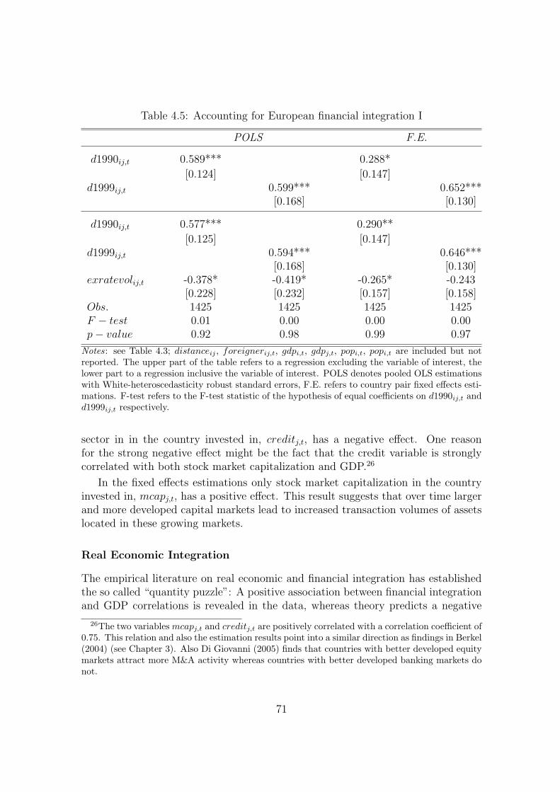
Table 4.5: Accounting for European financial integration I

POLS F.E.

d1990ij,t 0.589*** 0.288*

[0.124] [0.147]d1999ij,t 0.599*** 0.652***

[0.168] [0.130]

d1990ij,t 0.577*** 0.290**

[0.125] [0.147]d1999ij,t 0.594*** 0.646***

[0.168] [0.130]exratevolij,t -0.378* -0.419* -0.265* -0.243

[0.228] [0.232] [0.157] [0.158]Obs. 1425 1425 1425 1425F − test 0.01 0.00 0.00 0.00p− value 0.92 0.98 0.99 0.97

Notes: see Table 4.3; distanceij , foreignerij,t, gdpi,t, gdpj,t, popi,t, popi,t are included but notreported. The upper part of the table refers to a regression excluding the variable of interest, thelower part to a regression inclusive the variable of interest. POLS denotes pooled OLS estimationswith White-heteroscedasticity robust standard errors, F.E. refers to country pair fixed effects esti-mations. F-test refers to the F-test statistic of the hypothesis of equal coefficients on d1990ij,t andd1999ij,t respectively.

sector in in the country invested in, creditj,t, has a negative effect. One reasonfor the strong negative effect might be the fact that the credit variable is stronglycorrelated with both stock market capitalization and GDP.26

In the fixed effects estimations only stock market capitalization in the countryinvested in, mcapj,t, has a positive effect. This result suggests that over time largerand more developed capital markets lead to increased transaction volumes of assetslocated in these growing markets.

Real Economic Integration

The empirical literature on real economic and financial integration has establishedthe so called “quantity puzzle”: A positive association between financial integrationand GDP correlations is revealed in the data, whereas theory predicts a negative

26The two variables mcapj,t and creditj,t are positively correlated with a correlation coefficient of0.75. This relation and also the estimation results point into a similar direction as findings in Berkel(2004) (see Chapter 3). Also Di Giovanni (2005) finds that countries with better developed equitymarkets attract more M&A activity whereas countries with better developed banking markets donot.

71

Table 4.6: Accounting for European financial integration II

POLS F.E.

d1990ij,t 0.601*** 0.346**

[0.130] [0.170]d1999ij,t 0.745*** 0.739***

[0.212] [0.159]

d1990ij,t 0.595*** 0.417**

[0.153] [0.171]d1999ij,t 0.782*** 0.784***

[0.200] [0.151]crediti,t−1 0.853*** 0.938*** 0.00 0.066

[0.127] [0.119] [0.192] [0.191]creditij,t−1 -0.583*** -0.499** 0.387 0.44

[0.217] [0.208] [0.452] [0.449]mcapi,t−1 -0.191*** -0.232*** -0.025 -0.049

[0.072] [0.069] [0.078] [0.076]mcapj,t−1 0.334** 0.294** 0.388** 0.367*

[0.145] [0.141] [0.190] [0.189]Obs. 1159 1159 1159 1159F − test 0.00 0.04 0.17 0.09p− value 0.97 0.85 0.68 0.76

Notes: see Table 4.5.

relation if anything.27 There is growing evidence that real integration among EMUmembers has been strengthened in terms of real business cycle synchronization andtrade.28 As both developments, real economic and financial integration, intertwine,real economic integration might account for part of the financial integration mea-sured by the dummy variables of stage one and three.

Using the same methodology as above, GDP growth correlation is included inthe regressions, gdpcorrij,t, as a proxy for real economic convergence (Table 4.7). Inorder to account for the effect that GDP growth correlations has for EMU countries,it also enters interacted with the EMU dummy, dEMUij.

The results of the pooled OLS regressions show that GDP growth correlationswith EMU countries have a significant positive effect on transactions whereas theyhave no effect for the rest of the sample. In the fixed-effects case there is a weakly

27See Imbs (2004) and Imbs (2006) for a detailed discussion of the puzzle.28Refer e.g. to Boewer and Guillemineau (2006) and Massmann and Mitchell (2004) with respect

to business cycle synchronization as well as Frankel and Rose (1997) and Micco, Stein and Ordonez(2003) with respect to trade.

72

Table 4.7: Accounting for European financial integration III

POLS F.E.

d1990ij,t 0.552*** 0.293*

[0.122] [0.145]d1999ij,t 0.587** 0.663***

[0.167] [0.130]

d1990ij,t 0.421*** 0.270*

[0.140] [0.154]d1999ij,t 0.428** 0.652***

[0.167] [0.128]gdpcorrij,t -0.28 -0.239 0.317 0.362*

[0.173] [0.170] [0.194] [0.188]gdpcorrij,t ∗ dEMUij 0.768*** 0.945*** 0.495* 0.352

[0.233] [0.233] [0.254] [0.242]Obs. 1437 1437 1437 1437F − test 0.87 0.91 0.02 0.01p− value 0.35 0.34 0.88 0.93

Notes: see Table 4.5

significant positive effect that is not significantly larger for EMU countries. Theeffect is smaller compared to the POLS estimation for EMU countries. This findingsuggests that the link between real and financial integration is larger across countriesthan within countries over time. Moreover, the link within countries tends to bea more general phenomenon. The inclusion of GDP growth correlations leads tosmaller coefficients of the stage one and stage three dummies. However, the F-test indicates that coefficients do not significantly change in size. Real integrationproxied by GDP growth correlations in this empirical setting is not able to accountfor financial integration measured by d1990ij,t and d1999ij,t.

29

Estimated coefficients on GDP growth correlations in Table 4.7 might be biaseddue to endogeneity of GDP growth correlations, reflecting real economic integration,and transaction volumes, mirroring financial integration. Accounting for endogene-ity would lead to a lower impact of business cycle correlations on transactions,thereby lowering also its ability to reduce the coefficients of the stage one and threedummies. As there is no significant reduction in the size of coefficients anyway,endogeneity does not affect the interpretation of the coefficients of interest on thedummy variables, d1990ij,t and d1999ij,t.

Overall, none of the included variables in this section involve a decrease in thedummy variable effects measuring stage one and three of the EMU. Most strikingly,

29Similar results are obtained when using 10 year rolling correlations of GDP growth.

73

reduced exchange rate volatility does not even account for part of the effect.30 Ob-viously, the effect of the formation of the EMU captures something more than ismeasured by the above mentioned explicit factors in this framework. As discussedin the conclusion this finding might be due to measurement or model specificationissues.

4.4.3 Do Countries Respond Differently to the EMU?

European financial market integration and the formation of the EMU are likely tohave a different impact in every country. One can easily think of differences thatdepend on countries’ financial market development or structure and on how impor-tant costs associated with cross-border portfolio investment are. Countries with lowtransaction and information costs and relatively developed, efficient and large finan-cial markets might see a large increase in gross flows induced by European financialmarket integration. At the same time, it is also possible that an increase in cross-border trading activity might be larger for countries starting with relatively hightransactions costs as well as less developed, efficient and smaller financial markets.Ex ante, these effects are not clear. Countries can also be differentiated with respectto the extent of real economic integration. Given the results in Section 4.4.2, oneexpects countries with more synchronized business cycles, i.e., countries that aremore integrated in real terms, to be more financially integrated in the sense thatthey experience larger transaction volumes.

In order to explore differences in the effect of European financial integrationon portfolio investment across countries, the basic regression is expanded by aninteraction term between the dummy variable for the first stage of the EMU andthe variable of interest:31

log(Tij,t) = β0 + β1log(gdpi,t) + β2log(gdpj,t) + β3log(popi,t)

+ β4log(popj,t) + β5log(distanceij,t) + β6log(foreignerij,t)

+ β7Xij,t + β8d1990ij,t + β9Xij,t ∗ d1990ij,t +N∑

n=10

βnZnij,t + εij,t,

where Xij,t refers to the variable of interest. The estimated coefficient of the dummyvariable for the first stage of the EMU, β8, the effect of the interaction term, β9,as well as the own effect of the variable of interest, β7, are reported in Table 4.8.As heterogeneous responses of countries are of interest, only pooled OLS regressionsare undertaken. First, financial market structure and development are considered asfactors of interest that differentiate the EMU effect on transactions across countries.

30Also lagged values of exchange rate volatility and two or three year averages have been used.Results do not change.

31Similar results can be obtained using interactions with dEMUij or d1999ij,t.

74

Second, the role of information costs proxied by distance is explored. Finally, the linkbetween the volume of transactions and real economic integration is investigated.

Financial Market Structure and Development

An indicator variable that equals one if a country is more market-based and zero ifit is more bank-based, marketi,t and marketj,t, is included. It is used to investigatewhether economies with higher stock market or with higher banking activity responddifferently. In bank-based systems, banks play a leading role in mobilizing savingsand allocating capital whereas in market-based systems securities markets take therole of getting society’s savings to firms, exerting corporate control and easing riskmanagement. Demirguc-Kunt and Levine (2001) find that financial systems tend tobe more market-based in higher income countries where stock markets become moreactive and efficient than banks. The literature does not reveal a clear support foreither the market-based or the bank-based system to perform better in attractingcapital and favoring growth (Levine 2002).

In order to proxy the development of financial markets again two different mea-sures are used for country i and j: stock market capitalization relative to GDPand the amount of credit provided by the banking sector relative to GDP, mcapi,t,mcapj,t, crediti,t and creditj,t.

Results in Table 4.8 show that, first, countries invested in, i.e., countries j, thatare more market-based countries are associated with higher portfolio transactions(specification (1)). This result is consistent with the finding in Section 4.4.2 thatrelative stock market capitalization of country j has a positive impact on portfoliotransactions. However, the effect of higher transactions due to stage one of the EMUis not linked to the classification of countries into more market-based and bank-basedfinancial markets as the interaction terms are insignificant. In this respect there isno heterogeneity among countries.

Second, transacting countries with more developed financial markets, in termsof more private credit provided by the banking sector relative to GDP, experiencehigher transaction volumes during stage one of the EMU (specification (2)). Thesame finding applies to financial development measured by stock market capitaliza-tion relative to GDP (specification (3)).32

32If both interaction effects are investigated in one single regression, the same effects can beobserved. Note that the estimated coefficients on crediti,t and mcapj,t correspond very well tothe estimated coefficients estimated in a joint regression (Table 4.6). Now, mcapi,t and creditj,tare insignificant and do not yield negative signs as before. This finding suggests that the negativesigns are likely to be driven by positive correlations among the two variables and with GDP.

75

Table 4.8: Heterogenous country responses

(1) (2)

d1990ij,t 0.882*** d1990ij,t 0.654***

[0.149] [0.173]marketi,t -0.237 crediti,t−1 0.831***

[0.146] [0.096]marketj,t 0.969*** creditj,t−1 -0.171

[0.178] [0.209]d1990ij,t * marketi,t -0.185 d1990ij,t * crediti,t−1 0.882***

[0.222] [0.238]d1990ij,t * marketj,t -0.157 d1990ij,t * creditj,t−1 0.11

[0.234] [0.257]

(3)

d1990ij,t 1.197***

[0.246]mcapi,t−1 0.042

[0.067]mcapj,t−1 0.317***

[0.123]d1990ij,t * mcapi,t−1 0.284**

[0.123]d1990ij,t * mcapj,t−1 0.157

[0.120]

(4) (5)

d1990ij,t 0.032 d1990ij,t 0.347**

[0.640] [0.149]distanceij -0.393*** gdpcorrij,t -0.204

[0.060] [0.166]d1990ij,t * distanceij 0.085 d1990ij,t * gdpcorrij,t 0.630**

[0.088] [0.252]

Notes: Pooled OLS regressions with White-heteroscedasticity robust standard errors in brackets;dependent variable: gross portfolio flows, Tij,t; *, **, *** denote 10%, 5% and 1% significancelevels; a constant, year dummies, dummies for financial centers, distanceij , foreignerij,t, gdpi,t,gdpj,t, popi,t, popi,t, and dummies for banking crises are included but not reported.

76

Distance

Information costs proxied by distance play a major role when explaining volumesof portfolio investment in gravity models. Portes and Rey (2005) document thatgeographical distance presents a good proxy for these costs. The question arisesof whether countries closer to Germany are associated with a larger increase intransaction volumes in the wake of the formation of the EMU compared to countriesfurther away. The results in Table 4.8, specification (4) suggest that there is nodifference in the positive effect of the first stage of the EMU on transactions withrespect to distance.

Real Economic Integration

Results in Table 4.8, specification (5), show that countries participating in stage oneof the EMU and countries having higher GDP growth correlations ceteris paribusexperience larger portfolio investment compared to the rest of the sample. If largerportfolio investment signifies increased financial integration, it can be concludedthat increased financial integration is associated with increased business cycle syn-chronization for EMU countries. This finding is in line with the “quantity puzzle”documented in the recent empirical literature on real integration.33 Imbs (2004)shows that business cycles in financially integrated regions are significantly moresynchronized, even though financial integration may also result in more specializedeconomies, and consequently less synchronized cycles.

4.5 Conclusion

Although there is a growing literature on the effects of the EMU on different seg-ments of financial markets, no comprehensive empirical analysis of the effects onportfolio asset trade using a gravity model approach has yet been undertaken. Thispaper not only investigates the increase in gross portfolio flows induced by Euro-pean financial market integration and the EMU but also potential underlying drivingforces and the heterogeneity of responses to European financial integration.

The estimations indicate that there is a substantial increase in gross portfolioflows with Germany since the first and the third stage of the EMU. The latter marksthe fixation of exchange rates with the Euro. The estimations indicate that ceterisparibus gross portfolio flows increased on average by about 60 percent for countriestaking part in the third stage. These are time series effects remaining after countrypair fixed effects have been taken into account. As has been shown, the positiveeffect induced by the formation of the EMU evolves smoothly over time. Since the

33Again one has to be aware of the fact that real economic and financial integration are likelyto be interdependent in both directions. However, this section aims at characterizing countryresponses and does not draw conclusions about causality.

77

end 1990s it increases relative to a group of countries including Denmark, the UK,and Sweden that are part of EU-15 but not of the Euro area. In 2002 it seemsto be significantly larger for EMU countries compared to Denmark, the UK, andSweden. Though it is left to future research using updated data to confirm whetherthis finding is indeed robust.

The formation of the EMU is intertwined with changes in financial markets andreal economic integration. In a second step, this paper examines to what extentthese developments account for the estimated positive effect measured by dummyvariables. Lower exchange rate volatility, higher financial market development, andincreased business cycle correlations have significant effects on gross portfolio flows.However, they are not able to account for the positive effect induced by the formationof the EMU.

In the third part of the empirical analysis of the present paper, the coefficients ofthe dummies for different stages of the EMU are forced to be equal across countries.This paper also analyzes factors that lead to heterogeneous country responses. TheEMU effect on gross portfolio flows is larger for transacting countries with moredeveloped banking and equity markets and country pairs with more correlated busi-ness cycles. The latter result is in line with other empirical studies investigating realeconomic and financial integration (Boewer and Guillemineau (2006), Imbs (2006),and Imbs (2004)). There are no differences in countries’ responses to the EMUdepending on geographical distance to Germany or on whether countries are moremarket-based.

The gravity model is a useful approach to empirically reveal and describe thedifferences of German portfolio flows with EMU countries compared to the othertrading partners. It does not explain the effects of a common currency union onasset trade, though. The present empirical analysis can not sufficiently reveal, whichfactors actually account for the EMU effect on portfolio flows measured by dummyvariables for different stages of the EMU. On the one hand, this finding can be dueto measurement problems. One would expected that at least exchange rate riskexplains part of the EMU effect. However, it is very difficult to effectively measureexpected exchange rate risk at an annual frequency. On the other hand, these in-significant results might be comparable to the pessimistic “Nothing is Robust” inthe growth literature (Levine and Renelt 1992). Similar to the set up in this paper,growth theories are not explicit about what variables belong in the regression. Whensimply trying and adding variables, results may turn out to be inconclusive andnot robust. As Sala-i-Martin (1997) suggests, using alternative and less restrictivemeans of testing the relationship between variables by modeling whole distributionsof estimators may nevertheless yield strong and meaningful relationships betweenvariables.

As far as known by the author, no theoretical model yet exists in the literaturethat structurally links the formation of currency unions and asset trade and thatprovides testable empirical hypotheses. In line with the methodology stated in

78

Deaton (2000),34 this lack of theory motivates the descriptive characterization ofthe effects of the EMU in the present paper. Based on the results, it is desirable toadvance future theoretical and related empirical research that clarifies the channelsthrough which a common currency union, e.g., the EMU, affects asset trade, financialand real economic integration.

4.6 Appendix

4.6.1 Appendix A - Countries by Regions

Table 4.9: Countries by regions

Western Europe Southern Europe Eastern AsiaBelgium Greece JapanFrance Italy KoreaLuxembourg Portugal ChinaThe Netherlands SpainAustria South-central AsiaSwitzerland Northern Africa India

Egypt PakistanNorthern Europe Morocco Sri LankaDenmark South AfricaFinland South-eastern AsiaIreland Northern America IndonesiaNorway Canada The PhilippinesSweden USA SingaporeThe UK Thailand

Central AmericaEastern Europe Mexico Western AsiaCzech Republic Argentina IsraelPoland Brazil JordanRussian Federation Chile TurkeyHungary Colombia

Peru OceaniaVenezuela Australia

New Zealand

34Rf. to p. 3ff.

79

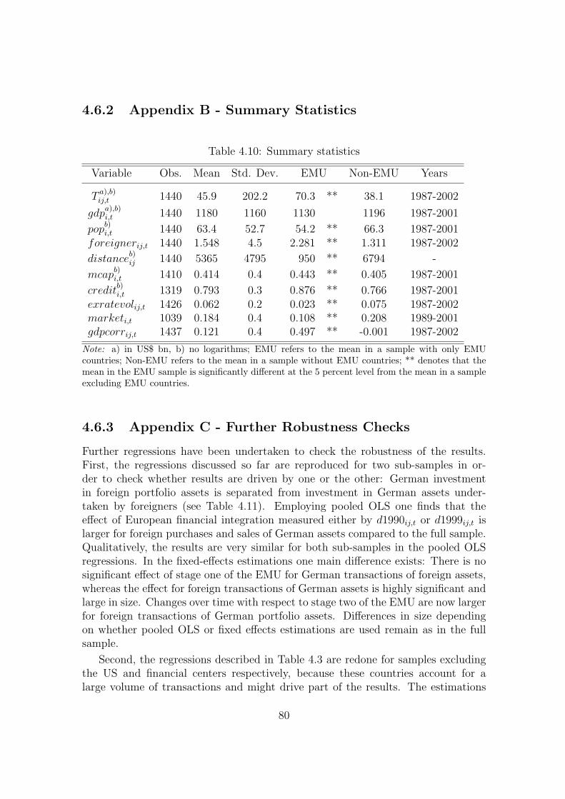
4.6.2 Appendix B - Summary Statistics

Table 4.10: Summary statistics

Variable Obs. Mean Std. Dev. EMU Non-EMU Years

Ta),b)ij,t 1440 45.9 202.2 70.3 ** 38.1 1987-2002

gdpa),b)i,t 1440 1180 1160 1130 1196 1987-2001

popb)i,t 1440 63.4 52.7 54.2 ** 66.3 1987-2001

foreignerij,t 1440 1.548 4.5 2.281 ** 1.311 1987-2002

distanceb)ij 1440 5365 4795 950 ** 6794 -

mcapb)i,t 1410 0.414 0.4 0.443 ** 0.405 1987-2001

creditb)i,t 1319 0.793 0.3 0.876 ** 0.766 1987-2001

exratevolij,t 1426 0.062 0.2 0.023 ** 0.075 1987-2002marketi,t 1039 0.184 0.4 0.108 ** 0.208 1989-2001gdpcorrij,t 1437 0.121 0.4 0.497 ** -0.001 1987-2002

Note: a) in US$ bn, b) no logarithms; EMU refers to the mean in a sample with only EMUcountries; Non-EMU refers to the mean in a sample without EMU countries; ** denotes that themean in the EMU sample is significantly different at the 5 percent level from the mean in a sampleexcluding EMU countries.

4.6.3 Appendix C - Further Robustness Checks

Further regressions have been undertaken to check the robustness of the results.First, the regressions discussed so far are reproduced for two sub-samples in or-der to check whether results are driven by one or the other: German investmentin foreign portfolio assets is separated from investment in German assets under-taken by foreigners (see Table 4.11). Employing pooled OLS one finds that theeffect of European financial integration measured either by d1990ij,t or d1999ij,t islarger for foreign purchases and sales of German assets compared to the full sample.Qualitatively, the results are very similar for both sub-samples in the pooled OLSregressions. In the fixed-effects estimations one main difference exists: There is nosignificant effect of stage one of the EMU for German transactions of foreign assets,whereas the effect for foreign transactions of German assets is highly significant andlarge in size. Changes over time with respect to stage two of the EMU are now largerfor foreign transactions of German portfolio assets. Differences in size dependingon whether pooled OLS or fixed effects estimations are used remain as in the fullsample.

Second, the regressions described in Table 4.3 are redone for samples excludingthe US and financial centers respectively, because these countries account for alarge volume of transactions and might drive part of the results. The estimations

80

are robust with respect to the two dummy effects. Size and significance levels ofthe estimated coefficients of interest increase if financial centers are excluded (Table4.12).

Third, as discussed in Section 4.3.1, GDP growth in country i and j are addedas additional scaling variables, gdpgrowthi,t and gdpgrowthj,t, (Table 4.13). How-ever, as the results in specification (1) show, ceteris paribus these variables haveno significant explanatory power. Fourth, in order to address a potential endogene-ity problem, lagged values for the scaling variables, gdpi,t, gdpj,t, popi,t, and popj,t,are used instead of contemporaneous values. The estimated coefficients on thesevariables hardly change (specification (2), Table 4.13).

Fifth, one might also ask, whether other country linkages that are not accountedfor by the empirical model drive the results. Standard variables employed in gravitymodels that might capture such effects are added: a dummy equal to one if bothcountries share a common border, adjacencyij,t, and a dummy equal to one if bothcountries speak the same language, languageij,t. The coefficient on adjacencyij,t ishighly significant and results with respect to the other coefficients are unchanged,except for the distance coefficient, which decreases in absolute size (specifications(3) and (4), 4.13). languageij,t has no significant impact on portfolio transactions.

Sixth, as some cross-border portfolio flows are reported with zero values, esti-mating a linear model might lead to biased coefficients. In total only less than 5percent of all observations are reported zero flows, though. In order to investigatethe sensitivity of the estimated coefficients towards nonlinearities, a Tobit modelis estimated for comparison (Table 4.14). As specifications (1) and (2) show, theestimated effects, especially on the various dummy variables measuring the financialintegration within EMU and EU-15 countries, do hardly change.

Seventh, variables such as transaction volumes, GDP, market capitalization andbank credit might not be non-stationarity. If these variables are not stationaryand not co-integrated, inference is screwed. Panel unit root tests by Im, Pesaranand Shin (2003) and Levin, Lin and Chu (2002) have been undertaken.35 The testssuggest that non-stationarity is not a problem. As the power of panel unit root testsis often criticized, a time trend that may capture the persistence in time series oftransactions, GDP, market capitalization and bank credit, is entered (specifications(3) to (6)). The time trend is significant in the fixed effects regressions (specification(5) and (6)), however, this does hardly affect the other estimated coefficients.

Finally, single year regressions are run in order to reproduce Figure 4.1.36 In thiscase, the estimated coefficients on the non-interacted variables are not restricted tobe constant over time. The estimated size and significance of the dummy variablesdo not change, however.

35Test statistics are not reported, but can be obtained from the author upon request.36These results are not reported in the Appendix, but can be obtained from the author upon

request.

81

Tab

le4.

11:

Reg

ress

ion

resu

lts

for

sub-s

ample

s

For

eign

inve

stm

entin

Ger

man

port

folio

asse

tsG

erm

anin

vest

men

tin

fore

ign

port

folio

asse

ts

gdp i

,t1.

774*

**0.

764*

*1.

804*

**0.

714*

[0.0

72]

[0.3

82]

[0.0

73]

[0.3

86]

gdp j

,t3.

392*

**0.

955

3.42

0***

0.66

9[0

.152

][0

.763

][0

.150

][0

.775

]po

p i,t

-1.0

67**

*-0

.494

-1.0

86**

*-0

.404

[0.0

83]

[0.4

05]

[0.0

83]

[0.4

16]

pop j

,t-2

.226

***

1.77

4*-2

.238

***

2.27

0**

[0.1

56]

[0.9

67]

[0.1

56]

[0.9

94]

dis

tance

ij-0

.512

***

-0.5

72**

*-0

.181

*-0

.237

***

[0.0

51]

[0.0

47]

[0.0

92]

[0.0

77]

for

eigner

ij,t

0.04

3***

-0.1

010.

043*

**-0

.119

*0.

065*

**0.

063

0.06

4***

0.09

5[0

.008

][0

.064

][0

.008

][0

.062

][0

.009

][0

.089

][0

.009

][0

.087

]d19

90ij

,t0.

613*

**0.

581*

**0.

481*

*-0

.055

[0.1

10]

[0.1

64]

[0.2

18]

[0.2

45]

d19

99ij

,t0.

726*

**0.

564*

**0.

495*

0.75

5***

[0.1

46]

[0.1

30]

[0.2

58]

[0.2

29]

Obs

737

737

737

737

703

703

703

703

R2

0.83

0.61

0.82

0.61

0.72

0.48

0.72

0.49

No.

ofpai

rs47

4747

47

Not

es:

robu

stst

anda

rder

rors

inbr

acke

ts;de

pend

ent

vari

able

:gr

oss

port

folio

flow

s,T

ij;*,

**,**

*de

note

sign

ifica

ntat

the

10%

,5%

and

1%si

gnifi

canc

ele

vel;

odd

colu

mns

are

esti

mat

edw

ith

pool

edO

LS

usin

gW

hite

-het

eros

ceda

stic

ity

robu

stst

anda

rder

rors

,eve

nco

lum

nsw

ith

fixed

effec

ts,R

2re

fers

to’w

ithi

n’va

lues

inth

isca

se;a

cons

tant

,ye

ardu

mm

ies,

and

dum

mie

sfo

rfin

anci

alce

nter

sar

ein

clud

edbu

tno

tre

port

ed.

82

Tab

le4.

12:

Addit

ional

robust

nes

sch

ecks

I

excl

udi

ng

the

US

excl

udi

ng

finan

cial

cente

rsa

gdp i

,t2.

209*

**0.

564

2.24

5***

0.41

82.

167*

**0.

717

2.20

0***

0.69

4

[0.0

76]

[0.3

77]

[0.0

76]

[0.3

75]

[0.0

69]

[0.4

83]

[0.0

69]

[0.4

84]

gdp j

,t3.

005*

**1.

191*

3.04

2***

1.01

72.

965*

**1.

972*

*2.

998*

**1.

925*

*[0

.139

][0

.717

][0

.137

][0

.723

][0

.131

][0

.972

][0

.130

][0

.966

]po

p i,t

-1.2

52**

*-0

.632

-1.2

69**

*-0

.376

-1.2

51**

*-0

.651

-1.2

68**

*-0

.49

[0.0

79]

[0.4

28]

[0.0

79]

[0.4

31]

[0.0

79]

[0.5

14]

[0.0

80]

[0.5

15]

pop j

,t-2

.049

***

1.87

2**

-2.0

66**

*2.

169*

*-2

.045

***

1.25

6-2

.063

***

1.45

1[0

.141

][0

.949

][0

.141

][0

.959

][0

.141

][1

.150

][0

.142

][1

.145

]dis

tance

ij-0

.337

***

-0.3

91**

*-0

.325

***

-0.3

89**

*[0

.054

][0

.048

][0

.055

][0

.048

]for

eigner

ij,t

0.05

4***

-0.0

250.

053*

**-0

.018

0.05

4***

-0.0

10.

054*

**-0

.005

[0.0

06]

[0.0

57]

[0.0

06]

[0.0

58]

[0.0

06]

[0.0

58]

[0.0

06]

[0.0

60]

d19

90ij

,t0.

515*

**0.

254*

0.65

2***

0.33

3**

[0.1

28]

[0.1

47]

[0.1

28]

[0.1

59]

d19

99ij

,t0.

541*

**0.

638*

**0.

861*

**0.

801*

**[0

.170

][0

.132

][0

.179

][0

.137

]O

bs14

0814

0814

0814

0812

8012

8012

8012

80R

20.

730.

50.

730.

510.

70.

50.

70.

5N

o.of

pai

r92

9284

84

Not

es:

see

Tab

le4.

11

aFin

anci

alce

nter

sin

clud

eH

ong

Kon

g,Ir

elan

d,Lux

embo

urg,

the

UK

,Si

ngap

ore

and

Swit

zerl

and.

83

Table 4.13: Additional robustness checks II

(1) (2) (3) (4)

gdpi,t 2.009*** 2.137*** 2.164***

[0.068] [0.067] [0.068]gdpj,t 3.148*** 2.931*** 2.959***

[0.145] [0.129] [0.128]popi,t -1.239*** -1.240*** -1.253***

[0.077] [0.078] [0.079]popj,t -2.039*** -2.029*** -2.042***

[0.149] [0.140] [0.140]gdpgrowthi,t 0.026

[0.020]gdpgrowthj,t -0.018

[0.032]distanceij -0.444*** -0.428*** -0.162** -0.221***

[0.047] [0.046] [0.079] [0.072]foreignerij,t 0.056*** 0.056*** 0.065*** 0.065***

[0.007] [0.007] [0.007] [0.007]d1990ij,t 0.547***

[0.128]d1999ij,t 0.610*** 0.562***

[0.152] [0.171]gdpi,t−1 2.205***

[0.071]gdpj,t−1 2.980***

[0.130]popi,t−1 -1.280***

[0.082]popj,t−1 -2.058***

[0.143]languageij -0.159 -0.023

[0.147] [0.121]adjacencyij 0.913*** 0.909***

[0.172] [0.171]Obs. 1421 1356 1440 1440R2 0.75 0.74 0.74 0.74

Notes: see Table 4.11

84

Table 4.14: Additional robustness checks III

(1) (2) (3) (4) (5) (6)

gdpi,t 2.163*** 2.194*** 2.161*** 2.192*** 0.581 0.437

[0.081] [0.080] [0.069] [0.069] [0.375] [0.374]gdpj,t 2.965*** 2.997*** 2.953*** 2.985*** 1.201* 1.028

[0.084] [0.083] [0.131] [0.130] [0.716] [0.722]gdpi,t -1.245*** -1.262*** -1.244*** -1.261*** -0.633 -0.377

[0.100] [0.100] [0.078] [0.079] [0.424] [0.429]gdpj,t -2.039*** -2.057*** -2.031*** -2.049*** 1.859** 2.157**

[0.102] [0.102] [0.141] [0.142] [0.941] [0.952]distanceij -0.344*** -0.407*** -0.343*** -0.407***

[0.053] [0.048] [0.054] [0.047]foreignerij,t 0.054*** 0.054*** 0.054*** 0.054*** -0.024 -0.019

[0.011] [0.011] [0.006] [0.006] [0.057] [0.058]d1990ij,t 0.568*** 0.572*** 0.275*

[0.161] [0.123] [0.145]d1999ij,t 0.581** 0.584*** 0.646***

[0.247] [0.167] [0.130]yearij,t -0.022 -0.024 0.134*** 0.144***

[0.018] [0.018] [0.038] [0.039]Obs. 1440 1440 1440 1440 1440 1440R2 0.25 0.25 0.74 0.74 0.51 0.51No. of pairs 94 94

Notes: robust standard errors in brackets; dependent variable: gross portfolio flows, Tij ; *, **,*** denote 10%, 5% and 1% significance levels; column (5) and (6) refer to Tobit estimations,columns (3) and (4) refer to pooled OLS, and (5) and (6) to country-pair fixed effects estimations;a constant, year dummies, and dummies for financial centers are included but not reported.

85

Tab

le4.

15:

Reg

ress

ion

and

F-t

ests

ofFig

ure

4.1

vari

able

coeffi

cien

tst

d.

err.

vari

able

coeffi

cien

tst

d.

err.

F-t

est

p-v

alue

gdp i

,t2.

058*

**0.

070

gdp j

,t2.

853*

**0.

128

pop i

,t-1

.147

***

0.08

0po

p j,t

-1.9

34**

*0.

139

dis

tance

ij-0

.199

***

0.06

4for

eigner

ij,t

0.05

9***

0.00

7dE

MU

ij∗1

987

0.70

3*0.

421

dE

Unon

EM

Uij∗1

987

1.27

6**

*0.

435

2.77

0.09

6dE

MU

ij∗1

988

0.81

9*0.

481

dE

Unon

EM

Uij∗1

988

1.49

6***

0.49

92.

870.

091

dE

MU

ij∗1

989

1.12

9**

0.45

2dE

Unon

EM

Uij∗1

989

1.86

8***

0.40

57.

290.

007

dE

MU

ij∗1

990

0.65

2*0.

375

dE

Unon

EM

Uij∗1

990

1.43

2***

0.36

37.

90.

005

dE

MU

ij∗1

991

0.98

8***

0.37

0dE

Unon

EM

Uij∗1

991

1.46

4***

0.35

53.

770.

053

dE

MU

ij∗1

992

0.79

0**

0.32

5dE

Unon

EM

Uij∗1

992

1.36

6***

0.28

15.

390.

020

dE

MU

ij∗1

993

1.17

9***

0.32

7dE

Unon

EM

Uij∗1

993

1.62

6***

0.35

42.

290.

131

dE

MU

ij∗1

994

0.91

7***

0.32

5dE

Unon

EM

Uij∗1

994

1.33

7***

0.34

72.

90.

089

dE

MU

ij∗1

995

0.75

8***

0.28

1dE

Unon

EM

Uij∗1

995

1.09

7***

0.30

41.

60.

206

dE

MU

ij∗1

996

0.65

8**

0.25

4dE

Unon

EM

Uij∗1

996

0.89

1***

0.32

30.

710.

399

dE

MU

ij∗1

997

0.58

0**

0.26

4dE

Unon

EM

Uij∗1

997

0.75

3***

0.26

80.

830.

362

dE

MU

ij∗1

998

0.91

6***

0.27

7dE

Unon

EM

Uij∗1

998

0.93

6***

0.36

00.

000

0.94

9dE

MU

ij∗1

999

1.14

4***

0.26

6dE

Unon

EM

Uij∗1

999

0.95

6***

0.33

60.

410.

524

dE

MU

ij∗2

000

1.66

7***

0.36

3dE

Unon

EM

Uij∗2

000

1.33

9***

0.39

21.

220.

270

dE

MU

ij∗2

001

1.53

5***

0.36

9dE

Unon

EM

Uij∗2

001

1.08

4***

0.34

32.

540.

111

dE

MU

ij∗2

002

1.37

8***

0.32

6dE

Unon

EM

Uij∗2

002

0.77

7***

0.28

83.

970.

047

Obs

.14

40R

20.

75

Not

es:

Poo

led

OLS

regr

essi

ons

wit

hW

hite

-het

eros

ceda

stic

ity

robu

stst

anda

rder

rors

;de

pend

ent

vari

able

:gr

oss

port

folio

flow

s,T

ij;

*,**

,**

*de

note

10%

,5%

and

1%si

gnifi

canc

ele

vels

;F-t

est

and

corr

espo

ndin

gp-

valu

esre

fer

toF-t

ests

ofeq

ualit

yof

both

dum

my

vari

able

sin

the

resp

ecti

veye

ar,i

.e.,

H0

:dE

MU

ij∗1

997

=dE

Unon

EM

Uij∗1

997

;aco

nsta

nt,y

ear

dum

mie

s,an

ddu

mm

ies

for

finan

cial

cent

ers

are

incl

uded

but

not

repo

rted

.

86

Chapter 5

Retirement Age, RetirementEntry Decisions and PensionReforms

5.1 Pension Reform in Germany: The Impact on

Retirement Decisions

5.1.1 Introduction1

The option of early retirement is a highly prized, but at the same time highlycostly, social achievement in Germany. With an increasingly aging population andthe precarious financial state of the public pension system, these costs are onceagain the focus of discussion about pension reform, especially as the governmenthas committed itself to take adjustment measures should contributions exceed 20percent of gross income in the year 2020 (22 percent in the year 2030) or pensionbenefits fall below a certain minimum level. This minimum level is defined as 67percent of net pensions by the “Riester reform” in 2001, and as 46 percent of tax-adjusted gross pensions in the “Sustainability Law” of 2004. The latest forecastsbased on new population and labor force projections show that, barring furtherreform, these two goals are incompatible and further reform is required.

Since the 2004 reform has kept the retirement age largely untouched, the reformdiscussion is shifting once again to the pivotal retirement age, currently age 65. Anincrease in the age of retirement will boost the number of contributors to the sys-tem whilst simultaneously reducing the number of beneficiaries. This is particularlyattractive from a financial point of view in a system, which is not fully actuari-ally neutral, since changing the ratio of contributors to beneficiaries will then also

1This is a joint paper with Axel Borsch-Supan that has been published in FinanzArchiv (2004),5(1), pp. 71-90.

87

improve the financial balance of the system. Bearing increasing life expectancy inmind, raising the age of retirement would also appear to be a rather natural reformoption. What is more, there is no sign that an increase in the age of retirement islikely to be prevented by deteriorating health. On the contrary, age-specific rates ofillness have dropped even faster than mortality rates (Cutler and Sheiner 1998).

The aim of this paper is to provide an econometric estimate of the long-termimpact of various reform options on retirement decisions in Germany, especiallyon the distribution of actual retirement ages and its mean, the effective averageretirement age. “Long term” is defined as the state of play after all transitionalregulations and behavioral changes have taken effect. A model is presented whichrelates the actual retirement decisions of older workers, as observed in the dataprovided by the 1984-1997 German Socio-Economic Panel (GSOEP), to the relevantstatutory pension rules. Based on the model estimates, future retirement decisionsunder reformed pension rules are predicted. However, the full budget implicationsof these changes in retirement behavior are not modeled. This is a complicatedexercise due to complex interactions of the pension budget with other parts of theGerman social safety net, and is left to future research.2

The approach in the present paper takes as point of departure the econometricanalysis by Borsch-Supan, Schnabel, Kohnz and Mastrobuoni (2004b) which wasundertaken in the framework of an international project on the causes and impli-cations of early retirement.3 In contrast to this international comparative analysis,however, the present paper takes account of the institutional peculiarities apply-ing in Germany and, specifically, addresses the 1992 and 1999 reforms as well as theproposals discussed by the “Commission for Sustainability in Financing the GermanSocial Security System”, referred to in the following as the “Rurup Kommission”.Some of these proposals have been adopted as recommendations by the Commis-sion, while other proposals did not find a majority in the Commission. The reformoptions encompass an increase in the normal pension age by one or two years, ad-justment factors of between 4.5 and 6 percent per year of earlier retirement, and theintroduction of actuarial individual pension accounts based on the Swedish model4

with their implied adjustment factors and no predefined “normal” retirement age.While none of these proposals have been explicitly put into the pension reform lawof 2004, it includes a clause that will provide for a formal review of the system ofretirement ages by 2008.

The paper is structured as follows: Section 5.1.2 describes the institutional frame-work determining retirement in Germany. Section 5.1.3 looks at the reform optionsanalyzed. Section 5.1.4 presents the data, model specifications, and the results ofestimates. Section 5.1.5 discusses the simulations which represent the core aspectof the present work. Finally, the most important findings are summarized.

2See Borsch-Supan, Kohnz and Schnabel (2004a) for a first and preliminary analysis.3Refer to Gruber and Wise (1999, 2004a and 2004b).4Notional Defined Contribution (NDC) System, see Section 5.1.3.

88

5.1.2 The German Public Pension System

The largest part of the German public pension system is the “public retirementinsurance” (“Gesetzliche Rentenversicherung”, GRV). It covers about 85 percentof the German workforce. Most of these are private sector workers but the GRValso includes those public sector workers who are not civil servants. Civil servants,about 7 percent of the workforce, have their own pension system. The self-employed,about 9 percent of the workforce, are mainly self-insured although some of themalso participate in the public retirement insurance system. For the average worker,occupational pensions do not play a major role in the German system of old-ageprovision, neither do individual retirement accounts yet, but their importance isincreasing since the last reform in 1999/2001.

The sample, taken from the German Socio-Economic Panel (GSOEP) 1984-1997,includes only cohorts that enter retirement until 1997. Therefore, in the retrospec-tive econometric analysis, retirement entry decisions are modeled on the basis of the1972 legislation. Because most parts of the 1992 reform have not been phased in by1997, the 1972 legislation is relevant for the present sample and therefore described inthe following section. Where necessary, however, those institutional changes whichhave been legislated in the 1992 and 1999 reforms are mentioned. The description islimited to the possible pathways into retirement, which are particularly relevant forthe analysis, whereas a detailed description of retirement payments, which go intothe estimations as well, can be found in Borsch-Supan et al. (2004b). A detailed de-scription of the recent history of institutional changes is surveyed by Borsch-Supanand Wilke (2003).

Private Sector Pensions

First, old-age pensions are considered. Until 1972, retirement was mandatory atage 65. In 1972, several early retirement options were introduced, “early” definedas before age 65, the “normal” retirement age. Since then the system of the GRVpays old-age pensions for employees from age 60 on if certain conditions are met.A main feature of the German old-age pensions is “flexible retirement” from age 63for workers with a long service history. Moreover, retirement at age 60 is possiblefor women, the unemployed, and workers who cannot be appropriately employed forhealth or labor-market reasons. In addition, preretirement (i.e., retirement beforeage 60) is possible using other parts of the public transfer system, mainly unemploy-ment compensation. Labor force exit before age 60 is frequent: about 45 percent ofall men call themselves “retired” at age 59. Only about half of them retire becauseof disability; the other 50 percent make use of one of the many official and unoffi-cial preretirement schemes, e.g., unemployment compensation in combination withseverance pay.5

5For a comprehensive illustration of retirement entry rules see also Reimann (2003).

89

Because of the numerous exceptions that enable retirement entry before age 65,the reforms of 1992 and 1999 introduced an increase of retirement age limits to age65. The system has been simplified, in that there will no longer be exceptions forthe unemployed, part-time employees and women. After a transitional period retire-ment entry rules of these persons will be adjusted to those of long-time insured. Ifadjustments (see below) are accepted, long-time insured can choose early retirementfrom age 62 on. Similarly disabled people can obtain old-age pensions at age 63and with adjustments even at age 60. The transitional rules of retirement entry aredisplayed in Figure 5.1.

Figure 5.1: Statutory retirement age

6061

6263

6465

1997 1999 2001 2003 2005 2007 2009 2011 2013 2015 2017Jahr

longterm insured longterm insured (with adj.)unempl./partial ret. unempl./partial ret. (with adj.)disabled disabled (with adj.)women

The 1992 reform introduced explicit adjustment factors for retirement beforeage 65. Before 1992, adjustment of benefits to retirement age was only implicit viacontribution periods. There were no actuarial adjustments at all. The 1992 socialsecurity reform will change this stepwise by the year 2004. Age 65 will then act asthe “pivotal age” for benefit computations.

Table 5.1 displays the retirement-age-specific adjustments for a worker who hasearnings that remain constant after age 60. The table relates the retirement incomefor retirement at age 65 to that for retirement at earlier and later ages, and compares

90

the implicit adjustments after 1972 with the total adjustments after the 1992 socialsecurity reform is fully phased in. As references, actuarial adjustments computedusing a 3 percent discount rate are shown as well.6

According to the 1992 reform benefits will be reduced by 0.3 percent per month(up to a maximum of 10.8 percent) for each year of earlier retirement. The 1992reform also introduced rewards for later retirement in a systematic way. For eachyear of retirement postponed past the minimum age indicated in Table 5.1, thepension is increased by 0.5 percent per month or 6 percent p.a.

Table 5.1: Adjustment of public pensions by retirement age

Pension as a percentage of the pension that onewould obtain if one had retired at age 65

age pre− 1992a) post− 1992b) Actuarialfairc)

62 100 89.2 80.5

63 100 92.8 86.364 100 96.4 92.865 100 100 10066 107.2 106 108.167 114.4 112 117.268 114.4 118 127.469 114.4 124 139.1

Notes: a) GRV 1972-1992. b) GRV after 1992 reform has fullyphased in. c) Evaluated at a 3 percent discount rate.Source: Borsch-Supan and Schnabel (1999).

Besides old-age pensions the contributions to the German retirement insurancealso finance disability benefits to workers of all ages. These are converted into old-age pensions latest at age 65.

The disability pathway has provided a frequently used option for entrance intoearly retirement (besides the flexible retirement option) before the pivot age of 65.A person who was not able to carry on a regular employment received full old-agebenefits, the so called disability pension (“Erwerbsunfahigkeitsrente”, EU). A personwho could work at most half the time a healthy person could received two-thirdsof the standard old-age benefits (“Berufsunfahigkeitsrente”, BU). In the 1970s andearly 1980s, the German authorities have interpreted both rules very broadly, inparticular the applicability of the first rule.

The previous rules governing total and partial disability pensions, as well as thespecial old-age pension for those aged 60 or over and suffering from partial or total

6A higher discount rate yields steeper adjustments.

91

disability, were abolished in 2001 under the 1999 Pension Reform Act. However,generous hardship and other provisions designed to sustain confidence in the systemmean that the old rules will continue to be effective over a relatively long transitionalperiod (some rules until 2017). After this period, insured beneficiaries will stillbe able to draw pension benefits for partial or full disability until the age of 65but under different conditions.7 One main aspect is that the current labor-marketsituation needs no longer be taken into account. Moreover, if a pension is claimedfor disability prior to the age of 63, adjustment costs similar to those which applyto old-age pensions payable to the long-term insured are phased in until 2004. Thepension adjustment factor for each calendar month for which the pension is drawnfor a partial or full disability prior to age 63 is -0.3 percent, up to a maximum of-10.8 percent (see Table 5.1).

Besides the above-mentioned retirement pathways, survivor pensions are paidto wives if the insured husband dies. Survivor pensions are 60 percent of the hus-band’s applicable pension for widows who are aged 45 and over or have childrenin the household (“grosse Witwenrente”), otherwise they are 25 percent (“kleineWitwenrente”). For couples married after the year 2001 a new law applies: Survivorpensions are no longer 60 percent, but only 55 percent, of the husband’s disabilitypension. In return, however, the number of children is now taken positively intoaccount when determining survivor benefits.

Survivor benefits are a large component of the public pension budget and of totalpension wealth. Certain earnings tests apply if the widow has her own income, e.g.,her own pension. This is only relevant for a very small (below 10 percent) share ofwidows. Only recently have male and female survivors been treated symmetrically.Additionally, spouses can now choose whether to receive a survivor pension or anewly introduced pension splitting.

The average retirement age in 1999 was 59.7 years for men and 60.7 years forwomen. These numbers refer to West Germany. In the East, retirement age was 57.9years for men and 58.2 years for women. The fraction of those who enter retirementthrough a disability pension has declined and was 29 percent in 1998. Only about20 percent of all entrants used the “normal” pathway of an old-age pension at age65. The most popular retirement age is age 60.8

Public-Sector Pensions

Civil servants do not pay explicit contributions for their pensions as the other em-ployees in the private and public sectors do.9 Instead, the “gross” wage for civil

7They are now referred to as partial or full “Erwerbsminderungsrente (EM)”.8Cf. Borsch-Supan and Schnabel (1999) for a distribution of pathways to retirement over time.9Civil servants are also exempt from unemployment insurance contributions, since civil servants

have a life-time job guarantee. The government pays a certain fraction of health expenses of thecivil servant and his or her dependents (ranging from 50 to 80 percent). The rest has to be covered

92

servants is lower than that of other public sector employees with a comparable ed-ucation. The generosity of gross pensions received by civil servants vis-a-vis theprivate sector workers is partially offset by the preferential tax treatment of privatesector pensions.

There are three pathways for civil servants: the standard, the early, and thedisability retirement option. The standard retirement age is 65. Before July 1, 1997the early retirement age for civil servants was 62 and thus one year less than in thesocial security system. In 1997 it was raised to 63. Adjustment factors for earlyretirement were phased in linearly between the years 1998 and 2003, and are now 0.3percentage points per month of early retirement, the same as in the private sector.10

The average retirement age for civil servants in the year 1999 was 58.9 yearsand thus almost one year lower than in the private sector. Disability is the mostimportant pathway to retirement for civil servants: 47 percent of those who retiredin the year 1999 used disability retirement. Only about 9 percent of civil servantsretired at the regular retirement age of 65.11

5.1.3 Pension Reform Scenarios

As stated in the introduction, this generous system is financially unsustainable dueto the pressures exerted by the rapid aging of the German population.12 Variousincremental reform steps have been legislated and are currently being phased in,other reform steps are under discussion. The aim of this paper is to estimate thelong-term impact of these reform measures on the retirement decisions of olderworkers in Germany.

Six possible reform measures are considered. As a reference scenario, the pensionreforms already implemented in 1992 and 1999 are examined. Then, four reform pro-posals involving higher actuarial adjustment factors and higher statutory retirementage are considered. Finally, it is of interest to investigate how retirement probabil-ities would respond to the introduction of an individual pension account systembased on the Swedish model. These six reform scenarios are defined in more detailin the following.

The core aspects of the reference scenario encompass an increase of the earlyretirement ages, the introduction of actuarial adjustment factors in the 1992 pension

by private insurance.10Very specific rules apply to some civil servants. For example, the regular retirement age for

police officers is age 60; for soldiers it is even lower and depends on their rank.11Refer to “Zweiter Versorgungsbericht der Bundesregierung”, Bundesdrucksache 14/7220,

19.10.2001.12See Borsch-Supan (2000b) for a concise account of the demographic and economic problems

confronting the German public pension system. The term “unsustainable” is not well defined in theliterature, see Kommission fur die Nachhaltigkeit der Finanzierung der Sozialen Sicherungssystem(2003), Section 1.2. A system is defined as sustainable if the (possibly implicit) debt left to thenext generation by this system does not increase over time.

93

reform described in Section 5.1.2, and the new rules, which took effect in 1999,designed to accelerate the implementation of the 1992 reform. The transition pathis neglected. Instead, the long-term impact of the reforms after full implementationis simulated. The rules for the reference scenario are stated in the following:

• The adjustment factors for early retirement introduced by the 1992 reformamount to 3.6 percent (not exceeding a maximum of 10.8 percent) for eachyear of early retirement. The adjustment factors introduced in 1992 only beganto be implemented on an incremental basis subsequent to the period coveredby the present sample and will only take full effect after 2017 (see Figure 5.1).A long-term insured employee will then only be able to take retirement, witha maximum deduction of 10.8 percent, at the age of 62. The value of 3.6percent corresponds (under current mortality rates) to an implicit discountrate of 0.5 percent, which corresponds to the expected interest rate of returnof the German pay-as-you-go system.13

• Adjustment factors will now also be introduced for each calendar month dur-ing which an insured person claims a disability pension prior to the age of63. These adjustment factors are the same as those for old-age pensions: 0.3percent per month and a maximum of 10.8 percent.

• There will be reductions in widow/widower’s pensions from 60 percent to 55percent of the spouse’s partial disability pension.14

• The child-raising pension and unemployment pensions are no longer available.The only channels now open to all claimants are those of early retirement forthe long-term insured, the partially or severely disabled.

This reference scenario describes the retirement probabilities generated if the statu-tory status quo remains unchanged and no new reform measures are passed. Theseoutcomes are then compared with those of five reform elements. To begin with, theeffects of higher actuarial adjustment factors on retirement decisions are examined.15

• Variant adjustment factor of 4.5 percent : Compared with the reference sce-nario which provides for deductions of 3.6 percent p.a., this scenario is basedon deductions of 4.5 percent p.a., and a maximum of 13.5 percent. All otherrules are identical to those in the reference scenario. The value of 4.5 percentcorresponds to a discount rate of 1.75 percent.

13See Kommission fur die Nachhaltigkeit in der Finanzierung der Sozialen Sicherungssysteme(2003), p. 86.

14As the incentives to retire are specified in case of married couples as a unit, the estimates takeaccount of the survivor’s pension rules but not of pension splitting.

15Borsch-Supan and Schnabel (1998) describe the direct effects of these adjustment factors onthe total value of German pension benefits.

94

• Variant adjustment factor of 6.0 percent : This scenario introduces deductionsof 6.0 percent p.a. (maximum 18 percent). All other factors remain unchanged.The value of 6.0 percent corresponds to a discount rate of 3.5 percent.

There was no majority in the “Rurup Kommission” for these proposed increasesin the actuarial adjustment factors. The actuarial adjustment is highly unpopular,and the recent increase from 0 to 3.6 percent percent is still not fully phased in.Therefore, little is known about the actual response to this recent reform step.

The right level of the adjustment factors depends on one’s point of view.16 Thevalue of 3.6 percent is approximately actuarially neutral in the sense that the presentdiscounted value of benefits is not affected by the actual retirement age if the presentdiscounted value is computed at the internal rate of return of the pension system.However, workers are likely to use a different rate of interest when they are com-puting the present discounted value in order to make retirement decisions. Also,society will use a different rate of interest when evaluating social expenditures. Thisdifference then creates a wedge between actuarial neutrality and the absence of la-bor supply disincentives, the latter being defined as the case in which the presentdiscounted value of benefits is independent of the retirement age, if the present dis-counted value is computed using the personal discount rate of workers. The crucialquestion is then, what is the personal discount rate of workers, and what is soci-ety’s discount rate? If it is the market rate of interest, then it is usually largerthan the internal rate of return of the pension system, especially in times of agingpopulations.17

The distinction is important: Pension systems may be actuarially neutral, butthey may still create substantial labor-supply disincentives. The root cause for thisdiscrepancy is the difference in the discount rates that are applied to the actuarialadjustment. There are at least three candidates: (a) the internal rate of return,which is n + g in a pay-as-you-go-system; (b) the market rate of interest r, whichis also the internal rate of return of a funded system; (c) and the rate of timepreference of the employees who make the retirement decision. The market rate ofinterest r tends to be higher than n + g. While one may argue that the averagerate of time preference should be approximately equal to the market rate of interest,the empirical evidence shows that the worker’s rate of time preference, guiding theirretirement behavior, is even larger than r.

In addition to different adjustment factors, the effect of a further increase in thestatutory retirement ages is examined. A rule of thumb used by the Federal Ministryfor Health and Social Security (BMGS) states that, in response to a change in theretirement rules, one-third of workers retire at the new retirement age, one-thirdcontinue to retire at the old one and accept the deductions that this implies, and

16See Ohsmann, Stolz and Thiede (2003).17Borsch-Supan and Schnabel (1998) describe the direct effects of these adjustment factors on

the total value of German pension benefits.

95

one-third avoid the new rules by claiming benefits for disability. The next twovariants examine the validity of this rule of thumb. Note that these changes affectnot only the “normal” retirement age but the entire system of statutory retiremententry ages.

• Variant age limit +1 : All the age limits reached after the transition periodshown in Figure 5.1 are increased by one year. As a result, the normal pensionage, for example, is raised from age 65 to 66; the earliest retirement age forthe long-term employed from age 62 to 63; etc. Only the contributory periodsfor old-age pensions of partially and fully disabled persons remain unchangedat age 60.

• Variant age limit +2 : All age limits are increased by 2 years. All otherfactors remain unchanged. This is the proposal submitted by the “RurupKommission”.

Finally, as an alternative to these parametric reforms, the transition from thecurrent defined benefit system to a “notional defined contribution (NDC)” system ismodeled. As its proponents argue, it would be more sustainable, more flexible, andmore transparent while retaining the essential features of the current public pensionsystem.18 Notional defined contributions involve an “individual pension accountssystem” in which pension entitlements would be based on the actual amount of con-tributions paid in to an otherwise unchanged (i.e., pay-as-you-go) pension system.Paid contributions would be accumulated on individual pension accounts where theywould receive fictitious (“notional”) interest based on the rate of return providedby the pay-as-you-go system. As a rule, the interest rate would correspond to thegrowth rate of the total wage bill, responding to both demographic and employmentchanges. Assets bearing fictitious interest of this type would be converted, on re-tirement, into a lifelong pension annuity based on actuarial calculations. The levelof pension would depend on remaining life expectancy and would therefore respondto demographic factors.

• Variant NDC system: In this case a system is considered which is again basedon the 1992 and 1999 legislative reforms. The most significant difference be-tween this and the reference scenario is the change in the actuarial adjustmentfactors which are implicitly based on the internal rate of interest in the NDCsystem and remaining life expectancy. This system does not, therefore, havefixed adjustment factors. They increase with age and decrease with increasinglife expectancy. The latter effect is almost exactly compensated by the de-clining internal rate of return, so that the age-specific adjustment factors areroughly constant over time. In 2015, 65 year old workers will receive about 7.7

18See Borsch-Supan (2003) and Clemens (2003) regarding the introduction of an NDC systemin Germany.

96

percent higher pensions if they postpone their retirement by one year, whileworkers, who shift their retirement from age 62 to 63, will receive 7.2 percenthigher benefits.

A similar system has been legislated in Sweden about ten years ago.19 A reformpackage along these lines was also passed in Italy in 1995.

5.1.4 Econometric Estimation of the Incentive Effects toRetire

The methodology follows the seminal work by Stock and Wise (1990). They intro-duced the option value as a central incentive variable that captures the impact ofpension rules on retirement behavior.

Earlier analyses of the German pension system using this framework were carriedout by Borsch-Supan (1992), Schmidt (1995), Borsch-Supan and Schmidt (1996),Siddiqui (1997), and Borsch-Supan (2000a and 2001). The present work is directlylinked to Borsch-Supan et al. (2004b), which is part of an international projectabout the causes and consequences of early retirement. Their work is improvedalong the following lines: First, cumulative retirement entry probabilities are esti-mated instead of hazard rates, which they employ. Cumulative retirement entryprobabilities turn out to generate more robust estimation results for Germany thanhazard rates. Second, a broader sample is employed that ascertains a represen-tative estimation of retirement entry decisions of German workers and employees.Finally, the special features and institutional conditions in Germany are taken intoaccount. The concrete reform options mentioned in Section 5.1.3 rather than thesynthetic hypothetical reform proposals in Gruber and Wise’s (2004a) internationalcomparisons are simulated.

In the following first the data and methodology is described, then the econometricestimation procedure and, finally the base model estimates.

Data and Methodology

The German Socio-Economic Panel (GSOEP) is an annual panel study of some6,000 households and some 15,000 individuals.20 The panel started in 1984; 14waves through 1997 are used.21 The GSOEP data provide a detailed account of in-come and employment status. The sample is an unbalanced panel of all persons aged

19See Palmer (2000), Settergren (2001) and Wadensjo (2003) for the workings of and initialexperiences with the Swedish system.

20Burkhauser (1991) provides an English-language description, code books and links to an in-ternationally accessible GSOEP version. Borsch-Supan (2000a) discusses the merits and limits ofthe GSOEP data for studies of retirement behavior.

21Ending in 1997 gives a clean estimate of the actual pension rules in place.

97

55 through 70 in West Germany for which earnings data is available.22 This panelincludes 2,223 individuals with 14,401 observations. Average observation time is 6.5years. The panel is left-censored as only persons are included who have worked atleast one year during the sample window in order to reconstruct an earnings history.23

Aggregate information on average earnings, system entries, and the actual distribu-tion of retirement age by year is provided by the Association of German RetirementInsurance Organizations (“Verband deutscher Versicherungstrager”, VDR).

The variable to be explained is old-age labor force status. Because Germany hasvery few part-time employees, only two states are modeled - fully in labor force andfully retired. The definition of “retired” is problematic, because there exist differentalternatives. Retirement definitions commonly employed in the literature includeinter alia the retirement status self-reported by the respondent, the fact that thereare few work hours, and the receipt of retirement benefits. The first concept is usedin this context - self-reported status. It includes preretirement, mainly financed bya mixture of unemployment compensation and severance pay.

The main explanatory variable is the option value established by Stock and Wise(1990). This “incentive variable of the retirement decision” evaluates all current andfuture payments of the different retirement pathways less possible required contri-butions, and compares these present values with the utility of leisure when beingretired. It is explained in the following how to calculate these present values underdifferent retirement pathways.

Handling of Multiple Retirement Programs

At least theoretically, a worker at age 55 has the choice among three retirementprograms:

• old-age pensions starting with age 60,

• disability pensions, and

• preretirement schemes.

The set of choices is actually larger because some of these programs have severalbranch programs (within old-age pensions: unemployment, long service life, etc.)as was depicted in Figure 5.1. These choices are referred to in the following as“pathways”. It is important to notice that all of these pathways pay the samebenefit, once a person is eligible.24

22East Germany is excluded because retirement patterns in the East are dominated by thetransition problems to a market economy. See Borsch-Supan and Schmidt (1996) for a comparison.

23See Borsch-Supan et al. (2004b) for a detailed construction of the earnings history.24In principle, preretirement programs can have any benefit level because they are negotiated

between workers and employers. In practice, however, the outcome of these negotiations is guidedby the public insurance benefits.

98

In practice, there is no free choice, since most of these pathways are subjectto eligibility criteria. Among those, “strict eligibility rules” are distinguished from“soft eligibility rules”. Strict rules are tied to objective variables such as age, genderand previous contribution history whereas soft rules are subject to discretionarydecisions,25 notably the determination of a worker’s disability status.26

In the construction of social security wealth and the incentive variables below,expected pension benefits need to be computed which depend on the choice of path-way. In the computation of this expected value, observed frequencies are used asweights. Let’s suppose, the observed frequency of disability status at age 59 is 33percent, and the sample person is not eligible for any other pathway at that age.Then expected benefits at age 59 for this person would be a third of the (common)benefit level.27

Construction of Social Security Wealth

A key statistic in the computation of budget impacts is the change in the net presentvalue of all future benefits (which is the present value of all future benefits less contri-bution payments) when retirement is postponed. In a slight misuse of terminology,the net present value of all future benefits is called “social security wealth” (SSW).Social security wealth is defined as the expected present discounted value of benefits(YRET) minus applicable contributions that are levied on gross earnings (c·Y LAB).Seen from the perspective of a worker who is S years old and plans to retire at ageR, social security wealth (SSW ) is

SSWS(R) =∞∑

t=R

Y RETt(R) · at · δt−S −R−1∑t=S

ct · Y LABt · at · δt−S, (5.1)

with: SSW net present discounted value of retirement benefits,S planning age,R retirement age,Y LABt gross labor income at age t,Y RETt(R) net pension income at age t for retirement at age R,ct contribution rate to pension system at age t,at probability to survive at least until age t given survival until

age S,δ discount factor = 1/(1 + r).

25See Schnabel (1999) for details.26Under the 1972 legislation “disability” depends on health as well as labor-market characteris-

tics.27Borsch-Supan (2001) provides an instrumental variables interpretation of this method and

explores the sensitivity with respect to a more sophisticated choice of instruments.

99

A discount rate of 3 percent is chosen. Conditional survival probabilities are com-puted from the standard life tables of the German Bureau of the Census (“Statistis-ches Bundesamt”). SSW depends also on the joint survival probabilities of spousesthrough survivor pensions.28 Independence of survival of spouses is assumed tocompute the joint probability.

Moreover, future contribution rates and pensions have to be predicted. In orderto obtain consistent policy simulations, they are simulated using the macroeconomicpension model underlying Birg and Borsch-Supan (1999). This internal consistencyis important. Assume a policy proposal, which reduces the replacement rate by xpercent. This immediately lowers the contribution rates by the same x percent if thesystem is pay-as-you-go and financed through contributions. The effect on SSW isambiguous and varies by cohort.

The Option Value of Delayed Retirement

Economic incentives to retire also include the value of leisure in retirement. It iscaptured in the option value to postpone retirement (Stock and Wise 1990). Thisvalue expresses for each retirement age the trade-off between retiring now (resultingin a stream of retirement benefits that depends on this retirement age) and keepingall options open for some later retirement date (with associated streams of first laborthen retirement incomes for all possible later retirement ages).

The option value function adds utility from consumption and leisure to the fi-nancial incentives. Let Vt(R) denote the expected discounted future utility at age tif the worker retires at age R, specified as follows:

VS(R) =R−1∑t=S

u(Y LABNETt ) · at · δt−S + α

∞∑t=R

u(Y RETt(R)) · at · δt−S, (5.2)

with: Y LABNETt after-tax labor income at age t, t = S ... R− 1,

Y RETt(R) after-tax pension income at age t, t ≥ R,α relative utility of leisure, to be estimated.

Utility from consumption is represented by an isoelastic utility function in after-taxincome, u(Y ) = Y γ. To capture utility from leisure, utility during retirement isweighted by α > 1, where 1/α is the marginal disutility of work.

The option value for a specific age is defined as the difference between the max-imum attainable consumption utility if the worker postpones retirement to somelater year minus the utility of consumption that the worker can afford if he or shewould retire now. Let R∗(S) denote the optimal retirement age if the worker post-pones retirement past age S, i.e., argmax[VS(R)] for R > S. With this notation,the option value is

28For the significance of this extension, see Coile (1999).

100

G(S) = VS(R∗(S))− VS(S). (5.3)

Since a worker is likely to retire as soon as the utility of the option to postponeretirement becomes smaller than the utility of retiring now, retirement probabilitiesshould depend negatively on the option value.

The option value captures the economic incentives created by the pension sys-tem and the labor market because the retirement income Y RETt(R) depends onretirement age according to the adjustment factors in Table 5.1 and on previouslabor income according to the benefit computations.29

For every person in the sample the option value is computed using the applicablepension regulations and the imputed earnings histories. The parameters chosen area discount rate δ of 3 percent and a curvature parameter γ of 1.0; the relative utilityparameter α has been estimated by a grid search algorithm and amounts to 2.8.30

Additional private pension income is ignored, because it represents only a very smallproportion of retirement income in Germany.

Other Explanatory Variables

Besides the option value and the social security wealth, the usual socio-demographicvariables such as age, gender and marital status are incorporated in the regressionanalysis. The complexity of possible age effects is modeled by a set of age-specificdummy variables. Moreover, wealth (variables for labor income, financial assetsand home ownership) and a self-assessed health measure are included. The legaldisability status is not used as a measure of health since this is endogenous to theretirement decision. The desire for early retirement may prompt workers to seekdisability status, and frequently the employer helps in this process in order to al-leviate restructuring. Until recently, disability status was sometimes granted forlabor-market reasons without a link to health.

Econometric Estimation Method

A decision model is estimated with labor status “retired” as dependent variablethat covers normal retirement as well as different forms of early retirement. Theexplanatory variables are linked to the dependent variable by a binary probit model.Using this simple functional form has two disadvantages from a theoretical point ofview.

First, a cross-sectional probit model does some injustice to the panel nature ofthe present data and probably underestimates the true effect; see Borsch-Supan

29Benefits are computed on a lifetime contribution basis. They are the product of four elements:(1) the employee’s relative wage position, averaged over the entire earnings history, (2) the numberof years of service, (3) several adjustment factors, and (4) the average pension level. For moredetails see Borsch-Supan et al. (2004b).

30For details of the grid search see Borsch-Supan et al. (2004b).

101

(2001), who experiments with several specifications of panel probit models withparameterized correlation patterns over time. He demonstrates that the effects ofthe incentive variables are slightly strengthened. However, the results did not changesignificantly.

Second, the probit functional form ignores the structure of the dynamic opti-mization that underlies the worker’s decision when to retire.31 Inserting the optionvalue in this type of a regression model, however, can be interpreted as a flexiblediscrete-time duration model explaining the timing of retirement entry. Previousinvestigations have shown that this pragmatic approach generates robust estimatesof the average effects of the incentive variables on retirement, although it is likely tofail predicting the individual variation as precisely as the true dynamic optimizationmodel.32

In order to correct for possible sample bias, the dependent variable (the observa-tions of retired and non-retired persons) are weighted by aggregate sample frequen-cies computed from the VDR statistics which include all retirement entries into thepublic retirement insurance system.33 Therefore, after scaling the present sampleusing age-specific weights the base model that is based on the 1972 legislation isable to reproduce representative retirement probabilities.

The estimation approach is slightly different from the one applied by Gruberand Wise (2004a and 2004b). The international comparisons in Gruber and Wiseuse for the dependent variable the probability of entering retirement (the hazardrate), which is the probability of being retired, given that the sample person hasworked during the year before. Therefore, they include repeated observations of thesame person only while this person is employed. In contrast, the present estimationsample includes repeated observations of the same person while employed and whileretired, since retirement is not necessarily an absorbing state. Hence, the dependentvariable is the probability of being retired, given that the sample person has workeduntil the beginning of the window period (age 53):

pt = Prob(retired in t | worked until 53),

which is the cumulative distribution function. Given the estimated probability ofbeing retired, the probability of retiring can be computed - if the sample person hasnot been retired before - as the differences of the cumulative distribution functionat each age between 54 and 72:

31The full underlying dynamic programming model has been estimated by Rust and Phelan(1997).

32See Lumsdaine, Stock and Wise (1992) for a comprehensive account of the relative predictiveproperties of three competing approaches: the full dynamic optimization model, the FIML-option-value-model, and the discrete-choice-cum-option-value approach employed in the present paper.

33“Rentenversicherung in Zeitreihen”, various issues.

102

qt = pt − pt−1 = Prob(retired in t | not retired in t− 1).

The probability of choosing a retirement age a is then qa and the expected retirementage is

∑qa · a.

Both estimation approaches are compared. For Germany the estimated andsimulated cumulative probabilities of retiring are more robust than those estimatedby a hazard model.34

Base Model Estimates

Table 5.2 shows full regression results. A positive coefficient indicates that theexplanatory variable increases the probability of being retired.35 In addition tothe option values, health and an array of socio-economic variables, a full set ofage dummies is included to capture non-parametrically all other unmeasured effectson the retirement decision that are systematically related to age. Because of thedifferent employment histories of men and women, resulting in very different claimson the retirement insurance and different incentives to retire, separate regressionsfor males and females are undertaken.

The incentive variable (option value) and the set of age dummies are highlysignificant for both males and females. For males the age dummies clearly elevate theprobabilities to retire after ages 60, 63 and 65, the earliest retirement ages under thevarious pathways. Self-reported health is also highly significant: Healthier workersretire substantially later than those who report poor health.

Married males do not have a different retirement behavior compared to singlemales. However, if there is (still) a child in the household, retirement is more likelyto be deferred. The effect of an university degree on retirement age is very strongand remains though an income measure is included as an additional control.

The wealth effect on retirement is clearly significant: Persons with higher wealth(home ownership, financial securities) afford earlier retirement. The income effectis not significant for males. Note that the higher opportunity costs of retirementhave already been accounted for in the option value variable and in the wealthvariables. Hence, the effect of higher labor income is over and above those variablesand therefore only significant for income squared at the 10 percent level.

34More “robust” in the following sense: The methodology in Gruber and Wise (2004a and 2004b)produces quite a few individual negative retirement probabilities when they are computed from thehazards, since no summation constraint is imposed on several observations of the same individualin the panel data. This is not the case in the approach of the present paper, although the implicitsummation constraints when computing qt = pt − pt−1 are also ignored.

35The estimated coefficients represent the marginal effects of each variable on the implicit in-direct utilities in the discrete-choice equations. Their absolute values have therefore no intuitiveinterpretation. Hence, the reader should focus on their signs and their levels of significance, butignore their absolute values. Descriptive statistics of the variables used in Table 5.2 can be foundin the Appendix, Table 5.4.

103

Table 5.2: Regression output

Males FemalesVariable Coef. Std. Err. Coef. Std. Err.

Optval -0.006 0.001*** -0.003 0.001***

SSW -0.002 0.001*** 0.001 0.001SSW partner 0.001 0.000 0.000 0.002Age=55 0.363 0.220 0.305 0.131**Age=56 0.684 0.215*** 0.445 0.131***Age=57 0.588 0.217*** 0.551 0.131***Age=58 0.581 0.314** 0.579 0.135***Age=59 0.570 0.249** 0.582 0.138***Age=60 1.422 0.273*** 2.010 0.147***Age=61 1.641 0.282*** 2.178 0.153***Age=62 1.748 0.284*** 2.263 0.163***Age=63 2.127 0.282*** 2.317 0.178***Age=64 2.443 0.306*** 2.242 0.178***Age=65 3.722 0.283*** 3.916 0.185***Age=66 3.824 0.348*** 3.974 0.225***Age=67 4.051 0.496*** 3.963 0.259***Age=68 3.376 0.396*** 4.007 0.269***Age=69 3.993 0.453*** 4.264 0.281***Age=70 4.374 0.505*** 4.370 0.337***Age=71 4.582 0.514*** 4.864 0.380***Age=72 5.319 0.484*** 6.293 0.418***Health status -0.133 0.0131*** -0.145 0.016***Married -0.127 0.145 -0.966 0.112***University degree -0.566 0.270** -1.011 0.223***Skill -0.141 0.093 -0.120 0.060**Home ownership 0.367 0.080*** -0.193 0.060***No financial assets -0.168 0.149 -0.142 0.942Financial securities 0.227 0.088** 0.142 0.068**Period of insurance 0.035 0.025 0.046 0.009***Period of insurance squ. -0.001 0.000* -0.001 0.000***Labor income 0.011 0.010 0.012 0.005***Labor income squared 0.000 0.000* 0.000 0.000***Self-employed -0.458 0.170*** -0.786 0.128***Civil service 0.621 0.156*** 0.977 0.289***Kids -0.363 0.087*** -0.078 0.065Constant 0.037 0.483 -0.162 0.224

No. of obs. 2321 4206

Notes: dependent variable: labor status “retired”; probit estimation; *, **, *** denote significantat the 10%, 5% and 1% significance level; Source: GSOEP, working sample 1984-1997.

104

Two dummy variables are indicating the former labor-force status. These vari-ables take the value one if the person is currently (or used to be) self-employed or acivil servant. The model indicates that the self-employed tend to work longer, whilecivil servants retire earlier, even after all other variables such as pension rules andincome levels have been taken into account.

For females the peaks of the age dummies are much more pronounced at age60 and 65, in accordance with an accentuation of habitual effects over and abovethe economic incentives created by different pension rules for women. In contrastwith males, the coefficient on social security wealth is not significant for females. Aprobable explanation is the fact that women have a less continuous working life.

Most socio-economic variables have effects of size similar to that in the malesample, but are more significant. This is especially the case for the effect of beingmarried: Married women retire later, probably because they have raised childrenand therefore have an interrupted earnings record such that they are not eligible forretirement at age 60. This effect dominates that of the fact that married women,who are in general younger than their husbands, often try to retire at approximatelythe same time as their husbands.36 There is no additional effect of having childrenon the retirement decision of women. The fact of being married appears to absorbthe effect of having children in the household for the cohorts in the present sample.

5.1.5 Simulations of Reform Variants

Now the estimated coefficients are applied to several simulation experiments men-tioned in Section 5.1.3. First the 1992 and 1999 reform is simulated as the referencescenario such as if it was already fully implemented. Note that until 1997, theend of the sample period, the rules of the 1992 pension reform had not been fullyphased in. On top of the reference scenario the implementation of different actuarialadjustment factors and a change in the regular statutory retirement age of 65 byone or two years is simulated. Finally the impact of installing a Notional DefinedContribution (NDC) System is demonstrated.

The parameter values estimated in Section 5.1.4 are applied to each reform sce-nario to calculate the retirement probabilities for the ages 54 to 72, based on theassumption that an employee has previously worked up to the age of 53. The incen-tive variables implicit in each reform scenario are calculated, i.e., a new option valueand a new social security wealth for each of the individuals in the present sample.The age indicators in the scenarios involving an increase in retirement age are alsoincreased by one or two years in the forecast, as these capture the habitual effect of,for example, the statutory pension age.

36Note that joint retirement decisions of married couples are not considered. In the case ofmarriage the social security wealth variable of the married partner is included. However, the effectis insignificant.

105

The results are shown in Table 5.3 and Figures 5.2 and 5.3. Table 5.3 summarizesthe key data for the distribution of retirement ages, separately for men and women,- viz., the average retirement age and the percentage of people retiring before ages60, 62 or 65.

Table 5.3: The impact of different reform options on retirement age

Percentage of persons

Mean who retire before ageretirement age 60 62 65

MEN

1972 legislation 61.2 * 17.20 58.20 81.90Pension reforms 1992 + 1999 63 4.70 42.40 51.70... plus adjustment costs of 4,5% 63.7 3.20 31.30 37.40... plus adjustment costs of 6% 64.9 2.10 18.60 20.00... plus “pivotal age” +1 year 63.3 5.80 26.00 52.60... plus “pivotal age” +2 years 63.7 7.20 11.30 53.40NDC System 65.3 2.30 19.20 19.40

WOMEN

1972 legislation 61.7* 10.80 58.60 66.90Pension reforms 1992 + 1999 62.4 6.30 52.40 54.80... plus adjustment costs of 4,5% 62.7 5.30 48.60 50.10... plus adjustment costs of 6% 63.2 4.10 42.00 42.90... plus “pivotal age” +1 year 62.6 6.70 42.80 55.00... plus “pivotal age” +2 years 62.3 6.90 9.40 55.10NDC System 63.3 4.20 41.80 41.80

Note: *) These values correspond to the mean retirement age calculated from the VDR statisticsof 1995, based on old-age pensions and disability entries for all persons aged 54 to 72.

The overall distribution of new retirees is shown in diagrammatic form in Figures5.2 and 5.3, again separately for men and women. The graphs on the left show thedistribution of retirement ages, i.e., the probability that a person will enter retire-ment at a specific age. The graphs on the right show the accumulated retirementprobabilities, i.e., the probability with which a person of a specified age has retired,for each age. The calculations include all people retiring between the ages of 54 and72 who draw an old-age pension or disability benefits.

First the results for male workers are presented, then follows a discussion ofwomen’s responses to the introduction of actuarial adjustment factors and thechanges in initial retirement rules. Finally, the results with respect to the intro-duction of a NDC system are described.

Based on the status quo established by the 1972 reform - i.e. the main provisions

106

affecting the people in the present sample - the full implementation of the 1992 and1999 reforms would lift the average male retirement age by almost two years, fromage 61.2 to 63. The impact on women, as shown below, is much weaker. An increasein the average age of retirement is thus foreseeable in the future on the basis ofexisting legislation alone and is already apparent in the latest figures issued by theVDR (Reimann 2003).

An upward shift in the entire fabric of age limits by two years increases theaverage effective retirement age for men by a further 9 months from age 63 to63.7. Figure 5.2 (lower left) clearly illustrates how the two ages at which mostinsured persons retire - 60 or 65 - increase by two years. However, some peopledraw benefits for loss of earning capacity or put up with the actuarial deductionsattached to earlier retirement rather than going along with this shift in age limits.The resulting increase in the effective age of retirement is somewhat greater thansuggested by the BMGS, the German ministry of social security. Its rule of thumbstates that in response to a change in the retirement rules, one-third of workers retireat the new retirement age, one-third continue to retire at the old age of retirementand accept the deductions this implies, and one-third avoid the new rules by claimingbenefits for disability. This rule of thumb would suggest an increase in the averageretirement age of less than 9 months.

The introduction of higher adjustment factors also has a very distinctive impacton retirement decisions. Deductions of 4.5 percent p.a. increase the average re-tirement age by nine months from age 63 to 63.7. Deductions of 6 percent have aconsiderably stronger incentive effect and even lift the average retirement age up toage 64.9. As shown in Figure 5.1, more people retire at age 65 and fewer at age 60or 61.

Women respond less strongly than men to a shift in age limits. Under the 1972pension legislation, the average age of retirement for women is 61.7 and will only riseby 0.7 years to 62.4 when all the 1992 and 1999 pension reform rules are implementedin full.

An increase in the entire fabric of age limits for women by one year producesa postponement of 3 months, and the average age of retirement moves up from62.4 to 62.6. An increase of two years is accompanied by a stronger drift towardsdisability benefits. The average age of retirement in this scenario is only 62.3, andthus remains to all intents and purposes unchanged.

This behavior is very clearly illustrated by Figure 5.3 (below left): In the basicscenario, most women retire between the ages of 60 and 65. A shift in the agelimits by one (or two) years also postpones the bulk of retirements among womenby the same one-year (or two-year) period. However, not everybody retires later.Some people claim disability benefits earlier (the second peak flattens out as the agelimits are progressively increased, while the first peak rises). This is the primaryeffect for women.

107

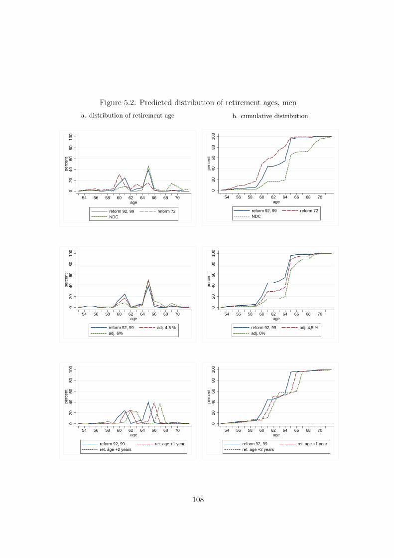
Figure 5.2: Predicted distribution of retirement ages, men

a. distribution of retirement age

020

4060

8010

0pe

rcen

t

54 56 58 60 62 64 66 68 70age

reform 92, 99 reform 72NDC

b. cumulative distribution

020

4060

8010

0pe

rcen

t

54 56 58 60 62 64 66 68 70age

reform 92, 99 reform 72NDC

020

4060

8010

0pe

rcen

t

54 56 58 60 62 64 66 68 70age

reform 92, 99 adj. 4,5 %adj. 6%

020

4060

8010

0pe

rcen

t

54 56 58 60 62 64 66 68 70age

reform 92, 99 adj. 4,5 %adj. 6%

020

4060

8010

0pe

rcen

t

54 56 58 60 62 64 66 68 70age

reform 92, 99 ret. age +1 yearret. age +2 years

020

4060

8010

0pe

rcen

t

54 56 58 60 62 64 66 68 70age

reform 92, 99 ret. age +1 yearret. age +2 years

108

Figure 5.3: Predicted distribution of retirement ages, women

a. distribution of retirement age

020

4060

8010

0pe

rcen

t

54 56 58 60 62 64 66 68 70age

reform 92, 99 reform 72NDC

b. cumulative distribution

020

4060

8010

0pe

rcen

t

54 56 58 60 62 64 66 68 70age

reform 92, 99 reform 72NDC

020

4060

8010

0pe

rcen

t

54 56 58 60 62 64 66 68 70age

reform 92, 99 adj. 4,5 %adj. 6%

020

4060

8010

0pe

rcen

t

54 56 58 60 62 64 66 68 70age

reform 92, 99 adj. 4,5 %adj. 6%

020

4060

8010

0pe

rcen

t

54 56 58 60 62 64 66 68 70age

reform 92, 99 ret. age +1 yearret. age +2 years

020

4060

8010

0pe

rcen

t

54 56 58 60 62 64 66 68 70age

reform 92, 99 ret. age +1 yearret. age +2 years

109

The incentive effect of higher adjustment factors is also weaker for women: adeduction of 4.5 percent p.a. increases the average age of retirement by 3 monthsfrom 62.4 to 62.7. A deduction of 6 percent p.a. increases the average retirementage by another 6 months to 63.2 years.

Finally, the simulations demonstrate that the introduction of the NDC systemwould also have a major impact on the average age of retirement in comparisonwith the 1992 and 1999 reforms (refer to Table 5.3). The average age of retirementincreases by more than two years for men (from 63 to 65.3) and, less dramatically,by almost one year for women (from 62.4 to 63.3). Of the five reforms examined,this variant generates the highest average retirement age and thus evidently hasthe most powerful incentive effects. As demonstrated by Figures 5.2 and 5.3, thedistribution of new retirements is similar to that in the scenario involving higheradjustment factors. This applies equally to men and women.

Although the NDC system in fact differs both in technical respects and in under-lying transfer philosophy from the pay-as-you-go system, the earnings points rulesembodied in the German pay-as-you-go system resemble fairly closely the actuarialprinciple of equivalence between contributions and benefits. The main difference be-tween the two systems is that the NDC system includes explicit actuarial adjustmentfactors that are considerably higher than in the reference scenario.

It is important to bear in mind that the estimates summarized in this paper arebased on the behavior of employees and employers from the mid-1980s to the 1990s.The future behavior particularly of female workers may well change significantly,viz., more closely resemble that of male workers, in the period 2005 to 2025 towhich the projections in this paper apply.

5.1.6 Summary and Conclusions

The accelerating process of population aging will have a momentous impact on thefinancial sustainability of the German pay-as-you-go pension system. The increase inthe old-age dependency ratio means that the pensions of a growing number of peopleat retirement age will have to be financed by a smaller workforce. Quite apart fromthese demographic problems, there are also strong incentive effects favoring earlyretirement built into the German pension system. These incentives increase theold-age dependency ratio even more than would be dictated by demographic factorsalone.

In the present paper the influence of pension legislation on retirement decisionsin Germany is modeled and estimated. Retirement probability is summarized as afunction of an incentive variable, which encompasses pension legislation and othercontrol variables. The option value of postponing retirement by one year is em-ployed as an incentive variable. This model is then used to simulate various reformsto the retirement rules: the 1992 and 1999 reforms, as well as a range of reformvariants offered for discussion by the “Rurup Kommission”, including an increase in

110

standard retirement age limits, an increase in the actuarial adjustment factors, andthe implementation of a notional defined contribution (NDC) system modeled afterthe Swedish pension system.

The calculations show that the introduction of an actuarial adjustment factor of3.6 percent p.a. and other changes to the retirement rules already introduced by the1992 and 1999 reforms will, over the next few years, increase the average effectiveretirement age for men by almost two years and that for women by a considerablyshorter period of not quite 9 months.

A shift in the structure of age limits as a whole by a further two years wouldpostpone the effective retirement age of men by, on average, around 9 months, andwould have little or no effect on the retirement age of women. Alternatively, anincrease in the actuarial adjustment factor from 3.6 percent to 6 percent wouldincrease the average age of retirement of men by almost 2 years. This effect wouldbe considerably weaker for women; nevertheless, their average age of retirementwould increase by around one year.

These results illustrate that an increased actuarial adjustment factor and anincrease in the statutory retirement age based on higher remaining life expectancyoffer major potential for postponing the effective age of retirement. This is animportant finding. Since the pension system from which we depart distorts theretirement decision - in that the present discounted value of pension benefits as seenby a current worker decreases substantially with increasing age of retirement - anincrease in the effective retirement age will reduce the financial burden of the publicpension system.37 This is the case as long as the adjustment factors are basedon an interest rate below the economy-wide discount rate.38 From an economicperspective, therefore, these policy options offer suitable measures which help toput the German pay-as-you-go public pension system on a path on which it canregain its financial sustainability.

37Borsch-Supan and Schnabel (1998) provide empirical estimates and graphical representationsof the decline in the present value of benefits with increasing retirement age. It is importantto note that the budget effect is caused by the current actuarial non-neutrality of the Germanpension system. It vanishes once the system has gained actuarial neutrality, see e.g. Breyer andKifmann (2002) for a theoretical analysis, and Gruber and Wise (2004b), in their introduction, foran empirical international comparison of the size of these budget effects. The exact quantificationof the budget effects is a subject of current research. Borsch-Supan, Kohnz and Schnabel (2004a)provide preliminary budget effect estimations based on a simplified model of the German socialsecurity system.

38For a discussion of the involved discount and interest rates, see Borsch-Supan (2003).

111

5.1.7 Appendix

Table 5.4: Descriptive statistics of variables used in Table 5.2

Males Females

Variable Mean Std. Err. Mean Std. Err.

labor status “retired” 0.400 0.011 0.312 0.007

Optval 184.62 3.606 141.36 9.925SSW 301.39 3.135 129.89 1.820SSW, sqrd. 52.37 2.302 218.50 2.889Health status 8.223 0.063 9.197 0.032Married 0.947 0.005 0.913 0.004University degree 0.079 0.006 0.038 0.003Skill 0.850 0.011 0.478 0.009Home ownership 0.488 0.011 0.517 0.008No financial assets 0.085 0.006 0.105 0.005Financial securities 0.251 0.009 0.226 0.007Period of insurance 39.92 0.145 21.02 0.201Period of insurance squ. 1640.1 9.245 604.3 9.681Income 55.64 0.490 29.64 1.062Income squared 3637.5 73.06 5452.6 1756.9Self-employed 0.072 0.005 0.086 0.004Civil service 0.119 0.007 0.010 0.002Kids 0.312 0.010 0.303 0.007No. of obs. 2321 4206

Source: GSOEP, working sample, 1984-1997.

112

5.2 Retirement Age and Preretirement in Ger-

man Administrative Data

5.2.1 Introduction

Early retirement and preretirement39 are costly achievements that aggravate thealready tight financial situation of the German pay-as-you-go pension system due topopulation aging. Since 1992, pension and labor-market reforms have been adoptedand they greatly restrain publicly subsidized early retirement and preretirementpossibilities. Because of these reforms, the distribution of retirement age of olderworkers is expected to be changing. These changes can be exploited to investigatethe impact of policy reforms on retirement entry behavior.

So far, there is hardly any research on the impact of pension reforms on preretire-ment in Germany. The difficulty consists in observing preretirement in the data andin providing for a sufficiently long time-series that allows to analyze policy reforms.The only empirical analysis in this area has been undertaken by Wubbeke (2005)who uses a data set based on administrative information of labor-market historiesand retirement entries.40 She investigates the impact of firms’ employment and pub-lic social security policy on employees’ changes from employment into retirement inthe period of 1975 to 1995.

Recently, the German Pension Insurance (“Deutsche Rentenversicherung”) hasstarted to release administrative data for research purposes. This administrativedata is a promising source for investigating the impact of labor and pension reformson individual retirement behavior, because it includes detailed information aboutindividuals’ employment status and pension insurance characteristics. So far, onlycross-sectional but no time-series data of individuals’ retirement entries and insur-ance histories are available. The data set used in this study, i.e., the Scientific UseFile (SUF) Versichertenrentenzugang 2003, is a representative sample of publiclyinsured persons who retired in 2003. This data is used to learn more about howto describe preretirement which will be useful for future economic analysis of pol-icy reforms based on German administrative data.41 The present paper discusses

39Preretirement refers to effective retirement before old-age public pension payments can bereceived from age 60 onwards and includes the option of partial retirement (“Altersteilzeit”). Ne-gotiations between employers and employees, and state subsidies enable preretirement. In contrast,official retirement is defined as receiving public old-age pension payments and, thus, includes earlyretirement from age 60 onwards. For a more detailed description of early retirement pathways seeSection 5.1.2.

40This data is not publicly available but results from an - until now - unique example of combiningdata on labor-market histories issued by the Institute for Employment Research (“Institut furArbeitsmarkt- und Berufsforschung”) of the Federal Employment Agency (“Bundesargentur furArbeit”) and data on retirement entries issued by the German Pension Insurance (“DeutscheRentenversicherung”)

41As discussed in Appendix B the data provided so far by the German Pension Insurance, i.e.,

113

differences between individual determinants of retirement for those choosing pre-retirement programs as opposed to official public pension plans. A reduced formeconometric approach is employed in order to explore this question.

Based on the SUF Versichertenrentenzugang 2003, the present sample revealsthat 40 percent of all men and women preretire, that is they withdraw from thelabor market before official pathways into old-age retirement can be taken. Onaverage individuals stay 2.4 years in preretirement before taking one of the officialearly retirement entries based on the unemployment or partial retirement (“Alters-teilzeit”) pathway or retirement plans for women. Moreover, differences in effects ofindividual determinants - such as rehabilitation services, income before retirementand pension payments - on retirement age can be observed for preretired personscompared to persons taking official retirement entries.

The paper proceeds as follows: Section 5.2.2 summarizes institutional facts andrecent changes of early retirement, partial retirement and preretirement in Germany.In Section 5.2.3 the data, the sample, and the definition of preretirement are dis-cussed. Characteristics of the retirement age are presented in Section 5.2.4 and,finally, Section 5.2.5 concludes.

5.2.2 Early Retirement, Partial Retirement and Preretire-ment in Germany

Early retirement, preretirement and partial retirement refer to regularly used officialand unofficial pathways into retirement before reaching the statutory age of 65. Inorder to clarify these concepts and in order to motivate institutional changes withrespect to the public pension system and unemployment insurance since 1992, theyare described in the following.

Early retirement refers to retirement entry before age 65 by one of the officialpathways into old-age retirement, which results in an income stream paid by theGerman public pension system. It has been introduced in Germany with the pen-sion reform in 1972. With the age of 60 women, partial retirees,42 unemployed oremployees, who can not be appropriately employed due to health or labor-marketreasons, can enter retirement (“Fruhrente”). All other employees who have beencontributing to the public pension system for at least 35 years can retire at the ageof 63. These pathways into retirement are not related to any additional adjustmentcosts. Consequently, strong incentives are set to retire before the age of 65 andindividuals react accordingly.

A recent survey reveals that two out of three employees would leave the labor

the SUF Versichertenrentenzugang, does not allow for policy analysis of retirement entry behaviorbased on option value models.

42The term “partial retirees” refers to persons who enter a partial retirement plan (“Alter-steilzeit”).

114

force between age 55 and 60 if this was financially feasible (Pfeiffer and Simons2004). Preretirement (“Vorruhestand”) meets these preferences and refers to laborforce exits that take place before early retirement is possible. This labor forceexit can be referred to as preretirement if a person receives income paid by theunemployment insurance or other state subsidies that burden the tax and socialsecurity systems and/or income that results from arrangements between employersand employees.

One can distinguish between two different ways of entering preretirement. On theone hand, unemployment compensation is an important way of financing preretire-ment. If a firm wants to lay off older workers in a restructuring process, employeescan receive a negotiable combination of unemployment compensation and a supple-ment or severance pay. At the age of sixty they enter early retirement via the publicpension system, i.e., by taking the unemployment pathway. In the case of prere-tirement, the date of the labor force exit is very often determined by the maximumduration of unemployment benefit payments. Until 2005 the duration of benefitspaid by the unemployment insurance (“Arbeitslosenversicherung”) lasted between24 and 32 months.43 Even earlier labor force exits and corresponding retiremententries can be induced by paying the employee the difference between the last salaryand unemployment assistance (“Arbeitslosenhilfe”), which, until 2005, lasted for oneadditional year. Unemployment insurance benefits can amount to 67 percent of thelast salary and are especially attractive as the unemployment insurance additionallypays the contributions to the public pension system.

On the other hand, partial retirement (“Altersteilzeit”) is another means of pre-retirement. This scheme provides for part-time work between the age of 55 or aboveand early retirement at age 60 or 63 depending on the above mentioned pathways.Effectively, many employees continue to work full time at first and then leave theirjob earlier (“Blockmodell”). Partial retirement is state-subsidized: The unemploy-ment insurance pays an additional 20 percent of the usual part-time earnings if theemployer hires a young employee. This rule also encourages employers to substituteolder by younger employees and meets employees’ interest in retiring early.

Figure 5.4 shows the fraction of different pathways into retirement relative tototal retirement for the period of 1978 to 2003. It demonstrates that old-age pensionsdue to unemployment have become an important pathway into retirement since theearly 1990s for men, whereas among women the unemployment pathway is notfrequently used. Due to low labor-market participation, women rather take thepathway for women which allows to enter retirement at age 60.

Starting with the pension reforms of 1992 and 1999 and continuing with labor-market reforms in 2003, several changes to these rules have been adopted. Thesechanges constrain generous early retirement and preretirement options. The reformsof 1992 and 1999 introduced an increase of the retirement age limits to age 65 or

43The exact duration depended on the duration of compulsory insurance coverage and on theage of the beneficiary.

115

Figure 5.4: Pathways into retirement0

2040

6080

100

perc

ent

1978 1982 1986 1990 1994 1998 2002

normal oldage pensionat age 65

flexible retirementat age 63

pension dueto unemploymentafter age 60

old agedisability pensionafter age 60

disability pension

MEN

020

4060

8010

0pe

rcen

t

1978 1982 1986 1990 1994 1998 2002

normal oldage pensionat age 65 flexible retirementat age 63 old agepension, womenafter age 60 pension dueto unemploymentafter age 60 old agedisability pensionafter age 60 disability pension

WOMEN

Sources: Own calculations based on VDR (1978-2004).

116

age 63 for long-term insured. These changes will be fully implemented after a longtransitional period in 2015.44 There will no longer be exceptions for the unemployed,partially retired or women. In Figure 5.4 a small decrease in the early retirementoptions of unemployment pensions for men and women old-age pensions can alreadybe observed since the late 1990s. Moreover, the government introduced adjustmentcosts that reduce pension payments by 0.3 percent for each month of early retire-ment before age 65. If employers do not want to accept the lower pension benefit,they either need to work longer or have to extend the preretirement period, i.e.,the period between labor force exit and retirement payments. From 2005 onwards,unemployment benefits are shortened from a maximum of 32 to 18 months (“HartzIV”). Unemployment assistance will be paid only if the preconditions for welfarepayments are fulfilled (“Arbeitslosengeld II”). Thus, state-promoted preretirementbetween labor force exit and pension benefit payments is now greatly reduced andlimited to 18 months. Transition rules of the pension reforms of 1992 and 1999already apply to most cohorts retiring in 2003, whereas the new labor-market regu-lations have not been effective before 2005.

All these reform steps indicate a change in paradigm from promoting early andpreretirement towards working longer. These reform steps are backed by the insightthat skills of older workers are needed, especially in the course of population aging,and encouraged by governmental initiatives to bring older workers above age 50back into work (“Initiative 50 plus”). Based on descriptive statistics of recent ad-ministrative data of aggregate retirement entries, Reimann (2003) shows that thesechanges have already had an effect as the retirement entry behavior slowly startsto change. However, the pension reforms in 1992 and 1999 have long transitionalperiods and are not yet fully phased in. It is of great interest to exploit this policychange in future research in more detail and to investigate the responsiveness of re-tirement entries, preretirement and old-age unemployment to institutional changesfor simulations of future pension and labor-market reform scenarios.

5.2.3 The Data and Sample

The data employed in this study is based on administrative data of the Germanpublic pension insurance that are collected and provided by the German Pension In-surance (“Deutsche Rentenversicherung”). As these data are made virtually anony-mous, scientific use files entail only a representative sub-sample of all publicly in-sured individuals or pensioners of the public pension system. This paper employs theSUF Versichertenrentenzugang 2003 (SUFRTZN03XVST Berk) which is a sampleof about 100,000 individuals that started to receive public pensions in 2003. Peoplethat are publicly insured but are not yet retired are not part of the sample.

44For a more detailed description of the 1992 and 1999 reforms and a graphical description ofstatutory age limits during the transition period refer to Berkel and Borsch-Supan (2004) or Figure5.1, Section 5.1.2.

117

Administrative data are very valuable to analyze questions on retirement entrybehavior. They have the following advantages compared to German survey-baseddata such as the GSOEP: First, samples are large representative draws of the wholepopulation of publicly insured persons. Second, there is no attrition. Third, thereare no problems with the interpretation of questions as it is often the case with sur-vey responses. Fourth and most importantly, the sample provides information onindividuals’ insurance status before retirement and entails all the relevant informa-tion to determine a person’s pension claims, e.g., information on earnings points45,on various contribution periods and the type of pension that is received.

But administrative data are also associated with difficulties.46 One major issueis the measurement of the effective retirement age, which is discussed in detail inthe remainder of the paper. Other issues are the measurement of income, wealthand socio-economic variables.47 Information on these characteristics are available asfar as the public pension system retains them for the determination of individualpension claims. Income refers to income subject to social security contributions onlyand wealth is not recorded at all. Person’s health status can be inferred by usinga variable that describes whether medical rehabilitation services have been takenin the last 5 years before retirement. Direct information is available, for example,on education, family status, residence and details necessary for the calculation ofpublic pension payments.

For some variables more than pure cross-sectional information is provided, i.e.,gross yearly income subject to social security contributions and the status of insur-ance in the three years before retirement. The latter provides additional informationon individuals’ situation, i.e., whether they are self-employed or unemployed beforeretirement.

For the subsequent analysis the sample is limited to individuals between age54 and 72 that receive an old-age or disability pension for the first time in 2003.Individuals with partial pensions are excluded from the sample as these personsare likely to be still partially employed. Observations with pension payments thatare significantly determined by inter- or supranational legislation are not considered,because these are determined by factors that are out of reach in this study. Problem-atic for the analysis are also pensions paid on the basis of the “Fremdrentengesetz”(FRG) which include mainly East-Germans that took refuge from Eastern to West-ern Germany and resettlers (“Aussiedler” and “Spataussiedler”). As suggested byMika (2005), these observations are excluded from the sample as their pension pay-ments and corresponding information in the data are based on fictive contributions.

45In Germany the calculation of pension payments is based on earnings points. For each personthe number of earnings points depends mainly on the relative earnings position and the numberof contributions.

46These difficulties differ from problems with German survey data. It would therefore be inter-esting to compare the GSOEP to the present administrative data in detail. This, however, liesbeyond the scope of the present paper.

47For a detailed description of the data see also Himmelreicher (2006) and Radl (2005).

118

The adjustment of pension payments in East Germany to West German levels hasalmost been completed in 2003. Therefore, differences affecting the retirement entryage should be minimal and observations from both East and West Germany areincluded in the sample.

Retirement Age in German Administrative Data

Administrative data provide detailed and reliable information on individual pensionclaims that are necessary for meaningful analyses of individual retirement entriesand labor force exits. The retirement age in administrative data is defined as theage at which a pension is received from the German public pension insurance for thefirst time. This retirement age is referred to in the following as the official retirementage. Thus preretirement is not considered. There are three main motivations fortaking account of preretirement and for considering the effective instead of the offi-cial retirement age in economic analyses of retirement entries: First, recent pensionand labor-market reforms, among other things, aim at limiting preretirement as itaggravates the financial situation of the social security systems. It is of great inter-est to investigate the impact of these reforms on preretirement using administrativedata. Second, it is important to take account of preretirement if overall financialeffects of retirement entries on social security systems are of interest instead of finan-cial effects on the public pension system alone as preretirement typically burdensthe unemployment insurance. Third, survey-based data show that individuals referto themselves as retired when they have not yet officially retired but are preretired(Borsch-Supan et al. 2004b). For a consistent estimation of individual retiremententry decisions it is, thus, necessary to use the effective as opposed to the officialretirement entry age.

Preretirement cases can be identified in the data as information on individuals’insurance status is available not only for the year before retirement, i.e., for 2002,but also for 2001 and 2000. The insurance status specifies whether a person (i) hadan employment that was subject to social security contributions, whether a personwas (ii) marginally employed (“geringfugig beschaftigt”),48 (iii) eligible for a partialpension plan (“Altersteilzeit”), (iv) voluntarily insured,49 (v) compulsorily insuredmainly due to unemployment or sickness,50 (vi) passively insured or (vii) in someother insurance category.51 Table 5.5 summarizes the fraction of each insurancecategory in the present sample. Half of the individuals have been passively insured

48A person is considered marginally employed if he or she does not earn more than 400 Eurosper month. Special rules with respect to social security insurance apply to these persons.

49These are mainly self-employed persons or housewives who have no income subject to socialsecurity insurance but voluntarily take part in the German public pension system.

50For exact definitions refer to the German Social Security Code (“Sozialgesetzbuch”), SGB IIIand § 3 Nr. 3 SGB VI.

51This category includes for example persons that were eligible to insurance credits (“Anrech-nungszeiten”) or other compulsory insurances that are not part of (v).

119

or compulsorily insured due to unemployment or sickness. Passive insurance refersto all persons that have not paid any social insurance contributions in the year beforeretirement. 50 percent of these individuals have not paid any contributions for morethan 20 years. This group inter alia includes civil servants or self-employed thathave earned pension claims due to employment subject to social security insuranceat some point in time, typically very early in their career. A third group is madeup of individuals that gave up employment early which are mostly housewives.

Table 5.5: Insurance status before official retirement

insurance status percent*

employment s.t. social insurance contributions 20.64

marginally employed 4.14

compulsorily insured (unemployment, sickness) 23.92

partial retirement plan 12.46

voluntarily insured 3.31

passively insured 25.60

others 9.93

Source: Own calculations based on SUF Versichertenrentenzugang 2003(SUFRTZN03XVST Berk).*) Percentages relative to all individuals in the sample that officiallyretired in 2003.

As summarized in Section 5.2.2 individuals are considered to be preretired ifthey were unemployed, partially retired, marginally employed or passively insured.In order to rule out cases that have been passively insured for a very long period,(e.g. housewives, self-employed or civil servants) only those are included that havepaid contributions to the public pension insurance at least once during the last10 years before official retirement in 2003. At the same time, persons that returnto an employment status subject to social security contributions or to voluntaryinsurance are not included in this pool of preretired persons.52 This classification ofpreretirement is taken from Pfeiffer and Simons (2004) who investigate preretirementin Germany using various data sources. With this definition, 47 percent of men and37 percent of women preretired in the present sample, i.e., effectively retired before2003.53

52Also, persons that enter preretirement at age 63 or later are not considered as preretired.These are only a few cases.

53Due to a censoring problem for the year 2000 it is not possible to determine whether individualswho are effectively retired in 2000 entered retirement in 2000 or before. For the determination ofthe effective retirement age this is, however, necessary. All individuals preretired before 2001 areassumed to have entered preretirement in 2000. Compared to the alternative of excluding these

120

The sample also includes disability pensions. Note that preretirement in thisstudy covers part of the disability cases. Persons retiring due to disability amountto 10 percent in the present sample. Half of them receive a disability pension directlyafter leaving the labor force, another 30 percent after a period of unemployment.According to the above mentioned definition, the latter case may fall into the prere-tirement category, whereas the first does not. Declaring part of the disability cases aspreretired is reasonable, because obtaining a disability pension due to labor-marketreasons is still possible for cohorts retiring in 2003. However, it has become muchmore difficult over time.54

Figure 5.5 displays retirement entry probabilities in 2003 for men and womenaged 54 to 72 that take official pathways into retirement. Preretirement is notaccounted for in the data underlying this figure. The distributions for men andwomen are characterized by two large spikes at age 60 and 65. There is also a thirdspike for men at age 63. For women the spikes at age 60 and 65 are more pronouncedthan for men. These differences can be explained by differences in employmenthistories and different retirement pathways for men and women. 27 percent of allwomen retire at age 60. This high value is due to a pension pathway that allowswomen under certain conditions to enter retirement at age 60. This pathway stillexists in 2003, however, adjustment costs have to be taken into account. Another41 percent of all women retire at age 65. Due to interrupted employment histories,women often have not contributed a sufficiently long time period into the publicpension system such that they are not eligible to choose this or any other pathwayto retire before age 65.

The distribution of retirement age between age 54 and 72 is smoother for men:20 percent retire at age 60, 18 percent at age 63 and 25 percent at age 65. Fromage 60 onwards men can retire via the unemployment or partial retirement pathway.From age 63, they are eligible for retirement if they are long-term insured. In 2003adjustment costs apply to almost all cohorts that choose one of these retirementpathways.

The average official retirement entry age55 for men and women as reported in thepresent sample amounts to 62.3 and 62.5 years respectively. Once preretirement isconsidered, the average effective retirement age is about one year lower: 61.3 yearsfor men and 61.6 years for women. In the present sample men and women preretireon average at age 59.3 and 59.2 respectively and officially retire after 2.4 years.56

observations from the sample, this assumption is justified: The resulting average of duration inpreretirement in the present sample amounts to 2.4 years and is only slightly lower than the averageduration of preretirement in the GSOEP data which is 2.5 years (Pfeiffer and Simons 2004).

54Note the reduction in disability pensions since 1978 in Figure 5.4.55“Official” refers to the fact that these individuals enter retirement through one of the official

pathways (old-age or disability pensions) and receive pension payments from the German PensionInsurance. The numbers refer to average values in the present sample and, therefore, do not exactlymatch statistics issued by the German Pension Insurance.

56These average values are only approximately correct. Note that the group of preretired persons

121

Figure 5.5: Distribution of retirement entry age in 2003

010

2030

4050

perc

ent

54 55 56 57 58 59 60 61 62 63 64 65 66 67 68 69 70 71 72age

men women

Source: Own calculations based on SUF Versichertenrentenzu-gang 2003 (SUFRTZN03XVST Berk), German Pension Insurance(“Deutsche Rentenversicherung”).

Other Variables

In order to characterize retirement entry age the data set provides several variablesfor the subsequent regression analysis: income before retirement, pension payments,socio-demographic characteristics such as highest educational degree, status of sick-ness, marital status, and times of child-caring.

Income in administrative data refers to income subject to social security contri-butions. It does not mirror a person’s complete income position. Therefore, incomeof passively or voluntarily insured individuals is missing. These individuals mainlyobtain income from other sources, e.g., self-employed or civil servants who have hadan employment subject to social security contributions only at the beginning of theircareer. Also housewives belong to this group. In case of housewives but also moregenerally in the case of couples, especially with children, it would be desirable touse a couple’s income. However, the data does not allow to match couples.

As the idea of the following econometric analysis is to provide a picture of the

in this sample refers to persons preretiring in 2000 to 2002 and officially retiring in 2003. Inorder for this group to be representative for preretirement cases in 2003, one has to assume thatpreretirement cases in 2000 to 2002 are representative for preretirement cases in 2003 that officiallyretire in 2004 to 2006, i.e., one has to assume that no cohort and time effects exist for the years2000 to 2006. As retirement entry rules are changing due to long transitional periods of the reformsof 1992 and 1999, time effects can not fully be ruled out.

122

characteristics of retirement entry age as provided by the administrative data athand, observations with missing income values are not dropped, but explicitly con-trolled for. An income dummy is constructed that is equal to one if the incomevalue is missing, income mis. 26 percent of all men and 44 percent of all womenhave reported missing incomes values. Almost 70 percent of these men and womenare passively insured.57

Another shortcoming of the income variable is the censoring of yearly incomevalues greater than 55,000 Euros. In order to circumvent the censoring problem atthe top end of the income distribution, dummies for income quintiles are constructedfor men and women with reported income values.58

Pension payments are directly obtained from the data. The corresponding vari-able refers to public pensions only. As pension payments are censored at valuesgreater than 1800 Euros per month, again dummies for pension payment quintilesare constructed.59

Information on education is classified by the highest individual educational de-gree: secondary school (“Hauptschule” and “Mittlere Reife”), high school (“Abitur”),technical college (“Fachhochschule”) or university. The categories secondary andhigh school are subdivided into cases with and without vocational training (“Beruf-sausbildung”). Dummy variables equal to one for the highest educational degreeare constructed and included in the regression analysis. Furthermore, there is onecategory referring to unknown education levels and another category referring tomissing values. The latter category includes about one-third of all observations.These are mostly individuals that entered retirement not directly after employment:57 percent are passively insured and 20 percent are unemployed in the year beforeretirement. Thus, no information on the educational degree was provided by a for-mer employer.60 The category of missing educational degrees is clearly non-randomand related to the insurance status before retirement and is, therefore, separatelyincluded in the regression. The distribution of observations with unknown educa-tional degree across income classifications is also likely to be non-random and entersas an additional dummy variable.61

The health status can be proxied by two different variables: An indicator variablethat denotes whether a person has claimed rehabilitation services during the last 5

57Because of missing income values one could alternatively consider to drop all passively insuredpersons who have not contributed to the public pension system within the last 10 years and allvoluntarily insured persons. Another way to deal with the problem would be to impute incomeand wealth by using the GSOEP.

58For exact quintile ranges see Table 5.9, Appendix A.59For the exact range of quintiles see Table 5.9, Appendix A.60For further background information on the education variable refer to Fitzenberger, Osikominu

and Volter (2005).61In this group 33 percent of individuals are employed subject to social security contributions,

21 percent are unemployed and 25 percent are marginally employed, the rest splits up into all othercategories.

123

years previous to retirement62 and a variable that comprises months of insurancecredits due to sickness or rehabilitation.

Information on a person’s marital status and on the number of months dedicatedto child-caring are provided. It is important to mention that this number refersonly to cases in which times of child-caring are credited and lead to higher pensionbenefits. This variable, therefore, does not directly measure the number of children.

Finally, information on individuals insurance status is categorized. The follow-ing dummy variables are included in the regression analysis: employment subjectto social insurance contributions; partial retirement; compulsory insurance due tounemployment, sickness or rehabilitation; marginal employment; voluntary employ-ment; passive insurance and others.

Tables 5.9 and 5.10 in Appendix A provide definitions and summary statisticsof all variables that are of interest in the subsequent regression analysis.

5.2.4 Characteristics of the Official and Effective Retire-ment Age

As all people in the sample officially retire in 2003 or effectively retire during theshort window between 2000 and 2003, the main sample variation results from thedifferences in retirement age across individuals. The determinants of this varia-tion are investigated using standard OLS regressions with heteroscedasticity robuststandard errors. Estimations are undertaken separately for men and women asretirement entry behavior and the corresponding retirement age are likely to be af-fected by systematic differences in employment histories. In a first step, retirementage is defined as a person’s age in 2003, which is the official retirement age. In asecond step, retirement entry age refers to a person’s age when effectively retiring.Therefore, individuals who preretire are identified and their official retirement ageis adjusted to their effective retirement age.

The Official Retirement Age

Two different specifications are estimated: The first one includes variables for in-come, pension, education, health status, marital status and child-caring (Table 5.6),whereas the second specification additionally includes dummies for insurance cate-gories as described in the previous section (Table 5.6). Variables referring to incomesubject to social security contributions in the year before retirement and retire-ment income paid by the public pension insurance in 2003 are defined as dummyvariables of income or pension income classes: A dummy for missing income val-ues, income mis, as well as dummies for income and pension payment quintiles are

62Persons that receive a disability pension have often taken rehabilitation services before retiring.However, this is no precondition for obtaining a disability pension in Germany.

124

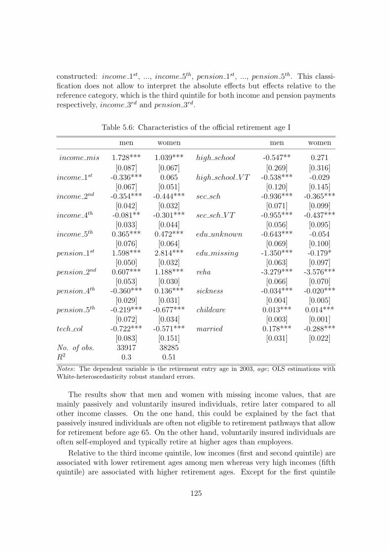
constructed: income 1st, ..., income 5th, pension 1st, ..., pension 5th. This classi-fication does not allow to interpret the absolute effects but effects relative to thereference category, which is the third quintile for both income and pension paymentsrespectively, income 3rd and pension 3rd.

Table 5.6: Characteristics of the official retirement age I

men women men women

income mis 1.728*** 1.039*** high school -0.547** 0.271

[0.087] [0.067] [0.269] [0.316]income 1st -0.336*** 0.065 high school V T -0.538*** -0.029

[0.067] [0.051] [0.120] [0.145]income 2nd -0.354*** -0.444*** sec sch -0.936*** -0.365***

[0.042] [0.032] [0.071] [0.099]income 4th -0.081** -0.301*** sec sch V T -0.955*** -0.437***

[0.033] [0.044] [0.056] [0.095]income 5th 0.365*** 0.472*** edu unknown -0.643*** -0.054

[0.076] [0.064] [0.069] [0.100]pension 1st 1.598*** 2.814*** edu missing -1.350*** -0.179*

[0.050] [0.032] [0.063] [0.097]pension 2nd 0.607*** 1.188*** reha -3.279*** -3.576***

[0.053] [0.030] [0.066] [0.070]pension 4th -0.360*** 0.136*** sickness -0.034*** -0.020***

[0.029] [0.031] [0.004] [0.005]pension 5th -0.219*** -0.677*** childcare 0.013*** 0.014***

[0.072] [0.034] [0.003] [0.001]tech col -0.722*** -0.571*** married 0.178*** -0.288***

[0.083] [0.151] [0.031] [0.022]No. of obs. 33917 38285R2 0.3 0.51

Notes: The dependent variable is the retirement entry age in 2003, age; OLS estimations withWhite-heteroscedasticity robust standard errors.

The results show that men and women with missing income values, that aremainly passively and voluntarily insured individuals, retire later compared to allother income classes. On the one hand, this could be explained by the fact thatpassively insured individuals are often not eligible to retirement pathways that allowfor retirement before age 65. On the other hand, voluntarily insured individuals areoften self-employed and typically retire at higher ages than employees.

Relative to the third income quintile, low incomes (first and second quintile) areassociated with lower retirement ages among men whereas very high incomes (fifthquintile) are associated with higher retirement ages. Except for the first quintile

125

the effect for women looks similar. This category tends to retire later: Women withvery low incomes have typically very unstable employment histories and insuranceperiods due to child-caring. Therefore, they often might not be eligible to earlyretirement, i.e., retirement before age 65.

The lower pension payments, the higher are - relative to the third quintile -retirement entry ages (refer to the coefficients on pension 1st and pension 2nd).This result is in line with the following consideration: Many people who retire late,i.e., with the age of 65, are not eligible to one of the pathways into early retirement.These are mostly passively and voluntarily insured people that typically receive lowpension payments. This way into retirement applies to the typical housewife andis, therefore, more common among women compared to men. In line with thisconsideration, there is a much larger effect for women compared to men.

Income and pension payments are of course strongly correlated. Note, however,that in the present data this correlation is actually weaker than one might expect atfirst:63 For several cases income values are not reported (see previous section) or em-ployment histories are rather instable before retirement such that income measuredin the year before retirement is no perfect proxy for individuals’ relative incomepositions over the life cycle.

Compared to persons with lower educational degrees, men with a university de-gree, uni, have a higher retirement age.64 This finding is in line with the generalnotion that people with higher education are more attached to their jobs and, there-fore, tend to work longer. Moreover, they are typically less physically strained andare able to work longer. Men with a technical college degree, tech col, or secondaryschooling degree, sec sch or sec sch V T , have comparatively low retirement ages,i.e., they retire on average between 8 to 11 month earlier. Men with high schooldegrees, high sch and high sch V T , lie in between these two extremes. Results forwomen are similar, though smaller in size and less significant. The fact that theassociation between education and retirement age is much weaker for women couldagain be explained by interrupted employment histories. Due to child bearing andcaring, many women have not followed a career that is suggested by their educationaldegree.

Both health measures, reha and sickness, reveal that a higher degree of healthis associated with a higher retirement entry age for men and women which is a welldocumented phenomenon.65 The number of months credited by the public pensioninsurance due to sickness or rehabilitation has only a very small quantitative effecton the retirement age.66 If men or women have claimed rehabilitation services dueto sickness, they retire on average more than three years earlier. The present data

63The actual correlation coefficient amounts to 0.71.64The reference category are men or women with a university degree.65Refer to e.g. Larsen and Gupta (2004) who provide for a large literature on this topic.66An exact quantitative interpretation is not very reliable as the measure is censored at 48

months of credited insurance contributions due to sickness.

126

show that these are mostly cases that take the disability pathway into retirement.However, rehabilitation is no necessary precondition for receiving a disability pensionin Germany.

The number of months dedicated to child-caring as measured by the public pen-sion insurance, childcare, on average leads to a higher retirement age for both menand women, though the effect is low in size. This result is well in line with Hank(2004) who investigates in great detail the relationship between women’s retirementbehavior and fertility biographies.

Married women retire on average three to four months earlier than singles or wid-ows. This finding could be explained by the fact that wives are generally youngerthan husbands and often try to retire at approximately the same age as their hus-bands. For men the effect is mirror-inverted: Married men retire about two monthslater on average. The result is in line with the consideration that in the generationof interest married men are mostly responsible for the main family income sourceand, thus, work longer in order to afford retirement for the couple and possiblyeducation for the children.

In a second specification, additional dummy variables for individuals with par-tial retirement, part ret, compulsory insurance due to unemployment, sickness orrehabilitation, comp ins, marginal employment, marg emp, voluntary insurance,vol ins, passive insurance, pas ins, and other insurance status, others, before re-tirement in 2003 are added (Table 5.7). The reference category is employmentsubject to social social security contributions.

Men and women with partial retirement or compulsory insurance due to unem-ployment have a lower retirement age. Both groups are able to retire early due to aspecial retirement pathway for unemployment and partial retirement that still ap-plies to cohorts in the present sample, though adjustment costs have already phasedin. The effect is smaller for women. This corresponds well with the possibility ofwomen to enter retirement under the same conditions and as early as unemployedpersons or as individuals subject to a partial retirement plan. Marginally employed,voluntarily and passively insured persons on average retire much later. Most of theindividuals in these three categories are not eligible for retirement before age 65,probably because of too short insurance and contribution periods. Effects for menand women are qualitatively the same and just slightly differ in size.67

Naturally, correlations between individual characteristics and the retirement ageare largely driven by the institutional framework such as insurance categories or re-habilitation services and to a smaller extent by socio-economic characteristics such

67Note that in this specification the estimated coefficients of the income and pension paymentdummies differ. The change is due to a correlation of income and insurance categories. Only inthe case of the missing income category, income mis, there is a substantial qualitative change inthe estimated coefficient. As this category is strongly correlated with the insurance categories ofpassively and voluntarily insured persons, the positive effect is now captured by these dummies,passive and vol ins.

127

Table 5.7: Characteristics of the official retirement age II

men women men women

income mis -0.818*** -1.262*** sec sch V T -0.982*** -0.318***

[0.116] [0.076] [0.070] [0.098]income 1st -0.366*** -0.465*** edu unknown -0.672*** -0.118

[0.066] [0.051] [0.069] [0.099]income 2nd -0.194*** -0.305*** edu missing -1.341*** -0.251***

[0.043] [0.032] [0.065] [0.097]income 4th -0.027 -0.273*** reha -3.262*** -3.340***

[0.033] [0.042] [0.067] [0.069]income 5th 0.284*** 0.259*** sickness -0.034*** -0.017***

[0.075] [0.061] [0.004] [0.004]pension 1st 0.871*** 2.049*** childcare 0.010*** 0.013***

[0.054] [0.036] [0.003] [0.001]pension 2nd 0.141*** 0.821*** married 0.165*** -0.275***

[0.053] [0.030] [0.030] [0.021]pension 4th -0.304*** 0.104*** part ret -0.683*** -0.294***

[0.028] [0.030] [0.035] [0.035]pension 5th -0.243*** -0.862*** comp ins -0.683*** -0.308***

[0.074] [0.041] [0.038] [0.036]tech col -0.688*** -0.465*** marg emp 0.951*** 1.848***

[0.081] [0.150] [0.119] [0.060]high school -0.539*** 0.028 vol ins 2.520*** 2.360***

[0.119] [0.143] [0.110] [0.090]high school V T -0.629** 0.267 pas ins 3.000*** 2.999***

[0.266] [0.328] [0.100] [0.070]sec sch -0.978*** -0.362*** others 0.261*** 0.743***

[0.056] [0.094] [0.081] [0.057]No. of obs. 33917 38285R2 0.35 0.57

Notes: see Table 5.6.

as education, child-caring or marriage. The level of income subject to social securitycontributions and pension payments are also but to a smaller extent important de-terminants. The results in Tables 5.6 and 5.7 underline the importance of employingincentive variables that bundle the institutional framework as well as individuals’employment histories and future expected pension payments when determining in-dividuals’ retirement entry ages, as e.g. undertaken in Berkel and Borsch-Supan(2004) in Section 5.1.

128

The Effective Retirement Age

Due to generous preretirement possibilities, about 40 percent of individuals in thesample effectively retire before their official retirement date. These cases are identi-fied and their effective retirement age is defined as described in Section 5.2.3. Thepresent section investigates whether individuals’ characteristics are significantly dif-ferent with respect to retirement age for preretired individuals as opposed to in-dividuals taking official pension plans. The regressions documented in Table 5.6are repeated with interaction terms between a preretirement dummy, P , and eachexplanatory variable (Table 5.8).68

Table 5.8: Characteristics of the effective retirement age

men women men women

income mis 0.32 0.054 income mis ∗ P 0.349 0.108

[0.197] [0.120] [0.273] [0.192]income 1st -0.071 -0.058 income 1st ∗ P 0.073 -0.228

[0.143] [0.097] [0.201] [0.143]income 2nd -0.210** -0.503*** income 2nd ∗ P -0.365*** 0.029

[0.083] [0.048] [0.106] [0.069]income 4th -0.251*** -0.587*** income 4th ∗ P 1.342*** 1.423***

[0.053] [0.064] [0.064] [0.073]income 5th 0.166 0.059 income 5th ∗ P -0.751*** -0.663***

[0.168] [0.122] [0.242] [0.182]pension 1st 1.481*** 2.672*** pension 1st ∗ P 0.276* 0.239***

[0.056] [0.044] [0.150] [0.062]pension 2nd 0.761*** 1.400*** pension 2nd ∗ P -0.664*** -0.632***

[0.065] [0.044] [0.115] [0.058]pension 4th -0.560*** 0.081* pension 4th ∗ P 0.228*** 0.104*

[0.050] [0.048] [0.058] [0.059]pension 5th -0.207*** -0.680*** pension 5th ∗ P -0.304 -0.085

[0.067] [0.043] [0.283] [0.060]tech col -0.673*** -0.791*** tech col ∗ P 0.182 0.363

[0.118] [0.231] [0.155] [0.279]high school -0.740* 0.631* high school ∗ P 0.098 -0.771

[0.403] [0.377] [0.500] [0.508]high school V T -0.655*** 0.054 high school V T ∗ P 0.303 -0.465*

[0.167] [0.214] [0.222] [0.268]Note: This table continues on the next page.

68The estimation of interacted effects for preretired persons is equivalent to a separate regressionfor this group.

129

sec sch -1.028*** -0.399*** sec sch ∗ P 0.112 -0.162[0.095] [0.151] [0.130] [0.186]

sec sch V T -1.151*** -0.407*** sec sch V T ∗ P 0.466*** -0.159[0.070] [0.145] [0.102] [0.179]

edu unknown -0.578*** 0.096 edu unknown ∗ P -0.269** -0.510***[0.091] [0.152] [0.126] [0.187]

edu missing -0.848*** 0.293* edu missing ∗ P 0.028 -0.805***[0.106] [0.150] [0.132] [0.183]

reha -4.245*** -4.000*** reha*P 2.533*** 1.936***[0.089] [0.093] [0.124] [0.132]

sickness -0.043*** -0.022*** sickness*P 0.008 0.01[0.006] [0.006] [0.008] [0.008]

childcare 0.009** 0.012*** childcare*P 0.009 0[0.004] [0.001] [0.007] [0.001]

married 0.069 -0.368*** married*P 0.222*** 0.215***[0.046] [0.028] [0.060] [0.041]

P -3.317*** -2.664*** No. of obs. 33557 37992[0.388] [0.257] R2 0.54 0.67

Notes: The dependent variable is retirement entry age in 2000-2003 which is adjusted for pre-retirement, agef ; P is a dummy equal to one if a person preretires as defined in Section 5.2.3;OLS estimations with White-heteroscedasticity robust standard errors.

Overall, the effects for preretired individuals69 are qualitatively similar to thereference category, i.e., individuals that take official pension plans. Main differencesexist with respect to the size of the effects on rehabilitation, income and pension pay-ments: Most importantly, the negative association between claims of rehabilitationservices before retirement, reha, and retirement age is much smaller for preretiredmen and women. If rehabilitation services are taken, the retirement age of personswith regular pension plans is on average almost four years lower whereas preretiredmen are only about one and a half years and preretired women two years youngercompared to persons not claiming any rehabilitation services. This observation canbe explained by the fact that the frequency of rehabilitation services in the presentdata is much higher for persons between age 54 and 60 compared to older persons.At the same time, rehabilitation is strongly correlated with disability pension entriesat ages below 60. Therefore, persons who take rehabilitation services seem less likelyto take the preretirement pathway but rather the disability pathway.

Differences in effects between preretired individuals and the rest of the sampleare large for individuals with middle and high incomes: The estimated effects differsubstantially for the fourth and fifth quintile, whereas there is no or only a smalldifference with respect to the missing values dummy and the first and second income

69These effects are obtained by adding the interaction effect and the respective effect for thereference group.

130

quintile.

There are also significant differences between preretired individuals and thosetaking official pathways into retirement across all pension payments quintiles, exceptfor the fifth quintile. In spite of the quantitative differences, there is still a similarqualitative pattern for both groups, though: Relative to the third quintile, lowerpension payments are associated with a higher retirement age and higher pensionpayments are associated with a lower retirement age.

To summarize: Claiming rehabilitation services before retirement has a muchlower effect on retirement age for preretired individuals compared to the rest of thesample. Also income in the year before retirement and pension payments in 2003have different effects for preretired persons. However, there is no obvious and easy tointerpret pattern of differences in income and pension effects between the two groups.Further minor differences can be observed with respect to marital status and edu-cation.70 Overall, the estimated differences in effects with respect to rehabilitationservices, income and pensions as well as the large number of identified preretirementcases underline the relevance of taking account of preretirement in administrativedata when individual retirement entry decisions and effects of retirement entries onthe overall social security system are of interest.

5.2.5 Conclusion and Outlook

The present paper employs administrative data of individuals’ retirement entries in2003 (SUF Versichertenrentenzugang 2003 ) provided by the German Pension In-surance. Retirement entry in administrative data is defined as receiving pensionpayments for the first time. This does, however, not include the possibility of prere-tirement. The issue of preretirement plays an important role in recent pension andlabor-market reforms.

Preretirement is defined as leaving the labor force and effectively retiring beforeany official pathways into retirement can be taken. Until official retirement individu-als receive financial support through arrangements between the state, employers andemployees that typically burden the social security system. These arrangements areoften very generous for the employee such that this option has been frequently used:40 percent of all men and women in the sample preretire. They stay on average 2.4years in preretirement before taking one of the regular retirement plans. Moreover,the present paper investigates individual determinants of retirement entry age suchas income, pension payments, measures for education, health and family status. Itis investigated whether individuals’ characteristics are significantly different withrespect to retirement age for the group of preretired individuals and individuals tak-ing regular pension plans. Noticeable differences arise with respect to rehabilitation

70There is a difference in estimated effects of edu unknown and edu missing which is per defi-nition mainly driven by a larger number of passively insured persons in the preretired sub-sample.

131

claims before retirement, income before retirement and pension payments.

These insights are based on analyzing German administrative data. Such data isvery advantageous with respect to detailed and reliable information on individualspension characteristics and the number of observations. Information is only providedas far as it is relevant for the calculation of pensions. Consequently, income variablesare censored, information on wealth is non-existent and retirement entry is defined asobtaining public pension payments. In order to provide useful information for futurestudies based on German administrative data provided by the German PensionInsurance, the paper discusses those issues.

In light of recent reform initiatives in Germany concerning the labor market(unemployment insurance) or social security legislation (retirement entry rules andadjustment costs) interesting future research questions arise: What is the impactof these reforms on retirement entries, labor force exits and preretirement? Howwill future pension and labor-market reforms change the distribution of retiremententry age? Such research questions are typically analyzed in option value modelsof individual retirement entry behavior, e.g., Borsch-Supan (1992), Schmidt (1995),Borsch-Supan and Schmidt (1996), Siddiqui (1997), Borsch-Supan (2000a), Berkeland Borsch-Supan (2004), Antolin and Scarpetta (1998). Administrative data thatis available so far, i.e., the SUF Versichertenrentenzugang 2003, does not yet includesufficient variation in individuals’ retirement entry decisions in order to investigatethese questions. Appendix B discusses why an option value approach is not feasiblewith the data at hand and describes the necessary data characteristics for suchan undertaking. In particular, it is essential to have data that includes not onlyobservations of retirement entries but also of older workers still in the labor forceand not yet retired. It is of great interest to release such administrative data in orderto accomplish the estimation of structural models of retirement entry decisions andlabor force exits that can be used for policy analysis.

132

5.2.6 Appendix

Appendix A - The Data

Table 5.9: Variable definitions

Variable Description

age retirement entry age in 2003

agef retirement entry age in 2000-2003, preretirement is taken intoaccount as described in Section 5.2.3

income mis dummy variable equal to one if income subject to social security .contributions is missing in 2002

income 1st dummy variable equal to one if income subject to social securityranges between ]0; 428] Euros per month in 2002

income 2nd dummy variable equal to one if income subject to social securityranges between ]428; 1141] Euros per month in 2002

income 3rd dummy variable equal to one if income subject to social securityranges between ]1141; 1957] Euros per month in 2002

income 4th dummy variable equal to one if income subject to social securityranges between ]1957; 2870[ Euros per month in 2002

income 5th dummy variable equal to one if income subject to social securityis above 2870 Euros per month in 2002

pension 1st dummy equal to one if public pension payments rangebetween ]0; 266] Euros per month in 2003

pension 2nd dummy equal to one if public pension payments rangebetween ]266; 537] Euros per month in 2003

pension 3rd dummy equal to one if public pension payments rangebetween ]537; 794] Euros per month in 2003

pension 4th dummy equal to one if public pension payments rangebetween ]794; 1122[ Euros per month in 2003

pension 5th dummy equal to one if public pension payments are above1122 Euros per month in 2003

reha dummy variable equal to one if rehabilitation services wereclaimed during the last 5 years before retirement

sickness number of months with insurance credits due to sicknessor rehabilitation

childcare number of months with insurance credits for child-caringmarried dummy variable equal to one if an individual is married

or widowedsec sch dummy variable equal to one if the highest educational degree

is from secondary school

133

sec sch VT dummy variable equal to one if the highest educational degreeis from secondary school plus vocational training

high sch dummy variable equal to one if the highest educational degreeis from high school

high sch VT dummy variable equal to one if the highest educational degreeis from high school plus vocational training

tech col dummy variable equal to one if the highest educational degreeis from a technical college

uni dummy variable equal to one if the highest educational degreeis from university

edu missing dummy variable equal to one if the highest educational degreeis a missing value

edu unknown dummy variable equal to one if the highest educational degreeis unknown

full emp dummy variable equal to one if the individual had an employ-ment subject to social social security contributions in the yearbefore retirement

partial ret dummy variable equal to one if the individual was partlyretired in the year before retirement

comp ins dummy variable equal to one if the individual was compulsorilyinsured due to unemployment, sickness or rehabilitation71 inthe year before retirement

marg emp dummy variable equal to one if the individual was marginallyemployed in the year before retirement

vol ins dummy equal to one if a person was voluntarily insured in theyear before retirement

pas ins dummy equal to one if a person was passively insured in theyear before retirement

others dummy equal to one for all other individuals that are neitherpassive, vol ins, marg emp, comp ins, part ret or full emp,which includes the following employment categories: creditedinsurance, other compulsory insurances, other statusand unknown status

71Refer to SGB III and § 3 Nr. 3 SGB VI.

134

Tab

le5.

10:

Sum

mar

yst

atis

tics

Men

Wom

en

Var

iable

Obs

Mea

nStd

.D

ev.

Min

Max

Obs

Mea

nStd

.D

ev.

Min

Max

age

3391

762

.26

2.48

5472

3828

562

.48

2.61

5472

age f

3355

761

.28

2.94

5472

3799

261

.63

3.03

5472

inco

me

3391

716

.84

13.4

70

45.1

538

285

7.66

9.01

045

.36

pensi

on33

917

9.70

4.24

0.17

18.9

738

285

4.80

3.05

0.05

18.9

7uni

3391

70.

030.

180

138

285

0.01

0.10

01

tech

col

3391

70.

030.

170

138

285

0.01

0.09

01

hig

hsc

hV

T33

917

0.01

0.10

01

3828

50.

010.

080

1hig

hsc

h33

917

0.00

0.05

01

3828

50.

000.

040

1se

csc

hV

T33

917

0.42

0.49

01

3828

50.

250.

430

1se

csc

h33

917

0.08

0.27

01

3828

50.

100.

300

1ed

uunknow

n33

917

0.09

0.28

01

3828

50.

110.

320

1ed

um

issi

ng

3391

70.

340.

470

138

285

0.51

0.50

01

reha

3391

70.

060.

250

138

285

0.04

0.20

01

sick

nes

s33

917

0.98

3.14

048

3828

50.

632.

390

48ch

ildc

are

3391

70.

303.

030

6038

285

23.3

914

.65

060

mar

ried

3391

70.

820.

390

138

285

0.73

0.44

01

full

emp

3391

70.

280.

450

138

285

0.22

0.42

01

part

ret

3391

70.

170.

370

138

285

0.08

0.27

01

com

pin

s33

917

0.29

0.45

01

3828

50.

190.

390

1m

arg

emp

3391

70.

010.

110

138

285

0.07

0.25

01

vol

ins

3391

70.

040.

190

138

285

0.03

0.16

01

pas

ins

3391

70.

170.

370

138

285

0.33

0.47

01

othe

rs33

917

0.07

0.26

01

3828

50.

120.

330

1

Sour

ce:

Ger

man

Pen

sion

Insu

ranc

e(“

Deu

tsch

eR

ente

nver

sich

erun

g”),

SUF

Ver

sich

erte

nren

tenz

ugan

g20

03(S

UFRT

ZN

03X

VST

Ber

k).

Not

e:in

com

ean

dpe

nsio

nar

esu

mm

ariz

edin

100

Eur

ospe

rm

onth

.

135

Appendix B - The Option Value Model and SUF Versichertenrentenzu-gang 2003

The individual retirement decision is a sequential inter-temporal discrete choiceproblem under uncertainty that depends on socioeconomic as well as present andfuture institutional and legal determinants. This inter-temporal nature of the deci-sion process is reflected in option value models such as by Stock and Wise (1990).72

The option value model assumes that individuals compare the present value of allfuture discounted retirement income when retiring now to all present values of re-tiring in all possible future points in time. An individual chooses to retire now ifthe utility from retiring today is higher than utility from retiring at any later pointin time.

Due to its structural nature the estimation of an option value model allows pol-icy analyses. More specifically, one can simulate the impacts of pension reforms onindividuals retirement entry decisions and, therefore, on the distribution of retire-ment age in the population. This section discusses, why the option value model cannot be applied to the data of the SUF Versichertenrentenzugang 2003.

In order to employ an option value model based on Stock and Wise (1990) asestimated e.g. by Berkel and Borsch-Supan (2004) (see Section 5.1), panel data onindividuals retiring during the sample period is required. Ideally, the data should bea representative draw from the German population of the elderly. Most importantly,variation in the option value is needed that arises from different characteristics acrossindividuals retiring at different ages and still working, and from differences in pensionlegislation across years and cohorts. The time series information on each individualhas to be sufficiently long in order to observe changes in the option value beforeretiring.

The data structure of the SUF Versichertenrentenzugang 2003 does not suffi-ciently match these requirements. First, the data is cross-sectional as it refers toretirement entries in 2003 only. The mechanism of the option value model can notbe revealed in such data as the decision of each single individual has to be followedover time. A very short but insufficient time series can be extracted from the data,though, as one has information on individuals’ labor-market and insurance statusin 2000 to 2002.

Second and most importantly, all individuals retire in 2003. The importance ofthis point becomes clear if one describes the final measure of interest, the probabilityof retiring at age a conditional on the option value at age b in the present sample,Pr(RA = a|OVb), more formally by applying Bayes’ Rule:

72The model by Stock and Wise (1990) does not provide for a complete solution of the complexinter-temporal optimization problem, but includes all relevant economic incentives. Models solvingthe full inter-temporal optimization problem can be found e.g. in Rust (1996), Rust and Phelan(1997). Lumsdaine, Stock and Wise (1992) discuss and compare three alternative approaches ofestimating an option value model. More general surveys about option value models can be foundin Arnds and Bonin (2002) and Lumsdaine and Mitchell (1999).

136

Pr(RA = a|OVb) = Pr(RA = a)Pr(OVb|RA = a)

Pr(OVb),

where Pr(RA = a) is the unconditional probability of retiring at age a, Pr(OVb)is the unconditional probability of an option value OV at age b, and Pr(OVb|RA = a)is the probability of observing an option value OV at age b if an individual retireswith age a. In the present sample a refers to retirement age in 2003 and b takesthe values b = a, b = a − 1, b = a − 2 or b = a − 3. The unconditional probabil-ity of retirement age a, Pr(RA = a), and the probability of an option value OVb

conditioned on retirement entry age a, Pr(OVb|RA = a), can be obtained from thedata sample at hand. If necessary both terms can be weighted by age such that therepresentative age structure in the population is matched. However, information onPr(OVb) is only available for individuals retiring in 2003 and not for a represen-tative draw from the whole population including also individuals retiring later. IfPr(OVb) is significantly different for individuals inside and outside the sample, thesample has too little variation and estimation results will be biased.73 Additionalvariation would come from a longer time-series dimension including people that arestill working and covering a longer period of institutional changes. Potentially Ger-man data of retirement entries between 1997 and 2015 are very useful as duringthis period adjustment costs of early retirement are phased in and retirement agelimits are gradually increased. As no true time-series information is contained inthe data at hand, such variation is not sufficiently provided. Crucial information forthe model is not existent and econometric models with weighting procedures, suchas the “weighted” exogenous sampling Maximum-Likelihood estimator (WESLM)74,can not help. As the option value is a complex construction, it can not be easilyobtained from other data sources.

Third, the sample is only representative with respect to the population of allretirement entries in 2003 whereas it is not representative for the German populationof retired and non-retired individuals. There is a large portion of 60, 63 and 65 yearsold individuals retiring, as these are popular retirement ages, but there are only fewpeople with age 59, 61 and 64. After constructing an artificial panel from 2000 to2003 with all individuals retiring in 2003 the sample is not at all representative tothe German population. One can solve this problem by weighting observations byage classes. However, weights take very extreme values.

73Estimations indeed reveal that there is not sufficient variation concerning the option value inthe data. In the model individuals have an incentive to retire if the option value of postponingthe retirement entry decision becomes negative. The option value falls the closer an individualgets to its optimal moment of retirement. Therefore, individuals tend to have small option valuesaround the moment of retirement. In order to obtain variation, observations on individuals stillbeing further away from their entries into retirement are essential.

74Refer to Manski and McFadden (1981).

137

Overall, no robust estimation method can be found to solve the most severeproblem of missing information on individuals not retiring during the sample period.Additional data on older individuals not yet retired is needed. Ideally, a randomdraw of insured persons of age 54 to 72 is needed that covers a period of about 15years and that includes persons that retire within the sample period and others whoare still in the labor force or not yet retired.

138

Bibliography

Acemoglu, D., S. Johnson and J. A. Robinson (2002): “Reversal of Fortune:Geography and Institutions in the Making of the Modern World IncomeDistribution”. The Quarterly Journal of Economics 117(4): pp. 1231–1294.

Adam, K., T. Jappelli, M. Padula and M. Pagano (2002): “Analyse, Compareand Apply Alternative Indicators and Monitoring Methodologies to Mea-sure the Evolution of Capital Market Integration in the European Union”.Technical Report, European Commission, Directorate General for InternalAffairs.

Adler, M. and B. Dumas (1981): “International Portfolio Choice and Corpo-rate Finance: A Synthesis”. Journal of Finance 38(3): pp. 925–984.

Ahearne, A. G., W. Griever and F. E. Warnock (2004): “Information costsand home bias: An analysis of U.S. holdings of foreign equities”. Journalof International Economics 62: pp. 313–336.

Altig, D., A. Auerbach, L. Kotlikoff, K. Smetters and J. Walliser (2001): “Sim-ulating fundamental tax reform in the United States”. American EconomicReview 91: pp. 574–959.

Antolin, P. and S. Scarpetta (1998): “Microeconometric Analysis of the Re-tirement Decision: Germany”. OECD Economics Department Working Pa-pers, No. 204.

Ariyoshi, A., K. Habermeier, B. Laurens, I. Otker-Robe, J. Canales-Kriljenkoand A. Kirilenko (2000): “Capital controls: Country experiences with theiruse and liberalization”. IMF Occasional Paper No. 190.

Arnds, P. and H. Bonin (2002): “Fruhverrentung in Deutschland:Okonomische Anreize und institutionelle Strukturen.” IZA discussion pa-pers, No. 666.

Auerbach, A. and L. Kotlikoff (1987): Dynamic Fiscal Policy. Cambridge, MA:Cambridge University Press.

Aviat, A. and N. Coeurdacier (2004): “The Geography of Trade in Goods andAsset Holdings”. DELTA, mimeo.

139

Backus, D., F. Kydland and P. Kehoe (1994): “Dynamics of the Trade Balanceand the Terms of Trade”. American Economic Review 84(1): pp. 84–103.

Baele, L. (2005): “Volatility Spillover Effects in European Equity Markets”.Journal of Financial and Quantitative Analysis 40(2): pp. 373–401.

Baele, L., A. Ferrando, P. Hoerdahl, E. Krylova and C. Monnet (2004): “Mea-suring Financial Integration in the Euro Area”. Oxford Review of EconomicPolicy 20(4): pp. 509–530.

Barro, R. and G. Becker (1988): “A reformulaion of the economic theory offertility”. Quarterly Journal of Economics 103: pp. 1–25.

Bartram, S., S. Taylor and Y. Wang (2005): “The Euro and Eu-ropean Financial Market Integration”. SSRN working paper:http://ssrn.com/abstract=673641.

Baxter, M. and U. J. Jermann (1997): “The International DiversificationPuzzle Is Worse Than You Think”. American Economic Review 87(1):pp. 170–180.

Beck, T., A. Demirguk-Kunt and R. Levine (2001): “The Financial StructureDatabase”. In A. Demirguk-Kunt and R. Levine (Eds.), “Financial Struc-ture and Economic Growth”, Ch. 2, The MIT Press, Cambridge, Mass.,pp. 17–81.

Becker, G., L. Edward and K. M. Murphy (1999): “Population and EconomicGrowth”. American Economic Review 89(2): pp. 145–150.

Berkel, B. (2004): “Institutional Determinants of International Equity Portfo-lios - A Country-Level Analysis”. MEA discussion paper No. 61-04, MEA.

Berkel, B. and A. Borsch-Supan (2004): “Pension Reform in Germany: TheImpact on Retirement Decisions”. Finanzarchiv 60(3): pp. 393–421.

Berkel, B., A. Borsch-Supan, A. Ludwig and J. Winter (2004): “Sind die Prob-leme der Bevolkerungsalterung durch eine hohere Geburtenrate losbar?”Perspektiven der Wirtschaftspolitik 5(1): pp. 71–90.

Birg, H. (2001): Die demographische Zeitenwende - Der Bevolkerungsruckgangin Deutschland und Europa. Munschen: C.H. Beck.

Birg, H. and A. Borsch-Supan (1999): Fur eine neue Aufgabenteilung zwischengesetzlicher und privater Altersvorsorge. GDV, Berlin.

Black, F. (1974): “International capital market equilibrium with investmentbarriers”. Journal of Financial Economics 1(1): pp. 337–352.

Blanchard, O. and F. Giavazzi (2002): “Current Account Deficits in the EuroArea. The End of the Feldstein-Horioka Puzzle?” Brookings Papers onEconomic Activity 2: pp. 147–209.

140

Bloom, D. E., D. Canning and J. Sevilla (2001): “Economic Growth and theDemographic Transition”. Working Paper Series 86855, NBER.

Boewer, U. and Guillemineau (2006): “Determinants of Business Cycle Syn-chronisation Across Euro Area Countries”. ECB Working Paper No. 587.

Borsch-Supan, A. (1992): “Population Aging, Social Security Design, andEarly Retirement”. Journal of Institutional and Theoretical Economics148: pp. 533–557.

Borsch-Supan, A. (2000a): “Incentive Effects of Social Security on Labor ForceParticipation: Evidence in Germany and Across Europe”. Journal of PublicEconomics 78: pp. 25–49.

Borsch-Supan, A. (2000b): “A Model under Siege: A Case Study of the Ger-man Retirement Insurance System”. The Economic Journal 110: pp. 24–45.

Borsch-Supan, A. (2001): “Incentive Effects of Social Security Under an Un-certain Disability Option”. In D. A. Wise (Ed.), “Themes in the Economicsof Aging”, Chicago, pp. 281–311.

Borsch-Supan, A. (2002): “Nach der Reform ist vor der Reform: WeitereSchritte fur eine nachhaltige Reform der Altersvorsorge in Deutschland”.MEA Discussion Paper No.15-02.

Borsch-Supan, A. (2003): “What are NDC Pension Systems? What Do TheyBring to Reform Strategies?” World Bank Discussion Paper, Social Pro-tection Series, The World Bank, Washington D.C.

Borsch-Supan, A. (2003b): “Labor Market Effects on Population Aging”. Re-view of Labor and Industrial Relations 17, special issue: pp. 5–44.

Borsch-Supan, A., B. Berkel, A. Ludwig and J. Winter (2002): Geburten,Wachstum und Alterung - Gutachten fur das Heidelberger Buro fur Fam-ilienfragen und Soziale Sicherheit. MEA, Universitat Mannheim.

Borsch-Supan, A., I. Duzgun and M. Weiss (2005): “Altern und Produktivitat:Zum Stand der Forschung”. MEA Discussion Paper No. 73-05.

Borsch-Supan, A., F. Heiss, A. Ludwig and J. Winter (2003a): “Pension Re-form, Capital Markets, and the Rate of Return”. German Economic Review4(2): pp. 151–181.

Borsch-Supan, A., A. Kohnz and R. Schnabel (2004a): “Budget Effects ofPension Reform in Germany”. In J. Gruber and D. Wise (Eds.), “BudgetEffects of Reforming Public Pension Systems”, Chicago.

Borsch-Supan, A., A. Ludwig and J. Winter (2003b): “Aging and internationalcapital flows”. In A. Auerbach and H. Hermann (Eds.), “Aging, FinancialMarkets and Monetary Policy”, Springer, Heidelberg, pp. 55–83.

141

Borsch-Supan, A., A. Ludwig and J. Winter (2007): “Aging, pension reform,and capital flows: A multi-country simulation model”. Economica, forth-coming .

Borsch-Supan, A. and P. Schmidt (1996): “Early Retirement in East and WestGermany”. In R. Riphan, D. Snower and K. Zimmermann (Eds.), “Em-ployment Policy in the Transition to Free Enterprise: German Integrationand Its Lessons for Europe”, London, pp. 83–102.

Borsch-Supan, A. and R. Schnabel (1998): “Social Security and DecliningLabor Force Particiapation in Germany”. American Economic Review 88:pp. 173–178.

Borsch-Supan, A. and R. Schnabel (1999): “Social Security and Retirement inGermany”. In J. Gruber and D. Wise (Eds.), “International Social SecurityComparisons”, Chicago, pp. 135–181.

Borsch-Supan, A., R. Schnabel, S. Kohnz and G. Mastrobuoni (2004b): “MicroModelling of Retirement Choices in Germany”. In J. Gruber and D. Wise(Eds.), “Social Security Programs and Retirement around the World”,Chicago, pp. 285–343.

Borsch-Supan, A. and C. Wilke (2003): “The German Social Security System:How it Was and How it Will Be”. MEA Discussion Paper 43-2003.

Breyer, F. and M. Kifmann (2002): “Incentives to Retire Later - A Solution tothe Social Security Crises?” Journal of Pension Economics and Finance1: pp. 111–130.

Brooks, R. (2002): “Asset Market Effects of the Baby-Boom and Social Secu-rity Reform”. American Economic Review 92: pp. 402–406.

Buch, C. (2005): “Distance and International Banking”. Review of Interna-tional Economics 13(4): pp. 787–804.

Bundesregierung (2001): “Zweiter Versorgungsbericht der Bundesregierung”.Bundestagsdrucksache 14/220, 19.10.2001.

Burkhauser, R. V. (1991): “An Introduction to the German Socio-EconomicPanel for English Speaking Researchers”. Project Paper No.1, SyracuseUniversity.

Caprio, G. and D. Klingebiel (2003): “Episodes of systemic and borderlinefinancial crisis”. World Bank mimeo.

Cheng, I. and H. J. Wall (2005): “Controlling for Heterogeneity in GravityModels of Trade and Integration”. Federal Reserve Bank of St. Louis Re-view 87(1): pp. 49–63.

Chinn, M. D. and H. Ito (2006): “What Matters for Financial Development?Capital Controls, Institutions, and Interactions”. Journal of DevelopmentEconomics, forthcoming .

142

Cigno, A. (1991): Economics of the Family. Oxford: Clarendon Press.

Clemens, J. (2003): ““Notional Defined Contributions” als Alternative zurAnhebung des Renteneintrittsalters?” Hintergrundpapier der Kommissionfur Nachhaltigkeit in der Finanzierung der Sozialen Sicherungssysteme.

Coeurdacier, N. (2005): “Do Trade Costs in Goods Market Lead to Home Biasin Equity?” PSE-ENS, mimeo.

Coeurdacier, N. and S. Guibaud (2005): “International Equity Holdings andStock Returns Correlations: Does Diversification Matter At All for thePortfolio Choice?” Paris-Jourdan Sciences Economiques, mimeo.

Coile, C. (1999): “Retirement Incentives and Couples’ Retirement Decisions”.Ph.D. Dissertation, MIT.

Cooper, I. and E. Kaplanis (1994): “Home Bias in Equity Portfolios, InflationHedging, and International Capital Market Equilibrium”. The Review ofFinancial Studies 7(1): pp. 45–60.

Coval, J. and T. Moskowitz (1999): “Home bias at home: Local equity pref-erence in domestic portfolios”. Journal of Finance 54(6): pp. 2045–2073.

Cutler, D. and L. M. Sheiner (1998): “Demographics and Medical Care Spend-ing: Standard and Non-Standard Effects”. NBER Working Paper No. 6866.

Cutler, D. M., J. M. Poterba, L. M. Sheiner and L. H. Summers (1990):“An Aging Society: Opportunity or Challenge?” Brookings Papers onEconomic Activity 1: pp. 1–73.

Dahlquist, M., L. Pinkowitz, R. Stulz and R. Williamson (2003): “CorporateGovernance and the Home Bias”. Journal of Financial and QuantitativeAnalysis 38(1): pp. 87–110.

Danthine, J.-P., F. Giavazzi and E.-L. von Thadden (2001): “European Fi-nancial Markets after EMU: A First Assessment”. In C. Wyplosz (Ed.),“EMU: Its Impact on Europe and the World”, Oxford University Press.

De Gregorio, J., S. Edwards and R. O. Valdes (2000): “Controls on CapitalInflows: Do They Work?” NBER working paper No. 7645.

De Nardi, M., S. Imrohoroglu and T. Sargent (1999): “Projected U.S. demo-graphics and social security”. Review of Economic Dynamics 2: pp. 575–615.

Deaton, A. (2000): The Analysis of Household Surveys. Baltimore and Lon-don.

Demirguc-Kunt, A. and R. Levine (2001): “Bank-Based and Market-BasedFinancial Systems: Cross-Country Comparisons”. In A. Demirgc-Kunt andR. Levine (Eds.), “Financial Structure and Economic Growth”, The MITPress Cambridge, Massachusetts; London, England.

143

Di Giovanni, J. (2005): “What drives capital flows? The case of cross-borderM&A activity”. Journal of International Economics 65(2): pp. 421–445.

Diamond, P. (1965): “National debt in a neoclassical growth model”. Ameri-can Economic Review 55: pp. 1126–1150.

Dumas, B. and B. Solnik (1995): “The world price of foreign exchange risk”.The Journal of Finance 50(2): pp. 445–479.

Edison, H., M. Klein, L. Ricci and T. Sloek (2002): “Capital Account Liberal-ization and Economic Performance: Survey and Synthesis”. NBER Work-ing Paper No. 9100.

Edison, H. and F. Warnock (2004): “U.S. investors’ emerging market equityportfolios: A security-level analysis”. Review of Economics and Statistics86(3): pp. 691–704.

Egger, P. (2000): “A Note on the Proper Econometric Specification of theGravity Equation”. Economics Letters 66: pp. 25–31.

Favero, C., F. Giavazzi and L. Spaventa (1997): “High Yields: The Spread onGerman Interest Rates”. Economic Journal 107(663).

Fehr, H. (2000): “Pension reform during the demographic transition”. Scan-dinavian Journal of Economics 102: pp. 419–443.

Feldstein, M. and C. Horioka (1980): “Domestic savings and internationalcapital flows”. Economic Journal 90: pp. 314–329.

Fernandez-Villaverde, J. (2001): “Was Malthus right? Economic growth andpopulation dynamics”. Unpublished manuscript, University of Pennsylva-nia.

Fitzenberger, B., R. Osikominu and R. Volter (2005): “Imputation rules toimprove the education variable in the IAB Employment Sample”. ZEWDiscussion Paper No. 05-10, ZEW: Mannheim.

Fougere, M. and M. Merette (1999): “Population aging and economic growthin seven OECD countries”. Economic Modelling 16: pp. 411–427.

Frankel, J. and A. Rose (1997): “Is EMU more justifiable ex post than exante?” European Economic Review 41: pp. 753–760.

Frankel, J., E. Stein and S. Wei (1995): “Trading Blocs and the Americas: TheNatural, the Unnatural and the Supernatural”. Journal of DevelopmentEconomics 47(1): pp. 61–95.

Frankel, J. A. (1992): “Measuring International Capital Mobility: A Review”.American Economic Review 82: pp. 197–202.

Fratzscher, M. (2002): “Financial Market Integration in Europe: On the Ef-fects of EMU on Stock Markets”. International Journal of Finance andEconomics 7: pp. 165–194.

144

French, K. R. and J. M. Poterba (1991): “Investor Diversification and Interna-tional Equity Markets”. The American Economic Review 81(2): pp. 222–226.

Ghosh, S. and H. Wolf (2000): “Is there a curse of location?” In S. Edwards(Ed.), “Capital flows and the emerging economies”, Ch. 5, The Universityof Chicago Press, Chicago and London, pp. 136–158.

Grilli, V. and G. Milesi-Ferretti (1995): “Economic effects and structural de-terminants of capital controls”. IMF Staff Papers 42(3): pp. 517–551.

Gruber, J. and D. A. Wise (Eds.) (1999): Social Security and RetirementAround the World. Chicago.

Gruber, J. and D. A. Wise (Eds.) (2004a): Social Security Programs andRetirement around the World. Chicago.

Gruber, J. and D. A. Wise (Eds.) (2004b): Budget Effects of Reforming PublicPension Systems. Chicago.

Guest, R. S. and I. M. McDonald (2002): “Would a Decrease in Fertility Bea Threat to Living Standards in Australia?” The Australian EconomicReview 25(1): pp. 29–44.

Guiso, L., M. Haliassos and T. Japelli (2003): “Household Stockholdings inEurope: Where Do We Stand and Where Do We Go?” Economic Policy36: pp. 123–170.

Hank, K. (2004): “Effects of Early Life Family Events on Women’s Late LifeLabour Market Behavior: An Analysis of the Relationship between Child-bearing and Retirement in Western Germany”. European Sociological Re-view 20(3): pp. 189–198.

Hardouvelis, G., D. Malliaropulos and R. Priestly (2006): “EMU and Euro-pean Stock Market Integration”. Journal of Business, forthcoming .

Hayashi, F. (1982): “Tobin’s marginal q and average q: A neoclassical inter-pretation”. Econometrica 50: pp. 213–224.

Heathcote, J. and F. Perri (2004): “The International Diversivication PuzzleIs Not As Bad As You Think”. Working paper.

Hertel, J. (1998): “Aufwendung fur den Lebensunterhalt von Kindern”.Wirtschaft und Statistik 6: pp. 523–533.

Himmelreicher, R. K. (2006): “Analysepotenzial des Scientific Use Files Ver-sichertenrentenzugang”. DRV-Schriften Band (55/2005): pp. 38–92.

Hirte, G. (2002): “Welfare and Macroeconomic Effects of the German Pen-sion Acts of 1992 and 1999: A Dynamic CGE Study”. German EconomicReview 3: pp. 81–106.

145

Huberman, G. (2001): “Familiarity Breeds Investment”. The Review of Fi-nancial Studies 14(3): pp. 659–680.

Im, K. S., M. H. Pesaran and Y. Shin (2003): “Testing for Unit Roots inHeterogeneous Panels.” Journal of Econometrics 115: pp. 53–74.

Imbs, J. (2004): “Trade, finance, specialization and synchronization”. Reviewof Economics and Statistics 86(3): pp. 723–734.

Imbs, J. (2006): “The Real Effects of Financial Integration”. Journal of In-ternational Economics, forthcoming .

Karolyi, G. and R. Stulz (2003): “Are financial assets priced locally or glob-ally?” In G. Constantinides, M. Harris and R. Stulz (Eds.), “Handbook ofthe Economics of Finance”, Vol. 1B.

Kommission (2003): “Kommission fur die Nachhaltigkeit in der Finanzierungder sozialen Sicherungssysteme, Abschlussbericht”. Bundesministerium furGesundheit und Soziale Sicherung.

Kotlikoff, K. S., L. J. and J. Walliser (2001): “Finding a way out of America´sdemographic dilemma”. NBER Working Paper No. 8258.

Kotlikoff, L., K. Smetters and J. Walliser (1999): “Privatizing social security inthe United States: Comparing the options”. Review of Economic Dynamics2: pp. 532–574.

Kotlikoff, L. J. (1998): “The A-K model - Its past, present and future”. NBERWorking Paper No. 6684.

La Porta, R., F. L. de Silanes, A. Shleifer and R. W. Vishney (1998): “Lawand Finance”. Journal of Political Economy 106: pp. 1113–1155.

La Porta, R., F. Lopez-de Silanes, A. Schleifer and R. W. Vishny (1997):“Legal Determinants of External Finance”. Journal of Finance 52(3):pp. 1131–1150.

Lane, P. and G. Milesi-Ferretti (2004): “International Investment Patterns”.IIIS Discussion Paper No. 24.

Larsen, M. and N. D. Gupta (2004): “The Impact of Health on IndividualRetirement Plans: A Panel Analysis Comparing Self-Reported versus Di-agnostic Measures”. Aarhus School of Business, Department of Economics,Working Paper No. 04-7.

Levin, A., C. Lin and C. J. Chu (2002): “Unit Root Tests and Panel Data:Asymptotic and Finite Sample Properties.” Journal of Econometrics 108:pp. 1–24.

Levine, R. (2002): “Bank-Based or Market-Based Financial Systems: Whichis Better?” William Davidson Working Paper Number 442.

146

Levine, R. and D. Renelt (1992): “A Sensitivity Analysis of Cross-CountryGrowth Regressions”. American Economic Review 82(4): pp. 942–963.

Lewis, K. K. (1999): “Trying to Explain Home Bias in Equities and Consump-tion”. Journal of Economic Literature 37: pp. 571–608.

Lintner, J. (1965): “The valuation of risky assets and the selection of riskyinvestment in stock portfolio and capital budgets”. Review of Economicsand Statistics 47: pp. 103–124.

Lucas, R. (1988): “On the mechanics of economic development”. Journal ofMonetary Economics 22: pp. 3–42.

Ludwig, A. (2002): Rentenreformen im globalen Kontext. Frankfurt: PeterLang.

Luhrmann, M. (2003): “Demographic Change, Foresight and InternationalCapital Flows”. MEA discussion paper No. 38-03.

Luhrmann, M. (2005): “Population Aging and the Demand for Goods andServices”. MEA Discussion Paper No. 95-05.

Lumsdaine, R. L. and O. S. Mitchell (1999): “New Developments in the Eco-nomic Analysis of Retirement”. In O. Ashenfelter and D. Card (Eds.),“Handbook of Labor Economics, Bd. 3”, Amsterdam: North-Holland, pp.3261–3307.

Lumsdaine, R. L., J. H. Stock and D. A. Wise (1992): “Three Models of Re-tirement: Computational Complexity versus Predictive Validity”. In D. A.Wise (Ed.), “Topics in the Economics of Aging”, Chicago, pp. 16–60.

Manski, C. F. and D. McFadden (1981): “Alternative Estimators and SampleDesigns for Discrete Choice Analysis”. In C. F. Manski and D. McFadden(Eds.), “Structural Analysis of Discrete Data with Econometric Applica-tions”, Cambridge, Mass., pp. 2–50.

Martin, P. and H. Rey (2000): “Financial integration and asset returns”.European Economic Review 44: pp. 1327–1350.

Martin, P. and H. Rey (2004): “Financial Super-Markets: Size Matters forAsset Trade”. Journal of International Economics 64(2): pp. 335–361.

Massmann, M. and J. Mitchell (2004): “Reconsidering the Evidence: AreEurozone Business Cycles Converging?” Journal of Business Cycle Mea-surement and Analysis 1: pp. 275–307.

Merton, R. (1987): “A Simple Model of Capital Market Equilibrium withIncomplete Information”. The Journal of Finance 42(3): pp. 483–510.

Micco, A., E. Stein and G. Ordonez (2003): “The Currency Union Effect onTrade: Early Evidenc from EMU”. Economic Policy 37: pp. 315–356.

147

Mika, T. (2005): “Zuwanderung, Einwanderung und Ruckwanderung in denDatensatzen des FDZ-RV”. In “Forschungsrelevante Daten der Rentenver-sicherung”, Deutsche Rentenversicherung Bund, Berlin, pp. 93–113.

Miles, D. and A. Iben (2000): “The reform of pension systems: Winnersand losers across generations in the United Kingdom and in Germany”.Economica 67: pp. 203–228.

Mossin, J. (1966): “Equilibrium in a capital asset market”. Econometrica 34:pp. 768–783.

Neely, C. (1999): “An introduction to capital controls”. Review, Federal Bankof St. Louis : pp. 13–30.

Obstfeld, M. and K. Rogoff (2000): “The Six Puzzles in International Macroe-conomics: Is There a Common Cause?” NBER Macroeconomics Annual15: pp. 339–390.

OECD (1999): Labor Force Statistics. Paris: Organization for Economic Co-operation and Development (OECD).

Ohsmann, S., U. Stolz and R. Thiede (2003): “Rentenabschlage bei vorge-zogenem Rentenbeginn: Welche Abschlagssatze sind “richtig”?” DieAngestelltenversicherung 4/03.

Pagano, M. and E.-L. von Thadden (2004): “The European Bond Marketsunder EMU”. CEPR Discussion Paper No. 4779.

Palmer, E. (2000): “The Swedish Pension Reform Model: Framework andIssues”. Social Protection Discussion Paper Series No. 0012, World Bank.

Pfeiffer, U. and H. Simons (2004): Fruhruhestand vor dem Ende. Diekurzfristigen Auswirkungen auf den Arbeitsmarkt. DIA, Koeln.

Portes, R. and H. Rey (2005): “The determinants of cross-border equity flows”.Journal of International Economics 65(2): pp. 269–296.

Portes, R., H. Rey and Y. Oh (2001): “Information and Capital Flows: TheDeterminants of Transactions in Financial Assets”. European EconomicReview 45: pp. 783–796.

Poterba, J. (2001): “Demographic Structure and Asset Returns”. Review ofEconomics and Statistics 83: pp. 565–584.

Poterba, J. (2004): “The Impact of Population Aging on Financial Markets”.NBER Working Paper No. 10851.

Radl, J. (2005): “Individuelle Determinanten des Renteneintrittsalters. Eineempirische Analyse von Ubergangen in den Ruhestand anhand des SUFVersichertenrentenzugang 2004”. Diplomarbeit, Berlin.

148

Reimann, A. (2003): “Auswirkungen der Renteneintrittsregelungen inDeutschland”. In “Arbeitsmarkt und Alterssicherung”, DRV-SchriftenBand 42.

Romer, P. (1986): “Increasing returns and long-run growth”. Journal of Po-litical Economy 94: pp. 1002–1037.

Rose, A. and E. van Wincoop (2001): “National Money as a Barrier to In-ternational Trade: The Real Case for Currency Union”. The AmericanEconomic Review 91(2): pp. 386–390.

Rust, J. (1996): “Numerical Dynamic Programming in Economics”. In H. M.Amman (Ed.), “Handbook of Computational Economics”, Elsevier, Ams-terdam, pp. 619–629.

Rust, J. and C. Phelan (1997): “How Social Security and Medicare AffectRetirement Behavior in a World of Incomplete Markets”. Econometrica65: pp. 781–831.

Sala-i Martin, X. (1997): “I just ran four million regressions”. American Eco-nomic Review 87(2): pp. 178–183.

Samuelson, P. (1958): “An exact consumption-loan model of interest with orwithout the social contrivance of money”. Journal of Political Economy66: pp. 467–482.

Schmidt, P. (1995): Die Wahl des Rentenalters - Theoretische und Em-pirische Analyse des Rentenzugangsverhaltens in West- und Ostdeutsch-land. Frankfurt.

Schnabel, R. (1999): “Opting Out of Social Security: Incentives and Partici-pation in the German Public Pension System”. SFB504 Discussion paperNo. 99-42, Mannheim University.

Settergren, O. (2001): “The Automatic Balance Mechanism of the SwedishPension System”. Wirtschaftspolitische Blatter 48: pp. 339–349.

Sharpe, W. (1964): “Capital asset prices: a theory of market equilibriumunder the condition of risk”. Journal of Finance 19: pp. 425–442.

Siddiqui, S. (1997): “The Pension Incentive to Retire: Empirical Evidence forWest Germany”. Journal of Population Economics 10: pp. 463–486.

Siegel, J. (1998): Stocks for the Long Run. New York: McGraw Hill.

Sinn, H. W. (1998): “The pay-as-you-go pension system as a fertility insuranceand enforcement device”. NBER Working Paper No. 6610.

Solow, R. (1956): “A contribution to the theory of economic growth”. Journalof Economics 70: pp. 65–94.

StatistischesBundesamt (2001): Statistisches Jahrbuch 2001 fur die Bundesre-publik Deutschland. Wiesbaden: Statistisches Bundesamt.

149

Stock, J. H. and D. A. Wise (1990): “The Pension Inducement to Retire: AnOption Value Analysis”. In D. A. Wise (Ed.), “Issues in the Economics ofAging”, NBER, Chicago, pp. 205–230.

Stulz, R. (1981): “On the effects of barriers to international investment”.Journal of Finance 36: pp. 923–934.

Stulz, R. (1995): “International Portfolio Choice and Asset Pricing: An In-tegrative Survey”. In R. Jarrow, M. Maksimovic and W. Ziemba (Eds.),“Handbook of Modern Finance”, North Hollond, Elsevier, pp. 201–223.

Tamuara, R. (2000): “Growth, fertility and human capital: A survey”. SpanishEconomic Review 2: pp. 183–229.

Tesar, L. and I. Werner (1995): “Home bias and high turnover”. Journal ofInternational Money and Finace 14: pp. 467–493.

Turnovsky, S. J. (1999): International Macroeconomic Dynamics. MIT Press.

UN (2000): World Population Prospects: The 1998 Revision. New York:United Nations, Departement of Economic and Social Affairs, PopulationDivision.

VDR (1978-2004): Die Rentenversicherung in Zeitreihen, Verband deutscherRentenversicherungstrager. Frankfurt am Main.

Wadensjo, E. (2003): “Arbeitsmarkt und alterssicherung im internationalenKontext”. In “Arbeitsmarkt und Alterssicherung”, DRV Schriften 42.

Weil, D. N. (1999): “Population Growth, Dependency, and Consumption”.American Economic Review 89(2): pp. 251–259.

Wooldridge, J. (2002): Econometric Analysis of Cross Section and Panel Data.Cambridge, Mass.: The MIT Press.

Wubbeke, C. (2005): “Der Ubergang in den Rentenbezug im Spannungs-feld betrieblicher Personal- und staatlicher Sozialpolitik”. IAB Beitragezur Arbeitsmarkt- und Berufsforschung, BeitrAB 290(1).

Wurgler, J. (2000): “Financial markets and the allocation of capital”. Journalof Financial Economics 58: pp. 187–214.

150

B a r b a r a B e r k e l

L 13, 17, D-68131 Mannheim Tel. 0621-181 3505, berkel@mea.uni-mannheim.de

Geboren am 5. April 1977 in Marl

AKTUELLE TÄTIGKEIT

Nov. 2001 – Dez. 2006 Universität Mannheim Wissenschaftliche Mitarbeiterin am Mannheim Research Institute for the Economics of Aging (MEA)

AUSBILDUNG

Seit Nov. 2001 Promotion Universität Mannheim, Fakultät für Volkswirtschaftslehre, Prof. Axel Börsch-Supan, Ph.D.

Oktober 2001 Abschluß als Diplom-Volkswirtin, Universität Bonn

Aug. 1999 – Mai 2000 Studium „Economics“ an der University of British Columbia (UBC), Vancouver, Kanada

Okt. 1996 – Okt. 2001 Studium der Volkswirtschaftslehre, Universität Bonn

Aug. 1987 – Juni 1996 Abitur am St. Ursula Gymnasium, Dorsten

BERUFSERFAHRUNG

Okt. 2004 – Feb. 2005 Praktikum, Europäische Zentralbank, Frankfurt am Main, Generaldirektion Volkswirtschaft, Abteilung Kapitalmärkte und Finanzstruktur

Okt. 2000 – Feb. 2001 Tutorin Mikroökonomik, Universität Bonn

Mai – Juli 2000 Praktikum, Friedrich-Ebert-Stiftung, El Salvador

April – Juli 1999 Wissenschaftliche Hilfskraft, Zentrum für Entwicklungsforschung (ZEF), Bonn

Aug. – Sept. 1998 Praktikum, o.tel.o communications, Düsseldorf

Ehrenwortliche Erklarung

Hiermit erklare ich ehrenwortlich, dass ich diese Dissertationsschrift selbstandigangefertigt habe und mich anderer als der in ihr angegebenen Hilfsmittel nicht be-dient habe. Entlehnungen aus anderen Schriften sind ausdrucklich als solche gekenn-zeichnet und mit Quellenangaben versehen.

Mannheim, 18. Juli 2006 Barbara Berkel