trade and environment: further empirical evidence from
TRANSCRIPT
Trade and environmenT: FurTher empirical evidence From heTerogeneous panels using aggregaTe daTaDocuments de travail GREDEG GREDEG Working Papers Series
Thomas JobertFatih KaranfilAnna Tykhonenko
GREDEG WP No. 2015-31http://www.gredeg.cnrs.fr/working-papers.html
Les opinions exprimées dans la série des Documents de travail GREDEG sont celles des auteurs et ne reflèlent pas nécessairement celles de l’institution. Les documents n’ont pas été soumis à un rapport formel et sont donc inclus dans cette série pour obtenir des commentaires et encourager la discussion. Les droits sur les documents appartiennent aux auteurs.
The views expressed in the GREDEG Working Paper Series are those of the author(s) and do not necessarily reflect those of the institution. The Working Papers have not undergone formal review and approval. Such papers are included in this series to elicit feedback and to encourage debate. Copyright belongs to the author(s).

1
Trade and Environment: Further Empirical Evidence from Heterogeneous Panels Using Aggregate Data
GREDEG Working Paper No. 2015-31
Abstract
Despite the growing body of work devoted to the impacts of development and international
trade flows on the environment, the current state of empirical research is still controversial. In
this line of analysis, the empirical studies using panel data face two simultaneous challenges.
One is associated with the potential presence of unobserved cross-country heterogeneity in the
panel, and the other with the use of aggregate data on international trade. In this paper, we
apply both the dynamic fixed effects and empirical iterative Bayes estimators to a global panel of
annual data on 55 countries spanning the period 1970-2013, to show that when country
heterogeneity is accurately accounted for in the estimation, it is possible to obtain significant
impacts of trade variables on the environment, even with aggregate data. Based on the
estimation results and further information on the stringency of environmental regulations in
both developed and developing countries involved in the analysis, we identify different country
groups having similar features with respect to the trade-environment relationship. Future
multilateral actions and agreements on climate change should account for differences in
countries’ trade structures and development levels that determine their capabilities to mitigate
and adapt to climate change.
Keywords: FDI; trade openness; CO2 emissions; regulatory stringency; Bayesian
shrinkage estimator
JEL Codes: C33; F18; Q56
Thomas Jobert Fatih Karanfil Anna Tykhonenko Nice Sophia Antipolis University University of Paris Ouest Nice Sophia Antipolis University GREDEG – CNRS EconomiX – CNRS GREDEG – CNRS 250, rue Albert Einstein 200, av. de la République 250, rue Albert Einstein 06560 Valbonne, France 92001, Nanterre, France 06560 Valbonne, France [email protected] and Galatasaray University [email protected]
Economic Research Center 34349, Istanbul, Turkey
2
1. Introduction
Studying the impacts of economic growth and international trade flows on the
environment has been one of the most extensively researched topics in the field of
environmental and development economics. Theoretically, there are three effects that
contribute to the overall environmental impact of trade (Grossman and Krueger, 1991).
The first one is the scale effect. As a result of globalization, increasing international trade
leads to an increase in global economic activities, which, in turn, may have an impact on
the environment. Considering this impact as a ceteris paribus one (i.e. composition of
trade is constant and there is no technical progress), more trade means more economic
activity, and therefore, more environmental pollution. From this point of view, the scale
effect should indicate a detrimental impact of trade on the environment. However,
carrying further the above reasoning, more economic activity means also more income.
But how income affects environmental quality is a question that does not have a
straightforward answer, which may depend on many factors (Copeland and Taylor,
2004). The empirical literature on this point suggests that the income-environment
relationship may be non-linear and that environmental degradation may follow an
inverted U-shaped curve relative to income. This situation, known also as the
environmental Kuznets curve (EKC) hypothesis (Grossman and Krueger, 1992, 1995;
Shafik and Bandyopadhyay, 1992), suggests that increasing trade cannot be always
invoked as the driving force of environmental degradation.
The second effect is called technique effect. As indicated by the endogenous growth
theories (Romer, 1990; Grossman and Helpman, 1991; Aghion and Howitt, 1992),
human capital accumulation and technological innovation are the main drivers of
economic growth as they increase factor productivities. While most of research and
development (R&D) activities are concentrated in the developed countries, within the
globalization process, knowledge-based assets (i.e. R&D created know-how and
innovations) can be transferred to the developing world. At this point, foreign direct
investments (FDI) and international trade serve as crucial channels for such a transfer1,
which, by decreasing pollution per output, is very likely to have a positive impact on the
environment. We will return to this point shortly.
1 See Merlevede et al. (2014) for an empirical analysis of the spillover effects of FDI.
3
Let us now mention the third effect of trade on the environment, that is, the composition
effect. This one stems from the theory of comparative advantage, according to which,
countries specialize in the production and trade of goods in which they have a
comparative advantage. In consequence, whether the composition effect generates a
negative or positive impact on the environment depends on the areas in which countries
have a comparative advantage.
Since the three effects that we mentioned here may be of opposite signs and counteract,
it is difficult to know what is the net environmental impact of trade. Although this
question represents still a puzzle for the environmental and development economists, a
number of studies extended the basic framework of trade-environment relationship to
account for other factors that might influence the impact of trade on the environment.
One of the directions that have been pursued focuses on how differences in
environmental regulations influence trade. The hypothesis to be tested, which is called
pollution haven hypothesis (Copeland and Taylor, 1994), postulates that pollution
intensive industries in the developed countries, having generally stringent
environmental regulations, tend to be relocated in the developing world, where
environmental regulations are more lax, if not non-existent. From such a perspective,
the developing world may become a pollution haven. To avoid such an industrial
relocation (called also as carbon leakage), governments may choose to adopt less
stringent environmental policies than they would have chosen without the “threat” of
pollution havens. In the end, successive deregulations may create sub-optimal
environmental policies.2
Against the pollution haven hypothesis, it might be argued that inter-country differences
in factor intensities and factor endowments determine comparative advantages and
that, as such, pollution-intensive industries are more likely to be relocated as inward FDI
in capital-intensive developed countries. Under this scenario, pollution levels in the
developing world, where capital is scarcer, should be expected to decrease. Another
argument that is made against the pollution haven hypothesis is that inward FDI and
trade bring to host countries more efficient and environmentally friendly technologies,
equipment, products and management. As a result of this process, which is what the
2 For a detailed discussion on the impact of competitiveness on the environmental policy dynamics, see Esty and Geradin (1998).

4
pollution halo hypothesis postulates (Zarsky, 1999), international trade and FDI can
provide significant environmental benefits for developing countries.
Despite the growing body of work devoted to the aforementioned investigations, the
current state of empirical research is still controversial, making it difficult to assess the
effects of trade and FDI on the environment.3 A small number of country-specific studies
have used time series analysis to investigate the relationships between FDI inflows and
pollution (e.g. Kohler, 2013; Lau et al., 2014). Again there are relatively scarce studies
that have employed panel data techniques to analyze the trade-environment nexus for a
given group of countries (e.g. Lee, 2013; Omri et al., 2014). The common point of these
country-specific and panel data studies is that they use aggregate data on trade or FDI
flows and environmental indicators (such as carbon dioxide (CO2) emissions). On the
other hand, a more abundant literature estimates mostly gravity or input-output models
of bilateral trade flows to study trade-environment nexus. Gravity models take into
account the distance between two countries to analyze the above-mentioned hypotheses
while input-output models allow tracing both the indirect and indirect CO2 emissions
associated with a product sold in the national or international markets. The
distinguishing feature of this literature is that it uses disaggregated data by splitting the
industry sample into clean and dirty industries, and that most analyses have been
carried out at the two-, three- or even four-digit SIC (Standard Industrial Classification)
levels of industry aggregation (see for example, Ederington and Minier, 2003; Hubbard,
2014; Dong et al., 2010; Aichele and Felbermayr, 2015).
Levinson and Taylor (2008) discuss econometric problems associated with this line of
research. The authors distinguish three main problems, namely, unobserved
heterogeneity, unobserved foreign regulation, and aggregation bias. Firstly, unobserved
heterogeneity may result from unobserved differences and comparative advantages at
the industry, sectoral, or economy-wide level. To cope with this problem, fixed effects
estimation including also country-year dummies may be used. On the other hand,
unobserved foreign environmental regulations generate another empirical problem. The
authors show that an increase in unobserved foreign pollution taxes increases pollution
abatement costs in the home country and decreases its imports. Finally, aggregation bias
3 We do not attempt to offer a comprehensive review of this literature. Brunnermeir and Levinson (2004) and Copeland and Taylor (2004) survey the earlier literature, and the very recent paper by Shahbaz et al. (forthcoming) review the newer studies.
5
may arise from the fact that sectors (national economies) are a heterogeneous mix of
industries (sectors). This heterogeneity comes from the fact that some industries
(sectors) have different pollution intensities, abatement costs, and thus, may be more
sensitive to pollution taxes and to FDI movements. In other words, pollution haven
effects may exist only in some specific industries (sectors). This point was previously
underlined by Grether and De Melo (2003) who indicated that aggregate data could
provide very little information about industry choices, and that the relationship between
the location decisions of multinational firms and environmental conditions of host
countries is very likely to disappear when aggregate data are used in the empirical work.
Furthermore, the authors argue, “when one goes beyond aggregate industry data, the
pollution havens hypothesis may be a popular myth” (Grether and De Melo, 2003, pp.5).
Nevertheless, using disaggregate data is not free of problems. In fact, the use of industry
level data may lead to a selection bias. More precisely, as indicated by Brunnermeier and
Levinson (2004), some industries may share unobservable characteristics (such as fossil
fuel intensities for the case of dirty industries) that make them immobile. By considering
only such industries, not only there would be a significant loss of variation in the data,
but also only the least geographically footloose industries would be included in the
empirical analysis, and this is very likely to bias the results against, for instance, finding
pollution havens.
With this background, this paper proposes an alternative method to study the trade-
environment nexus. It contains two main sections. The first investigates whether there
exists a global trade-environment relationship by estimating an econometric model that
includes gross domestic product, trade openness and inward FDI as the explanatory
variables of CO2 emissions. For this purpose, we use a panel of 55 countries over the
period from 1970 to 2013 and employ the dynamic fixed effects (DFE) estimator
(Pesaran et al., 1996; 1999). This estimator imposes the homogeneity assumption for all
parameters of the trade-environment relationship except for the country fixed effects.
The second is to reestimate the same model by means of the empirical iterative Bayes’
estimator in order to relax this homogeneity assumption. As we discuss there, the
advantage of this estimator is that it allows one to analyze the cross-country dispersions
in the trade-environment nexus while considering at the same time, common dynamics
of international trade and pollution that affect individual patterns. Using aggregate data,

6
this two-step estimation strategy enables us to examine whether there exist global
and/or country-specific impacts of international trade on the countries’ pollution levels.
Put another way, by switching from the DFE estimator to the empirical iterative Bayes’
estimator, it is possible to investigate whether significant impacts of trade and inward
FDI on the environment can be detected when aggregate trade data is used and country
heterogeneity is accounted for, simultaneously. Furthermore, we use the estimation
results along with an indicator of stringency of environmental regulations in the
countries under consideration to identify different country groups having similar trade-
environment relationship and regulation properties. No study that we are aware of
approaches this research question from this perspective. Finally, it should be noted that,
as suggested by this research, if the international trade-environment relationship is
characterized by heterogeneity, which implies that different countries have, on the one
hand, different priorities in terms of their energy, environmental and economic policies,
and on the other hand, different capabilities to mitigate and adapt to climate change,
taking into account these differences should be a core principle of the design of
international climate-change agreements.
The remainder of the paper is organized as follows. Section 2 presents the data used in
this study, and outlines the methods employed in the estimations. Section 3 first
provides empirical results, and then introduces a country classification based on both
the empirical findings and environmental regulatory stringency. Section 4 concludes the
paper and highlights the policy implications of this study.
2. Methods
2.1 Data
The study covers the period from 1970 to 2013. The time period is chosen to be as large
as possible so that the estimators provide robust results. Annual data on CO2 emissions
(in millions tones of CO2 (MtC)) are taken from British Petroleum (BP, 2014), which
uses standard global average conversion factors to estimate CO2 emissions. Data on GDP,
population, inward FDI, as well as exports and imports (which are used to calculate
trade openness) are obtained from the United Nation's database (UNCTAD, 2015).
Population data are expressed in thousands of people, while data on the economic
variables are in millions US dollars at constant (2005) prices and exchange rates. The
FDI data include three components, namely, equity capital, reinvested earnings and
7
intra-company loans. On the other hand, the trade data include merchandise exports and
imports (excluding services).
We selected 55 countries based on the availability of the data.4 Our sample excludes
essentially most of the Sub-Saharan African countries and former Soviet republics, for
which there are no reliable reconstructed data before 1990. In spite of this exclusion,
this panel of 55 countries covers over 90% of world GDP, more than three quarters of
the global population and nearly 90% of worldwide CO2 emissions. On the other hand,
our database includes 80% of global FDI flows and nearly 90% of international
merchandise trade. Hence, we can conclude that the data coverage is very good.
Another notable feature of the data is that among the countries involved in the analysis
there is important heterogeneity. Let us give a few examples to illustrate this point. Over
the period of the study, the average level of per capita income of the Arabian Gulf
countries (United Arab Emirates or Qatar) is 100 times higher than that of countries like
India or Pakistan. The oil-exporting countries (United Arab Emirates, Kuwait, Qatar,
Venezuela) have seen their wealth decreased or stagnated, whereas for some countries
in Asia (such as Taiwan, South Korea or China) per capita GDP has increased strongly
(an increase of about 800% on average, and 2000% for China). With regards to the level
of per capita CO2 emissions, in the low-income countries, emissions are very low (e.g.
0.91 tones of CO2 for Pakistan), for European countries, the level increases to about 7
tones of CO2, for North American countries it is nearing to 20 of CO2, and for the Arabian
Gulf countries it exceeds even 30 tones of CO2. Among the developed countries, those
having the lowest trade openness are the United States and Japan (about 20% of GDP),
while among the middle- and low-income countries India, Brazil and Argentina are those
who are less open to international trade. The most open European countries (about
100% of GDP) are Hungary, Ireland, Netherlands, Bulgaria and Belgium. In the panel,
Hong Kong and Singapore are the most open countries with a degree of openness to
international trade over 200%. On the other hand, the share of inward FDI in GDP is
very low for Japan and Kuwait, while Belgium, Hong Kong and Singapore have very high
average levels (over 8% of GDP).
4 The list of the countries included in the panel as well as country codes used in the figures and tables are provided in Table A.1 in Appendix A.
8
2.2 Model and theoretical framework
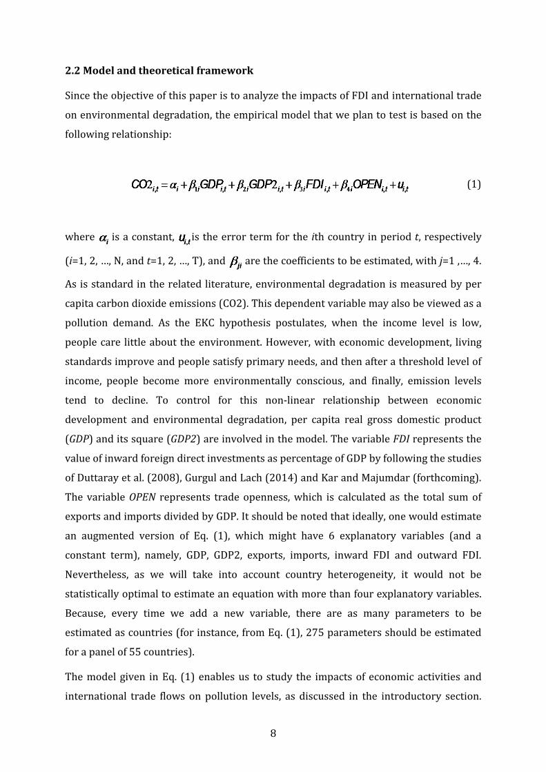
Since the objective of this paper is to analyze the impacts of FDI and international trade
on environmental degradation, the empirical model that we plan to test is based on the
following relationship:
(1)
where is a constant, is the error term for the ith country in period t, respectively
(i=1, 2, …, N, and t=1, 2, …, T), and are the coefficients to be estimated, with j=1 ,…, 4.
As is standard in the related literature, environmental degradation is measured by per
capita carbon dioxide emissions (CO2). This dependent variable may also be viewed as a
pollution demand. As the EKC hypothesis postulates, when the income level is low,
people care little about the environment. However, with economic development, living
standards improve and people satisfy primary needs, and then after a threshold level of
income, people become more environmentally conscious, and finally, emission levels
tend to decline. To control for this non-linear relationship between economic
development and environmental degradation, per capita real gross domestic product
(GDP) and its square (GDP2) are involved in the model. The variable FDI represents the
value of inward foreign direct investments as percentage of GDP by following the studies
of Duttaray et al. (2008), Gurgul and Lach (2014) and Kar and Majumdar (forthcoming).
The variable OPEN represents trade openness, which is calculated as the total sum of
exports and imports divided by GDP. It should be noted that ideally, one would estimate
an augmented version of Eq. (1), which might have 6 explanatory variables (and a
constant term), namely, GDP, GDP2, exports, imports, inward FDI and outward FDI.
Nevertheless, as we will take into account country heterogeneity, it would not be
statistically optimal to estimate an equation with more than four explanatory variables.
Because, every time we add a new variable, there are as many parameters to be
estimated as countries (for instance, from Eq. (1), 275 parameters should be estimated
for a panel of 55 countries).
The model given in Eq. (1) enables us to study the impacts of economic activities and
international trade flows on pollution levels, as discussed in the introductory section.
9
More specifically, depending on the significance and the sign of the estimated
parameters, we are able to distinguish three effects. First, the income effect can be
captured by the parameters and . The income-emissions nexus follows an inverted
U-shaped pattern (i.e. EKC) if and . Some countries in the panel may
experience such a pattern for at least three reasons: first, there may be a structural
transformation in the composition of economic activities, which modifies energy
intensity and carbon intensity of the economy; second, increase in environmental
awareness and knowledge (or increasing demand by consumers for environmentally
friendly products) leads to a reduction in environmental degradation; and third,
establishment of strict environmental regulations to reduce the level of pollutant
emissions (Suri and Chapman, 1998).
The second effect that can be studied by the estimation of Eq. (1) is the inward FDI
effect. Different hypotheses can be suggested depending on the sign of . A positive
suggests that inward FDI contributes to the development of a pollutant sector. Such a
situation may occur if the host country has lax environmental regulations, validating
thus the pollution haven hypothesis. This is most likely to happen for the case of a
developing country. On the contrary, if the host country is a developed one, which is
very likely to have more stringent environmental policies, factor endowments should be
viewed as the main driving force behind inward FDI. If is found to have a negative
sign, the technique effect should be put forward. Then it might be concluded that inward
FDI allow financing (for developed countries) or distribution of (for developing
countries) more efficient production technologies that can curb pollution emissions.
The last effect that can be deduced from Eq. (1) is called openness effect and can be
examined by the estimated sign of . If all three effects of Grossman and Krueger
(1991) that we discussed above (i.e. scale, technique and composition effects) are
present, the sign of depends on which effect outweighs the others. For instance, if it
is found to be positive (negative), it should be concluded that the scale (technique) effect
dominates the others in determining the overall impact of trade openness on CO2
emissions.
10
2.3 Preliminary analysis
We begin our empirical analysis by employing panel data techniques to estimates Eq.
(1). First, we examine the stationarity properties of the variables by using a battery of
panel unit root tests.5 If all variables are found to be non-stationary and cointegrated,
then the relationship under examination can be studied in a standard cointegration
framework (such as panel dynamic ordinary least squares (DOLS) estimator proposed
by Kao and Chiang (2000)). However, if the variables involved in the analysis are a
mixture of I(0) and I(1) processes, we should follow Pesaran et al. (1999) and estimate
a dynamic fixed effects model in a panel auto-regressive distributed lag (ARDL)
structure. This method has an advantage over the static fixed-effects estimator since it
allows for dynamics. But the most important feature of this method is that it yields
consistent estimates if the variables are either I(1) or I(0) (Pesaran et al., 1996). As a
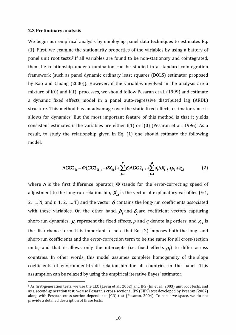
result, to study the relationship given in Eq. (1) one should estimate the following
model.
(2)
where is the first difference operator, stands for the error-correcting speed of
adjustment to the long-run relationship, is the vector of explanatory variables (i=1,
2, …, N, and t=1, 2, …, T) and the vector contains the long-run coefficients associated
with these variables. On the other hand, and are coefficient vectors capturing
short-run dynamics, represent the fixed effects, p and q denote lag orders, and is
the disturbance term. It is important to note that Eq. (2) imposes both the long- and
short-run coefficients and the error-correction term to be the same for all cross-section
units, and that it allows only the intercepts (i.e. fixed effects ) to differ across
countries. In other words, this model assumes complete homogeneity of the slope
coefficients of environment-trade relationship for all countries in the panel. This
assumption can be relaxed by using the empirical iterative Bayes’ estimator. 5 As first-generation tests, we use the LLC (Levin et al., 2002) and IPS (Im et al., 2003) unit root tests, and as a second-generation test, we use Pesaran’s cross-sectional IPS (CIPS) test developed by Pesaran (2007) along with Pesaran cross-section dependence (CD) test (Pesaran, 2004). To conserve space, we do not provide a detailed description of these tests.

11
2.4 The empirical iterative Bayes’ estimator
In order to better take into consideration the cross-country heterogeneity, we will use
the empirical iterative Bayes’ estimator, which is a shrinkage-type estimator. According
to Maddala et al. (1997), in the panel data analysis, it is customary to pool the
observations, with or without individual-specific dummies. These dummy variables are
assumed to be fixed (fixed-effects models, named FE models) or random (random-
effects or variance-components models, named RE models). In RE models, heterogeneity
is modeled through the random effects (individual and temporal) absorbed into the
regression residual term. This procedure, however, assumes a complete homogeneity of
the slope coefficients. On the other hand, when the time series estimation is used to
obtain separate estimates of cross-section coefficients, the parameters are all assumed
to be different. This implies that the equations should be estimated separately for each
country rather than obtaining an overall pooled estimate.
For Maddala et al. (1997), the reality is situated between complete homogeneity and
complete heterogeneity. “The truth probably lies somewhere in between. The
parameters are not exactly the same, but there is some similarity between them. One
way of allowing for the similarity is to assume that the parameters all come from a joint
distribution with a common mean and a nonzero covariance matrix” (Maddala et al.,
1997, p. 91). The authors show that the resulting parameter estimates are a weighted
average of the overall pooled estimate and the separate time-series estimates based on
each cross-section. In this framework, the empirical Bayes method allows us to calculate
the shrinkage-type estimators, that is, each individual estimator is shrunk toward the
overall pooled estimate.
Maddala et al. (1997) and Hsiao et al. (1999) show that, in the case of panel data models
with coefficient heterogeneity, this method provides more stable estimates and better
predictions, since the two other estimation methods, of either pooling the data or
obtaining separate estimates for each cross-section are based on extreme assumptions
(namely, cross-sectional homogeneity and heterogeneity of slope coefficients). Similarly,
Maddala and Hu (1996) have presented some Monte Carlo evidence to demonstrate that
the iterative procedure gives better estimates for panel data models. Furthermore, Hsiao
(2003) and Trapani and Urga (2009) also confirmed that in the case of panel data
models with coefficient heterogeneity, the shrinkage estimators should be preferred,
12
even when the time dimension is small. We describe the structure of this estimation
procedure in Appendix B.
3. Results and discussion
3.1 Results
As described in the previous section, we test for stationarity of the variables in order to
decide which estimation procedure to use in the preliminary analysis. Applying the
above-mentioned panel unit root tests we find that FDI is a stationary process (i.e. I(0))
while the remaining variables are integrated of order 1 (i.e. I(1)).6 On the basis of this
result, we follow Pesaran et al. (1996) and estimate Eq. (2). The results are given in
Table 1.
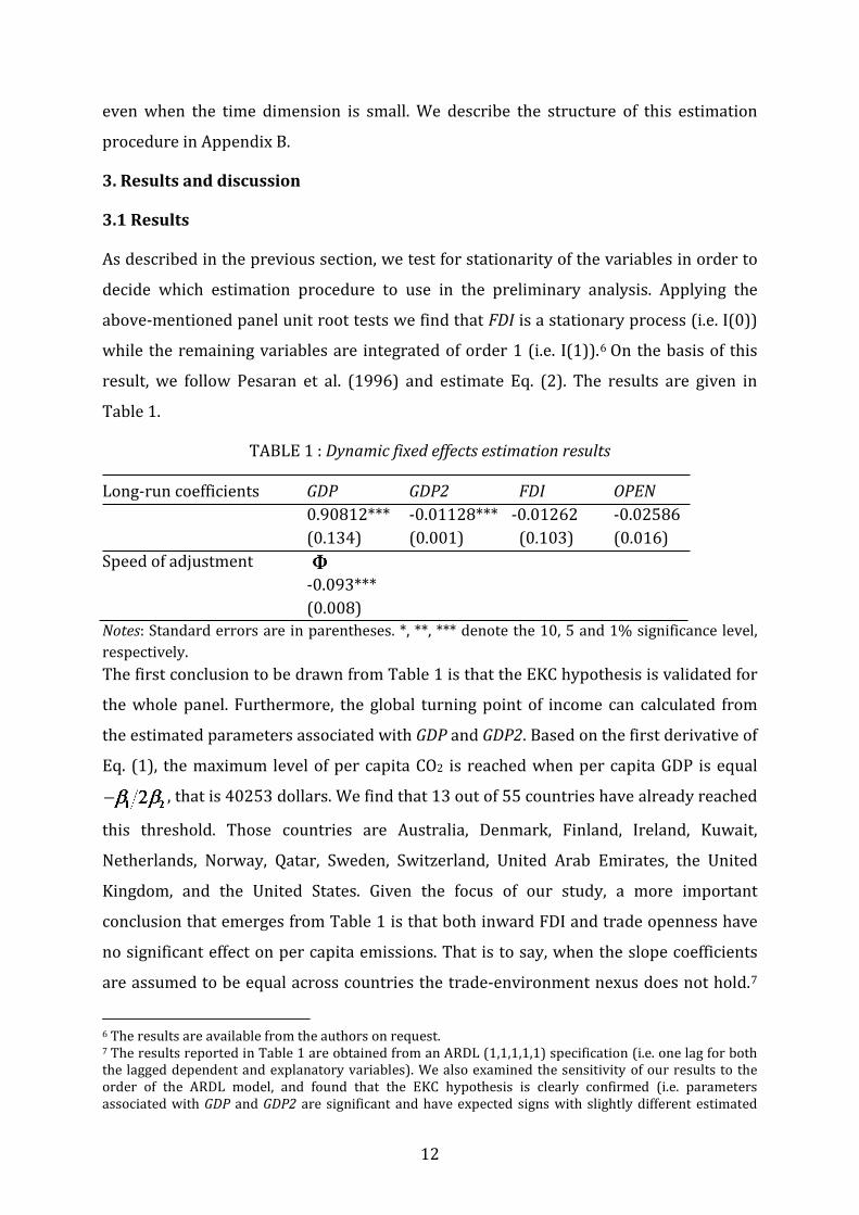
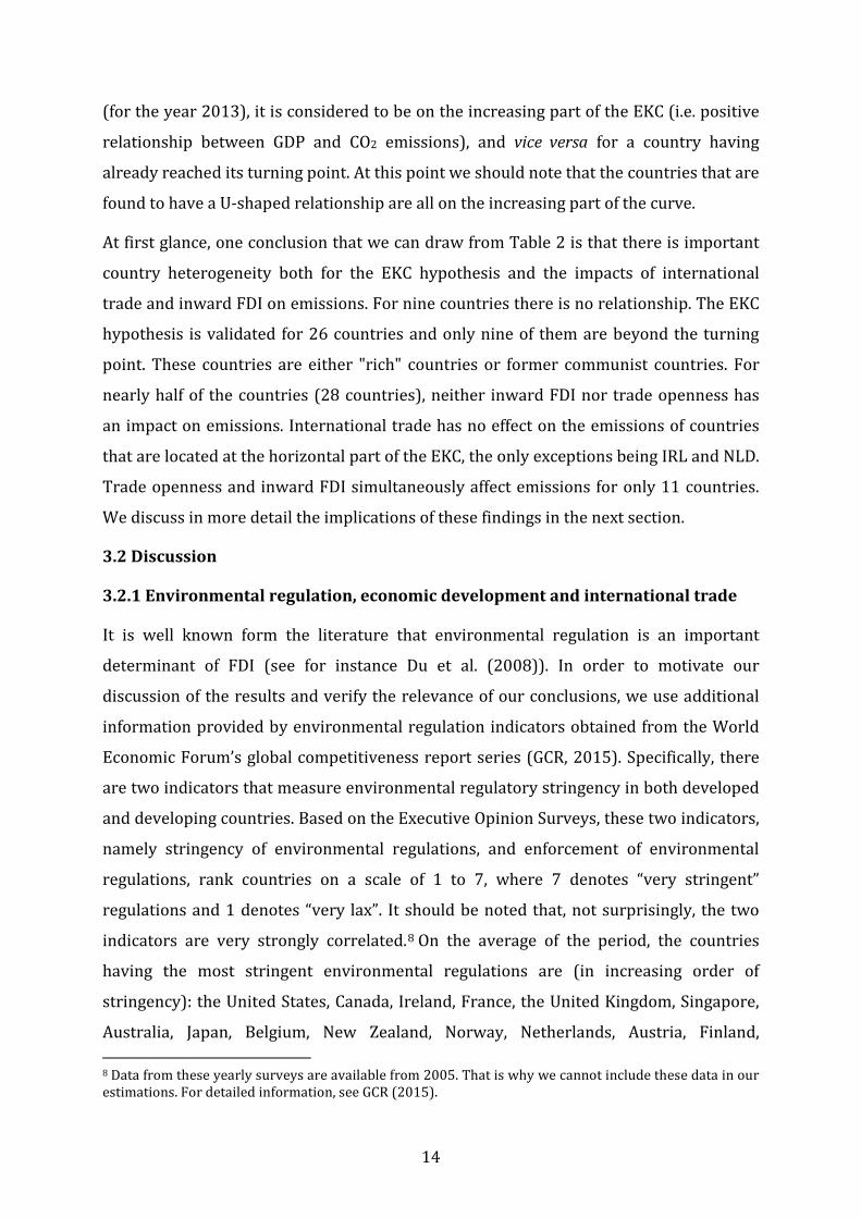
TABLE 1 : Dynamic fixed effects estimation results Long-run coefficients GDP GDP2 FDI OPEN
0.90812*** -0.01128*** -0.01262 -0.02586 (0.134) (0.001) (0.103) (0.016) Speed of adjustment
-0.093*** (0.008) Notes: Standard errors are in parentheses. *, **, *** denote the 10, 5 and 1% significance level, respectively. The first conclusion to be drawn from Table 1 is that the EKC hypothesis is validated for
the whole panel. Furthermore, the global turning point of income can calculated from
the estimated parameters associated with GDP and GDP2. Based on the first derivative of
Eq. (1), the maximum level of per capita CO2 is reached when per capita GDP is equal
, that is 40253 dollars. We find that 13 out of 55 countries have already reached
this threshold. Those countries are Australia, Denmark, Finland, Ireland, Kuwait,
Netherlands, Norway, Qatar, Sweden, Switzerland, United Arab Emirates, the United
Kingdom, and the United States. Given the focus of our study, a more important
conclusion that emerges from Table 1 is that both inward FDI and trade openness have
no significant effect on per capita emissions. That is to say, when the slope coefficients
are assumed to be equal across countries the trade-environment nexus does not hold.7
6 The results are available from the authors on request. 7 The results reported in Table 1 are obtained from an ARDL (1,1,1,1,1) specification (i.e. one lag for both the lagged dependent and explanatory variables). We also examined the sensitivity of our results to the order of the ARDL model, and found that the EKC hypothesis is clearly confirmed (i.e. parameters associated with GDP and GDP2 are significant and have expected signs with slightly different estimated

13
As we described above, there is a considerable degree of heterogeneity among the
countries in terms of CO2 emissions and economic development levels, as well as FDI
flows and trade openness. It is thus evident that this issue of heterogeneity becomes
particularly important within the context of actual debates about whether trade
openness and FDI flows increase or decrease emissions. To address this, we employ the
above-described empirical iterative Bayes’ estimator, and the estimation results are
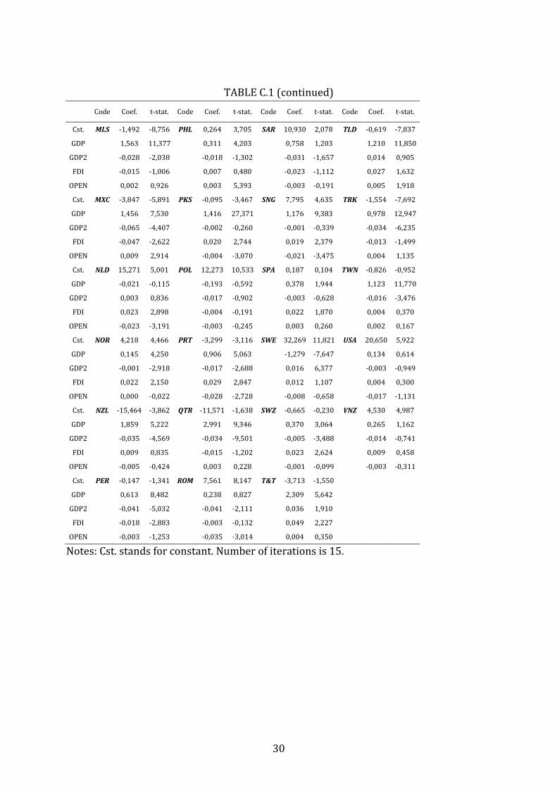
given in Table C.1 in Appendix C. To facilitate the interpretation of these results, we
consider Table 2, which presents the information provided in Table C.1 with a focus on
the estimated environment-trade relationships for each country.
TABLE 2 : Summary of estimation results state by state
OPEN FDI GDP and GDP2 Neutral Positive Negative
Neutral
Neutral
AUT; CND; FND; POL; SAR; AFR; USA; VNZ; SPA
ARG; GRC; IND; KWT; MLS; KOR; TWN; TRK; EMI; IRN; PHL; SWE; TLD
AUS (2003); DNK (1983); ISR (2012); NZL (2003); QTR (1997); FRA
Positive NOR; ECD; JPN; T&T SWZ (1979) Negative PER
Positive Neutral IRL CHK; EGY; INS; CHN BLG Positive Negative MXC GER (1970)
Negative
Neutral CLM; ALG ROM (1992)
Positive NLD PRT; BEL; BRZ; CHL;
ITL; PKS; SNG GBR
Negative HUN (1999) Notes: Countries shown in bold, italic and underlined codes are those having inverted U-shape, U-shape and linear relationship, respectively.
Let us first discuss some examples on how Table 2 is to be read. For a given country, if a
parameter is non-significant at the 5% level in Table C.1, we conclude in Table 2 that the
variable associated with that parameter has no impact on CO2 emissions. On the other
hand, if a country following an EKC pattern has not yet reached the turning point income
values, which yields a somewhat different global turning point income), and that our variables of interest FDI and OPEN remain non-significant.
14
(for the year 2013), it is considered to be on the increasing part of the EKC (i.e. positive
relationship between GDP and CO2 emissions), and vice versa for a country having
already reached its turning point. At this point we should note that the countries that are
found to have a U-shaped relationship are all on the increasing part of the curve.
At first glance, one conclusion that we can draw from Table 2 is that there is important
country heterogeneity both for the EKC hypothesis and the impacts of international
trade and inward FDI on emissions. For nine countries there is no relationship. The EKC
hypothesis is validated for 26 countries and only nine of them are beyond the turning
point. These countries are either "rich" countries or former communist countries. For
nearly half of the countries (28 countries), neither inward FDI nor trade openness has
an impact on emissions. International trade has no effect on the emissions of countries
that are located at the horizontal part of the EKC, the only exceptions being IRL and NLD.
Trade openness and inward FDI simultaneously affect emissions for only 11 countries.
We discuss in more detail the implications of these findings in the next section.
3.2 Discussion
3.2.1 Environmental regulation, economic development and international trade
It is well known form the literature that environmental regulation is an important
determinant of FDI (see for instance Du et al. (2008)). In order to motivate our
discussion of the results and verify the relevance of our conclusions, we use additional
information provided by environmental regulation indicators obtained from the World
Economic Forum’s global competitiveness report series (GCR, 2015). Specifically, there
are two indicators that measure environmental regulatory stringency in both developed
and developing countries. Based on the Executive Opinion Surveys, these two indicators,
namely stringency of environmental regulations, and enforcement of environmental
regulations, rank countries on a scale of 1 to 7, where 7 denotes “very stringent”
regulations and 1 denotes “very lax”. It should be noted that, not surprisingly, the two
indicators are very strongly correlated.8 On the average of the period, the countries
having the most stringent environmental regulations are (in increasing order of
stringency): the United States, Canada, Ireland, France, the United Kingdom, Singapore,
Australia, Japan, Belgium, New Zealand, Norway, Netherlands, Austria, Finland, 8 Data from these yearly surveys are available from 2005. That is why we cannot include these data in our estimations. For detailed information, see GCR (2015).
15
Switzerland, Sweden, Denmark, and Germany. As expected, in this list we find only
industrialized countries. To prove the consistency of our results, countries having
stringent environmental regulations should be found on the downward sloping part of
the EKC, and this is what we observe from Table 2. In fact, the countries for which we
found a negative dynamic relationship between emissions and development are all in
the above list with the exceptions of Qatar, which has a stringency index just below that
of the United States, and the former communist countries Hungary, Romania, Bulgaria.
Jobert et al. (2014) classify these three Central and Eastern European countries as
“ecological despite themselves”, and compositional changes in their industrial outputs
during and after the transition process may explain this common characteristic (Repkine
and Walsh, 1999). On the other hand, among the countries listed above, Singapore,
Japan, Belgium, Norway, Sweden are found to be on the upward sloping part of the EKC.
This finding would seem to contradict the hypothesis that strict environmental
regulations help to reduce CO2 emissions. However, it should be noted that CO2
emissions in these countries increased until the 2000s, and environmental stringency
indicators are only available since 2005.
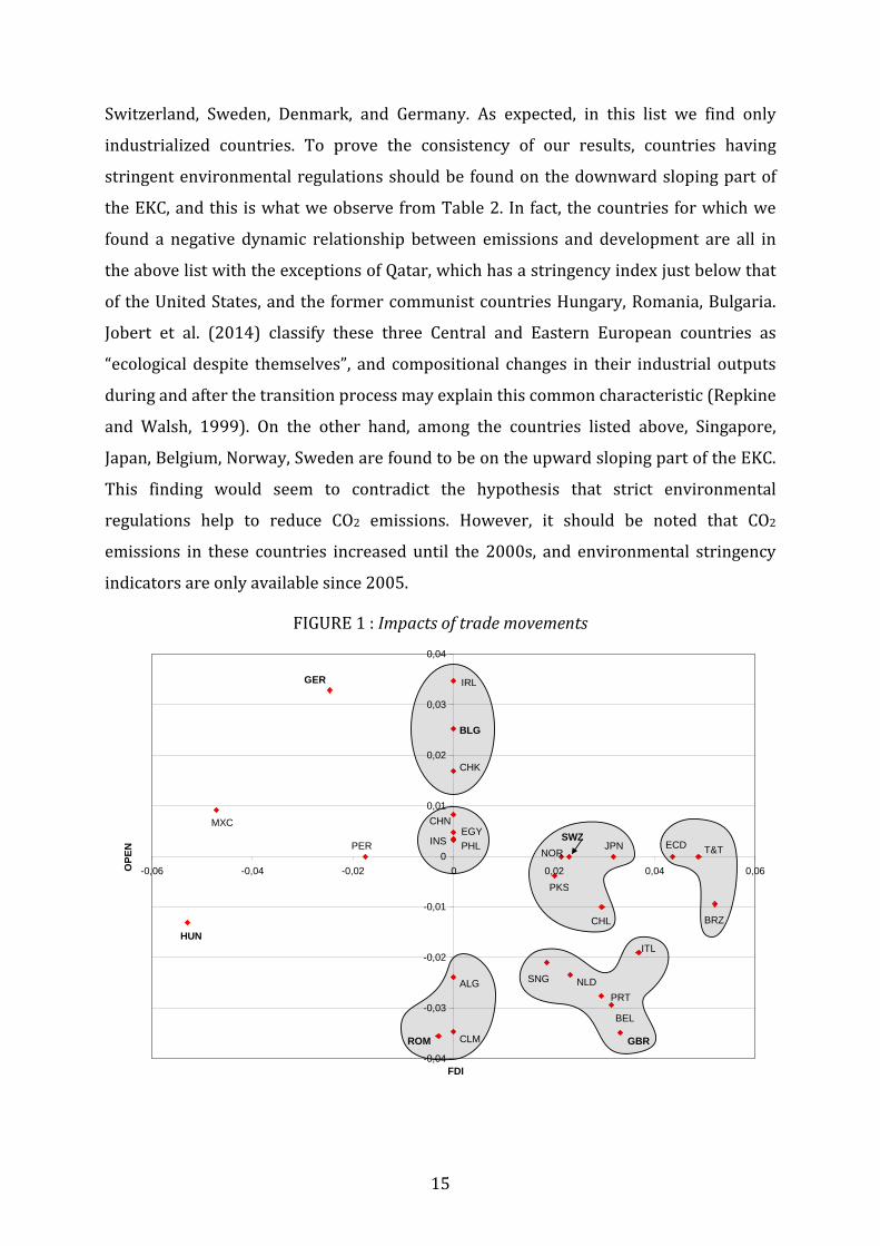
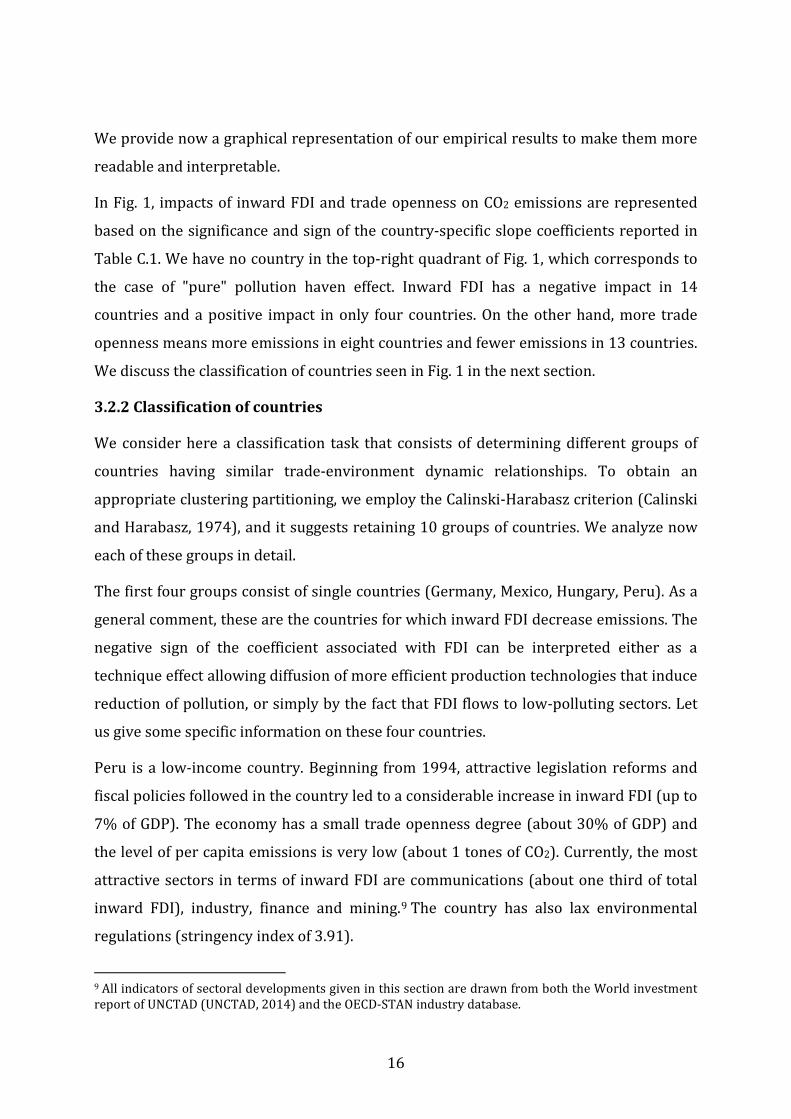
FIGURE 1 : Impacts of trade movements
-0,04
-0,03
-0,02
-0,01
0
0,01
0,02
0,03
0,04
-0,06 -0,04 -0,02 0 0,02 0,04 0,06
FDI
OPE
N
ROM GBRCLM
BEL
PRTALG NLDSNG
ITLHUN
CHL BRZ
PKS
PERNOR
SWZJPN ECD T&TPHLINS
EGYCHNMXC
CHK
BLG
GER IRL
16
We provide now a graphical representation of our empirical results to make them more
readable and interpretable.
In Fig. 1, impacts of inward FDI and trade openness on CO2 emissions are represented
based on the significance and sign of the country-specific slope coefficients reported in
Table C.1. We have no country in the top-right quadrant of Fig. 1, which corresponds to
the case of "pure" pollution haven effect. Inward FDI has a negative impact in 14
countries and a positive impact in only four countries. On the other hand, more trade
openness means more emissions in eight countries and fewer emissions in 13 countries.
We discuss the classification of countries seen in Fig. 1 in the next section.
3.2.2 Classification of countries
We consider here a classification task that consists of determining different groups of
countries having similar trade-environment dynamic relationships. To obtain an
appropriate clustering partitioning, we employ the Calinski-Harabasz criterion (Calinski
and Harabasz, 1974), and it suggests retaining 10 groups of countries. We analyze now
each of these groups in detail.
The first four groups consist of single countries (Germany, Mexico, Hungary, Peru). As a
general comment, these are the countries for which inward FDI decrease emissions. The
negative sign of the coefficient associated with FDI can be interpreted either as a
technique effect allowing diffusion of more efficient production technologies that induce
reduction of pollution, or simply by the fact that FDI flows to low-polluting sectors. Let
us give some specific information on these four countries.
Peru is a low-income country. Beginning from 1994, attractive legislation reforms and
fiscal policies followed in the country led to a considerable increase in inward FDI (up to
7% of GDP). The economy has a small trade openness degree (about 30% of GDP) and
the level of per capita emissions is very low (about 1 tones of CO2). Currently, the most
attractive sectors in terms of inward FDI are communications (about one third of total
inward FDI), industry, finance and mining.9 The country has also lax environmental
regulations (stringency index of 3.91).
9 All indicators of sectoral developments given in this section are drawn from both the World investment report of UNCTAD (UNCTAD, 2014) and the OECD-STAN industry database.
17
Mexico is also a low-income country. During the study period, per capita emissions have
sharply increased in the country (from 1.5 tones of CO2 to 4 tones). There has been a
very rapid growth of inward FDI (an increase of 400%) that reached 3% of GDP, and the
economy opens to international trade significantly (currently 60% of GDP, which was
only 7% in the 1970s). These trends made Mexico one of the most FDI-intensive
emerging countries. FDI are concentrated along the cities on the Mexico-US border,
where assembly plants, called “maquiladoras”, are located (see Hadjimarcou (2013) for
a discussion). The most FDI-intensive sectors are financial services, automotive,
electronics, and energy. Environmental regulations in the country are not very stringent
(with an index value of 4.01).
Hungary is a middle-income country that received a lot of FDI in the 1990s (5% of GDP),
and its degree of openness increased drastically (from 50% to 160%). Per capita CO2
emissions (currently 6 tones of CO2) follow a downward trend. Recently, the inward FDI
that the country receives shifted from both textile sectors with low value added and the
food industry to luxury vehicle sector, renewable energy, luxury tourism, and
information technologies. The index of environmental regulation is mediocre (namely
4.68). Overall, Hungary is a country for which both FDI and international trade are found
to be environmentally friendly.
Germany is an industrialized country, for which trade openness is found to be sharply
increasing the level of emissions and inward FDI decreasing it slightly. It has a high level
of CO2 emissions (12 tones of CO2), although having a decreasing trend. It is a very open
economy (over 100% of GDP), but receives only a small amount of FDI (less than 1%).
The key sectors for FDI are financial intermediation (almost 50% of FDI in 2012), real
estate, renting and business activities (over 25% of FDI) and transport, storage and
communication, and trade and repairs.
Let us now analyze the remaining six groups of countries. The first one is composed of
Bulgaria, Hong Kong and Ireland. Trade openness decreases environmental quality and
FDI has no impact. There is heterogeneity with respect to these countries’ per capita
incomes, but they all experienced strong economic growth (more than 250% over the
study period). They have similar levels of CO2 emissions (7 tones of CO2) and high
degrees of openness (over 100%). In consequence, this group is a group of “prosperous
traders and polluters” with a strong scale effect of international trade flows.
18
The second group is composed of China, Egypt, Indonesia and Philippines. While trade
openness slightly increases pollution, there is no FDI effect. In fact, the negative impact
of trade openness in both China and Philippines was already confirmed by Hossain
(2011). All four countries belong to low-income group of countries, having similar levels
of per capita income (about 1000 dollars), and small degrees of openness (less than
50%). On the other hand, although the level of CO2 emissions in these countries has
increased considerably during the last decades, it remains at a reasonable level (less
than 3 tones of CO2, except for China whose emissions doubled in the last decade and
reached the level of 7 tones of CO2). In support to this finding, He (2006) shows that the
overall impact of FDI on the environmental pollution in Chinese industry is very weak
(1% increase in FDI rise emissions only by 0.099%). Consequently the countries of this
group should be considered as emerging countries with again dominant scale effect of
trade.
Algeria, Colombia and Romania form the third group of countries. While trade openness
improves significantly the environment, FDI has no effect. The average per capita
income is about 3000 dollars; per capita CO2 emissions levels are relatively low (less
than 4 tones); and trade openness is quite small (less than 50%). Thus, the central
characteristic of the countries of this group is that they are middle-income countries
benefiting from the composition and/or technique effect.
Two remarks should be made at this stage. First, what differentiate Romania from
Bulgaria are the level of FDI flows received since 1991 (Bulgaria’s inward FDI are about
half of Romania’s inward FDI), and the degree of openness. Although both of the
countries had almost the same average growth rates over the period we studied,
Romania has reduced its per capita emissions two times more rapidly than Bulgaria.
Inward FDI in Romania are directed towards the industrial sector and metallurgy,
whereas in Bulgaria FDI have flowed into the real estate, finance and trade sectors.
Second, the difference between the second and the third groups of countries is the level
of per capita income.
In the forth group of countries, which includes Belgium, the United Kingdom, Italy,
Netherlands, Portugal, Singapore, trade openness greatly improves the environment,
while FDI inflows deteriorate it. These are countries that have a high index of
environmental regulation (slightly less strong for Portugal and Italy). As the main
19
characteristic of the countries in this group, we may indicate that they are industrialized
countries with strong composition and factor endowments effects. Note also that, except
Singapore, the countries in this group are all OECD countries and the beneficial impact of
trade on the environment was previously found by Managi et al. (2009), who reported
that a 1% increase in trade openness causes a decrease of 0.018% in CO2 emissions in
OECD countries.
For another group of countries made up of Brazil, Ecuador, and Trinidad and Tobago,
inward FDI strongly increase CO2 emissions. These are countries that have relatively low
index of stringency of environmental regulations. With its natural resources, Trinidad
and Tobago has an energy sector that alone represents 40% of GDP and 86% of total
exports, attracting an important amount of FDI. It experienced a strong development of
the steel and aluminum industries, which transformed the economy to a heavy polluter.
Brazil is the most inward FDI-intensive economy in Latin America and the fifth
worldwide destination for FDI inflows. The sectors that most attract FDI are finance
sector followed by polluting industries such as chemical or beverage industries, oil and
gas. Ecuador has a very low level of FDI that mainly come from countries in the region
and flow into the oil sector. Overall, it is reasonable to conclude that these are the
countries that are victims of pollution haven, which is in line with the findings of Blanco
et al. (2013).
Finally, the last group of countries is constituted by Chile, Japan, Norway, Pakistan,
Switzerland. In this group, FDI inflows deteriorate slightly the environment, and trade
openness improves it only for the less developed countries of the group (i.e. Pakistan
and Chile). There is important degree of heterogeneity in this group in terms of both per
capita income and stringency of environmental regulations. High-income countries of
the group have high stringency indexes (e.g. 6.33 for Switzerland), Pakistan has a very
low (3.13) and Chile has an intermediate (4.57) index. On the other hand, Chile has
received substantial FDI flows beginning from 1990 (with half of the inward FDI
directed to mining sector), while other countries of the group have not. While in Japan,
FDI have flowed into the sectors like electrical machinery (36.5%), glass and ceramics
(22.2%), and finance and insurance (15.8%), in Norway the most attractive industries
have been oil and gas (50%), followed by manufacturing, retail and wholesale trade, and
banking. In Pakistan the telecommunications sector remains the major recipient of FDI,
20
followed by financial and energy sectors. In Switzerland, finance (52.1%), trade (18.4%)
and chemicals and plastics (7%) are the biggest recipient sectors of FDI. We should
finally note that the common characteristic of the countries in this group (besides the
fact that they are all highlands) is that they are slightly or moderately open to
international trade.
4. Conclusions and policy implications
Empirical analysis of the relationship between CO2 emissions and international trade
presents two simultaneous problems: the first one is heterogeneity of countries, and the
second one is the effect of aggregation of international trade data for a given country.
The use of the empirical iterative Bayes’ estimator allows dealing with the heterogeneity
problem while standard panel estimators may fall short of solving it. In this paper, the
results obtained by using the empirical iterative Bayes’ estimator are indeed
interpretable, which led us to identify countries for which international trade
movements decrease pollution and those for which they increase it. Consequently, the
pollution haven hypothesis seems to be confirmed for some countries, and not for
others.
Global per capita CO2 emissions stagnated between 1970 and 2002. Since then, we
observe an increase of 20% in emissions. Our results show that it is empirically
unrealistic to believe in the existence of EKC that would solve the climate change
problem once a certain level of development is reached. This problem will be the focus
of the 21st Session of the Conference of the Parties to the United Nations Framework
Convention on Climate Change (COP21/CMP11) that will be organized in Paris at the
end of this year with the aim of achieving a new international agreement on the climate
in order to keep global warming below 2°C. In order to be successful, such an agreement
should be binding and applicable to all countries. However, in view of the results
presented in this paper, to obtain a consensus or a convergence of the countries’
priorities seems to be a hard row to hoe. Indeed, as shown in this study, the trade-
environment nexus involves significant heterogeneity not only at the global level but
also within the developed countries that have a crucial role in climate negotiations. It is
evident that these countries should provide technological and financial assistance to
developing economies in order to support their adaptation and mitigation efforts. In line
of this argument, since we found that both composition and technique effects are
21
significant in some countries, reducing trade barriers for climate-friendly technologies
may be seen particularly important for mitigation policies. Equally importantly, the
effect of carbon constraining regulations on the countries’ competitiveness should be
considered in all its aspects in order not to yield substantial carbon leakage. Both the
heterogeneous structure of the trade-environment nexus and differences in
environmental regulations among countries indicate that some countries (and naturally
some sectors) are more at risk of carbon leakage. That is why, while negotiating an
international agreement on climate change, mitigation efforts have to be discussed on a
country-by-country (even sector-by-sector) basis. As such, energy and environmental
policies can be designed in a manner that distinguishes countries with respect to their
capabilities to mitigate, and that accounts for differences in their income levels and
trade structures.
Related to these policy issues, within the framework that this study proposed, a number
of extensions can be considered. First, to make a more complete assessment of the
impacts of international trade on the environment, for each country similar models
would be estimated at the sectoral level (or even sub-sectoral level) to control for
composition effects depending on the degree of pollution in each sector (or sub-sector).
On the other hand, for countries in which legislations may differ from state to state (e.g.
the United States), it would be more appropriate to conduct an analysis at the state level.
Future research may focus on these dimensions.
References
Aghion, P., Howitt, P., 1992. A Model of Growth Through Creative Destruction.
Econometrica 60, 323-351.
Aichele, R., Felbermayr, G., 2015. Kyoto and carbon leakage: An empirical analysis
of the carbon content of bilateral trade. Review of Economics and Statistics 97, 104-115.
Blanco, L., Gonzalez, F., Ruiz, I., 2013. The impact of FDI on CO2 emissions in Latin
America. Oxford Development Studies 41, 104-121.
British Petroleum (BP), 2014. Statistical Review of World Energy 2014.
Brunnermeier, S., Levinson, A., 2004. Examining the Evidence on Environmental
Regulations and Industry Location. Journal of the Environment and Development 13, 6-
41.

22
Caliński, T., Harabasz, J., 1974. A dendrite method for cluster analysis.
Communications in Statistics-theory and Methods 3, 1-27.
Copeland, B.R., Taylor, M.S., 1994. North–South trade and the environment.
Quarterly Journal of Economics 109, 755-787.
Copeland, B.R., Taylor, M.S., 2004. Trade, growth, and the environment. Journal of
Economic Literature 42, 7-71.
Dong, Y., Ishikawa, M., Liu, X., & Wang, C., 2010. An analysis of the driving forces
of CO 2 emissions embodied in Japan–China trade. Energy Policy 38, 6784-6792.
Du, J., Lu, Y., Tao, Z., 2008. Economic institutions and FDI location choice:
Evidence from US multinationals in China. Journal of Comparative Economics 36, 412-
429
Duttaray, M., Dutt, A.K., Mukhopadhyay, K., 2008. Foreign direct investment and
economic growth in less developed countries: an empirical study of causality and
mechanisms. Applied Economics 40, 1927-1939.
Ederington, J., Minier, J., 2003. Is Environmental Policy a Secondary Trade
Barrier? An Empirical Analysis. Canadian Journal of Economics 36, 137-54.
Esty, D.C., Geradin, D., 1998. Environmental Protection and International
Competitiveness: A Conceptual Framework. Yale Law School Faculty Scholarship Series.
Paper 445.
GCR, 2015. Global Competitiveness Report, World Economic Forum, Switzerland.
Grether, J.M., De Melo, J., 2003. Globalization and dirty industries: Do pollution
havens matter? NBER Working Paper n. 9776, Cambridge, MA, USA.
Grossman, G., Helpman, E., 1991. Quality Ladders in the Theory of Growth.
Review of Economic Studies 58, 43-61.
Grossmann, G., Krueger, A., 1991. Environmental impacts of a North American
free trade agreement. NBER Working Paper No. 3914.
Grossman, G., Krueger, A., 1992. Environmental Impacts of a North American Free
Trade Agreement. Discussion Papers in Economics no. 158, Woodrow Wilson School of
Public and International Affairs, Princeton, NJ.

23
Grossman, G., Krueger, A., 1995. Economic growth and the environment. The
Quarterly Journal of Economics 110, 352-377.
Gurgul, H., Lach, L., 2014. Globalization and economic growth: Evidence from two
decades of transition in CEE. Economic Modelling 36, 99-107.
Hadjimarcou, J., Brouthers, L.E., McNicol, J.P., Michie, D.E., 2013. Maquiladoras in
the 21st century: Six strategies for success. Business Horizons 56, 207-217.
He, J., 2006. Pollution haven hypothesis and environmental impacts of foreign
direct investment: the case of industrial emission of sulfur dioxide (SO2) in Chinese
province. Ecological Economics, 60, 228-245.
Hossain, M.S., 2011. Panel estimation for CO2 emissions, energy consumption,
economic growth, trade openness and urbanization of newly industrialized countries.
Energy Policy 39, 6991-6999.
Hsiao, C., Pesaran, H. M., Tahmiscioglu, K.A., 1999. Bayes estimation of short-run
coefficients in dynamic panel data models. In: Hsiao, C., Lahiri, K., Lee, L.-F., Pesaran, H.
M. (Eds), Analysis of Panels and Limited Dependent Variable Models, Cambridge
University Press, Cambridge, 268-296.
Hsiao, C., 2003. Analysis of Panel Data, Cambridge University Press, Cambridge.
Hubbard, T.P., 2014. Trade and transboundary pollution: quantifying the effects
of trade liberalization on CO2 emissions. Applied Economics 46, 483-502.
Im, K.S., Pesaran, M.H., Shin, Y., 2003. Testing for unit roots in heterogeneous
panels. Journal of Econometrics 109, 53-74.
Jobert, T., Karanfil, F., Tykhonenko, A., 2014. Estimating country-specific
environmental Kuznets curves from panel data: a Bayesian shrinkage approach. Applied
Economics 46, 1449-1464.
Kao, C., Chiang, M.H., 2000. On the estimation and inference of a cointegrated
regression in panel data. Advances in Econometrics 15, 179-222.
Kar, S., Majumdar, D., forthcoming. MFN Tariff Rates and Carbon Emission:
Evidence from Lower-Middle-Income Countries. Environmental and Resource
Economics. doi: 10.1007/s10640-015-9918-9
24
Kohler, M., 2013. CO2 emissions, energy consumption, income and foreign trade:
A South African perspective. Energy Policy 63, 1042-1050.
Lau, L.-S., Choong, C.-K., Eng, Y.-K., 2014. Investigation of the environmental
Kuznets curve for carbon emissions in Malaysia: Do foreign direct investment and trade
matter? Energy Policy 68, 490-497.
Lee, J.W., 2013. The contribution of foreign direct investment to clean energy use,
carbon emissions and economic growth. Energy Policy 55, 483-489.
Levin, A., Lin, C., Chu, C., 2002. Unit root tests in panel data: asymptotic and finite-
sample properties. Journal of Econometrics 108, 1-24.
Levinson, A., Taylor, M.S., 2008. Unmasking the pollution haven effect.
International Economic Review 49, 223-254.
Maddala, G.S., Hu, W., 1996. The Pooling Problem. In: Mátyás, L., Sevestre, P.
(Eds.), The Econometrics of Panel Data: a Handbook of Theory with Applications, Kluwer
Academic Publishers, 2nd Ed. Boston, 307-322.
Maddala, G.S., Li, H., Robert, P., Joutz, F., 1997. Estimation of Short-run and Long-
run Elasticities of Energy Demand From Panel Data Using Shrinkage Estimators. Journal
of Business and Economic Statistics 15, 90-100.
Managi, S., Hibiki, A., Tsurumi, T., 2009. Does trade openness improve
environmental quality? Journal of Environmental Economics and Management 58, 346-
363.
Merlevede, B., Schoors, K., Spatareanu, M., 2014. FDI spillovers and time since
foreign entry. World Development 56, 108-126.
Omri, A. Nguyen, D.K., Rault, C., 2014. Causal interactions between CO2 emissions,
FDI, and economic growth: Evidence from dynamic simultaneous equation models.
Economic Modelling 42, 382-389.
Pesaran, M.H., 2004. General Diagnostic Tests for Cross Section Dependence in
Panels. CESifo Working Papers, no. 1233.
Pesaran, M.H., 2007. A Simple Panel Unit Root Test in the Presence of Cross
Section Dependence. Journal of Applied Econometrics 22, 265-312.

25
Pesaran, M.H., Shin, Y., Smith, R.J., 1996. Testing for the existence of a long-run
relationship. DAE Working Paper no. 9622, Department of Applied Economics,
University of Cambridge.
Pesaran, M.H., Shin, Y., Smith, R.P., 1999. Pooled mean group estimation of
dynamic heterogeneous panels. Journal of the American Statistical Association 94, 621-
634.
Repkine, A., Walsh, P.P., 1999. Evidence of European trade and investment U-
shaping industrial output in Bulgaria, Hungary, Poland, and Romania. Journal of
Comparative Economics 27, 730-752.
Romer, P., 1990. Endogenous Technical Change. Journal of Political Economy 98,
71-102.
Shafik, N., Bandyopadhyay, S., 1992. Economic Growth and Environmental
Quality: Time Series and Cross-Section Evidence. Policy Research Working Paper no.
904, The World Bank, Washington, D.C.
Shahbaz, M., Nasreen, S., Abbas, F., Anis, O., forthcoming. Does Foreign Direct
Investment Impede Environmental Quality in High, Middle and Low-income Countries?
Energy Economics. doi:10.1016/j.eneco.2015.06.014.
Smith, A.F., 1973. A general Bayesian linear model, Journal of the Royal Statistical
Society 35, 67-75.
Suri, V., Chapman, D., 1998. Economic growth, trade and energy: implications for
the environmental Kuznets curve. Ecological Economics 25, 195-208.
Trapani, L., Urga, G., 2009. Optimal forecasting with heterogeneous panels: a
Monte Carlo study, International Journal of Forecasting 25, 567-86.
United Nations Conference on trade and Development (UNCTAD), 2014. World
Investment Report 2014.
United Nations Conference on trade and Development (UNCTAD), 2015.
Handbook of Statistics.
Zarsky, L., 1999. Havens, Halos and Spaghetti: Untangling the Evidence about
Foreign Direct Investment and the Environment. In OECD (Organisation for Economic
26
Co-operation and Development) 1999 Foreign Direct Investment and the Environment,
OECD, Paris, 47-73.
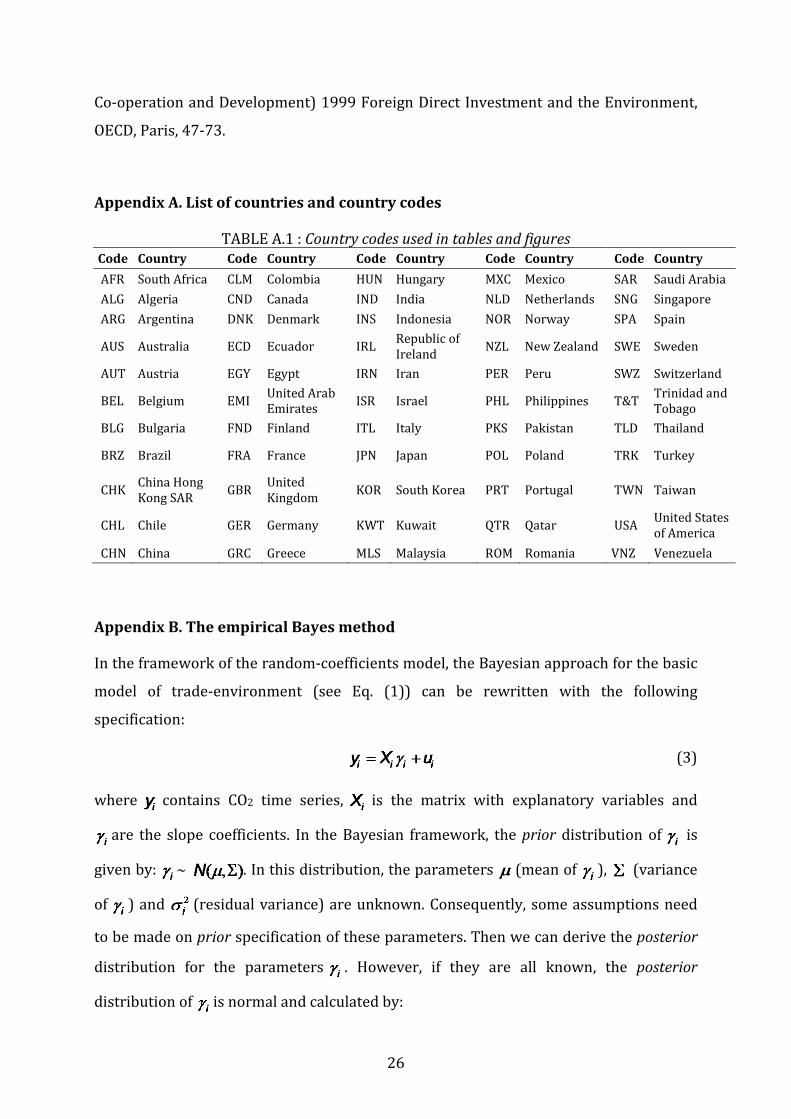
Appendix A. List of countries and country codes
TABLE A.1 : Country codes used in tables and figures Code Country Code Country Code Country Code Country Code Country AFR South Africa CLM Colombia HUN Hungary MXC Mexico SAR Saudi Arabia ALG Algeria CND Canada IND India NLD Netherlands SNG Singapore ARG Argentina DNK Denmark INS Indonesia NOR Norway SPA Spain
AUS Australia ECD Ecuador IRL Republic of Ireland NZL New Zealand SWE Sweden
AUT Austria EGY Egypt IRN Iran PER Peru SWZ Switzerland
BEL Belgium EMI United Arab Emirates ISR Israel PHL Philippines T&T Trinidad and
Tobago BLG Bulgaria FND Finland ITL Italy PKS Pakistan TLD Thailand
BRZ Brazil FRA France JPN Japan POL Poland TRK Turkey
CHK China Hong Kong SAR GBR United
Kingdom KOR South Korea PRT Portugal TWN Taiwan
CHL Chile GER Germany KWT Kuwait QTR Qatar USA United States of America
CHN China GRC Greece MLS Malaysia ROM Romania VNZ Venezuela
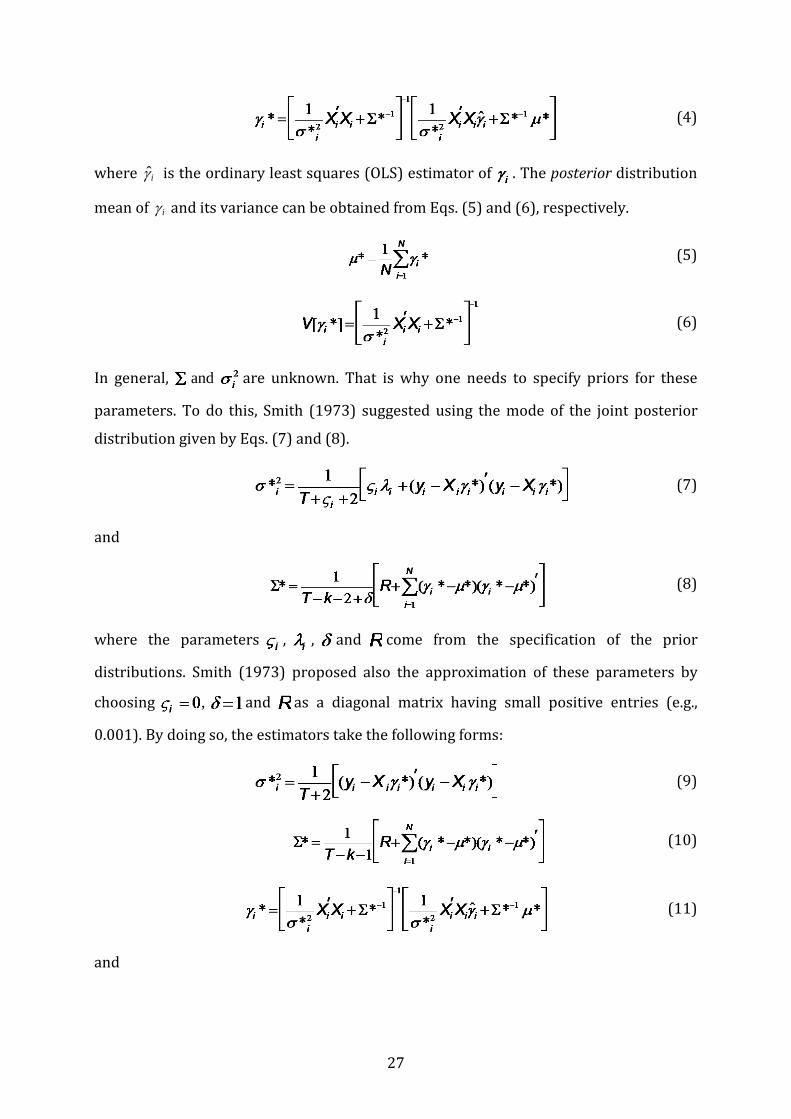
Appendix B. The empirical Bayes method
In the framework of the random-coefficients model, the Bayesian approach for the basic
model of trade-environment (see Eq. (1)) can be rewritten with the following
specification:
(3)
where contains CO2 time series, is the matrix with explanatory variables and
are the slope coefficients. In the Bayesian framework, the prior distribution of is
given by: ∼ . In this distribution, the parameters (mean of ), (variance
of ) and (residual variance) are unknown. Consequently, some assumptions need
to be made on prior specification of these parameters. Then we can derive the posterior
distribution for the parameters . However, if they are all known, the posterior
distribution of is normal and calculated by:
27
(4)
where iγ̂ is the ordinary least squares (OLS) estimator of . The posterior distribution
mean of iγ and its variance can be obtained from Eqs. (5) and (6), respectively.
(5)
(6)
In general, and are unknown. That is why one needs to specify priors for these
parameters. To do this, Smith (1973) suggested using the mode of the joint posterior
distribution given by Eqs. (7) and (8).
(7)
and
(8)
where the parameters , , and come from the specification of the prior
distributions. Smith (1973) proposed also the approximation of these parameters by
choosing , and as a diagonal matrix having small positive entries (e.g.,
0.001). By doing so, the estimators take the following forms:
(9)
(10)
(11)
and
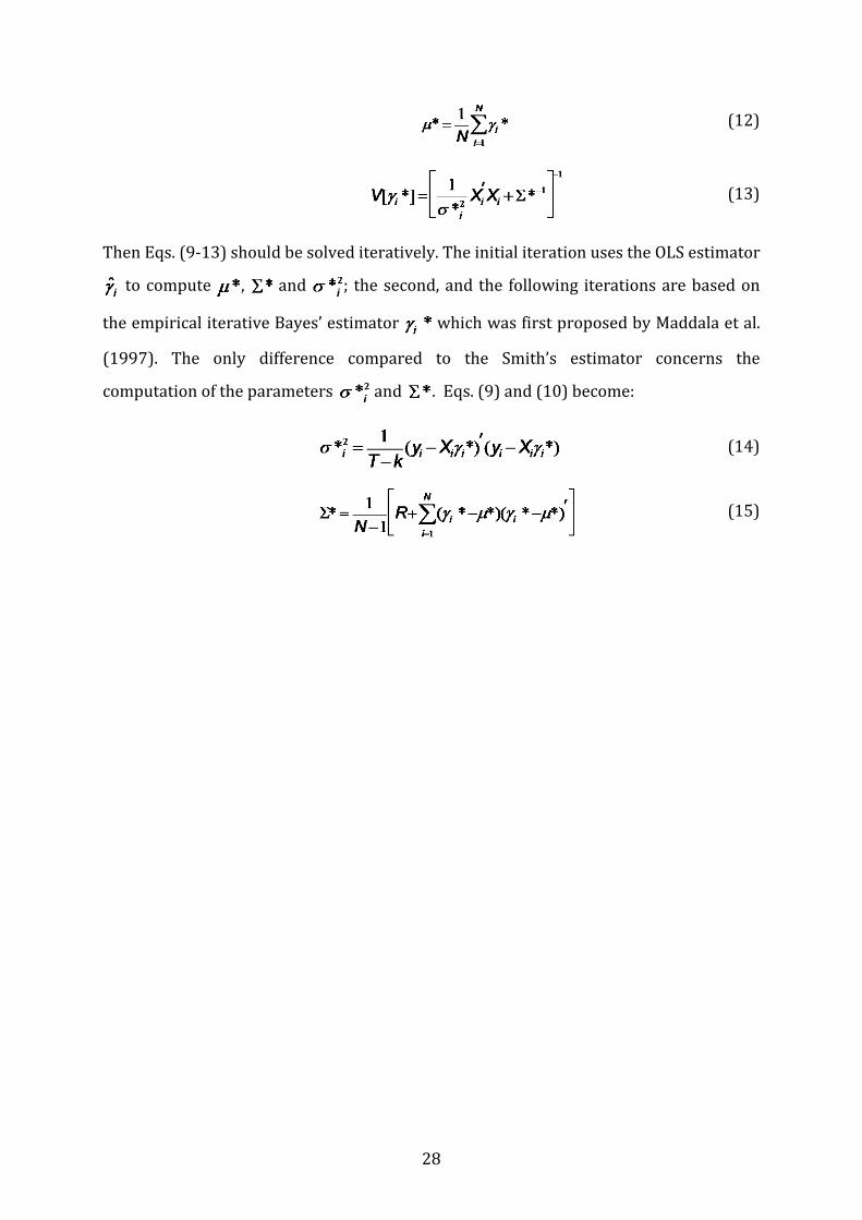
28
(12)
(13)
Then Eqs. (9-13) should be solved iteratively. The initial iteration uses the OLS estimator
to compute , and ; the second, and the following iterations are based on
the empirical iterative Bayes’ estimator which was first proposed by Maddala et al.
(1997). The only difference compared to the Smith’s estimator concerns the
computation of the parameters and . Eqs. (9) and (10) become:
(14)
(15)

29
Appendix C. Shrinkage estimators state by state
TABLE C.1 : Shrinkage estimators state by state Code Coef. t-stat. Code Coef. t-stat. Code Coef. t-stat. Code Coef. t-stat.
Cst. AFR 5,680 3,694 CHK -1,231 -1,715 EMI -2,224 -0,350 INS -0,389 -6,547
GDP 0,495 1,248 0,352 6,494 1,893 7,794 1,379 25,552
GDP2 -0,008 -0,417 -0,004 -2,548 -0,021 -9,057 -0,029 -2,490
FDI 0,006 0,273 0,010 1,463 -0,003 -0,240 -0,015 -1,451
OPEN 0,003 0,236 0,017 3,047 -0,003 -0,179 0,004 2,061
Cst. ALG -1,357 -3,059 CHL 0,353 1,448 FND 5,644 2,424 IRL 1,775 2,086
GDP 1,940 10,031 0,588 6,170 0,311 1,925 0,095 1,065
GDP2 -0,035 -1,769 -0,005 -0,748 -0,005 -1,786 0,000 0,132
FDI -0,005 -0,229 0,030 2,942 0,009 0,828 -0,003 -0,452
OPEN -0,024 -4,596 -0,010 -2,589 0,007 0,518 0,035 3,977
Cst. ARG 1,177 3,470 CHN 0,954 16,388 FRA 17,105 6,232 IRN 0,095 0,088
GDP 0,696 5,159 1,615 21,681 -0,517 -2,490 1,609 4,054
GDP2 -0,029 -2,451 -0,019 -1,191 0,006 1,539 -0,011 -0,528
FDI -0,011 -0,884 -0,015 -0,856 0,014 1,222 -0,002 -0,099
OPEN 0,002 0,549 0,008 2,889 0,000 -0,017 0,010 0,707
Cst. AUS -11,369 -4,927 CLM 0,689 4,557 GBR 17,324 11,278 ISR -11,042 -6,043
GDP 1,668 10,312 0,669 6,862 -0,278 -2,522 1,881 9,084
GDP2 -0,024 -8,843 -0,049 -4,440 0,003 1,380 -0,041 -6,817
FDI 0,003 0,225 -0,006 -0,492 0,033 3,239 -0,011 -1,058
OPEN 0,010 0,677 -0,035 -6,051 -0,035 -2,844 0,004 0,437
Cst. AUT 4,035 2,783 CND 14,926 4,344 GER 9,111 5,285 ITL 8,593 5,622
GDP 0,168 1,811 0,146 0,586 0,423 3,433 -0,166 -1,264
GDP2 -0,002 -1,058 -0,002 -0,384 -0,013 -5,455 0,006 2,041
FDI 0,011 1,039 -0,003 -0,292 -0,025 -2,600 0,037 3,795
OPEN 0,014 1,256 0,011 0,867 0,033 3,605 -0,019 -1,988
Cst. BEL 26,025 7,839 DNK 5,041 1,074 GRC -9,631 -3,521 JPN 14,378 10,321
GDP -0,757 -3,285 0,501 1,978 1,606 4,982 -0,502 -4,864
GDP2 0,016 3,659 -0,008 -2,330 -0,034 -3,712 0,011 5,943
FDI 0,031 3,893 0,019 1,632 -0,002 -0,124 0,032 3,089
OPEN -0,029 -3,104 -0,012 -0,852 -0,001 -0,074 -0,013 -1,202
Cst. BLG 6,436 13,051 ECD -1,248 -7,988 HUN 2,600 2,485 KOR -0,066 -0,145
GDP -0,538 -2,667 0,914 9,557 1,244 5,194 0,912 18,586
GDP2 -0,018 -1,190 0,016 1,240 -0,070 -4,946 -0,009 -3,899
FDI -0,012 -0,754 0,044 3,101 -0,053 -3,159 0,017 1,892
OPEN 0,025 8,057 0,001 0,325 -0,013 -2,872 -0,006 -0,854
Cst. BRZ 0,111 0,826 EGY -0,043 -1,310 IND 0,126 5,399 KWT 6,333 1,212
GDP 0,369 6,261 1,622 53,488 1,288 8,786 0,873 3,576
GDP2 0,011 1,674 -0,015 -2,014 -0,031 -2,128 -0,008 -3,422
FDI 0,052 7,572 -0,001 -0,118 -0,013 -0,828 0,010 0,872
OPEN -0,009 -3,386 0,005 8,954 0,000 0,086 -0,010 -0,662
Notes: Cst. stands for constant. Number of iterations is 15.
30
TABLE C.1 (continued) Code Coef. t-stat. Code Coef. t-stat. Code Coef. t-stat. Code Coef. t-stat.
Cst. MLS -1,492 -8,756 PHL 0,264 3,705 SAR 10,930 2,078 TLD -0,619 -7,837
GDP 1,563 11,377 0,311 4,203 0,758 1,203 1,210 11,850
GDP2 -0,028 -2,038 -0,018 -1,302 -0,031 -1,657 0,014 0,905
FDI -0,015 -1,006 0,007 0,480 -0,023 -1,112 0,027 1,632
OPEN 0,002 0,926 0,003 5,393 -0,003 -0,191 0,005 1,918
Cst. MXC -3,847 -5,891 PKS -0,095 -3,467 SNG 7,795 4,635 TRK -1,554 -7,692
GDP 1,456 7,530 1,416 27,371 1,176 9,383 0,978 12,947
GDP2 -0,065 -4,407 -0,002 -0,260 -0,001 -0,339 -0,034 -6,235
FDI -0,047 -2,622 0,020 2,744 0,019 2,379 -0,013 -1,499
OPEN 0,009 2,914 -0,004 -3,070 -0,021 -3,475 0,004 1,135
Cst. NLD 15,271 5,001 POL 12,273 10,533 SPA 0,187 0,104 TWN -0,826 -0,952
GDP -0,021 -0,115 -0,193 -0,592 0,378 1,944 1,123 11,770
GDP2 0,003 0,836 -0,017 -0,902 -0,003 -0,628 -0,016 -3,476
FDI 0,023 2,898 -0,004 -0,191 0,022 1,870 0,004 0,370
OPEN -0,023 -3,191 -0,003 -0,245 0,003 0,260 0,002 0,167
Cst. NOR 4,218 4,466 PRT -3,299 -3,116 SWE 32,269 11,821 USA 20,650 5,922
GDP 0,145 4,250 0,906 5,063 -1,279 -7,647 0,134 0,614
GDP2 -0,001 -2,918 -0,017 -2,688 0,016 6,377 -0,003 -0,949
FDI 0,022 2,150 0,029 2,847 0,012 1,107 0,004 0,300
OPEN 0,000 -0,022 -0,028 -2,728 -0,008 -0,658 -0,017 -1,131
Cst. NZL -15,464 -3,862 QTR -11,571 -1,638 SWZ -0,665 -0,230 VNZ 4,530 4,987
GDP 1,859 5,222 2,991 9,346 0,370 3,064 0,265 1,162
GDP2 -0,035 -4,569 -0,034 -9,501 -0,005 -3,488 -0,014 -0,741
FDI 0,009 0,835 -0,015 -1,202 0,023 2,624 0,009 0,458
OPEN -0,005 -0,424 0,003 0,228 -0,001 -0,099 -0,003 -0,311
Cst. PER -0,147 -1,341 ROM 7,561 8,147 T&T -3,713 -1,550 GDP 0,613 8,482 0,238 0,827 2,309 5,642
GDP2 -0,041 -5,032 -0,041 -2,111 0,036 1,910 FDI -0,018 -2,883 -0,003 -0,132 0,049 2,227
OPEN -0,003 -1,253 -0,035 -3,014 0,004 0,350 Notes: Cst. stands for constant. Number of iterations is 15.
Documents De travail GreDeG parus en 2015GREDEG Working Papers Released in 2015
2015-01 Laetitia Chaix & Dominique Torre The Dual Role of Mobile Payment in Developing Countries2015-02 Michaël Assous, Olivier Bruno & Muriel Dal-Pont Legrand The Law of Diminishing Elasticity of Demand in Harrod’s Trade Cycle (1936)2015-03 Mohamed Arouri, Adel Ben Youssef & Cuong Nguyen Natural Disasters, Household Welfare and Resilience: Evidence from Rural Vietnam2015-04 Sarah Guillou & Lionel Nesta Markup Heterogeneity, Export Status and the Establishment of the Euro2015-05 Stefano Bianchini, Jackie Krafft, Francesco Quatraro & Jacques Ravix Corporate Governance, Innovation and Firm Age: Insights and New Evidence2015-06 Thomas Boyer-Kassem, Sébastien Duchêne & Eric Guerci Testing Quantum-like Models of Judgment for Question Order Effects2015-07 Christian Longhi & Sylvie Rochhia Long Tails in the Tourism Industry: Towards Knowledge Intensive Service Suppliers2015-08 Michael Dietrich, Jackie Krafft & Jolian McHardy Real Firms, Transaction Costs and Firm Development: A Suggested Formalisation2015-09 Ankinée Kirakozian Household Waste Recycling: Economics and Policy2015-10 Frédéric Marty Régulation par contrat2015-11 Muriel Dal-Pont Legrand & Sophie pommet Nature des sociétés de capital-investissement et performances des firmes : le cas de la France2015-12 Alessandra Colombelli, Jackie Krafft & Francesco Quatraro Eco-Innovation and Firm Growth: Do Green Gazelles Run Faster? Microeconometric Evidence from a Sample of European Firms2015-13 Patrice Bougette & Christophe Charlier La difficile conciliation entre politique de concurrence et politique industrielle : le soutien aux énergies renouvelables2015-14 Lauren Larrouy Revisiting Methodological Individualism in Game Theory: The Contributions of Schelling and Bacharach2015-15 Richard Arena & Lauren Larrouy The Role of Psychology in Austrian Economics and Game Theory: Subjectivity and Coordination2015-16 Nathalie Oriol & Iryna Veryzhenko Market Structure or Traders’ Behaviour? An Assessment of Flash Crash Phenomena and their Regulation based on a Multi-agent Simulation2015-17 Raffaele Miniaci & Michele Pezzoni Is Publication in the Hands of Outstanding Scientists? A Study on the Determinants of Editorial Boards Membership in Economics2015-18 Claire Baldin & Ludovic Ragni L’apport de Pellegrino Rossi à la théorie de l’offre et de la demande : une tentative d’interprétation

2015-19 Claire Baldin & Ludovic Ragni Théorie des élites parétienne et moment machiavélien comme principes explicatifs de la dynamique sociale : les limites de la méthode des approximations successives2015-20 Ankinée Kirakozian & Christophe Charlier Just Tell me What my Neighbors Do! Public Policies for Households Recycling2015-21 Nathalie Oriol, Alexandra Rufini & Dominique Torre Should Dark Pools be Banned from Regulated Exchanges?2015-22 Lise Arena & Rani Dang Organizational Creativity versus Vested Interests: The Role of Academic Entrepreneurs in the Emergence of Management Education at Oxbridge2015-23 Muriel Dal-Pont Legrand & Harald Hagemann Can Recessions be ‘Productive’? Schumpeter and the Moderns2015-24 Alexandru Monahov The Effects of Prudential Supervision on Bank Resiliency and Profits in a Multi-Agent Setting 2015-25 Benjamin Montmartin When Geography Matters for Growth: Market Inefficiencies and Public Policy Implications 2015-26 Benjamin Montmartin, Marcos Herrera & Nadine Massard R&D Policies in France: New Evidence from a NUTS3 Spatial Analysis 2015-27 Sébastien Duchêne, Thomas Boyer-Kassem & Eric Guerci Une nouvelle approche expérimentale pour tester les modèles quantiques de l’erreur de conjonction 2015-28 Christian Longhi Clusters and Collective Learning Networks: The Case of the Competitiveness Cluster ‘Secure Communicating Solutions’ in the French Provence-Alpes-Côte d’Azur Region2015-29 Nobuyuki Hanaki, Eizo Akiyama, Yukihiko Funaki & Ryuichiro Ishikawa Diversity in Cognitive Ability Enlarges Mispricing2015-30 Mauro Napoletano, Andrea Roventini & Jean-Luc Gaffard Time-Varying Fiscal Multipliers in an Agent-Based Model with Credit Rationing2015-31 Thomas Jobert, Fatih Karanfil & Anna Tykhonenko Trade and Environment: Further Empirical Evidence from Heterogeneous Panels Using Aggregate Data