doctorat de l'universitÉ de toulouse · nomenclature latin symbols a speed of sound c chord...
TRANSCRIPT
En vue de l'obtention du
DOCTORAT DE L'UNIVERSITÉ DE TOULOUSEDélivré par :
Institut National Polytechnique de Toulouse (INP Toulouse)
Discipline ou spécialité :Dynamique des fluides
Présentée et soutenue par :M. DAMIEN SZUBERT
le lundi 29 juin 2015
Titre :
Unité de recherche :
Ecole doctorale :
ANALYSE PHYSIQUE ET MODELISATION D'ECOULEMENTS
TURBULENTS INSTATIONNAIRES AUTOUR D'OBSTACLES
AERODYNAMIQUES A HAUT NOMBRE DE REYNOLDS PAR
SIMULATION NUMERIQUE
Mécanique, Energétique, Génie civil, Procédés (MEGeP)
Institut de Mécanique des Fluides de Toulouse (I.M.F.T.)
Directeur(s) de Thèse :MME MARIANNA BRAZA
M. GILLES HARRAN
Rapporteurs :M. BRUNO KOOBUS, UNIVERSITE MONTPELLIER 2
M. GEORGE BARAKOS, UNIVERSITY OF LIVERPOOL
Membre(s) du jury :1 M. ALAIN DERVIEUX, INRIA SOPHIA ANTIPOLIS, Président
2 M. FLAVIEN BILLARD, DASSAULT AVIATION, Membre
2 M. FRANK THIELE, TECHNISCHE UNIVERSITAT BERLIN, Membre
2 M. GILLES HARRAN, INP TOULOUSE, Membre
2 M. JEAN-PAUL DUSSAUGE, UNIVERSITE AIX-MARSEILLE 1, Membre
2 Mme MARIANNA BRAZA, INP TOULOUSE, Membre

Contents
Acknowledgements iii
Nomenclature v
1 Introduction 1
1.1 Objectives of this thesis . . . . . . . . . . . . . . . . . . . . . . . . . 11.2 Governing equations in fluid dynamics . . . . . . . . . . . . . . . . . 2
1.2.1 General transport equation . . . . . . . . . . . . . . . . . . . . 31.2.2 The Navier-Stokes equations . . . . . . . . . . . . . . . . . . . 4
1.2.2.1 Continuity equation . . . . . . . . . . . . . . . . . . 41.2.2.2 Momentum equation . . . . . . . . . . . . . . . . . . 51.2.2.3 Energy equation . . . . . . . . . . . . . . . . . . . . 61.2.2.4 Additional relations . . . . . . . . . . . . . . . . . . 7
1.2.3 The Reynolds-averaged Navier-Stokes equations . . . . . . . . 81.2.4 The eddy-viscosity assumption . . . . . . . . . . . . . . . . . . 91.2.5 Organised-Eddy Simulation . . . . . . . . . . . . . . . . . . . 9
1.3 Thesis outline . . . . . . . . . . . . . . . . . . . . . . . . . . . . . . . 10
2 Tandem of two inline cylinders 13
2.1 Flow analysis - Static case . . . . . . . . . . . . . . . . . . . . . . . . 142.1.1 Context . . . . . . . . . . . . . . . . . . . . . . . . . . . . . . 142.1.2 Test-case description . . . . . . . . . . . . . . . . . . . . . . . 152.1.3 Numerical method . . . . . . . . . . . . . . . . . . . . . . . . 162.1.4 Results . . . . . . . . . . . . . . . . . . . . . . . . . . . . . . . 18
2.1.4.1 Flow overview . . . . . . . . . . . . . . . . . . . . . . 182.1.4.2 Convergence study . . . . . . . . . . . . . . . . . . . 202.1.4.3 Turbulence model study . . . . . . . . . . . . . . . . 212.1.4.4 POD analysis . . . . . . . . . . . . . . . . . . . . . . 27
2.1.5 3D Simulations . . . . . . . . . . . . . . . . . . . . . . . . . . 412.2 Fluid-structure interaction - Dynamic case . . . . . . . . . . . . . . . 43
2.2.1 Introduction . . . . . . . . . . . . . . . . . . . . . . . . . . . . 432.2.2 Results . . . . . . . . . . . . . . . . . . . . . . . . . . . . . . . 43
2.2.2.1 Fluid-structure interaction . . . . . . . . . . . . . . . 432.2.2.2 POD analysis . . . . . . . . . . . . . . . . . . . . . . 45
2.3 Conclusion . . . . . . . . . . . . . . . . . . . . . . . . . . . . . . . . . 49
i
Contents
3 Physics and modelling around two supercritical airfoils 513.1 Shock-vortex shear-layer interaction in transonic buffet conditions . . 51
3.1.1 Shock-vortex shear-layer interaction in the transonic flow arounda supercritical airfoil at high Reynolds number in buffet con-ditions . . . . . . . . . . . . . . . . . . . . . . . . . . . . . . . 52
3.1.2 Upscale turbulence modelling . . . . . . . . . . . . . . . . . . 803.2 Laminar airfoil . . . . . . . . . . . . . . . . . . . . . . . . . . . . . . 81
4 Numerical study of an oblique-shock/boundary-layer interaction 117
5 Conclusion 129
Appendix A Turbulence models 135A.1 One-equation eddy-viscosity models . . . . . . . . . . . . . . . . . . . 135
A.1.1 Spalart-Allmaras model . . . . . . . . . . . . . . . . . . . . . 135A.1.2 Modified Spalart-Allmaras models . . . . . . . . . . . . . . . . 137
A.1.2.1 Edwards-Chandra model . . . . . . . . . . . . . . . . 137A.1.2.2 Secundov’s compressibility correction . . . . . . . . . 137
A.2 Two-equation eddy-viscosity models . . . . . . . . . . . . . . . . . . . 138A.2.1 Chien’s k-ε model . . . . . . . . . . . . . . . . . . . . . . . . . 138A.2.2 Wilcox’ k-ω model . . . . . . . . . . . . . . . . . . . . . . . . 139A.2.3 Menter’s k-ω models . . . . . . . . . . . . . . . . . . . . . . . 139
A.2.3.1 Baseline model . . . . . . . . . . . . . . . . . . . . . 139A.2.3.2 Shear Stress Transport model . . . . . . . . . . . . . 141
Appendix B γ − Rθ laminar/turbulent transition model 143
Appendix C Tecplot 360 147C.1 Quick start . . . . . . . . . . . . . . . . . . . . . . . . . . . . . . . . 148
C.1.1 Load data . . . . . . . . . . . . . . . . . . . . . . . . . . . . . 148C.1.2 2D data . . . . . . . . . . . . . . . . . . . . . . . . . . . . . . 148C.1.3 3D data . . . . . . . . . . . . . . . . . . . . . . . . . . . . . . 150C.1.4 XY lines . . . . . . . . . . . . . . . . . . . . . . . . . . . . . . 151C.1.5 Export and save . . . . . . . . . . . . . . . . . . . . . . . . . . 151
C.2 In more details . . . . . . . . . . . . . . . . . . . . . . . . . . . . . . 152C.3 Scripting . . . . . . . . . . . . . . . . . . . . . . . . . . . . . . . . . . 154
C.3.1 Overview . . . . . . . . . . . . . . . . . . . . . . . . . . . . . 154C.3.2 Examples . . . . . . . . . . . . . . . . . . . . . . . . . . . . . 154
Appendix D Monitoring files extractor GUI 157
ii
Acknowledgements
These three years and half spent in the Institut de Mécanique des Fluides deToulouse let me time and opportunities to meet many people, researchers, colleagues,students, and friends I want to thank here.
I want above all to express my deepest thanks to my supervisor MariannaBRAZA, who offered to me the opportunity to work in a practical way on fluiddynamics, and more particularly on turbulence modelling in the context of the Com-putational Fluid Dynamics, involving various test cases described in this manuscript.I was able to experience supervision of small groups of students, exchanging withthem on technical and scientifical aspects. I also thank her a lot for helping me tosurvive in Stanford during summer 2014 after loosing my credit card, just beforeleaving France. Finally, I appreciated a lot the discussions we had concerning ourvision of the World, society and humanity, with our respective experience and skills.
I am also very thankful to Prof. George Barakos for discussions we had regardingrelations between research and industry, and for sharing is point of view regardingthe situation of research more generally. I thank him as well as Flavien Billard,for their comments and corrections of this manuscript, as well as for sharing theirspecial point of view on specific test cases.
I thank Prof. George Barakos and Prof. Bruno Koobus for having accepted theinvitation to review my thesis. I also wish to thank all other members of the ex-amining committee: Alain Dervieux, Jean-Paul Dussauge, Gilles Harran and Prof.Frank Thiele. I also thank Loïc Boudet, from DGA, and Prof. Julian Hunt, fortaking part of the discussion during the defense. I would like to particularly thankProf. Hunt for sharing his experience and his knowledge that conducted, amongother, to the redaction of an article published in the Journal of Fluid Dynamics.
I want to express special thanks to Fernando Grossi, who helped a lot on phys-ical and technical aspects when I arrived at IMFT for my internship and then forthe beginning of my PhD while he was in first year of his PhD, as well as duringcongresses. I appreciated a lot his point of view regarding the environment andmethod of work.
I would not have been able to do all the work presented here withtout the pre-cious assistance of Yannick Hoarau, regarding mesh generation in particular, butalso for technical, programming aspects, despite his huge amount of work, and Iam very grateful for this. For this last point, I also want to thank Jan Vos, from
iii

Acknowledgements
CFS Engineering, coordinator of the NSMB consortium, and who recieved me fewdays in his head quarters for implementing the transition model based on transportequations in NSMB.
My deepest gratitude to Parviz Moin, director of the Center for Turbulence Re-search, and his team, who received Marianna and me in Stanford during summer2014, and Ik Jang, for the collaboration there. It was a great opportunity to discovera different work environment as well as the culture and lifestyle in Stanford and inthe Bay Area in general.
I thank again Gilles Harran, as well as Alain Sévrain, for their precious con-tribution to improve my expertise in signal processing as well as in fluid-structureinteractions.
My grateful thanks to Thibaut Deloze, Ioannis Asproulias, Wouter Van Veen,Antonio Jimenez Garcia, Saul Ferriera Perez, Vilas Shinde, Rogier Giepman andthe BEI students for their precious contributions to the work presented in thismanuscript. I also thank them, as well as Rémi Bourguet, Johannes Scheller, Math-ieu Marrant, Julie Albagnac, Simon Gsell and Christophe Korbuly for the enjoyablemoments we had at the lab.
I thank all the services of the laboratory, from administration (Florence Colom-bies, Nadine Mandement, Aurélie Labrador, Denis Bourrel, Sandrine Chupin) tocomputing, reprography, documentation, as well as the direction of the lab, FrançoisCharru and Éric Climent, and of the group EMT2, Carlo Cossu, that allow re-searchers and students to work in a great environment in the IMFT and contributeto the cohesion of the research teams.
Finally, my relatives. First of all, Lucas, who offered me opportunities to breath,to relieve, to open my mind, and to consider more and less seriously the future. Ithank him for this and for his support during tough moments, during the finale rushin particular. I thank also Yann, with whom I shared more or less a similar journey,and for funny and cultural moments we had in Toulouse as well as for the discus-sions about the world in general. Thank you Amély, for being there for years, evenif I moved quite far from you and you little family. I gratefully thank my parents,who really cared about my appetite and curiosity to explore and discover that crazy,incredible world, as well as my brother and sister.
A huge thank to Ciel mon doctorat. Any PhD student will understand.
The work presented in this memoir has been made possible thanks to the fel-lowship of the DGA (Direction Général de l’Armement) and the funding allocatedby the ANR (Agence Nationale pour la Recherche) in the context of the Baresafeproject (ANR-11-MONU-0004)
iv
Nomenclature
Latin symbols
a Speed of soundc Chord lengthCD Drag coefficientCL Lift coefficientCp Pressure coefficient, Cp = (P − P∞)/(0.5ρ∞U2
∞)
dw Wall distanceD Cylinder diameterfV K Vortex-shedding frequency of the von Kármán instabilityH Shape factork Turbulent kinetic energyl Turbulence length scaleL Distance between cylinders centerP Static pressureRe Chord and diameter-based Reynolds numberReθ Momentum-thickness Reynolds number, ρθU∞/µReθt Transition onset momentum-thickness Reynolds numberReν Vorticity Reynolds number, ρy2Ω/µSt Strouhal number (St = fV KD/U∞)t Physical timet∗ Non-dimensionalised time (t∗ = tU∞/c or t∗ = tU∞/D)Tu Turbulence intensity, 100(2k/3)1/2/UU Local velocityU∞ Inlet reference velocityxt Laminar-turbulent transition location
v

Nomenclature
Greek symbols
δ99 Boundary-layer thicknessδ∗ Displacement thicknessδij Kronecker deltaε Turbulence dissipation rateγ Intermittency factorγf , γair specific heat ratio of the fluid and airλθ Pressure gradient parameterµ Dynamic viscosityν Kinematic viscosity, µ/ρνt Eddy viscosityω Specific turbulence dissipation rateΩ Absolute value of vorticityρ Fluid densityθ Momentum thickness
Abbreviations
ATAAC Advanced Turbulence Simulationfor Aerodynamic Application Challenges
BSL Menter’s Baseline modelCFD Computational Fluid DynamicsDDES Delayed Detached-Eddy SimulationDNS Direct Numerical SimulationMIV Movement induced vibrationNSMB Navier-Stokes MultiblockOSBLI Oblique-shock/boundary-layer interactionPIV Particle Image VelocimetryPOD Proper Orthogonal DecompositionPSD Power Spectral DensityRANS Reynolds-averaged Navier-Stokes
RMS Root mean square, RMS(x) =√
1/N (x21 + x2
2 + . . . + x2N)
SA Spalart-Allmaras one-equation modelSST Shear Stress Transport modelSWBLI Shock-wave/boundary-layer interactionTFAST Transition Location Effect
on Shock-Wave/Boundary-Layer InteractionTNT Turbulent/non-turbulentTUD Technische Universiteit Delft or Delft University of TechnologyURANS Unsteady Reynolds-averaged Navier-StokesVIV Vortex induced vibrationWM-LES Wall-modelled Large Eddy Simulation
vi
Mathematics
∇ Gradient, ∇U(x) =(
∂Ux(x)∂x
, ∂Uy(x)∂y
, ∂Uz(x)∂z
)
, with x = (x, y, z)
∇· Divergence, ∇ · U(x) = div(U(x)) = ∂Ux(x)∂x
+ ∂Uy(x)∂y
+ ∂Uz(x)∂z
⊗ Tensor product
vii

Nomenclature
viii
Chapter 1
Introduction
Contents1.1 Objectives of this thesis . . . . . . . . . . . . . . . . . . . 1
1.2 Governing equations in fluid dynamics . . . . . . . . . . . 2
1.2.1 General transport equation . . . . . . . . . . . . . . . . . 3
1.2.2 The Navier-Stokes equations . . . . . . . . . . . . . . . . 4
1.2.2.1 Continuity equation . . . . . . . . . . . . . . . . 4
1.2.2.2 Momentum equation . . . . . . . . . . . . . . . . 5
1.2.2.3 Energy equation . . . . . . . . . . . . . . . . . . 6
1.2.2.4 Additional relations . . . . . . . . . . . . . . . . 7
1.2.3 The Reynolds-averaged Navier-Stokes equations . . . . . . 8
1.2.4 The eddy-viscosity assumption . . . . . . . . . . . . . . . 9
1.2.5 Organised-Eddy Simulation . . . . . . . . . . . . . . . . . 9
1.3 Thesis outline . . . . . . . . . . . . . . . . . . . . . . . . . . 10
1.1 Objectives of this thesis
The present thesis investigates high-Reynolds number unsteady turbulent flows in-teracting with the solid wall from the low subsonic to the high-transonic and su-personic regimes, by means of numerical simulation. A specific attention is paid tothe prediction of unsteady separation, including fluid-structure interaction aspects,as well as shock/boundary-layer and shock-vortex interaction. A considerable ef-fort is devoted in the state of the fundamental research and applications domainsin order to improve the simulation and turbulence modelling approaches (statisti-cal (RANS, URANS), Large-Eddy Simulations (LES) and Hybrid (RANS-LES)) forthe prediction of unsteady separation and reattachment, of natural instabilities andvortex structures responsible for movement induced vibration and acoustic noisearound bodies, as well as prediction of shock-wave/boundary-layer interaction, acrucial issue for next generation of ‘laminar’ wing design with reduced drag and
1
Chapter 1. Introduction
CO2 emissions. A considerable effort is devoted internationally in order to providemore efficient High-Fidelity (Hi-Fi) approaches and to carry out modal analysis bysuitable and specific methods, in order to elaborate reliable Reduced Order Mod-elling (ROM), which will allow for faster design cycles. The need of improvement ofHi-Fi and ROM approaches has been emphasized in a number of important interna-tional conferences as the 4th and 5th hybrid RANS-LES methods symposia (20121,20142), the ERCOFTAC symposium “Unsteady separation in Fluid-Structure inter-action” 20133, the biannual “Center for Turbulence Research” summer programme20144 and the “Whither Turbulence and Big Data” symposium 2015, among other.Through these meetings clearly appears the continuous need of advancing in tur-bulence modelling efforts in crucial regimes governed by strong adverse pressuregradients, by movement/deformation of the solid structure and by compressibilityeffects in order to provide more improved predictions for the design.
This thesis aims at contributing in this context by studying turbulence mod-elling approaches and their ability to capture important phenomena and crucialinstabilities arising in aerodynamics and hydrodynamics, as well as the unsteadyloads evolution, crucial for the design and to develop a detailed physical analysisof the flow phenomena arising in the near-wall and near-wake regions. Further-more, it aims at providing a detailed modal analysis of the complex flow structurein order to prepare efficient reconstruction of the fields able to be used further on inROM. These investigations have been carried out by means of well focused test-casesfrom the European Research programmes of the FP7: ATAAC5 (Advanced Turbu-lence simulations for Aerodynamic Application Challenges), coordinated by DLR -Göttingen, and TFAST6 (Transition location effect on shock wave boundary layerinteraction), coordinated by IMP - Gdansk (Polish Academy of Science), as well asfrom the national ANR7 (Agence Nationale pour la Recherche) research programmeBaresafe (Simulation of Safety Barrier Reliability), coordinated by EDF (Electricitéde France).
1.2 Governing equations in fluid dynamics
In his Ph.D. thesis manuscript, Grossi (2014) described in a very comprehensiveway the principles of the transport and governing equations in fluid dynamics. Thissection re-uses his work.
Fluid motion is governed by three fundamental laws: conservation of mass, ofmomentum and of energy. These principles can be expressed through conservationlaws, which describe the evolution of the conserved quantities in a given domainby means of transport equations. In the governing equations of fluid dynamics theflowfield is treated as a continuous medium. This means that the mean free path ofthe fluid molecules is assumed to be very small compared to the length scale charac-
1 Fu et al. (2012), http://www.hrlm-4th.org2 Girimaji et al. (2014)3 http://www.smartwing.org/ercoftac4 https://ctr.stanford.edu5 http://cfd.mace.manchester.ac.uk/ATAAC/WebHome6 http://tfast.eu/7 http://www.agence-nationale-recherche.fr
2
1.2. Governing equations in fluid dynamics
teristic of the problem (e.g. the diameter of a cylinder or the chord of an airfoil) sothat the interaction between the fluid molecules is much more important than theirindividual motion. Therefore, the whole system can be investigated using continuummechanics imagining a fluid particle a as very large number of fluid molecules withina small volume. All flow properties (as velocity, pressure, temperature, viscosity,etc.) are in fact mean properties which reflect the statistical motion of the fluidmolecules at each point of the flowfield.
1.2.1 General transport equation
Assuming that φ is a scalar conserved quantity per unit volume and that V is anarbitrary control volume fixed in space, the conservation law of φ states that theamount of this quantity inside V can vary as a result of its net flux across the surfaceS enclosing V and due to volume and surface sources of φ only. This law can beformalized in integral form as:
∂
∂t
∫
VφdV = −
∫
S(FC · n) dS −
∫
S(FD · n) dS +
∫
VQV dV +
∫
S(QS · n) dS. (1.1)
The term on the left-hand side of Eq. 1.1 is the time variation of the total amountof φ inside V . The flux of φ across the volume boundaries is usually split intotwo components of different physical nature. FC is the ‘convective flux’, whichcorresponds to the time rate of φ crossing the surface S per unit surface. Convectivefluxes are directional, being proportional to and aligned with the local flow velocityU = [Ux, Uy, Uz]T and are given by FC = φU. The second contribution, FD, iscalled ‘diffusive flux’ and is proportional and opposite to the gradient of φ. It isgeneralized by the ‘law of Fick’:
FD = −κρ∇(
φ
ρ
)
. (1.2)
where κ is a diffusivity coefficient. The physical mechanism of diffusion is related tomolecular agitation and can have a net effect even in a fluid at rest if the distributionof φ is inhomogeneous. The minus signs in front of the fluxes are due to the fact thatthe surface normal vector n is considered positive when pointing outwards (i.e. thedot products are negative when φ enters the control volume). QV and QS are thevolume and surface sources, respectively. The resulting expression is a convection-diffusion equation in integral form, which allows the fluxes to be discontinuous (asin the case of shock-waves). Moreover, in the absence of volume forces, the variationof the conserved variable inside the control volume depends only on the net flux of φacross the boundaries. A local differential form of the conservation law can be easilyderived from the integral form. Using the divergence theorem (Gauss’ theorem), thesurface integrals in Eq. 1.1 can be replaced by volume integrals of the divergencesof the fluxes and surface sources. Also, assuming that the control volume is fixedin space, the time derivative on the left-hand side of the equation can be placedinside the integral (Reynolds’ transport theorem). Finally, since the integral formis written for an arbitrary control volume, the volume integrals can be dropped,yielding:
3
Chapter 1. Introduction
∂φ
∂t= −∇ · FC − ∇ · FD + QV + ∇ · QS, (1.3)
which is valid at any point in the flowfield and requires the fluxes to be continuouslydifferentiable (which is not always the case). It shows that surface sources aremathematically equivalent to fluxes and may be regarded in the same way. Moreover,if an equation is in conservative form, all the space derivative terms can be groupedas a divergence operator. Substituting the expressions obtained for the fluxes andrearranging the terms, one obtains:
∂φ
∂t= −∇ · (φU) + ∇ ·
[
κρ
(
φ
ρ
)]
+ QV + ∇ · QS. (1.4)
In general, convective fluxes are non linear and yield first-order spatial derivativeswhile diffusive fluxes generate second-order ones. In the case where the conservedquantity is a vector, each component of φ can be regarded as a scalar quantity andthe above equations can be applied. Alternatively, the equations written for a scalarproperty can be slightly modified, replacing the fluxes and surface sources by tensorsand the volume source by a vector. Hence, the integral conservation equation for avector reads:
∂
∂t
∫
VφdV = −
∫
S
(
FC · n)
dS −∫
S
(
FD · n)
dS +∫
VQVdV +
∫
S
(
QS · n)
dS. (1.5)
where · stands for tensor. In differential form, Eq. 1.5 becomes:
∂φ
∂t= −∇ · FC − ∇ · FD + QV + QS. (1.6)
Using tensorial notation (for the sake of simplicity), the convective and diffusivefluxes are given by:
(FC)ij = φiUj, (FD)ij = −κρ∂
∂xj
(
φi
ρ
)
. (1.7)
1.2.2 The Navier-Stokes equations
In this section, the three fundamental conservation laws that describe fluid motionare derived, namely the continuity equation, the momentum equation and the energyequation. For viscous flows, the resulting set of equations is commonly known asthe ‘Navier-Stokes equations’.
1.2.2.1 Continuity equation
The principle of conservation of mass in a fluid is expressed through the continuityequation, which states that mass cannot be created nor destroyed in the system.The transported quantity is the fluid density ρ, which is a scalar quantity and hasunits of mass per unity volume. The continuity equation does not present a diffusiveflux term since there is no mass diffusion in a fluid at rest. By replacing φ by ρ in
4

1.2. Governing equations in fluid dynamics
Eq. 1.1 and suppressing all source terms, the integral formulation of the continuityequation is obtained:
∂
∂t
∫
VρdV +
∫
Sρ(U · n)ds = 0. (1.8)
The term in the left-hand side of Eq. 1.8 represents the time rate of change of massinside a given control volume and the surface integral on the right side is the totalmass flow across its boundaries. For the latter, negative values mean a net fluxentering the control volume while positive ones correspond to an outflow. ApplyingGauss’ and Reynolds’ theorems, the continuity equation written in differential formreads:
∂ρ
∂t+ ∇ · (ρU) = 0. (1.9)
For incompressible flows, ρ is constant and Eq. 1.9 reduces to ∇ · U = 0.
1.2.2.2 Momentum equation
Newton’s second law states that the variation of the momentum of a body is equalto the net force acting on it. By applying this fundamental principle to a fluid, oneobtains the momentum equation, which expresses the conservation of momentumin the fluid system. Since the momentum of a infinitesimally small fluid element ofvolume dV is defined as ρUdV , the transported variable in the momentum equationis the momentum per unit volume ρU, which is a vector quantity. Alternatively, theconservation of momentum can be expressed by means of three separated transportequations for the individual components of momentum ρUx, ρUy and ρUz. As thecontinuity equation, the momentum equation has no diffusive flux since, by defini-tion, the velocity (and thus the momentum) is zero in a fluid at rest. Hence, Eq. 1.5applied for the transport of momentum yields:
∂
∂t
∫
VρUdV +
∫
SρU (U · n) dS =
∫
VQVdV +
∫
S
(
QS · n)
dS. (1.10)
where the volume sources QV represent all existing body forces per unit volume,which act over dV and are also called external or volume forces (e.g. Coriolis, grav-itational, centrifugal and electromagnetic forces). The surface sources QS representthe second kind of forces that act on a fluid element: the surface (or internal) forces.In this group, there are the static pressure and the viscous stresses, which havea net effect only on the boundary of the volume. The pressure P exerted by thesurroundings acts in the direction normal to S, pointing inwards the fluid element.Therefore, the surface sources can be computed as −P I + σ, where I is the unittensor and σ is the viscous stress tensor. In aerodynamics, the effect of the gravi-tational force on the fluid elements can be neglected and other volume sources areusually not present. Hence, the momentum equation becomes:
∂
∂t
∫
VρUdV +
∫
SρU (U · n) dS = −
∫
SP
(
I · n)
dS +∫
S(σ · n) dS, (1.11)
or in differential form:
5

Chapter 1. Introduction
∂ρU
∂t+ ∇ · (ρU ⊗ U) = −∇P + ∇ · σ. (1.12)
Since air behaves as a Newtonian fluid, the shear stresses are proportional to thevelocity gradients. Using tensorial notation, the general form of the viscous stresstensor σij reads:
σij = µ
(
∂Uj
∂xi
+∂Ui
∂xj
)
+ λ∂Uk
∂xk
δij, (1.13)
where the first index in the subscript indicates the direction normal to the planeon which the stress is acting while the second one gives its direction. If i = j thecomponent is a ‘normal stress’ and otherwise, a ‘shear stress’. Shear stresses aregenerated by the friction resulting from the relative motion of a body immersed ina fluid or of different fluid layers. In Eq. 1.13, µ is the dynamic viscosity and λ isthe second viscosity of the fluid. According to Stoke’s hypothesis for a Newtonianfluid in local thermodynamic equilibrium:
λ +2
3µ = 0. (1.14)
This relation is called ‘bulk viscosity’ and is a property of the fluid. It is responsiblefor the energy dissipation in a fluid of smooth temperature distribution submitted toexpansion or compression at a finite rate. So far, there is no experimental evidencethat Eq. 1.14 does not hold except for extremely high temperatures or pressures.Using relation 1.14, Eq. 1.13 becomes:
σij = µ
(
∂Uj
∂xi
+∂Ui
d∂xj
)
− 2µ
3
∂Uk
∂xk
δij. (1.15)
Although the viscous stresses were derived as being surface sources, they play therole of diffusive fluxes of momentum (thus requiring fluid motion), with the dynamicviscosity acting as the diffusion coefficient.
1.2.2.3 Energy equation
In fluid dynamics, the conservation law for energy is obtained from the applicationof the first law of thermodynamics to a control volume. It expresses the fact thatthe time variation of the total energy inside a control volume is obtained from thebalance between the work of the external forces acting on the volume and the netheat flux into it. In the energy equation, the transported quantity is the total energyper unit volume ρE, where E is the total energy per unit mass. It is defined as thesum of the internal energy per unit mass e (a state variable) and the kinetic energyper unit mass |U|2/2. The transport equation features a diffusive flux term whichdepends only on the gradient of e since, by definition, U = 0 at rest. It accountsfor the effects of thermal conduction related to molecular agitation and is given byFD = −γfρκ∇e, where γf is the ratio of specific heat coefficients of the consideredfluid, γf = cp/cv. For dry air at 20C, γair = 1.4. Since the internal energy can beexpressed in terms of the static temperature T by e = cvT , heat diffusion is moreusually described using Fourrier’s law:
6
1.2. Governing equations in fluid dynamics
FD = −γfρκ∇e = −κ∇T, (1.16)
where k is the thermal conductivity coefficient (k = cpρκ) and the negative signaccounts for the fact that heat is transferred from high- towards low-temperatureregions.Surface sources contribute to the energy equation through the work done by thepressure and viscous stresses (both normal and shear parts) acting on the boundariesof the fluid element QS = −pU + (σ · U). Therefore, neglecting the work done bybody forces as well as that of internal energy sources (e.g. radiation, chemicalreactions, etc.), the integral form of the energy equation reads:
∂
∂t
∫
VρEdV +
∫
SρE(U · n)dS = −
∫
SP (U · n)dS
+∫
S(σ · U) · ndS +
∫
Sk (∇T · n) dS, (1.17)
which is also frequently written in terms of the total enthalpy:
H = h +|U|2
2= E +
P
ρ, (1.18)
where h is the enthalpy per unit mass. This yields:
∂
∂t
∫
VρEdV +
∫
SρH(U · n)dS =
∫
S(σ · U) · ndS +
∫
Sk (∇T · n) dS, (1.19)
In differential form, Eq. 1.17 can be rewritten as:
∂ρE
∂t+ ∇ · ρUE = −∇ · PU + ∇ · (σ · U) + ∇ · (k∇T ) . (1.20)
1.2.2.4 Additional relations
In order to close the system of the Navier-Stokes equations, additional relationsbetween the flowfield variables are needed. In aerodynamics, the air is usuallymodeled as a perfect gas and, therefore, a thermodynamic relation between thestate variables P , ρ and T can be obtained by means of the equation of state:
P = ρRT, (1.21)
where R = cp − cv is the gas constant per unit mass (for a perfect gas, cp, cv andthus γf and R are constants). In compressible viscous flow, heating due to highvelocity gradients is responsible for variations in the fluid viscosity. To accountfor such effect, a common practice in aerodynamics is to adopt Sutherland’s law(Sutherland, 1893), which expresses the dynamic viscosity µ of an ideal gas as afunction of temperature only as:
µ
µref
=(
T
Tref
)3/2 Tref + S
T + S. (1.22)
7
Chapter 1. Introduction
µref is a reference viscosity corresponding to the reference temperature Tref , andthe constant S is the Sutherland’s parameter (or Sutherland’s temperature). Valuescommonly used for air are µref = 1.715×10⁻⁵ Pa.s, Tref = 273.15 K and S = 110.4 K.Sutherland’s Law gives reasonably good results at transonic and supersonic speeds.For hypersonic flows, however, more elaborated formulas are usually employed.The thermal conductivity coefficient k varies with temperature in a similar way toµ. For this reason, the Reynolds’ analogy is frequently used to compute k, reading:
k = cpµ
Pr(1.23)
where Pr if the Prandtl number, which is usually taken as 0.72 for air.
1.2.3 The Reynolds-averaged Navier-Stokes equations
According to ‘Morkovin’s hypothesis’, the effect of density fluctuations on turbulenteddies in wall-bounded flows is insignificant provided that they remain small com-pared to the mean density. Indeed, this hypothesis is verified up to Mach numbersof about five (Blazek, 2005) and, therefore, a common approach in turbulence mod-eling is to apply ‘Reynolds averaging’ to the flow variables (otherwise one shoulduse Favre averaging).
In Reynolds averaging, the flow variables are decomposed into two parts: a meanpart and a fluctuating part. The velocity, for instance, is represented as U = U +U ′,where U is its mean value and U ′ its instantaneous fluctuation. For stationary turbu-lent flows, U is normally computed using time-averaging, which is the most commonReynolds-averaging procedure and is appropriate for a large number of engineeringproblems. Time-averaging can also be used for problems involving very slow meanflow oscillations that are not turbulent in nature, as long as the characteristic timescale of such oscillations is much larger than that of turbulence. In this way, themean velocity is computed as:
U = limT →∞
∫ t+T
tUdt (1.24)
Also, by definition, the average of U ′ i is zero. Substituting the flow variablesin the Navier-Stokes equations by Reynolds-averaged ones and taking the average,obtains in differential form:
∂ρ
∂t+
∂
∂xi
(ρUi) = 0, (1.25)
∂
∂t(ρUi) +
∂
∂xj
(ρUiUj) = −∂P
∂xi
+∂
∂xj
(σij + τij), (1.26)
∂
∂t
(
ρE)
+∂
∂xj
(
ρUjE)
= − ∂
∂xj
(
P Uj
)
+∂
∂xj
[(σij + τij)] +∂
∂xj
(
k∂T
∂xj
+ qtj
)
.
(1.27)
The only difference between the Reynolds-averaged Navier-Stokes (RANS) equa-tions shown above and the original set of Navier-Stokes equations is the existenceof a turbulent stress tensor τij = −ρU ′
iU′
j (also called Reynolds stress tensor) and
8
1.2. Governing equations in fluid dynamics
of a turbulent transport of heat qtj. Both quantities are computed by means of ad-
ditional equations (the so-called ‘turbulence models’) whose equations are reportedin appendix A page 135.
1.2.4 The eddy-viscosity assumption
In the previous subsection, the Reynolds-averaged Navier-Stokes equations werepresented and the turbulent stress tensor τij and the turbulent heat flux qij wereintroduced. In this thesis, all turbulence models make use of Boussinesq hypothesis(Boussinesq, 1877), which relates the turbulent stresses to the mean-flow velocitygradients by:
τij = 2µtSij − 2
3ρkδij, (1.28)
where µt is a scalar ‘eddy viscosity’ (also called turbulent viscosity) and Sij is themean strain-rate tensor.
The Boussinesq hypothesis assumes that the principal axes of the turbulent stressand mean strain-rate tensors are collinear and is unable to capture anisotropy effectsof the normal turbulent stresses. In practice, however, Eq. 1.28 provides accurateresults for many engineering applications, including aerodynamic flows.
Based on the concept of eddy viscosity, the turbulent heat flux is then calculatedby means of the ‘Reynolds analogy’:
qtj= −kt
∂T
∂xj
= −cpµt
Prt
∂T
∂xj
, (1.29)
where kt is the turbulent thermal conductivity coefficient and Prt is the turbulentPrandtl number (which for air is 0.9).
1.2.5 Organised-Eddy Simulation
Details of the Organised-Eddy Simulation (OES) method used in the 3D configu-ration of a tandem cylinders (chapter 2 page 13) as well as in the 2D simulationof a supercritical airfoil (chapter 3 page 51) have been published in Bourguet et al.(2008). This method was described as follows: The statistical turbulence modellingoffers robustness of the simulations in this region at high Reynolds numbers but ithas proven a strong dissipative character that tends to damp crucial instabilities oc-curring in turbulent flows around bodies, as for example low frequency modes as vonKármán instability, buffet or flutter phenomenon. The OES (Organised-Eddy Sim-ulation) approach offers an alternative that is robust and captures the above phys-ical phenomena. This approach consists in splitting the energy spectrum in a firstpart that regroups the organised flow structures (resolved part) and a second partthat includes the chaotic processes due to the random turbulence (to be modelled).In the time-domain, the spectrum splitting leads to phase--averaged Navier-Stokesequations (Jin and Braza, 1994). A schematic illustration of the OES approach ispresented in Fig. 1.1. The turbulence spectrum to be modelled is extended from lowto high wavenumber range and statistical turbulence modelling considerations canbe adopted inducing robustness properties. However, the use of standard URANSmodelling is not sufficient in this case. In non-equilibrium turbulence, the inequality
9

Chapter 1. Introduction
Figure 1.1: Sketch of the energy spectrum splitting in OES: (a) energy spectrum,(b) coherent part (resolved) and (c) random, chaotic part (modelled). kc denotescoherent process wavenumber.
between turbulence production and dissipation rate modifies drastically the shapeand slope of the turbulence spectrum in the inertial range (Fig. 1.1), comparingto the equilibrium turbulence, according to Kolmogorov’s cascade (slope equals to−5/3). This modification has been quantified by the experimental study of Brazaet al. (2006). Therefore, the turbulence scales used in standard URANS modellinghave to be reconsidered in OES, to capture the effects due to the non-linear interac-tion between the coherent structures and the random turbulence. In the context ofthe OES approach, a modification of the turbulence scales in two-equation modelswas achieved on the basis of the second-order moment closure (Bourdet et al., 2007).By using the Boussinesq law 1.28 as well as the dissipation rate and the turbulentstresses evaluated by DRSM, a reconsidered eddy-diffusivity coefficient was derived.It was shown that the Cµ values were lower (order of 0.02) than the equilibrium tur-bulence value (Cµ = 0.09) in two-equation modelling. Furthermore, the turbulencedamping near the wall needed also to be revisited because of the different energydistribution between coherent and random processes in non-equilibrium near-wallregions. A damping law with a less abrupt gradient than in equilibrium turbu-lence was suggested, fµ = 1− exp(−0.0002y+ −0.000064y+2) (Jin and Braza, 1994).The efficiency of the OES approach in 2D and 3D has been proven in a numberof strongly detached high Reynolds number flows, especially around wings (Hoarauet al., 2006), as well as in the context of DES (El Akoury, 2007).
1.3 Thesis outline
This Ph.D. was a great opportunity to work on three main test-cases, covering awide range of Mach numbers at high Reynolds numbers, by means of advancedstatistical CFD methods.
The first configuration is a tandem of two inline cylinders at Mach number 0.12.The main flow features in static as well as in dynamic case, with the downstreamcylinder free to move crosswise, is studied at this subsonic velocity. The results aregiven in chapter 2 (page 13). The transonic flow around two different supercriticalairfoils, in the Mach number range 0.70–0.75, is next studied. Detailed results ofthe study around the OAT15A airfoil, involving time-frequency as well as PODanalysis, and introducing a stochastic forcing method focussing on the Turbulent/-non-Turbulent interfaces prediction, are presented in chapter 3 (page 51) by means of
10
1.3. Thesis outline
an article published in the Journal of Fluids and Structures (Szubert et al., 2015b) inincluded in this manuscript. The V2C profil has also been studied in the context ofthe TFAST european project in 2D and 3D, involving laminar/turbulent transitionlocation study, and the results have been detailed in an article submitted to theEuropean Journal of Mechanics – B\Fluids, and also included in this manuscript(section 3.2 page 81. Finally, the predictive capabilities of a hybrid RANS-LESmodel, on the one hand, and of a wall-modelled LES, on the other hand, have beenanalysed during the summer programme 2014 handled by the Center for TurbulenceResearch, CA. All the results of this study are presented in chapter 4 (page 117)by means of the proceeding following the programme. The last chapter (page 129)is the conclusion of this manuscript. Appendices have also be written for extracontributions, such as a page/poster containing the equations of the γ − Reθ two-equation transition model for implementation consideration, as this work as beendone during this Ph.D., or a short user guide of the post-processing software Tecplot,for future users to benefit my knowledge of this complex but powerful software.
11

Chapter 1. Introduction
12

Chapter 2
Tandem of two inline cylinders
Contents2.1 Flow analysis - Static case . . . . . . . . . . . . . . . . . . 14
2.1.1 Context . . . . . . . . . . . . . . . . . . . . . . . . . . . . 14
2.1.2 Test-case description . . . . . . . . . . . . . . . . . . . . . 15
2.1.3 Numerical method . . . . . . . . . . . . . . . . . . . . . . 16
2.1.4 Results . . . . . . . . . . . . . . . . . . . . . . . . . . . . 18
2.1.4.1 Flow overview . . . . . . . . . . . . . . . . . . . 18
2.1.4.2 Convergence study . . . . . . . . . . . . . . . . . 20
2.1.4.3 Turbulence model study . . . . . . . . . . . . . . 21
2.1.4.4 POD analysis . . . . . . . . . . . . . . . . . . . . 27
2.1.5 3D Simulations . . . . . . . . . . . . . . . . . . . . . . . . 41
2.2 Fluid-structure interaction - Dynamic case . . . . . . . . 43
2.2.1 Introduction . . . . . . . . . . . . . . . . . . . . . . . . . 43
2.2.2 Results . . . . . . . . . . . . . . . . . . . . . . . . . . . . 43
2.2.2.1 Fluid-structure interaction . . . . . . . . . . . . 43
2.2.2.2 POD analysis . . . . . . . . . . . . . . . . . . . . 45
2.3 Conclusion . . . . . . . . . . . . . . . . . . . . . . . . . . . 49
The tandem cylinder arrangement is a canonical problem to advance modelingtechniques for flow interactions. Tandem cylinders with similar diameters can befound in several locations on a landing gear, such as multiple wheels, axles, andhydraulic lines. This configuration can be found in cooling, venting systems, orplatform support. In section 2.1, the modelling capabilities as well as the physicsaround two static inline cylinders are studied. In section 2.2, the fluid-structureproblems are considered by giving one degree of freedom in translation to the down-stream cylinder.
13
Chapter 2. Tandem of two inline cylinders
2.1 Flow analysis - Static case
2.1.1 Context
The 36-month ATAAC (Advanced Turbulence Simulation for Aerodynamic Applica-tion Challenges) European project, ended in 2012, handled sereval geometries withthe aim of investigating the capabilities of turbulence modelling approaches availablein CFD methods to model complex aerodynamic flows at high Reynolds number. 21partners focussed on restricted set of CFD approaches: Differential Reynolds StressModels (DRSMs), advanced Unsteady RANS models, Scale-Adaptive Simulation(SAS), Wall Modelled LES and different hybrid RANS-LES coupling schemes. Ba-sic URANS models show indeed their limits in the case of complex situations suchas stall, detached flows, high-lift applications, swirling flows, buffet, etc.
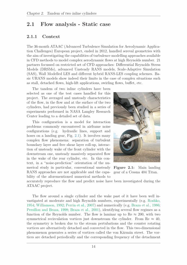
Figure 2.1: Main landinggear of a Cessna 404 Titan.
The tandem of two inline cylinders have beenselected as one of the test cases handled for thisproject. The averaged and unsteady characteristicsof the flow, in the flow and at the surface of the twocylinders, had previously been studied in a series ofexperiments performed in NASA Langley ResearchCenter leading to a detailed set of data.
This configuration is a model for interactionproblems commonly encountered in airframe noiseconfigurations (e.g. hydraulic lines, support andhoses on a landing gear, Fig. 2.1). It involves manycomplex flow phenomena: separation of turbulentboundary layer and free shear layer roll-up, interac-tion of unsteady wake of the front cylinder with thedownstream one, unsteady massively separated flowin the wake of the rear cylinder, etc. In this con-text, in a “noise-prediction” orientation of the nu-merical study in particular, conventional unsteadyRANS approaches are not applicable and the capa-bility of the aforementioned numerical methods toaccurately reproduce the flow and predict noise have been investigated during theATAAC project.
The flow around a single cylinder and the wake past of it have been well in-vastigated at moderate and high Reynolds numbers, experimentally (e.g. Roshko,1954; Williamson, 1992; Perrin et al., 2007) and numerically (e.g. Braza et al., 1986;Persillon and Braza, 1998; Braza et al., 2001), identifying several flow regimes as afunction of the Reynolds number. The flow is laminar up to Re ≈ 200, with twosymmetrical recirculation vortices just downstream the cylinder. From Re ≈ 40,the symmetry is broken due to the stream pertubations and the counter rotatingvortices are alternatively detached and convected in the flow. This two-dimensionalphenomenon generates a series of vortices called the von Kármán street. The vor-tices are detached periodically and the corresponding frequency of the detachment
14
2.1. Flow analysis - Static case
is non dimensionalised to give the Strouhal number:
St =fV K D
U∞
(2.1)
where fV K is the frequency of the vortices detachment (two successive detachmentsof the counter-rotating vortices is one period of the phenomenon), D the diameterof the cylinder (or the characteristic length of the body) and U∞ the freestreamvelocity of the flow. The Strouhal number depends on the body shape and theReynolds number. This periodical detachment is caracterised by a time evolution ofthe aerodynamic forces applying on the body at fV K for the perpendicular ones (lift)and fV K/2 for the streamwise ones (drag). Close to Re ≈ 200, three-dimensionaleffects can be observed: the von Kármán vortices ondulate in the crosswise direction,parallel to the cylinder, with a wavelength of about 4D. For Reynolds numbershigher than 200, this wavelength is reduced to 1D and first turbulence phenomenadevelop in the wake. The flow is fully turbulent for Re > 300 which is the case inthis study, as the Reynolds number equals to 166,000 as detailed in the next section.
A first synthesis of numerical simulations carried out for this test case was car-ried out by Lockhard, regrouping 13 contributions involving different modelling ap-proaches, as well as previous simulations by Khorrami et al. (2007), using URANSSST. These simulations indicated that the majority of the approaches captured quitewell the Strouhal number of the vortex shedding frequency around the first cylinder,(St = 0.24). Furthermore, as is seen in the ATAAC European program, the DESapproaches better capture the complex vortex dynamics of the present flow, espe-cially the formation of Kelvin-Helmholtz vortices in the separated shear layers. Inthe experimental context, it was found that the shear layers formed downstream ofthe first cylinder wrap around the second cylinder and interact non-linearly with thecomplex turbulence background, producing predominant frequencies in the energyspectrum, in the range of acoustic noise. Moreover, the numerical studies reportedby Lockard in the context of the workshop for airframe noise computation, evalu-ated the mean drag coefficient provided by the different simulations, that had shownquite a dispersion among the different studies, with a most probable mean value oforder 0.484 around the first cylinder.
2.1.2 Test-case description
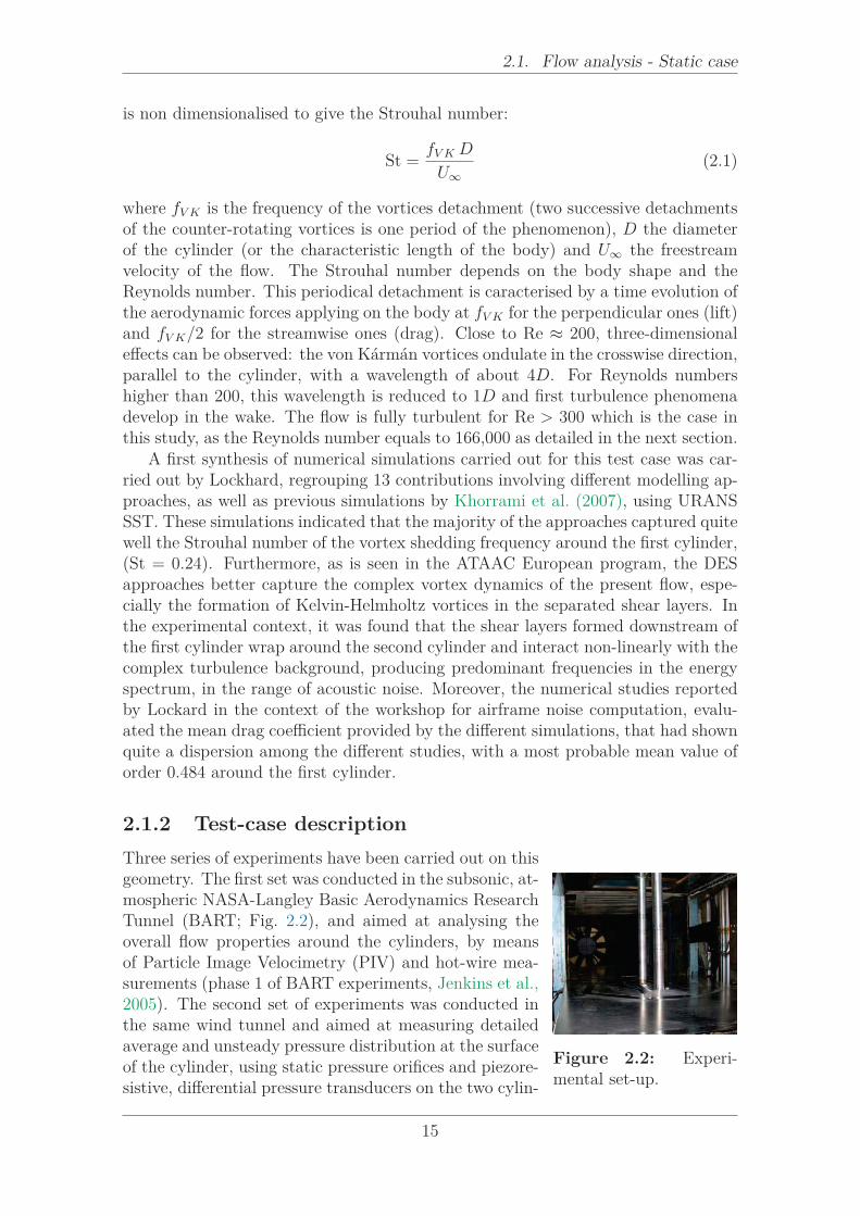
Figure 2.2: Experi-mental set-up.
Three series of experiments have been carried out on thisgeometry. The first set was conducted in the subsonic, at-mospheric NASA-Langley Basic Aerodynamics ResearchTunnel (BART; Fig. 2.2), and aimed at analysing theoverall flow properties around the cylinders, by meansof Particle Image Velocimetry (PIV) and hot-wire mea-surements (phase 1 of BART experiments, Jenkins et al.,2005). The second set of experiments was conducted inthe same wind tunnel and aimed at measuring detailedaverage and unsteady pressure distribution at the surfaceof the cylinder, using static pressure orifices and piezore-sistive, differential pressure transducers on the two cylin-
15
Chapter 2. Tandem of two inline cylinders
L
!
0° 180°
Y
X
D
Flow
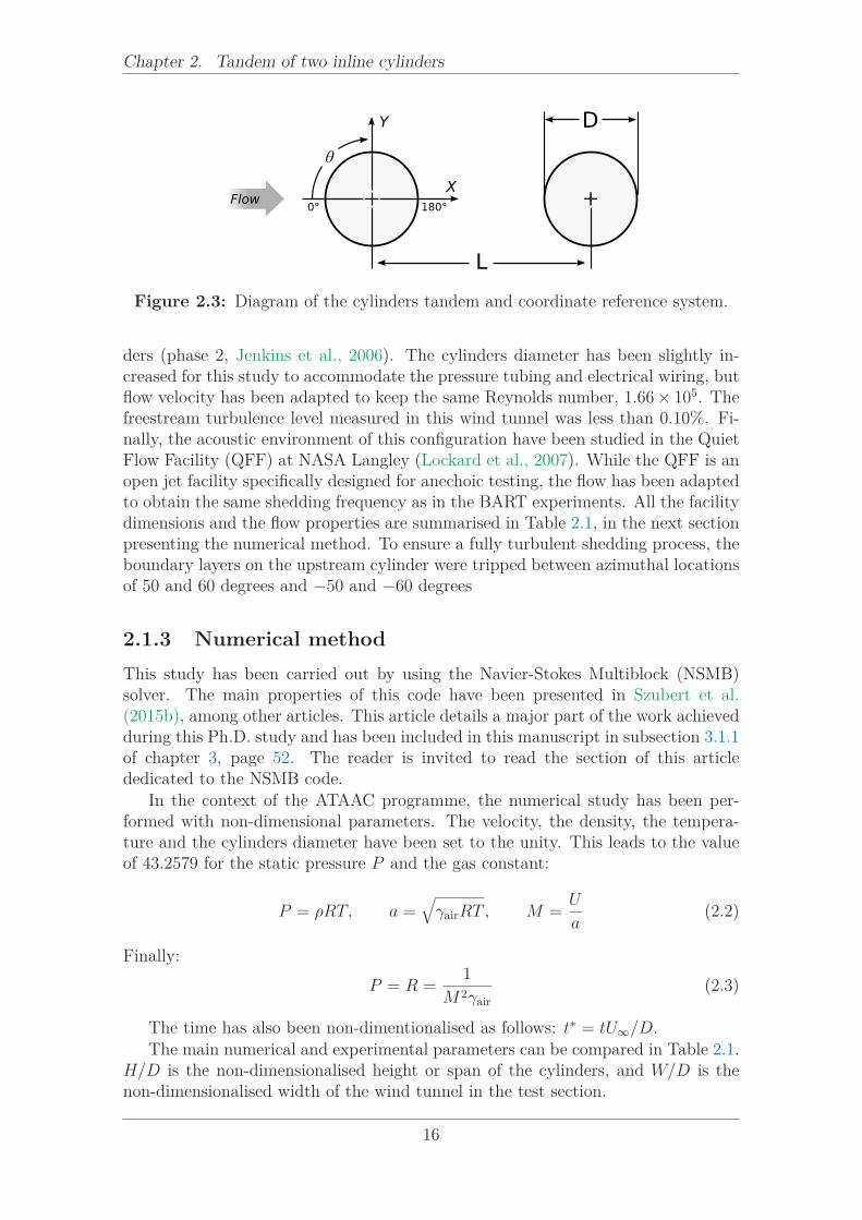
Figure 2.3: Diagram of the cylinders tandem and coordinate reference system.
ders (phase 2, Jenkins et al., 2006). The cylinders diameter has been slightly in-creased for this study to accommodate the pressure tubing and electrical wiring, butflow velocity has been adapted to keep the same Reynolds number, 1.66 × 10⁵. Thefreestream turbulence level measured in this wind tunnel was less than 0.10%. Fi-nally, the acoustic environment of this configuration have been studied in the QuietFlow Facility (QFF) at NASA Langley (Lockard et al., 2007). While the QFF is anopen jet facility specifically designed for anechoic testing, the flow has been adaptedto obtain the same shedding frequency as in the BART experiments. All the facilitydimensions and the flow properties are summarised in Table 2.1, in the next sectionpresenting the numerical method. To ensure a fully turbulent shedding process, theboundary layers on the upstream cylinder were tripped between azimuthal locationsof 50 and 60 degrees and −50 and −60 degrees
2.1.3 Numerical method
This study has been carried out by using the Navier-Stokes Multiblock (NSMB)solver. The main properties of this code have been presented in Szubert et al.(2015b), among other articles. This article details a major part of the work achievedduring this Ph.D. study and has been included in this manuscript in subsection 3.1.1of chapter 3, page 52. The reader is invited to read the section of this articlededicated to the NSMB code.
In the context of the ATAAC programme, the numerical study has been per-formed with non-dimensional parameters. The velocity, the density, the tempera-ture and the cylinders diameter have been set to the unity. This leads to the valueof 43.2579 for the static pressure P and the gas constant:
P = ρRT, a =√
γairRT, M =U
a(2.2)
Finally:
P = R =1
M2γair
(2.3)
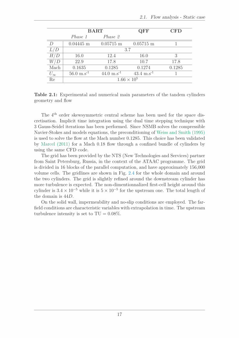
The time has also been non-dimentionalised as follows: t∗ = tU∞/D.The main numerical and experimental parameters can be compared in Table 2.1.
H/D is the non-dimensionalised height or span of the cylinders, and W/D is thenon-dimensionalised width of the wind tunnel in the test section.
16
2.1. Flow analysis - Static case
BART QFF CFDPhase 1 Phase 2
D 0.04445 m 0.05715 m 0.05715 m 1L/D 3.7H/D 16.0 12.4 16.0 3W/D 22.9 17.8 10.7 17.8Mach 0.1635 0.1285 0.1274 0.1285U∞ 56.0 m.s-1 44.0 m.s-1 43.4 m.s-1 1Re 1.66 × 10⁵
Table 2.1: Experimental and numerical main parameters of the tandem cylindersgeometry and flow
The 4th order skewsymmetric central scheme has been used for the space dis-cretisation. Implicit time integration using the dual time stepping technique with3 Gauss-Seidel iterations has been performed. Since NSMB solves the compressibleNavier-Stokes and models equations, the preconditioning of Weiss and Smith (1995)is used to solve the flow at the Mach number 0.1285. This choice has been validatedby Marcel (2011) for a Mach 0.18 flow through a confined bundle of cylinders byusing the same CFD code.
The grid has been provided by the NTS (New Technologies and Services) partnerfrom Saint Petersburg, Russia, in the context of the ATAAC programme. The gridis divided in 16 blocks of the parallel computation, and have approximately 156,000volume cells. The gridlines are shown in Fig. 2.4 for the whole domain and aroundthe two cylinders. The grid is slightly refined around the downstream cylinder hasmore turbulence is expected. The non-dimentionnalized first-cell height around thiscylinder is 3.4 × 10⁻⁵ while it is 5 × 10⁻⁵ for the upstream one. The total length ofthe domain is 44D.
On the solid wall, impermeability and no-slip conditions are employed. The far-field conditions are characteristic variables with extrapolation in time. The upstreamturbulence intensity is set to TU = 0.08%.
17

Chapter 2. Tandem of two inline cylinders
Figure 2.4: Multiblock domain of the tandem of cylinders.
2.1.4 Results
2.1.4.1 Flow overview
Eight snapshots of the vorticity field from a preliminary k-ω-SST simulation coveringone period of the von Kármán phenomenon can be observed in Fig. 2.5. The maincharacteristic of the field is that the vortex shedding occurs at the same frequencyfor the two cylinders, due to the wake of the first cylinder that intensively influencesthe generation of vortices by the second cylinder. The distance L/D = 3.7 betweenthe two cylinder is optimal to observe this phenomenon. In case of a smaller ora bigger distance, the vortex shedding would be in phase opposition between thetwo cylinders, generating a more complexe wake downstream the whole geometry.After this preliminary overview of the flow structure, a numerical study is carriedout in order to determine the best convergence criterion and turbulence models tosimulate this test case. These parameters don’t change the overall flow structureand the above description remains valid.
18

2.1. Flow analysis - Static case
Figure 2.5: Snapshots of the vorticity field by k-ω-SST simulation covering oneperiod of von Kármán.
19

Chapter 2. Tandem of two inline cylinders
2.1.4.2 Convergence study
In the context of the dual-time stepping, a sensitivity study of the physical resultsregarding the tolerance of the convergence criterion is first carried out. The con-vergence criterion at the inner step n is defined by the ratio between the L2−normof the density equation residual at the inner step n and the one at the initial in-ner step. It is calculated at each inner computation step and when the toleranceis reached, the physical solution is saved at the current physical time step and theprocess goes on at the next outerstep. The system of equations needs to convergeenough to provide a good prediction of the physical solution. However, a very lowtolerance implies long computation time to reach the requested value and becomesuseless compared to the numerical uncertainties (time and grid resolutions, com-puter precision). This study is performed to determine the better tolerence for thethree-dimensional computations.
For this study, the k-ω-SST model of Menter (1994) (see also section A.2.3.2 ofappendix A, page 141) is used, as it is well designed for flows under high pressuregradient, and the non-dimensionalised time step ∆t∗ = 0.00845 has been chosenfrom the ATAAC programme.
The RMS value of the lift and drag coefficient fluctuations of the two cylindersare calculated at each outerstep. The last steps are plotted in Fig. 2.6 for the threetolerance values analysed. The curves trend shows at first glance that the differencebetween the two smaller tolerances is less than between 10−3 and 10−4. While thephysical solutions were well converged, small oscillations are visible in the RMSvalues and are due to numerical resolution.
Figure 2.6: Evolution of the RMS values of the lift and drag coefficients fluctuationsfor three convergence tolerances.
The final values of the RMS, as well as the mean of the lift and drag coefficients,are reported in Table 2.2 for a quantitative comparison. The three tolerances give
20

2.1. Flow analysis - Static case
Tol.Upstream cylinder Downstream cylinder
CD CL RMS(C ′
L) RMS(C ′
D) CD CL RMS(C ′
L) RMS(C ′
D)
10−3 0.7997 0.0022 0.0512 0.5765 0.2035 -0.0020 0.2590 1.1363
10−4 0.7990 0.0028 0.0509 0.5746 0.2047 -0.0036 0.2584 1.1370
10−5 0.7991 0.0027 0.0510 0.5749 0.2045 -0.0049 0.2583 1.1377
Table 2.2: Mean values of the lift and drag coefficients and RMS values of theirfluctuactions for the two cylinders.
very close results with a difference < 1%, except for the mean lift value on bothcylinders. Between 10−3 and 10−4, CL is increased by 20% on the first cylinderand 44% on the second one, while between 10−4 and 10−5, CL is 4% smaller on theupstream cylinder, and 27% higher on the downstream one. In the spirit of gettingmeaningful physical results in a reasonnable computation time, the tolerance 10−4
is retained for the the remaining simulations.
2.1.4.3 Turbulence model study
A similar comparison is carried out to compare the results of four turbulence models.The mean and RMS values of the lift and drag coefficient time evolution are reportedin Table 2.3. The Edwards and Chandra (1996) modified Spalart and Allmaras(1994) (see also section A.1.1 of appendix A, page 135) and the k-ω-SST (Menter,1994 and section A.2.3.2 page 141) give very close results in mean and amplitude.The k-ω-BSL (Menter, 1994 and section A.2.3.1 page 139) is more dissipative andas a consequence, the amplitude of the aerodynamic coefficients are smaller.
ModelsUpstream cylinder Downstream cylinder
CD CL RMS(C′
L) RMS(C′
D) CD CL RMS(C′
L) RMS(C′
D)
SA-E 0.7826 0.0028 0.0742 0.6246 0.2008 0.0018 0.3068 1.3295
k-ω-SST 0.7990 0.0028 0.0509 0.5746 0.2047 -0.0036 0.2581 1.1370
k-ω-BSL 0.5567 0.0011 0.0167 0.2523 0.2852 -0.0054 0.1246 0.8045
Table 2.3: Mean values of the lift and drag coefficients and RMS values of theirfluctuactions for three turbulence models.
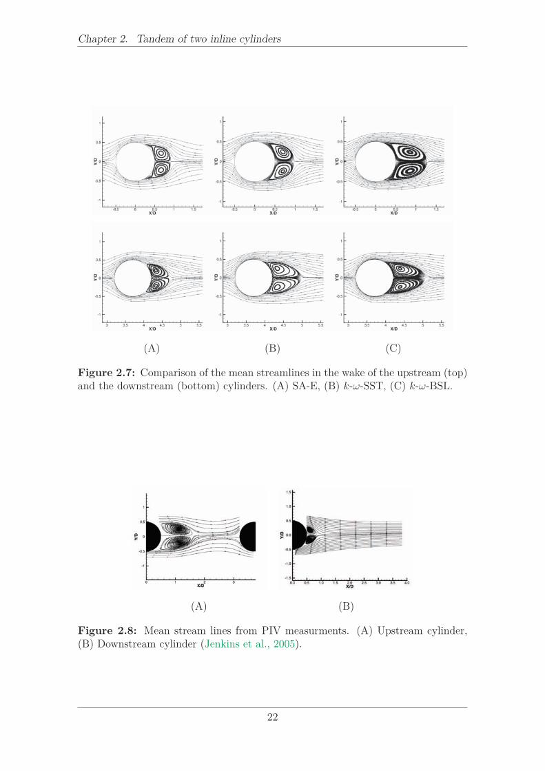
The mean streamlines in the wake of each cylinder are plotted for the threeturbulence models in Fig. 2.7. The overall prediction of the flow is similar betweenthe three models and the experiment (Fig. 2.8) and the symmetry between theupper and lower sides of the flow is observed. However, they predict slight differentsize of the recirculation area, in particular none of them matches the experimentalmeasurements.
The non-dimensionalised streamwise velocity at y = 0 measured in the wake ofthe two cylinders is plotted in Fig. 2.9, and the recirculation lengths (x ∧ U(x) = 0)are reported in Table 2.4. In the BART experiment, the second recirculation hasbeen reduced by 80% compared to the first. This difference might by due to theposition of the cylinders compared to each other. The velocity in the wake of the
21
Chapter 2. Tandem of two inline cylinders
(A) (B) (C)
Figure 2.7: Comparison of the mean streamlines in the wake of the upstream (top)and the downstream (bottom) cylinders. (A) SA-E, (B) k-ω-SST, (C) k-ω-BSL.
(A) (B)
Figure 2.8: Mean stream lines from PIV measurments. (A) Upstream cylinder,(B) Downstream cylinder (Jenkins et al., 2005).
22

2.1. Flow analysis - Static case
(A) (B)
Figure 2.9: Comparison between turbulence models en experiment of normalisedstreamwise velocity in the wake. (A) Upstream cylinder, (B) Downstream cylinder.
first cylinder is limited by the presence of the second cylinder and this favours thedevelopment of the vortices before they detach, while this is not the case for thesecond cylinder. However, this phenomenon is not observed in the simulations,which give an opposite trend, and the difference between the two regions is lessimportant (SA-E and k-ω-SST: +20%, k-ω-SST: +67%).
Models/SourceLrecirc/D
Upstream cyl. Downstream cyl.
PIV (Jenkins et al., 2005) 1.2 0.25
SA-E 0.4 0.5
k-ω-SST 0.45 0.75
k-ω-BSL 0.75 0.9
Table 2.4: Recirculation length downstream each cylinder.
Spectral analysis
A spectral analysis is carried out on the time evolution of the lift and drag coefficientsrecorded at a physical time step ∆t∗ = 0.00845, the same as the simulation itself. Allsignals are 17751 sample length, and are processed by the Welch’s method (Welch,1967) with the following parameters:
• Window: Hanning,
• Window size: Nwind = 8192 samples,
• Overlap: 65%,
23
Chapter 2. Tandem of two inline cylinders
• Zero padding: NF F T = 218 = 262144.
These parameters give the following resolutions:
• ∆f ≈ 4.5 × 10⁻⁴ Hz,
• B ≈ 5.8 × 10⁻² Hz.
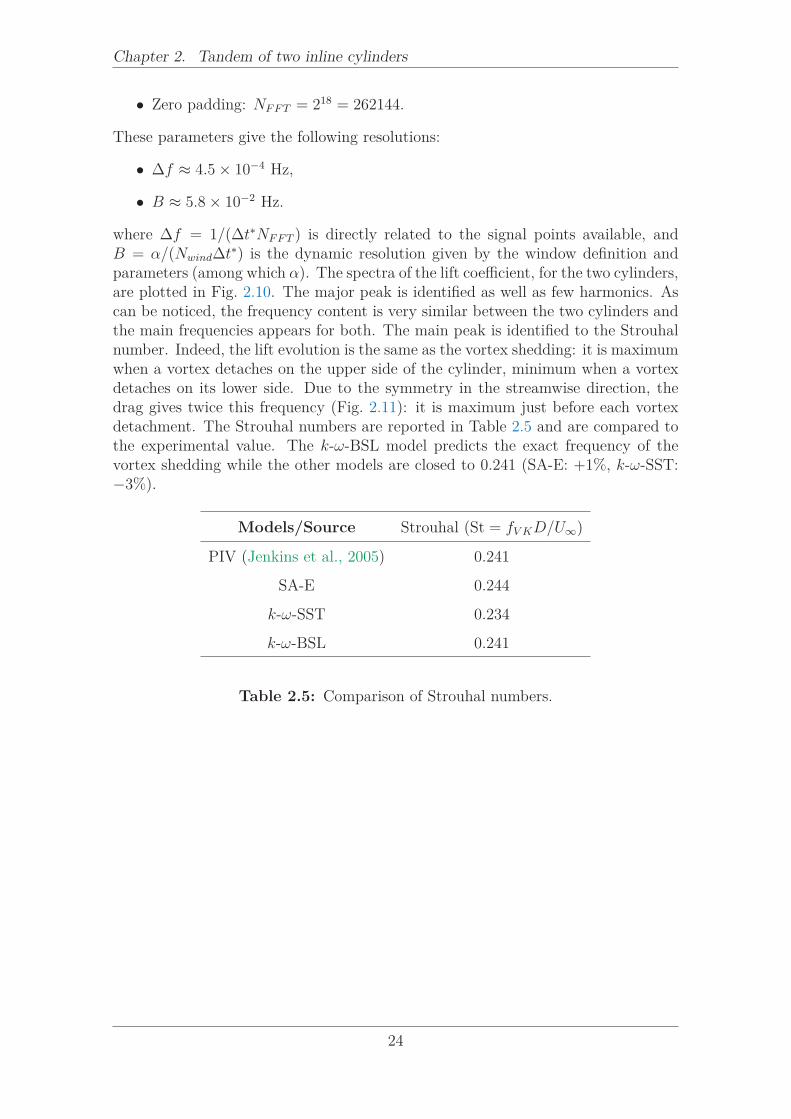
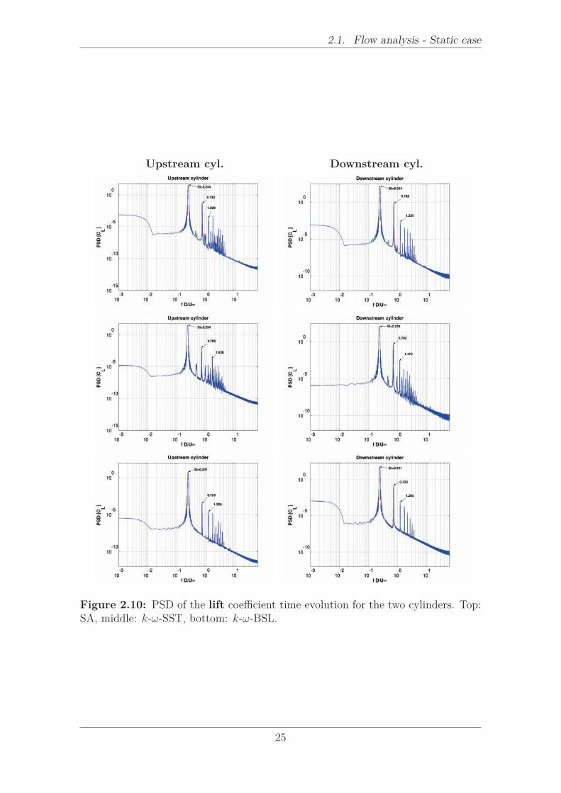
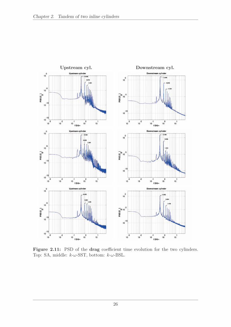
where ∆f = 1/(∆t∗NF F T ) is directly related to the signal points available, andB = α/(Nwind∆t∗) is the dynamic resolution given by the window definition andparameters (among which α). The spectra of the lift coefficient, for the two cylinders,are plotted in Fig. 2.10. The major peak is identified as well as few harmonics. Ascan be noticed, the frequency content is very similar between the two cylinders andthe main frequencies appears for both. The main peak is identified to the Strouhalnumber. Indeed, the lift evolution is the same as the vortex shedding: it is maximumwhen a vortex detaches on the upper side of the cylinder, minimum when a vortexdetaches on its lower side. Due to the symmetry in the streamwise direction, thedrag gives twice this frequency (Fig. 2.11): it is maximum just before each vortexdetachment. The Strouhal numbers are reported in Table 2.5 and are compared tothe experimental value. The k-ω-BSL model predicts the exact frequency of thevortex shedding while the other models are closed to 0.241 (SA-E: +1%, k-ω-SST:−3%).
Models/Source Strouhal (St = fV KD/U∞)
PIV (Jenkins et al., 2005) 0.241
SA-E 0.244
k-ω-SST 0.234
k-ω-BSL 0.241
Table 2.5: Comparison of Strouhal numbers.
24
2.1. Flow analysis - Static case
Upstream cyl. Downstream cyl.
Figure 2.10: PSD of the lift coefficient time evolution for the two cylinders. Top:SA, middle: k-ω-SST, bottom: k-ω-BSL.
25
Chapter 2. Tandem of two inline cylinders
Upstream cyl. Downstream cyl.
Figure 2.11: PSD of the drag coefficient time evolution for the two cylinders.Top: SA, middle: k-ω-SST, bottom: k-ω-BSL.
26

2.1. Flow analysis - Static case
Figure 2.12: First POD mode of the streamwise (left) and crosswise (right) velocitycomponents.
2.1.4.4 POD analysis
The Proper Orthogonal Decomposition (POD) is a mathematical technique used toanalyzed complex physical systems of a great number of degrees of freedom, allowingto represent these systems in an optimal way. This method is applied in a wide rangeof scientifical fields such that signal and image processing, chemistery, medecine,oceanography, meteorology. In the context of the fluid dynamics, this method hasbeen introduced by (Lumley, 1967) to analyse the coherent structures in a turbulentflow, which are usually of high energy, the lowest energy range corresponding tothe random fluctuations. The current POD analysis is carried out based on the‘separable POD’ (Holmes et al., 1996). The objective is to find an approximation ofthe physical flow as follows:
U(x, t) = U(x) + u(x, t) = U(x) +NPOD∑
n=2
an(t)φn(x), (2.4)
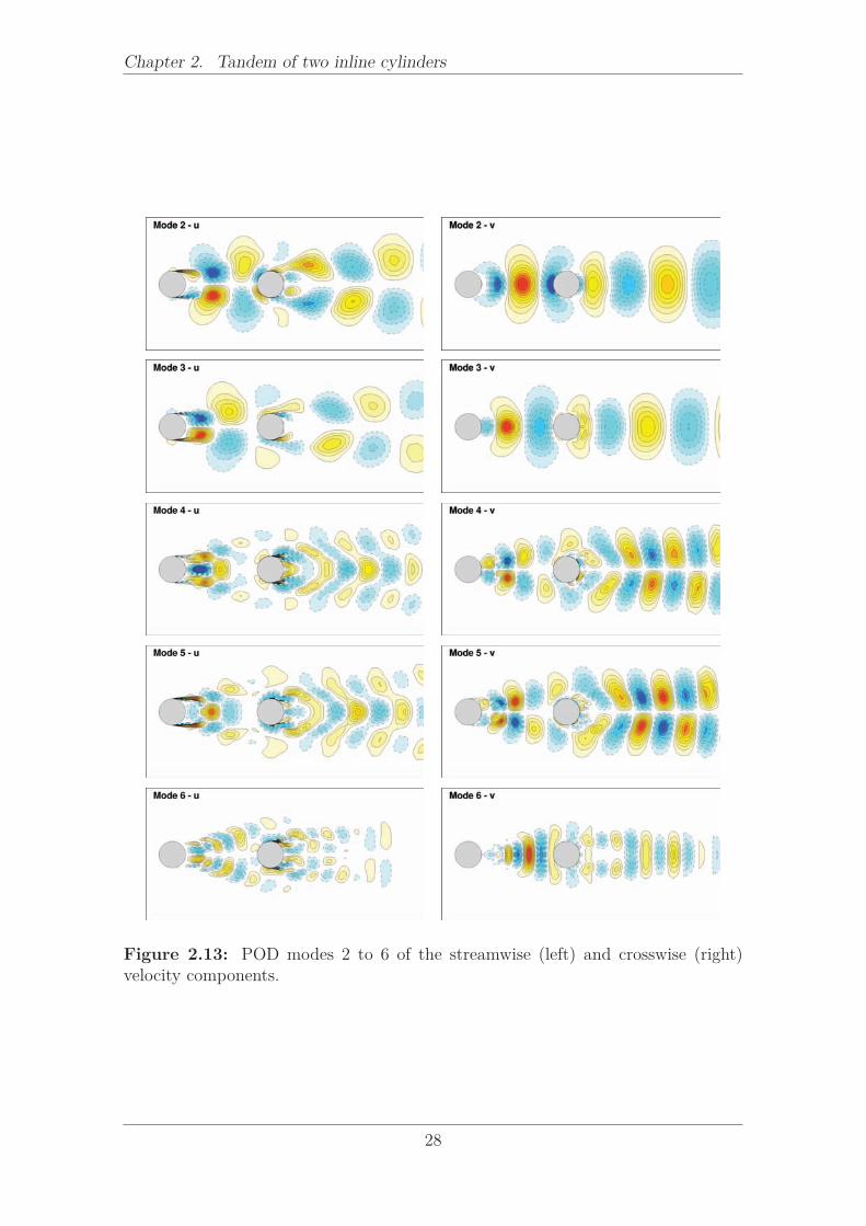
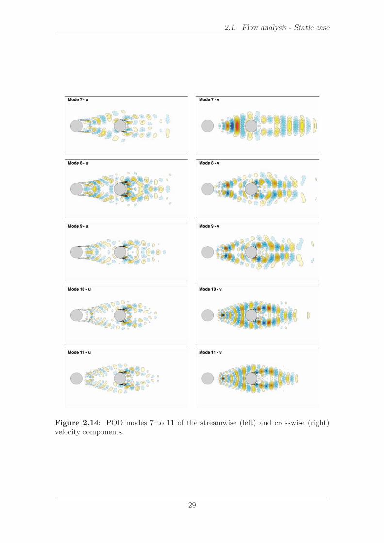
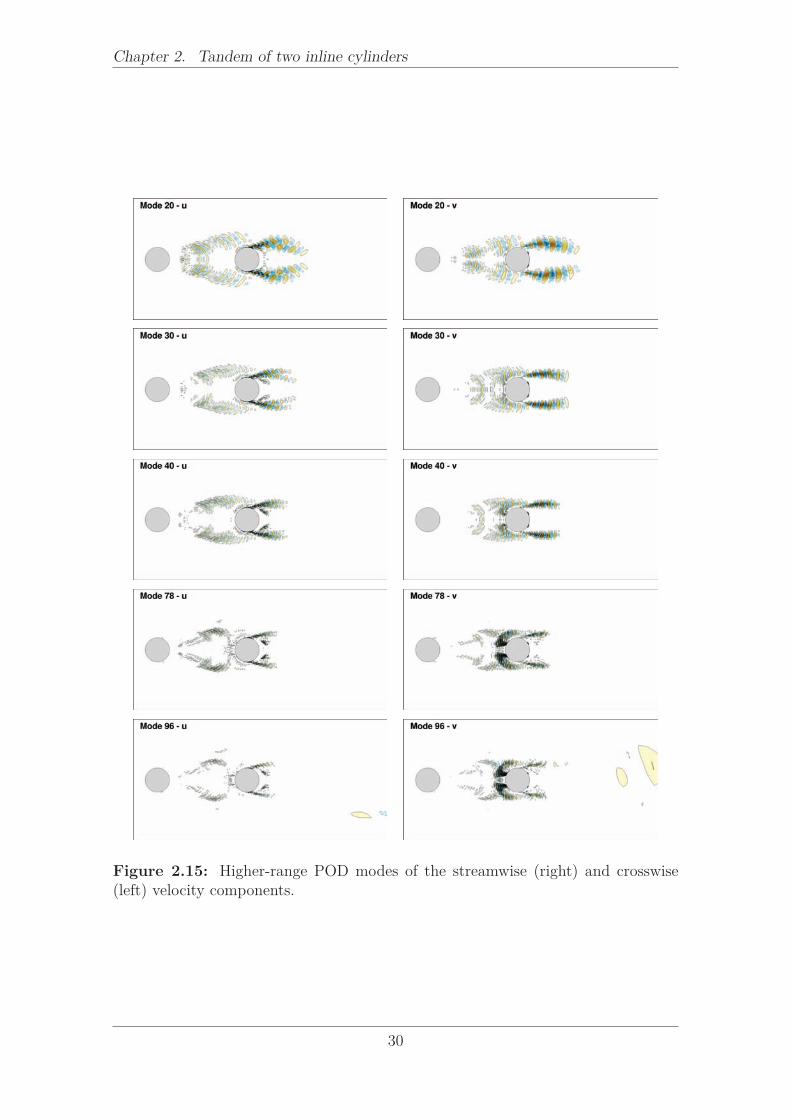
where φn(x) are the shape (spatial) functions and an(t) are the associated temporalcoefficients. In the context of this study, the ‘snapshot POD’ (Sirovich, 1987; Aubryet al., 1991) is used to determine the temporal coefficients from the time correlationsarised from the snapshots generated during the simulation. The spatial modes aredetermined by projecting the physical field on these temporal coefficients. A fortrancode developed in our research group as been used to read the data, calculate thetemporal coefficients and spatial modes and write results. Here, 1132 snapshotsof the streamwise and crosswise velocity components, generated from a k-ω-SSTsimulation every t∗ = 0.04225, 5 times the simulation time step, are used covering10 periods of vortex shedding. The first POD mode corresponds to the mean field asit is included in the original database (Fig. 2.12). Shape functions from modes 2 to6 are plotted in Fig. 2.13, and are clearly identified to the von Kármán phenomenon,giving sub-spatial frequencies as the mode order increases. Shape functions of thenext 5 modes are plotted in Fig. 2.14. They confirm the tendency of the sub-division of the spatial modes structures as their range increases. Moreover, thehigher shape values move from the vortex shedding area to the shear-layer one,characterised by Kelvin-Helmotz vortices. The tendency is confirmed at higher-range modes (Fig. 2.15).
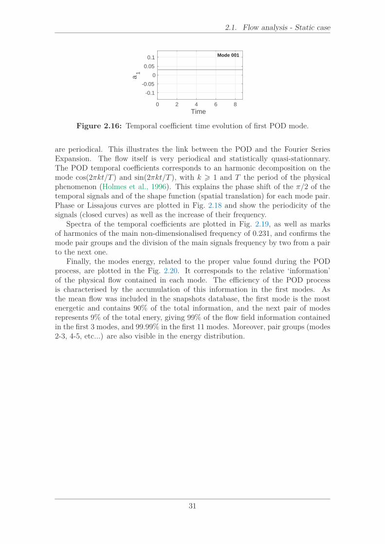
The time evolution of the temporal coefficients are plotted in the Fig. 2.16and 2.17. For the first mode, the constant time evolution confirms the propertyof the first mode which represents the mean field. Other modes are associated twoby two, corresponding to two different phases, similarly to the shape functions, and
27
Chapter 2. Tandem of two inline cylinders
Figure 2.13: POD modes 2 to 6 of the streamwise (left) and crosswise (right)velocity components.
28
2.1. Flow analysis - Static case
Figure 2.14: POD modes 7 to 11 of the streamwise (left) and crosswise (right)velocity components.
29
Chapter 2. Tandem of two inline cylinders
Figure 2.15: Higher-range POD modes of the streamwise (right) and crosswise(left) velocity components.
30
2.1. Flow analysis - Static case
Time
0 2 4 6 8
a1
-0.1
-0.05
0
0.05
0.1Mode 001
Figure 2.16: Temporal coefficient time evolution of first POD mode.
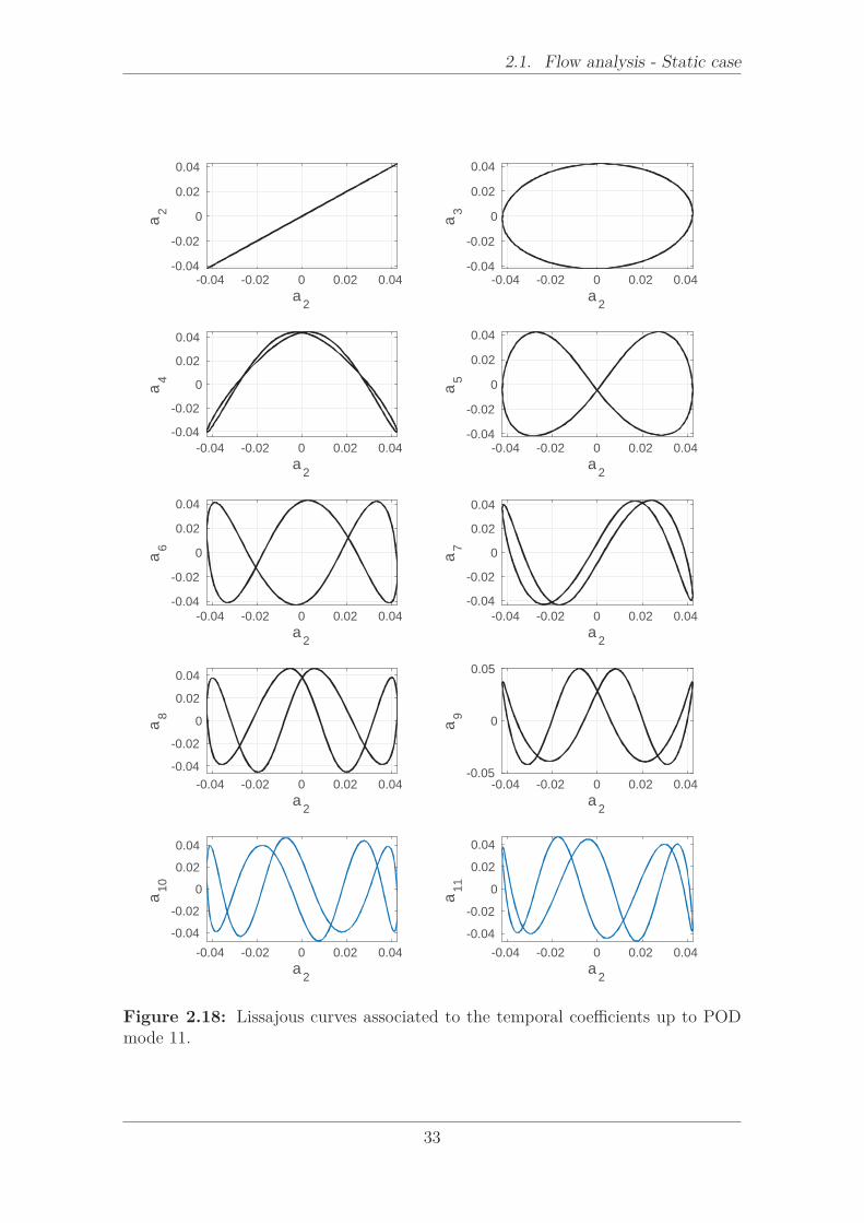
are periodical. This illustrates the link between the POD and the Fourier SeriesExpansion. The flow itself is very periodical and statistically quasi-stationnary.The POD temporal coefficients corresponds to an harmonic decomposition on themode cos(2πkt/T ) and sin(2πkt/T ), with k > 1 and T the period of the physicalphenomenon (Holmes et al., 1996). This explains the phase shift of the π/2 of thetemporal signals and of the shape function (spatial translation) for each mode pair.Phase or Lissajous curves are plotted in Fig. 2.18 and show the periodicity of thesignals (closed curves) as well as the increase of their frequency.
Spectra of the temporal coefficients are plotted in Fig. 2.19, as well as marksof harmonics of the main non-dimensionalised frequency of 0.231, and confirms themode pair groups and the division of the main signals frequency by two from a pairto the next one.
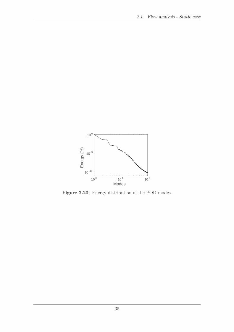
Finally, the modes energy, related to the proper value found during the PODprocess, are plotted in the Fig. 2.20. It corresponds to the relative ‘information’of the physical flow contained in each mode. The efficiency of the POD processis characterised by the accumulation of this information in the first modes. Asthe mean flow was included in the snapshots database, the first mode is the mostenergetic and contains 90% of the total information, and the next pair of modesrepresents 9% of the total enery, giving 99% of the flow field information containedin the first 3 modes, and 99.99% in the first 11 modes. Moreover, pair groups (modes2-3, 4-5, etc...) are also visible in the energy distribution.
31

Chapter 2. Tandem of two inline cylinders
Time
0 2 4 6 8
a2
-0.1
-0.05
0
0.05
0.1Mode 002
Time
0 2 4 6 8
a3
-0.1
-0.05
0
0.05
0.1Mode 003
Time
0 2 4 6 8
a4
-0.1
-0.05
0
0.05
0.1Mode 004
Time
0 2 4 6 8
a5
-0.1
-0.05
0
0.05
0.1Mode 005
Time
0 2 4 6 8
a6
-0.1
-0.05
0
0.05
0.1Mode 006
Time
0 2 4 6 8
a7
-0.1
-0.05
0
0.05
0.1Mode 007
Time
0 2 4 6 8
a8
-0.1
-0.05
0
0.05
0.1Mode 008
Time
0 2 4 6 8
a9
-0.1
-0.05
0
0.05
0.1Mode 009
Time
0 2 4 6 8
a10
-0.1
-0.05
0
0.05
0.1Mode 010
Time
0 2 4 6 8
a11
-0.1
-0.05
0
0.05
0.1Mode 011
Figure 2.17: Temporal coefficient time evolution of POD modes 2 to 11.
32
2.1. Flow analysis - Static case
a2
-0.04 -0.02 0 0.02 0.04
a2
-0.04
-0.02
0
0.02
0.04
a2
-0.04 -0.02 0 0.02 0.04
a3
-0.04
-0.02
0
0.02
0.04
a2
-0.04 -0.02 0 0.02 0.04
a4
-0.04
-0.02
0
0.02
0.04
a2
-0.04 -0.02 0 0.02 0.04a
5
-0.04
-0.02
0
0.02
0.04
a2
-0.04 -0.02 0 0.02 0.04
a6
-0.04
-0.02
0
0.02
0.04
a2
-0.04 -0.02 0 0.02 0.04
a7
-0.04
-0.02
0
0.02
0.04
a2
-0.04 -0.02 0 0.02 0.04
a8
-0.04
-0.02
0
0.02
0.04
a2
-0.04 -0.02 0 0.02 0.04
a9
-0.05
0
0.05
a2
-0.04 -0.02 0 0.02 0.04
a10
-0.04
-0.02
0
0.02
0.04
a2
-0.04 -0.02 0 0.02 0.04
a11
-0.04
-0.02
0
0.02
0.04
Figure 2.18: Lissajous curves associated to the temporal coefficients up to PODmode 11.
33

Chapter 2. Tandem of two inline cylinders
f
10-2
10-1
100
101
PS
D
10-15
10-10
10-5
100 0.23114
Mode 002
f
10-2
10-1
100
101
PS
D
10-15
10-10
10-5
100 0.23114
Mode 003
f
10-2
10-1
100
101
PS
D
10-15
10-10
10-5
100 0.23114
Mode 004
f
10-2
10-1
100
101
PS
D
10-15
10-10
10-5
100 0.23114
Mode 005
f
10-2
10-1
100
101
PS
D
10-15
10-10
10-5
100 0.23114
Mode 006
f
10-2
10-1
100
101
PS
D
10-15
10-10
10-5
100 0.23114
Mode 007
f
10-2
10-1
100
101
PS
D
10-15
10-10
10-5
100 0.23114
Mode 008
f
10-2
10-1
100
101
PS
D
10-15
10-10
10-5
100 0.23114
Mode 009
Figure 2.19: PSD associated to the temporal coefficients up to POD mode 9(non-dimensionalised frequencies).
34
2.1. Flow analysis - Static case
Modes10
010
110
2
Energ
y (
%)
10-10
10-5
100
Figure 2.20: Energy distribution of the POD modes.
35
Chapter 2. Tandem of two inline cylinders
Reconstruction
The velocity fields are reconstructed from a limited number of POD modes usingthe relation 2.4 (here, NPOD = 3, 5 and 41). The vorticity is then calculatedand compared to the original high-fidelity unprocessed field (snapshots form thesimulation). They are plotted at 0×TV K and TV K/4 in Fig. 2.21, and 2TV K/4 (left)and 3TV K/4 in Fig. 2.21, TV K being the period of the von Kármán vortex shedding.While their shapes are different from the orginal ones, the vortical structures arealready reconstructed with only 3 modes (including the first mode). With 11 modes,their spatial expension is very close to the high-fidelity simulation. However, somespatial oscillation remains, in particular between the two cylinders. They disappearby adding more modes to the reconstruction (here, 30 more modes), where thevorticity field is almost qualitatively identical to the original one.
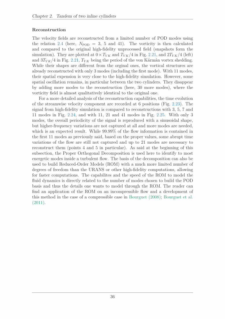
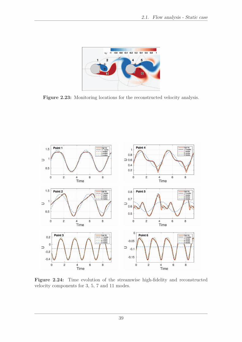
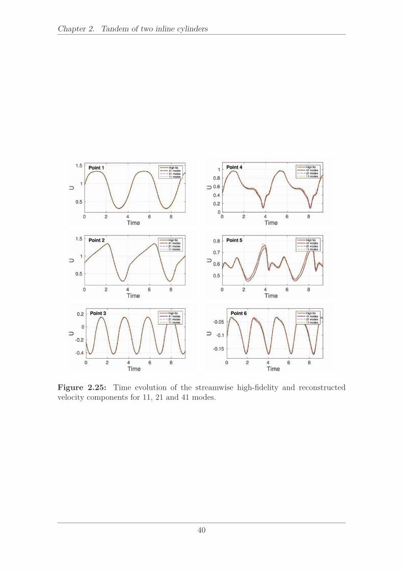
For a more detailed analysis of the reconstruction capabilities, the time evolutionof the streamwise velocity component are recorded at 6 positions (Fig. 2.23). Thesignal from high-fidelity simulation is compared to reconstructions with 3, 5, 7 and11 modes in Fig. 2.24, and with 11, 21 and 41 modes in Fig. 2.25. With only 3modes, the overall periodicity of the signal is reproduced with a sinusoidal shape,but higher-frequency variations are not captured at all and more modes are needed,which is an expected result. While 99.99% of the flow information is contained inthe first 11 modes as previously said, based on the proper values, some abrupt timevariations of the flow are still not captured and up to 21 modes are necessary toreconstruct them (points 4 and 5 in particular). As said at the beginning of thissubsection, the Proper Orthogonal Decomposition is used here to identify to mostenergetic modes inside a turbulent flow. The basis of the decomposition can also beused to build Reduced-Order Models (ROM) with a much more limited number ofdegrees of freedom than the URANS or other high-fidelity computations, allowingfor faster computations. The capabilites and the speed of the ROM to model thefluid dynamics is directly related to the number of modes chosen to build the PODbasis and thus the details one wants to model through the ROM. The reader canfind an application of the ROM on an incompressible flow and a development ofthis method in the case of a compressible case in Bourguet (2008); Bourguet et al.(2011).
36

2.1. Flow analysis - Static case
Figure 2.21: Vorticity field from URANS (top) and POD reconstruction from 3,5 and 41 modes at 0 × TV K (left) and TV K/4 (right) in static case.
37

Chapter 2. Tandem of two inline cylinders
Figure 2.22: Vorticity field from URANS (top) and POD reconstruction from 3,5 and 41 modes at 2TV K/4 (left) and 3TV K/4 (right) in static case.
38
2.1. Flow analysis - Static case
Figure 2.23: Monitoring locations for the reconstructed velocity analysis.
Figure 2.24: Time evolution of the streamwise high-fidelity and reconstructedvelocity components for 3, 5, 7 and 11 modes.
39
Chapter 2. Tandem of two inline cylinders
Figure 2.25: Time evolution of the streamwise high-fidelity and reconstructedvelocity components for 11, 21 and 41 modes.
40
2.1. Flow analysis - Static case
2.1.5 3D Simulations
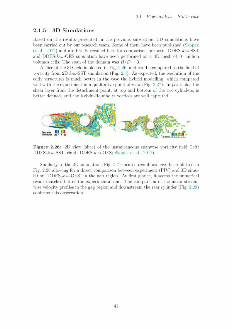
Based on the results presented in the previous subsection, 3D simulations havebeen carried out by our research team. Some of them have been published (Skopeket al., 2012) and are briefly recalled here for comparison purpose. DDES-k-ω-SSTand DDES-k-ω-OES simulation have been performed on a 3D mesh of 16 millionvolumes cells. The span of the domain was H/D = 3.
A slice of the 3D field is plotted in Fig. 2.26, and can be compared to the field ofvorticity from 2D k-ω-SST simulation (Fig. 2.5). As expected, the resolution of theeddy structures is much better in the case the hybrid modelling, which comparedwell with the experiment in a qualitative point of view (Fig. 2.27). In particular theshear layer from the detachment point, at top and bottom of the two cylinders, isbetter defined, and the Kelvin-Helmholtz vortices are well captured.
Figure 2.26: 2D view (slice) of the instantaneous spanwise vorticity field (left:DDES-k-ω-SST, right: DDES-k-ω-OES; Skopek et al., 2012).
Similarly to the 2D simulation (Fig. 2.7) mean streamlines have been plotted inFig. 2.28 allowing for a direct comparison between experiment (PIV) and 3D simu-lation (DDES-k-ω-OES) in the gap region. At first glance, it seems the numericalresult matches better the experimental one. The comparison of the mean stream-wise velocity profiles in the gap region and downstream the rear cylinder (Fig. 2.29)confirms this observation.
41
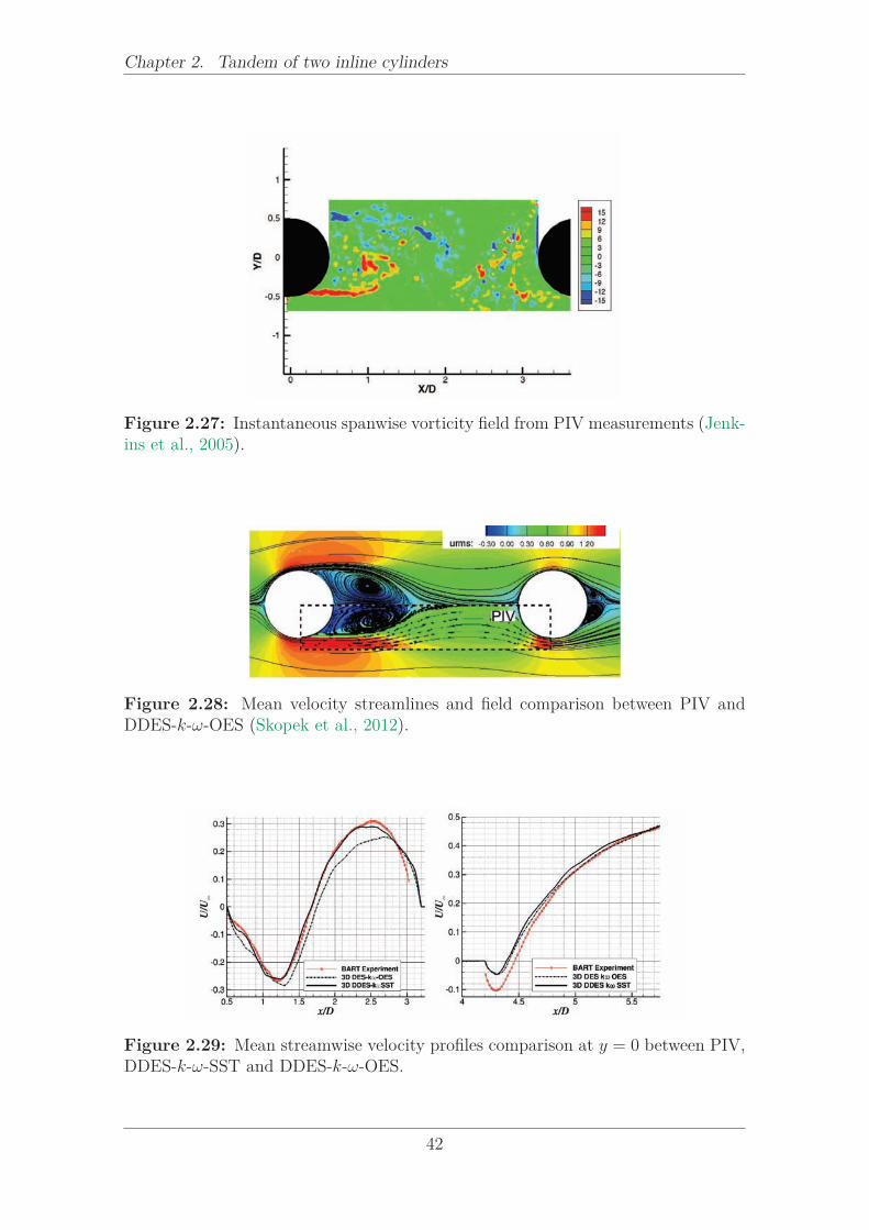
Chapter 2. Tandem of two inline cylinders
Figure 2.27: Instantaneous spanwise vorticity field from PIV measurements (Jenk-ins et al., 2005).
Figure 2.28: Mean velocity streamlines and field comparison between PIV andDDES-k-ω-OES (Skopek et al., 2012).
Figure 2.29: Mean streamwise velocity profiles comparison at y = 0 between PIV,DDES-k-ω-SST and DDES-k-ω-OES.
42
2.2. Fluid-structure interaction - Dynamic case
2.2 Fluid-structure interaction - Dynamic case
2.2.1 Introduction
The tandem cylinders configuration is related to the sizing of the heat exchangersin nuclear reactor technology. The configuration is also a model problem related toMovement Induced Vibration (MIV) dynamics extracted from a more complex cylin-ders bundle configuration as pointed out in the national research project ANR-Bare-safe coordinated by EDF and including partnership of the main nuclear engineeringindustrial partners in France, CEA and AREVA. In this context, the objective is topropose High-Fidelity CFD-CSM approaches able to predict the loads (amplitudesand frequencies) as a function of the structural parameters (reduced velocity andthe mass-damping number; Scruton number) with sufficient accuracy as requiredfor design. Furthermore, the objective is to develop efficient low-order decomposi-tion and reconstruction of the flow dynamics coupled with the structural dynamics,for further use in Reduced Order Modelling (ROM) which will enable faster designcycles for the end user. The present thesis aims at providing efficient turbulencemodelling for the CFD part, coupled with the solid structure’s motion by means ofthe Arbitrary Lagrangian-Eulerian method (ALE) and to simulate the spontaneousvibrational instability onset, when the structural parameters coupled with the fluid’svelocity and time scales overpass critical limits.
Beyond the static configuration studied in the ATAAC European programmeand as a link with the ANR-Baresafe program, the fluid-structure interaction will beexamined, leading to vibration of the downstream cylinder in the tandem, because ofthe shearing mechanisms and vortex shedding developed past the upstream cylinder.This problem is also related to the vibrations occuring in the landing gear cylindricalsupports.
A suitable POD reconstruction will be presented applied to the vibrational case,on view of further use in the Reduced Order Modelling context.
2.2.2 Results
2.2.2.1 Fluid-structure interaction
Fig. 2.30 presents the evolutions of the lift coefficient in comparison with the po-sition of the downstream cylinder versus time, for Scruton number Sc = 1. Forlow values of the reduced velocity up to 3, these evolutions are in phase, show-ing synchronisation between the force and displacement. This indicates a ‘lock-in’mechanism corresponding to the Vortex Induced Vibration (VIV) as depicted alsoin the simulations by Shinde et al. (2014) in a cylinders bundle configuration. At re-duced velocity value of 4, a slight phase lag occurs, which becomes more pronouncedand progressively increases in the reduced velocity range [5, 10]. This behaviour in-dicates the passage to the Movement Induced Vibration (MIV), where the phaselag increases and is associated to vibrational instability which can lead to negativedamping (Fig. 2.31).
The Strouhal number of the lift oscillations does not considerably vary as a func-tion of the reduced velocity (Table 2.6). The Strouhal number of the downstreamcylinder position is practically constant in the VIV range and decreases in the MIV
43
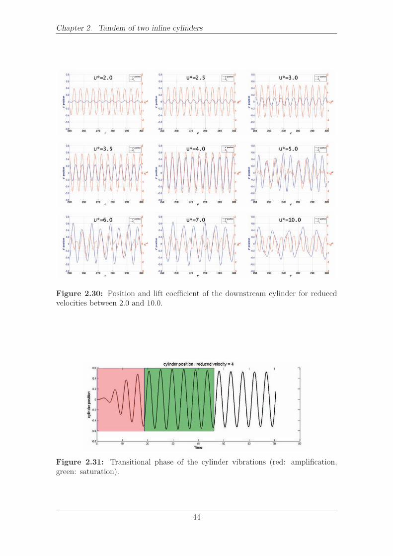
Chapter 2. Tandem of two inline cylinders
Figure 2.30: Position and lift coefficient of the downstream cylinder for reducedvelocities between 2.0 and 10.0.
Figure 2.31: Transitional phase of the cylinder vibrations (red: amplification,green: saturation).
44
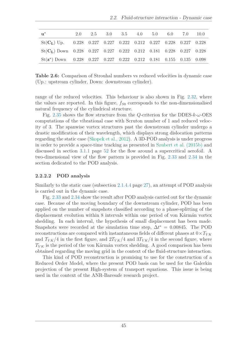
2.2. Fluid-structure interaction - Dynamic case
u∗ 2.0 2.5 3.0 3.5 4.0 5.0 6.0 7.0 10.0
St(CL) Up. 0.228 0.227 0.227 0.222 0.212 0.227 0.228 0.227 0.228
St(CL) Down 0.228 0.227 0.227 0.222 0.212 0.181 0.228 0.227 0.228
St(z∗) Down 0.228 0.227 0.227 0.222 0.212 0.181 0.155 0.135 0.098
Table 2.6: Comparison of Strouhal numbers vs reduced velocities in dynamic case(Up.: upstream cylinder, Down: downstream cylinder).
range of the reduced velocities. This behaviour is also shown in Fig. 2.32, wherethe values are reported. In this figure, fS0 corresponds to the non-dimensionalisednatural frequency of the cylindrical structure.
Fig. 2.35 shows the flow structure from the Q-criterion for the DDES-k-ω-OEScomputations of the vibrational case with Scruton number of 1 and reduced veloc-ity of 3. The spanwise vortex structures past the downstream cylinder undergo adrastic modification of their wavelength, which displays strong dislocation patternsregarding the static case (Skopek et al., 2012). A 3D-POD analysis is under progressin order to provide a space-time tracking as presented in Szubert et al. (2015b) anddiscussed in section 3.1.1 page 52 for the flow around a supercritical aerofoil. Atwo-dimensional view of the flow pattern is provided in Fig. 2.33 and 2.34 in thesection dedicated to the POD analysis.
2.2.2.2 POD analysis
Similarly to the static case (subsection 2.1.4.4 page 27), an attempt of POD analysisis carried out in the dynamic case.
Fig. 2.33 and 2.34 show the result after POD analysis carried out for the dynamiccase. Because of the moving boundary of the downstream cylinder, POD has beenapplied on the number of snapshots classified according to a phase-splitting of thedisplacement evolution within 8 intervals within one period of von Kármán vortexshedding. In each interval, the hypothesis of small displacement has been made.Snapshots were recorded at the simulation time step, ∆t∗ = 0.00845. The PODreconstructions are compared with instantaneous fields of different phases at 0×TV K
and TV K/4 in the first figure, and 2TV K/4 and 3TV K/4 in the second figure, whereTV K is the period of the von Kármán vortex shedding. A good comparison has beenobtained regarding the moving grid in the context of the fluid-structure interaction.
This kind of POD reconstruction is promising to use for the construction of aReduced Order Model, where the present POD basis can be used for the Galerkinprojection of the present High-system of transport equations. This issue is beingused in the context of the ANR-Baresafe research project.
45
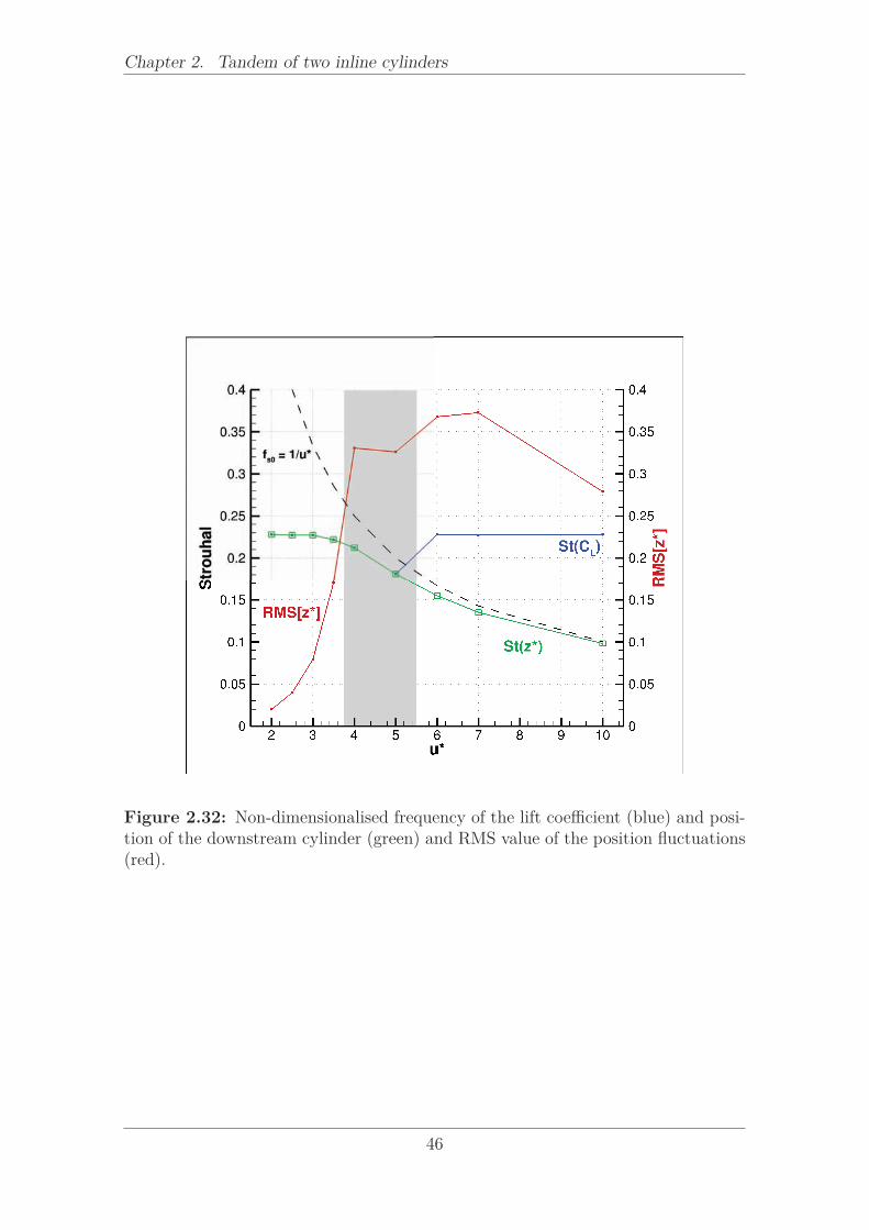
Chapter 2. Tandem of two inline cylinders
Figure 2.32: Non-dimensionalised frequency of the lift coefficient (blue) and posi-tion of the downstream cylinder (green) and RMS value of the position fluctuations(red).
46

2.2. Fluid-structure interaction - Dynamic case
Figure 2.33: Vorticity field from URANS (top) and POD reconstruction from 3,5 and 69 modes at 0 × TV K (left) and TV K/4 (right) in dynamic case.
47

Chapter 2. Tandem of two inline cylinders
Figure 2.34: Vorticity field from URANS (top) and POD reconstruction from 3,5 and 69 modes at 2TV K/4 (left) and 3TV K/4 (right) in dynamic case.
48
2.3. Conclusion
2.3 Conclusion
2D simulations of the tandem cylinders configuration have been performed to deter-mine the optimal convergence criterion, as well as to study the capability of threeturbulence models to predict the flow around this geometry, compared to experimen-tal results. All these results have been used for DDES computations (Skopek et al.,2012), that highlighted the importance of the third dimension in the prediction , andconfirmed that classical URANS modelling is not suitable to capture high-frequencyphenomena, in particular in the noise range. However, hybrid modelling was able topredict with high accuracy these phenomena, as well as the mean flow properties.
The present study has shown the ability of spontaneous oscillatory motion gen-eration on the downstream cylinder, which was allowed moving freely in the verticaldirection along the lift coefficient. The computations have shown the passage fromthe VIV lock-in mechanism towards the MIV mechanism of vibrational instabilitycharacterized by negative damping. The corresponding progressive increase of thephase-lag from zero (in the VIV case) to higher values (in the MIV case) reachingalso phase opposition by 180 has been quantified, as well as the appearance of neg-ative damping in the transient phases of the motion. This behaviour is in qualitativeagreement with the Connors experimental diagram as well as with other DDES sim-ulations in the context of the ANR-Baresafe program (Shinde et al., 2014). Thesesimulations predicted the von Kármán instability frequencies as well as the evolu-tion as a function of the reduced velocity, of the von Kármán mode Strouhal numberand of the RMS of lift coefficient. The fluid-structure interaction is currently beingstudied by means of hybrid DDES simulations aforementioned Fig.2.35)
Based on the present High-Fidelity approaches, the present thesis carried out aPOD reconstruction of the static and dynamic structural oscillation flow cases, byusing an adapted phasing of the POD snapshots in the dynamic case. The providedreconstructions are able to capture the principal dynamics of the flow field and themethod is currently in use in the Baresafe context for the Reduced Order Modellingof the dynamic case.
49
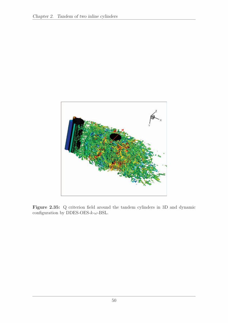
Chapter 2. Tandem of two inline cylinders
Figure 2.35: Q criterion field around the tandem cylinders in 3D and dynamicconfiguration by DDES-OES-k-ω-BSL.
50