conférence technoark 2016 - 14 epfl-valais
TRANSCRIPT

©Francois Marechal -IPESE-IGM-STI-EPFL 2014
IPESEIndustrial Process and
Energy Systems Engineering
E-transition : the role of the E-technology for the Energy
transition
Prof François Marechal Industrial Process and Energy Systems Engineering
EPFL VALAIS-WALLIS

©Francois Marechal -IPESE-IGM-STI-EPFL 2014
IPESEIndustrial Process and
Energy Systems Engineering
• E-technology for engineering – E-technology for modelling – E-technology for data structuring – E-technology for decision support – E-technology for understanding
• E-technology for operating • E-technology for teaching
E-techonology for the energy transition

©Francois Marechal -IPESE-IGM-STI-EPFL 2014
IPESEIndustrial Process and
Energy Systems Engineering
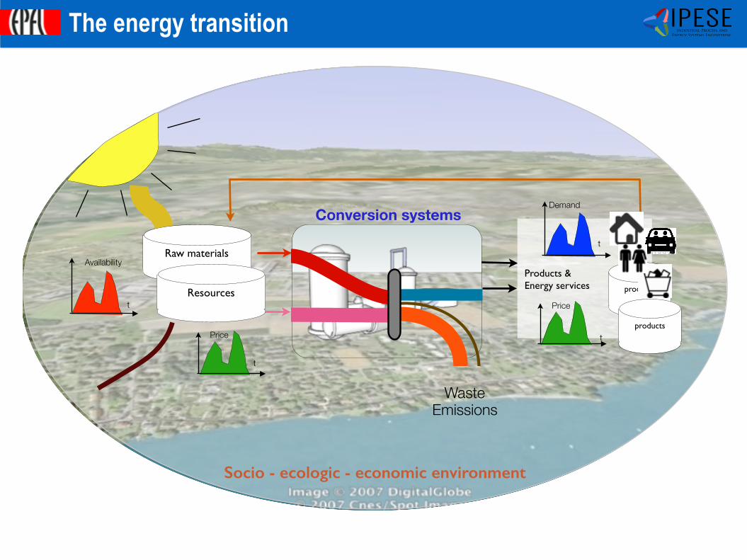
Socio - ecologic - economic environment
The energy system
Conversion systems
Waste Emissions
Raw materials
Resources
Price
Availability
t
t
Products &Energy services products
products
Demand
Price
t
t
©Francois Marechal -IPESE-IGM-STI-EPFL 2014
IPESEIndustrial Process and
Energy Systems Engineering
Socio - ecologic - economic environment
The energy transition
Conversion systems
Raw materials
Resources
Price
Availability
t
t
Waste Emissions
Products &Energy services products
products
Demand
Price
t
t
©Francois Marechal -IPESE-IGM-STI-EPFL 2014
IPESEIndustrial Process and
Energy Systems Engineering
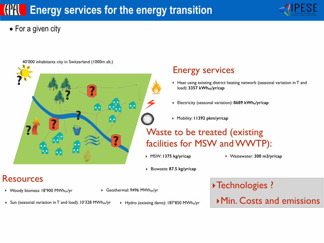
• For a given city
Energy services for the energy transition
Energy services
‣Technologies ?
‣Min. Costs and emissions
‣ Heat using existing district heating network (seasonal variation in T and load): 3357 kWhth/yr/cap
Waste to be treated (existing facilities for MSW and WWTP):
Resources
‣ Electricity (seasonal variation): 8689 kWhe/yr/cap
‣ Mobility: 11392 pkm/yr/cap
‣ MSW: 1375 kg/yr/cap ‣ Wastewater: 300 m3/yr/cap
‣ Biowaste: 87.5 kg/yr/cap
‣ Woody biomass: 18’900 MWhth/yr
‣ Sun (seasonal variation in T and load): 10‘328 MWhth/yr ‣ Hydro (existing dams): 187‘850 MWhe/yr
‣ Geothermal: 9496 MWhth/yr
?
??
??
??
40’000 inhabitants city in Switzerland (1000m alt.)
©Francois Marechal -IPESE-IGM-STI-EPFL 2014
IPESEIndustrial Process and
Energy Systems Engineering
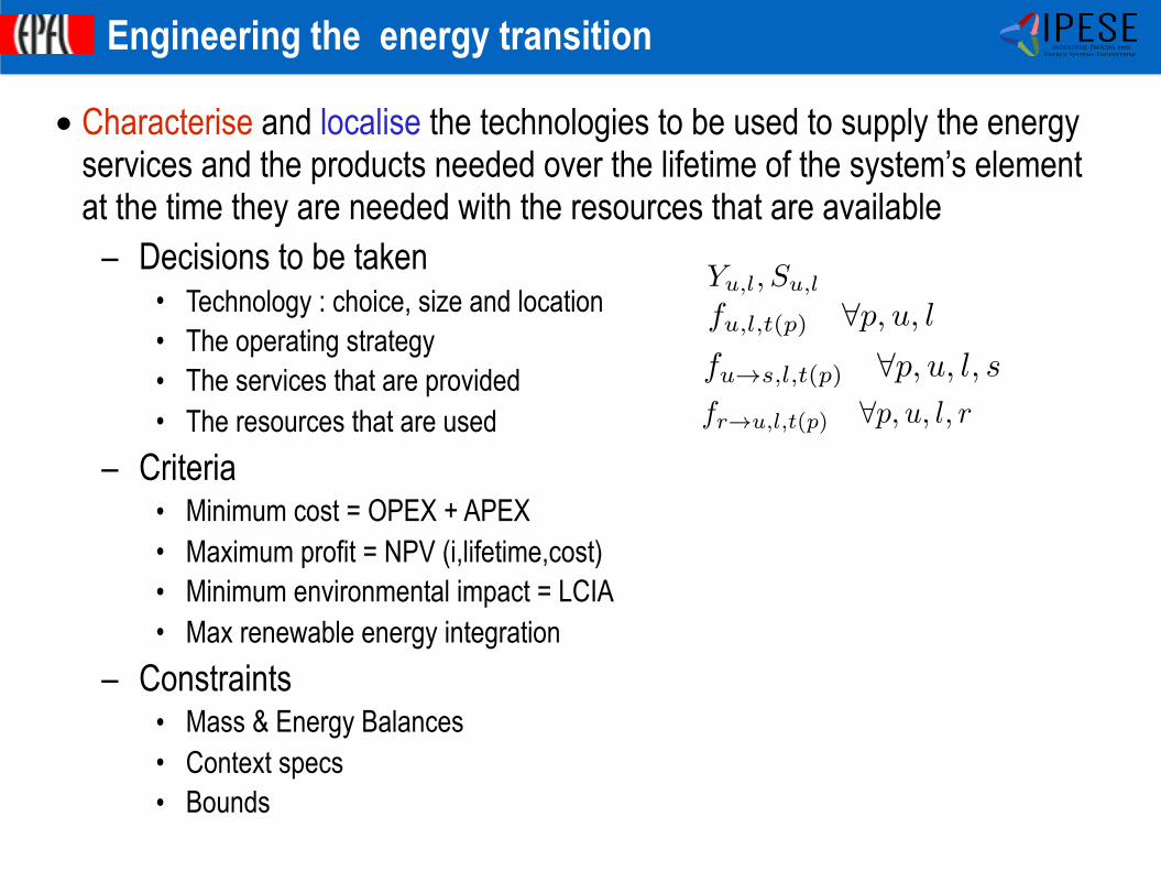
• Characterise and localise the technologies to be used to supply the energy services and the products needed over the lifetime of the system’s element at the time they are needed with the resources that are available
– Decisions to be taken • Technology : choice, size and location • The operating strategy • The services that are provided • The resources that are used
– Criteria • Minimum cost = OPEX + APEX • Maximum profit = NPV (i,lifetime,cost) • Minimum environmental impact = LCIA • Max renewable energy integration
– Constraints • Mass & Energy Balances • Context specs • Bounds
Engineering the energy transition
Yu,l, Su,l
fu,l,t(p) 8p, u, lfu!s,l,t(p) 8p, u, l, sfr!u,l,t(p) 8p, u, l, r

©Francois Marechal -IPESE-IGM-STI-EPFL 2014
IPESEIndustrial Process and
Energy Systems Engineering
E-technology for engineering

©Francois Marechal -IPESE-IGM-STI-EPFL 2014
IPESEIndustrial Process and
Energy Systems EngineeringThe energy systems engineering methodology
Solutions
Energy services Resources Context & Constraints
Superstructure
System Boundaries
System performances indicators•Economic•Thermodynamic• Life cycle environmental impact
Results analysis•Exergy analysis•Composite curves•Sensitivity analysis•Multi-criteria
Technology options
Models
250
300
350
400
450
500
550
600
0 5000 10000 15000 20000 25000 30000
T(K
)
Q(kW)
Cold composite curve
Hot composite curveHeat & Mass integration
Decision variables
Solving method
Thermo-economic Pareto
Multi-objectiveOptimization
Out=F(In,P)

©Francois Marechal -IPESE-IGM-STI-EPFL 2014
IPESEIndustrial Process and
Energy Systems EngineeringMulti-scale problem 9
9
EnA / EnMS
Common element is the energy planning
• Energy consumption profile determination
• Energy performance evaluation
• Energy baseline generation
• Identification and evaluation of improvement options
• Implementation and monitoring
Step 1
Step 2
• Systematic approach
• Methodologies
• Tools
Context Literature review Problematic 1st year research Research plan Conclusion
Step 3
Details
Scale
Technologies
Processes
IndustrialClusters
Districts
RegionsE-technologyfordecisionsupport
*Modellingtheinteractions* Identifyingthesynergies* Implementingthebestinteractions=>NetworkorGrid
MaterialsEngineering:
frommaterialsdevelopmenttosystemintegration

©Francois Marechal -IPESE-IGM-STI-EPFL 2014
IPESEIndustrial Process and
Energy Systems Engineering
• Model of the interconnectivity (mass, heat, energy) • Model of the emissions (Equipment, Emissions) • Model of the cost (size => cost, maintenance)
E-technology for modelling
-Equipmentsizingmodel-Costestimation
Heattransferrequirement
Heattransfer
Thermo-chemicalconversion Model
MaterialstreamsProductstreams
ElectricityHeattransferrequirement
WaterstreamsWaterstreams
WastestreamsWastestreams
ElectricityUnitparametersDecisionVariables
Lifecycleemissions
Lifecycleofequipment-Production-Dismantling
MaintenanceInvestmentcost
LCAmodels
LCAmodels
©Francois Marechal -IPESE-IGM-STI-EPFL 2014
IPESEIndustrial Process and
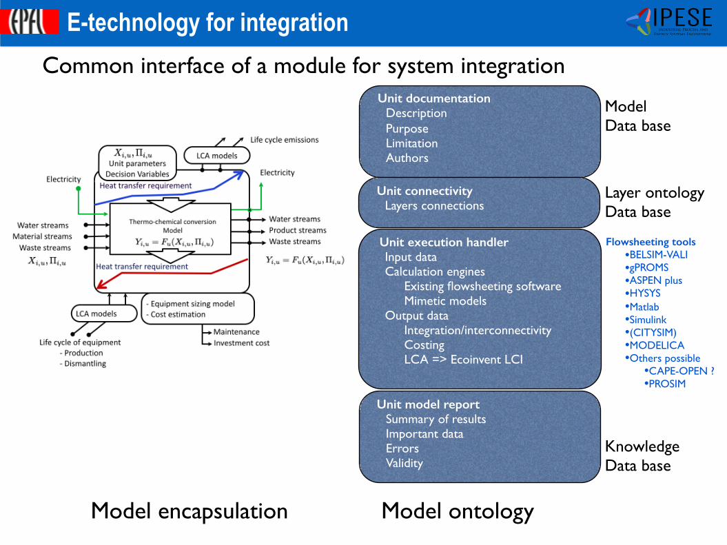
Energy Systems EngineeringE-technology for integration
Unit documentation DescriptionPurposeLimitationAuthors
Unit model report Summary of resultsImportant dataErrorsValidity
Unit execution handler Input dataCalculation engines
Existing flowsheeting softwareMimetic models
Output dataIntegration/interconnectivityCostingLCA => Ecoinvent LCI
Model ontologyModel encapsulation
Common interface of a module for system integration
Flowsheeting tools •BELSIM-VALI•gPROMS•ASPEN plus•HYSYS•Matlab•Simulink•(CITYSIM)•MODELICA•Others possible
•CAPE-OPEN ?•PROSIM
Unit connectivity Layers connections
Layer ontologyData base
ModelData base
KnowledgeData base
©Francois Marechal -IPESE-IGM-STI-EPFL 2014
IPESEIndustrial Process and
Energy Systems Engineering
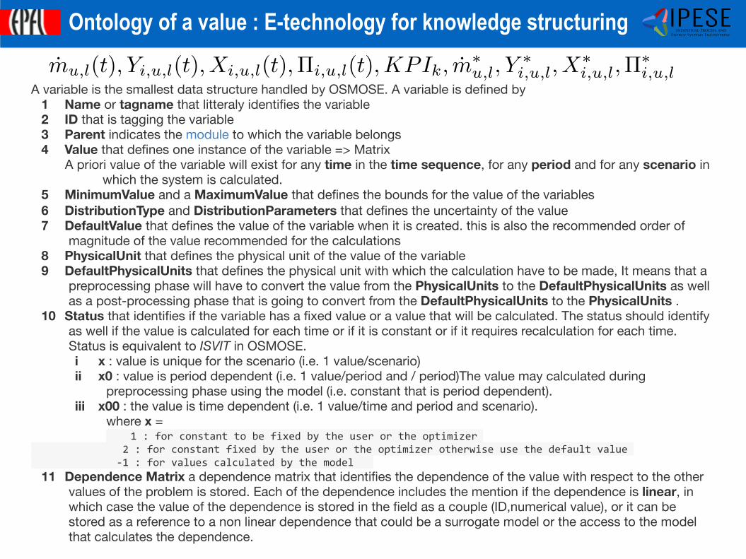
A variable is the smallest data structure handled by OSMOSE. A variable is defined by1 Name or tagname that litteraly identifies the variable2 ID that is tagging the variable3 Parent indicates the module to which the variable belongs4 Value that defines one instance of the variable => Matrix
A priori value of the variable will exist for any time in the time sequence, for any period and for any scenario in which the system is calculated.
5 MinimumValue and a MaximumValue that defines the bounds for the value of the variables 6 DistributionType and DistributionParameters that defines the uncertainty of the value
7 DefaultValue that defines the value of the variable when it is created. this is also the recommended order of magnitude of the value recommended for the calculations
8 PhysicalUnit that defines the physical unit of the value of the variable9 DefaultPhysicalUnits that defines the physical unit with which the calculation have to be made, It means that a
preprocessing phase will have to convert the value from the PhysicalUnits to the DefaultPhysicalUnits as well as a post-processing phase that is going to convert from the DefaultPhysicalUnits to the PhysicalUnits .
10 Status that identifies if the variable has a fixed value or a value that will be calculated. The status should identify as well if the value is calculated for each time or if it is constant or if it requires recalculation for each time. Status is equivalent to ISVIT in OSMOSE.i x : value is unique for the scenario (i.e. 1 value/scenario)ii x0 : value is period dependent (i.e. 1 value/period and / period)The value may calculated during
preprocessing phase using the model (i.e. constant that is period dependent).iii x00 : the value is time dependent (i.e. 1 value/time and period and scenario).
where x = 1 : for constant to be fixed by the user or the optimizer
2 : for constant fixed by the user or the optimizer otherwise use the default value -1 : for values calculated by the model
11 Dependence Matrix a dependence matrix that identifies the dependence of the value with respect to the other values of the problem is stored. Each of the dependence includes the mention if the dependence is linear, in which case the value of the dependence is stored in the field as a couple (ID,numerical value), or it can be stored as a reference to a non linear dependence that could be a surrogate model or the access to the model that calculates the dependence.
Ontology of a value : E-technology for knowledge structuring
mu,l(t), Yi,u,l(t), Xi,u,l(t),⇧i,u,l(t),KPIk, m⇤u,l, Y
⇤i,u,l, X
⇤i,u,l,⇧
⇤i,u,l

©Francois Marechal -IPESE-IGM-STI-EPFL 2014
IPESEIndustrial Process and
Energy Systems EngineeringE-technology : Models & knowledge data base
©Francois Marechal -IPESE-IGM-STI-EPFL 2014
IPESEIndustrial Process and
Energy Systems Engineering
LENI Systems
Flowsheet generation (2)Energy-integration model
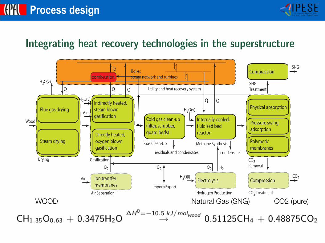
Integrating heat recovery technologies in the superstructure
43 / 87
Process design
WOOD Natural Gas (SNG) CO2 (pure)

©Francois Marechal -IPESE-IGM-STI-EPFL 2014
IPESEIndustrial Process and
Energy Systems Engineering
• Explicit – In flowsheeting software
• Automatic – Based on the connectivity description – Restricted matches – Routing
• Implicit – Heat cascades
• Combined – Mass and Energy
Modeling the systems interactions
Luc Girardin page 25/77
Travail de diplôme : Méthodologie de conception optimale d'un réseau hydrogène d'un site industriel.
7.2 DÉFINITION DE LA SUPERSTRUCTURE
Le réseau d'hydrogène est conçu comme une superstructure qui contient toutes les sources et puits desunités productrices/consommatrices d'hydrogène, et qui incorpore toutes les connections possibles entre cessources et ces puits (Figure 7.2). Toutes les connections de la superstructure ne sont pas admissibles, cequi revient à introduire dans le modèle des contraintes sur l'établissement des nouvelles connexions.
Le point de fonctionnement de la structure est défini par l'ensemble des données requises pour chaqueconsommateur, chaque producteur, et chaque unité.
Chaque source de la structure est caractérisée par :
! la pureté de l'hydrogène produit Xp
! la pureté en impuretés produites x p , j
! un débit d'hydrogène disponible délivré "mp
! le niveau de pression total du flux délivré P p .
En contrepartie, chaque puits est défini par :
! la pureté requise du flux d'entrée Xc
! les limites de composition en impuretés du mélange admis xc , jmax
! un besoin de débit d'hydrogène "mc
! la pression totale requise du mélange à l'entrée Pc .
Le nombre des puits et sources, regroupé au sein d'une même unité, est égal au nombre de niveaux distinctsde pureté des flux d'hydrogène admis, respectivement rejetés. Dans un premier temps, on peut admettre quechaque unité possède au maximum 1 consommateur et 2 producteurs. Un nombre plus élevé de ceséléments par unité correspond à un affinement du modèle, et entraîne une augmentation de la densité deconnexions au sein de la superstructure
On a vu que les unités regroupent, dans une même structure, des puits et des sources qu'on appelleconsommateurs et producteurs.
Elles sont définies par :
! l'identité des puits et sources qui la compose,
! leurs coordonnées (X,Y) géo-référencées,
! un identifiant, qui permet de les regrouper en sous-systèmes pour l'analyse dans les diagrammes dePincement (cf. Chapitre "Représentation graphiques").
25/77 18/02/05
Figure 7.1 : Schéma de la superstructure complexe
250
300
350
400
450
500
550
600
0 5000 10000 15000 20000 25000 30000
T(K
)
Q(kW)
Cold composite curve
Hot composite curve
©Francois Marechal -IPESE-IGM-STI-EPFL 2014
IPESEIndustrial Process and
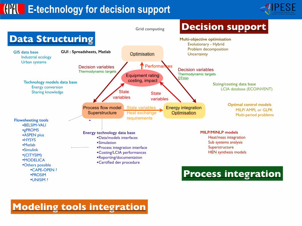
Energy Systems EngineeringE-technology for decision support
Flowsheeting tools •BELSIM-VALI•gPROMS•ASPEN plus•HYSYS•Matlab•Simulink•(CITYSIM)•MODELICA•Others possible
•CAPE-OPEN ?•PROSIM•UNISIM ?
Energy technology data base •Data/models interfaces•Simulation•Process integration interface•Costing/LCIA performances•Reporting/documentation•Certified dev procedure
Modeling tools integration
MILP/MINLP models Heat/mass integrationSub systems analysisSuperstructureHEN synthesis models
Optimal control models MILP/ AMPL or GLPKMulti-period problems
Sizing/costing data base LCIA database (ECOINVENT)
Process integration
Grid computing
Multi-objective optimisation Evolutionary - HybridProblem decompositionUncertainty
Decision support
GIS data base Industrial ecologyUrban systems
GUI : Spreadsheets, Matlab
Data Structuring
Technology models data base Energy conversionSharing knowledge
©Francois Marechal -IPESE-IGM-STI-EPFL 2014
IPESEIndustrial Process and
Energy Systems Engineering
LENI Systems
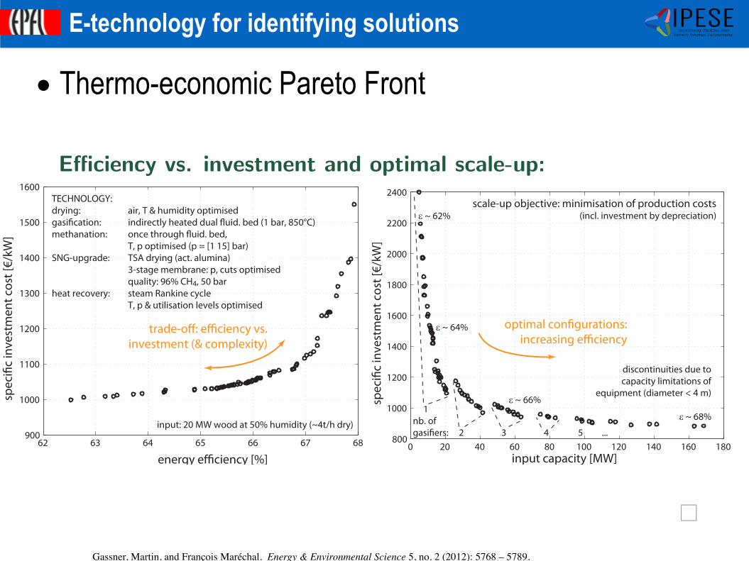
Thermo-economic optimisationTrade-o�s: e⇥ciency and scale vs. investment
E⇥ciency vs. investment and optimal scale-up:
62 63 64 65 66 67 68900
1000
1100
1200
1300
1400
1500
1600
energy efficiency [%]
spec
ific
inve
stm
ent
cost
[€/k
W]
trade-off: efficiency vs.investment (& complexity)
TECHNOLOGY: drying: air, T & humidity optimisedgasification: indirectly heated dual fluid. bed (1 bar, 850°C)methanation: once through fluid. bed, T, p optimised (p = [1 15] bar)SNG-upgrade: TSA drying (act. alumina) 3-stage membrane: p, cuts optimised quality: 96% CH4, 50 barheat recovery: steam Rankine cycle T, p & utilisation levels optimised
input: 20 MW wood at 50% humidity (~4t/h dry)
0 20 40 60 80 100 120 140 160 180800
1000
1200
1400
1600
1800
2000
2200
2400
input capacity [MW]
spec
ific
inve
stm
ent
cost
[€/k
W]
scale-up objective: minimisation of production costs(incl. investment by depreciation)ε ~ 62%
ε ~ 66%
ε ~ 64%
ε ~ 68%
optimal configurations:increasing efficiency
discontinuities due tocapacity limitations of
equipment (diameter < 4 m)
1nb. ofgasifiers: 2 3 4 5 ...
61 / 87Gassner, Martin, and François Maréchal. Energy & Environmental Science 5, no. 2 (2012): 5768 – 5789.
• Thermo-economic Pareto Front
E-technology for identifying solutions
©Francois Marechal -IPESE-IGM-STI-EPFL 2014
IPESEIndustrial Process and
Energy Systems Engineering
LENI Systems
Some resultsCmparing technologies and processes
Thermo-economic Pareto front(cost vs e�ciency):
LENI Systems
Quelques resultatsComparaison des technologies
Optimisation de toutes les combinaisions technologiques(cout et e�cacite):
� gaz. pressurise a chau�age direct est la meilleure option� The best solution is the pressurised directly heated gasifier
69 / 87
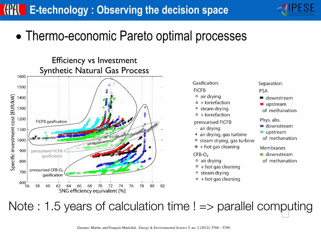
• Thermo-economic Pareto optimal processes
E-technology : Observing the decision space
Gassner, Martin, and François Maréchal. Energy & Environmental Science 5, no. 2 (2012): 5768 – 5789.
Note : 1.5 years of calculation time ! => parallel computing
Efficiency vs InvestmentSynthetic Natural Gas Process

©Francois Marechal -IPESE-IGM-STI-EPFL 2014
IPESEIndustrial Process and
Energy Systems Engineering
• Graphical representations – Composite curves – Sankeydiagrams
• PDF reports • Sensitivity analysis • Pareto curves => data base of solutions
– Decision variables values
– Uncertainty analysis => most probable optimal solutions
E-technology for understanding the results
250
300
350
400
450
500
550
600
0 5000 10000 15000 20000 25000 30000
T(K
)
Q(kW)
Cold composite curve
Hot composite curve
64 66 68 70 72 74 76 78 80 82 84 86 88600
700
800
900
1000
1100
1200
1300
SNG efficiency equivalent εchem [%]
Spe
cifi
c in
vest
me
nt
cost
cG
R [U
SD/k
W]
pressurisation
pressurisation, gas turbine integration,steam drying
& hot gas cleaning
hot gas cleaning & steam dryingwith heat cogeneration
453 K
513 K
5 %
35 %
1073 K
1173 K
573 K
873 K
1 bar
50 bar
573 K
673 K
573 K
673 K
0
1
40 bar
100 bar
623 K
823 K
323 K
523 K
SNG Outputminimal
maximal
min
max
min
max
min
max
Td,in Φw,out Tg Tg,p
pm Tm,in Tm,out yRankine
ps,p Ts,s Ts,u2
0 20 40 60 80 100 1200
0.01
0.02
0.03
0.04
0.05
0.06
0.07
0.08
0.09
0.1
SNG proccess configuration number
Pro
babi
lity
to b
e in
top
10 [−
]
Prod. costRes. profitabilityBM Break even
4.3. COMPARISON WITH CONVENTIONAL LCA 45
-500 %
-400 %
-300 %
-200 %
-100 %
0 %
100 %
200 %
scale-independent,conventional LCIA
(average lab/pilot tech.)
without cogenerationIntegrated industrial base case scenario (8 MWth)
with cogeneration
(a) Overall impacts
0
5
10
15
20
25
Remaining processes
Rape methyl ester
NOx emissions
Solid waste
Charcoal
Olivine
Infrastructure
Wood chips production
Electricity cons./prod.
Avoided NG extraction
Avoided CO2 emissions
UBP/
MJ w
ood
scale-independent,conventional LCIA
(average lab/pilot tech.)
harm
ful
bene
ficia
l
harm
ful
bene
ficia
l
harm
ful
bene
ficia
l
without cogenerationIntegrated industrial base case scenario (8 MWth)
with cogeneration
(b) Detailed contribution
Figure 4.3: Comparison of LCIA results obtained by conventional LCA and the proposedmethodology for Ecoscarcity06, single score, with detailed process contributions (Gerberet al. (2011a))
The differences between the conventional LCA and the base case scenario without and witha Rankine cycle are mainly due to the improved conversion efficiency obtained by applyingprocess design method, which has a direct influence on the quantity of SNG produced perunit of biomass. In the base case scenarios, the efficiency is considerably higher becausethe energy integration is optimized in the process design. As a direct consequence, the

©Francois Marechal -IPESE-IGM-STI-EPFL 2014
IPESEIndustrial Process and
Energy Systems EngineeringE-technology : Large renewable energy integration
Use B M
Use G M
Photo synthesis
S
CO2 CH4
DH
TS
EL
SOEC M
SOFC
RNE
Biomethane
Gasification
Storage
Dist
rict h
eatin
g
Co-electrolysis
Electrolysis
Renewable Electricity
Sun
Biomass
CO2
H2O2
CH4
Heat
Renewable Electricity
SunWind
Grid Electricity
Fuel appl.
O2
H2O
H2O
P MSun
Captureatm. CO2
CaptureFlue gases
B : BiomethanisationC : CO2 CaptureG : GasificationM : methanationS : CO2 separationP : Photocatalysis for CO2 reductionSOFC : Solid Oxide Fuel CellSOEC : Solid Oxid electrolysis CellET : Electro thermal storageCO2 : CO2 StorageCH4 : Methane StorageDH : District Heating
CO2
H2
O2
CH4
H2O
Elec
Ren Elec
atm. CO2
CO2
H2O
EPFL Valais-Wallis DemonstratorIntegration of processes in the conversion chain : CO2 valorisation options

©Francois Marechal -IPESE-IGM-STI-EPFL 2014
IPESEIndustrial Process and
Energy Systems Engineering
•Coordinates attributed to locations – GIS : Data bases
• Buildings • Resources
– GIS :Infrastructure • Roads, district heating network,
electricity grid – GIS Tools : Routing, Layers, Representations
•Link between GIS data and Models –Link with unit models parameters –Access to GIS tools in the workflow
E-technology : Data bases and Geographical Information Systems
Locationi,(xi,yi,zi)
Location1,(x1,y1,z1)
Location2,(x2,y2,z2)
Geneva
T TTT -20
0
20
40
60
80
0 50 100 150 200 250 300 350 400
T(C
)Q(kW)
AirWaste Water
Heating Hot water
recoveryRecoverable
Heat requirement
Atagivenlocation:combinationofenergytechnologies

©Francois Marechal -IPESE-IGM-STI-EPFL 2014
IPESEIndustrial Process and
Energy Systems EngineeringE-technology : defining the interactions
1 Symbols
Roman lettersAn Annuities of a given investment [-]Ai,j,p Surface of the pipe of network p between nodes i and j [m2]B Arbitrarily big valueCaw Investment costs for air/water heat pump(s) [CHF]Cboiler Annual investment costs of the boiler(s) [CHF/year]Cfix Fix part of investment costs for a given device [CHF]Cgas Total gas costs [CHF]cgas Gas costs [CHF/kWh]Cgrid Total grid costs [CHF]cgrid Grid costs [CHF/kWh]C inv Investment costs of a given device [CHF]C inv
an Annual investment costs of a given device [CHF]Cpipes Total costs for the piping [CHF]Cprop Fix part of investment costs for a given device [CHF/kW]Cref Investment costs of a device chosen as reference [CHF]Cww Investment costs for water/water heat pump(s) [CHF]CO2
gas Total CO2 emissions for one year due to the combustion of gas [kg]co2
gas CO2 emissions due to the combustion of gas per kWh [kg/kWh]CO2
grid Total CO2 emissions for one year due to the consumption of electricity from the grid [kg]co2
grid CO2 emissions due to the consumption of electricity from the grid [kg/kWh]COP aw
t,k Coe⇤cient of performance for the air/water heat pump during period t at node k [-]COPww
t,k Coe⇤cient of performance for a water/water heat pump during period t at node k [-]cp Isobaric specific heat [kJ/(K· kg)]Disti,j Distance between nodes i and j [m]Ht Number of hours in period t [hour]Econs
t,k Electricity consumption during period t at node k [kW]Eexp
t,k Eletricity exported to the grid during period t by device e [kW]Egrid
t,k Electricity bought from the grid during period t [kW]Eaw
t,k Electricity consumed by the air/water heat pump during period t at node k [kW]Eww
t,k Electricity consumed by the water/water heat pump during period t at node k [kW]Eloss
t,k Electricity losses during period t [kW]Epump
t Pumping power for the network during period t [kW]Etech
t,k,e Electricity produced or consumed during period t at node k by device e [kW]Fm Maintenance factor [-]Gast Overall gas consumption during period t [kg]Lmin
e Minimum allowable part-load of device e [-]
Mbuildt,k
Mass flow of water from the network, circulating during period t through thebuilding at node k to heat up the building [kg/s]
Mpipet,i,j,p
Mass flow of water flowing during period t, in network p, from node i to nodej [kg/s]
Mmaxt,p,i,j
Maximum mass flow of water flowing in network p, from node i to node j, overall periods of time [kg/s]
M techt,k
Mass flow from the network being heated up by the device(s) at node k duringperiod t [kW]
MT buildt,k
Mass flow from the network flowing through a device at node k during periodt, to be re-heated, times its temperature [(kg/s)K]
2
MT pipet,i,j,p
Mass flow flowing during period t from node i to node j in the network p, timesits temperature [(kg/s)K]
N Expected lifetime for a given investment [year]Ploss Pressure losses in the pipes [Pa/m]Qaw
t,k Heat delivered by the air/water heat pump to the consumer at node k during period t [kW]Qboiler
t,k Heat delivered by the boiler at node k during period t [kW]Qcons
t,k Heat consumption at node k during period t [kW]Qnet
t,k Heat delivered by the network to the consumer at node k during period t [kW]Qnet ww
t,k Heat delivered by the network to the water/water heat pump at node k during period t [kW]Qtech
t,k,e Heat produced by device e located at node k during period k [kW]Qww
t,k Heat delivered by an water/water heat pump to the consumer at node k during period t [kW]r Interest rate [-]S Size of a given device [kW]Saw
k Nominal size of the air/water heat pump located at node k [kW]Sboiler
k Nominal size of the boiler at node k [kW]Snom
e Nominal power of a device [kW]Sref Size of a device chosen as reference [kW]Sww
k Nominal power of the water/water heat pump located at node k [kW]T atm Atmospheric temperature [K]T cold Temperature of the heat source for heat pumps [K]T cons
t,k Temperature at which the heat is required by the consumer at node k during period t [K]T hot Temperature of the heat sink for heat pumps [K]T net Design temperature of the network [K]v Velocity of the water through the pipes [m/s]X = 1 if a device exists, 0 otherwiseXaw
k = 1 if there is an air/water heat pump at node k, 0 otherwiseXboiler
k = 1 if there is a boiler at node k, 0 otherwiseXgas
e = 1 if device e needs gas to operate, 0 otherwiseXnode
k = 1 if a device e is implemented at node k, 0 otherwiseXtech
k,e = 1 if a device can be implemented at node k, 0 otherwiseXww
k = 1 if there is an water/water heat pump at node k, 0 otherwiseY i,j,p = 1 if a connection exists between i and j for network p , 0 otherwise
Greek letters�Theat Pinch at the heat-exchangers [K]�Tnet ww Temperature di⇥erence of the water in the network when it serves as heat source for water/water heat pump(s) [K]�boiler Thermal e⌅ciency of the boiler(s) [-]�ele Electric e⌅ciency of device e [-]�grid E⌅ciency of the grid [-]�the Thermal e⌅ciency of device e [-]⇥ Exergetic e⌅ciency [-]⇤ Density [kg/m3]
Indicesk nodesi, j connection from node i to node jt timee technologies
3
Networks superstructure
1 Symbols
Roman lettersAn Annuities for a given investment [-]Ai,j,p Area of the pipe between nodes i and j of network p [m2]B Arbitrarily big valueCaw Investment costs for air/water heat pump(s) [CHF]Cboiler Annual investment costs for the boiler(s) [CHF/year]Cfix Fix part of the investment costs for a given device [CHF]Cgas Total annual natural gas costs [CHF/year]cgas Natural gas costs [CHF/kWh]Cgrid Total annual grid costs [CHF/year]cgrid Grid costs [CHF/kWh]C inv Investment costs of a given device [CHF]C inv
an Annual investment costs of a given device [CHF/year]Cpipes Total annual costs for the piping [CHF/year]Cprop Fix part of the investment costs for a given device [CHF/kW]Cref Investment costs of a device chosen as reference [CHF]Cww Investment costs for water/water heat pump(s) [CHF]CO2
gas Total annual CO2 emissions due to the combustion of natural gas [kg/year]co2
gas CO2 emissions due to the combustion of natural gas [kg/kWh]CO2
grid Total annual CO2 emissions due to the consumption of electricity from the grid [kg/year]co2
grid CO2 emissions due to the consumption of electricity from the grid [kg/kWh]COPhp Coe⇤cient of performance of the central heat pumpCOP aw
t,k Coe⇤cient of performance for the air/water heat pump during period t at node k [-]COPww
t,k Coe⇤cient of performance for a water/water heat pump during period t at node k [-]cp Isobaric specific heat [kJ/(K· kg)]Disti,j Distance between nodes i and j [m]Ht Number of hours in period t [hour]Econs
t,k Electricity consumption during period t at node k [kW]Eexp
t,e Eletricity exported to the grid during period t by device e [kW]Egrid
t,k Electricity bought from the grid during period t by node k [kW]Eaw
t,k Electricity consumed by the air/water heat pump during period t at node k [kW]Eww
t,k Electricity consumed by the water/water heat pump during period t at node k [kW]Eloss
t Electricity losses during period t [kW]Epump
t Pumping power for the network during period t [kW]Etech
t,k,e Electricity produced or consumed during period t at node k by device e [kW]Fs Scaling factor [-]Fm Maintenance factor [-]Gast Natural gas consumption during period t [kg]Lmin
e Minimum allowable part-load of device e [-]Mbuild
t,k Water circulating during period t through the building at node k, to heat it up [kg/s]Mpipe
t,i,j,p Water flowing during period t, from node i to node j, in network p [kg/s]Mmax
i,j,p Maximum flow of water between nodes i and j, in network p, over all periods [kg/s]M tech
t,k Water being heated up by the device(s) during period t, at node k [kg/s]MT tech
t,k Water flowing through a device during period t at node k to be re-heated, times its temperature [(kg/s)K]
2
Q1..T
E1..T
Q1..T
E1..T
Q1..T
E1..T
Q1..T
E1..T
Q1..T
E1..TQ1..T
E1..T
Q1..T
E1..T
Q1..T
E1..T
Cinv =ne�
e=1
nk�
k=1
ae + ae � Se,k
Investment
Cgas =ne�
e=1
nk�
k=1
np�
t=1
HtQe,k,t
�the
1 Symbols
Roman lettersAn Annuities for a given investment [-]Ai,j,p Area of the pipe between nodes i and j of network p [m2]B Arbitrarily big valueCaw Investment costs for air/water heat pump(s) [CHF]Cboiler Annual investment costs for the boiler(s) [CHF/year]Cfix Fix part of the investment costs for a given device [CHF]Cgas Total annual natural gas costs [CHF/year]cgas Natural gas costs [CHF/kWh]Cgrid Total annual grid costs [CHF/year]cgrid Grid costs [CHF/kWh]C inv Investment costs of a given device [CHF]C inv
an Annual investment costs of a given device [CHF/year]Cpipes Total annual costs for the piping [CHF/year]Cprop Fix part of the investment costs for a given device [CHF/kW]Cref Investment costs of a device chosen as reference [CHF]Cww Investment costs for water/water heat pump(s) [CHF]CO2
gas Total annual CO2 emissions due to the combustion of natural gas [kg/year]co2
gas CO2 emissions due to the combustion of natural gas [kg/kWh]CO2
grid Total annual CO2 emissions due to the consumption of electricity from the grid [kg/year]co2
grid CO2 emissions due to the consumption of electricity from the grid [kg/kWh]COPhp Coe⇤cient of performance of the central heat pumpCOP aw
t,k Coe⇤cient of performance for the air/water heat pump during period t at node k [-]COPww
t,k Coe⇤cient of performance for a water/water heat pump during period t at node k [-]cp Isobaric specific heat [kJ/(K· kg)]Disti,j Distance between nodes i and j [m]Ht Number of hours in period t [hour]Econs
t,k Electricity consumption during period t at node k [kW]Eexp
t,e Eletricity exported to the grid during period t by device e [kW]Egrid
t,k Electricity bought from the grid during period t by node k [kW]Eaw
t,k Electricity consumed by the air/water heat pump during period t at node k [kW]Eww
t,k Electricity consumed by the water/water heat pump during period t at node k [kW]Eloss
t Electricity losses during period t [kW]Epump
t Pumping power for the network during period t [kW]Etech
t,k,e Electricity produced or consumed during period t at node k by device e [kW]Fs Scaling factor [-]Fm Maintenance factor [-]Gast Natural gas consumption during period t [kg]Lmin
e Minimum allowable part-load of device e [-]Mbuild
t,k Water circulating during period t through the building at node k, to heat it up [kg/s]Mpipe
t,i,j,p Water flowing during period t, from node i to node j, in network p [kg/s]Mmax
i,j,p Maximum flow of water between nodes i and j, in network p, over all periods [kg/s]M tech
t,k Water being heated up by the device(s) during period t, at node k [kg/s]MT tech
t,k Water flowing through a device during period t at node k to be re-heated, times its temperature [(kg/s)K]
2
Maintenance
Gas Grid
Electricity
Electricity
Emissions
1 Symbols
Roman lettersAn Annuities for a given investment [-]Ai,j,p Area of the pipe between nodes i and j of network p [m2]B Arbitrarily big valueCaw Investment costs for air/water heat pump(s) [CHF]Cboiler Annual investment costs for the boiler(s) [CHF/year]Cfix Fix part of the investment costs for a given device [CHF]Cgas Total annual natural gas costs [CHF/year]cgas Natural gas costs [CHF/kWh]Cgrid Total annual grid costs [CHF/year]cgrid Grid costs [CHF/kWh]C inv Investment costs of a given device [CHF]C inv
an Annual investment costs of a given device [CHF/year]Cpipes Total annual costs for the piping [CHF/year]Cprop Fix part of the investment costs for a given device [CHF/kW]Cref Investment costs of a device chosen as reference [CHF]Cww Investment costs for water/water heat pump(s) [CHF]CO2
gas Total annual CO2 emissions due to the combustion of natural gas [kg/year]co2
gas CO2 emissions due to the combustion of natural gas [kg/kWh]CO2
grid Total annual CO2 emissions due to the consumption of electricity from the grid [kg/year]co2
grid CO2 emissions due to the consumption of electricity from the grid [kg/kWh]COPhp Coe⇤cient of performance of the central heat pumpCOP aw
t,k Coe⇤cient of performance for the air/water heat pump during period t at node k [-]COPww
t,k Coe⇤cient of performance for a water/water heat pump during period t at node k [-]cp Isobaric specific heat [kJ/(K· kg)]Disti,j Distance between nodes i and j [m]Ht Number of hours in period t [hour]Econs
t,k Electricity consumption during period t at node k [kW]Eexp
t,e Eletricity exported to the grid during period t by device e [kW]Egrid
t,k Electricity bought from the grid during period t by node k [kW]Eaw
t,k Electricity consumed by the air/water heat pump during period t at node k [kW]Eww
t,k Electricity consumed by the water/water heat pump during period t at node k [kW]Eloss
t Electricity losses during period t [kW]Epump
t Pumping power for the network during period t [kW]Etech
t,k,e Electricity produced or consumed during period t at node k by device e [kW]Fs Scaling factor [-]Fm Maintenance factor [-]Gast Natural gas consumption during period t [kg]Lmin
e Minimum allowable part-load of device e [-]Mbuild
t,k Water circulating during period t through the building at node k, to heat it up [kg/s]Mpipe
t,i,j,p Water flowing during period t, from node i to node j, in network p [kg/s]Mmax
i,j,p Maximum flow of water between nodes i and j, in network p, over all periods [kg/s]M tech
t,k Water being heated up by the device(s) during period t, at node k [kg/s]MT tech
t,k Water flowing through a device during period t at node k to be re-heated, times its temperature [(kg/s)K]
2
Industry
Powerplant
Wastetreat.
Building plant.
. [5] Francois Marechal, Celine Weber, and Daniel Favrat. Multi-Objective Design and Optimisation of Urban Energy Systems, pages 39–81. Number ISBN: 978-3-527-31694-6. Wiley, 2008.
Water
Fuel
Water
FuelIndustrial plant.

©Francois Marechal -IPESE-IGM-STI-EPFL 2014
IPESEIndustrial Process and
Energy Systems Engineering
• Mid-season typical day demand
E-technology : Integrating renewable sources
Time
Exe
rgy
Pow
er re
quire
men
t [kW
]
Heat
Electricity
PV production
©Francois Marechal -IPESE-IGM-STI-EPFL 2014
IPESEIndustrial Process and
Energy Systems Engineering
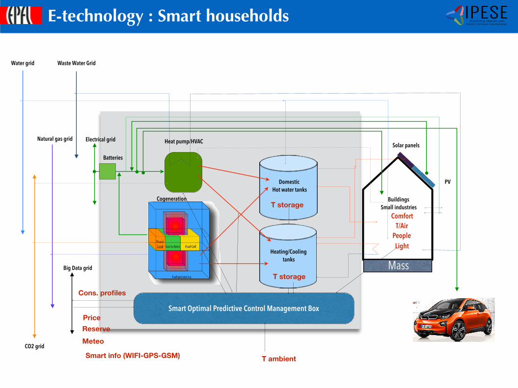
Fuel-Cell GT
Domestic Hot water tanks
Heat pump/HVACElectrical gridNatural gas grid
Buildings Small industries
E-technology : Smart households
Smart Optimal Predictive Control Management BoxPrice
T ambient
Comfort T/Air
People Light
T storage
Batteries
PV
Solar panels
Heating/Cooling tanks
Reserve
Cons. profiles
Big Data grid
Water grid
Meteo
Smart info (WIFI-GPS-GSM)
T storageMass
Waste Water Grid
Cogeneration
CO2 grid
©Francois Marechal -IPESE-IGM-STI-EPFL 2014
IPESEIndustrial Process and
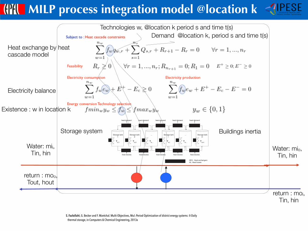
Energy Systems EngineeringMILP process integration model @location k
Water: mii, Tin, hin
return : moo, Tout, hout
Water: mio, Tin, hin
return : moi, Tin, hin
Technologies w, @location k period s and time t(s)Demand @location k, period s and time t(s)
Storage tank
2
Tst,2
HEX h1(t)
heat demand
Storage tank
1
Tst,1
...
Tst,...
Storage tank
l
Tst,l
...
Tst,...
Storage tank
nl
Tst,nl
HEX h2(t) HEX h
..(t) HEX h
l(t) HEX h
nl-1(t)
heat demand heat demand heat demand heat demand
heat excess
HEX c1(t)
heat excess
HEX c2(t)
heat excess
HEX c..(t)
heat excess
HEX cl(t)
heat excess
HEX cnl-1
(t)
Units for heat integration
HL HL HL HL HL HL
HEX: Heat exchangers
HL: Heat losses
Storage system
S. Fazlollahi, G. Becker and F. Maréchal. Multi-Objectives, Mul.-Period Optimization of district energy systems: II-Daily thermal storage, in Computers & Chemical Engineering, 2013a
Buildings inertia
Heat exchange by heat cascade model
Electricity balance
Existence : w in location k

©Francois Marechal -IPESE-IGM-STI-EPFL 2014
IPESEIndustrial Process and
Energy Systems Engineering
• Energy system = for each VPP (n) – Investments (expected life time : 20 Years)
• Energy Conversion Units • Storage
– Operating costs (expected operation time = 25x8760h) • Management strategy
– Constraints • Energy services • Grid capacities • Grid constraints
Energy system design problem
8u 2 Units; 8n 2 Nodes ) Sizeu,n
8s 2 Storage; 8n 2 Nodes ) Vs,n
8s 2 Storage; 8n 2 Nodes; 8t 2 time ) mu,n(t), Vs,n(t), E(t)
Z Time
t=1(unitsX
u=1
(c+r (t)mr(u),n(t)) + c+e (t)E+(t))dt
8t 2 T ime :NodesX
n=1
E(t) Emax
(t)
8n 2 Nodes; 8t 2 T ime; 8c 2 Cons. ) Qn,c(t), En,c(t)
NodesX
n=1
UnitsX
u=1
1
⌧y,i
(I(Sizeu,n
) + I(Vs,n
))
8q 2 quarter(T ime) :NodesX
n=1
Zq+15
t=q
��En
(t)� En
(t� 1)�� dt �E
max
(t)

©Francois Marechal -IPESE-IGM-STI-EPFL 2014
IPESEIndustrial Process and
Energy Systems EngineeringE-technology : decision support tool
Predefined data
Project data base
OSMOSE LUA
Saved user dataEnergy technologies
Problems
ModulesDefault values
ThermodynamicSizing
Costing Life Cycle Inventory
EcoInvent
Work flow
ModelsSolving methods
in locations
GIS data base
GUI
Results data base
Layer Ontology
Superstructure
Yi,u,l(p(t)) = Fu(Xi,u,l(p(t)),⇧i,u,l(p(t)))

©Francois Marechal -IPESE-IGM-STI-EPFL 2014
IPESEIndustrial Process and
Energy Systems Engineering
Design and Control of thermo-electric energy systems
Single family house : 4 pers 160 m2 : with heat pump
E-technology : Optimal design of solar systems
19.11.2015
Fig 4. Pareto front for HP system configuration
III
III
Long term storage : 85%
Long term storage : 55%
SF =kWPV
kWbuilding
Self sufficiency (SF)PV production/needs
Self consumption (SC)PV production used on site
SC
SF
SF and SC as a function of the PV areaOff-site storage
Extra Electricity from PVUsed by the building later
SC =kWused
kWPV

©Francois Marechal -IPESE-IGM-STI-EPFL 2014
IPESEIndustrial Process and
Energy Systems Engineering
Design and Control of thermo-electric energy systems
Single family house : 4 pers 160 m2 : with heat pump
Self sufficiency ?
19.11.2015
Fig 4. Pareto front for HP system configuration
III
III
Cas
e I
Energy system Off-site storage
PV array 88 m2 Battery 4.95 kWh HW tank 2.43 m3
Heat Pump 3.59 kW
Redox Battery 8.14 MWh 406.9 m3 (20 Wh/l) 4’070’000 € (500 €/kWh)
Cas
e III
Energy system Off-site storage
PV array 156.9 m2 Battery 8.63 kWh HW tank 2.39 m3
Heat Pump 3.7 kW
Redox Battery 17.1 MWh 854.6 m3
8’550’000 €
Cas
e II
Energy system Off-site storage
PV array 109.7 m2 Battery 7 kWh HW tank 2.46 m3
Heat Pump 3.5 kW
Redox Battery 10.8 MWh 540.2 m3
5’400’000 €
Annual energy balance
Long term storage : 85%
Long term storage : 55%
©Francois Marechal -IPESE-IGM-STI-EPFL 2014
IPESEIndustrial Process and
Energy Systems Engineering
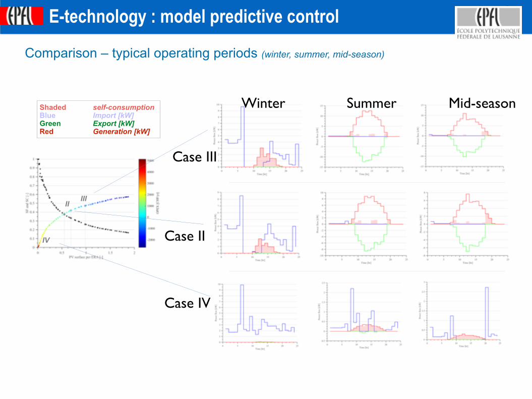
Design and Control of thermo-electric energy systems
Comparison – typical operating periods (winter, summer, mid-season)
E-technology : model predictive control
19.11.2015
IIIII
IV
Shaded self-consumption Blue Import [kW] Green Export [kW] Red Generation [kW]
Winter Summer Mid-season
Case III
Case II
Case IV

©Francois Marechal -IPESE-IGM-STI-EPFL 2014
IPESEIndustrial Process and
Energy Systems Engineering
Design and Control of thermo-electric energy systems
• Self Sufficiency : + 40 % • Self Consumption : + 68 %
E-technology : Model predictive control
SF + 41 % SC + 68 %
NetZero without MPC
©Francois Marechal -IPESE-IGM-STI-EPFL 2014
IPESEIndustrial Process and
Energy Systems Engineering
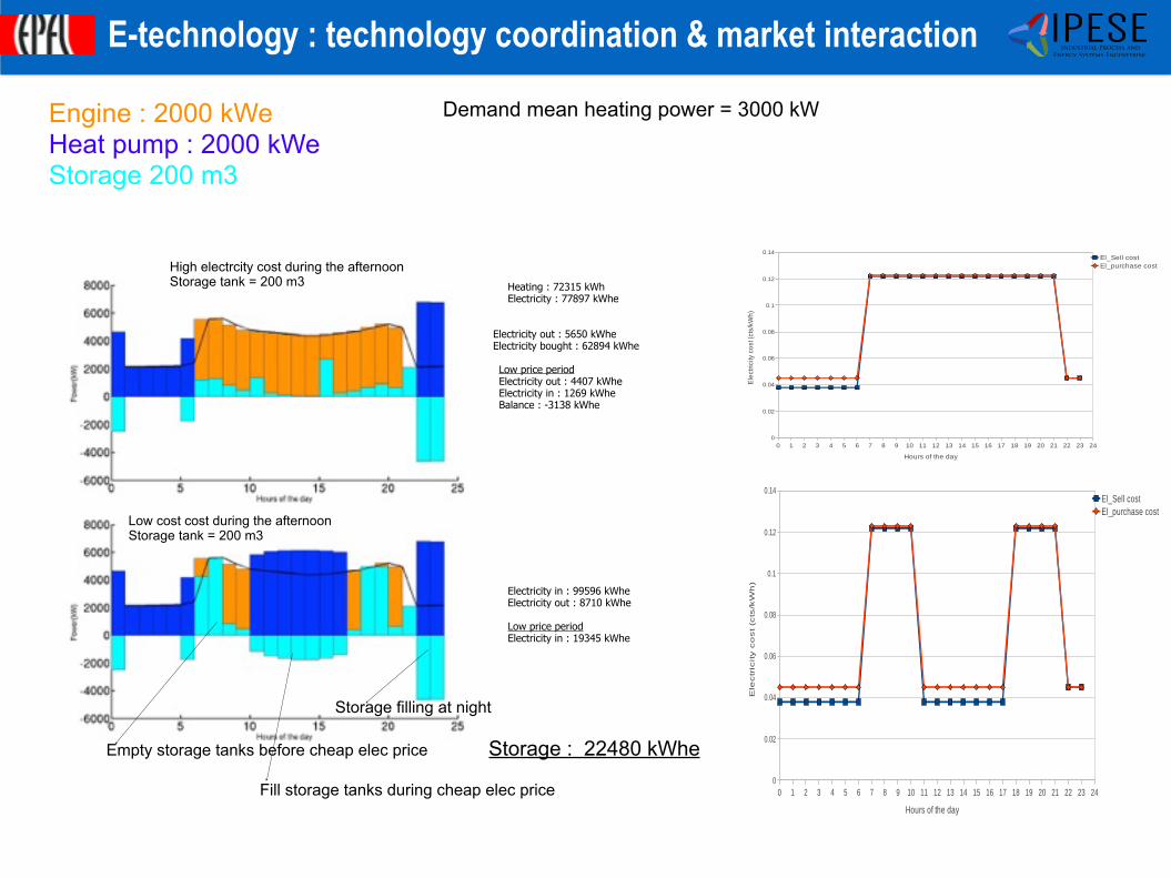
E-technology : technology coordination & market interaction
High electrcity cost during the afternoon Storage tank = 200 m3
Low cost cost during the afternoon Storage tank = 200 m3
Heating : 72315 kWh Electricity : 77897 kWhe
Electricity in : 99596 kWhe Electricity out : 8710 kWhe
Low price period Electricity in : 19345 kWhe
Electricity out : 5650 kWhe Electricity bought : 62894 kWhe
Low price period Electricity out : 4407 kWhe Electricity in : 1269 kWhe Balance : -3138 kWhe
Storage : 22480 kWhe
Engine : 2000 kWe Heat pump : 2000 kWe Storage 200 m3
Demand mean heating power = 3000 kW
Storage filling at night
Empty storage tanks before cheap elec price
Fill storage tanks during cheap elec price

©Francois Marechal -IPESE-IGM-STI-EPFL 2014
IPESEIndustrial Process and
Energy Systems Engineering
E-technology for operation

©Francois Marechal -IPESE-IGM-STI-EPFL 2014
IPESEIndustrial Process and
Energy Systems Engineering
• From design to operation
E-technology : Optimal management box
Optimization
ProblemResolution
MANAGEMENT
UNIT
MILP PROBLEM DESCRIPTION (AMPL )
Optimization Problem
data set -up
Predicteddata
Previous states
.mods .dats
u sh*u vlv*ub*ucg*
System Systemparameter
values
System Model
Prediction
Actual
State data
OPTIMIZATION (CPLEX )
States database(Current state & previous states )
(House structure - Matlab )
Data acquisitionand database
Tariff info
Tdhw
TshText
T in
Equations & constraints
Collazos et al., Computers and Chemical Eng. 2009
Grid connexions
Sensors
Operation set-points

©Francois Marechal -IPESE-IGM-STI-EPFL 2014
IPESEIndustrial Process and
Energy Systems Engineering
• Predictive Control Algorithm : Moving horizon – hour 1 : set-point control + 24 h Cyclic : strategy
Predictive Controller
©Francois Marechal -IPESE-IGM-STI-EPFL 2014
IPESEIndustrial Process and
Energy Systems Engineering
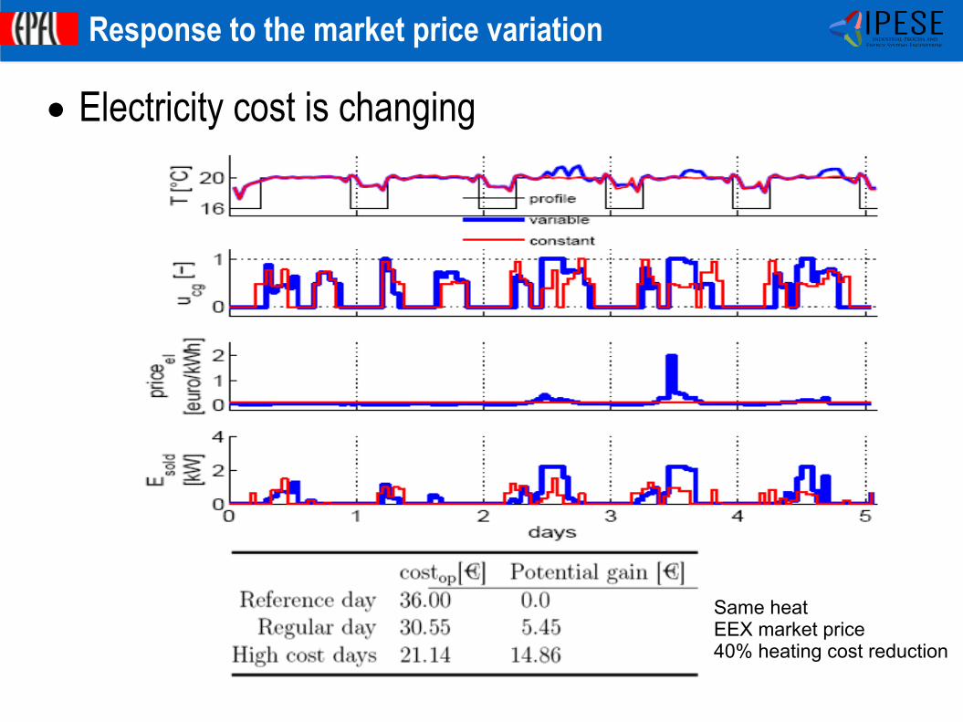
• Electricity cost is changing
Response to the market price variation
Same heat EEX market price 40% heating cost reduction
©Francois Marechal -IPESE-IGM-STI-EPFL 2014
IPESEIndustrial Process and
Energy Systems Engineering
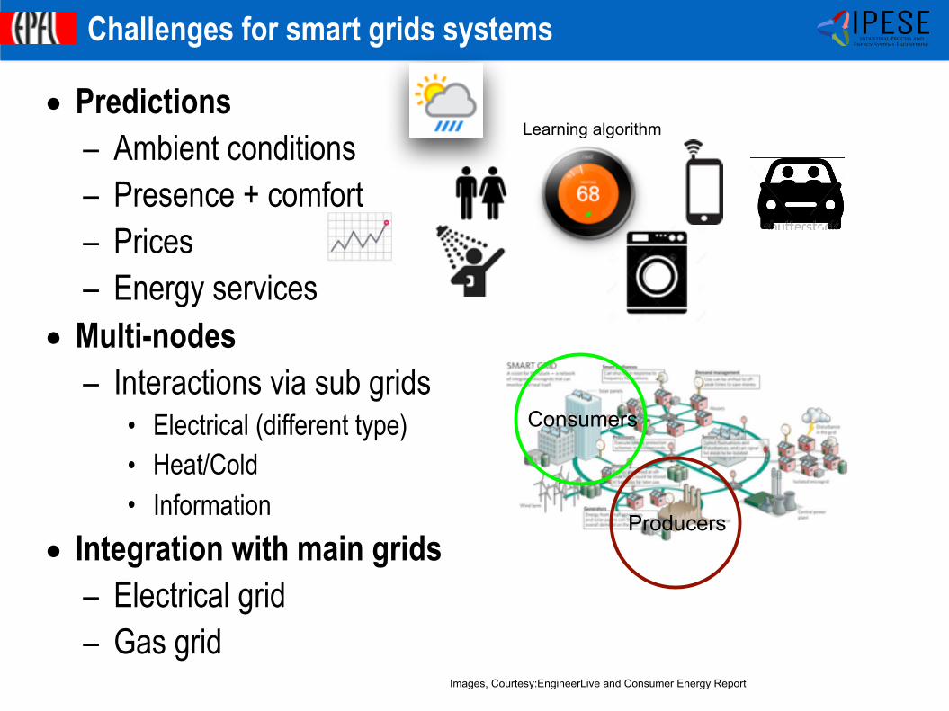
• Predictions – Ambient conditions – Presence + comfort – Prices – Energy services
• Multi-nodes – Interactions via sub grids
• Electrical (different type) • Heat/Cold • Information
• Integration with main grids – Electrical grid – Gas grid
Challenges for smart grids systems
Learning algorithm
Images, Courtesy:EngineerLive and Consumer Energy Report
Producers
Consumers

©Francois Marechal -IPESE-IGM-STI-EPFL 2014
IPESEIndustrial Process and
Energy Systems Engineering
Fuel-Cell GT
Domestic Hot water tanks
Heat pump/HVACElectrical gridNatural gas grid
Buildings Small industries
E-technology : smart households operation
Smart Optimal Predictive Control Management BoxPrice
T ambient
Comfort T/Air
People Light
T storage
Batteries
PV
Solar panels
Heating/Cooling tanks
Reserve
Cons. profiles
Big Data grid
Water grid
Meteo
Smart info (WIFI-GPS-GSM)
T storageMass
Waste Water Grid
Cogeneration
CO2 grid

©Francois Marechal -IPESE-IGM-STI-EPFL 2014
IPESEIndustrial Process and
Energy Systems EngineeringE-technology : Optimal process control
2nd European Conference on Polygeneration - 30th March-1st April, 2011 - Tarragona, Spain
4 Perspectives of the integration of the trigeneration system
The approach presented above is based on the time averaging approach that allows to considerthat all the streams are simultaneous. Considering the batch operation dimension requires theadaptation of the approach to integrate in the analysis the calculation of the storage tanksthat are required to make the heat recovery feasible. When studying the trigeneration systemintegration, it will be necessary to size the tanks not only to allow the heat recovery but alsoto take opportunities from the electricity market. The trigeneration system is indeed a wayof storing electricity from the grid in the form of heat or cold. The heat or cold storage alsoallows the cogeneration unit to play the role of the peak shaving.
The final configuration is presented on figure 8. The optimization method based on amulti-objective optimization strategy presented by Weber et al. ([17]) allows to design thetrigeneration system and the storage tanks considering the use of a predictive optimal manage-ment strategy. In addition, methods like the one proposed by Collazos et al. ([11]) can be usedto implement the predictive optimal management strategy in a control system.
3
6
Process hot water
CIP system
CoolingGlycol
110 °C
50 °C
2 °C
EngineGas
Industrial process
Refrigeration/Heat Pump
Electricity
Figure 8: Storage tank system configuration
5 Conclusion
The optimal integration of trigeneration systems is realized in several steps. The first stepis the definition of the requirement followed by the definition of the heat recovery potentialbetween the hot and the cold streams of the process. This step is mandatory since it allows todefine the heating and cooling requirement to be satisfied by the trigeneration system. Otherapproaches based on the use of the present utility system would lead to bigger systems andunnecessary investment that would in addition prevent the future energy savings options. Thetrigeneration system is sized by first identifying the possible trigeneration options based on theanalysis of the Grand composite curve of the system. The configuration of the system is thendefined by applying an optimization model that calculates the best flows in the system. It hasbeen demonstrated that the proper analysis of the trigeneration system requires to accountfor the possible integration, not only at the level of the process, but also at the level of thepossible integration inside the trigeneration system. The example presented shows that thecombination of a refrigeration cycle where the condensation heat is used as a heat pump topreheat the process streams with a mechanical vapor recompression system that allows for
9
Smart Optimal Predictive Control Management Box
©Francois Marechal -IPESE-IGM-STI-EPFL 2014
IPESEIndustrial Process and
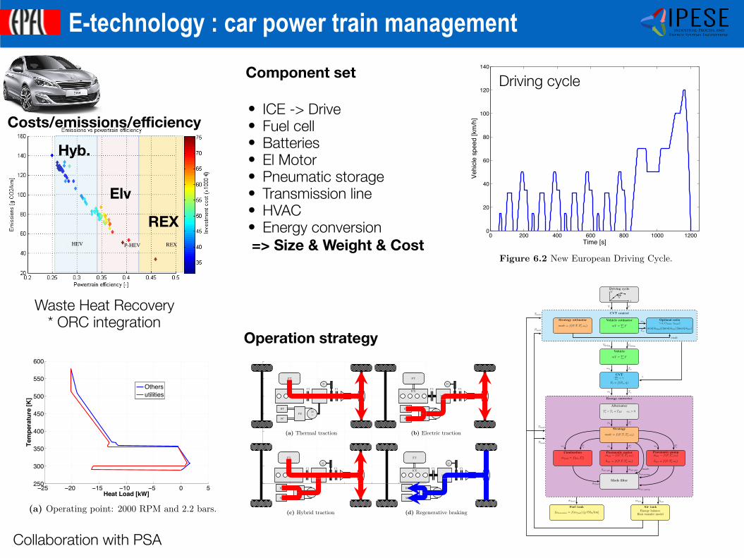
Energy Systems EngineeringE-technology : car power train management
6 THERMAL ELECTRIC HYBRID POWERTRAIN
Table 6.1 Continued: Peugeot 508 SW model characteristics.
FuelType DieselDensity [kg/l] 0.84Lower heating value [MJ/kg] 42.5
6.2 Driving cycle
The New European Driving Cycle is the current test cycle in Europe. All European lightweightvehicles, both conventional and hybrid, are assessed on this cycle in terms of fuel consumptionand emissions. The cycle, illustrated in Figure 6.2, is composed of four repetitions of an urbancyle (UDC) and one extra-urban cycle (EUDC). Basic characteristics of the cycle are given inTable 6.2.
0 200 400 600 800 1000 12000
20
40
60
80
100
120
140
Time [s]
Vehi
cle
spee
d [k
m/h
]
Figure 6.2 New European Driving Cycle.
Table 6.2 NEDC characteristics.
Distance [m] Duration [s] Average speed [km/h] Repeats [-]
UDC 1’017 195 18.54 4EUDC 6’956 400 62.22 1
Total cycle 11’023 1’180 32.26 -
6.3 Simulation results
The engine power and fuel consumption profiles are given in Figure 6.3. During decelerationphases fuel injection is cut o↵, as is the case for modern engines. Figure 6.4a gives the fuelconsumption points relative to the engine consumption point. The NEDC does clearly not posemuch di�culty for the 2.2 liter engine in terms of load as the consumption points are scatteredin the lower left quadrant. However this zone is not near the region of higher e�ciency.
Table 6.3 compares the simulated emissions result with that of the real vehicle. With anerror of less than 2%, the thermal powertrain model is deemed su�ciently precise.
52Collaboration with PSA
Driving cycle
5 PNEUMATIC HYBRID
Driving cycle
t
V
h
CVT control
Strategy estimator
mode = f(P, T, T 0s,!s)
Vehicle estimator
mV =P
F
Optimal ratio� 2 (�min, �max)
min(mfuel)||min(mair)||max(mair)
V V
mode
!w
Tw
Vehicle
mV =P
F
Vdelay Vdelay
CVT!s
!w
= �
Ps = f(Pw, ⌘)
!w Tw
�
Energy converter
Alternator
T 0s = Ts + TAT !s > 0
Strategy
mode = f(P, T, T 0s,!s)
Combustion
mfuel = f(!s, T 0s)
Pneumatic motormair = f(P, T, T 0
s,!s)
hair = f(P, T, T 0s,!s)
Pneumatic pumpmair = f(P, T 0
s,!s)
hair = f(P, T 0s,!s)
Mode filter
!s Ts
!s T 0s
!s T 0s
!s T 0s
!s T 0s
hair,pm mair,pm
hair,pump
mair,pump
mfuel
mode
Fuel tank
fEmissions = f(mfuel) [g CO2
/km]
mfuel
Air tankEnergy balance
Heat transfer model
mair hair
Ptank
Ttank
Ptank
Ttank
Figure 5.9 Pneumatic hybrid powertrain model flowchart.
42
4 THERMAL ELECTRIC HYBRID
DT
C1
G
PSD
C2ICE
FT
M⇠PE
BT
SC
Figure 4.3 Parallel thermal electric hybrid powertrain: BT : Battery pack; C1: Primary clutch; C2:Secondary clutch; D: Di↵erential; FT : Fuel tank; G: Alternator; ICE: Internal combustion engine;M : Electric motor; PE: Power electronics; PSD: Power split device; SC: Supercapacitor pack; T :Transmission.
DT
C1
G
PSD
C2ICE
FT
M⇠PE
BT
SC
(a) Thermal traction
DT
C1
G
PSD
C2ICE
FT
M⇠PE
BT
SC
(b) Electric traction
DT
C1
G
PSD
C2ICE
FT
M⇠PE
BT
SC
(c) Hybrid traction
DT
C1
G
PSD
C2ICE
FT
M⇠PE
BT
SC
(d) Regenerative braking
Figure 4.4 Parallel hybrid powertrain operating modes.
27
• ICE -> Drive • Fuel cell • Batteries • El Motor • Pneumatic storage • Transmission line • HVAC • Energy conversion => Size & Weight & Cost
Operation strategy
13 UTILITY INTEGRATION
−25 −20 −15 −10 −5 0 5250
300
350
400
450
500
550
600
Heat Load [kW]
Tem
pera
ture
[K]
Othersutilities
(a) Operating point: 2000 RPM and 2.2 bars.
−25 −20 −15 −10 −5 0 5−0.1
0
0.1
0.2
0.3
0.4
0.5
0.6
Heat Load [kW]
Car
not F
acto
r 1−T
a/T[−]
Othersutilities
(b) Operating point: 2000 RPM and 2.2 bars.
Figure 13.2 Organic Rankine cycle integration. Text = 0 �C
where the E+
E are the exergetic services of the engine hot streams. They can be computed fora given hot source i using the fundamental equation:
E+
i =
Z ✓1� Ta
Ti
◆�Q+
i
where Ta is the ambient temperature and Ti the temperature of the hot source. Since the specificheat of all hot streams is assumed to be constant, the integral can be removed by approximatingTi by the logarithmic temperature di↵erence:
TLTD =Tin � Tout
lnTin
Tout
The energetic and exergetic e�ciency values of the maps, with values between 9 and 12 % and30 and 40 % respectively are similar to results found in [10].
13.2 Refrigeration cycle
For the case where Text = 30 �C, a single refrigeration cycle is added as a cold utility to coolthe cabin to below ambient temperature. The cycle is composed of an evaporator, compressor,condenser and an expansion valve (Figure 13.5a) and uses the following processes:
• 1 ! 2: Evaporation
• 2 ! 3: Compression
• 3 ! 3”: Isobaric cooling
• 3” ! 4: Condensation
• 4 ! 1: Expansion
The following assumptions are made:
• The working fluid is ammonia, same as the ORC.
• Compressor isentropic e�ciency is 80 %.
101
Waste Heat Recovery * ORC integration
Component set
8.4 - Multi objective optimization results for hybrid electric vehicles with different usages
179
The life cycle inventory is done for each computation iteration of the decision variables and the environmental impacts are calculated according to the definition of the impacts in section 3.9.
8.4 Multi objective optimization results for hybrid electric vehicles with different usages
8.4.1 New European Driving Cycle (NEDC)
The solutions of a two objectives optimization converged on a Pareto Frontier optimal curve (Figure 8-6), representing the trade-off between the energy consumption and the cost of the vehicles on normalized driving cycle.
Figure 8-6: Pareto curve energy consumption to cost (color bar in thousands of Euros) –NEDC
The vehicle body mass of around 1500 kg is characterizing the D–class vehicles. These vehicles are usually used for family transportation or business trips on long distances. The D-class vehicles are well equipped and the technology is considered as additional value for the customer. The powertrain technology for low CO2 emissions is an important requirement for the customers of these vehicles. The official technical characteristics are referenced on the NEDC by the car makers. The Pareto curve for the NEDC (Figure 8-6) defines a wide range of points for improved powertrain efficiencies (25- 45.2%) and fuel emissions (30 to 140 g CO2/km). In contrast, a thermal powertrain D-class vehicle of 1660 kg of mass, with 2.2 diesel liters engine yields 17 % of powertrain efficiency and 151 g CO2 / km [147]. To archive such high powertrain efficiency in the Pareto curves for all usages, the electric half of the powertrain is increased and more electric energy stored in the battery is needed. Indead the battery capacity increases from 5 to 50 kWh (Figure 8-7 d). This considerably increases the vehicle mass (Figure 8-7 a). To follow the dynamic requirement on the cycle, the electric motor power also increases from 20 to 150 kW. The emitted tank-to-wheel CO2 emissions, which are proportional to the diesel consumption, are related to the hybridization ratio expressed through the electric motor and the thermal motor size.
HEV P-HEV REX
7 PNEUMATIC HYBRID POWERTRAIN
7 Pneumatic hybrid powertrain
This chapter presents the validation of the thermal powertrain underlying the pneumatic hybrid.The test is conducted for a Peugeot 308 (Figure 7.1) with a 1.2 liter gasoline engine on the NewEuropean Driving Cycle.
Figure 7.1 Peugeot 308.
7.1 Powertrain characteristics
The main powertrain model parameters are given in Table 7.1.
Table 7.1 Peugeot 308 model characteristics.
VehicleNominal mass [kg] 1075Wheel diameter [m] 0.406Rolling friction coe�cient cr [-] 0.015Bearing friction coe�cient µ [-] 0.002Aerodynamic coe�cient Scx = Ca ·A [m2] 0.65
Gearbox
Number of gears [-] 5E�ciency [-] 0.94Final drive1 [-] 4.05Ratio 1 [-] 3.02Ratio 2 [-] 1.6Ratio 3 [-] 1.13Ratio 4 [-] 0.86Ratio 5 [-] 0.68
Engine
Displacement [l] 1.2Number of cylinders [-] 3Rated power [kW] 60Maximum speed [RPM] 6000Maximum torque [Nm] 120Idle speed [RPM] 950Idle fuel consumption [l/h] 0.33Deceleration Fuel Cut-O↵ yes
FuelType GasolineDensity [kg/l] 0.745Lower heating value [MJ/kg] 42.7
55
Costs/emissions/efficiency
REX
Elv
Hyb.

©Francois Marechal -IPESE-IGM-STI-EPFL 2014
IPESEIndustrial Process and
Energy Systems Engineering
E-technology for education

©Francois Marechal -IPESE-IGM-STI-EPFL 2014
IPESEIndustrial Process and
Energy Systems EngineeringE-technology for education : www.energyscope.ch
©Francois Marechal -IPESE-IGM-STI-EPFL 2014
IPESEIndustrial Process and
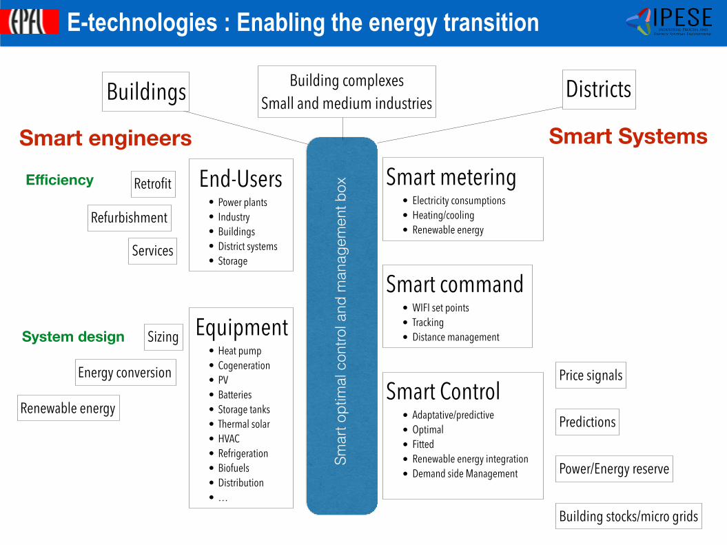
Energy Systems EngineeringE-technologies : Enabling the energy transition
Smart metering • Electricity consumptions • Heating/cooling • Renewable energy
Smart command • WIFI set points • Tracking • Distance management
Smart Control • Adaptative/predictive • Optimal • Fitted • Renewable energy integration • Demand side Management
Price signals
Predictions
Power/Energy reserveSmar
t opt
imal
con
trol a
nd m
anag
emen
t box
Equipment • Heat pump • Cogeneration • PV • Batteries • Storage tanks • Thermal solar • HVAC • Refrigeration • Biofuels • Distribution • …
End-Users • Power plants • Industry • Buildings • District systems • Storage
Building stocks/micro grids
Retrofit
Refurbishment
Sizing
Energy conversion
Services
Buildings Building complexes Small and medium industries
Districts
Renewable energy
Smart engineers Smart Systems
Efficiency
System design

©Francois Marechal -IPESE-IGM-STI-EPFL 2014
IPESEIndustrial Process and
Energy Systems Engineering
Thank you for your attention
Prof François Marechal http://ipese.epfl.ch EPFL Valais-Wallis