centre international d’études supérieures en - supagro.fr · m guido sonnemann rapporteur mme...

Délivré par le

Centre international d’études supérieures en

sciences agronomiques

Montpellier

Préparée au sein de l’école doctorale Sciences des Procédés –

Sciences des Aliments

Et de l’unité de recherche UMR ITAP

Spécialité : Génie des Procédés

Présentée par Philippe Loubet

Soutenue le 27 novembre 2014 devant le jury composé de

Mme Véronique BELLON-MAUREL Directrice de thèse

Mme Cecile BULLE Rapporteur

M Guido SONNEMANN Rapporteur

Mme Ligia BARNA Examinatrice

Mme Maite ALDAYA Examinatrice

M Philippe ROUX Examinateur

M Denis CHANTEUR Invité

Assessing the environmental impacts of a complex urban water system based on the life

cycle assessment framework

Development of a versatile model and advanced water deprivation indicators

Remerciements

Une nouvelle page se tourne, longue de plus de trois ans,

Et oui, il s’en passe des choses dans la vie d’un doctorant.

De Montpellier à Paris, bien des personnes m’ont aidé à l’écrire,

Et c’est par ces quelques lignes que je vous remercie.

Tout d’abord, merci à ma directrice de thèse, Véronique Bellon Maurel,

Pour ta confiance, ton accompagnement durant ces trois ans

Ton aide et tes encouragements de tous les moments.

Merci à toi, Philippe Roux pour ton encadrement immense

Pour toutes ces discussions longues et intenses,

Depuis l’ACV jusqu’aux matchs de rugby entre le Stade et Montpellier.

Merci à mes rapporteurs de thèse, Cécile Bulle et Guido Sonnemann,

Pour vos commentaires et critiques constructifs, pour cette dernière pierre apportée à l’édifice

Aux examinatrices aussi, Maïté Aldaya et bien sûr Ligia Barna, du temps a passé depuis l’INSA

Ce jury de thèse, c’est un peu mon passé, mon présent, mon futur, ça ne s’arrêtera pas là

Merci à vous, Denis Chanteur, Pauline Danel et Cédric Feliers

Pour m’avoir, au sein de Veolia Eau d’Île-de-France, suivi et accompagné

Aux autres membres du comité rapproché, Jean Michel Roger, Laetitia Guérin-Schneider et Gilles Belaud

Pour vos conseils aiguisés en modélisation, hydrologie et gestion de l’eau.

Aux membres du comité élargi, Jacques Lesavre, Alain Grasmick et Daniel Dunet

Pour votre regard extérieur, cette prise de recul sur tous les sujets abordés.

Merci à tous les autres qui ont participé à mon travail de thèse

A Laureline Catel, collègue et stagiaire d’une grande aide

A Emmanuelle Aoustin et Jean-Baptiste Bayart,

Pour vos conseils et nos collaborations depuis VERI ou Quantis

Merci aux autres collègues de Veolia que ce soit à VEDIF, OTV ou VERI,

A Blandine Catelas pour ta disponibilité, à Sébastien Worbe et Anne Flesch pour les échanges

Merci à tout le pôle ELSA, de la salle Casagrande à la salle Pascal

Pour tous ces moments agréables, quelle ambiance de travail !

Merci à la team thésard, Eléonore ton aide a été précieuse

Pierre encore merci pour m’avoir laissé ton appart

Ludivine, même exilée à Irstea, Juliette, qui dit deux ?

Bref, c’est aussi pour ces moments en Edison

Cette salle, on a bien fait de la transformer en cours de ping pong

D’ailleurs, j’en place une spéciale pour Pyrène

Les prochaines pauses de midi seront bien tristes

A Montse aussi, pour les discussions d’eau et de gin tonic

A little Italy, Federica, Valentina, Crista et Nathalie,

Vous avez amené beaucoup des Abruzzes et de Calabre dans nos vies

A Ibrahima, pour tes fins pronostics et tes pirouettes de pongistes

A Sylvain, un jour je te maitriserai au volley ou au tennis de table

Merci Eva pour tes sorties sportives et tes bons plans resto,

Merci à Melissa, Mary, Evelyne, Sonia, Catherine, Carole, Cyril, Yves, Ralph, Arnaud,

Merci aussi à tout le génie rural et une dédicace pour les exilés de l’UMR ITAP ou du CIRAD

Spécialement Anthony, Yannick, Cécile, Sandra, Claudine,

Et tous les autres que j’ai oubliés, vous êtes dans mes pensées

Merci aussi à Cynthia, et le petit bout de chemin passé avec toi

Une énorme pensée pour tous mes potes, ceux de maintenant, ceux de toujours

De Saint-Gi’ à Paris, en passant par Toulouse, sans vous, ma vie c’est la lose

C’est spécialement pour tous les bougres Ariégeois,

La famille Toulousaine et les anciens de l’INSA

Je l’ai déjà dit mais je le répète GPE je le suis et je le reste

Pour les conteurs d’histoires ST-MW, établis en 1987, mais aussi pour le SBSW, le BBBA, le 3G+H,

Et aussi pour ces rencontres simples et inattendues, devant un bar ou dans la rue,

Désolé, je ne peux pas citer de nom, je vais en oublier certains comme un vieux 21 juin

Merci à mon frère, quelques années plus tard, c’est moi qui m’y colle

Merci à ma mère et mon père, désolé si je ne décroche pas toujours au téléphone

Merci, merci, merci à vous tous, vous me rendez aphone

i

Table of Contents

Table of Contents ...................................................................................................................... i

Tables ........................................................................................................................................ vi

Figures ..................................................................................................................................... vii

Acronyms and abbreviations .................................................................................................. ix

Preface .................................................................................................................................... xiii

Chapter 1. General introduction ............................................................................................. 1

Content of Chapter 1 .............................................................................................................. 3

1.1. Towards sustainable cities: the challenge of urban water systems (UWS) ..................... 4

1.2. To measure is to know: introduction to life cycle assessment (LCA) ............................ 5

1.3. Water in environmental evaluations ................................................................................ 6

1.3.1. Water, a unique resource and a sensitive environmental habitat ............................. 6

1.3.2. Water footprint and water in LCA ........................................................................... 7

1.4. Objectives of the thesis ................................................................................................... 9

Chapter 2. Life cycle assessments of urban water systems: A comparative analysis of

selected peer-reviewed literature .......................................................................................... 13

Content of Chapter 2 ............................................................................................................ 15

2.1. Introduction ................................................................................................................... 16

2.2. Material and methods .................................................................................................... 18

2.2.1. Selection of LCA papers dealing with UWS .......................................................... 18

2.2.2. Analysis grid of LCA papers focusing on whole UWS ......................................... 19

2.3. Results ........................................................................................................................... 23

2.3.1. LCA phase 1 - goal and scope ................................................................................ 23

2.3.2. LCA phase 2 - life cycle inventory ........................................................................ 26

2.3.3. LCA phases 3 and 4 – life cycle impact assessment and interpretation ................. 29

2.4. Discussion and perspectives .......................................................................................... 33

2.4.1. Goal and scope ....................................................................................................... 33

2.4.2. Life cycle inventory ................................................................................................ 35

2.4.3. Life cycle impact assessment ................................................................................. 37

ii

2.4.4. Uncertainty management ........................................................................................ 38

2.4.5. Towards integrating LCA results for UWS decision-makers ................................ 38

2.5. Conclusions ................................................................................................................... 39

Chapter 3. Assessing water deprivation at the sub- river basin scale in life cycle

assessment integrating downstream cascade effects ........................................................... 41


3.1. Introduction ................................................................................................................... 44

3.2. Methods ......................................................................................................................... 45

3.2.1. Water scarcity: consumption-to-availability ratio .................................................. 46

3.2.2. Characterization factors for water deprivation ....................................................... 50

3.2.3. Midpoint assessment: choice of the weighting parameter ...................................... 51

3.2.4. Water deprivation midpoint impacts ...................................................................... 52

3.2.5. Identifying upstream and downstream SRBs to streamline CTA and CFWD ......... 52

3.2.6. Illustrative case study ............................................................................................. 53

3.3. Results ........................................................................................................................... 53

3.3.1. CTA and CFWD for selected sub-river basins ......................................................... 53

3.3.2. Results of land planning scenarios ......................................................................... 56

3.4. Discussion ..................................................................................................................... 56

3.4.1. Completeness of scope ........................................................................................... 57

3.4.2. Environmental relevance ........................................................................................ 57

3.4.3. Scientific robustness and certainty ......................................................................... 58

3.4.4. Documentation, transparency and reproducibility ................................................. 59

3.4.5. Applicability ........................................................................................................... 59

3.4.6. Outlook ................................................................................................................... 59

Chapter 4. Accounting for quality of urban water flows taking into account existing

LCIA and water footprint methods ...................................................................................... 61


4.1. Introduction ................................................................................................................... 64


4.2.1. Identification of urban water flows and their associated composition ................... 65

4.2.2. Characterization of urban water flows ................................................................... 68

4.2.3. Implementation of the proposed damage score to a water footprint method

(advanced water impact index - WIIX) ............................................................................ 72

iii

4.3. Results and discussion ................................................................................................... 73

4.3.1. Damage scores analysis for natural water resources .............................................. 73

4.3.2. Analysis of damage scores of selected urban water flows ..................................... 75

4.3.3. Application to a water footprint method (Water Impact Index – WIIX) ............... 78

4.4. Proposed classification of urban water flows ................................................................ 78

4.5. Conclusions and outlook ............................................................................................... 79

Chapter 5. WaLA, a versatile model for the life cycle assessment of urban water

systems: Part 1 – formalism and framework for a modular approach ............................. 81


5.1. Introduction ................................................................................................................... 85

5.2. Urban water system modeling ....................................................................................... 86

5.2.1. Specifications for an integrated UWS model ......................................................... 86

5.2.2. The general framework of the WaLA model ......................................................... 87

5.2.3. Goal and scope definition ....................................................................................... 88

5.2.4. LCI/LCIA associated to the technologies/users generic components .................... 89

5.2.5. Practical details ....................................................................................................... 96

5.2.6. Implementation of the model within a computer program ..................................... 97

5.2.7. Virtual case study ................................................................................................. 100

5.3. Results and discussion ................................................................................................. 101

5.3.1. The graphical representation of the UWS ............................................................ 101

5.3.2. Environmental impacts ......................................................................................... 102

5.3.3. Provided services and impact/service ratio .......................................................... 105

5.3.4. Opportunities and limits ....................................................................................... 106

5.4. Conclusions ................................................................................................................. 107

Chapter 6. WaLA, a versatile model for the life cycle assessment of urban water

systems: Part 2 – Learning points from the assessment of water management scenarios

in Paris suburban area ......................................................................................................... 109

Content of Chapter 6 .......................................................................................................... 111

6.1. Introduction ................................................................................................................. 112

6.2. Material and methods .................................................................................................. 114

6.2.1. The greater metropolitan Paris UWS ................................................................... 114

6.2.2. Scenarios investigated and the associated LCA goals and scopes ....................... 116

6.2.3. Customization of the model components: establishing the attribute values ........ 122

iv

6.2.4. Inventory linked to operating of the UWS components (energy, chemicals) ...... 124

6.2.5. Life cycle impact assessment ............................................................................... 125

6.2.6. Example of the construction of a scenario using the model ................................. 127


6.3.1. Baseline scenario .................................................................................................. 130

6.3.2. Forecasting scenarios ........................................................................................... 133

6.3.3. Sensitivity analysis on impact/service ratio choices ............................................ 137


6.4. Conclusions and outlook ............................................................................................. 140

Chapter 7. Discussion and conclusion ................................................................................ 141

Content of Chapter 7 .......................................................................................................... 142

7.1. The need to better assess impacts associated to water use .......................................... 143

7.1.1. Towards appropriate scales for LCA practitioners ............................................... 143

7.1.2. Towards the use of consensual hydrological data and models for LCIA developers

........................................................................................................................................ 144

7.1.3. Current gap between midpoint indicators based on water stress and the endpoint

indicators ........................................................................................................................ 145

7.1.4. Towards mechanistic approaches in LCIA: combining downstream cascade effect

with a consistent water fate model ................................................................................. 146

7.1.5. Current limits of water footprint related to water quality assessment .................. 150

7.2. Perspectives for the WaLA model .............................................................................. 152


7.2.2. Towards scenario assessment in a decision making context ................................ 152

7.2.3. Towards a tool for benchmarking ........................................................................ 153

7.3. General conclusion ...................................................................................................... 155

References ............................................................................................................................. 157

Annex A. Life cycle assessments of urban water systems: A comparative analysis of

selected peer-reviewed literature ........................................................................................ 173

Annex B. Assessing water deprivation at the sub-river basin scale in LCA integrating

downstream cascade effects ................................................................................................. 181

v

Annex C. WaLA, a versatile model for the life cycle assessment of urban water systems

195

Résumé étendu ...................................................................................................................... 231

Abstract ................................................................................................................................. 244

Résumé .................................................................................................................................. 244

vi

Tables

Table 2-1. Classification of papers dealing with LCA of water technologies. ...................................................... 19

Table 2-2. Description of criteria taken into account within the review ............................................................... 20

Table 2-3. Key points of the analysis of the reviewed papers ............................................................................... 24

Table 2-4. Electricity consumption of the technologies composing UWS in 11 studies. ...................................... 26

Table 2-5. Water flows through the different components of the UWS and associated impacts from 8 studies. .. 28

Table 4-1. Composition of selected water flows for nutrients and metals (non-exhaustive list). Concentrations

highlighted in grey are not known and taken equal to the ones associated to a very good state ............. 66

Table 4-2. Threshold values for the definition of physico-chemical state from the water framework directive

applied in France ..................................................................................................................................... 68

Table 4-3. List of impact categories affected by emissions to water for three LCIA methods. ............................ 69

Table 4-4. Conversion factor for endpoint ecosystem damages between LCIA categories .................................. 71

Table 4-5. Proposition of water types for urban water flows and corresponding damage scores to ecosystems .. 79

Table 5-1. Specific glossary for the WaLA model (Chapters 5 and 6) ................................................................. 84

Table 5-2. Classification of impacts at the component scale ................................................................................ 91

Table 6-1. Classification of identified management issues. ................................................................................ 113

Table 6-2. The complexity of water management in the greater Paris metropolitan area: responsibility shares for

the different components. Area of the case study is underlined in red. ................................................ 115

Table 6-3. List of evaluated forecasting scenarios and their key parameters. ..................................................... 117

Table 6-4. List of extrinsic parameters for the construction of each scenario ..................................................... 129

Table 6-5. Relative evolutions of Impact 2002+ damages and water deprivation impacts for forecasting scenarios

compared to baseline scenario. ............................................................................................................. 134

vii

Figures

Figure 1-1. General criteria and life cycle stages from different environmental evaluation methodologies.

Adapted from Risch et al. (2012) .............................................................................................................. 5

Figure 1-2. Main impact pathways in LCA and presentation of the water footprint profile and single-score.

Adapted from Impact World+ (http://www.impactworldplus.org/en/index.php) and Boulay et al. (2014)

.................................................................................................................................................................. 8

Figure 1-3. Structure of the thesis ......................................................................................................................... 12

Figure 2-1. Graphical abstract of Chapter 2 .......................................................................................................... 14

Figure 2-2. Timeline and journal distribution of water technology LCA papers. ................................................. 17

Figure 2-3. Map of LCA papers focusing on water technology, when location of the case study is available.

Names refer to first authors of the papers. Numbers in brackets refer to the number of papers related to

this author. When the city is unknown, the location is placed randomly within the country. ................. 18

Figure 2-4. Climate change impacts of the technologies composing the UWS of 6 studies. ................................ 30

Figure 2-5. Technology contribution analysis of LCA single score, climate change & eutrophication impacts and

electricity consumption inventory. .......................................................................................................... 32


Figure 3-2. Water balance at the sub-river basin scale. ......................................................................................... 46

Figure 3-3. Summary of cause-effect chains leading from water consumption inventory to different areas of

protection, adapted from Kounina et al. (2012) ...................................................................................... 52

Figure 3-4. Sub-river basin CFWD (p=area) and CTA of the Seine river basin (France) ....................................... 55

Figure 3-5. Sub-river basins CFWD (p=area) and CTA of the Guadalquivir river basin (Spain) ........................... 55

Figure 3-6. CFWD and CTA evolution from upstream to downstream locations in three selected lines. ............... 56

Figure 4-1. Average damage score due to eutrophication of 2534 water resources versus physico-chemical state

from the WFD, from 1 (very good state) to 5 (bad state); LCIA method is Impact 2002+. ................... 74

Figure 4-2.: Average damage score due to ecotoxicity of 2534 water resources versus chemical state from WFD;

LCIA method is Impact 2002+. .............................................................................................................. 75

Figure 4-3. Damage scores on ecosystem (including eutrophication and ecotoxicity) of selected water flows

assessed with different LCIA methods. All scores are converted in species.yr. ..................................... 75

Figure 4-4. Damage scores on human health of selected water flows assessed with different LCIA methods. .... 77

Figure 4-5. WIIX quality index related to the original approach and the advanced approach .............................. 78


Figure 5-2. Simplified presentation of the modular formalism and boundaries of the urban water system. ......... 88

Figure 5-3. Description of water flows and associated impacts/services of the generic component. .................... 89

Figure 5-4. Representation of the unique class (superclass) associated with the generic component, its sub-

classes associated with each technology/user component, and the instances of each sub-class associated

with the specific components. ................................................................................................................. 98

Figure 5-5. Procedure to define an UWS scenario and compute its environmental impacts and impact/service

ratios. Practitioners are represented by a character. .............................................................................. 100

Figure 5-6. Graphical representation of the virtual case study and its extrinsic parameters ............................... 102

viii

Figure 5-7. Relative contributions of technologies and users. The LCIA method is ILCD 1.03. ....................... 104

Figure 5-8. Relative contributions of direct and indirect contributors. The LCIA method is ILCD 1.03. .......... 105

Figure 6-1. Graphical abstract of Chapter 6 ........................................................................................................ 110

Figure 6-2. General and detailed situation of the case study. .............................................................................. 116

Figure 6-3. CFWD for the Seine river basin (November) and locations of main withdrawals and releases for the

baseline and forecasting scenarios. ....................................................................................................... 126

Figure 6-4. Graphical representation of the baseline scenario with all components, all technosphere flows (black

arrows) and major withdrawals (blue arrows) and releases (green arrows). ......................................... 128

Figure 6-5. Simplified Sankey diagram of water flows within the urban water system of the baseline scenario.

.............................................................................................................................................................. 130

Figure 6-6. Relative contributions of UWS components in the baseline scenario. LCIA method: ILCD. .......... 132

Figure 6-7. Relative contributions of direct/indirect impacts in the baseline scenario. LCIA method: ILCD. ... 132

Figure 6-8. Monthly evolution of water deprivation impacts for several scenarios ............................................ 136

Figure 6-9. Comparison of various impact/service ratios of forecasting scenario L1 to the baseline (set at 100%,

whatever the unit). LCIA method: Impact 2002+ endpoint and water deprivation midpoint. .............. 138

Figure 7-1: illustration of the gap between current mid-point indicators based on stress and damage assessment

based on volume deprivation effects (source Boulay, WULCA) .......................................................... 146

Figure 7-2. Description of the water cycle within a multimedia scheme. Adapted from Usetox multimedia fate

model (Rosenbaum et al., 2008). .......................................................................................................... 148

Figure 7-3. Proposed framework of the fate of water flows within a multimedia scheme: modification of

environmental water flows (yellow arrows) caused by human interventions (red arrows). Name of water

exchange processes are in italic. (source: Roux, P., Nunez, M. Loubet, P., for WULCA group in 2014)

.............................................................................................................................................................. 148

Figure 7-4. Representation of water cycle at the sub-river basin scale. Thick black arrows represent downstream

cascade effect ........................................................................................................................................ 149

Figure 7-5. Different options for taking into account water quality within a water footprint profile or single score

.............................................................................................................................................................. 151

ix

Acronyms and abbreviations

AC: Acidification

BOD: Biological oxygen demand

C: Consumption (also noted WC – water consumption – in Chapter 3)

CC: Climate change

CF: Characterization factor

CED: Cumulative energy demand

COD: Chemical oxygen demand

CTA: Consumption-to-availability

D: Discharge

DS: Damage score

DWP: Drinking water production

DWD: Drinking water distribution

EE: Eco-efficiency

EQ: Ecosystem quality

ET: Evapotranspiration

EWR: Environmental water requirements

FET: Freshwater ecotoxicity

FEu: Freshwater eutrophication

FU: Functional unit

HH: Human health

HT: Human toxicity

I: Impact

x

IS: Impact/service

IR: Ionizing radiation

IUWM: Integrated urban water management

IWRM: Integrated water resource management

LCA: Life cycle assessment

LCI: Life cycle inventory

LCIA: Life cycle impact assessment

MEu: Marine eutrophication

OOP: Object-oriented programming

P: Precipitation

PAF: Potentially affected fraction

PDF: Potentially disappeared fraction

PNOF: Potentially not occurring fraction

R: Release (also noted WR – water release – in Chapter 3)

RO: Runoff

S: Services

SD: Species density

SEDIF: Syndicat des Eaux d’Île-de-France

SEOL: Sludge end of life

SIAAP: Syndicat Interdépartemental pour l’Assainissement de l’Agglomération Parisienne

SRB: Sub-river basin

SWC: Stormwater collection

TEu: Terrestrial eutrophication

xi

U: User

UWS: Urban water system

V: Water volume

W: Withdrawal (also noted WW – water withdrawal – in Chapter 3)

WA: Water availability

WD: Water deprivation

WFD: Water framework directive

WIIX: Water impact index

WTA: Water-to-availability

WWC: Wastewater collection

WWT: Wastewater treatment

xiii

Preface

This thesis was supported by a “Convention Industrielle pour la Formation par la Recherche -

CIFRE” scholarship (convention 0418/2011) from the French National Association for

Technical Research. The thesis was done in association with Veolia Eau d’Île-de-France and

UMR ITAP, Irstea Montpellier, within the ELSA (Environmental Life cycle & Sustainability

Assessment) research group. Veolia Eau d’Île-de-France is the delegatee of Syndicat des Eaux

d’Île-de-France (SEDIF).

The thesis is essentially based on the following papers, which have either been published, or

submitted in international peer-reviewed journals:

- Loubet, P., Roux, P., Núñez, M., Belaud, G., & Bellon-Maurel, V. (2013). Assessing

Water Deprivation at the Sub-river Basin Scale in LCA Integrating Downstream

Cascade Effects. Environmental Science & Technology, 47(24), 14242–9.

doi:10.1021/es403056x

- Loubet, P., Roux, P., Loiseau, E., & Bellon-Maurel, V. (2014). Life cycle assessments

of urban water systems: A comparative analysis of selected peer-reviewed literature.

Water Research, 67(0), 187–202. doi:10.1016/j.watres.2014.08.048

- Loubet, P., Roux, P. & Bellon-Maurel, V. WaLA, a versatile model for the life cycle

assessment of urban water systems: Part 1 – formalism & framework for a modular

approach. Submitted to Water Research

- Loubet, P., Roux, P., Guerin-Schneider L. & Bellon-Maurel, V. WaLA, a versatile

model for the life cycle assessment of urban water systems: Part 2 – Learning points

from the assessment of water management scenarios in Paris suburban area. Submitted

to Water Research

The work included in the thesis was presented in oral communications and posters in

international conferences:

- Loubet, P., Bayart, J., & Danel, P. (2011). Measuring the Water Impact Index of water

services. In Ecotech & Tools. Montpellier, France.

xiv

- Loubet, P., Roux, P., Nunez, M., & Bellon-Maurel, V. (2013). Assessing water

deprivation at sub-river basin scale in LCA integrating downstream cascade effects. In

SETAC Europe 23rd Annual Meeting. Glasgow, UK.

- Loubet, P., Roux, P., & Bellon-Maurel, V. (2014). Modelling technique for territorial

LCA applied to urban water systems : evaluation of prospective scenarios in mega

cities. In SETAC Europe 24th Annual Meeting. Basel, Switzerland.

- Loubet, P., Roux, P., Nunez, M., & Bellon-Maurel, V. (2014). Sub-river basin scale

water deprivation at midpoint and endpoint levels in LCIA. In SETAC Europe 24th

Annual Meeting. Basel, Switzerland.

1

Chapter 1. General introduction

« 361 degrés de rotation, du rien au tout, et puis du tout au rien.

Juste que nous ne sommes rien du tout, en fait on sait rien, c’est tout »

Akhenaton – Mon texte, le savon

3

Content of Chapter 1

1.1. Towards sustainable cities: the challenge of urban water systems (UWS) ..................... 4

1.2. To measure is to know: introduction to life cycle assessment (LCA) ............................ 5

1.3. Water in environmental evaluations ................................................................................ 6

1.3.1. Water, a unique resource and a sensitive environmental habitat ............................. 6

1.3.2. Water footprint and water in LCA ........................................................................... 7

1.4. Objectives of the thesis ................................................................................................... 9

4

1.1. Towards sustainable cities: the challenge of urban water

systems (UWS)

Since the yearly 1970’s, the mankind has raised awareness about the natural environment

vulnerability. In its famous report, the club of Rome warned about the finite natural resources

and discussed the limits to growth (Meadows et al., 1972). Indeed, in a biophysical system

with finite resources, it is impossible for an economy based on these resources to grow

infinitely. From these alarming signals, new concepts have risen. Among them, the

sustainable development posits a desirable future state for human societies in which living

conditions and resource-use meet human needs without undermining the sustainability of

natural systems and the environment, so that future generations may also have their needs met

(Brundtland, 1987). More radical concepts, such as the “degrowth”, question the idea of

development and propose a window of opportunity for political changes that will make the

inevitable economic recession socially and environmentally sustainable (Kallis, 2011).

In this context of transition, the key role of cities was emphasized (Beck, 2011). After a

twentieth century marked by considerable rural flight, the world has never been that

urbanized. The world’s population has reached 7 billion, and more people live in cities than in

rural areas (United Nations, 2012). Megacities, defined as a metropolitan area with a total

population in excess of 10 million people are becoming more and more common. As of today,

there are 30 megacities in existence (Population Reference Bureau, 2013) and some of them

are or will be facing acute problems, particularly related to water (Abderrahman, 2000). The

urban sprawl poses challenges for urban planners, as it causes congestion, environmental

degradation and increases the cost of service delivery (UN-Habitat, 2009). There is a need to

rethink and modify the standards and principles for urban planning.

To meet the water challenges at the city scale, the integrated urban water management

framework (IUWM) has been developed (Global Water Partnership Technical Committee,

2012). It aims at improving water management for different purposes within the urban area

both in terms of quality and quantity. Nested within the broader framework of integrated

water resources management (IWRM) (Global Water Partnership Technical Advisory

Committee, 2000), it can contribute to meet water challenges at a river basin scale. By doing

so, the IUWM framework enable stakeholders to look at the system holistically and facilitate

the development of innovative solutions for urban water management. However, there is still

room in the framework for tools and methods that can help managers to evaluate urban water

5

system (UWS) sustainability and prospective scenarios. Measuring all environmental impacts

associated with human activities is a necessary condition to reduce their footprint. Amongst

the available tools for assessing environmental impacts of such systems, life cycle assessment

(LCA) has already proven its worth. The LCA method is explained in the following section

by underlining briefly its main forces and its limitations for the assessment of urban water

systems.

1.2. To measure is to know: introduction to life cycle assessment

(LCA)

LCA is a standardized approach for environmental evaluation (ISO, 2006a) and is widely

recognized at world wide scale. This tool quantifies impacts of a product or a service within

all its life cycle stages, i.e., from cradle-to-grave. It includes raw material extraction through

materials processing, manufacture, distribution, use, repair and maintenance, and disposal or

recycling. LCA is a multi-criteria approach that takes into account a wide range of impacts to

the environment (e.g., climate change, eutrophication, resources depletion, etc.) and differs in

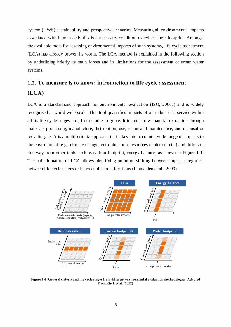
this way from other tools such as carbon footprint, energy balance, as shown in Figure 1-1.

The holistic nature of LCA allows identifying pollution shifting between impact categories,

between life cycle stages or between different locations (Finnveden et al., 2009).

Figure 1-1. General criteria and life cycle stages from different environmental evaluation methodologies. Adapted

from Risch et al. (2012)

Environmental criteria (impacts, resource depletion, ecotoxicity …)

Carbon footprint® Risk assessment

LCA

CO2

Industrial site

Water footprint

m3 equivalent water

Energy balance

MJ

All potential impacts

All potential impacts

6

LCA provides two main types of indicators. Midpoint indicators assess a change in the

environment (an environmental mechanism) that links a human intervention (e.g., emission of

CO2) to a problem (e.g., global warming potential). Generally, endpoint indicators quantify

the damages on areas of protection, generally human health, ecosystem quality and resources,

due to these problems. These relations are described by cause-effect pathways. A

representation of major pathways is shown in Figure 1-2.

Another LCA key feature is that it is based on a functional approach: potential impacts of a

product or a service are quantified per unit of provided service, namely the functional unit.

For a given service (e.g., “to participate to a meeting”), it allows to compare contrasted

systems (e.g., train, car and videoconferencing).

LCA was initially developed according to a product-oriented approach, with the aim to bring

information on goods and services to the public (eco-labeling), to decision makers or to

industries for eco-design purpose. Recent proposals have been made to adapt the LCA

framework in order to broaden its scope towards larger scale systems such as cities (Loiseau

et al., 2013). This is a relevant scale to assess environmental impacts of urban water systems.

However, LCA studies can be time consuming and their application to large systems such as

megacity UWS requires a huge amount of data. In addition to diagnosis purposes, the

evaluation of forecasting scenarios would also require important modeling efforts. Therefore,

in line to the analysis of (Schulz et al., 2012), there is a great need for developing simplified

procedures to easily provide stakeholders indicators about the environmental performance of

UWS and their forecasting scenarios.. This means creating new procedures for modeling

UWS, in order to easily feed LCA analysis.

In addition to methodological needs in terms of UWS modeling for matching LCA models,

another challenge in LCA applied to UWS is the assessment of water use impacts. Water is

both a resource and an environmental compartment, and its consideration within

environmental evaluation raises some challenges, today unresolved, as pointed out hereafter.

1.3. Water in environmental evaluations

1.3.1. Water, a unique resource and a sensitive environmental habitat

Water has this specific property to be both a resource for humans and an environmental

habitat, explaining the many concerns we place on this “blue gold”. Of course, water is not as

scarce as gold. On the contrary, it is a renewable resource and water moves continually on

7

earth through a cycle. There are approximately 1,400,000,000 km3 of water on earth but only

3% is freshwater; of which 69% is locked up in glaciers and snow (Oki and Kanae, 2006).

The remaining water is usable for human but it is poorly distributed within the world. More

than 2.5 billion people face water scarcity during at least one month of the year (Hoekstra et

al., 2012), meaning that sufficient available water resources are lacking for meeting demands

of water usages. Human interventions exacerbate the situation. This is principally due to

agriculture that is responsible of 70% of water withdrawals, whereas domestic users are 12%

and industrial users 18% (FAO, 2012). The future is not bright, as climate change and

population growth tend to increase this threat (Vorosmarty, 2000). Besides the issue of

quantity, the limited access to water is also linked to water quality. Degradation of water

quality leads to unavailable water resources for certain usages (Peters and Meybeck, 2000).

Freshwater is also an environmental habitat that can be affected by water scarcity and

pollutions. In terms of biological value, rivers contain a rich and varied biota, i.e., at least

100,000 species, almost 6% of all described species (Dudgeon et al., 2006). Ecosystem

destruction due to water abstraction, habitat alteration incurred by damming or water

transferring, changes in water chemistry because of pollutions, and species removal and

additions are the main disturbances from anthropogenic activities (Malmqvist and Rundle,

2002).

All these concerns show the importance of assessing impacts of water use and pollution on

species, i.e., on ecosystems and human health. Such methods have been increasingly

developed as shown hereafter.

1.3.2. Water footprint and water in LCA

In the beginning of the 2000’s, the concepts of “virtual water” and “water footprint” have

been developed in order to account for these water issues in supply chains (Allan, 1998;

Hoekstra and Hung, 2002). It accounts for the withdrawal of surface and ground water

(named “blue water”), the evapotranspiration of rainwater (named “green water”) and the

pollution of freshwater (named “grey water”). It results in amounts of equivalent cubic meters

needed to produce the targeted goods or services: for example one kilogram of beef represents

15 400 L of water (Mekonnen and Hoekstra, 2010) or one kilogram of coffee almost 19 000 L

(Mekonnen and Hoekstra, 2011). These considerable amounts raise awareness in the public.

However, the interpretation of this volumetric approach is questionable. For example, one

cubic meter of water transpired in a wet area (e.g. Scotland) is not equivalent to one cubic

8

meter of water consumed in a dry one (e.g. in the Colorado). In addition, the quantification of

pollution in “grey-water” is based on a dilution volume approach, which does not consider

substance fate, contrarily to what life cycle impact assessment (LCIA) models do.

Alternatively to the virtual water concept, LCA characterizes the inventory data in order to

quantify potential impacts and damages to the environment. Originally, LCA assesses only

impacts and damages on aquatic ecosystems through the categories freshwater eutrophication,

and ecotoxicity. The assessment of water use is at an early development stage but new

methods are currently developed and certain ones are operational (Kounina et al., 2012). In

this context, the recently developed water footprint standard (ISO, 2013) states that a water

footprint profile should be presented as a compilation of LCIA results related to water: water

use, eutrophication, freshwater ecotoxicity, etc. (Figure 1-2).

Figure 1-2. Main impact pathways in LCA and presentation of the water footprint profile and single-score. Adapted

from Impact World+ (http://www.impactworldplus.org/en/index.php) and Boulay et al. (2014)

The application of these approaches to UWS is highly needed as urban systems play a key

role in the water management at the scale of river basin, and there is a need to assess properly

Emissions

to air, soil,

water

CO2

Phospahtes

Pesticides

etc.

Inputs

Water

Crude oil

Arable land

etc.

Human toxicity

Photochemical oxidation

Ozone layer depletion

Global warming

Ecotoxicity

Acidification

Eutrophication

Water use

Land use

Resources use

Multi-criteria

LCA framework (Example of IMPACT

World+ )

Mono-criteria

footprints Water footprint single-score

Aiming to combine water quality indicators (pollutions)

with water quantitative ones (water deprivation) in a

single unit (generally m3 equivalent of water)

Examples: WIIX (Bayart et al., 2014), method of

Ridout and Pfister (2013), Water Footrpint Network

Human Health

Ecosystem quality

Resources

Water

footprint

profile

Life Cycle inventory Midpoint impact categoriesEndpoint damage categories

(areas of protection)

http://www.impactworldplus.org/en/index.php

9

their impacts related to water for mitigation purposes. In terms of quality, UWS have a

significant role to ensure good quality of the rivers (Niemczynowicz, 1999). In terms of

quantity, even if the urban systems is often not the main water consumer compared to

irrigated agriculture, it may have an influence on water deprivation; the variety of water

sources that the UWS can use in a river basin, as well as the distance between withdrawals

and releases points lead to different water deprivation levels (Jønch-Clausen and Fugl, 2001).

However, several challenges remain in the evaluation of water deprivation impacts. The main

one is that the current scale for assessing water deprivation is the river basin (Pfister et al.,

2009), which is not appropriate to the evaluation of urban water systems that can use many

water sources within a same river basin and that typically release water far from the

withdrawal points.

1.4. Objectives of the thesis

With the aim to address the urgent need for tools to easily supply stakeholders with indicators

about the environmental performance of UWS and forecasting scenarios, the research

question of this thesis is:

“Is it possible to model a urban water system in order to assess the environmental

impacts it induces in regards with services provided to the users, using the conceptual

framework of LCA ?”

This global question is approached through two axes, each one related to a crucial phase of

LCA. In the goal & scope and life cycle inventory (LCI) phases, the question is: “how to

model the UWS of big cities, in order to be at the same time, simple to implement,

representative of a given UWS scenario, and compliant to LCA specifications?” In the LCIA

phase, the question is: “regarding the fact that UWS will have major qualitative and

quantitative effects on the water compartment, how to better take this effects into account?”

Following these two axes, five sub-objectives are defined:

1. Identifying the main methodological challenges related to LCA applied to urban

water systems and demonstrate the need for a standardized approach.

2. Refining the impact category related to water deprivation, at an appropriate

scale, in order to make it applicable and relevant for urban water systems.

3. Accounting for quality of urban water flows taking into account existing LCIA and

water footprint methods

10

4. Developing a model and an associated formalism that reduces the complexity of the

system and that is versatile enough to implement forecasting scenarios, while being

still relevant for life cycle assessment.

5. Demonstrating the capacity of the model to address stakeholder’s expectations

when evaluating forecasting scenarios.

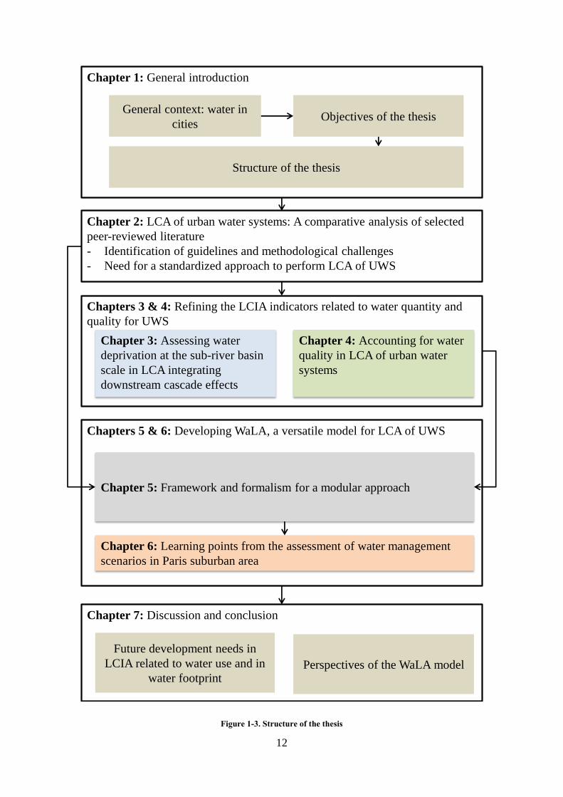
Each sub-objective is addressed by a chapter of the thesis referring to a scientific publication

(either published or submitted), as described hereafter and summarized in Figure 1-3.

After the introduction (Chapter 1), Chapter 2 is a review which aims at comparing papers

dealing with LCA of the entire UWS (including drinking water production and distribution, as

well as wastewater collection and treatment): 18 different case studies have been found. It is

based on a compilation and analysis of LCA results for urban water systems, and it ends up by

the identification of several guidelines for streamlining LCA of UWS and of methodological

challenges for the future.

From the guidelines and challenges pointed out within the review chapter, Chapter 3 and

Chapter 4 propose original approaches in order to better take into account water-related

impacts in urban water system (respectively the quantitative and qualitative aspects).

More specifically, Chapter 3 presents the development of a methodology to assess water

deprivation issues at the sub-river basin scale in LCA integrating “downstream cascade

effects”, i.e. effects of withdrawals on downstream users and ecosystems. Following the

present framework used to assess impacts of water deprivation, this method differentiates the

withdrawal and release points within a river basin. It is based on a two-steps approach that

first defines the “local water scarcity” at the sub-river basin scale and, second, computes

water deprivation for downstream users. The methodology is then validated on two different

river basins. Whereas Chapter 3 focuses on the quantitative impact of water use, Chapter 4

reviews current approaches to assess the qualitative impacts of water use. It aims at assessing

the damage scores of the different water flows found within the UWS, and to classify these

flows.

The development of these methods is a prerequisite for the development of the UWS model

which is presented in Chapter 5, i.e., the core of the thesis. This model, named WaLA (for

Water system Lifecycle Assessment), is elaborated to tackle the methodological issues of

LCA applied to UWS, which have been pointed out in chapter 2. It integrates the

11

developments described in chapters 3 and 4. The model is based on a formalism which

defines a generic component that characterize both water users and water technologies. These

components can be interconnected and interoperated, and are linked to water resources. This

enables to build a representation of a UWS scenarios through a modular approach. The model

is implemented within a Matlab/Simulink user-friendly interface. It computes environmental

impacts induced by the system, as well as services provided to the users. It is tested on a

theoretical case study.

Chapter 6 is the application of the model to forecasting scenarios. It aims at verifying the

capacity of the versatile model to assess scenarios and address stakeholders’ questions. The

chosen case study is Paris suburban area. Several scenarios related to changes of water users,

water resources and water technologies are studied.

Finally, a discussion about the two main outcomes of the thesis, i.e. (i) the LCIA model for

assessing water deprivation at the sub-river basin scale, and (ii) the WaLA model for the LCA

of UWS and its perspectives, is provided in Chapter 7.

12

Figure 1-3. Structure of the thesis

Chapter 2: LCA of urban water systems: A comparative analysis of selected

peer-reviewed literature

- Identification of guidelines and methodological challenges

- Need for a standardized approach to perform LCA of UWS

Chapters 3 & 4: Refining the LCIA indicators related to water quantity and

quality for UWS

Chapters 5 & 6: Developing WaLA, a versatile model for LCA of UWS

Chapter 3: Assessing water

deprivation at the sub-river basin

scale in LCA integrating

downstream cascade effects

Chapter 4: Accounting for water

quality in LCA of urban water

systems

Chapter 5: Framework and formalism for a modular approach

Chapter 1: General introduction

Chapter 6: Learning points from the assessment of water management

scenarios in Paris suburban area

Chapter 7: Discussion and conclusion

General context: water in

citiesObjectives of the thesis

Structure of the thesis

Future development needs in

LCIA related to water use and in

water footprintPerspectives of the WaLA model

13

Chapter 2. Life cycle assessments of urban

water systems: A comparative analysis of

selected peer-reviewed literature

« Les égouts ont refoulé, la bécosse a débordé

Y'avait des coliformes fécaux qui flottaient su'l terrazzo »

Les Cowboys Fringants – Le plombier

14

This chapter aims at reviewing papers dealing with LCA applied to water technologies in

order to identify the main methodological challenges in that field. It compiles all LCA papers

related to water technologies, out of which 18 LCA studies deals with whole urban water

systems (UWS). A focus is carried out on these 18 case studies which are analyzed according

to criteria derived from the four phases of LCA international standards. The results show that

whereas the case studies share a common goal, i.e., providing quantitative information to

policy makers on the environmental impacts of UWS and their forecasting scenarios, they are

based on different scopes, resulting in the selection of different functional units and system

boundaries. A quantitative comparison of life cycle inventory (LCI) and life cycle impact

assessment (LCIA) data is provided, and the results are discussed. It shows the superiority of

information offered by multi-criteria approaches for decision making compared to that

derived from mono-criterion. From this review, recommendations on the way to conduct the

environmental assessment of UWS are given, e.g., the need to provide consistent mass

balances in terms of emissions and water flows. Remaining challenges for urban water system

LCAs are identified, such as a better consideration of water users and resources and the

inclusion of recent LCA developments (territorial approaches and water-related impacts). This

chapter refers to the following published paper: “Loubet, P., Roux, P., Loiseau, E., & Bellon-

Maurel, V. (2014). Life cycle assessments of urban water systems: A comparative analysis of

selected peer-reviewed literature. Water Research, 67(0), 187–202.

doi:10.1016/j.watres.2014.08.048”

Figure 2-1. Graphical abstract of Chapter 2

Review of urban water systems LCAs

Drinking water

production

Drinking water

distribution

Waste water

collection

Waste water

treatment

Illustration: Olivier Aubert for Irstea

Water users

Water resources

15


2.1. Introduction ................................................................................................................... 16


2.2.1. Selection of LCA papers dealing with UWS .......................................................... 18

2.2.2. Analysis grid of LCA papers focusing on whole UWS ......................................... 19

2.2.2.1. Criteria for LCA phase 1 – goal and scope .................................................................................................. 20

2.2.2.2. Criteria for LCA phase 2 – life cycle inventory ........................................................................................... 20

2.2.2.3. Criteria for LCA phases 3 and 4 – life cycle impact assessment and interpretation .................................... 22

2.3. Results ........................................................................................................................... 23

2.3.1. LCA phase 1 - goal and scope ................................................................................ 23

2.3.1.1. Goal of the studies ....................................................................................................................................... 23

2.3.1.2. Scope: functional unit .................................................................................................................................. 25

2.3.1.3. Scope: boundaries, life cycle steps, allocation procedures........................................................................... 25

2.3.2. LCA phase 2 - life cycle inventory ........................................................................ 26

2.3.2.1. Operation (energy) ....................................................................................................................................... 26

2.3.2.2. Direct water flows ....................................................................................................................................... 27

2.3.2.3. Direct emissions (water, air and soil)........................................................................................................... 28

2.3.3. LCA phases 3 and 4 – life cycle impact assessment and interpretation ................. 29

2.3.3.1. Impacts taken into account .......................................................................................................................... 29

2.3.3.2. Climate change impacts ............................................................................................................................... 29

2.3.3.3. Water use impacts ........................................................................................................................................ 30

2.3.3.4. Water pollution impacts ............................................................................................................................... 31

2.3.3.5. Normalization, weighting ............................................................................................................................ 31

2.3.3.6. Contribution analysis ................................................................................................................................... 32

2.3.3.7. Sensitivity check .......................................................................................................................................... 33

2.4. Discussion and perspectives .......................................................................................... 33

2.4.1. Goal and scope ....................................................................................................... 33

2.4.1.1. Functional unit ............................................................................................................................................. 33

2.4.1.2. Boundaries of the system ............................................................................................................................. 34

2.4.1.3. Towards a territorial/city LCA approach ..................................................................................................... 35

2.4.2. Life cycle inventory ................................................................................................ 35

2.4.2.1. Mass balances .............................................................................................................................................. 35

2.4.2.2. Sources of data............................................................................................................................................. 36

2.4.3. Life cycle impact assessment ................................................................................. 37

2.4.4. Uncertainty management ........................................................................................ 38

2.4.5. Towards integrating LCA results for UWS decision-makers ................................ 38

2.5. Conclusions ................................................................................................................... 39

16

2.1. Introduction

In 2012, about half of the world’s population lived in urban areas. This figure is expected to

swell to 60% by 2030 (United Nations, 2012). Domestic, commercial and industrial water

demand is consequently growing in cities. In the meantime, water scarcity is increasing,

leading to water competition between users (World Water Assessment Programme UN,

2009). The degradation of water quality due to various forms of pollution has led to higher

costs (both financial and environmental) in water treatment. Hence, water management is a

significant challenge in the administration of growing cities. Urban water systems (UWS) are

complex, as they are composed of many components that are often managed separately (raw

water abstraction, drinking water production and distribution, water usage, wastewater

collection and treatment, etc.). Integrated urban water management (IUWM) is a holistic

approach that integrates water sources, water-use sectors, water services and water

management scales (Global Water Partnership Technical Committee, 2012). The development

of IUWM requires quantitative tools to assess the environmental impacts of UWS, in order to

manage them in a sustainable way.

In the last 20 years, life cycle assessment (LCA) has proven its worth in the evaluation of the

environmental sustainability of water systems. LCA is a standardized method (ISO, 2006b)

used to assess the environmental performance of a product, service or activity from a life

cycle perspective. LCA makes it possible to identify environmental hotspots within systems

for eco-design purposes and helps at avoiding pollution shifts between impact categories (e.g.,

toxicity and eutrophication versus climate change) or between life cycle stages (e.g., treatment

and discharge versus sludge end-of-life) (Finnveden et al., 2009).

LCA has been applied to water technology assessment since the late 1990s (Figure 2-2). Early

LCAs focused on parts of the urban water system, mainly wastewater treatment (WWT)

(Emmerson et al., 1995) and drinking water production (DWP) (Sombekke et al., 1997). Since

2005, the number of LCA studies has sharply increased. While some papers deal specifically

with drinking water distribution (DWD), few focus on wastewater collection (WWC).

Concerning the geographical distribution, more than half of the case studies are located in

Europe, while the others are distributed in North America, Australia, South Africa, China and

Southeast Asia (Figure 2-3).

17

Each paper is named by the name of first author ( “et al.” has been removed for clarity). Numbers within brackets show the

numbers of papers published corresponding to each case study. Abbreviations of journals: WST: Water Science and

Technology, IJLCA: International Journal of Life Cycle Assessment, JCP: Journal of Cleaner Production, ES&T:

Environmental Science & Technology.

Figure 2-2. Timeline and journal distribution of water technology LCA papers.

Lundin and Morrison (2002) proposed the first framework based on LCA to assess the

environmental impacts of UWS. Kenway et al. (2011) and Nair et al. (2014) reviewed the

water-energy nexus in UWS, focusing on energy use and climate change. A review of LCA

water treatment studies has been published by Buckley et al. (2011), focusing on South

Africa. Recently, Corominas et al. (2013) published a complete review of wastewater

treatment plant LCAs with the inclusion of some urban water system LCAs. More

particularly, Yoshida et al. (2013) reviewed LCAs of sewage sludge management.

However, none of these studies provide a review of LCAs related to the whole UWS.

Therefore, this paper aims to provide a comprehensive review of urban water system LCAs.

Case studies are selected from a compilation of all LCA papers related to water technologies.

They are then analyzed using criteria from the 4 phases described in LCA international

standards, goal and scope definition, life cycle inventory (LCI), life cycle impact assessment

(LCIA), and interpretation. The comparison allows pointing out the main methodological

guidelines in the assessment of urban water system regarding critical points such as the

system multi-functionality, the LCI and the LCIA related to water, both in terms of quantity

DWD

DWP

WWC

WWT

UWS

DWP DWD

Journal distributionTechnology distribution

18

and quality. Future research needs in order to perform a comprehensive environmental

assessment in regards with the IUWM requirements to integrate each parts of the system (i.e.,

water resources, users and technologies) are also discussed.

Figure 2-3. Map of LCA papers focusing on water technology, when location of the case study is available. Names

refer to first authors of the papers. Numbers in brackets refer to the number of papers related to this author. When

the city is unknown, the location is placed randomly within the country.

2.2. Material and methods

2.2.1. Selection of LCA papers dealing with UWS

Water technologies LCA papers can be separated according to three different nested scales: (i)

“urban water systems (UWS)” which comprise (ii), “water technologies” (plants or networks)

which in turn comprise (iii), “unit processes”, as shown in Table 2-1.

Water technologies are classified using 4 categories: drinking water production (DWP) plant,

drinking water distribution (DWD) network, wastewater collection (WWC) network and

wastewater treatment (WWT) plant. The function of DWP and WWT plants is to improve

water quality, while the function of DWD and WWC networks is to transfer water. The

present review does not aim at compiling papers related to the unit process scale; therefore we

only compiled papers at water technologies and UWS scales. Urban water system case studies

19

are then selected according to the two following criteria, i.e., (i) they should include several

water technologies (i.e., comprising at least DWP and WWT) and (ii) they should be partial or

full LCA as long as they include one impact category or a multi-criteria impact assessment.

Table 2-1. Classification of papers dealing with LCA of water technologies.

Scale Built

from

Number

of

papers

Scheme

Legend: = Functional Unit; = Water flow; = provided service to users

Unit process Physical

models

*

Plant: DWP,

WWT; or

Network: DWD,

WWC

Unit

processes

100+

Technological

urban water

system

(combination of

technologies)

Plants

and

networks

24

Urban water

system

as a combination

of technologies,

users and

resources

Plants,

networks,

users and

water

resources

0

* Includes several papers not compiled in the present review, but two PhD dissertation have compiled most of the models

used for drinking water production (Mery, 2012; Vince, 2007). R = Resources, DWP = Drinking water production, DWD =

Drinking water distribution, WWC = Wastewater collection, WWT = Wastewater treatment

2.2.2. Analysis grid of LCA papers focusing on whole UWS

The case studies analysis follows the four steps of LCA according to ISO (2006): (phase 1)

definition of goal and scope, (phase 2) life cycle inventory (LCI), (phase 3) life cycle impact

assessment (LCIA) and (phase 4) interpretation of the results. For each phase, a set of criteria

has been selected from the ISO and ILCD guidelines (EC - JRC - IES, 2010a). The set of

criteria is detailed below and a summary is provided in Table 2-2.

Ozonation Coagulation Aeration

DWP

DWD

WWC

WWT

UserDWP DWD WWC WWTUWS =

DWP DWD WWC WWTUser

R R

UWS =

20

Table 2-2. Description of criteria taken into account within the review

LCA Phase Qualitative criteria Quantitative criteria

Phase 1 – Goal and scope

definition - Goal

- System boundaries

- Life cycle steps considered

- Functional Unit

- Geographic location

- Number of inhabitants

Phase 2 – LCI - Source of foreground data (ad-

hoc measurements, literature,

etc.)

- Source of background data

(databases)

- Electricity consumption data

- Water flows data

- Water consumption data

Phase 3 – LCIA - LCIA method selected

- Impacts and damages taken

into account

- Normalization (yes/ no?)

- Weighting (yes/ no?)

- Climate change impacts data

- Eutrophication impacts data

- Water consumption impacts

estimation

- Single score data

Phase 4 – Interpretation - Mono or multi criteria

- Sensitivity check - Contribution analysis from

technologies and group of

processes

2.2.2.1. Criteria for LCA phase 1 – goal and scope

The studies’ goals are compared according to their intended applications and the reasons for

carrying out the studies. A focus is placed on whether or not the studies intend to evaluate

prospective scenarios, and if this is the case, whether or not a classification of scenarios is

conducted. The analysis of the scope definition includes (i) the choice of functional unit (FU);

(ii) key information about the system (geographic location, number of inhabitants); (iii) the

definition of system boundaries; (iv) the life cycle steps considered; and (v) allocation

procedures. Concerning the boundaries, the analysis investigates whether or not the case

studies include foreground technologies (DWP, DWD, WWC, WWT or others), sludge end-

of-life (within DWP and WWT), transportation of sludge, chemicals, consumables and fuels.

Concerning the life cycle step, the inclusion of construction (both infrastructure components

and associated civil works), operation, and deconstruction is reviewed.

2.2.2.2. Criteria for LCA phase 2 – life cycle inventory

The analysis of the LCI phase deals with the procedures used to collect foreground and

background data (i.e., source of data) and the completeness of the inventories. It also aims at

collecting data and providing a quantitative analysis of electricity consumption and water

flow inventories.

21

Electricity consumption is represented according to the contributions of the different

technologies (DWP, DWD, WWC, and WWT). Data related to water abstraction by pumping

are included within DWD since it is a “water transfer” technology and not a form of water

treatment. Results found in the case studies are compared according to three different

approaches, having different metrics: (i) process approach, in kWh per m3 of water processed

by the technology, (ii) technological system approach, in kWh per m3 of water delivered to

the end users and (iii) territorial system approach, in kWh per capita per year. This

classification follows the definition of process and system approaches from Friedrich et al.

(2009a). Calculations are performed using data found in the papers when available and eq (1)

and (2). These LCI data are only collected and computed for the baseline scenario of the case

studies.

user

process

processm/userm/ V

VEE 33

(1)

year/capita/userm/year/capita/ VdemEE 3

(2)

Where E/m3process is the technology electricity consumption for 1 m3 at the input of the

technology (kWh/m3 at the process), E/m3user is the technology electricity consumption for 1

m3 provided to the user (kWh/m3 at the user) and E/capita/year is the technology electricity

consumption per capita during one year (kWh/capita/year), Vprocess is the water flow rate at the

input of the technology (m3/year), Vuser is the water flow rate delivered to the users (m3/year),

and Vdem/capita/year is the specific water demand per capita (m3/year/capita).

Beyond the energy consumption, water flow data are collected from the case studies and

equilibrated water balances are then checked. When available, water consumption data,

defined as the water evaporated or transpired through the system (Bayart et al., 2010), is

collected. If these data are not available, we estimated them by considering a simplified

assumption that 50% of the water losses within the system are evaporated or transpired and

are considered as water consumption. The remaining 50% is considered as water returned to

the environment. This first estimation of water consumption does not take into account the

specific climatic conditions of each case study, as done by Risch et al. (2014). Also, water

that is released to the sea is considered as lost for the local environment and is considered as

water consumption.

22

A qualitative analysis of direct emissions (to air, soil and water) is performed, including

emissions to water from each technology, sludge emissions to the soil from DWP and WWT

and emissions to air from WWT.

2.2.2.3. Criteria for LCA phases 3 and 4 – life cycle impact assessment and interpretation

The criteria used for analyzing the LCIA phase of the various case studies include the chosen

LCIA methodology, the list of selected impact categories at both the midpoint and endpoint

levels and the presence of normalization and weighting, which are optional elements. The

weighting steps and associated single scores are based on value choices and are not

scientifically based (ISO, 2006b). Specific LCIA results are collected and compared among

the studies for relevant and available impact categories, i.e., climate change, eutrophication,

and single score. These data are only collected for the basis scenario of the case studies.

Most of the examined studies were performed before the recent advances in the inclusion of

water use impacts in LCIA. These new methods provide indicators at the midpoint and

endpoint level that are geographically differentiated at the country and river basin scales and

that take into account water availability heterogeneity around the world (Kounina et al.,

2012).We aim at evaluating water use impacts on the same basis, when possible. For this

purpose, the process is the following: inventory data of water consumption obtained from the

LCI (section 2.2.2) are converted into Eco-indicator 99 and ReCiPe damages (ecosystem,

human health, resources) according to the method of Pfister et al. (2011, 2009). Damage

scores are converted to a single score and compared to the original single scores (only those

obtained from Eco-indicator 99 or ReCiPe) found in the papers that do not take into account

water use damages. The Eco-indicator 99 single score is calculated using default

normalization and the Hierarchist perspective (Goedkoop and Spriensma, 2001). The ReCiPe

single score is calculated using European normalization, the Hierarchist perspective and

average weighting factors. Even though research on water use impacts is still ongoing, we

decided to apply the Pfister et al. approach because it is operational and compatible with both

Eco-indicator 99 and ReCiPe units, and because characterization factors (CFs) at the endpoint

level are available on a global scale. We decided to compute single score in order to be able to

compare our computations with results found in the paper on a same basis, even if weighting

step is questionable (ISO, 2006b).

The analysis of the interpretation phase includes the identification of hot spots based on the

relative contributions from technologies and from types of contributors (electricity, chemicals,

23

direct emissions, infrastructures). Finally, we determine whether a sensitivity check had been

performed (i.e., sensitivity analysis and uncertainty analysis).

2.3. Results

Twenty-four papers dealing with LCAs of urban water system were found, as shown in Figure

2-2. However, two papers compiled several LCAs of technologies without studying the whole

system (Godskesen et al., 2011; Klaversma et al., 2013) and were not considered in our

review. Also two case studies were covered by several papers: Friedrich et al. (2009) was also

covered by 3 other references (Buckley et al., 2011; Friedrich and Pillay, 2007; Friedrich et

al., 2009b) that studied Durban UWS, and Lundie et al. (2004) was also covered by Rowley et

al. (2009) that studied Sydney UWS. Therefore, six papers were disregarded and the review

focused on eighteen case studies.

Table 2-3 presents the key points of the analysis grid. The papers studied medium towns to

big cities and whole regions, ranging from 8 500 houses to 20 million inhabitants, with 39%

of the papers dealing with case studies that have more than 1 million inhabitants.

2.3.1. LCA phase 1 - goal and scope

2.3.1.1. Goal of the studies

All of the studies aimed to provide quantitative information to policy makers on the

environmental profiles and hot spots of UWS. Among the studies, 78% also evaluated

prospective scenarios that could improve the environmental performance of the systems.

Fagan et al. (2010) and Schulz et al. (2012) studied nonexistent or developing urban areas in

Australia and thus also aimed at eco-designing UWS.

Three main types of scenarios that can be combined have been identified in the concerned

papers: (i) change or improvement of a technology (e.g., the construction of a new treatment

plant or an increase in the connection rate of a wastewater collection system), (ii) change of

water resources, (e.g., abstracting water from another river, releasing wastewater into the sea)

and (iii) change of users (e.g., increase of the population, change of users’ behavior).

According to our review, all of the scenarios found in the literature can be categorized into

one or more of these three types.

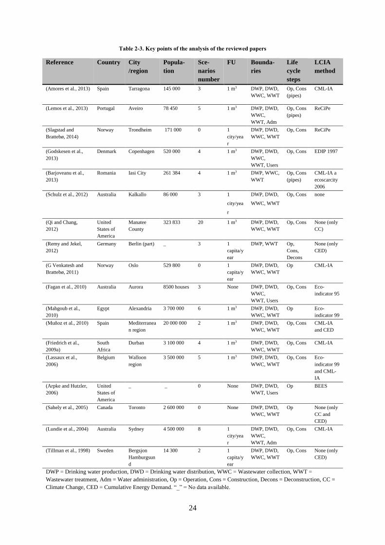
24

Table 2-3. Key points of the analysis of the reviewed papers

Reference Country City

/region

Popula-

tion

Sce-

narios

number

FU Bounda-

ries

Life

cycle

steps

LCIA

method

(Amores et al., 2013) Spain Tarragona 145 000 3 1 m3 DWP, DWD,

WWC, WWT

Op, Cons

(pipes)

CML-IA

(Lemos et al., 2013) Portugal Aveiro 78 450 5 1 m3 DWP, DWD,

WWC,

WWT, Adm

Op, Cons

(pipes)

ReCiPe

(Slagstad and

Brattebø, 2014)

Norway Trondheim 171 000 0 1

city/yea

r

DWP, DWD,

WWC, WWT

Op, Cons ReCiPe

(Godskesen et al.,

2013)

Denmark Copenhagen 520 000 4 1 m3 DWP, DWD,

WWC,

WWT, Users

Op, Cons EDIP 1997

(Barjoveanu et al.,

2013)

Romania Iasi City 261 384 4 1 m3 DWP, WWC,

WWT

Op, Cons

(pipes)

CML-IA a

ecoscarcity

2006

(Schulz et al., 2012) Australia Kalkallo 86 000 3 1

city/yea

r

DWP, DWD,

WWC, WWT

Op, Cons none

(Qi and Chang,

2012)

United

States of

America

Manatee

County

323 833 20 1 m3 DWP, DWD,

WWC, WWT

Op, Cons None (only

CC)

(Remy and Jekel,

2012)

Germany Berlin (part) _ 3 1

capita/y

ear

DWP, WWT Op,

Cons,

Decons

None (only

CED)

(G Venkatesh and

Brattebø, 2011)

Norway Oslo 529 800 0 1

capita/y

ear

DWP, DWD,

WWC, WWT

Op CML-IA

(Fagan et al., 2010) Australia Aurora 8500 houses 3 None DWP, DWD,

WWC,

WWT, Users

Op, Cons Eco-

indicator 95

(Mahgoub et al.,

2010)

Egypt Alexandria 3 700 000 6 1 m3 DWP, DWD,

WWC, WWT

Op Eco-

indicator 99

(Muñoz et al., 2010) Spain Mediterranea

n region

20 000 000 2 1 m3 DWP, DWD,

WWC, WWT

Op, Cons CML-IA

and CED

(Friedrich et al.,

2009a)

South

Africa

Durban 3 100 000 4 1 m3 DWP, DWD,

WWC, WWT

Op, Cons CML-IA

(Lassaux et al.,

2006)

Belgium Walloon

region

3 500 000 5 1 m3 DWP, DWD,

WWC, WWT

Op, Cons Eco-

indicator 99

and CML-

IA

(Arpke and Hutzler,

2006)

United

States of

America

_ _ 0 None DWP, DWD,

WWT, Users

Op BEES

(Sahely et al., 2005) Canada Toronto 2 600 000 0 None DWP, DWD,

WWC, WWT

Op None (only

CC and

CED)

(Lundie et al., 2004) Australia Sydney 4 500 000 8 1

city/yea

r

DWP, DWD,

WWC,

WWT, Adm

Op, Cons CML-IA

(Tillman et al., 1998) Sweden Bergsjon

Hamburgsun

d

14 300 2 1

capita/y

ear

DWP, DWD,

WWC, WWT

Op, Cons None (only

CED)

DWP = Drinking water production, DWD = Drinking water distribution, WWC = Wastewater collection, WWT =

Wastewater treatment, Adm = Water administration, Op = Operation, Cons = Construction, Decons = Deconstruction, CC =

Climate Change, CED = Cumulative Energy Demand. “_” = No data available.

25

2.3.1.2. Scope: functional unit

A total of 50% of the studies defined the FU as the “provision and treatment of 1 m3 of water

at the user” or the equivalent, which can be summarized as “1 m3” whereas a total of 17% of

the studies defined the FU as the “provision and treatment of water per capita for one year” or

the equivalent, which can be summarized as “1 capita/year”. A total of 17% of the studies

defined the FU as the “provision and treatment of water for the city and one year”, which can

be summarized as “1 city/year” Three papers did not define any FU, but implicitly consider “1

m3” (Arpke and Hutzler, 2006; Sahely et al., 2005) or ”1 city/year” (Fagan et al., 2010).

2.3.1.3. Scope: boundaries, life cycle steps, allocation procedures

All of the studies considered at least DWP and WWT in the boundaries of the systems, which

is straightforward since it is the criterion of selection of the papers. Fifteen (83%) studies

include all the main water technologies (DWP, DWD, WWC and WWT).

Only three papers, i.e., Fagan et al. (2010), Arpke and Hutzler (2006) and Godskesen et al.

(2013), considered water users (domestic and industrial) as a part of the system. This

acknowledges that users can have an impact on the environment, for instance when using

technologies such as water heaters or in relation to direct water release at the user’s location.

Lemos et al. (2013) and Lundie et al. (2004) included water management administration

(office buildings, vehicle fleets, etc.).

WWT sludge end-of-life was taken into account in twelve (61%) studies (combinations of

agricultural application, landfill, incineration and composting). Amores et al. (2013) also took

into account DWP sludge end-of-life (recycled in a cement plant), but they do not provide

information on its contribution to the DWP process. Among the studies that took into account

WWT sludge end-of-life, six used substitution by chemical fertilizers and one used system

expansion integrating fertilization and energy production in the system functions in order to

take into account the environmental benefits of sludge end-of-life (Remy and Jekel, 2012).

Four studies did not consider environmental benefits for sludge.

Concerning the life cycle steps, all the studies included the operational phase. Three studies

took into account the pipe infrastructure (DWD and WWC), and ten studies include the

infrastructure of the whole system. However, only the needed components and materials were

taken into account for the infrastructure, and none of these studies accounted for the necessary

civil works (e.g., excavation) associated with construction.

26

2.3.2. LCA phase 2 - life cycle inventory

Inventories of foreground flows (use of energy, chemicals, quantity and quality of water, etc.)

were mostly collected from site specific data gathered in internal reports or databases. Other

foreground flows (such as infrastructure) were collected from estimations and data in the

literature. Eleven (61%) studies provided the reference or the source of these data. Foreground

data were often assumed to be of fair quality but only Lemos et al., (2013) provided

indications on the data quality, classifying data from low quality to high quality whereas

Friedrich et al. (2009a) and Qi and Chang (2012) commented data quality. Concerning

background data, twelve studies used ecoinvent (Frischknecht et al., 2007) as a database for

background processes, two used the GaBi database (PE International), and three used other

sources. Twelve (67%) studies provided LCI data; a comparison of LCI results regarding

energy and water flows is presented below.

2.3.2.1. Operation (energy)

The energy for water technologies (pumps, stirring reactors, retro washing, etc.) is electricity.

Electricity consumptions of eleven case studies are presented in Table 2-4, following the three

metrics introduced in section 2.2.2.2.

Table 2-4. Electricity consumption of the technologies composing UWS in 11 studies.

kWh/m3 process kWh/m3 user kWh/capita/year

Reference DWP DWD WWC WWT DWP DWD WWC WWT total DWP DWD WWC WWT total

(Amores et al., 2013) 0.37 0.48 0.00 1.09 0.44 0.58 0.00 1.09 2.11 34 45 0 85 165

(Godskesen et al., 2013) _ _ _ _ 0.18 0.10 0.08 0.68 1.03 10 6 4 39 59

(Lemos et al., 2013) 0.64 0.15 0.21 0.87 0.88 0.21 0.21 0.73 2.04 49 12 0 41 101

(Barjoveanu et al., 2013) 0.04 0.27 0.04 0.17 0.07 0.45 0.04 0.14 0.69 10 63 5 19 97

(Slagstad and Brattebø, 2014) - 0.17 0.00 0.14 - 0.25 0.00 0.32 0.58 - 20 0 26 47

(Venkatesh and Brattebø, 2012) 0.23 0.18 0.06 0.75 0.29 0.22 0.06 0.88 1.44 51 39 10 156 256

(Muñoz et al., 2010) EWRT avg* 0.55 0.50 _ 0.30 0.67 0.61 _ 0.30 1.58 34 31 _ 15 79

(Friedrich et al., 2009a) 0.09 0.10 0.14 0.44 0.12 0.14 0.14 0.26 0.67 _ _ _ _ _

(Lassaux et al., 2006) 0.21 0.18 0.00 0.31 0.30 0.25 0.00 0.24 0.79 18 15 0 14 47

(Arpke and Hutzler, 2006) low 0.34 0.11 _ 0.21 _ _ _ _ _ _ _ _ _ _

(Arpke and Hutzler, 2006) high 0.37 0.44 _ 0.77 _ _ _ _ _ _ _ _ _ _

(Sahely et al., 2005) _ 0.60 _ 0.47 _ _ _ _ _ _ _ _ _ _

(Lundie et al., 2004) 0.08 0.24 0.06 0.41 0.08 0.25 0.06 0.33 0.73 11 34 8 45 98

Median 0.23 0.21 0.05 0.43 0.23 0.25 0.06 0.33 0.91 18 31 2 39 97

Average 0.26 0.28 0.06 0.49 0.30 0.31 0.06 0.50 1.17 24 29 3 49 105

Standard deviation 0.21 0.17 0.08 0.31 0.28 0.18 0.07 0.32 0.58 18 18 4 46 67


Wastewater treatment. “_” = No data available. *avg means the average value between optimistic and pessimistic EWRT

scenario.

27

In most studies, the highest share of electricity consumption was due to WWT, closely

followed by DWD and DWP. It should be noted that DWP electricity consumption might be

overestimated in some studies since part of that energy might be used for pumping at the exit

of the DWP plant and should thus be allocated to DWD network. WWC was negligible since

this water transfer is mostly driven by gravity. According to the “technological system”

approach, UWS require 0.58 to 2.11 kWh per m3 delivered to the user. The “territorial

system” approach yields a different classification of the case studies, ranging from 47 to 256

kWh per capita per year. Compared with average European electricity consumption, UWS

contribute for 1 – 2% of the total consumption which is approximately 5 700 kWh/capita

(European Environment Agency, 2008).

These results emphasize the importance of functional unit choice and the consideration of

users’ behavior. It should be noted that no DWP desalination data is included in Table 2-4

since no case study included it in basis scenarios. Muñoz et al. (2010) gave values ranging

from 1 kWh/m3 of water produced (optimistic value for brackish water desalination) to 4

kWh/m3 of water produced (pessimistic value for seawater desalination) in their prospective

scenarios. Arpke and Hutzler (2006) also considered electricity consumption for water heaters

and found a consumption of 63 kWh/m3 to heat water in the United States. In this study, the

proportion of hot water used is 10% in office buildings and 46% in apartments (domestic use).

This results in overall user water heating electricity consumption ranging from 6.3 kWh/m3

for office user to 29 kWh/m3 for domestic user. This energy amount is 5 to 23 times greater

than the average electricity consumption in all other technologies of the urban water system.

2.3.2.2. Direct water flows

Half of the studies indicated the volumes of water flows within the system. Table 2-5 shows

water flows at the input of the technologies, after data normalization for 1 m3 at the user.

Two studies considered the water losses of DWP (Friedrich et al., 2009a; Slagstad and

Brattebø, 2014), finding values of 4 % and 8 % (respectively). The average DWD losses were

25%. Wastewater flows were greatly variable because systems may have combined sewer

systems, separated sewer systems, or both. Studies did not provide a comprehensive water

balance according to the framework of Bayart et al. (2010), i.e., the total amount of water

withdrawn and released within the local environment, as well as the water evaporated to the

global environment or released to the sea (consumptive use). Our rough estimation of water

28

consumption through the systems shows a range from 0.13 to 1.11 m3 of water consumption

for 1 m3 of water at the user.

Table 2-5. Water flows through the different components of the UWS and associated impacts from 8 studies.

Water flow inventory (/m3 at the user) Water consumption damages*

Reference DWP DWD User WWC WWT Unww

Released

water to

sea?

Estimated

WC ReCiPe damage/m3

ReCiPe

single

score/m3

EI99

single

score/m3

Unit (/m3 user) m3 m3 m3 m3 m3 m3

m3

HH

(E-06

DALY.yr)

EQ (E-09

species.yr)

Res

($) Pt Pt

(Amores et al., 2013) 1.20 1.20 1.00 1.00 1.00 0 Y 1.10 0 7.005 1.825 1.200 0.135

(Barjoveanu et al., 2013) 1.70 1.70 1.00 0.81 2.09 0.193 N 0.44 0.002 1.240 0 0.003 0.014

(Lemos et al., 2013) 1.38 1.38 1.00 0.84 0.84 0 Y 1.11 0 2.099 0 0.005 0.009

(Slagstad et al. 2013) 1.60 1.47 1.00

2.28 0.115 N 0.30 0 0.338 0 0.001 0.005

(Venkatesh et al., 2012) 1.25 1.25 1.00 1.17 1.17 0 N 0.13 0 0.141 0 0.000 0.006

(Friedrich et al., 2007) 1.47 1.42 1.00 0.60 0.60 0 Y 1.04 0.365 4.981 0 0.018 0.033

(Lassaux et al., 2006) 1.42 1.42 1.00 0.78 0.78 0 N 0.32 0 0.796 0 0.002 0.012

(Lundie et al., 2004) 1.05 1.05 1.00 0.81 0.78 0 Y 0.92 0 3.545 0 0.008 0.019

Average 1.38 1.36 1.00 0.86 1.19

0.67 0.155 0.029


Wastewater treatment, Unww = Untreated wastewater, WC = Water consumption, * Damages are computed with regard

to water consumption using Pfister et al. (2009).

2.3.2.3. Direct emissions (water, air and soil)

DWP direct emissions to water were not considered and only Amores et al. (2013) studied

DWP sludge emissions. Furthermore, none of the studies addressed emissions from the

sewage network (WWC).

A total of 61% of the studies inventoried direct emissions to water from WWT effluent

release, and 44% of the studies accounted for emissions to air from WWT. This lack of

consideration is mainly because several studies only focused their environmental assessments

on the energy use and/or the infrastructures of the systems (Arpke and Hutzler, 2006;

Godskesen et al., 2013; Sahely et al., 2005; G. Venkatesh and Brattebø, 2011).

Concerning the pollutants taken into account in WWT, emissions to water always included

nitrogen (total nitrogen or nitrates, nitrites and ammonia) and phosphorus (total phosphorus,

phosphates). Six studies included COD and/or BOD. Heavy metals emissions to water were

only considered in one study (Fagan et al., 2010). Air emissions mostly included nitrous oxide

(N2O) (five studies), CO2 (four studies), CH4 (three studies) and occasionally other pollutants

(particulates, volatile compounds, CO, SO2). Emissions to soil (from sludge spreading)

29

included heavy metals in three studies. Equilibrated mass balances of pollutants were not

provided in the reviewed studies.

2.3.3. LCA phases 3 and 4 – life cycle impact assessment and interpretation

2.3.3.1. Impacts taken into account

Four (22%) studies performed a mono-criterion assessment, evaluating the impacts on climate

change and/or the cumulative energy demand of the urban water system (Qi and Chang, 2012;

Remy and Jekel, 2012; Sahely et al., 2005; Tillman et al., 1998). Seven studies applied CML-

IA (Guinée et al., 2002), three applied Eco-indicator 99 (Goedkoop and Spriensma, 2001),

two applied ReCiPe (Goedkoop et al., 2009) and one applied EDIP (Potting and Hauschild,

2004). Lassaux et al. (2006) used two methods (Eco-indicator 99 and CML-IA) and found

similar results. None of the studies showed endpoint indicator results according to the three

areas of protection (human health, ecosystem quality and resources).

When only considering multi-criteria studies (fourteen studies), 100% of the papers included

climate change and eutrophication, 89% included acidification, 44% included ecotoxicity

(marine, aquatic or terrestrial), and only 22% included water use impacts. In four studies, raw

midpoint results were not displayed, and results were only shown in the single score, thus

omitting useful information. Hence, we focused on climate change impacts, water use impacts

and water pollution impacts.

2.3.3.2. Climate change impacts

A total of sixteen studies calculated the impact on climate change, and results were available

in six studies. The impacts ranged from 0.51 to 1.57 kg CO2 eq/m3 at the user (Figure 2-4) and

are highly dependent on electricity consumption and the electricity mix used in each country.

Lundie et al. (2004) (Sydney) and Friedrich et al. (2009a) (Durban) indicated relatively high

impacts on climate change, whereas their electricity consumption was relatively low in

comparison with other studies. This is because the electricity mixes used in their countries

generate twice the amount of GHG emissions (respectively, 1.03 kg CO2 eq/kWh for Australia

and 0.97 kg CO2 eq/kWh for South Africa) than in other case studies (e.g., 0.45 kg CO2

eq/kWh in Spain) (Itten et al., 2013).

One study took into account the contribution of user-related water technologies, and found out

that 93% of the impacts on climate change were related to electric water heating systems

(Fagan et al., 2010).

30

Figure 2-4. Climate change impacts of the technologies composing the UWS of 6 studies.

2.3.3.3. Water use impacts

Three studies have taken into account the water use impacts. Amores et al. (2013) and Muñoz

et al. (2010) use freshwater ecosystem impact (FEI), which is calculated from the withdrawal-

to-availability (WTA) ratio of the river basins where water is withdrawn or released (Milà i

Canals et al., 2008). The case study published by Muñoz et al. (2010) is relevant because

water is withdrawn and released in different basins and it justifies the use of indicators

differentiated at the river basin scale. Godskesen et al. (2013) used CF values determined

using the methodology of Lévová and Hauschild (2011), which is also based on WTA. It

should be noted that they considered all of the withdrawn water as consumed water because

wastewater is returned to the sea and thus lost to the local freshwater environment.

We have computed water use impacts from the water consumption estimations described in

section 2.3.2.2 and from the ReCiPe and Eco-indicator 99 endpoint single score CFs (Table

2-5). The results range from 0.002 to 0.149 EI99-Point/m3 at the user and from 0.0011 to

1.200 ReCiPe-Point/m3 at the user. These huge variations are caused by the regional water

scarcity context. Ecosystem damages vary from one order of magnitude. Human health

damage is pointed out in two studies only, located in South Africa (Friedrich et al., 2009a)

and Romania (Barjoveanu et al., 2013), where the Human Development Index (HDI) is below

0.88. Resources damages are also identified in one study only, located in Spain (Amores et

al., 2013), where the water stress defined by the WTA is higher than 1 (Pfister et al., 2009).

Single score results related to water use can be compared to single score of the whole urban

water system (see section 2.3.3.5). EI99 and ReCiPe single score results for the whole urban

water system were collected from two studies. Lassaux et al. (2006) found 0.4 EI99-Pt/m3 at

the user and Lemos et al. (2013) found 0.151 ReCiPe-Pt/m3 at the user, respectively 100 and

0.0

0.5

1.0

1.5

2.0

Lundie

Friedrich

Munoz ERWT avg

Slagstad

Lemos

Godskesen

Amores

Climate change impacts

kg eq CO2 / m3 user

DWP

DWD

WWC

WWT

31

30 times higher than the water use single score. However, these 2 studies were located in

areas with low water scarcity (Belgium and Portugal). Other locations, in areas of scarce

water might find a high contribution of water use damage to the total score, such as Amores et

al. (2013).

2.3.3.4. Water pollution impacts

Eutrophication, ecotoxicity and acidification are major direct impacts generated by UWS.

Eutrophication figures were available in and gathered from eight studies. Since the units are

different, only the relative contributions of the technologies are compared. WWT contributes

to the highest share of impacts due to the release of treated water containing residual amounts

of eutrophicating substances (Figure 2-5). This direct contribution accounted for more than

50% of the total eutrophication impacts. Marine eutrophication was assessed in one study

with ReCiPe (Lemos et al., 2013), whereas the other studies only regarded freshwater

eutrophication.

Concerning ecotoxicity, none of the studies examined used the consensual method Usetox

(Rosenbaum et al., 2008), because it was not included in the selected LCIA methods. Muñoz

et al. (2010) chose not to include toxicity-related impacts because of the lack of information

on the toxicity effects of emerging pollutants. However, some studies provided a full

inventory of toxic substances. Hence, direct ecotoxicity impacts were mostly caused by

background processes.

2.3.3.5. Normalization, weighting

Eight studies used normalization and four of these displayed normalization results at the

midpoint level (all with European values). From these studies, the impacts with the greatest

contribution were all related to water pollution, i.e., eutrophication (2 studies), marine

ecotoxicity (1 study) and acidification (1 study).

Seven studies provided a single score after weighting. Weighting factors depend on the

selected methods, including the hierarchist perspective with average weighting in ReCiPe or

Eco-indicator 99, Eco-indicator 95 weighting adapted to Australian data, and weighting

provided by CML-IA or the USEPA scheme. Because of the discrepancy, single score results

from these different studies cannot be compared.

32

Only DWP, DWD, WWC and WWT are taken into account. Spaces left blank mean that no data were available. The results

of Fagan et al. (2010) do not include user contribution.

Figure 2-5. Technology contribution analysis of LCA single score, climate change & eutrophication impacts and

electricity consumption inventory.

2.3.3.6. Contribution analysis

A total of fifteen studies provided a contribution analysis of the technologies (i.e., DWP,

DWD, WWC and WWT) used in the systems. They are presented in Figure 2-5. Regardless

the impact category analyzed, the highest contributions came from WWT (average

contribution of 66% to single score, 44% to climate change, 78% to eutrophication and 39%

to electricity consumption). Following, DWP and DWD had equivalent contributions. WWC

had a low contribution in all criteria. Water administration, which has been studied in two

papers, did not contribute to a large share of the impacts. However, water users, which were

also included in two studies, contributed to a large share of the impacts: Fagan et al. (2010)

found a contribution of 50% on the single score result, mainly because of water heating.

Eight studies provided a contribution analysis according to types of contributors (such as

energy, chemicals, infrastructures, direct emissions, etc.). In all cases, electricity contributes

to the largest share of impacts. A contribution of infrastructures was considered in seven

studies. Three of these studies found high contributions, i.e., more than 20% (Fagan et al.,

2010; Lassaux et al., 2006; Slagstad and Brattebø, 2014), whereas the other four studies found

lower contributions, i.e., less than 10% (Lemos et al., 2013; Lundie et al., 2004; Remy and

33

Jekel, 2012; Schulz et al., 2012). Infrastructure can differ depending on the density and

topography of cities and thus can lead to different shares of the impacts. However, the results

showed that infrastructure should be considered and is most likely under-estimated since civil

work is not taken into account, as noted by Roux et al. (2010).

2.3.3.7. Sensitivity check

Sensitivity analysis has been performed in 50% of the studies. The evaluation of scenarios

(done in 78% of the cases) can also be considered as sensitivity analysis. This is done was

done by comparing with basis scenario values and by showing the increase or decrease for

each category of impact. This review does not collect LCI and LCIA results from the

prospective scenarios. Finally, a proper uncertainty analysis with Monte Carlo simulation has

been provided in only one study (Muñoz et al., 2010).

2.4. Discussion and perspectives

In addition to providing a comprehensive analysis of data and figures, results section point out

several questions associated with UWS LCAs. This section discusses the most relevant issues,

following all LCA phases as well as additional focuses on uncertainty and decision makers’

issues. Based on that, recommendations are proposed and remaining methodological

challenges are identified.

2.4.1. Goal and scope

2.4.1.1. Functional unit

FUs defined in the reviewed studies (“1m3”, “1 capita/year” or “1 city/year”) are linked to the

goal and scope and are related to the functionality of the systems. The “1 m3” FU represents

water as a product processed and distributed by a technological system and is linked to the

efficiency of the system. In this case the functionality is to produce, to deliver or to treat water

and to deliver it at the users’ location. On the other hand, the “1 capita/year” FU depicts water

as a provided service to a user within an integrated urban water system. The functionality is to

provide enough water (both in terms of quantity and quality) for users. Therefore, this FU

includes the behavior of the user. In the case studies, the volume used per capita ranges from

50 to 177 m3 per year. Hence, depending on the FU (based on volume or capita), the results

can radically change. If a policy for the integrated urban water management reduces the water

use per capita, the impacts per m3 will slightly not change, whereas the impacts per capita

will likely be reduced, assuming that WWC and WWT can face marginal variations in flows.

34

This improvement is not due to a technological change within the urban water system, but to a

change within the whole system, which includes the user. The amount of water use per capita

is dependent on the climate, the socioeconomic level of the country, the awareness of the

users, etc. The 1 city/year” FU “is relevant when comparing the overall impacts of different

UWS management scenario. It is also an interesting approach in order to solve the issue faced

with the FU “1 capita/year” that only defines one kind of user (domestic), whereas other users

such as industries, services, etc. should be taken into account.

2.4.1.2. Boundaries of the system

Since the majority of energy consumption stem from water heating which is mainly done at

the user’s place, the inclusion of the water users’ technologies should be questioned. If the

goal and scope of the LCA is to only assess different technologies (of DWP, DWD, WWT,

etc.), users and their water heating system can be excluded; but if the goal and scope claims to

study the entire urban water system, it cannot. In the latter case, even if the main energy

consumption is due to water heating, the other contributors (direct emissions in air, water,

soil, chemicals and infrastructures, etc.) should not be neglected. While energy consumption

is the greater contributor of several specific impacts categories (ionizing radiation, abiotic

depletion, etc.) the other contributors predominantly affect other impact categories such as

eutrophication, toxicity, water deprivation.

Also, the status of sludge is still controversial: it can be considered either as a by-product

when it has an economic value (due to its mineral, organic or energetic content) or as a waste

when the value is equal or less than zero (Frischknecht, 1998). The review shows that both

considerations have been chosen. However, these statuses are dependent on the today’s

economy and the local context of the studies. When evaluating sludge as a by-product, several

options can be adopted in order to take into account its environmental benefit: substitution

with a fertilizer or another energy source, expansion of the system including supplementary

functions or allocation (EC - JRC - IES, 2010b). Allocation, which should be avoided

according to ISO 14044, has never been used and is clearly not adapted to assess sludge. ISO

rather recommends to use expansion of the system but do not mention substitution, even if we

can consider that both alternatives are equivalent (Heijungs, 2013).

35

2.4.1.3. Towards a territorial/city LCA approach

As an urban water system is part of a given territorial system, its environmental evaluation

could benefit from recent research on the adaptation of the LCA framework to territorial

assessment (Loiseau et al., 2013). This approach proposes to define the reference flow (i.e. the

LCA input) as the association of a given territory and a specific land-planning scenario. This

adaptation allows considering all the services provided by the so-called reference flow and is

thus suitable to UWS which are multi-functional (provision of water for domestic, industrial,

recreational users) and which are associated to planning scenarios (choices of resources

abstraction and technologies, city growth, etc.). In such a multi-functional system, the

functional unit is no longer a unity but becomes a vector of services which can be assessed in

a qualitative (based on stakeholder involvements) or quantitative (based on statistic and

economic data and models) way. This would enable the evaluation of different FUs (“1m3”,

“1 capita/year”, “1 city/year”) in the same time to calculate several eco-efficiency ratios and

compare them (Seppäläa and Melanen, 2005). This adaptation requires first to clearly identify

the different kind of water users (Bayart et al., 2010; Boulay et al., 2011) and which services

are provided by the UWS to them.

2.4.2. Life cycle inventory

2.4.2.1. Mass balances

In the inventory phase, a major challenge is the provision of equilibrated mass balances of

water and of pollutants at each stage of the UWS. There is a particular need to formalize the

water balance within UWS for LCA purposes and to evaluate the different water flows. A

water technology can exchange water with three different compartments: the technosphere

(i.e., other technologies and users), the local environment (i.e., the (sub) river basin where the

technology withdraws and releases water) and the global environment (i.e., the atmosphere,

where water is evapotranspirated and ultimately consumed from the local water cycle, or the

sea) (Loubet et al., 2013). The Quantis Water database (Quantis, 2011), which is implemented

within ecoinvent 3.01, already provides a comprehensive water inventory for industrial

processes. Research is still required to compute water balances in other water processes,

especially the networks (the share of leaks that are evaporated or returned to surface and

ground water), and at the users’ place differentiating domestic, and industries. WWT might

also be an important water consumer, particularly in the case of reed bed filters or lagoon

treatments (Risch et al., 2014).

36

Mass balances of pollutants should be performed, first at the WWT scale (Risch et al., 2011),

and also in the other components of the urban water system scale, because the fluxes of

pollutants emitted to the environment from the other technologies are often disregarded.

Studies focusing on DWP have shown that the impacts due to emissions of metals from

chemicals (e.g., aluminum) in water and soil should not be neglected (Igos et al., 2014).

Concerning WWC, emissions of methane, nitrous oxide and hydrogen sulfide should be

quantified (Guisasola et al., 2008; Hjerpe, 2005; Short et al., 2014).

Additionally, pollutants that are released within the environment might come from the same

local environment. For example, a drinking water plant withdraws water from the

environment, removes pollutants from this water and finally releases them within the same

local environment (as water release or sludge). Therefore, pollutants that are withdrawn from

the local environment should not be accounted for when they are released again within the

same environment.

2.4.2.2. Sources of data

Registers such as the European Transfer Pollutant Transfer Register (E-PRTR) can be used to

provide accessible, standardized and up to-data direct data emission (to air, soil, water) from

industries and thus water technologies (Yoshida et al., 2014). Nevertheless, such database

does not provide data for electricity or chemical consumption whereas this review showed

that these processes contribute for a large share of impact. Data gathering at the plant scale is

still needed since they are mainly site-specific. Energy demand for water transfer technologies

(DWD and WWC) highly depends on the density and the topography of the city and on the

locations of raw water abstraction and wastewater release. Energy demand for water treatment

technologies (DWP and WWT) also depends on the quality of input and output water.

Another challenge is the gathering of inventory data for future scenarios. New technologies

should be assessed, such as alternative WWT plants (Foley et al., 2010), microtunnelling

technologies for DWP (Piratla et al., 2012), etc. An effort should be made on the knowledge

regarding infrastructures and civil works associated since important trade-offs can occur

between operation and construction of new infrastructures (Roux et al. 2010). Future effects

of climate change on urban water system should be taken into account, primarily regarding

the choice of water resources, since it is a key issue for future scenarios (Short et al., 2012).

37

2.4.3. Life cycle impact assessment

The review showed that several impact categories are significant for UWS, in particular those

in links with water quality and quantity. Thus, mono-criterion approaches such as carbon

footprint and energy-balances should be avoided in the future. The role of UWS is central

within water resource management. The evaluation of the direct impacts of these systems on

water resource should thus be improved and relevant LCIA methods for UWS should be

refined. Water footprint methodologies are often cited to meet this issue. They have been

developed outside and inside the scope of LCA (Hoekstra et al., 2011; Kounina et al., 2012),

to evaluate the impacts on water as a resource (quantitative issues) and water as a

compartment receiving pollution (qualitative issues). The impact assessment of water use is

recent and no consensus has been reached yet. New approaches are currently being developed

in order to improve the geographical and temporal resolution of the characterization factors

(Pfister and Bayer, 2014), as well as the link between midpoint and endpoint damages. Loubet

et al. (2013) developed a method relevant for UWS studies, that differentiates impacts at the

sub-river basin scale and takes into account downstream cascade effects of water withdrawal.

It makes possible to compare scenarios in which different withdrawal and release locations

are proposed within the same river basin. Otherwise, conventional methods use the same

water stress indicator for the entire river basin and are therefore unable to discriminate such

scenarios. As for the LCI phase, effects of climate change on water deprivation indicators at

the global scale should be taken into account when computing forecasting scenarios as a first

study did for Spain (Nunez et al., submitted).

Impact assessment of water pollution also needs improvements in the time and space

resolution, especially for eutrophication. New methodologies within the LC-Impact project

address regionalized freshwater and marine eutrophication, both at the midpoint and endpoint

level (Azevedo et al., 2013; Cosme et al., 2013). These methodologies should be of great

interest for urban water system LCAs. Concerning ecotoxicity, the relevancy of heavy metals

characterization should be revisited (Muñoz et al., 2008) Furthermore, the assessment of

pathogens on human health was not yet possible and sharply limited water system

environmental assessments, but a recent work opens interesting perspective (Harder et al.,

2014).

38

2.4.4. Uncertainty management

Three main sources of uncertainty can be addressed in LCA according to ILCD: stochastic

uncertainty of LCI data and LCIA methods, uncertainty due to choices and lack of knowledge

of the studied system. Stochastic uncertainties linked to foreground data should be definitely

quantified in future studies, especially for significant flows such as water (quantity and

quality) and energy. When uncertainties are not known, standard deviation can be estimated

with the pedigree approach (Weidema and Wesnæs, 1996). This requires defining data quality

indicators. Stochastic uncertainties linked to background processes and LCIA methods are

inherent to LCA studies and are already provided within the database. Second, uncertainties

due to choices are already treated by some of the reviewed papers with the provision of

sensitivity analysis and in a lesser extent with the evaluation of different scenarios. Worst and

base case scenario should also be computed, as done by Muñoz et al. (2010). Finally, paucity

of data in developing countries is a real challenge (Sonnemann et al., 2013) and can be barrier

to conduct LCAs: at present, UWS LCAs are conducted in developed countries, as shown in

Figure 2-3.

2.4.5. Towards integrating LCA results for UWS decision-makers

Decision-making process is dependent on the stakeholders that have different goal and scope

regarding urban water system management, and two of them are discussed here after.

(i) For decision about future investments done by regional and local authorities at the scale of

a river basin or a city, forecasting scenarios should be evaluated in order to inform on their

potential environmental impacts. There is a need for a common formalism and associated

tools that can model water users, water technologies and water resources in an integrated way

in order to facilitate scenario building and their analysis by decision-makers. Simplified or

streamlined tools which have the capacity to provide results with less time and data

requirements are needed, as stated by Schulz et al. (2012). This is also relevant when

decisions with potential large environmental consequences have to be made in short time.

These models should tackle the methodological challenges pointed out in this review.

(ii) For day-to-day management of water services done by operators, LCA could be used to

select the most interesting solution on an environmental point of view. For instance, it is the

case when managing the water production from different DWP which withdraw water at

different locations. However, data gathering, temporal and spatial scales as well as

uncertainties of current LCA models are a barrier and such an application would require large

39

developments and can’t be expected at short term. Particularly, traditional LCA models

associated with annual time step are not suited for this goal and dynamic tools running at a

hourly or daily time step would be needed, as the one developed by Fagan et al. (2010).

More generally, efforts on communicating and teaching stakeholders with LCA methodology

should be made (Corominas et al., 2013). These wider questions related to decision-making

are generic in LCA.

2.5. Conclusions

This chapter reviews urban water system LCAs and provides a synthesis and analysis of the

main LCI and LCIA results available. It shows that LCA offers an interesting holistic

approach for evaluating UWS. This review highlights several recommendations and

challenges on the way to conduct the LCA of UWS. These guidelines are summarized below:

- When assessing an integrated UWS as a whole, the definition of the functional unit should

include the water user since the function of the system is to comply with users’ water

demand (both in terms of quality and quantity).

- The multi-functional urban water system LCAs should take advantage of the adaptation of

the LCA framework to territorial assessment (Loiseau et al., 2013).

- Forecasting scenarios definition should combine and differentiate changes of water

technologies, water users and water resources.

- Boundaries of the system should include each step (construction, operation and

deconstruction). A specific focus should be done on civil works associated with the

networks.

- Appropriate inventory of all water flows should be provided: water flows within the

technosphere, water withdrawn and released to the local environment and water

evapotranspiration to the atmosphere (water consumption).

- Mass balance of pollutants (to air, water and soil), particularly nitrogen, phosphorus,

Carbon, should be equilibrated along the whole system.

- LCIA developments now enable full and comprehensive multi-criteria assessment of

urban water system. Thus mono-criterion approaches such as carbon footprint should be

avoided in order to prevent pollution shifting, especially on water related impacts such as

eutrophication, ecotoxicity and water deprivation.

40

- Recent advances in impact assessment models related to water use and water quality

(eutrophication, ecotoxicity) should be implemented. Spatial and temporal differentiation

at an appropriate scale enables site specific assessments that are useful to assess UWS.

- Efforts should be made to include uncertainty analysis, going beyond the sensitivity

analysis.

This review also paves the way for further research, with the aim of developing a standardized

approach for assessing the environmental performance of UWS, a current burning issue. This

is the aim of the following chapters.

41

Chapter 3. Assessing water deprivation at

the sub- river basin scale in life cycle

assessment integrating downstream cascade

effects

« Introspections comme remèdes, une attitude neuve

Du torrent à la rivière, de la rivière au fleuve

Dans la mer, molécules éparpillées, noyées, évaporées

Retour métempsychique dans les cieux sous forme de nuages chargés

Pluies cycliques, éveil du disque

L'âme purifiée revient sur terre telle un phénix »

Akhenaton – Entrer dans la légende

42

Chapter 2 identified several methodological challenges for the LCA of UWS. One of the most

burning issues is the impact assessment of water deprivation at an appropriate scale. Indeed,

physical water deprivation at the midpoint level is assessed in water-related LCIA methods

using water scarcity indicators at the river basin scale. Although these indicators represent a

great step forward in the assessment of water-use-related impacts in LCA, significant

challenges still remain in improving their accuracy and relevance. This chapter presents a

methodology that can be used to derive midpoint characterization factors for water

deprivation taking into account downstream cascade effects within a single river basin. This

effect is considered at a finer scale than the one of a river basin, because water can be

withdrawn in one location of the water basin and released in one other, far away; therefore the

river basin must be split into different sub-units. The proposed framework is based on a two-

step approach. First, water scarcity is defined at the sub-river basin scale with the

consumption-to-availability (CTA) ratio, and second, characterization factors for water

deprivation (CFWD) are calculated, integrating the effects on downstream sub-river basins.

The sub-river basin CTA and CFWD were computed for two different river basins based on

runoff data, water consumption data and a water balance. The results show significant

differences between the CFWD in a given river basin, depending on the upstream or

downstream position. Finally, an illustrative example is presented, in which different land

planning scenarios, taking into account additional water consumption in a city, are assessed.

This work demonstrates how crucial it is to localize the withdrawal and release positions

within a river basin. This chapter refers to the following published paper: “Loubet, P., Roux,

P., Núñez, M., Belaud, G., & Bellon-Maurel, V. (2013). Assessing Water Deprivation at the

Sub-river Basin Scale in LCA Integrating Downstream Cascade Effects. Environmental

Science & Technology, 47(24), 14242–9. doi:10.1021/es403056x”


43


3.1. Introduction ................................................................................................................... 44

3.2. Methods ......................................................................................................................... 45

3.2.1. Water scarcity: consumption-to-availability ratio .................................................. 46

3.2.1.1. Water balance .............................................................................................................................................. 46

3.2.1.2. Water consumption definition ..................................................................................................................... 47

3.2.1.3. Water availability definition ........................................................................................................................ 48

3.2.1.4. Consumption-to-availability ratio ................................................................................................................ 49

3.2.2. Characterization factors for water deprivation ....................................................... 50

3.2.3. Midpoint assessment: choice of the weighting parameter ...................................... 51

3.2.4. Water deprivation midpoint impacts ...................................................................... 52

3.2.5. Identifying upstream and downstream SRBs to streamline CTA and CFWD ......... 52

3.2.6. Illustrative case study ............................................................................................. 53

3.2.6.1. Characterizing river basins .......................................................................................................................... 53

3.2.6.2. Assessing land planning scenarios ............................................................................................................... 53

3.3. Results ........................................................................................................................... 53

3.3.1. CTA and CFWD for selected sub-river basins ......................................................... 53

3.3.2. Results of land planning scenarios ......................................................................... 56

3.4. Discussion ..................................................................................................................... 56

3.4.1. Completeness of scope ........................................................................................... 57

3.4.2. Environmental relevance ........................................................................................ 57

3.4.3. Scientific robustness and certainty ......................................................................... 58

3.4.4. Documentation, transparency and reproducibility ................................................. 59

3.4.5. Applicability ........................................................................................................... 59

3.4.6. Outlook ................................................................................................................... 59

44

3.1. Introduction

Water scarcity affects a significant share of the world’s population and many sensitive

ecosystems. It is an increasing threat because of the combination of population growth,

economic development and potential regional impacts of climate change on water availability.

To address this major environmental issue, methods aimed at assessing the environmental

impacts of human activities on water resources have been developed in recent decades. Life

cycle assessment (LCA) is a multi-indicator method that estimates the environmental burdens

of a product system along its entire life cycle (ISO, 2006a). LCA now complements existing

indicators related to water quality issues (pollution) by providing indicators related to the

quantitative effects associated with water consumption.

Several life cycle impact assessment (LCIA) approaches for water scarcity have been

proposed and compared (Kounina et al., 2012). Recent midpoint approaches (Frischknecht et

al., 2006; Lévová and Hauschild, 2011; Milà i Canals et al., 2008; Pfister et al., 2009)

evaluate water deprivation using water scarcity indicators that quantify the relationship

between water withdrawal or consumption and the amount of water availability at a given

location. Midpoint methods are geographically differentiated at the country and river basin

scales and take into account water availability heterogeneity around the world. They are all

based on global water models, such as Watergap (Alcamo et al., 2003), which evaluate water

availability and water consumption. Hoff et al. (2010) reviewed and compared some of these

global water models, which also provide water scarcity indicators unrelated to LCA (Hoekstra

et al., 2012; Smakhtin et al., 2004; Wada et al., 2011).

While current water deprivation indicators are currently in use to assess water consumption

related impacts in LCA, significant challenges still remain in improving their relevance and

accuracy. First, they are based on water scarcity indices that compare water demand to the

available water in an area. These water scarcity indices are related to the state of the river

basin in which the water is consumed. Nevertheless, within the LCA framework, the

definition of water deprivation should be related to the downstream effects of a specific

human activity: consumption at the source of a river would deprive more users and

ecosystems than consumption at the mouth of the same river. According to Vörösmarty et al.

(2005), this upstream-downstream perspective is important when considering the needs of

competing users. Also, Falkenmark (2000) states that in an integrated basin approach, side

effects of water-impacting land use conversions upstream on water-dependent activities and

on ecosystem health downstream have to be considered. Thus, differentiation between

45

upstream and downstream water consumption within a river basin should be taken into

account. Second, current aggregation scales do not always satisfy the required level of detail

(Jeswani and Azapagic, 2011; Milà i Canals et al., 2008). This is especially true for large

countries or large river basins with heterogeneous internal water availability and for systems

where water is expected to become one of the main environmental issues (Jeswani and

Azapagic, 2011). Third, current LCA indicators do not consider the fact that additional water

consumption alters the sensitivity of a river basin to water scarcity, which would be

encountered in the LCA of a large expansion of an irrigated area or of a growing megapolis

(Berger and Finkbeiner, 2013). This means that current midpoint characterization factors are

only suitable for the study of systems that are characterized by marginal water consumption.

Furthermore, temporal specification beyond the year scale has been mostly disregarded in

water scarcity indicators. Although temporally resolved methods take into account the intra-

annual variations in water flows, they only provide a single indicator for the whole year

(Pfister et al., 2009; Smakhtin et al., 2004). This resolution is adequate for cases in which

water consumption is constant throughout the year, but this is not usually the case for the

heaviest water users. Only Hoekstra et al. (2012), Wada et al. (2011) and Pfister and Baumann

(2012) have calculated monthly water scarcity indicators, thus offering more temporal

precision for impact evaluation.

The objective of this chapter is to provide a new reproducible methodology for assessing

water deprivation at the sub-river basin scale to better capture the environmental impacts of

water consumption at the midpoint level in LCA. This two-step framework aims to define, at

the sub-river basin scale, (i) the consumption-to-availability (CTA) ratio and (ii) the water

deprivation characterization factor (CFWD). While CTA shows the current water scarcity state

of a sub-river basin, the CFWD assesses the cascade effect of water deprivation in a sub-river

basin on the downstream impacted sub-river basins. Finally, the methodology is applied to

two river basins according to a chosen scale, and an illustrative example is provided through a

case study.

3.2. Methods

The proposed methodology can be applied at any scale but requires that the assessed river

basin be split into different sub-river basins (SRB). The following hypothesis, assumptions

and data are chosen to make the methodology applicable on a global scale for the future

provision of global indicators.

46

3.2.1. Water scarcity: consumption-to-availability ratio

The framework is based on a water balance at the sub-river basin scale (Figure 3-2) that aims

to define water consumption and water availability.

3.2.1.1. Water balance

Three compartments can be distinguished: (i) the global environment, i.e., the global water

cycle, (ii) the local environment, which is the local water cycle within the considered river

basin, and (iii) the technosphere, which represents the human activities within the river basin.

A river basin is defined as the total land area that drains water to a sea or an ocean. The LCA

literature also uses the term watershed instead of river basin (Pfister et al., 2009). The river

basin is considered to be linear and is divided into n sub-river basins, from SRB1 (i.e., the

most upstream position) to SRBn (i.e., the most downstream position). Three sub-

compartments are defined based on their relative location within the river basin, i.e., the

assessed sub-river basin, denoted SRBi, its upstream sub-river basins, denoted SRB1 to i-1, and

its downstream sub-river basins, denoted SRBi+1 to n.

a=agriculture, id=industrial and domestic, t=total, P=Precipitation (m3), ET=Evapotranspiration (m3), RO=generated runoff

in SRBi (m3), Di-1=discharge from upstream sub-river basin (m3), Di=discharge to downstream sub-river basin (m3),

WW=water withdrawal (m3), WR=water release (m3), WC=water consumption (m3).

Figure 3-2. Water balance at the sub-river basin scale.

Three types of flow enter and leave the assessed sub-compartment SRBi. (i) “Global

environment” water flows consist of the input precipitation (P) and the output

evapotranspiration (ET). The difference between P and ET generates local runoff (ROi) on

47

SRBi. (ii) “Local environment” water flows consist of the input discharge Di-1 from upstream

SRBi-1 and the output discharge Di to downstream SRBi+1. (iii) “Technosphere” water flows

represent the input water release (tWR) and water withdrawal (tWW) for human activities. It

should be stated that the quality of the water that is released to the environment might be

different than that of the withdrawn water. This is an important issue currently assessed in

LCA only by water quality indicators at the midpoint level, such as eutrophication,

ecotoxicity and acidification. Pathways linking quality changes at the midpoint level and

potential effects at the endpoint level (i.e., the effect of water deprivation due to quality losses

on humans) are addressed by Boulay et al. (2011) and still need to be improved (Kounina et

al., 2012). These issues are not within the scope of the present chapter, which only addresses

quantitative issues.

3.2.1.2. Water consumption definition

The difference between withdrawal and release is the total water consumption output (tWC).

tWC takes into account evaporation, transpiration and water incorporated in products within

the technosphere. tWC crosses the boundary between the technosphere and the global

environment, and the water represented by tWC is no longer available to the local

environment. In Figure 3-2, two types of human activities are distinguished, i.e., agriculture

and industry & domestic use.

Agriculture is a specific human activity in terms of water consumption because system

boundary between the technosphere and the local environment is not easy to define and not

consensual. Evapotranspiration on agricultural fields that comes from precipitation (often

called green water in the literature)(Hoekstra et al., 2011) could be considered as human-

activity related water consumption. Nevertheless, we choose to assign irrigation-fed fields to

the technosphere, and natural precipitation-fed fields to local environment. Only water

evapotranspiration occurring in the technosphere is considered as water consumption. The

LCA community is currently discussing the indirect impacts on downstream water availability

linked to evapotranspiration changes under human land occupation compared to a reference

situation (Núñez et al., 2013a). This issue is closely linked to the current efforts to define a

natural terrestrial land reference state. The discussion of these wide-ranging issues is beyond

the scope of this chapter.

According to Wada et al. (2011), if groundwater is drawn at a renewable rate, i.e., the

extraction does not outstrip recharge, it can be considered as surface water because both flows

are interconnected and groundwater withdrawal would only decrease river base flow. If

48

groundwater abstraction exceeds the natural recharge, overexploitation occurs, and there is

groundwater depletion. We consider non-renewable as well as fossil groundwater depletion to

be a different environmental issue to that of renewable water deprivation because it affects

abiotic water resources (Milà i Canals et al., 2008), as shown in Figure 3-3. Global water

depletion has been quantified by Wada et al. (2010) We subtracted this amount of

groundwater depletion from total water consumption to get the total blue water consumption.

Based on the above assumptions, the chapter focuses now on the impacts caused by total

surface water (from river and renewable groundwater) consumption. tWC data at a resolution

of 5 arc minutes are taken from Hoekstra et al. (2012).

3.2.1.3. Water availability definition

Van Beek et al. (2011) defined three hydrologic regimes, reflecting different human

interference levels, to evaluate water availability. Natural discharge (Dnat.) is the discharge

that would occur without any human interference, regulated discharge (Dreg.) is that in which

natural discharge is altered by reservoir operations, and modified discharge (Dmod.) is the

regulated discharge minus the total water consumption resulting from human activities. Here,

we assume that the total water availability (tWA) in a sub-river basin is the regulated

discharge. This assumption has been established by Smakhtin et al. (2004) and Hoekstra et al.

(2012) Natural discharge could be used as a reference when assessing the impact of

anthropogenic flow regulation systems, such as large reservoirs.

Discharge data at a 30-arc minute resolution were obtained from the Composite Runoff v1.0

database (Fekete, 2002). This database provides modified runoff data (ROmod.) that take into

account human activities (reservoir operations and water consumption) by combining a

simulated runoff model and actual river discharge measurements from gauging stations

managed by the Global Runoff Data Centre.

From this database, the modified discharge Dmod. for each SRBi is computed as the sum of

upstream modified runoff (eq (3)):

)RO(Di

1j

.mod

j

mod.

i

(3)

Because the modified discharge is the regulated discharge minus total water consumption,

upstream tWC is added to Dmod. to get Dreg. (eq (4)):

i

1j

j

.mod

i

reg.

i tWCDD

(4)

49

As mentioned above, tWA is equal to Dreg.. Environmental Water Requirements (EWR), i.e.,

the flows needed to maintain ecological functions, are accounted for in different ways in

global water scarcity indicators. Smakhtin et al. (2004) and Hoekstra et al. (2012) subtracted

EWR from the total available water. Pfister et al. (2009) took into account EWR by assuming

that water scarcity does not vary linearly with water availability; they chose to modify their

water stress index by calculating nonlinear values set between 0.01 and 1. We used the first

option, i.e., we assumed that the real available water WA, is the difference between tWA and

EWR. EWR is not defined for each river basin or sub-river basin because its evaluation must

take into account the hydrological properties of the river. Richter et al. (2012) have proposed

a presumptive standard for environmental flow protection to be used in cases where river

basin-specific studies have not yet been performed. It is stated that a moderate level of

protection is provided when flows are altered by 11-20%. In this case, there will be minimal

changes in ecosystem functions. In keeping with Hoekstra et al. (2012), EWR was set at 80%

of tWA. Therefore, the real water availability in SRBi, denoted by WAi, is:

reg.

ii DEWR%1WA (5)

Where %EWR is the percentage of tWA that can be consumed without causing any change to

the ecosystems (unitless).

3.2.1.4. Consumption-to-availability ratio

In current LCA indicators (Frischknecht et al., 2006; Lévová and Hauschild, 2011; Milà i

Canals et al., 2008; Pfister et al., 2009), the withdrawal-to-availability (WTA) ratio is

routinely chosen to characterize water scarcity. The difference between “water withdrawal”

and “water consumption” is that water consumption takes into account water that is returned

to the flow (i.e., withdrawal minus release). It appears that water consumption is more

relevant when water scarcity issues are being addressed in LCA because released water is

made available again in the ecosystem for new users (Bayart et al., 2010). In these conditions,

we apply the CTA ratio as previously done or suggested (Berger and Finkbeiner, 2013;

Boulay et al., 2011b; Hoekstra et al., 2012; Wada et al., 2011).

WA

tWCCTA

(6)

Where tWC is the total water consumption (m3) and WA is the available water (m3) in the

river basin. When tWC is above 20% of tWA, CTA is above 1 and there is a moderate to

major change in natural structure and ecosystem function.

50

This definition is modified at the sub-river basin scale (illustrated by the Figure B-1 in Annex

B.1). In an SRBi, the total local water consumption (tWCi) plus the upstream water

consumption (tWC1 to i-1) lowers the local water availability (WAi), quantified by:

i

i

1k

k

iWA

tWC

CTA

(7)

This ratio shows the local water scarcity, which is a characteristic of SRBi, but does not depict

how specific water consumption in this SRBi would lower downstream water availability.

3.2.2. Characterization factors for water deprivation

The LCA literature always considers a river basin as a whole and does not provide values for

specific locations within the river basin. It is assumed that the total water consumption (or

withdrawal) within a river basin affects the water availability of the river basin, as depicted by

eq (6).

In reality, the water consumed at a specific location only affects SRBs downstream from this

location: specific water consumption in SRBi will affect SRBi to SRBn. This causes a cascade

effect on potential downstream usages and ecosystems, something that is not captured by

water scarcity indicators. This effect can be measured by the sum of downstream CTA ratios.

Nevertheless, downstream SRBs are affected differently because they vary in terms of area,

water volume, density of population, etc. This means that each downstream impact should be

weighted by a chosen parameter p (area, water discharge, etc.). Consequently, the

characterization factor for water deprivation in SRBi is the weighted sum of all downstream

CTA ratios (including itself), as described in eq (8):

n

ij

jj

down

i,WD pCTANp

1CF (8)

Where pj is the chosen weighting parameter of downstream SRBj,p is the average value of

the weighting parameters among all the SRBs within the river basin andNdown is the average

number of SRBs downstream from each SRB within the river basin. The CFWD fulfills two

requirements: (i) For each SRBi, the product of CTAj and pj must be constant because

regardless of the location of upstream water consumption, the impact of this upstream

consumption on SRBi will be the same; (ii) the average CFWD within a river basin should be in

the range of the river basin CTA value in order to be able to compare CFWD of SRBs with

CTA ratios at a higher scale (river basin or country).

51

3.2.3. Midpoint assessment: choice of the weighting parameter

The CFWD aims to assess downstream water deprivation. It is based on water scarcity and thus

can be used as a midpoint indicator as done by previous authors (Boulay et al., 2011b;

Frischknecht et al., 2006; Milà i Canals et al., 2008; Pfister et al., 2009) and suggested within

the framework of Bayart et al. (2010) and the review of Kounina et al. (2012). The choice of

the weighting parameter can differently reflect the downstream potentially affected entities

(human population, terrestrial areas and freshwater volumes). It is important to note that there

is not yet empirical evidence of a link between midpoint indicators based on water scarcity

and damages on ecosystems (Kounina et al., 2012). This midpoint-endpoint link is further

discussed in the “Environmental relevance” section (Discussion chapter) where it is

demonstrated how the downstream cascade effect could be adapted to endpoint indicators that

are not based on water scarcity.

We consider the following hypotheses, which assume a homogeneous climate and ecosystem

river basin: the terrestrial species potentially affected within an SRB are a function of the SRB

surface, the aquatic species potentially affected are a function of the river water volume, the

wetland-dependent species potentially affected are a function of the wetland surface area, and

human health is related to the amount of users that are deprived of water. The proposed

weighting parameters area, river volume and number of inhabitants are applied in the

calculation of three different CFWD values. The SRB areas are taken from the HYDRO1k

database (U.S. Geological Survey Center for Earth Resources Observation and Science,

2004). The river volumes are calculated as done by Hanafiah et al. (2011) (see Annex B.6).

The numbers of inhabitants are taken from the GPWV3 database (Center for International

Earth Science Information Network (CIESIN) and Centro Internacional de Agricultura

Tropical (CIAT), 2005).

52

p1=volume within the rivers, p2=wetland area, p3=sub-river basin area, p4=population.

Figure 3-3. Summary of cause-effect chains leading from water consumption inventory to different areas of

protection, adapted from Kounina et al. (2012)

3.2.4. Water deprivation midpoint impacts

Potential midpoint impacts on the water deprivation of a studied system are calculated based

on the difference between water withdrawal and water release, characterized by their

respective CFWD values, as previously done by Boulay et al. (2011):

B,WDA,WDWD CFWRCFWWI (9)

where IWD is the midpoint impact of water deprivation (m3 equivalent or m3 eq.), WW is the

water withdrawal volume of the studied system that occurs at location A (m3), WR is the

water release volume of the studied system that occurs at location B (m3), and CFWD,A and

CFWD,B characterize locations A and B, respectively. If WW and WR occur at the same

location A, then IWD can be simplified as the product of WC and CFWD,A.

3.2.5. Identifying upstream and downstream SRBs to streamline CTA and CFWD

Figure 3-2 shows a linear river basin scheme. In reality, river basin topology is much more

complex and is generally composed of many tributaries.

Tributaries of a specific sub-river basin were extracted from the HYDRO1k drainage basin

database (U.S. Geological Survey Center for Earth Resources Observation and Science,

2004). This database covers a global scale while offering a 0.5 arc minute resolution. Runoff

and water consumption data previously defined are available at the grid cell scale. They are

obtained for the different sub-river basins as the average values of the grid cells contained

within the SRB boundaries. The upstream and downstream sub-river basins for each SRB

53

have been identified from the Pfafstetter sub-river basin coding system (Pfafstetter, 1989)

provided by the HYDRO1k database. From this identification and ROi and tWCi data, CTAi

and CFWD,i are respectively computed with eq (7) and (8). The reproducible procedure is

available in the Annex B.3.

3.2.6. Illustrative case study

3.2.6.1. Characterizing river basins

The proposed framework was applied to calculate the CFWD on two river basins: the Seine, in

France, and the Guadalquivir, in Spain. These river basins were chosen due to their diverse

climatic conditions and because they face high human pressure (Hoekstra et al., 2012).

3.2.6.2. Assessing land planning scenarios

To apply sub-river basin scale CFWD values to a case study, we assessed the impacts of a

hypothetical urbanization development on different water bodies in the greater Paris area.

This development would attract 200 000 inhabitants, as well as industries that would

withdraw an additional 8 million cubic meters of water every year. We assumed that 90% of

the water withdrawal would be released to the environment, i.e., 7.2 million m3. Figure 3-4

shows the locations of the different withdrawal and release location options: WW at point A

(SRB id41) at a current drinking water plant on the Oise river, WW at point B (SRB id20) at

the source of the Eure river where an aqueduct conveys water to Paris, and WR at point C

(SRB id30), located at the current wastewater treatment plant of Achères. Two scenarios were

analyzed, each one combining one withdrawal and one release location option: (S1) WW at

point A, WR at point C and (S2) WW at point B, WR at point C. In the different scenarios,

withdrawal and release do not occur in the same SRB. The midpoint impact of water

deprivation is calculated from eq (9). The scenarios are then compared to the case where

geographic location within the river basin is not taken into account: CTA is considered as the

river basin CFWD, as is typically the case in LCA.

3.3. Results

3.3.1. CTA and CFWD for selected sub-river basins

Figure 3-4 and Figure 3-5 show CTA and the CFWD (p = area) of the SRB constituting the

Seine river basin and the Guadalquivir river basin (full results and raw data are presented in

Annex B.4: Table B-3 and Table B-4). Obviously, SRBs that have the highest CFWD are

located at the source of the rivers because water consumption in these locations affects a

greater downstream area. SRBs located at the mouth of the river basin (i.e., the most

54

downstream position) have the lowest CFWD because no other downstream SRBs are affected

by their water consumption. This is consistent with the fact that seawater is an unlimited

resource and does not contribute to any related water consumption impacts (Milà i Canals et

al., 2008). Low CFWD values in downstream locations guarantee continuity with the CFWD of

seawater resources, which are equal to 0.

As shown in Figure 3-6, the CFWD inevitably decreases in downstream SRBs regardless of the

weighting parameter p (area, volume, inhabitants). Nevertheless, there are differences

depending on the choice of p. When p is the volume, the CFWD values are generally much

higher in the selected lines because each SRB affects the last downstream SRB, which has a

high volume. Thus, the effect of water deprivation on aquatic ecosystems is high in the most

downstream SRB, and all CFWD values increase. Area- and population-weighted CFWD results

follow the same trends in the first selected line of the Seine and the selected line of the

Guadalquivir because the population density is well-distributed within these SRBs. However,

in Figure 3-6.b, the CFWD increases noticeably in the upstream position because most of the

greater Paris area is in SRB id70. Consequently, water consumption in SRBs id70 and 90

deprives this large share of the population. In this case, it should be noted that the human

health of the population will not be damaged because the region is developed and

compensation with backup technology can occur (Boulay et al., 2011b). Nevertheless,

damages are not accounted for in the present framework, only the water deprivation is

quantified.

CTA does not follow any specific trends. Depending on local conditions, CTA can

alternatively increase in downstream SRBs (Figure 3-6.a) or first decrease and then increase

(Figure 3-6.c). In addition, CTAn, which characterizes the most downstream SRB (at the

mouth of the river), is equal to the river basin CTA. In fact WAn is equal to WAriver basin

because they are both the total sum of runoff occurring in the river basin, and tWC1 to n is

equal to tWCriver basin because they are both the total sum of water consumption occurring in

the river basin. Table B-5 in Annex provides a comparison between the different methods

used to assess water scarcity at the river basin scale.

55

Numbers give the simplified SRB coding (idxx) from the Pfafstetter system (two last digits) and the CFWD. Red and green

arrows show the pumping and release locations of the illustrative example.

Figure 3-4. Sub-river basin CFWD (p=area) and CTA of the Seine river basin (France)

Numbers give the simplified SRB coding (idxx) from the Pfafstetter system (two last digits) and the CFWD.

Figure 3-5. Sub-river basins CFWD (p=area) and CTA of the Guadalquivir river basin (Spain)

3

CTA

CFWD

2

1

0

0.25 0.50

A

C

B

id10: id of the SRB

3

CTA

CFWD

2

1

0

1.00 2.00

id41: id of the SRB

56

Figure 3-6. CFWD and CTA evolution from upstream to downstream locations in three selected lines.

3.3.2. Results of land planning scenarios

Water deprivation impacts (IWD) are calculated with eq (9) and p=area. The IWD for scenario

S1 (WW in point A and WR in point C) and scenario S2 (WW in point B and WR in point C)

are 0.88 Mm3 eq. and 0.26 Mm3 eq., respectively. These results show how diverse the impact

on water deprivation can be depending on the withdrawal and release locations. If the water

deprivation impact were calculated using the river basin scale CTA ratio (S3), the result

would be 0.20 Mm3 eq. for both, which is lower than the values obtained in the two scenarios

because scenarios S1 and S2 describe two situations where the water is released downstream

from the withdrawal position.

3.4. Discussion

The method was evaluated against the specific criteria for water use impacts defined in the

ILCD handbook (EC - JRC - IES, 2010c). Following the guidelines provided in this handbook

facilitated the comparison between our method and other approaches used to assess water use

in LCA.

0.0

0.1

0.2

0.3

0.4

0.5

0.6

10304143454749

CFwd P=area

CFwd P=volume

CFwd P=inhabs

CTA

CTA (river basin)

0

0.5

1

1.5

2

2.5

3

3.5

4

4.5

4143454749

CFwd p=area

CFwd p= volume

CFwd p=inhabs

CTA

CTA (river basin)

Upstream Downstream

id of SRB

Upstream Downstream

id of SRB

c. Guadalquivir

0.0

0.1

0.2

0.3

0.4

0.5

0.6

0.7

0.8

0.9

1030507090

b. Seine (line 2)Location of Greater Paris area

Upstream Downstream

id of SRB

CTA

or C

FW

D

CTA

or C

FW

D

CTA

or C

FW

D

a. Seine (line 1)

57

3.4.1. Completeness of scope

The framework provides a methodology to account for the environmental impacts related to

water deprivation in LCA. The method focuses on the impacts on downstream ecosystems

and users linked to water consumption from rivers and renewable aquifers. It takes into

account downstream cascade effects. Degradative use (water quality alteration) is not

considered. We propose to use the concept of “water deprivation” in LCA, which is assessed

with the CFWD, instead of the concept of “water scarcity”, which is assessed with CTA.

Because the indicator is regionalized at the SRB scale, it captures the variability of water

availability within the same river basin, thus providing a geographically detailed CF. The

SRB spatial differentiation is relevant for foreground systems where water consumption is of

high importance for the river basin management: urban water system, large irrigated areas,

etc. Concerning conventional products LCAs, focusing on local impacts from the whole

product system is not necessary (Hauschild, 2006) and a river basin or country scale approach

remains sufficient (i.e. for background systems and foreground systems without identified

water issues).

3.4.2. Environmental relevance

This framework aims to assess the effects of water use on downstream deprivation at

midpoint level but not the potential damages associated to deprivation (endpoint level). By

weighting the CFWD by either the area, the water volume or the population of downstream

SRBs, different midpoint indicators are proposed, reflecting potential water deprivation on

downstream users and ecosystems. Other weighting parameter can be applied, such as water

withdrawals of specific activities and thus can depict the deprivation on human usages which

are not directly linked to population, e.g. agriculture or specific industries.

The cascade effect methodology could also be used to calculate current endpoint indicators

at the SRB scale. As methods covering human health mostly use water scarcity indicators

(Boulay et al., 2011b; Pfister et al., 2009), our proposed indicator could be adapted to their

calculation at SRB scale. Most of the existing endpoint approaches considering ecosystem

quality do not include water scarcity as an element of the equations (Kounina et al., 2012)

(e.g., methods assessing impacts on terrestrial (Pfister et al., 2009), aquatic (Hanafiah et al.,

2011), or wetland ecosystems (Verones et al., 2012)). In these cases, the present methodology

for assessing downstream cascade effects could also be applied by replacing CTA with the

appropriate effect factor. As an illustration of the applicability, we have adapted the CFs

developed by Hanafiah et al. (2011) to consider downstream cascade effects on freshwater

fish species at the endpoint level (adaptation and results are available in Annex B.6). As soon

58

as a consensus will be reached for a set of consistent midpoint and endpoint indicators, the

cascade effect methodology could be applied on water scarcity and non-water scarcity based

indicators (including different weighting). Resource depletion falls outside the scope of the

present study because this area of protection is only damaged by water withdrawals made

from non-renewable and fossil groundwater, as shown in Figure 3-3.

3.4.3. Scientific robustness and certainty

Uncertainties, as well as the geographic and temporal resolution of the models, are discussed

below, and the main needs for further developments are identified.

(i) The HYDRO1K database, which provides SRB boundaries, is based on the USGS 30

arc-second digital elevation model (DEM) of the world (GTOPO30). GTOPO30 is a digital

elevation model and can be inconsistent when dealing with flat areas as it can lead to the

generation of incorrect sub-river basin boundaries. This was the case with the Seine river

basin, where two SRBs located in the eastern part actually belong to the Meuse river basin.

This problem is recurrent in DEM (Holmes et al., 2000) and can be tackled by using more

accurate databases (e.g., BD TOPO® for France). However, such databases are not available

on a world-wide scale. Here, the choice of geographical scale is practical because the database

used is available globally and provides physical SRBs and a river ordering scheme. We

suggest using this database for global application.

(ii) In global water models, tWC is estimated from GIS data related to population density,

country statistics and land cover data. Moreover, water withdrawal and release do not

automatically take place in the sub-river basin or river basin where water consumption

actually occurs (for example, a city that draws water from canals or long-distance pipes). It

would be more relevant to use water withdrawal and release location information, i.e., a

bottom-up approach instead of a top-down one. This type of data is much more difficult to

obtain than GIS–based water consumption estimates. In addition, water can be withdrawn

from desalinized sea and ocean water, which are not accounted for in this framework. Thus,

these inputs should not be accounted for in blue water deprivation. Recently, Wada et al.

(2011) have taken into account such inputs and have subtracted them from water demand.

Further developments should take into account these advances. Regarding temporal

resolution, seasonality should be applied to domestic and industrial water consumption, as has

been recently done with monthly data (Hoekstra et al., 2012; Wada et al., 2011). Additionally,

in the case of non-marginal water consumption of a studied system, CFWD recalculations

would be necessary to take into account additional WC within tWC.

59

(iii) Water availability is calculated from runoff and water consumption databases and needs

the same refinement as specified above. Moreover, the environmental water requirement

definition, although taken from the literature, is somewhat arbitrary and merits further study.

Lastly, monthly values for water availability should be computed.

3.4.4. Documentation, transparency and reproducibility

Sub-river basin topology, WA and WC data are available and accessible online on a world-

wide scale. However, as detailed above, more recent and accurate databases (van Beek et al.,

2011; Wada et al., 2011) can be used to recalculate the CFWD using our reproducible method.

3.4.5. Applicability

This methodology is mainly targeted to LCA practitioners who study foreground systems

where water is a main issue. This requires having an access to inventory data at the local scale

in particular withdrawals and discharges locations which are generally available from the

stakeholders who intend to study systems with a focus on water.

In cases where several alternatives of water withdrawal locations are available within a given

river basin (e.g., for irrigated land area or water provision in big cities), land planners need

tools to assess the relevancy of the various water resources options. This is also the case when

the withdrawal location is far away from release location (e.g., water transfers between river

basins). The illustrative example confirmed that the localization of water withdrawal and

release within a river basin is important because it can lead to different impacts and

demonstrated the applicability of the methodology.

The localized assessment of water consumption impacts can also be useful for the emerging

territorial LCAs which assess land planning options within a territory (Loiseau et al., 2013).

Beyond the scope of LCA, water managers could use this indicator as a stand-alone one for

comparing different resources in an upstream/downstream perspective. UN Water notes that

imbalances between availability and demand, intersectoral competition and interregional and

international conflicts all bring water issues to the fore (UN-Water, 2006). The proposed

framework for assessing water deprivation provides an efficient tool for coping with these

challenges at a proper scale, i.e., the sub-basin.

3.4.6. Outlook

It is intended to develop the CFWD at a world-wide scale, as done by current LCA indicators.

To be able to generalize the methodology at this scale, the main simplifications made in this

study would have to remain. Average river basin and country scale CFs could also be

calculated. Finally, following the recommendations of Mutel et al. (2012) regarding the

60

spatial scale of impact assessment, minimization of global spatial autocorrelation should be

applied to aggregate small spatial units and build typologies of sub-river basins.

61

Chapter 4. Accounting for quality of urban

water flows taking into account existing

LCIA and water footprint methods

« Don't go near the water

Don't you think it's sad

What's happened to the water

Our water's going bad »

Beach boys – Don’t go near the water

62

In addition to water quantity issues presented in Chapter 3, impact assessment associated with

water quality should be taken into account in LCA of UWS. Chapter 4 proposes to review

different LCIA method to assess water quality of urban water flows from their associated

nutrient and chemical composition. Damage scores of urban water flows (e.g., water

resources, wastewater, etc.) are computed with Impact 2002+, ILCD and ReCiPe, and

compared to damage scores of states of water from the water framework directive (WFD).

These damage scores are also used to build up an advanced water quality indicators for the

Water Impact Index (WIIX), a water footprint single score. From the results, a classification

of urban water flows according to their associated damage scores is built. It classifies urban

water flows into five main types, in order to implement it in the model presented in the

Chapter 5.

63


4.1. Introduction ................................................................................................................... 64


4.2.1. Identification of urban water flows and their associated composition ................... 65

4.2.2. Characterization of urban water flows ................................................................... 68

4.2.3. Implementation of the proposed damage score to a water footprint method

(advanced water impact index - WIIX) ............................................................................ 72

4.3. Results and discussion ................................................................................................... 73

4.3.1. Damage scores analysis for natural water resources .............................................. 73

4.3.2. Analysis of damage scores of selected urban water flows ..................................... 75

4.3.3. Application to a water footprint method (Water Impact Index – WIIX) ............... 78

4.4. Proposed classification of urban water flows ................................................................ 78

4.5. Conclusions and outlook ............................................................................................... 79

64

4.1. Introduction

Water can be polluted from many chemical substances emitted by human activities. This is a

threat to water users including human and ecosystems. Ensuring good quality within the

environment is a growing challenge in order to cope with all water usages. In this context the

evaluation of water quality is typically done through the analysis of the composition of water.

However, the analysis of raw composition of water including lots of parameters (chemical,

biological, physical) can be difficult to communicate. The use of water quality indices

simplifies this large amount of data provided by water analysis, by aggregating the

information into a single indicator. Such indices have been widely developed in the past, for

example to strengthen communication for the public , to better inform decision makers

(Carvalho et al., 2010; Dadolahi-Sohrab et al., 2012) or to develop high scale policies such as

the European water framework directive (WFD) (Official Journal of the European

Communities, 2000).

In addition, there is an increasing demand from industries for developing single scores for

water footprint, which would include water quality assessment. Several single score indicators

which take into account water quality have been developed such as the Water Impact Index

(WIIX) (Bayart et al., 2014), the single-score stand-alone water footprint index of Ridoutt and

Pfister (2012) or the method from the Water Footprint Network (Hoekstra et al., 2011).

According to the recent international standards (ISO, 2013), water footprint should refer to the

potential impact occurring because of water use and pollutions. This is done with

characterization factors (CF) in life cycle assessment (LCA). CFs quantifies the extent to

which each emission (to air, soil or water) contribute to different environmental impacts and

damages. They therefore enable to aggregate amounts of chemical compounds diffused in the

media, into impact or damage scores. Life cycle impact assessment (LCIA) methods, which

carry out this transformation, take into account fate, exposure and effect of the pollutants, thus

strengthen the evaluation of their potential impacts and damages. Ridoutt and Pfister (2012)

use LCIA methods in order to build their water footprint single score. However, no study has

fully explored and discussed the use of LCA impact and damage score computation methods

to build water quality indices and classify water flows of urban water systems (UWS).

The objectives of this chapter are: (i) to compare damage scores of natural water resources

with classification of water from the water framework directive, (ii) to analyze the water

quality of urban water flows according to their associated damage scores and different LCIA

65

methods, (iii) to apply the damage scores of urban water flows to a simplified water footprint

methodology, and (iv) finally, it is to build a typology of urban water flows based on these

results, in order to implement it in the it in the model we will develop in Chapter 5.


The proposed methodology follows three steps: (step 1) identification of typical water flows

found in UWS and definition of their chemical composition, (step 2) characterization and

aggregation of the water flow compounds in damage scores and (step 3) implementation of

the proposed damage score to an existing water footprint method (advanced water impact

index - WIIX). These three steps are presented in the following sections.

4.2.1. Identification of urban water flows and their associated composition

Different types of water associated with diverse quality can be identified in UWS:

- Natural water resources: surface water, ground water, sea water, rainwater

- Produced water: drinking water, industrial water

- Raw wastewater generated by users: domestic wastewater, industrial wastewater

- Water effluents from drinking water plants (DWP effluent)

- Water effluents from wastewater treatment plants (WWT effluent)

Twelve water flows are selected from ecoinvent process data dealing with urban water (i.e.,

input and output of WWT) and French context data, as detailed in Table 4-1. In addition, a set

of 2534 analyses of water corresponding to different measurement stations within the French

basins of Garonne, Loire, and Seine have also been selected to make a focus on natural water

resources.

66

Table 4-1. Composition of selected water flows for nutrients and metals (non-exhaustive list). Concentrations highlighted in grey are not known and taken equal to the

ones associated to a very good state

Natural water resources

Produced

water Raw wastewater

Drinking

water

plant effluent

Wastewater plant

effluent

Water WFD :

very good state

WFD : good state

WFD :

moderate state

WFD : poor state

Seine river

Drinking water

French

context wastewater

ecoinvent wastewater

Highly

polluted wastewater

DWP

effluent France

WWT

effluent France

WWT

effluent ecoinvent

Source

(Ministère de l’écologie et du développement

durable, 2005)

(AESN,

2014)

(SEDIF,

2012) Irstea

(Doka,

2009)

(Henze

and

Comeau,

2008)

(SEDIF,

2012)

(SIAAP,

2012)

(Doka,

2009)

Pollutants CAS COD - 2.00E+01 3.00E+01 3.00E+01 3.00E+01 1.77E+01 3.50E-01 6.46E+02 1.55E+02 1.20E+03 1.17E+01 5.50E+01 2.75E+01

BOD - 3.00E+00 6.00E+00 6.00E+00 6.00E+00 2.09E+00 3.00E+00 2.65E+02 1.04E+02 5.60E+02 3.00E+00 1.30E+01 8.15E+00

Phosphore total (Pt)

7723140 5.00E-02 2.00E-01 5.00E-01 1.00E+00 1.57E-01 1.00E-02 9.40E+00 3.07E+00 2.50E+01 5.00E-01 9.00E-01 8.49E-01

Ion

ammonium (NH4+)

14798039 1.00E-01 5.00E-01 2.00E+00 5.00E+00 8.75E-01 3.00E-02 5.49E+01 1.92E+01 9.64E+01 1.00E-01 9.51E+00 1.10E+01

Nitrate (NO3-

) 14797650 1.00E+01 5.00E+01 5.00E+01 5.00E+01 2.45E+01 1.81E+01 2.50E+00 4.65E+00 1.11E+00 3.18E+00 4.25E+01 4.83E+01

Nitrite (NO2-) 14797650 1.00E-01 3.00E-01 5.00E-01 1.00E+00 5.16E-01 1.00E-02 4.00E-01 1.31E+00 8.21E-01 6.00E-02 1.00E-01 6.44E-01

Cadmium

(Cd) 7440439 7.50E-05 7.50E-05 1.50E-04 1.50E-04 7.50E-05 1.00E-08 2.54E-04 2.81E-04 4.00E-03 7.50E-05 2.81E-04 2.81E-04

Mercury (Hg) 7439976 2.50E-05 2.50E-05 5.00E-05 5.00E-05 1.63E-05 1.00E-08 5.36E-04 2.00E-04 3.00E-03 1.50E-04 2.00E-04 2.00E-04

Arsenic (As) 7440382 2.10E-03 2.10E-03 4.20E-03 4.20E-03 1.01E-03 1.00E-08 1.49E-03 9.00E-04 2.10E-03 2.10E-03 4.20E-03 4.20E-03

Aluminum

(Al) 7429905 1.00E-01 1.00E-01 2.00E-01 2.00E-01 1.00E-01 1.00E-08 1.20E+00 1.04E+00 1.00E+00 1.36E+00 1.04E+00 1.04E+00

Iron (Fe) 7439896 5.00E-02 5.00E-02 5.00E-02 5.00E-02 5.00E-02 1.00E-08 1.60E+00 7.09E+00 5.00E-02 5.00E-02 7.09E+00 7.09E+00

Chromium

(Cr) 7440473 1.70E-03 1.70E-03 3.40E-03 3.40E-03 7.49E-04 1.00E-08 1.35E-02 1.22E-02 4.00E-02 1.70E-03 1.22E-02 1.22E-02

Copper (Cu) 7440508 7.00E-04 7.00E-04 1.40E-03 1.40E-03 2.25E-03 1.00E-08 8.49E-02 3.74E-02 1.00E-01 3.82E-03 3.74E-02 3.74E-02

Lead (Pb) 7439921 3.60E-03 3.60E-03 7.20E-03 7.20E-03 3.60E-03 1.00E-08 2.31E-02 8.63E-03 8.00E-02 8.10E-04 8.63E-03 8.63E-03

Zinc (Zn) 7440666 3.90E-03 3.90E-03 7.80E-03 7.80E-03 8.01E-03 1.00E-08 1.88E-01 1.09E-01 3.00E-01 9.80E-03 3.24E-02 3.24E-02

67

A defined set of pollutants was chosen from the European water framework directive (WFD)

(Official Journal of the European Communities, 2000) and from its application in France,

namely the “directive cadre sur l’eau” (Ministère de l’écologie et du développement durable,

2005). WFD classifies water quality according to its biological, hydromorphological and

physico-chemical (both of three representing the ecological state) as well as its chemical state.

Biological parameters (such as species richness) and hydromorphological parameters (such as

hydrological regime) have been disregarded here since they do not correspond to typical

inventory data for LCA. Therefore, only parameters defining the physico-chemical and the

chemical states have been kept. These parameters were chosen since it is more likely that they

are measured, especially for natural water resources, and also because the biological

parameters are generally a consequence of the chemical and physico-chemical conditions.

The physico-chemical state is defined according to five states (bad, poor, moderate, good,

very good). Each pollutant of the classification is compared to threshold values, as shown in

Table 4-2. The water class depends on the worst status found for the pollutants describing the

physico-chemical state of water (chemical oxygen demand, nitrogen and phosphorus

compounds). Chemical state can only be described by two states, i.e. good or bad, depending

on the concentration of fifty chemical compounds classified as “priority compounds” (metals,

pesticides, etc.). If one pollutant exceeds the threshold between good and bad quality, the

water is automatically classified as “bad chemical state”.

Compositions of selected water flows are inventoried from various sources. The missing data

concerning pollutant concentrations for each water flow has been managed following the rule

of thumb, hereafter: when a pollutant concentration was unknown for a water flow, it was set

as equal to the threshold of the very good state of water for nutrients and half the threshold

between good and bad state for chemical compounds. Nutrient and metal concentrations are

presented in Table 4-1.

68

Table 4-2. Threshold values for the definition of physico-chemical state from the water framework directive applied in

France

Parameters Thresholds values defining the state

Very

good

Good Moderate Poor Bad

Oxygen

Dissolved oxygen (mg O2/L) 8 6 4 3 <3

BOD5 (mg O2/L) 3 6 10 25 >25

Dissolved organic carbon (mg

C/L)

5 7 10 15 >15

Temperature

Salmonid waters (°C) 20 21.5 25 28 >28

Cyprinid waters (°C) 24 25.5 27 28 >28

Nutrients

Phosphates PO43- (mg/L) 0.1 0.5 1 2 >2

Total phosphorus (mg/L) 0.005 0.2 0.5 1 >1

Ammonium NH4+ 0.1 0.5 2 5 >5

Nitrites NO2- (mg/L) 0.1 0.3 0.5 1 >1

Nitrates NO3- (mg/L) 10 50 50 50 >50

Acidification

Minimum pH 6.5 6 5.5 4.5 <4.5

Maximum pH 8.2 9 9.5 10 >10

4.2.2. Characterization of urban water flows

4.2.2.1. Identification and selection of LCIA categories

Each selected water flow is characterized according to the potential impact it would have if

released to the environment. This is done in order to aggregate the different pollutants in

impact or damage categories found in LCIA methods. Emissions to water compartment may

affect aquatic ecosystems (because of freshwater/marine eutrophication and ecotoxicity), but

also terrestrial ecosystem, (terrestrial ecotoxicity, terrestrial acidification) and human health

(toxicity). These induced impacts are first due to the fact that emissions of pollutant to water

have a fate and can be re-emitted to air and soil, and second water can be a pathway for

human exposure (Rosenbaum et al., 2008).

There are different LCIA methodologies (e.g., Impact 2002+, ReCiPe, ILCD, etc.) which

deliver different impact categories, or, for the same impact category, which may have

different characterization factors. Therefore, depending on the LCIA methodologies, midpoint

impact and damage categories affected by emissions to water differ. We listed below the

69

considered impacts categories for three different LCIA methods and which area of protection

is ultimately affected from emissions to water, i.e., either the ecosystem quality or human

health.

Table 4-3. List of impact categories affected by emissions to water for three LCIA methods.

Area of

protection

affected

Impact type Impact categories

Impact 2002+

(Jolliet et al., 2003)

ReciPe (Goedkoop

et al., 2009)

ILCD (EC - JRC -

IES, 2010a)

Abbre-

viation

Ecosystem

quality (E)

Eutrophication Aquatic

eutrophication

Freshwater

eutrophication

Freshwater

eutrophication

(ReCiPe)

FEu

- Marine

Eutrophication (only

midpoint)

Marine

Eutrophication

(only midpoint,

ReCiPe)

MEu

Ecotoxicity Aquatic ecotoxicity Freshwater

ecotoxicity

Freshwater

ecotoxicity

(UseTOX)

FET

- Marine ecotoxicity - MET

Terrestrial

ecotoxicity

Terrestrial

ecotoxicity

- TET

Acidification Aquatic

acidification

- - AC

Ionizing

radiation

- - Ionizing radiation E IR

Human

Health (HH)

Ionizing radiation

HH

Ionizing radiation

HH

Ionizing radiation

HH

IR

Toxicity Carcinogens Human toxicity Cancer (UseTOX) HTC

Non carcinogens Non cancer

(UseTOX)

HTNC

We considered that no ionizing compound is emitted within urban water flows and thus

ionizing radiation will not be considered. Each water flow and its associated composition is

characterized according to each LCIA method and its associated characterization factors for

midpoint impacts and endpoint damages. Endpoint damage scores are aggregated for

ecosystem and human health since they have the same unit:

70

p

i

pp,ACp,MTETp,TETp,FETp,MEup,FEu

i

E C)CFCFCFCFCFCF(DS

(10)

p

i

pp,HTNCp,HTC

i

HH C)CFCF(DS

(11)

Where DSEi is the damage score to ecosystem associated with water flow i (e.g., species.yr/L

for ReCiPe method), DSHHi, the damage score to human health associated with water flow i

(DALY/L), CFx,p are the different characterization factors for pollutant p on impact categories

x in endpoint units (e.g., species.yr/kg for ReCiPe) , Cpi is the concentration of pollutant p in

water flow i (kg/L). Categories of impact x correspond to categories detailed above.

It should be noted that for Impact 2002+ method for eutrophication, it has been considered an

undefined river basin, meaning that both nitrogen and phosphorus emissions have an impact

on aquatic eutrophication. Also, CF related to toxicity of phosphorous in ReCiPe has been

disregarded since it concerns white phosphorus, which is an allotrope compound and not the

form of phosphorus which is found in water flows.

4.2.2.2. Setting conversion factors to compare damage scores from different

LCIA method

Since one of the proposed step is the aggregation of the water flows compounds in damage

scores, it sounds interesting to assess the sensitivity to LCIA methods. For that purpose,

damage scores are compared for Impact 2002+, ReCiPe, and ILCD recommended endpoint

pathways. This comparison requires setting conversion factors between the various units used

by each method. All the methods use the same unit for characterizing human health damages,

i.e., disability-adjusted life year (DALY) but different ones for ecosystem quality: Impact

2002+ uses PDF.m2.yr – with PDF standing for “potentially disappeared fraction of species”,

ReCiPe uses species.yr, and ILCD uses species.yr for eutrophication damages (based on

ReCiPe) and PAF.m3.d – with PAF standing for “potentially affected fraction of species” - for

ecotoxicity (based on UseTOX).

Therefore, all damages on ecosystem scores are translated into species.yr in order to compare

the different methods. Conversion factors between units are necessary. (i) Dong et al. (2013)

considered that 1 PAF (potentially affected fraction of species) = 1 PDF (potentially

disappeared fraction of species) = 1 PNOF (potentially not occurring fraction of species),

whereas Humbert et al. (2012) considered alternatively 2 PAF per PDF. This equivalence is

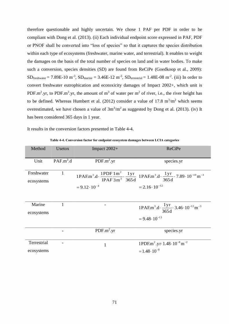
71

therefore questionable and highly uncertain. We chose 1 PAF per PDF in order to be

compliant with Dong et al. (2013). (ii) Each individual endpoint score expressed in PAF, PDF

or PNOF shall be converted into “loss of species” so that it captures the species distribution

within each type of ecosystems (freshwater, marine water, and terrestrial). It enables to weight

the damages on the basis of the total number of species on land and in water bodies. To make

such a conversion, species densities (SD) are found from ReCiPe (Goedkoop et al., 2009):

SDfreshwater = 7.89E-10 m-3, SDmarine = 3.46E-12 m-3, SDterrestrial = 1.48E-08 m-2. (iii) In order to

convert freshwater eutrophication and ecotoxicity damages of Impact 2002+, which unit is

PDF.m2.yr, to PDF.m3.yr, the amount of m3 of water per m2 of river, i.e., the river height has

to be defined. Whereas Humbert et al. (2012) consider a value of 17.8 m3/m2 which seems

overestimated, we have chosen a value of 3m3/m2 as suggested by Dong et al. (2013). (iv) It

has been considered 365 days in 1 year.

It results in the conversion factors presented in Table 4-4.

Table 4-4. Conversion factor for endpoint ecosystem damages between LCIA categories

Method Usetox Impact 2002+ ReCiPe

Unit PAF.m3.d PDF.m2.yr species.yr

Freshwater

ecosystems

1

4

3

23

1012.9

d365

yr1

m3

m1

PAF1

PDF1d.m.PAF1

12

3103

1016.2

m1089.7d365

yr1d.m.PAF1

Marine

ecosystems

1 -

13

3123

1048.9

m1046.3d365

yr1d.m.PAF1

- PDF.m2.yr species.yr

Terrestrial

ecosystems

- 1

8

282

1048.1

m1048.1yr.m.PDF1

72

4.2.3. Implementation of the proposed damage score to a water footprint

method (advanced water impact index - WIIX)

The water impact index (WIIX) is a simplified single indicator approach for water

footprinting (Bayart et al., 2014) that includes issues related to water scarcity and water

quality:

i

j

WIIX

ji

i

i

WIIX

ii WSIQWVWSIQWVWIIX __

(12)

Where Wi and Rj are quantities of water withdrawn from water body “i” and returned to water

body “j”, respectively (in volume unit), QiWIIX and Qj

WIIX are quality indices of water

withdrawn from water body “i” and returned to water body “j”, respectively (unitless), WSIi

and WSIj are water scarcity indices for water bodies “i” and “j”, respectively (unitless).

In this approach, water quality index QWIIX is based on the minimum ratio between pollutant

concentrations in ambient quality standard water flows (for example WFD in Europe) and in

the assessed water flow as shown in Eq. (13). It is comprised between 0 and 1 where 0

represents a bad water quality whereas 1 represents a good water quality.

i

p

ref

p

p

WIIX

iC

CQ ;1min

(13)

Where QiWIIX

is the quality index of WIIX (unitless, bounded between 0 and 1), Cpi is the

concentration of pollutant p in water flow i (kg/L) and Cpref is the concentration of pollutant p

in the chosen reference flow (kg/L).

This approach is therefore based on the most penalizing pollutant, as done within the WFD

when defining water classes. This simplification has a masking effect on the variation of other

pollutants. Therefore, Bayart et al. (2014) discussed the possibility to build a quality index

based on several pollutants, through an aggregation. We here propose to calculate an

advanced WIIX quality indicator based on LCIA, which has the advantage of taking into

account several pollutants in a single indicator as shown in eq. (14). Damage score on

ecosystem is chosen because it takes into account both eutrophication and ecotoxicity.

73

i

E

ref

EWIIX

iDS

DSQ ;1min

(14)

Where QiWIIX+

is the advanced quality index of WIIX (unitless, bounded by 0 and 1), DSEref is

the damage score on ecosystem of the reference flow, and DSEi is the damage score on

ecosystem of the studied flow i, both based on eq (10). Both QiWIIX and Qi

WIIX+ are computed

for water flows selected in section 4.2.1. The chosen reference is the good physico-chemical

state (column 2 of Table 4-2) and good chemical state from WFD.

4.3. Results and discussion

Specific results found for damage scores of the natural water resource are first discussed, in

comparison with the classifications of the WFD. For this purpose, only Impact 2002+ method

is chosen to simplify the comparison. Then, damage scores results for all selected urban water

flows are analyzed according to all LCIA methods. Finally damage scores are applied to

compute the advanced quality index of WIIX and this index is compared to the original water

quality index WIIX.

4.3.1. Damage scores analysis for natural water resources

Figure 4-1 represents the damage scores of the stations on ecosystem (only including

eutrophication) according to values measured for the physico-chemical state. There is a

correlation between the state and the damage scores: obviously, better the physico-chemical

state, lower the damage score. However, there is a high variability in damage scores for each

state, except for the very good state. In addition, Figure 4-1 shows in blue the damage scores

of the flows defined with threshold values for each physico-chemical parameters taken into

account, i.e., the highest damage score that can be found for each class. For example, damage

score of the flow defined with threshold value of water class 2 (i.e., good state class) have a

similar damage score than the highest value found for class 5 (bad state class). It means that a

water classified with good state could lead to more potential impact than a water classified

with bad state. It demonstrates the limitations of the state definition depending on thresholds

values. The aggregated damage score obtained from LCIA enables us to consider several

pollutants and could be an interesting option to classify waters.

Damage scores to freshwater ecotoxicity and human toxicity can be compared to the chemical

state of stations. Nevertheless, only two states are considered for chemicals: good or bad,

which greatly limits the potential for comparison. State 1 (good) average, minimum and

74

maximum values are similar. This is because when concentration of chemical compounds was

not know, it was set to the concentration of the good state. Therefore, most water resources

have the same damage score to ecotoxicity since there were considered to have the same

concentration.

Box-and-whiskers figure details: box extends from the 25th to 75th percentiles, the line in the middle of the box is plotted at

the median and whiskers refer to min and max.

Figure 4-1. Average damage score due to eutrophication of 2534 water resources versus physico-chemical state from

the WFD, from 1 (very good state) to 5 (bad state); LCIA method is Impact 2002+.

Box-and-whiskers figure details: box extends from the 25th to 75th percentiles, the line in the middle of the box is plotted at

the median and whiskers refer to min and max.

75

Figure 4-2.: Average damage score due to ecotoxicity of 2534 water resources versus chemical state from WFD; LCIA

method is Impact 2002+.

4.3.2. Analysis of damage scores of selected urban water flows

Figure 4-3 compare damage scores to ecosystems of the selected urban water flows,

depending on the LCIA method. It also shows the contribution of eutrophication and

ecotoxicity to total damage.

FEu = Freshwater eutrophication, FET = Freshwater ecotoxicity, TET : Terrestrial ecotoxicity, MET = Marine ecotoxicity

Figure 4-3. Damage scores on ecosystem (including eutrophication and ecotoxicity) of selected water flows assessed

with different LCIA methods. All scores are converted in species.yr.

The three methods differentiate the different water flows with their damage scores, from the

lower potential damage (drinking water) to the highest potential damage (raw highly polluted

wastewater).When comparing all the methods with the same basis (species.yr/L), damages

76

calculated with Impact 2002+ are much higher than the two others methods, which can be

explained by several reasons.

First, regarding ecotoxicity, Impact 2002+ results show a higher contribution of ecotoxicity

compared to others methods. This is because metals are overestimated in Impact 2002+, and

some pollutants evaluated in Impact 2002+ (such as aluminum) are not evaluated in the two

other methods. There is still an important challenge to assess metals in LCIA, as noted by

Rosenbaum et al. (2008). For example, Usetox still considers characterization factors for

metals as “interim” because the model does not account for speciation and other important

specific processes for metals.

Second, concerning freshwater eutrophication, Impact 2002+ takes into account Nitrogen,

phosphorus and COD whereas ReCiPe and ILCD only take phosphorus into account.

However, the consideration of N emissions in Impact 2002+ for freshwater eutrophication is

questionable. We chose to apply a damage CF for N emissions in Impact 2002+ by

considering unknown river basin limiting nutrient, whereas most of river basins are

phosphorus-limiting (and not affected by N emissions). This assumption is made to take into

account N emissions at the endpoint level for freshwater eutrophication. Actually, nitrogen

emissions affect marine eutrophication, which is still not assessed at the endpoint level in

consensual methods. New models that develop fate and effect factors for marine

eutrophication are currently being developed (Cosme et al., 2013) but the resulting

characterization factors are still under research and it was not possible to include them in the

current chapter (Dong et al., 2013).

Third, modeling choices to assess the damage are different for each method, and the

conversion factors used are also uncertain, which also explain the different results.

In the context of urban water system, Impact 2002+ enables us to assess the potential damages

of key pollutants, such as nitrogen, COD, aluminum, etc. However, the impact assessment

models and the associated assumptions are subject to high uncertainties.

Regardless the chosen LCIA methods, contributions of the different kinds of ecotoxicity are

similar: urban water flow pollutants contribute in majority to freshwater ecotoxicity,

compared to marine and terrestrial ecotoxicity. Even if terrestrial ecotoxicity models are

limited and are not always taken into account (e.g., UseTOX), the results clearly shows that

urban water flows contribute significantly to eutrophication and freshwater ecotoxicity only.

77

However, sludge spreading, that was not considered here as it is not strictly a water flow, has

an important contribution on terrestrial ecotoxicity.

For damages on human health (Figure 4-4), since only toxic compounds (and not nutrients)

are taken into account, the differentiation between water qualities is limited: this is because

concentrations of several toxic compounds are not known and are, therefore, set to “very good

state” water quality in our “gap filling procedure”. Results are not satisfying, and further data

on the composition of water flows is needed. However, the methods give similar results.

It also raises concerns on the present methodology with regards to human health. In order to

assess damage scores, the original assumption is that the water flow is released to the aquatic

environment. However, flows which stay within the technosphere can be exposed to human

(such as drinking water) and thus would require modified characterization factors considering

new exposure factors. This issue is important when assessing impacts of drinking water

production but has never been explored so far.

Figure 4-4. Damage scores on human health of selected water flows assessed with different LCIA methods.

78

4.3.3. Application to a water footprint method (Water Impact Index –

WIIX)

Figure 4-5 represents the WIIX quality index score depending on the original approach (QWIIX

eq. (13)) and the advanced approach (QWIIX+ eq. (14)). The advanced QWIIX+ allows a better

differentiation of water. For example, different polluted water (i.e., effluents from WWT and

DWP and raw wastewater) have a similar QWIIX close to 0, whereas QWIIX+ clearly

differentiate these types of flows, which have different water quality. This is because QWIIX+

takes into account all pollutants and is less sensitive to the high concentration of one pollutant.

Figure 4-5. WIIX quality index related to the original approach and the advanced approach

4.4. Proposed classification of urban water flows

From the damage scores analysis, a preliminary classification of flows is set according to the

ecosystem damage scores and the QWIIX+ indicator. Damages to human health were

disregarded since the differentiation of water types is not possible here, as shown in section

4.3.2. Five main types of water flows and their associated damage scores are defined to feed

the UWS model: from A,best water quality, to D, worst quality (A - Produced water, B -

79

Natural water resources, C - Effluents from DWP and WWT, D - Raw wastewater), with a last

type E, which represents “sludge”. These types follow specific ranges of damage scores and

of QWIIX+ as shown in Table 4-5. This classification also allows to use these typical values to

evaluate an urban water flow of a certain type, without knowing exactly its composition.

Within each type, several levels can be defined to be even more precise (e.g., A1, A2… Ai in

“A - Produced water” type) and to represent all water flows of the case studies.

Table 4-5. Proposition of water types for urban water flows and corresponding damage scores to ecosystems

Range of “damage score” for the

proposed water quality type

Range of

QWIIX+

Water flow types Water flow

indices as named

in the WaLA

model

Impact 2002+

ecosystem score

(10-3 PDF.m2.yr/L)

ReCiPe

ecosystem score

(10-12

species.yr/L)

A - Produced

water

A1, A2, …, Ai 0 – 11 0 – 1 1

B - Natural water

resources

B1, B2, …, Bi 11 – 40 2.5 – 10 0.5 – 1

C - Effluents from

DWP and WWT

C1, C2, …, Ci 15 – 100 10 – 50 0.2 – 0.5

D - Raw

wastewater

D1, D2, …, Di 100 – 1000 100 – 1200 0 – 0.2

E – Sludge E1, E2, …, Ei - - -

4.5. Conclusions and outlook

Water-related LCIA methods have been applied to aggregate water composition of urban

water flows into two quality scores: a damage score for ecosystem quality and a damage score

for human health. Damage scores of natural water resources show a correlation with their

physico-chemical and chemical state as described by WFD. However, it also points out the

limits of the definition of water quality states built by WFD, which are based on threshold

values. It opens an interesting discussion about using aggregated water quality scores based

on LCA as new indicators to classify natural water resources. Within the LCA framework,

Boulay et al. (2011) also developed categories of natural water resources depending on their

80

functionalities towards different kind of users. Their approach is also based on threshold

values, as the WFD. It would be interesting to evaluate the average damage scores for several

flows within each of their categories. A further step would be to compare damage scores with

ecological state, which is also based on biological and hydromorphological elements.

Studied urban water flows show a high sensitivity of the damage scores on ecosystems,

allowing the flows to be differenciated. The Impact 2002+ method enables us to take into

account a larger set of pollutants of importance, but relies on more uncertain models than

ReCiPe or ILCD. Damage scores on human health do not permit such a differentiation

because of lacking inventory data on toxic compounds. The implementation of the damage

scores on ecosystems to the quality indicator of water footprint methodology (WIIX) has led

to a new indicator, named QWIIX+ which has proven its worth compared to the original quality

indicator (QWIIX ) based on the most penalizing pollutants. This kind of simplification, which

consists in focusing only on water issues, clearly helps for the interpretation of the results: a

water footprint is generally easier to interpret than results from a full multi-criteria approach.

There is also an increasing demand from industries for developing this kind of metrics.

Nevertheless, it should be stated that such a simplification doesn't allow the identification of

pollution shifting to other impact categories, which would not be related to water.

Chapter 2 has shown that LCA has already proven its worth in assessing the environmental

impacts of UWS but it also pointed out methodological challenges related to LCA of UWS,

and the need for a standardized approach. Following this review, methodological

developments related to the assessment of water deprivation and water quality are presented

Chapter 3 and 4. The following chapter, which is the core of the thesis, aims to develop a

framework and an associated model for the LCA of UWS, following the identified

specifications and implementing the methodological advances.

81

Chapter 5. WaLA, a versatile model for the

life cycle assessment of urban water systems:

Part 1 – formalism and framework for a

modular approach

« On my block, it ain't no different than the next block »

Scarface – On my block

82

In this chapter, which is the heart of the thesis, we propose a versatile model, termed WaLA

model (Water system Lifecycle Assessment), which reduces the complexity of the system

while ensuring a good representation with regards to water issues and LCA requirements.

Indeed, LCAs require building UWS models, which can be tedious if several scenarios are to

be compared. The WaLA model is based on a framework that uses a “generic component”

representing alternately water technologies and users, with their associated water flows, and

the associated impacts due to emissions, operation and infrastructure. UWS scenarios can be

built by inter-operating and connecting the technologies and users components in a modular

and integrated way. The model calculates monthly outputs of life cycle impacts for a set of

services provided to users, as defined by the scenario. It leads to the impact/service ratio (e.g.,

impact/capita) and useful pieces of information for UWS diagnosis or comparison of different

scenarios. The model is implemented in a Matlab/Simulink interface thanks to object-oriented

programming. The applicability of the model is demonstrated using a virtual case study based

on ecoinvent processes. This chapter refers to the following paper submitted to Water

Research: “Loubet, P., Roux, P. & Bellon-Maurel, V. WaLA, a versatile model for the life

cycle assessment of urban water systems: Part 1 – formalism & framework for a modular

approach.”


Technosphere

(Urban Water System)

Environment

Q2

Q0

Provided services

Indirect

impacts

Q1 Q0 Q3 Q2Q0

Q0

Q3

Q3

Production Distribution Users Collection Treatment

Drinking water Wastewater

Q1Water

flow

WaLA Model

83


5.1. Introduction ................................................................................................................... 85

5.2. Urban water system modeling ....................................................................................... 86

5.2.1. Specifications for an integrated UWS model ......................................................... 86

5.2.2. The general framework of the WaLA model ......................................................... 87

5.2.3. Goal and scope definition ....................................................................................... 88

5.2.4. LCI/LCIA associated to the technologies/users generic components .................... 89

5.2.4.1. Water quantity: Volumetric water flows (LCI) .............................................................................................92

5.2.4.2. Water quality (LCI) ......................................................................................................................................92

5.2.4.3. Direct impacts associated with water quantity (LCIA) .................................................................................93

5.2.4.4. Direct impacts associated to quality of released water (LCIA) .....................................................................93

5.2.4.5. Direct impacts associated with emissions of water to air and soil (LCIA) ....................................................94

5.2.4.6. Direct and indirect impacts associated with life cycle supporting activities (LCIA) ....................................95

5.2.4.7. Total impacts (LCIA)....................................................................................................................................96

5.2.4.8. Computation of the impact/service ratio .......................................................................................................96

5.2.5. Practical details ....................................................................................................... 96

5.2.5.1. Spatial and temporal scales ...........................................................................................................................96

5.2.5.2. Uncertainty propagation management ..........................................................................................................97

5.2.6. Implementation of the model within a computer program ..................................... 97

5.2.6.1. Objects representing technologies and users components .............................................................................97

5.2.6.2. Arrows representing water flow ....................................................................................................................98

5.2.6.3. Building a specific model: inter-operation of the objects .............................................................................99

5.2.6.4. Computation ...............................................................................................................................................100

5.2.7. Virtual case study ................................................................................................. 100


5.3.1. The graphical representation of the UWS ............................................................ 101

5.3.2. Environmental impacts ......................................................................................... 102

5.3.3. Provided services and impact/service ratio .......................................................... 105


5.4. Conclusions ................................................................................................................. 107

84

Table 5-1. Specific glossary for the WaLA model (Chapters 5 and 6)

Technologies/Users designation Variables and parameters

DWP Drinking water production DEM Total water demand

(m3/time)

DWD Drinking water distribution dem Specific water demand

(m3/user/time)

SEOL Sludge end of life I Impact matrix (e.g., kg CO2

eq)

SWC Stormwater collection i Specific impact matrix (e.g.,

kg CO2 eq/m3)

U User Q Water quality index of a

given flow

UWS Urban water wystem q Water quality distribution

vector

WH Water heaters S Services provided (amount of

users)

WWC Wastewater collection V Volumetric water flow

(m3/time)

WWT Wastewater treatment v Volumetric water flow

distribution vector

Flows designation Superscripts of I and i

C Consumption direct, air-soil Direct impacts in link with air

& soil emissions

P Precipitation direct, water Direct impacts in link with

water emissions

R Release indirect, support Indirect impacts due to

supporting activities

Tin Technosphere in indirect, chem Indirect impacts due to

chemicals

Tout Technosphere out (liquid) indirect, ener Indirect impacts due to energy

Tout2 Technosphere out (sludge) indirect, infra Indirect impacts due to

infrastructures

W Withdrawal

85

5.1. Introduction

Water management in cities faces many challenges, which are linked to water resources, water

users and water technologies (Global Water Partnership Technical Committee, 2012).

Decision makers require tools to assess the environmental impacts of urban water systems

(UWS) and thereby compare technical solutions. Holistic approaches are required to evaluate

all components of the system in an integrated way (Falkenmark, 1998).

A large amount of literature provides integrated UWS models. Mitchell et al. (2007) reviewed

65 studies, which predict water flows and water quality in cities. Some of these models go

beyond calculating water quantity and water quality fluxes to include environmental aspects.

For example, the SWITCH city water balance also aims to quantify energy consumption and

simplified life cycle costs (Mackay and Last, 2010). Fagan et al. (2010) include environmental

impact scores in their complex model for a specific UWS in Australia. However, none of

these scoping tools include multi-criteria approaches, such as a full life cycle assessment

(LCA)

A recent review shows that LCA is used more often to assess the environmental performance

of UWS (Loubet et al., 2014). It highlights guidelines and the need for methodological

frameworks in that field for all LCA phases. In the meantime, several scientific developments

have occurred for LCAs to better assess impacts associated with water use (Kounina et al.,

2012). These recent advances have been implemented in only a few UWS LCAs (Godskesen

et al., 2013; Muñoz et al., 2010). However, LCA of UWS is still an open issue: in their review

of the water-energy-greenhouse gas nexus of UWS, Nair et al. (2014) noted the interest of

LCA but underlined the current static nature of the simulation tools.

The objective of this work is to model the complex UWS of megacities within the LCA

framework with the aim of assessing its environmental impacts in relation to the services

provided to water users. The model is termed “WaLA” as an acronym for “Water system Life-

cycle Assessment”. It reduces the complexity of the system to easily implement forecasting

scenarios while ensuring a good representation from the LCA perspective.

We first propose a framework and its associated modeling formalism based on a combination

of generic components, representing either water technologies or water users. The

technologies and users composing the UWS are then interoperated in an integrated way and

connected to water resources to model the water flows and the associated impacts linked to

86

water flows, operation and infrastructures. WaLA is run through a Matlab/Simulink

(Mathworks Inc., 2007) graphical interface where the practitioner implements his own UWS

scenarios in an interactive manner. Calculations of the model provide the LCIA results and the

impact/service ratio. The model is finally tested on a first case study that represents a virtual

UWS based on ecoinvent processes and assumptions.

5.2. Urban water system modeling

5.2.1. Specifications for an integrated UWS model

The objective of the WaLA model is to assess the environmental impacts of a UWS using the

LCA framework. Therefore, the model should fulfill the requirements of the four phases

defined in the international LCA standard (ISO, 2006a): goal and scope definition, LCI, LCIA

and interpretation of the results. The proposed model should also be compliant with the

specific methodological challenges associated with the LCA of UWS, as noted in Chapter 2

(Loubet et al., 2014), i.e., it should address issues/specifications related to the following

points:

- (S1) Multi-functionality: UWS is a typical multifunctional activity (including

domestic, industrial, agricultural, service users), whereas conventional LCAs were

originally designed to assess a single service quantified by a functional unit. This issue

can be solved by using the conceptual framework proposed by Loiseau et al. (2013)

for LCA of regions, called “territorial LCA”.

- (S2) Modularity: There is an increasing demand for modeling forecasting scenarios in

land and city management processes (Bach et al., 2014). A modular and interactive

approach that simplifies the definition and modification of the UWS model is required

for such forecasting.

- (S3) LCI and LCIA requirements linked to water quantity. As water is central in UWS

, a precise accounting of water withdrawals, releases and consumption is therefore

necessary; the model should follow the conceptual framework for assessing off-stream

water use in LCI, as defined by Bayart et al. (2010), and the various LCIA methods

that have been developed to assess the impacts related to water deprivation (Kounina

et al., 2012).

- (S4) LCI and LCIA requirements linked to water quality: the mass balance of

pollutants within the entire water systems must be satisfied for LCI (Risch et al.,

87

2011). The model should also be able to include recent and future LCIA developments

regarding water quality, particularly those related to eutrophication and toxicity.

- (S5) Accounting for all impacts associated with operation and infrastructures: In

addition to impacts due to water deprivation and pollution, UWS generate impacts by

operating the system and from infrastructures that should be considered to avoid

burden shifting.

- (S6) Appropriate spatial scale: In a conventional LCA, the present trend is to conduct

an impact assessment of water deprivation at the river basin scale (Pfister et al., 2009).

Concerning UWS, the plurality of water resources within the basin is large and can

lead to different impacts, depending on the location (upstream/downstream) of the

water sources as shown in Chapter 2 (Loubet et al., 2013; Vörösmarty et al., 2005).

Therefore, it is necessary to consider finer scales for UWS, i.e., the sub-river basin.

- (S7) Appropriate temporal scale: Whereas most UWS models include calculations at a

daily scale (Mitchell et al., 2007), LCA is generally designed to assess impacts on a

yearly basis. However, yearly timescales are not appropriate when water issues are

being addressed because of high seasonal variations. Therefore, for a water-related

impact assessment, a monthly scale appears appropriate to capture the climatic and

hydrologic variations (Pfister and Bayer, 2014).

- (S8) Uncertainty management: Uncertainty has been disregarded in most previous

LCAs applied to UWS (Loubet et al., 2014). The model should be able to compute

uncertainties in the impact scores.

In the sections 5.2.3 and 5.2.4 each UWS modeling proposal is presented by following the

first three LCA phases (goal & scope definition, LCI, LCIA), including a discussion for each

relevant requirement (S1 to S8) defined above. The implementation of the model within a

computer program is developed in section 5.2.6. The fourth LCA phase (interpretation) is

addressed in detail within the application to a case study introduced in the section 5.2.7.

5.2.2. The general framework of the WaLA model

Figure 5-2 is a simplified representation of the general framework of the WaLA model. It is

based on a combination of generic components, which have been instanced various parts of

the UWS, i.e. water technology and user components. Both components are connected to

water resources. The modularity requirement (S2) is achieved thanks to this modeling

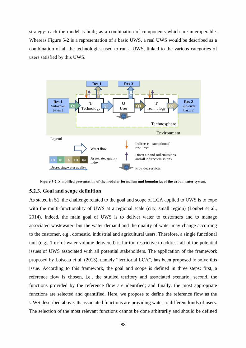
88

strategy: each the model is built; as a combination of components which are interoperable.

Whereas Figure 5-2 is a representation of a basic UWS, a real UWS would be described as a

combination of all the technologies used to run a UWS, linked to the various categories of

users satisfied by this UWS.

Figure 5-2. Simplified presentation of the modular formalism and boundaries of the urban water system.

5.2.3. Goal and scope definition

As stated in S1, the challenge related to the goal and scope of LCA applied to UWS is to cope

with the multi-functionality of UWS at a regional scale (city, small region) (Loubet et al.,

2014). Indeed, the main goal of UWS is to deliver water to customers and to manage

associated wastewater, but the water demand and the quality of water may change according

to the customer, e.g., domestic, industrial and agricultural users. Therefore, a single functional

unit (e.g., 1 m3 of water volume delivered) is far too restrictive to address all of the potential

issues of UWS associated with all potential stakeholders. The application of the framework

proposed by Loiseau et al. (2013), namely “territorial LCA”, has been proposed to solve this

issue. According to this framework, the goal and scope is defined in three steps: first, a

reference flow is chosen, i.e., the studied territory and associated scenario; second, the

functions provided by the reference flow are identified; and finally, the most appropriate

functions are selected and quantified. Here, we propose to define the reference flow as the

UWS described above. Its associated functions are providing water to different kinds of users.

The selection of the most relevant functions cannot be done arbitrarily and should be defined

TTechnology

UUser

TTechnology

Technosphere

Environment

Q1 Q0 Q3

Q2

Res 2Sub-river

basin 2

Q0

Res 1Sub-river

basin 1

Res 1 Res 3

Q0 Q1 Q2 Q3 Q4

Decreasing water quality

Indirect consumption of

resources

Direct air and soil emissions

and all indirect emissions

Legend

Provided services

Water flow

Associated quality

index

Q2

89

in accordance with stakeholder’s issues. As a first approach, the functions are defined by a

representative indicator of each type of user (e.g., the number of domestic users, industrial

jobs), which are simply quantified through the description. Thus, we do not create a single

functional unit but a set of functions represented by a vector of values termed S. An

alternative function is defined as the volumetric amount of water supplied at the user’s place,

which can be useful to assess the efficiency of the “technological system”. However, this

function does not consider user behavior and may be less relevant when considering an

integrated urban water system, including its social dimension (Loubet et al., 2014). Water

users are characterized by their water demand (in terms of both quantity and quality), noted

dem (m3 of a given quality/user unit/unit of time). The total water demand of a user, termed

DEM, is the product of the number of users S and the specific water demand dem.

5.2.4. LCI/LCIA associated to the technologies/users generic components

The model is based on a generic component formalism that represents both water technologies

and water users (Figure 5-3). Water technologies are typically drinking water production

(DWP), drinking water distribution (DWD), wastewater collection (WWC) and wastewater

treatment (WWT). Water users (U) are domestic, industrial, or agricultural users, among

others. Because technologies and user components are related to anthropogenic activities, they

are located within the technosphere and are in the foreground system.

Figure 5-3. Description of water flows and associated impacts/services of the generic component.

SoilLocal environment

111110Technology/User

Technosphere in

(Tin)

Technosphere out

(Tout)

Consumption

C

Withdrawal

from env. (W)

Release to

env. (R)

Technosphere

Water Local environment

AtmosphereGlobal environment Water flow V (m3)

with water quality Q

Indirect and direct

impacts due to emissions

and resouces use related

to supporting activities

(electricity, chemical,

infrastructures) Isupport

Provided services to

users S

Provided services

to users

Precipitation

P

Direct impacts linked to

emissions to air and soil

Idirect,air-soil

Direct impacts linked

to water quantity and

quality Idirect,water

Life Cycle Inventory

Life Cycle Impact

Assessment

Technosphere out2,

sludge (Tout2)

90

Model components exchange water flows with other components and the local or global

environment. “Local environment” is defined as the sub-river basin where the component

withdraws or releases water, and “global environment” is defined as the atmosphere.

Consequently, six types of water flows enter or leave each component as shown in Figure 5-3:

(1) input water from the technosphere, Tin; (2) output water to the technosphere, Tout; (3) input

from the local environment, W (withdrawal); (4) output to the local environment, R (release);

(5) input from the global environment, P (precipitation); and (6) output to the global

environment C (consumption). Two different technosphere flows, termed Tout and Tout2, are

defined for water flow and sludge flow, respectively. Water consumption is the water

evaporated, transpired or exported in product (Bayart et al., 2010). According to the

international standards (ISO, 2006), within-technosphere flows (Tin and Tout) are considered

intermediate flows, and environment flows (W, R, P, C) are considered elementary flows.

Each flow is characterized by two parameters: the volumetric water flow (V), which is

expressed in m3 per unit of time, and the water quality (Q), which is expressed by an index.

Each flow parameter is defined by the component name to which it is linked (e.g., “DWP” for

drinking water production), the flow name (e.g., “Tout” for water flow going to the

technosphere) and the considered parameter (e.g., V) as shown below:

T_V_DWP

name flow

in

parametercomponentsub

(15)

When the water flow crosses the boundary between the technosphere and the local

environment, it leads to impacts because of its quantity and quality changes, as shown in

Figure 5-3. Estimations of these associated impacts are explained in the sections 5.2.4.3 and

5.2.4.4.

In addition to the direct impacts linked to water flow exchanges, water technologies generate

direct impacts due to emissions to the air (e.g., CH4 in WWT) and soil (e.g., metals in sludge)

from the water and sludge lines, defined in section 5.2.4.5.

Other water technology impacts come from supporting activities of the UWS: energy

(primarily electricity), chemicals, transportation of sludge and chemicals, and infrastructure

(construction, maintenance, and deconstruction). These processes are generally considered

background processes because they are typically found in locations other than the UWS

territory, as defined by Azapagic et al. (2007). However, some supporting activities can occur

in the foreground system, and the related emissions to the air and soil are considered direct. It

91

can concern certain types of energy (e.g., gas to heat water, generator group to produce

electricity, methanization of sludge), chemical production (e.g., ozone production) or

infrastructure (e.g., civil works). Because these activities are occurring within the UWS

territory and are usually under the control of the UWS decision-maker, they should be

considered foreground and as generating direct impacts (Frischknecht, 1998; Loiseau et al.,

2014). The calculation of these impacts is detailed in section 5.2.4.6.

At the component scale, impacts can be classified according to two different groupings, as

shown in Table 5-2: (i) related to foreground (leading to direct impacts) and background

activities (leading to indirect impacts) and (ii) related to water and sludge lines or supporting

activities. If direct impacts linked to supporting activities are not considered, which should be

likely the case, the two groupings are equivalent: direct impacts occur in water and sludge

lines, and indirect impacts occur in supporting activities.

Table 5-2. Classification of impacts at the component scale

Foreground activities (direct

impacts)

Background activities

(indirect impacts)

Water and sludge lines - Emissions

to water

- Water use

- Emissions

to air and soil

Supporting activities - Production of energy,

chemicals and materials for

infrastructures occurring in

the territory

- Production of energy,

chemicals and materials for

infrastructures occurring

elsewhere the territory

Impacts are stored in a matrix Itotal of n lines, each of which represents an impact category j,

noted Ij, depending on the chosen LCIA method. Itotal is calculated by adding different

contributors to impacts: direct impact due to the exchange of water of various qualities

between the technosphere and the environment (Idirect,water), direct impacts due to emissions to

the air and soil from the water and sludge lines (Idirect,air-soil), and direct and indirect impacts

related to supporting activities (Isupport) for operation (energy Iener, chemicals Ichem) and

infrastructures (Iinfra). Each vector has the same number of n lines, but depending on the

contributor considered, not all impact categories are necessarily concerned and can be thus set

to 0 (e.g., fossil fuel depletion is set to 0 for Idirect,water vector). The generic component related

to users also generates the services provided to the users, as detailed in the section 5.2.3.

92

5.2.4.1. Water quantity: Volumetric water flows (LCI)

Volumetric water flows (in m3 per unit of time) are represented by a vector V defined in eq

(16). They are balanced for each component to comply with specification S3 regarding the

inventory of water quantity. To achieve this water balance, the sum of the volumetric flows

that are entering (Tin, W, P) must be equal to the volumetric flows that are exiting (Tout, Tout2,

R, C) any component. The volumetric water flows are calculated from a water flow

distribution vector, namely v, and a known input variable, which is either V_Tin or V_W (eq

3). v is a vector of intrinsic parameters (m3/m3), specific to each component, that defines the

distribution of flows entering (Tin, W, P) and exiting (Tout, Tout2, R, C) the component for 1 m3

at the input (Tin or W for DWP).

0)C_VR_VT_VT_V()P_VW_VT_V( where

C_V

P_V

R_V

W_V

T_V

T_V

T_V

V 2outoutin

2out

out

in

(16)

C_v

P_v

R_v

W_v

T_v

T_v

T_v

v where vW_VV DWPor F

vT_VV WWT WWC, U,DWD,For 2out

out

in

in

(17)

5.2.4.2. Water quality (LCI)

Quality is defined by an index, Q that refers to a chemical load in the water. This chemical

load is also associated with the potential impacts when water is released to the environment,

as explained in the section 5.2.4.4. At this stage of model development, definition of indices is

based on Chapter 4: A1, A2, … are drinking water qualities, B1, B2, … are water resource

qualities, C1, C2, … are qualities of water effluents from DWP or WWT, D1, D2, … define

raw domestic wastewater qualities and E1, E2, … define sludge qualities. The chemical

composition of each index is given in Chapter 4 and Annex C.3.

93

For each component, a vector of “intrinsic parameters”, namely q, defines the indices Q of

water flows exiting (eq. 4). To build these vectors, it is first necessary to determine the mass

balance of the chemicals considered between the inputs and outputs at the component scale

(specification S4).

C_Q

0

R_Q

0

T_Q

T_Q

0

q

2out

in

(18)

Qualities of water entering the component (Q_Tin, Q_W, Q_P) are known input variables.

5.2.4.3. Direct impacts associated with water quantity (LCIA)

Withdrawals deprive downstream users from water, whereas releases make the water

available again. The water deprivation impacts (IWD) associated with each component are

computed based on characterization factors (CF) defined at the sub-river basin scale, as

recommended in Chapter 3 (Loubet et al., 2013):

B,WDA,WD

waterdirect,

WD CFR_VCFW_VI

(19)

Where IWD is the midpoint impact of water deprivation (m3 equivalent or m3 equiv), V_W is

the volume of water withdrawn at location A (m3), V_R is the volume of water released at

location B (m3), and CFWD,A and CFWD,B are the characterization factors for water deprivation

at locations A and B, respectively. Water deprivation CFs differentiated at the sub-river basin

scale are used to calculate the cascade effects on downstream sub-river basins. The use of this

LCIA model is compliant with the spatial scale required for UWS (S7). IWD is then stored

within the vector Idirect, water.

5.2.4.4. Direct impacts associated to quality of released water (LCIA)

The different water quality indices introduced in the section 5.2.4.2 refer to the chemical

compositions and associated impacts. Impacts are calculated for each component as the

difference in the potential impacts associated with water releases and the potential impacts

associated with water withdrawals (eq. 5). Indeed, because emitting pollutants affects the

environment, it is counted as positive, whereas uptaking the pollutant from the environment is

a benefit for the environment and is counted as negative.

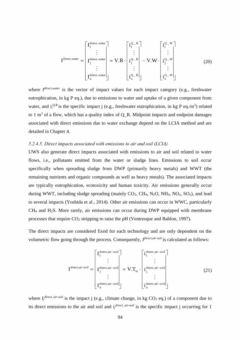
94

W_Q

n

W_Q

j

W_Q

1

R_Q

n

R_Q

j

R_Q

1

water,direct

n

water,direct

j

water,direct

1

waterdirect,

i

i

i

W.V

i

i

i

R.V

I

I

I

I

(20)

where Idirect,water is the vector of impact values for each impact category (e.g., freshwater

eutrophication, in kg P eq.), due to emissions to water and uptake of a given component from

water, and ijQ.R is the specific impact j (e.g., freshwater eutrophication, in kg P eq./m3) related

to 1 m3 of a flow, which has a quality index of Q_R. Midpoint impacts and endpoint damages

associated with direct emissions due to water exchange depend on the LCIA method and are

detailed in Chapter 4.

5.2.4.5. Direct impacts associated with emissions to air and soil (LCIA)

UWS also generate direct impacts associated with emissions to air and soil related to water

flows, i.e., pollutants emitted from the water or sludge lines. Emissions to soil occur

specifically when spreading sludge from DWP (primarily heavy metals) and WWT (the

remaining nutrients and organic compounds as well as heavy metals). The associated impacts

are typically eutrophication, ecotoxicity and human toxicity. Air emissions generally occur

during WWT, including sludge spreading (mainly CO2, CH4, N2O, NH4, NOx, SOx), and lead

to several impacts (Yoshida et al., 2014). Other air emissions can occur in WWC, particularly

CH4 and H2S. More rarely, air emissions can occur during DWP equipped with membrane

processes that require CO2 stripping to raise the pH (Ventresque and Bablon, 1997).

The direct impacts are considered fixed for each technology and are only dependent on the

volumetric flow going through the process. Consequently, Idirect,air-soil is calculated as follows:

soilair,direct

n

soilair,direct

j

soilair,direct

1

in

soilair,direct

n

soilair,direct

j

soilair,direct

1

soil-airdirect,

i

i

i

T.V

I

I

I

I

(21)

where Ijdirect, air-soil is the impact j (e.g., climate change, in kg CO2 eq.) of a component due to

its direct emissions to the air and soil and ijdirect, air-soil is the specific impact j occurring for 1

95

m3 entering into a component (e.g., climate change, in kg CO2 eq./m3). V_Tin is replaced by

V_Tout for DWP technology.

5.2.4.6. Direct and indirect impacts associated with life cycle supporting activities (LCIA)

Iimpacts linked to supporting activities are represented by two vectors, one vector

representing direct impacts (Idirect,support) and the other representing indirect impacts

(Iindirect,support). In the two cases, specific impacts linked to energy, termed iener, specific impacts

linked to chemicals and others, termed ichem, and specific impacts linked to infrastructure,

termed iinfra, should be defined. These specific impacts are either correlated to the volumetric

water flow entering/exiting the system or the quality of water entering/exiting the system or

fixed. It is considered that the energy and chemical consumption within the generic

component are fully correlated with the volumetric flow entering/exiting the technology. The

infrastructure is already built and maintained for the actual volumetric flow rate of the city.

Therefore, its associated impacts are fixed, independent of the volumetric water flow. For this

situation, the total impacts of the infrastructure (Iinfra) are considered and are divided by the

lifetime (in years or months). Eq (22) and (23) define the direct and indirect impacts for

supporting activities.

t

1

i

i

i

i

i

i

i

i

i

T.V

I

I

I

I

rainf,direct

n

rainf,direct

j

rainf,direct

1

chem,direct

n

chem,direct

j

chem,direct

1

ener,direct

n

ener,direct

j

ener,direct

1

in

portsup,direct

n

portsup,direct

j

portsup,direct

1

supportdirect,

(22)

t

1

i

i

i

i

i

i

i

i

i

T.V

I

I

I

I

rainf,indirect

n

rainf,indirect

j

rainf,indirect

1

chem,indirect

n

chem,indirect

j

chem,indirect

1

ener,indirect

n

ener,indirect

j

ener,indirect

1

in

portsup,indirect

n

portsup,indirect

j

portsup,indirect

1

supportindirect,

(23)

The quantification of these impacts are typically well known because the LCA literature on

water systems focused on technological impacts (Loubet et al., 2014) and because the

ecoinvent database provides data on the background processes for energy and chemical

production. Infrastructure-related impacts and associated civil works require further study.

Other water technologies that were not typically accounted for in UWS LCA must be added to

96

the model, particularly technologies that are present at the user’s place, such as water heating

systems, which generate a large proportion of impacts (Arpke and Hutzler, 2006; Fagan et al.,

2010).

5.2.4.7. Total impacts (LCIA)

Finally, the total impacts of a component are the sum of all of the above-mentioned impacts.

t

1i)ii(T_V

iT_V)iW_ViR_V()CFR_VCFW_V(I

activities supporting torelated Impacts

rainfchemelec

in

lines sludge and water torelated impactsDirect

soilair,direct

in

W_QR_Q

B,WDA,WD

total

(24)

5.2.4.8. Computation of the impact/service ratio

As stated in section 5.2.3, no unique functions exist due to the multi-functionality of UWS. To

refer the total impacts of the system to services (amount of users supplied by water),

impact/service ratios (IS ratio, impacts/user) can be computed using eq (25). IS ratio is the

inverse of the eco-efficiency ratio (EE) as defined by (Seppäläa and Melanen, 2005).

DEM

DEM

S

I

EE

1SI i

i

system,total

i

(25)

Where ISi is the total impact of the system for one user in category i (impact/user), Itotal,system is

the total impact of the system, Si is the number of users in category i, DEMi is the water

demand from users i (m3), and ΣDEM is the total water demand from all of the users (m3).

If the provided service chosen by the stakeholder is the m3 supplied at the user’s place, the

impact/service ratio (ISm3 ratio, impact/m3) is computed using eq. 11.

DEM

ISI

system,total

3m

(26)

5.2.5. Practical details

The description of the model framework enabled us to show that it was compliant to five out

of eight requirements for easily carrying out a LCA based on it. The way its implementation

allows us to fit with the three other requirements as described below.

5.2.5.1. Spatial and temporal scales

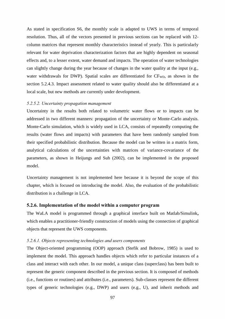
97

As stated in specification S6, the monthly scale is adapted to UWS in terms of temporal

resolution. Thus, all of the vectors presented in previous sections can be replaced with 12-

column matrices that represent monthly characteristics instead of yearly. This is particularly

relevant for water deprivation characterization factors that are highly dependent on seasonal

effects and, to a lesser extent, water demand and impacts. The operation of water technologies

can slightly change during the year because of changes in the water quality at the input (e.g.,

water withdrawals for DWP). Spatial scales are differentiated for CFWD, as shown in the

section 5.2.4.3. Impact assessment related to water quality should also be differentiated at a

local scale, but new methods are currently under development.

5.2.5.2. Uncertainty propagation management

Uncertainty in the results both related to volumetric water flows or to impacts can be

addressed in two different manners: propagation of the uncertainty or Monte-Carlo analysis.

Monte-Carlo simulation, which is widely used in LCA, consists of repeatedly computing the

results (water flows and impacts) with parameters that have been randomly sampled from

their specified probabilistic distribution. Because the model can be written in a matrix form,

analytical calculations of the uncertainties with matrices of variance-covariance of the

parameters, as shown in Heijungs and Suh (2002), can be implemented in the proposed

model.

Uncertainty management is not implemented here because it is beyond the scope of this

chapter, which is focused on introducing the model. Also, the evaluation of the probabilistic

distribution is a challenge in LCA.

5.2.6. Implementation of the model within a computer program

The WaLA model is programmed through a graphical interface built on Matlab/Simulink,

which enables a practitioner-friendly construction of models using the connection of graphical

objects that represent the UWS components.

5.2.6.1. Objects representing technologies and users components

The Object-oriented programming (OOP) approach (Stefik and Bobrow, 1985) is used to

implement the model. This approach handles objects which refer to particular instances of a

class and interact with each other. In our model, a unique class (superclass) has been built to

represent the generic component described in the previous section. It is composed of methods

(i.e., functions or routines) and attributes (i.e., parameters). Sub-classes represent the different

types of generic technologies (e.g., DWP) and users (e.g., U), and inherit methods and

98

attributes from the unique class. As instances of these sub-classes, the objects are specific

technologies and users (Figure 5-4).

Three methods are defined for the class: (i) the “calculation” routine computes the volumetric

water flows V, water quality Q, impacts I from eq (16), (17), (24); (ii) the “adder” routine

manages the sum of the different flows entering a block; and (iii) the “dispatcher” routine

manages the various outputs exiting the block to the technosphere.

Attributes, i.e., variables that allow for the customization of the block, are either “intrinsic” or

“extrinsic”. The “intrinsic” attributes are defined a priori and are specific to each object (i.e.,

each technology/user). These are the volumetric water flow distribution vector v, the quality

distribution vector q and the specific impacts matrix i. User objects also include the specific

water demand dem. The “extrinsic attributes” are defined in the model, either by the

practitioner or as a result of the model initialization. These are the number of inputs (in) and

outputs (out) from and to the technosphere, the name of the local water resource (Res) to

which the object is connected, and, the number of water users (S). Methods and attributes for

technologies and users are summarized in Figure 5-4.

v = volumetric water flow distribution vector, q = quality distribution vector, i = specific impacts matrix.

Figure 5-4. Representation of the unique class (superclass) associated with the generic component, its sub-classes

associated with each technology/user component, and the instances of each sub-class associated with the specific

components.

5.2.6.2. Arrows representing water flow

class

sub-classes

instances

(objects)

Methods

• Calculation

• Adder

• Dispatcher

Intrinsic attributes

v

qi

Generic

component

v_DWP

q_DWPi_DWP

Generic DWP

v_DWD

q_DWDi_DWD

Generic DWD

v_U

q_Udem

Generic U

v_SWC

q_SWCi_SWC

Generic SWC

v_WWC

q_WWCi_WWC

Generic

WWC

v_WWT

q_WWTi_WWT

Generic

WWT

v_DWPecoinvent

q_DWPecoinventi_DWPecoinvent

DWP

_ecoinvent

v_DWP_1

q_DWP_1i_DWP_1

DWP_1

99

Arrows represent water flows exchanged by the components in the technosphere. They

convey volumetric water flow (V) and quality index (Q) variables. Several technosphere

water flows can go in and/or out of a graphical object. Note that water flows exiting the

technosphere to the environment are not represented by an arrow but are directly translated

into impacts.

5.2.6.3. Building a specific model: inter-operation of the objects

Each technology and user is represented by a graphical object that has methods and intrinsic

attributes. They are stored in a Simulink library and can be selected via “drag and drop” in the

graphical Simulink® window. Extrinsic attributes of the objects are defined through the

practitioner interface. The different objects are connected with the arrows (technosphere water

flows). Figure 5-5 schematizes the entire procedure for the construction of an UWS scenario

and the computation of impacts. The structure of the Simulink objects and the associated

algorithms are presented in Annex C.1.

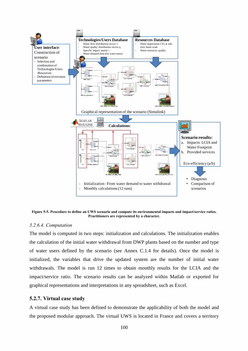
100

Figure 5-5. Procedure to define an UWS scenario and compute its environmental impacts and impact/service ratios.

Practitioners are represented by a character.

5.2.6.4. Computation

The model is computed in two steps: initialization and calculations. The initialization enables

the calculation of the initial water withdrawal from DWP plants based on the number and type

of water users defined by the scenario (see Annex C.1.4 for details). Once the model is

initialized, the variables that drive the updated system are the number of initial water

withdrawals. The model is run 12 times to obtain monthly results for the LCIA and the

impact/service ratio. The scenario results can be analyzed within Matlab or exported for

graphical representations and interpretations in any spreadsheet, such as Excel.

5.2.7. Virtual case study

A virtual case study has been defined to demonstrate the applicability of both the model and

the proposed modular approach. The virtual UWS is located in France and covers a territory

Scenario results:a. Impacts: LCIA and

Water Footprint

b. Provided services

- Initialization : From water demand to water withdrawal

- Monthly calculations (12 runs)

• Diagnosis

• Comparison of

scenarios

Eco-efficiency (a/b)

Calculations:

Technologies/Users Database- Water flow distribution vector v

- Water quality distribution vector q

- Specific impact matrix i

- Water demand dem (for water users)

Resources Database- Water deprivation CFs at sub-

river basin scale

- Water resources qualityUser interface:

Construction of

scenario - Selection and

combination of

Technologies/Users

/Resources

- Definition of extrinsic

parameters

Graphical representation of the scenario (Simulink)

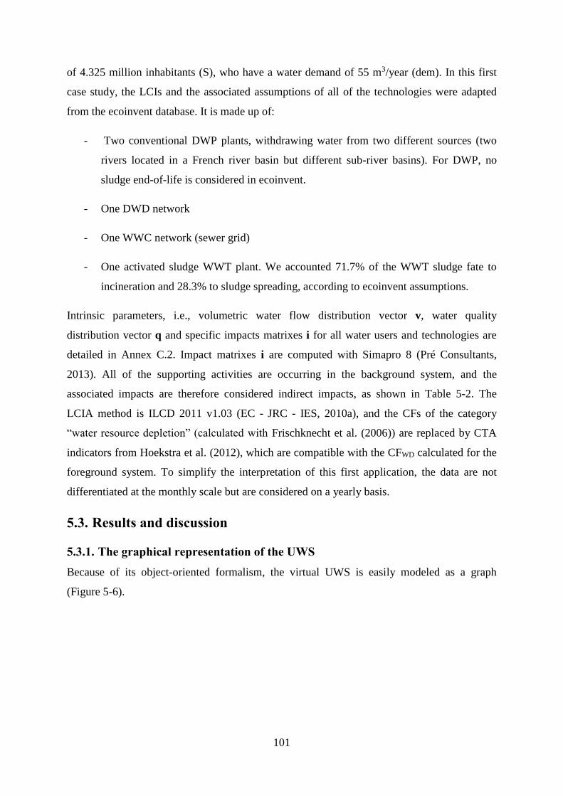
101

of 4.325 million inhabitants (S), who have a water demand of 55 m3/year (dem). In this first

case study, the LCIs and the associated assumptions of all of the technologies were adapted

from the ecoinvent database. It is made up of:

- Two conventional DWP plants, withdrawing water from two different sources (two

rivers located in a French river basin but different sub-river basins). For DWP, no

sludge end-of-life is considered in ecoinvent.

- One DWD network

- One WWC network (sewer grid)

- One activated sludge WWT plant. We accounted 71.7% of the WWT sludge fate to

incineration and 28.3% to sludge spreading, according to ecoinvent assumptions.

Intrinsic parameters, i.e., volumetric water flow distribution vector v, water quality

distribution vector q and specific impacts matrixes i for all water users and technologies are

detailed in Annex C.2. Impact matrixes i are computed with Simapro 8 (Pré Consultants,

2013). All of the supporting activities are occurring in the background system, and the

associated impacts are therefore considered indirect impacts, as shown in Table 5-2. The

LCIA method is ILCD 2011 v1.03 (EC - JRC - IES, 2010a), and the CFs of the category

“water resource depletion” (calculated with Frischknecht et al. (2006)) are replaced by CTA

indicators from Hoekstra et al. (2012), which are compatible with the CFWD calculated for the

foreground system. To simplify the interpretation of this first application, the data are not

differentiated at the monthly scale but are considered on a yearly basis.


5.3.1. The graphical representation of the UWS

Because of its object-oriented formalism, the virtual UWS is easily modeled as a graph

(Figure 5-6).

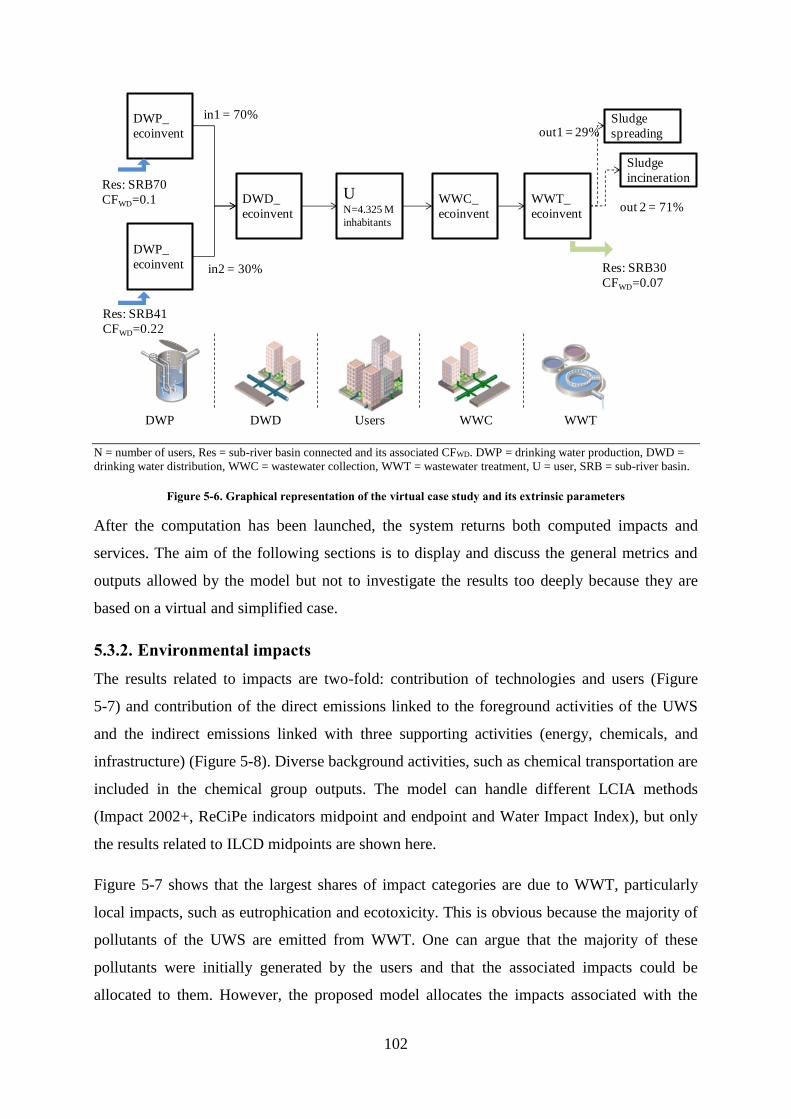
102

N = number of users, Res = sub-river basin connected and its associated CFWD. DWP = drinking water production, DWD =

drinking water distribution, WWC = wastewater collection, WWT = wastewater treatment, U = user, SRB = sub-river basin.

Figure 5-6. Graphical representation of the virtual case study and its extrinsic parameters

After the computation has been launched, the system returns both computed impacts and

services. The aim of the following sections is to display and discuss the general metrics and

outputs allowed by the model but not to investigate the results too deeply because they are

based on a virtual and simplified case.

5.3.2. Environmental impacts

The results related to impacts are two-fold: contribution of technologies and users (Figure

5-7) and contribution of the direct emissions linked to the foreground activities of the UWS

and the indirect emissions linked with three supporting activities (energy, chemicals, and

infrastructure) (Figure 5-8). Diverse background activities, such as chemical transportation are

included in the chemical group outputs. The model can handle different LCIA methods

(Impact 2002+, ReCiPe indicators midpoint and endpoint and Water Impact Index), but only

the results related to ILCD midpoints are shown here.

Figure 5-7 shows that the largest shares of impact categories are due to WWT, particularly

local impacts, such as eutrophication and ecotoxicity. This is obvious because the majority of

pollutants of the UWS are emitted from WWT. One can argue that the majority of these

pollutants were initially generated by the users and that the associated impacts could be

allocated to them. However, the proposed model allocates the impacts associated with the

DWP_

ecoinvent

DWP_

ecoinvent

DWD_

ecoinvent

UN=4.325 M

inhabitants

WWC_

ecoinvent

WWT_

ecoinvent

in1 = 70%

in2 = 30%

Sludge

spreading

Sludge

incineration

out 2 = 71%

DWP DWD Users WWC WWT

out1 = 29%

Res: SRB30

CFWD=0.07

Res: SRB70

CFWD=0.1

Res: SRB41

CFWD=0.22

103

released flows in each component, and because WWT is the end-of-pipe technology, it is the

main contributor. It would be desirable to allocate the impacts associated with released water

to the entire UWS. The current mode of representation does not preclude an analysis of

pollution sources. Even if most of the pollution comes from the users, other unexpected

sources can occur within the system. For example, sulfates emitted at the DWP plants as a

result of the use of sulfate-based coagulants (aluminum or ferric) increase the generation of

H2S within the WWC, which is a pollutant and is corrosive to the network (Pikaar et al.,

2014).

DWP and DWD also generate a non-negligible share of impacts, primarily in the global

impact categories, which are due to background activities. WWC contributes to less than 10%

of the impact categories studied because only the impacts of infrastructure are considered for

this technology. User contribution is negligible because no technology present at the user

place (e.g., water heating systems) was considered in this first theoretical application. Water

quantity and quality releases in the environment at the users’ places are the only impacts

considered. Three impact categories have negative contributions for certain technologies,

which means that benefits for the environment occur. First, DWP lowers the impact on

freshwater eutrophication and ecotoxicity because it uptakes water and pollutants from the

environment and leads to a negative value for impacts, as stated in eq (20). Second, WWT

releases water into the local environment and makes it available for the downstream users,

thus leading to a negative value for water deprivation. For the water deprivation category, the

withdrawn and released water volumes are weighted by CFWD, which is different for the two

theoretical water resources, and the release point (lower downstream deprivation). The model

also offers a contribution analysis of each technology component, i.e., when there are several

plants or networks or when differentiating the sludge end-of-life impacts within WWT or

DWP.

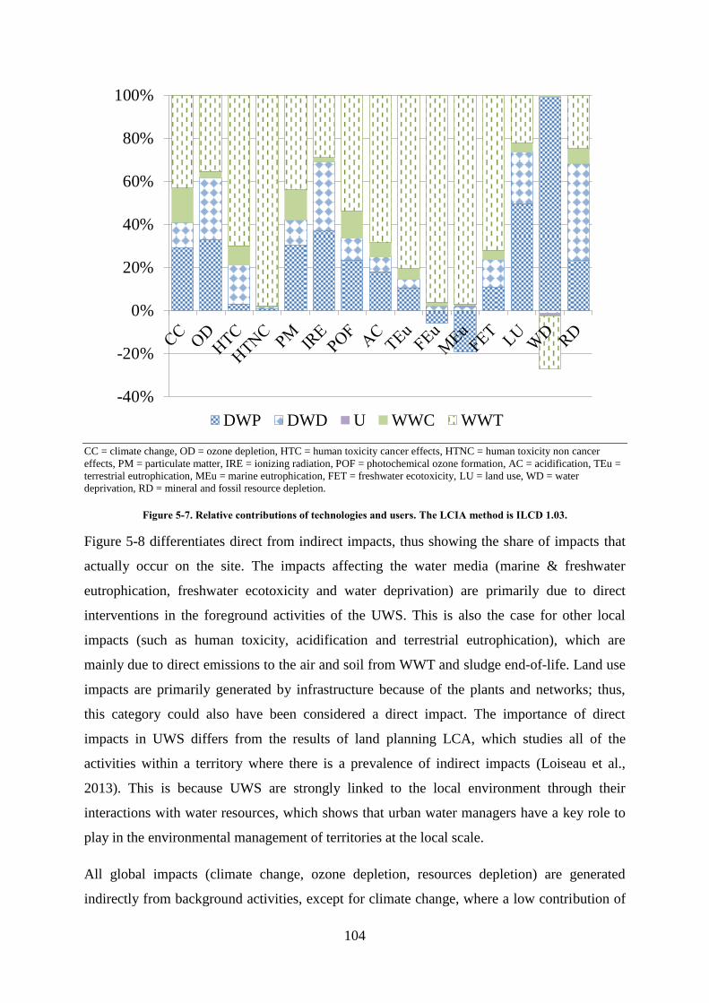
104

CC = climate change, OD = ozone depletion, HTC = human toxicity cancer effects, HTNC = human toxicity non cancer

effects, PM = particulate matter, IRE = ionizing radiation, POF = photochemical ozone formation, AC = acidification, TEu =

terrestrial eutrophication, MEu = marine eutrophication, FET = freshwater ecotoxicity, LU = land use, WD = water

deprivation, RD = mineral and fossil resource depletion.

Figure 5-7. Relative contributions of technologies and users. The LCIA method is ILCD 1.03.

Figure 5-8 differentiates direct from indirect impacts, thus showing the share of impacts that

actually occur on the site. The impacts affecting the water media (marine & freshwater

eutrophication, freshwater ecotoxicity and water deprivation) are primarily due to direct

interventions in the foreground activities of the UWS. This is also the case for other local

impacts (such as human toxicity, acidification and terrestrial eutrophication), which are

mainly due to direct emissions to the air and soil from WWT and sludge end-of-life. Land use

impacts are primarily generated by infrastructure because of the plants and networks; thus,

this category could also have been considered a direct impact. The importance of direct

impacts in UWS differs from the results of land planning LCA, which studies all of the

activities within a territory where there is a prevalence of indirect impacts (Loiseau et al.,

2013). This is because UWS are strongly linked to the local environment through their

interactions with water resources, which shows that urban water managers have a key role to

play in the environmental management of territories at the local scale.

All global impacts (climate change, ozone depletion, resources depletion) are generated

indirectly from background activities, except for climate change, where a low contribution of

-40%

-20%

0%

20%

40%

60%

80%

100%

DWP DWD U WWC WWT

105

direct emissions to the air occurs in WWT. Electricity contributes the largest share of ionizing

radiation impacts because we considered the French electricity mix. The majority of other

indirect impacts are dominated by infrastructure.


effects, PM = particulate matter, IRE = ionizing radiation, POF = photochemical ozone formation, AC = acidification, TEu =


deprivation, RD = mineral and fossil resource depletion.

Figure 5-8. Relative contributions of direct and indirect contributors. The LCIA method is ILCD 1.03.

5.3.3. Provided services and impact/service ratio

In addition to showing the total impacts of the UWS, the model generates an impact/service

ratio, which are useful for comparing different scenarios. On the one hand, the values for

impacts per user (e.g., capita) allow us to account for user behavior and provide a more

complete image of the UWS environmental and social performance. In this case study, only

the domestic user has been considered. If we focus on climate change using the above-

mentioned scenario, the impact/service ratio results in a value of 30.1 kg CO2 eq/domestic

user/year. On the other hand, the computation of the impacts per m3 at the user’s place

pictures the environmental performance regarding the technologies: a value of 0.51 kg CO2

0%

20%

40%

60%

80%

100%

Em. to water Em. to soil & air Electricity Chemical & others Infrastructure

Direct impacts Indirect impacts

106

eq/m3 is found. This is compliant with the values found in the literature and summarized in

Chapter 3 (Loubet et al. 2014), which range from 0.51 to 1.57 kg CO2 eq./m3 at the user’s

place.

5.3.4. Opportunities and limits

This case study is a virtual one and is dedicated to determining whether the WaLA model runs

correctly. The data used in this case study are not refined and should be reviewed and

improved for future case studies to try to better fit the local characteristics of the UWS.

Regarding water users, this virtual case study has been simplified by only considering

domestic users. As stated by Loiseau et al. (2013), the provided services could be calculated

according to complex land occupation combining several activities and would thus be a result

of the system. This type of model improvement is possible in a future evolution using

geographical information system (GIS), for example.

Concerning volumetric water flow distribution vectors, the ecoinvent database has included

equilibrated water balances of the various plants since version 3. However, they are neither

well documented nor site-specific. Various models in the literature only provide water

balances for the whole UWS and not for each component (S. Kenway et al., 2011; Vanham,

2012). Risch et al. (2014)presented water-balanced processes for WWT, but research on water

flow inventory remains necessary for other processes. Concerning the water quality

distribution vector, it should be noted that the model does not compute a dynamic mass

balance of pollutants. The mass balance is defined a priori for each component. Therefore,

each component that modifies the water quality (DWP, WWT, U) is to be connected only to a

water flow with one specific water quality. As a next step, two options can be explored: either

enabling each component to treat different water qualities or computing the mass balance for

each component within the model. However, the last option is not straightforward because no

current model is able to predict mass balances dynamically and in a consistent way for WWT

plants. It could be implemented for DWP technologies (Mery et al., 2013), but it would be

time consuming. Additionally, further work on the classification of urban water quality should

consider the water quality categories defined by Boulay et al. (2011). Currently, eight types of

surface water quality, depending on the usage, can be provided. Therefore, these types should

be implemented as water resource qualities and should be only connected to the specific usage

they can fulfill.

107

Regarding specific indirect impacts related to technologies, the results of recent and diverse

LCAs should be added to the model’s library to free it from ecoinvent generic data. Indeed,

the ecoinvent database only includes one technology for DWP (conventional treatment) and

one technology for WWT (activated sludge). Other technologies, such as membrane processes

(for both DWP and WWT), and wetland systems (e.g., lagoons, polishing pounds, reed bed

filter) for WWT should be implemented, based on literature results or local data. However,

this is beyond the scope of this chapter. Finally, monthly scale modeling was not used here

(i.e., the data were considered constant throughout the year), whereas water cycle conditions

may exhibit significant variations during the year. Efforts should be made to gather monthly

data and provide monthly characterization factors, particularly for water deprivation.

An inherent problem of stand-alone LCA tools using the impact results calculated from LCA

software (Simapro 8) is updating the LCIA results because the LCIA methods and ecoinvent

database are modified in different versions. This could be solved by using a database

management service within the modeling tool.

Despite these points for improvement, the level of usability and interactivity for a non-

specialist is very good for generating scenarios. A great advantage is that despite this first

prototype model, which uses proprietary software (Matlab/Simulink), it can be implemented

using any other languages or software due to OOP.

5.4. Conclusions

Our objective was to develop a framework to tackle the methodological challenges raising

from LCA applied to UWS. A versatile model, WaLA, has been built to consistently and

easily determine water flows, related environmental impacts and services within any UWS.

The implementation of the model through an object approach and a Matlab/Simulink interface

provides a usable and operational tool. Thanks to the proposed framework and OOP

implementation, various UWS scenarios can be easily designed and tested by water

authorities, industries, or academic institutions that intend to design their own tool for UWS

environmental assessment. However, it still can be refined through better management of

water quality, the implementation of uncertainty analysis based on error propagation, or

Monte-Carlo simulations.

A first virtual case study based on ecoinvent processes has been tested and demonstrated the

capacity of the modular approach to easily build the UWS. The results of the contribution

108

analysis based on technologies have shown the predominance of impacts due to WWT. It also

reveals the importance of direct impacts on local issues (e.g., eutrophication) and the high

contribution of supporting activities (energy, chemicals, infrastructures) on global impacts.

The impact/service ratios based on the provided services of the UWS (either users or m3

delivered to the user) are useful results that can be compared with other systems or scenarios.

The appropriation of such tools by stakeholders was not the objective of this work but will be

a great challenge when performing environmental evaluations in a decision-making context.

The evaluation of forecasting scenarios is the object of Chapter 6, which focuses on the urban

water system of the Paris suburban area (France).

109

Chapter 6. WaLA, a versatile model for the

life cycle assessment of urban water

systems: Part 2 – Learning points from the

assessment of water management scenarios

in Paris suburban area

« Paname

Quand tu t'ennuies tu fais les quais

Tu fais la Seine et les noyés

Ça fait prend' l'air et ça distrait »

Léo Ferré - Paname

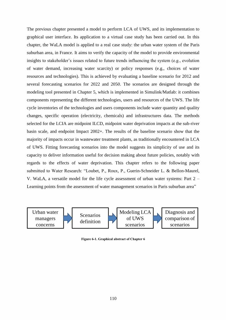
110

The previous chapter presented a model to perform LCA of UWS, and its implementation to

graphical user interface. Its application to a virtual case study has been carried out. In this

chapter, the WaLA model is applied to a real case study: the urban water system of the Paris

suburban area, in France. It aims to verify the capacity of the model to provide environmental

insights to stakeholder’s issues related to future trends influencing the system (e.g., evolution

of water demand, increasing water scarcity) or policy responses (e.g., choices of water

resources and technologies). This is achieved by evaluating a baseline scenario for 2012 and

several forecasting scenarios for 2022 and 2050. The scenarios are designed through the

modeling tool presented in Chapter 5, which is implemented in Simulink/Matlab: it combines

components representing the different technologies, users and resources of the UWS. The life

cycle inventories of the technologies and users components include water quantity and quality

changes, specific operation (electricity, chemicals) and infrastructures data. The methods

selected for the LCIA are midpoint ILCD, midpoint water deprivation impacts at the sub-river

basin scale, and endpoint Impact 2002+. The results of the baseline scenario show that the

majority of impacts occur in wastewater treatment plants, as traditionally encountered in LCA

of UWS. Fitting forecasting scenarios into the model suggests its simplicity of use and its

capacity to deliver information useful for decision making about future policies, notably with

regards to the effects of water deprivation. This chapter refers to the following paper

submitted to Water Research: “Loubet, P., Roux, P., Guerin-Schneider L. & Bellon-Maurel,

V. WaLA, a versatile model for the life cycle assessment of urban water systems: Part 2 –

Learning points from the assessment of water management scenarios in Paris suburban area”


Scenarios

definition

Urban water

managers

concerns

Modeling LCA

of UWS

scenarios

Diagnosis and

comparison of

scenarios

111


6.1. Introduction ................................................................................................................. 112

6.2. Material and methods .................................................................................................. 114

6.2.1. The greater metropolitan Paris UWS ................................................................... 114

6.2.2. Scenarios investigated and the associated LCA goals and scopes ....................... 116

6.2.2.1. Goal and scope ............................................................................................................................................116

6.2.2.2. Description of the baseline scenario ...........................................................................................................118

6.2.2.3. Description of forecasting scenarios ...........................................................................................................120

6.2.3. Customization of the model components: establishing the attribute values ......... 122

6.2.3.1. Volumetric water flow distribution .............................................................................................................122

6.2.3.2. Quality water flow distribution ...................................................................................................................122

6.2.3.3. Direct emissions to air and soil ...................................................................................................................123

6.2.4. Inventory linked to operating of the UWS components (energy, chemicals) ...... 124

6.2.4.1. Inventory linked to the infrastructure of UWS ............................................................................................125

6.2.5. Life cycle impact assessment ............................................................................... 125

6.2.5.1. Water deprivation impact ............................................................................................................................125

6.2.5.2. Other impacts ..............................................................................................................................................127

6.2.6. Example of the construction of a scenario using the model ................................. 127


6.3.1. Baseline scenario .................................................................................................. 130

6.3.1.1. Water flows .................................................................................................................................................130

6.3.1.2. Environmental impacts ...............................................................................................................................131

6.3.1.3. Provided services and impact/service ratios................................................................................................133

6.3.2. Forecasting scenarios............................................................................................ 133

6.3.2.1. Short term forecasting scenarios .................................................................................................................135

6.3.2.2. Scenarios with changes in water users ........................................................................................................135

6.3.2.3. Scenarios with changes in water resources .................................................................................................135

6.3.2.4. Scenarios with change in water technologies ..............................................................................................137

6.3.3. Sensitivity analysis on impact/service ratio choices ............................................ 137


6.4. Conclusions and outlook ............................................................................................. 140

112

6.1. Introduction

Stakeholders face many challenges related to the management of urban water system (UWS):

demographic, water demand and water resource changes (e.g., effects of climate change)

(McDonald et al., 2011). The decision making process covering future evolutions should

include the environmental evaluation of forecasting scenarios based on the planned

modifications of the UWS. Unfortunately, holistic approaches such as life cycle assessment

(LCA) are time-intensive and require a high degree of expertise. Chapter 5 proposed a

formalism and developed a model, namely WaLA, for applying a LCA to UWS (as a modular

approach), to reduce the complexity of UWS environmental evaluation. After showing the

feasibility of this method on a virtual case study, this model is applied to a real case study to

compare various evolutionary scenarios.

Various types of scenarios have been formalized, differentiating future-trend based scenarios

and policy-responsive scenarios (Mahmoud et al., 2009). The first scenarios are based on

extrapolations that can be either projective, i.e., using trends experienced over a past period,

or prospective, i.e., anticipating upcoming changes that differ from the past. UWS typically

include endured changes, indicating that stakeholders of water service institutions do not

control the parameters associated with water management, such as urban development or

climate change effects on water resources. Conversely, policy-responsive scenarios anticipate

events or actions, but with high subjectivity. These scenarios are either based on expert

judgment or driven by stakeholders.

A large set of management questions are classified in Table 6-1 according to the type of

associated scenario, the questions asked by the stakeholders, the nature of the stakeholder

involved and their scale of action. These questions have been identified from a review of

UWS LCAs (Loubet et al., 2014), and from water service experts. The model developed in

Chapter 5 aims to provide the environmental assessment of these management questions.

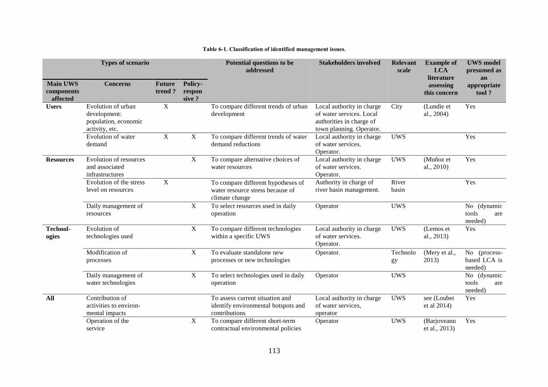
113

Table 6-1. Classification of identified management issues.

Types of scenario Potential questions to be

addressed

Stakeholders involved Relevant

scale

Example of

LCA

literature

assessing

this concern

UWS model

presumed as

an

appropriate

tool ?

Main UWS

components

affected

Concerns Future

trend ?

Policy-

respon

sive ?

Users Evolution of urban

development:

population, economic

activity, etc.

X To compare different trends of urban

development

Local authority in charge

of water services. Local

authorities in charge of

town planning. Operator.

City (Lundie et

al., 2004)

Yes

Evolution of water

demand

X X To compare different trends of water

demand reductions


of water services.

Operator.

UWS Yes

Resources Evolution of resources

and associated

infrastructures

X To compare alternative choices of

water resources


of water services.

Operator.

UWS (Muñoz et

al., 2010)

Yes

Evolution of the stress

level on resources

X To compare different hypotheses of

water resource stress because of

climate change

Authority in charge of

river basin management.

River

basin

Yes

Daily management of

resources

X To select resources used in daily

operation

Operator UWS No (dynamic

tools are

needed)

Technol-

ogies

Evolution of

technologies used

X To compare different technologies

within a specific UWS


of water services.

Operator.

UWS (Lemos et

al., 2013)

Yes

Modification of

processes

X To evaluate standalone new

processes or new technologies

Operator. Technolo

gy

(Mery et al.,

2013)

No (process-

based LCA is

needed)

Daily management of

water technologies

X To select technologies used in daily

operation

Operator UWS No (dynamic

tools are

needed)

All Contribution of

activities to environ-

mental impacts

To assess current situation and

identify environmental hotspots and

contributions


of water services,

operator

UWS see (Loubet

et al 2014)

Yes

Operation of the

service

X To compare different short-term

contractual environmental policies

Operator UWS (Barjoveanu

et al., 2013)

Yes

114

The objective of this chapter is to implement the UWS model using a real case study located

in suburbs of Paris and to verify the capacity of the model to address identified stakeholders’

questions. These objectives achieved by evaluating forecasting scenarios associated with

specific concerns covering modifications of users, resources or technologies within the

system. After a description of the various scenarios and associated questions they intend to

address, the UWS model developed in Chapter 5 is applied. The results for the baseline

scenario are the water flows (characterized by their quantities and qualities) the environmental

impacts and impact/service ratios. The results provide a comparison of the forecasting

scenarios in regards to their environmental impacts. Based on this comparison, conclusions

and perspectives on the environmental evaluation of UWS using the proposed model are

provided.


6.2.1. The greater metropolitan Paris UWS

In France, UWS fall under the responsibility of public local authorities at the municipal level.

However, this responsibility can be transferred to intermunicipal organizations to take

advantage of economies of scale. Such transfers can be full or partial. For instance, drinking

water production (DWP) is transferred to the intermunicipal level, whereas wastewater

collection (WWC) remains under the responsibility of each municipality. The operation and

investment of these water services either remain under direct public management or are

delegated to a third party, typically a private operator (Guerin-Schneider et al., 2002). In this

context, a water service can be defined as a set of infrastructures and related services that are

under the responsibility of one given local authority and under the operation of one given

operator. In 2010 more than 14,000 water service and more than 17,200 collective sewerage

services operated in France (EauFrance, 2012). Thus water management in the greater

metropolitan Paris area is complex as it is composed of many water services. Numerous DWP

and drinking water distribution (DWD) services are in operation. The two main services are

Eau de Paris (direct management) that covers the city of Paris and Syndicat des Eaux d’Île-de-

France (SEDIF, delegated management) that covers more than half of the suburban area. More

than ten other DWP and DWD services cover the other cities within the suburban area. WWC

is managed at three scales: city collection managed by municipal authorities, departmental

transport managed by intermunicipal syndicates and interdepartmental transport managed by

the Syndicat Interdépartemental pour l’Assainissement de l’Agglomération Parisienne

(SIAAP). Wastewater treatment (WWT) is also managed by the SIAAP. Other small services

115

manage WWT in further sub-urban areas that are not considered in this Chapter. Table 6-2

summarizes the different water services in the Parisian area according to the geographical area

they cover and the systems they manage.

Table 6-2. The complexity of water management in the greater Paris metropolitan area: responsibility shares for the

different components. Area of the case study is underlined in red.

Components Greater metropolitan Paris area

Paris suburban area 1 Paris suburban area 2 City of Paris

DWP SEDIF Several

intermunicipal

syndicates

Eau de Paris

DWD

WWC Collection

(City scale)

Several municipalities

WWC Transport

(Department scale)

Several intermunicipal syndicates

WWC Transport

(Interdepartmental scale)

SIAAP

WWT

Paris

Suburban area 1

Suburban area 2

116

Our case study focuses on the urban water system of the SEDIF geographical perimeter,

named “Paris suburban area 1” and highlighted in red in Table 6-2 and in Figure 6-2. This

focus results from the fact that the main stakeholders involved in the decision making process

is the SEDIF and its delegatee, Veolia Eau d’Île-de-France. A map of the case study is

provided in Figure 6-2.

The WWT and DWP plants are : CR = Choisy-le-Roi, MO = Mery-sur-Oise, NM = Neuilly-sur-Marne, MA = Marne Aval,

SAm = Seine amont, SAv = Seine aval, SC = Seine centre, SG = Seine Grésillons, SM = Seine Morée.

Figure 6-2. General and detailed situation of the case study.

6.2.2. Scenarios investigated and the associated LCA goals and scopes

6.2.2.1. Goal and scope

In a multifunctional system, the goals are complex and can have different dimensions. In this

study, a set of stakeholder’s questions are selected from Table 6-1 to establish and investigate

different scenarios and test the capacity of the model. Table 6-3 presents the different

scenarios that are to be assessed and the related questions.

Seine river basin

France

117

Table 6-3. List of evaluated forecasting scenarios and their key parameters.

Ref Stakeholder question

addressed

Modified parameters related to users Modified parameters related to resources Modified parameters related to technologies

Policy-

responsive

Future-trend Policy-responsive Future-trend Policy-responsive Future-

trend

S1 To compare different

short-term

environmental policies

of the DWP operator

- ↑ Population (+3.3%)

↓ Specific water demand

(-5%)

- - ↑ Water losses in DWD (15%) -

S2 ↓ Water demand

(-0.8%)

↑ Population (+3.3%)


(-5%)

- - ↓ Electricity use DWP&D (-

6%)

↓ Chemicals used DWP (-3%)

-

S3 ↓ Water demand

(-2.7%)

↑ Population (+3.3%)


(-5%)

↑ withdrawals in upstream

plants

- ↓ Water losses in DWD (5%)

↓ Electricity use DWP&D (-

10%)

↓ Chemicals used DWP (-6%)

-

L1 To compare different

trends of urban

development and

water demand

- ↑ Population (+9.3 %)


(-21 %)

- Climate

change effects

- -

L2 - ↑ Population (+9.3 %)

→ Specific water dem

- Identical to L1 - -

L3 - ↑↑ Population (+21%)

→ Specific water dem

- Identical to L1 - -

L4 To compare trends in

climate change effects

- Identical to L1 - No climate

change effects

- -

L5 To compare alternative

choices of water

resources

- Identical to L1 Water transfer (42%) from

downstream river

Identical to L1 Membrane DWP technology to

treat downstream river water

(low quality of water)

-

L6 - Identical to L1 Water transfer (15 %) from

upstream source

Identical to L1 Simple DWP technology to

treat upstream source water

(high quality of water)

-

L7 To compare different

technologies within a

specific UWS

- Identical to L1 - Identical to L1 All DWP are membrane

processes

-

L8 - Identical to L1 - Identical to L1 All DWP are conventional

processes with electricity and

chemical consumption of S3

-

118

As explained in Chapter 5, we follow the “territorial LCA” approach (Loiseau et al., 2013):

for each scenario, a “reference flow” is studied, which is the association of the studied UWS

within its geographical borders and the implemented scenario. A set of functions is then

selected to describe and quantify the multifunctional services provided by the UWS, i.e.,

supplying different categories of users with water. The indicators associated to these functions

are used in the “territorial LCA” to calculate impact/service ratio (inverse of eco-efficiency

ratio from Seppäläa and Melanen (2005)) as the ratio between the given impacts and the

function indicators (e.g., kg CO2/hab). Six different types of users and associated indicators

that relate the provided service are identified within the urban territory. Domestic users are

described by the number of inhabitants in the area. For other users, the five categories of

activities, based on INSEE NAF5 classification (INSEE, 2013) are used. Three of these five

categories are found in the system: i.e., non-market services (public administration, education,

health and social work), market services (commerce, transports, construction and diverse), and

industries. These categories were characterized by the number of associated jobs. Because

agriculture activity is low in the system (less than 350 jobs), this category has been included

in the “other users” category. The “other users” category also includes urban watering, street

washing, and firefighting. This category is expressed in total surface of the system (hectares).

A last category is defined to encompass all users (i.e., “equivalent inhabitant”), and the

associated indicator is the number of inhabitants. Because the selection of the function is

dependent on the stakeholder’s goal and scope, an alternative and complementary function is

defined: one cubic meter delivered to the users.

Boundaries include all components of the UWS, i.e., DWP, DWD, U, stormwater collection

(SWC), WWC, WWT. The DWP and WWT components include sludge end-of-life. The

operation and infrastructure are considered, but not the associated civil works. The boundaries

of the baseline and forecasting scenarios are further explained hereafter.

6.2.2.2. Description of the baseline scenario

In 2012, the perimeter of SEDIF represented 142 towns in the suburbs of Paris. This region

comprises a total of 4.3 million inhabitants and an area of 76,198 ha. The specific water

demand for each type of user is determined by combining demographic and employment data

from French national statistics at the municipal scale (INSEE, 2013) with the customer

database from the SEDIF delegatee (namely Veolia Eau d’Île-de-France, confidential source).

From the database, the volume of water sold to the different categories of users is known for

2012. The resulting data reported 4,362,705 domestic users (and equivalent inhabitants),

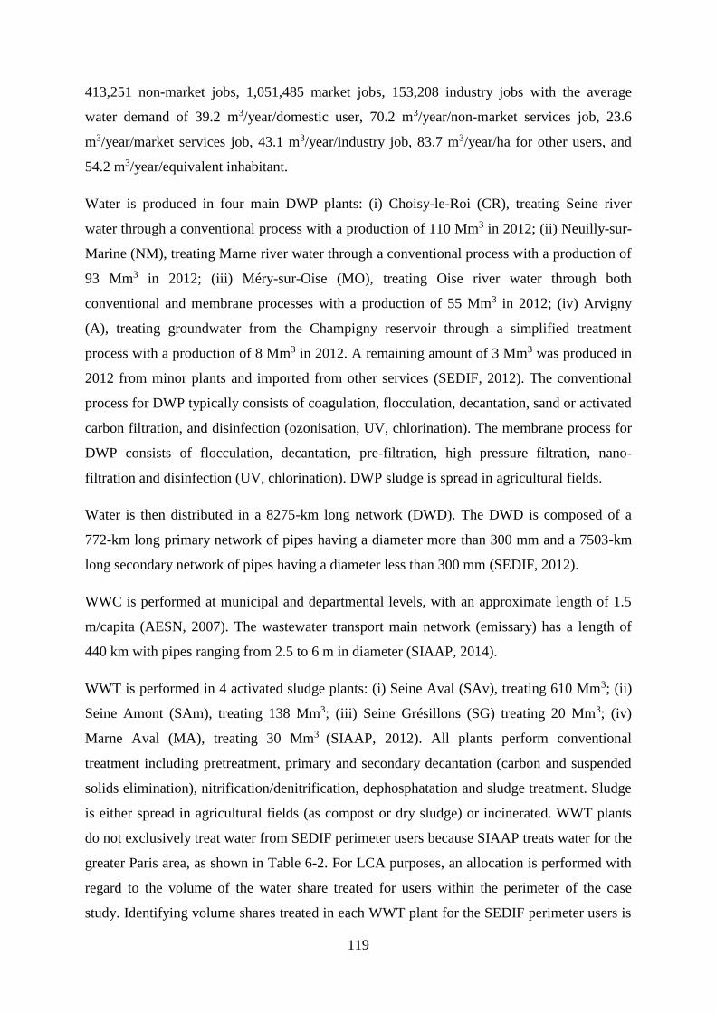
119

413,251 non-market jobs, 1,051,485 market jobs, 153,208 industry jobs with the average

water demand of 39.2 m3/year/domestic user, 70.2 m3/year/non-market services job, 23.6

m3/year/market services job, 43.1 m3/year/industry job, 83.7 m3/year/ha for other users, and

54.2 m3/year/equivalent inhabitant.

Water is produced in four main DWP plants: (i) Choisy-le-Roi (CR), treating Seine river

water through a conventional process with a production of 110 Mm3 in 2012; (ii) Neuilly-sur-

Marine (NM), treating Marne river water through a conventional process with a production of

93 Mm3 in 2012; (iii) Méry-sur-Oise (MO), treating Oise river water through both

conventional and membrane processes with a production of 55 Mm3 in 2012; (iv) Arvigny

(A), treating groundwater from the Champigny reservoir through a simplified treatment

process with a production of 8 Mm3 in 2012. A remaining amount of 3 Mm3 was produced in

2012 from minor plants and imported from other services (SEDIF, 2012). The conventional

process for DWP typically consists of coagulation, flocculation, decantation, sand or activated

carbon filtration, and disinfection (ozonisation, UV, chlorination). The membrane process for

DWP consists of flocculation, decantation, pre-filtration, high pressure filtration, nano-

filtration and disinfection (UV, chlorination). DWP sludge is spread in agricultural fields.

Water is then distributed in a 8275-km long network (DWD). The DWD is composed of a

772-km long primary network of pipes having a diameter more than 300 mm and a 7503-km

long secondary network of pipes having a diameter less than 300 mm (SEDIF, 2012).

WWC is performed at municipal and departmental levels, with an approximate length of 1.5

m/capita (AESN, 2007). The wastewater transport main network (emissary) has a length of

440 km with pipes ranging from 2.5 to 6 m in diameter (SIAAP, 2014).

WWT is performed in 4 activated sludge plants: (i) Seine Aval (SAv), treating 610 Mm3; (ii)

Seine Amont (SAm), treating 138 Mm3; (iii) Seine Grésillons (SG) treating 20 Mm3; (iv)

Marne Aval (MA), treating 30 Mm3 (SIAAP, 2012). All plants perform conventional

treatment including pretreatment, primary and secondary decantation (carbon and suspended

solids elimination), nitrification/denitrification, dephosphatation and sludge treatment. Sludge

is either spread in agricultural fields (as compost or dry sludge) or incinerated. WWT plants

do not exclusively treat water from SEDIF perimeter users because SIAAP treats water for the

greater Paris area, as shown in Table 6-2. For LCA purposes, an allocation is performed with

regard to the volume of the water share treated for users within the perimeter of the case

study. Identifying volume shares treated in each WWT plant for the SEDIF perimeter users is

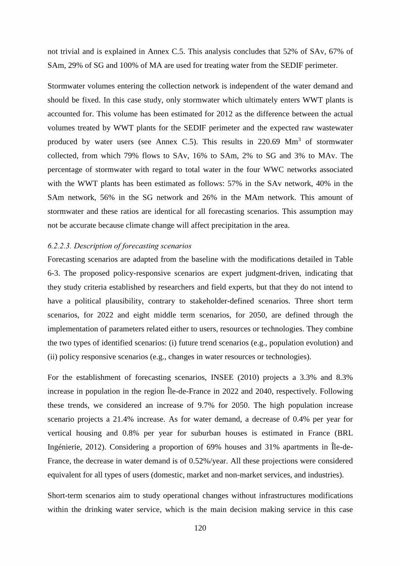
120

not trivial and is explained in Annex C.5. This analysis concludes that 52% of SAv, 67% of

SAm, 29% of SG and 100% of MA are used for treating water from the SEDIF perimeter.

Stormwater volumes entering the collection network is independent of the water demand and

should be fixed. In this case study, only stormwater which ultimately enters WWT plants is

accounted for. This volume has been estimated for 2012 as the difference between the actual

volumes treated by WWT plants for the SEDIF perimeter and the expected raw wastewater

produced by water users (see Annex C.5). This results in 220.69 Mm3 of stormwater

collected, from which 79% flows to SAv, 16% to SAm, 2% to SG and 3% to MAv. The

percentage of stormwater with regard to total water in the four WWC networks associated

with the WWT plants has been estimated as follows: 57% in the SAv network, 40% in the

SAm network, 56% in the SG network and 26% in the MAm network. This amount of

stormwater and these ratios are identical for all forecasting scenarios. This assumption may

not be accurate because climate change will affect precipitation in the area.

6.2.2.3. Description of forecasting scenarios

Forecasting scenarios are adapted from the baseline with the modifications detailed in Table

6-3. The proposed policy-responsive scenarios are expert judgment-driven, indicating that

they study criteria established by researchers and field experts, but that they do not intend to

have a political plausibility, contrary to stakeholder-defined scenarios. Three short term

scenarios, for 2022 and eight middle term scenarios, for 2050, are defined through the

implementation of parameters related either to users, resources or technologies. They combine

the two types of identified scenarios: (i) future trend scenarios (e.g., population evolution) and

(ii) policy responsive scenarios (e.g., changes in water resources or technologies).

For the establishment of forecasting scenarios, INSEE (2010) projects a 3.3% and 8.3%

increase in population in the region Île-de-France in 2022 and 2040, respectively. Following

these trends, we considered an increase of 9.7% for 2050. The high population increase

scenario projects a 21.4% increase. As for water demand, a decrease of 0.4% per year for

vertical housing and 0.8% per year for suburban houses is estimated in France (BRL

Ingénierie, 2012). Considering a proportion of 69% houses and 31% apartments in Île-de-

France, the decrease in water demand is of 0.52%/year. All these projections were considered

equivalent for all types of users (domestic, market and non-market services, and industries).

Short-term scenarios aim to study operational changes without infrastructures modifications

within the drinking water service, which is the main decision making service in this case

121

study. These scenarios follow future trends in the evolution of population. The evolving trend

of specific water demand is modulated by different policies towards the behavior of users

from water service bodies. The present technologies are used with minor improvements to the

processes, i.e., decreased energy and chemicals used. Scenario S1 is a business-as-usual

scenario, following forecasting trends in water demand and low maintenance efforts of the

DWD network and occasioning an increase of water losses. Scenario S2 is a scenario

following contractual actions from the delegatee. The specific water demand per inhabitant is

reduced by 0.6%/year (instead of the expected trend of 0.52%) because of a communication

program geared towards the users and the resulting increase in awareness. Water losses in

DWD decrease, leading to a network performance of up to 90%. Electricity consumption of

the DWP plants and DWD networks and the chemical consumption in the plants are reduce by

6% and 3%, respectively, because of the optimization of the processes and pumps. Scenario

S3 is an eco-designed scenario aiming to achieve a lower water footprint, i.e., reducing water

deprivation impacts. The specific water demand is reduced by 0.8%/year (instead of the

expected trend of 0.52%) because of the installation of domestic eco-designed equipment

(e.g., tap aerator). The reduction of water losses in DWD allows a performance of the network

of 95%. A higher reduction of the electricity and chemical consumed by the plants and

networks are considered. Additionally, water is withdrawn preferably from downstream

locations to reduce water deprivation impacts.

Long term scenarios aim at modeling large and structural changes for 2050. Scenario L1 is

similar to the baseline scenario with the modification of future-trend parameters (increase of

population, decrease of water demand, effects of climate change on water scarcity). Scenario

L2 and L3 study different hypothesis in the trends regarding two different projections of

population (medium and high) and the evolution of the water demand per capita. Scenario L4

is similar to L1 without considering the effect of climate change on water resources. Scenario

L5 and L6 study changes in resource withdrawal choices, either transferring low quality water

from downstream Seine (L5) or transferring clean water from upstream sources (L6).

Scenarios L7 and L8 study changes in DWP technologies, either selecting advanced treatment

processes such as membrane processes or selecting low impact technologies.

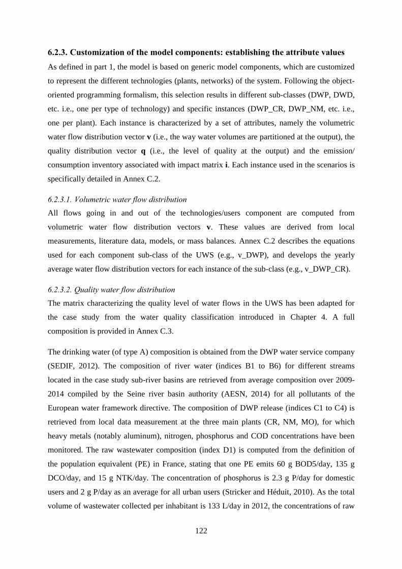
122

6.2.3. Customization of the model components: establishing the attribute values

As defined in part 1, the model is based on generic model components, which are customized

to represent the different technologies (plants, networks) of the system. Following the object-

oriented programming formalism, this selection results in different sub-classes (DWP, DWD,

etc. i.e., one per type of technology) and specific instances (DWP_CR, DWP_NM, etc. i.e.,

one per plant). Each instance is characterized by a set of attributes, namely the volumetric

water flow distribution vector v (i.e., the way water volumes are partitioned at the output), the

quality distribution vector q (i.e., the level of quality at the output) and the emission/

consumption inventory associated with impact matrix i. Each instance used in the scenarios is

specifically detailed in Annex C.2.

6.2.3.1. Volumetric water flow distribution

All flows going in and out of the technologies/users component are computed from

volumetric water flow distribution vectors v. These values are derived from local

measurements, literature data, models, or mass balances. Annex C.2 describes the equations

used for each component sub-class of the UWS (e.g., v_DWP), and develops the yearly

average water flow distribution vectors for each instance of the sub-class (e.g., v_DWP_CR).

6.2.3.2. Quality water flow distribution

The matrix characterizing the quality level of water flows in the UWS has been adapted for

the case study from the water quality classification introduced in Chapter 4. A full

composition is provided in Annex C.3.

The drinking water (of type A) composition is obtained from the DWP water service company

(SEDIF, 2012). The composition of river water (indices B1 to B6) for different streams

located in the case study sub-river basins are retrieved from average composition over 2009-

2014 compiled by the Seine river basin authority (AESN, 2014) for all pollutants of the

European water framework directive. The composition of DWP release (indices C1 to C4) is

retrieved from local data measurement at the three main plants (CR, NM, MO), for which

heavy metals (notably aluminum), nitrogen, phosphorus and COD concentrations have been

monitored. The raw wastewater composition (index D1) is computed from the definition of

the population equivalent (PE) in France, stating that one PE emits 60 g BOD5/day, 135 g

DCO/day, and 15 g NTK/day. The concentration of phosphorus is 2.3 g P/day for domestic

users and 2 g P/day as an average for all urban users (Stricker and Héduit, 2010). As the total

volume of wastewater collected per inhabitant is 133 L/day in 2012, the concentrations of raw

123

wastewater pollutants are 444.5 mg BOD/L, 1000 mg COD/L, 111.1 mg NTK/L and 14.8 mg

P/L when considering all water users. The composition of urban runoff, from roofs, roads and

yards has been measured in the city of Paris (Gromaire-Mertz, 1998). For stormwater, this

runoff provides average values for COD, BOD5, cadmium, copper and zinc. The wastewater

quality in the collection network (indices D3 to D6) results from raw wastewater and

stormwater mixing according to their different shares explained in section 6.2.2.2. The

composition of treated wastewater (indices C5 to C9) is based on local measurements of

nitrogen and phosphorus emissions (SIAAP, 2012). Heavy metals and emerging pollutants in

wastewater are taken from ecoinvent 3. In each component, mass balances are equilibrated

with air and soil emissions as shown hereafter.

6.2.3.3. Direct emissions to air and soil

Emissions to the air during DWP processes are only accounted for in membrane processes

with the release of CO2 during stripping after nanofiltration. Small amounts of ozone

emissions to the air can occur when ozone is produced in-site; however, most ozone is treated.

Emissions to the air and soil occurring during end-of-life of DWP sludge, especially

aluminum emissions, are evaluated from the amount of aluminum sulfate introduced in the

coagulation process by equilibrating mass balances.

In WWT processes, the emissions to the air include multiple sources and more complex to

estimate. Nitrogen emissions to the air occur during nitrification/denitrification (N2O released

in the air), the digestion of sludge and the incineration of biogas (NO2, N2O, and NH3 released

in the air). These emissions are evaluated according to the ecoinvent model (Doka, 2009).

Residual nitrogen, calculated as the difference between the WWT plant nitrogen input and the

emissions to the water and air during the process, is embedded in the exported sludge. In

sludge spreading, emissions of NH3 and N2O to the air and uptake of nitrogen by the plants

occur (see Annex C.6.3). The phosphorus exported through the sludge is simply the difference

between phosphorus contained in raw wastewater and phosphorus released in water. In sludge

spreading, the phosphorus that is not taken up by the plants is released into the soil. Heavy

metals emissions are modeled following the ecoinvent process in sludge end-of-life. In sludge

incineration, ecoinvent emissions for all pollutants have been considered, leading to a non-

equilibrated mass balance for nitrogen and phosphorus during this stage.

124

6.2.4. Inventory linked to operating the UWS components (energy, chemicals)

To compute impacts matrixes i of water technologies, LCI related to supporting activities (i.e.,

energy, chemicals and infrastructures) are needed. They are described hereafter for each

technology and full LCI tables are provided in Annex C.4.

DWP technologies of the case study are either conventional or membrane-based ones. Data

are based on local measurements, but full inventory details cannot be provided because of

confidential information. The energy use for conventional treatment ranges from 0.25 kWh/m3

(CR and NM plants) to 0.36 kWh/m3 of water produced (MO conventional plant). The

chemicals used include aluminum sulfate, polymers, liquid carbon dioxide, powder activated

carbon and sulfuric acid for the clarification step; liquid oxygen for the ozonation step;

granulated activated carbon for filtration; phosphoric acid, sodium hypochlorite, sodium

chloride, sodium hydroxide and sodium sulfate for disinfection/stabilization; and quicklime

for sludge treatment. The energy use for membrane treatment is 0.73 kWh/m3 of water

produced. The chemicals used are similar to conventional technologies with the addition of

ethylenediamine-tetracetic acid, polycarboxylates and sodium tripolyphosphate for membrane

washing and epoxy resin, glass fibers and polyvinylchloride for membranes replacement. The

transport of chemicals is considered. DWP sludge end-of-life operation includes transport and

spreading.

DWD operation only considers the electricity consumption for the pumping at the output of

plants and all along the network. Electricity data are based on local measurements, resulting in

0.376 kWh/m3 at the input of the network. WWC is considered to be gravity driven and does

not use energy.

WWT plants are conventional designs. Data covering WWT is public (SIAAP, 2012) but is

not as detailed as for DWP technologies. The energy sources are diverse (electricity, gas, oil),

and part of the energy is auto-produced in the plant. Overall energy use ranges from 0.94

kWh/m3 (SG plant) to 1.55 kWh/m3 (SAm plant). Excluding auto-production (from biogas

burning), the energy use ranges from 0.69 kWh/m3 (SAm plant) to 1.25 kWh/m3 (MAv plant),

which are slightly higher than values found in the literature (Loubet et al., 2014). WWT plants

use ferric chloride (0.056 kg/m3), calcium nitrate (0.030 kg/m3, methanol (0.043 kg/m3) and

polymers (0.015 kg/m3). The chemical consumptions are considered as identical for all WWT

plants in the case study because only overall consumption for all plants is known.

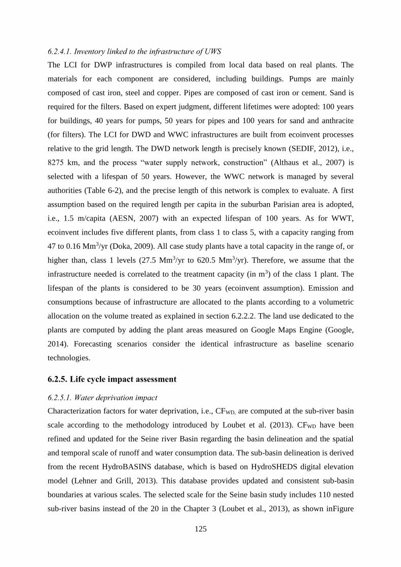
125

6.2.4.1. Inventory linked to the infrastructure of UWS

The LCI for DWP infrastructures is compiled from local data based on real plants. The

materials for each component are considered, including buildings. Pumps are mainly

composed of cast iron, steel and copper. Pipes are composed of cast iron or cement. Sand is

required for the filters. Based on expert judgment, different lifetimes were adopted: 100 years

for buildings, 40 years for pumps, 50 years for pipes and 100 years for sand and anthracite

(for filters). The LCI for DWD and WWC infrastructures are built from ecoinvent processes

relative to the grid length. The DWD network length is precisely known (SEDIF, 2012), i.e.,

8275 km, and the process “water supply network, construction” (Althaus et al., 2007) is

selected with a lifespan of 50 years. However, the WWC network is managed by several

authorities (Table 6-2), and the precise length of this network is complex to evaluate. A first

assumption based on the required length per capita in the suburban Parisian area is adopted,

i.e., 1.5 m/capita (AESN, 2007) with an expected lifespan of 100 years. As for WWT,

ecoinvent includes five different plants, from class 1 to class 5, with a capacity ranging from

47 to 0.16 Mm3/yr (Doka, 2009). All case study plants have a total capacity in the range of, or

higher than, class 1 levels (27.5 Mm3/yr to 620.5 Mm3/yr). Therefore, we assume that the

infrastructure needed is correlated to the treatment capacity (in m3) of the class 1 plant. The

lifespan of the plants is considered to be 30 years (ecoinvent assumption). Emission and

consumptions because of infrastructure are allocated to the plants according to a volumetric

allocation on the volume treated as explained in section 6.2.2.2. The land use dedicated to the

plants are computed by adding the plant areas measured on Google Maps Engine (Google,

2014). Forecasting scenarios consider the identical infrastructure as baseline scenario

technologies.

6.2.5. Life cycle impact assessment

6.2.5.1. Water deprivation impact

Characterization factors for water deprivation, i.e., CFWD, are computed at the sub-river basin

scale according to the methodology introduced by Loubet et al. (2013). CFWD have been

refined and updated for the Seine river Basin regarding the basin delineation and the spatial

and temporal scale of runoff and water consumption data. The sub-basin delineation is derived

from the recent HydroBASINS database, which is based on HydroSHEDS digital elevation

model (Lehner and Grill, 2013). This database provides updated and consistent sub-basin

boundaries at various scales. The selected scale for the Seine basin study includes 110 nested

sub-river basins instead of the 20 in the Chapter 3 (Loubet et al., 2013), as shown inFigure

126

6-2. Monthly runoff data for 2012 are computed from the GLDAS model (NASA, 2012) to

match meteorological and hydrological conditions of the baseline scenario. The data for 2012

was representative of normal conditions in France. Runoff data for forecasting CFWD at the

horizon 2050 are based on previsions models accounting for climate change in the Seine river

basin (Ducharne et al., 2009). A 20% decrease of runoff during the summer months in 2050

has been considered. Monthly water consumptions are estimated from Hoekstra et al. (2012).

Figure 6-3 shows monthly CFWD for November 2012. Resulting CFWD for the baseline and

forecasting scenarios are fully presented in Annex C.7.

Figure 6-3. CFWD for the Seine river basin (November) and locations of main withdrawals and releases for the baseline

and forecasting scenarios.

The locations of water withdrawal and water release at the sub-basin scale are diverse. The

main locations corresponding to DWP and WWT plants are shown in Figure 6-3. These plants

are located in four sub-basins: downstream Marne, downstream Oise, downstream and

upstream Seine. Withdrawal locations planned in forecasting scenarios L5 and L6 are also

shown in downstream Seine and sources of the Loing river.

Month: November

127

6.2.5.2. Other impacts

Others impact categories are evaluated at the midpoint level with ILCD and at the endpoint

level with Impact 2002+. The ILCD category “water resource depletion” has been replaced

with “water deprivation” as introduced in section 6.2.5.1. Foreground CFWD are derived from

Seine sub-river basins at monthly scale, whereas background CFWD are derived from CTA of

Hoekstra et al. (2012) which are implemented in ecoinvent 3 at the country scale. All other

emissions to air/soil, energy, chemicals and infrastructures are characterized with these two

LCIA methods. This is accomplished using Simapro software (Pré Consultants, 2013) and

results in impact matrices i for each component of the system.

6.2.6. Example of the construction of a scenario using the model

As described in Chapter 5, the volumetric water flow distribution vector v, quality distribution

vector q, and specific impacts matrix i are documented for each component of the system and

characterize the graphical objects (i.e., instances) of the Simulink library. The baseline

scenario is implemented in the Simulink interface by selecting and connecting the graphical

objects corresponding to the components of the UWS (Figure 6-4). Extrinsic parameters (i.e.,

water demand, number of water users, number and ratio of inputs and outputs for each

components, connection to water resources) are then defined as shown in Figure 6-4. Each

other scenarios are then derived from this representation, with the changes of extrinsic

parameters, as summarized in Table 6-4.

128

CR=Choisy-le-Roi, NM=Neuilly-sur-Marne, MO=Mery-sur-Oise, A=Arvigny, NS=Neuilly-sur-Seine, U_dom=domestic

users, U_ind=industrial users, U_nm=non-market users, U_m=market users, U_oth=others users, SAv= Seine Aval, SAm=

Seine Amont, SG=Seine Grésillons, MA=Marne Aval.

Figure 6-4. Graphical representation of the baseline scenario with all components, all technosphere flows (black

arrows) and major withdrawals (blue arrows) and releases (green arrows).

CR

NM

MO

A

NS

DWD

U_dom

U_ind

U_nm

U_m

U_oth

WWC

WWC

WWC

WWC

SAv

SAm

SG

MA

SWC41.2%

34.7%

20.5%

2.9%

0.7%

64.9%

25.9%

1.9%

7.3%

Sludge

spreading

Sludge

spreading

Sludge

incineration

100%

62%

38%

89%

11%

DWP DWD Users SWC WWC WWT

Seine up

Marne

Oise

Champigny

Seine

Seine down

Seine up

Seine down

Marne

12 runs per year

(monthly)

129

Table 6-4. List of extrinsic parameters for the construction of each scenario

B S1 S2 S3 L1 L2 L3 L4 L5 L6 L7 L8

Water Users Domestic

users

Number of users (capita) 4362705 4506674 4506674 4506674 4785887 4785887 5296324 4785887 4785887 4785887 4785887 4785887

Water demand

(m3/year/user)

39.2 37.2 36.9 36.2 32.4 39.2 39.2 32.4 32.4 32.4 32.4 32.4

Non market

services users

Number of users (jobs) 413251 426888 426888 426888 453336 453336 501687 453336 453336 453336 453336 453336

Water demand

(m3/year/user)

70.2 66.6 66.1 64.8 58.0 70.2 70.2 58.0 58.0 58.0 58.0 58.0

Market

services users


Water demand

(m3/year/user)

23.6 22.4 22.2 21.8 19.5 23.6 23.6 19.5 19.5 19.5 19.5 19.5

Industrial

users


Water demand

(m3/year/user)

43.2 41.0 40.7 39.9 35.7 43.2 43.2 35.7 35.7 35.7 35.7 35.7

Others users Surface (ha) 76280 76280 76280 76280 76280 76280 76280 76280 76281 76282 76283 76284

Water demand

(m3/year/ha)

83.7 79.4 78.8 77.2 69.2 83.7 83.7 69.2 69.2 69.2 69.2 69.2

Water

resources

Withdrawals

from DWP

(%)

Seine upstream River - CR

(%)

41.2 41.2 41.2 35.5 41.2 41.2 41.2 41.2 0 27.2 42 42

Seine down River (%) 0 0 0 0 0 0 0 0 42 0 0 0

Marne River - NM (%) 34.7 34.7 34.7 28.2 34.7 34.7 34.7 34.7 34.7 34.7 36 36

Oise River - MO (%) 20.5 20.5 20.5 35.6 20.5 20.5 20.5 20.5 20.5 20.5 22 22

Champigny aquifer (%) 2.9 2.9 2.9 0 2.9 2.9 2.9 2.9 2.9 2.9 0 0

Albien aquifer (%) 0.7 0.7 0.7 0.7 0.7 0.7 0.7 0.7 0 0.7 0 0

Sources of the Loing River

(%)

0 0 0 0 0 0 0 0 0 14 0 0

Release from

WWT (%)

Seine downstream - SAv

(%)

64.9 64.9 64.9 64.9 64.9 64.9 64.9 64.9 64.9 64.9 64.9 64.9

Seine upstream - SAm (%) 26.0 26.0 26.0 26.0 26.0 26.0 26.0 26.0 26.0 26.0 26.0 26.0

Seine downstream - SG

(%)

1.85 1.85 1.85 1.85 1.85 1.85 1.85 1.85 1.85 1.85 1.85 1.85

Marne - M (%) 7.26 7.26 7.26 7.26 7.26 7.26 7.26 7.26 7.26 7.26 7.26 7.26

Water

technologies

DWP Conventional (%) 82.7 82.7 82.7 78.6 82.7 82.7 82.7 82.7 41.5 68.7 0.0 100.0

Membrane (%) 13.7 13.7 13.7 17.8 13.7 13.7 13.7 13.7 55.7 13.7 100.0 0.0

Simple treatment (%) 3.6 3.6 3.6 3.6 3.6 3.6 3.6 3.6 2.9 17.6 0.0 0.0

DWD Network yield (%) 89 85 90 95 90 90 90 90 90 90 90 95

WWT Conventional (%) 100 100 100 100 100 100 100 100 100 100 100 100

130


Results for the baseline scenario are detailed hereafter for water flows, total environmental

impacts and impact/service ratios. The ratios are computed by dividing the impacts with the

indicators associated with functions of the UWS. For simplicity, only total environmental

impacts are shown for forecasting scenario and are compared to the baseline scenario. A

sensitivity analysis on the selection of impact/service ratio (based on user or m3) for the

comparison between two scenarios is then discussed.

6.3.1. Baseline scenario

6.3.1.1. Water flows

Figure 6-5 shows the different water flows in the UWS that were computed by the model to

check for the water balance of the system. This representation is performed using a Sankey

diagram, which is specific type of flow diagram in which the width of the arrows is

proportional to the flow quantity. This diagram provides a representation that is easily

communicable to stakeholders by mapping the different water flows within the urban water

cycle.

Figure 6-5. Simplified Sankey diagram of water flows within the urban water system of the baseline scenario.

131

6.3.1.2. Environmental impacts

Assessing the impacts of the baseline scenario determines the contribution of each component

of the system and the shares between the direct (foreground activities) and indirect impacts

(background activities). This assessment provides stakeholders with results for identifying the

environmental hotspots of the UWS. The order of magnitude of the baseline scenario

contributions is consistent with the previous result found in Chapter 5 that was based on a

theoretical model using only ecoinvent. Figure 6-6 shows that the majority of impact

categories, particularly those related to water pollution, are dominated by WWT. This result

differs from the results of Chapter 5, in which WWT technologies contributed far less. This

difference is because WWT plants of this case study use more electricity and chemicals than

the ecoinvent ones. WWT plants in this case study include the advanced processes treatment

of phosphorus and nitrification/denitrification, which increase the use of energy and

chemicals. Additionally, a large amount of stormwater is treated within the case study plants,

whereas stormwater treatment was not considered in Chapter 5. Another main difference with

the ecoinvent model is the high contribution of WWC (which includes stormwater collection)

to water deprivation. This difference is because the collected stormwater (precipitation) is

considered as a withdrawal, and we assume that stormwater would runoff to river water in the

absence of a collection system.

The contribution of direct and indirect impacts (Figure 6-7) shows results similar to the

ecoinvent model, suggesting that this result is generalizable to all UWS.

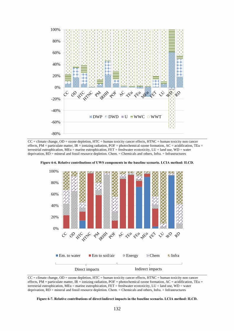
132


effects, PM = particulate matter, IR = ionizing radiation, POF = photochemical ozone formation, AC = acidification, TEu =


deprivation, RD = mineral and fossil resource depletion. Chem. = Chemicals and others, Infra. = Infrastructures

Figure 6-6. Relative contributions of UWS components in the baseline scenario. LCIA method: ILCD.


effects, PM = particulate matter, IR = ionizing radiation, POF = photochemical ozone formation, AC = acidification, TEu =


deprivation, RD = mineral and fossil resource depletion. Chem. = Chemicals and others, Infra. = Infrastructures

Figure 6-7. Relative contributions of direct/indirect impacts in the baseline scenario. LCIA method: ILCD.

-80%

-60%

-40%

-20%

0%

20%

40%

60%

80%

100%

DWP DWD U WWC WWT

0%

20%

40%

60%

80%

100%

Em. to water Em to soil/air Energy Chem Infra

Direct impacts Indirect impacts

133

6.3.1.3. Provided services and impact/service ratios

In addition to the total impact of the UWS, the model details the functions provided by the

system, i.e., the amount of each type of user supplied with water. Based on this information,

the model computes impact/service ratios that are useful for comparisons with other scenarios

or other systems. With the example of the climate change impact category, impact/service

ratios found for the different users are the following: 72.55 kg CO2 eq/year/domestic user,

129.92 kg CO2 eq/year/non market service job, 43.68 kg CO2 eq/market service job, 79.95 kg

CO2 eq/year/industry job, 154.9 kg CO2 eq/year/ha (other uses) and 100.89 kg

CO2/year/equivalent inhabitant. In this study, we considered equivalent water users in terms

of input and output water quality. The share of impact relative to each user is only dependent

on the water demand and the amount of water users. Therefore, 72% of the impacts result

from domestic users, 3% result from industries, 12% result from non-market services, 10%

result from market services and 3% result from others users. The low share of impacts

resulting from industries is mainly because the low industrial activity in the case study (8.8%

of all jobs are in industry in 2012). However, not accounting for the different levels of raw

wastewater quality generated by the various users tends to underestimate industries’

responsibility in wastewater treatment (the presence of heavy metals and emerging

pollutants). A methodological challenge remains to allocate the impacts of a wastewater

treatment plant according to the different types of users.

Regarding climate change, the impact/service ratio related to one cubic meter at the user’s

place results in a value of 1.85 kg CO2 eq/m3. This result agrees with values found in the

literature and summarized in Loubet et al. (2014), which range from 0.51 to 1.57 kg CO2

eq./m3 at the user’s place.

6.3.2. Forecasting scenarios

The results of the forecasting scenarios compared to the baseline total impacts are shown in

Table 6-5 and discussed hereafter. To simplify the results, only midpoint water deprivation

impacts and endpoint damages from Impact 2002+ are considered here.

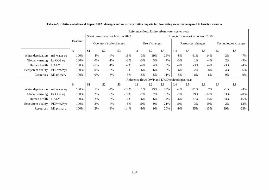
134

Table 6-5. Relative evolutions of Impact 2002+ damages and water deprivation impacts for forecasting scenarios compared to baseline scenario.

Reference flow: Entire urban water system/year

Baseline

Short term scenarios horizon 2022 Long term scenarios horizon 2050

Operators' scale changes Users' changes Resources' changes Technologies' changes

B S1 S2 S3 L1 L2 L3 L4 L5 L6 L7 L8

Water deprivation m3 water eq 100% 4% -4% -19% 3% 19% 29% -8% -61% 14% -2% -7%

Global warming kg CO2 eq 100% 0% -1% -2% -3% 3% 7% -3% 1% -4% 2% -5%

Human health DALY 100% -1% -1% -2% -4% 4% 9% -4% -3% -4% -3% -4%

Ecosystem quality PDF*m2*yr 100% 0% -2% -3% -6% 6% 12% -6% -2% -8% -4% -6%

Resources MJ primary 100% 0% -3% -5% -5% 5% 11% -5% 8% -6% 9% -9%

Reference flow: DWP and DWD technologies/year

B S1 S2 S3 L1 L2 L3 L4 L5 L6 L7 L8

Water deprivation m3 water eq 100% 1% -4% -12% 1% 23% 35% -4% -31% 7% -1% -4%

Global warming kg CO2 eq 100% 2% -6% -10% -7% 7% 16% -7% 29% -12% 33% -20%

Human health DALY 100% 2% -5% -6% -6% 6% 14% -6% 27% -15% 33% -15%

Ecosystem quality PDF*m2*yr 100% 2% -4% -8% -10% 9% 21% -10% 3% -19% -2% -12%

Resources MJ primary 100% 2% -8% -14% -9% 9% 20% -9% 35% -13% 39% -23%

135

6.3.2.1. Short term forecasting scenarios

The short term policies assessed in scenarios S1, S2 and S3 show small variations of damages

at the UWS scale, i.e., from 0 to -5% changes. This small variation is because the studied

scenario changes only concern DWP & DWD which have a small contribution in the overall

system. The fact that damages decrease in all scenarios results from the decrease in the overall

water demand. Concerning water deprivation impacts, the policy can have an important effect

over short terms by managing the water resource choice; for example, the water deprivation

decreases by 19% for scenario S3, which is designed towards high impact/service.

6.3.2.2. Scenarios with changes in water users

Scenarios L1 to L4 aim to study the variability of impacts resulting from contrasted trends in

water demand projection of the urban area for 2050 (-10 to +21%). Scores of the “ecosystem

quality” range from -6% to +12% in comparison with the baseline. Water deprivation

potentially increases from 3% to 29%. This shows the high variability of the system impacts

because of different projections of urban development and user’s behavior. Knowledge about

urban development and water demand is consequently a key point when assessing forecasting

scenario because the system is driven by these parameters. These results also demonstrate the

capacity of the model to implement easily different water demand scenarios. However, a main

limitation of these scenarios is the fact that the wastewater load and WWT plant operation are

considered identical to the baseline scenario. This is a strong assumption because a reduced

water demand per capita coupled with the identical pollutant load released would increase the

concentration of pollutants in the wastewater, thus modifying the residence time in WWC and

WWT and the energy and chemical consumption. Nevertheless, determining wastewater

pollutant concentrations for future scenarios is complex. Behavior changes of the users might

affect the pollutant load released into wastewater because of the decreased use of chemicals

and the increasing efficiency of water appliances (Friedler, 2004). Additionally, no LCA

model can yet predict impacts of WWT technologies effect on the quality of wastewater.

6.3.2.3. Scenarios with changes in water resources

Scenario L4 studies the water deprivation impact that potentially occurs in 2050 by

considering the current state of water scarcity (instead of the water scarcity state that would

occur because of climate change, as studied in scenario L1). This scenario results in a -13%

decrease of water deprivation impact compared to scenario L1, suggesting a non-negligible

effect of climate change on this impact.

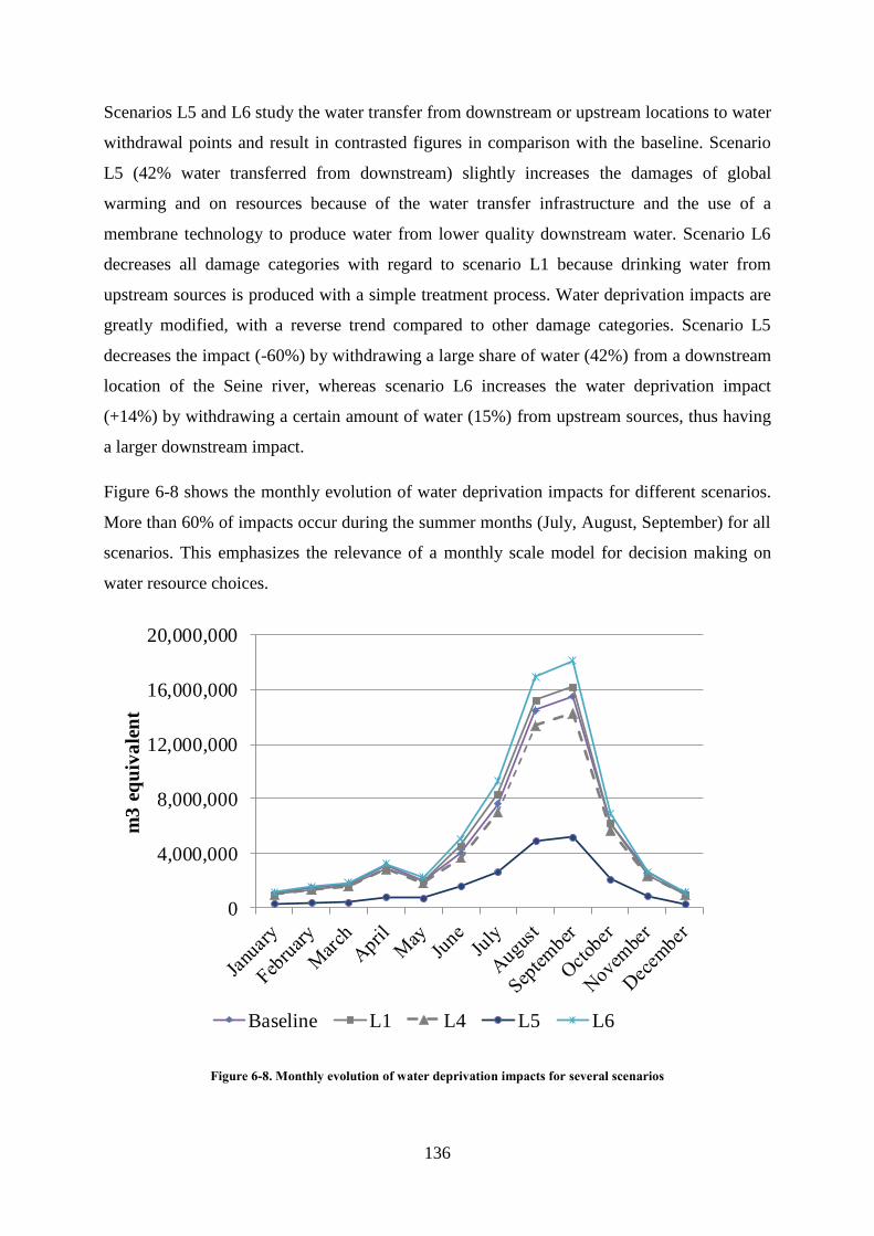
136

Scenarios L5 and L6 study the water transfer from downstream or upstream locations to water

withdrawal points and result in contrasted figures in comparison with the baseline. Scenario

L5 (42% water transferred from downstream) slightly increases the damages of global

warming and on resources because of the water transfer infrastructure and the use of a

membrane technology to produce water from lower quality downstream water. Scenario L6

decreases all damage categories with regard to scenario L1 because drinking water from

upstream sources is produced with a simple treatment process. Water deprivation impacts are

greatly modified, with a reverse trend compared to other damage categories. Scenario L5

decreases the impact (-60%) by withdrawing a large share of water (42%) from a downstream

location of the Seine river, whereas scenario L6 increases the water deprivation impact

(+14%) by withdrawing a certain amount of water (15%) from upstream sources, thus having

a larger downstream impact.

Figure 6-8 shows the monthly evolution of water deprivation impacts for different scenarios.

More than 60% of impacts occur during the summer months (July, August, September) for all

scenarios. This emphasizes the relevance of a monthly scale model for decision making on

water resource choices.

Figure 6-8. Monthly evolution of water deprivation impacts for several scenarios

0

4,000,000

8,000,000

12,000,000

16,000,000

20,000,000

m3

eq

uiv

ale

nt

Baseline L1 L4 L5 L6

137

6.3.2.4. Scenarios with change in water technologies

Changes in DWP technologies do not produce significant impact changes at the UWS scale.

Differences are only noted in the DWP and DWD parts of the system. Scenario L7, which

studies the implementation of membrane DWP technologies, increases the damages for the

“resource” category by +39%, whereas scenario L8, which studies eco-efficient DWP

technologies, decreases the damages by -23% (“resource” category). Although membrane

processes are substantial consumers of energy and chemicals, they also produce high quality

drinking water that could provide more services to users. In particular, these processes

decrease the water hardness, thus saving energy and lifespan expectations of water appliances

(water heaters, washing machines, etc.) (Godskesen et al., 2012). This case study does not

include these appliances because of the lack of data, but the developed framework enables

such an inclusion. Research would also be needed on the LCI linked to energy use of water

appliances depending on the quality of the drinking water.

6.3.3. Sensitivity analysis on impact/service ratio choices

Impact-services ratio (i.e., inverse of eco-efficiency ratios) are indicators that are useful for

communicating with stakeholders. Since the model compute several impact/service ratios that

can be interpreted differently by stakeholders, it is important to discuss the relevancy of each

ratio, as it is done hereafter.

Figure 6-9 shows the evolution of damages between the baseline scenario and forecasting

scenario L1 that models the UWS in 2050 with the expected changes in population (+ 9,3%),

water demand (-21%) and water scarcity. Depending on the impact/service ratio, the results

radically change. With the impact/service ratio related to the entire urban water system, the

damages are expected to decrease with increasing population. This decrease is because the

expected reduction in water demand will decrease the overall water demand of the urban area,

and therefore the impacts: 215.1 Mm3 in 2050 versus 237.8 Mm3 in 2012 (scenario L1). For

this scenario, however, the water deprivation is expected to swell because of a higher water

scarcity. The impact/service ratio related to users (equivalent inhabitants) decrease (up to

14%) because of additional population and less overall damages in scenario L1 compared to

B. Nevertheless, impact/service ratios related to one cubic meter increase because the total

water demand is lower in scenario L1 but the infrastructure is considered to be unchanged.

Consequently, infrastructure damages related to one cubic meter are more important in

scenario L1 than in B. These different results provide useful information for the stakeholder

depending on the question. The impact/service ratio related to the entire UWS aims to assess

138

the overall impacts of a territorial system. This assessment is relevant for local authorities that

aim to reduce the non-marginal overall impacts on a territory. The impact/service ratio related

to users is useful for comparing different types of users’ impacts and for analyzing the

contribution to an UWS within the total impacts generated by one user in a city (policy-

making at a larger scale). The impact/service ratio related to one cubic meter at the user’s

place is useful for comparing technological efficiencies of different UWS. However, this

metric is not relevant in comparing integrated forecasting scenarios of an UWS because it

does not account for user’s behavior.

Figure 6-9. Comparison of various impact/service ratios of forecasting scenario L1 to the baseline (set at 100%,

whatever the unit). LCIA method: Impact 2002+ endpoint and water deprivation midpoint.


Other scenarios can be easily investigated because of the modularity of the modeling tool and

would provide opportunities to address emerging concerns in urban water management. For

example, policy-responsive scenarios regarding water technologies could compare different

systems of water softening (central softening, such as membrane processes, or household

systems), separation of wastewater streams (into blackwater and greywater), wastewater reuse

(Meneses et al., 2010) or rainwater harvesting (Angrill et al., 2011). Future-trend scenarios

0%

20%

40%

60%

80%

100%

120%

Global warming Human health Ecosystemquality

Resources Water resourcedeprivation

Rel

ati

ve

con

trib

uti

on

Impact categories

Baseline Forecasting L1 - FU=UWS/year

Forecasting L1 - FU=1 inhabitant/year Forecasting L1 - FU=1 m3 at the user

139

related to technologies were not regarded in this case study but could include a prospective

electricity mix.

The fine temporal and geographical scales associated with water deprivation impacts are

useful for decision making regarding water resource choices. In this case study, whereas

decision makers of DWP have low flexibility for decreasing impacts linked to technologies,

they do have a high contribution on water deprivation impacts by selecting withdrawal

locations.

These scales could also be important when dealing with water quality associated impacts. The

future implementation of refined LCIA methods (e.g., marine and freshwater eutrophication)

with a spatial differentiation of the fate and the effect will improve the site-dependent

property of the model, and therefore, interest in this method by the stakeholders.

In addition to the generic limits of the model noted in part 1, more specific limits emerge from

this case study. The predictions of future wastewater quality and the resulting emissions with

an equilibrated mass balance are a real challenge for a LCA. Additionally, uncertainties

related to WWT inventory data are high, both in LCI phases - concerning emissions to air and

soil at the plant and at the sludge end-of-life and in the LCIA phase concerning in particular

the assessment of metals (Rosenbaum et al., 2008).

The integration of stormwater collection within the system also raises concerns and

methodological challenges. The assumption under which all stormwater collected is

considered as withdrawal is questionable. In the absence of any collection system, not all

water would runoff to the river because a portion can evapotranspirate or infiltrate into the

soil. This portion of the runoff is dependent on the land use. For urban cover, most of the

water would runoff. However, if we consider a natural land reference such as forest, then a

much larger portion would evapotranspirate and infiltrate. This question of land use is still a

debate in LCA (Núñez et al., 2013b). In addition, a further step would be to consider all

stormwater collection and run-off within the area and not only the water collected in

combined sewers.

Another challenge is the decision-making process with several stakeholders. As shown in

Table 6-2, many water service institutions manage the UWS of the greater metropolitan Paris

area. These case study scenarios have been built with one specific stakeholder managing

drinking water in a suburban area of the system being related to the environmental

140

performance of the entire UWS. The evaluation of the entire greater Paris area UWS would be

an interesting further step because this is a coherent territorial unit. The cooperation of the

different water services is also a notable issue in the context of the “Grand Paris” development

(Desjardins, 2010).

6.4. Conclusions and outlook

The model for assessing the environmental impacts of UWS developed in Chapter 5 is

implemented on a real case study in the suburban areas of Paris with various associated

scenarios. This application demonstrates the applicability of the model to assess the

environmental impacts of an UWS and the capacity to address several stakeholder’s potential

questions related to urban water management. This approach therefore provides useful

quantitative information for decision making processes related to policy-response scenarios on

water resources and technological choices and related to future-trend scenarios projecting

urban development and behavior. The use of this modeling tool and its modular approach

greatly facilitates the generation and the evaluation of scenarios.

The results have shown that UWS impacts predominantly result from WWT. The study of the

forecasting scenarios results in many findings. A high variability of impacts in forecasting

scenarios is noted because of different trends in water demand. Because of their low

contribution in the system, changes in DWP and DWD do not produce important

modifications of technology-based impacts. However, DWP and DWD have a great effect on

water deprivation impacts depending on the choice of water withdrawal location. Further

scenarios could be investigated such as the implementation of emerging technologies in DWP

and WWT plants.

The different UWS components developed in this case study could be used for the

environmental assessment of water management scenarios elsewhere in the world. It would

require updated data in the library and the calculations of downstream cascade effect (CFWD)

for all sub-river basins because global coverage is not yet available.

141

Chapter 7. Discussion and conclusion

« Elle a coulé, notre rivière

Depuis ce jour d'antan.

Elle a coulé, notre rivière

Depuis mille et mille ans. »

Hugues Aufray – Notre rivière

142


7.1. The need to better assess impacts associated to water use .......................................... 143

7.1.1. Towards appropriate scales for LCA practitioners ............................................... 143

7.1.2. Towards the use of consensual hydrological data and models for LCIA developers

........................................................................................................................................ 144

7.1.3. Current gap between midpoint indicators based on water stress and the endpoint

indicators ........................................................................................................................ 145

7.1.4. Towards mechanistic approaches in LCIA: combining downstream cascade effect

with a consistent water fate model ................................................................................. 146

7.1.5. Current limits of water footprint related to water quality assessment .................. 150

7.2. Perspectives for the WaLA model .............................................................................. 152


7.2.2. Towards scenario assessment in a decision making context ................................ 152

7.2.3. Towards a tool for benchmarking......................................................................... 153

7.3. General conclusion ...................................................................................................... 155

143

This chapter is split in two complementary sections related to the two main outcomes of the

thesis: first methods for improving LCIA of water use (Chapter 3 and Chapter 4), and second,

WaLA, a versatile model for LCA of UWS (Chapter 5 and Chapter 6).

7.1. The need to better assess impacts associated to water use

In this section, opportunities and limits of the method for assessing water deprivation at the

sub-river basin scale and the perspectives, such as its combination within a mechanistic model

for assessing water fate, are presented. Finally, water quality indicators are discussed and the

limitation of their integration in water footprint is debated.

7.1.1. Towards appropriate scales for LCA practitioners

The methodology for assessing water deprivation at the sub-river basin scale has proven its

worth for LCA of UWS. The evaluation of forecasting scenarios in Chapter 6 has shown that

such a method is useful to compare scenarios having chosen different water resources. Even if

this methodology was applied to LCA of UWS, its application is wider and could benefit to

other LCA application such as agriculture or industries, which are also big water users.

The proposed scale, i.e., the sub-river basin is a step towards site-dependent impact

assessment. It would greatly benefit to the appropriation of the methodology by stakeholders

who are asking for a consistent assessment of local impacts. In Chapter 6, characterization

factors for water deprivation have been calculated at a finer scale than it was originally done

in Chapter 3, in order to better address the stakeholder’s questions about choices of water

resources in the Seine river basin. It is a big output as it makes water-related LCIA methods

applicable at any scales dependently to the goal and scope of the study. A further step in this

direction would be to use local hydrologic model of a given river basin instead of global water

models.

Up to now, in the literature, the scales for LCIA of water use was the river basin, and in the

methodology we propose, the sub-river basin scale raises several challenges. LCA

practitioners who assess global life cycle of goods or services usually do not know exactly the

locations of water withdrawal or release and a sub-river basin scale is not relevant. Therefore,

such a fine scale for LCIA methods can be currently used only for foreground processes with

a good knowledge of the processes. Also computing the water use impact, at river-basin or

finer scales, can only be done outside LCA software, as it is not integrated, yet. These

challenges require future development for LCIA methods as well as databases and software

144

developers: (i) as proposed by Mutel et al. (2012), minimization of global spatial

autocorrelation should be applied to aggregate small spatial units and build typologies of (sub-

)river basins; (ii) the issue of spatial differentiation should also be tackled by LCA software

and database. Famous LCA software such as SimaPro (Pré Consultants, 2013), GaBi (PE

International, 2011) or Umberto do not allow to select locations of elementary flows.

OpenLCA (Ciroth, 2007), which is an open source LCA software, provides the possibility to

analyze locations of impacts in a world map. This is a unique feature in LCA software, so far,

and a great opportunity to assess water use impacts. LCA database, such as ecoinvent do not

differentiate the locations of water elementary flows (withdrawal, release, consumption) at a

scale finer than the country one.

7.1.2. Towards the use of consensual hydrological data and models for LCIA

developers

It has been shown in Chapter 3 and Chapter 6 that several hydrological data and models can

be used to compute CFWD, resulting in different values. There is a high amount of database

describing basin topography (e.g., in this thesis: “Hydro1K” and the updated version

“HydroBASINS”) and water consumption, as well as of runoff models (e.g., in this thesis:

averaged data from 1960-2000 from the “Composite Runoff fields model” and data for the

year 2012 from the model “GLDAS”). Data are highly variable, because of the different

models used and the time representativeness of the models. These differences emphasize the

need for a consensual choice on reliable and recent database at a global scale, which is a

question common to all methods related to water use in LCIA. It could be solved by

comparing different hydrological models (e.g. runoff model) available in the literature, such

as done by Boulay et al. (2014). Outside LCA, the World Resources Institute (WRI) compiled

several database for computing the Aqueduct model, which assesses the water risk – ie water

scarcity - at the global scale (Gassert et al., 2013). It includes several and recent data sources

such as basin delineation, withdrawals, consumption, runoff, etc. that could be used for LCIA

of water use.

In addition, the use of a common GIS web-based tool that could compute several LCIA

methods according to different database would be an interesting approach for LCIA

developers. Such web-based interfaces have already been developed in the hydrogeology or

ecology communities, in order to supply users with a large amount of data. Representative

145

examples are the global freshwater biodiversity atlas1 or the data mapped by the Global

Hydrology group of Utrecht University2. The latter allows us to calculate data within the web

tool, as well as representing data according to specific time representativeness.

Therefore, such tools could be used to compute the downstream cascade effect for all sub-

river basins in the world. The algorithms to compute the downstream cascade effect should be

automatized and modeling options could be chosen within the proposed GIS web-based tool

including (i) choice of database (runoff, water consumption, etc.), (ii) choice of sub-river

basin delineation, (iii) choice and combination of weighting parameters for computing the

downstream cascade effect (e.g., surface, water volume of rivers, population, etc.).

Site-specific indicators would require local models that would allow to take into account

canals, reservoirs, inter- and intra- basins transfers (Rousset, 2004). These kind of human

interventions on water resources are not well represented in global models, but are important

to the hydrologic regimes in a river basin such as the Seine’s one. Also, consideration of

groundwater resources should be examined. These challenges can be tackled by the

development of mechanistic approaches that is introduced in next section.

7.1.3. Current gap between midpoint indicators based on water stress and the

endpoint indicators

UNEP-SETAC Life Cycle Initiative solicited the Water Use in LCA (WULCA) Working

Group to undertake the task for a consensual set of methods for water use impact assessment.

A focus is placed on three sets of indicators representing: impact pathways leading to

damages on human health, impact pathways leading to damages on ecosystem, and a generic

stress/scarcity indicator (Boulay et al., 2014), as shown in Figure 7-1. Water scarcity

indicators raise concern since they are not in the cause-effect chain of water use impacts, from

an LCA perspective. Indeed, water scarcity does not represent actual impacts or damages on

ecosystem or human health, as pointed out in Chapter 3. It is rather a characteristic of a basin

with regard to risk assessment as it informs us about “the extent to which demand for water

compares to the replenishment of water in an area, such as a river basin” (ISO, 2013).

However, there is a strong demand from industry to provide such an indicator. This advocates

1 http://atlas.freshwaterbiodiversity.eu/index.php/maps

2 http://www.globalhydrology.nl/maps

http://atlas.freshwaterbiodiversity.eu/index.php/maps

146

for the development of a mechanistic model that can be the base for assessing the effects

(damages) at steady state of any marginal changes in the water balance.

Figure 7-1: illustration of the gap between current mid-point indicators based on stress and damage assessment based

on volume deprivation effects (source Boulay, WULCA)

7.1.4. Towards mechanistic approaches in LCIA: combining downstream cascade

effect with a consistent water fate model

For damage to human health and to ecosystems, a mechanistic approach should be followed.

One proposal is to represent the damage by the product of a fate factor and of an effect factor

(and possibly an exposure factor for human health) as it is typically done in other LCIA

impact categories such as toxicity or eutrophication. Savard (2013) has reviewed most of

pathways of water-use related impacts and discussed in an extended manner on the fate and

effect factors found in the literature. Fate factor for water can be defined as the modification

of environmental water flows because of a human intervention. Effect factor is the

consequence of the modified environmental water flow on ecosystem or human health

damages (the same occurs for other water natural resources, such as lakes and groundwater).

dQ

dS

dW

dQEFFFCF (27)

147

Where dW is the marginal change of the human intervention (e.g., water withdrawal within a

river basin), dQ is the marginal modification of the environmental flow (e.g., flow rate of a

river), dS is the marginal damage (e.g., damage to species richness).

Effect factors have already been defined for several impact pathways: damages to fish due to

decrease flow in river (Hanafiah et al., 2011; Tendall et al., 2014), damages to ecosystems due

to decreased wetland volume (Verones et al., 2013), damages to plants due to decrease level

of groundwater (van Zelm et al., 2011). However, fate has been mostly disregarded or

considered as equal to one, meaning that an intervention has a direct effect on one flow. Also,

the difference between inventory and fate of water is still unclear. For instance, Berger et al.

(2014) propose to take into account atmospheric evaporation recycling at the inventory phase

to compute net consumption, whereas it could be considered as fate. There is a need to bridge

the gap between inventory and impact assessment, as it is discussed for example in the

pesticides and LCA field (van Zelm et al., 2013).

The development of a multimedia fate model would allow to account for all modifications of

environmental water flows because of a human intervention. Figure 7-2 is a representation of

the water cycle at the scale of a river basin, i.e., the exchanges of water between

environmental compartments, as adapted from the representation of Usetox multimedia model

(Rosenbaum et al., 2008, 2007). Human intervention modify the different water flow

exchanged by the compartments. For example, water which is withdrawn from a river to be

used on an agricultural soil will cause several modifications on: the river flow, the

groundwater table, the soil moisture, the evapotranspiration and recirculation of water within

the atmosphere, etc. This is shown in Figure 7-3 where the inventory, i.e., the water

withdrawal from groundwater, and the fate, i.e., the modifications on environmental flows are

represented. Each arrow representing a water flow exchange would be defined by a

hydrological water model.

148

Figure 7-2. Description of the water cycle within a multimedia scheme. Adapted from Usetox multimedia fate model

(Rosenbaum et al., 2008).

Figure 7-3. Proposed framework of the fate of water flows within a multimedia scheme: modification of environmental

water flows (yellow arrows) caused by human interventions (red arrows). Name of water exchange processes are in

italic. (source: Roux, P., Nunez, M. Loubet, P., for WULCA group in 2014)

Global scale (and other river basins)

AIR

OCEANSurface freshwaterSOIL

River basin scale

Surface freshwater

SOIL

AIR

TOP-SOILAgricultural

TOP-SOIL Natural

Groundwater (Stock)

Groundwater (Fund)

Wetlands

Global scale (and other river basins)

AIR

OCEANSurface freshwaterSOIL

River basin scale

Surface freshwater

SOIL

AIR

TOP-SOILAgricultural

TOP-SOIL Natural

Groundwater (Stock)

Groundwater (Fund)

Wetlands

WithdrawalEvaporation

Infiltration

Runoff

Recharge

Internal evaporation

recycling

External evaporationrecycling

Inventory Fate

149

In this context, the “downstream cascade effect” developed in this thesis could be considered

within the fate to account for modification of environmental water flows at the sub-river basin

scale. This effect can be represented with two nested scales: river basin and sub-river basins.

There are n river basins that can exchanges water with ocean and with other river basins

through atmospheric recycling of water. Within a river basin termed i, there are m sub-river

basins exchanging water from upstream to downstream (downstream cascade effect) and

ultimately ocean through surface freshwater flow (i.e., rivers). This is shown in Figure 7-4.

Figure 7-4. Representation of water cycle at the sub-river basin scale. Thick black arrows represent downstream

cascade effect

More research is required for presenting the general framework of fate model for water and to

integrate hydrological model of water exchanges between compartments. This task is

currently undertaken within ELSA-PACT industrial chair and the WULCA group.

150

7.1.5. Current limits of water footprint related to water quality assessment

Impacts associated to water quality (pollutants) or quantity (water resource consumption) can

be presented in a simplified way, in the form of the water footprint profile (ISO, 2013) or a

water footprint single score e.g., the Water Impact Index (WIIX) (Bayart et al., 2014), the

index of Ridoutt and Pfister (2012) or the one from the Water Footprint Network (Hoekstra et

al., 2011). Impacts related to water use have been fully discussed in the previous section.

Impacts related to water quality, described in Chapter 4, should be more thoroughly discussed.

Indeed, water quality related impacts that should be taken into account in a water footprint

profile or single score have not been clearly defined so far. The ISO standard specifies that all

life cycle emissions (to air, soil and water) with impact on water quality should be considered

(ISO, 2013). Alternatively, the Ridoutt and Pfister (2012) method only takes into account

emissions to water. Also, WIIX only quantifies emissions to water and only consider impacts

occurring in the water media.

Therefore, qualitative water footprint profiles or single scores differ according to LCI and

LCIA choices. In the LCI phase of a water footprint, either only emissions to the water

compartment or all emissions to soil, air and water are included. As for the LCIA phase of a

water footprint, either only impacts occurring within the water media or all impacts affected

by emissions to water (that do not necessarily concern aquatic environment, but terrestrial or

human for example) are taken into account. It leads to four different options for considering

water quality:

- (1) Direct emissions to water leading to impact categories related or not with water

- (2) Direct emissions to water leading to impact categories related to water

- (3) Direct emissions to air, soil, water, leading to impact categories related to water

- (4) Direct emissions to air, soil, water, leading to impact categories related or not to

water

The four different options are illustrated in Figure 7-5. This shows that this issue has not

clearly been addressed so far and should be solved for developing standardized method of

water footprint profile or single score.

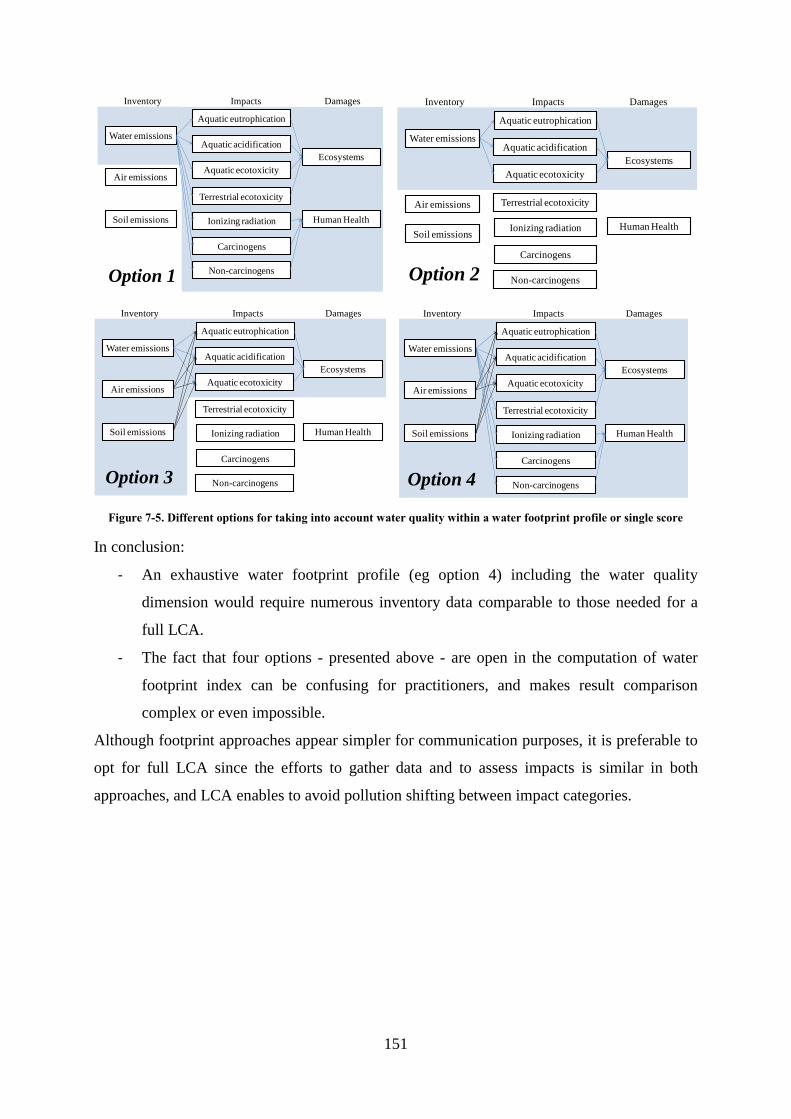
151

Figure 7-5. Different options for taking into account water quality within a water footprint profile or single score

In conclusion:

- An exhaustive water footprint profile (eg option 4) including the water quality

dimension would require numerous inventory data comparable to those needed for a

full LCA.

- The fact that four options - presented above - are open in the computation of water

footprint index can be confusing for practitioners, and makes result comparison

complex or even impossible.

Although footprint approaches appear simpler for communication purposes, it is preferable to

opt for full LCA since the efforts to gather data and to assess impacts is similar in both

approaches, and LCA enables to avoid pollution shifting between impact categories.

Water emissions

Air emissions

Soil emissions

Inventory Impacts

Aquatic eutrophication

Aquatic acidification

Aquatic ecotoxicity

Terrestrial ecotoxicity

Carcinogens

Ionizing radiation

Damages

Human Health

Ecosystems

Non-carcinogensOption 1

Water emissions

Air emissions

Soil emissions

Inventory Impacts



Aquatic ecotoxicity


Carcinogens

Ionizing radiation

Damages

Human Health

Ecosystems


Water emissions

Air emissions

Soil emissions

Inventory Impacts



Aquatic ecotoxicity


Carcinogens

Ionizing radiation

Damages

Human Health

Ecosystems


Water emissions

Air emissions

Soil emissions

Inventory Impacts



Aquatic ecotoxicity


Carcinogens

Ionizing radiation

Damages

Human Health

Ecosystems


152

7.2. Perspectives for the WaLA model


The WaLA model opportunities and limits are identified and discussed in chapters 5 and 6. In

summary, the main novelties of the model are its modularity that enables the easy

construction and assessment of scenarios, and the refined assessment of water related impacts,

taking into account fine temporal (monthly) and spatial (sub-basin) scales. Also, the modeling

formalism based on the definition of a generic component (for both water users and

technologies), represented by an object, allows the appropriation of the model by companies

or academics to develop their own tool (with their own data), thanks to the object-oriented

programing (OOP). The provision of a large amount of data defining the components of UWS

(i.e., volume and quality distribution, impacts of associated activities) could also be used by

others practitioners.

Limits are still numerous and require further developments concerning (i) modeling choices

and (ii) data collection to conduct case studies:

(i) The management of pollutant mass balance in link with water quality changes at

the component scale could be included, as component functions. This requires

models able to carry out mass balances for all pollutants (and not only for carbon

and nitrogen). It seems possible for DWP (Mery et al., 2013) but requires further

research for WWT (including sludge fate). Also, uncertainty management is not

implemented in the model but should be dealt with since it is an essential feature

for improving the reliability of LCA in the context of decision making. Moreover,

the data management within model programmed in Matlab/Simulink interface has

not been optimized and should be improved in order to allow update of LCI and

LCIA methods.

(ii) The library already includes several components to represent water technologies

and water users but still need to be completed: for example, with emerging

technologies or water appliances at the user’s place (e.g., water heater). As for

water users, they need to be better differentiated in terms of water flows and water

quality changes.

7.2.2. Towards scenario assessment in a decision making context

As shown in Chapter 6, the proposed framework and its associated model supply the

stakeholder with an integrated tool for decision-making by taking into account a large set of

153

environmental criteria offered by LCA. However, it must be remained that the scenarios

assessed in the present study have been built by researchers and field experts, with the aim of

assessing the capability of the WaLA model, but that they do not intend to have any political

plausibility. Therefore, they have not been assessed in a decision making process where all

stakeholders (i.e., all operators of water services, river basin agencies, citizens, etc.) are

involved. Contributions of stakeholders to the scenario building process would be beneficial

in many aspects. First, it is important that the results are presented to the various stakeholders

to assess their level of understanding and adhesion among the public. In this context, the set of

chosen indicators is an important issue for communication purposes. In addition, stakeholders

can provide relevant analytical elements in the definition and evaluation functions of the

systems. Also, they have a crucial role in the construction of policy responses scenarios.

7.2.3. Towards a tool for benchmarking

In addition to comparing different scenarios, the use of the proposed framework could also be

used to compare impact/service ratios of different cities, and therefore compare the

sustainability of diverse urban water system. This could be done by using a limited set of

indicators such as the WIIX+ or, the endpoint damage scores. The use of the WaLA model for

the UWS of another megacity has not been done yet, but the modularity of the model would

allow it without much effort except for collecting ad hoc data. In addition, there are still

remaining challenges to gather data from contrasted UWS, for example, with the presence of

decentralized systems, such as wells for drinking water, or on-site sanitation. In developing

countries, challenges related to UWS are different from those in developed countries. The

level of services provided by the systems is way lower, with a limited access to safe drinking

water, a non-continuous service, low sanitation (Montgomery and Elimelech, 2007). It also

raises concerns about the LCA methodology for taking into account damages to human health

occurring because of non-potable water use and non-sanitation (Harder et al., 2014;

Heimersson et al., 2014).

Also, this approach could be integrated within a full assessment of a territory, as proposed by

Loiseau et al. (2013), in order to compare environmental impacts of the urban water sector

with other activities within the territory. More specifically regarding water use, consumption

activities related to food lead to high impacts in other river basins of the world because of

imported food, agriculture being an important water consumer. It is more likely that this

induced water use would lead to higher impacts than the ones related to the urban water

system (Hoekstra, 2012). Therefore stakeholders involved with water management in the

154

territory have low room of maneuver for mitigating these impacts. However, such comparison

of activities would be useful as it would raise awareness of the public. In the context of

competition on water resources, using water for an activity instead of another would lead to

consequential effects at different upper scales (neighboring territories, national, regional,

continental) that should be studied.

Following the concept of carbon neutrality, there is a growing trend towards the water

neutrality of industries (Hoekstra, 2008). In this context, there is a concern of the water

services to mitigate water use impacts. This can be done by eco-design actions, in order to

lower water footprint as studied in scenarios of Chapter 6. Also, compensation for negative

impacts can be done for example by investing in improved watershed management - in the

same hydrological unit - for example to reduce the upstream pollution. This is a step to go

from integrated urban water management (IUWM) to the larger scale of integrated water

resource management (IWRM). Investing in other river basins for compensating a water

footprint is highly questionable since water impacts are local (ISO, 2013), on the contrary of

carbon footprint which is a global impact. A first operational benefit of this thesis is that such

a process to go water neutral has been engaged by Veolia Eau d’Île-de-France, delegatee of

the SEDIF, in collaboration with the consulting company Quantis, based on the outputs of this

thesis. However, this process must be completed by a full LCA-based multi criteria analysis

for avoiding pollution shifting between impact categories.

155

7.3. General conclusion

The work done in this thesis sought to develop a method for the multi-criteria environmental

assessment of urban water system seen as a whole (i.e., including water technologies, water

users and water resources), in order to evaluate forecasting scenarios. The research hypothesis

was: “a methodology can be developed in order to easily and consistently assess scenarios of

urban water systems in megacities, within the framework of LCA.” This global issue has been

approached through two axes, each one related to a crucial phase of LCA. In the goal & scope

and LCI phases, the question was: “how to model the UWS of big cities, in order to be at the

same time, simple to implement, representative of a given UWS scenario, and compliant to

LCA specifications?” In the LCIA phase, the question was: “regarding the fact that UWS will

have major qualitative and quantitative effects on the water compartment, how to better take

this effects into account?” These axes have led us to identify five sub-objectives.

The first sub-objective (Chapter 2) was to show that LCA is a worthy methodology in the

environmental evaluation of UWS. The literature review revealed that LCA has been

increasingly used to assess forecasting scenarios. However, there are still methodological

challenges, such as the multi-functionality of the UWS, the need for better accounting of

water quantity and quality.

The second and third sub-objectives (Chapter 3 and Chapter 4) are linked to the axe related to

water-related impacts. They are of prime interest in the development of a model for LCA to be

applied to UWS. A methodology for assessing water deprivation at the sub-river basin scale

integrating “downstream cascade effect” has been developed in Chapter 3. The proposed

scale, i.e., the sub-basin instead of the whole basin, is crucial for assessing water deprivation

impacts of UWS since there are multiple choices of water withdrawal sources within a same

river basin, and since locations of water release can be far from withdrawal ones. This

approach proposes to go beyond the assessment of water scarcity at a finer scale by taking

into account the impacts that a water withdrawal or consumption will have on downstream

users and ecosystems, i.e., the extent to which it will deprive water in downstream sub-basins.

Chapter 4 aims at accounting for water quality of urban water flows in order to manage the

issue of water quality within the model. A classification of urban water flows is done,

according to the damage scores of the different water types.

Fourth and fifth sub-objectives deal with the creation and implementation of a model, for

representing UWS and assessing their environmental performance through LCA. The fourth

156

sub-objective (Chapter 5) was the development of a versatile model for the LCA of UWS,

namely the WaLA model. A framework has been proposed in order to tackle main

methodological challenges related to the application of LCA to UWS, as identified in Chapter

2, and to integrate the developments presented in Chapter 3 and Chapter 4. This framework

allows to easily build up scenarios of UWS composed of water users, water technologies and

water resources, through a user-friendly graphical interface. It relies on the definition of a

formalism based on a “generic component” that represents the water technologies and the

water users. This generic component consistently manages the water quantity and quality

going in and out, as well as the associated impacts related to water flows and to supporting

activities (i.e., energy, chemicals, infrastructures, etc.). The model follows the territorial LCA

approach, introduced by Loiseau et al. (2013), by computing environmental impacts and

provided services for a UWS scenario.

The last sub-objective was to apply the WaLA model on a real case study, the urban water

system of a suburban Parisian area, in order to address potential stakeholder’s questions and

evaluate environmental impacts of associated forecasting scenarios. This application has

shown the capacity of the model to easily implement scenarios, including changes in water

users, technologies and resources within the UWS, and to provide indicators, i.e.,

environmental impacts and impact/service ratio. Based on this case study, opportunities and

limits of the WaLA model have been identified. The main novelties of this model are its

modularity and the possibility to define various types of water users and of water resources.

However, remaining limits related to the management of pollutant mass balances and

uncertainties require further developments. Finally, gathering LCI data for other water

technologies and water users, as well as applying new LCIA methods related to water quality

that are site-dependent, would increase the reliability and the completeness of the model.

The perspectives of the methodologies developed in this thesis are numerous. First,

concerning the methodology for assessing water deprivation at the sub-basin scale, its

application to the world basins still has to be done. Next step would be to implement the

proposed methodology to multimedia fate model for assessing the impacts of water use within

a mechanistic approach. Second, regarding the WaLA model, its application to other case

studies in different context would be an interesting process to demonstrate its applicability.

The appropriation of results by the stakeholders, and their contribution to the decision-making

process are important challenges to be met with such tools.

157

References

Abderrahman, W., 2000. Urban water management in developing arid countries. Water

Resour. Dev. 16, 7–20.

AESN, 2007. Financement et renouvellement de la collecte des eaux usées - Etude comparée

dans les Hauts-de-Seine, la Seine-Saint-Denis et le Val-de-Marne. http://www.eau-seine-

normandie.fr/index.php?id=3380

AESN, 2014. Base de données qualité des eaux de l’agence de l'eau Seine-Normandie.

http://www.eau-seine-normandie.fr/index.php?id=1629 (accessed 7.1.14).

Alcamo, J., Döll, P., Henrichs, T., Kaspar, F., Lehner, B., Rösch, T., Siebert, S., 2003.

Development and testing of the WaterGAP 2 global model of water use and availability.

Hydrol. Sci. J. 48, 317–337.

Allan, J.A., 1998. Virtual Water: A Strategic Resource Global Solutions to Regional Deficits.

Ground Water 36, 545–546.

Althaus, H., Chudacoff, M., Hischier, R., Jungbluth, N., Osses, M., Primas, A., 2007. Life

Cycle Inventories of Chemicals. ecoinvent report No. 8, v2.0. Dübendorf.

Amores, M.J., Meneses, M., Pasqualino, J., Antón, A., Castells, F., 2013. Environmental

assessment of urban water cycle on Mediterranean conditions by LCA approach. J.

Clean. Prod. 43, 84–92.

Angrill, S., Farreny, R., Gasol, C.M., Gabarrell, X., Viñolas, B., Josa, A., Rieradevall, J.,

2011. Environmental analysis of rainwater harvesting infrastructures in diffuse and

compact urban models of Mediterranean climate. Int. J. Life Cycle Assess. 17, 25–42.

Arpke, A., Hutzler, N., 2006. Domestic Water Use in the United States. Environ. Eng. 10,

169–184.

Azapagic, A., Pettit, C., Sinclair, P., 2007. A life cycle methodology for mapping the flows of

pollutants in the urban environment. Clean Technol. Environ. Policy 9, 199–214.

Azevedo, L.B., Henderson, A.D., van Zelm, R., Jolliet, O., Huijbregts, M. a J., 2013.

Assessing the importance of spatial variability versus model choices in Life Cycle

Impact Assessment: the case of freshwater eutrophication in Europe. Environ. Sci.

Technol. 47, 13565–70.

Bach, P.M., Rauch, W., Mikkelsen, P.S., McCarthy, D.T., Deletic, A., 2014. A critical review

of integrated urban water modelling – Urban drainage and beyond. Environ. Model.

Softw. 54, 88–107.

Barjoveanu, G., Comandaru, I.M., Rodriguez-Garcia, G., Hospido, A., Teodosiu, C., 2013.

Evaluation of water services system through LCA. A case study for Iasi City, Romania.

Int. J. Life Cycle Assess. 19, 449–462.

158

Bayart, J.-B., Bulle, C., Deschênes, L., Margni, M., Pfister, S., Vince, F., Koehler, A., 2010.

A framework for assessing off-stream freshwater use in LCA. Int. J. Life Cycle Assess.

15, 439–453.

Bayart, J.-B., Worbe, S., Grimaud, J., Aoustin, E., 2014. The Water Impact Index: a

simplified single-indicator approach for water footprinting. Int. J. Life Cycle Assess. 19,

1336–1344.

Beck, M.B., 2011. Cities as Forces for Good in the Environment: Sustainability in the Water

Sector. Warnell School of Forestry and Natural Resources, University of Georgia,

Athens, Georgia, ISBN 9781615842.

Berger, M., Finkbeiner, M., 2013. Methodological Challenges in Volumetric and Impact-

Oriented Water Footprints. J. Ind. Ecol. 17, 79–89.

Berger, M., van der Ent, R., Eisner, S., Bach, V., Finkbeiner, M., 2014. Water accounting and

vulnerability evaluation (WAVE): considering atmospheric evaporation recycling and

the risk of freshwater depletion in water footprinting. Environ. Sci. Technol. 48, 4521–8.

Boulay, A.-M., Bare, J., Benini, L., Berger, M., Klemmayer, I., Lathuilliere, M., Loubet, P.,

Manzardo, A., Margni, M., Ridoutt, B., 2014a. Building consensus on a generic water

scarcity indicator for LCA-based water footprint : preliminary results from WULCA. In:

LCA FOOD 2014. San Francisco, California.

Boulay, A.-M., Bouchard, C., Bulle, C., Deschênes, L., Margni, M., 2011a. Categorizing

water for LCA inventory. Int. J. Life Cycle Assess. 16, 639–651.

Boulay, A.-M., Bulle, C., Bayart, J.-B., Deschênes, L., Margni, M., 2011b. Regional

characterization of freshwater Use in LCA: modeling direct impacts on human health.

Environ. Sci. Technol. 45, 8948–57.

Boulay, A.-M., Motoshita, M., Pfister, S., Bayart, J.-B., Franceschini, H., Muñoz, I., Bulle, C.,

Margni, M., 2014b. Water use impact assessment methods (Part A): Methodological and

quantitative comparison of scarcity and human health impacts models. Int. J. Life Cycle

Assess. Under revi.

BRL Ingénierie, 2012. Ressources et besoins en eau en France à l’horizon 2030.

http://www.reseau-

eau.educagri.fr/files/fichierRessource1_ressources_besoins_eau_france_2030.pdf

Brundtland, G.H., 1987. Our Common Future: World Commission on Environment and

Development. Oxford University Press, Oxford.

Buckley, C., Friedrich, E., Blottnitz, H. von, 2011. Life-cycle assessments in the South

African water sector: A review and future challenges. WaterSA 37, 719–726.

Carvalho, M., Jr, W. da S., Machado, T., 2010. Use of index analysis to evaluate the water

quality of a stream receiving industrial effluents. Water SA 33, 459–466.

159

Center for International Earth Science Information Network (CIESIN), Centro Internacional

de Agricultura Tropical (CIAT), 2005. Gridded Population of the World Version 3

(GPWv3): Population Density Grids.

Ciroth, A., 2007. ICT for environment in life cycle applications openLCA — A new open

source software for life cycle assessment. Int. J. Life Cycle Assess. 12, 209–210.

Corominas, L., Foley, J., Guest, J.S., Hospido, A., Larsen, H.F., Morera, S., Shaw, A., 2013.

Life cycle assessment applied to wastewater treatment: state of the art. Water Res. 47,

5480–92.

Cosme, N., Larsen, H.F., Hauschild, M.Z., 2013. Endpoint characterisation modelling for

marine eutrophication in LCIA Marine Eutrophication. In: SETAC Europe 23rd Annual

Meeting.

Dadolahi-Sohrab, a., Arjomand, F., Fadaei-Nasab, M., 2012. Water quality index as a simple

indicator of watersheds pollution in southwestern part of Iran. Water Environ. J. 26, 445–

454.

Desjardins, X., 2010. La bataille du Grand Paris. Inf. Geogr. 74.

Doka, G., 2009. Life Cycle Inventories of Waste Treatment Services. ecoinvent report No. 13.

Part IV. Dübendorf.

Dong, Y., Laurent, A., Hauschild, M.Z., 2013. Recommended assessment framework ,

characterisation models and factors for environmental impacts and resource use -

prosuite.

Ducharne, A., Habets, F., Déqué, M., Evaux, L., Hachour, A., Lepaillier, A., Lepelletier, T.,

Martin, E., Oudin, L., Pagé, C., Ribstein, P., Sauquet, E., Thiéry, D., Terray, L., Viennot,

P., Boé, J., Bourqui, M., Crespi, O., Gascoin, S., J, R., 2009. Climate change impact on

the Water Resources and Hydrological Extremes of the Seine and Somme river basins.

Dudgeon, D., Arthington, A.H., Gessner, M.O., Kawabata, Z.-I., Knowler, D.J., Lévêque, C.,

Naiman, R.J., Prieur-Richard, A.-H., Soto, D., Stiassny, M.L.J., Sullivan, C. a, 2006.

Freshwater biodiversity: importance, threats, status and conservation challenges. Biol.

Rev. Camb. Philos. Soc. 81, 163–82.

EauFrance, 2012. Observatoire des services publics d’eau et d’assainissement. Panorama des

services et de leurs performances.

Emmerson, R.H.C., Morse, G.K., Lester, J.N., Edge, D.R., 1995. The Life-Cycle Analysis of

Small-Scale Sewage-Treatment Processes. Water Environ. J. 9, 317–325.

European Commission - Joint Research Centre - Institute for Environment and Sustainability,

2010a. International Reference Life Cycle Data System (ILCD) Handbook: General

guide for Life Cycle Assessment - Provisions and Action Steps. Eur 24378 en - 2010,

European Commission. Publications Office of the European Union, Luxembourg, ISBN

9789279158551.

160


2010b. International Reference Life Cycle Data System ( ILCD ) Handbook : Specific

guide for Life Cycle Inventory data sets. EUR 24709 EN, European Commission.

Publications Office of the European Union, Luxembourg, ISBN 9789279190933.


2010c. International Reference Life Cycle Data System (ILCD) Handbook : Framework

and Requirements for Life Cycle Impact Assessment Models and Indicators. Eur. Comm.

116.


2010d. International Reference Life Cycle Data System (ILCD) Handbook: Framework

and Requirements for Life Cycle Impact Assessment Models and Indicators. Eur. Comm.

116.

European Environment Agency, 2008. Electricity consumption per capita in 2008.

http://www.eea.europa.eu/data-and-maps/figures/electricity-consumption-per-capita-in-

1#tab-european-data (accessed 5.4.14).

Fagan, J.E., Reuter, M. a., Langford, K.J., 2010. Dynamic performance metrics to assess

sustainability and cost effectiveness of integrated urban water systems. Resour. Conserv.

Recycl. 54, 719–736.

Falkenmark, M., 1998. Society’s interaction with the water cycle: a conceptual framework for

a more holistic approach 42, 451–466.

Falkenmark, M., 2000. Competing Freshwater and Ecological Services in the River Basin

Perspective. Water Int. 25, 172–177.

FAO, 2012. AQUASTAT database, Food and Agriculture Organization of the United Nations

(FAO). http://www.fao.org/nr/water/aquastat/data/ (accessed 8.29.12).

Fekete, B.M., 2002. High-resolution fields of global runoff combining observed river

discharge and simulated water balances. Global Biogeochem. Cycles 16, 1042.

Finnveden, G., Hauschild, M.Z., Ekvall, T., Guinée, J., Heijungs, R., Hellweg, S., Koehler,

A., Pennington, D., Suh, S., 2009. Recent developments in Life Cycle Assessment. J.

Environ. Manage. 91, 1–21.

Foley, J., de Haas, D., Hartley, K., Lant, P., 2010. Comprehensive life cycle inventories of

alternative wastewater treatment systems. Water Res. 44, 1654–66.

Friedler, E., 2004. Quality of individual domestic greywater streams and its implication for

on-site treatment and reuse possibilities. Environ. Technol. 25, 997–1008.

Friedrich, E., Pillay, S., 2007. The use of LCA in the water industry and the case for an

environmental performance indicator. Water SA 33, 443–452.

161

Friedrich, E., Pillay, S., Buckley, C., 2009a. Environmental life cycle assessments for water

treatment processes a South African case study of an urban water cycle. Water SA 35,

73–84.

Friedrich, E., Pillay, S., Buckley, C., 2009b. Carbon footprint analysis for increasing water

supply and sanitation in South Africa: a case study. J. Clean. Prod. 17, 1–12.

Frischknecht, R., 1998. Life cycle inventory analysis for decision-making. PhD thesis. Swiss

federal institute of technology Zurich, ISBN 3952066133.

Frischknecht, R., Jungbluth, N., Althaus, H., Doka, G., Dones, R., Heck, T., Hellweg, S.,

Hischier, R., Nemecek, T., Rebitzer, G., Spielmann, M., 2007. Overview and

Methodology. ecoinvent report No. 1. Dübendorf.

Frischknecht, R., Steiner, R., Braunschweig, A., Egli, N., Hildesheimer, G., 2006. Swiss

ecological scarcity method: the new version 2006, Berne, Switzerland. http://www.esu-

services.ch/download/Frischknecht-2006-EcologicalScarcity-Paper.pdf

Furnans, J., Olivera, F., 2001. Watershed Topology: The Pfafstetter System. In: Esri

International User Conference. ESRI, San Diego, CA.

Gassert, F., Landis, M., Luck, M., Reig, P., Shiao, T., 2013. Aqueduct Global Maps 2.0.

Washington, DC. http://www.wri.org/publication/aqueduct-metadata-global.

Global Water Partnership Technical Advisory Committee, 2000. Integrated Water Resources

Management, TAC Bakgro. ed. Global Water Partnership, Stockholm, ISBN

9163092298.

Global Water Partnership Technical Committee, 2012. Integrated urban water management.

Global Water Partnership, Stockholm, ISBN 9789185321872.

Godskesen, B., Hauschild, M., Rygaard, M., Zambrano, K., Albrechtsen, H.-J., 2012. Life

cycle assessment of central softening of very hard drinking water. J. Environ. Manage.

105, 83–9.

Godskesen, B., Hauschild, M., Rygaard, M., Zambrano, K.C., Albrechtsen, H.-J., 2013. Life-

cycle and freshwater withdrawal impact assessment of water supply technologies. Water

Res. 47, 2363–2374.

Godskesen, B., Zambrano, K.C., Trautner, A., Johansen, N.-B., Thiesson, L., Andersen, L.,

Clauson-Kaas, J., Neidel, T.L., Rygaard, M., Kløverpris, N.H., Albrechtsen, H.-J., 2011.

Life cycle assessment of three water systems in Copenhagen--a management tool of the

future. Water Sci. Technol. 63, 565–72.

Goedkoop, M., Spriensma, R., 2001. The Eco-indicator 99 - A damage oriented method for

Life Cycle Impact Assessment. Amersfoort, NL.

Goedkoop, M.J., Heijungs, R., Huijbregts, M., De Schryver, A., Struijs, J., Van Zelm, R.,

2009. ReCiPe 2008, A life cycle impact assessment method which comprises harmonised

category indicators at the midpoint and the endpoint level. http://www.lcia-recipe.net

162

Google, 2014. Google Maps Engine Lite. https://mapsengine.google.com/map/

Gromaire-Mertz, M.-C., 1998. La pollution des eaux pluviales urbaines en réseau

d’assainissement unitaire. PhD thesis. Ecole nationale des ponts et chaussées.

Guerin-Schneider, L., Nakhla, M., Grand d’Esnon, A., 2002. Gestion et organisation des

services d’eau en Europe. Cah. CGS 45.

Guinée, J.B., Gorrée, M., Heijungs, R., Huppes, G., Kleijn, R., Koning, A. de, Oers, L. van,

Wegener Sleeswijk, A., Suh, S., Udo de Haes, H.A., Bruijn, H. de, Duin, R. van,

Huijbregts, M.A.., 2002. Handbook on life cycle assessment. Operational guide to the

ISO standards. I: LCA in perspective. IIa: Guide. IIb: Operational annex. III: Scientific

background. Kluwer Academic Publishers, Dordrecht, ISBN 1-4020-0228-9.

Guisasola, A., de Haas, D., Keller, J., Yuan, Z., 2008. Methane formation in sewer systems.

Water Res. 42, 1421–30.

Haase, D., 2009. Effects of urbanisation on the water balance – A long-term trajectory.

Environ. Impact Assess. Rev. 29, 211–219.

Hanafiah, M.M., Xenopoulos, M. a, Pfister, S., Leuven, R.S.E.W., Huijbregts, M. a J., 2011.

Characterization factors for water consumption and greenhouse gas emissions based on

freshwater fish species extinction. Environ. Sci. Technol. 45, 5272–8.

Harder, R., Heimersson, S., Svanström, M., Peters, G.M., 2014. Including pathogen risk in

life cycle assessment of wastewater management. 1. Estimating the burden of disease

associated with pathogens. Environ. Sci. Technol. 48, 9438–45.

Hauschild, M., 2006. Spatial Differentiation in Life Cycle Impact Assessment: A decade of

method development to increase the environmental realism of LCIA. Int. J. Life Cycle

Assess. 11, 11–13.

Heijungs, R., 2013. Ten easy lessons for good communication of LCA. Int. J. Life Cycle

Assess. 19, 473–476.

Heijungs, R., Suh, S., 2002. The computational Structure of Life Cycle Assessment. Kluwer

Academic Publishers, ISBN 1-4020-0672-1.

Heimersson, S., Harder, R., Peters, G.M., Svanström, M., 2014. Including pathogen risk in

life cycle assessment of wastewater management. 2. Quantitative comparison of

pathogen risk to other impacts on human health. Environ. Sci. Technol. 48, 9446–53.

Henze, M., Comeau, Y., 2008. Wastewater Characterization. In: Henze, M., van Loosdrecht,

M.C.., Ekama, G.., Brdjanovic, D. (Eds.), Biological Wastewater Treatment: Principles

Modelling and Design. IWA Publishing, London UK, ISBN 9781843391883.

Hjerpe, M., 2005. Sustainable Development and Urban Water Management : Linking Theory

and Practice of Economic Criteria. Linköping, ISBN 91-85297-87-9.

163

Hoekstra, A.Y., 2008. Water neutral: reducing and offsetting the impacts of water footprints.

Value of Water Research Report Series No. 28, UNESCO-IHE, Delft, The Netherlands.

Hoekstra, A.Y., 2012. The water footprint of France. Value of Water Research Report Series

No. 56, UNESCO-IHE, Delft, The Netherlands.

Hoekstra, A.Y., Chapagain, A.K., Aldaya, M.M., Mekonnen, M.M., 2011. The Water

Footprint Assessment Manual. Setting the Global Standard. Earthscan, ISBN 978-1-

84971-279-8.

Hoekstra, A.Y., Hung, P., 2002. Virtual water trade. A quantification of virtual water flows

between nations in relation to international crop trade. Value of Water Research Report

Series No. 11, UNESCO-IHE, Delft, The Netherlands.

Hoekstra, A.Y., Mekonnen, M.M., Chapagain, A.K., Mathews, R.E., Richter, B.D., 2012.

Global monthly water scarcity: blue water footprints versus blue water availability. PLoS

One 7, e32688.

Hoff, H., Falkenmark, M., Gerten, D., Gordon, L., Karlberg, L., Rockström, J., 2010.

Greening the global water system. J. Hydrol. 384, 177–186.

Holmes, K.., Chadwick, O.., Kyriakidis, P.., 2000. Error in a USGS 30-meter digital elevation

model and its impact on terrain modeling. J. Hydrol. 233, 154–173.

Humbert, S., De Schryver, A.M., Bengoa, X., Margni, M., Jolliet, O., 2012. IMPACT 2002 +:

User Guide V Q2.21.

Igos, E., Dalle, A., Tiruta-Barna, L., Benetto, E., Baudin, I., Mery, Y., 2014. Life Cycle

Assessment of water treatment: what is the contribution of infrastructure and operation at

unit process level? J. Clean. Prod. 65, 424–431.

INSEE, 2010. La population des régions en 2040. Paris.

http://www.insee.fr/fr/themes/document.asp?ref_id=ip1326

INSEE, 2013. Nombre d’établissements et effectifs salariés par secteur d'activité et tranche

d'effectifs salariés au 31 décembre 2011.

http://www.insee.fr/fr/themes/detail.asp?reg_id=99&ref_id=etab-eff-sal-par-sates

ISO, 2006a. ISO - 14040 - Environmental Management - Life cycle assessment - Principles

and framework. Geneva.

ISO, 2006b. ISO - 14044 - Environmental management - Life cycle assessment -

Requirements and guidelines. Intec, Geneva.

ISO, 2013. ISO/DIS 14046.2 Environmental management - Water footprint - Principles,

requirements and guidelines. Geneva.

Itten, R., Frischknecht, R., Stucki, M., Scherrer, P., Psi, I., 2013. Life Cycle Inventories of

Electricity Mixes and Grid.

164

Jeswani, H.K., Azapagic, A., 2011. Water footprint: methodologies and a case study for

assessing the impacts of water use. J. Clean. Prod. 19, 1288–1299.

Jolliet, O., Margni, M., Charles, R., Humbert, S., Payet, J., Rebitzer, G., 2003. Presenting a

New Method IMPACT 2002 + : A New Life Cycle Impact Assessment Methodology 8,

324–330.

Jønch-Clausen, T., Fugl, J., 2001. Firming up the Conceptual Basis of Integrated Water

Resources Management. Int. J. Water Resour. Dev. 17, 501–510.

Kallis, G., 2011. In defence of degrowth. Ecol. Econ. 70, 873–880.

Kenway, S., Gregory, A., McMahon, J., 2011. Urban Water Mass Balance Analysis. J. Ind.

Ecol. 15, 693–706.

Kenway, S.J., Lant, P. a., Priestley, A., Daniels, P., 2011. The connection between water and

energy in cities: a review. Water Sci. Technol. 63, 1983.

Klaversma, E., van der Helm, A.W.C., Kappelhof, J.W.N.M., 2013. The use of life cycle

assessment for evaluating the sustainability of the Amsterdam water cycle. J. Water

Clim. Chang. 4, 103.

Kounina, A., Margni, M., Bayart, J.-B., Boulay, A.-M., Berger, M., Bulle, C., Frischknecht,

R., Koehler, A., Milà i Canals, L., Motoshita, M., Núñez, M., Peters, G., Pfister, S.,

Ridoutt, B., Zelm, R., Verones, F., Humbert, S., 2012. Review of methods addressing

freshwater use in life cycle inventory and impact assessment. Int. J. Life Cycle Assess.

18, 707–721.

Lassaux, S., Renzoni, R., Germain, A., 2006. Life Cycle Assessment of Water: From the

pumping station to the wastewater treatment plant (9 pp). Int. J. Life Cycle Assess. 12,

118–126.

Lehner, B., Grill, G., 2013. Global river hydrography and network routing: baseline data and

new approaches to study the world’s large river systems. Hydrol. Process. 27, 2171–

2186.

Lemos, D., Dias, A.C., Gabarrell, X., Arroja, L., 2013. Environmental assessment of an urban

water system. J. Clean. Prod. 54, 157–165.

Lévová, T., Hauschild, M.Z., 2011. Assessing the impacts of industrial water use in life cycle

assessment. CIRP Ann. - Manuf. Technol. 60, 29–32.

Loiseau, E., Roux, P., Junqua, G., Maurel, P., Bellon-Maurel, V., 2013. Adapting the LCA

framework to environmental assessment in land planning. Int. J. Life Cycle Assess. 18,

1533–1548.

Loiseau, E., Roux, P., Junqua, G., Maurel, P., Bellon-Maurel, V., 2014. Implementation of an

adapted LCA framework to environmental assessment of a territory: important learning

points from a French Mediterranean case study. J. Clean. Prod. 80, 17–29.

165

Loubet, P., Roux, P., Loiseau, E., Bellon-Maurel, V., 2014. Life cycle assessments of urban

water systems: A comparative analysis of selected peer-reviewed literature. Water Res.

67, 187–202.

Loubet, P., Roux, P., Núñez, M., Belaud, G., Bellon-Maurel, V., 2013. Assessing Water

Deprivation at the Sub-river Basin Scale in LCA Integrating Downstream Cascade

Effects. Environ. Sci. Technol. 47, 14242–9.

Lundie, S., Peters, G.M., Beavis, P.C., 2004. Life cycle assessment for sustainable

metropolitan water systems planning. Environ. Sci. Technol. 38, 3465–73.

Lundin, M., Morrison, G.M., 2002. A life cycle assessment based procedure for development

of environmental sustainability indicators for urban water systems. Urban Water 4, 145–

152.

Mackay, R., Last, E., 2010. SWITCH city water balance: a scoping model for integrated urban

water management. Rev. Environ. Sci. Bio/Technology 9, 291–296.

Mahgoub, M.E., van der Steen, N.P., Abu-Zeid, K., Vairavamoorthy, K., 2010. Towards

sustainability in urban water: a life cycle analysis of the urban water system of

Alexandria City, Egypt. J. Clean. Prod. 18, 1100–1106.

Mahmoud, M., Liu, Y., Hartmann, H., Stewart, S., Wagener, T., Semmens, D., Stewart, R.,

Gupta, H., Dominguez, D., Dominguez, F., Hulse, D., Letcher, R., Rashleigh, B., Smith,

C., Street, R., Ticehurst, J., Twery, M., van Delden, H., Waldick, R., White, D., Winter,

L., 2009. A formal framework for scenario development in support of environmental

decision-making. Environ. Model. Softw. 24, 798–808.

Malmqvist, B., Rundle, S., 2002. Threats to the running water ecosystems of the world.

Environ. Conserv. 29, 134–153.

Mathworks Inc., 2007. Simulink – Simulation and Model-Based Design.

McDonald, R.I., Green, P., Balk, D., Fekete, B.M., Revenga, C., Todd, M., Montgomery, M.,

2011. Urban growth, climate change, and freshwater availability. Proc. Natl. Acad. Sci.

U. S. A. 108, 6312–7.

Meadows, D.H., Meadows, D.L., Randers, J., Behrens, W., 1972. Limits to growth, Universe

b. ed. London.

Mekonnen, M.M., Hoekstra, a. Y., 2011. The green, blue and grey water footprint of crops

and derived crop products. Hydrol. Earth Syst. Sci. 15, 1577–1600.

Mekonnen, M.M., Hoekstra, A.Y., 2010. The green, blue and grey water footprint of farm

animals and animal products - Volume 1. Value of Water Research Report Series No.47,

UNESCO-IHE, Delft, The Netherlands.

Meneses, M., Pasqualino, J.C., Castells, F., 2010. Environmental assessment of urban

wastewater reuse: treatment alternatives and applications. Chemosphere 81, 266–72.

166

Mery, Y., 2012. Development of an integrated tool for Process Modelling and Life Cycle

Assessment: Ecodesign of process plants and application to drinking water treatment.

PhD thesis. Université de Toulouse.

Mery, Y., Tiruta-Barna, L., Benetto, E., Baudin, I., 2013. An integrated “process modelling-

life cycle assessment” tool for the assessment and design of water treatment processes.

Int. J. Life Cycle Assess. 18, 1062–1070.

Milà i Canals, L., Chenoweth, J., Chapagain, A.K., Orr, S., Antón, A., Clift, R., 2008.

Assessing freshwater use impacts in LCA: Part I—inventory modelling and

characterisation factors for the main impact pathways. Int. J. Life Cycle Assess. 14, 28–

42.

Ministère de l’écologie et du développement durable, 2005. Circulaire DCE 2005/12 relative à

la définition du “bon état” et à la constitution des référentiels pour les eaux douces de

surface.

Mitchell, V.., Duncan, H., Inman, M., 2007. State of the art review of integrated urban water

models. In: Novatech Lyon, …. pp. 507–514.

Mitchell, V.G., Mein, R.G., McMahon, T. a., 2001. Modelling the urban water cycle. Environ.

Model. Softw. 16, 615–629.

Montgomery, M., Elimelech, M., 2007. Water and sanitation in developing countries:

including health in the equation. Environ. Sci. Technol.

Muñoz, I., Milà-i-Canals, L., Fernández-Alba, A.R., 2010. Life Cycle Assessment of Water

Supply Plans in Mediterranean Spain. J. Ind. Ecol. 14, 902–918.

Muñoz, I., Rodríguez, A., Rosal, R., Fernández-alba, A.R., 2008. Life Cycle Assessment of

urban wastewater reuse with ozonation as tertiary treatment A focus on toxicity-related

impacts. Sci. Total Environ. 407, 1245–1256.

Mutel, C.L., Pfister, S., Hellweg, S., 2012. GIS-Based Regionalized Life Cycle Assessment:

How Big Is Small Enough? Methodology and Case Study of Electricity Generation.

Environ. Sci. Technol. 46, 13028.

Nair, S., George, B., Malano, H.M., Arora, M., Nawarathna, B., 2014. Water–energy–

greenhouse gas nexus of urban water systems: Review of concepts, state-of-art and

methods. Resour. Conserv. Recycl. 89, 1–10.

NASA, 2012. Global Land Data Assimilation System Version 2 (GLDAS-2).

http://disc.sci.gsfc.nasa.gov/hydrology/ data-holdings

Niemczynowicz, J., 1999. Urban hydrology and water management ± present and future

challenges 1, 1–14.

Núñez, M., Pfister, S., Antón, A., Muñoz, P., Hellweg, S., Koehler, A., Rieradevall, J., 2013a.

Assessing the Environmental Impact of Water Consumption by Energy Crops Grown in

Spain. J. Ind. Ecol. 17, 90–102.

167

Núñez, M., Pfister, S., Roux, P., Antón, A., 2013b. Estimating water consumption of potential

natural vegetation on global dry lands: building an LCA framework for green water

flows. Environ. Sci. Technol. 47, 12258–65.

Núñez, M., Pfister, S., Vargas, M., Anton, A., 2014. Spatial and temporal specific

characterisation factors for water use impact assessment in Spain. Int. J. Life Cycle

Assesment.

Official Journal of the European Communities, 2000. Directive 2000/60/EC of the european

parliament and of the council of 23 october 2000 establishing a framework for

Community action in the field of water policy.

Oki, T., Kanae, S., 2006. Global hydrological cycles and world water resources. Science (80-.

). 313, 1068–72.

PE International, 2011. GABI software. www.gabi-software.com

Peters, N.E., Meybeck, M., 2000. Water Quality Degradation Effects on Freshwater

Availability: Impacts of Human Activities. Water Int. 25, 185–193.

Pfafstetter, O., 1989. Classification of hydrographic basins: coding methodology, unpublished

manuscript. Departamento Nacional de Obras de Saneamento, Rio de Janeiro.

Pfister, S., Baumann, J., 2012. Monthly characterization factors for water consumption and

application to temporally explicit cereals inventory. In: 8th Internation Conference on

LCA in the Agri-Food Sector. Saint-Malo, France.

Pfister, S., Bayer, P., 2014. Monthly water stress: spatially and temporally explicit

consumptive water footprint of global crop production. J. Clean. Prod. 73, 52–62.

Pfister, S., Koehler, A., Hellweg, S., 2009. Assessing the environmental impacts of freshwater

consumption in LCA. Environ. Sci. Technol. 43, 4098–104.

Pfister, S., Saner, D., Koehler, A., 2011. The environmental relevance of freshwater

consumption in global power production. Int. J. Life Cycle Assess. 16, 580–591.

Pikaar, I., Sharma, K.R., Hu, S., Gernjak, W., Keller, J., Yuan, Z., 2014. Reducing sewer

corrosion through integrated urban water management. Science (80-. ). 345, 812–814.

Piratla, K.R., Ariaratnam, S.T., Cohen, A., 2012. Estimation of Emissions from the Life Cycle

of a Potable Water Pipeline Project. J. Manag. Eng. 28, 22–30.

Population Reference Bureau, 2013. 2013 World population data sheet.

http://www.prb.org/wpds/popup.html#credits

Potting, J., Hauschild, M., 2004. Background for spatial differentiation in life cycle impact

assessment: The EDIP2003 Methodology, Danish Environmental Protection Agency, ….

http://www.dtu.dk/English/Service/Phonebook.aspx?lg=showcommon&id=177946

Pré Consultants, 2013. SimaPro 8.0.2. www.pre.nl/ simapro

168

Qi, C., Chang, N.-B., 2012. Integrated carbon footprint and cost evaluation of a drinking

water infrastructure system for screening expansion alternatives. J. Clean. Prod. 27, 51–

63.

Quantis, 2011. Water Database. Lausanne, Switzerland.

Remy, C., Jekel, M., 2012. Energy analysis of conventional and source-separation systems for

urban wastewater management using Life Cycle Assessment. Water Sci. Technol. 65,

22–9.

Richter, B.D., Davis, M.M., Apse, C., Konrad, C., 2012. A presumptive standard for

environmental flow protection. River Res. Appl. 28, 1312–1321.

Ridoutt, B.G., Pfister, S., 2012. A new water footprint calculation method integrating

consumptive and degradative water use into a single stand-alone weighted indicator. Int.

J. Life Cycle Assess. 18, 204–207.

Risch, E., Boutin, C., Roux, P., Gillot, S., Héduit, A., 2011. LCA in wastewater treatment -

Applicability and limitations for constructed wetland systems: using vertical Reed Bed

Filters. In: LCM 2011 - Towards Life Cycle Sustainability Management. Berlin.

Risch, E., Loubet, P., Núñez, M., Roux, P., 2014. How environmentally significant is water

consumption during wastewater treatment?: Application of recent developments in LCA

to WWT technologies used at 3 contrasted geographical locations. Water Res. 57, 20–30.

Risch, E., Roux, P., Boutin, C., Heduit, A., 2012. L’analyse de cycle de vie (ACV) des

systèmes d’assainissement : un outil complémentaire d’aide à la décision. Sci. Eaux

Territ. 9, 82–91.

Rosenbaum, R.K., Bachmann, T.M., Gold, L.S., Huijbregts, M. a. J., Jolliet, O., Juraske, R.,

Koehler, A., Larsen, H.F., MacLeod, M., Margni, M., McKone, T.E., Payet, J.,

Schuhmacher, M., Meent, D., Hauschild, M.Z., 2008. USEtox—the UNEP-SETAC

toxicity model: recommended characterisation factors for human toxicity and freshwater

ecotoxicity in life cycle impact assessment. Int. J. Life Cycle Assess. 13, 532–546.

Rosenbaum, R.K., Margni, M., Jolliet, O., 2007. A flexible matrix algebra framework for the

multimedia multipathway modeling of emission to impacts. Environ. Int. 33, 624–34.

Rousset, F., 2004. Hydrometeorological modeling of the Seine basin using the SAFRAN-

ISBA-MODCOU system. J. Geophys. Res. 109, D14105.

Roux, P., Boutin, C., Risch, E., Heduit, A., 2010. Life Cycle environmental Assessment

(LCA) of sanitation systems including sewerage: Case of vertical flow constructed

wetlands versus activated sludge. In: 12th Conference on Wetland Systems for Water

Pollution Control.

Rowley, H. V., Lundie, S., Peters, G.M., 2009. A hybrid life cycle assessment model for

comparison with conventional methodologies in Australia. Int. J. Life Cycle Assess. 14,

508–516.

169

Sahely, H.R., Kennedy, C.A., Adams, B., 2005. Developing sustainability criteria for urban

infrastructure systems. Can. J. Civ. Eng. 32, 72–85.

Savard, J.-D., 2013. Revue des méthodes évaluant l’impact de l'utilisation de l'eau sur la santé

des écosystèmes en analyse du cycle de vie et proposition d'une approche intégratrice.

PhD thesis. Université de Montréal.

Schulz, M., Short, M.D., Peters, G.M., 2012. A streamlined sustainability assessment tool for

improved decision making in the urban water industry. Integr. Environ. Assess. Manag.

8, 183–93.

SEDIF, 2012. Rapport annuel. http://www.sedif.com/Publications-institutionnelles

Seppäläa, J., Melanen, M., 2005. How Can the Eco-efficiency of a Region be Measured and

Monitored? J. Ind. Ecol. 9, 117–130.

Short, M.D., Daikeler, A., Peters, G.M., Mann, K., Ashbolt, N.J., Stuetz, R.M., Peirson, W.L.,

2014. Municipal gravity sewers: an unrecognised source of nitrous oxide. Sci. Total

Environ. 468-469, 211–8.

Short, M.D., Peirson, W.L., Peters, G.M., Cox, R.J., 2012. Managing Adaptation of Urban

Water Systems in a Changing Climate. Water Resour. Manag. 26, 1953–1981.

SIAAP, 2012. Les usines du Syndicat Interdépartemental pour l’Assainissement de

l’Agglomération Parisienne. www.siaap.fr/nos-equipements/les-usines

SIAAP, 2014. Le réseau du Syndicat Interdépartemental pour l’Assainissement de

l’Agglomération Parisienne. http://www.siaap.fr/nos-equipements/le-reseau/emissaires/

Slagstad, H., Brattebø, H., 2014. Life cycle assessment of the water and wastewater system in

Trondheim, Norway – A case study. Urban Water J. 11, 323–334.

Smakhtin, V., Revenga, C., Döll, P., 2004. A Pilot Global Assessment of Environmental

Water Requirements and Scarcity. Water Int. 29, 307–317.

Sombekke, H., Voorhoeve, D., Hiemstra, P., 1997. Environmental impact assessment of

groundwater treatment with nanofiltration. Desalination 113, 293–296.

Sonnemann, G., Vigon, B., Rack, M., Valdivia, S., 2013. Global guidance principles for life

cycle assessment databases: development of training material and other implementation

activities on the publication. Int. J. Life Cycle Assess. 18, 1169–1172.

Stefik, M., Bobrow, D.G., 1985. Object-Oriented Programming: Themes and Variations. AI

Mag. 6, 40–62.

Stricker, A., Héduit, A., 2010. Phosphore des eaux usées, état des lieux et perspectives.

http://cemadoc.irstea.fr/oa/PUB00033089-phosphore-des-eaux-usees-etat-des-lieux-

perspectiv.html

170

Tendall, D.M., Hellweg, S., Pfister, S., Huijbregts, M. a J., Gaillard, G., 2014. Impacts of

river water consumption on aquatic biodiversity in life cycle assessment-a proposed

method, and a case study for europe. Environ. Sci. Technol. 48, 3236–44.

Tillman, A.M., Svingby, M., Lundström, H., 1998. Life cycle assessment of municipal waste

water systems. Int. J. Life Cycle Assess. 3, 145–157.

U.S. Geological Survey Center for Earth Resources Observation and Science, 2004.

HYDRO1k Elevation Derivative Database.

http://gcmd.nasa.gov/records/GCMD_HYDRO1k.html (accessed 2.1.12).

UN-Habitat, 2009. Planning Sustainable Cities: Global Report on Human Settlements 2009.

Earthscan, London, ISBN 9781844078998.

United Nations, 2012. Fact sheet - Cities.

http://www.un.org/en/sustainablefuture/pdf/Rio+20_FS_Cities.pdf

UN-Water, 2006. Coping with Water Scarcity-A Strategic Issue and Priority for System-wide

Action. UN-Water Themat. Initiat.

Van Beek, L.P.H., Wada, Y., Bierkens, M.F.P., 2011. Global monthly water stress: 1. Water

balance and water availability. Water Resour. Res. 47.

Van Zelm, R., Larrey-Lassalle, P., Roux, P., 2013. Bridging the gap between life cycle

inventory and impact assessment for toxicological assessments of pesticides used in crop

production. Chemosphere 100, 175–181.

Van Zelm, R., Schipper, A.M., Rombouts, M., Snepvangers, J., Huijbregts, M.A.J., 2011.

Implementing groundwater extraction in life cycle impact assessment: characterization

factors based on plant species richness for The Netherlands. Environ. Sci. Technol. 45,

629–35.

Vanham, D., 2012. A holistic water balance of Austria - how does the quantitative proportion

of urban water requirements relate to other users? Water Sci. Technol. 66, 549–55.

Venkatesh, G., Brattebø, H., 2011. Environmental impact analysis of chemicals and energy

consumption in wastewater treatment plants: case study of Oslo, Norway. Water Sci.

Technol. 63, 1018–31.

Venkatesh, G., Brattebø, H., 2011. Energy consumption, costs and environmental impacts for

urban water cycle services: Case study of Oslo (Norway). Energy 36, 792–800.

Venkatesh, G., Brattebø, H., 2012. Environmental analysis of chemicals and energy

consumption in water treatment plants: case study of Oslo, Norway. Water Sci. Technol.

Water Supply 12, 200.

Ventresque, C., Bablon, G., 1997. The integrated nanofiltration system of the Mery-sur-Oise

surface water treatment plant (37 mgd). Desalination 113, 263–266.

171

Verones, F., Bartl, K., Pfister, S., Jiménez Vílchez, R., Hellweg, S., 2012. Modeling the local

biodiversity impacts of agricultural water use: case study of a wetland in the coastal arid

area of Peru. Environ. Sci. Technol. 46, 4966–74.

Verones, F., Saner, D., Pfister, S., Baisero, D., Rondinini, C., Hellweg, S., 2013. Effects of

consumptive water use on biodiversity in wetlands of international importance. Environ.

Sci. Technol. 47, 12248–57.

Vince, F., 2007. Design approach for the improvement of the economic and environmental

performances of potable water supply. PhD thesis. Ecole polytechnique fédérale de

Lausanne.

Vorosmarty, C.J., 2000. Global Water Resources: Vulnerability from Climate Change and

Population Growth. Science (80-. ). 289, 284–288.

Vörösmarty, C.J., Douglas, E.M., Green, P. a, Revenga, C., 2005. Geospatial indicators of

emerging water stress: an application to Africa. Ambio 34, 230–6.

Wada, Y., van Beek, L.P.H., van Kempen, C.M., Reckman, J.W.T.M., Vasak, S., Bierkens,

M.F.P., 2010. Global depletion of groundwater resources. Geophys. Res. Lett. 37, 1–5.

Wada, Y., van Beek, L.P.H., Viviroli, D., Dürr, H.H., Weingartner, R., Bierkens, M.F.P.,

2011. Global monthly water stress: 2. Water demand and severity of water stress. Water

Resour. Res. 47, 1–17.

Weidema, B., Wesnæs, M., 1996. Data quality management for life cycle inventories—an

example of using data quality indicators. J. Clean. Prod. 4, 167–174.

World Water Assessment Programme UN, 2009. The United Nations World Water

Development Report 3: Water in a changing world. Earthscan, Paris, France and London,

England, ISBN 9789231040955.

Yoshida, H., Christensen, T.H., Scheutz, C., 2013. Life cycle assessment of sewage sludge

management: a review. Waste Manag. Res. 31, 1083–101.

Yoshida, H., Clavreul, J., Scheutz, C., Christensen, T.H., 2014. Influence of data collection

schemes on the Life Cycle Assessment of a municipal wastewater treatment plant. Water

Res. 56, 292–303.

173

Annex A. Life cycle assessments of urban water systems: A

comparative analysis of selected peer-reviewed literature

This annex corresponds to the Supplementary Material of the publication presented in

Chapter 2 and published in Water Research (Loubet et al. 2014).

174

Table A-1. Complete list of the 116 compiled LCA papers dealing with water technologies

Citation Year Full Citation Journal Technol

ogy

City Country

Amores2013 2013 Amores, M.J., Meneses, M., Pasqualino, J., Antón, A.,

Castells, F., 2013. Environmental assessment of urban

water cycle on Mediterranean conditions by LCA

approach. J. Clean. Prod. 43, 84–92.

Journal of Cleaner

Production

UWS Tarrago

na

Spain

Arpke2006 2006 Arpke, A., Hutzler, N., 2006. Domestic Water Use in

the United States. Environ. Eng. 10, 169–184. Environmental

Engineering

UWS United

States$

Barjoveanu201

3

2013 Barjoveanu, G., Comandaru, I.M., Rodriguez-Garcia,

G., Hospido, A., Teodosiu, C., 2013. Evaluation of

water services system through LCA. A case study for

Iasi City, Romania. Int. J. Life Cycle Assess. 19, 449–

462.

The International

Journal of Life

Cycle Assessment

UWS Iasi

City

Romania

Barrios2008 2008 Barrios, R., Siebel, M., Vanderhelm, A., Bosklopper, K.,

Gijzen, H., 2008. Environmental and financial life cycle

impact assessment of drinking water production at

Waternet. J. Clean. Prod. 16, 471–476.

Journal of Cleaner

Production

DWP Amster

dam

Netherla

nds

Basupi2013 2013 Basupi, I., Kapelan, Z., Butler, D., 2013. Reducing life-

cycle carbon footprint in the (re)design of water

distribution systems using water demand management

interventions. Urban Water J. 1–17.

Urban Water

Journal

DWD New

York

United

States

Beavis2003 2003 Beavis, P., Lundie, S., 2003. Integrated environmental

assessment of tertiary and residuals treatment--LCA in

the wastewater industry. Water Sci. Technol. 47, 109–

16.

Water Science

and Technology

WWT Sydney Australia

Benetto2009 2009 Benetto, E., Nguyen, D., Lohmann, T., Schmitt, B.,

Schosseler, P., 2009. Life cycle assessment of ecological

sanitation system for small-scale wastewater treatment.

Sci. Total Environ. 407, 1506–16.

The Science of

the total

environment

WWT Luxem

bourg

Luxembo

urg

Bonton2011 2011 Bonton, A., Bouchard, C., Barbeau, B., Jedrzejak, S.,

2011. Comparative life cycle assessment of water

treatment plants. Desalination.

Desalination DWP Lebel Canada

Bravo2011 2011 Bravo, L., Ferrer, I., 2011. Life Cycle Assessment of an

intensive sewage treatment plant in Barcelona (Spain)

with focus on energy aspects. Water Sci. Technol. 64,

440.

Water Science

and Technology

WWT Barcelo

na

Spain

Brix1999 1999 Brix, H., 1999. How “green”are aquaculture,

constructed wetlands and conventional wastewater

treatment systems? Water Sci. Technol.

Water Science

and Technology

WWT

Buckley2011 2011 Buckley, C., Friedrich, E., Blottnitz, H. von, 2011. Life-

cycle assessments in the South African water sector : A

review and future challenges. WaterSA 37, 719–726.

Water SA UWS South

Africa

Clauson-

Kaas2004

2004 Clauson-Kaas, J., Poulsen, T.S., Neergaard-Jacobsen,

B., Guildal, T., Thirsing, C., 2004. Economic and

environmental optimization of phosphorus removal.

Water Sci. Technol. 50, 243–8.

Water Science

and Technology

WWT Damhu

saen

Denmark

Coats2011 2011 Coats, E.R., Watkins, D.L., Kranenburg, D., 2011. A

Comparative Environmental Life-Cycle Analysis for

Removing Phosphorus from Wastewater: Biological

versus Physical/Chemical Processes. Water Environ.

Res. 83.

Water

Environment

Research

WWT United

States

Corominas2013

a

2013 Corominas, L., Foley, J., Guest, J.S., Hospido, A.,

Larsen, H.F., Morera, S., Shaw, A., 2013. Life cycle

assessment applied to wastewater treatment: state of the

art. Water Res. 47, 5480–92.

Water research WWT

Crettaz1999 1999 Crettaz, P., Jolliet, O., Cuanillon, J.M., Orlando, S.,

1999. Life cycle assessment of drinking water and rain

water for toilets flushing. Aqua 48.

Aqua DWP Swiss

Dennison1998 1998 Dennison, F.J., Azapagic, A., 1998. Assessing

management options for wastewater treatment works in

the context of life cycle assessment. Water Sci. Technol.

38, 23–30.

Water Science

and Technology

WWT London United

Kingdom

Dixon2003 2003 Dixon, A., Simon, M., Burkitt, T., 2003. Assessing the

environmental impact of two options for small-scale

wastewater treatment: comparing a reedbed and an

aerated biological filter using a life cycle approach.

Ecol. Eng. 20, 297–308.

Ecological

Engineering

WWT United

Kingdom

Mahgoub2010 2010 Mahgoub, M.E., van der Steen, N.P., Abu-Zeid, K.,

Vairavamoorthy, K., 2010. Towards sustainability in

urban water: a life cycle analysis of the urban water

system of Alexandria City, Egypt. J. Clean. Prod. 18,

1100–1106.

Journal of Cleaner

Production

UWS Alexan

dria

Egypt

EMMERSON1

995

1995 Emmerson, R.H.C., Morse, G.K., Lester, J.N., Edge,

D.R., 1995. The Life-Cycle Analysis of Small-Scale

Sewage-Treatment Processes. Water Environ. J. 9, 317–

325.

Water and

Environment

Journal

WWT

Fagan2010 2010 Fagan, J.E., Reuter, M. a., Langford, K.J., 2010.

Dynamic performance metrics to assess sustainability

and cost effectiveness of integrated urban water

systems. Resour. Conserv. Recycl. 54, 719–736.

Resources,

Conservation and

Recycling

UWS Aurora Australia

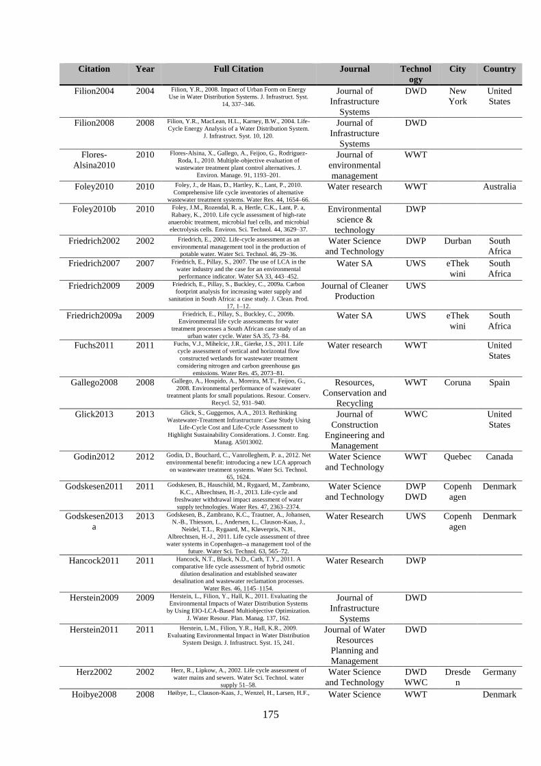
175


ogy

City Country

Filion2004 2004 Filion, Y.R., 2008. Impact of Urban Form on Energy

Use in Water Distribution Systems. J. Infrastruct. Syst.

14, 337–346.

Journal of

Infrastructure

Systems

DWD New

York

United

States

Filion2008 2008 Filion, Y.R., MacLean, H.L., Karney, B.W., 2004. Life-

Cycle Energy Analysis of a Water Distribution System.

J. Infrastruct. Syst. 10, 120.

Journal of

Infrastructure

Systems

DWD

Flores-

Alsina2010

2010 Flores-Alsina, X., Gallego, A., Feijoo, G., Rodriguez-

Roda, I., 2010. Multiple-objective evaluation of

wastewater treatment plant control alternatives. J.

Environ. Manage. 91, 1193–201.

Journal of

environmental

management

WWT

Foley2010 2010 Foley, J., de Haas, D., Hartley, K., Lant, P., 2010.

Comprehensive life cycle inventories of alternative

wastewater treatment systems. Water Res. 44, 1654–66.

Water research WWT Australia

Foley2010b 2010 Foley, J.M., Rozendal, R. a, Hertle, C.K., Lant, P. a,

Rabaey, K., 2010. Life cycle assessment of high-rate

anaerobic treatment, microbial fuel cells, and microbial

electrolysis cells. Environ. Sci. Technol. 44, 3629–37.

Environmental

science &

technology

DWP

Friedrich2002 2002 Friedrich, E., 2002. Life-cycle assessment as an

environmental management tool in the production of

potable water. Water Sci. Technol. 46, 29–36.

Water Science

and Technology

DWP Durban South

Africa

Friedrich2007 2007 Friedrich, E., Pillay, S., 2007. The use of LCA in the

water industry and the case for an environmental

performance indicator. Water SA 33, 443–452.

Water SA UWS eThek

wini

South

Africa

Friedrich2009 2009 Friedrich, E., Pillay, S., Buckley, C., 2009a. Carbon

footprint analysis for increasing water supply and

sanitation in South Africa: a case study. J. Clean. Prod.

17, 1–12.

Journal of Cleaner

Production

UWS

Friedrich2009a 2009 Friedrich, E., Pillay, S., Buckley, C., 2009b.

Environmental life cycle assessments for water

treatment processes a South African case study of an

urban water cycle. Water SA 35, 73–84.

Water SA UWS eThek

wini

South

Africa

Fuchs2011 2011 Fuchs, V.J., Mihelcic, J.R., Gierke, J.S., 2011. Life

cycle assessment of vertical and horizontal flow

constructed wetlands for wastewater treatment

considering nitrogen and carbon greenhouse gas

emissions. Water Res. 45, 2073–81.

Water research WWT United

States

Gallego2008 2008 Gallego, A., Hospido, A., Moreira, M.T., Feijoo, G.,

2008. Environmental performance of wastewater

treatment plants for small populations. Resour. Conserv.

Recycl. 52, 931–940.

Resources,

Conservation and

Recycling

WWT Coruna Spain

Glick2013 2013 Glick, S., Guggemos, A.A., 2013. Rethinking

Wastewater-Treatment Infrastructure: Case Study Using

Life-Cycle Cost and Life-Cycle Assessment to

Highlight Sustainability Considerations. J. Constr. Eng.

Manag. A5013002.

Journal of

Construction

Engineering and

Management

WWC United

States

Godin2012 2012 Godin, D., Bouchard, C., Vanrolleghem, P. a., 2012. Net

environmental benefit: introducing a new LCA approach

on wastewater treatment systems. Water Sci. Technol.

65, 1624.

Water Science

and Technology

WWT Quebec Canada

Godskesen2011 2011 Godskesen, B., Hauschild, M., Rygaard, M., Zambrano,

K.C., Albrechtsen, H.-J., 2013. Life-cycle and

freshwater withdrawal impact assessment of water

supply technologies. Water Res. 47, 2363–2374.

Water Science

and Technology

DWP

DWD

Copenh

agen

Denmark

Godskesen2013

a

2013 Godskesen, B., Zambrano, K.C., Trautner, A., Johansen,

N.-B., Thiesson, L., Andersen, L., Clauson-Kaas, J.,

Neidel, T.L., Rygaard, M., Kløverpris, N.H.,

Albrechtsen, H.-J., 2011. Life cycle assessment of three

water systems in Copenhagen--a management tool of the

future. Water Sci. Technol. 63, 565–72.

Water Research UWS Copenh

agen

Denmark

Hancock2011 2011 Hancock, N.T., Black, N.D., Cath, T.Y., 2011. A

comparative life cycle assessment of hybrid osmotic

dilution desalination and established seawater

desalination and wastewater reclamation processes.

Water Res. 46, 1145–1154.

Water Research DWP

Herstein2009 2009 Herstein, L., Filion, Y., Hall, K., 2011. Evaluating the

Environmental Impacts of Water Distribution Systems

by Using EIO-LCA-Based Multiobjective Optimization.

J. Water Resour. Plan. Manag. 137, 162.

Journal of

Infrastructure

Systems

DWD

Herstein2011 2011 Herstein, L.M., Filion, Y.R., Hall, K.R., 2009.

Evaluating Environmental Impact in Water Distribution

System Design. J. Infrastruct. Syst. 15, 241.

Journal of Water

Resources

Planning and

Management

DWD

Herz2002 2002 Herz, R., Lipkow, A., 2002. Life cycle assessment of

water mains and sewers. Water Sci. Technol. water

supply 51–58.

Water Science

and Technology

DWD

WWC

Dresde

n

Germany

Hoibye2008 2008 Høibye, L., Clauson-Kaas, J., Wenzel, H., Larsen, H.F., Water Science WWT Denmark

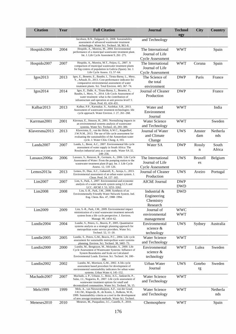
176


ogy

City Country

Jacobsen, B.N., Dalgaard, O., 2008. Sustainability

assessment of advanced wastewater treatment

technologies. Water Sci. Technol. 58, 963–8.

and Technology

Hospido2004 2004 Hospido, A., Moreira, M., 2004. Environmental

performance of a municipal wastewater treatment plant.

Int. J. Life Cycle Assesment 9, 261–271.

The International

Journal of Life

Cycle Assessment

WWT Spain

Hospido2007 2007 Hospido, A., Moreira, M.T., Feijoo, G., 2007. A

comparison of municipal wastewater treatment plants

for big centres of population in Galicia (Spain). Int. J.

Life Cycle Assess. 13, 57–64.

The International

Journal of Life

Cycle Assessment

WWT Coruna Spain

Igos2013 2013 Igos, E., Benetto, E., Baudin, I., Tiruta-Barna, L., Mery,

Y., Arbault, D., 2013. Cost-performance indicator for

comparative environmental assessment of water

treatment plants. Sci. Total Environ. 443, 367–74.

The Science of

the total

environment

DWP Paris France

Igos2014 2014 Igos, E., Dalle, A., Tiruta-Barna, L., Benetto, E.,

Baudin, I., Mery, Y., 2014. Life Cycle Assessment of

water treatment: what is the contribution of

infrastructure and operation at unit process level? J.

Clean. Prod. 65, 424–431.

Journal of Cleaner

Production

DWP France

Kalbar2013 2013 Kalbar, P.P., Karmakar, S., Asolekar, S.R., 2013.

Assessment of wastewater treatment technologies: life

cycle approach. Water Environ. J. 27, 261–268.

Water and

Environment

Journal

WWT India

Karrman2001 2001 Kärrman, E., Jönsson, H., 2001. Normalising impacts in

an environmental systems analysis of wastewater

systems. Water Sci. Technol. 43, 293–300.

Water Science

and Technology

WWT Sweden

Klaversma2013 2013 Klaversma, E., van der Helm, A.W.C., Kappelhof,

J.W.N.M., 2013. The use of life cycle assessment for

evaluating the sustainability of the Amsterdam water

cycle. J. Water Clim. Chang. 4, 103.

Journal of Water

and Climate

Change

UWS Amster

dam

Netherla

nds

Landu2007 2007 Landu, L., Brent, A.C., 2007. Environmental life cycle

assessment of water supply in South Africa: The

Rosslyn industrial area as a case study. Water SA 32,

249–256.

Water SA DWP Rossly

n

South

Africa

Lassaux2006a 2006 Lassaux, S., Renzoni, R., Germain, A., 2006. Life Cycle

Assessment of Water: From the pumping station to the

wastewater treatment plant (9 pp). Int. J. Life Cycle

Assess. 12, 118–126.

The International

Journal of Life

Cycle Assessment

UWS Bruxell

es

Belgium

Lemos2013a 2013 Lemos, D., Dias, A.C., Gabarrell, X., Arroja, L., 2013.

Environmental assessment of an urban water system. J.

Clean. Prod. 54, 157–165.

Journal of Cleaner

Production

UWS Aveiro Portugal

Lim2007 2007 Lim, S., Park, J., 2007. Environmental and economic

analysis of a water network system using LCA and

LCC. AIChE J. 53, 3253–3262.

AIChE Journal DWP

DWD

Lim2008 2008 Lim, S.-R., Park, J.M., 2008. Synthesis of an

Environmentally Friendly Water Network System. Ind.

Eng. Chem. Res. 47, 1988–1994.

Industrial &

Engineering

Chemistry

Research

DWD

Lim2009 2009 Lim, S.-R., Park, J.M., 2009. Environmental impact

minimization of a total wastewater treatment network

system from a life cycle perspective. J. Environ.

Manage. 90, 1454–62.

Journal of

environmental

management

WWC

WWT

Lundie2004 2004 Lundie, S., Peters, G., Beavis, P., 2005. Quantitative

systems analysis as a strategic planning approach for

metropolitan water service providers. Water Sci.

Technol. 52, 11–20.

Environmental

science &

technology

UWS Sydney Australia

Lundie2005 2005 Lundie, S., Peters, G.M., Beavis, P.C., 2004. Life cycle

assessment for sustainable metropolitan water systems

planning. Environ. Sci. Technol. 38, 3465–73.

Water Science

and Technology

WWT

Lundin2000 2000 Lundin, M., Bengtsson, M., Molander, S., 2000. Life

Cycle Assessment of Wastewater Systems: Influence of

System Boundaries and Scale on Calculated

Environmental Loads. Environ. Sci. Technol. 34, 180–

186.

Environmental

science &

technology

WWT Lulea Sweden

Lundin2002 2002 Lundin, M., Morrison, G.M., 2002. A life cycle

assessment based procedure for development of

environmental sustainability indicators for urban water

systems. Urban Water 4, 145–152.

Urban Water

Journal

UWS Gotebo

rg

Sweden

Machado2007 2007 Machado, a. P., Urbano, L., Brito, A.G., Janknecht, P.,

Salas, J.J., Nogueira, R., 2007. Life cycle assessment of

wastewater treatment options for small and

decentralized communities. Water Sci. Technol. 56, 15.

Water Science

and Technology

WWT

Mels1999 1999 Mels, A., van Nieuwenhuijzen, A.F., van der Graaf,

J.H.J.M., Klapwijk, B., de Konin, J., Rulkens, W.H.,

1999. Sustainability criteria as a tool in the development

of new sewage treatment methods. Water Sci. Technol.

Water Science

and Technology

WWT Netherla

nds

Meneses2010 2010 Meneses, M., Pasqualino, J.C., Castells, F., 2010. Chemosphere WWT Spain

177


ogy

City Country

Environmental assessment of urban wastewater reuse:

treatment alternatives and applications. Chemosphere

81, 266–72.

Mery2013 2013 Mery, Y., Tiruta-Barna, L., Benetto, E., Baudin, I.,

2013. An integrated “process modelling-life cycle

assessment” tool for the assessment and design of water

treatment processes. Int. J. Life Cycle Assess.

The International

Journal of Life

Cycle Assessment

DWP Paris France

Mo2010 2010 Mo, W., Nasiri, F., Eckelman, M.J., Zhang, Q.,

Zimmerman, J.B., 2010. Measuring the embodied

energy in drinking water supply systems: a case study in

the Great Lakes region. Environ. Sci. Technol. 44,

9516–21.

Environmental

science &

technology

DWP

DWD

Kalama

zoo

United

States

Mo2011 2011 Mo, W., Zhang, Q., Mihelcic, J.R., Hokanson, D.R.,

2011. Embodied energy comparison of surface water

and groundwater supply options. Water Res. 45, 5577–

5586.

Water research DWP

DWD

Kalama

zoo \&

Tampa

United

States

Mohamed-

Zine2013

2013 Mohamed-Zine, M.-B., Hamouche, A., Krim, L., 2013.

The study of potable water treatment process in Algeria

(boudouaou station) -by the application of life cycle

assessment (LCA). J. Environ. Heal. Sci. Eng. 11, 37.

Journal of

environmental

health science &

engineering

DWP Algeria

Mohapatra2002 2002 Mohapatra, P., Siebel, M., Gijzen, H., Van der Hoek, J.,

Groot, C., 2002. Improving eco-efficiency of

Amsterdam water supply: A LCA approach. Aqua 51,

217–227.

Aqua DWP Amster

dam

Netherla

nds

Moore2013 2013 Moore, T.L.C., Hunt, W.F., 2013. Predicting the carbon

footprint of urban stormwater infrastructure. Ecol. Eng.

58, 44–51.

Ecological

Engineering

WWC United

States

Munoz2008 2008 Muñoz, I., Fernández-Alba, A.R., 2008. Reducing the

environmental impacts of reverse osmosis desalination

by using brackish groundwater resources. Water Res.

42, 801–11.

Water research DWP Almeri

a

Spain

Munoz2010b 2010 Muñoz, I., Milà-i-Canals, L., Fernández-Alba, A.R.,

2010. Life Cycle Assessment of Water Supply Plans in

Mediterranean Spain. J. Ind. Ecol. 14, 902–918.

Journal of

Industrial Ecology

UWS Spain

Nogueira2009 2009 Nogueira, R., Brito, A.G., Machado, A.P., Janknecht, P.,

Salas, J.J., Vera, L., Martel, G., 2009. Economic and

environmental assessment of small and decentralized

wastewater treatment systems. Desalin. Water Treat. 4,

16–21.

Desalination and

Water Treatment

WWT Minho Portugal

Ortiz2007 2007 Ortiz, M., Raluy, R., Serra, L., 2007. Life cycle

assessment of water treatment technologies: wastewater

and water-reuse in a small town. Desalination 204, 121–

131.

Desalination WWT Tauste Spain

Pasqualino2009 2009 Pasqualino, J.C., Meneses, M., Abella, M., Castells, F.,

2009. LCA as a decision support tool for the

environmental improvement of the operation of a

municipal wastewater treatment plant. Environ. Sci.

Technol. 43, 3300–7.

Environmental

science &

technology

WWT Tarrago

na

Spain

Pasqualino2011

a

2011 Pasqualino, J.C., Meneses, M., Castells, F., 2011. Life

Cycle Assessment of Urban Wastewater Reclamation

and Reuse Alternatives. J. Ind. Ecol. 15, 49–63.

Journal of

Industrial Ecology

WWT Barcelo

na

Spain

Piratla2012 2011 Piratla, K., Ariaratnam, S.T., Cohen, A., 2011.

Estimation of CO 2 emissions from the life cycle of a

potable water pipeline project. J. Manag. … 22–30.

Urban Water

Journal

DWD Phoeni

x

United

States

Poussade2011 2011 Poussade, Y., Vince, F., Robillot, C., 2011. Energy

consumption and greenhouse gases emissions from the

use of alternative water sources in South East

Queensland. Water Sci. Technol. Water Supply 11, 281.

Water Science

and Technology

DWP South

East

Queens

land

Australia

Qi2012 2012 Qi, C., Chang, N.-B., 2012. Integrated carbon footprint

and cost evaluation of a drinking water infrastructure

system for screening expansion alternatives. J. Clean.

Prod. 27, 51–63.

Journal of Cleaner

Production

UWS Manate

e

County

United

States

Racoviceanu20

07a

2007 Racoviceanu, A.I., Karney, B.W., Kennedy, C.A.,

Colombo, A.F., 2007. Life-Cycle Energy Use and

Greenhouse Gas Emissions Inventory for Water

Treatment Systems. J. Infrastruct. Syst. 13, 261–270.

Journal of

Infrastructure

Systems

WWT Toront

o

Canada

Raluy2004 2004 Raluy, R.G., Serra, L., Uche, J., 2004. Life Cycle

Assessment of Water Production Technologies - Part 1:

Life Cycle Assessment of Different Commercial

Desalination Technologies (MSF, MED, RO) (9 pp). Int.


The International

Journal of Life

Cycle Assessment

DWP

Raluy2004a 2004 Raluy, R.G., Serra, L., Uche, J., Valero, A., 2004. Life

Cycle Assessment of Water Production Technologies -

Part 2: Reverse Osmosis Desalination versus the Ebro

River Water Transfer (9 pp). Int. J. Life Cycle Assess.

10, 346–354.

The International

Journal of Life

Cycle Assessment

DWP Spain

Remy2008 2008 Remy, C., Jekel, M., 2008. Sustainable wastewater

management: life cycle assessment of conventional and Water Science WWT Germany

178


ogy

City Country

source-separating urban sanitation systems. Water Sci.

Technol. 58, 1555–62. and Technology

Remy2012 2012 Remy, C., Jekel, M., 2012. Energy analysis of

conventional and source-separation systems for urban

wastewater management using Life Cycle Assessment.

Water Sci. Technol. 65, 22–9.

Water Science

and Technology

UWS Berlin Germany

Renou2008 2008 Renou, S., Thomas, J.S., Aoustin, E., Pons, M.N., 2008.

Influence of impact assessment methods in wastewater

treatment LCA. J. Clean. Prod. 16, 1098–1105.

Journal of Cleaner

Production

WWT France

Ribera2013 2013 Ribera, G., Clarens, F., Martínez-Lladó, X., Jubany, I.,

V Martí, Rovira, M., 2013. Life cycle and human health

risk assessments as tools for decision making in the

design and implementation of nanofiltration in drinking

water treatment plants. Sci. Total Environ. 466-467C,

377–386.

The Science of

the total

environment

DWP Manres

a

Spain

Risch2014 2014 Risch, E., Loubet, P., Núñez, M., Roux, P., 2014. How

environmentally significant is water consumption during

wastewater treatment? : Application of recent

developments in LCA to WWT technologies used at 3

contrasted geographical locations. Water Res.

Water Research WWT France

Rodriguez-

Garcia2011

2011 Rodriguez-Garcia, G., Molinos-Senante, M., Hospido,

A., Hernandez-Sancho, F., Moreira, M.T., Feijoo, G.,

2011. Environmental and economic profile of six

typologies of wastewater treatment plants. Water Res. 5.

Water Research WWT Spain

Roeleveld1997 1997 Roeleveld, P., Klapwijk, A., Eggels, P.G., Rulkens,

W.H., van Starkenburg, W., 1997. Sustainability of

municipal waste water treatment. Water Sci. Technol.

Water science and

Technology

WWT Netherla

nds

Rowley2009 2009 Rowley, H. V., Lundie, S., Peters, G.M., 2009. A hybrid

life cycle assessment model for comparison with

conventional methodologies in Australia. Int. J. Life

Cycle Assess. 14, 508–516.

The International

Journal of Life

Cycle Assessment

UWS Australia

Sahely2005 2005 Sahely, H.R., Kennedy, C.A., Adams, B., 2005.

Developing sustainability criteria for urban

infrastructure systems. Can. J. Civ. Eng. 32, 72–85.

Canadian Journal

of Civil

Engineering

UWS Toront

o

Canada

Sharaai2009b 2009 Sharaai, A.H., Mahmood, N.Z., Sulaiman, A.H., 2009.

Life Cycle Impact Assessment (LCIA) of Potable Water

Treatment Process in Malaysia: Comparison Between

Dissolved Air Flotation (DAF) and Ultrafiltration (UF)

Technology. Aust. J. Basic Appl. Sci. 3, 3625–3632.

Australian Journal

of Basic and

Applied Sciences

DWP

Sharaai2010 2010 Sharaai, A.H., Mahmood, N.Z., Sulaiman, A.H., 2010.

Life Cycle Impact Assessment ( LCIA ) in Potable

Water Production in Malaysia : Potential Impact

Analysis Contributed from Production and Contruction

Phase Using Eco-indicator 99 Evaluation Method.

World Appl. Sci. J. 11, 1230–1237.

World Applied

Sciences Journal

DWP Malaysia

Sharaai2011 2011 Sharaai, A.H., Mahmood, N.Z., Sulaiman, A.H., 2011.

Life cycle impact assessment (LCIA) using EDIP 97

method: An analysis of potential impact from potable

water production. Sci. Res. Essays 6, 5658–5670.

Scientific

Research and

Essays

DWP Malaysia

Slagstad2013 2013 Slagstad, H., Brattebø, H., 2013. Life cycle assessment

of the water and wastewater system in Trondheim,

Norway – A case study. Urban Water J. 1–12.

Urban Water

Journal

UWS Trondh

eim

Norway

Sombekke1997 1997 Sombekke, H., Voorhoeve, D., Hiemstra, P., 1997.

Environmental impact assessment of groundwater

treatment with nanofiltration. Desalination 113, 293–

296.

Desalination DWP Hamme

rflier

Netherla

nds

Stokes2005 2005 Stokes, J., Horvath, A., 2005. Life Cycle Energy

Assessment of Alternative Water Supply Systems (9

pp). Int. J. Life Cycle Assess. 11, 335–343.

The International

Journal of Life

Cycle Assessment

DWP

DWD

Califor

nia

United

States

Stokes2006 2006 Stokes, J., Horvath, A., 2006. LCA Methodology and

Case Study Life Cycle Energy Assessment of

Alternative Water Supply Systems. Int. J. Life Cycle

Assess. 11, 335 – 343.

The International

Journal of Life

Cycle Assessment

DWP

DWD

Stokes2009 2009 Stokes, J., Horvath, A., 2009. Energy and air emission

effects of water supply. Environ. Sci. Technol. 43,

2680–2687.

Environmental

science &

technology

DWP

DWD

Califor

nia

United

States

Stokes2011 2011 Stokes, J., Horvath, A., 2011. Life-Cycle Assessment of

Urban Water Provision: Tool and Case Study in

California. J. Infrastruct. Syst. 17, 15.

Journal of

Infrastructure

Systems

DWP

DWD

Califor

nia

United

States

Tarnacki2011 2011 Tarnacki, K.M., Melin, T., Jansen, a. E., van Medevoort,

J., 2011. Comparison of environmental impact and

energy efficiency of desalination processes by LCA.

Water Sci. Technol. Water Supply 11, 246.

Water Science

and Technology

DWP

Tillman1998 1998 Tillman, A.M., Svingby, M., Lundström, H., 1998. Life

cycle assessment of municipal waste water systems. Int.


The International

Journal of Life

UWS Bergsjo

n

Sweden

179


ogy

City Country

Cycle Assessment

Uche2013 2013 Uche, J., Martínez-Gracia, A., Carmona, U., 2013. Life

cycle assessment of the supply and use of water in the

Segura Basin. Int. J. Life Cycle Assess.

The International

Journal of Life

Cycle Assessment

DWP

DWD

Alicant

e

Spain

VanderHelm20

08

2008 Van der Helm, a. W.C., Rietveld, L.C., Bosklopper,

T.G.J., Kappelhof, J.W.N.M., van Dijk, J.C., 2008.

Objectives for optimization and consequences for

operation, design and concept of drinking water

treatment plants. Water Sci. Technol. Water Supply 8,

297.

Water Science

and Technology

DWP Amster

dam

Netherla

nds

Venkatesh2009 2009 Venkatesh, G., Brattebø, H., 2011. Energy consumption,

costs and environmental impacts for urban water cycle

services: Case study of Oslo (Norway). Energy 36, 792–

800.

Journal of

Industrial Ecology

WWC Oslo Norway

Venkatesh2011 2011 Venkatesh, G., Brattebø, H., 2011. Environmental

impact analysis of chemicals and energy consumption in

wastewater treatment plants: case study of Oslo,

Norway. Water Sci. Technol. 63, 1018–31.

Energy UWS Oslo Norway

Venkatesh2011

a

2011 Venkatesh, G., Brattebø, H., 2012a. Assessment of

Environmental Impacts of an Aging and Stagnating

Water Supply Pipeline Network. J. Ind. Ecol. 00, no–no.

Water Science

and Technology

WWT Oslo Norway

Venkatesh2012 2012 Venkatesh, G., Brattebø, H., 2012b. Environmental

analysis of chemicals and energy consumption in water

treatment plants: case study of Oslo, Norway. Water Sci.

Technol. Water Supply 12, 200.

Journal of

Industrial Ecology

DWD Oslo Norway

Venkatesh2012

a

2012 Venkatesh, G., Hammervold, J., Brattebø, H., 2009.

Combined MFA-LCA for Analysis of Wastewater

Pipeline Networks. J. Ind. Ecol. 13, 532–550.

Water Science

and Technology

DWP Oslo Norway

Vidal2002 2002 Vidal, N., Poch, M., Marti, E., Rodriguez-Roda, I.,

2002. Evaluation of the environmental implications to

include structural changes in a wastewater treatment

plant. J. Chem. Technol. Biotechnol. 77, 1206–1211.

Journal of

Chemical

Technology&

Biotechnology

WWT Spain

Vince2008 2008 Vince, F., Aoustin, E., Breant, P., Marechal, F., 2008.

LCA tool for the environmental evaluation of potable

water production. Desalination 220, 37–56.

Desalination DWP

Vlasopoulos200

6

2006 Vlasopoulos, N., Memon, F. a, Butler, D., Murphy, R.,

2006. Life cycle assessment of wastewater treatment

technologies treating petroleum process waters. Sci.

Total Environ. 367, 58–70.

The Science of

the total

environment

WWT

Wang2012 2012 Wang, X., Liu, J., Ren, N.-Q., Duan, Z., 2012.

Environmental profile of typical anaerobic/anoxic/oxic

wastewater treatment systems meeting increasingly

stringent treatment standards from a life cycle

perspective. Bioresour. Technol. 126C, 31–40.

Bioresource

technology

WWT China

Wenzel2008 2008 Wenzel, H., Larsen, H.F., Clauson-Kaas, J., Høibye, L.,

Jacobsen, B.N., 2008. Weighing environmental

advantages and disadvantages of advanced wastewater

treatment of micro-pollutants using environmental life

cycle assessment. Water Sci. Technol. 57, 27–32.

Water Science

and Technology

WWT

Wu2010 2010 Wu, J.-G., Meng, X.-Y., Liu, X.-M., Liu, X.-W., Zheng,

Z.-X., Xu, D.-Q., Sheng, G.-P., Yu, H.-Q., 2010. Life

cycle assessment of a wastewater treatment plant

focused on material and energy flows. Environ. Manage.

46, 610–7.

Environmental

management

WWT Bengdu

City

China

Wu2010a 2010 Wu, W., Maier, H.R., Simpson, A.R., 2010a. Single-

Objective versus Multiobjective Optimization of Water

Distribution Systems Accounting for Greenhouse Gas

Emissions by Carbon Pricing. J. Water Resour. Plan.

Manag. 136, 555–565.

Journal of Water

Resources

Planning and

Management

DWD Australia

Wu2010b 2010 Wu, W., Simpson, A.R., Maier, H.R., 2010b.

Accounting for Greenhouse Gas Emissions in

Multiobjective Genetic Algorithm Optimization of

Water Distribution Systems. J. Water Resour. Plan.

Manag. 136, 146–155.

Journal of Water

Resources

Planning and

Management

DWD

Yldrm2012 2012 Yıldırım, M., Topkaya, B., 2012. Assessing

Environmental Impacts of Wastewater Treatment

Alternatives for Small-Scale Communities. CLEAN -

Soil, Air, Water 40, 171–178.

CLEAN - Soil,

Air, Water

WWT

Zhang2000 2000 Zhang, Q.H., Wang, X.C., Xiong, J.Q., Chen, R., Cao,

B., 2010. Application of life cycle assessment for an

evaluation of wastewater treatment and reuse project--

case study of Xi’an, China. Bioresour. Technol. 101,

1421–5.

Water and

Environment

Journal

WWT Singapor

e

Zhang2010a 2010 Zhang, Z., 2000. Life-Cycle Assessment of a Sewage-

Treatment Plant in South-East Asia. Water Environ. J.

14, 51–56.

Bioresource

technology

WWT Xi'an China

181

Annex B. Assessing water deprivation at the sub-river basin scale

in LCA integrating downstream cascade effects


Chapter 3 and published in Environmental Science & Technology (Loubet et al. 2013).

182

B.1. Illustration of the Consumption-to-Availability ratio at the sub-

river basin scale

Figure B-1. Water consumption and water availability propagation through a river basin. Subscripts: i=assessed SRB, 1 to

i=all upstream SRBs, i+1=first downstream SRB; Superscripts: mod.=modified, reg.=regulated; RO=Runoff, D=Discharge,

tWC=total Water Consumption, WA=Water Availability, EWR=Environmental Water Requirements.

B.2. Description of the Pfafstetter topologic navigation system

The identification of the upstream and downstream sub-river basins for each SRB has been

made from the Pfafstetter sub-river basin coding system provided by the HYDRO1k database.

The Pfafstetter system is hierarchal, and sub-river basins are delineated from junctions on a

river network. Level 1 basins correspond to continental scale basins. Higher levels (levels 2,

3, 4, etc.) represent ever-finer tessellations of the land surface into smaller basins. Each basin

is assigned a specific Pfafstetter Code based on its location within the overall drainage system

and on the total drainage area upstream of the watershed’s outlet. In the Hydro1K database,

each smallest sub-river basin unit has 6 Pfafstetter digits, each one corresponding to a level of

basin.

183

Figure B-2. Downstream and upstream SRBs identification according to the Pfafstetter system.

In Figure B-2. Downstream and upstream SRBs identification according to the

Pfafstetter system.Figure B-2 is presented the original ID of each sub-river basin of the Seine

river basin according to Hydro1k database. The four first digits (i.e., 9132) are common for

each SRB and characterize the Seine river basin. The two last digits are those presented in the

paper and are different for each SRB.

The last digit which is not zero gives information on the position of the sub-river basin: if it is

an even digit (2, 4, 6, 8), the SRB has no upstream SRB, if it is an odd digit (1, 3, 5, 7, 9), the

SRB has two upstream SRBs, excepted the last upstream SRB. The most downstream SRB

has the digit 1 and the two most upstream have the digit 8 and 9. Consequently, a SRB which

has an odd last digit k will have two upstream SRBs k+1 and k+2 and one downstream SRB

k-2. For example, in the Figure B-2, basin 913270 have two direct upstream basins (913280

and 913290) and one direct downstream SRB (913250). It has also two other downstream

SRBs (k-4 and k-6), i.e., 913230 and 913210.

Since the routine made available by Furnans and Olivera (2001) gives automatically the two

direct upstream and the direct downstream basins of each basin, we built a routine which

navigates within the SRBs data table to locate all the downstream and upstream SRBs of each

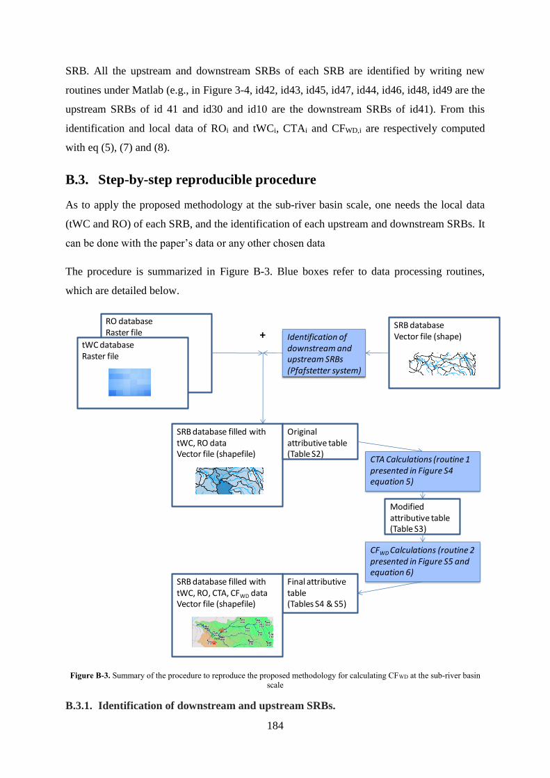
184

SRB. All the upstream and downstream SRBs of each SRB are identified by writing new

routines under Matlab (e.g., in Figure 3-4, id42, id43, id45, id47, id44, id46, id48, id49 are the

upstream SRBs of id 41 and id30 and id10 are the downstream SRBs of id41). From this

identification and local data of ROi and tWCi, CTAi and CFWD,i are respectively computed

with eq (5), (7) and (8).

B.3. Step-by-step reproducible procedure

As to apply the proposed methodology at the sub-river basin scale, one needs the local data

(tWC and RO) of each SRB, and the identification of each upstream and downstream SRBs. It

can be done with the paper’s data or any other chosen data

The procedure is summarized in Figure B-3. Blue boxes refer to data processing routines,

which are detailed below.

Figure B-3. Summary of the procedure to reproduce the proposed methodology for calculating CFWD at the sub-river basin

scale

B.3.1. Identification of downstream and upstream SRBs.

RO databaseRaster file

tWC databaseRaster file

SRB databaseVector file (shape)+

SRB database filled with tWC, RO dataVector file (shapefile)

Original attributive table(Table S2)

Identification of downstream and upstream SRBs (Pfafstetter system)

CTA Calculations (routine 1 presented in Figure S4 equation 5)

CFWD Calculations (routine 2 presented in Figure S5 and equation 6)

Final attributive table(Tables S4 & S5)

SRB database filled with tWC, RO, CTA, CFWD dataVector file (shapefile)

Modified attributive table(Table S3)

185

One method (Pfafstetter) is explained in the previous part of SI. From this identification and

the merging of SRBs vector file and tWC, RO and p (area, population, volume) raster files,

the following attributive table is built:

Table B-1. Attributive table filled with hydrologic parameters and identification of upstream and downstream SRBs. a is the

index of the SRB, id is the simplified Pfafstetter identifier of SRBi, down is the simplified Pfafstetter identifier of the

downstream SRB of SRBi, up1 and up2 are the simplified Pfafstetter identifiers of the two upstream SRBs of SRB i.

Displayed data are not real and are shown as an example.

a id

=SRBi

down

=SRBi+1

up1

=SRBi-1

up2

=SRBi-2

tWCi (m3) ROi (m3) p (area,

population,

…)

5 (n) 10 0 20 30 10 50

4 20 10 0 0 10 50

3 30 10 40 50 10 100

2 40 30 0 0 10 100

1 50 30 0 0 10 100

B.3.2. CTA calculations – upstream parameters

First, tWC1 to i and RO1 to i are calculated for each SRBs, taking into account upstream data.

From the Table B-1 data and the Figure B-4, the following routine is applied to calculate the

upstream sum of a parameter (tWC or RO).

186

Figure B-4. Routine that calculates upstream parameters (e.g. tWC, here). uptWC(i) represents tWC1 to i. J is assigned from

Figure B-5.

The array that contains j and k indices stocks all the upstream SRBs for each SRBi, according

to Figure B-5.

k = 2J ?

j = J?

uptWC(a) = uptWC(a) + tWC(b)

array(j+1,2*k-1) = up1(b)

array(j+1,2*k) = up2(b)

NO

YES

Attributive table filled with

upstream parameters (Table S3)

NOj = j+1

k = k+1array(j,k)

= 0 ?

NOYES

b=array(j,k)

a = n?YES

NO

a = a+1

a = 1

YES

Load attributive Table S2

j = 1k = 1

array(j,k) = up1(a)array(j,k+1) = up2(a)

uptWC(a) = 0

187

Figure B-5. Scheme representing the possible upstream SRBs of a SRBi

Then, WA and CTA are simply calculated for each SRBs according to eq (5) and (7). From

there, the attributive table is modified as shown in Figure B-2.

Table B-2. Modified attributive table filled with upstream parameters and CTA. Displayed data are not real and are shown as

an example.

a id

=SRBi

down

=SRBi+1

up1

=SRBi-1

up2

=SRBi-2

tWCi

(m3)

ROi

(m3)

p (area,

population)

uptWCi WAi CTA

5 10 0 20 30 10 50 50 80 0.625

4 20 10 0 0 10 50 10 10 1

3 30 10 40 50 10 100 30 60 0.5

2 40 30 0 0 10 100 10 20 0.5

1 50 30 0 0 10 100 10 20 0.5

SRBi

SRB1…

row

s

columns

…

upstream

downstream

1J

2J1k =

j=

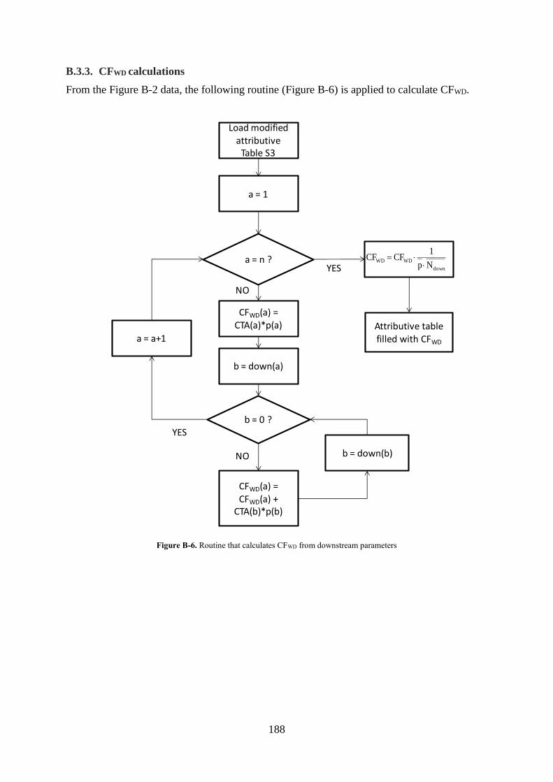
188

B.3.3. CFWD calculations

From the Figure B-2 data, the following routine (Figure B-6) is applied to calculate CFWD.

Figure B-6. Routine that calculates CFWD from downstream parameters

CFWD(a) = CFWD(a) +

CTA(b)*p(b)

b = 0 ?

a = n ?

NO

YES

a = 1

NO

YES

a = a+1

b = down(b)

CFWD(a) = CTA(a)*p(a)

b = down(a)

Attributive table filled with CFWD

Load modified attributive

Table S3

down

WDWDNp

1CFCF

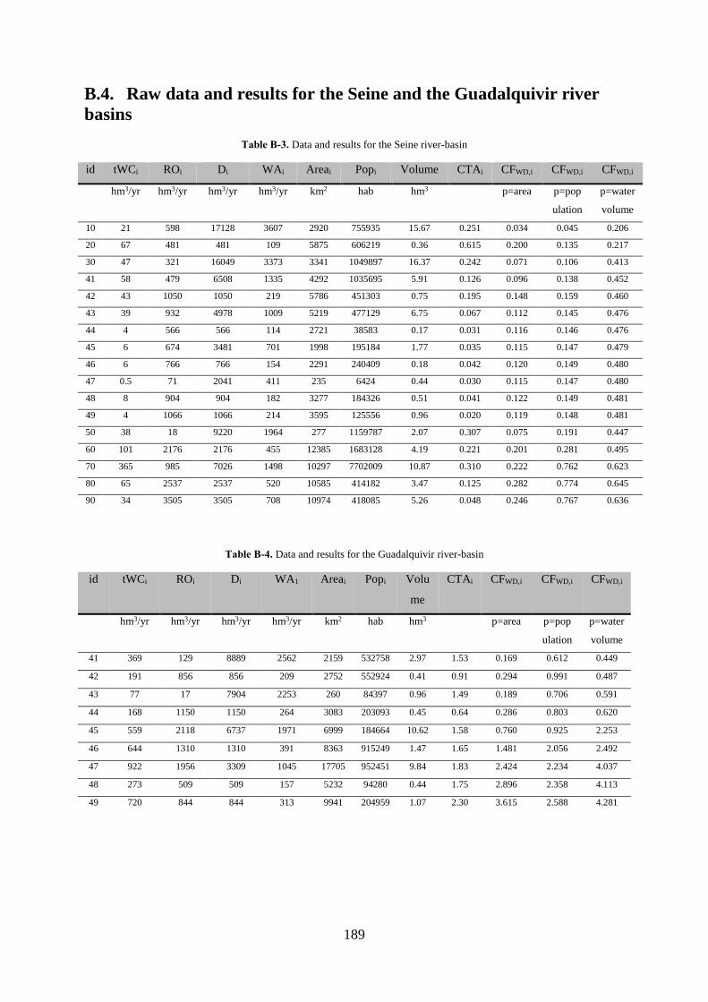
189

B.4. Raw data and results for the Seine and the Guadalquivir river

basins

Table B-3. Data and results for the Seine river-basin

id tWCi ROi Di WAi Areai Popi Volume CTAi CFWD,i CFWD,i CFWD,i

hm3/yr hm3/yr hm3/yr hm3/yr km2 hab hm3 p=area p=pop

ulation

p=water

volume

10 21 598 17128 3607 2920 755935 15.67 0.251 0.034 0.045 0.206

20 67 481 481 109 5875 606219 0.36 0.615 0.200 0.135 0.217

30 47 321 16049 3373 3341 1049897 16.37 0.242 0.071 0.106 0.413

41 58 479 6508 1335 4292 1035695 5.91 0.126 0.096 0.138 0.452

42 43 1050 1050 219 5786 451303 0.75 0.195 0.148 0.159 0.460

43 39 932 4978 1009 5219 477129 6.75 0.067 0.112 0.145 0.476

44 4 566 566 114 2721 38583 0.17 0.031 0.116 0.146 0.476

45 6 674 3481 701 1998 195184 1.77 0.035 0.115 0.147 0.479

46 6 766 766 154 2291 240409 0.18 0.042 0.120 0.149 0.480

47 0.5 71 2041 411 235 6424 0.44 0.030 0.115 0.147 0.480

48 8 904 904 182 3277 184326 0.51 0.041 0.122 0.149 0.481

49 4 1066 1066 214 3595 125556 0.96 0.020 0.119 0.148 0.481

50 38 18 9220 1964 277 1159787 2.07 0.307 0.075 0.191 0.447

60 101 2176 2176 455 12385 1683128 4.19 0.221 0.201 0.281 0.495

70 365 985 7026 1498 10297 7702009 10.87 0.310 0.222 0.762 0.623

80 65 2537 2537 520 10585 414182 3.47 0.125 0.282 0.774 0.645

90 34 3505 3505 708 10974 418085 5.26 0.048 0.246 0.767 0.636

Table B-4. Data and results for the Guadalquivir river-basin

id tWCi ROi Di WA1 Areai Popi Volu

me

CTAi CFWD,i CFWD,i CFWD,i

hm3/yr hm3/yr hm3/yr hm3/yr km2 hab hm3 p=area p=pop

ulation

p=water

volume

41 369 129 8889 2562 2159 532758 2.97 1.53 0.169 0.612 0.449

42 191 856 856 209 2752 552924 0.41 0.91 0.294 0.991 0.487

43 77 17 7904 2253 260 84397 0.96 1.49 0.189 0.706 0.591

44 168 1150 1150 264 3083 203093 0.45 0.64 0.286 0.803 0.620

45 559 2118 6737 1971 6999 184664 10.62 1.58 0.760 0.925 2.253

46 644 1310 1310 391 8363 915249 1.47 1.65 1.481 2.056 2.492

47 922 1956 3309 1045 17705 952451 9.84 1.83 2.424 2.234 4.037

48 273 509 509 157 5232 94280 0.44 1.75 2.896 2.358 4.113

49 720 844 844 313 9941 204959 1.07 2.30 3.615 2.588 4.281

190

B.5. Comparison with other water scarcity indicators found in the

literature

Table B-5. Water deprivation/scarcity indicators calculated for two river basins using different available methods

Seine Guadalquivir

Yearly CFWD at sub-river basin scale (m3 equivalent/m3)

1 -Sub-river basin CFWD p=area: average (min - max)

[Paper data]

0.18

(0.03 – 0.28)

1.89

(0.16 – 3.46)

1bis -Sub-river basin CFWD p=population: average (min -

max) [Paper data]

0.47

(0.04 – 0.77)

1.62

(0.61 – 2.59)

1ter -Sub-river basin CFWD p=volume: average (min -

max) [Paper data]

0.44

(0.20 – 0.64)

2.70

(0.45 – 4.28)

Yearly CTA (or WTA) at river basin scale (m3 equivalent/m3)

2- River basin CTA [Paper data or Hoekstra et al. (2012)] 0.25 1.58

3- River basin WTA [WaterGap2: Alcamo et al. (2003)] –

used by Water Stress Index (WSI) of Pfister et al. (2009)

0.52 1.37

4- River basin WTA [Smakhtin et al. (2004)] – used by

Water Stress Indicator (WSI) of (Milà i Canals et al.,

2008)

0.53 1.77

5- River basin CTA – used by “Water Use Scarcity”

(Frischknecht et al., 2006)

0.58 1.50

Average of monthly CTA at river basin scale (m3 equivalent/m3)

6- River basin CTA (Hoekstra et al., 2012) 0.83 2.38

Table B-5 provides a comparison between the different methods used to assess water scarcity

at the river basin scale. Mean CFWD values, as well as river basin scale CTA values, were

calculated with this paper data. In both river basins, the difference between the minimum and

maximum values of the CFWD is greater than one order of magnitude. This significant

variation underscores the interest and need for taking into account downstream effects. CFWD

values at the SRB scale have a high variation in both examples and thus provide useful

information that cannot be shown by previous indicators. It should be noted that the yearly

CTA (line 2) is different from the arithmetic average of monthly CTA values (line 6), even

though the same databases (water consumption (Hoekstra et al., 2012) and runoff (Fekete,

191

2002)) were used in both cases. The ratio of the yearly values is not equal to the average of

the monthly ratios.

B.6. Adaptation of the framework to existing endpoint CFs (from

Hanafiah et al.)

Hanafiah et al. (2011) developed following endpoint CF for water use impacts on freshwater

species richness as following:

river

river,mouth

riverint,endpo VD

4,0FC (S1)

Where CFendpoint, river is expressed in PDF.m3.yr.m-3, Dmouth, river is the discharge (m3.yr-1) of the

river at the mouth, Vriver basin is the estimated volume (m3) of the river.

Using our framework, this CF can be adapted at the sub-river basin scale as per eq S2:

n

ij

j

j

i,intendpo VD

4,0FC

(S2)

where Dj is the discharge (m3.yr-1) of the SRBj, Vj is the estimated volume (m3) of the SRBj

and Dj is the discharge (m3.yr-1) of the SRBj. The CF is the sum of effects on downstream

SRBs. Each effect on SRB is calculated with eq S1 adapted according data at the SRB scale.

We can note that no weighted parameter is needed since volume is already taken into account

in the effect factor.

Hanafiah et al. calculated the volume of a river as following:

river

90.0

river,mouth

river L2

D47.0V

(S3)

where Vriver is in m3, Dmouth, river is in m3.s-1 and Lriver is the length of the river within the river

basin (m).

This volume calculation is adapted to a SRB. D/2 is supposed to be the mean discharge within

a river basin. At the sub-river basin scale, this hypothesis is adapated: the mean discharge

would be the upstream runoff plus half of the local runoff. Eq S4 shows the evaluation of the

volume within a SRBi.

192

i

90.0

i1ii L

2

ROD47.0V

(S4)

Where Vi is the volume of the rivers contained in SRBi (m3) , Di-1 is the water discharge

coming in SRBi (m3.s-1), ROi is the local runoff within SRBi (m

3.s-1) and Li is the length of the

rivers which are within SRBi. Length of the streams come from the Hydro1k database (U.S.

Geological Survey Center for Earth Resources Observation and Science, 2004).

CFendpoint were calculated for each sub-river basin of the Guadalquivir river basin with eq S2

and CFendpoint for the entire river basin with eq S1. We consider that the estimated volume of

the river basin is the sum of the estimated volume of the streams in each sub-river basin. This

is different from Hanafiah et al. who only takes one stream of a river basin in their

assessment.

Results are shown in Figure B-7. CFendpoint are obviously decreasing in downstream locations.

The difference between minimum and maximum values are greater than one order of

magnitude. The average of SRB CFendpoint (0.0011 PDF.m3.yr.m-3) is similar to the river basin

CFendpoint (0.0013 PDF.m3.yr.m-3).

Figure B-7. CF for water consumption on freshwater fish species calculated at the SRB scale for the Guadalquivir

river basin.

Upstream Downstream

0

0.0005

0.001

0.0015

0.002

0.0025

0.003

4143454749

CF

(PD

F.m

3.y

r.m

-3)

CFendpoint SRB

CF endpoint river basin

idCFendpoint

(PDF. m3.yr.m-3)

41 0.000134

42 0.000327

43 0.000182

44 0.000340

45 0.000812

46 0.001261

47 0.002001

48 0.002346

49 0.002510

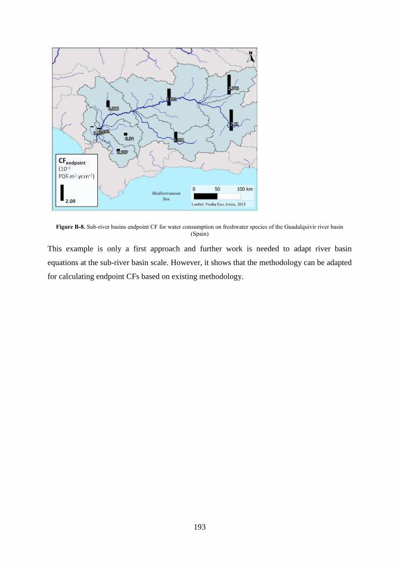
193

Figure B-8. Sub-river basins endpoint CF for water consumption on freshwater species of the Guadalquivir river basin

(Spain)

This example is only a first approach and further work is needed to adapt river basin

equations at the sub-river basin scale. However, it shows that the methodology can be adapted

for calculating endpoint CFs based on existing methodology.

195

Annex C. WaLA, a versatile model for the life cycle assessment of

urban water systems


Chapter 5 and 6 and submitted for publication in "Water Research" as part 1 and part 2.

196

C.1. Structure of the Matlab/Simulink computer program

C.1.1. General structure of the program

The WaLA model is run through a Matlab program called “MAIN.m” that runs the following

tasks:

- 1. A Matlab window is opened where the practitioner can load or create a UWS

scenario file (e.g., ecoinvent.mdl) as shown in Figure C-2.

- 2. Once this is done, the model and the library of components are opened in a

Simulink window, as explained in section C.1.2. The structure of the library and its

associated components are developed in section C.1.3.

- 3. Through the Simulink interface, the practitioner select and combine the different

water technologies and users components (drag and drop of the components from the

library to the model window). The extrinsic attributes of each component can be

customized by the user through the graphical mask of each component. Once the UWS

model is ready, the practitioner can run the simulation from the Matlab interface

(Figure C-2).

- 5. The model is initialized thanks to the function “ini_model.m”, as explained in

section C.1.4.

- 6. The model is run on Simulink with 12 steps of time representing the 12 months

- 7. Results of the model are stored in the Matlab workspace as matrixes results and

rearranged thanks to a Matlab script “Formating_Results.m”

This procedure is summarized in Figure C-1. The different scripts, functions and Simulink

libraries are not provided here but can be provided upon request to the author.

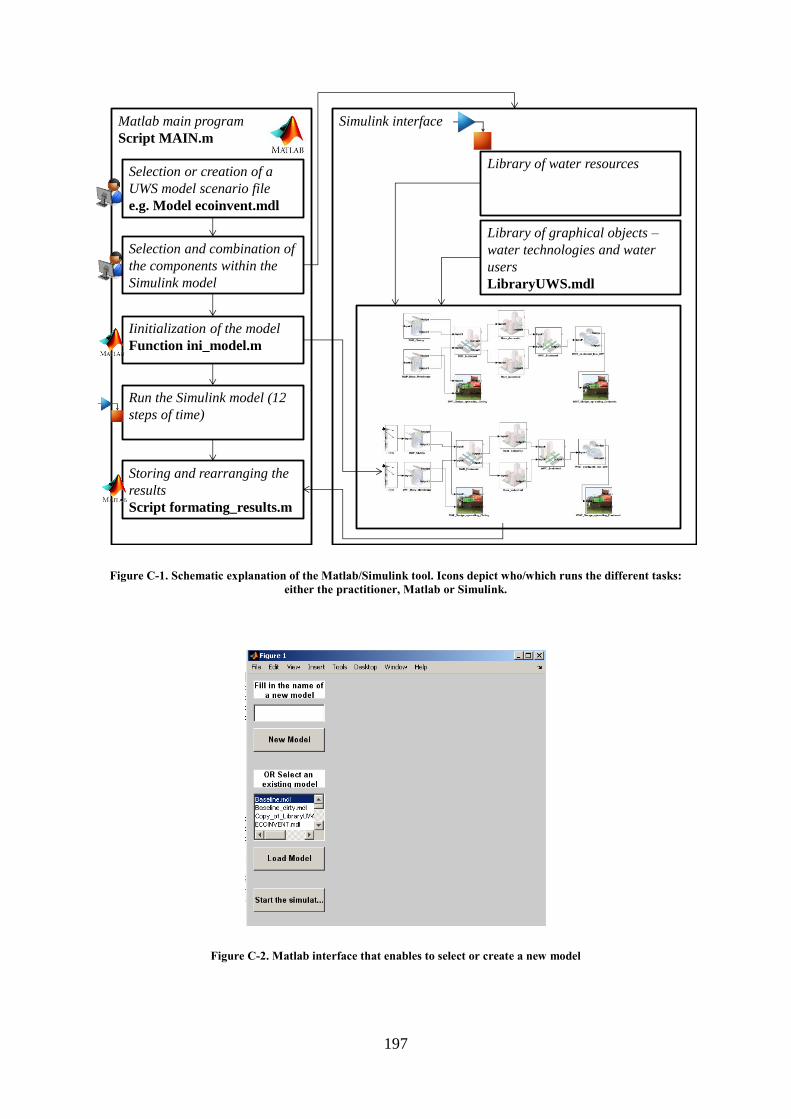
197

Figure C-1. Schematic explanation of the Matlab/Simulink tool. Icons depict who/which runs the different tasks:

either the practitioner, Matlab or Simulink.

Figure C-2. Matlab interface that enables to select or create a new model

Simulink interface

Library of graphical objects –

water technologies and water

users

LibraryUWS.mdl

Library of water resources

Matlab main program

Script MAIN.m

Iinitialization of the model

Function ini_model.m

Run the Simulink model (12

steps of time)

Storing and rearranging the

results

Script formating_results.m

Selection and combination of

the components within the

Simulink model

Selection or creation of a

UWS model scenario file

e.g. Model ecoinvent.mdl

198

C.1.2. Structure of the Simulink library for UWS components

The components are stored within a library (LibraryUWS.mdl) with different folders for each

sub-class of components (e.g., DWP, DWD, etc.).

Figure C-3. Library of components

C.1.3. Structure of Simulink graphical objects

We describe here the structure of the graphical objects. The graphical object is a Simulink

subsystem composed of built-in objects that represent the methods (i.e., functions: calculator,

dispatcher, adder) and the intrinsic attributes of the components (Figure C-4). The extrinsic

attributes related to each component are defined within the masking of the block where the

user can select the parameters through an interface (Figure C-5). This structure is the same for

all graphical objects representing technologies and users.

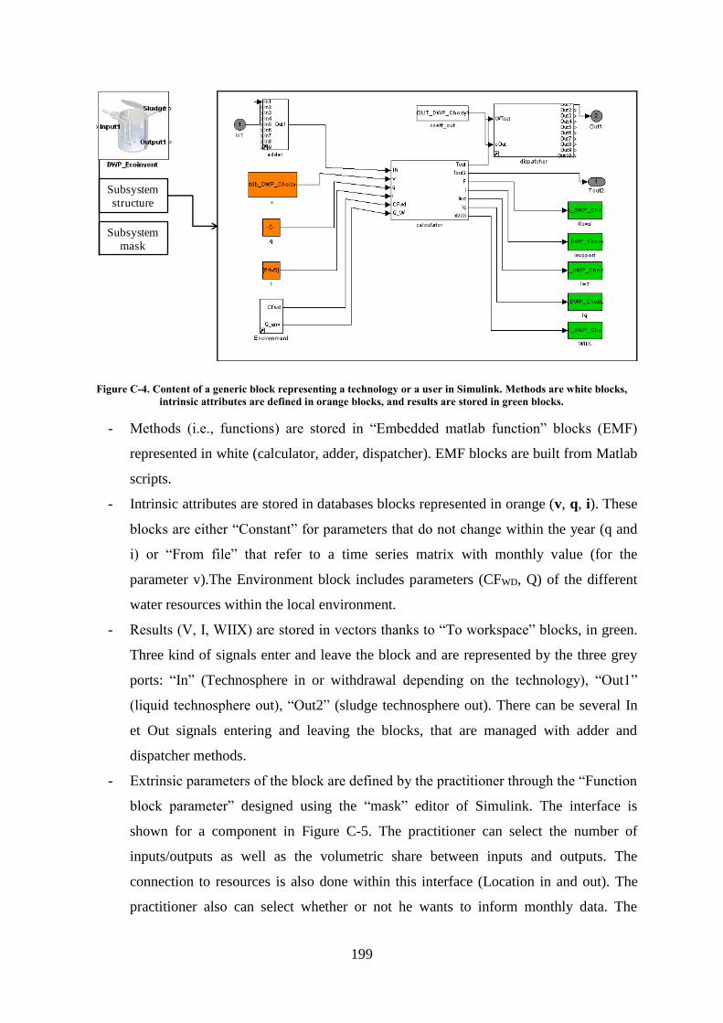
199

Figure C-4. Content of a generic block representing a technology or a user in Simulink. Methods are white blocks,

intrinsic attributes are defined in orange blocks, and results are stored in green blocks.

- Methods (i.e., functions) are stored in “Embedded matlab function” blocks (EMF)

represented in white (calculator, adder, dispatcher). EMF blocks are built from Matlab

scripts.

- Intrinsic attributes are stored in databases blocks represented in orange (v, q, i). These

blocks are either “Constant” for parameters that do not change within the year (q and

i) or “From file” that refer to a time series matrix with monthly value (for the

parameter v).The Environment block includes parameters (CFWD, Q) of the different

water resources within the local environment.

- Results (V, I, WIIX) are stored in vectors thanks to “To workspace” blocks, in green.

Three kind of signals enter and leave the block and are represented by the three grey

ports: “In” (Technosphere in or withdrawal depending on the technology), “Out1”

(liquid technosphere out), “Out2” (sludge technosphere out). There can be several In

et Out signals entering and leaving the blocks, that are managed with adder and

dispatcher methods.

- Extrinsic parameters of the block are defined by the practitioner through the “Function

block parameter” designed using the “mask” editor of Simulink. The interface is

shown for a component in Figure C-5. The practitioner can select the number of

inputs/outputs as well as the volumetric share between inputs and outputs. The

connection to resources is also done within this interface (Location in and out). The

practitioner also can select whether or not he wants to inform monthly data. The

Subsystem

structure

Subsystem

mask

200

dynamic management of ports at the input and the output of the block is done through

the use of an initialization function built as a Matlab function and named “ini_block”.

Figure C-5. Function block parameter of a User block

C.1.4. Initialization of the model

When the graphical construction of the model using Simulink interface is completed, it has to

be initialized in order to calculate the water withdrawals from DWP for each month, i.e., the

variables that runs the model. This initialization is run through a Matlab script that looks up at

all connections of the Simulink model. This script first get water demand from all water users,

then ascend the graph to calculate how much water each DWP plant must withdraw to satisfy

this water demand. This is done with a loop programmed in a Matlab function “ini_model.m”.

Subsystem

structure

Subsystem

mask

201

C.2. Description of components attributes: sub-classes and their

instances

Following sub-sections C.2.1 to C.2.6 aim at describing volumetric water flow distribution

vector v, quality distribution q, and sources of data for LCI of operation and infrastructures

(for impacts matrix i) of the main components found in UWS. One form is provided for each

generic sub-class defined in Chapter 5: drinking water production, drinking water distribution,

user, stormwater collection, wastewater collection, wastewater treatment. Specific instances

(i.e., objects) from the sub-classes are also developed. Figure C-6 summarizes the main

instances available.

Each following sub-section includes:

- A schematic representation of the flows going in and out the technology/user per m3

- A description of the flows.

- The calculations needed for estimating flows

- A table summarizing attributes v and q for the generic sub-class and for specific

instances (ecoinvent and case study), as well as source of data for computing impacts

matrixes i for each instance.

The different flows going in and out are characterized for 1m3 at the input of the technology

(i.e., V_W = 1 m3 for drinking water production, V_P = 1 m3 for stormwater collection and

V_Tin = 1 m3 for all others technologies). Thus they refer to the parameter v introduced in

Chapter 5. Water flow distribution v can be estimated from: (i) measurement from flow meter

(V, m3), (ii) calculation from an external model, (iii) literature data, (iv) result of a mass

balance when all other flows are known. Quality of these flow refer to the indices introduced

in Chapter 4. The chemical composition of each index is provided in section C.3.

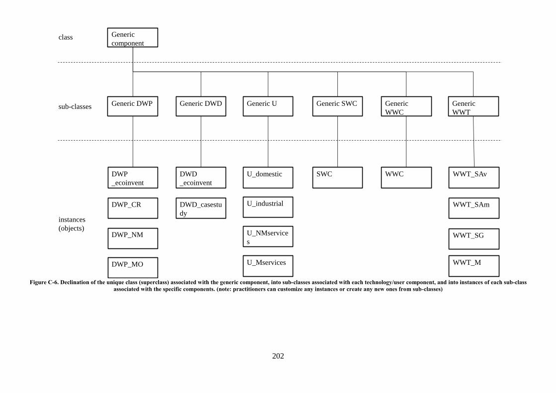
202

Figure C-6. Declination of the unique class (superclass) associated with the generic component, into sub-classes associated with each technology/user component, and into instances of each sub-class

associated with the specific components. (note: practitioners can customize any instances or create any new ones from sub-classes)

class

sub-classes

instances

(objects)

Generic

component

Generic DWP Generic DWD Generic U Generic SWC Generic

WWC

Generic

WWT

DWP

_ecoinvent

DWP_CR

DWP_NM

DWP_MO

DWD

_ecoinvent

DWD_casestu

dy

U_domestic

U_industrial

U_NMservice

s

U_Mservices

SWC WWC WWT_SAv

WWT_SAm

WWT_SG

WWT_M

203

C.2.1. Sub-class: drinking water production (DWP)

Attributes: volumetric water flow distribution v, quality distribution q, and sources of data for impacts i

Generic sub-class DWP

Specific instances (objects) available

DWP_ecoinvent DWP_CR (conventional) DWP_MO (membrane)

Vo

lum

e an

d q

ual

ity

Flow

name

v_DWP q_DWP v_DWP-

ecoinvent

q_DWP-

ecoinvent

v_DWP-CR q_DWP-

CR

v_DWP-

NM

q_DWP-

NM

v_DWP-

membrane

q_DWP-

membrane

Tin 0 - 0 - 0 - - 0 -

Tout V_Tout/V_W A 0.933 A1 0.909 A1 A1 0.798 A1

Tout2 mS*(1-S)/V_W E 0 E1 3.18E-5 E1 E1 3.25E-5 E1

W V_W/V_W B 1 B1 1 B2 B5 1 B6

R V_R/V_W C 0.057 C1 0.072 C3 C2 0.198 C4

P 0 - 0 - 0 - - 0 -

C v_W-

(v_Tout+v_Tout2+v_R) - 0.01 - 0.019 - - 0.003 -

Imp

acts

operation - “tap water, at user {CH}|

tap water production and

supply” Based on local data from

Choisy-le-Roi plant

Based on local data from

Neuilly-sur-Marne plant


Mery-sur-Oise plant infra. - “water works {CH}|

construction”

DWP_CR

Description

DWP plant usually withdraws (W) water directly from the environment (surface, ground or seawater).

However, water can be conveyed to the plants through aqueducts. In this specific case, water going in DWP

comes from the technosphere (Tin). Precipitation is not considered for this process since they directly runoff to

the river. Water releases (R) to the environment (river or sea water) are dependent on the process

(conventional, membrane) and include backwash water from filters and membranes, overflows and reservoirs

washing. Evaporation (C) occurs in reservoirs and during sludge drying. Two flows go out to the

technosphere: Tout that is the drinking water produced and Tout2 that is the water incorporated in sludge.

Estimation of water flows (models and/or data from literature)

v_Tout and v_R are obtained from local measurement of yearly water flows (V_Tout, V_W V_R). v_Tout2 is

computed from the sludge dry content d and its total mass ms (kg) ( W_V)d1(m2outT_v Ss ). v_C is

computed from mass balance of water flows.

111110

Drinking Water

Production

v_Tin=0

v_Tout=0.909

v_C=0.019

v_W=1 v_R=0.072

v_P=0

v_Tout2=3E-5

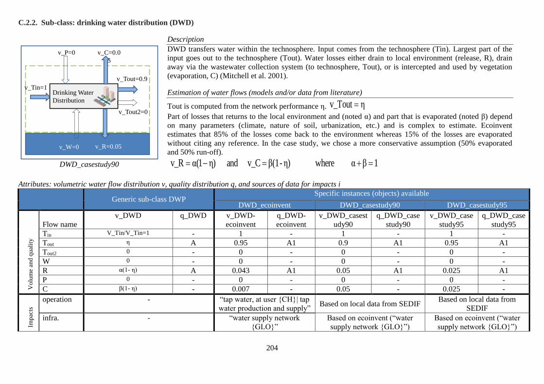
204

C.2.2. Sub-class: drinking water distribution (DWD)




DWD_ecoinvent DWD_casestudy90 DWD_casestudy95

Vo

lum

e an

d q

ual

ity

Flow name

v_DWD q_DWD v_DWD-

ecoinvent

q_DWD-

ecoinvent

v_DWD_casest

udy90

q_DWD_case

study90

v_DWD_case

study95

q_DWD_case

study95

Tin V_Tin/V_Tin=1 - 1 - 1 - 1 -

Tout η A 0.95 A1 0.9 A1 0.95 A1

Tout2 0 - 0 - 0 - 0 -

W 0 - 0 - 0 - 0 -

R α(1- η) A 0.043 A1 0.05 A1 0.025 A1

P 0 - 0 - 0 - 0 -

C β(1- η) - 0.007 - 0.05 - 0.025 -

Imp

acts

operation - “tap water, at user {CH}| tap

water production and supply” Based on local data from SEDIF


SEDIF

infra. - “water supply network

{GLO}”

Based on ecoinvent (“water

supply network {GLO}”)



DWD_casestudy90

Description

DWD transfers water within the technosphere. Input comes from the technosphere (Tin). Largest part of the

input goes out to the technosphere (Tout). Water losses either drain to local environment (release, R), drain

away via the wastewater collection system (to technosphere, Tout), or is intercepted and used by vegetation

(evaporation, C) (Mitchell et al. 2001).


Tout is computed from the network performance η. ηTout_v

Part of losses that returns to the local environment and (noted α) and part that is evaporated (noted β) depend

on many parameters (climate, nature of soil, urbanization, etc.) and is complex to estimate. Ecoinvent

estimates that 85% of the losses come back to the environment whereas 15% of the losses are evaporated

without citing any reference. In the case study, we chose a more conservative assumption (50% evaporated

and 50% run-off).

1βα where )η-(1βC_ vand )η1(αR_v

111110

Drinking Water

Distribution

v_Tin=1

v_Tout=0.9

v_C=0.0

5

v_W=0 v_R=0.05

v_P=0

v_Tout2=0

205

C.2.3. Sub-class: user (U)



Specific instances (objects)

available

U_domestic

Vo

lum

e an

d q

ual

ity

Flow name v_DWD q_DWD v_U_domestic q_U_domestic

Tin 1 - 1 -

Tout v_Tin – v_R – v_C D 0.87 D1

Tout2 0 - 0 -

W 0 - 0 -

R v_R A 0.03 A1

P 0 - 0 -

C v_C - 0.10 -

Imp

acts

operation - -

infra. - -

U_domestic

Description

Most of water supplied to water users is released as wastewater, which is collected and stays in the

technosphere (Tout). The other part which is not collected (watering, car washing, etc.) is either released to the

local environment (R) or evaporated (C). It largely depends on the type of housing (apartment, house with or

without garden and swimming pool, etc.).


Evaporation (v_C) and release (v_R) are estimated from the literature.

111110Domestic user

v_Tin=1v_Tout=0.87

v_C=0.1

v_W=0 v_R=0.03

v_P=0

v_Tout2=0

206

C.2.4. Sub-class: stormwater collection (SWC)



Specific instances (objects)

available

SWC

Vo

lum

e an

d q

ual

ity

Flow name V_SWC q_SWC v_SWC q_SWC

Tin 0 - 0 -

Tout 1 B 1 -

Tout2 0 - 0 -

W 0 - 0 -

R 0 - 0 -

P 1 B 1 -

C Csystem-Cref - 0 -

Imp

acts

operation - -

infra. - -

Description

SWC collects precipitation (P) and outputs water in the technosphere (Tout) to a combined sewer system or a

retention basin. Evapo(transpi)ration (C) related to stormwater system should follow the framework for green

water in LCI (Núñez et al., 2013b). In this case, we need to consider the net change in the evapo(transpi)ration

of the stormwater collection system compared to a reference situation. The identification of the reference

situation is complex: it is more relevant to consider as a reference city without stormwater collection than

natural vegetation. Indeed urbanization increases runoff and decreases evapotranspiration compared to natural

vegetation (Haase, 2009), and this would lead to a benefit from the city system compared to vegetation if the

time scale considered is one year. However, this benefit is a bias: rainwater runoff actually increases

occurrence of flood whereas natural vegetation enables to stock water in soil for the dry season. In the case of

an urban area without stormwater collection, largest part of water would run-off to streams


refsystemnet CCC )CP(WW nettotal

111110

Wastewater

collection

v_Tin=1

v_Tout=1

v_C=0

v_W=0 v_R=0

v_P=0

v_Tout2=0

207

C.2.5. Sub-class: wastewater collection (WWC)


Generic sub-class WWC


WWC_ecoinvent WWC_casestudy

Vo

lum

e an

d q

ual

ity

Flow name

v_DWD q_DWD v_DWD-

ecoinvent

q_DWD-

ecoinvent

v_WWC q_WWC

Tin 1 - 1 - 1 -

Tout v_Tin-v_W-v_R D 1 D2 1 D3, D4, D5,

D6

Tout2 0 - 0 - 0 -

W In - 0 - 0 -

R Ex D 0 - 0 -

P 0 - 0 - 0 -

C 0 - 0 - 0 -

Imp

acts

operation - - -

infra. - “water supply network

{GLO}”



Description

Unitary sewers collect from the technosphere (Tin) wastewater from the users. In the case of combined sewers,

rainwater collected from stormwater system also comes from the technosphere (Tin). In the case of draining

system, part of water from the ground can infiltrate within the system, and it is considered as a withdrawal

from the local environment (W). There is also exfiltration of wastewater from the system that is considered as

release to the local environment (R). More rarely, water losses from DWD system can inflow within the

sewers (Tin). Resulting wastewater (more or less diluted) is then transported to a WWT plant within the

technosphere (Tout).


Infiltration (In) and exfiltration (Ex) rates can be estimated according to literature values. In the case study,

they were not considered.

111110

Wastewater

collection

Tin=1Tout=1

C=0

W=0 R=0

P=0

Tout2=0

208

C.2.6. Sub-class: wastewater treatment (WWT)


Generic sub-class WWT


WWT_ecoinvent WWT_SAv WWT_SAm WWT_SG WWT_M

Vo

lum

e an

d q

ual

ity

Flow name

v_WWT q_WWT v_WWT-

ecoinvent

q_WWT-

ecoinvent

v q v q v q v q

Tin 1 - 1 - 1 - 1 - 1 - 1 -

Tout 0 - 0 - 0 - 0 - 0 - 0 -

Tout2 mS*(1-S)/V_W E 1.85E-3 - 2.2E-4 - 2.5E-4 - 7.8E-4 - 0 -

W 0 - 0 - 0 - 0 - 0 - 0 -

R 1-v_Tout2-v_C C 0.9 C5 0.99 C6 0.99 C7 0.99 C8 0.99 C9

P 0 - 0 - 0 - 0 - 0 - 0 -

C v_C - 0.099 - 6.8E-4 - 1.2E-3 - 5.4E-4 - 1.1E-3 -

Imp

acts

operation - “wastewater, average {CH}|

treatment of, capacity

4.7E10l/year effluent ”

Based on local data from SIAAP

infra. - “wastewater treatment facility,

capacity 4.7E10l/year”

Based on ecoinvent

WWT_SAv

Description

Wastewater plant treats water coming from collection system (Tin). Depending on the technology, part of

water is evaporated (C) from basins (activated sludge) and/or from lagoons. Water from sludge is evaporated

when dried (C), and the remaining amount is exported within the technosphere (Tout2) to incineration,

agricultural spreading or landfill. Treated water is finally released to the local environment (R).


Evapo(transpi)ration in WWT plants can be estimated according to Risch et al. (2014) that compute

evaporation from open water surfaces in the activated sludge basins (EAS, in m/year) and polishing ponds and

evapotranspiration from planted vertical reed bed filters (ETplants, in m/year), depending on the location. Total

consumption (C) is from the surfaces of basins (SAS, in m2) and planted ponds (Splants, in m2). Tin_V/)SETSE(C_v plantsplantsASAS

Amount exported in sludge is estimated according to the mass of sludge exported and its dryness. Finally

release to local environment result from mass balance between inputs and outputs.

111110

Wastewater

treatment

v_Tin=1v_Tout

v_C=6.8E-4

v_W=0 v_R=0.999

v_P=0

v_Tout2=2.2E-4

209

C.3. LCI for the quality indexes

In the sub-sections C.2.1 to C.2.6, vectors q are presented for each instance in order to give water quality indices of water at the output. Each

water quality index (ex. A1, B1, etc.) refers to a type of water presented in Chapter 4. Chemical composition of each index is presented in Table

C-1.

Table C-1. Composition of water flows from the case studies. Concentrations highlighted in grey are not known and taken equal to very good state

A B – Resources water C – Releases from plants

Indiex A1 B1 B2 B3 B4 B5 B6 C1 C2 C3 C4

Description

Drinking

water

SEDIF

Vanne

river at

Molinons

Seine

river at

Orly

Seine

river at

Paris

Seine

river at

poissy

Marne

river at

joinville

Oise river

at Meriel

Release

DWP_

ecoinvent

Release

DWP_NM

Release

DWP_CR

Release

MO

Pollutants CAS (SEDIF,

2012) (AESN, 2014) (SEDIF, 2012)

COD - 3,50E-01 7,01E+00 1,64E+01 1,58E+01 1,77E+01 1,64E+01 1,86E+01 1,17E+01 1,17E+01 5,33E+01 2,50E+01

BOD - 3,00E+00 9,63E-01 1,56E+00 1,36E+00 2,09E+00 1,60E+00 1,47E+00 3,00E+00 3,00E+00 3,00E+00 3,00E+00

Phosphorus total

(Pt) 7723140 1,00E-02 4,00E-02 6,30E-02 1,06E-01 1,57E-01 8,56E-02 1,16E-01 5,00E-01 5,00E-01 5,00E-02 3,80E-01

Ion ammonium

(NH4+) 14798039 3,00E-02 6,28E-02 7,15E-02 1,21E-01 8,75E-01 1,10E-01 1,32E-01 1,00E-01 1,00E-01 1,00E-01 8,60E-02

Nitrate (NO3-) 14797650 1,81E+01 2,52E+01 1,96E+01 2,02E+01 2,45E+01 1,67E+01 1,93E+01 3,18E+00 3,18E+00 2,00E+01 1,34E+01

Nitrite (NO2-) 14797650 1,00E-02 4,69E-02 7,81E-02 1,03E-01 5,16E-01 1,09E-01 1,12E-01 6,00E-02 6,00E-02 1,00E-01 1,00E-01

Cadmium (Cd) 7440439 1,00E-08 7,50E-05 7,50E-05 7,50E-05 7,50E-05 7,50E-05 7,50E-05 7,50E-05 7,50E-05 7,50E-05 7,50E-05

Mercury (Hg) 7439976 1,00E-08 5,00E-04 1,60E-05 2,50E-05 1,63E-05 1,68E-05 1,63E-05 2,50E-05 1,50E-04 2,50E-05 2,50E-05

Arsenic (As) 7440382 1,00E-08 1,74E-03 9,67E-04 2,10E-03 1,01E-03 8,98E-04 9,84E-04 2,10E-03 2,10E-03 2,10E-03 2,10E-03

Aluminum (Al) 7429905 1,00E-08 1,00E-01 1,00E-01 1,00E-01 1,00E-01 1,00E-01 1,00E-01 1,29E+00 1,36E+00 6,00E+00 5,10E-01

Iron (Fe) 7439896 1,00E-08 5,00E-02 5,00E-02 5,00E-02 5,00E-02 5,00E-02 5,00E-02 5,00E-02 5,00E-02 5,00E-02 1,00E-01

Chromium (Cr) 7440473 1,00E-08 2,18E-03 5,83E-04 1,70E-03 7,49E-04 6,80E-04 9,32E-04 1,70E-03 1,70E-03 1,70E-03 1,70E-03

Copper (Cu) 7440508 1,00E-08 1,01E-03 1,46E-03 2,17E-03 2,25E-03 1,79E-03 1,58E-03 7,00E-04 3,82E-03 7,00E-04 7,00E-04

Lead (Pb) 7439921 1,00E-08 3,60E-03 3,60E-03 3,60E-03 3,60E-03 3,60E-03 3,60E-03 3,60E-03 8,10E-04 3,60E-03 3,60E-03

Zinc (Zn) 7440666 1,00E-08 4,89E-03 4,69E-03 3,90E-03 8,01E-03 5,22E-03 5,81E-03 3,90E-03 9,80E-03 3,90E-03 3,90E-03

210

Table C 1 continued. Composition of water flows from the case studies. Concentrations highlighted in grey are not known and taken equal to very good state

C – Release from plants D - Wastewater

Index C5 C6 C7 C8 C9 D1 D2 D3 D4 D5 D6

Descriptio

n

Release

WWT_ecoi

nvent

Release

WWT_SA

v

Release

WWT_SA

m

Release

WWT_SG

Release

WWT_M

Raw waste

water from

France

Input

WWT_

ecoinvent

Input

WWT_SA

v

Input

WWT_SA

m

Input

WWT_SG

Input

WWT_M

Pollutants CAS (SIAAP, 2012) (Stricker and Héduit, 2010) (Doka, 2009) (SIAAP, 2012) COD - 2,75E+01 5,50E+01 2,70E+01 2,60E+01 4,50E+01 2,00E+01 1,55E+02 4,58E+02 6,75E+02 3,71E+02 6,43E+02

BOD - 8,15E+00 1,30E+01 3,00E+00 5,00E+00 7,90E+00 3,00E+00 1,04E+02 1,86E+02 3,00E+02 1,67E+02 2,63E+02

Phosphorus total

(Pt) 7723140 8,49E-01 9,00E-01 7,00E-01 6,00E-01 5,00E-01 5,00E-02 3,07E+00 5,81E+00 7,00E+00 6,00E+00 7,14E+00

Ion ammonium

(NH4+) 14798039 1,10E+01 9,51E+00 2,06E+00 2,31E+00 4,61E+00 1,00E-01 1,92E+01 1,00E-01 1,00E-01 1,00E-01 1,00E-01

Nitrate (NO3-) 14797650 4,83E+01 4,25E+01 8,10E+01 2,75E+01 2,88E+01 2,00E+01 4,65E+00 2,00E+01 2,00E+01 2,00E+01 2,00E+01

Nitrite (NO2-) 14797650 6,44E-01 1,00E-01 1,00E-01 1,00E-01 1,00E-01 1,00E-01 1,31E+00 1,00E-01 1,00E-01 1,00E-01 1,00E-01

Cadmium (Cd) 7440439 2,81E-04 2,81E-04 7,50E-05 7,50E-05 7,50E-05 7,50E-05 2,81E-04 2,54E-04 2,54E-04 2,54E-04 2,54E-04

Mercury (Hg) 7439976 2,00E-04 2,00E-04 2,50E-05 2,50E-05 2,50E-05 2,50E-05 2,00E-04 5,36E-04 5,36E-04 5,36E-04 5,36E-04

Arsenic (As) 7440382 4,20E-03 4,20E-03 2,10E-03 2,10E-03 2,10E-03 2,10E-03 9,00E-04 1,49E-03 1,49E-03 1,49E-03 1,49E-03

Aluminum (Al) 7429905 1,04E+00 1,04E+00 1,00E-01 1,00E-01 1,00E-01 1,00E-01 1,04E+00 1,20E+00 1,20E+00 1,20E+00 1,20E+00

Iron (Fe) 7439896 7,09E+00 7,09E+00 5,00E-02 5,00E-02 5,00E-02 5,00E-02 7,09E+00 1,60E+00 1,60E+00 1,60E+00 1,60E+00

Chromium (Cr) 7440473 1,22E-02 1,22E-02 1,70E-03 1,70E-03 1,70E-03 1,70E-03 1,22E-02 1,35E-02 1,35E-02 1,35E-02 1,35E-02

Copper (Cu) 7440508 3,74E-02 3,74E-02 7,00E-04 7,00E-04 7,00E-04 7,00E-04 3,74E-02 8,49E-02 8,49E-02 8,49E-02 8,49E-02

Lead (Pb) 7439921 8,63E-03 8,63E-03 3,60E-03 3,60E-03 3,60E-03 3,60E-03 8,63E-03 2,31E-02 2,31E-02 2,31E-02 2,31E-02

Zinc (Zn) 7440666 3,24E-02 3,24E-02 3,90E-03 3,90E-03 3,90E-03 3,90E-03 1,09E-01 1,88E-01 1,88E-01 1,88E-01 1,88E-01

211

C.4. Water users database

Table C-2. Database of numbers of users in each city of the SEDIF perimeter for the year 2012. Source (INSEE, 2013)

Cities of the SEDIF

perimeter

Post

code

Area

(ha)

Popu-

lation

(capita)

Non

market

services

(jobs)

Market

services

(jobs)

Indus-

tries

(jobs)

Agri-

culture

(jobs)

Total

TOTAL 761.48 4 362

705

413 251 1 164 261 153 028 335 1 730 875

Brou-sur-Chantereine 77177 4.28 4 306 340 171 14 1 526

Villeparisis 77270 8.29 24 296 1 196 2 577 235 2 4 010

Vaires-sur-Marne 77360 6.02 12 459 463 1 048 248 0 1 759

Chelles 77500 15.90 53 238 3 379 7 439 1 169 3 11 990

Vélizy-Villacoublay 78140 8.93 20 348 2 085 25 229 13 659 0 40 973

Viroflay 78220 3.49 16 224 1 406 2 671 72 0 4 149

Jouy-en-Josas 78350 10.14 8 316 1 531 2 303 125 55 4 014

LesLoges-en-Josas 78351 2.48 1 596 148 584 115 0 847

Sartrouville 78500 8.46 51 504 2 908 5 764 1 286 0 9 958

LeMesnil-le-Roi 78600 3.25 6 543 309 657 33 37 1 036

Houilles 78800 4.43 31 849 1 548 2 369 209 1 4 127

Palaiseau 91120 11.51 31 175 4 177 6 067 840 0 11 084

Athis-Mons 91200 8.56 30 845 3 760 3 673 157 0 7 590

Juvisy-sur-Orge 91260 2.24 14 756 1 672 2 239 116 0 4 027

Massy 91300 9.43 43 006 4 684 16 132 4 957 0 25 773

Wissous 91320 9.11 5 965 271 11 297 939 1 12 508

Verrières-le-Buisson 91370 9.91 15 830 894 3 132 218 0 4 244

Igny 91430 3.82 10 878 487 1 558 311 1 2 357

Bièvres 91570 9.69 4 747 663 2 017 233 21 2 934

Boulogne-Billancourt 92100 6.17 115 264 9 887 75 787 3 833 11 89 518

Clichy 92110 3.08 59 228 7 108 32 918 3 533 1 43 560

Montrouge 92120 2.07 48 983 3 029 17 682 1 703 10 22 424

Issy-les-Moulineaux 92130 4.25 65 178 5 127 45 717 4 846 0 55 690

Clamart 92140 8.77 53 113 4 927 7 132 3 398 0 15 457

Antony 92160 9.56 62 644 6 189 14 080 2 027 1 22 297

Vanves 92170 1.56 27 314 2 699 5 344 129 0 8 172

Meudon 92190 9.90 45 834 4 259 13 604 1 801 0 19 664

Neuilly-sur-Seine 92200 3.73 62 565 7 778 39 242 2 243 0 49 263

Bagneux 92220 4.19 38 384 2 597 5 241 1 467 0 9 305

Malakoff 92240 2.07 31 325 1 999 12 106 282 0 14 387

Fontenay-aux-Roses 92260 2.51 23 603 1 871 4 862 47 0 6 780

Châtenay-Malabry 92290 6.38 32 573 3 762 2 871 81 6 6 720

Levallois-Perret 92300 2.41 64 757 5 377 53 701 4 501 0 63 579

Sèvres 92310 3.91 23 412 2 375 6 621 467 2 9 465

Châtillon 92320 2.92 32 947 2 037 10 965 956 0 13 958

Sceaux 92330 3.60 19 986 2 553 1 920 172 0 4 645

Bourg-la-Reine 92340 1.86 20 303 1 654 2 917 75 0 4 646

LePlessis-Robinson 92350 3.43 27 931 2 363 4 147 4 946 2 11 458

Chaville 92370 3.55 18 887 980 1 529 53 0 2 562

Puteaux 92800 3.19 45 093 8 412 80 859 7 005 19 96 295

Bobigny 93000 6.77 47 855 26 327 10 726 1 265 0 38 318

212

Cities of the SEDIF

perimeter

Post

code

Area

(ha)

Popu-

lation

(capita)

Non

market

services

(jobs)

Market

services

(jobs)

Indus-

tries

(jobs)

Agri-

culture

(jobs)

Total

Montreuil 93100 8.92 103 675 15 791 27 190 2 338 0 45 319

Rosny-sous-Bois 93110 5.91 41 431 3 338 9 125 868 0 13 331

LaCourneuve 93120 7.52 38 361 2 365 7 385 2 677 0 12 427

Noisy-le-Sec 93130 5.04 39 949 2 919 5 472 1 037 0 9 428

Bondy 93140 5.47 53 934 4 504 7 167 377 0 12 048

Noisy-le-Grand 93160 12.95 63 526 7 569 15 208 2 127 0 24 904

Bagnolet 93170 2.57 34 232 3 802 9 264 931 1 13 998

Livry-Gargan 93190 7.38 42 060 2 717 4 693 363 0 7 773

Saint-Denis 93200 12.36 107 959 19 488 52 167 7 110 7 78 772

Gagny 93220 6.83 39 350 2 942 1 861 119 0 4 922

Romainville 93230 3.44 26 025 1 714 2 888 1 019 0 5 621

Stains 93240 5.39 34 048 2 652 3 613 582 0 6 847

Villemomble 93250 4.04 28 257 1 811 2 538 182 0 4 531

LesLilas 93260 1.26 22 410 1 444 3 109 123 0 4 676

Sevran 93270 7.28 50 225 2 800 2 642 512 6 5 960

Aubervilliers 93300 5.76 76 728 6 208 19 301 1 722 0 27 231

LePré-Saint-Gervais 93310 0.70 18 171 969 1 668 236 0 2 873

LesPavillons-sous-

Bois

93320 2.92 21 972 1 368 3 678 220 0 5 266

Neuilly-sur-Marne 93330 6.86 33 781 4 219 4 865 1 030 0 10 114

LeRaincy 93340 2.24 14 194 1 714 2 132 55 0 3 901

LeBourget 93350 2.08 14 943 1 187 4 090 354 0 5 631

Neuilly-Plaisance 93360 3.42 20 683 1 242 3 610 318 0 5 170

Montfermeil 93370 5.45 25 499 3 432 3 118 197 0 6 747

Pierrefitte-sur-Seine 93380 3.41 28 076 1 395 1 597 398 0 3 390

Clichy-sous-Bois 93390 3.95 29 998 1 371 1 891 196 0 3 458

Saint-Ouen 93400 4.31 47 604 3 555 30 481 5 626 0 39 662

Vaujours 93410 3.78 6 601 644 651 500 0 1 795

Villetaneuse 93430 2.31 12 662 2 049 1 757 195 0 4 001

Dugny 93440 3.89 10 735 644 359 127 0 1 130

L'Ile-Saint-Denis 93450 1.77 7 070 303 1 380 135 0 1 818

Gournay-sur-Marne 93460 1.68 6 457 278 469 49 0 796

Coubron 93470 4.14 4 795 207 359 18 0 584

Pantin 93500 5.01 54 464 6 264 16 905 3 133 0 26 302

Aulnay-sous-Bois 93600 16.20 82 778 6 131 13 933 5 454 0 25 518

Drancy 93700 7.76 67 202 3 681 6 175 540 1 10 397

Epinay-sur-Seine 93800 4.57 54 775 2 822 5 104 326 0 8 252

Arcueil 94110 2.33 19 964 1 773 14 677 707 2 17 159

Fontenay-sous-Bois 94120 5.58 53 667 4 547 22 141 1 415 7 28 110

Nogent-sur-Marne 94130 2.80 31 975 2 978 3 359 212 6 6 555

Alfortville 94140 3.67 44 439 2 099 6 323 864 0 9 286

Rungis 94150 4.20 5 729 688 21 788 3 357 10 25 843

Saint-Mandé 94160 0.92 22 666 3 106 2 389 213 0 5 708

LePerreux-sur-Marne 94170 3.96 32 799 1 689 2 797 190 0 4 676

Ivry-sur-Seine 94200 6.10 58 189 5 661 29 058 2 497 0 37 216

Charenton-le-Pont 94220 1.85 29 664 2 165 13 514 619 0 16 298

Cachan 94230 2.74 28 550 4 407 4 142 446 0 8 995

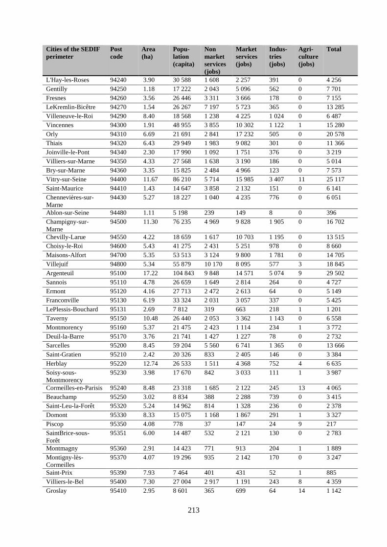
213

Cities of the SEDIF

perimeter

Post

code

Area

(ha)

Popu-

lation

(capita)

Non

market

services

(jobs)

Market

services

(jobs)

Indus-

tries

(jobs)

Agri-

culture

(jobs)

Total

L'Hay-les-Roses 94240 3.90 30 588 1 608 2 257 391 0 4 256

Gentilly 94250 1.18 17 222 2 043 5 096 562 0 7 701

Fresnes 94260 3.56 26 446 3 311 3 666 178 0 7 155

LeKremlin-Bicêtre 94270 1.54 26 267 7 197 5 723 365 0 13 285

Villeneuve-le-Roi 94290 8.40 18 568 1 238 4 225 1 024 0 6 487

Vincennes 94300 1.91 48 955 3 855 10 302 1 122 1 15 280

Orly 94310 6.69 21 691 2 841 17 232 505 0 20 578

Thiais 94320 6.43 29 949 1 983 9 082 301 0 11 366

Joinville-le-Pont 94340 2.30 17 990 1 092 1 751 376 0 3 219

Villiers-sur-Marne 94350 4.33 27 568 1 638 3 190 186 0 5 014

Bry-sur-Marne 94360 3.35 15 825 2 484 4 966 123 0 7 573

Vitry-sur-Seine 94400 11.67 86 210 5 714 15 985 3 407 11 25 117

Saint-Maurice 94410 1.43 14 647 3 858 2 132 151 0 6 141

Chennevières-sur-

Marne

94430 5.27 18 227 1 040 4 235 776 0 6 051

Ablon-sur-Seine 94480 1.11 5 198 239 149 8 0 396

Champigny-sur-

Marne

94500 11.30 76 235 4 969 9 828 1 905 0 16 702

Chevilly-Larue 94550 4.22 18 659 1 617 10 703 1 195 0 13 515

Choisy-le-Roi 94600 5.43 41 275 2 431 5 251 978 0 8 660

Maisons-Alfort 94700 5.35 53 513 3 124 9 800 1 781 0 14 705

Villejuif 94800 5.34 55 879 10 170 8 095 577 3 18 845

Argenteuil 95100 17.22 104 843 9 848 14 571 5 074 9 29 502

Sannois 95110 4.78 26 659 1 649 2 814 264 0 4 727

Ermont 95120 4.16 27 713 2 472 2 613 64 0 5 149

Franconville 95130 6.19 33 324 2 031 3 057 337 0 5 425

LePlessis-Bouchard 95131 2.69 7 812 319 663 218 1 1 201

Taverny 95150 10.48 26 440 2 053 3 362 1 143 0 6 558

Montmorency 95160 5.37 21 475 2 423 1 114 234 1 3 772

Deuil-la-Barre 95170 3.76 21 741 1 427 1 227 78 0 2 732

Sarcelles 95200 8.45 59 204 5 560 6 741 1 365 0 13 666

Saint-Gratien 95210 2.42 20 326 833 2 405 146 0 3 384

Herblay 95220 12.74 26 533 1 511 4 368 752 4 6 635

Soisy-sous-

Montmorency

95230 3.98 17 670 842 3 033 111 1 3 987

Cormeilles-en-Parisis 95240 8.48 23 318 1 685 2 122 245 13 4 065

Beauchamp 95250 3.02 8 834 388 2 288 739 0 3 415

Saint-Leu-la-Forêt 95320 5.24 14 962 814 1 328 236 0 2 378

Domont 95330 8.33 15 075 1 168 1 867 291 1 3 327

Piscop 95350 4.08 778 37 147 24 9 217

SaintBrice-sous-

Forêt

95351 6.00 14 487 532 2 121 130 0 2 783

Montmagny 95360 2.91 14 423 771 913 204 1 1 889

Montigny-lès-

Cormeilles

95370 4.07 19 296 935 2 142 170 0 3 247

Saint-Prix 95390 7.93 7 464 401 431 52 1 885

Villiers-le-Bel 95400 7.30 27 004 2 917 1 191 243 8 4 359

Groslay 95410 2.95 8 601 365 699 64 14 1 142

214

Cities of the SEDIF

perimeter

Post

code

Area

(ha)

Popu-

lation

(capita)

Non

market

services

(jobs)

Market

services

(jobs)

Indus-

tries

(jobs)

Agri-

culture

(jobs)

Total

Auvers-sur-Oise 95430 12.69 6 953 223 339 108 8 678

Ecouen 95440 7.59 7 515 414 489 435 5 1 343

Pierrelaye 95480 9.21 8 122 352 2 479 216 12 3 059

LaFrette-sur-Seine 95530 2.02 4 621 114 170 25 0 309

Méry-sur-Oise 95540 11.17 9 410 443 1 159 217 14 1 833

Bessancourt 95550 6.39 7 090 346 234 55 3 638

Andilly 95580 2.70 2 570 356 745 235 1 1 337

Margency 95581 0.72 2 891 477 249 8 0 734

Eaubonne 95600 4.42 24 386 3 420 2 528 186 0 6 134

Montlignon 95680 2.84 2 685 236 288 365 0 889

Bezons 95870 4.16 28 277 2 163 12 838 1 494 0 16 495

Enghien-les-Bains 95880 1.77 11 959 1 391 2 927 109 0 4 427

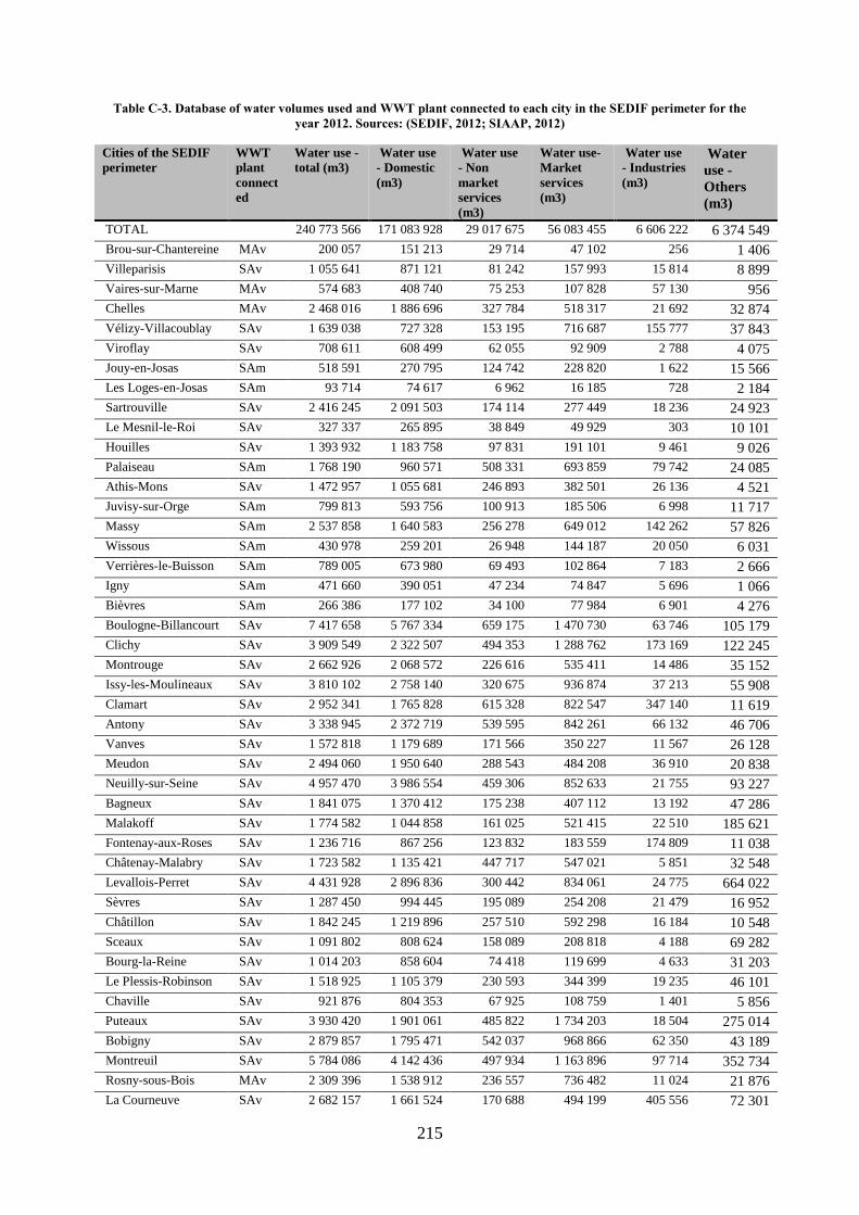
215

Table C-3. Database of water volumes used and WWT plant connected to each city in the SEDIF perimeter for the

year 2012. Sources: (SEDIF, 2012; SIAAP, 2012)

Cities of the SEDIF

perimeter

WWT

plant

connect

ed

Water use -

total (m3)

Water use

- Domestic

(m3)

Water use

- Non

market

services

(m3)

Water use-

Market

services

(m3)

Water use

- Industries

(m3)

Water

use -

Others

(m3)

TOTAL 240 773 566 171 083 928 29 017 675 56 083 455 6 606 222 6 374 549

Brou-sur-Chantereine MAv 200 057 151 213 29 714 47 102 256 1 406

Villeparisis SAv 1 055 641 871 121 81 242 157 993 15 814 8 899

Vaires-sur-Marne MAv 574 683 408 740 75 253 107 828 57 130 956

Chelles MAv 2 468 016 1 886 696 327 784 518 317 21 692 32 874

Vélizy-Villacoublay SAv 1 639 038 727 328 153 195 716 687 155 777 37 843

Viroflay SAv 708 611 608 499 62 055 92 909 2 788 4 075

Jouy-en-Josas SAm 518 591 270 795 124 742 228 820 1 622 15 566

Les Loges-en-Josas SAm 93 714 74 617 6 962 16 185 728 2 184

Sartrouville SAv 2 416 245 2 091 503 174 114 277 449 18 236 24 923

Le Mesnil-le-Roi SAv 327 337 265 895 38 849 49 929 303 10 101

Houilles SAv 1 393 932 1 183 758 97 831 191 101 9 461 9 026

Palaiseau SAm 1 768 190 960 571 508 331 693 859 79 742 24 085

Athis-Mons SAv 1 472 957 1 055 681 246 893 382 501 26 136 4 521

Juvisy-sur-Orge SAm 799 813 593 756 100 913 185 506 6 998 11 717

Massy SAm 2 537 858 1 640 583 256 278 649 012 142 262 57 826

Wissous SAm 430 978 259 201 26 948 144 187 20 050 6 031

Verrières-le-Buisson SAm 789 005 673 980 69 493 102 864 7 183 2 666

Igny SAm 471 660 390 051 47 234 74 847 5 696 1 066

Bièvres SAm 266 386 177 102 34 100 77 984 6 901 4 276

Boulogne-Billancourt SAv 7 417 658 5 767 334 659 175 1 470 730 63 746 105 179

Clichy SAv 3 909 549 2 322 507 494 353 1 288 762 173 169 122 245

Montrouge SAv 2 662 926 2 068 572 226 616 535 411 14 486 35 152

Issy-les-Moulineaux SAv 3 810 102 2 758 140 320 675 936 874 37 213 55 908

Clamart SAv 2 952 341 1 765 828 615 328 822 547 347 140 11 619

Antony SAv 3 338 945 2 372 719 539 595 842 261 66 132 46 706

Vanves SAv 1 572 818 1 179 689 171 566 350 227 11 567 26 128

Meudon SAv 2 494 060 1 950 640 288 543 484 208 36 910 20 838

Neuilly-sur-Seine SAv 4 957 470 3 986 554 459 306 852 633 21 755 93 227

Bagneux SAv 1 841 075 1 370 412 175 238 407 112 13 192 47 286

Malakoff SAv 1 774 582 1 044 858 161 025 521 415 22 510 185 621

Fontenay-aux-Roses SAv 1 236 716 867 256 123 832 183 559 174 809 11 038

Châtenay-Malabry SAv 1 723 582 1 135 421 447 717 547 021 5 851 32 548

Levallois-Perret SAv 4 431 928 2 896 836 300 442 834 061 24 775 664 022

Sèvres SAv 1 287 450 994 445 195 089 254 208 21 479 16 952

Châtillon SAv 1 842 245 1 219 896 257 510 592 298 16 184 10 548

Sceaux SAv 1 091 802 808 624 158 089 208 818 4 188 69 282

Bourg-la-Reine SAv 1 014 203 858 604 74 418 119 699 4 633 31 203

Le Plessis-Robinson SAv 1 518 925 1 105 379 230 593 344 399 19 235 46 101

Chaville SAv 921 876 804 353 67 925 108 759 1 401 5 856

Puteaux SAv 3 930 420 1 901 061 485 822 1 734 203 18 504 275 014

Bobigny SAv 2 879 857 1 795 471 542 037 968 866 62 350 43 189

Montreuil SAv 5 784 086 4 142 436 497 934 1 163 896 97 714 352 734

Rosny-sous-Bois MAv 2 309 396 1 538 912 236 557 736 482 11 024 21 876

La Courneuve SAv 2 682 157 1 661 524 170 688 494 199 405 556 72 301

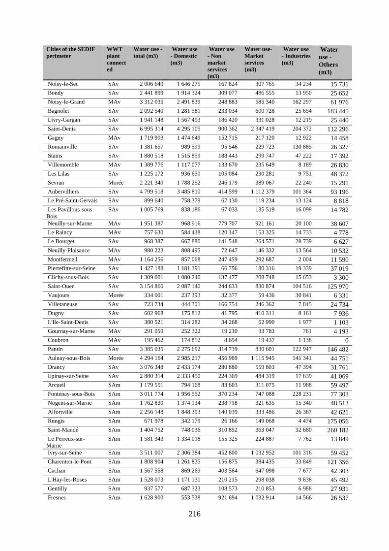
216

Cities of the SEDIF

perimeter

WWT

plant

connect

ed

Water use -

total (m3)

Water use

- Domestic

(m3)

Water use

- Non

market

services

(m3)

Water use-

Market

services

(m3)

Water use

- Industries

(m3)

Water

use -

Others

(m3)

Noisy-le-Sec SAv 2 006 649 1 646 275 167 824 307 765 34 234 15 731

Bondy SAv 2 441 899 1 914 324 309 077 486 555 13 950 25 652

Noisy-le-Grand MAv 3 312 035 2 491 839 248 883 585 340 162 297 61 976

Bagnolet SAv 2 092 540 1 281 581 233 034 600 728 25 654 183 445

Livry-Gargan SAv 1 941 148 1 567 493 186 420 331 028 12 219 25 440

Saint-Denis SAv 6 995 314 4 295 105 900 362 2 347 419 204 372 112 296

Gagny MAv 1 719 903 1 474 649 152 715 217 120 12 922 14 458

Romainville SAv 1 381 657 989 599 95 546 229 723 130 885 26 327

Stains SAv 1 880 518 1 515 859 188 443 299 747 47 222 17 392

Villemomble MAv 1 389 776 1 117 077 133 670 235 649 8 189 26 830

Les Lilas SAv 1 225 172 936 650 105 084 230 281 9 751 48 372

Sevran Morée 2 221 340 1 788 252 246 179 389 067 22 240 15 291

Aubervilliers SAv 4 799 518 3 485 810 414 599 1 112 379 101 364 93 196

Le Pré-Saint-Gervais SAv 899 640 758 379 67 130 119 234 13 124 8 818

Les Pavillons-sous-

Bois

SAv 1 005 769 838 186 67 033 135 519 16 099 14 782

Neuilly-sur-Marne MAv 1 951 387 968 916 779 707 921 161 20 100 38 607

Le Raincy MAv 757 630 584 438 120 147 153 325 14 733 4 778

Le Bourget SAv 968 387 667 880 141 548 264 571 28 739 6 627

Neuilly-Plaisance MAv 980 223 808 495 72 647 146 332 13 564 10 532

Montfermeil MAv 1 164 256 857 068 247 459 292 687 2 004 11 590

Pierrefitte-sur-Seine SAv 1 427 188 1 181 391 66 756 180 316 19 339 37 019

Clichy-sous-Bois SAv 1 309 001 1 080 240 137 477 208 748 15 653 3 300

Saint-Ouen SAv 3 154 866 2 087 140 244 633 830 874 104 516 125 970

Vaujours Morée 334 001 237 393 32 377 59 436 30 841 6 331

Villetaneuse SAv 723 734 444 301 166 754 246 362 7 845 24 734

Dugny SAv 602 968 175 812 41 795 410 311 8 161 7 936

L'Ile-Saint-Denis SAv 380 521 314 282 34 268 62 990 1 977 1 103

Gournay-sur-Marne MAv 291 059 252 322 19 210 33 783 761 4 193

Coubron MAv 195 462 174 812 8 694 19 437 1 138 0

Pantin SAv 3 385 035 2 275 692 314 739 830 601 122 947 146 482

Aulnay-sous-Bois Morée 4 294 164 2 985 217 456 969 1 115 945 141 341 44 751

Drancy SAv 3 076 348 2 433 174 280 880 559 803 47 394 31 761

Epinay-sur-Seine SAv 2 880 314 2 333 450 224 369 484 319 17 639 41 069

Arcueil SAm 1 179 551 794 168 83 603 311 075 11 988 59 497

Fontenay-sous-Bois SAm 3 011 774 1 956 552 370 234 747 088 228 231 77 303

Nogent-sur-Marne SAm 1 762 839 1 374 134 238 718 321 635 15 340 48 513

Alfortville SAm 2 256 148 1 848 393 140 039 333 486 26 387 42 621

Rungis SAm 671 978 342 179 26 166 149 068 4 474 175 056

Saint-Mandé SAm 1 404 752 748 036 310 852 363 047 32 680 260 182

Le Perreux-sur-

Marne

SAm 1 581 343 1 334 018 155 325 224 887 7 762 13 849

Ivry-sur-Seine SAm 3 511 007 2 306 384 452 800 1 032 952 101 316 59 452

Charenton-le-Pont SAm 1 808 904 1 261 835 156 875 384 435 33 849 121 356

Cachan SAm 1 567 558 869 269 403 564 647 098 7 677 42 303

L'Hay-les-Roses SAm 1 528 073 1 171 131 210 215 298 038 9 838 45 492

Gentilly SAm 937 577 687 323 108 573 210 853 6 988 27 931

Fresnes SAm 1 628 900 553 538 921 694 1 032 914 14 566 26 537

217

Cities of the SEDIF

perimeter

WWT

plant

connect

ed

Water use -

total (m3)

Water use

- Domestic

(m3)

Water use

- Non

market

services

(m3)

Water use-

Market

services

(m3)

Water use

- Industries

(m3)

Water

use -

Others

(m3)

Le Kremlin-Bicêtre SAm 1 664 265 780 955 603 526 806 889 8 729 67 468

Villeneuve-le-Roi SAm 979 745 657 605 101 487 200 801 87 013 24 255

Vincennes SAm 2 805 741 1 982 800 158 540 522 982 13 079 283 737

Orly SAm 1 278 839 990 292 166 671 255 395 8 055 23 913

Thiais SAm 1 859 459 1 425 850 184 447 383 306 8 300 38 043

Joinville-le-Pont SAm 943 521 707 531 54 465 178 986 21 605 29 843

Villiers-sur-Marne SAm 1 365 578 1 018 817 241 001 311 504 6 323 27 786

Bry-sur-Marne SAm 978 445 623 360 157 897 320 144 7 279 27 662

Vitry-sur-Seine SAm 5 256 487 3 129 416 381 278 998 767 1 013 369 100 406

Saint-Maurice SAm 861 722 411 798 292 110 335 067 1 669 112 510

Chennevières-sur-

Marne

SAm 1 010 223 788 962 102 110 193 426 15 142 12 442

Ablon-sur-Seine SAm 233 687 189 986 21 695 33 153 910 9 296

Champigny-sur-

Marne

SAm 3 528 050 2 843 687 339 557 569 818 26 425 66 123

Chevilly-Larue SAm 1 486 200 1 166 011 133 456 226 897 50 970 39 875

Choisy-le-Roi SAm 1 999 044 1 610 325 151 795 326 621 28 540 31 785

Maisons-Alfort SAm 3 198 462 1 917 743 384 816 877 735 345 835 48 560

Villejuif SAm 3 372 994 2 190 302 802 388 1 026 711 22 571 132 590

Argenteuil SAv 5 179 867 3 521 709 676 076 1 228 079 297 790 62 016

Sannois SAv 1 192 164 961 593 121 038 207 094 9 311 13 147

Ermont SAv 1 406 077 1 143 204 162 607 230 934 7 453 20 486

Franconville SG 1 504 759 1 176 873 219 132 333 614 16 632 16 394

Le Plessis-Bouchard SAv 328 345 326 999 0 187 0 1 159

Taverny SG 1 296 403 937 686 205 901 281 817 42 825 22 065

Montmorency SAv 1 129 634 879 160 160 412 205 322 3 988 41 030

Deuil-la-Barre SAv 1 061 729 947 626 56 401 96 550 4 519 12 220

Sarcelles SAv 3 230 235 2 463 115 444 680 693 286 53 356 15 410

Saint-Gratien SAv 1 110 527 909 511 83 847 178 478 2 792 19 416

Herblay SAv 1 256 968 969 136 136 465 254 154 11 419 18 628

Soisy-sous-

Montmorency

SAv 900 892 729 365 88 897 151 892 1 688 17 947

Cormeilles-en-Parisis SAv 993 827 789 740 127 167 180 651 3 996 10 088

Beauchamp SG 427 896 313 096 21 737 78 854 28 546 7 400

Saint-Leu-la-Forêt SAv 689 103 572 331 74 202 105 829 3 945 5 661

Domont SAv 642 909 536 592 51 896 87 901 3 593 14 240

Piscop SAv 38 762 29 251 3 550 9 459 179 414

Saint Brice-sous-

Forêt

SAv 670 639 497 509 57 474 157 557 4 873 3 889

Montmagny SAv 590 600 503 348 52 093 76 123 5 354 5 234

Montigny-lès-

Cormeilles

SG 880 117 689 308 91 859 178 267 6 177 5 202

Saint-Prix SAv 353 749 289 878 45 808 58 605 280 4 986

Villiers-le-Bel SAv 1 459 290 1 045 254 275 177 393 904 10 388 8 164

Groslay SAv 369 504 304 343 38 524 52 530 5 813 6 039

Auvers-sur-Oise SAv 281 565 232 151 16 945 44 081 2 036 2 871

Ecouen SAv 312 642 258 184 33 012 51 657 1 244 1 557

Pierrelaye SAv 408 589 268 072 36 276 116 561 18 937 4 123

La Frette-sur-Seine SAv 190 573 172 296 10 124 15 441 1 726 1 110

218

Cities of the SEDIF

perimeter

WWT

plant

connect

ed

Water use -

total (m3)

Water use

- Domestic

(m3)

Water use

- Non

market

services

(m3)

Water use-

Market

services

(m3)

Water use

- Industries

(m3)

Water

use -

Others

(m3)

Méry-sur-Oise SAv 395 265 339 693 19 686 44 116 3 848 6 286

Bessancourt SG 320 229 217 648 18 363 97 786 903 2 494

Andilly SAv 146 474 105 672 25 555 34 992 2 041 3 321

Margency SAv 140 231 114 829 22 446 24 418 159 825

Eaubonne SAv 1 230 852 865 788 292 046 336 291 14 060 12 946

Montlignon SAv 142 224 118 744 18 071 19 707 1 882 1 891

Bezons SAv 1 575 793 1 027 539 170 196 340 201 193 802 1 736

Enghien-les-Bains SAv 733 964 572 623 35 683 126 056 6 245 28 365

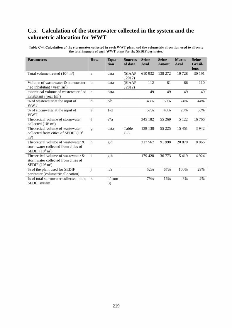
219

C.5. Calculation of the stormwater collected in the system and the

volumetric allocation for WWT

Table C-4. Calculation of the stormwater collected in each WWT plant and the volumetric allocation used to allocate

the total impacts of each WWT plant for the SEDIF perimeter.

Parameters Row Equa-

tion

Sources

of data

Seine

Aval

Seine

Amont

Marne

Aval

Seine

Grésil-

lons

Total volume treated (103 m3) a data (SIAAP

, 2012)

610 932 138 272 19 728 30 191

Volume of wastewater & stormwater

/ eq inhabitant / year (m3)

b data (SIAAP

, 2012)

112 81 66 110

theoretical volume of wastewater / eq

inhabitant / year (m3)

c data 49 49 49 49

% of wastewater at the input of

WWT

d c/b 43% 60% 74% 44%

% of stormwater at the input of

WWT

e 1-d 57% 40% 26% 56%

Theoretical volume of stormwater

collected (103 m3)

f e*a 345 182 55 269 5 122 16 766

Theoretical volume of wastewater

collected from cities of SEDIF (103

m3)

g data Table

C-3

138 138 55 225 15 451 3 942

Theoretical volume of wastewater &

stormwater collected from cities of

SEDIF (103 m3)

h g/d 317 567 91 998 20 870 8 866

Theoretical volume of wastewater &

stormwater collected from cities of

SEDIF (103 m3)

i g-h 179 428 36 773 5 419 4 924

% of the plant used for SEDIF

perimeter (volumetric allocation)

j h/a 52% 67% 100% 29%

% of total stormwater collected in the

SEDIF system

k i / sum

(i)

79% 16% 3% 2%

220

C.6. LCI for computing impact matrices i

In the sub-sections C.2.1 to C.2.6, sources of LCI for computing impact matrices i are

presented. LCI data for processes based on local data are developed hereafter. LCI data

corresponding to ecoinvent processes are not presented here. The resulting matrices i obtained

from these LCI data are computed within Simapro 8 (Pré Consultants, 2013). As a matter of

simplicity, only one example of matrix i is presented in section C.6.4.

C.6.1. Drinking water production and distribution

Data for life cycle inventory of drinking water production and distribution are confidential.

They have been gathered during an internship done in the context of this thesis (Catel, L.

2012. Analyse du cycle de vie de trois usines de production d’eau potable. Confidential

report). The report can be requested upon request.

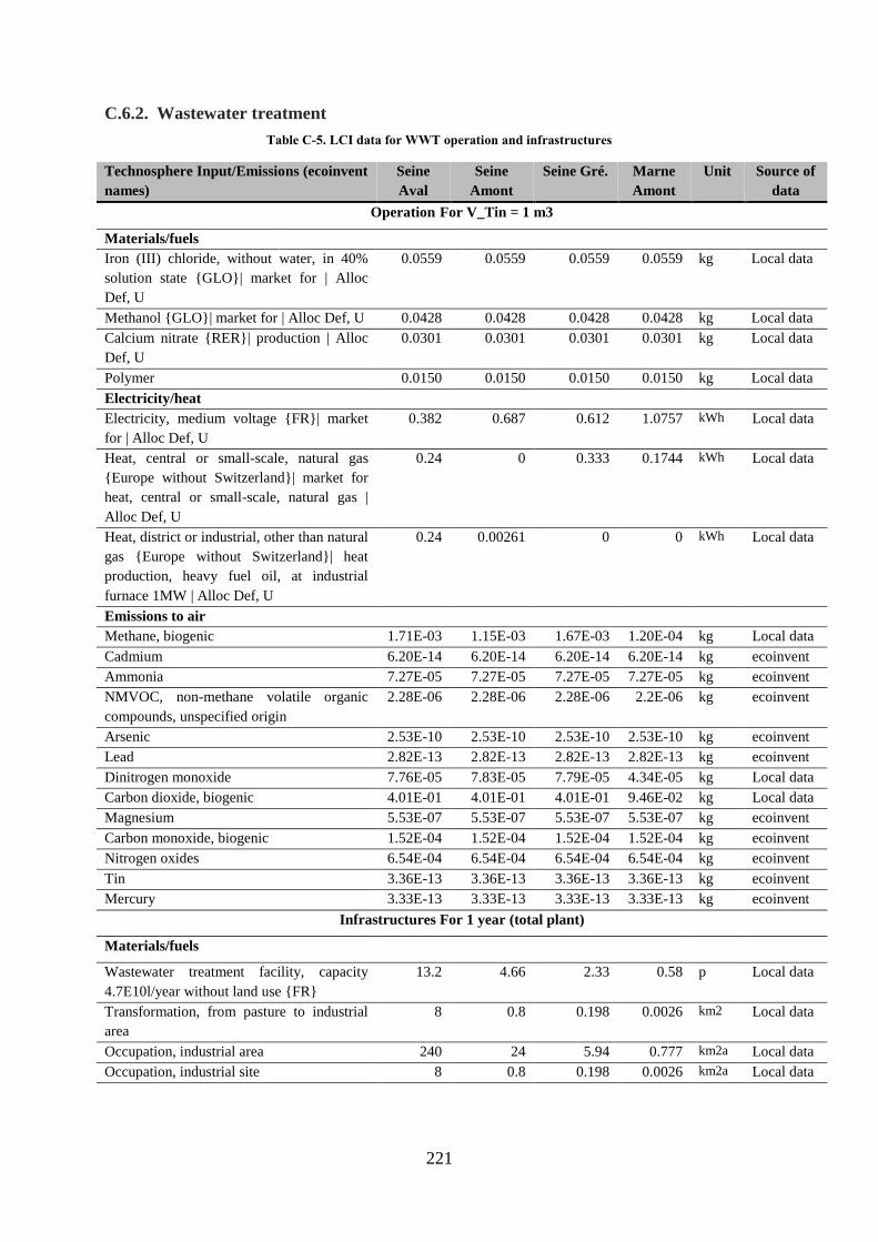
221

C.6.2. Wastewater treatment

Table C-5. LCI data for WWT operation and infrastructures

Technosphere Input/Emissions (ecoinvent

names)

Seine

Aval

Seine

Amont

Seine Gré. Marne

Amont

Unit Source of

data

Operation For V_Tin = 1 m3

Materials/fuels

Iron (III) chloride, without water, in 40%

solution state {GLO}| market for | Alloc

Def, U

0.0559 0.0559 0.0559 0.0559 kg Local data

Methanol {GLO}| market for | Alloc Def, U 0.0428 0.0428 0.0428 0.0428 kg Local data

Calcium nitrate {RER}| production | Alloc

Def, U

0.0301 0.0301 0.0301 0.0301 kg Local data

Polymer 0.0150 0.0150 0.0150 0.0150 kg Local data

Electricity/heat

Electricity, medium voltage {FR}| market

for | Alloc Def, U

0.382 0.687 0.612 1.0757 kWh Local data

Heat, central or small-scale, natural gas

{Europe without Switzerland}| market for

heat, central or small-scale, natural gas |

Alloc Def, U

0.24 0 0.333 0.1744 kWh Local data

Heat, district or industrial, other than natural

gas {Europe without Switzerland}| heat

production, heavy fuel oil, at industrial

furnace 1MW | Alloc Def, U

0.24 0.00261 0 0 kWh Local data

Emissions to air

Methane, biogenic 1.71E-03 1.15E-03 1.67E-03 1.20E-04 kg Local data

Cadmium 6.20E-14 6.20E-14 6.20E-14 6.20E-14 kg ecoinvent

Ammonia 7.27E-05 7.27E-05 7.27E-05 7.27E-05 kg ecoinvent

NMVOC, non-methane volatile organic

compounds, unspecified origin

2.28E-06 2.28E-06 2.28E-06 2.2E-06 kg ecoinvent

Arsenic 2.53E-10 2.53E-10 2.53E-10 2.53E-10 kg ecoinvent

Lead 2.82E-13 2.82E-13 2.82E-13 2.82E-13 kg ecoinvent

Dinitrogen monoxide 7.76E-05 7.83E-05 7.79E-05 4.34E-05 kg Local data

Carbon dioxide, biogenic 4.01E-01 4.01E-01 4.01E-01 9.46E-02 kg Local data

Magnesium 5.53E-07 5.53E-07 5.53E-07 5.53E-07 kg ecoinvent

Carbon monoxide, biogenic 1.52E-04 1.52E-04 1.52E-04 1.52E-04 kg ecoinvent

Nitrogen oxides 6.54E-04 6.54E-04 6.54E-04 6.54E-04 kg ecoinvent

Tin 3.36E-13 3.36E-13 3.36E-13 3.36E-13 kg ecoinvent

Mercury 3.33E-13 3.33E-13 3.33E-13 3.33E-13 kg ecoinvent

Infrastructures For 1 year (total plant)

Materials/fuels

Wastewater treatment facility, capacity

4.7E10l/year without land use {FR}

13.2 4.66 2.33 0.58 p Local data

Transformation, from pasture to industrial

area

8 0.8 0.198 0.0026 km2 Local data

Occupation, industrial area 240 24 5.94 0.777 km2a Local data

Occupation, industrial site 8 0.8 0.198 0.0026 km2a Local data

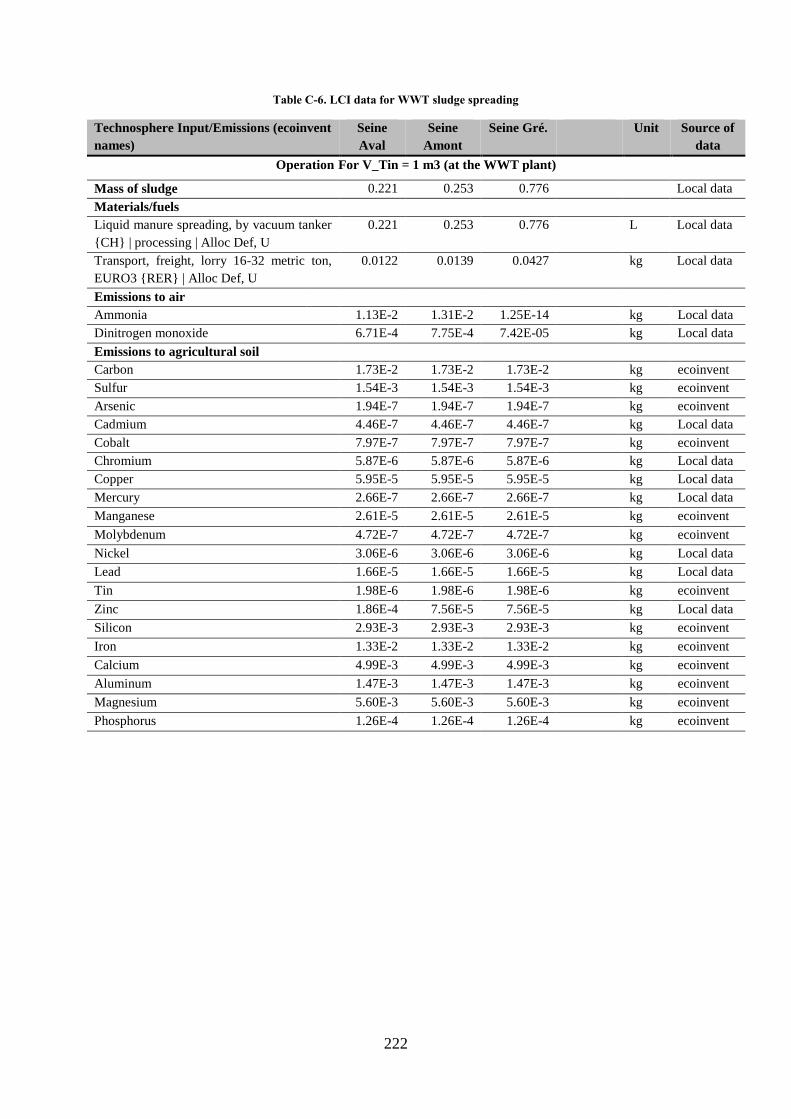
222

Table C-6. LCI data for WWT sludge spreading

Technosphere Input/Emissions (ecoinvent

names)

Seine

Aval

Seine

Amont

Seine Gré. Unit Source of

data

Operation For V_Tin = 1 m3 (at the WWT plant)

Mass of sludge 0.221 0.253 0.776 Local data

Materials/fuels

Liquid manure spreading, by vacuum tanker

{CH} | processing | Alloc Def, U

0.221 0.253 0.776 L Local data

Transport, freight, lorry 16-32 metric ton,

EURO3 {RER} | Alloc Def, U

0.0122 0.0139 0.0427 kg Local data

Emissions to air

Ammonia 1.13E-2 1.31E-2 1.25E-14 kg Local data

Dinitrogen monoxide 6.71E-4 7.75E-4 7.42E-05 kg Local data

Emissions to agricultural soil

Carbon 1.73E-2 1.73E-2 1.73E-2 kg ecoinvent

Sulfur 1.54E-3 1.54E-3 1.54E-3 kg ecoinvent

Arsenic 1.94E-7 1.94E-7 1.94E-7 kg ecoinvent

Cadmium 4.46E-7 4.46E-7 4.46E-7 kg Local data

Cobalt 7.97E-7 7.97E-7 7.97E-7 kg ecoinvent

Chromium 5.87E-6 5.87E-6 5.87E-6 kg Local data

Copper 5.95E-5 5.95E-5 5.95E-5 kg Local data

Mercury 2.66E-7 2.66E-7 2.66E-7 kg Local data

Manganese 2.61E-5 2.61E-5 2.61E-5 kg ecoinvent

Molybdenum 4.72E-7 4.72E-7 4.72E-7 kg ecoinvent

Nickel 3.06E-6 3.06E-6 3.06E-6 kg Local data

Lead 1.66E-5 1.66E-5 1.66E-5 kg Local data

Tin 1.98E-6 1.98E-6 1.98E-6 kg ecoinvent

Zinc 1.86E-4 7.56E-5 7.56E-5 kg Local data

Silicon 2.93E-3 2.93E-3 2.93E-3 kg ecoinvent

Iron 1.33E-2 1.33E-2 1.33E-2 kg ecoinvent

Calcium 4.99E-3 4.99E-3 4.99E-3 kg ecoinvent

Aluminum 1.47E-3 1.47E-3 1.47E-3 kg ecoinvent

Magnesium 5.60E-3 5.60E-3 5.60E-3 kg ecoinvent

Phosphorus 1.26E-4 1.26E-4 1.26E-4 kg ecoinvent

223

C.6.3. Nitrogen mass balance in WWT

Figure C-7. Nitrogen mass balance in WWT

WWT plant

Em

ission

s

to w

ate

r

N=58.6 glocal data

measurement

Em

issi

on

s

to a

ir

N=5.4 gecoinvent model

N-NO2=3g/m3 biogaz

N-NH3=0.9g/m3 biogaz

N-N2O=0.46g/m3 biogaz

Nitrification/Denitrification

+ Digestion/Biogaz incineration

sludge

N=17 g

(NO3-,NO2

-)local data

measurement

N=36.2 gmass balance

Sludge spreading

N to plants = 26.4g

mass balance

Air

N=9.7 gecoinvent model

N-NH3=0.258*Nsludge

N-N2O=0.0118*Nsludge

224

C.6.4. Example of impact matrix i

Table C-7. Matrix of specific impacts i, for the instance WWT_Marne-Aval

LCIA

Method

Impact category Unit direct, air

and soil

indirect,

energy

indirect,

chemicals

& others

(for 1m3)

indirect,

infrastructure

(total)

Impact

2002+

Carcinogens DALY 8,828E-13 6,43E-09 4,08E-08 2,79E-01

Non-carcinogens DALY 1,925E-11 7,11E-09 1,19E-08 3,06E-01

Respiratory inorganics DALY 6,45E-08 7,89E-08 1,36E-07 3,03E+00

Ionizing radiation DALY 0 1,85E-08 5,29E-10 4,29E-03

Ozone layer depletion DALY 0 1,05E-10 3,37E-11 1,48E-04

Respiratory organics DALY 2,92E-12 6,65E-11 1,79E-10 4,15E-03

Aquatic ecotoxicity PDF*m2*yr 1,495E-08 1,89E-03 7,87E-04 1,08E+04

Terrestrial ecotoxicity PDF*m2*yr 6,488E-06 3,49E-02 2,46E-02 6,04E+05

Terrestrial acid/nutri PDF*m2*yr 0,0048667 1,91E-03 4,59E-03 8,43E+04

Land occupation PDF*m2*yr 0 2,43E-03 2,33E-03 8,00E+04

Aquatic acidification PDF*m2*yr 5,247E-06 5,40E-06 1,10E-05 1,80E+02

Aquatic eutrophication PDF*m2*yr 0 1,97E-04 6,13E-04 1,05E+04

Global warming kg CO2 eq 0,0073617 1,48E-01 1,86E-01 3,97E+06

Non-renewable energy MJ primary 0 1,27E+01 3,54E+00 3,51E+07

Mineral extraction MJ primary 0 6,73E-03 2,09E-02 8,72E+05

Human health DALY 6,45E-08 1,11E-07 1,90E-07 3,63E+00

Ecosystem quality PDF*m2*yr 4,88E-03 4,13E-02 3,29E-02 7,90E+05

Resources MJ primary 0,00E+00 1,28E+01 3,56E+00 3,60E+07

ILCD Climate change kg CO2 eq 0,0156269 1,56E-01 2,22E-01 4,05E+06

Ozone depletion kg CFC-11

eq

0 9,96E-08 3,21E-08 1,41E-01

HT, cancer effects CTUh 1,098E-13 7,49E-09 8,88E-09 5,81E-01

HT, non-cancer effects CTUh 4,61E-12 5,78E-08 8,28E-08 1,87E+00

Particulate matter kg PM2.5

eq

9,942E-06 6,66E-05 1,33E-04 2,86E+03

Ionizing radiation HH kBq U235

eq

0 8,65E-01 2,49E-02 2,02E+05

Ionizing radiation E

(interim)

CTUe 0 1,06E-06 5,73E-08 6,91E-01

Photochemical ozone

formation

kg

NMVOC eq

0,000658 3,37E-04 6,48E-04 1,65E+04

Acidification molc H+ eq 0,0007039 7,34E-04 1,55E-03 2,29E+04

Terrestrial

eutrophication

molc N eq 0,0037698 1,11E-03 3,00E-03 5,55E+04

Freshwater

eutrophication

kg P eq 0 2,88E-05 6,07E-05 1,20E+03

Marine eutrophication kg N eq 0,0002613 1,09E-04 2,47E-04 5,08E+03

Freshwater ecotoxicity CTUe 4,287E-06 9,55E-01 2,14E+00 9,78E+07

Land use kg C deficit 0 8,57E-02 1,78E-01 1,13E+07

CTA Hoekstra m3 water eq 0 5,43E-04 3,84E-03 47832,654

resource depletion kg Sb eq 0 5,71E-06 2,10E-05 1,61E+02

225

C.7. Updated CFWD for baseline and forecasting scenarios

Updated monthly CFWD computed in Chapter 6 are shown hereafter for 2012 (Table C-8) and

2050 (Table C-9, considering climate change effects). Only the CFWD from 12 sub-river

basins (on a total of 110 within the Seine river basin), are shown as a matter of simplicity, and

because these are the concerned SRBs in the case study. Since the boundaries and numbers of

SRBs in the updated model are different from Chapter 3, id of each sub-river basins are

different from those defined in Figure 3-4. The updated ids are from HydroSHEDS. We also

defined simplified ids to easily locate the different SRBs. Locations of SRBs are shown in

Figure C-8.

Table C-8. Updated CFWD at the monthly scale for 2012

simp

lified

id

Id

(2080

4-)

Jan Feb Mar Apr May Jun Jul Aug Sep Oct Nov Dec

1 55490 0,06 0,08 0,10 0,17 0,11 0,23 0,42 0,80 0,87 0,32 0,14 0,05

2 55180 0,08 0,11 0,12 0,22 0,16 0,32 0,58 1,13 1,20 0,47 0,19 0,07

3 55290 0,08 0,11 0,13 0,24 0,16 0,31 0,57 1,10 1,18 0,44 0,19 0,08

4 59800 0,09 0,13 0,15 0,26 0,17 0,35 0,65 1,23 1,33 0,52 0,22 0,09

5 59960 0,12 0,17 0,21 0,36 0,23 0,46 0,88 1,67 1,80 0,68 0,28 0,12

6 64550 0,13 0,19 0,23 0,40 0,25 0,51 0,99 1,90 2,03 0,76 0,31 0,13

7 64540 0,20 0,27 0,32 0,56 0,34 0,66 1,17 2,21 2,46 0,92 0,38 0,18

8 70760 0,14 0,19 0,23 0,41 0,25 0,51 0,99 1,92 2,05 0,77 0,31 0,14

9 70920 0,15 0,21 0,25 0,44 0,27 0,56 1,08 2,08 2,24 0,86 0,35 0,15

10 81100 0,16 0,22 0,28 0,48 0,31 0,61 1,19 2,28 2,47 0,97 0,42 0,17

11 77390 0,18 0,24 0,29 0,50 0,32 0,63 1,20 2,27 2,44 0,98 0,45 0,19

12 C-A 0,13 0,18 0,22 0,38 0,24 0,48 0,93 1,79 1,92 0,72 0,29 0,13

Table C-9. Updated CFWD at the monthly scale for 2050

simp

lified

id

id

(2080

4-)

Jan Feb Mar Apr May Jun Jul Aug Sep Oct Nov Dec

1 55490 0,06 0,08 0,10 0,17 0,13 0,28 0,50 0,92 0,98 0,35 0,14 0,05

2 55180 0,08 0,11 0,12 0,22 0,18 0,38 0,70 1,29 1,37 0,52 0,19 0,07

3 55290 0,08 0,11 0,13 0,24 0,17 0,38 0,68 1,25 1,34 0,48 0,19 0,08

4 59800 0,09 0,13 0,15 0,26 0,19 0,42 0,77 1,41 1,51 0,57 0,22 0,09

5 59960 0,12 0,17 0,21 0,36 0,25 0,56 1,05 1,91 2,04 0,74 0,28 0,12

6 64550 0,13 0,19 0,23 0,40 0,28 0,62 1,18 2,18 2,31 0,84 0,31 0,13

7 64540 0,20 0,27 0,32 0,56 0,38 0,80 1,39 2,52 2,77 1,00 0,38 0,18

8 70760 0,14 0,19 0,23 0,41 0,28 0,62 1,19 2,19 2,33 0,84 0,31 0,14

9 70920 0,15 0,21 0,25 0,44 0,30 0,68 1,29 2,38 2,55 0,94 0,35 0,15

10 81100 0,16 0,22 0,28 0,48 0,34 0,75 1,42 2,62 2,80 1,06 0,42 0,17

11 77390 0,15 0,22 0,27 0,46 0,32 0,71 1,36 2,53 2,71 1,01 0,38 0,16

12 C-A 0,13 0,18 0,22 0,38 0,26 0,59 1,11 2,05 2,18 0,79 0,29 0,13

226

Figure C-8. Locations of the SRBs concerned in Chapter 6 within the Seine river basin.

227

C.8. Full results of environmental impacts for the baseline and forecasting scenarios

Table C-10. Full results of the baseline and the forecasting scenarios: impacts for the entire UWS

B S1 S2 S3 L1 L2 L3 L4 L5 L6 L7 L8

Impact

2002+

Carcinogens DALY 5,17E+

01

5,14E+

01

5,12E+

01

5,09E+

01

5,01E+

01

5,33E+

01

5,53E+

01

5,01E+

01

5,10E+

01

4,99E+

01

5,12E+

01

4,97E+

01

Non-carcinogens DALY 8,24E+

02

8,17E+

02

8,13E+

02

8,09E+

02

7,88E+

02

8,60E+

02

9,03E+

02

7,88E+

02

7,91E+

02

7,85E+

02

7,93E+

02

7,88E+

02

Respiratory

inorganics

DALY 6,18E+

02

6,14E+

02

6,10E+

02

6,06E+

02

5,95E+

02

6,42E+

02

6,70E+

02

5,95E+

02

6,08E+

02

5,93E+

02

6,09E+

02

5,90E+

02

Ionizing radiation DALY 7,30E+

00

7,35E+

00

6,97E+

00

6,72E+

00

6,80E+

00

7,80E+

00

8,40E+

00

6,80E+

00

8,36E+

00

6,68E+

00

8,50E+

00

6,31E+

00

Ozone layer

depletion

DALY 6,27E-

02

6,28E-

02

6,05E-

02

5,89E-

02

5,90E-

02

6,64E-

02

7,08E-

02

5,90E-

02

6,85E-

02

5,82E-

02

6,91E-

02

5,61E-

02

Respiratory organics DALY 3,26E-

01

3,25E-

01

3,22E-

01

3,21E-

01

3,18E-

01

3,33E-

01

3,42E-

01

3,18E-

01

3,28E-

01

3,17E-

01

3,29E-

01

3,15E-

01

Aquatic ecotoxicity PDF*m2

*yr

2,21E+

08

2,22E+

08

2,16E+

08

2,10E+

08

2,07E+

08

2,35E+

08

2,52E+

08

2,07E+

08

2,10E+

08

1,97E+

08

2,05E+

08

2,04E+

08

Terrestrial

ecotoxicity

PDF*m2

*yr

1,06E+

10

1,06E+

10

1,04E+

10

1,03E+

10

1,00E+

10

1,12E+

10

1,19E+

10

1,00E+

10

1,04E+

10

9,76E+

09

1,02E+

10

9,94E+

09

Terrestrial acid/nutri PDF*m2

*yr

7,54E+

07

7,47E+

07

7,44E+

07

7,39E+

07

7,21E+

07

7,86E+

07

8,24E+

07

7,21E+

07

7,25E+

07

7,21E+

07

7,25E+

07

7,20E+

07

Land occupation PDF*m2

*yr

7,76E+

06

7,76E+

06

7,66E+

06

7,48E+

06

7,61E+

06

7,91E+

06

8,09E+

06

7,61E+

06

7,84E+

06

7,55E+

06

7,45E+

06

7,17E+

06

Acidification PDF*m2

*yr

8,92E+

04

8,84E+

04

8,79E+

04

8,74E+

04

8,54E+

04

9,29E+

04

9,73E+

04

8,54E+

04

8,66E+

04

8,53E+

04

8,68E+

04

8,51E+

04

Eutrophication PDF*m2

*yr

2,78E+

07

2,75E+

07

2,76E+

07

2,75E+

07

2,68E+

07

2,89E+

07

3,01E+

07

2,68E+

07

2,60E+

07

2,66E+

07

2,70E+

07

2,69E+

07

Global warming kg CO2

eq

3,86E+

08

3,85E+

08

3,81E+

08

3,78E+

08

3,74E+

08

3,98E+

08

4,12E+

08

3,74E+

08

3,90E+

08

3,72E+

08

3,92E+

08

3,69E+

08

Non-renewable

energy

MJ

primary

8,43E+

09

8,44E+

09

8,16E+

09

7,97E+

09

7,98E+

09

8,86E+

09

9,39E+

09

7,98E+

09

9,12E+

09

7,89E+

09

9,22E+

09

7,62E+

09

Mineral extraction MJ

primary

4,58E+

07

4,58E+

07

4,54E+

07

4,51E+

07

4,50E+

07

4,67E+

07

4,77E+

07

4,50E+

07

4,61E+

07

4,48E+

07

4,62E+

07

4,46E+

07

Human health DALY 1,50E+

03

1,49E+

03

1,48E+

03

1,47E+

03

1,44E+

03

1,56E+

03

1,64E+

03

1,44E+

03

1,46E+

03

1,44E+

03

1,46E+

03

1,44E+

03

Ecosystem quality PDF*m2

*yr

1,09E+

10

1,09E+

10

1,07E+

10

1,06E+

10

1,03E+

10

1,16E+

10

1,23E+

10

1,03E+

10

1,07E+

10

1,01E+

10

1,05E+

10

1,03E+

10

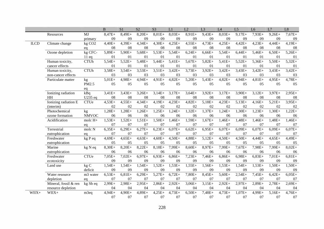
228

B S1 S2 S3 L1 L2 L3 L4 L5 L6 L7 L8

Resources MJ

primary

8,47E+

09

8,49E+

09

8,20E+

09

8,01E+

09

8,03E+

09

8,91E+

09

9,43E+

09

8,03E+

09

9,17E+

09

7,93E+

09

9,26E+

09

7,67E+

09

ILCD Climate change kg CO2

eq

4,40E+

08

4,39E+

08

4,34E+

08

4,30E+

08

4,25E+

08

4,55E+

08

4,73E+

08

4,25E+

08

4,42E+

08

4,23E+

08

4,44E+

08

4,19E+

08

Ozone depletion kg CFC-

11 eq

5,89E+

01

5,90E+

01

5,68E+

01

5,53E+

01

5,54E+

01

6,24E+

01

6,66E+

01

5,54E+

01

6,44E+

01

5,46E+

01

6,50E+

01

5,26E+

01

Human toxicity,

cancer effects

CTUh 5,54E+

01

5,52E+

01

5,48E+

01

5,44E+

01

5,41E+

01

5,67E+

01

5,82E+

01

5,41E+

01

5,52E+

01

5,36E+

01

5,50E+

01

5,32E+

01

Human toxicity,

non-cancer effects

CTUh 3,58E+

03

3,54E+

03

3,53E+

03

3,51E+

03

3,42E+

03

3,73E+

03

3,92E+

03

3,42E+

03

3,43E+

03

3,42E+

03

3,43E+

03

3,42E+

03

Particulate matter kg

PM2.5

eq

5,01E+

05

4,98E+

05

4,94E+

05

4,91E+

05

4,82E+

05

5,20E+

05

5,43E+

05

4,82E+

05

4,94E+

05

4,81E+

05

4,95E+

05

4,78E+

05

Ionizing radiation

HH

kBq

U235 eq

3,41E+

08

3,43E+

08

3,26E+

08

3,14E+

08

3,17E+

08

3,64E+

08

3,92E+

08

3,17E+

08

3,90E+

08

3,12E+

08

3,97E+

08

2,95E+

08


(interim)

CTUe 4,53E+

02

4,55E+

02

4,34E+

02

4,19E+

02

4,23E+

02

4,82E+

02

5,18E+

02

4,23E+

02

5,13E+

02

4,16E+

02

5,21E+

02

3,95E+

02

Photochemical

ozone formation

kg

NMVOC

1,28E+

06

1,28E+

06

1,26E+

06

1,25E+

06

1,24E+

06

1,32E+

06

1,37E+

06

1,24E+

06

1,30E+

06

1,23E+

06

1,30E+

06

1,22E+

06

Acidification molc H+

eq

1,53E+

07

1,52E+

07

1,51E+

07

1,50E+

07

1,46E+

07

1,59E+

07

1,67E+

07

1,46E+

07

1,48E+

07

1,46E+

07

1,48E+

07

1,46E+

07

Terrestrial

eutrophication

molc N

eq

6,35E+

07

6,29E+

07

6,27E+

07

6,23E+

07

6,07E+

07

6,62E+

07

6,95E+

07

6,07E+

07

6,09E+

07

6,07E+

07

6,09E+

07

6,07E+

07

Freshwater

eutrophication

kg P eq 4,69E+

05

4,65E+

05

4,63E+

05

4,60E+

05

4,50E+

05

4,88E+

05

5,12E+

05

4,50E+

05

4,50E+

05

4,44E+

05

4,65E+

05

4,49E+

05

Marine

eutrophication

kg N eq 8,30E+

06

8,20E+

06

8,22E+

06

8,18E+

06

7,99E+

06

8,60E+

06

8,97E+

06

7,99E+

06

7,67E+

06

7,98E+

06

7,99E+

06

8,02E+

06

Freshwater

ecotoxicity

CTUe 7,05E+

09

7,02E+

09

6,97E+

09

6,93E+

09

6,86E+

09

7,23E+

09

7,46E+

09

6,86E+

09

6,98E+

09

6,83E+

09

7,01E+

09

6,81E+

09

Land use kg C

deficit

1,54E+

09

1,54E+

09

1,54E+

09

1,52E+

09

1,53E+

09

1,55E+

09

1,56E+

09

1,53E+

09

1,54E+

09

1,53E+

09

1,50E+

09

1,50E+

09

Water resource

depletion

m3 water

eq

6,53E+

07

6,81E+

07

6,29E+

07

5,27E+

07

6,72E+

07

7,80E+

07

8,45E+

07

5,60E+

07

2,54E+

07

7,45E+

07

6,42E+

07

6,05E+

07

Mineral, fossil & ren

resource depletion

kg Sb eq 2,99E+

04

2,98E+

04

2,95E+

04

2,86E+

04

2,92E+

04

3,06E+

04

3,15E+

04

2,92E+

04

2,97E+

04

2,89E+

04

2,78E+

04

2,69E+

04

WIIX+ WIIX+ m3eq 4,94E+

07

4,90E+

07

4,89E+

07

4,25E+

07

4,73E+

07

6,50E+

07

7,48E+

07

4,73E+

07

1,07E+

07

4,99E+

07

5,16E+

07

4,76E+

07

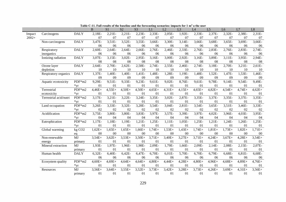
229

Table C-11. Full results of the baseline and the forecasting scenarios: impacts for 1 m3 a the user

B S1 S2 S3 L1 L2 L3 L4 L5 L6 L7 L8

Impact

2002+

Carcinogens DALY 2,18E-

07

2,21E-

07

2,21E-

07

2,23E-

07

2,33E-

07

2,05E-

07

1,92E-

07

2,33E-

07

2,37E-

07

2,32E-

07

2,38E-

07

2,31E-

07

Non-carcinogens DALY 3,47E-

06

3,51E-

06

3,52E-

06

3,55E-

06

3,66E-

06

3,30E-

06

3,14E-

06

3,66E-

06

3,68E-

06

3,65E-

06

3,69E-

06

3,66E-

06

Respiratory

inorganics

DALY 2,60E-

06

2,64E-

06

2,64E-

06

2,66E-

06

2,76E-

06

2,46E-

06

2,33E-

06

2,76E-

06

2,83E-

06

2,76E-

06

2,83E-

06

2,74E-

06

Ionizing radiation DALY 3,07E-

08

3,15E-

08

3,02E-

08

2,95E-

08

3,16E-

08

3,00E-

08

2,92E-

08

3,16E-

08

3,89E-

08

3,11E-

08

3,95E-

08

2,94E-

08

Ozone layer

depletion

DALY 2,64E-

10

2,70E-

10

2,62E-

10

2,58E-

10

2,74E-

10

2,55E-

10

2,46E-

10

2,74E-

10

3,18E-

10

2,70E-

10

3,21E-

10

2,61E-

10

Respiratory organics DALY 1,37E-

09

1,40E-

09

1,40E-

09

1,41E-

09

1,48E-

09

1,28E-

09

1,19E-

09

1,48E-

09

1,52E-

09

1,47E-

09

1,53E-

09

1,46E-

09

Aquatic ecotoxicity PDF*m2

*yr

9,29E-

01

9,51E-

01

9,33E-

01

9,23E-

01

9,61E-

01

9,02E-

01

8,76E-

01

9,61E-

01

9,78E-

01

9,14E-

01

9,54E-

01

9,49E-

01

Terrestrial

ecotoxicity

PDF*m2

*yr

4,46E+

01

4,55E+

01

4,50E+

01

4,50E+

01

4,65E+

01

4,31E+

01

4,15E+

01

4,65E+

01

4,82E+

01

4,54E+

01

4,74E+

01

4,62E+

01

Terrestrial acid/nutri PDF*m2

*yr

3,17E-

01

3,21E-

01

3,22E-

01

3,24E-

01

3,35E-

01

3,02E-

01

2,87E-

01

3,35E-

01

3,37E-

01

3,35E-

01

3,37E-

01

3,35E-

01

Land occupation PDF*m2

*yr

3,26E-

02

3,33E-

02

3,32E-

02

3,28E-

02

3,54E-

02

3,04E-

02

2,81E-

02

3,54E-

02

3,65E-

02

3,51E-

02

3,46E-

02

3,33E-

02

Acidification PDF*m2

*yr

3,75E-

04

3,80E-

04

3,80E-

04

3,83E-

04

3,97E-

04

3,57E-

04

3,39E-

04

3,97E-

04

4,02E-

04

3,96E-

04

4,03E-

04

3,95E-

04

Eutrophication PDF*m2

*yr

1,17E-

01

1,18E-

01

1,19E-

01

1,21E-

01

1,25E-

01

1,11E-

01

1,05E-

01

1,25E-

01

1,21E-

01

1,24E-

01

1,26E-

01

1,25E-

01

Global warming kg CO2

eq

1,62E+

00

1,65E+

00

1,65E+

00

1,66E+

00

1,74E+

00

1,53E+

00

1,43E+

00

1,74E+

00

1,81E+

00

1,73E+

00

1,82E+

00

1,71E+

00

Non-renewable

energy

MJ

primary

3,54E+

01

3,62E+

01

3,53E+

01

3,50E+

01

3,71E+

01

3,40E+

01

3,27E+

01

3,71E+

01

4,24E+

01

3,67E+

01

4,28E+

01

3,54E+

01

Mineral extraction MJ

primary

1,93E-

01

1,97E-

01

1,96E-

01

1,98E-

01

2,09E-

01

1,79E-

01

1,66E-

01

2,09E-

01

2,14E-

01

2,08E-

01

2,15E-

01

2,07E-

01

Human health DALY 6,32E-

06

6,40E-

06

6,42E-

06

6,47E-

06

6,70E-

06

6,01E-

06

5,70E-

06

6,70E-

06

6,79E-

06

6,68E-

06

6,81E-

06

6,68E-

06

Ecosystem quality PDF*m2

*yr

4,60E+

01

4,69E+

01

4,64E+

01

4,64E+

01

4,80E+

01

4,44E+

01

4,28E+

01

4,80E+

01

4,96E+

01

4,68E+

01

4,89E+

01

4,76E+

01

Resources MJ

primary

3,56E+

01

3,64E+

01

3,55E+

01

3,52E+

01

3,73E+

01

3,42E+

01

3,28E+

01

3,73E+

01

4,26E+

01

3,69E+

01

4,31E+

01

3,56E+

01

230

B S1 S2 S3 L1 L2 L3 L4 L5 L6 L7 L8

ILCD Climate change kg CO2

eq

1,85E+

00

1,88E+

00

1,88E+

00

1,89E+

00

1,98E+

00

1,75E+

00

1,65E+

00

1,98E+

00

2,05E+

00

1,97E+

00

2,06E+

00

1,95E+

00

Ozone depletion kg CFC-

11 eq

2,48E-

07

2,53E-

07

2,46E-

07

2,43E-

07

2,57E-

07

2,40E-

07

2,32E-

07

2,57E-

07

2,99E-

07

2,54E-

07

3,02E-

07

2,44E-

07

Human toxicity,

cancer effects

CTUh 2,33E-

07

2,37E-

07

2,37E-

07

2,39E-

07

2,51E-

07

2,18E-

07

2,02E-

07

2,51E-

07

2,57E-

07

2,49E-

07

2,56E-

07

2,47E-

07

Human toxicity,

non-cancer effects

CTUh 1,50E-

05

1,52E-

05

1,53E-

05

1,54E-

05

1,59E-

05

1,43E-

05

1,36E-

05

1,59E-

05

1,59E-

05

1,59E-

05

1,59E-

05

1,59E-

05

Particulate matter kg

PM2.5

eq

2,11E-

03

2,14E-

03

2,14E-

03

2,15E-

03

2,24E-

03

2,00E-

03

1,89E-

03

2,24E-

03

2,30E-

03

2,24E-

03

2,30E-

03

2,22E-

03

Ionizing radiation

HH

kBq

U235 eq

1,43E+

00

1,47E+

00

1,41E+

00

1,38E+

00

1,48E+

00

1,40E+

00

1,36E+

00

1,48E+

00

1,81E+

00

1,45E+

00

1,85E+

00

1,37E+

00


(interim)

CTUe 1,90E-

06

1,95E-

06

1,88E-

06

1,84E-

06

1,97E-

06

1,85E-

06

1,80E-

06

1,97E-

06

2,39E-

06

1,93E-

06

2,42E-

06

1,84E-

06

Photochemical

ozone formation

kg

NMVOC

eq

5,39E-

03

5,49E-

03

5,47E-

03

5,50E-

03

5,77E-

03

5,07E-

03

4,76E-

03

5,77E-

03

6,02E-

03

5,74E-

03

6,04E-

03

5,69E-

03

Acidification molc H+

eq

6,43E-

02

6,51E-

02

6,53E-

02

6,58E-

02

6,80E-

02

6,13E-

02

5,82E-

02

6,80E-

02

6,88E-

02

6,80E-

02

6,89E-

02

6,78E-

02

Terrestrial

eutrophication

molc N

eq

2,67E-

01

2,70E-

01

2,71E-

01

2,73E-

01

2,82E-

01

2,54E-

01

2,42E-

01

2,82E-

01

2,83E-

01

2,82E-

01

2,83E-

01

2,82E-

01

Freshwater

eutrophication

kg P eq 1,97E-

03

2,00E-

03

2,00E-

03

2,02E-

03

2,09E-

03

1,88E-

03

1,78E-

03

2,09E-

03

2,09E-

03

2,07E-

03

2,16E-

03

2,09E-

03

Marine

eutrophication

kg N eq 3,49E-

02

3,52E-

02

3,56E-

02

3,59E-

02

3,72E-

02

3,30E-

02

3,12E-

02

3,72E-

02

3,56E-

02

3,71E-

02

3,72E-

02

3,73E-

02

Freshwater

ecotoxicity

CTUe 2,96E+

01

3,01E+

01

3,02E+

01

3,04E+

01

3,19E+

01

2,78E+

01

2,60E+

01

3,19E+

01

3,24E+

01

3,18E+

01

3,26E+

01

3,16E+

01

Land use kg C

deficit

6,47E+

00

6,61E+

00

6,64E+

00

6,68E+

00

7,12E+

00

5,94E+

00

5,42E+

00

7,12E+

00

7,15E+

00

7,11E+

00

6,99E+

00

6,97E+

00

Water resource

depletion

m3 water

eq

2,75E-

01

2,92E-

01

2,72E-

01

2,31E-

01

3,12E-

01

3,00E-

01

2,94E-

01

3,12E-

01

1,18E-

01

3,46E-

01

2,98E-

01

2,81E-

01

Mineral, fossil & ren

resource depletion

kg Sb eq 1,26E-

04

1,28E-

04

1,28E-

04

1,25E-

04

1,36E-

04

1,18E-

04

1,10E-

04

1,36E-

04

1,38E-

04

1,35E-

04

1,29E-

04

1,25E-

04

WIIX+ WIIX+ m3eq 2,08E-

01

2,06E-

01

2,12E-

01

1,86E-

01

2,20E-

01

2,50E-

01

2,60E-

01

2,20E-

01

4,98E-

02

2,32E-

01

2,40E-

01

2,21E-

01

231

Résumé étendu

Chapitre 1 : Introduction

Depuis les années 1970, l’Homme a pris conscience du caractère vulnérable des milieux

naturels. Le rapport du club de Rome, publication majeure marquant l’apparition des

préoccupations environnementales, donne l’alerte sur la finitude des ressources naturelles

dans un contexte de croissance démographique. Cette prise de conscience a encouragé la

construction d’un nouveau paradigme environnemental et a favorisé l’émergence du concept

de développement durable. Dans ce contexte, les villes, grandes consommatrices de

ressources naturelles, ont un rôle essentiel à jouer. Les projections montrent que plus de 60%

de la population mondiale résidera dans des zones urbaines en 2030 augmentant encore la

pression sur les ressources naturelles dont les ressources en eau. Ces dernières sont déjà rares

et la concurrence entre les différents usagers (domestiques, agricoles, industriels) s’intensifie

(World Water Assessment Programme UN, 2009). La gestion de l’eau en milieu urbain est

une réelle problématique d’un point de vue environnemental (Global Water Partnership

Technical Committee, 2012).

Les décideurs ont besoin d’outils pour évaluer la performance environnementale des systèmes

d’eau urbains (comprenant les technologies, les usagers de l'eau et des ressources en eau).

Dans ce contexte, l’analyse du cycle de vie (ACV) est un outil d’évaluation environnementale

normalisé (ISO, 2006) et largement reconnu au niveau mondial. Cet outil quantifie les impacts

d’un produit ou d’un service tout au long de son cycle de vie (de l’extraction des matières

premières, à sa production, distribution, utilisation et jusqu’à la gestion de sa fin de vie). A la

différence d’autres outils d’évaluation environnementale (par exemple, l’empreinte carbone

ou le bilan énergétique), l’ACV est une approche multicritère qui prend en compte toutes les

étapes du « cycle de vie » d’un bien ou d’un service. Ce caractère holistique de l’ACV permet

d’identifier les transferts de pollution entre catégories d’impacts, entre étapes du cycle de vie

et/ou entre lieux géographiques. Alors que l’ACV a été initialement conçue pour des

approches orientées « produit/service », son application à des systèmes territoriaux émerge

avec le concept d’ACV territoriale (Loiseau et al., 2013). Le territoire est une échelle

pertinente pour évaluer les impacts environnementaux associés aux systèmes d'eau urbains.

Cependant les études ACV appliquées à des systèmes conséquents tels que les systèmes d’eau

des mégapoles urbaines nécessite une importante quantité de données et des efforts de

modélisation, notamment lorsque de multiples scénarios doivent être étudiés (Schulz et al.,

232

2012). Par conséquent, il y a un besoin pressent de développer des outils simplifiés afin de

fournir aux décideurs des indicateurs sur la performance environnementale des systèmes d'eau

urbains existants ou issus de scénarios prospectifs.

Au-delà des besoins méthodologiques en termes de modélisation du système d'eau urbain, un

autre défi scientifique fait l’objet de nombreux travaux dans la communauté ACV :

l'évaluation des impacts associés à l'utilisation de la ressource en eau. L’eau a cette propriété

d’être à la fois une ressource et un habitat environnemental, deux raisons qui expliquent les

nombreuses préoccupations portées sur cet « or bleu ». Bien entendu l’eau n’est pas aussi rare

que l’or. Bien au contraire puisque c’est une ressource renouvelable l’eau se déplace

continuellement sur Terre à travers un cycle global. Mais les ressources en eau sont très mal

distribuées dans le monde et les activités humaines exacerbent cette situation. Plus de 2.5

milliards de personnes font face à la rareté de l’eau pendant au moins un mois de l’année, ce

qui signifie qu’ils ne disposent pas assez d’eau disponible pour répondre aux demandes

(Hoekstra et al., 2012). En plus de la quantité, l’accès limité à l’eau est lié à des problèmes de

qualité affectant la santé de population vulnérable. Par ailleurs, l’eau étant aussi un habitat

environnemental, la rareté de l’eau et ses pollutions impactent de nombreux écosystèmes

sensibles.

Afin de tenir compte des problématiques liées à la prise en compte de la ressource en eau dans

l’évaluation environnementale des activités humaines, les concepts d'eau virtuelle et

d’empreinte de l'eau ont été développés. Ces méthodes permettent de quantifier les mètres

cubes équivalents nécessaires pour produire des biens ou des services, en prenant en compte

l’eau bleue (eau de surface), l’eau verte (eau evapotranspirée) et l’eau grise (eau polluée). Par

exemple, un kilogramme de viande de bœuf représente 15 400 L d'eau ou un kilogramme de

café près de 19 000 L. Cependant, l'interprétation de ces approches volumétriques pose des

problèmes car elles ne prennent pas en compte les impacts potentiels associés à l’utilisation et

à la pollution de l’eau sur les écosystèmes, sur la santé humaine et sur les ressources. Au

contraire, l’ACV caractérise les données d'inventaire afin de quantifier tous les impacts

potentiels sur l'environnement. A l'origine, l'ACV évaluait seulement les dommages dus à la

pollution de l'eau (aspects qualitatifs), à travers les catégories d’impact eutrophisation, et

écotoxicité. L'évaluation des impacts liés à l'utilisation de la ressource en eau (aspect

quantitatif) est plus récente et est à un stade de développement précoce, mais de nouvelles

méthodes sont en cours de développement et certaines sont opérationnelles (Kounina et al.,

2012). L'application et le raffinement de ces approches d’évaluation environnementale pour

233

les systèmes d’eau urbains sont nécessaires car ces systèmes jouent un rôle clé dans la gestion

de l'eau à l'échelle de bassins versants.

A partir de ces éléments de contexte, i.e. (i) la nécessité de concevoir des outils simplifiés

permettant aux décideurs de disposer d’indicateurs fiables sur la performance

environnementale des systèmes d'eau urbains et (ii) une meilleure prise en compte des

impacts liés à l’utilisation de la ressource en eau dans les méthodes d’évaluation

environnementale, la question de recherche de cette thèse peut être formulée ainsi: "Est-il

possible de modéliser un système d’eau urbain dans sa globalité afin d'évaluer ses impacts

environnementaux et les services rendus aux usagers, en utilisant le cadre conceptuel de

l'ACV?" Pour répondre à cette question de recherche, cinq sous-objectifs ont été définis :

- Identifier les principaux verrous méthodologiques liés à l'application de l’ACV aux

systèmes d'eau urbains et justifier la nécessité d'une approche standardisée. Ce sous

objectif est traité à travers une revue bibliographique dans le chapitre 2, qui

correspond à une publication scientifique publiée dans Water Research (Loubet et al.,

2014).

- Evaluer l'impact de la privation d'eau à une échelle appropriée et pertinente pour être

applicable aux systèmes d'eau urbains. Ce sous objectif est traité dans le chapitre 3,

qui correspond à une publication scientifique publiée dans Environmental Science &

Technology (Loubet et al., 2013).

- Caractériser et comptabiliser la qualité des flux d’eau urbain grâce aux méthodes

d’évaluation d’impacts du cycle de vie et d’empreinte eau. Ce sous objectif est traité

dans le chapitre 4.

- Développer un cadre conceptuel, un formalisme associé et un modèle pour évaluer les

impacts environnementaux des scénarios prospectifs de systèmes d’eau urbains. Ce

modèle, nommé WaLA (pour « Water systems Life cycle Assessment ») réduit la

complexité du système tout en étant représentatif pour l’ACV. Il s’agit de la partie

centrale de la thèse qui intègre les besoins méthodologiques identifiés et développés

dans les chapitres précédents. Ce sous-objectif est traité dans le chapitre 5, qui

correspond à une publication soumise dans Water Research.

- Démontrer l’applicabilité et la capacité du modèle à répondre à des questions de

gestion de l’eau avec l'évaluation des scénarios prospectifs. Le modèle est ainsi

appliqué au système d’eau urbain correspondant au périmètre géographique du

syndicat des eaux d’Île-de-France (SEDIF), en banlieue parisienne. Ce sous objectif

234

est traité dans le chapitre 6, qui correspond à une publication soumise dans Water

Research.

Chapitre 2. Analyse comparative des publications sur l’ACV des systèmes d’eau urbains

L’analyse du cycle de vie (ACV) a été largement utilisée pour évaluer les performances

environnementales des technologies liées à l’eau depuis les 20 dernières années. Une revue de

la littérature a été réalisée afin de compiler toutes les publications traitant des ACV de ces

technologies, c'est-à-dire la production et la distribution d’eau potable et la collecte et le

traitement des eaux usées. 130 publications ont été inventoriées, dont 18 qui traitent des

systèmes d’eau urbains dans leur globalité. Une attention particulière a été portée sur ces 18

publications qui ont été analysés selon des critères définis pour chacune des quatre phases de

l’ACV : définition des objectifs et du champ d’étude, inventaire du cycle de vie, évaluation

des impacts du cycle de vie et interprétation.

Les résultats de l’étude comparative montrent que les cas d’étude partagent un objectif

similaire en apportant des informations quantitatives aux gestionnaires sur les impacts

environnementaux des systèmes d’eau urbains et de leurs scénarios prospectifs. Néanmoins,

les études existantes sont basées sur des objectifs et des champs différents : les unités

fonctionnelles (UF) différent ainsi que les frontières des systèmes étudiés. Trois UF sont

relevées : distribuer et traiter 1 m3 chez l’usager (en résumé, « 1m3 »), distribuer et traiter

l’eau nécessaire pour un usager pendant un an (en résumé, « 1 usager/an ») ou le

fonctionnement du système d’eau urbain pendant un an (en résumé « système/an »). Les

données d’inventaire disponibles (utilisation d’électricité et les flux d’eau) et les résultats

d’évaluation des impacts (changement climatique, eutrophisation et le score unique) sont

comparés quantitativement. Cette revue de littérature apporte ainsi des données et résultats

synthétiques sur l’ACV des systèmes d’eau urbains.

La revue formule des recommandations sur la manière de conduire les ACV des systèmes

d’eau urbain et identifie des verrous méthodologiques :

- Pour l’évaluation environnementale d’un système d’eau urbain, la définition de l’unité

fonctionnelle devrait inclure l’usager car la fonction de ce système est de satisfaire ses

besoins (en termes de qualité et de quantité).

- La multifonctionnalité des systèmes d’eau urbains devrait profiter de l’adaptation du

cadre de l’ACV à l’évaluation territoriale (Loiseau et al., 2013).

235

- L’évaluation de scénarios prospectifs par l’ACV devrait permettre de différencier et

combiner les changements de technologies, d’usagers de l’eau et de ressources en eau.

- Les frontières du système devraient inclure toutes les étapes (construction, opération,

déconstruction) du cycle de vie des systèmes d’eau urbains. Une attention particulière

devrait être apportée sur le génie civil lors des travaux sur les réseaux.

- Un inventaire approprié de tous les flux d’eau devrait être fourni, en différenciant les

flux dans la technosphère, les eaux prélevées et rejetées dans l’environnement local et

l’eau évapotranspirée vers l’atmosphère (i.e. eau consommée) (Bayart et al., 2010).

- Le bilan de matière des polluants (en particulier l'azote, le phosphore et le carbone)

devrait être équilibré tout au long du système.

- Les méthodes d’évaluation des impacts actuelles permettent des évaluations

multicritères des systèmes d’eau urbains. Les approches monocritères telles que

l’empreinte carbone devraient donc être évitées afin de limiter les transferts de

pollution, en particulier vers les catégories d’impacts reliées à l’eau telles que

l’eutrophisation, l’écotoxicité et la privation d’eau.

- Les recherches récentes sur les méthodes d’évaluation des impacts de l’usage de l’eau

devraient être implémentées. La différentiation spatiale et temporelle à des échelles

appropriées devrait permettre une évaluation site-dépendant qui est très utile à

l’évaluation des systèmes d’eau urbains.

Cette revue a permis d’identifier un certain nombre d’axes de recherche qui ont été investis au

cours de cette thèse, dans le but de développer un modèle pour l’évaluation de la performance

environnementale des systèmes d’eau urbains.

Chapitre 3. Evaluation de la privation d’eau à l’échelle du sous bassin versant en ACV :

intégration des effets cascades en aval

L’une des principales problématiques identifiées est la nécessité de prendre en compte la

privation de l’eau dans les ACV des systèmes d’eau urbains. La privation d’eau au niveau

midpoint est actuellement étudiée dans les méthodes d’impacts d’ACV en utilisant des

indicateurs de stress hydrique à l’échelle du bassin versant (Kounina et al., 2012; Pfister et al.,

2009). Bien que ces indicateurs représentent un grand pas en avant dans l’évaluation des

impacts liés à l’utilisation des ressources en eau en ACV, d'importants points restent encore à

améliorer concernant leur précision et leur pertinence. Plus précisément, dans le cadre de

l’ACV, la définition de la privation d’eau associée à une activité humaine devrait être reliée

236

aux effets que celle-ci pourrait occasionner en aval de la dite activité. En effet, la

consommation à la source d’une rivière prive plus d’usagers et d’écosystèmes qu’une

consommation à l’embouchure (Vörösmarty et al., 2000) et le fait de considérer les impacts à

l’échelle du bassin versant entier ne permet pas cette différentiation. Pour les systèmes d’eau

urbains qui disposent de ressources en eau variées au sein même d’un bassin versant, cette

différentiation est nécessaire.

Une méthodologie quantifiant des facteurs de caractérisation midpoint de privation d'eau à

l’échelle du sous bassin versant a été développée en tenant compte des effets cascades. Le

cadre proposé est basé sur une approche en deux étapes. Tout d'abord, le stress hydrique est

quantifié à l'échelle du sous-bassin versant par un ratio entre la quantité d’eau consommée et

la quantité d’eau disponible (ratio plus communément appelé « consumption-to-availability »

ou CTA). D'autre part, les facteurs de caractérisation de privation d'eau (notés CFWD) sont

calculés en sommant et en pondérant les CTA des sous bassins en aval. Ainsi, le CFWD d’un

sous bassin donné mesure l’impact d’un prélèvement ou d’une consommation d’eau sur la

privation d’eau dans les sous-bassins en aval, comme le montre la Figure a.

Figure a. Illustration de l’effet cascade. SBV : Sous bassin versant

Les CTA et les CFWD ont été calculés grâce à un bilan d’eau à l’échelle du sous bassin

versant, et avec des bases de données hydrologiques sur les écoulements d’eau et la

consommation d'eau. Ces calcules ont été menés pour les bassins versant de la Seine (France)

et du Guadalquivir (Espagne, Figure b).

Les résultats montrent des différences significatives entre les CFWD calculés au sein d’un

même bassin versant (un ordre de grandeur), en fonction de la position en amont ou en aval.

Consommation d’eau (e.g., evaporation)

Amont

Aval

Sous bassins versant impactés

Bassin versant

SBV

SBV

SBV

SBV

SBV

SBV

237

En effet, plus un sous bassin est en amont, plus un prélèvement va impacter la quantité d’eau

disponible pour les sous-bassins en aval et plus le CFWD sera important. Les CFWD sont

appliqués à un cas d’étude théorique démontrant leur applicabilité pour étudier des scénarios

de gestion de l’eau. Cette méthodologie démontre qu’il est essentiel de localiser les points de

prélèvement et de rejet d’eau dans un bassin versant.

Figure b. CTA et CFWD du bassin versant Guadalquivir (Espagne)

Chapitre 4. Evaluation de la qualité des flux d’eau urbains avec les méthodes existantes

d’évaluation des impacts du cycle de vie et d’empreinte eau

En plus des problèmes de quantité d'eau présentés dans le chapitre 3, les impacts associés à la

qualité de l'eau doivent être pris en compte dans les ACV de systèmes d'eau urbains. Le

chapitre 4 propose une revue des méthodes d’évaluation des impacts du cycle de vie (EICV)

et d’empreinte eau pour évaluer la qualité des flux d’eau de systèmes urbains. Ainsi, des

scores de dommages sur les écosystèmes et la santé humaine sont calculés pour différents

types de flux d’eau (ex. ressources en eau, eaux usées, rejets d’usines, etc.) à partir de

concentrations en polluants. Les polluants caractérisés sont ceux de la directive cadre sur

l’eau, permettant de définir l’état physico-chimique et chimique de l’eau. Les méthodes

d’impacts utilisées sont Impact 2002+, ReCiPe, ILCD, permettant d’évaluer les impacts sur

l’eutrophisation, l’écotoxicité, l’acidification, et les dommages sur les écosystèmes et la santé

humaine. Les scores de dommages sont aussi utilisés pour calculer un indicateur simplifié

d’empreinte eau le Water Impact Index (WIIX).

3

CTA

CFWD

2

1

0

1.00 2.00

id41: id of the SRB

238

Les résultats permettent de comparer les scores de dommages avec les états physico-

chimiques et chimiques des ressources en eau. Cette comparaison montre l’intérêt de l’ACV

d’agréger plusieurs polluants en un score de dommage par rapport à la définition des états de

la directive cadre sur l’eau qui est basée sur des valeurs de seuils de polluants à ne pas

dépasser. Ils permettent aussi de classer les différents types de flux d’eau urbains selon leurs

scores de dommage et leurs indices de qualité calculés avec la méthode WIIX avancée. Cette

classification est utilisée par ailleurs dans le chapitre suivant pour gérer la qualité des flux

d’eau dans un système d’eau urbain.

Chapitre 5. WaLA, un modèle pour l’analyse du cycle de vie des systèmes d’eau

urbains : cadre conceptuel et formalisme pour une approche modulaire

Ce chapitre représentant le cœur de la thèse vise à élaborer un cadre conceptuel, un

formalisme et un modèle associé pour réaliser l’ACV de systèmes d’eau urbains et de leurs

scénarios prospectifs. Le modèle, nommé WaLA pour « Water systems Lifecycle

Assessment », a pour but de résoudre les questions méthodologiques identifiées dans le

chapitre 2 et d’intégrer les développements méthodologiques des chapitres 3 et 4. Comme la

construction de modèles de systèmes d’eau urbains est complexe si plusieurs scénarios sont à

évaluer, le modèle proposé réduit la complexité du système, tout en assurant une bonne

représentation du point de vue de l'ACV.

Le cadre proposé est basé sur la définition d’un composant générique qui peut représenter les

technologies et les usagers, et qui sont connectés à des ressources en eau spécifiques (cf.

Figure c).

239

Figure c. Description des flux d’eau et des impacts et services associés à un composant générique

Ces composants permettent de calculer les flux d’eau en entrée et en sortie (quantité et

qualité), ainsi que les impacts associés dus aux prélèvements et rejets d’eau directs et aux

activités de support (énergie, produits chimiques, infrastructures). Ces composants peuvent

être reliés entre eux d’une manière modulaire, afin de construire un scénario de système d’eau

urbain. Le modèle calcule les impacts du cycle de vie et les services fournis aux usagers, tels

que définis par le scénario, et pour un pas de temps mensuel. En effet, le système étudié est

multifonctionnel selon le cadre de l’ACV territoriale : plusieurs types d’usagers sont pris en

compte (ex. usagers domestiques, industriels etc.). Ceci permet de calculer des ratios

d’impacts sur services rendus (ex. impact/habitant) qui sont utiles pour le diagnostic ou la

comparaison de différentes alternatives. Le modèle est mis en œuvre dans une interface

Matlab/Simulink grâce à la programmation orientée objet. L'applicabilité du modèle est

démontrée en utilisant une étude de cas virtuelle basée sur des processus ecoinvent (Doka,

2009).

Chapitre 6. WaLA, un modèle pour l’analyse du cycle de vie des systèmes d’eau urbain :

mise en œuvre pour l’évaluation de scénarios de gestion de l’eau dans la banlieue

parisienne

Le modèle WaLA est appliqué à un cas d’étude: le système d’eau urbain de la banlieue

parisienne (périmètre géographique du syndicat des eaux d’Île-de-France – SEDIF), en

France. Ce cas d’étude vise à vérifier la capacité du modèle à évaluer les impacts

SoilLocal environment

111110Technology/User

Technosphere in

(Tin)

Technosphere out

(Tout)

Consumption

C

Withdrawal

from env. (W)

Release to

env. (R)

Technosphere

Water Local environment

AtmosphereGlobal environment Water flow V (m3)

with water quality Q

Indirect and direct

impacts due to emissions

and resouces use related

to supporting activities

(electricity, chemical,

infrastructures) Isupport

Provided services to

users S

Provided services

to users

Precipitation

P

Direct impacts linked to

emissions to air and soil

Idirect,air-soil

Direct impacts linked

to water quantity and

quality Idirect,water

Life Cycle Inventory

Life Cycle Impact

Assessment

Technosphere out2,

sludge (Tout2)

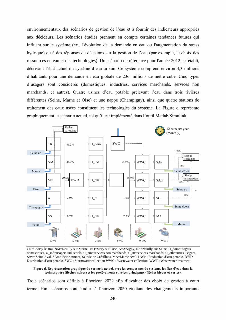
240

environnementaux des scénarios de gestion de l’eau et à fournir des indicateurs appropriés

aux décideurs. Les scénarios étudiés prennent en compte certaines tendances futures qui

influent sur le système (ex., l'évolution de la demande en eau ou l'augmentation du stress

hydrique) ou à des réponses de décisions sur la gestion de l’eau (par exemple, le choix des

ressources en eau et des technologies). Un scénario de référence pour l'année 2012 est établi,

décrivant l’état actuel du système d’eau urbain. Ce système comprend environ 4,3 millions

d’habitants pour une demande en eau globale de 236 millions de mètre cube. Cinq types

d’usagers sont considérés (domestiques, industries, services marchands, services non

marchands, et autres). Quatre usines d’eau potable prélevant l’eau dans trois rivières

différentes (Seine, Marne et Oise) et une nappe (Champigny), ainsi que quatre stations de

traitement des eaux usées constituent les technologies du système. La Figure d représente

graphiquement le scénario actuel, tel qu’il est implémenté dans l’outil Matlab/Simulink.

CR=Choisy-le-Roi, NM=Neuilly-sur-Marne, MO=Mery-sur-Oise, A=Arvigny, NS=Neuilly-sur-Seine, U_dom=usagers

domestiques, U_ind=usagers industriels, U_nm=services non marchands, U_m=services marchands, U_oth=autres usagers,

SAv= Seine Aval, SAm= Seine Amont, SG=Seine Grésillons, MA=Marne Aval. DWP : Production d’eau potable, DWD :

Distribution d’eau potable, SWC : Stormwater collection WWC : Wastewater collection, WWT : Wastewater treatment

Figure d. Représentation graphique du scenario actuel, avec les composants du systems, les flux d’eau dans la

technosphère (flèches noires) et les prélèvements et rejets principaux (flèches bleues et vertes).

Trois scénarios sont définis à l’horizon 2022 afin d’évaluer des choix de gestion à court

terme. Huit scénarios sont étudiés à l’horizon 2050 étudiant des changements importants

CR

NM

MO

A

NS

DWD

U_dom

U_ind

U_nm

U_m

U_oth

WWC

WWC

WWC

WWC

SAv

SAm

SG

MA

SWC41.2%

34.7%

20.5%

2.9%

0.7%

64.9%

25.9%

1.9%

7.3%

Sludge

spreading

Sludge

spreading

Sludge

incineration

100%

62%

38%

89%

11%

DWP DWD Users SWC WWC WWT

Seine up

Marne

Oise

Champigny

Seine

Seine down

Seine up

Seine down

Marne

12 runs per year

(monthly)

241

concernant les usagers (évolution de la population, de la demande en eau), les ressources

(choix des ressources, effets du changement climatique sur le stress hydriques) et les

technologies. Tous les scénarios sont construits facilement dans une interface

Matlab/Simulink, tel que présenté dans le chapitre 5. Les méthodes choisies pour l’évaluation

des impacts du cycle de vie sont Impact 2002+ endpoint, ILCD midpoint et les impacts de la

privation de l'eau à l’échelle du bassin versant (défini dans le chapitre 3). Les résultats

d’impact du scénario actuel permettent d’évaluer les contributions par rapport aux

technologies, montrant que la majorité des impacts sont générés par les usines de traitement

des eaux usées. L’analyse des contributions entre impacts directs et indirects (associés aux

activités de support), montrent que les impacts locaux (ex. eutrophisation, écotoxicité) sont

dominés par les impacts directs du système, alors que les impacts globaux (tels que le

réchauffement global et l’épuisement des ressources fossiles) sont dus aux activités de

support. L’analyse des résultats mensuels de la privation d’eau montre que la majorité des

impacts a lieu pendant les mois d’été. L’étude des scénarios prospectifs démontre la capacité

du modèle à fournir des informations pertinentes et utiles quant aux politiques futures. Les

scénarios proposés étudient principalement des changements au niveau de la production et de

la distribution d’eau potable et montrent que les gestionnaires de ces services ont peu

d’influence sur la majorité des impacts environnementaux (en comparaison au traitement des

eaux usées), mais ont une grande influence sur l’impact de privation d’eau du système en

choisissant les ressources en eau dans le bassin versant.

Sur la base de cette étude de cas, les apports et les limites du modèle WaLA sont identifiés.

Les principales nouveautés de ce modèle sont sa modularité et la prise en compte des usagers

de l'eau et des ressources en eau (à travers l'évaluation affinée des impacts liés à l'eau). Aussi,

le formalisme du modèle, qui est programmé selon une méthode orientée objet, permet son

appropriation par de futurs développeurs et son implémentation dans des logiciels autres que

Matlab/Simulink. Toutefois, en l’état actuel de son développement, certaines limites du

modèle demeurent, notamment sur la gestion du bilan équilibré des polluants à l’échelle des

composants, et sur la gestion des incertitudes. Ces limites nécessitent de nouveaux

développements. Enfin, la collecte de données d’inventaires pour des technologies émergentes

et pour d’autres usagers, ainsi que l'application de nouvelles méthodes d’EICV spatialisées et

liées à la qualité de l'eau, pourraient améliorer la fiabilité et l'exhaustivité du modèle.

242

Perspectives et conclusion

L’objectif principal de la thèse a consisté à développer un modèle d'évaluation

environnementale multicritère de scénarios de gestion (actuels ou prospectifs) de systèmes

d’eau urbains. L'hypothèse de recherche, i.e. une méthode peut être développée afin d'évaluer

facilement et régulièrement des scénarios de gestion de systèmes d'eau urbains dans le cadre

de l'ACV, a été validée à travers les développements méthodologiques menés dans les cinq

sous objectifs de la thèse détaillés ci-dessus.

Les résultats de cette thèse débouchent sur des perspectives de travaux à la fois scientifiques

et opérationnels. D’un point de vue scientifique, des développements méthodologiques

doivent encore être menés pour évaluer les facteurs de devenir liés à l’utilisation des

ressources en eau selon un modèle mécaniste et consensuel. La méthodologie d'évaluation de

la privation de l'eau à l'échelle des sous-bassins conçue au cours de la thèse pourrait alors être

intégrée dans ce type d’approche. D’un point de vue plus opérationnel, cette méthodologie

basée sur les effets cascades reste encore à déployer sur les bassins versants du monde entier

pour pouvoir être utilisée en routine dans les ACV. En ce qui concerne le modèle WaLA, son

application à d'autres études de cas dans des contextes différents serait un pas de plus pour

démontrer sa faisabilité et son intérêt. Enfin, l'appropriation des résultats par les parties

prenantes et les décideurs, et leur contribution dans un processus de prise de décision restent

des défis importants pour les sciences de gestion.

Références du résumé étendu

Bayart, J.-B., Bulle, C., Deschênes, L., Margni, M., Pfister, S., Vince, F., Koehler, A., 2010.

A framework for assessing off-stream freshwater use in LCA. Int. J. Life Cycle Assess.

15, 439–453.

Doka, G., 2009. Life Cycle Inventories of Waste Treatment Services. ecoinvent report No. 13.

Part IV. Dübendorf.

Global Water Partnership Technical Committee, 2012. Integrated urban water management.

Global Water Partnership, Stockholm, ISBN 9789185321872.

Hoekstra, A.Y., Mekonnen, M.M., Chapagain, A.K., Mathews, R.E., Richter, B.D., 2012.

Global monthly water scarcity: blue water footprints versus blue water availability. PLoS

One 7, e32688.

ISO, 2006. ISO - 14040 - Environmental Management - Life cycle assessment - Principles

and framework. Geneva.

243

Kounina, A., Margni, M., Bayart, J.-B., Boulay, A.-M., Berger, M., Bulle, C., Frischknecht,

R., Koehler, A., Milà i Canals, L., Motoshita, M., Núñez, M., Peters, G., Pfister, S.,

Ridoutt, B., Zelm, R., Verones, F., Humbert, S., 2012. Review of methods addressing

freshwater use in life cycle inventory and impact assessment. Int. J. Life Cycle Assess.

18, 707–721.

Loiseau, E., Roux, P., Junqua, G., Maurel, P., Bellon-Maurel, V., 2013. Adapting the LCA

framework to environmental assessment in land planning. Int. J. Life Cycle Assess. 18,

1533–1548.

Loubet, P., Roux, P., Loiseau, E., Bellon-Maurel, V., 2014. Life cycle assessments of urban

water systems: A comparative analysis of selected peer-reviewed literature. Water Res.

67, 187–202.

Loubet, P., Roux, P., Núñez, M., Belaud, G., Bellon-Maurel, V., 2013. Assessing Water

Deprivation at the Sub-river Basin Scale in LCA Integrating Downstream Cascade

Effects. Environ. Sci. Technol. 47, 14242–9.

Pfister, S., Koehler, A., Hellweg, S., 2009. Assessing the environmental impacts of freshwater

consumption in LCA. Environ. Sci. Technol. 43, 4098–104.

Schulz, M., Short, M.D., Peters, G.M., 2012. A streamlined sustainability assessment tool for

improved decision making in the urban water industry. Integr. Environ. Assess. Manag.

8, 183–93.

Vörösmarty, C.J., Fekete, B.M., Meybeck, M., Lammers, R.B., 2000. Global system of rivers:

Its role in organizing continental land mass and defining land-to-ocean linkages. Global

Biogeochem. Cycles 14, 599.

World Water Assessment Programme UN, 2009. The United Nations World Water

Development Report 3: Water in a changing world. Earthscan, Paris, France and London,

England, ISBN 9789231040955.

244

Abstract

To improve water management at the scale of large cities is a real challenge. However, the

quantification of flows and environmental impacts linked to water use are not yet sufficiently

developed. This is the objective of the thesis: “how to model complex urban water system of a

megacity for assessing its environmental impacts in relation to the provided services to water users,

within the life cycle assessment (LCA) framework?” The core of the thesis is the development of a

generic framework defining water flows and environmental impacts associated with 3 categories of

items – i.e., water technologies, water users and water resources – from a LCA point of view. The

UWS model (termed WaLA) is built through a modular approach allowing the interoperation of these

three components in an integrated way. The model provides indicators of impacts on services which

may be useful to decision makers and stakeholders. It simplifies the evaluation of forecasting

scenarios and decreases the complexity of the urban water system while ensuring its good

representation from a LCA perspective. In addition to this main objective, the thesis also aims at

refining water use impact indicators at a relevant scale for UWS. A methodology that assesses water

deprivation at the sub-river basin scale in life cycle impact assessment (LCIA) integrating downstream

cascade effects has been developed. It allows differentiating the withdrawal and release locations

within a same river basin. The WaLA model and its associated indicators are applied to assess the

environmental impacts of the water system of a Paris suburban area (perimeter of Syndicat des Eaux

d’Île-de-France). It shows the interest and the applicability of the model for assessing and comparing

baseline and forecasting scenarios.

Key words: life cycle assessment (LCA), environmental impacts, urban water system, water use,

water footprint, drinking water, wastewater, modeling, suburbs of Paris

Résumé

La gestion intégrée de l'eau à l'échelle des grandes villes est un réel défi. Cependant, la quantification

des flux et des impacts environnementaux liés à l'utilisation de l'eau n'est pas encore suffisamment

développée. Dans ce contexte, la question de recherche de la thèse est: "comment modéliser le système

d'eau urbain complexe d'une mégapole pour l'évaluation de ses impacts sur l'environnement et des

services fournis aux usagers de l'eau, dans le cadre de l'analyse du cycle de vie (ACV)?" Le cœur de la

thèse est le développement d'un cadre général définissant les flux d'eau et les impacts

environnementaux associés aux trois composants principaux du système d'eau urbain, à savoir, les

technologies de l'eau, les usagers de l'eau et les ressources en eau. Le modèle proposé de système d'eau

urbain (nommé WaLA) se construit à travers une approche modulaire permettant l'interopérabilité des

trois composants. Le modèle fournit des indicateurs d'impacts et de services rendus qui peuvent être

utiles aux décideurs et aux parties prenantes. Il simplifie l'évaluation des scénarios et diminue la

complexité du système tout en assurant sa bonne représentation du point de vue de l'ACV. En plus de

cet objectif principal, la thèse vise à raffiner les indicateurs d'impact sur la privation d'eau afin qu'ils

soient pertinents pour les systèmes d'eau urbains. Une méthode qui permet d'évaluer la privation d'eau

à l'échelle du sous bassin versant en intégrant les effets en aval a ainsi été développée. Cette méthode

permet de différencier les impacts selon les points de prélèvements et de rejets dans un même bassin

versant. Enfin, le modèle WaLA et les indicateurs associés sont mis en œuvre pour évaluer les impacts

environnementaux du système d'eau urbain de la banlieue parisienne (périmètre du Syndicat des Eaux

d'Ile-de-France). L'intérêt et l'applicabilité du modèle pour évaluer et comparer des scénarios actuels et

prévisionnels sont ainsi démontrés.

Mots clés : analyse du cycle de vie (ACV), impacts environnementaux, système d’eau urbain,

utilisation de l’eau, empreinte eau, eau potable, eaux usées, modélisation, banlieue parisienne

centre international d’études supérieures en - supagro.fr · m guido sonnemann rapporteur mme...

Documents