applicazioni dinamiche e spettrali della teoria di gromov-hausdorff
TRANSCRIPT

Université Joseph Fourier / Université Pierre Mendès France / Université Stendhal / Université de Savoie / Grenoble INP
THÈSE Pour obtenir le grade de
DOCTEUR DE L’UNIVERSITÉ DE GRENOBLE DOTTORE DI RICERCA DELL’UNIVERSITA’ DI ROMA «SAPIENZA» préparée dans le cadre d’une cotutelle entre l’Université de Grenoble et l’Università di Roma «Sapienza»
Spécialité : Mathématiques Arrêté ministériel : le 6 janvier 2005 -7 août 2006
Présentée par
Filippo CEROCCHI Thèse co-dirigée par S. GALLOT et A. SAMBUSETTI préparée au sein de l’Institut Fourier et de l’Istituto G. Castelnuovo dans l’Ecole Doctorale MSTII et dans la Scuola di Dottorato Vito Volterra
Applicazioni dinamiche e spettrali della teoria di Gromov-Hausdorff Thèse soutenue publiquement le 8 juillet 2013, devant le jury composé de :
M. S. GALLOT Professeur, Université de Grenoble I, Directeur de Thèse M. M. HERZLICH Professeur, Université de Montpellier II, Rapporteur M. C. PETRONIO Professeur, Università di Pisa, Rapporteur M. R. PIERGALLINI Professeur, Università di Camerino, Examinateur M. A. SAMBUSETTI Professeur, Università di Roma « Sapienza », Directeur de Thèse


Al cuore fragile di mio padre,
alla fiducia incrollabile di mia madre.

Contents
Presentation 5
Presentazione 13
Introduction 21
Part 1. The Barycenter Method. Applications to Rigidity Problems andSpectral Geometry 29
Chapter 1. The Barycenter Method 311.1. Strategic foreword 341.2. Barycenter Method in curvature of variable sign 351.3. Proof of the Theorem 1.2.1 401.4. Regularized Gromov-Hausdor↵ "-approximations via the Barycenter Method
in variable curvature 53
Chapter 2. The Conjugacy Rigidity Problem 592.1. Introduction 612.2. Geodesic conjugacies and quasi isometries 622.3. C1-conjugacy rigidity of flat manifolds 67
Chapter 3. A Spectra Comparison Theorem and its applications 733.1. Introduction 773.2. Geometric-analytic tools 803.3. Spectral comparison between di↵erent manifolds in the presence of a map
with bounded energy 883.4. Spectral comparison between manifolds in terms of their Gromov-Hausdor↵
distance 94Appendix A. Stability of the geometric-arithmetic inequality. 100Appendix B. Estimates for the function ⇠. 102Appendix C. A counterexample. 103
Part 2. Margulis Lemma without curvature assumptions 105
Chapter 4. Margulis Lemma without curvature assumptions 1074.1. Introduction 1114.2. Notations and background 1134.3. Proof of the Theorem 4.1.1 1144.4. Proof of the Theorem 4.1.2 and Applications 1164.5. Examples and Counterexamples 119Appendix 122
Ringraziamenti 125
Bibliography 127
3


Presentation
Cette These est divisee en deux parties. Dans la premiere partie on s’interesse aune nouvelle version de la methode du barycentre, introduite initialement par G. Besson,G. Courtois et S. Gallot, et a de nouvelles applications de cette methode aux problemesde rigidite dynamique et de comparaison entre spectres du Laplacien de deux varietesriemanniennes. Dans la deuxieme partie on aborde un theme classique de la Geometrieriemannienne concernant les actions de groupes discrets : le Lemme de Margulis, dont nousdonnons une version sans courbure, reposant uniquement sur les proprietes algebriques dugroupe qui agit.
La premiere partie de cette these est composee de trois chapitres :
Dans le Chapitre 1 nous presentons la methode du barycentre de G. Besson, G. Courtoiset S. Gallot. Cette methode a ete introduite par ses auteurs avec l’objectif de demontrerla conjecture de l’Entropie Minimale (voir [BCG1]). La methode du barycentre est unetechnique qui permet, a partir de la donnee d’une application (eventuellement non con-tinue, eventuellement definie seulement sur l’orbite d’un groupe discret), de construireune application reguliere dont le determinant jacobien est majore de maniere optimale.Un exemple d’application de cette methode (developpe par G. Besson, G. Courtois et S.Gallot) est le suivant :Soit (Y, g) une variete riemannienne compacte, connexe, orientee, de dimension n , quiadmet une application continue f a valeurs dans un espace localement symetrique (X, g0)de courbure negative et de meme dimension, alors la methode du barycentre produit unefamille d’applications Fc : Y ! X entre les revetements universels, de classe C1, quidependent d’un parametre c (qu’il faut choisir plus grand que l’entropie volumique de(Y, g) ), qui sont equivariantes par rapport a l’homomorphisme entre les groupes fonda-mentaux de Y et de X induit par l’application f de depart, et dont le jacobien estmajore optimalement selon l’inegalite :
| Jac(Fc)| (1 + "(c))
✓
Entvol(Y, g)Entvol(X, g0)
◆n
ou Entvol(Y, g) (resp. Entvol(X, g0) ) designe l’entropie volumique de (Y, g) (resp. de(X, g0) ) et ou "(c) ! 0 quand c tend vers l’entropie volumique de (Y, g) . L’equivariancepermet aux applications Fc d’induire des applications Fc entre les quotients Y et X , quisont toutes homotopes a l’application f de depart et qui sont presque-contractantes.
Dans le cas general (voir [BCG2], [BCG5] et [BCG6]), on definit de meme une familled’applications Fc : Y ! X, chaque application Fc se construisant comme suit :
• on construit une application y 7! ⌫cy de Y dans l’espace des mesures de prob-
abilite sur Y , choisie de telle maniere que la derivee logarithmique de ⌫cy parrapport a y soit donnee par c et que ⌫c�y = �⇤⌫
cy pour tout � 2 ⇡1(Y ) (ici
⇡1(Y ) est vu comme l’ensemble des transformations de revetement correspon-dant au revetement universel Y ! Y ),
5
6 PRESENTATION
• on transporte chacune de ces mesures ⌫cy en une mesure1 µcy definie sur X (ou
sur son bord ideal @X ),• on definit Fc(y) comme le barycentre de la mesure µc
y .
Il y a plusieurs choix possibles pour la definition du barycentre sur l’espace (X, g0) , cha-cun de ces choix correspondant a des applications di↵erentes de la methode : G. Besson, G.Courtois et S. Gallot ([BCG1] et [BCG2]) definissaient le barycentre d’une mesure µ sup-portee par le bord ideal @X comme l’unique point ou la fonction x 7! R
@XB(x, ✓) dµ(✓)
atteint son minimum (ou B est la fonction de Busemann de X ) et, dans un travail plusrecent ([BCG5] et [BCG6]), il definissent le barycentre d’une mesure µ supportee parX (lorsque la courbure sectionnelle de X est inferieure ou egale a �K2 ) comme l’uniquepoint ou la fonction x 7! R
Xcosh (K dX(x, z)) dµ(z) atteint son minimum (pour une
mesure µ telle que cette fonction soit finie).Toujours lorsque la courbure sectionnelle de X est inferieure ou egale a �K2 , A. Sam-busetti ([Samb2]) definissait le barycentre d’une mesure µ supportee par X commel’unique point ou la fonction x 7! R
XdX(x, z)2 dµ(z) atteint son minimum (pour une
mesure µ telle que cette fonction soit finie).Ces auteurs definissaient le barycentre dans le cas ou la courbure sectionnelle de (X, g0)est strictement negative ([BCG1], [BCG2], [BCG5], [BCG6] et [Samb2]) ou dans le casou (X, g0) est un produit d’espaces symetriques, dont chacun est de courbure strictementnegative ([BCG4]).
L. Sabatini ([Saba1], [Saba2]) a ensuite remarque que la notion de barycentre introduitepar A. Sambusetti se generalise au cas de courbure negative ou nulle (redonnant, dans lecas plat, la notion classique de barycentre de l’espace euclidien); il a demontre ensuite quecette notion de barycentre se generalise au cas de courbure bornee de signe quelconque,lorsque le support de chacune des mesures µc
y est de diametre su�samment petit (pourplus de precisions voir ([Saba1] et le Theoreme 1.4.1 de la presente these). Dans le casou la donnee initiale est une "�approximation de Hausdor↵ f : (Y, g) ! (X, g0) (etquand " est su�samment petit), il invente une nouvelle maniere (plus directe) de definirl’application y 7! µc
y de Y dans l’espace des mesures de probabilite sur X de sorteque µc
y soit de densite controlee par rapport a la mesure riemannienne dvg0
. Ceci luipermet de comparer optimalement les volumes des deux varietes (Y, g) et (X, g0) sansfaire d’hypotheses sur la courbure de (Y, g) .
Dans cette these nous utilisons une variante de la methode de L. Sabatini pour atteindredeux objectifs qui semblaient a priori hors de portee de sa methode :
• etablir un resultat du type “conjugaison des flots =) isometrie”(ce resultat exige une version de la methode de L. Sabatini qui soit valable pourles (1, C)�quasi isometries, lorsque C n’est pas petit),
• comparer les spectres des laplaciens de (Y, g) et de (X, g0) sans faire d’hypothesesur la courbure de (Y, g) , ce qui exige une etude precise de ce que devientl’application Fc (construite ci-dessus) dans le cas de presque-egalite entre vol-umes de (Y, g) et de (X, g0) , ainsi que des estimees des normes L1 des fonc-tions propres du Laplacien de (X, g0) , que l’on transplante sur (Y, g) en lescomposant par Fc .
1Dans le cas ou la donnee initiale est une application f : Y ! X , on pose ⌫cy = e
�c d˜Y(y,z)
dvg(z)
et on definit µcy comme le transporte de cette mesure par l’application f : Y ! X relevee de
l’application f . Dans le cas ou la donnee initiale est une representation ⇢ : � = ⇡1
(Y ) ! ⇡1
(X) (voir[BCG2] et [BCG6]), on peut faire de meme en utilisant comme mesure ⌫c
y une combinaison lineairede mesures de Dirac ��.y
0
supportee par une orbite �.y0
, qu’on transporte (par la representation) en
une combinaison lineaire µcy de mesures de Dirac �⇢(�).x
0
supportee par une orbite ⇢(�).x0
⇢ X ; plusprecisement, on peut par exemple definir
⌫cy =
X
�2�
e�c d
˜Y(y,�.y
0
)
��.y0
, µcy =
X
�2�
e�c d
˜Y(y,�.y
0
)
�⇢(�).x0
.

PRESENTATION 7
On definit l’energie au point y 2 Y d’une application k : (Y, g) ! (X, g0) , de classe C1,comme le nombre
ey(k) =nX
i=1
k dyk(ei) k2g0
,
ou {ei}ni=1 est n’importe quelle base g�orthonormee de (TyY, gy) . Notre version person-nelle de la methode de L. Sabatini s’enonce alors comme suit :
Theorem 0.1. (Version simplifiee, pour une version complete voir le Theoreme 1.2.1)Soient (X, g0) et (Y, g) deux varietes riemanniennes connexes, completes, de dimensionn , telles que X soit simplement connexe; notons ⇢ et d les distances riemanniennessur X et sur Y associees respectivement aux metriques g0 et g . On suppose2 queinj(X, g0) > 0 et que inj(Y, g) > 0 . On note respectivement � et �0 les courbures section-nelles de (Y, g) et de (X, g0). Supposons que |�0| 2
0 et que |�| est bornee.Soient �Y (resp �X) un sous-groupe discret du groupe des isometries de (Y, g) (resp. de(X, g0)), agissant de facon libre et proprement discontinue sur Y (resp. sur X ). Sup-posons qu’il existe un isomorphisme � : �Y ! �X et deux applications f : X ! Y eth : Y ! X , equivariantes par rapport a ��1 et � respectivement, qui verifient, pour toutx 2 X et pour tout y 2 Y :
⇢(h(y), x) ↵ · d(y, f(x)) + " , d(y, f(x)) ↵ · ⇢(h(y), x) + " ,
⇢(x, (h � f)(x)) ", d(y, (f � h)(y)) " .
pour des constantes ↵ � 1 et " donnees.Pour toute donnee de constantes strictement positives " , c , R et ↵ telles que
↵ � 1 , R <17↵
·min
⇢
inj(X, g0),⇡
20
�
, " <R
5,
il existe une application �-equivariante HRc : Y ! X , de classe C1, telle que
8y 2 Y ⇢(HRc (y), h(y)) A(n,↵, c, ",0, R) ·
✓
"
0
◆
1
2
,
(ou la constante universelle A(n,↵, c, ",0, R) est une fonction explicite3 de (n,↵, c, ",0, R) ,qui est bornee superieurement lorsqu’il existe trois constantes positives B1 , B2 et B3
telles que c " B1 , c "1
2 � B2 1
2
0 et ↵ B3 ) et dont l’energie verifie, en tout pointy 2 Y ,
ey(HRc ) n · (1 + ⌘(n,↵, c, ",0, R)) ,
ou ⌘(n,↵, c, ",0, R) est une fonction explicite4 de (n,↵, c, ",0, R) , qui tend vers zero
lorsqu’il existe deux constantes positives B01 , et B0
2 telles que cR � B01 et c "
9
10 B02
1
10
0
et lorsque 0 " , (↵� 1) et 0 R tendent simultanement vers zero.Si de plus l’application h de depart est continue, alors HR
c est homotope a h par unehomotopie �-equivariante.
Il est important, dans les applications (afin que celles-ci soient optimales), que le majorantde l’energie ponctuelle soit proche de n comme c’est le cas dans le theoreme precedent,car la valeur n est precisement l’energie d’une isometrie.La demonstration de ce theoreme est donnee dans le chapitre 1, sections 1.2 et 1.3.
Dans la section 3.1, nous montrons que ce theoreme redonne le resultat suivant de L.Sabatini ([Saba1], Theoreme 4.6.1). C’est ce corollaire que nous utiliserons dans la suitedu chapitre 3 pour comparer les spectres de deux varietes riemanniennes :
2L’hypothese inj(X, g0
) > 0 (resp. inj(Y, g) > 0 ) est automatiquement verifiee lorsque (X, g0
)(resp. (Y, g)) possede un groupe cocompact d’isometries, par exemple lorsque (X, g
0
) (resp. (Y, g)) estle revetement universel riemannien d’une variete riemannienne compacte.
3Pour une valeur explicite de A(n,↵, c, ",0
, R) , voir l’enonce du Theoreme 1.2.1. Remarquer quel’introduction de la constante
0
complique un peu les expressions, mais qu’elle est utile pour fixerl’echelle et rendre les constantes et estimees invariantes par les homotheties.
4Pour une valeur explicite de ⌘(n,↵, c, ",0
, R) , voir l’enonce du Theoreme 1.2.1. Ici aussil’introduction de la constante
0
est necessaire pour fixer l’echelle et rendre les constantes et estimeesinvariantes par les homotheties.

8 PRESENTATION
Theorem 0.2. Soit (X, g0) une variete riemannienne compacte, connexe, de dimen-sion n , dont la courbure sectionnelle verifie |�0| 2
0 . Soit (Y, g) une variete rieman-nienne compacte connexe de dimension n . Supposons que dGH((Y, g), (X, g0)) < " ou
0 " < C(n)�4 Min�
[0 inj(X, g0)]4 , 1
�
ou C(n) = (n+ 1)8 28n .
Il existe alors une application H" : (Y n, g) ! (Xn, g0) , de classe C1, qui possede lesproprietes suivantes:
(i) H" est une
10 · C(n)(0 ")
3
4
0
!
-approximation de Gromov-Hausdor↵;
(ii) en tout point y 2 Y l’energie ponctuelle de cette application verifie :
ey(H") n⇣
1 + 20 (0 ")1
4
⌘
;
(iii) en tout point y 2 Y le determinant Jacobien de cette application verifie :
Jac(H")(y) ⇣
1 + 20 (0 ")1
4
⌘
n2
.
Si de plus il existe une "-approximation de Gromov-Hausdor↵ continue h : (Y, g) !(X, g0) , alors H" est homotope a h .
Pour obtenir le Theoreme 0.2 a partir du Theoreme 0.1, il faut utiliser la theorie des⌧ -revetements (voir G. Reviron [Rev], ou il est explique comment on peut relever uneapproximation de Gromov-Hausdor↵ entre deux varietes riemanniennes compactes enune “bonne” quasi-isometrie entre leurs revetements universels riemanniens). Nous in-troduirons rapidement des elements de cette theorie dans la section 1.4.2.
Le Chapitre 2 est consacre au probleme de la rigidite par conjugaison du flot geodesique.Nous nous interesserons au probleme suivant, pose a l’origine par E. Hopf : quelles sontles varietes riemanniennes compactes qui sont determinees (a isometries pres) par leur flotgeodesique ? Pour etre plus precis, en faisant la convention qu’un di↵eomorphisme C0 estun homeomorphisme, introduisons la:
Definition. Une variete riemannienne compacte (X, g0) est dite Ck-rigide par con-jugaison si et seulement si toute variete riemannienne dont le flot geodesique est conjuguea celui de (X, g0) (par un di↵eomorphisme Ck) est isometrique a (X, g0).
Nous pouvons maintenant reformuler le probleme pose par E. Hopf de la maniere suivante:
Question. Quelles sont les varietes riemanniennes compactes qui sont C1-rigides parconjugaison ? Quelles sont celles qui sont C0-rigides par conjugaison ?
Tres tot, des contre-exemples a cette conjecture ont ete trouves : en e↵et A. Weinsten aremarque que les surfaces de Zoll sont C1-conjuguees a la sphere canonique bien qu’ellesne lui soient pas isometriques (voir [Besse], §4.F).
Il s’est avere plus di�cile de trouver des reponses positives a la Question , nous tentonsde donner ici un panorama de ces reponses positives :
• dans [Besse], Appendix D, Marcel Berger a donne le premier exemple de varieteC0-rigide par conjugaison : le projectif reel RPn (n � 2 ) muni de sa metriquecanonique.
• C. Croke et J. P. Otal ([Cr1], [Ot]) ont demontre independamment la C1-rigiditepar conjugaison des surfaces de courbure negative. Leur resultat a ete ensuiteetendu a la C0-rigidite (par conjugaison) par C. Croke, A. Fathi et J. Feldman([CFF]).
• En 1994 C. Croke et B. Kleiner ont montre la C1-rigidite par conjugaison detoute variete riemannienne qui admet un champ de vecteurs parallele (voir[Cr-Kl]); ce qui implique la C1-rigidite de toute variete plate.

PRESENTATION 9
• En 1995, G. Besson, G. Courtois et S. Gallot ont demontre la C1-rigidite par con-jugaison des varietes localement symetriques de courbure strictement negativeet de dimension n � 3, comme consequence de la resolution de la conjecture del’Entropie Minimale. Leur resultat a ete ensuite repris par U. Hamenstadt quia prouve la C0-rigidite (par conjugaison) des varietes localement symetriquesde courbure strictement negative et de dimension n � 3 dans l’ensemble desvarietes de courbure sectionnelle negative, comme corollaire de l’invariance duVolume par conjugaison C0.
• Plus recemment P. Eberlein ([Eb]) et d’autres mathematiciens ont commencea s’interesser au cas des nilvarietes5. En particulier C. Gordon et Y. Mao([Go-Ma]) ont prouve la C0-rigidite par conjugaison (dans l’ensemble des nil-varietes compactes) de certaines familles de nilvarietes compactes d’ordre denilpotence egal a 2 .
Les preuves de ces resultats sont tres di↵erentes les unes des autres; en particulier, leresultat de rigidite par conjugaison de Besson Courtois et Gallot est base sur la preuve dela conjecture de l’Entropie Minimale et il n’est pas evident de voir si leur argument peutetre generalise en une strategie permettant de resoudre d’autres problemes de rigiditedynamique. L’existence d’une telle strategie serait tres interessante au vu des recentsdeveloppements de la methode du barycentre.Je travaille actuellement dans cette direction, et montre deja dans cette these qu’unegeneralisation de cette methode (en modifiant la notion de barycentre utilisee) donne unepreuve de la C1-rigidite par conjugaison des varietes plates (Chapitre 2, sections 2.3, 2.4):
Theorem 2.3.1. Soit (X, g0) une variete riemannienne compacte, plate de dimen-sion n � 3 . Alors (X, g0) est C1-rigide par conjugaison des flots.
La methode est constructive : en e↵et, a l’aide de la methode du barycentre (modifie), onconstruit l’isometrie comme limite d’une suite d’applications HR
c : Y ! X (construitescomme dans le Theoreme 0.1) en partant d’une quasi-isometrie f : (Y , g) ! (X, g0).L’existence de cette quasi-isometrie et ses proprietes seront etablies dans la propositionsuivante :
Proposition 2.2.2. Soient (Y, g) et (X, g0) deux varietes connexes, compactesde meme dimension n � 3, dont les flots geodesiques sont C0-conjugues. On note �l’isomorphisme entre les groupes fondamentaux de Y et de X induit par la conjugaisondes flots geodesiques6.
(i) Il existe une constante C > 0 et une (1, C)-quasi isometrie f : (Y , g) ! (X, g0).
(ii) Si de plus (X, g0) est un K(⇡, 1), il existe une constante C > 0 et une (1, C)-quasi isometrie f : (Y , g) ! (X, g0), continue et �-equivariante (dont le (1, C)-quasi inverse sera note h : (X, g0) ! (Y , g)), telles que les applications f eth (induites par passage au quotient) soient des equivalences d’homotopie entreles varietes de base Y et X et telles que les morphismes induits f⇤ et h⇤entre les groupes fondamentaux de Y et de X coıncident respectivement avecles isomorphismes � et ��1 .
Ce dernier resultat donne par ailleurs une preuve quasi-immediate de la rigidite C0 (parconjugaison) des varietes plates dans l’ensemble des varietes de courbure de Ricci positiveou nulle (nous donnons ici deux versions de cette preuve).
5Considerons les groupes de Lie nilpotents, munis chacun d’une metrique riemannienne invariantea gauche, une nilvariete est un quotient (riemannien) d’un tel groupe par l’action d’un reseau.
6Si ' : UY ! UX est la C0-conjugaison, et si ⇡X : UX ! X et ⇡Y : UY ! Y sont lesprojections canoniques, alors (⇡Y )⇤ est un isomorphisme entre ⇡
1
(UY, v) et ⇡1
(Y,⇡Y (v)) et on definitalors � comme egal a (⇡X)⇤ � '⇤ � ((⇡Y )⇤)
�1 .

10 PRESENTATION
Le Chapitre 3 traite de la comparaison entre spectres de deux varietes. Pour comprendreles resultats de ce chapitre, rappelons que, dans le cas d’une variete riemannienne com-pacte, connexe, sans bord, quelconque (Y, g) , on appelle “Spectre de cette variete” la suite{�i(Y, g)}i2N des valeurs propres du laplacien de (Y, g) , classees dans l’ordre croissant etrepetees autant de fois que l’exige leur multiplicite. Ce spectre etant discret, on a donc
0 = �0(Y, g) < �1(Y, g) �2(Y, g) . . . �i(Y, g) . . .
e �i(Y, g) ! +1 quand i ! +1 .
Enonce de maniere naıve, le probleme qui nous interesse dans ce Chapitre 3 est le suivant:
QUESTION NAIVE : Que peut-on dire du spectre d’une variete qui se trouve a distancede Gromov-Hausdor↵ bornee d’une autre variete compacte fixee ?
Il existe de nombreuses estimees (asymptotiquement optimales a une constante universellemultiplicative pres) de chacune des valeurs propres du Laplacien d’une variete riemanni-enne, estimees qui sont universelles sur l’ensemble des varietes riemanniennes de courburede Ricci minoree et de diametre majore (voir par exemple [Cheng], [Gro6], [Li-Yau],[Ga1], [Ga2], [Ga3]). Les resultats etablissant la convergence des spectres quand onprend des limites de Gromov-Hausdor↵ sont plus rares ([Dod-Pat], [Ch-Co]); le resultatle plus acheve sur ce sujet est celui de J. Cheeger et T. Colding ([Ch-Co]), qui resoutnotre question naıve initiale en faisant deux hypotheses supplementaires :
• la distance de Gromov-Hausdor↵ est supposee tendre vers zero (et non plusbornee), i. e. on considere (quand k ! +1 ) les spectres d’une suite de varietesriemanniennes (Yk, gk) quand cette suite de varietes converge (au sens de ladistance de Gromov-Hausdor↵) vers une variete riemannienne (X, g0) de memedimension, et on compare cette suite de spectres avec le spectre de la variete-limite,
• on suppose qu’il existe un minorant uniforme (i. e. independant de n ) de lacourbure de Ricci des (Yk, gk) ;
La conclusion est alors que chacune des valeurs propres �i(Yk, gk) du spectre de (Yk, gk)converge (quand k ! +1 ) vers la valeur propre correspondante de (X, g0) .
Le resultat que nous demontrerons dans cette these a des objectifs di↵erents et plus prochesde notre question naıve initiale : en e↵et, si (X, g0) designe une variete compacte fixeeet si (Y, g) designe une variete quelconque qui se trouve a distance de Gromov-Hausdor↵bornee de (X, g0) :
• la distance de Gromov-Hausdor↵ entre (Y, g) et (X, g0) n’est plus supposeetendre vers zero, mais seulement bornee par une constante " donnee, la seulerestriction etant que cette constante " doit etre inferieure a une constante uni-verselle "0 (calculable) pour que le resultat soit non trivial.
• aucune hypothese n’est faite sur la courbure de (Y, g) ,• le resultat n’est pas un resultat de convergence, mais un resultat d’approximation,
ou l’on donne une majoration de l’erreur d’approximation.
Nos hypotheses etant beaucoup plus faibles, elles ne nous permettent pas de redemontrerle resultat de J. Cheeger et T. Colding ([Ch-Co]); en particulier nous demontrons qu’ilest impossible, sous nos hypotheses, d’obtenir une minoration du spectre de (Y, g) (voirl’Exemple 3.4.3 et la Proposition 3.4.4). Une autre demonstration de la faiblesse de noshypotheses est qu’elles n’imposent quasiment aucune restriction topologique a la varieteY : on peut par exemple, pour toute donnee de la variete (X, g0) , trouver une suite(Yk, gk) de varietes riemanniennes qui convergent (au sens de la distance de Gromov-Hausdor↵) vers (X, g0) , qui verifient nos hypotheses, et telles que les Yk soient deux adeux non homotopes (voir l’Exemple 3.4.1 et la Proposition 3.4.2) alors que, si une tellesuite de varietes riemanniennes verifiait les hypotheses du Theoreme de J. Cheeger et T.Colding, cela impliquerait que tous les Yk , sauf un nombre fini, sont di↵eomorphes a X .Plus precisement, voici l’enonce de notre resultat de comparaison des spectres:

PRESENTATION 11
Theorem 3.1.2. Soit (Xn, g0) une variete riemannienne compacte, connexe satis-faisant les conditions:
Diam(X, g0) D , inj(X, g0) � i0 , |�0| 2,
ou D, i0, sont des constantes positives arbitraires.Soit (Y n, g) une variete riemannienne compacte, connexe telle qu’il existe une "-approximationde Gromov-Hausdor↵ continue f : (Y, g) ! (X, g0) de degre absolu di↵erent de zero, ou
" < "1(n, i0,) =1·min
8
<
:
min{ 1 ; inj(X, g0)}28n (n+ 1)8
�4
;
0
@
�
109
�
2
n � 1
20(n+ 1)
1
A
49
=
;
;
on suppose que le volume de (Y, g) verifie
[1� 10n (n+ 1) (")1
4 ] ·Volg(Y ) < Volg0
(X)
alors, pour tout i 2 N, on a
(1) �i(Y, g) ⇣
1 + C1(n)(")1
16
⌘
·⇣
1 + C2(n, D, D2 · �i(X, g0))(")1
8
⌘
· �i(X, g0) ,
ouC1(n) = 14(n� 1)
pn+ 1 ,
C2(n, ↵,⇤) = 4(n+ 1)h
(2n+ 1) en [1 +B(↵)p
⇤+ (n� 1)↵2]n + 2i
,
ou B(↵) est la constante isoperimetrique definie dans la Proposition 3.2.4. On remarqueraque le membre de droite de l’inegalite (1) tend vers �i(X, g0) quand "! 0+ .
Le point faible de ce resultat est evidemment l’hypothese “Volume de (Y, g) presqueinferieur au Volume de (X, g0) ”. Remarquons cependant que cette hypothese est egalementpresente dans le resultat de J. Cheeger et T. Colding cite ci-dessus, puisque leurs hy-potheses assurent que la suite des volumes (Vol(Yk, gk))k2N converge vers le volumeVol(X, g0) de la variete-limite.
La seconde partie de cette these (constituee du seul chapitre 4) est consacree a l’etuded’un probleme classique : le Lemme de Margulis.Pour comprendre ce probleme, rappelons que la “systole” (ou “systole globale”) sys(X, g)d’une variete riemannienne quelconque (X, g) est definie comme l’infimum de la longueurde toutes les courbes fermees non homotopes a zero sur X ; introduisons la notion de“systole ponctuelle” syst(x) en un point x 2 X , definie comme l’infimum de la longueurdes lacets non homotopes a zero de point-base x : la systole (globale) est donc l’infimum(quand x parcourt X ) de la systole ponctuelle syst(x) . En revanche, la “diastole”dias(X, g) de (X, g) sera definie comme le supremum (quand x parcourt X ) de la systoleponctuelle syst(x) . Le lemme de Margulis classique minore la diastole de (X, g) enfonction de sa dimension et de bornes superieure et inferieure de sa courbure sectionnelle;une version ulterieure (due a M. Gromov) minore la systole de (X, g) en fonction de sadimension, de bornes superieure et inferieure de sa courbure sectionnelle et d’une bornesuperieure de son diametre.Apres avoir presente rapidement le Lemme de Margulis classique, nous expliquerons lageneralisation proposee par G. Besson, G. Courtois et S. Gallot dans leur prepublicationdatee de 2003 : Un lemme de Margulis sans courbure et ses applications ([BCG3]).Nous presenterons ensuite la preuve d’un nouveau Lemme de Margulis, sans hypothese decourbure, qui s’applique a toutes les varietes connexes, de dimension n � 3, dont l’entropievolumique est bornee superieurement et dont le groupe fondamental est isomorphe a unproduit libre et est suppose sans torsion d’ordre 2 :
Theorem 4.1.1. Soit H un nombre reel positif quelconque et soit (X, g) une varieteriemannienne connexe quelconque telle que Ent(X, g) H , dont le groupe fondamentalest un produit libre sans element de torsion d’ordre 2 . Alors
dias(X, g) � log(3)6H
.

12 PRESENTATION
Nous donnerons ensuite la borne inferieure universelle suivante de la systole :
Theorem 4.1.2. Soient H,D deux nombres reels positifs quelconques et soit (X, g)une variete riemannienne compacte connexe quelconque telle que Ent(X, g) H etDiam(X, g) D, dont le groupe fondamental est un produit libre sans torsion. Alors
sys(X, g) � 1H
· log✓
1 +4
e2DH � 1
◆
.
A la di↵erence des resultats de G. Margulis et de M. Gromov cites ci-dessus, il n’est faitici (comme c’est aussi le cas dans [BCG3]) aucune hypothese sur la courbure de (X, g) .Le resultat de G. Besson, G. Courtois et S. Gallot [BCG3] peut etre reinterprete commeun resultat de transport de proprietes, i. e. si une variete (X0, g0) verifie les hypothesesdu theoreme de Margulis (ou de Gromov) alors, sur toute variete X dont le groupefondamental est isomorphe a un sous-groupe non cyclique du groupe fondamental deX0 , toute metrique g sur X (d’entropie volumique majoree) herite de proprietes “a laMargulis”, i. e. la diastole de (X, g) est minoree et la systole de (X, g) est minoree sison diametre est majore.A la di↵erence des resultats de [BCG3], les proprietes “a la Margulis” demontrees ici dansles deux theoremes ci-dessus decoulent directement des proprietes algebriques du groupefondamental et non de l’existence d’une autre action (par isometries) de ce groupe sur uneautre variete de courbure sectionnelle � �1 , dont le quotient est de rayon d’injectiviteminore.
En suivant la meme demarche que G. Besson, G. Courtois et S. Gallot dans [BCG3],citons deux applications du Theoreme 4.1.2:
Precompactness Theorem. Soient H,D, V, l quatre nombres reels positifs quel-conques. Notons Mdec
n (D,V,H; l) l’ensemble des varietes riemanniennes compactes, con-nexes (X, g) (modulo isometries ) de dimension n , dont le diametre, le volume et l’entropievolumique sont plus petits de D, V et H respectivement, dont le groupe fondamental estisomorphe a un produit libre sans torsion, et telles que la longueur du plus court lacetgeodesique du revetement universel (X, g) de (X, g) soit plus grande que l.Cet ensemble est precompact quand il est muni de la topologie associee a la distance deGromov-Hausdor↵.De plus Mdec
n (D,V,H; l) contient un nombre fini de:
(i) types d’homotopie, pour tout n 2 N ,(ii) types topologiques (a homeomorphismes pres) lorsque n = 4 ,(iii) types di↵erentiables (a di↵eomorphismes pres) lorsque n � 5 .
Volume estimate. Soient H,D deux nombres reels positifs quelconques; pour toutevariete riemannienne compacte connexe (X, g) , 1-essentielle, dont le groupe fondamentalest un produit libre sans torsion, et dont l’entropie volumique et le diametre sont majoresrespectivement par H et D , on a :
Vol(X, g) � Cn
Hn· log
✓
1 +4
e2DH � 1
◆n
ou Cn > 0 est une constante universelle qui ne depend que de la dimension n (voir[Gro5], Theorem 0.1.A pour une valeur explicite -non optimale- de la constante Cn ).

Presentazione
Questa Tesi di Dottorato e divisa in due parti. Nella prima parte ci si interessa aduna nuova versione del metodo del baricentro, una tecnica originariamente introdotta daG. Besson, G. Courtois e S. Gallot, e ad alcune nuove applicazioni di questo metodo aiproblemi di rigidita dinamica e al paragone tra gli spettri del Laplaciano di due varietaRiemanniane. Nella seconda parte invece a↵ronteremo un tema classico della GeometriaRiemanniana: il Lemma di Margulis, del quale forniamo una versione senza curvatura chesi basa unicamente sulle proprieta algebriche del gruppo che agisce.
La prima parte e divisa in tre capitoli. Descrivero brevemente il loro contenuto.
Nel Capitolo 1 presento il metodo del baricentro di G. Besson, G. Courtois e S. Gallot.Questo metodo fu originariamente introdotto dai suoi autori per risolvere la congetturadell’Entropia Minimale (vedere [BCG1]). Il metodo del baricentro e una tecnica che per-mette, a partire dal dato iniziale di una mappa (possibilmente non continua, possibilmentedefinita unicamente sull’orbita di un gruppo discreto) di costruire una applicazione rego-lare il cui determinante Jacobiano e maggiorato in modo ottimale.Un esempio di applicazione di questo metodo (sviluppato da G. Besson, G. Courtois et S.Gallot) e il seguente:Sia (Y, g) una varieta Riemanniana, compatta, connessa, orientata di dimensione n cheammette una applicazione continua f a valori in uno spazio localmente simmetrico (X, g0)di curvatura strettamente negativa della stessa dimensione di Y , allora il metodo pro-duce una famiglia di applicazioni Fc : (Y , g) ! (X, g0) di classe C1, dipendenti daun parametro c (che bisogna scegliere strettamente maggiore dell’entropia volumica di(Y, g) ), che sono equivarianti rispetto all’omomorfismo tra i gruppi fondamentali indottodalla mappa f di partenza, e il cui determinante Jacobiano e stimato ottimalmente secondola disuguaglianza:
| Jac(Fc)| (1 + "(c)) ·✓
Entvol(Y, g)Entvol(X, g0)
◆n
dove Entvol(Y, g) (risp. Entvol(X, g0) ) denota l’entropia volumica di (Y, g) (risp. (X, g0) )e dove " ! 0 quando c ! Entvol(Y, g) . Per equivarianza le mappe Fc inducono delleapplicazioni Fc tra i quozienti Y ed X , tutte omotope all’applicazione f di partenza eche sono quasi contraenti.
Nel caso generale (vedere [BCG1], [BCG2] e [BCG6]) si puo ugualmente definire unafamiglia di applicazioni Fc : Y ! X , ciascuna costruita come segue:
• si costruisce una applicazione y ! ⌫cy da Y nello spazio delle misure di prob-
abilita su Y , scelta in modo tale che la derivata logaritmica di ⌫cy rispetto ay sia data da c e tale che ⌫c� y = �⇤⌫
cy per ogni � 2 ⇡1(Y ) (qui ⇡1(Y ) e
visto come l’insieme delle trasformazioni di rivestimento corrispondente al rives-timento universale),
13

14 PRESENTAZIONE
• si trasporta ciascuna di queste misure ⌫cy in una misura7 µcy definita su X (o
sul suo bordo ideale @X ),• si definisce Fc(y) come il baricentro della misura µc
y .
Ci sono molte scelte possibili per la definizione del baricentro sullo spazio (X, g0) , cias-cuna di queste scelte corrisponde a delle applicazioni di↵erenti del metodo: G. Besson, G.Courtois e S. Gallot ([BCG1], [BCG2]) hanno definito il baricentro di una misura µ asupporto sul bordo ideale @X come l’unico punto dove la funzione x ! R
@XB(x, ✓) dµ(✓)
raggiunge il suo minimo (dove B e la funzione di Busemann di X ) e, in un lavoro piurecente ([BCG5], [BCG6]), definiscono il baricentro di una misura µ a supporto su X
(quando la curvatura sezionale di X e inferiore o uguale a �K2 )come l’unico punto diminimo della funzione x ! R
Xcosh(dX(x, z)) dµ(z) (ovviamente per una misura µ per
la quale questa funzione sia finita).Sempre nel caso in cui la curvatura sezionale X e inferiore o uguale a �K2 , A. Sam-busetti ([Samb2]) ha definito il baricentro di una misura µ a supporto su X come l’unicopunto di minimo della funzione x ! R
XdX(x, z)2 dµ(z) (per una misura µ per la quale
questa funzione sia finita).Questi autori hanno definito il baricentro nel caso in cui la curvatura sezionale di (X, g0)sia strettamente negativa ([BCG1], [BCG2], [BCG5], [BCG6] e[Samb2]) o nel caso incui la varieta (X, g0) sia un prodotto di spazi simmetrici, ciascuno di curvatura stretta-mente negativa ([BCG4]).
L. Sabatini ([Saba1], [Saba2]) ha successivamente osservato che la nozione di baricentrointrodotta da A. Sambusetti puo essere generalizzata al caso di curvatura negativa o nulla(nozione che, nel caso piatto, restituisce la nozione classica di baricentro nello spazio eu-clideo); successivamente ha mostrato che questa nozione si generalizza al caso di curvaturalimitata senza ipotesi di segno, qualora il supporto di ciascuna delle misure µc
y sia di di-ametro su�cientemente piccolo (vedere [Saba1] e il Teorema 1.2.1 di questa tesi). Nel casodove il dato iniziale sia una Gromov-Hausdor↵ "-approssimazione f : (Y, g) ! (X, g0)(e quando " e su�cientemente piccolo), egli fornisce una nuova maniera (piu diretta) didefinire l’applicazione y ! µc
y di Y nello spazio delle misure di probabilita su X in modotale che µc
y sia di densita controllata rispetto alla misura Riemanniana dvg0
. Questo glipermette di confrontare in modo ottimale i volumi delle due varieta (Y, g) e (X, g0) senzafare ipotesi sulla curvatura della varieta (Y, g) .
In questa tesi utilizzeremo una variante del metodo di L. Sabatini per ottenere due obiettiviche sembrano a priori fuori dalla portata del suo metodo:
• stabilire un risultato del tipo “coniugio del flusso ) isometria” (questo risultatorichiede una versione del metodo di Sabatini che sia valida per le (1, C)-quasiisometrie, quando C non e piccolo),
• paragonare gli spettri dei Laplaciani di (Y, g) ed (X, g0) senza fare ipotesisulla curvatura di (Y, g) , cosa che esige uno studio preciso della natura delleapplicazioni Fc , costruite come sopra, nel caso di quasi-uguaglianza tra i volumidi (Y, g) ed (X, g0) , cosı come delle stime delle norme L1 delle autofunzionidel Laplaciano di (X, g0) , che trasportiamo su (Y, g) , per composizione con lemappe Fc .
7Nel caso in cui il dato iniziale sia una applicazione f : Y ! X , si pone ⌫cy = e
�c d˜Y(y,z)
dvg(z) e
si definisce µcy come il trasportato di questa misura attraverso l’applicazione f : Y ! X , sollevamento
della mappa f . Nel caso in cui il dato iniziale sia una rappresentazione ⇢ : � = ⇡1
(Y ) ! ⇡1
(X)si procede in modo analogo utilizzando come misure ⌫c
y una combinazione lineare di misure di Dirac�� y
0
a supporto su un’orbita � y0
, che vengono trasportate (tramite la rappresentazione ⇢ ) su combi-
nazioni lineari µcy di misure di Dirac �⇢(�) x
0
, combinazioni supportate su un’orbita ⇢(�) x0
⇢ X ; piuprecisamente si puo semplicemente definire
⌫cy =
X
�2�
e�c d
˜Y(y,� y
0
)
, µcy =
X
�2�
e�c d
˜X(x,⇢(�) x
0
)

PRESENTAZIONE 15
Si definisce l’energia al punto y 2 Y di una applicazione k : (Y, g) ! (X, g0) , di classeC1 , come il numero ey(k) =
Pni=1 k dyk(ei) k2g
0
, dove {ei} e una qualsiasi base g-ortonormale di TyY . La nostra personale versione del metodo di L. Sabatini puo essereenunciata come segue:
Theorem 0.1. (Versione semplificata, per una versione completa vedere il Teorema1.2.1) Siano (X, g0) e (Y, g) due varieta Riemanniane connesse, complete, di dimensionen , tali che X sia semplicemente connessa; denotiamo ⇢ e d le distanze Riemanniane suX e su Y associate rispettivamente alle metriche g0 e g . Supponiamo 8 che inj(X, g0) >0 e che inj(Y, g) > 0 . Denotiamo rispettivamente � e �0 le curvature sezionali di (Y, g)e di (X, g0) . Supponiamo che |�0| 2
0 e che |�| sia limitata.Siano �Y (risp. �X ) un sottogruppo discreto del gruppo di isometrie di (Y, g) (risp. di(X, g0) ), che agiscono in modo libero e propriamente discontinuo su Y (risp. sur X ).Supponiamo che esista un isomorfismo � : �Y ! �X e due applicazioni f : X ! Y eh : Y ! X , equivarianti rispetto a ��1 e � rispettivamente, che verificano, per ognix 2 X e per ogni y 2 Y :
⇢(h(y), x) ↵ · d(y, f(x)) + " , d(y, f(x)) ↵ · ⇢(h(y), x) + " ,
⇢(x, (h � f)(x)) ", d(y, (f � h)(y)) " .
per delle constanti ↵ � 1 e " date.Per ogni assegnazione di costanti strettamente positive " , c , R e ↵ tali che
↵ � 1 , R <17↵
·min
⇢
inj(X, g0),⇡
20
�
, " <R
5,
esiste una applicazione �-equivariante HRc : Y ! X , di classe C1, tale che
8y 2 Y ⇢(HRc (y), h(y)) A(n,↵, c, ",0, R) ·
✓
"
0
◆
1
2
,
(dove la costante universale A(n,↵, c, ",0, R) e una funzione esplicita9 di (n,↵, c, ",0, R) ,che e limitata superiormente quando esistono tre costanti B1, B2, B3 tali che c " B1,
B2 1
2
0 c "1
2 e ↵ B3) e la cui energia verifica, in ogni punto y 2 Y ,
ey(HRc ) n · (1 + ⌘(n,↵, c, ",0, R)) ,
dove ⌘(n,↵, c, ",0, R) e una funzione esplicita10 di (n,↵, c, ",0, R) , che tende a zero
quando esistono due costanti positive B01 e B0
2 tali che cR � B01 e c "
9
10 B02
1
10
0 e 0 ",↵� 1 e 0 R tendono simultaneamente a zero.Inoltre se l’applicazione h di partenza e continua, allora HR
c e omotopa a h attraversouna omotopia �-equivariante.
E importante, nelle applicazioni (a�nche queste siano ottimali), che il maggiorante dell’energiapuntuale sia prossima ad n come nel caso del teorema precedente, perche tale valore e pre-cisamente l’energia di una isometria.La dimostrazione di questo teorema e data nel Capitolo 1, sezioni 1.2, 1.3.
Nella sezione 1.4 mostriamo che questo teorema restituisce il risultato di L. Sabatini([Saba1], Teorema 4.6.1) . E questo corollairo che utilizzeremo nel Capitolo 3 per parag-onare gli spettri di due varieta Riemanniane:
8L’ipotesi inj(X, g0
) > 0 (risp. inj(Y, g) > 0 ) e automaticamente verificata quando (X, g0
) (risp.(Y, g)) possiede un gruppo cocompatto di isometrie, per esempio quando (X, g
0
) (risp. (Y, g)) e ilrivestimento universale Riemanniano di una varieta Riemanniana compatta.
9Per un valore esplicito di A(n,↵, c, ",0
, R) , vedere l’enunciato del Teorema 1.2.1. Si osserviche l’introduzione della costante
0
complica un po’ le espressioni, ma essa e utile per fissare la scala erendere le costanti e le stime invarianti per omotetie.
10Per un valore esplicito di ⌘(n,↵, c, ",0
, R) , vedere l’enunciato del Teorema 1.2.1. Anche inquesto caso fissare il parametro
0
ha la funzione di fissare la scala e rendere costanti e stime invariantiper omotetie.

16 PRESENTAZIONE
Theorem 0.2. Sia (X, g0) una varieta Riemanniana compatta, connessa di dimen-sione n la cui curvatura sezionale verifichi |�0| 2
0 . Sia (Y, g) una varieta Riemannianacompatta n-dimensionale. Assumiamo che dGH((Y, g), (X, g0)) < " dove
0 " < C(n)�4 min{[0 inj(X, g0)]4 , 1} dove C(n) = (n+ 1)8 28n
Esiste allora una mappa H" : (Y n, g) ! (Xn, g0) , di classe C1 , che possiede le seguentiproprieta:
(i) H" e una
✓
10C(n) (0
")3
4
0
◆
-approssimazione di Gromov-Hausdor↵;
(ii) in ogni punto y 2 Y l’energia puntuale verifica:
ey(H") n⇣
1 + 20 (0 ")1
4
⌘
;
(iii) in ogni punto y 2 Y il determinante Jacobiano di questa applicazione verifica:
Jac(H")(y) ⇣
1 + 20 (0 ")1
4
⌘
n2
.
Se inoltre esiste una "-approssimazione di Gromov-Hausdor↵ continua h : (Y, g) !(X, g0) , allora H" e omotopa ad h .
Per ottenere il Teorema 0.1 a partire dal Teorema 0.2, e necessario richiede l’utilizzodei ⌧ -rivestimenti (vedere [Rev], dove e spiegato come sia possibile sollevare in una ap-prossimazione di Gromov-Hausdor↵ tra due varieta ad una “buona” quasi-isometria tra ilrivestimento universale di X ed un opportuno rivestimento della varieta Y ). Introdur-remo rapidamente degli elementi di questa teoria nella sottosezione 1.4.2.
Il Capitolo 2 e dedicato al problema della rigidita per coniugio del flusso geodetico. Ciinteresseremo cioe alla seguente questione, originariamente posta da E. Hopf: quali sonole varieta Riemanniane compatte che sono unicamente determinate (a meno di isome-trie) dal loro flusso geodetico? Per essere piu precisi, utilizzando la convenzione che undi↵eomorfismo di classe C0 e un omeomorfismo, intorduciamo la:
Definition. Un varieta Riemanniana compatta (X, g0) e detta Ck-rigida per coni-ugio se e soltanto se ogni varieta Riemanniana compatta (Y, g) il cui flusso geodetico econiugato a quello di (X, g0) (attraverso un di↵eomorfismo di classe Ck ) e isometrica a(X, g0) .
Possiamo ora riformulare il problema posto da E. Hopf nel modo seguente:
Question. Quali sono le varieta Riemanniane compatte che sono C1 rigide per co-niugio? Quali sono quelle che sono C0 -rigide per coniugio?
Molto presto furono trovati dei controesempi a questa congettura: A. Weinstein osservoche le superfici di Zoll sono C1-coniugate alla sfera canonica benche non siano isomet-riche ad essa (vedere [Besse], §4.F).
Si e rivelato piu di�cile invece trovare risposte a↵ermative. Cerchiamo di fornire quidi seguito un panorama di queste risposte positive:
• Marcel Berger in [Besse], Appendix D, ha fornito il primo esempio di varietaC0-rigida: RPn, dotata della sua metrica standard e C0-rigida per n � 2.
• C. Croke e J. P. Otal ([Cr1],[Ot]) hanno dimostrato indipendentemente la C1-rigidita delle superfici di curvatura negativa ; successivamente questo risultatoe stato esteso alla C0-rigidita da C. Croke, A. Fathi, J. Feldman in [CFF].
• Nel 1994 C. Croke e B. Kleiner hanno dimostrato la C1-rigidita delle varietache ammettono un campo di vettori parallelo ([Cr-Kl]); questo in particolaredimostra la C1-rigidita di ogni varieta piatta.

PRESENTAZIONE 17
• Nel 1995 G. Besson, G. Courtois e S. Gallot hanno fornito una prova della C1-rigidita delle varieta localmente simmetriche di curvatura strettamente negativae di dimensione n � 3 , come conseguenza della risoluzione della congetturadell’Entropia Minimale. Il loro risultato e stato recentemente ripreso da U.Hamenstadt che ha dimostrato la C0-rigidita (per coniugio) delle varieta local-mente simmetriche di curvatura strettamente negativa all’interno della classedelle varieta Riemanniane di curvatura strettamente negativa, come corollariodell’invarianza del volume attraverso il C0-coniugio.
• Piu recentemente P. Eberlein ([Eb]) ed altri matematici hanno cominciato adinvestigare il caso delle nilvarieta 11.In particolare C. Gordon e Y. Mao hanno dimostrato in [Go-Ma] la C0-rigidita(all’interno della classe delle nilvarieta compatte) di determinate famiglie dinilvarieta compatte con ordine di nilpotenza uguale a 2 .
Le dimostrazioni di questi vari risultati sono di spirito molto di↵erente l’una dall’altra;in particolare il risultato di rigidita dinamica di Besson Courtois e Gallot si basa sulladimostrazione della congettura dell’Entropia Minimale e non e facile capire se il loroargomento possa fornire una strategia generale per risolvere i problemi di rigidita dinamica.L’esistenza di un tale strategia sarebbe particolarmente interessante anche alla luce degliultimi sviluppi del metodo del baricentro.Lavoro in questa direzione, e fornisco una dimostrazione basata sul metodo del baricentrodella C1-rigidita per coniugio del flusso delle varieta piatte (Capitolo 2, sezione 2.3) :
Theorem 2.3.1. Sia (X, g0) una varieta Riemanniana, compatta, piatta di dimen-sion n � 3 . Allora (X, g0) e C1-rigida per coniugio del flusso.
Il metodo e costruttivo: grazie al metodo del baricentro (modificato), si costruisce l’isometriacome limite di una successione di applicazioni HR
c : Y ! X (costruite come nel Teorema0.1) e partendo da una quasi isometria f : (Y , g) ! (X, g0). L’esistenza di questa quasiisometria e le sue proprieta sono stabilite nella seguente proposizione:
La dimostrazione si basa essenzialmente sul risultato seguente:
Proposition 2.2.2. Siano (Y, g) ed (X, g0) due varieta Riemanniane compatte,connesse di dimensione n � 3 , con flussi geodetici C0-coniugati. Denotiamo con �l’isomorfismo tra i gruppi fondamentali di Y e di X indotto dal coniugio dei flussi geode-tici12.
(i) Esiste una costante C > 0 ed una (1, C)-quasi isometria f : (Y , g) ! (X, g0) .
(ii) Inoltre, se (X, g0) e uno spazio K(⇡, 1) esiste una costante C > 0 ed una(1, C)-quasi isometria continua e �-equivariante, f : Y ! X , h : Y ! X (lacui (1, C)-quasi inversa e denotata h : (X, g0) ! (Y , g) ). Le mappe f e hinducono due equivalenze omotopiche f, h tra le varieta di base Y , X , tali chei morfismi indotti f⇤ e h⇤ tra i gruppo fondamentali di Y ed X coincidonorispettivamente con gli isomorfismi � , ��1 .
Una applicazione di questo risultato e una dimostrazione quasi immediata della C0-rigiditaper coniugio del flusso delle varieta piatte all’interno della classe delle varieta di curvaturadi Ricci positiva (forniremo due versioni di questa dimostrazione).
Nel Capitolo 3 viene invece dimostrato un teorema di paragone per lo spettro del Lapla-ciano. Per comprendere i risultati di questo capitolo, ricordiamo che, nel caso di una va-rieta Riemanniana compatta, connessa, senza bordo, (Y, g) , si chiama “Spettro di questavarieta” la successione {�i(Y, g)}i2N degli autovalori del Laplaciano di (Y, g) , in ordine
11Una nilvarieta e il quoziente di un gruppo di Lie nilpotente semplicemente connesso, dotato diuna metrica invariante a sinistra, per l’azione di un suo sottogruppo discreto.
12Se ' : UY ! UX e il C0-coniugio e se ⇡X : UX ! X e ⇡Y : UY ! Y sono le proiezionicanoniche allora (⇡Y )⇤ e un isomorfismo tra ⇡
1
(UY, v) e ⇡1
(Y,⇡(v)) e si definisce allora � come(⇡X)⇤ � '⇤ � ((⇡Y )
+
)�1 .

18 PRESENTAZIONE
crescente e ripetuti tante volte quante e la loro molteplicita. Tale spettro e discreto edunque si ha:
0 = �0(Y, g) < �1(Y, g) �2(Y, g) · · · �i(Y, g) · · ·e �i(Y, g) ! +1 quando i ! 1 .
DOMANDA INGENUA: Cosa possiamo dire dello spettro di una varieta che si trova adistanza di Gromov-Hausdor↵ limitata da un’altra varieta compatta fissata?
Esistono numerose stime (asintoticamente ottimali a meno di una costante moltiplica-tiva) per ciascuno degli autovalori del Laplaciano di una varieta Riemanniana, stime chesono universali sull’insieme delle varieta Riemanniane con curvatura di Ricci limitatainferiormente e diametro limitato superiormente (vedere per esempio [Cheng], [Gro6],[Li-Yau], [Ga1], [Ga2], [Ga3]). I risultati che stabiliscono la convergenza dello spet-tro quando si prendono limiti di Gromov-Hausdor↵ sono invece piu rari (ad esempio[Dod-Pat], [Ch-Co] e piu recentemente [Aub2]); il risultato piu completo a questoproposito e quello di J. Cheeger e T. Colding ([Ch-Co]), che risolve la domanda ingenuadalla quale eravamo partiti facendo due ipotesi supplementari:
• si suppone che la distanza di Gromov-Hausdor↵ stia tendendo a zero (dunquenon piu semplicemente limitata), ovvero si considerano per k ! 1 gli spettridi una successione di varieta Riemanniane (Yk, gk) quando questa successioneconverge (rispetto alla distanza di Gromov-Hausdor↵) ad una varieta Riemanni-ana (X, g0) della stessa dimensione, e si paragona questa successione di spettricon lo spettro della varieta limite.
• si assume che esista un limite inferiore uniforme (cioe non dipendente dall’indicek ) per la curvatura delle varieta (Yk, gk) .
La conclusione allora e che ciascun autovalore �i(Yk, gk) dello spettro di (Yk, gk) converge(per k ! 1 ) verso l’autovalore corrispondente di (X, g0) .Il risultato che dimostreremo in questa tesi a degli obiettivi di↵erenti, piu vicini a quella
che era la nostra domanda iniziale: infatti, se (X, g0) e una varieta compatta fissata e se(Y, g) e una qualunque varieta che si trova a distanza limitata da (X, g0)
• la distanza di Gromov-Hausdor↵ tra (Y, g) e (X, g0) non e piu supposta tenderea zero, ma si richiede solamente che sia limitata da una costante " assegnata,inferiore di una costante universale "1 (calcolabile) per la quale il risultato sianon banale.
• nessuna ipotesi viene fatta sulla curvatura di (Y, g)• il risultato non e un risultato di convergenza ma di approssimazione, dove viene
fornita una maggiorazione dell’errore di approssimazione.
Poiche le nostre ipotesi sono molto piu deboli, esse non ci permettono di ridimostrare ilrisultato di J. Cheeger e T. Colding ([Ch-Co]); in particolare dimostreremo che e impos-sibile, sotto le nostre ipotesi, fornire una stima inferiore dello spettro di (Y, g) (vedereExample 3.4.3 e Proposition 3.4.4). Un’ulteriore dimostrazione della debolezza delle nos-tre ipotesi e che non impongono pressoche alcuna restrizione topologica alla varieta Y :per ogni varieta (X, g0) fissata e possibile trovare una successione (Yk, gk) di varieta Rie-manniane che convergono (nel senso della distanza di Gromov-Hausdor↵) a (X, g0) , cheverificano le nostre ipotesi e tali che le Yk sono a due a due non omotope (vedere Example3.4.1 e Proposition 3.4.2), mentre, se una successione di varieta Riemanniane verifica leipotesi del Teorema di J. Cheeger e T. Colding, questo implica il fatto che tutte le Yk adeccezione di un numero finito debbano essere di↵eomorfe ad X ).Piu precisamente questo e l’enunciato del nostro risultato di paragone dello spettro:
Theorem 3.1.2. Sia (Xn, g0) una varieta compatta, connessa che verifica le ipotesi:
Diam(X, g0) D, inj(X, g0) � i0, |�0| 2,
dove D, i0, sono costanti positive arbitrarie.Sia (Y n, g) una varieta Riemanniana compatta, connessa che ammette una "-approssimazione

PRESENTAZIONE 19
di Gromov-Hausdor↵, f : (Y, g) ! (X, g0) , di grado assoluto non nullo, dove
" < "1(n, i0,) =1min
8
<
:
min{ 1 ; inj(X, g0)}28n (n+ 1)8
�4
;
0
@
�
109
�
2
n � 1
20
1
A
49
=
;
Se assumiamo la seguente disuguaglianza per il volume di (Y n, g)
[1� 10n (")1
4 ] ·Volg(Y ) < Volg0
(X) ·Adeg(f)
allora, per ogni i 2 N , abbiamo
�i(Y, g) ⇣
1 + C1(n)(")1
16
⌘
·⇣
1 + C2(n, D, D2 · �i(X, g0))(")1
8
⌘
· �i(X, g0)
doveC1(n) = 14(n� 1) 4
pn
C2(n, ↵,⇤) = 4pnh
(2n+ 1) en [1 +B(↵)p
⇤+ (n� 1)↵2]n + 2i
Qui B(↵) e la costante isoperimetrica della Proposizione 3.2.4. Si osservi che il lato destrodell’ultima disuguaglianza converge verso �i(X, g0) quando "! 0+ .
Il punto debole di questo risultato e evidentemente la condizione imposta sul volume dellavarieta (Y, g) : “Volume di (Y, g) quasi inferiore al Volume di (X, g0) ”. Osserviamo tut-tavia che questa ipotesi e implicitamente presente nel risultato di J. Cheeger e T. Coldingsuccitato, poiche le loro ipotesi assicurano la convergenza della successione dei volumi{Volgk (Yk)} verso il volume Volg
0
(X) della varieta limite.
La seconda parte della Tesi (costituita unicamente dal Capitolo 4), e invece dedicata adun argomento classico: il Lemma di Margulis.Per comprendere questo problema, ricordiamo che la “sistole” (o “sistole globale”) sys(X, g)di una varieta Riemanniana qualunque (X, g) e definita come l’estremo inferiore dellelunghezze di tutte le curve chiuse non omotope a zero su X ; introduciamo la nozione di“sistole puntuale” sys(x) in un punto x 2 X , definita come l’estremo inferiore di tutti icappi non omotopi a zero di punto base x : la sistole (globale) e allora l’estremo inferi-ore (al variare di x in X ) della sistole puntuale sys(x) . Definiremo invece la “diastole”dias(X, g) di (X, g) come l’estremo superiore (al variare di x in X ) della sistole puntualesys(x) . Il Lemma di Margulis classico fornisce un limite inferiore alla diastole di (X, g)in funzione della sua dimensione e dei limiti, superiore e inferiore, della sua curvaturasezionale; una versione ulteriore (dovuta a M. Gromov) fornisce una stima inferiore perla sistole di (X, g) in funzione della dimensione, dei limiti, superiore e inferiore, alla cur-vatura sezionale e di un limite superiore sul diametro.Dopo aver rapidamente presentato il Lemma di Margulis classico, spiegheremo la general-izzazione proposta da G. Besson, G. Courtois e S. Gallot nella loro prepubblicazione del2003, Un lemme de Margulis sans courbure et ses applications, ([BCG4]) .Presentero la dimostrazione di un nuovo Lemma di Margulis senza ipotesi di curvaturache si applica a tutte le varieta Riemanniane connesse di dimensione n � 3 la cui en-tropia volumica e limitata superiormente e il cui gruppo fondamentale e decomponibile(cioe isomorfo ad un prodotto libero) e privo di elementi di torsione di ordine 2 :
Theorem 4.1.1. Sia H > 0 e sia X varieta Riemanniana connessa di dimensionen , tale che Ent(X) H e il cui gruppo fondamentale sia decomponibile e privo di 2-torsione. Allora:
dias(X) � log(3)6H
.
Inoltre, esibiremo un limite inferiore universale per la sistole (omotopica):
Theorem 4.1.2. Siano H, D > 0 . Sia X una varieta Riemanniana compatta taleche Ent(X) H , Diam(X) D , il cui gruppo fondamentale e decomponibile e privo ditorsione. Allora:
sys⇡1(X) � 1H
· log✓
1 +4
e2DH � 1
◆
.
20 PRESENTAZIONE
A di↵erenza dei risultati di G. Margulis e di M. Gromov precedentemente citati, nonsi fa alcuna ipotesi sulla curvatura di (X, g) (come nel caso di [BCG4]). Il risultato di G.Besson, G. Courtois e S. Gallot puo essere reinterpretato come un risultato di trasportodi proprieta, ovvero se una varieta (X0, g0) verifica le ipotesi del teorema di Margulis (odi Gromov) allora per tutte le varieta X il cui gruppo fondamentale e isomorfo ad unsottogruppo non ciclico del gruppo fondamentale di X0 e per ogni metrica g su X (dientropia volumica limitata) eredita la proprieta a la Margulis, cioe la diastole di (X, g) elimitata inferiormente e se il suo diametro e limitato superiormente lo e anche la sistole.Di↵erentemente dal risultato dimostrato in [BCG3], le proprieta “alla Margulis” chesono stabilite nei due teoremi precedenti, seguono direttamente dalle proprieta algebrichedel gruppo fondamentale e non dall’esistenza di un’altra azione (per isometrie) di questogruppo su un altro spazio di curvatura sezionale � �1 , il cui quoziente abbia raggio diiniettivita limitato inferiormente.
Seguendo un procedimento analogo a quello di G. Besson, G. Courtois e S. Gallot in[BCG4] citiamo due applicazioni del Teorema 4.1.2:
Precompactness Theorem. Sia Mdecn (D,V,H; l) la famiglia delle varieta Rieman-
niane compatte di dimensione n i cui gruppi fondamentali sono decomponibili e privi ditorsione e tali che diametro, volume e entropia volumica siano rispettivamente piu piccolidi D,V,H , e tali che la lunghezza del piu corto laccio geodetico nel rivestimento universaleRiemanniano sia piu grande di l . Tale famiglia e precompatta with rispetto alla topologiadi Gromov-Hausdor↵.Inoltre Mdec
n (D,V,H; l) e finita a meno di:
(i) omotopia, per ogni n 2 N ;(ii) omeomorfismo, per n = 4 ;(iii) di↵eomorfismo, per n � 5 .
Volume estimate. Per ogni varieta Riemanniana compatta, connessa, 1-essenzialedi dimensione n , X , di gruppo fondamentale decomponibile e senza torsione e la cuientropia volumica e diametro sono limitati superiormente da H,D > 0 rispettivamente,abbiamo la seguente stima:
Vol(X) � Cn
Hn· log
✓
1 +4
e2DH � 1
◆n
dove Cn > 0 e una costante universale dipendente esclusivamente dalla dimensione n(un valore esplicito per Cn -seppur non ottimale- puo essere trovato in [Gro5], Theorem0.1.A).

Introduction
This Ph.D. Thesis is divided into two parts. In the first part we are interested by a newversion of the barycenter method, a technique originally introduced by G. Besson, G.Courtois and S. Gallot, and by its applications to dynamical rigidity problems and to thecomparison between the Laplace spectrum of two Riemannian manifolds. In the secondpart we shall deal with a classical subject in Riemannian Geometry: the Margulis Lemma.We shall provide a version of Margulis Lemma without curvature assumptions, based onlyon the algebraic properties of the group acting on the manifold.
The first part is divided into three chapters. We shall quickly give a description of theircontents.
In Chapter 1 we present the Barycenter Method of G. Besson G. Courtois and S. Gallot.This method has been introduced by its authors in order to solve the Minimal Entropyconjecture (see [BCG1]). The method is a technique that allows, starting from the initialdata of a map (possibly non continuous, possibly defined only on the orbit of a discretegroup), to construct a regular map whose Jacobian determinant is sharply bounded fromabove.To give an example of application of this method (developed by G. Besson, G. Courtoisand S. Gallot) let us consider a compact, connected, oriented Riemannian manifold ofdimension n , (Y, g) , and suppose that it admits a continuous map which takes its values ina n-dimensional locally symmetric space of negative curvature (X, g0) . Then the methodproduces a family of smooth maps Fc : (Y , g) ! (X, g0) , depending on a parameterc (greater than the volume entropy of (Y, g) ), which are equivariant with respect tothe homomorphism between the fundamental groups induced by the map f , and whoseJacobian is sharply bounded by:
| Jac(Fc)| (1 + "(c)) ·✓
Entvol(Y, g)Entvol(X, g0)
◆n
where Entvol(Y, g) (resp. Entvol(X, g0) ) denotes the volume entropy of (Y, g) (resp.(X, g0) ) and where " ! 0 when c ! Entvol(Y, g) . By the equivariance of the maps Fc ,these maps induce maps Fc between the quotients Y , X , which are all homotopic tothe original map f , and which almost contracts volumes.
In the general case (see [BCG2], [BCG5] and [BCG6]) we can define a family of mapsFc : Y ! X , each of them constructed as follows:
• we construct a map y ! ⌫cy from Y into the space of probability measures on
Y , chosen in such a way that the logarithmic derivative of ⌫cy with respect to y, is given by c , and such that ⌫c� y = �⇤⌫
cy , for any � 2 ⇡1(Y ) (here ⇡1(Y ) is
considered as the group of deck transformations of the universal covering),• we send each of these measures ⌫cy onto a measure13 µc
y defined on X (or on
the ideal boundary @X ),
13In the case where the initial data is a map f : Y ! X we define ⌫cy = e
�c d˜Y(y,z)
dvg(z) and
we define µcy as the transportation of this measure by the map f : Y ! X , where f is the lift of the
map f . When the initial data is a representation ⇢ : � = ⇡1
(Y ) ! ⇡1
(X) (see [BCG2] and [BCG6])we proceed in an analogous way, using measures ⌫c
y which are linear combinations of Dirac measures�� y
0
, supported by the orbit of y0
under the action of � , that we transport (via the representation
⇢ ) onto linear combinations of Dirac measures �⇢(�) x0
, whose support is ⇢(�).x0
⇢ X ; more precisely
21

22 INTRODUCTION
• we define Fc as the barycenter of the measure µcy.
There are many possible choices for the definition of the barycenter on the space (X, g0) ,each of them corresponding to a di↵erent application of this method: G. Besson, G.Courtois and S. Gallot ([BCG1] and [BCG2]) defined the barycenter of a measure µ
with support on the ideal boundary @X as the unique minimum point of the functionx ! R
@XB(x, ✓) dµ(✓) (here B stands for the Busemann function of X ) and, in a more
recent work ([BCG5] and [BCG6]), they define the barycenter of a measure µ supportedon X (when the sectional curvature of X is less or equal to �K2 ) as the unique pointin X where the function x ! R
Xcosh(dX(x, z)) dµ(z) attains its minimum.
Still in the case where the sectional curvature is bounded from above by �K2 , A. Sam-busetti ([Samb2]) has defined the barycenter of a measure supported on X as the uniqueminimum point of the function x ! R
XdX(x, z)2 dµ(z) .
These authors have defined the barycenter in the case where the sectional curvature of(X, g0) is negative ([BCG1], [BCG2], [BCG5], [BCG6], [Samb2]) or in the case wherethe manifold (X, g0) is a product of symmetric spaces, each one of negative curvature([BCG4]).
L. Sabatini ([Saba1],[Saba2]) has successively remarked that the notion of barycenterintroduced by A. Sambusetti may be generalized to the case of non-positive curvature (ap-plying this notion of barycenter in the flat case, one gets the standard notion of barycenterin the euclidean space); afterwards he proved that this notion of barycenter can be ex-tended to the case where the sectional curvature is only bounded (without any assumptionon the sign of this curvature), provided that the support of the measures µc
y has diametersu�ciently small (see [Saba1] and Theorem 1.2.1 of this Thesis). In the case where theinitial data is a Gromov-Hausdor↵ "-approximation f : (Y, g) ! (X, g0) (and when "is su�ciently small), he provides a new (and more direct) manner of defining the mapy ! µc
y from Y into the space of probability measures on X , so that the image measuresµcy have controlled densities with respect to the Riemannian measure dvg
0
. This allowshim to compare the volumes of the manifolds (Y, g) and (X, g0) without making anycurvature-assumption on (Y, g) .
In the present thesis we shall modify the method of L. Sabatini in order to attain twoaims:
• establish a result of the type “conjugacy of geodesic flows ) isometry” (thisresult requires a version of Sabatini’s method which is valid for (1, C)-quasiisometries, when C is not a small number).
• compare the Laplace Spectra of two Riemannian manifolds (Y, g) and (X, g0)when their Gromov-Hausdor↵ distance is bounded, without assuming any con-dition on the curvature of the manifold (Y, g) ; this last result requires the mapsFc (constructed above) to be “almost isometric” (in a rather weak sense) in thecase where the volumes of (Y, g) and (X, g0) are almost equal.
We define the pointwise energy at the point y 2 Y of a C1 map k : (Y, g) ! (X, g0) , asthe number ey(k) =
Pni=1 k dyk(ei) k2g
0
, where {ei} is any g-orthonormal basis of TyY .Our version of L. Sabatini’s method may be stated as follows:
Theorem 0.1. (Simplified version, for a complete statement see the Theorem 1.2.1)Let (X, g0) and (Y, g) be two complete, connected Riemannian manifolds of dimensionn such that X is simply connected; let us denote by ⇢ and d the Riemannian distanceson X and Y associated to the metrics g0 and g respectively. Let us assume 14 thatinj(X, g0) > 0 and that inj(Y, g) > 0 . We denote by � and �0 the sectional curvatures
we can define:⌫cy =
X
�2�
e�c d
˜Y(y,� y
0
)
, µcy =
X
�2�
e�c d
˜X(x,⇢(�) x
0
)
.
14The assumption inj(X, g0
) > 0 (resp. inj(Y, g) > 0 ) is automatically verified when (X, g0
)(resp. (Y, g)) possesses a cocompact group of isometries, for example when (X, g
0
) (resp. (Y, g)) is theRiemannian universal covering of a compact Riemannian manifold.

INTRODUCTION 23
of (Y, g) and (X, g0) respectively. Let us suppose that |�0| 20 and that |�| is bounded.
Let �Y (resp. �X ) be a discrete subgroup of the isometry group of (Y, g) (resp. of(X, g0) ), which acts freely and properly discontinuously on Y (resp. on X ). Assume thatthere exists an isomorphism � : �Y ! �X and two maps f : X ! Y and h : Y ! X ,equivariant with respect to ��1 and � respectively, which verifies, for any x 2 X and forany y 2 Y :
⇢(h(y), x) ↵ · d(y, f(x)) + " , d(y, f(x)) ↵ · ⇢(h(y), x) + " ,
⇢(x, (h � f)(x)) ", d(y, (f � h)(y)) " .
for some given constants ↵ � 1 and " .For any data of positive constants " , c , R and ↵ such that
↵ � 1 , R <17↵
·min
⇢
inj(X, g0),⇡
20
�
, " <R
5,
there exists a �-equivariant C1 map HRc : Y ! X such that
8y 2 Y ⇢(HRc (y), h(y)) A(n,↵, c, ",0, R) ·
✓
"
0
◆
1
2
,
(where the universal constant A(n,↵, c, ",0, R) is an explicit function15 of (n,↵, c, ",0, R) ,which is bounded from above when there exist three positive constants B1, B2, B3 such that
B1 � c ", B2 1
2
0 c "1
2 and ↵ B3) and whose pointwise energy verifies, for any pointy 2 Y ,
ey(HRc ) n · (1 + ⌘(n,↵, c, ",0, R)) ,
where ⌘(n,↵, c, ",0, R) is an explicit function16 of (n,↵, c, ",0, R) , which goes to zero
when there exist two positive constants B01, B
02 such that cR � B0
1 and c "9
10 B02
1
10
0 andwhen 0 ", (↵� 1) and 0 R simultaneously go to zero.Moreover if the initial data h is a continuous map, then HR
c is homotopic to h by a�-equivariant homotopy.
It is important in many applications (in order to maintain the sharpness of the estimates)that the upper bound of the pointwise energy would be almost equal to n (as in theprevious theorem), since the value n is precisely the energy of an isometry.The proof of this theorem is given in sections 1.2, 1.3.
In the section 1.4 we show how Theorem 1.2.1 can be used to obtain L. Sabatini’s result([Saba1], Theorem 4.6.1). The corollary that we shall need in the Chapter 3 to comparethe spectra of two Riemannian manifolds is the following:
Theorem 0.2. Let (X, g0) be a n-dimensional compact, connected Riemannian man-ifold with bounded sectional curvature |�0| 2
0 . Let (Y, g) be any n-dimensional compactRiemannian manifold. Assume that dGH((Y, g), (X, g0)) < " where
0 " < C(n)�4 ·min{[0 inj(X, g0)]4 ; 1} where C(n) = (n+ 1)8 28n .
Then there exists a C1 map H" : (Y n, g) ! (Xn, g0) which satisfies the following prop-erties:
(i) H" is a Gromov-Hausdor↵
✓
10.C(n) (0
")3
4
0
◆
-approximation;
15For an explicit value of A(n,↵, c, ",0
, R) , see the statement of Theorem 1.2.1. Remark thatthe presence of the parameter
0
makes the estimates a little more complicated, but is needed in orderto make the estimates invariant by changes of scale.
16For an explicit value of ⌘(n,↵, c, ",0
, R) , see the statement of Theorem 1.2.1. As before, wefix the parameter
0
in order to make the estimates invariant by changes of scale.

24 INTRODUCTION
(ii) For any y 2 Y we have the following pointwise energy estimate:
ey(H") n⇣
1 + 20 (0 ")1
4
⌘
;
(iii) For any y 2 Y we have the following bound for the Jacobian determinant ofHr :
Jac(H")(y) ⇣
1 + 20 (0 ")1
4
⌘
n2
.
Moreover if there exists a continuous Gromov-Hausdor↵ "-approximation h : (Y, g) !(X, g0) , then H" is homotopic to h .
To obtain Theorem 0.2 from Theorem 0.1 we must deal with the theory of the ⌧ -coverings(see G. Reviron, [Rev], where it is explained how it is possible to lift a Gromov-Hausdor↵approximation between two manifolds to a “good” quasi-isometry between a suitable cov-ering of Y and the universal covering of X ). We shall briefly introduce some elementsof this theory in section 1.4.2.
Chapter 2 is devoted to the Conjugacy Rigidity problem. Namely, we are concerned withthe following question, originally asked by E. Hopf: which are the compact Riemannianmanifolds that are uniquely determined by their geodesic flow? To be more precise wegive the following
Definition. A compact Riemannian manifold (X, g0) is said to be Ck-conjugacyrigid if and only if any compact Riemannian manifold (Y, g) whose geodesic flow is con-jugate to the one of (X, g0) (via a Ck-di↵eomorphism) is isometric to (X, g0)
We can now restate E. Hopf’s conjecture as follows:
Question. Which compact Riemannian manifolds are C1 conjugacy rigid? Whichones are C0 conjugacy rigid?
Counterexamples to the rigidity conjecture were soon discovered: A. Weinstein pointedout that Zoll surfaces are C1-conjugate to the standard sphere though they are notisometric to it (see [Besse], §4.F).It turned out to be more di�cult to find positive answers to the previous Question. Wetry to give here a brief panorama of positive answers to the conjugacy rigidity problem:
• Marcel Berger in [Besse], Appendix D, provided the first example of C0-conjugacyrigid manifold: RPn , endowed with the canonical metric, is C0-conjugacy rigidfor n � 2.
• C. Croke J. P. Otal (see [Cr1], [Ot]), independently proved the C1-conjugacyrigidity for surfaces of nonpositive curvature ; successively this result has beenimproved to the C0-rigidity by C.Croke, A. Fathi and J. Feldman in [CFF].
• In 1994 Croke and Kleiner proved the C1-conjugacy rigidity for n�dimensionalmanifolds (n � 2 ) which admit a parallel vector field (see [Cr-Kl]); in particularthis implies the C1-rigidity of flat manifolds.
• In 1995 G. Besson, G. Courtois and S. Gallot proved the C1-conjugacy rigidityof locally symmetric n�dimensional manifolds of negative curvature (n � 3), asa consequence of the solution of the Minimal Entropy conjecture (see [BCG1]).Their result has been recently used by U. Hamenstadt who proved the C0-rigidity of locally symmetric manifolds of negative curvature within the class ofcompact Riemannian manifolds of negative curvature as a consequence of theinvariance of volumes under C0-conjugacy of geodesic flows (see [Ham]).
• More recently P. Eberlein ([Eb]) and other mathematicians started to investi-gate the case of nilmanifolds 17.
17A nilmanifold is the quotient of a simply connected nilpotent Lie group, endowed with a leftinvariant metric, by the action of a lattice.

INTRODUCTION 25
C. Gordon and Y. Mao proved in [Go-Ma] the C0-rigidity (within the class ofall compact nilmanifolds) of some families of compact 2-step nilmanifolds.
The proofs of these results use quite di↵erent approaches; in particular the conjugacyrigidity result of G. Besson, G. Courtois and S. Gallot relies on the solution of the MinimalEntropy conjecture, and it is not easy to understand whether or not their argumentprovides a general approach for solving dynamical rigidity problems. The existence ofsuch a strategy would be of great interest in view of the more recent developements of thebarycenter method (see [BCG4], [Saba1]).We work in this direction and we show that a generalization of this technique (up tomodifications of the notion of barycenter) gives a proof of the C1-rigidity of flat manifolds(Chapter 2, section 2.3)
Theorem 2.3.1. Let (X, g0) be a compact flat Riemannian manifold of dimensionn � 3 . Then (X, g0) is C1-conjugacy rigid.
The method is constructive: in fact, thanks to the (modified) barycenter method we canconstruct the isometry as the limit of a sequence of maps HR
c : Y ! X (constructed asin Theorem 0.1) obtained by deformation of a quasi-isometry f : (Y , g) ! (X, g0) . Theexistence of this quasi-isometry and its properties are stated in the following proposition:
Proposition 2.2.2. Let (Y, g) and (X, g0) be two compact connected Riemannianmanifolds of dimension n � 3 , with C0-conjugate geodesic flows. Let us denote by � theisomorphism between the fundamental groups of Y and X induced by the conjugacy ofthe geodesic flows18.
(i) There exists a constant C > 0 and a (1, C)-quasi isometry f : (Y , g) ! (X, g0).
(ii) Moreover, if (X, g0) is a K(⇡, 1)-space we can find a continuous, �-equivariant(1, C)-quasi isometry f : Y ! X (whose (1, C)-quasi inverse is denoted byh : Y ! X ). This induces two homotopy equivalences f, h between the basis-manifolds Y and X , such that the induced morphisms f⇤ and h⇤ between thefundamental groups of Y and X coincide with the isomorphisms � and ��1.
The latter result gives a quasi immediate proof of the C0-conjugacy rigidity of flat mani-folds among the manifolds of non-negative Ricci curvature (we shall give two versions ofthis proof).
In Chapter 3 we are concerned with comparing the spectra of two Riemannian manifolds.To understand the results of this chapter, we recall that in the case of a compact, connectedRiemannian manifold without boundary (Y, g) , we call “spectrum of (Y, g) ” the sequence{�i(Y, g)}i2N of the eigenvalues of the Laplacian of (Y, g), in increasing order and countedwith multiplicities. Since this spectrum is discrete we have:
0 = �0(Y, g) < �1(Y, g) �2(Y, g) · · · �i(Y, g) · · ·and �i(Y, g) ! +1 when i ! +1 .Naively we can state the problem as follows:
NAIVE QUESTION: what can be said about the spectrum of a Riemannian manifold ifwe only know that its Gromov-Hausdor↵ distance to another fixed compact Riemannianmanifold is bounded ?
There exist a large number of estimates (which are asymptotically sharp up to a multi-plicative constant) for each of the eigenvalues of the Laplacian of a compact Riemannianmanifold. These estimates are universal in the set of compact Riemannian manifolds with
18If ' : UY ! UX is a C0-conjugacy of geodesic flows and if ⇡X : UX ! X and ⇡Y : UY ! Yare the canonical projections, then (⇡Y )⇤ is an isomorphism between ⇡
1
(UY, v) and ⇡1
(Y,⇡Y (v)) ,and we define � as the composition (⇡X)⇤ � '⇤ � ((⇡Y )⇤)
�1
26 INTRODUCTION
Ricci curvature uniformly bounded from below and diameter uniformly bounded fromabove (see for example [Cheng], [Gro6], [Li-Yau], [Ga1], [Ga2], [Ga3]). On the otherhand there are few results that establish the convergence of the spectrum when we takeGromov-Hausdor↵ limits (for example [Dod-Pat], [Ch-Co] and more recently [Aub2]);between these convergence results, the most celebrated one is the result of J. Cheegerand T. Colding ([Ch-Co]), which solves our naive question under the following additionalassumptions:
• instead of assuming the Gromov-Hausdor↵ distance to be bounded, they assumethat it goes to zero, i. e. they consider (when k ! 1 ) a sequence of Riemannianmanifold (Yk, gk)k2N which converges to a Riemannian manifold of the samedimension (X, g0) and they compare the limit of the spectra of the (Yk, gk)’swith the spectrum of the limit manifold,
• they assume the existence of a uniform lower bound of the Ricci curvature of allthe (Yk, gk)’s;
they conclude that each eigenvalue �i(Yk, gk) of the spectrum of (Yk, gk) converges (whenk ! 1 ) to the corresponding eigenvalue of (X, g0) .
The result that we shall prove in this Thesis has a di↵erent aim, more similar to ourinitial naive question: if (X, g0) is a fixed compact Riemannian manifold and if (Y, g) isany Riemannian manifold (of the same dimension as (X, g0) ) lying at bounded Gromov-Hausdor↵ distance from (X, g0) :
• the Gromov-Hausdor↵ distance between (Y, g) and (X, g0) is not assumed togo to zero, but is just assumed to be bounded by a given constant " , which mustbe chosen smaller than some universal constant (that we compute in section 3),
• no curvature assumptions are made on the manifold (Y, g) ,• it is not a convergence result but an approximation result, because we give an
explicit bound of the error (�i(Y, g)� �i(X, g0)) (for other, more complete,approximation results, see [Aub2]).
Since our assumptions are much weaker than the ones of J. Cheeger and T. Colding’s result,our conclusions are also weaker and we cannot recover their result ([Ch-Co]); in particularwe prove that it is impossible, under our assumptions, to bound from below the spectrumof (Y, g) (see Example 3.4.3 and Proposition 3.4.4). Another illustration of the weaknessof our assumptions is that they do not impose any topological restriction on the manifoldY : in fact, for any given manifold (X, g0) we can find a sequence of Riemannian manifolds(Yk, gk) , converging to (X, g0) (with respect to the Gromov-Hausdor↵ distance), whichverify our assumptions, and such that the Yk’s are pairwise non homotopic (see Example3.4.1 and Proposition 3.4.2), whereas the assumptions made by J. Cheeger and T. Coldingimply that, except for a finite number, all the Yk’s are di↵eomorphic to X .More precisely, here is the statement of our comparison result:
Theorem 3.1.2. Let (Xn, g0) be a compact, connected, Riemannian manifold satis-fying the assumptions:
Diam(X, g0) D, inj(X, g0) � i0, |�0| 2,
where D, i0, are arbitrary positive constants.Let (Y n, g) be any compact, connected Riemannian manifold such that there exists acontinuous Gromov-Hausdor↵ "-approximation f : (Y, g) ! (X, g0) of non zero absolutedegree, where
" < "1(n, i0,) =1
min
8
<
:
min{ 1 ; inj(X, g0)}28n (n+ 1)8
�4
;
0
@
�
109
�
2
n � 1
20
1
A
49
=
;
If we assume that
[1� 10n (")1
4 ] ·Volg(Y ) < Volg0
(X) ·Adeg(f)
then, for every i 2 N , we have
�i(Y, g) ⇣
1 + C1(n)(")1
16
⌘
·⇣
1 + C2(n, D, D2 · �i(X, g0))(")1
8
⌘
· �i(X, g0)

INTRODUCTION 27
whereC1(n) = 14(n� 1) 4
pn
C2(n, ↵,⇤) = 4pnh
(2n+ 1) en [1 +B(↵)p
⇤+ (n� 1)↵2]n + 2i
where B(↵) is the isoperimetric constant defined in the Proposition 3.2.4 and where theright hand side of the latter inequality goes to �i(X, g0) when "! 0+ .
The weak point of this result is clearly the assumption which (in degree one) writes“Volume of (Y, g) almost smaller than Volume of (X, g0) ”. We remark however that thisassumption is implicit in the result of J. Cheeger and T. Colding, since their assumptionsimply that the sequence of volumes {Volgk (Yk)}k2N converges to the volume Volg
0
(X)of the limit manifold.
In order to prove the Theorem 3.1.2, we first prove that the maps Fc (constructed asabove) are “almost isometric” (in a rather weak sense which will be specified in the sec-tion 3.3.1) in the case where the volumes of (Y, g) and (X, g0) are almost equal. Thisallows to compare the L2 norms of f and df on (X, g0) to the L2 norms of f � Fc
and d (f � Fc) on (Y, g) for any function f of the vector space AX(�) spanned by theeigenfunctions of the Laplacian of (X, g0) corresponding to eigenvalues �k � (sections3.3.2 and 3.3.3). This comparison is possible only if we know how to bound (from above)the L1 norms of f and df in terms of their L2 norms19. This is done using iterationsof Sobolev quantitative inequalities (see section 3.2).
The second part of this Thesis (section 4) is devoted to a new approach of a very classicalsubject: the Margulis Lemma.In order to illustrate the problem we recall that the “systole” (or “global systole”) sys(X, g)of a Riemannian manifold (X, g) is defined as the infimum of the lengths of the homo-topically non trivial loops in X ; we introduce the notion of “pointwise systole” sys(x)at a point x 2 X , which is defined as the infimum of the lengths of the homotopicallynon trivial loops based at x : thus we observe that the (global) systole is the infimumof the pointwise systole sys(x) , when x runs in X . On the other hand, the “diastole”dias(X, g) of (X, g) is defined as the supremum (when x runs in X ) of the pointwisesystole, sys(x) .
Let us also recall that the “Entropy” (or “Volume Entropy”) of a compact Riemannianmanifold (X, g) (denoted by Ent(X, g) ) is defined as:
Ent(X, g) = lim infR!1
1R
log(Vol(B(x, R)))
where B(x, R) denotes the geodesic ball of radius R and centered at x in the Riemannianuniversal covering (X, g) (the limit exists and this definition does not depend on the choiceof the point x ).
The classical Margulis Lemma (see for instance [Bu-Za] chapter 37) gives a lower boundfor the diastole of (X, g) in terms of its dimension and of lower and upper bounds of thesectional curvature; a more recent version, due to M. Gromov (see [Bu-Ka], Proposition2.5.3), gives a lower bound for the global systole of (X, g) in terms of its dimension, oflower and upper bounds of the sectional curvature and of an upper bound of the diameter.After a quick introduction to the classical Margulis Lemma, we shall explain the gener-alization introduced by G. Besson, G. Courtois and S. Gallot in a preprint of 2003, Unlemme de Margulis sans courbure et ses applications, ([BCG3]).We shall give a proof of a new Margulis Lemma which gives a lower bound for the diastoleof (X, g) without assuming any curvature condition, and which writes:
19Notice that it is important that, for any function f 2 AX(�) , the bounds ofkfkL1
kfkL2
and of
kdfkL1
kdfkL2
that we obtain depend on � , but not on the dimension of AX(�) .

28 INTRODUCTION
Theorem 4.1.1. Let H > 0 and let (X, g) be any connected Riemannian n-manifoldsuch that Ent(X, g) H , whose fundamental group is decomposable and without 2-torsion. Then:
dias(X, g) � log(3)6H
.
From this we deduce our new version of Gromov’s Margulis Lemma, i. e. the followinglower bound for the global systole:
Theorem 4.1.2. Let H,D > 0 . Let (X, g) be any compact Riemannian manifoldsuch that Ent(X, g) H , Diam(X, g) D , whose fundamental group is decomposableand torsion-free. Then we have:
sys(X, g) � 1H
· log✓
1 +4
e2DH � 1
◆
.
Contrary to the results of G. Margulis and M. Gromov, we do not assume any curvaturecondition on (X, g) : in fact, following [BCG3], we replace these classical assumptions oncurvature by a much weaker assumption on the Entropy, whose e↵ect is to fix the scale. Asthis lack of curvature assumptions is already present in [BCG3], we have to explain whyour result is new with respect to [BCG3] : the result of G. Besson, G. Courtois and S.Gallot may be viewed as a kind of heredity property, i. e. (roughly speaking) if a manifold(X0, g0) verifies the assumptions of the classical Margulis Lemma, for any manifold Xwhose fundamental group is isomorphic to a noncyclic subgroup of the fundamental groupof X0 , any metric g on X (with bounded Entropy) inherits the following “Margulisproperty”: the diastole of (X, g) is bounded from below (resp. the systole of (X, g) isbounded from below if the diameter is bounded).Contrary to the results of [BCG3], the “Margulis property”proved by theorems 4.1.1 and4.1.2 follows directly from the algebraic properties of the fundamental group, and not fromthe existence of an action (by isometries) of this group on another manifold of sectionalcurvature � �1, whose quotient has injectivity radius bounded from below.
Following the ideas of G. Besson, G. Courtois and S. Gallot in [BCG3] we state twoapplications of Theorem 4.1.2:
Precompactness Theorem. Let Mdecn (D,V,H; l) denote the family of compact,
Riemannian n-manifolds whose fundamental groups are decomposable and torsion-free,whose diameter, volume and volume-entropy are respectively smaller than D,V,H andsuch that the length of the shortest geodesic loop in the universal covering is greater thanl . This family is precompact with respect to the Gromov-Hausdor↵ topology.Moreover Mdec
n (D,V,H; l) is finite up to:
(i) homotopy, for all n 2 N ;(ii) homeomorphism, for n = 4 ;(iii) di↵eomorphism, for n � 5 .
Volume estimate. For any connected and compact, 1-essential Riemannian n-manifold, X with decomposable, torsion-free fundamental group and whose volume-entropyand diameter are bounded above by H,D > 0 respectively, we have the following estimate:
Vol(X) � Cn
Hn· log
✓
1 +4
e2DH � 1
◆n
where Cn > 0 is a universal constant depending only on the dimension n (an explicit –although not sharp – upper bound to Cn can be found in [Gro5], Theorem 0.1.A).

Part 1
The Barycenter Method.Applications to Rigidity Problems
and Spectral Geometry


CHAPTER 1
The Barycenter Method
Apercu du chapitre 1 : Dans ce chapitre nous allons presenter la methode du barycentreen courbure de signe variable (sections 1.2, 1.3). Pour demontrer le theoreme principal(Theoreme 1.2.1), l’idee est de construire, a partir d’une quasi-isometrie h donnee, uneapplication HR
r, c (homotope a h , dependant de parametres1 R, c, r et dont l’energie estbornee de maniere optimale, voir la preuve du Theoreme 1.2.1) en associant, a chaquepoint y de la variete de depart (Y, g) , une mesure µc
y sur la variete (X, g0) , mesuredont le support est de diametre controle, de maniere a ce qu’elle admette une notion debarycentre2. On definit alors HR
r, c(y) comme le barycentre3 de cette mesure.Dans l’espace euclidien E, le barycentre bµ d’une mesure µ est defini comme le point oula fonction de Leibniz4 x ! Bµ(x) atteint son minimum et il est classique d’estimer ladistance de x a bµ (le barycentre) en termes de l’ecart Bµ(x)� Bµ(bµ).Dans la section 1.2.3, des proprietes similaires sont etudies dans le cadre general desvarietes Riemanniennes: a toute mesure finie µ (dont le support est de diametre controle)nous associons une fonction de Leibniz Bµ de facon analogue au cas euclidien et nous al-lons definir le barycentre comme le point ou la fonction Bµ atteint son minimum5 (voirla Proposition 1.2.13); meme dans le cas Riemannien nous allons controler la distanceentre les barycentres HR
r, c(y) et HRr, c(y
0) des mesures µcy, µ
cy0 en termes de l’ecart entre
les densites associes a ces mesures, et de la distance entre y et y0 .L’idee est simple mais, a priori, donne uniquement une estimee assez grossier pour laconstante de Lipschitz de l’application barycentre HR
r, c (il est simple s’appercoir que,dans le cas general, il est impossible de fournir un borne superieur proche de 1 pour cetteconstante). En revanche, l’ estimee pour l’energie ponctuelle (resp. pour le determinantJacobien) de HR
r, c donnee dans le Theoreme 1.2.1 est optimale, dans le sense que le bornesuperieur approche6 la valeur optimale n (resp. 1 ) quand l’application initiale h est une"-approximation de Gromov-Hausdor↵.Une des di�cultes dans la preuve du Theoreme 1.2.1 reside dans le fait que il est necessairese mettre en coordonnees exponentielles centrees en HR
r, c(y) (le barycentre de la mesure
1Le parametre c est le coe�cient de decroissance exponentielle de la densite de chacune de cesmesures µc
y en fonction de la distance au point y , le parametre R donne la valeur de cette distance apartir de laquelle on applique un “cut o↵” a la densite de la mesure µc
y , de telle sorte que R majore lediametre maximal des supports des mesures µc
y , le parametre r est impose par la presence du cut-locusde (Y, g) : il mesure l’erreur introduite en remplacant la distance au point y par une fonction reguliere(voir la section 1.3.1.1).
2Ceci permet egalement d’eviter les problemes causes par la presence du cut-locus de (X, g0
) ,problemes qu’on ne rencontre pas dans le cadre classique de courbure negative ou nulle.
3La notion de barycentre utilisee ici sera precisee dans la Proposition 1.2.13.
4La fonction de Leibniz Bµ est definie par la formule: Bµ(x) =RE d(x, z)2 dµ(z).
5Dans le cas de courbure sectionelle negative ce procede marche sans aucune hypothese sur lataille du support de la mesure µ. En revanche, sans hypothese sur le signe de la courbure sectionnelle,le raisonnement marche uniquement si le support est de diametre controle, car ceci permet d’eviter lesproblemes causes par la presence du cut-locus dans la variete de reference (X, g
0
) .
6Il est en e↵et important, dans les applications (afin que celles-ci soient optimales), que le majorantde l’energie ponctuelle (resp. du determinant jacobien) obtenu soit proche de n (resp. de 1 ) pour desvaleurs bien choisies des parametres, comme c’est le cas dans les theoremes 1.2.1 et 1.4.1, car la valeurn (resp. 1 ) est precisement l’energie (resp. le determinant jacobien) d’une isometrie.
31

32 1. BARYCENTER METHOD
µcy ). Nous sommes donc forces a substituer dans les formules h(y) par HR
r, c et bornerl’erreur commis en faisant cette substitution, ce qui rend necessaire une estimee plusfine de la distance entre h(y) et HR
r, c(y) : ceci est acheve7 dans la Proposition 1.3.4.L’une des consequences de la Proposition 1.3.4 est que, quand l’application initiale d’une"-approximation de Gromov-Hausdor↵, HR
r, c est aussi une "0-approximation de Gromov-
Hausdor↵ (ou "0 = C · " 3
4 ).Corollaire du Theoreme 1.2.1 et de la theorie des ⌧ -revetements developpee par G. Reviron([Rev]) est le Theoreme 1.4.1 (prouve initialment par L. Sabatini [Saba1]) qui donne unborne superieur explicit et simple pour l’energie ponctuelle (resp. le determinant Jaco-bien) de HR
r, c qui est proche de n (resp. proche de 1 ) quand l’application initiale est une"-approximation de Gromov-Hausdor↵.
Prospetto del capitolo 1: In questo capitolo presenteremo il metodo del baricentro incurvatura di segno variabile (sezioni 1.2, 1.3). Per dimostrare il teorema principale (Teo-rema 1.2.1) l’idea e quella di costruire, a partire da una quasi isometria h assegnata, unaapplicazione HR
r, c (omotopa ad h , dipendente dai parametri8 R, c, r e la cui energia elimitata in modo ottimale, vedere la dimostrazione del Teorema 1.2.1) associando ad ognipunto y della varieta di partenza (Y, g) , una misura µc
y sulla varieta (X, g0) , misura ilcui supporto e di diametro controllato, per far sı che sia possibile definirne il baricentro9.Si definisce allora HR
r, c(y) come il baricentro10 di questa misura.Nello spazio euclideo E , il baricentro bµ di una misura µ e definito come il punto dovela funzione di Leibniz11 x ! Bµ(x) raggiunge il suo minimo, ed e un argomento classicoquello che consente di stimare la distanza tra x e bµ (il baricentro) in termini della dif-ferenza Bµ(x)� Bµ(bµ) .Nella sezione 1.2.3 studiamo delle proprieta simili nel caso generale delle varieta Rie-manniane: ad ogni misura finita µ (il cui supporto e di diametro controllato) associamouna funzione di Leibniz Bµ in modo analogo al caso euclideo ed andiamo a definire ilbaricentro come il punto di minimo della funzione Bµ
12 (vedere la Proposition 1.2.13);anche nel caso Riemanniano abbiamo un controllo sulla distanza tra i baricentri HR
r, c(y)e HR
r, c(y0) delle misure µc
y , µcy0 in termini della di↵erenza tra le densita di queste misure
e della distanza tra y e y0 .L’idea e semplice ma, a priori, fornisce una stima abbastanza grezza per la costante diLipschitz dell’applicazione baricentro HR
r, c (e facile accorgersi che, nel caso generale, eimpossibile fornire un limite superiore prossimo ad 1 per questa costante). Tuttavia, la
7La aussi, l’idee est simple, mais sa realisation delicate : il s’agit de faire apparaıtre le point h(y)lui-meme comme le barycentre d’une mesure ⌫c
y (centree en h(y) ) proche de la mesure µcy , puis de
controler (comme dans le cas euclidien) la distance entre les barycentres HRr, c(y) et h(y) des mesures
µcy et ⌫c
y a l’aide de l’ecart entre ces deux mesures.
8Il parametro c e il coe�ciente di decrescita esponenziale della densita di ciascuna delle misureµcy in funzione della distanza dal punto y , il parametro R fornisce il valore della distanza a partire
dalla quale si applica un “cut o↵” alla densita della misura µcy in modo tale che R sia un maggiorante
per il diametro massimale dei supporti delle misure µcy , il parametro r invece e imposto dalla presenza
del cut-locus di (Y, g) : esso misura l’errore introdotto quando si rimpiazza la distanza al punto y conuna sua regolarizzazione (vedere la sezione 1.3.1.1).
9Questo permette di evitare i problemi causati dalla presenza del cut-locus di (X, g0
) , problemache non si incontra nel caso classico di curvatura negativa o nulla.
10La nozione di baricentro qui utilizzata verra precisata nella Proposizione 1.2.13.
11La funzione di Leibniz e definita dalla formula: Bµ(x) =RE d(x, z)2 dµ(z) .
12Nel caso di curvatura negativa o nulla questo procedimento funziona senza porre alcuna ipotesisulla taglia del supporto della misura µ . D’altra parte, senza ipotesi sul segno della curvatura sezionale,il ragionamento funziona unicamente se il supporto e di diametro controllato, poiche cio permette dievitare i problemi causati dalla presenza del cut-locus sulla varieta di referenza (X, g
0
) .

1. BARYCENTER METHOD 33
stima per l’energia puntuale (resp. per il determinante Jacobiano) di HRr, c data nel Teo-
rema 1.2.1 e ottimale, nel senso che il limite superiore e vicino13 al valore ottimale n(risp. 1 ) quando l’applicazione h e una "-approssimazione di Gromov-Hausdor↵.Una delle di�colta nella dimostrazione del Teorema 1.2.1 sta nel fatto che per fare iconti e necessario mettersi in coordinate esponenziali centrate in HR
r, c(y) (il baricentrodella misura µc
y ). Siamo quindi costretti a sostituire nelle formule h(y) con HRr, c(y) e
a stimare l’errore commesso e↵ettuando questa sostituzione, il che rende necessaria unastima piu fine della distanza tra h(y) e HR
r, c(y) : questo e fatto14 nella Proposizione1.3.4. Una delle conseguenze della Proposizione 1.3.4 e che, quando l’applicazione inizialee una "-approssimazione di Gromov-Hausdor↵, HR
r, c e anch’essa una "0-approssimazione
di Gromov-Hausdor↵ (dove "0 = C · " 3
4 ).Corollario del Teorema 1.2.1 e della teoria dei ⌧ -rivestimenti sviluppata da G. Reviron([Rev]) e il Teorema 1.4.1 (dimostrato originariamente da L. Sabatini [Saba1]) che for-nisce un limite superiore esplicito e semplice per l’energia puntuale (risp. il determinanteJacobiano) di HR
r, c che e prossimo ad n (risp. ad 1 ) quando l’applicazione iniziale euna "-approssimazione di Gromov-Hausdor↵.
Sketch of the chapter 1: In this chapter we shall introduce the barycenter method incurvature of variable sign (sections 1.2, 1.3). To prove the main theorem (Theorem 1.2.1)the idea is the following: starting from a given quasi isometry we construct a map HR
r, c
(homotopic to h , depending on the parameters15 R, c, r and whose energy is sharplybounded from above, see the proof of the Theorem 1.2.1) by associating to any y in (Y, g)a measure µc
y on X such that one can define a notion of barycenter for this measure; wethen define HR
r, c(y) as the barycenter16 of the measure µcy .
In the euclidean space E , the barycenter bµ of some measure µ can be defined as thepoint where the Leibniz function17 x 7! Bµ(x) attains its minimum and it is then classicalto estimate the distance from x to the barycenter bµ in terms of the gap Bµ(x)�Bµ(bµ) .In section 1.2.3, the similar properties are studied in the case of Riemannian manifolds:to any finite measure µ (with support of controlled diameter), we associate a Leibnitzfunction Bµ in a similar way and define the barycenter as the point where Bµ attains itsminimum18 (see Proposition 1.2.13); as in the euclidean case, we can then estimate thedistance from x to the barycenter bµ in terms of the gap Bµ(x)�Bµ(bµ) (see the stabil-ity/concavity inequality given by Lemma 1.2.12). The idea is then to use this estimate tocontrol the distance between the barycenters HR
r, c(y) and HRr, c(y
0) of the measures µcy, µ
cy0
in terms of the di↵erence between the densities of these two measures, and then in terms
13Ai fini delle applicazioni, a�nche esse siano ottimali, e importante che il maggiorante dell’energiapuntuale (risp. del determinante Jacobiano) ottenuto sia vicino ad n (risp. di 1 ) per dei valori oppor-tuni dei parametri, come nel caso dei teoremi 1.2.1 e 1.4.1, poiche il valore n (risp. 1 ) e precisamentel’energia (risp. il determinante Jacobiano) di una isometria.
14Anche in questo caso, l’idea e semplice ma la sua realizzazione e delicata: si tratta di far apparireil punto h(y) anch’esso come baricentro di una opportuna misura ⌫c
y (centrata in h(y) ) vicina alla
misura µcy , quindi di controllare (come nel caso euclideo) la distanza tra i baricentri HR
r, c(y) e h(y)delle misure µc
y e ⌫cy attraverso lo scarto tra le due misure.
15The parameter c is a coe�cient which measures the exponential rate of decreasing of the densityof any measure µc
y in function of the distance from the point y , the parameter R gives the value ofthe distance at which me must apply a cut-o↵ to the density of the measure µc
y in such a way that R
is an upper bound for the diameter of the support of the measures µcy . The parameter r is imposed by
the existence of the cut-locus of the manifold (Y, g) : it measures the error done when we replace thedistance at y by a regularization of this distance-function (see section 1.3.1.1).
16We shall explain the notion of barycenter that we shall use in Proposition 1.2.13.
17The Leibniz function is the function Bµ defined by Bµ(x) =RE d(x, z)2 dµ(z) .
18In nonpositive curvature this works without any assumption on the diameter of the support ofthe measure µ . On the contrary, in curvature of any sign, this only works for measures whose supporthas controlled diameter, in order to overcome the problems arising the existence of a cut-locus on thereference manifold (X, g
0
) .

34 1. BARYCENTER METHOD
of the distance between y and y0 .This idea is simple, but a priori it gives just a rough estimate for the Lipschitz constantof the map HR
r, c (it is easy to see that, in the general case, it is not possible to boundfrom above this constant by a number close to 1 ). On the contrary, the upper bounds forthe pointwise energy (resp. for the Jacobian determinant) of HR
r, c provided by the maintheorem 1.2.1 are sharp, in the sense that these upper bounds are close19 to n (resp. to1 ) when the initial map h is a Gromov-Hausdor↵ "�approximation.One of the di�culties, in the proof of Theorem 1.2.1, is that it is necessary to computeeverything with respect to a unique system of exponential coordinates centered at HR
r, c(y)(the barycenter of µc
y ). This compels to change h(y) for HRr, c(y) and to bound the error
induced by this change, we thus have to get a small upper bound for the distance betweenh(y) and HR
r, c(y) : this is obtained20 in the Proposition 1.3.4. Another consequence ofthe Proposition 1.3.4 is to prove that, when the initial map h is a Gromov-Hausdor↵ "-
approximation, then HRr, c is a Gromov-Hausdor↵ "0-approximation (where "0 = C · " 3
4 ).Once proved Theorem 1.2.1 we obtain, as a corollary of the Theorem 1.2.1 and of thetheory of ⌧ -coverings developed by G. Reviron ([Rev]), the Theorem 1.4.1 (initially dueto L. Sabatini [Saba1]) which provides a simple explicit upper bound for the pointwiseenergy (resp. for the Jacobian determinant) of HR
r, c which is close to n (resp. close to1 ) when the initial map h is a Gromov-Hausdor↵ "-approximation.
1.1. Strategic foreword
The Barycenter Method is a technique introduced during the nineties by G. Besson, G.Courtois and S. Gallot ([BCG1],[BCG2]), in order to give an answer to the MinimalEntropy conjecture (conjectured by M. Gromov and implicitely by A. Katok, see [Gro5],[Katok] ) and the Minimal Volume conjecture (conjectured by M. Gromov , [Gro4])
We are not interested into a detailed description of the proofs of these conjectures, but wefind useful to give a synthetic overview on the strategy, in view of the detailed treatmentof the last generalization of the Barycenter Method that we shall present in sections §§1.2,1.3, 1.4 (see also [Saba1]).
We try to summarize the original technique.
First they construct an isometric action ⇢ of ⇡1(X) on the space L2(@X, d#) the spaceof L2-functions on (@X, d#) (the ideal boundary of the symmetric space (X, g0) endowedwith d# , the standard probability measure on Sn�1 ' @X ).
Then they exhibit a family {�c} of ⇢-equivariant, Lipschitz (with an explicit controlon the Lipschitz constant) embeddings of the Riemannian manifold (X, g) into the spaceL2(@X, d#) . The parameter c is chosen to be strictly greater than the volume entropy ofthe metric g .
Next they show that there is a well defined notion of the barycenter of a positive measureof finite mass, without atoms on @X . By barycenter they intend a law which assigns toany positive measure of finite mass, without atoms µ on @X a unique point x = bar(µ) .In this case the assignement is the following: we associate to any positive measure of finite
19In view of the applications to be sharp, it is important that the upper bound for the pointwiseenergy (resp. for the Jacobian determinant) that we obtain is close to n (resp. close to 1 ) for suitablevalues of the parameters (as it is the case in Theorems 1.2.1 and 1.4.1) because the value n (resp. 1 )is precisely the energy (resp. the Jacobian determinant) of an isometry.
20Also in this case the idea is simple. The idea is to show that the point h(y) is the barycenter ofa suitable measure ⌫c
y (centered at h(y) ) close to the measure µcy , and to control (as in the euclidean
case) the distance between the barycenters of HRr, c and h(y) of the measures µc
y and ⌫cy by means of
the di↵erence between the two measures.
1.2. BARYCENTER METHOD IN CURVATURE OF VARIABLE SIGN 35
mass, without atoms µ the unique point in (X, g0) such that the following equalitieshold:
(1.2)
Z
@X
dB(x,#)(ei) dµ(#) = 0
where B : X ⇥ @X ! R denotes the Busemann function of the locally symmetric metricg0 and where {ei} is a basis of TxX . Such a point exists and is unique. In particularthe barycenter is equivariant with respect to the actions of the isometry group of (X, g0)on the space of measures by push-forward and on the Riemannian manifold (X, g0) byisometries.
The next step is to observe that if µ is a positive measure of finite mass, without atomsand ⌫ = ↵ · µ for ↵ > 0 , then the barycenter of ⌫ coincide with the barycenter ofµ. Moreover, if µ has a density which is in L2(@X, d#) , it makes sense to study thebarycenter in restriction to the intersection S1
+ of the positive cone with the unit spherein L2(@X, d#) . Let ⇡ : S1
+ ! X be the map ⇡(') = bar('(#)2 d#) . They show that ⇡is a ⇡1(X)-equivariant, C1-submersion and that the di↵erential of ⇡ can be explicitelycomputed with respect to two orthonormal bases, one of H' , the horizontal subspace ofthe submersion ⇡ at ' 2 ⇡�1(x) , and the other in TxX .
Taking the barycenter of the image measures of the immersions �c they obtain a familyof equivariant C1-maps Hc : X ! X , Hc = ⇡ ��c . The map Hc is called the barycentermap. Moreover, in §5 of [BCG1] they show that the di↵erentials of the maps Hc can beexplicitely controlled, and the control is sharp as the parameter c tends to the volumeentropy of (X, g) .
As a consequence in [BCG1] the authors go further, obtaining other inequalities andrigidity results.
We stress the fact that the whole argument strongly relies on the assumption �0 0 .
It is evident that there is no hope of finding analogous rigidity results for manifolds withcurvature of variable sign, however, keeping in mind the previous road map, we shall seehow to treat this case.
1.2. Barycenter Method in curvature of variable sign
1.2.1. Introduction. We shall present a new version of Besson Courtois and Gal-lot’s Barycenter Method. During the years the original method has been slightly modifiedin order to answer di↵erent questions (see for example ([BCG4], [Samb2]).In 2009 L. Sabatini gave a first version of the Barycenter Method in curvature of variablesign ([Saba1]). Unfortunatly, since he was looking for a di↵erent kind of result (namelyhe proved some volume estimates without curvature assumptions), the whole descriptionof the machinery became rather technical. The purpose of this section (and of the nextone) is to present a simpler description of the barycenter method in curvature of variablesign. We state the main theorem:
Theorem 1.2.1. Let (X, g0) and (Y, g) be two connected, complete Riemannian man-ifolds of dimension n . Let us denote � and �0 respectively the sectional curvature of(Y, g) and (X, g0) . Assume that (X, g0) is simply connected and that |�0| 2
0 and|�| 2 . As X, Y could be non-compact we assume inj(X, g0) > 0, inj(Y, g) > 0 . Letus denote by ⇢, d the Riemannian distances associated to g0, g respectively.Let �X and �Y be two discrete subgroups of isometries acting freely and properly dis-continuously on (X, g0) and (Y, g) respectively. Suppose that there exist � : �Y ! �X
isomorphism and two maps f : X ! Y , h : Y ! X which are equivariant with respectto �,��1 respectively and which satisfy for every x 2 X and y 2 Y :
(1.3) ⇢(h(y), x) ↵ · d(y, f(x)) + ", d(y, f(x)) ↵ · ⇢(h(y), x) + ",
36 1. BARYCENTER METHOD
(1.4) ⇢(x, (h � f)(x)) ", d(y, (f � h)(y)) ".
for some ↵ � 1 and
(1.5) 0 " 2 rad(X, g0)5↵+ 1
where
rad(X, g0) =15·min
⇢
inj(X, g0),⇡
20
�
.
Let R1 = ↵ · (R+ "+ 2r) and consider the function
�n,↵,",0
(R, r, c) = min
(
2R1 c ;
(n+ 1)2 2n�1
9 ↵n+1 e2c ("+r) ·
c
✓
"+3 r2
◆
+ ↵2n+3 (↵� 1) + 20 R
21 + 3n+4 "
R
�
1
2
)
We associate to (n, ↵, ", 0) the subset Dn,↵,",0
⇢ R3+ of those elements (R, r, c) 2 R3
+
satisfying the conditions
(1.6) ↵ (R+ 2") < rad(X, g0) .
(1.7) r min
⇢
1
; inj(Y, g) ;12
rad(X, g0)↵
� (R+ 2")
�
;"
4
�
.
(1.8) "+ 2r <R
2.
Assume that Dn,↵,",0
6= ? . Then for any (R, r, c) 2 Dn,↵,",0
there exists a �-
equivariant, C1-map HRr, c such that ⇢(HR
r,c(y), h(y)) �n,↵,",0
(R,r,c)
cand whose point-
wise energy ( ey(HRr,c) =
Pni=1 k dyH
Rr,c(ei) k2 for any {ei}ni=1 orthonormal basis of
TyY ) satisfies:
ey(HRr, c) n · ↵4n+2 · e �
↵+c(4"+6r) · (1 + ( r)2)2 ·
"
1 +92
✓
↵ (R+ "+ 2r) +�
c
◆2
20
#2
·
·"
1 +20
2
✓
↵ (R+ "+ 2r) +�
c
◆2#2(n�1)
·
1 + (n+ 1) · 3n+1 2"+ 3rR+ "+ 2r
�2
·
(1.9) ·
1 +�
n↵
✓
1 +n+ 1
c (R+ ")
◆�
where � = �n,↵,",0
(R, r, c) . Thus, for r su�ciently small we obtain the following bound:
ey(HRr, c) n · ↵4n+2 · e �
↵+5 c" ·
"
1 +20
2
✓
↵ (R+ ") +�
c
◆2#2(n�1)
·
·"
1 +92
✓
↵ (R+ ") +�
c
◆2
20
#2
·
1 + 2 (n+ 1) 3n+1 · "
R+ "
�2
·
1 +�
n↵
✓
1 +n+ 1
c (R+ ")
◆�
(1.10)
Moreover, if h is continuous HRr, c is �-equivariantly homotopic to h .
Remark 1.2.2 (The set Dn,↵,",0
). Conditions (1.6), (1.7), (1.8), show that when↵! 1 and "! 0 there exists a non empty open set Dn,↵,",
0
⇢ R3+ of values (R, r, c) 2
R3+ satisfying all the conditions: when " it is su�ciently small and ↵ =
⇣
1 + 1M (2 (n+2))
⌘
,
with M 2 N su�ciently large, the triple ("1/4 �10 , [0 "]
�1/2, "2 �10 ) is in Dn,↵,C,
0
.

1.2. BARYCENTER METHOD IN CURVATURE OF VARIABLE SIGN 37
Remark 1.2.3 (Optimality). We underline the fact that the bound for the pointwiseenergy of the map HR
r, c is sharp in the following sense: when the intial data tend tobe sharp (that is ↵ ! 1 , " ! 0 ) we can choose the parameters (R, c, r) 2 Dn,↵,",
0
to obtain the convergence of the right hand term of (1.9) to n : as we shall show insection §1.4 the choices made for the parameters in the subsection §1.4.3 give the estimateannounced in the Theorem 1.4.1, which tends to be sharp as "! 0 (in §1.4 ↵ appears asan explicit function of the Gromov-Hausdor↵ distance " , converging to 1 when " goesto 0 ).
Remark 1.2.4 (The geometric assumptions on (Y, g)). We want to stress the fact thatthe geometric assumptions on (Y, g) , inj(Y, g) > 0 , |�| 2 are automatically satisfiedwhen (Y, g) is a Riemannian covering of some compact Riemannian manifold (i.e. whenthe action of �Y is cocompact).
Remark 1.2.5 (The parameter r). The dependence of r on the geometry of (Y, g)is necessary, but, when the sectional curvature of (Y, g) is bounded at infinity (and inparticular when (Y, g) is a Riemannian covering of some compact manifold), there existssome such that |�| 2 and then the parameter r can be chosen arbitrarily small,thus this parameter has a arbitrarily small (though non zero) influence on the condition(1.8).
Remark 1.2.6 (Best values and Lipschitz maps). Assume that �X and �Y actcocompactly on X , Y respectively and assume that Dn,↵,",
0
is not empty. Consider asequence {(Rk, rk, ck)}k2N ⇢ Dn,↵,",
0
such that
ey(HRkrk,ck ) �! inf
(R,r,c)2Dn,↵,",0
{ey(HRr, c)}
Since the actions are equivariant the maps HRkrk,ck ’s induce maps H
Rkrk,ck : Y/�Y !
X/�X . An Ascoli-Arzela argument shows that, up to extraction of a subsequence, themaps H
Rkrk,ck converge uniformly to a continuous map H . It follows that the maps
HRkrk,ck converge uniformly to a continuous map H (lift of H ). Moreover the condition
satisfied by the pointwise energy of the maps HRkrk,ck implies that the H
Rkrk,ck are Lipschitz
with bounded Lipschitz constant, and thus the map H is Lipschitz, where the Lipschitzconstant is given by the square root of the infimum of the values of ey(H
Rr, c) for (R, r, c) 2
Dn,↵,",0
.
The lack of strong assumptions on the sectional curvature of (X, g0) (i.e. constancy,constancy of sign) induces two di↵erent problems:
(A) As the curvature is not constant we do not have explicit formulas for the vol-ume form and for the Hessian of the distance function; we have to use Rauch’sTheorem and Bishop-Gunther’s Theorem to obtain estimates of these invariants.
(B) The Hessian of the distance function is even not defined when the distance func-tion is greater than inj(X, g0) . Thus a priori the barycenter of a measure µ isnot defined when supp(µ) 6⇢ Bg
0
(x0, 2 · inj(X, g0)) for some x0 2 X .
We shall produce a map y 7! µcy from Y into a space of localized measures of finite mass
on X , i. e. a space of measures of finite mass whose supports have su�ciently small di-ameter in order that each of these measures admits a “barycenter” (the precise definitionof the “barycenter” will be given in the Proposition 1.2.13). The barycenter map will thenbe y 7! barycenter of µc
y .
1.2.2. Two results from comparison geometry. Throughout this section weshall use the following comparison results: Rauch’s Theorem and Bishop-Gunther’s The-orem. We give statements which are adapted to our purposes (proofs can be found in[Ch-Eb]).

38 1. BARYCENTER METHOD
Theorem 1.2.7 (Rauch). Let (X, g0) be a Riemannian manifold of dimension n .Let us denote by ⇢ the Riemannian distance associated to the metric g0 and by �0 thesectional curvature. For any (x, z) 2 X ⇥X such that ⇢(x, z) inj(X, g0) :
(i) if �0 20 and ⇢(x, z) < ⇡
0
:
Dd(⇢)|(x,z) � 0
tg(0 ⇢(x, z))· (g0 � d⇢⌦ d⇢) ;
(ii) if �0 � �20 :
Dd(⇢)|(x,z) 0
th(0 ⇢(x, z))· (g0 � d⇢⌦ d⇢) ;
where the derivatives are computed with respect to the first variable x .
Theorem 1.2.8 (Bishop-Gunther). Let (X, g0) be a Riemannian manifold and letx 2 X . The exponential map expx is a di↵eomorphism between B(0x, inj(X, g0)) ⇢ TxXand B(x, inj(X, g0)) . We define
' : (0, inj(X, g0))⇥ Sn�1 ! B(x, inj(X, g0)) \ {x}, '(t, v) = expx(t v)
Let us write '⇤dvg0
= #(t, v) dt dv (where dv denotes the standard measure on Sn�1 )and �0 for the sectional curvature. Then we have:
(i) if �0 20 and t ⇡
0
then #(t, v) �⇣
sin(0
t)0
⌘n�1;
(ii) if �0 � �20 then #(t, v)
⇣
sinh(0
t)0
⌘n�1.
1.2.3. Localized measures of finite mass. In this subsection we shall give asu�cient condition for a finite measure on (X, g0) to admit a barycenter. First of all letus give the definition of barycentric radius of the manifold (X, g0) .
Definition 1.2.9. Let (X, g0) be a complete Riemannian manifold of dimension nand sectional curvature |�0| 2
0 . The barycentric radius of (X, g0) , rad(X, g0) , isdefined as: rad(X, g0) = 1
5 ·min{inj(X, g0), ⇡2
0
} .
Let x0 2 X and let µ be a finite measure whose support is contained into B(x0, R)where R < rad(X, g0) . Let us define the following “Leibniz function” from X to R+ :
Bµ(x) =
Z
X
⇢(x, z)2 dµ(z)
Lemma 1.2.10. The function Bµ is continuous and C2 in B(x0, inj(X, g0) � R) .Moreover, for any x 2 B(x0, inj(X, g0)�R) we have:
rBµ(x) =
Z
X
r(⇢2z)(x) dµ(z)
and, for every u, v 2 TxX ,
DdBµ(u, v) =
Z
X
Dd(⇢2z)|x(u, v) dµ(z) .
Proof. The function x ! ⇢(x, z) is continuous so for any x1 2 X and z 2 supp(µ)if x 2 B(x1, R) we have:
⇢(x, z)2 [⇢(x, x0) +R]2 [⇢(x1, x0) + 2R]2
Hence ⇢2x = ⇢(x, ·)2 is µ-integrable, and Bµ is continuous. For what concerns the regular-ity of Bµ observe that ⇢(x, z)2 is C1 on B(x0, i0�R)⇥B(x0, R) (where i0 = inj(X, g0) ).Moreover, the second derivatives of this function with respect to x are bounded by a con-stant (independent from x ) when (x, z) 2 B(x0, i0 �R0)⇥B(x0, R) , for any R0 > R ; thisfollows from a standard compactness argument. By the Lebesgue’s dominated derivationtheorem for integrals, it follows that Bµ is C2 on B(x0, i0 � R) , and its derivatives arecomputed as shown in the statement. ⇤

1.2. BARYCENTER METHOD IN CURVATURE OF VARIABLE SIGN 39
Lemma 1.2.11. The function Bµ attains its minimum; every minimum point is inB(x0, 2R) and verifies:
(1.11)
Z
X
r(⇢2)|(x,z) dµ(z) = 0x
Proof. A classical compactness argument proves that the restriction of Bµ toB(x0, 2R) attains its minimum at some point b 2 B(x0, 2R) . Let x 2 X \ B(x0, 2R) .Then for any z 2 supp(µ) we have:
⇢(x, z) � ⇢(x, x0)� ⇢(z, x0) > 2R�R = R
it follows that Bµ(x) > R2 · µ(X) � Bµ(x0) � Bµ(b) , and thus b is a global absoluteminimum for Bµ . In the Lemma 1.2.10 we proved that Bµ is C2 in B(x0, inj(X, g0)�R)for every x 2 B(x0, 4R) ⇢ B(x0, inj(X, g0)�R) . We thus have rBµ(b) = 0 . ⇤
Let us give a proof of the unicity of the minimum point of Bµ :
Lemma 1.2.12. Let (X, g0) be a complete Riemannian manifold of dimension n andsectional curvature |�0| 2
0 . Let µ be a finite measure on (X, g0) whose supportis contained into B(x0, R) for R < rad(X, g0) , x0 2 X . For any couple of pointsx, b 2 B(x0, 2 rad(X, g0)) if b satisfies equation (1.11) then:
(1.12) Bµ(x)� Bµ(b) � 0R0
tg(0R0)· ⇢(x, b)2 · µ(X)
where R0 = R+ ⇢(x0, b) + ⇢(x, x0) .
Proof. First we observe that since ⇢(x, b) 4 · rad(X, g0) < inj(X, g0) there exists aunique minimizing geodesic from x to b . Let c be the geodesic defined by the conditionsc(0) = b, c(t0) = x (with t0 = ⇢(x, b) ); for all t 2 [0, t0] and z 2 supp(µ) :
⇢(c(t), z)2 � ⇢(c(0), z)2 = t d⇢2|(c(0),z)(c(0)) +Z t
0
(t� s)Dd⇢2|(c(s),z)(c(s), c(s)), ds
and, applying the version of the Rauch’s Theorem (Theorem 1.2.7) mentioned above weobtain
⇢(c(t), z) ⇢(x0, z) + min[⇢(x0, b) + ⇢(c(t), b); ⇢(x0, x) + ⇢(c(t), x)]
R+12· [⇢(x0, b) + ⇢(b, x) + ⇢(x, x0)]
R+ ⇢(x0, b) + ⇢(x, x0) = R0 < 5R < inj(X, g0)
Now since ⇢(c(t), z) < inj(X, g0) we have that the function t ! ⇢(c(t), z)2 is regular. Wedevelop the function at the first order in t = 0 and we find:
⇢(c(t), z)2 � ⇢(b, z)2 � t · d(⇢2)|(b,z)(c(0)) +Z t
0
(t� s)20 ⇢(c(s), z)
tg(0 ⇢(c(s), z))ds
On the other hand the function t ! 20
ttg(
0
t) is decreasing on [0, ⇡2
0
] and ⇢(c(t), z) R0 < ⇡
20
and thus: 20
⇢(c(t),z)tg(
0
⇢(c(t),z)) � 20
R0
tg(0
R0) . We plug this estimate into the previousinequality and we obtain:
⇢(c(t), z)2 � ⇢(b, z)2 � t · d(⇢2)|(b,z)(c(0)) + 0 R0
tg(0 R0)· t2
thus integrating with respect to µ :
Bµ(c(t))� Bµ(b) � t ·Z
X
d(⇢2)|(b,z)(c(0)) dµ(z) + 0 R0
tg(0R0)· t2 · µ(X)
Since by assumption b satisfies equation (1.11) we deduce that:
Bµ(c(t))� Bµ(b) � 0 R0
tg(0 R0)· t2 · µ(X)
and we conclude taking t = t0 = ⇢(b, x) . ⇤

40 1. BARYCENTER METHOD
Proposition 1.2.13. Let µ be a finite measure on (X, g0) whose support is containedin a geodesic ball B(x0, R) of radius R (for some R < rad(X, g0) ). The measure µadmits a barycenter i.e. there exists a unique minimum point x for Bµ , denoted bybar(µ) . Moreover, bar(µ) 2 B(x0, 2R) .
Proof. By the Lemma 1.2.10, Bµ attains its minimum and every point where theminimum is attained astisfies the critical equation 1.2.11 and lies in B(x0, 2R) ; by the
Lemma 1.2.12 x, x0 2 B(x0, 2R) and 0 = Bµ(x0)�Bµ(x) �
0
R0
tg(0
R0) µ(X) ⇢(x, x0)2 which
implies that x = x0 and thus that the minimum is attained at a unique point. ⇤
Definition 1.2.14. We define the set of localized measures L(X, g0) as the set of allfinite measures without atoms on X whose support is contained in some geodesic ball ofradius R (for some R < rad(X, g0) ).
1.3. Proof of the Theorem 1.2.1
1.3.1. The barycenter map: definition and first properties. Let us recallthat � : �Y ! �X is an isomorphism such that the map h (resp. f ) is equivariant withrespect to � (resp. ��1 ). We construct a family of maps {HR
r, c} satisfying the followingproperties:
• Equivariance: 8� 2 �Y , 8y 2 Y, HRr, c(� y) = �(�)HR
r, c(y) .• Regularity: HR
r, c 2 C1(Y,X) .• Homotopy: whenever h is continuous, HR
r, c is homotopic to h by an homo-topy which is �-equivariant.
We follow the road-map of section 1.1. The idea is to embed (Y, g) into L(X, g0) in themost isometric way as possible and to take the barycenter of the push-forward measures.
1.3.1.1. Regularized cut-o↵ distance function and the barycenter map. Let d denotethe Riemannian distance on (Y, g) , let r be arbitrarily small, and let dr denote a functiondr : Y ⇥ Y ! R+ , C1 with respect to the first variable, satisfying:
(1) d� r dr d+ r ;(2) 8� 2 Is(Y, g) , and 8y, y0 2 Y , dr(� y, � y
0) = dr(y, y0) ;
(3) k rdr kg 1 + c1 · ( r)2 < 1 + ( r)2 , for any r < min{inj(Y, g), 1} , where we
put c1 = cosh(1)2 ;
the construction of such an approximation of the distance function d is classical; it wasoriginally introduced by K. Grove and K. Shiohama in [Gr-Sh]. For the sake of com-pleteness we shall explain how such a regularization is constructed and we shall prove theaforementioned properties.
Let us consider a C1 function : [0,+1) ! [0, 1] such that ⌘ 1 in a neighbourhoodof 0 , (x) = 0 for x � 1 and 0 0 . Take r < inj(Y, g) and define the function:
r(t) = �
tr
�
!n�1
R r
0 �
sr
�
sn�1dt
where !n�1 denotes the volume of the standard (n� 1)-dimensional unit sphere !n�1 =Volcan(S
n�1) . Consider now a point y 2 Y and B(0y, r) ⇢ TyY . If f : Y ! R is aLipschitz function we define:
fr(y) =
Z
B(0y,r)
f(expy(w)) r(k w k) dw
By the Proposition 2.1 in [Gr-Sh] we know that fr is a C1 function and that itsdi↵erential is given by the formula:
(1.13) (dfr)|y =
Z r
0
Z
Sn�1
y
(df)expy(tv)(Ju(t)) r(t) tn�1 dv dt
where Ju is the Jacobi field along the geodesic cv : t ! expy(t v) satisfying the initialconditions Ju(0) = u , rvJu = 0 .
1.3. PROOF OF THE THEOREM 1.2.1 41
We take f(y) = d(y, z) and we define
dr(y, z) =
Z r
0
Z
Sn�1
y
d(expy(t v), z) r(t) tn�1 dv dt .
Proof of property (1). By the definition of dr(y, z) we have that:
dr(y, z)� d(y, z) =
Z
B(0y,r)
�
d(expy(v), z)� d(y, z)� · r(k v k) dv
By the triangle inequality |d(expy(v), z)� d(y, z)| < d(y, expy(v)) k v k< r . ⇤
Proof of property (2). Let � be an isometry of (Y, g) and d� its di↵erential. Weremark that d� is an isometry from B(0y, r) to B(0� y, r) (whose Jacobian determinantis equal to ±1 ), hence, making the change of variables w = d� v :
Z
B(0� y,r)
d(exp� y(w), � z)dw =
Z
B(0y,r)
d(expy(d�(v)), � z) | Jac(d�)| dv =
=
Z
B(0y,r)
d(expy(v), z) dv
which proves the property (2). ⇤
Proof of property (3). Let us consider the di↵erential of the function dr(y, z) (takenwith respect to the variable y ), which is given by the formula:
rdr(y, z) =
Z r
0
Z
Sn�1
y
g(rd(expy(t v), z), Ju(t)) r(t) tn�1 dv dt
where Ju is the Jacobi field along cv : t ! expy(t v) determined by the initial conditionsJu(0) = u , rvJu = 0 ; by the properties of the distance function rd is a unitary vectorfield and |g(rd(expy(t v), z), Ju(t))| k Ju(t) k . Since r < 1
< ⇡
2 and � < 2 weknow that there are no focal points for Ju in (0, r) and, on the other hand we knowthat � � �2 . Hence the assumptions of Rauch II ([Ch-Eb], Theorem 1.29) are sat-isfied and we can conclude that k Ju(t) kk J
u (t) k where Ju is the corresponding
Jacobi field in the model space of constant curvature �2 ; we conclude by remarkingthat k J
u (t) k= cosh( t) (1 + ( t)2) (1 + ( r)2) because of the assumptions madeon r . ⇤
Given an approximation of the distance function, dr , we can define a cut-o↵ distancedcutr by composition with a cut-o↵ function, i.e. a C1-function ' : R+ ! R+ such that
• 8t � 0 , 0 '0(t) 1 ;• '(t) = t for t 2 [0, R� r] ;• '(t) = R for t 2 [R+ r,+1) ;
hence the cut-o↵ distance dcutr = ' � dr satisfies the following properties:
(i) dcutr is a C1 function.(ii) For any � 2 �Y and for any y, y0 2 Y : dcutr (� y, � y0) = dcutr (y, y0) .(iii) k rdcutr kg 1 + ( r)2 for dr(y, y
0) R+ r (= 0 otherwise).
The next Lemma provides a simple but crucial estimate:
Lemma 1.3.1. Let f+(x) = max{0, f(x)} . We have the following inequality:
e�c ("+r)⇣
e�c↵⇢(h(y), z) � e�c (R�"�r)⌘
+ e�c dcut
r (y, f(z)) � e�cR
ec ("+2r)⇣
e�c↵⇢(h(y), z) � e�c (R+"+2r)
⌘
+
42 1. BARYCENTER METHOD
Proof. By the definition of ' we have:
min{t� r ; R} '(t) min{t ; R}hence we obtain:
(1.14) min{dr(y, y0)� r ; R} dcutr (y, y0) min{dr(y, y0) ; R}and finally:
min{↵�1 · ⇢(h(y), z)� "� 2r; R} dcutr (y, f(z)) min{↵ · ⇢(h(y), z) + "+ r ; R}. ⇤
Definition 1.3.2. Let dµy(z) =⇣
e�c dcutr (y, f(z)) � e�cR
⌘
dv0(z) . By the Lemma
1.3.1 the support of µy is contained into the geodesic ball B(h(y), R1) where R1 =↵ · (R+ "+ 2r) . By assumption R1 < rad(X, g0) . The barycenter map is the map givenby:
HRr, c(y) = barq(µy)
Remark 1.3.3. Let d⌫y(z) =⇣
e�c↵⇢(h(y), z) � e�c (R�"�r)⌘
+d((exph(y))⇤Lh(y)) , where
Lh(y) is the Lebesgue measure on Th(y)X . Then we have
supp(⌫y) ⇢ B(h(y),↵�1 (R� "� r)) .
Hence, since ↵ � 1 , supp(⌫y) ⇢ B(h(y), R) . We shall show that h(y) = bar(⌫y) . In fact,by the definition of ⌫y we have
12
Z
X
r(⇢2z)(h(y)) d⌫y(z) =
=12
Z
Th(y)
Y
r(⇢2exph(y)
(v))(h(y))⇣
e�c↵⇢(h(y),exph(y)
(v)) � e�c (R�"�r)⌘
+dLh(y)(v) =
=
Z
Th(y)
(�v)⇣
e�c↵kvk � e�c (R�"�r)⌘
+dLh(y)(v) = 0h(y)
which proves the equality.
1.3.1.2. Distance of the barycenter map from the initial data. The aim of this sectionis to give an estimate of the C0-distance between the maps HR
r,c and h . We shall provethe following
Proposition 1.3.4 (Distance between h(y) and HRr,c(y) ). Assume that
↵ (R+ "+ 2r) < rad(X, g0),
then we have the following estimate for the distance between HRr, c and h :
⇢(h(y), HRr, c(y)) 1
c· (n+ 1)2 2
n�1
9 ↵n+1 ec (2"+3r)·
·
c
✓
"+32r
◆
+ ↵2n+3 (↵� 1) + 20 R
21 +
(R+ "+ 2r)n+2
(R� "� r)n+3(2"+ 3r)
�
1
2
where R1 = ↵ (R+ "+ 2r) . Moreover if " < R2 and r < "
4 :
⇢(h(y), HRr,c(y)) 1
c(n+ 1)2 2
n�1
9 ↵n+1 e2c ("+3r)·
·
c
✓
"+3 r2
◆
+ ↵2n+3 (↵� 1) + 20 R
21 + 3n+4 "
R
�
1
2
and if moreover r is su�ciently small:
⇢(h(y), HRr,c(y)) 1
c(n+1)2 2
n�1
9 ↵n+1 e2c "·
c "+ ↵2n+3 (↵� 1) + 20 R
21 + 3n+4 "
R+ "
�
1
2
1.3. PROOF OF THE THEOREM 1.2.1 43
In order to prove the Proposition 1.3.4 we need to prove the following
Lemma 1.3.5. Under the assumptions of the Theorem 1.2.1 we have the followingestimate for the distance between HR
r, c and h :
⇢(h(y), HRr, c(y))
�0n,",↵,0
,(R, r, c)
c=
1c·r
tg(3R1 0)3R1 0
· n (n+ 1)2↵2
·
·
ec (2"+3r) ↵2n+4
✓
sinh(0 R1)Rsin(0 R)R1
◆n�1
R c (R+"+2r)
0tn+2 e�t dt
R c(R�"�r)
0tn+2 e�t dt
!
� 1
!
1
2
where R1 = ↵ · (R+ "+ 2r) .
Proof. Let us remark that we have HRr, c(y) 2 B(h(y), 2R1) . In particular we have
⇢(HRr, c(y), h(y)) < 2R1 ; however we would like to show that the distance between h
and HRr, c is small with respect to R1 . Since HR
r, c(y) and h(y) are respectively thebarycenters of the measures µy , ⌫y , we have by equation (1.12):
(1.15) Bµy (h(y)) � Bµy (HRr, c(y)) +
3R1 0
tg(3R1 0)· ⇢(h(y), HR
r, c(y))2 · µy(X)
(1.16) B⌫y (HRr, c(y)) � B⌫y (h(y)) +
3R1 0
tg(3R1 0)· ⇢(h(y), HR
r, c(y))2 · ⌫y(X)
Using Bishop-Gunther’s Theorem we can write:
exp⇤h(y) dv0 = #(t, v) dt dv �
✓
sin(0 t)0 t
◆n�1
tn�1 dt dv �✓
sin(0 t)0 t
◆n�1
dLh(y)
From the previous inequality and using the Lemma 1.3.1 we see that✓
sin(0 R)0 R
◆n�1
e�c ("+r)B⌫y (HRr, c(y)) Bµy (H
Rr, c(y))
hence, if we sum to (1.15) inequality (1.16) times
�⇣
sin(0
R)0
R
⌘n�1e�c ("+r)
�
, we get:
3R1 0
tg(3R1 0)⇢(HR
r, c(y), h(y))2
"
µy(X) + e�c ("+r)
✓
sin(0 R)0 R
◆n�1
⌫y(X)
#
(1.17) Bµy (h(y))�✓
sin(0 R)0 R
◆n�1
e�c ("+r)B⌫y (h(y))
We want to estimate the unknown terms in (1.17). We start with Bµy (h(y)) :
Bµy (h(y)) =
Z
X
⇢(h(y), z)2⇣
e�c dcutr (y, f(z)) � e�cR
⌘
dv0(z)
ec ("+2r)Z
X
⇢(h(y), z)2⇣
e�c↵
⇢(h(y), z) � e�c (R+"+2r)⌘
+dv0(z) =
= ec ("+2r)Z +1
0
t2⇣
e�c↵
t � e�c↵
R1
⌘
+·Z
Sn�1
#(t, v) dv dt
✓
sinh(0 R1)0 R1
◆n�1ec ("+2r) !n�1 ↵
n+2
(n+ 2) cn+2
Z c↵
R1
0
e�t tn+2 dt
where the last inequality is proved using the fact that, for a > 0 , we have:
(1.18)
Z +1
0
tn⇣
e�a t � e�aR⌘
+dt =
1(n+ 1) an+1
Z aR
0
tn+1e�t dt
Now we give an estimate of µy(X) :
µy(X) =
Z
X
⇣
e�c dcutr (y, f(z)) � e�cR
⌘
dv0(z) �
� e�c ("+r)
✓
sin(0 R)0 R
◆n�1
!n�1
Z +1
0
tn�1⇣
e�c↵t � e�c (R�"�r)⌘
+dt �

44 1. BARYCENTER METHOD
�✓
sin(0 R)0 R
◆n�1
· !n�1 e�c ("+r)
n · cn ↵n·Z c (R�"�r)
0
tn e�t dt
Computations in polar coordinates, together with equation (1.18):
B⌫y (h(y)) =!n�1
(n+ 2) (c↵)n+2·Z c (R�"�r)
0
tn+2 e�t dt
⌫y(X) =!n�1
n cn ↵n·Z c (R�"�r)
0
tn e�t dt
Plugging these estimates into equation (1.17) and using the fact that the function x !⇣ R x
0
tn+2 e�t dtR x0
tn e�t dt
⌘
is an increasing function bounded above by (n+ 2) (n+ 1) we obtain:
⇢(h(y), HRr, c(y))
2 tg(3R1 0)3R1 0
· n (n+ 1)2↵2
·
· 1c2
·"
ec (2"+3r) ↵2n+4
✓
sinh(0 R1)Rsin(0 R)R1
◆n�1
R c (R+"+2r)
0tn+2 e�t dt
R c (R�"�r)
0tn+2 e�t dt
!
� 1
#
which is the desired inequality. ⇤
Proof of the Proposition 1.3.4. Let us write
C1 =tg(3R1 0)6R1 0
, C2 =n(n+ 1)c2 ↵2
, C3 = ec (2"+3r),
C4 = ↵2n+4, C5 =
✓
sinh(0 R1)Rsin(0 R)R1
◆n�1
, C6 =
R c (R+"+2r)
0tn+2 e�t dt
R c (R�"�r)
0tn+2 e�t dt
!
.
In the Lemma 1.3.5 we proved that:
(1.19) ⇢(h(y), HRr,c(y))
pC1 ·
pC2 · (C3 C4 C5 C6 � 1)
1
2
where C3, C4, C5, C6 � 1 . First of all let us remark that:
(1.20)C3 C4 C5 C6 � 1
C3 C4 C5 (C3 � 1) + (C4 � 1) + (C5 � 1) + (C6 � 1)
as is shown by the following computation:
[(C3 � 1) + (C4 � 1) + (C5 � 1) + (C6 � 1)]C3 C4 C5 �� (C6 � 1)C3 C4 C5 + (C5 � 1)C3 C4 + (C4 � 1)C3 + (C3 � 1) =
= C3 C4 C5 C6 � C3 C4 C5 + C3 C4 C5 � C3 C4 + C3 C4 � C3 + C3 � 1 = C3 C4 C5 C6 � 1
We shall provide more readable estimates. By elementary computations we see thatpC2 n+1
c↵and
pC1
r
tg( 3⇡10
)6⇡10
p0, 855 < 0, 95 . Now let us prove the following
inequality:
(1.21) C5 =
✓
sinh(0 R1)0 R1
· 0 R
sin(0 R)
◆n�1
1 + (n� 1) 2n�1
6 20 R
21
In order to prove (1.21) let us observe that:
sinh(0 R1)0 R1
cosh(0 R1) 1 +cosh(0 R1)
220 R
21 1 + 0, 5252
0 R21
andsin(0 R)0 R
� cos(0 R) � 1� 20 R
2
2.
Since R < R1 and 0 R1 < ⇡10 we obtain:
sinh(0 R1)0 R1
· 0 R
sin(0 R) 1 +
✓
205200� ⇡2
◆
20 R
21
hence✓
sinh(0 R1)0 R1
· 0 R
sin(0 R)
◆n�1
✓
1 +
✓
205200� ⇡2
◆
20 R
21
◆n�1
1 + (n� 1)
✓
1 +
✓
205200� ⇡2
◆
20 R
21
◆n�2
·✓
20520 R
21
200� ⇡2
◆

1.3. PROOF OF THE THEOREM 1.2.1 45
1 + (n� 1)
✓
1 +
✓
205200� ⇡2
◆
⇡2
100
◆n�1
20 R
21 1 + (n� 1) 2
n�1
6 20 R
21
where the last inequality follows from the fact that:⇣
205200�⇡2
⌘
⇡2
100 + 1 6
p2 . Finally we
get the following inequality for C5 :
(1.22) C5
sinh�
⇡10
�
sin�
⇡10
�
!n�1
(1, 03)n�1 2n�1
20
The term C3 can easily be estimated by:
(1.23) C3 1 + ec(2"+3r) · c (2"+ 3r)
Finally let us estimate C6:
(1.24) C6 1 + (n+ 3)(R+ "+ 2r)n+2
(R� "� r)n+3(2"+ 3r)
Let us prove inequality (1.24). First of all let us remark thatZ x
0
tn+2 e�t dt � e�x
Z x
0
tn+2 dt =xn+3 e�x
n+ 3, 8x 2 R+.
We deduce that xn+2 e�xR x0
tn+2 e�t dt n+3
x, for any x � 0 . On the other hand we have
8x, h 2 R+ :Z x+h
x
tn+2 e�t dt e�x (x+ h)n+2 h
hence, using the last two inequalities, and taking x = (R � " � r) and h = 2" + 3r weobtain:
C6 � 1 =
R x+h
xtn+2 e�t dt
R x
0tn+2 e�t dt
(n+ 3)(x+ h)n+2
xn+3h
which is exactly (1.24). Moreover, when " < R2 and r is such that "+2r < R
2 we obtain
(1.25) C6 1 + (n+ 3) 3n+3
✓
2"+ 3rR+ "+ 2r
◆
Now take inequality (1.19). Using inequality 1.20, the estimates find for C1 , C2 and(1.21), (1.22), (1.23), (1.24) we find:
⇢(h(y), HRr,c(y)) 1
c· (n+ 1)2 · 2n�1
9 ↵n+1e2c ("+ 3
2
r)·
(1.26) ·
c ("+32r) + ↵2n+3 (↵� 1) + 2
0 R21 +
(R+ "+ 2r)n+2
(R� "� r)n+3(2"+ 3r)
�
1
2
which is the desired inequality. The second inequality follows from (1.26) using (1.25). ⇤
1.3.2. Equivariance. We verify the equivariance of the map HRr, c with respect to
the isomorphism � : �Y ! �X .
Proposition 1.3.6 (Equivariance of HRr, c ). The map HR
c, r is �-equivariant.
Proof. Is su�cient to show that Bµ� y (�(�)x) = Bµy (x) :
Bµ� y (�(�)x) =
Z
X
⇢(�(�)x, z)2 dµ� y(z) =
=
Z
X
⇢(�(�)x, z)2⇣
e�c dcutr (� y, f(z)) � e�cR
⌘
dv0(z) =
=
Z
X
⇢(x,�(�)�1 z)2⇣
e�c dcutr (y, f(�(�)�1 z)) � e�cR
⌘
dv0�
�(�)�1 · z� = Bµy (x)
where in the last equality we used the invariance of the Riemannian measure under isome-tries and the invariance of dcutr . ⇤
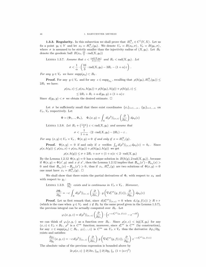
46 1. BARYCENTER METHOD
1.3.3. Regularity. In this subsection we shall prove that HRr, c 2 C1(Y,X) . Let us
fix a point y0 2 Y and let x0 = HRr, c(y0) . We denote U� = B(x0,�) , V� = B(y0,�) ,
where � is assumed to be strictly smaller than the injectivity radius of (X, g0) . Let B0
denote the geodesic ball B(x0,103 · rad(X, g0))
Lemma 1.3.7. Assume that " < rad(X,g0
)3 (↵+1) and R1 < rad(X, g0) . Let
� <1↵
·✓
103
· rad(X, g0)� 3R1 � (1 + ↵) "
◆
.
For any y 2 V� we have supp(µy) ⇢ B0 .
Proof. For any y 2 V� and for any z 2 suppµy, recalling that ⇢(h(y0), H
Rr,c(y0))
2R1 we have:
⇢(x0, z) ⇢(x0, h(y0)) + ⇢(h(y0), h(y)) + ⇢(h(y), z) 2R1 +R1 + ↵ d(y0, y) + (1 + ↵) "
Since d(y0, y) < � we obtain the desired estimate. ⇤
Let � be su�ciently small that there exist coordinates {xi}i=1,..,n , {yi}i=1,..,n onU�, V� respectively. Let
� = (�1, ..,�n), �i(x, y) =
Z
X
d(⇢2)|(x,z)✓
@
@xi
◆
dµy(z)
Lemma 1.3.8. Let R1 +�
1+↵2
�
" < rad(X, g0) and assume that
� <1
1 + ↵· (2 · rad(X, g0)� 2R1)� " .
For any (x, y) 2 U� ⇥ V� , �(x, y) = 0 if and only if x = HRr, c(y) .
Proof. �(x, y) = 0 if and only if x verifiesR
Xd(⇢2)|(x,z) dµy(z) = 0x . Since
⇢(x, h(y)) ⇢(x0, x) + ⇢(x0, h(y0)) + ⇢(h(y0), h(y)) we get
⇢(x, h(y)) � + 2R1 + ↵� + (1 + ↵)" < 2 · rad(X, g0)
By the Lemma 1.2.12 �(x, y) = 0 has a unique solution in B(h(y), 2 rad(X, g0)) , becauseif �(x, y) = �(x0, y) and x 6= x0 , then the Lemma 1.2.12 implies that Bµy (x
0)�Bµy (x) >0 and that Bµy (x) � Bµy (x
0) > 0 , thus if x1, HRr, c(y) are two solutions of �(x, y) = 0
one must have x1 = HRr, c(y) . ⇤
We shall show that there exists the partial derivatives of �i with respect to xk andwith respect to yj :
Lemma 1.3.9. @�i@yj
exists and is continuous in U� ⇥ V� . Moreover,
@�i
@yj= �c
Z
X
d(⇢2)|(x, z)✓
@
@xi
◆
· g✓
rdcutr (y, f(z)),@
@yj
◆
dµy(z)
Proof. Let us first remark that, since d(dcutr )|(x,z) = 0 when dr(y, f(z)) � R + r(which is the case when y 2 V� and z 62 B0 by the same proof given in the Lemma 1.3.7),the previous integral can be actually computed over B0 . Let
'i(x, y, z) = d(⇢2)|(x, z)✓
@
@xi
◆
·⇣
e�c dcutr (y, f(z)) � e�cR
⌘
we can think of 'i(x, y, ·) as a function over B0 . Since ⇢(x, z) < inj(X, g0) for any(x, z) 2 U� ⇥ B0 , ⇢
2 is a C1 function; moreover, since dcutr is C1 (by construction),for any z 2 supp(µy) ⇢ B0 , 'i(·, ·, z) is C1 on U� ⇥ V� thus the derivative @'i/@yjexists and satisfies:
@'i
@yj(x, y, z) = �c d(⇢2)|(x, z)
✓
@
@xi
◆
g
✓
rdcutr (y, f(z)),@
@yj
◆
e�c dcutr (y, f(z))
The absolute value of the previous expression is bounded above by
2c ⇢(x, z) k @/@xi kg0
k @/@yj kg (1 + ( r)2)

1.3. PROOF OF THE THEOREM 1.2.1 47
We choose � su�ciently small. There are two constants A(�), B(�) such that k @/@xi kg0
A(�) and k @/@yj kg B(�) . On the other hand ⇢(x, z) , for z 2 B0 is bounded aboveby two times the radius of B0 . Hence, over B0 ,
�
�
�
�
@'i
@yj
�
�
�
�
3c · 203
rad(X, g0) ·A(�) ·B(�)
where the right hand side of this inequality is independent of (x, y) and integrable on B0 ,thus we can use Lebesgue’s theorem to di↵erentiate under the integral sign and we obtainthe existence and the continuity of @�i
@yjand the formula @�i
@yj=R
B0
@'i@yj
(x, y, z) dv0(z) .
⇤
Lemma 1.3.10. @�i@xk
exists and is continuous. Moreover, for x = HRr, c(y) we have:
@�i
@xk(x, y) =
Z
X
Dd(⇢2)|(x, z)✓
@
@xi,@
@xk
◆
dµy(z)
Proof. Let 'i denote the function defined in the proof of the Lemma 1.3.9. Weknow that 'i is C1 with respect to (x, y) 2 U� ⇥ V� . Moreover, we have
@
@xk
d(⇢2)
✓
@
@xi
◆�
= Dd(⇢2)
✓
@
@xi,@
@xk
◆
+ d(⇢2)
✓
D @@xk
@
@xi
◆
and thus
@'i
@xk=
Dd(⇢2)
✓
@
@xi,@
@xk
◆
+ d(⇢2)
✓
D @@xk
@
@xi
◆�
·⇣
e�c dcutr (y, f(z)) � e�cR
⌘
Since 8x 2 U� and 8z 2 B�
x0,103 rad(X, g0)
�
we have
⇢(x, z) ⇢(x, x0) + ⇢(x0, z) � +103
rad(X, g0) < inj(X, g0)
this implies that the (x, z) ! ⇢(x, z)2 is C1 on the (compact) closure of U�⇥B�
x0,103
�
thus k Dd⇢2|(x,z) k is bounded above by some constant independent of (x, z) . On theother hand, the existence of a C1 -coordinate system on U2� implies that k D @
@xk
@dexi
kis bounded above by a constant independent of x on U� . Hence | @'i
@xk| is bounded (on
U� ⇥ V� ⇥B0 ) by some constant independent of (x, y, z) .As in the proof of the Lemma 1.3.9 we can use Lebesgue’s theorem to di↵erentiate underthe integral sign. Thus we obtain the existence of the derivatives with respect to x andtheir continuity. To obtain the formula just observe that if x = HR
r, c(y) = bar(µy) ,equation (1.11) implies:
Z
B0
d(⇢2)|(x, z)✓
D @@xk
@
@xi
◆
dµy(z) = 0. ⇤
Proposition 1.3.11 (Regularity). The map HRr, c is C1(Y,X) .
Proof. Consider the function � . By the Lemmas 1.3.9, 1.3.10 we know that thefunction � is C1(Y ⇥ X) . Let y0 be any point of Y and assume x0 = HR
r, c(y0) . We
want to show that the matrix⇣
@�i@xj
(x0, y0)⌘
i, jis invertible. Consider the corresponding
quadratic form:X
i, j
✓
@�i
@xj(x0, y0)
◆
ui uj =
Z
X
Dd(⇢2)|(x0
,z)(u, u) dµy0
(z)
where u =Pn
1 ui · @@xi
. Observe that since ⇢(x0, z) < 103 rad(X, g0) by Rauch’s Theorem
(Theorem 1.2.7):
Dd(⇢2)|(x, z)(u, u) �203 · rad(X, g0) · 0
tg�
103 · rad(X, g0) · 0
� · g0
Thus the quadratic form si positive definite, which implies that the matrix⇣
@�i@yj
⌘
i, jis
invertible. By the implicit function theorem we know that there exists an open neigh-bourhood V�0 of y0 and a C1 map hr : V�0 ! X , uniquely defined by the equation

48 1. BARYCENTER METHOD
�(hr(y), y) = 0 . It follows that HRr, c|V�0 = hr ; hence HR
r, c 2 C1(Y,X) . ⇤
1.3.4. The pointwise energy estimate. This subsection is devoted to the proof ofthe estimate (1.9) of the Theorem 1.2.1. We shall denote by R1 the quantity ↵ (R+"+2r) .
N.B. All derivatives of ⇢2 and dcutr are computed with respect to the first variable.
1.3.4.1. 2nd derivatives of � . Let us fix y0 2 Y and let x0 = h(y0) ; we consider� = (�1, ..,�n) ,
�i(x, y) =
Z
X
d(⇢2)|(x, z)✓
@
@xi
◆
dµy(z)
where {xi}i=1,..,n is a coordinate system around x0 . Let {yj}j=1,..,n be a coordinatesystem around y0 . For any y 2 Y we have �(HR
r, c(y), y) = 0 . Let us derive the previousidentity with respect to @
@yj:
0 =@
@yj(�i(H
Rr, c(y), y)) =
=@�i
@yj(HR
r, c(y), y) +nX
k=1
@�i
@xk(HR
r, c(y), y) ·✓
dyHRr, c
✓
@
@yj
◆◆
k
where uk is the k-th component of the vector u 2 THRr,c(y)
X with respect to the framen
@@xk
o
1kn. Using the explicit expressions for the partial derivatives of �i derived from
the previous subsection (we can apply the Lemmas 1.3.9, 1.3.10 because (HRr,c(y), h(y))
lies in a small neighbourhood of (HRr,c(y0), y0) ) and writing @xi = @
@xi, @yj = @
@yjwe
obtain:
0 =nX
k=1
Z
X
Dd(⇢2)|(HRr, c(y), z)
(@xi , @xk ) ·⇣
dyHRr, c
�
@yj�
⌘
kdµy(z)�
�c
Z
X
d(⇢2)|(HRr, c(y), z)
(@xi) · d(dcutr )|(y, f(z))(@yj ) e�c dcutr (y, f(z)) dv0(z)
We multiply both sides for vi , uj and we sum over i, j :
12
Z
X
Dd(⇢2)|(HRr, c(y), z)
(v, dyHRr, c(u)) dµy(z) =
(1.27) =c
2
Z
X
d(⇢2)|(HRr, c(y),z)
(v) · d(dcutr )|(y, f(z))(u) e�c dcutr (y, f(z)) dv0(z)
where u =Pn
1 uj @yj , v =Pn
1 vi @xi . We remark that the second integral in equation(1.27) is computed on B(h(y), R1) since ⇢(h(y), z) � R1 implies dr(y, f(z)) � R+r andthus dcutr ⌘ R which implies that rdcutr (y, f(z)) ⌘ 0 when z outside B(h(y), R1) .
1.3.4.2. Inequality between bilinear forms. We shall work on equation (1.27).
Let u 2 TyY and let v =dyH
Rr, c(u)
kdyHRr, c(u)k
. We recall that ⇢(HRr, c(y), h(y)) �
c(see the
Proposition 1.3.4), hence the triangle inequality gives ⇢(HRr, c(y), z) R1 + �
c.
Since R1 + �c
< min{inj(X, g0), ⇡2
0
} it follows that we can apply Rauch’s Theorem(Theorem 1.2.7):
(1.28)12Dd(⇢2)|(HR
r, c(y), z)(v, dyH
Rr, c(u)) �
�
R1 + �c
�
0
tg��
R1 + �c
�
0
� · k dyHRr, c(u) k
Using the estimate (1.28) and applying the Cauchy-Schwarz inequality to the secondintegral in equation (1.27) we find:
�
R1 + �c
�
0
tg��
R1 + �c
�
0
� · k dyHRr, c(u) k ·µy(X)

1.3. PROOF OF THE THEOREM 1.2.1 49
Z
B(h(y),R1
)
g0(r⇢(HRr, c(y), z), v)
2 ⇢(HRr, c(y), z) e
�c dcutr (y, f(z)) dv0(z)
!
1
2
·
(1.29) ·
Z
B(h(y),R1
)
g(rdcutr (y, f(z)), u)2 ⇢(HRr, c(y), z) e
�c dcutr (y, f(z)) dv0(z)
!
1
2
· c
1.3.4.3. An intermediate estimate. We want to estimate the two integrals in the righthand side of (1.29). Let us remark that if z 2 B(h(y), R1) we have, using inequality(1.14):
dcutr (y, f(z)) � min{d(y, f(z))� 2r, R} � min
⇢
(⇢(h(y), z)� ")↵
� 2r, R
�
�
� min
⇢
⇢(h(y), z)↵
� "� 2r, R
�
=⇢(h(y), z)
↵� "� 2r � ⇢(HR
r,c(y), z)
↵� �
c↵� "� 2r
where the last inequality comes from the Proposition 1.3.4. Thus we can write:Z
B(h(y),R1
)
g0(r⇢(HRr, c(y), z), v)
2 ⇢(HRr, c(y), z)e
�c dcutr (y, f(z)) dv0(z)
exp
✓
�
↵+ c ("+ 2r)
◆
·
·Z
B(HRr, c(y),R1
+ �c)
g0(r⇢(HRr, c(y), z), v)
2 ⇢(HRr, c(y), z) e
� c↵
⇢(HRr, c(y), z) dv0(z)
Denoting by Sn�1 the unit sphere of THRr,c(y)
X , we use the exponential map centered at
HRr,c(y) to define the parametrization
� :
✓
0, R1 +�
c
◆
⇥ Sn�1 ! X, �(t, w) = expHRr,c(y)
(t w)
of B(HRr, c(y), R1 + �
c) \ {HR
r, c(y)}. By Bishop-Gunther’s Theorem (Theorem 1.2.8) wehave:
Z
B(h(y),R1
)
g0(r⇢(HRr, c(y), z), v)
2 ⇢(HRr, c(y), z) e
�c dcutr (y, f(z)) dv0(z)
e�↵+c ("+2r)
sinh�
( �c+R1)0
�
( �c+R1)0
!n�1
·Z R
1
+ �c
0
✓
Z
Sn�1
g0(w, v)2 dw
◆
tn e�c↵
t dt
where we have used the fact that, for every w 2 Sn�1 and any t 2 �
0, R1 + �c
�
, w =
r⇢(HRr,c(y),�(t, v)) . Thus, since
R
Sn�1
g0(u, v)2 du =
!n�1
n· g0(v, v) = !n�1
n, we get
Z
B(h(y),R1
)
g0(r⇢(HRr, c(y), z), v)
2 ⇢(HRr, c(y), z) e
�c dcutr (y, f(z)) dv0(z)
e�↵+c("+2r) ↵
n+1 !n�1
n cn+1·
sinh�
( �c+R1)0
�
( �c+R1)0
!n�1Z
cR1
+�↵
0
tn e�t dt
(1.30)
Plugging (1.30) into (1.29), and using the estimate for µy(X) given in the proof of theProposition 1.3.4 we find:
k dyHRr, c(u) k2
tg��
R1 + �c
�
0
�
�
R1 + �c
�
0
!2
· n
!n�1cn�1 · c2 ↵3n+1 e
�↵+c (3"+4r)·
·
sinh�
( �c+R1)0
�
( �c+R1)0
!n�1
·✓
0 R
sin(0 R)
◆2(n�1)
·
0
B
@
R c(R+"+2r)+ �↵
0tn e�t dt
⇣
R c(R�"�r)
0tn e�t dt
⌘2
1
C
A
·
·Z
B(h(y),R1
)
g(rdcutr (y, f(z)), u)2 ⇢(HRr, c(y), z) e
�c dcutr (y, f(z)) dv0(z)

50 1. BARYCENTER METHOD
We can estimate the last integral as follows:Z
B(h(y),R1
)
g(rdcutr (y, f(z)), u)2 ⇢(HRr, c(y), z) e
�c dcutr (y, f(z)) dv0(z)
ec ("+2r) ·Z
B(h(y),R1
)
g(rdcutr (y, f(z)), u)2 ⇢(HRr, c(y), z) e
� c↵
⇢(h(y),z) dv0(z)
Now let {ei}i=1,..,n be a g-orthonormal base for TyY . Using property (iv) of the cut-o↵distance dcutr and the Bishop-Gunther’s Theorem (Theorem 1.2.8) we can write:
nX
i=1
Z
B(h(y),R1
)
g(rdcutr (y, f(z)), ei)2 ⇢(HR
r, c(y), z) e� c
↵⇢(h(y), z) dv0(z)
(1 + ( r)2)2Z
B(h(y),R1
)
⇢(HRr, c(y), z) e
� c↵⇢(h(y), z) dv0(z)
(1 + ( r)2)2 !n�1
✓
sinh(R1 0)R1 0
◆n�1 Z R1
0
✓
�
ctn�1 e�
c↵t + tn e�
c↵t
◆
dt
where in the last inequality we used the fact that ⇢(HRr, c(y), h(y)) �
cand we have
computed the integral using the parametrization (t, w) ! exph(y)(t w) . Thus we get thefollowing estimate for the pointwise energy:
ey(HRr, c) n · ↵4n+2 · e �
↵+c(4"+6r) · (1 + ( r)2)2
tg�
(R1 + �c)0
�
(R1 + �c)0
!2
·
·
sinh(R1 0) · sinh�
( �c+R1)0
�
sin(0 R)2
!n�1
·
R2
R1 · ( �c +R1)
!(n�1)
·
(1.31) ·0
@
R c(R+"+2r)+ �↵
0tn e�t dt
R c(R�"�r)
0tn e�t dt
1
A ·"
R c↵
R1
0
�
�↵tn�1 e�t + tn e�t
�
dtR c(R�"�r)
0tn e�t dt
#
1.3.4.4. Proof of the estimates (1.9) and (1.10). We shall now show how to manipulatethe inequality (1.31) in order to prove (1.9) and (1.10).
Lemma 1.3.12.
(1.32)sinh(0 R1)sin(0 R1)
✓
1 +20 R
21
2
◆n�1 ✓R1
R
◆n�1
Proof. In order to prove (1.32) let us remark that:
sinh(0 R1)sin(0 R1)
=sinh(0 R1)sin(0 R1)
· sin(0 R1)sin(0 R)
sinh(0 R1)sin(0 R1)
· R1
R
thus, since 0 R1 ⇡10 it is su�cient to prove that 8x 2 (0, ⇡
10 )
(1.33)sinh(x)sin(x)
1 +x2
2
Using the Taylor’s formula with remainder we get:
sinh(x) = x+
Z x
0
(x� t)2
2· cosh(t) · dt x+ cosh(x) · x
3
6
and, analogously, we have cos(t) 1 and thus
sin(x) = x�Z x
0
(x� t)2
2· cos(t) · dt � x� x3
6.
Hence we obtain:
sinh(x)sin(x)
1 + cosh(x) · x2
6
1� x2
6
1 + cosh( ⇡10 ) · x2
6
1� x2
6
1 + 0, 525 · x2
3
1� 0, 5 · x2
3
1 +
✓
205200� ⇡2
◆
· x2
3 1 +
x2
2⇤

1.3. PROOF OF THE THEOREM 1.2.1 51
Lemma 1.3.13.
(1.34)
sinh�
0
�
R1 + �c
��
sin(0 R)
!n�1
"
1 +20
�
R1 + �c
�2
2
#n�1
·
R1 + �c
R
!n�1
Proof. The proof of this inequality is analogous to the one of inequality (1.32). Wejust need to notice that here we have R1 + �
c 3R1 3⇡
10 . ⇤
(1.35)
tg��
R1 + �c
�
0
�
�
R1 + �c
�
0
!2
1 +92
✓
R1 +�
c
◆2
20
!2
As in the previouses cases we use the Taylor’s formula with remainder:
tg(x) = x+
Z x
0
(x� t)2
2· d3
dt3[tg(t)] dt x+
x2
2·Z x
0
d3
dt3[tg(t)] dt
x+ x2 · ⇥tg(t) (1 + tg2(t))⇤x
0 x+
✓
tg(x)x
· (1 + tg2(x))
◆
· x3
if x 3⇡10 we have
tg(x)x
1 +
tg�
3⇡10
�
3⇡10
!
·
1 + tg2✓
3⇡10
◆�
· x2 1 +92· x2
Since R1 + �c 3R1 3⇡
10 , this concludes the proof of inequality (1.35). ⇤
Lemma 1.3.14.
sinh(R1 0) · sinh��
R1 + �c
�
0
�
sin(0 R)2
!n�1
·
R2
R1
�
R1 + �c
�
!n�1
(1.36) "
1 +1220
✓
R1 +�
c
◆2#2(n�1)
Proof. Using (1.32) and (1.34) we obtain:
sinh(R1 0) · sinh��
R1 + �c
�
0
�
sin(0 R)2
!n�1
·
R2
R1
�
R1 + �c
�
!n�1
✓
1 +20 R
21
2
◆n�1
·
R2
R1
�
�c+R1
�
!n�1
·
1 +20
�
R1 + �c
�2
2
!n�1
·
·
R1 + �c
R
!n�1
·✓
R
R1
◆n�1
·
R
R1 + �c
!n�1
✓
1 +20 R
21
2
◆n�1
·
1 +20
�
R1 + �c
�2
2
!n�1
1 +1220
✓
R1 +�
c
◆2!2 (n�1)
. ⇤
Lemma 1.3.15.
(1.37)
R c(R+"+2r)+ �↵
0tn e�t dt
R c(R�"�r)
0tn e�t dt
1 + (n+ 1) 3n+1 2"+ 3rR+ "+ 2r
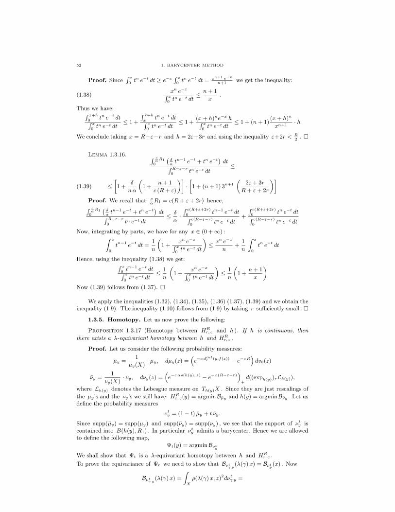
52 1. BARYCENTER METHOD
Proof. SinceR x
0tn e�t dt � e�x
R x
0tn e�t dt = xn+1 e�x
n+1 we get the inequality:
(1.38)xn e�x
R x
0tn e�t dt
n+ 1x
.
Thus we have:R x+h
0tn e�t dt
R x
0tn e�t dt
1 +
R x+h
xtn e�t dt
R x
0tn e�t dt
1 +(x+ h)ne�x hR x
0tn e�t dt
1 + (n+ 1)(x+ h)n
xn+1· h
We conclude taking x = R�"�r and h = 2"+3r and using the inequality "+2r < R2 . ⇤
Lemma 1.3.16.R c
↵R
1
0
�
�↵tn�1 e�t + tn e�t
�
dtR R�"�r
0tn e�t dt
(1.39)
1 +�
n↵
✓
1 +n+ 1
c (R+ ")
◆�
·
1 + (n+ 1) 3n+1
✓
2"+ 3rR+ "+ 2r
◆�
Proof. We recall that c↵R1 = c(R+ "+ 2r) hence,
R c↵R
1
0
�
�↵tn�1 e�t + tn e�t
�
dtR R�"�r
0tn e�t dt
�
↵·R c(R+"+2r)
0tn�1 e�t dt
R c(R�"�r)
0tn e�t dt
+
R c(R+"+2r)
0tn e�t dt
R c(R�"�r)
0tn e�t dt
Now, integrating by parts, we have for any x 2 (0 +1) :Z x
0
tn�1 e�t dt =1n
✓
1 +xn e�x
R x
0tn e�t dt
◆
xn e�x
n+
1n
Z x
0
tn e�t dt
Hence, using the inequality (1.38) we get:R x
0tn�1 e�t dt
R x
0tn e�t dt
1n
✓
1 +xn e�x
R x
0tn e�t dt
◆
1n
✓
1 +n+ 1x
◆
Now (1.39) follows from (1.37). ⇤
We apply the inequalities (1.32), (1.34), (1.35), (1.36) (1.37), (1.39) and we obtain theinequality (1.9). The inequality (1.10) follows from (1.9) by taking r su�ciently small. ⇤
1.3.5. Homotopy. Let us now prove the following:
Proposition 1.3.17 (Homotopy between HRr, c and h ). If h is continuous, then
there exists a �-equivariant homotopy between h and HRr, c .
Proof. Let us consider the following probability measures:
µy =1
µy(X)· µy, dµy(z) =
⇣
e�c dcutr (y,f(z)) � e�cR
⌘
dv0(z)
⌫y =1
⌫y(X)· ⌫y, d⌫y(z) =
⇣
e�c↵⇢(h(y), z) � e�c (R�"�r)⌘
+d((exph(y))⇤Lh(y)),
where Lh(y) denotes the Lebesgue measure on Th(y)X . Since they are just rescalings ofthe µy’s and the ⌫y’s we still have: HR
r, c(y) = argminBµy and h(y) = argminB⌫y . Let usdefine the probability measures
⌫ty = (1� t) µy + t ⌫y.
Since supp(µy) = supp(µy) and supp(⌫y) = supp(⌫y) , we see that the support of ⌫ty iscontained into B(h(y), R1) . In particular ⌫ty admits a barycenter. Hence we are allowedto define the following map,
t(y) = argminB⌫ty
We shall show that t is a �-equivariant homotopy between h and HRr, c .
To prove the equivariance of t we need to show that B⌫t� y
(�(�)x) = B⌫ty(x) . Now
B⌫t� y
(�(�)x) =
Z
X
⇢(�(�)x, z)2d⌫t� y =
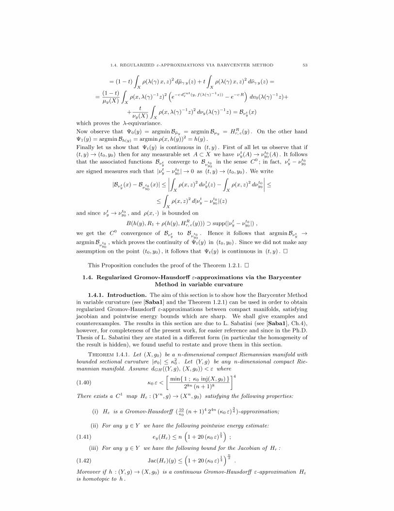
1.4. REGULARIZED "-APPROXIMATIONS VIA BARYCENTER METHOD 53
= (1� t)
Z
X
⇢(�(�)x, z)2 dµ� y(z) + t
Z
X
⇢(�(�)x, z)2 d⌫� y(z) =
=(1� t)µy(X)
Z
X
⇢(x,�(�)�1z)2⇣
e�c dcutr (y, f(�(�)�1z)) � e�cR
⌘
dv0(�(�)�1z)+
+t
⌫y(X)
Z
X
⇢(x,�(�)�1z)2 d⌫y(�(�)�1z) = B⌫t
y(x)
which proves the �-equivariance.
Now observe that 0(y) = argminBµy = argminBµy = HRr, c(y) . On the other hand
1(y) = argminBh(y) = argmin ⇢(x, h(y))2 = h(y) .
Finally let us show that t(y) is continuous in (t, y) . First of all let us observe that if(t, y) ! (t0, y0) then for any measurable set A ⇢ X we have ⌫ty(A) ! ⌫t0y
0
(A) . It followsthat the associated functions B⌫t
yconverge to B
⌫t0
y0
in the sense C0 ; in fact, ⌫ty � ⌫t0y0
are signed measures such that |⌫ty � ⌫t0y0
| ! 0 as (t, y) ! (t0, y0) . We write
|B⌫ty(x)� B
⌫t0
y0
(x)| �
�
�
�
Z
X
⇢(x, z)2 d⌫ty(z)�Z
X
⇢(x, z)2 d⌫t0y0
�
�
�
�
Z
X
⇢(x, z)2 d|⌫ty � ⌫t0y0
|(z)and since ⌫ty ! ⌫t0y
0
, and ⇢(x, ·) is bounded on
B(h(y), R1 + ⇢(h(y), HRr, c(y))) � supp(|⌫ty � ⌫t0y
0
|) ,we get the C0 convergence of B⌫t
yto B
⌫t0
y0
. Hence it follows that argminB⌫ty
!argminB
⌫t0
y0
, which proves the continuity of t(y) in (t0, y0) . Since we did not make any
assumption on the point (t0, y0) , it follows that t(y) is continuous in (t, y) . ⇤
This Proposition concludes the proof of the Theorem 1.2.1. ⇤
1.4. Regularized Gromov-Hausdor↵ "-approximations via the BarycenterMethod in variable curvature
1.4.1. Introduction. The aim of this section is to show how the Barycenter Methodin variable curvature (see [Saba1] and the Theorem 1.2.1) can be used in order to obtainregularized Gromov-Hausdor↵ "-approximations between compact manifolds, satisfyingjacobian and pointwise energy bounds which are sharp. We shall give examples andcounterexamples. The results in this section are due to L. Sabatini (see [Saba1], Ch.4),however, for completeness of the present work, for easier reference and since in the Ph.D.Thesis of L. Sabatini they are stated in a di↵erent form (in particular the homogeneity ofthe result is hidden), we found useful to restate and prove them in this section.
Theorem 1.4.1. Let (X, g0) be a n-dimensional compact Riemannian manifold withbounded sectional curvature |�0| 2
0 . Let (Y, g) be any n-dimensional compact Rie-mannian manifold. Assume dGH((Y, g), (X, g0)) < " where
(1.40) 0 " <
min{ 1 ; 0 inj(X, g0) }28n (n+ 1)8
�4
There exists a C1 map H" : (Y n, g) ! (Xn, g0) satisfying the following properties:
(i) H" is a Gromov-Hausdor↵ ( 100
(n+ 1)4 24n (0 ")3
4 )-approximation;
(ii) For any y 2 Y we have the following pointwise energy estimate:
(1.41) ey(H") n⇣
1 + 20 (0 ")1
4
⌘
;
(iii) For any y 2 Y we have the following bound for the Jacobian of Hr :
(1.42) Jac(H")(y) ⇣
1 + 20 (0 ")1
4
⌘
n2
.
Moreover if h : (Y, g) ! (X, g0) is a continuous Gromov-Hausdor↵ "-approximation H"
is homotopic to h .

54 1. BARYCENTER METHOD
1.4.2. ⌧-coverings and the Reviron Lemma.
Definition 1.4.2. Let (Y, g) be a Riemannian manifold and let ⌧ > 0 . The ⌧ -covering of (Y, g) is the normal covering corresponding to the normal subgroup ⇡⌧
1 (Y, y0)/⇡1(Y, y0) generated by the ⌧ -lassos that is, ⇡⌧
1 (Y, y0) is the subgroup generated by thoseelements � that admit a representation c�1 � c where � is a closed loop contained in ageodesic ball of radius ⌧ , whereas c is a continuous path connecting y0 with �(0) = �(1) .
In [Rev] G. Reviron proved an interesting result reconstructing the large scale met-ric structure of ⌧ -coverings (for su�ciently small values of ⌧ ) of a compact (connected)length space (Y, dY ) which is at small Gromov-Hausdor↵ distance from a compact (con-nected) length space (X, dX) , admitting a universal covering, whose systole is boundedbelow by some constant.
The following result follows directly from [Rev], Theorem 16:
Lemma 1.4.3 (Reviron). Let (X, g0) be a closed (connected) n-dimensional Riemann-ian manifold and let (X, g0) be the Riemannian universal covering. Let i0 = inj(X, g0)and let ", ⌧ > 0 be such that
(1.43) 5" < ⌧ <i02
� 3 "2
.
Let (Y, g) be a n-dimensional compact (connected) Riemannian manifold, and let p :(Y , g) ! (Y, g) be a ⌧ -covering for (Y, g) .If dGH((Y, g), (X, g0)) < " there exists a triple (�, f , h) such that:
(i) � is an isomorphism between the group of deck transformations of the ⌧ -coveringp : Y ! Y and the fundamental group of X (thought as the group of the auto-morphisms of the universal covering).
(ii) There exists two maps f : X ! Y , h : Y ! X which are ��1 and � equi-variant respectively; they are the lifts of the Gromov-Hausdor↵ "-approximationsf : (X, g0) ! (Y, g) , h : (Y, g) ! (X, g0) , and they satisfy:
(1.44) ⇢(h(y), x) ✓
1� 3"2 ⌧
◆�1
d(y, f(x)) + 2" ,
(1.43’) d(y, f(x)) ✓
1� 3"2 ⌧
◆�1
⇢(h(y), x) + 2" ;
(1.45) ⇢((h � f)(x), x) " , d((f � h)(y), y) " .
1.4.3. Proof of the Theorem 1.4.1. Consider the covering (Y , g) of the manifold
(Y, g) provided by the Lemma 1.4.3, corresponding to ⌧ = inj(X,g0
)3 . The idea is to apply
the Theorem 1.2.1 to the two manifolds (X, g0) and (Y , g) , the maps h, f and the iso-morphism � produced by the Lemma 1.4.3 of G. Reviron, where we have identified thegroups �X , �Y of the Theorem 1.2.1 respectively with the fundamental group of X andthe group of deck transformations of the covering Y ! Y .
Let us make the following choices for the parameters:
0R =(0 ")
1
4
22n (n+ 1)2;
c
0=
(0 ")� 1
2
(n+ 1)4 24n;
0r < min
⇢
0 "
100, 0 inj(Y, g),
0
232n (n+ 1)32
�
.

1.4. REGULARIZED "-APPROXIMATIONS VIA BARYCENTER METHOD 55
We show that for these choices of the parameters R, c, r the triple (R, r, c) is in the setD
n,⇣
2i0
2i0
�9"
⌘,2",
0
. By the definition of " we have that:
(1.46) " <5
232n (n+ 1)32· rad(X, g0)
and
(1.47)"
inj(X, g0)<
min{1 ; 30 inj(X, g0)
3}232n (n+ 1)32
2�32n (n+ 1)�32
We may then apply the Lemma 1.4.3, choosing ⌧ = i0
3 (we recall that i0 = inj(X, g0) );
it implies that the two maps f : X ! Y , h : Y ! X satisfy the assumptions of theTheorem 1.2.1, i. e.
⇢(h(y), x) ↵ · d(y, f(x)) + "0, d(y, f(x)) ↵ · ⇢(h(y), x) + "0,
⇢(x, (h � f)(x)) "0 , d(y, (f � h)(y)) "0 .
where
↵ =
✓
1� 3"2 ⌧
◆�1
=
✓
1� 9"2i0
◆�1
and "0 = 2 "
This gives the following estimate:
(1.48) ↵ 1
1� 92 · 2�32n (n+ 1)�32
We apply (1.48) and we obtain:
15↵+ 1
>1� 9
2 · 2�32n (n+ 1)�32
6>
5232n (n+ 1)32
,
and thus (1.46) implies that the assumption "0 2 rad(X, g0)5↵+ 1
of the Theorem 1.2.1 is
fulfilled.From the definitions of 0 R and 0 " we deduce that
R <min{inj(X, g0) ; 1
0
}210n (n+ 1)10
<5 rad(X, g0)210n (n+ 1)10
The last inequality and inequality (1.46) imply that
R+52"0 = R+ 5" <
✓
5210n (n+ 1)10
+25
232n (n+ 1)32
◆
· rad(X, g0) <
<
✓
1� 92 · 232n (n+ 1)32
◆
· rad(X, g0) rad(X, g0)↵
and this proves that the assumption ↵ (R+2"0) = ↵ (R+4") < rad(X, g0) of the Theorem1.2.1 is fulfilled, and simultaneously that
12
rad(X, g0)↵
�R� 2"0�
=12
rad(X, g0)↵
�R� 4"
�
>"
2� 50 r ;
hence, to show that the assumptions of the Theorem 1.2.1 concerning the parameter r(i.e. inequality (1.7)) are fulfilled it is su�cient to show that r min{inj(Y , g) ; 1
},
which follows directly from the definition of r. The last assumption of the Theorem 1.2.1,i. e. "0 + 2r = 2 "+ 2r < R
2 is also satisfied : this follows directly from the definitions of", R and r. Finally we remark that:
4("+ r) <404100
· " < 4041000
· 2�32n (n+ 1)�32.
The previous discussion shows that we can apply the Theorem 1.2.1; this theorem saysthat there exists a C1-map, HR
r,c : Y ! X satisfying the following properties:
(i) ⇢0(HRr,c(y), h(y)) <
�c, where the expression for � = �
n,⇣
2i0
2i0
�9"
⌘,2",
0
(R, r, c) is
given in the statement of Theorem 1.2.1 ;
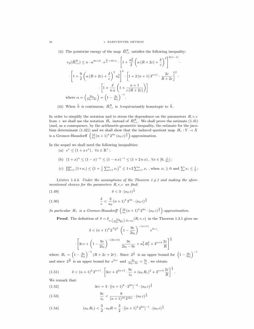
56 1. BARYCENTER METHOD
(ii) The pointwise energy of the map HRr,c satisfies the following inequality:
ey(HRr,c) n · ↵4n+2 · e �
↵+10 c" ·
"
1 +20
2
✓
↵ (R+ 2") +�
c
◆2#2(n�1)
·
·"
1 +92
✓
↵ (R+ 2") +�
c
◆2
20
#2
·
1 + 2 (n+ 1) 3n+1 · 2"R+ 2"
�2
·
·
1 +�
n↵
✓
1 +n+ 1
c (R+ 2")
◆�
where ↵ =⇣
2i0
2i0
�9"
⌘
=⇣
1� 9"2i
0
⌘�1.
(iii) When h is continuous, HRr,c is �-equivariantly homotopic to h .
In order to simplify the notation and to stress the dependence on the parameters R, r, cfrom " we shall use the notation H" instead of HR
r,c . We shall prove the estimate (1.41)(and, as a consequence, by the arithmetic-geometric inequality, the estimate for the jaco-bian determinant (1.42)) and we shall show that the induced quotient map H" : Y ! X
is a Gromov-Hausdor↵⇣
100
(n+ 1)4 24n (0 ")3
4
⌘
-approximation.
In the sequel we shall need the following inequalities:
(a) ex (1 + x ex) , 8x 2 R+ ;
(b) (1 + x)n (1� x)�n (1� nx)�1 (1 + 2nx) , 8x 2 [0, 12n ] ;
(c)Qn
i=1 (1+xi) �
1 + 1n
Pni=1 xi
�n 1+2Pn
i=1 xi , when xi � 0 andP
xi 12 ;
Lemma 1.4.4. Under the assumptions of the Theorem 1.4.1 and making the afore-mentioned choices for the parameters R, r, c we find:
(1.49) � < 3 · (0 ")1
4
(1.50)�
c<
30
(n+ 1)4 24n · (0 ")3
4
In particular H" is a Gromov-Hausdor↵⇣
100
(n+ 1)4 24n · (0 ")3
4
⌘
-approximation.
Proof. The definition of � = �n,⇣
2i0
2i0
�9"
⌘,2",
0
(R, r, c) in the Theorem 1.2.1 gives us:
� < (n+ 1)2 2n�1
9
✓
1� 9"2i0
◆�(n+1)
e5c "·
·"
3c "+
✓
1� 9"2i0
◆�(2n+3) 9"2i0 � 9"
+ 20 R
21 + 3n+4 2"
R
#
1
2
where R1 =⇣
1� 9"2i
0
⌘�1(R + 2" + 2r) . Since 2
1
9 is an upper bound for⇣
1� 9"2i
0
⌘�1
and since 28
9 is an upper bound for e5c" and 9"2i
0
�9" < 9"i0
, we obtain:
(1.51) � < (n+ 1)2 2n+1 ·
3c"+ 22n+3 · 9"i0
+ (0 R1)2 + 3n+4 2"
R
�
1
2
.
We remark that:
(1.52) 3c" = 3 · [(n+ 1)2 · 22n]�2 · (0 ")1
2
(1.53)9"i0
<9
(n+ 1)16 216n· (0 ")
1
2
(1.54) (0 R1) <32· 0R =
32· [(n+ 1)2 22n]�1 · (0 ")
1
4
1.4. REGULARIZED "-APPROXIMATIONS VIA BARYCENTER METHOD 57
(1.55)2"R
< 2 · (n+ 1)2 22n
(n+ 1)8 28n· (0 ")
1
2
Thus using (1.52), (1.53), (1.54), (1.55) in (1.51) we obtain:
� < (n+ 1)2 2n+1 ·"
3 (0 ")1
2
(n+ 1)4 24n+
22n+3 9 (0 ")1
2
(n+ 1)16 216n+
4 (0 ")1
2
(n+ 1)4 24n+
2 · 3n+4 · (0 ")1
2
(n+ 1)6 26n
#
1
2
< (n+ 1)2 2n+1
19 (0 ")1
2
(n+ 1)4 24n
!
1
2
< 3 · (0 ")1
4
which proves (1.49), (1.50) follows from this estimate and from the choice made for theparameter c . ⇤
Let us now prove the pointwise energy estimate:
Lemma 1.4.5. Under the assumptions of the Theorem 1.4.1 and making the aforemen-tioned choices for the parameters R, r, c we find the following pointwise energy estimate:
(1.56) ey(H") n · (1 + 20 · (0 ")1
4 )
Proof. We recall that, by the Theorem 1.2.1 the pointwise energy verifies the follow-ing estimate:
ey(H") n ·✓
1� 9"2i0
◆�(4n+2)
·e�+10 c" ·"
1 +20
2
✓
1� 9"2i0
◆�1
(R+ 3") +�
c
!2#2(n�1)
·
·"
1 +92
✓
1� 9"2i0
◆�1
(R+ 3") +�
c
!2
20
#2
·
1 + 2 (n+ 1) 3n+1 · 3"R+ 3"
�2
·
(1.57) ·
2
6
4
1 +�
n⇣
1� 9"2i
0
⌘�1
✓
1 +n+ 1
c (R+ 2")
◆
3
7
5
Let us remark that, by the assumptions made on the parameters we can apply equality
(b) to the terms⇣
1� 9"2i
0
⌘�(4n+2)and
h
1 +2
0
2
⇣
2i0
2i0
�9" · (R+ 3") + �c
⌘i2(n�1)
,
(1.58)
✓
1� 9"2i0
◆�(4n+2)
<
✓
1 + 9 (4n+ 2)"
i0
◆
(1.59)
"
1 +20
2
✓
2i02i0 � 9"
· (R+ 3") +�
c
◆2#2(n�1)
< 1 + 2 (n� 1)20
✓
2R+�
c
◆2
Using inequality (a) for the term e�+10c " we obtain:
(1.60) e�+10c " < (1 + 2 (� + 10c "))
Using these inequalities and the fact that cR � (n+1)2 22n (by the choice of the param-eters) we get the following estimate for ey(H") :
ey(H") n ·✓
1 + 9 (4n+ 2)"
i0
◆
· (1 + 2(� + 10c ")) ·
1 + 1820
✓
2R+�
c
◆2!
·
·⇣
1 + 18 · 3n+1 (n+ 1)"
R
⌘
·
1 + 2(n� 1)20
✓
2R+�
c
◆2!
·✓
1 +�
n
✓
1 +1n
◆◆
the assumptions made on ", R, r, c allow us to use inequality (c) and thus:
ey(H") n ·
1 + 2 ·
9 (4n+ 2)"
i0+ 2(� + 10c ") + 182
0
✓
2R+�
c
◆2
+
+18 (n+ 1) 3n+1 "
R+ 2 (n� 1)2
0
✓
2R+�
c
◆2
+�
n·✓
1 +1n
◆
!!

58 1. BARYCENTER METHOD
We observe that:
9 (4n+ 2) · "i0
<9 (4n+ 2)
(n+ 1)24 224n· (0 ")
1
4
2(� + 10c ") <132
· (0 ")1
4
20
✓
2R+�
c
◆2
<
"
2 (0 ")1
4
(n+ 1)2 22n+
3 (n+ 1)4 24n (0 ")1
4
(n+ 1)16 216n
#2
<5 (0 ")
1
4
(n+ 1)12 212n
18 (n+ 1) 3n+1 "
R< 18 (n+ 1) 3n+1 (n+ 1)2 22n
(0 ")1
4
(n+ 1)16 216n<
(0 "0)1
4
(n+ 1)11 211n
�
n·✓
1 +1n
◆
< 3 (0 ")1
4 .
Thus we get:
ey(H") n ·⇣
1 + 20 (0 ")1
4
⌘
which proves the estimate (1.56) of the energy. ⇤1.4.4. End of the proof of the Theorem 1.4.1. We proved that the map H" is
a �-equivariant C1-map satisfying the pointwise energy bound (1.56) and such that the
induced quotient map H" : (Y, g) ! (X, g0) is a Gromov-Hausdor↵⇣
100
(n+ 1)4 24n⌘
-
approximation (Lemma 1.4.4). Clearly, the pointwise energy estimate (1.56) holds alsofor the induced quotient map H" . Moreover, when h is continuous h is continuous andwhen h is continuous, by the Theorem 1.2.1, the map H" is �-equivariantly homotopicto h , hence H" is homotopic to h and this concludes the proof of the Theorem 1.4.1. ⇤

CHAPTER 2
The Conjugacy Rigidity Problem
Apercu du chapitre 2 : Dans ce chapitre nous nous interessons a un probleme classiquede la Geometrie Riemannienne et des Systemes Dynamiques : quand peut-on dire que deuxvarietes riemanniennes dont les flots geodesiques sont conjugues sont isometriques ?Nous commencerons (dans la section 2.2) par demontrer un resultat general (Proposition2.2.2) : deux varietes riemanniennes dont les flots geodesiques sont C0�conjugues ontleurs revetements universels riemanniens quasi-isometriques1. Nous utiliserons ensuitece resultat et la nouvelle version de l’application barycentre (definie au chapitre 1) pourobtenir une nouvelle demonstration du fait que toute variete riemannienne dont le flotgeodesique est C0�conjugue a celui d’une variete plate est isometrique a cette variete plate(Theorem 2.3.1), nous appellerons cette propriete la “rigidite dynamique” des varietesplates. La methode est constructive :
• Pour demontrer la Proposition 2.2.2, l’idee est d’utiliser l’isomorphisme entre lesgroupes fondamentaux des deux varietes (notees Y et X ) pour construire unebijection entre l’orbite de l’action de ⇡1(Y ) sur le revetement universel rieman-nien Y et l’orbite de l’action de ⇡1(X) sur le revetement universel riemannienX ; on demontre que, lorsque les flots geodesiques sont C1�conjugues, cette bi-jection est une C0�approximation de Gromov-Hausdor↵ entre ces orbites (ouC0 est une constante finie), qui est equivariante par rapport aux deux actions(voir le Lemme 2.2.8)2; comme ces deux orbites sont respectivement a distancesde Gromov-Hausdor↵ de Y et de X inferieures aux diametres de Y et de X ,on a construit, a partir de la bijection entre les orbites, une C� approximationde Gromov-Hausdor↵ equivariante f entre les revetements universels rieman-niens Y et X (ou C est une constante finie). Si de plus une des deux varietesest un espace K(⇡, 1) 3, nous pouvons choisir f de sorte qu’elle soit continueet induise (en passant au quotient) une equivalence d’homotopie entre Y et X(voir le Lemma 2.2.9 et la preuve du point (ii) de la Proposition 2.2.2).Une consequence presque immediate de la Proposition 2.2.2 est une preuve (dontl’on donne ici deux versions di↵erentes) du fait que toute variete de courbure deRicci non-negative, dont le flot geodesique est C0-conjugue a celui d’une varieteplate, est isometrique a celle-ci.
• Pour demontrer le Theorem 2.3.1, on applique une variante de la methodedu barycentre decrite au chapitre 1 en utilisant comme donnee initiale la C-approximation de Gromov-Hausdor↵ construite dans la Proposition 2.2.2 (ii)4.Nous exhibons ainsi une suite d’applications Lipschitziennes presque isometriques
1Dans ce chapitre, cela signifie que la distance de Gromov-Hausdor↵ entre ces deux revetementsest bornee. Voir la Definition 2.2.1 pour plus de precisions.
2La comparaison entre les distances sur les deux orbites repose fortement sur le fait que la con-jugaison des flots preserve le temps de parcours le long de toute geodesique et sur la cocompacite desgroupes fondamentaux.
3Un espace topologique est un K(⇡, 1) si tous ses groupes d’homotopie (excepte le premier) sonttriviaux; lorsque le groupe ⇡ est specifie, on suppose de plus que son groupe fondamental est isomorphea ⇡.
4Il faut remarquer ici que l’application de la methode c’est pas totalement triviale: bien que laconstante multiplicative de notre quasi isometrie soit egale a 1 (ce qui est la valeur optimale pour leparametre ↵ dans le Theoreme 1.2.1), nous ne sommes pas capables d’avoir un controle su�sammentbon de la constante additive C . C’est alors la geometrie du revetement universel riemannien X del’espace de reference X (et en particulier le fait que son rayon d’injectivite soit infini, puisqu’il est
59

60 2. CONJUGACY RIGIDITY
explicites (sections 2.3.2 et 2.3.3 et Proposition 2.3.8) dont la limite est l’isometrierecherchee 5.
Prospetto del capitolo 2: In questo capitolo ci interessiamo ad un problema classicodi Geometria Riemanniana e Sistemi Dinamici: quando due varieta Riemanniane i cuiflussi geodetici sono coniugati sono isometriche?Cominceremo (nella sezione 2.2) dimostrando un risultato di carattere generale (Propo-sizione 2.2.2) : due varieta Riemanniane i cui flussi geodetici sono C0-coniugati hannoi rivestimenti universali Riemanniani quasi isometrici6. Utilizzeremo successivamentequesto risultato e la nuova versione dell’applicazione baricentro (definita nel capitolo 1)per ottenere una nuova dimostrazione del fatto che ogni varieta Riemanniana il cui flussogeodetico e C1-coniugato a quello di una varieta piatta e isometrica a questa varieta piatta(Teorema 2.3.1), chiameremo questa proprieta “rigidita dinamica” delle varieta piatte. Ilmetodo e costruttivo:
• Per dimostrare la Proposizione 2.2.2, l’idea e quella di sfruttare l’isomorfismotra i gruppi fondamentali delle due varieta (denotate Y ed X ) per costruireuna biiezione tra l’orbita dell’azione di ⇡1(Y ) sul rivestimento universale Rie-manniano Y e l’orbita dell’azione di ⇡1(X) sul rivestimento universale Rie-manniano X ; si dimostra che, quando i flussi geodetici sono C0-coniugati,tale biiezione e una C0-approssimazione di Gromov-Hausdor↵ tra queste orbite(dove C0 e una costante fissata), che e equivariante rispetto alle due azioni(vedere il Lemma 2.2.8)7 ; poiche le due orbite sono rispettivamente a distanzadi Gromov-Hausdor↵ limitata da Y e X inferiori ai diametri di Y ed X ,abbiamo costruito, a partire dalle biiezioni tra le orbite, una C-approssimazionedi Gromov-Hausdor↵ equivariante f tra i rivestimenti universali RiemannianiY e X (dove C e una costante finita). Se inoltre una delle due varieta e unospazio K(⇡, 1)8 possiamo scegliere f in modo tale che essa sia continua ed in-duca (passando al quoziente) una equivalenza omotopica tra Y e X (vedere ilLemma 2.2.9 e la dimostrazione del punto (ii) della Proposizione 2.2.2).Una conseguenza quasi immediata della Proposizione 2.2.2 e una dimostrazione(della quale forniamo due di↵erenti versioni) del fatto che ogni varieta di cur-vatura di Ricci non negativa il cui flusso geodetico e C0-coniugato a quello diuna varieta piatta, e isometrica a tale varieta.
• Per dimostrare il Teorema 2.3.1 si applica una variante del metodo del baricen-tro descritto nel capitolo 1 utilizzando come dato iniziale la C-approssimazionedi Gromov-Hausdor↵ costruita nella Proposizione 2.2.2 (ii)9. Esibiremo dunqueuna successione di applicazioni Lipschitziane, quasi isometriche esplicite (sezioni2.3.2 e 2.3.3 e Proposizione 2.3.8) il cui limite e l’isometria cercata.
euclidien) qui nous permet d’appliquer la methode.
5Remarquons que ceci implique que les deux resultats de rigidite dynamique des varietes platesd’une part et des espaces localement symetriques de courbure strictement negative d’autre part sedemontrent par une meme methode.
6In questo capitolo cio significa che la distanza di Gromov-Hausdor↵ tra i due rivestimenti e limi-tata. Vedere la Definizione 2.2.1 per una definizione piu precisa.
7Il paragone tra le distanze su queste orbite poggia fortemente sul fatto che il coniugio del flussopreserva il tempo di percorrenza lungo ogni geodetica e sulla cocompattezza dei gruppi fondamentali.
8Uno spazio topologico e un K(⇡, 1) se tutti i suoi gruppi di omotopia (ad eccezione del primo)sono nulli; quando ⇡ e un gruppo specifico, si suppone in piu che il suo gruppo fondamentale e isomorfoa ⇡ .
9Bisogna osservare che l’applicazione del metodo non e del tutto banale: difatti, benche la costantemoltiplicativa della nostra quasi isometria sia uguale a 1 (che e il valore ottimale per il parametro ↵ nelTeorema 1.2.1), non siamo capaci di ottenere un controllo su�cientemente preciso sulla costante additiva
C. E dunque la geometria del rivestimento universale Riemanniano X dello spazio di riferimento X apermetterci di applicare il metodo.
2.1. INTRODUCTION 61
Sketch of the chapter 2: In this chapter we are concerned with a classical subject inRiemannian Geometry and Dynamical Systems: in which cases two Riemannian manifoldswhose geodesic flows are conjugate are isometric?We shall start (in section 2.2) with the proof of a general result (Proposition 2.2.2): twoRiemannian manifolds whose geodesic flows are C0-conjugate have quasi isometric10. Af-terwards we shall use this result and the new version of the barycenter map (defined inchapter 1 ) to obtain a new proof of the fact that any Riemannian manifold whose geodesicflow is C1-conjugate to the one of a flat manifold is isometric to this flat manifold (The-orem 2.3.1), we shall call this property “dynamic rigidity” of flat manifolds. The methodis constructive:
• To prove Proposition 2.2.2 the idea is to use the isomorphism between the funda-mental groups of the two manifolds (denoted Y and X ) to construct a bijectionbetween the orbit of the action of ⇡1(Y ) on the Riemannian universal coveringY and the orbit of the action ⇡1(X) on X ; we show that, when the geodesicflows are C0-conjugate this bijection is a Gromov-Hausdor↵ C0-approximationbetween these orbits (here C0 is a fixed constant), equivariant with respect tothe two actions (see the Lemma 2.2.8)11; since the two orbits are at Gromov-Hausdor↵ distance (from Y and X respectively) bounded above by the maxi-mum between the diameters of Y and X , we have constructed an equivariantGromov-Hausdor↵ C-approximation (where C is a fixed constant). Moreover,when one of the two manifold is a K(⇡, 1)-space12 we can choose f such thatit is continuous and such that it induces (passing to the quotients) a homotopyequivalence between Y and X (see the Lemma 2.2.9 and the proof of point (ii)of the Proposition 2.2.2).A quasi immediate consequence of the Proposition 2.2.2 is a proof (of which weprovide two di↵erent versions) of the fact that any Riemannian manifold of nonnegative Ricci curvature whose geodesic flow is C0-conjugate to the one of a flatmanifold, is isometric to this manifold.
• To prove Theorem 2.3.1 we apply a slightly di↵erent version of the barycen-ter method described in chapter 1 using as initial data the Gromov-Hausdor↵C-approximation constructed in Proposition 2.2.2 (ii)13. We shall exhibit a se-quence of quasi isometric Lipschitz maps (sections 2.3.2 and 2.3.3 and Proposi-tion 2.3.8), the limit of which is an isometry.
2.1. Introduction
In this chapter we shall be concerned with the following question: which compactRiemannian manifolds are uniquely determined by their geodesic flow14? In order to statethe problem in a more precise way let us introduce some definitions:
Definition 2.1.1. Let (X, g0) and (Y, g) be two Riemannian manifolds. We willsay that they have Cr-conjugate geodesic flows if there exists a Cr-di↵eomorphism ' :UgY ! Ug
0
X between their unit tangent bundles, which commutes with the geodesicflows: ' � gt = gt0 � ' where we denoted by gt (resp. gt0 ) the geodesic flow of (Y, g)(resp. (X, g0) ) at the time t .
10In this chapter this means that the Gromov-Hausdor↵ distance between the two coverings isbounded. See Definition 2.2.1 for the precise notion of quasi isometry.
11The comparison between the distances on the two orbits strongly relies on the fact that theconjugacy preserves the travel time along the geodesic paths , and on the cocompactness of the actions.
12A topological space is a K(⇡, 1) if all its homotopy groups (except for the first) are trivial; whenthe ⇡ is a specific group we assume morever that the fundamental group is isomorphic to ⇡ .
13We remark here that the application of the barycenter method is not completely trivial: infact, although the multiplicative constant of our quasi isometry is equal to 1 (the optimal value for theparameter ↵ in the Theorem 1.2.1), we have no e↵ective control on the additive constant C. It is thegeometry of the Riemannian universal covering of the reference manifold that allows us to apply themethod.
14Let us recall that, the geodesic flow gt of (Y, g) is defined for any v 2 UgY , by gt(v) = cv(t) ,where cv is the geodesic with initial data cv(0) = v .

62 2. CONJUGACY RIGIDITY
Definition 2.1.2. Let (X, g0) be a complete Riemannian manifold. We say that(X, g0) is Cr-conjugacy rigid if any Riemannian manifold (Y, g) whose geodesic flow isCr-conjugate to the one of (X, g0) is isometric to (X, g0) . We say that (X, g0) is Cr-rigidwithin some class M of Riemannian manifold if any Riemannian manifold (Y, g) 2 Mwhose geodesic flow is Cr-conjugate to the one of (X, g0) is isometric to (X, g0) .
Early counterexamples to conjugacy rigidity were discovered by Weinstein, who pointedout that Zoll surfaces and the standard sphere have C1-conjugate geodesic flows thoughthey are not isometric manifolds (see [Besse], §4.F). On the other hand, as a consequenceof the Blashke’s Conjecture for spheres, proved by Marcel Berger (see [Besse], AppendixD), a first example of C0-conjugacy rigid manifold was found: RPn endowed with thecanonical metric is C0-conjugacy rigid for n � 2 . A more general result was given by C.Croke and independently by J.P. Otal (see [Cr1], [Ot]), who proved the C1-conjugacyrigidity for surfaces of nonpositive curvature, this was later improved to the C0 case byC.Croke, A. Fathi and J. Feldman in [CFF]. In fact, when both the surfaces X andY have negative curvature the conjugacy-rigidity problem turned out to be linked withthe question whether the isospectrality of X and Y (with respect to the marked lengthspectrum) implies the existence of an isometry between X and Y (see [Cr1],[CFF] and[Ot]). In 1994 C. Croke and B. Kleiner proved the C1-conjugacy rigidity for manifoldswhich admit a parallel vector field (see [Cr-Kl]), and one year later G. Besson, G. Courtoisand S. Gallot gave a proof of the C1-conjugacy rigidity of locally symmetric manifolds ofnegative curvature of dimension n � 3 , as a consequence of the solution of the minimalentropy conjecture (see [BCG1]). The result of G. Besson, G. Courtois and S. Gallot hasbeen later improved: in [Ham] U. Hamenstadt proved the C0-rigidity of locally symmet-ric manifolds of negative curvature within the class of Riemannian manifolds of negativecurvature. In fact, she has shown the C0-conjugacy invariance of volumes when one man-ifold has negative curvature and the other one is a locally symmetric space of negativecurvature. In 1996 another paper by C. Croke, P. Eberlein and B. Kleiner, [CEK], provedthe C0-conjugacy rigidity of locally symmetric manifolds of non-positive curvature of di-mension n � 3 and rank d � 2 , within the class of manifolds of non-positive curvature.
During the nineties a fundamental paper of P. Eberlein ([Eb]) brought the attentionof some mathematicians to the investigation of 2-step nilmanifolds (i.e. compact quo-tients of a 2-step nilpotent Lie Group -endowed with a left invariant metric- obtainedby the action of a lattice). A result by C. Gordon and W. Mao (see [Go-Ma]) statesthe C0-conjugacy rigidity of a particular class of compact 2-step nilmanifolds (namelynon-singular of Heisenberg type) within the class of compact nilmanifolds.
The proofs of these results are very di↵erent theorethically; in particular the conjugacyrigidity result of Besson, Courtois and Gallot relies on the study if the equality case in theproof of the minimal entropy conjecture, and it is not evident whether or not their argu-ment gives a general strategy for solving the conjugacy rigidity problems. The existenceof such a strategy would be of great interest in view of the more recent generalizations ofthe Barycenter Method (see [BCG4], [Saba1]).
This Chapter is organized as follows: in section 2.2 we present a general result of in-dependent interest which shows how a C0-conjugacy of geodesic flows imply the existenceof a (1, C)-quasi isometry between the Riemannian universal coverings. This result isstronger when the initial data (X, g0) is a K(⇡, 1)-space. As a consequence we shall givetwo short proofs of the C0-conjugacy rigidity of flat manifolds within the class of mani-folds of non-negative Ricci curvature. In section 2.3 we combine our general result withthe Barycenter Method, to give a new proof of the C1-conjugacy rigidity of flat manifolds.
2.2. Geodesic conjugacies and quasi isometries
The purpose of this section is to present a general remark that we shall use in thesection 2.3 to provide a new proof of the C1-conjugacy rigidity of flat manifolds.

2.2. GEODESIC CONJUGACIES AND QUASI ISOMETRIES 63
This general result has an independent interest: starting from a C0-conjugacy of geodesicflows, it gives rather precise informations on the large scale geometry of the universalcovering of the unknown manifold (Y, g) .
Let us recall the following definitions:
Definition 2.2.1. A map f : (Y, d) ! (X, ⇢) between two non compact metricspaces is said to be (↵, C)-quasi Lipschitz if it satisfies
(2.61) ⇢(f(y), f(y0)) ↵ · d(y, y0) + C, 8y, y0 2 Y.
The map f is a (↵, C)-quasi-isometry if there exists h : (X, dX) ! (Y, dY ) such thatboth f and h are (↵, C)-quasi Lipschitz and
(2.62) 8x 2 X, ⇢((f � h)(x), x) C, 8y 2 Y, d((h � f)(y), y) C.
and we shall say that h is a (↵, C)-quasi inverse for f . We remark that quasi-Lipschitzmaps and quasi-isometries are in general non-continuous.
As ⇡ : UM ! M induces an isomorphism ⇡1(UM, v) ! ⇡1(M,⇡(v)) when thedimension of M is greater or equal to 3 we may state the following result:
Proposition 2.2.2. Let (Y, g) and (X, g0) be two compact connected Riemannianmanifolds of dimension n � 3 , with C0-conjugate geodesic flows. Let us denote by � theisomorphism between the fundamental groups of Y and X induced by the conjugacy ofthe geodesic flows.
(i) There exists a constant C > 0 and a (1, C)-quasi isometry f : (Y , g) ! (X, g0)(whose (1, C)-quasi inverse is denoted by h : (X, g0) ! (Y , g) ).
(ii) Moreover, if (X, g0) is a K(⇡, 1)-space we can find two continuous, �-equivariant(1, C)-quasi isometries f : Y ! X , h : X ! Y which are quasi inverses.They induce two homotopy equivalences f, h between the base manifolds Y ,X , such that h�1
⇤ = f⇤ = (⇡X)⇤ � '⇤ � ((⇡Y )⇤)�1 where ⇡X : UX ! X and
⇡Y : UY ! Y are the projections and ' : UY ! UX the C0-conjugacy.
Let us give the definition of a non-principal ultrafilter and of an asymptotic cone ofa metric space in order to state an immediate consequence of the Proposition 2.2.2:
Definition 2.2.3. A non-principal ultrafilter on N is a finitely additive probabilitymeasure ! such that every subset S ⇢ N is !-measurable and satisfies !(S) 2 {0, 1}and !(S) = 0 if #S < 1 .
The reason why we introduce non-principal ultrafilters is that, roughly speaking, theypick out a convergent subsequence from any given bounded sequence of real numbers. Herewe give a precise statement of this property:
Property. Let ! be a non-principal ultrafilter on N . For every bounded sequence of realnumbers {an}n2N there exists a unique point l 2 R such that !({n : |an � l| < "}) = 1for every " > 0 . We shall write l = lim! an .
Definition 2.2.4. Let ! be a non-principal ultrafilter on N . Let (Xn, dn) a se-quencence of metric spaces with basepoints pn and let X1 denote the set of sequences{xn} where xn 2 Xn and dn(xn, pn) is bounded independently of n . Consider theequivalence relation [{xn} ⇠ {yn} i↵ lim! dn(xn, yn) = 0] . Let X! denote the set ofequivalence classes and endow X! with the metric d!({xn}, {yn}) = lim! dn(xn, yn) .One writes (X!, d!) = lim!(Xn, dn) (if the choice of the basepoints is not important,otherwise we can stress the dependence from the sequence of the basepoints).When we take Xn = X , dn = d
nand we fix the basepoint p 2 X , (X!, d!) is called the
asymptotic cone of X and it is also denoted by Cone!(X, p) .
The following corollary follows immediately from the Proposition 2.2.2:
64 2. CONJUGACY RIGIDITY
Corollary 2.2.5 (C0-conjugacy ) asymptotic isometry). Let (Y, g) and (X, g0) betwo compact, connected Riemannian manifolds of dimension n � 3 whose geodesic flowsare C0-conjugate; let (Y , g) and (X, g0) be their Riemannian universal covering and let! be any non-principal ultrafilter. For any choice of a base point y0 2 Y the asymptoticcone Cone!(Y , y0) is isometric to Cone!(X, f(y0)) - and the isometry is induced by themap f provided by the Proposition 2.2.2.
Before going into the proof of the Proposition 2.2.2 we point out two facts:
Lemma 2.2.6. Let ' : UgY ! Ug0
X be a Ck-conjugacy of geodesic flows k � 0 .Then ' lifts to a Ck-conjugacy ' : UgY ! Ug
0
X.
Proof. Let pY : Y ! Y and pX : X ! X be the universal coverings, then dpY :gUgY = UgY ! UgY and dpX : Ug
0
X = Ug0
X ! Ug0
X are the universal coverings ofUgY and Ug
0
X and the homeomorphism ' : UgY ! Ug0
X lifts to an homeomorphism '
between the universal coverings UgY and Ug0
X such that dpX � ' = ' �dpY . Moreover,as the lift of a geodesic is a geodesic we have dpY � gt = gt �dpY and dpX � gt0 = gt0 �dpXand thus, for any v 2 UY :
dpX � ' � gt(v) = ' � dpY � gt(v) = ' � gt � dpY (v) = gt0 � ' � dpY (v)
where we used the fact that ' is a conjugacy of geodesic flows. On the other hand wehave:
dpX � gt0 � '(v) = gt0 � dpX � '(v) = gt0 � ' � dpY (v)
Hence both t ! ' � gt(v) and t ! gt0 � '(v) are liftings (via the covering map dpX ) ofthe same path t ! gt0 � ' � dpY (v) . Moreover, these two liftings satisfy the same initialcondition, since ' � g0(v) = '(v) = g00 � '(v) , hence(2.63) ' � gt = gt0 � ', 8t 2 R ⇤
Lemma 2.2.7. Let (Y, g) and (X, g0) be two compact connected Riemannian mani-folds of dimension n � 3 , and assume that (X, g0) is a K(⇡, 1)-space. Let ⇡X : UX !X and ⇡Y : UY ! Y be the unit tangent bundles and assume that UY and UX arehomeomorphic by means of an homeomorphism ' . Then there is a homotopy equivalencef : Y ! X , which induces the isomorphism (⇡X)⇤ � '⇤ � (⇡Y )�1
⇤ .
Proof. It is known that any orientable Riemannian manifold of dimension n � 3whose unit tangent bundle is homeomorphic to the one of a K(⇡, 1) manifold, is itself aK(⇡, 1)-space (see for instance [BCG1], Proposition D.1). Remark that the orientabilityassumption made in [BCG1], Proposition D.1, is inessential in the proof.Now we observe that the homeomorphism ' induces an isomorphism between the fun-damental groups of the unit tangent bundles '⇤ : ⇡1(UgY ) ! ⇡1(Ug
0
X) . Consider theisomorphism (pX)⇤ �'⇤ � ((pY )⇤)
�1 : ⇡1(Y ) ! ⇡1(X) . By the Proposition 1.B.9 in [Hat],there must exist a continuous map f which induces this isomorphism between fundamen-tal groups. Hence by Whitehead’s Theorem (see [Hat], Theorem 4.5) f is an homotopyequivalence between Y and X . ⇤
Lemma 2.2.8. Let (Y, g) and (X, g0) be compact, connected Riemannian manifoldsof dimension n � 3 . Assume that ' : UY ! UX is a C0-conjugacy of geodesic flows.Let ' : UY ! UX be the lift of ' to the universal coverings and let [w0, x0] = '[v0, y0](where we shall denote a point from T Y sometimes by [v, y] and sometimes simply by v ).Let us denote by � = (⇡X)⇤ � '⇤ � ((⇡Y )⇤)
�1 the isomorphism between the fundamentalgroups. The map induced between the orbits
f� : ⇡1(Y ) · y0 ! ⇡1(X) · x0, given by f�(� · y0) = �(�) · x0
is a �-equivariant, (1, C)-quasi isometry between orbits (that we consider as metric sub-spaces of (Y , g) and (X, g0) respectively), where C is the constant:
C = 2 ·max{Diam(⇡X('((Uy0
Y ))), Diam(⇡Y ('�1(Ux0
X)))}.
2.2. GEODESIC CONJUGACIES AND QUASI ISOMETRIES 65
Proof. To simplify the notation observe that ((⇡Y )⇤)�1� = d� , i.e. the inverse
of the isomorphism induced by the natural projection ⇡Y : UY ! Y send the decktransformation � into its di↵erential d� . We remark that f�(� ·y0) = ⇡X('(d� ·[v0, y0])) ,where
d� · [v, y] = [d� · v, � · y] .This follows directly from the definition of the isomorphism � . The map f� is triviallyequivariant with respect to the isomorphism � and is a bijection and the inverse map isgiven by:
f�1� (�(�) · x0) = � · y0 .
In analogy with f� we remark that we have
f�1� (�(�) · x0) = ⇡Y ('�1(((⇡X)⇤)
�1�(�) · [w0, x0])) .
The roles of Y , X being interchangeable it is su�cient to show that f� is (1, C)-quasiLipschitz for a suitable C > 0 . Let c : [0, T ] ! Y , a minimizing geodesic of unit speedbetween � · y0 and �0 · y0 (hence T = d(� y0, �
0 y0) ) and consider the path ↵ = ⇡X � '[ ˙c] .Since ' is a C0-conjugation of geodesic flows we have that
↵(t) = ⇡X('( ˙c(t))) = ⇡X � ' � gt[ ˙c(0)] = ⇡X � gt0 � '[ ˙c(0)]thus ↵ is the geodesic of (X, g0) with initial speed '[ ˙c(0)] and length `(↵) = T . Observethat ↵(0) = ⇡X('[ ˙c(0)]) and ↵(T ) = ⇡X('[ ˙c(T )]) . As ˙c(0) 2 U�y
0
Y and ˙c(T ) 2 U�0y0
Ywe have
⇢(f�(�0 · y0), f�(� · y0))
⇢(f�(� · y0), ↵(0)) + ⇢(↵(0), ↵(T )) + ⇢(↵(T ), f�(�0 · y0))
By the �-equivariance of f� and by the definition of the isomorphism � we have
⇢(f�(� · y0), ↵(0)) = ⇢(⇡X � '[d� · v0], ⇡X � '( ˙c(0)))and, as d� · v0 and ˙c(0) both belong to U�y
0
Y , this is bounded above by the Diam(⇡X �'[d� · Uy
0
Y ]) = Diam(⇡X � '[Uy0
Y ]) , because (⇡X � ')[d� · Uy0
Y ] = [(⇡X � ')⇤] · (⇡X �')(Uy
0
Y ) = �(�) · (⇡X � ')(Uy0
Y ) . Analogously we can prove that
⇢(f�(�0 · y0), ↵(T )) Diam(⇡X('(Uy
0
Y )))
hence we obtain the following inequality
⇢(f�(�0 · y0), f�(� · y0)) d(� · y0, �0 · y0) + 2 ·Diam(⇡X('(Uy
0
Y ))) .
In analogy with the previous inequality we obtain:
d(f�1� (�(�) · x0), f
�1� (�(�0) · x0)) ⇢(�(�) · x0,�(�
0) · x0) + 2 ·Diam(⇡Y ('�1(Ux0
X))) .
Setting C = 2 · max{Diam(⇡X('((Uy0
Y ))), Diam(⇡Y ('�1(Ux0
X)))} , this proves thatf�, f
�1� are two (1, C)-quasi isometries between the orbits ⇡1(Y ) · y0 and ⇡1(X) · x0 ,
which are equivariant with respect to � , ��1 respectively. ⇤
Lemma 2.2.9. Let (X, g0), (Y, g) be compact Riemannian manifolds and � : ⇡1(Y ) !⇡1(X) an isomorphism. Assume that there exists a �-equivariant map between the orbits
f� : ⇡1(Y ) · y0 ! ⇡1(X) · x0
which is (↵, C)-quasi Lipschitz (when considering the orbits as metric subspaces of (Y , g)and (X, g0) ). Then any continuous map f : Y ! X such that the induced morphismf⇤ : ⇡1(Y ) ! ⇡1(X) is equal to � lifts to a (↵, C +D)-quasi Lipschitz continuous mapf : Y ! X , for some D > 0 (depending on f ).
Proof. Let K0 be the compact closure of a Dirichlet domain centered at y0 for theaction of ⇡1(Y ) on Y . Let us denote
D0 = supy2K
0
d(y0, y), D00 = sup
y2K0
⇢(x0, f(y)).
For any y, y0 2 Y , let �, �0 2 ⇡1(Y ) be such that ��1 y, (�0)�1 y0 2 K0 . As f is�-equivariant we have:
⇢(f(y), f(y0))
66 2. CONJUGACY RIGIDITY
⇢(f(y), f�(� y0)) + ⇢(f�(� y0), f�(�0 y0)) + ⇢(f�(�
0 y0), f(y0))
↵ · d(� y0, �0 y0) + 2 ·D00 + C ↵ · d(y, y0) + 2 · (D0
0 + ↵D0) + C
Hence f is (↵, C +D)-quasi Lipschitz for D = 2 · (D00 + ↵D0) . ⇤
We can now prove the Proposition 2.2.2:
Proof of the Proposition 2.2.2, (i). By the Lemma 2.2.8 the existence of a C0-conjugacy of geodesic flows implies the existence of a �-equivariant, (1, C)-quasi isometrybetween the orbits of two points y0 2 Y , x0 2 X under the isometric actions of ⇡1(Y ) ,⇡1(X) on Y , X respectively. Since both fundamental groups act cocompactly (X, g0) is(1, C0)-quasi isometric to ⇡1(X) · x0 and (Y , g) is (1, C00)-quasi isometric to ⇡1(Y ) · y0 .Hence (X, g0) and (Y , g) are (1, 3(C + C0 + C00))-quasi isometric. ⇤
Proof of the Proposition 2.2.2, (ii). Take the map f , which is a lift of thehomotopy equivalence f given by the Lemma 2.2.7 for the isomorphism � = (⇡X)⇤ �'⇤ � (⇡Y )�1
⇤ . The map f� : ⇡1(Y ) · y0 ! ⇡1(X) · x0 defined in the Lemma 2.2.8 is a(1, C0)-quasi isometry. It follows by the Lemma 2.2.9 that there exists D > 0 such thatf is (1, C0 + D)-quasi Lipschitz. Changing Y with X , the same argument shows thath : X ! Y , lift of the homotopy equivalence h : X ! Y given by the isomorphism ��1 ,is (1, C0 +D)-quasi Lipschitz.We need to show that there exists a constant C00 such that
⇢(f � h(x), x) C00, d(h � f(y), y) C00
Let D0 = d(h � f(y0), y0) , for a fixed y0 and let D0 be the diameter of the Dirichletdomain K0 centered at y0 . By definition (h�f)⇤ = Id⇡
1
(Y ) , so h� f(� · y) = � · h� f(y) ,hence 8� 2 ⇡1(Y )
d(h � f(� · y0), � · y0) = d(h � f(y0), y0) = D0
Let � be such that ��1 · y belongs to K0 . Then:
d(h � f(y), y) d(h � f(y), h � f(� · y0)) + d(y, � · y0) + d(h � f(y0), y0) D0 +D0 +D0
0
where D00 is the diameter of h � f(K0) . By the same argument we get an analogous
bound for ⇢(f � h(x), x) . Let C00 be the maximum between these two numbers. Thenthe maps f , h are (1, C)-quasi isometries for C = max{C00, C0 +D} . ⇤
As an example of the flexibility of the Proposition 2.2.2 we shall present two di↵erentproofs of the C0-conjugacy rigidity of flat manifolds within the class of manifolds of non-negative Ricci curvature:
Theorem 2.2.10. Let (X, g0) be a compact flat manifold of dimension n � 3 . Let(Y, g) be a compact Riemannian manifold whose Ricci curvature satisfies Riccig � 0 . If(Y, g) and (X, g0) have, C0-conjugate geodesic flows they are isometric.
“Bochner-type” Proof. Let � = (pX)⇤ �'⇤ � (pX)�1⇤ . By Proposition 2.2.2, (ii) it
follows that there exists a continuous �-equivariant, (1, C)-quasi isometry f : (Y , g) !(X, g0) which induces an homotopy equivalence f : Y ! X . Since there exists a flat torus(X, g0) which covers (X, g0) we consider the corresponding covering (Y , g) of (Y, g) andthe lift of ' : UgY ! Ug
0
X , ' : UgY ! Ug0
X . We observe that in particular the firstBetti number of (Y , g) is equal to n . By assumption Riccig � 0 and we can apply aclassical result of Bochner (see [Boch], [Boch-Ya]):
Theorem (for instance, [GHL], Theorem 4.37). Let (Y, g) be a compact n-dimensionalRiemannian manifold. If the Ricci curvature is non-negative and the first Betti number isequal to n , then (Y, g) is an n-dimensional flat torus.

2.3. RIGIDITY OF FLAT MANIFOLDS 67
It follows that (Y, g) is a flat manifold. Since (Y , g) and (X, g0) are two simplyconnected flat manifolds they must be isometric both to En . In particular (Y, g) and(X, g0) are quotients of En by the actions of two isomorphic (1, C)-quasi isometric lattices.An easy metric argument shows that the two maximal rank free abelian subgroups of thetwo isomorphic, (1,C)-quasi isometric lattices are realized on En one from the other bya rotation. Moreover the Second Bieberbach Theorem (see for instance Theorem 2.1.2 in[Dek]) says that the isomorphism � is actually a conjugation by an a�ne transformation,(A, a) 2 A↵(Rn) . Combining the two informations we find that the linear transformationA is actually a rotation, hence (A, a) 2 Isom(En) . We conclude that (Y, g) is isometricto (X, g0) . ⇤
“Asymptotic” Proof. By Proposition 2.2.2, (ii) we have a �-equivariant, continu-ous, (1, C) -quasi isometry which induces an homotopy equivalence between the quotientspaces. Since (Y , g) is (1, C)-quasi isometric to (X, g0) which is a Euclidean space itfollows that the asymptotic cone of (Y , g) is isometric to (X, g0) , hence is a Euclideanspace. Since Riccig � 0 we can use the following result:
Theorem ([Col], Theorem 0.3). Let Mn be a Riemannian manifold of non-negativeRicci curvature and let M1 denote an asymptotic cone for M . If M1 is isometric toEn , then Mn is isometric to En .
Since (Y , g) and (X, g0) are two simply connected flat manifolds it follows that theyare both isometric to En . On the other hand a (1, C)-quasi isometry between two iso-morphic lattices into En must be an isometry and it follows that (Y, g) and (X, g0) areisometric. ⇤
Remark 2.2.11. The C0-rigidity of flat manifolds within the class of compact man-ifolds with non-negative Ricci curvature follows from Bochner’s Theorem and the resultsin [CEK].
2.3. C1-conjugacy rigidity of flat manifolds
In this section we shall give a proof of the C1-conjugacy rigidity of flat manifolds ofdimension n � 3 based on the Barycenter Method. We state the theorem:
Theorem 2.3.1. Let (X, g0) be a compact flat Riemannian manifold of dimensionn � 3 . Then (X, g0) is C1-conjugacy rigid.
The idea is to use the map which is guaranteed by the Proposition 2.2.2 as startingmap for the Barycenter Method adapted to the flat case.
First of all let us remark that a flat Riemannian manifold (X, g0) is a K(⇡, 1)-space.In fact its Riemannian universal covering is di↵eomorphic to Rn where n = dim(X) , so itis contractible, hence (X, g0) is an aspherical manifold. It follows that its kth homotopygroup is trivial for k � 2 , hence it is a K(⇡, 1)-space.
As a corollary of the Proposition 2.2.2 we have:
Corollary 2.3.2. Let (Y, g) and (X, g0) be two compact Riemannian manifolds ofdimension n � 3 with C0-conjugate geodesic flows and assume that (X, g0) is flat. Thenthere exist two �-equivariant, continuous (1, C)-quasi-isometries f : (Y , g) ! (X, g0)and h : (X, g0) ! (Y, g) , which induce two homotopy equivalences f : (Y, g) ! (X, g0)and h : (X, g0) ! (Y, g) (with f⇤ = (h⇤)
�1 = � ).
We will use these maps to construct a family of maps {Fc,r}c2(0,+1),r>0 between Y
and X with the following properties:
• Equivariance: for any � 2 ⇡1(Y ) , Fc,r(� · y) = f⇤(�) · Fc,r(y) .
• Regularity: we shall verify that Fc,r are C1(Y , X) , 8c 2 (0,+1) , 0 < r <min{inj(Y, g), 1
} .

68 2. CONJUGACY RIGIDITY
• Homotopy equivalence: the induced maps Fc,r : Y ! X are all homotopicto f (in particular they are homotopy equivalences).
Moreover, we shall show that the induced maps Fc,r converge to an isometry, F : (Y, g) !(X, g0) , as the parameters c and r go to 0 .
2.3.1. The barycenter map. Let c 2 (0,+1) , 0 < r < min�
inj(Y, g) , 1
and
let ⇢ and d denote the Riemannian distances of (X, g0) and (Y , g) respectively and letdr be a regularization of d constructed as in §1.2.1.1. For any y 2 Y let us define thefollowing function:
Bcy(x) =
Z
X
⇢(x, z)2 · e�c dr(y, h(z))dv0(z)
Lemma 2.3.3. For any y 2 Y the function Bcy is well defined. Moreover, it is a
strictly convex, C1 function, such that Bcy(x) ! +1 as ⇢(x, 0) ! 1 .
Proof. Since we have chosen c > Entvol(X, g0) = 0 , using properties (2.61), (2.62)of quasi isometries, it is easy to see that:
Bcy(x) =
Z
X
⇢(x, z)2 · e�c dr(y, h(z)) dv0(z)
ec (d(y, h(x))+3C+r)Z
X
⇢(x, z)2 · e�c ⇢(x, z) dv0(z) < 1where the last integral is finite by the definition of volume entropy. For what concernsthe regularity, since (X, g0) is the Euclidean space of dimension n , we observe that⇢(x, z)2 = g0(x � z, x � z) . In particular it follows that Bc
y is a polynomial of degree 2.Hence Bc
y is C1 and that Bcy ! 1 as ⇢(x, 0) ! 1 . Convexity follows once you notice
that:
DdBcy(x) =
✓
2
Z
X
e�c dr(y,h(z)) dv0(z)
◆
· g0 ⇤
As a consequence of the Lemma 2.3.3 the function Bcy admits a global minimum on
X , and this minimum is attained at a unique point. So we define the map Fc,r : Y ! X
as Fc,r(y) = argmin(Bcy) . We observe that since Bc
y is C1 and Fc,r(y) is the only point
in X where the minimum of Bcy is attained, we have:
(2.64) 0 = rBcy(Fc,r(y)) = 2 ·
Z
X
(Fc,r(y)� z) · e�c dr(y, h(z)) dv0(z)
Lemma 2.3.4 (Equivariance). The maps Fc,r are equivariant with respect to the iso-morphism � = f⇤ : ⇡1(Y ) ! ⇡1(X) .
Proof. First we observe that from the characterization of Fc,r given by equation(2.64) we obtain an explicit expression for the baycenter map:
Fc,r(y) =
R
Xz · e�c dr(y, h(z)) dv0(z)
R
Xe�c dr(y, h(z)) dv0(z)
The function y ! R
Xe�c dr(y, h(z)) dv0(z) is invariant by the action of ⇡1(Y ) , by the
invariance of v0 with respect to the action of the isometries of (X, g0) . So we only need
to prove the equivariance of y ! R
Xz · e�c dr(y, h(z)) dv0(z) :
Z
X
z · e�c dr(�·y, h(z)) dv0(z) =
Z
X
z · e�c dr(y, ��1h(z)) dv0(z) =
=
Z
X
z · e�c dr(y, h(�(�)�1z)) dv0(�(�)
�1z) =
Z
X
(�(�) · z) · e�c dr(y, h(z)) dv0(z)
for all � 2 ⇡1(Y ) . So Fc,r(� · y) = �(�) · Fc,r(y) , for all � 2 ⇡1(Y ) . ⇤
Lemma 2.3.5 (Regularity). The maps Fc,r are C1(Y , X) .

2.3. RIGIDITY OF FLAT MANIFOLDS 69
Proof. It is su�cient to verify that both y ! R
Xz e�c dr(y,h(z)) dv0(z) and y !
R
Xe�c dr(y,h(z))dv0(z) are regular functions. To this purpose we remark that the functions
|e�c dr(y, h(z)) � e�c dr(y0, h(z))|
d(y, y0)
are dominated by 2c·e�c dr(y, h(z)) (here we use the regularity of the function e�c dr(y,h(z))
and the property (3) of the regularized distance -see subsection 1.2.1.1-).Since the function e�c dr(y,z) is C1 (actually C1 ) in y we apply Lebesgue’s dominated
convergence Theorem to obtain the C1-regularity of y ! R
Xz e�c dr(y,h(z)) dv0(z) and
y ! R
Xe�c dr(y,h(z))dv0(z) and thus of Fc,r . ⇤
Lemma 2.3.6 (Homotopy). The maps Fc,r are all homotopic to f , by an homotopywhich is equivariant with respect to the isomorphism � = f⇤ : ⇡1(Y ) ! ⇡1(X) .
Proof. Take the homotopy H(y, t) = (1� t) Fc,r(y) + t f(y) . ⇤
2.3.2. The jacobian and pointwise energy estimates. In this subsection weshall prove optimal estimates for the jacobian and the pointwise energy of the maps Fc,r .The first step is to estimate the distance between the map Fc,r and the map f .
Proposition 2.3.7. The following estimate holds:
⇢(f(y), Fc,r(y)) pn (2C + r) e4c (C+ r
2
) = A(n, c, C, r)
Proof. By the definition of Fc,r we have that:
(2.65) Fc,r(y) ·Z
X
e�c dr(y,h(z)) dv0(z) =
Z
X
z e�c dr(y,h(z)) dv0(z)
hence, since (X, g0) = (Rn, h· , ·i) , for any unitary vector v 2 Rn ,✓
Z
Rn
e�c dr(y,h(z)) dv0(z)
◆
· hFc,r(y)� f(y), vi =Z
Rn
hz � f(y), vi e�c dr(y,h(z)) dv0(z) =
=
Z
Rn
⌧
z � f(y)
k z � f(y) k , v
�
· k z � f(y) k e�c kf(y)�zk dv0(z)+
+
Z
Rn
⌧
z � f(y)
k z � f(y) k , v
�
· k z � f(y) k ·e�ckf(y)�zk ·⇣
ec(kf(y)�zk�dr(y,h(z))) � 1⌘
dv0(z)
Writing the first integral of the right hand side of the previous equality in polar coordinatescentered at f(y) we find
Z +1
0
0
@
Z
Sn�1
˜f(y)
hw, vi dw1
A t e�c t tn�1 dt = 0
Plugging this equality in the previous one and calculating the equality for v =kFc,r(y)�f(y)kkFc,r(y)�f(y)k
we obtain:Z
Rn
e�c dr(y,h(z)) dv0(z)· k Fc,r(y)� f(y) k
(2.66) ⇣
ec(2C+r) � 1⌘
Z
Rn
�
�
�
�
⌧
z � f(y)
k z � f(y) k , v
�
�
�
�
�
· k z � f(y) k ·e�c kz�f(y)k
where we used the fact that h, f are quasi-inverses (1, C)-quasi isometries and that|dr � d| r . The same estimates gives
Z
Rn
e�c dr(y,h(z)) dv0(z) � e�c (2C+r)Z
Rn
e�c kf(y)�zk dv0(z) �
� e�c(2C+r) !n�1
Z +1
0
e�ct tn�1 dt

70 2. CONJUGACY RIGIDITY
we plug the new estimate into (2.66) and computing the right hand term in polar coordi-nates centered at f(y) we get:
k Fc,r(y)� f(y) k ec(2C+r) ·⇣
ec(2C+r) � 1⌘
·R +10
✓
R
Sn�1
˜f(y)
|hw, vi| dw◆
e�c t tn dt
!n�1
R +10
e�c t tn�1 dt
Since 1!n�1
R
Sn�1
|hv, wi| dw ⇣
1!n�1
R
Sn�1
|hv, wi|2 dw⌘
1pn
we get:
k Fc,r(y)� f(y) k pn ec(2C+r)
✓
ec(2C+r) � 1c
◆
pn 2 e2c(2C+r) ·
⇣
C +r
2
⌘
⇤
We are now able to prove the following:
Proposition 2.3.8. Let us define the pointwise energy of the map Fc,r as ey(Fc,r) =Pn
1 g0(dFc,r(ei), dFc,r(ei)) , where {ei}n1 is a g-orthonormal basis of TyY . We have the
following estimates for the pointwise energy and the jacobian of Fc,r at the point y 2 Y :
(2.67) ey(Fc,r) e4c (2C+r) (1 + ( r)2)2 · n · e2cA(n, c, C, r)
(2.68) | Jac(Fc,r)(y)| e2nc (2C+r) (1 + ( r)2)n · en cA(n, c, C, r)
Proof. We di↵erentiate equation (2.3.7) we obtain:✓
Z
Rn
e�c dr(y,h(z)) dv0(z)
◆
dyFc,r(u) =
= �c
Z
Rn
(z � Fc,r(y)) · g(rdr(y, h(y)), u) e�c dr(y,h(z)) dv0(z)
Let v =dyFc,r(u)
kdyFc,r(u)kand consider the scalar product of the previous equation with v :
✓
Z
Rn
e�c dr(y,h(z)) dv0(z)
◆
k dyFc,r(u) k=
= �c
Z
Rn
hz � Fc,r(y), vi g(rdr(y, h(z)), u) e�c dr(y,h(z)) dv0(z)
and using Cauchy-Schwartz together with the fact that | k f(y)� x k �d(y, h(x))| 2Cand | dr � d| r we obtain
✓
Z
Rn
e�c dr(y,h(z))
◆2
k dyFc,r(u) k2
c2
Z
Rn
⌧
z � Fc,r(y)
k z � Fc,r(y) k, v
�2
k z � Fc,r(y) k e�c dr(y,h(z)) dv0(z)
!
·
·✓
Z
Rn
g(rdr(y, h(z)), u)2 k z � Fc,r(y) k e�c dr(y,h(z)) dv0(z)
◆
c2 e2c(2C+r)
Z
Rn
⌧
z � Fc,r(y)
k z � Fc,r(y) k, v
�2
k z � Fc,r(y) k e�c kz�f(y)k dv0(z)
!
·
·✓
Z
Rn
g(rdr(y, h(z)), u)2 k z � Fc,r(y) k e�c kz�f(y)k dv0(z)
◆
We sum over an orthonormal basis {ei}1in of TyY and we obtain:
e�2c(2C+r)
✓
Z
Rn
e�ckf(y)�zkdv0(z)
◆2
·nX
i=1
k dyFc,r(ei) k2 c2 e2c (2C+r) e2c kFc,r(y)�f(y)k·
·
Z
Rn
⌧
z � Fc,r(y)
k z � Fc,r(y) k, v
�2
k z � Fc,r(y) k e�c kz�Fc,r(y)k dv0(z)
!
·
·✓
Z
Rn
k rdr(y, h(z)) k2 k z � Fc,r(y) k e�ckz�Fc,r(y)k dv0(z)
◆
c2 e2c (2C+r) e2cA(n, c, C, r) (1 + ( r)2)2!n�1·

2.3. RIGIDITY OF FLAT MANIFOLDS 71
·0
@
Z +1
0
0
@
Z
Sn�1
˜Fc,r(y)
hw, vi2 dw1
A e�ct tn dt
1
A ·✓
Z +1
0
e�ct tn dt
◆
thus we get:
nX
i=1
k dyFc,r(ei) k2 c2
ne4c (2C+r)+2cA(n,c,C,r) · (1 + ( r)2)2
R +10
e�ct tn dtR +10
e�ct tn�1 dt
!2
since
✓ R+10
e�ct tn dtR+10
e�ct tn�1 dt
◆
= nc
which proves (2.67). The Jacobian estimate (2.68) follows
directly from (2.68). ⇤2.3.3. End of the proof of the Theorem 2.3.1. In the previous subsections we
have constructed a family of C1 maps from Y to X , depending on the parameters c ,r , equivariant with respect to the isomorphism � = f⇤ : ⇡1(Y ) ! ⇡1(X) and satisfyingthe bounds for the pointwise energy and the jacobian proved in the Proposition 2.3.8.Moreover, the induced maps Fc,r : Y ! X are all homotopic to the starting homotopyequivalence f (and obviously satisfy the same bounds for the pointwise energy and thejacobian). We shall show that we can extract a subsequence {Fcn,rn}n2N converging toan isometry F : Y ! X .
The explicit formula for A(n, c, C, r) shows that 4c (2C + r) + 2cA(n, c, C, r) ! 0 whenc, r ! 0 . Hence, if we denote "(c, r) = (1 + ( r)2)n e2nc (2C+r)+ncA(n,c,C,r) � 1 , theestimates in the Proposition 2.3.8 can be written as follows:
ey(Fc) n · (1 + "(c, r))2
n , | Jac(Fc)| (1 + "(c, r)) with "(c, r) ! 0 for c, r ! 0 .
We put r = c . Take a sequence {cn}n2N converging to 0 . We shall denote by Fcn
the maps Fcn,cn . The family {Fcn}n2N is a uniformly bounded, equicontinuous family ofC1(Y,X) functions; we extract a sequence {Fcn}n2N converging to a map F 2 C0(Y,X) .We remark that F is also homotopic to the map f , hence it is a homotopy equivalence.In particular Adeg(F ) = Adeg(Fcn) = 1 . By the C1-conjugacy rigidity of volumes (seethe Proposition 1.2 in [Cr-Kl]) we know that Vol(Y, g) = Vol(X, g0) . Hence we can usethe coarea formula (Theorem 13.4.2, [Bu-Za]) and the Jacobian estimates for the mapsFcn obtaining:
Vol(X, g0) = Vol(Y, g) � limn!1
Z
Y
| Jac(Fcn)(y)| dvg(y) �
� limn!1
Z
X
#(F�1c(n)(x)) dvg0(x) � lim
n!1Adeg(Fcn) Vol(X, g0) = Vol(X, g0)
where in the last inequality we used the fact that Adeg(Fcn) = 1 . It follows that| Jac(Fcn)| ! 1 a.e. which implies that ey(Fcn) ! n , a.e. . Since ey(Fcn) ! n and
Jac(Fc) ! 1 a.e. we deduce the convergence a.e. of k dyFcn kg, g0
= supv2TyY
kdyFcn ·vkg0
kvkg :
k dyFcn kg, g0
! 1 , a.e.. On the other hand the upper bound for the pointwise energysays that k dyFcn kg, g
0
is uniformly bounded above by 2n . It follows that we havea sequence of maps {Fcn} uniformly converging to a map F , such that the sequence{k dyFcn kg, g
0
}y2Y, n2N is bounded and coverges to 1 a.e.; hence (see [BCG1], Lemme7.8) F must be a Lipschitz function and the Lipschitz constant is 1 , i.e. is a contrac-tion from (Y, g) to (X, g0) .Moreover, F is an homotopy equivalence and Adeg(F ) = 1 .Since we have equality of volumes, we can deduce that it is an isometry, as in the Propo-sition C.1 in [BCG1] (as modified for non orientable manifolds in [Samb1]). ⇤
Remark 2.3.9. Observe that the C1-regularity is only needed to provide the equalityof volumes. In fact, by the same argument we can prove that a flat manifold (X, g0) isC0-conjugacy rigid within the class of Riemannian manifolds with volume less or equalto Vol(X, g0) . The reason is that the opposite (large) inequality Vol(Y, g) � Vol(X, g0)is provided by the Jacobian estimate in the subsection 2.3.2, hence, within this class, thevolume is preserved and we can conclude as in the previous case.


CHAPTER 3
A Spectra Comparison Theorem and itsapplications
Apercu du chapitre 3: Dans ce chapitre nous presentons une application de la methodedu barycentre a la Geometrie Spectrale. Enonce de maniere naıve, notre but est de com-parer le spectre du Laplacien d’une variete Riemannienne quelconque a celui d’unevariete de reference fixee lorsque ces deux varietes sont "�proches (au sens de la dis-tance Gromov-Hausdor↵ et pour une valeur fixee de la constante " > 0).De facon plus precise: etant donnee une variete compacte connexe de reference (Xn, g0) ,de geometrie bornee1, considerons n’importe quelle variete riemannienne (Y, g) de memedimension qui admet une "�approximation de Gromov-Hausdor↵2, continue et de degreabsolu di↵erent de zero, sur (Xn, g0) . Nous supposerons egalement que le volume de(Y, g) est presque inferieur a celui de (X, g0) .Dans le Theoreme principal 3.1.2 nous montrons que chaque valeur propre �i(Y, g) duLaplacien de (Y, g) est alors presque inferieure a la valeur propre correspondante de(Xn, g0) , plus precisement on a �i(Y, g) (1 + ⌘("))�i(X, g0) , ou la fonction ⌘(")est explicite (donnee dans l’enonce du Theoreme 3.1.2) et tend vers zero quand " tendvers zero.
Apres avoir, dans la section 3.1, fait un bref rappel historique sur le probleme de l’estimationdes valeurs propres du spectre du Laplacien dans le cadre des varietes Riemanniennes etavoir presente et discute l’enonce du Theoreme principal 3.1.2, nous allons (dans la sec-tion 3.2) faire des rappels sur les inegalites de Sobolev quantitatives (precisant comment lesconstantes qui y interviennent dependent des bornes de la geometrie globale, voir section3.2.1) et, a l’aide de la methode d’iteration de Moser, nous allons montrer comment endeduire des bornes superieures du rapport entre norme L1 et norme L2 de f et de dfpour toute fonction f de l’espace vectoriel AX(�) engendre par les fonctions propres duLaplacien de (X, g0) associees aux valeurs propres �i(X, g0) � (voir section 3 3.2.2).Dans la section 3.3 nous allons demontrer un resultat de comparaison “technique” (laProposition 3.1.4) qui nous permettra, a l’aide de la methode du barycentre, de demontrerle Theoreme 3.1.2. Ce resultat compare le spectre d’une variete Riemannienne quelconque(Y, g) a celui d’une variete (X, g0) de “geometrie faiblement bornee4” lorsque ces deux
1 Ici “geometrie bornee” signifie que le diametre et la valeur absolue de la courbure sectionnelle de(Xn, g
0
) sont majores et que son rayon d’injectivite est minore. La condition de “geometrie bornee”n’impose aucune restriction a la geometrie de (Xn, g
0
) , puisque toute variete compacte admet de tellesbornes; cette “condition” indique seulement que toutes les constantes universelles qui interviendrontdans le resultat seront calculees en fonction de ces bornes de la geometrie de (Xn, g
0
) .
2 Bien que " ne soit pas suppose petit, il faut cependant le choisir inferieur a une valeur critique,calculable en fonction des bornes de la geometrie de la variete de reference (X, g
0
) , pour que les resultatsque nous obtenons ne soient pas vides.
3 Les resultats de cette section constituent une reference detaillee pour les resultats demontres parS. Gallot dans deux notes aux Comptes Rendus de l’Academie des Sciences ([Ga1], [Ga2].Notons une contrainte importante : pour toute fonction f 2 AX(�) , les bornes que nous obtiendrons
pour les rapportskfkL1
kfkL2
etkdfkL1
kdfkL2
(qui dependront evidemment de � ) ne doivent pas dependre
de la dimension de AX(�) .
4En e↵et, dans la Proposition 3.1.4, l’hypothese de “geometrie bornee” faite sur la variete (X, g0
)peut etre a↵aiblie en une hypothese de “geometrie faiblement bornee”, cette derniere hypothese signifiantque la courbure de Ricci de (X, g
0
) est minoree et son diametre majore.
73
74 3. A SPECTRA COMPARISON THEOREM
varietes sont "�proches au sens de la distance Gromov-Hausdor↵ (pour une valeur fixee dela constante " > 0) et lorsqu’il existe une application Lipschitzienne F : (Y, g) ! (X, g0)(de degre absolu non trivial), dont l’energie ponctuelle est presque inferieure a n (la valeurn etant critique, puisqu’il s’agit de la valeur de l’energie d’une isometrie).La preuve de la Proposition 3.1.4 se fait en trois etapes : dans la section 3.3.1, nousmontrons que la variete Y de depart est divisee en deux parties : une premiere partie oule determinant Jacobien de F est presque egal a 1 (ce qui implique que l’application Fest presque isometrique sur cette partie) et une deuxieme partie ou nous n’avons plus decontrole sur le determinant Jacobien, mais qui est de volume petit relativement au vol-ume total de la variete (Lemma 3.3.5); dans la section 3.3.2, nous rappelons un theoremede comparaison general et simple (Lemme 3.3.9, deja present dans [Aub2]), base sur lePrincipe du Minimax, qui nous permettra, dans la section 3.3.3, d’achever la preuve de laProposition “technique” 3.1.4 en etablissant des estimes des normes L2 (sur Y ) de f �Fet de d(f � F ) en fonction des normes L2 et L1 (sur X ) de f et de df (pour toutefonction f 2 AX(�) ) et en utilisant les estimees du rapport entre norme L1 et normeL2 de f et de df demontres dans la section 3.2.Dans la section 3.4.1, nous donnons une preuve du Theoreme 3.1.2 : c’est une consequencepresque immediate de la methode du barycentre (Chapitre 1) et du resultat de comparaisontechnique (Proposition 3.1.4).Enfin, dans la section 3.4.2, nous donnons des exemples qui illustrent la faiblesse deshypotheses du Theoreme 3.1.2, comparees5 aux hypotheses du resultat de convergencede J. Cheeger et T. Colding ([Ch-Co]) : en particulier, une premiere serie d’exemplesprouve que, sous nos hypotheses, il est impossible d’obtenir une minoration des valeurs pro-pres �i(Y, g) du Laplacien de (Y, g) (Example 3.4.3 et Proposition 3.4.4), alors qu’unetelle minoration est assuree sous les hypotheses choisies par J. Cheeger et T. Colding([Ch-Co]); une seconde serie d’exemples (Example 3.4.1 et Proposition 3.4.2) prouve queles hypotheses que nous faisons dans le Theoreme 3.1.2 sont verifiees (pour au moins unemetrique g ) sur toute variete Y obtenue par somme connexe de X et de n’importe quellevariete Z de meme dimension, ce qui signifie que nos hypotheses n’impliquent pratique-ment aucune restriction sur la topologie de Y , alors que, sous les hypotheses choisies parJ. Cheeger et T. Colding, Y est forcement di↵eomorphe a X .
Prospetto del capitolo 3: In questo capitolo presenteremo un’ applicazione del metododel baricentro nell’ambito della Geometria Spettrale. In modo semplificato il nostro scopoe quello di paragonare lo spettro del Laplaciano di una varieta Riemanniana qualunque aquello di una varieta Riemanniana di riferimento fissata quando queste due varieta sono "-vicine (nel senso della distanza di Gromov-Hausdor↵ e per un valore fissato della costante" > 0 ).Piu precisamente, supponiamo che sia assegnata una varieta Riemanniana di riferimento(Xn, g0) compatta, connessa di geometria limitata6, consideriamo una qualunque va-rieta Riemanniana (Y, g) della stessa dimensione che ammetta una "-approssimazionedi Gromov-Hausdor↵7 continua e di grado assoluto non nullo, su (Xn, g0). Supporremoinoltre il volume di (Y, g) quasi inferiore al volume di (X, g0).Nel Teorema principale 3.1.2 mostriamo che ogni autovalore �i(Y, g) del Laplaciano di
5La comparaison illustre la di↵erence entre notre choix et celui fait par J. Cheeger et T. Colding:nous avons choisi de prendre des hypotheses plus faibles que celles de J. Cheeger et T. Colding etd’obtenir des conclusions egalement plus faibles.
6Quando parliamo di “geometria limitata” questo significa che il diametro ed il valore assoluto dellecurvature sezionali sono limitati superiormente mentre il raggio di iniettivita e limitato inferiormente. Lacondizione di “geometria limitata” non impone alcuna restrizione alla geometria di (Xn, g
0
) , poiche ognivarieta compatta ammette tali limiti; questa “condizione” indica semplicemente che tutte le costantiuniversali che compaiono nel risultato sono calcolate in funzione di questi limiti sulla geometria di(Xn, g
0
)7Benche non sia necessario scegliere " piccolo, e comunque necessario che sa inferiore ad un valore
critico che puo essere calcolato in funzione dei limiti della geometria della varieta di riferimento (X, g0
) ,a�nche i risultati che otteniamo non siano vuoti.

3. A SPECTRA COMPARISON THEOREM 75
(Y, g) e quasi inferiore all’autovalore corrispondente di (Xn, g0) , piu precisamente abbi-amo �i(Y, g) (1+⌘("))�i(X, g0) , dove la funzione ⌘(") e esplicita (data nell’enunciatodel Teorema 3.1.2) e tende a zero quando " tende a zero.
Nella sezione 3.1, dopo un breve richiamo storico sul problema della stima degli auto-valori dello spettro del Laplaciano nel contesto delle varieta Riemanniane e dopo averpresentato e discusso l’enunciato del Teorema principale 3.1.2, faremo (nella sezione 3.2)dei richiami sulle disuguaglianze di Sobolev quantitative (precisando il modo in cui lecostanti che vi intervengono dipendano dai limiti sulla geometria globale, vedere la sezione3.2.1) e , grazie al metodo di iterazione di Moser, mostreremo come dedurne dei limitisuperiori per il rapporto tra le norme L1 ed L2 di f e df per ogni funzione f nellospazio vettoriale AX(�) generato dalle autofunzioni del Laplaciano di (X, g0) associatead autovalori �i(X, g0) � (vedere la sezione8 3.2.2). Nella sezione 3.3 dimostreremo unrisultato di paragone “tecnico” (la Proposizione 3.1.4) che ci permettera, grazie al metododel baricentro, di dimostrare il Teorema 3.1.2. Questo risultato permette di paragonarelo spettro di una varieta Riemanniana qualunque (Y, g) a quello di una varieta (X, g0)di “geometria debolmente limitata9” quando queste due varieta sono "-vicine rispetto alladistanza di Gromov-Hausdor↵ (per un valore fissato della costante " > 0) e quando esisteuna applicazione Lipschitziana F : (Y, g) ! (X, g0) (di grado assoluto non banale), lacui energia puntuale e quasi inferiore a n (laddove il valore n e critico, poiche esso e ilvalore dell’energia di una isometria).La dimostrazione della Proposizione 3.1.4 e ottenuta in tre passi: nella sezione 3.3.1mostriamo che la varieta Y puo essere suddivisa in due parti: una prima parte dove ildeterminante Jacobiano di F e quasi uguale ad 1 (il che implica che l’applicazione Fe quasi isometrica su tale parte) ed una seconda sulla quale non abbiamo piu controllosul determinante Jacobiano, e che e di volume piccolo rispetto al volume totale della va-rieta (Lemma 3.3.5); nella sezione 3.3.2, richiamiamo un teorema di paragone generalee semplice (Lemma 3.3.9, gia presente in [Aub2]) basato sul Principio del Minimax, checi permettera, nella sezione 3.3.3, di concludere la dimostrazione della Proposizione “tec-nica” 3.1.4, stabilendo delle stime delle norme L2 (su Y ) di f � F e di d(f � F ) infunzione delle norme L2 ed L1 (su X ) di f e df (per ogni funzione f 2 AX(�) )ed utilizzando le stime del rapporto tra le norme L1 ed L2 di f e df dimostrate nellasezione 3.2.Nella sezione 3.4.1 forniamo una dimostrazione del Teorema 3.1.2: si tratta di una con-seguenza quasi immediata del metodo del baricentro (Capitolo 1) e del risultato di paragonetecnico (Proposizione 3.1.4).Infine nella sezione 3.4.2 presenteremo degli esempi che illustrano la debolezza delle ipotesidel Teorema 3.1.2 paragonate 10 alle ipotesi del risultato di convergenza di J. Cheeger eT. Colding ([Ch-Co]); una seconda serie di esempi (Esempio 3.4.1 e Proposizione 3.4.2)provano che le ipotesi da noi fatte nel Teorema 3.1.2 sono verificate (per almeno una met-rica g ) su ogni varieta Y otteuta per somma connessa da X e da una qualunque varietaZ della stessa dimensione, il che significa che le nostre ipotesi non implicano praticamentealcuna restrizione sulla topologia di Y , mentre, sotto le ipotesi scelte da J. Cheeger e T.Colding, Y e necessariamente di↵eomorfa a X.
8I risultati di questa sezione costituiscono una referenza dettagliata per i risultati dimostrati daS. Gallot in due note pubblicate nei Comptes Rendus de l’Academie de Sciences ([Ga1], [Ga2]). Os-serviamo un vincolo importante: per ogni funzione f 2 AX(�) i limiti che noi otterremo per i rapportikfk1kfk
2
e kdfk1kdfk
2
(che devono evidentemente dipendere da � ) non decvono dipendere dalla dimensione
di AX(�) .
9Nella Proposizione 3.1.4 l’ipotesi di “geometria limitata” fatta sulla varieta (X, g0
) puo essereindebolita in una ipotesi di “geometria debolmente limitata”, il che consiste nell’imporre unicamente unlimite inferiore alla curvatura di Ricci di (X, g
0
) ed uno superiore sul suo diametro.
10Il paragone illustra la di↵erenza tra la nostra scelta e quella fatta da J. Cheeger e T. Colding:abbiamo scelto di prendere ipotesi piu deboli di quelle di J. Cheeger e T. Colding e di ottenere quindiconclusioni piu deboli.

76 3. A SPECTRA COMPARISON THEOREM
Sketch of the chapter 3: In this chapter we shall present an application of the barycentermethod to the Spectral Geometry. Naively our aim is to compare the Laplace spectrum ofany Riemannian manifold to the one of a fixed Riemannian manifold, when the Gromov-Hausdor↵ distance between the two manifolds is smaller than " (here the proximity isintended for a fixed value of the constant " > 0 ).More precisely, given a compact, connected Riemannian manifold (Xn, g0) of boundedgeometry11, let us consider any Riemannian manifold (Y n, g) which admits a continuousGromov-Hausdor↵ "-approximation12 of non zero absolute degree onto (Xn, g0) ; we shallassume that the volume of (Y n, g) is almost smaller than the volume of (Xn, g0) .In the Theorem 3.1.2 we shall prove that any eigenvalue �i(Y
n, g) of the Laplacian of(Y n, g) is almost smaller than the corresponding eigenvalue of (Xn, g0) , more preciselywe have �i(Y
n, g) (1 + ⌘("))�i(Xn, g0) , where the function ⌘(") is explicit (it is given
in the statement of Theorem 3.1.2) and goes to zero if " goes to zero.
In the section 3.1, after a brief history of previous estimates on the eigenvalues of theLaplace spectrum in the context of Riemannian manifolds and after the statement and dis-cussion of the Main Theorem (Theorem 3.1.2) we shall recall (in section 3.2) some factsabout quantitative Sobolev inequalities (precising how the constants which are involved inthese inequalities depend on the bounds on the global geometry of the manifolds, see thesection 3.2.1) and, thanks to the Moser’s iteration method, we shall show how to deducesome upper bounds for the ratio between the L1 and L2 norms of f and df for anyfunction f in the vector space AX(�) generated by the eigenfunctions of the Laplacianof (Xn, g0) associated to the eigenvalues �i(X
n, g0) � (see section13 3.2.2). In thesection 3.3 we shall prove a “technical” comparison result (the Proposition 3.1.4), thatwe shall need, in combination with the barycenter method, in order to prove our MainTheorem 3.1.2. This result compares the spectrum of any Riemannian manifold (Y n, g)to the one of a reference manifold (Xn, g0) of “weakly bounded geometry14” when theGromov-Hausdor↵ distance between the two manifolds is smaller than " (for a fixed valueof the constant " > 0 ) and when there exists a Lipschitz map F : (Y n, g) ! (Xn, g0)(of non zero absolute degree) whose pointwise energy is almost smaller than n (where thevalue n is critical since it is the value of the pointwise energy of an isometry).The proof of the Proposition 3.1.4 is obtained in three steps: in the section 3.3.1 we showthat the manifold Y can be divided in two subsets: the first one where the Jacobian deter-minant of F is almost equal to 1 (this implies that the map F is quasi isometric on thissubset), and the second one (where we do not have such a control on the Jacobian deter-minant) whose volume is small with respect to the total volume of the manifold (Lemma3.3.5); in the section 3.3.2 we recall a general and simple comparison theorem (Lemma3.3.9, see also [Aub2]) based on the Minimax Principle, which allows, in section 3.3.3,to conclude the proof of the “technical” Proposition 3.1.4 by proving some estimates forthe norms L2 (on Y ) of f � F and d(f � F ) in terms of the L2 and L1 norms (onX ) of f and df (for any function f 2 AX(�) ) and by using the estimates for the ratiosbetween the L1 and L2 norms of f and df obtained in section 3.2.
11A Riemannian manifold has “bounded geometry” when its diameter and the absolute value of itssectional curvature are bounded above, and when its injectivity radius is bounded below. Saying that(Xn, g
0
) has “bounded geometry” (i. e. that there exists bounds for the geometry of (Xn, g0
) ) doesnot imply any restriction on the geometry of (Xn, g
0
) , since any compact manifold admits such bounds(however, when we fix the values of these bounds, it implies some restriction on the possible geometriesof (Xn, g
0
) ); this “condition” only says that all the universal constants which appear in the result arecomputed in terms of these bounds on the geometry of (Xn, g
0
) .
12Though " is not supposed arbitrarily small, it must however be smaller than a critical value(which will be computed in terms of the bounds of the geometry of the reference manifold (X, g
0
) ).
13This subsection provides a detailed reference for the results proved by S. Gallot in two shortnotes at the Comptes Rendus de l’Academie de Sciences ([Ga1], [Ga2]). We underline an importantconstraint: for any function f 2 AX(�) we do not want the bounds that we shall obtain for the ratioskfk1kfk
2
and kdfk1kdfk
2
(which shall obviously depend on �) to depend on the dimension of AX(�) .
14In the Proposition 3.1.4, the usual assumption “bounded geometry” can be weakened into theassumption “weakly bounded geometry”, which means that we only assume a lower bound on the Riccicurvature of (Xn, g
0
) and an upper bound on the diameter.

3.1. INTRODUCTION 77
In section 3.4.1, we give the proof of the main result, Theorem 3.1.2: it is a quasi imme-diate consequence of the barycenter method (chapter 1) and of the technical comparisonresult (Proposition 3.1.4).Finally, in section 3.4.2, we shall present some examples which make evident the weak-ness of the assumptions of our Main Theorem 3.1.2 compared15 to the assumptions of theconvergence result of J. Cheeger and T. Colding ([Ch-Co]); in particular, a first series ofexamples proves that, under the assumptions of our Main Theorem 3.1.2, it is impossibleto obtain lower bounds of the eigenvalues �i(Y
n, g) of the Laplacian of (Y n, g) (Example3.4.3 and Proposition 3.4.4), while such lower bounds are automatic under the assumptionschosen by J. Cheeger et T. Colding in [Ch-Co]. A second series of examples (Example3.4.1 and Proposition 3.4.2) proves that, for every Riemannian manifold (Xn, g0) , anymanifold (Y n, g") obtained by connected sum of (Xn, g0) with any Riemannian manifold(Zn, h") of diameter smaller than C." satisfies the assumptions of our Main Theorem3.1.2; this proves that our assumptions do not imply any topological restriction on themanifold Y n , whereas, under the assumptions made by J. Cheeger and T. Colding, Y n
is necessarily di↵eomorphic to Xn .
3.1. Introduction
The aim of this chapter is to compare the spectra of two Riemannian manifolds (Y, g)and (X, g0) and to bound the gap in terms of the Gromov-Hausdor↵ distance betweenthese two spaces when this distance is smaller than some universal constant (see Theorem3.1.2).
Estimates from above and from below for the eigenvalues of the Laplace-Beltrami op-erator of manifolds satisfying a lower bound of the Ricci curvature and an upper bound ofthe diameter were derived in the decade from 1975 to 1985. Namely, following S. Y. Cheng[Cheng], and P. Li and S. T. Yau, [Li-Yau], we know that, when (Y, g) is a compactRiemannian n-manifold of diameter Diam(Y, g) D , whose Ricci curvature, Riccig ,satisfies the bound Riccig � �(n � 1)2 , then the eigenvalues of the Laplace-Beltramioperator admit the following upper bound:
(3.69) �k(Y, g) C(↵)
Volg(Y )2
n
· k 2
n
where ↵ = D . On the other hand under the same assumptions we have the followinginferior bound for the eigenvalues of the Laplace-Beltrami operator of (Y, g) (see P. Liand S. T. Yau [Li-Yau], M. Gromov [Gro2] and S. Gallot, [Ga1], [Ga2], [Ga3]):
(3.70) �k(Y, g) � �(↵)Diam(Y, g)2
· k 2
n .
Explicit values for the constants C(↵) and �(↵) can be found in [Li-Yau], [Ga1], [Ga2],[Ga3] or [BBG].
Remark 3.1.1. As long as we are only concerned by their dependence with respect tothe index k , the inequalities (3.69) and (3.70) agree with the well known Weyl asymptoticformula which says that the sequence of the eigenvalues of the Laplace-Beltrami operatorof a compact Riemannian n-manifold (Y, g) behaves asymptotically like
�k ⇠ (2⇡)2
(Vol(Bn) ·Volg(M))2
n
· k 2
n .
For the same reason, assume that we have two compact Riemannian n-manifolds(Y, g) , (X, g0) , whose Ricci curvatures satisfy the same lower bound
Riccig � �(n� 1)2, Riccig0
� �(n� 1)2
15Comparing our assumptions with Cheeger-Colding’s, we have chosen to take weaker assumptionsand, consequently, to obtain weaker conclusions.

78 3. A SPECTRA COMPARISON THEOREM
and such that Diam(Y, g),Diam(X, g0) D . From inequalities (3.69) and (3.70) weobtain:
�k(Y, g) C(↵)�(↵)
·✓
Diam(X, g0)n
Volg(Y )
◆
2
n
· �k(X, g0)
and, exchanging the roles of (Y, g) and (X, g0) :
�k(X, g0) C(↵)�(↵)
·✓
Diam(Y, g)n
Volg0
(X)
◆
2
n
· �k(Y, g)
However, since the quantity C(↵)/�(↵) is considerably greater than 1 (although the con-
stants involved are sharp!) and as the ratio (Diam)n
Vol can be arbitrarily large, even if wesuppose that the diameters and the volumes of (Y, g) and (X, g0) are almost the same, wecannot infer an equality or deduce some sharp pinching result between the kth eigenvalues.
In [Ch-Co], Theorem 7.11, J. Cheeger and T. Colding gave a convergence result forthe eigenvalues of the Laplace operators of a sequence of n-dimensional manifolds (Yk, gk)whose Ricci curvatures are bounded from below by �(n � 1) and which converge withrespect to the Gromov-Hausdor↵ distance to a given smooth manifold (X, g0) of the samedimension (notice that, (X, g0) being fixed, its Ricci curvature is automatically boundedfrom below). Namely, they prove that, for any fixed j 2 N⇤ , the jth eigenvalue �j(Yk, gk)of the Laplace-Beltrami operator of (Yk, gk) converges to �j(X, g0) as k ! +1 .Notice that the Gromov-Hausdor↵ convergence is not, in itself, a strong assumption (inparticular it gives no informations on the local geometries of the (Yk, gk) ), but that be-comes quite a strong one when it is combined with a uniform lower bound on the Riccicurvature of the Riemannian manifolds (Yk, gk) . Assuming together these two propertiesone obtains that, for large values of k , the local geometries of (Yk, gk) are almost thesame (J. Cheeger, T. Colding [Ch-Co] and T. Colding [Col]), in particular, for every" > 0 , if yk ! x , the volume of the geodesic ball B(yk, ") of (Yk, gk) converges to thevolume of the geodesic ball B(x, ") of (X, g0) . Moreover Yk is di↵eomorphic to (X, g0)for large values of k ([Ch-Co]), and Volgk (Yk) ! Volg
0
(X) as k ! +1 ([Col]). Thefact that Diam(Yk, gk) converges to Diam(X, g0) is an immediate consequence of theGromov-Hausdor↵ convergence.
We remark that the eigenvalues approximation methods shows that we have conver-gence of �i(Yk, gk) ! �i(X, g0) when (Yk, gk) is a sequence of polyedral approximationsconverging to (X, g0) (see [Dod-Pat], §3). However the result of Dodziuk and Patodidoes not provide an upper bound of the ”error” |�i(Yk, gk)� �i(X, g0)| .
Comparing with the aforementioned results, the comparison between the spectra oftwo manifolds (Y, g) and (X, g0) that we aim must obey to quite di↵erent rules: namelywe are authorized to assume that the geometry of (X, g0) is bounded. On the contrary,on (Y, g) , any assumption which implies a control on the local topology or geometry isprohibited. Let us denote by �0 the sectional curvature of (X, g0) and by inj(X, g0) itsinjectivity radius, the main result in this direction is the following:
Theorem 3.1.2. Let (Xn, g0) be a compact, connected, Riemannian manifold satis-fying the assumptions:
Diam(X, g0) D, inj(X, g0) � i0, |�0| 2,
where D, i0, are arbitrary positive constants.Let (Y n, g) be any compact, connected Riemannian manifold such that there exists acontinuous Gromov-Hausdor↵ "-approximation f : (Y, g) ! (X, g0) of non zero absolutedegree, where
(3.71) " < "1(n, i0,) =1·min
8
<
:
min{ 1 ; inj(X, g0)}28n (n+ 1)8
�4
;
0
@
�
109
�
2
n � 1
20
1
A
49
=
;
If we assume that
[1� 10n (")1
4 ] ·Volg(Y ) < Volg0
(X)

3.1. INTRODUCTION 79
then, for every i 2 N , we have
(3.72) �i(Y, g) ⇣
1 + C1(n)(")1
16
⌘
·⇣
1 + C2(n, D, D2 · �i(X, g0))(")1
8
⌘
· �i(X, g0)
where
C1(n) = 14(n� 1) 4
pn
C2(n, ↵,⇤) = 4pnh
(2n+ 1) en [1 +B(↵)p
⇤+ (n� 1)↵2]n + 2i
where B(↵) is the isoperimetric constant defined in the Proposition 3.2.4 and where theright hand side of (3.71) goes to �i(X, g0) when "! 0+ .
Remark 3.1.3. Let us point out the following facts:
(1) The inequality (3.71) given by the Theorem 3.1.2 is sharp: in fact it provides an
upper bound of �i(Y,g)�i(X,g
0
) which goes to 1 as "! 0+ .
(2) Notice that the only assumptions that we make on (Y, g) in the Theorem 3.1.2are:
(i) the existence of a continuous Gromov-Hausdor↵ approximation of nonzeroabsolute degree from (Y, g) to (X, g0) ;
(ii) the assumption that the volume of (Y, g) is almost smaller than the volumeof (X, g0) .
Notice that there is no assumption on the curvature of (Y, g) .The weakness of these assumptions on (Y, g) is first illustrated by the fact thatthey give no information on the local topology of (Y, g) or on the local topologyof Y . In fact, in the Example 3.4.1, for every (Xn, g0) we construct a familyof pairwise non homotopic Riemannian manifolds (Y", g") which satisfy the as-sumptions (i) and (ii) above (with " ! 0+ ) and thus converge to (X, g0) as"! 0+ .
(3) Another illustration of the weakness of the assumptions made on (Y, g) is the
fact that it is impossible to get a lower bound of �i(Y,g)�i(X,g
0
) under these assump-tions. In fact, in the Example 3.4.3 we construct, for any fixed Riemannianmanifold (X, g0) , a sequence of Riemannian manifolds (Yk, gk) (di↵eomor-phic to (X, g0) ), which satisfy assumptions (i) and (ii) above, and such that�1
(Yk,gk)�1
(X,g0
) ! 0 when k ! +1 . Let us stress the fact that the counter-examplesmentioned above in the previous Remark satisfy all the assumptions of the The-orem 3.1.2 for arbitrarily small values of " .
(4) The Theorem 3.1.2 is not only a convergence result: in fact, it is valid for nonsmall values of " (i.e. for every " < "1(n, i0,) ). For every " < "1(n, i0,) , it
provides an explicit upper bound for the ”error term”⇣
�i(Y,g)��i(X,g0
)�i(X,g
0
)
⌘
.
(5) The Theorem 3.1.2 also works when g is not a smooth Riemannian metric (forexample if g is piecewise C1 ). It thus provides a sharp estimate of �i(X, g0)by the corresponding eigenvalue of a polyedral "-approximation and a bound ofthe error (in one sense).
The Theorem 3.1.2 is a consequence of the Theorem 1.4.1 and of the following technicalresult:
Proposition 3.1.4. Let , D > 0. Let (X, g0) be a connected, compact Riemannianmanifold which satisfy Riccig
0
� �(n � 1)2 and Diam(X, g0) D . Let (Y, g) beanother compact, connected Riemannian manifold such that (1� ⌘)Volg(Y ) Volg
0
(X)(where 0 < ⌘ 1
9 ) and such that there exists a Lipschitz map F : (Y, g) ! (X, g0)

80 3. A SPECTRA COMPARISON THEOREM
of non zero absolute degree which verifies the following bound on the pointwise energy:ey(F ) n(1 + ⌘)2/n a.e.. Then
�i(Y, g) (1 + 7(n� 1) ⌘1
4 ) · (1 + C(n,D2�i(X, g0),↵) ⌘1
2 ) · �i(X, g0)
where ↵ = ·D and where
C(n,D2�i,↵) = (2n+ 1) · en ·⇣
1 +B(↵)p
�iD2 + (n� 1)↵2⌘n
+ 2 .
Remark 3.1.5. Let us point out two facts:
(i) It is natural that the constants C and C2 , which appear in the estimates of theTheorem 3.1.2 and of the Proposition 3.1.4, increase when we try to estimategreat eigenvalues �i . However, we observe that the interplay of ⌘ and �i D
2
makes sure that the error term C(n, D2 �i(X, g0)2, ↵) ⌘
1
2 remains small when⌘ is small with respect to (�i D
2)�n .(ii) All the geometric quantities from which the constant C depends are invariant
by homotheties.
Remark 3.1.6 (Dimension n = 2 ). In order to simplify the notations we give theproofs only for dimensions n > 2 . However, the same arguments hold in dimension n = 2 ,provided some slight modifications. Just observe that:
(a) Lemma 3.2.1, (i) is valid for n = 2 ;(b) Lemma 3.2.1 (ii) is valid if we replace n by p where p = n for n > 2 and
p > n for n = 2 (it is su�cient to replace, in the definition of h , the function
f2(n�1)
n�2 by f2(p�1)
p�2 );
all the arguments then works, substituting n by p , included the Sobolev inequality (whichis not sharp in dimension 2 ) which says that there exists a constant C such that
k f k2p
p�2
C· k df k2 + k f k2Moser’s iteration method then works with � = p
p�2 . We are only missing the sharpnessin the inequality of Corollary 3.2.9.
3.2. Geometric-analytic tools
3.2.1. Quantitative Sobolev inequalities. The results of this section are due toS. Gallot. However as S. Gallot’s original results were published in a short note in theComptes Rendus de l’Academie des Sciences (see [Ga1]), the original proofs are ratherdense and we found useful to give more explanations about the method and more detailedproofs.
Let us consider any compact Riemannian manifold (M, g) (without boundary), whosevolume will be denoted by Volg(M) or by V according to the context, and whose diam-eter will be denoted by Diam(M, g) .Let us consider the Cheeger’s isoperimetric constant, h , and the usual isoperimetric con-stant, C , defined by
(3.73) h = inf⌦
Volg(@⌦)Volg(⌦)
, C = inf⌦
Volg(@⌦)
Volg(⌦)n�1
n
where ⌦ runs over all domains in M (with piecewise regular boundary) whose volumesatisfies Volg(⌦) 1
2 Volg(M) 16.
In the euclidean space (Rn, can) , the isoperimetric constant is
C⇤ =Volcan(Sn�1)
(Volcan(Bn(1)))n�1
n
=Volcan(@ B
n(R))
(Volcan(Bn(R)))n�1
n
16 This restriction is necessary, because otherwise the infima ofVolg(@⌦)
Volg(⌦)
and ofVolg(@⌦)
Volg(⌦)
n�1
n
are
zero (just make the choice of ⌦ = M \ B(x0
, ") and let " ! 0 ).

3.2. GEOMETRIC-ANALYTIC TOOLS 81
where Bn(R) denotes the euclidean ball of radius R the classical isoperimetric inequalitysays that, for every domain ⌦0 in Rn (with piecewise regular boundary),
Volcan(@⌦0)
(Volcan(⌦0))n�1
n
� C⇤
(the equality being attained if and only if ⌦⇤ is a ball).For any open subset U in Rn it is classical that this isoperimetric inequality is equivalentto the Sobolev inequality:
(3.74) C⇤ ·✓
Z
U
|f | nn�1 dvcan
◆
n�1
n
Z
U
|rf | dvcan
which is valid for any f :2 C1c (U) (where C1
c (U) is the space of smooth functionson U whose support is compact in U ). Denoting by H1
1, c(U, can) the completion ofC1
c (U) for the norm k f k11=R
U|rf | dvcan , the inequality (3.74) remains valid for every
f 2 H11, c(U) , moreover, in the inequality (3.74), the equality is attained when f is
the characteristic function of some euclidean ball included in U . Thus the inequality(3.74) is sharp. Using the symmetrization method we shall prove analogous results fordomains in Riemannian manifolds, and we shall deduce from these estimates some Sobolevinequalities for the whole manifold. In the sequel, we define the Lp-norms on (M, g) by
k u kp=⇣
1Volg(M)
R
M|u|p dvg
⌘
1
p, and the space Hp
1 (M, g) , p � 1 , as the completion of
C1(M) with respect to the norm k f kHp1
=k f kp + k rf kp .Lemma 3.2.1. Let (M, g) be a compact Riemannian manifold of dimension n . For
every domain ⌦ in M such that Volg(⌦) 12 Volg(M) , and for any regular function
f � 0 over ⌦ , such that f |@⌦= 0 we have:
(i)R
⌦|rf | dvg � C ·
⇣
R
⌦f
nn�1 dvg
⌘
n�1
n;
(ii)�R
⌦|rf |2 dvg
�
1
2 � n�22(n�1) · C ·
⇣
R
⌦f
2nn�2 dvg
⌘
n�2
2n.
Proof. We start proving (i). Let ⌦t = {x 2 ⌦| f(x) > t} and let ⌦⇤t be the open ball
in Rn (centered at the origin), whose radius is determined by Volg(⌦t) = Volcan(⌦⇤t ) .
We denote by ⌦⇤ the open ball in Rn (centered at the origin) such that Volg(⌦) =Volcan(⌦⇤) . We will define A(t) = Volg(⌦t) and A⇤(t) = Volcan(⌦
⇤t ) , where ⌦
⇤t is the
euclidean ball (centered at the origin) such that Vol(⌦⇤t ) = Vol(⌦t) . We construct the
function f⇤ : ⌦⇤ ! R such that
f⇤(x) =
⇢
t when x 2 @⌦⇤t ;
2 (t� ", t] when x 2 ⌦⇤t�" \ ⌦⇤
t ;
(i.e. ifT
">0 ⌦⇤t�" \ ⌦⇤
t 6= ? , the function f⇤ is constant and equal to t on this set).We remark that sup(f) = sup(f⇤) since sup(f) is the infimum of the values t such thatA(t) = 0 (or the sup of the values t such that A(t) > 0 ). Consider now a partition
0 = t0 < · · · < tN = sup(f) of the interval [0, sup(f)] such that ti+1 � ti =sup(f)
N. Since
A(t) is a strictly decreasing function of t we have:
S�N =
N�1X
i=1
(ti)n
n�1 (A(ti)�A(ti+1)) Z
⌦
fn
n�1 dvg
N�1X
i=1
(ti+1)n
n�1 (A(ti)�A(ti+1)) = S+N
It is easy to see that S+N , S�
N converge toR
⌦f
nn�1 dvg . By definition we have that f⇤ > t
on ⌦⇤t and f⇤ t on the complement of this set. It follows that for x 2 ⌦⇤
ti \ ⌦⇤ti+1
,ti < f⇤(x) ti+1 , so that:
N�1X
i=1
(ti)n
n�1 (A⇤(ti)�A⇤(ti+1)) Z
⌦⇤
(f⇤)n
n�1 dvcan

82 3. A SPECTRA COMPARISON THEOREM
N�1X
i=1
(ti+1)n
n�1 (A⇤(ti)�A⇤(ti+1))
By definition A⇤(t) = A(t) hence, we find:
S�N
Z
⌦⇤
(f⇤)n
n�1 dvcan S+N
Taking the limit for N ! 1 we get the equalityZ
⌦
fn
n�1 dvg =
Z
⌦⇤
(f⇤)n
n�1 dvcan
On the other hand, using the coarea formula ([Bu-Za], Theorem 13.4.2) we obtain:Z
⌦
|rf | dvg =
Z sup(f)
0
Volg({f = t}) dt =Z sup(f)
0
Volg(@⌦t) dt �
�Z sup(f)
0
C ·A(t)n�1
n dt =C
C⇤
Z sup(f⇤)
0
C⇤A⇤(t)
n�1
n dt =
=C
C⇤
Z sup(f⇤)
0
Volcan(@⌦⇤t ) dt
where the last equality comes from the fact that we are in the equality-case for the
isoperimetric inequality in Rn and where we intendR sup(f)
0as the integral on the set
[0, sup(f)] \ Sf where Sf is the set of singular values of f which has measure zero bySard’s theorem. It follows that,
Z
⌦
|rf | dvg � C
C⇤
Z sup(f⇤)
0
Volcan({f⇤ = t}) dt = C
C⇤
Z
⌦⇤
|rf⇤| dvcan
because the symmetrization method certify that f⇤ is Lipschitz, and thus we can applythe coarea formula ([Bu-Za], Theorem 13.4.2) to f⇤ . From this and from inequality(3.74), we get
Z
⌦
|rf | dvg � C
C⇤
Z
⌦⇤
|rf⇤| dvcan � C ·✓
Z
⌦⇤
(f⇤)n
n�1 dvcan
◆
n�1
n
=
= C ·✓
Z
⌦
fn
n�1 dvg
◆
n�1
n
This ends the proof of (i).
Next we prove (ii). Let h = f2(n�1)
n�2 ; since f is a regular function and f � 0 , and since
x ! x2(n�1)
(n�2) is Lipschitz on [0, sup(f)] , the function h is Lipschitz on (M, g) (withbounded Lipschitz constant), so it is a.e.-di↵erentiable, and h 2 H1
1 (M, g) . We have:
|rh| = 2(n� 1)n� 2
· f nn�2 · |rf |
By the Lemma 3.2.1 (i) we know that
C ·✓
Z
⌦
hn
n�1 dvg
◆
n�1
n
Z
⌦
|rh| dvgso that,
C ·✓
Z
⌦
f2n
n�2 dvg
◆
n�1
n
2(n� 1)n� 2
Z
⌦
fn
n�2 |rf | dvg
2(n� 1)n� 2
✓
Z
⌦
f2n
n�2 dvg
◆
1
2
·✓
Z
⌦
|rf |2 dvg◆
1
2
which implies,
n� 22(n� 1)
· C ·✓
Z
⌦
f2n
n�2 dvg
◆
n�2
2n
✓
Z
⌦
|rf |2 dvg◆
1
2
and this proves the Lemma 3.2.1 (ii). ⇤

3.2. GEOMETRIC-ANALYTIC TOOLS 83
Lemma 3.2.2. Let (M, g) be a compact Riemannian manifold of dimension n . Letf 2 C1(M) and let a 2 R be such that ⌦+
a = {f > a} and ⌦�a = {f < a} have volume
less or equal toVolg(M)
2 . Then if V = Volg(M) we have:
(i)⇣
1V
R
M|f � a| 2n
n�2 dvg⌘
n�2
2n 2(n�1)
(n�2)C V� 1
n· � 1
V
R
M|rf |2 dvg
�
1
2
(ii) Moreover ifR
Mf dvg = 0 , we have, a 1
V
R
M|f | dvg , and
⇣
1V
R
M|f | 2n
n�2 dvg⌘
n�2
2n
2(n�1)
(n�2)C V� 1
n+ 2
h
�
· � 1V
R
M|rf |2 dvg
�
1
2
Proof. First we prove (i). From the Lemma 3.2.1 (ii) we deduce that✓
Z
⌦±a
|f � a| 2nn�2 dvg
◆
n�2
n
✓
2(n� 1)(n� 2)C
◆2
·Z
⌦±a
|rf |2 dvg
if we sum the two inequalities obtained in this way for ⌦±a we obtain:
✓
Z
⌦±a
|f � a| 2nn�2
◆
n�2
4
✓
Z
⌦+
a
(f � a)2n
n�2 dvg
◆
n�2
n
+
✓
Z
⌦�a
|f � a| 2nn�2 dvg
◆
n�2
n
✓
2(n� 1)(n� 2)C
◆2
·Z
M
|rf |2 dvg
Since (↵n�2
n + �n�2
n ) � (↵+ �)n�2
n when ↵, � � 0 , we get✓
Z
M
|f � a| 2nn�2 dvg
◆
n�2
n
✓
2(n� 1)(n� 2)C
◆2
·Z
M
|rf |2 dvgand this proves (i). Changing eventually f in (�f) we can suppose that a � 0 . Let usnow remark that, as
R
Mf dvg = 0 and
R
M\⌦�a(f � a) dvg � 0 ,
0 Z
M\⌦�a
(f � a) dvg =
Z
M\⌦�a
f dvg
!
� a ·Volg(M \ ⌦�a )
hence using the fact that Vol(M \ ⌦�a ) � V
2 we see that a · V2 R
M\⌦�afdvg . On the
other handZ
M
f dvg = 0 )Z
⌦�a
(�f) dvg =
Z
M\⌦�a
f dvg
so, ifR
Mf dvg = 0 we have:
aVolg(M) 2
Z
M\⌦�a
f dvg =
Z
⌦�a
(�f) dvg +
Z
M\⌦�a
f dvg
Z
⌦�a
|f | dvg +
Z
M\⌦�a
|f | dvg =
Z
M
|f | dvg
which proves that, a 1V
R
M|f | dvg �
1V
R
M|f |2 dvg
�
1
2 . From this, from the triangleinequality and from (i) we deduce, when
R
Mf dvg = 0 ,
✓
1V
Z
M
|f | 2nn�2 dvg
◆
n�2
2n
✓
1V
Z
M
|f � a| 2nn�2 dvg
◆
n�2
2n
+ a
2(n� 1)
(n� 2)CV � 1
n
!
·✓
1V
Z
M
|rf |2 dvg◆
1
2
+
✓
1V
Z
M
f2 dvg
◆
1
2
2(n� 1)
(n� 2)CV � 1
n
+2h
!
·✓
1V
Z
M
|rf |2 dvg◆
1
2
where the last inequality comes from the inequalityRM |rf |2 dvgR
M f2 dvg� �1(M, g) � h2/4
(here �1(M, g) stands for the first nonzero eigenvalue of the Laplace-Beltrami operatorof (M, g) ) proved by J. Cheeger in [Cheeger2], from which follows that, for any functionf 2 H1
1 (M, g) such thatR
Mf dvg = 0 , we have
h2
4
Z
M
f2 dvg Z
M
|rf |2 dvg.
84 3. A SPECTRA COMPARISON THEOREM
This ends the proof of (ii). ⇤
Definition 3.2.3. Let (M, g) be a Riemannian manifold. Let us denote by Riccigthe Ricci curvature of (M, g) . We define the invariant rmin as the infimum of Riccigviewed as function on the unit tangent bundle UgM .
Proposition 3.2.4 (Sobolev inequality, [Ga1]). Let (M, g) be a compact Riemannianmanifold of dimension n , such that Diam(M, g) D and rmin ·D2 � �(n� 1)↵2 . Forevery function f : M ! R in H2
1 (M, g) we have:
(i)
✓
1V
Z
M
|f � f | 2nn�2 dvg
◆
n�2
2n
2(n� 1)(n� 2)�(↵)
+2
H(↵)
�
·D ·✓
1V
Z
M
|rf |2 dvg◆
1
2
(ii)
✓
1V
Z
M
f2n
n�2 dvg
◆
n�2
2n
✓
2(n� 1)(n� 2)�(↵)
+2
H(↵)
◆
·D ·✓
1V
Z
M
|rf |2 dvg◆
1
2
+
✓
1V
Z
M
f2 dvg
◆
1
2
where we denote by f the mean value of f , i.e. f = 1V
R
Mf dvg , where
H(↵) = ↵
Z ↵/2
0
(cosh(t))n�1dt
!�1
and where
�(↵) = ↵
Z ↵
0
✓
↵
H(↵)cosh(t) +
1nsinh(t)
◆n�1
dt
!� 1
n
We will use the notation B(↵) to refer to the quantity⇣
2(n�1)(n�2)�(↵) +
2H(↵)
⌘
.
Remark 3.2.5. We discuss here the behaviour of the invariants of the Proposition3.2.4 under the action of the homotheties of (M, g) (i.e. we look at what happens tothese invariants when we change the metric g into the metric �2g ):
(i) (rmin Diam(M, g)2) is invariant by the action of the homotheties, hence thesame holds for ↵ , H(↵) and �(↵) ;
(ii) the Sobolev constant
Sob(g) = inff2H2
1
(M,g), f not const
⇣
1Volg(M)
R
M|rf |2 dvg
⌘
1
2
⇣
1Volg(M)
R
M|f � f | 2n
n�2 dvg⌘
n�2
2n
verifies the equation Sob(�2g) = 1�Sob(g) , so it is impossible to bound from
below Sob(g) by a function depending only on ↵ . On the other hand Sob(g) ·Diam(M, g) is invariant by homotheties hence it is reasonable (but not easy!)to look for a lower bound of this constant in terms of ↵ .
Proof. The triangle inequality
k f k2n
n�2
k f � f k2n
n�2
+|f | k f � f k2n
n�2
+ k f k2easily shows that (i) ) (ii). Hence it is su�cient to prove (i). We admit the followingisoperimetric inequalities proved by S. Gallot ([Ga1], [Ga3]), valid for every compactmanifold (M, g) such that rmin ·Diam(M, g)2 � �(n� 1)↵2 and for any domain ⌦ with
regular boundary and volume at mostVolg(M)
2 :
(3.75)Volg(@⌦)Volg(⌦)
� H(↵)D
,Volg(@⌦)
(Volg(⌦))n�1
n Volg(M)1
n
� �(↵)D

3.2. GEOMETRIC-ANALYTIC TOOLS 85
hence, passing to the infimum with respect to ⌦:
(3.76) h � H(↵)D
, C V � 1
n � �(↵)D
Now we apply the Lemma 3.2.2 (ii) to the function (f � f) and we obtain:✓
1V
Z
M
|f � f | 2nn�2 dvg
◆
n�2
2n
"
2(n� 1)
(n� 2)CV � 1
n
+2h
#
·✓
1V
Z
M
|rf |2 dvg◆
1
2
✓
2(n� 1)(n� 2)�(↵)
+2
H(↵)
◆
·D ·✓
1V
Z
M
|rf |2 dvg◆
1
2
where the second inequality comes from the inequalities (3.76). ⇤3.2.2. Moser’s iteration method. The method that we are going to use in this
section has been introduced by J. Moser in 1961 (see [Mos]) in order to prove a Harnack’sinequality for solutions of second order, uniformly elliptic partial di↵erential equation ofselfadjoint form. The original method allows to derive L1 estimates, for eigenfunctionsof a di↵erential operator of the prescribed type, in terms of the geometric data of thedomain under consideration, this is achieved by means of an iterated use of a Sobolevinequality (see [Mos], §4).
Moser’s iteration method has been widely used in Spectral Geometry to obtain eigen-values estimates for the Laplace-Beltrami operator, the Hodge-de Rham Laplacian andthe p-Laplacian under appropriate geometric assumptions, see [Li], [Ga1], [Ga2] and, fora more recent application, [ACGR].
We shall use the same symbol �g to denote on one hand the usual Laplace-Beltramioperator on functions and, on the other hand, the Hodge-de Rham Laplacian viewedas an operator acting on the space d[C1(M)] of exact di↵erential forms of degree 1(the discrimination between these two cases will be given by the context). As �g com-mutes with the exterior derivative d , it comes that the Hodge-de Rham Laplacian mapsd[C1(M)] onto d[C1(M)] and that d maps each eigenspace of the Laplace operator onthe eigenspace of the Hodge-de Rham Laplacian (restricted to d[C1(M)] ) correspondingto the same eigenvalue.Let us define A(�) as the direct sum of the eigenspaces of the Laplace-Beltrami operator(acting on functions) corresponding to the eigenvalues �i � , the above commutationimplies that A1(�) := d[A(�)] is also a direct sum of the eigenspaces of the Hodge-deRham Laplacian (acting on d[C1(M)] ) corresponding to the eigenvalues �i � .In order to obtain a clearer statement for the next Proposition, let � = n
n�2 and let usdefine the function:
⇠(x) =1Y
i=0
1 +�i
p
2�i � 1· x!��i
Remark 3.2.6. We remark here that the infinite product defining ⇠ is convergent,as proved in Appendix B.
Proposition 3.2.7 (revisiting [Ga2]). Let (M, g) be a compact Riemannian manifoldsuch that
rmin ·Diam(M, g)2 � �(n� 1)↵2
and such that Diam(M, g) D . For any function f 2 A(�) , we have:
(i) k f k1 ⇠(B(↵)Dp�)· k f k2 exp
n
2· B(↵)D
p�
1 +B(↵)Dp�
!
·⇣
1 +B(↵)Dp�⌘
n2 · k f k2
(ii) k df k1 ⇠⇣
B(↵)p
�D2 + (n� 1)↵2⌘
· k df k2
exp
n
2· B(↵)
p
�D2 + (n� 1)↵2
1 +B(↵)p
�D2 + (n� 1)↵2
!
·⇣
1 +B(↵)p
�D2 + (n� 1)↵2⌘
n2 · k df k2
where B(↵) is the Sobolev constant that we defined in the statement of the Proposition3.2.4.
86 3. A SPECTRA COMPARISON THEOREM
Remark 3.2.8. The quantities ↵ and �D2 in the previous statement are invariantunder homotheties.
Proof of the Proposition 3.2.7. Let S denote any element of A1(�) (resp. ofA(�) ), such that S = df (resp. S = f ) for some C1 function f . As we have supposedthat rmin � �(n � 1)2 (where = ↵/Diam(M, g) ), we may introduce a new constant0 , which allows to handle both cases (i.e. the case where S 2 A1(�) and the case whereS 2 A(�) ) in a unique computation: we thus define 0 by:
0 =
⇢
when �g is the Hodge-de Rham Laplacian and when S 2 A1(�);0 when �g is the Laplace-Beltrami operator and when S 2 A(�).
We precise that we use the notation |S| or |S|(x) to denote the pointwise norm of S ,whereas we use the notation k S kp when we consider the global Lp norm of S .By the Bochner Formula (resp. by definition of the Laplace-Beltrami operator) we have:
hr⇤rS, Si = h�gS, Si � Riccig(rf,rf) |�gS| · |S|+ (n� 1)2 |S|2when S 2 A1(�) (resp. hr⇤rS, Si = �gS ·S , when S 2 A(�) ), which gives the followingformula:
(3.77) hr⇤rS, Si �|�gS|+ (n� 1)20 |S|
� |S|which is valid in both cases (the case S 2 A1(�) and the case S 2 A(�) ) by definitionof 0 . We define (in the case S 2 A1(�) as in the case S 2 A(�) ), the function s" bys" =
p|S|2 + "2 . A direct computation leads to |ds"|2 |rS|2 and �g(s2") = �g(|S|2) ,
so that:
s"�gs" =12�g(s
2") + |ds"|2 1
2�g(|S|2) + |rS|2 = hr⇤rS, Si
(|�gS|+ (n� 1)20 |S|)|S| (|�gS|+ (n� 1)2
0 |S|)s"For every k > 1
2 , we deduce thatZ
M
|d(sk")|2 dvg =k2
2k � 1
Z
M
hds", d(s2k�1" )i dvg =
k2
2k � 1
Z
M
s2k�1" (�gs") dvg
k2
2k � 1
Z
M
|�gS| · s2k�1" dvg + (n� 1)2
0
Z
M
|S| · s2k�1" dvg
�
k2V
2k � 1
h
k �gS k2k · k s" k2k�12k +(n� 1)2
0 k S k2k · k s" k2k�12k
i
where, in the last inequality, we just applied Holder’s inequality. It follows that:
(3.78)
✓
1V
Z
M
|d(sk")|2 dvg◆
1
2
kp2k � 1
k s" kk�1
2
2k · �k �gS k2k +(n� 1)20 k S k2k
�
1
2
On the other hand the Sobolev inequality of the Proposition 3.2.4 (ii) gives:✓
1V
Z
M
|d(sk")|2 dvg◆
1
2
� 1B(↵)D
h
k sk" k2n
n�2
� k sk" k2i
hence, putting together this estimate with inequality (3.78), we get:
k s" kk2knn�2
� k s" kk2k
(3.79) [B(↵)D] · kp2k � 1
· k s" kk�1
2
2k · ⇥k �gS k2k +(n� 1)20 k S k2k
⇤
1
2
Observe that, by the triangle inequality:
k S k22p k (|S|2 + "2) kp = k s" k22p k (|S|2) kp +"2 k S k22p +"2
so that, for every p > 12 , k s" k2p!k S k2p when " ! 0+; thus, when " ! 0+, inequality
(3.79) becomes:
k S kk2knn�2
[B(↵)D] · kp2k � 1
·
(3.80) · �k �gS k2k +(n� 1)20 k S k2k
�
1
2 k S kk�1
2
2k + k S kk2k

3.2. GEOMETRIC-ANALYTIC TOOLS 87
As we shall show in the Appendix C, it is impossible to give an upper bound to k �gS k2kin terms of � k S k2k . Nevertheless, we go beyond this di�culty using the followingargument: we observe, as we are in the case where S 2 A1(�) (resp. S 2 A(�) ), that Sand �gS can be written as
S =X
i s.t. �i�
↵iSi , �gS =X
i s.t. �i�
↵i�iSi,
where {Si} is a L2-orthonormal basis of eigenvectors for �g , which implies that �gS 2A1(�) (resp. A(�) ), and, if Ap is the supremum of the ratio
k�kpk�k
2
when � runs in
A1(�) \ {0} (resp. in A(�) \ {0} ), we have:
(3.81)k �gS k2kk �gS k2 A2k
On the other hand the decomposition of S in terms of the Si’s and the Parseval identitygive:
k �gS k22 =X
i s.t. �i�
�2i↵
2i �2
X
i s.t. �i�
↵2i = �2 k S k22
This inequality and inequality (3.81) give
k �gS k2kk S k2 =
k �gS k2kk �gS k2 · k �gS k2
k S k2 A2k �
Now bearing this estimate in equation (3.80), we obtain:
Ak2knn�2
[B(↵)D] · kp2k � 1
· ⇥A2k �+ (n� 1)20 A2k
⇤
1
2 ·Ak� 1
2
2k +Ak2k
and thus
A2knn�2
1 +[B(↵)D] · kp
2k � 1
�
�+ (n� 1)20
�
1
2
�
1
k
·A2k
Now let us replace k by �i (we recall that � = nn�2 ) we see that
A2�m =m�1Y
i=0
A2�i+1
A2�i
m�1Y
i=0
"
1 + [B(↵)D] · �i
p
2�i � 1(�+ (n� 1)2
0)1
2
#
1
�i
Now, letting m go to infinity, we obtain
A1 1Y
i=0
"
1 + [B(↵)D] · �i
p
2�i � 1(�+ (n� 1)2
0)1
2
#
1
�i
and we deduce that:k S k1k S k2 ⇠
⇣
[B(↵)D] · (�+ (n� 1)20)
1
2
⌘
.
When S = f 2 A(�) this becomes
k f k1 ⇠⇣
B(↵)Dp�⌘
k f k2,which proves the first inequality of (i); when S = df 2 A1(�) = d[A(�)] we obtain
k df k1 ⇠⇣
B(↵)Dp
�+ (n� 1)2⌘
k df k2which proves the first inequality of (ii). We conclude the proof by noticing that ⇠(x) exp
⇣
n2 · x
1+x
⌘
(1 + x)n2 , as proved in Appendix B. ⇤
The sharpness of the upper bound of kfk1kfk
2
given by the Proposition 3.2.7 is a con-sequence of the following corollary, and will be debated in the successive remark.
Corollary 3.2.9. Let (M, g) be a compact Riemannian n-manifold such that rmin ·Diam(M, g)2 � �(n � 1)↵2 and Diam(M, g) D . Let us define the function N(�) =#{i | �i �} , where the �i’s are the eigenvalues of the Laplace-Beltrami operator, then
N(�) [⇠2(B(↵)Dp�)]
"
exp
n · B(↵)Dp�
1 +B(↵)Dp�
!
(1 +B(↵)Dp�)n
#
88 3. A SPECTRA COMPARISON THEOREM
(here [·] stands for the integer part of a real number).
Remark 3.2.10 (About the sharpness of the estimate given by the Corollary 3.2.9).A consequence of the Corollary 3.2.9 (and of the upper bounds of ⇠ given in the AppendixB, Lemma B.2) is that:
(a) N(�) h
(1 +B(↵)Dp�)2n
i
1 when � <
✓
21
2n �1B(↵)D
◆2
;
(b) N(�) (4 e)n2 (B(↵)D)n �
n2 when � � (B(↵)2 D2)�1 .
As N(�) � 1 for every � 2 [0,+1) (because �0 = 0 is an eigenvalue of the Laplace-Beltrami operator, the corresponding eigenfunctions being the constant ones), the inequal-
ity (a) is sharp for every � 2"
0,
✓
21
2n �1B(↵)D
◆2#
.
As Weyl’s asymptotic formula says that N(�) ⇠ C(n) · V · �n2 when � ! +1 (where
C(n) is a constant depending on the dimension), the inequality (b) is sharp (up to mul-tiplicative universal constant) when �! +1 . As a consequence the upper bound of theratio k f k1 / k f k2 (when f runs in A(�) ), given by the Proposition 3.2.7 (i) is sharpwhen � is small and when �! +1 .
Proof of the Corollary 3.2.9. Let m 2 M . Consider the following quadratic form,defined over the vector space A(�) , Qm : f ! f(m)2 . For any L2-orthonormal basis{f1, ..., fN(�)} of A(�) we have:
(3.82) Tr(Qm) =N(�)X
i=1
Qm(fi) =N(�)X
i=1
fi(m)2 ,
where the Trace of Qm is, by definition, the trace of the corresponding symmetric bilinearform on A(�)⇥A(�) with respect to the L2-scalar product on A(�) . Since Qm has rankequal to 1 , only one of the eigenvalues of Qm (with respect to the L2 scalar product) isdi↵erent from zero. Hence there exists a L2-orthonormal basis of A(�) {gm1 , ..., gmN(�)}such that 8i � 2 , Qm(gmi ) = 0 , which implies (by equation (3.82) and by the Proposition3.2.7 (i)) that
Tr(Qm) = Qm(gm1 ) = gm1 (m)2 k gm1 k21 ⇠2(B(↵)D
p�) k gm1 k22= ⇠2(B(↵)D
p�)
From equation (3.82) we deduce
N(�) =N(�)X
i=1
1V
Z
M
fi(m)2dvg =1V
Z
M
Tr(Qm)dvg ⇠2(B(↵)Dp�) .
This proves the first inequality of the Corollary 3.2.9. The second inequality is nothingbut the upper bound of ⇠ given by the Lemma B.1 of the Appendix B. ⇤
3.3. Spectral comparison between di↵erent manifolds in the presence of amap with bounded energy
We find useful to introduce the following definitions:
Definition 3.3.1. Let (Y, g) , (X, g0) be two compact, connected Riemannian man-ifold. Let F : (Y, g) ! (X, g0) be a Lipschitz map. In every point y 2 Y where F isdi↵erentiable (thus in almost every point of Y ) we can define the pointwise energy of themap F at y as
ey(F ) =nX
1
g0(dyF (ei), dyF (ei))
where {ei} is any g-orthonormal basis of TyY . Hence the global energy of the map F isgiven by integration: E(F ) =
R
Yey(F ) dvg(y) . We remark that this notion makes sense
because ey(F ) is almost everywhere defined.

3.3. SPECTRAL COMPARISON AND MAPS OF BOUNDED ENERGY 89
Throughout the paper we shall use the notion of absolute degree of a continuousmap f between two n-dimensional compact manifolds (Adeg(f) ) which is a homotopyinvariant. Instead of defining here the absolute degree (the definition can be found, forexample, in [Epst], §1) we shall give the notion of geometric degree (more suitable forour purposes) and we remark that in [Epst] Epstein proved that they are actually equal.Moreover, they coincide with the absolute value of the usual cohomological degree in casef is a map between orientable manifolds.
Definition 3.3.2 (Geometric degree). Given a continuous map between two compactmanifolds of dimension n , f : Y ! X , the geometric degree of f is defined as
Gdeg(f) = inf{G(h) | h : Y ! X is properly homotopic to f}where G(h) denotes the minimum number of connected components ofh�1(D) , where D varies among the top dimensional n -cells of X such that h : h�1(D) !D is a covering (if such a disk does not exist we say that G(h) = 1 ).
Remark 3.3.3. First we observe that what Epstein proved in [Epst] is that, for everycontinuous map f between two n-dimensional compact manifolds, there exists a map ghomotopic to f which satisfies Adeg(g) = G(g) (whether in general just the inequalityAdeg(f) G(f) holds). In other terms: Adeg(f) = Gdeg(f) .Then we recall that, as pointed out in [Epst], in contrast with the topological degree, theabsolute degree is only submultiplicative.
Remark 3.3.4. Let f : Y ! X be a continuous map between two n-dimensionalcompact manifolds. It follows from the definition of geometric degree and the discussionin the Remark 3.3.3 that we have: Adeg(f) #f�1({x}) , 8x 2 X .
3.3.1. A Bienayme-Cebysev inequality. This subsection is devoted to the proofof a Bienayme-Cebysev-like inequality, that we will use to derive crucial estimates in thenext subsection. We will state and prove this inequality, and we will enlighten the intrinsicinterest of the result:
Lemma 3.3.5. Let (Y, g) and (X, g0) be two connected, compact Riemannian mani-folds of the same dimension, satisfying the following inequality between volumes:
Volg(Y ) · (1� ⌘) Volg0
(X), for some ⌘ 2 [0, 1),
and let F : (Y, g) ! (X, g0) be a Lipschitz map with non-zero absolute degree, such that| Jac(F )(y)| (1 + ⌘) , in every point y where F is di↵erentiable. Let us define the set:Y F⌘ = {y 2 Y | | Jac(F )(y)| (1�p
⌘)} . Then we have:
Volg(YF⌘ )
Volg(Y ) 2 ·p⌘.
Proof. Since the map F is Lipschitz, it is di↵erentiable almost everywhere, so thebounds that we gave in the statement are valid almost everywhere; we can apply thecoarea formula ([Bu-Za], Theorem 13.4.2) and, using the Remark 3.3.4, we get:
Adeg(F ) ·Volg0
(X) Z
X
#(F�1({x})) dvg0
(x) =
=
Z
Y
| Jac(F )(y)| dvg(y) (1�p⌘) ·Volg(Y F
⌘ ) + (1 + ⌘) ·Volg(Y \ Y F⌘ )
Since we are assuming Adeg(F ) 6= 0 and because of the inequality between the volumesof (Y, g) and (X, g0) we obtain:
(1� ⌘) ·Volg(Y ) (1�p⌘) ·Volg(Y F
⌘ ) + (1 + ⌘) · (Volg(Y )�Volg(YF⌘ ))
thus we infer,Volg(Y
F⌘ )
Volg(Y ) 2 ·p⌘ which is the required inequality. ⇤
Let us consider a Lipschitz map F : (Y, g) ! (X, g0) between two compact, connectedRiemannian manifolds, which satisfy the inequality between volumes Volg(Y ) · (1� ⌘) Volg
0
(X) . If we assume that Adeg(F ) 6= 0 and that the pointwise energy of the mapF satisfies the upper bound ey(F ) n · (1 + ⌘)2/n , at almost every point y , then F

90 3. A SPECTRA COMPARISON THEOREM
satisfies the assumptions of the Lemma 3.3.5: in fact the geometric-arithmetic inequalityQn
i=1 �2i �
1n�2i
�nimplies that
| det(dyF )| = �
det[(dyF )t � (dyF )]�
1
2 ✓
1nTr((dyF )t � (dyF ))
◆
n2
=
(3.83) =
1ney(F )
�
n2
1 + ⌘
Under these new assumptions we obtain the following
Lemma 3.3.6. Let 0 < ⌘ 14 . Let (X, g0) , (Y, g) be two compact, connected Rie-
mannian manifolds which satisfy the inequality Volg(Y )(1� ⌘) Volg0
(X) . In any point
y 2 Y such that | Jac(F )(y)| � (1�p⌘) and ey(F ) n(1+⌘)
2
n , dyF is a quasi-isometry;more precisely we have 8u 2 TyY
(1� 5(n� 1)⌘1
4 ) k u k2g k dyF (u) k2g0
(1 + 5(n� 1)⌘1
4 ) k u k2gProof. Let us consider the bilinear symmetric form given by
(u, v) ! g0(dyF (u), dyF (v)) = g((dyF )t � (dyF )(u), v)
defined on TyY ⇥ TyY . We denote by A the matrix associated to the endomorphism(dyF )t � (dyF ) in a g-orthonormal basis of (TyY, gy) ; this matrix being symmetric andnon-negative with determinant greater or equal to (1 � p
⌘)2 by assumption and with
trace equal to ey(F ) (hence, by assumption, less or equal to n (1 + ⌘)2
n ), we can applythe Proposition A.1 in Appendix A, which gives, 8u 2 TyY ,
| k dyF (u) k2g0
� k u k2g | = |g((A� Id)u, u)|
2(n� 1) ⌘1
4
✓
1 +n+ 102n
p⌘
◆
1
2
k u k2g 5(n� 1)⌘1
4 k u k2gwhere the last inequality comes from the fact that ⌘ 1
4 . ⇤
3.3.2. A general comparison Lemma. Let us start with some definitions:
Definition 3.3.7. Let f be a function in H21 (M, g) \ {0} where (M, g) is a fixed
Riemannian manifold; the Rayleigh quotient of f is defined as the positive real number:
Rg(f) =
R
M|df |2 dvg
R
M|f |2 dvg .
Definition 3.3.8. We will denote by �i(X, g0) and �i(Y, g) the eigenvalues of theLaplace-Beltrami operators of (X, g0) and (Y, g) respectively, indexed in increasing orderand counted with their multiplicity from zero to infinity. We recall that, on compactmanifolds, �0 = 0 and that the multiplicity of �0 is equal to 1 .
We denote by AX(�) the direct sum of the eigenspaces of the Laplace-Beltramioperator of (X, g0) corresponding to the eigenvalues which are less or equal to � . Weremark that the eigenvalues of the Laplacian �g of (Y, g) , are also the eigenvalues of thequadratic form u ! R
Y|du|2 dvg with respect to the L2-scalar product. Let us prove the
following general comparison lemma:
Lemma 3.3.9. If there exists a linear map � : AX(�) ! H21 (Y ) such that 8u 2
AX(�)
(i) k �(u) k22� (1� �) k u k22 where � 2 [0, 1) ;(ii) 1
Volg(Y )
R
Y|d(�(u))|2 dvg (1 + ") 1
Volg0
(X)
R
X|du|2 dvg
0
;
then, for every i 2 N such that �i(X, g0) � , we have
�i(Y, g) ✓
1 + "
1� �
◆
�i(X, g0).
Proof. First we remark that the condition (i) implies that � is injective (in particularthe dimension of its image is equal to the dimension of AX(�) ). Now let us recall theMinimax Principle

3.3. SPECTRAL COMPARISON AND MAPS OF BOUNDED ENERGY 91
Minimax Principle. Let (M, g) be a closed, connected Riemannian manifold andlet Spec(M, g) = {0 = �0 < �1 �2 · · · } ; for any (k + 1)-dimensional subspaceV ✓ H2
1 (M, g) if we denote by mg(V ) the supremum of Rg(f) when f runs in V \ {0}we have �k(M, g) mg(V ) ; equality holds in particular when V is the subspace generatedby the first (k + 1) eigenfunctions of �g .
It is now clear how to prove the Lemma 3.3.9: for any i such that �i(X, g0) �consider the linear subspace Ei ⇢ AX(�) generated by the first i+1 eigenfunctions. Byinjectivity of � the dimension of Ei equals the dimension of its image by the map � . Bythe estimates (i), (ii) we have 8u 2 Ei
Rg(�(u)) ✓
1 + "
1� �
◆
· Rg0
(u) .
It comes that Rg(f) ⇣
1+"1��
⌘
�i(X, g0) for every f 2 �(Ei) . As dim[�(Ei)] = i+1 , the
result follows by applying the Minimax Principle to the space �(Ei) . ⇤
3.3.3. Proof of the Proposition 3.1.4. We start with the following lemma:
Lemma 3.3.10. Under the assumptions of the Proposition 3.1.4, for any functionf : X ! R such that f 2 AX(�) , if ⌘ 1
9 we have:
(i)
✓
1� ⌘
1 + ⌘
◆
· 1Volg
0
(X)
Z
X
f2 dvg0
1Volg(Y )
Z
Y
(f � F )2 dvg
h
1 + 3p⌘⇣
1 + ⇠2(B(↵)Dp�)⌘i
· 1Volg
0
(X)
Z
X
f2 dvg0
(ii)1
Volg(Y )
Z
Y
|d(f � F )|2 dvg (1 + 5(n� 1)⌘1
4 )·
·⇣
1 +h
2 + (2n+ 1)⇠2(B(↵)p
�D2 + (n� 1)↵2)i
⌘1
2
⌘
· 1Volg
0
(X)
Z
X
|df |2 dvg0
Proof. We start with the proof of the first inequality of the property (i). As discussedin section 3.1 (see equation (3.83)), the bound on the pointwise energy of F implies that| Jac(F )| is bounded above by (1 + ⌘) . Hence, using the assumptions and the coareaformula ([Bu-Za], Theorem 13.4.2), we find:
1 + ⌘
Volg(Y )·Z
Y
|(f � F )(y)|2 dvg(y) �
� 1Volg(Y )
·Z
Y
|(f � F )(y)|2 | Jac(F )(y)| dvg(y) �
� 1� ⌘
Volg0
(X)·Z
X
|f(x)|2 #(F�1({x})) dvg0
(x) � 1� ⌘
Volg0
(X)·Z
X
|f(x)|2 dvg0
(x)
which proves the first inequality of (i). We remark that the second inequality of (i) is notnecessary in order to prove the Proposition 3.1.4. However we shall provide a proof of thisinequality for the sake of completeness. We notice that we are under the assumptions of
the Lemma 3.3.5 and thusVolg(Y
F⌘ )
Volg(Y ) 2p⌘ where Y F
⌘ = {y 2 Y | | Jac(F )|(y) < 1�p⌘} .
As the absolute degree is not trivial, F is surjective and thus #(F�1({x})) � 1 for everyx 2 X . Thus we can get a first estimate for the L2-norm of F ⇤(f) = f � F in terms ofthe L1-norm and the L2-norm of f ; in fact using the coarea formula ([Bu-Za], Theorem13.4.2) we find on Y \ Y F
⌘
(1�p⌘) ·
Z
Y \Y F⌘
|f � F |2 dvg Z
Y
|f � F |2| Jac(F )(y)| dvg =
=
Z
X
#(F�1({x}))|f(x)|2 dvg0
(x)
(3.84) Volg0
(X) k f k22 + k f k21Z
X
(#(F�1({x}))� 1) dvg0

92 3. A SPECTRA COMPARISON THEOREM
where the last equality comes from the fact that #(F�1({x})) � 1 for every x 2 X . Onthe other hand we know that Volg(Y )(1 � ⌘) < Volg
0
(X) and from the coarea formulaand the upper bound on the Jacobian of F we deduce:
0 Z
X
(#(F�1({x}))� 1) dvg0
(3.85) Z
Y
| Jac(F )(y)| dvg(y)� (1� ⌘)Volg(Y ) 2⌘ ·Volg(Y )
using the fact that | Jac(F )| 1+ ⌘ a.e. and that F is surjective and applying the coareaformula, we get
(3.86) Volg0
(X) Z
X
#(F�1({x})) dvg0
(x) =
Z
Y
| Jac(F )(y)| dvg(y) (1 + ⌘)Volg(Y )
hence we obtain, from (3.84), (3.85) and this last estimate:Z
Y \Y F⌘
|f � F |2 dvg ✓
1 + ⌘
1�p⌘k f k22 +
2⌘1�p
⌘k f k21
◆
·Volg(Y )
whereas on Y F⌘ , using the Lemma 3.3.5, we inferZ
Y F⌘
|f � F |2 dvg k f k21 ·Volg(Y F⌘ ) 2
p⌘· k f k21 ·Volg(Y )
we sum these two inequalities, and we divide both sides by Volg(Y ) :
k f � F k22✓
1 + ⌘
1�p⌘
◆
·✓
k f k22 +2p⌘
1 + ⌘k f k21
◆
Now we can use the Proposition 3.2.7 (i), which tells us that, for every f 2 AX(�) ,
k f k21k f k22
⇠2(B(↵)Dp�)
where ↵ = D . Thus we obtain the estimate:
k f � F k2L2(Y )✓
1 + ⌘
1�p⌘
◆
1 +2p⌘
1 + ⌘· ⇠2(B(↵)D
p�)
�
· k f k2L2(X)
which can be simplified, thanks to the assumption ⌘ 19 , in
k f � F k2L2(Y )h
1 + 3p⌘⇣
1 + ⇠2(B(↵)Dp�)⌘i
· k f k2L2(X)
This ends the proof of inequalities (i) of the Lemma 3.3.10.Now we shall prove the inequality (ii). For every y 2 Y we have
|dy(f � F )|2 supu2TyY \{0y}
✓ |dF (y)f(dyF (u))|2|dyF (u)|2 · |dyF (u)|2
|u|2◆
and thus|dy(f � F )|2 |dF (y)f |2· k| dyF |k2
where k| dyF |k denotes the operator norm of dyF . By the Lemma 3.3.6 we get for everyy in Y \ Y F
⌘
(3.87) |dy(f � F )|2 (1 + 5(n� 1)⌘1
4 ) · |dF (y)f |2
whereas for every y 2 Y F⌘ we have k| dyF |k2 ey(F ) n(1+⌘)
2
n , which gives 8y 2 Y F⌘
(3.88) |dy(f � F )|2 n(1 + ⌘)2
n · |dF (y)f |2 n(1 + ⌘)2
n k df k21From equation (3.88) we deduce that:
1Volg(Y )
Z
Y F⌘
|d(f � F )|2 dvg
(3.89) Volg(YF⌘ )
Volg(Y )n (1 + ⌘)
2
n k df k21 2np⌘ (1 + ⌘)
2
n k df k21 ,
3.3. SPECTRAL COMPARISON AND MAPS OF BOUNDED ENERGY 93
where the last inequality deduces from the Lemma 3.3.5. On the other hand, from equation(3.87) and from the definition of Y F
⌘ , we deduce that
1Volg(Y )
Z
Y \Y F⌘
|d(f � F )|2 dvg
(1 + 5(n� 1)⌘1
4 )Volg(Y )(1�p
⌘)
Z
Y \Y F⌘
|dF (y)f |2| Jac(F )(y)| dvg(y)
(1 + 5(n� 1)⌘1
4 )Volg(Y )(1�p
⌘)
Z
X
|dxf |2(#(F�1({x}))) dvg0
(x)
(1 + 5(n� 1)⌘1
4 )Volg(Y )(1�p
⌘)
✓
Z
X
|df |2 dvg0
+ k df k21Z
X
(#F�1({x})� 1) dvg0
(x)
◆
,
from this inequality and from inequalities (3.85) and (3.86), we have
1Volg(Y )
Z
Y \Y F⌘
|d(f � F )|2 dvg (1 + 5(n� 1)⌘1
4 )1�p
⌘·
Volg0
(X)Volg(Y )
k df k22 +2⌘ k df k21�
Now we sum the last inequality with equation (3.89); since
Volg0
(X) Adeg(F ) ·Volg0
(X) (1 + ⌘)Volg(Y )
we obtain:
k d(f � F ) k22 (1 + 5(n� 1)⌘1
4 )(1�p
⌘)
⇥
(1 + ⌘) k df k22 +2⌘ k df k21⇤
+ 2np⌘ (1 + ⌘)
2
n k df k21
Now using the fact that for ⌘ 19 the following inequalities hold,
• (1 + ⌘)2
n 1 + 5(n� 1)⌘1
4 ;• 1
1�p⌘ 1 + 3
2
p⌘ ;
• 2⌘1�p
⌘ p
⌘
we get the estimate:
k d(f � F ) k22 (1 + 5(n� 1)⌘1
4 )⇥
(1 + 2p⌘) k df k22 +(2n+ 1)
p⌘ k df k21
⇤
To conclude it is su�cient to apply the Proposition 3.2.7 (ii) which gives
k df k21 ⇠2(B(↵)p
�D2 + (n� 1)↵2) k df k22and thus achieves the proof of inequality (ii) of the Lemma 3.3.10. ⇤
End of the Proof of the Proposition 3.1.4. We just apply the Lemma 3.3.9 tothe linear map F ⇤ : f ! f � F . This map is linear and sends AX(�) onto a subspaceof H2
1 (Y, g) : in fact, as f is C1 , f � F is continuous and Lipschitz, thus f � F and|d(f � F )| are bounded and have finite L2-norms, this proves that f � F 2 H2
1 (Y, g) andthat F ⇤[AX(�)] is included in H2
1 (Y, g) . By the Lemma 3.3.10 the assumptions of theLemma 3.3.9 are verified for every f 2 AX(�) and applying the Lemma 3.3.9, we obtain
�i(Y, g)
(1 + 5(n� 1)⌘1
4 )(1 + ⌘)1� ⌘
!
·
·⇣
1 +h
2 + (2n+ 1)⇠2⇣
B(↵)p
�D2 + (n� 1)↵2⌘i
⌘1
2
⌘
�i(X, g0).
Using the estimate of ⇠ computed in Appendix B we see that:
�i(Y, g) (1 + 7(n� 1)⌘1
4 )·
·⇣
1 +h
2 + (2n+ 1)en⇣
1 +B(↵)p
�D2 + (n� 1)↵2⌘ni
⌘1
2
⌘
· �i(X, g0)
We conclude by taking � = �i(X, g0) in the last inequality. ⇤

94 3. A SPECTRA COMPARISON THEOREM
Corollary 3.3.11. Let (Y, g) , (X, g0) and F : Y ! X be as stated in the Propo-sition 3.1.4. Let us denote by Ng
0
(�) (resp. Ng(�) ) the dimension of the vector spacegenerated by the eigenfunctions corresponding to the eigenvalues �i of �g
0
(resp. of �g )such that �i � . If we define the function E(�) = En,,D,⌘(�) by
En,,D,⌘(�) = (1 + 7(n� 1)⌘1
4 )(1 + C(n,D2�,↵)⌘1
2 )� 1
(where C is the constant defined in the Proposition 3.1.4 and ↵ = D ) we have:
Ng(�) � Ng0
✓
�
E(�) + 1
◆
Notice that En,,D,⌘(�) goes to zero when ⌘ ! 0+ .
3.4. Spectral comparison between manifolds in terms of theirGromov-Hausdor↵ distance
The main purpose of this subsection is to present the link between the spectra com-parison theorem which we proved in the previous subsection and the barycenter methodby Besson, Courtois and Gallot (see [BCG1],[BCG2]). More precisely we will use a re-cent developement of this technique by L. Sabatini, [Saba1]. The main feature of thislast version of the barycenter method is that, on one hand, no assumption is made on thesign of the sectional curvature of the “known” manifold (X, g0) (only its boundedness isrequired), on the other hand, no condition is assumed on the geometry of the “unknown”manifold (Y, g) , except for the fact that the Gromov-Hausdor↵ distance between (Y, g)and (X, g0) is supposed to be smaller than some universal constant, which is precisedin Chapter 1, Theorem 1.4.1. This technique, combined with the Proposition 3.1.4, willprovide a spectra comparison theorem between manifolds satisfying weak assumptions.
3.4.1. Proof of the Theorem 3.1.2. We showed in Chapter 1 (Theorem 1.4.1) themore recent version of the Barycenter Method of G. Besson, G. Courtois and S. Gallot.We shall show how Sabatini’s result can be applied in our context.
End of the proof of the Theorem 3.1.2. Any pair of Riemannian manifolds whichsatisfies the assumptions of the Theorem 3.1.2 also satisfies the assumption of Chapter 1,Theorem 1.4.1. Applying Chapter 1, Theorem 1.4.1 (2), we obtain the existence of a C1
map F : (Y, g) ! (X, g0) homotopic to f and thus of non zero absolute degree which(by Chapter 1, Theorem 1.4.1 (1)) satisfies, at every point y 2 Y ,
ey(F ) n (1 + ⌘("))2
n ,
where ⌘(") is defined by
⌘(") =h
1 + 20 ( ")1
4
i
n2 � 1 .
The assumption " < 1
( 10
9
)2
n �1
20
!4
immediately implies that ⌘(") < 19 . Finally, the
assumption:Volg
0
(X)Volg(Y )
� 1� 10n ( ")1
4
implies thatVolg
0
(X)
Volg(Y ) > 1 � ⌘(") because (1 + x)n2 � 1 � n
2 x , 8x 2 R+ . We may thus
apply the Proposition 3.1.4 which proves that
�i(Y, g)�i(X, g0)
h
1 + 7 (n� 1) ⌘(")1
4
i
·h
1 + C(n, D2 �i(X, g0), D) ⌘(")1
2
i
we conclude the proof when noticing that, 8x 2 R+ we have (1+x)n2 �1 n
2 (1+x)n2 x ,
and thus
⌘(") 10n (1 + ⌘(")) ( ")1
4 1009
n ( ")1
4
which leads to
7 (n� 1) ⌘(")1
4 < 14 (n� 1) 4
pn (")
1
16 = C1(n) (")1
16 ,

3.4. SPECTRAL COMPARISON IN TERMS OF GROMOV-HAUSDORFF DISTANCE 95
C(n, D2 �i(X, g0), D) ⌘(")1
2 103
pn ( ")
1
8 ·
·⇣
2 + (2n+ 1) enh
1 +B(D)Dp
�i(X, g0) + (n� 1)2in⌘
C2(n, D, D2 �i(X, g0)) · ( ") 1
8
this concludes the proof of the Theorem 3.1.2. ⇤
3.4.2. Examples. This subsection is devoted to the construction of examples andcounterexamples regarding the Theorem 3.1.2.
Let us consider a triple [(Xn, g0), (Yn, g), f ] where (Xn, g0) and (Y n, g) are two Rie-
mannian manifolds and f : Y n ! Xn is a continuous map. We shall say that the triple[(Xn, g0), (Y
n, g), f ] satisfies the assumptions of the Theorem 3.1.2 for some value " > 0if there exist three positive real numbers D, i0, such that
(i) Diam(Xn, g0) D, inj(Xn, g0) � i0, |�0| 2 and " < "1(n, i0, ) , where�0 denotes the sectional curvature of g0 and where the value of the universalconstant "1(n, i0, ) is given in the Theorem 3.1.2;
(ii) (1� 10n (n+ 1) ( ")1
4 ) Volg(Yn) < Volg
0
(Xn) ;(iii) f is a Gromov-Hausdor↵ "-approximation of non zero absolute degree from
(Y n, g) to (Xn, g0) .
Example 3.4.1. The following Proposition proves that the fact that some triple[(Xn, g0), (Y
n, g), f ] satisfies the assumptions of the Theorem 3.1.2 does not imply anysimilarity between the topologies or the homotopies of Xn and Y n or between the localgeometries of (Y n, g) and (Xn, g0) . This underlines the weakness of the assumptions ofthe Theorem 3.1.2.It shows as well that the assumptions of the Theorem 3.1.2 have very di↵erent implicationsfrom the “convergence assumption with Ricci curvature bounded below” of J. Cheegerand T. Colding ([Ch-Co]), because Cheeger-Colding’s assumptions imply that, when theGromov-Hausdor↵ distance is small enough, then the manifolds (Y n, g) and (Xn, g0) aredi↵eomorphic and that their small balls have almost the same volume.
Proposition 3.4.2. For any pair of n�dimensional Riemannian manifolds (X, g)and (Z, h) and for any " > 0 su�ciently small, there exists, on the connected sum X#Z ,a metric g" and a continuous map
f" : X#Z �! X
such that the triple [(X, g), (X#Z, g"), f"] satisfies the assumptions of the Theorem 3.1.2for this value of ".
Before giving the proof of the Proposition 3.4.2, we shall provide another example; infact, the proofs of the Proposition 3.4.2 and of the Proposition 3.4.4 are based on similarconstructions by Riemannian surgery.
Example 3.4.3 (Mushrooms). For any i 2 N⇤ , for any " such that 0 < " <"1(n, i0, ) ( where the value of the universal constant "1(n, i0, ) is given in the Theo-rem 3.1.2) and for any triple [(Xn, g0), (Y
n, g), f ] which satisfies the assumptions of the
Theorem 3.1.2 for this value of " , the ratio�i(Y
n, g)�i(Xn, g0)
admits an explicit upper bound
(it is the result stated in the Theorem 3.1.2). On the other hand it is impossible to obtain,under the same assumptions, a lower bound for the same ratio, as we shall show in thefollowing
Proposition 3.4.4. For any compact Riemannian manifold (Xn, g0) , and for anyi 2 N⇤ there exists a family of Riemannian metrics {g"}">0 , a family of continuous maps{f"}">0 from Xn to itself and a constant "2(n, i0,, D, i) > 0 such that:
(i) the triple [(Xn, g0), (Xn, g"), f"] satisfies the assumptions of the Theorem 3.1.2
for any " such that 0 < " < "2(n, i0,, D, i) ;

96 3. A SPECTRA COMPARISON THEOREM
(ii) for any j 2 {1, ..., i} , �j(Xn, g")
�j(Xn, g0)! 0 when "! 0 .
3.4.2.1. Proofs of the two propositions 3.4.2 and 3.4.4. As the arguments of the firstpart of the proof are rather classical (and in order to avoid technicalities), we shall onlygive a sketch of the proofs in the main text. However some of the parameters, which are apriori small (or controlled), must be precisely computed in order that they remain small(or controlled) after the contractions or deformations of the metrics due to the gluings andto the fact that we want the Gromov-Hausdor↵ distance to be small, this is the reasonwhy we shall precise these technical arguments in footnotes.
The connected sum of two manifolds:Let (X, g) and (Z, h) be two compact, oriented, n�dimensional manifolds and let us fixtwo points x0 2 X and z0 2 Z . Let Sn�1
� be the euclidean sphere of radius � and letBg(x0, �) (resp. Bh(z0, �) ) be the geodesic ball of (X, g) (resp. of (Z, h) ) of radius �centered at x0 (resp. at z0 ); we construct the new manifold Y" by gluing X \Bg(x0, �)and Z \Bh(z0, �) at the two ends of the euclidean cylinder Sn�1
� ⇥ [0, �] by means of theidentifications of @Bg(x0, �) and @Bh(z0, �) respectively with Sn�1
� ⇥{0} and Sn�1� ⇥{�} .
This construction17 provides a new smooth manifold Y" , which is the connected sum ofX and Z , denoted by X#Z .
Construction of the glued metric g" on the connected sum Y" :There are two a priori problems :
• First we cannot identify the Riemannian metrics of @Bg(x0, �) and @Bh(z0, �)respectively with the canonical metrics of Sn�1
� ⇥{0} and Sn�1� ⇥{�} , because
these spaces are not isometric. We solve this problem by replacing the metricg on X by a metric g0 which is given by the
Lemma 3.4.5. Let X be an upper bound of |�X | 12 , where �X is the sec-
tional curvature of (X, g) ; for any � such that 0 < � < 14 min
⇣
inj(X, g), 1X
⌘
there exists another Riemannian metric18 g0 on X such that– Bg
0
(x0, 2�) = Bg(x0, 2�) as sets;– Bg
0
(x0, 2�) is isometric to the euclidean ball of the same radius and thus@Bg
0
(x0, �) is isometric to Sn�1� ⇥ {0} ;
– IdX is a Gromov-Hausdor↵ (122X �3)-approximation from (X, g0) to (X, g) ,
where 2X is a upper bound of the absolute value |�| of the sectional curvature
of (X, g) .
We could do the same change of metrics on (Z, h) , but we previously have tosolve the following second problem:
• The second problem comes from the fact that we want the Gromov-Hausdor↵distance between (X#Z, g") and (X, g) to be smaller than " , and thus wewant the diameter of Z to be much smaller than " . More precisely, let D be
greater than the diameter of (Z, h) and let Z be an upper bound of |�Z | 12(where �Z is the sectional curvature of (Z, h) ), for any " > 0 such that " <
min⇣
inj(Z, h), 1Z
⌘
, we define ↵(") = "4D and we replace the initial metric h
17 Since this point we only need @Bg(x0
, �), @Bh(z0, �) and Sn�1
� to be di↵eomorphic, conditionwhich is automatically verified if � is smaller than the injectivity radii of (X, g) and (Z, h) . There isa choice of the orientation of Z such that X#Z admits an orientation which coincides with the initialorientation of X on X \ Bg(x0
, �) .18 More precisely, let expg
x0
be the exponential map associated to the metric g and centered
at the point x0
and let injx0
(X, g) be the injectivity radius of expgx0
. Then the value gx0
of the
metric g on the tangent space at the point x0
is an euclidean metric on Tx0
X and its pushed-forwardg0
:= (expgx0
)⇤gx0
is a flat metric on the ball Bg(x0
, injx0
(X, g)) such that dg0
(x0
, x) = dg(x0
, x) for
every x 2 Bg(x0
, injx0
(X, g)) . For any 0 < � <injx
0
(X,g)
4
, let ' be a smooth function with compact
support in Bg(x0
, 3 �) such that 0 ' 1 and ' = 1 on Bg(x0
, 2 �) , it is then su�cient to define thenew Riemannian metric g
0
on X by g0
= (1� ') · g + ' · g0
. We then bound the Gromov-Hausdor↵distance between (X, g
0
) and (X, g) by means of Rauch’s comparison Theorem which compares themetrics g and (expg
x0
)⇤gx0
.

3.4. SPECTRAL COMPARISON IN TERMS OF GROMOV-HAUSDORFF DISTANCE 97
on Z by the metric h" = ↵(")2 h . For every � > 0 such that � < "2
16D2
wecan then apply19 the Lemma 3.4.5 to the initial manifold (Z, h") and get a newmetric h0
" on Z such that Diam(Z, h0") "
4 and @Bh0
"(z0, �) is isometric to
Sn�1� ⇥ {�} .
Let us denote by Y0 , Y1 and Y2 the respective images of (X \Bg0
(x0, �)) , Sn�1� ⇥ [0, �]
and (Z \Bh0
"(z0, �)) by the quotient map
(X \Bg0
(x0, �)) [�
Sn�1� ⇥ [0, �]
� [⇣
Z \Bh0
"(z0, �)
⌘
�! Y"
which identifies (isometrically) @Bg0
(x0, �) and @Bh0
"(z0, �) respectively with Sn�1
� ⇥ {0}and Sn�1
� ⇥ {�} . We construct the Riemannian metric g" on Y" by setting
g" = g0 on Y0 , g" = (dr)2 � gSn�1
�on Y1 , g" = h0
" on Y2
(where gSn�1
�is the canonical metric of the euclidean sphere of radius � ); this metric g"
is continuous and moreover piecewise C1 , but we can find a smooth metric g" arbitrarilynear to g" (in the C0 sense, hence with respect to the Gromov-Hausdor↵ distance).
The Gromov-Hausdor↵ "�approximation:It follows from the
Lemma 3.4.6. If ", � > 0 moreover satisfy the assumptions
" <
✓
Vol(Z, h)Vol(Bn, can)
◆
1
n
, � <"2
16D2,
the manifold (Y", g") verifies:
(i) Vol(Y", g") Vol(X, g) ·h
1 + Vol(Z,h)2n Vol(X,g) ·
⇣
"Diam(Z,h)
⌘ni
;
(ii) The map f" : Y" ! X defined by:
f"(y) =
8
<
:
= y when y 2 Y0 ;= expg
0
x0
�⇥
1� t�
⇤ · v� when y = (v, t) 2 Sn�1� ⇥ [0, �] ' Y1 ;
= x0 when y 2 Y2 .
is a Gromov-Hausdor↵�
"2 + ⇡ �
�
-approximation from (Y", g") to (X, g) whichis continuous of degree 1.
Remark 3.4.7. By the Lemma 3.4.5 it follows that the map f" defined in the Lemma3.4.6 is a Gromov-Hausdor↵
�
"2 + ⇡� + 122
X�3�
-approximation from (Y", g") to (X, g).
Proof of the Lemma. We obtain the inequality (i) by summing the g" -volumes of Y0 ,Y1 , Y2
20.The continuity of f" follows directly from the definition of the map. The fact that f" hasdegree one comes from the choice of the orientation of Y" and from the fact that f�1
" ({x})is a single point when x 2 X \Bg
0
(x0, �).
19 In fact the assumption of the Lemma 3.4.5 is satisfied because, as inj(Z, h") = "4D inj(Z, h) ,
we get
� <"2
16D2
<1
4min
inj(Z, h") ,
1
(Z,h")
!.
20 More precisely, summing the g" -volumes of Y0
, Y1
, Y2
, we obtain:
Vol(Y", g") < Vol(X, g0
) + Vol(Z, h0
") + � Vol(Sn�1
� , can)
< Vol(X, g) + Vol(Z, h") + 2 Vol(Bn, can) (3�)n + n Vol(Bn
, can) �n
< Vol(X, g) +"n
4nDnVol(Z, h) +
�2 · 3n + n
�Vol(Bn
, can)"2n
16nD2n
and the inequality (i) then follows from the assumptions satisfied by " and �.

98 3. A SPECTRA COMPARISON THEOREM
We can verify directly that the map f" is a contraction21 from (Y", g") to (X, g0) .We now have to prove that dg
0
(f"(y), f"(y0)) � dg"(y, y
0)� ⇡ � � "2 :
Let us observe that22
(3.90) 8y 2 Y1 [ Y2 dg"(y, Y0) = dg"(y, Sn�1� ⇥ {0}) "
4.
From this and from the triangle inequality, we deduce that, for every y 2 Y" and everyy0 2 Y1 [ Y2 , one has
dg"(y, y0) dg"(y, @Bg
0
(x0, �)) + dg"(y0, Y0) + Diam(Sn�1
� ⇥ {0}) dg"(y, @Bg
0
(x0, �)) +"
4+ ⇡� dg
0
(f(y), f(y0)) +⇣ "
2+ ⇡�
⌘
,
where the last inequality deduces from the fact that dg"(y, @Bg0
(x0, �)) is bounded aboveby "
4 when y 2 Y1 [ Y2 and by dg0
(f(y), f(y0)) when y 2 Y0 (because, in this last case,f(y0) 2 Bg
0
(x0, �) and f(y) = y 2 X \Bg0
(x0, �) ).Finally when y, y0 2 Y0 we have two distinct cases: either the minimizing g0-geodesic cwhich joins y to y0 in X does not meet the ball @Bg
0
(x0, �), and this implies that
dg"(y, y0) `g"(c) = `g
0
(c) = dg0
(y, y0) = dg0
(f(y), f(y0)) ,
or c meets @Bg0
(x0, �) and then:
dg0
(y, y0) � dg0
(y, @Bg0
(x0, �)) + dg0
(y0, @Bg0
(x0, �))
and thus, by the triangle inequality,
dg"(y, y0) dg
0
(y, @Bg0
(x0, �)) + Diam(@Bg0
(x0, �), g") + dg0
(y0, @Bg0
(x0, �))
dg0
(y, y0) + ⇡ � dg0
(f(y), f(y0)) + ⇡ � .
This concludes the proof of the Lemma 3.4.6. ⇤
3.4.2.2. End of the proof of the Proposition 3.4.2. Consider any pair of Riemannianmanifolds (Xn, g) and (Zn, h) , and let us denote by i0 , D0 and three fixed numberssuch that Diam(Xn, g) D0, inj(Xn, g) � i0, |�X | 2
X (where �X denotes thesectional curvature of (X, g) ); let us denote by D and Z two fixed numbers such thatDiam(Zn, h) D, |�Z | 2
Z (where �Z denotes the sectional curvature of (Z, h) ).Let us still call "1(n, i0, ) the universal constant defined in the Theorem 3.1.2. For any", � > 0 such that
" < min
"1(n, i0, ) ; inj(Z, h) ; 1Z
;⇣
Vol(Z,h)Vol(Bn,can)
⌘
1
n; 1
X
⇣
Vol(X,g)Vol(Z,h)
⌘
2
n⇣
Diam(Z,h)Diam(X,g)
⌘2�
� <14min
"2
4D2; inj(X, g) ;
1X
�
,
we have constructed above, on the connected sum Y" = Xn#Zn , a Riemannian metricg" whose volume satisfies, by the Lemma 3.4.6 (i),
Vol(X#Z, g") Vol(X, g) ·
1 +Vol(Z, h)
2n Vol(X, g)·✓
"
Diam(Z, h)
◆n�
⇣
1� 10n ( ")1
4
⌘�1Vol(X, g)
(where the last inequality can be deduced from the choice of " ). Moreover the Lemma 3.4.6(ii) constructs a Gromov-Hausdor↵
�
"2 + ⇡ �
�
-approximation f" from (Y", g") to (X, g)
21 In order to prove that f" is a contraction, it is su�cient to prove that (f⇤" g0)|y g"|y for
every y 2 Y" . By the definition of the map f" and of the metric g" , we have (f⇤" g0)|y = g"|y when
y 2 Y0
and (f⇤" g0)|y = 0 g"|y when y 2 Y
2
. Since, by the Lemma 3.4.5, expg0
x0
is an isometry from
the euclidean ball of radius � (in the tangent space Tx0
X ) to Bg0
(x0
, �) and since (v, t) 7! (v, � � t)
is an isometry of the cylinder Sn�1
� ⇥ [0, �] , the definition of f" and the fact that (v, t) 7! t · v� is
a contraction from the cylinder Sn�1
� ⇥ [0, �] to the euclidean ball of radius � prove that f" is acontraction when restricted to Y
1
, and this ends the proof of the fact that f" is a contraction.
22 The inequation 3.90 follows from the fact that, for every y 2 Y1
, we have dg" (y, Y0
) � < "4
andfrom the fact that, when y 2 Y
2
, we have:
dg" (y, Y0
) dg" (y, @Bh" (z0, �)) + � Diam(Z, h") "
4.

3.4. SPECTRAL COMPARISON IN TERMS OF GROMOV-HAUSDORFF DISTANCE 99
which is continuous of degree 1. By the assumptions on � , f" is a Gromov-Hausdor↵"-approximation and thus the triple [(X, g), (X#Z, g"), f"] satisfies the assumptions ofthe Theorem 3.1.2 for any " satisfying the above upper bound. ⇤
3.4.2.3. End of the proof of the Proposition 3.4.4. Let (Xn, g0) be any compact,connected, oriented Riemannian manifold, and let us denote i0 = inj(Xn, g0), D =Diam(Xn, g0) and |�X | 2
X (where �X is the sectional curvature of the metric g0).We shall construct a Riemannian manifold by gluing (in the way exhibited in the begin-ning of the general proof above and in the Lemma 3.4.6) to (Xn, g0) a sphere Sn endowedwith a Riemannian metric hi, r defined in the following way: we start from the standardsphere (Sn, can) and we fix a point z0 2 Sn, we consider a great circle (a geodesic) c oflength 2⇡ lying in the “equatorial sphere” i.e. in the set {z 2 Sn | dcan(z, z0) = ⇡
2 }. Letus choose, on the great circle c , (i+ 1) points x0, ..., xi such that dcan(xj , xj+1) = 2⇡
i+1 ,
8j = 0, .., i� 1 , and dcan(x0, xi) = 2⇡i+1 . Then we have for any r 2 [0, 1
4(i+1) ] and for any
j, k 2 {0, .., i} such that j 6= k, Bcan(xj , 4r) \Bcan(xk, 4r) = ?.Let us consider Sn
cut = Sn \Sij=0 Bcan(xj , r). We consider i + 1 copies C0, ..., Ci of the
cylinder [0, r1/3] ⇥ Sn�1sin r (where Sn�1
sin r denotes the standard euclidean sphere of radiussin r ) and i + 1 copies (denoted by Z0, .., Zi) of Sn \ B(z00, r), where z00 is a fixed pointon Sn. We glue the cylinders C0, ..., Ci to Sn
cut in the following way: for each valueof j 2 {0, 1, .., i} , we glue the cylinder Cj to Sn
cut by means of an identification of thegeodesic sphere @B(xj , r) with the submanifold {0} ⇥ Sn�1
sin r ⇢ Cj (notice that this sub-manifold is isometric to @B(xj , r)). At the other end of the cylinder Cj , we glue the sphere(with one hole) Zj , identifying {r1/3}⇥ Sn�1
sin r with @B(z0, r). We thus obtain a new Rie-mannian manifold (Z, hi,r) which is a sphere with i+1 “mushrooms” and such that thepoint z0 2 Sn
cut ⇢ Z is far from each “mushroom”. This new Riemannian manifold isdi↵eomorphic to Sn and verifies:
(3.91) Diam(Z, hi,r) 3(⇡ + 1)
(3.92) injz0
(Z, hi,r) � 1
Now we proceed as in the Lemma 3.4.623: for any " such that 0 < " < 12⇡ (hence " <
injz0
(Z, hi,r)) we put ↵(") = "12(⇡+1) (in particular we have ↵(") "
4 Diam(Z,hi,r)) and we
choose � such that
0 < � <14·min
⇢
1X
; i0 ;"2
6(⇡ + 1)
�
.
Hence, as we did in the Lemma 3.4.6 we do the connected sum (Y", g"), starting from(Xn, g0) and (Zn, hi,r). We deduce that:
Volg"(Y") Volg0
(X) +Volcan(S
n) (i+ 1)12n(⇡ + 1)n
· "n + n ·Volcan(Bn) �n
Volg0
(X) ·
1 +Volcan(S
n) (i+ 2)12n (⇡ + 1)n Volg
0
(X)"n�
Moreover, in the Lemma 3.4.6 we constructed a Gromov-Hausdor↵�
"2 + ⇡� + 122
X�3�
-approximation f" from (Y", g") to (X, g0). The choices made for " and � imply the existenceof a "2(n, i0,X , D, i) such that the triple [(Xn, g0), (Y
n" , g"), f"] verifies the assumptions
of the Theorem 3.1.2.
23We have to remark at this point that the whole construction of the Lemma 3.4.6 is still validif we fix a priori the two points x
0
2 X and z0
2 Z where we perform the gluing, and if we replaceinj(X, g), inj(Z, h) with injx
0
(X, g) and injz0
(Z, h) respectively. In fact it is a local construction andwe do not need an assumption on the global injectivity radius: it is su�cient to know the injectivityradii of the exponential maps of the metrics g and h at the center of the balls where we perform thegluing.

100 3. A SPECTRA COMPARISON THEOREM
Let us denote by f0, ..., fi the following functions:
fj(y) =
8
>
>
<
>
>
:
1 if y 2 Zj ⇢ Z = Y3 ;t�
if y = (t, v) 2 Cj ⇢ Z = Y3 ;0 if y 2 Z \ (Cj [ Zj) ;0 if y 2 Y0 [ Y2 ;
Hence, taking a point y 2 Cj , since g" = ↵(")2hi,r in y, we have
k dfj kg" (y) =1
↵(")· k dfj khi,r (y) =
1
↵(") r1/3
andZ
Y"
k dfj k2g" (y) dvg"(y) =↵(")n�2
r2
3
Volhi,r (Cj) =↵(")n�2
r1
3
· !n�1 · (sin r)n�1
↵(")n�2 · !n�1 · rn� 4
3
On the other hand we haveZ
Y"
f2j (y) dvg"(y) � ↵(")n Volhi,r (Zj) > ↵(")n ·Volcan(Bn) =
↵(")n
n· !n�1
hence the Rayleigh quotient can be written as follows:
Rg"(fj) =
R
Y"k dfj k2g" dvg"R
Y"f2j dvg"
<nrn� 4
3
↵(")2
For any " we choose r = r(") such that
r <"6
(12 (⇡ + 1)pn)3
and we obtain that for all j = 0, ..., i, Rg"(fj) < "2. Since the fj ’s have disjoint supportswe have that the same inequality is true for every function f =
Pij=0 ↵j fj of the (i +
1)�dimensional subspace spanned by f0, . . . , fi . By the Minimax Principle this provesthat �j(Y", g") "2 for any j i. ⇤
Appendix A. Stability of the geometric-arithmetic inequality.
Proposition A. 1. Let A be a symmetric, non-negative matrix with real entrieswhich satisfies the conditions:
det(A) � (1�p⌘)2, Tr(A) n(1 + ⌘)
2
n
where 0 < ⌘ 14 . Then,
k A� Id k2 4(n� 1)2p⌘ ·
✓
1 +n+ 10
n
p⌘
◆
Before giving the proof of the previous Proposition we state and prove the followingLemmas:
Lemma A. 2. Let (x1, .., xn) 2 Rn be such that �1 < x1 x2 · · · xn and suchthat
Pn1 xi = 0 , then
nY
i=1
(1 + xi) 1� n
2(n� 1)x21 1�
Pn1 x2
i
2(n� 1)2
Proof of the Lemma A.2. By assumption we have x1 0 andPn
i=2 xi = �x1 =|x1|; so the geometric-arithmetic inequality gives:
nY
i=2
(1 + xi) "
1n� 1
nX
i=2
(1 + xi)
#n�1
=
✓
1 +|x1|n� 1
◆n�1
Hence we obtain the inequality:
(3.93)nY
i=1
(1 + xi) ✓
1 +|x1|n� 1
◆n�1
(1� |x1|)
APPENDIX A. STABILITY OF THE GEOMETRIC-ARITHMETIC INEQUALITY. 101
We now study the sign of
f(x) = log
2
4
(1 + x)n�1(1� (n� 1)x)⇣
1� n(n�1)2 x2
⌘
3
5
for x 2h
0, 1n�1
⌘
. We have f(0) = 0 and, for x 2⇣
0, 1n�1
⌘
,
1n(n� 1)x
f 0(x) =1nx
·"
11 + x
� 11� (n� 1)x
+nx
1� n(n�1)2 x2
#
=
=1
1� n(n�1)2 x2
� 1(1 + x)(1� (n� 1)x)
=
=(n� 2)(n� 1)
2x
✓
x� 2n� 1
◆
1⇣
1� n(n�1)2 x2
⌘
(1 + x)(1� (n� 1)x) 0
it follows that f(x) 0 for x 2h
0, 1n�1
⌘
. If we replace x by |x1
|(n�1) we obtain:
✓
1 +|x1|n� 1
◆n�1
(1� |x1|) 1� n(n� 1)2
✓ |x1|n� 1
◆2
and putting this estimate in (3.93) we end the proof of the first inequality. To prove thesecond inequality let x1 = �a ; the problem is to find the maximum of
Pni=1 x
2i over the
setn
(x1, .., xn) 2 Rn| x1 = �a, 8i xi � �a,X
xi = 0o
We make the change of variables yi = xi + a , so that we have to look for the maximumof the function h(y) =
Pni=1(yi � a)2 over the (n� 2)-dimensional simplex
D =n
y | 8i yi � 0, y1 = 0,X
yi = nao
Since h is convex the maximum must be attained at one vertex, so when all entries arezero except a single one, which means that there exists i 2 {2, .., n} such that;
• 8j 6= i, yj = 0 ;• yi = na
and we get:maxy2D
h(y) = (n� 1)a2 + (n� 1)2a2 = n(n� 1)x21
so thatP
x2i = h(y) n(n� 1)x2
1 , and this proves the second inequality. ⇤
Lemma A. 3 (Stability of the function A ! det(A)
( 1
nTr(A))n
near its maximum). For any
real, symmetric, non-negative (n⇥ n)-matrix A we have 8⌘0 2 (0, 1)
1� ⌘0 det(A)�
1nTr(A)
�n )k A� 1nTr(A) · Id k2 2(n� 1)2⌘0
✓
1nTr(A)
◆2
Proof of the Lemma A.3. Since det(A) 6= 0 all the eigenvalues �i of A are strictlypositive. Let � = 1
nTr(A) = 1
n
Pn1 �i . As, by assumption, 0 < �1 �2 · · · �n , we
find
�1 �1 � �
� �2 � �
� · · · �n � �
�we can thus apply the Lemma A.2 which gives
(1� ⌘0) nY
i=1
✓
1 +�i � �
�
◆
1� 12(n� 1)2
nX
i=1
(�i � �)2
�2
and thusPn
1 (�i� �)2 2(n�1)2⌘0 · �2 ; but the (�i� �) are the eigenvalues of A� � Idthus, for any orthonormal basis {ei} , we obtain:
k A� � Id k2=nX
i=1
h(A� � Id)ei, (A� � Id)eii

102 3. A SPECTRA COMPARISON THEOREM
where the previous inequality is independent from the particular orthonormal basis {ei} ;hence, choosing a orthonormal basis composed of eigenvectors, we obtain:
k A� � Id k2=nX
i=1
(�i � �)2
which proves the Lemma. ⇤
Proof of the Proposition A.1. Let � = 1nTr(A) ; by the assumptions and the
geometric-arithmetic inequality we have:
(3.94) (1�p⌘)
2
n [det(A)]1
n � (1 + ⌘)2
n
so that
k (�� 1) Id k2= n(�� 1)2 nh
1� (1�p⌘)
2
n
i2.
Since the function f(x) = (1� x)2
n is concave, and by the mean value theorem, we havef(0)� f(x) |f 0(x)|x and we deduce
(3.95) k � Id� Id k2 4n⌘ (1 + 2
p⌘)2 16
n⌘
when ⌘ 14 . By the assumptions of the Proposition A.1 we get the following inequalities:
det(A)�
1nTr(A)
�n � (1�p⌘)2
(1 + ⌘)2= 1� ⌘0 ,
where ⌘0 =p⌘ ·
h
2�p⌘+⌘
(1+⌘)2
i
· (1 +p⌘) ; by the Lemma A.3 we deduce that:
k A� � Id k2 2(n� 1)2 ⌘0 �2 4(n� 1)2p⌘ (1 +
p⌘) �2 .
because 2�p⌘+⌘
(1+⌘)2 2 . Using equation (3.94) we see that
k A� � Id k2 4(n� 1)2p⌘ (1 +
p⌘) (1 + ⌘)
4
n
which implies, when ⌘ 14 ,
(3.96) k A� � Id k2 4(n� 1)2p⌘
"
1 +
✓
n+ 2n
◆2 p⌘
#
Since Id and A�� are orthogonal we can use Pythagoras Theorem, and use the estimates(3.95), (3.96) and we obtain:
k A� Id k2=k A� � Id k2 + k � Id� Id k2 4(n� 1)2p⌘
✓
1 +n+ 10
n
p⌘
◆
. ⇤
Appendix B. Estimates for the function ⇠.
Lemma B. 1. The infinite productQ1
i=0
✓
1 + �ip2�i�1
x
◆��i
is converging for every
x 2 R+ and � = nn�2 , to a continuous function ⇠(x) which satisfies:
⇠(x) en2
( x1+x ) (1 + x)
n2 , 8x � 0.
Proof. We apply the equality (1 + ax) = (1 + x)⇣
1 + (a� 1) xx+1
⌘
, which gives the
following estimate:
(3.97) (1 + ax) (1 + x) · e(a�1) x1+x
If we apply the estimate (3.97) for a = �i2 we obtain
1 +�i
p
2�i � 1x (1 + �
i2 x) (1 + x)e
x1+x
(�i2 �1)

APPENDIX C. A COUNTEREXAMPLE. 103
so we get for the infinite product:
1Y
i=0
1 +�i
p
2�i � 1x
!��i
1Y
i=0
h
(1 + x) e�x
1+x
i��i!
· 1Y
i=0
ex
1+x�� i
2
!
=
=h
(1 + x)e�x
1+x
i
P1i=0
1
�i · exp
x
1 + x·
1X
i=0
1
�i2
!
sinceP1
01�i = 1
1� 1
�
= n2 (since we have chosen � = n
n�2 ) and
1X
i=0
1
�i2
=1
1� 1p�
=1 + 1p
�
1� 1�
=n
2
1 +
r
n� 2n
!
n
we deduce that ⇠(x) en2
( x1+x )(1 + x)
n2 . ⇤
The following estimates are useful in order to prove the sharpness of the upper boundof N(�) given in Corollary 3.2.9:
Lemma B. 2. (i) for every x 2 R+ , ⇠(x) (1 + x)n ;(ii) for every x 2 [1,+1) , ⇠(x) (4 e)
n4 x
n2 .
Proof of (i). Bounding from above the derivative of the exponential function, oneobtains, for every t 2 R+ , et � e0 t et and thus:
ex
1+x � 1 11 + x
ex
1+x ,
which leads to ex
1+x (1 + x) . From this and from the Lemma B.1, we deduce that
⇠(x) en2
( x1+x )(1 + x)
n2 (1 + x)n. ⇤
Proof of (ii). As t ! et
tis decreasing on [ 12 , 1] it comes that
et
t e
1
2
12
= 2pe .
When x � 1 , then xx+1 2 [ 12 , 1) and thus
ex
1+x
✓
1 + x
x
◆
2pe.
A direct consequence is the estimate:
⇠(x) en2
( x1+x )(1 + x)
n2 =
e(x
1+x )✓
1 + x
x
◆�
n2
xn2 (2
pe)
n2 x
n2 . ⇤
Appendix C. A counterexample.
Lemma C. 1. In general it is not possible to find a bound of the type:
supf2A(�)\{0}
✓k �f kpk f kp
◆
�.
Proof. Let us consider, for instance, the case where (M, g) = (Sn, can) . We willdenote by �can the corresponding Laplace-Beltrami operator. Let � = 2(n + 1) , thenA(�) is the direct sum of the eigenspaces corresponding to of first three eigenvalues of�can , i.e. A(�) = E0 � E1 � E2 where:
• E0 is the set of the constant functions, it is the eigenspace relative to theeigenvalue �0 = 0 and dim(E0) = 1 ;
• E1 is the space generated by f1, .., fn+1 , where fi(x) = xi (here x are thecartesian coordinates for Sn ). E1 is the eigenspace corresponding to �1 = nand its dimension is dim(E1) = n+ 1 ;

104 3. A SPECTRA COMPARISON THEOREM
• E2 is the space generated by the functions of the form:
f : Sn ! R, f(x) = Q(x)
where Q is a quadratic form with trace equal to zero. E2 is the eigenspacecorresponding to �2 = 2(n+ 1) and
dim(E2) =(n+ 2)(n+ 1)
2� 1
(i.e. the dimension of the (n+1)⇥ (n+1) symmetric matrices with trace equalto zero).
We can consider the functions:
'0(x) = �✓
n� 12(n+ 1)
◆
, '0 2 E0
'2(x) =1
n+ 1
⇥
nx21 � x2
2 � ...� x2n+1
⇤
=1
(n+ 1)
"
(n+ 1)x21 �
n+1X
i=1
x2i
#
(hence, since we are restricted to Sn , '2(x) = x21 � 1
(n+1) ). We remark that '2 2 E2
and that k '2 k1= nn+1 . We define u = '0 + '2 ; then u 2 A(�) and
u(x) = x21 � 1
(n+ 1)� n� 1
2(n+ 1)= x2
1 � 12,
hence k u k1= 12 . On the other hand �canu = �'2 = 2(n+ 1)'2 , so
k �canu k1= 2(n+ 1) k '2 k1= 2n
so we have: k �canu k1k u k1 = 4n > � = 2(n+ 1)
Since the ratios k�can
uk2k
kuk2k
converge to k�can
uk1kuk1 when k ! 1 , there are infinite values
of k for which k�can
uk2k
kuk2k
> � . ⇤

Part 2
Margulis Lemma withoutcurvature assumptions

CHAPTER 4
Margulis Lemma without curvature assumptions
Apercu du chapitre 4 : Dans ce chapitre, nous nous interessons a un theme classiquede la Geometrie Riemannienne: le celebre Lemme de Margulis.Rappelons en e↵et que la “systole” (ou “systole globale”) sys⇡1(X) d’une variete rieman-nienne quelconque (X, g) est definie comme l’infimum des longueurs de toutes les courbesfermees non homotopes a zero sur X ; introduisons la notion de “systole ponctuelle”syst(x) en un point x 2 X , definie comme l’infimum des longueurs des lacets non homo-topes a zero de point-base x .L’enonce classique le plus simple du “Lemme” de Margulis (voir par exemple [Bu-Za]) ditqu’on peut determiner a priori des constantes universelles "0(n,K) > 0 et "1(n,K) > 0telles que toute variete Riemannienne compacte (Xn, g0) , dont la courbure sectionnelle� verifie �K2 � < 0 , soit de volume minore par "0(n,K) > 0 et verifie1 syst(x) �"1(n,K) en au moins un point x 2 X .Une autre version de ce Lemme (due a M. Gromov, voir [Bu-Ka]) calcule une constanteuniverselle "2(n,K,D) > 0 telle que toute variete Riemannienne compacte (Xn, g0) dontla courbure sectionnelle verifie �K2 � < 0 et dont le diametre est majore par D soitde systole globale minoree2 par "2(n,K,D) .
Ce resultat a ete recemment generalise par G. Besson, G. Courtois et S. Gallot ([BCG3]):ils ont montre que les minorations de la systole obtenues dans les deux versions ci-dessus duLemme de Margulis ne sont pas des proprietes dues a la geometrie de la variete (Xn, g0) ,mais des proprietes algebriques de son groupe fondamental, a tel point que ces minora-tions de la systole restent valables pour toute autre metrique riemannienne g sur la memevariete X et, plus generalement, pour toute autre variete Y dont le groupe fondamen-tal est isomorphe a un sous-groupe non abelien du groupe fondamental de X et pourtoute metrique g sur Y dont l’entropie volumique est majoree3. L’hypothese “entropievolumique majoree” s’avere beaucoup plus faible que l’hypothese “courbure sectionnellenegative bornee” du Lemme de Margulis classique4, c’est pourquoi nous l’avons adopteeici.
1En fait, formellement, l’enonce classique du Lemme de Margulis dit que c’est le rayon d’injectivite
inj(x) qui est minore, en au moins un point x , par"1
(n,K)
2
, mais ceci est equivalent a l’enonce donneici car, en courbure negative ou nulle, syst(x) = 2 inj(x) .
2 La conclusion du Lemme de Margulis classique est donc que supx2X syst(x) � "1
(n,K) , tandisque la conclusion de la version due a M. Gromov est que infx2X syst(x) � "
2
(n,K,D) .
3 En e↵et, par “minorations de la systole”, il faut entendre que la minoration vaut apres normal-isation de la systole ponctuelle : cette normalisation est indispensable car, la systole etant multiplieepar � quand la metrique est multipliee par �2 , il est impossible d’en trouver un minorant non trivial.Le Lemme de Margulis classique normalise la systole par la borne de courbure en minorant l’invariant
max(|�|1
2 ).syst(x) . Dans [BCG3], G. Besson, G. Courtois et S. Gallot normalisent la systole parl’entropie volumique de la variete (Y, g) consideree et minorent l’invariant Ent(Y, g).syst(x) ; c’est pourassurer cette normalisation que la majoration de l’entropie volumique est une hypothese indispensable.Nous suivrons cet exemple en normalisant nous aussi par l’entropie volumique.
4 En e↵et la connaissance d’un majorant de l’entropie volumique ne donne aucune informationsur la geometrie locale, comme le prouve l’exemple 3.4.3, ou l’adjonction de petits “mushrooms” afortement perturbe la geometrie locale alors qu’elle a tres peu perturbe l’entropie volumique, de memela connaissance d’un majorant de l’entropie volumique ne permet pas de limiter la topologie, comme leprouve l’exemple 3.4.1, qui montre que l’adjonction a X (par sommes connexes) de petits champignonsZ
1
, . . . , Zk , tous di↵eomorphes a un projectif complexe, perturbe fortement la topologie alors qu’elleperturbe tres peu l’entropie volumique.
107

108 4. MARGULIS LEMMA WITHOUT CURVATURE ASSUMPTIONS
Dans ce chapitre, apres avoir normalise les deux notions de systole en les multipliant parun majorant de l’entropie volumique, nous allons etablir une minoration universelle de lasystole ponctuelle (en au moins un point, Theoreme 4.1.1) et une minoration universelle dela systole globale (Theoreme 4.1.2), valables pour toutes les varietes Riemanniennes con-nexes, dont le groupe fondamental est un produit libre non trivial et n’admet pas d’elementsde torsion d’ordre deux5.La principale di↵erence entre nos resultats et les resultats anterieurs de G. Besson, G.Courtois et S. Gallot est que, chez eux, les proprietes algebriques du groupe fondamen-tal de Y qui assurent la minoration des systoles de toute metrique g d’entropie borneesur Y sont heritees d’une representation injective du groupe fondamental de Y dans legroupe fondamental d’une autre variete compacte de courbure negative et de systole glob-ale minoree alors que, dans notre resultat, la propriete algebrique du groupe fondamentalde Y qui assure la minoration des systoles de toute metrique g d’entropie bornee sur Ys’exprime directement sur le groupe fondamental de Y .
Dans la section 4.1 nous introduisons le Lemme de Margulis et la generalisation proposeepar G. Besson, G. Courtois et S. Gallot. Nous y presentons aussi nos propres resultatsenonces ci-dessus, ainsi que deux consequences presque directes de notre minoration de lasystole globale : un theoreme de precompacite et de finitude et une minoration du volumesans hypothese de courbure.Dans la section 4.2 nous introduisons rapidement di↵erentes notions d’entropie dont nousavons besoin dans ce chapitre, et nous presentons leurs proprietes.Dans la section 4.3 nous donnons une preuve du Theoreme 4.1.1; la demonstration procedepar l’absurde en utilisant un argument de connexite; un role important est joue par leTheoreme de Kurosh (un theoreme de structure pour les sous groupes finiment engendresd’un produit libre) et par l’existence d’un minorant universel de l’entropie algebrique desproduits libres, a l’exception de Z2 ⇤ Z2.Dans la section 4.4 nous donnons une demonstration du Theoreme 4.1.2. Cette preuve estbasee sur le calcul de l’entropie d’un groupe libre a deux generateurs dote d’une distancealgebrique avec des longueurs d’aretes inegales. Nous presenterons egalement les preuvesdes resultats de compacite, de finitude et de minoration du Volume obtenus comme appli-cations du Theoreme 4.1.2.La section 4.5 est consacree aux exemples et contrexemples qui prouvent l’optimalite denos hypotheses.
Prospetto del capitolo 4: In questo capitolo ci interessiamo ad un tema classico diGeometria Riemanniana: il celebre Lemma di Margulis.Ricordiamo che la “sistole” (o “sistole globale”) sys⇡1(X) di una varieta Riemannianaqualunque (X, g) e definita come l’estremo inferiore delle lunghezze di tutte le curve chiusenon omotope a zero su X ; intorduciamo la nozione di “sistole puntuale”, syst(x) in unpunto x 2 X , definito come l’estremo inferiore delle lunghezze dei lacci non nullomotopidi punto base x .L’enunciato classico e piu semplice del “Lemma” di Margulis (vedere per esempio [Bu-Za])a↵erma che e possibile determinare a priori delle costanti universali "0(n,K) > 0 e"1(n,K) > 0 tali che ogni varieta Riemanniana compatta (Xn, g0) , la cui curvaturasezionale � verifichi �K2 � < 0 , abbia volume limitato inferiormente da "0(n,K) everifichi6 syst(x) � "1(n,K) in almeno un punto x 2 X .Un’altra versione di questo Lemma (dovuta a M. Gromov, vedere [Bu-Ka]) calcola una
5Plus precisement, sur toute variete riemannienne (Y, g) (d’entropie volumique notee Ent(Y, g) )dont le groupe fondamental est un produit libre non trivial et n’admet pas d’elements de torsion d’ordre2, ces deux resultats s’ecrivent
Ent(Y, g). supy2Y
syst(y) �log(3)
6et Ent(Y, g). inf
y2Ysyst(y) � log
✓1 +
4
e2D.Ent(Y,g) � 1
◆,
ou la seconde inegalite exige deux hypotheses supplementaires : le diametre de la variete doit etre majorepar D et le groupe fondamental doit etre sans torsion.
6Formalmente l’enunciato classico del Lemma di Margulis fornisce una minorazione per il raggio
di iniettivita inj(x) , in almeno un punto x , uguale a"1
(n,K)
2
, ma questo e equivalente all’enunciatoda noi fornito, poiche in curvatura negativa o nulla vale l’uguaglianza syst(x) = 2 · inj(x) .

4. MARGULIS LEMMA WITHOUT CURVATURE ASSUMPTIONS 109
costante universale "2(n,K,D) > 0 tale che ogni varieta Riemanniana compatta (Xn, g0)la cui curvatura sezionale verifica �K2 � < 0 ed il cui diametro e maggiorato da Dha sistole globale limitata inferiormente7 da "2(n,K,D) .
Questo risultato e stato recentemente generalizzato da G. Besson, G. Courtois e S. Gal-lot ([BCG3]): essi hanno mostrato che i limiti inferiori per la sistole ottenuti nelle dueversioni succitate del Lemma di Margulis non sono dovuti alla geometria della varieta(Xn, g0) , bensı a delle proprieta algebriche del suo gruppo fondamentale, al punto chetali minorazioni restano valide per ogni altra metrica g su tale varieta X , e piu in gen-erale per ogni altra varieta Y il cui gruppo fondamentale ısomorfo ad un sottogruppo nonabeliano del gruppo fondamentale di X e per ogni metrica g su Y la cui entropia volu-mica e limitata superiormente8. L’ipotesi “entropia volumica maggiorata” si rivela esseredecisamente piu debole dell’ipotesi “curvatura sezionale negativa limitata” del Lemma diMargulis classico9, ed e per questo che abbiamo preferito tale ipotesi.
In questo capitolo, dopo aver normalizzato le due nozioni di sistole attraverso la molti-plicazione per l’entropia volumica, stabiliremo una minorazione universale della sistolepuntuale (in almeno un punto, Teorema 4.1.1) ed una minorazione universale della sistoleglobale (Teorema 4.1.2), valida per ogni varieta Riemanniana connessa il cui gruppo fon-damentale e un prodotto libero non banale e non ammette elementi di torsione di ordinedue10.La principale di↵erenza tra i nostri risultati e i risultati precedenti di G. Besson, G.Courtois e S. Gallot e che, nel loro caso, le proprieta algebriche del gruppo fondamen-tale che garantivano la minorazione della sisstole per ogni metrica g su Y di entropialimitata sono eredita di una rappresentazione iniettiva del gruppo fondamentale di Y nelgruppo fondamentale di un’altra varieta compatta di curvatura negativa e di sistole glob-ale limitata inferiormente, mentre, nel nostro risultato, la proprieta algebrica del gruppofondamentale di Y che assicura la minorazione delle sistoli per ogni metrica g di entropiavolumica limitata su Y si esprime direttamente sul gruppo fondamentale di Y .
Nella sezione 4.1 introduciamo il Lemma di Margulis e la generalizzazione proposta da G.Besson, G. Courtois e S. Gallot. Presenteremo anche i nostri risultati sopra enunciati, edue conseguenze quasi dirette della minorazione della sistole globale: un teorema di preo-compattezza e finitezza ed una minorazione del volume senza ipotesi di curvatura.
7La conclusione del Lemma di Margulis classico e dunque che supx2X syst(x) � "1
(n,K) mentrela versione dovuta a M. Gromov dimostra che infx2X syst(x) � "
2
(n,K,D) .
8In realta, per “dare un minorante della sistole”, bisogna intendere la minorazione della sistolepuntuale come valida dopo la normalizzazione: in e↵etti questa normalizzazione e necessaria perche,dato che quando la metrica e moltiplicata per �2 la sistole puntuale e moltiplicata per � , e impossibiletrovare un minorante diverso da zero. Il Lemma di Margulis classico normalizza la sistole con un
limite sulla curvatura, fornendo una minorazione per l’invariante max(|�|1
2 ) · syst(x) . In [BCG3],G. Besson, G. Courtois e S. Gallot normalizzano la sistole attraverso l’entropia volumica della varieta(Y, g) considerata e forniscono un minorante per l’invariante Ent(Y, g) · syst(y) : e per assicurare questanormalizzazione che e necessario fare questa ipotesi di maggiorazione dell’entropia. Seguiremo questoesempio nei nostri risultati, assumendo l’entropia maggiorata da una costante.
9La conoscenza di un maggiorante per l’entropia volumica non fornisce alcuna informazione sullageometria locale, come dimostra l’esempio 3.4.3 dove l’aggiunta di piccoli “mushrooms” perturba sensi-bilmente la geometria locale senza produrre cambiamenti rilevanti a livello dell’entropia volumica, allostesso modo l’esistenza di una tale maggiorazione non impone dei vincoli a livello dellla topologia, comesi puo osservare attraverso l’esempio 3.4.1; tale esempio infatti mostra come aggiungendo ad X (at-traverso somme connesse) dei piccoli funghi Z
1
, ..., Zk di↵eomorfi ad un proiettivo complesso, perturbamolto la topologia senza cambiare l’entropia volumica.
10Piu precisamente, su ogni varieta Riemanniana (Y, g) (di entropia volumica denotata Ent(Y, g) )il cui gruppo fondamentale e un prodotto libero non banale privo di elementi di trosione di ordine due,questi due risultati si scrivono come segue:
Ent(Y, g) · supy2Y
syst(y) �log(3)
6e Ent(Y, g) · inf
y2Ysyst(y) � log
✓1 +
4
e2D Ent(Y,g) � 1
◆
dove la seconda disuguaglianza richiede due ipotesi supplementari: il diametro della varieta deve esserelimitato superiormente da D e il gruppo fondamentale deve essere privo di torsione.

110 4. MARGULIS LEMMA WITHOUT CURVATURE ASSUMPTIONS
Nella sezione 4.2 introduciamo rapidamente di↵erenti nozioni di entropia delle quali ne-cessitiamo nel corso del capitolo, e presenteremo le loro proprieta.Nella sezione 4.3 forniamo una dimostrazione del Teorema 4.1.1; la dimostrazione pro-cede per assurdo sfruttando un argomento di connessione; un ruolo rilevante e giocato dalTeorema di Kurosh (un teorema di struttura per i sottogruppi finitamente generati di unprodotto libero) e dall’esistenza di una minorazione universale dell’entropia algebrica deiprodotti liberi, ad eccezione di Z2 ⇤ Z2.Nella sezione 4.4 forniamo una dimostrazione del Teorema 4.1.2. Questa dimostrazione ebasata sul calcolo dell’entropia di un gruppo libero a due generatori, dotato di una distanzaalgebrica con delle lunghezze per i lati diseguali. Presenteremo anche le dimostrazioni deirisultati di compattezza, finitezza e di minorazione del volume, ottenuti come conseguenzedel Teorema 4.1.2.La sezione 4.5 e dedicata agli esempi ed ai controesempi che dimostrano l’ottimalita dellenostre ipotesi.
Sketch of the chapter 4: In this chapter we shall be concerned with a classical themein Riemannian Geometry: the celebrated Margulis Lemma.We recall that the “systole” (or “global systole”) sys⇡1(X) of any Riemannian manifold(X, g) , is defined as the infimum of the lengths of the homotopically non trivial closedpaths in X ; we introduce the notion of “pointwise systole”, syst(x) , at the point x 2 X ,defined as the infimum of the lengths of the homotopically non trivial loops based at x .The classical (and simplest) statement of the Margulis Lemma (see for example [Bu-Za])says that it is possible to determine a priori two universal constants "0(n,K) > 0 and"1(n,K) > 0 such that any compact Riemannian manifold (Xn, g0) , whose sectional cur-vature � verifies �K2 � < 0 , has volume bounded below by "0(n,K) and satisfies11
syst(x) � "1(n,K) in at least one point x 2 X .Another version of this Lemma (due to M. Gromov, see [Bu-Ka]) gives a universal con-stant "2(n,K,D) > 0 such that any compact Riemannian manifold (Xn, g0) whose sec-tional curvature verifies �K2 � < 0 and whose diameter is bounded above by D hasglobal systole bounded below12 by "2(n,K,D) .
This result has been recently generalized by G. Besson, G. Courtois and S. Gallot ([BCG3]):they have shown that the lower bounds for the systole obtained in the two aforementionedversions of the Margulis Lemma do not come from the geometry of the manifold (Xn, g0) ,but from the algebraic properties of its fundamental group; in particular these lower boundsremain valid for any other metric g (of bounded volume entropy) on X ; they also remainvalid, on any other manifold Y whose fundamental group is isomorphic to a non abeliansubgroup of the fundamental group of X , for any metric g on Y with bounded volumeentropy13. The assumption “bounded volume entropy” is considerably weaker than the as-sumption “negative and bounded sectional curvature” of the classical Margulis Lemma14
11To be more precise the classical statement of the Margulis Lemma gives a lower bound of the
injectivity radius inj(x) (at at least one point x 2 X ), this lower bound being equal to"1
(n,K)
2
;however, this is equivalent to the statement that we give here, since every Riemannian manifold of nonpositive curvature verifies the equality: 8x syst(x) = 2 · inj(x) .
12The conclusion of the classical Margulis Lemma is thus that supx2X syst(x) � "1
(n,K) whereasM. Gromov’s version proves that infx2X syst(x) � "
2
(n,K,D) .
13In fact, by “getting a lower bound of the systole” we mean that we provide such a bound afterhaving normalized the systole: this normalization is necessary because, as syst(x) is multiplied by �
when the Riemannian metric is multiplied by �2 , the infimum of syst(x) is zero in the absence of somenormalization. On any Riemannian manifold (Y, g) , the classical Margulis Lemma normalizes the systole
by the sectional curvature of (Y, g) , providing a lower bound for the invariant max(|�|1
2 ) · syst(y) ; in[BCG3] G. Besson, G. Courtois and S. Gallot normalize the systole by the volume entropy of (Y, g) , i.e. they give a lower bound for the invariant Ent(Y, g) · syst(y) ; an equivalent normalization is obtainedby assuming the entropy to be bounded. We shall choose the same normalization in our results.
14The weakness of the assumption “bounded volume entropy” is stressed by the fact that theassumption Ent(Y, g) 1 (even when normalized by another assumption like “ V ol(Y, g) fixed” or“Diam(Y, g) fixed”, or “ sys⇡
1
(Y ) fixed”) does not give any information about the local geometry of(Y, g) , as it is shown in the Example 3.4.3, where we add small “mushrooms” to a fixed manifold: this

4.1. INTRODUCTION 111
and this is the reason why we prefer this normalization (by an upper bound of the entropy)in our results.
In this chapter, after having normalized the two notions of systole by multiplication by thevolume entropy, we shall establish a universal lower bound of the pointwise systole (in atleast one point, Theorem 4.1.1) and a universal lower bound of the global systole (Theorem4.1.2), which are valid for any connected Riemannian manifold whose fundamental groupis a non trivial free product and does not admit torsion elements of order two15
The main di↵erence between our results and the ones of G. Besson, G. Courtois andS. Gallot is that, in their case, the algebraic properties of the fundamental group whichguarantee the existence of the lower bounds of the systoles (for any metric g on Y withbounded volume entropy) are inherited from an injective representation of the fundamen-tal group of Y into the fundamental group of another compact manifold, which admitsa Riemannian metric with sectional curvature bounded above (by a strictly negative con-stant) and global systole bounded from below, whereas, in our result, the algebraic propertyof the fundamental group of Y (which guarantee that any metric g of bounded volumeentropy on Y has its systoles bounded from below by an explicit constant) is expresseddirectly in terms of the fundamental group of Y .
In section 4.1 we shall introduce briefly the classical Margulis Lemma and the generaliza-tion given by G. Besson, G. Courtois and S. Gallot. We shall state our aforementionedresults and two quasi immediate consequences of the existence of a lower bound for theglobal systole: a precompactness and a finiteness theorem and a volume estimate withoutcurvature assumptions.In section 4.2 we introduce the notions of entropy that we shall need during this chapterand we shall present some of their properties.In section 4.3 we shall give a proof of the minoration of the pointwise systole at at least onepoint (Theorem 4.1.1); the proof is by contradiction and it uses a connectedness argument;a key role is played by the Kurosh’ Theorem (a structure theorem for finitely generatedsubgroups of a free product ) and by the existence of a uniform lower bound for the alge-braic entropy of the free products di↵erent from Z2 ⇤ Z2.In section 4.4 we shall provide a proof of the minoration of the global systole (Theorem4.1.2). This proof is based on the computation of the entropy of a free group with 2 gener-ators endowed with di↵erent weights. We shall give as well the proofs of the compactness,finiteness results and of the volume estimate from below, which are obtained as conse-quences of Theorem 4.1.2.Section 4.5 is devoted to examples and counterexamples which prove the sharpness of ourassumptions.
4.1. Introduction
The celebrated Margulis Lemma, can be stated as follows:
changes drastically the local geometry of the manifold without relevant e↵ect on the values of the volumeentropy, of the Volume, of the Diameter and of the systole. Similarly the assumption Ent(Y, g) 1 (evenwhen normalized by another assumption like “V ol(Y, g) fixed”, or “Diam(Y, g) fixed”, or “ sys⇡
1
(Y )fixed”) does not imply any topological restriction on Y , as can be noticed by looking at the Example3.4.1: this example shows that we can add, to a fixed manifold X , by connected sum, small mushroomsZ
1
, .., Zk , each of them di↵eomorphic (for example) to a complex projective space, changing the topologywithout inducing great perturbations of the volume entropy, of the Volume, of the Diameter and of thesystole.
15More precisely, on any Riemannian manifold (Y, g) (with volume entropy Ent(Y, g) ) whosefundamental group is a non trivial free product without torsion elements of order two, these results canbe written as follows:
Ent(Y, g) · supy2Y
syst(y) �log(3)
6and Ent(Y, g) · inf
y2Ysyst(y) � log
✓1 +
4
e2D Ent(Y,g) � 1
◆
where the second inequality requires two additional assumptions: the diameter of the manifold must besmaller than D and the fundamental group must be torsionless.

112 4. MARGULIS LEMMA WITHOUT CURVATURE ASSUMPTIONS
Margulis Lemma. Let X be any compact Riemannian manifold of dimension n �2 , whose sectional curvature �(X) satisfies �K2 �(X) < 0 . Then:
supx2X
injx(X) � C2(n)K
, Vol(X) � C1(n)Kn
where injx(X) denotes the injectivity radius at x , and C1 , C2 are two universal constantsdepending only on the dimension n .
G. Besson, G. Courtois and S. Gallot gave in [BCG3] a more general version ofMargulis’ result: they replaced the strong assumption on the sectional curvature, by analgebraic hypothesis on the fundamental group ( �-non abelianite) together with an upperbound of the volume-entropy to obtain a lower bound for lx(X), the length of the shortestnon-nullhomotopic geodesic loop based at some point x. We call this invariant the diastoleof X , dias(X) = supx lx(X) for easier reference throughout the chapter:
Corollaire 0.5 in [BCG3]. Let �, H > 0 . If X is any Riemannian manifoldwhose fundamental group � is �-nonabelian, and such that the commutation relation istransitive on � \ {id} , with Entvol(X) H we have:
dias(X) � � log(2)4 + �
· 1H
.
Replacing supx2X injx(X) with dias(X) is the price to pay for dropping the negativecurvature assumption.
We will denote by sys⇡1(X) the homotopy systole of a compact Riemannian manifoldX , i.e. the length of the shortest non-contractible loop in X . We remark that if X isthe Riemannian universal covering of X and d its distance function we have sys⇡1(X) =inf x2X inf�2⇡
1
(X)\{id} d(x, � x) and dias(X) = supx2X inf�2⇡1
(X)\{id} d(x, � x)
Following [Wall] we say that a fundamental group is decomposable if it is isomorphic toa non trivial free product. We will say that a discrete group � is without 2-torsion (or2-torsionless) if there is no element � 2 � such that �2 = id .
The main results in this chapter are the following:
Theorem 4.1.1. Let H > 0 and let X be a connected Riemannian n-manifold suchthat Ent(X) H , whose fundamental group is decomposable, without 2-torsion. Then:
dias(X) � log(3)6H
.
Theorem 4.1.2. Let H,D > 0 . Let X be a compact Riemannian manifold such thatEnt(X) H , Diam(X) D , whose fundamental group is decomposable and torsion-free.Then we have:
sys⇡1(X) � 1H
· log✓
1 +4
e2DH � 1
◆
.
The first theorem is based on the Kurosh subgroup theorem (see [Wall], Theorem 3.1,pg. 151), the investigation of subgroups generated by ”small elements” of ⇡1(X) and aconnectedness argument. The second one is a consequence of the Kurosh subgroup theoremand of an estimate of the entropy of the Cayley graph of a free group generated by twoelements when the corresponding edges have two di↵erent lengths. We remark that in[BCG3] there is an analogous statement which is valid only for �-thick groups (see §5).As a byproduct of the Theorem 4.1.2, using an argument of S. Sabourau ([Sbr], proof ofthe Theorem A), under some extra geometric assumption, we obtain a precompactnessand homotopy finiteness theorem:
Precompactness Theorem. Let Mdecn (D,V,H; l) denote the family of compact,
Riemannian n-manifolds whose fundamental groups are decomposable and torsion-free,whose diameter, volume and volume-entropy are smaller than D,V,H respectively, andsuch that the length of the shortest geodesic loop in the universal covering is greater thanl . This family is precompact with respect to the Gromov-Hausdor↵ topology.Moreover Mdec
n (D,V,H; l) is finite up to:
(i) homotopy, for all n 2 N ;

4.2. NOTATIONS AND BACKGROUND 113
(ii) homeomorphism, for n = 4 ;(iii) di↵eomorphism, for n � 5 .
Moreover, combining the Theorem 4.1.2 and the celebrated Isosystolic Inequalityof Michael Gromov ([Gro5], Theorem 0.1.A) we will prove a volume estimate, withoutcurvature assumptions, for a certain class of Riemannian manifolds:
Volume estimate. For any connected and compact, 1-essential Riemannian n-manifold,X with decomposable, torsion-free fundamental group and whose volume-entropy and di-ameter are bounded above by H,D > 0 respectively, we have the following estimate:
Vol(X) � Cn
Hn· log
✓
1 +4
e2DH � 1
◆n
where Cn > 0 is a universal constant depending only on the dimension n (an explicit-although not optimal- upper bound to Cn can be found in [Gro5], Theorem 0.1.A).
In section 4.3 we recall some basic facts about entropy. Section 4.4 is devoted to theproof of the Theorem 4.1.1, while in section 4.5 we give the proof of the Theorem 4.1.2,with some applications. In section 4.6 we give examples showing that the class of manifoldscovered by the Theorem 4.1.1 is distinct from the class considered in [BCG3], Corollaire0.5 (and in particular is orthogonal to the class of �-thick groups, cf. section 5). We alsoproduce counterexamples showing that the torsion-free assumption in the Theorem 4.1.2cannot be dropped: namely, we construct a manifold X with ⇡1(X) = Zp ⇤ G, for a nontrivial group G, and a sequence of metrics with diameter and volume entropy boundedfrom above, whose homotopy systole tends to zero.
4.2. Notations and background
Definition 4.2.1. Let (�, d) be a metric discrete group, i.e. a group � endowedwith a left invariant distance such that #{� | d(�, id) < R} < +1 , 8R > 0 (we call sucha distance an admissible distance). We define the entropy of the metric discrete group(�, d) , Ent(�, d) as:
Ent(�, d) = limR!1
1R
log(#{� | d(�, �) < R})This limit exists and does not depend on the element � .
Remark 4.2.2. We are interested in two di↵erent kinds of admissible distances on � .If � is a finitely generated group and ⌃ is a finite generating set we denote by d⌃ thealgebraic distance on � associated to ⌃ . If � is the fundamental group of a Riemannianmanifold X , for any point x in the Riemannian universal covering X , we define theadmissible distance dgeo on � by: dgeo(�, �) = d(� x, � x) where d is the Riemanniandistance on X .
Definition 4.2.3. Let � be a discrete, finitely generated group. The algebraic en-tropy of � is Entalg(�) = inf⌃ Ent(�, d⌃) , where the inf is taken over the finite generatingsets of � .
Definition 4.2.4. Let X be any Riemannian manifold. Its entropy is defined as:
Ent(X) = lim infR!11R
log(Vol(B(x, R)))
where B(x, R) denotes the geodesic ball of radius R and centered at x in the Riemannianuniversal covering X (this definition does not depend on the choice of the point x ). WhenX is compact, the above inf lim is a full limit, and this limit is (by definition) the volume-entropy of the Riemannian manifold X .
Notation 1. When we need to stress the dependence of Ent(X) from the Riemann-ian metric g on X we use the notation Ent(X, g) (or Entvol(X, g) , in the compactcase).
We shall use the following basic properties of the entropy:

114 4. MARGULIS LEMMA WITHOUT CURVATURE ASSUMPTIONS
(0) When X is a Riemannian manifold and � its fundamental group, then: Ent(X) �Ent(�, dgeo) ([BCG3], Lemma 2.3). Equality holds when X is compact (see[Rob], Proposition 1.4.7).
(1) Let d1 d2 be two admissible distances on � , then we have:Ent(�, d1) � Ent(�, d2) .
(2) Let d be an admissible distance on � and let � > 0 , then we have: Ent(�,�d) =1�Ent(�, d) .
4.3. Proof of the Theorem 4.1.1
The proof of the Theorem is by contradiction and essentially relies on the followingresults:
i) A structure theorem for finitely generated subgroups of free products (the wellknown Kurosh subgroup theorem).
ii) The existence of a universal lower bound for the algebraic entropy of nontrivialfree products 6= Z2 ⇤ Z2 ([delaH], §VII.18):
(4.98) Entalg(A ⇤B) � log(3)6
iii) The comparison between entropies of X and (⇡1(X), dgeo) (see property (0) ofthe entropy of a metric discrete group).
We recall that ⇡1(X) is decomposable and 2-torsionless. Let l0 = log(3)6H and define the
following family of sets:
I(x, l0) = {� 2 A ⇤B \ {id} | d(x, �x) < l0}, 8x 2 X.
Since A ⇤ B acts by isometries on X and the action is free and properly discontinuous,all these sets are finite. Moreover we underline the fact that they are symmetric (i.e. if� 2 I(x, l0) , then ��1 2 I(x, l0) ).
4.3.1. Three Lemmas. We will resume in the following three Lemmas the principalproperties of the sets I(x, l0) :
Lemma A. For any x 2 X , then I(x, l0)(i) either is included in �xA�
�1x , for at least one �x 2 A ⇤B ;
(ii) or is included in �xB��1x , for at least one �x 2 A ⇤B ;
(iii) or hI(x, l0)i ⇠= Z and does not satisfy (i) or (ii).
Proof. Assume that conditions (i), (ii), (iii) are not verified; by the Kurosh SubgroupTheorem we know that the subgroup generated by I(x, l0) writes
hI(x, l0(H))i = C1 ⇤ · · ⇤Ck ⇤ �1A1��11 ⇤ · · ⇤�rAr�
�1r ⇤ �1B1�
�11 ⇤ · · ⇤�sBs�
�1s
where the Ci’s are infinite cyclic subgroups of A ⇤ B which are not contained in anyconjugate of A or B , where �i 6= �j and �i 6= �j for i 6= j , and where Aj , Bi
are respectively subgroups of A , B . Since conditions (i), (ii), (iii) are not verified thereshould be at least two factors giving a nontrivial free product 6= Z2⇤Z2 , hence by estimate4.98 we should have Entalg(hI(x, l0)i) � log(3)/6 . On the other hand, by the triangleinequality, we have the inequality dI(x,l
0
) · l0 > dgeo , which is valid on hI(x, l0)i ; henceusing properties (0), (1) and (2) of the entropy and the upper bound on the entropy ofX we prove that
Ent(hI(x, l0)i, dI(x,l0
)) < Ent
✓
hI(x, l0)i, 1l0
· dgeo◆
=
= l0 · Ent(hI(x, l0)i, dgeo) H · l0 =log(3)
6which contradicts estimate (4.98). ⇤
Lemma B. For all x 2 X there exists an " = "(x) such that, for any x0 , if d(x0, x) <" the following inclusion holds: I(x, l0) ✓ I(x0, l0) .
4.3. PROOF OF THE THEOREM 4.1.1 115
Proof. Let us fix " < 12
h
l0 � sup�2I(x,l0
) d(x, �x)i
then by the triangular inequality
we get the inclusion. ⇤
Lemma C. For all x 2 X and for all � 2 � the following equality holds:
�I(x, l0)��1 = I(�(x), l0).Proof. Let � 2 I(x, l0) ; then ����1 satisfies the inequality:
d(�x, ����1 · �x) = d(�x, ��x) = d(x, �x) < l0
hence ����1 2 I(�x, l0) . To obtain the reverse inclusion suppose to have � 2 I(�x, l0) ,proceeding as before we obtain ��1�� 2 I(x, l0) ; hence � is a �-conjugate of an elementin I(x, l0) . ⇤
4.3.2. End of the proof. We assume that I(x, l0) 6= ? , for all x 2 X and weshall show that this leads to a contradiction. Let us now define the following sets:
• X1 = {x 2 X | 9� 2 A ⇤B such that I(x, l0) ✓ �A��1} ;• X2 = {x 2 X | 9� 2 A ⇤B such that I(x, l0) ✓ �B��1} ;• X3 = {x 2 X \ (X1 [ X2) | 9⌧ 2 A ⇤B such that hI(x, l0)i = h⌧i} ;
the next lemma enlightens some key properties of these sets:
Lemma 4.3.1. The Xi’s are open and disjoint.
Proof. X3 is disjoint from X1 and X2 by definition, whereas X1 and X2 aredisjoint since I(x, l0) 6= ? , id 62 I(x, l0) and
�A��1 \ �B��1 = {id} 8�, � 2 A ⇤B.
Now we will prove that Xi is open. Let us take a point x in Xi ; by the Lemma B, for x0
in an open neighbourhood of x we have the inclusion, I(x, l0) ✓ I(x0, l0) . Now, by theLemma A, for x0 one condition between (i), (ii) and (iii) should hold, i.e. 9j 2 {1, 2, 3}such that x0 2 Xj . As the Xi are disjoint, by the inclusion above it follows that ifx 2 Xi , then also x0 2 Xi . Hence the Xi’s are open. ⇤
Since the Xi’s are open and disjoint subsets of X and X is connected one of thefollowing conditions should hold:
(1) X = X1 ;(2) X = X2 ;(3) X = X3 ;
we will now show that each of these conditions leads to a contradiction.
Case (1). We shall prove that there exists �0 , independent from x such that allthe sets I(x, l0) belong to the same conjugate �0A�
�10 of A in A ⇤ B . For each fixed
� 2 (A ⇤B)/A we define the subset of X1 :
X1(�) = {x 2 X | 9� 2 � such that I(x, l0) ✓ �A��1}and we remark that since X = X1 , we have X = [�X1(�) . The sets X1(�) are disjoint:the proof is analogous to the proof of the Lemma 4.3.1. Moreover every X1(�) is open:let x 2 X1(�) and consider a x0 at distance d(x, x0) < " , where " is chosen as in theLemma B. By the Lemma B we know that I(x, l0) ✓ I(x0, l0) so if x 2 X1(�) since byassumption I(x, l0) 6= ? then also x0 2 X1(�) , because X1(�) and X1(�
0) are disjointif � 6= �0 . Hence X is covered by the family of disjoint, open sets X1(�)�2(A⇤B)/A , and
by connectedness of X , there exists one �0 2 (A ⇤ B)/A such that X = X1(�0) . Sothere exists �0 2 A ⇤ B such that every subset I(x, l0) is included in some �A��1 for� 2 �0 = �0A (i.e. in �0A�
�10 ). It follows that the whole subgroup G = hI(x, l0)ix2X is
included in �0A��10 . By construction of G and by the Lemma C, G should be a normal
subgroup of A ⇤B , and this is a contradiction, as no normal subgroup of a nontrivial freeproduct is included in a conjugate of one factor.

116 4. MARGULIS LEMMA WITHOUT CURVATURE ASSUMPTIONS
Case (2). Proof of Case (2) is analogous to Case (1).
Case (3). Let T ⇢ A⇤B be the subset of primitive elements of A⇤B 16 with infiniteorder, which are not contained in any conjugate of A or B . Similarly to (1) we will showthat there exists ⌧0 2 T such that hI(x, l0)i ⇢ h⌧0i for all x 2 X . For each ⌧ 2 T let
X3(⌧) = X3(⌧�1) = {x | 9k 2 Z such that hI(x, l0)i = h⌧ki}
We want to show that X =S
⌧2T X3(⌧) ; by assumption every subgroup hI(x, l0)i isisomorphic to an infinite cyclic subrgoup h�i hence it is su�cient to show that for anyelement � in A⇤B there exists an element ⌧ 2 T and k 2 Z such that � = ⌧k . We argueby contradiction: assume that there is an element � , which cannot be written as a power ofa primitive element ⌧ 2 T ; by definition there exists a sequence of elements {�n}n2N and asequence of integers {pn}n2N such that �0 = � and �i = (�i+1)
pi+1 (with |Qi1 pj | ! 1 ).
Let ⌃ be any generating system and d0 = d⌃(�, id) ; for any i 2 N consider �i a cyclicallyreduced word associated to �i and let N1(i) = l⌃(�i) � l⌃(�i), N2(i) = l⌃(�i) . Observethat since � 6= id we shall have N2(i) � 1 . Then d⌃(�
pii , id) = N1(i) + |pi| · N2(i) so
that:
d0 = d⌃(�Qi
1
pji , id) � |
iY
1
pj | ·N2(i) � |iY
1
pj |
which gives a contradiction for i ! 1 .
Let us show that the sets X3(⌧) are disjoint. Actually assume that x 2 X3(⌧) \ X3(⌧0) ,
for ⌧ 0 6= ⌧±1 ; then there exists k, k0 such that � = ⌧k = (⌧ 0)k0generates hI(x, l0)i .
The following lemma shows that one among ⌧ and ⌧ 0 is not primitive, a contradiction:
Lemma 4.3.2 (Primitive powers in free products). Let �, �0 2 A⇤B\{id} be such that
�s = (�0)s0( s, s0 2 N ), and assume that they are not contained in any conjugate of A
or B . Then there exists an element ⌧ 2 A⇤B and q, q0 2 N such that � = ⌧ q, �0 = ⌧ q0.
In particular if �, �0 are primitive elements then q, q0 2 {�1, 1} and � = (�0)±1 .
The proof of this Lemma is rather simple but tedious and will be given in the Appen-dix. We now prove that the sets X3(⌧) are open. Let x 2 X3(⌧) : we know by the LemmaB that, for all x0 su�ciently close to x we have I(x, l0) ✓ I(x0, l0) ; if x0 62 X3(⌧) then
h(⌧ 0)k0i = hI(x0, l0)i � hI(x, l0)i = h⌧kifor some k, k0 2 Z and ⌧ 0 2 T di↵erent from ⌧±1 . Again the Lemma 4.3.2 impliesthat ⌧ 0 or ⌧ is not primitive, a contradiction. It follows, by connectedness, that X =X3(⌧) for some fixed ⌧ 2 T . Therefore, the group h⌧i (that contains hI(x, l0)i , forany x 2 X ) is a normal subgroup: in fact, for any � 2 A ⇤ B there exists k, k0 such
that hI(� x, l0)i = h⌧ki = h�⌧k0��1i ; since ⌧ and �⌧��1 are both primitive elements
it follows that �⌧��1 = ⌧±1 . Hence h⌧i is an infinite cyclic subgroup of A ⇤ B , whichis normal. This is not possible since no free product di↵erent from Z2 ⇤ Z2 admits aninfinite cyclic normal subgroup17. This excludes also Case (3).
Therefore I(x, l0) = ? for some x 2 X , which proves the Theorem 4.1.1. ⇤
4.4. Proof of the Theorem 4.1.2 and Applications
4.4.1. Proof of the Theorem 4.1.2. Let X be a compact Riemannian manifoldwith decomposable, torsion free fundamental group and assume the bounds Ent(X) H ,Diam(X) D . The proof relies on the following Lemma:
Lemma 4.4.1. Let C(�, {�1, �2}) be the Cayley graph of a free group with two gen-erators �1, �2 . Let dl be the left invariant distance on C(�, {�1, �2}) , defined by theconditions dl(id, �1) = l(�1) and dl(id, �2) = l(�2) . Then h = Ent(�, dl) solves theequation:
(4.99) (eh·l(�1
) � 1)(eh·l(�2
) � 1) = 4
16i.e. elements which cannot be written as powers of any other element in A ⇤ B .17In fact by [Wall], Theorem 3.11, p. 160, every normal subgroup in A⇤B must have finite index,
and an infinite cyclic group in A ⇤ B can have finite index if and only if A ⇤ B = Z2
⇤ Z2
.

4.4. PROOF OF THE THEOREM 4.1.2 AND APPLICATIONS 117
Proof. Let I(c) =P
�2� e�c dl(id,�) . Since l(�1) and l(�2) are strictly positive, theentropy of (�, dl) is finite (but not necessarily bounded independently from l(�1) , l(�2) ),{c > 0 | I(c) < +1} 6= ? and Ent(�, dl) = inf{c > 0 | I(c) < +1} . Let us define thesets S
�±1
1
, S�±1
2
as the sets of elements of � whose reduced writing starts by �±11 , �±1
2
(respectively). We define Is(c) =P
�2Sse�c dl(id,�) where s 2 {�1, ��1
1 , �2, ��12 } . By
definition we have I(c) = 1 + I�1
(c) + I��1
1
(c) + I�2
(c) + I��1
2
(c) that is:
(4.100) I(c) = 1 + 2(I�1
(c) + I�2
(c))
Moreover, since S�1
= �1 · (S�1
[ S�2
[ S��1
2
) we have:
I�1
(c) = e�c l(�1
) · (I�1
(c) + I�2
(c) + I��1
2
(c)).
Hence we have: I�1
(c) + e�c l(�1
) I��1
1
(c) = e�c l(�1
) · I(c) and since I�1
(c) = I��1
1
(c) we
get:
(4.101) I�1
(c) =I(c)
(ec l(�1
) + 1)
Analogously one has:
(4.102) I�2
(c) =I(c)
(ec l(�2
) + 1)
Now we plug equations (4.101) and (4.102) into equation (4.100):
I(c) = 1 + 2 ·
1
ec l(�1
) + 1+
1
ec l(�2
) + 1
�
· I(c)
and since I(c) ! +1 as c ! h+ we see that equation (4.99) holds. ⇤
End of the proof of Theorem 4.1.2. Let us now fix a point x 2 X ; let �1, �2 2 A⇤Bbe two elements such that h�1,�2i ' F2 is a nontrivial free product (hence a free groupsince A ⇤ B is torsion free). Let us denote l(�1) = d(�1x, x) , l(�2) = d(�2x, x) . Usingthe Lemma 4.4.1, we obtain
H � Ent(⇡1(X), dgeo) � Ent(h�1,�2i, dgeo) � Ent(h�1,�2i, dl) �
� 1l(�1)
· log✓
1 +4
eEnt(h�1
,�2
i,dl) l(�2
) � 1
◆
� 1l(�1)
· log✓
1 +4
eH l(�2
) � 1
◆
from which we deduce:
(4.103) d(x,�1x) � 1H
· log✓
1 +4
eH d(x,�2
x) � 1
◆
Let � be a geodesic loop realizing sys⇡1(X) and let x belong to � . Let ⌃ = {⌧i} bea finite generating set such that d(⌧ix, x) 2D ([Gro6], Proposition 5.28). There existsat least one ⌧i 2 ⌃ such that h⌧i,�i ' F2 is a free product (hence a free group), since ⌃is a generating set and A ⇤B is a free product. As d(x, ⌧ix) 2D , the inequality (4.103)applied to � , ⌧i gives:
sys⇡1(X) = d(�x, x) � 1H
· log✓
1 +4
e2DH � 1
◆
This ends the proof of the Theorem 4.1.2. ⇤
Remark 4.4.2. Other lower bounds for the homotopy systole, with upper boundsfor the volume entropy and the diameter (in addition to some algebraic assumption on⇡1(X) ) have been proved in [BCG3]. However in the next section we shall show a quitelarge class of examples where our estimate can be applied but not those of [BCG3].
118 4. MARGULIS LEMMA WITHOUT CURVATURE ASSUMPTIONS
4.4.2. Applications. Let Y be a complete Riemannian manifold; we will denoteby sgl(Y ) the length of the shortest (possibly homotopically trivial) geodesic loop in Y .
Theorem 4.4.3. Let X be a simply connected, Riemannian manifold. The fam-ily Mdec
X (D,V,H) of compact, Riemannian quotients of X with torsionless, decompos-able fundamental group such that diameter, volume and volume-entropy are bounded byD,V,H , respectively, is finite up to homotopy (for all n 2 N ), homeomorphism (n = 4 ),di↵eomorphism (n � 5 ).
Proof. It is a direct consequence of the Precompactness Theorem.⇤
Proof of the Precompactness Theorem. We follow the proof of the Proposition4.3 of [BCG3]. Let X 2 Mdec
n (D,V,H; l) ; and let X be its Riemannian universal cov-ering. For any x 2 X , the distance between distinct points x1, x2 of the x-fiber in X isgreater or equal to sys⇡1(X) , so B(x, sys⇡
1
(X)2 ) is isometric to B(x, sys⇡
1
(X)2 ) , for x in
the x-fiber in X . Since in B(x, sys⇡1
(X)2 ) we do not have geodesic loops of length less
than sgl(X) (by definition of sgl(X) ), it follows that sgl(X) = min{sys⇡1(X), sgl(X)} .Hence by the Theorem 4.1.2 and by the assumption we made on sgl(X) it follows thatsgl(X) � l0 = min{l, 1
H· log(1 + 4
e2DH�1)} . A theorem of Sabourau ([Sbr], Theorem
A) states that if M is a complete Riemannian manifold of dimension n there exists aconstant Cn , depending only on the dimension of M such that Vol(B(x,R)) � CnR
n ,for every ball of radius R 1
2 sgl(M) . This means that we can bound the maximumnumber N(X, ") of disjoint geodesic balls in X of radius " by the function V/(Cn"
n) ,and the estimate holds for any manifold in Mdec
n (D,V,H; l) (obviously for " l0/2 ).Then using the Gromov’s packing argument as shown in [Gro6] §5.1-5.3 and, for ex-ample, in [Fuk], Lemma 2.4, we get the precompactness of the family Mdec
n (D,V,H; l) .For what concerns the finiteness results for Mdec
n (D,V,H; l) we proved that manifoldsX 2 Mdec
n (D,V,H; l) satisfy the condition sgl(X) � l0 = min{l, 1H
· log(1 + 4e2DH�1
)} .Let ↵n = 1
(4.3)n�1�1. S. Sabourau shows in the proof of the Theorem A in [Sbr] that the
function ⇢ : [0,↵n sgl(X)) ! R+ , ⇢(r) = (4.3)n r is a local geometric contractibility func-tion18 for X ; in particular ⇢|[0,↵n l
0
) ! R+ is a local geometric contractibility function forthe family Mdec
n (D,V,H; l) . Hence the family Mdecn (D,V,H; l) is contained in C(⇢, V, n) ,
i.e. the family of compact Riemannian n-manifolds whose volume is bounded above byV , which admit ⇢ : [0,↵n l0) ! R+ , ⇢(r) = (4.3)n r as local geometric contractibilityfunction. We apply the Theorem 2 in [GP] and we obtain the finiteness statements. ⇤
Remark 4.4.4. We want to compare our precompactness and finiteness theorem withthe classical ones by J. Cheeger and M. Gromov ([Cheeger1], [Gro5] §8.20, [Gro1]) andwith more recent results by I. Belegradek ([Bel]). The first finiteness result has beenobtain combining the results of Cheeger and Gromov (see [Fuk], Theorem 14.1): theyconsidered the class of n-manifolds with bounded sectional curvature |�| 1, volumebounded below by a universal constant v > 0 and diameter bounded above by a constantD > 0 and they proved the finiteness of di↵eomorphism classes (the proof given by Gromovuses the Lipschitz precompactness of the family and his rigidity theorem, see also [Kat],[Fuk]). Observe that the assumptions of this result implies our geometric assumptions: infact the first assumption (on curvature) implies the boundedness of the volume-entropy,while the three assumptions both imply the boundedness of the volume and a lower boundof sgl.
Another finiteness theorem has been proved by Gromov in [Gro1]: he assumes tohave the following bounds �1 � < 0 on the sectional curvature and an upper boundfor the volume, V , and establishes the finiteness of di↵eomorphism types for the classof Riemannian manifolds (of dimension n 6= 3 ) satisfying these bounds. The result is aconsequence of the Theorem 1.2 in [Gro1], which gives an upper bound for the diameterof a negatively curved Riemannian manifold of sectional curvature �1 � < 0 in termsof its volume, combined with Cheeger’s finiteness theorem and with Margulis’ Lemma.
18See the introduction of [GP] for the definition.

4.5. EXAMPLES AND COUNTEREXAMPLES 119
We observe that also in this case since the Riemannian universal covering X satisfiessgl(X) = +1 , the assumptions made by M. Gromov imply our geometric assumptions;moreover, the prescribed sign and the boundedness of the sectional curvature imposealgebraic restrictions on the possible fundamental groups.
More recently I. Belegradek showed that once we fix a group � for any b 2 [�1, 0)there exist at most finitely many nondi↵eomorphic closed Riemannian manifolds satisfying�1 � b < 0 and whose fundamental group is isomorphic to � ([Bel], Corollary 1.4).Here the isomorphism class of the fundamental group is prescribed, but no assumption hasbeen made on the volume and the diameter (whereas boundedness of sectional curvatureimplies the boundedness of the volume-entropy).
Another application of the Theorem 4.1.2 is a volume estimate for 1-essential, com-pact, Riemannian n-manifolds with decomposable torsion free fundamental groups. Werecall that a manifold X is said to be 1-essential whenever it admits a map f into aK(⇡, 1)-space K , such that the induced homomorphism Hn(X,Z) ! Hn(K,Z) does notvanish.
Proof of the Volume estimate. Just combine the estimate for the homotopy sys-tole in the Theorem 4.1.2 with the inequality sys⇡1(X)nCn Vol(X) proved in Theorem0.1.A in [Gro5]. ⇤
4.5. Examples and Counterexamples
In [Zud] the following class of groups is defined: a N -nonabelian group is a group� without nontrivial normal, abelian subgroups, such that the commutation relation istransitive on � \ {id} and such that 8�1, �2 2 � that do not commute, there exist twoelements in B(id, N) ⇢ (h�1, �2i, dalg) (here dalg denotes the algebraic distance d{�
1
,�2
} ),which generate a free semi-group (we call this last property the FSG(N) property). Thisnotion is inspired by the one of �-nonabelian group, introduced in [BCG3]. We remarkthat in general a �-nonabelian group (in the sense of [BCG3]) is not N -nonabelian (in thesense of [Zud]), however �-nonabelian groups whose commutation relation is transitiveare always [ 4
�]-nonabelian. Simple examples of N -nonabelian groups are:
• �-thick groups in the terminology of [BCG3] (i.e. fundamental groups of Rie-mannian manifolds with sectional curvature less or equal to �1 and injectivityradius greater than � ) are [ 4
�]-nonabelian.
• Free products of �-thick groups, and free products of �-thick groups with abeliangroups are [ 4
�]-nonabelian.
• More generally free products of N -nonabelian groups and free products of N -nonabelian groups with abelian groups are N -nonabelian (this is an easy corol-lary of the Proposition 1.3 in [Zud]).
• ⇡1(X) ⇤ ⇡1(Y ) , the free product of the fundamental groups of two compactRiemannian manifolds X , Y with sectional curvature less or equal to �1 isN -nonabelian for N � 4 ·max{ 1
inj(X) ,1
inj(Y )} (see [Zud], §1.4).• Zn ⇤ Z , for every odd integer n , is N -nonabelian for N = 4 (again in [Zud],
§1.4). This example is important since it shows that there are N -nonabeliangroups which are not �-nonabelian.
Following Zuddas we remark that �-nonabelian groups in the sense of [BCG3] satisfy astrictly stronger condition than the FSG(N) property. We give some examples of manifoldswhich satisfy the assumptions of our Theorem 4.1.2, whose fundamental groups are notN -nonabelian or �-nonabelian:
Example 4.5.1 (Connected sums with flat manifolds). Consider Y = X#Z theconnected sum of a quotient X of En by the action of a discrete, nonabelian, torsionfree and cocompact subgroup of Is(En) , with a compact manifold Z whose fundamentalgroup is torsion free and non trivial. Let A = ⇡1(X) and B = ⇡1(Z) then, if n � 3 ,⇡1(X#Z) = A ⇤ B . Then, the group A ⇤ B does not possess the FSG(N)-property.As A is nonabelian there exist two elements a1, a2 which do not commute; since A isa Bieberbach group, it is a group of polynomial growth (it contains a Zn with finite

120 4. MARGULIS LEMMA WITHOUT CURVATURE ASSUMPTIONS
index): this means that A does not contain any free semigroup. So A has a couple ofelements not commuting and such that @N 2 N for which we can find two elements inB(id, N) ⇢ (ha1, a2i, d{a
1
,a2
}) that generate a free semigroup.
Example 4.5.2 (Connected sums with infranilmanifolds). More generally the abovearguments hold for the connected sums with infranilmanifolds (a infranilmanifold is thequotient of a simply connected nilpotent Lie group by a nonabelian, torsion free, quasi-crystallographic group, see [Dek], section 2.2). For instance if Xk is the quotient of theHeisenberg group by
�k = ha, b, c| [b, a] = ck, [c, a] = [c, b] = idi(where a, b, c are the standard generators) and Yk = Xk#M , where M has non triv-ial, torsion free fundamental group, we have an infinite number of distinct di↵erentiablemanifolds, all non N -nonabelian, to which our Theorem 4.1.2 applies (for any choice of aRiemannian metric on Yk ).
Remark 4.5.3. It is well known that connected sums of 1-essential n-manifolds withother n-manifolds are still 1-essential, so the examples above also provide a class ofmanifolds for which our Volume estimate holds.
Let us do some comments about the Theorem 4.1.1. First of all we considerablyenlarge the class of manifolds for which the Margulis Lemma a la Besson Courtois Gallotholds: in fact the only free products considered in [BCG3] and [Zud] were free productsof N -nonabelian groups or free proudcts of N -nonabelian groups with certain abeliangroups; on the contrary we consider free products without restrictions, except for the2-torsionless assumption. Finally a remark about the necessity of requiring � without2-torsion: it might be su�cient to ask � 6= Z2 ⇤ Z2 -i.e. to exclude the unique case of afree product for which estimate (4.98) does not hold-; however our proof of the Theorem4.1.1 is not su�cient to conclude even in the case when � = A ⇤B and B (or A ) admits2-torsion.
Example 4.5.4. We now exhibit a family of manifolds which proves that the ’torsionfree’ assumption of the Theorem 4.1.2 cannot be dropped. Fix a p 2 N and let X be theconnected sum of a lens space Mp = S3/Zp with any non simply connected manifold Y .We can endow X with a family of metrics g" , such that for all " 2 (0, 1] :
(1) Diam(X, g") D for a suitable D 2 (0,+1) ;(2) sys⇡1(X, g") 2⇡"/p .(3) Ent(X, g") H for a suitable H 2 (0,+1) ;
4.5.4.1. Construction of the metrics g" on X . First we recall that if S3 is endowed withthe canonical metric (which we will denote by h1 in the sequel) then we have an isometricaction of S1 which can be described as follows:
(S3, can) = {(u, v) 2 C2||u|2 + |v|2 = 1},S1 ⇥ S3 ! S3, (ei✓, (u, v)) ! (ei✓u, ei✓v).
Then Mp = S3/he 2⇡p i , so ⇡1(Mp) = h�pi where �p = e
2⇡p . Let �p be the shortest
non contractible loop of Mp representing gp (corresponding to an arc �p on a maxi-mal circle � in S3 ). Since the normal bundle of � , N�(�) , is topologically trivial (i.e.N�(�) ' � ⇥D2
� where D2� is a euclidean disk of radius � ), in a tubular neighbourhood
N�(�) we modify the canonical metric of S3 only in the direction tangent to the S1-actionby a smooth factor �"(r) (where r is the distance from the maximal circle � ), where�" 1 everywhere, �"(r) ⌘ 1 outside N
2�3
(�) and �" ⌘ "2 on N �3
(�) . We remark
that �" can be constructed in N2�3
(�) \N �3
(�) in order to keep the sectional curvatures
bounded below by a negative constant C , independent from " . We obtain a new metrich" . The new metric is still invariant by the action of Zp defined before, hence the actionof Zp on (S3, h") is still isometric and induce a metric h" on S3/Zp . Now, for anyfixed metric k on Y we can glue (Mp, h") to (Y, k) by gluing Mp \ Bm and Y \ By
on the boundaries of two small balls Bm and By of (Mp, h") and (Y, k) (respectively)such that Bm lies outside N�(�) . We will call (X, g") the manifolds obtained in this way.

4.5. EXAMPLES AND COUNTEREXAMPLES 121
4.5.4.2. Proof of (1), (2), (3). As the metric g" is equal to g1 except for the tubular neigh-bourhood of � and as �" is bounded above by 1 we remark that 0 < d0 < Diam(X, g") Diam(X, g1) = D for constants d0 and D independent from " . Moreover, with respectto this metric lg"(�) = d"(x,�px) = 2⇡"
pwhen x 2 � , which proves (2). Let us now prove
(3). We choose a point x0 2 X such that inj(x, g") � i0 > 0 (such a point exists sinceg" = g1 in Y \ By ). We define the norms k � k"= d"(x, �(x)) on � = ⇡1(X) = Zp ⇤ G ,where x is in the x-fiber in X . For all " the sets ⌃" = {� 2 � | k � k" 3D} aregenerating sets for Zp ⇤G . So:
(4.104) d1(x, �x) 3D· k � k⌃1
3DS· k � k⌃"DS
d0· (3 d"(x, �x) + 1)
for some S < 1 . Actually the first and the last inequality are well known (see [Gro6],3.22); for the second one let us define S" = sup{k � k⌃
1
| � 2 ⌃"} and we show that
S = sup{S" | " 2 (0, 1]} < +1In fact since the sectional curvatures (and hence the Ricci curvature) of g" are boundedbelow independently from " , there exists a N(D, i0) 2 N (independent from " ) boundingthe maximum number of disjoint g"-balls of radius i0 in a g"-ball of radius 3D ; it followsthat #⌃" N(D, i0) , for all " > 0 ; moreover ⌃" ✓ ⌃"0 for "0 < " as d"0 d" . Wededuce that the sets ⌃" are all included in a maximal finite subset ⌃ , so S < +1 . Thenfrom estimate (4.104) we deduce readily: Entvol(X, g") 3DS
d0
Entvol(X, g1) = H.⇤
Example 4.5.5. This example shows the necessity of the upper bound for the diameterin the Theorem 4.1.2 and the ’sharpness’ of the result. Let us denote M"
1 = (S1 ⇥Sn�1, "2 · g0), M"0
2 = (S1 ⇥ Sn�1, 1("0)2 · g0) (where g0 is the canonical product metric
of S1 ⇥ Sn�1 ). Let X = M"1#M"0
2 where the metric is constructed as follows: we
cut a geodesic ball B1 ⇢ M"1 (resp. B2 ⇢ M"0
2 ) of radius "2 . Consider the cylinderC = [0, 1]⇥ Sn�1 ; we endow {0}⇥ Sn�1 (resp. {1}⇥ Sn�1 ) with a Riemannian metrich0 (resp. h1 ) such that {0} ⇥ Sn�1 is isometric to (@B1, "
2 · g0) (resp. {1} ⇥ Sn�1 isisometric to (@B2,
1("0)2 ·g0) ). Next we define the following metric on C : h","0 = (dr)2+hr
where hr is the metric on {r} ⇥ Sn�1 defined by hr = (1 � r)h0 + r h1 . Finally we
construct the connected sum gluing M"1 and M"0
2 at the two boundary component of C ,and we construct the metric g"," as follows:
g","0 =
8
<
:
"2 · g0 on M"1 \B1;
h","0 on C;1
("0)2 · g0 on M"02 \B2;
We remark that g","0 is not C1 but just piecewise C1 . However it is not di�cult toshow that we can produce smooth metrics arbitrairely close in the sense C0 to g","0 .That is why we are allowed to use the metric g","0 .
Let a , (resp. b ) be the generator of the image of ⇡1(M"1 ) (resp. ⇡1(M
"02 ) ) in the free
product. By construction sys⇡1(X, g","0) is the length of the periodic geodesic freelyhomotopic to the geodesic loop a , so that:
(4.105) sys⇡1(X, g","0) = 2⇡"
On the other hand the diameter D","0 of (X, g","0) satisfies
(4.106)⇡
"0+ 1 D","0 ⇡
"0+ 1 + ⇡"
Take x 2 @B2 . Every geodesic loop based at x can be written in ⇡1(X,x) in the form:� = ap
1bq1 · · · apmbqm . Such a decomposition corresponds to a partition of the loop � bypoints x = x0, y0, x1, ..., xm�1, ym�1, xm = x 2 @B2 such that api (resp. bqi ) is thehomotopy class of the loop obtained by composition of ↵i (resp. �i ), the portion of thepath � corresponding to [xi�1, yi�1] (resp. [yi�1, xi] ), with the minimizing geodesicsjoining x with xi�1 and yi�1 (resp. with yi�1 and xi ) in @B2 , whose lengths are
122 4. MARGULIS LEMMA WITHOUT CURVATURE ASSUMPTIONS
bounded above by "2 · C where C 2⇡ + 1 . Hence we find:
l(�) �mX
i=1
(l(↵i)� 2C"2) +mX
i=1
(l(�i)� 2C"2)
By construction we have l(↵i) � (2⇡") |pi|+1, l(�i) � 2⇡"0 |qi|, so that taking " su�ciently
small we get: l(�) � Pmi=1 |pi| (2⇡") +
Pmi=1 |qi| 2⇡
"0 ; hence if x is in the fiber of x in
the Riemannian universal covering X we see that dgeo(id, �) = dg","0 (x, �x) � dl(id, �)where dl is the distance on Z ⇤ Z corresponding to the choice of the generating system{a, b} with lengths l(a) = 2⇡" , l(b) = 2⇡
"0 . Since X is compact we have:
Ent(X, g","0) Ent(�, dgeo) Ent(�, dl) = h
where, by the Lemma 4.4.1, h satisfies the equation:
(4.107) (e2⇡h" � 1)(e2⇡h"0 � 1) = 4
4.5.5.1. End of the counterexample. If " = "0 by the estimates (4.105), (4.106) thesystole and the diameter of (X, g","0) tends respectively to 0 and +1 . On the otherhand equation (4.107) shows that Ent(X, g","0) is bounded above by 1
⇡. This proves the
necessity of the boundedness of the diameter in the Theorem 4.1.2.
4.5.5.2. Optimality. By (4.107) we know that H","0 = Ent(X, g","0) satisfies
2⇡" 1H","0
· log✓
1 +4
e2·H","0 ·⇡"0 � 1
◆
Since ⇡"0 ' Diam(X, g","0) the estimate given of the Theorem 4.1.2 is optimal.
Appendix
This appendix is devoted to the proof of the Lemma 4.3.2 that we used in the proofof the Theorem 4.1.1. We recall that a word � = ↵1 · · ·↵p in � = A ⇤ B is said to bein the reduced form if 8i ↵i 2 A or ↵i 2 B and if ↵i,↵i+1 do not belong to the samefactor in � for all i = 1, .., p� 1 ; in this case the length of the reduced word is l(�) = p .We remark that this corresponds to the ’algebraic length’ of � only if we consider AtBas the generator system of A ⇤ B . Notice that the reduced form is unique. We say thata word � is cyclically reduced if its reduced form � = ↵1 · · ·↵p is such that ↵p 6= ↵�1
1 .
Proof of the Lemma 4.3.2 Let � = ↵1 · · ·↵p , and �0 = ↵01 · · ·↵0
p0 be the reducedforms for � , �0 .
• If p is even, then ↵1 , ↵p belong to two di↵erent factors, and the reduced formfor �r is:
�r = (↵1 · · ·↵p) · · · (↵1 · · ·↵p)
and the initial letter in the reduced form is not the inverse of the final one, i.e�r is cyclically reduced. It is clear that, in this case, the knowledge of p and�r allows us to recover the whole sequence of letters ↵1, ..,↵p .
• If p is odd, then ↵1,↵p belong to the same factor and the writing
�r = (↵1 · · ·↵p) · · · (↵1 · · ·↵p)
can be reduced a first time by grouping together (↵p↵1) ; we can not reducefurther unless ↵p = ↵�1
1 , and so on until ↵p�i 6= (↵i+1)�1 this condition
beeing realized for some i [ p2 ] . We find
� = (↵1 · · ·↵i)(↵i+1 · · ·↵p�i)(↵�1i · · ·↵�1
1 )
and we get that �r = (↵1 · · ·↵i)(↵i+1 · · ·↵p�i)r(↵�1
i · · ·↵�11 ) , so that, grouping
together ↵p�i and ↵i+1 , we obtain l(�r) pr� (2i+ 1)(r� 1) . Moreover theinitial letter in the reduced form of �r is the inverse of the final one. Also inthis case the knowledge of �r impose the values of ↵1, ...,↵p .

APPENDIX 123
The same arguments hold for the decomposition of �0 , i.e. given (�0)r0, ↵0
1, ..,↵0p0 are
determined. In particular �r = (�0)r0implies that the initial and the final letter in the
reduced forms of �r , (�0)r0are the same. Thus the first (resp. the final) letter of the
reduced word corresponding to � lies in the same subgroup (A or B ) of the first (resp.the final) letter of �0 ; this implies that p, p0 are both even or both odd. So we are led toconsider the following cases:
Case (1). p, q even. Let w be the word in the alphabet A⇤tB⇤ given by the reduced
form of �r = (�0)r0above; since w is invariant by the shift of p and p0 places, then it
is also invariant by the shift of d = GCD(p, p0) places. Therefore, setting ⌧ = ↵1 · · ·↵d
we have � = ⌧ q , �0 = ⌧ q0for q = p/d and q0 = p0/d .
Case (2). p, q odd. We know that
�r = (↵1 · · ·↵i)(↵i+1 · · ·↵p�i)r(↵1...↵i)
�1
(�0)r0= (↵0
1 · · ·↵0i0)(↵
0i0+1 · · ·↵0
p0�i0)r0(↵0
1 · · ·↵0i0)
�1
with �1 = (↵i+1 · · ·↵p�i) and �01 = (↵0
i0+1 · · ·↵0p0�i0) cyclically reduced hence, comparing
the two expressions we deduce that i = i0 and ↵k = ↵0k for k i . Now consider
�r1 = (↵i+1 · · ·↵p�i)
r , (�01)
r0 = (↵i+1 · · ·↵p0�i)r0 . We have �r
1 = (�01)
r0 . As �1 , �01 are
cyclically reduced, with l(�1) , l(�01) odd, the only reduction that we can perform on �r
1
is to group together ↵p�i and ↵i+1 (and ↵p0�i , ↵i0+1 in (�01)
r0 ):
�r1 = ↵i+1 · · · (↵p�i↵i+1) · · · (↵p�i↵i+1)↵i+2 · · ·↵p�i
(�01)
r = ↵0i+1 · · · (↵0
p0�i↵0i+1) · · · (↵0
p0�i↵0i+1)↵
0i+2 · · ·↵0
p0�i
this implies ↵i+1 = ↵0i+1 and so setting
�1 = ↵i+2 · · ·↵p�i�1(↵p�i↵i+1), �01 = ↵0
i+1 · · ·↵0p0�i�1(↵
0p0�i↵
0i+1)
we have �r1 = (↵i+1)
�1 �r1 ↵i+1 = (↵i+1)
�1 (�01)
r0 ↵i+1 = (�01)
r0 and we are reduced tothe case where l(�1) and l(�0
1) are even, which we treat as before. Therefore we can
find a ⌧ and integers q, q0 such that �1 = ⌧ q , �01 = (⌧ 0)q
0. Setting ⌧ = ↵⌧↵�1 for
↵ = ↵1 · · ·↵i+1 we finally have: � = ⌧ q , �0 = ⌧ q0. ⇤


Ringraziamenti
Non sarebbe mia intenzione cimentarmi in quello che oramai e un genere letterarioradicato, con i suoi canoni e i suoi topoi, lunghi elenchi di parenti, amici, conoscenti, ricer-catori e professori con i quali si ha avuto occasione di scambiare opinioni ed informazioni,che ricordano vagamente le rassegne degli eroi Achei dell’Iliade. Cionnondimeno un per-corso cosı lungo e complesso, vissuto frequentando due istituti di Matematica (l’IstitutoG. Castelnuovo e l’Institut Fourier), richiede certamente alcuni ringraziamenti.
Voglio innanzitutto ringraziare i miei Direttori di Tesi, Andrea e Sylvain. E di�cile perme, alla fine di questo percorso, distinguere i miei meriti da quelli che sono stati gli e↵ettidelle vostre scelte formative e della vostra direzione scientifica. L’attenzione che avetemesso in ogni dettaglio, la pazienza dimostrata (e talvolta da me non capita), la capacitadi rinnovare il mio entusiasmo, costituiscono un piccolo tesoro che custodiro, nella spe-ranza un giorno di poterne fare dono a mia volta.
Ad Andrea voglio dire grazie. Nel lontano 2008, durante la Laurea Specialistica, in un(forse fisiologico) momento di stanchezza negli studi, mi ha praticamente impacchettatoe spedito all’Institut Fourier di Grenoble, ad imparare i rudimenti della Geometria Rie-manniana e della Teoria Geometrica dei Gruppi. E qualcosa che non dimentichero.La fiducia che mi hai accordato nel corso di questi anni, che spero di avere almeno inparte ripagato, e stata per me preziosa, ispiratrice del mio impegno e della mia tenacianei momenti piu faticosi.
A Sylvain voglio dire grazie per lo sguardo sereno ed esperto che ha sempre avuto su di mein questi quattro anni. L’impegno e il tempo che hai dedicato ad inquadrarmi, farmi un“profilo”, per cosı dire, allo scopo di rendere il piu e�cace possibile la nostra interazionesono un fulgido esempio di professionalita ed umanita. La tua passione per la Geometriae semplicemente coinvolgente.
(credo sarebbe presuntuoso da parte mia elogiare le vostre qualita matematiche o la vostravisione della Geometria, ed immagino che non gradireste: mi asterro dal farlo)
Un sentito grazie ai membri della commissione, i Professori Marc Herzlich, Carlo Petronioe Riccardo Piergallini, per aver accettato di valutare il mio lavoro di questi quattro anni.E per me un privilegio presentare la mia Tesi di fronte a questa giuria.
Ringrazio il Direttore G. Besson (che originariamente doveva far parte della commissione)il quale nel corso di questi anni ha osservato il mio percorso e dispensato suggerimenti. Sel’Institut Fourier (e piu specificamente il Seminaire de Theorie Spectrale et Geometrie) eun luogo cosı aperto e produttivo buona parte del merito e certamente suo.
Voglio ringraziare il Prof. Manlio Bordoni per aver seguito l’avanzamento della mia tesinella sua parte di Geometria Spettrale durante i periodi romani. Il suo aiuto e i suoiconsigli sono stati per me importanti.
Ringrazio il Prof. Bruno Colbois per l’attenzione da subito dimostrata verso il mio lavoro.Le critiche fatte a gennaio al mio testo sono state puntuali ed utili, ed hanno aperto imiei occhi su problemi e possibili linee di ricerca. Lo ringrazio anche per l’opportunita che
125

126 RINGRAZIAMENTI
mi ha dato di partecipare al Workshop on Spectral Theory and Geometry che si e tenutoa Neuchatel i primi di Giugno: e stata un’esperienza molto arricchente sotto il profiloscientifico.
Sempre durante il soggiorno a Neuchatel ho avuto modo di raccogliere le opinioni ed alcuneindicazioni di carattere sia formale che sostanziale da parte del Prof. Alessandro Savo edegli M.d.C. Erwann Aubry e Francois Grosjean. Anche a loro va il mio “grazie”.
Infine un grazie al Prof. Paolo Piazza. La mia passione per la Geometria nasce con i suoicorsi (benche mia madre voglia farla risalire a quando giocavo con i cubi nel box), i primipassi li ho mossi emozionato dalle sue lezioni.
In cima alla salita alzo lo sguardo e vedo altra strada. We’re climbing Jacob’s ladder,ne parla la Bibbia, lo canta The Boss, Bruce Springsteen, nell’album We shall overcome:The Seeger Sessions (2006, fondamentale), vi fa riferimento Marcel Berger nel titolo di unsuo libro del 2010, [Berger]. I gradini da salire sono ancora tanti, o, in altre parole,“Ce n’est qu’un debut, continuons le combat!”

Bibliography
[Aub] E. Aubry, Pincement sur le spectre et le volume en courbure de Ricci positive, Ann. Sci. Ec.Norm. Sup. 38 (2005), 387-405.
[Aub2] E. Aubry, Approximation of the spectrum of a manifold by discretization,http://arxiv.org/abs/1301.3663.
[ACGR] E. Aubry, B. Colbois, P. Ghanaat, E. Ruh, Curvature, Harnack’s Inequality, and aSpectral Characterization of Nilmanifolds, Annals of Global Analysis and Geometry 23 (2003),227-246.
[Bel] I. Belegradek, Lipschitz precompactness for closed negatively curved manifolds, Proc. Amer.Math. Soc. Vol. 127, Number 4 (1999), 1201-1208.
[Berger] M. Berger, Geometry Revealed, a Jacob’s Ladder to Modern Higher Geometry, Spinger &
Cassini Editeurs, (2010).[BBG] P. Berard, G. Besson, S. Gallot, Sur une inegalite isoperimetrique qui generalise celle de
Paul Levy-Gromov, Inv. Math. 80 (1985), 295-308.[Besse] A. Besse, Manifolds all of whose geodesics are closed, Ergebnisse Math. u.i. Grenzgeb., no.93,
Springer, Berlin, 1978.[BCG1] G. Besson, G. Courtois, S. Gallot, Entropies et rigidites des espaces localement
symetriques de courbure strictement negative , G.A.F.A. Vol. 5, No. 2 (1995), 731-799.[BCG2] G. Besson, G. Courtois, S. Gallot, Lemme de Schwarz reel et applications geometriques,
Acta Math. Vol.183, No. 2 (1999), 145-169.[BCG3] G. Besson, G. Courtois, S. Gallot, Un lemme de Margulis sans courbure et ses applica-
tions, Prepublication de l’Institut Fourier 595 (2003).[BCG4] G. Besson, G. Courtois, S. Gallot, Inegalites de Milnor-Wood geometriques, Comm. Math.
Helv. 82 (2007), 753-803.[BCG5] G. Besson, G. Courtois, S. Gallot, Rigidity of amalgamated products in negative curvature,
Journ. of Di↵ererential Geometry 79 (2008), pp. 335-387.[BCG6] G. Besson, G. Courtois, S. Gallot, Uniform Growth of groups acting on Cartan-Hadamard
Spaces, J. Eur. Math. Soc. 13 (2011), pp. 1343-1371.[Boch] S. Bochner, Vector fields and Ricci curvature, Bull. Amer. Math. Soc. 52 (1946), 776-797.[Boch-Ya] S. Bochner, K. Yano, Curvature and Betti numbers, Annals of Mathematics Studies, no.
32. Princeton University Press, 1953.[Bu-Iv] D. Burago, S. Ivanov, On asymptotic volume of tori, G.A.F.A. Vol. 5, No. 5 (1995), 800-808.[Bu-Za] Yu. D. Burago, V. A. Zalgaller, Geometric Inequalities, Grundlehren der mathematischen
Wissenschaften 285, Springer, 1980.[Bu-Ka] P. Buser, H. Karcher, Gromov’s almost flat manifolds, Asterisque 81 (1981), Soc. Math.
Fr. Edit.[Cha] I. Chavel, Eigenvalues in Riemannian Geometry, Pure and Applied Mathematics no. 115,
Academic Press, 1984.[Cheeger1] J. Cheeger, Finiteness theorems for Riemannian manifolds, Amer. J. Math. 92 (1970),
61-74.[Cheeger2] J. Cheeger, A lower bound for the smallest eigenvalue of the Laplacian, Problems in
Analysis, Princeton University Press, Princeton, 1970.[Ch-Co] J. Cheeger, T. Colding, On the structure of spaces with Ricci curvature bounded below.III,
J. Di↵. Geo. 52 (1999), 37-74.[Ch-Eb] J. Cheeger, D.G. Ebin, Comparison Theorems in Riemannian Geometry, North Holland
Mathematical Library, vol. 9, New York (1975).[Cheng] S.Y. Cheng, Eigenvalues Comparison Theorems and Its Geometric Applications, Math. Z.
143 (1975), 289-297.[Col] T. Colding, Ricci curvature and volume convergence, Annals of Math. 145 (1997), 477-501.[Cr1] C. Croke, Rigidity for surfaces of non-positive curvature, Comm. Math. Helv. 65 (1990), 150-
169.[Cr2] C. Croke, Volumes of balls in manifolds without conjugate points, Internat. J. Math. 3 (1992),
455-467.[CEK] C. Croke, P. Eberlein, B. Kleiner, Conjugacy and rigidity for nonpositively curved mani-
folds of higher rank, Topology 35 n.2 (1996), 273-286.[CFF] C. Croke, A. Fathi, J. Feldman, The marked length-spectrum of a surface of non-positive
curvature, Topology 31 (1992), 847-855.[Cr-Kl] C.B. Croke, B. Kleiner, Conjugacy and Rigidity for manifolds with a parallel vector field,
J. Di↵erential Geometry 39 (1994), 659-680.[Dek] K. Dekimpe, Almost-Bieberbach Groups: A�ne and Polynomial Structures, LNM 1639
(1996), Springer.[delaH] P. de la Harpe, Topics in Geometric Group Theory, Chicago Lectures in Mathematics . The
University of Chicago Press, 2000.[Dod-Pat] J. Dodziuk, V.K. Patodi, Riemannian structures and triangulations of manifolds, Jour.
of the Ind. Math. Soc. 40 (1976), 1-52.
127
128 BIBLIOGRAPHY
[Eb] P. Eberlein, Geometry of 2-step nilpotent groups with a left invariant metric, A.S.E.N.S. Vol.27 n 5 (1994), 611-660.
[Epst] D.B.A. Epstein, The degree of a map, Proc. Lond. Math. Soc. 16 (1966), 369-383.[Fr-Si] R. Frigerio, A. Sisto, Characterizing hyperbolic spaces and real trees, Geom. Ded. 142 (2009),
139-149.[Fuk] K. Fukaya, Hausdor↵ Convergence of Riemannian manifolds and its applications, Recent top-
ics in di↵erential and analytic geometry, 143–238, Adv. Stud. Pure Math. 18-I (1990), AcademicPress, Boston, MA.
[Ga1] S. Gallot, Inegalites isoperimetriques, courbure de Ricci et invariants geometriques I, C. R.Acad. Sc. 296 (1983), 333-336.
[Ga2] S. Gallot, Inegalites isoperimetriques, courbure de Ricci et invariants geometriques II, C.R.Acad. Sc. 296 (1983), 365-368.
[Ga3] S. Gallot, A Sobolev Inequality and some geometric applications, Spectra of RiemannianManifolds, Kaigai Publications, Tokyo, 1983, 45-55.
[GHL] S. Gallot, D. Hulin, J. Lafontaine, Riemannian Geometry, Third Edition, Springer, 2004.[GP] R.E. Greene, P. Petersen, Little topology, big volume, Duke Math. Jour. 67 n.2 (1992), 273-290.[Go-Ma] C. Gordon, Y. Mao, Geodesic conjugacies of 2-step nilmanifolds, Mich. Math. J. 45 (1998)
451-481.[Gro1] M.Gromov, Manifolds of negative curvature, J. Di↵. Geo. 13 (1978),223-230.[Gro2] M. Gromov, Paul Levy’s isoperimetric inequality , Preprint I.H.E.S. (1980).[Gro3] M.Gromov, Groups of polynomial growth and expanding maps, Publ. Math. I.H.E.S. 53
(1981), 53-73.[Gro4] M. Gromov, Volume and bounded cohomology, Publ. Math. I.H.E.S. 56 (1981),213-307.[Gro5] M.Gromov, Filling riemannian manifolds, J. Di↵. Geo. 18 (1983), 1-147.[Gro6] M.Gromov, Metric Structures for Riemannian and Non-Riemannian Spaces, Modern
Birkha Classics, Birkauser, 2001.[Gr-Sh] K. Grove, K. Shiohama, A generalized sphere theorem, Annals of Math. 106 (1977), 201-211.[Ham] U. Hamenstadt, Cocycles, symplectic structures and intersection, G.A.F.A. Vol. 9 (1999),
90-140.[Hat] A. Hatcher, Algebraic Topology, Cambridge University Press, 2002.[HK] E. Heintze, H. Karcher, A general comparison theorem with applications to volume estimates
for submanifolds, Ann. Sc. Ec. Norm. Sup. Paris 11 (1978),451-470.[Katok] A. Katok, Four applications of conformal equivalence to geometry and dynamics, Erg. Th.
& Dynam. Sys. 12 (1988), 139-152.[Kat] A. Katsuda, Gromov’s convergence theorem and its applications, Nagoya Math. J., Vol. 100
(1983), 11-48.[Li] P. Li, On the Sobolev constant and the p-spectrum of a compact Riemannian manifold, Ann.
Scie. E.N.S. 4eme serie, Vol. 13, n. 4 (1980), 451-468.[Li-Yau] P. Li, S.T. Yau, Estimates of eigenvalues of a compact Riemannian manifold, Proc. Symp.
Pure and App. Math. 36 (1980), 205-239.[Mos] J. Moser, On Harnack’s Theorem for Elliptic Di↵erential Equations, Comm. Pure and App.
Math., Vol. xiv (1961), 577-591.[Ot] J. P. Otal, Le spectre marque des longuers des surfaces a courbure negative, Annals of Math.
131 (1990), 151-162.[Rev] G. Reviron, Rigidite topologique sous l’hypothese entropie majoree et applications, Com. Math.
Hel. 83 (2008),815-846.[Rob] G. Robert, Invariants topologiques et geometriques relies aux longuers des geodesiques et aux
sections harmoniques de fibres, These de Doctorat, Institut Fourier, Grenoble, 1994.[Saba1] L. Sabatini, Volume comparison, without curvature assumption, between riemannian man-
ifolds, in presence of a Gromov-Hausdor↵ ✏-approximation, These de Doctorat, Institut Fourier,Grenoble, 2009.
[Saba2] L. Sabatini, Volume comparison in the presence of a Gromov-Hausdor↵ ✏-approximation I,Math. Zeit. Vol. 274, Issue 1-2 , (2013), 1-20.
[Sbr] S.Sabourau, Global and Local Volume Bounds and the Shortest Geodesic Loops, Communica-tions in Analysis and Geometry, Vol. 12, Number 5 (2004),1039-1053.
[Samb1] A. Sambusetti, Aspetti topologici e geometrici di un lemma di Schwarz in geometria rie-manniana, Tesi di Dottorato, 1998.
[Samb2] A. Sambusetti, Minimal entropy and simplicial volume, Man. Math. 99 (1999), 541-560.
[Samb3] A. Sambusetti, Growth tightness of free and amalgamated products, Ann. Scient. Ec. Norm.Sup. 35 (2002), 477-488.
[So-We] C. Sormani, G. Wei, Hausdor↵ convergence and universal covers, Trans. Amer. Math. Soc.353 (2001), 3585-3602.
[Wall] C.T.C. Wall editor, Homological Group Theory, Lecture Notes 36 (1986),London MathematicalSociety.
[Zud] F.Zuddas, Some finiteness results for groups with bounded algebraic entropy, Geometriae Ded-icata 143 (2009), 49-62.