HAL Id: tel-00768037https://tel.archives-ouvertes.fr/tel-00768037

Submitted on 20 Dec 2012

HAL is a multi-disciplinary open accessarchive for the deposit and dissemination of sci-entific research documents, whether they are pub-lished or not. The documents may come fromteaching and research institutions in France orabroad, or from public or private research centers.

L’archive ouverte pluridisciplinaire HAL, estdestinée au dépôt et à la diffusion de documentsscientifiques de niveau recherche, publiés ou non,émanant des établissements d’enseignement et derecherche français ou étrangers, des laboratoirespublics ou privés.

Vulnérabilité des écosystèmes montagnards auxchangements globaux par une modélisation spatialement

explicite -implications pour la conservationIsabelle Boulangeat

To cite this version:Isabelle Boulangeat. Vulnérabilité des écosystèmes montagnards aux changements globaux par unemodélisation spatialement explicite -implications pour la conservation. Sciences agricoles. Universitéde Grenoble, 2012. Français. �NNT : 2012GRENV018�. �tel-00768037�

THÈSE Pour obtenir le grade de

DOCTEUR DE L’UNIVERSITÉ DE GRENOBLE Spécialité : Biodiversité Ecologie Environnement

Arrêté ministériel : 7 août 2006

Présentée par

Isabelle BOULANGEAT Thèse dirigée par Wilfried THUILLER et codirigée par Sébastien LAVERGNE préparée au sein du Laboratoire d'Ecologie Alpine dans l'École Doctorale de Chimie et Sciences du Vivant

Vulnérabilité des écosystèmes montagnards aux changements globaux par une modélisation spatialement explicite - implications pour la conservation - Thèse soutenue publiquement le 6 juin 2012, devant le jury composé de :

M. Niklaus ZIMMERMANN Directeur de recherches, WSL Zürich, Rapporteur

M. Frank SCHURR Chargé de recherches, CNRS, Rapporteur

M. Paul LEADLEY Professeur, Université Paris Sud XI, Examinateur

M. Xavier MORIN Chargé de recherches, CNRS, Examinateur

M. Wilfried THUILLER Directeur de recherches, CNRS, Directeur de thèse

M. Sébastien LAVERGNE Chargé de recherches, CNRS, Directeur de thèse

!

"""!

!

!

!

!

!

!

!

!"#$%"&'()*"+$"

!

"#!

!

#!

$%&%$'(%&%)*+!

!

C’est au moment d’écrire ces lignes que je repense au chemin parcouru ces trois, presque quatre dernières années. Je me souviens avoir rencontré en 2007 alors que je recherchais un stage et que « Laboratoire d’Ecologie Alpine » évoquait pour moi une porte vers un vieux rêve d’enfance : travailler au Parc National des Ecrins. Je suis donc entrée dans le monde de la recherche (et de l’écologie) avec une grande naïveté… et beaucoup de chance ! Ce n’est que plus tard que j’ai découvert la qualité de la recherche scientifique effectuée par Wilfried Thuiller et son envergure internationale en tant que chercheur. Je lui dois beaucoup et le remercie pour son écoute et sa disponibilité, ses nombreux encouragements, ses conseils avisés, et sa capacité à transformer des petites idées en grands projets... J’ai toujours été impressionnée par le fait qu’il m’ait souvent donné envie d’aller plus loin, de faire mieux que ce que j’aurais imaginé, d’être motivée à nouveau après un creux… Je le vois comme un excellent coach dans ces moments là. Je suis aujourd’hui étonnée moi-même par ce que j’ai pu faire, et c’est en grande partie grâce à toi Wilfried, merci beaucoup.

Je remercie aussi , qui a été là dès le début, même s’il a rejoint officiellement mon encadrement de thèse plus tard. Il m’a apporté un autre regard, très précieux, sur mon travail de thèse et la recherche en générale. Seb, je te remercie tout particulièrement pour ton soutien pendant la rédaction du manuscrit, et tes nombreux encouragements.

Je souhaiterais remercier , qui a accepté de m’encadrer au début de ma thèse, puis de continuer à participer en tant que co-auteur à une partie de mon travail. Ta collaboration fut précieuse et très enrichissante. Merci.

Une thèse est rarement le fruit d’un travail d’une seule personne, isolée dans son appartement ou dans son laboratoire pendant trois années. La mienne fut en tout cas loin de ressembler à une telle description. J’ai eu la chance de participer à plusieurs projets scientifiques et de rencontrer de nombreux chercheurs, au LECA, en visite à l’étranger, lors de réunions de projets, ou encore lors de conférences internationales. Mes remerciements vont à ceux toutes ces personnes qui m’ont conseillée, guidée, et aux côtés de qui j’ai appris le métier de chercheur.

Un grand merci tout particulier à qui m’a apporté une collaboration mouvementée (une visite dans une université en flammes !) mais très enrichissante et fructueuse. Merci Dom au temps que tu as pris, entre deux expériences, pour mettre au point

!

#"!

l’analyse (chapitre II), mettre en place la rédaction, et discuter des résultats.

Merci également à ceux qui m’ont emmené sur le terrain, je pense à et , avec qui j’ai eu aussi la

chance de travailler sur des analyses. J’ai beaucoup appris à vos côtés et dans une ambiance toujours chaleureuse.

Merci à grâce à qui j’ai pu travailler sur des données de dispersion. Un grand merci à avec qui j’ai eu le plaisir de discuter sur la spécialisation et la recherche en général. Merci également à tous les ceux qui m’ont posé des questions, critiquée ou ont collaboré avec moi, qui m’a conseillée lors de mon comité de thèse, ,

, et tous ceux que j’ai rencontrés dans le cadre du projet Diversitalp.

J’ai eu la chance de visiter des laboratoires et d’être invitée à des workshops, ce qui à largement participé à l’enrichissement de ma culture scientifique. Un grand merci à tout le groupe de recherche « Metapopulation research group» de l’université d’Helsinki en Finlande, et particulièrement et qui m’ont hébergée. Mes remerciements vont également à tout le groupe de travail sur la dispersion, que j’ai été invitée à rejoindre, ce qui m’a permis d’élargir mes connaissances et mon point de vue sur le sujet. Merci particulièrement à et pour l’organisation.

J’ai eu un grand plaisir à travailler aux côtés de botanistes et de naturalistes bien plus avertis que moi ! Au LECA, l et

ont toujours été disponibles pour répondre à mes questions. Merci au CBNA et en particulier à ,

et h . Vous m’avez tous fait voir mon sujet d’un autre point de vue, très complémentaire, et je suis très contente d’avoir pu apprendre et échange auprès de vous. Merci au Parc National des Ecrins et en particulier à et

. Cette interaction m’a permis de travailler sur une zone d’étude privilégiée, de replacer mon travail dans un contexte de gestion des zones protégées, et d’en apercevoir les applications possibles. Cette rencontre a également concrétisé un rêve d’enfance, puisque, née à Gap, j’ai toujours rêvé de « travailler au parc ».

Une thèse n’est pas seulement un projet de recherche mais aussi une aventure humaine. Les gens que j’ai côtoyés au LECA l’ont rendue agréable et riche au quotidien, à la fois humainement et scientifiquement. J’ai vu s’agrandir petit à petit l’équipe EMABIO et je remercie qui a pris la relève pour les bases de données, et m’a soulagée d’une lourde tâche. Je remercie aussi

, sans qui les deux derniers chapitres de ma thèse

!

#""!

n’auraient pas vu le jour sans avec qui nous avons développé FATE-H. J’ai adoré réfléchir sur les façons d’implémenter tel ou tel truc, et Damien, tu as vraiment été génial car tu m’as donné l’occasion de le faire avec toi, d’implémenter les développements que nous imaginions ensuite, et de m’accompagner lorsqu’il fallait chercher à comprendre les résultats inattendus et bizarres. Merci beaucoup pour ta disponibilité et ton soutien.

Je voudrais également remercier les deux stagiaires de M2 que j’ai pu co-encadrer, tu m’a fait réfléchir en me posant plein de questions fondamentales, et tu as testé pour moi le modèle FATE-H et as soulevé les premiers problèmes, merci pour ton travail et ta bonne humeur de tous les jours.

Je remercie le LECA pour son accueil et et et et , toujours disponibles ! Je pense aussi à ceux qui m’ont supportée et soutenue au quotidien, avec qui se sont parfois mêlées les interactions scientifiques et autres, pour mon plus grand bonheur. Merci aux filles de mon bureau, , (pour tout !) et G, et ceux d’à côté, , , ,

, , , , , , , Z (merci pour ta relecture du manuscrit !), , et bien sûr à mes premiers collègues de bureau et - . Je pense aussi à ceux qui ne sont plus là, qui nous ont rendu visite, ou qui sont dans d’autres équipes, , , et tous ceux du bureau 111 (et leurs gâteaux !), , , , , ,

, , , , (les deux), , , , , , , , et j’en oublie…

Je voudrais enfin rendre hommage à mes parents, qui m’ont fait découvrir la nature dans les montagnes des Hautes-Alpes, m’ont appris à aimer y vivre, aimer la parcourir, l’observer et la respecter.

Merci à tous ceux qui ont participé à mon équilibre de vie en général, sans lequel cette thèse n’aurait jamais aboutie. d’abord, et tous les amis qui ont partagé mon quotidien, en montagne, en musique, à la boxe et ailleurs.

Enfin merci aux membres du jury ( , , et ), vous qui avez accepté de

lire ce manuscrit, et de juger et critiquer le travail résultant de ces années de thèse.

!

#"""!

!

"#!

$%&'(!)*+)+,!

Cette étude à été réalisée au sein du laboratoire d’écologie alpine à

Grenoble, et a été principalement financée par le projet Européen PF6

ECOCHANGE et le projet ANR 6th Extinction SCION. Elle s’est

déroulée pendant la naissance de l’équipe EMABIO dirigée par

Wilfried Thuiller. J’ai activement pris part à la concrétisation des

collaborations que Wilfried Thuiller avait engagées avec le

Conservatoire Botanique National Alpin (CBNA) et le Parc national des

Ecrins dans le cadre de l’ANR DIVERSITALP. En parallèle de mon

travail de recherche, je me suis également occupée à trier, annoter, et

rendre accessibles la large base de données de communautés végétales

dont disposait le CBNA, jusqu’à l’arrivée de Julien Renaud, ingénieur

d’étude en géomatique, en novembre 2011.

Le texte qui suit est composé d’une introduction, de cinq chapitres et

d’une synthèse. L’introduction et la synthèse sont rédigées en français.

Les chapitres sont écrits en anglais et constituent des articles publiés

(chapitres I et II), soumis (chapitre III) ou en préparation (chapitres IV

et V) dont je suis premier auteur. Tous ces articles ont été réalisés en

étroite collaboration avec mes encadrants (Wilfried Thuiller et

Sébastien Lavergne), avec Damien Georges, ingénieur programmeur,

d’autres chercheurs du LECA (Sandra Lavorel et Rolland Douzet) et

d’autres laboratoires (Dominique Gravel et Pascal Vittoz), des

botanistes du CBNA (Luc Garraud, Jérémie Van Es et Sylvain

Abdulhak) et avec le Parc national des Ecrins (Cédric Dentant et

Richard Bonet). Les travaux dont je suis co-auteur sont présentés en

annexe.

!

#!

!

#"!

-",(.!/.,!0+'(*"12("+',!!

!"#$%&'()*

Boulangeat, I., Lavergne, S., Van Es, J., Garraud, L. Thuiller, W. (2012) Niche

breadth, rarity and ecological characteristics within a regional flora spreading over

large environmental gradients. Journal of Biogeography, 39, 204-214.

Boulangeat, I., Gravel, D. and Thuiller, W. (2012) Accounting for dispersal and

biotic interactions to disentangle the drivers of species distributions and their

abundances. Ecology Letters, 15, 584-593.

Boulangeat, I., Philippe, P., Abdulhak, S., Douzet, R., Garraud, L., Lavergne

Sébastien, Lavorel S., Van Es, J., Vittoz, P., and Thuiller, W. Optimizing plant

functional groups for dynamic models of biodiversity: at the crossroads between

functional and community ecology. Accepted in Global Change Biology.

Boulangeat, I., Georges, D., Dentant, C., Thuiller, W. FATE-H: A spatially and

temporally explicit hybrid model for predicting the vegetation structure and diversity

at regional scale. In preparation.

Boulangeat, I., Georges, D., Dentant, C., Bonet, R., Van Es, J., Abdulayak, A.,

Zimmermann, N.E. and Thuiller, W. Consequences of climate and land use change on

the vegetation structure and diversity in the Ecrins National Park. In preparation.

+,,(-()*

Gallien, L., Münkemüller, T., Albert, C.H., Boulangeat, I. & Thuiller, W. (2010)

Predicting species invasions: where to go from here? Diversity and Distributions, 16,

331-342.

Thuiller W., Gallien, L., Boulangeat, I., de Bello, F., Münkemüller, T., Roquet-Ruiz,

C. & Lavergne, S. (2010) Resolving Darwin’s naturalization conundrum: a quest for

evidence. Diversity and Distributions, 16, 461-475.

Thuiller, W., Lavergne, S., Roquet, C., Boulangeat, I., Lafourcade, B. & Araújo,

M.B. (2011) Consequences of climate change on the Tree of Life in Europe. Nature,

470, 531-534

Albert, C.H., de Bello, F., Boulangeat, I., Pellet, G., Lavorel, S. & Thuiller, W.

(2012) On the importance of intraspecific variability for the quantification of

functional diversity. Oikos, 121, 116-126.

de Bello, F., Lavorel, S., Lavergne, S., Albert, C.H., Boulangeat, I., Mazel, F. &

Thuiller, W. (2012) Hierarchical effects of environmental filters on the functional

structure of plant communities: a case study in the French Alps. Ecography, in press.

Travis, J.M.J., Delgado, M., Bocedi, G., Baguette, M., Barto!, K., Bonte, D.,

Boulangeat, I., Hodgson, J.A., Kubisch, A., Penteriani, V., Saastamoinen, M.,

Stevens, V.M., Bullock, J.M. Dispersal and biodiversity responses to climate change.

Submitted.

Meynard, C.H., Lavergne, S., Boulangeat, I., Garraud, L., Van Es, J., Mouquet, N.,

Thuiller, W. Disentangling the drivers of metacommunity structure across spatial

scales. Submitted.

!

#""!

xiii

T A B L E D E S M A T I È R E S

REMERCIEMENTS ........................................................................................................... v

AVANT PROPOS ............................................................................................................... ix

LISTE DES CONTRIBUTIONS ....................................................................................... xi

TABLE DES MATIÈRES .................................................................................................. xiii

INTRODUCTION .............................................................................................................. 1

L'EROSION DE LA BIODIVERSITE FACE AUX CHANGEMENTS ENVIRONNEMENTAUX ............................................................................................................... 3

Qu╆est ce que la biodiversité ╂ .................................................................................. 3

Les changements environnementaux et la crise de la biodiversité ........... 3

CADRE CONCEPTUEL .................................................................................................................. 8

La coexistence des espèces ........................................................................................ 8

De la diversité spécifique à la diversité fonctionnelle ..................................... 14

Modéliser┸ l╆art du compromis ................................................................................. 18

CADRE METHODOLOGIQUE ..................................................................................................... 20

Les mesures de diversité spécifique et fonctionnelle ....................................... 20

Les assemblages d╆espèces et l╆écologie des communautés .......................... 22

Modéliser la biodiversité : vers une approche dynamique ............................ 23

OBJECTIFS GENERAUX DE LA THESE ET ORGANISATION ........................................ 29

CADRE BIOGEOGRAPHIQUE ET ECOLOGIQUE ................................................................ 31

Les Alpes françaises...................................................................................................... 31

La végétation de montagne ...................................................................................... 33

Le parc national des Ecrins ....................................................................................... 36

QUELQUES ÉLÉMENTS SUR LES DONNÉES PRINCIPALES ........................................ 40

CHAPITRE I: ...................................................................................................................... 43

ABSTRACT ........................................................................................................................................ 45

INTRODUCTION ............................................................................................................................. 46

MATERIALS AND METHODS .................................................................................................... 48

RESULTS ............................................................................................................................................ 54

DISCUSSION ..................................................................................................................................... 58

ACKNOWLEDGEMENTS ............................................................................................................. 63

SUPPORTING INFORMATION .................................................................................................. 64

xiv

CHAPITRE II: .................................................................................................................... 67

ABSTRACT........................................................................................................................................ 69

INTRODUCTION ............................................................................................................................ 70

MATERIALS AND METHODS ................................................................................................... 72

RESULTS ........................................................................................................................................... 81

DISCUSSION..................................................................................................................................... 85

ACKNOWLEDGEMENTS ............................................................................................................. 89

SUPPORTING INFORMATION ................................................................................................. 90

CHAPITRE III: .................................................................................................................. 105

ABSTRACT........................................................................................................................................ 106

INTRODUCTION ............................................................................................................................ 107

CONCEPTUAL AND METHODOLOGICAL FRAMEWORK ............................................. 109

CASE STUDY: FLORA IN THE ECRINS NATIONAL PARK, FRANCE ......................... 113

DISCUSSION..................................................................................................................................... 120

ACKNOWLEDGEMENTS ............................................................................................................. 122

SUPPORTING INFORMATION ................................................................................................. 123

CHAPITRE IV: .................................................................................................................. 127

ABSTRACT........................................................................................................................................ 128

INTRODUCTION ............................................................................................................................ 129

MATERIAL AND METHODS ...................................................................................................... 132

RESULTATS ..................................................................................................................................... 138

DISCUSSION..................................................................................................................................... 143

ACKNOWLEDGEMENTS ............................................................................................................. 147

SUPPORTING INFORMATION ................................................................................................. 148

CHAPITRE V: .................................................................................................................... 165

ABSTRACT........................................................................................................................................ 166

INTRODUCTION ............................................................................................................................ 167

MATERIAL AND METHODS ...................................................................................................... 169

RESULTS ........................................................................................................................................... 172

DISCUSSION..................................................................................................................................... 175

SUPPORTING INFORMATION ................................................................................................. 177

xv

SYNTHESE : DISCUSSION GÉNÉRALE ET PERSPECTIVES .................................. 181

COMPRENDRE LES MÉCANISMES DE COEXISTENCE .................................................. 183

Une vision hiérarchique des mécanismes validée............................................. 183

Les interactions biotiques .......................................................................................... 183

De la structure spatiale à la dispersion ................................................................ 188

Comment tenir compte des variations temporelles de structure des

communautés ? .............................................................................................................. 190

MODÉLISER LA DYNAMIQUE DE LA VÉGÉTATION DOMINANTE .......................... 192

Les lignes fortes des mécanismes de coexistence résumées dans des groupes

fonctionnels ..................................................................................................................... 192

Bilan et perspectives concernant FATE-H ........................................................... 194

Vers une modélisation multi-trophique de l╆écosystème ............................... 196

QUELLES IMPLICATIONS POUR LA CONSERVATION ? ................................................ 198

Du point de vue des espèces ...................................................................................... 198

Du point de vue des habitats .................................................................................... 199

Explorer des scenarios possibles de la végétation dans les Ecrins ............ 200

REFERENCES .................................................................................................................... 203

ANNEXES ............................................................................................................................ 225

ANNEXE 1 ......................................................................................................................................... 227

ANNEXE 2 ......................................................................................................................................... 229

ANNEXE 3 ......................................................................................................................................... 231

ANNEXE 4 ......................................................................................................................................... 233

ANNEXE 5 ......................................................................................................................................... 235

ANNEXE 6 ......................................................................................................................................... 237

ANNEXE 7 ......................................................................................................................................... 239

xvi

-1-

I N T R O D U C T I O N

- 2 -

-Introduction-

- 3 -

-Introduction-

L'EROSION DE LA BIODIVERSITE FACE AUX CHANGEMENTS ENVIRONNEMENTAUX

QU╆EST CE QUE LA BIODIVERSITE ?

C’est à Rio en 1992, dans le cadre d’un sommet planétaire sur

l’environnement et le développement, que le terme « biodiversité » est

apparu pour la première fois, forme contractée de « diversité

biologique ». Le concept sous-jacent est plutôt né dans le milieu

politique autour des années 1980 et reste aujourd’hui très mal défini

scientifiquement. Dès le début, il est utilisé tantôt comme synonyme de

la richesse en espèces, tantôt décrivant plus largement toute sorte de vie

sur Terre (Hamilton 2005). Pendant des années, il est utilisé par la

communauté scientifique, principalement parce que sa popularité

permet d’attirer les financeurs sur des travaux de recherche plutôt

théoriques, dont l’intérêt est souvent difficile à démontrer à court terme

(Hamilton 2005a). Cette utilisation très diverse du terme biodiversité

conduit DeLong (DeLong 1996) à relever 85 définitions différentes,

soulignant le flou qui règne autour de ce terme. En 2003, la convention

internationale sur la biodiversité (CBD) utilise une très large définition,

qui inclue trois niveaux d’organisation : les gènes, les espèces et les

écosystèmes. Cette définition fait référence à tout ce qui crée et

maintient la diversité des espèces, notamment la variété des gènes, les

réseaux trophiques et les interactions des espèces entre elles et avec leur

environnement physique. Nous considérons dans cette thèse plus

particulièrement la diversité écologique, qui comprend la diversité des

espèces, des ressources et des habitats (Hamilton 2005a).

LES CHANGEMENTS ENVIRONNEMENTAUX ET LA CRISE DE LA BIODIVERSITE

Un point de rupture : la révolution industrielle

Au cours du XIXe siècle, les sociétés agraires et artisanales achèvent de

se transformer en sociétés de commerce et d’industrie. Cette révolution

industrielle se traduit par une considérable intensification de la pression

de l’Homme sur les écosystèmes, comme l’augmentation de l’utilisation

- 4 -

-Introduction-

des énergies fossiles et une déforestation massive ou encore

l’émergence de pollutions diverses. La croissance démographique qui

l’a accompagnée a entrainé un accroissement de la demande de produits

agricoles, ayant pour conséquence une profonde transformation de

l’agriculture. En plaine, celle-ci va s’intensifier et les sols vont être

surexploités. Au contraire, en zone de montagne l’exode rural va

conduire à une déprise agricole et au développement des zones

urbaines. Ces changements dans les pratiques agricoles et l’utilisation

des terres sont la première cause des changements environnementaux au

niveau mondial.

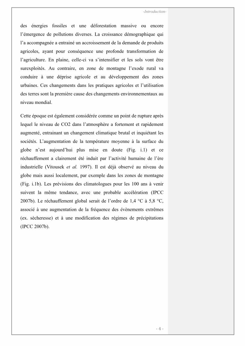
Cette époque est également considérée comme un point de rupture après

lequel le niveau de CO2 dans l’atmosphère a fortement et rapidement

augmenté, entrainant un changement climatique brutal et inquiétant les

sociétés. L’augmentation de la température moyenne à la surface du

globe n’est aujourd’hui plus mise en doute (Fig. i.1) et ce

réchauffement a clairement été induit par l’activité humaine de l’ère

industrielle (Vitousek et al. 1997). Il est déjà observé au niveau du

globe mais aussi localement, par exemple dans les zones de montagne

(Fig. i.1b). Les prévisions des climatologues pour les 100 ans à venir

suivent la même tendance, avec une probable accélération (IPCC

2007b). Le réchauffement global serait de l’ordre de 1,4 °C à 5,8 °C,

associé à une augmentation de la fréquence des évènements extrêmes

(ex. sècheresse) et à une modification des régimes de précipitations

(IPCC 2007b).

- 5 -

-Introduction-

(a)

(b)

Conséquences pour la biodiversité et les écosystèmes

D’une manière générale, tous les composants de la biodiversité, des

organismes aux biomes, peuvent être affectés par le changement

climatique (Parmesan 2006) et par les changements relatifs à

l’utilisation des terres (Vitousek et al. 1997). En termes d’espèces, des

extinctions à un taux jamais atteint sont attendues (Millennium

Ecosystem Assessment 2005a; Pereira et al. 2010), certaines pouvant

entrainer des cascades d’extinctions dues aux relations biotiques entre

espèces (Koh et al. 2004; Memmott et al. 2007; Rafferty & Ives 2011).

Par exemple, les changements climatiques peuvent causer des décalages

phénologiques entre des plantes et leurs pollinisateurs, conduisant à des

extinctions potentielles dans les deux groupes à la fois (Harrington et al.

1999). En termes d’habitats, on a aussi observé d’importantes

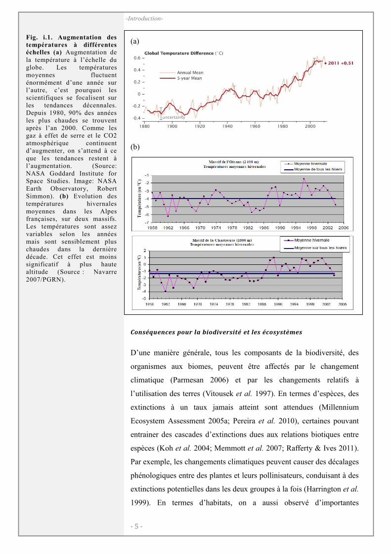
Fig. i.1. Augmentation des

températures à différentes échelles (a) Augmentation de la température à l’échelle du globe. Les températures moyennes fluctuent énormément d’une année sur l’autre, c’est pourquoi les scientifiques se focalisent sur les tendances décennales. Depuis 1980, 90% des années les plus chaudes se trouvent après l’an 2000. Comme les gaz à effet de serre et le CO2 atmosphérique continuent d’augmenter, on s’attend à ce que les tendances restent à l’augmentation. (Source: NASA Goddard Institute for Space Studies. Image: NASA Earth Observatory, Robert Simmon). (b) Evolution des températures hivernales moyennes dans les Alpes françaises, sur deux massifs. Les températures sont assez variables selon les années mais sont sensiblement plus chaudes dans la dernière décade. Cet effet est moins significatif à plus haute altitude (Source : Navarre 2007/PGRN).

- 6 -

-Introduction-

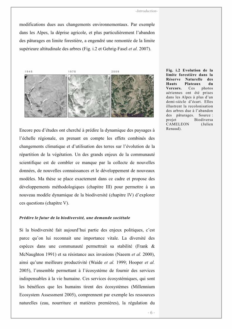
modifications dues aux changements environnementaux. Par exemple

dans les Alpes, la déprise agricole, et plus particulièrement l’abandon

des pâturages en limite forestière, a engendré une remontée de la limite

supérieure altitudinale des arbres (Fig. i.2 et Gehrig-Fasel et al. 2007).

Encore peu d’études ont cherché à prédire la dynamique des paysages à

l’échelle régionale, en prenant en compte les effets combinés des

changements climatique et d’utilisation des terres sur l’évolution de la

répartition de la végétation. Un des grands enjeux de la communauté

scientifique est de combler ce manque par la collecte de nouvelles

données, de nouvelles connaissances et le développement de nouveaux

modèles. Ma thèse se place exactement dans ce cadre et propose des

développements méthodologiques (chapitre III) pour permettre à un

nouveau modèle dynamique de la biodiversité (chapitre IV) d’explorer

ces questions (chapitre V).

Prédire le futur de la biodiversité, une demande sociétale

Si la biodiversité fait aujourd’hui partie des enjeux politiques, c’est

parce qu’on lui reconnait une importance vitale. La diversité des

espèces dans une communauté permettrait sa stabilité (Frank &

McNaughton 1991) et sa résistance aux invasions (Naeem et al. 2000),

ainsi qu’une meilleure productivité (Waide et al. 1999; Hooper et al.

2005), l’ensemble permettant à l’écosystème de fournir des services

indispensables à la vie humaine. Ces services écosystémiques, qui sont

les bénéfices que les humains tirent des écosystèmes (Millennium

Ecosystem Assessment 2005), comprennent par exemple les ressources

naturelles (eau, nourriture et matières premières), la régulation du

Fig. i.2 Evolution de la

limite forestière dans la

Réserve Naturelle des

Hauts Plateaux du Vercors. Ces photos aériennes ont été prises dans les Alpes à plus d’un demi-siècle d’écart. Elles illustrent la recolonisation des arbres due à l’abandon des pâturages. Source : projet Biodiversa CAMELEON (Julien Renaud).

- 7 -

-Introduction-

climat et des ravageurs, la séquestration du carbone ou la pollinisation

par les insectes. Ce sont ces bénéfices qui sont menacés par la crise de

la biodiversité.

Afin d’améliorer la préservation des systèmes naturels face aux

changements globaux, plusieurs institutions internationales ont vu le

jour. En 1988, le GIEC (Groupement intergouvernemental d’experts sur

l’évolution du climat) a été créé pour synthétiser les connaissances

scientifiques mondiales sur le climat. Cet organisme a joué un rôle

essentiel dans la prise de conscience des changements globaux.

Aujourd’hui, deux autres organismes existent, plus particulièrement

axés sur la préservation de la biodiversité. La Convention sur la

diversité biologique (CDB) est l’organe qui encadre les négociations

internationales visant à enrayer la perte de biodiversité et des services

qui y sont associés, et la Plateforme sur la biodiversité et les services

écosystémiques (IPBES), nouvellement crée, regroupera les données

scientifiques et produira des recommandations sur la base des travaux

des chercheurs du monde entier. La recherche que j’ai menée lors de ma

thèse a particulièrement été stimulée par cette demande sociétale. Pour

mieux comprendre l’émergence, la maintenance et le déclin de la

biodiversité, de nouveaux modèles sont nécessaires. Ils doivent

néanmoins se baser sur un cadre théorique consistent afin de produire

des scenarios robustes. La section suivante est destinée à présenter ce

cadre conceptuel.

- 8 -

-Introduction-

CADRE CONCEPTUEL

LA COEXISTENCE DES ESPECES

Le concept de niche et la spécialisation écologique

Comprendre les mécanismes qui créent et maintiennent la diversité des

espèces est crucial pour prévoir l’influence des changements

environnementaux. Dans ce domaine, les théories de la coexistence des

espèces jouent un rôle central. La principale, développée au 20ème

siècle, est basée sur le concept de niche écologique, décrite de multiples

façons par Grinnell (1917), Elton (1927), Hutchinson (1957), ou encore

Levins et MacArthur (1966). Dans tous les cas, la notion de ressources

est centrale (Chase & Leibold 2003). La niche est généralement définie

comme les conditions nécessaires à la survie de l’espèce (ex. type de

ressources) et l’impact qu’elle a sur les ressources (ex. exploitation des

ressources). La différenciation de niche permet à chaque espèce de se

distinguer par son rôle ou ses besoins et d’éviter ainsi la compétition, ce

qui aboutit à une coexistence stable des espèces. Ce mécanisme de

coexistence est un effet « stabilisateur » (Chesson 2000a). A l’inverse,

deux espèces ayant des niches trop semblables vont entrer en

compétition jusqu’à ce que l’une soit exclue (principe de Gause, 1934).

Cependant, si les deux espèces sont suffisamment similaires, elles vont

coexister temporairement de la même manière que deux individus d’une

même espèce. La coexistence est alors le résultat d’un d’effet

« égalisateur » (Chesson 2000a).

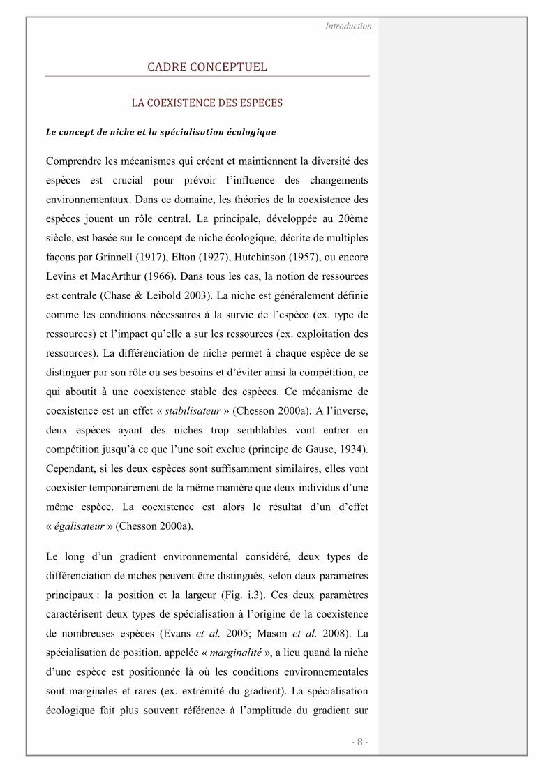
Le long d’un gradient environnemental considéré, deux types de

différenciation de niches peuvent être distingués, selon deux paramètres

principaux : la position et la largeur (Fig. i.3). Ces deux paramètres

caractérisent deux types de spécialisation à l’origine de la coexistence

de nombreuses espèces (Evans et al. 2005; Mason et al. 2008). La

spécialisation de position, appelée « marginalité », a lieu quand la niche

d’une espèce est positionnée là où les conditions environnementales

sont marginales et rares (ex. extrémité du gradient). La spécialisation

écologique fait plus souvent référence à l’amplitude du gradient sur

- 9 -

-Introduction-

laquelle s’étend la niche de l’espèce (Futuyma & Moreno 1988). Cette

spécialisation, appelée aussi « largeur de niche » est illustrée Fig. i.3 (à

droite, espèce 1).

La spécialisation, fondamentale pour la coexistence des espèces et le

maintien d’une forte diversité, est très importante pour établir la

vulnérabilité des espèces. Par exemple, en cas de modification rapide

des facteurs environnementaux, les espèces ayant une largeur de niche

restreinte peuvent être plus affectées que les plus généralistes, si la

direction du changement les exposent fortement (McKinney 1997;

Clavel et al. 2011).

Beaucoup d’études sur la spécialisation ont ciblé des petits groupes

d’espèces dans leur région. Au contraire, encore peu d’études ont

cherché à décrire et expliquer les différents degrés de spécialisation

d’une flore complète sur une région biogéographique hétérogène.

D’autre part, la majorité des études se sont focalisées sur quelques axes

de différenciation de niche sélectionnés a priori. Prendre en compte de

nombreux axes de différenciation de niche et relier le degré de

spécialisation à différents critères de rareté ainsi qu’à des traits

d’histoire de vie devrait pourtant pouvoir permettre de mieux

comprendre les mécanismes de distribution et de coexistence des

espèces et estimer leur vulnérabilité (voir Chapitre I)

Fig. i.3. Différenciation de niche. A gauche, selon la position, à droite, selon la tolérance. La fitness détermine la compétitivité de l’espèce. Les deux espèces se partagent les zones du gradient pour lesquelles elles sont meilleures compétitrices. Dans les deux cas, les fitness sont différentes en tout point du gradient, sauf au croisement des courbes ou la relation entre les espèces est neutre.

- 10 -

-Introduction-

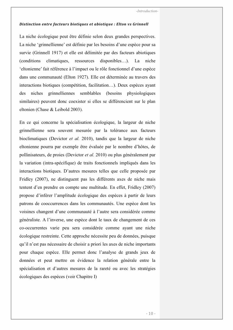
Distinction entre facteurs biotiques et abiotiq ue : Elton vs Grinnell

La niche écologique peut être définie selon deux grandes perspectives.

La niche „grinnellienne’ est définie par les besoins d’une espèce pour sa

survie (Grinnell 1917) et elle est délimitée par des facteurs abiotiques

(conditions climatiques, ressources disponibles…). La niche

„eltonienne’ fait référence à l’impact ou le rôle fonctionnel d’une espèce

dans une communauté (Elton 1927). Elle est déterminée au travers des

interactions biotiques (compétition, facilitation…). Deux espèces ayant

des niches grinnelliennes semblables (besoins physiologiques

similaires) peuvent donc coexister si elles se différencient sur le plan

eltonien (Chase & Leibold 2003).

En ce qui concerne la spécialisation écologique, la largeur de niche

grinnellienne sera souvent mesurée par la tolérance aux facteurs

bioclimatiques (Devictor et al. 2010), tandis que la largeur de niche

eltonienne pourra par exemple être évaluée par le nombre d’hôtes, de

pollinisateurs, de proies (Devictor et al. 2010) ou plus généralement par

la variation (intra-spécifique) de traits fonctionnels impliqués dans les

interactions biotiques. D’autres mesures telles que celle proposée par

Fridley (2007), ne distinguent pas les différents axes de niche mais

tentent d’en prendre en compte une multitude. En effet, Fridley (2007)

propose d’inférer l’amplitude écologique des espèces à partir de leurs

patrons de cooccurrences dans les communautés. Une espèce dont les

voisines changent d’une communauté à l’autre sera considérée comme

généraliste. A l’inverse, une espèce dont le taux de changement de ces

co-occurrentes varie peu sera considérée comme ayant une niche

écologique restreinte. Cette approche nécessite peu de données, puisque

qu’il n’est pas nécessaire de choisir a priori les axes de niche importants

pour chaque espèce. Elle permet donc l’analyse de grands jeux de

données et peut mettre en évidence la relation générale entre la

spécialisation et d’autres mesures de la rareté ou avec les stratégies

écologiques des espèces (voir Chapitre I)

- 11 -

-Introduction-

La dimension spatio-temporelle et la théorie neutre de la biodiversité

La théorie de la niche a suscité de nombreuses critiques, notamment

parce qu’elle ne permettait pas d’expliquer le fonctionnement des

écosystèmes où le nombre d’espèces est supérieur au type/nombre de

ressources et aux moyens de les exploiter (Bell 2001; Hubbell 2001).

Ces écosystèmes riches en espèces comme les forêts tropicales ou les

barrières de corail (Chave 2004) ont inspiré la théorie neutre de la

biodiversité « The Unified Neutral Theory of Biodiversity and

Biogeography » (Hubbell 2001). Ce modèle théorique, basé sur des

individus, met en jeu des processus stochastiques (survie, dispersion,

spéciation), et permet d’expliquer la richesse en espèces des

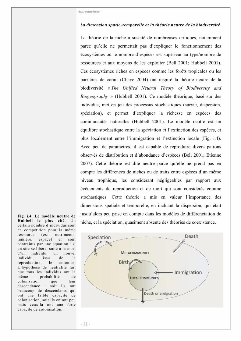
communautés naturelles (Hubbell 2001). Le modèle neutre est un

équilibre stochastique entre la spéciation et l’extinction des espèces, et

plus localement entre l’immigration et l’extinction locale (Fig. i.4).

Avec peu de paramètres, il est capable de reproduire divers patrons

observés de distribution et d’abondance d’espèces (Bell 2001; Etienne

2007). Cette théorie est dite neutre parce qu’elle ne prend pas en

compte les différences de niches ou de traits entre espèces d’un même

niveau trophique, les considérant négligeables par rapport aux

évènements de reproduction et de mort qui sont considérés comme

stochastiques. Cette théorie a mis en valeur l’importance des

dimensions spatiale et temporelle, en incluant la dispersion, qui était

jusqu’alors peu prise en compte dans les modèles de différenciation de

niche, et la spéciation, quasiment absente des théories de coexistence.

Fig. i.4. Le modèle neutre de Hubbell le plus cité. Un certain nombre d’individus sont en compétition pour la même ressource (ex. nutriments, lumière, espace) et sont contraints par une équation : si un site se libère, suite à la mort d’un individu, un nouvel individu, issu de la reproduction, le colonise. L’hypothèse de neutralité fait que tous les individus ont la même probabilité de colonisation que leur descendance : soit ils ont beaucoup de descendants qui ont une faible capacité de colonisation, soit ils en ont peu mais ceux-là ont une forte capacité de colonisation.

- 12 -

-Introduction-

Ce modèle a d’abord suscité une vive critique (Clark et al. 2007).

Toutefois, le nouveau regard qu’il a apporté a permis de revisiter la

théorie de la niche, incluant la dispersion (Kneitel & Chase 2004) ou

même des processus démographiques stochastiques (Tilman 2004). Les

visions contemporaines de la théorie de niche (Chase 2005)

reconnaissent que les différenciations de niches écologiques peuvent

être temporelles (phénologie, perturbation, démographie), spatiales

(répartition des ressources), concerner les réseaux d’interactions

(parasitisme, prédation) ou le type de ressource. Le principal problème

est devenu celui de choisir les mécanismes les plus importants pour la

coexistence dans le système étudié, parmi une multitude de possibilités

La dispersion, un processus central

La théorie neutre a mis en avant l’importance capitale de la dispersion

pour la coexistence des espèces. La réconciliation des deux théories de

coexistence des espèces a ouvert la voie aux analyses comparant

l’importance de la dynamique spatio-temporelle générée par la

dispersion à l’importance de la différenciation de niches (Kneitel &

Chase 2004; Gravel et al. 2006; Holyoak et al. 2006). La dispersion des

espèces agit à diverses échelles et influence la coexistence à travers

plusieurs mécanismes. La dynamique source-puits va permettre à une

espèce de se maintenir là où elle devrait être exclue par la compétition

ou parce que les conditions abiotiques ne lui sont pas favorables

(Pulliam 2000; Soberon 2007). La limitation de la distance de

dispersion aboutit à une concentration des individus de l’espèce,

augmentant la compétition intra-spécifique et favorisant la coexistence

(Holyoak et al. 2006). Il en résulte des effets variés sur la diversité,

agissant parfois dans des directions opposées (Cadotte & Fukami 2005),

qui sont difficiles à résumer par de simples facteurs explicatifs.

La dispersion, qui se divise en trois phases (émigration, transfert,

établissement), est un processus difficile à isoler en cela qu’il dépend de

beaucoup d’autres. La phase d’émigration est sensible aux conditions

environnementales lors du développement de l’espèce (ex. manque de

ressources), et aux conditions environnementales avoisinantes. Elle

- 13 -

-Introduction-

dépend donc de la structure spatiale des habitats favorables au

développement de l’espèce. L’efficacité du transfert est affectée par la

santé des matures (ex. taille des plantes), les habitats alentours

(structure et identité), et par la présence des vecteurs pour la dispersion

passive (ex. oiseaux), qui vont déterminer la distance de dispersion.

Enfin, la phase d’établissement dépend des conditions

environnementales dans le lieu d’arrivée. La dispersion est donc un

processus central très sensible aux changements directs et indirects du

climat (Travis et al., voir annexe 6). Les changements de vents peuvent

affecter par exemple la distance de dispersion des graines (Simmons &

Thomas 2004). Les impacts peuvent être aussi indirects. Le climat peut

agir sur le développement des plantes et leur taille adulte peut varier en

conséquence, diminuant la distance de dispersion des graines (Zhang et

al. 2012).

Une vision hiérarchique et multi-échelles des mécanismes

Pour expliquer la présence d’une espèce à un endroit donné Il est

évident que plusieurs facteurs agissent à différents niveaux

d’organisation des écosystèmes, impliquant des mécanismes variés.

Tout d’abord, le pool d’espèces disponibles doit être restreint en

considérant l’histoire biogéographique de la région. Les processus de

spéciation et d’extinction mais aussi les glaciations, les volcans, et la

dérive des continents, peuvent expliquer en grande partie les patrons de

richesse d’espèces au niveau du globe (Wiens & Donoghue 2004).

Ensuite, les facteurs abiotiques comme le climat sont souvent suffisants

pour expliquer la présence ou l’absence d’une espèce sur de vastes

étendues géographiques (Guisan et al. 1998). Les contraintes abiotiques

agissent comme un premier filtre qui délimite les conditions dans

lesquelles l’espèce peut s’établir, étant donné ses capacités

physiologiques (Fig. i.5). La capacité de dispersion constitue un

deuxième filtre, permettant aux espèces d’avoir accès aux sites où

l’environnement abiotique leur est favorable (Fig. i.5).

- 14 -

-Introduction-

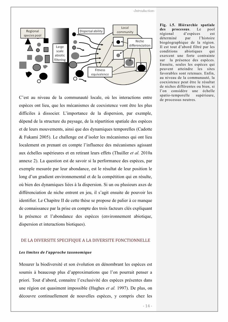
C’est au niveau de la communauté locale, où les interactions entre

espèces ont lieu, que les mécanismes de coexistence vont être les plus

difficiles à dissocier. L’importance de la dispersion, par exemple,

dépend de la structure du paysage, de la répartition spatiale des espèces

et de leurs mouvements, ainsi que des dynamiques temporelles (Cadotte

& Fukami 2005). Le challenge est d’isoler les mécanismes qui ont lieu

localement en prenant en compte l’influence des mécanismes agissant

aux échelles supérieures et en retirant leurs effets (Thuiller et al. 2010a

annexe 2). La question est de savoir si la performance des espèces, par

exemple mesurée par leur abondance, est le résultat de leur position le

long d’un gradient environnemental et de la compétition qui en résulte,

où bien des dynamiques liées à la dispersion. Si un ou plusieurs axes de

différenciation de niche entrent en jeu, il s’agit ensuite de pouvoir les

identifier. Le Chapitre II de cette thèse se propose de palier à ce manque

de connaissance par la prise en compte des trois facteurs clés expliquant

la présence et l’abondance des espèces (environnement abiotique,

dispersion et interactions biotiques).

DE LA DIVERSITE SPECIFIQUE A LA DIVERSITE FONCTIONNELLE

Les limites de l╆approche taxonomique

Mesurer la biodiversité et son évolution en dénombrant les espèces est

soumis à beaucoup plus d’approximations que l’on pourrait penser a

priori. Tout d’abord, connaitre l’exclusivité des espèces présentes dans

une région est quasiment impossible (Hughes et al. 1997). De plus, on

découvre continuellement de nouvelles espèces, y compris chez les

Fig. i.5. Hiérarchie spatiale des processus. Le pool régional d’espèces est déterminé par l’histoire biogéographique de la région. Il est tout d’abord filtré par les conditions abiotiques qui exercent une forte contrainte sur la présence des espèces. Ensuite, seules les espèces qui peuvent atteindre les sites favorables sont retenues. Enfin, au niveau de la communauté, la coexistence peut être le résultat de niches différentes ou bien, si l’on considère une échelle spatio-temporelle supérieure, de processus neutres.

- 15 -

-Introduction-

mammifères (Ceballos et al. 2005). Enfin la description et la

classification des taxons ne sont pas une tâche facile. Le concept

d’espèce le plus répandu est basé sur l'isolement reproductif. Ernst

Mayr (Mayr 1940) définit les espèces comme des « groupes de

populations naturelles, effectivement ou potentiellement interfécondes,

qui sont génétiquement isolées d'autres groupes similaires, et qui

peuvent engendrer une descendance viable et féconde ». Ce concept, né

d’une réflexion sur les oiseaux, n’est pas forcément adapté à d'autres

organismes. Chez les plantes par exemple, les hybridations entre

espèces sont fréquentes et rendent particulièrement complexe leur

classification. Quand il n'y a pas de reproduction sexuée (ex. bactéries)

cette définition d'espèce atteint rapidement ses limites. D’autres

mesures de biodiversité que celles uniquement basées sur la richesse en

espèces doivent donc être envisagées.

Du concept d╆espèce à celui de groupe fonctionnel

En 1859, Darwin reconnaissait déjà que le concept d’espèce était flou :

« Jusqu’à présent, on n’a pas pu tracer une ligne de démarcation entre

les espèces et les sous-espèces, c’est-à-dire entre les formes qui dans

l’opinion de quelques naturalistes pourraient être presque mises au

rang des espèces sans le mériter tout à fait ; on n’a pas réussi

davantage à tracer une ligne de démarcation entre les sous-espèces et

les variétés fortement accusées ou entre les variétés à peine sensibles et

les différences individuelles. » (L’origine des espèces). Cette idée de

continuité des différences entre individus aux différences entre espèces

peut être prise en compte lorsque l’unité de base n’est plus l’espèce,

mais l’individu. Tout à fait cohérente avec cette notion, l'écologie

fonctionnelle, plus particulièrement développée pendant les 20

dernières années, propose de décrire les organismes par leurs

caractéristiques biologiques et leurs fonctions au sein de

l'environnement (Calow 1987). Ces caractéristiques, les traits

fonctionnels, sont mesurables et comparables entre espèces (d’un même

niveau trophique) et ont un impact sur la survie, la croissance ou la

reproduction de l’individu (Violle et al. 2007). Dans l’idéal, pour

détecter et étudier des mécanismes assez fins et s’affranchir totalement

- 16 -

-Introduction-

du concept d’espèce, la mesure des caractères devrait être faite au

niveau des individus (Albert et al. 2010a; Albert et al. 2012 annexe 4).

En pratique, lorsque le nombre d’espèces et de populations étudiées

devient trop important, on a recours aux valeurs moyennes de traits,

mesurée à partir de quelques individus, et que l’on attribue ensuite à

l’espèce et toutes à ses populations indifféremment. La variabilité intra-

spécifique peut néanmoins être non négligeable (Albert et al. 2010a), et

l’approximation des traits individuels par une moyenne est donc une

forte contrainte sur le niveau de détail que l’on peut considérer dans les

analyses et les modèles. Cependant, pour des espèces suffisamment

contrastées, les différences interspécifiques permettent tout de même de

distinguer les principales stratégies fonctionnelles (Albert et al. 2010a).

Basés sur un jeu de traits fonctionnels non-redondants et bien choisis,

on peut alors définir des groupes fonctionnels (Lavorel et al. 1997) qui

caractérisent les principales stratégies et les rôles fonctionnels des

espèces au sein de l’écosystème. Dans certains modèles, ces unités

peuvent remplacer les espèces (Woodward & Diament 1991; Albert et

al. 2008) puisque dans certains cas peu nous importe l'identité

taxonomique des espèces, ce sont leurs fonctions qui nous intéressent.

Toutefois, jusqu’à présent, une certaine dichotomie persiste entre les

écologistes travaillant sur les traits fonctionnels, ceux travaillant sur la

théorie de la coexistence et ceux modélisant les espèces. Ces trois sous

champs disciplinaires sont néanmoins complémentaires et peu de

travaux ont cherché à mixer les trois approches. Les groupes

fonctionnels définis en réponse aux changements globaux (Lavorel et

al. 1997) ne font pas explicitement le lien avec les mécanismes de

coexistence implémentés dans les modèles de distribution (ex. niche

abiotique). D’un autre côté, les groupes fonctionnels destinés aux

modèles, lorsqu’ils font le lien avec la niche climatique, ne prennent pas

en compte des traits liés à la dispersion (ex. Laurent et al. 2004).

Finalement, une proposition de groupes fonctionnels basés sur les

mécanismes de coexistence ne prend pas en compte le processus de

filtre abiotique (Herault 2007). Une approche intégrative combinant les

trois points de vue serait donc un développement majeur pour

- 17 -

-Introduction-

l’écologie. De tels groupes fonctionnels, basés à la fois sur des traits

nécessaires à la coexistence des espèces, des traits impliqués dans leur

réponse aux gradients environnementaux, et compatibles avec les

modèles, rendraient possible une nouvelle rencontre entre l’écologie

fonctionnelle et la modélisation de la biodiversité (voir chapitres III et

IV).

L╆approche fonctionnelle┸ un pont entre l╆individu et l╆écosystème

Les traits fonctionnels permettent de relier les caractéristiques des

individus à celui des écosystèmes (Shipley 2007). Par exemple, Garnier

et al. (2007) ont montré comment les traits peuvent être utilisés pour

prédire la réponse des individus, des communautés et des écosystèmes

aux changements d’utilisation des terres. Ils ont notamment mis en

relation les traits foliaires comme la teneur en matière sèche (TMSF ou

LDMC), indicatrice de la stratégie d’exploitation des ressources

(Wright et al. 2004), avec des propriétés des écosystèmes comme la

décomposition des litières et l’accumulation de biomasse, qui sont

impliquées dans les processus comme les cycles du carbone et de

l’azote. Deux mécanismes, basés sur les traits, peuvent expliquer la

relation entre la diversité et le fonctionnement des écosystèmes.

Lorsque la diversité est grande, la probabilité d’occurrence d’une

modalité ou valeur de trait importante pour une fonction de

l’écosystème augmente (Crawley et al. 1999). Dans ce cas, l’identité

fonctionnelle est importante. La deuxième explication est l’effet de

complémentarité (Loreau 1998). Si la divergence fonctionnelle est

élevée, la variété de traits permet une diversité d’exploitation des

ressources, c’est-à-dire qu’un grand nombre de niches est occupé, et

l’utilisation des ressources atteint une efficacité maximale. Les mesures

de diversité fonctionnelle qui prennent en compte les traits des espèces,

permettent donc de faire le lien entre la diversité et le fonctionnement

des écosystèmes (Diaz & Cabido 2001). Par exemple, la valeur

moyenne des traits foliaires et racinaires au niveau d’une communauté

de plantes explique une grande partie de la fertilité du sol (Diaz et al.

2007).

- 18 -

-Introduction-

C’est grâce à ces propriétés que la modélisation de groupes fonctionnels

pourra représenter les caractéristiques des écosystèmes (chapitre III). La

modélisation dynamique de ces groupes fonctionnels (chapitre IV) sera

une voie vers la prédiction de l’évolution des propriétés des

écosystèmes et des services qu’ils fournissent.

MODÉLISER┸ L╆ART DU COMPROMIS

La modélisation est une façon de représenter la nature, en la simplifiant

pour comprendre les phénomènes, faire des prédictions, et

éventuellement agir sur les phénomènes. La modélisation est nécessaire

pour tester des hypothèses et en formuler de nouvelles. Richard Levins,

dans son article « The Strategy of Model Building in Population

Biology » (Levins 1966), est l’un des premiers à présenter les problèmes

fondamentaux concernant la construction de modèles. Son point de vue

a largement influencé les biologistes depuis 50 ans. Il part du postulat

que la construction de modèles, qu’ils soient théoriques, mathématiques

ou informatiques, implique nécessairement une simplification des

phénomènes et fait appel à des compromis. Un modèle doit inclure les

aspects les plus importants selon l’objectif et l’état des connaissances.

En effet, l’approche de „force brute’ consistant à représenter chacun des

éléments du système étudié par un modèle mathématique fidèle n’a pas

de sens pour trois raisons : les données sont limitées, la résolution

mathématique serait trop compliquée, et l’interprétation serait

impossible.

Levins décrit trois qualités d’un modèle : la généralité, le réalisme et la

précision. Etant donné qu’il est difficile d’inclure ces trois propriétés

dans un même modèle, Levins propose trois types de compromis. Les

modèles qui abandonnent l’objectif de généralité demandent beaucoup

de données et de connaissances, et s’appliquent à un système

particulier, mais sont précis et réalistes. Ils permettent de comprendre

en détail les mécanismes qui aboutissent au patron observé, et peuvent

être utilisés pour faire des prédictions robustes. Les modèles sacrifiant

le réalisme sont par exemple des équations générales, des lois. Ils

peuvent être utiles pour réaliser des prédictions sans accumuler

- 19 -

-Introduction-

beaucoup de données, mais pas pour comprendre les phénomènes en

détail. Les derniers modèles, peu précis, retiennent particulièrement

l’attention de Levins. En effet, lorsque la quantification des

phénomènes n’est pas importante, cette solution offre la possibilité de

construire des modèles réalistes et généraux, qui permettent de

comprendre assez bien les phénomènes et prédire leur tendance

générale.

Le principal objectif de notre approche de modélisation sera de

déterminer les facteurs les plus importants (chapitre II) pour pouvoir

extraire l’essentiel. Nous appliquerons ce principe dans le chapitre III,

où la diversité végétale sera réduite à son essence fonctionnelle, et lors

du développement du modèle FATE-H (chapitre IV), où seuls les

principaux mécanismes seront pris en compte.

Deux autres idées fondamentales moins connues sont apportées par

Levins. Tout d’abord, il incite les approches multiples et

complémentaires, toutes étant partiellement fausses et incomplètes, en

écrivant que ‘la vérité se trouve à l’intersection de mensonges

indépendants’. Il présente aussi l’idée d’emboitement de modèles à

différentes échelles, chacun apportant une justification des paramètres

suffisants pour le niveau supérieur. Notre approche de modélisation sera

basée sur la combinaison de modèles, où chacun agit à une échelle

différente. Par exemple, le mécanisme de filtre biotique sera modélisé

par un premier modèle, et ses sorties deviendront l’entrée des modèles

de succession décrivant les processus locaux (Chapitre IV).

- 20 -

-Introduction-

CADRE METHODOLOGIQUE

LES MESURES DE DIVERSITE SPECIFIQUE ET FONCTIONNELLE

La biodiversité peut être mesurée à chaque niveau (habitat, espèces,

gènes, traits) par deux composantes. La richesse correspond au nombre

de catégories différentes du système étudié (ex. nombre d’espèces ou

habitats, différentes valeurs de traits) et l’équitabilité mesure la

régularité de la distribution des effectifs associés à chaque catégorie

(Whittaker 1965). Les indices couramment utilisés permettent de

prendre en compte l’abondance des espèces et donc évaluer à la fois la

richesse et l’équitabilité. Whittaker (1960) a proposé de considérer trois

niveaux de diversités emboitées, g, く et け. Les diversités g et け sont

semblables, la diversité g étant mesurée localement et la diversité け

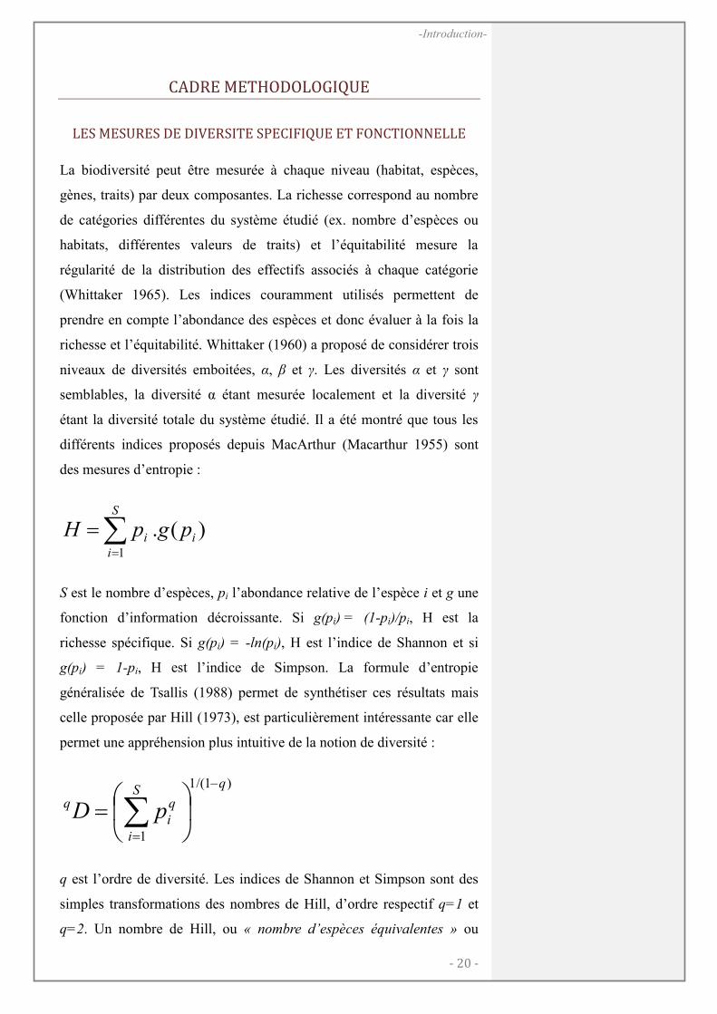
étant la diversité totale du système étudié. Il a été montré que tous les

différents indices proposés depuis MacArthur (Macarthur 1955) sont

des mesures d’entropie :

)(.1

i

S

i

i pgpH

S est le nombre d’espèces, pi l’abondance relative de l’espèce i et g une

fonction d’information décroissante. Si g(pi) = (1-pi)/pi, H est la

richesse spécifique. Si g(pi) = -ln(pi), H est l’indice de Shannon et si

g(pi) = 1-pi, H est l’indice de Simpson. La formule d’entropie

généralisée de Tsallis (1988) permet de synthétiser ces résultats mais

celle proposée par Hill (1973), est particulièrement intéressante car elle

permet une appréhension plus intuitive de la notion de diversité :

)1/(1

1

qS

i

q

i

q pD

q est l’ordre de diversité. Les indices de Shannon et Simpson sont des

simples transformations des nombres de Hill, d’ordre respectif q=1 et

q=2. Un nombre de Hill, ou « nombre d’espèces équivalentes » ou

- 21 -

-Introduction-

encore « nombres d’espèces efficaces », de valeur X, peut être interprété

comme la diversité d’une communauté de X espèces équitablement

distribuées (i.e. de même abondance).

La diversité く est en général dérivée des deux premières (Whittaker

1960) et mesure le taux de changement entre différentes localités. Il y a

plusieurs manières de la définir et de l’interpréter (Tuomisto 2010),

selon les mesures utilisées pour g et け et leur façon d’être combinées (く

= け/g ou く = け-g). La décomposition qui est la plus consistante est celle

qui implique les nombres de Hill et une approche multiplicative. Dans

ce cas, く peut être interprété comme un nombre d’espèces équivalentes

et correspond à la « vraie diversité » (Jost 2006; Tuomisto 2010;

Tuomisto 2011).

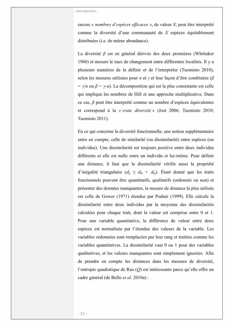
En ce qui concerne la diversité fonctionnelle, une notion supplémentaire

entre en compte, celle de similarité (ou dissimilarité) entre espèces (ou

individus). Une dissimilarité est toujours positive entre deux individus

différents et elle est nulle entre un individu et lui-même. Pour définir

une distance, il faut que la dissimilarité vérifie aussi la propriété

d’inégalité triangulaire (dij ≤ dik + dkj). Étant donné que les traits

fonctionnels peuvent être quantitatifs, qualitatifs (ordonnés ou non) et

présenter des données manquantes, la mesure de distance la plus utilisée

est celle de Gower (1971) étendue par Podani (1999). Elle calcule la

dissimilarité entre deux individus par la moyenne des dissimilarités

calculées pour chaque trait, dont la valeur est comprise entre 0 et 1.

Pour une variable quantitative, la différence de valeur entre deux

espèces est normalisée par l’étendue des valeurs de la variable. Les

variables ordonnées sont remplacées par leur rang et traitées comme les

variables quantitatives. La dissimilarité vaut 0 ou 1 pour des variables

qualitatives, et les valeurs manquantes sont simplement ignorées. Afin

de prendre en compte les distances dans les mesures de diversité,

l’entropie quadratique de Rao (Q) est intéressante parce qu’elle offre un

cadre général (de Bello et al. 2010a) :

- 22 -

-Introduction-

DppdQ j

S

j

iij

S

i2

11

11

dij est la distance entre l’espèce i et l’espèce j. En outre, l’entropie

quadratique est une simple transformation des nombres de Hill d’ordre

q=2 (Jost 2006; Tuomisto 2010a), ce qui permet de calculer la « vraie »

diversité fonctionnelle く (Voir Chapitre I).

LES ASSEMBLAGES D╆ESPECES ET L╆ECOLOGIE DES COMMUNAUTES

La condition principale pour le maintien de la biodiversité est la

coexistence des espèces qui ont une écologie similaire, dans la même

région. Ces espèces sont donc dans un même niveau trophique et

utilisent les mêmes ressources (Chesson 2000a). Si la coexistence fait

clairement référence à des situations où la persistance des espèces

considérées est infinie, on se basera la plupart du temps sur

l’observation de simples cooccurrences à un moment donné. Les

données de base utilisées dans ce cas sont des relevés de communautés,

où la quasi-totalité des espèces à été notée, ainsi que, dans certains cas,

leurs abondances approximatives. L’objectif de ces relevés est de se

placer à l’échelle où les espèces interagissent, afin d’identifier et de

comprendre les mécanismes qui permettent leur coexistence et qui

expliquent la structure des communautés.

Les propriétés étudiées sont par exemple la diversité de la communauté,

la distribution des traits ou des abondances relatives des espèces, la

productivité et d’autres propriétés impliquées dans le fonctionnement

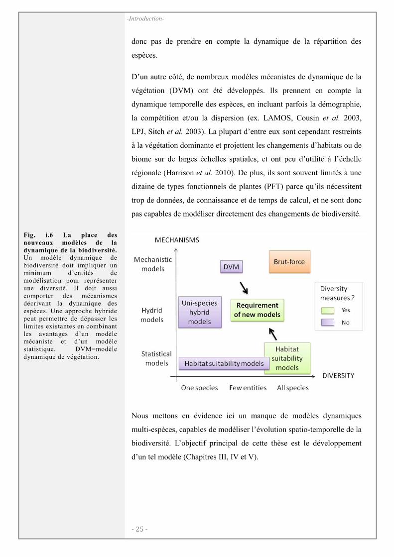
des écosystèmes. Par exemple, la hiérarchie des filtres

environnementaux (Fig. i.6) peut être testée. Les facteurs qui ont des

variations régionales (ex. température) devraient plutôt déterminer la

valeur de trait moyenne de la communauté, résultat du premier filtre

abiotique. Les variables agissant localement devraient permettre la

différenciation de niches et influenceraient plutôt la distribution des

traits des espèces dominantes. Cette hypothèse a été validée

empiriquement dans la vallée de la Guisane (Hautes-Alpes, France)

- 23 -

-Introduction-

pour des communautés végétales (de Bello et al., voir annexe 5). Dans

d’autres cas, les analyses peuvent se placer dans un contexte de méta-

communautés (plusieurs communautés connectées par la dispersion),

afin d’évaluer l’importance relative de la structure spatiale et de

l’environnement abiotique (ex. Meynard et al. Annexe 7).

Mettre en évidence l’importance relative de la compétition, de la

dispersion et de l’environnement abiotique pour expliquer les

assemblages d’espèces peut avoir des applications directes, comme par

exemple la gestion des invasives (Thuiller et al. 2010a), mais reste un

challenge. La dispersion est souvent représentée par un terme d’auto-

corrélation spatiale (ex. Borcard et al. 1992), sans aucune relation à la

capacité de dispersion de d’espèce. Cette approche limite fortement

l’interprétation de l’importance du terme spatial. La compétition est un

mécanisme qui est particulièrement difficile à détecter (Voir chapitre

II). Son effet est mesurable à l’intérieur de la communauté seulement, et

il est mélangé à celui des variables abiotiques locales. L„enjeu est donc

de choisir la dimension spatiale appropriée, les bonnes métriques, un

modèle nul qui permettra d’isoler le mécanisme à tester, notamment en

retirant les effets des facteurs agissant à plus large échelle, et une

mesure de similarité de niche entre deux espèces pertinente, tout en

étant adaptée aux connaissances et aux données accumulées (Thuiller et

al. 2010a). Une approche sera proposée dans le chapitre II pour

analyser l’importance relative de l’environnement abiotique, de la

dispersion et des interactions biotiques sur la présence et l’abondance

locale d’une espèce.

MODÉLISER LA BIODIVERSITÉ : VERS UNE APPROCHE DYNAMIQUE

Des modèles basés sur les filtres abiotiques régionaux

L’approche biogéographique pour comprendre et prédire la présence

d’une espèce à un endroit donné est basée sur la relation espèce-milieu.

Les progrès informatiques de ces dernières décennies ont permis aux

scientifiques d’utiliser de grandes bases de données pour mettre en

relation les présences observées des espèces avec le climat, qui est

- 24 -

-Introduction-

connu depuis De Candolle (1955) comme étant un facteur de premier

ordre pour expliquer la répartition de nombreuses espèces. Les

méthodes statistiques concernées ont été largement développées

(Guisan & Thuiller 2005; Heikkinen et al. 2006; Elith & Leathwick

2009; Thuiller et al. 2009) et ces modèles, dit « d’habitat », ont été

utilisés extensivement, que ce soit pour prédire la réponse des espèces

aux changements environnementaux (Thuiller et al. 2006a; Beaumont

et al. 2011) ou l’évolution de la diversité fonctionnelle (Thuiller et al.

2006b) ou phylogénétique (Thuiller et al. 2011).

L’approche est basée sur le concept de niche grinnelliennne

(environnement abiotique), et sa projection dans l’espace géographique.

Cependant, la répartition observée de l’espèce résulte également des

conditions biotiques et des mécanismes de dispersion (Soberon 2007).

Hutchinson (1957) est le premier à distinguer deux types de niches

grinnelliennes. La niche dite « fondamentale » est déterminée par les

conditions environnementales tolérées en l’absence d’interactions

biotiques. La niche dite « réalisée » correspond aux conditions

environnementales dans lesquelles l’espèce est effectivement observée,

résultat des interactions biotiques, de la limitation par la dispersion et

d’autres mécanismes (ex. source-puits). Les modèles d’habitat estiment

la niche réalisée des espèces, et présentent donc des limites évidentes

pour la projection dans des situations biotiques ou des configurations

spatiales différentes (Guisan & Zimmermann 2000; Thuiller et al.

2008). Cette approche reste cependant très intéressante à une certaine

échelle où les interactions biotiques sont négligeables, et sera la base de

nombreux autres modèles.

Approches multi-espèces et interactions biotiques

Lorsqu’il s’agit de modéliser la distribution de plusieurs espèces en

même temps, pour mesurer ensuite la biodiversité, plusieurs approches

sont utilisées. Tout d’abord, les modèles d’habitat peuvent être

appliqués à un très grand nombre d’espèces, mais n’incluent pas les

mécanismes de dispersion ni d’interactions biotiques. Ils ne permettent

- 25 -

-Introduction-

donc pas de prendre en compte la dynamique de la répartition des

espèces.

D’un autre côté, de nombreux modèles mécanistes de dynamique de la

végétation (DVM) ont été développés. Ils prennent en compte la

dynamique temporelle des espèces, en incluant parfois la démographie,

la compétition et/ou la dispersion (ex. LAMOS, Cousin et al. 2003,

LPJ, Sitch et al. 2003). La plupart d’entre eux sont cependant restreints

à la végétation dominante et projettent les changements d’habitats ou de

biome sur de larges échelles spatiales, et ont peu d’utilité à l’échelle

régionale (Harrison et al. 2010). De plus, ils sont souvent limités à une

dizaine de types fonctionnels de plantes (PFT) parce qu’ils nécessitent

trop de données, de connaissance et de temps de calcul, et ne sont donc

pas capables de modéliser directement des changements de biodiversité.

Nous mettons en évidence ici un manque de modèles dynamiques

multi-espèces, capables de modéliser l’évolution spatio-temporelle de la

biodiversité. L’objectif principal de cette thèse est le développement

d’un tel modèle (Chapitres III, IV et V).

Fig. i.6 La place des

nouveaux modèles de la

dynamique de la biodiversité. Un modèle dynamique de biodiversité doit impliquer un minimum d’entités de modélisation pour représenter une diversité. Il doit aussi comporter des mécanismes décrivant la dynamique des espèces. Une approche hybride peut permettre de dépasser les limites existantes en combinant les avantages d’un modèle mécaniste et d’un modèle statistique. DVM=modèle dynamique de végétation.

- 26 -

-Introduction-

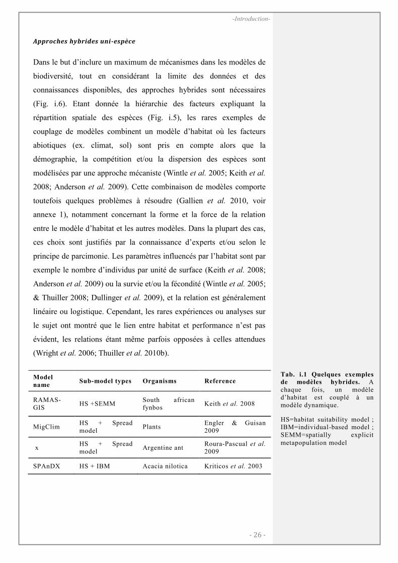
Approches hybrides uni-espèce

Dans le but d’inclure un maximum de mécanismes dans les modèles de

biodiversité, tout en considérant la limite des données et des

connaissances disponibles, des approches hybrides sont nécessaires

(Fig. i.6). Etant donnée la hiérarchie des facteurs expliquant la

répartition spatiale des espèces (Fig. i.5), les rares exemples de

couplage de modèles combinent un modèle d’habitat où les facteurs

abiotiques (ex. climat, sol) sont pris en compte alors que la

démographie, la compétition et/ou la dispersion des espèces sont

modélisées par une approche mécaniste (Wintle et al. 2005; Keith et al.

2008; Anderson et al. 2009). Cette combinaison de modèles comporte

toutefois quelques problèmes à résoudre (Gallien et al. 2010, voir

annexe 1), notamment concernant la forme et la force de la relation

entre le modèle d’habitat et les autres modèles. Dans la plupart des cas,

ces choix sont justifiés par la connaissance d’experts et/ou selon le

principe de parcimonie. Les paramètres influencés par l’habitat sont par

exemple le nombre d’individus par unité de surface (Keith et al. 2008;

Anderson et al. 2009) ou la survie et/ou la fécondité (Wintle et al. 2005;

& Thuiller 2008; Dullinger et al. 2009), et la relation est généralement

linéaire ou logistique. Cependant, les rares expériences ou analyses sur

le sujet ont montré que le lien entre habitat et performance n’est pas

évident, les relations étant même parfois opposées à celles attendues

(Wright et al. 2006; Thuiller et al. 2010b).

Model

name Sub-model types Organisms Reference

RAMAS-GIS

HS +SEMM South african fynbos

Keith et al. 2008

MigClim HS + Spread model

Plants Engler & Guisan 2009

x HS + Spread model

Argentine ant Roura-Pascual et al. 2009

SPAnDX HS + IBM Acacia nilotica Kriticos et al. 2003

Tab. i.1 Quelques exemples de modèles hybrides. A chaque fois, un modèle d’habitat est couplé à un modèle dynamique.

HS=habitat suitability model ; IBM=individual-based model ; SEMM=spatially explicit metapopulation model

- 27 -

-Introduction-

Modéliser la dynamique de la biodiversité

Afin de modéliser la dynamique de la biodiversité, l’enjeu est de

représenter la diversité des espèces en utilisant un nombre suffisant

d’entités de modélisation (Fig. i.6), qu’il soit aussi possible de

paramétrer. Un tel modèle pourrait projeter d’autres composantes de la

biodiversité que la richesse en espèce, comme par exemple la diversité

des habitats, ou la diversité fonctionnelle. Les modèles hybrides qui ont

été développés jusqu’à maintenant sont principalement destinés à

comprendre et prédire la répartition d’une espèce cible mais l’approche

de combinaison de modèle peut être appliquée aux modèles de

végétation (Hickler et al. 2004 et Chapitre IV et V).

Notre objectif est de pouvoir modéliser des entités qui puissent

représenter la biodiversité à l’échelle régionale. Nous utiliserons pour

cela le modèle dynamique de la végétation de BIOMOVE (Midgley et

al. 2010) et nous le développerons. Ce modèle (FATE-H) est un

couplage entre un modèle d’habitat et un modèle de succession

végétale. Il a principalement été utilisé sur de petites échelles spatiales

et pour un très petit nombre de groupes fonctionnels (ex. Albert et al.

2008). Notre objectif est de l’utiliser pour modéliser la dynamique du

paysage à l’échelle régionale, en utilisant des groupes fonctionnels qui

représentent la diversité et la structure de la végétation dominante. Le

modèle peut aussi combiner un module de dispersion, que l’on

développera pour nos groupes fonctionnels, et un module de

perturbation. Il permettra donc de prédire l’évolution de la végétation

en fonction du climat et de l’utilisation des terres (chapitre V).

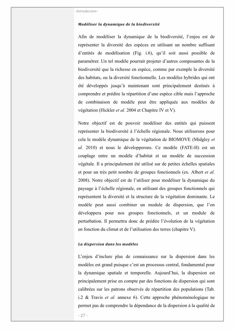
La dispersion dans les modèles

L’enjeu d’inclure plus de connaissance sur la dispersion dans les

modèles est grand puisque c’est un processus central, fondamental pour

la dynamique spatiale et temporelle. Aujourd’hui, la dispersion est

principalement prise en compte par des fonctions de dispersion qui sont

calibrées sur les patrons observés de répartition des populations (Tab.

i.2 & Travis et al. annexe 6). Cette approche phénoménologique ne

permet pas de comprendre la dépendance de la dispersion à la qualité de

- 28 -

-Introduction-

l’habitat ou à la démographie de l’espèce et produit donc des

prédictions peu robustes. L’enjeu est d’inclure la dispersion de manière

plus mécanistique, en prenant en compte les phases d’émigration, de

transfert, et d’établissement de l’espèce. Quelques modèles existent déjà

(ex. PATCH, SPAndX), où plus de mécanismes sont intégrés (Tab. i.2).

Nous chercherons à prendre en compte la dispersion dans son ensemble

dans le modèle de dynamique de végétation développé au cours de cette

thèse (chapitre IV).

Model type How dispersal is

implemented

Example Model

name

Niche-based model

Full dispersal/ no dispersal Thuiller et al. 2011 (European plants, birds and mammals)

Biomod

Landscape model

Species specific dispersal kernels based on species mean dispersal distances

Lischke et al. 2006 (Swiss trees)

TreeMig

Landscape model

Seed dispersal kernel based on effective and maximum dispersal distances.

Scheller et al. 2008 (New Jersey Pine Barrens)

LANDIS

Migration model

All cohorts optimize their position according to their possible interactions with all other cohorts.

Saltré et al. 2009 (Fagus sylvatica)

Gibbs-based model

Cellular automaton

Jump-dispersal events based on distance and habitat quality

Roura-Pascual et al.

2009 (Argentine ant) Spread model

Probability function based on dispersal distance, landscape and time since colonization

Engler & Guisan 2009

MigClim

Spatially explicit metapopulation models

Incidence functions Keith et al. 2008 (South african fynbos),

RAMAS-GIS

Spatially explicit Individual Based population model

Animals search for suitable and unoccupied breeding sites within minimal and maximal distances using random walks

Schumaker et al. 2004 (species in the Oregon’s Willamette basin)

PATCH

Hybrid model Seed dispersal probability affected by livestock and presence of watercourses

Kriticos et al. 2003 (Acacia nilotica)

SPAnDX

Tab. i.2

Implementation de la dispersion dans plusieurs types de modèles.

- 29 -

-Introduction-

OBJECTIFS GENERAUX DE LA THESE ET ORGANISATION

L’objectif principal de la thèse est de caractériser les espèces et les

habitats vulnérables aux changements climatiques et d’utilisation des

terres dans les Alpes Françaises. La démarche utilisée consiste à (1)

déterminer les mécanismes et les facteurs les plus importants pour

expliquer la présence et l’abondance des espèces (2) utiliser ces

connaissances pour adapter un modèle de dynamique de la végétation

puis le valider (3) Utiliser ce modèle pour construire des scenarios, qui

pourront éventuellement servir d’aide à la décision.

(1)Décrire et Analyser les patrons de rareté et d'abondance

Chapitre I. Niche breadth, rarity and ecological

characteristics of the French Alps flora. Article publié dans

Journal of Biogeography (Janvier 2012)

Ce premier chapitre explore la spécialisation des plantes dans les Alpes

à partir de la cooccurrence des espèces au niveau de la communauté. La

largeur de niche ainsi déterminée est mise en relation avec d’autres

mesures de rareté et des traits qui représentent des stratégies

fonctionnelles.

Chapitre II. Accounting for dispersal and biotic interactions in

order to disentangle the drivers of species distributions and their

abundances. Article publié dans Ecology Letters (online)

Ce chapitre propose un modèle hiérarchique pour analyser l’importance

relative du filtre abiotique, de la dispersion et des interactions biotiques

(directes ou indirectes) sur la présence et l’abondance d’une espèce.

(2)Modéliser la végétation à l'échelle d'un espace naturel protégé

Chapitre III. Optimizing plant functional groups for dynamic

models of biodiversity: at the crossroads between functional and

community ecology. Article soumis à Global Change Biology

- 30 -

-Introduction-

Dans ce chapitre, l’objectif a été de construire des groupes fonctionnels

capables de représenter la structure des communautés et d’être

paramétrés pour un modèle dynamique de végétation. Ces groupes ont

été construits à partir d’une poignée de traits qui représentent les

principaux mécanismes à l’origine de la structure des communautés

(Fig. i.7). Leur capacité à mesurer la diversité a été évaluée.

Chapitre IV. Fate-h: a spatially and temporally explicit hybrid

model for predicting the vegetation structure and diversity at

regional scale. Article en préparation pour Journal of Applied

Ecology.

Le développement d’un modèle hybride de dynamique de végétation

(FATE-H), qui puisse reproduire les patrons de structure et de diversité

de la végétation, a été validé dans ce chapitre, sur le territoire du Parc

national des Ecrins.

(3)Prédire le futur de la diversité de la végétation dans les Ecrins

Chapitre V. Consequences of climate and land use change on

the vegetation structure and diversity in the Ecrins National

Park. Article en préparation.

Ce chapitre explore les futurs possibles de la végétation du parc

national des Ecrins, selon deux scenarios de pâturage contrastés.

L’interaction de ces scenarios avec un changement climatique est aussi

examinée.

- 31 -

-Introduction-

CADRE BIOGEOGRAPHIQUE ET ECOLOGIQUE

Toutes les études présentées dans les chapitres qui suivent se sont

focalisées sur les Alpes françaises et sa végétation. La suite présente

quelques éléments qui caractérisent cette région, les plantes qui y vivent

et le Parc National des Ecrins, sur lequel se sont concentrés les derniers

chapitres.

LES ALPES FRANÇAISES

Une diversité climatique à l╆origine d╆une importante biodiversité

La principale particularité des écosystèmes montagnards est leur

gradient altitudinal et leur topographie complexe, responsable de larges

variations climatiques sur de très courtes distances. Cette forte

hétérogénéité spatiale de l’environnement, combinée aux diverses

influences climatiques (Fig. i.8), est à l’origine de la grande diversité

d’espèces que l’on peut trouver dans les Alpes (Körner 1999). Nous

pouvons y observer par exemple environ 2/3 de la flore Française (voir

aussi Fig. i.9).

Fig. i.7. Représentation

schématique de la place des

chapitres par rapport au

cadre conceptuel.

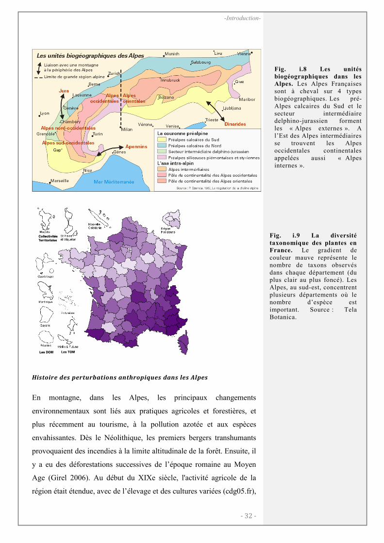
- 32 -

-Introduction-

Histoire des perturbations anthropiques dans les Alpes

En montagne, dans les Alpes, les principaux changements

environnementaux sont liés aux pratiques agricoles et forestières, et

plus récemment au tourisme, à la pollution azotée et aux espèces

envahissantes. Dès le Néolithique, les premiers bergers transhumants

provoquaient des incendies à la limite altitudinale de la forêt. Ensuite, il

y a eu des déforestations successives de l’époque romaine au Moyen

Age (Girel 2006). Au début du XIXe siècle, l'activité agricole de la

région était étendue, avec de l’élevage et des cultures variées (cdg05.fr),

Fig. i.8 Les unités

biogéographiques dans les Alpes. Les Alpes Françaises sont à cheval sur 4 types biogéographiques. Les pré-Alpes calcaires du Sud et le secteur intermédiaire delphino-jurassien forment les « Alpes externes ». A l’Est des Alpes intermédiaires se trouvent les Alpes occidentales continentales appelées aussi « Alpes internes ».

Fig. i.9 La diversité

taxonomique des plantes en France. Le gradient de couleur mauve représente le nombre de taxons observés dans chaque département (du plus clair au plus foncé). Les Alpes, au sud-est, concentrent plusieurs départements où le nombre d’espèce est important. Source : Tela Botanica.

- 33 -

-Introduction-

mais la majorité des zones qui étaient labourées et fauchées à l’étage

subalpin sont aujourd’hui des zones de pâturage (Clément et al. 2003).

Cette déprise agricole, généralisée en zone de montagne, est encore la

tendance actuelle, même si le Parc National des Ecrins s’efforce de

maintenir la fauche dans quelques prairies (ex. Col du Lautaret). La

forêt a donc recolonisé naturellement les terres cultivables

abandonnées, mais elle a aussi gagné de l’espace grâce au reboisement.

Néanmoins, dans les années 70, le développement du tourisme avec

l’arrivée des stations de ski a apporté une nouvelle vague de

déboisement. La répartition actuelle des forêts s’explique donc par

l’histoire de l’utilisation des terres plutôt que par le climat (Gehrig-

Fasel et al. 2007).

LA VEGETATION DE MONTAGNE

Les plantes comme sujet d╆étude

Les plantes offrent plusieurs avantages à être étudiées. Elles constituent

un niveau trophique central, étant la ressource de nombreux

organismes. De plus, les espèces dominantes structurent le paysage,

créant les habitats pour de nombreuses autres espèces. La végétation est

par conséquent centrale dans l’évaluation de la biodiversité. D’autre

part, la botanique est une discipline ancienne, qui est partagée par de

nombreux passionnés (16892 inscrits à Tela Botanica, France), et dont

les connaissances sont assez développées. De nombreuses bases de

données sont donc disponibles sur la répartition et les caractéristiques

de beaucoup d’espèces végétales.

Les plantes sont regroupées de plusieurs façons selon leurs stratégies

fonctionnelles. La classification des types biologiques selon Raunkiaer

(1934) est particulièrement intéressante parce qu’elle représente les

principales différences démographiques (Chapin III et al. 1996; Lavorel

et al. 1997; Lavorel & Garnier 2002). Elle regroupe les plantes selon la

manière dont elles protègent leurs bourgeons pendant la mauvaise

saison (Fig. i.10):

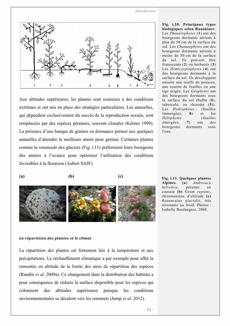
- 34 -

-Introduction-

Aux altitudes supérieures, les plantes sont soumises à des conditions

extrêmes et ont mis en place des stratégies particulières. Les annuelles,

qui dépendent exclusivement du succès de la reproduction sexuée, sont

remplacées par des espèces pérennes, souvent clonales (Körner 1999).

La présence d’une banque de graines en dormance permet aux quelques

annuelles d’attendre la meilleure année pour germer. Certaines plantes

comme la renoncule des glaciers (Fig. i.11) préforment leurs bourgeons

des années à l’avance pour optimiser l’utilisation des conditions

favorables à la floraison (Aubert SAJF).

(a) (b) (c)

La répartition des plantes et le climat

La répartition des plantes est fortement liée à la température et aux

précipitations. Le réchauffement climatique a par exemple pour effet la

remontée en altitude de la limite des aires de répartition des espèces

(Randin et al. 2009a). Ce changement dans la distribution des habitats a

pour conséquence de réduire la surface disponible pour les espèces qui

colonisent des altitudes supérieures puisque les conditions

environnementales se décalent vers les sommets (Jump et al. 2012).

Fig. i.10. Principaux types

biologiques selon Raunkiaer. Les Phanérophytes (1) ont des bourgeons dormants aériens à plus de 50 cm de la surface du sol. Les Chamaephytes ont des bourgeons dormants aériens à moins de 50 cm de la surface du sol. Ils peuvent être frutescents (2) ou herbacés (3) Les Hémicryptophytes (4) ont des bourgeons dormants à la surface du sol. Ils développent ensuite une touffe de pousses, une rosette de feuilles ou une tige érigée. Les Géophytes ont des bourgeons dormants sous la surface du sol (bulbe (6), tubercule, ou rhizome (5)). Les Hydrophytes : (feuilles immergées, 8) et les Hélophytes (feuilles émergées, 7) ont des bourgeons dormants sous l'eau.

Fig. i.11. Quelques plantes Alpines. (a) Androsace

helvetica, pérenne en coussin (b) Geum reptens, rhizomateuse d’altitude (c)

Ranunculus glacialis, très résistante au froid. Photos : Isabelle Boulangeat, 2008.

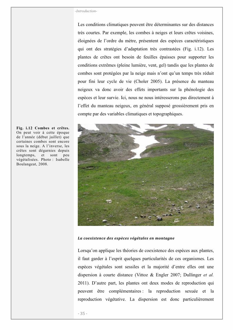
- 35 -

-Introduction-

Les conditions climatiques peuvent être déterminantes sur des distances

très courtes. Par exemple, les combes à neiges et leurs crêtes voisines,

éloignées de l’ordre du mètre, présentent des espèces caractéristiques

qui ont des stratégies d’adaptation très contrastées (Fig. i.12). Les

plantes de crêtes ont besoin de feuilles épaisses pour supporter les

conditions extrêmes (pleine lumière, vent, gel) tandis que les plantes de

combes sont protégées par la neige mais n’ont qu’un temps très réduit

pour fini leur cycle de vie (Choler 2005). La présence du manteau

neigeux va donc avoir des effets importants sur la phénologie des

espèces et leur survie. Ici, nous ne nous intéresserons pas directement à

l’effet du manteau neigeux, en général supposé grossièrement pris en

compte par des variables climatiques et topographiques.

La coexistence des espèces végétales en montagne

Lorsqu’on applique les théories de coexistence des espèces aux plantes,

il faut garder à l’esprit quelques particularités de ces organismes. Les

espèces végétales sont sessiles et la majorité d’entre elles ont une

dispersion à courte distance (Vittoz & Engler 2007; Dullinger et al.

2011). D’autre part, les plantes ont deux modes de reproduction qui

peuvent être complémentaires : la reproduction sexuée et la

reproduction végétative. La dispersion est donc particulièrement

Fig. i.12 Combes et crêtes. On peut voir à cette époque de l’année (début juillet) que certaines combes sont encore sous la neige. A l’inverse, les crêtes sont dégarnies depuis longtemps, et sont peu végétalisées. Photo : Isabelle Boulangeat, 2008.

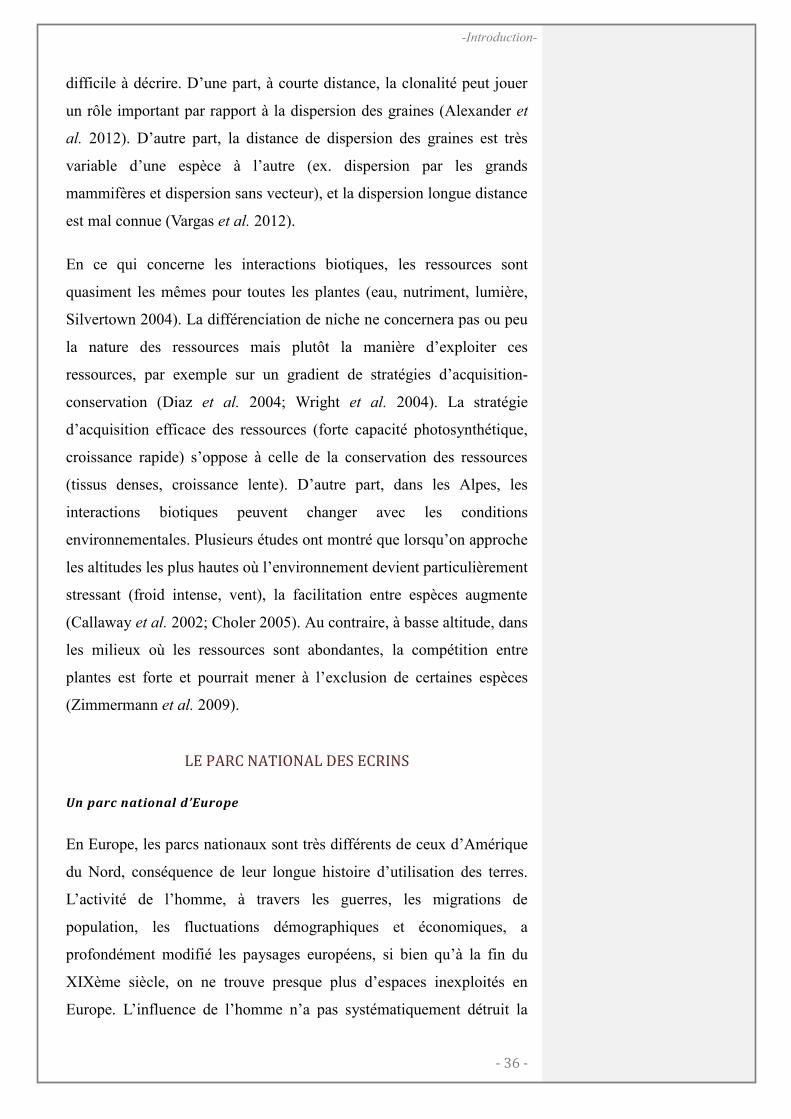
- 36 -

-Introduction-

difficile à décrire. D’une part, à courte distance, la clonalité peut jouer

un rôle important par rapport à la dispersion des graines (Alexander et

al. 2012). D’autre part, la distance de dispersion des graines est très

variable d’une espèce à l’autre (ex. dispersion par les grands

mammifères et dispersion sans vecteur), et la dispersion longue distance

est mal connue (Vargas et al. 2012).

En ce qui concerne les interactions biotiques, les ressources sont

quasiment les mêmes pour toutes les plantes (eau, nutriment, lumière,

Silvertown 2004). La différenciation de niche ne concernera pas ou peu

la nature des ressources mais plutôt la manière d’exploiter ces

ressources, par exemple sur un gradient de stratégies d’acquisition-

conservation (Diaz et al. 2004; Wright et al. 2004). La stratégie

d’acquisition efficace des ressources (forte capacité photosynthétique,

croissance rapide) s’oppose à celle de la conservation des ressources

(tissus denses, croissance lente). D’autre part, dans les Alpes, les

interactions biotiques peuvent changer avec les conditions

environnementales. Plusieurs études ont montré que lorsqu’on approche

les altitudes les plus hautes où l’environnement devient particulièrement

stressant (froid intense, vent), la facilitation entre espèces augmente

(Callaway et al. 2002; Choler 2005). Au contraire, à basse altitude, dans

les milieux où les ressources sont abondantes, la compétition entre

plantes est forte et pourrait mener à l’exclusion de certaines espèces

(Zimmermann et al. 2009).

LE PARC NATIONAL DES ECRINS

Un parc national d╆Europe

En Europe, les parcs nationaux sont très différents de ceux d’Amérique

du Nord, conséquence de leur longue histoire d’utilisation des terres.

L’activité de l’homme, à travers les guerres, les migrations de

population, les fluctuations démographiques et économiques, a

profondément modifié les paysages européens, si bien qu’à la fin du

XIXème siècle, on ne trouve presque plus d’espaces inexploités en

Europe. L’influence de l’homme n’a pas systématiquement détruit la

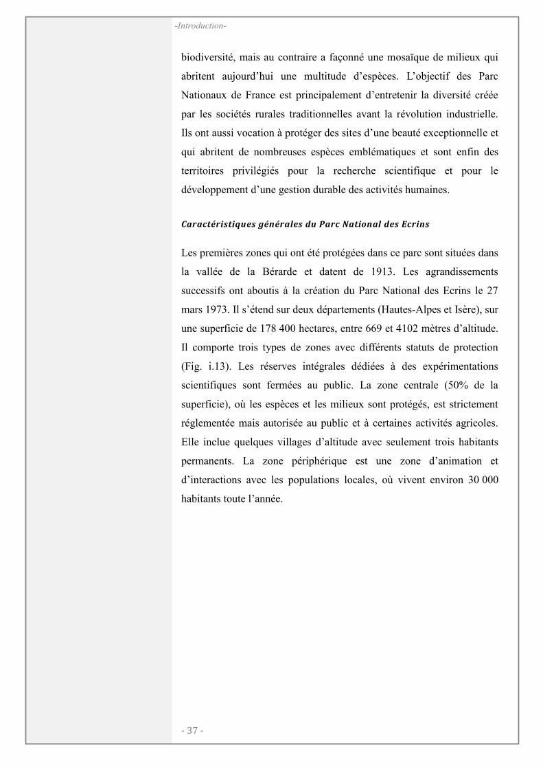
- 37 -

-Introduction-

biodiversité, mais au contraire a façonné une mosaïque de milieux qui

abritent aujourd’hui une multitude d’espèces. L’objectif des Parc

Nationaux de France est principalement d’entretenir la diversité créée

par les sociétés rurales traditionnelles avant la révolution industrielle.

Ils ont aussi vocation à protéger des sites d’une beauté exceptionnelle et

qui abritent de nombreuses espèces emblématiques et sont enfin des

territoires privilégiés pour la recherche scientifique et pour le

développement d’une gestion durable des activités humaines.

Caractéristiques générales du Parc National des Ecrins

Les premières zones qui ont été protégées dans ce parc sont situées dans

la vallée de la Bérarde et datent de 1913. Les agrandissements

successifs ont aboutis à la création du Parc National des Ecrins le 27

mars 1973. Il s’étend sur deux départements (Hautes-Alpes et Isère), sur

une superficie de 178 400 hectares, entre 669 et 4102 mètres d’altitude.

Il comporte trois types de zones avec différents statuts de protection

(Fig. i.13). Les réserves intégrales dédiées à des expérimentations

scientifiques sont fermées au public. La zone centrale (50% de la

superficie), où les espèces et les milieux sont protégés, est strictement

réglementée mais autorisée au public et à certaines activités agricoles.

Elle inclue quelques villages d’altitude avec seulement trois habitants

permanents. La zone périphérique est une zone d’animation et

d’interactions avec les populations locales, où vivent environ 30 000

habitants toute l’année.

- 38 -

-Introduction-

La végétation du Parc National des Ecrins

La flore du parc comporte environ 2000 espèces dont 216 répertoriées

comme rares ou menacées et 350 endémiques dont 146 sont protégées.

Ses habitats sont principalement des espaces ouverts (Fig. i.14) qui

constituent 60% de la surface totale, pour seulement 24% de forêts. Le

reste du Parc est dénué de toute végétation (glaciers et neiges

éternelles). Les essences forestières naturelles (non plantées)

caractéristiques sont, dans les Alpes externes, le sapin (Abies alba) et le

hêtre (Fagus sylvatica), et dans les Alpes internes le pin sylvestre

(Pinus sylvestris) et le mélèze (Larix decidua) (Fig. i.15).

Fig. i.13 Le parc national des Ecrins. Il est situé dans le Sud Est de la France, non loin de la frontière Italienne et de Grenoble. Il est divisé en trois zones de statut de protection différent. La zone centrale (cœur de parc), la zone périphérique (aire optimale d’adhésion) et la réserve intégrale. La zone périphérique n’a pas de statut de protection particulier. Source : site des Parc Nationaux de France.

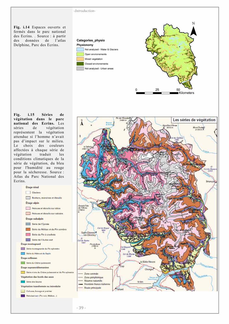
- 39 -

-Introduction-

Fig. i.15 Séries de

végétation dans le parc national des Ecrins. Les séries de végétation représentent la végétation attendue si l’homme n’avait pas d’impact sur le milieu. Le choix des couleurs affectées à chaque série de végétation traduit les conditions climatiques de la série de végétation, du bleu pour l'humidité au rouge pour la sécheresse. Source : Atlas du Parc National des Ecrins.

Fig. i.14 Espaces ouverts et fermés dans le parc national des Ecrins. . Source : à partir des données de l’atlas Delphine, Parc des Ecrins.

- 40 -

-Introduction-

QUELQUES ÉLÉMENTS SUR LES DONNÉES PRINCIPALES

Dans les Alpes Françaises, le protocole de relevés utilisé en masse est

celui de Braun-Blanquet (1946). Dans une zone où la végétation est

homogène, pouvant varier de 9m² à 10000m² selon les types de milieux,

jusqu’à quatre strates de hauteur sont définies et toutes les espèces sont

relevées avec leur classe d’abondance (selon le pourcentage de

couverture de leur strate). Les classes d’abondance sont

logarithmiques : moins de 1%, de 1 à 5%, de 5 à 25% de 25 à 50% de

50 à 75% et plus de 75%. Dans la majorité des études, la stratification

n’est pas prise en compte, ni le pourcentage de sol nu (donné par strate).

L’échantillonnage des espèces annuelles et des espèces rares, petites et

de couleurs ternes est sujet à de fortes incertitudes, selon l’année et la

date du relevé, sans compter l’expertise de l’observateur. Cette courte

description du protocole de relevé des espèces permet d’avoir une idée

des incertitudes associées aux données et des limites de leur précision.

Néanmoins, on dispose dans les Alpes Françaises de plus de 10000 de

ces relevés (Fig. i.16), qui ont été échantillonnés après 1980 et qui ont

subi un premier « contrôle qualité » prenant en compte la précision de

la localisation, l’expertise des observateurs, l’homogénéité du milieu et

les incertitudes taxonomiques. Malgré une information incomplète sur

la surface des relevés, une deuxième sélection a été effectuée dans les

études qui suivent, afin de retirer les relevés atypiques. Puisque la

végétation d’un relevé est homogène, on peut toutefois supposer

raisonnablement que les individus des espèces assez abondantes

(>25%) se trouvent très proches, à l’échelle où la coexistence a encore

un sens.

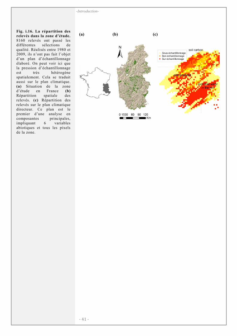
- 41 -

-Introduction-

(a) (b) (c)

Fig. i.16. La répartition des

relevés dans la zone d’étude. 8160 relevés ont passé les différentes sélections de qualité. Réalisés entre 1980 et 2009, ils n’ont pas fait l’objet d’un plan d’échantillonnage élaboré. On peut voir ici que la pression d’échantillonnage est très hétérogène spatialement. Cela se traduit aussi sur le plan climatique. (a) Situation de la zone d’étude en France (b)

Répartition spatiale des relevés. (c) Répartition des relevés sur le plan climatique directeur. Ce plan est le premier d’une analyse en composantes principales, impliquant 6 variables abiotiques et tous les pixels de la zone.

- 42 -

-Introduction-

-44-

CHAPITRE I:

N I C H E B R E A D T H , R A R I T Y A N D E C O L O G I C A L

C H A R A C T E R I S T I C S W I T H I N A R E G I O N A L

F L O R A S P A N N I N G L A R G E E N V I R O N M E N T A L

G R A D I E N T S

Boulangeat, I., Lavergne, S., Van Es, J., Garraud, L. Thuiller, W. (2012)

Niche breadth, rarity and ecological characteristics within a regional

flora spreading over large environmental gradients. Journal of

Biogeography, 39, 204-214

Author contributions: I.B., S.L. and W.T. designed the study; L.G and

J.VE collected the data and helped to interpret it; and I.B. ran the

analyses and wrote the paper with substantial contributions from W.T.

and S.L.

Editor: Ole Vetaas

- 44 -

-Chapitre I : Plant niche breath and ecological characteristics-

Abstract

Aim Species specialization, which plays a fundamental role in niche differentiation and species coexistence, is a key biological trait in relation to population responses to changing environments. Species with a limited niche breadth are considered to experience higher extinction risks than generalist species. This work aims to measure the degree of specialization in the regional flora of the French Alps and test whether species specialization is related to species rarity and ecological characteristics.

Location This study was conducted in the French Alps region, which encompasses a large elevational gradient over a relatively limited area (26,000 km2).

Methods Specialization was estimated for approximately 1200 plant species found in the region. Given the inherent difficulty in pinpointing the critical environmental niche axes for each individual species, we used a co-occurrence-based index to estimate species niche breadths (specialization index). This comprehensive measurement included crucial undetermined limiting niche factors, acting on both local and regional scales, and related to both biotic and abiotic interactions. The specialization index for each species was then related to a selection of plant typologies such as Grime strategies and Raunkiaer life forms, and to two measurements of plant rarity, namely regional area of occupancy and local abundance.

Results Specialist species were mainly found in specific and harsh environments such as wetlands, cold alpine habitats and dry heathlands. These species were usually geographically restricted but relatively dominant in their local communities. Although none of the selected traits were sufficient predictors of specialization, pure competitors were over-represented amongst generalist species, whereas stress-tolerant species tended to be more specialized.

Main conclusions Our results suggest that co-occurrence-based indices of niche breadth are a satisfactory method for inferring plant specialization using large species samples across very heterogeneous environments. Our results are an empirical validation of the tolerance–dominance trade-off and also provide interesting insights into the long-standing question of which biological properties characterize species with narrow niche breadth that are potentially threatened by global changes in the environment.

- 45 -

-Chapitre I : Plant niche breath and ecological characteristics-

INTRODUCTION

The functioning of ecosystems involving complex interactions is

strongly altered by ongoing global changes (Chapin, 2000; Thuiller,

2007), and may lead to unprecedented biodiversity losses (Pimm &

Raven, 2000). However, not all species or ecosystems are expected to

have the same vulnerability (Sala et al., 2000). Some regions, such as

alpine regions, are considered as „biodiversity hotspots’ (Körner, 2004)

because they harbour numerous rare or specialist species expected to be

particularly sensitive to extinction (Pimm et al., 1988; Gaston, 1997).

Species specialization, resulting from evolutionary trade-offs between a

species’ ability to exploit a wide range of resources and the

effectiveness with which it uses each of these, may provide indicators

of species response to global changes in the environment (Gregory et

al., 2005; Broennimann et al., 2006; Winck et al., 2007). Apart from

rare exceptions recorded in highly arid climates where environmental

changes may favour specialist species over generalist species (Attum et

al., 2006), those with limited environmental tolerance and resource use

spectra are expected to be more sensitive to environmental changes than

generalists (Evans et al., 2005; Wilson et al., 2008). This has recently

been shown for a large range of individual taxa including plants

(Thuiller et al., 2004a), birds (Jiguet et al., 2007; Devictor et al.,

2008a), fish (Munday, 2004; Feary, 2007), mammals (Laidre et al.,

2008) and bumblebees (Williams, 2005). Conversely, generalist species

are expected to dominate as a result of habitat fragmentation or

anthropogenic disturbance (for an example on birds, see Devictor et al.,

2008b).

Ecological specialization is one of the main mechanisms of niche

differentiation, which in turn favours species coexistence (Chase &

Leibold, 2003). A species’ niche is usually defined as the n-dimensional

environmental space occupied by a species along different environment

axes (Hutchinson, 1957). As formulated in Gause’s law, two species

competing for the same resource cannot coexist if all other ecological

factors remain constant. One scenario that may explain observed

- 46 -

-Chapitre I : Plant niche breath and ecological characteristics-

patterns of diversity is that one of the two species initially competing

for similar resources escapes from competitive exclusion by

specializing in a small part of the multi-dimensional ecological space.

This species becomes more competitive in this restricted ecological

space where it may dominate, to the detriment of other parts of the

gradient where it becomes a weaker competitor and may even be

excluded. Specialist species are therefore expected to have a high local

relative abundance and to occur in peculiar or stressful environments

such as high elevations, wetlands or xeric habitats (Thompson et al.,

1998; Lavergne et al., 2004). These patterns would be explained by a

tolerance–dominance trade-off across species (Wisheu, 1998).

A range of metrics for measuring niche specialization have been applied

in ecological studies (Devictor et al., 2010). For instance, specialization

has been inferred indirectly from species distributions and

environmental data (Thuiller et al., 2004a), from direct measurements

of species performance in multiple environments (Kassen, 2002), or

from detailed measurements of species diets, such as variance in prey

size (Bolnick et al., 2003). All these methods require the pre-selection

of the main factors limiting resource acquisition (Austin et al., 1984;

Austin, 1985). However, niche differentiation based on a few selected

resource-limiting axes does not seem to explain plant coexistence as

most plants require common resources (light, water, CO2, phosphorus,

potassium and certain othermineral nutrients) and there are a limited

number of ways in which they can acquire them (Silvertown, 2004).

There is increasing evidence that numerous axes of niche differentiation

are needed to explain species coexistence (Clark et al., 2007),

particularly in species-rich communities such as herbaceous habitats.

Given the lack of understanding of the key environmental variables that

determine each species’ niche and the paucity of reliable spatial data on

all potential environmental variables, the description of a species’ niche

is generally based on the few niche axes that are relatively easy to

measure or to gather from spatial datasets (Vetaas, 2002; Chase &

Leibold, 2003). To investigate niche specialization over a large set of

species and a large spatial scale whilst accounting for niche axes that

- 47 -

-Chapitre I : Plant niche breath and ecological characteristics-

explain coexistence at the community scale, we chose a metric that does

not require any pre-selection of environmental variables. Fridley et al.

(2007) proposed using the co-occurring species to depict diversity

across a given species’ habitats. They consider that „Co-occurrence data

offer an approach that is in effect a biological assay for ‘habitat

diversity’ or ‘niche width’ that requires no assumptions about the

definition of a habitat or the most critical environmental factors that

control plant species distributions’ (Fridley et al., 2007, p. 708). This

indirectly accounts for numerous niche axes that may be of importance

at both local and regional scale, and which may differ from one species

to another.

Here, we use an extensive vegetation survey across the French Alps

region that encompasses a broad elevation gradient from 55 to 3200

metres a.s.l., and investigate the overall pattern of plant niche

specialization for more than 1200 plant species. The study region

provides an optimal ecological setting for studying plant specialization

as it presents steep environmental gradients over small spatial scales

(Körner, 1999). We specifically address the following questions: (1) Do

specialist species occur in particular habitats? (2) Is species

specialization related to their geographical range and local dominance?

(3) Which biological characteristics are common among specialist

species?

MATERIALS AND METHODS

Data

This study was conducted over the French Alps region (Fig. 1), which

covers over 26,000 square kilometres and presents a wide range of

environmental conditions due to mixed continental, oceanic and

Mediterranean climatic influences, with annual precipitation ranging

from 522 to 2895mm, mean annual temperatures ranging from -7 to

12.6 °C and slope angle up to 78° (data extracted from the

meteorological model Aurelhy (Bénichou and Le Breton, 1987), based

on interpolated measurements at a resolution of 250x250m). We used a

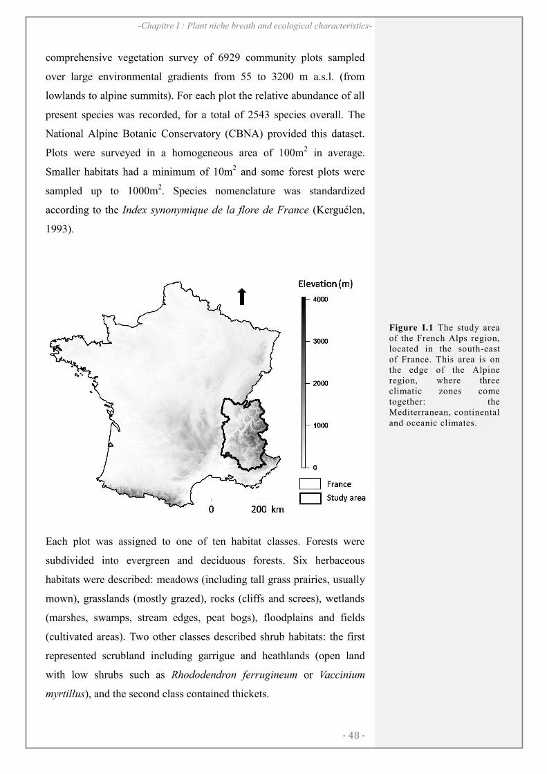
- 48 -

-Chapitre I : Plant niche breath and ecological characteristics-

comprehensive vegetation survey of 6929 community plots sampled

over large environmental gradients from 55 to 3200 m a.s.l. (from

lowlands to alpine summits). For each plot the relative abundance of all

present species was recorded, for a total of 2543 species overall. The

National Alpine Botanic Conservatory (CBNA) provided this dataset.

Plots were surveyed in a homogeneous area of 100m2 in average.

Smaller habitats had a minimum of 10m2 and some forest plots were

sampled up to 1000m2. Species nomenclature was standardized

according to the Index synonymique de la flore de France (Kerguélen,

1993).

Each plot was assigned to one of ten habitat classes. Forests were

subdivided into evergreen and deciduous forests. Six herbaceous

habitats were described: meadows (including tall grass prairies, usually

mown), grasslands (mostly grazed), rocks (cliffs and screes), wetlands

(marshes, swamps, stream edges, peat bogs), floodplains and fields

(cultivated areas). Two other classes described shrub habitats: the first

represented scrubland including garrigue and heathlands (open land

with low shrubs such as Rhododendron ferrugineum or Vaccinium

myrtillus), and the second class contained thickets.

Figure I.1 The study area of the French Alps region, located in the south-east of France. This area is on the edge of the Alpine region, where three climatic zones come together: the Mediterranean, continental and oceanic climates.

- 49 -

-Chapitre I : Plant niche breath and ecological characteristics-

Studied species were assigned to different Grime ecological strategies

(sensu Grime, 1974) for 891 species (competitor, ruderal, stress-

tolerator or mixed), life span for 864 species (annual/biennial, perennial

herbs, perennial woody species) and life forms for all species

(Raunkiaer’s classification, Raunkiaer, 1934). This was done using the

field observations of botanists from the Alpine Botanical Conservatory

and two available databases: LEDA (Knevel et al., 2003) and BiolFlor

(Kühn et al., 2004).

Methods

In order to estimate plant specialization, we used the co-occurrence

index „theta’ proposed by Fridley et al. (2007). The overall method

relies on the assumption that the species found in many different

habitats (i.e. generalists) have a relatively high rate of species turnover

across the plots in which they occur. Reciprocally, specialist species,

regardless of their frequency in the data set, should have a low species

turnover in their plots because they consistently occur within the same

set of species (Fridley et al., 2007). The general idea is very similar to

indirect species ordination such as (detrended) correspondence analysis

(DCA; ter Braak, 1987). However, this recently developed method

makes it possible to include a re-sampling procedure that accounts for

differences in species frequencies in the dataset and makes it possible to

select the appropriate underlying distance and turnover (beta) diversity

metrics. This last point seems crucial given the recent literature on beta

diversity estimation (de Bello et al., 2010a; Tuomisto, 2010a,b;

Anderson et al., 2011). To ensure the method is comprehensive, we

provided a comparison of species niche breadth estimates using the

theta index (Fridley et al., 2007), an indirect gradient ordination, DCA

(ter Braak, 1988) and a direct gradient ordination, outlying mean index

(OMI) (see Table S1 in Appendix S1 in the Supporting Information).

The overall frequency of a species in the sampled plots results from

both the vegetation survey sampling strategy and the species’ niche

specialization. Following the framework proposed by Fridley et al.

(2007), we removed the effects of the sampling design in the dataset by

- 50 -

-Chapitre I : Plant niche breath and ecological characteristics-

applying a randomization procedure. We randomly chose a fixed

number of plots containing the focal species before calculating the

turnover among these plots, thereby keeping the plot frequency constant

between species. For each species we applied the randomization 100

times. Theta is the resulting average turnover. We also calculated the

standard deviation of turnover from these 100 repetitions.

The number of selected plots for each randomization had to be

determined arbitrarily, based on the number of species present in the

vegetation database but also on the minimum number for species

occurrence. Setting the threshold too high (e.g. > 40 plots) removed too

many species with few occurrences, whereas setting the threshold too

low affected the relevance of the measure. We selected a threshold of 10

plots after having checked that the results were consistent for 5, 10 and

15 plots (see Table S2 in Appendix S1). Furthermore, we decided to

only calculate theta for species occurring in more than 20 plots in order

to be able to resample the plots for all the species analysed. Species

occurring in fewer than 20 plots were, however, kept in the community

data to compute the theta value for all other species. The specialization

index was thus computed for 1216 plant species.

The most critical point of this approach is the estimation of the species

turnover among the sampled plots. Fridley et al. (2007) originally

proposed using the additive beta measure [く = け – た(g)], where け is the

total number of species in the 10 sampled plots and た(g) is the mean

species richness of these 10 plots. This choice was recently criticized on

the grounds that this beta measure „is dependent on the size of species

pool at the position of species optima’ (Manthey & Fridley, 2009;

Zelen´y, 2009). Another set of possible measurements was then

proposed including the Jaccard index, two other indices based on

Simpson or Sørensen for multiple sites (Baselga et al., 2007) and one

based on R.H. Whittaker's decomposition. Based on the

recommendations, we could still use several indices according to what

we aim to measure. In the recent literature, several authors attempted to

gather all these beta diversity indices into a more comprehensive

framework in order to guide ecologists in their choices (Jost, 2006,

- 51 -

-Chapitre I : Plant niche breath and ecological characteristics-

2007; de Bello et al., 2010a; Tuomisto, 2010a,b; Anderson et al., 2011).

In light of all these discussions, we chose an index that estimates the

proportional species turnover between plots and that generalizes the

methodological framework, allowing the inclusion of species

abundances and functional or phylogenetic dissimilarities between

species if available. This index is based on Rao’s quadratic entropy

formula (Rao, 1982):

S

i

S

j

jiij ppdQ1 1

(1)

where S is species richness, ijd is the dissimilarity between each pair of

species i and j (equal to 1 when ji or 0 else) and ip , jp , the relative

abundance of species i and j in each sample. When ijd is composed of 0

and 1 as in our case, Rao’s quadratic entropy is equal to the Gini-

Simpson diversity index and is related to the true diversity D (Jost,

2007; Tuomisto, 2010a) and the Jost's „number equivalents’ (Jost, 2007;

de Bello et al., 2010a):

(a)

Q

D 1

1, (b)

Q

D 1

1and (c)

Q

D 1

1 (2)

The true く diversity component D is „the number of communities that

have no diversity overlap’ in de Bello et al. (2010a, p. 995)

and Q represent „the proportion of diversity accounted for by the

differentiation between communities’ (de Bello et al. 2010a, p. 996). In

Tuomisto (2010a, p.12) Q corresponds to the „proportional effective

species turnover’ (with an order of diversity 2q ). The turnover

formula is thus:

Q

QQ

D

DDQ

1

(3)

where Q is the mean quadratic entropy of the selected plots, and Q is

the quadratic entropy including all species from the selected plots. To

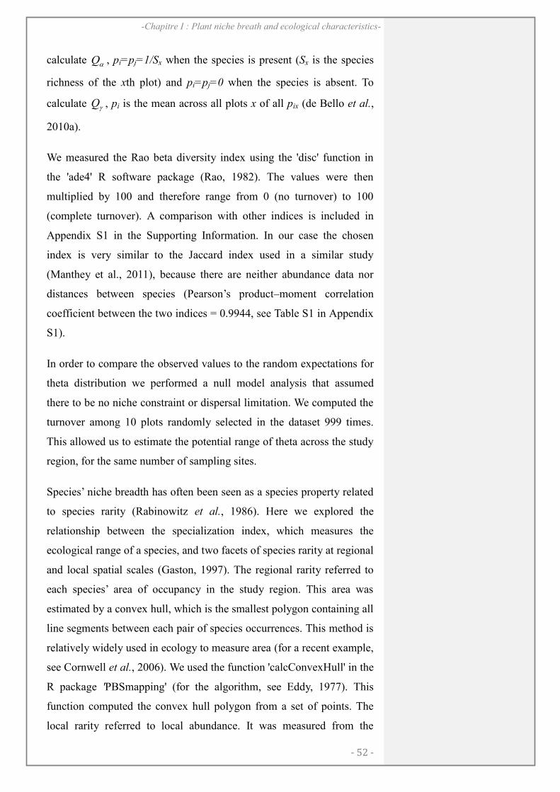
- 52 -

-Chapitre I : Plant niche breath and ecological characteristics-

calculate Q , pi=pj=1/Sx when the species is present (Sx is the species

richness of the xth plot) and pi=pj=0 when the species is absent. To

calculate Q , pi is the mean across all plots x of all pix (de Bello et al.,

2010a).

We measured the Rao beta diversity index using the 'disc' function in

the 'ade4' R software package (Rao, 1982). The values were then

multiplied by 100 and therefore range from 0 (no turnover) to 100

(complete turnover). A comparison with other indices is included in

Appendix S1 in the Supporting Information. In our case the chosen

index is very similar to the Jaccard index used in a similar study

(Manthey et al., 2011), because there are neither abundance data nor

distances between species (Pearson’s product–moment correlation

coefficient between the two indices = 0.9944, see Table S1 in Appendix

S1).

In order to compare the observed values to the random expectations for

theta distribution we performed a null model analysis that assumed

there to be no niche constraint or dispersal limitation. We computed the

turnover among 10 plots randomly selected in the dataset 999 times.

This allowed us to estimate the potential range of theta across the study

region, for the same number of sampling sites.

Species’ niche breadth has often been seen as a species property related

to species rarity (Rabinowitz et al., 1986). Here we explored the

relationship between the specialization index, which measures the

ecological range of a species, and two facets of species rarity at regional

and local spatial scales (Gaston, 1997). The regional rarity referred to

each species’ area of occupancy in the study region. This area was

estimated by a convex hull, which is the smallest polygon containing all

line segments between each pair of species occurrences. This method is

relatively widely used in ecology to measure area (for a recent example,

see Cornwell et al., 2006). We used the function 'calcConvexHull' in the

R package 'PBSmapping' (for the algorithm, see Eddy, 1977). This

function computed the convex hull polygon from a set of points. The

local rarity referred to local abundance. It was measured from the

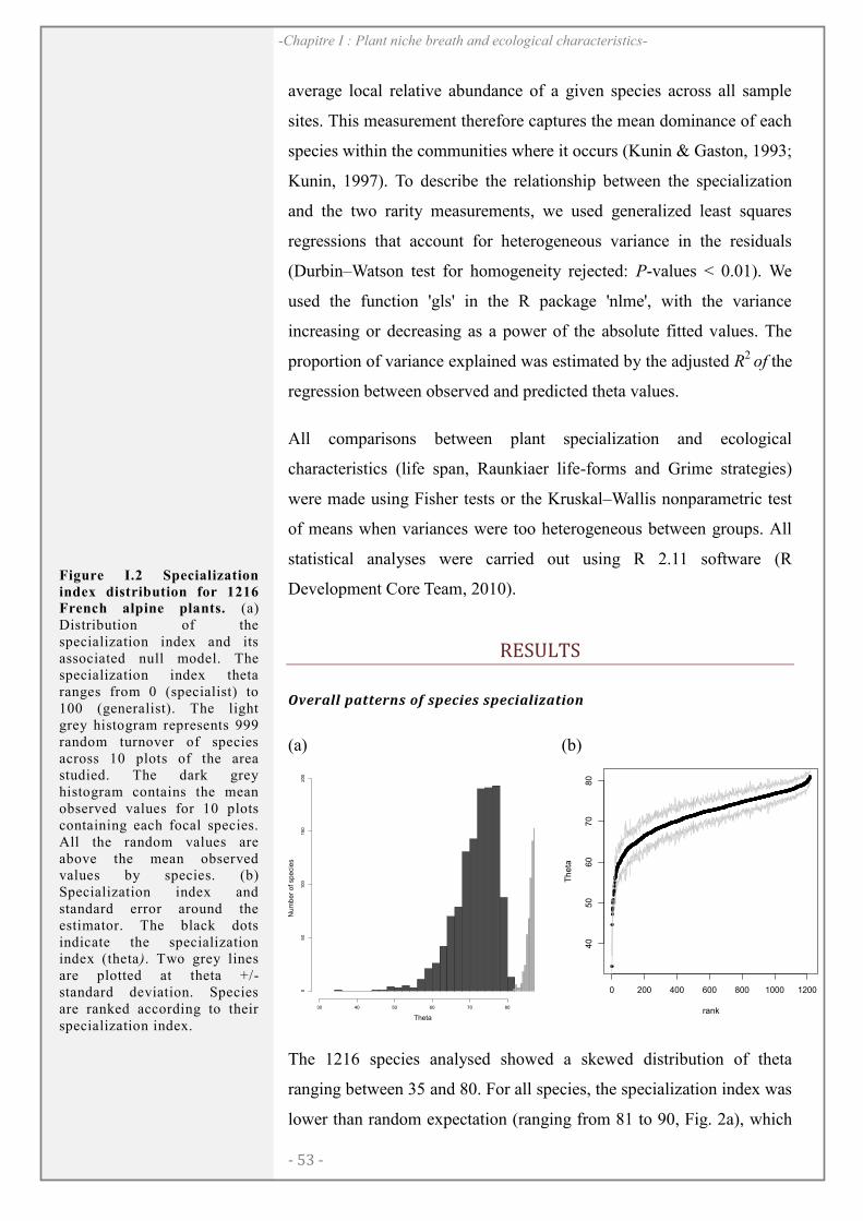
- 53 -

-Chapitre I : Plant niche breath and ecological characteristics-

average local relative abundance of a given species across all sample

sites. This measurement therefore captures the mean dominance of each

species within the communities where it occurs (Kunin & Gaston, 1993;

Kunin, 1997). To describe the relationship between the specialization

and the two rarity measurements, we used generalized least squares

regressions that account for heterogeneous variance in the residuals

(Durbin–Watson test for homogeneity rejected: P-values < 0.01). We

used the function 'gls' in the R package 'nlme', with the variance

increasing or decreasing as a power of the absolute fitted values. The

proportion of variance explained was estimated by the adjusted R2 of the

regression between observed and predicted theta values.

All comparisons between plant specialization and ecological

characteristics (life span, Raunkiaer life-forms and Grime strategies)

were made using Fisher tests or the Kruskal–Wallis nonparametric test

of means when variances were too heterogeneous between groups. All

statistical analyses were carried out using R 2.11 software (R

Development Core Team, 2010).

RESULTS

Overall patterns of species specialization

(a) (b)

Theta

Nu

mb

er

of spe

cie

s

30 40 50 60 70 80

05

0100

15

02

00

0 200 400 600 800 1000 1200

40

50

60

70

80

rank

Th

eta

The 1216 species analysed showed a skewed distribution of theta

ranging between 35 and 80. For all species, the specialization index was

lower than random expectation (ranging from 81 to 90, Fig. 2a), which

Figure I.2 Specialization

index distribution for 1216 French alpine plants. (a) Distribution of the specialization index and its associated null model. The specialization index theta ranges from 0 (specialist) to 100 (generalist). The light grey histogram represents 999 random turnover of species across 10 plots of the area studied. The dark grey histogram contains the mean observed values for 10 plots containing each focal species. All the random values are above the mean observed values by species. (b) Specialization index and standard error around the estimator. The black dots indicate the specialization index (theta). Two grey lines are plotted at theta +/- standard deviation. Species are ranked according to their specialization index.

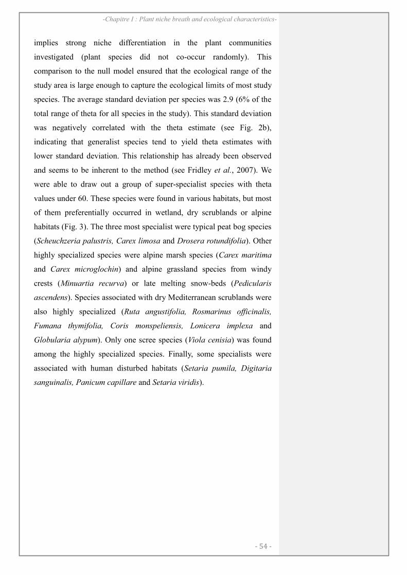
- 54 -

-Chapitre I : Plant niche breath and ecological characteristics-

implies strong niche differentiation in the plant communities

investigated (plant species did not co-occur randomly). This

comparison to the null model ensured that the ecological range of the

study area is large enough to capture the ecological limits of most study

species. The average standard deviation per species was 2.9 (6% of the

total range of theta for all species in the study). This standard deviation

was negatively correlated with the theta estimate (see Fig. 2b),

indicating that generalist species tend to yield theta estimates with

lower standard deviation. This relationship has already been observed

and seems to be inherent to the method (see Fridley et al., 2007). We

were able to draw out a group of super-specialist species with theta

values under 60. These species were found in various habitats, but most

of them preferentially occurred in wetland, dry scrublands or alpine

habitats (Fig. 3). The three most specialist were typical peat bog species

(Scheuchzeria palustris, Carex limosa and Drosera rotundifolia). Other

highly specialized species were alpine marsh species (Carex maritima

and Carex microglochin) and alpine grassland species from windy

crests (Minuartia recurva) or late melting snow-beds (Pedicularis

ascendens). Species associated with dry Mediterranean scrublands were

also highly specialized (Ruta angustifolia, Rosmarinus officinalis,

Fumana thymifolia, Coris monspeliensis, Lonicera implexa and

Globularia alypum). Only one scree species (Viola cenisia) was found

among the highly specialized species. Finally, some specialists were

associated with human disturbed habitats (Setaria pumila, Digitaria

sanguinalis, Panicum capillare and Setaria viridis).

- 55 -

-Chapitre I : Plant niche breath and ecological characteristics-

Scru

bla

nd

Wetlan

d

Flo

odp

lain

Eve

rgre

en

fore

st

Decid

uou

s f

ore

st

Mead

ow

Tic

kets

Rocks

Fie

ld

Gra

ssla

nd

40

50

60

70

80

Favourite habitat

Th

eta

Specialization and rarity

(a) (b)

0 10000 20000 30000 40000 50000

30

40

50

60

70

80

Th

eta

Species range(km2)

30

40

50

60

70

80

0.1 0.25 0.5 1 2.5 5 10 25 50

Th

eta

Mean local abundance (%)

The specialization index was correlated with our two rarity measures.

The comparison between specialization and species geographical ranges

showed a positive trend, indicating that generalist species are usually

widespread species whilst specialist species tend to be geographically

restricted (Fig. 4a). The generalized least squares regression slope was

significantly different from zero (P-value < 0.001) and the variance

explained was meaningful (adjusted R2 = 30.3%). However, some

generalist species were detected even among species with narrow

Figure I.3 Specialization

index among 1216 French alpine plants grouped according to their favourite habitats. Box plots show extremes values and quartiles. The horizontal line indicates the median theta for all species. The black dots represent the most specialized species. Widths are proportional to the square root of the number of species in each class. If the notches for two plots do not overlap then the medians are significantly different at = 0.05. The theta index ranges from 0 (specialist) to 100 (generalist). The means for each group are significantly different (Kruskal–Wallis rank sum test: P-value < 2.2 × 10-16).

Figure I.4 Specialization index of 1216 French alpine plants as a function of two different measures of rarity. Box plots along each axis show extreme values and quartiles. The middle line indicates the median value for all species. (a) Specialization as a function of the regional area of occupancy (km2). The solid lines indicate the generalized least squares regression fit. The slope is significantly different from zero (P-value < 2 × 10–16). Adjusted R

2 = 30.3%. (b) Specialization as a function of the logarithm of the mean relative abundance in the community plots where the species occurs. The solid lines indicate the generalized least squares regression fit. The x-axis is log-scaled. The slope is significantly different from zero (P-value < 2.2 × 10 -16). Adjusted R2 = 4.5%.

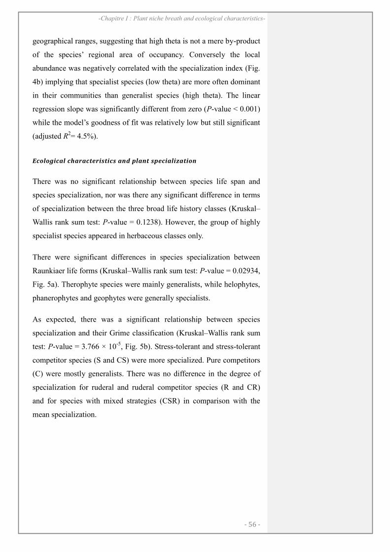
- 56 -

-Chapitre I : Plant niche breath and ecological characteristics-

geographical ranges, suggesting that high theta is not a mere by-product

of the species’ regional area of occupancy. Conversely the local

abundance was negatively correlated with the specialization index (Fig.

4b) implying that specialist species (low theta) are more often dominant

in their communities than generalist species (high theta). The linear

regression slope was significantly different from zero (P-value < 0.001)

while the model’s goodness of fit was relatively low but still significant

(adjusted R2= 4.5%).

Ecological characteristics and plant specialization

There was no significant relationship between species life span and

species specialization, nor was there any significant difference in terms

of specialization between the three broad life history classes (Kruskal–

Wallis rank sum test: P-value = 0.1238). However, the group of highly

specialist species appeared in herbaceous classes only.

There were significant differences in species specialization between

Raunkiaer life forms (Kruskal–Wallis rank sum test: P-value = 0.02934,

Fig. 5a). Therophyte species were mainly generalists, while helophytes,

phanerophytes and geophytes were generally specialists.

As expected, there was a significant relationship between species

specialization and their Grime classification (Kruskal–Wallis rank sum

test: P-value = 3.766 × 10-5, Fig. 5b). Stress-tolerant and stress-tolerant

competitor species (S and CS) were more specialized. Pure competitors

(C) were mostly generalists. There was no difference in the degree of

specialization for ruderal and ruderal competitor species (R and CR)

and for species with mixed strategies (CSR) in comparison with the

mean specialization.

- 57 -

-Chapitre I : Plant niche breath and ecological characteristics-

(a) (b)

HEL GE PH CH HE TH

30

40

50

60

70

80

Raunkiaer's life forms

Th

eta

S CS R CSR CR C SR

30

40

50

60

70

80

Grime's stategies

Th

eta

DISCUSSION

In this paper we aimed to use an extensive vegetation survey across the

French Alps region, that encompasses a wide elevational gradient, to

investigate the overall pattern of plant specialization. With regard to our

first objective, we have indeed shown that specialized species tend to be

found in specific habitats located on the edges of environmental

gradients, namely xeric Mediterranean scrublands, wetlands, or alpine

grasslands. We have also demonstrated that specialist species appear to

be over-represented in the hydrophyte and geophyte life form classes,

and are mainly associated with Grime’s stress-tolerant strategy. Our

analysis shows that habitat specialization positively correlates with a

species’ area of occupancy, and to a lesser extent inversely correlates

with the species’ local dominance.

An integrated index of specialization

The unbiased measurement of species specialization in a large species

sample has always seemed problematic. The approach we use was

shown by Fridley et al. (2007) to be unbiased with respect to the

number of occurrences for each species (Fridley et al., 2007). The same

applies to our study, where the correlation between the specialization

index and the frequency of occurrence is weak (adjusted R2 = 4.6%, see

Appendix S2) whilst the variance of this frequency of occurrence within

the dataset increases with increasing species’ theta, which means that

Figure I.5 Specialization

index among 1216 French alpine plants grouped according to their traits. Box plots show extreme values and quartiles. The horizontal line indicates the median theta for all species. The black dots represent the most specialist species. Widths are proportional to the square root of number of species in each class. If the notches for two plots do not overlap then the medians are significantly different at = 0.05. Theta index ranges from 0 (specialist) to 100 (generalist). (a) Specialization index among Raunkiaer’s life forms. CH=chamaephytes; GE=geophytes; HE=hemicryptophytes; HEL=helophytes; PH=phanerophytes; TH=therophytes. The means for each group are significantly different (Kruskal–Wallis rank sum test: P-value = 0.02934). (b) Specialization index among Grime’s strategies, for herbaceous species only. S = stress-tolerator, C = competitor, R = ruderal. The means for each group are significantly different (Kruskal–Wallis rank sum test: P-value = 3.766 × 10 -5).

- 58 -

-Chapitre I : Plant niche breath and ecological characteristics-

there are no specialist species with a high number of occurrences in the

dataset (Appendix S2).

More generally, the use of an integrated index of specialization is

appealing as it is intended to include numerous species niche axes, as

well as factors that may explain species coexistence on the local

community scale. Fridley's theta framework is particularly interesting

because of the re-sampling procedure that accounts for differences in

species frequencies. Another advantage of this framework is that it is

more flexible on the underlying distance measurements, for instance

when compared to an indirect gradient analysis such as DCA. Although

both approaches produce highly correlated results (Pearson correlation

with theta = 0.7, see, Table S1 in Appendix S1), the DCA is based on a

chi-square distance, which is not entirely comparable to turnover as

measured by Rao, multiple Simpson or Jaccard indices.

A species-based niche breadth estimate is particularly useful in

detecting local environmental effects, or niches axes that are only

relevant for some species. For large-scale datasets, other methods based

on species distributions and environmental data cannot include the local

environment because this information is not usually documented in

vegetation databases and it cannot be inferred from large-scale

environmental data. Although high-resolution climatic data and land

cover variables are increasingly available (Hijmans et al., 2005), they

are usually interpolated or modelled data with uncertainties inherent in

the process and are therefore unable to capture local information or

even landscape heterogeneity. We show that using a direct ordination

method (outlying mean index, OMI) with six topographic and climatic

variables results in a similar species ordination (Pearson’s correlation

with theta = 0.45, see Tables S1 and S2 in Appendix S1). This result is

not entirely surprising because we preselected six variables that explain

most of the environmental variation across the entire study area but

probably fail to describe the local environmental conditions that explain

species co-existence and species-specific requirements. By using

species as indirect indicators of the environment we are able to take

local conditions into account. With the same approach, Manthey et al.

- 59 -

-Chapitre I : Plant niche breath and ecological characteristics-

(2011) suggest that some micro-environmental factors that are usually

not taken into account may have led to overestimating the effect of

competition between species. We also reveal the importance of the local

environmental conditions defined by the vegetation structure. For

instance, Juncus subnodulosus makes dense tussocks that may exclude

other species in the community, creating a very specific habitat. Another

example of the effect of vegetation structure is the impact of forest trees

on the herbaceous plant undergrowth. In dark forests such as beech–fir

(Fagus–Abies) forests we found a large proportion of specialist species,

which could be explained by the effects of trees on herbaceous species

(e.g. limiting light availability, retaining soil moisture). Furthermore,

the canopy, which provides various resource-related stress levels, is

known to change competitive relationships between species (Maestre et

al., 2009).

Which species are more likely to be specialized?

Theoretically, specialist species are confined to a small part of the

ecological space where they can locally outcompete species belonging

to the competitor strategy class, which are less adapted to a specific

habitat (Wisheu, 1998). Our findings corroborate this hypothesis, as

most specialist species are preferentially dominant in the communities

where they occur (Fig. 4b). Specialist species are indeed mainly located

in stressful habitats and co-occur with the few other species adapted to

the extreme local conditions. Consequently, they tend to have high

relative abundance. On the other hand, generalist species may be found

in very rich communities where competition is intense, leading to high

species evenness.

There is a positive correlation between the specialization index theta

and the geographical range (P-value < 2.2 × 10-16, R2 = 30.3%). We did

however observe that generalist species are not necessarily widespread

because variance in the geographical range increases with increasing

species' theta. This pattern could be explained by a high level of

environmental heterogeneity across the region and the landscape

mosaics, implying species experience a wide range of environmental

- 60 -

-Chapitre I : Plant niche breath and ecological characteristics-

conditions over a restricted territory. Although species spreading across

20,000 square kilometres with a fairly low theta value have been

observed, the more specialist the species are, the smaller their

geographic range. This is certainly due to the main climatic gradients

that are spatially auto-correlated (e.g. temperature). In this context,

specialist species are more likely to be restricted to a small area due to

their narrow tolerance of environmental conditions. However, some

specific wetland specialized species, for instance, should be less

sensitive to these gradients, implying relative independence between the

geographical range and the ecological range. The observed spatial

restriction of specialist species may relate to the effect of distance

decay. As the species niche breadth is estimated from species co-

occurrence, a wetland species may have high theta if it occurs in two

distant sites that differ in species composition due to historical legacies

and dispersal limitation.

In order to test whether some specialist species are hidden among

generalists, we measured the number of distinct habitats used for every

species, a commonly used measurement of niche breadth (Devictor et

al., 2010), and related it to theta. Although the habitats have been

roughly defined, the two measures are consistent (Appendix S3,

Kruskal–Wallis rank sum test: P-value < 2.2 × 10-16). In particular,

species occurring in only one type of habitat have the lowest theta

values. We therefore consider that theta is a satisfactory surrogate for

estimating plant specialization for numerous species occurring in a wide

range of habitats.

These two results challenge the established macroecological rule which

stipulates that regional distribution and local abundance are positively

related (Gaston & Lawton, 1990), by showing that this relationship does

not hold (and indeed tends to be inversed) for specialist species (Fig. 4),

which are located in habitats that turn out to be peculiar on the regional

scale. However, it is difficult to generalize such patterns because they

are sensitive to the study scale and to the measures of regional and local

abundances that are used.

- 61 -

-Chapitre I : Plant niche breath and ecological characteristics-

Longevity attributes do not distinguish generalists from specialists.

Nevertheless, specialist species are not randomly distributed across life-

form classes. Therophytes are over-represented amongst generalist

species, which may be explained by the fact that they are opportunistic

and pioneering annual plants capable of colonizing bare ground after a

disturbance, which could occur in very different habitats. However,

some of these species may occur in very specific habitats with sandy or

acid soils. Conversely, helophytes are disproportionately represented

amongst specialist species, which may be due to the particular

adaptations required by wetland habitats. The geophytes class also

contains numerous specialist species, which could be explained by the

fact that they invest resources in bulbs or rootstock, which allows them

to resist dryness or grazing (Hadar et al., 1999; Jutila, 1999; Noy-Meir

& Oron, 2001). This resistance mechanism implies a trade-off that

limits the potential of species to adapt to a large range of habitats.

The comparison of the specialization index to Grime’s strategies

corresponded to expected trends. Pure competitors are overrepresented

among generalists whereas species classified as stress-tolerant tend to

be specialists. Once again this may be viewed as an empirical validation

of the tolerance–dominance trade-off (Wisheu, 1998). Species that are

generally weak competitors may have found refuge and adapt at the

extreme end of environmental gradients, where generalist species may

fail to become dominant. On the other hand, competitive lotteries may

allow pure competitors to become locally dominant over a wider range

of habitats within the limits of their physiological tolerances, thus

making them appear to be more generalist species.

Conclusions

In this paper we estimate niche specialization for a large number of

plant species using an approach that makes it possible to account

indirectly account for various factors that either explain species

coexistence on both regional and local community scale, or are only

relevant for some specific species. Our results are an empirical

validation of the tolerance–dominant trade-off, showing that specialist

- 62 -

-Chapitre I : Plant niche breath and ecological characteristics-

species are not strong competitors (sensu Grime’s strategies), and

generally find refuge on the stressful edges of environmental gradients,

in communities where they tend to dominate.

ACKNOWLEDGEMENTS

This research was conducted on the long-term research site Zone Atelier Alpes (ZAA), a member of the European Long-Term Ecosystem Research Network — LTER-Europe. This is ZAA publication no. 17. The authors received support from the Agence Nationale de la Recherche (ANR) DIVERSITALP (Forecasting the impacts of global changes on French Alpine Flora: distribution of specific, functional and phylogenetic diversities, simulations and conservation strategies, ANR- 07-BDIV-014) and the Sixth European Framework Program ECOCHANGE (Challenges in assessing and forecasting biodiversity and ecosystem changes in Europe, GOCE-CT-2007-036866). Insightful comments and suggestions from two anonymous referees also helped to improve the first draft. Most of the computations presented in this paper were performed using the CIMENT infrastructure (https://ciment.ujf-grenoble.fr), which is funded by the Rhône-Alpes region (GRANT CPER07 13 CIRA: http://www.ci-ra.org) and France-Grille (http://www.france-grilles.fr). This paper has been proofread by a language professional at Version Originale.

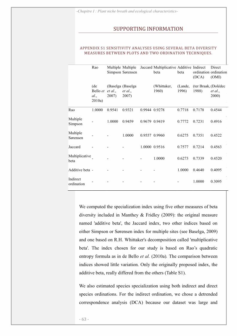
- 63 -

-Chapitre I : Plant niche breath and ecological characteristics-

SUPPORTING INFORMATION

APPENDIX S1 SENSITIVITY ANALYSES USING SEVERAL BETA DIVERSITY MEASURES BETWEEN PLOTS AND TWO ORDINATION TECHNIQUES.

We computed the specialization index using five other measures of beta

diversity included in Manthey & Fridley (2009): the original measure

named 'additive beta', the Jaccard index, two other indices based on

either Simpson or Sørensen index for multiple sites (see Baselga, 2009)

and one based on R.H. Whittaker's decomposition called 'multiplicative

beta'. The index chosen for our study is based on Rao’s quadratic

entropy formula as in de Bello et al. (2010a). The comparison between

indices showed little variation. Only the originally proposed index, the

additive beta, really differed from the others (Table S1).

We also estimated species specialization using both indirect and direct

species ordinations. For the indirect ordination, we chose a detrended

correspondence analysis (DCA) because our dataset was large and

Rao Multiple

Simpson Multiple Sørensen

Jaccard Multiplicative beta

Additive beta

Indirect ordination (DCA)

Direct ordination (OMI)

(de Bello et

al., 2010a)

(Baselga et al., 2007)

(Baselga et al., 2007)

(Whittaker, 1960)

(Lande, 1996)

(ter Braak, 1988)

(Dolédec et al., 2000)

Rao 1.0000 0.9541 0.9321 0.9944 0.9278 0.7718 0.7178 0.4544

Multiple Simpson

- 1.0000 0.9459 0.9679 0.9419 0.7772 0.7231 0.4916

Multiple Sørensen

- - 1.0000 0.9557 0.9960 0.6275 0.7351 0.4522

Jaccard - - - 1.0000 0.9516 0.7577 0.7214 0.4563

Multiplicative beta

- - - - 1.0000 0.6273 0.7339 0.4520

Additive beta - - - - - 1.0000 0.4640 0.4095

Indirect ordination

- - - - - - 1.0000 0.3095

–

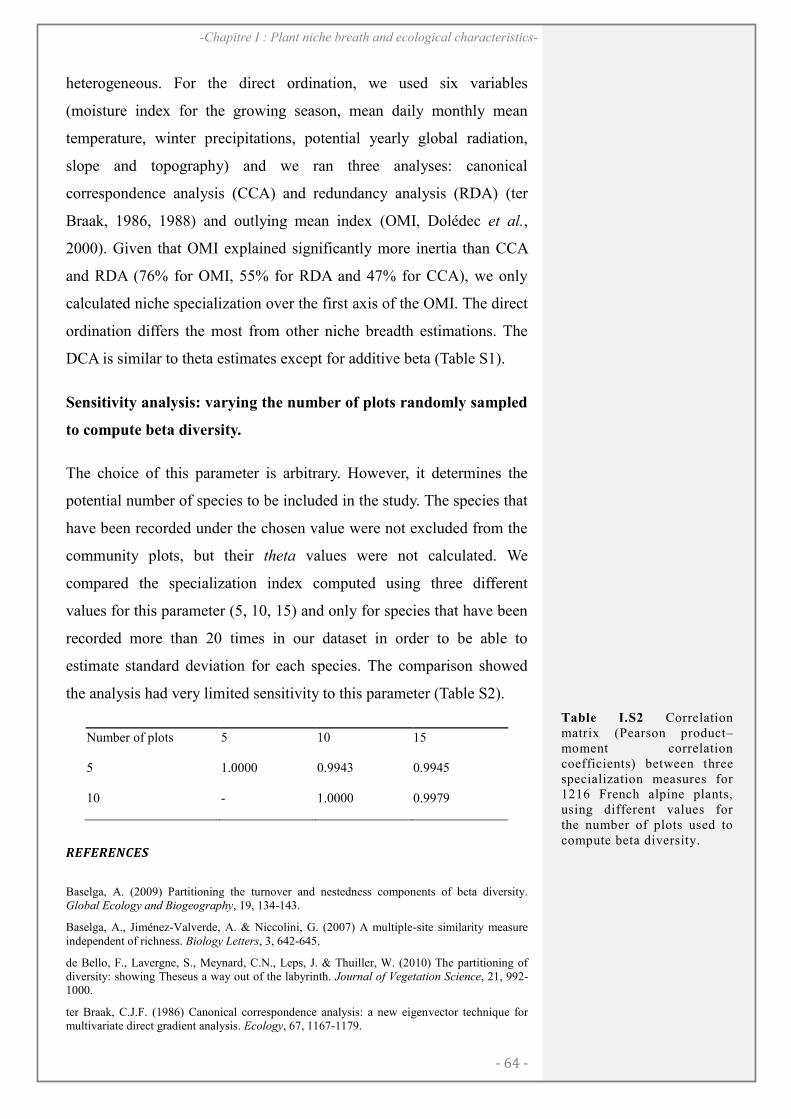
- 64 -

-Chapitre I : Plant niche breath and ecological characteristics-

heterogeneous. For the direct ordination, we used six variables

(moisture index for the growing season, mean daily monthly mean

temperature, winter precipitations, potential yearly global radiation,

slope and topography) and we ran three analyses: canonical

correspondence analysis (CCA) and redundancy analysis (RDA) (ter

Braak, 1986, 1988) and outlying mean index (OMI, Dolédec et al.,

2000). Given that OMI explained significantly more inertia than CCA

and RDA (76% for OMI, 55% for RDA and 47% for CCA), we only

calculated niche specialization over the first axis of the OMI. The direct

ordination differs the most from other niche breadth estimations. The

DCA is similar to theta estimates except for additive beta (Table S1).

Sensitivity analysis: varying the number of plots randomly sampled

to compute beta diversity.

The choice of this parameter is arbitrary. However, it determines the

potential number of species to be included in the study. The species that

have been recorded under the chosen value were not excluded from the

community plots, but their theta values were not calculated. We

compared the specialization index computed using three different

values for this parameter (5, 10, 15) and only for species that have been

recorded more than 20 times in our dataset in order to be able to

estimate standard deviation for each species. The comparison showed

the analysis had very limited sensitivity to this parameter (Table S2).

Number of plots 5 10 15

5 1.0000 0.9943 0.9945

10 - 1.0000 0.9979

REFERENCES

Baselga, A. (2009) Partitioning the turnover and nestedness components of beta diversity. Global Ecology and Biogeography, 19, 134-143.

Baselga, A., Jiménez-Valverde, A. & Niccolini, G. (2007) A multiple-site similarity measure independent of richness. Biology Letters, 3, 642-645.

de Bello, F., Lavergne, S., Meynard, C.N., Leps, J. & Thuiller, W. (2010) The partitioning of diversity: showing Theseus a way out of the labyrinth. Journal of Vegetation Science, 21, 992-1000.

ter Braak, C.J.F. (1986) Canonical correspondence analysis: a new eigenvector technique for multivariate direct gradient analysis. Ecology, 67, 1167-1179.

Table I.S2 Correlation matrix (Pearson product–moment correlation coefficients) between three specialization measures for 1216 French alpine plants, using different values for the number of plots used to compute beta diversity.

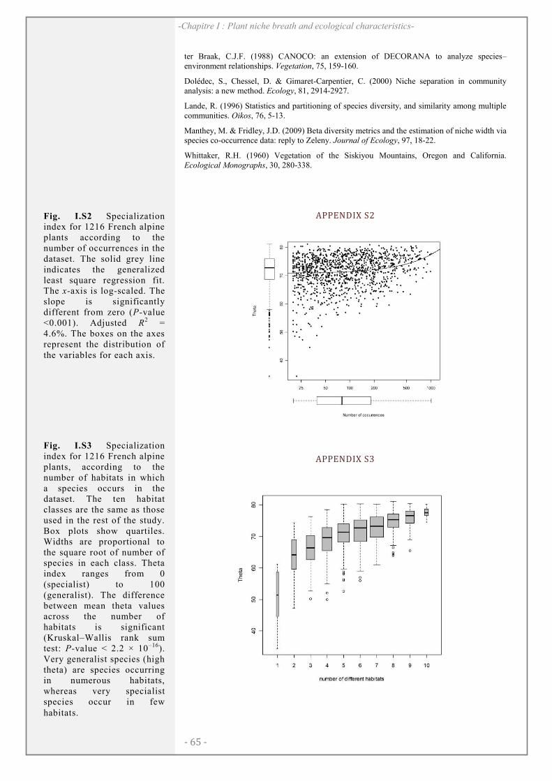
- 65 -

-Chapitre I : Plant niche breath and ecological characteristics-

ter Braak, C.J.F. (1988) CANOCO: an extension of DECORANA to analyze species–environment relationships. Vegetation, 75, 159-160.

Dolédec, S., Chessel, D. & Gimaret-Carpentier, C. (2000) Niche separation in community analysis: a new method. Ecology, 81, 2914-2927.

Lande, R. (1996) Statistics and partitioning of species diversity, and similarity among multiple communities. Oikos, 76, 5-13.

Manthey, M. & Fridley, J.D. (2009) Beta diversity metrics and the estimation of niche width via species co-occurrence data: reply to Zeleny. Journal of Ecology, 97, 18-22.

Whittaker, R.H. (1960) Vegetation of the Siskiyou Mountains, Oregon and California. Ecological Monographs, 30, 280-338.

APPENDIX S2

APPENDIX S3

Fig. I.S2 Specialization index for 1216 French alpine plants according to the number of occurrences in the dataset. The solid grey line indicates the generalized least square regression fit. The x-axis is log-scaled. The slope is significantly different from zero (P-value <0.001). Adjusted R

2 = 4.6%. The boxes on the axes represent the distribution of the variables for each axis.

Fig. I.S3 Specialization index for 1216 French alpine plants, according to the number of habitats in which a species occurs in the dataset. The ten habitat classes are the same as those used in the rest of the study. Box plots show quartiles. Widths are proportional to the square root of number of species in each class. Theta index ranges from 0 (specialist) to 100 (generalist). The difference between mean theta values across the number of habitats is significant (Kruskal–Wallis rank sum test: P-value < 2.2 × 10–16). Very generalist species (high theta) are species occurring in numerous habitats, whereas very specialist species occur in few habitats.

- 66 -

-Chapitre I : Plant niche breath and ecological characteristics-

!

"#$"!

!

!

%&'()*+,!))-!

'%%./0*)01!2.+!3)4(,+4'5 !

'03!6).*)% ! )0*,+'%*).04 !

)0 !.+3,+!*. !3)4,0*'015,!

*&,!3+)7,+4 !.2 !4(,%),4 !

3)4*+)6/*).04 !'03!*&,)+ !

'6/03'0%,4 ! !

Boulangeat, I., Gravel, D. and Thuiller, W. (2012) Accounting for

dispersal and biotic interactions in order to disentangle the drivers of

species distributions and their abundances. Ecology Letters, 15, 584-593.

Statement of authorship: WT, DG and IB designed the study. IB

performed the analyses and led the writing. All the authors contributed

substantially to the writing.

Editor David Storch

!

#8!

-Chapitre II : The importance of dispersal and biotic interactions for species distributions-

'9:;<=>;!

Although abiotic factors, together with dispersal and biotic interactions,

are often suggested to explain the distribution of species and their

abundances, species distribution models usually focus on abiotic factors

only. We propose an integrative framework linking ecological theory,

empirical data and statistical models to understand the distribution of

species and their abundances together with the underlying community

assembly dynamics. We illustrate our approach with 21 plant species in

the French Alps. We show that a spatially nested modelling framework

significantly improves the model’s performance and that the spatial

variations of species presence-absence and abundances are

predominantly explained by different factors. We also show that

incorporating abiotic, dispersal and biotic factors into the same model

bring new insights to our understanding of community assembly. This

approach, at the crossroads between community ecology and

biogeography, is a promising avenue for a better understanding of species

co-existence and biodiversity distribution.

!

#?! !

-Chapitre II : The importance of dispersal and biotic interactions for species distributions-

)0*+.3/%*).0!

Understanding the factors driving the distribution of species and their

abundances is an important research area in ecology since it refers to

species coexistence and the maintenance of species diversity (Chesson

2000a). Soberon (2007) proposed a conceptual framework distinguishing

three main drivers. Abiotic constraints delimit the species’ fundamental

niche within which the species could establish and maintain itself given

its intrinsic physiological limits (Chase & Leibold 2003). Dispersal

limitations may then restrict a species’ range by preventing it from

reaching a suitable site. Dispersal limitation is inherently linked to the

species’ dispersal capability, but may also be influenced by historical

legacies (Vellend et al. 2007). Some species may reach high abundance

in unsuitable sites due to frequent immigration from neighbouring

suitable sites, as predicted by source-sink dynamics or mass effect

(Pulliam 2000). Finally, biotic interactions may modify either the

resources availability or the local abiotic environment with potentially

contrasting consequences on abundance (e.g. competition and

facilitation, Lortie et al. 2004). These three main drivers could interact

together and influence the observed spatial distribution of the

environmental conditions suitable for a given species (i.e. species’

realized niche).

These drivers of species distributions may act at different spatial scales

(Kneitel & Chase 2004). For instance, frequent consideration is given to

abiotic variables acting at large spatial scales (Davies et al. 2004).

Climate and soil variables have been shown to be the most relevant

variables when predicting continental to regional-scale plant species

presence-absence distributions (Thuiller et al. 2004b). Other factors, such

as land cover, are also important to understand species distribution at

regional scales (Randin et al. 2009b). On the other hand, biotic

interactions and consumer-resource dynamics are assumed to occur at

smaller spatial scales (Soberon 2007). Dispersal limitations are most

likely to occur at a larger extent than species dispersal distances, whereas

source-sink dynamics occur at the same scale as dispersal.

!

$@!

-Chapitre II : The importance of dispersal and biotic interactions for species distributions-

So far, species distribution has been modelled using species distribution

models (SDMs), which, most of the time, ignore the effects of dispersal

and biotic interactions (VanDerWal et al. 2009). Even if SDMs provide

satisfactory predictions for presence-absence, they typically fail to

explain and predict species’ abundances across sites (Pearce & Ferrier

2001; Sagarin et al. 2006). Here we argue that this failure is due to the

omission of the above-mentioned dynamic drivers (i.e. dispersal, biotic

interactions) and that all processes acting at different spatial scales are

fitted in a unique response model. The abundance of a given species is

obviously driven to some extent by the same processes as the presence-

absence, but additional processes might come into play to determine the

abundance when the species is present. They operate at finer resolutions

where community composition, population dynamics and the

microenvironment interact. For explaining and modelling species

abundances, the use of a spatially nested approach, which model

separately the processes underlying presence-absence and abundance

variation, seems therefore particularly relevant.

We propose to account explicitly for the spatial nestedness of processes

in a comprehensive modelling framework where the species undergoes

successive filters. The first filter, related to larger scale factors,

determines the presence or absence of the species. This filter is expected

to be primarily driven by abiotic variables (eco-physiological limitations)

and by dispersal when site accessibility is limited. Once a species is able

to reach a suitable site, the second filter, expected to be mainly

determined by local scale factors such as biotic interactions and dispersal

in case source-sink dynamics occur, will determine the local abundance

and other absences (Fig. II.1, Theoretical model). Our objective here is to

test these expectations using an operational statistical framework (Fig.

II.1, Model structure). Firstly, we introduce a set of key innovations to

account for biotic interactions, using co-occurrence based indices, and for

dispersal by proposing a measurement based on species dispersal

capabilities and observed spatial distributions. Secondly, in order to

separate presence-absence from abundance underlying processes, we

propose a two-step modelling approach: (1) modelling species presence

!

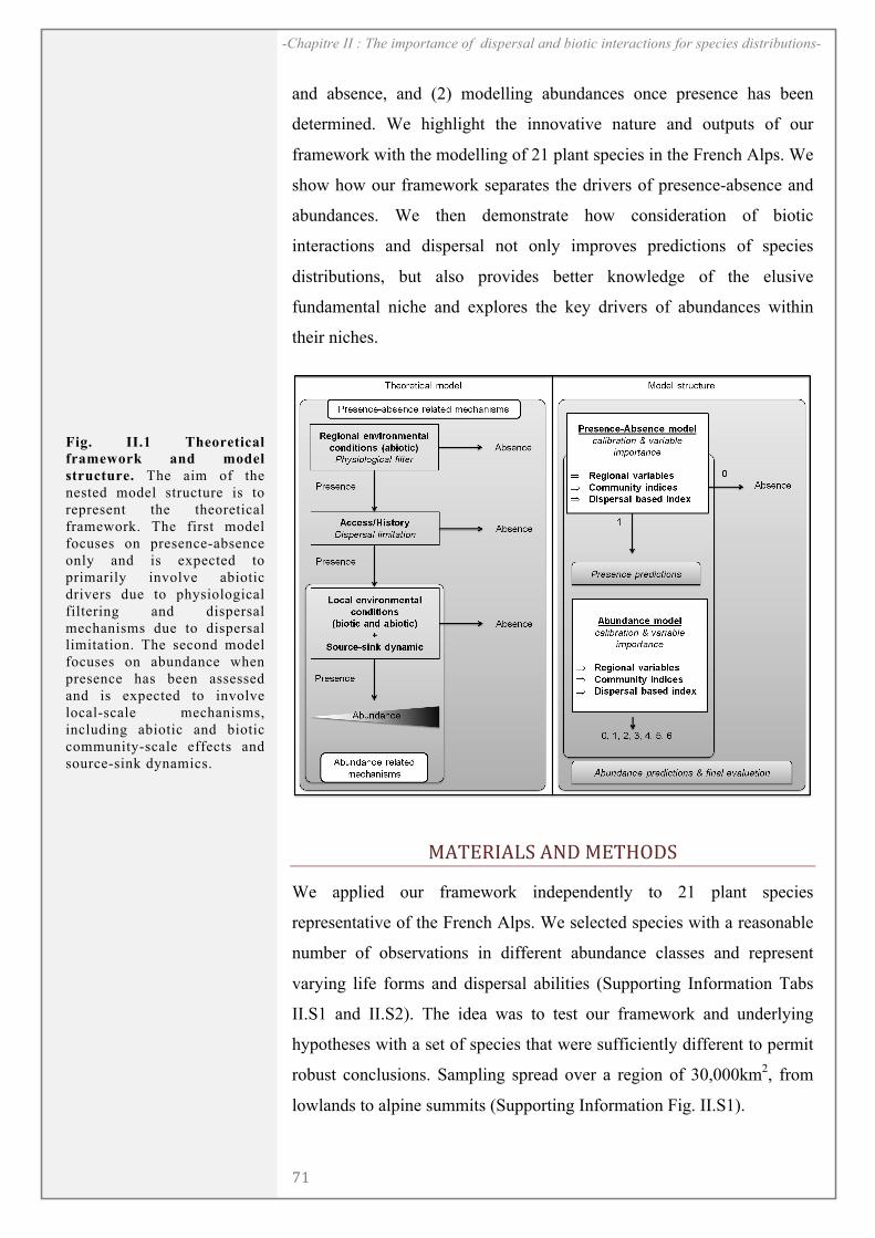
$A! !

-Chapitre II : The importance of dispersal and biotic interactions for species distributions-

and absence, and (2) modelling abundances once presence has been

determined. We highlight the innovative nature and outputs of our

framework with the modelling of 21 plant species in the French Alps. We

show how our framework separates the drivers of presence-absence and

abundances. We then demonstrate how consideration of biotic

interactions and dispersal not only improves predictions of species

distributions, but also provides better knowledge of the elusive

fundamental niche and explores the key drivers of abundances within

their niches.

B'*,+)'54!'03!B,*&.34!

We applied our framework independently to 21 plant species

representative of the French Alps. We selected species with a reasonable

number of observations in different abundance classes and represent

varying life forms and dispersal abilities (Supporting Information Tabs

II.S1 and II.S2). The idea was to test our framework and underlying

hypotheses with a set of species that were sufficiently different to permit

robust conclusions. Sampling spread over a region of 30,000km2, from

lowlands to alpine summits (Supporting Information Fig. II.S1).

Fig. II.1 Theoretical

framework and model

structure. The aim of the

nested model structure is to

represent the theoretical

framework. The first model

focuses on presence-absence

only and is expected to

primarily involve abiotic

drivers due to physiological

filtering and dispersal

mechanisms due to dispersal

limitation. The second model

focuses on abundance when

presence has been assessed

and is expected to involve

local-scale mechanisms,

including abiotic and biotic

community-scale effects and

source-sink dynamics.

!

$C!

-Chapitre II : The importance of dispersal and biotic interactions for species distributions-

!"#"$%$&'()*%$%+%,")

We used a database of vegetation surveys provided by the National

Alpine Botanical Conservatory (CBNA), including 8,160 community-

plots sampled in natural or semi-natural areas from 1980 to 2009 (Fig.

II.S1 left) and with a total of 2,170 plant species (Boulangeat et al. 2012).

Plot size information was not systematically available but was

approximately 10x10m. Within each community-plot, species

abundances were recorded using a cover scheme with six classes (1: less

than 1%; 2: from 1 to 5%; 3: from 5 to 25%; 4: from 25 to 50%; 5: from

50 to 75%; 6: up to 75%) (Braun-Blanquet 1946). Species abundance

classes were converted to relative abundances for co-occurrence based

indices (see below). We first converted cover classes to their mean

percentages (0.5%, 3%, 15%, 37.5%, 62.5%, 87.5%) and then

normalized them between 0 and 1 to obtain the relative abundance of

each species.

We used a second dataset from the same source (CBNA) to build the

dispersal-based index and some of the co-occurrence based indices (see

below). This dataset contains approximately two million spatially

localized single occurrences (i.e. presence-only data, Fig. II.S1 right)

recorded from 1980 to 2009. Each of the 2,170 plant species has been

recorded at least 20 times.

-+&'$&.)/%0&%+1",)

We considered climate, topography and soil (see Supporting Information

Tab. II.S3 and Fig. II.S2). Four climatic variables (temperature,

precipitation, moisture index and radiation) were extracted from the

Aurelhy meteorological model (Bénichou and Le Breton, 1987), based on

interpolated measurements at a resolution of 100x100m. We used a

50x50m digital elevation model to generate slope angle (°), topography

(elevation range within the pixels) and the topographic wetness index.

Soil carbon and available water capacity were extracted from the

European soil database (1x1 km). We used land cover maps

(100mx100m) extracted from the 2006 Europe-wide Corine Land Cover

(artificial surfaces, agricultural areas, forest, scrub, open spaces, wetlands

!

$D! !

-Chapitre II : The importance of dispersal and biotic interactions for species distributions-

and water bodies) (see Tab. II.S3) to build the dispersal index and the

expected community assembly (see below). For community plots, we

assigned a land cover type from the plot description provided by the

botanists (i.e. wetland, open land, shrubland and wood), pairing the

European Corine land cover classification (Bossard et al. 2000).

2&,3"0,%1)+%,"*)&(*"4)

We developed an index modelling the potential effects of dispersal on

species distribution and abundance. It aimed to account explicitly for the

spatial auto-correlation of species distributions with the inclusion of the

biological hypotheses underlying species dispersal abilities. This index

was based on a seed rain model and the integration of the species

presence-absence distribution in the neighbourhood of the community

(Fig. II.2).

We first approximated the actual spatial patterns of species presences and

absences at the regional scale using traditional SDMs because a complete

sampling of the entire region at a reasonable resolution is practically

impossible. We assumed that there would be a strong match between the

first environmental filter and the presence-absence distribution at a

coarse resolution (100x100m). We used random forest models as they

have been shown to be of very good predictive accuracy (Peters et al.

2007). Our objective was to closely match the observed distribution and

Fig. II.2 Contribution of

neighbouring cells to the

dispersal-based index. A

kernel function is applied

to weight species presences

around each focal cell

(sampled point, black dot).

Pixels under distance d99

contribute by short distance

dispersal and pixels

between d99 and ldd

contribute by long distance

dispersal (see equations).

The neighbourhood map

displays the species

presence (black) and

absence (white) around the

focal community. The pixel

contribution map shows the

weights of each pixel. The

resulting map is then added

up to obtain the potential

seed rain, known as the

dispersal-based index.

!

$E!

-Chapitre II : The importance of dispersal and biotic interactions for species distributions-

only detect potential missing presences (not sampled). The calibrations

were made using all available species observations (i.e. using both

datasets, with a minimum of 500 presences per focal species) and all

gridded abiotic variables (Fig. II.S2).

Based on these estimated presence-absence distributions (Supporting

Information Fig. II.S4), we modelled the potential seed rain received

each year in a plot using a spatially-explicit dispersal model (adapted

from Engler et al. 2009). The expected seed rain of a species in a plot

was modelled as an integration of the presences in the neighbourhood

weighted by a species-specific seed dispersal kernel. The neighbouring

pixels (from 0m to a threshold distance dk) contributed to the seed rain

as:

R

r

d

kr

d

kRr

kk

..2

)1ln(.exp.

)1ln().(exp

!

""#

$%%&

' ((""

#

$%%&

' ((

where r is the distance from the pixel to the community, k is the

proportion of seeds that fall before the distance dk and R is the pixel size

(here 100m). The long distance pixels, from distance dk to maximal

dispersal distance ldd, contributed to the seed rain as:

)).(.(

1

kkdldddldd

k

!+

!

"

The parameter k was fixed at 0.99, and ldd and d99 were assigned from

independent literature information in accordance with Vittoz & Engler

(2007) and Engler et al. (2009) (Supporting Information Tab. II.S2). The

species-specific dispersal index for a site was the overall potential seed

rain received in a community-plot (Eq. II.1 + Eq. II.2) integrated over all

neighbouring pixels (Fig.II.2). Despite the effect of the abiotic

environment on species distributions and thus on the dispersal index, the

correlations between dispersal index and abiotic variables were lower

(Eq.II.1)

(Eq.II.2)

!

$F! !

-Chapitre II : The importance of dispersal and biotic interactions for species distributions-

than 0.7 for the 21 focal species and all variables (Supporting

Information Tab. II.S4).

5'6'..700"(.")+%,"*)&(*&.",)

We computed four site-specific co-occurrence-based indices to estimate

the effects of biotic interactions on species distribution. The indices

aggregated pair-wise species interaction strength measurements at

community level. We took into account the interactions between each of

our 21 species with all species occurring in the French Alps dataset. We

used three different strategies based on (1) the observed co-occurrences,

(2) the expected community composition according to abiotic

environmental filters, and (3) a comparison between observations and

expectations. The rationale was to depict resource competition and

coexistence resulting from species interactions. Observed species co-

occurrences (1) were a proxy for actual species interactions. Expected

species co-occurrences (2) described the potential competitive pressure.

The comparison between the two (3) measured the resulting species

interactions when controlling for the effect of the abiotic environment.

1) Observed co-occurrences (Community Aggregated C-score).

Pair-wise species association strengths between the focal species j and

the co-occurring species k were calculated using the C-score measure

(Stone & Roberts 1990). Pair-wise C-score represents the average

number of checkerboard units (i.e. when the two species occur in distinct

sites) and was calculated as (Nj-Njk).(Nk-Njk), were Nj and Nk are the

regional number of observations of species j and k respectively, and Nik

the number of co-occurrences between j and k. Pair-wise C-scores were

then aggregated at the community level, weighted by the relative

abundance of species k (pk).

!=k

kjkjx pII .

where Ijk was the pair-wise C-score between the focal species j and

another species k and Ijx the community aggregated C-score at site x. A

(Eq.II.3)

!

$#!

-Chapitre II : The importance of dispersal and biotic interactions for species distributions-

value close to zero indicates independence between the focal species and

the local community. Conversely, a high value suggests a strong

repulsion between the focal species and the local community.

2) Expected co-occurrences (niche overlap index).

Expected communities (i.e. expected species co-occurrences) were

constructed by relating observations to abiotic variables for all species

involved in the sampled communities (2,170 species). A species was

expected to be present in a community-plot if the local conditions fell

into the observed species’ environmental range, delimited by minimum

and maximum observed values for all abiotic variables simultaneously.

The rationale behind this was to identify those species that were not

observed in locations potentially suitable for them. Species found in the

community-plots could be viewed as the ‘winners’ that had already

withstood the prevailing biotic interactions within their communities. By

accounting for all species for which the environment of the observed

community-plots were suitable, we took into account the ‘absent’ part of

biodiversity or ‘dark diversity’ that theoretically could inhabit a

particular site after accounting for the physiological constraints (Pärtel et

al. 2011).

The niche overlap index was evaluated in each plot by accounting for all

species expected to be present in the site and their niche overlap with the

focal species. The abiotic niche space was defined by the first two axes

of a principal component analysis (PCA, the first two axes accounted for

73% of the total variation) of all pixels of the study region (at a

resolution of 100mx100m) and all abiotic variables. Species niche

overlaps were calculated in the abiotic space using the D statistic

(Schoener 1968). It ranges from zero to one (method adapted from

Broennimann et al. 2011). The niche overlap index was calculated as the

mean D between all species expected to be present in a given site and the

focal species. It aims at describing the competitive pressure of the

expected species pool on the focal species.

!

$$! !

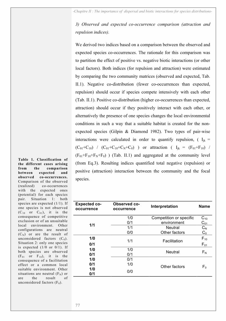
-Chapitre II : The importance of dispersal and biotic interactions for species distributions-

3) Observed and expected co-occurrence comparison (attraction and

repulsion indices).

We derived two indices based on a comparison between the observed and

expected species co-occurrences. The rationale for this comparison was

to partition the effect of positive vs. negative biotic interactions (or other

local factors). Both indices (for repulsion and attraction) were estimated

by comparing the two community matrices (observed and expected, Tab.

II.1). Negative co-distribution (fewer co-occurrences than expected,

repulsion) should occur if species compete intensively with each other

(Tab. II.1). Positive co-distribution (higher co-occurrences than expected,

attraction) should occur if they positively interact with each other, or

alternatively the presence of one species changes the local environmental

conditions in such a way that a suitable habitat is created for the non-

expected species (Gilpin & Diamond 1982). Two types of pair-wise

interactions were calculated in order to quantify repulsion, ( Ijk =

(C01+C10) / (C01+C10+CN+C0) ) or attraction ( Ijk = (F01+F10) /

(F01+F10+FN+F0) ) (Tab. II.1) and aggregated at the community level

(from Eq.3). Resulting indices quantified total negative (repulsion) or

positive (attraction) interaction between the community and the focal

species.

Expected co-occurrence

Observed co-occurrence

Interpretation Name

1/1

1/0 Competition or specific environment

C10 0/1 C01

1/1 Neutral CN

0/0 Other factors C0

1/0 1/1 Facilitation

F10

0/1 F01

1/0 1/0 Neutral FN 0/1 0/1

1/0 0/1

Other factors F0 0/1 1/0

1/0 0/0

0/1

)

Table 1. Classification of

the different cases arising

from the comparison

between expected and

observed co-occurrences.

Comparison of the observed

(realized) co-occurrences

with the expected ones

(potential) for each species

pair. Situation 1: both

species are expected (1/1). If

one species is not observed

(C10 or C01), it is the

consequence of competitive

exclusion or of an unsuitable

local environment. Other

configurations are neutral

(CN) or are the result of

unconsidered factors (C0).

Situation 2: only one species

is expected (1/0 or 0/1). If

both species are observed

(F01 or F10), it is the

consequence of a facilitation

effect or a common local

suitable environment. Other

situations are neutral (FN) or

are the result of

unconsidered factors (F0).

!

$8!

-Chapitre II : The importance of dispersal and biotic interactions for species distributions-

83".&",)%+7(*%(.")9'*"1)

We followed the nested modelling framework presented in the

Introduction (Fig.II.1). Inspired by the general idea of Zero Inflated

Poisson models for count data (Welsh et al. 1996), we first modelled

species presence and absence and then, in a second step, we did the same

with abundance cover classes for locations with predicted presence. In

order to evaluate the models, final predictions were given by absences

predicted from the first model and abundance classes (potentially

including other absences) predicted using the second model (see

Supporting Information Fig.II.S3 for a detailed workflow of the method).

We compared this nested model to a non-nested model (i.e. without the

first step) in order to evaluate its performance.

We used random forests (RF) to model both presence-absence and

abundance data. This choice was driven by the ability of RF to deal with

both binary and multilevel data and to estimate the importance of

predictor variables in high dimensional settings. They provide estimates

of the independent contribution of each predictor (Strobl et al. 2009). We

performed nine repetitions, following a cross-validation procedure (see

Fig. II.S3).

We calibrated and evaluated four models using different sets of predictor

variables to evaluate the performance of our framework and estimate the

relevance of the proposed indices: abiotic variables (A), abiotic variables

and co-occurrence based indices (AC), abiotic variables and dispersal

index (AD) and all predictors (ACD). Predictions about final abundance

classes were evaluated using the Hanssen-Kuipers discriminant statistic

(Gandin & Murphy 1992) (see Supporting Information Eq. II.S1 for the

formula). We computed variable importance with a re-sampling method

implemented into random forest models (Breiman et al. 2011) (see

Supporting Information Eq. II.S2 for details and formula). We averaged

the importance values across the nine repetitions and then normalized the

results for each species by calculating the relative importance of the

different variables. A variable was considered as not significant when the

confidence interval included zero.

!

$?! !

-Chapitre II : The importance of dispersal and biotic interactions for species distributions-

All analyses were carried out in R (R Development Core Team 2010)

with the ‘raster’ package for spatial data management, the ‘ade4’

package for PCAs, and the ‘party’ package for random forest models and

variable importance.

:&'$&.)&($"0%.$&'(,)%(*)*&,3"0,%1)";;".$,)'()$<")%+&'$&.)(&.<")

We illustrated how community-scale and dispersal mechanisms affected

the abiotic niche for the four species for which the addition of the

proposed indices increased performance the most. We derived different

predictions from the complete model (ACD) and projected them onto the

abiotic niche space. This space was defined by the first two axes of a

PCA involving the abiotic variables of the sampled plots. These two axes

together explained 53% of the total inertia. In this space, we drew the

density of presences derived from different model predictions, computed

with observed values of explicative variables or with dispersal and/or

biotic interactions set to zero. We grouped all repetitions into a single

prediction. First, absences were determined where predicted absences

had a majority amongst repetitions and then for presences, abundance

classes were given by the majority amongst repetitions’ predicted classes.

Following Soberon (2007) we defined sinks as the sites where the model

predicted presences with observed values but absences with null dispersal

and we defined sources as the sites where the model predicted presences

with observed values as with null dispersal. Then, in order to locate

competition and facilitation areas, we compared the current predictions

with predictions where all co-occurrence indices were set to zero. A

predicted absence that became a presence with a release of biotic

interactions indicated a negative impact of biotic interactions and

conversely, a presence changed to absence indicated a positive impact of

biotic interactions. We also compared the two response curves (current

predictions and those with co-occurrence indices equalling zero) as a

function of the temperature, which is the most important climatic

gradient in the region (explaining 70% of the first axis of the PCA). We

estimated these curves using local least square regressions between

probabilities of presences and temperature. We used the ‘loess’ function

(Cleveland et al. 1992).

!

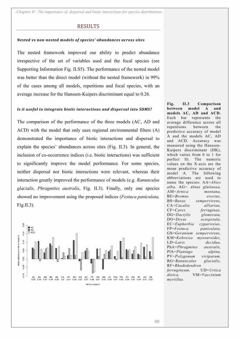
8@!

-Chapitre II : The importance of dispersal and biotic interactions for species distributions-

+,4/5*4!

=",$"*)/,)('(6(",$"*)9'*"1,)';),3".&",>)%+7(*%(.",)%.0',,),&$",)

The nested framework improved our ability to predict abundance

irrespective of the set of variables used and the focal species (see

Supporting Information Fig. II.S5). The performance of the nested model

was better than the direct model (without the nested framework) in 99%

of the cases among all models, repetitions and focal species, with an

average increase for the Hanssen-Kuipers discriminant equal to 0.26.

?,)&$)7,";71)$')&($"#0%$")+&'$&.)&($"0%.$&'(,)%(*)*&,3"0,%1)&($')82@8A))

The comparison of the performance of the three models (AC, AD and

ACD) with the model that only uses regional environmental filters (A)

demonstrated the importance of biotic interactions and dispersal to

explain the species’ abundances across sites (Fig. II.3). In general, the

inclusion of co-occurrence indices (i.e. biotic interactions) was sufficient

to significantly improve the model performance. For some species,

neither dispersal nor biotic interactions were relevant, whereas their

interaction greatly improved the performance of models (e.g. Ranunculus

glacialis, Phragmites australis, Fig. II.3). Finally, only one species

showed no improvement using the proposed indices (Festuca paniculata,

Fig.II.3).

HK for model A

Mean d

iffe

rence in H

K t

o m

odel A

!0.1

0!

0.0

50.0

00.0

50.1

00.1

50.2

0

AC

AD

ACD

AA

0.55

AG

0.43

AM

0.57

BE

0.49

BS

0.59

CA

0.6

CF

0.47

DG

0.48

DO

0.51

EC

0.57

FP

0.68

GS

0.61

KM

0.54

LD

0.49

PhA

0.57

PlA

0.55

PV

0.59

RG

0.61

RF

0.54

UD

0.51

VM

0.52

)

Fig. II.3 Comparison

between model A and

models AC, AD and ACD.

Each bar represents the

average difference across all

repetitions between the

predictive accuracy of model

A and the models AC, AD

and ACD. Accuracy was

measured using the Hanssen-

Kuipers discriminant (HK),

which varies from 0 to 1 for

perfect fit. The numeric

values on the X-axis are the

mean predictive accuracy of

model A. The following

abbreviations are used to

name the species: AA=Abies

alba, AG= Alnus glutinosa,

AM=Arnica montana,

BE=Bromus erectus,

BS=Buxus sempervirens,

CA=Cacalia alliariae,

CF=Carex ferruginae,

DG=Dactylis glomerata,

DO=Dryas octopetala,

EC=Euphorbia cyparissias,

FP=Festuca paniculata,

GS=Geranium sempervirens,

KM=Kobresia myosuroides,

LD=Larix decidua,

PhA=Phragmites australis,

PlA=Plantago alpina,

PV=Polygonum viviparum,

RG=Ranunculus glacialis,

RF=Rhododendron

ferrugineum, UD=Urtica

dioica, VM=Vaccinium

myrtillus.

!

8A! !

-Chapitre II : The importance of dispersal and biotic interactions for species distributions-

2&,"($%(#1&(#),3".&",)%+7(*%(.")%(*),3".&",)30","(."6%+,"(.")*0&/"0,))

The separate analysis of variable importance at each model step

highlighted major differences in the main drivers of presence-absence or

abundance (Fig. II.4). In general, dispersal was relatively important in

predicting presence or absence but less for the abundance class where

presence was expected (Fig.II.4). The most important biotic interaction

index was the repulsion one, followed by the community aggregated C-

score, and the attraction index for some species. The niche overlap index

was a poor predictor of both presence-absence and abundance. The biotic

interactions indices were more important (for all species) in the second

step of the model in predicting the abundance class where presence was

expected. For instance, Bromus erectus well illustrated these results (Fig.

II.4). Dispersal was more important for presence-absence, and the

importance of biotic interactions increased for abundance. Abiotic

variables, although they varied in relative importance between species,

were relevant to both modelling steps.

(a)

AA AG AM BE BS CA CF DG DO EC FP GS KM LD PhA PlA PV RF RG UD VM

rela

tive im

port

ance

0.0

0.2

0.4

0.6

0.8

1.0

abiotic

niche overlap

repulsion

attraction

C!score

dispersal

n.s

. n.s

.n.s

.

n.s

.

n.s

.

n.s

.n.s

.n.s

.n.s

.

n.s

. n.s

.

n.s

.

n.s

.

n.s

.

n.s

.

n.s

.

n.s

.

n.s

.

n.s

. n.s

.

n.s

.

(b)

AA AG AM BE BS CA CF DG DO EC FP GS KM LD PhA PlA PV RF RG UD VM

rela

tive im

port

ance

0.0

0.2

0.4

0.6

0.8

1.0

abiotic

niche overlap

repulsion

attraction

C!score

dispersal

n.s

.

n.s

.

n.s

.

n.s

.

n.s

.

n.s

.

n.s

.

n.s

.

n.s

.

n.s

.

n.s

.

n.s

.

Fig. II.4 Importance of

variables. Each barplot

represents the relative

importance of each

variable or group of

variables. The relative

importance of each abiotic

variable was added

together.! Species

abbreviations are the same

as for Fig. II.3. Non-

significant variables are

marked with n.s. (a)

Importance of variables to

explain presence-absence

distribution (modelling

step 1). (b) Importance of

variables to explain

abundance distribution

(modelling step 2).

!

8C!

-Chapitre II : The importance of dispersal and biotic interactions for species distributions-

:&'$&.)&($"0%.$&'(,)%(*)*&,3"0,%1)";;".$,)'(),3".&",>)%+&'$&.)(&.<",)

Our modelling framework allowed us to visualise the effects of the

different indices on the abiotic niche space (e.g. Bromus erectus in Fig.

II.5, other species in Supporting Information Fig. II.S7). For Bromus

erectus, we found that the realized abiotic niche lies in drier and warmer

places than the average of the sampled plots (Fig. II.5a). Using a

comparison between the realized niche and a prediction with no

dispersal, we identified abiotic conditions of sources and sinks (Fig.

II.5b). Surprisingly, sources were located where the density of presences

was relatively low (Figs. II.5a and II.5b). Interestingly, sources

corresponded to high abundance and sinks to lower abundance (Figs.

II.5a and II.5b). With a release of biotic interactions, the abiotic niche did

not expand significantly but became denser, particularly in the warmer

part of the gradient (Figs II.5c), suggesting there is competition in these

areas (red, Fig. II.5c, right panel). At the colder edge of the niche, the

density decreased, pointing to positive effects of biotic interactions

(green, Fig II.5c, right panel). Some sinks were potentially due to biotic

interactions, as they occurred in the same abiotic region as negative

biotic interactions (Figs II.5b and II.5c).

!

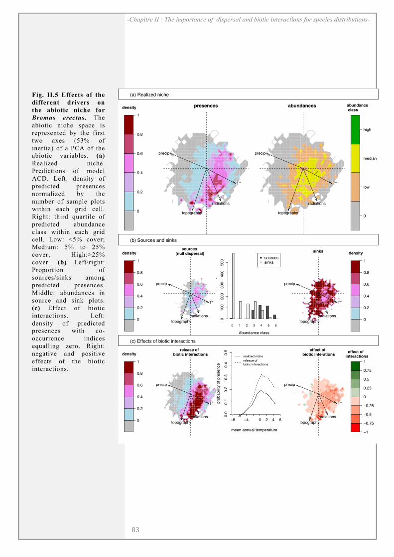
8D! !

-Chapitre II : The importance of dispersal and biotic interactions for species distributions-

0

0.2

0.4

0.6

0.8

1

density

0

0.2

0.4

0.6

0.8

1

density

0

0.2

0.4

0.6

0.8

1

density

0

0.2

0.4

0.6

0.8

1

density

0

low

median

high

abundance class

!1

!0.75

!0.5

!0.25

0

0.25

0.5

0.75

1

effect of interactions

(a) Realized niche

T°

precip

radiations

topography

presences

T°

precip

radiations

topography

abundances

(b) Sources and sinks

T°

precip

radiations

topography

sources (null dispersal)

0 1 2 3 4 5 6

Abundance class

Fre

quency

0100

200

300

400

500

sourcessinks

T°

precip

radiations

topography

sinks

(c) Effects of biotic interactions

T°

precip

radiations

topography

release of biotic interactions

0.0

0.1

0.2

0.3

0.4

0.5

mean annual temperature

pro

babili

ty o

f pre

sence

!8 !4 0 2 4 6

realized niche

release of biotic interactions

T°

precip

radiations

topography

effect of biotic interations

Fig. II.5 Effects of the

different drivers on

the abiotic niche for

Bromus erectus. The

abiotic niche space is

represented by the first

two axes (53% of

inertia) of a PCA of the

abiotic variables. (a)

Realized niche.

Predictions of model

ACD. Left: density of

predicted presences

normalized by the

number of sample plots

within each grid cell.

Right: third quartile of

predicted abundance

class within each grid

cell. Low: <5% cover;

Medium: 5% to 25%

cover; High:>25%

cover. (b) Left/right:

Proportion of

sources/sinks among

predicted presences.

Middle: abundances in

source and sink plots.

(c) Effect of biotic

interactions. Left:

density of predicted

presences with co-

occurrence indices

equalling zero. Right:

negative and positive

effects of the biotic

interactions.

!

8E!

-Chapitre II : The importance of dispersal and biotic interactions for species distributions-

3)4%/44).0!

We proposed and tested a comprehensive framework for investigating

mechanisms underlying species distributions and their abundances.

Firstly, we demonstrated that the nested modelling structure greatly

improves our understanding of distribution and abundance, increasing

model performance for all species studied here. Secondly, our nested

framework allowed us to show that the ranking in variable importance

was reversed between presence-absence and abundance when presence

was expected, supporting the hypothesis that different processes were

intertwined. Thirdly, we showed that including the three groups of

drivers (abiotic, biotic and dispersal) in the same model could offer

insights into the mechanisms of community assembly and revealed how

they ultimately shape the realized niche from the abiotic niche of species.

:&'$&.)&($"0%.$&'(,)

We showed that community-scale effects of biotic interactions were more

important for the second modelling step in explaining abundance when

presence was established. This result supports the hypothesis that

mechanisms underlying abundance variations occur at community scale,

which is where species interact. In our example (Bromus erectus), the

interaction with the community is essentially negative, particularly at the

warm edge of the abiotic niche (Fig. II.5d) where the environment is

suitable for a large number of species. Moreover, co-occurrence indices

associated to repulsion are relatively important for the abundance model

step (Fig. II.4b). These results suggest that co-occurrence indices are

strongly related to negative biotic interactions, such as competition for

resources (Chase & Leibold 2003; Soberon 2007). At the same time, we

observed positive effects of biotic interactions at the colder edge of the

abiotic niche. This may be the consequence of facilitation, which has

been suggested to be an important factor of species coexistence in harsh

conditions (Choler et al. 2001; Callaway et al. 2002).

Observed species co-occurrence has long been used to infer community

assembly rules (Gilpin & Diamond 1982; Gotelli & McCabe 2002) and

several co-occurrence based indices have been used in SDMs as a proxy

!

8F! !

-Chapitre II : The importance of dispersal and biotic interactions for species distributions-

for unmeasured abiotic conditions and species interactions (Leathwick

2002; Cottenie 2005; Araujo & Luoto 2007; Meier et al. 2010). The main

limitation of these approaches is that non co-occurring species pairs

could be interpreted either as the result of competitive exclusion or

different species’ environmental niches (Gilpin & Diamond 1982). Here,

we propose to use a comparison between observed and expected

community composition to tease apart the effects of environment from

those of competition (Chesson 2000a; Chase & Leibold 2003; Silvertown

2004). Moreover, these new metrics allow distinguishing between

positive (attraction) and negative (repulsion) effects. In further studies, it

would also be interesting to separate the cases where a species undergoes

competition (or facilitation) from the situation where the species has the

strongest competitive ability (or facilitate other species) (Tab. II.1).

These indices still cannot distinguish biotic interactions from micro-

environmental conditions effects that may have a prominent role (e.g.

topographical heterogeneity inducing thermal differences, Scherrer &

Körner 2011). For instance, the co-occurrence indices for Phragmites

australis possibly relate to specific local abiotic conditions (small

wetlands) whereas the repulsion index for Dactylis glomerata, a common

and widely distributed grass, probably reveals its competitive strategy.

Because we will never be able to measure every abiotic variable at

community scale, the attraction and repulsion indices provide an

interesting proxy for describing local abiotic and biotic environments.

Their influence on species distributions are stronger than the niche

overlap index and are relatively easy to interpret in respect to the

aggregated C-score.

The construction of the expected species pool is crucial for most of the

proposed indices and requires particular attention. As we assume no

dispersal limitation when calculating the expected species pool, we may

overestimate expected species richness at inaccessible sites. For some

species, important limiting variables might also be missing or imprecise

(e.g. soil data). These species would thus be wrongly added to the species

pool. However, this bias cannot explain alone the poor predictive power

of the niche overlap index because the expected species pool is also used

!

8#!

-Chapitre II : The importance of dispersal and biotic interactions for species distributions-

to build the repulsion index. This pattern might suggest that competition

does occur in few plots only, while in the others plots, spatial and

temporal environmental heterogeneity allow species coexistence

(Silvertown, 2004). Finally, although competition would preferentially

occur between functionally similar species, we did not consider species

identity. The addition of weights based on functional traits to our indices

might be worth considering, as they may be directly linked to resource

acquisition or exploitation (Lavorel & Garnier 2002).

2&,3"0,%1)

There are now several studies supporting the importance of dispersal on

species distributions (e.g. Bahn & McGill 2007). This is, however,

usually approximated by spatial autocorrelation functions (e.g. Borcard et

al. 1992), generally built with little or no attention to the true spatial

processes that drive biogeographical patterns. Although the fraction of

variance explained by these variables is often interpreted as the spatial

signature of dispersal limitations (Beale et al. 2008), this spatial structure

could also result from unaccounted spatially auto-correlated

environmental factors (Gravel et al. 2008; Araujo et al. 2009). Here, we

had an underlying hypothesis with an explicit formulation based on

species-specific dispersal distances, which allows us to progress in our

understanding of the processes driving spatial distribution. Confusion

may however still arise when missing spatially autocorrelated abiotic

drivers operate at the same spatial scale as dispersal mechanisms

(Cottenie 2005).

Our study showed that dispersal mechanisms were more important for

determining presence-absence patterns, suggesting strong dispersal

limitations. Far from its geographical range, a species is systematically

predicted to be absent because it cannot reach the site, even if the

environment is suitable. It can introduce a bias in the relationship

between species distribution and abiotic variables, because in these sites,

abiotic constraints might be neglected. It is not possible however to

reveal the real cause of such absences if all sampled plots with similar

abiotic conditions are systematically far from the species geographical

!

8$! !

-Chapitre II : The importance of dispersal and biotic interactions for species distributions-

distribution. Ideally, to estimate the true relationship between species

distribution and abiotic variables (i.e. the fundamental abiotic niche), the

sampling should be homogeneous not only in relation to the abiotic

variables but also spatially.

The importance of the dispersal index in the second model step highlights

the implication of dispersal mechanisms at local scale, such as source-

sink dynamics. Interestingly, the sources identified in our case study (and

three other examples, Fig. II.S7) are not related to the density of presence

but to species’ abundance (Fig. II.5). These results support the source-

sink theory, which predicts species occurrences in unsuitable habitat if

immigration from surrounding source populations is sufficiently large

(Pulliam 2000).

83".&",)*&,$0&+7$&'()%(*)%+&'$&.)(&.<",)

Species distribution models generally use topoclimatic predictors only

(Guisan & Zimmermann 2000). Consequently, the relationship they

model between abiotic variables and the distribution includes at the same

time abiotic constraints, dispersal mechanisms and interaction between

species (Guisan & Zimmermann 2000; Soberon 2007). Here, because we

introduced other explicative variables to describe dispersal and species

interactions mechanisms, the modelled relationship between abiotic

variables and the species distribution is refined and should be closer to

the fundamental niche. Although the approximation of the fundamental

niche is obviously constrained by the area considered and should be valid

only for the gradient sampled, our method refines the relationship

between topoclimatic variables and species distribution for our region.

Whilst we agree that only experiments can define the fundamental niche

(e.g. Vetaas 2002; Kearney & Porter 2009) whereas we only approximate

it here, our model allows us to explore the effects of dispersal and biotic

interactions on the abiotic niche, including the identification of sources

and sinks (Fig. II.5b) and is able to point out potential sites where

facilitation or competition have a strong impact (Fig. II.5c).

)

!

88!

-Chapitre II : The importance of dispersal and biotic interactions for species distributions-

B"0,3".$&/",)

Our framework extends the boundaries of SDMs and should allow

important ecological questions to be addressed. It offers an innovative

way to improve our understanding of community assembly processes for

large spatial scales and for many species at once, based on largely

available data: coarse scale environmental variables, community surveys

at the scale of species interactions, and species-specific dispersal

abilities. For instance, understanding and predicting species invasion

might benefit from this framework, as the potential distribution of the

invader species in a region is often unknown because the realized

distribution of the species usually reflects the place of introduction,

dispersal capability of the species and biotic resistance of the native

communities (Gallien et al. 2010). More fundamentally, not all species

are influenced by the same factors. Applying our framework to a large set

of species could help providing general rules or patterns for groups of

species. For instance, dominant and generalist species are in theory less

likely to be influenced by negative biotic interactions than subordinated

species (Boulangeat et al. 2012). These relatively old but generally

unresolved questions in ecology and biogeography might be now tackled

or addressed from a different angle.

'%G0.H5,31,B,0*4!

The research leading to these results had received funding from the

European Research Council under the European Community's Seven

Framework Programme FP7/2007-2013 Grant Agreement no. 281422. IB

was funded by the French “Agence Nationale de la Recherche” with the

project SCION (ANR-08-PEXT-03) and initially by the European

Commission’s FP6 ECOCHANGE project (GOCE-CT-2007-036866).

DG acknowledged support from the NSERC Discovery. The authors

wish to thank the EMABIO team for insightful comments on the

preliminary ideas for the paper, and Pascal Vittoz for the dispersal data.

Most of the computations presented in this paper were performed using

the CIMENT infrastructure (https://ciment.ujf-grenoble.fr), which is

supported by the Rhône-Alpes region (GRANT CPER07 13 CIRA:

http://www.ci-ra.org) and France-Grille (http://www.france-grilles.fr).

Thanks also to Version Original for checking and correcting the English

in this article.

!

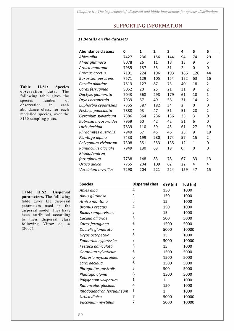
8?! !

-Chapitre II : The importance of dispersal and biotic interactions for species distributions-

4/((.+*)01!)02.+B'*).0!

CD)2"$%&1,)'()$<")*%$%,"$,)

!"#$%&$'()'*&++(+,) -) .) /) 0) 1) 2) 3)

!"#$%&'("'& !"#!$ #%&$ '(&$ '""$ )"$ !"$ #)$

!()*%&+(*,#)-%'& *+!*$ #&$ ''$ '*$ '%$ )$ ($

!.)#/'&0-),')'& !)%($ '%!$ (($ %'$ #$ +$ +$

1.-0*%&$.$/,*%& !')'$ ##"$ ')&$ ')%$ '*&$ '#&$ ""$

1*2*%&%$03$.4#.$)%& !(!'$ '#)$ '+($ '("$ '##$ &%$ '&$

5'/'(#'&'((#'.#'$& !*'%$ '#!$ *!$ !%$ "+$ '*$ #$

5'.$2&6$..*+#)$'& *+(#$ #+$ #($ #'$ %'$ )$ #$

7'/,8(#%&+(-0$.','& !+"%$ (&*$ #)*$ '!)$ &'$ '+$ '$

7.8'%&-/,-3$,'('& !)%)$ &!$ ")$ (*$ %'$ '"$ #$

9*3:-."#'&/83'.#%%#'%& !%(($ (*!$ '*#$ %"$ #$ +$ +$

;$%,*/'&3')#/*(','& !***$ )%$ "!$ ('$ ('$ #*$ #$

<$.')#*0&%8(4',#/*0& !%*&$ %&"$ #%&$ '%&$ %($ %$ +$

=-".$%#'&08-%*.-#>$%& !)()$ &+$ "#$ "#$ ('$ &$ +$

?'.#2&>$/#>*'& !*%)$ ''+$ ()$ "($ &'$ #!$ ')$

@:.'+0#,$%&'*%,.'(#%& !)")$ &!$ "($ "&$ #($ )$ ')$

@('),'+-&'(3#)'& !"%%$ '))$ #*+$ '!"$ (!$ '($ #$

@-(8+-)*0&4#4#3'.*0& !%+*$ %('$ %(%$ '%($ '#$ '$ +$

A')*)/*(*%&+('/#'(#%& !)")$ '%+$ &%$ '*$ +$ +$ +$

A:->->$)>.-)&

6$..*+#)$*0& !!%*$ '"*$ *%$ !*$ &!$ %%$ '%$

B.,#/'&>#-#/'& !!(($ #+"$ '+)$ &#$ ##$ "$ "$

C'//#)#*0&08.,#((*%& !#)+$ #+"$ ##'$ ##"$ '()$ "!$ '($

!

45('6(+) 76+5(8+&*)'*&++) %99):;<) *%%):;<)

!"#$%&'("'& "$ '(+$ '+++$

!()*%&+(*,#)-%'& "$ '(+$ '+++$

!.)#/'&0-),')'& %$ '($ '+++$

1.-0*%&$.$/,*%& "$ '(+$ '+++$

1*2*%&%$03$.4#.$)%& %$ '($ '+++$

5'/'(#'&'((#'.#'$& ($ (++$ (+++$

5'.$2&6$..*+#)$'& &$ '(++$ (+++$

7'/,8(#%&+(-0$.','& !$ (+++$ '++++$

7.8'%&-/,-3$,'('& %$ '($ '+++$

9*3:-."#'&/83'.#%%#'%& !$ (+++$ '++++$

;$%,*/'&3')#/*(','& %$ '($ '+++$

<$.')#*0&%8(4',#/*0& &$ '(++$ (+++$

=-".$%#'&08-%*.-#>$%& &$ '(++$ (+++$

?'.#2&>$/#>*'& &$ '(++$ (+++$

@:.'+0#,$%&'*%,.'(#%& ($ (++$ (+++$

@('),'+-&'(3#)'& &$ '(++$ (+++$

@-(8+-)*0&4#4#3'.*0& '$ '$ '+++$

A')*)/*(*%&+('/#'(#%& "$ '(+$ '+++$

A:->->$)>.-)&6$..*+#)$*0& '$ '$ '+++$

B.,#/'&>#-#/'& !$ (+++$ '++++$

C'//#)#*0&08.,#((*%& !$ (+++$ '++++$

Table II.S1: Species

observation data. The

following table gives the

species number of

observation in each

abundance class, for each

modelled species, over the

8160 sampling plots.

Table II.S2: Dispersal

parameters. The following

table gives the dispersal

parameters used in the

dispersal model. They have

been attributed according

to their dispersal class

following Vittoz et. al

(2007).

!

!

?@!

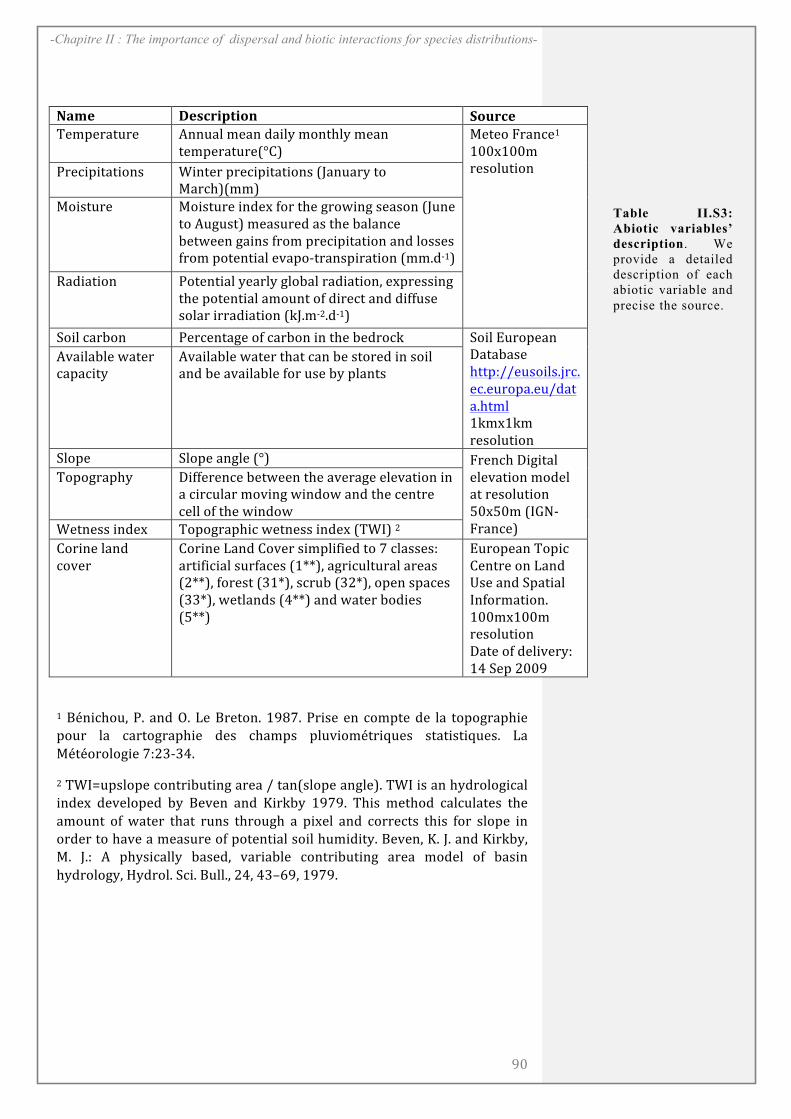
-Chapitre II : The importance of dispersal and biotic interactions for species distributions-

!!

"#$%! &%'()*+,*-.! /-0)(%!

*IJKI<=;L<I! 'MML=N!JI=M!O=PNQ!JRM;SNQ!JI=M!

;IJKI<=;L<ITU%V!

BI;IR!2<=M>IA!

A@@WA@@J!

<I:RNL;PRM!(<I>PKP;=;PRM:! HPM;I<!K<I>PKP;=;PRM:!TX=ML=<Q!;R!

B=<>SVTJJV!

BRP:;L<I! BRP:;L<I!PMOIW!YR<!;SI!Z<R[PMZ!:I=:RM!TXLMI!

;R!'LZL:;V!JI=:L<IO!=:!;SI!9=N=M>I!

9I;[IIM!Z=PM:!Y<RJ!K<I>PKP;=;PRM!=MO!NR::I:!

Y<RJ!KR;IM;P=N!I\=KR";<=M:KP<=;PRM!TJJ]O"AV!

+=OP=;PRM! (R;IM;P=N!QI=<NQ!ZNR9=N!<=OP=;PRM^!IWK<I::PMZ!

;SI!KR;IM;P=N!=JRLM;!RY!OP<I>;!=MO!OPYYL:I!

:RN=<!P<<=OP=;PRM!T_X]J"C]O"AV!

4RPN!>=<9RM! (I<>IM;=ZI!RY!>=<9RM!PM!;SI!9IO<R>_! 4RPN!,L<RKI=M!

3=;=9=:I!

S;;K-``IL:RPN:]a<>]

I>]IL<RK=]IL`O=;

=]S;JN!

A_JWA_J!

<I:RNL;PRM!

'\=PN=9NI![=;I<!

>=K=>P;Q!

'\=PN=9NI![=;I<!;S=;!>=M!9I!:;R<IO!PM!:RPN!

=MO!9I!=\=PN=9NI!YR<!L:I!9Q!KN=M;:!

4NRKI!! 4NRKI!=MZNI!TUV!! 2<IM>S!3PZP;=N!

INI\=;PRM!JROIN!

=;!<I:RNL;PRM!

F@WF@J!T)10"

2<=M>IV!

*RKRZ<=KSQ! 3PYYI<IM>I!9I;[IIM!;SI!=\I<=ZI!INI\=;PRM!PM!

=!>P<>LN=<!JR\PMZ![PMOR[!=MO!;SI!>IM;<I!

>INN!RY!;SI![PMOR[!

HI;MI::!PMOIW! *RKRZ<=KSP>![I;MI::!PMOIW!T*H)V!C!

%R<PMI!N=MO!

>R\I<!

%R<PMI!5=MO!%R\I<!:PJKNPYPIO!;R!$!>N=::I:-!

=<;PYP>P=N!:L<Y=>I:!TAbbV^!=Z<P>LN;L<=N!=<I=:!

TCbbV^!YR<I:;!TDAbV^!:><L9!TDCbV^!RKIM!:K=>I:!

TDDbV^![I;N=MO:!TEbbV!=MO![=;I<!9ROPI:!

TFbbV!

,L<RKI=M!*RKP>!

%IM;<I!RM!5=MO!

/:I!=MO!4K=;P=N!

)MYR<J=;PRM]!!

A@@JWA@@J!

<I:RNL;PRM!

3=;I!RY!OINP\I<Q-!

AE!4IK!C@@?!

!

A!6cMP>SRL^!(]! =MO!.]! 5I!6<I;RM]!A?8$]!(<P:I! IM! >RJK;I!OI! N=! ;RKRZ<=KSPI!

KRL<! N=! >=<;RZ<=KSPI! OI:! >S=JK:! KNL\PRJc;<PdLI:! :;=;P:;PdLI:]! 5=!

Bc;cR<RNRZPI!$-CD"DE]!

C!*H)eLK:NRKI!>RM;<P9L;PMZ!=<I=!`!;=MT:NRKI!=MZNIV]!*H)!P:!=M!SQO<RNRZP>=N!

PMOIW! OI\INRKIO! 9Q! 6I\IM! =MO! GP<_9Q! A?$?]! *SP:! JI;SRO! >=N>LN=;I:! ;SI!

=JRLM;! RY! [=;I<! ;S=;! <LM:! ;S<RLZS! =! KPWIN! =MO! >R<<I>;:! ;SP:! YR<! :NRKI! PM!

R<OI<!;R!S=\I!=!JI=:L<I!RY!KR;IM;P=N!:RPN!SLJPOP;Q]!6I\IM^!G]!X]!=MO!GP<_9Q^!

B]! X]-! '! KSQ:P>=NNQ! 9=:IO^! \=<P=9NI! >RM;<P9L;PMZ! =<I=! JROIN! RY! 9=:PM!

SQO<RNRZQ^!&QO<RN]!4>P]!6LNN]^!CE^!EDf#?^!A?$?]!

!

!

Table II.S3:

Abiotic variables’

description. We

provide a detailed

description of each

abiotic variable and

precise the source.

!

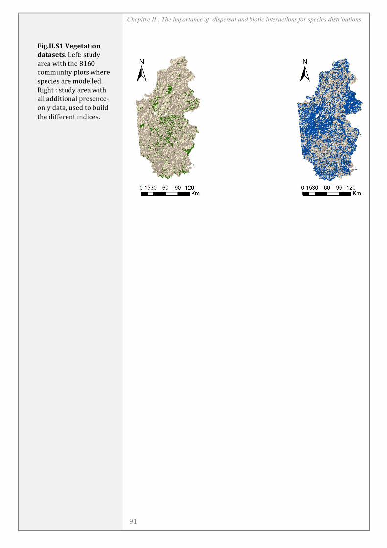
?A! !

-Chapitre II : The importance of dispersal and biotic interactions for species distributions-

!!

!

1*23443/5!6%2%,#,*-.!

7#,#'%,']!5IY;-!:;LOQ!

=<I=![P;S!;SI!8A#@!

>RJJLMP;Q!KNR;:![SI<I!

:KI>PI:!=<I!JROINNIO]!

+PZS;!-!:;LOQ!=<I=![P;S!

=NN!=OOP;PRM=N!K<I:IM>I"

RMNQ!O=;=^!L:IO!;R!9LPNO!

;SI!OPYYI<IM;!PMOP>I:]!

!

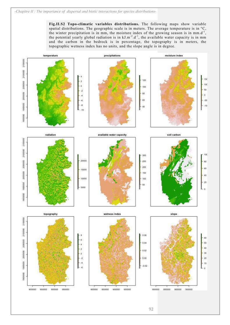
?C!

-Chapitre II : The importance of dispersal and biotic interactions for species distributions-

Fig.II.S2 Topo-climatic variables distributions. The following maps show variable

spatial distributions. The geographic scale is in meters. The average temperature is in °C,

the winter precipitation is in mm, the moisture index of the growing season is in mm.d-1

,

the potential yearly global radiation is in kJ.m-2

.d-1

, the available water capacity is in mm

and the carbon in the bedrock is in percentage, the topography is in meters, the

topographic wetness index has no units, and the slope angle is in degree.

!

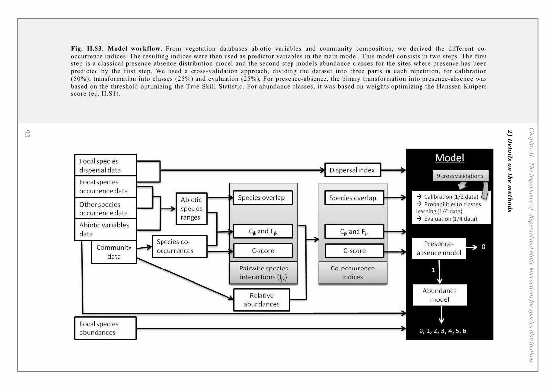
!?D!

!

-Ch

ap

itre II : Th

e imp

orta

nce o

f disp

ersal a

nd

bio

tic intera

ction

s for sp

ecies distrib

utio

ns-

ED)2

"$%&1,)'()$<

")9"$<'*,)

!

!

Fig. II.S3. Model workflow. From vegetation databases abiotic variables and community composition, we derived the different co-

occurrence indices. The resulting indices were then used as predictor variables in the main model. This model consists in two steps. The first

step is a classical presence-absence distribution model and the second step models abundance classes for the sites where presence has been

predicted by the first step. We used a cross-validation approach, dividing the dataset into three parts in each repetition, for calibration

(50%), transformation into classes (25%) and evaluation (25%). For presence-absence, the binary transformation into presence-absence was

based on the threshold optimizing the True Skill Statistic. For abundance classes, it was based on weights optimizing the Hanssen-Kuipers

score (eq. II.S1).

!

!

?E!

-Chapitre II : The importance of dispersal and biotic interactions for species distributions-

Eq. II.S1 Calculation of the Hanssen-Kuipers discriminant score.

!

where N is the total number of sites, n(Pi, Oi) is the number of predictions

that match with obervations for the class i, N(Oi) is the number of

observations in the class i and N(Pi) is the number of predictions in the

class i.

!

Eq. II.S2 Calculation of variable importance.

The variable importance for the variable x is calculated using the Out-Of-

Bag (OOB) sample which is a subsample of the data that has been put

aside during the calibration and is used as independant data to evaluate

the model. The variable importance is the mean difference in accuracy

between normal predictions and predictions with a randomly permuted

variable x. For each permuation, the variable importance VI is equal to :

!

where N is the number of plots in the OOB sample, n(Pi, Oi) is the

number of predictions that match with observations for the class i and Px

is the prediction vector obtained after randomly permuting the predictor

variable x.

FD)?($"09"*&%$")0",71$,)

!

!

!

!

Table II.S4: Correlations between proposed indices and topo-climatic variables. The

following table gives the Pearson correlations in sampled sites between the proposed indices

and all topo-climatic variables, for the 21 focal species. Highest correlations (above 0,6) are

highlighted. T°: average temperature, Precip: winter precipitations, Moist:moisture index for

the growing season, Rad: potential yearly radiation, WC: soil available water capacity,

Carbon: percentage of carbon in the bedrock, topo: topography, wetness: topographic wetness

index, slope.

!

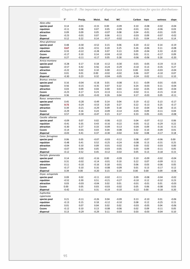
?F! !

-Chapitre II : The importance of dispersal and biotic interactions for species distributions-

)

=>) ?8('65@) AB6+C@) D&%@) EF) F&8"B$) CB5B) G(C$(++) +*B5()

!"#$%&'("'&

$ $ $ $ $ $ $ $ $+5('6(+)5BB*) $+,'"$$$$ -+,+'$$$$ -+,'($$$$ +,++$$$$$$ -+,+)$$$$ $+,'+$$$$ -+,+*$$$$ -+,+#$$$$ -+,+"$$$$

8(5#*+6B$) -+,''$$$$ $+,+*$$$$ $+,+!$$$$ $+,+($$$$ -+,+)$$$$ -+,+'$$$$ $+,+'$$$$ -+,+&$$$$ $+,+%$$$$

&CC8&'C6B$) $+,+)$$$$ $+,+)$$$$ $+,+($$$$ -+,+!$$$$ $+,+*$$$$ $+,+"$$$$ -+,+'$$$$ -+,+'$$$$ $+,+($$$$

F+'B8() -+,#%$$$$ -+,+'$$$$ $+,+!$$$$ $+,+&$$$$ -+,''$$$$ -+,+%$$$$ $+,+)$$$$ -+,+!$$$$ -+,+#$$$$

%6+5(8+&*) $+,'#$$$$ $+,##$$$$ $+,'"$$$$ -+,'!$$$$ -+,+#$$$$ $+,'($$$$ $+,+"$$$$ -+,'"$$$$ $+,'"$$$$

!()*%&+(*,#)-%'&

$ $ $ $ $ $ $ $ $+5('6(+)5BB*) $+,"*$$$$ -+,%+$$$$ -+,(#$$$$ $+,'($$$$ $+,+&$$$$ $+,#+$$$$ -+,'#$$$$ $+,'"$$$$ -+,')$$$$

8(5#*+6B$) )-@3H)))) -+,#&$$$$ -+,('$$$$ $+,#+$$$$ $+,#($$$$ $+,#&$$$$ -+,+&$$$$ $+,''$$$$ -+,+*$$$$

&CC8&'C6B$) $+,%%$$$$ -+,##$$$$ -+,#*$$$$ $+,+!$$$$ $+,'%$$$$ $+,+)$$$$ -+,+"$$$$ $+,%%$$$$ -+,#+$$$$

F+'B8() -+,'!$$$$ $+,'+$$$$ $+,'"$$$$ -+,+"$$$$ -+,'+$$$$ $+,+'$$$$ $+,''$$$$ -+,'!$$$$ $+,+)$$$$

%6+5(8+&*) $+,#!$$$$ -+,''$$$$ -+,'!$$$$ $+,+($$$$ $+,#*$$$$ -+,+&$$$$ -+,+&$$$$ $+,#&$$$$ -+,#+$$$$

!.)#/'&0-),')'&

$ $ $ $ $ $ $ $ $+5('6(+)5BB*) -+,#*$$$$ $+,'!$$$$ $+,'*$$$$ -+,'#$$$$ -+,%+$$$$ -+,+'$$$$ -+,+($$$$ -+,')$$$$ $+,'%$$$$

8(5#*+6B$) -+,(!$$$$ $+,"#$$$$ $+,(&$$$$ -+,#"$$$$ -+,#)$$$$ -+,'+$$$$ $+,'%$$$$ -+,%($$$$ $+,#!$$$$

&CC8&'C6B$) -+,##$$$$ $+,+#$$$$ $+,'+$$$$ $+,++$$$$$$ -+,'%$$$$ +,++$$$$$$ $+,+%$$$$ -+,+%$$$$ -+,+"$$$$

F+'B8() $+,+'$$$$ $+,+'$$$$ +,++$$$$$$ -+,+#$$$$ -+,+#$$$$ $+,+&$$$$ $+,+!$$$$ -+,'+$$$$ $+,+!$$$$

%6+5(8+&*) -+,%+$$$$ $+,#%$$$$ $+,%#$$$$ -+,+"$$$$ -+,+($$$$ -+,#"$$$$ $+,+#$$$$ -+,''$$$$ $+,'+$$$$

1.-0*%&&$.$/,*%&

$ $ $ $ $ $ $ $ $+5('6(+)5BB*) $+,'&$$$$ -+,+"$$$$ -+,'*$$$$ $+,+'$$$$ -+,+*$$$$ $+,''$$$$ -+,+)$$$$ -+,+'$$$$ -+,+($$$$

8(5#*+6B$) $+,(&$$$$ -+,'($$$$ -+,%($$$$ $+,+!$$$$ $+,##$$$$ $+,#"$$$$ -+,+%$$$$ $+,''$$$$ -+,+"$$$$

&CC8&'C6B$) $+,+%$$$$ $+,+)$$$$ $+,+"$$$$ $+,++$$$$$ $+,+%$$$$ -+,+#$$$$ -+,+($$$$ $+,+%$$$$ -+,+"$$$$

F+'B8() -+,#%$$$$ $+,'!$$$$ $+,#%$$$$ -+,'%$$$$ -+,''$$$$ -+,+#$$$$ $+,''$$$$ -+,'($$$$ $+,'+$$$$

%6+5(8+&*) $+,%&$$$$ -+,#)$$$$ -+,"%$$$$ $+,#&$$$$ $+,+"$$$$ $+,'!$$$$ -+,+%$$$$ $+,+($$$$ -+,''$$$$

1*2*%&&%$03$.4#.$)%&

$ $ $ $ $ $ $ $ $+5('6(+)5BB*) $+,"($$$$ -+,#*$$$$ -+,")$$$$ $+,'"$$$$ $+,+"$$$$ $+,')$$$$ -+,'#$$$$ $+,'%$$$$ -+,'!$$$$

8(5#*+6B$) )-@H/)))) -+,#"$$$$ -+,(%$$$$ $+,#+$$$$ $+,#!$$$$ $+,##$$$$ -+,'%$$$$ $+,#($$$$ -+,'!$$$$

&CC8&'C6B$) $+,%)$$$$ -+,#'$$$$ -+,#)$$$$ $+,+)$$$$ $+,'*$$$$ $+,'+$$$$ -+,+"$$$$ $+,#*$$$$ -+,'($$$$

F+'B8() -+,#)$$$$ $+,'&$$$$ $+,#"$$$$ -+,+)$$$$ -+,'"$$$$ -+,+($$$$ $+,+)$$$$ -+,''$$$$ $+,+"$$$$

%6+5(8+&*) $+,(!$$$$ -+,%+$$$$ -+,"!$$$$ $+,'($$$$ $+,'!$$$$ $+,%%$$$$ $+,+($$$$ -+,+'$$$$ -+,+*$$$$

5'/'(#'&&'((#'.#'$&

$ $ $ $ $ $ $ $ $+5('6(+)5BB*) -+,+)$$$$ $+,+!$$$$ $+,+#$$$$ -+,+&$$$$ -+,##$$$$ $+,+"$$$$ -+,+!$$$$ -+,'#$$$$ $+,+&$$$$

8(5#*+6B$) -+,"'$$$$ $+,%($$$$ $+,"%$$$$ -+,'&$$$$ -+,##$$$$ -+,+($$$$ $+,'#$$$$ -+,#)$$$$ $+,##$$$$

&CC8&'C6B$) -+,%+$$$$ $+,#!$$$$ $+,%%$$$$ -+,+)$$$$ -+,'%$$$$ -+,+"$$$$ $+,+)$$$$ -+,'&$$$$ $+,'($$$$

F+'B8() -+,'"$$$$ -+,+'$$$$ $+,+%$$$$ $+,+"$$$$ -+,+*$$$$ $+,+#$$$$ $+,'+$$$$ -+,+)$$$$ $+,+'$$$$

%6+5(8+&*) -+,+%$$$$ $+,"'$$$$ $+,%!$$$$ -+,%+$$$$ -+,+#$$$$ $+,+#$$$$ $+,+*$$$$ -+,'!$$$$ $+,'*$$$$

5'.$2&&6$..*+#)$'&

$ $ $ $ $ $ $ $ $+5('6(+)5BB*) $+,+&$$$$ $+,+($$$$ -+,+!$$$$ -+,+%$$$$ -+,'#$$$$ $+,+*$$$$ -+,+!$$$$ -+,+&$$$$ +,++$$$$$$

8(5#*+6B$) -+,"*$$$$ $+,"'$$$$ $+,(#$$$$ -+,#($$$$ -+,#"$$$$ -+,+*$$$$ $+,'%$$$$ -+,%'$$$$ $+,#($$$$

&CC8&'C6B$) -+,+"$$$$ $+,'+$$$$ $+,+)$$$$ -+,+'$$$$ -+,+#$$$$ $+,++$$$$$$ $+,+#$$$$ -+,+%$$$$ $+,++$$$$$$

F+'B8() -+,+!$$$$ $+,+"$$$$ $+,+($$$$ -+,+%$$$$ -+,+($$$$ $+,+%$$$$ $+,+)$$$$ -+,''$$$$ $+,+($$$$

%6+5(8+&*) -+,'#$$$$ $+,(#$$$$ $+,"($$$$ -+,'#$$$$ -+,+#$$$$ $+,+($$$$ $+,'%$$$$ -+,'*$$$$ $+,'($$$$

7'/,8(#%&&+(-0$.','&

$ $ $ $ $ $ $ $ $+5('6(+)5BB*) $+,'"$$$$ -+,+#$$$$ -+,'&$$$$ +,++$$$$$$ -+,+)$$$$ $+,'+$$$$ -+,+)$$$$ -+,+#$$$$ -+,+"$$$$

8(5#*+6B$) $+,%'$$$$ -+,+#$$$$ -+,'"$$$$ -+,+'$$$$ $+,'+$$$$ $+,##$$$$ $+,+!$$$$ -+,+)$$$$ $+,''$$$$

&CC8&'C6B$) $+,''$$$$ -+,'+$$$$ -+,'&$$$$ $+,'*$$$$ -+,+'$$$$ $+,+&$$$$ $+,+%$$$$ -+,+&$$$$ $+,+($$$$

F+'B8() -+,'!$$$$ $+,'+$$$$ $+,'&$$$$ -+,+*$$$$ -+,+)$$$$ $+,+'$$$$ $+,'%$$$$ -+,'!$$$$ $+,'#$$$$

%6+5(8+&*) $+,%)$$$$ +,++$$$$$$ -+,#+$$$$ $+,'($$$$ $+,')$$$$ +,++$$$$$$ +,++$$$$$$ $+,+)$$$$ -+,+*$$$$

7.8'%&&-/,-3$,'('&

$ $ $ $ $ $ $ $ $+5('6(+)5BB*) $+,+)$$$$ $+,+#$$$$ -+,''$$$$ -+,+#$$$$ -+,''$$$$ $+,+)$$$$ -+,+*$$$$ -+,+"$$$$ -+,+#$$$$

8(5#*+6B$) -+,(#$$$$ $+,%)$$$$ $+,('$$$$ -+,#'$$$$ -+,#!$$$$ -+,'+$$$$ $+,'#$$$$ -+,%#$$$$ $+,#%$$$$

&CC8&'C6B$) $+,+%$$$$ -+,+%$$$$ -+,+"$$$$ $+,+#$$$$ $+,+'$$$$ -+,+'$$$$ -+,+'$$$$ $+,+'$$$$ -+,+%$$$$

F+'B8() +,++$$$$$$ $+,+($$$$ $+,+%$$$$ -+,+%$$$$ -+,+#$$$$ $+,+($$$$ $+,+&$$$$ -+,+*$$$$ $+,+%$$$$

%6+5(8+&*) -+,"#$$$$ $+,''$$$$ $+,%'$$$$ -+,')$$$$ -+,'+$$$$ -+,##$$$$ +,++$$$$$$ -+,'*$$$$ $+,#+$$$$

9*3:-."#'&&

/83'.#%%#'%&

$ $ $ $ $ $ $ $ $+5('6(+)5BB*) $+,#'$$$$ -+,''$$$$ -+,#&$$$$ $+,+"$$$$ -+,+)$$$$ $+,'%$$$$ -+,'+$$$$ $+,+'$$$$ -+,+&$$$$

8(5#*+6B$) -+,'%$$$$ $+,'($$$$ $+,'*$$$$ -+,'#$$$$ -+,'+$$$$ $+,+*$$$$ $+,'#$$$$ -+,#($$$$ $+,'($$$$

&CC8&'C6B$) $+,+'$$$$ $+,+!$$$$ $+,+"$$$$ $+,+#$$$$ $+,+#$$$$ -+,+%$$$$ -+,+($$$$ $+,+"$$$$ -+,+&$$$$

F+'B8() -+,'#$$$$ $+,'+$$$$ $+,'%$$$$ -+,+*$$$$ -+,+&$$$$ $+,+#$$$$ $+,+)$$$$ -+,''$$$$ $+,+($$$$

%6+5(8+&*) $+,'%$$$$ -+,#)$$$$ -+,#)$$$$ $+,''$$$$ -+,+%$$$$ $+,+%$$$$ -+,+%$$$$ -+,+"$$$$ $+,'+$$$$

!

?#!

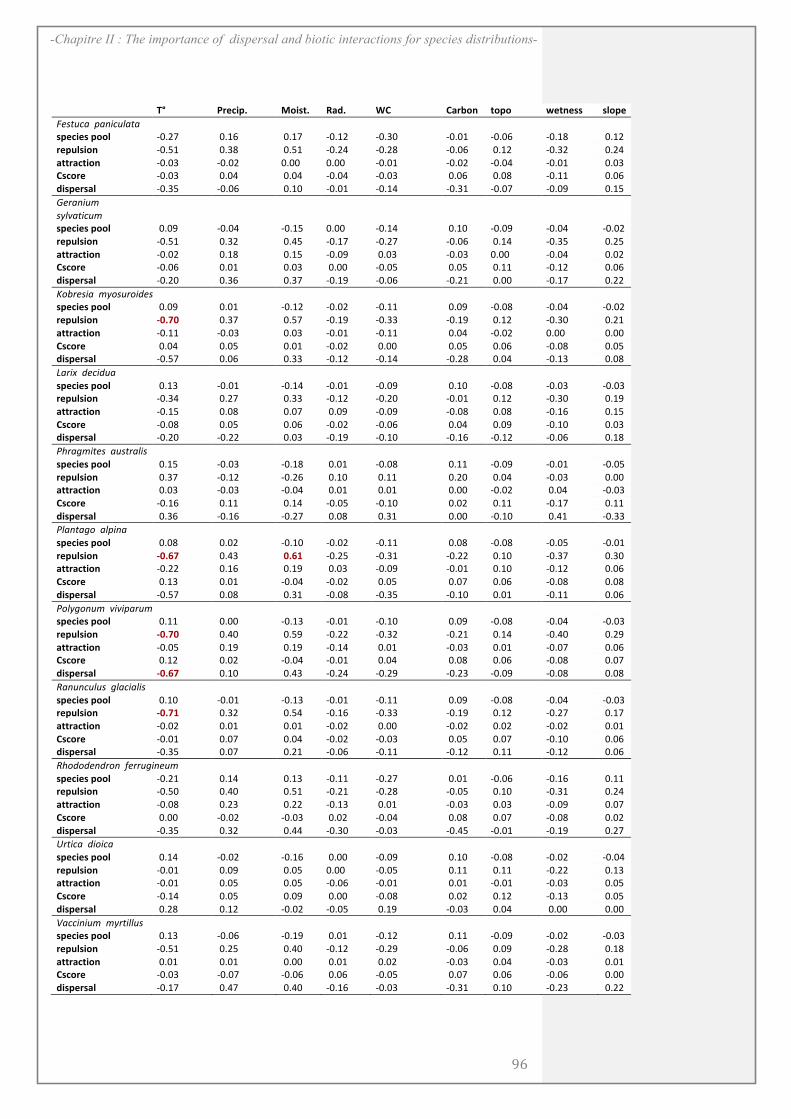
-Chapitre II : The importance of dispersal and biotic interactions for species distributions-

)

=>) ?8('65@) AB6+C@) D&%@) EF) F&8"B$) CB5B) G(C$(++) +*B5()

;$%,*/'&&3')#/*(','&

$ $ $ $ $ $ $ $ $+5('6(+)5BB*) -+,#!$$$$ $+,'&$$$$ $+,'!$$$$ -+,'#$$$$ -+,%+$$$$ -+,+'$$$$ -+,+&$$$$ -+,'*$$$$ $+,'#$$$$

8(5#*+6B$) -+,('$$$$ $+,%*$$$$ $+,('$$$$ -+,#"$$$$ -+,#*$$$$ -+,+&$$$$ $+,'#$$$$ -+,%#$$$$ $+,#"$$$$

&CC8&'C6B$) -+,+%$$$$ -+,+#$$$$ +,++$$$$$$ +,++$$$$$$ -+,+'$$$$ -+,+#$$$$ -+,+"$$$$ -+,+'$$$$ $+,+%$$$$

F+'B8() -+,+%$$$$ $+,+"$$$$ $+,+"$$$$ -+,+"$$$$ -+,+%$$$$ $+,+&$$$$ $+,+*$$$$ -+,''$$$$ $+,+&$$$$

%6+5(8+&*) -+,%($$$$ -+,+&$$$$ $+,'+$$$$ -+,+'$$$$ -+,'"$$$$ -+,%'$$$$ -+,+!$$$$ -+,+)$$$$ $+,'($$$$

<$.')#*0&&

%8(4',#/*0&

$ $ $ $ $ $ $ $ $+5('6(+)5BB*) $+,+)$$$$ -+,+"$$$$ -+,'($$$$ +,++$$$$$$ -+,'"$$$$ $+,'+$$$$ -+,+)$$$$ -+,+"$$$$ -+,+#$$$$

8(5#*+6B$) -+,('$$$$ $+,%#$$$$ $+,"($$$$ -+,'!$$$$ -+,#!$$$$ -+,+&$$$$ $+,'"$$$$ -+,%($$$$ $+,#($$$$

&CC8&'C6B$) -+,+#$$$$ $+,'*$$$$ $+,'($$$$ -+,+)$$$$ $+,+%$$$$ -+,+%$$$$ +,++$$$$$$ -+,+"$$$$ $+,+#$$$$

F+'B8() -+,+&$$$$ $+,+'$$$$ $+,+%$$$$ $+,++$$$$$$ -+,+($$$$ $+,+($$$$ $+,''$$$$ -+,'#$$$$ $+,+&$$$$

%6+5(8+&*) -+,#+$$$$ $+,%&$$$$ $+,%!$$$$ -+,')$$$$ -+,+&$$$$ -+,#'$$$$ $+,++$$$$$$ -+,'!$$$$ $+,##$$$$

=-".$%#'&&08-%*.-#>$%$

$ $ $ $ $ $ $ $+5('6(+)5BB*) $+,+)$$$$ $+,+'$$$$ -+,'#$$$$ -+,+#$$$$ -+,''$$$$ $+,+)$$$$ -+,+*$$$$ -+,+"$$$$ -+,+#$$$$

8(5#*+6B$) I-@H-)))) $+,%!$$$$ $+,(!$$$$ -+,')$$$$ -+,%%$$$$ -+,')$$$$ $+,'#$$$$ -+,%+$$$$ $+,#'$$$$

&CC8&'C6B$) -+,''$$$$ -+,+%$$$$ $+,+%$$$$ -+,+'$$$$ -+,''$$$$ $+,+"$$$$ -+,+#$$$$ +,++$$$$$$ $+,++$$$$$$

F+'B8() $+,+"$$$$ $+,+($$$$ $+,+'$$$$ -+,+#$$$$ $+,++$$$$$$ $+,+($$$$ $+,+&$$$$ -+,+*$$$$ $+,+($$$$

%6+5(8+&*) -+,(!$$$$ $+,+&$$$$ $+,%%$$$$ -+,'#$$$$ -+,'"$$$$ -+,#*$$$$ $+,+"$$$$ -+,'%$$$$ $+,+*$$$$

?'.#2&&>$/#>*'&

$ $ $ $ $ $ $ $ $+5('6(+)5BB*) $+,'%$$$$ -+,+'$$$$ -+,'"$$$$ -+,+'$$$$ -+,+)$$$$ $+,'+$$$$ -+,+*$$$$ -+,+%$$$$ -+,+%$$$$

8(5#*+6B$) -+,%"$$$$ $+,#!$$$$ $+,%%$$$$ -+,'#$$$$ -+,#+$$$$ -+,+'$$$$ $+,'#$$$$ -+,%+$$$$ $+,')$$$$

&CC8&'C6B$) -+,'($$$$ $+,+*$$$$ $+,+!$$$$ $+,+)$$$$ -+,+)$$$$ -+,+*$$$$ $+,+*$$$$ -+,'&$$$$ $+,'($$$$

F+'B8() -+,+*$$$$ $+,+($$$$ $+,+&$$$$ -+,+#$$$$ -+,+&$$$$ $+,+"$$$$ $+,+)$$$$ -+,'+$$$$ $+,+%$$$$

%6+5(8+&*) -+,#+$$$$ -+,##$$$$ $+,+%$$$$ -+,')$$$$ -+,'+$$$$ -+,'&$$$$ -+,'#$$$$ -+,+&$$$$ $+,'*$$$$

@:.'+0#,$%&&'*%,.'(#%&

$ $ $ $ $ $ $ $ $+5('6(+)5BB*) $+,'($$$$ -+,+%$$$$ -+,'*$$$$ $+,+'$$$$ -+,+*$$$$ $+,''$$$$ -+,+)$$$$ -+,+'$$$$ -+,+($$$$

8(5#*+6B$) $+,%!$$$$ -+,'#$$$$ -+,#&$$$$ $+,'+$$$$ $+,''$$$$ $+,#+$$$$ $+,+"$$$$ -+,+%$$$$ $+,++$$$$$$

&CC8&'C6B$) $+,+%$$$$ -+,+%$$$$ -+,+"$$$$ $+,+'$$$$ $+,+'$$$$ $+,++$$$$$$ -+,+#$$$$ $+,+"$$$$ -+,+%$$$$

F+'B8() -+,'&$$$$ $+,''$$$$ $+,'"$$$$ -+,+($$$$ -+,'+$$$$ $+,+#$$$$ $+,''$$$$ -+,'!$$$$ $+,''$$$$

%6+5(8+&*) $+,%&$$$$ -+,'&$$$$ -+,#!$$$$ $+,+*$$$$ $+,%'$$$$ $+,++$$$$$ -+,'+$$$$ $+,"'$$$$ -+,%%$$$$

@('),'+-&&'(3#)'&

$ $ $ $ $ $ $ $ $+5('6(+)5BB*) $+,+*$$$$ $+,+#$$$$ -+,'+$$$$ -+,+#$$$$ -+,''$$$$ $+,+*$$$$ -+,+*$$$$ -+,+($$$$ -+,+'$$$$

8(5#*+6B$) I-@3H)))) $+,"%$$$$ )-@3.)))) -+,#($$$$ -+,%'$$$$ -+,##$$$$ $+,'+$$$$ -+,%!$$$$ $+,%+$$$$

&CC8&'C6B$) -+,##$$$$ $+,'&$$$$ $+,')$$$$ $+,+%$$$$ -+,+)$$$$ -+,+'$$$$ $+,'+$$$$ -+,'#$$$$ $+,+&$$$$

F+'B8() $+,'%$$$$ $+,+'$$$$ -+,+"$$$$ -+,+#$$$$ $+,+($$$$ $+,+!$$$$ $+,+&$$$$ -+,+*$$$$ $+,+*$$$$

%6+5(8+&*) -+,(!$$$$ $+,+*$$$$ $+,%'$$$$ -+,+*$$$$ -+,%($$$$ -+,'+$$$$ $+,+'$$$$ -+,''$$$$ $+,+&$$$$

@-(8+-)*0&&4#4#3'.*0$

$ $ $ $ $ $ $ $+5('6(+)5BB*) $+,''$$$$ $+,++$$$$$$ -+,'%$$$$ -+,+'$$$$ -+,'+$$$$ $+,+)$$$$ -+,+*$$$$ -+,+"$$$$ -+,+%$$$$

8(5#*+6B$) I-@H-)))) $+,"+$$$$ $+,()$$$$ -+,##$$$$ -+,%#$$$$ -+,#'$$$$ $+,'"$$$$ -+,"+$$$$ $+,#)$$$$

&CC8&'C6B$) -+,+($$$$ $+,')$$$$ $+,')$$$$ -+,'"$$$$ $+,+'$$$$ -+,+%$$$$ $+,+'$$$$ -+,+!$$$$ $+,+&$$$$

F+'B8() $+,'#$$$$ $+,+#$$$$ -+,+"$$$$ -+,+'$$$$ $+,+"$$$$ $+,+*$$$$ $+,+&$$$$ -+,+*$$$$ $+,+!$$$$

%6+5(8+&*) I-@3H)))) $+,'+$$$$ $+,"%$$$$ -+,#"$$$$ -+,#)$$$$ -+,#%$$$$ -+,+)$$$$ -+,+*$$$$ $+,+*$$$$

A')*)/*(*%&&+('/#'(#%&

$ $ $ $ $ $ $ $ $+5('6(+)5BB*) $+,'+$$$$ -+,+'$$$$ -+,'%$$$$ -+,+'$$$$ -+,''$$$$ $+,+)$$$$ -+,+*$$$$ -+,+"$$$$ -+,+%$$$$

8(5#*+6B$) I-@H.)))) $+,%#$$$$ $+,("$$$$ -+,'&$$$$ -+,%%$$$$ -+,')$$$$ $+,'#$$$$ -+,#!$$$$ $+,'!$$$$

&CC8&'C6B$) -+,+#$$$$ $+,+'$$$$ $+,+'$$$$ -+,+#$$$$ $+,++$$$$$$ -+,+#$$$$ $+,+#$$$$ -+,+#$$$$ $+,+'$$$$

F+'B8() -+,+'$$$$ $+,+!$$$$ $+,+"$$$$ -+,+#$$$$ -+,+%$$$$ $+,+($$$$ $+,+!$$$$ -+,'+$$$$ $+,+&$$$$

%6+5(8+&*) -+,%($$$$ $+,+!$$$$ $+,#'$$$$ -+,+&$$$$ -+,''$$$$ -+,'#$$$$ $+,''$$$$ -+,'#$$$$ $+,+&$$$$

A:->->$)>.-)&&6$..*+#)$*0$

$ $ $ $ $ $ $ $+5('6(+)5BB*) -+,#'$$$$ $+,'"$$$$ $+,'%$$$$ -+,''$$$$ -+,#!$$$$ $+,+'$$$$ -+,+&$$$$ -+,'&$$$$ $+,''$$$$

8(5#*+6B$) -+,(+$$$$ $+,"+$$$$ $+,('$$$$ -+,#'$$$$ -+,#*$$$$ -+,+($$$$ $+,'+$$$$ -+,%'$$$$ $+,#"$$$$

&CC8&'C6B$) -+,+*$$$$ $+,#%$$$$ $+,##$$$$ -+,'%$$$$ $+,+'$$$$ -+,+%$$$$ $+,+%$$$$ -+,+)$$$$ $+,+!$$$$

F+'B8() $+,++$$$$$$ -+,+#$$$$ -+,+%$$$$ $+,+#$$$$ -+,+"$$$$ $+,+*$$$$ $+,+!$$$$ -+,+*$$$$ $+,+#$$$$

%6+5(8+&*) -+,%($$$$ $+,%#$$$$ $+,""$$$$ -+,%+$$$$ -+,+%$$$$ -+,"($$$$ -+,+'$$$$ -+,')$$$$ $+,#!$$$$

B.,#/'&&>#-#/'&

$ $ $ $ $ $ $ $ $+5('6(+)5BB*) $+,'"$$$$ -+,+#$$$$ -+,'&$$$$ $+,++$$$$$ -+,+)$$$$ $+,'+$$$$ -+,+*$$$$ -+,+#$$$$ -+,+"$$$$

8(5#*+6B$) -+,+'$$$$ $+,+)$$$$ $+,+($$$$ +,++$$$$$$ -+,+($$$$ $+,''$$$$ $+,''$$$$ -+,##$$$$ $+,'%$$$$

&CC8&'C6B$) -+,+'$$$$ $+,+($$$$ $+,+($$$$ -+,+&$$$$ -+,+'$$$$ $+,+'$$$$ -+,+'$$$$ -+,+%$$$$ $+,+($$$$

F+'B8() -+,'"$$$$ $+,+($$$$ $+,+)$$$$ $+,++$$$$$$ -+,+*$$$$ $+,+#$$$$ $+,'#$$$$ -+,'%$$$$ $+,+($$$$

%6+5(8+&*) $+,#*$$$$ $+,'#$$$$ -+,+#$$$$ -+,+($$$$ $+,')$$$$ -+,+%$$$$ $+,+"$$$$ $+,++$$$$$ $+,++$$$$$$

C'//#)#*0&&08.,#((*%&

$ $ $ $ $ $ $ $ $+5('6(+)5BB*) $+,'%$$$$ -+,+&$$$$ -+,')$$$$ $+,+'$$$$ -+,'#$$$$ $+,''$$$$ -+,+)$$$$ -+,+#$$$$ -+,+%$$$$

8(5#*+6B$) -+,('$$$$ $+,#($$$$ $+,"+$$$$ -+,'#$$$$ -+,#)$$$$ -+,+&$$$$ $+,+)$$$$ -+,#*$$$$ $+,'*$$$$

&CC8&'C6B$) $+,+'$$$$ $+,+'$$$$ $+,++$$$$$$ $+,+'$$$$ $+,+#$$$$ -+,+%$$$$ $+,+"$$$$ -+,+%$$$$ $+,+'$$$$

F+'B8() -+,+%$$$$ -+,+!$$$$ -+,+&$$$$ $+,+&$$$$ -+,+($$$$ $+,+!$$$$ $+,+&$$$$ -+,+&$$$$ $+,++$$$$$$

%6+5(8+&*) -+,'!$$$$ $+,"!$$$$ $+,"+$$$$ -+,'&$$$$ -+,+%$$$$ -+,%'$$$$ $+,'+$$$$ -+,#%$$$$ $+,##$$$$

!

!

?$! !

-Chapitre II : The importance of dispersal and biotic interactions for species distributions-

!

!

!

!

76+5(8+&*)'*&++) .) 0) 1) 2) 3) H)

.) ',++$ ',++$ +,!%$ +,*"$ +,)($ +,)*$

0) $ ',++$ +,!%$ +,*"$ +,)($ +,)*$

1) $ $ ',++$ +,)!$ +,**$ +,!!$

2) $ $ $ ',++$ +,)&$ +,*&$

3) $ $ $ $ ',++$ +,)($

H) $ $ $ $

$

',++$

Table II.S5: Sensitivity to

the dispersal distance

class. The table shows

Pearson correlations

between various estimates

of the dispersal index for

Geranium sempervirens.

Each time, we estimated

the dispersal index using

distance parameters from a

different dispersal class (1,

3, 4, 5, 6, and 7).

!

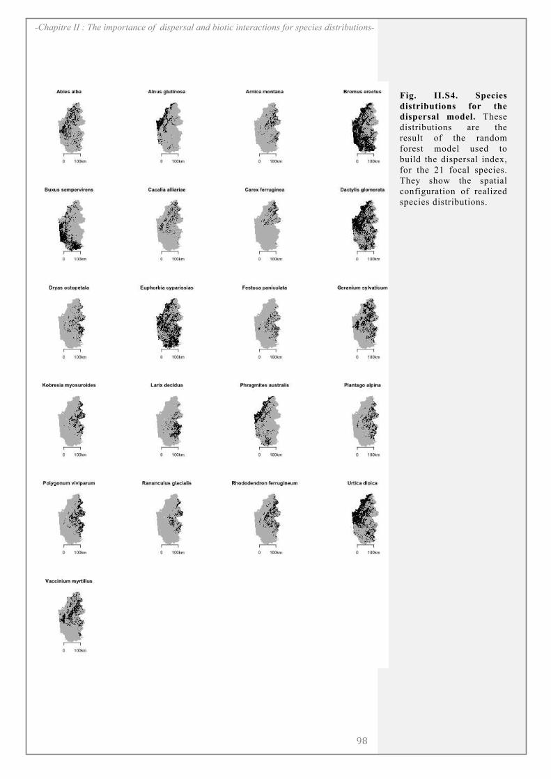
?8!

-Chapitre II : The importance of dispersal and biotic interactions for species distributions-

!

Fig. II.S4. Species

distributions for the

dispersal model. These

distributions are the

result of the random

forest model used to

build the dispersal index,

for the 21 focal species.

They show the spatial

configuration of realized

species distributions.

!

??! !

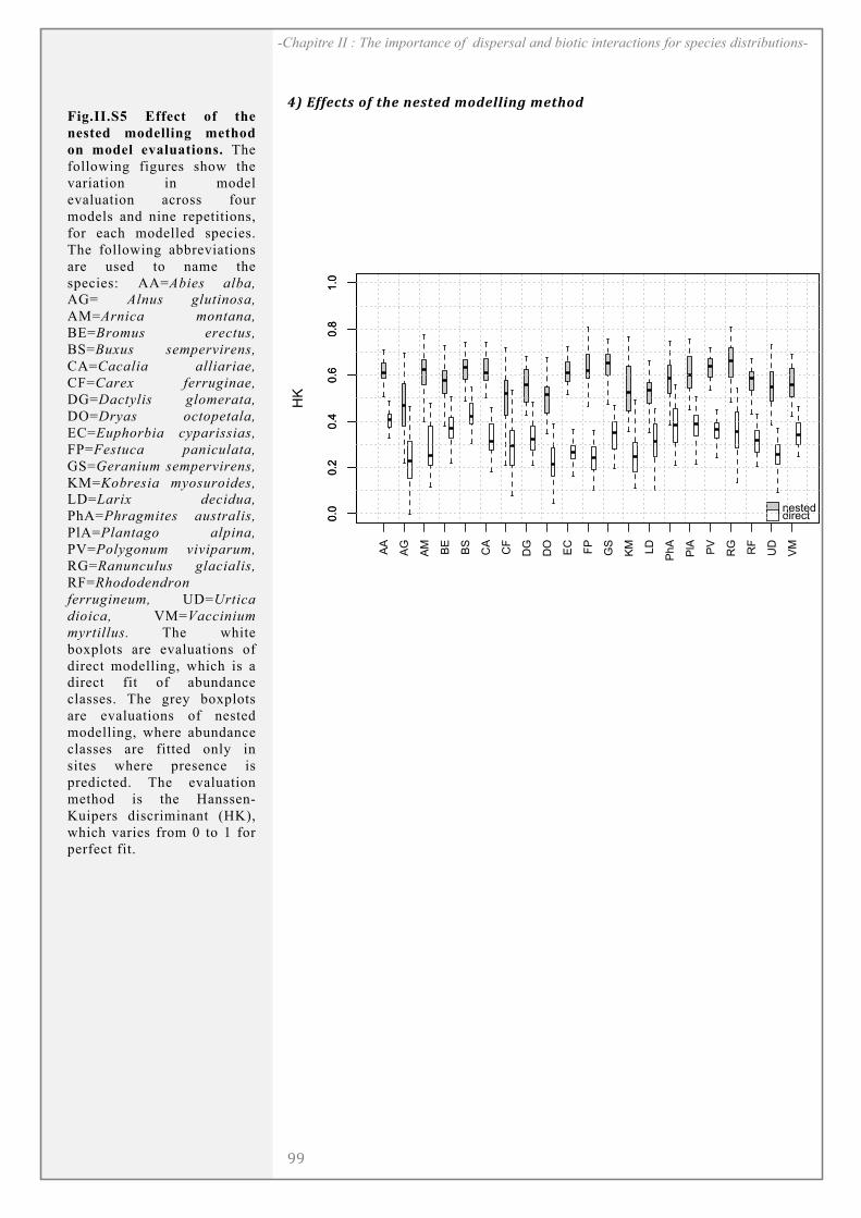
-Chapitre II : The importance of dispersal and biotic interactions for species distributions-

GD)H;;".$,)';)$<")(",$"*)9'*"11&(#)9"$<'*)

!

!

AA

AG

AM

BE

BS

CA

CF

DG

DO

EC

FP

GS

KM

LD

PhA

PlA

PV

RG

RF

UD

VM

0.0

0.2

0.4

0.6

0.8

1.0

HK

0.0

0.2

0.4

0.6

0.8

1.0

nesteddirect

!

)

)

)

)

)

!

Fig.II.S5 Effect of the

nested modelling method

on model evaluations. The

following figures show the

variation in model

evaluation across four

models and nine repetitions,

for each modelled species.

The following abbreviations

are used to name the

species: AA=Abies alba,

AG= Alnus glutinosa,

AM=Arnica montana,

BE=Bromus erectus,

BS=Buxus sempervirens,

CA=Cacalia alliariae,

CF=Carex ferruginae,

DG=Dactylis glomerata,

DO=Dryas octopetala,

EC=Euphorbia cyparissias,

FP=Festuca paniculata,

GS=Geranium sempervirens,

KM=Kobresia myosuroides,

LD=Larix decidua,

PhA=Phragmites australis,

PlA=Plantago alpina,

PV=Polygonum viviparum,

RG=Ranunculus glacialis,

RF=Rhododendron

ferrugineum, UD=Urtica

dioica, VM=Vaccinium

myrtillus. The white

boxplots are evaluations of

direct modelling, which is a

direct fit of abundance

classes. The grey boxplots

are evaluations of nested

modelling, where abundance

classes are fitted only in

sites where presence is

predicted. The evaluation

method is the Hanssen-

Kuipers discriminant (HK),

which varies from 0 to 1 for

perfect fit.

!

!

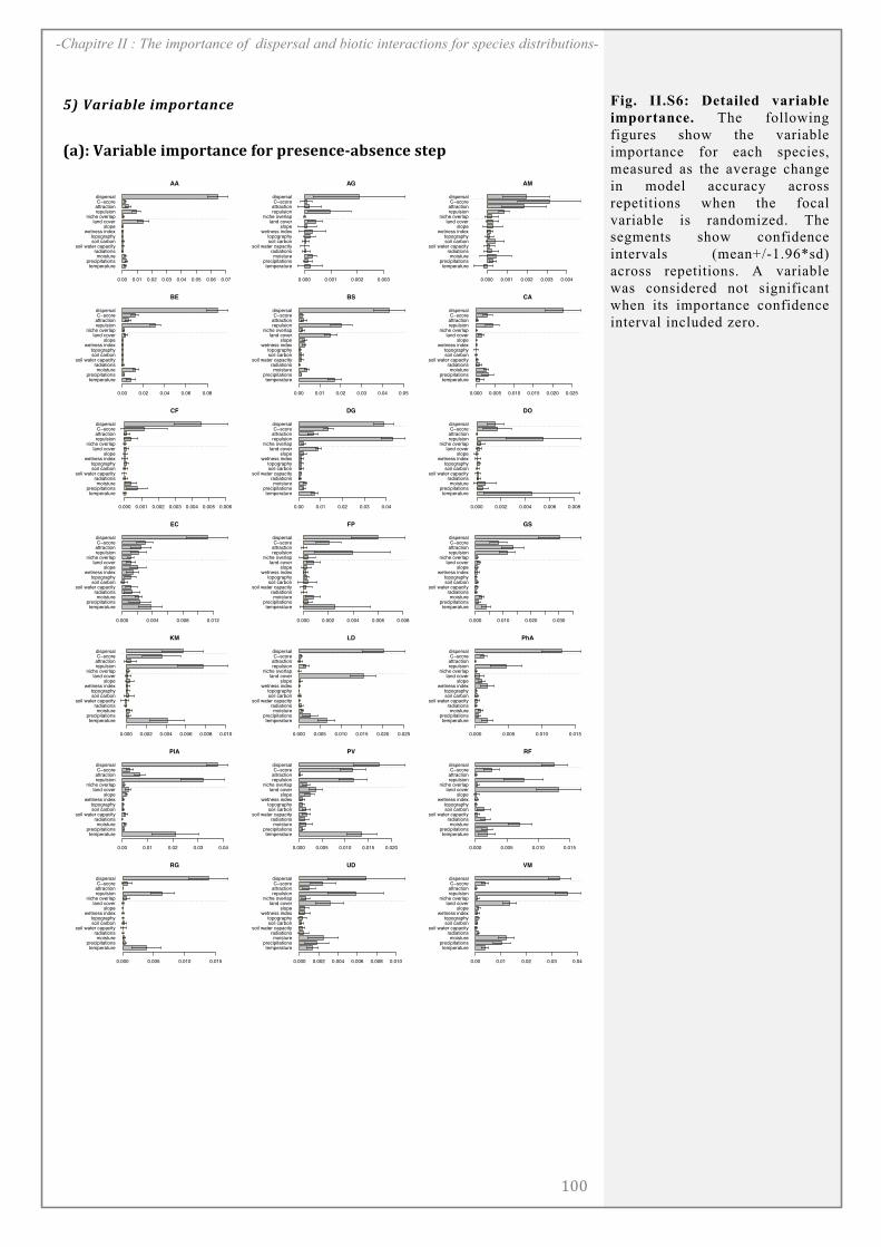
A@@!

-Chapitre II : The importance of dispersal and biotic interactions for species distributions-

ID)!%0&%+1")&93'0$%(.")

8#9:!6#)*#;<%!*$+-),#.(%!=-)!+)%'%.(%>#;'%.(%!',%+!

temperatureprecipitations

moistureradiations

soil water capacitysoil carbontopography

wetness indexslope

land coverniche overlap

repulsionattractionC!scoredispersal

0.00 0.01 0.02 0.03 0.04 0.05 0.06 0.07

AA

temperatureprecipitations

moistureradiations

soil water capacitysoil carbontopography

wetness indexslope

land coverniche overlap

repulsionattractionC!scoredispersal

0.000 0.001 0.002 0.003

AG

temperatureprecipitations

moistureradiations

soil water capacitysoil carbontopography

wetness indexslope

land coverniche overlap

repulsionattractionC!scoredispersal

0.000 0.001 0.002 0.003 0.004

AM

temperatureprecipitations

moistureradiations

soil water capacitysoil carbontopography

wetness indexslope

land coverniche overlap

repulsionattractionC!scoredispersal

0.00 0.02 0.04 0.06 0.08

BE

temperatureprecipitations

moistureradiations

soil water capacitysoil carbontopography

wetness indexslope

land coverniche overlap

repulsionattractionC!scoredispersal

0.00 0.01 0.02 0.03 0.04 0.05

BS

temperatureprecipitations

moistureradiations

soil water capacitysoil carbontopography

wetness indexslope

land coverniche overlap

repulsionattractionC!scoredispersal

0.000 0.005 0.010 0.015 0.020 0.025

CA

temperatureprecipitations

moistureradiations

soil water capacitysoil carbontopography

wetness indexslope

land coverniche overlap

repulsionattractionC!scoredispersal

0.000 0.001 0.002 0.003 0.004 0.005 0.006

CF

temperatureprecipitations

moistureradiations

soil water capacitysoil carbontopography

wetness indexslope

land coverniche overlap

repulsionattractionC!scoredispersal

0.00 0.01 0.02 0.03 0.04

DG

temperatureprecipitations

moistureradiations

soil water capacitysoil carbontopography

wetness indexslope

land coverniche overlap

repulsionattractionC!scoredispersal

0.000 0.002 0.004 0.006 0.008

DO

temperatureprecipitations

moistureradiations

soil water capacitysoil carbontopography

wetness indexslope

land coverniche overlap

repulsionattractionC!scoredispersal

0.000 0.004 0.008 0.012

EC

temperatureprecipitations

moistureradiations

soil water capacitysoil carbontopography

wetness indexslope

land coverniche overlap

repulsionattractionC!scoredispersal

0.000 0.002 0.004 0.006 0.008

FP

temperatureprecipitations

moistureradiations

soil water capacitysoil carbontopography

wetness indexslope

land coverniche overlap

repulsionattractionC!scoredispersal

0.000 0.010 0.020 0.030

GS

temperatureprecipitations

moistureradiations

soil water capacitysoil carbontopography

wetness indexslope

land coverniche overlap

repulsionattractionC!scoredispersal

0.000 0.002 0.004 0.006 0.008 0.010

KM

temperatureprecipitations

moistureradiations

soil water capacitysoil carbontopography

wetness indexslope

land coverniche overlap

repulsionattractionC!scoredispersal

0.000 0.005 0.010 0.015 0.020 0.025

LD

temperatureprecipitations

moistureradiations

soil water capacitysoil carbontopography

wetness indexslope

land coverniche overlap

repulsionattractionC!scoredispersal

0.000 0.005 0.010 0.015

PhA

temperatureprecipitations

moistureradiations

soil water capacitysoil carbontopography

wetness indexslope

land coverniche overlap

repulsionattractionC!scoredispersal

0.00 0.01 0.02 0.03 0.04

PlA

temperatureprecipitations

moistureradiations

soil water capacitysoil carbontopography

wetness indexslope

land coverniche overlap

repulsionattractionC!scoredispersal

0.000 0.005 0.010 0.015 0.020

PV

temperatureprecipitations

moistureradiations

soil water capacitysoil carbontopography

wetness indexslope

land coverniche overlap

repulsionattractionC!scoredispersal

0.000 0.005 0.010 0.015

RF

temperatureprecipitations

moistureradiations

soil water capacitysoil carbontopography

wetness indexslope

land coverniche overlap

repulsionattractionC!scoredispersal

0.000 0.005 0.010 0.015

RG

temperatureprecipitations

moistureradiations

soil water capacitysoil carbontopography

wetness indexslope

land coverniche overlap

repulsionattractionC!scoredispersal

0.000 0.002 0.004 0.006 0.008 0.010

UD

temperatureprecipitations

moistureradiations

soil water capacitysoil carbontopography

wetness indexslope

land coverniche overlap

repulsionattractionC!scoredispersal

0.00 0.01 0.02 0.03 0.04

VM

!

Fig. II.S6: Detailed variable

importance. The following

figures show the variable

importance for each species,

measured as the average change

in model accuracy across

repetitions when the focal

variable is randomized. The

segments show confidence

intervals (mean+/-1.96*sd)

across repetitions. A variable

was considered not significant

when its importance confidence

interval included zero.

!

!

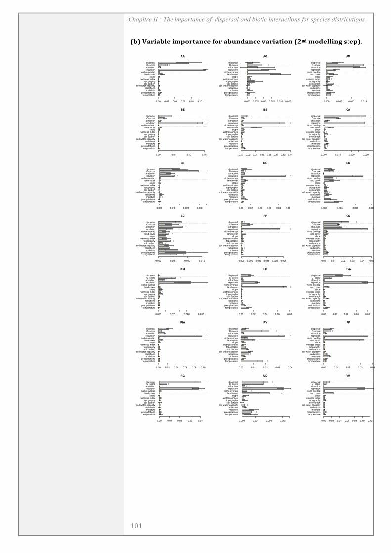
A@A! !

-Chapitre II : The importance of dispersal and biotic interactions for species distributions-

8;9!6#)*#;<%!*$+-),#.(%!=-)!#;0.7#.(%!?#)*#,*-.!8@.7!$-7%<<*.2!',%+93!

temperatureprecipitations

moistureradiations

soil water capacitysoil carbontopography

wetness indexslope

land coverniche overlap

repulsionattractionC!scoredispersal

0.00 0.02 0.04 0.06 0.08 0.10

AA

temperatureprecipitations

moistureradiations

soil water capacitysoil carbontopography

wetness indexslope

land coverniche overlap

repulsionattractionC!scoredispersal

0.000 0.005 0.010 0.015 0.020 0.025

AG

temperatureprecipitations

moistureradiations

soil water capacitysoil carbontopography

wetness indexslope

land coverniche overlap

repulsionattractionC!scoredispersal

0.000 0.005 0.010 0.015

AM

temperatureprecipitations

moistureradiations

soil water capacitysoil carbontopography

wetness indexslope

land coverniche overlap

repulsionattractionC!scoredispersal

0.00 0.05 0.10 0.15

BE

temperatureprecipitations

moistureradiations

soil water capacitysoil carbontopography

wetness indexslope

land coverniche overlap

repulsionattractionC!scoredispersal

0.00 0.02 0.04 0.06 0.08 0.10 0.12 0.14

BS

temperatureprecipitations

moistureradiations

soil water capacitysoil carbontopography

wetness indexslope

land coverniche overlap

repulsionattractionC!scoredispersal

0.000 0.010 0.020 0.030

CA

temperatureprecipitations

moistureradiations

soil water capacitysoil carbontopography

wetness indexslope

land coverniche overlap

repulsionattractionC!scoredispersal

0.000 0.010 0.020 0.030

CF

temperatureprecipitations

moistureradiations

soil water capacitysoil carbontopography

wetness indexslope

land coverniche overlap

repulsionattractionC!scoredispersal

0.00 0.02 0.04 0.06 0.08 0.10

DG

temperatureprecipitations

moistureradiations

soil water capacitysoil carbontopography

wetness indexslope

land coverniche overlap

repulsionattractionC!scoredispersal

0.000 0.005 0.010 0.015

DO

temperatureprecipitations

moistureradiations

soil water capacitysoil carbontopography

wetness indexslope

land coverniche overlap

repulsionattractionC!scoredispersal

0.000 0.005 0.010 0.015

EC

temperatureprecipitations

moistureradiations

soil water capacitysoil carbontopography

wetness indexslope

land coverniche overlap

repulsionattractionC!scoredispersal

0.000 0.005 0.010 0.015 0.020 0.025

FP

temperatureprecipitations

moistureradiations

soil water capacitysoil carbontopography

wetness indexslope

land coverniche overlap

repulsionattractionC!scoredispersal

0.00 0.01 0.02 0.03 0.04 0.05

GS

temperatureprecipitations

moistureradiations

soil water capacitysoil carbontopography

wetness indexslope

land coverniche overlap

repulsionattractionC!scoredispersal

0.000 0.010 0.020 0.030

KM

temperatureprecipitations

moistureradiations

soil water capacitysoil carbontopography

wetness indexslope

land coverniche overlap

repulsionattractionC!scoredispersal

0.00 0.02 0.04 0.06 0.08

LD

temperatureprecipitations

moistureradiations

soil water capacitysoil carbontopography

wetness indexslope

land coverniche overlap

repulsionattractionC!scoredispersal

0.00 0.02 0.04 0.06 0.08

PhA

temperatureprecipitations

moistureradiations

soil water capacitysoil carbontopography

wetness indexslope

land coverniche overlap

repulsionattractionC!scoredispersal

0.00 0.02 0.04 0.06 0.08 0.10

PlA

temperatureprecipitations

moistureradiations

soil water capacitysoil carbontopography

wetness indexslope

land coverniche overlap

repulsionattractionC!scoredispersal

0.00 0.01 0.02 0.03 0.04

PV

temperatureprecipitations

moistureradiations

soil water capacitysoil carbontopography

wetness indexslope

land coverniche overlap

repulsionattractionC!scoredispersal

0.00 0.01 0.02 0.03 0.04

RF

temperatureprecipitations

moistureradiations

soil water capacitysoil carbontopography

wetness indexslope

land coverniche overlap

repulsionattractionC!scoredispersal

0.00 0.01 0.02 0.03 0.04

RG

temperatureprecipitations

moistureradiations

soil water capacitysoil carbontopography

wetness indexslope

land coverniche overlap

repulsionattractionC!scoredispersal

0.000 0.004 0.008 0.012

UD

temperatureprecipitations

moistureradiations

soil water capacitysoil carbontopography

wetness indexslope

land coverniche overlap

repulsionattractionC!scoredispersal

0.00 0.02 0.04 0.06 0.08 0.10 0.12

VM

!

!

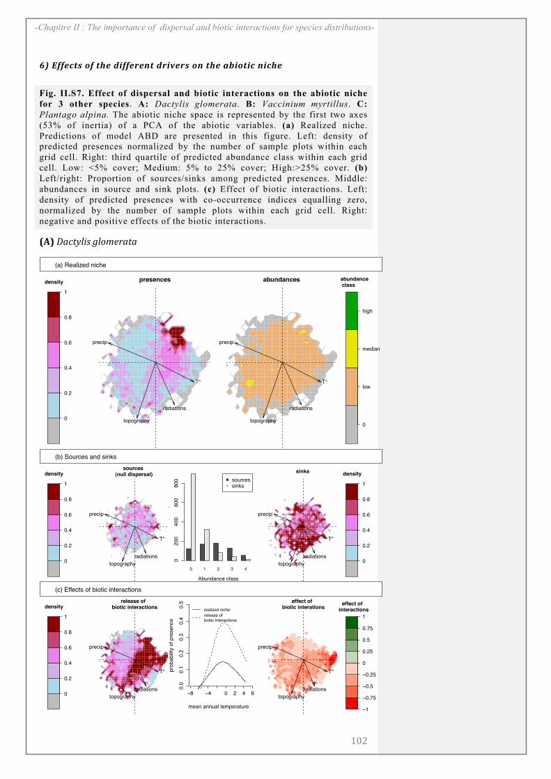
A@C!

-Chapitre II : The importance of dispersal and biotic interactions for species distributions-

!

JD)H;;".$,)';)$<")*&;;"0"($)*0&/"0,)'()$<")%+&'$&.)(&.<")

Fig. II.S7. Effect of dispersal and biotic interactions on the abiotic niche

for 3 other species. A: Dactylis glomerata. B: Vaccinium myrtillus. C:

Plantago alpina. The abiotic niche space is represented by the first two axes

(53% of inertia) of a PCA of the abiotic variables. (a) Realized niche.

Predictions of model ABD are presented in this figure. Left: density of

predicted presences normalized by the number of sample plots within each

grid cell. Right: third quartile of predicted abundance class within each grid

cell. Low: <5% cover; Medium: 5% to 25% cover; High:>25% cover. (b)

Left/right: Proportion of sources/sinks among predicted presences. Middle:

abundances in source and sink plots. (c) Effect of biotic interactions. Left:

density of predicted presences with co-occurrence indices equalling zero,

normalized by the number of sample plots within each grid cell. Right:

negative and positive effects of the biotic interactions.

8A9!!"#$%&'()*&+,-."$")

0

0.2

0.4

0.6

0.8

1

density

0

0.2

0.4

0.6

0.8

1

density

0

0.2

0.4

0.6

0.8

1

density

0

0.2

0.4

0.6

0.8

1

density

0

low

median

high

abundance class

!1

!0.75

!0.5

!0.25

0

0.25

0.5

0.75

1

effect of interactions

(a) Realized niche

T°

precip

radiations

topography

presences

T°

precip

radiations

topography

abundances

(b) Sources and sinks

T°

precip

radiations

topography

sources (null dispersal)

0 1 2 3 4

Abundance class

Fre

quency

0200

400

600

800 sources

sinks

T°

precip

radiations

topography

sinks

(c) Effects of biotic interactions

T°

precip

radiations

topography

release of biotic interactions

0.0

0.1

0.2

0.3

0.4

0.5

mean annual temperature

pro

babili

ty o

f pre

sence

!8 !4 0 2 4 6

realized niche

release of biotic interactions

T°

precip

radiations

topography

effect of biotic interations

!

!

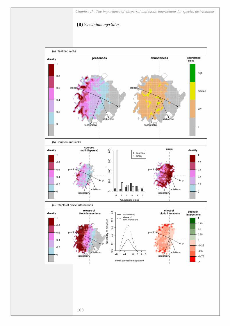
A@D! !

-Chapitre II : The importance of dispersal and biotic interactions for species distributions-

8B9!/"##'0'1,),%.$'&&1()

!

!

0

0.2

0.4

0.6

0.8

1

density

0

0.2

0.4

0.6

0.8

1

density

0

0.2

0.4

0.6

0.8

1

density

0

0.2

0.4

0.6

0.8

1

density

0

low

median

high

abundance class

!1

!0.75

!0.5

!0.25

0

0.25

0.5

0.75

1

effect of interactions

(a) Realized niche

T°

precip

radiations

topography

presences

T°

precip

radiations

topography

abundances

(b) Sources and sinks

T°

precip

radiations

topography

sources (null dispersal)

0 1 2 3 4 5

Abundance class

Fre

quency

0200

400

600

800

sourcessinks

T°

precip

radiations

topography

sinks

(c) Effects of biotic interactions

T°

precip

radiations

topography

release of biotic interactions

0.0

0.1

0.2

0.3

0.4

0.5

mean annual temperature

pro

babili

ty o

f pre

sence

!8 !4 0 2 4 6

realized niche

release of biotic interactions

T°

precip

radiations

topography

effect of biotic interations

!

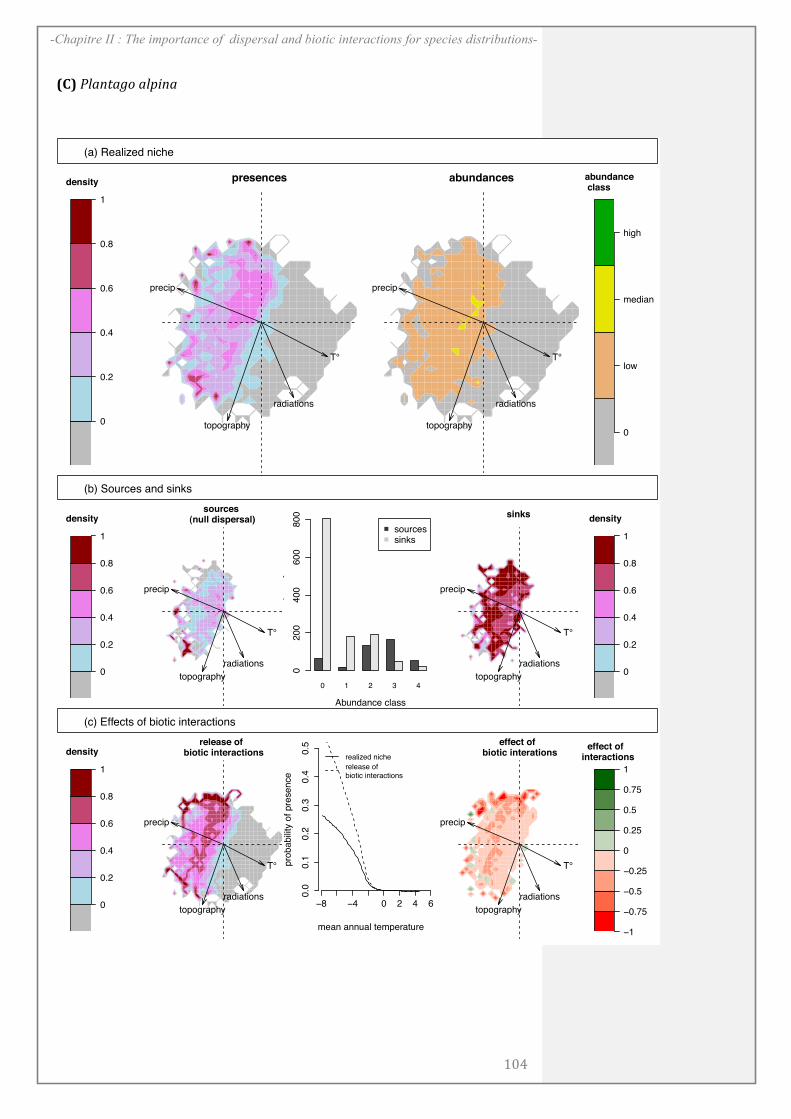
A@E!

-Chapitre II : The importance of dispersal and biotic interactions for species distributions-

8C9!2&"0$"*+)"&3'0")

!

!

!

0

0.2

0.4

0.6

0.8

1

density

0

0.2

0.4

0.6

0.8

1

density

0

0.2

0.4

0.6

0.8

1

density

0

0.2

0.4

0.6

0.8

1

density

0

low

median

high

abundance class

!1

!0.75

!0.5

!0.25

0

0.25

0.5

0.75

1

effect of interactions

(a) Realized niche

T°

precip

radiations

topography

presences

T°

precip

radiations

topography

abundances

(b) Sources and sinks

T°

precip

radiations

topography

sources (null dispersal)

0 1 2 3 4

Abundance class

Fre

quency

0200

400

600

800

sourcessinks

T°

precip

radiations

topography

sinks

(c) Effects of biotic interactions

T°

precip

radiations

topography

release of biotic interactions

0.0

0.1

0.2

0.3

0.4

0.5

mean annual temperature

pro

babili

ty o

f pre

sence

!8 !4 0 2 4 6

realized niche

release of biotic interactions

T°

precip

radiations

topography

effect of biotic interations

-105-

CHAPITRE III:

O P T I M I Z I N G P L A N T F U N C T I O N A L G R O U P S F O R

D Y N A M I C M O D E L S O F B I O D I V E R S I T Y : A T T H E C R O S S RO A D S B E T W E E N

F U N C T I O N A L A N D C O M M U N I T Y E C O L O G Y

Boulangeat, I., Philippe, P., Abdulhak, S., Douzet, R., Garraud, L.,

Lavergne Sébastien, Lavorel S., Van Es, J., Vittoz, P., and Thuiller, W.

Optimizing plant functional groups for dynamic models of biodiversity:

at the crossroads between functional and community ecology. Submitted

to Global Change Biology

- 106 -

-Chapitre III : Plant functional groups for dynamic models of biodiversity-

Abstract

The pace of on-going climate change calls for reliable plant biodiversity

scenarios. Traditional dynamic vegetation models use plant functional types that

are summarized to such an extent that they become meaningless for biodiversity

scenarios. Hybrid dynamic vegetation models of intermediate complexity

(hybrid-DVMs) have recently been developed to address this issue. These

models, at the crossroads between phenomenological and process-based models,

usually focus on well-chosen plant functional groups (PFGs). The challenge is

to build meaningful PFGs that are representative of plant biodiversity, and

consistent with the parameters and processes of hybrid-DVMs. Here, we

propose and test a framework based on few selected traits to define a limited

number of PFGs, which are both representative of the diversity (functional and

taxonomic) of the flora in the Ecrins National Park, and adapted to hybrid-

DVMs. This new classification scheme, together with recent advances in

vegetation modeling, constitutes a step forward for mechanistic biodiversity

modeling.

- 107 -

-Chapitre III : Plant functional groups for dynamic models of biodiversity-

INTRODUCTION

There is compelling evidence of a new biodiversity crisis with species

already facing extinction or shifting their geographic ranges and altering

their phenology in response to climate change (Bellard et al., 2012,

Parmesan, 2006). Effective conservation strategies to counterbalance the

effects of environmental change are critical in protecting biological

diversity, and need to be supported by sound biodiversity scenarios

(Thuiller et al., 2008). This challenge should be met by developing new

tools for modeling biodiversity, which involve multiple species and aim

to understand and predict changes in biological diversity (e.g. taxonomic

or functional diversity). However, despite the efforts of the last ten years,

our capacity to predict the impact of environmental changes on

biodiversity remains limited (Pereira et al., 2010).

In this context, modeling vegetation is crucial given its pivotal role in

determining overall biodiversity and ecosystem functioning. Two

different approaches are traditionally used to model vegetation (Thuiller

et al., 2008). On one hand, phenomenological models (i.e. habitat

distribution models HDMs) can be run on thousands of species, but do

not integrate certain key mechanisms (e.g. co-existence and demographic

mechanisms), which could hamper their use in biodiversity and

ecosystem management at regional scale (Guisan & Thuiller, 2005). On

the other hand, process-based models require much more data and

knowledge (e.g. LANDIS-II, Scheller et al., 2007), so cannot be applied

across large numbers of species. As a consequence, models depicting

whole vegetation dynamics over large spatial extents usually involve just

a dozen broad plant functional types (PFTs), with insufficient detail to

represent plant diversity (e.g. LPJ, Sitch et al., 2003).

Over the last decade hybrid dynamic vegetation models of intermediate

complexity (hybrid-DVMs) have been developed. They usually combine

existing process-based models with habitat suitability models (Gallien et

al., 2010). In order to be run over a large extent, hybrid-DVMs require

the modeling entities of intermediate complexity between species level

characteristics and broad PFT classifications. These newly defined plant

- 108 -

-Chapitre III : Plant functional groups for dynamic models of biodiversity-

functional groups (PFGs) should be constructed in relation to the hybrid-

DVM sub-models, usually habitat suitability models based on abiotic

species niches, and process-based models involving biotic interactions,

dispersal, and successional dynamics. Although these mechanisms are

explicitly included in hybrid-DVMs, the PFTs available for DVMs are

not usually built to model all these ecological mechanisms. For instance,

few classifications have used both the species’ vegetative properties

(representing their dynamic responses to environment) and species’

climatic affinity (but see Laurent et al., 2004).

Quite independently of this field of research, functional ecology has

always searched for associations between abiotic and biotic environment

and species characteristics (Calow, 1987). Significant efforts have been

put into building PFTs to predict grassland (e.g. Lavorel et al., 1998) and

forest ecosystems (e.g. Verheyen et al., 2003) responses to global

changes. These approaches provide a sensible theoretical basis for

selecting relevant species characteristics with which to design new PFGs

(Lavorel et al., 1997, Pausas & Lavorel, 2003). However, moving from

species-level responses to modeling biodiversity dynamics requires the

inclusion of species characteristics involved in community assembly

mechanisms. For instance, Hérault (2007) proposed an emergent group

approach that aimed to both maximize niche differentiation between

groups and functional equivalence within groups.

In this paper, we present a framework for building PFGs for hybrid-

DVMs to represent vegetation dynamics and ecosystem functioning

whilst also depicting biodiversity. We first present the principles of the

framework, its features and adaptation to different regional settings. We

then apply it to regional flora (National Park in the French Alps) and test

its robustness in relation to the aims of biodiversity modeling.

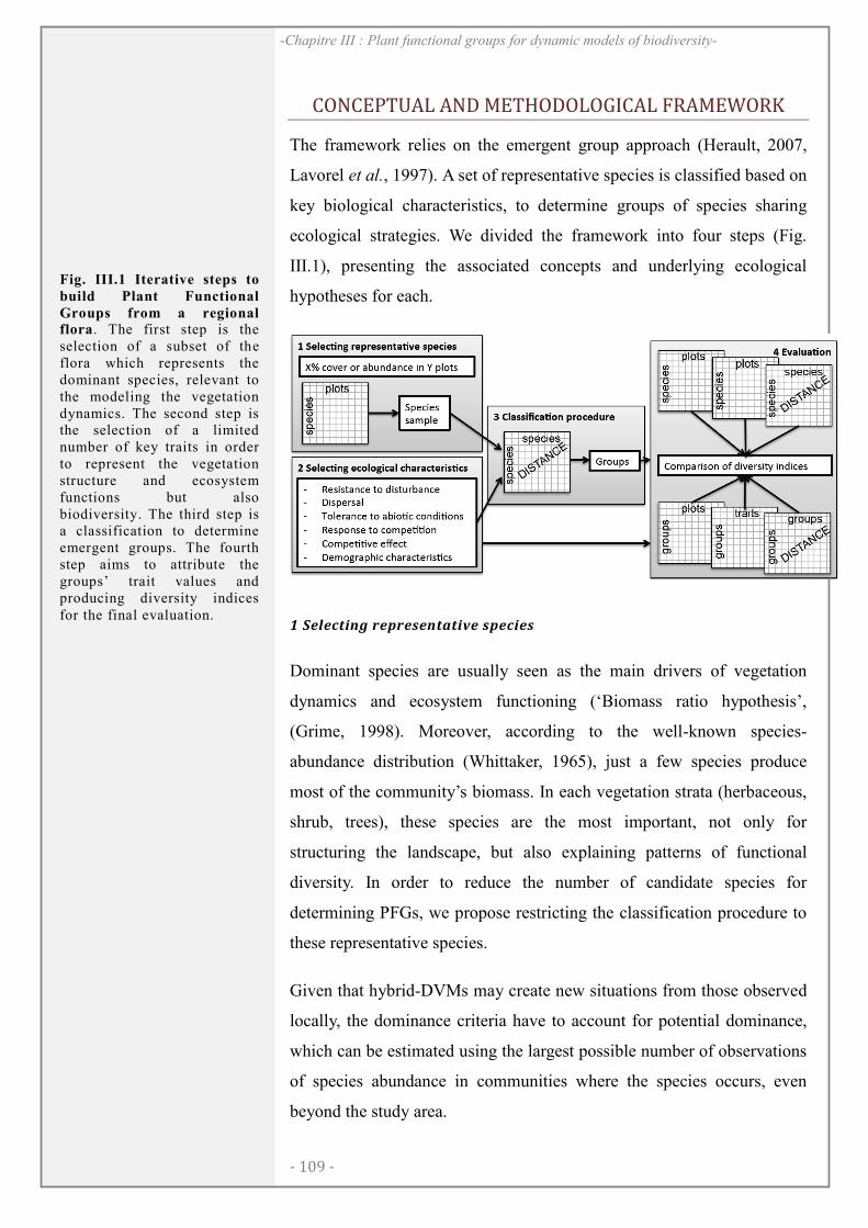
- 109 -

-Chapitre III : Plant functional groups for dynamic models of biodiversity-

CONCEPTUAL AND METHODOLOGICAL FRAMEWORK

The framework relies on the emergent group approach (Herault, 2007,

Lavorel et al., 1997). A set of representative species is classified based on

key biological characteristics, to determine groups of species sharing

ecological strategies. We divided the framework into four steps (Fig.

III.1), presenting the associated concepts and underlying ecological

hypotheses for each.

1 Selecting representative species

Dominant species are usually seen as the main drivers of vegetation

dynamics and ecosystem functioning („Biomass ratio hypothesis’,

(Grime, 1998). Moreover, according to the well-known species-

abundance distribution (Whittaker, 1965), just a few species produce

most of the community’s biomass. In each vegetation strata (herbaceous,

shrub, trees), these species are the most important, not only for

structuring the landscape, but also explaining patterns of functional

diversity. In order to reduce the number of candidate species for

determining PFGs, we propose restricting the classification procedure to

these representative species.

Given that hybrid-DVMs may create new situations from those observed

locally, the dominance criteria have to account for potential dominance,

which can be estimated using the largest possible number of observations

of species abundance in communities where the species occurs, even

beyond the study area.

Fig. III.1 Iterative steps to

build Plant Functional

Groups from a regional flora. The first step is the selection of a subset of the flora which represents the dominant species, relevant to the modeling the vegetation dynamics. The second step is the selection of a limited number of key traits in order to represent the vegetation structure and ecosystem functions but also biodiversity. The third step is a classification to determine emergent groups. The fourth step aims to attribute the groups’ trait values and producing diversity indices for the final evaluation.

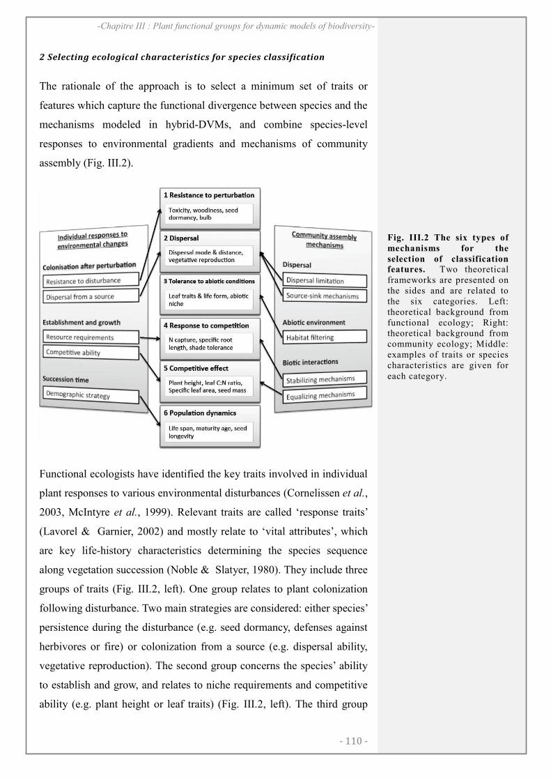
- 110 -

-Chapitre III : Plant functional groups for dynamic models of biodiversity-

2 Selecting ecological characteristics for species classification

The rationale of the approach is to select a minimum set of traits or

features which capture the functional divergence between species and the

mechanisms modeled in hybrid-DVMs, and combine species-level

responses to environmental gradients and mechanisms of community

assembly (Fig. III.2).

Functional ecologists have identified the key traits involved in individual

plant responses to various environmental disturbances (Cornelissen et al.,

2003, McIntyre et al., 1999). Relevant traits are called „response traits’

(Lavorel & Garnier, 2002) and mostly relate to „vital attributes’, which

are key life-history characteristics determining the species sequence

along vegetation succession (Noble & Slatyer, 1980). They include three

groups of traits (Fig. III.2, left). One group relates to plant colonization

following disturbance. Two main strategies are considered: either species’

persistence during the disturbance (e.g. seed dormancy, defenses against

herbivores or fire) or colonization from a source (e.g. dispersal ability,

vegetative reproduction). The second group concerns the species’ ability

to establish and grow, and relates to niche requirements and competitive

ability (e.g. plant height or leaf traits) (Fig. III.2, left). The third group

Fig. III.2 The six types of

mechanisms for the

selection of classification features. Two theoretical frameworks are presented on the sides and are related to the six categories. Left: theoretical background from functional ecology; Right: theoretical background from community ecology; Middle: examples of traits or species characteristics are given for each category.

- 111 -

-Chapitre III : Plant functional groups for dynamic models of biodiversity-

concerns life-history traits influencing species position along ecological

successions (e.g. maturity age, longevity) (Fig. III.2, left).

In order to move from species-level responses to community composition

and biodiversity, relevant traits must also capture community assembly

mechanisms (Suding et al., 2008). In doing so, we directly refer to the

coexistence mechanisms implemented in hybrid-DVMs. Three types of

mechanisms are commonly distinguished in community assembly theory,

namely dispersal, abiotic filtering and biotic interactions (Soberon, 2007)

(Fig. III.2, right). Dispersal mechanisms are usually involved in parts of

hybrid-DVMs to reflect the spatial dynamics (e.g. dispersal limitation

and source-sink mechanisms, Pulliam, 2000) and need to be represented

by traits related to species dispersal distances. However, dispersal

characteristics, although often considered in functional ecology (Herault,

2007, Pausas et al., 2004), have rarely been included in the PFT

classifications available for DVMs. Habitat filtering or the abiotic niche

(Guisan & Zimmermann, 2000) is usually derived from habitat

suitability models in hybrid-DVMs (e.g. Keith et al., 2008, Midgley et

al., 2010). Although climate tolerance is closely related to some

vegetative traits (e.g. leaf size, leaf phenology, life form) (Harrison et al.,

2010), PFGs need to explicitly merge species with similar abiotic niches,

which account for the main abiotic forces of the ecosystem studied (e.g.

climatic and soil variables). Finally, the main advantage of hybrid-DVMs

is their ability to model biotic interactions. For instance, competition for

light is often modeled (e.g. TreeMig, (Lischke et al., 2006), LAMOS,

(Cousins et al., 2003)). More generally speaking, competition for

resources involves two mechanisms (Chesson, 2000a). Firstly, the

equalizing mechanism implies a hierarchy of species according to their

competitive effect (e.g. efficiency in resource capture) and results in the

dominance of the best competitor. Secondly, the stabilizing mechanism

counterbalances the established hierarchy though niche differentiation

(e.g. in space, time or type of resource) and can be considered as a

response to competition. These two mechanisms are the basis for

maintaining species diversity (Chesson, 2000a) and have been shown to

contribute to functional diversity (Navas & Violle, 2009).

- 112 -

-Chapitre III : Plant functional groups for dynamic models of biodiversity-

By combining individual responses to environmental change and

community assembly, we have identified six different features that need

to be homogeneous within PFGs (Fig. III.2): (1) resistance to

disturbance, (2) dispersal, (3) tolerance to abiotic conditions, (4) response

to competition, (5) competitive effect, and (6) demographic

characteristics.

3 Classification procedure

Once traits and species have been selected, the aim is to reduce the

number of modeling entities by defining emergent groups of species

(Herault & Honnay, 2007, Lavorel et al., 1997, Pillar, 1999). This issue

is usually tackled using a clustering algorithm, for instance

agglomerative hierarchical clustering based on a distance matrix

(Herault, 2007, Mouchet et al., 2008, Pillar, 1999). If the plant traits are

continuous, categorical and/or ordinal, the appropriate measure is the

Gower distance, which mixes categorical and quantitative traits (Pavoine

et al., 2005, Podani & Schmera, 2006). The agglomerative hierarchical

clustering algorithm is based on the distance matrix and provides a

dendrogram that is then pruned to form the groups. The choice of the

number of groups can be validated using several metrics (Halkidi et al.,

2001).

4 Assessing PFGs╆ ability to represent biodiversity

The aim here is to evaluate how well the PFG delimitation can capture

and predict biodiversity patterns using hybrid-DVMs. In addition to

taxonomic diversity (TD), functional diversity (FD) is crucial as it

directly relates to ecosystem functioning (Hooper et al., 2005). Two FD

dimensions could be considered. Firstly, functional divergence (FDiv,

Mason et al., 2005) is expected to influence ecosystem processes through

complementary resource use (Tilman et al., 1997). Secondly, the

functional identity of dominant species has been shown to be the most

relevant determinant for some biogeochemical processes (Diaz et al.,

2007, Mokany et al., 2008). It can be measured using the community

- 113 -

-Chapitre III : Plant functional groups for dynamic models of biodiversity-

weighted mean (CWM), which represents the expected trait value for a

random community biomass sample (Garnier et al., 2004).

Many elements are simplified for the purposes of clarification, including

trait selection and the choice of a limited number of groups. It is

therefore important to evaluate the amount of information lost during the

process by comparing species-based to PFG-based functional metrics at

community level. In other words, if PFG-based functional metrics are

able to significantly explain species-based metrics, then the PFG

classification is robust and can be used for biodiversity modeling.

Species-based and PFG-based diversity measures can be compared using

the classification traits, which provide information on the robustness of

the clustering, and using independent traits (not used for the classification

process) providing cross-validation of the trait selection procedure and

testing the robustness of newly built PFGs in capturing the main

ecosystem features.

CASE STUDY: FLORA IN THE ECRINS NATIONAL PARK, FRANCE

We applied the PFG construction framework to flora in the Ecrins

National Park in order to represent the whole vegetation with limited

number of plant functional groups that could be further modeled.

Vegetation database

The Ecrins National Park ('Ecrins' hereafter), in the French Alps (Fig.

III.3), is characterized by mountainous to alpine ecosystems (700m to

4000m a.s.l.) and contains over 2000 plant species (Kerguélen, 1993).

The National Alpine Botanical Conservatory (CBNA) provided the

vegetation-plot database of flora in the surrounding region, including

11,628 community-plots and 1,579 species sampled between 1980 and

2009 (Fig. III.3 and Chapter I). Within each community-plot, species

cover (in its strata) was recorded in six classes (1: less than 1%; 2: 1 to

5%; 3: 5 to 25%; 4: 25 to 50%; 5: 50 to 75%; 6: up to 75%) (Braun-

Blanquet, 1946). We converted these values to relative abundance using

mean cover class percentages.

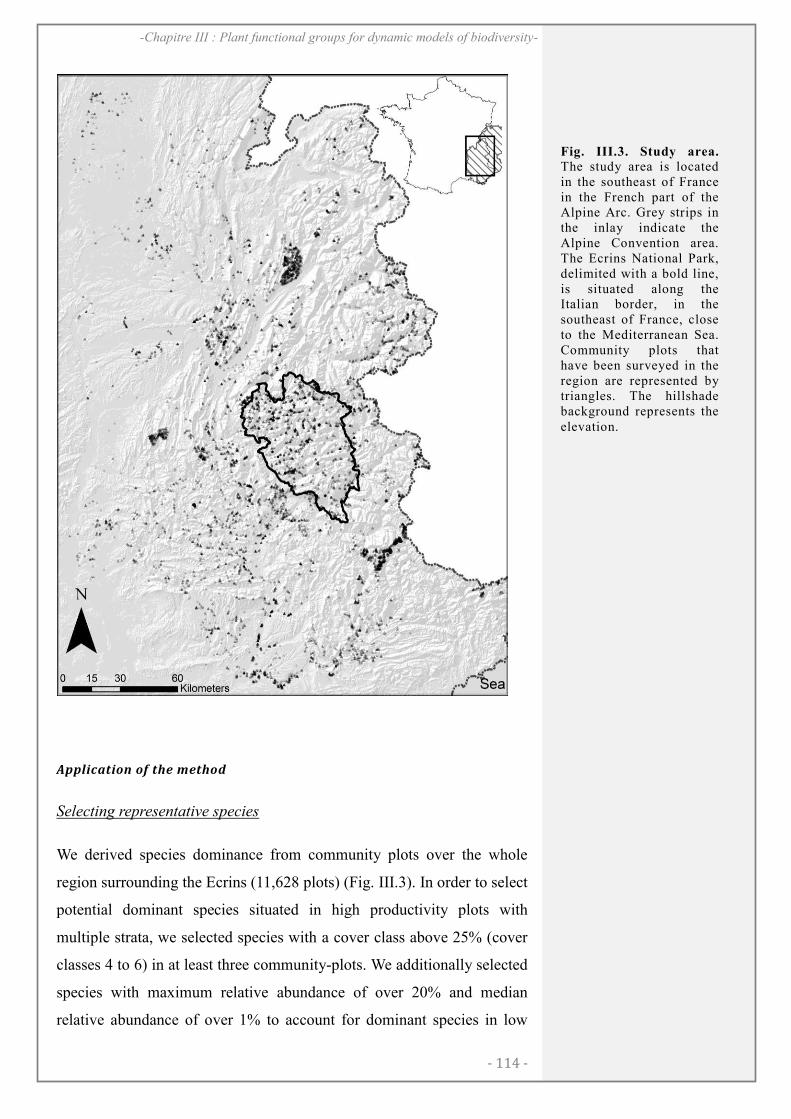
- 114 -

-Chapitre III : Plant functional groups for dynamic models of biodiversity-

Application of the method

Selecting representative species

We derived species dominance from community plots over the whole

region surrounding the Ecrins (11,628 plots) (Fig. III.3). In order to select

potential dominant species situated in high productivity plots with

multiple strata, we selected species with a cover class above 25% (cover

classes 4 to 6) in at least three community-plots. We additionally selected

species with maximum relative abundance of over 20% and median

relative abundance of over 1% to account for dominant species in low

Fig. III.3. Study area. The study area is located in the southeast of France in the French part of the Alpine Arc. Grey strips in the inlay indicate the Alpine Convention area. The Ecrins National Park, delimited with a bold line, is situated along the Italian border, in the southeast of France, close to the Mediterranean Sea. Community plots that have been surveyed in the region are represented by triangles. The hillshade background represents the elevation.

- 115 -

-Chapitre III : Plant functional groups for dynamic models of biodiversity-

productivity plots (e.g. scree, sparse grassland). From this pool of

dominant species we selected the one with a minimum of 10 observations

within the Ecrins. Finally, we retained 412 representative species

representing together at least 70% abundance in 80% of the community-

plots within the Ecrins.

Selecting ecological characteristics for species classification

Given the limited amount of available data at regional scale, we used a

pre-classification based on Raunkiaer’s life forms (Raunkiaer, 1934)

shown to capture a wide range of plant traits related to ecosystem

functioning and ecological succession. For instance, the simple

distinction between woody and non-woody species is related to

competition, litter decomposition and litter production (Dorrepaal, 2007).

As the herbaceous species were mostly hemicryptophytes (261 species),

with few geophytes (34 species) and therophytes (17 species), we only

distinguished three classes, namely phanerophyte, chamaephyte and

herbaceous species. We then chose additional species features to

represent the six previously identified categories (Fig. III.2).

1. Resistance to disturbance: In the Ecrins, the main disturbance being

grazing by domestic stock, we used a palatability index based on pastoral

values (Jouglet, 1999).

2. Dispersal: was represented by distances classes, extracted from Vittoz

& Engler (2007) and additional determination following the same

protocol. This classification is based on the most efficient dispersal

mode, plant height, habitat, seed mass and dispersal attributes (e.g.

wings, pappus). It identifies seven classes that discriminate for a log-

increase of dispersal distances.

3. Tolerance to abiotic conditions: We conducted a Principal Component

Analysis (PCA) on 19 BIOCLIM variables (biologically meaningful

variables derived from temperature and rainfall values, see Supporting

Information Tab. III.S3) (Hutchinson et al., 2009) at 250m resolution in

the Ecrins. Pairwise similarities of species abiotic niches were estimated

- 116 -

-Chapitre III : Plant functional groups for dynamic models of biodiversity-

from the overlap of their observed distributions (D-metric, Schoener,

1970) projected into the first PCA plan (Broennimann et al., 2011).

4. Response to competition: Because competition for light is commonly

modeled (e.g. TreeMig, (Lischke et al., 2006), LAMOS (Cousins et al.,

2003)), we chose to depict response to competition by shade tolerance.

We used an ecological indicator value for species light requirements

(Landolt et al., 2010), adapted to the study region.

5. Competitive effect: Species’ competitive ability was represented by

plant height, which is involved in competition for light (Westoby et al.,

2002) and is also a good proxy for individual biomass (Moles et al.,

2009) thus partly including ecosystem productivity (de Bello et al.,

2010b).

6. Demographic characteristics: These were considered as broadly

included in the pre-classification into life forms representing the main

differences in demographic traits such as individual longevity, age at

maturity and fecundity (Chapin III et al., 1996, Lavorel & Garnier, 2002,

Lavorel et al., 1997). For instance, in our dataset, maturity ages were

clearly different for phanerophytes (11.57 +/- 5.68 years), chamaephytes

(4.36 +/- 2.48 years) and other species (2.77 +/- 0.80 years).

Classification procedure

For each life form group (phanerophyte, chamaephyte, and herbaceous),

we built a distance matrix using Gower’s formula (Gower, 1971).

Dominant species with missing data were removed, which restricted the

set to 290 species representing together at least 70% abundance in 60%

of the Ecrins’ community-plots. The total pairwise distance between

species x and species y was:

D(x, y) = (1/5).( |Hx– Hy|/(Hmax-Hmin) + |Lx-Ly|/NL + |Dx-Dy|/ND + |Px-Py|/NP + (1-O(x,y)) )

where H is plant height (squared-transformed), L light class, D dispersal

class (exponentially-transformed), P palatability class, O climatic overlap

(Schoener’s D metric) and Nt the number of classes for trait t. We used

the Unweighted Pair Group Method with Arithmetic Mean clustering

- 117 -

-Chapitre III : Plant functional groups for dynamic models of biodiversity-

algorithm (UPGMA, Kaufman & Rousseeuw, 1990), as it has been

shown to distort the distance matrix less than other methods (Mouchet et

al., 2008). We used the Dunn index, the R-squared (Halkidi et al., 2001),

the index of Calinski & Harabasz (Calinski & Harabasz, 1974) and the

average silhouette (Kaufman & Rousseeuw, 1990) to choose the number

of groups.

The classification identified height phanerophyte groups (P1 to P8), six

chamaephyte groups (C1 to C6) and ten herbaceous groups (H1 to H10)

(see Supporting Information Fig. III.S1 and Tab. III.S1). Phanerophyte

groups separated pioneer trees (e.g. Larix decidua P4, and Betula alba

P8) from climax trees for various types of climate (e.g. external alps P5,

internal alps P6), intermediate forests (e.g. Pinus cembra P1, Populus

tremula P2) and subordinate trees (e.g. Acer opalus P7, Fraxinus

excelsior P3).

Chamaephyte groups distinguished between shrubs (e.g. Alnus

alnobetula C4), dwarf shrubs (e.g. Vaccinium myrtillus C6, Calluna

vulgaris C5), cushion plants (e.g. Silene acaulis C3) and other

chamaephytes (e.g. Teucrium chamaedrys C1, Cerastium uniflorum C2).

Some of these groups were found in mountainous to subalpine

ecosystems (C1, C4, C5) and other modeled alpine ecosystems (C2, C3,

C6).

Among the ten herbaceous groups, one represented understorey species

(Prenanthes purpurea H4). Two other groups represented mountainous to

subalpine herbaceous, separated by their dispersal abilities either over

short (Cacalia alliariae H6) or long distances (Arrhenatherum elatius

H3). Four groups were mostly found in subalpine ecosystems and

differed in terms of their dispersal abilities, palatability or climatic

preferences (H2, H5, H7, and H10). Finally, three groups formed alpine

meadows with different grazing tolerance, ranging from high (e.g.

Nardus stricta H9, Festuca quadriflora H1) to low palatability (Cirsium

spinosissimum H8).

- 118 -

-Chapitre III : Plant functional groups for dynamic models of biodiversity-

Assessing PFGs’ ability to represent biodiversity

We tested the resulting PFGs’ ability to represent plant diversity by

comparing species-based measurements (also including rare species

originally excluded from the classification procedure) to PFG-based

measurements of diversity. Using the representative species associated to

each PFG we built PFG communities, with each PFG having cover class

equal to the highest cover class of contributing species in each plot,

followed by a standardization to estimate the PFGs’ relative abundance.

Concerning functional diversity, we selected several sets of traits

reasonably represented in our database (i.e. involving at least 657

species, see Tab. III.1).

The seven supplementary traits (woodiness, mowing tolerance, dispersal

vector, seed mass, leaf area, specific leaf area, and leaf dry matter

content) were extracted from the database ANDROSACE (Thuiller et al.

unpublished, see Supporting Information Tab. III.S3). We attributed trait

values to each PFG after removing outlier species (i.e. with mean

distances to other species of the group falling outside of the 95% left-

handed confidence interval) (see Supporting Information Fig. III.S2 and

Tab. III.S2).

We computed different measures of biodiversity at community scale for

the 1,902 Ecrins community plots sampled, and for the 1,128 correctly

represented (i.e. where PFGs represent at least 70% of plot abundance).

First, we computed the Community Weighted Mean (CWM) for plant

height and two independent traits (i.e. not used to build PFGs), namely

seed mass and mowing tolerance. Secondly, we used Rao Quadratic

entropy as a common framework for taxonomic diversity and functional

divergence (de Bello et al., 2010a). We computed functional divergence

for classification traits and for independent traits. In addition, we

computed functional divergence using traits of the LHS scheme of

ecological strategies, as proposed by Westoby (1998), since they are

intended to represent the main inter-specific differences in ecological

strategies.

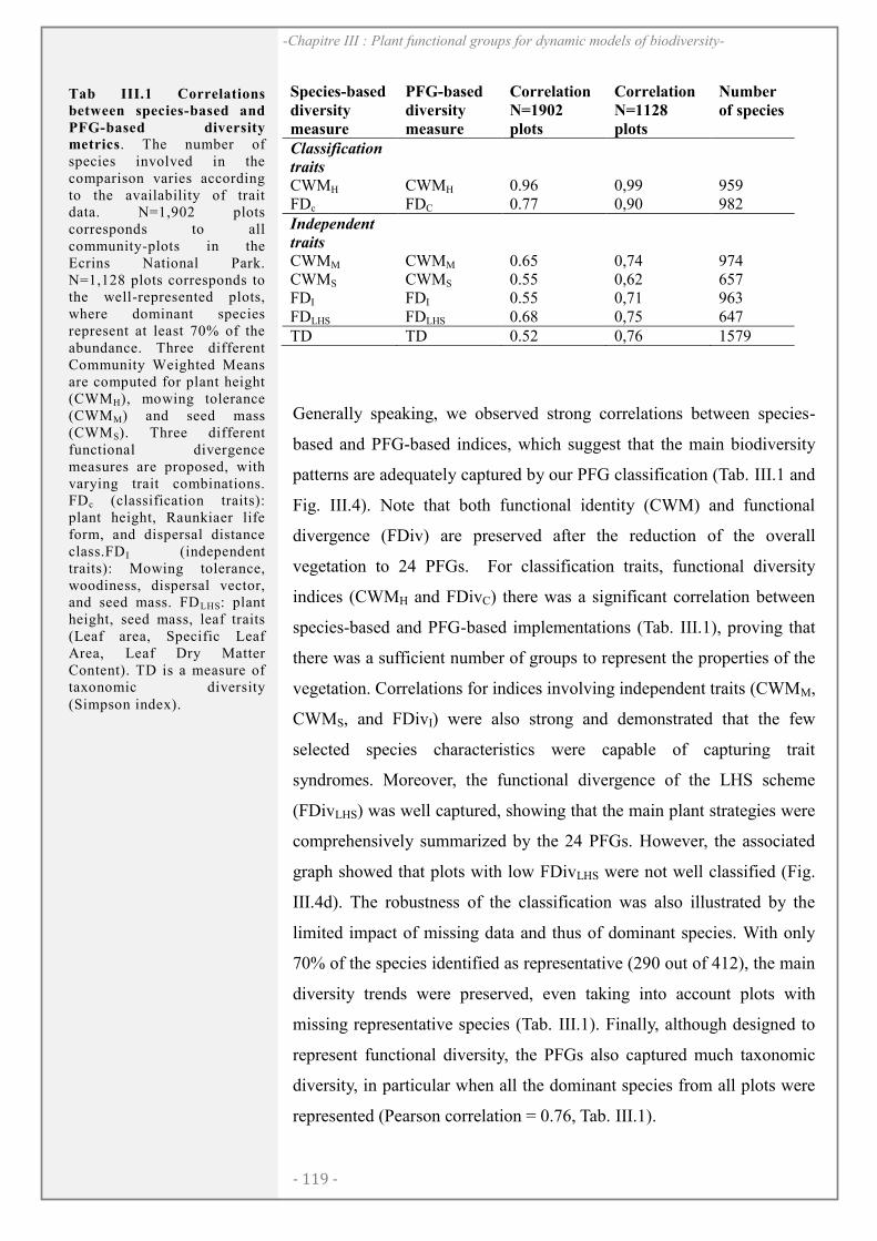
- 119 -

-Chapitre III : Plant functional groups for dynamic models of biodiversity-

Species-based

diversity

measure

PFG-based

diversity

measure

Correlation

N=1902

plots

Correlation

N=1128

plots

Number

of species

Classification

traits

CWMH CWMH 0.96 0,99 959 FDc FDC 0.77 0,90 982 Independent

traits

CWMM CWMM 0.65 0,74 974 CWMS CWMS 0.55 0,62 657 FDI FDI 0.55 0,71 963 FDLHS FDLHS 0.68 0,75 647 TD TD 0.52 0,76 1579

Generally speaking, we observed strong correlations between species-

based and PFG-based indices, which suggest that the main biodiversity

patterns are adequately captured by our PFG classification (Tab. III.1 and

Fig. III.4). Note that both functional identity (CWM) and functional

divergence (FDiv) are preserved after the reduction of the overall

vegetation to 24 PFGs. For classification traits, functional diversity

indices (CWMH and FDivC) there was a significant correlation between

species-based and PFG-based implementations (Tab. III.1), proving that

there was a sufficient number of groups to represent the properties of the

vegetation. Correlations for indices involving independent traits (CWMM,

CWMS, and FDivI) were also strong and demonstrated that the few

selected species characteristics were capable of capturing trait

syndromes. Moreover, the functional divergence of the LHS scheme

(FDivLHS) was well captured, showing that the main plant strategies were

comprehensively summarized by the 24 PFGs. However, the associated

graph showed that plots with low FDivLHS were not well classified (Fig.

III.4d). The robustness of the classification was also illustrated by the

limited impact of missing data and thus of dominant species. With only

70% of the species identified as representative (290 out of 412), the main

diversity trends were preserved, even taking into account plots with

missing representative species (Tab. III.1). Finally, although designed to

represent functional diversity, the PFGs also captured much taxonomic

diversity, in particular when all the dominant species from all plots were

represented (Pearson correlation = 0.76, Tab. III.1).

Tab III.1 Correlations

between species-based and

PFG-based diversity metrics. The number of species involved in the comparison varies according to the availability of trait data. N=1,902 plots corresponds to all community-plots in the Ecrins National Park. N=1,128 plots corresponds to the well-represented plots, where dominant species represent at least 70% of the abundance. Three different Community Weighted Means are computed for plant height (CWMH), mowing tolerance (CWMM) and seed mass (CWMS). Three different functional divergence measures are proposed, with varying trait combinations. FDc (classification traits): plant height, Raunkiaer life form, and dispersal distance class.FD I (independent traits): Mowing tolerance, woodiness, dispersal vector, and seed mass. FDLHS: plant height, seed mass, leaf traits (Leaf area, Specific Leaf Area, Leaf Dry Matter Content). TD is a measure of taxonomic diversity (Simpson index).

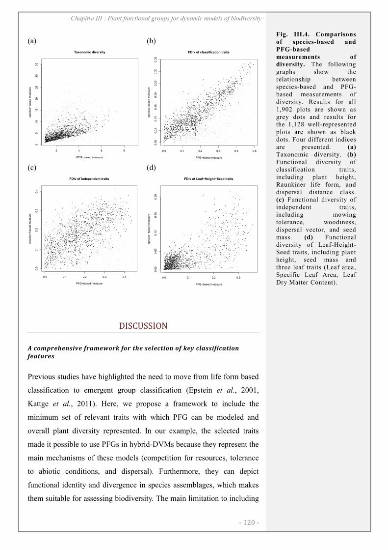
- 120 -

-Chapitre III : Plant functional groups for dynamic models of biodiversity-

(a) (b)

ズズ

ズズ

ズ

ズ

ズ

ズズ

ズズ ズ

ズ

ズ

ズズ

ズ

ズ

ズ

ズ

ズ

ズ

ズズ

ズ ズ

ズズ

ズズ

ズ

ズ ズズ

ズ

ズ

ズ

ズズ ズズズ

ズ

ズ ズズズ

ズ

ズ

ズ

ズ

ズ

ズ

ズ

ズ

ズズ

ズ

ズ

ズ

ズ

ズ

ズ

ズズズズ

ズ

ズ

ズ

ズズ

ズ

ズ

ズ ズ

ズズ

ズ

ズ

ズ

ズ

ズ

ズ

ズ

ズズ

ズ

ズズ

ズ

ズズ

ズ

ズ

ズ

ズ

ズ

ズ

ズ

ズ

ズ

ズ

ズ

ズ

ズ

ズ

ズ

ズ

ズ

ズ

ズ

ズ

ズ

ズ

ズ

ズ

ズ

ズ

ズ

ズ

ズ

ズ

ズ

ズ

ズ

ズ

ズ

ズ

ズ

ズズ

ズ

ズ

ズ

ズ

ズ

ズ

ズ

ズ

ズ

ズ

ズ

ズズ

ズ

ズ

ズ

ズ

ズ

ズ

ズ

ズ

ズ

ズ

ズ

ズ

ズ

ズ

ズ

ズズ

ズ

ズ

ズ

ズ

ズ

ズ

ズ

ズ

ズ

ズ

ズ

ズ

ズ

ズ

ズ

ズ

ズズ

ズ

ズズ

ズ

ズ

ズ

ズ

ズ

ズ

ズ

ズ

ズ

ズ

ズ

ズズ

ズ

ズズ

ズ

ズ

ズ

ズズ

ズズ

ズズ

ズ

ズズ

ズ

ズ

ズ

ズ

ズズ

ズ

ズ

ズ

ズズ ズ

ズ

ズズ ズ

ズ ズ

ズズ

ズ

ズ

ズ

ズ

ズズ

ズ

ズ ズズ

ズズ

ズ

ズズズ

ズ ズ ズズ

ズズ

ズ

ズ

ズ

ズ

ズ

ズ

ズズズ

ズ

ズ

ズ

ズ

ズ

ズ

ズ

ズズ

ズズ

ズ

ズズ ズ

ズ

ズズ

ズ

ズ

ズ

ズ

ズ

ズ

ズ

ズズ ズ

ズ

ズ

ズズ

ズ

ズ

ズ

ズ

ズ ズ

ズ

ズ

ズ

ズ

ズ

ズ

ズ

ズ

ズ

ズ

ズ

ズ

ズ

ズズ

ズ

ズ

ズ

ズ ズ

ズ

ズズ

ズ

ズズ

ズ

ズ

ズ

ズ

ズ

ズ ズズ

ズ

ズ

ズ ズズ

ズ

ズ

ズ

ズ ズ

ズ

ズ

ズ

ズズズズ

ズズ

ズ

ズ

ズ

ズ

ズ

ズ

ズ

ズ

ズズズ ズ

ズ

ズ

ズズ

ズ

ズ ズ

ズズ

ズ

ズズ ズ

ズ

ズ

ズ

ズ

ズズ

ズ

ズ

ズズ

ズ

ズズ ズ

ズ

ズ

ズ

ズ

ズズ

ズズズ

ズ

ズ

ズ

ズ

ズ

ズ

ズ

ズ

ズ

ズ

ズ

ズ

ズ

ズ

ズズ

ズ

ズ

ズ

ズ

ズ

ズ

ズ

ズ

ズ ズ

ズ

ズ

ズ

ズズ

ズ

ズ

ズ

ズ

ズ

ズ

ズズ

ズ

ズ

ズ

ズ

ズズ

ズズズ

ズ

ズ

ズズ

ズ

ズ

ズ

ズズ ズ

ズ

ズズ

ズ

ズズ

ズ

ズズ

ズズズ

ズ

ズ

ズズ ズズ

ズズ

ズ

ズ

ズ

ズズズ

ズ

ズ

ズズ

ズ

ズズ

ズ

ズ ズ

ズ

ズ

ズズ

ズズ

ズ

ズ

ズ

ズ

ズ

ズズ

ズ

ズ

ズ

ズ ズ

ズ

ズ

ズ

ズ

ズズ

ズ

ズ

ズ

ズズ

ズ

ズ

ズ

ズ

ズ

ズ ズ

ズ

ズ

ズ

ズ

ズ

ズ

ズ

ズズ

ズ

ズ

ズ

ズ

ズ

ズ

ズ

ズ

ズ

ズ

ズズズ

ズズ ズ ズ

ズ

ズズズ

ズ

ズ

ズ

ズ

ズ

ズ

ズズ

ズ

ズ

ズズ ズ

ズ

ズズ

ズ

ズ

ズ

ズ

ズ

ズ

ズズ

ズ

ズ

ズ

ズ

ズズ

ズ

ズ

ズ

ズズ

ズ

ズ ズ

ズ

ズ

ズ

ズ

ズズ

ズ

ズ

ズズ

ズ

ズ

ズ

ズ

ズ

ズズズ

ズ

ズ

ズ

ズズ

ズズ

ズズ

ズズ

ズ ズ

ズ

ズ ズ

ズ

ズズ

ズ

ズ

ズ

ズ

ズズ ズ

ズ

ズズ

ズ

ズ

ズ

ズ

ズ

ズ

ズ

ズ

ズ

ズズ

ズ

ズ

ズ

ズ

ズズ

ズ

ズ

ズ

ズ

ズ

ズ

ズズ

ズ

ズ

ズ

ズ

ズ

ズ

ズ

ズズ

ズズ

ズ

ズ

ズ

ズ

ズ

ズ ズ

ズズ

ズ

ズ

ズズ

ズズ

ズズ

ズズズ

ズズ

ズ

ズ

ズズ

ズ

ズ

ズズ

ズズ

ズ

ズズ

ズズズ

ズ

ズ

ズ

ズ

ズ

ズズ

ズ

ズ

ズ

ズズ

ズ

ズズ ズズ ズ ズ

ズ

ズズ

ズ ズ

ズズ

ズ

ズズ

ズ

ズズ

ズ

ズ

ズ

ズ

ズズ

ズ

ズズ

ズ

ズズ

ズ

ズ

ズズ

ズズズ

ズズ

ズ

ズズ ズ

ズ

ズズ

ズズ

ズズズ

ズ ズズ

ズ

ズ

ズ

ズズ

ズ

ズ

ズズ ズ

ズ

ズズ ズ

ズ

ズズ

ズズ

ズズ

ズ

ズ

ズ

ズ

ズ

ズ

ズ

ズ

ズ

ズ

ズ

ズ

ズ

ズ

ズズ

ズ

ズズ

ズ

ズズ

ズ

ズ ズ

ズ

ズ

ズズ

ズ

ズ

ズズ

ズズズ

ズ

ズ

ズ

ズ

ズズ

ズ

ズ

ズ

ズ

ズ

ズ

ズ

ズ

ズ

ズズ

ズ

ズ

ズ

ズズ

ズ

ズ

ズズ

ズ

ズ

ズ

ズ

ズ

ズ

ズ

ズ

ズ

ズ

ズ

ズ

ズ

ズズ

ズ

ズ

ズ

ズズ

ズ

ズ

ズ

ズ

ズズ

ズ

ズ

ズ

ズ

ズズ

ズ

ズ

ズ ズ

ズズズ ズ

ズ

ズズ

ズ

ズ

ズ

ズ

ズ

ズ

ズ

ズ

ズ

ズ

ズ

ズ

ズズ

ズズ

ズ

ズ

ズ

ズ

ズ

ズ

ズ ズ

ズズ

ズ

ズ

ズ

ズズ

ズ

ズズ

ズ

ズ ズ

ズ

ズ

ズ ズズ

ズ

ズ

ズズ

ズ

ズ

ズ

ズズ

ズズ ズ

ズズ

ズ

ズ

ズ

ズ

ズ

ズ

ズ

ズ

ズ

ズ

ズ

ズ

ズ

ズ

ズ

ズ

ズズ

ズズ

ズズ

ズ

ズ

ズ

ズズ

ズズ

ズ

ズズ ズ

ズ

ズ

ズ

ズ

ズズ

ズ

ズ

ズズ

ズ

ズ

ズ

ズ

ズ

ズ

ズ

ズ ズ

ズ

ズズ

ズ

ズ

ズ

ズ

ズ

ズ

ズ

ズ

ズ

ズ

ズ

ズ

ズ

ズ

ズ

ズ

ズ

ズ

ズ

ズ

ズ

ズ

ズ

ズ

ズ

ズ

ズ

ズズ

ズズ

ズ

ズ

ズ

ズ

ズ

ズ

ズ

ズ

ズ

ズ

ズ

ズ

ズ

ズ

ズズ

ズ

ズ

ズ

ズ

ズ

ズ

ズ

ズ

ズ

ズ

ズズ

ズズ

ズ

ズ

ズ

ズ

ズ

ズ

ズ

ズ

ズ

ズズ

ズ

ズ

ズ

ズ

ズ

ズ

ズ

ズ

ズ

ズ

ズ

ズ

ズ

ズ

ズ

ズ

ズ

ズ

ズズ

ズ

ズ

ズ

ズ

ズ

ズ

ズ

ズ ズズ

ズ

ズ

ズ

ズ

ズ

ズ

ズ

ズ

ズ

ズズ

ズ

ズ

ズ

ズ

ズズ ズ

ズ

ズ

ズ ズ

ズズ

ズ

ズズ

ズズズ

ズズ

ズ

ズ ズズ

ズ

ズ

ズズ

ズ

ズ

ズ

ズ

ズ

ズ

ズズズ

ズ

ズ

ズ

ズ

ズ

ズ

ズ

ズ

ズ

ズ

ズズ

ズ

ズズズズ

ズ

ズ

ズ

ズ ズ

ズズ

ズ

ズ

ズズ

ズ

ズ

ズ

ズ

ズ

ズ

ズ

ズ

ズ

ズズ

ズ

ズズ

ズ ズ

ズ

ズ ズ

ズ ズ

ズ

ズ ズズ

ズズ

ズズ

ズ

ズ

ズ

ズズ

ズズ

ズズ

ズ

ズズ ズ

ズ

ズ

ズ

ズ

ズズ

ズ

ズズ

ズ

ズ

ズズ

ズ

ズ

ズ

ズズ

ズ ズ

ズズ

ズ

ズ

ズ

ズズ

ズ

ズ

ズ

ズ

ズズ

ズ ズ

ズ ズズ

ズ

ズ

ズ

ズ

ズ

ズ

ズ

ズ

ズズ

ズ

ズ

ズ

ズ

ズ

ズズ

ズ

ズズ

ズ

ズ

ズ

ズ

ズ

ズ

ズ

ズズ

ズズ

ズ

ズズ

ズ ズ

ズ

ズ

ズズ

ズズ

ズ

ズ

ズ

ズズ

ズ

ズ

ズ

ズ

ズ

ズ

ズ

ズ

ズ

ズ

ズ

ズ ズズ

ズ

ズ

ズ

ズ

ズ

ズ

ズ

ズ

ズ

ズ

ズ

ズ ズ

ズ

ズ

ズ

ズ

ズ

ズズ

ズ

ズ ズズ

ズ

ズ

ズ

ズ

ズ

ズズ

ズ

ズ

ズ

ズ

ズ

ズ

ズ

ズズ

ズ

ズ

ズ

ズ

ズズ

ズ

ズ

ズ

ズ

ズズ

ズ

ズ

ズ ズ

ズ

ズ

ズズ

ズ

ズズ

ズ

ズズ

ズ

ズ

ズ

ズ

ズ

ズ ズ

ズ

ズ

ズ

ズ ズ

ズズ

ズ

ズズ

ズ

ズ

ズ

ズ

ズ

ズ

ズズ

ズ

ズズ

ズ

ズ

ズ ズ

ズ

ズ

ズ

ズ

ズ

ズ

ズ

ズ

ズ

ズ

ズ

ズ

ズズ

ズ

ズ

ズズ

ズ

ズ

ズズ

ズ

ズ

ズ

ズ

ズ

ズ

ズ

ズ

ズ

ズ

ズ

ズ

ズ

ズ

ズ

ズ

ズ

ズ

ズ

ズ

ズ

ズ

ズズズズ

ズ ズズ ズズ

ズ ズ

ズズ

ズ

ズズ

ズ

ズズ

ズ

ズ

ズ

ズズ

ズ

ズ

ズ

ズ

ズ

ズ

ズ ズ

ズ

ズズ

ズ

ズ

ズ

ズズ

ズ

ズ

ズ

ズ

ズ

ズ

ズズ

ズ

ズ

ズ

ズ

ズ

ズ

ズ

ズ

ズ

ズ

ズ

ズ

ズズ

ズ

ズ

ズ

ズ

ズズ

ズズ

ズ

ズズ

ズズ

ズズズ

ズ

ズズ

ズ

ズ

ズ

ズ

ズ

ズ

ズ

ズ

ズ

ズ

ズズ

ズ

ズ

ズ

ズ

ズ

ズ

ズ

ズ

ズズ

ズ

ズズ ズ

ズズ

ズ

ズ

ズ

ズズ

ズ

ズ

ズ

ズ

ズ

ズ

ズ

ズ

ズ

ズズ

ズ

ズ

ズ

ズ

ズ

ズズ

ズ

ズ

ズ

ズ

ズ

ズ

ズズ ズ

ズ

ズ

ズ ズ

ズ

ズ ズ

ズ ズ

ズ

ズ

ズ

ズズ

ズ

ズ

ズ

ズ

ズズ

ズズズ

ズズ

ズ ズ

ズ

ズ

ズ

ズ

ズ

ズ

ズ

ズ

ズ

ズ

ズ

ズズ

ズ

ズ

ズ

ズ

ズ

ズ

ズ

ズ

ズ

ズ

ズ

ズ

ズ

ズ

ズ

ズ

ズ

ズ

ズ

ズ

ズ

ズ

ズ ズ

ズ

ズ

ズズ ズ

ズ

ズ

ズ

ズ

ズ

ズズ

ズ

ズ

ズ

ズ

ズ

ズズ

ズ ズ

ズ ズ ズ

ズ

ズ

ズ ズ

ズ

ズ

ズ

ズ ズ

ズ

ズ

ズ

ズ

ズ

ズ

ズ

ズ

ズ

ズ

ズ

ズ

ズ

ズ

ズ

ズ

ズ

ズ

ズ

ズ

ズ

ズ

ズ

ズ

ズ

ズ

ズ

ズ

ズズ

ズ

ズ

ズ

ズ

ズ

ズ

ズ

ズ

ズ

ズ

ズ

ズ

ズ

ズ

ズ

ズ

ズ

ズ

ズ

ズズ

ズ

ズ

ズ

ズ

ズ

ズ

ズ

ズズ

ズ

ズ

ズ ズズ

ズ

ズ

ズ

ズ

ズ

ズ

ズ

ズ

ズ

ズ

ズ

ズズ

ズ

ズ

ズ

ズ

ズ

ズ

ズ

ズ

ズ

ズ

ズズ

ズ

ズ

ズ

ズ

ズズ

ズ

ズ

ズ

ズ

ズ

ズ

ズ ズ

ズ ズ

ズ

ズ

ズ

ズ

ズ

ズ

ズ

ズ

ズ

ズ

ズ

ズ

ズ

ズ

ズ

ズズ

ズ

ズ

ズ

ズ

ズ

ズ ズ

ズ

ズ

ズ

ズ

ズ

ズ

ズ

ズ

ズ

ズ ズ

ズズ

ズ

ズ

ズ

ズ

ズズ

ズズ

ズ

ズ

ズ

ズ

ズ

ズ

ズズ

ズ

ズ

ズ

ズズ

ズ

ズ

ズ

ズ

ズ

ズ

ズ

ズ

ズ

ズ

ズ

ズ

ズ

2 4 6 8

05

10

15

20

25

30

35

Taxonomic diversity

PFG−based measure

spe

cie

s−b

ased m

ea

sure

ズ

ズ

ズ

ズ

ズズ

ズ

ズズ

ズズ

ズズ

ズ

ズ

ズズ

ズ ズズ

ズ

ズ

ズ

ズ

ズ

ズ

ズズ

ズ

ズズズ

ズ

ズ

ズ

ズ

ズズ ズ

ズ

ズ

ズ

ズ

ズ

ズズ

ズ

ズズズ

ズ

ズ

ズ

ズ

ズ

ズ

ズ

ズズ

ズ

ズ

ズ

ズ

ズズ

ズ

ズ

ズ

ズ

ズズ

ズ

ズ

ズ

ズズ

ズ

ズ

ズ

ズ

ズ

ズズ

ズ

ズ

ズズ ズ

ズ

ズ ズ

ズ

ズ

ズズズ ズズ

ズズ

ズ ズ

ズ

ズ

ズ

ズ

ズ

ズ

ズ

ズ

ズズ

ズズ

ズ

ズ ズ

ズ

ズ

ズ

ズ

ズズ

ズ

ズ

ズ

ズ

ズ

ズ

ズ

ズズ

ズ

ズ

ズズ

ズ

ズ

ズ

ズ

ズ

ズ ズズ

ズ

ズ

ズ

ズ ズ

ズ

ズ

ズ

ズズズズ

ズ

ズズ

ズ

ズ

ズ

ズ

ズズ

ズ

ズ

ズズ

ズ ズ

ズズ

ズズ ズ

ズズ

ズ

ズ

ズ

ズズ

ズ

ズ

ズ

ズ

ズ

ズ

ズ

ズ

ズ

ズズ

ズ

ズ

ズ

ズ

ズ

ズ

ズ

ズ

ズズ

ズズ

ズ

ズ

ズ

ズ

ズズ

ズズ

ズズ

ズ

ズ

ズ

ズズ

ズズ

ズ

ズズ

ズ

ズズズ

ズ

ズ

ズズ ズズ

ズズ

ズ

ズ

ズ

ズズ

ズ

ズ

ズズ

ズ

ズズ

ズ ズ

ズ ズ

ズズ

ズ

ズ

ズ

ズ ズ

ズ

ズ

ズ

ズ

ズ

ズ

ズ

ズ

ズ

ズ ズ

ズ

ズズ

ズ

ズ

ズズ

ズ

ズ

ズ

ズ

ズズ

ズ

ズズズ

ズズ ズ ズ

ズ

ズ

ズ

ズ

ズ

ズ

ズ

ズ

ズズ

ズ

ズ ズ

ズ

ズズ

ズ ズ

ズズ

ズ

ズズ

ズ

ズ

ズズ

ズズズ

ズズ

ズズ

ズ

ズズ

ズ

ズ

ズ ズ

ズ

ズズ

ズ

ズズ

ズ

ズ

ズズ

ズ

ズ

ズ

ズ

ズ

ズ

ズズズ

ズ

ズ

ズ

ズ

ズ

ズズ

ズ

ズ

ズ

ズ

ズ

ズ

ズズズズ

ズズ

ズ

ズズズ

ズズ

ズ

ズ

ズズ

ズ

ズ

ズズ

ズズ

ズズ ズズ

ズ

ズ

ズ

ズ

ズ ズ

ズ

ズ

ズ

ズズ

ズ

ズズ

ズ ズ

ズズ

ズ

ズ

ズ

ズ

ズ

ズズ

ズ

ズ

ズ

ズ

ズ

ズ

ズズ

ズズズ

ズズ

ズ

ズズ

ズ

ズズ

ズズ

ズズ

ズ ズズズ

ズ

ズ

ズズ

ズ

ズズ ズ

ズ

ズズ

ズ

ズ

ズ

ズズ

ズ

ズ ズ

ズ

ズズ

ズ

ズ

ズズ

ズズズ

ズ

ズ

ズズ

ズ

ズ

ズズ

ズ

ズズ

ズ

ズ

ズズ

ズ

ズ

ズズ

ズ

ズ

ズ

ズ

ズ

ズ

ズ

ズズ

ズズ

ズ

ズ

ズ

ズ

ズ

ズ

ズズ

ズ

ズズズ ズ

ズ

ズ

ズズ

ズ

ズ

ズ

ズ

ズズ

ズ

ズ

ズ

ズ

ズ

ズ

ズ ズ

ズズ

ズ

ズ

ズ

ズ

ズズ

ズ

ズ

ズ

ズ

ズ

ズ

ズ

ズ

ズ

ズ

ズズ ズ

ズ

ズ

ズ

ズ

ズ

ズ

ズ

ズ

ズ

ズズ

ズズ

ズズ

ズ

ズ

ズ

ズズ

ズズ

ズ

ズズ ズ

ズ

ズ

ズ

ズ

ズ

ズ

ズズ

ズ

ズ

ズ

ズ

ズ

ズ

ズ

ズ

ズ

ズ

ズ

ズ

ズズ

ズ

ズ

ズ

ズズ

ズズ

ズ

ズ

ズ

ズ

ズ

ズ

ズ

ズ

ズ

ズ

ズ

ズ

ズ

ズ

ズ

ズ

ズズ

ズ

ズズ

ズ

ズ

ズズ

ズ

ズ

ズ

ズズ

ズ

ズ

ズズ

ズズ

ズ

ズ

ズ ズ

ズ

ズズ

ズ

ズ

ズ

ズ

ズ

ズズ

ズ

ズズ

ズ ズ

ズ

ズ

ズ ズ

ズズ

ズ

ズズ

ズズズ

ズ

ズ

ズ ズズ

ズ

ズズ

ズ

ズ

ズズ

ズ

ズ

ズ

ズズ

ズ

ズズ ズズ

ズズ

ズ

ズ

ズ ズ

ズズズ

ズ ズ

ズ

ズ

ズ

ズ

ズ

ズ

ズ

ズ

ズ

ズズ

ズ

ズ

ズズズ

ズズ

ズズ

ズ

ズズ ズ

ズ

ズ

ズ

ズ

ズ

ズ

ズ

ズ

ズ

ズズ

ズ

ズ

ズ

ズズ

ズ

ズ

ズ

ズズ

ズ

ズ

ズズ ズ

ズ ズズ

ズ

ズ

ズ

ズ

ズ

ズ

ズ

ズズ

ズ

ズ

ズ

ズ

ズ

ズズ

ズズ

ズ

ズ

ズ

ズ

ズズ

ズズ

ズ

ズ

ズズ

ズ

ズ

ズ

ズ

ズ

ズ

ズ

ズ

ズ

ズ

ズ ズズ

ズ

ズ

ズ

ズ

ズ

ズ ズズ

ズ

ズズ

ズ

ズズ

ズ

ズ

ズ

ズ

ズ

ズ

ズズ

ズ

ズ

ズ

ズ

ズズ

ズ

ズ

ズ

ズ

ズ

ズズ

ズ

ズ

ズズ

ズ

ズ ズ

ズ

ズ

ズ

ズ

ズズ

ズ

ズ

ズ

ズ

ズ

ズ

ズズ

ズ

ズズ

ズ

ズ

ズ

ズ

ズ

ズ

ズ

ズ

ズ

ズ

ズズ

ズズ

ズズズ

ズ

ズ

ズ

ズズ

ズ

ズズズ

ズ

ズ

ズ

ズ

ズ

ズ

ズズズズ

ズ ズズ ズズ

ズ ズ

ズズ

ズズ

ズ

ズズ

ズ

ズ

ズ

ズ

ズ

ズ

ズ ズ

ズ

ズズ

ズ

ズ

ズ

ズ

ズ

ズ

ズ

ズ

ズ

ズ

ズ

ズ

ズ

ズ

ズ

ズ

ズ

ズ

ズズズ

ズズ

ズ

ズ

ズ

ズ

ズ

ズ

ズズ

ズ

ズズ

ズ

ズ

ズ

ズ

ズ

ズ

ズ

ズ

ズ

ズ

ズ

ズズ

ズズ

ズズ

ズ

ズ

ズ

ズ

ズズ ズ

ズ

ズ

ズ ズ

ズ

ズ

ズ

ズ

ズズ

ズ

ズ

ズ

ズ

ズズ

ズ

ズ

ズ

ズ

ズ

ズズ

ズ

ズ

ズ

ズ

ズ

ズ

ズ ズ

ズ

ズ

ズ

ズズ

ズ

ズ

ズズ

ズ ズ

ズ ズ

ズ

ズ

ズ

ズ

ズ

ズ

ズ

ズ

ズ

ズズ

ズ

ズ

ズ

ズ

ズ

ズ

ズ

ズ

ズ

ズズ

ズ

ズ

ズ

ズ

ズ

ズ

ズ

ズズ

ズ

ズ

ズ

ズ

ズ

ズ

ズ

ズ

ズ

ズ

ズ

ズ

ズズ

ズズ

ズ

ズ

ズ

ズ

ズ

ズ

ズ

ズ ズ

ズ ズ

ズ

ズズ

ズ

ズ

ズ

ズ

ズ

ズズ

ズ

ズ ズ

ズ

ズ

ズ

ズ

ズズ

ズ ズ

ズズ

ズ

ズ

ズズ

ズ

ズズ

ズ

ズズ

ズ

ズ

ズズ

ズ

ズ

ズ

ズズ

ズ

ズ

ズ

ズ

ズ

ズ

ズ

ズ

ズ

ズ

ズ ズ

ズ

ズ

ズ

ズ

ズ

ズ

ズ

ズ

ズ

ズズ

ズ

ズ

ズ

ズ

ズ

ズ

ズ

ズ

ズ

ズ

ズ

ズ

ズ

ズ

ズ

ズズ

ズ

ズ

ズズズ

ズズ

ズ

ズ

ズ

ズ

ズ

ズ

ズ

ズ

ズ ズズ

ズ

ズ

ズ

ズ

ズ

ズ

ズ

ズ

ズ

ズ

ズ

ズ

ズ

ズ

ズ

ズ

ズ

ズ

ズ

ズ

ズ

ズ

ズ

ズ ズズ

ズ

ズズズ

ズズ

ズ

ズ

ズ

ズ

ズ

ズ

ズ

ズ

ズズ

ズ

ズ

ズ

ズ

ズ

ズ

ズ

ズ

ズ

ズ

ズ

ズ

ズ

ズ

ズ

ズ

ズ

ズ

ズ

ズズ

ズズ

ズ

ズ

ズ

ズ

ズ

ズ

ズ

ズズ

ズ ズ

ズ

ズズ

ズズ

ズズ

ズ

ズズズ

ズ

ズ

ズ

ズ

ズ

ズ

ズズ

ズズ

ズ

ズ

ズ

ズ

ズ

ズ

ズ

ズ

ズズ

ズズ

ズ

ズ

ズ

ズ

ズ

ズ

ズ

ズ

ズ

ズ

ズ

ズ

ズ

ズ

ズズ

ズ

ズ

ズ

ズ

ズ

ズ

ズ

ズ

ズ

ズ

ズ

ズ

ズ

ズ

ズ

ズ

ズ

ズズ

ズ

ズ

ズ

ズ

ズズ

ズズ

ズ

ズ

ズ

ズ

ズズズ

ズ

ズ

ズ

ズ

ズ

ズ

ズ

ズ

ズ

ズ

ズ

ズ

ズ

ズ

ズ

ズ

ズ

ズ

ズズ ズズ

ズ

ズズ

ズ

ズ

ズ

ズ

ズ

ズ

ズ

ズズズ ズ

ズ

ズ

ズ

ズ

ズ

ズ

ズ

ズ

ズズ

ズ

ズズズ

ズズ

ズ

ズ

ズズズ ズ

ズ

ズ

ズ

ズ

ズ

ズ

ズズ

ズ

ズ

ズ

ズズ

ズ

ズ ズ

ズズ

ズ

ズ

ズ

ズ

ズ

ズ

ズ

ズ

ズ

ズ

ズ

ズ

ズ

ズ

ズズズ

ズ

ズ

ズ

ズズ ズ

ズ

ズ

ズズ

ズ

ズ

ズ

ズ

ズ

ズ

ズ

ズ

ズ

ズズ

ズ

ズ

ズ

ズ

ズ

ズ

ズ

ズ

ズ

ズ

ズ

ズズ

ズズ

ズ

ズ

ズ

ズ

ズ

ズズ

ズ

ズ

ズ

ズ

ズ

ズ

ズズ

ズ

ズ

ズ

ズ

ズ

ズ

ズ

ズ

ズ

ズ

ズ

ズ

ズ

ズ

ズ

ズズ

ズ

ズ

ズ

ズ

ズズ

ズズ

ズズ

ズ

ズ

ズ

ズ

ズ

ズ

ズ

ズ

ズ ズ

ズズ

ズ

ズ

ズ

ズ

ズ

ズ

ズ

ズ

ズ

ズ

ズ

ズ

ズ

ズズ ズ

ズ

ズ

ズズ

ズ

ズ

ズ

ズ

ズ

ズ

ズ

ズ

ズ

ズ

ズ

ズ

ズ

ズズ

ズ

ズ

ズ

ズ

ズ

ズ

ズ

ズズ

ズ

ズ

ズ

ズ ズ

ズ

ズ

ズズ

ズ

ズ ズ

ズズ

ズ

ズ

ズ

ズ

ズ

ズ

ズ

ズ

ズ

ズ

ズズ

ズ

ズ

ズ

ズ

ズ

ズ

ズ

ズ

ズ

ズズ

ズ

ズ

ズ

ズ

ズ

ズ

ズ

ズズ

ズ

ズ

ズ

ズ

ズ

ズズ

ズ

ズ

ズ ズ

ズ

ズ

ズ

ズ

ズ

ズ

ズ

ズ

ズ

ズ

ズズ

ズズ

ズ

ズ

ズ

ズ

ズ

ズズ

ズ ズ

ズ

ズ

ズ

ズ

ズ

ズズ

ズ

ズ

ズ

ズズ

ズ

ズ

ズ

ズ

ズ

ズ

ズ

ズ

ズ

ズ

ズ

ズ

ズ

ズ

ズ

ズズ

ズズ ズ

ズズ

ズ

ズ

ズ

ズ

ズ

ズ

ズ

ズ

ズ

ズズ

ズ ズ

ズズズ

ズズ

ズ

ズ

ズ

ズ

ズ

ズ

ズ

ズ

ズ

ズ

ズ

ズズ

ズズ

ズ

ズ

ズ

ズ

ズズ

ズ

ズ

ズ

ズ

ズ

ズ

ズ

ズ

ズ

ズ

ズ

ズ

ズズ

ズ

ズ

ズ

ズ

ズズ

ズ

ズ

ズ

ズ

ズ

ズ

ズ

ズ

ズ

ズ

ズ

ズ

ズ

ズズズ

ズズ

ズ

ズ

ズ

ズ

ズ

ズ

ズ ズ

ズ

ズ

ズ

ズ

ズ

ズ

ズ

ズ

ズ

ズ

ズ

ズズ

ズズ

ズ

ズズ

ズ

ズ

ズ

ズ

ズ

ズ

ズ

ズ

ズ

ズ

ズ

ズ

ズ

ズ

ズ

ズ

ズ

ズ

ズ

ズ

ズ

ズ

ズ

ズ

ズ

ズ

ズ

ズ

ズ

ズ

ズ

ズ

ズ

ズ

ズ

ズ

ズ

ズズ

ズ

ズズ

ズズ

ズ

ズ

ズ

ズ

ズズ

ズ

ズ

ズ

ズ

ズ

ズ

ズ

ズ

ズ

ズ

ズ

ズ

ズ

ズ

ズ

ズ

ズ

ズ

ズ

ズ

ズ

ズ

ズ

ズ

ズ

ズ

ズズ

ズ

ズ

ズ

ズ

ズ

ズ

ズ

ズ

ズ

ズ

ズ

ズ

ズ

ズ

ズ

ズ

ズ

ズズ

ズ

ズズ

ズ

ズ

ズ

ズ

ズズ

ズ

ズ

ズ ズ

ズ

ズ

ズ

ズ ズ

ズ

ズ

ズズ

ズ

ズ

ズ

ズ

ズ

ズ

ズ

ズ

ズ

ズ

ズ

ズ

ズ

ズズ

ズズ

ズズ

ズ

ズ

ズ

ズ

ズ

ズ

ズ

ズ

ズ

ズ

ズ

ズ

ズズ

ズ

ズ

ズ

ズ

ズ

ズ

ズ

ズ

ズ

ズ

ズ

ズ

ズ

ズ

ズ

ズ

ズズ

ズ

ズ

ズ

ズ

ズ

ズ ズズ

ズ

ズ

ズ

ズ

ズ

ズ

ズ

ズ

ズ

ズ

ズ

ズ

ズ

ズ

ズ

ズ

ズ

ズ

ズ

ズ

ズ

ズ

ズ

ズ

ズ

ズ

ズ ズ

ズ

ズズズ

ズ ズ

ズ

ズ

ズ

ズ

ズ

ズ

ズ

ズ

ズズ

ズ

ズ

ズ

ズ

ズ

ズズ

ズズ

ズ

ズ

ズ

ズ

ズ

ズ

ズ

ズ

ズ

ズ

ズ

ズ

ズ

ズ

ズ

ズズ

ズ

ズ

ズ

ズ

ズ

ズ

ズ

ズ

ズ

ズ

ズ

ズ

ズズ

ズ

ズ

ズ

ズ

ズズ

ズ

ズ

ズ

ズズ

ズ

ズ

ズ

ズ

ズ

ズ

ズ

ズ

ズ

ズ

ズ

ズ

ズ

ズ

ズ

ズズ

ズ

ズズ

ズ

ズ

ズ

ズズ

ズ

ズ

ズ

ズ

ズ

ズ

ズ

ズズ

ズ

ズ

ズ

ズ

ズ

ズズ

ズ

ズ

ズ

ズ

ズ

ズ

ズ

ズ

ズ

ズ

ズ

ズ

ズ

ズ

ズ

ズ

ズ

ズ

ズ ズ

ズ

ズズ

ズ

ズ

ズ

ズ

ズ

ズ

ズ

ズ

ズ

ズ

ズズ

ズ

ズ

ズ

ズ

ズ

ズ

ズ

ズ

ズズ

ズ

ズ

ズ

ズ

ズズ

ズ

ズ

ズ

ズ

ズ

ズ

ズズ

ズ

ズ

ズ

ズ

ズ

ズ

ズ

ズ

ズ

ズズ

ズ

ズ

ズ

ズ

ズ

ズズ ズズズズ

ズ

ズ

ズ

ズ

ズ

ズ

ズズ

ズ

ズ ズ

ズ

ズ

ズ

ズ

ズ

ズ

ズ

ズ

ズ ズ

ズ

ズ

ズ

ズ

ズ

ズ

ズズ

ズ

ズ

ズ

ズ

ズ

ズ

ズ

ズ

ズズ

ズ

ズ

ズ

ズ

ズ

ズ

ズ

ズ

ズズ

ズ

ズ

ズ

ズ

ズ

ズ

ズ

ズ

ズ

ズズ

ズ

ズ

ズ

ズ

ズ

ズ

ズ

ズ

ズ

ズズ

ズ

ズ

ズ

ズ

ズ

ズ

ズ

ズズ

ズ

ズ

ズ

ズ

ズ

ズ

ズ

ズ

ズ

ズ

ズ

ズ

ズ

ズ ズズズ

ズ

ズ

ズ

ズ

ズ

ズ

ズ

ズ

ズ

ズ

ズ

ズ

ズ

ズ

ズ

ズ

ズ

ズ

ズ

ズ

ズ ズ

ズ

ズ

ズ

ズ

ズ

ズ

ズ

ズ

ズ

ズ

ズ

ズ

ズ ズズズ

ズ

ズ

ズ

ズ

ズ

ズ

ズズ

ズ

ズ

ズ

ズ

ズ

ズ

ズ

ズ

ズ

ズ

ズ

ズ

ズ

ズ

ズ

ズ

ズ

ズ

ズ

ズ

ズ

ズ

ズ

ズ

ズ

ズ

ズ

ズズ

ズズ

ズ

ズ

ズ

ズ

ズ

ズ

ズ

ズ

ズ

ズズ

ズ

ズ

ズ

ズ

ズ

ズ

ズズ

ズ

ズ

ズ

ズ

ズ

ズズ

ズ

ズ

ズ

ズ

ズ

ズ

ズズ

ズ

ズ

ズ

ズ

ズ

ズ

ズ

ズ

ズズ ズ

ズ

ズ

ズ

ズ

ズ

ズ

ズ

ズ

ズ

ズ

ズ

ズズ

ズ

ズ

ズ

ズ

ズ

ズ

ズ

ズ

ズ

ズ

ズ

ズ

ズ

ズ

ズ

ズ

ズ

ズ

ズ

ズ

ズ

ズ

ズ

ズ

ズ

ズ

ズ

ズ

ズ

ズ

ズ

ズ

ズ

ズズ

ズ

ズ

ズ

ズ

ズズ

ズズ

ズ

ズ

ズ

ズ

ズ

ズ

ズ

ズ

ズ

ズ

ズ

ズ

ズズ

ズズ

ズ

ズズ

ズ

ズ

ズ

ズズ

ズ

ズ

ズ

ズ

ズ

ズ

ズ

ズ

ズ

ズ

ズ

ズ

ズ

ズ

ズ

ズ

ズ

ズ

ズ

ズ

ズ

ズ

ズ

ズ

ズ

ズ

ズ

ズ

ズ

ズ

ズ

ズズ

ズ

ズ

ズ

ズ

ズ

ズズ

ズズ

ズ

ズ

ズ

ズ

ズ

ズ

ズ

ズズ

ズ

ズ

ズ

ズ

ズ

ズ

ズ

ズ

ズ

ズ

ズ

ズ

ズ

ズ

ズ

ズ

ズ

ズ

ズズ

ズ

ズ

ズ

ズ

ズ

ズ

ズ

ズ

ズ

ズ

ズズ

ズ

ズ

ズ

ズ

ズズ

ズ

ズ ズ

ズ

ズ

ズ

ズ

ズ

ズ

ズ

ズ

ズ

ズ

ズ

ズ

ズ

ズ

ズ

ズ

ズ

ズ

ズ

ズ

ズズ

ズズ

ズ

ズ

ズ

ズ

ズ

ズ

ズ

ズ

ズ

ズ

ズ

ズ

ズ

ズ

ズ

ズ

ズ

ズ

ズ ズ

ズ

ズ

ズ

ズ

ズ

ズ

ズ

ズ

ズ

ズ

ズ

ズズ ズズ

ズ

ズ

ズ

ズ

ズ

ズ

ズ

ズ

ズ

ズ

ズ

ズ

ズ

ズ

ズ

ズ

ズ

ズズ

ズ

ズ

ズ

ズ

ズ

ズ

ズ

ズ

ズ

ズ

ズ

ズ

ズ

ズ

ズ

ズ ズ

ズ

ズ

ズ

ズ

ズ

ズ

ズズ

ズズ

ズ

ズ

ズ

ズ

ズ ズ

ズ

ズ

ズ

ズ

ズ

ズ

ズズ

ズ

ズ

ズ

ズ

ズ

ズ

ズ

ズ

ズ

ズ

ズ

ズ

ズ

ズ

ズ ズ

ズ

ズ

ズ

ズ

ズ

ズ

ズ

ズズ

ズ

ズ

ズ

ズ

ズ

ズ

ズ

ズ

ズ

ズズ

ズ

ズ

ズ

ズ

ズズ

ズ

ズ

ズ

ズ ズ

ズ

ズズ

ズ

ズ

ズ

ズ

ズ

ズ

ズ ズ

ズ

ズ

ズ

ズ

ズ

ズ

ズズ

ズズズ

ズ

ズ

ズ

ズ

ズ

ズ ズズ

ズ

ズ

ズ

ズ

ズ

ズ

ズ

ズ

ズ

ズ

ズ

ズ

ズ

ズ

ズ

ズ

ズ

ズ

ズ

ズ

ズ

ズ

ズ

ズ

ズ

ズ

ズ

ズズ

ズ

ズ

ズ ズ

ズ

ズ

ズ

ズ

ズ

ズ

ズズ

ズ

ズ

ズ

ズ

ズ

ズ

ズ ズ

ズ

ズ

ズ

ズ

ズズ

ズ

ズ

ズ

ズズ ズ

ズ

ズ

ズ

ズ

ズ

ズ

ズズ

ズ

ズ

ズ

ズ

ズ

ズ

ズ

ズ

ズ

ズ

ズ

ズ

ズ

ズ

ズ

ズ

ズズ

ズ

ズ

ズ

ズ

ズ

ズ

ズ

ズズ

ズ

ズ

ズ

ズ

ズ

ズ

ズ

ズ

ズ

ズ

ズ

ズ

ズ

ズ

ズズ

ズ

ズ

ズ

ズ

ズ

ズ

ズ

ズ

ズズ

ズ

ズ

ズ

ズ

ズ

ズズ

ズ

ズ

ズ

ズ

ズ

ズ

ズ

ズ

ズ

ズ ズ

ズズ

ズ

ズ

ズ ズ

ズ

ズ

ズズ

ズ

ズ

ズ

ズ

ズ

ズ

ズズ

ズ

ズ

ズ

ズ

ズ

ズ

ズ

ズ

ズ

ズ

ズズ

ズ

ズ

ズ

ズ

ズ

ズ

ズ

ズ

ズ

ズズ

ズズズ

ズ

ズ

ズ

ズ

ズ

ズ

ズ

ズ

ズ

ズ

ズ

ズ

ズ

ズ

ズ

ズ

ズ

ズ

ズ

ズズ

ズ

ズ

ズ

ズ

ズ

ズ

ズ

ズ

ズ

ズ

ズ

ズ

ズ

ズ

ズ

ズ

ズ

ズ

ズ

ズ

ズ

ズ

ズ

ズ

ズ

ズ

ズ

ズ

ズ

ズ

ズ

ズ

ズ

ズ

ズ

ズ

ズ

ズズ

ズ

ズ

ズ

ズ

ズ

ズ

ズ

ズ

ズ

ズ

ズ

ズ

ズ

ズ

ズ

0.0 0.1 0.2 0.3 0.4 0.5

0.0

00.0

50.1

00

.15

0.2

00.2

50.3

00.3

5

FDiv of classification traits

PFG−based measure

spe

cie

s−b

ased m

ea

sure

ズ

ズ

ズ

ズ

ズ

ズ

ズ

ズ

ズ

ズ

ズ

ズ

ズ

ズ

ズ ズ

ズズズ

ズ

ズ

ズ

ズ

ズ

ズ

ズ

ズズ

ズ

ズ

ズ

ズ

ズ

ズ

ズ

ズ

ズ

ズズ

ズ

ズ ズズ

ズ

ズズズ

ズズズ

ズ

ズ

ズ

ズ

ズ

ズ

ズ

ズ

ズ

ズズ

ズ

ズ

ズ

ズ

ズ

ズ

ズ

ズ

ズ

ズズ

ズ

ズ

ズズ

ズズ

ズ

ズ

ズズズ

ズ

ズ

ズ

ズ

ズ

ズ

ズ

ズ

ズ

ズ

ズ

ズ

ズ

ズズズ ズ

ズ

ズ

ズ

ズ

ズ

ズ

ズ

ズ

ズズ

ズ

ズ

ズズズ

ズ

ズ

ズ

ズ

ズ

ズズ

ズ

ズ

ズ

ズ

ズズ

ズ

ズ

ズズ

ズ

ズ

ズ

ズ

ズ

ズ

ズ

ズズ

ズ

ズ

ズ

ズ

ズ

ズズズ

ズズ

ズ

ズ

ズ

ズ

ズ

ズ

ズ

ズ

ズ

ズ

ズズ

ズ

ズ

ズ

ズ

ズ

ズ

ズ

ズ

ズ

ズ

ズ

ズズ

ズズ

ズズ

ズ

ズ

ズ

ズ

ズ

ズ

ズ

ズ

ズ

ズ

ズ

ズズ

ズ

ズズ

ズ

ズ

ズ

ズ

ズ

ズ

ズ

ズ

ズ

ズ

ズ

ズ

ズズ

ズ

ズ

ズ

ズ

ズズ

ズ

ズ ズ

ズ

ズ

ズ

ズ

ズ

ズ

ズ

ズ

ズズ

ズ

ズ

ズ

ズ

ズ

ズ

ズ

ズ

ズ

ズズ

ズ

ズ

ズ

ズ

ズ

ズ

ズズ

ズ

ズ

ズ

ズ

ズズ

ズ ズ

ズ

ズ

ズ

ズズ

ズズ

ズ

ズ

ズズ

ズ

ズ

ズ

ズズ

ズ

ズ

ズ

ズ

ズ

ズ

ズ

ズ

ズ

ズ

ズ

ズ

ズ

ズ

ズ

ズズ

ズズ ズ

ズズ

ズ

ズ

ズ

ズ

ズ

ズ

ズ

ズズ

ズ

ズズ

ズズ

ズ

ズ

ズ

ズ

ズ

ズ

ズズ

ズ

ズ

ズ

ズ

ズ

ズズ

ズ

ズ

ズ

ズ

ズ

ズ

ズ

ズ

ズズズ

ズズ

ズ

ズ

ズ

ズ

ズズ

ズ

ズ

ズ

ズ

ズ

ズ

ズ

ズ

ズ

ズ

ズ

ズ

ズ

ズ

ズ

ズ

ズ

ズ

ズ

ズ

ズ

ズ

ズ

ズ

ズ

ズ

ズ

ズ

ズ

ズ

ズ

ズ

ズ

ズズ

ズズ

ズ

ズ

ズ

ズ

ズズ

ズ

ズ

ズ

ズ

ズ

ズ

ズ

ズ

ズ

ズ

ズ

ズ

ズ

ズ

ズ

ズ

ズ

ズ

ズ

ズ

ズ

ズ

ズ

ズ

ズ

ズ

ズ

ズ

ズ

ズ

ズズ

ズ

ズ

ズ

ズ

ズ

ズズ

ズ

ズ

ズ ズ

ズ

ズ

ズ

ズ ズ

ズ

ズズ

ズ

ズ

ズ

ズ

ズ

ズ

ズ

ズ

ズ

ズズ

ズズ

ズ

ズ

ズ

ズ

ズ

ズ

ズ

ズ

ズ

ズズ

ズ

ズ

ズ

ズ

ズ ズズ

ズ

ズ

ズ

ズ

ズ

ズ

ズ

ズ

ズ

ズ

ズ

ズ

ズ

ズ

ズ

ズ

ズ

ズ

ズ

ズ ズ

ズ

ズズズ

ズ ズ

ズ

ズ

ズ

ズ

ズ

ズ

ズ

ズ

ズ

ズ

ズズ

ズ

ズ

ズ

ズ

ズ

ズ

ズズ

ズ

ズ

ズ

ズ

ズ

ズ

ズ

ズ

ズ

ズ

ズ

ズ

ズ

ズ

ズズ

ズ

ズ

ズ

ズ

ズ

ズ

ズ

ズ

ズ

ズ

ズ

ズ

ズ

ズ

ズ

ズ

ズズ

ズ

ズ

ズ

ズ

ズ

ズズ

ズ

ズ

ズ

ズ

ズ

ズ

ズ

ズ

ズ

ズ

ズ

ズ

ズ

ズ

ズ

ズ

ズ ズ

ズ

ズズ

ズ

ズ

ズ

ズ

ズ

ズ

ズ

ズ

ズズ

ズ

ズ

ズ

ズ

ズ

ズ

ズ

ズズ

ズ

ズ

ズ

ズ

ズ

ズ

ズズ

ズ

ズ

ズ ズズズズ

ズ

ズ

ズ

ズ

ズ

ズズ

ズ

ズ ズ

ズ

ズ

ズ

ズ

ズ

ズ

ズ

ズ

ズズ

ズ

ズ

ズ

ズ

ズ

ズ

ズ

ズ

ズ

ズ

ズ

ズ

ズ

ズズ

ズ

ズ

ズ

ズ

ズ

ズ

ズ

ズズ

ズ

ズ

ズ

ズ

ズ

ズ

ズ

ズ

ズ

ズ

ズ

ズ

ズ

ズ

ズ

ズ ズズズ

ズ

ズ

ズ

ズ

ズ

ズ

ズ

ズ

ズ

ズ

ズ

ズ

ズズ ズ ズ

ズ

ズ

ズ

ズ

ズ

ズ

ズ

ズ ズズ

ズ

ズ

ズ

ズ

ズ

ズズ

ズズ

ズ

ズ

ズ

ズ

ズ

ズ

ズ

ズ

ズ

ズ

ズ

ズ

ズズ

ズ

ズ

ズ

ズ

ズ

ズズ

ズ

ズ

ズ

ズ

ズ

ズ

ズズ

ズ

ズ

ズ

ズズ

ズ

ズ

ズ

ズ

ズ

ズ

ズズ

ズ

ズ

ズ

ズ

ズズ

ズ

ズ

ズ

ズ

ズ

ズ

ズ

ズ

ズ

ズ

ズ

ズ

ズ

ズ

ズ

ズ

ズ

ズ

ズ

ズ

ズ

ズ

ズ

ズ

ズ

ズ

ズ

ズ

ズ

ズ

ズ

ズ

ズズ

ズ

ズズ

ズ

ズ

ズ

ズ

ズ

ズ

ズ

ズ

ズ

ズ

ズ

ズズ

ズ

ズズ

ズ

ズ

ズ

ズ

ズ

ズ

ズ

ズ

ズ

ズ

ズ

ズ

ズ

ズ

ズ

ズ

ズ

ズ

ズ

ズ

ズズ

ズ

ズ

ズ

ズ

ズ

ズ

ズ

ズ

ズ

ズ

ズ

ズ

ズ

ズ

ズ

ズ

ズズ

ズ

ズ

ズ

ズ

ズ

ズ

ズ

ズ

ズ

ズ

ズ

ズ

ズ

ズズ

ズ

ズ

ズ

ズ

ズ ズ

ズ

ズ

ズ

ズ

ズ

ズ

ズ

ズ

ズ

ズ

ズ

ズ

ズズ

ズ

ズ

ズ

ズ

ズ

ズ

ズ

ズ

ズ

ズ

ズ

ズ

ズ

ズ

ズ

ズ ズ

ズ

ズ

ズ

ズ

ズ

ズ

ズ

ズ

ズ

ズ

ズズ ズズ

ズ

ズ

ズ

ズ

ズ

ズ

ズ

ズズ

ズ

ズ

ズ ズ

ズ

ズ

ズ

ズ

ズ

ズ

ズ

ズ

ズ

ズ

ズ

ズ

ズ

ズ ズ

ズ

ズ

ズ

ズ

ズ

ズ

ズ

ズ

ズ

ズ

ズ

ズ

ズズ

ズ

ズ

ズ

ズ

ズ

ズ

ズ

ズ

ズ

ズ

ズズ

ズ

ズ

ズ

ズ

ズ

ズ

ズ

ズ

ズ

ズ

ズ

ズ

ズ

ズ

ズ

ズ

ズズズ

ズ

ズ

ズ

ズ

ズ ズズ

ズズ

ズ

ズ

ズ

ズ

ズ

ズ

ズ

ズ

ズ

ズ ズ

ズ

ズ

ズ

ズ

ズ

ズ ズ

ズ

ズ

ズズズ

ズ

ズ

ズ

ズズ

ズ

ズ

ズ

ズズ

ズ

ズ

ズ

ズ

ズ

ズ

ズ

ズ

ズ

ズ

ズ

ズ

ズ

ズ

ズズ

ズ

ズ

ズズ

ズ

ズ

ズ

ズズ

ズズ

ズズ

ズ

ズ

ズ

ズ

ズ

ズ

ズズ

ズ

ズ

ズ

ズ

ズ

ズ

ズ

ズ

ズ

ズ

ズ

ズズ

ズズ

ズ

ズ

ズ

ズ

ズ

ズ

ズ

ズ

ズ

ズ

ズ

ズ

ズ

ズ

ズ

ズ

ズ

ズ

ズ

ズ

ズ

ズ

ズ

ズ

ズ

ズ

ズ

ズ

ズ

ズ

ズ

ズ

ズ

ズ

ズ

ズズ

ズ

ズ

ズ

ズ

ズ

ズ

ズ

ズ

ズ

(c) (d)

ズ

ズ

ズ

ズ

ズ

ズ

ズ

ズ

ズ

ズ

ズ

ズ

ズ

ズ

ズ

ズ

ズ

ズズ

ズ

ズ

ズ

ズ

ズ

ズ

ズ

ズ

ズ ズ

ズ

ズ

ズ ズ

ズ

ズ

ズ

ズ

ズ

ズ

ズ

ズ

ズ

ズ

ズ

ズ

ズ

ズ

ズ

ズ

ズ

ズ

ズ

ズ

ズ

ズ

ズ

ズ

ズ

ズズ

ズ

ズ

ズ

ズ

ズ

ズ

ズ

ズ

ズ

ズ

ズ

ズ

ズ

ズ

ズ

ズ

ズ

ズ

ズ

ズ ズ

ズ

ズ

ズ

ズ

ズ

ズ

ズ

ズ

ズ ズ

ズズ

ズ

ズ

ズ

ズ

ズ

ズ

ズ

ズ

ズ

ズ

ズ

ズ

ズ

ズ

ズ

ズ

ズ

ズ

ズ

ズ

ズ

ズ

ズ

ズ

ズ

ズ

ズ

ズ

ズ

ズ

ズ

ズ

ズ

ズ

ズ

ズ

ズ

ズズ

ズ

ズ

ズ

ズ

ズ

ズ

ズ

ズ

ズ

ズ

ズ

ズズ

ズ

ズ

ズ

ズ

ズ

ズ

ズ

ズ

ズ

ズ

ズ

ズ

ズ

ズ

ズ

ズズ

ズ

ズ

ズ

ズ

ズズ

ズ

ズ

ズ

ズズズ

ズ

ズ

ズ

ズ

ズ

ズズ

ズ

ズ

ズ

ズ

ズ

ズ

ズ

ズ

ズ

ズ

ズ

ズ

ズ

ズ

ズ

ズ

ズ ズ

ズ

ズ

ズ

ズ

ズ

ズ

ズ

ズ

ズ

ズ

ズ

ズ

ズ

ズ ズ

ズ

ズ

ズ

ズ

ズ

ズ

ズ

ズ

ズ

ズ

ズ

ズ

ズ

ズ

ズ

ズ

ズ

ズ

ズ

ズ

ズ

ズ

ズ

ズ

ズ

ズ

ズズ

ズ

ズ

ズ

ズ

ズ

ズ

ズ

ズ

ズ

ズズ

ズ

ズ

ズ

ズ

ズ

ズ

ズ

ズ

ズズ

ズ

ズ ズズ

ズ

ズ

ズ

ズ

ズズ

ズ

ズ

ズ

ズ

ズ

ズ

ズ

ズ

ズズ

ズ

ズ

ズ

ズ

ズ

ズ

ズ

ズ

ズ

ズ

ズ

ズ

ズ

ズ

ズ

ズ

ズ

ズ

ズ

ズ

ズ

ズ

ズズ

ズズ

ズ

ズ

ズ ズ

ズ

ズズ

ズ

ズ

ズ

ズ

ズ

ズ

ズ

ズ

ズ

ズ

ズ

ズ

ズ

ズズ

ズ

ズズ

ズ

ズ

ズ

ズズ

ズ

ズ

ズ

ズ

ズ

ズ

ズ

ズ

ズ

ズ

ズ

ズ

ズ

ズ

ズ

ズ

ズ

ズ

ズ

ズ

ズズ

ズ

ズ

ズ

ズ

ズ

ズ

ズ

ズ

ズ

ズ

ズ

ズ

ズ

ズ

ズ

ズ

ズズ

ズ

ズ

ズズ

ズ

ズ

ズ

ズズ

ズ

ズ

ズ

ズ

ズ

ズ

ズ

ズ

ズ

ズ

ズ

ズ

ズ

ズ

ズ

ズ

ズ

ズ

ズ

ズ

ズ

ズ

ズ

ズ

ズ

ズ

ズ

ズ

ズ

ズ

ズズ

ズ

ズ

ズ

ズ

ズ

ズ

ズ

ズ

ズ

ズ

ズ

ズ

ズ

ズ

ズ

ズ

ズ

ズ

ズ

ズズズ ズ

ズ

ズ

ズ

ズ

ズ ズ

ズ

ズ

ズ

ズ

ズ

ズ

ズ

ズ

ズ

ズ

ズ

ズ

ズ ズ

ズズ

ズ

ズ

ズ

ズ

ズ

ズ

ズ

ズ

ズ

ズ

ズ

ズ

ズ

ズ

ズ

ズ

ズズ

ズ

ズ

ズ

ズ

ズ

ズ

ズ

ズ

ズ

ズ

ズ

ズズ

ズ

ズ

ズ

ズ

ズ

ズ

ズ

ズ

ズズ

ズ

ズ

ズ

ズ

ズ

ズ

ズ

ズ

ズ

ズズ

ズ

ズ

ズ

ズズ

ズ

ズ

ズ

ズ

ズ

ズ

ズ

ズズ

ズ

ズ

ズ

ズ

ズ

ズ

ズ

ズ

ズ

ズ

ズ

ズ

ズ

ズ

ズ

ズ

ズ

ズ

ズ

ズ

ズ

ズ

ズズ

ズ

ズ

ズ

ズ

ズ

ズ

ズ

ズ

ズズ

ズ

ズズ

ズ

ズ ズ

ズ

ズ

ズ

ズ

ズ

ズズ

ズ

ズ

ズ

ズ

ズ

ズ

ズ

ズ

ズ

ズ

ズ

ズ

ズ

ズ

ズ

ズ ズ

ズズ

ズ

ズズ

ズ

ズ

ズ

ズ

ズ

ズ

ズ

ズズ

ズ

ズ

ズ

ズ

ズ

ズ ズ

ズ

ズ

ズ

ズ

ズ

ズ

ズ

ズ

ズ

ズ

ズ

ズ

ズ ズ

ズ

ズ

ズ

ズ

ズ

ズ

ズ

ズ

ズ

ズ

ズ

ズ

ズ

ズズ

ズ

ズ

ズ

ズ

ズ

ズ

ズ

ズ

ズ

ズ

ズ ズ

ズ

ズ

ズ

ズ

ズ

ズ

ズ

ズ

ズ

ズ

ズ

ズ

ズ

ズ

ズ

ズ

ズ

ズ

ズ

ズ

ズ

ズ

ズ

ズ

ズ

ズ

ズ

ズ

ズ

ズ

ズ

ズズ

ズズ

ズ

ズ

ズ

ズ

ズ

ズ

ズ

ズ

ズ

ズ

ズ

ズ

ズ

ズ ズズ

ズ

ズ

ズ

ズ

ズズ

ズ

ズ

ズ

ズ

ズ

ズ

ズ

ズ

ズ

ズ

ズ

ズ

ズ

ズ

ズ

ズズ

ズ

ズ

ズ

ズ

ズ

ズ

ズ

ズ

ズ

ズ

ズ

ズ ズ

ズ

ズ

ズ

ズ

ズ

ズ

ズ

ズ

ズ

ズ

ズ

ズ

ズ

ズ

ズ

ズ

ズ

ズ

ズ ズ

ズ

ズ

ズ

ズ

ズ

ズ

ズ

ズ

ズ ズ

ズ

ズ

ズ

ズ

ズ

ズ

ズ

ズ

ズ

ズ

ズ

ズ

ズ

ズ

ズ

ズ

ズ

ズ

ズ

ズ

ズ

ズズ

ズ

ズ

ズ

ズズ

ズ

ズ

ズ

ズ

ズ

ズ

ズ

ズ

ズ

ズ

ズ

ズ

ズ

ズ

ズ

ズ

ズ

ズ

ズ

ズ

ズズズ

ズ

ズ

ズ

ズ

ズズ

ズ

ズ

ズ

ズ

ズ

ズ

ズ

ズ

ズ

ズ

ズ

ズ

ズ

ズ

ズ

ズ

ズ

ズ

ズ

ズ

ズ

ズ

ズ

ズ

ズ ズズ

ズ

ズ

ズ

ズ

ズ

ズ

ズ

ズ

ズ

ズズ

ズ

ズ

ズ

ズズ

ズズ

ズ

ズズ

ズ

ズ

ズ ズ

ズ

ズ

ズ

ズ

ズ

ズ

ズ

ズ

ズ

ズ

ズ

ズ

ズ

ズ

ズ

ズ

ズ

ズ

ズ ズ

ズ

ズ

ズ

ズズズ

ズ

ズ

ズ

ズ

ズ

ズ

ズ

ズ

ズ

ズ

ズ

ズ

ズ ズ

ズ

ズ

ズズ

ズ

ズ

ズ

ズ

ズ

ズ

ズ

ズ

ズ

ズ

ズ

ズ

ズ

ズ

ズ

ズ

ズ

ズ

ズ

ズ

ズ

ズ

ズ

ズズ

ズ

ズ

ズ

ズ

ズ

ズ

ズ

ズ

ズ

ズ

ズ

ズ

ズ

ズ

ズ

ズ

ズ

ズ

ズズ

ズ

ズ

ズ

ズ

ズ

ズ

ズ ズ

ズ

ズ

ズ

ズ

ズ

ズ

ズ

ズ

ズ

ズ

ズ

ズ

ズ

ズ

ズ

ズズ

ズ

ズ

ズ

ズ

ズ

ズ

ズ

ズ

ズ

ズ

ズ

ズ

ズ

ズ

ズ

ズ

ズ

ズ

ズ

ズ

ズ

ズ

ズ

ズ ズ

ズ

ズ

ズズ

ズ

ズ

ズ

ズ

ズ

ズ

ズ

ズ

ズ

ズ

ズ

ズ

ズ

ズ

ズ

ズズ

ズ

ズ

ズ

ズ

ズズ

ズ

ズ

ズ

ズ

ズ ズ

ズ

ズ

ズ

ズ

ズ

ズズ

ズ

ズ ズ

ズ

ズ

ズズ

ズ

ズ

ズ

ズ

ズ

ズズ

ズ

ズ

ズ

ズ

ズ

ズ

ズ

ズ

ズ

ズ

ズ

ズ

ズ

ズ

ズ

ズ

ズ

ズ

ズ

ズ

ズ

ズ

ズ

ズ

ズ

ズ

ズ

ズ

ズ

ズ

ズ

ズ

ズ

ズ

ズ

ズ

ズズ

ズ

ズ

ズ

ズ

ズ

ズ

ズ

ズズ

ズ

ズ

ズ

ズ

ズ

ズ

ズ

ズ

ズ

ズ

ズ

ズ

ズ

ズ

ズ

ズ

ズ

ズ

ズ

ズ

ズ

ズ

ズ

ズ

ズ

ズ

ズ

ズズ

ズ

ズ

ズ

ズ

ズ

ズ

ズ

ズ

ズ

ズ

ズ

ズ

ズ

ズ

ズ

ズ

ズ

ズ

ズ

ズ

ズズ

ズ

ズ

ズズ

ズ

ズ

ズズ

ズ

ズ

ズ

ズ

ズ

ズ

ズ

ズ

ズ

ズ

ズ

ズ

ズ

ズ

ズ

ズズ

ズ

ズ

ズ

ズ

ズ

ズ

ズ

ズ

ズ

ズ

ズ

ズ

ズ

ズ ズ

ズ

ズ

ズ

ズ

ズ

ズズ

ズ

ズ

ズ

ズ

ズズ

ズ

ズ

ズ

ズ

ズ

ズ

ズズ

ズ

ズ

ズ

ズズ

ズ

ズ

ズ

ズ

ズ

ズ

ズ

ズ

ズ

ズ

ズ

ズ

ズ

ズ

ズ

ズ

ズ

ズ

ズ

ズズ

ズ

ズズ

ズ

ズ

ズ

ズ

ズ

ズ

ズ

ズ

ズ

ズ

ズ

ズ

ズ ズ

ズズ

ズ

ズ

ズ

ズ

ズ

ズズ

ズ

ズ

ズ

ズ

ズ

ズ

ズ

ズ

ズ

ズ

ズ

ズ

ズ

ズ

ズ

ズ

ズ

ズ

ズ

ズ

ズ

ズ

ズ

ズ

ズ

ズ

ズ

ズ

ズ

ズ

ズ

ズ

ズ

ズ

ズ

ズ

ズ

ズ

ズズ

ズ

ズ

ズ

ズ

ズ

ズ

ズ

ズ

ズ

ズ

ズ

ズ

ズ

ズズ

ズズ

ズ ズ

ズ

ズズ

ズ

ズ

ズ

ズ

ズズ

ズ

ズ

ズ

ズ ズ

ズ

ズ

ズ

ズ

ズ

ズ

ズ

ズズ

ズ

ズ

ズ

ズ

ズ

ズ

ズ

ズ

ズ

ズ

ズ

ズ

ズ

ズ

ズ

ズ

ズ

ズ

ズ

ズ

ズ

ズ

ズ

ズ

ズズ

ズ

ズ

ズ

ズ

ズ

ズ

ズ

ズ

ズ

ズ

ズ

ズ

ズ

ズ

ズ

ズ

ズズ

ズ

ズ ズ

ズ

ズ

ズ

ズ

ズ

ズ

ズ

ズ

ズ

ズ

ズ

ズ

ズ

ズ

ズ

ズ

ズ

ズ

ズ

ズ

ズ

ズ

ズ

ズズ

ズ

ズ

ズ

ズ

ズズ

ズ

ズ ズズ

ズ ズ

ズ

ズ

ズ

ズ

ズ

ズ

ズ

ズ

ズ

ズ

ズ

ズ

ズ

ズ

ズ

ズ

ズ

ズ ズ

ズ

ズ

ズ

ズ

ズ

ズ

ズ

ズ

ズ

ズ

ズ

ズズ

ズ

ズ

ズ

ズ

ズ

ズ

ズ

ズズ

ズ

ズ

ズ

ズ

ズ

ズズ

ズ

ズ

ズズ

ズ ズ

ズ

ズ

ズ

ズ

ズ

ズ

ズ

ズ

ズ

ズ

ズ

ズ

ズ

ズ

ズ

ズ

ズ

ズ

ズ

ズ

ズ

ズズ ズ

ズ

ズ

ズ

ズ

ズ

ズ

ズ

ズ ズ

ズ

ズ

ズ

ズ

ズ

ズ

ズ

ズ

ズ

ズ

ズ

ズ

ズ

ズ

ズ

ズ

ズ

ズ

ズ

ズ

ズ

ズ

ズ

ズ

ズ

ズ

ズ

ズズ

ズズ

ズ

ズ

ズ

ズ

ズ

ズ

ズ

ズ

ズ

ズ

ズ

ズ

ズ

ズ

ズ

ズ

ズ

ズ

ズ

ズ

ズ

ズ

ズ

ズ

ズ

ズ

ズ

ズ

ズ

ズ

ズズ

ズ

ズ

ズ

ズ

ズ

ズ

ズ

ズ

ズ

ズ

ズ

ズ

ズ

ズ

ズ

ズ

ズ

ズ

ズ

ズ

ズ

ズ

ズ

ズ

ズ

ズ

ズ

ズ

ズ

ズ

ズ

ズ

ズ

ズ

ズ

ズ

ズ

ズ

ズ

ズ

ズ

ズ

ズ

ズ

ズ

ズ

ズ

ズ

ズ

ズズ

ズ

ズ

ズ

ズ

ズズ

ズ

ズ

ズ

ズ

ズズ

ズ

ズ

ズ

ズ

ズ

ズ

ズ

ズ

ズズ

ズ

ズ

ズ

ズ

ズ

ズ

ズ

ズ

ズ

ズ

ズ

ズ

ズ

ズ

ズ

ズ

ズ

ズ

ズ

ズ

ズ

ズ

ズ

ズ

ズ

ズズ

ズ

ズ

ズ ズ

ズ

ズ

ズ

ズ

ズズ

ズ

ズ

ズ

ズズ

ズ

ズ

ズ

ズ

ズ

ズ

ズズ

ズ

ズ

ズ

ズ

ズ

ズ

ズ

ズ

ズ

ズ

ズ

ズ

ズ

ズ

ズ

ズ

ズ

ズ

ズ

ズ

ズ

ズ

ズ

ズズ

ズ

ズ

ズ

ズ

ズ

ズ

ズ

ズ

ズ

ズズ

ズ

ズズ

ズ

ズ

ズズ

ズ

ズ

ズ

ズ

ズ

ズズ

ズ

ズ

ズ

ズ

ズ

ズ

ズ

ズ

ズ

ズ

ズ

ズズ

ズ

ズ

ズ

ズ

ズ

ズ

ズ

ズ

ズ

ズ

ズ

ズ

ズ

ズ

ズ

ズ

ズ

ズ

ズ

ズ

ズ

ズ

ズ

ズ

ズ

ズ

ズ

ズ

ズ

ズ

ズ

ズ

ズ

ズ

ズ

ズ

ズ

ズ

ズ

ズ

ズ

ズ

ズ

ズ

ズ

ズ

ズ ズ

ズ

ズ

ズ

ズ

ズ

ズ

ズ

ズ

ズ

ズ

ズ

ズ

ズ

ズ

ズ

ズ

ズ

ズ

ズ

ズ

ズ

ズ

ズ

ズ

ズズ

ズ

ズ ズズ

ズ

ズ

ズ

ズ

ズ

ズ

ズ

ズ

ズ

ズ

ズ

ズ

ズズ

ズ

ズズ

ズ ズ

ズ

ズ

ズ

ズ

ズ

ズ

ズ

ズ

ズ

ズズ

ズ

ズ

ズ

ズ

ズ

0.0 0.1 0.2 0.3 0.4

0.0

0.1

0.2

0.3

0.4

FDiv of independent traits

PFG−based measure

spe

cie

s−b

ased m

ea

sure

ズズ

ズ

ズ

ズ

ズ

ズ

ズ

ズ

ズ ズ

ズ

ズ

ズ

ズ

ズ

ズ

ズ

ズ

ズ

ズ

ズ

ズ

ズ

ズ

ズ

ズ

ズ

ズ

ズ

ズ

ズ

ズ

ズ

ズ

ズ

ズ

ズ

ズ ズ

ズ

ズ

ズ

ズ

ズ

ズ

ズ

ズ

ズ

ズ ズ

ズ

ズ

ズ

ズ

ズ

ズ

ズズ

ズ

ズ

ズ

ズ

ズ

ズズ

ズ

ズ

ズ

ズ

ズ

ズ

ズ

ズ

ズ

ズ

ズ

ズ

ズ ズ

ズ

ズ

ズ

ズ

ズ

ズ

ズ

ズ

ズ

ズ

ズ

ズ

ズ

ズ

ズ

ズ

ズ

ズ

ズズ

ズ

ズ

ズ

ズ

ズ

ズ

ズ

ズ

ズ

ズ

ズ

ズ

ズズ

ズ

ズ

ズ

ズ

ズ

ズ

ズ

ズ

ズ

ズ

ズ

ズ

ズ

ズ

ズ ズ

ズ

ズ

ズ

ズ

ズ

ズ

ズ

ズ

ズ

ズズ

ズ

ズズ

ズ

ズ

ズズ

ズ

ズ

ズ

ズ

ズ

ズ

ズ

ズ

ズ

ズ

ズ

ズ

ズ

ズズ

ズ

ズ

ズ

ズ

ズ

ズ

ズ

ズ

ズ

ズ

ズ

ズ

ズ

ズズ

ズズ

ズ

ズ

ズ

ズ

ズ

ズ

ズ

ズ

ズ

ズ

ズ

ズ

ズ

ズ

ズズ

ズ

ズ

ズ

ズ

ズ

ズ

ズ

ズ

ズ

ズズズ ズ

ズ

ズ

ズ

ズ

ズ

ズ

ズ

ズ

ズ

ズ

ズ

ズ

ズ

ズ ズ

ズズ

ズ

ズ

ズ

ズ

ズ

ズ

ズ

ズ

ズ

ズ

ズ

ズ

ズ

ズ

ズズ

ズ

ズ

ズ

ズ

ズ

ズ

ズ

ズ

ズ

ズズ

ズ

ズ

ズ

ズ

ズ

ズ

ズ

ズ

ズ

ズ

ズズ

ズ

ズ

ズ

ズ

ズ

ズズ

ズ

ズ

ズ

ズ

ズ

ズ

ズ

ズ

ズ

ズ

ズ

ズ

ズ

ズ

ズ

ズ

ズ

ズズ

ズ

ズ

ズズ

ズ

ズ

ズズ

ズ

ズズ

ズ

ズ

ズ

ズ

ズ

ズ

ズズ

ズ

ズ

ズ

ズ

ズ

ズ

ズ

ズ ズ

ズ

ズ

ズ

ズ

ズ

ズ

ズ

ズ

ズ ズ

ズ

ズ

ズ

ズ

ズ

ズ

ズ

ズ

ズ

ズ ズ

ズ

ズ

ズ

ズ

ズ

ズ

ズ

ズ

ズ

ズ

ズ

ズズ

ズ

ズ

ズ

ズ

ズ

ズ

ズズ

ズ

ズ

ズ

ズ

ズズ

ズ

ズ

ズ

ズ

ズ

ズ

ズ

ズ

ズ

ズ

ズ

ズ

ズ ズズ

ズ

ズ

ズ

ズ

ズ

ズ

ズ

ズ

ズ

ズ

ズ

ズ

ズ

ズ

ズ

ズ

ズズ

ズ

ズズ

ズ

ズ

ズ

ズ ズ

ズズ

ズ

ズ

ズ

ズ

ズ

ズ

ズ

ズ

ズ

ズ

ズ

ズ

ズ

ズ

ズ

ズ

ズ

ズ

ズ

ズ ズ

ズ

ズ

ズ

ズ

ズ

ズ

ズ

ズ

ズ

ズ

ズ

ズ

ズ

ズ

ズ

ズ

ズ

ズ

ズ

ズズ

ズ

ズ

ズ

ズ

ズ

ズ

ズズ

ズ

ズ

ズ

ズ

ズ

ズ

ズ

ズ

ズ

ズ

ズ

ズ

ズ

ズ

ズ

ズ

ズ

ズ

ズ ズ

ズ

ズ

ズ

ズ

ズ

ズ

ズ

ズ

ズズ

ズ

ズ

ズ

ズズ

ズズ

ズ

ズ

ズ

ズ ズ

ズ

ズ

ズ

ズ

ズズ

ズ

ズ ズ

ズズズ

ズ

ズ

ズ

ズ

ズ

ズ

ズ

ズ

ズ

ズズ

ズ

ズ

ズ

ズ

ズ

ズ

ズ

ズ

ズ

ズ

ズ

ズ

ズ

ズ

ズ

ズ

ズ

ズ

ズズ

ズ

ズ

ズ

ズ

ズ

ズ

ズ

ズ

ズ

ズ

ズ

ズ

ズ

ズ

ズ

ズ

ズ ズ

ズ

ズ

ズ

ズ

ズ

ズ

ズ

ズ

ズ

ズ

ズズ

ズ

ズ

ズ

ズ

ズ

ズ

ズ

ズズ

ズ

ズ

ズ

ズ

ズ

ズ

ズ

ズ

ズ

ズ

ズ

ズ

ズ

ズ

ズ

ズ

ズ

ズ

ズ

ズ

ズ

ズ

ズ

ズ ズ

ズ

ズ

ズ

ズ

ズ

ズ

ズ

ズ ズ

ズ

ズ

ズ

ズ

ズ

ズズ

ズ

ズ

ズ

ズ

ズ

ズ

ズ

ズ

ズ

ズ

ズ

ズ

ズ

ズ

ズ

ズ

ズ

ズ

ズ

ズ

ズ

ズ

ズ

ズ

ズズ

ズズ

ズ

ズ

ズ

ズ

ズ

ズ

ズ

ズ

ズズ

ズ

ズ

ズ

ズ

ズ

ズ

ズ

ズズ

ズ

ズ

ズ

ズ

ズ

ズ

ズ

ズ

ズ

ズ

ズ

ズ

ズ

ズ

ズ

ズズ

ズズ

ズ

ズ

ズ

ズ

ズ

ズ

ズ

ズ

ズ

ズ

ズ

ズ

ズ

ズズ

ズ

ズ

ズ

ズ

ズ

ズ ズ

ズ

ズズ

ズ

ズズ

ズ

ズ

ズ

ズ

ズ

ズ

ズ

ズズ

ズ

ズ

ズ

ズ

ズ

ズ

ズ

ズ

ズ

ズ

ズ

ズ

ズ

ズ

ズ

ズ

ズ

ズズ

ズ

ズズ

ズ

ズ

ズ

ズ

ズ

ズ

ズ

ズ

ズ

ズ

ズ

ズ

ズ

ズ

ズズ

ズ

ズ

ズ

ズ

ズ

ズ

ズ

ズ

ズ

ズ

ズ

ズ

ズズ

ズ

ズ

ズ

ズ

ズ

ズ

ズ

ズ

ズ

ズ

ズ

ズ

ズ

ズ

ズ

ズ

ズ

ズ

ズ

ズ

ズ

ズズ

ズズ

ズ ズズ

ズ

ズ

ズ

ズ

ズ

ズ

ズ

ズ

ズ

ズ

ズズ

ズ

ズ

ズ

ズ

ズ

ズ

ズ

ズ

ズ

ズ

ズ

ズ

ズ

ズ

ズ

ズ

ズ

ズ

ズ

ズ

ズ

ズ

ズ

ズ

ズ

ズ

ズ

ズ

ズ

ズ

ズ

ズ

ズ

ズ

ズ

ズ

ズ

ズ

ズ

ズ

ズ

ズ

ズ

ズ

ズ

ズズ

ズ

ズズ

ズ ズズ

ズ

ズ

ズ

ズ

ズ

ズ

ズ

ズ

ズ

ズズ

ズ

ズ

ズ

ズ

ズ

ズ

ズ

ズ

ズ

ズズ

ズ

ズ

ズ

ズ

ズ

ズ

ズ

ズズ

ズ

ズ

ズ

ズ

ズ

ズ

ズ

ズ

ズズ

ズ ズ

ズ

ズ

ズ

ズ

ズ

ズ

ズ

ズ

ズ

ズ

ズ

ズ ズ

ズ

ズ

ズ ズ

ズ

ズ

ズ

ズ

ズ

ズ

ズ

ズ ズ

ズ

ズ

ズ

ズ

ズ

ズ

ズ

ズ

ズ

ズ

ズ

ズ

ズ

ズ

ズ

ズ

ズ

ズ

ズ

ズ

ズ

ズ

ズ

ズ

ズ

ズ

ズ

ズ

ズ

ズ

ズ

ズ

ズ

ズ

ズ

ズ

ズズ

ズ

ズ

ズ

ズ

ズ

ズ

ズ

ズ

ズ ズ

ズ

ズ

ズ

ズ

ズ

ズ

ズ

ズ

ズ

ズ

ズ

ズ

ズ

ズズ

ズ

ズ

ズ

ズ

ズ

ズ

ズ

ズ

ズ

ズ

ズ

ズ

ズズ

ズ

ズ

ズ

ズ

ズ

ズズ

ズ

ズ

ズ

ズ

ズ

ズ

ズ

ズ

ズ

ズ

ズ

ズ

ズ

ズ

ズ

ズ

ズ

ズ

ズズ

ズ

ズ

ズ

ズ

ズ

ズ

ズ

ズ

ズ

ズ

ズ

ズ

ズ

ズ

ズ

ズ

ズ

ズ

ズ

ズ

ズ

ズ

ズ

ズ

ズ

ズ

ズ

ズ

ズ

ズ

ズ

ズ

ズ

ズ

ズ

ズ

ズ

ズ

ズ

ズ

ズ

ズ

ズ

ズ

ズズ

ズ

ズ

ズ

ズ

ズ

ズ

ズ

ズ

ズ

ズ

ズ

ズ

ズ

ズ ズズ

ズ

ズ

ズ

ズ

ズ

ズ

ズ

ズ

ズ

ズ

ズ

ズ

ズ

ズ

ズズ

ズ

ズ

ズ

ズ

ズズ

ズ

ズ

ズ

ズ

ズ

ズ

ズ

ズ

ズ

ズズ

ズ

ズ

ズズ

ズズズ

ズ

ズズ

ズ ズ

ズ

ズズ

ズズ

ズズ

ズ

ズ

ズ

ズ

ズ

ズ

ズ

ズ

ズズ

ズ

ズ ズ

ズ

ズズ

ズズ

ズ

ズ

ズズ

ズ

ズ

ズ

ズズ

ズ ズズ

ズズ

ズズズ ズ

ズ

ズ

ズ

ズ

ズズ

ズ

ズ

ズ

ズ

ズ

ズ ズ

ズズズ

ズ

ズズズ

ズ

ズ

ズ

ズ

ズ

ズ

ズズ

ズ

ズ

ズ

ズ

ズ

ズ

ズ

ズ

ズ ズ

ズ

ズ

ズ

ズ

ズ

ズ

ズ

ズ

ズ

ズ

ズ

ズ

ズ

ズ

ズ

ズ

ズ

ズ

ズ

ズ

ズ

ズズ

ズ

ズ ズズ

ズ

ズズ

ズ

ズズ

ズズ ズ

ズズ

ズ

ズ

ズ

ズ

ズ

ズ ズ

ズズ

ズズ

ズ

ズ

ズ

ズ

ズ

ズズ

ズ

ズ

ズ

ズズズ

ズ

ズ

ズズ

ズ

ズ

ズ

ズ

ズ

ズ

ズ

ズ

ズ

ズ

ズ

ズ

ズ

ズ

ズ

ズ

ズ

ズ ズ

ズ

ズズ

ズ

ズズ

ズ

ズ

ズズズ

ズ

ズ

ズズ

ズズ

ズズ

ズズ

ズ

ズ

ズ

ズズ ズズズ

ズ

ズ

ズ

ズ

ズズ

ズズズ

ズ

ズ

ズ

ズ

ズズ

ズズ

ズ

ズズ

ズ

ズ

ズズズ

ズズ

ズ

ズ

ズ

ズズ

ズ

ズ

ズ

ズ

ズ

ズズズ

ズ

ズ

ズズ

ズ

ズ

ズ

ズズズ

ズ

ズ

ズ

ズ

ズ

ズ ズ

ズ

ズ

ズ

ズ

ズズ

ズ ズ

ズ

ズズ

ズズズ

ズズ

ズ

ズ

ズズ

ズズ

ズ

ズ

ズズズ

ズ

ズ

ズ

ズ

ズ

ズズ

ズ

ズ

ズ

ズズ

ズ

ズ

ズズ

ズズ

ズ

ズ

ズズ

ズ

ズ

ズ

ズ

ズ

ズ

ズ

ズ

ズ

ズ

ズ

ズ

ズ

ズズ

ズ

ズ

ズズ

ズ

ズ

ズ

ズ

ズ

ズ

ズ

ズ

ズ

ズズ

ズズ

ズ

ズ ズ

ズ

ズ ズ

ズ

ズ

ズ

ズ

ズ

ズ

ズ

ズ

ズ

ズ

ズ

ズ

ズ

ズズ

ズ

ズ

ズズズ

ズ

ズズズ

ズズ

ズズ ズ

ズ

ズ

ズ

ズズ

ズズ

ズ

ズ

ズズ

ズ

ズ

ズズ

ズ

ズ

ズズ

ズ

ズ

ズ

ズ

ズズ

ズズ ズ

ズズ

ズ

ズ

ズ

ズ

ズ

ズ

ズ

ズ

ズズ

ズ

ズ

ズ

ズ

ズ

ズズ

ズ

ズ

ズ

ズズ

ズ

ズ

ズ

ズ

ズ

ズ

ズ

ズ

ズ

ズ

ズズ

ズ

ズ

ズ

ズ

ズ

ズ

ズ

ズ

ズ

ズズ

ズズ

ズズ

ズ

ズ

ズズ

ズ

ズ

ズズ

ズ

ズ

ズ

ズ

ズ

ズズ

ズ

ズ

ズ

ズ

ズズズ

ズ

ズ

ズ

ズ

ズ

ズズズズ

ズ

ズ

ズズズ ズ

ズ

ズズ ズ

ズズ

ズ

ズ ズ

ズ

ズ

ズ

ズ

ズ

ズ

ズ ズ

ズ

ズ

ズ

ズ

ズ

ズ ズ

ズ

ズ

ズ

ズ

ズ

ズズ ズズズ

ズ

ズズ

ズ

ズ ズ

ズズ

ズズ

ズズ ズ

ズズ

ズ

ズ

ズ

ズ

ズ

ズ

ズズ

ズ

ズズ ズ

ズズズ ズ

ズズズズ

ズ

ズ

ズ

ズ

ズ

ズズ

ズ

ズ

ズ

ズ

ズ

ズ

ズ

ズ

ズ

ズ

ズズ

ズ

ズ

ズ ズズ

ズ

ズ

ズズ

ズ

ズズズ ズ

ズ

ズ

ズズ

ズ

ズ

ズ

ズ ズ

ズズ

ズ

ズ

ズ

ズ

ズ

ズ

ズ

ズ

ズ

ズ ズ

ズ

ズ

ズズ

ズ

ズ

ズ

ズ

ズ

ズズ

ズズ

ズ

ズ

ズ

ズ

ズ

ズズ

ズ

ズ

ズ

ズ

ズ

ズ

ズ

ズ

ズ

ズ

ズ

ズ

ズ

ズ

ズ

ズ

ズ

ズ

ズズ

ズ

ズ

ズ

ズズ

ズ

ズ

ズ

ズ

ズズ

ズズ

ズ

ズ

ズ

ズ

ズ

ズ

ズ

ズ

ズ

ズ

ズ

ズ

ズ

ズ

ズ

ズ

ズ

ズズ

ズ

ズ

ズ

ズ

ズ

ズ

ズ

ズ

ズ

ズ ズ

ズ

ズ

ズ

ズ

ズ

ズ

ズ

ズ

ズ

ズ

ズ

ズ

ズ

ズ

ズズズズ

ズ

ズズ

ズズズ

ズ

ズ

ズ

ズ

ズズ

ズズズ

ズ ズ

ズ

ズ ズ

ズ

ズ ズズ

ズ

ズ ズ

ズ

ズズズ

ズズ

ズ

ズ

ズズ ズ

ズ

ズズ

ズ

ズ

ズ

ズ

ズ

ズズ

ズ

ズ

ズ

ズ

ズ

ズ

ズ

ズ

ズ

ズ

ズズズズズ

ズ

ズ

ズ

ズ

ズ

ズズ

ズ

ズ

ズ

ズ ズズズ ズ

ズ

ズ

ズ

ズ

ズ

ズ

ズ

ズ

ズ

ズ

ズ

ズ

ズ

ズ

ズ

ズ

ズ

ズ

ズ

ズ

ズ

ズズ

ズ

ズ ズ

ズズ

ズ

ズ ズ

ズ ズ

ズ

ズ

ズ

ズ

ズ

ズ

ズ

ズ

ズズ

ズ

ズ

ズ

ズ

ズ

ズ

ズ

ズ

ズ

ズ

ズズ

ズズ

ズ

ズ

ズズ

ズ

ズ

ズ

ズ

ズ

ズ

ズ

ズ

ズ

ズ

ズ

ズ

ズ

ズ

ズ

ズ

ズ

ズ

ズ

ズ

ズ

ズ

ズ

ズ

ズ

ズ

ズ

ズ

ズ

ズ

ズ

ズ

ズ

ズ

ズ

ズ

ズ

ズ ズ

ズ

ズ

ズ

ズ

ズ

ズ

ズ

ズ

ズ

ズズ

ズ

ズ

ズ

ズ

ズズ

ズ

ズ

ズズ

ズ

ズ

ズ

ズ

ズ

ズ

ズ

ズ

ズ

ズ

ズ

ズ

ズ

ズ

ズ

ズ

ズズ

ズズ

ズ

ズズ

ズ

ズ

ズ

ズ

ズ

ズ

ズ

ズズ

ズ

ズ ズ

ズズ

ズ ズ

ズ

ズズ

ズ

ズ

ズ

ズ ズ

ズ

ズ

ズ

ズ

ズ

ズ

ズ

ズ

ズ

ズ

ズ

ズ

ズ ズ

ズ

ズ

ズズズ

ズ

ズズ ズ

ズ

ズ

ズ

ズ

ズ

ズ

ズ

ズ

ズズズ ズ

ズ

ズ

ズ

ズ

ズ

ズ

ズ

ズ

ズズズ

ズ

ズ

ズ

ズズズ

ズ ズズ

ズ

ズ

ズズ

ズ

ズ

ズ

ズ

ズ

ズ

ズ

ズ

ズ

ズ

ズ

ズ

ズ

ズ

ズ

ズ

ズ

ズ

ズ

ズ

ズ

ズ

ズ

ズ

ズ

ズ

ズ

ズ

ズ

ズ

ズ

ズズ

ズ

ズ

ズ

ズ

ズ

ズ

ズ

ズ

ズ

ズズ

ズ

ズ

ズ

ズズ

ズ

ズ

ズ

ズズズ ズ

ズ

ズ

ズズ

ズ

ズ

ズ

ズ

ズ

ズ

ズ ズ

ズ

ズ

ズ

ズ

ズズ

ズ

ズ

ズ

ズ

ズ

ズ

ズ

ズズ

ズ

ズ

ズ

ズ

ズ

ズ

ズ

ズ

ズ

ズ

ズ

ズ

ズ

ズ

ズ

ズ

ズ

ズ

ズ

ズ

ズ

ズ

ズ

ズ

ズ

ズ

ズ

ズ

ズズ

ズ

ズ

ズ

ズ

ズ

ズ

ズ

ズ

ズ

ズ

ズズ

ズ

ズ

ズ

ズ

ズズズズ

ズ

ズ

ズ

ズ

ズズ

ズズ

ズ

ズ

ズ

ズ

ズ

ズ

ズ

ズ ズ

ズ

ズズ

ズ

ズ

ズ

ズ

ズ

ズ

ズズ

ズズ

ズ

ズ

ズ

ズ

ズ

ズ

ズ

ズ

ズ

ズ

ズ

ズ

ズ

ズ

ズ

ズ

ズ

ズ

ズ

ズズ

ズ

ズ

ズ

ズ

ズ ズ

ズ

ズ

ズ

ズ

ズ

ズ ズ

ズ ズ

ズ

ズズズ

ズ

ズズ ズ

ズ

ズ

ズズ

ズ

ズ

ズ

ズ

ズ

ズ

ズ

ズズ

ズズ

ズ

ズズ

ズ

ズ

ズ

ズ

ズ

ズ

ズ

ズ

ズ

ズ

ズ

ズズ

ズ

ズ

ズ

ズ

ズ

ズ

ズ

ズ

ズ

ズ

ズ

ズズ

ズ

ズ

ズ

ズ

ズ

ズ

ズ

ズズ

ズ

ズ

ズ

ズ

ズ

ズ

ズ

ズ

ズ

ズ

ズズズ ズ

ズズ

ズ

ズズ

ズ

ズ

ズ

ズズ

ズ ズ

ズ

ズ

ズ ズ

ズ

ズズ

ズ

ズ

ズ

ズ

ズ

ズ

ズ

ズ

ズ

ズ

ズ ズ

ズ

ズズ

ズ

ズ

ズ

ズ

ズ

ズ

ズズズ

ズ

ズ

ズ

ズ

ズ

ズ

ズ

ズ

ズ

ズ

ズ

ズ

ズ

ズ

ズ

ズ

ズズズ

ズ

ズ

ズ

ズ

ズ

ズ

ズ

ズ

ズ

ズ

ズ

ズ

ズ

ズズ

ズ

ズ

ズ

ズ

ズ

ズ

ズ

ズ

ズ

ズ

ズ

ズ

ズ

ズ

ズ

ズ

ズ

ズ

ズ

ズ

ズ

ズ

ズ

ズ

ズ

ズ

ズ

ズ

ズ

ズズ

ズ

ズ

ズズ

ズ

ズ

ズ

ズ

ズズ

ズ

ズ

ズ

ズ

ズ

ズ

ズ

ズ

ズズ

ズ

ズ

ズ

ズ

ズ

ズ

ズ

ズ

ズ

ズ

ズ

ズ

ズ ズ

ズ

ズ

ズズ ズズ ズ

ズ

ズ

ズ

ズ

ズズ

ズ

ズ

ズ

ズ

ズ ズズ ズズ

ズ ズ

ズ

ズ

ズ

ズ

ズ

ズ

ズ

ズ

ズズ

ズ

ズ

ズ

ズ

ズ

ズ

ズ

ズ

ズ

ズ

ズ

ズ

ズ

ズ

ズ

ズ

ズ

ズ

ズズ

ズ

ズ

ズ

ズ

ズ

ズズ

ズ

ズ

ズ

ズ

ズ

ズ

ズ

ズ

ズ

ズ

ズ

ズ

ズ

ズ

ズ

ズ

ズズ

ズ

ズ

ズ

ズ

ズ

ズ

ズ ズ

ズ

ズズ

ズズ

ズ

ズ

ズ

ズ

ズ

ズ

ズ

ズ

ズ ズ

ズズ

ズ ズ

ズズ

ズズ

ズ

ズ

ズズ

ズ ズ

ズ

ズ

ズ

ズ

ズ

ズズ

ズ

ズ

ズ

ズ

ズ

ズ

ズ

ズ

ズ

ズ

ズ

ズズ

ズ

ズ

ズ

ズ

ズ

ズ

ズズ

ズ ズ

ズ

ズズ

ズ

ズ

ズズ

ズ

ズ

ズ

ズ

ズ

ズ

ズ

ズ

ズズ

ズ

ズ ズ ズ

ズズ

ズ

ズ

ズ

ズ

ズズズ

ズ

ズ

ズ

ズ

ズ

ズ

ズ

ズ

ズズ

ズ

ズ

ズ

ズ

ズ

ズ

ズ

ズ

ズズ ズズズ

ズ

ズ

ズ

ズ

ズ

ズ

ズ

ズズ

ズ

ズ

ズ

ズズ

ズ

ズズ

ズ

ズ

ズ

ズ

ズ

ズ

ズ

ズ

ズズ

ズ

ズ

ズ

ズ

ズ

ズ

ズ ズ

ズ

ズ

ズ

ズ

ズ

ズ

ズ

ズズ

ズ

ズ

ズ

ズ

ズ

ズ

ズ

ズズ

ズ

ズ

ズ

ズ

ズ

ズ

ズ

ズ

ズ

ズ

ズ

ズ

ズ

ズ

ズ

ズ

ズ

ズ

ズズ

ズ ズ

ズ

ズズ

ズズ

ズ

ズ

ズ

ズ

ズ

ズ

ズ

ズズ

ズ

ズ

ズ

ズ

ズ

ズ

ズ

ズ

ズ

ズ

ズ

ズ

ズ

ズ

ズ

ズ

ズ

ズ

ズ

ズ

ズズ

ズ

ズ

ズ

ズ

ズ

ズ

ズ

ズ ズズ

ズ

ズ

ズ

ズ

ズ

ズ

ズ

ズ

ズ

ズ

ズ

ズズ

ズズ

ズズ

ズズ

ズ

ズ

ズ

ズ

ズ

ズズ

ズ

ズ

ズ

ズ

ズ

ズ

ズ

ズ

ズ

ズ

ズズ

ズ

ズ

ズ

ズ

ズ

ズ

ズズ

ズ

ズ

ズ

ズ

ズ

ズ

ズ

ズ

ズズ

ズ

ズ

ズ

ズ

ズ

ズ

ズ

ズ

ズ

ズズ

ズ

ズ

ズ

ズ

ズ

ズ ズ

ズ

ズ

ズ

ズ

ズ ズズ

ズ

ズ

ズ

ズ

ズ

ズ

ズズ

ズズ

ズズ

ズ

ズ

ズ

ズ

ズズ

ズ

ズ

ズ

ズ

ズ

ズ

ズ

ズ

ズズ

ズズ

ズ

ズ

ズ

ズ

ズ

ズ

ズ

ズ

ズ

ズ

ズ

ズ

ズ

ズ

ズ

ズ

0.0 0.1 0.2 0.3

0.0

00.0

50

.10

0.1

50

.20

FDiv of Leaf−Height−Seed traits

PFG−based measure

spe

cie

s−b

ased m

ea

sure

ズ

ズ

ズ ズ

ズ

ズ

ズ

ズ

ズ

ズ

ズ

ズズ

ズズ

ズ

ズ

ズ ズ

ズ

ズ

ズ

ズ

ズズ

ズ

ズ

ズズ

ズ

ズズ ズ

ズズ

ズズ

ズ

ズ ズ

ズズズ

ズ

ズズズ

ズ

ズ

ズ

ズ

ズ

ズ

ズ ズ

ズ

ズ

ズズ

ズ

ズズ

ズ

ズ

ズ

ズ

ズ

ズ

ズ ズ

ズズ

ズ

ズ

ズズ

ズズ

ズ

ズ

ズ

ズズ ズ

ズ

ズ

ズ

ズ

ズ

ズ

ズ

ズ

ズ

ズ

ズ

ズ

ズ

ズズ

ズ

ズズ

ズ

ズ

ズ

ズズ

ズ

ズズズ

ズ

ズ

ズ

ズ

ズ ズ

ズ

ズ

ズズ

ズ

ズ

ズズ

ズ

ズズ

ズ

ズ

ズ

ズ

ズ

ズズ

ズ

ズ

ズ

ズ

ズ

ズ

ズ

ズ

ズ

ズ

ズ

ズズ

ズズ

ズ

ズ

ズ

ズ

ズ

ズズ

ズズ

ズ

ズ

ズ ズ

ズ

ズ

ズ

ズ

ズ

ズズ

ズ

ズ

ズ

ズ

ズ

ズズズ

ズ

ズ

ズ

ズ

ズ

ズ

ズズズ

ズ

ズ

ズ

ズ

ズズ

ズ

ズズ ズ

ズ

ズ

ズ

ズ

ズ

ズズ

ズズ

ズ

ズ

ズ

ズズ

ズズ

ズ ズ

ズ

ズ

ズ

ズズ

ズ

ズ

ズ

ズ

ズ

ズ

ズズズ

ズズ

ズ

ズ

ズズ

ズ

ズ

ズズ

ズ

ズ

ズ

ズ

ズズ

ズ

ズ

ズ

ズ

ズズ

ズ

ズ

ズ

ズズズ

ズ

ズズ ズ

ズズ

ズ

ズ ズズ ズ

ズ

ズ

ズ

ズ

ズ

ズ

ズ

ズ

ズ

ズズ ズズズ

ズ

ズズ

ズズ

ズズ

ズズ ズ

ズズ

ズ

ズ

ズ

ズ

ズズ

ズ

ズズ ズ

ズ ズズズ

ズズ

ズ

ズズ

ズ

ズ

ズ

ズ

ズ

ズズ

ズ

ズ

ズ

ズズ

ズ

ズ

ズ

ズ

ズ

ズ

ズ

ズ ズ

ズ

ズ

ズ

ズ

ズ

ズ ズ

ズ

ズ

ズ

ズ

ズ

ズ

ズ

ズ

ズ

ズ

ズ

ズ

ズ

ズ

ズ

ズズ

ズ

ズ

ズ

ズ

ズズ

ズ

ズ

ズ

ズ

ズ

ズ

ズ

ズ

ズ

ズ

ズ

ズ

ズ

ズズ

ズ

ズ

ズ

ズ

ズ

ズ

ズ

ズ

ズ ズ

ズズ

ズ

ズ

ズ

ズ

ズ

ズズ

ズ

ズズズ

ズ

ズ

ズ

ズ

ズ

ズ

ズズズズ

ズ

ズ

ズ ズズ

ズ

ズ

ズ

ズ

ズ

ズズ

ズ

ズ

ズズ ズ

ズ

ズズ

ズ

ズ

ズ

ズ

ズズ

ズ

ズ

ズ

ズ

ズ

ズ

ズ

ズズ

ズ

ズ

ズ

ズ

ズ

ズズ

ズ

ズ

ズ

ズ

ズ

ズ

ズ

ズ

ズ

ズ

ズ ズ

ズズ

ズ

ズ ズ

ズ ズ

ズ

ズ

ズ

ズズ

ズ

ズズ

ズ

ズ

ズ

ズ

ズ

ズズ

ズズ

ズ

ズ

ズズ

ズ

ズ

ズ

ズ

ズ

ズズ

ズ

ズ

ズ

ズ

ズ

ズ

ズ

ズ

ズ

ズ

ズ

ズ

ズ

ズ

ズ

ズ

ズ

ズ

ズ

ズ

ズ

ズ

ズ

ズ

ズ

ズ

ズズ

ズ

ズ

ズ

ズ

ズ

ズ

ズ

ズ

ズ

ズ

ズ

ズ

ズ

ズ

ズ

ズ

ズ

ズ

ズズ

ズ

ズ

ズ

ズ

ズ ズ

ズ

ズ

ズ

ズ ズ

ズ

ズ ズ

ズ

ズ

ズ

ズ

ズ

ズズ

ズ

ズ

ズ

ズ

ズズズ

ズ

ズズ ズ

ズ

ズ

ズ

ズ

ズ

ズ

ズズズ ズ

ズ

ズ

ズ

ズ

ズ

ズ

ズ

ズズ

ズ

ズズ

ズ

ズ

ズ

ズ

ズ

ズ

ズ

ズ

ズ

ズ

ズ

ズズ

ズ

ズ

ズ

ズ

ズ

ズ

ズ

ズ

ズ ズ

ズ

ズ ズ

ズ

ズ

ズ

ズ

ズズ

ズ

ズ

ズ

ズ

ズ

ズ

ズ

ズズ

ズ

ズ

ズ

ズ

ズ

ズ

ズ

ズ

ズ

ズ

ズ

ズ

ズ

ズ

ズ

ズ

ズ

ズ

ズ

ズ

ズ

ズ

ズ

ズ

ズ

ズ

ズズ

ズ

ズ

ズ

ズ

ズズ

ズ

ズ

ズ

ズズ

ズ

ズ

ズ

ズ

ズ

ズ

ズズ

ズズ

ズ

ズ

ズ

ズズ

ズズ

ズ

ズ

ズ

ズ

ズ

ズズズ

ズ

ズ

ズ

ズ

ズ

ズ

ズ

ズ

ズ

ズ

ズ

ズ ズ

ズ

ズズ

ズ ズ

ズ

ズズズ

ズ

ズズ ズ

ズ

ズ

ズズ

ズズ

ズ

ズ

ズ

ズズ

ズズ

ズ

ズズ

ズ

ズ

ズ

ズ

ズ

ズズズ

ズ

ズ

ズ

ズ

ズ

ズ

ズ

ズ

ズズ

ズ

ズ

ズ

ズ

ズ

ズ

ズ

ズズ

ズ

ズ

ズ

ズ

ズ

ズ

ズ

ズズ ズ

ズズ

ズ

ズズ

ズズ

ズ

ズ

ズ

ズ

ズ

ズ

ズ

ズ

ズ

ズ ズ

ズ ズ

ズ

ズ

ズ

ズ

ズ

ズ

ズ

ズ

ズ

ズ

ズ

ズ

ズ

ズ

ズ

ズ

ズ

ズ

ズ

ズ

ズ

ズ

ズ

ズ

ズズ

ズ

ズ

ズ

ズ

ズ

ズ

ズ

ズズ

ズ

ズ

ズ

ズ

ズ

ズ

ズズ

ズ

ズ

ズ

ズ

ズ

ズズ

ズ

ズ

ズ

ズ

ズ

ズ

ズ

ズ

ズズ

ズ

ズ

ズ

ズ

ズ

ズ

ズ

ズ

ズズ ズズ ズズ

ズ

ズ

ズ

ズ

ズ

ズズ ズ

ズズ

ズ

ズ

ズ

ズ

ズ

ズ

ズズ

ズ

ズ

ズ

ズ

ズ

ズ

ズ

ズ

ズ

ズ

ズ

ズ

ズ

ズ

ズ

ズ

ズ

ズ

ズ

ズ

ズズ

ズ

ズ

ズ

ズ

ズ

ズズ

ズ

ズ

ズ

ズ

ズ

ズ

ズ

ズズ

ズズ

ズ

ズ

ズ

ズ

ズズ

ズズ

ズ

ズ

ズ

ズ

ズ

ズ

ズ

ズ

ズズ

ズ

ズ

ズ

ズ

ズズ

ズ

ズ

ズ

ズ

ズズ

ズ

ズ

ズズ

ズ

ズズ

ズ

ズ ズ

ズ

ズ

ズ

ズ

ズ

ズ

ズ

ズ

ズ

ズ

ズ

ズ

ズズ

ズ

ズ

ズ

ズ

ズ

ズズ

ズズ

ズ

ズ

ズ

ズ

ズ

ズ

ズ

ズ

ズ

ズ

ズ

ズ

ズ

ズ

ズ

ズ

ズズ

ズ

ズ

ズ

ズ

ズ

ズ

ズ

ズ

ズ

ズ

ズ

ズ

ズ

ズズ

ズ

ズ

ズ

ズ

ズ

ズ

ズ

ズ

ズ

ズズ

ズ

ズ

ズ

ズ

ズ

ズ

ズ

ズ

ズ

ズ

ズ

ズ

ズ

ズ

ズ

ズ

ズ

ズ

ズズ

ズ

ズ

ズ

ズ

ズ

ズズ

ズ

ズ

ズ

ズ

ズ

ズ

ズ

ズ

ズ

ズ

ズ

ズズ

ズ ズズ

ズズ

ズ

ズ

ズ ズ

ズ

ズ

ズ ズ

ズ

ズ

ズ

ズ

ズ

ズ

ズズ

ズズ

ズ

ズ

ズ

ズズ

ズ

ズ

ズ

ズ

ズ

ズ

ズ

ズ

ズ

ズ

ズ

ズ

ズ

ズ

DISCUSSION

A comprehensive framework for the selection of key classification

features

Previous studies have highlighted the need to move from life form based

classification to emergent group classification (Epstein et al., 2001,

Kattge et al., 2011). Here, we propose a framework to include the

minimum set of relevant traits with which PFG can be modeled and

overall plant diversity represented. In our example, the selected traits

made it possible to use PFGs in hybrid-DVMs because they represent the

main mechanisms of these models (competition for resources, tolerance

to abiotic conditions, and dispersal). Furthermore, they can depict

functional identity and divergence in species assemblages, which makes

them suitable for assessing biodiversity. The main limitation to including

Fig. III.4. Comparisons

of species-based and

PFG-based

measurements of diversity. The following graphs show the relationship between species-based and PFG-based measurements of diversity. Results for all 1,902 plots are shown as grey dots and results for the 1,128 well-represented plots are shown as black dots. Four different indices are presented. (a) Taxonomic diversity. (b) Functional diversity of classification traits, including plant height, Raunkiaer life form, and dispersal distance class. (c) Functional diversity of independent traits, including mowing tolerance, woodiness, dispersal vector, and seed mass. (d) Functional diversity of Leaf-Height-Seed traits, including plant height, seed mass and three leaf traits (Leaf area, Specific Leaf Area, Leaf Dry Matter Content).

- 121 -

-Chapitre III : Plant functional groups for dynamic models of biodiversity-

more species and improving trait selection remains data availability,

although considerable efforts have been made to compile global plant

trait databases (Kattge et al., 2011).

Representing diversity using a limited number of entities

The comparison between species-based and PFG-based functional

diversity indices shows that although some information is lost, the

variation of functional diversity between plots remains similar (Tab.

III.1). Previous studies have already showed that CWM is well described

even when only the species that produce the largest proportion of the

biomass are used (Garnier et al., 2004, Pakeman & Quested, 2007)

because these species are expected to be the determinant of ecosystem

properties (Grime, 1998). Concerning taxonomic diversity, the biomass

ratio hypothesis suggests that dominant species are structuring the

communities, and may facilitate the establishment of subordinate species

(Grime, 1998). A strong association may therefore exist between

dominant and subordinate species, allowing dominant species to reflect

the diversity of the entire community. However, ignoring less abundant

species might make it difficult to represent the dynamics of the

vegetation in certain situations. For instance, some very special habitats

such as scree slopes, or peat bogs with mostly rare species might be

poorly modeled.

Classifying species into groups is justified by functional redundancy

(Walker, 1992) but although we assumed that dominant species represent

all the relevant characteristics of the vegetation and that emergent groups

are clearly distinct, it is more likely that species are positioned along a

functional continuum (Westoby et al., 2002). Therefore, some species

may have characteristics that are shared by several groups or continuous

traits that overlap between two groups. New methods need to be

developed in order to optimize the number of groups. For instance, they

could include fuzzy classification methods (e.g. Pillar & Sosinski, 2003)

and optimize correlations of functional diversity measures (with species-

level based measures) in addition to traditional indices measuring

homogeneity within, and heterogeneity between groups.

- 122 -

-Chapitre III : Plant functional groups for dynamic models of biodiversity-

Future directions

The validity of plant functional classifications has been tested in the

literature using experimental (e.g. Bret-Harte et al., 2008, Keith et al.,

2008), empirical (e.g. McIntyre & Lavorel, 2001, Pausas et al., 2004)

and theoretical approaches (e.g. Bond et al., 2005, Bradstock et al.,

1998). However, neither these studies nor our own account for vegetation

dynamics. Further work is needed to test the validity of these groups in a

dynamic context, for instance retrieving the observed diversity and

vegetation structure using a hybrid-DVM. We also suggest that our

approach is tested in other regions of the world, in different biomes

(Mediterranean, sub-tropical) where different ecological mechanisms are

structuring the vegetation (e.g. fires rather than grazing).

ACKNOWLEDGMENTS

The research leading to these results received funding from the European Research Council under the European Community's Seven Framework Programme FP7/2007-2013 Grant Agreement no. 281422. IB was funded by the French “Agence Nationale de la Recherche” with the project SCION (ANR-08-PEXT-03) and by the European Commission’s FP6 ECOCHANGE project (GOCE-CT-2007-036866). We would also like to thank the Ecrins National Park (especially Cédric Dentant and Richard Bonnet), for their valuable input and insightful comments on our work. Thanks also to Version Original for checking and correcting the English in this article.

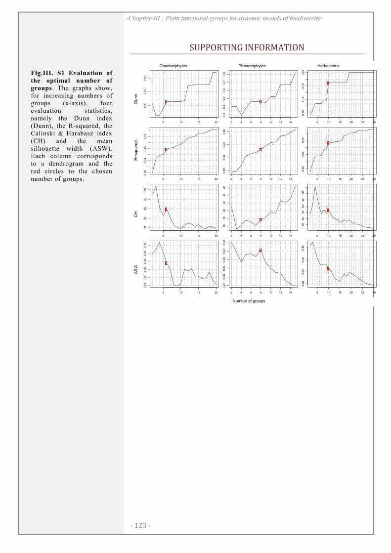
- 123 -

-Chapitre III : Plant functional groups for dynamic models of biodiversity-

SUPPORTING INFORMATION

Chamaephytes Phanerophytes Herbaceous

Dunn

R−s

quare

dC

HA

SW

5 10 15 20

0.2

00.2

50.3

0

Number of groups

Dun

n

5 10 15 20

0.6

00.6

40

.68

0.7

2

Number of groups

R2

5 10 15 20

30

35

40

45

50

Number of groups

ch

5 10 15 20

0.2

80

.30

0.3

20

.34

0.3

60.3

8

Number of groups

avera

ge

silh

oue

tte

wid

th

2 4 6 8 10 12 14

0.3

0.4

0.5

0.6

0.7

0.8

Number of groups

Dun

n

2 4 6 8 10 12 14

0.6

50.7

00.7

50

.80

Number of groups

R2

2 4 6 8 10 12 14

16

18

20

22

24

26

Number of groups

ch

2 4 6 8 10 12 14

0.2

00.2

50.3

00

.35

0.4

00

.45

Number of groups

avera

ge

silh

oue

tte

wid

th

5 10 15 20 25 30

0.1

00

.14

0.1

80

.22

Number of groups

Dun

n

5 10 15 20 25 30

0.6

20.6

60

.70

Number of groups

R2

5 10 15 20 25 30

50

60

70

80

90

10

0

Number of groups

ch

5 10 15 20 25 30

0.2

00.2

50

.30

0.3

5Number of groups

avera

ge

silh

oue

tte

wid

th

Number of groups

Fig.III. S1 Evaluation of

the optimal number of groups. The graphs show, for increasing numbers of groups (x-axis), four evaluation statistics, namely the Dunn index (Dunn), the R-squared, the Calinski & Harabasz index (CH) and the mean silhouette width (ASW). Each column corresponds to a dendrogram and the red circles to the chosen number of groups.

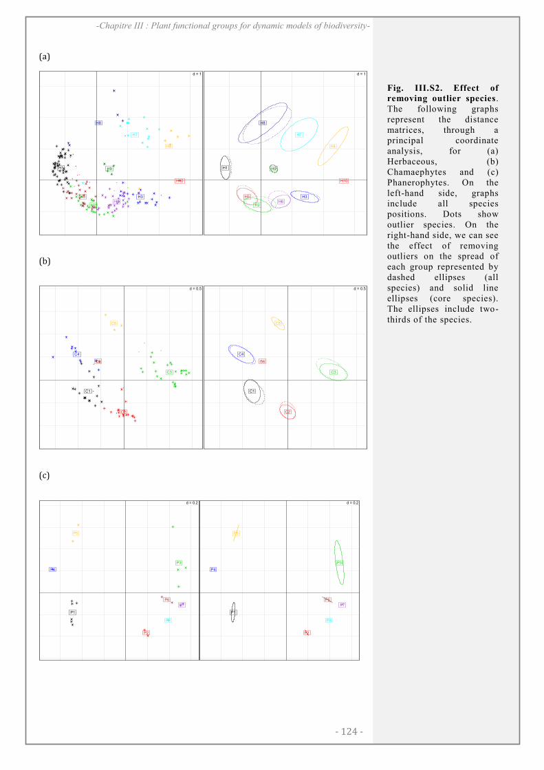
- 124 -

-Chapitre III : Plant functional groups for dynamic models of biodiversity-

(a)

d = 1

ズ

ズ

ズ

ズ

ズ

ズ

ズ

ズ

ズ

ズ

ズ

ズズ

ズ

ズ

ズ

ズ

ズ

ズ

ズ

ズ

ズ

ズ

ズ ズ

ズ

ズ

ズ

ズ

ズ

ズ

ズ

ズ

ズ

ズ

ズ ズ

ズ

ズ

ズ

ズ

ズ

ズズ

ズ

ズ

ズズズ

ズズ

ズ

ズ

ズ

ズ

ズ

ズ

ズ

ズ

ズ

ズ

ズ

ズ ズ

ズ

ズ

ズ

ズ

ズ

ズズ

ズ

ズズ

ズズ

ズ

ズ

ズ

ズ

ズ

ズ

ズ

ズ

ズズ

ズ

ズ

ズズ

ズズ

ズ

ズ

ズ

ズ

ズ ズ

ズ

ズ

ズ

ズ

ズ

ズ

ズ

ズ

ズ ズ

ズ

ズ

ズ

ズ

ズズ

ズズ

ズ

ズ

ズ

ズ

ズ

ズ ズ

ズ

ズ

ズ

ズ

ズ

ズ

ズ ズ

ズ

ズ

ズ

ズ

ズ

ズ

ズズ

ズズ

ズ

ズ

ズ

ズ

ズ

ズ

ズ

ズ

ズ

ズ

ズ

ズ

ズズ

ズ

ズ

ズ

ズ

ズ

ズ

ズ

ズ

ズ

ズ

ズズ

ズ

ズ

ズ

ズ

ズズ

ズ

ズ

ズズ

ズ

ズ

ズ

ズ

ズ

ズ

ズ

ズ

ズ

ズズ

ズ

ズズ

ズ

H1

H10

H2

H3

H4

H5

H6

H7

H8

H9

d = 1

H1

H10

H2

H3

H4

H5

H6

H7

H8

H9

(b)

d = 0.5

ズ

ズ

ズ

ズ

ズ

ズ

ズ

ズ

ズズズ

ズズ

ズ

ズ

ズ

ズ

ズ

ズズ

ズズ

ズ

ズ

ズズ

ズ

ズ

ズズ

ズ

ズ

ズズズ

ズ

ズ

ズ

ズ

ズ

ズ ズ

ズズ

ズズ

ズ

ズ

ズズ

ズ

ズ

ズズ

ズズ

ズ

ズ

ズ

ズ

ズ

ズ

ズ

ズ

ズ

ズ

ズ

ズ ズ

ズズ

ズ

ズ

ズ

ズ

ズ

ズ ズ

C1

C2

C3

C4

C5

C6

d = 0.5

C1

C2

C3

C4

C5

C6

(c)

d = 0.2

ズズ

ズ

ズ

ズ

ズ

ズ

ズ

ズ

ズ

ズズ

ズ

ズ

ズ

ズ

ズ

ズズ

ズ

P1

P2

P3

P4

P5

P6

P7

P8

d = 0.2

P1

P2

P3

P4

P5

P6

P7

P8

Fig. III.S2. Effect of removing outlier species. The following graphs represent the distance matrices, through a principal coordinate analysis, for (a) Herbaceous, (b) Chamaephytes and (c) Phanerophytes. On the left-hand side, graphs include all species positions. Dots show outlier species. On the right-hand side, we can see the effect of removing outliers on the spread of each group represented by dashed ellipses (all species) and solid line ellipses (core species). The ellipses include two-thirds of the species.

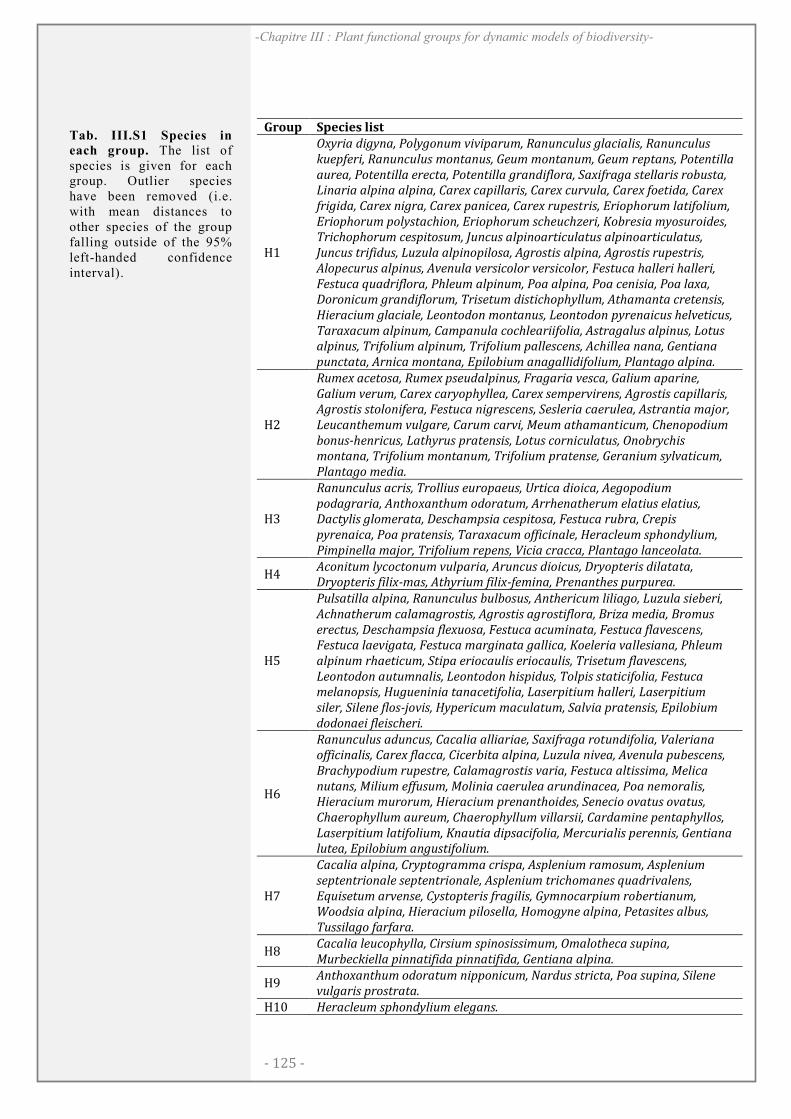
- 125 -

-Chapitre III : Plant functional groups for dynamic models of biodiversity-

Group Species list

H1

Oxyria digyna, Polygonum viviparum, Ranunculus glacialis, Ranunculus

kuepferi, Ranunculus montanus, Geum montanum, Geum reptans, Potentilla

aurea, Potentilla erecta, Potentilla grandiflora, Saxifraga stellaris robusta,

Linaria alpina alpina, Carex capillaris, Carex curvula, Carex foetida, Carex

frigida, Carex nigra, Carex panicea, Carex rupestris, Eriophorum latifolium,

Eriophorum polystachion, Eriophorum scheuchzeri, Kobresia myosuroides,

Trichophorum cespitosum, Juncus alpinoarticulatus alpinoarticulatus,

Juncus trifidus, Luzula alpinopilosa, Agrostis alpina, Agrostis rupestris,

Alopecurus alpinus, Avenula versicolor versicolor, Festuca halleri halleri,

Festuca quadriflora, Phleum alpinum, Poa alpina, Poa cenisia, Poa laxa,

Doronicum grandiflorum, Trisetum distichophyllum, Athamanta cretensis,

Hieracium glaciale, Leontodon montanus, Leontodon pyrenaicus helveticus,

Taraxacum alpinum, Campanula cochleariifolia, Astragalus alpinus, Lotus

alpinus, Trifolium alpinum, Trifolium pallescens, Achillea nana, Gentiana

punctata, Arnica montana, Epilobium anagallidifolium, Plantago alpina.

H2

Rumex acetosa, Rumex pseudalpinus, Fragaria vesca, Galium aparine,

Galium verum, Carex caryophyllea, Carex sempervirens, Agrostis capillaris,

Agrostis stolonifera, Festuca nigrescens, Sesleria caerulea, Astrantia major,

Leucanthemum vulgare, Carum carvi, Meum athamanticum, Chenopodium

bonus-henricus, Lathyrus pratensis, Lotus corniculatus, Onobrychis

montana, Trifolium montanum, Trifolium pratense, Geranium sylvaticum,

Plantago media.

H3

Ranunculus acris, Trollius europaeus, Urtica dioica, Aegopodium

podagraria, Anthoxanthum odoratum, Arrhenatherum elatius elatius,

Dactylis glomerata, Deschampsia cespitosa, Festuca rubra, Crepis

pyrenaica, Poa pratensis, Taraxacum officinale, Heracleum sphondylium,

Pimpinella major, Trifolium repens, Vicia cracca, Plantago lanceolata.

H4 Aconitum lycoctonum vulparia, Aruncus dioicus, Dryopteris dilatata,

Dryopteris filix-mas, Athyrium filix-femina, Prenanthes purpurea.

H5

Pulsatilla alpina, Ranunculus bulbosus, Anthericum liliago, Luzula sieberi,

Achnatherum calamagrostis, Agrostis agrostiflora, Briza media, Bromus

erectus, Deschampsia flexuosa, Festuca acuminata, Festuca flavescens,

Festuca laevigata, Festuca marginata gallica, Koeleria vallesiana, Phleum

alpinum rhaeticum, Stipa eriocaulis eriocaulis, Trisetum flavescens,

Leontodon autumnalis, Leontodon hispidus, Tolpis staticifolia, Festuca

melanopsis, Hugueninia tanacetifolia, Laserpitium halleri, Laserpitium

siler, Silene flos-jovis, Hypericum maculatum, Salvia pratensis, Epilobium

dodonaei fleischeri.

H6

Ranunculus aduncus, Cacalia alliariae, Saxifraga rotundifolia, Valeriana

officinalis, Carex flacca, Cicerbita alpina, Luzula nivea, Avenula pubescens,

Brachypodium rupestre, Calamagrostis varia, Festuca altissima, Melica

nutans, Milium effusum, Molinia caerulea arundinacea, Poa nemoralis,

Hieracium murorum, Hieracium prenanthoides, Senecio ovatus ovatus,

Chaerophyllum aureum, Chaerophyllum villarsii, Cardamine pentaphyllos,

Laserpitium latifolium, Knautia dipsacifolia, Mercurialis perennis, Gentiana

lutea, Epilobium angustifolium.

H7

Cacalia alpina, Cryptogramma crispa, Asplenium ramosum, Asplenium

septentrionale septentrionale, Asplenium trichomanes quadrivalens,

Equisetum arvense, Cystopteris fragilis, Gymnocarpium robertianum,

Woodsia alpina, Hieracium pilosella, Homogyne alpina, Petasites albus,

Tussilago farfara.

H8 Cacalia leucophylla, Cirsium spinosissimum, Omalotheca supina,

Murbeckiella pinnatifida pinnatifida, Gentiana alpina.

H9 Anthoxanthum odoratum nipponicum, Nardus stricta, Poa supina, Silene

vulgaris prostrata.

H10 Heracleum sphondylium elegans.

Tab. III.S1 Species in each group. The list of species is given for each group. Outlier species have been removed (i.e. with mean distances to other species of the group falling outside of the 95% left-handed confidence interval).

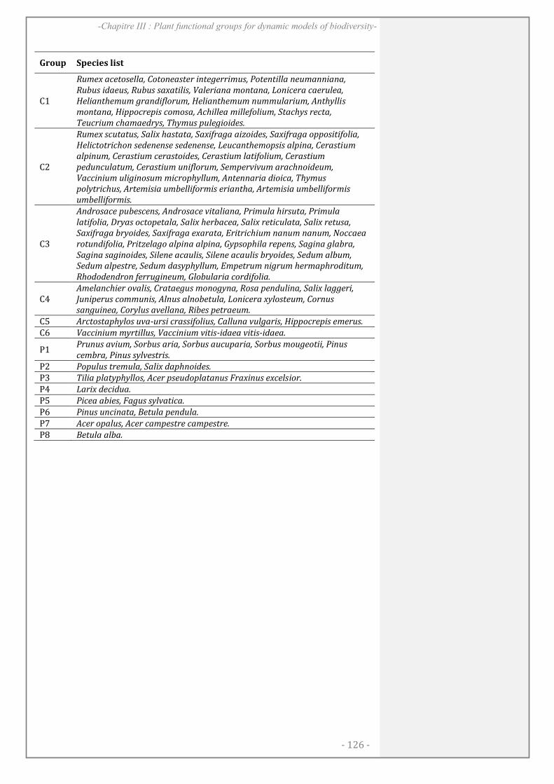
- 126 -

-Chapitre III : Plant functional groups for dynamic models of biodiversity-

Group Species list

C1

Rumex acetosella, Cotoneaster integerrimus, Potentilla neumanniana,

Rubus idaeus, Rubus saxatilis, Valeriana montana, Lonicera caerulea,

Helianthemum grandiflorum, Helianthemum nummularium, Anthyllis

montana, Hippocrepis comosa, Achillea millefolium, Stachys recta,

Teucrium chamaedrys, Thymus pulegioides.

C2

Rumex scutatus, Salix hastata, Saxifraga aizoides, Saxifraga oppositifolia,

Helictotrichon sedenense sedenense, Leucanthemopsis alpina, Cerastium

alpinum, Cerastium cerastoides, Cerastium latifolium, Cerastium

pedunculatum, Cerastium uniflorum, Sempervivum arachnoideum,

Vaccinium uliginosum microphyllum, Antennaria dioica, Thymus

polytrichus, Artemisia umbelliformis eriantha, Artemisia umbelliformis

umbelliformis.

C3

Androsace pubescens, Androsace vitaliana, Primula hirsuta, Primula

latifolia, Dryas octopetala, Salix herbacea, Salix reticulata, Salix retusa,

Saxifraga bryoides, Saxifraga exarata, Eritrichium nanum nanum, Noccaea

rotundifolia, Pritzelago alpina alpina, Gypsophila repens, Sagina glabra,

Sagina saginoides, Silene acaulis, Silene acaulis bryoides, Sedum album,

Sedum alpestre, Sedum dasyphyllum, Empetrum nigrum hermaphroditum,

Rhododendron ferrugineum, Globularia cordifolia.

C4 Amelanchier ovalis, Crataegus monogyna, Rosa pendulina, Salix laggeri,

Juniperus communis, Alnus alnobetula, Lonicera xylosteum, Cornus

sanguinea, Corylus avellana, Ribes petraeum.

C5 Arctostaphylos uva-ursi crassifolius, Calluna vulgaris, Hippocrepis emerus.

C6 Vaccinium myrtillus, Vaccinium vitis-idaea vitis-idaea.

P1 Prunus avium, Sorbus aria, Sorbus aucuparia, Sorbus mougeotii, Pinus

cembra, Pinus sylvestris.

P2 Populus tremula, Salix daphnoides.

P3 Tilia platyphyllos, Acer pseudoplatanus Fraxinus excelsior.

P4 Larix decidua.

P5 Picea abies, Fagus sylvatica.

P6 Pinus uncinata, Betula pendula.

P7 Acer opalus, Acer campestre campestre.

P8 Betula alba.

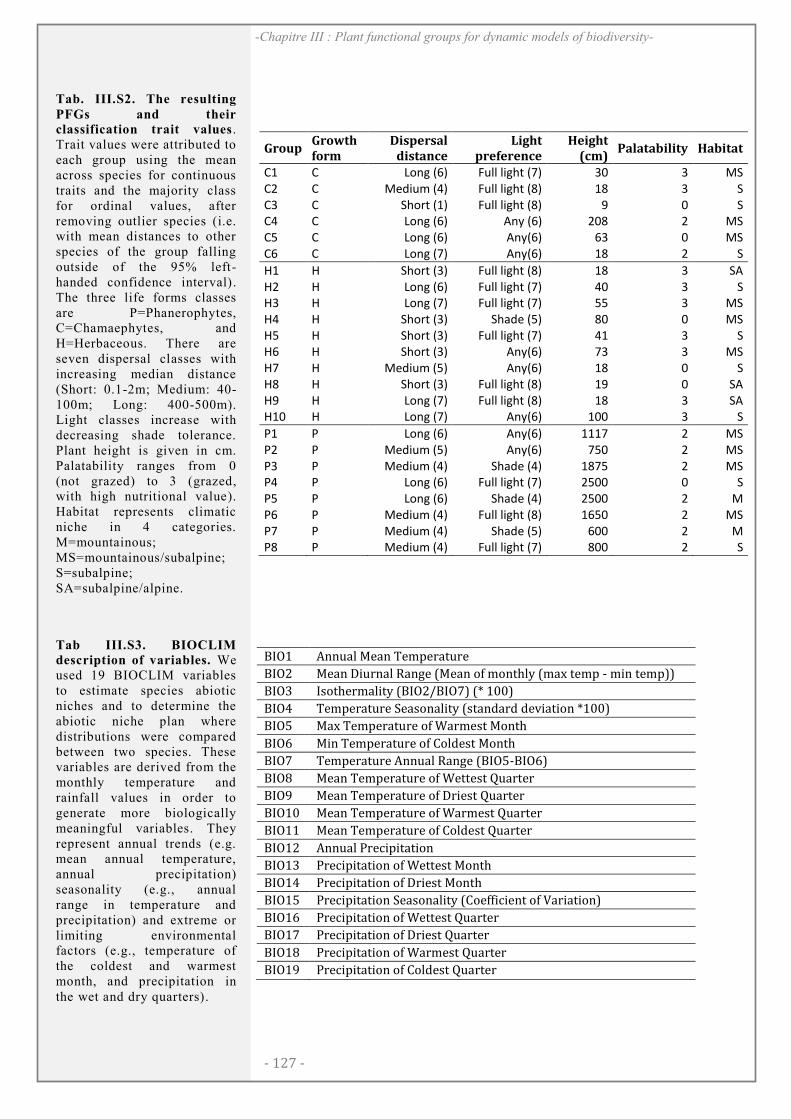
- 127 -

-Chapitre III : Plant functional groups for dynamic models of biodiversity-

Group Growth form

Dispersal distance

Light preference

Height (cm)

Palatability Habitat

C1 C Long (6) Full light (7) 30 3 MS

C2 C Medium (4) Full light (8) 18 3 S

C3 C Short (1) Full light (8) 9 0 S

C4 C Long (6) Any (6) 208 2 MS

C5 C Long (6) Any(6) 63 0 MS

C6 C Long (7) Any(6) 18 2 S

H1 H Short (3) Full light (8) 18 3 SA

H2 H Long (6) Full light (7) 40 3 S

H3 H Long (7) Full light (7) 55 3 MS

H4 H Short (3) Shade (5) 80 0 MS

H5 H Short (3) Full light (7) 41 3 S

H6 H Short (3) Any(6) 73 3 MS

H7 H Medium (5) Any(6) 18 0 S

H8 H Short (3) Full light (8) 19 0 SA

H9 H Long (7) Full light (8) 18 3 SA

H10 H Long (7) Any(6) 100 3 S

P1 P Long (6) Any(6) 1117 2 MS

P2 P Medium (5) Any(6) 750 2 MS

P3 P Medium (4) Shade (4) 1875 2 MS

P4 P Long (6) Full light (7) 2500 0 S

P5 P Long (6) Shade (4) 2500 2 M

P6 P Medium (4) Full light (8) 1650 2 MS

P7 P Medium (4) Shade (5) 600 2 M

P8 P Medium (4) Full light (7) 800 2 S

BIO1 Annual Mean Temperature BIO2 Mean Diurnal Range (Mean of monthly (max temp - min temp)) BIO3 Isothermality (BIO2/BIO7) (* 100) BIO4 Temperature Seasonality (standard deviation *100) BIO5 Max Temperature of Warmest Month BIO6 Min Temperature of Coldest Month BIO7 Temperature Annual Range (BIO5-BIO6) BIO8 Mean Temperature of Wettest Quarter BIO9 Mean Temperature of Driest Quarter BIO10 Mean Temperature of Warmest Quarter BIO11 Mean Temperature of Coldest Quarter BIO12 Annual Precipitation BIO13 Precipitation of Wettest Month BIO14 Precipitation of Driest Month BIO15 Precipitation Seasonality (Coefficient of Variation) BIO16 Precipitation of Wettest Quarter BIO17 Precipitation of Driest Quarter BIO18 Precipitation of Warmest Quarter BIO19 Precipitation of Coldest Quarter

Tab. III.S2. The resulting

PFGs and their classification trait values . Trait values were attributed to each group using the mean across species for continuous traits and the majority class for ordinal values, after removing outlier species (i.e. with mean distances to other species of the group falling outside of the 95% left-handed confidence interval). The three life forms classes are P=Phanerophytes, C=Chamaephytes, and H=Herbaceous. There are seven dispersal classes with increasing median distance (Short: 0.1-2m; Medium: 40-100m; Long: 400-500m). Light classes increase with decreasing shade tolerance. Plant height is given in cm. Palatability ranges from 0 (not grazed) to 3 (grazed, with high nutritional value). Habitat represents climatic niche in 4 categories. M=mountainous; MS=mountainous/subalpine; S=subalpine; SA=subalpine/alpine.

Tab III.S3. BIOCLIM description of variables. We used 19 BIOCLIM variables to estimate species abiotic niches and to determine the abiotic niche plan where distributions were compared between two species. These variables are derived from the monthly temperature and rainfall values in order to generate more biologically meaningful variables. They represent annual trends (e.g. mean annual temperature, annual precipitation) seasonality (e.g., annual range in temperature and precipitation) and extreme or limiting environmental factors (e.g., temperature of the coldest and warmest month, and precipitation in the wet and dry quarters).

- 128 -

-Chapitre III : Plant functional groups for dynamic models of biodiversity-

Databases References

Field measurements

Choler P (2005) Consistent shifts in Alpine plant traits along a mesotopographical gradient. Arctic, Antartic, and Alpine Research, 37, 444-453.

Field measurements

Albert CH, Thuiller W, Yoccoz NG, Soudant A, Boucher F, Saccone P, Lavorel S (2010) Intraspecific functional variability: extent, structure and sources of variation. Journal of Ecology, 98, 604-613.

Field measurements

Lavorel S, Grigulis K, Lamarque P et al. (2011) Using plant functional traits to understand the landscape distribution of multiple ecosystem services. Journal of Ecology, 99, 135-147.

VISTA Garnier E, Lavorel S, Ansquer P et al. (2007) Assessing the effects of land-use change on plant traits, communities and ecosystem functioning in grasslands: A standardized methodology and lessons from an application to 11 European sites. Annals of Botany, 99, 967-985.

LEDA Knevel IC, Bekker RM, Bakker JP, Kleyer M (2003) Life-history traits of the Northwest European flora: the LEDA database. Journal of Vegetation Science, 14, 611-614.

BiolFlor Kühn I, Durka W, Klotz S (2004) BiolFlor: a new plant-trait database as a tool for plant invasion ecology. Diversity and Distributions, 10, 363-365.

Flora Indicativa Landolt E, Bäumler B, Erhardt A et al. (2010) Flora indicativa. Ecological indicator values and biological attributes of the flora of Switzerland and the Alp, Berne, Haupt Verlag.

Tab III.S4. Databases

used for species traits or characteristics. They all form the database ANDROSACE that compiles trait values from field measurements in the study area and other trait databases containing species from the study area.

-127-

CHAPITRE IV:

F A T E - H : A S P A T I A L L Y A N D T E M P O R A L L Y E X P L I C I T

H Y B R I D M O D E L F O R P R E D I C T I N G T H E

V E G E T A T I O N S T R U CT U R E A N D D I V E R S I T Y A T R E G I O N A L

S C A L E .

Boulangeat, I., Georges, D., Dentant, C., Thuiller, W. FATE-H: A spatially

and temporally explicit hybrid model for predicting the vegetation

structure and diversity at regional scale. In preparation for Journal of

Applied Ecology

- 128 -

-Chapitre IV : Fate-H, a spatially explicit model of vegetation structure and diversity-

Abstract

1. Forecasting biodiversity at regional scales, and particularly vegetation structure and diversity, is a major challenge of the scientific research, as it is the primary producer providing resources and habitats for most species. However, current approaches are limited. On one hand, phenomenological habitat suitability models, extensively used to forecast changes in species distribution in response to climate and land use change, do not account for any mechanisms and for the temporal and spatial dynamic of species distributions. On the other hand, existing dynamic vegetation models (DVMs) usually involve only few modelling entities (e.g. plant functional types) that are not designed to represent biodiversity but rather coarse vegetation types. Coupling both approaches have been suggested to extend the current limitations.

2. Here, we propose an innovative hybrid-DVM, combining mechanistic and phenomenological sub-models, and allowing simulating the distribution and abundance of more modelling entities than traditional DVMs, with reasonable computing time and data requirement for parameterization. It includes mechanisms of succession, dispersal, disturbances and habitat suitability. We analyse its capability to retrieve the vegetation structure and diversity at a regional scale, in the Ecrins National Park (France), where the extensive vegetation surveys and knowledge allow the comparisons with models outputs.

3. FATE-H shows a very high accuracy in simulating and distinguishing open and closed habitats, but is weaker to estimate the canopy cover of intermediate and non-equilibrium habitats. The difference between observations and predictions is partly explained by slope and the percentage of mineral soil. The canopy cover of non-equilibrium situation such as recently abandoned pastures and mown areas are generally over-predicted.

4. The diversity of habitats, measured by the diversity of height strata, was highly correlated between observations and the model outputs. The functional diversity, measured using two different sets of plant traits (e.g. LHS strategies), was also significantly related to observations.

5. Synthesis. We believe that this hybrid vegetation model addresses one of the major challenges of the ecological research: providing more realistic simulations of vegetation dynamics in a context of climate and land use change at a regional scale relevant for biodiversity management and conservation. Using specific-sub models that can be easily parameterised and fined tune depending on the region of interest, it allows simulating not only changes in vegetation distribution but also changes in functional diversity, a key element for ecosystem functioning.

- 129 -

-Chapitre IV : Fate-H, a spatially explicit model of vegetation structure and diversity-

INTRODUCTION

They are now plenty of evidence that vegetation ecosystems are changing

as a consequence of climate and land use change, leading to an

unprecedented rate of species’ loss, landscape modification and

ecosystem disruptions (Lawton & May 1995; Bellard et al. 2012). In this

context, modelling tools play an important role to investigate the effect of

various management practices on biodiversity or to forecast the future of

the vegetation under climate and land use change scenarios, ultimately

helping decision makers to select the best conservation strategy (Thuiller

et al. 2008; Parmesan et al. 2011). Although forecasting changes in

biodiversity has become an important field in ecology, models are still

insufficiently robust and not predictive enough. Moreover, they are not

dedicated to model biodiversity at regional scales (e.g. protected areas)

where biodiversity management and conservation takes place (Pereira et

al. 2010; Bellard et al. 2012).

Biodiversity, although originally referring to species richness,

encompasses more generally species diversity, the diversity of resources

and the structural complexity of the environment (Hamilton et al. 2005).

The focus on the dominant vegetation is therefore a basis to evaluate

biodiversity changes as it structures the environment by creating habitats

and resources for other species. Moreover, the plant functional diversity,

mostly determined by dominant plant species (“Biomass ratio

hypothesis”, Grime 1998), can be directly related to ecosystem

functioning and ultimately to ecosystem services (de Bello et al. 2010b).

These two facets of biodiversity, namely habitat diversity and the plant

functional diversity are also expected to be correlated with species

richness (across trophic levels) at regional to global scale (Kerr & Packer

1997; Kerr, Southwood & Cihlar 2001; Tews et al. 2004).

To be of any used in conservation planning, biodiversity forecasts also

needs to account for the spatial and temporal dynamics of change due, for

instance, to species’ migration rates. There is consequently a demand for

models explicitly including the temporal and spatial mechanisms of the

response of biodiversity to environmental changes (Bellard et al. 2012).

- 130 -

-Chapitre IV : Fate-H, a spatially explicit model of vegetation structure and diversity-

This context makes dynamic vegetation models (DVMs) particularly

appropriate to be developed and adapted for dynamic biodiversity

modelling.

There are a large range of existing DVMs but most of them are designed

to simulate vegetation or biome shifts at regional to global scale (e.g.

LPJ, Sitch et al. 2003). These DVMs, although very promising for

predicting changes in broad vegetation types and biogeochemical

processes are of little use for biodiversity forecasting at regional scale

(Harrison et al. 2010). Moreover, restricted by knowledge, data or

computing time, they are not detailed enough, particularly concerning

herbaceous ecosystems, and their ability to represent biodiversity has

never been explicitly tested (Gallien et al. 2010). That is why models

capable to account for numerous species such as habitat suitability

models (Guisan & Thuiller 2005), although they lack dynamic processes,

have constituted until now the most prominent approach to forecast

trends in biodiversity (Peterson et al. 2002; Lawler et al. 2009; Thuiller

et al. 2011).

Interestingly, the last few years have seen the development of DVMs of

intermediate complexity usually based on a coupling of existing process-

based models such as demographic models with habitat suitability

models (Wintle et al. 2005; Keith et al. 2008; Brook et al. 2009;

Anderson et al. 2009). These models, hereafter called „hybrid-DVMs’,

are usually designed to be run over landscape or regional scales and

explicitly represent co-existence and/or dispersal mechanisms (e.g. LPJ-

GUESS, Hickler et al. 2004 ; LAMOS, Albert et al. 2008). The inclusion

of process-based sub-models allows them to account for vegetation

dynamics (e.g. dispersal, biotic interactions, disturbance) and the use of

habitat suitability models to account for multiple modelling entities with

reasonable simulation times (Gallien et al. 2010). These models point the

way to predict community composition dynamics and are promising for

biodiversity modelling at regional scale such as protected areas. The

challenge is that although the level of details they require prevents their

use over large number of species and spatial extent, they need to include

- 131 -

-Chapitre IV : Fate-H, a spatially explicit model of vegetation structure and diversity-

a minimum number of modelling entities to be able to represent

biodiversity.

Here we present a newly developed hybrid-DVM called “FATE-H”, a

spatially and temporally explicit model combining a succession model, a

disturbance model, a dispersal model and including habitat suitability

information. We show how, with 24 well-chosen plant functional groups

(PFGs), it is able to retrieve the vegetation structure and the spatial

biodiversity patterns of an entire national park. We first analyse the

modelled spatial distribution of open and closed vegetation by

comparison against observations. We then analyse the potential missing

factors explaining the mismatching between observed and potential

distribution at equilibrium. We expect to potentially overestimate tree

cover in recently abandoned areas or where local perturbations have not

been taken into account (e.g. avalanches). We also test whether the

difference between observed and potential vegetation may be related to

missing drivers. We then test how the different model outputs can be

transformed and used for forecasting biodiversity patterns. To do so, we

first compare observed and predicted habitat diversity (measured by

vegetation layers’ diversity). Secondly, we relate observed functional

diversity patterns (from field observations) to those retrieved from the

simulations. We finally discuss the limits and the potential of FATE-H for

future applications.

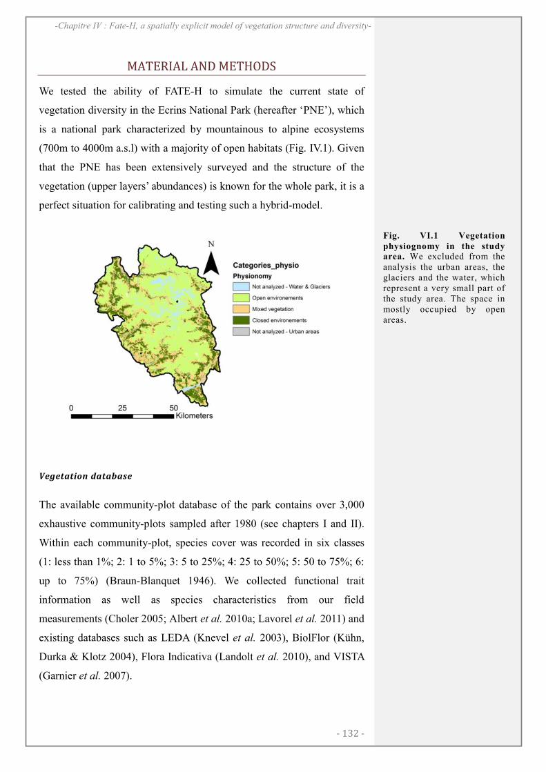
- 132 -

-Chapitre IV : Fate-H, a spatially explicit model of vegetation structure and diversity-

MATERIAL AND METHODS

We tested the ability of FATE-H to simulate the current state of

vegetation diversity in the Ecrins National Park (hereafter „PNE’), which

is a national park characterized by mountainous to alpine ecosystems

(700m to 4000m a.s.l) with a majority of open habitats (Fig. IV.1). Given

that the PNE has been extensively surveyed and the structure of the

vegetation (upper layers’ abundances) is known for the whole park, it is a

perfect situation for calibrating and testing such a hybrid-model.

Vegetation database

The available community-plot database of the park contains over 3,000

exhaustive community-plots sampled after 1980 (see chapters I and II).

Within each community-plot, species cover was recorded in six classes

(1: less than 1%; 2: 1 to 5%; 3: 5 to 25%; 4: 25 to 50%; 5: 50 to 75%; 6:

up to 75%) (Braun-Blanquet 1946). We collected functional trait

information as well as species characteristics from our field

measurements (Choler 2005; Albert et al. 2010a; Lavorel et al. 2011) and

existing databases such as LEDA (Knevel et al. 2003), BiolFlor (Kühn,

Durka & Klotz 2004), Flora Indicativa (Landolt et al. 2010), and VISTA

(Garnier et al. 2007).

Fig. VI.1 Vegetation

physiognomy in the study area. We excluded from the analysis the urban areas, the glaciers and the water, which represent a very small part of the study area. The space in mostly occupied by open areas.

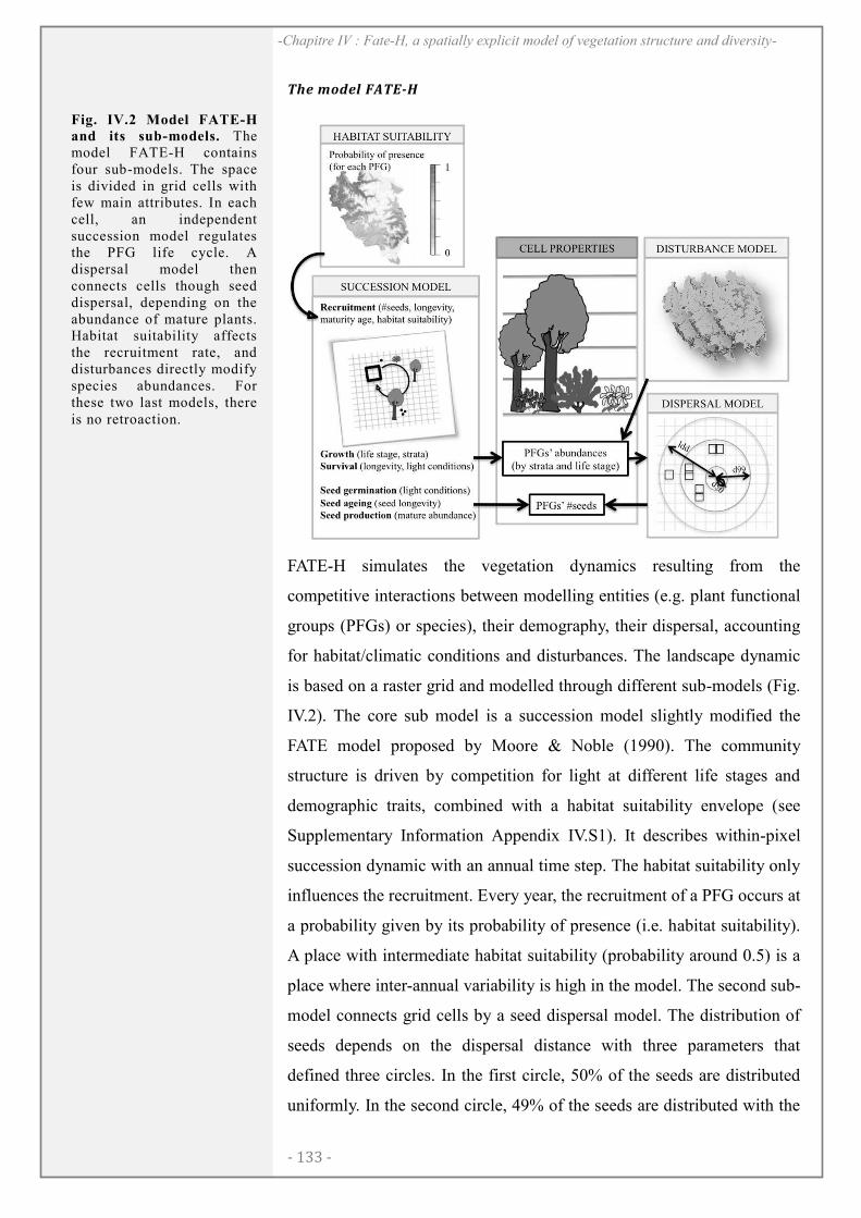
- 133 -

-Chapitre IV : Fate-H, a spatially explicit model of vegetation structure and diversity-

The model FATE-H

FATE-H simulates the vegetation dynamics resulting from the

competitive interactions between modelling entities (e.g. plant functional

groups (PFGs) or species), their demography, their dispersal, accounting

for habitat/climatic conditions and disturbances. The landscape dynamic

is based on a raster grid and modelled through different sub-models (Fig.

IV.2). The core sub model is a succession model slightly modified the

FATE model proposed by Moore & Noble (1990). The community

structure is driven by competition for light at different life stages and

demographic traits, combined with a habitat suitability envelope (see

Supplementary Information Appendix IV.S1). It describes within-pixel

succession dynamic with an annual time step. The habitat suitability only

influences the recruitment. Every year, the recruitment of a PFG occurs at

a probability given by its probability of presence (i.e. habitat suitability).

A place with intermediate habitat suitability (probability around 0.5) is a

place where inter-annual variability is high in the model. The second sub-

model connects grid cells by a seed dispersal model. The distribution of

seeds depends on the dispersal distance with three parameters that

defined three circles. In the first circle, 50% of the seeds are distributed

uniformly. In the second circle, 49% of the seeds are distributed with the

Fig. IV.2 Model FATE-H and its sub-models. The model FATE-H contains four sub-models. The space is divided in grid cells with few main attributes. In each cell, an independent succession model regulates the PFG life cycle. A dispersal model then connects cells though seed dispersal, depending on the abundance of mature plants. Habitat suitability affects the recruitment rate, and disturbances directly modify species abundances. For these two last models, there is no retroaction.

- 134 -

-Chapitre IV : Fate-H, a spatially explicit model of vegetation structure and diversity-

same concentration as in the first circle but by pairs of pixels, simulating

spatial autocorrelation. In the third circle, 1% of the seeds fall into a

random pixel, which is very similar to a fat tail distribution in classical

kernel functions. The third sub-model is a disturbance model that affects

a proportion of each defined age class of each PFG by death or

resprouting according to the PFGs characteristics and their tolerance to

disturbance.

Defining PFGs

We defined the plant functional groups based on an emergent group

approach (Lavorel et al. 1997 and chapter III). We selected six

characteristics that represent habitat suitability (climatic niche),

competition for light (plant height and light niche), dispersal (seed

dispersal distance class), demography (Raunkier life forms) and response

to grazing (palatability index). Within each life form, we computed pair-

wise species distances based on all these features using the Gower metric

(Podani et al. 1999). We then performed a hierarchical ascendant

classification per life form (UPGMA, Podani & Schmera 2006). The

number of groups was determined using a selection of 4 indices (Dunn

index, average silhouette width, R-squared and Calinski & Harabatz

index (1974)) measuring the heterogeneity between groups and/or the

homogeneity within groups. We obtained 24 groups that proved to keep

most of the information required to estimate vegetation biodiversity such

as species richness, taxonomic and functional diversity (see details in

chapter III).

Parameterization

General parameters: The model was run over a regular grid at 100m

resolution (251,762 pixels) and the vegetation height was divided into

five strata (0-1.5m; 1.5-4m; 4-10m; 10-20m; above 20m).

Succession model: Parameters for the succession model were derived

from five characteristics, computed as the median or average trait value

among representative species of each PFG: the competitive ability for

light, estimated by light preference from Landolt et al. (2010), the plant

- 135 -

-Chapitre IV : Fate-H, a spatially explicit model of vegetation structure and diversity-

height, the longevity, the maturity age class and Raunkiaer’s life form.

The full set of parameters for each PFG and calculation details are

provided in Supplementary Information (Appendix IV.S2).

Habitat suitability: Habitat suitability was modelled for each PFG using

the BIOMOD package in R (Thuiller et al. 2009). Species presence-

absence representatives of each PFT were pulled together and related to

seven environmental variables, namely the slope, the percentage of soil

carbon, and five bioclimatic variables (Isothermality, temperature

seasonality, temperature annual range, mean temperature of coldest

quarter, and annual precipitation, see Hutchinson et al. 2009). We used

five different statistical models (Generalized Linear Model, Generalized

Additive Model, Random Forest, Multivariate Adaptive Regression

Splines and Generalized Boosted Models). We performed an ensemble

forecasting to combine the binary models outputs of these five models,

using weights calculated on the basis of models’ predictive accuracy on

the test data (Thuiller et al. 2009). A detailed description of habitat

suitability models is provided in Supplementary Information (Appendix

IV.S3).

Dispersal: Dispersal parameters were attributed for all representative

species of each group, following Vittoz & Engler (2007) and Engler et al.

(2009). The median category was then given to the group (see Appendix

IV.S2).

Disturbance: Grazing and mowing areas were extracted from the

database „Delphine’, which is the result of a complete description and

mapping of the environment in the PNE carried out between 1992 and

1998. Three levels of grazing were considered, affecting an increasing

proportion of the PFG’s abundance in three different age classes

(juvenile, mature and senescent) and with two responses, either death or

resprouting (Appendix IV.S2). PFG’s affected abundances were

differentiated according to their average palatability (Jouglet 1999).

Mowing disturbance affected 50% of juveniles of all PFGs and 100% of

herbaceous mature plants every two years. The PFGs’ response to

mowing was exclusively resprouting. Whatever the disturbance

- 136 -

-Chapitre IV : Fate-H, a spatially explicit model of vegetation structure and diversity-

considered, juveniles resprouted at age zero, matures at maturity age

minus one and senescent plants at maturity age.

Simulations

Simulations started with an empty initial state and ran over 400 years at

total. The first 100 years consisted in a seedling time, which allow forests

to grow where the environment is suitable, to reach their upper strata and

to create shadow for undergrowth. After the seedling, we run 300 years to

make sure PFGs distributions were close to equilibrium (Supplementary

Information Appendix IV.S4). We analysed the last year of the

simulations given the quite steady equilibrium we achieved after seedling

(Appendix IV.S4). The stochasticity included in the model (in the habitat

suitability model and in the dispersal model) brought very little

variability to the final PFGs’ distributions (Appendix IV.S4). We

therefore presented the results for only one run.

Vegetation structure

We first compared the spatial pattern of the canopy closure (% cover

above 1m) with observations using the Cohen’s Kappa (せ) for multiple

classes. Although it is generally considered as an overly conservative

measure of agreement, it is expected to be a more robust measure than

simple percent agreement calculation since せ takes into account the

agreement occurring by chance (Srijbos et al. 2006). Fleiss's equally

arbitrary guidelines characterize せ over 0.75 as excellent, 0.40 to 0.75 as

fair to good, and below 0.40 as poor. In our case, we did not expect

excellent agreement because our model outputs correspond to stable

ecosystems whereas the studied area includes transition zones. In order to

verify this hypothesis, we specifically looked at the level of canopy

closure across seven types of observed vegetation physiognomy (rock,

grasslands, moors, 10-40% closing, 40-60% closing, alder forest and

forest). We also calculated the difference between observed and predicted

cover above one meter and tested whether it was the result of non-

equilibrium situations or neglected mechanisms. In order to identify

dissimilarities that were persistent through scales, differences between

- 137 -

-Chapitre IV : Fate-H, a spatially explicit model of vegetation structure and diversity-

observations and predictions (predicted minus observed canopy cover)

were estimated at incremental scales, each time giving the resulting value

to the central pixel, with radius varying from one to ten pixels, and

finally averaged (Gaucherel, Alleaume & Hely 2008). We used random

forests models to relate the average model disagreement (predicted minus

observed) and five potential explanatory variables. These were the

percentage of mineral and carbon in the soil representing missing drivers

related to soil resources, and slope and aspect as a proxy for missing

local disturbances such as avalanches and rock falls. The presence of

mowing and grazing at different levels was used to represent different

management legacies. Although these variables were either included into

the habitat distribution modelling (e.g. soil, slope) or taken into account

in the simulation process (e.g. disturbance), we wanted to further test

whether they were not sufficiently explicitly accounted for.

Biodiversity assessment

Habitat diversity

We compared the diversity of vegetation strata against observations using

the Gini-Simpson index. We considered three different strata according to

observations (0-1m; 1-4m; above 4m). For the comparison, we needed to

pull together the three upper strata of model outputs. The diversity index

was calculated for observations and predictions using relative

abundances of each stratum.

Functional diversity

We focussed on a functional divergence measure (FD) that is widely

used, the Rao Quadratic entropy (de Bello et al. 2010a). Observed FD

was computed using the community plots, which are complete botanical

surveys with recorded abundance covers for all species (see Vegetation

database). We performed the analysis on 112 selected cells with at least

three community plots in which species abundances were averaged. We

used two different sets of traits representing different plant strategies. The

first set included specific leaf area (SLA), plant height and seed mass,

representing the ecological strategies (LHS), proposed by Westoby

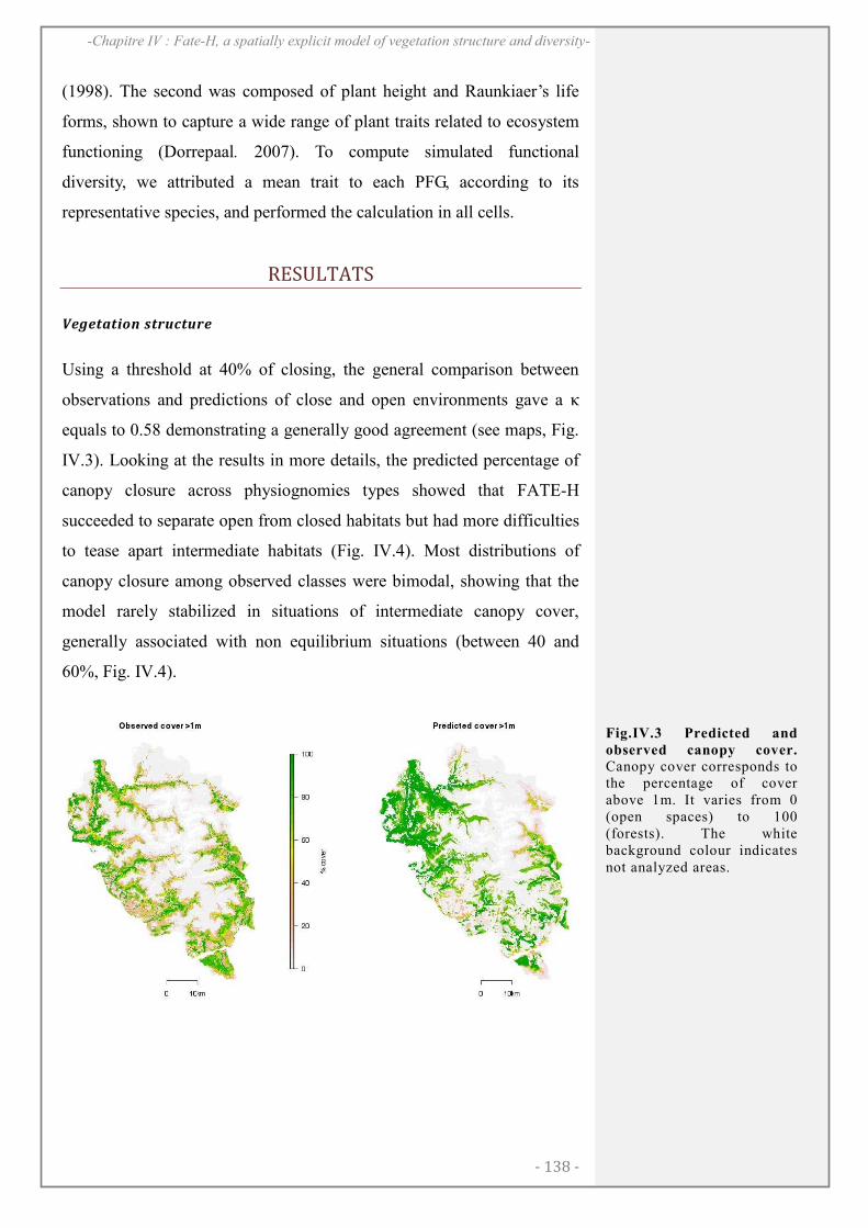
- 138 -

-Chapitre IV : Fate-H, a spatially explicit model of vegetation structure and diversity-

(1998). The second was composed of plant height and Raunkiaer’s life

forms, shown to capture a wide range of plant traits related to ecosystem

functioning (Dorrepaal. 2007). To compute simulated functional

diversity, we attributed a mean trait to each PFG, according to its

representative species, and performed the calculation in all cells.

RESULTATS

Vegetation structure

Using a threshold at 40% of closing, the general comparison between

observations and predictions of close and open environments gave a せ

equals to 0.58 demonstrating a generally good agreement (see maps, Fig.

IV.3). Looking at the results in more details, the predicted percentage of

canopy closure across physiognomies types showed that FATE-H

succeeded to separate open from closed habitats but had more difficulties

to tease apart intermediate habitats (Fig. IV.4). Most distributions of

canopy closure among observed classes were bimodal, showing that the

model rarely stabilized in situations of intermediate canopy cover,

generally associated with non equilibrium situations (between 40 and

60%, Fig. IV.4).

Fig.IV.3 Predicted and

observed canopy cover. Canopy cover corresponds to the percentage of cover above 1m. It varies from 0 (open spaces) to 100 (forests). The white background colour indicates not analyzed areas.

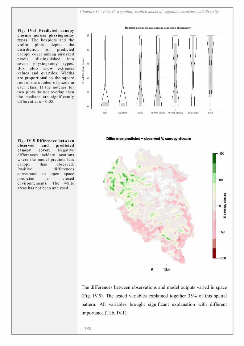
- 139 -

-Chapitre IV : Fate-H, a spatially explicit model of vegetation structure and diversity-

rock grassland moors 10−40% closing 40−60% closing Alnus viridis forest

020

40

60

80

100

Modelled canopy closure accross vegetation physionomy

% m

ode

lled c

anopy c

losure

The differences between observations and model outputs varied in space

(Fig. IV.5). The tested variables explained together 35% of this spatial

pattern. All variables brought significant explanation with different

importance (Tab. IV.1).

Fig. IV.4 Predicted canopy

closure across physiognomy types. The boxplots and the violin plots depict the distribution of predicted canopy cover among analyzed pixels, distinguished into seven physiognomy types. Box plots show extremes values and quartiles. Widths are proportional to the square root of the number of pixels in each class. If the notches for two plots do not overlap then the medians are significantly different at g= 0.05.

Fig. IV.5 Difference between

observed and predicted canopy cover. Negative differences incidate locations where the model predicts less canopy than observed. Positive differences correspond to open space predicted as closed environnements. The white areas has not been analysed.

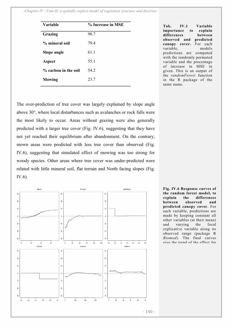
- 140 -

-Chapitre IV : Fate-H, a spatially explicit model of vegetation structure and diversity-

Variable % Increase in MSE

Grazing 98.7

% mineral soil 79.4

Slope angle 61.1

Aspect 55.1

% carbon in the soil 54.2

Mowing 23.7

The over-prediction of tree cover was largely explained by slope angle

above 30°, where local disturbances such as avalanches or rock falls were

the most likely to occur. Areas without grazing were also generally

predicted with a larger tree cover (Fig. IV.6), suggesting that they have

not yet reached their equilibrium after abandonment. On the contrary,

mown areas were predicted with less tree cover than observed (Fig.

IV.6), suggesting that simulated effect of mowing was too strong for

woody species. Other areas where tree cover was under-predicted were

related with little mineral soil, flat terrain and North facing slopes (Fig.

IV.6).

Tab. IV.1 Variable

importance to explain

differences between

observed and predicted canopy cover. For each variable, models predictions are computed with the randomly permuted variable and the precentage of increase in MSE in given. This is an output of the randomForest function in the R package of the same name.

Fig. IV.6 Response curves of

the random forest model, to

explain the differences

between observed and predicted canopy cover . For each variable, predictions are made by keeping constant all other variables (at their mean) and varying the focal explicative variable along its observed range (package R Biomod). The final curves give the trend of the effect for each variable.

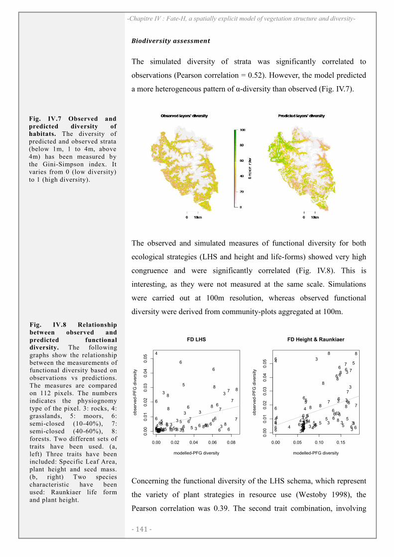
- 141 -

-Chapitre IV : Fate-H, a spatially explicit model of vegetation structure and diversity-

Biodiversity assessment

The simulated diversity of strata was significantly correlated to

observations (Pearson correlation = 0.52). However, the model predicted

a more heterogeneous pattern of g-diversity than observed (Fig. IV.7).

The observed and simulated measures of functional diversity for both

ecological strategies (LHS and height and life-forms) showed very high

congruence and were significantly correlated (Fig. IV.8). This is

interesting, as they were not measured at the same scale. Simulations

were carried out at 100m resolution, whereas observed functional

diversity were derived from community-plots aggregated at 100m.

3444334346

8

5 36

8

3

3

3

4

7

3355

86

7

56

7

8

6

335333

7

33

85

5 5 354

5

6

3

6

3

67

6

4

7

3

8

3

66

6

5

85

6

34 333

4

6

4 465

5

3

34 6

43

84

6

66

58

56

6

8

64

0.00 0.02 0.04 0.06 0.08

0.0

00.0

10

.02

0.0

30.0

40

.05

FD LHS

modelled-PFG diversity

observ

ed

-PF

G d

ive

rsity

3444

3

34 34

6

8

5

3

6

8

3

3

3

4

7

3355

8

6

7

5

6

7

86

335333

7

3

3

8

5

55 3

54

5

6

3

6

3

6

7

6

4

7

3

8

3

6

6

6

5

85

6

3

4 3

33

46

44

6

55

3

3

46

43

84

6

6

65

8

5

6

6

8

6

4

0.00 0.05 0.10 0.15

0.0

00.0

10.0

20

.03

0.0

40

.05

FD Height & Raunkiaer

modelled-PFG diversity

observ

ed

-PF

G d

ive

rsity

Concerning the functional diversity of the LHS schema, which represent

the variety of plant strategies in resource use (Westoby 1998), the

Pearson correlation was 0.39. The second trait combination, involving

Fig. IV.7 Observed and

predicted diversity of habitats. The diversity of predicted and observed strata (below 1m, 1 to 4m, above 4m) has been measured by the Gini-Simpson index. It varies from 0 (low diversity) to 1 (high diversity).

Fig. IV.8 Relationship

between observed and

predicted functional diversity. The following graphs show the relationship between the measurements of functional diversity based on observations vs predictions. The measures are compared on 112 pixels. The numbers indicates the physiognomy type of the pixel. 3: rocks, 4: grasslands, 5: moors, 6: semi-closed (10-40%), 7: semi-closed (40-60%), 8: forests. Two different sets of traits have been used. (a, left) Three traits have been included: Specific Leaf Area, plant height and seed mass. (b, right) Two species characteristic have been used: Raunkiaer life form and plant height.

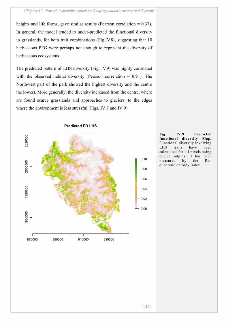
- 142 -

-Chapitre IV : Fate-H, a spatially explicit model of vegetation structure and diversity-

heights and life forms, gave similar results (Pearson correlation = 0.37).

In general, the model tended to under-predicted the functional diversity

in grasslands, for both trait combinations (Fig.IV.8), suggesting that 10

herbaceous PFG were perhaps not enough to represent the diversity of

herbaceous ecosystems.

The predicted pattern of LHS diversity (Fig. IV.9) was highly correlated

with the observed habitat diversity (Pearson correlation = 0.91). The

Northwest part of the park showed the highest diversity and the centre

the lowest. More generally, the diversity increased from the centre, where

are found scarce grasslands and approaches to glaciers, to the edges

where the environment is less stressful (Figs. IV.7 and IV.9).

870000 890000 910000 930000

19

600

00

1980

000

20

000

00

202

0000

Predicted FD LHS

0.00

0.02

0.04

0.06

0.08

0.10

Fig. IV.9 Predicted

functional diversity Map. Functional diversity involving LHS traits have been calculated for all pixels using model outputs. It has been measured by the Rao quadratic entropy index.

- 143 -

-Chapitre IV : Fate-H, a spatially explicit model of vegetation structure and diversity-

DISCUSSION

Why using an hybrid-DVM?

The new approach proposed here, relying on combined sub-models at the

regional and landscape scales, offers several avenues for predicting

biodiversity dynamics.

First, the use of habitat suitability modelling as an input variable and

influencing recruitment fulfils the most important assumption of

traditional succession model such as FATE, which is the suitability of the

study site for the modelled entity. Therefore, the way we accounted for

this habitat suitability allows giving some environmental stochasticity in

the case of moderate suitability. It is indeed very likely that areas where

the habitat suitability of a particular group is difficult to model

correspond to places where the PFG dynamic is strongly influenced by

other important mechanisms such as competition or dispersal processes.

Including both abiotic and biotic conditions in landscape dynamics

thereby increases the realism of projections.

Second, FATE-H inherently combines two different study scales. As a

first step, habitat-suitability models can be established at the scale

relevant for the study area (e.g. regional or global scales). Under these

conditions one of the most important assumptions of these models can be

fulfilled: pseudo-equilibrium between the plant functional group of

interest and the current environment (Guisan & Thuiller 2005). In our

example, we included information about climate and soil because we

believed they were the most plausible drivers of the large-scale

distribution of PFGs. Other important drivers might certainly be included

when available (e.g. soil water holding capacity, soil nitrogen). As a

second step, the community dynamics modelled by the combination of

the succession model together with the dispersal and disturbance models,

take place at a level of details appropriated for landscape modelling. The

proposed approach appears promising for addressing scaling problems,

including limitations of models at each scale (Peters et al. 2004). As far

as we know, few model combinations have already been implemented in

- 144 -

-Chapitre IV : Fate-H, a spatially explicit model of vegetation structure and diversity-

such a way (Guisan & Thuiller 2005). They are some examples for

animal species where landscape models are used as variables for the

niche-based models (Wintle et al. 2005). Concerning plants, there are

very few studies presenting such a combination (for a review see Gallien

et al. 2010, Franklin 2010). Dullinger et al. (2004) carried out a similar

analysis by building a spatially explicit model incorporating both climate,

biotic interactions and dispersal (see also Albert et al. 2008; Williams et

al. 2008; Smolik et al. 2010)

Modeling biodiversity with a hybrid-DVM

To the best of our knowledge, this is one of the first times that a hybrid-

DVM is tested empirically to model both the vegetation structure and

diversity of an entire region. We demonstrated that FATE-H was able to

retrieve the general patterns of the vegetation structure and diversity of

the PNE. Using more entities than traditional DGVMs (e.g. LPJ, Sitch et

al. 2003), and considering not only trees as in Forest Gap Models (e.g.

TreeMig, Lischke et al. 2006), FATE-H is able to involve a sufficient

number of PFGs than can represent the vegetation diversity (see chapter

III). In other words, our simulations based on 24 plant functional groups

for an entire national park holding more than 1,500 plant species, are able

to not only accurately predict the vegetation structure and its distribution

but also give insights on the diversity patterns such as functional

diversity. These results have some strong implications in terms of

biodiversity forecasting. Using such an approach into a protected area

would allows to make reliable projections of vegetation diversity

patterns, but would also permit to simulate the spatial and temporal

response of the vegetation structure and diversity in response to climate

and land use change scenarios. It has thus tremendous implications for

biodiversity managements in the PNE.

Conceptually, the inclusion of the main coexistence mechanisms into the

model and into the PFGs’ construction (i.e. abiotic filtering, biotic

interactions and dispersal), makes an important step forward in

comparison to phenomenological models such as habitat suitability

models (Thuiller et al. 2008), and should lead to the construction of more

- 145 -

-Chapitre IV : Fate-H, a spatially explicit model of vegetation structure and diversity-

robust forecasts. To give an example, FATE-H simulated the whole

dispersal process. The number of dispersed seed depends on the

abundance of mature plants that are influenced by the overall community

dynamics, and the recruitment depends on the proportion of available

seeds and habitat conditions. This is a real progress compared to the

simple combination of habitat suitability models and dispersal kernels

(e.g. Engler & Guisan 2009, Iverson et al. 2006).

Scale considerations and limits

FATE-H, as all DVMs, is clearly limited in precision. It is designed to

give intermediate scale trends at regional scales and general patterns

only. For instance, it is not made to model within cell heterogeneity, nor

to account for biotic interactions between cells, which make the ultimate

choice of the resolution decisive for the outcomes precision (see Gallien

et al. 2010). We also decided to implement a somehow simple dispersal

kernel instead of a complicated seed dispersal model. Indeed, the

dispersal model needs to remain consistent with the level of details of the

whole model and simulation experiment, which is semi-quantitative, with

numerous parameters representing more a rank between species rather

than continuous values. At this spatial scale (a region) and resolution

(100m), we believe it is more important to relate seed dispersal to

community dynamics rather than overly complicate the seed dispersal

model. Indeed, at 100m resolution, most of plant seeds are expected to

fall within the neighboring pixels, while rare long dispersal events are

generally highly stochastic and difficult to predict accurately (Kunstler et

al. 2007). The use of complex kernel functions is therefore limited by the

poor available knowledge, is also not consistent with the model scale of

details and would increase the simulation time, but would not change the

general patterns (results not shown).

Our results suggest that the number of herbaceous PFGs might need to be

increased to better represent grassland structure and diversity. The main

limitation is the availability of trait data for most of the species.

Increasing the number of PFGs with the same dataset would ultimately

create some PFGs represented by a single species. In three particular

- 146 -

-Chapitre IV : Fate-H, a spatially explicit model of vegetation structure and diversity-

cases, this is difficult to know whether these groups represent distinct

herbaceous types or if they are the result of data uncertainties (e.g.

missing data, local error, and extreme field measurement). The number of

modeling entities has also to be consistent with the model complexity.

For instance, competition for light is not occurring between herbaceous

species (no light competition within strata but between strata). This is

indeed impossible to parameterize herbaceous competition for light

because the model does not account for phenology and we do not know

which PFG would grow first in the year, creating shadow for the others.

Another challenge for modeling more accurately herbaceous functional

groups relates to the resolution and competition for resource. Indeed,

coexistence is unlikely to be limited by competition for light in a

100x100m pixel, when only herbaceous species co-occur. Therefore,

competition for soil resources is also likely to interplay with competition

for light. Unfortunately, information on soil resources such as available

nitrogen is lacking over large spatial scale. This lack of competition

between herbaceous species could likely explain the under-estimation of

certain grasslands diversity.

Missing factors and potential improvements

Subject to available data, the modeling might still be improved. Our

results suggest local stochastic disturbances such as avalanches or rock

falls might be worth to include in future modeling attempts. It is known

that vegetation structure and avalanches do influence each other creating

feedback loops (Bebi, Kulakowski & Rixen 2009). The inclusion of a

complete avalanche model could turn out to be an improvement in our

study area. On the other side, it is very specific to the study area, and

would have no general application. Without modifying the present

model, it would however be possible to include avalanches as other

disturbances, without retroaction. Any other disturbance may be added to

the modeling in this way (e.g. fire). As discussed previously, FATE-H

lacks mechanisms related to soil resources. It is obvious that coupling

FATE-H with a soil water and nitrogen model would complete our

approach and open new opportunities to increase the degree of details.

On the other hand, it would require more data and will increase

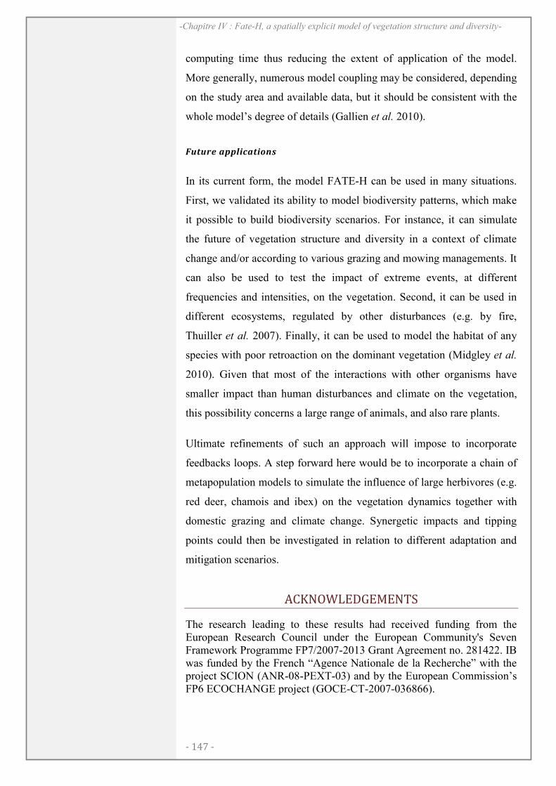
- 147 -

-Chapitre IV : Fate-H, a spatially explicit model of vegetation structure and diversity-

computing time thus reducing the extent of application of the model.

More generally, numerous model coupling may be considered, depending

on the study area and available data, but it should be consistent with the

whole model’s degree of details (Gallien et al. 2010).

Future applications

In its current form, the model FATE-H can be used in many situations.

First, we validated its ability to model biodiversity patterns, which make

it possible to build biodiversity scenarios. For instance, it can simulate

the future of vegetation structure and diversity in a context of climate

change and/or according to various grazing and mowing managements. It

can also be used to test the impact of extreme events, at different

frequencies and intensities, on the vegetation. Second, it can be used in

different ecosystems, regulated by other disturbances (e.g. by fire,

Thuiller et al. 2007). Finally, it can be used to model the habitat of any

species with poor retroaction on the dominant vegetation (Midgley et al.

2010). Given that most of the interactions with other organisms have

smaller impact than human disturbances and climate on the vegetation,

this possibility concerns a large range of animals, and also rare plants.

Ultimate refinements of such an approach will impose to incorporate

feedbacks loops. A step forward here would be to incorporate a chain of

metapopulation models to simulate the influence of large herbivores (e.g.

red deer, chamois and ibex) on the vegetation dynamics together with

domestic grazing and climate change. Synergetic impacts and tipping

points could then be investigated in relation to different adaptation and

mitigation scenarios.

ACKNOWLEDGEMENTS

The research leading to these results had received funding from the European Research Council under the European Community's Seven Framework Programme FP7/2007-2013 Grant Agreement no. 281422. IB was funded by the French “Agence Nationale de la Recherche” with the project SCION (ANR-08-PEXT-03) and by the European Commission’s FP6 ECOCHANGE project (GOCE-CT-2007-036866).

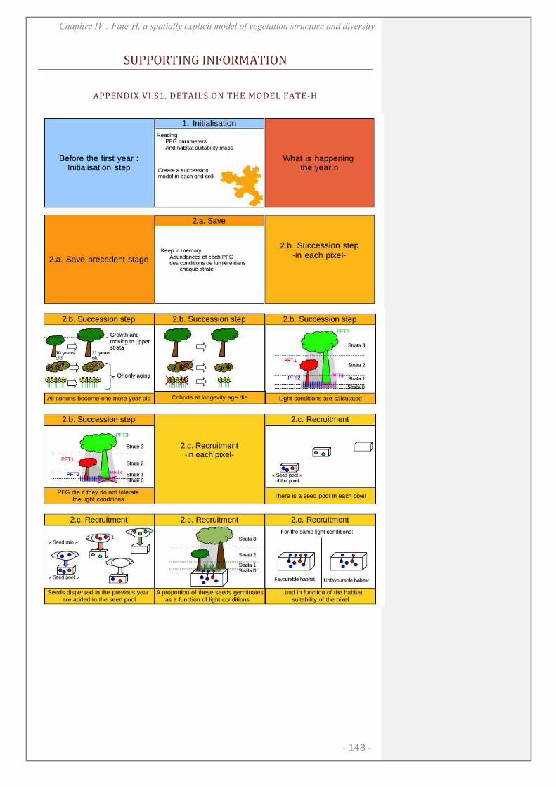
- 148 -

-Chapitre IV : Fate-H, a spatially explicit model of vegetation structure and diversity-

SUPPORTING INFORMATION

APPENDIX VI.S1. DETAILS ON THE MODEL FATE-H

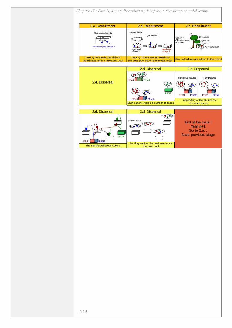
- 149 -

-Chapitre IV : Fate-H, a spatially explicit model of vegetation structure and diversity-

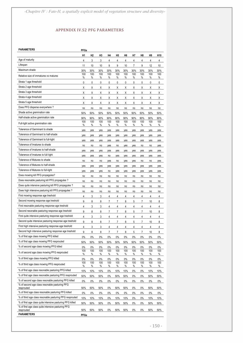
- 150 -

-Chapitre IV : Fate-H, a spatially explicit model of vegetation structure and diversity-

APPENDIX IV.S2 PFG PARAMETERS

PARAMETERS PFGs

H1 H2 H3 H4 H5 H6 H7 H8 H9 H10

Age of maturity 4 3 3 4 4 4 4 4 4 4

Lifespan 11 10 10 9 9 10 7 9 12 10

Maximum shade 30% 30% 30% 30% 30% 30% 30% 30% 30% 30%

Relative size of immatures vs matures 100%

100%

100%

100%

100%

100%

100%

100%

100%

100%

Strata 1 age threshold 0 0 0 0 0 0 0 0 0 0

Strata 2 age threshold X X X X X X X X X X

Strata 3 age threshold X X X X X X X X X X

Strata 4 age threshold X X X X X X X X X X

Strata 5 age threshold X X X X X X X X X X

Does PFG disperse everywhere ? no no no no no no no no no no

Shade active gremination rate 50% 50% 50% 50% 50% 50% 50% 50% 50% 50%

Half-shade active gremination rate 90% 90% 90% 90% 90% 90% 90% 90% 90% 90%

Full-light active gremination rate 100%

100%

100%

100%

100%

100%

100%

100%

100%

100%

Tolerence of Germinant to shade yes yes yes yes yes yes yes yes yes yes

Tolerence of Germinant to half-shade yes yes yes yes yes yes yes yes yes yes

Tolerence of Germinant to full-light yes yes yes yes yes yes yes yes yes yes

Tolerence of Imatures to shade no no no yes no yes yes no no yes

Tolerence of Imatures to half-shade yes yes yes yes yes yes yes yes yes yes

Tolerence of Imatures to full-light yes yes yes no yes yes yes yes yes yes

Tolerence of Matures to shade no no no yes no yes yes no no yes

Tolerence of Matures to half-shade yes yes yes yes yes yes yes yes yes yes

Tolerence of Matures to full-light yes yes yes no yes yes yes yes yes yes

Does mowing kill PFG propagules? no no no no no no no no no no

Does resonable pasturing kill PFG propagules ? no no no no no no no no no no

Does quite intensive pasturing kill PFG propagules ? no no no no no no no no no no

Does high intensive pasturing kill PFG propagules ? no no no no no no no no no no

First mowing response age treshold 4 3 3 4 4 4 4 4 4 4

Second mowing response age treshold 9 8 8 7 7 8 5 7 10 8

First resonable pasturing response age treshold 4 3 3 4 4 4 4 4 4 4

Second resonable pasturing response age treshold 9 8 8 7 7 8 5 7 10 8

First quite intensive pasturing response age treshold 4 3 3 4 4 4 4 4 4 4

Second quite intensive pasturing response age treshold 9 8 8 7 7 8 5 7 10 8

First high intensive pasturing response age treshold 4 3 3 4 4 4 4 4 4 4

Second high intensive pasturing response age treshold 9 8 8 7 7 8 5 7 10 8

% of first age class mowing PFG killed 0% 0% 0% 0% 0% 0% 0% 0% 0% 0%

% of first age class mowing PFG resprouted 50% 50% 50% 50% 50% 50% 50% 50% 50% 50%

% of second age class mowing PFG killed 0% 0% 0% 0% 0% 0% 0% 0% 0% 0%

% of second age class mowing PFG resprouted 100%

100%

100%

100%

100%

100%

100%

100%

100%

100%

% of third age class mowing PFG killed 0% 0% 0% 0% 0% 0% 0% 0% 0% 0%

% of third age class mowing PFG resprouted 100%

100%

100%

100%

100%

100%

100%

100%

100%

100%

% of first age class resonable pasturing PFG killed 10% 10% 10% 0% 10% 10% 0% 0% 10% 10%

% of first age class resonable pasturing PFG resprouted 50% 50% 50% 0% 50% 50% 0% 0% 50% 50%

% of second age class resonable pasturing PFG killed 0% 0% 0% 0% 0% 0% 0% 0% 0% 0%

% of second age class resonable pasturing PFG resprouted 50% 50% 50% 0% 50% 50% 0% 0% 50% 50%

% of third age class resonable pasturing PFG killed 0% 0% 0% 0% 0% 0% 0% 0% 0% 0%

% of third age class resonable pasturing PFG resprouted 10% 10% 10% 0% 10% 10% 0% 0% 10% 10%

% of first age class quite intensive pasturing PFG killed 50% 50% 50% 0% 50% 50% 0% 0% 50% 50%

% of first age class quite intensive pasturing PFG resprouted 50% 50% 50% 0% 50% 50% 0% 0% 50% 50%

PARAMETERS PFGs

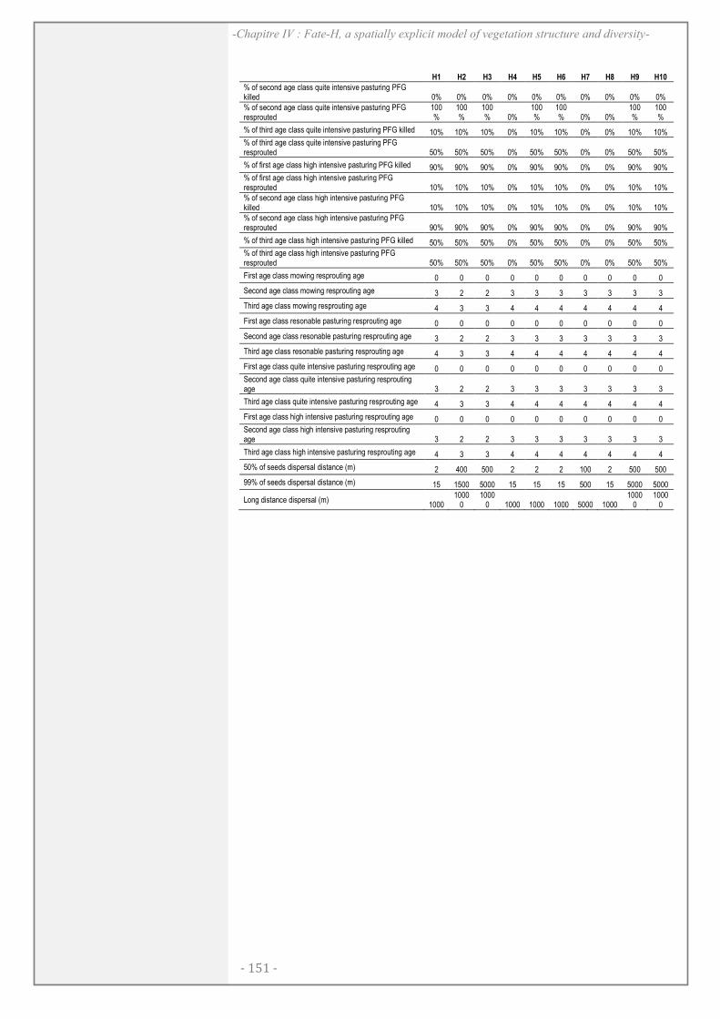
- 151 -

-Chapitre IV : Fate-H, a spatially explicit model of vegetation structure and diversity-

H1 H2 H3 H4 H5 H6 H7 H8 H9 H10

% of second age class quite intensive pasturing PFG killed 0% 0% 0% 0% 0% 0% 0% 0% 0% 0%

% of second age class quite intensive pasturing PFG resprouted

100%

100%

100% 0%

100%

100% 0% 0%

100%

100%

% of third age class quite intensive pasturing PFG killed 10% 10% 10% 0% 10% 10% 0% 0% 10% 10%

% of third age class quite intensive pasturing PFG resprouted 50% 50% 50% 0% 50% 50% 0% 0% 50% 50%

% of first age class high intensive pasturing PFG killed 90% 90% 90% 0% 90% 90% 0% 0% 90% 90%

% of first age class high intensive pasturing PFG resprouted 10% 10% 10% 0% 10% 10% 0% 0% 10% 10%

% of second age class high intensive pasturing PFG killed 10% 10% 10% 0% 10% 10% 0% 0% 10% 10%

% of second age class high intensive pasturing PFG resprouted 90% 90% 90% 0% 90% 90% 0% 0% 90% 90%

% of third age class high intensive pasturing PFG killed 50% 50% 50% 0% 50% 50% 0% 0% 50% 50%

% of third age class high intensive pasturing PFG resprouted 50% 50% 50% 0% 50% 50% 0% 0% 50% 50%

First age class mowing resprouting age 0 0 0 0 0 0 0 0 0 0

Second age class mowing resprouting age 3 2 2 3 3 3 3 3 3 3

Third age class mowing resprouting age 4 3 3 4 4 4 4 4 4 4

First age class resonable pasturing resprouting age 0 0 0 0 0 0 0 0 0 0

Second age class resonable pasturing resprouting age 3 2 2 3 3 3 3 3 3 3

Third age class resonable pasturing resprouting age 4 3 3 4 4 4 4 4 4 4

First age class quite intensive pasturing resprouting age 0 0 0 0 0 0 0 0 0 0

Second age class quite intensive pasturing resprouting age 3 2 2 3 3 3 3 3 3 3

Third age class quite intensive pasturing resprouting age 4 3 3 4 4 4 4 4 4 4

First age class high intensive pasturing resprouting age 0 0 0 0 0 0 0 0 0 0

Second age class high intensive pasturing resprouting age 3 2 2 3 3 3 3 3 3 3

Third age class high intensive pasturing resprouting age 4 3 3 4 4 4 4 4 4 4

50% of seeds dispersal distance (m) 2 400 500 2 2 2 100 2 500 500

99% of seeds dispersal distance (m) 15 1500 5000 15 15 15 500 15 5000 5000

Long distance dispersal (m) 1000

10000

10000 1000 1000 1000 5000 1000

10000

10000

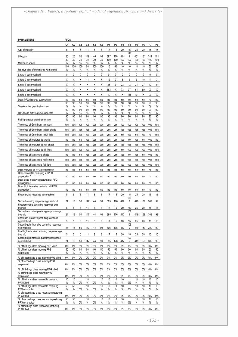
- 152 -

-Chapitre IV : Fate-H, a spatially explicit model of vegetation structure and diversity-

PARAMETERS PFGs

C1 C2 C3 C4 C5 C6 P1 P2 P3 P4 P5 P6 P7 P8

Age of maturity 5 5 6 11 8 8 17 15 20 15 25 20 15 15

Lifespan 26 20 52 149 46 93 397 178 414 1101 451 161 311 101

Maximum shade 30%

30%

30%

70%

30%

30%

100%

100%

100%

100%

100%

100%

100%

100%

Relative size of immatures vs matures 100%

100%

100%

50%

100%

100%

10%

50%

10%

10%

10%

10%

50%

50%

Strata 1 age threshold 0 0 0 0 0 0 0 0 0 0 0 0 0 0

Strata 2 age threshold X X X 11 X X 12 3 8 5 8 10 4 3

Strata 3 age threshold X X X X X X 36 9 23 13 21 27 12 8

Strata 4 age threshold X X X X X X 183 X 73 37 61 89 X X

Strata 5 age threshold X X X X X X X X X 115 191 X X X

Does PFG disperse everywhere ? no no no no no no no no no no no no no no

Shade active gremination rate 90%

90%

90%

90%

90%

90%

90%

90%

90%

90%

90%

90%

90%

90%

Half-shade active gremination rate 90%

90%

90%

90%

90%

90%

90%

90%

90%

90%

90%

90%

90%

90%

Full-light active gremination rate 90%

90%

90%

90%

90%

90%

90%

90%

90%

90%

90%

90%

90%

90%

Tolerence of Germinant to shade yes yes yes yes yes yes yes yes yes yes yes yes yes yes

Tolerence of Germinant to half-shade yes yes yes yes yes yes yes yes yes yes yes yes yes yes

Tolerence of Germinant to full-light yes yes yes yes yes yes yes yes no yes no yes no yes

Tolerence of Imatures to shade no no no yes yes yes yes yes yes no yes no yes no

Tolerence of Imatures to half-shade yes yes yes yes yes yes yes yes yes yes yes yes yes yes

Tolerence of Imatures to full-light yes yes yes yes yes yes yes yes no yes yes yes yes yes

Tolerence of Matures to shade no no no yes yes yes yes yes yes no yes no yes no

Tolerence of Matures to half-shade yes yes yes yes yes yes yes yes yes yes yes yes yes yes

Tolerence of Matures to full-light yes yes yes yes yes yes yes yes yes yes yes yes yes yes

Does mowing kill PFG propagules? no no no no no no no no no no no no no no

Does resonable pasturing kill PFG propagules ? no no no no no no no no no no no no no no

Does quite intensive pasturing kill PFG propagules ? no no no no no no no no no no no no no no

Does high intensive pasturing kill PFG propagules ? no no no no no no no no no no no no no no

First mowing response age treshold 5 5 6 11 8 8 17 15 20 15 25 20 15 15

Second mowing response age treshold 24 18 50 147 44 91 395 176 412 1099 449 159 309 99

First resonable pasturing response age treshold 5 5 6 11 8 8 17 15 20 15 25 20 15 15

Second resonable pasturing response age treshold 24 18 50 147 44 91 395 176 412

1099 449 159 309 99

First quite intensive pasturing response age treshold 5 5 6 11 8 8 17 15 20 15 25 20 15 15

Second quite intensive pasturing response age treshold 24 18 50 147 44 91 395 176 412

1099 449 159 309 99

First high intensive pasturing response age treshold 5 5 6 11 8 8 17 15 20 15 25 20 15 15

Second high intensive pasturing response age treshold 24 18 50 147 44 91 395 176 412

1099 449 159 309 99

% of first age class mowing PFG killed 0% 0% 0% 0% 0% 0% 0% 0% 0% 0% 0% 0% 0% 0%

% of first age class mowing PFG resprouted

50%

50%

50%

50%

50%

50%

50%

50%

50%

50%

50%

50%

50%

50%

% of second age class mowing PFG killed 0% 0% 0% 0% 0% 0% 0% 0% 0% 0% 0% 0% 0% 0%

% of second age class mowing PFG resprouted 0% 0% 0% 0% 0% 0% 0% 0% 0% 0% 0% 0% 0% 0%

% of third age class mowing PFG killed 0% 0% 0% 0% 0% 0% 0% 0% 0% 0% 0% 0% 0% 0%

% of third age class mowing PFG resprouted 0% 0% 0% 0% 0% 0% 0% 0% 0% 0% 0% 0% 0% 0%

% of first age class resonable pasturing PFG killed

10%

10% 0%

10% 0%

10%

10%

10%

10% 0%

10%

10%

10%

10%

% of first age class resonable pasturing PFG resprouted

50%

50% 0%

10% 0%

10%

10%

10%

10% 0%

10%

10%

10%

10%

% of second age class resonable pasturing PFG killed 0% 0% 0% 0% 0% 0% 0% 0% 0% 0% 0% 0% 0% 0%

% of second age class resonable pasturing PFG resprouted

50%

50% 0%

10% 0%

10%

10%

10%

10% 0%

10%

10%

10%

10%

% of third age class resonable pasturing PFG killed 0% 0% 0% 0% 0% 0% 0% 0% 0% 0% 0% 0% 0% 0%

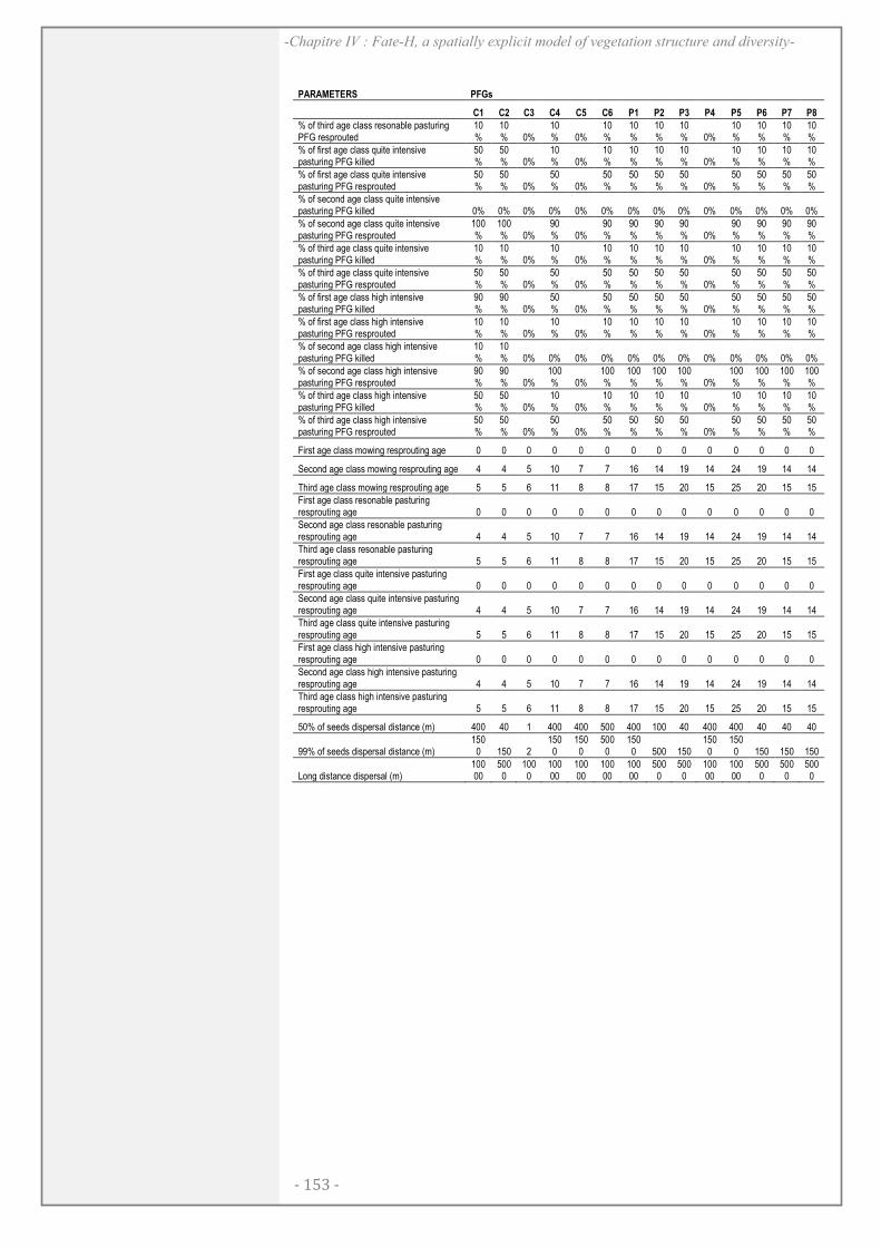
- 153 -

-Chapitre IV : Fate-H, a spatially explicit model of vegetation structure and diversity-

PARAMETERS PFGs

C1 C2 C3 C4 C5 C6 P1 P2 P3 P4 P5 P6 P7 P8

% of third age class resonable pasturing PFG resprouted

10%

10% 0%

10% 0%

10%

10%

10%

10% 0%

10%

10%

10%

10%

% of first age class quite intensive pasturing PFG killed

50%

50% 0%

10% 0%

10%

10%

10%

10% 0%

10%

10%

10%

10%

% of first age class quite intensive pasturing PFG resprouted

50%

50% 0%

50% 0%

50%

50%

50%

50% 0%

50%

50%

50%

50%

% of second age class quite intensive pasturing PFG killed 0% 0% 0% 0% 0% 0% 0% 0% 0% 0% 0% 0% 0% 0%

% of second age class quite intensive pasturing PFG resprouted

100%

100% 0%

90% 0%

90%

90%

90%

90% 0%

90%

90%

90%

90%

% of third age class quite intensive pasturing PFG killed

10%

10% 0%

10% 0%

10%

10%

10%

10% 0%

10%

10%

10%

10%

% of third age class quite intensive pasturing PFG resprouted

50%

50% 0%

50% 0%

50%

50%

50%

50% 0%

50%

50%

50%

50%

% of first age class high intensive pasturing PFG killed

90%

90% 0%

50% 0%

50%

50%

50%

50% 0%

50%

50%

50%

50%

% of first age class high intensive pasturing PFG resprouted

10%

10% 0%

10% 0%

10%

10%

10%

10% 0%

10%

10%

10%

10%

% of second age class high intensive pasturing PFG killed

10%

10% 0% 0% 0% 0% 0% 0% 0% 0% 0% 0% 0% 0%

% of second age class high intensive pasturing PFG resprouted

90%

90% 0%

100% 0%

100%

100%

100%

100% 0%

100%

100%

100%

100%

% of third age class high intensive pasturing PFG killed

50%

50% 0%

10% 0%

10%

10%

10%

10% 0%

10%

10%

10%

10%

% of third age class high intensive pasturing PFG resprouted

50%

50% 0%

50% 0%

50%

50%

50%

50% 0%

50%

50%

50%

50%

First age class mowing resprouting age 0 0 0 0 0 0 0 0 0 0 0 0 0 0

Second age class mowing resprouting age 4 4 5 10 7 7 16 14 19 14 24 19 14 14

Third age class mowing resprouting age 5 5 6 11 8 8 17 15 20 15 25 20 15 15

First age class resonable pasturing resprouting age 0 0 0 0 0 0 0 0 0 0 0 0 0 0

Second age class resonable pasturing resprouting age 4 4 5 10 7 7 16 14 19 14 24 19 14 14

Third age class resonable pasturing resprouting age 5 5 6 11 8 8 17 15 20 15 25 20 15 15

First age class quite intensive pasturing resprouting age 0 0 0 0 0 0 0 0 0 0 0 0 0 0

Second age class quite intensive pasturing resprouting age 4 4 5 10 7 7 16 14 19 14 24 19 14 14

Third age class quite intensive pasturing resprouting age 5 5 6 11 8 8 17 15 20 15 25 20 15 15

First age class high intensive pasturing resprouting age 0 0 0 0 0 0 0 0 0 0 0 0 0 0

Second age class high intensive pasturing resprouting age 4 4 5 10 7 7 16 14 19 14 24 19 14 14

Third age class high intensive pasturing resprouting age 5 5 6 11 8 8 17 15 20 15 25 20 15 15

50% of seeds dispersal distance (m) 400 40 1 400 400 500 400 100 40 400 400 40 40 40

99% of seeds dispersal distance (m) 150

0 150 2 1500

1500

5000

1500 500 150

1500

1500 150 150 150

Long distance dispersal (m) 10000

5000

1000

10000

10000

10000

10000

5000

5000

10000

10000

5000

5000

5000

- 154 -

-Chapitre IV : Fate-H, a spatially explicit model of vegetation structure and diversity-

APPENDIX IV.S3 DETAILS ON HABITAT SUITABILITY MODELING

Calibration area:

The calibration was performed in the whole French Alps region. We then

projected the models on 'Ecrins National Park' (our study area).

From species occurrences to PFG occurrences:

We considered a PFG as present where at least one of its determining

species has been seen. A community where none of its determining

species have been seen was considered as a true absence.

Environmental variables:

We used seven environmental variables: the slope, the percentage of

carbon in the soil, and 5 BIOCLIM variables (isothermality, temperature

seasonality, temperature annual range, mean temperature of coldest

quarter and annual precipitation). These variables have been downscaled

from a regional climatic model.

BIOMOD parameters:

We used 5 models: Generalized Linear Model (each environmental

variables considered as polynomial and stepwise 'best' model selection

considering AIC value); Generalized Boosted Models (with a maximum

of 3000 trees considered); Generalized Additive Model (with a 4 degree

of smoothing of the spline function); Multivariate Adaptive Regression

Splines; Random Forest

The prevalence was fixed at 0.5.

We performed 10 repetitions of each run, with a cross-validation (70% of

data to calibrate and 30% of data for evaluate the models)

Ensemble Forecasting:

We used an ensemble forecasting to derive consensus probability of our

PFG distributions, as follow: 1) We projected of all models 2) We

transformed the probabilities of presence into presences and absences

according to the thresholds optimized by TSS in the evaluation

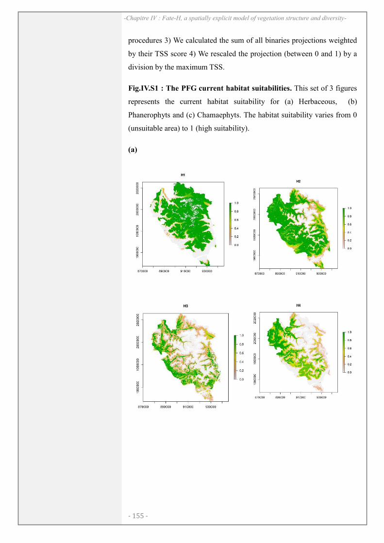
- 155 -

-Chapitre IV : Fate-H, a spatially explicit model of vegetation structure and diversity-

procedures 3) We calculated the sum of all binaries projections weighted

by their TSS score 4) We rescaled the projection (between 0 and 1) by a

division by the maximum TSS.

Fig.IV.S1 : The PFG current habitat suitabilities. This set of 3 figures

represents the current habitat suitability for (a) Herbaceous, (b)

Phanerophyts and (c) Chamaephyts. The habitat suitability varies from 0

(unsuitable area) to 1 (high suitability).

(a)

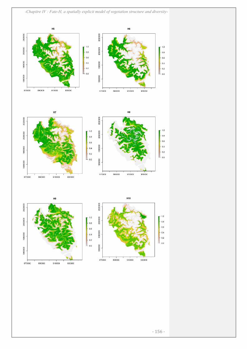
- 156 -

-Chapitre IV : Fate-H, a spatially explicit model of vegetation structure and diversity-

- 157 -

-Chapitre IV : Fate-H, a spatially explicit model of vegetation structure and diversity-

(b)

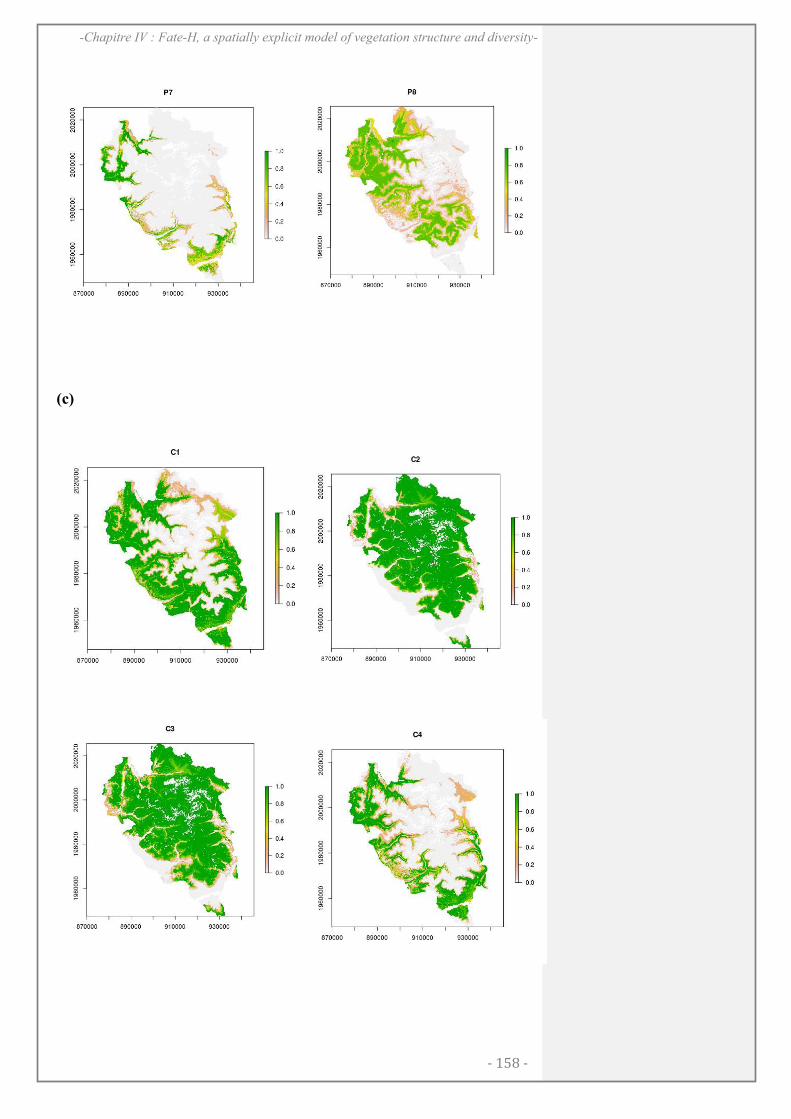
- 158 -

-Chapitre IV : Fate-H, a spatially explicit model of vegetation structure and diversity-

(c)

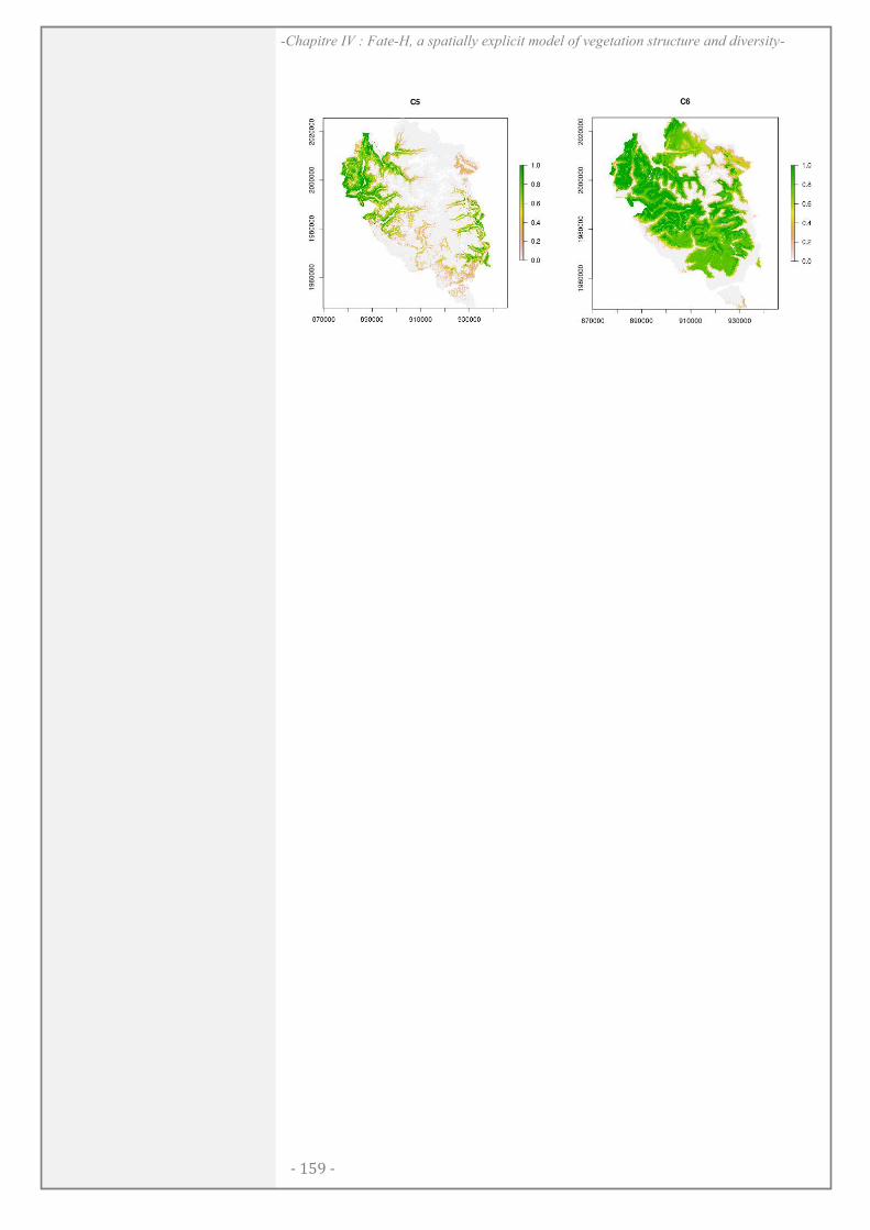
- 159 -

-Chapitre IV : Fate-H, a spatially explicit model of vegetation structure and diversity-

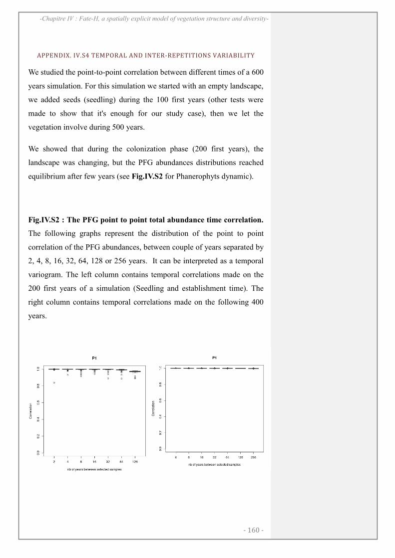
- 160 -

-Chapitre IV : Fate-H, a spatially explicit model of vegetation structure and diversity-

APPENDIX. IV.S4 TEMPORAL AND INTER-REPETITIONS VARIABILITY

We studied the point-to-point correlation between different times of a 600

years simulation. For this simulation we started with an empty landscape,

we added seeds (seedling) during the 100 first years (other tests were

made to show that it's enough for our study case), then we let the

vegetation involve during 500 years.

We showed that during the colonization phase (200 first years), the

landscape was changing, but the PFG abundances distributions reached

equilibrium after few years (see Fig.IV.S2 for Phanerophyts dynamic).

Fig.IV.S2 : The PFG point to point total abundance time correlation.

The following graphs represent the distribution of the point to point

correlation of the PFG abundances, between couple of years separated by

2, 4, 8, 16, 32, 64, 128 or 256 years. It can be interpreted as a temporal

variogram. The left column contains temporal correlations made on the

200 first years of a simulation (Seedling and establishment time). The

right column contains temporal correlations made on the following 400

years.

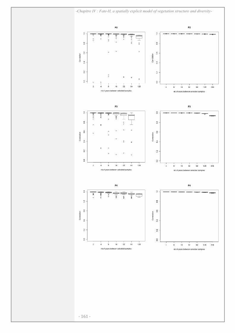
- 161 -

-Chapitre IV : Fate-H, a spatially explicit model of vegetation structure and diversity-

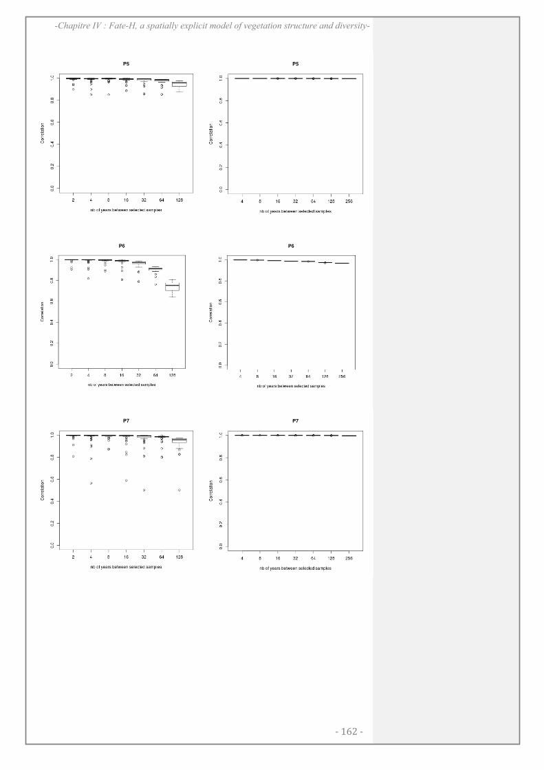
- 162 -

-Chapitre IV : Fate-H, a spatially explicit model of vegetation structure and diversity-

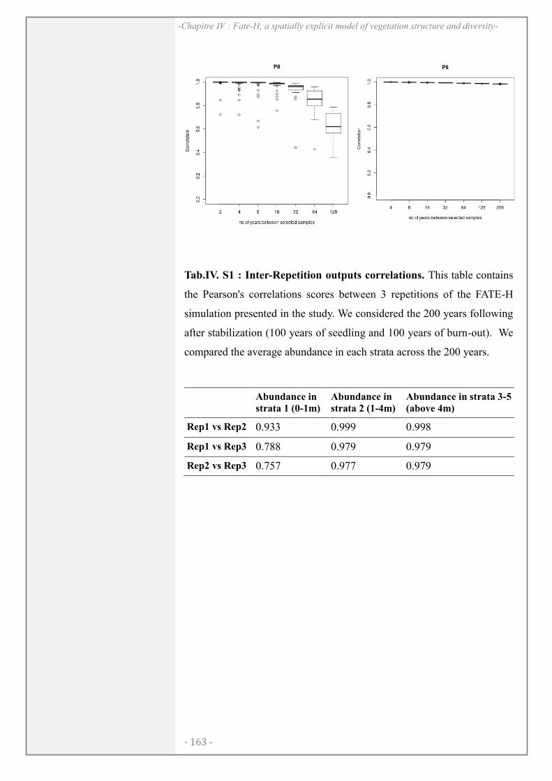
- 163 -

-Chapitre IV : Fate-H, a spatially explicit model of vegetation structure and diversity-

Tab.IV. S1 : Inter-Repetition outputs correlations. This table contains

the Pearson's correlations scores between 3 repetitions of the FATE-H

simulation presented in the study. We considered the 200 years following

after stabilization (100 years of seedling and 100 years of burn-out). We

compared the average abundance in each strata across the 200 years.

Abundance in

strata 1 (0-1m)

Abundance in

strata 2 (1-4m)

Abundance in strata 3-5

(above 4m)

Rep1 vs Rep2 0.933 0.999 0.998

Rep1 vs Rep3 0.788 0.979 0.979

Rep2 vs Rep3 0.757 0.977 0.979

- 164 -

-Chapitre IV : Fate-H, a spatially explicit model of vegetation structure and diversity-

-165-

CHAPITRE V:

C O N S E Q U E N C E S O F C L I M A T E A N D L A N D U S E C H A N G E O N

T H E V E G E T A T I O N S T R U C T U R E A N D P L A N T

F U N C T I O N A L D I V E R S I T Y I N T H E E C R I N S N A T I O N A L P A R K

Boulangeat, I., Georges, D., Dentant, C., Bonet, R., Van Es, J., Abdulayak,

A., Zimmermann, N.E. and Thuiller, W. Consequences of climate and

land use change on the vegetation structure and diversity in the Ecrins

National Park. In preparation.

- 166 -

-Chapitre V : Scenarios of the vegetation in the Ecrins National Park-

Abstract

Modeling tools offer the possibility to quantify the potential impacts of global change on biodiversity. However, very few are adapted to be used at regional scales where management decisions are actually made. The main consequence is that low confidence is given to projections at this scale. New kinds of models are currently developed to overtake these limitations. These models, called „hybrid-models’ take advantage of both mechanistic and statistical approaches, and should be able to produce more robust scenarios at regional scales and over contrasted landscapes.

Here, we make use of a newly developed hybrid model of vegetation dynamics to simulate the potential impacts of both climate change and management practices on the biodiversity of the Ecrins National Park in the French Alps. We simulated the dynamic of 24 plant functional groups, shown to significantly represent the different facets of vegetation diversity. In partnership with the park managers, we developed three extreme management practices over the national park (no change, grazing intensification and grazing break down).

The effects of management practices on the regional vegetation dynamics was simulated alone but also in interaction with regional climate change. Our simulations showed that after abandonment, the colonisation of grasslands by the forest was rapid. On the contrary, under climate change, there was a time lag before we could observe the colonisation of new suitable areas by trees. The effect of grazing intensification was immediate, reducing the total tree cover, but didn’t affected the long-term dynamic induced by climate change. We showed that the functional diversity could increase as a consequence of the abandonment of pastures or during the first years of climate change. However, long-term perspectives for functional diversity under climate change were a general decrease whatever the chosen management.

We conclude that the use of a dynamic and temporally explicit model is necessary to disentangle short-term and long-term perspectives of global changes, and to determine tipping points after which the subtle alteration of the environment may lead to drastic transformations. Our modelling approach with FATE-H also pointed out the interest of accounting for spatial and temporal mechanisms in models, in order to understand and predict the interplay effects of land-use and climate change in time and space.

- 167 -

-Chapitre V : Scenarios of the vegetation in the Ecrins National Park-

INTRODUCTION

The construction of scenarios to predict the future dynamic of the

vegetation diversity is a major challenge in ecology (Pereira et al. 2010;

Bellard et al. 2012). To address it, ecological modeling is a privileged

tool as it allows the quantification of diversity changes, and the

exploration of large time scales. However, most of existing models are

unable to give robust predictions at the regional scale (Parmesan et al.

2011), where reserve networks (e.g. NATURA 2000) and protected areas

are designed and most of conservation decisions are made.

To overcome the limitations of existing models, new approaches have

been recently developed (Gallien et al., Boulangeat et al. Chapter IV).

They are usually based on a combination of mechanistic and

phenomenological models (Wintle et al. 2005; Keith et al. 2008;

Anderson et al. 2009). The inclusion of mechanisms allows to account

for the processes driving species distributions and co-existence and

should improve the robustness of predictions, and the use of statistical

models permits to decrease the calculation time and allow increasing the

extent of the study or the number of modeling entities (Chapter IV).

These models are thus particularly adapted to investigate the potential

impacts of environmental change scenarios at regional spatial scales and

over realistic time-scales.

Amongst the five major drivers of changes on biodiversity (climate, land

use change, nitrogen deposition, atmospheric CO2, biotic exchange, Sala

et al. 2000, Thuiller 2007), climate and land use are expected to be the

most prominent in temperate countries in the near future. Climate, which

has been recognized as a first order factor to determine species diversity

(O’Brien et al. 2000; Whittaker et al. 2001), is expected to drastically

change in the next century (IPCC 2007b). As a consequence, every

component of biodiversity might be affected through various means (e.g.

change in phenology, distribution and physiology, Bellard et al. 2012).

The on-going climate change has already been shown to impact species

distribution and biodiversity (Parmesan 2006; Lenoir et al. 2010;

Gottfried et al. 2012) and more particularly causing a shift of the tree line

- 168 -

-Chapitre V : Scenarios of the vegetation in the Ecrins National Park-

at highest elevations (Randin et al. 2009a). Although climate is a key

driver, changes in land-use and practices is also known to strongly

influence the vegetation structure and diversity (Foley et al. 2005). This

is particularly true in rural landscape and mountain systems where past

land uses over centuries have shaped the current landscape (Quetier et al.

2007; Quetier et al. 2010). In Europe, two main trends of land use

changes have been observed in the past decades. On one hand, the

agricultural crisis has led to a drift from the land, resulting in shrub and

tree encroachments in old pastures and cultivated lands (Gehrig-Fasel et

al. 2007). On the other hand, lowland areas have seen a dramatic increase

in intensive agriculture and farming leading to unprecedented rates of

local species extinctions (Hodgson et al. 2005). There is thus a crucial

need to investigate the interplay between climate and land use changes

and its impacts on biodiversity at regional scales.

Here, we use a hybrid dynamic vegetation model called FATE-H, which

is able to model the vegetation dynamics with enough details to represent

the vegetation structure and the plant functional diversity at the regional

scale (chapitre IV). We analyzed the short and long term consequences of

land-use and climate changes, taken separately and their interplay, on the

regional biodiversity of the Ecrins National Park (PNE). The PNE is a

national park located in the French Alps, relatively large for Europe. It

harbors a heterogeneous landscape due to a complex topography and a

large proportion of its surface is being moderately to intensively grazed

by domestic stock.

For this particular exercise, and in partnership with the PNE managers,

we developed three land use change scenarios: no changes, domestic

grazing intensification, and domestic grazing abandonment. Our

expectations was that the effects of climate change should likely be

visible at the sub-alpine belt, where species were expected to shift their

distributions upward (Jump et al. 2012), and the forest to colonize higher

elevations (Randin et al. 2009a). The abandonment of domestic grazing

should have a similar effect that is the colonization of abandoned

pastures by the forest. An intensification of grazing should reversely

maintain open environment and compensate the effect of climate. Finally,

- 169 -

-Chapitre V : Scenarios of the vegetation in the Ecrins National Park-

species diversity was expected to decrease, at short term, in both land-use

abandonment and land-use intensification scenarios (Niedrist et al.

2009).

MATERIAL AND METHODS

(a)The dynamic hybrid model

We simulated the vegetation dynamic with a spatially and temporally

explicit model called FATE-H (see chapter IV). This hybrid-DVM

combines the strengths of different sub-models and simulates the spatial

and temporal dynamics of plant functional groups (PFGs) in an annual

time-step. The region of interest was represented as a grid of 100x100m

resolution. A succession model, simulating the demography (e.g.

fecundity, recruitment and mortality) of PFGs and the competition for

light between the PFGs, was run within each grid cell (adapted from

Moore & Noble 1990). The total recruitment of each PFG within each

grid cell was influenced by topo-climatic suitability of the pixel

estimated using a habitat suitability model (Guisan & Thuiller 2005). The

spatially explicit processes between grid cells was simulated through a

seed dispersal model, in which the proportion of dispersed seeds was

determined by the abundance of mature PFGs. Seed dispersal distance

was function of the PFG dispersal parameters and a stochastic function

(see Chapitre IV). The recruitment and then survival of the seeds within

each pixel depended on the light availability in the pixel and the PFGs

light preferences. A disturbance model was also included to simulate the

effects of both grazing and mowing. These two disturbances influenced

the abundance of juveniles and mature plants differentially depending on

the sensitivity and response of each PFG to the intensity and frequency of

the two disturbances (see chapter IV for details). In this study, we used

three intensity levels for grazing.

We modelled 24 PFGs, determined by an emergent group approach

(Lavorel et al. 1997; Herault 2007) in which the dominant species of the

area were grouped based on a selection of six key species characteristics

and using a classification procedure (see chapter III). Species were first

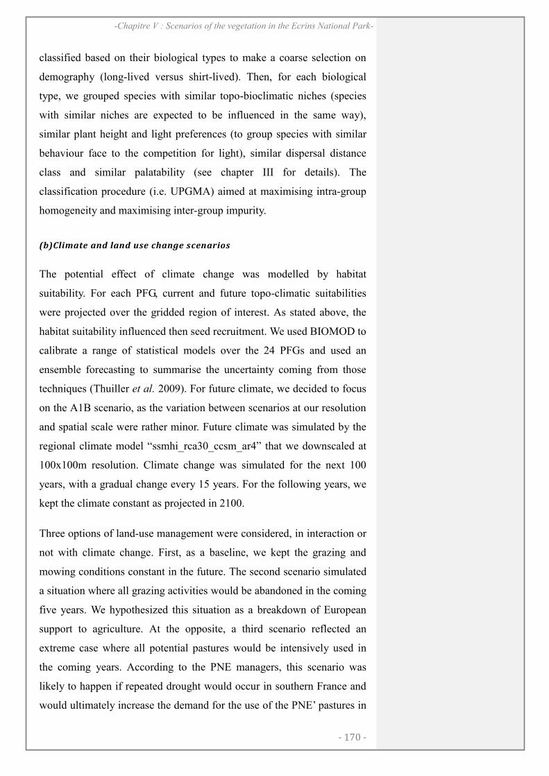
- 170 -

-Chapitre V : Scenarios of the vegetation in the Ecrins National Park-

classified based on their biological types to make a coarse selection on

demography (long-lived versus shirt-lived). Then, for each biological

type, we grouped species with similar topo-bioclimatic niches (species

with similar niches are expected to be influenced in the same way),

similar plant height and light preferences (to group species with similar

behaviour face to the competition for light), similar dispersal distance

class and similar palatability (see chapter III for details). The

classification procedure (i.e. UPGMA) aimed at maximising intra-group

homogeneity and maximising inter-group impurity.

(b)Climate and land use change scenarios

The potential effect of climate change was modelled by habitat

suitability. For each PFG, current and future topo-climatic suitabilities

were projected over the gridded region of interest. As stated above, the

habitat suitability influenced then seed recruitment. We used BIOMOD to

calibrate a range of statistical models over the 24 PFGs and used an

ensemble forecasting to summarise the uncertainty coming from those

techniques (Thuiller et al. 2009). For future climate, we decided to focus

on the A1B scenario, as the variation between scenarios at our resolution

and spatial scale were rather minor. Future climate was simulated by the

regional climate model “ssmhi_rca30_ccsm_ar4” that we downscaled at

100x100m resolution. Climate change was simulated for the next 100

years, with a gradual change every 15 years. For the following years, we

kept the climate constant as projected in 2100.

Three options of land-use management were considered, in interaction or

not with climate change. First, as a baseline, we kept the grazing and

mowing conditions constant in the future. The second scenario simulated

a situation where all grazing activities would be abandoned in the coming

five years. We hypothesized this situation as a breakdown of European

support to agriculture. At the opposite, a third scenario reflected an

extreme case where all potential pastures would be intensively used in

the coming years. According to the PNE managers, this scenario was

likely to happen if repeated drought would occur in southern France and

would ultimately increase the demand for the use of the PNE’ pastures in

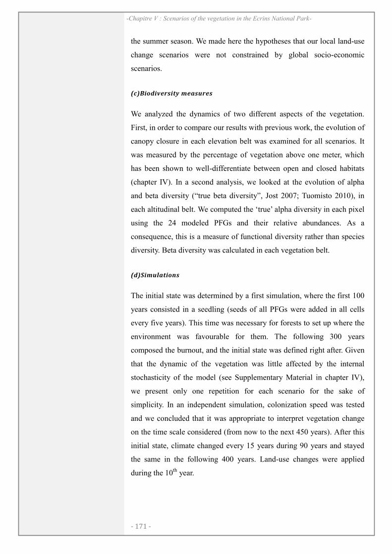
- 171 -

-Chapitre V : Scenarios of the vegetation in the Ecrins National Park-

the summer season. We made here the hypotheses that our local land-use

change scenarios were not constrained by global socio-economic

scenarios.

(c)Biodiversity measures

We analyzed the dynamics of two different aspects of the vegetation.

First, in order to compare our results with previous work, the evolution of

canopy closure in each elevation belt was examined for all scenarios. It

was measured by the percentage of vegetation above one meter, which

has been shown to well-differentiate between open and closed habitats

(chapter IV). In a second analysis, we looked at the evolution of alpha

and beta diversity (“true beta diversity”, Jost 2007; Tuomisto 2010), in

each altitudinal belt. We computed the „true’ alpha diversity in each pixel

using the 24 modeled PFGs and their relative abundances. As a

consequence, this is a measure of functional diversity rather than species

diversity. Beta diversity was calculated in each vegetation belt.

(d)Simulations

The initial state was determined by a first simulation, where the first 100

years consisted in a seedling (seeds of all PFGs were added in all cells

every five years). This time was necessary for forests to set up where the

environment was favourable for them. The following 300 years

composed the burnout, and the initial state was defined right after. Given

that the dynamic of the vegetation was little affected by the internal

stochasticity of the model (see Supplementary Material in chapter IV),

we present only one repetition for each scenario for the sake of

simplicity. In an independent simulation, colonization speed was tested

and we concluded that it was appropriate to interpret vegetation change

on the time scale considered (from now to the next 450 years). After this

initial state, climate changed every 15 years during 90 years and stayed

the same in the following 400 years. Land-use changes were applied

during the 10th year.

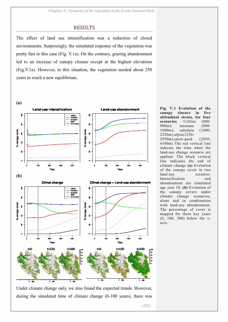
- 172 -

-Chapitre V : Scenarios of the vegetation in the Ecrins National Park-

RESULTS

The effect of land use intensification was a reduction of closed

environments. Surprisingly, the simulated response of the vegetation was

pretty fast in this case (Fig. V.1a). On the contrary, grazing abandonment

led to an increase of canopy closure except at the highest elevations

(Fig.V.1a). However, in this situation, the vegetation needed about 250

years to reach a new equilibrium.

(a)

(b)

Under climate change only, we also found the expected trends. However,

during the simulated time of climate change (0-100 years), there was

Fig. V.1 Evolution of the

canopy closure in five

altitudinal strata, for four scenarios. Colline (800-900m); montane (900-1600m); subalpin (1600-2250m);alpin(2250-2950m);snow-pack (2950-4100m) The red vertical line indicate the time when the land-use change scenario are applied. The black vertical line indicates the end of climate change (a) Evolution of the canopy cover in two land-use scenario. Intensification and abandonment are simulated age year 10. (b) Evolution of the canopy covers under climate change scenarios, alone and in combination with land-use abandonment. The percentage of cover is mapped for three key years (0, 100, 500) below the x-axis.

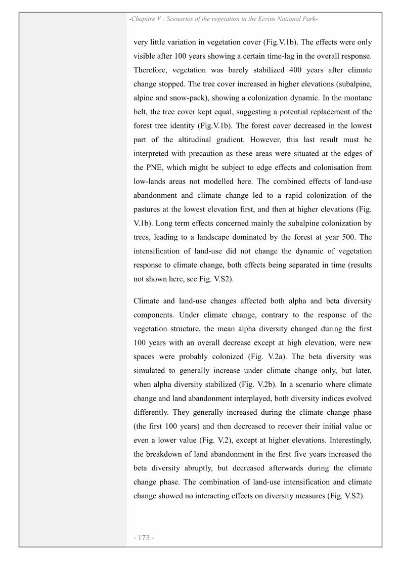
- 173 -

-Chapitre V : Scenarios of the vegetation in the Ecrins National Park-

very little variation in vegetation cover (Fig.V.1b). The effects were only

visible after 100 years showing a certain time-lag in the overall response.

Therefore, vegetation was barely stabilized 400 years after climate

change stopped. The tree cover increased in higher elevations (subalpine,

alpine and snow-pack), showing a colonization dynamic. In the montane

belt, the tree cover kept equal, suggesting a potential replacement of the

forest tree identity (Fig.V.1b). The forest cover decreased in the lowest

part of the altitudinal gradient. However, this last result must be

interpreted with precaution as these areas were situated at the edges of

the PNE, which might be subject to edge effects and colonisation from

low-lands areas not modelled here. The combined effects of land-use

abandonment and climate change led to a rapid colonization of the

pastures at the lowest elevation first, and then at higher elevations (Fig.

V.1b). Long term effects concerned mainly the subalpine colonization by

trees, leading to a landscape dominated by the forest at year 500. The

intensification of land-use did not change the dynamic of vegetation

response to climate change, both effects being separated in time (results

not shown here, see Fig. V.S2).

Climate and land-use changes affected both alpha and beta diversity

components. Under climate change, contrary to the response of the

vegetation structure, the mean alpha diversity changed during the first

100 years with an overall decrease except at high elevation, were new

spaces were probably colonized (Fig. V.2a). The beta diversity was

simulated to generally increase under climate change only, but later,

when alpha diversity stabilized (Fig. V.2b). In a scenario where climate

change and land abandonment interplayed, both diversity indices evolved

differently. They generally increased during the climate change phase

(the first 100 years) and then decreased to recover their initial value or

even a lower value (Fig. V.2), except at higher elevations. Interestingly,

the breakdown of land abandonment in the first five years increased the

beta diversity abruptly, but decreased afterwards during the climate

change phase. The combination of land-use intensification and climate

change showed no interacting effects on diversity measures (Fig. V.S2).

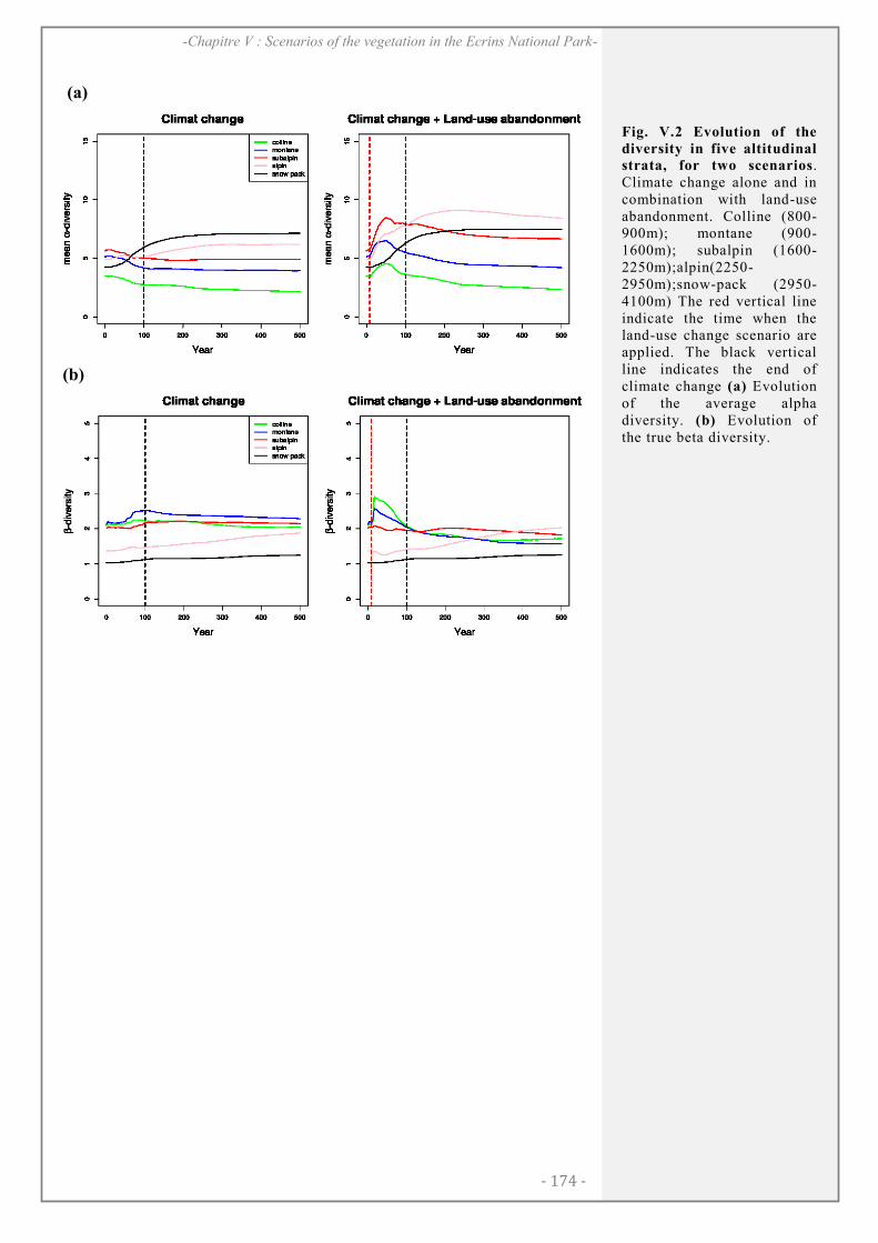
- 174 -

-Chapitre V : Scenarios of the vegetation in the Ecrins National Park-

(a)

(b)

Fig. V.2 Evolution of the

diversity in five altitudinal strata, for two scenarios. Climate change alone and in combination with land-use abandonment. Colline (800-900m); montane (900-1600m); subalpin (1600-2250m);alpin(2250-2950m);snow-pack (2950-4100m) The red vertical line indicate the time when the land-use change scenario are applied. The black vertical line indicates the end of climate change (a) Evolution of the average alpha diversity. (b) Evolution of the true beta diversity.

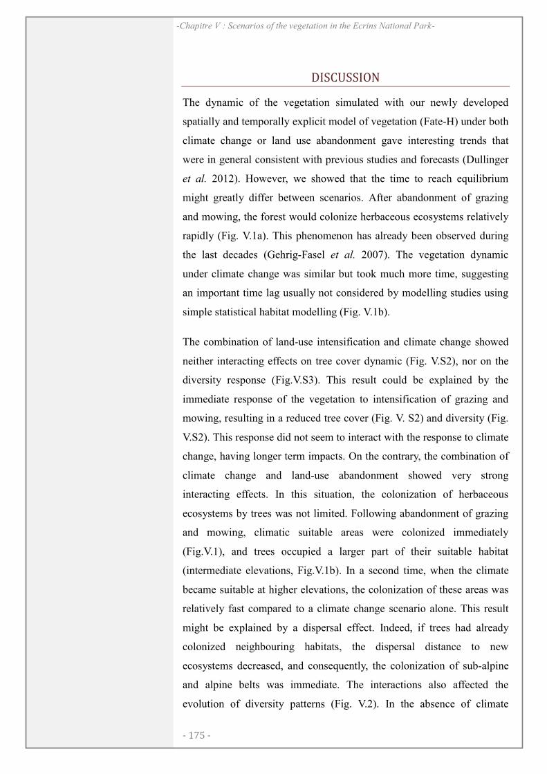
- 175 -

-Chapitre V : Scenarios of the vegetation in the Ecrins National Park-

DISCUSSION

The dynamic of the vegetation simulated with our newly developed

spatially and temporally explicit model of vegetation (Fate-H) under both

climate change or land use abandonment gave interesting trends that

were in general consistent with previous studies and forecasts (Dullinger

et al. 2012). However, we showed that the time to reach equilibrium

might greatly differ between scenarios. After abandonment of grazing

and mowing, the forest would colonize herbaceous ecosystems relatively

rapidly (Fig. V.1a). This phenomenon has already been observed during

the last decades (Gehrig-Fasel et al. 2007). The vegetation dynamic

under climate change was similar but took much more time, suggesting

an important time lag usually not considered by modelling studies using

simple statistical habitat modelling (Fig. V.1b).

The combination of land-use intensification and climate change showed

neither interacting effects on tree cover dynamic (Fig. V.S2), nor on the

diversity response (Fig.V.S3). This result could be explained by the

immediate response of the vegetation to intensification of grazing and

mowing, resulting in a reduced tree cover (Fig. V. S2) and diversity (Fig.

V.S2). This response did not seem to interact with the response to climate

change, having longer term impacts. On the contrary, the combination of

climate change and land-use abandonment showed very strong

interacting effects. In this situation, the colonization of herbaceous

ecosystems by trees was not limited. Following abandonment of grazing

and mowing, climatic suitable areas were colonized immediately

(Fig.V.1), and trees occupied a larger part of their suitable habitat

(intermediate elevations, Fig.V.1b). In a second time, when the climate

became suitable at higher elevations, the colonization of these areas was

relatively fast compared to a climate change scenario alone. This result

might be explained by a dispersal effect. Indeed, if trees had already

colonized neighbouring habitats, the dispersal distance to new

ecosystems decreased, and consequently, the colonization of sub-alpine

and alpine belts was immediate. The interactions also affected the

evolution of diversity patterns (Fig. V.2). In the absence of climate

- 176 -

-Chapitre V : Scenarios of the vegetation in the Ecrins National Park-

change, alpha and beta diversity increased as a result of land-use

abandonment, and then stabilized. Climate change modified this dynamic

in a long-term perspective, which resulted in a final decrease for both

alpha and beta diversity.

Conclusion

Our simulations highlighted the importance of the time required for

ecosystems to respond to environmental changes. We showed that, even

if no or little effect is detected during the continuous change in climate,

strong modification in the vegetation dynamics response might be then

seen over 400 years. Short and long term effects are thus inter-wined and

difficult to tease-apart when all potential changes are put together. Our

simulations based on climate only, land use change only, and then

interactions between the two drivers allowed to disentangle their

respective effects and demonstrated the difficulty to make realistic

projections within a simplified modelling exercise. Concerning diversity

changes, we showed that the functional diversity could increase as a

consequence of environmental changes, whereas previous studies,

focusing on species diversity, generally predicted a decline in species

richness (Niedrist et al. 2009).

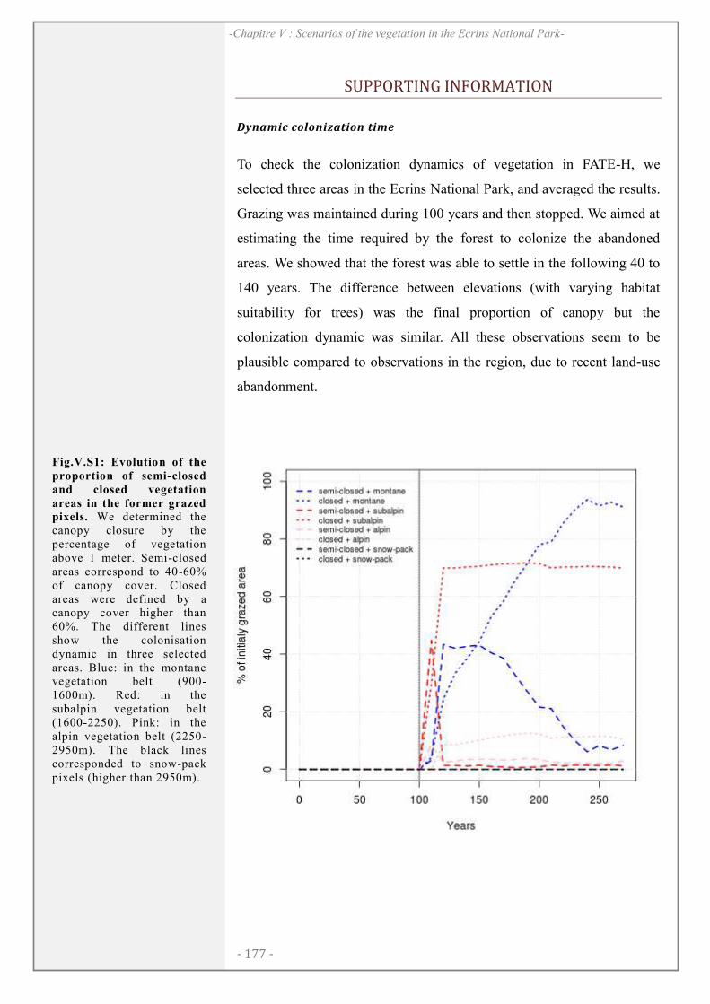
- 177 -

-Chapitre V : Scenarios of the vegetation in the Ecrins National Park-

SUPPORTING INFORMATION

Dynamic colonization time

To check the colonization dynamics of vegetation in FATE-H, we

selected three areas in the Ecrins National Park, and averaged the results.

Grazing was maintained during 100 years and then stopped. We aimed at

estimating the time required by the forest to colonize the abandoned

areas. We showed that the forest was able to settle in the following 40 to

140 years. The difference between elevations (with varying habitat

suitability for trees) was the final proportion of canopy but the

colonization dynamic was similar. All these observations seem to be

plausible compared to observations in the region, due to recent land-use

abandonment.

Fig.V.S1: Evolution of the

proportion of semi-closed

and closed vegetation

areas in the former grazed pixels. We determined the canopy closure by the percentage of vegetation above 1 meter. Semi-closed areas correspond to 40-60% of canopy cover. Closed areas were defined by a canopy cover higher than 60%. The different lines show the colonisation dynamic in three selected areas. Blue: in the montane vegetation belt (900-1600m). Red: in the subalpin vegetation belt (1600-2250). Pink: in the alpin vegetation belt (2250-2950m). The black lines corresponded to snow-pack pixels (higher than 2950m).

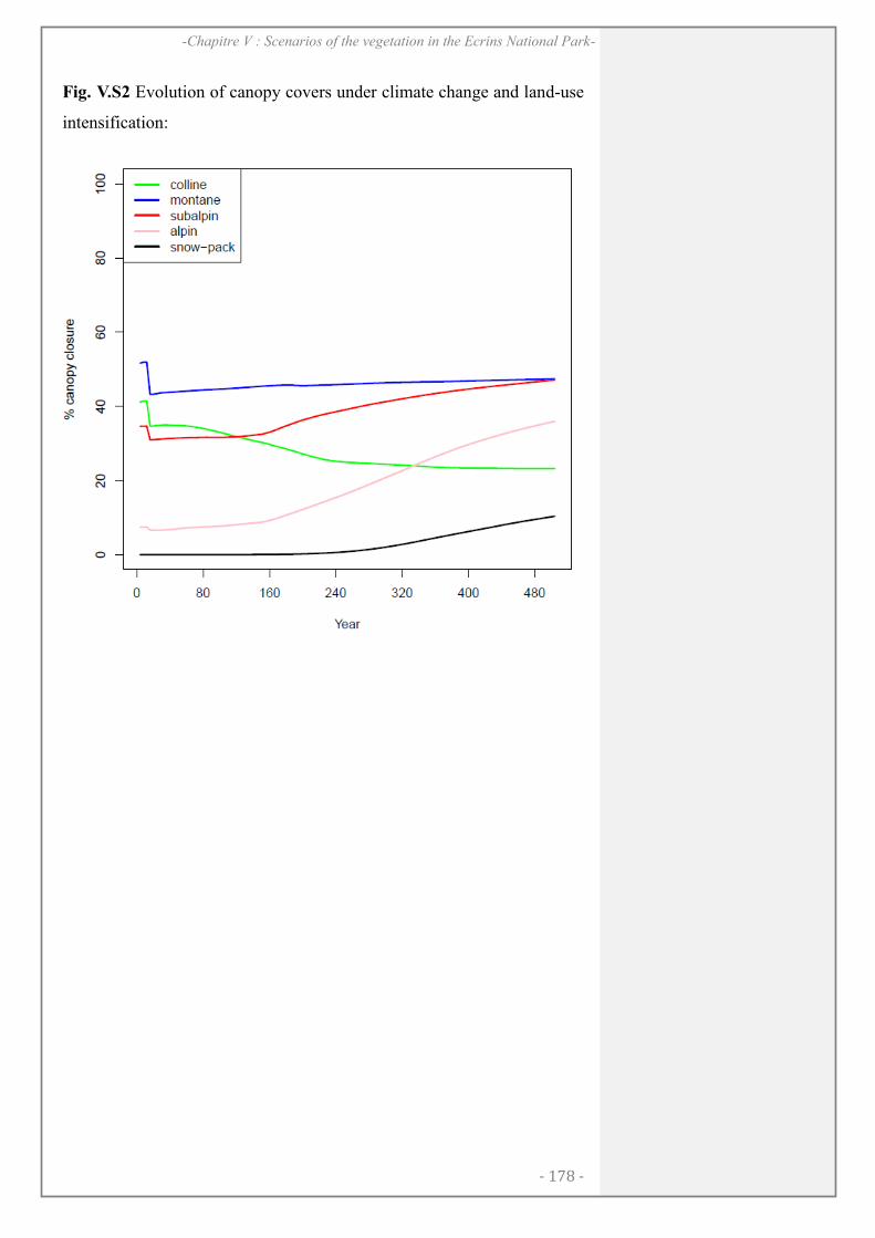
- 178 -

-Chapitre V : Scenarios of the vegetation in the Ecrins National Park-

Fig. V.S2 Evolution of canopy covers under climate change and land-use

intensification:

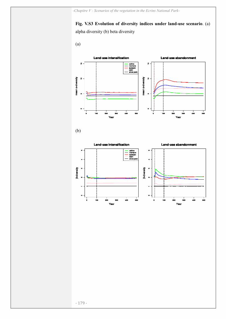
- 179 -

-Chapitre V : Scenarios of the vegetation in the Ecrins National Park-

Fig. V.S3 Evolution of diversity indices under land-use scenario. (a)

alpha diversity (b) beta diversity

(a)

(b)

- 180 -

-Chapitre V : Scenarios of the vegetation in the Ecrins National Park-

-181-

S Y N T H E S E : D I S C U S S I O N G É N É R A L E E T P E R S P E C T I V E S

- 182 -

-Synthèse-

- 183 -

-Synthèse-

COMPRENDRE LES MÉCANISMES DE COEXISTENCE

UNE VISION HIÉRARCHIQUE DES MÉCANISMES VALIDEE

Le chapitre II nous a permis de tester l’ensemble du cadre théorique

hiérarchique proposé dans l’introduction (Fig. i.7). Nous avons trouvé

que l’absence (ou la présence) des espèces modélisées était bien décrite

par les variables abiotiques et l’indice de dispersion (Fig. II.4a),

suggérant l’importance première des mécanismes de filtres

environnementaux et de limitation par la dispersion. L’influence

secondaire des indices d’interactions biotiques à cette étape pourrait

être le résultat de mécanismes d’exclusion compétitive.

L’approche de modélisation emboitée nous a permis de démontrer la

nécessité de prendre en compte les mécanismes agissants aux échelles

spatiales supérieures pour analyser ce qui se passe au niveau de la

communauté. En effet, l’efficacité d’un modèle hiérarchique est

largement supérieure à celle d’un modèle traditionnel (Fig. II.S5). Cette

méthode nous a permis d’analyser la variation d’abondance des espèces

au sein de leur niche, et d’étudier le résultat des mécanismes de

coexistence. Notamment, les modèles mettent en évidence l’importance

des interactions biotiques négatives, qui peuvent être le résultat de la

compétition. D’un autre côté, les facteurs abiotiques ne sont pas

négligeables pour expliquer la variation d’abondance d’une espèce. Ils

sont même prépondérants pour certaines espèces (Fig. II.4b), ce qui est

en accord avec des études où le climat a été relié à la performance des

espèces (ex. Riba et al. 2002; Thuiller et al. 2010b).

LES INTERACTIONS BIOTIQUES

Compétition ou conditions abiotiques locales ?

Nous avons montré dans le chapitre II l’importance des processus qui

ont lieu à l’échelle de la communauté pour expliquer l’abondance des

espèces, et dans une moindre mesure leur probabilité de présence en un

site donné. Cependant, même si l’on suppose que la compétition est un

mécanisme important, son effet est très difficile à distinguer des effets

- 184 -

-Synthèse-

de l’environnement abiotique local qui n’est pas représenté par les

variables choisies. À l’intérieur de la communauté, les conditions

abiotiques peuvent également être modifiées par la présence d’autres

espèces (ex. la canopée modifie la température près du sol). Le seul

moyen d’être certain de la présence d’une certaine forme de

compétition est de la tester expérimentalement, ce qui est impossible

lorsqu’on étudie toute une flore à l’aide de données empiriques.

Spécialisation et stratégie compétitive

La différenciation de niche permettrait à deux espèces de coexister

parce que leur compétitivité se croise le long d’un gradient, chaque

espèce dominant l’autre dans certaines conditions (Fig. i.3 ; Chesson

2000a ; Silvertown 2004). Nous avons étudié les patrons de

spécialisation (de largeur de niche) dans le chapitre I et deux principales

hypothèses peuvent être formulées pour expliquer la restriction de

l’amplitude écologique des espèces. Les résultats nous ont montré que

les espèces compétitrices sensu Grime (Fig. I.5) sont plutôt généralistes

(de largeur de niche étendue) alors que les espèces spécialistes (de

largeur de niche restreinte) sont plutôt tolérantes au stress (Fig. I.5b).

Ces tendances nous suggèrent que dans de nombreux cas, la

spécialisation est le résultat de l’exclusion d’espèces par de meilleures

compétitrices, dans les milieux les plus productifs. Les perdantes se

réfugient alors dans des milieux plus stressants (Bonesi & Macdonald

2004), où la compétitivité de leurs concurrentes est réduite et où elles

seront alors dominantes. Par conséquent, ces spécialistes se

différencient à la fois par une largeur de niche restreinte et par une

marginalité sur un gradient de productivité (ou stress) non déterminé.

D’un autre côté, certaines spécialistes sont plutôt compétitrices (Fig.

I.5b), et donc le premier scenario ne peut pas s’appliquer à celles-ci.

Dans ce cas, la faible amplitude écologique peut s’expliquer par une

faible tolérance aux milieux peu productifs. En contrepartie, ces

spécialistes auraient une compétitivité augmentée dans les milieux

fertiles (Wisheu 1998). Ces deux situations suggèrent qu’un des axes

importants de différenciation de niche est celui de productivité.

Cependant, l’amplitude écologique mesurée dans le chapitre I mélange

- 185 -

-Synthèse-

tous les gradients et ne caractérise pas la position de niche grâce à des

données environnementales. L’approche de mesure de la spécialisation

par analyse des patrons de cooccurrence d’espèces permet de capter

tous les axes de spécialisation, même ceux liés à des conditions micro-

environnementales, généralement difficiles à caractériser avec les

données disponibles (ex. type de sol), mais ne permet pas de distinguer

les différents types de spécialisation.

Vers une séparation des gradients de différenciation

Afin de mieux comprendre les mécanismes de différenciation de niche,

il serait très intéressant de séparer la spécialisation Grinnellienne et la

spécialisation Eltonienne chez les plantes (Devictor et al. 2010). En ce

qui concerne la niche Eltonienne chez les plantes, la manière de la

mesurer et de l’interpréter n’est pas évidente. La position pourrait être

définie par le rôle fonctionnel d’une espèce et une spécialiste aurait un

rôle marginal (ex. une fixatrice d’azote). La largeur de niche pourrait

être définie par la variabilité de ce rôle à travers les individus, les

populations, ou au cours du temps. Une approche pourrait être

l’utilisation de traits fonctionnels et leur variabilité intra-spécifique.

D’un autre côté, la spécialisation écologique totale mesurée par le biais

des cooccurrences résulte à la fois de la spécialisation grinnellienne et

de la spécialisation eltonienne. Une approche indirecte serait d’utiliser

les résidus d’un modèle « spécialisation totale ~ spécialisation

Grinnellienne », qui décrirait la diversité des interactions biotiques

possibles.

Nous avons exploré cette piste lors dans le cadre de ma thèse, en

utilisant la même approche que celle du chapitre I (Fridley et al. 2007),

appliquée à une mesure de diversité fonctionnelle. La niche eltonienne a

ainsi été caractérisée par le « turnover » fonctionnel des communautés

dans lesquelles l’espèce se trouvait. La spécialisation totale a ainsi pu

être décomposée en deux axes indépendants. La spécialisation

grinnellienne, mesurée par une méthode d’analyses multivariées

(Outlying Mean Index, Dolédec et al. 2000) et impliquant des variables

topo-climatiques importantes, était relativement indépendante de la

- 186 -

-Synthèse-

spécialisation eltonienne ainsi estimée, toute deux contribuant à la

spécialisation totale. Autrement dit, le « turnover » fonctionnel des

communautés ou une espèce est présente semble peu lié au « turnover »

bioclimatique. Cependant, le « turnover fonctionnel » ainsi mesuré peut

représenter d’autres différenciations de niche qui sont locales, et qui

n’ont rien avoir avec les interactions biotiques. Finalement, cette

décomposition nous a montré que la différenciation de niche peut être

décomposée sur un axe de gradients régionaux (mesuré par les gradients

topo-climatiques ici) et sur un axe de gradients locaux (mesuré par le

« turnover » fonctionnel des communautés). Cependant, la niche

eltonienne n’a pas pu être vraiment caractérisée.

Le principal problème à résoudre pour appliquer une telle approche

chez les plantes est peut-être de mieux définir la niche eltonienne des

espèces végétales. En effet, ce concept est à l’origine basé sur les

relations trophiques (Elton 1927) et n’est pas évident à appliquer pour

les plantes. Si la niche Eltonienne représente l’environnement biotique,

est-il possible de la mesurer par la structure fonctionnelle de la

communauté ? Et quelle mesure choisir dans le cas échéant ? Un trait

moyen ? Une divergence fonctionnelle ? En conclusion, nous pensons

que la décomposition des spécialisations grinnellienne et eltonienne

seraient plus facilement applicable chez les animaux, comme les

oiseaux par exemple, où la niche eltonienne est bien caractérisée par des

types de ressources et d’acquisition des ressources.

Quel type de compétition entre en jeu ?

Une perspective intéressante serait de mettre en évidence le lien entre la

compétition et la spécialisation sur un gradient bien identifié. Ceci a été

exploré mais non présenté précédemment. Nous avons ainsi tenté

d’expliquer la tolérance bioclimatique des espèces, par un ensemble de

traits qui décrivent les stratégies d’acquisition des ressources (Grime et

al. 1997; Reich et al. 1999). Dans ce travail annexe, l’analyse des pistes

(qui analyse la structure causale entre variables à l’aide de corrélations

partielles) nous a suggéré que, dans notre zone d’étude, la capacité de

compétition pour la lumière plutôt que la stratégie d’utilisation des

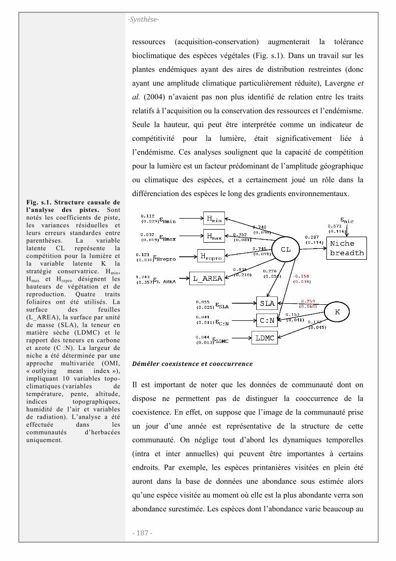
- 187 -

-Synthèse-

ressources (acquisition-conservation) augmenterait la tolérance

bioclimatique des espèces végétales (Fig. s.1). Dans un travail sur les

plantes endémiques ayant des aires de distribution restreintes (donc

ayant une amplitude climatique particulièrement réduite), Lavergne et

al. (2004) n’avaient pas non plus identifié de relation entre les traits

relatifs à l’acquisition ou la conservation des ressources et l’endémisme.

Seule la hauteur, qui peut être interprétée comme un indicateur de

compétitivité pour la lumière, était significativement liée à

l’endémisme. Ces analyses soulignent que la capacité de compétition

pour la lumière est un facteur prédominant de l’amplitude géographique

ou climatique des espèces, et a certainement joué un rôle dans la

différenciation des espèces le long des gradients environnementaux.

Démêler coexistence et cooccurrence

Il est important de noter que les données de communauté dont on

dispose ne permettent pas de distinguer la cooccurrence de la

coexistence. En effet, on suppose que l’image de la communauté prise

un jour d’une année est représentative de la structure de cette

communauté. On néglige tout d’abord les dynamiques temporelles

(intra et inter annuelles) qui peuvent être importantes à certains

endroits. Par exemple, les espèces printanières visitées en plein été

auront dans la base de données une abondance sous estimée alors

qu’une espèce visitée au moment où elle est la plus abondante verra son

abondance surestimée. Les espèces dont l’abondance varie beaucoup au

Fig. s.1. Structure causale de l’analyse des pistes. Sont notés les coefficients de piste, les variances résiduelles et leurs erreurs standardes entre parenthèses. La variable latente CL représente la compétition pour la lumière et la variable latente K la stratégie conservatrice. Hmin, Hmax et Hrepro désignent les hauteurs de végétation et de reproduction. Quatre traits foliaires ont été utilisés. La surface des feuilles (L_AREA), la surface par unité de masse (SLA), la teneur en matière sèche (LDMC) et le rapport des teneurs en carbone et azote (C :N). La largeur de niche a été déterminée par une approche multivariée (OMI, « outlying mean index »), impliquant 10 variables topo-climatiques (variables de température, pente, altitude, indices topographiques, humidité de l’air et variables de radiation). L’analyse a été effectuée dans les communautés d’herbacées uniquement.

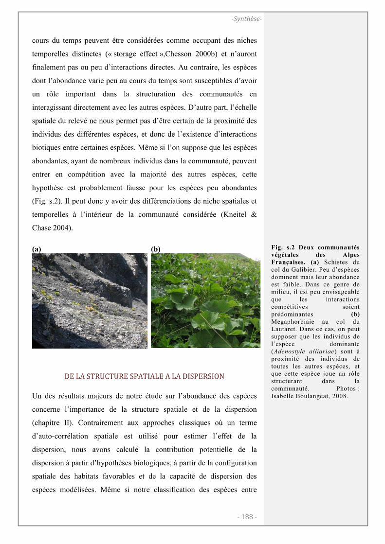
- 188 -

-Synthèse-

cours du temps peuvent être considérées comme occupant des niches

temporelles distinctes (« storage effect »,Chesson 2000b) et n’auront

finalement pas ou peu d’interactions directes. Au contraire, les espèces

dont l’abondance varie peu au cours du temps sont susceptibles d’avoir

un rôle important dans la structuration des communautés en

interagissant directement avec les autres espèces. D’autre part, l’échelle

spatiale du relevé ne nous permet pas d’être certain de la proximité des

individus des différentes espèces, et donc de l’existence d’interactions

biotiques entre certaines espèces. Même si l’on suppose que les espèces

abondantes, ayant de nombreux individus dans la communauté, peuvent

entrer en compétition avec la majorité des autres espèces, cette

hypothèse est probablement fausse pour les espèces peu abondantes

(Fig. s.2). Il peut donc y avoir des différenciations de niche spatiales et

temporelles à l’intérieur de la communauté considérée (Kneitel &

Chase 2004).

(a) (b)

DE LA STRUCTURE SPATIALE A LA DISPERSION

Un des résultats majeurs de notre étude sur l’abondance des espèces

concerne l’importance de la structure spatiale et de la dispersion

(chapitre II). Contrairement aux approches classiques où un terme

d’auto-corrélation spatiale est utilisé pour estimer l’effet de la

dispersion, nous avons calculé la contribution potentielle de la

dispersion à partir d’hypothèses biologiques, à partir de la configuration

spatiale des habitats favorables et de la capacité de dispersion des

espèces modélisées. Même si notre classification des espèces entre

Fig. s.2 Deux communautés

végétales des Alpes Françaises. (a) Schistes du col du Galibier. Peu d’espèces dominent mais leur abondance est faible. Dans ce genre de milieu, il est peu envisageable que les interactions compétitives soient prédominantes (b) Megaphorbiaie au col du Lautaret. Dans ce cas, on peut supposer que les individus de l’espèce dominante (Adenostyle alliariae) sont à proximité des individus de toutes les autres espèces, et que cette espèce joue un rôle structurant dans la communauté. Photos : Isabelle Boulangeat, 2008.

- 189 -

-Synthèse-

différents groupes de dispersion peut paraître grossière (chapitre II)

notre approche est très conservative car elle permet de séparer des

grands groupes d’espèces selon leur capacité supposée de dispersion,

sur la base d’un certain nombre de traits biologiques et écologiques

(Vittoz & Engler 2007). En effet, l’analyse des patrons d’abondance

menée dans le chapitre II montre que des mécanismes source-puits

opèrent pour déterminer la distribution des espèces. L’abondance, pour

les espèces analysées, est plus forte dans les sites qui sont supposés être

des sources que dans ceux qui sont supposés être des puits (Fig. II.5).

Nous avons aussi montré que l’importance relative de la dispersion, par

rapport au filtre abiotique et aux interactions biotiques, varie selon les

espèces et si l’on s’intéresse à la présence-absence d’une espèce

seulement ou à son abondance. Cette différence ne s’explique pourtant

pas simplement par la distance de dispersion des graines. En effet,

l’importance de l’indice de dispersion qui décrit la proximité de milieux

favorables à l’espèce, varie selon les espèces indépendamment de leur

capacité de dispersion. Ce résultat suggère que la limitation par la

dispersion de l’accès aux sites est vraisemblablement autant le résultat

de la configuration spatiale des habitats favorables que de la capacité de

dispersion des espèces. En ce qui concerne l’abondance locale des

espèces, l’importance ou non de la dispersion peut résulter d’un

compromis stratégique. S’il s’agit d’un compromis entre compétition et

colonisation, il pourrait être déterminé par une combinaison de traits de

dispersion et de traits de compétition. Cette hypothèse reste à explorer.

Dans tous les cas, pour aller plus loin, il faudrait appréhender le

mécanisme de dispersion dans son ensemble (parfois appelé migration,

Higgins et al. 2003), à partir de la production de graines jusqu’à la

germination de celles-ci, et déterminer un ensemble de traits qui

représenterait l’efficacité de la dispersion. Pour de nombreuses plantes,

la majorité des graines tombent dans les 100 m aux alentours (Vittoz et

al. 2007), et seule une petite poignée qui est dispersée plus loin peut

prétendre participer aux effets source-puits et à la colonisation de

nouveaux espaces. Le succès de la dispersion dépend fortement de la

survie de ces graines et de leur établissement. Au sein même d’une

- 190 -

-Synthèse-

espèce, si la probabilité de survie des graines était inversement corrélée

à leur distance de dispersion, alors les évènements rares de dispersion

longue distance seraient plus probables. Pour augmenter le succès

d’établissement, les graines peuvent aussi entrer en dormance et

attendre plusieurs années que les conditions environnementales soient

favorables pour germer. Mieux comprendre la dispersion dans son

ensemble permettrait de différencier les espèces selon leurs stratégies et

de mieux prédire leurs réponses aux changements environnementaux.

COMMENT TENIR COMPTE DES VARIATIONS TEMPORELLES DE STRUCTURE DES COMMUNAUTES ?

La discussion concernant les interactions biotiques soulève un point très

important. Lorsque nous observons les assemblages d’espèces, nous

nous plaçons en un point particulier de l’espace et du temps. Selon le

moment de l’année, les espèces échantillonnées et leurs abondances

relatives peuvent changer dans une même communauté, notamment dus

à certains décalages de phénologie. D’une année sur l’autre, les

assemblages peuvent également diverger en fonction des d’évènements

de dispersion (Kneitel & Chase 2004). Prendre en compte cet aspect

temporel lors de l’analyse des données pourrait apporter une meilleure

compréhension des mécanismes d’assemblage des communautés.

Une première approche serait l’exploration des variations intra

annuelles de la composition et la structure des communautés. Ceci nous

permettrait de séparer les espèces qui sont différenciées par des niches

temporelles, et entrent peu en interaction, des espèces qui occupent des

niches similaires ou totalement chevauchantes et qui sont en interaction

directe. Cette approche nécessite de nouvelles données dont nous ne

disposons pas à l’heure actuelle, ni dans notre équipe ni en général.

Cela demanderait en effet des échantillonnages successifs tout au long

de la période de végétation. Le projet TEEMBIO (Towards Eco-

Evolutionary Models of BIOdiversity) coordonné par W. Thuiller

effectuera de tels relevés dès cet été.

Une deuxième approche possible n’étudierait pas les dynamiques intra-

annuelles mais chercherait à mieux exploiter les données existantes.

- 191 -

-Synthèse-

Pour déterminer le climat associé au relevé, l’idée serait de prendre en

compte la date exacte à laquelle le relevé a été fait, et non plus une

moyenne sur plusieurs années (ex. Bateman et al. 2012). Cette approche

permettrait de mieux caractériser la niche climatique des espèces et

donc d’établir des prédictions plus robustes, ou de mieux séparer les

mécanismes pour les comprendre. La relation ainsi modélisée pourrait

être utilisée dans des scenarios où le climat varie chaque année, et serait

adaptée pour tester l’effet d’années successives de sècheresses par

exemple. En ce qui concerne les interactions biotiques, une idée serait

de considérer comme co-occurrentes seules les espèces dominantes dont

l’abondance varie peu au cours de l’année (ex. Pellissier et al. 2010).

Ces espèces sont en effet les plus susceptibles de structurer les

interactions biotiques. Leur niche chevauche entièrement celle des

autres dans le temps, et leurs individus sont répartis sur toute la surface

de la communauté (Fig. s.2b). Les interactions avec les espèces

dominantes peuvent être prises en compte dans les modèles statistiques

comme une variable environnementale décrivant l’habitat, comme c’est

habituellement le cas pour les animaux. La végétation dominante peut

également être modélisée dynamiquement, en utilisant un modèle

comme celui présenté dans cette thèse (FATE-H). De cette manière, des

séquences temporelles de changement de l’habitat pourront être

déterminées.

- 192 -

-Synthèse-

MODÉLISER LA DYNAMIQUE DE LA VÉGÉTATION DOMINANTE

LES LIGNES FORTES DES MECANISMES DE COEXISTENCE RESUMEES DANS DES GROUPES FONCTIONNELS

La modélisation de systèmes complexes tels qu’un écosystème entier

nécessite de négliger certains mécanismes et de garder seulement ceux

qui sont prépondérants pour prédire la dynamique de ces systèmes. Ici,

nous avons commencé par nous focaliser sur la végétation et réduire sa

complexité, en représentant des milliers d’espèces végétales par

quelques dizaines de groupes fonctionnels végétaux (PFGs), tout en

gardant le maximum d’information. Il fallait aussi que les interactions

biotiques entre PFGs aient un sens, et que la dynamique des PFGs soit

facilement paramétrable. D’un autre côté, les données de traits

disponibles pour toutes les espèces sont toujours limitées. Nous avons

donc établi une stratégie pour sélectionner un minimum de

caractéristiques connues pour la majorité des espèces susceptibles de

structurer la végétation. Avec un nombre raisonnable de PFGs (24), il

s’agit d’une simplification drastique, mais cette simplification montre

des résultats très probants (chapitre III).

La méthode de construction des PFGs que nous avons développée est

basée sur le cadre conceptuel présenté dans l’introduction (Fig. i7). Les

principaux mécanismes de coexistence qui peuvent déterminer la

répartition des PFGs sont pris en compte (i.e. la compétition pour la

lumière, la dispersion, et le filtre abiotique régional), ainsi que la

réponse des PFGs aux principaux changements environnementaux

(climat et pâturage). L’échantillon de traits utilisé pour grouper les

espèces dominantes permet aux PFGs d’avoir un comportement

homogène lorsqu’ils sont impliqués dans ces processus. Le filtre

abiotique est représenté par la niche bioclimatique des espèces, la

dispersion est représentée par une classe de distance de dispersion. Les

interactions biotiques considérées sont centrées sur la compétition pour

la lumière, et deux traits sont utilisés pour la prendre en compte : la

hauteur végétative et la préférence lumineuse. La différenciation de

- 193 -

-Synthèse-

niche est possible par la prise en compte de la démographie, représentée

par des types biologiques. En créant 26 groupes à partir de ces traits,

nous avons montré que peu d’information est perdue lors de

l’estimation de la diversité fonctionnelle (chapitre III). Même si les

résultats du modèle dynamique amènent un peu plus d’incertitudes, les

patrons de diversité fonctionnelle et de la structure de la végétation

actuels sont bien prédits par le modèle (chapitre IV). Ce résultat suggère

que les principales stratégies végétales sont correctement décrites par

l’ensemble de traits choisis. De plus, leur homogénéité de réponse aux

changements de climat (niche climatique similaire) et de pâturage

(appétence semblable) permet leur utilisation pour construire des

scenarios du futur de la végétation en fonction des changements

environnementaux.

Cependant, il ne faut pas perdre de vu le degré de détail représenté, et

les limites associées. Par exemple, les résultats du chapitre IV nous

suggèrent que les systèmes herbacés sont difficiles à modéliser. Les

PFGs de ces milieux, construits à partir de nombreuses espèces, sont

tout d’abord assez compliqués à appréhender. D’autre part, le

mécanisme de compétition implémenté étant la compétition pour la

lumière, sur un pas de temps annuel, il est difficile à paramétrer entre

herbacées. Actuellement, la compétition entre herbacées n’est pas

modélisée. C’est un problème que la multiplication des groupes

d’herbacées ne pourra pas résoudre. De plus, certains traits comme la

hauteur végétative des plantes matures varient beaucoup entre

populations d’une même espèce, et souvent ne sont pas

significativement différents d’une espèce à l’autre (Albert et al. 2010a).

L’idéal serait de pourvoir prendre en compte ces variations, ainsi que

les incertitudes de mesures, lors de la classification, pour construire des

groupes fonctionnels plus robustes. Le principal obstacle à cette

démarche est de pouvoir estimer une variabilité intra-spécifique pour

toutes les espèces de la classification. Ces données seront peut-être

disponibles pour beaucoup d’espèces dans les années à venir, mais

concernent trop peu d’espèces et de traits aujourd’hui (Kattge et al.

2011).

- 194 -

-Synthèse-

BILAN ET PERSPECTIVES CONCERNANT FATE-H

L’objectif était de développer un modèle dynamique de végétation

capable de modéliser la biodiversité (Midgley et al. 2010). Nous avons

utilisé une approche hybride, assemblant plusieurs sous-modèles pour

représenter par des règles, des équations ou des relations statistiques les

mécanismes de coexistence principaux (Gallien et al. 2010, voir annexe

1). Les filtres abiotiques ont été modélisés par une relation statistique

entre la distribution des PFGs et plusieurs variables topo-climatiques.

La dispersion a été modélisée comme un processus, considérant les trois

phases. La production de graines dépend de l’abondance des plantes

matures. Le transfert des graines est stochastique, basé sur la distance

de dispersion des graines. L’établissement prend en compte les

conditions lumineuses et la qualité de l’habitat. Finalement, le modèle

de succession intègre les interactions biotiques à travers la compétition

pour la lumière. Le modèle de pâturage permet de tester l’effet de

l’utilisation des terres sur la végétation. Les résultats du chapitre IV ont

permis de valider le comportement du modèle et son intérêt pour

prédire les patrons de biodiversité.

Cependant, la validation du modèle n’est pas évidente. Alors que la

répartition actuelle des forêts dans les Alpes et des alpages est en partie

le résultat de l’histoire de l’utilisation des terres par l’Homme (Gehrig-

Fasel et al. 2007; Di Filippo et al. 2012), l’état initial de nos

modélisations est déterminé par l’état d’équilibre atteint par les PFGs

sous les contraintes actuelles d’utilisation des terres et de climat. Il y a

donc un écart attendu entre les observations et le résultat des

simulations. Dans la limite des connaissances disponibles, nous

pourrions inclure certains facteurs historiques dans les modèles

d’habitat, pour différencier différentes trajectoires d’utilisation des

terres (Quetier et al. 2007). De manière générale, la meilleure prise en

compte de l’histoire passée de l’utilisation des terres et de l’histoire

biogéographique dans les modèles reste un important challenge.

En ce qui concerne le modèle de succession et le modèle de dispersion,

inclure plus de détails me paraitrait incohérent par rapport au reste du

- 195 -

-Synthèse-

modèle. Le premier enjeu serait plutôt de se rapprocher de la relation

fondamentale entre climat et PFGs. Ceci va être déterminant pour avoir

des scenarios de changement climatique robustes. Une approche pour

améliorer cette relation est d’inclure d’autres facteurs explicatifs dans

les modèles d’habitat, pour que la relation modélisée avec les facteurs

climatiques n’englobe aucun autre phénomène. Quelques pistes ont été

proposées dans le chapitre II, mais d’autres sont aussi possibles. Cette

approche a aussi ses limites, notamment parce que toutes les

combinaisons de facteurs ne sont pas observées, et qu’il n’est donc pas

toujours possible de différencier les effets du climat des autres facteurs

(Chapitre II). Cependant, un échantillonnage optimisé peut repousser un

peu ces limites (Albert et al. 2010b; Zurell et al. 2012). Un tel

échantillonnage se dessine dans l’espace des variables explicatives, et

l’objectif est de quadriller cet espace. Les points ainsi choisis sont une

combinaison des facteurs explicatifs et s’ils existent à plusieurs endroits

géographiques, sont déterminés au hasard, ou bien au plus pratique.

En ce qui concerne le modèle de perturbation (pâturage et fauche), il est

difficile à paramétrer, et les avis d’experts concernant les valeurs

fourragères et la palatabilité des espèces sont parfois divergents.

Cependant, l’effet général du pâturage dans le modèle FATE-H est

cohérent avec les observations (chapitre IV). L’amélioration dont

l’enjeu semble le plus grand serait de pouvoir modéliser l’effet du

moment de l’année où a lieu le pâturage. En effet, les agriculteurs

modifient cette date chaque année selon le climat, et les effets sur la

végétation pourraient être grands étant donné que certaines espèces ne

pourraient pas fructifier si les troupeaux arrivaient trop tôt.

Pour pallier au manque de mécanismes de coexistence chez les

herbacées, le plus simple serait peut-être d’introduire un paramètre

décrivant la phénologie des espèces. Ainsi, les strates de hauteurs au

dessous d’un mètre pourraient être détaillées et la compétition pour la

lumière pourrait avoir lieu entre herbacées qui utilisent les mêmes

fenêtres phénologiques. Dans un deuxième temps, ce paramètre de

phénologie pourrait varier en fonction du climat. Ceci est très

- 196 -

-Synthèse-

intéressant puisque les décalages phénologiques sont une réponse

directe au changement climatique déjà observé (Hughes 2000).

VERS UNE MODÉLISATION MULTI-TROP(IQUE DE L╆ÉCOSYSTÈME

Les perspectives de développement et d’utilisation de FATE-H visent

l’inclusion d’autres niveaux trophiques (Midgley et al. 2010 McRae et

al. 2008 et Fig. s.3). Par exemple, le modèle dynamique de la

végétation peut être combiné avec un modèle de métapopulations (ex.

Keith et al. 2008) ou tout autre modèle de dynamique de populations

(Gallien et al. 2010, annexe 1). Le principal challenge reste

l’articulation entre les sous-modèles. Plusieurs modèles

démographiques prennent déjà en compte l’influence de l’habitat sur la

démographie de l’espèce cible, mais la rétroaction de la dynamique des

populations animales sur la végétation reste un défi majeur. Dans

FATE-H, une voie d’entrée est le modèle de perturbation, qui peut, à

partir de la distribution spatiale des espèces animales à chaque pas de

temps, et de règles d’interactions, influencer la dynamique des PFGs. Il

serait intéressant mais plus difficile d’agir sur la dispersion des plantes,

tout en gardant un temps raisonnable de simulation à l’échelle

régionale.

Comme la répartition de nombreux animaux est directement influencée

par la végétation, le couplage de FATE-H à un modèle démographique

concernant une espèce cible ouvrirait de nombreuses possibilités (Fig.

s.3). La gestion des espèces dont la démographie est contrôlée, comme

les grands herbivores ou les espèces invasives, ou au contraire des

espèces menacées comme le chardon bleu (Eryngium alpinum) ou

certaines chauves-souris, pourraient bénéficier d’un tel développement.

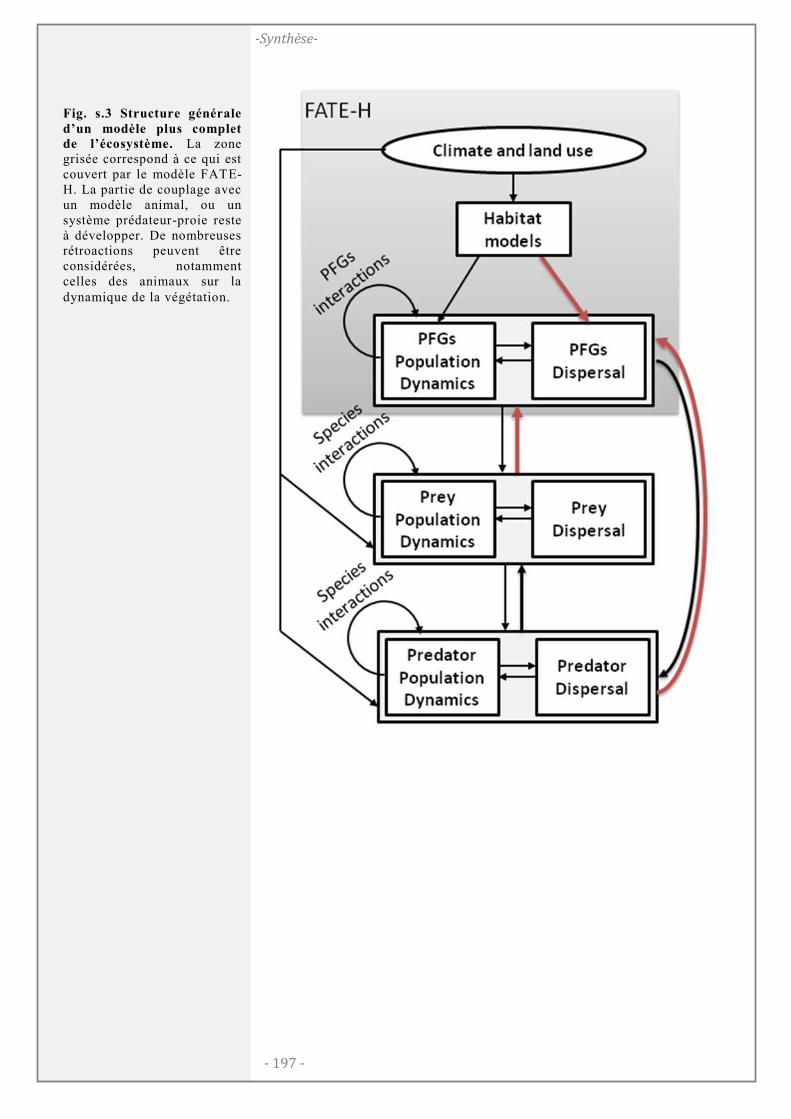
- 197 -

-Synthèse-

Fig. s.3 Structure générale

d’un modèle plus complet de l’écosystème. La zone grisée correspond à ce qui est couvert par le modèle FATE-H. La partie de couplage avec un modèle animal, ou un système prédateur-proie reste à développer. De nombreuses rétroactions peuvent être considérées, notamment celles des animaux sur la dynamique de la végétation.

- 198 -

-Synthèse-

QUELLES IMPLICATIONS POUR LA CONSERVATION ?

DU POINT DE VUE DES ESPÈCES

La spécialisation des plantes est un aspect très important en biologie de

la conservation. Les espèces spécialistes peuvent en effet répondre de

manière plus forte aux perturbations qui modifient leurs habitats que les

généralistes, et seront dans ce cas plus propices à l'extinction (Evans et

al. 2005; Willson et al. 2008). Ceci a été montré pour de nombreux taxa

(ex. oiseaux, Jiguet et al. 2007 ; plantes, Thuiller et al. 2004a). Si ces

espèces sont également très localisées, dans des habitats menacés, et

contiennent peu d’individus dans chaque population, leur vulnérabilité

est maximale. Les analyses du chapitre I montrent que ces

caractéristiques ne sont pas toujours associées (Fig. I.4). Une grande

partie des espèces les plus spécialistes étudiées sont localement

abondantes comparée aux autres espèces (ex. Juncus subnodulosus).

D’un autre côté, les espèces les plus spécialistes ont, en général, une

répartition géographique très restreinte, ce qui fait qu’elles sont souvent

la cible des mesures de protection (ex. Scheuchzeria palustris, Genista

delphinensis, Carex maritima, Drosera rotundifolia). A l’inverse, les

espèces endémiques ne sont pas toutes spécialistes d’habitat (ex.

Delphinium dubium), et dans ce cas, devraient être moins sensibles aux

changements environnementaux. C’est aussi le cas des annuelles

(Marini et al. 2012), dont l’environnement biotique peut être varié, et

qui devraient être plus tolérantes aux changements de leur

environnement, tant qu’il n’est pas détruit. Enfin, l’extinction des

espèces vulnérables (i.e. endémiques et spécialiste occupant des habitats

menacés), entrainerait une diminution de la diversité spécifique, mais

pourrait avoir un impact plus diffus sur d’autres facettes de la diversité

comme la diversité phylogénétique (Thuiller et al. 2011, voir annexe 3).

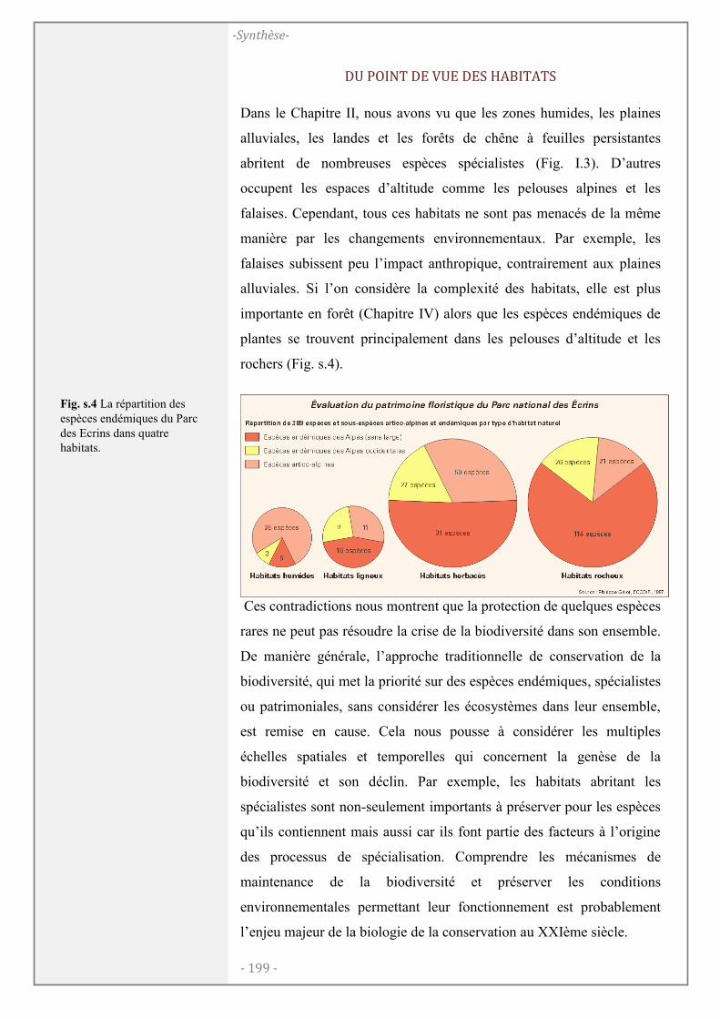
- 199 -

-Synthèse-

DU POINT DE VUE DES HABITATS

Dans le Chapitre II, nous avons vu que les zones humides, les plaines

alluviales, les landes et les forêts de chêne à feuilles persistantes

abritent de nombreuses espèces spécialistes (Fig. I.3). D’autres

occupent les espaces d’altitude comme les pelouses alpines et les

falaises. Cependant, tous ces habitats ne sont pas menacés de la même

manière par les changements environnementaux. Par exemple, les

falaises subissent peu l’impact anthropique, contrairement aux plaines

alluviales. Si l’on considère la complexité des habitats, elle est plus

importante en forêt (Chapitre IV) alors que les espèces endémiques de

plantes se trouvent principalement dans les pelouses d’altitude et les

rochers (Fig. s.4).

Ces contradictions nous montrent que la protection de quelques espèces

rares ne peut pas résoudre la crise de la biodiversité dans son ensemble.

De manière générale, l’approche traditionnelle de conservation de la

biodiversité, qui met la priorité sur des espèces endémiques, spécialistes

ou patrimoniales, sans considérer les écosystèmes dans leur ensemble,

est remise en cause. Cela nous pousse à considérer les multiples

échelles spatiales et temporelles qui concernent la genèse de la

biodiversité et son déclin. Par exemple, les habitats abritant les

spécialistes sont non-seulement importants à préserver pour les espèces

qu’ils contiennent mais aussi car ils font partie des facteurs à l’origine

des processus de spécialisation. Comprendre les mécanismes de

maintenance de la biodiversité et préserver les conditions

environnementales permettant leur fonctionnement est probablement

l’enjeu majeur de la biologie de la conservation au XXIème siècle.

Fig. s.4 La répartition des espèces endémiques du Parc des Ecrins dans quatre habitats.

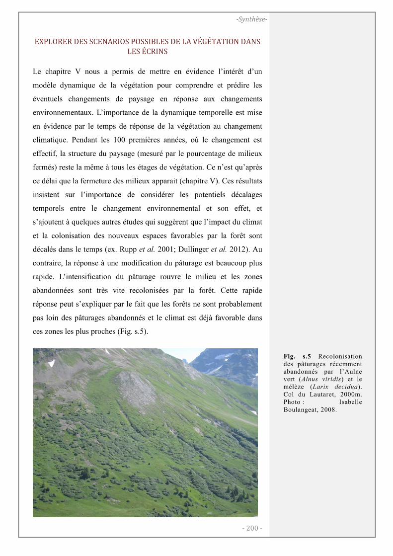
- 200 -

-Synthèse-

EXPLORER DES SCENARIOS POSSIBLES DE LA VÉGÉTATION DANS LES ÉCRINS

Le chapitre V nous a permis de mettre en évidence l’intérêt d’un

modèle dynamique de la végétation pour comprendre et prédire les

éventuels changements de paysage en réponse aux changements

environnementaux. L’importance de la dynamique temporelle est mise

en évidence par le temps de réponse de la végétation au changement

climatique. Pendant les 100 premières années, où le changement est

effectif, la structure du paysage (mesuré par le pourcentage de milieux

fermés) reste la même à tous les étages de végétation. Ce n’est qu’après

ce délai que la fermeture des milieux apparait (chapitre V). Ces résultats

insistent sur l’importance de considérer les potentiels décalages

temporels entre le changement environnemental et son effet, et

s’ajoutent à quelques autres études qui suggèrent que l’impact du climat

et la colonisation des nouveaux espaces favorables par la forêt sont

décalés dans le temps (ex. Rupp et al. 2001; Dullinger et al. 2012). Au

contraire, la réponse à une modification du pâturage est beaucoup plus

rapide. L’intensification du pâturage rouvre le milieu et les zones

abandonnées sont très vite recolonisées par la forêt. Cette rapide

réponse peut s’expliquer par le fait que les forêts ne sont probablement

pas loin des pâturages abandonnés et le climat est déjà favorable dans

ces zones les plus proches (Fig. s.5).

Fig. s.5 Recolonisation des pâturages récemment abandonnés par l’Aulne vert (Alnus viridis) et le mélèze (Larix decidua). Col du Lautaret, 2000m. Photo : Isabelle Boulangeat, 2008.

- 201 -

-Synthèse-

Un deuxième résultat très important du chapitre V est l’interaction entre

les effets du changement climatique et ceux de l’abandon du pâturage.

En effet, lorsque les deux scenarios sont combinés, la colonisation des

pâturages abandonnés dans un premier temps, permet aux arbres de

s’implanter très rapidement dans les zones rendues favorables par le

changement climatique. Cette synergie a pour effet final de réduire la

diversité beta des PFGs, alors qu’elle se maintenait dans chacun des

scenarios séparément.

Ces résultats démontrent l’intérêt des développements réalisés au cours

de cette thèse, qui ouvrent la voie à l’étude de scenarios plus

complexes, mettant en jeu des évènements extrêmes (ex. sècheresse

successive), modifiant leur fréquence et leur intensité. Ce modèle

permettra d’explorer les effets spatiaux et temporels de la dynamique

des populations dans un environnement hétérogène et fluctuant dans le

temps.

- 202 -

-Synthèse-

-203-

REFERENCES BIBLIOGRAPHIQUES

- 204 -

-Références bibliographiques-

- 205 -

-Références bibliographiques-

Albert, C. & Thuiller, W. (2008) Favourability functions against probability of presence: advantages and misuses. Ecography, 31, 417-422.

Albert, C. H., Thuiller, W., Lavorel, S., Davies, I. D. & Garbolino, E. (2008) Land-use change and subalpine tree dynamics: colonization of Larix decidua in French subalpine grasslands. Journal of Applied Ecology, 45, 659-669.

Albert, C. H., Thuiller, W., Yoccoz, N. G., Soudant, A., Boucher, F., Saccone, P. & Lavorel, S. (2010a) Intraspecific functional variability: extent, structure and sources of variation. Journal of Ecology, 98, 604-613.

Albert, C. H., Yoccoz, N. G., Edwards, T. C., Graham, C. H., Zimmermann, N. E. & Thuiller, W. (2010b) Sampling in ecology and evolution - bridging the gap between theory and practice. Ecography, 33, 1028-1037.

Albert, C. H., de Bello, F., Boulangeat, I., Pellet, G., Lavorel, S. & Thuiller, W. (2012) On the importance of intraspecific variability for the quantification of functional diversity. OIKOS, 121, 116-126.

Alexander, H. M., Foster, B. L., Ballantyne, F., Collins, C. D., Antonovics, J. & Holt, R. D. (2012) Metapopulations and metacommunities: combining spatial and temporal perspectives in plant ecology. Journal of Ecology, 100, 88-103.

Anderson, B. J., Akçakaya, H. R., Araújo, M. B., Fordham, D. A., Martinez-Meyer, E., Thuiller, W. & Brook, B. W. (2009) Dynamics of range margins for metapopulations under climate change. Proceedings of

the Royal Society of London B, Biological Sciences, 276, 1415-1420 Anderson, M. J., Crist, T. O., Chase, J. M., Vellend, M., Inouye, B. D., Freestone,

A. L., Sanders, N. J., Cornell, H. V., Comita, L. S., Davies, K. F., Harrison, S. P., Kraft, N. J. B., Stegen, J. C. & Swenson, N. G. (2011) Navigating the multiple meanings of beta diversity: a roadmap for the practicing ecologist. Ecology Letters, 14, 19-28.

Araujo, M. B. & Luoto, M. (2007) The importance of biotic interactions for modelling species distributions under climate change. Global

Ecology and Biogeography, 16, 743-753. Araujo, M. B., Thuiller, W. & Yoccoz, N. G. (2009) Reopening the climate

envelope reveals macroscale associations with climate in European birds. Proceedings of the National Academy of Sciences of the United

States of America, 106, E45-E46. Attum, O., Eason, P., Cobbs, G. & Baha El Din, S. M. (2006) Response of a

desert lizard community to habitat degradation: do ideas about habitat specialists/generalists hold? Biological Conservation, 133, 52-62.

Austin, M. P., Cunningham, R. B. & Fleming, P. M. (1984) New approaches to direct gradient analysis using environmental scalars and statistical curve-fitting procedures. Vegetatio, 55, 11-27.

Austin, M. P. (1985) Continuum concept, ordination methods, and niche theory. Annual Review of Ecology and Systematics, 16, 39-61.

Bahn, V. & McGill, B. J. (2007) Can niche-based distribution models outperform spatial interpolation? Global Ecology and Biogeography, 16, 733-742.

Baselga, A., Jiménez-Valverde, A. & Niccolini, G. (2007) A multiple-site similarity measure independent of richness. Biology Letters, 3, 642-645.

Bateman, B. L., VanDerWal, J. & Johnson, C. N. (2012) Nice weather for bettongs: using weather events, not climate means, in species distribution models. Ecography, 35, 306-314.

- 206 -

-Références bibliographiques-

Beale, C. M., Lennon, J. J. & Gimona, A. (2008) Opening the climate envelope reveals no macroscale associations with climate in European birds. Proceedings of the National Academy of Sciences of the United States

of America, 105, 14908-14912. Beaumont, L. J., Pitman, A., Perkins, S., Zimmermann, N. E., Yoccoz, N. G. &

Thuiller, W. (2011) Impacts of climate change on the world's most exceptional ecoregions. Proceedings of the National Academy of

Sciences of the United States of America, 108, 2306-2311. Bebi, P., Kulakowski, D. & Rixen, C. (2009) Snow avalanche disturbances in

forest ecosystems-State of research and implications for management. Forest Ecology and Management, 257, 1883-1892.

Bell, G. (2001) Ecology - Neutral macroecology. Science, 293, 2413-2418. Bellard, C., Bertelsmeier, C., Leadley, P., Thuiller, W. & Courchamp, F.

(2012) Impacts of climate change on the future of biodiversity. Ecology Letters, 15.

Bénichou, P. & Le breton, O. (1987) Prise en compte de la topographie pour la cartographie des champs pluviométriques statistiques. La

Météorologie, 7. Bolnick, D. I., Svanback, R., Fordyce, J. A., Yang, L. H., Davis, J. M., Hulsey, C.

D. & Forister, M. L. (2003) The ecology of individuals: incidence and implications of individual specialization. The American Naturalist, 161, 1-28.

Bond, W. J., Woodward, F. I. & Midgley, G. F. (2005) The global distribution of ecosystems in a world without fire. New Phytologist, 165, 525-538.

Bonesi, L. & Macdonald, D. W. (2004) Differential habitat use promotes sustainable coexistence between the specialist otter and the generalist mink. OIKOS, 106, 509-519.

Borcard, D., Legendre, P. & Drapeau, P. (1992) Partialling out the spatial component of ecological variation. Ecology, 73, 1045-1055.

Bossard, M., Feranec, J. & Otahel, J. (2000) CORINE land cover technical

guide ‒ addendum 2000. European Environment Agency, Copenhagen, Denmark.

Boulangeat, I., Lavergne, S., Van Es, J., Garraud, L. & Thuiller, W. (2012) Niche breadth, rarity and ecological characteristics within a regional flora spanning large environmental gradients. Journal of

Biogeography, 39, 204-214. Bradstock, R. A., Bedward, M., Kenny, B. J. & Scott, J. (1998) Spatially-

explicit simulation of the effect of prescribed burning on fire regimes and plant extinctions in shrublands typical of south-eastern Australia. Biological Conservation, 86, 83-95.

Braun-Blanquet, J. (1946) Über den Deckungswert der Arten in den Pfl anzengesellschaften der Ordnung Vaccinio-Piceetalia. Jahresber.

Naturforsch. Ges. Graubündens., 130, 115-119. Bret-Harte, M. S., Mack, M. C., Goldsmith, G. R., Sloan, D. B., DeMarco, J.,

Shaver, G. R., Ray, P. M., Biesinger, Z. & Chapin, F. S. (2008) Plant functional types do not predict biomass responses to removal and fertilization in Alaskan tussock tundra. Journal of Ecology, 96, 713-726.

Broennimann, O., Fitzpatrick, M. C., Pearman, P. B., Petitpierre, B., Pellissier, L., Yoccoz, N. G., Thuiller, W., Fortin, M.-J., Randin, C., Zimmermann, N. E., Graham, C. H. & Guisan, A. (2012) Measuring ecological niche

- 207 -

-Références bibliographiques-

overlap from occurrence and spatial environmental data. Global

Ecology and Biogeography, 21, 481-497. Brook, B. W., Akcakaya, H. R., Keith, D. A., Mace, G. M., Pearson, R. G. &

Araujo, M. B. (2009) Integrating bioclimate with population models to improve forecasts of species extinctions under climate change. Biology Letters, 5, 723-725.

Cadotte, M. W. & Fukami, T. (2005) Dispersal, spatial scale, and species diversity in a hierarchically structured experimental landscape. Ecology Letters, 8, 548-557.

Calinski, R. B. & Harabasz, J. (1974) A Dendrite Method for Cluster Analysis. Communications in Statistics, 3, 1-27.

Callaway, R. M., Brooker, R. W., Choler, P., Kikvidze, Z., Lortie, C. J., Michalet, R., Paolini, L., Pugnaire, F. I., Newingham, B., Aschehoug, E. T., Armas, C., Kikodze, D. & Cook, B. J. (2002) Positive interactions among alpine plants increase with stress. Nature, 417, 844-848.

Calow, P. (1987) Towards a Definition of Functional Ecology. Functional

Ecology, 1, 57-61. Ceballos, G., Ehrlich, P. R., Soberon, J., Salazar, I. & Fay, J. P. (2005) Global

mammal conservation: what must we manage? Science, 309, 603-607.

Chapin III, F. S., Bret-harte, M. S., Hobbie, S. E. & Zhong, H. (1996) Plant functional types as predictors of transient responses of arctic vegetation to global change. Journal of Vegetation Science, 7, 347-358.

Chapin, F. S., Zavaleta, E. S., Eviner, V. T., Naylor, R. L., Vitousek, P. M., Reynolds, H. L., Hooper, D. U., Lavorel, S., Sala, O. E., Hobbie, S. E., Mack, M. C. & Diaz, S. (2000) Consequences of changing biodiversity. Nature, 405, 234-242.

Chase, J. M. & Leibold, M. A. (2003) Ecological Niches. Chicago University Press, Chicago.

Chase, J. M. (2005) Towards a really unified theory for metacommunities. Functional Ecology, 19, 182-186.

Chave, J. (2004) Neutral theory and community ecology. Ecology Letters, 7, 241-253.

Chesson, P. (2000a) Mechanisms of maintenance of species diversity. Annual Review of Ecology and Systematics, 31, 343-366.

Chesson, P. (2000b) General theory of competitive coexistence in spatially-varying environments. Theoretical Population Biology, 58, 211-237.

Choler, P., Michalet, R. & Callaway, R. M. (2001) Facilitation and competition on gradients in alpine plant communities. Ecology, 82, 3295-3308.

Choler, P. (2005) Consistent shifts in Alpine plant traits along a mesotopographical gradient. Arctic, Antartic, and Alpine Research, 37, 444-453.

Clark, J. S., Dietze, M., Chakraborty, S., Agarwal, P. K., Ibanez, I., LaDeau, S. & Wolosin, M. (2007) Resolving the biodiversity paradox. Ecology

Letters, 10, 647-659. Clavel, J., Julliard, R. & Devictor, V. (2011) Worldwide decline of specialist

species: toward a global functional homogenization? Frontiers in

Ecology and the Environment, 9, 222-228. Clément, G., Quétier, F., Mallen, M., Choler, P., Douzet, R., Girel, J. & Lavorel, S┻ ゅにどどぬょ Les différentes trajectoires d╆utilisation des terres à l╆étage sub-alpin ont-elles laissé une marque significative dans le

- 208 -

-Références bibliographiques-

paysage actuel du Col du Lautaret ? Evaluation des risques

environnementaux pour une gestion durable des espaces. Actes des

journées はねねば de l╆Association Internationale pour l╆Ecologie du Paysage IALE Francepp. 117-122. Vanpeene-Bruhier, S. , Antony.

Cleveland, W. C., Grosse, E. & Shyu, W. M. (1992) Local regression models. Statistical Models (ed J. M. C. a. T. J. Hastie), pp. 309-376. Chapman and Hall, New York., New York.

Cornelissen, J. H. C., Lavorel, S., Garnier, E., Díaz, S., Buchmann, N., Gurvich, D. E., Reich, P. B., ter Steege, H., Morgan, H. D., van der Heijden, M. G. A., Pausas, J. G. & Poorter, H. (2003) Handbook of protocols for standardised and easy measurement of

plant functional traits worldwide. Australian journal of Botany, 51, 335-308.

Cornwell, W. K., Schwilk, D. W. & Ackerly, D. D. (2006) A trait-based test for habitat filtering: convex hull volume. Ecology, 87, 1465-1471.

Cottenie, K. (2005) Integrating environmental and spatial processes in ecological community dynamics. Ecology Letters, 8, 1175-1182.

Cousins, S. A. O., Lavorel, S. & Davies, I. (2003) Modelling the effects of landscape pattern and grazing regimes on the persistence of plant species with high conservation value in grasslands in south-eastern Sweden. Landscape Ecology, 18, 315-332.

Crawley, M. J., Brown, S. L., Heard, M. S. & Edwards, G. R. (1999) Invasion-resistance in experimental grassland communities: species richness or species identity? Ecology Letters, 2, 140-148.

Davies, T. J., Barraclough, T. G., Savolainen, V. & Chase, M. W. (2004) Environmental causes for plant biodiversity gradients. Phil. Trans.

R. Soc. Lond. B, 359, 1645-1656. de Bello, F., Lavergne, S., Meynard, C. N., Leps, J. & Thuiller, W. (2010a) The

partitioning of diversity: showing Theseus a way out of the labyrinth. Journal of Vegetation Science, 21, 992-1000.

de Bello, F., Lavorel, S., Diaz, S., Harrington, R., Cornelissen, J. H. C., Bardgett, R. D., Berg, M. P., Cipriotti, P., Feld, C. K., Hering, D., da Silva, P. M., Potts, S. G., Sandin, L., Sousa, J. P., Storkey, J., Wardle, D. A. & Harrison, P. A. (2010b) Towards an assessment of multiple ecosystem processes and services via functional traits. Biodiversity

and Conservation, 19, 2873-2893. De Candolle, A. I. (1955) Géographie botanique raisonnée. Masson, Paris. DeLong, D. C. (1996) Defining biodiversity. Wildlife Society Bulletin, 24,

738-749. Devictor, V., Julliard, R. & Jiguet, F. (2008a) Distribution of specialist and

generalist species along spatial gradients of habitat disturbance and fragmentation. OIKOS, 117, 507-514.

Devictor, V., Julliard, R., Clavel, J., Jiguet, F., Lee, A. & Couvet, D. (2008b) Functional biotic homogenization of bird communities in disturbed landscapes. Global Ecology and Biogeography, 17, 252-261.

Devictor, V., Clavel, J., Julliard, R., Lavergne, S., Mouillot, D., Thuiller, W., Venail, P., Villeger, S. & Mouquet, N. (2010) Defining and measuring ecological specialization. Journal of Applied Ecology, 47, 15-25.

Di Filippo, A., Biondi, F., Maugeri, M., Schirone, B. & Piovesan, G. (2012) Bioclimate and growth history affect beech lifespan in the Italian Alps and Apennines. Global Change Biology, 18, 960-972.

- 209 -

-Références bibliographiques-

Diaz, S. & Cabido, M. (2001) Vive la difference: plant functional diversity matters to ecosystem processes. Trends in Ecology & Evolution, 16, 646-655.

Diaz, S., Hodgson, J. G., Thompson, K., Cabido, M., Cornelissen, J. H. C., Jalili, A., Montserrat-Marti, G., Grime, J. P., Zarrinkamar, F., Asri, Y., Band, S. R., Basconcelo, S., Castro-Diez, P., Funes, G., Hamzehee, B., Khoshnevi, M., Perez-Harguindeguy, N., Perez-Rontome, M. C., Shirvany, F. A., Vendramini, F., Yazdani, S., Abbas-Azimi, R., Bogaard, A., Boustani, S., Charles, M., Dehghan, M., de Torres-Espuny, L., Falczuk, V., Guerrero-Campo, J., Hynd, A., Jones, G., Kowsary, E., Kazemi-Saeed, F., Maestro-Martinez, M., Romo-Diez, A., Shaw, S., Siavash, B., Villar-Salvador, P. & Zak, M. R. (2004) The plant traits that drive ecosystems: Evidence from three continents. Journal of

Vegetation Science, 15, 295-304. Diaz, S., Lavorel, S., de Bello, F., Quetier, F., Grigulis, K. & Robson, M. (2007)

Incorporating plant functional diversity effects in ecosystem service assessments. Proceedings of the National Academy of Sciences of the

United States of America, 104, 20684-20689. Dolédec, S., Chessel, D. & Gimaret-Carpentier, C. (2000) Niche separation in

community analysis : a new method. Ecology, 81, 2914-2927. Dorrepaal, E. (2007) Are plant growth-form-based classifications useful in

predicting northern ecosystem carbon cycling feedbacks to climate change? Journal of Ecology, 95, 1167-1180.

Dullinger, S., Dirnbock, T. & Grabherr, G. (2004) Modelling climate change-driven treeline shifts: relative effects of temperature increase, dispersal and invasibility. Journal of Ecology, 92, 241-252.

Dullinger, S., Kleinbauer, I., Peterseil, J., Smolik, M. & Essl, F. (2009) Niche based distribution modelling of an invasive alien plant: effects of population status, propagule pressure and invasion history. Biological Invasions, 11, 2401-2414.

Dullinger, S., Mang, T., Dirnböck, T., Ertl, S., Gattringer, A., Grabherr, G., Leitner, M. & Hülber, K. (2011) Patch configuration affects alpine plant distribution. Ecography, 34, 576-587.

Dullinger, S., Gattringer, A., Thuiller, W., Moser, D., Zimmermann, N. E., Guisan, A., Willner, W., Plutzar, C., Leitner, M., Mang, T., Caccianiga, M., Dirnböck, T., Ertl, S., Fischer, A., Lenoir, J., Svenning, J.-C., Psomas, P., Schmatz, D. R., Silc, U., Vittoz, P. & Hülber, K. (2012) Extinction debt of high-mountain plants under 21st-century climate change. NATURE Climate Change.

Eddy, W. F. (1977) A New Convex Hull Algorithm for Planar Sets. ACM

Transactions on Mathematical Software, 3, 398-403. Elith, J. & Leathwick, J. R. (2009) Species Distribution Models: Ecological

Explanation and Prediction Across Space and Time. Annual Review

of Ecology Evolution and Systematics, 40, 677-697. Elton, C. (1927) Animal Ecology. Sidgwick and Jackson, London. Engler, R. & Guisan, A. (2009) MIGCLIM: Predicting plant distribution and

dispersal in a changing climate. Diversity and Distributions, 15, 590-601.

Engler, R., Randin, C. F., Vittoz, P., Czaka, T., Beniston, M., Zimmermann, N. E. & Guisan, A. (2009) Predicting future distributions of mountain plants under climate change: does dispersal capacity matter? Ecography, 32, 34-45.

- 210 -

-Références bibliographiques-

Epstein, H. E., Chapin, F. S., Walker, M. D. & Starfield, A. M. (2001) Analyzing the functional type concept in arctic plants using a dynamic vegetation model. OIKOS, 95, 239-252.

Etienne, R. S. (2007) A neutral sampling formula for multiple samples and an 'exact' test of neutrality. Ecology Letters, 10, 608-618.

Evans, K. L., Greenwood, J. J. D. & Gaston, K. J. (2005) Dissecting the species‒energy relationship. Proceedings of the Royal Society B:

Biological Sciences, 272, 2155-2163. Feary, D. A. (2007) The influence of resource specialization on the response

of reef fish to coral disturbance. Marine Biology, 153, 153-161. Foley, J. A., DeFries, R., Asner, G. P., Barford, C., Bonan, G., Carpenter, S. R.,

Chapin, F. S., Coe, M. T., Daily, G. C., Gibbs, H. K., Helkowski, J. H., Holloway, T., Howard, E. A., Kucharik, C. J., Monfreda, C., Patz, J. A., Prentice, I. C., Ramankutty, N. & Snyder, P. K. (2005) Global consequences of land use. Science, 309, 570-574.

Frank, D. A. & McNaughton, S. J. (1991) Stability increases with diversity in plant-communities - empirical-evidence from the 1988 yellowstone drought. OIKOS, 62, 360-362.

Franklin, J. (2010) Moving beyond static species distribution models in support of conservation biogeography. Diversity and Distributions, 16, 321-330.

Fridley, J. D., Vandermast, D. B., Kuppinger, D. M., Manthey, M. & Peet, R. K. (2007) Co-occurrence based assessment of habitat generalists and specialists: a new approach for the measurement of niche width. Journal of Ecology, 95, 707-722.

Futuyma, D. J. & Moreno, G. (1988) The evolution of ecological specialization. Annual Review of Ecology and Systematics, 19, 207-233.

Gallien, L., Munkemuller, T., Albert, C. H., Boulangeat, I. & Thuiller, W. (2010) Predicting potential distributions of invasive species: where to go from here? Diversity and Distributions, 16, 331-342.

Gandin, L. S. & Murphy, A. H. (1992) Equitable skill scores for categorical forecasts. Monthly Weather Review, 120, 361-370.

Garnier, E., Cortez, J., Billes, G., Navas, M. L., Roumet, C., Debussche, M., Laurent, G., Blanchard, A., Aubry, D., Bellmann, A., Neill, C. & Toussaint, J. P. (2004) Plant functional markers capture ecosystem properties during secondary succession. Ecology, 85, 2630-2637.

Garnier, E., Lavorel, S., Ansquer, P., Castro, H., Cruz, P., Dolezal, J., Eriksson, O., Fortunel, C., Freitas, H., Golodets, C., Grigulis, K., Jouany, C., Kazakou, E., Kigel, J., Kleyer, M., Lehsten, V., Leps, J., Meier, T., Pakeman, R., Papadimitriou, M., Papanastasis, V. P., Quested, H., Quetier, F., Robson, M., Roumet, C., Rusch, G., Skarpe, C., Sternberg, M., Theau, J. P., Thebault, A., Vile, D. & Zarovali, M. P. (2007) Assessing the effects of land-use change on plant traits, communities and ecosystem functioning in grasslands: A standardized methodology and lessons from an application to 11 European sites. Annals of Botany, 99, 967-985.

Gaston, K. J. & Lawton, J. H. (1990) Effects of scale and habitat on the relationship between regional distributions and local abundance. Oikos, 58, 329-335.

Gaston, K. J. (1997) What is rarity? The Biology of Rarity: causes and

consequences of rare-common differences. (eds W. E. Kunin & K. J. Gaston), pp. 30-47. Chapman and Hall, London.

- 211 -

-Références bibliographiques-

Gaucherel, C., Alleaume, S. & Hely, C. (2008) The comparison map profile method: A strategy for multiscale comparison of quantitative and qualitative images. Ieee Transactions on Geoscience and Remote

Sensing, 46, 2708-2719. Gause, G. F. (1934) The struggle for existence. Williams & Wilkins. Gehrig-Fasel, J., Guisan, A. & Zimmermann, N. E. (2007) Tree line shifts in

the Swiss Alps: Climate change or land abandonment? Journal of

Vegetation Science, 18, 571-582. Gilpin, M. E. & Diamond, J. M. (1982) Factors contributing to non-

randomness in species co-occurrences on islands. Oecologia, 52, 75-84.

Girel, J. (2006) Quand le passé éclaire le présent : écologie et histoire du paysage. Géocarrefour, 81, 249-264.

Gotelli, N. J. & McCabe, D. J. (2002) Species co-occurrence: A meta-analysis of J. M. Diamond's assembly rules model. Ecology, 83, 2091-2096.

Gottfried, M., Pauli, H., Futschik, A., Akhalkatsi, M., Barancok, P., Alonso, J. L. B., Coldea, G., Dick, J., Erschbamer, B., Calzado, M. R. F., Kazakis, G., Krajci, J., Larsson, P., Mallaun, M., Michelsen, O., Moiseev, D., Moiseev, P., Molau, U., Merzouki, A., Nagy, L., Nakhutsrishvili, G., Pedersen, B., Pelino, G., Puscas, M., Rossi, G., Stanisci, A., Theurillat, J. P., Tomaselli, M., Villar, L., Vittoz, P., Vogiatzakis, I. & Grabherr, G. (2012) Continent-wide response of mountain vegetation to climate change. Nature Climate Change, 2, 111-115.

Gower, J. C. (1971) General coefficient of similarity and some of its properties. Biometrics, 27, 857-&.

Gravel, D., Canham, C. D., Beaudet, M. & Messier, C. (2006) Reconciling niche and neutrality: the continuum hypothesis. Ecology Letters, 9, 399-409.

Gravel, D., Beaudet, M. & Messier, C. (2008) Partitioning the factors of spatial variation in regeneration density of shade-tolerant tree species. Ecology, 89, 2879-2888.

Gregory, R. D., van Strien, A., Vorisek, P., Meyling, A. W. G., Noble, D. G., Foppen, R. P. B. & Gibbons, D. W. (2005) Developing indicators for European birds. Philosophocal Transactions of the Royal Society B:

Biological Sciences, 360, 269-288. Grime, J. P. (1974) Vegetation classification by reference to strategies.

Nature, 250, 26-31. Grime, J. P. (1998) Benefits of plant diversity to ecosystems: immediate,

filter and founder effects. Journal of Ecology, 86, 902-910. Grime, J. P., Thompson, K., Hunt, R., Hodgson, J. G., Cornelissen, J. H. C.,

Rorison, I. H., Hendry, G. A. F., Ashenden, T. W., Askew, A. P., Band, S. R., Booth, R. E., Bossard, C. C., Campbell, B. D., Cooper, J. E. L., Davison, A. W., Gupta, P. L., Hall, W., Hand, D. W., Hannah, M. A., Hillier, S. H., Hodkinson, D. J., Jalili, A., Liu, Z., Mackey, J. M. L., Matthews, N., Mowforth, M. A., Neal, A. M., Reader, R. J., Reiling, K., Ross-Fraser, W., Spencer, R. E., Sutton, F., Tasker, D. E., Thorpe, P. C. & Whitehouse, J. (1997) Integrated screening validates primary axes of specialisation in plants. Oikos, 79, 259-281.

Grinnell, J. (1917) The niche relationship of the California Thrasher. Auk, 34, 427-233.

Guisan, A., Theurillat, J.-P. & Kienast, F. (1998) Predicting the potential distribution of plant species in an alpine environment. Journal of

Vegetation Science, 9, 65-74.

- 212 -

-Références bibliographiques-

Guisan, A. & Zimmermann, N. E. (2000) Predictive habitat distribution models in ecology. Ecological Modelling, 135, 147-186.

Guisan, A. & Thuiller, W. (2005) Predicting species distribution: offering more than simple habitat models. Ecology Letters, 8, 993-1009.

Hadar, L., Noy-Meir, I. & Perevolotsky, A. (1999) The effect of shrub clearing and grazing on the composition of a Mediterranean plant community: functional groups versus species. Journal of Vegetation

Science, 10, 673-682. Halkidi, M., Batistakis, Y. & Vazirgiannis, M. (2001) On clustering validation

techniques. Journal of Intelligent Information Systems, 17, 107-145. Hamilton, A. J. (2005a) Species diversity or biodiversity? Journal of

Environmental Management, 75, 89-92. Hamilton, M. A., Murray, B. R., Cadotte, M. W., Hose, G. C., Baker, A. C., Harris,

C. J. & Licari, D. (2005b) Life-history correlates of plant invasiveness at regional and continental scales. Ecology Letters, 8, 1066-1074.

Harrington, R., Woiwod, I. & Sparks, T. (1999) Climate change and trophic interactions. Trends in Ecology & Evolution, 14, 146-150.

Harrison, S. P., Prentice, I. C., Barboni, D., Kohfeld, K. E., Ni, J. & Sutra, J. P. (2010) Ecophysiological and bioclimatic foundations for a global plant functional classification. Journal of Vegetation Science, 21, 300-317.

Heikkinen, R. K., Luoto, M., Araujo, M. B., Virkkala, R., Thuiller, W. & Sykes, M. T. (2006) Methods and uncertainties in bioclimatic envelope modelling under climate change. Progress in Physical Geography, 30, 751-777.

Herault, B. (2007) Reconciling niche and neutrality through the Emergent Group approach. Perspectives in Plant Ecology Evolution and

Systematics, 9, 71-78. Herault, B. & Honnay, O. (2007) Using life-history traits to achieve a

functional classification of habitats. Applied Vegetation Science, 10, 73-80.

Hickler, T., Smith, B., Sykes, M. T., Davis, M. B., Sugita, S. & Walker, K. (2004) Using a generalized vegetation model to simulate vegetation dynamics in northeastern USA. Ecology, 85, 519-530.

Higgins, S. I., Clark, J. S., Nathan, R., Hovestadt, T., Schurr, F., Fragoso, J. M. V., Aguiar, M. R., Ribbens, E. & Lavorel, S. (2003) Forecasting plant migration rates: managing uncertainty for risk assessment. Journal

of Ecology, 91, 341-347. Hijmans, R. J., Cameron, S. E., Parra, J. L., Jones, P. G. & Jarvis, A. (2005) Very

high resolution interpolated climate surfaces for global land areas. International Journal of Climatology, 25, 1965-1978.

Hill, M. O. (1973) Diversity and evenness - unifying notation and its consequences. Ecology, 54, 427-432.

Hodgson, J. G., Grime, J. P., Wilson, P. J., Thompson, K. & Band, S. R. (2005) The impacts of agricultural change (1963-2003) on the grassland flora of Central England: processes and prospects. Basic and Applied

Ecology, 6, 107-118. Holyoak, M., Loreau, M. & Strong, D. (2006) Neutral community ecology.

Ecology, 87, 1368-1369. Hooper, D. U., Chapin, F. S., Ewel, J. J., Hector, A., Inchausti, P., Lavorel, S.,

Lawton, J. H., Lodge, D. M., Loreau, M., Naeem, S., Schmid, B., Setala, H., Symstad, A. J., Vandermeer, J. & Wardle, D. A. (2005) Effects of

- 213 -

-Références bibliographiques-

biodiversity on ecosystem functioning: A consensus of current knowledge. Ecological Monographs, 75, 3-35.

Hubbell, S. P. (2001) The unified neutral theory of species abundance and

diversity., Princeton. Hughes, J. B., Daily, G. C. & Ehrlich, P. R. (1997) Population Diversity: Its

Extent and Extinction. Science, 278, 689-691. Hughes, L. (2000) Biological consequences of global warming: is the signal

already apparent? Trends in Ecology and Evolution, 15, 56-61. Hutchinson, G. E. (1957) Concluding remarks. Cold Spring Harbor Symposia

on Quantitative Biology, 22, 415-427. Hutchinson, M., Xu, T., Houlder, D., Nix, H. & McMahon, J. (2009) ANUCLIM は┻ど User╆s Guide. Australian National University., Fenner School of

Environment and Society. IPCC (2007b) Climate Change 2007: The Physical Science Basis. In

Contribution of Working Group I to the Fourth Assessment Report of the IPCC. Cambridge University Press, Cambridge, UK.

Iverson, L. R., Schwartz, M. W. & Prasad, A. (2004) How fast and far might tree species migrate in the eastern United States due to climate change? Global Ecology & Biogeography, 13, 209-219.

Jiguet, F., Gadot, A. S., Julliard, R., Newson, S. E. & Couvet, D. (2007) Climate envelope, life history traits and the resilience of birds facing global change. Global Change Biology, 13, 1672-1684.

Jost, L. (2006) Entropy and diversity. Oikos, 113, 363-375. Jost, L. (2007) Partitioning diversity into independent alpha and beta

components. Ecology, 88, 2427-2439. Jouglet, J. P. (1999) Les végétations des alpages des Alpes françaises du Sud:

guide technique pour la reconnaissance et la gestion des milieux

pâturés d'altitude. Cemagref, Antony, France. Jump, A. S., Huang, T.-J. & Chou, C.-H. (2012) Rapid altitudinal migration of

mountain plants in Taiwan and its implications for high altitude biodiversity. Ecography, 35, 204-210.

Jutila, H. (1999) Effect of grazing on the vegetation of shore meadows along the Bothnian Sea, Finland. Plant Ecology, 140, 77-88.

Kassen, R. (2002) The experimental evolution of specialists, generalists, and the maintenance of diversity. Journal of Evolutionary Biology, 15, 173-190.

Kattge, J., DÍAz, S., Lavorel, S., Prentice, I. C., Leadley, P., BÖNisch, G., Garnier, E., Westoby, M., Reich, P. B., Wright, I. J., Cornelissen, J. H. C., Violle, C., Harrison, S. P., Van Bodegom, P. M., Reichstein, M., Enquist, B. J., Soudzilovskaia, N. A., Ackerly, D. D., Anand, M., Atkin, O., Bahn, M., Baker, T. R., Baldocchi, D., Bekker, R., Blanco, C. C., Blonder, B., Bond, W. J., Bradstock, R., Bunker, D. E., Casanoves, F., Cavender-Bares, J., Chambers, J. Q., Chapin Iii, F. S., Chave, J., Coomes, D., Cornwell, W. K., Craine, J. M., Dobrin, B. H., Duarte, L., Durka, W., Elser, J., Esser, G., Estiarte, M., Fagan, W. F., Fang, J., FernÁNdez-MÉNdez, F., Fidelis, A., Finegan, B., Flores, O., Ford, H., Frank, D., Freschet, G. T., Fyllas, N. M., Gallagher, R. V., Green, W. A., Gutierrez, A. G., Hickler, T., Higgins, S. I., Hodgson, J. G., Jalili, A., Jansen, S., Joly, C. A., Kerkhoff, A. J., Kirkup, D., Kitajima, K., Kleyer, M., Klotz, S., Knops, J. M. H., Kramer, K., KÜHn, I., Kurokawa, H., Laughlin, D., Lee, T. D., Leishman, M., Lens, F., Lenz, T., Lewis, S. L., Lloyd, J., LlusiÀ, J., Louault, F., Ma, S., Mahecha, M. D., Manning, P., Massad, T., Medlyn, B. E., Messier, J., Moles, A. T., MÜLler, S. C., Nadrowski, K., Naeem, S., Niinemets, Ü.,

- 214 -

-Références bibliographiques-

NÖLlert, S., NÜSke, A., Ogaya, R., Oleksyn, J., Onipchenko, V. G., Onoda, Y., OrdoÑEz, J., Overbeck, G., Ozinga, W. A., et al. (2011) TRY ‒ a global database of plant traits. Global Change Biology, 17, 2905-2935.

Kaufman, L. & Rousseeuw, P. J. (1990) Finding Groups in Data: An

Introduction to Cluster Analysis. Wiley, New York. Kearney, M. & Porter, W. (2009) Mechanistic niche modelling: combining

physiological and spatial data to predict species' ranges. Ecology

Letters, 12, 334-350. Keith, D. A., Akcakaya, H. R., Thuiller, W., Midgley, G. F., Pearson, R. G.,

Phillips, S. J., Regan, H. M., Araujo, M. B. & Rebelo, T. G. (2008) Predicting extinction risks under climate change: coupling stochastic population models with dynamic bioclimatic habitat models. Biology Letters, 4, 560-563.

Kerguélen, M. (1993) Index synonymique de la flore de France. Musém National d'Histoire Naturelle, Paris.

Kerr, J. T. & Packer, L. (1997) Habitat heterogeneity as a determinant of mammal species richness in high-energy regions. Nature, 385, 252-254.

Kerr, J. T., Southwood, T. R. E. & Cihlar, J. (2001) Remotely sensed habitat diversity predicts butterfly species richness and community similarity in Canada. Proceedings of the National Academy of

Sciences, 98, 11365-11370. Kneitel, J. M. & Chase, J. M. (2004) Trade-offs in community ecology : linking

spatial scale and species coexistence. Ecology Letters, 7, 69-80. Knevel, I. C., Bekker, R. M., Bakker, J. P. & Kleyer, M. (2003) Life-history

traits of the Northwest European flora: the LEDA database. Journal

of Vegetation Science, 14, 611-614. Koh, L. P., Dunn, R. R., Sodhi, N. S., Colwell, R. K., Proctor, H. C. & Smith, V. S.

(2004) Species coextinctions and the biodiversity crisis. Science, 305, 1632-1634.

Körner, C. (1999) Alpine plant life. Springer-Verlag, Berlin. Körner, C. (2004) Mountain biodiversity, its causes and function. Ambio, 13,

11-17. Kriticos, D. J., Brown, J. R., Maywald, G. F., Radford, I. D., Nicholas, D. M.,

Sutherst, R. W. & Adkins, S. W. (2003) SPAnDX: a process-based population dynamics model to explore management and climate impacts on an invasive alien plant, Acacia nilotica. Ecological

Modelling, 163, 187-208. Kühn, I., Durka, W. & Klotz, S. (2004) BiolFlor: a new plant-trait database as

a tool for plant invasion ecology. Diversity and Distributions, 10, 363-365.

Kunin, W. E. (1997) Population biology and rarity: on the complexity of density dependence in insect-plant interactions. The Biology of

Rarity: causes and consequences of rare-common differences. (eds W. E. Kunin & K. J. Gaston). Chapman and Hall, London.

Kunin, W. E. & Gaston, K. J. (1993) The biology of rarity: patterns, causes and consequences. Trends in Ecology and Evolution, 8, 298-301.

Kunstler, G., Thuiller, W., Curt, T., Bouchaud, M., Jouvie, R., Deruette, F. & Lepart, J. (2007) Fagus sylvatica L. recruitment across a fragmented Mediterranean Landscape, importance of long distance effective dispersal, abiotic conditions and biotic interactions. Diversity and

Distributions, 13, 799-807.

- 215 -

-Références bibliographiques-

Laidre, K. L., Stirling, I., Lowry, L. F., Wiig, O., Heide-Jorgensen, M. P. & Ferguson, S. H. (2008) Quantifying the sensitivity of Arctic marine mammals to climate-induced habitat change. Ecological

Applications, 18, S97-S125. Landolt, E., Bäumler, B., Erhardt, A., Hegg, O., Klötzli, F., Lämmler, W., Nobis,

M., Rudmann-Maurer, K., Schweingruber, F. H., Theurillat, J.-P., Urmi, E., Vust, M. & Wohlgemuth, T. (2010) Flora indicativa.

Ecological indicator values and biological attributes of the flora of

Switzerland and the Alp. Haupt Verlag, Berne. Laurent, J. M., Bar-Hen, A., Francois, L., Ghislain, M. & Cheddadi, R. (2004)

Refining vegetation simulation models: From plant functional types to bioclimatic affinity groups of plants. Journal of Vegetation

Science, 15, 739-746. Lavergne, S., Thompson, J. D., Garnier, E. & Debussche, M. (2004) The

biology and ecology of narrow endemic and widespread plants: a comparative study of trait variation in 20 congeneric pairs. Oikos, 107, 505-518.

Lavorel, S., McIntyre, S., Landsberg, J. & Forbes, T. D. A. (1997) Plant functional classifications: from general groups to specific groups based on response to disturbance. Trends in Ecology and Evolution, 12, 471-478.

Lavorel, S., Touzard, B., Lebreton, J. D. & Clement, B. (1998) Identifying functional groups for response to disturbance in an abandoned pasture. Acta Oecologica-International Journal of Ecology, 19, 227-240.

Lavorel, S. & Garnier, E. (2002) Predicting changes in community composition and ecosystem functioning from plant trait: revisiting the Holy Grail. Functional ecology, 16, 545-556.

Lavorel, S., Grigulis, K., Lamarque, P., Colace, M. P., Garden, D., Girel, J., Pellet, G. & Douzet, R. (2011) Using plant functional traits to understand the landscape distribution of multiple ecosystem services. Journal of Ecology, 99, 135-147.

Lawler, J. J., Shafer, S. L., White, D., Kareiva, P., Maurer, E. P., Blaustein, A. R. & Bartlein, P. J. (2009) Projected climate-induced faunal change in the Western Hemisphere. Ecology, 90, 588-597.

Lawton, J. H. & May, R. M. (1995) Extinction rates. Oxford University Press, Oxford.

Leathwick, J. R. (2002) Intra-generic competition among Nothofagus in New Zealand╆s primary indigenous forests┻ Biodiversity and

Conservation, 11, 2117-2187. Lenoir, J., Gegout, J. C., Dupouey, J. L., Bert, D. & Svenning, J. C. (2010) Forest

plant community changes during 1989-2007 in response to climate warming in the Jura Mountains (France and Switzerland). Journal of

Vegetation Science, 21, 949-964. Levins, R. (1966) Strategy of model building in population biology.

American Scientist, 54, 421-&. Levins, R. & Macarthu.R (1966) Maintenance of genetic polymorphism in a

spatially heterogeneous environment - variations ona theme by howard levene. American Naturalist, 100, 585-&.

Lischke, H., Zimmermann, N. E., Bolliger, J., Rickebusch, S. & Loffler, T. J. (2006) TreeMig: A forest-landscape model for simulating spatio-temporal patterns from stand to landscape scale. Ecological

Modelling, 199, 409-420.

- 216 -

-Références bibliographiques-

Loreau, M. (1998) Biodiversity and ecosystem functioning: A mechanistic model. Proceedings of the National Academy of Sciences of the United

States of America, 95, 5632-5636. Lortie, C. J., Brooker, R. W., Callaway, R. M., Choler, P., Kikvidze, Z., Michalet,

R. & Pugnaire, F. I. (2004) Rethinking plant community theory. Oikos, 107, 433-438.

Macarthur, R. (1955) Fluctuations of animal populations, and a measure of community stability. Ecology, 36, 533-536.

Maestre, F. T., Callaway, R. M., Valladares, F. & Lortie, C. J. (2009) Refining the stress-gradient hypothesis for competition and facilitation in plant communities. Journal of Ecology, 97, 199-205.

Manthey, M., Fridley, J. D. & Peet, R. K. (2011) Niche expansion after competitor extinction? A comparative assessment of habitat generalists and specialists in the tree floras of south往eastern North America and south往eastern Europe┻ Journal of Biogeography, 38, 840-853.

Marini, L., Bruun, H. H., Heikkinen, R. K., Helm, A., Honnay, O., Krauss, J., Kühn, I., Lindborg, R., Pärtel, M. & Bommarco, R. (2012) Traits related to species persistence and dispersal explain changes in plant communities subjected to habitat loss. Diversity and

Distributions, Early view. Mason, N. W. H., Mouillot, D., Lee, W. G. & Wilson, J. B. (2005) Functional

richness, functional evenness and functional divergence: the primary components of functional diversity. Oikos, 111, 112-118.

Mason, N. W. H., Irz, P., Lanoiselée, C., Mouillot, D. & Argillier, C. (2008) Evidence that niche specialization explains species‒energy relationships in lake fish communities. Journal of Animal Ecology, 77, 285-296.

Mayr, E. (1940) Speciation phenomena in birds. American Naturalist, 74, 249-278.

McIntyre, S., Lavorel, S., Landsberg, J. & Forbes, T. D. A. (1999) Disturbance response in vegetation towards a global perspective on functional traits. Journal of Vegetation Science, 10, 621-630.

McIntyre, S. & Lavorel, S. (2001) Livestock grazing in subtropical pastures: steps in the analysis of attribute response and plant functional types. Journal of Ecology, 89, 209-226.

McKinney, M. L. (1997) Extinction vulnerability and selectivity: Combining ecological and paleontological views. Annual Review of Ecology and

Systematics, 28, 495-516. McRae, B. H., Schumaker, N. H., McKane, R. B., Busing, R. T., Solomon, A. M. &

Burdick, C. A. (2008) A multi-model framework for simulating wildlife population response to land-use and climate change. Ecological Modelling, 219, 77-91.

Meier, E. S., Kienast, F., Pearman, P. B., Svenning, J. C., Thuiller, W., Araujo, M. B., Guisan, A. & Zimmermann, N. E. (2010) Biotic and abiotic variables show little redundancy in explaining tree species distributions. Ecography, 33, 1038-1048.

Memmott, J., Craze, P. G., Waser, N. M. & Price, M. V. (2007) Global warming and the disruption of plant-pollinator interactions. Ecology Letters, 10, 710-717.

Midgley, G. F., Davies, I. D., Albert, C. H., Altwegg, R., Hannah, L., Hughes, G. O., O'Halloran, L. R., Seo, C., Thorne, J. H. & Thuiller, W. (2010)

- 217 -

-Références bibliographiques-

BioMove - an integrated platform simulating the dynamic response of species to environmental change. Ecography, 33, 612-616.

Millennium Ecosystem Assessment (2005a) Ecosystems and Human Well-

being: Synthesis. Island Press, Washington DC. Mokany, K., Ash, J. & Roxburgh, S. (2008) Functional identity is more

important than diversity in influencing ecosystem processes in a temperate native grassland. Journal of Ecology, 96, 884-893.

Moles, A. T., Warton, D. I., Warman, L., Swenson, N. G., Laffan, S. W., Zanne, A. E., Pitman, A., Hemmings, F. A. & Leishman, M. R. (2009) Global patterns in plant height. Journal of Ecology, 97, 923-932.

Moore, A. D. & Noble, I. R. (1990) An individualistic model of vegetation stand dynamics. Journal of Environmental Management, 31, 61-81.

Mouchet, M., Guilhaumon, F., Villeger, S., Mason, N. W. H., Tomasini, J. A. & Mouillot, D. (2008) Towards a consensus for calculating dendrogram-based functional diversity indices. OIKOS, 117, 794-800.

Munday, P. L. (2004) Habitat loss, resource specialization, and extinction on coral reefs. Global Change Biology, 10, 1642-1647.

Naeem, S., Knops, J. M. H., Tilman, D., Howe, K. M., Kennedy, T. & Gale, S. (2000) Plant diversity increases resistance to invasion in the absence of covarying extrinsic factors. OIKOS, 91, 97-108.

Navas, M. L. & Violle, C. (2009) Plant traits related to competition: how do they shape the functional diversity of communities? Community

Ecology, 10, 131-137. Niedrist, G., Tasser, E., Luth, C., Dalla Via, J. & Tappeiner, U. (2009) Plant

diversity declines with recent land use changes in European Alps. Plant Ecology, 202, 195-210.

Noble, I. R. & Slatyer, R. O. (1980) The use of vital attributes to predict successional changes in plant communities subject to recurrent disturbances. Plant Ecology, 43, 5-21.

Noy-Meir, I. & Oron, T. (2001) Effects of grazing on geophytes in Mediterranean vegetation. Journal of Vegetation Science, 12, 749-760. O╆Brien┸ E┻ M┻┸ Road┸ D┻┸ Field┸ R┻ ┃ Whittaker┸ R┻ J┻ ゅにどどどょ Climatic gradients in woody plant (tree and shrub) diversity:water-energy dynamics, residual variation, and topography. OIKOS, 89, 588-600.

Pakeman, R. J. & Quested, H. M. (2007) Sampling plant functional traits: What proportion of the species need to be measured? Applied

Vegetation Science, 10, 91-96. Parmesan, C. (2006) Ecological and evolutionary responses to recent

climate change. Annual Review of Ecology Evolution and Systematics, 37, 637-669.

Parmesan, C., Duarte, C. M., Poloczanska, E., Richardson, A. J. & Singer, M. C. (2011) Overstretching attribution. Nature Climate Change, 1, 1-4.

Pärtel, M., Szava-Kovats, R. & Zobel, M. (2011) Dark diversity: shedding light on absent species. Trends in Ecology & Evolution, 26, 124-128.

Pausas, J. G. & Lavorel, S. (2003) A hierarchical deductive approach for functional types in disturbed ecosystems. Journal of Vegetation

Science, 14, 409-416. Pausas, J. G., Bradstock, R. A., Keith, D. A., Keeley, J. E. & Network., G. F.

(2004) Plant functional traits in relation to fire in crown-fire ecosystems. Ecology, 85, 1085-1100.

- 218 -

-Références bibliographiques-

Pavoine, S., Ollier, S. & Pontier, D. (2005) Measuring diversity from dissimilarities with Rao╆s quadratic entropy┺ Are any dissimilarities suitable? Theoretical Population Biology, 67, 231-239.

Pearce, J. & Ferrier, S. (2001) The practical value of modelling relative abundance of species for regional conservation planning: a case study. Biological Conservation, 98, 33-43.

Pellissier, L., Anne Bråthen, K., Pottier, J., Randin, C. F., Vittoz, P., Dubuis, A., Yoccoz, N. G., Alm, T., Zimmermann, N. E. & Guisan, A. (2010) Species distribution models reveal apparent competitive and facilitative effects of a dominant species on the distribution of tundra plants. Ecography, 33, 1004-1014.

Pereira, H. M., Leadley, P. W., Proenca, V., Alkemade, R., Scharlemann, J. P. W., Fernandez-Manjarres, J. F., Araujo, M. B., Balvanera, P., Biggs, R., Cheung, W. W. L., Chini, L., Cooper, H. D., Gilman, E. L., Guenette, S., Hurtt, G. C., Huntington, H. P., Mace, G. M., Oberdorff, T., Revenga, C., Rodrigues, P., Scholes, R. J., Sumaila, U. R. & Walpole, M. (2010) Scenarios for Global Biodiversity in the 21st Century. Science, 330, 1496-1501.

Peters, D. P. C., Herrick, J. E., Urban, D. L., Gardner, R. H. & Breshears, D. D. (2004) Strategies for ecological extrapolation. OIKOS, 106, 627-636.

Peters, J., De Baets, B., Verhoest, N. E. C., Samson, R., Degroeve, S., De Becker, P. & Huybrechts, W. (2007) Random forests as a tool for ecohydrological distribution modelling. Ecological Modelling, 207, 304-318.

Peterson, A. T., Ortega-Huerta, M. A., Bartley, J., Sanchez-Cordero, V., Soberon, J., Buddemeier, R. H. & Stockwell, D. R. B. (2002) Future projections for Mexican faunas under global climate change scenarios. Nature, 416, 626-629.

Pillar, V. D. (1999) On the identification of optimal plant functional types. Journal of Vegetation Science, 10, 631-640.

Pillar, V. D. & Sosinski, E. E. (2003) An improved method for searching plant functional types by numerical analysis. Journal of Vegetation

Science, 14, 323-332. Pimm, S. L., Jones, H. L. & Diamond, J. (1988) On the risk of extinction. The

American Naturalist, 132, 757-785. Pimm, S. L. & Raven, P. (2000) Extinction by numbers. Nature, 403, 843-

845. Podani, J. (1999) Extending Gower's general coefficient of similarity to

ordinal characters. Taxon, 48, 331-340. Podani, J. & Schmera, D. (2006) On dendrogram-based measures of

functional diversity. OIKOS, 115, 179-185. Pulliam, H. R. (2000) On the relationship between niche and distribution.

Ecology Letters, 3, 349-361. Quetier, F., Lavorel, S., Thuiller, W. & Davies, I. (2007) Plant-trait-based

modeling assessment of ecosystem-service sensitivity to land-use change. Ecological Applications, 17, 2377-2386.

Quetier, F., Rivoal, F., Marty, P., de Chazal, J., Thuiller, W. & Lavorel, S. (2010) Social representations of an alpine grassland landscape and socio-political discourses on rural development. Regional

Environmental Change, 10, 119-130. R Development Core Team (2010) R: A Language and Environment for

Statistical Computing., R Foundation for Statistical Computing, Vienna, Austria. Available online at http://www.R-project.org.

- 219 -

-Références bibliographiques-

Rafferty, N. E. & Ives, A. R. (2011) Effects of experimental shifts in flowering phenology on plant-pollinator interactions. Ecology Letters, 14, 69-74.

Randin, C. F., Engler, R., Normand, S., Zappa, M., Zimmermann, N. E., Pearman, P. B., Vittoz, P., Thuiller, W. & Guisan, A. (2009a) Climate change and plant distribution: local models predict high-elevation persistence. Global Change Biology, 15, 1557-1569.

Randin, C. F., Jaccard, H., Vittoz, P., Yoccoz, N. G. & Guisan, A. (2009b) Land use improves spatial predictions of mountain plant abundance but not presence-absence. Journal of Vegetation Science, 20, 996-1008.

Rao, C. R. (1982) Diversity and dissimilarity coefficients - A unified approach. Theoretical Population Biology, 21, 24-43.

Raunkiaer, C. (1934) The Life Forms of Plants and Statistical Plant

Geography. Clarendon Press, Oxford, UK. Reich, P. B., Ellsworth, D. S., Walters, M. B., Vose, J. M., Gresham, C., Volin, J.

C. & Bowman, W. D. (1999) Generality of leaf trait relationships: A test across six biomes. Ecology, 80, 1955-1969.

Riba, M., Pico, F. X. & Mayol, M. (2002) Effects of regional climate and small-scale habitat quality on performance in the relict species Ramonda myconi. Journal of Vegetation Science, 13, 259-268.

Roura-Pascual, N., Bas, J. P., Thuiller, W., Hui, C., Krug, R. M. & Brotons, L. (2009) From introduction to equilibrium: reconstructing the invasive pathways of the Argentine ant in a Mediterranean region. Global Change Biology, 15, 2101-2115.

Rupp, T. S., Chapin, F. S. & Starfield, A. M. (2001) Modeling the influence of topographic barriers on treeline advance at the forest-tundra ecotone in northwestern Alaska. Climatic Change, 48, 399-416.

Sagarin, R. D., Gaines, S. D. & Gaylord, B. (2006) Moving beyond assumptions to understand abundance distributions across the ranges of species. Trends in Ecology & Evolution, 21, 524-530.

Sala, O. E., Chapin, S. F., III, Armesto, J. J., Berlow, E., Bloomfield, J., Dirzo, R., Huber-Sanwald, E., Huenneke, L. F., Jackson, R. B., Kinzig, A., Leemans, R., Lodge, D. M., Mooney, H. A., Oesterheld, M., Poff, N. L., Sykes, M. T., Walker, B. H., Walker, M. & Wall, D. H. (2000) Global biodiversity scenarios for the year 2100. Science, 287, 1770-1774.

Saltre, F., Chuine, I., Brewer, S. & Gaucherel, C. (2009) A phenomenological model without dispersal kernel to model species migration. Ecological Modelling, 220, 3546-3554.

Scheller, R. M., Domingo, J. B., Sturtevant, B. R., Williams, J. S., Rudy, A., Gustafson, E. J. & Mladenoff, D. J. (2007) Design, development, and application of LANDIS-II, a spatial landscape simulation model with flexible temporal and spatial resolution. Ecological Modelling, 201, 409-419.

Scheller, R. M., Van Tuyl, S., Clark, K., Hayden, N. G., Hom, J. & Mladenoff, D. J. (2008) Simulation of forest change in the New Jersey Pine Barrens under current and pre-colonial conditions. Forest Ecology and

Management, 255, 1489-1500. Scherrer, D. & Körner, C. (2011) Topographically controlled thermal-

habitat differentiation buffers alpine plant diversity against climate warming. Journal of Biogeography, 38, 406-416.

Schoener, T. W. (1968) Anolis lizards of Bimini - Ressource partitioning in a complex fauna. Ecology, 49, 704-&.

- 220 -

-Références bibliographiques-

Schumaker, N. H., Ernst, T., White, D., Baker, J. & Haggerty, P. (2004) Projecting wildlife responses to alternative future landscapes in Oregon's Willamette Basin. Ecological Applications, 14, 381-400.

Shipley, B. (2007) Comparative plant ecology as a tool for integrating across scales - Preface. Annals of Botany, 99, 965-966.

Silvertown, J. (2004) Plant coexistence and the niche. Trends in Ecology and

Evolution, 19, 605-611. Simmons, A. D. & Thomas, C. D. (2004) Changes in dispersal during species'

range expansions. American Naturalist, 164, 378-395. Sitch, S., Smith, B., Prentice, I. C., Arneth, A., Bondeau, A., Cramer, W.,

Kaplan, J. O., Levis, S., Lucht, W., Sykes, M. T., Thonicke, K. & Venevsky, S. (2003) Evaluation of ecosystem dynamics, plant geography and terrestrial carbon cycling in the LPJ dynamic global vegetation model. Global Change Biology, 9, 161-185.

Smolik, M. G., Dullinger, S., Essl, F., Kleinbauer, I., Leitner, M., Peterseil, J., Stadler, L. M. & Vogl, G. (2010) Integrating species distribution models and interacting particle systems to predict the spread of an invasive alien plant. Journal of Biogeography, 37, 411-422.

Soberon, J. (2007) Grinnellian and Eltonian niches and geographic distributions of species. Ecology Letters, 10, 1115-1123.

Stone, L. & Roberts, A. (1990) The checkerboard score and species distributions. Oecologia, 85, 74-79.

Strijbos, J. W., Martens, R. L., Prins, F. J. & Jochems, W. M. G. (2006) Content analysis: What are they talking about? Computers & Education, 46, 29-48.

Strobl, C., Malley, J. & Tutz, G. (2009) An Introduction to Recursive Partitioning: Rationale, Application, and Characteristics of Classification and Regression Trees, Bagging, and Random Forests. Psychological Methods, 14, 323-348.

Suding, K. N., Lavorel, S., Chapin III, F. S., Diaz, S., Garnier, E., Goldberg, D., Hooper, D. U., Jackson, S. T. & Navas, M. L. (2008) Scaling environmental change from traits to communities to ecosystems: the challenge of intermediate-level complexity. . Global Change

Biology, 14, 1125-1140. ter Braak, C. J. F. (1987) CANOCO: a FORTRAN program for canonical

community ordination by [partial] [detrended] [canonical] correspondence analysis and redundancy analysis. Microcomputer Power, Ithaca, New York.

ter Braak, C. J. F. (1988) CANOCO: an extension of DECORANA to analyze species-environment relationships. Vegetatio, 75, 159-160.

Tews, J., Brose, U., Grimm, V., Tielbörger, K., Wichmann, M. C., Schwager, M. & Jeltsch, F. (2004) Animal species diversity driven by habitat heterogeneity/diversity: the importance of keystone structures. Journal of Biogeography, 31, 79-92.

Thompson, K., Hodgson, J. G. & Gaston, K. J. (1998) Abundance-range size relationships in the herbaceous flora of central England. Journal of

Ecology, 86, 439-448. Thuiller, W., Lavorel, S., Midgley, G., Lavergne, S. & Rebelo, T. (2004a)

Relating plant traits and species distributions along bioclimatic gradients for 88 Leucadendron taxa. Ecology, 85, 1688-1699.

Thuiller, W., Araújo, M. B. & Lavorel, S. (2004b) Do we need land-cover data to model species distributions in Europe? Journal of Biogeography, 31, 353-361.

- 221 -

-Références bibliographiques-

Thuiller┸ W┻┸ Richardson┸ D┻ M┻┸ Pyšek┸ P┻┸ Midgley┸ G┻ F┻┸ (ughes┸ G┻ O┻ ┃ Rouget, M. (2005) Niche-based modelling as a tool for predicting the risk of alien plant invasions at a global scale. Global Change

Biology, 11, 2234‒2250. Thuiller, W., Midgley, G. F., Rouget, M. & Cowling, R. M. (2006a) Predicting

patterns of plant species richness in megadiverse South Africa. Ecography, 29, 733-744.

Thuiller, W., Lavorel, S., Sykes, M. T. & Araújo, M. B. (2006b) Using niche-based modelling to assess the impact of climate change on tree functional diversity in Europe. Diversity and Distributions, 12, 49-60.

Thuiller, W., Slingsby, J. A., Privett, S. D. J. & Cowling, R. M. (2007) Stochastic species turnover and stable coexistence in a fire-prone plant community. PloS One, 2, e938. doi:10.1371/journal.pone.0000938.

Thuiller, W. (2007) Biodiversity - Climate change and the ecologist. Nature, 448, 550-552.

Thuiller, W., Albert, C., Araujo, M. B., Berry, P. M., Cabeza, M., Guisan, A., Hickler, T., Midgely, G. F., Paterson, J., Schurr, F. M., Sykes, M. T. & Zimmermann, N. E. (2008) Predicting global change impacts on plant species' distributions: Future challenges. Perspectives in Plant

Ecology Evolution and Systematics, 9, 137-152. Thuiller, W., Lafourcade, B., Engler, R. & Araujo, M. B. (2009) BIOMOD - a

platform for ensemble forecasting of species distributions. Ecography, 32, 369-373.

Thuiller, W., Gallien, L., Boulangeat, I., de Bello, F., Munkemuller, T., Roquet, C. & Lavergne, S. (2010a) Resolving Darwin's naturalization conundrum: a quest for evidence. Diversity and Distributions, 16, 461-475.

Thuiller, W., Albert, C. H., Dubuis, A., Randin, C. & Guisan, A. (2010b) Variation in habitat suitability does not always relate to variation in species' plant functional traits. Biology Letters, 6, 120-123.

Thuiller, W., Lavergne, S., Roquet, C., Boulangeat, I., Lafourcade, B. & Araujo, M. B. (2011) Consequences of climate change on the tree of life in Europe. Nature, 470, 531-534.

Tilman, D., Knops, J., Wedin, D., Reich, P., Ritchie, M. & Siemann, E. (1997) The influence of functional diversity and composition on ecosystem processes. Science, 277, 1300-1302.

Tilman, D. (2004) Niche tradeoffs, neutrality, and community structure: A stochastic theory of resource competition, invasion, and community assembly. Proceedings of the National Academy of Sciences of the

United States of America, 101, 10854-10861. Tsallis, C. (1988) Possible generalization of boltzmann-gibbs statistics.

Journal of Statistical Physics, 52, 479-487. Tuomisto, H. (2010) A diversity of beta diversities: straightening up a

concept gone awry. Part 1. Defining beta diversity as a function of alpha and gamma diversity. Ecography, 33, 2-22.

Tuomisto, H. (2011) Commentary: do we have a consistent terminology for species diversity? Yes, if we choose to use it. Oecologia, 167, 903-911.

VanDerWal, J., Shoo, L. P., Johnson, C. N. & Williams, S. E. (2009) Abundance and the Environmental Niche: Environmental Suitability Estimated from Niche Models Predicts the Upper Limit of Local Abundance. American Naturalist, 174, 282-291.

- 222 -

-Références bibliographiques-

Vargas, P., Heleno, R., Traveset, A. & Nogales, M. (2012) Colonization of the Galápagos Islands by plants with no specific syndromes for long-distance dispersal: a new perspective. Ecography, 35, 33-43.

Vellend, M., Verheyen, K., Flinn, K. M., Jacquemyn, H., Kolb, A., Van Calster, H., Peterken, G., Graae, B. J., Bellemare, J., Honnay, O., Brunet, J., Wulf, M., Gerhardt, F. & Hermy, M. (2007) Homogenization of forest plant communities and weakening of species‒environment relationships via agricultural land use. Journal of Ecology, 95, 565-573.

Verheyen, K., Honnay, O., Motzkin, G., Hermy, M. & Foster, D. R. (2003) Response of forest plant species to land-use change: a life-history trait-based approach. Journal of Ecology, 91, 563-577.

Vetaas, O. R. (2002) Realized and potential climate niches: a comparison of four Rhododendron tree species. Journal of Biogeography, 29, 545-554.

Violle, C., Navas, M. L., Vile, D., Kazakou, E., Fortunel, C., Hummel, I. & Garnier, E. (2007) Let the concept of trait be functional! OIKOS, 116, 882-892.

Vitousek, P. M., Mooney, H. A., Lubchenco, J. & Melillo, J. M. (1997) Human domination of Earth's ecosystems. Science, 277, 494-499.

Vittoz, P. & Engler, R. (2007) Seed dispersal distances: a typology based on dispersal modes and plant traits. Botanica Helvetica, 117, 109-124.

Waide, R. B., Willig, M. R., Steiner, C. F., Mittelbach, G., Gough, L., Dodson, S. I., Juday, G. P. & Parmenter, R. (1999) The relationship between productivity and species richness. Annual Review of Ecology and

Systematics, 30, 257-300. Walker, B. H. (1992) Biodiversity and ecological redundancy. Conservation

Biology, 6, 18-23. Welsh, A. H., Cunningham, R. B., Donnelly, C. F. & Lindenmayer, D. B. (1996)

Modelling the abundance of rare species: Statistical models for counts with extra zeros. Ecological Modelling, 88, 297-308.

Westoby, M. (1998) A leaf-height-seed (LHS) plant ecology strategy scheme. Plant and Soil, 199, 213-227.

Westoby, M., Falster, D. S. & Moles, A. T. (2002) Plant ecological strategies: Some Leading Dimensions of Variation Between Species. Annu. Rev.

Ecol. Syst., 33, 125-159. Whittaker, R. H. (1960) Vegetation of the Siskiyou Mountains, Oregon AND

California. Ecological Monographs, 30, 280-338. Whittaker, R. H. (1965) Dominance and diversity in land plant

communities. Science, 147, 250-260. Whittaker, R. J., Willis, K. J. & Field, R. (2001) Scale and species richness:

towards a general, hierarchical theory of species diversity. Jounal of

Biogeography, 28, 453-470. Wiens, J. J. & Donoghue, M. J. (2004) Historical biogeography, ecology and

species richness. Trends in Ecology & Evolution, 19, 639-644. Williams, P. (2005) Does specialization explain rarity and decline British

bumblebees? - A response to Goulson et al. Biological Conservation, 122, 33-43.

Williams, N. S. G., Hahs, A. K. & Morgan, J. W. (2008) A dispersal-constrained habitat suitability model for predicting invasion of alpine vegetation. Ecological Applications, 18, 347-359.

Wilson, S. K., Burgess, S. C., Cheal, A. J., Emslie, M., Fisher, R., Miller, I., Polunin, N. V. C. & Sweatman, H. P. A. (2008) Habitat utilization by

- 223 -

-Références bibliographiques-

coral reef fish: implications for specialists vs. generalists in a changing environment. Journal of Animal Ecology, 77, 220-228.

Winck, G. R., dos Santos, T. G. & Cechin, S. Z. (2007) Snake assemblage in a disturbed grassland environment in Rio Grande do Sul State, southern Brazil: population fluctuations of Liophis poecilogyrus and Pseudablabes agassizii. Annales Zoologici Fennici, 44, 321-332.

Wintle, B. A., Bekessy, S. A., Venier, L. A., Pearce, J. L. & Chisholm, R. A. (2005) Utility of dynamic-landscape metapopulation models for sustainable forest management. Conservation Biology, 19, 1930-1943.

Wisheu, I. C. (1998) How organisms partition habitats: different types of community organization can produce identical patterns. Oikos, 83, 246-258.

Woodward, F. I. & Diament, A. D. (1991) Functional approaches to predicting the ecological effects of global change. Functional

Ecology, 5, 202-212. Wright, I. J., Reich, P. B., Westoby, M., Ackerly, D. D., Baruch, Z., Bongers, F.,

Cavender-Bares, J., Chapin, T., Cornelissen, J. H. C., Diemer, M., Flexas, J., Garnier, E., Groom, P. K., Gulias, J., Hikosaka, K., Lamont, B. B., Lee, T., Lee, W., Lusk, C., Midgley, J. J., Navas, M.-L., Niinemets, U., Oleksyn, J., Osada, N., Poorter, H., Poot, P., Prior, L., Pyankov, V. I., Roumet, C., Thomas, S. C., Tjoelker, M. G., Veneklaas, E. J. & Villar, R. (2004) The worldwide leaf economics spectrum. Nature, 428, 821-827.

Wright, J. W., Davies, K. F., Lau, J. A., McCall, A. C. & McKay, J. K. (2006) Experimental verification of ecological niche modelling in a heterogeneous environment. Ecology, 87, 2433-2439.

Zeleny, D. (2009) Co-occurrence based assessment of species habitat specialization is affected by the size of species pool: reply to Fridley et al. (2007). Journal of Ecology, 97, 10-17.

Zhang, Y., Chen, H. Y. H. & Reich, P. B. (2012) Forest productivity increases with evenness, species richness and trait variation: a global meta-analysis. Journal of Ecology, Early view.

Zimmermann, N. E., Yoccoz, N. G., Edwards, T. C., Meier, E. S., Thuiller, W., Guisan, A., Schmatz, D. R. & Pearman, P. B. (2009) Climatic extremes improve predictions of spatial patterns of tree species. Proceedings

of the National Academy of Sciences of the United States of America, 106, 19723-19728.

Zurell, D., Elith, J. & Schröder, B. (2012) Predicting to new environments: tools for visualizing model behaviour and impacts on mapped distributions. Diversity and Distributions, Early view.

- 224 -

-Références bibliographiques-

!

""#!

$%%&'&(!

Les annexes ont pour but de présenter les travaux secondaires dans

lesquels j’ai participé pendant ma thèse. Chaque article y est

représenté par son abstract.

Annexe 1. Gallien, L., Münkemüller, T., Albert, C.H., Boulangeat, I. &

Thuiller, W. (2010) Predicting species invasions: where to go from here?

Diversity and Distributions, 16, 331-342.

Annexe 2. Thuiller W., Gallien, L., Boulangeat, I., de Bello, F.,

Münkemüller, T., Roquet-Ruiz, C. & Lavergne, S. (2010) Resolving

Darwin’s naturalization conundrum: a quest for evidence. Diversity and

Distributions, 16, 461-475.

Annexe 3. Thuiller, W., Lavergne, S., Roquet, C., Boulangeat, I.,

Lafourcade, B. & Araújo, M.B. (2011) Consequences of climate change on

the Tree of Life in Europe. Nature, 470, 531-534

Annexe 4. Albert, C.H., de Bello, F., Boulangeat, I., Pellet, G., Lavorel, S. &

Thuiller, W. (2012) On the importance of intraspecific variability for the

quantification of functional diversity. Oikos, 121, 116-126.

Annexe 5. de Bello, F., Lavorel, S., Lavergne, S., Albert, C.H., Boulangeat,

I., Mazel, F. & Thuiller, W. (2012) Hierarchical effects of environmental

filters on the functional structure of plant communities: a case study in the

French Alps. Ecography. In press.

Annexe 6. Travis, J.M.J., Delgado, M., Bocedi, G., Baguette, M., Barto!, K.,

Bonte, D., Boulangeat, I., Hodgson, J.A., Kubisch, A., Penteriani, V.,

Saastamoinen, M., Stevens, V.M., Bullock, J.M. Dispersal and biodiversity

responses to climate change. Submitted.

Annexe 7. Meynard, C.H., Lavergne, S., Boulangeat, I., Garraud, L., Van Es,

J., Mouquet, N., Thuiller, W. Disentangling the drivers of metacommunity

structure across spatial scales. Submitted.

!

!

"")!

!

""*!

$%%&'&!+!

Gallien, L., Münkemüller, T., Albert, C.H., Boulangeat, I. & Thuiller, W. (2010)

Predicting species invasions: where to go from here? Diversity and Distributions,

16, 331-342.

!

"",!

!

""-!

$%%&'&!"!

Thuiller W., Gallien, L., Boulangeat, I., de Bello, F., Münkemüller, T., Roquet-

Ruiz, C. & Lavergne, S. (2010) Resolving Darwin’s naturalization conundrum: a

quest for evidence. Diversity and Distributions, 16, 461-475

!

"./!

!

".+!

$%%&'&!.!

Thuiller, W., Lavergne, S., Roquet, C., Boulangeat, I., Lafourcade, B. & Araújo,

M.B. (2011) Consequences of climate change on the Tree of Life in Europe. Nature,

470, 531-534

!

"."!

!

"..!

$%%&'&!0!

Albert, C.H., de Bello, F., Boulangeat, I., Pellet, G., Lavorel, S. & Thuiller, W.

(2012) On the importance of intraspecific variability for the quantification of

functional diversity. Oikos, 121, 116-126.

!

".0!

!

".#!

$%%&'&!#!

de Bello, F., Lavorel, S., Lavergne, S., Albert, C.H., Boulangeat, I., Mazel, F. &

Thuiller, W. (2012) Hierarchical effects of environmental filters on the functional

structure of plant communities: a case study in the French Alps, Ecography, In

press.

Abstract

Understanding the influence of the environment on the functional structure of ecological communities is

essential to predict the response of biodiversity to global change drivers. Ecological theory suggests that

multiple environmental factors shape local species assemblages by progressively filtering species from the

regional species pool to local communities. These successive filters should influence the various

components of community functional structure in different ways. In this paper, we tested the relative

influence of multiple environmental filters on various metrics of plant functional trait structure (i.e.

‘community weighted mean trait’ and components of functional trait diversity, i.e. functional richness,

evenness and divergence) in 82 vegetation plots in the Guisane Valley, French Alps. For the 211 sampled

species we measured traits known to capture key aspects of ecological strategies amongst vascular plant

species, i.e. leaf traits, plant height and seed mass (LHS). A comprehensive information theory framework,

together with null model based resampling techniques, was used to test the various environmental effects.

Particular community components of functional structure responded differently to various environmental

gradients, especially concerning the spatial scale at which the environmental factors seem to operate.

Environmental factors acting at a large spatial scale (e.g. temperature) were found to predominantly shape

community weighted mean trait values, while fine-scale factors (topography and soil characteristics)

mostly influenced functional diversity and the distribution of trait values among the dominant species. Our

results emphasize the hierarchical nature of ecological forces shaping local species assemblage: large-scale

environmental filters having a primary effect, i.e. selecting the pool of species adapted to a site, and then

filters at finer scales determining species abundances and local species coexistence. This suggests that

different components of functional community structure will respond differently to environmental change,

so that predicting plant community responses will require a hierarchical multi-facet approach.

Keywords: assembly rules, species coexistence, community mean trait values, LHS, inference model,

plant diversity

Hierarchical effects of environmental filters on the functional structure of plant

communities: a case study in the French Alps

Francesco de Bello, Sandra Lavorel, Sébastien Lavergne, Cécile H. Albert, Isabelle Boulangeat, Florent Mazel

& Wilfried

Thuiller

F. de Bello (fradebello@ctfc.es) Institute of Botany, Czech Academy of Sciences, Dukelská 135, CZ-379 82 T!ebo", Czech Republic and

Laboratoire d’Ecologie Alpine, UMR CNRS 5553, Université Joseph Fourier, BP 53 2233 Rue de la Piscine, 38041 Grenoble Cedex 9, France.

–S. Lavorel, S. Lavergne, I. Boulangeat, F. Mazel and W. Thuiller Laboratoire d’Ecologie Alpine, UMR CNRS 5553, Université Joseph

Fourier, BP 53 2233 Rue de la Piscine, 38041 Grenoble Cedex 9, France. – C.H. Albert Department of Biology, McGill University, 1205 Dr

Penfield, Montreal, Quebec H3A 1B1, Canada and Laboratoire d’Ecologie Alpine, UMR CNRS 5553, Université Joseph Fourier, BP 53 2233 Rue de la Piscine, 38041 Grenoble Cedex 9, France.

!

!

".)!

!

".*!

$%%&'&!)!

Travis, J.M.J., Delgado, M., Bocedi, G., Baguette, M., Barto!, K., Bonte, D.,

Boulangeat, I., Hodgson, J.A., Kubisch, A., Penteriani, V., Saastamoinen, M.,

Stevens, V.M., Bullock, J.M. Dispersal and biodiversity responses to climate

change. Submitted.

!

!

".,!

!

".-!

$%%&'&!*!

Meynard, C.H., Lavergne, S., Boulangeat, I., Garraud, L., Van Es, J., Mouquet, N.,

Thuiller, W. Disentangling the drivers of metacommunity structure across spatial

scales. Submitted.

!

"0/!

!

!

"#$%&#!

Les conséquences des récents changements environnementaux sont déjà observables sur les écosystèmes du monde

entier et menacent la biodiversité. Dans l’objectif de conserver les bénéfices que nous procurent les écosystèmes,

l’enjeu est de comprendre et prédire la dynamique spatiale et temporelle des paysages et de la biodiversité afin de mieux

anticiper les changements possibles et adapter les décisions de conservation. En zone de montagne, où l’environnement

est très hétérogène, les effets combinés des modifications du climat et de l’agriculture sont susceptibles d’avoir un

impact important sur les écosystèmes. La présente thèse a pour objectif principal de caractériser les espèces et les

habitats vulnérables aux changements climatiques et changements d’utilisation des terres dans les Alpes Françaises. Elle

apporte sa contribution en se basant sur des données accumulées par le Conservatoire Botanique National Alpin et le

Parc national des Ecrins (PNE), et en utilisant trois angles d’approche complémentaires. Dans une première partie, les

cadres théoriques expliquant la coexistence des espèces et leur répartition spatiale ont été testés empiriquement. Les

patrons de rareté des plantes des Alpes françaises ont ainsi été reliés aux caractéristiques des espèces, mettant en

évidence les compromis entre différentes stratégies fonctionnelles. Une seconde analyse de la répartition de 21 espèces

cibles a démontré la différence entre les facteurs expliquant la présence d’une espèce à un endroit donné et ceux

expliquant son abondance. Cette analyse a également permis de souligner l’importance de la dispersion et mis en

évidence des dynamiques source-puits chez certaines espèces. La deuxième partie s’appuie sur les mêmes cadres

théoriques et a consisté à développer un modèle dynamique de la structure et de la diversité de la végétation. Ce modèle

a été calibré et validé sur la végétation du PNE. Une troisième partie porte son attention sur les évolutions possibles de

la végétation sous plusieurs scénarios de changements climatiques et d’utilisation des terres. Les simulations ont montré

qu’il est nécessaire de considérer la dynamique temporelle du fait que les conséquences d’un changement climatique

peuvent être observées bien après la phase du changement. D’autre part, l’analyse a montré les effets conjugués que

peuvent avoir les changements climatiques et la déprise agricole sur la structure de la végétation. Un tel modèle ouvre la

voie à l’exploration de multiples scenarios, en permettant non seulement de décrire des paysages futurs potentiels mais

aussi les états de transition qui devraient y mener.

'%&&()*!

On-going global changes have already affected ecosystems and threaten the biodiversity all over the world. In order to

maintain the ecosystems services provided to humans and adapt conservation planning, the challenge is to improve our

understanding of the mechanisms underlying the maintenance of biodiversity and to predict its response to global

changes. In mountainous areas, where the environment is very heterogeneous, the modifications of both climate and

land use are expected to strongly influence the landscapes and current biodiversity. This PhD thesis has for main

objective to assess the vulnerability of species and habitat to environmental changes in the French Alps. It uses three

different approaches and relies on the large databases accumulated by two institutions: the National Alpine Botanical

Conservatory and the Ecrins National Park (PNE). The first part of the PhD confronts theoretical hypotheses for species

coexistence to observations and describes the characteristics of the regional flora. The species ecological niche breadth

has been estimated and related to other rarity facets and trade-off between plant functional strategies. A second analysis

disentangles the drivers of the presence or the local abundance of 21 focal species and highlights the importance of the

dispersion and the source-sink dynamics. The second part is based on the same conceptual background and aims to

develop a dynamic model of the vegetation structure and diversity. The model has been validated for the vegetation of

the PNE. The last part proposes an application of this dynamic model to provide multiple biodiversity scenarios in

respect to change in both climate and land management. The simulations showed that the consequences of climate

change might be visible only after a certain time-lag, demonstrating the interest of considering the spatial but also

temporal vegetation dynamics. Furthermore, the analysis pointed out the importance of the interplay effects between

climate and land use abandonment. Such a model should pave the way for the exploration of multiples scenarios and

will be able to describe not only the potential future landscapes but also the transition states leading to it. !