universitÉ de montrÉal direction of arrival …
TRANSCRIPT

UNIVERSITÉ DE MONTRÉAL
DIRECTION OF ARRIVAL ESTIMATION IN LOW-COST FREQUENCY SCANNING
ARRAY ANTENNA SYSTEMS
MONA AKBARNIAI TEHRANI
DÉPARTEMENT DE GÉNIE ÉLECTRIQUE
ÉCOLE POLYTECHNIQUE DE MONTRÉAL
THÈSE PRÉSENTÉE EN VUE DE L’OBTENTION
DU DIPLÔME DE PHILOSOPHIAE DOCTOR
(GÉNIE ÉLECTRIQUE)
AVRIL 2017
© Mona Akbarniai Tehrani, 2017.

UNIVERSITÉ DE MONTRÉAL
ÉCOLE POLYTECHNIQUE DE MONTRÉAL
Cette thèse intitulée:
DIRECTION OF ARRIVAL ESTIMATION IN LOW-COST FREQUENCY SCANNING
ARRAY ANTENNA SYSTEMS
présentée par : AKBARNIAI TEHRANI Mona
en vue de l’obtention du diplôme de : Philosophiae Doctor
a été dûment acceptée par le jury d’examen constitué de :
M. AUDET Yves, Ph. D., président
M. SAVARIA Yvon, Ph. D., membre et directeur de recherche
M. LAURIN Jean-Jacques, Ph. D., membre et codirecteur de recherche
M. BOYER François-Raymond, Ph. D., membre
M. GRENIER Dominic, Ph. D., membre externe

iii
DEDICATION
To my family
for their endless love and support.

iv
ACKNOWLEDGEMENTS
I would like to express my deepest gratitude to my director of research, Dr. Yvon Savaria and my
co-director of research Dr. Jean-Jacques Laurin for their constant support, encouragements and
supervision of my Ph. D research. Their valuable feedbacks and advice helped me through the
research and writing of the thesis.
I would also like to thank my colleagues at the Poly-Grames Research Center, Dr. Francis Siaka
and Mr. Maxime Thibault for their technical help during lab experiments and data collection. In
addition, I like to thank my all other colleagues in the GRM Research Group for their
encouragements and support during my studies at École Polytechnique de Montréal.
I would also like to thank the members of my thesis jury, Dr. Yves Audet and Dr. François-
Raymond Boyer from École Polytechnique de Montréal, and Dr. Dominic Grenier from Laval
University, for reviewing my work and providing constructive feedbacks.
Finally, I would like to thank my colleagues at Averna for their understanding, patience and
support during the time I was doing my Ph.D.

v
RÉSUMÉ
Cette thèse propose des méthodes d'estimation de la direction d'arrivée (DOA) et d'amélioration
de la résolution angulaire applicables aux antennes à balayage de fréquence (Frequency Scanning
Antenna ou FSA) et présente un développement analytique et des confirmations expérimentales
des méthodes proposées. Les FSA sont un sous-ensemble d'antennes à balayage électronique dont
l'angle du faisceau principal change en faisant varier la fréquence des signaux. L'utilisation des
FSA est un compromis entre des antennes à balayage de phase (phased arrays antennas) plus
coûteuses et plus complexes, et des antennes à balayage mécanique plus lentes et non agiles. Bien
que l'agilité et le faible coût des FSA les rendent un choix plausible dans certaines applications,
les FSA à faible coût peuvent ne pas être conformes aux exigences souhaitées pour l'application
cible telles que les exigences de résolution angulaire. Ainsi, cette recherche tente d'abord de
caractériser les capacités de résolution angulaire de certains systèmes d'antennes FSA
sélectionnés. Elle poursuit en explorant des modifications ou extensions aux algorithmes de
super-résolution capables d'améliorer la résolution angulaire de l'antenne et de les adapter pour
être appliqués aux FSA.
Deux méthodes d'estimation de la résolution angulaire, l'estimation du maximum de
vraisemblance (Maximum Likelihood ou ML) et la formation du faisceau de variance minimale de
Capon (Minimum Variance Beamforming ou MVB) sont étudiées dans cette recherche. Les deux
méthodes sont modifiées pour être applicables aux FSA. De plus, les méthodes d'étalonnage et de
pré-traitement requises pour chaque méthode sont également introduites. Les résultats de
simulation ont montré qu'en sélectionnant des paramètres corrects, il est possible d'améliorer la
résolution angulaire au-delà de la limitation de la largeur de faisceau des FSA en utilisant les
deux méthodes. Les critères pour lesquels chaque méthode fonctionne le mieux sont discutés et
l'analyse pour justifier les conditions présentées est donnée.
Les méthodes proposées sont également simulées à l'aide d'un diagramme de rayonnement
d'antenne mesuré d'une FSA à 8 éléments, qui est construite à la base d'un guide composite
droite/gauche (Composite Right/Left Handed ou CRLH). De plus, les résultats expérimentaux

vi
obtenus avec une antenne à réflecteur parabolique à balayage de faisceau utilisant une
alimentation d'antenne multiplexée en fréquence sont donnés. Les limites de conception de cette
antenne réduisent les performances des méthodes d'amélioration de la résolution angulaire. Par
conséquent, un système de balayage hybride combinant le balayage mécanique et de fréquence en
utilisant l'antenne de réflecteur à balayage de faisceau est également proposée. L'estimation ML
est adaptée et appliquée au système hybride et les résultats expérimentaux sont présentés. Il est
montré que le système hybride peut également obtenir une résolution angulaire au-delà de la
limite de la largeur de faisceau du système de balayage.

vii
ABSTRACT
This research investigates direction of arrival (DOA) estimation and angular resolution
enhancement methods applicable to frequency scanning antennas (FSA) and provides analytical
development and experimental validation for the proposed methods. FSAs are a subset of
electronically scanning antennas, which scan the angle of their main beam by varying the
frequency of the signals. Using FSA is a trade-off between more expensive and complex phase
array antennas and slower and non-agile mechanical scanning antennas. Although agility and
low-cost of FSAs make them a plausible choice in some application, low-cost FSAs may not
comply with the desired requirements for the target application such as angular resolution
requirements. Thus, this research attempts to first characterize the angular resolution capabilities
of some selected FSA antenna systems, and then modify or extend super-resolution algorithms
capable of enhancing the angular resolution of the antenna and adapt them to be applied to FSAs.
Two angular resolution estimation methods, maximum likelihood estimation (ML) and Capon
minimum variance beamforming (MVB), are studied in this research. Both methods are modified
to be applicable to FSAs. In addition, the calibration and pre-processing methods required for
each method are also introduced. Simulation results show that by selecting correct parameters, it
is possible to enhance angular resolution beyond the beamwidth limitation of FSAs using both
methods. The criteria for which each method performs the best are discussed and an analysis
supporting the presented conditions is given.
The proposed methods are also validated using the measured antenna radiation pattern of an 8-
element FSA which is built based on a composite right/left-handed (CRLH) waveguide. In
addition, the experimental results using a beam scanning parabolic reflector antenna using a
frequency multiplexed antenna feed is given. The design limitations of this antenna reduce the
performance of angular resolution enhancement methods. Therefore, a hybrid scanning system
combining mechanical and frequency scanning using the beam scanning reflector antenna is also
proposed. The ML estimation is adapted and applied to the hybrid system and experimental

viii
results are presented. It is shown that the hybrid system can also improve angular resolution
beyond beamwidth limitation of the scanning system.

ix
TABLE OF CONTENTS
DEDICATION ............................................................................................................................... iii
ACKNOWLEDGEMENTS ........................................................................................................... iv
RÉSUMÉ ......................................................................................................................................... v
ABSTRACT .................................................................................................................................. vii
TABLE OF CONTENTS ............................................................................................................... ix
LIST OF FIGURES ....................................................................................................................... xii
LIST OF ABBREVIATIONS AND NOTATIONS..................................................................... xiv
CHAPTER 1 INTRODUCTION ............................................................................................... 1
1.1 Why Studying Frequency Scanning Antennas? .............................................................. 1
1.2 Motivations ...................................................................................................................... 2
1.3 Summary of Contributions .............................................................................................. 3
1.4 Thesis Outline ................................................................................................................. 4
CHAPTER 2 REVIEW OF LITERATURE .............................................................................. 6
2.1 Superresolution Methods ................................................................................................. 6
2.2 Parametric Methods ......................................................................................................... 8
2.3 Non-Parametric Methods .............................................................................................. 11
2.4 Background Theory of the Selected Methods ............................................................... 14
2.4.1 Signal Model of PAAs .............................................................................................. 14
2.4.2 ML Estimation ........................................................................................................... 16
2.4.3 Capon Method ........................................................................................................... 17
2.4.4 Subspace Methods ..................................................................................................... 19

x
2.4.5 Spatial Smoothing ..................................................................................................... 20
CHAPTER 3 ARTICLE 1: MULTIPLE TARGETS DIRECTION-OF-ARRIVAL
ESTIMATION IN FREQUENCY SCANNING ARRAY ANTENNAS ..................................... 24
3.1 Introduction ................................................................................................................... 24
3.2 Brief Overview of Recent Works on DOA Estimation with Single Channel Antennas26
3.3 Problem Formulation ..................................................................................................... 27
3.4 Calibration and Interpolation ........................................................................................ 31
3.5 Proposed DOA Estimation Methods ............................................................................. 33
3.5.1 Minimum Variance Beamforming ............................................................................ 33
3.5.2 Maximum Likelihood Estimation ............................................................................. 34
3.6 Simulation Results with Emulated Antenna Pattern ..................................................... 35
3.7 Simulation Results with Real Antenna Pattern ............................................................. 40
3.8 Conclusion ..................................................................................................................... 44
3.9 Appendix A: CRLB Calculation ................................................................................... 44
CHAPTER 4 SUBSPACE BASED DOA ESTIMATION METHODS IN SCANNING
ANTENNAS ........................................................................................................................... 46
4.1 Ideal Signal Model for Scanning Antennas ................................................................... 46
4.2 Subspace Methods in Scanning Antennas ..................................................................... 48
4.3 Subspace Methods in Scanning Antennas in the Presence of Coherent Signals ........... 50
4.4 Frequency Scanning Antennas ...................................................................................... 52
4.5 Noise Whitening ............................................................................................................ 53
4.6 Subspace Based DOA Estimation Methods .................................................................. 54
4.7 Simulation Results ......................................................................................................... 54
4.8 Conclusion ..................................................................................................................... 57

xi
CHAPTER 5 RADAR SYSTEM WITH ENHANCED ANGULAR RESOLUTION BASED
ON A NOVEL FREQUENCY SCANNING REFLECTOR ANTENNA .................................... 58
5.1 Beam Scanning With a Parabolic Reflector .................................................................. 59
5.2 Signal Model of Frequency Scanning Reflector Antenna ............................................. 62
5.3 Combining Frequency Scanning with Mechanical Scanning ...................................... 64
5.4 Proposed DOA Estimation Method .............................................................................. 66
5.4.1 Maximum Likelihood Estimation ............................................................................. 66
5.5 DOA Estimation Experiment with Frequency Scanning Reflector Antenna ............... 67
5.5.1 FSA Scanning Results ............................................................................................... 68
5.5.2 FSA and Mechanical Scanning Combined Results ................................................... 69
5.5.3 Performance Evaluation ............................................................................................ 71
5.6 Conclusion ..................................................................................................................... 72
CHAPTER 6 GENERAL DISCUSSION ................................................................................ 74
CHAPTER 7 CONCLUSION AND RECOMMENDATIONS .............................................. 77
7.1 Future Works ................................................................................................................. 78
BIBLIOGRAPHY ......................................................................................................................... 80

xii
LIST OF FIGURES
Figure 2-1: Angular resolution of radars is normally defined by the antenna beamwidth [13]. ...... 7
Figure 2-2: Spatial smoothing scheme in uniform linear arrays .................................................... 21
Figure 3-1: Schematic representation of a frequency scanning antenna and the process of
selecting N frequencies for which the main beam is in the 𝛥𝑓𝑜𝑣 angular range ................... 28
Figure 3-2: Two-way antenna gain pattern. ................................................................................... 29
Figure 3-3: Results of applying the MVB method along with spatial smoothing.......................... 37
Figure 3-4: RMSE of target DOA estimation methods versus SNR for N= 21, 𝛾1 = -3 and 𝛾2= 3.
................................................................................................................................................ 38
Figure 3-5: RMSE of target DOA estimation methods versus N, SNR=20dB, 𝛾1 = -3 and 𝛾2= 3.
................................................................................................................................................ 39
Figure 3-6: RMSE of target DOA estimation methods versus angular separation between two
targets SNR=20dB, and N= 21. .............................................................................................. 40
Figure 3-7: Measured FSA 2-way antenna gain pattern in the range 8-8.8 GHz with frequency
steps of 20 MHz. a) Non-Calibrated b) Calibrated beams for N=31 ..................................... 41
Figure 3-8: DOA estimation RMSE versus SNR for N= 31, 𝛾1 = 9 and 𝛾2= 21. ......................... 43
Figure 3-9: DOA estimation RMSE versus angular separation between two targets SNR=20dB,
and N= 31. .............................................................................................................................. 43
Figure 4-1: Assumed Gaussian two-way antenna pattern ℎ(𝜃𝑚, 𝛾𝑘) for a beam pointing in the
direction 𝜃𝑚 ........................................................................................................................... 47
Figure 4-2: Spatial smoothing scheme in scanning antennas ......................................................... 50
Figure 4-3: DOA estimation methods results for two uncorrelated received signals. ................... 55
Figure 4-4: DOA estimation methods results for two coherent received signals without spatial
smoothing. .............................................................................................................................. 56

xiii
Figure 4-5: DOA estimation methods results for two coherent received signals with spatial
smoothing. .............................................................................................................................. 56
Figure 5-1: Picture of the parabolic dish fed by the frequency beam scanning system [12]. ........ 60
Figure 5-2: Measured radiation patterns of the proposed beam scanning reflector antenna. ......... 61
Figure 5-3: FSA radiation. a) Original measured FSA radiation pattern normalized at each
frequency, b) Antenna pattern of seven combined radiation patterns normalized at each
frequency [12]. ....................................................................................................................... 65
Figure 5-4: Top view of the test setup. The rotation axis of the antenna platform is perpendicular
to the plane of the image [12]. ................................................................................................ 68
Figure 5-5: FSA received signal from, a) One source at 0 degrees, b) Two sources at 0 and -3
degrees. ................................................................................................................................... 69
Figure 5-6: Results for combined emulated antenna. a) FSA received signal of one source at 0
degrees, b) FSA received signal of two sources at 0 and -3 degrees, c) ML DOA estimation
results for one source at 0 degrees, d) ML DOA estimation results for two sources at 0 and -
3 degrees [12]. ........................................................................................................................ 70
Figure 5-7: RMSE of ML DOA estimation for two sources moving between (-38,-35) and (31,
34) degrees [12]. ..................................................................................................................... 72

xiv
LIST OF ABBREVIATIONS AND NOTATIONS
Abbreviations
APES Amplitude and Phase Estimation of Sinusoid
CML Conditional Maximum Likelihood
CR Cross Range
CRLB Cramér–Rao lower bound
CRLH Composite Right/Left Handed
DFT Discrete Fourier Transform
DOA Direction Of Arrival
EM Expectation Maximization
ESPRIT Estimation of Signal Parameters via Rotational Invariance Techniques
EVD Eigen Value Decomposition
FDM Frequency Division Multiplexing
FFT Fast Fourier Transform
FIR Finite Impulse Response
FOV Field Of View
FSA Frequency Scanning Arrays
GCB General Capon Beamformer
LS Least Squares
MAP Maximum A Posteriori
ML Maximum Likelihood
MMSE Minimum Mean Square Error

xv
MMW Millimeter Wave
MP Matrix Pencil
MUSIC MUltiple SIgnal Classification
MVB Minimum Variance Beamforming
MVSE Minimum Variance Spectral Estimation
PAA Phased Array Antennas
RCS Radar Cross-Section
RMSE Root Mean Square Error
SLL Side Lobe Level
SMUSIC Scan MUSIC
SNR Signal to Noise Ratio
SVA Spatially Variant Apodization
SVD Singular Value Decomposition
UML Unconditional Maximum Likelihood
VNA Vector Network Analyzer

xvi
Notations
(. )𝑇 Transpose of a vector or a matrix
(. )𝐻 Hermitian transpose of a vector or a matrix
⊙ Hadamard product
tr(𝑨) Trace of matrix 𝑨
𝐸[. ] The statistical expectation
‖. ‖ Euclidean norm
𝒩(µ, 𝜎2) Normal distribution with mean of µ and variance of 𝜎2
𝒞𝒩(µ, 𝚪) Complex normal distribution with mean of µ and covariance matrix of 𝚪
diag(𝒂) Square diagonal matrix with elements of vector 𝒂 as the diagonal elements
arg min 𝑓(𝑥)𝑥
The value of x that minimize 𝑓(𝑥)
arg max 𝑓(𝑥)𝑥
The value of x that maximize 𝑓(𝑥)

1
CHAPTER 1 INTRODUCTION
1.1 Why Studying Frequency Scanning Antennas?
For many decades, beam scanning using mechanical steerable antennas was mainly used in
satellite communication and radar applications such as weather sensing, marine navigation,
tracking of fast rescue craft and person-in-water [1]-[6].
However, mechanical scanning systems have limited scanning speed, which affects their
performance. As an example, it is shown that replacing mechanical scanning with a fast
electronic scanning system (using phased array antennas (PAA)) in weather forecasting can
improve the performance of warning decision process in critical situations [7]. In addition,
maintenance and replacements of rotational parts of mechanically steerable antennas could have
considerable costs. With the emergence of many new applications in imaging, wireless
communication, automotive and meteorology that require low-cost and fast scanning systems,
finding electronic scanning methods that can be used for those applications is receiving
considerable attention.
Electronic scanning is commonly done using phased array antennas. Phased array antennas can
also be controlled adaptively and create beams and nulls in desired directions [8]. However, due
to the cost of high frequency components, phased array antennas could be too expensive for
many applications.
Another solution for electronic scanning is to use frequency scanning arrays (FSAs), which can
achieve low-cost and agile electronic scanning [8]. In FSA antennas, the main beam direction
varies by changing the carrier frequency of the transceiver. Unlike PAAs, in frequency scanning,
all radiating elements are parts of a waveguide with a frequency-sensitive feed as input.
Therefore, the array elements can be assumed connected to each other and there is only one
input/output channel for all the antenna elements. Thus, scanning with FSA can be done at lower-
cost compared to PAA. However, not having control of each element or access to each antenna
port reduces significantly the possibility to apply array processing techniques.

2
Another disadvantage of FSAs is that conventional FSAs require frequency variation over a wide
bandwidth [9] which is undesirable. Using a wide bandwidth not only reduces the spectral
efficiency but also requires a wideband transceiver. However, new FSAs using dispersive feed
networks based on metamaterial guiding structures can scan a wide angular range using a small
bandwidth [10]. Therefore, as a result of tremendous progress on metamaterial-based leaky-wave
antennas over the last two decades, using FSAs become practical in term of frequency bandwidth
allocation.
While FSAs provide a fast and low-cost electronic scanning, due to antenna design limitation, the
width of its main beam in FSAs can be wider than needed for a typical application, which results
in poor angular resolution. Thus appropriate signal processing for improving the angular
resolution is necessary.
The Poly-Grames Research Center of École Polytechnique de Montréal has conducted research
projects on the possibilities of designing low-cost scanning antennas for meteorological
applications. In order to achieve the desired angular resolution in a weather radar, the main beam
of antenna radiation pattern has to have a beamwidth of about two degrees [7]. Employing PAA
would have required hundreds of array elements, which together, with their electronics, would
have made the array expensive. Therefore, different FSA antennas were designed to improve the
cost/performance trade-off observed in this project. Consequently, evaluating the angular
resolution capabilities of the designed antennas and finding signal processing algorithms to
enhance their resolution in order to conform to application requirements became a priority.
1.2 Motivations
Considering meteorological applications as the main focus of this research, FSAs were chosen as
a means to achieve fast and low-cost scanning, the goal of this research is to evaluate the
performance of several available FSA scanning systems in order to explore the possibility of
improving them by suggesting changes in the scanning system. Thus, the angular resolution of
selected scanning systems will be analyzed. Appropriate signal processing methods to enhance
the resolution will be proposed and their performance limitations in the context of two novel FSA

3
antennas will be studied. The methodology followed in this research included developing of a
signal model representing our scanning system and proposing means to extend angular
superresolution methods applicable to the signal model.
Furthermore, since the practical FSA antennas and scanning system outputs can have deviations
from the chosen signal model, appropriate calibration and pre-processing algorithms have to be
considered. The selection of suitable calibration method will be done depending on the selected
superresolution algorithms.
Finally, in order to find the limitations and achievable performance of each superresolution
algorithm for each selected FSA scanning system, the validity of proposed methods will be
studied analytically and through various experiments. The conditions through which each
selected method could perform correctly and deliver its best performance in such conditions will
be given.
1.3 Summary of Contributions
In this thesis, frequency scanning as a means for fast and low-cost angular scanning is studied
and the angular resolution and direction of arrival (DOA) estimation methods of scanning
systems based on frequency scanning antennas are investigated.
Most of the reported works on superresolution and DOA estimation for electrical scanning are
based on phase array antennas, and usually imply that signals are available or can be controlled at
all or at subsets of array elements. Few works were found on improving angular resolution of
single-channel antenna scanning systems and no previous work was found on single-channel
antenna frequency scanning. Two signal processing methods, the maximum likelihood (ML)
estimation and the minimum variance beamforming (MVB) estimation, were adapted for DOA
estimation and angular resolution improvement of frequency scanning antennas. The proposed
methods are the extension of the original methods defined for PAA. Moreover, the conditions
that have to be met in order to extend the proposed methods to single-channel antenna scanning
systems are deduced using simulations and analytical considerations. Furthermore, it is shown
analytically and using simulations that the spatial smoothing methods used for decorrelation of

4
coherent incoming signals arriving to the antenna, can be extended to single antenna scanning
systems, provided that certain previously defined conditions are met.
In addition, a novel hybrid scanning method is proposed. This method is to be used when the
antenna design limits the achievable angular resolution. In such cases, the hybrid design can
serve as a relatively fast scanning with relatively fine resolution scanning solution.
Finally, simulations and experimental results are provided to support the applicability of
suggested algorithms and to evaluate the results.
Parts of this research was published in two IET Radar, Sonar and Navigation journal papers [11]-
[12] that are presented in chapter 3 and 5 of this thesis.
1.4 Thesis Outline
The thesis is organized as follows. Chapter 2 briefly reviews the literature on superresolution and
DOA estimation domain for phase array antennas and also some corresponding cases for
mechanical scanning and frequency scanning antennas.
In Chapter 3, a signal model that applies to FSA antennas is presented and the two existing DOA
estimation methods, MVB and ML, which have been extended to FSA antennas are briefly
described. In addition, the necessary compensation methods used to overcome gain and antenna
pattern variations with frequency during the FSA scan are presented. Considering a radar system
with a FSA antenna, the multiple targets DOA estimation capabilities of the system are evaluated.
Representative simulation results are given and the performance of selected methods with respect
to different system parameters is evaluated. Furthermore, an FSA system is selected, and the
results of the proposed methods, using the measured antenna patterns of the selected novel FSA
based on a CRLH waveguide are reported.
In Chapter 4, an analytic study of the methods proposed in Chapter 3 is given. In addition, it is
shown that subspace-based methods can be applied to single-channel antennas, scanning either
mechanically or electrically, as long as certain conditions apply. Moreover, it is shown
analytically that in case of coherent incoming signals, the spatial smoothing method can be

5
applied to decorrelate the signals, and therefore the DOA estimation can be applied to the single-
channel antenna scanning systems such as the frequency scanning antennas considered in this
research.
In Chapter 5, an experiment with a new novel frequency scanning reflector antenna is performed
and the achievable angular resolution is investigated. In addition, an angular resolution
enhancement method introduced in previous chapters is applied to obtain the presented results.
Since design limitations restrict the angular resolution enhancement for this specific antenna, a
novel hybrid method that combines mechanical scanning with frequency scanning is also
introduced. The angular resolution of the hybrid system is given and the discussion regarding the
trade-offs between the scanning speed and achieved resolution are provided.
In Chapter 6, a general discussion of the article, how it fits in the thesis and its connections is
provided. Conclusions and recommendation for future use are provided in Chapter 7.

6
CHAPTER 2 REVIEW OF LITERATURE
As mentioned before, with the advent of new applications in imaging, wireless communication,
automotive radars and meteorology, there is a need for low cost smart scanning systems.
While small and inexpensive mechanical scanning systems can be used for several applications,
the cost of rotational parts and maintenance is the main drawback. In addition, mechanically
scanning systems have limited scanning speed. Another option is to employ phase array antennas.
Array technologies have been studied for decades. Phase array antennas have the advantages of
being agile and of supporting fast scanning, however they require electronically controlled phase
shifters which are complex and expensive.
Frequency scanning can provide fast and agile scanning and be inexpensive too. While FSAs can
scan electronically and without any mechanical rotation, they can be modeled like mechanical
scanning antennas. This is because FSAs have only one input/output port and therefore many of
the original algorithms used to represent multi-channel antennas cannot be applied to FSAs
without modifications.
Considerable amount of work has been done on DOA estimation and superresolution algorithms
applicable to multi-channel array antennas like phase array antennas. However, there have been
much less reported studies on single-channel antennas angular resolution enhancement methods.
In this chapter, some of the most known methods in superresolution and DOA estimation are
discussed and the available corresponding angular resolution enhancement algorithms in single-
channel antennas are mentioned.
2.1 Superresolution Methods
The Cross Range (CR) or angular resolution in radars for two targets in the same range can be
expressed as:
∆𝐶𝑅 = 𝑅𝜃3𝑑𝐵, (2.1)
7
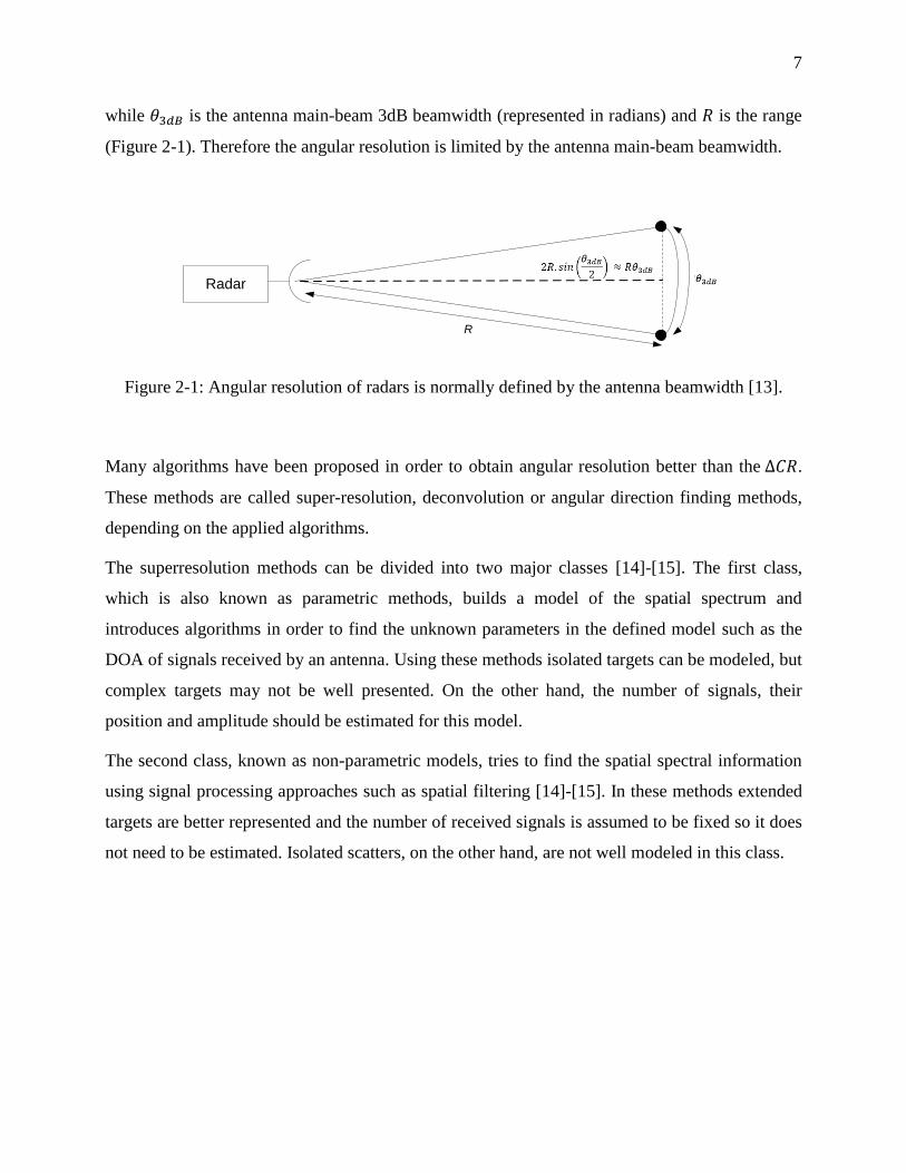
while 𝜃3𝑑𝐵 is the antenna main-beam 3dB beamwidth (represented in radians) and 𝑅 is the range
(Figure 2-1). Therefore the angular resolution is limited by the antenna main-beam beamwidth.
Radar
R
Figure 2-1: Angular resolution of radars is normally defined by the antenna beamwidth [13].
Many algorithms have been proposed in order to obtain angular resolution better than the ∆𝐶𝑅.
These methods are called super-resolution, deconvolution or angular direction finding methods,
depending on the applied algorithms.
The superresolution methods can be divided into two major classes [14]-[15]. The first class,
which is also known as parametric methods, builds a model of the spatial spectrum and
introduces algorithms in order to find the unknown parameters in the defined model such as the
DOA of signals received by an antenna. Using these methods isolated targets can be modeled, but
complex targets may not be well presented. On the other hand, the number of signals, their
position and amplitude should be estimated for this model.
The second class, known as non-parametric models, tries to find the spatial spectral information
using signal processing approaches such as spatial filtering [14]-[15]. In these methods extended
targets are better represented and the number of received signals is assumed to be fixed so it does
not need to be estimated. Isolated scatters, on the other hand, are not well modeled in this class.

8
2.2 Parametric Methods
One of the most well-known superresolution methods is the Multiple SIgnal Classification
(MUSIC) algorithm [16]. MUSIC uses eigenvector decomposition of the measured covariance
matrix to locate closely placed targets with high resolution with an array of sensors.
An extension of the MUSIC algorithm called Scan-MUSIC (SMUSIC) is presented in [17], [18]
to resolve closely spaced targets in step-scanned single-channel mechanical scanning radar. In
SMUSIC, the signal amplitude vector is formed by the antenna response as the antenna scans the
field of view (FOV) in discrete steps. This replaces the vector of outputs of linear array antenna
sensors.
Methods like MUSIC which use eigenvector decomposition of the measured signal covariance
matrix to estimate the location of targets are called subspace based methods. These methods do
not work in the presence of correlated signals. Since the returns in radars are correlated, the DOA
cannot be resolved using this method. However, spatial smoothing [19] can be used to overcome
this problem.
Spatial smoothing is applied to SMUSIC in [17], [20] by dividing the signal amplitude vector
into subvectors and then performing spatial smoothing by subvectors averaging. This method
offers poor results as the DOA seems to be different for each subvector. In order to resolve
coherent signals, a technique based on interpolation of multiple shifted virtual linear arrays from
beamspace data of signal amplitude vector is proposed in [21]. Spatial smoothing is then applied
to the interpolated virtual arrays. This method has also an unsolved problem due to nonuniform
Signal to Noise Ratio (SNR) profile across the virtual arrays. The work of Zhang et al. in [22]
uses another method to decorrelate coherent signals. They impose signal decorrelation by
transmitting orthogonal phase coded waveforms in each direction.
The SMUSIC algorithm is used to achieve higher angular resolution in single-channel antennas
in different applications like wireless communication [23], surveillance and imaging radars [22],
and Millimeter Wave (MMW) real-beam radars [20]. However, no mathematical proof is
presented for the validity of this method and the conditions that have to be respected for the
correct functionality of SMUSIC are not derived in any of these works.

9
ESPRIT is another well-known superresolution algorithm used for array antennas with multiple
sensors [24]. This method reduces computation and storage cost and it is more robust against
array imperfections and errors compared to MUSIC. The improvements with ESPRIT are
obtained by exploiting the fact that array sensors have displacement invariance so that the sensors
are grouped in matched pairs with identical displacement vectors. Another advantage of ESPRIT
is that, unlike MUSIC, complete knowledge of array manifold is not required in this method.
However this method is not used for superresolution in single-channel scanning antenna, as the
constraint of displacement invariance cannot be easily met for the samples in different scanning
directions. Since ESPRIT is based on grouping sets of sensors with identical displacement in
different vectors, extending this method to the single-channel antenna requires complex pre-
processing. So far, it seems that no work has been reported using ESPRIT in single-channel
antennas.
The CLEAN algorithm [25] is used widely in astronomy. In this method targets are considered as
point sources. The algorithm tries to find the sources in the scene by iteratively finding a point
source with the largest absolute value in the observed data and subtracting the system response to
a source of this strength at that position from the observed data. The resulting residual data is
used in the next iteration as the input observed data. The algorithm stops when a predefined limit
is reached. The limit can be the detection of a specified number of sources, or when the residual
data is reduced to noise power level. This algorithm works only if the scene does not include any
large scale object. Another disadvantage of CLEAN is that, in each iteration subtraction is done
only in relation with the largest absolute source value and the knowledge that other sources are
present in the scene is not considered. The CLEAN algorithm is also used in microwave imaging
in [26] where it is extended for the case of coherent radiation from target echoes from radar with
antenna array transmitter.
A relaxation (RELAX) algorithm is introduced in [27] as an extension to CLEAN. Here at each
iteration when a new target is found as the target with largest value, all the previously found
targets are also re-estimated. This results in a more accurate target estimate. The Zoom-FFT
algorithm presented in [28] reduces the RELAX computational requirement and avoids zero-
padding of FFT that is used in RELAX. CLEAN-based algorithms are independent of the number
of sensors in the array and can be applied to single-channel antennas as well.

10
Another superresolution method is the Matrix Pencil (MP) algorithm [29]. In this method, first
the number of targets in the scene is found by analyzing singular values of a data matrix built
from shifted versions of measured data. In the next step, the singular vectors of the built data
matrix is used to construct two filter matrices. The filter matrices are constructed using the
singular vectors for overlapping parts of the original data matrix and including only singular
values which do not correspond to noise. In the final step, the two filter matrices are combined
and the DOA of the target echoes are found by extracting the eigenvalues of the combined
filtered matrix. The complex amplitudes of the target echoes can then be determined using a
standard least-squares pseudo-inverse approach. Unlike MUSIC-based methods that require
several snapshots in order to form the covariance matrix, the Matrix Pencil method only needs
one snapshot to estimate the DOA and computing the covariance matrix is not required. The fact
that signals are correlated has no impact on the performance of this method and it can be even
extended to non-uniform array sensors. Unfortunately, this method is very sensitive to noise and
measurement errors and it therefore cannot perform well in low SNR conditions. This method is
designed to be used in array antennas and not been explored for single-channel antennas.
Another superresolution method that can be used to determine targets position is the Maximum
Likelihood (ML) estimation method [30] . In ML, high resolution target distribution is found by
maximizing the likelihood function (probability density of the observed low resolution target
distribution). The maximum likelihood estimator searches for the steering vectors which are
closest to the received data vector. The unknown parameters (like the DOA and the targets signal
amplitudes) in the data model can be accurately estimated by minimizing the noise which is the
difference between the steering vector of the incoming signal and the received data vector.
Reference [31] proposes a ML method to estimate DOA of multiple radar targets present in the
main beam of a single-channel mechanically scanning radar. The estimator is derived for both the
Conditional ML (CML) and Unconditional ML (UML) cases when target amplitude is
deterministic or stochastic respectively in white Gaussian noise. The estimator algorithm uses the
amplitude modulation of the backscatters echoes induced by antenna scanning.
Another popular ML based methods is the Richardson-Lucy algorithm also called Expectation
Maximization (EM) method [32]-[33]. This is a nonlinear iterative image restoration algorithm
which considers noise with Poisson probability density. The algorithm performs best when

11
images contain point sources over a zero background, like astronomical images, and is therefore
commonly used in astronomy. In [34] the Richardson-Lucy algorithm is used to achieve high
angular resolution in mechanically scanning radar. The method is iterative but converges quickly
and has little computational burden.
In [35] a new superresolution method is proposed for single-channel scanning antennas which
captures the antenna power in different directions and then uses a linear transformation to map
the received power vector to a spectral vector. The DOAs are then estimated using spectral
estimation approaches. This method can detect as many sources as half of the number of the
angles that power measurements are done for, but it only works when the sources are
uncorrelated.
2.3 Non-Parametric Methods
One of the most basic non-parametric superresolution approaches is the Least Square (LS)
deconvolution method. This approach minimizes the squared difference between the
received/measured data and the expected data (the convolution of antenna pattern and scene
information). Using matrix form, the LS problem is ill-posed and provides a pseudo-inverse
solution. This method is also known as matrix inversion method and is unstable in the presence
of noise. A well-known method to overcome ill-posed problem is Tikhonov regularization [36]. It
adds a regularization term also called penalty function in the minimization equation which
performs as a distance function between the solution and the observed data, as well as the
solution and desired properties. This method works well but it is relatively slow and produces
smoothed results. A special case of Tikhonov regularization is Wiener filtering which can be
achieved by selecting noise to signal power spectrum density ratio as the penalty function.
Wiener filtering drawback is the ringing effects artefacts and the need for spectral noise
estimation, but it is very fast [37]. Regularization can be extended by using a generalized penalty
function, such as those used for sidelobe reduction in antenna pattern synthesis. The most
commonly used functions are Gaussian, Hamming, Hann, and Blackman [37].

12
Minimum Mean Square Error (MMSE) is a method similar to the LS approach. It uses an
arbitrary threshold and iteratively computes the covariance matrix of the signal and the
superresolution scene information. The work on [38] uses MMSE for superresolution object
detection in scanning radars. The basic form of MMSE where the noise and scene covariance
matrices are known in advance is equivalent to applying a Wiener filter.
A superresolution method proposed to overcome the inherent instability of the deconvolution
approach is constraint iterative deconvolution [39]. The algorithm is using the geometric series of
the inverse of the antenna pattern in the Fourier domain to construct its iterative form. In order to
eliminate ringing artefacts in the result, the inverse Fourier transform of the estimated result
(reflectivity magnitude of the scene) is computed at all iterations and a positivity constraint is
applied to it. Then, it is converted back to the Fourier domain to be used in the next iteration. The
algorithm achieves good resolution but it converges slowly.
Superresolution can be studied from a Bayesian viewpoint [40] using the maximum a posteriori
(MAP) estimation method. The basic motivation to use Bayesian-based methods is to incorporate
the prior knowledge about the sources in the scene into the superresolution algorithm. The prior
information about the unknown source signals can be deduced from the probability distribution
of the unknown. Therefore in radar imaging, statistics of probability distribution of targets can be
used to estimate the targets distribution. The MAP estimation method incorporates the prior
information about target distribution into the estimation problem. Using MAP, it is essential to
determine a suitable prior information model that describes some statistical properties of the
scene. The work in [41] presents a MAP framework to improve angular resolution in
mechanically scanning radars. It is assumed that the unknown targets in the scene have a Poisson
distribution. In [42], MAP algorithm is used to improve weather radar images. The unknown
targets in the scene are considered to have exponential distribution. The algorithm requires heavy
computations and optimisation.
Capon Minimum Variance Spectral Estimation (MVSE) or Minimum Variance Beamforming
(MVB) [43] is a non-parametric model that concerns finding targets at a desired frequency. This
method uses a weighting that depends on the frequency of interest and finds the optimum weights
by minimizing the energy contributed by interferers (the filter output energy) while keeping unit

13
gain at the desired frequency. This method requires estimation and inverting the covariance
matrix of the observation. An extension of Capon’s method for mechanically step scanning radars
is proposed in [43], [21]. Several variations of this method are also developed, like the General
Capon beam-former (GCB) [44], which can be used even in the case of nonlinear sampling. GCB
is used in [45] for azimuth resolution enhancement in mechanically scanning radars.
Another technique based on successive FFT conversion is super Spatially Variant Apodization
(Super-SVA) [46]-[47]. SVA is a nonlinear operation which can be used to reduce the sidelobes
artefacts [48]. SVA is a special form of MVSE but it does not require matrix inversion. Super-
SVA achieves higher resolution by eliminating the sidelobes of the signal which consequently
increases the bandwidth of it. In this method, first the FFT of the sampled data is computed and
then the SVA is applied to the frequency domain signal to reduce sidelobes. After converting
back the signal to the time domain by IFFT, the inverse weights are applied and then the signal is
truncated to keep the bandwidth extension less than 60% of the original one. The central portion
of the spectrum is then replaced by the original data. This procedure is repeated until the
bandwidth reaches a desired threshold.
Another Capon-like method is the Amplitude and Phase Estimation of Sinusoid (APES) method,
for complex spectral estimation [49]. This method is based on adaptive Finite Impulse Response
(FIR) filtering which can achieve lower sidelobes and narrower spectral peaks than the
conventional FFT method. Moreover, this approach has even a better spectral estimation than
Capon method as it includes an estimate of the noise and interference covariance matrix to find
the weights. To compute the sample data covariance matrix, both forward and backward
covariance matrixes are used which can yield a numerically better condition matrix.
Singular Value Decomposition (SVD) is another approach in which the antenna pattern is
decomposed into two orthogonal matrices and a diagonal matrix with singular values in the
diagonal. Any singular value which is smaller than a threshold is set to zero and then the antenna
pattern is constructed again using the new singular value matrix. The inverse of the new antenna
pattern matrix is calculated while the inverse of the singular values set to zero in previous step are
set to zero again [38]. Removal of small singular values, which are responsible for the

14
amplification of noise, results in a better performance compared to the case when all singular
values are used. However, removal of too many singular values may lead to biased estimation.
2.4 Background Theory of the Selected Methods
In this thesis, two methods have been chosen, one parametric method (ML estimation) and one
non parametric method (Capon method) and they were extended to be applicable in single-
channel frequency scanning antennas. The ML method has good performance in low SNR
conditions and works well in presence of multipath and the Capon method is a simple
beamforming approach with good spectral estimation capability. The selected methods are among
the most popular and practical DOA estimation methods.
The original superresolution methods proposed for array antennas are presented in this section in
details for reference.
2.4.1 Signal Model of PAAs
In order to be able to describe these superresolution methods, first a signal model for the received
signals of an array antenna is presented here.
Consider having an M-element uniform linear array. If a narrow-band signal from a known
source in far-field impinges the array at the direction (𝛾𝑘) with respect to boresight, the complex
response signals at the output of the array elements can be expressed as:
𝒙(𝑙) = 𝒂(𝛾𝑘)𝑠(𝑙) + 𝒏(𝑙), 𝑙 = 1,… , 𝐿 (2.2)
with:
𝒙(𝑙) = [
𝑥1(𝑙)
𝑥2(𝑙)⋮
𝑥M(𝑙)
] , 𝒏(𝑙) = [
𝑛1(𝑙)𝑛2(𝑙)
⋮𝑛M(𝑙)
] , 𝒂(𝛾𝑘) = [
1𝑒𝑗𝜙
⋮𝑒𝑗(𝑀−1)𝜙
].

15
Here, 𝒙(𝑙) is the output of elements of array, L is the number of snapshots in time, 𝒂(𝛾𝑘) is the
steering vector at direction 𝛾𝑘, 𝑠(𝑙) is a scalar denoting the complex amplitude of the incoming
signal, 𝒏(𝑙) is zero mean white Gaussian noise at each element and 𝜙 is:
𝜙 =2𝜋
𝜆 𝑑 sin 𝛾𝑘. (2.3)
Where d is the distance between two elements and is the wavelength of signals. If K signals
impinging the array from the angles 𝜸 = [𝛾1, 𝛾2 , … , 𝛾𝐾], then the array response can be expressed
as:
𝒙(𝑙) = 𝑨(𝜸)𝒔(𝑙) + 𝒏(𝑙), (2.4)
with:
𝑨(𝜸) = [𝒂(𝛾1), 𝒂(𝛾2),… , 𝒂(𝛾𝐾)], (2.5)
𝒔(𝑙) = [𝑠1(𝑙), 𝑠2(𝑙), … , 𝑠K(𝑙)]𝑇 . (2.6)
In case of single-channel antenna, a signal amplitude vector is formed by the antenna response as
it scans the field of view (FOV) and it replaces the vector of outputs of a linear antenna array
sensor (Fig 3-1). Therefore 𝒂(𝛾𝑘) in (2.2) will be replaced with 𝒂(𝜃𝑚 , 𝛾𝑘) which is the one-way
antenna pattern at the angle 𝛾𝑘 when the antenna is pointed at the angle 𝜃𝑚 (Fig 3-2). However, if
the antenna is part of a monostatic radar pointing to a scene and the signals impinging the antenna
are from passive targets instead of emitters, then the 𝒂(𝜃𝑚 , 𝛾𝑘) will be the two-way antenna
pattern. Note that one snapshot in array antenna is taken from all array elements at the same time,
but in single-channel antenna one snapshot is taken from the antenna output at each scan position
with relatively the same delay in each scan position. Also note that in all the above mentioned
works in single-channel antenna domain, the antenna pattern is considered invariant in all
steering directions, similar to the case of mechanical scanning antennas. The rest of formulation
(2.4 to 2.6) will stay the same.

16
2.4.2 ML Estimation
In array antennas, the ML estimator searches for the M steering vectors which are most probable
to give the array received data vectors [30], [50]. The ML solution searches for maximum of the
likelihood function 𝑝(𝒙 |𝜸, 𝒔) which is the probability density function of the data vector 𝒙
conditioned to the unknowns (𝜸, 𝒔):
𝑀𝐿(𝜸, 𝒔) = max𝜸,𝒔
𝑝(𝒙|𝜸, 𝒔). (2.7)
Considering that each element of the noise vector 𝒏(𝑙) has a white complex Gaussian probability
distribution function with zero mean and variance of 𝜎2, 𝒏(𝑙) is modelled as white complex
Gaussian noise with zero mean and covariance matrix of 𝜎2𝑰
𝒏(𝑙) ~ 𝒞𝒩(0, 𝜎2𝑰). (2.8)
If the incoming signals are deterministic and the array received data vector, 𝒙(𝑙) is a stationary,
zero-mean, complex Gaussian process with 𝜸, 𝒔(𝑙), and 𝒏(𝑙) as unknown parameters, then the
probability density function of the data vector 𝒙 conditioned to the unknowns (𝜸, 𝒔(𝑙)) is
𝑝(𝒙(𝑙) |𝜸, 𝒔(𝑙)) =1
(𝜋𝜎2)𝑀exp (−
(𝒙(𝑙)−𝑨(𝜸)𝒔(𝑙))𝐻(𝒙(𝑙)−𝑨(𝜸)𝒔(𝑙))
𝜎2 ), (2.9)
where (. )𝐻 denotes complex conjugate transpose. Using log likelihood of (2.9), 𝜸 and 𝒔(𝑙) can be
estimated by minimizing the noise which is the difference between the steering vector of the
incoming signal 𝑨(𝛾)𝒔(𝑙) and the array’s received data vector 𝒙(𝑙) instead of (2.7). The method
can be stated in least square form as:
min𝜸 ,𝐬(𝑙)
∑ ‖𝒙(𝑙) − 𝑨(𝜸)𝒔(𝑙)‖2𝐿𝑙=1 . (2.10)
In order to minimize the above function, first 𝒔(𝑙) can be found as a function of 𝜸 and inserted
back to form a function of only 𝜸. The estimate of 𝒔(𝑙) is a standard Least Squares (LS) solution
[14] is:
��(𝑙) = [𝑨𝐻(𝜸)𝑨(𝜸)]−1𝑨𝐻(𝜸)𝒙(𝑙). (2.11)
After substituting the signal estimate back into (2.10), the minimization function can be rewritten
as:

17
min𝜸
∑ ‖𝒙(𝑙) − 𝑷𝑨𝒙(𝑙)‖2𝐿𝑙=1 = min
𝛾tr{𝑃𝐴
⊥𝑹��}, (2.12)
with:
𝑷𝑨 = 𝑨(𝛾)[𝑨𝐻(𝛾)𝑨(𝛾)]−1𝑨𝐻(𝛾) and 𝑷𝑨⊥ = 𝐼 − 𝑷𝑨 . (2.13)
and 𝑹𝑥 is array’s output covariance matrix
𝑹𝑥 = 𝐸{𝒙(𝑙)𝒙(𝑙)𝐻} = 𝑨(𝛾)𝑹𝒔𝑨𝐻(𝛾) + 𝜎𝑛
2𝑰, (2.14)
while 𝑹𝒔 = 𝐸{𝒔(𝑙)𝒔(𝑙)𝐻} is the signal covariance matrix and 𝜎𝑛2𝑰 is the white complex Gaussian
noise with zero mean and covariance matrix 𝑹𝑥 can be approximated with :
𝑹𝒙 ≈ 𝑹𝒙 =
1
𝐿∑ 𝒙(𝑙)𝒙(𝑙)𝐻𝐿
𝑙=1 . (2.15)
Therefore DOA can be found using the following minimization function:
�� = argmin𝜸
tr{𝑷𝑨⊥𝑹��} = argmax
𝜸tr{𝑷𝑨𝑹��}. (2.16)
If the incoming signals are stochastic, then instead of signal waveform 𝒔(𝑙), the signal covariance
matrix (𝑹𝑠) has to be estimated along with other unknown parameters. Therefore, the
minimization function would be more complicated.
In low SNR conditions, ML methods perform better than subspace methods. However, the
minimization function requires a non-linear multi-dimensional search which is computationally
very intensive. In order to reduce the computational load many modifications to ML estimation
method are proposed. For example, the alternating projection algorithm uses an iterative
relaxation-based technique in which the equation is minimized in each step using one signal
parameter while other parameters are kept fixed [50]. In single-channel antennas, the ML
estimator is proposed to be applied to the single-channel mechanically scanning antenna signal
model in similar way [31].
2.4.3 Capon Method
In beamforming, linear combination of the antenna outputs is formed by first multiplying each
output 𝑥𝑖 by a complex weight 𝑤𝑖 and then summing all the terms (2.17) [14]. By controlling

18
amplitude and phase of each element (changing the complex weights), it is possible to adjust the
side lobe levels, form different number of beams and also perform beam-steering and null-
forming in desired directions. The weighted output of the antenna array can be represented by
𝑦(𝑙) = ∑ 𝑤𝑖𝐻𝑥𝑖
𝑀𝑖=1 (𝑙) = 𝒘𝐻𝒙(𝑙). (2.17)
The conventional beamformer maximizes the output power of the array for a given input signal.
The noise is assumed to be spatially white and the norm of 𝒘 is constrained to unity. The
maximization problem can be stated as:
max𝒘
𝐸{|𝒘𝐻𝒙|2} subject to 𝒘𝐻𝒘 = 1. (2.18)
The solution to this maximization problem is:
𝒘𝐵𝐹 =𝒂(𝛾)
√𝒂(𝛾)𝐻𝒂(𝛾) , (2.19)
and the estimate of output power at direction γ is:
𝑃𝑦(γ) =𝒂(𝛾)𝐻𝑹𝒙 −1
𝒂(𝛾)
𝒂(𝛾)𝐻𝒂(𝛾) . (2.20)
The angles corresponding to the highest peaks in the output power spectrum signify the directions
of the incoming signals. The conventional beamformer has the limitation that it cannot resolve
two sources spaced closer than the beamwidth of the array. Therefore, when there is more than
one signal present within the beamforming interval, its performance is poor. Better resolution can
be achieved by Capon beamformer. The Capon beamformer minimizes the power of signal-plus-
noise at the output of the beamformer subject to the constraint that the response of the
beamformer to the desired signal with parameter 𝛾 is fixed [14], [43]. The optimization problem
can be stated as:
min𝒘
𝒘𝐻𝑹𝒙 𝒘 subject to 𝒘𝐻𝒂(𝛾) = 1. (2.21)
Using ( 𝑹𝒙 ) as the estimate of output covariance matrix computed from the array outputs
samples, the solution is:
𝒘𝑐𝑎𝑝𝑜𝑛 = 𝑹𝒙 −1
𝒂(𝛾)
𝒂𝐻(𝛾)𝑹𝒙 −1𝒂(𝛾)
. (2.22)

19
The full rank matrix inversion in Capon algorithm is computationally intensive. Besides, in
presence of correlated signals Capon’s method fails. In such situation spatial smoothing can be
used to decorrelate signals. Many other beamforming methods exist trying to maximize the
output signal to interference-plus-noise ratio, minimize mean square error, and so on. Extension
of Capon’s method for mechanically stepped scanning radar is proposed in [21] to be applied to
the single-channel mechanically scanning antenna signal model.
2.4.4 Subspace Methods
Subspace or Eigen-structure methods in PAAs are based on spectral decomposition of antenna
arrays output covariance matrix ( 𝑹𝑥). The eigen-decomposition of 𝑹𝑥 is:
𝑹𝑥 = ∑ λ𝑚𝒗𝑚𝒗𝑚𝐻𝑀
𝑚=1 , (2.23)
where λ𝑚 and 𝒗𝑚 are eigenvalues and eigenvectors of 𝑹𝑥 respectively. Arranging λ𝑚, in
descending order, (λ1 ≥ λ2 ≥ ⋯ ≥ λ𝐾 ≥ λ𝐾+1 = λ𝐾+2 = ⋯ = λ𝑀) the first K eigenvalues
correspond to the K signals. The K corresponding eigenvectors are referred to as the signal-
subspace eigenvectors (𝑬𝑠). The eigenvectors corresponding with the last M−K eigenvalues are
referred to as the noise-subspace eigenvectors (𝑬𝑛).
Subspace methods are based on the fact that the signal subspace spanned by the signal-subspace
eigenvectors is orthogonal to the noise subspace spanned by the noise-subspace eigenvectors, i.e.:
𝑠𝑝𝑎𝑛{𝑬𝑠} ⊥ 𝑠𝑝𝑎𝑛{𝑬𝑛}. (2.24)
On the other hand, the signal subspace is also spanned by the steering vectors:
𝑠𝑝𝑎𝑛{𝑬𝑠} = 𝑠𝑝𝑎𝑛{𝑨}. (2.25)
So we have:
𝒂(𝛾)𝐻𝑬𝑛 = 0. (2.26)
A typical subspace method having high resolution property is the MUSIC algorithm. The pseudo-
spectrum in MUSIC is composed as:

20
𝑃(𝛾) = 1
𝒂(𝛾)𝐻𝑬𝑛𝑬𝑛𝐻𝒂(𝛾)
. (2.27)
The K largest peaks of the pseudo-spectrum give the angle of arrival associated with K incoming
signals. If the rank of the covariance matrix is smaller than the number of signals, (i.e., if there
are coherent signals) the true steering vectors are not orthogonal to the noise subspace. In this
situation the MUSIC algorithm will not provide correct DOA. Consequently, in multipath
environment, spatial smoothing has to be used to decorrelate the coherent signals impinging the
array [19]. Spatial smoothing is achieved by dividing the array into several overlapped subarrays.
Then the average of subarrays covariance matrices is used to resolve the DOA of coherent
signals. In single-channel antenna domain, SMUSIC [17], [18] is introduced for mechanical
scanning radars to be applied to the single-channel mechanically scanning antenna signal model.
2.4.5 Spatial Smoothing
Spatial smoothing is a method to decorrelate signals impinging a uniform linear array [19]. The
details of this method are presented in [19] and are repeated in this section for reference.
As mentioned before, subspace-based methods are based on the assumption that the signal-
subspace eigenvectors are orthogonal to the noise subspace eigenvectors. Considering at least two
of the incoming signals are coherent, i.e. 𝑠2 = 𝛼𝑠1, with 𝑠1 and 𝑠2 are incoming signals with
respect to angles of 𝛾1 and 𝛾2, and 𝛼 is a complex value that represents the gain and phase
difference between two coherent signals, the signal matrix and antenna response matrix in (2.5)
and (2.6) can be rewritten as:
𝒔 = [ (1 + 𝛼)𝑠1, … , 𝑠𝐾]T, (2.28)
𝑨(𝜸) = [𝒂(𝛾1) + 𝛼𝒂(𝛾2) , 𝒂(𝛾3),… , 𝒂(𝛾𝐾)]. (2.29)
Since two of the incoming signals (𝑠1 and 𝑠2) are coherent, from (2.28) and (2.29) it can be
concluded that the signal covariance matrix 𝑹𝒔 is a (𝐾 − 1) × (𝐾 − 1) matrix of rank 𝐾 − 1 and
matrix 𝑨 has 𝐾 − 1 independent columns. Therefore, there will be only 𝐾 − 1 eigenvalue of 𝑹𝑥

21
corresponding to signal subspace and applying subspace based methods only 𝐾 − 1 can be
detected.
1 MM-12 Q Q +1 Q +2
x{1}
x{2}
x{3}
x{P}
x{P-1}
M-Q +1M-Q
Figure 2-2: Spatial smoothing scheme in uniform linear arrays
In spatial smoothing, the uniform linear array is divided into overlapping subvectors of 𝒙{𝑝}
for 1 < 𝑝 < 𝑃, where 𝑃 is the number of subvectors each containing Q samples of 𝒙, so that
𝑃 = 𝑀 − 𝑄 + 1 (see Fig. 2-2). Then we have:
𝒙{𝑝} = 𝑨 𝑫𝑝−1𝒔 + 𝒏{𝑝} for 1 < 𝑝 < 𝑃, (2.30)
where 𝑫𝑝−1 are diagonal matrices defined as:
𝑫𝑝−1 =
[ 𝑒
−𝑗2𝜋
𝜆 𝑑 (𝑝−1)𝑠𝑖𝑛 𝛾1 0 ⋯ 0
0 𝑒−𝑗2𝜋
𝜆 𝑑 (𝑝−1)𝑠𝑖𝑛 𝛾2 ⋯ 0
⋮ ⋮ ⋱ ⋮
0 0 ⋯ 𝑒−𝑗2𝜋
𝜆 𝑑(𝑝−1) 𝑠𝑖𝑛 𝛾𝐾]
. (2.31)
The spatially smoothed covariance matrix 𝑹𝒑 is:
𝑹𝒑 =1
𝑃∑ 𝒙{𝑝}𝒙{𝑝}𝐻
𝑃
𝑝=1= 𝑨(
1
𝑃∑ 𝑫𝑝−1𝑹𝒔𝑫𝑝−1
𝑯 )𝑨𝑯𝑃
𝑝=1+ 𝜎2𝑰, (2.32)
and the spatially smoothed signal covariance matrix is:

22
𝑹𝒔 =
1
𝑃∑ 𝑫𝑝−1𝑹𝒔𝑫𝑝−1
𝑯𝑃
𝑝=1 . (2.33)
In order to be able to apply subspace based DOA estimation methods, the modified signal
covariance matrix 𝑹𝒔 should be nonsingular and should have the rank of K. It is shown in [19]
that for P ≥ K, 𝑹𝒔 will be full rank and nonsingular. This is proven by rewriting 𝑹𝒔
as:
𝑹𝒔 = 𝑻 𝑻𝑯, (2.34)
where 𝑻 is a 𝐾 × 𝑃𝐾 block matrix defined by:
𝑻 = [𝑪 ,𝑫1𝑪,… ,𝑫𝑝−1𝑪 ]. (2.35)
In (2.35), matrix 𝑪 is the Hermitian square root of 1
𝑃𝑹𝒔 defined as:
𝑪𝑪𝑯 =1
𝑃𝑹𝒔 . (2.36)
It can be concluded from equation (2.34) that rank of 𝑹𝒔 is the same as rank of 𝑻 (𝑟𝑎𝑛𝑘(𝑹𝒔
) =
𝑟𝑎𝑛𝑘(𝑻) = 𝑟𝑎𝑛𝑘(𝑻𝑯)) and consequently if 𝑻 is non-singular, 𝑹𝒔 will be non-singular too.
In order to find the rank of 𝑻 and prove it is non-singular, a new matrix �� is constructed by
permutation of columns of matrix 𝑻. As column permutation does not change matrices rank, the
rank of 𝑻 and �� are equal. Therefore, the matrix �� is:
�� = [𝑐11𝒃𝟏 𝑐12𝒃𝟏 ⋯ 𝑐1𝐾𝒃𝟏
⋮ ⋮ ⋮𝑐𝐾1𝒃𝑲 𝑐𝐾2𝒃𝑲 𝑐𝐾𝐾𝒃𝑲
]. (2.37)
In (2.37), 𝑐𝑖𝑗 are the elements of matrix 𝑪, and 𝒃𝑖 (i = 1,.., K) are the vectors of:
𝒃𝑖 = [1, 𝑒−𝑗2𝜋
𝜆 𝑑 𝑠𝑖𝑛 𝛾𝑖 , … , 𝑒−𝑗
2𝜋
𝜆 𝑑(𝑃−1) 𝑠𝑖𝑛 𝛾𝑖]. (2.38)
For 𝑃 ≥ 𝐾, the 𝒃𝑖 vectors are linearly independent and form a Vandermode matrix. Also each
row of C has at least one nonzero element. Thus matrix �� is full rank and non-singular and has
rank K.
Consequently 𝑻 and 𝑹𝒔 has rank K and therefore it is possible to detect all K of signals using
spatial smoothing when incoming signals are coherent.

23
In the next chapter, the applicability and performance of the Capon MVB method along with
spatial smoothing and the ML estimation method on FSA scanning systems are studied.
24
CHAPTER 3 ARTICLE 1: MULTIPLE TARGETS DIRECTION-OF-
ARRIVAL ESTIMATION IN FREQUENCY SCANNING ARRAY
ANTENNAS
Mona Akbarniai Tehrani, Jean-Jacques Laurin, and Yvon Savaria
Department of Electrical Engineering,
École Polytechnique de Montréal, Montréal, Canada
Published at “IET Radar, Sonar & Navigation” in 2016-03-01
Abstract: In this work, we address the problem of resolving angular position of multiple targets in
the same range and separated by less than an antenna beamwidth using frequency scanning array
(FSA) antennas. First, the frequency scanning antenna signal model is derived and then the
necessary compensation methods to overcome antenna pattern variations with frequency during
the scan in FSAs are presented. Two direction-of-arrival (DOA) estimation algorithms, the
minimum variance beamforming (MVB) and the maximum likelihood (ML) estimation are
applied on the signal model. Simulation results show that both methods can separate targets with
angular separations smaller than a beamwidth by selecting correct parameters. The performance
of the two DOA estimation methods with respect to different system parameters are investigated
based on the signal model through Monte Carlo simulations and compared with the Cramér–Rao
lower bound (CRLB). In addition, an FSA antenna is presented in this work and simulations of
the DOA estimation algorithms are performed using the measured antenna pattern of this
antenna. The performance and limitations of target DOA estimation methods for the measured
antenna patterns are also discussed.
3.1 Introduction
Low-cost electronically scanning radars are receiving considerable attention. Frequency scanning
arrays (FSAs) are a solution to achieve low-cost and agile electronically scanning radars, without

25
the need for phase shifters on the array elements. Unlike conventional FSAs that require
frequency variation over a wide bandwidth [9], new FSAs using dispersive feed networks based
on metamaterial guiding structures, can scan a wide angular range using a small bandwidth [10].
Therefore, using FSAs become practical in term of frequency bandwidth allocation. However,
when the length of the array is limited, the width of its main beam can be wider than needed for a
typical radar application, which results in poor angular resolution. Thus appropriate signal
processing for improving the angular resolution is necessary.
Examples of FSA utilization in high resolution radars are presented in [7], [51]. This paper is
considering a system that is used to estimate the angular position of targets using standard
direction of arrival (DOA) algorithms. A pulsed step frequency mode of operation is assumed.
Although angular resolution in an FSA antenna is obtained along with range resolution in [52],
[53], improving angular resolution beyond beamwidth limitations in FSA has not been studied.
Consequently, considering the low cost of FSAs compared to phased arrays, it is relevant to
develop methods to improve the angular resolution of systems based on such antennas.
Unlike phased array antennas, in FSAs, all the radiating elements are fed with a waveguide
having a frequency dispersive characteristic. So, the array elements can be assumed connected to
each other and there is only one input/output port for all the antenna elements. Therefore the FSA
can be modelled like a mechanically or electronically scanning antenna, with the difference that
each part of the field of view (FOV) is illuminated by a different frequency related to the angle of
transmission. This differs from multiport antennas such as phased arrays in which elements can
be weighted to shape the beam.
There are several superresolution algorithms that are able to detect signals separated by less than
an antenna beamwidth. These algorithms are making use of multi-channel array antennas. DOA
estimation methods based on maximum likelihood (ML) [54] and superresolution subspace
methods like MUSIC [16] and ESPRIT [55] are some of the most well-known algorithms.
However, there has been little work on improving angular resolution of a single channel antenna,
so that it can resolve signals from directions separated by less than one beamwidth [17], [21],
[31], [35], [45], [56]-[60]. In this work we use two angular resolution improvement methods,

26
minimum variance beamforming (MVB) [43] and ML estimation, which were previously applied
to mechanically scanning antennas [31], [45] and adapt them for FSA antennas.
The paper is organized as follows. Section 3.2 briefly reviews the literature on single channel
antenna superresolution and DOA estimation domain. In Section 3.3, a signal model that applies
to FSA antennas is presented. In Section 3.4, the necessary compensation methods used to
overcome gain and antenna pattern variations with frequency during the scan in FSA are
presented. In Section 3.5, the MVB and ML estimation methods are briefly described. In Section
3.6, representative simulation results are given and the performance of selected methods with
respect to different system parameters is evaluated. In Section 3.7, an FSA antenna is presented
and the performance of the ML and MVB methods are evaluated for this FSA. Conclusions and
remarks are provided in Section 3.8.
3.2 Brief Overview of Recent Works on DOA Estimation with
Single Channel Antennas
Most of the work in the single channel antenna superresolution and DOA estimation domains is
based on the fact that antenna scanning induces amplitude modulation on signal backscatters and
therefore, by utilizing prior knowledge of the antenna pattern, the angular position of targets can
be extracted [56], [57]. For example, Ly [17] developed a MUSIC based technique called scan-
MUSIC (SMUSIC) to resolve target positions within a beam. In this method, the signal amplitude
vector is formed using the response of the antenna as it scans the FOV. This differs from multi
sensor array antennas in which multiple sensor outputs is used to form the signal amplitude
vector. However, subspace based methods do not work in the presence of correlated signals. In
order to resolve correlated signals, in Ref. [17] the signal vector is divided into subvectors and a
forward subvector averaging is performed as a form of spatial smoothing [19]. Ref. [21] proposes
a technique based on interpolation of multiple shifted signal vectors from beamspace data to
virtual multi sensor array antennas. Spatial smoothing is then applied to the interpolated vectors.
This method has performance limitations due to nonuniform signal-to-noise ratio (SNR) profile
across the interpolated vectors.

27
As an alternative to MUSIC based methods, beamforming approaches can be applied to the
signal amplitude vectors. Reference [52] studied the special case of a conventional beamformer
in FSA antennas. Capon’s MVB is also used in [21] to resolve DOA of signals in scanning
antennas. Extension of the MVB method for step scanning radars is proposed in [45]. Unlike
MUSIC based methods, beamforming methods do not need prior knowledge on the number of
targets.
In [31], DOAs of multiple radar targets present in the main beam of a rotating antenna are
estimated using the same concept as in [17] to form signal amplitude vector and by applying the
ML technique. Both cases of conditional and unconditional ML are studied in [31]. A simplified
version of the same method is presented in [58] as the pseudo-monopulse algorithm for target
direction estimation and compared with the monopulse technique. An asymptotic maximum
likelihood estimator is also used in [59], [60] for detecting targets and estimating their complex
amplitude and DOA in mechanically rotating antennas.
In [35], DOAs of multiple uncorrelated sources in single channel scanning antennas are estimated
by measuring the power of the radiation pattern received during scanning. Then the vector of
power measurements is transformed into a vector of spectral observations. Finally, DOA
estimation is performed by spectral analysis methods.
In this paper, the effectiveness and performance of two of the above methods, MVB with spatial
smoothing and ML estimation, when applied to FSA antennas are evaluated and compared. Using
a FSA antenna, there is no need for mechanical rotation of the antenna which could be an
advantage if targets move rapidly. FSA also enable agile operation not limited by constraints of
mechanical systems. The selected methods are applicable to coherent signals and therefore they
are able to estimate DOA of multiple targets.
3.3 Problem Formulation
In FSA antennas, the main beam direction varies by changing the carrier frequency of the
transceiver. This is achieved by using a series feed structure, in which the phase shift between

28
adjacent element ports varies as a function of frequency. Using the simple delay line concept, the
direction of the beam 𝜃𝑚 can be expressed as:
sin(𝜃𝑚) =𝜆
𝑑(
𝑠
𝜆𝑔− 𝑎) (3.1)
where 𝑠 is the length of the feed line between element ports, 𝜆 is the free-space wavelength, 𝜆𝑔 is
the wavelength in the feed line, d is the distance between radiating elements in the aperture plane,
and a is an integer (see Fig. 3-1) [8]. The main beam direction 𝜃𝑚 is taken with respect to the
normal of the antenna aperture. When the frequency varies, 𝜆 and 𝜆𝑔 change at different rates
which causes a variation of 𝜃𝑚.
Figure 3-1: Schematic representation of a frequency scanning antenna and the process of
selecting N frequencies for which the main beam is in the 𝛥𝑓𝑜𝑣 angular range
The field of view (FOV) of the antenna corresponds to the angular sector scanned by the main
beam direction when the frequency is swept over the complete frequency bandwidth of the
antenna. Consider K targets present in the FOV at the same known range of 𝑅𝑙 =𝑐𝑡𝑙
2 , where 𝑡𝑙
is the time for receiving an echo from targets at the range 𝑅𝑙 and c is the speed of light. When the
antenna main beam of an FSA radar is steered in the direction 𝜃𝑚, the received baseband signal
can be written as

29
𝑥𝑟(𝑡𝑙 , 𝜃𝑚) = ∑ 𝑠𝑘(𝑓𝑚)𝑔𝑚(𝛾𝑘)𝑒−𝑗2𝜋𝑓𝑚𝑡𝑙
𝐾
𝑘=1+ 𝑛(𝑡𝑙 , 𝜃𝑚), (3.2)
where 𝑓𝑚 is the carrier frequency when the FSA beam is pointed at the angle 𝜃𝑚, 𝑠𝑘(𝑓𝑚) is the
complex signal scattered from the k-th target with the angular position 𝛾𝑘, 𝑔𝑚(𝛾𝑘) is the two-way
antenna pattern at the angle 𝛾𝑘 when the antenna is pointed at the angle 𝜃𝑚 (see Fig. 3-2),
and 𝑛(𝑡𝑙 , 𝜃𝑚) is the complex white Gaussian noise coming from the scene and introduced by the
receiver components. It has been assumed that the Doppler shift of the echo can be neglected.
Figure 3-2: Two-way antenna gain pattern.
If the antenna pattern is approximated with a virtual linear array antenna pattern as:
ℎ(𝜃𝑚, 𝛾𝑘) = 𝐻𝑚 sin(𝑁𝑒 𝜓/2)
sin( 𝜓/2) 𝜓 = 𝛽𝑑[sin(𝛾𝑘) − sin(𝜃𝑚)], (3.3)
where 𝐻𝑚 is the maximum gain, 𝑁𝑒 is the number of elements in the array antenna, and 𝛽 is the
wave number, the two-way antenna pattern at the angle 𝛾𝑘 when the antenna is pointed at the
angle 𝜃𝑚 can be approximated as:
𝑔𝑚(𝛾𝑘) = ℎ2( 𝜃𝑚, 𝛾𝑘). (3.4)
It is assumed that the phase response of the antenna pattern can be removed by appropriate a
priori calibration of the FSA. In the vector notation of the signal model, the complex echo signal
vector and the steering vector for a target at angle 𝛾𝑘, when the antenna is steered to the angles
𝜃𝑚 with 𝑚 = 1, . . , 𝑀 are defined as:
𝒔𝑘 = [ 𝑠𝑘(𝑓1), 𝑠𝑘(𝑓2),… , 𝑠𝑘(𝑓𝑀)]𝑇, (3.5)

30
𝒂(𝛾𝑘) = [ 𝑎(𝜃1, 𝛾𝑘), 𝑎(𝜃2, 𝛾𝑘),… , 𝑎(𝜃𝑀, 𝛾𝑘)]𝑇, (3.6)
where (. )𝑇 denotes the transpose operation, M is the total number of the frequencies, and steering
vector elements are:
𝑎(𝜃𝑚 , 𝛾𝑘) = 𝑔𝑚(𝛾𝑘)𝑒−𝑗2𝜋𝑓𝑚𝑡𝑙. (3.7)
With K targets at directions 𝜸 = [𝛾1, 𝛾2 , … , 𝛾𝐾], the antenna response matrix and targets echo
matrix are:
𝑨(𝜸) = [𝒂(𝛾1), 𝒂(𝛾2) , … , 𝒂(𝛾𝐾)], (3.8)
𝑺 = [ 𝒔1, 𝒔2, … , 𝒔𝐾]. (3.9)
Eq. (3.2) can be rewritten in the vector form as:
𝒙𝒓 = (𝑨(𝜸) ⊙ 𝑺)𝟏𝑲×𝟏 + 𝒏 , (3.10)
where ⊙ is the Hadamard product, 𝟏𝑲×𝟏is a column vector of ones, and 𝒙 and 𝒏 are:
𝒏 = [ 𝑛(𝑡𝑙, 𝜃1), 𝑛(𝑡𝑙, 𝜃2),… , 𝑛(𝑡𝑙, 𝜃𝑀)]𝑇, (3.11)
𝒙𝒓 = [ 𝑥𝑟(𝑡𝑙, 𝜃1), 𝑥𝑟(𝑡𝑙, 𝜃2), … , 𝑥𝑟(𝑡𝑙, 𝜃𝑀)]𝑇. (3.12)
Note that the received signal 𝑥𝑟(𝑡𝑙, 𝜃𝑚) comprises the responses of all the visible targets when the
FSA is operated at frequency 𝑓𝑚. It has been assumed that the targets cross sections do not
change when the transmitted frequency changes, which may be a valid assumption when the used
bandwidth is narrow. Then we have:
𝑠𝑘 = 𝑠𝑘(𝑓1) = 𝑠𝑘(𝑓2) = ⋯ = 𝑠𝑘(𝑓𝑀), (3.13)
and
𝒔 = [ 𝑠1, 𝑠2, … , 𝑠𝐾]T. (3.14)
Thus the data model can be simplified to:
𝒙𝒓 = 𝑨(𝜸)𝒔 + 𝒏. (3.15)
The objective is to estimate the vector of target angular positions 𝜸 while the targets complex
echo vector, 𝒔 is unknown.

31
3.4 Calibration and Interpolation
When using FSAs, some preprocessing steps are required before applying subspace based target
DOA estimation methods in which spatial smoothing is required. Spatial smoothing works when
steering vectors can be divided into shift invariant overlapping subvectors [19]. It can be easily
shown that shift invariant subvectors can be formed from the steering vector only if:
1) the steering vector only includes the main beam of the antenna pattern,
2) the gain of the antenna pattern in different steering angles are balanced,
3) and the angular separation between steering angles (|𝜃𝑚 − 𝜃𝑚+1|) are uniform.
In order to achieve the above properties the following compensation methods are considered.
First, the FOV is divided into several sectors called 𝛥𝑓𝑜𝑣 and DOA estimation methods are
performed for each 𝛥𝑓𝑜𝑣 separately to find targets that are present in that sector. Using small
𝛥𝑓𝑜𝑣 reduces the computational complexity. In addition, for each 𝛥𝑓𝑜𝑣, only N of the
frequencies (N < M) for which the main beam belongs to that 𝛥𝑓𝑜𝑣, are used in (3.5-3.14) (Fig.
3-1). As mentioned before, using our signal model, the subspace based target DOA estimation
methods work well only if, for each 𝛥𝑓𝑜𝑣, only the beams having their main beam in that sector
are considered in the superresolution computations.
Furthermore, in a practical FSA the maximum gain of the antenna pattern always vary with
frequency. This variation must be compensated using suitable calibration prior to processing. In
order to compensate existing gain imbalance, one of the N frequencies in the set of fixed
frequencies 𝑓𝑛 (n=1,..,N) is selected as a reference (𝑓𝑟), and the ratio between the amplitude of
antenna pattern for the corresponding reference pointing angle (𝜃𝑟) with respect to other steering
angles are chosen as compensation weights 𝑐(𝜃𝑛) =𝑔𝑟(𝜃𝑟)
𝑔𝑛(𝜃𝑛) . The compensation matrix is then
formed as follows:
𝑪 = diag[ 𝑐1, 𝑐2, … , 𝑐𝑁], (3.16)
and the calibrated antenna response matrix 𝑨𝒄(𝛄) is:
𝑨𝒄(𝛄) = 𝑪𝑨(𝛄). (3.17)

32
Therefore (3.15) can be modified to:
𝑪𝒙𝒓 = 𝑨𝒄(𝛄)𝒔 + 𝑪𝒏. (3.18)
This process involves antenna pattern measurement and it has to be done once offline.
Moreover, according to (3.1), by changing the frequency in uniform steps, the antenna steering
angle will change nonlinearly. In other words, the steps between steering angles [𝜃1, 𝜃2, … , 𝜃𝑁]
are not equal. We can thus write
𝜃𝑛 = 𝜃1 + ∑ 𝛥𝜃𝑖𝑛−1𝑖=1 , (3.19)
where 𝛥𝜃𝑖 is the angular step between beam steering angles. While in some FSAs this
nonlinearity can be small and negligible, the performance of spatial smoothing degrades when
uniform frequency steps are assumed in the model. Therefore, an interpolated version of
𝑨𝒄(𝛾) can be used in (3.18) in which the relation between steering angle and frequency is linear.
Interpolation is performed using a method similar to the algorithm presented in [61] by
computing an interpolation matrix.
First, for each sector (𝛥𝑓𝑜𝑣) a set of interpolation angles is defined:
𝜞 = [��1, … , ��𝐷], (3.20)
where D is the number of hypothetical DOAs of targets that are only used for interpolation.
Then, an interpolation matrix is computed by mapping 𝑨𝒄(𝜞) = [𝒂𝒄(��1), 𝒂𝒄(��2) , … , 𝒂𝒄(��𝐷)] to
a virtual matrix ��(𝜞) = [��(��1), ��(��2) , … , ��(��𝐷)]. This is done so that in each virtual steering
vector ��(𝛾𝑑) = [ ��(��1, ��𝑑), ��(��2, ��𝑑),… , ��(��𝑁 , ��𝑑)]𝑇 the steps between virtual steering angles
[��1, ��2, … , ��𝑁] will be equal:
��𝑛 = 𝜃1 + (𝑛 − 1)𝛥𝜃 , 𝛥𝜃 = |𝜃1−𝜃𝑁|
N (3.21)
with 𝑛 = 1, . . , 𝑁. It is assumed that the virtual matrix ��(𝜞) can be obtained by linear
interpolation of the real matrix 𝑨𝒄(𝜞), so that
��(𝜞) = 𝑩𝑨𝒄(𝜞). (3.22)
In which the interpolation matrix 𝑩 is the least square solution of (3.22) that should be found
only once offline.
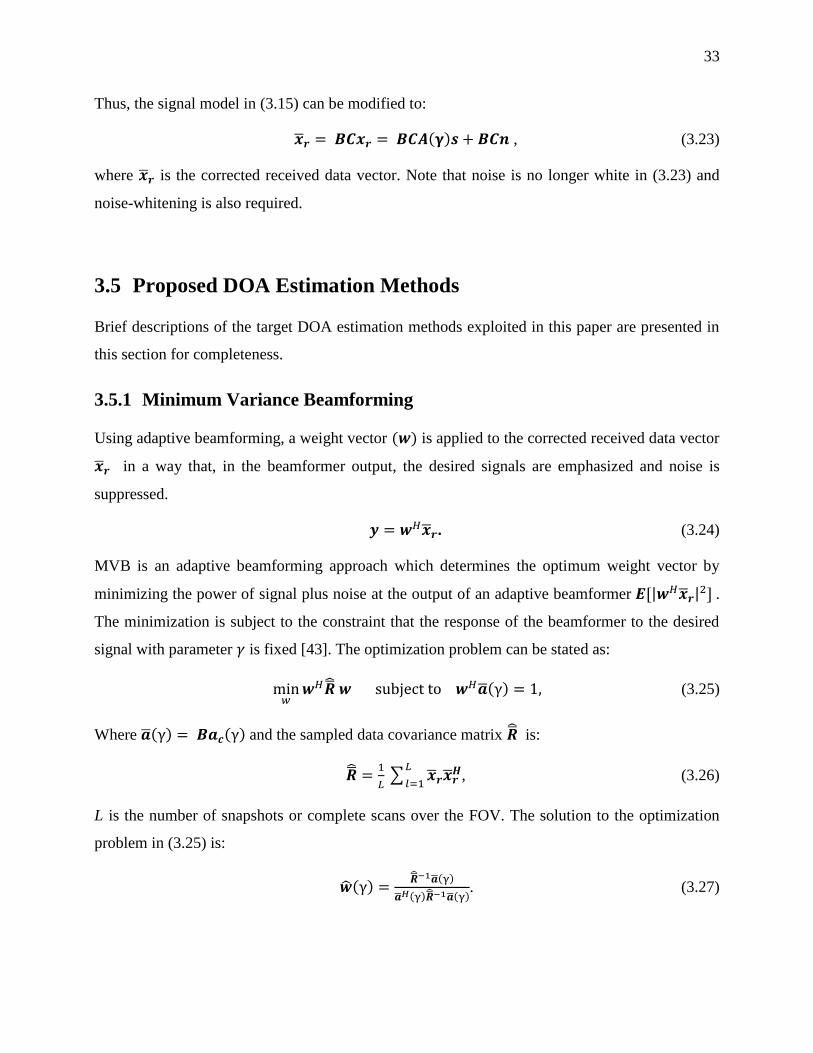
33
Thus, the signal model in (3.15) can be modified to:
��𝒓 = 𝑩𝑪𝒙𝒓 = 𝑩𝑪𝑨(𝛄)𝒔 + 𝑩𝑪𝒏 , (3.23)
where ��𝒓 is the corrected received data vector. Note that noise is no longer white in (3.23) and
noise-whitening is also required.
3.5 Proposed DOA Estimation Methods
Brief descriptions of the target DOA estimation methods exploited in this paper are presented in
this section for completeness.
3.5.1 Minimum Variance Beamforming
Using adaptive beamforming, a weight vector (𝒘) is applied to the corrected received data vector
��𝒓 in a way that, in the beamformer output, the desired signals are emphasized and noise is
suppressed.
𝒚 = 𝒘𝐻��𝒓. (3.24)
MVB is an adaptive beamforming approach which determines the optimum weight vector by
minimizing the power of signal plus noise at the output of an adaptive beamformer 𝑬[|𝒘𝐻��𝒓|2] .
The minimization is subject to the constraint that the response of the beamformer to the desired
signal with parameter 𝛾 is fixed [43]. The optimization problem can be stated as:
min𝑤
𝒘𝐻�� 𝒘 subject to 𝒘𝐻��(γ) = 1, (3.25)
Where ��(γ) = 𝑩𝒂𝒄(γ) and the sampled data covariance matrix �� is:
�� =1
𝐿∑ ��𝒓��𝒓
𝑯𝐿
𝑙=1, (3.26)
L is the number of snapshots or complete scans over the FOV. The solution to the optimization
problem in (3.25) is:
��(γ) =��−1��(γ)
��𝐻(γ)��−1��(γ). (3.27)

34
And the estimate of output power at direction γ is:
𝑃𝑦(γ) =1
��𝐻(γ)��−1��(γ). (3.28)
If the target response is coherent, �� will be rank deficient and the algorithm will fail to resolve
targets. In order to decorrelate target responses and to obtain a full rank covariance matrix, spatial
smoothing [19] can be used. In spatial smoothing, the sampled data vector is divided into
overlapping subvectors of ��𝑟{𝑖}
for 1 < 𝑖 < 𝑃, where 𝑃 is the number of subvectors each
containing Q samples of ��𝒓, so that 𝑃 = 𝑁 − 𝑄 + 1. The data covariance matrix can be then
estimated by:
𝑹𝒇 =
1
𝑃∑ ��{𝑖}
𝑃
𝑖=1. (3.29)
Spatial smoothing works when the number of subvectors is equal to or larger than the number of
targets (P ≥ K) and the size of each subvector 𝑄 is at least K+1[19]. Therefore we have:
𝑁 ≥ 2𝐾. (3.30)
The optimal subvector size is computed in [62] as:
𝑄𝑜𝑝𝑡 = 0.6(𝑁 + 1). (3.31)
3.5.2 Maximum Likelihood Estimation
The use of maximum likelihood (ML) to estimate multiple target directions in scanning antennas
is presented in [31]. The same method can be used for the case of an FSA antenna as the FSA
signal model is similar to the one found in [31]. The only difference is that in the FSA signal
model, the antenna response matrix 𝑨(𝛾) contains an extra phase term. Note that the
interpolation step is not needed for the ML estimation method and the signal model in (3.18) or
(3.15) is used for this method. Considering that each element of the noise vector n has a white
complex Gaussian probability distribution function with zero mean and variance of 𝜎2, n is
modelled as white complex Gaussian noise with zero mean and covariance matrix of 𝜎2𝑰

35
𝒏 ~ 𝒞𝒩(0, 𝜎2𝑰), (3.32)
Therefore the probability density function of the data vector 𝒙𝒓 conditioned to the unknowns
(𝜸, 𝒔) is
𝑝(𝒙𝒓|𝜸, 𝒔) =1
(𝜋𝜎2)𝑁exp (−
(𝒙𝒓−𝑨(𝛾)𝒔)𝐻(𝒙𝒓−𝑨(𝛾)𝒔)
𝜎2 ). (3.33)
The ML estimation of 𝜸 and 𝒔 can be found by maximizing the conditional probability density
function of 𝒙𝒓 with respect to 𝜸 and 𝒔. If 𝒔 is modelled as a deterministic unknown vector and 𝜸
as a deterministic constant vector then the conditional ML will be:
��, �� = argmax𝜸,𝒔
{𝑝(𝒙𝒓|𝜸, 𝒔)}. (3.34)
The above maximization gives the estimate of �� and �� as:
�� = (𝑨𝑯𝑨)−1𝑨𝑯𝒙𝒓, (3.35)
�� = argmax𝜸
𝒙𝑟𝐻𝑨(𝑨𝑯𝑨)−1𝑨𝑯𝒙𝒓. (3.36)
It is assumed that no prior knowledge is available for DOAs of 𝜸 = [𝛾1, 𝛾2 , … , 𝛾𝐾]. The ML
method can detect targets in both cases of correlated and non-correlated signals. It also has good
performance in presence of noise and in the cases where only as few as one scan of the FOV is
available. However, for K targets, the ML method requires a K-dimensional search over FOV to
find the DOAs. Therefore when the considered number of targets increases, the ML estimation
becomes more computationally intensive. In addition, ML estimation requires prior knowledge of
the number of targets. This number has to be estimated in a preprocessing step if no prior
information is available.
3.6 Simulation Results with Emulated Antenna Pattern
In order to verify the performance of the proposed methods with respect to different system
parameters, a two-way antenna pattern which is approximated using the array factor of a linear
array with uniform amplitude weighting as presented in (3.3) is used.

36
For this simulation, carrier frequency is considered to be changing between 8 GHz and 8.5GHz in
N=21 steps according to (3.1). This corresponds to the operation of an FSA described in [64],
which scans between -9.7 and 7.7 degrees in nonuniform steps in frequency. The -3dB
beamwidth of these patterns is 13 degrees.
In addition, the 𝛥𝑓𝑜𝑣 is selected to be the range of [-6, 6] degrees, and simulations are done to
detect targets in this region. As an arbitrary but representative example, a benchmark with two
targets is considered. Targets are assumed to be at the same range and at -3 and 3 degrees with
respect to boresight. The number of beams in the selected 𝛥𝑓𝑜𝑣 N and the subvector size Q are
selected equal to N=21 and 𝑄𝑜𝑝𝑡= 13 according to (3.31). The targets amplitude vector 𝒔 in
(3.14) is assumed to consist of two coherent random complex numbers (𝑠2 = 0.9𝑠1) and n is a
white Gaussian noise vector. The SNR is defined as the total power of the received signals over
the noise power.
Fig. 3-3 shows the result of applying the MVB method (Eq. 3.28) in two different SNR
conditions of SNR = 20dB and SNR = 5dB. It can be seen that at SNR = 20dB, the targets are
detected at 𝛾1 = -3 and 𝛾2= 3 degrees (Fig. 3-3a). However, when SNR = 5dB the MVB method
cannot detect two targets in the 𝛥𝑓𝑜𝑣 (Fig. 3-3b). The ML method also detects the targets DOA
at 𝛾1 = -3 and 𝛾2= 3 degrees when SNR = 20dB and 𝛾1 = -2 and 𝛾2= 4 degrees when SNR =
5dB. Note that the interpolation step described in Section 3.4 is applied with the MVB method.
Also note that both methods are implemented with one degree resolution.
In order to evaluate the performance of the two methods with respect to different parameters, the
root mean square error (RMSE) of the targets DOA estimation is calculated. Given the above
setup the RMSE is defined as:
RMSE = √𝐸[∑ (𝛾𝑘 − 𝛾��)2𝐾𝑘=1 ], (3.35)
where E(.) is the expected value estimated using 100 Monte Carlo trials and K=2 is the number of
targets. The Cramér–Rao Lower Bound (CRLB) [63] which serves as an optimality criterion for
DOA estimation is also computed and presented for evaluation of the results. CRLB estimation
of real parameters based on a complex data vector with complex Gaussian probability density

37
function is computed according to equations given in [31] and [63] with minor modifications and
reported in Appendix A.
a
b
Figure 3-3: Results of applying the MVB method along with spatial smoothing.
a) SNR=20dB. b) SNR=5dB.

38
Fig. 3-4 shows the RMSE of DOA estimation obtained with the two methods as a function of the
SNR. In that simulation, two targets were also assumed to be at -3 and 3 degrees and the number
of beams was also set to N=21. The estimation results in Fig. 3-4 show that in low SNR situations
(SNR <10dB), the DOA estimation performance is low. For SNR values lower than 10dB, the
ML method can detect two targets with a total error of 4 to 6 degrees and the MVB method
cannot detect two targets in the 𝛥𝑓𝑜𝑣. For the MVB method, when two targets cannot be
separated from each other in more than 5% of the trials, the RMSE values is not plotted in the
figures 3-4, 3-5 and 3-8, as RMSE calculation becomes ambiguous. Also note that both methods
are implemented with one degree resolution. Accuracy corresponding to this resolution is
achieved when SNR is above 15dB for the ML method and above 20dB for the MVB method.
Figure 3-4: RMSE of target DOA estimation methods versus SNR for N= 21, 𝛾1 = -3 and 𝛾2= 3.
Fig. 3-5 shows the RMSE obtained with the two methods as a function of N, the number of
beams in the 𝛥𝑓𝑜𝑣 form the received signal vector. For this simulation, the SNR is fixed at 20dB
and other parameters including 𝛥𝑓𝑜𝑣 and the frequency range are kept unchanged. This means

39
that by increasing N, the beams will be closer to each other. It can be seen that for the ML
method, increasing N decreases the RMSE. The MVB method also has better performance when
the number of beams is large (more than 21). However, this method cannot detect two targets in
the 𝛥𝑓𝑜𝑣 when N < 21.
Figure 3-5: RMSE of target DOA estimation methods versus N, SNR=20dB, 𝛾1 = -3 and 𝛾2= 3.
Next, the impact of angular separation of the two targets on the RMSE is studied (Fig. 3-6). It can
be seen that using the ML method, the RMSE decreases when the angular separation between the
two targets increases which means that ML can detect two targets more accurately when they
have larger angular distance from each other. However, when using the MVB method, the RMSE
increases if the angular separation between two targets is larger than 8 degrees. This is due to the
fact that for this simulated antenna patterns and with the current settings, the angular separation
between two targets larger than 8 degrees requires sampling from sidelobes of some of the
antenna patterns, which decreases the performance of the MVB method.

40
Figure 3-6: RMSE of target DOA estimation methods versus angular separation between two
targets SNR=20dB, and N= 21.
3.7 Simulation Results with Real Antenna Pattern
In this section the performance of the two considered DOA estimation methods is studied by
taking into account the antenna patterns of a real FSA antenna. The antenna was designed to
work in the X-band and the measured antenna patterns are used in the simulations.
Fig. 3-7a shows the two-way radiation pattern of an 8-element FSA which is built based on a
composite right/left-handed (CRLH) waveguide with air-filled double-ridge waveguide [64]. The
antenna scans the angles between -5 to 35 degrees by changing the frequency from 8 to 8.8 GHz
in 40 steps. The half-power beamwidth of the antenna varies between 15 and 21 degrees for the
different steering angles. This FSA antenna can scan the FOV continuously with controllable
frequency steps.
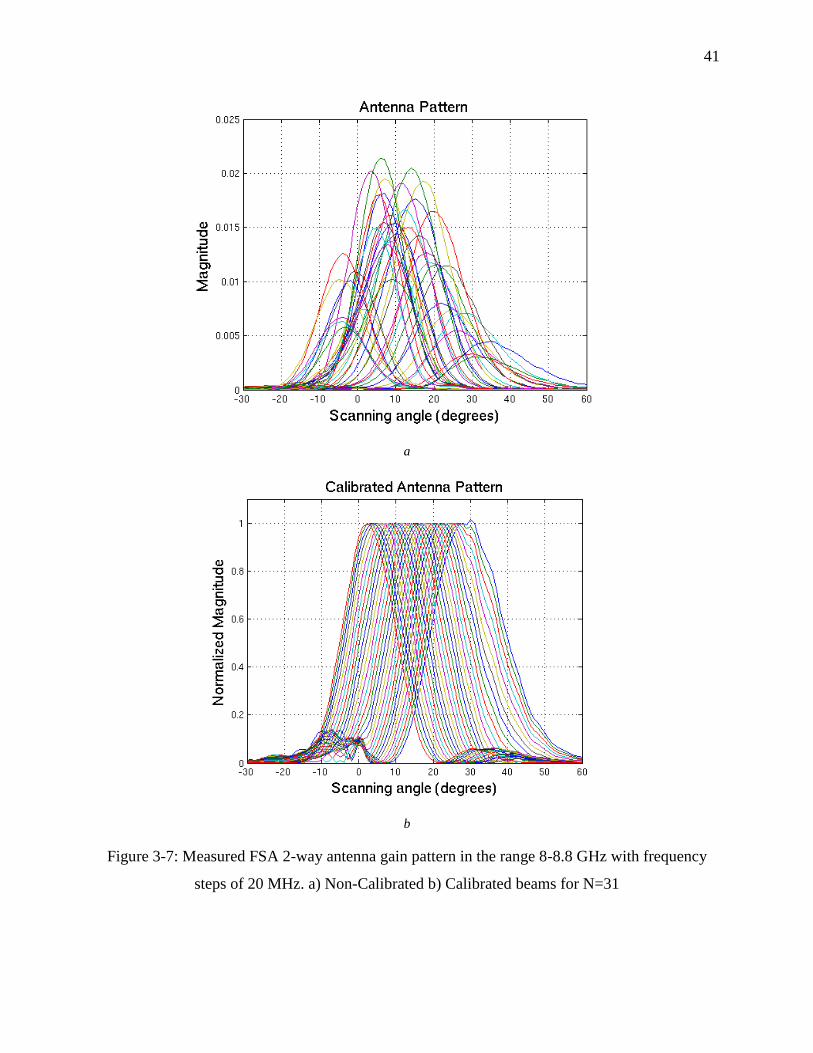
41
a
b
Figure 3-7: Measured FSA 2-way antenna gain pattern in the range 8-8.8 GHz with frequency
steps of 20 MHz. a) Non-Calibrated b) Calibrated beams for N=31

42
The 𝛥𝑓𝑜𝑣 is selected to be the range of [6, 24] degrees, and simulations are done to detect targets
in this region. As an arbitrary but representative example, a benchmark with two targets is
considered. Targets are to be at the same range and at 9 and 21 degrees with respect to boresight.
The number of beams in the selected 𝛥𝑓𝑜𝑣 N and the subvector size Q are selected equal to N =
31 and 𝑄𝑜𝑝𝑡= 19 according to (3.31). The targets amplitude vector 𝒔 in (3.14) is assumed to
consist of two coherent random complex numbers and n is a vector of white Gaussian noise.
In this FSA, the beamwidth and the gain of the antenna main beam is changing for the various
steering angles (Fig. 3-7a). Furthermore, the antenna steering angle changes nonlinearly when the
frequency is changed in uniform steps. Therefore, the compensation methods discussed in
Section 3.4 is applied before applying the MVB method. Fig. 3-7b shows the calibrated antenna
patterns.
Fig. 3-8 shows the RMSE of DOA estimation for the two methods as a function of the SNR. The
estimation results in Fig. 3-8 show that in low SNR situations (SNR < 5 dB), the ML method can
detect two targets with total error of 4 to 7 degrees while the MVB method cannot separate two
targets in more than 5% of trials and therefore is not plotted.
Fig. 3-9 shows the impact of angular separation of two targets on the RMSE. The achieved
results agree with the results in the previous section. It can be seen that using the ML method, the
RMSE decreases when the angular separation between two targets increases, which shows that
the ML method can detect two targets more accurately when they have more angular distance
from each other. However, using the MVB method, the RMSE increases when the angular
separation between two targets is larger than 12 degrees. Again, this is due to the fact that for this
FSA and with the current settings, the angular separation between two targets larger than 12
degrees requires sampling from sidelobes of antenna patterns, which decreases the performance
of the MVB method.

43
Figure 3-8: DOA estimation RMSE versus SNR for N= 31, 𝛾1 = 9 and 𝛾2= 21.
Figure 3-9: DOA estimation RMSE versus angular separation between two targets SNR=20dB,
and N= 31.

44
3.8 Conclusion
In this work, we addressed the problem of resolving the direction of arrival (DOA) of multiple
radar targets separated by less than an antenna beamwidth using frequency scanning array (FSA)
antennas. The FSAs are advantageous because frequency scanning can be done very rapidly and
accurately, therefore it is easier to track moving targets.
Performance of two DOA estimation algorithms, MVB and ML estimation are studied. These
methods were first adapted for our signal model and their performance were investigated through
Monte Carlo simulations and compared against each other in terms of root mean square error.
Simulation results showed that in low SNR situations, the RMSE of DOA estimation is large and
the MVB method cannot separate two targets. In addition, it was shown that sampling from
sidelobes of the antenna pattern decreases the performance of the MVB method. In other cases,
by selecting correct parameters, both methods can separate targets with angular separations
smaller than the antenna pattern beamwidth. We have also presented a calibration scheme which
worked efficiently when it was applied to different antenna pattern shapes at each frequency and
nonuniform scanning angles. In the next step, the proposed methods will be applied to the
experimental data captured from a radar experiment using real targets.
3.9 Appendix A: CRLB Calculation
Considering the complex-value amplitude 𝒔 being a deterministic unknown vector and defined
as 𝑠𝑖 = 𝐴𝑖𝑒𝑗Φ𝑖, then the vector of unknown parameters will be 𝜻 =
[𝛾1, … , 𝛾𝐾, 𝐴1, … , 𝐴𝐾 , Φ1, … ,Φ𝐾].
In addition, assuming that n is modeled as white complex Gaussian noise with zero mean and
covariance matrix of 𝜎2𝑰, then the Fisher information matrix [19] for our signal model in (3.2)
can be written as:
𝐽𝒊𝒋 = [𝑱]𝒊𝒋 =2
𝜎2 Re {∂𝝁𝐻
∂𝜁𝑖 ∂𝝁
∂𝜁j}, (3.36)

45
where 𝝁 = E{𝒙𝒓} =∑ 𝑠𝑘𝒂(𝛾𝑘)𝐾𝑘=1 . For the first K elements of 𝜻 that represent unknown targets
DOA, we have:
𝜕𝝁
𝜕𝜁𝑖= 𝑠𝑖𝝑𝑖 𝑓𝑜𝑟 1 ≤ 𝑖 ≤ 𝐾 , (3.37)
where 𝝑𝑖 is the vector with elements of :
[𝜗𝑖]𝑛 = 𝐻𝑛(𝑁𝑒𝛽𝑑 cos(𝑁𝑒𝑢)sin(𝑁𝑒𝑢)cos (𝛾𝑖)
sin2(𝑢)−
𝛽𝑑 cos(𝑢) sin2(𝑁𝑒𝑢) cos (𝛾𝑖)
sin3(𝑢))𝑒−𝑗2𝜋𝑓𝑛𝑡𝑙 , (3.38)
and 𝑢 = 𝛽𝑑 [sin(𝛾𝑖) − sin (𝜃1 +𝑛
𝑁(𝛥𝑓𝑜𝑣))] /2.
The CRLBs are then calculated form diagonal elements of 𝑱−𝟏 as CRLB(𝛾𝑖) = [𝑱]𝒊𝒊−𝟏
. Therefore
for one target (K=1), the CRLB(𝛾𝑖) will be:
CRLB(𝛾𝑖) = 1
2𝑆𝑁𝑅 Re{𝝑𝑖
𝑯𝝑𝑖}. (3.39)

46
CHAPTER 4 SUBSPACE BASED DOA ESTIMATION METHODS IN
SCANNING ANTENNAS
As mentioned before, in subspace-based methods and in the presence of coherent signals, spatial
smoothing is required to decorrelate the coherent signals. Spatial smoothing is based on dividing
the steering vectors into shift invariant overlapping subvectors. The validity of the spatial
smoothing method in scanning antennas can be investigated by following the same method used
in [19]. In this chapter the complete analysis of subspace based methods and spatial smoothing
applicability in scanning antennas is presented.
4.1 Ideal Signal Model for Scanning Antennas
In Chapter 3, it is shown using simulations that the MVB method and spatial smoothing can be
applied to scanning antennas when the steering vector has the following characteristics:
the steering vector only includes the main beam of the antenna pattern;
the gain of the antenna pattern in different steering angles are balanced;
and the angular separation between steering angles are uniform.
In addition, the preprocessing steps including calibration and interpolation required before
applying the MVB method, spatial smoothing and the subspace-based DOA estimation methods
are described in section 3.4. The preprocessing is required to compensate for gain and angular
steps variation in different scanning steps.
In order to prove analytically the validity of the 3 conditions mentioned above, a scanning system
which conforms to the proposed specifications is considered. The antenna pattern of such
scanning system, including only the main beam, can be approximated with a Gaussian function
[31]. Knowing that the 3dB beamwidth (𝐵𝑊) and the standard deviation of a Gaussian
function (𝜎𝐺) are related as follows [65]:
𝐵𝑊 = 2√2 ln (2) 𝜎𝐺, (4.1)

47
the antenna pattern can be written as:
ℎ(𝜃𝑚, 𝛾𝑘) = √𝐺 exp (−4 (ln 2) (𝜃𝑚−𝛾𝑘
𝐵𝑊)2
), (4.2)
where 𝜃𝑚 is the pointing angle of the antenna beam and 𝐺 is the maximum gain. Consequently, it
can be shown that the two-way antenna pattern at the angle 𝛾𝑘 when the antenna is pointed at the
angle 𝜃𝑚 is:
𝑔𝑚(𝛾𝑘) = ℎ2(𝜃𝑚, 𝛾𝑘) = 𝐺 exp (−8 (ln 2) (𝜃𝑚−𝛾𝑘
𝐵𝑊)2
). (4.3)
Figure 4-1: Assumed Gaussian two-way antenna pattern ℎ(𝜃𝑚, 𝛾𝑘) for a beam pointing in the
direction 𝜃𝑚
Considering that 𝑎(𝜃𝑚 , 𝛾𝑘) = 𝑔𝑚(𝛾𝑘), then the steering vector for a target at angle 𝛾𝑘, when the
antenna is pointed to the angles 𝜃𝑚 with 𝑚 = 1, . . , 𝑀 is defined as:
𝒂(𝛾𝑘) = [ 𝑎(𝜃1, 𝛾𝑘), 𝑎(𝜃2, 𝛾𝑘),… , 𝑎(𝜃𝑀, 𝛾𝑘)]𝑇, (4.4)
where (. )𝑇 denotes the transpose operation and M is the total number of the scanning angles. In
order to respect the previously stated specifications, it is assumed that 𝐺 is equal in all beam
directions and the steps between steering angles 𝛥𝜃 are equal so that:

48
𝜃𝑚 = 𝜃1 + (𝑚 − 1) 𝛥𝜃. (4.5)
Considering K signals are received by antenna, the signal matrix 𝒔 and antenna response matrix 𝑨
can be written as:
𝒔 = [ 𝑠1, 𝑠2, … , 𝑠𝐾]T, (4.6)
𝑨(𝜸) = [𝒂(𝛾1), 𝒂(𝛾2) , … , 𝒂(𝛾𝐾)]. (4.7)
The data model of the scanning system is:
𝒙𝒓 = 𝑨(𝜸)𝒔 + 𝒏. (4.8)
Note that a real scanning system normally do not conform to the three conditions mentioned
above. In other words, in a real scanning system the steering vector also includes the sidelobes of
the antenna pattern, the antenna pattern has different gains in different steering angles, and the
angular separation between steering angles may not be uniform.
4.2 Subspace Methods in Scanning Antennas
From (4.8), the received data covariance matrix 𝑹 = 𝐸[𝒙𝒓 𝒙𝒓𝑯] can be obtained as:
𝑹 = 𝑨𝑹𝒔𝑨𝑯 + 𝜎2𝑰, (4.9)
where 𝑹𝒔 is the covariance matrix of the received signals 𝑹𝒔 = 𝑬[𝒔𝒔𝑯]. The noise is assumed to
be white Gaussian with the variance of 𝜎2. In addition, signals and noise are assumed to be
stationary zero mean uncorrelated random processes. The matrix 𝑹𝒔 is non-singular when the
signals are uncorrelated or partially correlated, but singular when at least two of the signals are
fully correlated.
Considering the cases that signals are uncorrelated or partially correlated, and assuming that 𝜃1 =
0 and −8 ln2
𝐵𝑊2 = 𝑤 , then the matrix 𝑨 can be simplified to:
𝑨 = 𝐺𝑨1𝑨2𝑨3. (4.10)
with

49
𝑨1 = [
1 0 ⋯ 0
0 𝑒𝑤𝛥𝜃2⋯ 0
⋮ ⋮ ⋱ ⋮
0 0 ⋯ 𝑒𝑤(𝑀−1)2𝛥𝜃2
], (4.11)
𝑨2 = [
1 ⋯ 1𝑒−2𝑤∆𝜃𝛾1 ⋯ 𝑒−2𝑤∆𝜃𝛾𝐾
⋮ ⋱ ⋮𝑒−2𝑤(𝑀−1)∆𝜃𝛾1 ⋯ 𝑒−2𝑤(𝑀−1)∆𝜃𝛾𝐾
], (4.12)
and
𝑨3 =
[ 𝑒
𝑤𝛾12
0 ⋯ 0
0 𝑒𝑤𝛾22
⋯ 0⋮ ⋮ ⋱ ⋮
0 0 ⋯ 𝑒𝑤𝛾𝐾2 ]
. (4.13)
In equation (4.10), 𝑨1 and 𝑨3 are diagonal matrices with nonzero elements and therefore they are
full rank and nonsingular. On the other hand, matrix 𝑨2 has a Vandermonde structure with
distinct elements and linear independent columns when 𝑀 ≥ 𝐾. Therefore matrix 𝑨2 is also
nonsingular and has rank K. Since 𝑨1,𝑨2, and 𝑨3 are all non-singular, matrix 𝑨 is non-singular
and has rank K. As mentioned before, 𝑹𝒔 is non-singular for uncorrelated or partially correlated
signals. Consequently, 𝑨𝑹𝒔𝑨𝑯 is non-singular with rank K.
Considering {𝜆1 ≥ 𝜆2 ≥ ⋯ ≥ 𝜆𝑀} and {𝒗1, 𝒗2, … , 𝒗𝑀} eigenvelues and the corresponding
eigenvectors of 𝑹, the above rank property imply that the first K eigenvalues are corresponding to
the K received signals and the 𝑀 − 𝐾 minimal eigenvalues are equal to 𝜎2 and corresponding to
noise 𝜆𝑖 = 𝜎2 for 𝑖 ≥ 𝐾 + 1 . In addition, the eigenvectors corresponding to the last 𝑀 − 𝐾
eigenvalues, referred to as noise-subspace eigenvectors, are orthogonal to the steering vectors so
that {𝒗𝐾+1, 𝒗𝐾+2, … , 𝒗𝑀} ⊥ {𝒂(𝛾1), 𝒂(𝛾2) , … , 𝒂(𝛾𝐾)}.
The subspace based methods and eigenstructure techniques work only when rank 𝑹 is K and
therefore the above properties holds. Since 𝑨𝑹𝒔𝑨𝑯 is non-singular with rank K, subspace based
DOA estimation methods and the MVB method which requires inversing the matrix 𝑹 are
applicable to scanning antennas with the signal model defined in (4.8).

50
4.3 Subspace Methods in Scanning Antennas in the Presence of
Coherent Signals
Considering a case when at least two of the incoming signals are coherent, i.e. 𝑠2 = 𝛼𝑠1, with 𝑠1
and 𝑠2 are incoming signals with respect to angles of 𝛾1 and 𝛾2, and 𝛼 is a complex value that
may represent a difference of propagation delay and path loss, the signal matrix and antenna
response matrix in (4.6) and (4.7) can be rewritten as:
𝒔 = [ (1 + 𝛼)𝑠1, … , 𝑠𝐾]T, (4.14)
𝑨(𝜸) = [𝒂(𝛾1) + 𝛼𝒂(𝛾2) , 𝒂(𝛾3),… , 𝒂(𝛾𝐾)]. (4.15)
As two of the signals are coherent, from (4.14) and (4.15) it can be observed that the covariance
matrix is a (𝐾 − 1) × (𝐾 − 1) matrix of rank 𝐾 − 1 and therefore it will not be possible to
detect all K signals using subspace methods.
1 M-Q +1M-Q2 Q Q +1 Q +2
xr{1}
xr{2}
xr{3}
xr{P}
MM-1
xr{P-1}
Figure 4-2: Spatial smoothing scheme in scanning antennas
In general, if from K incoming signals, v of them are coherent, the subspace based methods can
detect only 𝐾 − 𝑣 DOAs. Spatial smoothing is an approach to decorrelate coherent signals and
results in detecting all the DOAs [19] .
51
To apply spatial smoothing, the sampled data vector 𝒙𝒓 is divided into overlapping subvectors of
𝒙𝑟{𝑝}
for 1 < 𝑝 < 𝑃, where 𝑃 is the number of subvectors each containing Q samples of 𝒙𝒓, so
that for a total number of M scanning angles we have: 𝑃 = 𝑀 − 𝑄 + 1 (see Fig. 4-2).
𝒙𝑟{𝑝}
= 𝑼𝑝−1 𝑨 𝑫𝑝−1𝒔 + 𝒏{𝑝} for 1 < 𝑝 < 𝑃, (4.16)
where 𝑼𝑝−1 and 𝑫𝑝−1 are diagonal matrices defined as
𝑫𝑝−1 = [
𝑒−2𝑤(𝑝−1)∆𝜃𝛾1 0 ⋯ 00 𝑒−2𝑤(𝑝−1)∆𝜃𝛾2 ⋯ 0⋮ ⋮ ⋱ ⋮0 0 ⋯ 𝑒−2𝑤(𝑝−1)∆𝜃𝛾𝐾
], (4.17)
And
𝑼𝑝−1 =
[ 𝑒
𝑤(𝑝−1)2𝛥𝜃2+2𝑤(𝑝−1)∆𝜃 0 ⋯ 0
0 𝑒𝑤(𝑝−1)2𝛥𝜃2+2𝑤2(𝑝−1)∆𝜃 ⋯ 0⋮ ⋮ ⋱ ⋮
0 0 ⋯ 𝑒𝑤(𝑝−1)2𝛥𝜃2+2𝑤𝑄(𝑝−1)∆𝜃]
(4.18)
The spatially smoothed covariance matrix 𝑹𝒇 can be written as:
𝑹𝒇 =1
𝑃∑ 𝒙𝑟
{𝑝}𝒙𝑟
{𝑝}𝐻𝑃
𝑝=1=
1
𝑃∑ 𝑼𝑝−1𝑨𝑫𝑝−1𝑹𝒔𝑫𝑝−1
𝑯 𝑨𝑯𝑼𝑝−1𝑯
𝑃
𝑝=1+ 𝜎2𝑰. (4.19)
As discussed before, in order to be able to apply subspace based DOA estimation methods, the
rank of 𝑹𝒇 should be K. In order to find the rank of 𝑹𝒇, it is rewritten as
𝑹𝒇 = 𝑽𝑻𝑯𝑻𝑽𝑯 +𝜎2𝑰, (4.20)
where 𝑽 is a 𝑄𝑃 × 𝑃𝐾 block matrix defined by:
𝑽 = [
𝑰𝑨 0 ⋯ 0⋮ 𝑼1𝑨 ⋱ ⋮0 0 ⋯ 𝑼𝑝−1𝑨
], (4.21)
and 𝑻 is a 𝐾 × 𝑃𝐾 block matrix defined by:
𝑻 = [𝑪 ,𝑫1𝑪,… ,𝑫𝑝−1𝑪 ]. (4.22)

52
In (4.22), matrix 𝑪 is the Hermitian square root of 1
𝑃𝑹𝒔 defined as:
𝑪𝑪𝑯 =1
𝑃𝑹𝒔. (4.23)
From equation (4.21), it can be observed that matrix 𝑽 and 𝑽𝑯 are block diagonal, full rank and
non-singular. Thus, 𝑹𝒇 and 𝑻 have the same rank (𝑟𝑎𝑛𝑘(𝑹𝒇) = 𝑟𝑎𝑛𝑘(𝑻) = 𝑟𝑎𝑛𝑘(𝑻𝑯)).
Therefore if 𝑻 is non-singular, 𝑹𝒇 will be non-singular too. In order to find the rank of 𝑻 and
prove it is non-singular, a new matrix �� is constructed by permutation of columns of matrix 𝑻. As
column permutation does not change matrices rank, the rank of 𝑻 and �� are equal.
�� = [𝑐11𝒃𝟏 𝑐12𝒃𝟏 ⋯ 𝑐1𝐾𝒃𝟏
⋮ ⋮ ⋮𝑐𝐾1𝒃𝑲 𝑐𝐾2𝒃𝑲 𝑐𝐾𝐾𝒃𝑲
]. (4.24)
In (4.24), 𝑐𝑖𝑗 are the elements of matrix 𝑪, and 𝒃𝑖 (i = 1,.., K) are the vectors of:
𝒃𝑖 = [1, 𝑒−2𝑤∆𝜃𝛾𝑖 , … , 𝑒−2𝑤(𝑃−1)∆𝜃𝛾𝑖]. (4.25)
For 𝑃 ≥ 𝐾, the 𝒃𝑖 vectors are linearly independent and form a Vandermode matrix. Also each
row of C has at least one nonzero element. Thus matrix �� is full rank and non-singular and has
rank K.
Consequently 𝑹𝒇 has rank K and therefore it is possible to detect all K of DOA using spatial
smoothing when incoming signals are coherent.
4.4 Frequency Scanning Antennas
The analysis done in Sections 4.2 and 4.3 is also valid for FSAs with the difference that in FSAs
we have an extra phase variation due to the frequency shift between each steering direction, i.e.
𝑎(𝜃𝑚 , 𝛾𝑘) = 𝑔𝑚(𝛾𝑘) 𝑒−𝑗2𝜋𝑓𝑚𝑡𝑙 . Assuming that the scanning frequency and antenna steering
angle vary linearly and therefore the frequency steps between steering angles 𝛥𝑓 are equal so
that 𝑓𝑚 = 𝑓1 + (𝑚 − 1) 𝛥𝑓, the equations 4.11 and 4.17 have the following form for FSA
antennas:

53
𝑨1 = [
𝑒−𝑗2𝜋𝑓1𝑡𝑙 0 ⋯ 0
0 𝑒𝑤𝛥𝜃2−𝑗2𝜋𝑓2𝑡𝑙 ⋯ 0⋮ ⋮ ⋱ ⋮
0 0 ⋯ 𝑒𝑤(𝑀−1)2𝛥𝜃2−𝑗2𝜋𝑓𝑀𝑡𝑙
], (4.26)
And
𝑼𝑝−1 = [
𝑒𝑤(𝑝−1)2𝛥𝜃2+2𝑤(𝑝−1)∆𝜃−𝑗2𝜋(𝑝−1)∆𝑓𝑡𝑙 ⋯ 00 ⋯ 0⋮ ⋱ ⋮
0 ⋯ 𝑒𝑤(𝑝−1)2𝛥𝜃2+2𝑤𝑄(𝑝−1)∆𝜃−𝑗2𝜋(𝑝−1)∆𝑓𝑡𝑙
].
(4.27)
As it can be observed, matrix 𝑨1 is still a diagonal matrix with nonzero elements and therefore it
is full rank and nonsingular. Consequently, 𝑨𝑹𝒔𝑨𝑯 is non-singular with rank K. Therefore
subspace based DOA estimation methods and the MVB method which requires inverting the
matrix 𝑹 are applicable to FSA antennas too. In addition, the new 𝑼𝑝−1 is still diagonal with
nonzero elements and therefore it is full rank and nonsingular. Consequently, matrices 𝑽 and 𝑽𝑯
are block diagonal, full rank and non-singular. Thus equations 4.19 up to 4.25 for FSAs are the
same as for scanning antennas. Therefore 𝑹𝒇 has rank K and it is possible to detect all K of DOA
using spatial smoothing when incoming signals are coherent in FSAs too.
4.5 Noise Whitening
As it is mentioned in section 3.4, after interpolation and calibration the noise is not white
anymore and noise pre-whitening is required. In this section the noise whitening procedure is
presented.
Considering that the calibrated signal model (3.23) can be simplified as:
��𝒓 = 𝑩𝒙𝒓 = 𝑩𝑨(𝛄)𝒔 + 𝑩𝒏 , (4.28)
Where 𝑩 is the calibration matrix, the sampled data covariance matrix �� is:
�� =1
𝐿∑ ��𝒓��𝒓
𝑯𝐿
𝑙=1 = 𝑩𝑨𝑹𝒔𝑨
𝑯𝑩𝑯 + 𝜎2𝑩𝑩𝑯 . (4.29)

54
As 𝑩𝑩𝑯 ≠ 𝑰, the noise is colored and not white anymore. Since DOA estimation methods work
with white noise, it is necessary to whiten the noise before applying DOA estimation techniques.
Assuming that
𝑹𝒏 = 𝑩𝑩𝑯, (4.30)
The pre-whitening can be done by [61]:
�� = [𝑹𝒏]−𝟏/𝟐 �� [𝑹𝒏]−𝑯/𝟐 , (4.31)
where (. )−𝟏/𝟐 denotes the square root of inverse matrix and (. )−𝑯/𝟐 denotes the square root of
the Hermitian transpose of the inverse matrix. Note that, this process does not change the rank of
covariance matrix. In another word 𝑟𝑎𝑛𝑘(��) = 𝑟𝑎𝑛𝑘(��).
4.6 Subspace Based DOA Estimation Methods
The MUSIC technique is a subspace technique which is based on the fact that noise eigenvectors
of covariance matrix are orthogonal to the signal steering vectors. The output spectrum of
MUSIC algorithm at direction γ is:
𝑃𝑀𝑈𝑆𝐼𝐶(γ) =1
∑ |𝒗𝑖𝐻𝒂(γ)|
2𝑀𝑖=𝐾+1
, (4.32)
where 𝒗𝑖 (𝑖 = 𝐾 + 1,… ,𝑀) are the eigenvectors of covariance matrix corresponding to the noise.
As the steering vector 𝒂(γ) is orthogonal to 𝒗𝑖, the denominator of (4.32) is identically zero.
Therefore, the peaks of the function 𝑃𝑀𝑈𝑆𝐼𝐶(γ) points to the DOAs of received signals.
4.7 Simulation Results
In this section, the simulation results of MUSIC method (4.32) and MVB method (3.28) in
presence of coherent signals are illustrated. A scanning antenna with the antenna pattern
approximated with a Gaussian function as presented in equation (4.2) is used. The selected
simulation parameters are identical to those of Section 3.6. As an arbitrary but representative

55
example, a benchmark with two signals with DOA at -3 and 3 degrees with respect to boresight is
considered. Targets are assumed to be at the same range. The number of beams M and the
subvector size Q are selected equal to N=21 and 𝑄𝑜𝑝𝑡= 13 according to (3.31) and SNR = 20dB.
Figure 4-3 shows the result of applying the MVB method (3.28) and MUSIC method when two
received signals are uncorrelated. As can be seen, when signals are uncorrelated both methods
can detect two targets.
In the next step, the received signal vector 𝒔 in (4.14) is assumed to consist of two coherent
random complex numbers (𝑠2 = 0.9𝑠1). Figure 4-4 and 4-5 show the results of MVB and MUSIC
methods with and without spatial smoothing respectively.
It can be seen that while without spatial smoothing none of the methods was able to detect the
DOAs of two received coherent signals correctly, after applying spatial smoothing both DOAs
were detected (at 𝛾1 = -3 and 𝛾2= 3 degrees) by the two methods.
Figure 4-3: DOA estimation methods results for two uncorrelated received signals.

56
Figure 4-4: DOA estimation methods results for two coherent received signals without spatial
smoothing.
Figure 4-5: DOA estimation methods results for two coherent received signals with spatial
smoothing.

57
4.8 Conclusion
In this chapter, it is shown analytically and with simulations that the MVB method and subspace-
based DOA estimation methods can be applied successfully to a scanning system which
conforms to the 3 proposed conditions listed in section 4.1. In addition, it is shown that spatial
smoothing can be applied to such system when incoming signals are coherent to uncorrelate
signals in order to detect the DOAs.

58
CHAPTER 5 RADAR SYSTEM WITH ENHANCED ANGULAR
RESOLUTION BASED ON A NOVEL FREQUENCY SCANNING
REFLECTOR ANTENNA
In this chapter, the results of applying a DOA estimation method on a radar system that uses a
novel beam scanning reflector antenna using a frequency multiplexed antenna feed is presented.
In section 3.7, the results of applying the same DOA estimation method on a different frequency
scanning antenna was presented. However, the reflector antenna system presented in this chapter
has a larger gain and narrower bandwidth. While the reflector antenna scans over 50 degrees
using a bandwidth of only 2.2%, the antenna presented in chapter 3 used a bandwidth of 8% to
scan the same scanning angle. Reducing the bandwidth used by the antenna scanning system is an
important improvement, since the radio transceiver systems needed to detect the targets (or
sources) which are transmitting over the full frequency band of the system can operate more
easily in narrower bandwidth. Also, from a practical spectrum management point of view,
reducing the bandwidth is an advantage in the context of limited available spectrum for weather
radars for instance.
The FSA used for the experiments presented in this chapter is a fast scanning and low-cost
antenna. The antenna system consists of a reflector and a frequency multiplexer as the feed chain.
The multiplexer has an input port and horn antennas as output ports which are placed in the focal
plane of the reflector. Depending on the frequency of the input signal, one horn is selected (by
passive bandpass channel filters) to feed the reflector. Due to the displacements of the output
horns, the beams generated by each horn are steered in a different direction by the reflector.
Therefore, this antenna can scan the FOV either by sequential switching the horns and by
stepping the frequency of the input signal or steer all the possible beam directions at the same
time by applying frequency division multiplexing (FDM) to the input signal. The later scenario
results in a significantly faster scanning.
The achievable angular resolution of this antenna depends on the number of horns in the antenna,
the width of the beams and the angular separation between each two adjacent beams. Due to the

59
limitation in the placement of the horns and the reflector, it is not possible to easily achieve the
desirable beams cross-over level and angular separation. For example, increasing the focal length
of the antenna can increase the beams cross-over level, it will also increase the spillover losses.
Because of the large separation between the adjacent beam directions in the employed FSA, the
angular scanning is done in very coarse steps which limits the angular resolution of the system.
This is shown in details in the section 5.5.1. In order to overcome this problem, a hybrid scanning
system is proposed. The hybrid system combines frequency scanning with mechanical scanning
over a limited angular range by time multiplexing the scanning results. The mechanical scanning
will cover the angular section between the frequency-scanned beams.
While the hybrid system has a slower scanning speed compared to pure electronic scan, it can
achieve higher angular resolution. The larger number of mechanical scanning steps results in
slower scanning and higher angular resolution. Therefore, the number of mechanical scanning
steps has to be selected based on the desired angular resolution and scanning speed. The scanning
speed of this hybrid system is increased by a factor approximately equal to the number of output
channels in the frequency multiplexing feed chain.
In the next section, the scanning antenna system will be briefly introduced. Then in Section 5.2, a
signal model that applies to this antenna will be presented. In Section 5.3 the hybrid scanning
model will be presented. In Section 5.4 the angular estimation method will be described and in
5.5 the experimental results obtained with the frequency scanning reflector antenna will be
shown.
5.1 Beam Scanning With a Parabolic Reflector
Before presenting the antenna signal processing results, the antenna architecture and operation
principles of a frequency scanning reflector antenna with a parabolic reflector and multiplexer
feeding system is briefly introduced in this section. This antenna was designed by Dr. F. Siaka as
part of his Ph.D. work [64].

60
The designed beam scanning reflector antenna is using the feed displacement concept (Fig. 5-1).
The direction of the main beam is changing by moving the position of the feed in the focal plane
of a reflector. The direction of the main beam can be estimated with:
𝜃 = BDF × tan−1 (𝑦
𝐹) , with BDF =
(4𝐹𝐷⁄ )
2+0.36
(4𝐹𝐷⁄ )
2+1
, (5.1)
where BDF is the Beam Deviation Factor, y is the feed displacement, F is the focal distance, and
D is the diameter of the reflector. Feed displacement is realized using a frequency multiplexer.
Having a multi-frequency signal at the input port of the multiplexer, each output horn will have a
single frequency signal with a displaced phase center. A picture of the complete system mounted
for tests in an anechoic chamber is shown in Fig. 5-1.
Figure 5-1: Picture of the parabolic dish fed by the frequency beam scanning system [12].
Fig. 5-2 shows the measured radiation patterns of the antenna. As expected, each frequency gives
a beam at a specific direction. A scanning angle of 50 degrees is obtained with a frequency

61
bandwidth of 2.2%. Since the system bandwidth depends on the characteristics of the filters
forming the multiplexers, by selecting higher-order filters narrower bandwidths can also be
achieved.
The rest of the chapter that is published in [12] is the contribution of the author of this thesis.
Figure 5-2: Measured radiation patterns of the proposed beam scanning reflector antenna.

62
5.2 Signal Model of Frequency Scanning Reflector Antenna1
In this section a signal model that can be used to predict DOA with a frequency scanning antenna
is developed. As mentioned before, it is assumed that the antenna performs horizontal scanning
and the DOA estimation is considered to be performed in only one dimension.
K targets are considered present in the field of view (FOV) at the same known range of 𝑅𝑙 =𝑐𝑡𝑙
2
, where 𝑡𝑙 is the time for receiving the signal from targets at the range 𝑅𝑙 and c is the speed of
light. The received baseband signal from the FSA antenna main beam, which is steered in the
direction 𝜃𝑚, can be written as
𝑥(𝑡𝑙 , 𝜃𝑚) = ∑ 𝑠𝑘(𝑓𝑚)𝑎𝑚(𝛾𝑘)𝐾
𝑘=1+ 𝑛(𝑡𝑙 , 𝜃𝑚), (5.2)
where 𝑓𝑚 is the center frequency of the FSA beam pointed at the angle 𝜃𝑚, 𝑠𝑘(𝑓𝑚) is the
complex signal from the k-th target with the angular position 𝛾𝑘, 𝑎𝑚(𝛾𝑘) is the complex antenna
pattern factor at the angle 𝛾𝑘 from the antenna beam pointed at the angle 𝜃𝑚, and 𝑛(𝑡𝑙 , 𝜃𝑚) is the
complex white Gaussian noise coming from the scene and introduced by the receiver
components. It has been assumed that the Doppler shift of the targets can be neglected. Note that
if FSA is part of a monostatic radar pointing to a scene and the signals impinging the FSA are
from passive targets, then the 𝑎𝑚(𝛾𝑘) will be the two-way antenna pattern. However, if the FSA
is only receiving signals from active emitters, then the 𝑎𝑚(𝛾𝑘) will be the one-way antenna
pattern.
The steering vector for a target at angle 𝛾𝑘, for the FSA antenna beams steered to the angles 𝜃𝑚
with 𝑚 = 1, . . , 𝑀 is defined as:
𝒂(𝛾𝑘) = [ 𝑎1(𝛾𝑘), 𝑎2(𝛾𝑘),… , 𝑎𝑀(𝛾𝑘)]𝑇, (5.3)
1 This section is an excerpt from section 5 of the following published journal paper:
F. Siaka, M. A. Tehrani, J. J. Laurin and Y. Savaria, “Radar system with enhanced angular resolution based
on a novel frequency scanning reflector antenna”, in IET Radar, Sonar & Navigation, 2016.

63
where (. )𝑇 denotes the transpose operation, and M is the total number of the frequencies (in the
multiplexed feed introduced in the previous section M = 8).
With K targets at directions 𝜸 = [𝛾1, 𝛾2 , … , 𝛾𝐾], the antenna response is:
𝑨(𝜸) = [𝒂(𝛾1), 𝒂(𝛾2) , … , 𝒂(𝛾𝐾)], (5.4)
and the targets signal matrix for the K targets at directions defined above can be defined as:
𝑺 = [𝑠1(𝑓1
), 𝑠2(𝑓1), … 𝑠𝐾(𝑓
1)
… … … …𝑠1(𝑓𝑀
), 𝑠2(𝑓𝑀), … 𝑠𝐾(𝑓
𝑀)]
𝑇
, (5.5)
where 𝑠𝑘(𝑓𝑚) is:
𝑠𝑘(𝑓𝑚) = 𝑠𝑘𝑒−𝑗2𝜋𝑓𝑚𝑡𝑙. (5.6)
Considering that the targets cross sections do not change when the transmitted frequency
changes, which may be a valid assumption when the used bandwidth is narrow, the targets signal
matrix can be decomposed to
𝑺 = [𝑒−𝑗2𝜋𝑓1𝑡𝑙 , 𝑒−𝑗2𝜋𝑓2𝑡𝑙 , … , 𝑒−𝑗2𝜋𝑓𝑀𝑡𝑙]𝑇[𝑠1, 𝑠2, … , 𝑠𝐾],
𝑺 = 𝒆𝒔𝒂𝑻. (5.7)
Considering 𝑬 = diag(𝒆), the data model can be rewritten as:
𝒙 = 𝑬𝑨(𝜸)𝒔𝒂 + 𝒏, (5.8)
where 𝒙 and 𝒏 are:
𝒏 = [ 𝑛(𝑡𝑙, 𝜃1), 𝑛(𝑡𝑙, 𝜃2),… , 𝑛(𝑡𝑙, 𝜃𝑀)]𝑇, (5.9)
𝒙 = [𝑥(𝑡𝑙, 𝜃1), 𝑥(𝑡𝑙, 𝜃2), … , 𝑥(𝑡𝑙, 𝜃𝑀)]𝑇. (5.10)
The objective is to estimate the vector of targets angular positions 𝜸 while the targets complex
echo vector 𝒔𝒂 is unknown.

64
5.3 Combining Frequency Scanning with Mechanical Scanning 2
As mentioned before, antenna design limitations impose a large separation between the different
antenna beam directions, which can be observed in Fig. 5-2. Therefore, the scanning increment of
the angular range is too coarse to enable accurate targets angular position estimation beyond
beamwidth limitations as will be shown later in section 5.5.1.
Considering that the antenna can be rotated mechanically over a small angular range, it is
possible to finely scan a large section of the FOV with a relatively small mechanical rotation.
This will allow further processing and achieving higher angular resolution (see Fig 5-3).
It can be assumed that the angular steps between the steering angles of the FSA are equal so
that 𝜃𝑚+1 = 𝜃𝑚 + 𝛥𝜃, and the FSA can be rotated mechanically, with 𝑀𝑟 steps of 𝛥𝜃/𝑀𝑟
degrees. Using the combination of frequency scanning and mechanical rotation, the FOV can be
scanned with total of 𝑁 = 𝑀𝑟 × 𝑀 beams. If the signal model of FSA for each mechanical
scanning position is defined as:
𝒙𝒊 = 𝑬𝑨𝒊(𝜸)𝒔𝒂 + 𝒏𝒊, 𝑖 = 1,… ,𝑀𝑟 (5.11)
The signal model of the combined mechanical and frequency scanning system can be written by
time-multiplexing the signal model of FSA for each mechanical scanning position as:
𝒙𝒄 = 𝑬𝒄𝑨𝒄(𝜸)𝒔𝒂 + 𝒏𝒄, (5.12)
where 𝒙𝒄, 𝒏𝒄 ∈ ℂ𝑁×1 , 𝑬𝒄 ∈ ℂ𝑁×𝑁 and 𝑨𝒄(𝜸) ∈ ℂ𝑁×𝐾 with elements of 𝒙𝒄(𝑛) = 𝒙𝒊(𝑚),
𝒏𝒄(𝑛) = 𝒏𝒊(𝑚) , 𝑬𝒄(𝑛) = 𝑬𝒊(𝑚), and 𝑨𝒄(𝑛, 𝑘) = 𝑨𝒊(𝑚, 𝑘) while 𝑛 = (𝑚 − 1)𝑀𝑟 + 𝑖.
2 This section is an excerpt from section 6 of the following published journal paper:
F. Siaka, M. A. Tehrani, J. J. Laurin and Y. Savaria, “Radar system with enhanced angular resolution based
on a novel frequency scanning reflector antenna”, in IET Radar, Sonar & Navigation, 2016.

65
a
b
Figure 5-3: FSA radiation. a) Original measured FSA radiation pattern normalized at each
frequency, b) Antenna pattern of seven combined radiation patterns normalized at each frequency
[12].

66
5.4 Proposed DOA Estimation Method 3
As the evaluation results in section 3.6 shows, the MVB method does not perform well when the
number of beams covering a selected FOV is small. In this experiment, it can be observed from
Fig. 5-3 that even with combined radiation pattern presented in Section 5.3, the number of beams
in each section of FOV will be 𝑁 ≅ 7 which is smaller than it is required for MVB method to
function properly (𝑀 > 21). However, the ML DOA estimation method that was introduced and
discussed in details in section 3.5.2 can be applied to (5.12). This method is using the fact that
antenna scanning induces amplitude modulation on signal backscatters and therefore, by utilizing
prior knowledge of the antenna pattern, the angular position of targets can be extracted.
5.4.1 Maximum Likelihood Estimation
Considering that each element of the noise vector 𝒏𝒄 has a white complex Gaussian probability
distribution function with zero mean and variance of 𝜎2, 𝒏𝒄 is modelled as white complex
Gaussian noise with zero mean and covariance matrix of 𝜎2𝑰
𝒏𝒄 ~ 𝒞𝒩(0, 𝜎2𝑰). (5.13)
Therefore, the probability density function of the data vector 𝒙𝒄 conditioned to the unknowns
(𝜸, 𝒔𝒂) is
𝑝(𝒙𝒄|𝜸, 𝒔𝒂) =1
(𝜋𝜎2)𝑁exp (−
(𝒙𝒄−𝑬𝒄𝑨𝒄(𝜸)𝒔𝒂)𝐻(𝒙𝒄−𝑬𝒄𝑨𝒄(𝜸)𝒔𝒂)
𝜎2 ). (5.14)
The ML estimation of 𝜸 and 𝒔𝒂 can be found by maximizing the conditional probability density
function of 𝒙𝒄 with respect to 𝜸 and 𝒔. If 𝒔𝒂 is modelled as a deterministic unknown vector and 𝜸
as a deterministic constant vector then the conditional ML will be:
3 This section is an excerpt from section 7 of the following published journal paper:
F. Siaka, M. A. Tehrani, J. J. Laurin and Y. Savaria, “Radar system with enhanced angular resolution based
on a novel frequency scanning reflector antenna”, in IET Radar, Sonar & Navigation, 2016.

67
��, 𝒔�� = argmax𝜸,𝒔𝒂
{𝑝(𝒙𝒄|𝜸, 𝒔𝒂)}. (5.15)
The above maximization gives the estimate of �� and 𝒔�� as:
𝒔�� = (𝑨𝒄𝑯𝑬𝒄
𝑯𝑬𝒄𝑨𝒄)−1𝑨𝒄
𝑯𝑬𝒄𝑯𝒙𝒓 (5.16)
and
�� = argmax𝜸
𝒙𝑐𝐻𝑬𝒄𝑨𝒄(𝑨𝒄
𝑯𝑬𝒄𝑯𝑬𝒄𝑨𝒄)
−1𝑨𝒄𝑯𝑬𝒄
𝑯𝒙𝒄. (5.17)
It is assumed that no prior knowledge is available for DOAs of 𝜸 = [𝛾1, 𝛾2 , … , 𝛾𝐾].
5.5 DOA Estimation Experiment with Frequency Scanning
Reflector Antenna 4
In order to study the direction of arrival (DOA) estimation capabilities of the reflector antenna,
experimental tests were conducted in an anechoic chamber. The FSA described in section 5.1 is
used to receive signals and patch antennas are used as transmitting sources to simulate reflections
from radar targets. The patches and the FSA operate in vertical polarization, perpendicular to the
scanning plane. The 3dB beamwidth of each patch is approximately 30 degrees. The FSA and
radiofrequency receiver are mounted on a rotating platform in the center of chamber. The targets
view angle is varied by rotating the platform with respect to stationary sources. The distance from
the receiver to the sources plane is only 3m, due to the limited size of our test chamber. The
sources are fed using a signal generator set at the frequencies corresponding to the bands of the
multiplexing feed (see Fig. 5-2). A vector network analyzer (VNA) is used to collect data from
the receiver. A schematic of the test setup can be seen in Fig. 5-4.
4 This section is an excerpt from section 8 of the following published journal paper:
F. Siaka, M. A. Tehrani, J. J. Laurin and Y. Savaria, “Radar system with enhanced angular resolution based
on a novel frequency scanning reflector antenna”, in IET Radar, Sonar & Navigation, 2016.
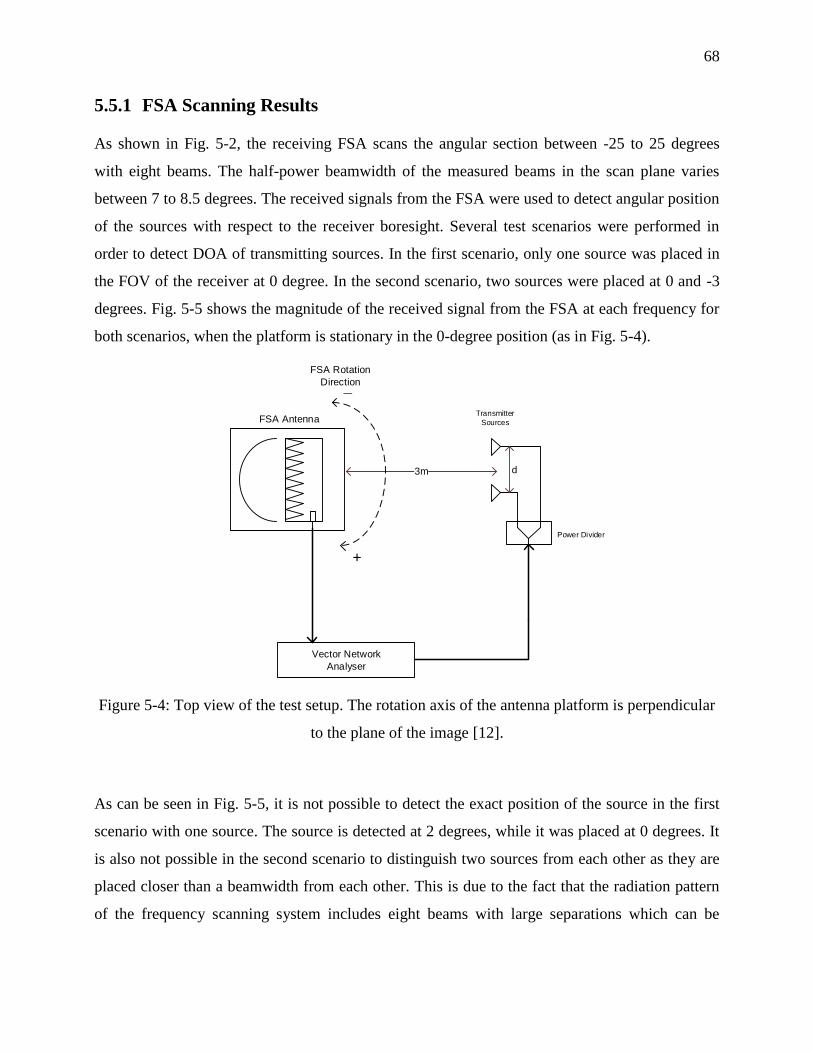
68
5.5.1 FSA Scanning Results
As shown in Fig. 5-2, the receiving FSA scans the angular section between -25 to 25 degrees
with eight beams. The half-power beamwidth of the measured beams in the scan plane varies
between 7 to 8.5 degrees. The received signals from the FSA were used to detect angular position
of the sources with respect to the receiver boresight. Several test scenarios were performed in
order to detect DOA of transmitting sources. In the first scenario, only one source was placed in
the FOV of the receiver at 0 degree. In the second scenario, two sources were placed at 0 and -3
degrees. Fig. 5-5 shows the magnitude of the received signal from the FSA at each frequency for
both scenarios, when the platform is stationary in the 0-degree position (as in Fig. 5-4).
Power Divider
FSA AntennaTransmitter
Sources
Vector Network
Analyser
3m d
FSA Rotation
Direction
+
_
Figure 5-4: Top view of the test setup. The rotation axis of the antenna platform is perpendicular
to the plane of the image [12].
As can be seen in Fig. 5-5, it is not possible to detect the exact position of the source in the first
scenario with one source. The source is detected at 2 degrees, while it was placed at 0 degrees. It
is also not possible in the second scenario to distinguish two sources from each other as they are
placed closer than a beamwidth from each other. This is due to the fact that the radiation pattern
of the frequency scanning system includes eight beams with large separations which can be

69
observed in Fig. 5-2. In order to be able to detect the angular position of sources more accurately,
a smaller scanning increment, such as the one realized by the proposed combination of electrical
and mechanical scanning is needed.
5.5.2 FSA and Mechanical Scanning Combined Results
The radiation patterns obtained by mechanical rotation of the FSA of Fig.5-2 are first normalized
with respect to their maximum value and using the prior information of antenna pattern and then
combined according to (5.12), and a new set of radiation patterns is constructed. This set
emulates an antenna with N=56 beams scanning the angles between -30 and 24 degrees with one
degree steps (see Fig. 5-3b). Note that as the angular distance between FSA beams are not equal,
the combined radiation patterns will have beams pointing to the same angle (i.e. at -24 degrees).
a b
Figure 5-5: FSA received signal from, a) One source at 0 degrees, b) Two sources at 0 and -3
degrees.
During the experiments, the antenna platform was rotated between -6 to 0 degrees and the
received signals at the eight frequencies were collected by the VNA at the common FSA port for
all the rotation angles. Using this data, we can reconstruct the received signal for the combined

70
radiation patterns by combining received signal from corresponding rotating angles of the FSA
antenna.
Figures 5-6a and 5-6b show the magnitude of the measured received signal for both previously
described scenarios and using the new combined radiation pattern.
a b
c d
Figure 5-6: Results for combined emulated antenna. a) FSA received signal of one source at 0
degrees, b) FSA received signal of two sources at 0 and -3 degrees, c) ML DOA estimation
results for one source at 0 degrees, d) ML DOA estimation results for two sources at 0 and -3
degrees [12].

71
As can be seen, for one source scenario and using the combined antenna radiation pattern, it is
now possible to detect the exact position of the source at 0 degrees. However, it is still not
possible to distinguish two targets form each other. For such cases, using the combined antenna
radiation pattern and applying the DOA estimation method proposed in section 5.4.1, it is
possible to detect two sources. Figures 5-6c and 5-6d show the ML estimation results for both
previously described scenarios while using the new combined radiation pattern in (5.12). For the
one-source scenario (Fig. 5-6c), it can be seen that the ML method (knowing the number of
sources) estimates the DOA at 𝛾1 = 0 degrees. However, applying ML estimation is not needed as
with a simple analysis of the combined radiation pattern the source position can be found (Fig. 5-
6a). Fig. 5-6d shows the result of applying the ML method for the second scenario. The ML
method that assumes knowledge of the number of sources estimates the DOA at 𝛾1 = -4 and 𝛾2=
0 degrees. Note that data acquisition was done in 1 degree steps. Therefore, the algorithm is
implemented with one degree resolution, which is approximately five times less than the actual
beamwidth of the reflector antenna.
5.5.3 Performance Evaluation
In order to evaluate the performance of the applied methods, the position of sources with respect
to FSA antenna is changed and the test is repeated. The root mean square error (RMSE) of the
DOA estimation is then calculated for all the source positions. Given the above setup and
discussed scenarios, the RMSE is defined as:
RMSE = √𝐸[∑ (𝛾𝑘 − 𝛾��)2𝐾𝑘=1 ]. (5.18)
Fig. 5-7 shows the result of applying the ML method for the second scenario with two sources
separated by 3 degrees, when the sources are moved between (𝛾1, 𝛾2) = (-38,-35) and (𝛾1, 𝛾2) =
(31, 34) degrees.

72
Figure 5-7: RMSE of ML DOA estimation for two sources moving between (-38,-35) and (31,
34) degrees [12].
As can be seen, the RMSE increases significantly when the sources are out of the range of the
scanning system (between -30 and 24 degrees) as expected. In the normal scanning range, on the
other hand, the RMSE is very low with 0 to 1.5 degree errors in most angles. The peaks in the
RMSE are due to the relatively large sidelobes that exist at the corresponding angles. In addition,
the assumption in (5.7) does not apply to the experimental case and the emitters’ frequency
response has some variations within the band. This can cause error in DOA estimation.
5.6 Conclusion
In this chapter, a DOA estimation method is proposed for a novel frequency scanning system
based on a frequency-multiplexed feed. It is shown using experiments that this estimation method
can achieve high angular resolution by applying a combination of mechanical and electrical
scanning. The proposed low-cost hybrid system can scan a large section of the FOV with a

73
relatively small mechanical rotation, which results in faster scanning compared to a pure
mechanical scanning. Analysing the DOA capabilities of the antenna, it could be seen that using a
combined radiation pattern from mechanical and electrical scanning and applying a proper DOA
estimation method, like ML estimation, it is possible to detect two sources separated by less than
a beamwidth distance from each other when scanning with this antenna.
74
CHAPTER 6 GENERAL DISCUSSION
In the last decades, electronic scanning has been investigated thoroughly. Fast electrical scanning
is of interest for many applications. Most of the previous works in this domain are dedicated to
phase array antennas, which are expensive when used in many applications. The goal of this work
was to investigate the possibility to use other scanning approaches and achieve fast and low-cost
scanning systems. The main motivation for this research was radars used in meteorological
forecast.
Therefore, the motivations for this thesis were:
- suggesting scanning methods applicable to meteorological applications;
- investigating the resolution of suggested methods and finding appropriate signal
processing methods to achieve high angular resolution;
- and finally optimize the results of each selected method by applying proper pre or post
processing algorithms.
Considering the above motivations, this thesis is focused on:
- frequency scanning as a means to obtain fast and low cost scanning;
- suggesting signal processing methods for DOA estimation and angular resolution
improvement,
- analytical development of the proposed methods;
- and providing simulation and experimental results to support the applicability of
suggested algorithms.
This research started by reviewing PAA functionality, DOA estimation methods applicable to
them and calibration methods proposed to compensate for the errors and imperfections in the
phase array design. Moving to FSA and considering similarities between FSA and PAA, the
possibility of extending available signal processing methods designed for PAAs to be used in
other either mechanically or electronically scanning antennas are investigated. In Chapter 2, the

75
literature review, including the signal model and main signal processing methods on the DOA
estimation and angular resolution enhancement available are introduced. In addition calibration
and pre-processing methods required to compensate for the antennas imperfections are also
presented. However, almost all the introduced algorithms were proposed for PAA.
Selecting two main DOA estimation methods namely ML and MVB, it is shown in Chapter 3 that
we can adapt those methods for FSA antennas. Preprocessing and calibration methods that should
be applied to FSAs before DOA estimation methods are also presented. Simulation results of
suggested methods and evaluation of the results with respect to different parameters are also
given. Two sets of simulations were provided in this chapter. First, results using simulated
antenna pattern and the second set of simulation results using measured antenna patterns from an
FSA antenna designed in the Poly-Grames Rresearch Center of École Polytechnique de Montréal.
Although, the effectiveness of the proposed methods are shown in Chapter 3, no mathematical
proof is presented to demonstrate the applicability of those methods to frequency scanning
antennas. In Chapter 4, we present such analysis to show that not only ML and MVB methods,
but also all the subspace-based methods are extendable to scanning antennas and in particular to
frequency scanning antennas. The pre-processing steps including calibration and interpolation
that are required, are also presented and justified analytically. In addition, it is shown that spatial
smoothing can be applied to scanning and frequency scanning antennas to decorrelate incoming
signals for the cases of DOA estimation of coherent incoming signals.
Finally in Chapter 5, the results of an experiment which is performed using a beam scanning
reflector antenna with a frequency multiplexed antenna feed is presented. Since the chosen
antenna had only eight non overlapping beams and the angular estimation using the MVB method
did not perform well when the number of beams covering a selected FOV is small, only the
results of the ML method were shown in this chapter. In addition, in order to achieve finer
angular resolution with an antenna having only eight scanning beams, a hybrid scanning system
is proposed that could scan relatively fast and achieve a finer angular resolution. The results of
such hybrid system was also presented and compared with the original full electronic scanning
system.

76
As mentioned before, most of the previous work in this domain target PAA. Very little work was
reported on superresolution for mechanically scanning antenna and available publications mostly
contain simulation results. Moreover, angular resolution enhancement in FSAs had not been
studied before. Therefore we can summarize the contributions of this thesis as:
- First in Chapter 3, angular resolution improvement methods for FSA is proposed along
with required preprocessing algorithms including calibration and interpolation that should be
applied before the suggested methods. In addition, simulation results evaluating the proposed
methods and the required parameters to achieve desired angular resolution are reported.
- In Chapter 4, analytical developments for suggested methods and their related
preprocessing algorithms is presented for all subspace-based methods applicable to scanning
antennas.
- And finally in Chapter 5, experimental results are provided and an alternative hybrid
scanning method is proposed to achieve relatively fast but low-cost scanning solution for the
situations where the antenna design limitation do not allow respecting the required parameters to
achieve some desired angular resolution.

77
CHAPTER 7 CONCLUSION AND RECOMMENDATIONS
In this chapter the achievements of this project are summarized and topics for future work in this
domain are discussed. This thesis addressed the problem of fast and low-cost scanning using
frequency scanning antennas. Since the FSA antennas may have limited angular resolution, we
focused on the direction of arrival (DOA) estimation and angular resolution enhancement of FSA
systems. This was obtained with proper calibration and pre-processing.
In Chapter 3, the performance of two DOA estimation algorithms, MVB and ML estimation
adapted for FSA antennas were studied. Monte Carlo simulations were used to evaluate the
performance of the proposed methods and their results were compared against each other in terms
of root mean square error. Simulation results showed that in low SNR situations, the RMSE of
DOA estimation is large and the MVB method cannot separate two targets. In other cases, by
selecting correct parameters, both methods can separate targets with angular separations smaller
than the antenna pattern beamwidth.
In addition, we showed the limitation of the proposed DOA estimation methods and the
conditions that had to be met before we can apply them. It was shown using simulations that
sampling from sidelobes of the antenna pattern decreases the performance of the MVB method.
In addition, the gain of the antenna pattern in different steering angles should be balanced and the
angular separation between steering angles should be uniform for the MVB method to function
properly. The ML methods only require a balanced gain for all the antenna patterns pointing to all
scanning angles.
We have also presented a calibration scheme that worked efficiently when it was applied to
different antenna pattern shapes at each frequency and non-uniform scanning angles. This
calibration method allows to compensate for imperfect antenna patterns by transforming them to
the shapes that conform to the specified conditions when needed. The contributions presented in
Chapter 3 are published in [11].
In Chapter 4, it was shown analytically that the MVB method, and the subspace-based DOA
estimation methods could be applied successfully to a scanning system which conforms to the

78
proposed conditions found in Chapter 3. In addition, it was shown that spatial smoothing could
be applied to such systems when incoming signals are coherent in order to decorrelate signals and
detect the DOAs.
In Chapter 5, the result of an experiment which was conducted using a novel beam scanning
reflector antenna based on a frequency-multiplexed feed proposed for frequency scanning was
presented. As the employed FSA antenna had only eight scanning beams with very small cross-
over, the previously proposed methods would not improve the angular resolution. Therefore, a
low-cost hybrid system was proposed that could scan a large section of the FOV with a relatively
small mechanical rotation, which results in faster scanning compared to a pure mechanical
scanning. Selecting the number of mechanical scanning steps is a trade-off between the desired
angular resolution and scanning time. It was shown using experiments that this estimation
method can achieve high angular resolution by applying a combination of mechanical and
electrical scanning. Since, according to the evaluation results in Chapter 3, the MVB method
does not perform well when the number of beams covering a selected FOV is small, only ML
estimation was performed. Analysing the DOA capabilities of the antenna, it could be seen that
using a combined radiation pattern from mechanical and electrical scanning and applying a
proper DOA estimation method, like ML estimation, it was possible to detect two sources
separated from each other by less than a beamwidth distance when scanning with this antenna. In
our experiments, the angular resolution was reduced to half of the beamwidth by adding six
mechanical scanning steps. The contributions presented in Chapter 5 are published in [12].
7.1 Future Works
In this thesis, we selected only two DOA estimation methods and shown analytically, as well as
using simulations the performance of those methods when extended so that they can be applied to
FSA antennas. There are many other DOA estimation methods proposed for PAA [16], [24],
[25], [27], [49], each have advantages and disadvantages when used for a specific application or
environment. We have just selected the most basic methods and provided the proof of their
applicability for the new scanning system as a first step. Indeed the adaptation of all other

79
methods can be investigated in the same way and their performance can be evaluated for different
applications. As an example, we have shown in Chapter 4 that the subspace based methods such
as MUSIC are also extendable to single-channel FSA antennas. Although not presented in this
thesis, the primary results of SMUSIC application on FSA were also found during this research.
A promising next step would be to work on the required preprocessing for SMUSIC and evaluate
the performance of SMUSIC in FSA systems. Another example would be employing the UML
method. In Chapters 3 and 5 we used the CML method in order to estimate target angular
resolutions. However, using the UML method may result in more realistic results since in UML,
the signals backscattered from targets are modeled as random variables. Using random variables
models, the targets backscattered fluctuation from scan to scan with varying frequency can be
modeled more accurately.
Moreover, trying to reproduce the results with a more realistic data model will be an interesting
next step. As described in section 3.3, a simplified data model is used during this research by
assuming that the targets cross sections do not change when the transmitted frequency changes.
Reproducing the results with the original data model in (3.10) may results in a lower level of
estimation error.
Finally, the performance of the methods proposed in this research can be analysed more
profoundly by evaluating the effects of other parameters such as having different SNRs or power
between received signals from different targets or having more than two sources in the 𝛥𝑓𝑜𝑣.
80
BIBLIOGRAPHY
[1] D. E. N. Davies, "Application of electronic sector scanning techniques to height-finding radar
systems," Electrical Engineers, Proceedings of the Institution of, vol. 110, no. 11, pp. 1941-
1948, November 1963.
[2] A. Brunner. "Possibilities of dimensioning doubly curved reflectors for azimuth-search radar
antennas," in IEEE Transactions on Antennas and Propagation, vol. 19, no. 1, pp. 52-57, Jan
1971.
[3] M.F. Radford, "Frequency scanning aerials in air traffic control radar," in IEE Conf. Report
Seriesed5, 1963, pp. 143-145.
[4] A. P. Hopf et al., "CASA Phased Array Radar System description, simulation and
products," 2009 IEEE International Geoscience and Remote Sensing Symposium, Cape
Town, 2009, pp. II-968-II-971.
[5] A. Parsa and N. H. Hansen, "Comparison of vertically and horizontally polarized radar
antennas for target detection in sea clutter — An experimental study," 2012 IEEE Radar
Conference, Atlanta, GA, 2012, pp. 0653-0658.
[6] A. Parsa, "Fast moving target detection in sea clutter using non-coherent X-band radar," 2014
IEEE Radar Conference, Cincinnati, OH, 2014, pp. 1155-1158.
[7] S. Torres et al., "A demonstration of adaptive weather surveillance and multifunction
capabilities on the National Weather Radar Testbed Phased Array Radar," 2014 International
Radar Conference, Lille, 2014, pp. 1-6.
[8] R.C. Hansen, Phased array antennas, New York: John Wiley & sons, 2nd edn., 2009.
[9] N. Yang, C. Caloz and K. Wu, "Full-Space Scanning Periodic Phase-Reversal Leaky-Wave
Antenna," in IEEE Transactions on Microwave Theory and Techniques, vol. 58, no. 10, pp.
2619-2632, Oct. 2010.
[10] Y. Dong and T. Itoh, "Substrate Integrated Composite Right-/Left-Handed Leaky-Wave
Structure for Polarization-Flexible Antenna Application," in IEEE Transactions on Antennas
and Propagation, vol. 60, no. 2, pp. 760-771, Feb. 2012.
[11] M. A. Tehrani, J. J. Laurin and Y. Savaria, "Multiple targets direction-of-arrival

81
estimation in frequency scanning array antennas," in IET Radar, Sonar & Navigation, vol. 10,
no. 3, pp. 624-631, 2016.
[12] F. Siaka, M. A. Tehrani, J. J. Laurin and Y. Savaria, "Radar system with enhanced
angular resolution based on a novel frequency scanning reflector antenna”, in IET Radar,
Sonar & Navigation, vol. 11, no. 2, pp. 350-358, 2017.
[13] M. Richards, Fundamentals of Radar Signal Processing, McGraw Hill Professional,
2005
[14] P. Stoica and R. L. Moses, Spectral analysis of signals. Prentice Hall, Upper Saddle
River, New Jersey, 1 edition, 2005.
[15] R. O. Lane, “Bayesian super-resolution with application to radar target recognition.” Diss.
UCL (University College London), 2008.
[16] R. Schmidt, "Multiple emitter location and signal parameter estimation," in IEEE
Transactions on Antennas and Propagation, vol. 34, no. 3, pp. 276-280, Mar 1986.
[17] C. Ly, H. Dropkin and A. Z. Manitius, "Array processing application: angular
superresolution for scanning antenna," Signals, Systems, and Computers, 1999. Conference
Record of the Thirty-Third Asilomar Conference on, Pacific Grove, CA, USA, 1999, pp. 164-
168 vol.1.
[18] H. Dropkin and C. Ly, "Superresolution for scanning antenna," Radar Conference, 1997,
IEEE National, Syracuse, NY, 1997, pp. 306-308.
[19] Tie-Jun Shan, M. Wax and T. Kailath, “On spatial smoothing for direction-of-arrival
estimation of coherent signals”, in IEEE Transactions on Acoustics, Speech, and Signal
Processing, vol. 33, no. 4, pp. 806-811, Aug 1985.
[20] C. Ly, H. Dropkin, and A. Z. Manitius, “An extension of the MUSIC algorithm to
millimeter-wave (MMW) real-beam radar scanning antennas,” Proceedings of SPIE, vol.
4744, no1, pp. 96-107, Jul. 2002.
[21] S. Uttam and N. A. Goodman, “Superresolution of Coherent Sources in Real-Beam
Data,” Aerospace and Electronic Systems, IEEE Transactions on, vol. 46, no. 3, pp. 1557 –
1566, Jul. 2010.
[22] Y. R. Zhang, Z. Li, S. Wang, Y. Pan, and H. Suarez, “Super-resolution technologies for
all-weather sense and avoidance (SAA) radar,” Proc. SPIE, vol. 8021, p. 80210S–80210S–

82
10, 2011.
[23] T. Quiniou and G. El Zein, “A new spatio-temporal measurement method using high-
resolution processing,” Microwave and Optical Technology Letters, vol. 37, no. 5, pp. 329–
330, 2003.
[24] R. Roy and T. Kailath, “ESPRIT-estimation of signal parameters via rotational invariance
techniques,” in IEEE Transactions on Acoustics, Speech, and Signal Processing, vol. 37, no.
7, pp. 984-995, Jul 1989.
[25] J. A. Högbom, “Aperture Synthesis with a Non-Regular Distribution of Interferometer
Baselines,” Astronomy and Astrophysics Supplement Series, vol. 15, p. 417, Jun. 1974.
[26] J. Tsao and B. D. Steinberg, “Reduction of sidelobe and speckle artifacts in microwave
imaging: the CLEAN technique,” IEEE Transactions on Antennas and Propagation, vol. 36,
no. 4, pp. 543–556, 1988.
[27] J. Li and P. Stoica, “Efficient mixed-spectrum estimation with applications to target
feature extraction,” in IEEE Transactions on Signal Processing, vol. 44, no. 2, pp. 281–295,
1996.
[28] Z. S. Liu and J. Li, “Implementation of the RELAX algorithm,” in IEEE Transactions on
Aerospace and Electronic Systems, vol. 34, no. 2, pp. 657–664, 1998.
[29] N. Yilmazer, J. Koh and T.K. Sarkar, "Utilization of a unitary transform for efficient
computation in the matrix pencil method to find the direction of arrival", IEEE Transactions
on Antennas and Propagation, vol. 54, no. 1, pp. 171-181, 2006.
[30] M. Miller and D. Fuhrmann, "Maximum likelihood direction-of-arrival estimation for
multiple narrow-band signals in noise", Proc. 1987 Conf. Inform. Sciences Syst., pp. 710-712.
[31] A. Farina, F. Gini, and M. Greco, “DOA estimation by exploiting the amplitude
modulation induced by antenna scanning,” IEEE Transactions on Aerospace and Electronic
Systems, vol. 38, no. 4, pp. 1276–1286, 2002.
[32] W. H. Richardson, “Bayesian-Based Iterative Method of Image Restoration,” J. Opt. Soc.
Am., vol. 62, no. 1, pp. 55–59, Jan. 1972.
[33] L. B. Lucy, “An iterative technique for the rectification of observed distributions,” The
Astronomical Journal, vol. 79, p. 745, Jun. 1974.
[34] Zhou Daolin; Huang Yulin; Yang Jianyu; , "Radar angular superresolution algorithm

83
based on Bayesian approach," 10th International Conference on Signal Processing (ICSP),
2010 IEEE, vol., no., pp.1894-1897, 24-28 Oct. 2010.
[35] J. P. Lie, T. Blu, and C.-M. S. See, “Single Antenna Power Measurements Based
Direction Finding,” IEEE Transactions on Signal Processing, vol. 58, no. 11, pp. 5682–5692,
2010.
[36] A. N. Tikhonov and V. I. Arsenin, Solutions of ill-posed problems. Winston, 1977.
[37] J. L. Starck, E. Pantin, and F. Murtagh, “Deconvolution in Astronomy: A Review,”
Publications of the Astronomical Society of the Pacific, vol. 114, no. 800, pp. 1051–1069,
Oct. 2002.
[38] S. S. Qureshi, X. Li, and T. Ahmad, “Applying super resolution techniques for objects
recognition in radar,” in 2011 4th IEEE International Conference on Broadband Network and
Multimedia Technology (IC-BNMT), 2011, pp. 483–487.
[39] M. A. Richards, "Iterative noncoherent angular superresolution [radar]," Radar
Conference, 1988., Proceedings of the 1988 IEEE National, Ann Arbor, MI, 1988, pp. 100-
105.
[40] J. Tian and K.-K. Ma, “A survey on super-resolution imaging,” Signal, Image and Video
Processing (SIViP), vol. 5, no. 3, pp. 329–342, Sep. 2011
[41] Jinchen Guan; Yulin Huang; Jianyu Yang; Wenchao Li; Junjie Wu; , "Improving angular
resolution based on maximum a posteriori criterion for scanning radar," Radar Conference
(RADAR), 2012 IEEE , vol., no., pp.0451-0454, 7-11 May 2012.
[42] J. Leinonen, V. Chandrasekar, D. Moisseev, “A Bayesian Algorithm for Tangential
Deconvolution of Weather Radar Images,” - European Conference on Radar in Meteorology
and Hydrology (ERAD), June 2012.
[43] J. Capon, “High-resolution frequency-wavenumber spectrum analysis,” Proceedings of
the IEEE, vol. 57, no. 8, pp. 1408–1418, 1969.
[44] A. Hassanien, S. Shahbazpanahi, and A. B. Gershman, “A generalized capon estimator
for localization of multiple spread sources,” IEEE Transactions on Signal Processing, vol.
52, no. 1, pp. 280–283, 2004.
[45] G. Liu, K. Yang, B. Sykora, and I. Salha, “Range and azimuth resolution enhancement for
94 GHz real-beam radar,” Proc. SPIE, vol. 6947, p. 69470I–69470I–9, 2008.

84
[46] J. A. C. Lee and D. C. Munson, “Effectiveness of spatially-variant apodization,” in
International Conference on Image Processing, 1995. Proceedings, 1995, vol. 1, pp. 147–
150.
[47] H. C. Stankwitz and M. R. Kosek, “Sparse aperture fill for SAR using super-SVA,” in
Radar Conference, 1996., Proceedings of the 1996 IEEE National, 1996, pp. 70–75.
[48] H. C. Stankwitz, R. J. Dallaire, and J. R. Fienup, “Nonlinear apodization for sidelobe
control in SAR imagery,” IEEE Transactions on Aerospace and Electronic Systems, vol. 31,
no. 1, pp. 267–279, Jan. 1995.
[49] J. Li and P. Stoica, “An adaptive filtering approach to spectral estimation and SAR
imaging,” IEEE Transactions on Signal Processing, vol. 44, no. 6, pp. 1469–1484, 1996.
[50] I. Ziskind and M. Wax, "Maximum likelihood localization of multiple sources by
alternating projection," in IEEE Transactions on Acoustics, Speech, and Signal Processing,
vol. 36, no. 10, pp. 1553-1560, Oct 1988.
[51] D. G. Johnson, "Development of a high resolution MMW radar employing an antenna
with combined frequency and mechanical scanning," 2008 IEEE Radar Conference, Rome,
2008, pp. 1-5.
[52] Y. Alvarez-Lopez, C. Garcia-Gonzalez, C. Vazquez-Antuna, S. Ver-Hoeye, and F. Las
Heras Andres, "Frequency scanning based radar system," Progress In Electromagnetics
Research, Vol. 132, pp. 275-296, 2012.
[53] Y. Álvarez et al., "Submillimeter-Wave Frequency Scanning System for Imaging
Applications," in IEEE Transactions on Antennas and Propagation, vol. 61, no. 11, pp. 5689-
5696, Nov. 2013.
[54] P. Stoica and K. C. Sharman, "Maximum likelihood methods for direction-of-arrival
estimation," in IEEE Transactions on Acoustics, Speech, and Signal Processing, vol. 38, no.
7, pp. 1132-1143, Jul 1990.
[55] R. Roy, A. Paulraj and T. Kailath, "Direction-of-arrival estimation by subspace rotation
methods - ESPRIT," Acoustics, Speech, and Signal Processing, IEEE International
Conference on ICASSP '86, 1986, pp. 2495-2498.
[56] O. Akhdar, D. Carsenat, C. Decroze and T. Monediere, "A simple technique for angle of
arrival measurement," 2008 IEEE Antennas and Propagation Society International

85
Symposium, San Diego, CA, 2008, pp. 1-4.
[57] O. Akhdar, M. Mouhamadou, D. Carsenat, C. Decroze and T. Monediere, "A New
CLEAN Algorithm for Angle of Arrival Denoising," in IEEE Antennas and Wireless
Propagation Letters, vol. 8, no. , pp. 478-481, 2009.
[58] A. Farina, G. Gabatel, R. Sanzullo, "Estimation of target direction by pseudo-monopulse
algorithm,” Signal Processing, vol. 80, Issue 2, pp.295 -310, February 2000.
[59] F. Gini, F. Bordoni and A. Farina, "Multiple radar targets detection by exploiting induced
amplitude modulation," in IEEE Transactions on Signal Processing, vol. 52, no. 4, pp. 903-
913, April 2004.
[60] M. Greco, F. Gini, A. Farina and L. Timmoneri, "Direction-of-arrival estimation in radar
systems: moving window against approximate maximum likelihood estimator," in IET Radar,
Sonar & Navigation, vol. 3, no. 5, pp. 552-557, Oct. 2009.
[61] B. Friedlander and A. J. Weiss, "Direction finding using spatial smoothing with
interpolated arrays," in IEEE Transactions on Aerospace and Electronic Systems, vol. 28, no.
2, pp. 574-587, Apr 1992.
[62] A. B. Gershman and V. T. Ermolaev, "Optimal subarray size for spatial smoothing,"
in IEEE Signal Processing Letters, vol. 2, no. 2, pp. 28-30, Feb. 1995.
[63] S. M. Kay, Fundamentals of Statistical Signal Processing, Volume I: Estimation Theory,
Englewood Cliffs, NJ: Prentice--Hall, 1993.
[64] F. Siaka, "Antenne à Balayage de Faisceau Angulaire avec Faible Variation de la
Fréquence". PhD Thesis, Ecole Polytechnique de Montreal, Canada, 2015.
[65] P. Swerling, "Maximum Angular Accuracy of a Pulsed Search Radar," in Proceedings of
the IRE, vol. 44, no. 9, pp. 1146-1155, Sept. 1956.
[66] B. Allen, M. Ghavami, Adaptive array systems: fundamentals and applications. Wiley,
Chichester, England; Hoboken, NJ, 2005.