thèse de doctorat de l’universitÉ paris...
TRANSCRIPT

École Doctorale Paris-EstMathématiques & Sciences et Technologiesde l’Information et de la Communication
Thèse de doctoratde l’UNIVERSITÉ PARIS EST
Domaine : Informatique
présentée par Victoria Rudakovapour obtenir le grade de
Docteur de l’UNIVERSITÉ PARIS EST
Vers l’étalonnage interne de caméra à haute précision
Soutenue publiquement le XXI janvier 2014 devant le jury composé de :
Rapporteurs : Andrès Almansa - Telecom ParisTechDavid Fofi - Université de Bourgogne
Directeur : Pascal Monasse - École des Ponts ParisTechExaminateurs : Jean-Michel Morel - ENS Cachan
Marc Pierrot-Deseilligny - ENSG Paris-Est

École des Ponts ParisTechLIGM-IMAGINE6, Av Blaise Pascal - Cité DescartesChamps-sur-Marne77455 Marne-la-Vallée cedex 2France
Université Paris-Est Marne-la-ValléeÉcole Doctorale Paris-Est MSTICDépartement Études Doctorales6, Av Blaise Pascal - Cité DescartesChamps-sur-Marne77454 Marne-la-Vallée cedex 2France
École Doctorale Paris-EstMathématiques & Sciences et Technologiesde l’Information et de la Communication
PHD thesisof UNIVERSITÉ PARIS EST
Speciality : Informatics
presented by Victoria Rudakovato obtain the title of
PhD of Science of UNIVERSITÉ PARIS EST
Towards high precision internal camera calibration
Presented on XXI january 2014 before the jury composed of :
Reviewers : Andrès Almansa - Telecom ParisTechDavid Fofi - Université de Bourgogne
Advisor : Pascal Monasse - École des Ponts ParisTechExaminators : Jean-Michel Morel - ENS Cachan
Marc Pierrot-Deseilligny - ENSG Paris-Est

École des Ponts ParisTechLIGM-IMAGINE6, Av Blaise Pascal - Cité DescartesChamps-sur-Marne77455 Marne-la-Vallée cedex 2France
Université Paris-Est Marne-la-ValléeÉcole Doctorale Paris-Est MSTICDépartement Études Doctorales6, Av Blaise Pascal - Cité DescartesChamps-sur-Marne77454 Marne-la-Vallée cedex 2France
Titre Vers l’étalonnage interne de caméra à haute précision
Établissment École des Ponts ParisTechIMAGINE / CERTIS Nobel B0066, Av Blaise Pascal - Cité Descartes, Champs-sur-Marne77455 Marne-la-Vallée cedex 2 - France
Resumé Cette thèse se concentre sur le sujet de l’étalonnage interne de la caméraet, en particuler, sur les aspects de haute précision. On suit et examine deux filsprincipaux: la correction d’une aberration chromatique de lentille et l’estimationdes paramétres intrinsèques de la caméra.
Pour la problème de l’aberration chromatique, on adopte une méthode de post-traitement numérique de l’image, afin de se débarrasser des artéfacts de couleurprovoqués par le phénomène de dispersion du système d’objectif de la caméra, cequi produit une désalignement perceptible des canaux couleur. Dans ce contexte,l’idée principale est de trouver un modéle de correction plus général pour réalignerles canaux de couleur que ce qui est couramment utilisé – différentes variantes dupolynôme radial. Celui-ci peut ne pas être suffisamment général pour assurer lacorrection précise pour tous les types de caméras. En combinaison avec une détectionprécise des points clés, la correction la plus précise de l’aberration chromatiqueest obtenue en utilisant un modèle polynomial qui est capable de capter la naturephysique du décalage des canaux couleur. Notre détection de points clés donne uneprécision allant jusqu’à 0,05 pixels, et nos expériences montrent sa grande résistanceau bruit et au flou. Notre méthode de correction de l’aberration, par opposition auxlogiciels existants, montre une erreur géométrique résiduelle inférieure à 0,1 pixels,ce qui est la limite de la perception de la vision humaine.
En ce qui concerne l’estimation des paramètres intrinsèques de la caméra, laquestion est de savoir comment éviter la compensation d’erreur résiduelle inhérenteaux méthodes globales d’étalonnage, dont le principe fondamental consiste à estimertous les paramètres de la caméra ensemble – l’ajustement de faisceaux. Détacherles estimations de la distorsion de la caméra et des paramètres intrinséques devientpossible lorsque la distorsion est compensée séparément. Cela peut se faire au moyende la harpe d’étalonnage, récemment développée, qui calcule le champ de distorsionen utilisant la mesure de la rectitude de fils tendus dans différentes orientations.Une autre difficulté, étant donnée une image déjà corrigée de la distorsion, est desavoir comment éliminer un biais perspectif. Ce biais dû à la perspective est présentquand on utilise les centres de cibles circulaires comme points clés, et il s’amplifieavec l’augmentation de l’angle de vue. Afin d’éviter la modélisation de chaquecercle par une fonction conique, nous intégrons plutôt une fonction de transformationaffine conique dans la procédure de minimisation pour l’estimation de l’homographie.

ii
Nos expériences montrent que l’élimination séparée de la distorsion et la correctiondu biais perspectif sont efficaces et plus stables pour l’estimation des paramètresintrinsèques de la caméra que la méthode d’étalonnage globale.
Mots clés Étalonnage interne, matrice de caméra, aberration chromatique la-térale, étalonnage de haute précision, correction de la distorsion, biais perspectif,points de contrôle circulaires.
Title Towards high precision internal camera calibration
Institution École des Ponts ParisTechIMAGINE / CERTIS Nobel B0066, Av Blaise Pascal - Cité Descartes, Champs-sur-Marne77455 Marne-la-Vallée cedex 2 - France
Abstract This dissertation focuses on internal camera calibration and, especially,on its high-precision aspects. Two main threads are followed and examined: lenschromatic aberration correction and estimation of camera intrinsic parameters.
For the chromatic aberration problem, we follow a path of digital post-processingof the image in order to get rid of the color artifacts caused by dispersion phenomenaof the camera lens system, leading to a noticeable color channels misalignment. Inthis context, the main idea is to search for a more general correction model torealign color channels than what is commonly used – different variations of radialpolynomial. The latter may not be general enough to ensure stable correction forall types of cameras. Combined with an accurate detection of pattern keypoints,the most precise chromatic aberration correction is achieved by using a polynomialmodel, which is able to capture physical nature of color channels misalignment. Ourkeypoint detection yields an accuracy up to 0.05 pixels, and our experiments showits high resistance to noise and blur. Our aberration correction method, as opposedto existing software, demonstrates a final geometrical residual error of less than 0.1pixels, which is at the limit of perception by human vision.
When referring to camera intrinsics calculation, the question is how to avoidresidual error compensation which is inherent for global calibration methods, themain principle of which is to estimate all camera parameters simultaneously - thebundle adjustment. Detachment of the lens distortion from camera intrinsics be-comes possible when the former is compensated separately, in advance. This can bedone by means of the recently developed calibration harp, which captures distortionfield by using the straightness measure of tightened strings in different orienta-tions. Another difficulty, given a distortion-compensated calibration image, is howto eliminate a perspective bias. The perspective bias occurs when using centers ofcircular targets as keypoints, and it gets more amplified with increase of view angle.In order to avoid modelling each circle by a conic function, we rather incorporateconic affine transformation function into the minimization procedure for homogra-phy estimation. Our experiments show that separate elimination of distortion andperspective bias is effective and more stable for camera’s intrinsics estimation thanglobal calibration method.
Keywords Internal calibration, camera matrix, lateral chromatic aberration, highprecision calibration, lens distortion correction, perspective bias, circular control

iv
points.
Contents
1 Introduction 11.1 Chromatic aberration correction . . . . . . . . . . . . . . . . . . . . . 11.2 Camera matrix extraction . . . . . . . . . . . . . . . . . . . . . . . . 31.3 The thesis chapter by chapter . . . . . . . . . . . . . . . . . . . . . . 31.4 Main contributions . . . . . . . . . . . . . . . . . . . . . . . . . . . . 4
2 Robust and precise feature detection of a pattern plane 72.1 Introduction . . . . . . . . . . . . . . . . . . . . . . . . . . . . . . . . 82.2 Sub-pixel keypoint detection . . . . . . . . . . . . . . . . . . . . . . . 10
2.2.1 Geometrical model . . . . . . . . . . . . . . . . . . . . . . . . 102.2.2 Intensity model . . . . . . . . . . . . . . . . . . . . . . . . . . 112.2.3 Parametric model estimation through minimization . . . . . . 12
2.3 Keypoint ordering . . . . . . . . . . . . . . . . . . . . . . . . . . . . 152.4 Sub-pixel ellipse center detection accuracy . . . . . . . . . . . . . . . 162.5 Conclusion . . . . . . . . . . . . . . . . . . . . . . . . . . . . . . . . . 17
3 High-precision correction of lateral chromatic aberration in digitalimages 213.1 Introduction . . . . . . . . . . . . . . . . . . . . . . . . . . . . . . . . 233.2 Calibration and correction . . . . . . . . . . . . . . . . . . . . . . . . 263.3 Experiments . . . . . . . . . . . . . . . . . . . . . . . . . . . . . . . . 29
3.3.1 Chromatic aberration correction accuracy with reflex cameras 293.3.2 Visual improvement for real scenes . . . . . . . . . . . . . . . 383.3.3 Experiments with compact digital cameras . . . . . . . . . . . 39
3.4 Conclusion . . . . . . . . . . . . . . . . . . . . . . . . . . . . . . . . . 40
4 Camera matrix calibration using circular control points 434.1 Introduction . . . . . . . . . . . . . . . . . . . . . . . . . . . . . . . . 44
4.1.1 Camera calibration workflow . . . . . . . . . . . . . . . . . . 464.1.2 Camera calibration basic steps and equations . . . . . . . . . 46
4.2 Incorporation of conic transform into homography estimation as pers-pective bias compensation . . . . . . . . . . . . . . . . . . . . . . . . 514.2.1 Center of conic’s image vs. image of conic’s center . . . . . . 514.2.2 Recovering homography by conic transform cost function . . . 53
4.3 Experiments . . . . . . . . . . . . . . . . . . . . . . . . . . . . . . . . 544.3.1 Homography estimation precision . . . . . . . . . . . . . . . . 544.3.2 Calibration matrix stability for synthetic data . . . . . . . . . 564.3.3 Calibration matrix stability for real data . . . . . . . . . . . . 58
4.4 Conclusion . . . . . . . . . . . . . . . . . . . . . . . . . . . . . . . . . 60
vi Contents
5 Thesis conclusions 61
A High-precision lens distortion correction using calibration harp 63A.1 Introduction . . . . . . . . . . . . . . . . . . . . . . . . . . . . . . . . 64A.2 The harp calibration method . . . . . . . . . . . . . . . . . . . . . . 66
A.2.1 Main equations . . . . . . . . . . . . . . . . . . . . . . . . . . 66A.2.2 A solution for the line angle θ . . . . . . . . . . . . . . . . . . 68A.2.3 Simplified minimization for obtaining the polynomial coefficients 69
A.3 Experiments . . . . . . . . . . . . . . . . . . . . . . . . . . . . . . . . 72A.3.1 Choice of polynomial degree . . . . . . . . . . . . . . . . . . . 72A.3.2 Real data experiments . . . . . . . . . . . . . . . . . . . . . . 73A.3.3 Measuring distortion correction of global calibration method . 74
A.4 Conclusion . . . . . . . . . . . . . . . . . . . . . . . . . . . . . . . . . 74
List of figures 77
List of tables 79
Bibliography 81
Chapter 1
Introduction
This thesis focuses on precision aspects of internal camera calibration, and it be-longs to the research project CALLISTO (Calibration en vision stéréo par méthodesstatistiques) funded by ANR (Agence Nationale de la Recherche), whose final aim isto reconstruct 3D scenes with high precision. For the dissertation two main calibra-tion directions are chosen: correction of chromatic aberration and camera internalparameters extraction.
The main reason why we refer to camera calibration in the context of highprecision 3D scenes is because it is the first step in a 3D reconstruction chain, andif the calibration is not done accurately, it will ruin the following steps, no matterhow accurate they are; the error will be propagated, amplified or mixed with thefollowing errors. As a result, it will lead to an imprecise 3D model. While it doesnot seem possible to directly improve the overall precision of the obtained imprecisedata, the proper way is to refer to each component separately and study its precision.Besides, the camera calibration needs to be done one time, once the camera settingsare fixed.
When referring to the calibration problem, one question arises – whether or notthe topic can be considered complete and solved, or if there is more work that canbe done in the area. The question is not simple and depends on what is consideredas a valuable research contribution and also if current solution satisfies the requiredoutcomes. For example, the calibration methods and models that were valid forpast precision requirements, are becoming unsatisfying for new digital cameras withhigher resolution, which means the topic is not entirely closed. The increasing sensorresolution also concerns the chromatic aberration problem. Visual perceptual testswere performed in order to see that existing solutions are not so effective anymore.
1.1 Chromatic aberration correction
The first part of the thesis is dedicated to the precise method for chromatic aber-ration correction. Due to the more rapid development of the sensor technology incomparison with the optical technology for imaging systems, the result quality lossthat occurs because of the lateral chromatic aberration is becoming more significantfor the increased sensor resolution. We aim at finding new ways to overcome resul-ting image quality limitations for the sake of higher performance and lighter lenssystems.
The main reason of the chromatic aberration is the physical phenomenon ofrefraction. It is the cause why color channels focus slightly differently. As a result
2 Chapter 1. Introduction
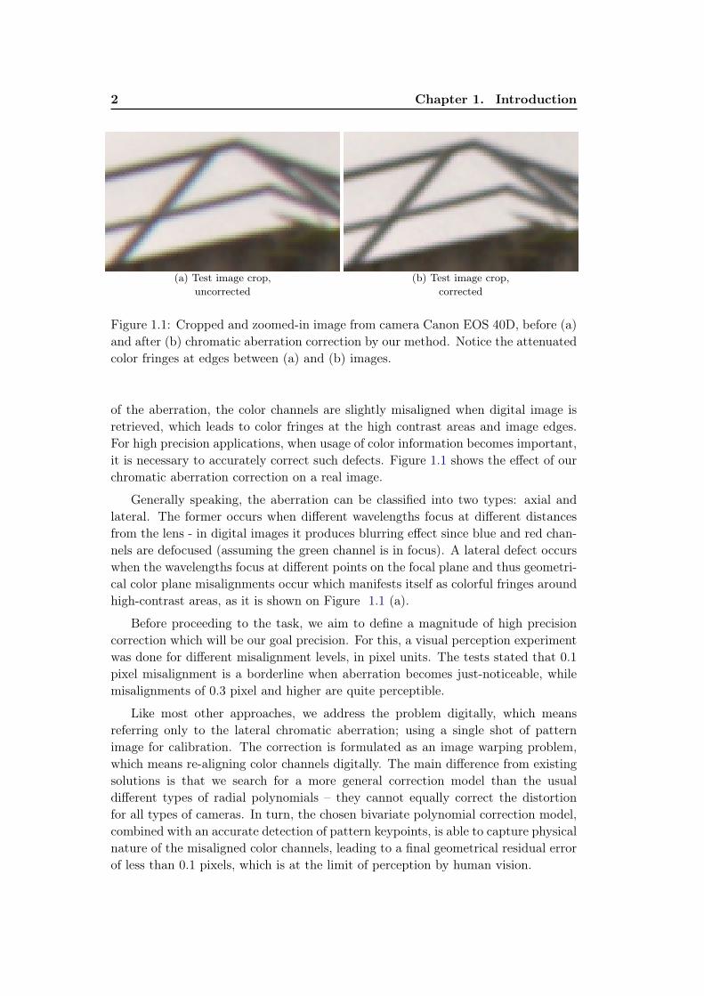
(a) Test image crop,uncorrected
(b) Test image crop,corrected
Figure 1.1: Cropped and zoomed-in image from camera Canon EOS 40D, before (a)and after (b) chromatic aberration correction by our method. Notice the attenuatedcolor fringes at edges between (a) and (b) images.
of the aberration, the color channels are slightly misaligned when digital image isretrieved, which leads to color fringes at the high contrast areas and image edges.For high precision applications, when usage of color information becomes important,it is necessary to accurately correct such defects. Figure 1.1 shows the effect of ourchromatic aberration correction on a real image.
Generally speaking, the aberration can be classified into two types: axial andlateral. The former occurs when different wavelengths focus at different distancesfrom the lens - in digital images it produces blurring effect since blue and red chan-nels are defocused (assuming the green channel is in focus). A lateral defect occurswhen the wavelengths focus at different points on the focal plane and thus geometri-cal color plane misalignments occur which manifests itself as colorful fringes aroundhigh-contrast areas, as it is shown on Figure 1.1 (a).
Before proceeding to the task, we aim to define a magnitude of high precisioncorrection which will be our goal precision. For this, a visual perception experimentwas done for different misalignment levels, in pixel units. The tests stated that 0.1pixel misalignment is a borderline when aberration becomes just-noticeable, whilemisalignments of 0.3 pixel and higher are quite perceptible.
Like most other approaches, we address the problem digitally, which meansreferring only to the lateral chromatic aberration; using a single shot of patternimage for calibration. The correction is formulated as an image warping problem,which means re-aligning color channels digitally. The main difference from existingsolutions is that we search for a more general correction model than the usualdifferent types of radial polynomials – they cannot equally correct the distortionfor all types of cameras. In turn, the chosen bivariate polynomial correction model,combined with an accurate detection of pattern keypoints, is able to capture physicalnature of the misaligned color channels, leading to a final geometrical residual errorof less than 0.1 pixels, which is at the limit of perception by human vision.
1.2. Camera matrix extraction 3
1.2 Camera matrix extraction
Considering the global calibration method by [ZHANG 2000], theoretically one canclaim that camera calibration is a closed topic. At the same time, when calibratinga camera, the major difficulty lies in optical distortion; its correction is a necessarystep for high precision results. The mentioned global calibration approach mixes thedistortion parameters with other camera parameters and their calculation is held bysimultaneous minimization. However, this could potentially lead to residual errorcompensation of distortion parameters and other camera parameters that woulddecrease the calibration stability, since the physics of distortion field would not becaptured correctly. Moreover, the error compensation cannot be eliminated in theframework of global methods, and therefore, the distortion compensation must beheld separately, as a preliminary step to any further calibration.
The recently developed method relying on the calibration harp by [TANG 2011]allows calculating a distortion field separately from other parameters. Its main ideais based on straightness measure of tightly stretched strings, pictures of which mustbe taken in different orientations. In that respect, it lies in the category of plumb-linemethdods. While it requires using an additional calibration pattern, the trade-offis that we are able to control the residual distortion error magnitude in addition tohaving distortion detached from other camera parameters. This separation shouldalso allow producing more reliable results since it solves the problem of residualerror compensation.
Another questions we address, given distortion compensated calibration image, ishow to eliminate a perspective bias. Since we deal with circular patterns and ellipsecenters as keypoints (as it is more precise than using square patterns), the detectedcontrol points can potentially be corrupted by perspective bias. It can be describedby fact that image of the ellipse center does not correspond to the center of theellipse image. Therefore, we try to compensate for the perspective bias by takinginto account rather circle-ellipse affine transformation than point transformationand then use correspondence of detected keypoints with pattern keypoints given theaffine conic transform.
In order to use the conic transform for the calibration matrix calculation, we doit by incorporating the conic affine transformation into the minimization step forhomography estimation. The transformation function is able to match center of thecircle of the pattern with center of the ellipse in the image. Therefore, the maindetection feature still remains an ellipse center, there is no need for ellipse contourextraction. The aforementioned function allows eliminating the perspective bias,thus, it produces more precise results for homography matrix estimation, and in thecontext of the calibration matrix extraction it leads to more stable results.
1.3 The thesis chapter by chapter
Chapter 2 shows a choice of the calibration pattern which is represented by a2D plane with printed black circles on it, and also how to detect the keypoints
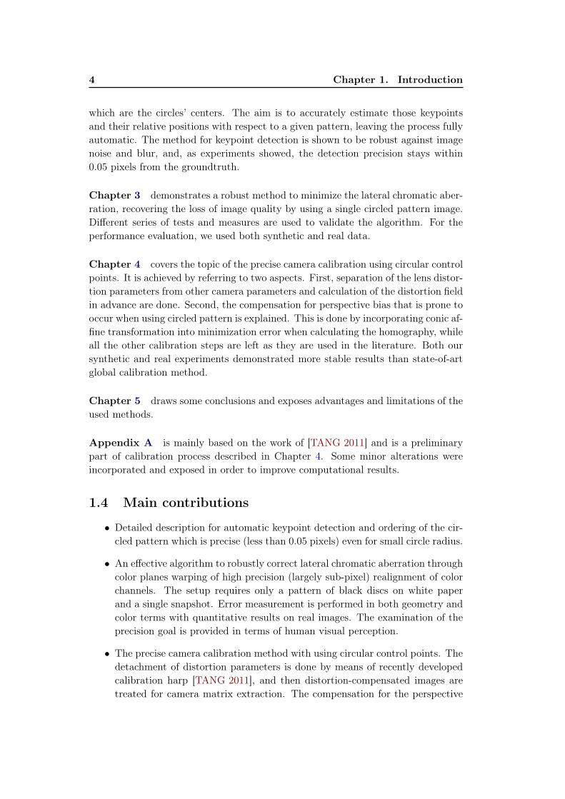
4 Chapter 1. Introduction
which are the circles’ centers. The aim is to accurately estimate those keypointsand their relative positions with respect to a given pattern, leaving the process fullyautomatic. The method for keypoint detection is shown to be robust against imagenoise and blur, and, as experiments showed, the detection precision stays within0.05 pixels from the groundtruth.
Chapter 3 demonstrates a robust method to minimize the lateral chromatic aber-ration, recovering the loss of image quality by using a single circled pattern image.Different series of tests and measures are used to validate the algorithm. For theperformance evaluation, we used both synthetic and real data.
Chapter 4 covers the topic of the precise camera calibration using circular controlpoints. It is achieved by referring to two aspects. First, separation of the lens distor-tion parameters from other camera parameters and calculation of the distortion fieldin advance are done. Second, the compensation for perspective bias that is prone tooccur when using circled pattern is explained. This is done by incorporating conic af-fine transformation into minimization error when calculating the homography, whileall the other calibration steps are left as they are used in the literature. Both oursynthetic and real experiments demonstrated more stable results than state-of-artglobal calibration method.
Chapter 5 draws some conclusions and exposes advantages and limitations of theused methods.
Appendix A is mainly based on the work of [TANG 2011] and is a preliminarypart of calibration process described in Chapter 4. Some minor alterations wereincorporated and exposed in order to improve computational results.
1.4 Main contributions
• Detailed description for automatic keypoint detection and ordering of the cir-cled pattern which is precise (less than 0.05 pixels) even for small circle radius.
• An effective algorithm to robustly correct lateral chromatic aberration throughcolor planes warping of high precision (largely sub-pixel) realignment of colorchannels. The setup requires only a pattern of black discs on white paperand a single snapshot. Error measurement is performed in both geometry andcolor terms with quantitative results on real images. The examination of theprecision goal is provided in terms of human visual perception.
• The precise camera calibration method with using circular control points. Thedetachment of distortion parameters is done by means of recently developedcalibration harp [TANG 2011], and then distortion-compensated images aretreated for camera matrix extraction. The compensation for the perspective

1.4. Main contributions 5
bias is carried out by incorporating the conic transform function into homo-graphy estimation.
• Implementation of the optical distortion correction method in C++, as wellas improvements of the formulas for the sake of simplicity and gain in compu-tational time.

Chapter 2
Robust and precise featuredetection of a pattern plane
The aim of the chapter is to accurately estimate the keypoints from an image andtheir relative positions with respect to a given pattern. The calibration patternis represented by a 2D plane with black circles printed on it. The process is fullyautomatic and is robust against image noise and blur, leaving the detected keypointsat deviation of average 0.05 pixels from the groundtruth.
Keywords. Precise keypoints, feature detection, pattern plane, circle center, el-lipse center, keypoint ordering.
Contents2.1 Introduction . . . . . . . . . . . . . . . . . . . . . . . . . . . . 82.2 Sub-pixel keypoint detection . . . . . . . . . . . . . . . . . . . 10
2.2.1 Geometrical model . . . . . . . . . . . . . . . . . . . . . . . . 102.2.2 Intensity model . . . . . . . . . . . . . . . . . . . . . . . . . . 112.2.3 Parametric model estimation through minimization . . . . . . 12
2.3 Keypoint ordering . . . . . . . . . . . . . . . . . . . . . . . . . 152.4 Sub-pixel ellipse center detection accuracy . . . . . . . . . . 162.5 Conclusion . . . . . . . . . . . . . . . . . . . . . . . . . . . . . 17
8 Chapter 2. Robust and precise feature detection of a pattern plane
2.1 Introduction
In the context of high precision camera calibration, we are interested in preciseallocation and detection of the keypoints which would ensure dense and consistentfield registrations, as well as robustness to noise and blur. The notion high precisionoften means the residual error between the camera and its obtained numerical modelis far smaller than a pixel size. For example, a calibration of lateral chromaticaberrations requires a correction model, residual of which is to stay within 0.1 pixelsin order not to be visually perceptible (more details on this experiment are givenin the Chapter 3), therefore, our main goal will be to detect the keypoints withdeviation no more than 0.1 pixels from the groundtruth.
One of the most common types of keypoints are feature based interest points.Such local image descriptors do not require any type of calibration pattern, and theyhave quite a broad range of applications – from object recognition [LOWE 2004] toimage retrieval [NISTER 2006, SIVIC 2006], and similar. The most famous local fea-ture extractor is Scale-Invariant Feature Transform (SIFT) algorithm [LOWE 1999],further developed into [LOWE 2004]. For the mentioned applications the precisionof spatial position may appear less important. Often the relative spatial layout ofinterest points are used together with a tolerance for large variations in the corres-ponding points relative position [SIVIC 2005].
An alternative to feature based interest points would be to pick the interestpoints at random, but it will be unlikely to obtain precise spatial correspondencebetween a sparse set of randomly picked points. The ability to detect correspon-ding interest points, in a precise and repeatable manner, is a desirable propertyfor obtaining geometric scene structure. Therefore, when it concerns applicationsof 3D reconstruction and camera calibration from interest points, it is of highimportance to have precise point correspondence [SNAVELY 2008, TORR 2000,FURUKAWA 2010] which assumes using some kind of calibration pattern to en-sure spatial consistency.
Different types of planar charts exist for the purpose of camera calibration assources of both 2D and 3D control points. Normally, these points are constructedon a planar surface by creating some high contrast pattern. The pattern also fa-cilitates the recovery of the control points projections on the image plane. Themost common pattern are: squares [WENG 1992, ZHANG 2000], chekerboards[LUCCHESE 2002], circles [ASARI 1999, HEIKKILÄ 2000, KANNALA 2006].Those became popular as they can be always manufactured to a sufficient precision,and their data points are recoverable through the use of standard image processingtechniques.
When choosing a plane calibration pattern, it is important to consider an aspectfor invariance to the potential bias from projective transformations and nonlineardistortions. [MALLON 2007b] provides a comparative study on the use of planarpatterns in the generations of control points for camera calibration. There, a circledpattern is compared to a checkerboard, and it is theoretically and experimentallyshown that the former can potentially be affected by bias sources. As a contrast,
2.1. Introduction 9
appropriate checkerboard pattern detection is shown to be bias free.At the same time [MALLON 2007a] provides results for sub-pixel detection error
of the keypoints which are the intersections of a chessboard pattern. The extrac-tion is done automatically using standard corner detector such as those describedby [LUCCHESE 2002, JAIN 1995] with sub-pixel refinement step of saddle points.Those results expose an accuracy magnitude of about 0.1-0.3 pixels, depending onthe camera. Such precision result would not be sufficient for high precision calibra-tion and could be potentially improved if we utilise higher precision detector of thecircled pattern with the condition of compensation for distortion (see Appendix A)and perspective bias (refer to Chapter 4) beforehand.
Under perspective transformation circles are observed as ellipses, therefore ourmain interest lies into ellipse center detection. One of the common ways to de-tect ellipse is through Hough transform [PRINCEN 1992] - it is based on votingsystem for some ellipse parameters using contribution of contour pixels; as anexample, [ÁLVAREZ LEÓN 2007] detect ellipses using Hough transform with pa-rameter space reduction and a final Least-Square Minimization refinement. WhileHough transform is a good tool in applications like pattern recognition, it may notbe sufficient since it has its limitations like dependence on the results from edgedetector and might be less precise in noisy and blurry environments.
Other types of estimation of an ellipse rely on accurate extraction of thecontour points with subpixel precision and then fitting ellipse parameters onthe obtained set of points. Numerous methods exist for fitting ellipse para-meters from a given set of contour points [GANDER 1994, KANATANI 1994,FITZGIBBON 1995, CABRERA 1996, FITZGIBBON 1999, KANATANI 2006,KANATANI 2011]. They differ from each other depending on their precision, ac-curacy, robustness to outliers, etc. All those rely on a set of contour points thatare extracted beforehand. Nevertheless, extracting contour points usually subsumesmultiple stages including gradient estimation, non-maximum suppression, threshol-ding, and subpixel estimation. Extracting contour points imposes making a decisionfor each of those points based on neighbourhood pixels in the image. The proces-sing of low contrast images would be quite challenging where each contour point canhardly be extracted along the ellipse, therefore, it is better to refer to the informa-tion encoded in all pixels in the ellipse surrounding. By eliminating the participationof contour points, the method would be greatly simplified and the uncertainty onthe recovered ellipse parameters will be assessed more closely to the image data.
The current chapter presents a method for high precision keypoint detection forthe purpose of camera calibration which takes into account both geometrical andcolor information. The method is based on defining intensity and affine parametersthat describe an ellipse, followed by minimization of those parameters so as to fitthe observed image of the ellipse and its surrounding pixels. No contour informa-tion is necessary. It allows a detection of maximum accuracy 0.05 pixels, and, asexperiments show, it is resistant to noise and blur.
The rest of chapter is organized as follows: Section 2.2 gives a description ofthe method, Section 2.3 demonstrates a simple way how the ordering of keypoints
10 Chapter 2. Robust and precise feature detection of a pattern plane
was performed, which is a necessary step for automatic camera matrix calibration.Finally Section 2.4 includes synthetic experiments for detection precision againstnoise and blur.
2.2 Sub-pixel keypoint detection
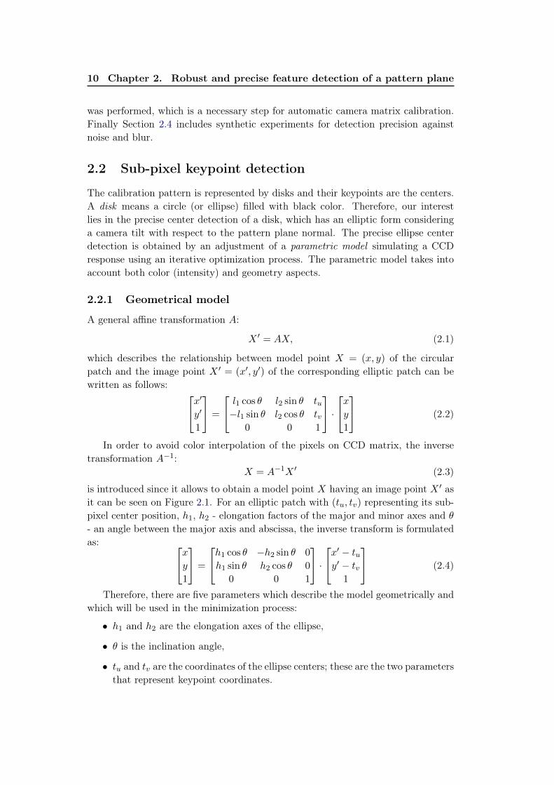
The calibration pattern is represented by disks and their keypoints are the centers.A disk means a circle (or ellipse) filled with black color. Therefore, our interestlies in the precise center detection of a disk, which has an elliptic form consideringa camera tilt with respect to the pattern plane normal. The precise ellipse centerdetection is obtained by an adjustment of a parametric model simulating a CCDresponse using an iterative optimization process. The parametric model takes intoaccount both color (intensity) and geometry aspects.
2.2.1 Geometrical model
A general affine transformation A:
X ′ = AX, (2.1)
which describes the relationship between model point X = (x, y) of the circularpatch and the image point X ′ = (x′, y′) of the corresponding elliptic patch can bewritten as follows: x′y′
1
=
l1 cos θ l2 sin θ tu−l1 sin θ l2 cos θ tv
0 0 1
·xy
1
(2.2)
In order to avoid color interpolation of the pixels on CCD matrix, the inversetransformation A−1:
X = A−1X ′ (2.3)
is introduced since it allows to obtain a model point X having an image point X ′ asit can be seen on Figure 2.1. For an elliptic patch with (tu, tv) representing its sub-pixel center position, h1, h2 - elongation factors of the major and minor axes and θ- an angle between the major axis and abscissa, the inverse transform is formulatedas: xy
1
=
h1 cos θ −h2 sin θ 0
h1 sin θ h2 cos θ 0
0 0 1
·x′ − tuy′ − tv
1
(2.4)
Therefore, there are five parameters which describe the model geometrically andwhich will be used in the minimization process:
• h1 and h2 are the elongation axes of the ellipse,
• θ is the inclination angle,
• tu and tv are the coordinates of the ellipse centers; these are the two parametersthat represent keypoint coordinates.
2.2. Sub-pixel keypoint detection 11
An objectDigital image
Sub-sampling
Digitizing
+ Noise+ Smooth
Camera
(x,y) (x',y')
Model Image
A
A-1
Luminance
Distance
1
-1
-1/k 1/k
centre peripherygradientFigure 2.1: Affine transformation A and its inverse A−1 for model point (x, y) andits corresponding image point (x′, y′).
An objectDigital image
Sub-sampling
Digitizing
+ Noise+ Smooth
Camera
(x,y) (x',y')
Model Image
A
A-1
Luminance
Distance
1
-1
-1/k 1/k
centre peripherygradient
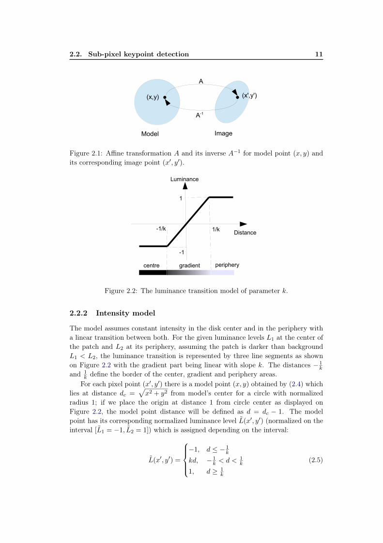
Figure 2.2: The luminance transition model of parameter k.
2.2.2 Intensity model
The model assumes constant intensity in the disk center and in the periphery witha linear transition between both. For the given luminance levels L1 at the center ofthe patch and L2 at its periphery, assuming the patch is darker than backgroundL1 < L2, the luminance transition is represented by three line segments as shownon Figure 2.2 with the gradient part being linear with slope k. The distances − 1
k
and 1k define the border of the center, gradient and periphery areas.For each pixel point (x′, y′) there is a model point (x, y) obtained by (2.4) which
lies at distance dc =√x2 + y2 from model’s center for a circle with normalized
radius 1; if we place the origin at distance 1 from circle center as displayed onFigure 2.2, the model point distance will be defined as d = dc − 1. The modelpoint has its corresponding normalized luminance level L(x′, y′) (normalized on theinterval [L1 = −1, L2 = 1]) which is assigned depending on the interval:
L(x′, y′) =
−1, d ≤ − 1
k
kd, − 1k < d < 1
k
1, d ≥ 1k
(2.5)
12 Chapter 2. Robust and precise feature detection of a pattern plane
The denormalization of L(x′, y′) is to be done:
L(x′, y′) = L1 +L(x′, y′) + 1
2(L2 − L1) (2.6)
Therefore, there are three parameters which describe the color model and which willbe used in the minimization process:
• L1 - luminance level at the center area of the patch
• L2 - luminance level at the periphery
• k - slope which defines the transition from the center to periphery areas
2.2.3 Parametric model estimation through minimization
Levenberg-Marquardt algorithm (LMA) is chosen to minimize the sum of squareddifferences of the gray levels between each pixel (x′, y′) of the elliptic patch in theimage I and corresponding point (x, y) obtained by (2.4) of the theoretical CCDmodel with intensity L as in (2.6). The model is represented by a set of parameters{h1, h2, θ, tu, tv, k, L1, L2} that comprises both geometry and color properties. Thefollowing distance function is to be minimized by the LMA:
arg minh1,h2,θ,tu,tv ,k,L1,L2
w∑x′
h∑y′
(I(x′, y′)− L(x′, y′))2. (2.7)
After the minimization process is terminated, among the set of obtained mo-del parameters, there is a sub-pixel center coordinate (tu, tv) which represents akeypoint.
2.2.3.1 Parameter initialization
Given three channels of the image, the very first step is to estimate initial positionof each disk and the size of its enclosing sub-image. This is done by proceeding:
Step 1. Binarization of each channel.
Step 2. Finding connected components of a black color for each binarized channel.
Step 3. Calculating moments for each component i:
(a) radii rix , riy ,
(b) compactness measure Ci = 4πSi
P 2i, where Pi is a closed curve of the connec-
ted component area Si,
(c) centroid (tiu , tiv).
2.2. Sub-pixel keypoint detection 13
Step 4. Noise elimination by meeting the conditions:min(rix , riy) > 8
1− δ ≤ Ci ≤ 1 + δ, δ ∈ [0.2, 0.4]
Si ∈ {S}freq,(2.8)
where {S}freq is a histogram area with most frequent connected componentsizes
As a result we obtain initial positions of each disk (tiu , tiv) and its enclosingsub-image with size wi = hi = ri
52 , where ri = 1
2(rix + riy).The initialization of other geometric parameters h1, h2 and θ is done with help
of principle component analysis. If we represent an ellipse by its covariance matrix
Cov =
[(σx)2 σxy
σxy (σy)2
], (2.9)
where σx - one-sigma uncertainty in x direction, σy - in y direction and σxy - cova-riance between x and y. The axes and their lengths are represented by eigenvectorsand eigenvalues accordingly. We are interested in eigenvalues in order to initializeh1 and h2. Given matrix Cov, a characteristic equation can be written:
|Cov − λI| =∣∣∣[(σx)2 σxy
σxy (σy)2
]−[λ 0
0 λ
]∣∣∣ = 0. (2.10)
The determinant calculation will lead to a quadratic equation:
λ2 − ((σx)2 + (σy)2)λ+ (σx)2(σy)2 − (σxy)2 = 0, (2.11)
which has roots
λ1,2 =(σx)2 + (σy)2 ±
√((σx)2 + (σy)2)2 − 4((σxσy)2 − (σxy)2)
2(2.12)
The lengths of the ellipse axes are square root of eigenvalues λ1, λ2 of covariancematrix Cov and since parameters h1 and h2 represent semi-axes, we can initializethem as
h1 =
√λ12
h2 =
√λ22
(2.13)
The counter-clockwise rotation θ of the ellipse then can be deduced from thefirst column of 2.10, which also means [cos θ sin θ]T , and therefore we can write
θ = atan2((σx)2 − λ1, σxy). (2.14)
The other model parameters are initialized: {k = 2, L1 = black∗, L2 = white∗},where black∗, white∗ are global maximum and minimum intensities for the givensub-image [wi × hi].
14 Chapter 2. Robust and precise feature detection of a pattern plane
2.2.3.2 Error
The element of an error vector E = (e(0,0), e(0,1), · · · , e(w,h)) for a set of pixels of theimage with size w × h of the elliptic patch is given by:
e(x′,y′) = I(x′, y′)− L(x′, y′) (2.15)
2.2.3.3 Jacobian matrix
The Jacobian matrix is determined as a matrix of all first-order partial derivativesof the vector function {λ1, λ2, θ, tu, tv, k, L1, L2} with respect to data vector. Thegeneric formulations for the geometry variables (not including k, L1, L2 variables)for a given image pixel (x′, y′) are:
∂e(x′,y′)
∂•= −∂L(x′, y′)
∂•∂L(x′, y′)
∂•= 1
2(L2 − L1)∂L(x′, y′)
∂•∂L(x′, y′)
∂•= k
∂d
∂•,
(2.16)
where the formulas of partial derivatives∂L(x′, y′)
∂•for each variable are given only
for the gradient interval − 1k < d < 1
k (since the derivatives will be zeros at peripheryand at the center areas, see (2.5)), and further on the derivatives are shown only forthis interval.
The derivatives for color variables k, L1, L2 are straightforward:∂e(x′,y′)
∂•= −∂L(x′, y′)
∂•∂L(x′, y′)
∂k= (L2 − L1)
d
2∂L(x′, y′)
∂L1= 1− L(x′, y′) + 1
2∂L(x′, y′)
∂L2=L(x′, y′) + 1
2
(2.17)
The formulas of partial derivatives∂d
∂•for each geometric variable are:
∂d
∂•=
1
d(x∂x
∂•+ y
∂y
∂•)
∂x
∂λ1= (x′ − tu) cos θ,
∂y
∂λ1= (x′ − tu) sin θ
∂x
∂λ2= −(y′ − tv) sin θ,
∂y
∂λ2= (y′ − tv) cos θ
∂x
∂θ= −(λ1(x
′ − tu) sin θ + λ2(y′ − tv) cos θ),
∂y
∂θ= (λ1(x
′ − tu) cos θ − λ2(y′ − tv) sin θ)
∂x
∂tu= −λ1 cos θ,
∂y
∂tu= −λ1 sin θ
∂x
∂tv= λ2 sin θ,
∂y
∂tv= −λ2 cos θ
(2.18)
2.3. Keypoint ordering 15
The resulting Jacobian matrix has the form:
J =
∂e(0,0)∂λ1
∂e(0,0)∂λ2
· · · ∂e(0,0)∂L1
∂e(0,0)∂L2
∂e(0,1)∂λ1
∂e(0,1)∂λ2
· · · ∂e(0,1)∂L1
∂e(0,1)∂L2
.... . .
∂e(w,h)
∂λ1
∂e(w,h)
∂λ2· · · ∂e(w,h)
∂L1
∂e(w,h)
∂L2
(2.19)
2.3 Keypoint ordering
The algorithm is fully automatic and does not require any user interaction. We aimat a set of very simple steps that help to order keypoints.
In order to process the set of keypoints to the algorithm, it is important to orderthem exactly same way as pattern keypoints are, for example from top to bottomcolumn-wise. Simple sorting techniques such as ordering according u and then v
coordinate may not be efficient since we deal with the image of the pattern whichwas rotated, translated and then projected into camera image. The simplest waywas to determine approximate homography Happ using match of corner keypointsof the image and the pattern, and then order the rest of image keypoints with helpof Happ. Therefore, we are interested in selecting the four ellipses that are locatedat the corners of the calibration pattern and then putting them in correspondencewith the corners of model pattern. If we are able to estimate this transformation,then we can easily estimate the correspondence for the rest of the points. This iscarried out by means of homography.
The similar idea is usually applied in human-assisted semi-automatic environ-ment where a user selects the four corners and the algorithm manages to do therest, for example, Matlab Calibration Toolbox [BOUGUET 2000]. Our goal is tohave fully automatic software.
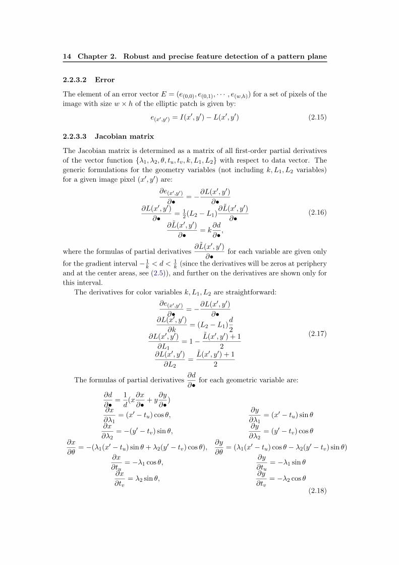
The principle for determination of corners from a given set of keypoints is dis-played in Figure 2.3. We followed these steps to order all the keypoints:
1. For each of the keypoint c (potentially corner) do:
• find its first three neighbours n1, n2 and n3 based on Euclidean distance;
• calculate the angles ∠n1cn2, ∠n1cn3, ∠n2cn3 and pick the maximum∠max = ∠ni1cni2 with i1 and i2 corresponding keypoint indices thatsatisfy maximum angle condition;
• if the angle is more than 180◦ then c is not a corner;
• otherwise for all the rest of the keypoints {ni}i=3,··· ,N , make sure theyare located within the maximum angle ∠ni1cni2 (within small toleranceε, for example, 2◦) and if this condition holds, c is a corner:
∠ni1cni2 > ∠nicni1 − ε∠ni1cni2 > ∠nicni2 − ε
(2.20)
16 Chapter 2. Robust and precise feature detection of a pattern plane
n1 n2
n3c
Figure 2.3: Defining the corner keypoint: when the maximum angle ∠n1cn3 bet-ween corner’s c first three neighbours n1, n2, n3 stays maximum for the rest of thekeypoints (within small tolerance) and at the same time less than 180◦.
An objectDigital image
Sub-sampling
Digitizing
+ Noise+ Smooth
Camera
(x,y) (x',y')
Model Image
A
A-1
Luminance
Distance
1
-1
-1/k 1/k
centre peripherygradient
Figure 2.4: Digitizing of the pattern.
2. Sort the four corners by coordinate - firstly by u, then by v.
3. Calculate approximate homography Happ using correspondence of corner key-points c1, c2, c3, c4, and corresponding pattern corner keypoint locations.
4. Sort all the keypoints same way as they are sorted for the pattern by calcu-lating approximate location of the keypoint in image xapp = HappX and thenidentifying the closest keypoint x to xapp.
2.4 Sub-pixel ellipse center detection accuracy
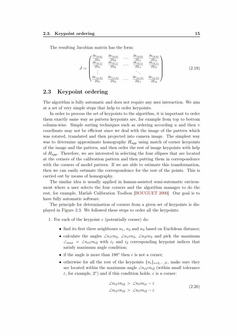
Experiments are performed to measure the ellipse center detection accuracy at dif-ferent ellipse sizes against noise and aliasing, and also against different angles of viewof the circle. The synthetic data was generated according a principle of digitizingshown on Figure 2.4.
Synthetic disk (filled circle) 8-bit images were generated on a large image of sizeW ×W pixels (W = 1000 for the first set and W = 2000 for the second), which wasblurred, downsampled and finally Gaussian noise was added. Subpixel disk centerlocation is used as ground truth and compared to detected disk center.
Each set includes four 8-bit images with a disk on each of a different radiussize. That is, an ellipse {x, y} is drawn with the fixed center (xc, yc), radius R
2.5. Conclusion 17
and rotation angle ϕ (fixed to 30◦) along z axis and changing angle of view θ asdescribed:
((x− xc) cosϕ− (y − yc) sinϕ)2
R2+
((x− xc) sinϕ+ (y − yc) cosϕ)2
(R cos θ)2≤ 1,
(xc, yc) = (0.5W + δx, 0.5W + δy),
R = nW
2,
(2.21)
where (δx, δy) are shifts from image center for x, y directions, and n =
[0.45, 0.6, 0.75, 0.9] is assigned so that to see if the ratio between image area anddisk area influences the detection accuracy.
The ground-truth circle centers for each sub-sampled image are found:
(xg.t, yg.t) = (0.5W
s+δxs, 0.5
W
s+δys
), (2.22)
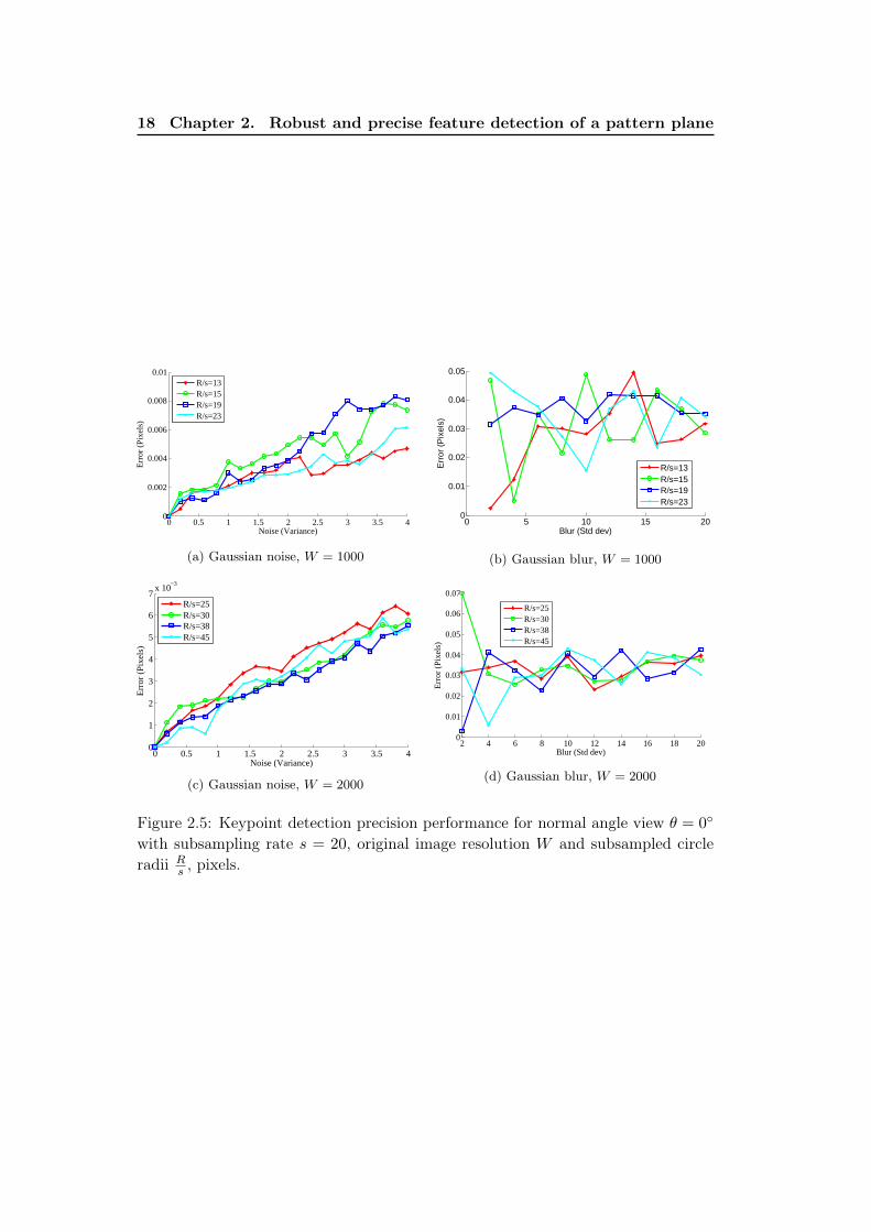
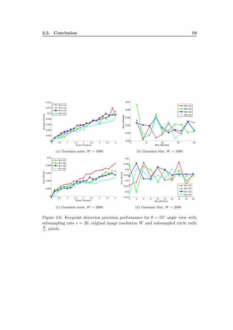
with s being a downsampling rate (s = 20 for both image sets). Figure 2.5 andFigure 2.6 show the performance of the algorithm against Gaussian noise level (me-dian error out of 100 iterations) and amount of blur for different disk radii (the viewangle θ is set to 0◦ on the first figure and 55◦ on the second). Similar experimentswere performed for other view angles, up to 70◦ and it was found that error alwayshas the same tendency as in shown figures.
2.5 Conclusion
The described algorithm allows automatic keypoint detection and ordering of thecircled pattern. From the graphs presented at experiment section it can be alsoconcluded:
1. In all the cases the average error is less than 0.05 pixels, even for small diskradius (11 pixels). And considering the fact that ratio of the disk area and itsenclosing image area has little impact on the precision detection, allows us topack more keypoints in a given pattern area.
2. The view of angle has little influence on precision even for large angles, whichmeans the detection stays robust even when pattern plane is viewed from alarge angle of view (here we don’t consider perspective bias which is a subjectin Chapter 4, but rather affine transform of the elliptic parameters).
3. As expected, the error increases linearly with noise level, but remains constantunder blur. This is important because in a Bayer pattern image, red and bluechannels are notoriously aliased. Figure 2.5 (b,d) and Figure 2.6 (b,d) showthat this does not affect the disk center detection.
18 Chapter 2. Robust and precise feature detection of a pattern plane
0 0.5 1 1.5 2 2.5 3 3.5 40
0.002
0.004
0.006
0.008
0.01
Noise (Variance)
Err
or (
Pixe
ls)
R/s=13R/s=15R/s=19R/s=23
(a) Gaussian noise, W = 1000
0 5 10 15 200
0.01
0.02
0.03
0.04
0.05
Blur (Std dev)
Err
or (
Pix
els)
R/s=13R/s=15R/s=19R/s=23
(b) Gaussian blur, W = 1000
0 0.5 1 1.5 2 2.5 3 3.5 40
1
2
3
4
5
6
7x 10
−3
Noise (Variance)
Err
or (
Pix
els)
R/s=25R/s=30R/s=38R/s=45
(c) Gaussian noise, W = 2000
2 4 6 8 10 12 14 16 18 200
0.01
0.02
0.03
0.04
0.05
0.06
0.07
Blur (Std dev)
Err
or (
Pixe
ls)
R/s=25R/s=30R/s=38R/s=45
(d) Gaussian blur, W = 2000
Figure 2.5: Keypoint detection precision performance for normal angle view θ = 0◦
with subsampling rate s = 20, original image resolution W and subsampled circleradii Rs , pixels.
2.5. Conclusion 19
0 0.5 1 1.5 2 2.5 3 3.5 40
0.002
0.004
0.006
0.008
0.01
0.012
0.014
Noise (Variance)
Dis
tanc
e (P
ixel
s)
R/s=13R/s=15R/s=19R/s=23
(a) Gaussian noise, W = 1000
0 5 10 15 200.02
0.03
0.04
0.05
0.06
0.07
Blur (Std dev)
Err
or (
Pix
els)
R/s=13R/s=15R/s=19R/s=23
(b) Gaussian blur, W = 1000
0 0.5 1 1.5 2 2.5 3 3.5 40
0.002
0.004
0.006
0.008
0.01
Noise (Variance)
Err
or (
Pixe
ls)
R/s=25R/s=30R/s=38R/s=45
(c) Gaussian noise, W = 2000
2 4 6 8 10 12 14 16 18 200.015
0.02
0.025
0.03
0.035
0.04
0.045
0.05
Blur (Std dev)
Err
or (
Pixe
ls)
R/s=25R/s=30R/s=38R/s=45
(d) Gaussian blur, W = 2000
Figure 2.6: Keypoint detection precision performance for θ = 55◦ angle view withsubsampling rate s = 20, original image resolution W and subsampled circle radiiRs , pixels.

Chapter 3
High-precision correction oflateral chromatic aberration in
digital images
Nowadays digital image sensor technology continues to develop much faster thanoptical technology for imaging systems. The result quality loss is due to lateralchromatic aberration and it is becoming more significant with the increase of sensorresolution. For the sake of higher performance and lighter lens systems, especiallyin the field of computer vision, we aim to find new ways to overcome resulting imagequality limitations.
This chapter demonstrates a robust method to minimize the lateral chromaticaberration, recovering the loss of image quality by using a single circled patternimage. Different series of tests and measures are used to validate the algorithm. Forthe performance evaluation we used both synthetic and real data.
The primary contribution of this work is an effective algorithm to robustly correctlateral chromatic aberration through color planes warping. We aim at high precision(largely sub-pixel) realignment of color channels. This is achieved thanks to twoingredients: high precision keypoint detection, which in our case are circle centers,and more general correction model than what is commonly used in the literature,radial polynomial. The setup is quite easy to implement, requiring a pattern ofblack disks on white paper and a single snapshot.
We perform the error measurements in terms of geometry and of color. Quanti-tative results on real images show that our method allows alignment of average 0.05pixel of color channels and residual color error divided by a factor 3 to 6. Finally, theperformance of the system is compared and analysed against three different softwareprograms in terms of geometrical misalignments.
Keywords Chromatic aberration, image warping, camera calibration,polynomial model, image enhancement
Contents3.1 Introduction . . . . . . . . . . . . . . . . . . . . . . . . . . . . 23
3.2 Calibration and correction . . . . . . . . . . . . . . . . . . . . 26
3.3 Experiments . . . . . . . . . . . . . . . . . . . . . . . . . . . . 29
3.3.1 Chromatic aberration correction accuracy with reflex cameras 29

22Chapter 3. High-precision correction of lateral chromatic aberration in
digital images
3.3.2 Visual improvement for real scenes . . . . . . . . . . . . . . . 383.3.3 Experiments with compact digital cameras . . . . . . . . . . 39
3.4 Conclusion . . . . . . . . . . . . . . . . . . . . . . . . . . . . . 40
3.1. Introduction 23
3.1 Introduction
Every optical system that uses lenses suffers from aberrations that occur due tothe refractive characteristics of the lenses [JÜRGEN 1995]. Loss in image accuracybecause of a known set of aberrations can be classified as either monochromaticor chromatic types of aberration. They occur due to physical interaction of lightwith materials, lens design constraints and manufacture limitations. The five Seidelmonochromatic aberrations include spherical aberration, comatic, astigmatic, cur-vature of field and distortion [SEIDEL 1856]. The chromatic type of aberration isindependent from monochromatic one.
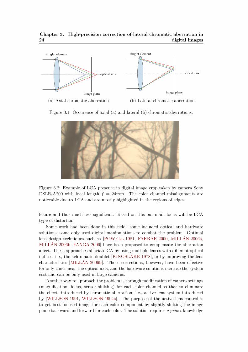
A type of distortion named Chromatic Aberration (CA) is inherent for any op-tical system due to result of the different refractive indices of the lens medium(typically some form of glass) for varying wavelength of the transmitted light, andsuch phenomena is termed dispersion [NEWTON 1704] and explains prismatic be-haviour. From aesthetic point of view, CA gives overall impression of poor qualityand definition, while from the view of computer vision application algorithms - mayreduce stability and precision for the application when color information matters (i.e.deteriorating of details on the texture or edge areas). The main classification of CAis two categories [SLAMA 1980]: Axial (or longitudinal) Chromatic Aberration -ACA, and Lateral (or transverse) Chromatic Aberration - LCA.
The ACA occurs when different wavelengths focus at different distances fromthe lens, i.e., different points on the optical axis as shown on Figure 3.1 (a). Itcauses a failure of all the wavelengths to be focused at the same convergence point,and as a result, as light strikes the sensor panel, out of focus rays contribute to acircle of confusion, or bokeh. In digital images it manifests as a subtle coloured haloaround the boundary of an object, especially in the circumstances like lens widestaperture setting. Such image artifacts might be decreased when the lens apertureis stopped down or reduced due to the increase in depth of field which brings theaxially-misaligned focal points nearer. Many modern digital cameras, when in fully-automatic mode, are able to balance the aperture size preventing significant spacialfrequency loss due to photon diffraction [MIELENZ 1999] and a shallow depth offield, increasing focus selectivity and focus error as a side effect. Thanks to camera’sautomatic mode, ACA is nominally minimised to imperceptible levels.
The LCA happens when the wavelengths focus at different points on the fo-cal plane and thus geometrical color plane misalignments occur as shown on Fi-gure 3.1 (b). It is relative and non-linear displacement of the three color planes;on the obtained digital images the channels are misaligned with respect to eachother. This source of degradation manifests itself as fringes of color at edges andhigh contrast areas which leads to a perceived detail loss. Less perceptible impactin lower-contrast areas reduces texture detail and generally tends to reduce theperception that LCA compromises image quality.
An example of CA is shown on Figure 3.2. It can be seen that CA limits imagedetail. Also the present CA has assymetric nature which means the type LCA is thedominant aberration and attenuating quality. ACA occurs symmetrically to image
24Chapter 3. High-precision correction of lateral chromatic aberration in
digital images
(a) Axial chromatic aberration (b) Lateral chromatic aberration
Figure 3.1: Occurence of axial (a) and lateral (b) chromatic aberrations.
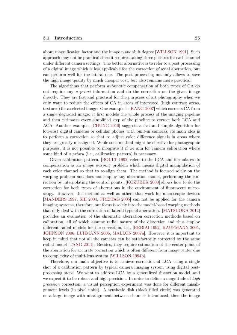
Figure 3.2: Example of LCA presence in digital image crop taken by camera SonyDSLR-A200 with focal length f = 24mm. The color channel misalignments arenoticeable due to LCA and are mostly highlighted in the regions of edges.
feaure and thus much less significant. Based on this our main focus will be LCAtype of distortion.
Some work had been done in this field: some included optical and hardwaresolutions, some only used digital manipulations to combat the problem. Optimallens design techniques such as [POWELL 1981, FARRAR 2000, MILLÁN 2006a,MILLÁN 2006b, FANGA 2006] have been proposed to compensate the aberrationaffect. These approaches alleviate CA by using multiple lenses with different opticalindices, i.e., the achromatic doublet [KINGSLAKE 1978], or by improving the lenscharacteristics [MILLÁN 2006b]. Those corrections, however, have been effectivefor only zones near the optical axis, and the hardware solutions increase the systemcost and can be only used in large cameras.
Another way to approach the problem is through modification of camera settings(magnification, focus, sensor shifting) for each color channel so that to eliminatethe effects introduced by chromatic aberration, i.e., active lens system introducedby [WILLSON 1991, WILLSON 1994a]. The purpose of the active lens control isto get best focused image for each color component by slightly shifting the imageplane backward and forward for each color. The solution requires a priori knowledge
3.1. Introduction 25
about magnification factor and the image plane shift degree [WILLSON 1991]. Suchapproach may not be practical since it requires taking three pictures for each channelunder different camera settings. The better alternative is to refer to a post processingof a digital image which is less applicable for the correction of axial aberration, butcan perform well for the lateral one. The post processing not only allows to savethe high image quality by much cheaper cost, but also remains more practical.
The algorithms that perform automatic compensation of both types of CA donot require any a priori information and do the correction on the given imagedirectly. They are fast and practical for the purposes of art photography when weonly want to reduce the effects of CA in areas of interested (high contrast areas,textures) for a selected image. One example is [KANG 2007] which corrects CA froma single degraded image: it first models the whole process of the imaging pipelineand then estimates every simplified step of the pipeline to correct both LCA andACA. Another example, [CHUNG 2010] suggests a fast and simple algorithm forlow-cost digital cameras or cellular phones with built-in cameras; its main idea isto perform a correction so that to adjust color difference signals in areas wherethey are greatly misaligned. While such method might be effective for photographicpurposes, it is not possible to integrate it if we aim for camera calibration wheresome kind of a priory (i.e., calibration pattern) is necessary.
Given calibration pattern, [BOULT 1992] refers to the LCA and formulates itscompensation as an image warping problem which means digital manipulation ofeach color channel so that to re-align them. The method is focused solely on thewarping problem and does not employ any aberration model, performing the cor-rection by interpolating the control points. [KOZUBEK 2000] shows how to do thecorrection for both types of aberrations in the environment of fluorescent micro-scopy. However, this method as well as others that work for microscopic devices[MANDERS 1997, SHI 2004, FREITAG 2005] can not be applied for the cameraimaging systems, therefore, our focus is solely into the model-based warping methodsthat only deal with the correction of lateral type of aberration. [MATSUOKA 2012]provides an evaluation of the chromatic aberration correction methods based oncalibration, all of which assume radial nature of the distortion and thus employdifferent radial models for the correction, i.e., [REBIAI 1992, KAUFMANN 2005,JOHNSON 2006, LUHMANN 2006, MALLON 2007a]. However, it is important tokeep in mind that not all the cameras can be satisfactorily corrected by the sameradial model [TANG 2011]. Besides, they require estimation of the center point ofthe aberration for accurate correction which is often different from image center dueto complexity of multi-lens system [WILLSON 1994b].
Therefore, our main objective is to achieve correction of LCA using a singleshot of a calibration pattern by typical camera imaging system using digital post-processing steps. We want to address LCA by a generalized distortion model, andwe expect it to be robust and high-precision. In order to define a magnitude of highprecision correction, a visual perception experiment was done for different misali-gnment levels (in pixel units). A synthetic disk (black filled circle) was generatedon a large image with misalignment between channels introduced, then the image
26Chapter 3. High-precision correction of lateral chromatic aberration in
digital images
(a) d = 0.05 (b) d = 0.1 (c) d = 0.2 (d) d = 0.3 (e) d = 0.5 (f) d = 1
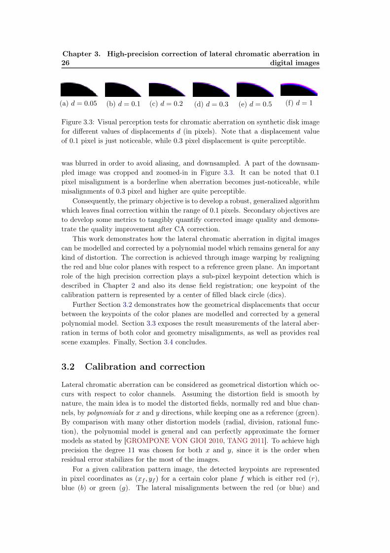
Figure 3.3: Visual perception tests for chromatic aberration on synthetic disk imagefor different values of displacements d (in pixels). Note that a displacement valueof 0.1 pixel is just noticeable, while 0.3 pixel displacement is quite perceptible.
was blurred in order to avoid aliasing, and downsampled. A part of the downsam-pled image was cropped and zoomed-in in Figure 3.3. It can be noted that 0.1
pixel misalignment is a borderline when aberration becomes just-noticeable, whilemisalignments of 0.3 pixel and higher are quite perceptible.
Consequently, the primary objective is to develop a robust, generalized algorithmwhich leaves final correction within the range of 0.1 pixels. Secondary objectives areto develop some metrics to tangibly quantify corrected image quality and demons-trate the quality improvement after CA correction.
This work demonstrates how the lateral chromatic aberration in digital imagescan be modelled and corrected by a polynomial model which remains general for anykind of distortion. The correction is achieved through image warping by realigningthe red and blue color planes with respect to a reference green plane. An importantrole of the high precision correction plays a sub-pixel keypoint detection which isdescribed in Chapter 2 and also its dense field registration; one keypoint of thecalibration pattern is represented by a center of filled black circle (dics).
Further Section 3.2 demonstrates how the geometrical displacements that occurbetween the keypoints of the color planes are modelled and corrected by a generalpolynomial model. Section 3.3 exposes the result measurements of the lateral aber-ration in terms of both color and geometry misalignments, as well as provides realscene examples. Finally, Section 3.4 concludes.
3.2 Calibration and correction
Lateral chromatic aberration can be considered as geometrical distortion which oc-curs with respect to color channels. Assuming the distortion field is smooth bynature, the main idea is to model the distorted fields, normally red and blue chan-nels, by polynomials for x and y directions, while keeping one as a reference (green).By comparison with many other distortion models (radial, division, rational func-tion), the polynomial model is general and can perfectly approximate the formermodels as stated by [GROMPONE VON GIOI 2010, TANG 2011]. To achieve highprecision the degree 11 was chosen for both x and y, since it is the order whenresidual error stabilizes for the most of the images.
For a given calibration pattern image, the detected keypoints are representedin pixel coordinates as (xf , yf ) for a certain color plane f which is either red (r),blue (b) or green (g). The lateral misalignments between the red (or blue) and
3.2. Calibration and correction 27
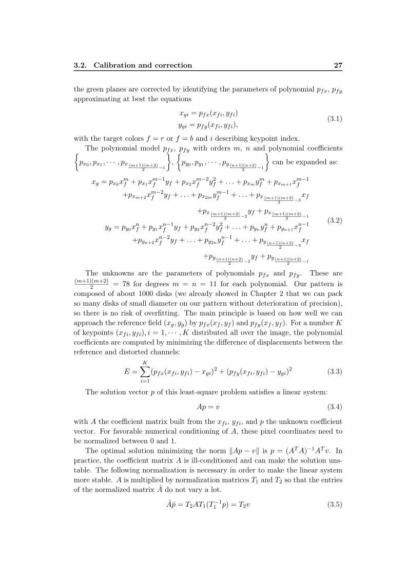
the green planes are corrected by identifying the parameters of polynomial pfx, pfyapproximating at best the equations
xgi = pfx(xfi, yfi)
ygi = pfy(xfi, yfi),(3.1)
with the target colors f = r or f = b and i describing keypoint index.The polynomial model pfx, pfy with orders m, n and polynomial coefficients{
px0 , px1 , · · · , px (m+1)(m+2)2 −1
},{py0 , py1 , · · · , py (n+1)(n+2)
2 −1
}can be expanded as:
xg = px0xmf + px1x
m−1f yf + px2x
m−2f y2f + . . .+ pxmy
mf + pxm+1x
m−1f
+pxm+2xm−2f yf + . . .+ px2my
m−1f + . . .+ px (m+1)(m+2)
2 −3xf
+px (m+1)(m+2)2 −2
yf + px (m+1)(m+2)2 −1
yg = py0xnf + py1x
n−1f yf + py2x
n−2f y2f + . . .+ pyny
nf + pyn+1x
n−1f
+pyn+2xn−2f yf + . . .+ py2ny
n−1f + . . .+ py (n+1)(n+2)
2 −3xf
+py (n+1)(n+2)2 −2
yf + py (n+1)(n+2)2 −1
(3.2)
The unknowns are the parameters of polynomials pfx and pfy. These are(m+1)(m+2)
2 = 78 for degrees m = n = 11 for each polynomial. Our pattern iscomposed of about 1000 disks (we already showed in Chapter 2 that we can packso many disks of small diameter on our pattern without deterioration of precision),so there is no risk of overfitting. The main principle is based on how well we canapproach the reference field (xg, yg) by pfx(xf , yf ) and pfy(xf , yf ). For a number Kof keypoints (xfi, yfi), i = 1, · · · ,K distributed all over the image, the polynomialcoefficients are computed by minimizing the difference of displacements between thereference and distorted channels:
E =
K∑i=1
(pfx(xfi, yfi)− xgi)2 + (pfy(xfi, yfi)− ygi)2 (3.3)
The solution vector p of this least-square problem satisfies a linear system:
Ap = v (3.4)
with A the coefficient matrix built from the xfi, yfi, and p the unknown coefficientvector. For favorable numerical conditioning of A, these pixel coordinates need tobe normalized between 0 and 1.
The optimal solution minimizing the norm ‖Ap − v‖ is p = (ATA)−1AT v. Inpractice, the coefficient matrix A is ill-conditioned and can make the solution uns-table. The following normalization is necessary in order to make the linear systemmore stable. A is multiplied by normalization matrices T1 and T2 so that the entriesof the normalized matrix A do not vary a lot.
Ap = T2AT1(T−11 p) = T2v (3.5)
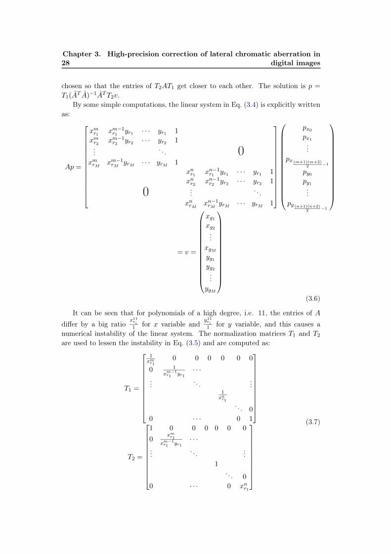
28Chapter 3. High-precision correction of lateral chromatic aberration in
digital images
chosen so that the entries of T2AT1 get closer to each other. The solution is p =
T1(AT A)−1ATT2v.
By some simple computations, the linear system in Eq. (3.4) is explicitly writtenas:
Ap =
xmr1 xm−1r1 yr1 · · · yr1 1
xmr2 xm−1r2 yr2 · · · yr2 1...
. . . 0xmrM xm−1rM
yrM · · · yrM 1
xnr1 xn−1r1 yr1 · · · yr1 1
xnr2 xn−1r2 yr2 · · · yr2 1
0 .... . .
xnrM xn−1rMyrM · · · yrM 1
px0px1...
px (m+1)(m+2)2 −1
py0py1...
py (n+1)(n+2)2 −1
= v =
xg1xg2...
xgMyg1yg2...
ygM
(3.6)
It can be seen that for polynomials of a high degree, i.e. 11, the entries of Adiffer by a big ratio
x11ri1 for x variable and
y11ri1 for y variable, and this causes a
numerical instability of the linear system. The normalization matrices T1 and T2are used to lessen the instability in Eq. (3.5) and are computed as:
T1 =
1xmr1
0 0 0 0 0 0
0 1xm−1r1
yr1· · ·
.... . .
...1xnr1
. . . 0
0 · · · 0 1
T2 =
1 0 0 0 0 0 0
0xmr1
xm−1r1
yr1· · ·
.... . .
...1
. . . 0
0 · · · 0 xnr1
(3.7)
3.3. Experiments 29
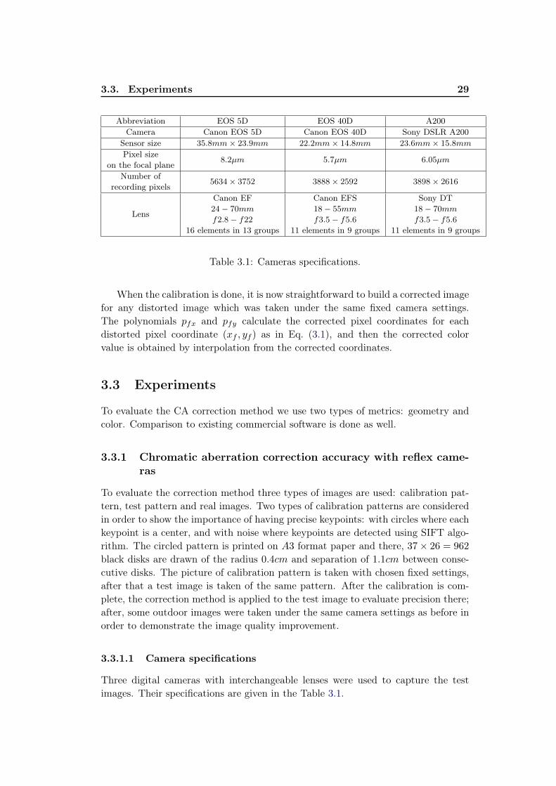
Abbreviation EOS 5D EOS 40D A200Camera Canon EOS 5D Canon EOS 40D Sony DSLR A200
Sensor size 35.8mm× 23.9mm 22.2mm× 14.8mm 23.6mm× 15.8mm
Pixel sizeon the focal plane
8.2µm 5.7µm 6.05µm
Number ofrecording pixels
5634× 3752 3888× 2592 3898× 2616
Lens
Canon EF24− 70mm
f2.8− f22
16 elements in 13 groups
Canon EFS18− 55mm
f3.5− f5.6
11 elements in 9 groups
Sony DT18− 70mm
f3.5− f5.6
11 elements in 9 groups
Table 3.1: Cameras specifications.
When the calibration is done, it is now straightforward to build a corrected imagefor any distorted image which was taken under the same fixed camera settings.The polynomials pfx and pfy calculate the corrected pixel coordinates for eachdistorted pixel coordinate (xf , yf ) as in Eq. (3.1), and then the corrected colorvalue is obtained by interpolation from the corrected coordinates.
3.3 Experiments
To evaluate the CA correction method we use two types of metrics: geometry andcolor. Comparison to existing commercial software is done as well.
3.3.1 Chromatic aberration correction accuracy with reflex came-ras
To evaluate the correction method three types of images are used: calibration pat-tern, test pattern and real images. Two types of calibration patterns are consideredin order to show the importance of having precise keypoints: with circles where eachkeypoint is a center, and with noise where keypoints are detected using SIFT algo-rithm. The circled pattern is printed on A3 format paper and there, 37× 26 = 962
black disks are drawn of the radius 0.4cm and separation of 1.1cm between conse-cutive disks. The picture of calibration pattern is taken with chosen fixed settings,after that a test image is taken of the same pattern. After the calibration is com-plete, the correction method is applied to the test image to evaluate precision there;after, some outdoor images were taken under the same camera settings as before inorder to demonstrate the image quality improvement.
3.3.1.1 Camera specifications
Three digital cameras with interchangeable lenses were used to capture the testimages. Their specifications are given in the Table 3.1.
30Chapter 3. High-precision correction of lateral chromatic aberration in
digital images
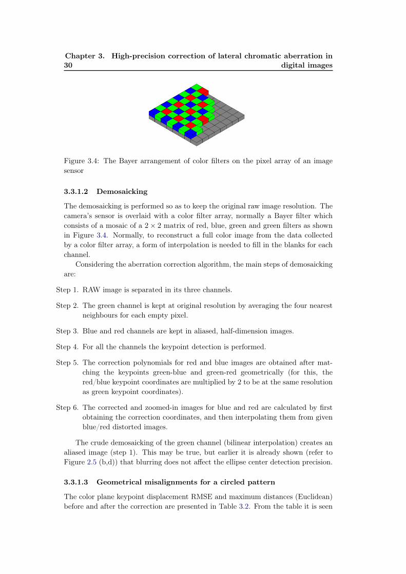
Figure 3.4: The Bayer arrangement of color filters on the pixel array of an imagesensor
3.3.1.2 Demosaicking
The demosaicking is performed so as to keep the original raw image resolution. Thecamera’s sensor is overlaid with a color filter array, normally a Bayer filter whichconsists of a mosaic of a 2× 2 matrix of red, blue, green and green filters as shownin Figure 3.4. Normally, to reconstruct a full color image from the data collectedby a color filter array, a form of interpolation is needed to fill in the blanks for eachchannel.
Considering the aberration correction algorithm, the main steps of demosaickingare:
Step 1. RAW image is separated in its three channels.
Step 2. The green channel is kept at original resolution by averaging the four nearestneighbours for each empty pixel.
Step 3. Blue and red channels are kept in aliased, half-dimension images.
Step 4. For all the channels the keypoint detection is performed.
Step 5. The correction polynomials for red and blue images are obtained after mat-ching the keypoints green-blue and green-red geometrically (for this, thered/blue keypoint coordinates are multiplied by 2 to be at the same resolutionas green keypoint coordinates).
Step 6. The corrected and zoomed-in images for blue and red are calculated by firstobtaining the correction coordinates, and then interpolating them from givenblue/red distorted images.
The crude demosaicking of the green channel (bilinear interpolation) creates analiased image (step 1). This may be true, but earlier it is already shown (refer toFigure 2.5 (b,d)) that blurring does not affect the ellipse center detection precision.
3.3.1.3 Geometrical misalignments for a circled pattern
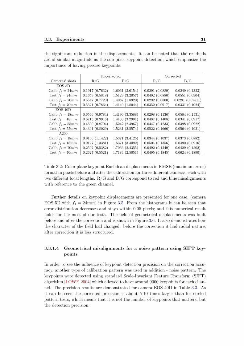
The color plane keypoint displacement RMSE and maximum distances (Euclidean)before and after the correction are presented in Table 3.2. From the table it is seen
3.3. Experiments 31
the significant reduction in the displacements. It can be noted that the residualsare of similar magnitude as the sub-pixel keypoint detection, which emphasize theimportance of having precise keypoints.
Uncorrected CorrectedCameras’ shots R/G B/G R/G B/G
EOS 5DCalib f1 = 24mm
Test f1 = 24mm
Calib f2 = 70mm
Test f2 = 70mm
0.1917 (0.7632)0.1659 (0.5818)0.5547 (0.7720)0.5321 (0.7864)
1.6061 (3.6154)1.5129 (3.2057)1.4087 (1.8920)1.4140 (1.8044)
0.0291 (0.0889)0.0492 (0.0880)0.0292 (0.0800)0.0352 (0.0917)
0.0249 (0.1323)0.0551 (0.0904)0.0291 (0.07511)0.0331 (0.1024)
EOS 40DCalib f1 = 18mm
Test f1 = 18mm
Calib f2 = 55mm
Test f2 = 55mm
0.6546 (0.9784)0.6713 (0.9916)0.4590 (0.8794)0.4391 (0.8029)
1.4190 (3.3588)1.4133 (3.2901)1.5242 (2.4967)1.5231 (2.5574)
0.0298 (0.1136)0.0487 (0.1408)0.0447 (0.1233)0.0522 (0.1666)
0.0584 (0.1531)0.0341 (0.0917)0.0398 (0.0922)0.0564 (0.1921)
A200Calib f1 = 18mm
Test f1 = 18mm
Calib f2 = 70mm
Test f2 = 70mm
0.9106 (1.1422)0.9127 (1.3381)0.2502 (0.5382)0.2627 (0.5521)
1.5371 (3.4125)1.5371 (3.4092)1.7066 (2.4355)1.7184 (2.5051)
0.0344 (0.1037)0.0504 (0.1356)0.0492 (0.1249)0.0495 (0.1845)
0.0373 (0.0882)0.0490 (0.0916)0.0429 (0.1502)0.0624 (0.1890)
Table 3.2: Color plane keypoint Euclidean displacements in RMSE (maximum error)format in pixels before and after the calibration for three different cameras, each withtwo different focal lengths. R/G and B/G correspond to red and blue misalignmentswith reference to the green channel.
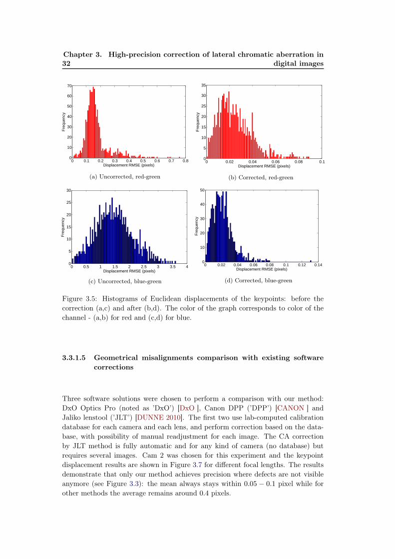
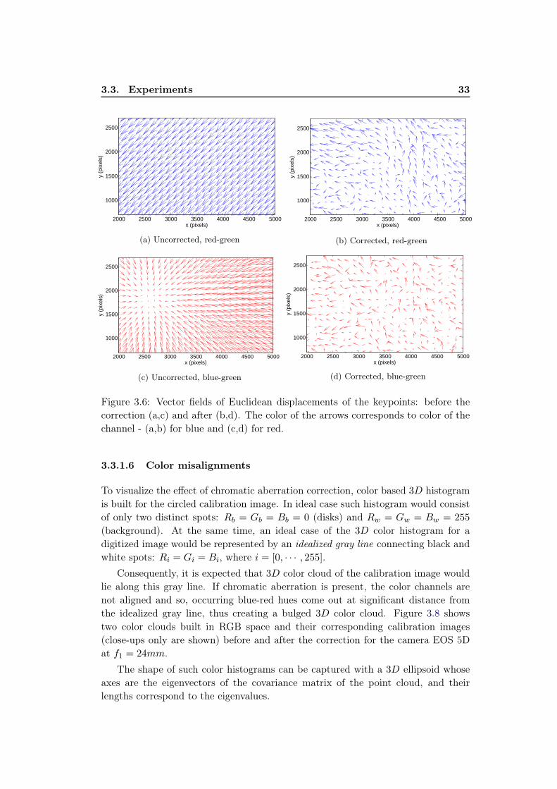
Further details on keypoint displacements are presented for one case, (cameraEOS 5D with f1 = 24mm) in Figure 3.5. From the histograms it can be seen thaterror distribution decreases and stays within 0.05 pixels; and this numerical resultholds for the most of our tests. The field of geometrical displacements was builtbefore and after the correction and is shown in Figure 3.6. It also demonstrates howthe character of the field had changed: before the correction it had radial nature,after correction it is less structured.
3.3.1.4 Geometrical misalignments for a noise pattern using SIFT key-points
In order to see the influence of keypoint detection precision on the correction accu-racy, another type of calibration pattern was used in addition - noise pattern. Thekeypoints were detected using standard Scale-Invariant Feature Transform (SIFT)algorithm [LOWE 2004] which allowed to have around 9000 keypoints for each chan-nel. The precision results are demonstrated for camera EOS 40D in Table 3.3. Asit can be seen the corrected precision is about 5-10 times larger than for circledpattern tests, which means that it is not the number of keypoints that matters, butthe detection precision.
32Chapter 3. High-precision correction of lateral chromatic aberration in
digital images
0 0.1 0.2 0.3 0.4 0.5 0.6 0.7 0.80
10
20
30
40
50
60
70
Displacement RMSE (pixels)
Fre
quen
cy
(a) Uncorrected, red-green
0 0.02 0.04 0.06 0.08 0.10
5
10
15
20
25
30
35
Displacement RMSE (pixels)
Fre
quen
cy
(b) Corrected, red-green
0 0.5 1 1.5 2 2.5 3 3.5 40
5
10
15
20
25
30
Displacement RMSE (pixels)
Fre
quen
cy
(c) Uncorrected, blue-green
0 0.02 0.04 0.06 0.08 0.1 0.12 0.140
10
20
30
40
50
Displacement RMSE (pixels)
Fre
quen
cy
(d) Corrected, blue-green
Figure 3.5: Histograms of Euclidean displacements of the keypoints: before thecorrection (a,c) and after (b,d). The color of the graph corresponds to color of thechannel - (a,b) for red and (c,d) for blue.
3.3.1.5 Geometrical misalignments comparison with existing softwarecorrections
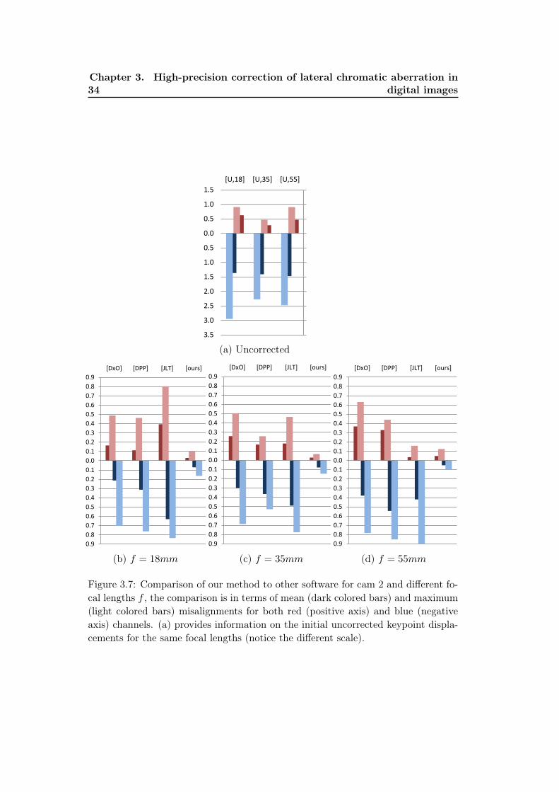
Three software solutions were chosen to perform a comparison with our method:DxO Optics Pro (noted as ’DxO’) [DxO ], Canon DPP (’DPP’) [CANON ] andJaliko lenstool (’JLT’) [DUNNE 2010]. The first two use lab-computed calibrationdatabase for each camera and each lens, and perform correction based on the data-base, with possibility of manual readjustment for each image. The CA correctionby JLT method is fully automatic and for any kind of camera (no database) butrequires several images. Cam 2 was chosen for this experiment and the keypointdisplacement results are shown in Figure 3.7 for different focal lengths. The resultsdemonstrate that only our method achieves precision where defects are not visibleanymore (see Figure 3.3): the mean always stays within 0.05 − 0.1 pixel while forother methods the average remains around 0.4 pixels.
3.3. Experiments 33
2000 2500 3000 3500 4000 4500 5000
1000
1500
2000
2500
x (pixels)
y (p
ixel
s)
(a) Uncorrected, red-green
2000 2500 3000 3500 4000 4500 5000
1000
1500
2000
2500
x (pixels)
y (p
ixel
s)
(b) Corrected, red-green
2000 2500 3000 3500 4000 4500 5000
1000
1500
2000
2500
x (pixels)
y (p
ixel
s)
(c) Uncorrected, blue-green
2000 2500 3000 3500 4000 4500 5000
1000
1500
2000
2500
x (pixels)
y (p
ixel
s)
(d) Corrected, blue-green
Figure 3.6: Vector fields of Euclidean displacements of the keypoints: before thecorrection (a,c) and after (b,d). The color of the arrows corresponds to color of thechannel - (a,b) for blue and (c,d) for red.
3.3.1.6 Color misalignments
To visualize the effect of chromatic aberration correction, color based 3D histogramis built for the circled calibration image. In ideal case such histogram would consistof only two distinct spots: Rb = Gb = Bb = 0 (disks) and Rw = Gw = Bw = 255
(background). At the same time, an ideal case of the 3D color histogram for adigitized image would be represented by an idealized gray line connecting black andwhite spots: Ri = Gi = Bi, where i = [0, · · · , 255].
Consequently, it is expected that 3D color cloud of the calibration image wouldlie along this gray line. If chromatic aberration is present, the color channels arenot aligned and so, occurring blue-red hues come out at significant distance fromthe idealized gray line, thus creating a bulged 3D color cloud. Figure 3.8 showstwo color clouds built in RGB space and their corresponding calibration images(close-ups only are shown) before and after the correction for the camera EOS 5Dat f1 = 24mm.
The shape of such color histograms can be captured with a 3D ellipsoid whoseaxes are the eigenvectors of the covariance matrix of the point cloud, and theirlengths correspond to the eigenvalues.
34Chapter 3. High-precision correction of lateral chromatic aberration in
digital images
3.5
3.0
2.5
2.0
1.5
1.0
0.5
0.0
0.5
1.0
1.5 [U,55] [U,35] [U,18]
0.9 0.8 0.7 0.6 0.5 0.4 0.3 0.2 0.1 0.0 0.1 0.2 0.3 0.4 0.5 0.6 0.7
[DxO] [DPP] [JLT] [ours]
0.9 0.8 0.7 0.6 0.5 0.4 0.3 0.2 0.1 0.0 0.1 0.2 0.3 0.4 0.5 0.6 0.7
[DxO] [DPP] [JLT] [ours]
0.9 0.8 0.7 0.6 0.5 0.4 0.3 0.2 0.1 0.0 0.1 0.2 0.3 0.4 0.5 0.6 0.7
[DxO] [DPP] [JLT] [ours]
(a) Uncorrected
3.5
3.0
2.5
2.0
1.5
1.0
0.5
0.0
0.5
1.0
1.5 [U,55] [U,35] [U,18]
0.9 0.8 0.7 0.6 0.5 0.4 0.3 0.2 0.1 0.0 0.1 0.2 0.3 0.4 0.5 0.6 0.7 0.8 0.9
[DxO] [DPP] [JLT] [ours]
0.9 0.8 0.7 0.6 0.5 0.4 0.3 0.2 0.1 0.0 0.1 0.2 0.3 0.4 0.5 0.6 0.7 0.8 0.9
[DxO] [DPP] [JLT] [ours]
0.9 0.8 0.7 0.6 0.5 0.4 0.3 0.2 0.1 0.0 0.1 0.2 0.3 0.4 0.5 0.6 0.7 0.8 0.9
[DxO] [DPP] [JLT] [ours] (b) f = 18mm
3.5
3.0
2.5
2.0
1.5
1.0
0.5
0.0
0.5
1.0
1.5 [U,55] [U,35] [U,18]
0.9 0.8 0.7 0.6 0.5 0.4 0.3 0.2 0.1 0.0 0.1 0.2 0.3 0.4 0.5 0.6 0.7 0.8 0.9
[DxO] [DPP] [JLT] [ours]
0.9 0.8 0.7 0.6 0.5 0.4 0.3 0.2 0.1 0.0 0.1 0.2 0.3 0.4 0.5 0.6 0.7 0.8 0.9
[DxO] [DPP] [JLT] [ours]
0.9 0.8 0.7 0.6 0.5 0.4 0.3 0.2 0.1 0.0 0.1 0.2 0.3 0.4 0.5 0.6 0.7 0.8 0.9
[DxO] [DPP] [JLT] [ours]
(c) f = 35mm
3.5
3.0
2.5
2.0
1.5
1.0
0.5
0.0
0.5
1.0
1.5 [U,55] [U,35] [U,18]
0.9 0.8 0.7 0.6 0.5 0.4 0.3 0.2 0.1 0.0 0.1 0.2 0.3 0.4 0.5 0.6 0.7 0.8 0.9
[DxO] [DPP] [JLT] [ours]
0.9 0.8 0.7 0.6 0.5 0.4 0.3 0.2 0.1 0.0 0.1 0.2 0.3 0.4 0.5 0.6 0.7 0.8 0.9
[DxO] [DPP] [JLT] [ours]
0.9 0.8 0.7 0.6 0.5 0.4 0.3 0.2 0.1 0.0 0.1 0.2 0.3 0.4 0.5 0.6 0.7 0.8 0.9
[DxO] [DPP] [JLT] [ours]
(d) f = 55mm
Figure 3.7: Comparison of our method to other software for cam 2 and different fo-cal lengths f , the comparison is in terms of mean (dark colored bars) and maximum(light colored bars) misalignments for both red (positive axis) and blue (negativeaxis) channels. (a) provides information on the initial uncorrected keypoint displa-cements for the same focal lengths (notice the different scale).
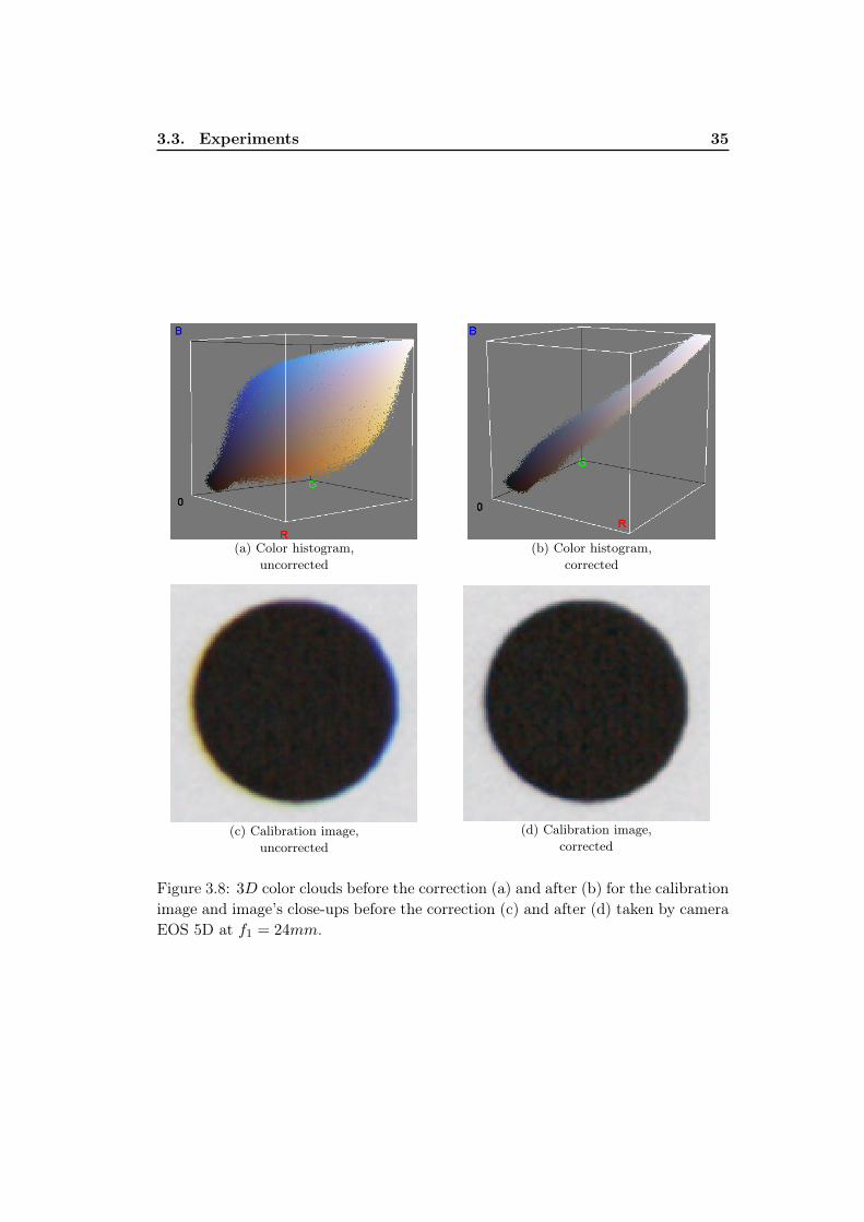
3.3. Experiments 35
(a) Color histogram,uncorrected
(b) Color histogram,corrected
(c) Calibration image,uncorrected
(d) Calibration image,corrected
Figure 3.8: 3D color clouds before the correction (a) and after (b) for the calibrationimage and image’s close-ups before the correction (c) and after (d) taken by cameraEOS 5D at f1 = 24mm.
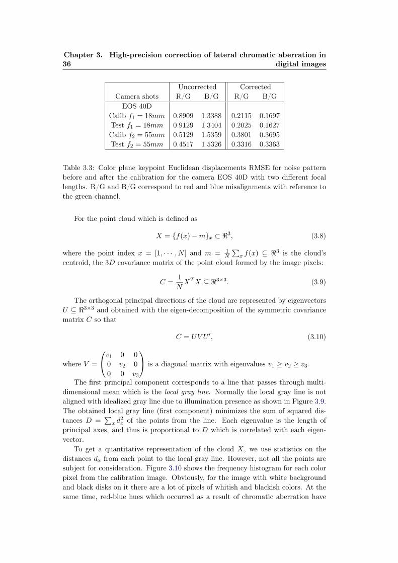
36Chapter 3. High-precision correction of lateral chromatic aberration in
digital images
Uncorrected CorrectedCamera shots R/G B/G R/G B/GEOS 40D
Calib f1 = 18mm
Test f1 = 18mm
Calib f2 = 55mm
Test f2 = 55mm
0.89090.91290.51290.4517
1.33881.34041.53591.5326
0.21150.20250.38010.3316
0.16970.16270.36950.3363
Table 3.3: Color plane keypoint Euclidean displacements RMSE for noise patternbefore and after the calibration for the camera EOS 40D with two different focallengths. R/G and B/G correspond to red and blue misalignments with reference tothe green channel.
For the point cloud which is defined as
X = {f(x)−m}x ⊂ <3, (3.8)
where the point index x = [1, · · · , N ] and m = 1N
∑x f(x) ⊆ <3 is the cloud’s
centroid, the 3D covariance matrix of the point cloud formed by the image pixels:
C =1
NXTX ⊆ <3×3. (3.9)
The orthogonal principal directions of the cloud are represented by eigenvectorsU ⊆ <3×3 and obtained with the eigen-decomposition of the symmetric covariancematrix C so that
C = UV U ′, (3.10)
where V =
v1 0 0
0 v2 0
0 0 v3
is a diagonal matrix with eigenvalues v1 ≥ v2 ≥ v3.
The first principal component corresponds to a line that passes through multi-dimensional mean which is the local gray line. Normally the local gray line is notaligned with idealized gray line due to illumination presence as shown in Figure 3.9.The obtained local gray line (first component) minimizes the sum of squared dis-tances D =
∑x d
2x of the points from the line. Each eigenvalue is the length of
principal axes, and thus is proportional to D which is correlated with each eigen-vector.
To get a quantitative representation of the cloud X, we use statistics on thedistances dx from each point to the local gray line. However, not all the points aresubject for consideration. Figure 3.10 shows the frequency histogram for each colorpixel from the calibration image. Obviously, for the image with white backgroundand black disks on it there are a lot of pixels of whitish and blackish colors. At thesame time, red-blue hues which occurred as a result of chromatic aberration have
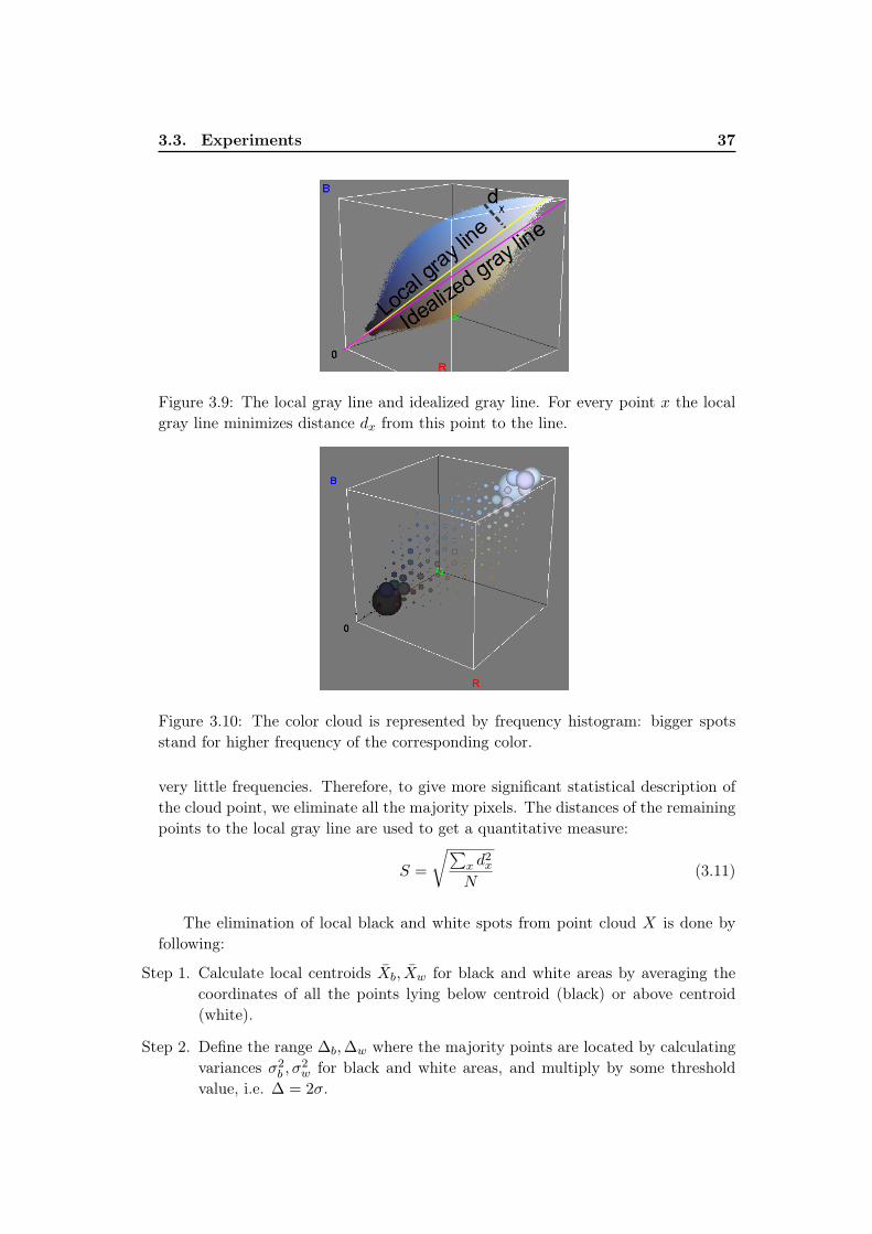
3.3. Experiments 37
Figure 3.9: The local gray line and idealized gray line. For every point x the localgray line minimizes distance dx from this point to the line.
Figure 3.10: The color cloud is represented by frequency histogram: bigger spotsstand for higher frequency of the corresponding color.
very little frequencies. Therefore, to give more significant statistical description ofthe cloud point, we eliminate all the majority pixels. The distances of the remainingpoints to the local gray line are used to get a quantitative measure:
S =
√∑x d
2x
N(3.11)
The elimination of local black and white spots from point cloud X is done byfollowing:
Step 1. Calculate local centroids Xb, Xw for black and white areas by averaging thecoordinates of all the points lying below centroid (black) or above centroid(white).
Step 2. Define the range ∆b,∆w where the majority points are located by calculatingvariances σ2b , σ
2w for black and white areas, and multiply by some threshold
value, i.e. ∆ = 2σ.
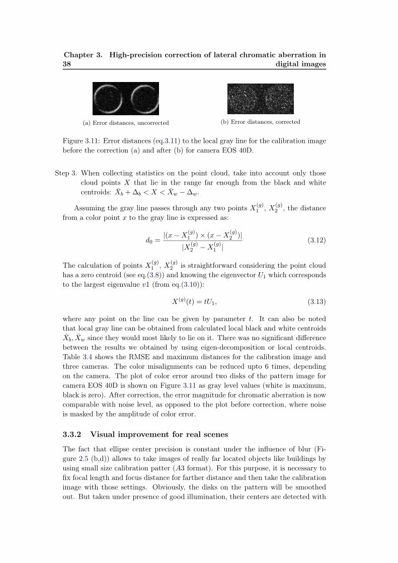
38Chapter 3. High-precision correction of lateral chromatic aberration in
digital images
(a) Error distances, uncorrected (b) Error distances, corrected
Figure 3.11: Error distances (eq.3.11) to the local gray line for the calibration imagebefore the correction (a) and after (b) for camera EOS 40D.
Step 3. When collecting statistics on the point cloud, take into account only thosecloud points X that lie in the range far enough from the black and whitecentroids: Xb + ∆b < X < Xw −∆w.
Assuming the gray line passes through any two points X(g)1 , X(g)
2 , the distancefrom a color point x to the gray line is expressed as:
d0 =|(x−X(g)
1 )× (x−X(g)2 )|
|X(g)2 −X(g)
1 |(3.12)
The calculation of points X(g)1 , X(g)
2 is straightforward considering the point cloudhas a zero centroid (see eq.(3.8)) and knowing the eigenvector U1 which correspondsto the largest eigenvalue v1 (from eq.(3.10)):
X(g)(t) = tU1, (3.13)
where any point on the line can be given by parameter t. It can also be notedthat local gray line can be obtained from calculated local black and white centroidsXb, Xw since they would most likely to lie on it. There was no significant differencebetween the results we obtained by using eigen-decomposition or local centroids.Table 3.4 shows the RMSE and maximum distances for the calibration image andthree cameras. The color misalignments can be reduced upto 6 times, dependingon the camera. The plot of color error around two disks of the pattern image forcamera EOS 40D is shown on Figure 3.11 as gray level values (white is maximum,black is zero). After correction, the error magnitude for chromatic aberration is nowcomparable with noise level, as opposed to the plot before correction, where noiseis masked by the amplitude of color error.
3.3.2 Visual improvement for real scenes
The fact that ellipse center precision is constant under the influence of blur (Fi-gure 2.5 (b,d)) allows to take images of really far located objects like buildings byusing small size calibration patter (A3 format). For this purpose, it is necessary tofix focal length and focus distance for farther distance and then take the calibrationimage with those settings. Obviously, the disks on the pattern will be smoothedout. But taken under presence of good illumination, their centers are detected with
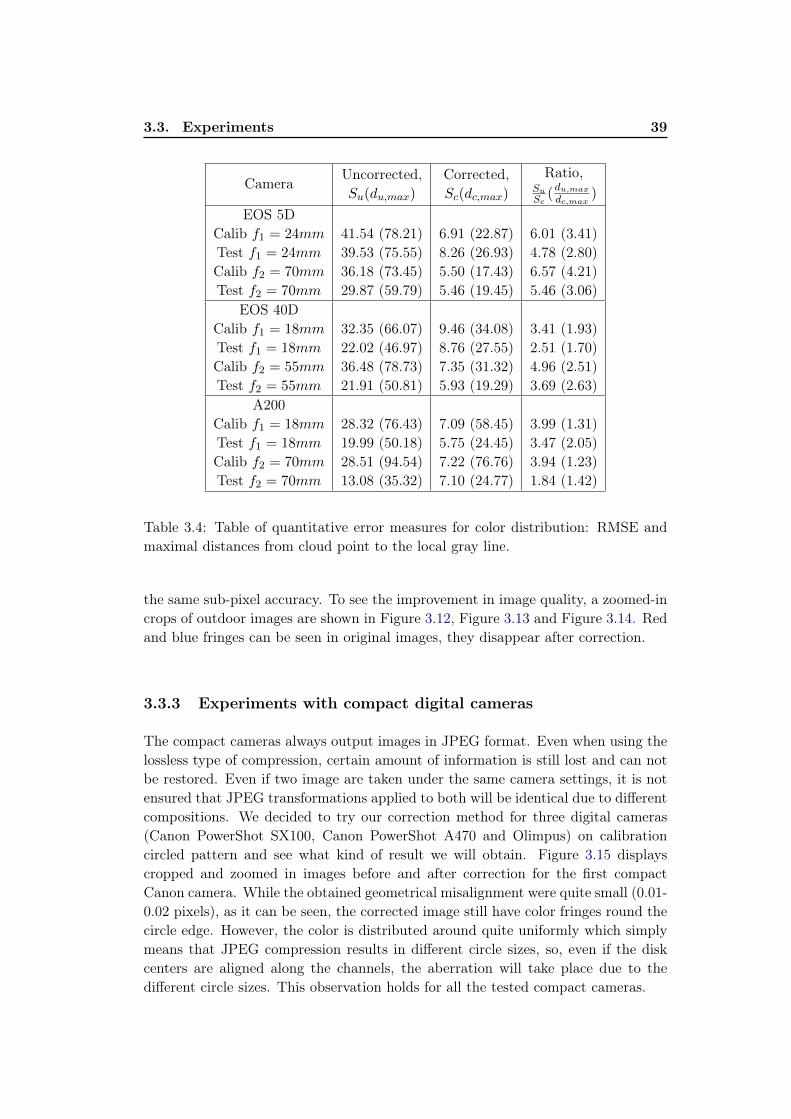
3.3. Experiments 39
CameraUncorrected,Su(du,max)
Corrected,Sc(dc,max)
Ratio,SuSc
(du,max
dc,max)
EOS 5DCalib f1 = 24mm
Test f1 = 24mm
Calib f2 = 70mm
Test f2 = 70mm
41.54 (78.21)39.53 (75.55)36.18 (73.45)29.87 (59.79)
6.91 (22.87)8.26 (26.93)5.50 (17.43)5.46 (19.45)
6.01 (3.41)4.78 (2.80)6.57 (4.21)5.46 (3.06)
EOS 40DCalib f1 = 18mm
Test f1 = 18mm
Calib f2 = 55mm
Test f2 = 55mm
32.35 (66.07)22.02 (46.97)36.48 (78.73)21.91 (50.81)
9.46 (34.08)8.76 (27.55)7.35 (31.32)5.93 (19.29)
3.41 (1.93)2.51 (1.70)4.96 (2.51)3.69 (2.63)
A200Calib f1 = 18mm
Test f1 = 18mm
Calib f2 = 70mm
Test f2 = 70mm
28.32 (76.43)19.99 (50.18)28.51 (94.54)13.08 (35.32)
7.09 (58.45)5.75 (24.45)7.22 (76.76)7.10 (24.77)
3.99 (1.31)3.47 (2.05)3.94 (1.23)1.84 (1.42)
Table 3.4: Table of quantitative error measures for color distribution: RMSE andmaximal distances from cloud point to the local gray line.
the same sub-pixel accuracy. To see the improvement in image quality, a zoomed-incrops of outdoor images are shown in Figure 3.12, Figure 3.13 and Figure 3.14. Redand blue fringes can be seen in original images, they disappear after correction.
3.3.3 Experiments with compact digital cameras
The compact cameras always output images in JPEG format. Even when using thelossless type of compression, certain amount of information is still lost and can notbe restored. Even if two image are taken under the same camera settings, it is notensured that JPEG transformations applied to both will be identical due to differentcompositions. We decided to try our correction method for three digital cameras(Canon PowerShot SX100, Canon PowerShot A470 and Olimpus) on calibrationcircled pattern and see what kind of result we will obtain. Figure 3.15 displayscropped and zoomed in images before and after correction for the first compactCanon camera. While the obtained geometrical misalignment were quite small (0.01-0.02 pixels), as it can be seen, the corrected image still have color fringes round thecircle edge. However, the color is distributed around quite uniformly which simplymeans that JPEG compression results in different circle sizes, so, even if the diskcenters are aligned along the channels, the aberration will take place due to thedifferent circle sizes. This observation holds for all the tested compact cameras.
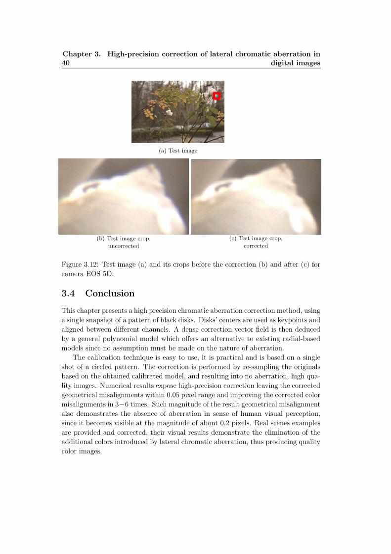
40Chapter 3. High-precision correction of lateral chromatic aberration in
digital images
(a) Test image
(b) Test image crop,uncorrected
(c) Test image crop,corrected
Figure 3.12: Test image (a) and its crops before the correction (b) and after (c) forcamera EOS 5D.
3.4 Conclusion
This chapter presents a high precision chromatic aberration correction method, usinga single snapshot of a pattern of black disks. Disks’ centers are used as keypoints andaligned between different channels. A dense correction vector field is then deducedby a general polynomial model which offers an alternative to existing radial-basedmodels since no assumption must be made on the nature of aberration.
The calibration technique is easy to use, it is practical and is based on a singleshot of a circled pattern. The correction is performed by re-sampling the originalsbased on the obtained calibrated model, and resulting into no aberration, high qua-lity images. Numerical results expose high-precision correction leaving the correctedgeometrical misalignments within 0.05 pixel range and improving the corrected colormisalignments in 3−6 times. Such magnitude of the result geometrical misalignmentalso demonstrates the absence of aberration in sense of human visual perception,since it becomes visible at the magnitude of about 0.2 pixels. Real scenes examplesare provided and corrected, their visual results demonstrate the elimination of theadditional colors introduced by lateral chromatic aberration, thus producing qualitycolor images.

3.4. Conclusion 41
(a) Test image
(b) Test image crop,uncorrected
(c) Test image crop,corrected
Figure 3.13: Test image (a) and its crops before the correction (b) and after (c) forcamera EOS 40D.
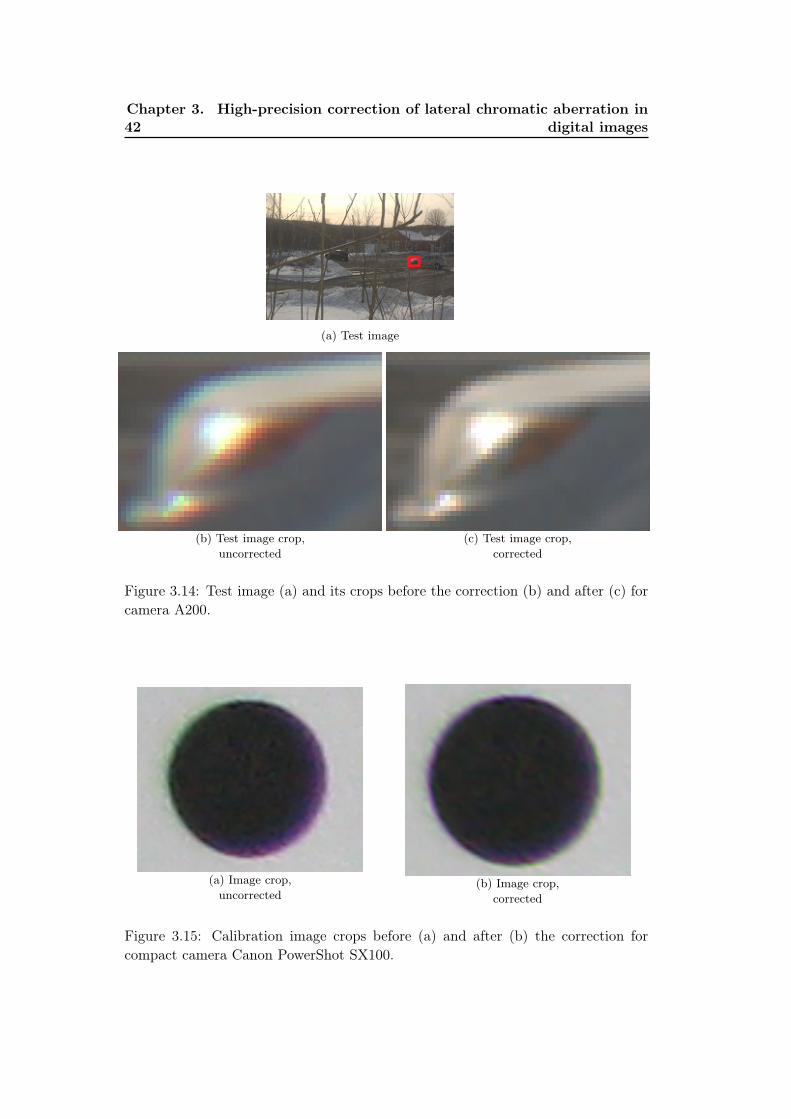
42Chapter 3. High-precision correction of lateral chromatic aberration in
digital images
(a) Test image
(b) Test image crop,uncorrected
(c) Test image crop,corrected
Figure 3.14: Test image (a) and its crops before the correction (b) and after (c) forcamera A200.
(a) Image crop,uncorrected
(b) Image crop,corrected
Figure 3.15: Calibration image crops before (a) and after (b) the correction forcompact camera Canon PowerShot SX100.
Chapter 4
Camera matrix calibration usingcircular control points
Abstract
The precise camera calibration using circular control points is achieved by, firstly,separation the lens distortion parameters from other camera parameters and calcu-lation of the distortion field in advance by using the calibration harp. Secondly, inorder to compensate for perspective bias which is prone to occur when using circledpattern, we incorporate conic affine transformation into minimization error whencalculating the homography, and leave all the other calibration steps as they areused in the literature. Such error function allows to compensate for the perspectivebias. Combined with precise keypoint detection, the approach showed to be morestable than existing state-of-art global calibration method.
Keywords Camera calibration, camera intrinsics, perspective bias, distortionbias, high precision calibration, planar homography, conic-based affine transforma-tion.
Contents4.1 Introduction . . . . . . . . . . . . . . . . . . . . . . . . . . . . 44
4.1.1 Camera calibration workflow . . . . . . . . . . . . . . . . . . 464.1.2 Camera calibration basic steps and equations . . . . . . . . . 46
4.2 Incorporation of conic transform into homography estima-tion as perspective bias compensation . . . . . . . . . . . . . 51
4.2.1 Center of conic’s image vs. image of conic’s center . . . . . . 514.2.2 Recovering homography by conic transform cost function . . 53
4.3 Experiments . . . . . . . . . . . . . . . . . . . . . . . . . . . . 544.3.1 Homography estimation precision . . . . . . . . . . . . . . . . 544.3.2 Calibration matrix stability for synthetic data . . . . . . . . . 564.3.3 Calibration matrix stability for real data . . . . . . . . . . . . 58
4.4 Conclusion . . . . . . . . . . . . . . . . . . . . . . . . . . . . . 60
44 Chapter 4. Camera matrix calibration using circular control points
4.1 Introduction
Camera calibration is the process of finding the true parameters of a camera givenan image (or video), and it is a first step towards computational computer vision.Although some information concerning the measuring of scenes can be obtained byuncalibrated cameras [HARTLEY 1994], calibration is an essential step when metricinformation is required.
During past decades a lot of work had been done on subject of cameracalibration for different kinds of applications – starting from photogrammetry[BROWN 1971, FAIG 1975], and more recent in computer vision, for example,dual space geometry based method [BOUGUET 1998a], flexible technique by[ZHANG 2000], plumb-line method [DEVERNAY 2001], plane-based calibration[STURM 1999, GURDJOS 2003], automatic calibration method by [JIANG 2005],pattern-free method [HARTLEY 2007]. The software packages are provided as well:calibration toolbox by [BOUGUET 1998b] and automatic bundle adjustment cali-bration software [PIERROT DESEILLIGNY 2011]. All of the methods allow ca-mera calibration and 3D scene reconstruction with no or little human interaction.
Naturally, many works in camera calibration have focused especially on achievinghigh calibration accuracy and stability. These studies are mainly based on highprecision control points of either 2D or 3D nature, and the accurate detection oftheir projections. The points are generally constructed on a planar surface by meansof some high contrast pattern. Linear and least-square techniques for calibration arebuilt upon [TSAI 1992] and [WENG 1992] who improve the calibration accuracy bythoroughly modelling lens distortion and further optimising with other parameterstogether.
For a real camera, an image of the calibration pattern is likely to be a subjectof two types of transformations: a projective transformation as a result of relative3D position, and a nonlinear transformation due to various lens distortions. Thecontrol point invariance to errors resulting from these two transformations is basedon combination of the pattern employed, and the detection method used. Therefore,there exist two possible sources of bias in control point recovery which are named[MALLON 2007b]: perspective bias and distortion bias. The main goal would be toobtain bias free data, as this is clearly necessary for obtaining unbiased estimatesfor calibration algorithms.
The most famous planar calibration techniques were presented by [STURM 1999]and [ZHANG 2000]. They only require the camera to observe the pattern shown at afew (at least three) different orientations to get a unique solution up to scale factor.Either the pattern or camera are moved and the motion need not to be known. Thepattern can be printed on a laser printer and attached to planar surface. The methodplaces the world coordinate system on the calibration object and thus require onlyarbitrary scaled 2D coordinates. While trying to eliminate distortion bias duringoptimization, the mentioned works assume that the detected image points have zeromean Gaussian distributions in order to correctly converge to the optimal solution.However, it is not always the case. The bias does not have the same magnitude for
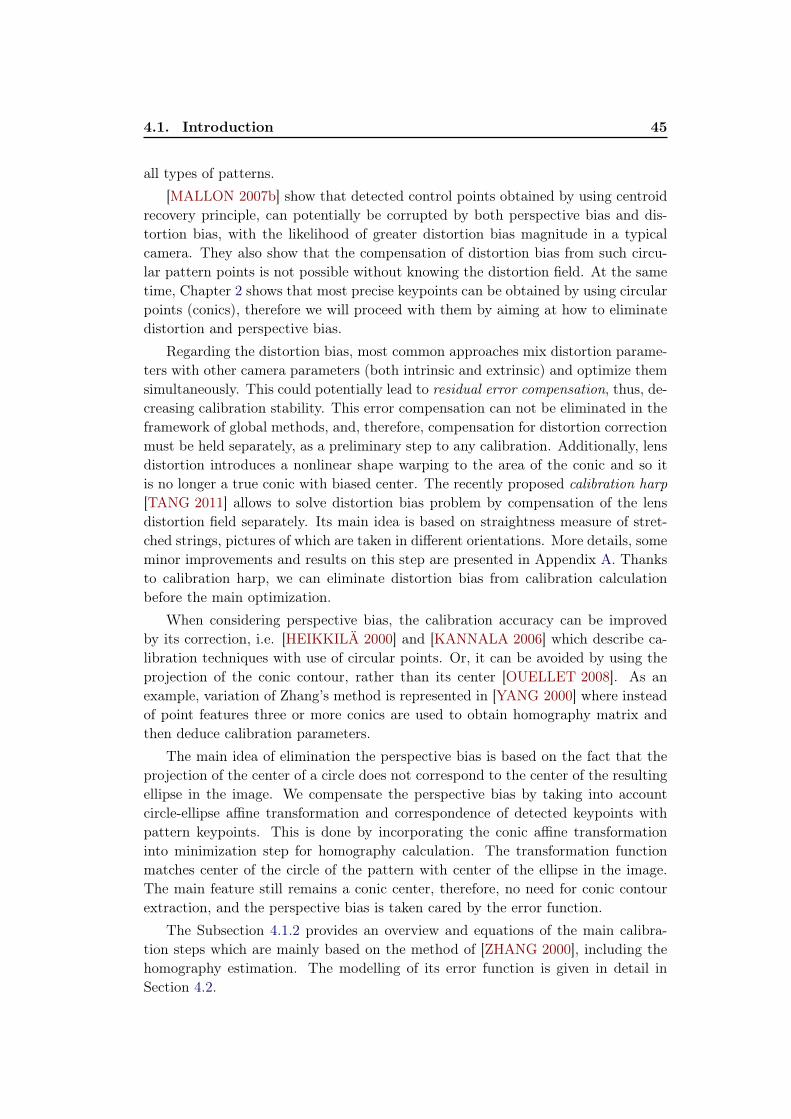
4.1. Introduction 45
all types of patterns.[MALLON 2007b] show that detected control points obtained by using centroid
recovery principle, can potentially be corrupted by both perspective bias and dis-tortion bias, with the likelihood of greater distortion bias magnitude in a typicalcamera. They also show that the compensation of distortion bias from such circu-lar pattern points is not possible without knowing the distortion field. At the sametime, Chapter 2 shows that most precise keypoints can be obtained by using circularpoints (conics), therefore we will proceed with them by aiming at how to eliminatedistortion and perspective bias.
Regarding the distortion bias, most common approaches mix distortion parame-ters with other camera parameters (both intrinsic and extrinsic) and optimize themsimultaneously. This could potentially lead to residual error compensation, thus, de-creasing calibration stability. This error compensation can not be eliminated in theframework of global methods, and, therefore, compensation for distortion correctionmust be held separately, as a preliminary step to any calibration. Additionally, lensdistortion introduces a nonlinear shape warping to the area of the conic and so itis no longer a true conic with biased center. The recently proposed calibration harp[TANG 2011] allows to solve distortion bias problem by compensation of the lensdistortion field separately. Its main idea is based on straightness measure of stret-ched strings, pictures of which are taken in different orientations. More details, someminor improvements and results on this step are presented in Appendix A. Thanksto calibration harp, we can eliminate distortion bias from calibration calculationbefore the main optimization.
When considering perspective bias, the calibration accuracy can be improvedby its correction, i.e. [HEIKKILÄ 2000] and [KANNALA 2006] which describe ca-libration techniques with use of circular points. Or, it can be avoided by using theprojection of the conic contour, rather than its center [OUELLET 2008]. As anexample, variation of Zhang’s method is represented in [YANG 2000] where insteadof point features three or more conics are used to obtain homography matrix andthen deduce calibration parameters.
The main idea of elimination the perspective bias is based on the fact that theprojection of the center of a circle does not correspond to the center of the resultingellipse in the image. We compensate the perspective bias by taking into accountcircle-ellipse affine transformation and correspondence of detected keypoints withpattern keypoints. This is done by incorporating the conic affine transformationinto minimization step for homography calculation. The transformation functionmatches center of the circle of the pattern with center of the ellipse in the image.The main feature still remains a conic center, therefore, no need for conic contourextraction, and the perspective bias is taken cared by the error function.
The Subsection 4.1.2 provides an overview and equations of the main calibra-tion steps which are mainly based on the method of [ZHANG 2000], including thehomography estimation. The modelling of its error function is given in detail inSection 4.2.
46 Chapter 4. Camera matrix calibration using circular control points
Pictures of calibration harp
Correction polynomial
Correct pictures of calibration pattern
Lens distortion correction
Corrected pictures of calibration pattern
Homography with perspective bias compensation
Calibration matrix extractionIntrinsics
calculation
Figure 4.1: Camera calibration workflow: distortion parameters are calculated se-parately from other parameter.
4.1.1 Camera calibration workflow
Figure 4.1 demonstrates the sequence of main calibration steps. From there, itcan be clearly seen the distortion correction phase is performed separately. Thedistortion compensation using calibration harp is explained in Appendix A.
4.1.2 Camera calibration basic steps and equations
We denote a 2D point as m = [u, v]T . A 3D point is denoted by M = [X,Y, Z]T .We use x to indicate the augmented vector by adding 1 as the last element, i.e.,m = [u, v, 1]T and M = [X,Y, Z, 1]T . The camera model is usual pinhole and therelationship between a 3D point M and its image projection m is given by
sm = K[R t
]M, (4.1)
where s is an arbitrary scale factor, (R, t) are the extrinsic parameters (rotationand translation) which relates the world coordinate system to camera coordinatesystem, and K is the intrinsic camera matrix given by
K =
α γ u00 β v00 0 1
, (4.2)
with (u0, v0) being the coordinates of the principal point, α and β the scale factorsin image with respect to u and v axes, and γ the parameter describing the skewnessof the image axes.
4.1. Introduction 47
4.1.2.1 Homography between model plane and its image
The ith column of the rotation matrix R is denoted by ri. Assuming the modelplane is located at Z = 0, we can write (4.1) as
s
uv1
= K[r1 r2 t
] XY1
. (4.3)
Since Z is always equal to zero, the 3D pointM will be denoted asM = [X,Y ]T
and its corresponding M = [X,Y, 1] (same holds form and m). The relation betweenmodel point M and image point m is described by homography H:
sm = HM, (4.4)
or, written more precisely
s
uv1
= H
XY1
, (4.5)
with homography defined up to scale factor
H = K[r1 r2 t
]. (4.6)
4.1.2.2 Estimation of the homography between the model plane and itsimage
The Direct Linear Transform (DLT) algorithm is a simple algorithm used to solvefor the homography matrix H given sufficient number of point correspondences,namely 4 (explained in chapter 4.1 of [HARTLEY 2004]).
We represent matrix H =
h11 h12 h13h21 h22 h23h31 h32 h33
and by dividing the first two rows
of (4.5) by the third row, we get
−h11X − h12Y − h13 + (h31X + h32Y + h33)u = 0
−h21X − h22Y − h23 + (h31X + h32Y + h33)v = 0.(4.7)
Eqs. (4.7) can be written in a matrix form as
Aih = 0,
where Ai =
[−X −Y −1 0 0 0 uX uY u
0 0 0 −X −Y −1 vX vY v
]and h =[
h11 h12 h13 h21 h22 h23 h31 h32 h33]T .
Each point correspondence provides 2 equations, therefore, 4 correspondencesare sufficient to solve for the 8 degrees of freedom of H. The only restrictions is that
48 Chapter 4. Camera matrix calibration using circular control points
no 3 points can be collinear. Four 2× 9 Ai matrices (one for each correspondence)are stacked on top of one another to get an 8× 9 matrix A, or if we deal with morethan four points, the dimension for A will be 2n × 9. The solution space for h isright singular vector of A associated with smallest singular value.
In many cases more that 4 correspondences are used to ensure a more robustsolution. A single and exact solution is possible only if all of the correspondencesare exact, however, in practice there will always be some uncertainty (influence bynoise), so there will be no exact solution. The problem then is to solve for a vectorh that minimizes a chosen cost function.
Normalization. The DLT algorithm result presented above is dependent on theorigin and scale of the coordinate system in the image as shown in chapter 4.4 of[HARTLEY 2004]. This is an undesirable property since it makes the algorithmunstable. The reason for this non-invariance is in how the DLT method uses SVDof A to obtain a solution to the over-determined set of equations Ah = 0 (explainedin detail by [HARTLEY 1997a]). If we deal with exact data and infinite precision,the result is fine, but in the presence of noise the solution typically diverges fromthe correct result.
In order to ensure the numerical accuracy of the solution, [HARTLEY 2004]propose a normalization step. The main steps of DLT algorithm are then:
1. Compute a similarity transform T that takes points Mi to a new set of pointsM ′i such that the centroid of the points M ′i is the coordinate origin and theiraverage distance from origin is
√2.
2. Compute a similar transformation T ′ transforming points mi to m′i.
3. Apply the DLT agorithm from above using M ′i and m′i to obtain homography
matrix H ′
4. Set H = (T ′)−1H ′T .
Precise estimation: dealing with noise. The homography estimation algo-rithm requires a set of correspondence as input. The real data always introducessome noise, therefore, it is necessary to take this into account. The estimate of theparameters is based on maximum likelihood criterion. If Mi and mi are the modeland image points respectively, then they should satisfy (4.4), but they do not for realdata because of the noise in extracted image points. If assume mi is corrupted byGaussian noise with mean 0 and covariance matrix Λmi , then maximum likelihoodestimation of H is obtained by minimizing the following functional∑
i
(mi − mi)TΛ−1mi
(mi − mi), (4.8)
where in the literature mi is estimated as
mi =1
h3TMi
[h1TMi
h2TMi
](4.9)
4.1. Introduction 49
with hi, the ith row of H. Later we will see that (4.9) cannot be applied for circledpattern due to perspective bias, and it will be replaced by applying homography toa conic, rather than to its center.
In practice it is assumed Λmi = σ2I for all i. This is reasonable if points areextracted independently with the same procedure. In this case the problem becomesa non-linear-least-square:
H = arg minH
∑i
‖mi − mi‖2 . (4.10)
The nonlinear minimization is conducted by using Levenberg-Marquardt Algo-rithm [MARQUARDT 1963]. It requires an initial guess which is estimated by DLTalgorithm as shown at the beginning of this sub-section.
4.1.2.3 Constraints on the intrinsic parameters
If we write the homography column-wise as H =[h1 h2 h3
], 4.6 will be[
h1 h2 h3]
= λK[r1 r2 t
], (4.11)
where λ is an arbitrary scale. Using condition that r1 and r2 are orthonormal, weget
hT1K−TK−1h2 = 0
hT1K−TK−1h1 = hT2K
−TK−1h2.(4.12)
Given one homography, these are two basic constraints on the intrinsic parameters.Because a homography has 8 degrees of freedom and there are 6 extrinsic parameters(3 for rotation and 3 for translation), we can only obtain 2 constraints on the intrinsicparameters.
4.1.2.4 Solving camera calibration
Let
B = K−TK−1 =
1α2 − γ
α2βv0γ−u0βα2β
− γα2β
γ2
α2β2 + 1β2 −γ(v0γ−u0β)
α2β2 − v0β2
v0γ−u0βα2β
−γ(v0γ−u0β)α2β2 − v0
β2(v0γ−u0β)2
α2β2 +v20β2 + 1
(4.13)
The matrix B is symmetric and so defined by a 6D vector
b = [B11, B12, B22, B13, B23, B33]T . (4.14)
If we note the ith column vector of H as hi = [h1i, h2i, h3i]T , then we can write
hTi Bhj = vTijb (4.15)
50 Chapter 4. Camera matrix calibration using circular control points
with
vij = [h1ih1j , h1ih2j + h2ih1j , h2ih2j , h3ih1j + h1ih3j , h3ih2j + h2ih3j , h3ih3j ]T .
(4.16)
Then the two fundamental constraints (4.12), from a given homography, can berewritten as 2 homogeneous equations in b:[
vT12(v11 − v22)T
]b = 0. (4.17)
If n images of the model plane are observed, by stacking n such equations as4.17 wehave
V b = 0, (4.18)
where V is a 2n× 6 matrix. If n ≥ 3, then there will be in general a unique solutionb defined up to scale factor. In fact, the solution to (4.18) is well known as theeigenvector of V TV associated with the smallest eigenvalue (or, the right singularvector of V associated with the smallest singular value).
Extraction of intrinsic parameters from matrix B. Once b is estimated, onecan compute all the camera intrinsic parameters, the matrix K. The matrix B isestimated up to a scale factor, i.e., B = λK−TK with λ an arbitrary scale. Theparameters are uniquely extracted as follows:
v0 =B12B13 −B11B23
B11B22 −B212
λ = B33 −B2
13 + v0(B12B13 −B11B23)
B11
α =
√λ
B11
β =
√λB11
B11B22 −B212
γ = −B12α2β
λ
u0 =γv0β− B13α
2
λ.
(4.19)
Extraction of extrinsic parameters. After K is obtained, the extrinsic para-meters for each image are from (4.6) computed as follows:
r1 = λK−1h1
r2 = λK−1h2
r3 = r1 × r2t = λK−1h3
(4.20)
with λ = 1‖K−1h1‖ = 1
‖K−1h2‖ .
4.2. Incorporation of conic transform into homography estimation asperspective bias compensation 51
4.2 Incorporation of conic transform into homographyestimation as perspective bias compensation
When we take a photo of a circle in 3D, it becomes an ellipse in the projectionplane. Both circle and ellipse shapes can be generalized as conics. A general conicis a curve which can be described by a second-degree equation on the plane. In2D projective geometry all non-degenerate conics are equivalent under projectivetransformations. The equation of conics in inhomogeneous coordinates is
s1x2 + s2xy + s3y
2 + s4x+ s5y + s6 = 0 (4.21)
that is, a polynomial of degree 2. When using homogeneous coordinates and repla-cing x→ x1
x3, y → x2
x3, we obtain
s1x21 + s2x1x2 + s3x
22 + s4x1x3 + s5x2x3 + s6x
23 = 0. (4.22)
Using the notations for homogeneous coordinates M = [X,Y, 1]T and settingX = x1and Y = x2, the matrix form of conics is
MTSM = 0, (4.23)
where the conic coefficient matrix S is given by
S =
s1 s2/2 s4/2
s2/2 s3 s5/2
s4/2 s5/2 s6
. (4.24)
The conic coefficient matrix is always symmetric and matrix S is its homogeneousrepresentation.
Transformation of conics. Under a point transformation (4.4), (4.23) becomes
mTH−TSH−1m = 0 (4.25)
so the transformed conic or image of conic S is the conic
H(S) = H−TSH−1. (4.26)
4.2.1 Center of conic’s image vs. image of conic’s center
Given (4.23) of a conic in homogeneous coordinates with S a 3×3 symmetric matrix,let’s define its center by operator
C(S) = −S−12×2S3, (4.27)
with S2×2 the top left 2× 2 block of S and S3 the 2× 1 top part of its last column:
S =
(S2×2 S3ST3 λ
). (4.28)
For conic S we can compute its image H(S) as in (4.26) and now we wish tocompare image of conic center HC(S) and center of image conic CH(S). We willsee it will not be the same point and the difference will be quantified.
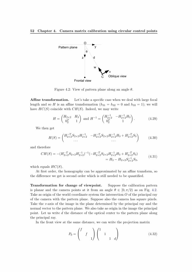
52 Chapter 4. Camera matrix calibration using circular control points
Pattern planeq
y
z
C
v
w
d
O
Frontal view
Oblique view
Figure 4.2: View of pattern plane along an angle θ.
Affine transformation. Let’s take a specific case when we deal with large focallength and so H is an affine transformation (h31 = h32 = 0 and h33 = 1); we willhave HC(S) coincide with CH(S). Indeed, we may write
H =
(H2×2 H3
0T2 1
)and H−1 =
(H−12×2 −H−12×2H3
0T2 1
). (4.29)
We then get
H(S) =
(H−T2×2S2×2H
−12×2 −H−T2×2S2×2H
−12×2H3 +H−T2×2S3
. . . . . .
)(4.30)
and therefore
CH(S) = −(H−T2×2S2×2H−12×2)
−1(−H−T2×2S2×2H−12×2H3 +H−T2×2S3)
= H3 −H2×2S−12×2S3,
(4.31)
which equals HC(S).At first order, the homography can be approximated by an affine transform, so
the difference we get is second order which is still needed to be quantified.
Transformation for change of viewpoint. Suppose the calibration patternis planar and the camera points at it from an angle θ ∈ [0, π/2) as on Fig. 4.2.Take as origin of the world coordinate system the intersection O of the principal rayof the camera with the pattern plane. Suppose also the camera has square pixels.Take the v-axis of the image in the plane determined by the principal ray and thenormal vector to the pattern plane. We also take as origin in the image the principalpoint. Let us write d the distance of the optical center to the pattern plane alongthe principal ray.
In the front view at the same distance, we can write the projection matrix
P0 =
f f
1
1
1
1 d
(4.32)
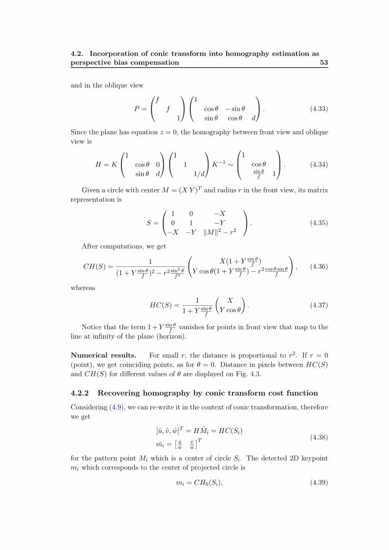
4.2. Incorporation of conic transform into homography estimation asperspective bias compensation 53
and in the oblique view
P =
f f
1
1
cos θ − sin θ
sin θ cos θ d
. (4.33)
Since the plane has equation z = 0, the homography between front view and obliqueview is
H = K
1
cos θ 0
sin θ d
1
1
1/d
K−1 ∼
1
cos θsin θf 1
. (4.34)
Given a circle with centerM = (X Y )T and radius r in the front view, its matrixrepresentation is
S =
1 0 −X0 1 −Y−X −Y ‖M‖2 − r2
. (4.35)
After computations, we get
CH(S) =1
(1 + Y sin θf )2 − r2 sin2 θ
f2
(X(1 + Y sin θ
f )
Y cos θ(1 + Y sin θf )− r2 cos θ sin θf
), (4.36)
whereas
HC(S) =1
1 + Y sin θf
(X
Y cos θ
). (4.37)
Notice that the term 1 +Y sin θf vanishes for points in front view that map to the
line at infinity of the plane (horizon).
Numerical results. For small r, the distance is proportional to r2. If r = 0
(point), we get coinciding points, as for θ = 0. Distance in pixels between HC(S)
and CH(S) for different values of θ are displayed on Fig. 4.3.
4.2.2 Recovering homography by conic transform cost function
Considering (4.9), we can re-write it in the context of conic transformation, thereforewe get
[u, v, w]T = HMi = HC(Si)
mi =[uw
vw
]T (4.38)
for the pattern point Mi which is a center of circle Si. The detected 2D keypointmi which corresponds to the center of projected circle is
mi = CH0(Si), (4.39)
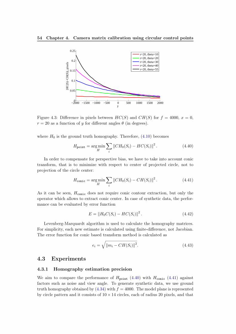
54 Chapter 4. Camera matrix calibration using circular control points
−2000 −1500 −1000 −500 0 500 1000 1500 20000
0.05
0.1
0.15
0.2
0.25
y
|HC
(S)−
CH
(S)|
, pix
els
r=20, theta=10r=20, theta=20r=20, theta=30r=20, theta=40r=20, theta=55
Figure 4.3: Difference in pixels between HC(S) and CH(S) for f = 4000, x = 0,r = 20 as a function of y for different angles θ (in degrees).
where H0 is the ground truth homography. Therefore, (4.10) becomes
Hpoint = arg minH
∑i
‖CH0(Si)−HC(Si)‖2 . (4.40)
In order to compensate for perspective bias, we have to take into account conictransform, that is to minimize with respect to center of projected circle, not toprojection of the circle center:
Hconic = arg minH
∑i
‖CH0(Si)− CH(Si)‖2 . (4.41)
As it can be seen, Hconic does not require conic contour extraction, but only theoperator which allows to extract conic center. In case of synthetic data, the perfor-mance can be evaluated by error function
E = ‖H0C(Si)−HC(Si)‖2 . (4.42)
Levenberg-Marquardt algorithm is used to calculate the homography matrices.For simplicity, each new estimate is calculated using finite-difference, not Jacobian.The error function for conic based transform method is calculated as
ei =
√‖mi − CH(Si)‖2. (4.43)
4.3 Experiments
4.3.1 Homography estimation precision
We aim to compare the performance of Hpoint (4.40) with Hconic (4.41) againstfactors such as noise and view angle. To generate synthetic data, we use groundtruth homography obtained by (4.34) with f = 4000. The model plane is representedby circle pattern and it consists of 10× 14 circles, each of radius 20 pixels, and that
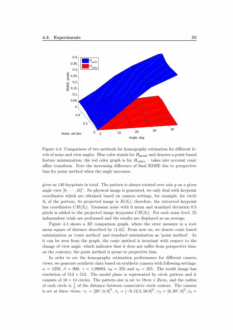
4.3. Experiments 55
0 10 20 30 400
0.2
0.4
0
0.05
0.1
0.15
0.2
0.25
0.3
0.35
0.4
Angle, degNoise, std dev
RM
SE
, pix
els
Hpoint
Hconic
Figure 4.4: Comparison of two methods for homography estimation for different le-vels of noise and view angles. Blue color stands for Hpoint and denotes a point-basedfeature minimization; the red color graph is for Hconic – takes into account conicaffine transform. Note the increasing difference of final RMSE due to perspectivebias for point method when the angle increases.
gives us 140 keypoints in total. The pattern is always rotated over axis y on a givenangle view [0, · · · , 45]◦. No physical image is generated, we only deal with keypointcoordinates which are obtained based on camera settings, for example, for circleSi of the pattern, its projected image is H(Si), therefore, the extracted keypointhas coordinates CH(Si). Gaussian noise with 0 mean and standard deviation 0.5
pixels is added to the projected image keypoints CH(Si). For each noise level, 25independent trials are performed and the results are displayed as an average.
Figure 4.4 shows a 3D comparison graph, where the error measure is a rootmean square of distance described by (4.42). From now on, we denote conic basedminimization as ’conic method’ and standard minimization as ’point method’. Asit can be seen from the graph, the conic method is invariant with respect to thechange of view angle, which indicates that it does not suffer from perspective bias;on the contrary, the point method is prone to perpective bias.
In order to see the homography estimation performance for different cameraviews, we generate synthetic data based on synthetic camera with following settings:α = 1250, β = 900, γ = 1.09083, u0 = 255 and v0 = 255. The result image hasresolution of 512 × 512. The model plane is represented by circle pattern and itconsists of 10 × 14 circles. The pattern size is set to 18cm × 25cm, and the radiusof each circle is 1
3 of the distance between consecutive circle centers. The camerais set at three views: r1 = [20◦, 0, 0]T , t1 = [−9, 12.5, 50.0]T , r2 = [0, 20◦, 0]T , t2 =
56 Chapter 4. Camera matrix calibration using circular control points
[−9,−12.5, 51.0]T , r3 = 1√5[−30◦,−30◦,−15◦]T , t3 = [−10.5,−12.5, 52.5]T . The
estimated homographies are compared to the ground truth which is obtained as in(4.6). The noise level varies from 0 to 1 pixels. For each noise level, 25 independenttrials are performed, and the results are displayed as average in Figure 4.5. It canbe seen from the graph that homography matrix which takes into account conictransform is closer to ground truth (smaller residual) since it allows compensationfor perspective bias.
4.3.2 Calibration matrix stability for synthetic data
Pattern and camera views synthesis The image resolution is set to 1296×864
pixels. The number of circles is 10× 14, each of radius 1cm, and consecutive circleshave 3cm separation between each other. The pattern has resolution 42cm× 30cm.The synthetic camera has following parameters: α = 1250, β = 1250, γ = 1.09083,u0 = 648, v0 = 432. For the high quality images, we firstly generate high resolutionpattern image and then subject it to the geometric displacement (all distortionis eliminated), Gaussian blurring and then down-sampling to the image resolution.Geometric image re-sampling is carried out by mapping from the transformed imageto the original pattern. This involves calculating for every pixel in the transformedimage, the corresponding pixel coordinate in the original image, which requires aninverse mapping. The transformed image intensity is then calculated based on thestandard linear interpolation around the corresponding coordinate of the originalpattern.
Pattern positioning In order to test calibration matrix stability, we generated5 sets of images, each set included 5 images (different views on the pattern). Thisallows to extract 5 calibration matrices so that to see stability of its parametersalong the sets. The generated image views are simulated by using pseudo-randomlygenerated homographies which consist of 3D rotation and translation whose valuesare drawn randomly from a specific range. This range limit ensures that the trans-formed image lies roughly within an image window. Meanwhile, there is alwaysvariance of rotations and translation along the sets. The roation angles always liewhithin the range [15◦,−45◦]. For the re-sampling of the transformed image, aninverse of homography matrices is used.
K matrix stability To compare our method with state-of-art method, we choseSoftware Package for Precise Camera Calibration [HIGUCHI 2012] which is builtupon Matlab Calibration Toolbox [BOUGUET 2000] with the difference that circlepattern can be used for the calibration, plus some minor improvements of the originalsoftware. The generated images are treated as distortion free for both software.Table 4.1 provides the standard deviation results for both methods (we denote state-of-art method as ’SoA’). As we had set both noise and distortion to zero, we canclearly see the improvement in calibration stability based on having more precisehomography matrices for our method.
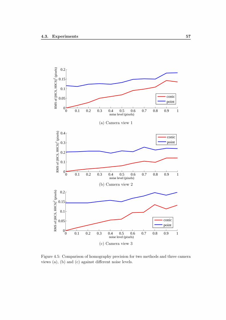
4.3. Experiments 57
0 0.1 0.2 0.3 0.4 0.5 0.6 0.7 0.8 0.9 10
0.05
0.1
0.15
0.2
noise level (pixels)
RM
S of
||H
CS,
H0C
S||2 (
pixe
ls)
conicpoint
(a) Camera view 1
0 0.1 0.2 0.3 0.4 0.5 0.6 0.7 0.8 0.9 10
0.05
0.1
0.15
0.2
noise level (pixels)
RM
S of
||H
CS,
H0C
S||2 (
pixe
ls)
conicpoint
0 0.1 0.2 0.3 0.4 0.5 0.6 0.7 0.8 0.9 10
0.1
0.2
0.3
0.4
noise level (pixels)
RM
S of
||H
CS,
H0C
S||2 (
pixe
ls)
conicpoint
0 0.1 0.2 0.3 0.4 0.5 0.6 0.7 0.8 0.9 10
0.05
0.1
0.15
0.2
noise level (pixels)
RM
S of
||H
CS,
H0C
S||2 (
pixe
ls)
conicpoint
(b) Camera view 2
0 0.1 0.2 0.3 0.4 0.5 0.6 0.7 0.8 0.9 10
0.05
0.1
0.15
0.2
noise level (pixels)
RM
S of
||H
CS,
H0C
S||2 (
pixe
ls)
conicpoint
0 0.1 0.2 0.3 0.4 0.5 0.6 0.7 0.8 0.9 10
0.1
0.2
0.3
0.4
noise level (pixels)
RM
S of
||H
CS,
H0C
S||2 (
pixe
ls)
conicpoint
0 0.1 0.2 0.3 0.4 0.5 0.6 0.7 0.8 0.9 10
0.05
0.1
0.15
0.2
noise level (pixels)
RM
S of
||H
CS,
H0C
S||2 (
pixe
ls)
conicpoint
(c) Camera view 3
Figure 4.5: Comparison of homography precision for two methods and three cameraviews (a), (b) and (c) against different noise levels.
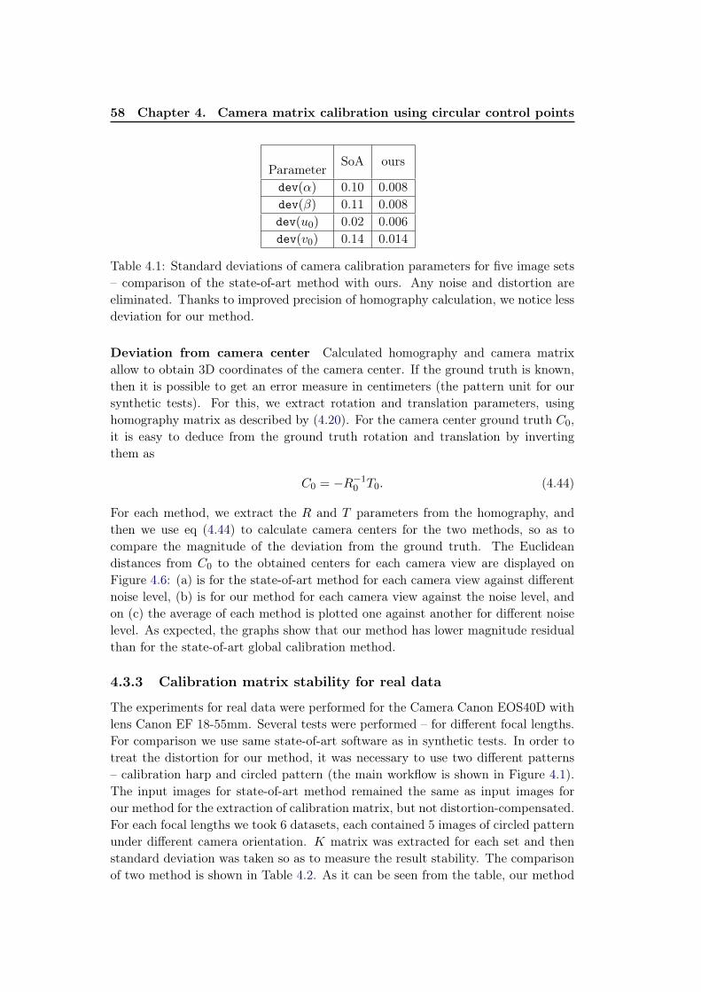
58 Chapter 4. Camera matrix calibration using circular control points
ParameterSoA ours
dev(α) 0.10 0.008dev(β) 0.11 0.008dev(u0) 0.02 0.006dev(v0) 0.14 0.014
Table 4.1: Standard deviations of camera calibration parameters for five image sets– comparison of the state-of-art method with ours. Any noise and distortion areeliminated. Thanks to improved precision of homography calculation, we notice lessdeviation for our method.
Deviation from camera center Calculated homography and camera matrixallow to obtain 3D coordinates of the camera center. If the ground truth is known,then it is possible to get an error measure in centimeters (the pattern unit for oursynthetic tests). For this, we extract rotation and translation parameters, usinghomography matrix as described by (4.20). For the camera center ground truth C0,it is easy to deduce from the ground truth rotation and translation by invertingthem as
C0 = −R−10 T0. (4.44)
For each method, we extract the R and T parameters from the homography, andthen we use eq (4.44) to calculate camera centers for the two methods, so as tocompare the magnitude of the deviation from the ground truth. The Euclideandistances from C0 to the obtained centers for each camera view are displayed onFigure 4.6: (a) is for the state-of-art method for each camera view against differentnoise level, (b) is for our method for each camera view against the noise level, andon (c) the average of each method is plotted one against another for different noiselevel. As expected, the graphs show that our method has lower magnitude residualthan for the state-of-art global calibration method.
4.3.3 Calibration matrix stability for real data
The experiments for real data were performed for the Camera Canon EOS40D withlens Canon EF 18-55mm. Several tests were performed – for different focal lengths.For comparison we use same state-of-art software as in synthetic tests. In order totreat the distortion for our method, it was necessary to use two different patterns– calibration harp and circled pattern (the main workflow is shown in Figure 4.1).The input images for state-of-art method remained the same as input images forour method for the extraction of calibration matrix, but not distortion-compensated.For each focal lengths we took 6 datasets, each contained 5 images of circled patternunder different camera orientation. K matrix was extracted for each set and thenstandard deviation was taken so as to measure the result stability. The comparisonof two method is shown in Table 4.2. As it can be seen from the table, our method
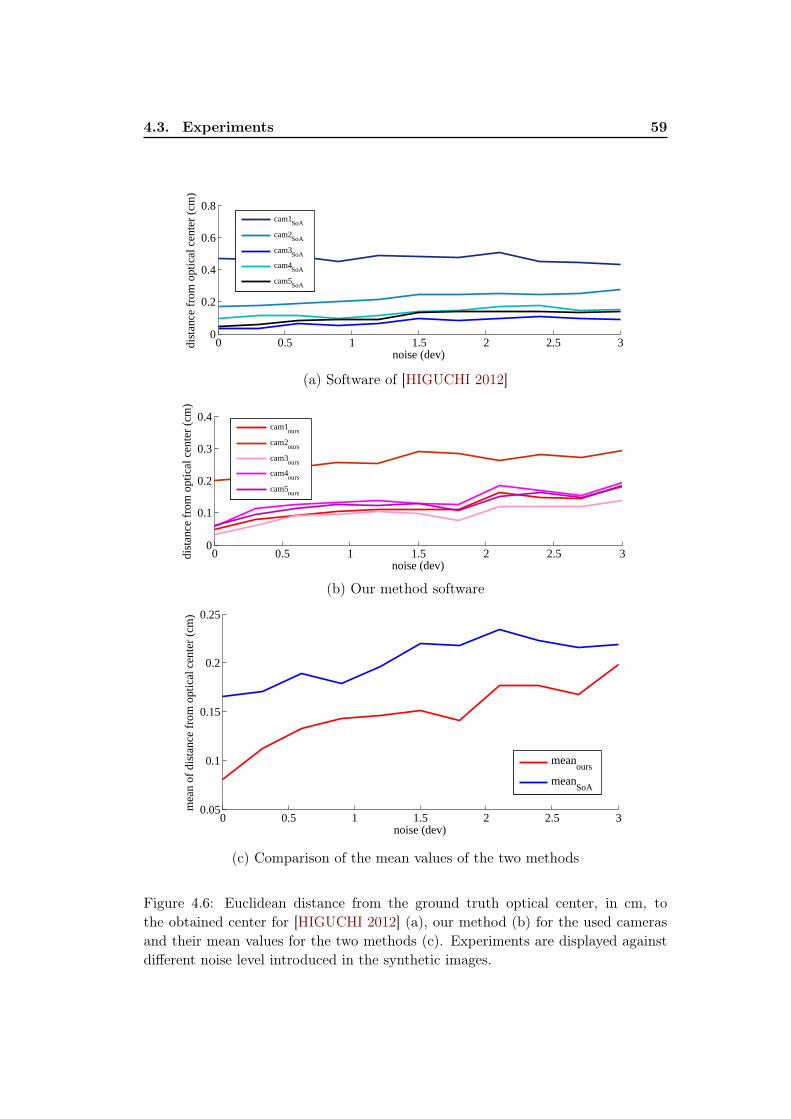
4.3. Experiments 59
0 0.5 1 1.5 2 2.5 30.05
0.1
0.15
0.2
0.25
noise (dev)
mea
n of
dis
tanc
e fr
om o
ptic
al c
ente
r (c
m)
meanours
meanSoA
0 0.5 1 1.5 2 2.5 30
0.1
0.2
0.3
0.4
noise (dev)di
stan
ce f
rom
opt
ical
cen
ter
(cm
)
cam1
ours
cam2ours
cam3ours
cam4ours
cam5ours
0 0.5 1 1.5 2 2.5 30
0.2
0.4
0.6
0.8
noise (dev)
dist
ance
fro
m o
ptic
al c
ente
r (c
m)
cam1SoA
cam2SoA
cam3SoA
cam4SoA
cam5SoA
(a) Software of [HIGUCHI 2012]
0 0.5 1 1.5 2 2.5 30.05
0.1
0.15
0.2
0.25
noise (dev)
mea
n of
dis
tanc
e fr
om o
ptic
al c
ente
r (c
m)
meanours
meanSoA
0 0.5 1 1.5 2 2.5 30
0.1
0.2
0.3
0.4
noise (dev)
dist
ance
fro
m o
ptic
al c
ente
r (c
m)
cam1
ours
cam2ours
cam3ours
cam4ours
cam5ours
0 0.5 1 1.5 2 2.5 30
0.2
0.4
0.6
0.8
noise (dev)
dist
ance
fro
m o
ptic
al c
ente
r (c
m)
cam1SoA
cam2SoA
cam3SoA
cam4SoA
cam5SoA
(b) Our method software
0 0.5 1 1.5 2 2.5 30.05
0.1
0.15
0.2
0.25
noise (dev)
mea
n of
dis
tanc
e fr
om o
ptic
al c
ente
r (c
m)
meanours
meanSoA
0 0.5 1 1.5 2 2.5 30
0.1
0.2
0.3
0.4
noise (dev)
dist
ance
fro
m o
ptic
al c
ente
r (c
m)
cam1
ours
cam2ours
cam3ours
cam4ours
cam5ours
0 0.5 1 1.5 2 2.5 30
0.2
0.4
0.6
0.8
noise (dev)
dist
ance
fro
m o
ptic
al c
ente
r (c
m)
cam1SoA
cam2SoA
cam3SoA
cam4SoA
cam5SoA
(c) Comparison of the mean values of the two methods
Figure 4.6: Euclidean distance from the ground truth optical center, in cm, tothe obtained center for [HIGUCHI 2012] (a), our method (b) for the used camerasand their mean values for the two methods (c). Experiments are displayed againstdifferent noise level introduced in the synthetic images.
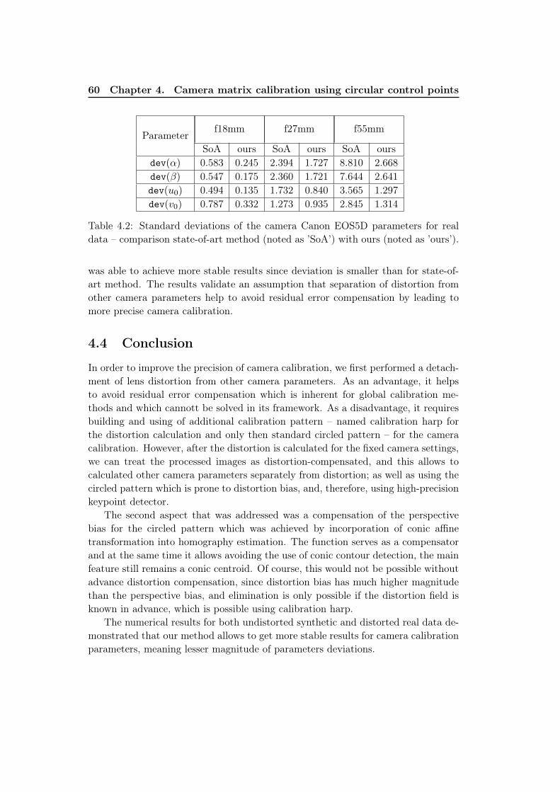
60 Chapter 4. Camera matrix calibration using circular control points
Parameterf18mm f27mm f55mm
SoA ours SoA ours SoA oursdev(α) 0.583 0.245 2.394 1.727 8.810 2.668dev(β) 0.547 0.175 2.360 1.721 7.644 2.641dev(u0) 0.494 0.135 1.732 0.840 3.565 1.297dev(v0) 0.787 0.332 1.273 0.935 2.845 1.314
Table 4.2: Standard deviations of the camera Canon EOS5D parameters for realdata – comparison state-of-art method (noted as ’SoA’) with ours (noted as ’ours’).
was able to achieve more stable results since deviation is smaller than for state-of-art method. The results validate an assumption that separation of distortion fromother camera parameters help to avoid residual error compensation by leading tomore precise camera calibration.
4.4 Conclusion
In order to improve the precision of camera calibration, we first performed a detach-ment of lens distortion from other camera parameters. As an advantage, it helpsto avoid residual error compensation which is inherent for global calibration me-thods and which cannott be solved in its framework. As a disadvantage, it requiresbuilding and using of additional calibration pattern – named calibration harp forthe distortion calculation and only then standard circled pattern – for the cameracalibration. However, after the distortion is calculated for the fixed camera settings,we can treat the processed images as distortion-compensated, and this allows tocalculated other camera parameters separately from distortion; as well as using thecircled pattern which is prone to distortion bias, and, therefore, using high-precisionkeypoint detector.
The second aspect that was addressed was a compensation of the perspectivebias for the circled pattern which was achieved by incorporation of conic affinetransformation into homography estimation. The function serves as a compensatorand at the same time it allows avoiding the use of conic contour detection, the mainfeature still remains a conic centroid. Of course, this would not be possible withoutadvance distortion compensation, since distortion bias has much higher magnitudethan the perspective bias, and elimination is only possible if the distortion field isknown in advance, which is possible using calibration harp.
The numerical results for both undistorted synthetic and distorted real data de-monstrated that our method allows to get more stable results for camera calibrationparameters, meaning lesser magnitude of parameters deviations.
Chapter 5
Thesis conclusions
This thesis had studied precision issues for two problems in internal camera calibra-tion: chromatic aberration correction and camera matrix extraction. Even thoughit could seem both problems are quite fundamental, the precision aspects were notstudied as extensively.
A simple human perception experiment had stated that chromatic aberration inimages is not noticeable if the magnitude of color channel geometric misalignmentis less than 0.1 pixels. This analysis defined our goal precision for the geometricalcolor channel misalignment. At the same time most of the existing approaches usedifferent types of radial polynomial to model the geometrical misalignments that isnot general enough and cannot provide satisfiable correction for all camera types.
For our method, we combine high-precision keypoint detection of the patternplane which was explained in Chapter 2 with the bivariate polynomial of degree11 which serves as a correction model for color plane misalignment. Our methodproved to be the most effective among existing state-of-art software - as a result italways leaves final geometric residual less than 0.1 pixels which was our precisiongoal. The calibration technique itself is easy to use, it is practical and is based ona single shot of circled pattern. It is performed by re-sampling the originals basedon the obtained calibrated model, and as a result it allows to obtain no aberration,high quality images.
We also measured the result images in terms of color metric which is based onthe color distance from local gray line. It was found this distance may decrease 3-6times, depending on the camera type.
Real scenes examples taken by three different reflex cameras are provided, cali-brated and corrected, their visual results demonstrated the elimination of the colorartefacts introduced by lateral chromatic aberration.
Compact digital cameras which can only output images in JPEG format weretested as well. Even though the final geometric misalignment was smaller than 0.1pixels, the method was not efficient in terms of visual evaluation: the disk size forcalibration images taken by a compact camera was different for each color plane,probably, due to compression, therefore, even if the disk centers are aligned, theaberration will take place because of the different disk sizes. From this, we concludethat high precision aberration correction is only possible for RAW images taken byreflex cameras.
One of the future directions could be incorporation and evaluation the precisionof optical flow technique and compare it to the current method performance.
62 Chapter 5. Thesis conclusions
Camera calibration is considered to have been solved since a long time. Theliterature shows a trend towards global camera calibration method from set of images- when optical distortion model is estimated as its part, together with internal andexternal camera parameters in a single minimization step. Even the precision andstability of the extracted parameters had always been considered enough for practicalapplications, it was not possible to measure carefully the precision of each set ofparameters. Moreover, as it was explained, the main drawback of global cameracalibration method is a potential for error compensation.
The solution we used lies in separation of the distortion correction from thecamera calibration to avoid error compensation. For the optical distortion correctionwe used recently developed calibration harp, the main principle of which is describedin Appendix A with some minor improvements.
Another issue which was addressed is how to eliminate perspective bias whenusing circular control points. It was achieved by incorporating of conic affine trans-formation into homography estimation step which matches center of pattern circlewith center of image ellipse, while leaving other calibration steps as it is describedin the literature.
As our experiments showed, the conic transform function allows to obtain moreprecise homography, thus, leading to more stable calibration results. Both syntheticand real experiments showed more stable results for camera calibration which meanssmaller deviation of camera parameters within several sets of images.
The limitation of the proposed method is that we have to deal with two differentcalibration patterns which can lead to incremental error, while global calibrationrequires only one pattern. However, as a result it allows us to directly process theoptical distortion before proceeding to camera calibration and thus avoid residualerror compensation.
As a future work, it would be interesting to expand experimental dataset (forexample, different reflex cameras), and also use a calibration pattern which is notprinted on paper and attached to the wall, but rather glued on aluminium sheet.The later could allow to avoid having non-flat areas which are difficult to avoid usinga paper pattern.
If considering more global future direction, the camera calibration is only onepart of the 3D reconstruction chain in high precision. After internal and externalcamera parameters are extracted, the reconstructed 3D scene can be cross-validatedby registering several 3D point clouds reconstructed from different view images. Suchprecision specification could be a preliminary step to perform 3D points merging.The precision of the obtained data can be compared with precision of the globalcalibration method vs. groundtruth data to check the precision gain using non-global calibration method.
Appendix A
High-precision lens distortioncorrection using calibration harp
The content of this chapter is mainly based on the work of [TANG 2011] and is apreliminary part of calibration process described in Chapter 4. Some minor altera-tions were incorporated in order to improve results, additionally, the method wasimplemented on C++ language.
Keywords Optical distortion, lens distortion, error compensation, plumb lines,polynomial model.
ContentsA.1 Introduction . . . . . . . . . . . . . . . . . . . . . . . . . . . . 64A.2 The harp calibration method . . . . . . . . . . . . . . . . . . 66
A.2.1 Main equations . . . . . . . . . . . . . . . . . . . . . . . . . . 66A.2.2 A solution for the line angle θ . . . . . . . . . . . . . . . . . . 68A.2.3 Simplified minimization for obtaining the polynomial coefficients 69
A.3 Experiments . . . . . . . . . . . . . . . . . . . . . . . . . . . . 72A.3.1 Choice of polynomial degree . . . . . . . . . . . . . . . . . . . 72A.3.2 Real data experiments . . . . . . . . . . . . . . . . . . . . . . 73A.3.3 Measuring distortion correction of global calibration method 74
A.4 Conclusion . . . . . . . . . . . . . . . . . . . . . . . . . . . . . 74
64Appendix A. High-precision lens distortion correction using calibration
harp
A.1 Introduction
When we refer to a notion high precision distortion correction, it is assumed thatresidual error between the camera and its obtained numerical model is far smal-ler than a pixel size. The problem seems to be solved adequately by globalcalibration methods, i.e. flexible pattern based method [ZHANG 2000], plumb-line [DEVERNAY 2001], pattern-free [HARTLEY 2005], dual-spaced geometry ba-sed method [BOUGUET 1998b, BOUGUET 1998a], automatic bundle adjustmentcalibration software [PIERROT DESEILLIGNY 2011], as well as many others[SLAMA 1980, TSAI 1992, WENG 1992, LAVEST 1998] that estimate internal andexternal parameters simultaneously. For example, the [LAVEST 1998] method is ba-sed on measurement the non-flatness of a pattern and results in a remarkably smallreprojection error - 0.02 pixels. For the computer vision goals this precision wouldbe sufficient. Yet, according to a measurement tool of lens distortion correction pre-cision developed by [TANG 2011] which is based on plumb line concept as distortionmeasure, the straightness criterion gives an RMSE as large as 0.2 pixels, which is acontradiction to the obtained 0.02 pixels re-projection accuracy.
This inconsistency have a meaning that, in the global optimization process, errorsin the external and internal camera parameters are being compensated by oppositeerrors in the distortion model. Therefore, an inaccurate distortion model may passundetected since it can not capture the real physical aspect of real lens distortion.Such facts raise an objection to simultaneous estimation of the lens distortion andcamera parameters.
Separation of those parameters one from each other will not only allow to capturethe distortion field more precisely, but will also perform more precise calibration ofexternal parameters like it was shown in Chapter 4 since it can be done indepen-dently from distortion.
Let’s consider the common camera model
C = DKR[I| − T ] (A.1)
with D non linear operator for lens distortion, K calibration matrix, R cameraorientation matrix and vector T the camera optic center in a fixed world frame.Given 3D point is first transformed in the camera-based frame by the translation Tthen rotation R. After, it is projected into the image plane by K, followed by thenon-linear lens distortion D. According to this model, camera calibration consistsof two parts:
• D and K - internal parameters calibration
• R and T - external parameters calibration
The first parameters should remain constant once the camera is fixed in its confi-guration. But in the experiments [TANG 2011] they vary from one test to another,even if the same camera settings were used. Thus, the internal calibration is notalways reusable for the other datasets. And this is a common drawback for many
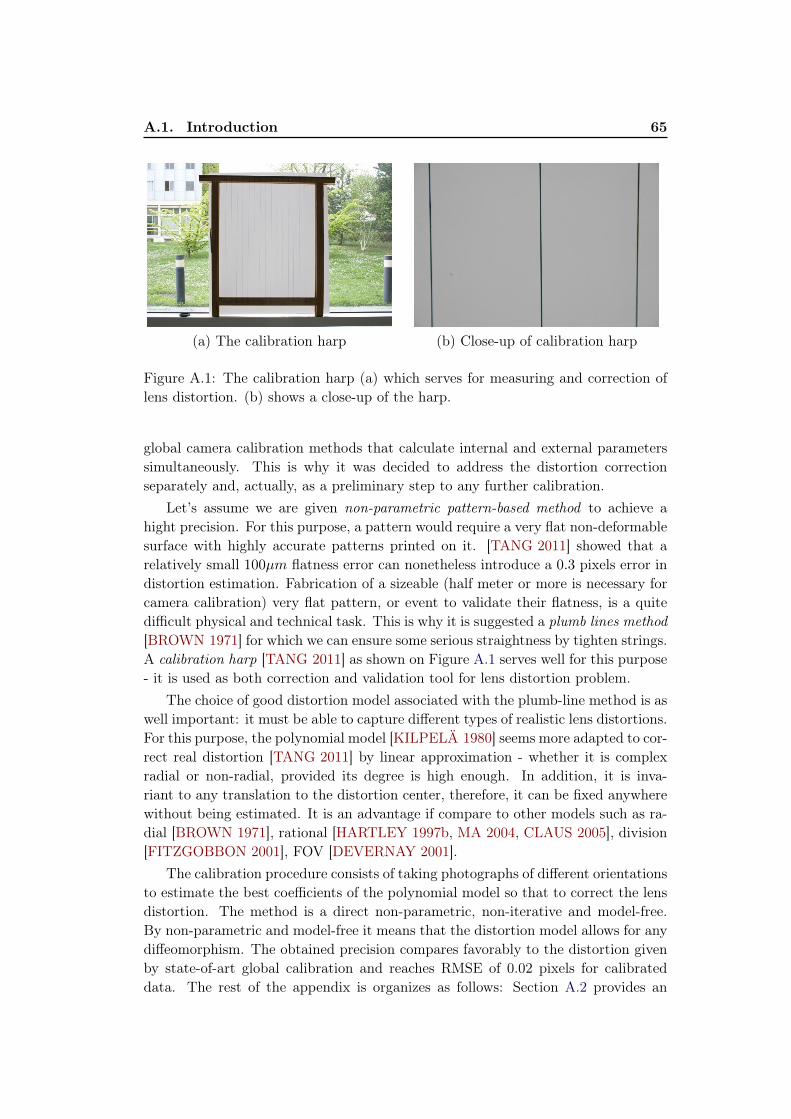
A.1. Introduction 65
(a) The calibration harp (b) Close-up of calibration harp
Figure A.1: The calibration harp (a) which serves for measuring and correction oflens distortion. (b) shows a close-up of the harp.
global camera calibration methods that calculate internal and external parameterssimultaneously. This is why it was decided to address the distortion correctionseparately and, actually, as a preliminary step to any further calibration.
Let’s assume we are given non-parametric pattern-based method to achieve ahight precision. For this purpose, a pattern would require a very flat non-deformablesurface with highly accurate patterns printed on it. [TANG 2011] showed that arelatively small 100µm flatness error can nonetheless introduce a 0.3 pixels error indistortion estimation. Fabrication of a sizeable (half meter or more is necessary forcamera calibration) very flat pattern, or event to validate their flatness, is a quitedifficult physical and technical task. This is why it is suggested a plumb lines method[BROWN 1971] for which we can ensure some serious straightness by tighten strings.A calibration harp [TANG 2011] as shown on Figure A.1 serves well for this purpose- it is used as both correction and validation tool for lens distortion problem.
The choice of good distortion model associated with the plumb-line method is aswell important: it must be able to capture different types of realistic lens distortions.For this purpose, the polynomial model [KILPELÄ 1980] seems more adapted to cor-rect real distortion [TANG 2011] by linear approximation - whether it is complexradial or non-radial, provided its degree is high enough. In addition, it is inva-riant to any translation to the distortion center, therefore, it can be fixed anywherewithout being estimated. It is an advantage if compare to other models such as ra-dial [BROWN 1971], rational [HARTLEY 1997b, MA 2004, CLAUS 2005], division[FITZGOBBON 2001], FOV [DEVERNAY 2001].
The calibration procedure consists of taking photographs of different orientationsto estimate the best coefficients of the polynomial model so that to correct the lensdistortion. The method is a direct non-parametric, non-iterative and model-free.By non-parametric and model-free it means that the distortion model allows for anydiffeomorphism. The obtained precision compares favorably to the distortion givenby state-of-art global calibration and reaches RMSE of 0.02 pixels for calibrateddata. The rest of the appendix is organizes as follows: Section A.2 provides an
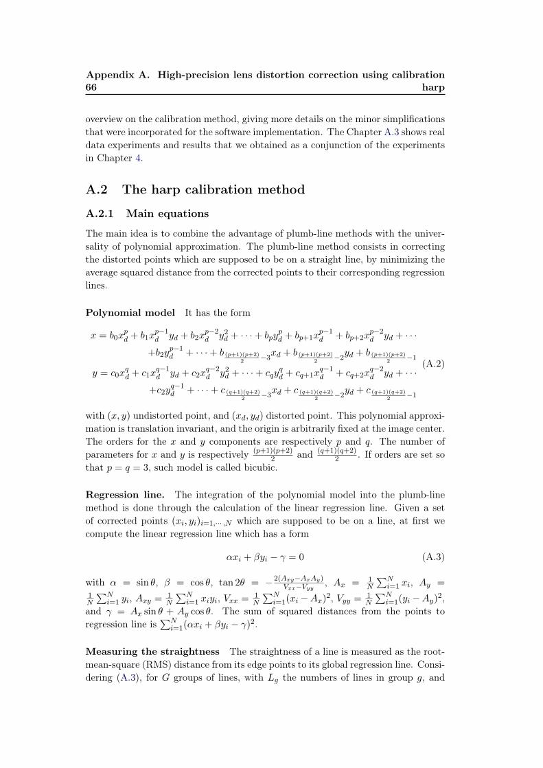
66Appendix A. High-precision lens distortion correction using calibration
harp
overview on the calibration method, giving more details on the minor simplificationsthat were incorporated for the software implementation. The Chapter A.3 shows realdata experiments and results that we obtained as a conjunction of the experimentsin Chapter 4.
A.2 The harp calibration method
A.2.1 Main equations
The main idea is to combine the advantage of plumb-line methods with the univer-sality of polynomial approximation. The plumb-line method consists in correctingthe distorted points which are supposed to be on a straight line, by minimizing theaverage squared distance from the corrected points to their corresponding regressionlines.
Polynomial model It has the form
x = b0xpd + b1x
p−1d yd + b2x
p−2d y2d + · · ·+ bpy
pd + bp+1x
p−1d + bp+2x
p−2d yd + · · ·
+b2yp−1d + · · ·+ b (p+1)(p+2)
2−3xd + b (p+1)(p+2)
2−2yd + b (p+1)(p+2)
2−1
y = c0xqd + c1x
q−1d yd + c2x
q−2d y2d + · · ·+ cqy
qd + cq+1x
q−1d + cq+2x
q−2d yd + · · ·
+c2yq−1d + · · ·+ c (q+1)(q+2)
2−3xd + c (q+1)(q+2)
2−2yd + c (q+1)(q+2)
2−1
(A.2)
with (x, y) undistorted point, and (xd, yd) distorted point. This polynomial approxi-mation is translation invariant, and the origin is arbitrarily fixed at the image center.The orders for the x and y components are respectively p and q. The number ofparameters for x and y is respectively (p+1)(p+2)
2 and (q+1)(q+2)2 . If orders are set so
that p = q = 3, such model is called bicubic.
Regression line. The integration of the polynomial model into the plumb-linemethod is done through the calculation of the linear regression line. Given a setof corrected points (xi, yi)i=1,··· ,N which are supposed to be on a line, at first wecompute the linear regression line which has a form
αxi + βyi − γ = 0 (A.3)
with α = sin θ, β = cos θ, tan 2θ = −2(Axy−AxAy)Vxx−Vyy , Ax = 1
N
∑Ni=1 xi, Ay =
1N
∑Ni=1 yi, Axy = 1
N
∑Ni=1 xiyi, Vxx = 1
N
∑Ni=1(xi −Ax)2, Vyy = 1
N
∑Ni=1(yi −Ay)2,
and γ = Ax sin θ + Ay cos θ. The sum of squared distances from the points toregression line is
∑Ni=1(αxi + βyi − γ)2.
Measuring the straightness The straightness of a line is measured as the root-mean-square (RMS) distance from its edge points to its global regression line. Consi-dering (A.3), for G groups of lines, with Lg the numbers of lines in group g, and
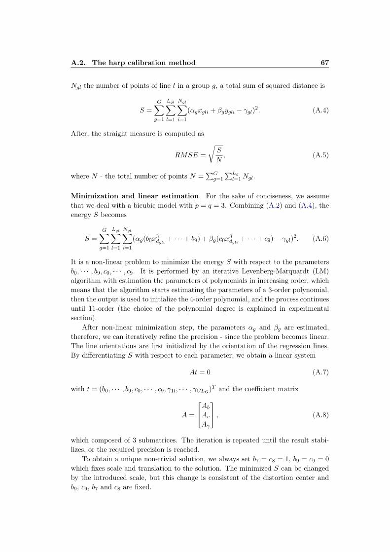
A.2. The harp calibration method 67
Ngl the number of points of line l in a group g, a total sum of squared distance is
S =
G∑g=1
Lgl∑l=1
Ngl∑i=1
(αgxgli + βgygli − γgl)2. (A.4)
After, the straight measure is computed as
RMSE =
√S
N, (A.5)
where N - the total number of points N =∑G
g=1
∑Lg
l=1Ngl.
Minimization and linear estimation For the sake of conciseness, we assumethat we deal with a bicubic model with p = q = 3. Combining (A.2) and (A.4), theenergy S becomes
S =G∑g=1
Lgl∑l=1
Ngl∑i=1
(αg(b0x3dgli
+ · · ·+ b9) + βg(c0x3dgli
+ · · ·+ c9)− γgl)2. (A.6)
It is a non-linear problem to minimize the energy S with respect to the parametersb0, · · · , b9, c0, · · · , c9. It is performed by an iterative Levenberg-Marquardt (LM)algorithm with estimation the parameters of polynomials in increasing order, whichmeans that the algorithm starts estimating the parameters of a 3-order polynomial,then the output is used to initialize the 4-order polynomial, and the process continuesuntil 11-order (the choice of the polynomial degree is explained in experimentalsection).
After non-linear minimization step, the parameters αg and βg are estimated,therefore, we can iteratively refine the precision - since the problem becomes linear.The line orientations are first initialized by the orientation of the regression lines.By differentiating S with respect to each parameter, we obtain a linear system
At = 0 (A.7)
with t = (b0, · · · , b9, c0, · · · , c9, γ1l, · · · , γGLG)T and the coefficient matrix
A =
AbAcAγ
, (A.8)
which composed of 3 submatrices. The iteration is repeated until the result stabi-lizes, or the required precision is reached.
To obtain a unique non-trivial solution, we always set b7 = c8 = 1, b9 = c9 = 0
which fixes scale and translation to the solution. The minimized S can be changedby the introduced scale, but this change is consistent of the distortion center andb9, c9, b7 and c8 are fixed.
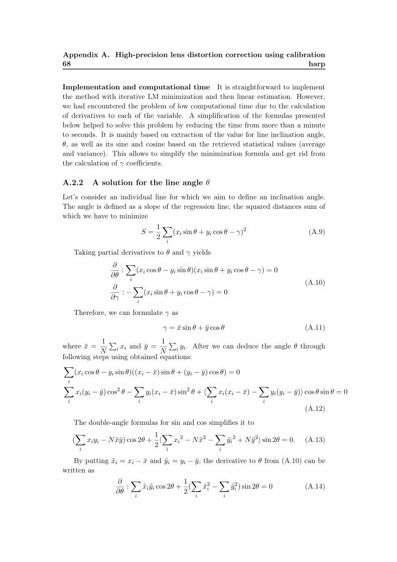
68Appendix A. High-precision lens distortion correction using calibration
harp
Implementation and computational time It is straightforward to implementthe method with iterative LM minimization and then linear estimation. However,we had encountered the problem of low computational time due to the calculationof derivatives to each of the variable. A simplification of the formulas presentedbelow helped to solve this problem by reducing the time from more than a minuteto seconds. It is mainly based on extraction of the value for line inclination angle,θ, as well as its sine and cosine based on the retrieved statistical values (averageand variance). This allows to simplify the minimization formula and get rid fromthe calculation of γ coefficients.
A.2.2 A solution for the line angle θ
Let’s consider an individual line for which we aim to define an inclination angle.The angle is defined as a slope of the regression line, the squared distances sum ofwhich we have to minimize
S =1
2
∑i
(xi sin θ + yi cos θ − γ)2 (A.9)
Taking partial derivatives to θ and γ yields
∂
∂θ:∑i
(xi cos θ − yi sin θ)(xi sin θ + yi cos θ − γ) = 0
∂
∂γ: −∑i
(xi sin θ + yi cos θ − γ) = 0
(A.10)
Therefore, we can formulate γ as
γ = x sin θ + y cos θ (A.11)
where x =1
N
∑i xi and y =
1
N
∑i yi. After we can deduce the angle θ through
following steps using obtained equations:∑i
(xi cos θ − yi sin θ)((xi − x) sin θ + (yi − y) cos θ) = 0∑i
xi(yi − y) cos2 θ −∑i
yi(xi − x) sin2 θ + 〈∑i
xi(xi − x)−∑i
yi(yi − y)〉 cos θ sin θ = 0
(A.12)
The double-angle formulas for sin and cos simplifies it to
(∑i
xiyi −Nxy) cos 2θ +1
2〈∑i
xi2 −Nx2 −
∑i
yi2 +Ny2〉 sin 2θ = 0. (A.13)
By putting xi = xi − x and yi = yi − y, the derivative to θ from (A.10) can bewritten as
∂
∂θ:∑i
xiyi cos 2θ +1
2(∑i
x2i −∑i
y2i ) sin 2θ = 0 (A.14)
A.2. The harp calibration method 69
There are two possible solutions which we denote as θ0 and θ1 and which arerelated as θ1 = θ0 +
π
2, but only one of them that provides a minimum will be of
the interest:
2θ0 = atan2(−2∑i
xiyi,∑i
x2i −∑i
y2i )
2θ1 = atan2(2∑i
xiyi,−(∑i
x2i −∑i
y2i ))(A.15)
To define which of them is a solution, a second derivative to θ is taken:
∂2S
∂θ2= −2
∑i
xiyi sin 2θ + (∑i
x2i∑i
y2i ) cos 2θ
= k sin 2θ0 sin 2θ + k cos 2θ0 cos 2θ = k cos 2(θ − θ0)(A.16)
where k is a normalization constant
k =
∣∣∣∣( ∑i x
2i −
∑i y
2i
−2∑
i xiyi
)∣∣∣∣ , (A.17)
which is always positive k ≥ 0.From (A.16) we can write{
for θ = θ0 we get k(≥ 0)
for θ = θ1 we get − k(≤ 0)(A.18)
The first solution for θ0 represents a minimum in which we are interested in,since the (A.16) is a second derivative and the first solution of (A.15) is an accordingconcave-up. Thus, the only one solution for the line angle
θ =1
2atan2(−2
∑i
xiyi,∑i
x2i −∑i
y2i ) (A.19)
Moreover, by taking into consideration the above notations for x and y, as wellas the (A.11) for γ, now the squared distance sum to minimize, (A.9), will have asimpler look of
S =∑i
(xi sin θ + yi cos θ)2 (A.20)
A.2.3 Simplified minimization for obtaining the polynomial coeffi-cients
For one line with number of points i = 1, · · · , N , given a set of distorted points(xd,i, yd,i) and a set of corresponding corrected points (xi, yi) which are supposed tolie on a linear regression line
αxi + βyi = 0 (A.21)
70Appendix A. High-precision lens distortion correction using calibration
harp
where xi = xi − x, yi = yi − y with x =
∑xiN
and y =
∑yi
N; and α = sin θ,
β = cos θ. The previous subsection gives a description for obtaining an angle θ for
the selected line. We denote Vxx =
∑x2iN
, Vyy =
∑y2iN
, Vxy =
∑xiyiN
and Ax = x
and Ay = y for further simplicity.Supposing, we deal with degree-3 polynomial correction model which is repre-
sented as {xi = b1xc,i
3 + b2xc,i2yc,i + · · ·+ b10 + xc
yi = c1xc,i3 + c2xc,i
2yc,i + · · ·+ c10 + yc(A.22)
where xc,i =xd,i − xc
Sand yc,i =
yd,i − ycS
with (xc, yc) being a center of the imageand S a normalization factor.
The sum of squared distances from the points (xd,i, yd,i) of a line to the corres-ponding regression line is presented as an equation (A.20).
Error Given a set of lines k = 1, · · · ,K, the error vector for LM algorithm isE = (e1e2 · · · eK)T . The root mean square distance ek which represents an error forone line k as in (A.20), is given by
ek =
√∑Ni=1(αxi + βyi)
2
N(A.23)
In the above formula, we have to know what are the constants α and β for eachline which are sine and cosine of the angle θ. It is possible to avoid calculation of theangle itself for simplicity and an advantage in running time by further expansion
ek =
√∑N (α2x2i + β2y2i + 2αβxiyi)
N(A.24)
From the first solution in (A.15), we can deduce the expressions for cosine andsine of the angle 2θ:
cos 2θ =1
cnorm(∑
x2i −∑
y2i ) =Vxx − V yycnorm
sin 2θ = − 2
cnorm
∑xiyi = − 2Vxy
cnorm,
(A.25)
where cnorm =√
(Vxx − Vyy)2 + 4V 2xy is a normalization coefficient.
Applying formulas for double angles cos 2θ = 2 cos2 θ − 1 = 1 − 2sin2θ, we canget an expressions for each constant
α2 = sin2 θ =1
2(1− cos2θ) =
1
2(1− Vxx − Vyy
cnorm)
β2 = cos2 θ =1
2(cos2θ + 1) =
1
2(1 +
Vxx − Vyycnorm
)
αβ = sin θ cos θ =1
2sin 2θ = − Vxy
cnorm.
(A.26)
A.2. The harp calibration method 71
Therefore, using the above expressions, we can expand (A.24) into
ek =
√∑(0.5(1− cos 2θ)x2i + 0.5(cos 2θ + 1)y2i + sin 2θxiyi)
N
=
√1
2((1− Vxx − Vyy
cnorm)Vxx + (1 +
Vxx − Vyycnorm
)Vyy −4V 2
xy
cnorm) =
√1
2〈Vxx + Vyy − cnorm〉
(A.27)
As a result
ek =
√1
2
(Vxx + Vyy −
√(Vxx − Vyy)2 + 4V 2
xy
)(A.28)
Jacobian The Jacobian matrix is determined as a matrix of all first-order par-tial derivatives of the vector function which is unknown parameters in our case(b1, b2, · · · , b10, c1, c2, · · · , c10). For a given line k the general formulation is expres-sed as
∂ek∂•
=1
4ek
∂Vxx∂•
+∂Vyy∂•−
4Vxy∂Vxy∂• + (Vxx − Vyy)(∂Vxx∂• −
∂Vyy∂• )√
(Vxx − Vyy)2 + 4V 2xy
(A.29)
The partial derivatives ∂Vxx∂• , ∂Vyy∂• and ∂Vxy
∂• are calculated as follows:
∂Vxx∂b1
=1
N
∂∑
(xi −Ax)2
∂b1=
1
N
∑2(xi −Ax)(
∂xi∂b1− ∂Ax∂b1
), · · · ,
∂Vyy∂b1
=1
N
∂∑
(yi −Ay)2
∂b1=
1
N
∑2(yi −Ay)(
∂yi∂b1− ∂Ax∂b1
), · · · ,
∂Vxy∂b1
=∂Axy∂b1
−Ay∂Ax∂b1
, · · · , ∂Vxy∂c1
=∂Axy∂c1
−Ax∂Ay∂c1
, · · · .
(A.30)
The partial derivatives ∂xi∂• and ∂yi
∂• are:
∂xi∂b1
= x3c,i,∂xi∂b2
= x2c,iyc,i, · · · ,∂xi∂c1
= 0,∂xi∂c2
= 0, · · · ,
∂yi∂b1
= 0,∂yi∂b2
= 0, · · · , ∂yi∂c1
= x3c,i,∂yi∂c2
= x2c,iyc,i, · · · .(A.31)
So, we just need the partial derivatives of Axy, Ax and Ay with respect to theunknown parameters b1, b2, · · · , b10, c1, c2, · · · , c10:∂Axy∂b1
=1
N
∂∑xiyi
∂b1=
1
N
∑(∂xi∂b1
yi + xi∂yi∂b1
), · · · ,
∂Ax∂b1
=1
N
∂∑xi
∂b1=
1
N
∑ ∂xi∂b1
, · · · , ∂Ay∂b1
=1
N
∂∑yi
∂b1=
1
N
∑ ∂yi∂b1
, · · · .(A.32)
The result Jacobian matrix has a form of
J =
∂e1∂b1
∂e1∂b2
· · · ∂e1∂c1
∂e1∂c2
· · ·∂e2∂b1
∂e2∂b2
· · · ∂e2∂c1
∂e2∂c2
· · ·...
. . .
(A.33)
72Appendix A. High-precision lens distortion correction using calibration
harp
In practice, xc = w2 and yc = h
2 are chosen to be the center of the images,
b1 = 0, b2 = 0, · · · , b8 = 1, b9 = 0, b10 = 0.
c1 = 0, c2 = 0, · · · , c8 = 0, c9 = 1, c10 = 0.(A.34)
b8, b9, b10, c8, c9, c10 are fixed as above and not estimated.
Denormalization As a final step, a normalization procedure must be performed:
b1 ← b1S3 c1 ← c1
S3
b2 ← b2S3 c2 ← c2
S3
b3 ← b3S3 c3 ← c3
S3
b4 ← b4S3 c4 ← c4
S3
b5 ← b5S2 c5 ← c5
S2
......
(A.35)
So, for the new distorted point the correction model is expressed as:{xi = b1(xc,i − xc)3 + b2xc,i − xc2(yc,i − yc) + · · ·+ xc
yi = c1(xc,i − xc)3 + c2xc,i − xc2(yc,i − yc) + · · ·+ yc(A.36)
A.3 Experiments
A.3.1 Choice of polynomial degree
A synthetic test was performed to see how the degree of the polynomial influencesthe obtained precision. We used 8 groups of lines with orientations θ as 10◦, 20◦, 30◦,40◦, 50◦, 60◦, 70◦ and 80◦ to estimate the correction parameters by minimizing S(see (A.20)). We also chose another independent group of lines with orientation 55◦
for verification. The ideal lines are plotted in an image with resolution 1761× 1174
pixels. The sampling step for each line is set to 30 pixels, and the number of sampleson each line is always more than 15. The step between each consecutive lines is 30pixels as well. The ideal lines are distorted by some radial distortion with tangentialcomponent, equation of which is given by
xd = x(k0 + k1r + k2r2) + · · ·+ [p1(r
2 + 2x2) + 2p2xy](1 + p3r2) + s1r
2
yd = y(k0 + k1r + k2r2) + · · ·+ [p2(r
2 + 2y2) + 2p1xy](1 + p3r2) + s2r
2,(A.37)
where k0, k1, · · · are the radial distortion coefficients (k0 = 1.0, k1 = 1.0e − 4,k2 = −2.0e − 7, k3 = −6.0e − 14); p1, p2, p3 - decentering distortion coefficients(p1 = 4.0e−6, p2 = −2.0e−6), s1, s2 thin prism distortion coefficients (s1 = 3.0e−6,s2 = 1.02−6). The correction results are shown in Table A.1. The residual stabilizesand does not change much after degree 11 is achieved. It was also confirmed by ourreal tests. And it is the reason why we always chose the degree 11 for calibration ofdistortion, i.e., in Chapter 3.
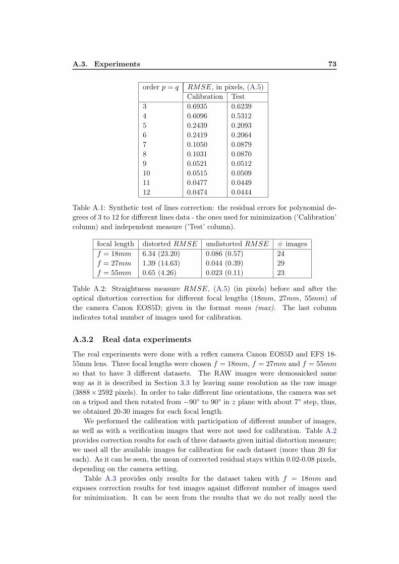
A.3. Experiments 73
order p = q RMSE, in pixels, (A.5)Calibration Test
3 0.6935 0.62394 0.6096 0.53125 0.2439 0.20936 0.2419 0.20647 0.1050 0.08798 0.1031 0.08709 0.0521 0.051210 0.0515 0.050911 0.0477 0.044912 0.0474 0.0444
Table A.1: Synthetic test of lines correction: the residual errors for polynomial de-grees of 3 to 12 for different lines data - the ones used for minimization (’Calibration’column) and independent measure (’Test’ column).
focal length distorted RMSE undistorted RMSE # imagesf = 18mm 6.34 (23.20) 0.086 (0.57) 24f = 27mm 1.39 (14.63) 0.044 (0.39) 29f = 55mm 0.65 (4.26) 0.023 (0.11) 23
Table A.2: Straightness measure RMSE, (A.5) (in pixels) before and after theoptical distortion correction for different focal lengths (18mm, 27mm, 55mm) ofthe camera Canon EOS5D; given in the format mean (max). The last columnindicates total number of images used for calibration.
A.3.2 Real data experiments
The real experiments were done with a reflex camera Canon EOS5D and EFS 18-55mm lens. Three focal lengths were chosen f = 18mm, f = 27mm and f = 55mm
so that to have 3 different datasets. The RAW images were demosaicked sameway as it is described in Section 3.3 by leaving same resolution as the raw image(3888× 2592 pixels). In order to take different line orientations, the camera was seton a tripod and then rotated from −90◦ to 90◦ in z plane with about 7◦ step, thus,we obtained 20-30 images for each focal length.
We performed the calibration with participation of different number of images,as well as with a verification images that were not used for calibration. Table A.2provides correction results for each of three datasets given initial distortion measure;we used all the available images for calibration for each dataset (more than 20 foreach). As it can be seen, the mean of corrected residual stays within 0.02-0.08 pixels,depending on the camera setting.
Table A.3 provides only results for the dataset taken with f = 18mm andexposes correction results for test images against different number of images usedfor minimization. It can be seen from the results that we do not really need the
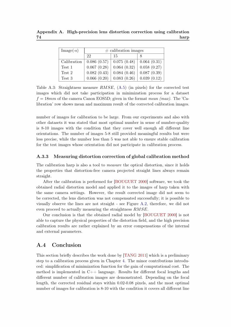
74Appendix A. High-precision lens distortion correction using calibration
harp
Image(-s) # calibration images22 15 8
Calibration 0.086 (0.57) 0.075 (0.48) 0.064 (0.31)Test 1 0.067 (0.28) 0.064 (0.32) 0.058 (0.27)Test 2 0.082 (0.43) 0.084 (0.46) 0.087 (0.39)Test 3 0.066 (0.20) 0.083 (0.26) 0.039 (0.12)
Table A.3: Straightness measure RMSE, (A.5) (in pixels) for the corrected testimages which did not take participation in minimization process for a datasetf = 18mm of the camera Canon EOS5D; given in the format mean (max). The ’Ca-libration’ row shows mean and maximum result of the corrected calibration images.
number of images for calibration to be large. From our experiments and also withother datasets it was stated that most optimal number in sense of number-qualityis 8-10 images with the condition that they cover well enough all different lineorientations. The number of images 5-8 still provided meaningful results but wereless precise, while the number less than 5 was not able to ensure stable calibrationfor the test images whose orientation did not participate in calibration process.
A.3.3 Measuring distortion correction of global calibration method
The calibration harp is also a tool to measure the optical distortion, since it holdsthe properties that distortion-free camera projected straight lines always remainstraight.
After the calibration is performed for [BOUGUET 2000] software, we took theobtained radial distortion model and applied it to the images of harp taken withthe same camera settings. However, the result corrected image did not seem tobe corrected, the lens distortion was not compensated successfully; it is possible tovisually observe the lines are not straight - see Figure A.2, therefore, we did noteven proceed to actually measuring the straightness RMSE.
Our conclusion is that the obtained radial model by [BOUGUET 2000] is notable to capture the physical properties of the distortion field, and the high precisioncalibration results are rather explained by an error compensations of the internaland external parameters.
A.4 Conclusion
This section briefly describes the work done by [TANG 2011] which is a preliminarystep to a calibration process given in Chapter 4. The minor contributions introdu-ced: simplification of minimization function for the gain of computational cost. Themethod is implemented in C++ language. Results for different focal lengths anddifferent number of calibration images are demonstrated. Depending on the focallength, the corrected residual stays within 0.02-0.08 pixels, and the most optimalnumber of images for calibration is 8-10 with the condition it covers all different line
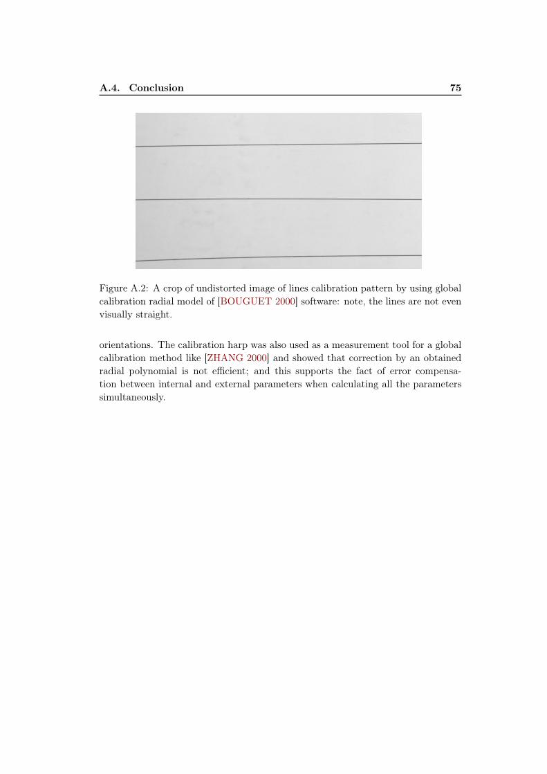
A.4. Conclusion 75
Figure A.2: A crop of undistorted image of lines calibration pattern by using globalcalibration radial model of [BOUGUET 2000] software: note, the lines are not evenvisually straight.
orientations. The calibration harp was also used as a measurement tool for a globalcalibration method like [ZHANG 2000] and showed that correction by an obtainedradial polynomial is not efficient; and this supports the fact of error compensa-tion between internal and external parameters when calculating all the parameterssimultaneously.

List of Figures
1.1 Cropped and zoomed-in image from camera Canon EOS 40D, before(a) and after (b) chromatic aberration correction by our method.Notice the attenuated color fringes at edges between (a) and (b) images. 2
2.1 Affine transformation A and its inverse A−1 for model point (x, y)
and its corresponding image point (x′, y′). . . . . . . . . . . . . . . . 112.2 The luminance transition model of parameter k. . . . . . . . . . . . . 112.3 Defining the corner keypoint: when the maximum angle ∠n1cn3 bet-
ween corner’s c first three neighbours n1, n2, n3 stays maximum forthe rest of the keypoints (within small tolerance) and at the sametime less than 180◦. . . . . . . . . . . . . . . . . . . . . . . . . . . . . 16
2.4 Digitizing of the pattern. . . . . . . . . . . . . . . . . . . . . . . . . . 162.5 Keypoint detection precision performance for normal angle view θ =
0◦ with subsampling rate s = 20, original image resolution W andsubsampled circle radii Rs , pixels. . . . . . . . . . . . . . . . . . . . . 18
2.6 Keypoint detection precision performance for θ = 55◦ angle view withsubsampling rate s = 20, original image resolutionW and subsampledcircle radii Rs , pixels. . . . . . . . . . . . . . . . . . . . . . . . . . . . 19
3.1 Occurence of axial (a) and lateral (b) chromatic aberrations. . . . . . 243.2 Example of LCA presence in digital image crop taken by camera
Sony DSLR-A200 with focal length f = 24mm. The color channelmisalignments are noticeable due to LCA and are mostly highlightedin the regions of edges. . . . . . . . . . . . . . . . . . . . . . . . . . . 24
3.3 Visual perception tests for chromatic aberration on synthetic diskimage for different values of displacements d (in pixels). Note thata displacement value of 0.1 pixel is just noticeable, while 0.3 pixeldisplacement is quite perceptible. . . . . . . . . . . . . . . . . . . . . 26
3.4 The Bayer arrangement of color filters on the pixel array of an imagesensor . . . . . . . . . . . . . . . . . . . . . . . . . . . . . . . . . . . 30
3.5 Histograms of Euclidean displacements of the keypoints . . . . . . . 323.6 Vector fields of Euclidean displacements of the keypoints . . . . . . . 333.7 Comparison of our method to other software for cam 2 and different
focal lengths f , the comparison is in terms of mean (dark coloredbars) and maximum (light colored bars) misalignments for both red(positive axis) and blue (negative axis) channels. (a) provides infor-mation on the initial uncorrected keypoint displacements for the samefocal lengths (notice the different scale). . . . . . . . . . . . . . . . . 34
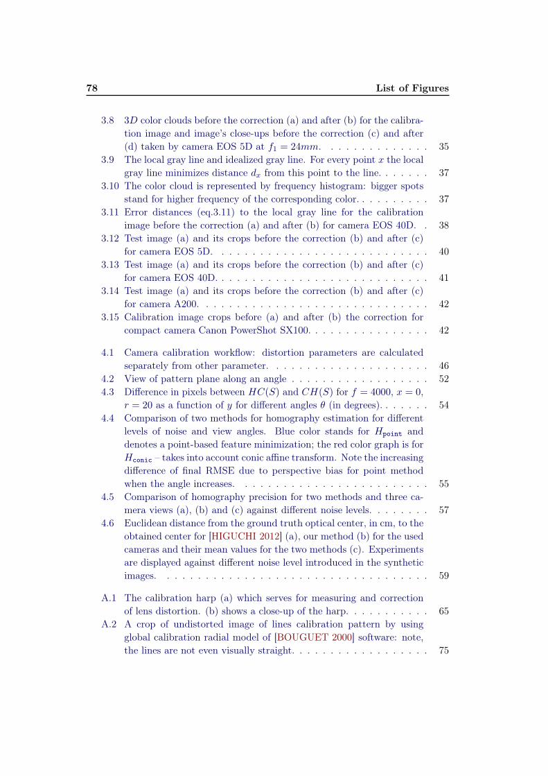
78 List of Figures
3.8 3D color clouds before the correction (a) and after (b) for the calibra-tion image and image’s close-ups before the correction (c) and after(d) taken by camera EOS 5D at f1 = 24mm. . . . . . . . . . . . . . 35
3.9 The local gray line and idealized gray line. For every point x the localgray line minimizes distance dx from this point to the line. . . . . . . 37
3.10 The color cloud is represented by frequency histogram: bigger spotsstand for higher frequency of the corresponding color. . . . . . . . . . 37
3.11 Error distances (eq.3.11) to the local gray line for the calibrationimage before the correction (a) and after (b) for camera EOS 40D. . 38
3.12 Test image (a) and its crops before the correction (b) and after (c)for camera EOS 5D. . . . . . . . . . . . . . . . . . . . . . . . . . . . 40
3.13 Test image (a) and its crops before the correction (b) and after (c)for camera EOS 40D. . . . . . . . . . . . . . . . . . . . . . . . . . . . 41
3.14 Test image (a) and its crops before the correction (b) and after (c)for camera A200. . . . . . . . . . . . . . . . . . . . . . . . . . . . . . 42
3.15 Calibration image crops before (a) and after (b) the correction forcompact camera Canon PowerShot SX100. . . . . . . . . . . . . . . . 42
4.1 Camera calibration workflow: distortion parameters are calculatedseparately from other parameter. . . . . . . . . . . . . . . . . . . . . 46
4.2 View of pattern plane along an angle . . . . . . . . . . . . . . . . . . 524.3 Difference in pixels between HC(S) and CH(S) for f = 4000, x = 0,
r = 20 as a function of y for different angles θ (in degrees). . . . . . . 544.4 Comparison of two methods for homography estimation for different
levels of noise and view angles. Blue color stands for Hpoint anddenotes a point-based feature minimization; the red color graph is forHconic – takes into account conic affine transform. Note the increasingdifference of final RMSE due to perspective bias for point methodwhen the angle increases. . . . . . . . . . . . . . . . . . . . . . . . . 55
4.5 Comparison of homography precision for two methods and three ca-mera views (a), (b) and (c) against different noise levels. . . . . . . . 57
4.6 Euclidean distance from the ground truth optical center, in cm, to theobtained center for [HIGUCHI 2012] (a), our method (b) for the usedcameras and their mean values for the two methods (c). Experimentsare displayed against different noise level introduced in the syntheticimages. . . . . . . . . . . . . . . . . . . . . . . . . . . . . . . . . . . 59
A.1 The calibration harp (a) which serves for measuring and correctionof lens distortion. (b) shows a close-up of the harp. . . . . . . . . . . 65
A.2 A crop of undistorted image of lines calibration pattern by usingglobal calibration radial model of [BOUGUET 2000] software: note,the lines are not even visually straight. . . . . . . . . . . . . . . . . . 75
List of Tables
3.1 Cameras specifications. . . . . . . . . . . . . . . . . . . . . . . . . . . 293.2 Color plane keypoint Euclidean displacements in RMSE (maximum
error) format in pixels before and after the calibration for three dif-ferent cameras, each with two different focal lengths. R/G and B/Gcorrespond to red and blue misalignments with reference to the greenchannel. . . . . . . . . . . . . . . . . . . . . . . . . . . . . . . . . . . 31
3.3 Geometrical misalignment results for noise pattern . . . . . . . . . . 363.4 Table of quantitative error measures for color distribution: RMSE
and maximal distances from cloud point to the local gray line. . . . . 39
4.1 Standard deviations of camera calibration parameters for five imagesets – comparison of the state-of-art method with ours. Any noiseand distortion are eliminated. Thanks to improved precision of ho-mography calculation, we notice less deviation for our method. . . . 58
4.2 Standard deviations of the camera Canon EOS5D parameters for realdata – comparison state-of-art method (noted as ’SoA’) with ours(noted as ’ours’). . . . . . . . . . . . . . . . . . . . . . . . . . . . . . 60
A.1 Synthetic test of line correction to chose the polynomial degree . . . 73A.2 Straightness measure RMSE, (A.5) (in pixels) before and after the
optical distortion correction for different focal lengths (18mm, 27mm,55mm) of the camera Canon EOS5D; given in the formatmean (max).The last column indicates total number of images used for calibration. 73
A.3 Straightness measure RMSE, (A.5) (in pixels) for the corrected testimages which did not take participation in minimization process for adataset f = 18mm of the camera Canon EOS5D; given in the formatmean (max). The ’Calibration’ row shows mean and maximum resultof the corrected calibration images. . . . . . . . . . . . . . . . . . . . 74

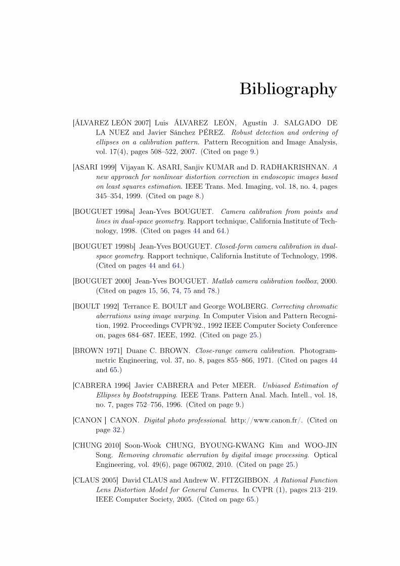
Bibliography
[ÁLVAREZ LEÓN 2007] Luis ÁLVAREZ LEÓN, Agustín J. SALGADO DELA NUEZ and Javier Sánchez PÉREZ. Robust detection and ordering ofellipses on a calibration pattern. Pattern Recognition and Image Analysis,vol. 17(4), pages 508–522, 2007. (Cited on page 9.)
[ASARI 1999] Vijayan K. ASARI, Sanjiv KUMAR and D. RADHAKRISHNAN. Anew approach for nonlinear distortion correction in endoscopic images basedon least squares estimation. IEEE Trans. Med. Imaging, vol. 18, no. 4, pages345–354, 1999. (Cited on page 8.)
[BOUGUET 1998a] Jean-Yves BOUGUET. Camera calibration from points andlines in dual-space geometry. Rapport technique, California Institute of Tech-nology, 1998. (Cited on pages 44 and 64.)
[BOUGUET 1998b] Jean-Yves BOUGUET. Closed-form camera calibration in dual-space geometry. Rapport technique, California Institute of Technology, 1998.(Cited on pages 44 and 64.)
[BOUGUET 2000] Jean-Yves BOUGUET. Matlab camera calibration toolbox, 2000.(Cited on pages 15, 56, 74, 75 and 78.)
[BOULT 1992] Terrance E. BOULT and George WOLBERG. Correcting chromaticaberrations using image warping. In Computer Vision and Pattern Recogni-tion, 1992. Proceedings CVPR’92., 1992 IEEE Computer Society Conferenceon, pages 684–687. IEEE, 1992. (Cited on page 25.)
[BROWN 1971] Duane C. BROWN. Close-range camera calibration. Photogram-metric Engineering, vol. 37, no. 8, pages 855–866, 1971. (Cited on pages 44and 65.)
[CABRERA 1996] Javier CABRERA and Peter MEER. Unbiased Estimation ofEllipses by Bootstrapping. IEEE Trans. Pattern Anal. Mach. Intell., vol. 18,no. 7, pages 752–756, 1996. (Cited on page 9.)
[CANON ] CANON. Digital photo professional. http://www.canon.fr/. (Cited onpage 32.)
[CHUNG 2010] Soon-Wook CHUNG, BYOUNG-KWANG Kim and WOO-JINSong. Removing chromatic aberration by digital image processing. OpticalEngineering, vol. 49(6), page 067002, 2010. (Cited on page 25.)
[CLAUS 2005] David CLAUS and Andrew W. FITZGIBBON. A Rational FunctionLens Distortion Model for General Cameras. In CVPR (1), pages 213–219.IEEE Computer Society, 2005. (Cited on page 65.)
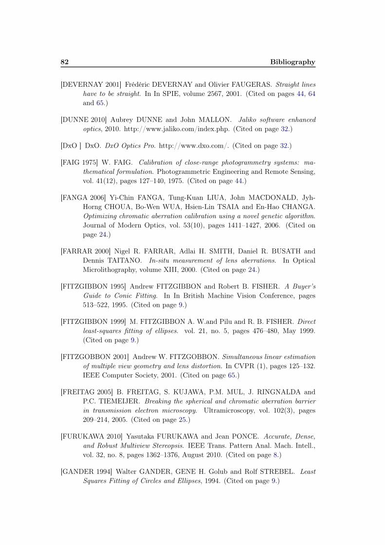
82 Bibliography
[DEVERNAY 2001] Frédéric DEVERNAY and Olivier FAUGERAS. Straight lineshave to be straight. In In SPIE, volume 2567, 2001. (Cited on pages 44, 64and 65.)
[DUNNE 2010] Aubrey DUNNE and John MALLON. Jaliko software enhancedoptics, 2010. http://www.jaliko.com/index.php. (Cited on page 32.)
[DxO ] DxO. DxO Optics Pro. http://www.dxo.com/. (Cited on page 32.)
[FAIG 1975] W. FAIG. Calibration of close-range photogrammetry systems: ma-thematical formulation. Photogrammetric Engineering and Remote Sensing,vol. 41(12), pages 127–140, 1975. (Cited on page 44.)
[FANGA 2006] Yi-Chin FANGA, Tung-Kuan LIUA, John MACDONALD, Jyh-Horng CHOUA, Bo-Wen WUA, Hsien-Lin TSAIA and En-Hao CHANGA.Optimizing chromatic aberration calibration using a novel genetic algorithm.Journal of Modern Optics, vol. 53(10), pages 1411–1427, 2006. (Cited onpage 24.)
[FARRAR 2000] Nigel R. FARRAR, Adlai H. SMITH, Daniel R. BUSATH andDennis TAITANO. In-situ measurement of lens aberrations. In OpticalMicrolithography, volume XIII, 2000. (Cited on page 24.)
[FITZGIBBON 1995] Andrew FITZGIBBON and Robert B. FISHER. A Buyer’sGuide to Conic Fitting. In In British Machine Vision Conference, pages513–522, 1995. (Cited on page 9.)
[FITZGIBBON 1999] M. FITZGIBBON A. W.and Pilu and R. B. FISHER. Directleast-squares fitting of ellipses. vol. 21, no. 5, pages 476–480, May 1999.(Cited on page 9.)
[FITZGOBBON 2001] Andrew W. FITZGOBBON. Simultaneous linear estimationof multiple view geometry and lens distortion. In CVPR (1), pages 125–132.IEEE Computer Society, 2001. (Cited on page 65.)
[FREITAG 2005] B. FREITAG, S. KUJAWA, P.M. MUL, J. RINGNALDA andP.C. TIEMEIJER. Breaking the spherical and chromatic aberration barrierin transmission electron microscopy. Ultramicroscopy, vol. 102(3), pages209–214, 2005. (Cited on page 25.)
[FURUKAWA 2010] Yasutaka FURUKAWA and Jean PONCE. Accurate, Dense,and Robust Multiview Stereopsis. IEEE Trans. Pattern Anal. Mach. Intell.,vol. 32, no. 8, pages 1362–1376, August 2010. (Cited on page 8.)
[GANDER 1994] Walter GANDER, GENE H. Golub and Rolf STREBEL. LeastSquares Fitting of Circles and Ellipses, 1994. (Cited on page 9.)
Bibliography 83
[GROMPONE VON GIOI 2010] R. GROMPONE VON GIOI, MONASSE P., J.-M. MOREL and Z. TANG. Self-consistency and universality of camera lensdistortion models. CMLA Preprint, 2010. (Cited on page 26.)
[GURDJOS 2003] Pierre GURDJOS and Peter F. STURM. Methods and Geome-try for Plane-Based Self-Calibration. In CVPR (1), pages 491–496. IEEEComputer Society, 2003. (Cited on page 44.)
[HARTLEY 1994] Richard I. HARTLEY. Euclidean Reconstruction from Uncali-brated Views. In Proceedings of the Second Joint European - US Workshopon Applications of Invariance in Computer Vision, pages 237–256, London,UK, UK, 1994. Springer-Verlag. (Cited on page 44.)
[HARTLEY 1997a] Richard I. HARTLEY. In defense of the eight-point algorithm.IEEE Trans. Pattern Anal. Mach. Intell., vol. 19, no. 6, pages 580–593, June1997. (Cited on page 48.)
[HARTLEY 1997b] Richard I. HARTLEY and Tushar SAXENA. The cubic rationalpolynomial camera model. In In Image Understanding Workshop, pages 649–653, 1997. (Cited on page 65.)
[HARTLEY 2004] Richard HARTLEY and Andrew ZISSERMAN. Multiple viewgeometry in computer vision. Cambridge University Press, ISBN 0521540518,New York, NY, USA, second édition, 2004. (Cited on pages 47 and 48.)
[HARTLEY 2005] Richard HARTLEY and Sing Bing KANG. Parameter-free radialdistortion correction with centre of distortion estimation. In In ICCV, pages1834–1841, 2005. (Cited on page 64.)
[HARTLEY 2007] Richard HARTLEY and Sing Bing KANG. Parameter-Free Ra-dial Distortion Correction with Center of Distortion Estimation. IEEE Trans.Pattern Anal. Mach. Intell., vol. 29, no. 8, pages 1309–1321, August 2007.(Cited on page 44.)
[HEIKKILÄ 2000] Janne HEIKKILÄ. Geometric camera calibration using circularcontrol points. IEEE Trans. Pattern Anal. Mach. Intell., vol. 22, no. 10, pages1066–1077, October 2000. (Cited on pages 8 and 45.)
[HIGUCHI 2012] Mirai HIGUCHI, Ankur DATTA and Takeo KANADE. Softwarepackage for precise camera calibration, 2012. (Cited on pages 56, 59 and 78.)
[JAIN 1995] Ramesh C. JAIN, Rangachar KASTURI and Brian G. SCHUNCK.Machine vision. McGraw-Hill, 1995. (Cited on page 9.)
[JIANG 2005] Guang JIANG and Long QUAN. Detection of Concentric Circlesfor Camera Calibration. In Proceedings of the Tenth IEEE InternationalConference on Computer Vision (ICCV’05) Volume 1 - Volume 01, ICCV’05, pages 333–340, Washington, DC, USA, 2005. IEEE Computer Society.(Cited on page 44.)
84 Bibliography
[JOHNSON 2006] M.K. JOHNSON and H. FARID. Exposing digital forgeriesthrough chromatic aberration. In ACM Multimedia and Security Workshop,Geneva, Switzerland, 2006. (Cited on page 25.)
[JÜRGEN 1995] R. Meyer-Arendt JÜRGEN. Introduction to classical and modernoptics. Prentice-Hall International, 1995. (Cited on page 23.)
[KANATANI 1994] Kenichi KANATANI. Statistical Bias of Conic Fitting and Re-normalization. IEEE Trans. Pattern Anal. Mach. Intell., vol. 16, no. 3, pages320–326, 1994. (Cited on page 9.)
[KANATANI 2006] Kenichi KANATANI. Ellipse Fitting with Hyperaccuracy.IEICE Transactions, vol. 89-D, no. 10, pages 2653–2660, 2006. (Cited onpage 9.)
[KANATANI 2011] Kenichi KANATANI and Prasanna RANGARAJAN. Hyperleast squares fitting of circles and ellipses. Computational Statistics & DataAnalysis, vol. 55, no. 6, pages 2197–2208, 2011. (Cited on page 9.)
[KANG 2007] Sing Bing KANG. Automatic removal of chromatic aberration froma single image. In IEEE Conference on Computer Vision and Pattern Re-cognition, pages 1–8, 2007. (Cited on page 25.)
[KANNALA 2006] Juho KANNALA and Sami S. BrANDT. A generic camera mo-del and calibration method for conventional, wide-angle, and fish-eye lenses.IEEE TRANS. PATTERN ANALYSIS AND MACHINE INTELLIGENCE,vol. 28, pages 1335–1340, 2006. (Cited on pages 8 and 45.)
[KAUFMANN 2005] V. KAUFMANN and R. LADSTÄDTER. Elimination of colorfringes in digital photographs caused by lateral chromatic aberration. In CIPAXX International Symposium, 2005. (Cited on page 25.)
[KILPELÄ 1980] E. KILPELÄ. Compensation of systematic errors of image andmodel coordinates. Photogrammetria, vol. 37(1), pages 15–44, 1980. (Citedon page 65.)
[KINGSLAKE 1978] Rudolf KINGSLAKE. Lens design fundamentals. AcademicPress, New York, 1978. (Cited on page 24.)
[KOZUBEK 2000] M. KOZUBEK and P. MATULA. An efficient algorithm formeasurement and correction of chromatic aberrations in fluorescence micro-scopy. Journal of Microscopy, vol. 200, no. 3, pages 206–217, 2000. (Citedon page 25.)
[LAVEST 1998] Jean-Marc LAVEST, Marc VIALA and Michel DHOME. Do wereally need an accurate calibration pattern to achieve a reliable camera ca-libration? In Hans Burkhardt and Bernd Neumann, editeurs, ECCV (1),volume 1406 of Lecture Notes in Computer Science, pages 158–174. Sprin-ger, 1998. (Cited on page 64.)
Bibliography 85
[LOWE 1999] David G. LOWE. Object Recognition from Local Scale-Invariant Fea-tures. In Proceedings of the International Conference on Computer Vision-Volume 2 - Volume 2, ICCV ’99, pages 1150–, Washington, DC, USA, 1999.IEEE Computer Society. (Cited on page 8.)
[LOWE 2004] David G. LOWE. Distinctive image features from scale-invariantkeypoints. Int. J. Comput. Vision, vol. 60, no. 2, pages 91–110, November2004. (Cited on pages 8 and 31.)
[LUCCHESE 2002] Luca LUCCHESE and Sanjit K. MITRA. Using saddle pointsfor subpixel feature detection in camera calibration targets. In Asia-PacificConference on Circuits and Systems, volume 2, pages 191–195, 2002. (Citedon pages 8 and 9.)
[LUHMANN 2006] Thomas LUHMANN, Heidi HASTEDT and Werner TECK-LENBURG. Modelling of chromatic aberration for high precision photogram-metry. In Commission V Symp. on Image Engineering and Vision Metrology,Proc. ISPRS, volume 36, pages 173–178, 2006. (Cited on page 25.)
[MA 2004] Lili MA, Yangquan Chen and Kevin L. Moore. Rational Radial Distor-tion Models of Camera Lenses with Analytical Solution for Distortion Cor-rection. I. J. Information Acquisition, vol. 1, no. 2, pages 135–147, 2004.(Cited on page 65.)
[MALLON 2007a] John MALLON and Paul F. WHELAN. Calibration and remo-val of lateral chromatic aberration in images. Pattern Recognition Letters,vol. 28, no. 1, pages 125–135, January 2007. (Cited on pages 9 and 25.)
[MALLON 2007b] John MALLON and Paul F. WHELAN. Which pattern? bia-sing aspects of planar calibration patterns and detection methods. PatternRecognition Letters, vol. 28(8), pages 921–930, 2007. (Cited on pages 8, 44and 45.)
[MANDERS 1997] E. M. M. MANDERS. Chromatic shift in multicolour confocalmicroscopy. Journal of Microscopy, vol. 185(3), pages 312–328, 1997. (Citedon page 25.)
[MARQUARDT 1963] Donald W. MARQUARDT. An algorithm for least-squaresestimation of nonlinear parameters. SIAM Journal on Applied Mathematics,vol. 11, no. 2, pages 431–441, 1963. (Cited on page 49.)
[MATSUOKA 2012] Ryuji MATSUOKA, Kazuyoshi ASONUMA, Genki TAKA-HASHI, Takuya DANJO and Kayoko HIRANA. Evaluation of correctionmethods of chromatic aberration in digital camera images. In ISPRS Photo-grammetric image analysis, volume I-3, 2012. (Cited on page 25.)
86 Bibliography
[MIELENZ 1999] K. MIELENZ. On the diffraction limit for lensless imaging. Jour-nal of Research of the National Institute of Standards and Technology,vol. 104(5), pages 479–485, 1999. (Cited on page 23.)
[MILLÁN 2006a] Maria S. MILLÁN, Joaquin OTÓN and Elisabet PÉREZ-CABRÉ. Dynamic compensation of chromatic aberration in a programmablediffractive lens. Optics Express, vol. 14(20), pages 9103–9112, 2006. (Citedon page 24.)
[MILLÁN 2006b] Maria S. MILLÁN, Joaquin OTÓN and Elisabet PÉREZ-CABRÉ. Dynamic compensation of chromatic aberration in a programmablefresnel lenses. Optics Express, vol. 14(13), pages 6226–6242, 2006. (Citedon page 24.)
[NEWTON 1704] Isaak NEWTON. Opticks. William Innys, 1704. (Cited onpage 23.)
[NISTER 2006] David NISTER and Henrik STEWENIUS. Scalable Recognitionwith a Vocabulary Tree. In Proceedings of the 2006 IEEE Computer SocietyConference on Computer Vision and Pattern Recognition - Volume 2, CVPR’06, pages 2161–2168, Washington, DC, USA, 2006. IEEE Computer Society.(Cited on page 8.)
[OUELLET 2008] Jean-Nicolas OUELLET, Felix ROCHETTE and Patrick HE-BERT. Geometric calibration of a structured light system using circularcontrol points. In 3D Data Processing, Visualization and Transmission, pages183–190, 2008. (Cited on page 45.)
[PIERROT DESEILLIGNY 2011] M. PIERROT DESEILLIGNY and I. CLERY.APERO, an open source bundle adjusment software for automatic calibra-tion and orientation of set of images. ISPRS - International Archives ofthe Photogrammetry, Remote Sensing and Spatial Information Sciences,vol. XXXVIII-5/W16, pages 269–276, 2011. (Cited on pages 44 and 64.)
[POWELL 1981] Ian POWELL. Lenses for correcting chromatic aberration of theeye. Applied Optics, vol. 20(24), pages 4152–4155, 1981. (Cited on page 24.)
[PRINCEN 1992] John PRINCEN, John ILLINGWORTH and Josef KILTTLER.A formal definition of the Hough transform: Properties and relationships.Journal of Mathematical Imaging and Vision, vol. 1, no. 2, pages 153–168,1992. (Cited on page 9.)
[REBIAI 1992] M. REBIAI, S. MANSOURI, F. PINSON and B. TICHIT. Imagedistortion from zoom lenses: modeling and digital correction. In BroadcastingConvention, pages 438–441, 1992. (Cited on page 25.)
[SEIDEL 1856] L. SEIDEL. Astronomische nachrichten, 1856. (Cited on page 23.)
Bibliography 87
[SHI 2004] Kebin SHI, Peng LI, Shizhuo YIN and Zhiwen LIU. Chromatic confocalmicroscopy using supercontinuum light. Optics Express, vol. 12(10), pages2096–2101, 2004. (Cited on page 25.)
[SIVIC 2005] J. SIVIC, B. C. RUSSELL, A. A. EFROS, A. ZISSERMAN and W. T.FREEMAN. Discovering objects and their location in images. volume 1,pages 370–377, 2005. (Cited on page 8.)
[SIVIC 2006] Josef SIVIC and Andrew ZISSERMAN. Video Google: Efficient Vi-sual Search of Videos. In Toward Category-Level Object Recognition, pages127–144, 2006. (Cited on page 8.)
[SLAMA 1980] Chester C. SLAMA. Manual of photogrammetry. American Societyof Photogrammetry, Falls Church, VA, 4th ed. édition, 1980. (Cited onpages 23 and 64.)
[SNAVELY 2008] Noah SNAVELY, Steven M. SEITZ and Richard SZELISKI. Mo-deling the World from Internet Photo Collections. Int. J. Comput. Vision,vol. 80, no. 2, pages 189–210, November 2008. (Cited on page 8.)
[STURM 1999] Peter F. STURM and Stephen J. MAYBANK. On Plane-BasedCamera Calibration: A General Algorithm, Singularities, Applications. InCVPR, pages 1432–1437. IEEE Computer Society, 1999. (Cited on page 44.)
[TANG 2011] Z. TANG. High accuracy measurement in 3d stereo reconstruction.PhD thesis, ENS Cachan, France, 2011. (Cited on pages 3, 4, 25, 26, 45, 63,64, 65 and 74.)
[TORR 2000] P.H.S. TORR and A. ZISSERMAN. Feature Based Methods for Struc-ture and Motion Estimation. In Vision Algorithms: Theory and Practice,number 1883 in LNCS, pages 278–295. Springer-Verlag, 2000. (Cited onpage 8.)
[TSAI 1992] Roger Y. TSAI. A versatile camera calibration technique for high-accuracy 3D machine vision metrology using off-the-shelf TV cameras andlenses. IEEE Journal on Robotics and Automation, vol. RA-3, pages 323–44, 1992. (Cited on pages 44 and 64.)
[WENG 1992] Juyang WENG, Paul COHEN and Marc HERNIOU. Camera cali-bration with distortion models and accuracy evaluation. IEEE Trans. PatternAnal. Mach. Intell., vol. 14, no. 10, pages 965–980, October 1992. (Cited onpages 8, 44 and 64.)
[WILLSON 1991] Reg WILLSON and Steven SHAFER. Active lens control for highprecision computer imaging. In Proc. IEEE ICRA, volume 3, pages 2063 –2070, April 1991. (Cited on pages 24 and 25.)
[WILLSON 1994a] Reg WILLSON. Modelling and calibration of automated zoomlenses. PhD thesis, Carnegie Mellon University, 1994. (Cited on page 24.)
88 Bibliography
[WILLSON 1994b] Reg WILLSON and Steven SHAFER. What is the center of theimage? JOSA A, vol. 11(11), pages 2946–2955, 1994. (Cited on page 25.)
[YANG 2000] Changjiang YANG, Fengmei SUN and Zhanyi HU. Planar conic basedcamera calibration. In ICPR, pages 1555–1558, 2000. (Cited on page 45.)
[ZHANG 2000] Zhengyou ZHANG. A flexible new technique for camera calibration.IEEE Trans. Pattern Anal. Mach. Intell., vol. 22, no. 11, pages 1330–1334,November 2000. (Cited on pages 3, 8, 44, 45, 64 and 75.)