statistiques en grande dimension
TRANSCRIPT
Statistiques en grande dimension
Christophe Giraud1,2 et Tristan Mary-Huart3,4
(1) Universite Paris-Sud(2) Ecole Polytechnique(3) AgroParistech(4) INRA - Le Moulon
M2 MathSV & Maths Alea
C. Giraud (Paris Sud) High-dimensional statistics M2 MathSV & Maths Alea 1 / 26

High-dimensional data
C. Giraud (Paris Sud) High-dimensional statistics M2 MathSV & Maths Alea 2 / 26
Donnees en grande dimension
Donnees biotech: mesure des milliers de quantites par ”individu”.
Images : images medicales, astrophysique, video surveillance, etc. Chaqueimage est constituees de milliers ou millions de pixels ou voxels.
Marketing: les sites web et les programmes de fidelite collectent de grandesquantites d’information sur les preferences et comportements des clients. Ex:systemes de recommandation...
Business: exploitation des donnees internes et externes de l’entreprisedevient primordial
Crowdsourcing data : donnees recoltees online par des volontaires. Ex:eBirds collecte des millions d’observations d’oiseaux en Amerique du Nord
C. Giraud (Paris Sud) High-dimensional statistics M2 MathSV & Maths Alea 3 / 26
Blessing?
, we can sense thousands of variables on each ”individual” : potentiallywe will be able to scan every variables that may influence the phenomenonunder study.
/ the curse of dimensionality : separating the signal from the noise is ingeneral almost impossible in high-dimensional data and computations canrapidly exceed the available resources.
C. Giraud (Paris Sud) High-dimensional statistics M2 MathSV & Maths Alea 4 / 26
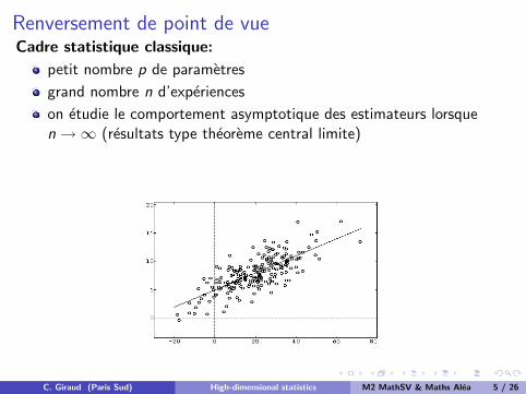
Renversement de point de vueCadre statistique classique:
petit nombre p de parametres
grand nombre n d’experiences
on etudie le comportement asymptotique des estimateurs lorsquen→∞ (resultats type theoreme central limite)
C. Giraud (Paris Sud) High-dimensional statistics M2 MathSV & Maths Alea 5 / 26
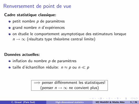
Renversement de point de vue
Cadre statistique classique:
petit nombre p de parametres
grand nombre n d’experiences
on etudie le comportement asymptotique des estimateurs lorsquen→∞ (resultats type theoreme central limite)
Donnees actuelles:
inflation du nombre p de parametres
taille d’echantillon reduite: n ≈ p ou n� p
=⇒ penser differemment les statistiques!(penser n→∞ ne convient plus)
C. Giraud (Paris Sud) High-dimensional statistics M2 MathSV & Maths Alea 5 / 26
Fleau de la dimension
C. Giraud (Paris Sud) High-dimensional statistics M2 MathSV & Maths Alea 6 / 26
Curse 1 : fluctuations cumulate
Exemple : linear regression Y = Xβ∗ + ε with cov(ε) = σ2In. TheLeast-Square estimator β ∈ argminβ∈Rp ‖Y − Xβ‖2 has a risk
E[‖β − β∗‖2
]= Tr
((XT X)−1
)σ2.
Illustration :
Yi =
p∑j=1
β∗j cos(πji/n) + εi = fβ∗(i/n) + εi , for i = 1, . . . , n,
with
ε1, . . . , εn i.i.d with N (0, 1) distribution
β∗j independent with N (0, j−4) distribution
C. Giraud (Paris Sud) High-dimensional statistics M2 MathSV & Maths Alea 7 / 26
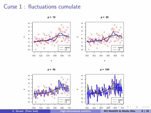
Curse 1 : fluctuations cumulate
0.0 0.2 0.4 0.6 0.8 1.0
-3-2
-10
12
34
p = 10
x
y
signalLS
0.0 0.2 0.4 0.6 0.8 1.0
-3-2
-10
12
34
p = 20
x
y
signalLS
0.0 0.2 0.4 0.6 0.8 1.0
-3-2
-10
12
34
p = 50
x
y
signalLS
0.0 0.2 0.4 0.6 0.8 1.0
-3-2
-10
12
34
p = 100
x
y
signalLS
C. Giraud (Paris Sud) High-dimensional statistics M2 MathSV & Maths Alea 8 / 26
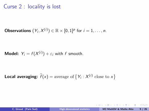
Curse 2 : locality is lost
Observations (Yi ,X(i)) ∈ R× [0, 1]p for i = 1, . . . , n.
Model: Yi = f (X (i)) + εi with f smooth.
Local averaging: f (x) = average of{Yi : X (i) close to x
}
C. Giraud (Paris Sud) High-dimensional statistics M2 MathSV & Maths Alea 9 / 26
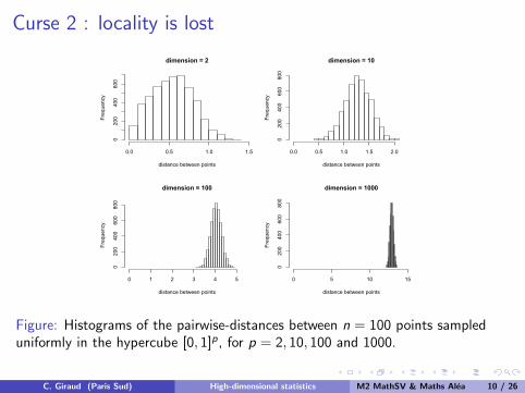
Curse 2 : locality is lost
dimension = 2
distance between points
Frequency
0.0 0.5 1.0 1.5
0200
400
600
dimension = 10
distance between points
Frequency
0.0 0.5 1.0 1.5 2.0
0200
400
600
800
dimension = 100
distance between points
Frequency
0 1 2 3 4 5
0200
400
600
800
dimension = 1000
distance between points
Frequency
0 5 10 150
200
400
600
800
Figure: Histograms of the pairwise-distances between n = 100 points sampleduniformly in the hypercube [0, 1]p, for p = 2, 10, 100 and 1000.
C. Giraud (Paris Sud) High-dimensional statistics M2 MathSV & Maths Alea 10 / 26
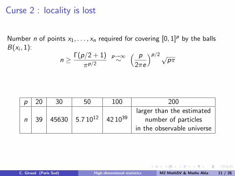
Curse 2 : locality is lost
Number n of points x1, . . . , xn required for covering [0, 1]p by the ballsB(xi , 1):
n ≥ Γ(p/2 + 1)
πp/2
p→∞∼( p
2πe
)p/2√pπ
p 20 30 50 100 200
larger than the estimatedn 39 45630 5.7 1012 42 1039 number of particles
in the observable universe
C. Giraud (Paris Sud) High-dimensional statistics M2 MathSV & Maths Alea 11 / 26
Some other curses
Curse 3 : an accumulation of rare events may not be rare (falsediscoveries, etc)
Curse 4 : algorithmic complexity must remain low
C. Giraud (Paris Sud) High-dimensional statistics M2 MathSV & Maths Alea 12 / 26
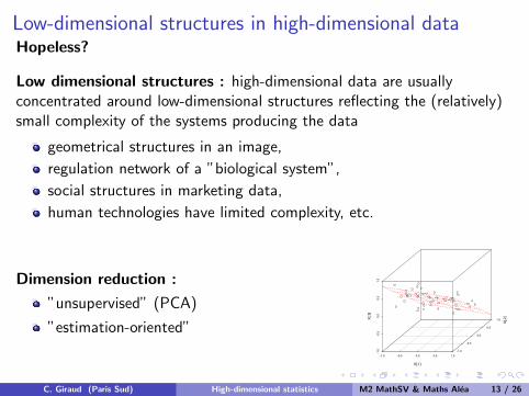
Low-dimensional structures in high-dimensional dataHopeless?
Low dimensional structures : high-dimensional data are usuallyconcentrated around low-dimensional structures reflecting the (relatively)small complexity of the systems producing the data
geometrical structures in an image,
regulation network of a ”biological system”,
social structures in marketing data,
human technologies have limited complexity, etc.
Dimension reduction :
”unsupervised” (PCA)
”estimation-oriented”
-1.0 -0.5 0.0 0.5 1.0
-1.0
-0.5
0.0
0.5
1.0
-1.0
-0.5
0.0
0.5
1.0
X[,1]
X[,2]
X[,3]
C. Giraud (Paris Sud) High-dimensional statistics M2 MathSV & Maths Alea 13 / 26
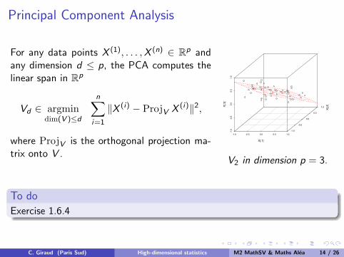
Principal Component Analysis
For any data points X (1), . . . ,X (n) ∈ Rp andany dimension d ≤ p, the PCA computes thelinear span in Rp
Vd ∈ argmindim(V )≤d
n∑i=1
‖X (i) − ProjV X (i)‖2,
where ProjV is the orthogonal projection ma-trix onto V .
-1.0 -0.5 0.0 0.5 1.0
-1.0
-0.5
0.0
0.5
1.0
-1.0
-0.5
0.0
0.5
1.0
X[,1]
X[,2]
X[,3]
V2 in dimension p = 3.
To do
Exercise 1.6.4
C. Giraud (Paris Sud) High-dimensional statistics M2 MathSV & Maths Alea 14 / 26
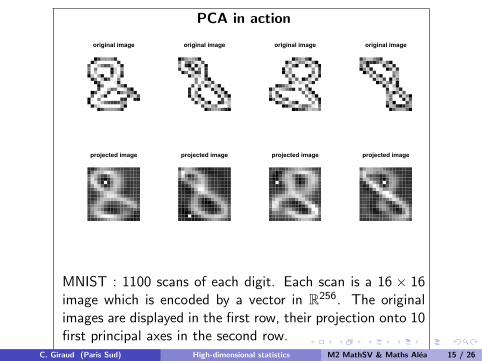
PCA in action
original image original image original image original image
projected image projected image projected image projected image
MNIST : 1100 scans of each digit. Each scan is a 16 × 16image which is encoded by a vector in R256. The originalimages are displayed in the first row, their projection onto 10first principal axes in the second row.
C. Giraud (Paris Sud) High-dimensional statistics M2 MathSV & Maths Alea 15 / 26
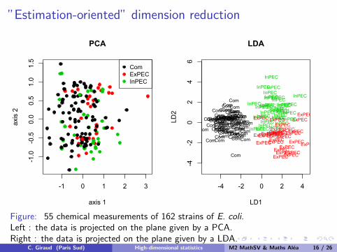
”Estimation-oriented” dimension reduction
-1 0 1 2 3
-1.0
-0.5
0.0
0.5
1.0
1.5
PCA
axis 1
axis
2
ComExPECInPEC
-4 -2 0 2 4-4
-20
24
6
LDA
LD1
LD2
InPECInPEC
InPEC
ExPEC
InPEC
ExPEC
InPEC
InPEC
InPECInPEC
InPEC
InPEC
InPECInPEC
ExPEC
ExPEC InPEC
InPEC
ExPEC
ExPEC
ExPECExPEC
ExPECExPECExPECExPEC
ExPEC
ExPEC
InPEC
ExPEC
ExPEC
InPECInPEC
InPECInPEC
InPEC
InPEC
InPEC
InPEC
InPEC
InPEC
InPEC
InPECInPEC
InPEC
ExPEC
ExPEC
ExPECCom
InPECInPECInPEC
InPEC
Com ComExPECExPEC
ExPEC
ExPECExPEC
ExPECExPEC
ExPEC
InPEC
ComCom
Com
ComComCom
ComComCom
Com
Com
Com
ComCom
Com ComComComCom
Com
ComCom
Com
ComComCom
ComCom
Com
Com
ComComCom
ComCom
ComCom
ComCom
ComCom
Com
ComCom
Com ComComCom
Com
Com
ComCom
Com Com
Com
Com
ComComCom
ComCom Com
Com
Com
ComCom
ComCom
Com
Com
Com
Com
Com
Com
Com
ComComCom
Com
ComCom
ComCom
Com
Com
ComCom
Com
ComComComCom
Com
InPEC
ExPECExPEC
InPEC
ExPEC
Figure: 55 chemical measurements of 162 strains of E. coli.Left : the data is projected on the plane given by a PCA.Right : the data is projected on the plane given by a LDA.
C. Giraud (Paris Sud) High-dimensional statistics M2 MathSV & Maths Alea 16 / 26
Resume
Difficulte statistique
donnees de tres grande dimension
peu de repetitions
Pour nous aiderDonnees issues d’un vaste systeme (plus ou moins dynamique etstochastique)
existence de structures de faible dimension ”effective”
parfois: existence de modeles theoriques
La voie du succesTrouver, a partir des donnees, ces structures ”cachees” pour pouvoir lesexploiter.
C. Giraud (Paris Sud) High-dimensional statistics M2 MathSV & Maths Alea 17 / 26
La voie du succes
Trouver, a partir des donnees, les structures cachees pourpouvoir les exploiter.
C. Giraud (Paris Sud) High-dimensional statistics M2 MathSV & Maths Alea 18 / 26
Exemples de structures
C. Giraud (Paris Sud) High-dimensional statistics M2 MathSV & Maths Alea 19 / 26
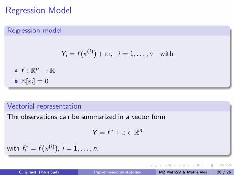
Regression Model
Regression model
Yi = f (x (i)) + εi , i = 1, . . . , n with
f : Rp → RE[εi ] = 0
Vectorial representation
The observations can be summarized in a vector form
Y = f ∗ + ε ∈ Rn
with f ∗i = f (x (i)), i = 1, . . . , n.
C. Giraud (Paris Sud) High-dimensional statistics M2 MathSV & Maths Alea 20 / 26
Low-dimensional x
Example 1: sparse piecewise constant regression
It corresponds to the case where f : R→ R is piecewise constant with a smallnumber of jumps.
This situation appears for example for CGH profiling.
C. Giraud (Paris Sud) High-dimensional statistics M2 MathSV & Maths Alea 21 / 26
Low-dimensional x
Example 2: sparse basis/frame expansion
We estimate f : R→ R by expanding it on a basis or frame {ϕj}j∈J
f (x) =∑j∈J
cjϕj(x),
with a small number of nonzero cj . Typical examples of basis are Fourier basis,splines, wavelets, etc.
The most simple example is the piecewise linear decomposition whereϕj(x) = (x − zj)+ where z1 < z2 < . . . and (x)+ = max(x , 0).
C. Giraud (Paris Sud) High-dimensional statistics M2 MathSV & Maths Alea 22 / 26
High-dimensional x
Example 3: sparse linear regression
It corresponds to the case where f is linear: f (x) = 〈β, x〉 where β ∈ Rp has onlya few nonzero coordinates.
This model can be too rough to model the data.
Example: relationship between some phenotypes and some proteinabundances.
only a small number of proteins influence a given phenotype,
but the relationship between these proteins and the phenotype isunlikely to be linear.
C. Giraud (Paris Sud) High-dimensional statistics M2 MathSV & Maths Alea 23 / 26
High-dimensional x
Example 4: sparse additive model
In the sparse additive model, we expect that f (x) =∑
k fk(xk) with most of thefk equal to 0.
If we expand each function fk on a frame or basis {ϕj}j∈Jkwe obtain the
decomposition
f (x) =
p∑k=1
∑j∈Jk
cj,kϕj(xk),
where most of the vectors {cj,k}j∈Jkare zero.
Such a model can be hard to fit from a small sample since it requires toestimate a relatively large number of non-zero cj ,k .
C. Giraud (Paris Sud) High-dimensional statistics M2 MathSV & Maths Alea 24 / 26
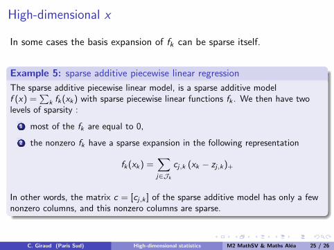
High-dimensional x
In some cases the basis expansion of fk can be sparse itself.
Example 5: sparse additive piecewise linear regression
The sparse additive piecewise linear model, is a sparse additive modelf (x) =
∑k fk(xk) with sparse piecewise linear functions fk . We then have two
levels of sparsity :
1 most of the fk are equal to 0,
2 the nonzero fk have a sparse expansion in the following representation
fk(xk) =∑j∈Jk
cj,k (xk − zj,k)+
In other words, the matrix c = [cj,k ] of the sparse additive model has only a fewnonzero columns, and this nonzero columns are sparse.
C. Giraud (Paris Sud) High-dimensional statistics M2 MathSV & Maths Alea 25 / 26
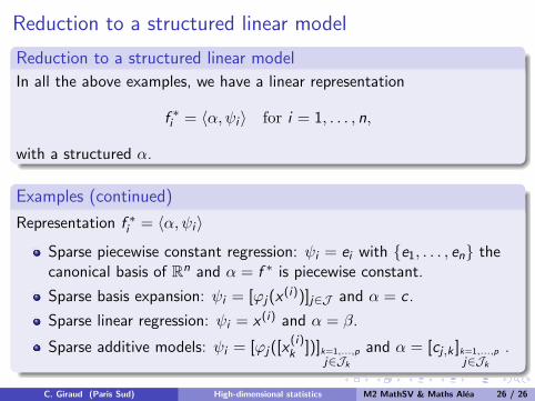
Reduction to a structured linear model
Reduction to a structured linear model
In all the above examples, we have a linear representation
f ∗i = 〈α,ψi 〉 for i = 1, . . . , n,
with a structured α.
Examples (continued)
Representation f ∗i = 〈α,ψi 〉
Sparse piecewise constant regression: ψi = ei with {e1, . . . , en} thecanonical basis of Rn and α = f ∗ is piecewise constant.
Sparse basis expansion: ψi = [ϕj(x(i))]j∈J and α = c .
Sparse linear regression: ψi = x (i) and α = β.
Sparse additive models: ψi = [ϕj([x(i)k ])]k=1,...,p
j∈Jk
and α = [cj ,k ]k=1,...,pj∈Jk
.
C. Giraud (Paris Sud) High-dimensional statistics M2 MathSV & Maths Alea 26 / 26