1

Thèse

présentée à

L’Université  Bordeaux  1

Ecole Doctorale  des  Sciences  Physiques  et  de  l’Ingénieur

par

Besira Mekonnen MIHIRETIE

Pour obtenir le grade de

Docteur

Spécialité : Lasers, matière et nanosciences (LMN)

Effets mécaniques de la lumière sur des particules anisotropes micrométriques  et  dynamique  du  mouillage  à  l’interface  eau-air

(Mechanical effects of light on anisotropic micron-sized particles and their wetting dynamics at the water-air interface)

Directeurs de thèse: Bernard POULIGNY et Jean-Christophe LOUDET

Devant  la  commission  d’examen  formée  de :

M. F. Ren Professeur, Université de Rouen Rapporteur M. S. Hanna Professeur, Université de Bristol Rapporteur M. B. Pouligny Directeur de Recherche, CNRS Directeur de thèse M. J-C. Loudet Maître de Conférences, Université de Bordeaux Directeur de thèse M. A.G. Yodh Professeur, Université de Pennsylvanie Examinateur M. J-P. Galaup Directeur de Recherche, CNRS Examinateur M. F. Nallet Professeur Université de Bordeaux Examinateur M. P. Richetti Directeur de Recherche, CNRS Examinateur

Numéro d’ordre : 4813

2

Acknowledgments First of all, I wish to thank my supervisors Bernard Pouligny and Jean-Christophe Loudet for

directing this work. They gave me the opportunity to work with them and contributed to this

thesis with many valuable ideas and helpful feedback. I would like to thank Patrick Snabre

for his support with software. I would also like to thank Juan Elezgaray for invaluable

discussions and his comments on part of this thesis. I would like to thank Florinda Schembri

for her help with the TISEAN software.

I express my heartfelt gratitude to the instrumentation team, Pascal Merzeau, Lionel Buisson

and Ahmed Bentaleb and to mechanical workshop teams, Philippe Barboteau , Jean-Yves

Juanico, Emmanuel Texier who provided me with the necessary support for the thesis.

I also express thanks to everybody in CRPP for providing me a very pleasant and friendly

atmosphere and for your supports whenever I needed.

I am also grateful to the COMPLOIDS (European network), which supported me financially

during the last 3 years.

On a more personal note, I would like to thank my family and friends for their unconditional

support.

Last but not least, I wish to thank all jury members for their willingness to participate in my

defense.

3

Glossary

PS Polystyrene

Tg Glass transition temperature

PVA Polyvinyl alcohol

K aspect ratio of the particles

a,b,c dimension of ellipsoids three semi-axis

ac, bc dimension of contact line (dry region)

T temperature

beam radius

o beam waist

I Intensity

Z axial distance on the beam axis

L lense

GM galvanometric mirror

M mirror

DM dichroic mirror

wave length

viscosity

P Power

PD photodiode

PH pin hole

kc critical aspect ratio

kcp,kco critical aspect ratio of prolate and oblate ellipsoids resp.

x,y,z the three co-ordinate axes

4

Résumé Nous  présentons  une  série  d’expériences  sur  des  particules  micrométriques  de  polystyrène de

formes   ellipsoïdales.   Les   rapports   d’aspects   (k) des particules sont variables, de 0.2 à 8

environ.  Ces   ellipsoïdes   sont  manipulés  dans   l’eau  par   faisceau   laser  modérément   focalisé.  

On  observe  la  lévitation  et  l’équilibre  dynamique  de  chaque  particule, dans le volume et au

contact   d’une   interface,   solide-liquide ou liquide-liquide. Dans une première partie, nous

montrons que des particules de k modéré sont piégées radialement. Par contre, les ellipsoïdes

allongés (k>3) ou aplatis (k<0.3) ne peuvent pas être immobilisés. Ces particules « dansent »

autour du faisceau, dans un mouvement permanent associant translation et rotation. Les

mouvements sont périodiques, ou irréguliers (chaotiques) selon les caractéristiques de la

particule et du faisceau. Un  modèle  en  2d  est  proposé  qui  permet  de  comprendre  l’origine  des  

oscillations. La seconde partie est une application de la lévitation optique pour une étude de

la transition mouillage total-mouillage   partiel   des   particules   à   l’interface   eau-air. Nous

montrons que la dynamique de la transition ne dépend pratiquement pas de la forme de

particule,  et  qu’elle  est  déterminée  par  le  mécanisme  d’accrochage-décrochage de la ligne de

contact.

Mots clés : lévitation optique, effet mécaniques de la lumière, piégeage, ellipsoïde, pinces

optiques, interface fluide.

Abstract We report experiments on ellipsoidal micrometre-sized polystyrene particles. The particle

aspect ratio (k) varies between about 0.2 and 8. These particles are manipulated in water by

means of a moderately focused laser beam. We observe the levitation and the dynamical state

of each particle in the laser beam, in bulk water or in contact to an interface (water-glass,

water-air, water-oil). In the first part, we show that moderate-k particles are radially trapped

with their long axis lying parallel to the beam. Conversely, elongated (k>3) or flattened

(k<0.3)   ellipsoids   never   come   to   rest,   and   permanently   “dance”   around   the   beam,   through  

coupled translation-rotation motions. The dynamics are periodic or irregular (akin to chaos)

depending on the particle type and beam characteristics. We propose a 2d model that indeed

predicts the bifurcation between static and oscillating states. In the second part, we apply

optical levitation to study the transition from total to partial wetting of the particles at the

5

water-air interface. We show that the dynamics of the transition is about independent of

particle shape, and mainly governed by the pinning-depinning mechanism of the contact line.

Keywords: optical levitation, mechanical effects of light, trapping, ellipsoid, optical tweezers,

fluid interface.

6

Contents Acknowledgments 2

Glossary 3

Résumé 4

Abstract 4

Introduction générale 8

General Introduction 11

Part A: Mechanical effect of light on micron sized ellipsoidal latex

particles 14

A-I: Optical manipulation and trapping of non spherical particles 15

A-II: Experimental hardware and methods 23

A-II.1 Preparation of anisotropic particles 23

A-II.1.a Prolate ellipsoids 23

A-II.1.b Oblate and disk-like ellipsoids 26

A-II.2 Beam characterization 28

A-II.3 Optical levitation setup 32

A-II.4 Data acquisition and analysis 36

A-II.4.a Photodiode signal 36

A-II.4.b Video 37

A-III: Results and Discussion 40

A-III.1 Levitation: Particle behavior in bulk water 40

A-III.2 Particle in contact to an interface, at the beam-waist (Z=0) 42

A-III.2a: Water-air and water-oil interfaces 42

A-III.2b: Water-glass interfaces 44

A-III.3 Particle in contact to water-glass interface, at variable Z 61

A-III.3a: Influence of varying beam diameter on particle oscillation 63

A-III.3b: Vertical to horizontal transition 69

A-III.3c: Summary 71

7

A-IV: Analysis of oscillations 73

A-IV.1 Phase space reconstruction 74

A-IV.2 Dynamics of ellipsoidal particles - Experimental results 78

A-IV.2a: Influence of ellipsoid aspect ratio 79

A-IV.2b: Influence of the beam diameter (parameter Z) 83

A-IV.3 Conclusion 86

A-V: Ray-optics 2d model 87

A-V.1: 2-dimensional ray-optics model 88

A-V.2: 4-pole force / 2-pole torque model 93

A-V.3: Conclusion and prospects 98

Part B: Wetting dynamics of micron sized particles on water air

interface 100

B-I: Introduction 101

B-II: Experimental methods 107

B-II.1 Sample preparation 107

B-II.2 Setup 108

B-III: Wetting dynamics of spheres 110

B-IV: Wetting dynamics of prolate and oblate ellipsoids 112

B-IV.1 Results for prolate ellipsoids 113

B-IV.2 Results for Oblate ellipsoids 116

B-IV.3 Discussion 118

Conclusion and prospects 122

Conclusion et perspectives 126

Bibliography 130

Appendix A 139

Appendix B 143

8

Introduction générale Le travail présenté dans ce manuscrit concerne essentiellement les comportements de

particules ellipsoïdales dans un faisceau laser modérément focalisé.

Historiquement, notre projet de thèse   a   débuté   en   juillet   2010.   A   l’origine,   il   s’agissait  

d’étudier  la  dynamique  d’adsorption  de  particules  micrométriques  à  l’interface  de  l’eau  et  de  

l’air.  La  question  venait  d’expériences  faites  quelques  années  auparavant  par  J.C.  Loudet  et  

B. Pouligny, avec des sphères de polystyrène ou de verre. Dans ces expériences, on manipule

optiquement  une  particule,  initialement  dans  l’eau,  et  on  la  transporte  jusqu’au  contact  avec  

l’interface.  On  s’attend  à  ce  que   la  particule  perce   l’interface,  et   s’immobilise ensuite dans

une configuration de mouillage partiel, avec une ligne de contact circulaire. La question

portait sur la vitesse à laquelle la transition se fait, entre états initial et final de la sphère.

Dans  le  cas  d’une  sphère idéale, la transition se décompose en une suite continue de lignes de

contact   circulaires,   depuis   un   rayon   infinitésimal   jusqu’à   celui   correspondant   à   l’angle   de  

contact   d’équilibre.   A   priori,   la   dynamique   de   la   transition   est   régie   par   la   dissipation  

visqueuse au voisinage de la ligne de contact qui se déplace sur la surface de la particule [de

Gennes 2005] (voir  également  l’exposé  de [Kaz 2012], documents annexes).

En fait, des expériences exploratoires datant des années 90 ont révélé que ce scenario

théorique est très éloigné de la réalité. Les observations avec des sphères de polystyrène ont

montré que la dynamique était beaucoup plus lente que celle attendue, et que des particules

apparemment identiques effectuaient la transition en des temps très différents [Bobadova

1995, Danjean 1996]. Corrélativement, les expérimentateurs ont observé que les lignes de

contact sur les particules émergées présentaient des irrégularités, et que celles-ci étaient

variables   d’une   particule   à   l’autre,   avec   des   valeurs   très   dispersées   des   angles   de   contact

moyens. Les expériences ont montré aussi que lorsque plusieurs particules sphériques étaient

simultanément  présentes  à  l’interface,  elles  formaient  des  agrégats  de  structures  aléatoires.

Les irrégularités sont dues à ce que les surfaces des particules ne sont pas parfaitement

homogènes [Chen 2005]. En conséquence les lignes de contact ne sont pas planes, et elles

déforment   la   surface   de   l’eau   autour   de   chaque   particule.   Ces   distorsions   sont   la   source  

d’interactions  capillaires  entre  les  particules  et la cause des agrégations observées [Lucassen

92, Kralchevsky 2001, Danov 2005]. A  partir  de  ces  éléments,   l’idée  est  venue  d’étudier  la  

transition avec des particules donnant lieu à des lignes de contact non planes, mais de forme

9

contrôlée et connue. Les ellipsoïdes déjà étudiés au laboratoire présentaient les bonnes

caractéristiques [Loudet 2005, 2006, 2009, 2011]. Nous   savions   déjà   qu’une   particule  

allongée (ellipsoïde « prolate »)   se   place   horizontalement   en   travers   de   l’interface,   avec   –à

l’équilibre- une ligne de contact en forme de selle de cheval [Loudet 2005, 2006, 2009, 2011,

Lehle 2008]. Notre   objectif   était   d’observer   si   de   telles   particules   présentaient   des  

dynamiques  d’émersion  différentes  de  celles  des  sphères.

Les  ellipsoïdes  ne  sont  qu’un  exemple très simple de forme non sphérique, dans un contexte

où   la   forme   sphérique  est   l’exception  et   non   la   règle.  D’un  point  de  vue   large,   l’étude  des  

dynamiques   d’émersion   de   particules   de   formes   variées   est   pertinente   pour   de   très  

nombreuses applications, où des particules jouent le rôle de stabilisant (voire de déstabilisant)

pour des émulsions et des mousses [Binks 2002, 2006, Velikov 2007].

Dans  la  pratique,  nous  devions  capturer  et  manipuler  une  particule  dans  l’eau  pour  ensuite  la  

faire monter jusqu’au  contact  avec  l’interface  (eau-air, typiquement). Une solution simple est

d’utiliser   la   pression   de   radiation   d’un   faisceau   laser,   dans   un   schéma   dit   de   « lévitation

optique » [Ashkin 1971]. Un montage de lévitation mis au point pour des projets précédents

[Loudet 2005] existait déjà au laboratoire, et nous disposions également de la technique pour

fabriquer des particules de polystyrène ellipsoïdales [Ho 1993].

Des  expériences  préliminaires,  avec  des  ellipsoïdes  peu  allongés  (rapport  d’aspect  k < 3) ont

fonctionné sans aucune surprise : une telle particule est facilement capturée par le faisceau, et

se   centre   sur   l’axe   en   position   verticale.   La   lévitation   et   l’ascension   de   la   particule   sont  

obtenues facilement, avec quelques milliwatts de puissance.

Par contre, et de façon très inattendue, nous avons constaté que des particules plus allongées

(k > 3) réagissent très différemment. Ces particules ne se piègent pas radialement, mais ne

sont pas rejetées par le faisceau non plus. Elles oscillent de façon permanente  autour  de  l’axe  

du faisceau, avec une fréquence qui croît avec la puissance du faisceau. Nous ainsi découvert

un  phénomène  d’oscillation  entretenue  d’une  particule  non  sphérique  dans  un  faisceau  laser.  

D’autres  cas  de  « danse de particule » avaient déjà été signalés dans la littérature, dans des

expériences utilisant des pinces optiques, avec des micro-bâtonnets   d’oxydes   métalliques

[Pauzauskie 2006] et avec des petits disques biréfringents [Cheng 2002, 2003]. Mais ces

10

données étaient sporadiques,   et   rien   n’était   proposé   dans   les   articles   afférents   qui   puisse  

expliquer  les  oscillations  que  nous  observions  en  volume  dans  l’eau1.

Cette « danse de particule »  s’est  rapidement  imposée  comme  un  problème  que  nous  voulions  

résoudre, dans un contexte où la   manipulation   par   la   lumière   d’objets   non   sphériques  

mobilise  beaucoup  d’efforts  dans  la  communauté  des  pinces  optiques  et  procédés  de  la  même  

famille. Nos particules étant simples et de caractéristiques bien connues, et nos conditions

d’observation   dans le montage de lévitation étant confortables, nous avons entrepris une

étude systématique du phénomène.

Cette étude des états dynamiques des particules dans le faisceau laser est devenue la

composante principale de notre travail de  thèse.  Elle  fait  l’objet des cinq chapitres de la partie

A du manuscrit. Cette partie devrait intéresser principalement les utilisateurs de techniques de

manipulation optique. Nous commençons par une courte revue des travaux menés dans le

domaine, concernant les effets mécaniques de la lumière des particules non sphériques

(chapitre A-I). Nos moyens et méthodes expérimentales sont décrits dans le chapitre A-II.

Les  résultats  essentiels  de  nos  expériences,  avec  des  particules  de  différents  rapports  d’aspect  

dans des conditions variées  d’illumination  sont  donnés  en  A-III. Comme nous le verrons, les

oscillations ne sont pas toujours périodiques. Des nombreux cas de mouvements irréguliers

sont mis en évidence (chapitre A-IV). Une interprétation des mouvements périodiques est

proposée dans le chapitre A-V,   à   partir   d’un   modèle   en   dimension   2.   Un   résultat   très  

significatif  du  modèle  est  que  les  oscillations  s’expliquent  par  la  nature  des  forces  et  couples  

optiques, indépendamment du couplage avec les parois du système.

L’objectif  initial du projet, concernant la dynamique de transition entre les états de mouillage

total et partiel, est traité dans la partie B. Cette partie est relativement courte, essentiellement

parce  qu’elle  ne  représente  que  quelques  mois  d’expériences  à  la  fin  de  notre contrat de trois

ans. Les expériences que nous avons faites avec les particules ellipsoïdales sont encore peu

nombreuses, mais suffisantes pour dégager quelques aspects essentiels des dynamiques

d’émersion  des  particules,  sphériques  et  non  sphériques.

Les résultats essentiels de la thèse sont résumés dans la dernière partie (résumé et

perspectives). Nous terminons par quelques propositions pour des travaux ultérieurs. 1 Dans  l’article  de  [Cheng 2003],  les  oscillations  ne  sont  observées  qu’au  contact  d’une  paroi  solide.  Les auteurs ont proposé un modèle où la friction le long de la surface est une condition nécessaire des oscillations. Dans notre cas, les oscillations sont présentes même très loin de toute paroi.

11

General Introduction The work presented in this manuscript is mainly concerned with the behaviours of ellipsoid-

shaped particles in response to optical forces from a moderately focused laser beam.

Historically, our PhD project has started in July 2010. It came from a problem that was posed

a few years ago by J.C. Loudet and B. Pouligny, about the dynamics of adsorption of

colloidal particles at interfaces. The problem was stated as follows: consider a solid particle,

of the order of a micrometer in size, initially in bulk water. The particle, made e.g. of glass or

polystyrene, is brought in contact to a water-air, or a water-oil, interface. One expects the

particle to end up in a partial wetting configuration across the interface, with a circular

contact line. The question was: how much time does it take for the particle to make the

transition from complete to partial wetting?

With an ideal spherical particle the transition can be decomposed into a very simple sequence

that amounts to a continuous series of circular contact lines growing from infinitesimal to the

radius corresponding to the equilibrium contact angle. The dynamics of the transition can be

inferred from the viscous dissipation due to the shear flow close to the moving contact line

[de Gennes 2005] (see also the detailed analysis of this problem in the supplementary

information of [Kaz 2012]).

In   fact,   exploratory   experiments   dating   back   to   the   90’s   showed   that   reality   differed  much  

from the above theoretical picture. Observations with polystyrene spheres demonstrated that

the transition was much slower than expected, and that seemingly identical particles would

emerge at very different rates [Bobadova 1995, Danjean 1996]. Correlatively to this finding,

contact lines were seen to be irregular on the micrometer scale. The irregularities were

different among different particles, and the average contact angles were different too. When

many particles were present at the interface, they would aggregate in random clusters, in

clear relation with the irregularities of contact lines.

These irregularities are caused by the fact that surfaces of the particles are not perfectly

homogeneous [Chen 2005]. As a consequence contact lines are non planar and distort the

water surface around each particle. The distortions are the source of capillary interactions

between particles and the cause of random aggregation [Lucassen 92, Kralchevsky 2001,

Danov 2005]. On this basis, we reasoned that much might be learnt from experiments where

the non-planarity of the contact line was not random but of simple shape and controlled.

12

Ellipsoid-shaped particles were a good candidate to meet this condition, as far one could tell

from previous studies of equilibrium configurations of these particles at water-air and water-

oil interfaces [Loudet 2005, 2006, 2009, 2011]. In principle, prolate ellipsoidal particles lie

horizontal at the interface, and the contact lines take on saddle-like shapes whose

characteristics are known [Loudet 2005, 2006, 2009, 2011, Lehle 2008 ]. Our objective was

to observe whether such particles would emerge through the interface in a way that differed

much from that of simple spheres.

Ellipsoidal particles are just a geometrically simple example in the general problem of non

spherical particles, which are much more common than spheres in nature and industrial

applications. From a wider perspective, studying the dynamics of how non spherical particles

get in partially wetted configurations at interfaces is of direct interest to chemical engineering

fields around particle stabilized emulsions and foams [Binks 2002, 2006, Velikov 2007].

In practice we had to pick up and manipulate a single particle in water and bring it up to the

interface. This job might be simply done using the radiation pressure from a laser beam in an

optical levitation scheme [Ashkin 1970]. A levitation setup, which was developed in the

course of previous studies on particles at interfaces [Loudet 2005], was available to us in the

laboratory, and the technique to fabricate ellipsoid shaped particles was already known and

mastered [Ho 1993]. Preliminary experiments with short aspect ratio ellipsoids worked with

no surprise: the particle would stand up in the laser beam, get radially trapped on the laser

axis and lift up under a few milliwatts of power. Much to our surprise, more elongated

ellipsoids behaved very differently: such particles could not be radially trapped; they rather

went in and out of the beam in a kind of dance that became faster when the laser power was

increased. We thus inadvertently came across a phenomenon of light driven sustained

oscillation of a non spherical  particle  in  a  laser  beam.  Observations  of  “dancing  particles”  had  

previously been reported in works with optical tweezers, with metal oxide micro-rods

[Pauzauskie 2006] and disks [Cheng 2002, 2003]. However the experimental data were

sporadic and no interpretation was available to explain the oscillations that we were

observing in bulk water2.  This   “particle   dance”  was   both   a   challenge   to   our   understanding  

and a problem of general interest in the frame of optical manipulation of non spherical

2 The model proposed by [Cheng 2003] infers the friction of the particle in contact to the cover slip of the sample chamber as the source of oscillations. Oscillations of elongated ellipsoids are observed in bulk water, away from bounding surfaces.

13

particles, currently a hot topic among the many applications of optical tweezers. We thus

focused our work on studying the particle oscillations through systematic experiments.

The  work  on  “dancing”  particles  has  become  the  major  part  of  our  PhD  project,   and   is   the

matter of Part A in this report. Due to the nature of the investigated problem, this work

should be interesting mostly to users of optical manipulation techniques. Part A includes a

short review of the literature about optical manipulation of non spherical particles (A-I),

followed by a description of our experimental means and methods (A-II). A detailed report of

our observations with many particles of different size parameters under different conditions

of laser illumination is given in A-III. As we will see, oscillations do not simply amount to

periodic motions; many configurations instead lead to chaotic dynamics (A-IV). A tentative

model of oscillations in 2 dimensions is presented in chapter A-V. Very importantly the

model supports the view that oscillations are due to the nature of radiation pressure forces

only, and is then a general property independent of bounding surfaces.

The initial objective about the transition from total to partial wetting is the matter of Part B.

This part is rather short, as it only represents a few months of experimenting at the end of our

3-year contract. Experiments with ellipsoids are rather exploratory, but we provide a few

novel and instructive data about how the transition proceeds with large aspect ratio prolate

particles.

The main results of our work are summarized in the end part together with suggestions for

future developments (conclusion and prospects).

14

Part A: Mechanical effect of light on micron sized ellipsoidal latex particles

15

A-I: Optical manipulation and trapping of non spherical particles Radiation pressure (RP) forces from a few-milliwatts laser beam are known to produce forces

in the picoNewton range, well enough to levitate and manipulate a small (micrometer sized)

dielectric particle [Ashkin 1970, 2006, Roosen 1976]. Since the invention of laser optical

tweezers (OT) [Ashkin 1986], based on a single very large aperture beam, considerable

savoir-faire and theoretical knowledge have been accumulated in the art of trapping and

manipulating particles with light. These works have generated a huge amount of literature; see

the reviews by e.g. [Neuman 2004] or [Jonáš  2008].

However research works have dealt essentially with the simplest kind of particles namely

spheres. In this case, solutions have been proposed to handle about any kind of particle, from

a few tens of nanometers up to about hundreds of micrometers. Transparent spheres whose

refractive index is larger than that of the surrounding medium ( Pn n , i.e. 1Pm n n ) may

be trapped around the focus of a single large aperture Gaussian beam [Ashkin 1986, Neumann

2004, Jonáš  2008], or between the foci of a couple of coaxial counter propagating Gaussian

beams [Ashkin 1970, Roosen 1976-78, Buican 1989, Vossen 2004, Rodrigo 2004,2005a,

Kraikivski 2006]. Spheres made of weakly refractive matter ( 1m ), of reflective or

absorbing materials are pushed out of classical Gaussian beams, but, within certain limits, the

difficulty may be circumvented by using beams with a hollow core. Laguerre-Gauss structures

or optical vortex beams [Gahagan 1996, 1998] and optical bottles [Arlt 2000, Shvedov 2011,

Alpmann 2012] are well-known solutions to this problem. An alternate solution, still with a

Gaussian beam, is to scan the beam to obtain a time-averaged structure that is equivalent to a

hollow beam [Jones 2007].

In the case of a particle made of a homogeneous isotropic non absorbing material, the optical

force may be represented as the sum of surface stresses that are everywhere perpendicular to

the surface3. Following [Simpson 2009, Simpson 2010b], the local force per unit surface at

position r may be written as:

3 In  this  context,  it  is  legitimate  to  use  the  term  “radiation  pressure  forces”  to  designate  the  result  of  momentum  transfer from the electromagnetic field to the particle, in general. We note here that this convention may be in

conflict   with   the   one   adopted   by   many   authors   who   restrict   “RP   forces”   to   the   non   conservative   part   of   the  

16

21 ˆ4

E f n n , (A-I.1)

The corresponding torque surface density is:

t r f , (A-I.2)

In the above equations E is the electric field, and p c is the difference between the

particle dielectric constant ( p ) and that of the outside continuous medium ( c ). n̂ is the

outwardly oriented unit vector n̂ normal to the surface, and the n function means that the

force is localized on the interface.

The interaction with the particle causes a change of the linear momentum of light ( k per

photon for a plane wave of wave vector k ); this is the source of the optical force (Eq. A-I.1).

Waves in general carry a finite amount of angular momentum, associated with the linear

momentum, and called « orbital » momentum. The torque, in Eq. A-I.2, may be viewed as due

to the change in the orbital angular momentum of light. There exists another source of angular

momentum, associated with the polarization state of light and called « spin » momentum

( per photon for a circularly polarized wave [Beth 1936]). Interaction with the particle in

general changes the polarization state; this change consequently creates a torque that can

make the particle rotate. The effect is well visible with birefringent particles and circularly

polarized beams. Several experiments have been reported where microcrystals have been

made to rotate continuously in optical tweezers with circularly polarized beams, see e.g.

[Friese 1998, Rodriguez-Otazo 2009].

In the following, we will restrict our attention to situations where polarization effects are

negligible. In practice, we will deal only with particles that are supposed to have negligible

birefringence, and with linearly polarized beams, unless otherwise stated. In this context,

mechanical effects of light are completely described by Eqs. (A-I.1, 2).

Since the force is directed along the normal to the surface, the optical torque acting on a

sphere made of a transparent isotropic material is null. Therefore the sphere cannot be made

optical forces. While we do not pretend to oppose this use, we find it useful to clearly indicate what definition

we adopt and why.

17

to rotate under the sole action of optical forces. The trajectory of the spherical particle thus

reduces to a triplet of translational degrees of freedom , ,x y z . The situation is very different

with a non spherical particle, since the resulting torque is not null in general. Laser light will

move the particle and make it rotate in the same time. Manipulating the particle now implies

handling 6 degrees of freedom, , ,x y z and 3 Euler angles.

Because of this complication, trapping of non-spherical particles is both very different and

much less mastered than that of spheres [Wilking 2008]. Little is known about possibilities to

effectively trap particles of various shapes, either experimentally or theoretically. There is

currently a lot of interest from physicists and engineers about trapping and manipulating

elongated particles, in great part due to the proliferating applications of nanotubes and

nanorods in biophysics, microfluidics, microelectronics and photonics [Neves 2010,

Pauzauskie 2006, Van der Horst 2007, Plewa 2004]. A goal pursued by engineers is to

assemble micron-sized structures and mechanisms made of such particles, a challenge that

necessitates optical trapping and control of the orientation of individual rods [Van der Horst

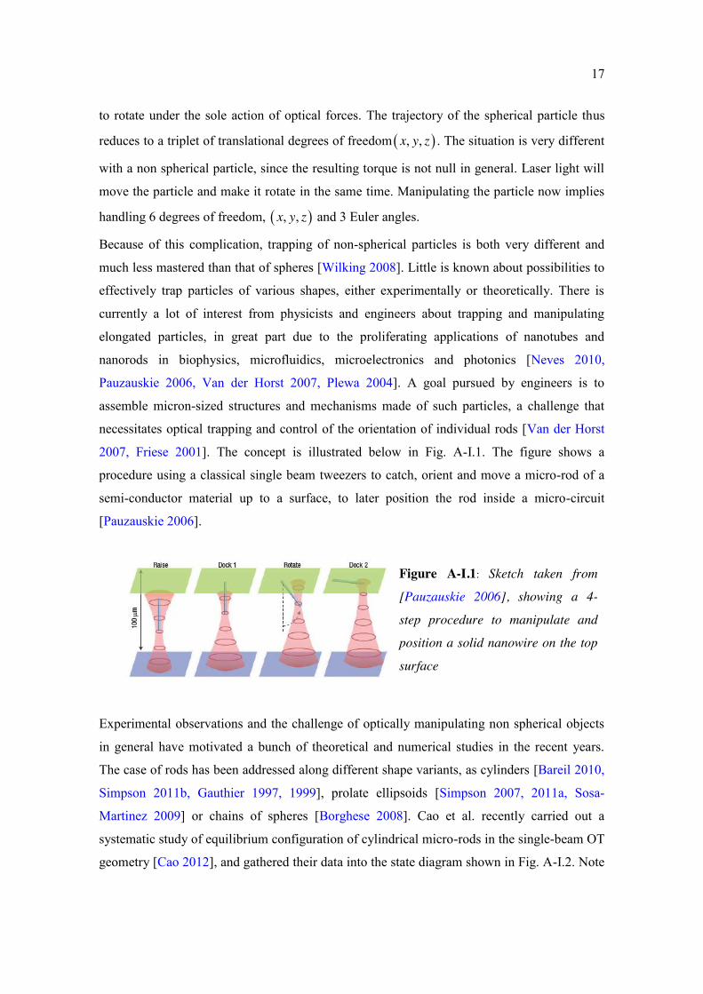
2007, Friese 2001]. The concept is illustrated below in Fig. A-I.1. The figure shows a

procedure using a classical single beam tweezers to catch, orient and move a micro-rod of a

semi-conductor material up to a surface, to later position the rod inside a micro-circuit

[Pauzauskie 2006].

Experimental observations and the challenge of optically manipulating non spherical objects

in general have motivated a bunch of theoretical and numerical studies in the recent years.

The case of rods has been addressed along different shape variants, as cylinders [Bareil 2010,

Simpson 2011b, Gauthier 1997, 1999], prolate ellipsoids [Simpson 2007, 2011a, Sosa-

Martinez 2009] or chains of spheres [Borghese 2008]. Cao et al. recently carried out a

systematic study of equilibrium configuration of cylindrical micro-rods in the single-beam OT

geometry [Cao 2012], and gathered their data into the state diagram shown in Fig. A-I.2. Note

Figure A-I.1: Sketch taken from

[Pauzauskie 2006], showing a 4-

step procedure to manipulate and

position a solid nanowire on the top

surface

18

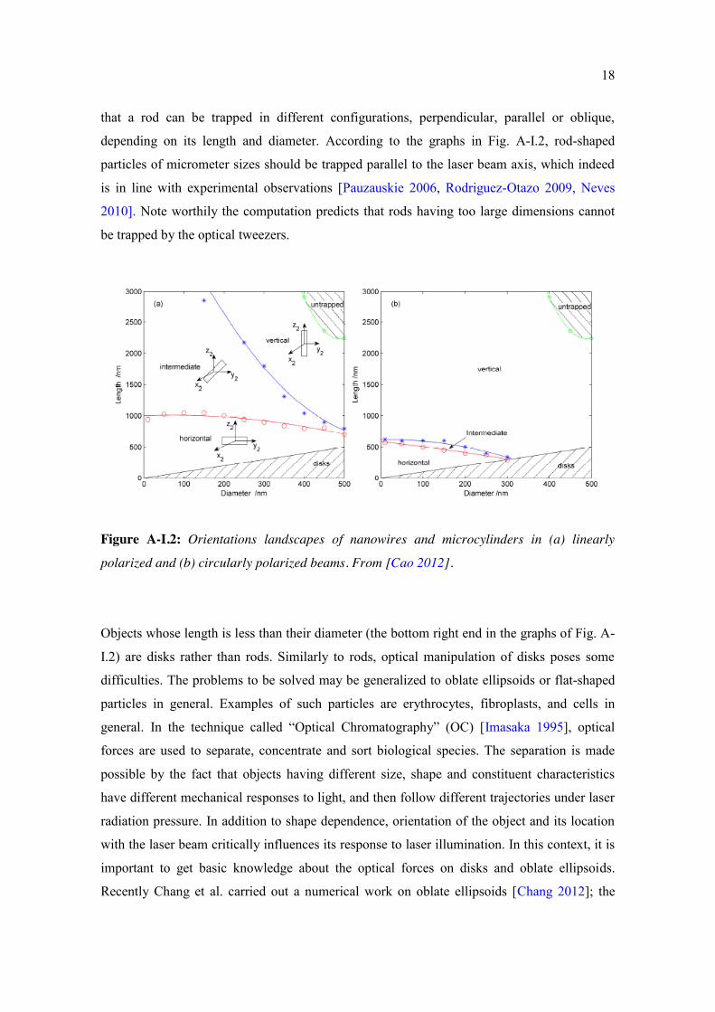
that a rod can be trapped in different configurations, perpendicular, parallel or oblique,

depending on its length and diameter. According to the graphs in Fig. A-I.2, rod-shaped

particles of micrometer sizes should be trapped parallel to the laser beam axis, which indeed

is in line with experimental observations [Pauzauskie 2006, Rodriguez-Otazo 2009, Neves

2010]. Note worthily the computation predicts that rods having too large dimensions cannot

be trapped by the optical tweezers.

Figure A-I.2: Orientations landscapes of nanowires and microcylinders in (a) linearly

polarized and (b) circularly polarized beams. From [Cao 2012].

Objects whose length is less than their diameter (the bottom right end in the graphs of Fig. A-

I.2) are disks rather than rods. Similarly to rods, optical manipulation of disks poses some

difficulties. The problems to be solved may be generalized to oblate ellipsoids or flat-shaped

particles in general. Examples of such particles are erythrocytes, fibroplasts, and cells in

general.   In   the   technique   called   “Optical   Chromatography”   (OC)   [Imasaka 1995], optical

forces are used to separate, concentrate and sort biological species. The separation is made

possible by the fact that objects having different size, shape and constituent characteristics

have different mechanical responses to light, and then follow different trajectories under laser

radiation pressure. In addition to shape dependence, orientation of the object and its location

with the laser beam critically influences its response to laser illumination. In this context, it is

important to get basic knowledge about the optical forces on disks and oblate ellipsoids.

Recently Chang et al. carried out a numerical work on oblate ellipsoids [Chang 2012]; the

19

goal was to predict trajectories of such objects in a weakly focused laser beam, of the kind

used in OC geometries. Particles, about 8 m in diameter, were definitely smaller than the

beam diameter (32 m at beam-waist). The authors computed the trajectories of an oblate

ellipsoid as a function of its aspect ratio for different initial locations and orientations. They

found that such particles might follow undulating trajectories, but that they would ultimately

get   laterally  trapped  along  the  laser  beam  axis,   in  “orthogonal”  configuration  (i.e.  with  their  

flat side parallel to the axis). This conclusion is in line with previous observations [Cheng

2002, 2003] and theoretical determination of equilibrium states [Grover 2000] of disks or red

blood cells in a laser beam (note that Grover et al.’s   computation   took   into   account   the  

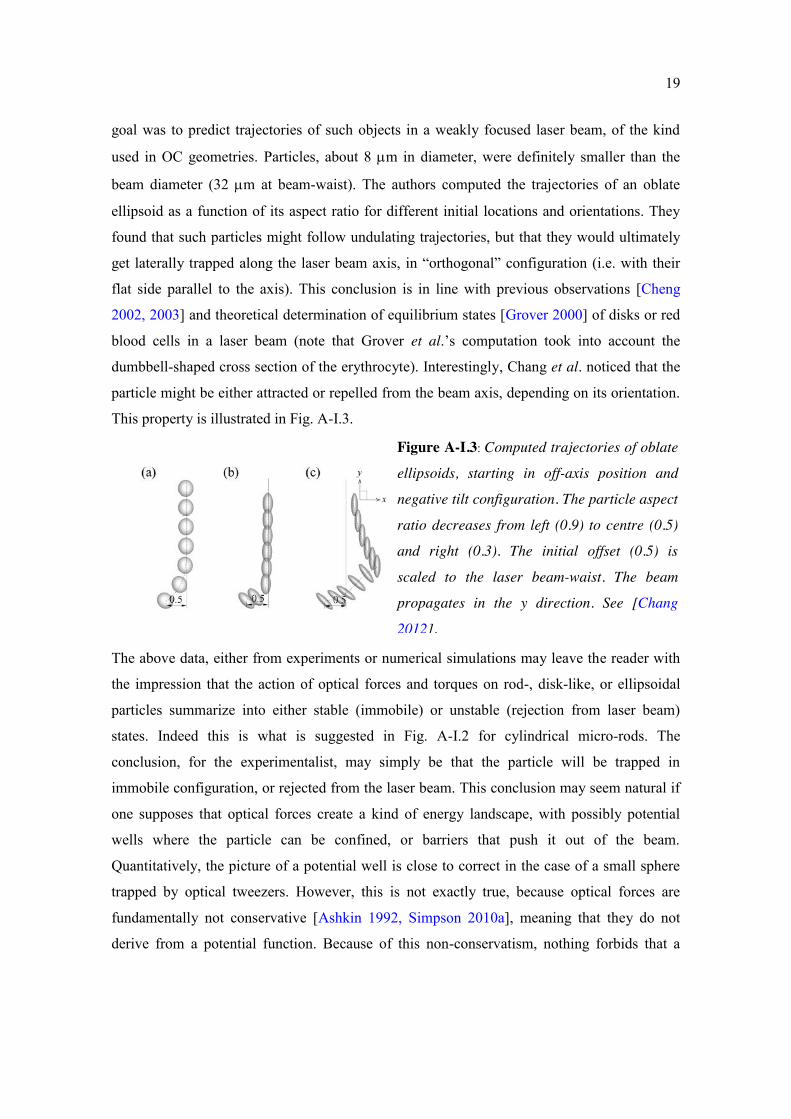
dumbbell-shaped cross section of the erythrocyte). Interestingly, Chang et al. noticed that the

particle might be either attracted or repelled from the beam axis, depending on its orientation.

This property is illustrated in Fig. A-I.3.

The above data, either from experiments or numerical simulations may leave the reader with

the impression that the action of optical forces and torques on rod-, disk-like, or ellipsoidal

particles summarize into either stable (immobile) or unstable (rejection from laser beam)

states. Indeed this is what is suggested in Fig. A-I.2 for cylindrical micro-rods. The

conclusion, for the experimentalist, may simply be that the particle will be trapped in

immobile configuration, or rejected from the laser beam. This conclusion may seem natural if

one supposes that optical forces create a kind of energy landscape, with possibly potential

wells where the particle can be confined, or barriers that push it out of the beam.

Quantitatively, the picture of a potential well is close to correct in the case of a small sphere

trapped by optical tweezers. However, this is not exactly true, because optical forces are

fundamentally not conservative [Ashkin 1992, Simpson 2010a], meaning that they do not

derive from a potential function. Because of this non-conservatism, nothing forbids that a

Figure A-I.3: Computed trajectories of oblate

ellipsoids, starting in off-axis position and

negative tilt configuration. The particle aspect

ratio decreases from left (0.9) to centre (0.5)

and right (0.3). The initial offset (0.5) is

scaled to the laser beam-waist. The beam

propagates in the y direction. See [Chang

2012].

20

particle in a laser beam never comes to rest, but instead moves permanently in a more or less

complicated manner. Indeed, a few such situations have been reported, as we explain below.

Experimental tests have revealed that the procedure of Fig. A-I works with certain rods but

not with all of them. Pazauskie et al. noticed that some of their rods would not stay vertically

trapped and would undergo sustained back-and-forth tilt motion around the laser beam axis

[Pazauskie 2006]. However no formal interpretation was provided to explain the

phenomenon. A similar observation was shortly mentioned by Wilking et al., with the letter I

from  a  colloidal  “alphabet  soup” [Wilking 2008], with no interpretation either.

Neves et al. worked with polymeric nano-fibres [Neves 2010], which they were able to align

along the beam axis and stably trap in bulk water. However when the fibre was brought in

contact to the cover slip of the sample chamber, it switched to a strongly oblique orientation.

In this configuration, the fibre was observed to continuously rotate around the laser axis.

Though the authors did not provide an explanation of how the particle would adopt a

configuration leading to sustained rotation, they could verify that angular velocities were in

line with computed values of optical torques [Neves 2010].

An observation that may have some similarities with the above mentioned oscillation of

micro-rods [Pazauskie 2006] has been reported by Cheng et al. from trapping experiments

with disk shaped organic particles [Cheng 2003]. The latter authors were able to stably trap

disks in bulk water over a large range of dimensions (between 0.4 and 20 m in diameter)

around the focus of a linearly polarized laser [Cheng 2002]. The disks were trapped with their

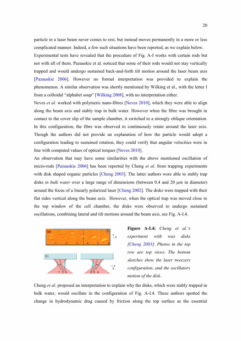
flat sides vertical along the beam axis. However, when the optical trap was moved close to

the top window of the cell chamber, the disks were observed to undergo sustained

oscillations, combining lateral and tilt motions around the beam axis, see Fig. A-I.4.

Cheng et al. proposed an interpretation to explain why the disks, which were stably trapped in

bulk water, would oscillate in the configuration of Fig. A-I.4. These authors spotted the

change in hydrodynamic drag caused by friction along the top surface as the essential

Figure A-I.4: Cheng   et   al.’s  

experiment with wax disks

[Cheng 2003]. Photos in the top

row are top views. The bottom

sketches show the laser tweezers

configuration, and the oscillatory

motion of the disk.

21

difference between both situations. They proposed a model expression for the force

introduced by the friction that coupled translation and tilt angle of the disk. Based on this

expression, they showed that their model would indeed produce a bifurcation, between static

and oscillating states disks [Cheng 2003]. The control parameter of the bifurcation is the

distance z between the beam-waist and the top surface.

Our own work, the matter of the following sections, is dedicated to more or less similar

phenomena which we observed with ellipsoidal particles, including prolate and oblate shapes.

Rather than a tightly focused beam in an optical tweezers configuration, we use a moderately

focused beam in a simple optical levitation scheme. The size parameters of the experiments,

and the beam diffraction length l (about 14 m), are definitely larger than those involved with

micro-rods and single beam traps, but they offer the decisive advantage that the particle can

be observed from different directions, while the main physical trends may be extrapolated to

the submicron range. Moreover, the ellipsoids have very few birefringence and show little

sensitivity to polarization of the laser beam, an appreciable simplification compared to disks

and nano-ribbons. As we will see, the ellipsoidal particles either come to rest inside the beam

or go through a characteristic back-and-forth motion, with a transition between both regimes

that critically depends on their aspect ratio. We offer a complete experimental characterization

of the phenomenon, and propose a physical interpretation based on a simple model of RP

forces for an ellipsoid, in 2-dimensions. Unlike Cheng et al.’s   analysis,   we   draw   the  

conclusion that sustained particle oscillations are due to the nature of RP forces alone, not to a

specific surface term in the hydrodynamic drag of the particle.

The following sections are organized as follows:

- In A-II we describe the experimental hardware and procedures. The section includes

details on the preparation of the ellipsoidal particles, the levitation setup, and the

devices for observation, signal acquisition and recording.

- The main experimental results are presented in A-III. Essentially we describe the

different behaviors of the particles, in bulk water, close to a fluid-fluid interface and

to a fluid-solid interface. As a major outcome of the observations, a state diagram is

proposed that gathers the different dynamic states of particles according to their size

parameters.

22

- Section A-IV   is   dedicated   to   the   analysis   of   particle’s   oscillations   using   standard  

tools of non linear systems dynamics. The goal is to clearly identify periodic and

non-periodic (akin to chaos) dynamics in the recorded experimental signals.

- In A-V we propose a simple model of light interaction with an ellipsoid. The model

is limited to dimension 2, as it only considers the interaction of light with an

elliptical body inside a plane. We compute the optical forces and torques in the ray-

optics approximation, in the simple case of a collimated beam, i.e. a collection of

parallel rays. As we will see, this very simplified picture is enough to produce a

bifurcation between static and oscillating states.

- General conclusion and propositions for future works is included at the end.

23

A-II: Experimental hardware and methods This chapter discusses the preparation of the materials used and methods applied in the

project. The first section explains the sample preparation technique, the second one deals with

the method of beam characterization, the third section describes the optical levitation setup

and in the last section, we describe the means applied for data acquisition and analysis.

A-II.1 Preparation of anisotropic particles The two main groups of methods to form non-spherical particles are:

(i) ab initio synthesis of non-spherical particles [Champion 2007]

(ii) Deforming already synthesized spherical particles [Champion 2007].

The former comprises lithography, photo polymerization [Xu 2005, Dendukuri 2005, 2006]

etc, whereas the later uses already fabricated spherical particles to deform to a non-spherical

geometry. We applied the latter method to obtain spheroidal particles of prolate or oblate

type.

A-II.1.a Prolate ellipsoids We used a technique initially designed by Ho et al., and later further developed by Champion

et al., to synthesize prolate ellipsoidal particles [Ho 1993; Champion, 2007]. This technique

consists in uniaxial mechanical stretching of polymeric spherical particles, which are

previously embedded in polymeric films. This process requires heating up the system above

the glass transition temperatures Tg of the spheres and slightly below that of the polymer

matrix. Below Tg, polymers are in a frozen glassy state and feature an elastic solid-like

behavior: they are almost not deformable and break quite easily when subjected to external

stresses. In contrast, above Tg, polymers become soft and behave like a viscoelastic fluid: they

can undergo a plastic deformation with high stretching capabilities. This sudden change in

state is related to the chain mobility of the polymer: at high temperature long-range segmental

motion appears (chain segments of 10 and 20 bonds begin to move) and in effect a rubbery

state is manifested [Daoud 1995]. Thus, a polymer at this state can be easily stretched to a

different form. Once the particles are stretched, the temperature is lowered below their Tg to

freeze their shape permanently since the polymer returns to a solid-like state. This process

may be applied to a rather broad range of particle size, typically going from a few hundreds of

nanometers up to a few tens of micrometers.

24

Concerning the present study, the starting particles are commercially available polystyrene

(PS) spheres with a diameter D=10 m (purchased from either Polysciences®, Molecular

Probes ® or Invitrogen®). The PS glass transition temperature is around 100°C. We used

polyvinyl alcohol (PVA) (FLUKA®) as the film-forming matrix. Hereafter, we list the

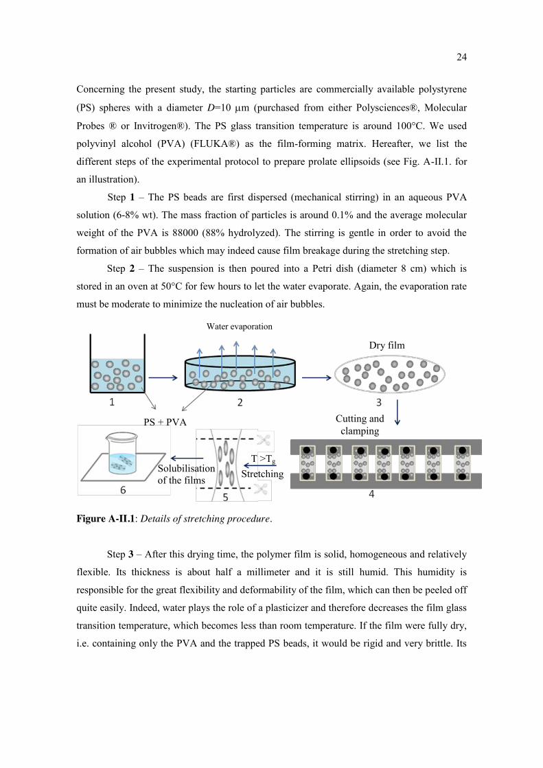
different steps of the experimental protocol to prepare prolate ellipsoids (see Fig. A-II.1. for

an illustration).

Step 1 – The PS beads are first dispersed (mechanical stirring) in an aqueous PVA

solution (6-8% wt). The mass fraction of particles is around 0.1% and the average molecular

weight of the PVA is 88000 (88% hydrolyzed). The stirring is gentle in order to avoid the

formation of air bubbles which may indeed cause film breakage during the stretching step.

Step 2 – The suspension is then poured into a Petri dish (diameter 8 cm) which is

stored in an oven at 50°C for few hours to let the water evaporate. Again, the evaporation rate

must be moderate to minimize the nucleation of air bubbles.

Figure A-II.1: Details of stretching procedure.

Step 3 – After this drying time, the polymer film is solid, homogeneous and relatively

flexible. Its thickness is about half a millimeter and it is still humid. This humidity is

responsible for the great flexibility and deformability of the film, which can then be peeled off

quite easily. Indeed, water plays the role of a plasticizer and therefore decreases the film glass

transition temperature, which becomes less than room temperature. If the film were fully dry,

i.e. containing only the PVA and the trapped PS beads, it would be rigid and very brittle. Its

Water evaporation

Dry film

Cutting and clamping

T >Tg Stretching Solubilisation

of the films

PS + PVA

25

properties would be close to those of pure PVA (Tg 85°C), which is semi-crystalline. In this

solid state, it is impossible to peel off the film.

Step 4 – The dry film is cut into identical strips of dimensions L x l = 2.5 cm x 1.5 cm

which are further clamped on the metal jaws of a stretching device which is fitted in an oven.

Only the upper jaw is mobile; its motion may be controlled through a step motor interfaced to

simple homemade LabVIEW software. The oven temperature is then raised and reaches

115°C (greater than the Tg of PS). Before stretching, the oven temperature is uniform

everywhere.

Step 5 – The strips are stretched vertically at a constant speed equal to 1 mm.s-1 till the

desired elongation is reached. The final elongation sets the prolate ellipsoid aspect ratios k1

and k2 : denoting a, b, c the ellipsoid three semi-axes (Fig. A-II.15), we have k1=a/b and

k2=a/c. Once stretched, the films are cooled down to room temperature to freeze the particle

ellipsoidal shape.

To locate the most homogeneous deformation zones on the strips, one may initially draw

black square grids on them (0.2 cm x 0.2 cm for example). After stretching, only the

rectangular regions with dimensions consistent with the desired targeted elongation are kept.

These regions are mostly located on the central parts of the strips where the stretching is the

most homogeneous, as expected.

Before implementing the last two steps, the above protocol may be repeated two or three

times (or even more) to get a sufficient amount of particles.

Step 6 – The central zones of the stretched strips are cut and dissolved in distilled

water at T = 50°C. The obtained solution is then centrifuged to make the PS ellipsoids

sediment and eliminate the upper PVA rich phase.

Many washing cycles with distilled water are necessary to remove PVA traces as much as

possible. It is very likely though that there remains some PVA adsorbed at the particle

surface, even after several washing cycles. Therefore, in our levitation experiments, it will be

important to compare the behavior of ellipsoids with that of PVA treated spheres; thereby

avoiding any possible artifact coming from differences in surface chemistry. The ellipsoids

are finally dispersed in distilled water and stored in the fridge at 4°C.

26

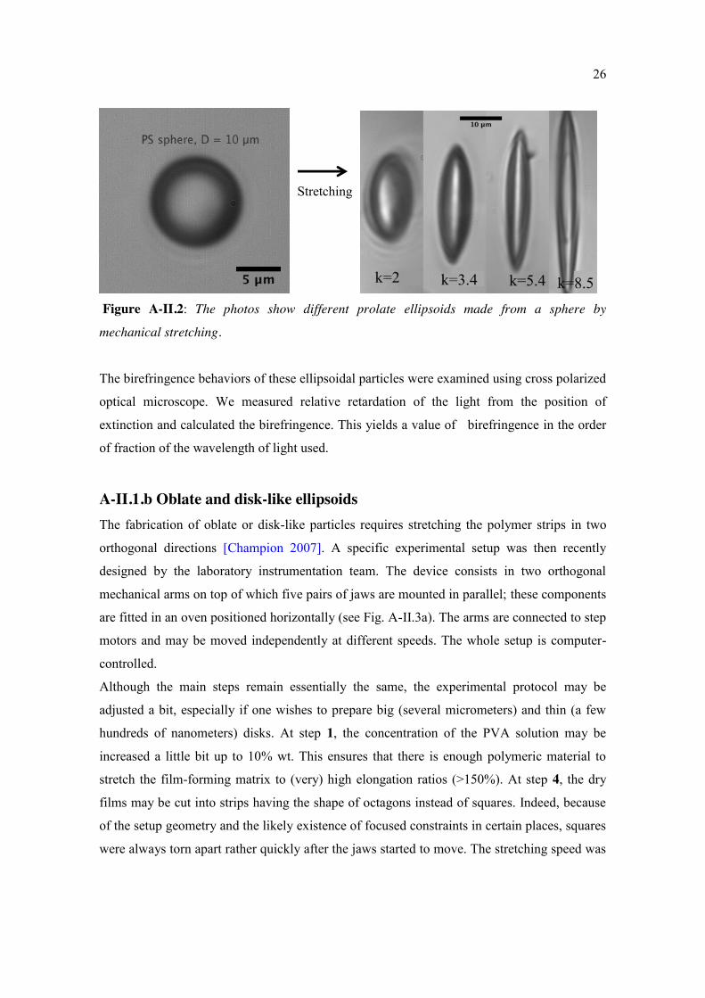
Figure A-II.2: The photos show different prolate ellipsoids made from a sphere by

mechanical stretching.

The birefringence behaviors of these ellipsoidal particles were examined using cross polarized

optical microscope. We measured relative retardation of the light from the position of

extinction and calculated the birefringence. This yields a value of birefringence in the order

of fraction of the wavelength of light used.

A-II.1.b Oblate and disk-like ellipsoids The fabrication of oblate or disk-like particles requires stretching the polymer strips in two

orthogonal directions [Champion 2007]. A specific experimental setup was then recently

designed by the laboratory instrumentation team. The device consists in two orthogonal

mechanical arms on top of which five pairs of jaws are mounted in parallel; these components

are fitted in an oven positioned horizontally (see Fig. A-II.3a). The arms are connected to step

motors and may be moved independently at different speeds. The whole setup is computer-

controlled.

Although the main steps remain essentially the same, the experimental protocol may be

adjusted a bit, especially if one wishes to prepare big (several micrometers) and thin (a few

hundreds of nanometers) disks. At step 1, the concentration of the PVA solution may be

increased a little bit up to 10% wt. This ensures that there is enough polymeric material to

stretch the film-forming matrix to (very) high elongation ratios (>150%). At step 4, the dry

films may be cut into strips having the shape of octagons instead of squares. Indeed, because

of the setup geometry and the likely existence of focused constraints in certain places, squares

were always torn apart rather quickly after the jaws started to move. The stretching speed was

Stretching

27

B

Jaws

A

Arms

also slowed down to 0.1 mm.s-1 on each axis and the stretching temperature was slightly

increased up to 130°C.

These conditions enable the stretching of five octagonal strips in parallel (each with an initial

thickness of about half a millimeter and sides equal to 2.5 cm) up to an elongation ratio of

175% on each axis. The final thickness is less than 100 m and all strips are deformed in the

same way, as illustrated on Fig. A-II.3b. However, the stretched zones on a given strip are not

homogeneous (see the black grid), except in the central region. If we cut out a larger area, we

end up with particles having a broad size and aspect ratio distributions. This may not be too

much of a problem if we are primarily interested in the behavior of one or two particles and

not a huge collection of them.

Figure A-II.3: Fabrication of oblate ellipsoids. (a) A 4-jaw device for 2-d stretching. (b)

Photos of stretched film, [ Mondiot 2011].

Sample cell Once the ellipsoids are prepared, they are diluted (< 0.01 % wt) in water and placed in a glass

cuvette (Fig. A-II.4). The sample cell is 1 or 2 mm in thickness and has polished sidewalls,

allowing for observation from all directions. It is placed on a motorized xy stage (we define x,

y as the horizontal directions) which can be moved in both directions with 50 nm resolution

(Aerotech). The sample cell can also be moved in the z direction (vertical) by means of a

manual translation stage. Resolution in z is about 1 micrometer.

28

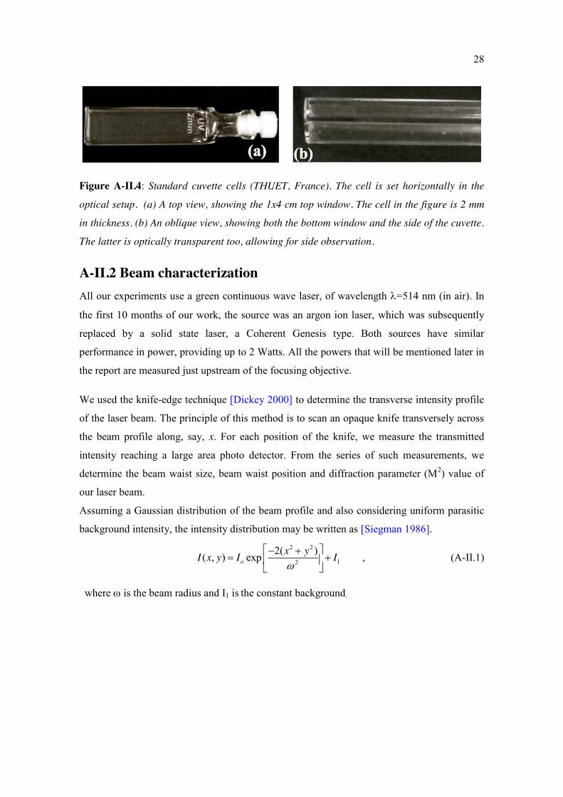
Figure A-II.4: Standard cuvette cells (THUET, France). The cell is set horizontally in the

optical setup. (a) A top view, showing the 1x4 cm top window. The cell in the figure is 2 mm

in thickness. (b) An oblique view, showing both the bottom window and the side of the cuvette.

The latter is optically transparent too, allowing for side observation.

A-II.2 Beam characterization All our experiments use a green continuous wave laser, of wavelength =514 nm (in air). In

the first 10 months of our work, the source was an argon ion laser, which was subsequently

replaced by a solid state laser, a Coherent Genesis type. Both sources have similar

performance in power, providing up to 2 Watts. All the powers that will be mentioned later in

the report are measured just upstream of the focusing objective.

We used the knife-edge technique [Dickey 2000] to determine the transverse intensity profile

of the laser beam. The principle of this method is to scan an opaque knife transversely across

the beam profile along, say, x. For each position of the knife, we measure the transmitted

intensity reaching a large area photo detector. From the series of such measurements, we

determine the beam waist size, beam waist position and diffraction parameter (M2) value of

our laser beam.

Assuming a Gaussian distribution of the beam profile and also considering uniform parasitic

background intensity, the intensity distribution may be written as [Siegman 1986]. 2 2

12

2( )( , ) expox yI x y I I

, (A-II.1)

where is the beam radius and I1 is the constant background.

29

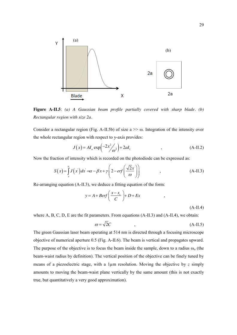
Figure A-II.5: (a) A Gaussian beam profile partially covered with sharp blade. (b)

Rectangular region with size 2a.

Consider a rectangular region (Fig. A-II.5b) of size a >> ω. Integration of the intensity over

the whole rectangular region with respect to y-axis provides:

22 1

2exp 2oxJ x AI aI

, (A-II.2)

Now the fraction of intensity which is recorded on the photodiode can be expressed as:

' ' 22x

xS x J x dx x erf

, (A-II.3)

Re-arranging equation (A-II.3), we deduce a fitting equation of the form:

cx xy A Berf D ExC

,

(A-II.4)

where A, B, C, D, E are the fit parameters. From equations (A-II.3) and (A-II.4), we obtain:

2C , (A-II.5)

The green Gaussian laser beam operating at 514 nm is directed through a focusing microscope

objective of numerical aperture 0.5 (Fig. A-II.6). The beam is vertical and propagates upward.

The purpose of the objective is to focus the beam inside the sample, down to a radius o (the

beam-waist radius by definition). The vertical position of the objective can be finely tuned by

means of a piezoelectric stage, with a 1m resolution. Moving the objective by z simply

amounts to moving the beam-waist plane vertically by the same amount (this is not exactly

true, but quantitatively a very good approximation).

(a)

(b)

30

The blade is located above the objective, at altitude zb, approximately where the sample (glass

cuvette) is located in the optical levitation experiments (Fig. A-II.10). The microscope on top

of the setup allows us to observe the transverse section of the beam, together with the blade,

as illustrated in Fig. A-II.6b. The diameter of the section (2) varies when we move the

objective vertically, and goes through a minimum (=o) when the blade crosses the beam-

waist plane, Z=0.

The knife edge technique thus allows us to measure in different horizontal sections, as a

function of Z, the distance to the beam-waist plane. The sharp blade is driven through the

focused beam in a step by step motion at 0.1µm/s (Fig. A-II.6a). The signal given by a

photodiode located above the blade is recorded at sampling frequency of 100Hz.

Figure A-II.6: (a) Knife edge technique. The blade (the black rectangle) is moved across the

beam, and the transmitted power is measured by means of the photodiode. (b) Image of the

blade (dark region) before it covers the beam (bright spot).

The intensity profile detected by the photodiode is fitted by equation (A-II.4). Below is an

example of a scan close to the beam-waist plane. Note that the scan profile is well fitted to,

with beam waist value of o =1.3µm.

(a)

31

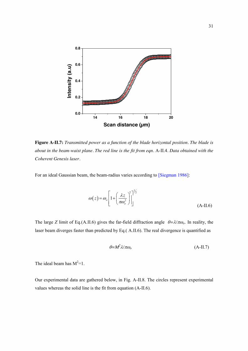
14 16 18 20

Inte

nsity

(a.u

)

Scan distance (µm)

0.0

0.2

0.4

0.6

0.8

Figure A-II.7: Transmitted power as a function of the blade horizontal position. The blade is

about in the beam-waist plane. The red line is the fit from eqn. A-II.4. Data obtained with the

Coherent Genesis laser.

For an ideal Gaussian beam, the beam-radius varies according to [Siegman 1986]:

1

2 2

21oo

zz

(A-II.6)

The large Z limit of Eq.(A.II.6) gives the far-field diffraction angle =/o. In reality, the

laser beam diverges faster than predicted by Eq.( A.II.6). The real divergence is quantified as

=M2/o (A-II.7)

The ideal beam has M2=1.

Our experimental data are gathered below, in Fig. A-II.8. The circles represent experimental

values whereas the solid line is the fit from equation (A-II.6).

32

Figure A-II.8: Evolution of the beam radius along the beam axis. Source: Coherent Genesis

laser.

The far field angle is obtained from the slope of the beam profile (Fig. A-II.8), i.e = 0.104

rad, which results in M2= 1.14 indicating that the laser has a good beam quality. The beam

diffraction length is calculated to be about 10 µm (in air).

A-II.3 Optical levitation setup Here we describe the optical levitation set-up that allows us to study the mechanical effect of

light on particles (both spherical and non spherical). The collimated laser light from the

source passes through three lenses (L1,2,3) before it is focused on the back–aperture of the

objective. These lenses are separated by the sum of their focal lengths (pair of lenses form

Keplerian telescopes), in such a way the light remains collimated after the telescope. We used

coupled galvanometric mirrors for beam steering. The translation of the beam on the sample

plane   is   achieved   by   a   rotation   of   the   beam   around   the   rear   focus   (F’)   of   the   microscope  

objective. The latter task is achieved by rotating  the  galvanometric  mirrors  (GM  and  F’  are  in  

conjugate planes, see Fig. A-II.9).

33

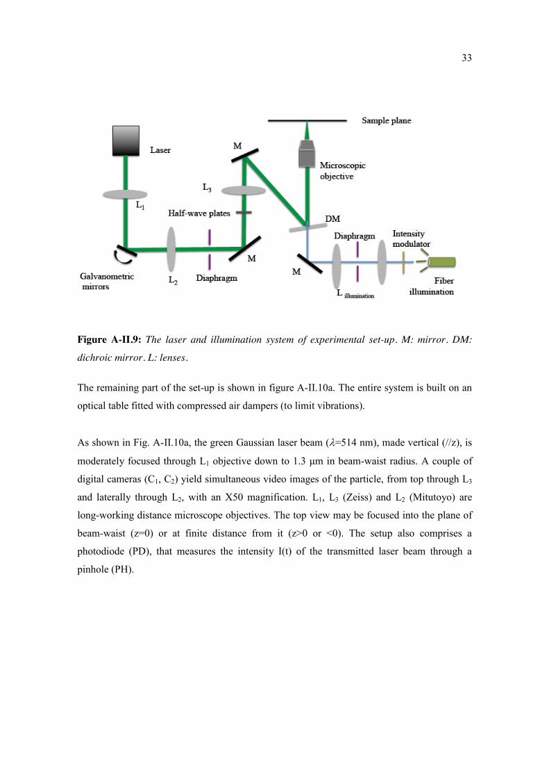
Figure A-II.9: The laser and illumination system of experimental set-up. M: mirror. DM:

dichroic mirror. L: lenses.

The remaining part of the set-up is shown in figure A-II.10a. The entire system is built on an

optical table fitted with compressed air dampers (to limit vibrations).

As shown in Fig. A-II.10a, the green Gaussian laser beam (=514 nm), made vertical (//z), is

moderately focused through L1 objective down to 1.3 μm in beam-waist radius. A couple of

digital cameras (C1, C2) yield simultaneous video images of the particle, from top through L3

and laterally through L2, with an X50 magnification. L1, L3 (Zeiss) and L2 (Mitutoyo) are

long-working distance microscope objectives. The top view may be focused into the plane of

beam-waist (z=0) or at finite distance from it (z>0 or <0). The setup also comprises a

photodiode (PD), that measures the intensity I(t) of the transmitted laser beam through a

pinhole (PH).

34

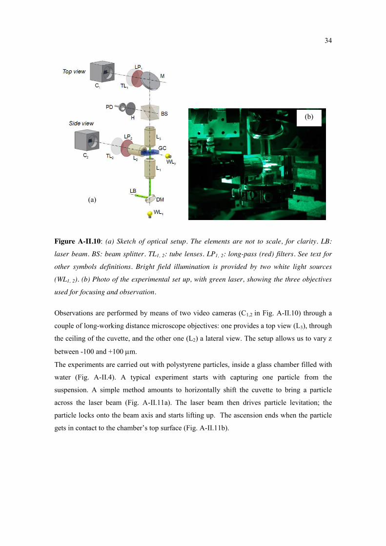
Figure A-II.10: (a) Sketch of optical setup. The elements are not to scale, for clarity. LB:

laser beam. BS: beam splitter. TL1, 2: tube lenses. LP1, 2: long-pass (red) filters. See text for

other symbols definitions. Bright field illumination is provided by two white light sources

(WL1, 2). (b) Photo of the experimental set up, with green laser, showing the three objectives

used for focusing and observation.

Observations are performed by means of two video cameras (C1,2 in Fig. A-II.10) through a

couple of long-working distance microscope objectives: one provides a top view (L3), through

the ceiling of the cuvette, and the other one (L2) a lateral view. The setup allows us to vary z

between -100 and +100 m.

The experiments are carried out with polystyrene particles, inside a glass chamber filled with

water (Fig. A-II.4). A typical experiment starts with capturing one particle from the

suspension. A simple method amounts to horizontally shift the cuvette to bring a particle

across the laser beam (Fig. A-II.11a). The laser beam then drives particle levitation; the

particle locks onto the beam axis and starts lifting up. The ascension ends when the particle

gets in contact to the  chamber’s  top surface (Fig. A-II.11b).

(a)

(b)

35

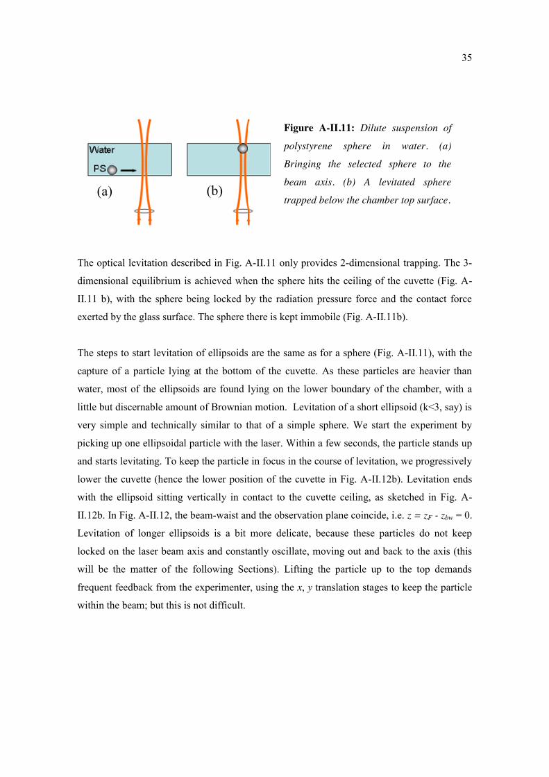
The optical levitation described in Fig. A-II.11 only provides 2-dimensional trapping. The 3-

dimensional equilibrium is achieved when the sphere hits the ceiling of the cuvette (Fig. A-

II.11 b), with the sphere being locked by the radiation pressure force and the contact force

exerted by the glass surface. The sphere there is kept immobile (Fig. A-II.11b).

The steps to start levitation of ellipsoids are the same as for a sphere (Fig. A-II.11), with the

capture of a particle lying at the bottom of the cuvette. As these particles are heavier than

water, most of the ellipsoids are found lying on the lower boundary of the chamber, with a

little but discernable amount of Brownian motion. Levitation of a short ellipsoid (k<3, say) is

very simple and technically similar to that of a simple sphere. We start the experiment by

picking up one ellipsoidal particle with the laser. Within a few seconds, the particle stands up

and starts levitating. To keep the particle in focus in the course of levitation, we progressively

lower the cuvette (hence the lower position of the cuvette in Fig. A-II.12b). Levitation ends

with the ellipsoid sitting vertically in contact to the cuvette ceiling, as sketched in Fig. A-

II.12b. In Fig. A-II.12, the beam-waist and the observation plane coincide, i.e. z = zF - zbw = 0.

Levitation of longer ellipsoids is a bit more delicate, because these particles do not keep

locked on the laser beam axis and constantly oscillate, moving out and back to the axis (this

will be the matter of the following Sections). Lifting the particle up to the top demands

frequent feedback from the experimenter, using the x, y translation stages to keep the particle

within the beam; but this is not difficult.

(b)

Figure A-II.11: Dilute suspension of

polystyrene sphere in water. (a)

Bringing the selected sphere to the

beam axis. (b) A levitated sphere

trapped below the chamber top surface.

(a) (b)

36

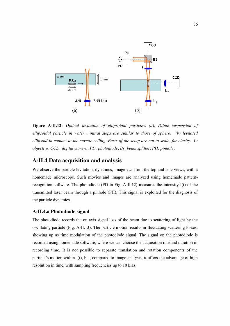
Figure A-II.12: Optical levitation of ellipsoidal particles. (a), Dilute suspension of

ellipsoidal particle in water , initial steps are similar to those of sphere. (b) levitated

ellipsoid in contact to the cuvette ceiling. Parts of the setup are not to scale, for clarity. L:

objective. CCD: digital camera. PD: photodiode. Bs: beam splitter. PH: pinhole.

A-II.4 Data acquisition and analysis We observe the particle levitation, dynamics, image etc. from the top and side views, with a

homemade microscope. Such movies and images are analyzed using homemade pattern-

recognition software. The photodiode (PD in Fig. A-II.12) measures the intensity I(t) of the

transmitted laser beam through a pinhole (PH). This signal is exploited for the diagnosis of

the particle dynamics.

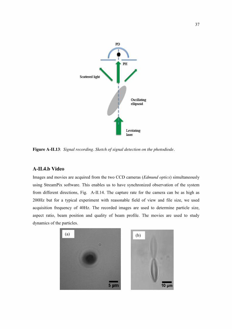
A-II.4.a Photodiode signal The photodiode records the on axis signal loss of the beam due to scattering of light by the

oscillating particle (Fig. A-II.13). The particle motion results in fluctuating scattering losses,

showing up as time modulation of the photodiode signal. The signal on the photodiode is

recorded using homemade software, where we can choose the acquisition rate and duration of

recording time. It is not possible to separate translation and rotation components of the

particle’s  motion  within  I(t),  but,  compared  to  image  analysis,  it  offers  the  advantage  of  high  

resolution in time, with sampling frequencies up to 10 kHz.

37

Figure A-II.13: Signal recording. Sketch of signal detection on the photodiode.

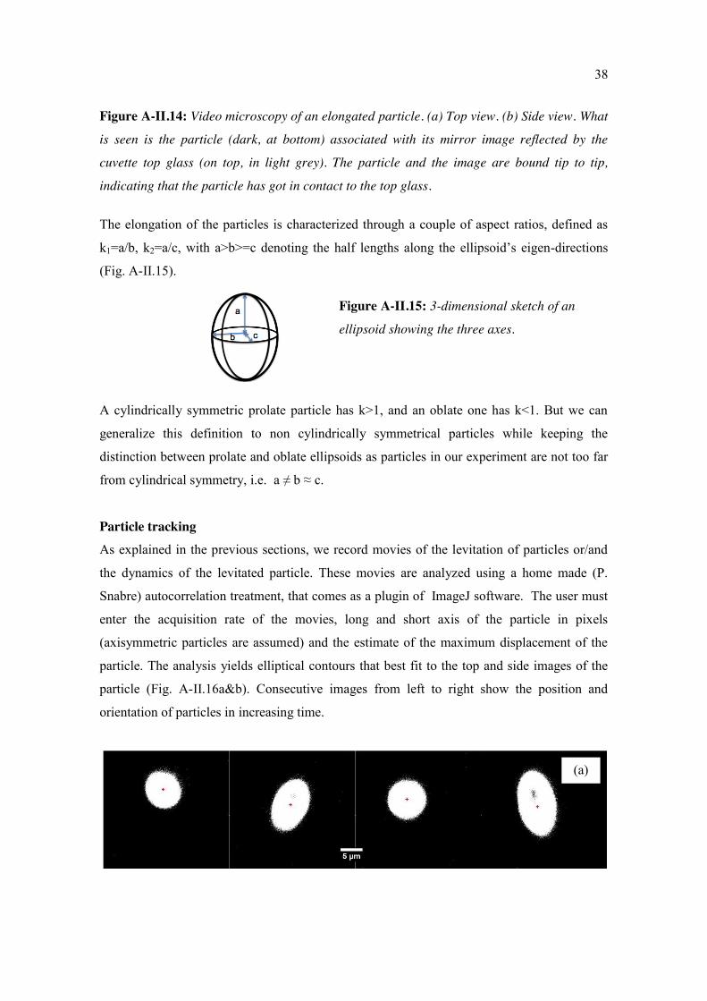
A-II.4.b Video Images and movies are acquired from the two CCD cameras (Edmund optics) simultaneously

using StreamPix software. This enables us to have synchronized observation of the system

from different directions, Fig. A-II.14. The capture rate for the camera can be as high as

200Hz but for a typical experiment with reasonable field of view and file size, we used

acquisition frequency of 40Hz. The recorded images are used to determine particle size,

aspect ratio, beam position and quality of beam profile. The movies are used to study

dynamics of the particles.

(a) (b)

38

Figure A-II.14: Video microscopy of an elongated particle. (a) Top view. (b) Side view. What

is seen is the particle (dark, at bottom) associated with its mirror image reflected by the

cuvette top glass (on top, in light grey). The particle and the image are bound tip to tip,

indicating that the particle has got in contact to the top glass.

The elongation of the particles is characterized through a couple of aspect ratios, defined as

k1=a/b, k2=a/c,  with   a>b>=c  denoting   the  half   lengths   along   the  ellipsoid’s   eigen-directions

(Fig. A-II.15).

A cylindrically symmetric prolate particle has k>1, and an oblate one has k<1. But we can

generalize this definition to non cylindrically symmetrical particles while keeping the

distinction between prolate and oblate ellipsoids as particles in our experiment are not too far

from cylindrical symmetry, i.e. a  ≠  b  ≈  c.  

Particle tracking As explained in the previous sections, we record movies of the levitation of particles or/and

the dynamics of the levitated particle. These movies are analyzed using a home made (P.

Snabre) autocorrelation treatment, that comes as a plugin of ImageJ software. The user must

enter the acquisition rate of the movies, long and short axis of the particle in pixels

(axisymmetric particles are assumed) and the estimate of the maximum displacement of the

particle. The analysis yields elliptical contours that best fit to the top and side images of the

particle (Fig. A-II.16a&b). Consecutive images from left to right show the position and

orientation of particles in increasing time.

(a)

Figure A-II.15: 3-dimensional sketch of an

ellipsoid showing the three axes.

39

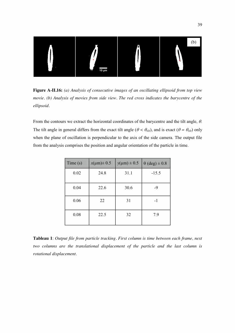
Figure A-II.16: (a) Analysis of consecutive images of an oscillating ellipsoid from top view

movie. (b) Analysis of movies from side view. The red cross indicates the barycentre of the

ellipsoid.

From the contours we extract the horizontal coordinates of the barycentre and the tilt angle, .

The tilt angle in general differs from the exact tilt angle ( < tilt), and is exact ( = tilt) only

when the plane of oscillation is perpendicular to the axis of the side camera. The output file

from the analysis comprises the position and angular orientation of the particle in time.

Time (s) x(µm)± 0.5 y(µm) ± 0.5 (deg) ± 0.8

0.02 24.8 31.1 -15.5

0.04 22.6 30.6 -9

0.06 22 31 -1

0.08 22.5 32 7.9

Tableau 1: Output file from particle tracking. First column is time between each frame, next

two columns are the translational displacement of the particle and the last column is

rotational displacement.

(b)

40

A-III: Results and Discussion The first section discusses the levitation behavior of particles in a bulk medium, whereas the

remaining two sections, address the behavior of these particles at an interface.

A-III.1 Levitation: Particle behavior in bulk water When a micron-sized particle is subjected to laser light, it can be locked at some point in

space, i.e. optically trapped, or simply pushed against gravity, i.e. levitated. We performed

single particle optical levitation. Optical levitation, as sketched in Fig. A-II. 11, only provides

a 2-dimensional (2d) trap. The low aperture laser beam does not provide axial trapping by

itself contrary to a large aperture beam (as in optical tweezers). However, the static

equilibrium may be achieved in bulk if the power is lowered such that the radiation pressure

levitation force just balances the particle weight [Ashkin 1970]. A polystyrene spherical

particle can be maintained about immobile in such condition, far from the walls of the cuvette.

The corresponding levitation power (Plev) is very small (< 3 mW), because of the very small

effective weight of a latex particle in water (polystyrene density is only 1.05). The obtained

vertical equilibrium is not strictly stable, meaning that the particle drifts up or down if no

feedback is applied. Fortunately the drift in water is very slow, leaving us enough time to

observe the particle behavior at about constant altitude (Fig. A-III. 1).

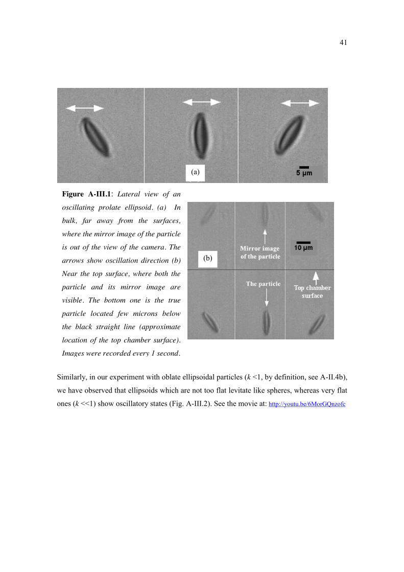
In a similar experiment with non-spherical particles, we observed that such particles, either

come to rest inside the beam or go through a characteristic dancing motion, with a transition

between both regimes that critically depends on their aspect ratio, i.e. oscillation appears

when  the  particle’s  elongation  reaches  a  threshold  value.  In  such  cases,  the  particle  is  seen  to  

oscillate as soon as it comes into the laser beam, at the beginning of the experiment and

during ascension. We thus bring the particle up in bulk water, away from the cell bottom and

still well below the cell ceiling. By tuning the laser beam power down to an appropriate

value, of the order of 3 mW, we are able to cancel ascension and maintain the particle at about

constant altitude. There, it undergoes sustained oscillations, combining angular and

translational excursions (Fig. A-III.1) . See the movie at : http://youtu.be/UWlMw3V3PZQ

41

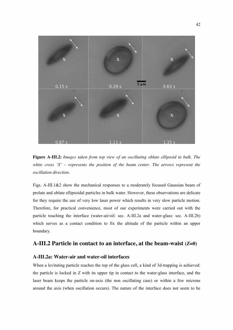
Similarly, in our experiment with oblate ellipsoidal particles (k <1, by definition, see A-II.4b),

we have observed that ellipsoids which are not too flat levitate like spheres, whereas very flat

ones (k <<1) show oscillatory states (Fig. A-III.2). See the movie at: http://youtu.be/6MorGQnzofc

Figure A-III.1: Lateral view of an

oscillating prolate ellipsoid. (a) In

bulk, far away from the surfaces,

where the mirror image of the particle

is out of the view of the camera. The

arrows show oscillation direction (b)

Near the top surface, where both the

particle and its mirror image are

visible. The bottom one is the true

particle located few microns below

the black straight line (approximate

location of the top chamber surface).

Images were recorded every 1 second.

(a)

(b)

42

Figure A-III.2: Images taken from top view of an oscillating oblate ellipsoid in bulk. The

white   cross   ’X’   – represents the position of the beam center. The arrows represent the

oscillation direction.

Figs. A-III.1&2 show the mechanical responses to a moderately focused Gaussian beam of

prolate and oblate ellipsoidal particles in bulk water. However, these observations are delicate

for they require the use of very low laser power which results in very slow particle motion.

Therefore, for practical convenience, most of our experiments were carried out with the

particle touching the interface (water-air/oil: sec. A-III.2a and water-glass: sec. A-III.2b)

which serves as a contact condition to fix the altitude of the particle within an upper

boundary.

A-III.2 Particle in contact to an interface, at the beam-waist (Z=0)

A-III.2a: Water-air and water-oil interfaces When a levitating particle reaches the top of the glass cell, a kind of 3d-trapping is achieved:

the particle is locked in Z with its upper tip in contact to the water-glass interface, and the

laser beam keeps the particle on-axis (the non oscillating case) or within a few microns

around the axis (when oscillation occurs). The nature of the interface does not seem to be

43

important: similarly to the water-glass interface, we have observed trapping of micron-sized

particles in contact to a fluid interface, namely a water-air or a water/oil interface. Dynamical

states were similar to those in bulk water, meaning that we observed both static and

oscillating states. In the case of the water-oil interface, the viscosity of the oil (79.5% decane

+ 20.5 % undecane) was matched to that of water (1 mPa.s), making the water-oil system a

continuous phase from the viewpoint of hydrodynamics, at low Reynolds number, as in the

experiments of [Loudet 2005]. The water-oil interface, in this situation, only ensures the

boundary condition in z, while the drag force and torque acting on the particle are the same as

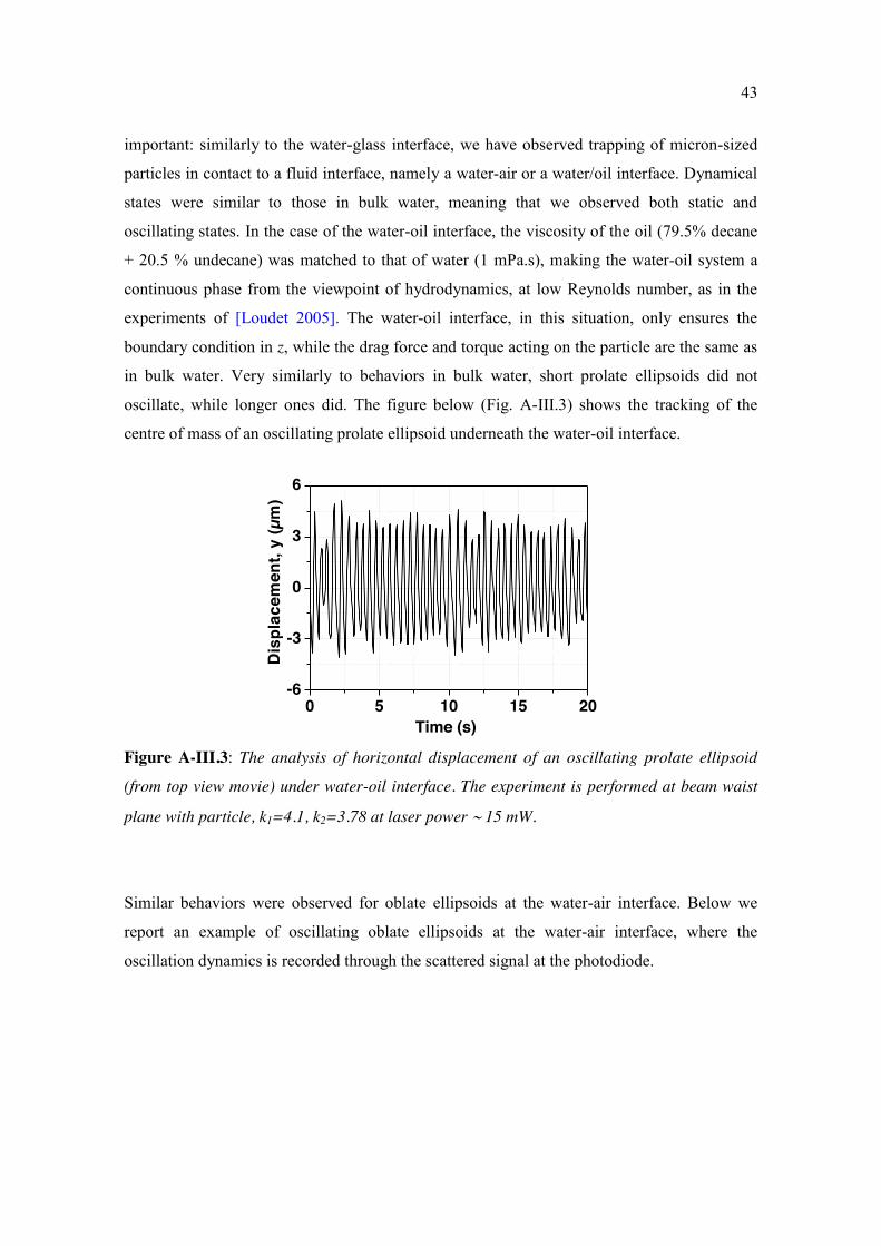
in bulk water. Very similarly to behaviors in bulk water, short prolate ellipsoids did not

oscillate, while longer ones did. The figure below (Fig. A-III.3) shows the tracking of the

centre of mass of an oscillating prolate ellipsoid underneath the water-oil interface.

0 5 10 15 20-6

-3

0

3

6

Dis

plac

emen

t, y

(µm

)

Time (s) Figure A-III.3: The analysis of horizontal displacement of an oscillating prolate ellipsoid

(from top view movie) under water-oil interface. The experiment is performed at beam waist

plane with particle, k1=4.1, k2=3.78 at laser power 15 mW.

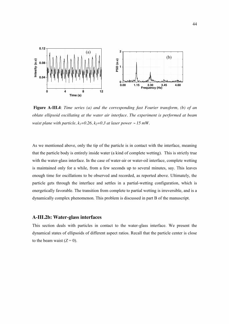
Similar behaviors were observed for oblate ellipsoids at the water-air interface. Below we

report an example of oscillating oblate ellipsoids at the water-air interface, where the

oscillation dynamics is recorded through the scattered signal at the photodiode.

44

Figure A-III.4: Time series (a) and the corresponding fast Fourier transform, (b) of an

oblate ellipsoid oscillating at the water air interface. The experiment is performed at beam

waist plane with particle, k1=0.26, k2=0.3 at laser power 15 mW.

As we mentioned above, only the tip of the particle is in contact with the interface, meaning

that the particle body is entirely inside water (a kind of complete wetting). This is strictly true

with the water-glass interface. In the case of water-air or water-oil interface, complete wetting

is maintained only for a while, from a few seconds up to several minutes, say. This leaves

enough time for oscillations to be observed and recorded, as reported above. Ultimately, the

particle gets through the interface and settles in a partial-wetting configuration, which is

energetically favorable. The transition from complete to partial wetting is irreversible, and is a

dynamically complex phenomenon. This problem is discussed in part B of the manuscript.

A-III.2b: Water-glass interfaces This section deals with particles in contact to the water-glass interface. We present the

dynamical states of ellipsoids of different aspect ratios. Recall that the particle center is close

to the beam waist (Z = 0).

0 4 8 12

0.04

0.08

0.12

Inte

sity

(a.u

)

Time (s)

0.00 1.15 2.30 3.45 4.600

1

2

Frequency (Hz)

PSD

(a.u

)

(a) (b)

45

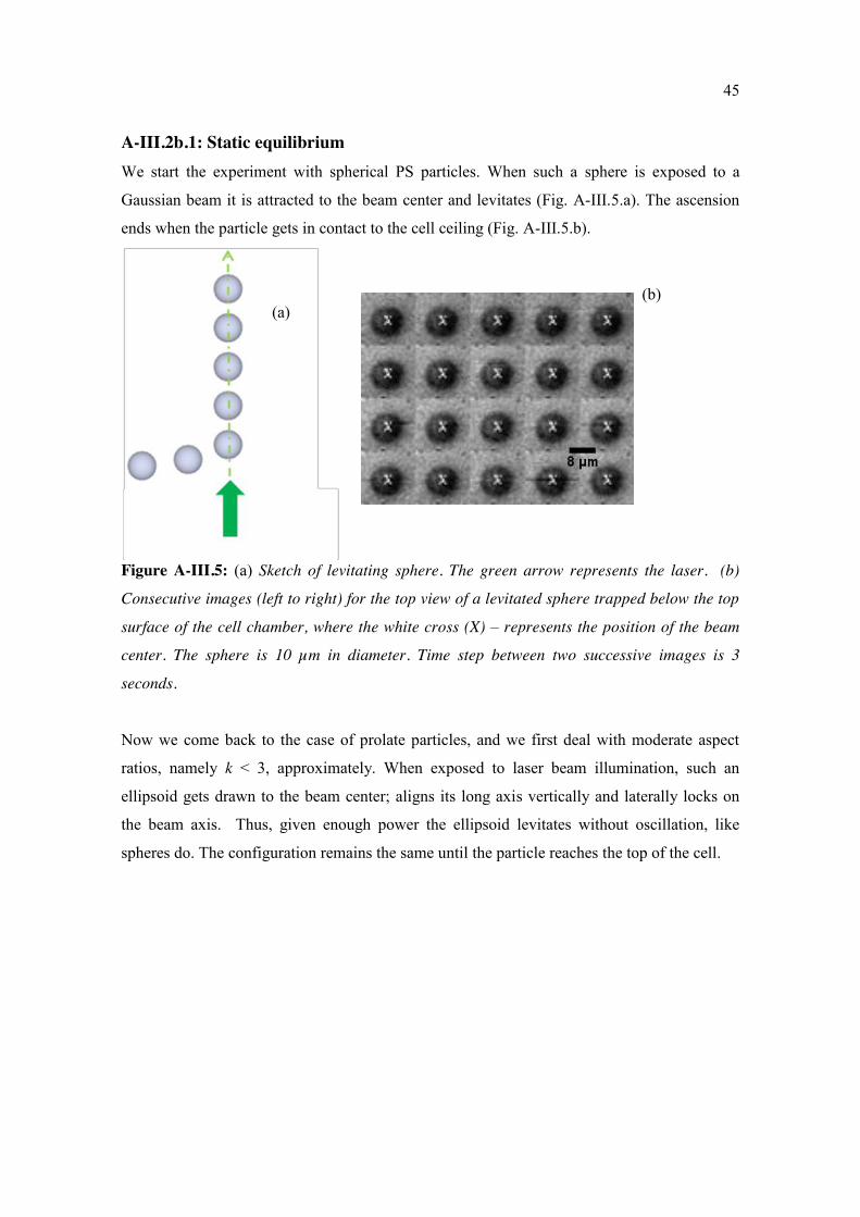
A-III.2b.1: Static equilibrium We start the experiment with spherical PS particles. When such a sphere is exposed to a

Gaussian beam it is attracted to the beam center and levitates (Fig. A-III.5.a). The ascension

ends when the particle gets in contact to the cell ceiling (Fig. A-III.5.b).

Figure A-III.5: (a) Sketch of levitating sphere. The green arrow represents the laser. (b)

Consecutive images (left to right) for the top view of a levitated sphere trapped below the top

surface of the cell chamber, where the white cross (X) – represents the position of the beam

center. The sphere is 10 µm in diameter. Time step between two successive images is 3

seconds.

Now we come back to the case of prolate particles, and we first deal with moderate aspect

ratios, namely k < 3, approximately. When exposed to laser beam illumination, such an

ellipsoid gets drawn to the beam center; aligns its long axis vertically and laterally locks on

the beam axis. Thus, given enough power the ellipsoid levitates without oscillation, like

spheres do. The configuration remains the same until the particle reaches the top of the cell.

(b) (a)

46

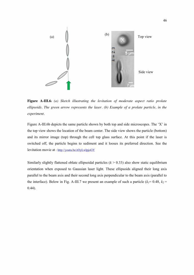
Figure A-III.6: (a) Sketch illustrating the levitation of moderate aspect ratio prolate

ellipsoids. The green arrow represents the laser. (b) Example of a prolate particle, in the

experiment.

Figure A-III.6b depicts the same particle shown by both top and side microscopes.  The  ‘X’  in  

the top view shows the location of the beam center. The side view shows the particle (bottom)

and its mirror image (top) through the cell top glass surface. At this point if the laser is

switched off, the particle begins to sediment and it looses its preferred direction. See the

levitation movie at : http://youtu.be/zOyLwlpjoGY

Similarly slightly flattened oblate ellipsoidal particles (k > 0.33) also show static equilibrium

orientation when exposed to Gaussian laser light. These ellipsoids aligned their long axis

parallel to the beam axis and their second long axis perpendicular to the beam axis (parallel to

the interface). Below in Fig. A-III.7 we present an example of such a particle (k1= 0.48, k2 =

0.44).

(a) (b) Top view

Side view

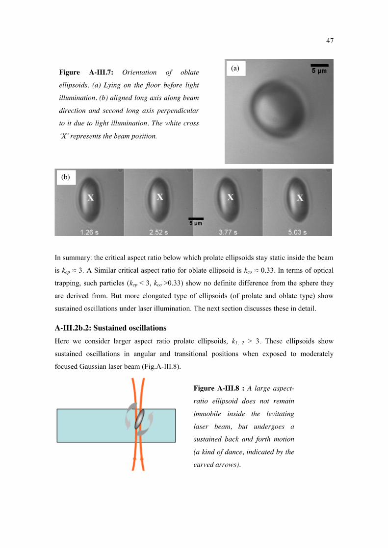
47

In summary: the critical aspect ratio below which prolate ellipsoids stay static inside the beam

is kcp ≈  3.  A  Similar  critical  aspect  ratio  for  oblate  ellipsoid  is  kco ≈  0.33.  In  terms  of  optical  

trapping, such particles (kcp < 3, kco >0.33) show no definite difference from the sphere they

are derived from. But more elongated type of ellipsoids (of prolate and oblate type) show

sustained oscillations under laser illumination. The next section discusses these in detail.

A-III.2b.2: Sustained oscillations Here we consider larger aspect ratio prolate ellipsoids, k1, 2 > 3. These ellipsoids show

sustained oscillations in angular and transitional positions when exposed to moderately

focused Gaussian laser beam (Fig.A-III.8).

Figure A-III.8 : A large aspect-

ratio ellipsoid does not remain

immobile inside the levitating

laser beam, but undergoes a

sustained back and forth motion

(a kind of dance, indicated by the

curved arrows).

Figure A-III.7: Orientation of oblate

ellipsoids. (a) Lying on the floor before light

illumination. (b) aligned long axis along beam

direction and second long axis perpendicular

to it due to light illumination. The white cross

‘X’  represents  the  beam  position.

(a)

(b)

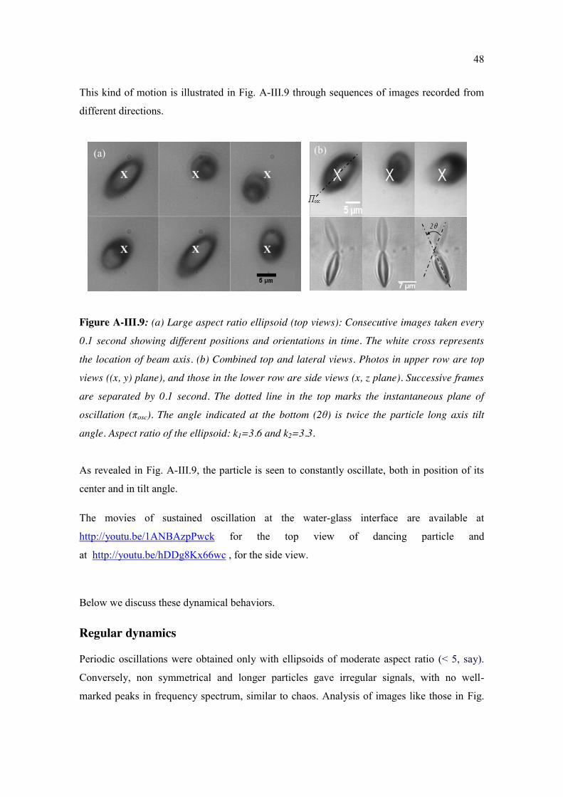
48

This kind of motion is illustrated in Fig. A-III.9 through sequences of images recorded from

different directions.

Figure A-III.9: (a) Large aspect ratio ellipsoid (top views): Consecutive images taken every

0.1 second showing different positions and orientations in time. The white cross represents

the location of beam axis. (b) Combined top and lateral views. Photos in upper row are top

views ((x, y) plane), and those in the lower row are side views (x, z plane). Successive frames

are separated by 0.1 second. The dotted line in the top marks the instantaneous plane of

oscillation (πosc). The angle indicated at the bottom (2θ) is twice the particle long axis tilt

angle. Aspect ratio of the ellipsoid: k1=3.6 and k2=3.3.

As revealed in Fig. A-III.9, the particle is seen to constantly oscillate, both in position of its

center and in tilt angle.

The movies of sustained oscillation at the water-glass interface are available at

http://youtu.be/1ANBAzpPwck for the top view of dancing particle and

at http://youtu.be/hDDg8Kx66wc , for the side view.

Below we discuss these dynamical behaviors.

Regular dynamics

Periodic oscillations were obtained only with ellipsoids of moderate aspect ratio (< 5, say).

Conversely, non symmetrical and longer particles gave irregular signals, with no well-

marked peaks in frequency spectrum, similar to chaos. Analysis of images like those in Fig.

(a) (b)

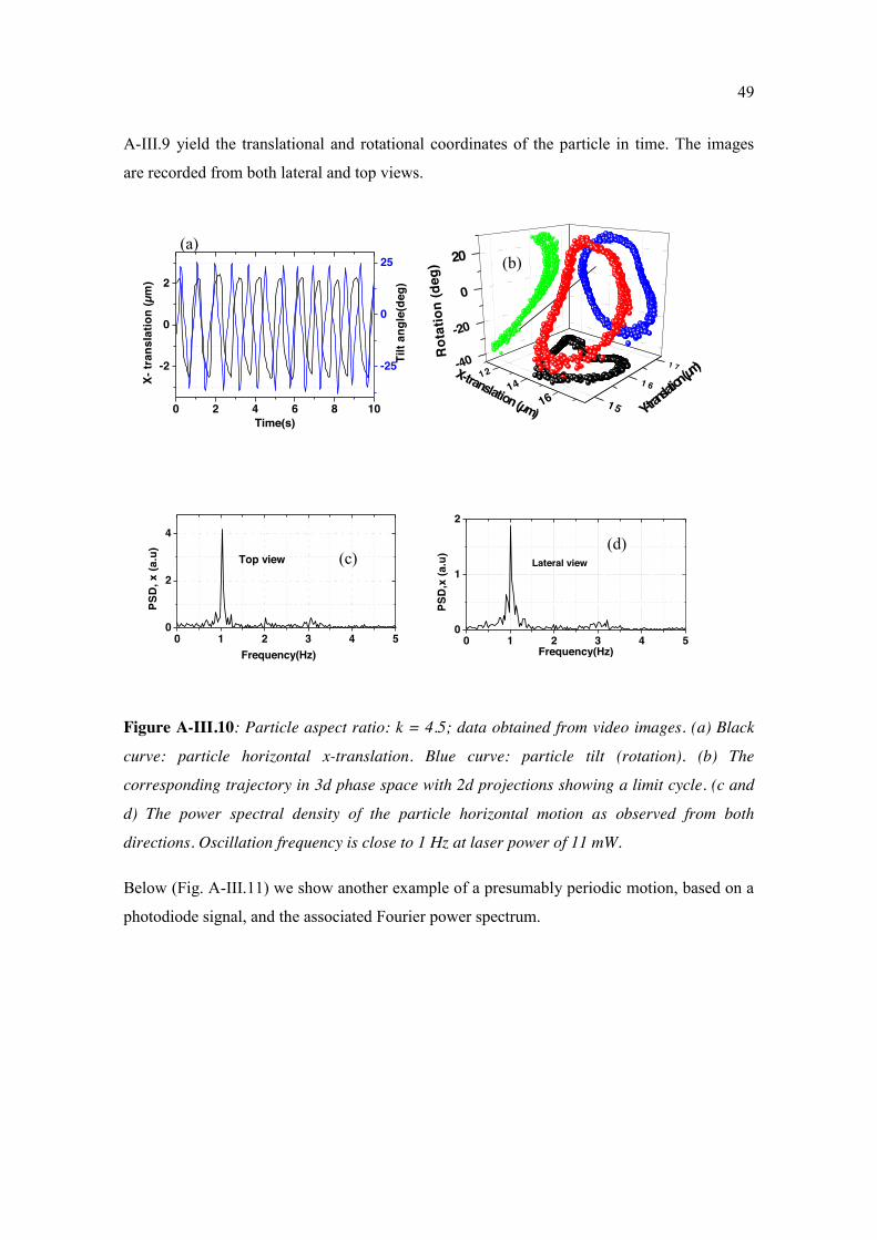
49

A-III.9 yield the translational and rotational coordinates of the particle in time. The images

are recorded from both lateral and top views.

0 2 4 6 8 10

-2

0

2

Time(s)

X- tr

ansl

atio

n (µ

m)

-25

0

25

Tilt

ang

le(d

eg)

1 214

16

-40

-20

0

20

1 5

1 6

1 7

Rot

atio

n (d

eg)

Y-transla

tion (µm)X-translation (µm)

Figure A-III.10: Particle aspect ratio: k = 4.5; data obtained from video images. (a) Black

curve: particle horizontal x-translation. Blue curve: particle tilt (rotation). (b) The

corresponding trajectory in 3d phase space with 2d projections showing a limit cycle. (c and

d) The power spectral density of the particle horizontal motion as observed from both

directions. Oscillation frequency is close to 1 Hz at laser power of 11 mW.

Below (Fig. A-III.11) we show another example of a presumably periodic motion, based on a

photodiode signal, and the associated Fourier power spectrum.

(a) (b)

0 1 2 3 4 50

2

4

Top view

Frequency(Hz)

PSD

, x (a

.u)

0 1 2 3 4 50

1

2

Lateral view

Frequency(Hz)

PSD

,x (a

.u)(c)

(d)

50

Figure A-III.11: Data recorded with a (k1= k2= 3.8) particle. (a) Modulation of the on-axis

laser power recorded with the photodiode and (b) corresponding power spectrum density

showing peaks at integral multiple of the fundamental   frequency   ≈   2  Hz.  Laser power :19

mW.

Influence of the laser power on the particle dynamics Here we investigate the effect of changing power on the dynamics of the particle. The

conclusion, drawn from observations of periodic motions, is very simple: the frequency of

oscillation just scales linearly with the laser power. Changing the power does not change the

dynamical state qualitatively. The latter conclusion is illustrated in Fig. A-III.12. The figure

shows the effect of increasing the power from 9.1mW (top row) to 22.3 mW (bottom row).

(a) (b)

0 5 10 15 20

0.1

0.2

0.3

0 5 10 150

30

60

0 5 10 15 20

0.2

0.4

0.6

0.8

0 4 8 120

40

80

120

Inte

nsity

(a.u

)

Time (s)

Nomalized frequency (Frequency(Hz)/Power )X 50)

PSD

(a.u

)

Inte

nsity

(a.u

)

Time (s)

Nomalized frequency (Frequency (Hz)/Power )X 50)

PSD

(a.u

)

(a) (b)

(c) (d)

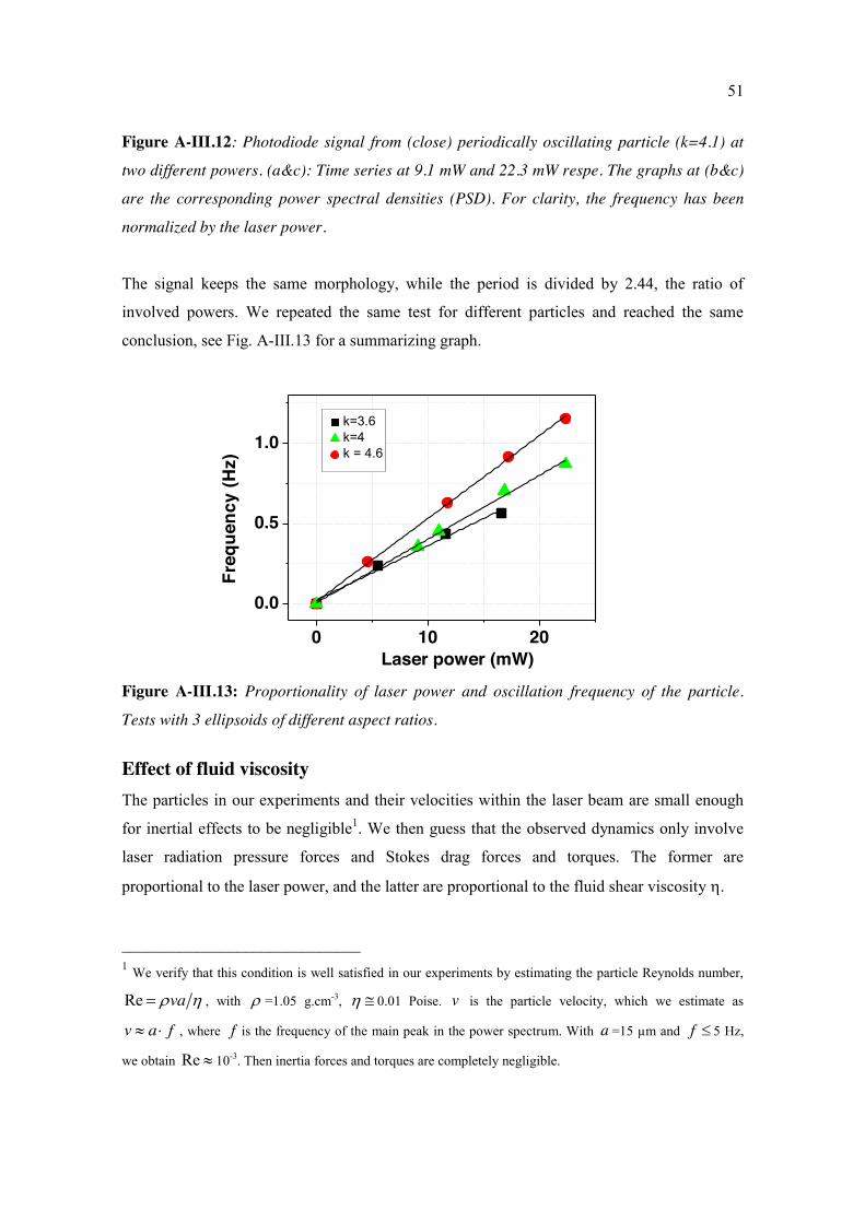
51

Figure A-III.12: Photodiode signal from (close) periodically oscillating particle (k=4.1) at

two different powers. (a&c): Time series at 9.1 mW and 22.3 mW respe. The graphs at (b&c)

are the corresponding power spectral densities (PSD). For clarity, the frequency has been

normalized by the laser power.

The signal keeps the same morphology, while the period is divided by 2.44, the ratio of

involved powers. We repeated the same test for different particles and reached the same

conclusion, see Fig. A-III.13 for a summarizing graph.

0 10 20

0.0

0.5

1.0

k=3.6 k=4k = 4.6

Freq

uenc

y (H

z)

Laser power (mW) Figure A-III.13: Proportionality of laser power and oscillation frequency of the particle.

Tests with 3 ellipsoids of different aspect ratios.

Effect of fluid viscosity The particles in our experiments and their velocities within the laser beam are small enough

for inertial effects to be negligible1. We then guess that the observed dynamics only involve

laser radiation pressure forces and Stokes drag forces and torques. The former are

proportional to the laser power, and the latter are proportional to the fluid shear viscosity .

_____________________________ 1 We verify that this condition is well satisfied in our experiments by estimating the particle Reynolds number,

Re va , with =1.05 g.cm-3, 0.01 Poise. v is the particle velocity, which we estimate as

v a f , where f is the frequency of the main peak in the power spectrum. With a =15 µm and f 5 Hz,

we obtain Re 10-3. Then inertia forces and torques are completely negligible.

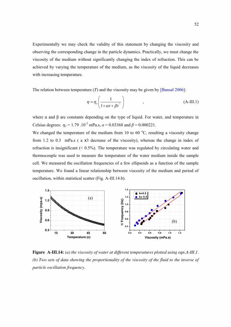
52

Experimentally we may check the validity of this statement by changing the viscosity and

observing the corresponding change in the particle dynamics. Practically, we must change the

viscosity of the medium without significantly changing the index of refraction. This can be

achieved by varying the temperature of the medium, as the viscosity of the liquid decreases

with increasing temperature.

The relation between temperature (T) and the viscosity may be given by [Bansal 2006]:

2

11o t t

, (A-III.1)

where α and β are constants depending on the type of liquid. For water, and temperature in

Celsius degrees: o = 1.79 .10-3 mPa.s, α = 0.03368 and β = 0.000221.

We changed the temperature of the medium from 10 to 60 oC, resulting a viscosity change

from 1.2 to 0.3 mPa.s ( a x3 decrease of the viscosity), whereas the change in index of

refraction is insignificant (< 0.5%). The temperature was regulated by circulating water and

thermocouple was used to measure the temperature of the water medium inside the sample

cell. We measured the oscillation frequencies of a few ellipsoids as a function of the sample

temperature. We found a linear relationship between viscosity of the medium and period of

oscillation, within statistical scatter (Fig. A-III.14.b).

15 30 45 60

0.3

0.6

0.9

1.2

1.5

Visc

osity

(mpa

.s)

Temperature (c)0.2 0.4 0.6 0.8 1.0 1.2

0.4

0.6

0.8

1.0

1.2

1.4

Viscosity (mPa.s)

k=4.3 k= 4.4

1/ F

requ

ency

(Hz)

Figure A-III.14: (a) the viscosity of water at different temperatures plotted using eqn.A-III.1.

(b) Two sets of data showing the proportionality of the viscosity of the fluid to the inverse of

particle oscillation frequency.

(a)

(b)

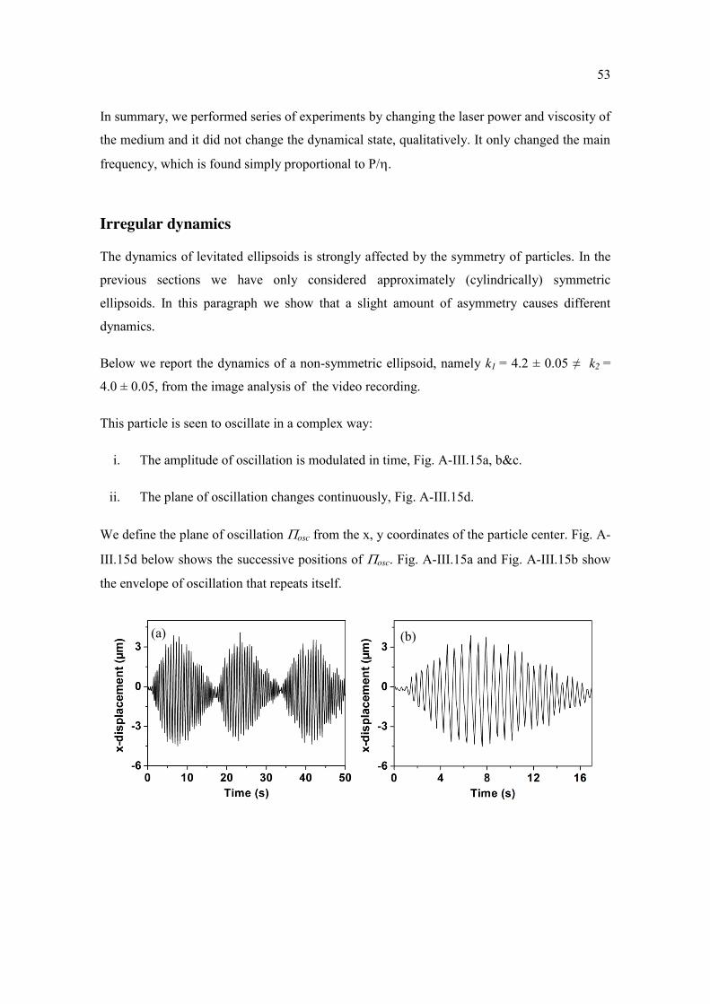
53

In summary, we performed series of experiments by changing the laser power and viscosity of

the medium and it did not change the dynamical state, qualitatively. It only changed the main

frequency, which is found simply proportional to P/.

Irregular dynamics

The dynamics of levitated ellipsoids is strongly affected by the symmetry of particles. In the

previous sections we have only considered approximately (cylindrically) symmetric

ellipsoids. In this paragraph we show that a slight amount of asymmetry causes different

dynamics.

Below we report the dynamics of a non-symmetric ellipsoid, namely k1 = 4.2 ± 0.05  ≠    k2 =

4.0 ± 0.05, from the image analysis of the video recording.

This particle is seen to oscillate in a complex way:

i. The amplitude of oscillation is modulated in time, Fig. A-III.15a, b&c.

ii. The plane of oscillation changes continuously, Fig. A-III.15d.

We define the plane of oscillation osc from the x, y coordinates of the particle center. Fig. A-

III.15d below shows the successive positions of osc. Fig. A-III.15a and Fig. A-III.15b show

the envelope of oscillation that repeats itself.

(a) (b)

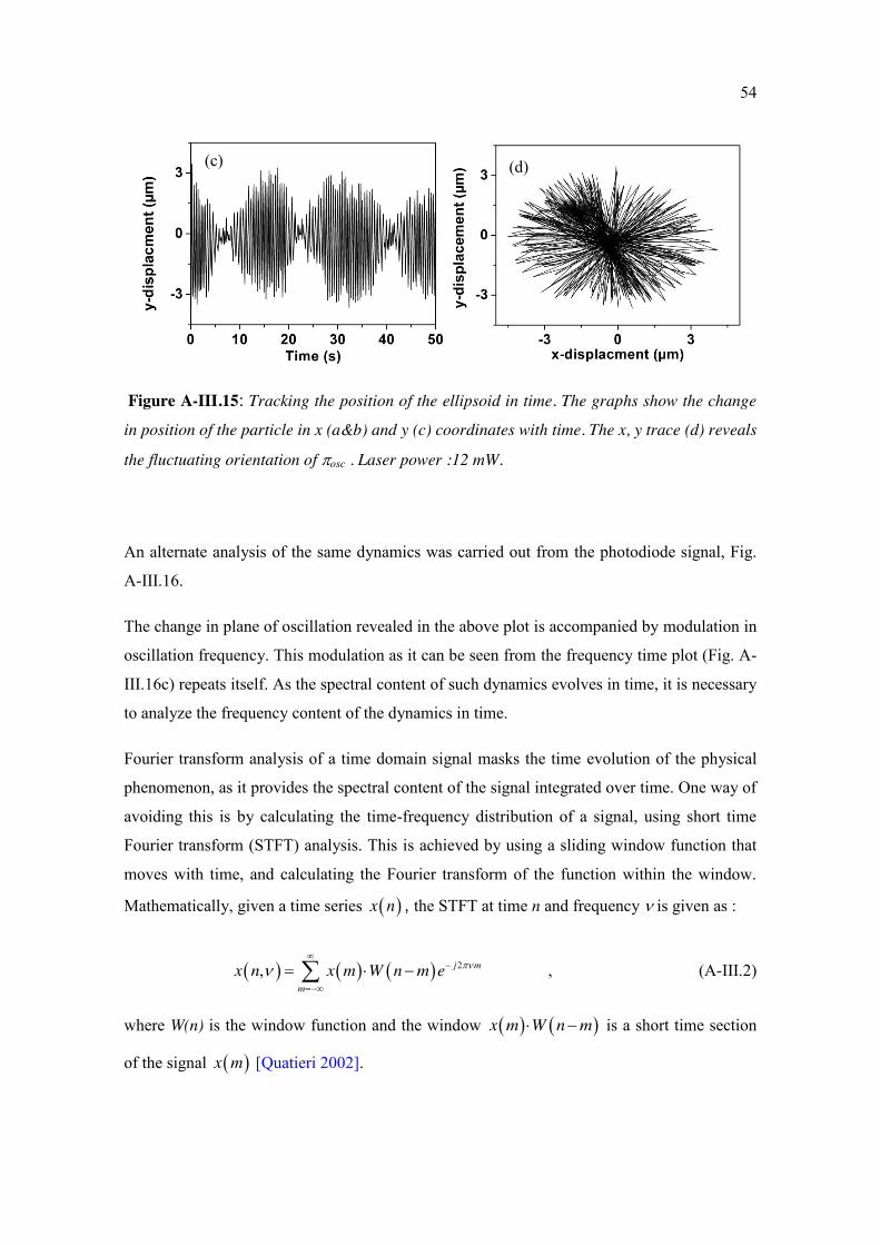
54

Figure A-III.15: Tracking the position of the ellipsoid in time. The graphs show the change

in position of the particle in x (a&b) and y (c) coordinates with time. The x, y trace (d) reveals

the fluctuating orientation of osc . Laser power :12 mW.

An alternate analysis of the same dynamics was carried out from the photodiode signal, Fig.

A-III.16.

The change in plane of oscillation revealed in the above plot is accompanied by modulation in

oscillation frequency. This modulation as it can be seen from the frequency time plot (Fig. A-

III.16c) repeats itself. As the spectral content of such dynamics evolves in time, it is necessary

to analyze the frequency content of the dynamics in time.

Fourier transform analysis of a time domain signal masks the time evolution of the physical

phenomenon, as it provides the spectral content of the signal integrated over time. One way of

avoiding this is by calculating the time-frequency distribution of a signal, using short time

Fourier transform (STFT) analysis. This is achieved by using a sliding window function that

moves with time, and calculating the Fourier transform of the function within the window.

Mathematically, given a time series x n , the STFT at time n and frequency is given as :

2, j m

mx n x m W n m e

, (A-III.2)

where W(n) is the window function and the window x m W n m is a short time section

of the signal x m [Quatieri 2002].

(c) (d)

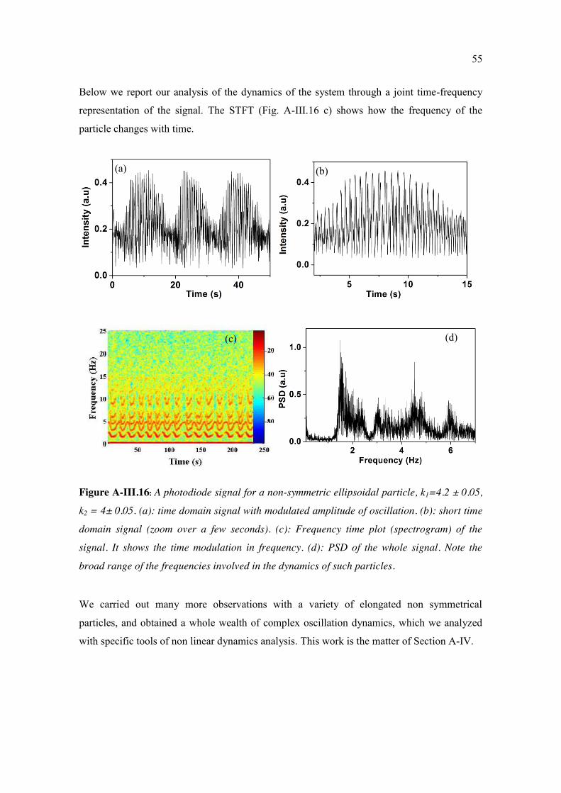
55

Below we report our analysis of the dynamics of the system through a joint time-frequency

representation of the signal. The STFT (Fig. A-III.16 c) shows how the frequency of the

particle changes with time.

Figure A-III.16: A photodiode signal for a non-symmetric ellipsoidal particle, k1=4.2 ± 0.05,

k2 = 4± 0.05. (a): time domain signal with modulated amplitude of oscillation. (b): short time

domain signal (zoom over a few seconds). (c): Frequency time plot (spectrogram) of the

signal. It shows the time modulation in frequency. (d): PSD of the whole signal. Note the

broad range of the frequencies involved in the dynamics of such particles.

We carried out many more observations with a variety of elongated non symmetrical

particles, and obtained a whole wealth of complex oscillation dynamics, which we analyzed

with specific tools of non linear dynamics analysis. This work is the matter of Section A-IV.

(d) (c)

(a) (b)

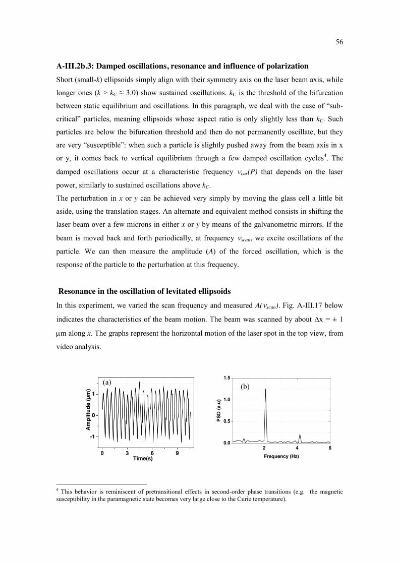
56

A-III.2b.3: Damped oscillations, resonance and influence of polarization Short (small-k) ellipsoids simply align with their symmetry axis on the laser beam axis, while

longer ones (k > kC ≈  3.0)  show  sustained  oscillations.  kC is the threshold of the bifurcation

between  static  equilibrium  and  oscillations.  In  this  paragraph,  we  deal  with  the  case  of  “sub-

critical”   particles,  meaning   ellipsoids  whose   aspect   ratio   is   only   slightly   less   than   kC. Such

particles are below the bifurcation threshold and then do not permanently oscillate, but they

are  very  “susceptible”:  when  such  a  particle  is  slightly  pushed  away  from  the  beam  axis  in  x  

or y, it comes back to vertical equilibrium through a few damped oscillation cycles4. The

damped oscillations occur at a characteristic frequency car(P) that depends on the laser

power, similarly to sustained oscillations above kC.

The perturbation in x or y can be achieved very simply by moving the glass cell a little bit

aside, using the translation stages. An alternate and equivalent method consists in shifting the

laser beam over a few microns in either x or y by means of the galvanometric mirrors. If the

beam is moved back and forth periodically, at frequency scan, we excite oscillations of the

particle. We can then measure the amplitude (A) of the forced oscillation, which is the

response of the particle to the perturbation at this frequency.

Resonance in the oscillation of levitated ellipsoids In this experiment, we varied the scan frequency and measured A(scan). Fig. A-III.17 below

indicates the characteristics of the beam motion. The beam was scanned by about x = ± 1

m along x. The graphs represent the horizontal motion of the laser spot in the top view, from

video analysis.

4 This behavior is reminiscent of pretransitional effects in second-order phase transitions (e.g. the magnetic susceptibility in the paramagnetic state becomes very large close to the Curie temperature).

2 4 60.0

0.5

1.0

1.5

Frequency (Hz)

PSD

(a.u

)

0 3 6 9

-1

0

1

Am

plitu

de (µ

m)

Time(s)

(b) (a)

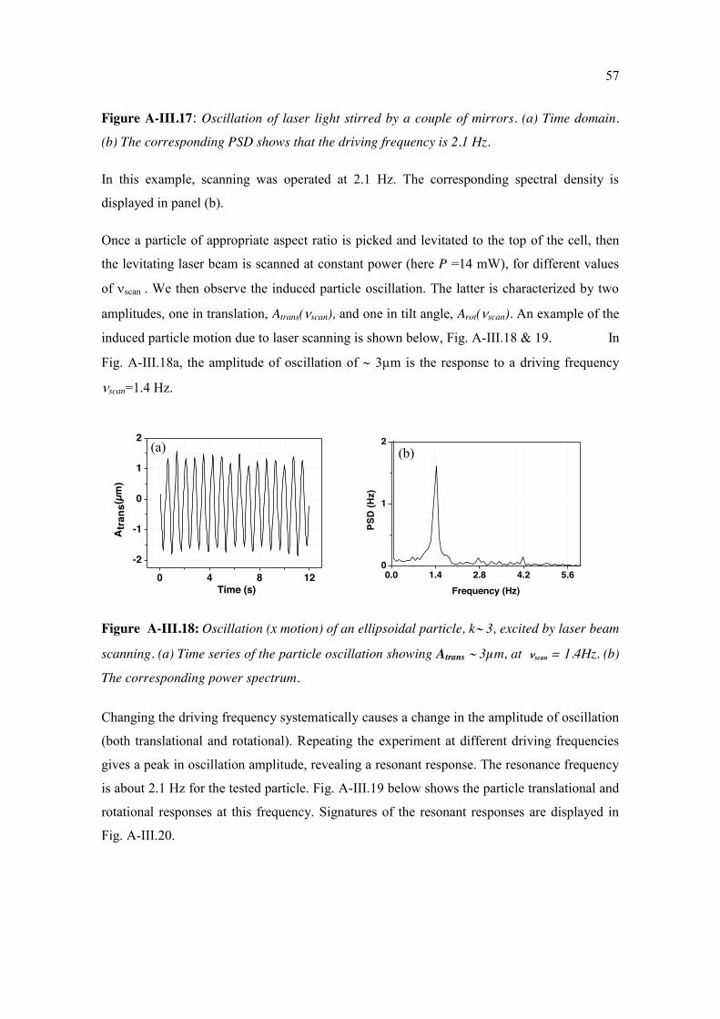
57

Figure A-III.17: Oscillation of laser light stirred by a couple of mirrors. (a) Time domain.

(b) The corresponding PSD shows that the driving frequency is 2.1 Hz.

In this example, scanning was operated at 2.1 Hz. The corresponding spectral density is

displayed in panel (b).

Once a particle of appropriate aspect ratio is picked and levitated to the top of the cell, then

the levitating laser beam is scanned at constant power (here P =14 mW), for different values

of scan . We then observe the induced particle oscillation. The latter is characterized by two

amplitudes, one in translation, Atrans(scan), and one in tilt angle, Arot(scan). An example of the

induced particle motion due to laser scanning is shown below, Fig. A-III.18 & 19. In

Fig. A-III.18a, the amplitude of oscillation of 3µm is the response to a driving frequency

scan=1.4 Hz.

0 4 8 12

-2

-1

0

1

2

Atr

ans(

µm)

Time (s)0.0 1.4 2.8 4.2 5.6

0

1

2

Frequency (Hz)

PSD

(Hz)

Figure A-III.18: Oscillation (x motion) of an ellipsoidal particle, k 3, excited by laser beam

scanning. (a) Time series of the particle oscillation showing Atrans 3µm, at scan = 1.4Hz. (b)

The corresponding power spectrum.

Changing the driving frequency systematically causes a change in the amplitude of oscillation

(both translational and rotational). Repeating the experiment at different driving frequencies

gives a peak in oscillation amplitude, revealing a resonant response. The resonance frequency

is about 2.1 Hz for the tested particle. Fig. A-III.19 below shows the particle translational and

rotational responses at this frequency. Signatures of the resonant responses are displayed in

Fig. A-III.20.

(b) (a)

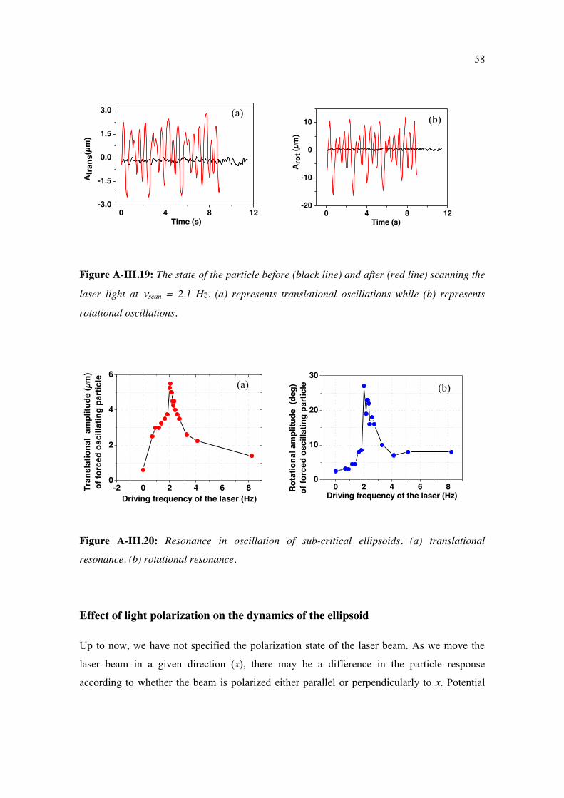
58

0 4 8 12-3.0

-1.5

0.0

1.5

3.0

A

tran

s(µm

)

Time (s)0 4 8 12

-20

-10

0

10

Time (s)

Aro

t (µm

)

Figure A-III.19: The state of the particle before (black line) and after (red line) scanning the

laser light at scan = 2.1 Hz. (a) represents translational oscillations while (b) represents

rotational oscillations.

Figure A-III.20: Resonance in oscillation of sub-critical ellipsoids. (a) translational

resonance. (b) rotational resonance.

Effect of light polarization on the dynamics of the ellipsoid

Up to now, we have not specified the polarization state of the laser beam. As we move the

laser beam in a given direction (x), there may be a difference in the particle response

according to whether the beam is polarized either parallel or perpendicularly to x. Potential

-2 0 2 4 6 80

2

4

6

Tran

slat

iona

l am

plitu

de (µ

m)

of fo

rced

osc

illat

ing

part

icle

Driving frequency of the laser (Hz)0 2 4 6 8

0

10

20

30

Rot

atio

nal a

mpl

itude

(de

g)of

forc

ed o

scill

atin

g pa

rtic

le

Driving frequency of the laser (Hz)

(a)

(a)

(b)

(b)

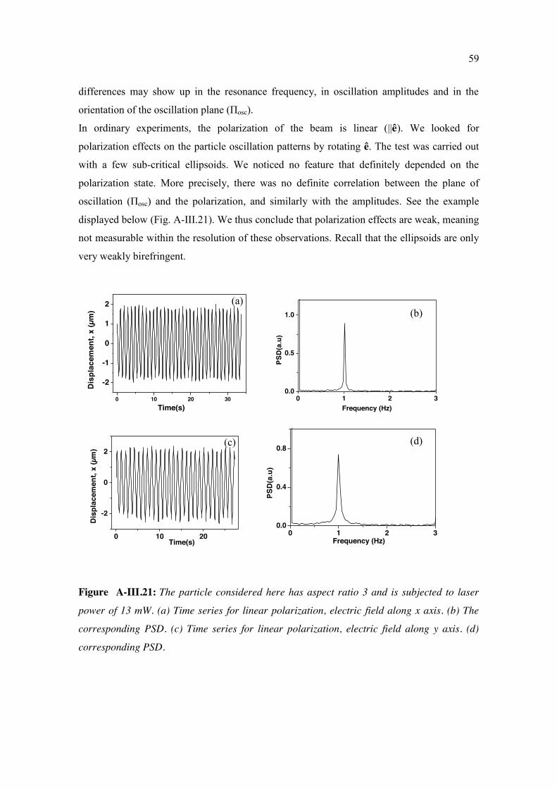
59

differences may show up in the resonance frequency, in oscillation amplitudes and in the

orientation of the oscillation plane (Πosc).

In ordinary experiments, the polarization of the beam is linear (||ê). We looked for

polarization effects on the particle oscillation patterns by rotating ê. The test was carried out

with a few sub-critical ellipsoids. We noticed no feature that definitely depended on the

polarization state. More precisely, there was no definite correlation between the plane of

oscillation   (Πosc) and the polarization, and similarly with the amplitudes. See the example

displayed below (Fig. A-III.21). We thus conclude that polarization effects are weak, meaning

not measurable within the resolution of these observations. Recall that the ellipsoids are only

very weakly birefringent.

0 10 20 30

-2

-1

0

1

2

Dis

plac

emen

t, x

(µm

)

Time(s)0 1 2 3

0.0

0.5

1.0

Frequency (Hz)

PSD

(a.u

)

0 10 20

-2

0

2

Dis

plac

emen

t, x

(µm

)

Time(s)

0 1 2 30.0

0.4

0.8

PSD

(a.u

)

Frequency (Hz)

Figure A-III.21: The particle considered here has aspect ratio 3 and is subjected to laser

power of 13 mW. (a) Time series for linear polarization, electric field along x axis. (b) The

corresponding PSD. (c) Time series for linear polarization, electric field along y axis. (d)

corresponding PSD.

(a) (b)

(c) (d)

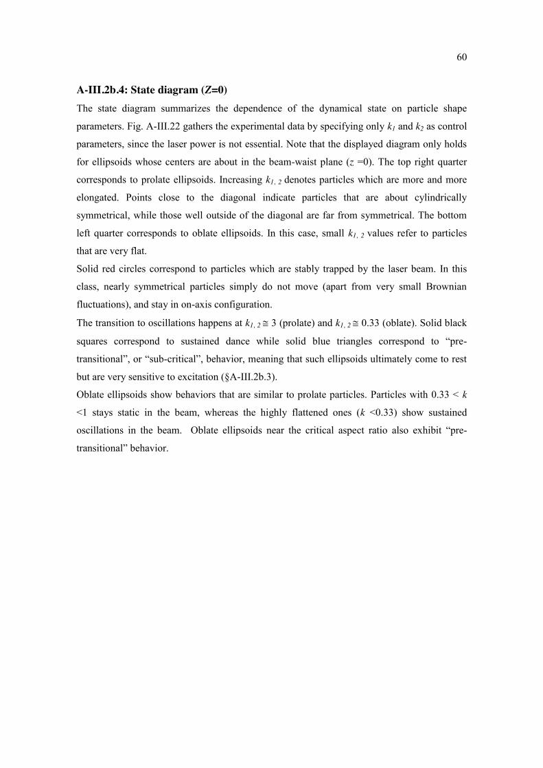
60

A-III.2b.4: State diagram (Z=0) The state diagram summarizes the dependence of the dynamical state on particle shape

parameters. Fig. A-III.22 gathers the experimental data by specifying only k1 and k2 as control

parameters, since the laser power is not essential. Note that the displayed diagram only holds

for ellipsoids whose centers are about in the beam-waist plane (z =0). The top right quarter

corresponds to prolate ellipsoids. Increasing k1, 2 denotes particles which are more and more

elongated. Points close to the diagonal indicate particles that are about cylindrically

symmetrical, while those well outside of the diagonal are far from symmetrical. The bottom

left quarter corresponds to oblate ellipsoids. In this case, small k1, 2 values refer to particles

that are very flat.

Solid red circles correspond to particles which are stably trapped by the laser beam. In this

class, nearly symmetrical particles simply do not move (apart from very small Brownian

fluctuations), and stay in on-axis configuration.

The transition to oscillations happens at k1, 2 3 (prolate) and k1, 2 0.33 (oblate). Solid black

squares   correspond   to   sustained   dance   while   solid   blue   triangles   correspond   to   “pre-

transitional”,  or  “sub-critical”,  behavior,  meaning  that  such  ellipsoids  ultimately  come  to  rest  

but are very sensitive to excitation (§A-III.2b.3).

Oblate ellipsoids show behaviors that are similar to prolate particles. Particles with 0.33 < k

<1 stays static in the beam, whereas the highly flattened ones (k <0.33) show sustained

oscillations in the beam. Oblate ellipsoids near the critical aspect   ratio   also   exhibit   “pre-

transitional”  behavior.

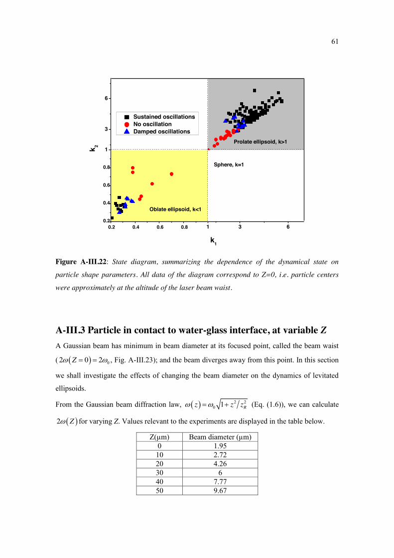
61

1 3 6

1

3

6

0.2 0.4 0.6 0.80.2

0.4

0.6

0.8

k 2

k1

Oblate ellipsoid, k<1

Sustained oscillations No oscillation Damped oscillations

Sphere, k=1

Prolate ellipsoid, k>1

Figure A-III.22: State diagram, summarizing the dependence of the dynamical state on

particle shape parameters. All data of the diagram correspond to Z=0, i.e. particle centers

were approximately at the altitude of the laser beam waist.

A-III.3 Particle in contact to water-glass interface, at variable Z A Gaussian beam has minimum in beam diameter at its focused point, called the beam waist

( 02 0 2Z , Fig. A-III.23); and the beam diverges away from this point. In this section

we shall investigate the effects of changing the beam diameter on the dynamics of levitated

ellipsoids.

From the Gaussian beam diffraction law, 2 20 1 Rz z z (Eq. (1.6)), we can calculate

2 Z for varying Z. Values relevant to the experiments are displayed in the table below.

Z(µm) Beam diameter (µm) 0 1.95 10 2.72 20 4.26 30 6 40 7.77 50 9.67

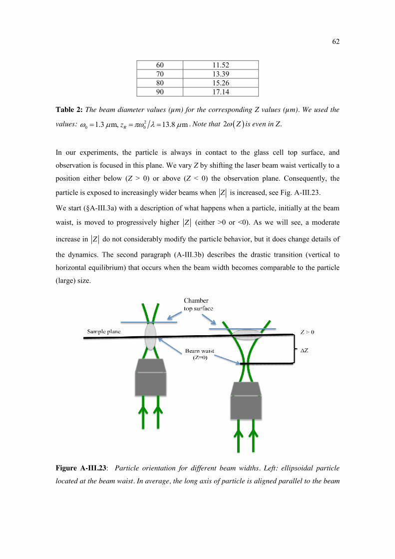
62

60 11.52 70 13.39 80 15.26 90 17.14

Table 2: The beam diameter values (µm) for the corresponding Z values (µm). We used the

values: 20 01.3 m, 13.8 mRz . Note that 2 Z is even in Z.

In our experiments, the particle is always in contact to the glass cell top surface, and

observation is focused in this plane. We vary Z by shifting the laser beam waist vertically to a

position either below (Z > 0) or above (Z < 0) the observation plane. Consequently, the

particle is exposed to increasingly wider beams when Z is increased, see Fig. A-III.23.

We start (§A-III.3a) with a description of what happens when a particle, initially at the beam

waist, is moved to progressively higher Z (either >0 or <0). As we will see, a moderate

increase in Z do not considerably modify the particle behavior, but it does change details of

the dynamics. The second paragraph (A-III.3b) describes the drastic transition (vertical to

horizontal equilibrium) that occurs when the beam width becomes comparable to the particle

(large) size.

Figure A-III.23: Particle orientation for different beam widths. Left: ellipsoidal particle

located at the beam waist. In average, the long axis of particle is aligned parallel to the beam

63

axis. Short particles (k<3) keep locked on beam axis, while longer ones (k>3) oscillate.

Right: the same particle, when far enough from the beam-waist, switches to horizontal static

equilibrium.

A-III.3a: Influence of varying beam diameter on particle oscillation In this paragraph, we only consider prolate ellipsoids, which are long enough to oscillate at

Z=0. Our goal is just to provide a few qualitative trends about the influence of the beam

diameter, and possibly beam divergence, on oscillations. We will come back to some of the

examples reported below in Section A-IV, to provide more elaborate, quantitative descriptions

of the particle trajectories.

Starting with a particle that oscillates at Z=0, and increasing Z, we systematically observe a

gradual slowing down of the ellipsoid oscillation, down to no oscillation at all when Z is large

enough. This trend is not surprising, if we realize that only a small fraction of the beam power

is intercepted by the particle at large Z. For instance, 2 90Z m = 17.14 m, comparable

to the particle long axis length. Consequently the effective power felt by the particle decreases

with Z, and so does the oscillation frequency.

More importantly, changing Z has an impact on the qualitative features of the particle

dynamics. As we will see from the data below, increasing the beam width may change the

particle dynamics from irregular to approximately periodic or reversely.

We start with two examples (I and II) corresponding to the type of oscillatory motion

discussed in §A-III.2b.2. As we explained, this kind of dynamics is observed at beam waist

for slightly non-symmetrical moderate aspect ratio ellipsoids. As a general feature of such

particles, the direction of the oscillation plane fluctuates, and the photodiode signal is clearly

non periodic. In I (Fig. A-III.24), Z is negative, meaning that the particle is located upstream

of the beam waist. The time series changes from modulated amplitude type of motion at the

beam waist to quasi-periodic motion at broader beam width. This trend is more evident from

the Fourier analysis where the broadband spectrum at Z= 0 changes to well discernible

discrete peaks (e.g at Z=-25).

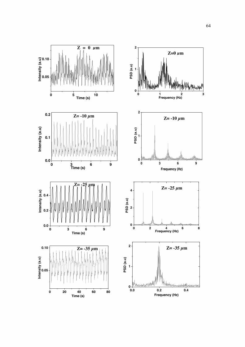
64

0 5 10

0.05

0.10

In

tens

ity (a

.u)

Time (s)0 1 2 3

0

1

2

Frequency (Hz)

PSD

(a.u

)

0 3 6 90.0

0.1

0.2

Time (s)

Inte

nsity

(a.u

)

0 3 6 90

1

2

PS

D (

a.u

)

Frequency (Hz)

0 3 6 90.0

0.2

0.4

Inte

nsity

(a.u

)

Time (s)

0 2 4 6 80

2

4

PSD

(a.u

)

Frequency (Hz)

0 20 40 60 80

0.05

0.10

Inte

nsity

(a.u

)

Time (s)

0.0 0.2 0.40

1

2

PSD

(a.u

)

Frequency (Hz)

Z= -10 µm

Z = 0 µm µm

Z= -25 µm

Z= -35 µm

Z=0 µm

Z= -10 µm

Z= -25 µm

Z= -35 µm

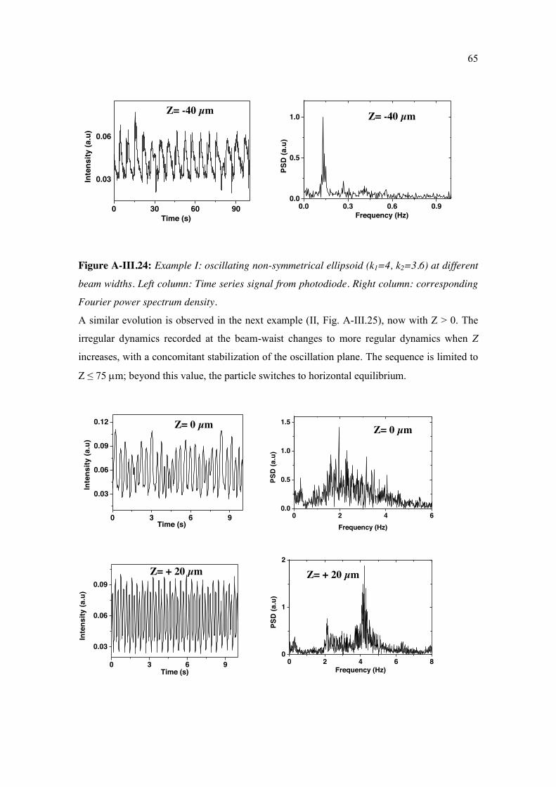
65

0 30 60 90

0.03

0.06

Inte

nsity

(a.u

)

Time (s)

0.0 0.3 0.6 0.90.0

0.5

1.0

PSD

(a.u

)

Frequency (Hz)

Figure A-III.24: Example I: oscillating non-symmetrical ellipsoid (k1=4, k2=3.6) at different

beam widths. Left column: Time series signal from photodiode. Right column: corresponding

Fourier power spectrum density. A similar evolution is observed in the next example (II, Fig. A-III.25), now with Z > 0. The

irregular dynamics recorded at the beam-waist changes to more regular dynamics when Z

increases, with a concomitant stabilization of the oscillation plane. The sequence is limited to

Z ≤  75  m; beyond this value, the particle switches to horizontal equilibrium.

0 3 6 9

0.03

0.06

0.09

0.12

Inte

nsity

(a.u

)

Time (s)0 2 4 6

0.0

0.5

1.0

1.5

Frequency (Hz)

PSD

(a.u

)

0 3 6 9

0.03

0.06

0.09

Inte

nsity

(a.u

)

Time (s)0 2 4 6 8

0

1

2

Frequency (Hz)

PSD

(a.u

)

Z= -40 µm Z= -40 µm

Z= 0 µm Z= 0 µm

Z= + 20 µm Z= + 20 µm

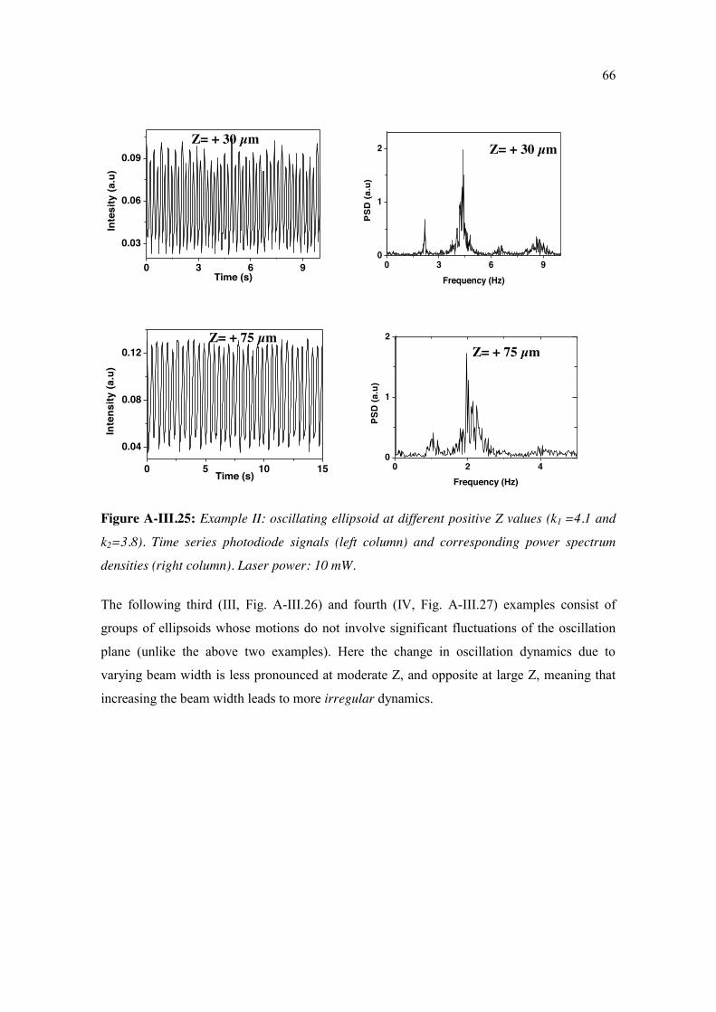
66

0 3 6 9

0.03

0.06

0.09

In

tesi

ty (a

.u)

Time (s)0 3 6 9

0

1

2

Frequency (Hz)

PS

D (a

.u)

0 5 10 15

0.04

0.08

0.12

Inte

nsity

(a.u

)

Time (s) 0 2 4

0

1

2

Frequency (Hz)

PSD

(a.u

)

Figure A-III.25: Example II: oscillating ellipsoid at different positive Z values (k1 =4.1 and

k2=3.8). Time series photodiode signals (left column) and corresponding power spectrum

densities (right column). Laser power: 10 mW.

The following third (III, Fig. A-III.26) and fourth (IV, Fig. A-III.27) examples consist of

groups of ellipsoids whose motions do not involve significant fluctuations of the oscillation

plane (unlike the above two examples). Here the change in oscillation dynamics due to

varying beam width is less pronounced at moderate Z, and opposite at large Z, meaning that

increasing the beam width leads to more irregular dynamics.

Z= + 30 µm Z= + 30 µm

Z= + 75 µm Z= + 75 µm

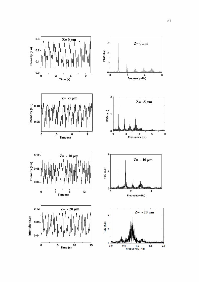
67

0 3 6 90.0

0.1

0.2

0.3

In

tens

ity (a

.u)

Time (s)0 2 4 6

0

1

2

3

Frequency (Hz)

PSD

(a.u

)

0 3 6 9

0.05

0.10

Inte

nsity

(a.u

)

Time (s) 0 2 4 6 8

0

1

2

Frequency (Hz)

PSD

(a.u

)

0 4 8 12

0.04

0.08

0.12

Inte

nsity

(a.u

)

Time (s)0 2 4

0

1

2

Frequency (Hz)

PSD

(a.u

)

0 5 10 15

0.04

0.08

0.12

Inte

nsity

(a.u

)

Time (s)

Z= 0 µm Z= 0 µm

Z= -5 µm Z= -5 µm

Z= - 10 µm Z= - 10 µm

Z= - 20 µm

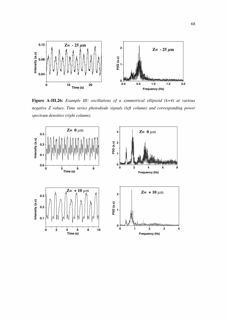
68

0 10 20

0.04

0.08

0.12

In

tens

ity (a

.u)

Time (s)0.0 0.5 1.0 1.5 2.0

0

1

2

Frequency (Hz)

PSD

(a.u

)

Figure A-III.26: Example III: oscillations of a symmetrical ellipsoid (k=4) at various

negative Z values. Time series photodiode signals (left column) and corresponding power

spectrum densities (right column).

0 3 6 90.0

0.1

0.2

0.3

Inte

nsity

(a.u

)

Time (s)0 2 4 6 8

0

1

2

3

Frequency (Hz)

PSD

(a.u

)

0 2 4 6 8 10

0.1

0.2

0.3

Inte

nsity

(a.u

)

Time (s)0 1 2 3 4

0

1

2

Frequency (Hz)

PSD

(a.u

)

Z= - 25 µm Z= - 25 µm

Z= 0 µm Z= 0 µm

Z= + 10 µm Z= + 10 µm

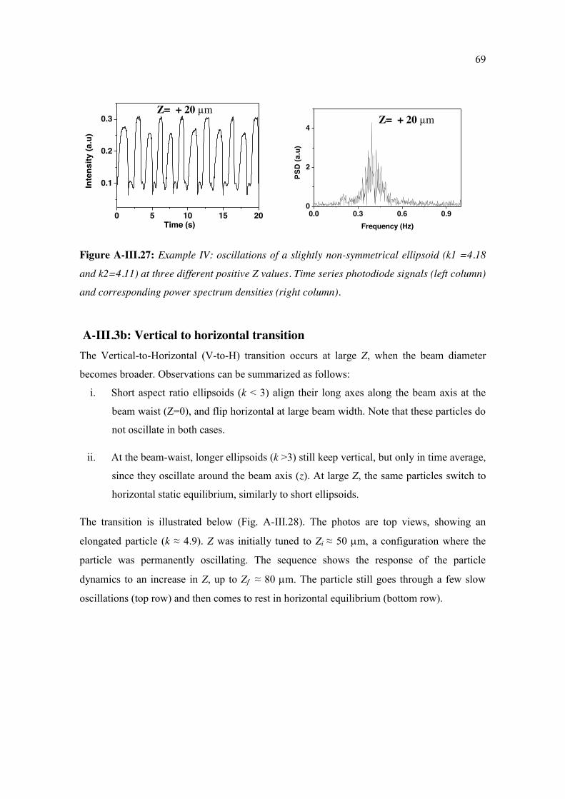
69

0 5 10 15 20

0.1

0.2

0.3

In

tens

ity (a

.u)

Time (s)0.0 0.3 0.6 0.9

0

2

4

Frequency (Hz)

PSD

(a.u

)

Figure A-III.27: Example IV: oscillations of a slightly non-symmetrical ellipsoid (k1 =4.18

and k2=4.11) at three different positive Z values. Time series photodiode signals (left column)

and corresponding power spectrum densities (right column).

A-III.3b: Vertical to horizontal transition The Vertical-to-Horizontal (V-to-H) transition occurs at large Z, when the beam diameter

becomes broader. Observations can be summarized as follows:

i. Short aspect ratio ellipsoids (k < 3) align their long axes along the beam axis at the

beam waist (Z=0), and flip horizontal at large beam width. Note that these particles do

not oscillate in both cases.

ii. At the beam-waist, longer ellipsoids (k >3) still keep vertical, but only in time average,

since they oscillate around the beam axis (z). At large Z, the same particles switch to

horizontal static equilibrium, similarly to short ellipsoids.

The transition is illustrated below (Fig. A-III.28). The photos are top views, showing an

elongated particle (k ≈  4.9).  Z was initially tuned to Zi ≈  50  m, a configuration where the

particle was permanently oscillating. The sequence shows the response of the particle

dynamics to an increase in Z, up to Zf ≈  80  m. The particle still goes through a few slow

oscillations (top row) and then comes to rest in horizontal equilibrium (bottom row).

Z= + 20 µm Z= + 20 µm

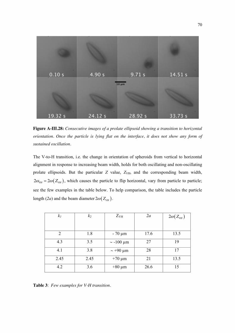
70

Figure A-III.28: Consecutive images of a prolate ellipsoid showing a transition to horizontal

orientation. Once the particle is lying flat on the interface, it does not show any form of

sustained oscillation.

The V-to-H transition, i.e. the change in orientation of spheroids from vertical to horizontal

alignment in response to increasing beam width, holds for both oscillating and non-oscillating

prolate ellipsoids. But the particular Z value, ZVH, and the corresponding beam width,

2 2VH VHZ , which causes the particle to flip horizontal, vary from particle to particle;

see the few examples in the table below. To help comparison, the table includes the particle

length (2a) and the beam diameter 2 VHZ .

k1 k2 ZVH 2a 2 VHZ

2 1.8 - 70 µm 17.6 13.5

4.3 3.5 -100 µm 27 19

4.1 3.8 +90 µm 28 17

2.45 2.45 +70 µm 21 13.5

4.2 3.6 +80 µm 26.6 15

Table 3: Few examples for V-H transition.

71

We shortly investigated the influence of the beam polarization on the horizontal equilibrium.

The conclusion is similar to that drawn for oscillating states, i.e. we did not notice any clear

correlation. H configurations of prolate ellipsoids were randomly oriented.

A-III.3c: Summary Whatever the type or shape of the particle, the oscillation disappears for large enough beam

width. Thus, the necessary conditions for the oscillations to exist are:

the particle should be elongated enough (k > 3),

the beam width should not be too large (Z < |Zmax|=ZVH)

whereas the type of dynamics is controlled by :

the symmetry and aspect ratio of the particle

the beam width.

The above statements are gathered into the graph below, Fig. A-III.29. Note that the dotted

lines are only indicative. Boundaries between the different regimes have not been accurately

determined yet.

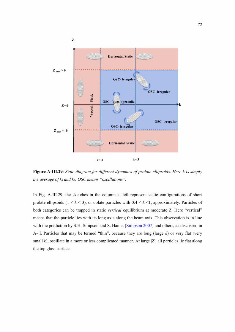
72

Figure A-III.29: State diagram for different dynamics of prolate ellipsoids. Here k is simply

the average of k1 and k2.  OSC  means  “oscillations”.  

In Fig. A-III.29, the sketches in the column at left represent static configurations of short

prolate ellipsoids (1 < k < 3), or oblate particles with 0.4 < k <1, approximately. Particles of

both categories can be trapped in static vertical equilibrium  at  moderate  Z.  Here   “vertical”  

means that the particle lies with its long axis along the beam axis. This observation is in line

with the prediction by S.H. Simpson and S. Hanna [Simpson 2007] and others, as discussed in

A- I.  Particles   that  may  be   termed  “thin”,  because   they  are   long   (large   k) or very flat (very

small k), oscillate in a more or less complicated manner. At large |Z|, all particles lie flat along

the top glass surface.

73

A-IV: Analysis of oscillations The present Section is devoted to an in-depth analysis of some of the temporal signals

reported in section A-III.3. Most generally, the system constituted by the solid particle has 6

degrees of freedom, namely 3 translational variables and 3 angles. Below we restrict the

analysis to the cases where the particle is in contact to the top surface; consequently we are

left with 5 variables ( ,x y , and 3 angles), which we may gather into a 5-coordinate vector s .

Equations that govern the motion of the particle may be cast in a simple form:

ς s F s (A-IV.1)

Here F is a generalized force, including the force and torque components due to laser

radiation pressure. The left hand side, ς s , is the a generalized hydrodynamic drag force due

to translational and rotational motion of the particle inside water. ς is the friction matrix,

whose coefficients are proportional to the water viscosity ( ), and s is the generalized

velocity of the particle. The above equation is valid in the Stokes limit, where inertia is

negligible (see page 41).

At this stage, we have no quantitative knowledge of how F depends on s , but we can be sure

that the dependence is strongly nonlinear. We base this statement on well established results

about spherical particles; see e.g. [Ren 1994]. Then Eq. (A-IV.1) is a set of non linear

ordinary differential equations, of dimension d =5. Control parameters are the beam

characteristics, which are determined by 0 and z , and the particle sizes ( , ,a b c ). The latter

may be replaced by the aspect ratios 1,2k , since all particles used in the experiments are

derived from the same type of polystyrene sphere. Based on experimental observation, we

may anticipate that the dynamical system (DS) Eq. (A-IV.1) has solutions of different types,

namely fixed points (corresponding to a stably trapped particle), limit cycles (periodic

motion) and possibly deterministic chaos (non periodic motion).

The purpose of this Section is to examine experimental time series and identify the attractors

corresponding to such different types of motion, using standard tools of nonlinear analysis.

Below we report the results that we obtained using the TISEAN package, which is a widely

used and freely available analysis tool (http://www.mpipks-dresden.mpg.de/ ~tisean/

Tisean_3.0.1/index.html). We do not provide an introductory overview of nonlinear dynamics

in general, a task that would be much beyond the volume of this Section and our own

expertise. The interested reader is of course referred to the abundant literature in this field; see

e.g. [Hegger 1999] and the many useful references therein. We opt for a simply practical

74

presentation, meaning that we only shortly describe the main steps of the analysis and provide

results for different values of the control parameters.

A-IV.1 Phase space reconstruction The full experimental characterization of the real DS involves measuring 5 parameters, which

generate a trajectory in a 5-dimensional phase space. In reality, we can at most measure 3 of

them, namely ,x y and , using video means and image analysis (A-II, A-III). Note that the

corresponding time series are strongly limited in information, because the sampling frequency

is upper bounded by the available video rate (< 40 Hz). Conversely, the photodiode

signal, I t , can be sampled up to 105 Hz, but it only provides a 1-dimensional information.

Of course, the bare I t signal cannot properly reflect the 5-dimensional trajectory of the real

DS. Fortunately,   however,   the   missing   information   can   be   recovered,   or   “unfolded”,   from  

time delayed copies of the original signal if certain requirements are fulfilled. The method,

called   the  “method  of  delays”, is one of the most important and widely used techniques for

phase space reconstruction.

Basically, we construct a time-delay series, namely the m -dimensional vector

, , ,X t I t I t I t m , with m d . The integer m is   the   “embedding  

dimension”,  and   is the delay time. If the value of is  “adequate”  and  if   m is large enough,

the obtained m -dimensional trajectory and the corresponding attractor are known to be

equivalent to their real counterpart in the full d -dimensional phase space. Here the

equivalence essentially means that both representations have the same topological properties

[Bergé 1986, Thomson 1986].

Choice of the delay time: An adequate value of the delay time is such that the time

delayed variables , , ,I t I t I t m are about independent. The latter criterion may

be satisfied by considering the value of autocorrelation function that yields linear

independence (zero autocorrelation) of coordinates. Numerically, this amounts to calculate

2

( ) ( )( )

( )x t x t T

c Tx t

, (A-IV.2)

Thus, the delay time, , is the value of T such that 1( )(0)

c T ec [Lai 2003].

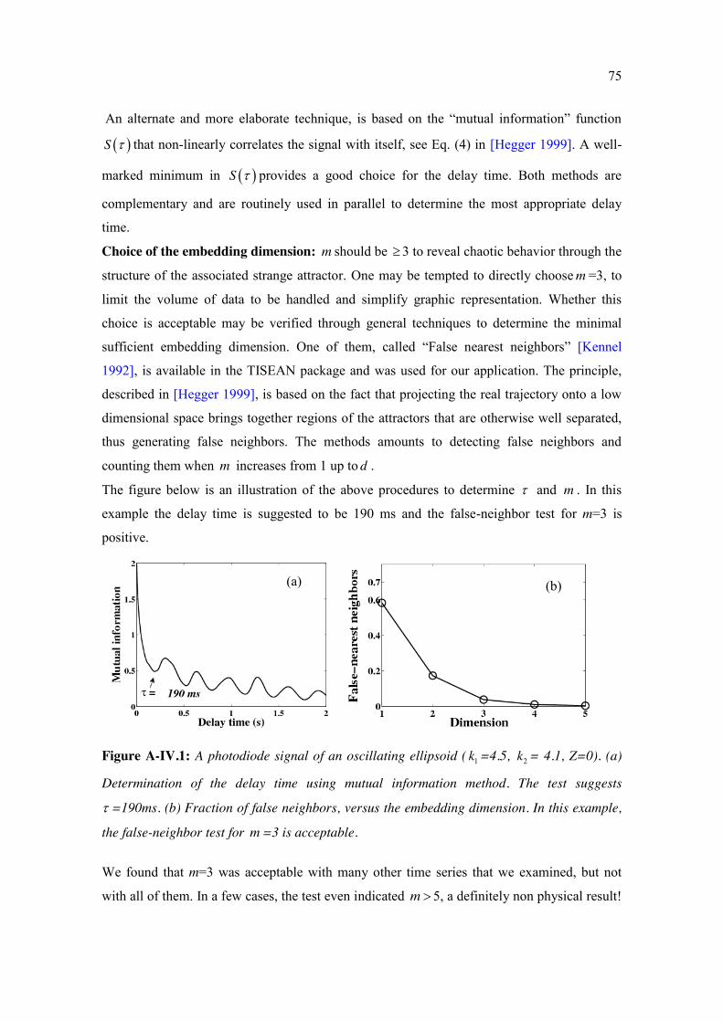
75

An   alternate   and  more   elaborate   technique,   is   based   on   the   “mutual   information”   function  

S that non-linearly correlates the signal with itself, see Eq. (4) in [Hegger 1999]. A well-

marked minimum in S provides a good choice for the delay time. Both methods are

complementary and are routinely used in parallel to determine the most appropriate delay

time.

Choice of the embedding dimension: m should be 3 to reveal chaotic behavior through the

structure of the associated strange attractor. One may be tempted to directly choose m =3, to

limit the volume of data to be handled and simplify graphic representation. Whether this

choice is acceptable may be verified through general techniques to determine the minimal

sufficient embedding dimension. One of them, called   “False   nearest   neighbors”   [Kennel

1992], is available in the TISEAN package and was used for our application. The principle,

described in [Hegger 1999], is based on the fact that projecting the real trajectory onto a low

dimensional space brings together regions of the attractors that are otherwise well separated,

thus generating false neighbors. The methods amounts to detecting false neighbors and

counting them when m increases from 1 up to d .

The figure below is an illustration of the above procedures to determine and m . In this

example the delay time is suggested to be 190 ms and the false-neighbor test for m=3 is

positive.

Figure A-IV.1: A photodiode signal of an oscillating ellipsoid ( 1k =4.5, 2k = 4.1, Z=0). (a)

Determination of the delay time using mutual information method. The test suggests

=190ms. (b) Fraction of false neighbors, versus the embedding dimension. In this example,

the false-neighbor test for m =3 is acceptable.

We found that m=3 was acceptable with many other time series that we examined, but not

with all of them. In a few cases, the test even indicated m 5, a definitely non physical result!

(a) (b)

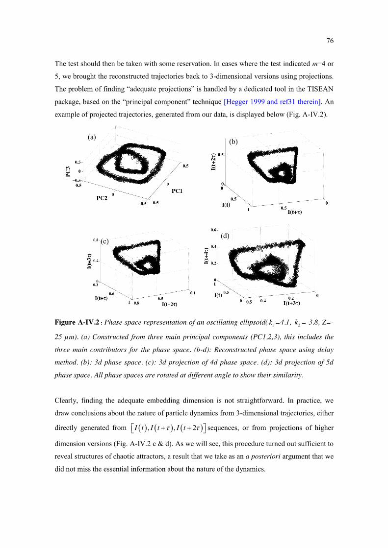
76

The test should then be taken with some reservation. In cases where the test indicated m=4 or

5, we brought the reconstructed trajectories back to 3-dimensional versions using projections.

The  problem  of  finding  “adequate  projections”  is  handled  by  a  dedicated  tool  in  the  TISEAN  

package,  based  on  the  “principal  component”  technique  [Hegger 1999 and ref31 therein]. An

example of projected trajectories, generated from our data, is displayed below (Fig. A-IV.2).

Figure A-IV.2 : Phase space representation of an oscillating ellipsoid( 1k =4.1, 2k = 3.8, Z=-

25 µm). (a) Constructed from three main principal components (PC1,2,3), this includes the

three main contributors for the phase space. (b-d): Reconstructed phase space using delay

method. (b): 3d phase space. (c): 3d projection of 4d phase space. (d): 3d projection of 5d

phase space. All phase spaces are rotated at different angle to show their similarity.

Clearly, finding the adequate embedding dimension is not straightforward. In practice, we

draw conclusions about the nature of particle dynamics from 3-dimensional trajectories, either

directly generated from , , 2I t I t I t sequences, or from projections of higher

dimension versions (Fig. A-IV.2 c & d). As we will see, this procedure turned out sufficient to

reveal structures of chaotic attractors, a result that we take as an a posteriori argument that we

did not miss the essential information about the nature of the dynamics.

(a) (b)

(c) (d)

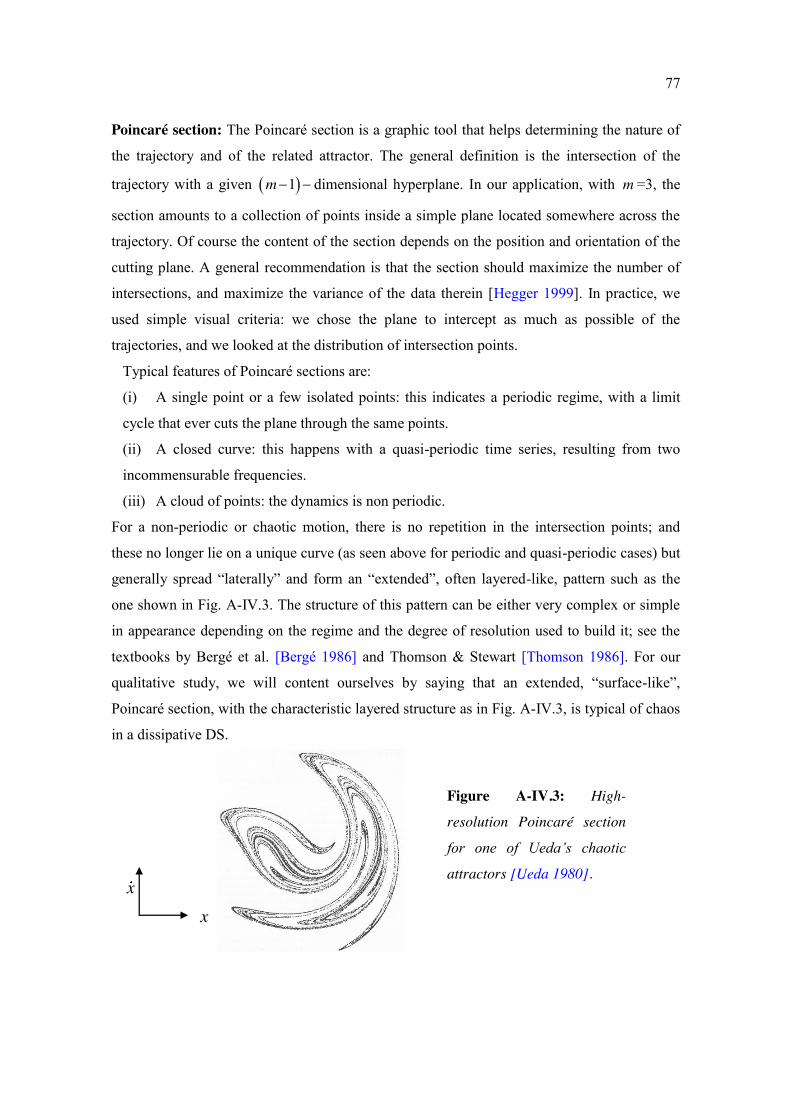
77

Poincaré section: The Poincaré section is a graphic tool that helps determining the nature of

the trajectory and of the related attractor. The general definition is the intersection of the

trajectory with a given 1m dimensional hyperplane. In our application, with m =3, the

section amounts to a collection of points inside a simple plane located somewhere across the

trajectory. Of course the content of the section depends on the position and orientation of the

cutting plane. A general recommendation is that the section should maximize the number of

intersections, and maximize the variance of the data therein [Hegger 1999]. In practice, we

used simple visual criteria: we chose the plane to intercept as much as possible of the

trajectories, and we looked at the distribution of intersection points.

Typical features of Poincaré sections are:

(i) A single point or a few isolated points: this indicates a periodic regime, with a limit

cycle that ever cuts the plane through the same points.

(ii) A closed curve: this happens with a quasi-periodic time series, resulting from two

incommensurable frequencies.

(iii) A cloud of points: the dynamics is non periodic.

For a non-periodic or chaotic motion, there is no repetition in the intersection points; and

these no longer lie on a unique curve (as seen above for periodic and quasi-periodic cases) but

generally   spread  “laterally”   and   form  an  “extended”,  often   layered-like, pattern such as the

one shown in Fig. A-IV.3. The structure of this pattern can be either very complex or simple

in appearance depending on the regime and the degree of resolution used to build it; see the

textbooks by Bergé et al. [Bergé 1986] and Thomson & Stewart [Thomson 1986]. For our

qualitative   study,   we   will   content   ourselves   by   saying   that   an   extended,   “surface-like”,  

Poincaré section, with the characteristic layered structure as in Fig. A-IV.3, is typical of chaos

in a dissipative DS.

Figure A-IV.3: High-

resolution Poincaré section

for   one   of   Ueda’s   chaotic  

attractors [Ueda 1980].

x x

78

A-IV.2 Dynamics of ellipsoidal particles - Experimental results In this section, we deal with the analysis of the experimental signals using the tools of the

TISEAN package. A variety of dynamical regimes of the particle could be generated either by

changing the ellipsoid aspect ratio or the beam diameter. In the next two paragraphs, we

examine in detail the influences of these two parameters.

Of course we are interested in the cases where the particles undergo sustained oscillations,

e.g. when 1,2k 3 for Z=0.  Nevertheless  the  “static”  cases  are  a  useful  source  of  information  as  

they may be exploited to estimate the importance of noise in general. Indeed the signal (either

video images or photodiode) from a stably trapped particle is not strictly constant in time.

Signal fluctuations have an extrinsic part due to the measurement technique, i.e. the electronic

noise in video images or in the photodiode signal. This is the source of stochastic errors,

whose consequence is presumably not more than a finite amount of blur along the

reconstructed trajectories. Indeed this source of noise is well visible as a statistical scatter of

points in all figures displaying trajectories and Poincaré sections, see below.

The other source of randomness is intrinsic to the physical system, as it is related to the

Brownian excursions of the particle in water. Strictly speaking, thermal noise modifies the DS

equations into:

ς s F s b s , (A-IV.3)

where b s is the random force at the origin of Brownian motion. In theory, if b s is large,

the presence of the random force may have deep consequences on the dynamics of the system

[Horsthemke 1984]. However, we always observed that random excursions of trapped

particles were very small compared to laser driven excursions. We then presume that b s is

“small”,  with  the  consequence that it does not change the main features of the dynamics and

that it only contributes a small amount of blur in the trajectories, similarly to electronic noise.

Based on this reasoning, we conclude that measurements carried out with stably trapped

particles may be exploited to estimate uncertainties in trajectories. In video images of axially

trapped particles, we determined uncertainties in , ,x y from the dispersion of the values

obtained by the image analysis procedure. Similarly, we measured rms fluctuations in I t for

trapped particles and supposed that this quantity still represents the uncertainty in I t in

general.

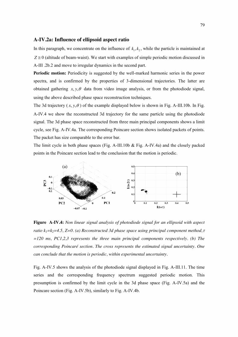
79

A-IV.2a: Influence of ellipsoid aspect ratio In this paragraph, we concentrate on the influence of 1 2,k k , while the particle is maintained at

Z 0 (altitude of beam-waist). We start with examples of simple periodic motion discussed in

A-III .2b.2 and move to irregular dynamics in the second part.

Periodic motion: Periodicity is suggested by the well-marked harmonic series in the power

spectra, and is confirmed by the properties of 3-dimensional trajectories. The latter are

obtained gathering , ,x y data from video image analysis, or from the photodiode signal,

using the above described phase space reconstruction techniques.

The 3d trajectory ( , ,x y ) of the example displayed below is shown in Fig. A-III.10b. In Fig.

A-IV.4 we show the reconstructed 3d trajectory for the same particle using the photodiode

signal. The 3d phase space reconstructed from three main principal components shows a limit

cycle, see Fig. A-IV.4a. The corresponding Poincare section shows isolated packets of points.

The packet has size comparable to the error bar.

The limit cycle in both phase spaces (Fig. A-III.10b & Fig. A-IV.4a) and the closely packed

points in the Poincare section lead to the conclusion that the motion is periodic.

Figure A-IV.4: Non linear signal analysis of photodiode signal for an ellipsoid with aspect

ratio k1=k2=4.5, Z=0. (a) Reconstructed 3d phase space using principal component method,

=120 ms, PC1,2,3 represents the three main principal components respectively. (b) The

corresponding Poincaré section. The cross represents the estimated signal uncertainty. One

can conclude that the motion is periodic, within experimental uncertainty.

Fig. A-IV.5 shows the analysis of the photodiode signal displayed in Fig. A-III.11. The time

series and the corresponding frequency spectrum suggested periodic motion. This

presumption is confirmed by the limit cycle in the 3d phase space (Fig. A-IV.5a) and the

Poincare section (Fig. A-IV.5b), similarly to Fig. A-IV.4b.

(a) (b)

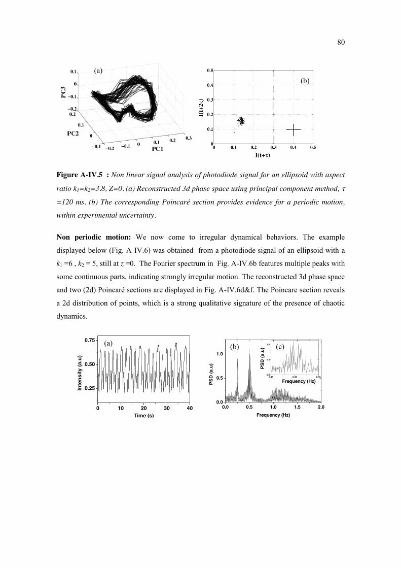
80

Figure A-IV.5 : Non linear signal analysis of photodiode signal for an ellipsoid with aspect

ratio k1=k2=3.8, Z=0. (a) Reconstructed 3d phase space using principal component method,

=120 ms. (b) The corresponding Poincaré section provides evidence for a periodic motion,

within experimental uncertainty.

Non periodic motion: We now come to irregular dynamical behaviors. The example

displayed below (Fig. A-IV.6) was obtained from a photodiode signal of an ellipsoid with a

k1 =6 , k2 = 5, still at z =0. The Fourier spectrum in Fig. A-IV.6b features multiple peaks with

some continuous parts, indicating strongly irregular motion. The reconstructed 3d phase space

and two (2d) Poincaré sections are displayed in Fig. A-IV.6d&f. The Poincare section reveals

a 2d distribution of points, which is a strong qualitative signature of the presence of chaotic

dynamics.

0 10 20 30 40

0.25

0.50

0.75

Inte

nsity

(a.u

)

Time (s)0.0 0.5 1.0 1.5 2.0

0.0

0.5

1.0

PSD

(a.u

)

Frequency (Hz)

Frequency (Hz)

PSD

(a.u

)

0.45 0.50 0.550.0

0.5

1.0

(a) (b)

(a) (b) (c)

81

Figure A-IV. 6: Analysis of an irregular signal for an ellipsoid with k1 =6, k2 = 5. (a) Time

series. (b) Fourier power spectrum. (c) Magnified version of the power spectrum to emphasize

the presence of multiple peaks in the spectrum. (d) Reconstructed 3d phase space using the

time delay method, = 0.5s . The faint blue plane marks the location of the Poincaré section

displayed in panel (e).

Below we provide more examples of chaotic behaviors obtained for different prolate

ellipsoids located at beam waist. All the time series were recorded with the photodiode. Note

the layered structure of the section in Fig. A-IV.7d, a clear signature of trajectory folding in

chaotic attractors (see Fig. A-IV.3).

0 5 10 15

0.3

0.6

Inte

nsity

(a.u

)

Time (s)0 1 2 3

0

2

4

Frequency (Hz)

PSD

(a.u

)

(e)

(a) (b)

(d)

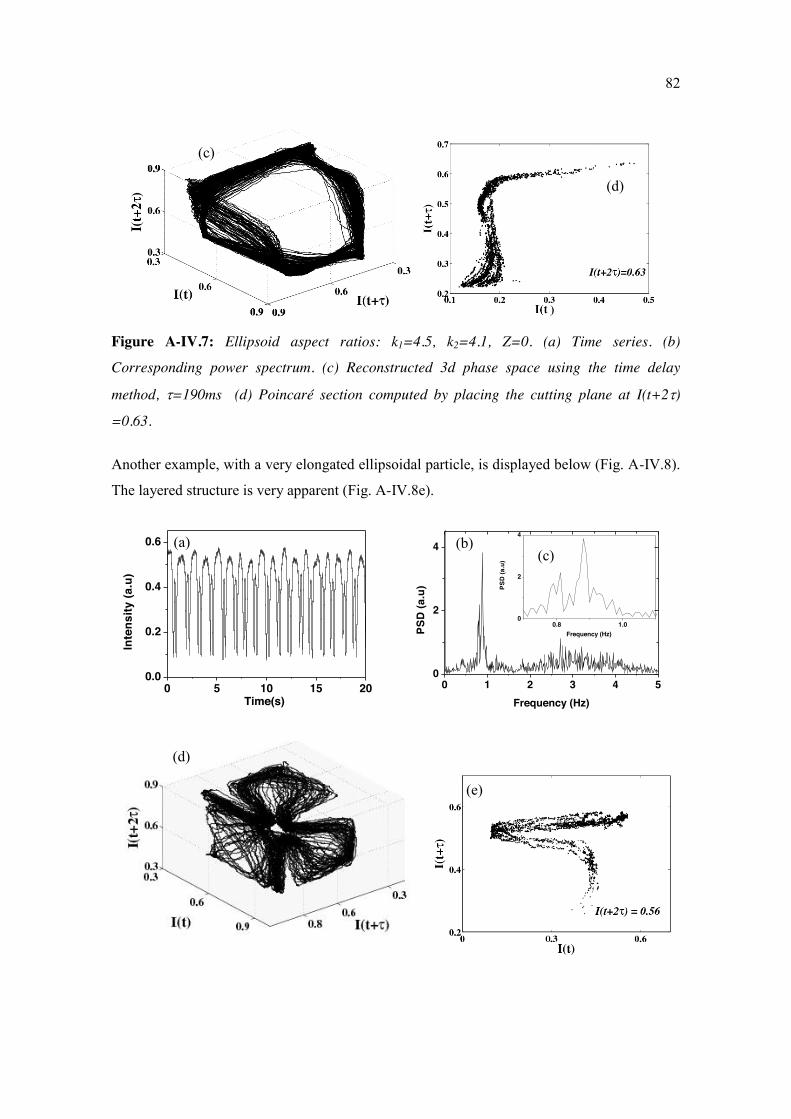
82

Figure A-IV.7: Ellipsoid aspect ratios: k1=4.5, k2=4.1, Z=0. (a) Time series. (b)

Corresponding power spectrum. (c) Reconstructed 3d phase space using the time delay

method, =190ms (d) Poincaré section computed by placing the cutting plane at I(t+2)

=0.63. Another example, with a very elongated ellipsoidal particle, is displayed below (Fig. A-IV.8).

The layered structure is very apparent (Fig. A-IV.8e).

0 5 10 15 200.0

0.2

0.4

0.6

Inte

nsity

(a.u

)

Time(s)0 1 2 3 4 5

0

2

4

Frequency (Hz)

PSD

(a.u

)

0.8 1.00

2

4

PSD

(a.u

)

Frequency (Hz)

(c)

(d)

(a) (b)

(d)

(e)

(c)

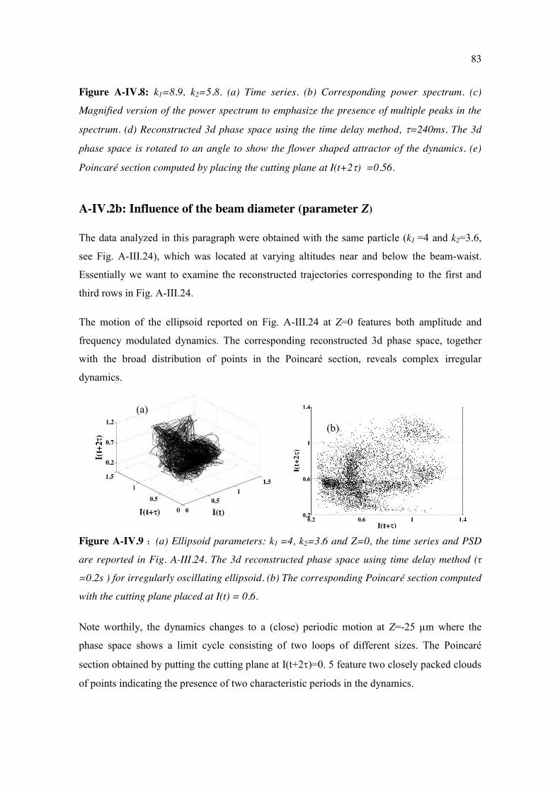
83

Figure A-IV.8: k1=8.9, k2=5.8. (a) Time series. (b) Corresponding power spectrum. (c)

Magnified version of the power spectrum to emphasize the presence of multiple peaks in the

spectrum. (d) Reconstructed 3d phase space using the time delay method, =240ms. The 3d

phase space is rotated to an angle to show the flower shaped attractor of the dynamics. (e)

Poincaré section computed by placing the cutting plane at I(t+2) =0.56.

A-IV.2b: Influence of the beam diameter (parameter Z)

The data analyzed in this paragraph were obtained with the same particle (k1 =4 and k2=3.6,

see Fig. A-III.24), which was located at varying altitudes near and below the beam-waist.

Essentially we want to examine the reconstructed trajectories corresponding to the first and

third rows in Fig. A-III.24.

The motion of the ellipsoid reported on Fig. A-III.24 at Z=0 features both amplitude and

frequency modulated dynamics. The corresponding reconstructed 3d phase space, together

with the broad distribution of points in the Poincaré section, reveals complex irregular

dynamics.

Figure A-IV.9 : (a) Ellipsoid parameters: k1 =4, k2=3.6 and Z=0, the time series and PSD

are reported in Fig. A-III.24. The 3d reconstructed phase space using time delay method (τ

=0.2s ) for irregularly oscillating ellipsoid. (b) The corresponding Poincaré section computed

with the cutting plane placed at I(t) = 0.6. Note worthily, the dynamics changes to a (close) periodic motion at Z=-25 µm where the

phase space shows a limit cycle consisting of two loops of different sizes. The Poincaré

section obtained by putting the cutting plane at I(t+2)=0. 5 feature two closely packed clouds

of points indicating the presence of two characteristic periods in the dynamics.

(a)

(b)

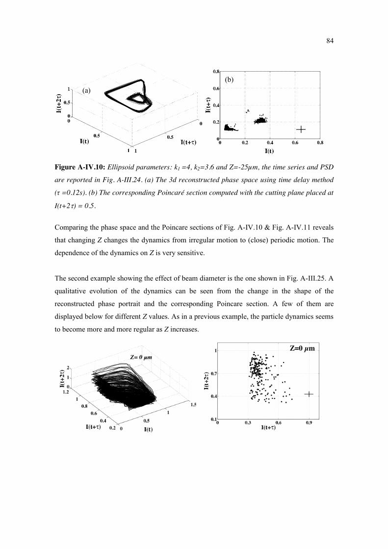
84

Figure A-IV.10: Ellipsoid parameters: k1 =4, k2=3.6 and Z=-25µm, the time series and PSD

are reported in Fig. A-III.24. (a) The 3d reconstructed phase space using time delay method

(τ =0.12s). (b) The corresponding Poincaré section computed with the cutting plane placed at

I(t+2) = 0.5.

Comparing the phase space and the Poincare sections of Fig. A-IV.10 & Fig. A-IV.11 reveals

that changing Z changes the dynamics from irregular motion to (close) periodic motion. The

dependence of the dynamics on Z is very sensitive.

The second example showing the effect of beam diameter is the one shown in Fig. A-III.25. A

qualitative evolution of the dynamics can be seen from the change in the shape of the

reconstructed phase portrait and the corresponding Poincare section. A few of them are

displayed below for different Z values. As in a previous example, the particle dynamics seems

to become more and more regular as Z increases.

(a) (b)

Z=0 µm

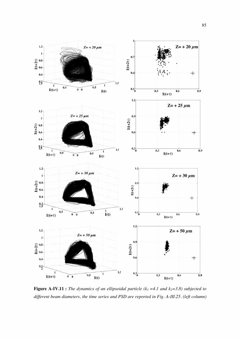
85

Figure A-IV.11 : The dynamics of an ellipsoidal particle (k1 =4.1 and k2=3.8) subjected to

different beam diameters, the time series and PSD are reported in Fig. A-III.25. (left column)

Z= + 20 µm

Z= + 25 µm

Z= + 30 µm

Z= + 50 µm

86

The 3d reconstructed phase space using time delay method. (right column). The

corresponding Poincaré sections computed with the cutting plane placed at the average I(t)

crossing. The Poincare section evolves from broadly distributed points at Z=0 µm to small

packet of points at Z= +50µm.

As evidenced from both the phase space and Poincare section, the dynamics oscillating

ellipsoids is strongly affected by the beam diameter.

A-IV.3 Conclusion

The phase space reconstruction techniques that we applied to the photodiode signals allowed

us to reveal characteristic features of  the  particles’  dynamics.  In  several  examples,  we  found  

trajectories that were limit cycles in 3 dimensions, meaning that the motion was periodic. This

result did not come as a surprise, as the corresponding power spectra were made of well

marked peaks, at frequencies that were integer multiples of a fundamental frequency. Other

examples instead revealed clearly non periodic motions. As we could see from the Poincaré

sections, the reconstructed trajectories had characteristics of strange attractors, meaning that

the particle motion pertained to deterministic chaos. A few other examples gave Poincaré

sections with no discernable structures, leaving the impression of extreme complexity akin to

turbulence.

A rather unexpected outcome of this study is the fact no simple relation seems to exist

between the control parameters, namely k1, k2 and z, and the nature of the dynamics. As we

saw, ellipsoids of moderate aspect ratio, i.e. k ≈   4,   undergo   periodic,   chaotic   and   even  

turbulent-like dynamics at z = 0, depending on the chosen particle. Chaos is observed at z = 0

equally with moderate (k ≈  4),  medium  (k ≈  6)  and   large  (k ≈  8)  aspect   ratios,  and  no  clear  

tendency emerges when a given particle is brought at different altitudes, i.e. at constant k and

variable z. This diversity of behaviors leaves us with some frustration, because we would have

liked to find a simple route from periodicity to chaos, for instance through a sequence of

period doubling [Thamilmaran 2002]. This possibly simple route might be searched as a line

in the space of control parameters (k1, k2, z). Unfortunately we cannot vary the aspect ratios in

the course of an experiment, since we can only pick up a particle of given dimensions. We

first hoped that simply varying z for a few given examples of (k1, k2) might be enough, but we

did not meet a complete periodic to chaotic sequence using this method yet. Nevertheless,

such a sequence may exist and it will be worth accumulating more data to find it.

87

A-V: Ray-optics 2d model The goal of this chapter  is  to  set  up  a  simulation  of  the  ellipsoidal  particles’  oscillations,  using  

a very simple optical model based on ray-optics.

To   simulate   the   particle’s   response,   we   must   first   calculate   the   optical   forceF and

torqueΓ acting on the particle in a laser beam of given characteristics. In a rigorous version,

the problem amounts to calculating the electromagnetic field scattered by the particle. In

theory, F and Γ can then obtained from the Maxwell stress tensor of the whole e.m. field

(incident+scattered) by integration on a surface that surrounds the particle [Jackson 1975,

Jonáš 2008].

When the particle is a few micrometers in size, the wave nature of the e.m. field must be taken

into account. The case of a sphere that scatters light from a focused laser beam has been the

matter of many dedicated works since the eighties. Rigorous solutions to this problem have

been  obtained  and  are  known  as  “Generalized  Lorenz-Mie theory”  (GLMT)  [Gouesbet 1988,

Ren 1994]. The GLMT has been extended to spheroidal shapes (i.e. cylindrically symmetrical

ellipsoids) by Xu et al. [Xu 2007]; these authors computed radiation pressure forces and

torques for particle aspect ratios (k) up to 1.5.

In general, calculation of the scattered field by particles of more complex shapes is a very

difficult task that can only be performed using numerical techniques. Different methods have

been proposed to be applicable to about any particle shape, namely the discrete dipole

approximation (DDA) [Draine 1994, Yurkin 2007, Chaumet 2002, Bonessi 2007, Simpson

2011a&b], the finite difference time domain (FDTD) [Benito 2008, Qin 2009], the vector

finite element [White 2000], multilevel multipole [Song 1995, Sheng 1998] and T-Matrix

methods [Varadan 1980]. A numerical tool box using the latter method has been proposed for

application to optical tweezers geometries, for different kinds of laser beams [Nieminen

2007].

Calculating the field scattered by our ellipsoidal particles, of large aspect ratio and several 10

m in size, is currently at the limit of possibilities of existing numerical methods5. In the

course of our PhD project, we opted for a very simplified analysis based on ray-optics (RO),

in two dimensions. The assumptions made in the model are rough, meaning that the

simulation has no pretention to be quantitatively accurate. In spite of these limitations, we

hope  that  the  model  still  captures  essential  trends  of  the  particle’s  mechanical  response  to  the   5 This work is scheduled as a future work in the frame of AMOCOPS project, headed by Prof. F. Ren (CORIA, Rouen. AMOCOPS acronym stands for “Advanced Methods for Optical Characterization of Complex Particle Systems”.

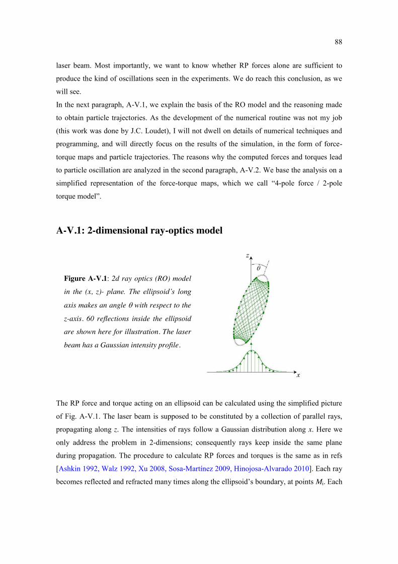
88

laser beam. Most importantly, we want to know whether RP forces alone are sufficient to

produce the kind of oscillations seen in the experiments. We do reach this conclusion, as we

will see.

In the next paragraph, A-V.1, we explain the basis of the RO model and the reasoning made

to obtain particle trajectories. As the development of the numerical routine was not my job

(this work was done by J.C. Loudet), I will not dwell on details of numerical techniques and

programming, and will directly focus on the results of the simulation, in the form of force-

torque maps and particle trajectories. The reasons why the computed forces and torques lead

to particle oscillation are analyzed in the second paragraph, A-V.2. We base the analysis on a

simplified representation of the force-torque maps, which we call “4-pole force / 2-pole

torque  model”.

A-V.1: 2-dimensional ray-optics model

The RP force and torque acting on an ellipsoid can be calculated using the simplified picture

of Fig. A-V.1. The laser beam is supposed to be constituted by a collection of parallel rays,

propagating along z. The intensities of rays follow a Gaussian distribution along x. Here we

only address the problem in 2-dimensions; consequently rays keep inside the same plane

during propagation. The procedure to calculate RP forces and torques is the same as in refs

[Ashkin 1992, Walz 1992, Xu 2008, Sosa-Martínez 2009, Hinojosa-Alvarado 2010]. Each ray

becomes  reflected  and  refracted  many  times  along  the  ellipsoid’s  boundary,  at  points  Mi. Each

Figure A-V.1: 2d ray optics (RO) model

in the (x, z)- plane.   The   ellipsoid’s   long  

axis makes an angle with respect to the

z-axis. 60 reflections inside the ellipsoid

are shown here for illustration. The laser

beam has a Gaussian intensity profile.

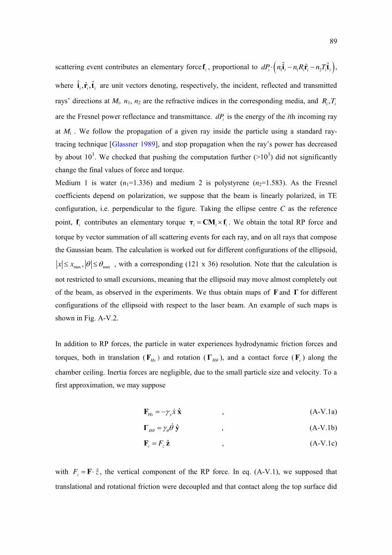
89

scattering event contributes an elementary force if , proportional to 1 1 2ˆ ˆˆi i i i i idP n n R n T i r t ,

where ˆ ˆˆ, ,i i ii r t are unit vectors denoting, respectively, the incident, reflected and transmitted

rays’  directions  at  Mi. n1, n2 are the refractive indices in the corresponding media, and ,i iR T

are the Fresnel power reflectance and transmittance. idP is the energy of the ith incoming ray

at Mi . We follow the propagation of a given ray inside the particle using a standard ray-

tracing technique [Glassner 1989],  and  stop  propagation  when  the  ray’s  power  has  decreased  

by about 103. We checked that pushing the computation further (>103) did not significantly

change the final values of force and torque.

Medium 1 is water (n1=1.336) and medium 2 is polystyrene (n2=1.583). As the Fresnel

coefficients depend on polarization, we suppose that the beam is linearly polarized, in TE

configuration, i.e. perpendicular to the figure. Taking the ellipse centre C as the reference

point, if contributes an elementary torque i i i τ CM f . We obtain the total RP force and

torque by vector summation of all scattering events for each ray, and on all rays that compose

the Gaussian beam. The calculation is worked out for different configurations of the ellipsoid,

max max,x x , with a corresponding (121 x 36) resolution. Note that the calculation is

not restricted to small excursions, meaning that the ellipsoid may move almost completely out

of the beam, as observed in the experiments. We thus obtain maps of F and Γ for different

configurations of the ellipsoid with respect to the laser beam. An example of such maps is

shown in Fig. A-V.2.

In addition to RP forces, the particle in water experiences hydrodynamic friction forces and

torques, both in translation ( HxF ) and rotation ( HΓ ), and a contact force ( cF ) along the

chamber ceiling. Inertia forces are negligible, due to the small particle size and velocity. To a

first approximation, we may suppose

ˆHx xx F x , (A-V.1a)

ˆH Γ y , (A-V.1b)

ˆc zFF z , (A-V.1c)

with ˆzF z F , the vertical component of the RP force. In eq. (A-V.1), we supposed that

translational and rotational friction were decoupled and that contact along the top surface did

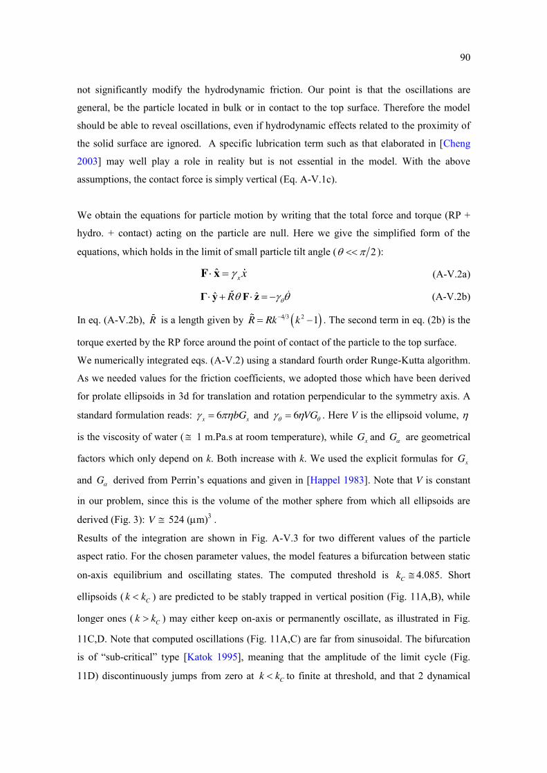
90

not significantly modify the hydrodynamic friction. Our point is that the oscillations are

general, be the particle located in bulk or in contact to the top surface. Therefore the model

should be able to reveal oscillations, even if hydrodynamic effects related to the proximity of

the solid surface are ignored. A specific lubrication term such as that elaborated in [Cheng

2003] may well play a role in reality but is not essential in the model. With the above

assumptions, the contact force is simply vertical (Eq. A-V.1c).

We obtain the equations for particle motion by writing that the total force and torque (RP +

hydro. + contact) acting on the particle are null. Here we give the simplified form of the

equations, which holds in the limit of small particle tilt angle ( 2 ):

ˆ xx F x (A-V.2a)

ˆ ˆR Γ y F z (A-V.2b)

In eq. (A-V.2b), R is a length given by 4 3 2 1R Rk k . The second term in eq. (2b) is the

torque exerted by the RP force around the point of contact of the particle to the top surface.

We numerically integrated eqs. (A-V.2) using a standard fourth order Runge-Kutta algorithm.

As we needed values for the friction coefficients, we adopted those which have been derived

for prolate ellipsoids in 3d for translation and rotation perpendicular to the symmetry axis. A

standard formulation reads: 6x xbG and 6 VG . Here V is the ellipsoid volume,

is the viscosity of water ( 1 m.Pa.s at room temperature), while xG and G are geometrical

factors which only depend on k. Both increase with k. We used the explicit formulas for xG

and G derived  from  Perrin’s  equations  and  given  in  [Happel 1983]. Note that V is constant

in our problem, since this is the volume of the mother sphere from which all ellipsoids are

derived (Fig. 3): V 524 (m)3 .

Results of the integration are shown in Fig. A-V.3 for two different values of the particle

aspect ratio. For the chosen parameter values, the model features a bifurcation between static

on-axis equilibrium and oscillating states. The computed threshold is Ck 4.085. Short

ellipsoids ( Ck k ) are predicted to be stably trapped in vertical position (Fig. 11A,B), while

longer ones ( Ck k ) may either keep on-axis or permanently oscillate, as illustrated in Fig.

11C,D. Note that computed oscillations (Fig. 11A,C) are far from sinusoidal. The bifurcation

is   of   “sub-critical”   type   [Katok 1995], meaning that the amplitude of the limit cycle (Fig.

11D) discontinuously jumps from zero at Ck k to finite at threshold, and that 2 dynamical

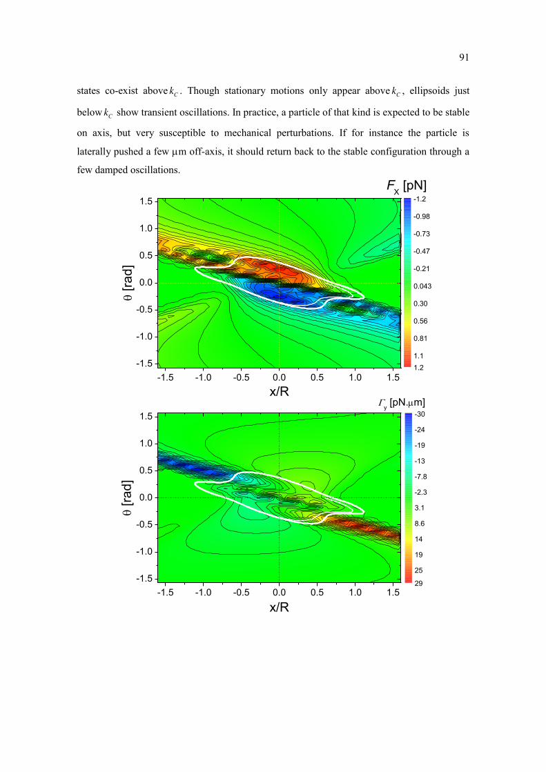
91

-1.5 -1.0 -0.5 0.0 0.5 1.0 1.5-1.5

-1.0

-0.5

0.0

0.5

1.0

1.5FX [pN]

x/R

[ra

d]

-1.2

-0.98

-0.73

-0.47

-0.21

0.043

0.30

0.56

0.81

1.11.2

-1.5 -1.0 -0.5 0.0 0.5 1.0 1.5-1.5

-1.0

-0.5

0.0

0.5

1.0

1.5y [pN.m]

x/R

[ra

d]

-30

-24

-19

-13

-7.8

-2.3

3.1

8.6

14

19

25

29

states co-exist above Ck . Though stationary motions only appear above Ck , ellipsoids just

below Ck show transient oscillations. In practice, a particle of that kind is expected to be stable

on axis, but very susceptible to mechanical perturbations. If for instance the particle is

laterally pushed a few m off-axis, it should return back to the stable configuration through a

few damped oscillations.

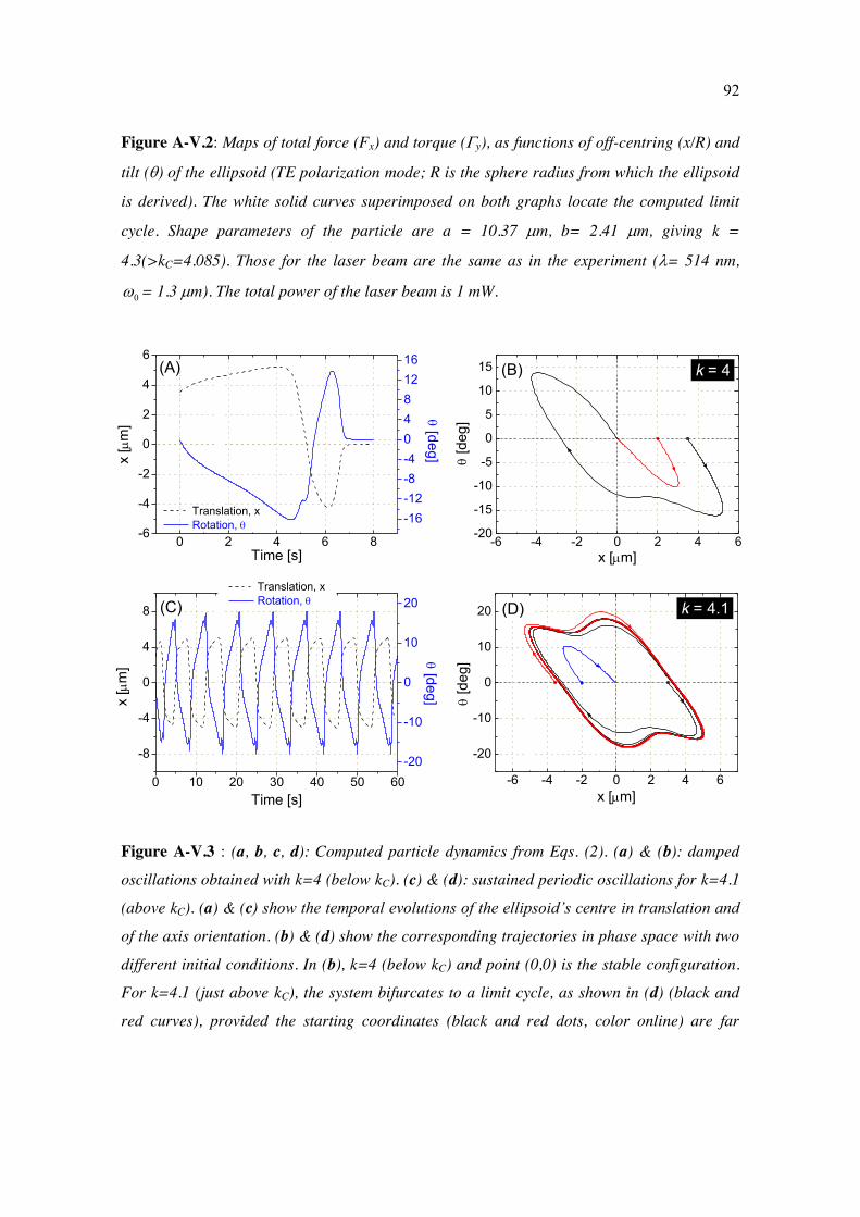
92

0 2 4 6 8-6

-4

-2

0

2

4

6(A)

Translation, x Rotation,

Time [s]

x [

m]

-16-12-8-40481216

[deg]

-6 -4 -2 0 2 4 6-20

-15

-10

-5

0

5

10

15 k = 4(B)

[d

eg]

x [m]

0 10 20 30 40 50 60

-8

-4

0

4

8 (C) Translation, x Rotation,

Time [s]

x [

m]

-20

-10

0

10

20

[deg]

-6 -4 -2 0 2 4 6

-20

-10

0

10

20 (D) k = 4.1

[d

eg]

x [m]

Figure A-V.2: Maps of total force (Fx) and torque (y), as functions of off-centring (x/R) and

tilt () of the ellipsoid (TE polarization mode; R is the sphere radius from which the ellipsoid

is derived). The white solid curves superimposed on both graphs locate the computed limit

cycle. Shape parameters of the particle are a = 10.37 m, b= 2.41 m, giving k =

4.3(>kC=4.085). Those for the laser beam are the same as in the experiment (= 514 nm,

0 = 1.3 m). The total power of the laser beam is 1 mW.

Figure A-V.3 : (a, b, c, d): Computed particle dynamics from Eqs. (2). (a) & (b): damped

oscillations obtained with k=4 (below kC). (c) & (d): sustained periodic oscillations for k=4.1

(above kC). (a) & (c)  show  the  temporal  evolutions  of  the  ellipsoid’s  centre  in  translation  and  

of the axis orientation. (b) & (d) show the corresponding trajectories in phase space with two

different initial conditions. In (b), k=4 (below kC) and point (0,0) is the stable configuration.

For k=4.1 (just above kC), the system bifurcates to a limit cycle, as shown in (d) (black and

red curves), provided the starting coordinates (black and red dots, color online) are far

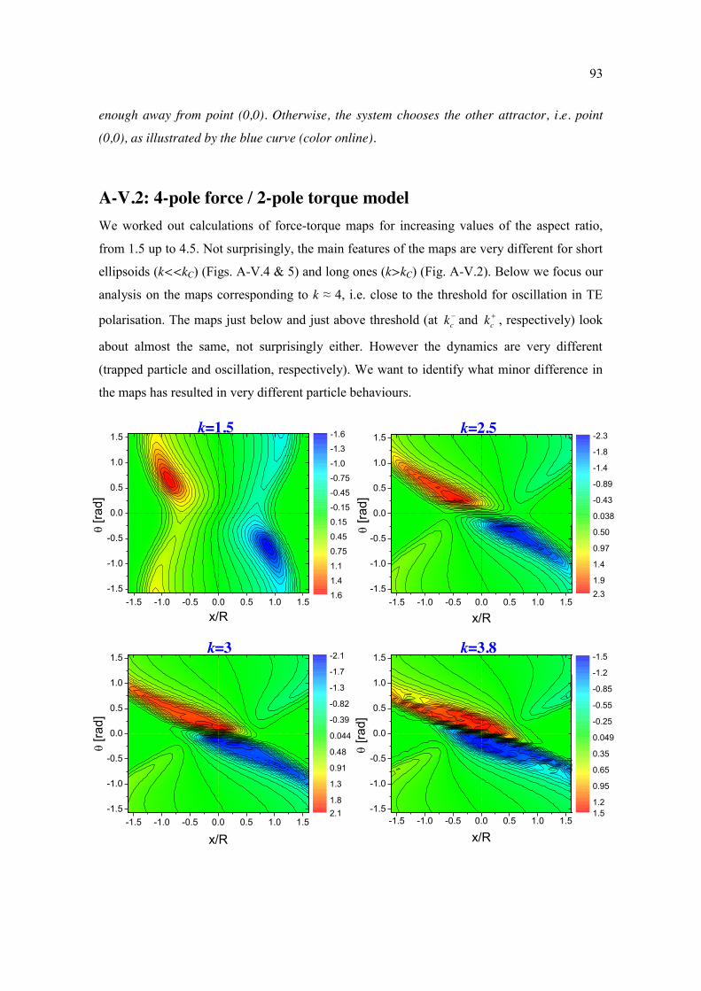
93

-1.5 -1.0 -0.5 0.0 0.5 1.0 1.5-1.5

-1.0

-0.5

0.0

0.5

1.0

1.5

x/R

[ra

d]

-1.6

-1.3

-1.0

-0.75

-0.45

-0.15

0.15

0.45

0.75

1.1

1.4

1.6-1.5 -1.0 -0.5 0.0 0.5 1.0 1.5

-1.5

-1.0

-0.5

0.0

0.5

1.0

1.5

x/R

[ra

d]

-2.3

-1.8

-1.4

-0.89

-0.43

0.038

0.50

0.97

1.4

1.92.3

-1.5 -1.0 -0.5 0.0 0.5 1.0 1.5-1.5

-1.0

-0.5

0.0

0.5

1.0

1.5

x/R

[ra

d]

-2.1

-1.7

-1.3

-0.82

-0.39

0.044

0.48

0.91

1.3

1.82.1

-1.5 -1.0 -0.5 0.0 0.5 1.0 1.5-1.5

-1.0

-0.5

0.0

0.5

1.0

1.5

x/R

[ra

d]

-1.5

-1.2

-0.85

-0.55

-0.25

0.049

0.35

0.65

0.95

1.21.5

enough away from point (0,0). Otherwise, the system chooses the other attractor, i.e. point

(0,0), as illustrated by the blue curve (color online).

A-V.2: 4-pole force / 2-pole torque model We worked out calculations of force-torque maps for increasing values of the aspect ratio,

from 1.5 up to 4.5. Not surprisingly, the main features of the maps are very different for short

ellipsoids (k<<kC) (Figs. A-V.4 & 5) and long ones (k>kC) (Fig. A-V.2). Below we focus our

analysis on the maps corresponding to k ≈  4,  i.e.  close  to  the  threshold  for  oscillation  in  TE

polarisation. The maps just below and just above threshold (at ck and ck , respectively) look

about almost the same, not surprisingly either. However the dynamics are very different

(trapped particle and oscillation, respectively). We want to identify what minor difference in

the maps has resulted in very different particle behaviours.

k=1.5 k=2.5

k=3 k=3.8

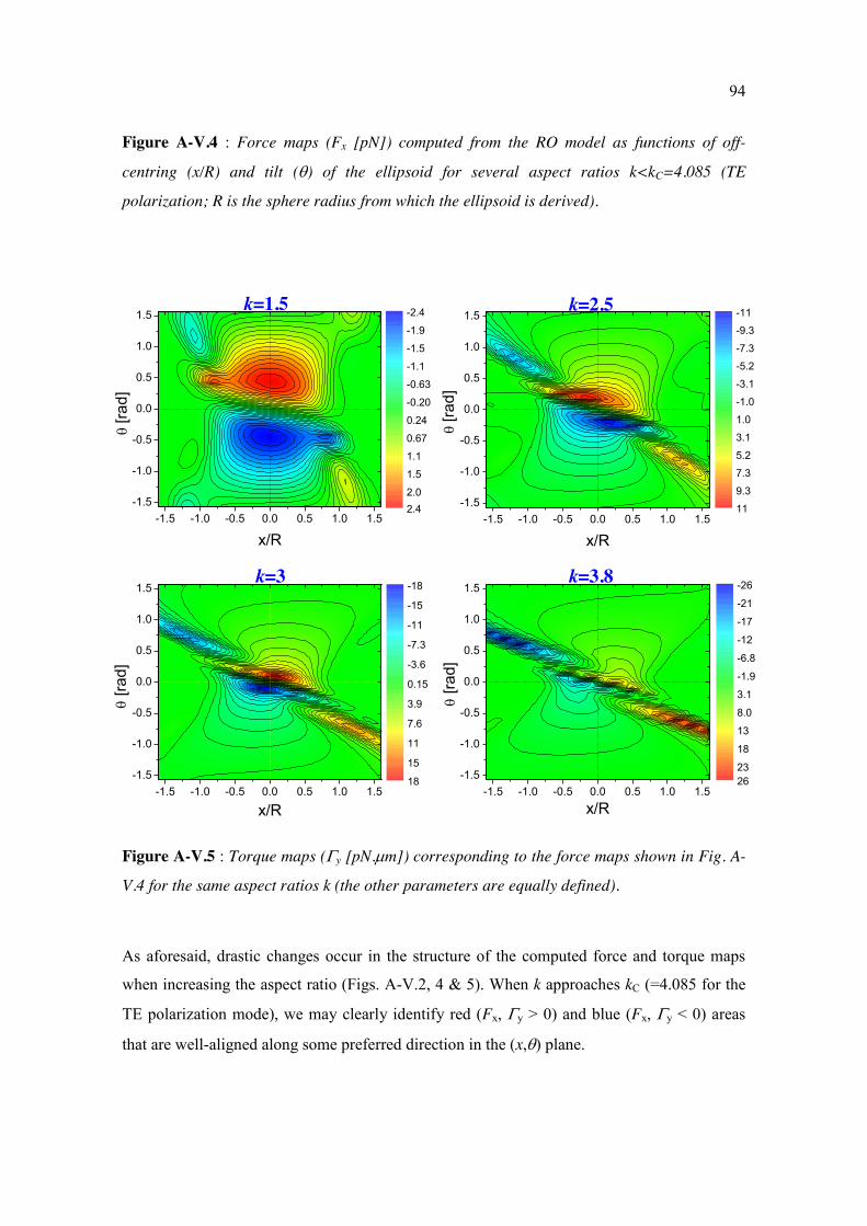
94

-1.5 -1.0 -0.5 0.0 0.5 1.0 1.5-1.5

-1.0

-0.5

0.0

0.5

1.0

1.5

x/R

[ra

d]

-2.4

-1.9

-1.5

-1.1

-0.63

-0.20

0.24

0.67

1.1

1.5

2.02.4

-1.5 -1.0 -0.5 0.0 0.5 1.0 1.5-1.5

-1.0

-0.5

0.0

0.5

1.0

1.5

x/R

[ra

d]

-11

-9.3

-7.3

-5.2

-3.1

-1.0

1.0

3.1

5.2

7.3

9.3

11

-1.5 -1.0 -0.5 0.0 0.5 1.0 1.5-1.5

-1.0

-0.5

0.0

0.5

1.0

1.5

x/R

[ra

d]

-18

-15

-11

-7.3

-3.6

0.15

3.9

7.6

11

15

18-1.5 -1.0 -0.5 0.0 0.5 1.0 1.5

-1.5

-1.0

-0.5

0.0

0.5

1.0

1.5

x/R

[ra

d]

-26

-21

-17

-12

-6.8

-1.9

3.1

8.0

13

18

2326

Figure A-V.4 : Force maps (Fx [pN]) computed from the RO model as functions of off-

centring (x/R) and tilt () of the ellipsoid for several aspect ratios k<kC=4.085 (TE

polarization; R is the sphere radius from which the ellipsoid is derived).

Figure A-V.5 : Torque maps (y [pN.m]) corresponding to the force maps shown in Fig. A-

V.4 for the same aspect ratios k (the other parameters are equally defined).

As aforesaid, drastic changes occur in the structure of the computed force and torque maps

when increasing the aspect ratio (Figs. A-V.2, 4 & 5). When k approaches kC (=4.085 for the

TE polarization mode), we may clearly identify red (Fx, y > 0) and blue (Fx, y < 0) areas

that are well-aligned along some preferred direction in the (x,) plane.

k=1.5 k=2.5

k=3 k=3.8

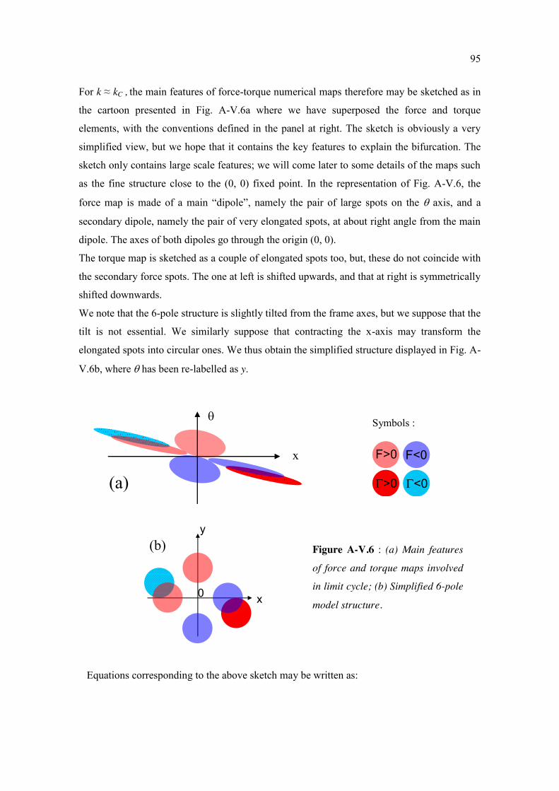
95

For k ≈  kC , the main features of force-torque numerical maps therefore may be sketched as in

the cartoon presented in Fig. A-V.6a where we have superposed the force and torque

elements, with the conventions defined in the panel at right. The sketch is obviously a very

simplified view, but we hope that it contains the key features to explain the bifurcation. The

sketch only contains large scale features; we will come later to some details of the maps such

as the fine structure close to the (0, 0) fixed point. In the representation of Fig. A-V.6, the

force  map   is  made  of   a  main   “dipole”,   namely   the   pair   of   large   spots   on   the   axis, and a

secondary dipole, namely the pair of very elongated spots, at about right angle from the main

dipole. The axes of both dipoles go through the origin (0, 0).

The torque map is sketched as a couple of elongated spots too, but, these do not coincide with

the secondary force spots. The one at left is shifted upwards, and that at right is symmetrically

shifted downwards.

We note that the 6-pole structure is slightly tilted from the frame axes, but we suppose that the

tilt is not essential. We similarly suppose that contracting the x-axis may transform the

elongated spots into circular ones. We thus obtain the simplified structure displayed in Fig. A-

V.6b, where has been re-labelled as y.

Equations corresponding to the above sketch may be written as:

Symbols :

>0 <0

F>0 F<0

Figure A-V.6 : (a) Main features

of force and torque maps involved

in limit cycle; (b) Simplified 6-pole

model structure.

(a)

x

y

0

(b)

(a) x

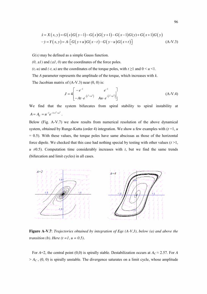
96

, 1 1 1 ( ) 1

,

x X x y G x G y G x G y G x G y G x G y

y Y x y A G y u G x t G y u G x t

(A-V.3)

G(x) may be defined as a simple Gauss function.

(0, ±1) and (±1, 0) are the coordinates of the force poles.

(t,-u) and (-t, u) are the coordinates of the torque poles, with t ≥1  and  0  <  u <1.

The A parameter represents the amplitude of the torque, which increases with k.

The Jacobian matrix of (A-V.3) near (0, 0) is:

2 2 2 2

1 1

4t u t u

e eJ

At e Au e

(A-V.4)

We find that the system bifurcates from spiral stability to spiral instability at 2 21 1 t u

CA A u e .

Below (Fig. A-V.7) we show results from numerical resolution of the above dynamical

system, obtained by Runge-Kutta (order 4) integration. We show a few examples with (t =1, u

= 0.5). With these values, the torque poles have same abscissas as those of the horizontal

force dipole. We checked that this case had nothing special by testing with other values (t >1,

u ≠0.5).   Computation time considerably increases with t, but we find the same trends

(bifurcation and limit cycles) in all cases.

Figure A-V.7: Trajectories obtained by integration of Eqs (A-V.3), below (a) and above the

transition (b). Here (t =1, u = 0.5).

For A=2, the central point (0,0) is spirally stable. Destabilization occurs at AC ≈  2.57. For A

> AC , (0, 0) is spirally unstable. The divergence saturates on a limit cycle, whose amplitude

For A > AC , (0, 0) is spirally unstable. The divergence saturates on a limit cycle, whose amplitude increases with A. Here A=4. For A=4, the cycle encompasses the (0, ±1) force poles, and gets through the (±1, 0) force poles.

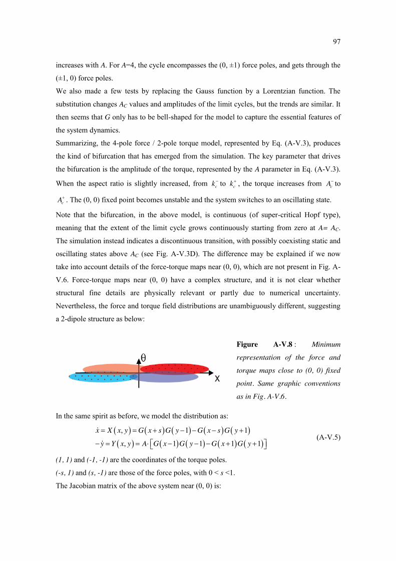
97

increases with A. For A=4, the cycle encompasses the (0, ±1) force poles, and gets through the

(±1, 0) force poles.

We also made a few tests by replacing the Gauss function by a Lorentzian function. The

substitution changes AC values and amplitudes of the limit cycles, but the trends are similar. It

then seems that G only has to be bell-shaped for the model to capture the essential features of

the system dynamics.

Summarizing, the 4-pole force / 2-pole torque model, represented by Eq. (A-V.3), produces

the kind of bifurcation that has emerged from the simulation. The key parameter that drives

the bifurcation is the amplitude of the torque, represented by the A parameter in Eq. (A-V.3).

When the aspect ratio is slightly increased, from ck to ck , the torque increases from cA to

cA . The (0, 0) fixed point becomes unstable and the system switches to an oscillating state.

Note that the bifurcation, in the above model, is continuous (of super-critical Hopf type),

meaning that the extent of the limit cycle grows continuously starting from zero at A= AC.

The simulation instead indicates a discontinuous transition, with possibly coexisting static and

oscillating states above AC (see Fig. A-V.3D). The difference may be explained if we now

take into account details of the force-torque maps near (0, 0), which are not present in Fig. A-

V.6. Force-torque maps near (0, 0) have a complex structure, and it is not clear whether

structural fine details are physically relevant or partly due to numerical uncertainty.

Nevertheless, the force and torque field distributions are unambiguously different, suggesting

a 2-dipole structure as below:

In the same spirit as before, we model the distribution as:

, 1 1

, 1 1 1 1

x X x y G x s G y G x s G y

y Y x y A G x G y G x G y

(A-V.5)

(1, 1) and (-1, -1) are the coordinates of the torque poles.

(-s, 1) and (s, -1) are those of the force poles, with 0 < s <1.

The Jacobian matrix of the above system near (0, 0) is:

Figure A-V.8 : Minimum

representation of the force and

torque maps close to (0, 0) fixed

point. Same graphic conventions

as in Fig. A-V.6.

98

2 21 124

s ss e eJ eA A

(A-V.6)

We find that (0, 0) is a stable fixed point, whatever the values of A (>0) and s. Due to the fine

structure of the force-torque maps near the origin, we expect the (0, 0) configuration (ellipsoid

on axis) to be stable. Gathering this result with that from the large scale structure, we expect

that (0, 0) and the limit cycle should coexist as attractors. This is in line with the results from

the full RO model.

A-V.3: Conclusion and prospects We worked out a calculation of RP forces and torque acting on an elliptical body in 2

dimensions. We proposed a model where the RP force and torque are balanced by

corresponding Stokes drag force and torque and we were able to produce a simulation of

ellipsoidal particles dynamics in the optical levitation experiment. Compared to reality, the

model was greatly simplified, as it was limited to 2d and within the ray-optics approximation.

Nevertheless this scheme predicts behaviours strikingly similar to those observed in

experiments. The model indeed predicts a bifurcation between static and oscillating states.

The difference between calculated and measured thresholds ( expcalcC Ck k ) is presumably not

essential, in view of the approximations made. Examination of the calculated force-torque

maps allowed us to identify the amplitude of the optical torque as the key parameter that

drives the bifurcation.

One of the limitations of the model, at the current stage, is our assumption of a collimated

beam (parallel rays). This assumption amounts to supposing that the laser beam structure is

invariant along z. This is not exactly so in the experiment because the beam-waist  (≈  2.6  m)

is small enough for diffraction to be well visible on the scale of particles lengths (the

diffraction length is about 15 m). Diffraction effects are not included in the RO model (by

definition), but we may simulate a focused beam, over an aperture about equal to that of the

real laser beam in the far-field. This extension of the model is currently in progress.

Beyond the work reported here, it would of course be most interesting to elaborate a 3d

version of the RO model. At the current stage, we are not able to estimate the influence of the

wave nature of light; we just keep to the vague argument that our particles are large enough

for ray optics to make sense. The argument mainly holds for the large dimension of the

99

ellipsoid particles (20 m, typically), but is questionable if one considers the short axes

lengths. Interestingly, we may envisage introducing interference effects within the RO

description, following the recent theory of [Ren 2011]  (“Vectorial  complex  ray  model”).  We

currently work along these lines.

100

Part B: Wetting dynamics of micron sized particles on water air interface

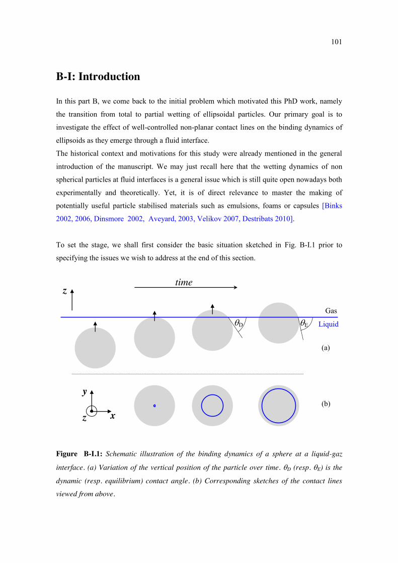
101

B-I: Introduction

In this part B, we come back to the initial problem which motivated this PhD work, namely

the transition from total to partial wetting of ellipsoidal particles. Our primary goal is to

investigate the effect of well-controlled non-planar contact lines on the binding dynamics of

ellipsoids as they emerge through a fluid interface.

The historical context and motivations for this study were already mentioned in the general

introduction of the manuscript. We may just recall here that the wetting dynamics of non

spherical particles at fluid interfaces is a general issue which is still quite open nowadays both

experimentally and theoretically. Yet, it is of direct relevance to master the making of

potentially useful particle stabilised materials such as emulsions, foams or capsules [Binks

2002, 2006, Dinsmore 2002, Aveyard, 2003, Velikov 2007, Destribats 2010].

To set the stage, we shall first consider the basic situation sketched in Fig. B-I.1 prior to

specifying the issues we wish to address at the end of this section.

Figure B-I.1: Schematic illustration of the binding dynamics of a sphere at a liquid-gaz

interface. (a) Variation of the vertical position of the particle over time. D (resp. E) is the

dynamic (resp. equilibrium) contact angle. (b) Corresponding sketches of the contact lines

viewed from above.

time

D

z

Gas

Liquid

y

x z

(a)

(b)

E

102

Figure B-I.1 is a schematic illustration of the adsorption trajectory of a sphere to a liquid-gas

interface. The sphere is initially completely wetted in water and rises towards the interface

thanks to, for example, a weak radiation pressure force exerted by a laser beam. With an ideal

sphere, i.e. whose surface is smooth and clean, we may surmise that the emersion process

proceeds through a continuous sequence of circular contact lines growing from infinitesimal

to the radius corresponding to the equilibrium contact angle (Fig. B-I.1b). In this case, simple

thermodynamic arguments suggest that the sphere likes to go to the interface because of the

large reduction in surface energy on binding. Indeed, the equilibrium position of the sphere is

determined by the minimum of the total surface free energy F which can be written as (see

appendix A for details)

22 2cos cos ,EF a h (B-I.1)

where E is the equilibrium contact angle, an arbitrary polar angle specifying the position of

the contact line at the particle surface and h the height measured with respect to the reference

configuration and given by cos cos Eh a (see Fig. A1 in appendix A). Plotting F as a

function of h/a (see Fig. B-I.2) reveals the presence of a minimum at = E . It is therefore

thermodynamically favourable for the sphere to adsorb at the interface instead of remaining

fully immersed in either bulk phase. The free energy barrier F for detachment of the particle

from the interface can be millions of times the thermal energy kBT for micrometer-sized

colloids.

-1.5 -1.0 -0.5 0.0 0.5 1.0

0.0

0.4

0.8

1.2

1.6

F/a2

h/a

F

h/a

F

1 cos E cos 1E

(a) (b)

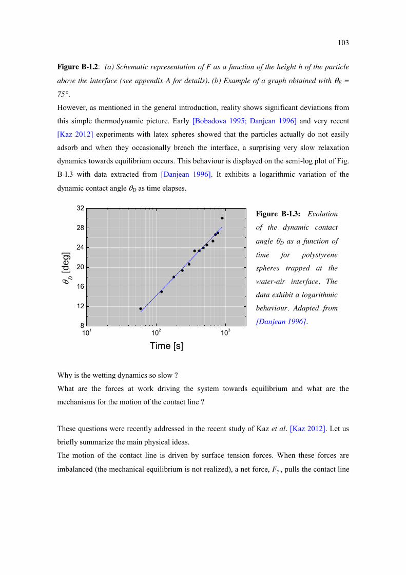
103

101 102 1038

12

16

20

24

28

32

D [d

eg]

Time [s]

Figure B-I.2: (a) Schematic representation of F as a function of the height h of the particle

above the interface (see appendix A for details). (b) Example of a graph obtained with E =

75°.

However, as mentioned in the general introduction, reality shows significant deviations from

this simple thermodynamic picture. Early [Bobadova 1995; Danjean 1996] and very recent

[Kaz 2012] experiments with latex spheres showed that the particles actually do not easily

adsorb and when they occasionally breach the interface, a surprising very slow relaxation

dynamics towards equilibrium occurs. This behaviour is displayed on the semi-log plot of Fig.

B-I.3 with data extracted from [Danjean 1996]. It exhibits a logarithmic variation of the

dynamic contact angle D as time elapses.

Why is the wetting dynamics so slow ?

What are the forces at work driving the system towards equilibrium and what are the

mechanisms for the motion of the contact line ?

These questions were recently addressed in the recent study of Kaz et al. [Kaz 2012]. Let us

briefly summarize the main physical ideas.

The motion of the contact line is driven by surface tension forces. When these forces are

imbalanced (the mechanical equilibrium is not realized), a net force, F , pulls the contact line

Figure B-I.3: Evolution

of the dynamic contact

angle D as a function of

time for polystyrene

spheres trapped at the

water-air interface. The

data exhibit a logarithmic

behaviour. Adapted from

[Danjean 1996].

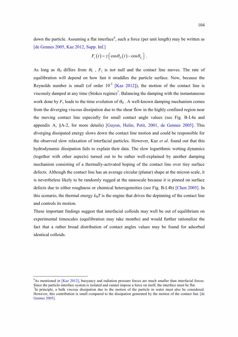
104

down the particle. Assuming a flat interface6, such a force (per unit length) may be written as

[de Gennes 2005, Kaz 2012, Supp. Inf.]

cos cos .D EF t t

As long as D differs from E , F is not null and the contact line moves. The rate of

equilibration will depend on how fast it straddles the particle surface. Now, because the

Reynolds number is small (of order 10-3 [Kaz 2012]), the motion of the contact line is

viscously damped at any time (Stokes regime)7. Balancing the damping with the instantaneous

work done by F leads to the time evolution of D . A well-known damping mechanism comes

from the diverging viscous dissipation due to the shear flow in the highly confined region near

the moving contact line especially for small contact angle values (see Fig. B-I.4a and

appendix A, §A-2, for more details) [Guyon, Hulin, Petit, 2001, de Gennes 2005]. This

diverging dissipated energy slows down the contact line motion and could be responsible for

the observed slow relaxation of interfacial particles. However, Kaz et al. found out that this

hydrodynamic dissipation fails to explain their data. The slow logarithmic wetting dynamics

(together with other aspects) turned out to be rather well-explained by another damping

mechanism consisting of a thermally-activated hoping of the contact line over tiny surface

defects. Although the contact line has an average circular (planar) shape at the micron scale, it

is nevertheless likely to be randomly rugged at the nanoscale because it is pinned on surface

defects due to either roughness or chemical heterogeneities (see Fig. B-I.4b) [Chen 2005]. In

this scenario, the thermal energy kBT is the engine that drives the depinning of the contact line

and controls its motion.

These important findings suggest that interfacial colloids may well be out of equilibrium on

experimental timescales (equilibration may take months) and would further rationalize the

fact that a rather broad distribution of contact angles values may be found for adsorbed

identical colloids.

6As mentioned in [Kaz 2012], buoyancy and radiation pressure forces are much smaller than interfacial forces. Since the particle-interface system is isolated and cannot impose a force on itself, the interface must be flat. 7In principle, a bulk viscous dissipation due to the motion of the particle in water must also be considered. However, this contribution is small compared to the dissipation generated by the motion of the contact line [de Gennes 2005].

105

Note that it has been known for a long time that the surfaces of macroscopic solid substrates

are far from ideal. Droplet spreading or film dewetting experiments revealed that both

chemical and physical defects anchor the contact line and hinders its motion leading to

hysteresis phenomena [de Gennes 2005, Seveno 2009]. At the colloidal scale, Kaz et al.

suggested that surface defects also control the binding dynamics of colloids to fluid interfaces.

Figure B-I.4: Schematic illustration of the two main damping mechanisms for the motion of

the contact line. (a) Hydrodynamic damping. The flow from the wedge created between the

particle and the interface dominates the dissipation. (b) Thermally-activated hoping of the

contact line over surface defects (black dots). The downwards black arrow indicates the

motion of the contact line. Adapted from [Kaz 2012].

Next, concerning anisotropic colloids, and to the best of our knowledge, we are not aware of

any experimental report dealing with such dynamic processes. The only work we know about

is the one by de Graaf et al. [de Graaf 2010] who numerically investigated adsorption

trajectories of anisotropic bodies through a fluid interface. The authors calculated how the

surface energy would vary as a function of the particle configuration, with the assumption that

the interface remains flat (planar) throughout the emersion. However, these authors did not

consider the contact line motion and the associated dissipation which, as we just saw, is of

paramount importance for the binding dynamics. Consequently, this work turns out to be of

limited   interest   and,   as   we   will   see   in   the   discussion   part,   predicts   “strange”   adsorption  

trajectories for prolate ellipsoids.

Gas

Liquid

Liquid

Gas

(a) (b)

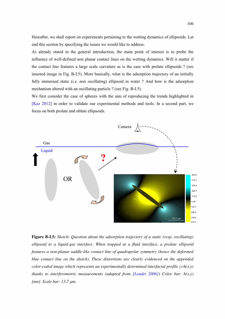
106

Hereafter, we shall report on experiments pertaining to the wetting dynamics of ellipsoids. Let

end this section by specifying the issues we would like to address.

As already stated in the general introduction, the main point of interest is to probe the

influence of well-defined non planar contact lines on the wetting dynamics. Will it matter if

the contact line features a large scale curvature as is the case with prolate ellipsoids ? (see

inserted image in Fig. B-I.5). More basically, what is the adsorption trajectory of an initially

fully immersed static (i.e. non oscillating) ellipsoid in water ? And how is the adsorption

mechanism altered with an oscillating particle ? (see Fig. B-I.5).

We first consider the case of spheres with the aim of reproducing the trends highlighted in

[Kaz 2012] in order to validate our experimental methods and tools. In a second part, we

focus on both prolate and oblate ellipsoids.

Figure B-I.5: Sketch: Question about the adsorption trajectory of a static (resp. oscillating)

ellipsoid to a liquid-gas interface. When trapped at a fluid interface, a prolate ellipsoid

features a non-planar saddle-like contact line of quadrupolar symmetry (hence the deformed

blue contact line on the sketch). These distortions are clearly evidenced on the appended

color-coded image which represents an experimentally determined interfacial profile z=h(x,y)

thanks to interferometric measurements (adapted from [Loudet 2006]) Color bar: h(x,y)

[nm]. Scale bar: 13.7 m.

13.7 m

Camera

Gas

Liquid

OR

?

107

B-II: Experimental methods

In this paragraph, we first elaborate on sample preparation before mentioning some special

features used to probe the wetting dynamics of spheres and ellipsoids.

B-II.1 Sample preparation As in part A, the samples either consist of polystyrene (PS) spheres (diameter 10 m) or

ellipsoids that are initially dispersed in water. The preparation of ellipsoids follows the same

procedure as the one already described in part A. However, it is worth mentioning here that

the spheres underwent the same chemical and thermal treatment as the ellipsoids except that

they were not stretched. Indeed, as already specified in part A, the preparation of ellipsoids

involves a dispersion step in a polyvinyl alcohol (PVA) solution. We know that part of the

PVA (although we have not quantified it) remains adsorbed at the ellipsoids surfaces, despite

the numerous washing cycles. PVA adsorption makes the particles more hydrophilic and

therefore changes the surface chemistry compared to the pristine, untreated spheres from the

manufacturer   which   have   not   “seen”   the   PVA.   The   “PVA   treatment”   for   spheres   was  

therefore necessary to insure that, on an average, all types of particles have the same surface

chemistry. This is rather important since wetting phenomena are generally very sensitive to

surface properties.

Unlike the levitation experiments described in part A, we used a specifically designed cell to

ensure a relative flatness of the water-air interface. The cell consists of two circular rings

(inner diameter: 1.5 cm; height: 2.5 mm) made of glass glued one on top of each other. The

ensemble is further glued on a glass cover slip to allow for transmission observation (see Fig.

B-II.1a). The cell is carefully filled with an aqueous particle dispersion (weight fraction <

0.01%) so that the water level just reaches the boundary separating the two rings. This results

in a pinning of the water-air interface and minimizes problems related to curved interfaces

because of the presence of menisci at the outer edges. Once filled, the cell is painstakingly

placed on the sample holder (Fig. B-II.1b) and wetting experiments can start.

108

Figure B-II.1: (a) Sketch of sample cell holder used for the wetting dynamics experiments at

the water-air interface (b) Zoomed-in view of the cell placed on the sample holder. As in part

A, the levitating beam is moderately focused by the objective located just underneath the cell.

B-II.2 Setup Similarly to [Kaz 2012], we use a weak radiation pressure force (power 10 mW force a

few pN) to levitate the particles (both spheres and ellipsoids) all the way up to the water-air

interface. We mainly used video means to detect the (approximate) moment when a particle

breaches the interface and take images of growing contact lines. In some of the experiments

we used the photodiode signal to better resolve the initial step when breaching starts.

The microscope was operated either in transmission or reflection modes. The illumination, in

reflection mode, is provided by a red diode. A system was fitted on the setup to instantly

switch between both modes. Images in transmission are ideal to visualize the particle body

below the W/A interface. In reflection mode, the water surface and the dry part of the particle

are well discernible, due to differences in reflectivity and collection efficiency through the

aperture of the microscope objective. In general the dry part appears dark, except on the very

top part of the particle, while the W/A interface appears in medium grey. The contact line can

be located as the boundary between both zones.

(b) (a)

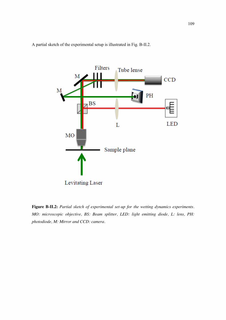
109

A partial sketch of the experimental setup is illustrated in Fig. B-II.2.

Figure B-II.2: Partial sketch of experimental set-up for the wetting dynamics experiments.

MO: microscopic objective, BS: Beam splitter, LED: light emitting diode, L: lens, PH:

photodiode, M: Mirror and CCD: camera.

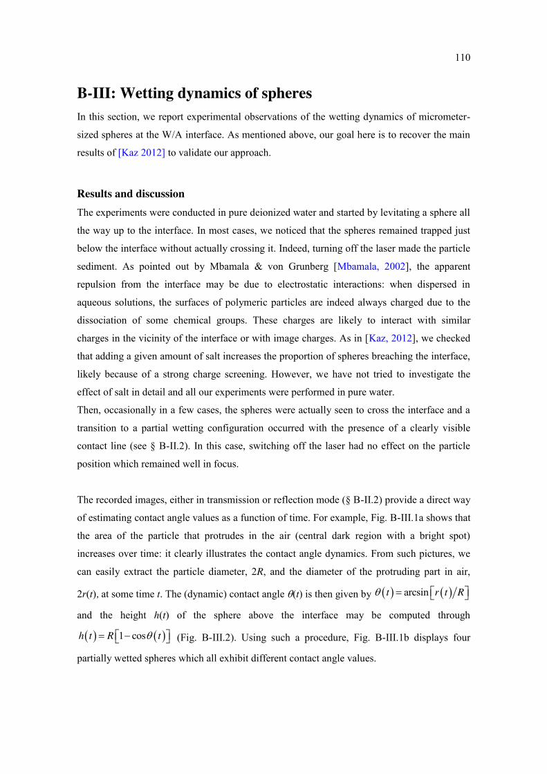
110

B-III: Wetting dynamics of spheres In this section, we report experimental observations of the wetting dynamics of micrometer-

sized spheres at the W/A interface. As mentioned above, our goal here is to recover the main

results of [Kaz 2012] to validate our approach.

Results and discussion The experiments were conducted in pure deionized water and started by levitating a sphere all

the way up to the interface. In most cases, we noticed that the spheres remained trapped just

below the interface without actually crossing it. Indeed, turning off the laser made the particle

sediment. As pointed out by Mbamala & von Grunberg [Mbamala, 2002], the apparent

repulsion from the interface may be due to electrostatic interactions: when dispersed in

aqueous solutions, the surfaces of polymeric particles are indeed always charged due to the

dissociation of some chemical groups. These charges are likely to interact with similar

charges in the vicinity of the interface or with image charges. As in [Kaz, 2012], we checked

that adding a given amount of salt increases the proportion of spheres breaching the interface,

likely because of a strong charge screening. However, we have not tried to investigate the

effect of salt in detail and all our experiments were performed in pure water.

Then, occasionally in a few cases, the spheres were actually seen to cross the interface and a

transition to a partial wetting configuration occurred with the presence of a clearly visible

contact line (see § B-II.2). In this case, switching off the laser had no effect on the particle

position which remained well in focus.

The recorded images, either in transmission or reflection mode (§ B-II.2) provide a direct way

of estimating contact angle values as a function of time. For example, Fig. B-III.1a shows that

the area of the particle that protrudes in the air (central dark region with a bright spot)

increases over time: it clearly illustrates the contact angle dynamics. From such pictures, we

can easily extract the particle diameter, 2R, and the diameter of the protruding part in air,

2r(t), at some time t. The (dynamic) contact angle (t) is then given by arcsint r t R

and the height h(t) of the sphere above the interface may be computed through

1 cosh t R t (Fig. B-III.2). Using such a procedure, Fig. B-III.1b displays four

partially wetted spheres which all exhibit different contact angle values.

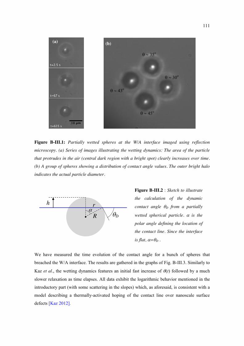
111

Figure B-III.1: Partially wetted spheres at the W/A interface imaged using reflection

microscopy. (a) Series of images illustrating the wetting dynamics: The area of the particle

that protrudes in the air (central dark region with a bright spot) clearly increases over time.

(b) A group of spheres showing a distribution of contact angle values. The outer bright halo

indicates the actual particle diameter.

We have measured the time evolution of the contact angle for a bunch of spheres that

breached the W/A interface. The results are gathered in the graphs of Fig. B-III.3. Similarly to

Kaz et al., the wetting dynamics features an initial fast increase of (t) followed by a much

slower relaxation as time elapses. All data exhibit the logarithmic behavior mentioned in the

introductory part (with some scattering in the slopes) which, as aforesaid, is consistent with a

model describing a thermally-activated hoping of the contact line over nanoscale surface

defects [Kaz 2012].

(a) (b)

35o

43o

30o

45o

D

h

R

r

Figure B-III.2 : Sketch to illustrate

the calculation of the dynamic

contact angle D from a partially

wetted spherical particle. is the

polar angle defining the location of

the contact line. Since the interface

is flat, =D .

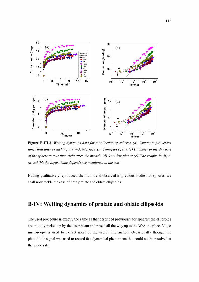
112

0 3 6 9 12 15

0

15

30

45

60

Diameter of sphere (µm)

10 10.5 11 11.75 10.8 9.6 10.75 10.5 10 10.6

Con

tact

ang

le (d

eg)

Time (min)10-1 100 101 102 103

20

40

60

Con

tact

ang

le (d

eg)

Time(s)

0 5 10

0

4

8

Dia

met

er o

f dry

par

t (µm

)

Time(s) 10-1 100 101 102 103

4

8

Dia

met

er o

f dry

par

t (µm

)

Time (s) Figure B-III.3: Wetting dynamics data for a collection of spheres. (a) Contact angle versus

time right after breaching the W/A interface. (b) Semi-plot of (a). (c) Diameter of the dry part

of the sphere versus time right after the breach. (d) Semi-log plot of (c). The graphs in (b) &

(d) exhibit the logarithmic dependence mentioned in the text.

Having qualitatively reproduced the main trend observed in previous studies for spheres, we

shall now tackle the case of both prolate and oblate ellipsoids.

B-IV: Wetting dynamics of prolate and oblate ellipsoids

The used procedure is exactly the same as that described previously for spheres: the ellipsoids

are initially picked up by the laser beam and raised all the way up to the W/A interface. Video

microscopy is used to extract most of the useful information. Occasionally though, the

photodiode signal was used to record fast dynamical phenomena that could not be resolved at

the video rate.

(c) (d)

(a) (b)

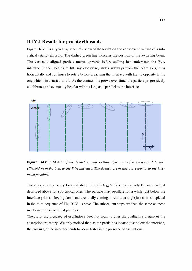
113

B-IV.1 Results for prolate ellipsoids Figure B-IV.1 is a typical xz schematic view of the levitation and consequent wetting of a sub-

critical (static) ellipsoid. The dashed green line indicates the position of the levitating beam.

The vertically aligned particle moves upwards before stalling just underneath the W/A

interface. It then begins to tilt, say clockwise, slides sideways from the beam axis, flips

horizontally and continues to rotate before breaching the interface with the tip opposite to the

one which first started to tilt. As the contact line grows over time, the particle progressively

equilibrates and eventually lies flat with its long axis parallel to the interface.

Figure B-IV.1: Sketch of the levitation and wetting dynamics of a sub-critical (static)

ellipsoid from the bulk to the W/A interface. The dashed green line corresponds to the laser

beam position.

The adsorption trajectory for oscillating ellipsoids (k1,2 > 3) is qualitatively the same as that

described above for sub-critical ones. The particle may oscillate for a while just below the

interface prior to slowing down and eventually coming to rest at an angle just as it is depicted

in the third sequence of Fig. B-IV.1 above. The subsequent steps are then the same as those

mentioned for sub-critical particles.

Therefore, the presence of oscillations does not seem to alter the qualitative picture of the

adsorption trajectory. We only noticed that, as the particle is located just below the interface,

the crossing of the interface tends to occur faster in the presence of oscillations.

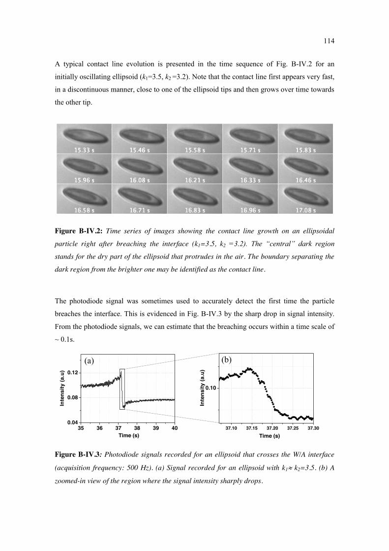
114

A typical contact line evolution is presented in the time sequence of Fig. B-IV.2 for an

initially oscillating ellipsoid (k1=3.5, k2 =3.2). Note that the contact line first appears very fast,

in a discontinuous manner, close to one of the ellipsoid tips and then grows over time towards

the other tip.

Figure B-IV.2: Time series of images showing the contact line growth on an ellipsoidal

particle right after breaching the interface (k1=3.5, k2 =3.2).   The   “central”   dark   region  

stands for the dry part of the ellipsoid that protrudes in the air. The boundary separating the

dark region from the brighter one may be identified as the contact line.

The photodiode signal was sometimes used to accurately detect the first time the particle

breaches the interface. This is evidenced in Fig. B-IV.3 by the sharp drop in signal intensity.

From the photodiode signals, we can estimate that the breaching occurs within a time scale of

~ 0.1s.

Figure B-IV.3: Photodiode signals recorded for an ellipsoid that crosses the W/A interface

(acquisition frequency: 500 Hz). (a) Signal recorded for an ellipsoid with k1 k2=3.5. (b) A

zoomed-in view of the region where the signal intensity sharply drops.

(b) (a)

37.10 37.15 37.20 37.25 37.30

0.10

Inte

nsity

(a.u

)

Time (s)

35 36 37 38 39 400.04

0.08

0.12

Inte

nsity

(a.u

)

Time (s)

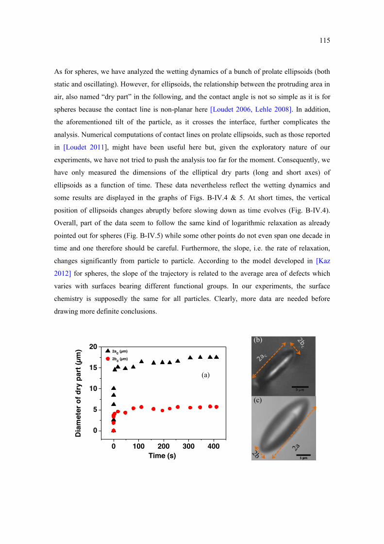
115

As for spheres, we have analyzed the wetting dynamics of a bunch of prolate ellipsoids (both

static and oscillating). However, for ellipsoids, the relationship between the protruding area in

air,  also  named  “dry  part”  in  the  following,  and  the  contact  angle is not so simple as it is for

spheres because the contact line is non-planar here [Loudet 2006, Lehle 2008]. In addition,

the aforementioned tilt of the particle, as it crosses the interface, further complicates the

analysis. Numerical computations of contact lines on prolate ellipsoids, such as those reported

in [Loudet 2011], might have been useful here but, given the exploratory nature of our

experiments, we have not tried to push the analysis too far for the moment. Consequently, we

have only measured the dimensions of the elliptical dry parts (long and short axes) of

ellipsoids as a function of time. These data nevertheless reflect the wetting dynamics and

some results are displayed in the graphs of Figs. B-IV.4 & 5. At short times, the vertical

position of ellipsoids changes abruptly before slowing down as time evolves (Fig. B-IV.4).

Overall, part of the data seem to follow the same kind of logarithmic relaxation as already

pointed out for spheres (Fig. B-IV.5) while some other points do not even span one decade in

time and one therefore should be careful. Furthermore, the slope, i.e. the rate of relaxation,

changes significantly from particle to particle. According to the model developed in [Kaz

2012] for spheres, the slope of the trajectory is related to the average area of defects which

varies with surfaces bearing different functional groups. In our experiments, the surface

chemistry is supposedly the same for all particles. Clearly, more data are needed before

drawing more definite conclusions.

0 100 200 300 400

0

5

10

15

20

2ac (µm)

2bc (µm)

Dia

met

er o

f dry

par

t (µm

)

Time (s)

(a)

(b)

(c)

116

Figure B-IV.4: (a) Time evolution of the protruding elliptical areas (long axis: 2ac; short

axis: 2bc) in air for a sub-critical ellipsoid (k1=k2=2.8) Black triangles: Long axis. Red

circles: short axis. Optical microscopy pictures obtained in reflection (b) and transmission (c)

modes.

10-1 100 101 102

2

4

6

k=2.6 k=3.4 k=1.9 k=2.8

Dia

met

er o

f sho

rt a

xis

(µm

)

Time(s) 10-1 100 101 102

0

5

10

15

20

Dia

met

er o

f lon

g ax

is (µ

m)

Time(s)

k=2.6 k=3.4 k=1.9 k=2.8

Figure B-IV.5: Semi-log plots of the diameter of the dry part (see text) as a function of time

for four prolate ellipsoids with different aspect ratios. (a) Data for short axis. (b) Data for the

corresponding long axes.

B-IV.2 Results for Oblate ellipsoids Oblate ellipsoids follow a similar trend of wetting dynamics as that of prolate ones. Whether

the particle is oscillating or static just below the interface, the wetting dynamics starts at an

angle from one end and then grows to the other end of the particle. Fig. B-IV.6 below shows a

time series (top view images) of an oblate ellipsoid (k1=0.45, k2= 0.33) getting partially

wetted. In the first image (t=0.35s), the longest axis of the particle is aligned along the z-axis

(beam axis) and the second larger axis is oriented parallel to the interface. This orientation

may   be   referred   as   the   “on-edge”   configuration.   In   the   second   image   (t=5.34s) the particle

starts to tilt and slide sideways forming an angle with the interface plane. In the remaining

images, the particle is partially wetted and the contact line growth is clearly visible.

(a) (b)

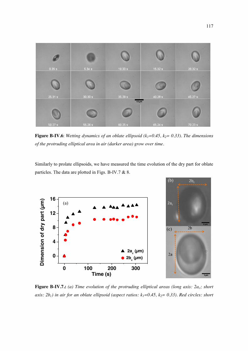
117

Figure B-IV.6: Wetting dynamics of an oblate ellipsoid (k1=0.45, k2= 0.33). The dimensions

of the protruding elliptical area in air (darker area) grow over time.

Similarly to prolate ellipsoids, we have measured the time evolution of the dry part for oblate

particles. The data are plotted in Figs. B-IV.7 & 8.

0 100 200 300

0

4

8

12

16

Dim

ensi

on o

f dry

par

t (µm

)

Time (s)

2ac (µm)2bc (µm)

Figure B-IV.7.: (a) Time evolution of the protruding elliptical areas (long axis: 2ac; short

axis: 2bc) in air for an oblate ellipsoid (aspect ratios: k1=0.45, k2= 0.33). Red circles: short

(b)

(a)

(c)

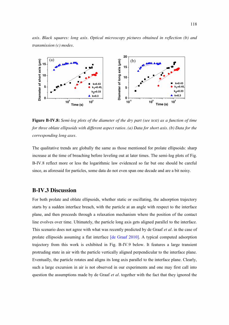
118

axis. Black squares: long axis. Optical microscopy pictures obtained in reflection (b) and

transmission (c) modes.

100 1020

5

10

15

k=0.43k1=0.45,

k2=0.33k=0.3

Dia

met

er o

f sho

rt a

xis

(µm

)

Time (s)10-2 100 102

0

5

10

15

20

k=0.43k1=0.45,

k2=0.33k=0.3

Time (s)

Dia

met

er o

f lon

g ax

is (µ

m)

Figure B-IV.8: Semi-log plots of the diameter of the dry part (see text) as a function of time

for three oblate ellipsoids with different aspect ratios. (a) Data for short axis. (b) Data for the

corresponding long axes.

The qualitative trends are globally the same as those mentioned for prolate ellipsoids: sharp

increase at the time of breaching before leveling out at later times. The semi-log plots of Fig.

B-IV.8 reflect more or less the logarithmic law evidenced so far but one should be careful

since, as aforesaid for particles, some data do not even span one decade and are a bit noisy.

B-IV.3 Discussion For both prolate and oblate ellipsoids, whether static or oscillating, the adsorption trajectory

starts by a sudden interface breach, with the particle at an angle with respect to the interface

plane, and then proceeds through a relaxation mechanism where the position of the contact

line evolves over time. Ultimately, the particle long axis gets aligned parallel to the interface.

This scenario does not agree with what was recently predicted by de Graaf et al. in the case of

prolate ellipsoids assuming a flat interface [de Graaf 2010]. A typical computed adsorption

trajectory from this work is exhibited in Fig. B-IV.9 below. It features a large transient

protruding state in air with the particle vertically aligned perpendicular to the interface plane.

Eventually, the particle rotates and aligns its long axis parallel to the interface plane. Clearly,

such a large excursion in air is not observed in our experiments and one may first call into

question the assumptions made by de Graaf et al. together with the fact that they ignored the

(a) (b)

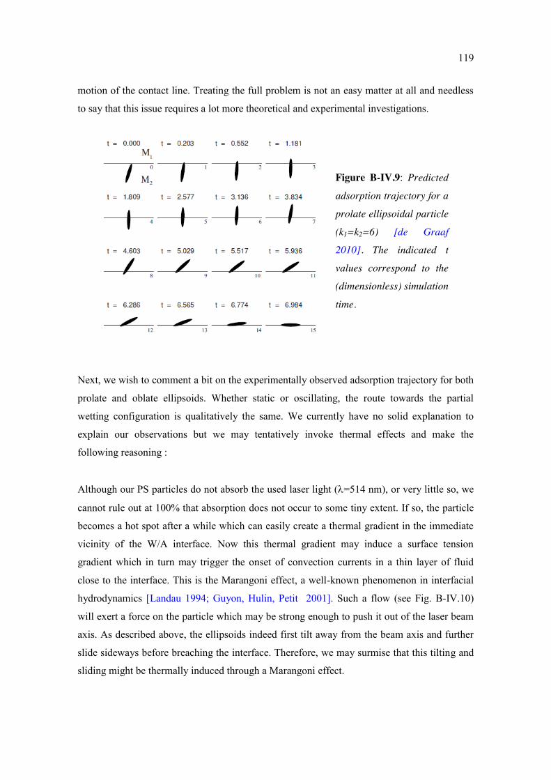
119

motion of the contact line. Treating the full problem is not an easy matter at all and needless

to say that this issue requires a lot more theoretical and experimental investigations.

Next, we wish to comment a bit on the experimentally observed adsorption trajectory for both

prolate and oblate ellipsoids. Whether static or oscillating, the route towards the partial

wetting configuration is qualitatively the same. We currently have no solid explanation to

explain our observations but we may tentatively invoke thermal effects and make the

following reasoning :

Although our PS particles do not absorb the used laser light (=514 nm), or very little so, we

cannot rule out at 100% that absorption does not occur to some tiny extent. If so, the particle

becomes a hot spot after a while which can easily create a thermal gradient in the immediate

vicinity of the W/A interface. Now this thermal gradient may induce a surface tension

gradient which in turn may trigger the onset of convection currents in a thin layer of fluid

close to the interface. This is the Marangoni effect, a well-known phenomenon in interfacial

hydrodynamics [Landau 1994; Guyon, Hulin, Petit 2001]. Such a flow (see Fig. B-IV.10)

will exert a force on the particle which may be strong enough to push it out of the laser beam

axis. As described above, the ellipsoids indeed first tilt away from the beam axis and further

slide sideways before breaching the interface. Therefore, we may surmise that this tilting and

sliding might be thermally induced through a Marangoni effect.

Figure B-IV.9: Predicted

adsorption trajectory for a

prolate ellipsoidal particle

(k1=k2=6) [de Graaf

2010]. The indicated t

values correspond to the

(dimensionless) simulation

time.

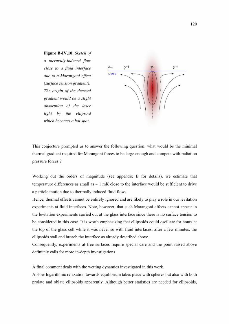
120

This conjecture prompted us to answer the following question: what would be the minimal

thermal gradient required for Marangoni forces to be large enough and compete with radiation

pressure forces ?

Working out the orders of magnitude (see appendix B for details), we estimate that

temperature differences as small as 1 mK close to the interface would be sufficient to drive

a particle motion due to thermally induced fluid flows.

Hence, thermal effects cannot be entirely ignored and are likely to play a role in our levitation

experiments at fluid interfaces. Note, however, that such Marangoni effects cannot appear in

the levitation experiments carried out at the glass interface since there is no surface tension to

be considered in this case. It is worth emphasizing that ellipsoids could oscillate for hours at

the top of the glass cell while it was never so with fluid interfaces: after a few minutes, the

ellipsoids stall and breach the interface as already described above.

Consequently, experiments at free surfaces require special care and the point raised above

definitely calls for more in-depth investigations.

A final comment deals with the wetting dynamics investigated in this work.

A slow logarithmic relaxation towards equilibrium takes place with spheres but also with both

prolate and oblate ellipsoids apparently. Although better statistics are needed for ellipsoids,

Figure B-IV.10: Sketch of

a thermally-induced flow

close to a fluid interface

due to a Marangoni effect

(surface tension gradient).

The origin of the thermal

gradient would be a slight

absorption of the laser

light by the ellipsoid

which becomes a hot spot.

121

our results might not be too surprising after all: indeed, although the contact lines for

ellipsoids are non planar at the micrometer scale, there are also likely to be rugged and

ondulated at the nanoscale because of tiny surface defects, similarly to spheres. If the motion

of the contact line is mainly governed by a thermally-activated pinning-depinning mechanism

over defects, as proposed by Kaz et al., the actual global shape of the contact line may not be

the most relevant factor influencing the wetting dynamics. So, as long as the particle surface

bears defects, a slow relaxation towards equilibrium could be a general trend whatever the

particle shape.

122

Conclusion and prospects

The main part of this report has been focused on the behaviour of ellipsoid-shaped particles in

response to optical forces from a moderately focused laser beam. The particles were

fabricated from polystyrene spheres, 10 m in diameter. Prolate ellipsoids (k > 1) were

generated by uniaxial stretching, and oblate ones (k < 1) by biaxial stretching of the spheres.

We thus obtained ellipsoids with dimensions between a few m and several 10 m. We

studied the behaviours of these particles in a classical levitation experiment, with a vertical

laser beam, in water. The beam waist diameter was 2.6 m, with a corresponding diffraction

length   ≈   14   m. We collected many observations with particles of different aspect ratios

located in different regions of the beam. The altitude in the beam was fixed either by using the

balance between the particle weight and the optical levitation force, or by bringing the particle

in contact to the upper surface of the sample cell. We thus observed the  particles’  responses  in  

bulk water and close to a surface, which might be solid (water-glass) or fluid (water-air and

water-oil interfaces).

Near the beam-waist, particles which were not too far from a sphere got trapped on the laser

beam axis in static configurations, with their long axes lying vertical. Conversely, we found

that particles of high ellipticity, either rod-like (k >> 1) or disk-like (k << 1) never came to

static configurations: they were seen to undergo sustained oscillations, in the form of coupled

translation and tilt motions.

We have proposed an interpretation of the observed dynamical behaviours on the basis of a

simple 2-dimensional (2d) model, using the ray-optics approximation. For prolate ellipsoids

and a simply parallel beam, the model indeed produced a bifurcation between static states and

limit cycles when k increases. As an essential outcome, the model showed that the non linear

dependence of the radiation pressure forces versus the particle position and angle coordinates

was enough to explain the oscillations. In our model, and contrary to [Cheng 2003], no special

hydrodynamic contribution from bounding surfaces was required as a necessary condition to

produce oscillations.

The model, being 2-dimensional, can only predict static equilibriums and periodic dynamical

states (limit cycles). Such states are indeed observed in experiments, but the 3-dimensional

character of the real system generates more complex dynamics in certain cases. Using

123

standard tools of non linear dynamics analysis, we indeed evidenced irregular dynamics akin

to deterministic chaos with particles of various size parameters, at various altitudes in the

laser beam. However, we were not able to evidence a simple route to chaos. From our

experience, we can tell whether a given particle will stay static in the beam or oscillate, but

we are not at the point were we can say a priori whether the motion of this particle will be

periodic or irregular.

The   work   on   particles’   dynamical   states   may   be   continued   and   extended in different

directions:

- Our experiments were limited to a simple levitation scheme, with a moderately

focused beam. In view of the applications related to optical manipulation, it would be

very interesting to move to configurations that allow for true 3d trapping, at least for

spheres. We might then go to more strongly focused beams, up to conditions of single

beam optical tweezers. As an alternative, we may keep the option of weak focusing

but add a second -contra-propagating- beam to set up a two-beam trap (see e.g.

[Rodrigo 2004-2005]). The latter configuration offers the advantage of long working

distances, which then would allow us to confine the particle far from the cell

boundaries for a wide range of laser power and then avoid complications due to

hydrodynamic coupling to surfaces. The configuration has the further advantage of

being compatible with side observation, contrary to optical tweezers.

- We need more feedback from theory and simulations. There is still much to be learnt

from the ray-optics model. Still in the 2d version, the model may be made more

complete by taking into account the divergence of the beam. This would help us

simulate the behaviours of particles in different regions of the beam, as we did in the

experiments. One relatively simple question to be addressed is the vertical-to-

horizontal transition that we observed with particles far from the beam-waist.

Extension to 3d is possible too, as was done recently by [Chang 2012].

In the course of our PhD we started a few calculations of optical forces and torques in

3d, using the discrete-dipole-approximation, under the supervision of Prof. F. Ren

(CORIA, Rouen). This work (not reported in this manuscript) has not gone further

than preliminary results with particle sizes limited to a few m. The project now has

been taken over by M. Yang and F. Ren, with the method called “Multilevel Fast

124

Multipole Algorithm”  (MLFMA). Most interestingly, this method allows dealing with

the large particle sizes of our experiments.

Much information is expected from the forthcoming simulations, both in the ray-optics

and MLFMA versions. Predictions of optical forces and torques for static states may

be verified by future experiments; these will be stringent tests to validate the

computation methods.

Prediction of oscillatory regimes is expectably a very demanding task, first because of

the many degrees of freedom (up to 6) of the particle to be included in the dynamical

equations. A second difficulty lies in the hydrodynamic part of the problem, to

represent the viscous drag force and torque that oppose the action of the radiation

pressure. In the 2d model, we simply supposed that translation and rotation were

decoupled, and we adopted constant drag coefficients. Reality is more complex

because the translation drag depends on the particle orientation [Happel 1983].

Ultimately, the hydrodynamic part of the problem may call for dedicated numerical

simulation (as in [Chang 2012]), in parallel to the part on optical force-torque.

Beyond the academic study of the   particles’   responses   to   optical   forces,   we   applied   the  

levitation technique to a problem pertaining to physical chemistry of surfaces. We

investigated how polystyrene particles, initially in bulk water, come to a static equilibrium

across the water-air interface, in partial wetting configuration. We focused our study on

possible differences between spheres and ellipsoids, because we suspected than the non

planarity of contact lines on ellipsoidal bodies might cause a difference in the dynamics of the

particle emersion, compared to spheres. In fact, the data that we collected showed that there

was no real difference. We concluded that in all cases the dynamics of the contact line is

mainly controlled by the pinning-depinning mechanism, in line with the recent results of [Kaz

2012] for spherical micrometre-sized spheres. This conclusion holds equally for spheres and

ellipsoids, either prolate or oblate. Conversely models that do not take this peculiar

mechanism into account [de Graaf 2010] lead to definitely  unrealistic  prediction  of  particles’  

emersion dynamics.

Coming back to mechanical effects of light, the problem of a particle that sits across an

interface (e.g. water-air) has not yet been fully addressed. Basically the problem amounts to

calculating the electromagnetic field scattered by a particle located across the planar boundary

between two semi-infinite dielectric media. To our knowledge, no accurate solution has been

125

proposed up to now, even in the case of a sphere. Solutions may be within reach of modern

computation methods (see cited references in chapter A-V), and would be very useful to

determine partial wetting configurations of particles from scattered light diagrams. Since

optical forces are the direct consequence of light scattering, we may check results of

calculations through simple measurements of forces and torques necessary to move particles

parallel to the interface. Such experiments may be readily performed using the tools

developed throughout this work.

126

Conclusion et perspectives

Dans la majeure partie de cette étude, nous nous sommes intéressés aux réponses de particules

en   forme   d’ellipsoïdes   aux   forces   optiques   exercées   par   un   faisceau   laser   modérément  

focalisé. Nos particules sont obtenues à partir de sphères de polystyrène, de 10 m de

diamètre, par étirement uniaxial (pour des ellipsoïdes prolates, k > 1) ou biaxial (pour des

ellipsoïdes oblates, k < 1). Ce procédé nous a permis de fabriquer toute une gamme de

particules, dont les dimensions vont de 5 à 50 m environ. Nous avons étudié les

comportements des ellipsoïdes dans une expérience classique de lévitation optique, avec un

faisceau  laser  vertical,  dans  l’eau.  Dans  ce  montage,  le faisceau est modérément focalisé, avec

un rayon au col (beam-waist) de 2.6 m et une longueur de diffraction ≈  14  m. Nous avons

fait   de   nombreuses   observations   avec   des   particules   de   rapports   d’aspect   variés   dans   des  

régions   différentes   du   faisceau.   Nous   avons   contrôlé   l’altitude   de   chaque   particule   dans   le  

faisceau  en  utilisant  l’équilibre  entre  son  poids et la force de lévitation optique, ou en amenant

la  particule  au  contact  de  la  surface  en  haut  de  la  cellule  d’expérience.  Cette  surface  était  dans  

la plupart des cas une paroi de verre, mais nous avons également étudié les cas de particules

au contact  d’interfaces  eau-air et eau-huile.

Nous   avons   montré   qu’au   voisinage   du   beam-waist, les particules prolates peu ou

modérément allongées (k <  3)  se  piègent  radialement  sur  l’axe  du  faisceau,  en  configuration  

verticale. Par contre, les particules fortement elliptiques, en forme de bâtonnet (k >> 1) ou de

disque (k << 1) ne peuvent pas être immobilisées. Ces particules « dansent » autour du

faisceau, dans un mouvement permanent associant translation et rotation.

Nous avons proposé une interprétation des dynamiques  observées  à  partir  d’un  modèle  simple  

en   dimension   2   (2d),   dans   l’approximation   de   l’optique   géométrique.   Pour   des   ellipsoïdes  

prolates et un faisceau parallèle (la diffraction est négligée), ce modèle prédit une bifurcation

entre états statiques et   dynamiques   périodiques   (cycles   limites)   lorsque   l’allongement   k

augmente. Une conclusion essentielle de cette analyse est que les oscillations viennent de la

non linéarité des forces et couples optiques en fonction des variables de position et

d’orientation de la particule. Dans ce modèle, la contribution hydrodynamique associée au

127

contact   avec   une   paroi   n’est   pas   une   condition   nécessaire   pour   l’existence   d’oscillations,  

contrairement au modèle de [Cheng 2003].

Ce modèle, étant limité à 2 dimensions, ne peut produire que des équilibres statiques ou des

oscillations périodiques. Ces états sont effectivement observés dans les expériences, mais le

caractère tridimensionnel du système réel engendre des dynamiques plus complexes dans

certains cas. En utilisant des  méthodes  standards  de  l’analyse  des  signaux  non  linéaires,  nous  

avons  montré  l’existence  de  dynamiques  irrégulières,  assimilables  à  du  chaos  déterministe.  

A  partir  de  l’ensemble  de  nos  observations,  nous  pouvons  dire  si  une  particule  ellipsoïdale  de  

caractéristiques données pourra être immobilisée dans le faisceau ou si elle va osciller. Par

contre nous ne savons pas prédire la nature des oscillations, périodique ou irrégulière. Pour le

moment,   l’ensemble  des  analyses  n’a  pas  permis  de  dégager  une  « route vers le chaos », en

changeant  simplement  les  rapports  d’aspect  ou  l’altitude  de  la  particule  dans  le  faisceau.

Plusieurs pistes se présentent pour continuer ce travail:

- nous avons limité nos expériences au seul schéma de la lévitation optique, avec un

faisceau modérément focalisé. Pour nous rapprocher des applications utilisant la

manipulation optique, il faudrait faire évoluer le montage vers des versions permettant

le piégeage en 3 dimensions, tout au moins pour des particules sphériques. Une option

est de focaliser beaucoup plus fortement le faisceau, comme dans la géométrie des

pinces  optiques.  Une  alternative  est  de  garder  le  principe  d’une  faible  focalisation,  mais  

d’ajouter  un  faisceau  coaxial  en  sens  inverse  pour  créer  un  piège  à  deux  faisceaux (voir

par ex. [Rodrigo 2004-2005]).  Cette  version  offre  l’avantage  d’une  grande  distance  de  

travail, ce qui permet de  travailler  loin  dans  le  volume  et  d’éviter  la  complication  d’un  

couplage hydrodynamique avec une paroi. On peut en même temps observer la particule

par le côté, ce qui est difficilement envisageable avec une pince optique.

- Il est souhaitable de pousser beaucoup plus loin la modélisation et les simulations. Le

simple  modèle  d’optique  géométrique  en  2d  peut   encore  nous   apprendre   beaucoup  de

choses,   en   particulier   l’effet   de   la   divergence   du   faisceau.   Le   modèle   pourrait   ainsi  

rendre   compte   de   l’effet   du   diamètre   de   faisceau   vu   par   la   particule   en   fonction   de  

l’altitude.   Une   question   relativement   simple   concerne   la   transition   entre   les  

configurations  verticale  et  horizontale  quand  on  s’éloigne  du  beam-waist.

128

Il   serait   évidemment   très  utile  d’aller  vers  une   version  3d  du  modèle,   comme  dans   la  

récente étude de Chang et al. [Chang 2012].

Au cours de cette thèse, nous avons entrepris des calculs des forces et couples optiques

en   3d   avec   l’aide   du   Prof.   F.   Ren,   par   la   technique   DDA   (« discrete-dipole-

approximation »).  Ce  travail  (non  décrit  dans  le  manuscrit)  est  resté  exploratoire  et  s’est  

limité à des particules de quelques m seulement. Le projet est mené maintenant par M.

Yang et F. Ren, qui utilisent la méthode MLFMA (“Multilevel Fast Multipole

Algorithm”).  Cette  technique  est  très  prometteuse,  parce  qu’elle  permet  de  traiter  les  cas  

des « grandes » particules de nos expériences.

La simulation permettra de calculer précisément les amplitudes des forces et couples.

Les valeurs calculées pourront être vérifiées avec les particules en équilibre statique.

Les mesures expérimentales des effets mécaniques de la lumière sur ces particules

serviront donc  d’outil  de  validation  des  codes  de  calcul.

- Prédire les oscillations en 3d est une affaire probablement beaucoup plus ambitieuse,

d’abord  parce  qu’il  faut  inclure  tous  les  degrés  de  liberté  (jusqu’à  6)  dans  les  équations  

du mouvement. Une deuxième difficulté se présente dans la partie hydrodynamique du

problème. Il faut modéliser les forces et couples de trainée dus à la viscosité du fluide.

Dans le modèle 2d que nous avons présenté, nous avons considéré que les composantes

translationnelle et rotationnelle de la trainée étaient découplées et régies par des

coefficients  constants.  En  réalité,  la  force  translationnelle  dépend  de  l’orientation  de  la  

particule [Happel 1983]. Une simulation complète devrait inclure une partie numérique

dédiée  à  l’hydrodynamique,  comme  dans  l’étude  de  [Chang 2012].

Dans la partie B du manuscrit nous avons présenté une application de la lévitation optique

pour une étude de la dynamique de démouillage des surfaces de nos particules. Nous avons

observé comment une particule de polystyrène,  initialement  dans  l’eau,  se  place  en  travers  de  

l’interface  eau-air, où elle adopte une configuration de mouillage partiel. Nous avons étudié la

dynamique de cette transition et recherché si elle dépend fortement de la forme de particule,

depuis  la  sphère  jusqu’à  des  ellipsoïdes  très  allongés  (prolates)  ou  plats  (oblates).  Nous  avons  

conclus   qu’il   n’y   avait   en   fait   pas   de   variations   notables   entre   ces   différents   cas.   Nos  

observations indiquent que, quelle que soit la forme de la particule, la dynamique de la ligne

de  contact  est  régie  essentiellement  par  le  mécanisme  d’accrochage-décrochage sur les défauts

de la surface. Cette conclusion corrobore celle de [Kaz 2012] dans leur récente étude pour

129

des  sphères  de  l’ordre  du  micromètre. Au contraire, les dynamiques que nous avons observées

sont très différentes de celles prédites par le modèle de [de Graaf 2010], qui ne prend pas en

compte ce mécanisme.

Nous terminons en revenant vers les effets mécaniques de la lumière, cette fois sur une

particule  à  l’interface,  en  mouillage  partiel.  Pour  calculer  les  forces  et  couples  exercés  par  un  

faisceau laser sur cette particule, il faut calculer le champ électromagnétique diffusé par cette

particule.  Le  problème  est  celui  d’un  corps  en  travers  d’une  surface plane à la frontière entre

deux milieux diélectriques semi-infinis. A notre connaissance, aucune solution de ce

problème   n’est   disponible   dans   la   littérature,   même   pour   une   sphère.   Des   solutions  

numériques peuvent certainement être obtenues avec les outils modernes que nous avons cités

(voir le chapitre A-V). On pourrait, à partir de la simulation, déterminer la configuration de

mouillage  partiel  à  partir  d’un  diagramme  de  diffusion.  Une  alternative  simple  est  de  mesurer  

la force nécessaire pour déplacer la particule parallèlement à la surface avec un faisceau laser.

La  valeur  de  cette  force  étant  directement  liée  au  champ  diffusé,  l’expérience  permettrait  de  

valider le calcul. Ces mesures sont faisables directement avec les outils que nous avons

développés au cours de cette thèse.

130

Bibliography Alpmann C., et al., Holographic optical bottle beams, Appl. Phys. Lett. 100, 111101 (2012).

Arlt J., and Padgett M. J., Generation of a beam with a dark focus surrounded by regions of higher intensity: the

optical bottle beam, Opt. Lett. 25, 191-193 (2000).

Ashkin A., Acceleration and trapping of particles by radiation pressure, Phys. Rev. Lett. 24, 156 (1970).

Ashkin A., et al., Observation of a single-beam gradient force optical trap for dielectric particles, Opt. Lett. 11,

288 (1986).

Ashkin A., Forces of a single beam gradient laser trap on a dielectric sphere in the ray optics regime, J. Biophys.

61, 569-82 (1992).

Ashkin A., Optical trapping and manipulation of neutral particles using lasers, (World Scientific, London 2006).

Aveyard R., Binks B. P., and Clint J. H., Emulsions stabilized solely by colloidal particles, Adv. Coll. Interface

Sci. 100-102, 503-546 (2003).

Bansal  R.K.,  “A  text  book  of  fluid  mechanics” (New Delhi, 2006).

Bareil P. B., and Sheng Y., Angular and position stability of a nanorod trapped in an optical tweezers, Opt.

Express 18, 26388-26398 (2010).

Benito D., Simpson S. H., and Hanna S., FDTD simulations of forces on particles during holographic assembly,

Opt. Express 16, 2942–2957 (2008).

Berge´  P.,  Pomeau  Y.,  and  Vidal  C.,  “Order within Chaos: Towards a Deterministic Approach to Turbulence”  

(Wiley, New York, 1986).

Beth R. A., Mechanical detection and measurement of the angular momentum of light, Phys. Rev. 50, 115-125

(1936).

Binks B. P., Particles as surfactants, Curr. Opinion Colloid Interface Sci. 7, 21 (2002).

Binks B. P., Horozov T. S. (Eds), “Colloidal Particles at Liquid Interfaces”,  Cambridge  Univ.  Press, 2006.

Bobadova-Parvanova P., and Pouligny B., unpublished (1995).

Bonessi D., Bonin K., and Walker T., Optical forces on particles of arbitrary shape and size, J. Opt. A, Pure

Appl. Opt. 9, S228–S234 (2007).

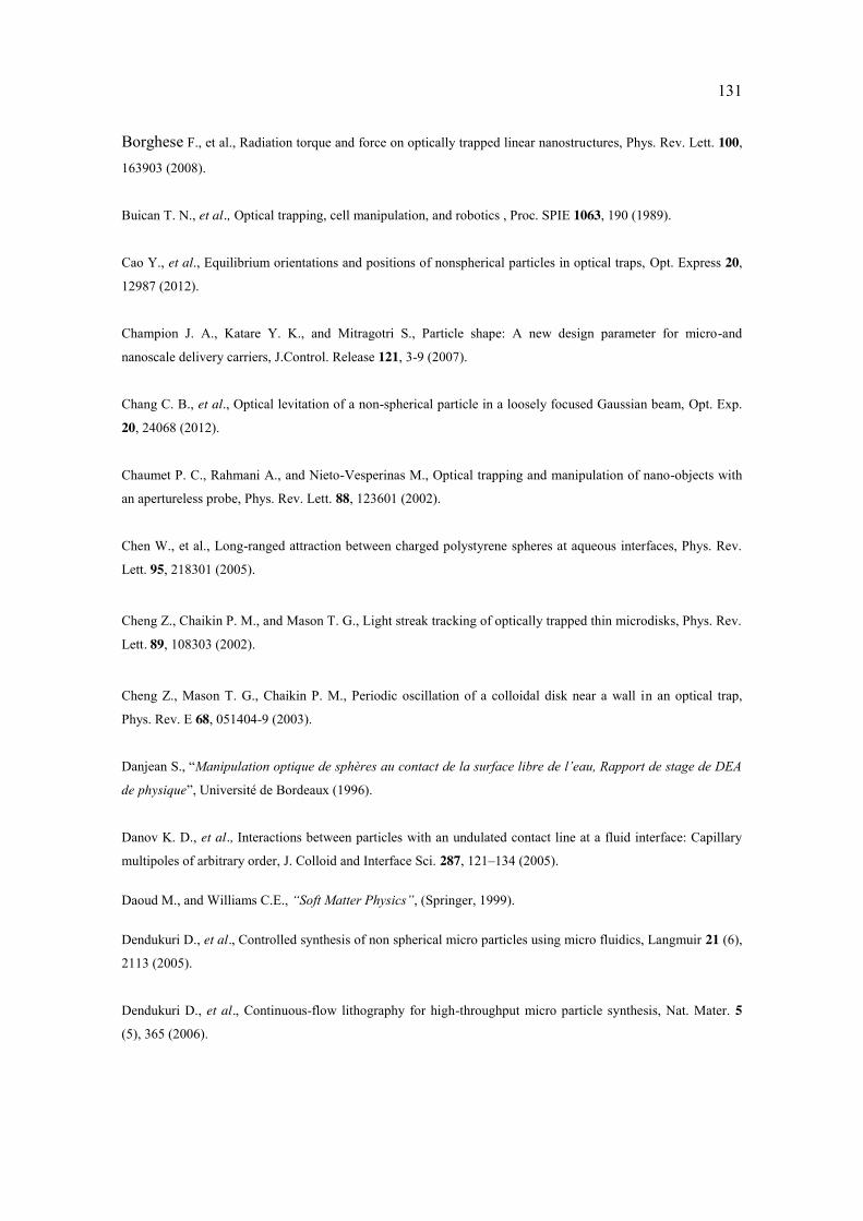
131

Borghese F., et al., Radiation torque and force on optically trapped linear nanostructures, Phys. Rev. Lett. 100,

163903 (2008).

Buican T. N., et al., Optical trapping, cell manipulation, and robotics , Proc. SPIE 1063, 190 (1989).

Cao Y., et al., Equilibrium orientations and positions of nonspherical particles in optical traps, Opt. Express 20,

12987 (2012).

Champion J. A., Katare Y. K., and Mitragotri S., Particle shape: A new design parameter for micro-and

nanoscale delivery carriers, J.Control. Release 121, 3-9 (2007).

Chang C. B., et al., Optical levitation of a non-spherical particle in a loosely focused Gaussian beam, Opt. Exp.

20, 24068 (2012).

Chaumet P. C., Rahmani A., and Nieto-Vesperinas M., Optical trapping and manipulation of nano-objects with

an apertureless probe, Phys. Rev. Lett. 88, 123601 (2002).

Chen W., et al., Long-ranged attraction between charged polystyrene spheres at aqueous interfaces, Phys. Rev.

Lett. 95, 218301 (2005).

Cheng Z., Chaikin P. M., and Mason T. G., Light streak tracking of optically trapped thin microdisks, Phys. Rev.

Lett. 89, 108303 (2002).

Cheng Z., Mason T. G., Chaikin P. M., Periodic oscillation of a colloidal disk near a wall in an optical trap,

Phys. Rev. E 68, 051404-9 (2003).

Danjean S., “Manipulation  optique  de  sphères  au  contact  de  la  surface  libre  de  l’eau,  Rapport  de  stage  de  DEA  

de physique”, Université de Bordeaux (1996).

Danov K. D., et al., Interactions between particles with an undulated contact line at a fluid interface: Capillary

multipoles of arbitrary order, J. Colloid and Interface Sci. 287, 121–134 (2005).

Daoud M., and Williams C.E., “Soft  Matter  Physics”, (Springer, 1999).

Dendukuri D., et al., Controlled synthesis of non spherical micro particles using micro fluidics, Langmuir 21 (6),

2113 (2005).

Dendukuri D., et al., Continuous-flow lithography for high-throughput micro particle synthesis, Nat. Mater. 5

(5), 365 (2006).

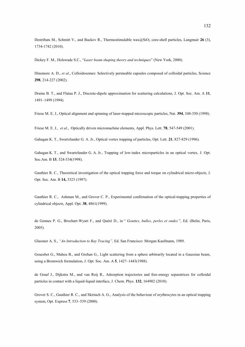
132

Destribats M., Schmitt V., and Backov R., Thermostimulable wax@SiO2 core-shell particles, Langmuir 26 (3),

1734-1742 (2010).

Dickey  F.  M.,  Holswade  S.C.,  “Laser beam shaping theory and techniques”  (New  York,  2000).

Dinsmore A. D., et al., Colloidosomes: Selectively permeable capsules composed of colloidal particles, Science

298, 214-227 (2002).

Draine B. T., and Flatau P. J., Discrete-dipole approximation for scattering calculations, J. Opt. Soc. Am. A 11,

1491–1499 (1994).

Friese M. E. J., Optical alignment and spinning of laser-trapped microscopic particles, Nat. 394, 348-350 (1998).

Friese M. E. J., et al., Optically driven micromachine elements, Appl. Phys. Lett. 78, 547-549 (2001).

Gahagan K. T., Swartzlander G. A. Jr., Optical vortex trapping of particles, Opt. Lett. 21, 827-829 (1996).

Gahagan K. T., and Swartzlander G. A. Jr., Trapping of low-index microparticles in an optical vortex, J. Opt.

Soc.Am. B 15, 524-534(1998).

Gauthier R. C., Theoretical investigation of the optical trapping force and torque on cylindrical micro-objects, J.

Opt. Soc. Am. B 14, 3323 (1997).

Gauthier R. C., Ashman M., and Grover C. P., Experimental confirmation of the optical-trapping properties of

cylindrical objects, Appl. Opt. 38, 4861(1999).

de Gennes P. G., Brochart-Wyart F., and Quéré D., in “ Gouttes, bulles, perles et ondes ”, Ed. (Belin, Paris,

2005).

Glassner A. S., “An  Introduction  to  Ray  Tracing”, Ed. San Francisco: Morgan Kaufmann, 1989.

Gouesbet G., Maheu B., and Grehan G., Light scattering from a sphere arbitrarily located in a Gaussian beam,

using a Bromwich formulation, J. Opt. Soc. Am. A 5, 1427–1443(1988).

de Graaf J., Dijkstra M., and van Roij R., Adsorption trajectories and free-energy separatrices for colloidal

particles in contact with a liquid-liquid interface, J. Chem. Phys. 132, 164902 (2010).

Grover S. C., Gauthier R. C., and Skirtach A. G., Analysis of the behaviour of erythrocytes in an optical trapping

system, Opt. Express 7, 533–539 (2000).

133

Guzowski   J.   J.,   PhD   thesis,   “Capillary interactions between colloidal particles at curved fluid interfaces”,  

Institut für Theoretische und Angewandte Physik Universität Stuttgart & Max-Planck-Institut für

Metallforschung Stuttgart (2010).

Guyon  E.,  Hulin  J.  P.,  and  Petit  L.,  “Hydrodynamique physique”,  EDP  Sciences  (CNRS  Editions),  2001.

Happel  J.,  Brenner  H.,  “Low Reynolds Number Hydrodynamics”,  Ed  The  Hague:  Martinus  Nijhoff  Publishers  

(1983).

Hegger R., Kantz H., and Schreiber T., Practical implementation of nonlinear time series methods: The TISEAN

package, Chaos 9 (2), 413 (1999).

Hinojosa-Alvarado A., Gutiérrez-Vega J. C., Geometrical optics calculation of forces and torques produced by a

ringed beam on a prolate spheroid, J. Opt. Soc. Am. B 27, 1651-8 (2010).

Ho C. C., et al., Preparation of monodisperse ellipsoidal polystyrene particles, Colloid Poym. Sci. 271, 469

(1993).

van der Horst A., et al., Manipulating metal-oxide nanowires using counter-propagating optical line tweezers,

Opt. Express 15, 11629-11639 (2007).

Horsthemke  W.,   and   Lefever   R.,   “Noise-Induced Transitions”,   ed.   Springer   Verlag,   Berlin   Heidelberg,   New

York, Tokyo (1984).

Imasaka T., et al., Optical Chromatography, Anal. Chem. 67(11), 1763-5 (1995).

Jackson  J.  D.,  “Classical Electrodynamics”, John Wiley & Sons Ltd. 1962.

Jonáš  A.,  Zemánek  P.,  Light  at  work:  The  use  of  optical  forces  for  particle  manipulation, sorting, and analysis,

Electrophoresis 29, 4813 (2008).

Jones P. H., Maragó O. M., and Stride E. P. J., Parametrization of trapping forces on microbubbles in scanning

optical tweezers, J. Opt. A: Pure and Applied Opt. 9, S278-S283 (2007).

Katok   A.,   Hasselblatt   B.,   “Introduction to the Modern Theory of Dynamical Systems”   Ed.   Cambridge:  

Cambridge Univ. Press, 1995.

Kaz D. M., et al., Physical ageing of the contact line on colloidal particles at liquid interfaces, Nature Materials

11, 138-142 (2012).

134

Kennel M. B., Brown R., and Abarbanel H. D. I., Determining embedding dimension for phase space

reconstruction using a geometrical construction, Phys. Rev. A 45, 3403 (1992).

Kraikivski P., Pouligny B., and Dimova R., Implementing both short- and long-working-distance optical

trapping into a commercial microscope, Rev. Sci. Instrum. 77, 113703 (2006).

Kralchevsky P. A., Denkov N. D., and Danov D. K., Particles with an undulated contact line at a fluid interface:

Interaction between capillary quadrupoles and rheology of particulate monolayers, Langmuir 17, 7694-7705

(2001).

Lai Y.-C., Ye N., Recent developments in chaotic time series analysis, Int. J. Bifurcation and Chaos 13, 1383-

1422 (2003).

Landau  L.  D.  and  Lifchitz  E.  M.,  “Cours de physique théorique – Mécanique des fluides”,  Ed.  Ellipses (Editions

Marketing, 1994).

Lehle H., Noruzifar E., Oettel M., Ellipsoidal particles at fluid interfaces, Eur. Phys. J. E 26, 151 (2008).

Lewandowski E. P., Bernate J. A., Searson P. C., and Stebe K. J., Rotation and alignment of anisotropic particles

on nonplanar interfaces, Langmuir 24, 9302-9307 (2008).

Loudet J. C., et al., Capillary interactions between anisotropic colloidal particles, Phys. Rev. Lett. 94, 018301

(2005).

Loudet J. C., Yodh A. G., and Pouligny B., Wetting and contact lines of micrometer-sized ellipsoids, Phys. Rev.

Lett. 97, 018304 (2006).

Loudet J. C., and Pouligny B., Self-assembled capillary arrows, Europhys. Lett. 85, 28003 (2009).

Loudet J. C., and Pouligny B., How do mosquito eggs self assemble on the water surface, Eur. Phys. J. E 34, 76 (2011). Lucassen J., Capillary forces between solid particles in fluid interfaces, Colloids and Surfaces 65, 131–137

(1992).

Mbamala E. And von Grunberg H., Effective interaction of a charged colloidal particle with an air-water

interface, J. Phys. Condens. Matter 14, 4881-4900 (2002).

Mondiot F., “Behavior  of  colloidal  particles  in  nematic  solvents:  shape  and  size  effects”, thesis, University of

Bordeaux 1(2011).

Neuman K. C., and Block S.M., Optical trapping, Rev. Sci. Instr. 75, 2787-809 (2004).

135

Neves A., et al., Rotational dynamics of optically trapped nanofibers, Opt. Express 18, 822-830 (2010).

Nieminen T. A., et al., Optical tweezers computational toolbox , Journal of Optics A: Pure and App. Opt. 9,

S196-S203 (2007).

Oettel M. and Dietrich S., Colloidal interactions at fluid interfaces, Langmuir 24(4), 1425-1441 (2008).

Pauzauskie P. J., et al., Optical trapping and integration of semiconductor nanowire assemblies in water, Nat.

Mat. 5, 97-101(2006).

Pickering S. U., Emulsions, J. Chem. Soc. 91, 2001-2021 (1907).

Plewa J., Processing carbon nanotubes with holographic optical tweezers, Opt. Express 12, 1978-1981 (2004).

Qin J.-Q., et al., FDTD approach to optical forces of tightly focused vector beams on metal particles, Opt.

Express 17, 8407–8416 (2009).

Quatieri T. F., “Discrete- Time  speech  signal  processing:  Principle  and  Practice”,  Prentice  hall  PTR,  2002.    

Ren K. F., Grehan G., and Gouesbet G., Radiation pressure forces exerted on a particle arbitrarily located in a

Gaussian beam by using the generalized Lorenz-Mie theory, and associated resonance effects, Opt. Commun.

108, 343–354 (1994).

Ren K. F., et al., Vectorial complex ray model and application to two-dimensional scattering of plane wave by a

spheroidal particle, Opt. Exp. Lett. 36, 3 ( 2011).

Rodrigo P. J., Daria V. R., and Glückstad J., Real-time three-dimensional optical micromanipulation of multiple

particles and living cell, J. Opt. Lett. 29, 2270 (2004).

Rodrigo P. J., et al., Actuation of microfabricated tools using multiple GPC-based counterpropagating-beam

traps, Opt. Express 13, 6899–6904 (2005a).

Rodrigo P. J, Daria V., and Glückstad J., Four-dimensional optical manipulation of colloidal particles, Appl.

Phys. Lett. 86, 074103 (2005b).

Rodriguez-Otazo M., et al., High rotation speed of single molecular microcrystals in an optical trap with

elliptically polarized light, Appl. Opt. 48, 2720-30. (2009).

Roosen G., and Imbert C., Optical levitation by means of two horizontal laser beams: A theoretical and

experimental study, Phys. Lett. 59A, 6 (1976).

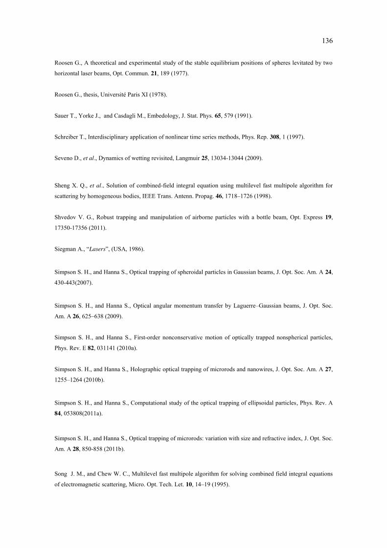
136

Roosen G., A theoretical and experimental study of the stable equilibrium positions of spheres levitated by two

horizontal laser beams, Opt. Commun. 21, 189 (1977).

Roosen G., thesis, Université Paris XI (1978).

Sauer T., Yorke J., and Casdagli M., Embedology, J. Stat. Phys. 65, 579 (1991).

Schreiber T., Interdisciplinary application of nonlinear time series methods, Phys. Rep. 308, 1 (1997).

Seveno D., et al., Dynamics of wetting revisited, Langmuir 25, 13034-13044 (2009).

Sheng X. Q., et al., Solution of combined-field integral equation using multilevel fast multipole algorithm for

scattering by homogeneous bodies, IEEE Trans. Antenn. Propag. 46, 1718–1726 (1998).

Shvedov V. G., Robust trapping and manipulation of airborne particles with a bottle beam, Opt. Express 19,

17350-17356 (2011).

Siegman A.,  “Lasers”,  (USA,  1986).

Simpson S. H., and Hanna S., Optical trapping of spheroidal particles in Gaussian beams, J. Opt. Soc. Am. A 24,

430-443(2007).

Simpson S. H., and Hanna S., Optical angular momentum transfer by Laguerre–Gaussian beams, J. Opt. Soc.

Am. A 26, 625–638 (2009).

Simpson S. H., and Hanna S., First-order nonconservative motion of optically trapped nonspherical particles,

Phys. Rev. E 82, 031141 (2010a).

Simpson S. H., and Hanna S., Holographic optical trapping of microrods and nanowires, J. Opt. Soc. Am. A 27,

1255–1264 (2010b).

Simpson S. H., and Hanna S., Computational study of the optical trapping of ellipsoidal particles, Phys. Rev. A

84, 053808(2011a).

Simpson S. H., and Hanna S., Optical trapping of microrods: variation with size and refractive index, J. Opt. Soc.

Am. A 28, 850-858 (2011b).

Song J. M., and Chew W. C., Multilevel fast multipole algorithm for solving combined field integral equations

of electromagnetic scattering, Micro. Opt. Tech. Let. 10, 14–19 (1995).

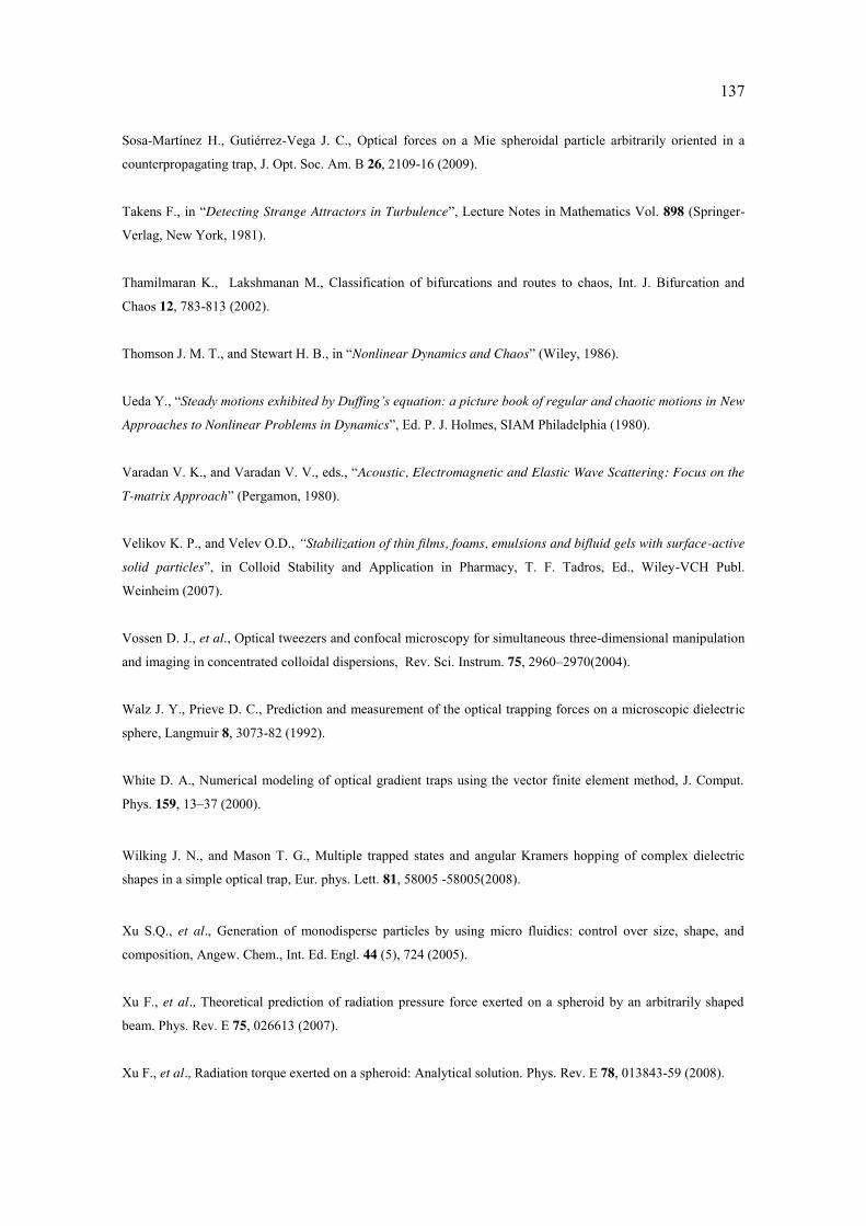
137

Sosa-Martínez H., Gutiérrez-Vega J. C., Optical forces on a Mie spheroidal particle arbitrarily oriented in a

counterpropagating trap, J. Opt. Soc. Am. B 26, 2109-16 (2009).

Takens  F.,  in  “Detecting Strange Attractors in Turbulence”,  Lecture  Notes  in  Mathematics  Vol.  898 (Springer-

Verlag, New York, 1981).

Thamilmaran K., Lakshmanan M., Classification of bifurcations and routes to chaos, Int. J. Bifurcation and

Chaos 12, 783-813 (2002).

Thomson  J.  M.  T.,  and  Stewart  H.  B.,  in  “Nonlinear Dynamics and Chaos”  (Wiley,  1986).

Ueda  Y.,  “Steady  motions  exhibited  by  Duffing’s  equation:  a  picture  book  of  regular  and  chaotic  motions  in New

Approaches to Nonlinear Problems in Dynamics”,  Ed.  P.  J.  Holmes,  SIAM  Philadelphia  (1980).

Varadan  V.  K.,  and  Varadan  V.  V.,  eds.,  “Acoustic, Electromagnetic and Elastic Wave Scattering: Focus on the

T-matrix Approach”  (Pergamon,  1980).

Velikov K. P., and Velev O.D., “Stabilization of thin films, foams, emulsions and bifluid gels with surface-active

solid particles”,   in   Colloid   Stability   and   Application   in   Pharmacy,   T.   F.   Tadros,   Ed.,   Wiley-VCH Publ.

Weinheim (2007).

Vossen D. J., et al., Optical tweezers and confocal microscopy for simultaneous three-dimensional manipulation

and imaging in concentrated colloidal dispersions, Rev. Sci. Instrum. 75, 2960–2970(2004).

Walz J. Y., Prieve D. C., Prediction and measurement of the optical trapping forces on a microscopic dielectric

sphere, Langmuir 8, 3073-82 (1992).

White D. A., Numerical modeling of optical gradient traps using the vector finite element method, J. Comput.

Phys. 159, 13–37 (2000).

Wilking J. N., and Mason T. G., Multiple trapped states and angular Kramers hopping of complex dielectric

shapes in a simple optical trap, Eur. phys. Lett. 81, 58005 -58005(2008).

Xu S.Q., et al., Generation of monodisperse particles by using micro fluidics: control over size, shape, and

composition, Angew. Chem., Int. Ed. Engl. 44 (5), 724 (2005).

Xu F., et al., Theoretical prediction of radiation pressure force exerted on a spheroid by an arbitrarily shaped

beam. Phys. Rev. E 75, 026613 (2007).

Xu F., et al., Radiation torque exerted on a spheroid: Analytical solution. Phys. Rev. E 78, 013843-59 (2008).

138

Yurkin M. A., and Hoekstra A. G., The discrete dipole approximation: an overview and recent developments, J.

Quant. Spectrosc. Radiat. Transf. 106, 558–589 (2007).

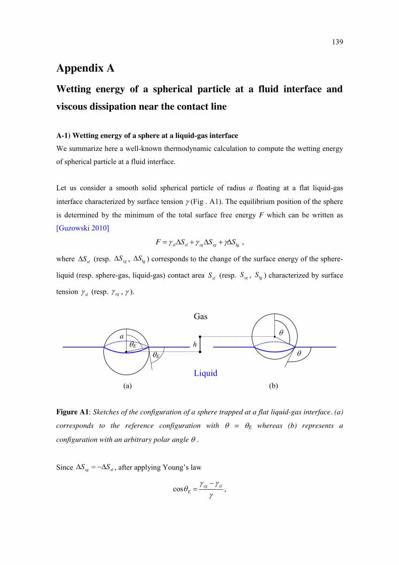
139

Appendix A Wetting energy of a spherical particle at a fluid interface and viscous dissipation near the contact line

A-1) Wetting energy of a sphere at a liquid-gas interface We summarize here a well-known thermodynamic calculation to compute the wetting energy

of spherical particle at a fluid interface.

Let us consider a smooth solid spherical particle of radius a floating at a flat liquid-gas

interface characterized by surface tension (Fig . A1). The equilibrium position of the sphere

is determined by the minimum of the total surface free energy F which can be written as

[Guzowski 2010]

lg ,sl sl sg sgF S S S

where slS (resp. sgS , lgS ) corresponds to the change of the surface energy of the sphere-

liquid (resp. sphere-gas, liquid-gas) contact area slS (resp. sgS , lgS ) characterized by surface

tension sl (resp. sg , ).

(a) (b)

Figure A1: Sketches of the configuration of a sphere trapped at a flat liquid-gas interface. (a)

corresponds to the reference configuration with = E whereas (b) represents a

configuration with an arbitrary polar angle .

Since sg slS S ,  after  applying  Young’s  law

cos ,sg slE

a h

E

E

Liquid

Gas

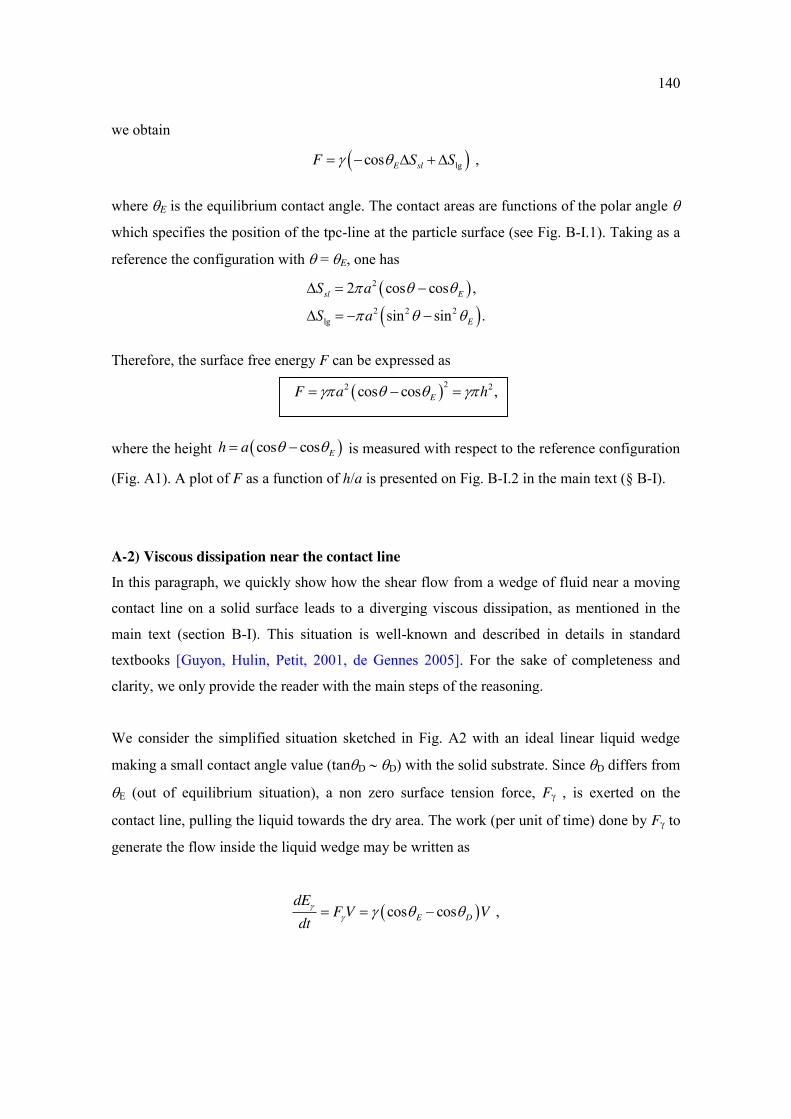
140

we obtain

lgcos ,E slF S S

where E is the equilibrium contact angle. The contact areas are functions of the polar angle

which specifies the position of the tpc-line at the particle surface (see Fig. B-I.1). Taking as a

reference the configuration with = E, one has

2

2 2 2lg

2 cos cos ,

sin sin .sl E

E

S a

S a

Therefore, the surface free energy F can be expressed as

22 2cos cos ,EF a h

where the height cos cos Eh a is measured with respect to the reference configuration

(Fig. A1). A plot of F as a function of h/a is presented on Fig. B-I.2 in the main text (§ B-I).

A-2) Viscous dissipation near the contact line In this paragraph, we quickly show how the shear flow from a wedge of fluid near a moving

contact line on a solid surface leads to a diverging viscous dissipation, as mentioned in the

main text (section B-I). This situation is well-known and described in details in standard

textbooks [Guyon, Hulin, Petit, 2001, de Gennes 2005]. For the sake of completeness and

clarity, we only provide the reader with the main steps of the reasoning.

We consider the simplified situation sketched in Fig. A2 with an ideal linear liquid wedge

making a small contact angle value (tanD D) with the solid substrate. Since D differs from

E (out of equilibrium situation), a non zero surface tension force, F , is exerted on the

contact line, pulling the liquid towards the dry area. The work (per unit of time) done by F to

generate the flow inside the liquid wedge may be written as

cos cos ,E D

dEF V V

dt

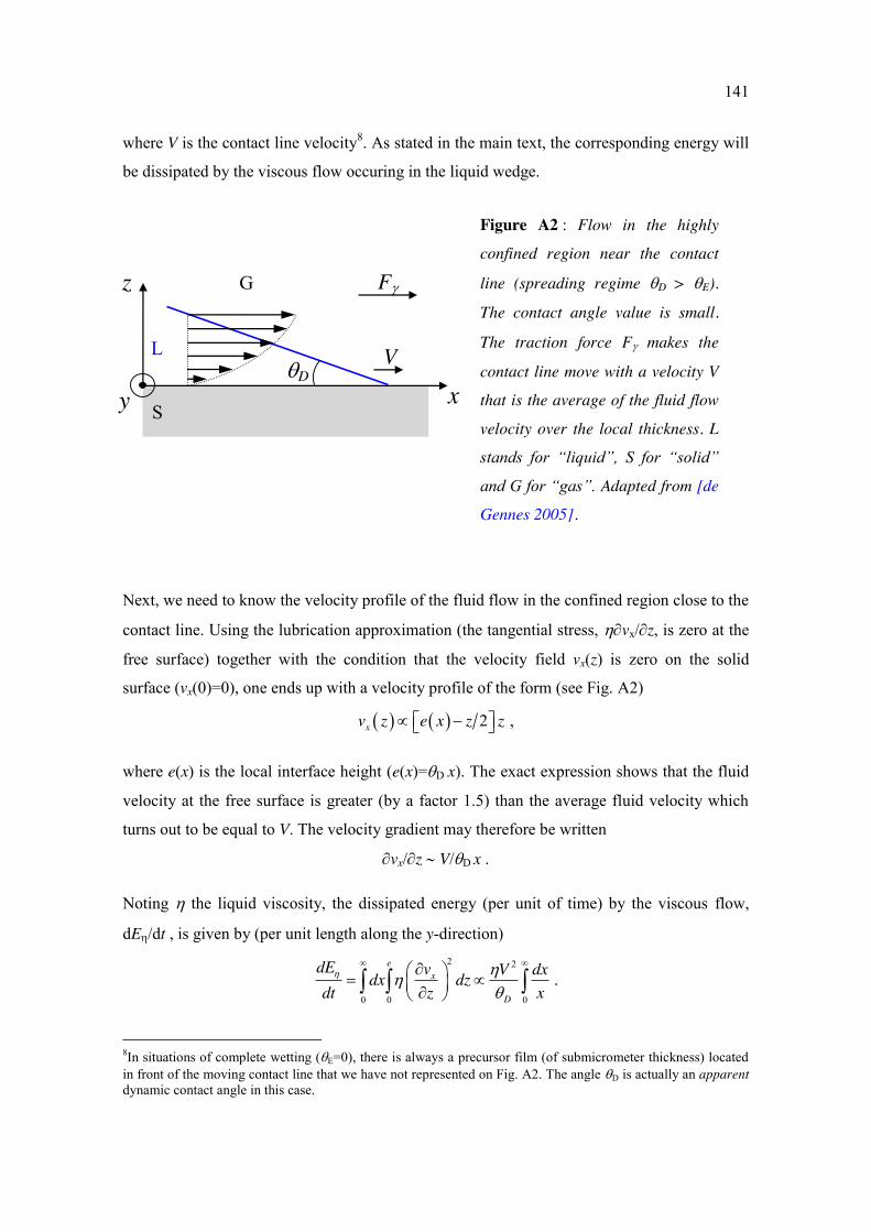
141

where V is the contact line velocity8. As stated in the main text, the corresponding energy will

be dissipated by the viscous flow occuring in the liquid wedge.

Next, we need to know the velocity profile of the fluid flow in the confined region close to the

contact line. Using the lubrication approximation (the tangential stress, vx/z, is zero at the

free surface) together with the condition that the velocity field vx(z) is zero on the solid

surface (vx(0)=0), one ends up with a velocity profile of the form (see Fig. A2)

2 ,xv z e x z z

where e(x) is the local interface height (e(x)=D x). The exact expression shows that the fluid

velocity at the free surface is greater (by a factor 1.5) than the average fluid velocity which

turns out to be equal to V. The velocity gradient may therefore be written

vx/z V/D x .

Noting the liquid viscosity, the dissipated energy (per unit of time) by the viscous flow,

dE/dt , is given by (per unit length along the y-direction) 2 2

0 0 0

.e

x

D

dE v V dxdx dzdt z x

8In situations of complete wetting (E=0), there is always a precursor film (of submicrometer thickness) located in front of the moving contact line that we have not represented on Fig. A2. The angle D is actually an apparent dynamic contact angle in this case.

Figure A2 : Flow in the highly

confined region near the contact

line (spreading regime D > E).

The contact angle value is small.

The traction force F makes the

contact line move with a velocity V

that is the average of the fluid flow

velocity over the local thickness. L

stands   for   “liquid”,   S   for   “solid”  

and  G  for  “gas”.  Adapted from [de

Gennes 2005].

z

x D

L

S

V

G F

y

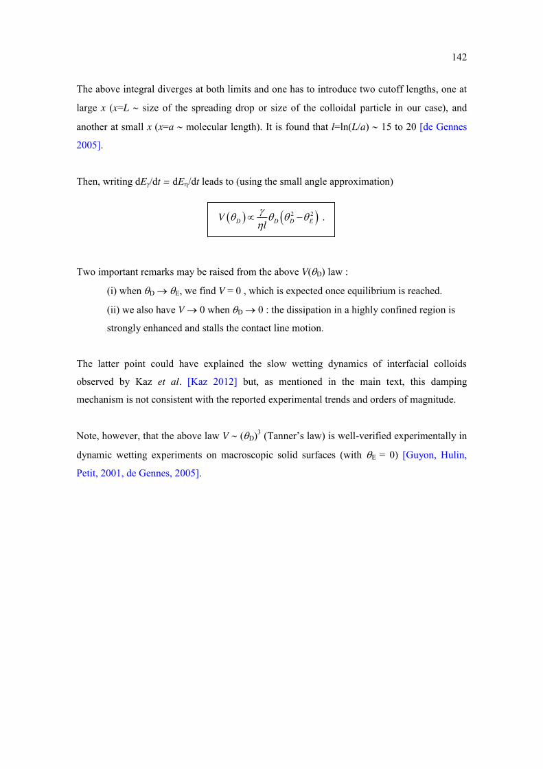
142

The above integral diverges at both limits and one has to introduce two cutoff lengths, one at

large x (x=L size of the spreading drop or size of the colloidal particle in our case), and

another at small x (x=a molecular length). It is found that l=ln(L/a) 15 to 20 [de Gennes

2005].

Then, writing dE/dt = dE/dt leads to (using the small angle approximation)

2 2 .D D D EVl

Two important remarks may be raised from the above V(D) law :

(i) when D E, we find V = 0 , which is expected once equilibrium is reached.

(ii) we also have V 0 when D 0 : the dissipation in a highly confined region is

strongly enhanced and stalls the contact line motion.

The latter point could have explained the slow wetting dynamics of interfacial colloids

observed by Kaz et al. [Kaz 2012] but, as mentioned in the main text, this damping

mechanism is not consistent with the reported experimental trends and orders of magnitude.

Note, however, that the above law V (D)3 (Tanner’s  law)  is  well-verified experimentally in

dynamic wetting experiments on macroscopic solid surfaces (with E = 0) [Guyon, Hulin,

Petit, 2001, de Gennes, 2005].

143

Appendix B Thermal gradients at fluid interfaces In this appendix, we shortly derive the orders of magnitude of the Marangoni and radiation

pressure (RP) forces to tentatively account for the adsorption trajectories observed with

ellipsoids (see discussion § B-IV.3).

(i) Radiation pressure forces, FRP, are of order:

FRP P/c ,

where P is the laser power, c the speed of light in vacuum and a factor of order 0.1 [Ashkin,

1970, 2006].

(ii) Marangoni forces stem from a surface tension gradient originating from an interfacial

thermal gradient [Landau 1994, Guyon, Hulin, Petit, 2001] and read :

FMar 2a(d) ,

where d = (d/dT)dT is the change in surface tension due to a temperature gradient dT and a

is the typical short dimension of a (prolate) ellipsoid.

Putting the following typical numbers, P = 10 mW, c = 3.108 m/s, a = 3 m and d/dT 3.10-

4 N.m-1.K-1 [Guyon, Hulin, Petit, 2001, de Gennes 2005], and writing that FRP FMar lead to

dT 1 mK .

Therefore, very small temperature differences close to the water-air interface would be

sufficient to make Marangoni forces comparable to radiation pressure ones.