doctorat de l'universitÉ de toulouse · bilevel optimization of eco-industrial parks for the...
TRANSCRIPT

En vue de l'obtention du
DOCTORAT DE L'UNIVERSITÉ DE TOULOUSEDélivré par :
Institut National Polytechnique de Toulouse (INP Toulouse)Discipline ou spécialité :
Génie des Procédés et de l'Environnement
Présentée et soutenue par :M. MANUEL RAMOS
le mardi 27 septembre 2016
Titre :
Unité de recherche :
Ecole doctorale :
OPTIMISATION BI-NIVEAU D'ECOPARCS INDUSTRIELS POUR UNEGESTION DURABLE DES RESSOURCES
Mécanique, Energétique, Génie civil, Procédés (MEGeP)
Laboratoire de Génie Chimique (L.G.C.)Directeur(s) de Thèse :
M. LUDOVIC MONTASTRUCM. MARIANNE BOIX
Rapporteurs :M. GILLES TRYSTRAM, AGROPARISTECH MASSY
M. JACK LEGRAND, UNIVERSITE DE NANTES
Membre(s) du jury :1 M. SERGE DOMENECH, INP TOULOUSE, Président2 M. DIDIER AUSSEL, UNIVERSITE DE PERPIGNAN, Membre2 M. GUILLAUME JUNQUA, ECOLE DES MINES D'ALES, Membre2 M. LUDOVIC MONTASTRUC, INP TOULOUSE, Membre2 M. MARIANNE BOIX, INP TOULOUSE, Membre2 Mme SOLENE LE BOURDIEC, EDF CLAMART, Membre


- 3 -
Optimisation Bi-Niveau d’Ecoparcs Industriels pour une Gestion Durable des Ressources
Résumé
Ce travail présente une optimisation bi-niveau pour la conception de réseaux durables de ressources
dans les parcs éco-industriels (EIP). Tout d'abord, les méthodes d'optimisation multiobjectif sont
explorées afin de gérer la nature multicritère des problèmes de conception de réseaux dans les EIP.
Ensuite, différents cas d’étude sont explorés et analysés afin de maintenir un équilibre concernant les
coûts opératoires des usines, tout en minimisant la consommation des ressources naturelles. Ainsi, le
problème est modélisé selon une structure bi-niveau reprenant les concepts de la théorie des jeux, où les
usines des entreprises jouent un jeu de Nash entre elles, tout en étant dans une structure de jeu de
Stackelberg avec l'autorité environnementale. Cette structure définit un modèle qui doit être transformé
en un problème MOPEC (Multiple Optimization Problems with Equilibrium Constraints).
Différents cas d’étude sont explorés : le premier cas est le réseau d'eau mono-polluant d’un EIP dans
lequel l’influence des paramètres opératoires des usines est étudiée afin de déterminer ceux qui
favorisent la symbiose entre les usines. Le réseau d'eau est composé d'un nombre fixe de procédés et
d’unités de régénération où les concentrations maximales d’entrée et de sortie des polluants sont définies
a priori. L'objectif est alors de déterminer quelles sont les allocations entre procédés et unités de
régénération. Les résultats obtenus mettent en évidence les avantages de la structure du modèle
proposée par rapport aux approches multiobjectif traditionnelles, en obtenant des gains économiques
équilibrés d’usines différentes (gains entre 12-25%) tout en maintenant une faible consommation globale
des ressources. Ensuite, d'autres études de cas sont abordées à l'aide de la structure bi-niveau : il s’agit
d'inclure simultanément les réseaux d'énergie et d’eau dans une formulation multi-leader multi-follower
où les deux « autorités » environnementales sont supposées jouer un jeu non-coopératif de Nash. Dans
un premier cas, le gain économique est plus important en incluant des réseaux d'énergie dans la structure
de l’EIP. La deuxième étude de cas industriel explore un modèle de réseau d’utilités offre-demande où
l'autorité environnementale vise à minimiser les émissions totales de CO2 dans le parc. La conclusion des
différents cas explorés montre des résultats extrêmement favorables en termes de coût et d’impact
environnemental ce qui vise à encourager les entreprises à participer à l'EIP.
Mots – clés : Écoparc Industriel, Optimisation bi-niveau, Durabilité, Equilibre de Nash, Théorie des Jeux

- 5 -
Bilevel Optimization of Eco-Industrial Parks for the Design of Sustainable Resource Networks
Abstract
This work presents a bilevel programming framework for the design of sustainable resource networks in
eco-industrial parks (EIP). First, multiobjective optimization methods are explored in order to manage the
multi-criteria nature of EIP network design problems. Then, different case studies are modeled in order to
minimize and maintain in equilibrium participating plants operating costs while minimizing resource
consumption. Thus, the structure of the model is constituted by a bilevel programming framework where
the enterprises’ plants play a Nash game between them while being in a Stackelberg game structure with
the authority. This structure defines a model which, in order to be solved, has to be transformed into a
MOPEC (Multiple Optimization Problems with Equilibrium Constraints) structure.
Regarding the case studies, mono-contaminant water networks in EIP are studied first, where the
influence of plants operating parameters are studied in order to determine the most important ones to
favor the symbiosis between plants. The water network is composed of a fixed number of process and
water regeneration units where the maximal inlet and outlet contaminant concentrations are defined a
priori. The aim is to determine which processes are interconnected and the water regeneration allocation.
Obtained results highlight the benefits of the proposed model structure in comparison with traditional
multiobjective approaches, by obtaining equilibrate different plants operating costs (i.e. gains between
12-25%) while maintaining an overall low resource consumption. Then, other case studies are
approached by using the bilevel structure to include simultaneously energy networks in a multi-leader-
multi-follower formulation where both environmental authorities are assumed to play a non-cooperative
Nash game. In the first case study, economic gain is proven to be more significant by including energy
networks in the EIP structure. The second industrial case study explores a supply-demand utility network
model where the environmental authority aims to minimize the total equivalent CO2 emissions in the EIP.
In all cases, the enterprises’ plants are encouraged to participate in the EIP by the extremely favorable
obtained results.
Keywords: Eco-Industrial Parks, Bilevel Optimization, Sustainability, Nash Equilibrium, Game Theory

- 7 -
Optimización Bi-nivel de Parques Eco-industriales para una Gestión Sostenible de los Recursos
Resumen
Este trabajo presenta una optimización bi-nivel para el diseño de redes sostenibles de recursos en los
parques eco-industriales (EIP). En primer lugar, se exploran los métodos de optimización multi-objetivo
para demostrar la naturaleza multi-criterio de los problemas de diseño de redes en los EIP. A
continuación, diferentes casos de estudio son llevados a cabo en pos de minimizar y mantener en
equilibrio los costos de operación de las plantas, manteniendo al mínimo el consumo de recursos
naturales. Para este fin, la estructura del modelo consiste en una programación bi-nivel donde las plantas
de diferentes empresas juegan un juego de Nash no cooperativo entre ellas, mientras que las mismas
están bajo una estructura de juego de Stackelberg con la “autoridad” medioambiental. Esta estructura
define un modelo que debe ser transformado en un problema MOPEC (Multiple Optimization Problems
with Equilibrium Constraints) con el fin de ser resuelto numéricamente
En lo que a los casos de estudio respecta, las redes de agua con un solo contaminante en los EIP son
estudiadas, donde la influencia de los parámetros de funcionamiento de las diferentes plantas es
analizada para determinar aquellos que favorecen la simbiosis entre plantas. La red de agua se compone
principalmente de un número fijo de procesos y unidades de regeneración donde las concentraciones
máximas de entrada y salida de los contaminantes son definidas a priori. El objetivo es determinar las
conexiones y asignaciones entre los procesos y unidades de regeneración. Los resultados ponen de
evidencia las ventajas de la estructura del modelo propuesto en comparación con los enfoques
tradicionales multi-objetivo, obteniendo ganancias económicas equilibradas en las distintas plantas (i.e.
ganancias entre 12-25%) manteniendo un bajo consumo total de recursos. Subsecuentemente, otros
casos de estudio se abordan mediante la misma estructura de dos niveles: se trata de la inclusión
simultánea de redes de energía en una formulación multi-líder multi-seguidor, donde es supuesto que
ambas "autoridades" medioambientales juegan un Nash juego no cooperativo. En el primer caso, la
ganancia económica resultó ser más importante al incluir redes de energía en la estructura del EIP. El
segundo caso de estudio explora un modelo industrial de la red utilidades de oferta y demanda, donde la
función objetivo de la autoridad medioambiental es minimizar las emisiones totales de CO2 equivalentes
en el EIP. En todos los casos, se incita a las plantas de las empresas a participar en el EIP por los
resultados extremadamente favorables obtenidos.
Palabras clave: Parque eco-industrial, Optimización bi-nivel, Sostenibilidad, Equilibrio de Nash, Teoría de juegos.


- 9 -
Table des matières
Table des matières
- 10 -
Avant - propos ..................................................................................................................... - 17 -
Chapitre 1 : Motivations de l’étude, analyse bibliographique et position du problème - 23 -
1. L’écologie industrielle : contexte et concepts ............................................................. - 25 -
1.1. Contexte général ................................................................................................ - 25 -
1.2. L’écologie industrielle : historique et définitions ................................................. - 25 -
1.3. L’écologie industrielle : études antérieures et exemples de mise en œuvre ...... - 28 -
1.4. Problématique .................................................................................................... - 31 -
2. Techniques actuelles de conception et d’évaluation des EIP ..................................... - 33 -
2.1. La conception des EIP via des méthodes de simulation .................................... - 33 -
2.2. Conception par optimisation mathématique ....................................................... - 37 -
2.3. Autres techniques .............................................................................................. - 38 -
2.3.1. Évaluation basée sur les indicateurs .............................................................. - 38 -
3. Méthodes d’optimisation pour la conception des EIP ................................................. - 39 -
3.1. Optimisation multiobjectif : concepts .................................................................. - 39 -
3.1.1. Problème d’optimisation multiobjectif ............................................................. - 39 -
3.1.2. La multiplicité des solutions ........................................................................... - 40 -
3.1.3. Dominance et front de Pareto ........................................................................ - 40 -
3.2. Techniques de résolution des problèmes d’optimisation multiobjectif ................ - 43 -
3.2.1. Classification des différentes méthodes ......................................................... - 43 -
4. Modèles spécifiques d’optimisation pour la conception des EIP ................................ - 46 -
4.1. Le concept de superstructure dans les EIP ........................................................ - 46 -
4.2. Formulation du problème de conception des EIP ............................................... - 48 -
4.3. Aspect multiobjectif lié à la conception des EIP ................................................. - 49 -
4.4. Études antérieures portant sur l’optimisation des EIP ........................................ - 49 -
5. Problématique et motivations ..................................................................................... - 51 -
6. Composition de la thèse ............................................................................................. - 56 -
Références ............................................................................................................................ - 59 -
Chapitre 2 – Multiobjective Optimization Using Goal Programming for Industrial Water Network Design ................................................................................................................................ - 65 -
Abstract ................................................................................................................................. - 69 -
1. Introduction ................................................................................................................ - 69 -
2. Solution methods for multiobjective optimization ........................................................ - 73 -
2.1. Methods classification ........................................................................................ - 73 -
2.2. A priori preference methods ............................................................................... - 75 -
2.2.1. Reference point methods ............................................................................... - 75 -
2.2.2. Goal programming ......................................................................................... - 77 -
Table des matières
- 11 -
2.3. A posteriori preference methods ........................................................................ - 79 -
2.3.1. Pareto front generation .................................................................................. - 79 -
2.3.2. Decision-making tools .................................................................................... - 81 -
3. Case studies .............................................................................................................. - 82 -
3.1. Introductive mathematical example .................................................................... - 83 -
3.1.1. Results ........................................................................................................... - 83 -
3.2. Industrial water network ..................................................................................... - 86 -
3.2.1. Problem statement ......................................................................................... - 87 -
3.2.2. Optimization problem formulation .................................................................. - 88 -
3.2.3. Results ........................................................................................................... - 89 -
3.3. Industrial water and energy network .................................................................. - 91 -
3.3.1. Problem statement ......................................................................................... - 91 -
3.3.2. Optimization problem formulation .................................................................. - 92 -
3.3.3. Results ........................................................................................................... - 93 -
4. Conclusions ............................................................................................................... - 96 -
5. Annexes ..................................................................................................................... - 97 -
5.1. IWN model statement ......................................................................................... - 97 -
5.2. Industrial water and energy network model statement ..................................... - 100 -
6. Nomenclature ........................................................................................................... - 101 -
References .......................................................................................................................... - 103 -
Chapitre 3 - Water Exchanges in Eco-Industrial Parks through Multiobjective Optimization and Game Theory ........................................................................................................................... - 109 -
Abstract ............................................................................................................................... - 113 -
1. Introduction .............................................................................................................. - 114 -
2. Methodology ............................................................................................................ - 115 -
2.1. Objective functions ........................................................................................... - 115 -
2.2. Modeling eco-industrial parks ........................................................................... - 115 -
2.3. Multi-objective optimization approaches........................................................... - 116 -
2.4. Characteristics of eco-industrial parks.............................................................. - 117 -
3. Multiobjective optimization through goal programming ............................................ - 118 -
3.1. Presentation of the case study ......................................................................... - 118 -
3.2. Results with the goal programming approach .................................................. - 119 -
3.3. A game theory perspective............................................................................... - 119 -
4. Conclusions ............................................................................................................. - 120 -
References .......................................................................................................................... - 121 -
Chapitre 4 - Water integration in Eco-Industrial Parks Using a Multi-Leader-Follower Approach ........................................................................................................................................ - 123 -
Abstract ............................................................................................................................... - 129 -
Table des matières
- 12 -
1. Introduction .............................................................................................................. - 129 -
2. Previous studies ....................................................................................................... - 133 -
3. Multi-leader-follower game approach ....................................................................... - 134 -
3.1. Authority/Regulator’s design of an EIP and game theory approach ................. - 135 -
3.2. Multi-leader single-follower game formulation .................................................. - 137 -
3.2.1. Bi-level model .............................................................................................. - 137 -
3.2.2. All equilibrium MPEC reformulation ............................................................. - 139 -
3.3. Single-leader multi-follower game formulation ................................................. - 140 -
3.4. Solution methodologies .................................................................................... - 142 -
4. EIP problem statement, case studies and results .................................................... - 144 -
4.1. Model without regeneration units formulation ................................................... - 146 -
4.1.1. Low-flowrate elimination algorithm ............................................................... - 150 -
4.1.2. Case study, results and discussion .............................................................. - 151 -
4.2. Model with regeneration units formulation ........................................................ - 154 -
4.2.1. Case study, results and discussion .............................................................. - 159 -
5. Conclusions ............................................................................................................. - 161 -
6. Nomenclature ........................................................................................................... - 162 -
References .......................................................................................................................... - 164 -
Chapitre 5 - Eco-Industrial Park Parameter Evaluation through Design of Experiments over a Multi-leader-follower Game Model Formulation ....................................................................... - 169 -
Abstract ............................................................................................................................... - 173 -
1. Introduction .............................................................................................................. - 173 -
2. Multi-leader-single-follower game approach............................................................. - 176 -
2.1. Authority/Regulator’s Design of an EIP and Game Theory Approach .............. - 176 -
2.2. Multi-Leader-Single-Follower Game Formulation ............................................. - 177 -
2.2.1. Bi-level model .............................................................................................. - 177 -
2.2.2. EIP problem statement and model ............................................................... - 179 -
2.2.3. All equilibrium MPEC reformulation ............................................................. - 183 -
2.3. Solution Methodologies .................................................................................... - 184 -
2.3.1. Low-flowrate elimination algorithm ............................................................... - 187 -
3. Case study and design of experiments (DoE) .......................................................... - 188 -
3.1. Case Study....................................................................................................... - 188 -
3.2. Design of Experiments Methodology ................................................................ - 189 -
3.3. Results and Discussion .................................................................................... - 191 -
3.3.1. MLR models ................................................................................................. - 193 -
3.3.2. PLS model ................................................................................................... - 196 -
4. Conclusions ............................................................................................................. - 199 -

Table des matières
- 13 -
5. Nomenclature ........................................................................................................... - 200 -
References .......................................................................................................................... - 202 -
Chapitre 6 - Optimal design of water exchanges in eco-industrial parks through a game theory approach ............................................................................................................................. - 207 -
Abstract ............................................................................................................................... - 211 -
1. Introduction .............................................................................................................. - 211 -
2. Methodology ............................................................................................................ - 213 -
2.1. Bi-level model ................................................................................................... - 213 -
2.2. Solution methodologies .................................................................................... - 214 -
2.3. Modeling EIP water networks ........................................................................... - 215 -
3. Multi-leader single-follower game approach ............................................................. - 215 -
3.1. Presentation of the case study ......................................................................... - 215 -
3.2. Results and discussion .................................................................................... - 216 -
4. Conclusions ............................................................................................................. - 218 -
References .......................................................................................................................... - 219 -
Chapitre 7 - Utility Network Optimization in Eco-Industrial Parks by a Multi-Leader Follower Game Methodology ........................................................................................................................ - 221 -
Abstract ............................................................................................................................... - 225 -
1. Introduction .............................................................................................................. - 225 -
2. Methodology ............................................................................................................ - 228 -
2.1. General Methodology ....................................................................................... - 228 -
2.2. Specific methodology ....................................................................................... - 231 -
2.2.1. EIP utility network model statement ............................................................. - 232 -
3. Case study ............................................................................................................... - 239 -
3.1. Coal Gasification .............................................................................................. - 240 -
3.2. CO2 Capture .................................................................................................... - 242 -
3.3. MeOH and DME Synthesis .............................................................................. - 243 -
3.4. Refinery ............................................................................................................ - 244 -
3.5. Power Plant ...................................................................................................... - 248 -
3.6. Air Separation .................................................................................................. - 250 -
3.7. Potential participating plants and utility analysis. ............................................. - 251 -
4. Results and discussion ............................................................................................ - 255 -
5. Conclusions and perspectives.................................................................................. - 259 -
6. Nomenclature ........................................................................................................... - 260 -
References .......................................................................................................................... - 261 -
Chapitre 8 - Simultaneous Water and Energy Network Optimization in Eco-Industrial Parks through a Hybrid Single-Leader-Follower Game/Goal Programming Approach ...................... - 267 -
Abstract ............................................................................................................................... - 271 -
Table des matières
- 14 -
1. Introduction .............................................................................................................. - 272 -
2. Literature review ....................................................................................................... - 274 -
3. Problem statement ................................................................................................... - 275 -
3.1. Model statement ............................................................................................... - 277 -
3.2. Case study ....................................................................................................... - 281 -
4. Regulator design of an EIP ...................................................................................... - 283 -
4.1. Methodology..................................................................................................... - 283 -
4.2. Hybrid approach MLFG/GP .............................................................................. - 285 -
4.3. Solution methodologies .................................................................................... - 289 -
5. Results and discussion ............................................................................................ - 292 -
5.1. Step I and II: SLMFG Pareto front generation and sorting. .............................. - 293 -
5.2. Step III: Pareto-compromise solution selection. ............................................... - 296 -
6. Conclusions ............................................................................................................. - 300 -
7. Nomenclature ........................................................................................................... - 301 -
References .......................................................................................................................... - 303 -
Chapitre 9 - Multi-Leader Multi-Follower Game Model for Simultaneous Water and Energy Integration in Eco-Industrial Parks ............................................................................................... - 307 -
Abstract ............................................................................................................................... - 311 -
1. Introduction .............................................................................................................. - 312 -
2. Multi-leader-multi-follower game approach .............................................................. - 313 -
2.1. Regulators’ design of an EIP and game theory approach ................................ - 315 -
2.2. Model formulation ............................................................................................. - 316 -
2.2.1. Bi-level model .............................................................................................. - 316 -
2.2.2. All equilibrium MOPEC reformulation ........................................................... - 322 -
3. Solution methodologies ............................................................................................ - 325 -
4. Case study ............................................................................................................... - 328 -
5. Results and discussion ............................................................................................ - 329 -
6. Conclusions and perspectives.................................................................................. - 333 -
7. Nomenclature ........................................................................................................... - 334 -
References .......................................................................................................................... - 336 -
Chapitre 10 – Conclusions et perspectives .................................................................... - 341 -
1. Conclusions ............................................................................................................. - 343 -
2. Perspectives ............................................................................................................ - 347 -


- 17 -
Avant - propos

Avant – propos
- 18 -
Avant – propos
- 19 -
Entre 1980 et 2010, à l’échelle mondiale, l’extraction des ressources naturelles a augmenté de
80% selon le Ministère du Développement Durable. Ce dernier a dressé un rapport datant de 2014
(Ministère de L’environnement, de L’Energie et de la Mer, 2014) destiné à informer, favoriser et
encourager les démarches visant à développer les initiatives d’écologie industrielle sur les territoires. Que
ce soit à l’échelle internationale (mise en place du Panel International sur les Ressources, IRP),
européenne (feuille de route sur l’utilisation efficace des ressources) ou nationale, il est aujourd’hui
largement démontré qu’il est important de trouver des solutions efficaces permettant de mieux
consommer nos ressources naturelles (UNEP, 2015; European Commission, 2011). L’économie
circulaire parait aujourd’hui constituer l’option la plus adaptée pour mener à bien cet objectif et permet de
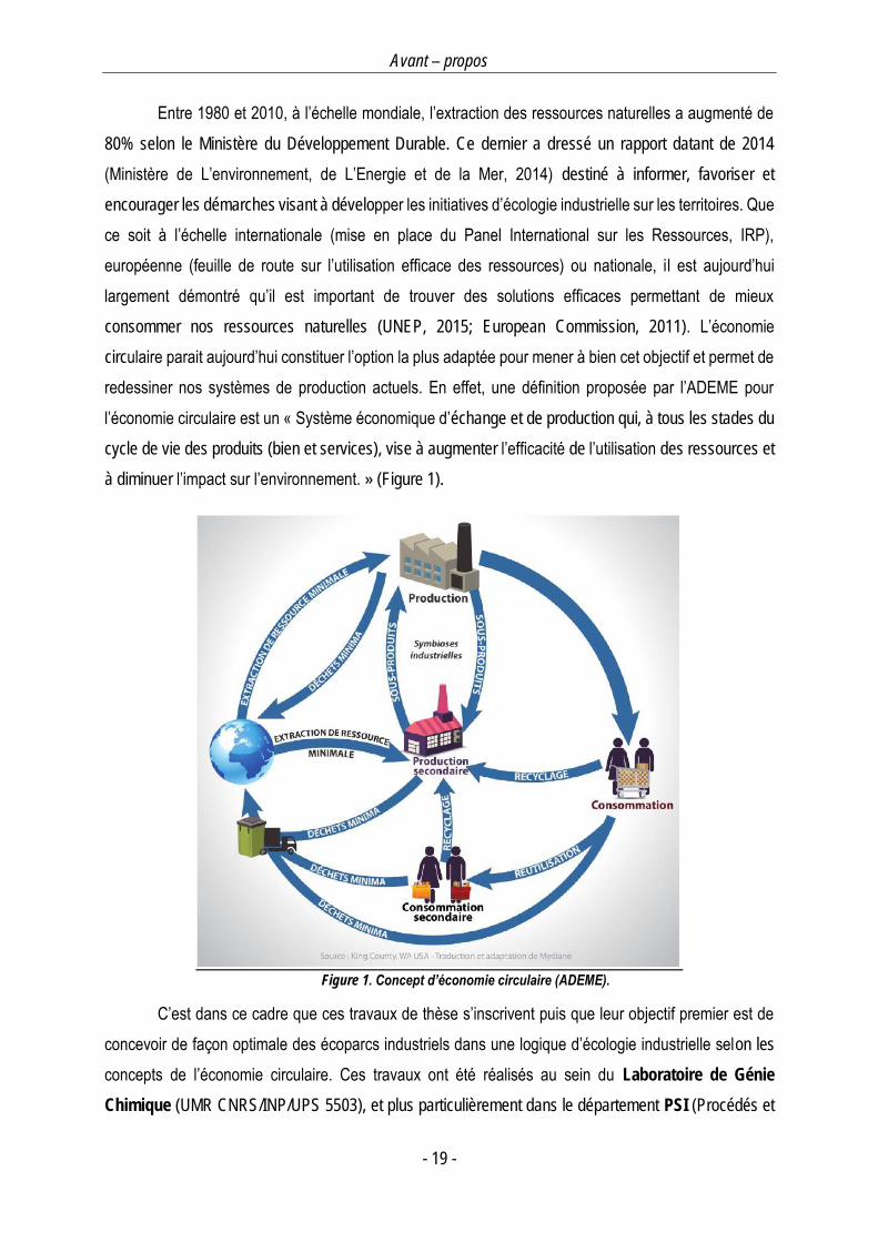
redessiner nos systèmes de production actuels. En effet, une définition proposée par l’ADEME pour
l’économie circulaire est un « Système économique d’échange et de production qui, à tous les stades du
cycle de vie des produits (bien et services), vise à augmenter l’efficacité de l’utilisation des ressources et
à diminuer l’impact sur l’environnement. » (Figure 1).
Figure 1. Concept d’économie circulaire (ADEME).
C’est dans ce cadre que ces travaux de thèse s’inscrivent puis que leur objectif premier est de
concevoir de façon optimale des écoparcs industriels dans une logique d’écologie industrielle selon les
concepts de l’économie circulaire. Ces travaux ont été réalisés au sein du Laboratoire de Génie
Chimique (UMR CNRS/INP/UPS 5503), et plus particulièrement dans le département PSI (Procédés et

Avant – propos
- 20 -
Systèmes Industriels). La thématique de recherches du département est axée sur le développement de
procédures systématiques pour la conception et l’exploitation de procédés et de systèmes de production,
lesquelles mettent généralement en jeu des stratégies numériques avancées. Les travaux prennent en
compte tout un ensemble de critères, parfois contradictoires, telles que la minimisation des coûts, le
respect de l’environnement, la sécurité absolue du procédé et autres.
Les objectifs qui ont conduit à la rédaction de ce mémoire sont multiples :
- Développer un modèle mathématique pour l’optimisation multiobjectif des parcs éco-
industriels
- Proposer une stratégie de résolution fiable et applicable à des réseaux de taille industrielle.
- Formuler mathématiquement un problème bi-niveau de façon à gérer les aspects inhérents
aux parcs éco-industriels : gestion de la confidentialité et de la pluralité des acteurs
- Développer une méthode robuste permettant de gérer différents réseaux simultanément pour
différentes ressources naturelles.
Le manuscrit a été rédigé sous forme d’une succession d’articles scientifiques publiés ou soumis
à des revues internationales à comité de lecture. Afin d’améliorer la compréhension de chaque article, un
premier chapitre, rédigé en français, permet de situer l’étude dans son contexte scientifique et de définir
clairement l’articulation entre chaque chapitre. Dans cette même optique, un résumé détaillé en français
est apposé avant chaque article tout au long de la thèse. Enfin, des conclusions et perspectives
également rédigées en français permettent au lecteur de se projeter et de connaitre le spectre d’activités
futures que ces travaux ont permis d’ouvrir.
Avant – propos
- 21 -
Références
European Commission (2011) Resource Efficiency - Environment. [Online]. 2011. Available from:
http://ec.europa.eu/environment/resource_efficiency/about/roadmap/index_en.htm [Accessed: 29 June
2016].
Ministère de L’environnement, de L’Energie et de la Mer (2014) CATEI - Écologie Industrielle
Territoriale: Le Guide Pour Agir Dans Les Territoires. [Online]. 2014. Available from:
http://www.developpement-durable.gouv.fr/-Ecologie-industrielle-territoriale-.html [Accessed: 29 June
2016].
UNEP (2015) International Resource Panel. [Online]. 2015. Available from:
http://www.unep.org/resourcepanel/ [Accessed: 29 June 2016].

- 23 -
Chapitre 1 : Motivations de l’étude, analyse bibliographique et position du
problème

Chapitre 1 : Motivations de l’étude, analyse bibliographique et position du problème
- 24 -

Chapitre 1 : Motivations de l’étude, analyse bibliographique et position du problème
- 25 -
1. L’écologie industrielle : contexte et concepts
1.1. Contexte général
Il est désormais admis par les industries de transformation de la matière, que, pour
appliquer les concepts de développement durable, il est nécessaire de passer par des progrès
économiques, sociaux et environnementaux simultanés. Ce principe découle de la prise de
conscience concernant les limites de notre environnement en termes d'épuisement des ressources
naturelles et de pollution des écosystèmes. Les activités humaines, la croissance économique et
l’augmentation de la population sont les principaux facteurs mis en cause. En effet, les activités
industrielles génèrent des flux d’échanges avec l’environnement et induisent ainsi des impacts
(émissions et extractions) sur celui-ci.
Afin de proposer des solutions durables, la France a défini sa deuxième feuille de route
pour la transition écologique (Ministère de l’Economie et des Finances, 2014) à la suite de la
Conférence environnementale qui s’est tenue en 2013. Les ressources ne pourront pas être
éternellement exploitées selon une approche de type "circuit ouvert". En conséquence, l’un des
principaux enjeux définis est le développement d’une économie de type “circulaire” afin de
répondre à la problématique de diminuer la consommation des ressources (énergies, matières
premières). Ces dernières années, de nombreux appels à projets scientifiques et initiatives (plans
pour la Nouvelle France Industrielle...) ont pour but de faire évoluer les modes de consommation,
de production et de distribution vers une économie circulaire et ont donc chercher à promouvoir le
concept de « développement durable ». Les objectifs de ces nouveaux challenges sont doubles :
préserver l'environnement tout en augmentant la réussite des entreprises ce qui constitue l'objectif
principal de l'écologie industrielle.
1.2. L’écologie industrielle : historique et définitions
La communauté scientifique s’est intéressée à cette problématique au début des années
90, bien avant que les politiques ne reprennent ce concept. Née sous l’impulsion des économistes,
l’écologie industrielle (Frosch & Gallopoulos, 1989) constitue une réponse aux nombreux
problèmes environnementaux actuels, en faisant l’analogie entre écosystèmes naturels et
systèmes industriels. Une première définition énoncée fut : « une organisation industrielle plus
rationnelle et plus équilibrée, en essayant d’imiter la structure des écosystèmes naturels ». Une
définition plus récente pour l'écologie industrielle a été énoncée par Allenby (Allenby, 2006), il
s’agissait alors "d’un discours multidisciplinaire basé sur les systèmes qui cherche à comprendre
le comportement émergent de systèmes intégrés complexes humains naturels". Dans les
Chapitre 1 : Motivations de l’étude, analyse bibliographique et position du problème
- 26 -
écosystèmes naturels, l'utilisation de l'énergie et des matériaux est optimisée pour réduire les
déchets. Par analogie avec les écosystèmes naturels, les entreprises impliquées dans une
symbiose industrielle peuvent être considérées comme les différents niveaux trophiques d’une
chaîne alimentaire avec des liens métaboliques entre eux (symbolisés par la matière et l’énergie)
(Ashton, 2008). Ce concept d’écologie industrielle se démarque par une approche systémique dans
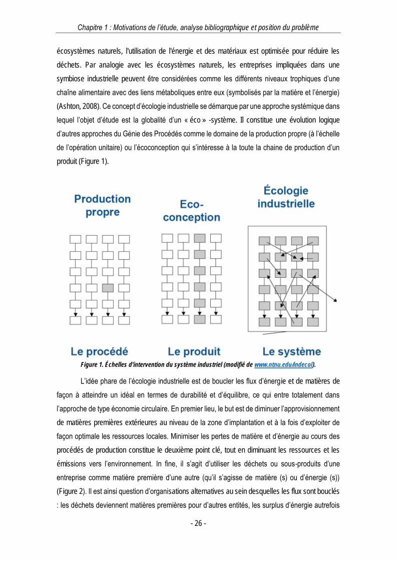
lequel l’objet d’étude est la globalité d’un « éco » -système. Il constitue une évolution logique
d’autres approches du Génie des Procédés comme le domaine de la production propre (à l’échelle
de l’opération unitaire) ou l’écoconception qui s’intéresse à la toute la chaine de production d’un
produit (Figure 1).
Figure 1. Échelles d'intervention du système industriel (modifié de www.ntnu.edu/indecol).
L’idée phare de l’écologie industrielle est de boucler les flux d’énergie et de matières de
façon à atteindre un idéal en termes de durabilité et d’équilibre, ce qui entre totalement dans
l’approche de type économie circulaire. En premier lieu, le but est de diminuer l’approvisionnement
de matières premières extérieures au niveau de la zone d’implantation et à la fois d’exploiter de
façon optimale les ressources locales. Minimiser les pertes de matière et d’énergie au cours des
procédés de production constitue le deuxième point clé, tout en diminuant les ressources et les
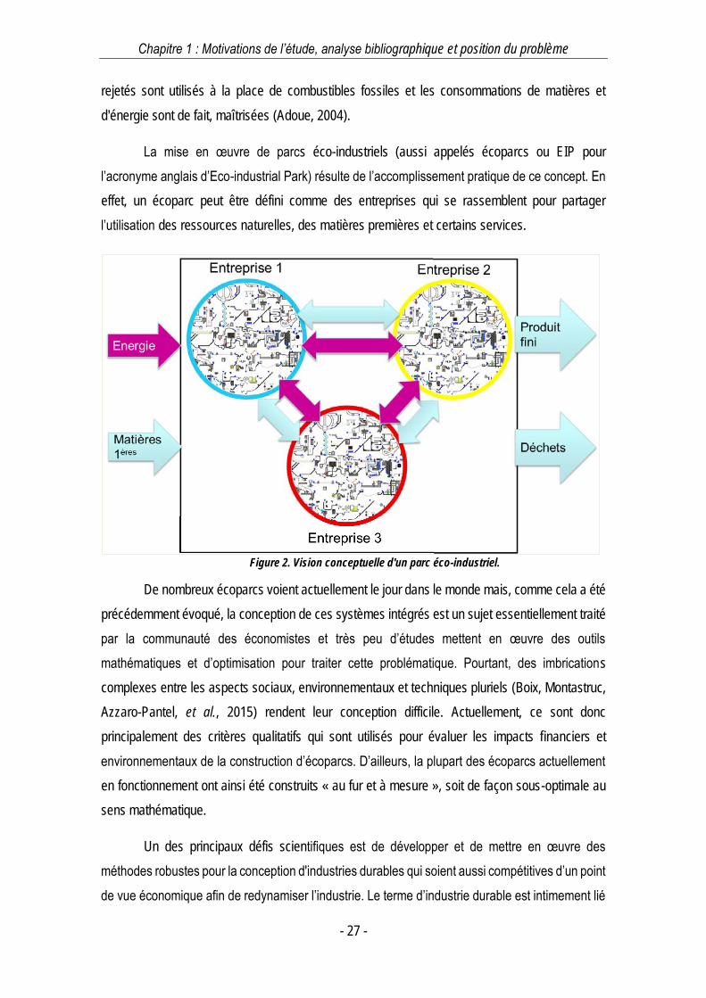
émissions vers l’environnement. In fine, il s’agit d’utiliser les déchets ou sous-produits d’une
entreprise comme matière première d’une autre (qu’il s’agisse de matière (s) ou d’énergie (s))
(Figure 2). Il est ainsi question d’organisations alternatives au sein desquelles les flux sont bouclés
: les déchets deviennent matières premières pour d’autres entités, les surplus d’énergie autrefois
Chapitre 1 : Motivations de l’étude, analyse bibliographique et position du problème
- 27 -
rejetés sont utilisés à la place de combustibles fossiles et les consommations de matières et
d'énergie sont de fait, maîtrisées (Adoue, 2004).
La mise en œuvre de parcs éco-industriels (aussi appelés écoparcs ou EIP pour
l’acronyme anglais d’Eco-industrial Park) résulte de l’accomplissement pratique de ce concept. En
effet, un écoparc peut être défini comme des entreprises qui se rassemblent pour partager
l’utilisation des ressources naturelles, des matières premières et certains services.
Figure 2. Vision conceptuelle d'un parc éco-industriel.
De nombreux écoparcs voient actuellement le jour dans le monde mais, comme cela a été
précédemment évoqué, la conception de ces systèmes intégrés est un sujet essentiellement traité
par la communauté des économistes et très peu d’études mettent en œuvre des outils
mathématiques et d’optimisation pour traiter cette problématique. Pourtant, des imbrications
complexes entre les aspects sociaux, environnementaux et techniques pluriels (Boix, Montastruc,
Azzaro-Pantel, et al., 2015) rendent leur conception difficile. Actuellement, ce sont donc
principalement des critères qualitatifs qui sont utilisés pour évaluer les impacts financiers et
environnementaux de la construction d’écoparcs. D’ailleurs, la plupart des écoparcs actuellement
en fonctionnement ont ainsi été construits « au fur et à mesure », soit de façon sous-optimale au
sens mathématique.
Un des principaux défis scientifiques est de développer et de mettre en œuvre des
méthodes robustes pour la conception d'industries durables qui soient aussi compétitives d’un point
de vue économique afin de redynamiser l’industrie. Le terme d’industrie durable est intimement lié

Chapitre 1 : Motivations de l’étude, analyse bibliographique et position du problème
- 28 -
au terme de « Symbiose industrielle »; selon Chertow (Chertow, 2000), une symbiose industrielle
engage des « industries distinctes dans une approche collective, avantageuse financièrement,
impliquant l'échange physique des matériaux, d'énergie, d'eau et des coproduits ». Une
caractéristique primordiale d’une symbiose industrielle est l‘opportunité offerte par la proximité
géographique de plusieurs industries. Enfin, une condition de base pour qu’un EIP soit
économiquement viable est que la somme des avantages obtenus en travaillant collectivement soit
plus élevée que lors d’une installation autonome (Boix, Montastruc, Pibouleau, et al., 2012).
D’un point de vue technique, la difficulté de la conception des parcs éco-industriels est
d’une part liée à des notions de réseaux (matières, énergies...) et d’autre part à des problèmes
d’optimisation. En effet, il est primordial de concevoir les écoparcs de façon à ce qu’ils bénéficient
d’une interopérabilité optimale. La spécificité de l’optimisation des parcs éco-industriels est le fait
que de nombreux acteurs interviennent et chaque participant œuvre pour son objectif économique
(minimisation des coûts de production par exemple). C’est alors la « communauté » constituée par
l'écoparc qui est garante d’un critère environnemental global (minimisation de la consommation
globale de matières premières, d'énergie...). Cependant, l'un des obstacles à la mise en œuvre
optimale de ces systèmes est la nécessité de mettre en commun des données liées à la production
de chacune des industries. En effet, bien que la notion d'écoparc soit par nature une structure
coopérative philosophiquement parlant, la confidentialité de certaines données peut poser
problème dans la mise en place ou l'optimisation de l’écoparc.
1.3. L’écologie industrielle : études antérieures et exemples
de mise en œuvre
La conception des parcs éco-industriels est une initiative relativement récente et quelques
approches quantitatives ont vu le jour au cours des dernières années.
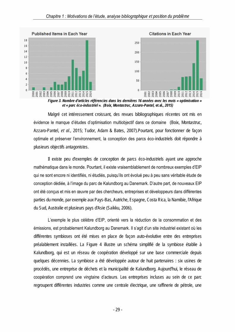
Une rapide analyse bibliométrique permet de démontrer l’intérêt croissant pour ce thème
depuis les dix dernières années (source : ISI Web of Science, Mai 2016). En effet, si l’on s’intéresse
aux mots-clefs « parc éco-industriel » ou « symbiose industrielle » et « optimisation », un total de
44 publications dans des revues internationales sont obtenues et le nombre de citations a été
multiplié par 5 en cinq ans (Figure 3).
Chapitre 1 : Motivations de l’étude, analyse bibliographique et position du problème
- 29 -
Figure 3. Nombre d'articles référencies dans les dernières 16 années avec les mots « optimisation »
et « parc éco-industriel ». (Boix, Montastruc, Azzaro-Pantel, et al., 2015)
Malgré cet intéressement croissant, des revues bibliographiques récentes ont mis en
évidence le manque d’études d’optimisation multiobjectif dans ce domaine (Boix, Montastruc,
Azzaro-Pantel, et al., 2015; Tudor, Adam & Bates, 2007).Pourtant, pour fonctionner de façon
optimale et préserver l’environnement, la conception des parcs éco-industriels doit répondre à
plusieurs objectifs antagonistes.
Il existe peu d'exemples de conception de parcs éco-industriels ayant une approche
mathématique dans le monde. Pourtant, il existe vraisemblablement de nombreux exemples d’EIP
qui ne sont encore ni identifiés, ni étudiés, puisqu’ils ont évolué peu à peu sans véritable étude de
conception dédiée, à l’image du parc de Kalundborg au Danemark. D’autre part, de nouveaux EIP
ont été conçus et mis en œuvre par des chercheurs, entreprises et développeurs dans différentes
parties du monde, par exemple aux Pays-Bas, Autriche, Espagne, Costa Rica, la Namibie, l'Afrique
du Sud, Australie et plusieurs pays d'Asie (Saikku, 2006).
L’exemple le plus célèbre d’EIP, orienté vers la réduction de la consommation et des
émissions, est probablement Kalundborg au Danemark. Il s’agit d’un site industriel existant où les
différentes symbioses ont été mises en place de façon auto-évolutive entre des entreprises
préalablement installées. La Figure 4 illustre un schéma simplifié de la symbiose établie à
Kalundborg, qui est un réseau de coopération développé sur une base commerciale depuis
quelques décennies. La symbiose a été développée autour de huit partenaires : six usines de
procédés, une entreprise de déchets et la municipalité de Kalundborg. Aujourd'hui, le réseau de
coopération comprend une vingtaine d’acteurs. Les entreprises incluses au sein de ce parc
regroupent différentes industries comme une centrale électrique, une raffinerie de pétrole, une

Chapitre 1 : Motivations de l’étude, analyse bibliographique et position du problème
- 30 -
cimenterie, une usine de placoplâtre, un laboratoire pharmaceutique, une pisciculture et le
chauffage de la ville de Kalundborg.
Figure 4. Symbiose industrielle de Kalundborg.
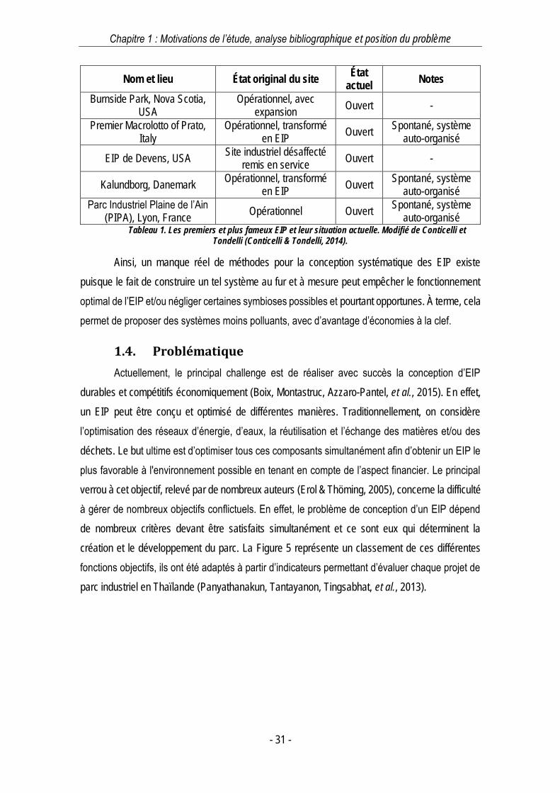
Ailleurs dans le monde, d’autres exemples existent également. Le Tableau 1 en recense
quelques-uns très connus d’EIP existants dans le monde (Conticelli & Tondelli, 2014).
La majorité des EIP les plus connus a donc été conçue de façon auto-évolutive, au fur et
à mesure. Pourtant, il est bien connu que cette façon spontanée d’établir une symbiose peut
devenir problématique à cause du fait que les entreprises voulant y participer doivent avoir des
motivations concrètes et tangibles pour accepter la collaboration.
Chapitre 1 : Motivations de l’étude, analyse bibliographique et position du problème
- 31 -
Nom et lieu État original du site État
actuel Notes
Burnside Park, Nova Scotia, USA
Opérationnel, avec expansion
Ouvert -
Premier Macrolotto of Prato, Italy
Opérationnel, transformé en EIP
Ouvert Spontané, système
auto-organisé
EIP de Devens, USA Site industriel désaffecté
remis en service Ouvert -
Kalundborg, Danemark Opérationnel, transformé
en EIP Ouvert
Spontané, système auto-organisé
Parc Industriel Plaine de l’Ain (PIPA), Lyon, France
Opérationnel Ouvert Spontané, système
auto-organisé Tableau 1. Les premiers et plus fameux EIP et leur situation actuelle. Modifié de Conticelli et
Tondelli (Conticelli & Tondelli, 2014).
Ainsi, un manque réel de méthodes pour la conception systématique des EIP existe
puisque le fait de construire un tel système au fur et à mesure peut empêcher le fonctionnement
optimal de l’EIP et/ou négliger certaines symbioses possibles et pourtant opportunes. À terme, cela
permet de proposer des systèmes moins polluants, avec d’avantage d’économies à la clef.
1.4. Problématique
Actuellement, le principal challenge est de réaliser avec succès la conception d’EIP
durables et compétitifs économiquement (Boix, Montastruc, Azzaro-Pantel, et al., 2015). En effet,
un EIP peut être conçu et optimisé de différentes manières. Traditionnellement, on considère
l’optimisation des réseaux d’énergie, d’eaux, la réutilisation et l’échange des matières et/ou des
déchets. Le but ultime est d’optimiser tous ces composants simultanément afin d’obtenir un EIP le
plus favorable à l'environnement possible en tenant en compte de l’aspect financier. Le principal
verrou à cet objectif, relevé par de nombreux auteurs (Erol & Thöming, 2005), concerne la difficulté
à gérer de nombreux objectifs conflictuels. En effet, le problème de conception d’un EIP dépend
de nombreux critères devant être satisfaits simultanément et ce sont eux qui déterminent la
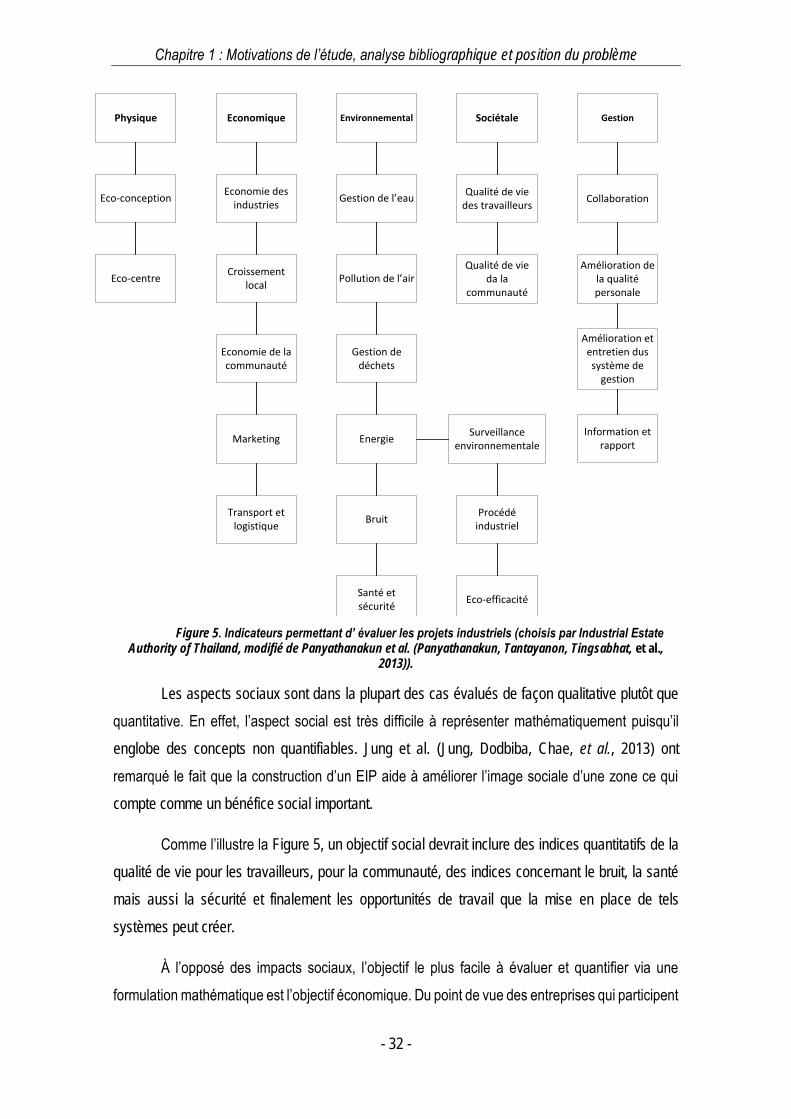
création et le développement du parc. La Figure 5 représente un classement de ces différentes
fonctions objectifs, ils ont été adaptés à partir d’indicateurs permettant d’évaluer chaque projet de
parc industriel en Thaïlande (Panyathanakun, Tantayanon, Tingsabhat, et al., 2013).
Chapitre 1 : Motivations de l’étude, analyse bibliographique et position du problème
- 32 -
Figure 5. Indicateurs permettant d’ évaluer les projets industriels (choisis par Industrial Estate
Authority of Thailand, modifié de Panyathanakun et al. (Panyathanakun, Tantayanon, Tingsabhat, et al., 2013)).
Les aspects sociaux sont dans la plupart des cas évalués de façon qualitative plutôt que
quantitative. En effet, l’aspect social est très difficile à représenter mathématiquement puisqu’il
englobe des concepts non quantifiables. Jung et al. (Jung, Dodbiba, Chae, et al., 2013) ont
remarqué le fait que la construction d’un EIP aide à améliorer l’image sociale d’une zone ce qui
compte comme un bénéfice social important.
Comme l’illustre la Figure 5, un objectif social devrait inclure des indices quantitatifs de la
qualité de vie pour les travailleurs, pour la communauté, des indices concernant le bruit, la santé
mais aussi la sécurité et finalement les opportunités de travail que la mise en place de tels
systèmes peut créer.
À l’opposé des impacts sociaux, l’objectif le plus facile à évaluer et quantifier via une
formulation mathématique est l’objectif économique. Du point de vue des entreprises qui participent
Physique Economique Environnemental Sociétale Gestion
Eco-conception
Eco-centre
Economie des industries
Croissement local
Economie de la communauté
Marketing
Transport et logistique
Gestion de l’eau
Pollution de l’air
Gestion de déchets
Energie
Bruit
Santé et sécurité
Surveillance environnementale
Procédé industriel
Qualité de vie des travailleurs
Qualité de vie da la
communauté
Eco-efficacité
Collaboration
Amélioration de la qualité personale
Amélioration et entretien dus système de
gestion
Information et rapport
Chapitre 1 : Motivations de l’étude, analyse bibliographique et position du problème
- 33 -
à l’EIP, il est aussi le plus important puisqu’il constitue le principal élément déclencheur pour
participer à un EIP. En effet, des coûts opératoires diminués constituent un réel intérêt à court
terme et un argument de choix pour convaincre les industriels d’en faire partie. L’analyse de la
littérature montre qu’il existe plusieurs indicateurs économiques disponibles, parmi lesquels on
retrouve notamment le bénéfice actualisé ou l’évaluation des coûts de fonctionnement. Dans toutes
les études, il est important de noter le fait que le coût est évalué pour tout l’EIP, dans son intégralité.
Néanmoins, il pourrait être plus rigoureux d’introduire une méthodologie, un modèle ou des
contraintes forçant ou emmenant les participants de l’EIP à avoir un gain relatif équivalent au sein
de l’EIP (Boix, 2011). Effectivement, un facteur clef déjà proposé pour le développement des EIP
(Tudor, Adam & Bates, 2007) est la confiance entre chaque partenaire et le fait que chaque
participant ait un gain relatif similaire pourrait contribuer à cela.
La conservation de l’environnement est une des motivations principales de l’écologie
industrielle et de la mise en œuvre dans la conception des EIP. La conception optimale des
échanges inter-entreprises permet de réduire les impacts environnementaux et la promotion des
activités industrielles en développant des synergies entre les acteurs de l’EIP. Ce concept mène à
stabiliser et très probablement diminuer l’impact environnemental des activités économiques. En
termes de critères, on peut relever la minimisation de l’utilisation des ressources naturelles en
quantités (débits d’eau utilisés, consommation énergétique...) ou les impacts environnementaux
formulés e.g. avec des méthodes de type analyse de cycle de vie ou les approches basées sur les
calculs d’empreintes (Water Footprint, Carbon Footprint...).
Finalement, les objectifs topologiques (liés à la structure du réseau) notamment liés au
coût du réseau, sont souvent négligés dans la littérature. La principale difficulté dans le fait de
prendre en compte les aspects topologiques (nombre de tuyaux, de connexions entre entreprises
et au sien des entreprises) est liée à l’introduction de variables discrètes dans les modèles
mathématiques. De plus, il existe une réelle distinction économique entre connexions internes (la
même usine) et externes (inter-usines).
2. Techniques actuelles de conception et d’évaluation
des EIP
2.1. La conception des EIP via des méthodes de simulation
L’utilisation des outils de simulation de procédés chimiques (CPS) permet de concevoir et
d’évaluer des EIP. Selon Casavant et Côté (Casavant & Côté, 2004), avec les CPS, il est possible
Chapitre 1 : Motivations de l’étude, analyse bibliographique et position du problème
- 34 -
de: (i) évaluer et comparer quantitativement les bénéfices environnementaux et financiers qui
peuvent émerger potentiellement à partir des liens matière et énergie entre entreprises; (ii)
résoudre les problèmes généraux de conception, de rénovation ou d’opération ; (iii) aider à
identifier des solutions complexes ou parfois contre-intuitives ; et (iv) évaluer des scénarios
hypothétiques. En fait, le domaine de l’écologie industrielle est strictement lié à l’utilisation de bilans
de matière et d’énergie, approche sur laquelle la discipline du génie des procédés a été construite.
Malgré cela, les CPS ne sont pas couramment utilisés dans le domaine de l’écologie industrielle.
Les CPS sont des logiciels spécialisés qui sont utilisés pour modéliser les procédés des
usines chimiques, ils font appel à des « computer-aided design » (CAD) pour concevoir le
diagramme des flux de procédé (PFD). Aujourd'hui, les CPS sont si avancés qu’ils peuvent
facilement remplacer des projets coûteux à échelle pilote. Ils sont en mesure de déterminer les
effets ou les changements potentiels sur un sujet déterminé, prédire les coûts de capital, les
émissions et évaluer les options d’optimisation et d’intégration, surtout énergétiques. Le
fonctionnement des CPS est basé sur la résolution de bilans d’énergie et de matière. Le même
principe de base peut ainsi être appliqué pour la conception de symbioses industrielles pouvant
également être décrite par des bilans. À l’intérieur des CPS, des modèles phénoménologiques
(physiques et chimiques) ou empiriques sont utilisés pour obtenir la solution d’un système (i.e. un
ensemble d’opérations unitaires). Parmi les logiciels de CPS les plus connus on peut citer les
suivants : Aspen Plus®, Aspen Hysys® (Aspen Technology, n.d.), Invensys SimSci Pro/II® et
ProSim Plus®.
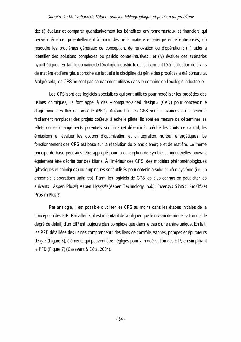
Par analogie, il est possible d’utiliser les CPS au moins dans les étapes initiales de la
conception des EIP. Par ailleurs, il est important de souligner que le niveau de modélisation (i.e. le
degré de détail) d’un EIP est toujours plus complexe que dans le cas d’une usine unique. En fait,
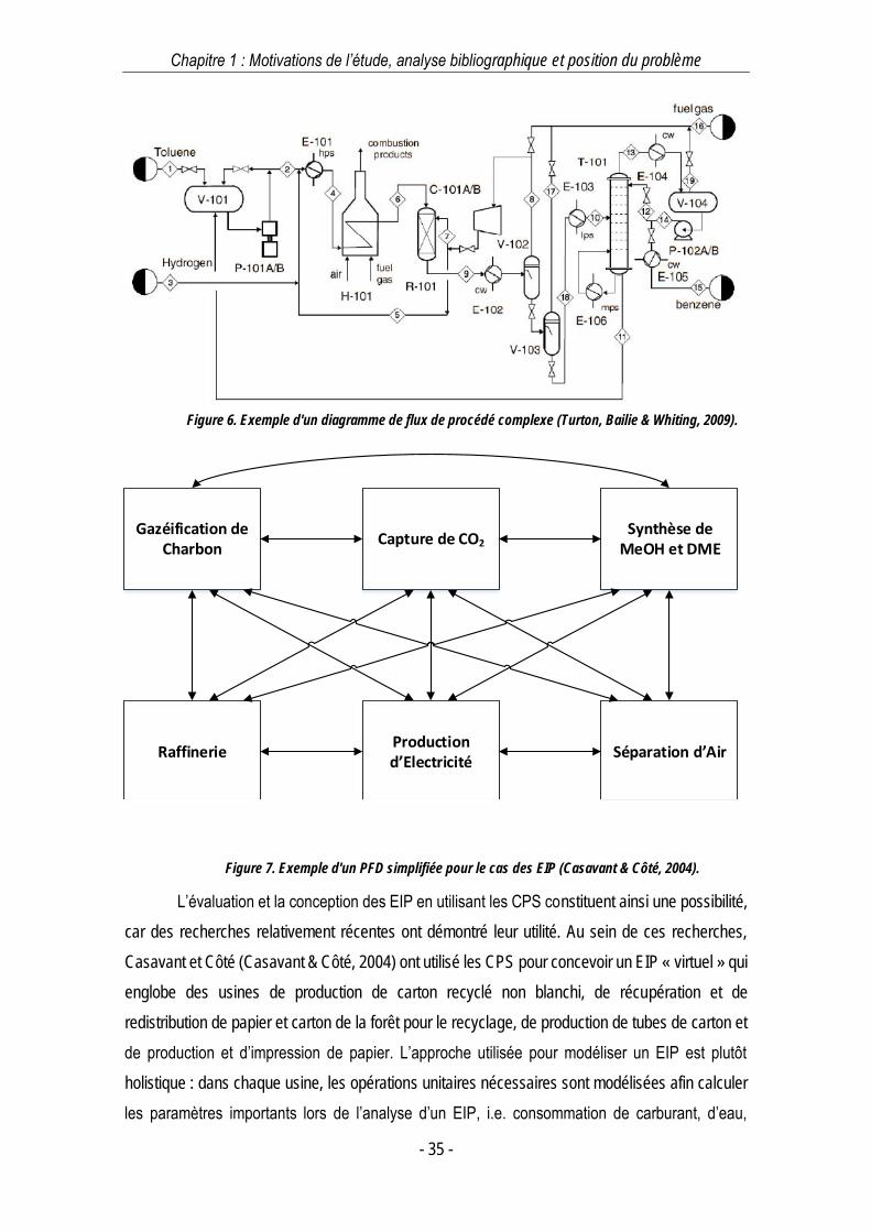
les PFD détaillées des usines comprennent : des liens de contrôle, vannes, pompes et épurateurs
de gaz (Figure 6), éléments qui peuvent être négligés pour la modélisation des EIP, en simplifiant
le PFD (Figure 7) (Casavant & Côté, 2004).
Chapitre 1 : Motivations de l’étude, analyse bibliographique et position du problème
- 35 -
Figure 6. Exemple d'un diagramme de flux de procédé complexe (Turton, Bailie & Whiting, 2009).
Figure 7. Exemple d'un PFD simplifiée pour le cas des EIP (Casavant & Côté, 2004).
L’évaluation et la conception des EIP en utilisant les CPS constituent ainsi une possibilité,
car des recherches relativement récentes ont démontré leur utilité. Au sein de ces recherches,
Casavant et Côté (Casavant & Côté, 2004) ont utilisé les CPS pour concevoir un EIP « virtuel » qui
englobe des usines de production de carton recyclé non blanchi, de récupération et de
redistribution de papier et carton de la forêt pour le recyclage, de production de tubes de carton et
de production et d’impression de papier. L’approche utilisée pour modéliser un EIP est plutôt
holistique : dans chaque usine, les opérations unitaires nécessaires sont modélisées afin calculer
les paramètres importants lors de l’analyse d’un EIP, i.e. consommation de carburant, d’eau,
Gazéification de Charbon
Capture de CO2
RaffinerieProduction d’Electricité
Synthèse de MeOH et DME
Séparation d’Air
Chapitre 1 : Motivations de l’étude, analyse bibliographique et position du problème
- 36 -
génération de déchets, émissions de polluants et pertes énergétiques. Dans cette étude, les
auteurs ont utilisé des analyses de sensibilité pour évaluer les connexions potentielles entre les
usines, en employant des scenarios hypothétiques.
Quelques années après, Zhang et al. (Zhang, Strømman, Solli, et al., 2008),se sont basés
sur des modèles en utilisant les CPS pour établir la planification et la conception d’un EIP à travers
une procédure en sept étapes. Les sept étapes proposées sont synthétisées ici :
1. Analyse des buts et des opportunités de former l’EIP.
2. Inventaire et analyse des activités existantes sur le site en considérant des dimensions
techniques, sociales et analyse du marché.
3. Identification de nouvelles activités potentielles, basée sur les résultats des étapes 1 et 2.
4. Conception de la structure préliminaire de l’EIP.
5. Modélisation et simulation des composants de l’EIP en utilisant les CPS.
6. Analyse de sensibilité des variables et des paramètres clés de chaque procédé ainsi que
ceux de l’EIP global, afin d’identifier les impacts que sur la performance d’un procédé, des
autres procédés et par conséquence sur l’EIP entier.
7. Proposition de stratégies et de scenarios alternatifs pour améliorer la structure proposée
dans l’étape 4.
Grâce aux étapes décrites ci-dessus, les auteurs ont développé une méthodologie pour la
planification et la conception initiale d’un EIP à Mongstad, en Norvège, autour d’une raffinerie de
pétrole et de gaz déjà existante. Cet EIP conceptuel comprend des usines de gazéification et de
production de syngas, de captage de CO2, de synthèse de méthanol et de DME (éther
diméthylique) ainsi qu’une usine de production combinée de chaleur et d’énergie.
Finalement, il est important de noter que la conception et l’analyse des EIP par
modélisation et simulation avec les CPS utilisent les analyses de sensibilité comme outil d’aide à
la décision. Dans ce cadre-là, les analyses de sensibilité peuvent fournir des informations
importantes mais sont surement moins efficaces qu’une solution optimale. La façon de choisir les
interconnexions de flux entre les différentes usines est primordiale, d’autant plus qu’elle est réalisée
« à la main » avec les CPS, i.e. basée uniquement sur des heuristiques plutôt que sur un support
mathématique. Un support mathématique permettant de choisir les interconnexions entre usines
peut être régi par des modèles mathématiques d’optimisation, car ce sont des décisions discrètes
plutôt que continues. Enfin, les CPS ne sont pas en capacité de traiter les décisions
Chapitre 1 : Motivations de l’étude, analyse bibliographique et position du problème
- 37 -
d’interconnexions (discrètes), puisqu’elles n’interagissent qu’avec des variables continues (e.g.
débits, composition, température des courants…).
C’est pour ces raisons que les méthodes basées sur les CPS sont plutôt des outils qui
servent à l’analyse lors de la première phase de conception des EIP. Dans ce cas, ils ont alors
comme principale finalité l’obtention de données opératoires des différentes usines composant
l’EIP. En mettent en œuvre les différents flowsheets des procédés et en les simulant, les conditions
opératoires peuvent être déterminées, e.g. la température et la composition des courants. Ces
informations, peuvent être utilisées a posteriori dans les modèles mathématiques d’optimisation.
En conclusion, les CPS ne sont pas en capacité de résoudre la problématique énoncée auparavant
puisque la simulation n’est pas en capacité de satisfaire de façon simultanée tous les critères dont
la conception d’un EIP fructueux en a besoin.
2.2. Conception par optimisation mathématique
La programmation mathématique est un outil très pertinent pour la conception et
l’évaluation des EIP. Elle conduit à la détermination des « meilleures » ou même dans certains cas
de la meilleure solution parmi un très grand ensemble de possibilités (Biegler, Grossmann &
Westerberg, 1997; Biegler, 2010; Himmelblau, 1989). Des algorithmes spécifiques sont utilisés afin
de générer cet ensemble de solutions répondant à des contraintes précises et satisfaisant une ou
plusieurs fonctions objectif.
Dans le cadre de la conception des EIP, l’optimisation globale du système est liée au
modèle mathématique de chaque acteur de l’EIP, il est donc possible d’utiliser des modèles basés
sur les CPS ou en fonction des cas, ajuster le niveau de détail qui peut être plus ou moins
complexe. En fait, l’optimisation peut être considérée comme le niveau supérieur de la simulation
dans le cadre de la conception des EIP, mais aussi des procédés chimiques et des usines
conventionnelles. Le but est d’obtenir les réseaux optimaux des échanges entre les différentes
usines/entreprises en modélisant les décisions discrètes et/ou hiérarchisées, à la différence des
méthodes basées uniquement sur la simulation (CPS).
L’état de l’art sur les méthodes utilisées pour la conception des EIP par optimisation est
traité en détail dans les sections suivantes (section 3) car elles constituent le socle de base pour
l’objectif principal de ces travaux de thèse.
Chapitre 1 : Motivations de l’étude, analyse bibliographique et position du problème
- 38 -
2.3. Autres techniques
2.3.1. Évaluation basée sur les indicateurs
Hormis les méthodes de conception, l’évaluation des EIP existants ou des solutions
proposées constitue un volet important puisqu’elle permet d’analyser les éventuels problèmes.
Parmi les techniques liées à l’évaluation plutôt qu’à la conception des EIP, la mise en œuvre
d’indicateurs afin d’évaluer la durabilité et/ou la faisabilité d’un EIP proposé est la plus utilisée. Ces
indicateurs sont surtout orientés vers une évaluation de la durabilité de l’EIP, dans le cadre des
impacts environnementaux, de l’utilisation d’énergie et de la performance économique. En fait,
certains travaux combinent l’utilisation des indicateurs avec les modèles d’optimisation ou les outils
de simulation de procédés. Dans cette section-ci, les travaux qui utilisent exclusivement les
indicateurs pour l’évaluation et/ou conception des EIP sont seulement pris en compte.
Parmi les indicateurs de durabilité, ceux qui ont été mis en œuvre pour l’évaluation des
EIP sont : l’« émergie», qui représente la quantité d’énergie sous forme d’exergie utilisée
directement ou indirectement pour la fabrication d’un produit (Lou, Kulkarni, Singh, & Hopper 2004).
L’évaluation des EIP en utilisant le concept d’émergie ou des indicateurs dérivés de celui-ci, a
principalement été étudiée par Lou et al. (Lou, Kulkarni, Singh, & Hopper 2004) . Dans ces travaux,
les auteurs proposent plusieurs indicateurs basés sur le concept d’émergie et étudient un cas d’EIP
composé de deux usines différentes, en comparant l’indice de durabilité de l’EIP avec celui des
deux usines considérées de façon individuelle (i.e. sans interconnexions entre elles). D’autre part,
parmi les méthodes d’évaluation environnementale, une des plus utilisée est l’analyse de cycle de
vie (LCA). Il s’agit d’ une méthode permettant d’analyser les impacts environnementaux
multidimensionnels d’un produit, procédé, entreprise, ville ou pays (Mattila, Lehtoranta, Sokka, et
al., 2012). Le LCA possède un cadre méthodologique strict et des lignes directrices claires qui sont
à respecter pour l’appliquer, et ce cadre est généralement accepté par la communauté scientifique.
Parmi les travaux qui appliquent la méthode du LCA, on peut citer notamment les travaux de Sokka
et al. (Sokka, Pakarinen & Melanen, 2011), qui ont étudié la symbiose industrielle de l’industrie
papetière en Finlande, et le travail de Singh et al. (Singh, Lou, Yaws, et al., 2007), dans lequel
l’évaluation d’un EIP comprenant 18 procédés est accomplie en employant une méthode du LCA.
Enfin, via ces méthodes, des auteurs ont aussi proposé de nouveaux indicateurs plus
adaptés pour certains cas d’étude. D’autres auteurs emploient différents indicateurs pour évaluer
la durabilité d’un EIP. Okkonen (Okkonen, 2008) utilise l’indicateur d’émissions équivalentes de
CO2 par tonne de déchets, en intégrant des usines spécifiques de gestion de déchets en Finlande.
Chapitre 1 : Motivations de l’étude, analyse bibliographique et position du problème
- 39 -
D’autre part, Tiejun (Tiejun, 2010) a proposé l’utilisation de deux nouveaux indicateurs quantitatifs
pour la planification et l’évaluation des EIP. Ces indicateurs sont : un indicateur de la quantité de
connexions (i.e. une mesure de la symbiose) de l’EIP et un indicateur de la quantité de recyclage
des sous-produits et des déchets de l’EIP. Dans cette étude, ces indicateurs servent à analyser la
faisabilité et la viabilité d’un EIP potentiel (cas d’étude localisé en Chine).
3. Méthodes d’optimisation pour la conception des EIP
Cette partie est dédiée à la présentation des méthodes d’optimisation multiobjectif existant
dans la littérature. En effet, il a précédemment été démontré que les problèmes de conception, de
gestion et d’évaluation des EIP est, par essence, un problème multiobjectif. En premier lieu, les
concepts de base de l’optimisation multiobjectif seront discutés et ensuite, les différentes
catégories de méthodes de résolution seront passées en revue. Certaines méthodes de résolution
sont décrites de façon détaillée, et, à titre illustratif, une partie de celles-ci est employée pour la
résolution de trois problèmes d’optimisation relativement simples. Enfin, une comparaison entre
les résultats est réalisée, ainsi qu’une analyse sur l’efficacité des méthodes présentées.
3.1. Optimisation multiobjectif : concepts
L’optimisation multiobjectif comprend l’étude et la résolution des problèmes d’optimisation
avec plus d’une fonction objectif. Il s’agit particulièrement des problèmes d’optimisation de cas
d’études réelles, où il y a toujours plus d’un but, un critère ou un objectif. Dans la partie suivante,
la théorie mathématique des concepts de l’optimisation multiobjectif est présentée.
3.1.1. Problème d’optimisation multiobjectif
D’une façon générale, un problème d’optimisation multiobjectif a au moins deux objectifs
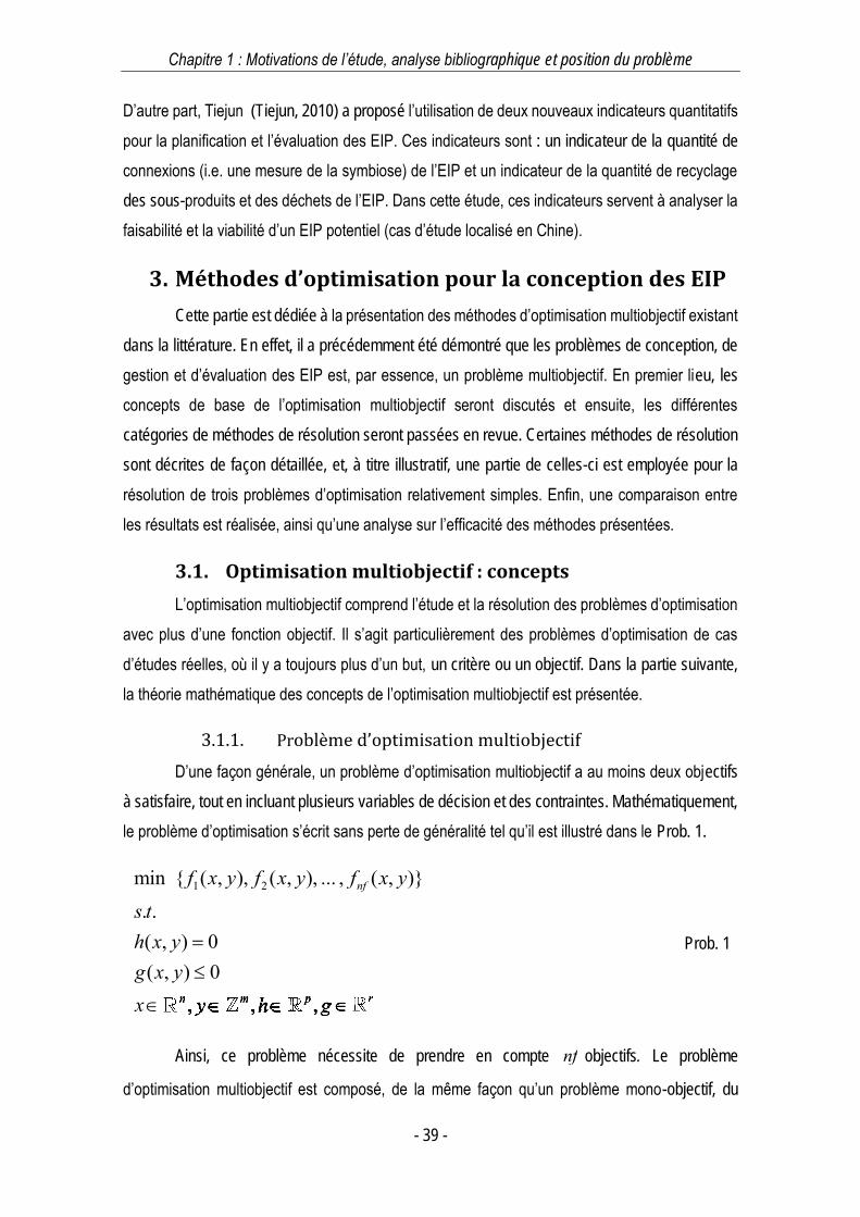
à satisfaire, tout en incluant plusieurs variables de décision et des contraintes. Mathématiquement,
le problème d’optimisation s’écrit sans perte de généralité tel qu’il est illustré dans le Prob. 1.
1 2min { ( , ), ( , ), ... , ( , )}
. .( , ) 0( , ) 0
, , ,
nf
n m p r
f x y f x y f x ys th x yg x yx y h g
n m p rx y h g, , ,x y h g, , ,n m p rx y h gn m p r n m p r n m p rx y h g x y h g, , ,x y h g, , , , , ,x y h g, , ,n m p rx y h gn m p r n m p rx y h gn m p r
Prob. 1
Ainsi, ce problème nécessite de prendre en compte nf objectifs. Le problème
d’optimisation multiobjectif est composé, de la même façon qu’un problème mono-objectif, du
Chapitre 1 : Motivations de l’étude, analyse bibliographique et position du problème
- 40 -
vecteur des variables continues (i.e. x ), du vecteur des variables discrètes (i.e. y ) et des vecteurs
des contraintes d’égalité et inégalité (i.e. ( , )h x y et ( , )g x y , respectivement).
3.1.2. La multiplicité des solutions
Dans les problèmes multiobjectif, on trouve une multitude de solutions car certains (sinon
la totalité) des objectifs sont contradictoires les uns envers les autres. Par conséquence, dans la
résolution d’un problème multiobjectif on obtient une grande quantité de solutions. Ces solutions
ne sont pas optimales au sens où elles ne minimiseront pas tous les objectifs du problème, mais
sont des solutions dites de « compromis » entre les différents objectifs, i.e. des solutions qui
minimisent un certain nombre d’objectifs tout en dégradant les performances sur d’autres objectifs
(Collette & Siarry, 2003).
3.1.3. Dominance et front de Pareto
Seul un nombre restreint de solutions obtenues constitue un intérêt pour le décideur. En
fait, pour qu’une solution soit intéressante, il faut qu’il existe une relation de dominance entre la
solution considérée et les autres solutions, dans le sens suivant (Collette & Siarry, 2003; Rangaiah
& Bonilla-Petriciolet, 2013) :
Définition : L’ensemble 1 2, ( ), ( )P P Px f x f x est dit être une solution optimale au sens de
Pareto pour le problème à deux objectifs ( 2i dans le Prob. 1) si et seulement si, il n’existe pas
d’autre vecteur x tel que 1 1 2 2( ) ( ) ( ) ( )P Pf x f x f x f x , avec l’inégalité inactive pour au
moins un des objectifs.
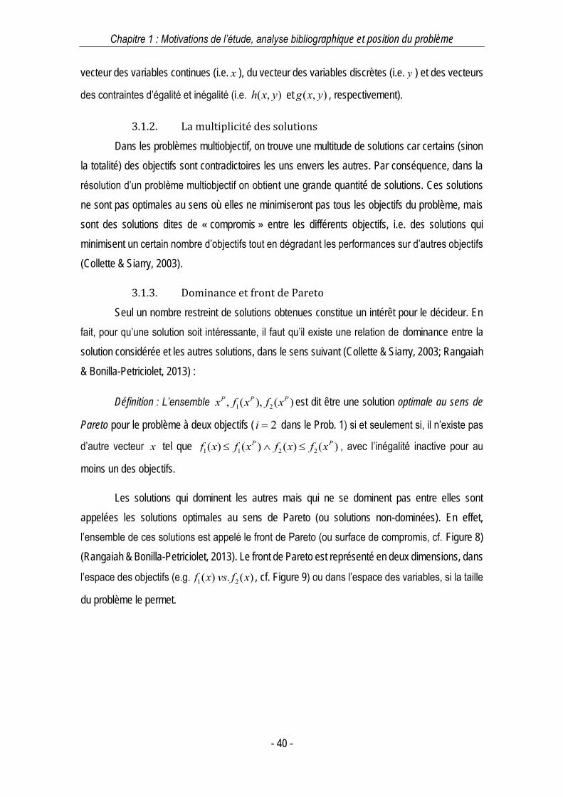
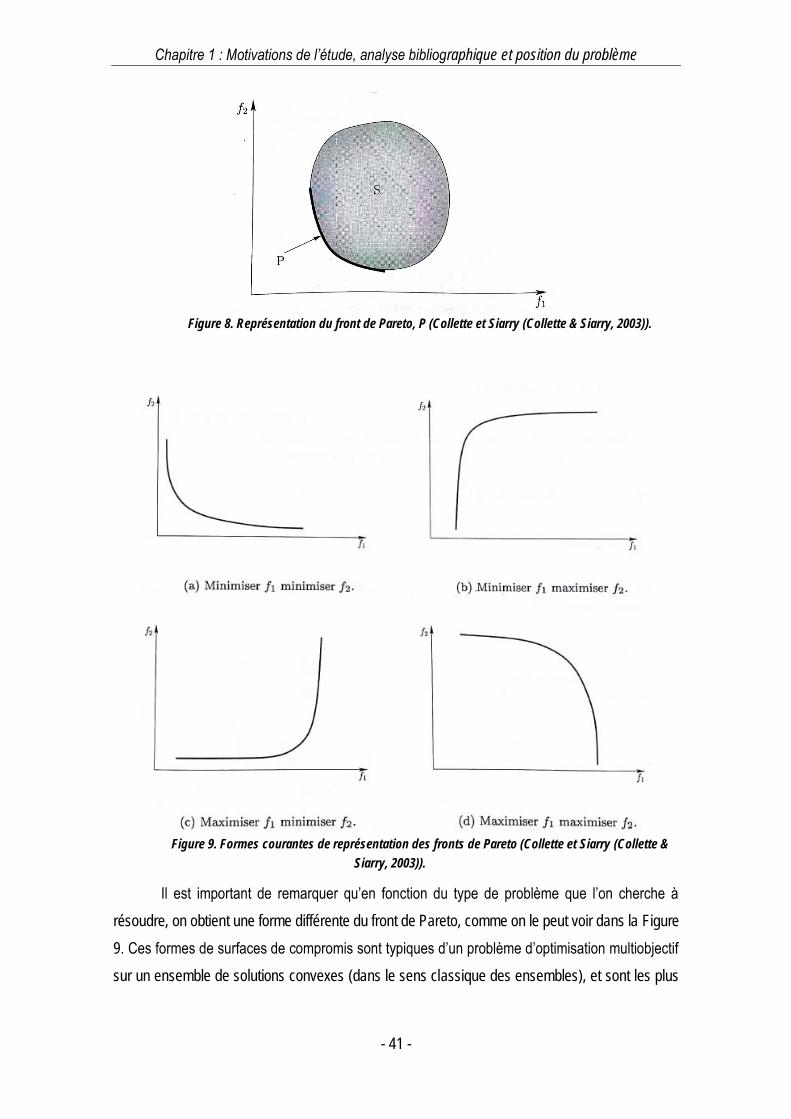
Les solutions qui dominent les autres mais qui ne se dominent pas entre elles sont
appelées les solutions optimales au sens de Pareto (ou solutions non-dominées). En effet,
l’ensemble de ces solutions est appelé le front de Pareto (ou surface de compromis, cf. Figure 8)
(Rangaiah & Bonilla-Petriciolet, 2013). Le front de Pareto est représenté en deux dimensions, dans
l’espace des objectifs (e.g. 1 2( ) . ( )f x vs f x , cf. Figure 9) ou dans l’espace des variables, si la taille
du problème le permet.
Chapitre 1 : Motivations de l’étude, analyse bibliographique et position du problème
- 41 -
Figure 8. Représentation du front de Pareto, P (Collette et Siarry (Collette & Siarry, 2003)).
Figure 9. Formes courantes de représentation des fronts de Pareto (Collette et Siarry (Collette &
Siarry, 2003)).
Il est important de remarquer qu’en fonction du type de problème que l’on cherche à
résoudre, on obtient une forme différente du front de Pareto, comme on le peut voir dans la Figure
9. Ces formes de surfaces de compromis sont typiques d’un problème d’optimisation multiobjectif
sur un ensemble de solutions convexes (dans le sens classique des ensembles), et sont les plus
Chapitre 1 : Motivations de l’étude, analyse bibliographique et position du problème
- 42 -
courantes. Cependant, on peut trouver des problèmes ou le front de Pareto présente des
discontinuités.
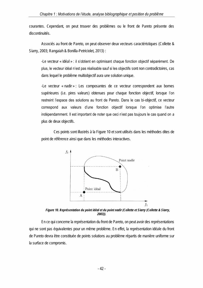
Associés au front de Pareto, on peut observer deux vecteurs caractéristiques (Collette &
Siarry, 2003; Rangaiah & Bonilla-Petriciolet, 2013) :
-Le vecteur « idéal » : il s’obtient en optimisant chaque fonction objectif séparément. De
plus, le vecteur idéal n’est pas réalisable sauf si les objectifs sont non contradictoires, cas
dans lequel le problème multiobjectif aura une solution unique.
-Le vecteur « nadir » : Les composantes de ce vecteur correspondent aux bornes
supérieures (i.e. pires valeurs) obtenues pour chaque fonction objectif, lorsque l’on
restreint l’espace des solutions au front de Pareto. Dans le cas bi-objectif, ce vecteur
correspond aux valeurs d’une fonction objectif lorsque l’on optimise l’autre
indépendamment. Il est important de noter que ceci n’est pas toujours le cas quand on a
plus de deux objectifs.
Ces points sont illustrés à la Figure 10 et sont utilisés dans les méthodes dites de
point de référence ainsi que dans les méthodes interactives.
Figure 10. Représentation du point idéal et du point nadir (Collette et Siarry (Collette & Siarry,
2003)).
En ce qui concerne la représentation du front de Pareto, on peut avoir des représentations
qui ne sont pas équivalentes pour un même problème. En effet, la représentation idéale du front
de Pareto devra être constituée de points solutions au problème répartis de manière uniforme sur
la surface de compromis.
Chapitre 1 : Motivations de l’étude, analyse bibliographique et position du problème
- 43 -
3.2. Techniques de résolution des problèmes
d’optimisation multiobjectif
Il existe un grand nombre de méthodes pour résoudre les problèmes d’optimisation
multiobjectif, et la plupart de ceux-ci impliquent la transformation du problème multicritère en une
série de problèmes monocritères.
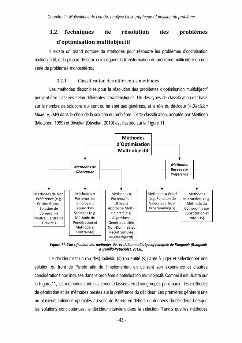
3.2.1. Classification des différentes méthodes
Les méthodes disponibles pour la résolution des problèmes d’optimisation multiobjectif
peuvent être classées selon différentes caractéristiques. Un des types de classification est basé
sur le nombre de solutions qui sont ou ne sont pas générées, et le rôle du décideur (« Decision
Maker », DM) dans le choix de la solution du problème. Cette classification, adoptée par Miettinen
(Miettinen, 1999) et Diwekar (Diwekar, 2010) est illustrée sur la Figure 11.
Figure 11. Classification des méthodes de résolution multiobjectif (adaptée de Rangaiah (Rangaiah
& Bonilla-Petriciolet, 2013)).
Le décideur est un (ou des) individu (s) (ou entité (s)) apte à juger et sélectionner une
solution du front de Pareto afin de l’implémenter, en utilisant son expérience et d’autres
considérations non incluses dans le problème d’optimisation multiobjectif. Comme il est illustré sur
la Figure 11, les méthodes sont initialement classées en deux groupes principaux : les méthodes
de génération et les méthodes basées sur la préférence du décideur. Les premières génèrent une
ou plusieurs solutions optimales au sens de Pareto en dehors de données du décideur. Lorsque
les solutions sont obtenues, le décideur intervient dans la sélection. Tandis que les méthodes
Méthodes d’Optimisation Multi-objectif
Méthodes de Génération
Méthodes Basées sur Préférence
Méthodes a Posteriori en
Utilisant Approche Multi-
Objectif (e.g. Algorithme
Génétique triée Non-Dominée et Recuit Simulée Multi-Objectif)
Méthodes de Non Préférence (e.g. Critère Global,
Solution de Compromis
Neutre, Centre de Gravité )
Méthodes a Posteriori en Employant Approches
Scalaires (e.g. Méthode de
Pondération et Méthode ε-Contrainte)
Méthodes a Priori (e.g. Function de Valeur et « Goal Programming »)
Méthodes Interactives (e.g.
Méthode du Compromis par Substitution et
NIMBUS)
Chapitre 1 : Motivations de l’étude, analyse bibliographique et position du problème
- 44 -
basées sur la préférence utilisent les préférences spécifiées par le décideur au cours des
différentes étapes pour résoudre le problème.
Les méthodes de génération sont donc divisées en trois sous-groupes, à savoir, les
méthodes de non préférence, les méthodes a posteriori en employant les approches scalaires et
enfin, les méthodes a posteriori en utilisant l’approche multiobjectif. Les premières, comment leur
nom l’indique, ne requièrent pas une spécification de priorité des objectifs. Les méthodes a
posteriori sont basées sur la transformation du problème multicritère en une série de problèmes
monocritères, qui doivent être résolus à l’optimalité afin de trouver le front de Pareto. Des exemples
de ces méthodes sont la méthode -contrainte et les méthodes de pondération.
Les méthodes a posteriori utilisent une approche multiobjectif pour classer les solutions
d’essai en se basant sur les valeurs des fonctions objectif, et finalement trouver plusieurs solutions
optimales. Celles-ci comprennent les méthodes évolutives et les méthodes stochastiques, e.g. les
algorithmes génétiques et le recuit simulé. En fait, les solutions obtenues sont ultérieurement
évaluées par le DM, qui choisit la solution à implémenter. Il est important de souligner que
l’importance du DM dans ces méthodes est essentielle, car la procédure de résolution seule n’est
pas capable de fournir une unique solution.
En deuxième lieu, les méthodes dites de préférence sont divisées en deux sous-groupes :
les méthodes a priori et les méthodes interactives. Dans les premières, les préférences du DM sont
d’abord incluses dans le problème d’optimisation multiobjectif, alors transformé en un problème
monocritère. Dans ces méthodes, on retrouve les méthodes de la fonction de valeur, l’approche
lexicographique et le « goal programming ». L’approche de la fonction de valeur implique la
formulation d’une fonction de valeur, qui inclut les objectifs originaux et les préférences du DM. La
méthode de pondération est considérée comme un cas particulier de ces méthodes. Ensuite, pour
mettre en œuvre la méthode lexicographique, le DM doit ranger les objectifs selon leur l’importance
et résoudre le problème monocritère résultant. Dans le goal programming, le DM fourni un niveau
d’aspiration pour chaque objectif (dont la réalisation est le but, ou goal) et en rajoutant des
contraintes sur ces buts, le problème est transformé en un problème monocritère équivalent.
Finalement, on trouve les méthodes interactives, qui demandent une interaction avec le
DM pendant la résolution du problème multicritère. Après chaque itération, le DM obtient la solution
Pareto-optimale et peut proposer des changements (soit amélioration, compromis ou aucun) pour
chacune des fonctions objectif. Ces préférences sont incluses dans le problème d’optimisation, qui
est résolu lors de la prochaine itération. Finalement, les méthodes interactives fournissent une ou

Chapitre 1 : Motivations de l’étude, analyse bibliographique et position du problème
- 45 -
plusieurs solutions Pareto-optimales. Des exemples de ces méthodes sont la méthode du
compromis par substitution et la méthode NIMBUS (Miettinen & Mäkelä, 2000).
En guise de résumé, le Tableau 2 récapitule les avantages et limitations relatives aux
groupes des méthodes évoquées.
Méthode Avantages Inconvénients
Méthodes de Non Préférence
Ne requièrent pas d’entrées du DM. Les
méthodes peuvent trouver une solution Pareto-
optimale proche du vecteur idéal.
Temps de calcul élevé
Méthodes a Posteriori en employant approche scalaire
La méthode de -contrainte est simple et
efficace pour les problèmes avec peu d’objectifs différents.
Résolution d’une série de problèmes d’optimisation monocritère. Il n’est pas trivial
de trouver les valeurs d’ pour la convergence du problème. La méthode de pondération n’est pas capable de trouver la
solution Pareto-optimale si la région est non-convexe. Difficile de déterminer les valeurs
des coefficients de pondération.
Méthodes a Posteriori en employant approche
Multiobjectif
Grand nombre de solutions pourvue. Rôle du DM après avoir obtenu les solutions optimales.
Presque toutes les solutions pourvues ne seront pas utilisées, donc elles sont
considérées comme une perte de temps d’un point de vue numérique. Avec des problèmes
de grande taille le temps de résolution est prohibitif.
Méthodes a Priori
Ces méthodes fournissent une solution Pareto-
optimale respectant les préférences, elles sont
donc relativement efficaces.
Requièrent les préférences du DM d’abord, ce qui peut s’avérer difficile sans bien
connaitre les valeurs des fonctions objectif.
Méthodes Interactives
Le DM joue un rôle actif pendant la résolution du problème. Puisqu’ils ne fournissent qu’une seule
ou quelques solutions Pareto-optimales, elles
sont efficaces.
Le temps passé et les efforts du DM sont nécessaires et ce n’est pas toujours possible.
Il est possible de n’explorer qu’un petit espace du front de Pareto.
Tableau 2. Caractéristiques, avantages et limitations des méthodes (adapté de Rangaiah (Rangaiah & Bonilla-Petriciolet, 2013)).
Le choix de la méthode dépend essentiellement du problème et de la modélisation
associée dans le paragraphe. Dans le cas de EIP, un concept de superstructure est envisagée.
Chapitre 1 : Motivations de l’étude, analyse bibliographique et position du problème
- 46 -
4. Modèles spécifiques d’optimisation pour la
conception des EIP
4.1. Le concept de superstructure dans les EIP
L’utilisation de programmes mathématiques pour la conception et l’intégration de procédés
consiste en la réalisation de trois étapes majeures, selon Biegler et al. (Biegler, Grossmann &
Westerberg, 1997) et Grossmann et al. (Grossmann, Caballero & Yeomans, 1999) :
La représentation de toutes les possibilités parmi lesquelles la solution optimale est
extraite. Il s’agit, par définition, de l’élaboration d’une superstructure.
La formulation d’un modèle mathématique incluant généralement des variables discrètes
et continues. Les principaux composants d’un modèle sont : a) les critères à optimiser qui
s’expriment sous forme d’une fonction mathématique et b) les contraintes qui peuvent être
soit de type égalité, soit inégalité.
La résolution du modèle mathématique afin de déterminer une ou plusieurs solutions
optimales.
Dans un premier temps, il est donc indispensable d’approfondir et de clarifier le concept
de superstructure, qui représente la base des modèles de conception des EIP.
Une superstructure est définie de façon générale comme une approche systématique de
représentation modulaire de l’ensemble de toutes les connexions possibles pour un réseau défini,
e.g. de matière et/ou d’énergie (Biegler, Grossmann & Westerberg, 1997; Yeomans & Grossmann,
1999; Ahmetović & Grossmann, 2011; Papalexandri & Pistikopoulos, 1996). Des modèles
mathématiques et d’optimisation sont ensuite employés afin de trouver un réseau optimal parmi
l’ensemble de ces représentations. Les questions posées sont : (i) A partir d’un ensemble de
possibilités qui doivent être analysées, quels sont les principaux types de représentations pouvant
être utilisés et quelles sont leurs implications sur la modélisation mathématique ? (ii) Pour une
représentation donnée et sélectionnée, quelles sont les différentes propriétés garantissant que
l’optimum global soit atteint ?
Ainsi, un exemple de superstructure générale pour la conception d’un EIP est représenté
dans la Figure 12. Il est important de noter que cette représentation est une superstructure d’un
EIP potentiel basée uniquement sur les échanges d’eau entre entreprises, mais elle pourrait
également être étendue à tout type d’échanges comme les échanges d’énergie et de matières
premières.
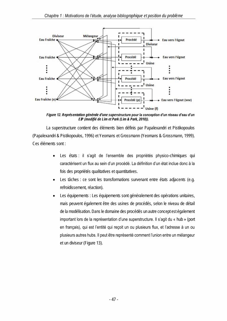
Chapitre 1 : Motivations de l’étude, analyse bibliographique et position du problème
- 47 -
Figure 12. Représentation générale d'une superstructure pour la conception d’un réseau d’eau d’un
EIP (modifié de Lim et Park (Lim & Park, 2010)).
La superstructure contient des éléments bien définis par Papalexandri et Pistikopoulos
(Papalexandri & Pistikopoulos, 1996) et Yeomans et Grossmann (Yeomans & Grossmann, 1999).
Ces éléments sont :
Les états : il s’agit de l’ensemble des propriétés physico-chimiques qui
caractérisent un flux au sein d’un procédé. La définition d’un état inclue donc à la
fois des propriétés qualitatives et quantitatives.
Les tâches : ce sont les transformations survenant entre états adjacents (e.g.
refroidissement, réaction).
Les équipements : Les équipements sont généralement des opérations unitaires,
mais peuvent également être des usines de procédés, selon le niveau de détail
de la modélisation. Dans le domaine des procédés un autre concept est également
important lors de la représentation d’une superstructure. Il s’agit du « hub » (port
en français), qui est l’entité qui reçoit un ou plusieurs flux, et l’adresse à un ou
plusieurs autres hubs. Il peut être représenté comment l’union entre un mélangeur
et un diviseur (Figure 13).
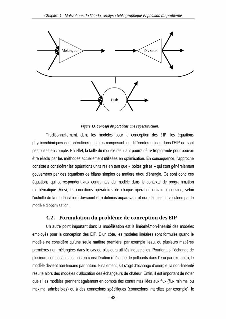
Chapitre 1 : Motivations de l’étude, analyse bibliographique et position du problème
- 48 -
Figure 13. Concept du port dans une superstructure.
Traditionnellement, dans les modèles pour la conception des EIP, les équations
physico/chimiques des opérations unitaires composant les différentes usines dans l’EIP ne sont
pas prises en compte. En effet, la taille du modèle résultant pourrait être trop grande pour pouvoir
être résolu par les méthodes actuellement utilisées en optimisation. En conséquence, l’approche
consiste à considérer les opérations unitaires en tant que « boites grises » qui sont généralement
gouvernées par des équations de bilans simples de matière et/ou d’énergie. Ce sont donc ces
équations qui correspondent aux contraintes du modèle dans le contexte de programmation
mathématique. Ainsi, les conditions opératoires de chaque opération unitaire (ou usine, selon
l’échelle de la modélisation) devraient être définies auparavant et non définies ni calculées par le
modèle d’optimisation.
4.2. Formulation du problème de conception des EIP
Un autre point important dans la modélisation est la linéarité/non-linéarité des modèles
employés pour la conception des EIP. D’un côté, les modèles linéaires sont formulés quand le
modèle ne considère qu’une seule matière première, par exemple l’eau, ou plusieurs matières
premières non mélangées dans le cas de plusieurs utilités industrielles. Pourtant, si l’échange de
plusieurs composants est pris en considération (mélange de polluants dans l’eau par exemple), le
modèle devient non-linéaire par nature. Finalement, s’il s’agit d’échange d’énergie, la non-linéarité
résulte alors des modèles d’allocation des échangeurs de chaleur. Enfin, il est important de noter
que si les modèles prennent également en compte des contraintes liées aux flux (flux minimal ou
maximal admissibles) ou à des connexions spécifiques (connexions interdites par exemple), le
Mélangeur Diviseur
Hub
Chapitre 1 : Motivations de l’étude, analyse bibliographique et position du problème
- 49 -
modèle intégrerait en plus une partie liée aux décisions discrètes par l’introduction de variables
binaires.
4.3. Aspect multiobjectif lié à la conception des EIP
Il n’existe pas de réponse triviale concernant le choix de la fonction objectif relative aux
modèles d’optimisation pour la conception des EIP. En fait, il s’agit d’une des questions les plus
étudiées dans le contexte de l’écologie industrielle. Ceci est dû au fait que, un parc étant constitué
de plusieurs entreprises, il s’agit d’un problème d’intégration où au minimum deux agents sont en
concurrence avec différents intérêts qui sont, en général, antagonistes. Le problème de conception
d’un EIP est, par conséquence, un problème de nature multicritère, dans lequel une fonction
objectif (i.e. optimisation monocritère) ne peut pas être bien définie et établie comme la fonction
objectif absolue. Dans cette optique, plusieurs auteurs (Boix, 2011; Boix, Montastruc, Pibouleau,
et al., 2011; Boix, Montastruc, Azzaro-Pantel, et al., 2015) ont montré que l’optimisation multicritère
restait à ce jour la façon la plus correcte de formuler le problème de conception des EIP, dans le
but de concevoir avec succès des EIP durables et compétitifs économiquement (Boix, Montastruc,
Azzaro-Pantel, et al., 2015).
Les deux principaux objectifs qui sont retenus sont, de façon générale, l’environnement et
l’économie. D’une part, l’intérêt dit « environnemental » est caractérisé par la minimisation des
impacts environnementaux (baisse des consommations de matières premières) et la minimisation
des émissions de polluants dans l’environnement. D’autre part, l’intérêt économique, quant à lui,
est directement lié aux bénéfices économiques que peuvent engendrer les entreprises lorsqu’elles
participent à une symbiose industrielle. En d’autres termes, l’intérêt des agents industriels est
économique et une entreprise ne participera pas à une symbiose industrielle si cela conduit à des
pertes monétaires par rapport au cas où elle opèrerait de façon autonome.
4.4. Études antérieures portant sur l’optimisation des EIP
L’absence de méthodologies systématiques pour gérer l’aspect conflictuel des fonctions
objectif (Erol & Thöming, 2005) lors de la conception des EIP a largement été mise en évidence.
Un état de l’art de travaux sélectionnés et classifiés par type de système étudié est donc l’objet de
cette section. Cela dit, un état des lieux plus complet et relatif à chaque partie de la thèse est
également contenu dans chaque article qui la compose. Les études d’optimisation recensées pour
la conception des EIP portent généralement sur deux principaux types de réseaux généralement
étudiés séparément : les réseaux d’eau et les réseaux d’énergie et de chaleur.

Chapitre 1 : Motivations de l’étude, analyse bibliographique et position du problème
- 50 -
En ce qui concerne l’optimisation des réseaux d’échanges d’énergie et de chaleur dans
les EIP, très peu d’études ont été recensées. Une des premières études sur ce sujet est celle de
Fichtner et al. (Fichtner, Frank & Rentz, 2004) qui ont développé un outil basé sur la programmation
mathématique pour le partage d’énergie entre entreprises, tout en maintenant la production
constante. Le modèle est formulé comme un MILP (Mixed Integer Linear Programming) multi-
période avec pour fonction objectif la minimisation du coût total annualisé. Plus tard, Chae et al.
(Chae, Kim, Yoon, et al., 2010) ont centré leur étude sur la symbiose industrielle d’un EIP en créant
un réseau d’échange de chaleur à travers un modèle MILP sur un cas d’étude potentiel en Corée
du Sud. Trois fonctions objectif ont été prises en compte séparément : le coût total, le coût
supplémentaire lié à la consommation de carburant et la flexibilité du réseau. Dans tous les
scénarios étudiés, les résultats démontrent des améliorations significatives et une réduction de
l’énergie consommée. Finalement, Boix et al. (Boix & Montastruc, 2011) ont réalisé l’optimisation
multiobjectif d’un EIP pour la conception d’un réseau d’eau et d’énergie et ont démontré que les
gains sur la consommation énergétique pouvaient aller jusqu’à 12% par rapport au cas où les
industries sont autonomes. Finalement, dans une étude qui intègre l’analyse de cycle de vie et
l’optimisation, Kantor et al. (Kantor, Fowler & Elkamel, 2012) ont modélisé un EIP composé de
différentes usines de production avec un modèle linéaire simple. Le modèle comprenait une seule
fonction objectif dans laquelle différents poids avaient été affectés pour la partie environnementale
et pour la partie des bénéfices économiques.
Par rapport aux échanges d’énergie, l’étude des réseaux d’eau au sein des EIP est
beaucoup plus répandue. Le point de départ de ces études est le travail de Olesen and Polley
(Olesen & Polley, 1996) où une seule usine comportant 15 procédés a été divisée en trois
différentes entités qui composent l’EIP. Dans cette étude, cet EIP utopique a été optimisé en
utilisant l’analyse du pincement appliquée aux échanges en eau. Plus tard, d’autres auteurs ont
repris cette étude en utilisant des modèles d’optimisation pour la minimisation de la consommation
d’eau dans les EIP : Geng et al. (Geng, Côté & Tsuyoshi, 2007) et Lovelady et al. (Lovelady, El-
Halwagi & Krishnagopalan, 2007 ; Lovelady & El-Halwagi, 2009) notamment. Boix et al. (Boix,
Montastruc, Pibouleau, et al., 2012) ont également réalisé une optimisation multiobjectif en prenant
en compte la minimisation de la consommation d’eau fraîche, le cout représenté par le coût de
traitement de l’eau polluée et le nombre de connexions avec la méthode d’ -contrainte. Cette
approche a permis la génération d’un front de Pareto couplée à une prise de décision avec la
méthode TOPSIS. Ensuite, Montastruc et al. (Montastruc, Boix, Pibouleau, et al., 2013) a continué
l’étude de Boix et al. (Boix, Montastruc, Pibouleau, et al., 2012) en examinant le degré de flexibilité
Chapitre 1 : Motivations de l’étude, analyse bibliographique et position du problème
- 51 -
permis par les niveaux de polluants. Des scénarios d’évolution des niveaux de productivité des
différentes entreprises ont également été explorés dans cette étude qui a conclu que les réseaux
mis en œuvre demeuraient très peu flexibles. Rubio-Castro et al. (Rubio-Castro, Ponce-Ortega,
Nápoles-Rivera, et al., 2010 ; Rubio-Castro, Ponce-Ortega, Serna-González, et al., 2011 ; Rubio-
Castro, Ponce-Ortega, Serna-González, et al., 2012), quant à eux, ont optimisé le coût total de
l’EIP annualisé pour différents cas d’étude en incluant les coûts de capital, les coûts des
connexions et canalisations et même des équipements. Les types de systèmes de livraison et de
stockage au sein des réseaux ont été finalement étudiés par Chew et al. (Chew, Tan, Ng, et al.,
2008) en étudiant, à travers un modèle mathématique, l’impact de la modélisation des EIP avec un
schéma direct (usine vers usine) versus indirect (échanges inter-entreprises uniquement via un
intercepteur).
Selon Kastner et al. (Kastner, Lau & Kraft, 2015), un des verrous récemment étudié est
comment, dans un système déjà établi, distribuer les gains de façon équitable. En effet, si le
système proposé permet de diminuer l’utilisation des ressources tout en n’étant pas en capacité
de fournir des économies pour les entreprises incluses dans la symbiose, le schéma de
coopération ne pourrait pas être adopté. En termes d’optimisation, une alternative intéressante et
récemment appliquée au cas de la conception des EIP est la théorie des jeux. À travers cette
approche, Lou et al. (Lou, Kulkarni, Singh, et al., 2004) ont mis en œuvre un modèle basé sur
l’émergie pour déterminer les conditions opératoires des usines intégrées. Ainsi, Hiete et al. (Hiete,
Ludwig & Schultmann, 2012) ont réalisé une intégration énergétique à l’aide de la théorie des jeux.
Une autre application a été réalisée par Chew et al. (Chew, Tan, Foo, et al., 2009) qui ont utilisé la
théorie des jeux pour l’analyse de configurations obtenues afin de maintenir un niveau de
satisfaction élevé pour les entreprises de l’EIP. Enfin, des modèles de logique floue ont été mis en
œuvre par Aviso et al. (Aviso, Tan & Culaba, 2009) qui ont optimisé simultanément les niveaux de
satisfaction de différentes usines. Ces auteurs ont ensuite étendu leur étude sur un modèle bi-
niveau dans lequel ils ont introduit le concept d’organisateur de l’EIP au niveau supérieur. Ce
régulateur ou organisateur est celui qui gère l’aspect environnemental de l’EIP alors que les usines,
au niveau inférieur du modèle, minimisent leur coût.
5. Problématique et motivations
Suite à l’analyse de la littérature précédemment présentée, deux aspects fondamentaux
n’ont pas encore été évoqués :
Chapitre 1 : Motivations de l’étude, analyse bibliographique et position du problème
- 52 -
Le premier concerne le niveau de détail fourni : en effet, la plupart des études
partent du principe que les informations détaillées sur les flux de procédé, les
niveaux de polluant, la température et autres propriétés intéressantes sont
fournies et que ces informations sont toujours disponibles pour toutes les
entreprises qui veulent intégrer l’EIP (Kastner, Lau & Kraft, 2015). Cependant,
pour la majorité des EIP existants ou potentiels, cette supposition est très
optimiste, en particulier quand les entreprises sont concurrentes sur un marché.
En fait, ceci est directement lié à la confidentialité industrielle, pratique
qu’empêche les autres entreprises de se procurer des informations relatives à la
production de leurs concurrents. En conséquence, l’utilité des méthodes
énoncées ci-dessus est compromise, car l’applicabilité de la majorité de ces
méthodes repose sur la connaissance de toutes les données.
D’autre part, les méthodes d’optimisation multiobjectif ne sont pas en mesure de
fournir une méthodologie systématique pour la conception « optimale » au sens
propre du concept. L’intervention d’un décideur externe pour choisir la « meilleure
solution » est une étape obligatoire avec ces méthodes. Le décideur choisit alors
parmi un ensemble de solutions grâce à des arguments de préférence ou
stratégiques. La subjectivité du décideur est très importante dans ces méthodes
et, par le manque d’arguments de poids ou soutenus par des théories
mathématiques, les entreprises pourraient refuser des réseaux proposés par les
régulateurs ou les décideurs.
L’objectif général de ce travail s’inscrit donc dans la catégorie de l’identification et de
l’analyse de la faisabilité des EIP, car il consiste à concevoir, en utilisant des techniques
d’optimisation, les EIP d’une façon durable. La démarche adoptée vise à concevoir une allocation
optimale des réseaux de matière, énergie et utilités. Cela consiste à définir les différents courants
(de matière et énergie) liant toutes les unités/usines/entreprises entre elles. En outre, il s’agit
également de choisir le niveau de modélisation des procédés ainsi que d’analyser l’impact du détail
de la modélisation sur les résultats obtenus. Pour que la symbiose fonctionne, il faut prendre en
compte les contraintes imposées par les acteurs mais aussi leurs différents objectifs et que tous
soient satisfaits. Ainsi, ce travail vise à proposer une solution liée au problème de confidentialité et
à faciliter la prise de décision lors de la conception des EIP. L’approche proposée est inspirée de
la théorie des jeux et vise à apporter alors une réponse efficace aux nombreux problèmes
environnementaux évoqués précédemment. En effet, par l'introduction d'un designer/régulateur qui
Chapitre 1 : Motivations de l’étude, analyse bibliographique et position du problème
- 53 -
ne sera pas placé, dans le modèle, au même niveau que les industries, les problèmes de
confidentialité sont alors éliminés. Ce designer/régulateur est en charge de la minimisation de
l'impact environnemental de l'écoparc. Cette approche permet ainsi de respecter les aspects de
confidentialité tout en favorisant les échanges inter-entreprises. Elle propose aussi un modèle
parfaitement adapté à l'optimisation de chacun des objectifs des différents acteurs de l'écoparc. Le
but est d’atteindre une satisfaction maximale pour chaque entité tout en respectant leur critère de
compétitivité et en respectant la confidentialité des données.
Ainsi, l’objectif est de favoriser la création d’écosystèmes industriels par des méthodes
d'optimisation de façon à réduire les impacts environnementaux des activités de production. Cette
thèse propose de développer des arguments techniques permettant de convaincre les différents
acteurs de coopérer afin d’accroitre la compétitivité/ l’attractivité des sites industriels puisque les
échanges optimaux permettront de diminuer les coûts de fabrication (énergie, matières) et d’ouvrir
vers de nouveaux marchés. L’aspect multi-échelles est ici fondamental car c’est à chacune des
échelles (procédé, site industriel, territoire) que des efforts doivent être faits et que l’optimisation
doit être réalisée, à l’image des écosystèmes naturels. De fait, dans ce travail, les échanges entre
procédés au sein d’une même entreprise (flux intermédiaires) seront optimisés de même que les
flux inter-entreprises. C’est à chaque échelle que la conception sera réalisée de façon optimale et
pas seulement sur les flux finaux, contrairement à la plupart des exemples de la littérature.
Dans cette optique, ce travail prend comme point de départ la thèse de Boix (Boix, 2011)
dans lequel le développement d’une stratégie multiobjectif d’optimisation a été mise en place en
utilisant la méthode -contrainte pour construire le front de Pareto du problème. Ensuite, un outil
de décision a posteriori a permis de trouver la solution de « compromis » entre les différentes
fonctions objectif. Bien que plusieurs travaux aient employé des méthodologies similaires, des
problèmes numériques sont rapidement apparus, plus spécifiquement lorsque les modèles sont de
grande taille et complexes. En effet, ils contiennent alors un grand nombre de variables et
notamment des variables binaires qui rendent la résolution des différents problèmes d’optimisation
à traiter plus difficile. Cela est un défi très important dans les problèmes de conception des EIP,
car les modèles impliqués sont souvent de grande taille. Par conséquent, dans ce travail on vise
en premier lieu à explorer des méthodes de résolution alternatives plus performantes et qui
s’adaptent mieux à la nature des modèles multicritères pour la conception des EIP.
A priori, les méthodes d’optimisation multiobjectif requièrent toujours des préférences
retenues par le décideur. Donc, une alternative très intéressante et potentiellement envisageable
Chapitre 1 : Motivations de l’étude, analyse bibliographique et position du problème
- 54 -
pour la conception optimale des EIP est liée à la théorie des jeux et notamment au concept
d’équilibre, au sens de Stackelberg et au sens de Nash. Dans cette structure, chaque leader définit
sa stratégie correspondante en prédisant d'abord le comportement de chaque follower et la
stratégie correspondante de l'autre leader. D’ailleurs tous les followers, choisissent simultanément
leurs stratégies en se basant sur la stratégie adoptée par les leaders et les stratégies des autres
followers. Ainsi, cette structure détermine un équilibre de Stackelberg entre les leaders et les
followers et un équilibre de Nash parmi les leaders et les followers (Kulkarni & Shanbhag, 2014).
En fait, un EIP peut être vu comme la congrégation de différents agents « non-coopératifs », (i.e.
les entreprises), qui entrent en « compétition » vis-à-vis des ressources naturelles et qui ont
comme objectif de minimiser leurs coûts opératoires annualisés ; ils jouent alors un jeu de Nash.
Par ailleurs, on peut également envisager un régulateur ou une autorité du parc, qui veille à la
minimisation des ressources et/ou aux émissions polluantes ; ce régulateur joue alors un jeu de
Stackelberg avec les différentes entreprises. Ce type de jeu Stackelberg-Nash est très intéressant
pour la conception d’EIP car le souci de confidentialité entre les entreprises pourrait ainsi être
surmonté. En effet, le régulateur est vu comme une autorité impartiale qui pourrait avoir accès à
toutes les données nécessaires pour réussir la conception/intégration de l’EIP tandis que les
entreprises pourraient garder leurs informations confidentielles sans les partager avec les autres.
Dans le contexte des jeux de Nash bi-niveaux non-coopératifs, une seule solution pour la
conception et la gestion d’un EIP peut être obtenue et elle correspond à l’ équilibre au sens de
Nash et Stackelberg (Leyffer & Munson, 2010; Kulkarni & Shanbhag, 2014). Par définition, dans
cette solution, aucun agent ne peut se dévier unilatéralement pour obtenir des bénéfices,
puisqu’une déviation de l’un des acteurs entraine toujours une détérioration de son propre objectif.
Dans le contexte des EIP et par rapport aux solutions obtenues avec des modèles
multiobjectif classiques, dans une solution équilibrée au sens de Nash, aucune des entreprises ne
serait motivée pour changer sa stratégie de façon unilatérale. L’équilibre de Nash est la solution
déterminée par un ensemble de stratégies individuelles dans lesquelles chaque agent choisit sa
stratégie optimale en fonction des stratégies optimales choisies par les autres joueurs, ceci est
clairement un point crucial dans la conception optimale des EIP. D’autre part, au sens du jeu de
Stackelberg, l’équilibre représente le choix des leaders parmi les équilibres de Nash des followers.
Ce type de problème est modélisé de façon générale comme un problème multi-leader-multi-
follower game (MLMFG), où les rôles des leaders et followers dépendent des priorités de l’EIP,
ceci est expliqué en détail dans les articles qui composent cette thèse. Ces différents types de
modèles sont constitués par des formulations mathématiques bien définies et complexes, et les

Chapitre 1 : Motivations de l’étude, analyse bibliographique et position du problème
- 55 -
solutions qui en résultent n’ont pas besoin de l’introduction d’un décideur, comme dans le cas des
modèles multiobjectif.
Par analogie avec cet exemple, un modèle MLMFG pour la conception d‘un EIP peut être
représenté par un régulateur du parc garant de l’aspect environnemental introduit comme agent
leader et les entreprises cherchant à minimiser leur coût comme agents followers. On notera que
cette affectation des joueurs peut être inversée, sujet qui est traité dans l’article 3 de ce travail. Cet
exemple est illustré dans la Figure 14.
Figure 14. Exemple de la modélisation d'un EIP par MLMFG.
Cette étude représente donc une approche originale pour la conception des écoparcs car
il implique à la fois le développement d’une nouvelle méthodologie couplée à une vision élargie
des écosystèmes étudiés. Les équilibres de Nash/Stackelberg modélisés via des problèmes multi-
niveaux couplés à l’optimisation multiobjectif sont des aspects n’ayant pas été explorés dans les
études antérieures pour la conception des écoparcs. Cette méthodologie pourrait permettre
d’étudier un volet important qui est la notion de flexibilité des solutions proposées et d’agilité des
écosystèmes en cas de variabilité de la production d’un ou de plusieurs acteurs. À travers des
études de cas concrets, cette approche permettra également de tester les méthodes développées
dans ce projet. Enfin, la vision étendue des écoparcs à un écosystème regroupant différents types
d’entités n’a jamais fait l’objet d’étude quantitative d’optimisation. Ce travail permettra ainsi
Chapitre 1 : Motivations de l’étude, analyse bibliographique et position du problème
- 56 -
d’explorer les types d’interconnexions disponibles avec différents acteurs et de multiplier les types
d’échanges (eaux, énergies, matières...).
6. Composition de la thèse
Comme il a été énoncé auparavant, le point de départ de cette thèse est celle de Boix
(Boix, 2011) ainsi que l’analyse bibliographique de Boix et al. (Boix, Montastruc, Azzaro-Pantel, et
al., 2015). En premier lieu, les modèles d’optimisation multiobjectif des réseaux d’eau et/ou
d’énergie ont été développés, étudiés puis étendus à la conception des EIP. En conséquence, il y
a deux points importants à souligner : i) pour pouvoir établir des comparaisons par rapport aux
travaux antérieurs, ce travail s’intéresse principalement à la conception de réseaux d’eau et/ou
énergie et ii) l’ordre des articles est évolutif : la première partie de cette thèse est dédiée à l’étude
des méthodes d’optimisation multiobjectif appliquées aux réseaux d’eau (individuels et dans un
EIP), la suite des articles étudie des nouvelles méthodologies principalement liées à la théorie des
jeux.
Chaque article est directement lié à celui qui le précède et à celui qui le suit avec
l’introduction d’un outil, d’un nouveau concept ou d’une amélioration, comme cela est illustré dans
la Figure 15. Chaque chapitre de cette thèse est donc représenté par un article scientifique (paru,
accepté ou soumis) destiné à être publié dans une revue internationale avec comité de lecture. Les
articles en italique, quant à eux, sont des articles mineurs qui servent, soit comme complément
d’un article, soit comme connexion entre deux articles. Ils ont été publiés dans Computer Aided
Chemical Engineering dans le cadre des congrès PSE2015/ESCAPE25 et ESCAPE26 (European
Symposium on Computer Aided Process Engineering/Process System Engineering,
respectivement).
Comme déjà évoqué précédemment, le schéma de la Figure 15 montre que ce travail de
thèse a comme point de départ la thèse de Boix (Boix, 2011) ainsi que la revue de Boix et al. (Boix,
Montastruc, Azzaro-Pantel, et al., 2015). Ces travaux ont permis de mettre en évidence deux
problématiques : une partie directement liée aux modèles et aux méthodologies de résolution des
problèmes de conception et d’opération des EIP et un autre volet concernant l’influence des
paramètres opératoires sur le fonctionnement d’un EIP. L’article 1 de ce travail répond à la première
problématique puisqu’il vise à étudier les méthodes d’optimisation multiobjectif, et s’intéresse
notamment à la façon de résoudre les problèmes multiobjectif de manière robuste et rapide grâce
à la méthode de programmation par but (« goal programming »). Le second article a pour but
d’introduire les modèles des EIP et d’étudier sa résolution à travers le goal programming. Ce travail
Chapitre 1 : Motivations de l’étude, analyse bibliographique et position du problème
- 57 -
permet de mettre en évidence les limitations des méthodes multiobjectif pour satisfaire de façon
« acceptable » plusieurs objectifs conflictuels. C’est à partir de là que la mise en œuvre d’un
modèle basé sur la théorie des jeux est proposé. Ainsi, l’article 3 introduit le concept de
régulateur/autorité de l’EIP, un modèle MLFG basé sur la théorie des jeux introduite auparavant,
est alors mis en œuvre. Partant de ce socle que constitue l’article 3, les articles 4 et 5 explorent
respectivement l’influence des paramètres critiques à travers des plans d’expériences ainsi que
l’analyse de sensibilité sur des modèles MLFG développés dans l’article 3. Ensuite, l’article 6
propose une extension des modèles MLFG et surtout, des applications pour la conception des EIP
en traitant un cas d’étude sur la conception de réseaux d’utilités et en proposant une méthodologie
complète pour la conception des EIP. Dans cette étude, les CPS ont notamment été utilisés pour
pallier le problème du manque de données en fonction du niveau de détail de la modélisation
choisie. Ensuite, l’article 7 revient sur les réseaux d’eau et propose de rajouter les réseaux
d’énergie de façon simultanée. Ce travail met en œuvre une méthode hybride multiobjectif/théorie
des jeux en reprenant des concepts étudiés dans l’article 1. Finalement, l’article 8 représente le
point culminant de la thèse en mettant en œuvre une méthodologie purement MLMFG en
introduisant deux régulateurs/autorités pour l’EIP, l’un pour l’eau et l’autre pour l’énergie.
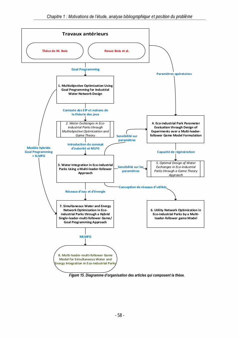
Chapitre 1 : Motivations de l’étude, analyse bibliographique et position du problème
- 58 -
Figure 15. Diagramme d’organisation des articles qui composent la thèse.
1. Multiobjective Optimization Using Goal Programming for Industrial
Water Network Design
3. Water Integration in Eco-industrial Parks Using a Multi-leader-follower
Approach
7. Simultaneous Water and Energy Network Optimization in Eco-
industrial Parks through a Hybrid Single-leader-multi-follower Game/
Goal Programming Approach
Goal Programming
Contexte des EIP et notions dela théorie des jeux
Introduction du concept d’autorité et MLFG
2. Water Exchanges in Eco-industrial Parks through
Multiobjective Optimization and Game Theory
Thèse de M. Boix
5. Optimal Design of Water Exchanges in Eco-industrial
Parks through a Game Theory Approach
Sensibilité sur lesparamètres
Paramètres opératoires
Réseaux d’eau et d’énergie
6. Utility Network Optimization in Eco-industrial Parks by a Multi-
leader-follower game Model
Conception de réseaux d’utilités
8. Multi-leader-multi-follower Game Model for Simultaneous Water and
Energy Integration in Eco-industrial Parks
MLMFG
Modèle hybrideGoal Programming
+ SLMFG
Revue Boix et al.
4. Eco-industrial Park Parameter Evaluation through Design of
Experiments over a Multi-leader-follower Game Model Formulation
Capacité de régénération
Sensibilité sur paramètres
Chapitre 1 : Motivations de l’étude, analyse bibliographique et position du problème
- 59 -
Références
Adoue, C. (2004) Méthodologie d’identification de Synergies Éco-Industrielles Réalisables
entre Entreprises sur le Territoire Français. PhD Thesis. Université de Technologie de Troyes.
Ahmetović, E. & Grossmann, I.E. (2011) Global Superstructure Optimization for the Design
of Integrated Process Water Networks. AIChE Journal. [Online] 57 (2), 434–457. Available from:
doi:10.1002/aic.12276.
Allenby, B. (2006) The Ontologies of Industrial Ecology? Progress in Industrial Ecology,
An International Journal. [Online] 3 (1/2), 28–40. Available from: doi:10.1504/PIE.2006.010039.
Ashton, W. (2008) Understanding the Organization of Industrial Ecosystems. Journal of
Industrial Ecology. [Online] 12 (1), 34–51. Available from: doi:10.1111/j.1530-9290.2008.00002.x.
Aspen Technology (n.d.) Aspen ONE. Cambridge, MA, USA, Aspen Technology.
Aviso, K.B., Tan, R.R. & Culaba, A.B. (2009) Designing Eco-Industrial Water Exchange
Networks Using Fuzzy Mathematical Programming. Clean Technologies and Environmental Policy.
[Online] 12 (4), 353–363. Available from: doi:10.1007/s10098-009-0252-1.
Biegler, L.T. (2010) Nonlinear Programming: Concepts, Algorithms, and Applications to
Chemical Processes. Philadelphia, Society for Industrial and Applied Mathematics : Mathematical
Optimization Society.
Biegler, L.T., Grossmann, I.E. & Westerberg, A.W. (1997) Systematic Methods of Chemical
Process Design. Upper Saddle River, N.J., Prentice Hall PTR.
Boix, M. (2011) Optimisation Multicritère Des Réseaux D’eau. PhD Thesis. Toulouse,
France, Université de Toulouse.
Boix, M. & Montastruc, L. (2011) Eco Industrial Parks for Water and Heat Management.
Computer Aided Chemical Engineering. [Online] 291175–1179. Available from: doi:10.1016/B978-
0-444-54298-4.50014-3.
Boix, M., Montastruc, L., Azzaro-Pantel, C. & Domenech, S. (2015) Optimization Methods
Applied to the Design of Eco-Industrial Parks: A Literature Review. Journal of Cleaner Production.
87303–317.
Boix, M., Montastruc, L., Pibouleau, L., Azzaro-Pantel, C., et al. (2011) A Multiobjective
Optimization Framework for Multicontaminant Industrial Water Network Design. Journal of
environmental management. [Online] 92 (7), 1802–1808. Available from:
doi:10.1016/j.jenvman.2011.02.016.
Boix, M., Montastruc, L., Pibouleau, L., Azzaro-Pantel, C., et al. (2012) Industrial Water
Management by Multiobjective Optimization: From Individual to Collective Solution Through Eco-
Industrial Parks. Journal of Cleaner Production. [Online] 22 (1), 85–97. Available from:
doi:10.1016/j.jclepro.2011.09.011.

Chapitre 1 : Motivations de l’étude, analyse bibliographique et position du problème
- 60 -
Casavant, T.E. & Côté, R.P. (2004) Using Chemical Process Simulation to Design
Industrial Ecosystems. Journal of Cleaner Production. [Online] 12 (8–10), 901–908. Available from:
doi:10.1016/j.jclepro.2004.02.034.
Chae, S.H., Kim, S.H., Yoon, S.-G. & Park, S. (2010) Optimization of a Waste Heat
Utilization Network in an Eco-Industrial Park. Applied Energy. [Online] 87 (6), 1978–1988. Available
from: doi:10.1016/j.apenergy.2009.12.003.
Chertow, M.R. (2000) Industrial Symbiosis: Literature and Taxonomy. Annual Review of
Energy and the Environment. [Online] 25 (1), 313–337. Available from:
doi:10.1146/annurev.energy.25.1.313.
Chew, I.M.L., Tan, R., Ng, D.K.S., Foo, D.C.Y., et al. (2008) Synthesis of Direct and Indirect
Interplant Water Network. Industrial & Engineering Chemistry Research. [Online] 47 (23), 9485–
9496. Available from: doi:10.1021/ie800072r.
Chew, I.M.L., Tan, R.R., Foo, D.C.Y. & Chiu, A.S.F. (2009) Game Theory Approach to the
Analysis of Inter-Plant Water Integration in an Eco-Industrial Park. Journal of Cleaner Production.
[Online] 17 (18), 1611–1619. Available from: doi:10.1016/j.jclepro.2009.08.005.
Collette, Y. & Siarry, P. (2003) Multiobjective Optimization: Principles and Case Studies.
Springer.
Conticelli, E. & Tondelli, S. (2014) Eco-Industrial Parks and Sustainable Spatial Planning:
A Possible Contradiction? Administrative Sciences. [Online] 4 (3), 331–349. Available from:
doi:10.3390/admsci4030331.
Diwekar, U. (2010) Introduction to Applied Optimization. 2nd edition. New York, Springer.
Erol, P. & Thöming, J. (2005) Eco-Design of Reuse and Recycling Networks by Multi-
Objective Optimization. Journal of Cleaner Production. [Online] 13 (15), 1492–1503. Available from:
doi:10.1016/j.jclepro.2005.04.008.
Fichtner, W., Frank, M. & Rentz, O. (2004) Inter-Firm Energy Supply Concepts: An Option
for Cleaner Energy Production. Journal of Cleaner Production. [Online] 12 (8–10), 891–899.
Available from: doi:10.1016/j.jclepro.2004.02.036.
Frosch, R.A. & Gallopoulos, N.E. (1989) Strategies for Manufacturing. Scientific American.
261 (3), 144–152.
Geng, Y., Côté, R. & Tsuyoshi, F. (2007) A Quantitative Water Resource Planning and
Management Model for an Industrial Park Level. Regional Environmental Change. [Online] 7 (3),
123–135. Available from: doi:10.1007/s10113-007-0026-4.
Grossmann, I.E., Caballero, J.A. & Yeomans, H. (1999) Mathematical Programming
Approaches to the Synthesis of Chemical Process Systems. Korean Journal of Chemical
Engineering. [Online] 16 (4), 407–426. Available from: doi:10.1007/BF02698263.
Chapitre 1 : Motivations de l’étude, analyse bibliographique et position du problème
- 61 -
Hiete, M., Ludwig, J. & Schultmann, F. (2012) Intercompany Energy Integration: Adaptation
of Thermal Pinch Analysis and Allocation of Savings. Journal of Industrial Ecology. [Online] 16 (5),
689–698. Available from: doi:10.1111/j.1530-9290.2012.00462.x.
Himmelblau, T.F.E.& D.M. (1989) Optimization of Chemical Processes. New Ed. McGraw-
Hill International Editions.
Jung, S., Dodbiba, G., Chae, S.H. & Fujita, T. (2013) A Novel Approach for Evaluating the
Performance of Eco-Industrial Park Pilot Projects. Journal of Cleaner Production. [Online] 3950–
59. Available from: doi:10.1016/j.jclepro.2012.08.030.
Kantor, I., Fowler, M. & Elkamel, A. (2012) Optimized Production of Hydrogen in an Eco-
Park Network Accounting for Life-Cycle Emissions and Profit. International Journal of Hydrogen
Energy. [Online] 37 (6), 5347–5359. Available from: doi:10.1016/j.ijhydene.2011.08.084.
Kastner, C.A., Lau, R. & Kraft, M. (2015) Quantitative Tools for Cultivating Symbiosis in
Industrial Parks; a Literature Review. Applied Energy. [Online] 155599–612. Available from:
doi:10.1016/j.apenergy.2015.05.037.
Kulkarni, A.A. & Shanbhag, U.V. (2014) A Shared-Constraint Approach to Multi-Leader
Multi-Follower Games. Set-Valued and Variational Analysis. [Online] 22 (4), 691–720. Available
from: doi:10.1007/s11228-014-0292-5.
Leyffer, S. & Munson, T. (2010) Solving Multi-Leader–Common-Follower Games.
Optimisation Methods & Software. 25 (4), 601–623.
Lim, S.-R. & Park, J.M. (2010) Interfactory and Intrafactory Water Network System To
Remodel a Conventional Industrial Park to a Green Eco-industrial Park. Industrial & Engineering
Chemistry Research. [Online] 49 (3), 1351–1358. Available from: doi:10.1021/ie9014233.
Lou, H.H., Kulkarni, M.A., Singh, A. & Hopper, J.R. (2004) Sustainability Assessment of
Industrial Systems. Industrial & Engineering Chemistry Research. [Online] 43 (15), 4233–4242.
Available from: doi:10.1021/ie049972w.
Lovelady, E.M., El-Halwagi, M. & Krishnagopalan, G.A. (2007) An Integrated Approach to
the Optimisation of Water Usage and Discharge in Pulp and Paper Plants. International journal of
environment and pollution. 29 (1–3), 274–307.
Lovelady, E.M. & El-Halwagi, M.M. (2009) Design and Integration of Eco-Industrial Parks
for Managing Water Resources. Environmental Progress & Sustainable Energy. [Online] 28 (2),
265–272. Available from: doi:10.1002/ep.10326.
Mattila, T., Lehtoranta, S., Sokka, L., Melanen, M., et al. (2012) Methodological Aspects of
Applying Life Cycle Assessment to Industrial Symbioses. Journal of Industrial Ecology. [Online] 16
(1), 51–60. Available from: doi:10.1111/j.1530-9290.2011.00443.x.
Miettinen, K. & Mäkelä, M.M. (2000) Interactive Multiobjective Optimization System Www-
Nimbus on the Internet. Computers & Operations Research. 27 (7), 709–723.
Chapitre 1 : Motivations de l’étude, analyse bibliographique et position du problème
- 62 -
Miettinen, K.M. (1999) Nonlinear Multiobjective Optimization. Springer.
Ministère de l’Economie et des Finances (2014) Présentation des feuilles de route des 34
plans de la nouvelle France industrielle.
Montastruc, L., Boix, M., Pibouleau, L., Azzaro-Pantel, C., et al. (2013) On the Flexibility
of an Eco-Industrial Park (EIP) for Managing Industrial Water. Journal of Cleaner Production.
[Online] 431–11. Available from: doi:10.1016/j.jclepro.2012.12.039.
Okkonen, L. (2008) Applying Industrial Ecosystem Indicators: Case of Pielinen Karelia,
Finland. Clean Technologies and Environmental Policy. [Online] 10 (4), 327–339. Available from:
doi:10.1007/s10098-007-0122-7.
Olesen, S.G. & Polley, G.T. (1996) Dealing with Plant Geography and Piping Constraints
in Water Network Design. Process Safety and Environmental Protection. [Online] 74 (4), 273–276.
Available from: doi:10.1205/095758296528626.
Panyathanakun, V., Tantayanon, S., Tingsabhat, C. & Charmondusit, K. (2013)
Development of Eco-Industrial Estates in Thailand: Initiatives in the Northern Region Community-
Based Eco-Industrial Estate. Journal of Cleaner Production. [Online] 5171–79. Available from:
doi:10.1016/j.jclepro.2012.09.033.
Papalexandri, K.P. & Pistikopoulos, E.N. (1996) Generalized Modular Representation
Framework for Process Synthesis. AIChE Journal. [Online] 42 (4), 1010–1032. Available from:
doi:10.1002/aic.690420413.
Rangaiah, G.P. & Bonilla-Petriciolet, A. (2013) Multi-Objective Optimization in Chemical
Engineering: Developments and Applications. 1st edition. Wiley.
Rubio-Castro, E., Ponce-Ortega, J.M., Nápoles-Rivera, F., El-Halwagi, M.M., et al. (2010)
Water Integration of Eco-Industrial Parks Using a Global Optimization Approach. Industrial &
Engineering Chemistry Research. [Online] 49 (20), 9945–9960. Available from:
doi:10.1021/ie100762u.
Rubio-Castro, E., Ponce-Ortega, J.M., Serna-González, M. & El-Halwagi, M.M. (2012)
Optimal Reconfiguration of Multi-Plant Water Networks into an Eco-Industrial Park. Computers &
Chemical Engineering. [Online] 4458–83. Available from:
doi:10.1016/j.compchemeng.2012.05.004.
Rubio-Castro, E., Ponce-Ortega, J.M., Serna-González, M., Jiménez-Gutiérrez, A., et al.
(2011) A Global Optimal Formulation for the Water Integration in Eco-Industrial Parks Considering
Multiple Pollutants. Computers & Chemical Engineering. [Online] 35 (8), 1558–1574. Available
from: doi:10.1016/j.compchemeng.2011.03.010.
Saikku, L. (2006) Eco-Industrial Parks: A Background Report for the Eco-Industrial Park
Project at Rantasalmi. Mikkeli, Finland: Publications of Regional Council of Etelä-Savo. 712006.
Chapitre 1 : Motivations de l’étude, analyse bibliographique et position du problème
- 63 -
Singh, A., Lou, H.H., Yaws, C.L., Hopper, J.R., et al. (2007) Environmental Impact
Assessment of Different Design Schemes of an Industrial Ecosystem. Resources, Conservation
and Recycling. [Online] 51 (2), 294–313. Available from: doi:10.1016/j.resconrec.2006.10.002.
Sokka, L., Pakarinen, S. & Melanen, M. (2011) Industrial Symbiosis Contributing to More
Sustainable Energy Use – an Example from the Forest Industry in Kymenlaakso, Finland. Journal
of Cleaner Production. [Online] 19 (4), 285–293. Available from: doi:10.1016/j.jclepro.2009.08.014.
Tiejun, D. (2010) Two Quantitative Indices for the Planning and Evaluation of Eco-Industrial
Parks. Resources, Conservation and Recycling. [Online] 54 (7), 442–448. Available from:
doi:10.1016/j.resconrec.2009.09.010.
Tudor, T., Adam, E. & Bates, M. (2007) Drivers and Limitations for the Successful
Development and Functioning of Eips (eco-Industrial Parks): A Literature Review. Ecological
Economics. [Online] 61 (2–3), 199–207. Available from: doi:10.1016/j.ecolecon.2006.10.010.
Turton, R., Bailie, R.C. & Whiting, W.B. (2009) Analysis, Synthesis, and Design of
Chemical Processes. Third. Prentice Hall.
Yeomans, H. & Grossmann, I.E. (1999) A Systematic Modeling Framework of
Superstructure Optimization in Process Synthesis. Computers & Chemical Engineering. [Online]
23 (6), 709–731. Available from: doi:10.1016/S0098-1354(99)00003-4.
Zhang, X., Strømman, A.H., Solli, C. & Hertwich, E.G. (2008) Model-Centered Approach
to Early Planning and Design of an Eco-Industrial Park Around an Oil Refinery. Environmental
science & technology. 42 (13), 4958–4963.

- 65 -
Chapitre 2 – Multiobjective Optimization Using Goal Programming
for Industrial Water Network Design

Article 1 - Multiobjective Optimization Using Goal Programming for Industrial Water Network Design
- 66 -
Article 1 - Multiobjective Optimization Using Goal Programming for Industrial Water Network Design
- 67 -
Ramos, Manuel A., Marianne Boix, Ludovic Montastruc, & Serge Domenech. 2014. “Multiobjective
Optimization Using Goal Programming for Industrial Water Network Design.” Industrial &
Engineering Chemistry Research 53 (45): 17722–17735.
Résumé
Cet article marque le début du travail de recherche de ces travaux de thèse. Il reprend les travaux
sur les réseaux d’eau industriels de Boix (Boix, 2011) en implémentant une approche d’optimisation
multiobjectif a posteriori se basant sur la méthode du goal programming (GP). Outre les aspects
méthodologiques, cette étude vise à démontrer la pertinence de l’utilisation du goal programming
dans le contexte des réseaux d’eau industriels en comparant cette méthodologie à d’autres
méthodes d’optimisation multiobjectif, parmi lesquelles, des méthodes à posteriori couplées avec
des outils d’aide à la décision (TOPSIS). Un état de l’art sur la modélisation et la résolution des
problèmes multiobjectif a d’abord été réalisé. Ensuite, les différentes méthodes sont testées sur
des problèmes simples de génie des procédés et finalement sur des réseaux d’eau et eau/énergie
en optimisant les mêmes fonctions objectif que Boix (Boix, 2011) afin d’avoir un point de
comparaison. De plus, dans le cas des réseaux d’eau et d’énergie, plusieurs scénarios ont été
étudiés en considérant des températures différentes pour l’eau fraîche. La méthode du goal
programming s’est avérée être très efficace notamment en ce qui concerne le temps de calcul et
la capacité de trouver une solution de Pareto sans utiliser des outils d’aide à la décision.
Néanmoins, il est important de noter que même les méthodes a priori comme le goal programming
dépendent des préférences d’un décideur, ce qui peut finalement biaiser la solution obtenue.

Article 1 - Multiobjective Optimization Using Goal Programming for Industrial Water Network Design
- 68 -
Article 1 - Multiobjective Optimization Using Goal Programming for Industrial Water Network Design
- 69 -
Multiobjective Optimization Using Goal
Programming for Industrial Water Network
Design
Manuel A. Ramos, Marianne Boix*, Ludovic Montastruc, Serge Domenech
Laboratoire de Génie Chimique, U.M.R. 5503 CNRS/INP/UPS, Université de Toulouse, 4, Allée
Emile Monso, 31432 Toulouse Cedex 4, France
* corresponding author: [email protected]
Keywords: Industrial Water Networks, Energy Integration, Multiobjective Optimization, Goal
Programming, MILP.
Abstract
The multiobjective optimization (MOO) of industrial water networks through goal programming is
studied using a mixed-integer linear programming (MILP) formulation. First, the efficiency of goal
programming for solving MOO problems is demonstrated with an introductive mathematical
example and then with industrial water and energy networks design problems, formerly tackled in
literature with other MOO methods. The first industrial water network case study is composed of 10
processes, one contaminant and 1 water regeneration unit. The second, a more complex real
industrial case study is made of 12 processes, one contaminant, 4 water regeneration units and
the addition of temperature requirements for each process, which implies the introduction of energy
networks alongside water networks. For MOO purposes, several antagonist objective functions are
considered according to the case, e.g. total freshwater flowrate, number of connections, total
energy consumption. The MOO methodology proposed is demonstrated to be very reliable as an
a priori method, by providing Pareto-optimal compromise solutions in significant less time
compared to other traditional methods for MOO.
1. Introduction
The interactions between industry and environment were practically nonexistent, or
considered as a secondary concern a few years ago. During the last decades, industrialization has
contributed to rapid depletion of natural resources such as water or natural gas. Consequently,
Article 1 - Multiobjective Optimization Using Goal Programming for Industrial Water Network Design
- 70 -
there is a real need in industry to ensure minimum natural resources consumption, while
maintaining good production levels. In particular, industrial development is always linked to the use
of high volumes of freshwater (Boix, Montastruc, Pibouleau, et al., 2011, 2010). Moreover, a direct
consequence of petroleum refineries as well as chemical and petrochemical industries intensive
usage of water, is that wastewater streams contain several contaminants and create an
environmental pollution problem (Bagajewicz & Faria, 2009).
Twenty per cent of the world total water consumption has been recently attributed to
industry (UNESCO, 2009). However, in a great portion of industrialized countries, this water
consumption widely exceeds 50 per cent. By developing cleaner and more economic industrial
water networks (IWN), freshwater consumption as well as wastewater can be reduced dramatically.
Nevertheless, feasible networks must assure reasonable costs and do not weaken productivity. In
addition, the great majority of involved processes need water with a given quality at a fixed
temperature. Hence, huge amounts of energy are also used in order to cool and/or heat water to
reach operating temperatures by means of cold and heat utilities. There is thus a critical need in
reducing both rejects of contaminants and the consumption of primary resources such as water
and energy.
In previous works, IWN allocation problems have been tackled by three main approaches,
including graphical (pinch) methodology (Linnhoff and Vredeveld 1984; Dunn and El-Halwagi 2003;
Jacob et al. 2002; Manan, Wan Alwi, and Ujang 2006), mathematical programming (M. Bagajewicz
and Savelski 2001; Feng et al. 2008; Huang et al. 1999; M. Bagajewicz 2000) and synthesis of
mass exchange networks (El-Halwagi 1997; Hallale and Fraser 2000; Shafiei et al. 2004). The
main drawback of the former, although easy to understand, is the difficulty of dealing with several
contaminants and complex water networks. On the other hand, due to modern mathematical
programming solving algorithms, pinch-based techniques have been competed by mixed-integer
programming approaches either linear (MILP) or nonlinear (MINLP). The linear model is generally
restricted to simple water networks involving only one contaminant, while the nonlinear one can be
applied to more complex networks (Boix, Montastruc, Pibouleau, et al., 2011).
Besides the mathematical model, IWN allocation problems entail several objective
functions which are often antagonist between themselves, e.g., as discussed above, minimizing
resources consumption while maximizing productivity. In fact, very few studies take into account
several objectives simultaneously. It is more common to choose a cost objective function to
Article 1 - Multiobjective Optimization Using Goal Programming for Industrial Water Network Design
- 71 -
minimize. However, it does not guarantee a simple topology for the network and it proposes only
suitable solutions according to one criteria.
The solution of multiobjective optimization (MOO) problems differs from single objective
optimization problems because there is no global optimal solution in a mathematical sense, due to
the contradictory nature of the set of objectives involved, i.e. a solution which minimizes all
objectives at the same time does not exist. On the contrary, there is a virtually infinite number of
equally significant solutions (i.e. the Pareto front) which are trade-off solutions between the
objectives. In fact, the best solution (without loss of generality) among the set of solutions should
be identified by a decision maker (DM), in accordance with his own criteria (Rangaiah and Bonilla-
Petriciolet 2013; Collette and Siarry 2003).
Indeed, the purpose of solving a MOO problem is in most cases to find a trade-off solution
(or a few of them), and there are several means to achieve this goal. One way is to determine the
Pareto front in its totality and choose the trade-off solution a posteriori, or offline. The other set of
methods consists in finding one trade-off solution a priori or online, by solving one or a series of
single objective optimization problems. In the former, the advantage is that the totality of the Pareto
front is found, with the important drawback that solution times are often prohibitive, since a very big
number of sub problems have to be solved, frequently in a stochastic way (Goldberg 1989; Fonseca
and Fleming 1993). This drawback is very limiting in the context of large-scale MILP/MINLP (as
IWN allocation problems might be), since solution times for a single sub problem is often prohibitive
by itself. Moreover, as the number of objective functions increases, so do complexity and solution
times. On the other hand, a priori methods do not provide the entire Pareto front, although any
solution found is inside it. The essential advantage is that DM preferences are included before the
optimization, so the solution of the MOO problem is reduced to the solution of one or a few single
objective optimization problems (Rangaiah and Bonilla-Petriciolet 2013; Collette and Siarry 2003).
The latter is more than convenient in large-scale optimization problems, for the reasons mentioned
above in this paragraph.
Only a few studies have dealt with the MOO of IWN (Vamvakeridou-Lyroudia et al., 2005
(Vamvakeridou-Lyroudia, Walters, and Savic 2005); Farmani et al., 2006 (Farmani, Walters, and
Savic 2006); Mariano-Romero et al., 2007 (Mariano-Romero, Alcocer-Yamanaka, and Morales
2007); Tanyimboh et al., 2010 (Tanyimboh, Ward, Prasad, et al., 2010)).Two studies
(Vamvakeridou-Lyroudia, Walters, and Savic 2005; Mariano-Romero, Alcocer-Yamanaka, and
Morales 2007) carry out the optimization of single-contaminant distribution networks each one
Article 1 - Multiobjective Optimization Using Goal Programming for Industrial Water Network Design
- 72 -
according to two different objectives, e.g. total freshwater consumption and capital or/and operating
costs. While Vamvakeridou-Lyroudia et al. (Vamvakeridou-Lyroudia, Walters, and Savic 2005)
employed fuzzy MOO as the decision-making tool and used stochastic algorithms to find the Pareto
front, Mariano-Romero et al. (Mariano-Romero, Alcocer-Yamanaka, and Morales 2007) linked the
principles of pinch technology with mathematical programming to obtain Pareto-solutions with a
heuristic algorithm without using/proposing any decision-making tool. Similarly, Farmani et al.
(Farmani, Walters, and Savic 2006) minimized total cost, reliability and water quality by using a
genetic algorithm to construct the Pareto front, and likewise Tanyimboh et al. (Tanyimboh, Ward,
Prasad, et al., 2010), by using analytic hierarchy process as the DM.
More recently, Boix et al. (Boix, Montastruc, Pibouleau, et al., 2010, 2011; Boix, Pibouleau,
Montastruc, et al., 2012) proposed the MOO of industrial water networks both single and multi-
contaminant by using the -constraint method to identify the Pareto front, as well as the
simultaneous water-energy network allocation. Among the objective functions, the authors
employed e.g. total freshwater consumption, number of connections between processes and total
energy consumed by the network. Also, the authors employed as DM process the TOPSIS (Ren,
Zhang, Wang, et al., 2010) (Technique for Order of Preference by Similarity to Ideal Solution)
method.
As noted above, none of the previous works have addressed the MOO of IWN by
employing a priori solution methods and what is more, by using goal programming. In fact, all works
are based in the construction of the Pareto front by several means, mostly by stochastic algorithms
or mathematical programming along with epsilon-constraint methodology. However, it is known that
these methods encounter some difficulties to deal with large and complex networks and it is always
a long task (with high computational times) to build a Pareto front. Furthermore, the problem of
water and/or energy network design involve not only continuous variables but also binary variables
that make the resolution very difficult in some cases. To overcome these difficulties, we propose
here an alternate methodology for solving MOO of IWN in a very efficient way, by using a priori
solution methods (specifically goal programming) and specifying DM priorities inside the
optimization problem. Case studies include networks tackled before by Boix et al. (Boix,
Montastruc, Pibouleau, et al., 2010; Boix, Pibouleau, Montastruc, et al., 2012). Moreover, we
present comparisons between the proposed methodology, other methods and the results obtained
by the other authors, in order to demonstrate its efficiency and reliability to solve MOO problems,
generally speaking.
Article 1 - Multiobjective Optimization Using Goal Programming for Industrial Water Network Design
- 73 -
In the subsequent sections, MOO solution methods employed are introduced and
explained and every case study is introduced punctually.
2. Solution methods for multiobjective optimization
MOO encompasses the solution of optimization problems with two or more objective
functions. Generally speaking, a MOO problem is mathematically formulated as it is illustrated in
Prob. .
𝑚𝑖𝑛{𝑓1(𝑥, 𝑦), 𝑓2(𝑥, 𝑦), … , 𝑓𝑛𝑓(𝑥, 𝑦)}
subject to
ℎ(𝑥, 𝑦) = 0
𝑔(𝑥, 𝑦) ≤ 0
𝑥 ∈ ℝ𝑛, 𝑦 ∈ ℝ𝑚, ℎ ∈ ℝ𝑝, 𝑔 ∈ ℝ𝑟
Prob. 1
As shown above, the problem has nf objectives, n continuous variables (i.e. x ) and m
discrete variables (i.e. y ) as well as the vectors of equality and inequality constraints (i.e.
respectively, ( , )h x y and ( , )g x y ).
There are several methods for the solution of MOO problems, where most of them imply
the transformation of the original problem in a series of single-objective optimization problems.
2.1. Methods classification
Solution methods for the solution of MOO problems are generally classified in accordance
to the number of solutions generated and the role of the DM inside the problem solution. This
classification, adopted by Miettinen (Miettinen, 1999) and Diwekar (Diwekar, 2010) is shown in
Figure 1.
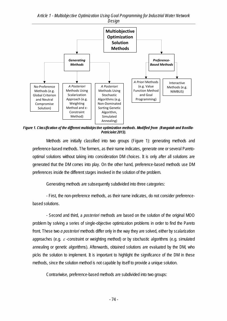
Article 1 - Multiobjective Optimization Using Goal Programming for Industrial Water Network Design
- 74 -
Figure 1. Classification of the different multiobjective optimization methods. Modified from (Rangaiah and Bonilla-
Petriciolet 2013).
Methods are initially classified into two groups (Figure 1): generating methods and
preference-based methods. The formers, as their name indicates, generate one or several Pareto-
optimal solutions without taking into consideration DM choices. It is only after all solutions are
generated that the DM comes into play. On the other hand, preference-based methods use DM
preferences inside the different stages involved in the solution of the problem.
Generating methods are subsequently subdivided into three categories:
- First, the non-preference methods, as their name indicates, do not consider preference-
based solutions.
- Second and third, a posteriori methods are based on the solution of the original MOO
problem by solving a series of single-objective optimization problems in order to find the Pareto
front. These two a posteriori methods differ only in the way they are solved, either by scalarization
approaches (e.g. -constraint or weighting method) or by stochastic algorithms (e.g. simulated
annealing or genetic algorithms). Afterwards, obtained solutions are evaluated by the DM, who
picks the solution to implement. It is important to highlight the significance of the DM in these
methods, since the solution method is not capable by itself to provide a unique solution.
Contrariwise, preference-based methods are subdivided into two groups:
Multiobjective Optimization
Solution Methods
Generating Methods
Preference-Based Methods
A Posteriori Methods Using
Stochastic Algorithms (e.g. Non-Dominated Sorting Genetic
Algorithm, Simulated Annealing)
No-Preference Methods (e.g.
Global Criterion and Neutral Compromise
Solution)
A Posteriori Methods Using
Scalarization Approach (e.g.
Weighting Method and ε-
Constraint Method)
A Priori Methods (e.g. Value
Function Method and Goal
Programming)
Interactive Methods (e.g.
NIMBUS)
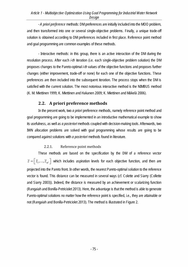
Article 1 - Multiobjective Optimization Using Goal Programming for Industrial Water Network Design
- 75 -
- A priori preference methods: DM preferences are initially included into the MOO problem,
and then transformed into one or several single-objective problems. Finally, a unique trade-off
solution is obtained according to DM preferences included in first place. Reference point method
and goal programming are common examples of these methods.
- Interactive methods: in this group, there is an active interaction of the DM during the
resolution process. After each i-th iteration (i.e. each single-objective problem solution) the DM
proposes changes to the Pareto-optimal i-th values of the objective functions and proposes further
changes (either improvement, trade-off or none) for each one of the objective functions. These
preferences are then included into the subsequent iteration. The process stops when the DM is
satisfied with the current solution. The most notorious interactive method is the NIMBUS method
(K. M. Miettinen 1999; K. Miettinen and Hakanen 2009; K. Miettinen and Mäkelä 2006).
2.2. A priori preference methods
In the present work, two a priori preference methods, namely reference point method and
goal programming are going to be implemented in an introductive mathematical example to show
its usefulness, as well as a posteriori methods coupled with decision-making tools. Afterwards, two
IWN allocation problems are solved with goal programming whose results are going to be
compared against solutions with a posteriori methods found in literature.
2.2.1. Reference point methods
These methods are based on the specification by the DM of a reference vector
1,..., nfz z z which includes aspiration levels for each objective function, and then are
projected into the Pareto front. In other words, the nearest Pareto-optimal solution to the reference
vector is found. This distance can be measured in several ways (cf. Colette and Siarry (Collette
and Siarry 2003)). Indeed, the distance is measured by an achievement or scalarizing function
(Rangaiah and Bonilla-Petriciolet 2013). Here, the advantage is that the method is able to generate
Pareto-optimal solutions no matter how the reference point is specified, i.e., they are attainable or
not (Rangaiah and Bonilla-Petriciolet 2013). The method is illustrated in Figure 2.
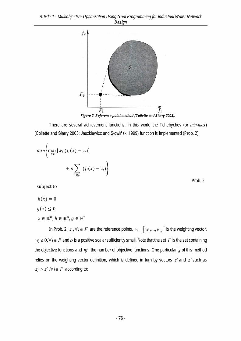
Article 1 - Multiobjective Optimization Using Goal Programming for Industrial Water Network Design
- 76 -
Figure 2. Reference point method (Collette and Siarry 2003).
There are several achievement functions: in this work, the Tchebychev (or min-max)
(Collette and Siarry 2003; Jaszkiewicz and Słowiński 1999) function is implemented (Prob. 2).
𝑚𝑖𝑛 {max𝑖∈𝐹
[𝑤𝑖 (𝑓𝑖(𝑥) − 𝑧��)]
+ 𝜌 ∑ (𝑓𝑖(𝑥) − 𝑧��)
𝑖∈𝐹
}
subject to
ℎ(𝑥) = 0
𝑔(𝑥) ≤ 0
𝑥 ∈ ℝ𝑛, ℎ ∈ ℝ𝑝, 𝑔 ∈ ℝ𝑟
Prob. 2
In Prob. 2, ,iz i F are the reference points, 1,..., nfw w w is the weighting vector,
0,iw i F and is a positive scalar sufficiently small. Note that the set F is the set containing
the objective functions and nf the number of objective functions. One particularity of this method
relies on the weighting vector definition, which is defined in turn by vectors rz and vz such as
,v ri iz z i F according to:
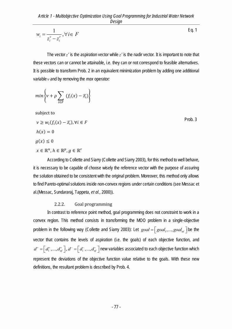
Article 1 - Multiobjective Optimization Using Goal Programming for Industrial Water Network Design
- 77 -
1 ,i v ri i
w i Fz z
Eq. 1
The vector rz is the aspiration vector while vz is the nadir vector. It is important to note that
these vectors can or cannot be attainable, i.e. they can or not correspond to feasible alternatives.
It is possible to transform Prob. 2 in an equivalent minimization problem by adding one additional
variable v and by removing the max operator:
𝑚𝑖𝑛 {𝜈 + 𝜌 ∑ (𝑓𝑖(𝑥) − 𝑧��)
𝑖∈𝐹
}
subject to
𝜈 ≥ 𝑤𝑖(𝑓𝑖(𝑥) − 𝑧��), ∀𝑖 ∈ 𝐹
ℎ(𝑥) = 0
𝑔(𝑥) ≤ 0
𝑥 ∈ ℝ𝑛, ℎ ∈ ℝ𝑝, 𝑔 ∈ ℝ𝑟
Prob. 3
According to Collette and Siarry (Collette and Siarry 2003), for this method to well behave,
it is necessary to be capable of choose wisely the reference vector with the purpose of assuring
the solution obtained to be consistent with the original problem. Moreover, this method only allows
to find Pareto-optimal solutions inside non-convex regions under certain conditions (see Messac et
al.(Messac, Sundararaj, Tappeta, et al., 2000)).
2.2.2. Goal programming
In contrast to reference point method, goal programming does not constraint to work in a
convex region. This method consists in transforming the MOO problem in a single-objective
problem in the following way (Collette and Siarry 2003): Let 1,..., nfgoal goal goal be the
vector that contains the levels of aspiration (i.e. the goals) of each objective function, and
1 1,..., , ,...,nf nfd d d d d d new variables associated to each objective function which
represent the deviations of the objective function value relative to the goals. With these new
definitions, the resultant problem is described by Prob. 4.
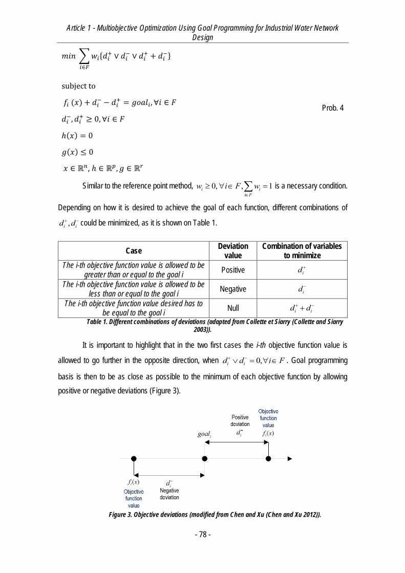
Article 1 - Multiobjective Optimization Using Goal Programming for Industrial Water Network Design
- 78 -
𝑚𝑖𝑛 ∑ 𝑤𝑖
𝑖∈𝐹
{𝑑𝑖+ ∨ 𝑑𝑖
− ∨ 𝑑𝑖+ + 𝑑𝑖
−}
subject to
𝑓𝑖 (𝑥) + 𝑑𝑖− − 𝑑𝑖
+ = 𝑔𝑜𝑎𝑙𝑖, ∀𝑖 ∈ 𝐹
𝑑𝑖−, 𝑑𝑖
+ ≥ 0, ∀𝑖 ∈ 𝐹
ℎ(𝑥) = 0
𝑔(𝑥) ≤ 0
𝑥 ∈ ℝ𝑛, ℎ ∈ ℝ𝑝, 𝑔 ∈ ℝ𝑟
Prob. 4
Similar to the reference point method, 0, , 1i ii F
w i F w
is a necessary condition.
Depending on how it is desired to achieve the goal of each function, different combinations of
,i id d could be minimized, as it is shown on Table 1.
Case Deviation
value Combination of variables
to minimize
The i-th objective function value is allowed to be greater than or equal to the goal i
Positive id
The i-th objective function value is allowed to be less than or equal to the goal i
Negative id
The i-th objective function value desired has to be equal to the goal i
Null i id d
Table 1. Different combinations of deviations (adapted from Collette et Siarry (Collette and Siarry 2003)).
It is important to highlight that in the two first cases the i-th objective function value is
allowed to go further in the opposite direction, when 0,i id d i F . Goal programming
basis is then to be as close as possible to the minimum of each objective function by allowing
positive or negative deviations (Figure 3).
Figure 3. Objective deviations (modified from Chen and Xu (Chen and Xu 2012)).
Article 1 - Multiobjective Optimization Using Goal Programming for Industrial Water Network Design
- 79 -
On the other hand, it is important to normalize both objective function values and goals:
min
max min
( )( )norm i ii
i i
f x ff x i Ff f
Eq. 2
min
max minnorm i ii
i i
goal fgoal i Ff f
Eq. 3
In Eq. 2-Eq. 3, min max, ,i if f i F are respectively the minimum and maximum value of
each i-th objective function attained in individual single-objective optimizations.
Finally, it is important to notice that goal programming is the most employed method for
multiobjective optimization (Chang, 2011).
2.3. A posteriori preference methods
These methods are based in the first place on the construction of the Pareto front and then
the implementation of multi-criteria decision-making (MCDM) tools.
2.3.1. Pareto front generation
The Pareto front can be generated traditionally by scalarization approaches or stochastic
methods.
Indeed, it can be generated by any method in capacity to produce Pareto-optimal solutions,
so even a priori methods are suitable for this task on conjunction with other algorithms
(Moghaddam, 2013). By using these methods, this algorithm deals with changing the weighting
coefficients and/or the aspiration levels.
On the other hand, the most common method to generate Pareto-optimal solutions is the
-constraint method (Miettinen, 1999). This method consists in minimizing one of the objective
functions at a time and by transforming the others in bounds through inequality constraints. This
implies some kind of knowledge of minimum and maximum values of objective functions, and in
consequence, the first step is to do single-objective optimizations of each problem separately. The
method is stated in Prob. 5.
Article 1 - Multiobjective Optimization Using Goal Programming for Industrial Water Network Design
- 80 -
min fi (x)
subject to
𝑓𝑖 (𝑥) ≤ 𝜀𝑗, ∀𝑗 ∈ 𝐹, 𝑗 ≠ 𝑖
ℎ(𝑥) = 0
𝑔(𝑥) = 0
𝑥 ∈ ℝ𝑛, ℎ ∈ ℝ𝑝, 𝑔 ∈ ℝ𝑟
Prob. 5
In Prob. 5, the vector 1,..., nf is the upper bound of the objective functions
, ,jf j F j i . The solution of Prob. 5 is always weak Pareto-optimal, and is Pareto-optimal if
and only if the solution is unique. Subsequently, to guaranty Pareto-optimality, it is needed to solve
nf problems (Rangaiah and Bonilla-Petriciolet 2013). The advantage of this method is that it is in
capacity to find every Pareto-optimal solution, even if the problem is non-convex. Therefore, the
Pareto-front obtainment is due to the solution of several single-objective optimizations by changing
functions bounds.
Practically, however, it is not always easy to find feasible upper bounds for Prob. 5. Also,
it can be difficult to determine which problem has to be optimized subsequently. Finally, when the
problem has several objective functions, the number of single-objective optimizations that have to
be carried out increases substantially, which is not desirable in most cases.
Beyond mathematical programming methods to generate the Pareto-front, stochastic
methods have become popular in order to generate the Pareto front in MOO problems. Among
these, evolutionary algorithms are the most commonly used since they are easy to implement and
are effective. Evolutionary algorithms are based on the emulation of natural selection mechanisms
(Zhou, Qu, Li, et al., 2011), and are particularly appropriated in order to solve MOO problems thanks
to their capacity to handle several solutions simultaneously and their ability to tackle different kinds
of problems without knowing important information about the problem structure, e.g. derivatives.
Nevertheless, evolutionary algorithms require a very significant amount of time to be solved to such
an extent that the solution of large-scale problems is prohibitive. The most widely-spread
evolutionary algorithm is the genetic algorithm and its variants (e.g. NSGA-II (Srinivas and Deb
1994)).
Article 1 - Multiobjective Optimization Using Goal Programming for Industrial Water Network Design
- 81 -
2.3.2. Decision-making tools
A posteriori methods generate several Pareto-optimal solutions, based in the dominance
relationship (see Rangaiah and Bonilla-Petriciolet (Rangaiah and Bonilla-Petriciolet 2013) and
Collette and Siarry (Collette and Siarry 2003)). This relationship allows to filter solutions and to
retain only comparable results. Yet, it remains the choice of “the best” solutions according to DM
preferences. There are several decision-making tools, but in this study, the interest lies only with
TOPSIS based methods.
2.3.2.1. M-TOPSIS
The idea beyond M-TOPSIS is described next (Ren, Zhang, Wang, et al., 2010). Let
1,...,S ns be a set with ns alternative solutions of the objective functions and ,ns nfA a matrix
with ns rows and nf columns:
1. Normalize the decision matrix A, accordingly:
,, , 2
,
( ),
( )i j
i j ns nfi j
i S
f xA a i S j F
f x
Eq. 4
2. Determine the ideal positive and negative solutions of matrix A:
, ,
, ,
max( )
min( )
i j i ji
i j i ji
a a j F
a a j F
Eq. 5
3. Compute the distance between each solution and the ideal positive and negative
solution using n-dimensional Euclidean distance:
2, ,
2, ,
( )
( )
i j i j i jj I
i j i j i jj I
D w a a i S
D w a a i S
Eq. 6
4. Calculate the distance of each solution to point O (min( ),max( )),i iD D i S :
2 2( min( )) ( max( ))i i i i ii S i SR D D D D i S
Eq.7
5. Class solutions in descendant order according to iR . Consequently, the solution with
greater iR is the best trade-off solution.
Article 1 - Multiobjective Optimization Using Goal Programming for Industrial Water Network Design
- 82 -
2.3.2.2. LMS-TOPSIS
This modification we propose, is based on a linear normalization rather than using the norm
as M-TOPSIS does. Indeed, this normalization is the same employed when using goal
programming in this study:
min,
, max min
( ),i j jnorm
i jj j
f x ff i S j F
f f
Eq. 8
The aforementioned modification is proposed due to poor performance of traditional and
M-TOPSIS procedures in non-trivial cases, as it is going to be demonstrated in the subsequent
sections.
3. Case studies
As case studies, we propose an introductory mathematical example to show the followed
methodology and two IWA problems, one traditional and one with simultaneous water and energy
allocation. For the introductory example, we implemented the two a priori methods addressed
above (i.e. reference point method and goal programming) and one a posteriori method, i.e.
generation of the Pareto front by stochastic methods and decision-making by TOPSIS methods.
On the other hand, for the IWA problems, we implemented goal programming in order to compare
a priori methods results and the results obtained by Boix et al. (Boix, Pibouleau, Montastruc, et al.,
2012; Boix, Montastruc, Pibouleau, et al., 2010) by implementing a posteriori methods. All a priori
implementations were modeled in GAMS® (Brooke, Kendrick, Meeraus, et al., 1998). For the
MINLP problem (i.e. the introductory example) the outer-approximation solver DICOPT (Duran and
Grossmann 1986) was used coupled with CPLEX® (IBM, 2013) and IPOPT (Wächter and Biegler
2002; Wächter and Biegler 2005). For the MILP problems, i.e. the IWA problems CPLEX® (IBM,
2013) was used as the solver. The Pareto front of the introductive example was generated by the
genetic algorithm, NSGA-II by using the multipurpose solver MULTIGEN (Gomez, 2008), whose
interface is available in Microsoft Excel® and ran several times before the construction of the Pareto
front. In all cases, weight factors are defined as1
iw nf , in order to obtain a trade-off solution
without any explicit preference to any objective in particular. In addition, the goal vector in goal
programming was defined for all cases as max min15 ,
16i i
if fgoal i F
and consequently the
normalized goal vector is always 0.062,normigoal i F in order to locate goals as close as
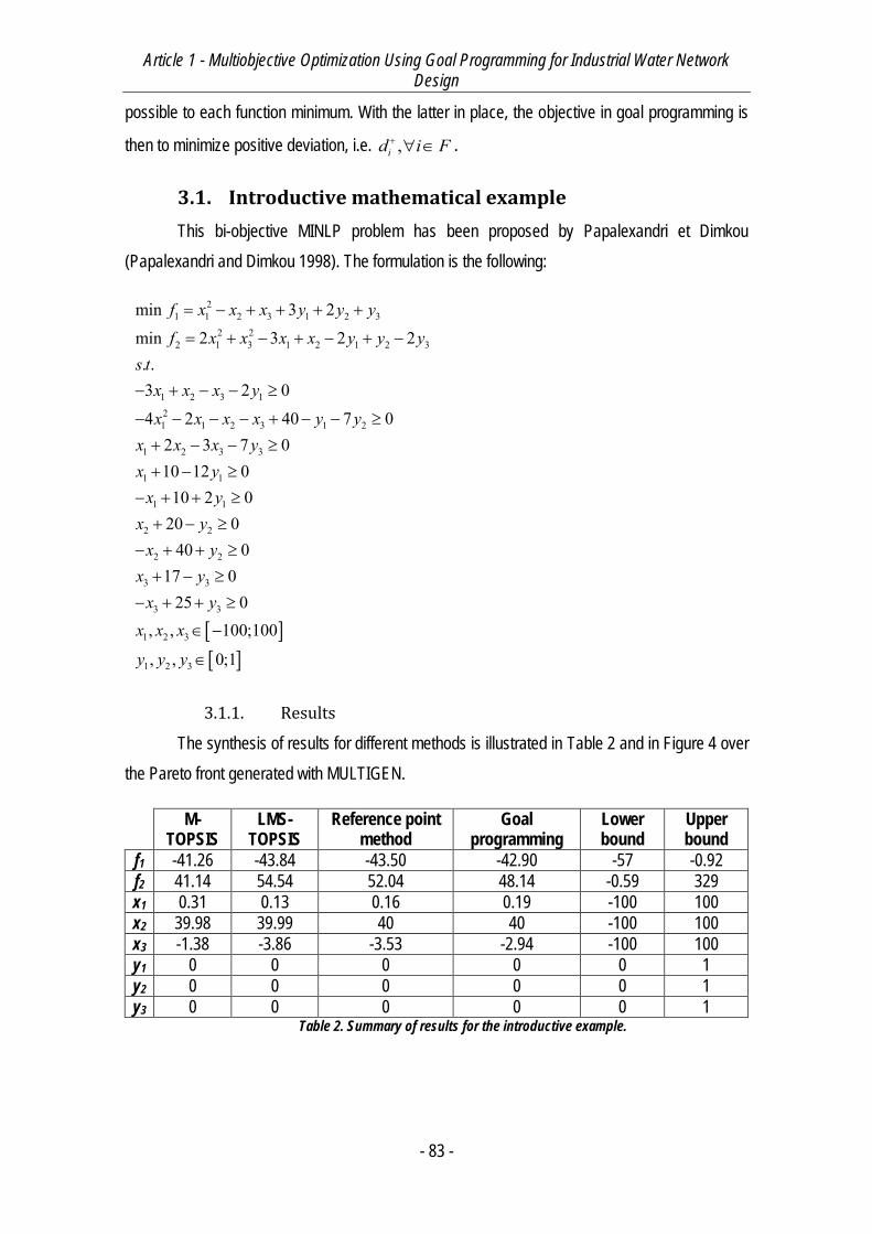
Article 1 - Multiobjective Optimization Using Goal Programming for Industrial Water Network Design
- 83 -
possible to each function minimum. With the latter in place, the objective in goal programming is
then to minimize positive deviation, i.e. ,id i F .
3.1. Introductive mathematical example
This bi-objective MINLP problem has been proposed by Papalexandri et Dimkou
(Papalexandri and Dimkou 1998). The formulation is the following:
21 1 2 3 1 2 3
2 22 1 3 1 2 1 2 3
1 2 3 121 1 2 3 1 2
1 2 3 3
1 1
1 1
2 2
2 2
3 3
3 3
1 2 3
min 3 2
min 2 3 2 2. .3 2 0
4 2 40 7 02 3 7 010 12 0
10 2 020 0
40 017 0
25 0, , 100
f x x x y y yf x x x x y y y
s tx x x yx x x x y y
x x x yx yx yx yx yx yx yx x x
1 2 3
;100
, , 0;1y y y
3.1.1. Results
The synthesis of results for different methods is illustrated in Table 2 and in Figure 4 over
the Pareto front generated with MULTIGEN.
M-
TOPSIS LMS-
TOPSIS Reference point
method Goal
programming Lower bound
Upper bound
f1 -41.26 -43.84 -43.50 -42.90 -57 -0.92
f2 41.14 54.54 52.04 48.14 -0.59 329
x1 0.31 0.13 0.16 0.19 -100 100
x2 39.98 39.99 40 40 -100 100
x3 -1.38 -3.86 -3.53 -2.94 -100 100
y1 0 0 0 0 0 1
y2 0 0 0 0 0 1
y3 0 0 0 0 0 1 Table 2. Summary of results for the introductive example.
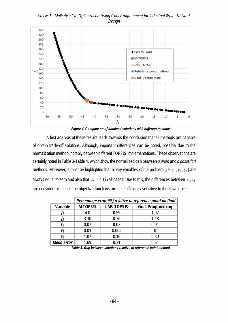
Article 1 - Multiobjective Optimization Using Goal Programming for Industrial Water Network Design
- 84 -
Figure 4. Comparison of obtained solutions with different methods
A first analysis of these results leads towards the conclusion that all methods are capable
of obtain trade-off solutions. Although, important differences can be noted, possibly due to the
normalization method, notably between different TOPSIS implementations. These observations are
certainly noted in Table 3-Table 4, which show the normalized gap between a priori and a posteriori
methods. Moreover, it must be highlighted that binary variables of the problem (i.e. 1 2 3, ,y y y ) are
always equal to zero and also that 2 40x in all cases. Due to this, the differences between 1 3,x x
are considerable, since the objective functions are not sufficiently sensitive to these variables.
Percentage error (%) relative to reference point method
Variable M-TOPSIS LMS-TOPSIS Goal Programming
f1 4.0 0.59 1.07
f2 3.30 0.76 1.18
x1 0.07 0.02 0.01
x2 0.01 0.005 0
x3 1.07 0.16 0.30
Mean error 1.69 0.31 0.51 Table 3. Gap between solutions relative to reference point method.
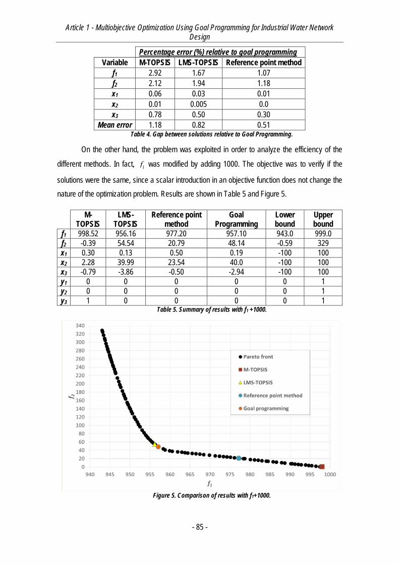
Article 1 - Multiobjective Optimization Using Goal Programming for Industrial Water Network Design
- 85 -
Percentage error (%) relative to goal programming
Variable M-TOPSIS LMS-TOPSIS Reference point method
f1 2.92 1.67 1.07
f2 2.12 1.94 1.18
x1 0.06 0.03 0.01
x2 0.01 0.005 0.0
x3 0.78 0.50 0.30
Mean error 1.18 0.82 0.51 Table 4. Gap between solutions relative to Goal Programming.
On the other hand, the problem was exploited in order to analyze the efficiency of the
different methods. In fact, 1f was modified by adding 1000. The objective was to verify if the
solutions were the same, since a scalar introduction in an objective function does not change the
nature of the optimization problem. Results are shown in Table 5 and Figure 5.
M-
TOPSIS LMS-
TOPSIS Reference point
method Goal
Programming Lower bound
Upper bound
f1 998.52 956.16 977.20 957.10 943.0 999.0
f2 -0.39 54.54 20.79 48.14 -0.59 329
x1 0.30 0.13 0.50 0.19 -100 100
x2 2.28 39.99 23.54 40.0 -100 100
x3 -0.79 -3.86 -0.50 -2.94 -100 100
y1 0 0 0 0 0 1
y2 0 0 0 0 0 1
y3 1 0 0 0 0 1 Table 5. Summary of results with f1 +1000.
Figure 5. Comparison of results with f1+1000.

Article 1 - Multiobjective Optimization Using Goal Programming for Industrial Water Network Design
- 86 -
Contrary to the first case, the solution is not the same as it was expected with certain
methods. Indeed, M-TOPSIS does not manage to achieve the good solution, while LMS-TOPSIS
does achieve it, due to the objective functions normalization proposed. On the other hand, goal
programming is able to find the correct solution while the reference point method is not, and is only
successful if the aspiration vector is changed. In fact, these results highlight the essential
relationship between the reference point method and the aspiration vector. Relative to it, a
sensitivity analysis of the solution obtained in function of the chosen vectors was carried out (see
Figure 6). It is necessary to clarify that the illustrated variation corresponds to ≈10% of the Pareto
front. The latter comports a considerable gap, mainly relative to other methods.
Figure 6. Sensitivity analysis of the results of reference point method in function to the aspiration
vector.
3.2. Industrial water network
The formulation of the IWN allocation problem is the same as in previous works (Boix et
al. 2010; M. Bagajewicz and Savelski 2001; M. J. Bagajewicz and Faria 2009). The way to model
a IWN allocation problem is based on the concept of superstructure (Yeomans and Grossmann
1999; Biegler, Grossmann, and Westerberg 1997). From a given number of regeneration units and
processes, all possible connections between them may exist, except recycling to the same unit.
This constraint forbids self-recycles on process and regeneration units, although the latter is often
relevant in some chemical processes. For each water-flowrate using process, input water may be
freshwater, output water from other process and/or regenerated water. Indeed, output water from
a process may be directly discharged, distributed to another process and/or to regeneration units.
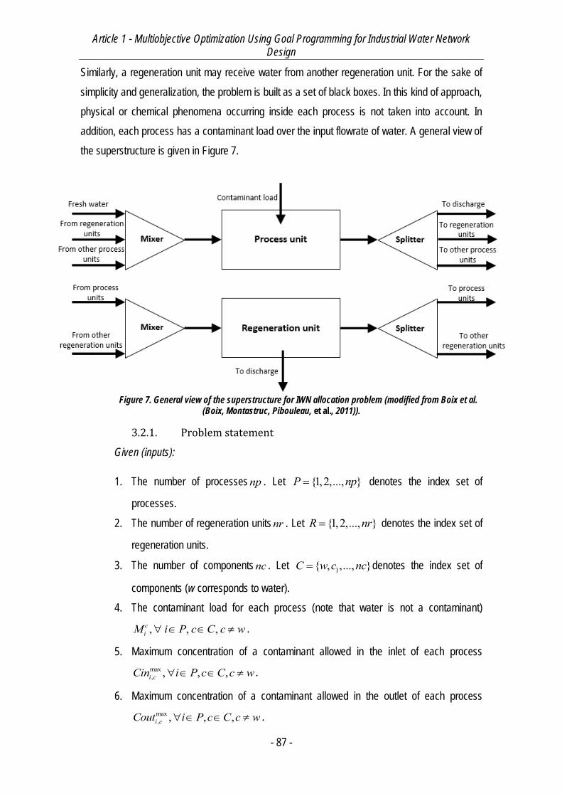
Article 1 - Multiobjective Optimization Using Goal Programming for Industrial Water Network Design
- 87 -
Similarly, a regeneration unit may receive water from another regeneration unit. For the sake of
simplicity and generalization, the problem is built as a set of black boxes. In this kind of approach,
physical or chemical phenomena occurring inside each process is not taken into account. In
addition, each process has a contaminant load over the input flowrate of water. A general view of
the superstructure is given in Figure 7.
Figure 7. General view of the superstructure for IWN allocation problem (modified from Boix et al.
(Boix, Montastruc, Pibouleau, et al., 2011)).
3.2.1. Problem statement
Given (inputs):
1. The number of processes np . Let {1,2,..., }P np denotes the index set of
processes.
2. The number of regeneration unitsnr . Let {1,2,..., }R nr denotes the index set of
regeneration units.
3. The number of components nc . Let 1{ , ,..., }C w c nc denotes the index set of
components (w corresponds to water).
4. The contaminant load for each process (note that water is not a contaminant)
, , ,ciM i P c C c w .
5. Maximum concentration of a contaminant allowed in the inlet of each process
max, , , ,i cCin i P c C c w .
6. Maximum concentration of a contaminant allowed in the outlet of each process
max, , , ,i cCout i P c C c w .
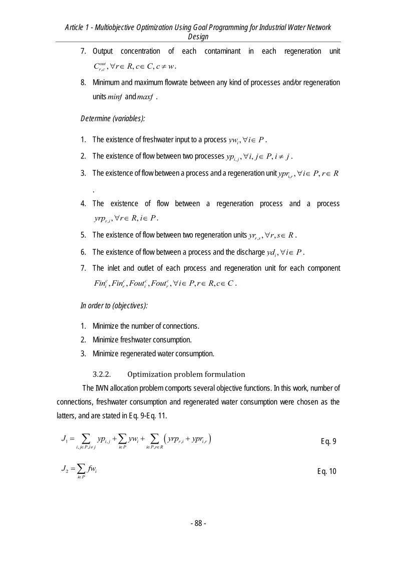
Article 1 - Multiobjective Optimization Using Goal Programming for Industrial Water Network Design
- 88 -
7. Output concentration of each contaminant in each regeneration unit
, , , ,outr cC r R c C c w .
8. Minimum and maximum flowrate between any kind of processes and/or regeneration
unitsminf andmaxf .
Determine (variables):
1. The existence of freshwater input to a process ,iyw i P .
2. The existence of flow between two processes , , , ,i jyp i j P i j .
3. The existence of flow between a process and a regeneration unit i, , ,rypr i P r R
.
4. The existence of flow between a regeneration process and a process
, , ,r iyrp r R i P .
5. The existence of flow between two regeneration units , , ,r syr r s R .
6. The existence of flow between a process and the discharge ,iyd i P .
7. The inlet and outlet of each process and regeneration unit for each component
, , , , , ,c c c ci r i rFin Fin Fout Fout i P r R c C .
In order to (objectives):
1. Minimize the number of connections.
2. Minimize freshwater consumption.
3. Minimize regenerated water consumption.
3.2.2. Optimization problem formulation
The IWN allocation problem comports several objective functions. In this work, number of
connections, freshwater consumption and regenerated water consumption were chosen as the
latters, and are stated in Eq. 9-Eq. 11.
1 , , ,, , ,
i j i r i i ri j P i j i P i P r R
J yp yw yrp ypr
Eq. 9
2 ii P
J fw
Eq. 10
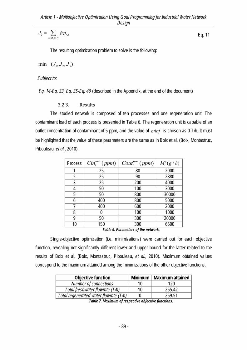
Article 1 - Multiobjective Optimization Using Goal Programming for Industrial Water Network Design
- 89 -
3 ,,
r ir R i P
J frp
Eq. 11
The resulting optimization problem to solve is the following:
1 2 3min ( , , )J J J
Subject to:
Eq. 14-Eq. 33, Eq. 35-Eq. 40 (described in the Appendix, at the end of the document)
3.2.3. Results
The studied network is composed of ten processes and one regeneration unit. The
contaminant load of each process is presented in Table 6. The regeneration unit is capable of an
outlet concentration of contaminant of 5 ppm, and the value of minf is chosen as 0 T/h. It must
be highlighted that the value of these parameters are the same as in Boix et al. (Boix, Montastruc,
Pibouleau, et al., 2010).
Process max ( )iCin ppm
max ( )iCout ppm ( / )ciM g h
1 25 80 2000
2 25 90 2880
3 25 200 4000
4 50 100 3000
5 50 800 30000
6 400 800 5000
7 400 600 2000
8 0 100 1000
9 50 300 20000
10 150 300 6500 Table 6. Parameters of the network.
Single-objective optimization (i.e. minimizations) were carried out for each objective
function, revealing not significantly different lower and upper bound for the latter related to the
results of Boix et al. (Boix, Montastruc, Pibouleau, et al., 2010). Maximum obtained values
correspond to the maximum attained among the minimizations of the other objective functions.
Objective function Minimum Maximum attained
Number of connections 10 120
Total freshwater flowrate (T/h) 10 255.42
Total regenerated water flowrate (T/h) 0 259.51 Table 7. Maximum of respective objective functions.
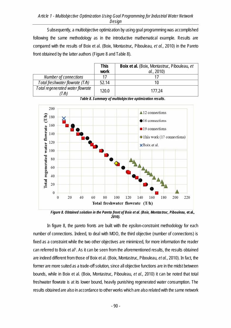
Article 1 - Multiobjective Optimization Using Goal Programming for Industrial Water Network Design
- 90 -
Subsequently, a multiobjective optimization by using goal programming was accomplished
following the same methodology as in the introductive mathematical example. Results are
compared with the results of Boix et al. (Boix, Montastruc, Pibouleau, et al., 2010) in the Pareto
front obtained by the latter authors (Figure 8 and Table 8).
This work
Boix et al. (Boix, Montastruc, Pibouleau, et al., 2010)
Number of connections 17 17
Total freshwater flowrate (T/h) 52.14 10
Total regenerated water flowrate (T/h)
120.0 177.24
Table 8. Summary of multiobjective optimization results.
Figure 8. Obtained solution in the Pareto front of Boix et al. (Boix, Montastruc, Pibouleau, et al.,
2010).
In figure 8, the pareto fronts are built with the epsilon-constraint methodology for each
number of connections. Indeed, to deal with MOO, the third objective (number of connections) is
fixed as a constraint while the two other objectives are minimized, for more information the reader
can referred to Boix et al1. As it can be seen from the aforementioned results, the results obtained
are indeed different from those of Boix et al. (Boix, Montastruc, Pibouleau, et al., 2010). In fact, the
former are more suited as a trade-off solution, since all objective functions are in the midst between
bounds, while in Boix et al. (Boix, Montastruc, Pibouleau, et al., 2010) it can be noted that total
freshwater flowrate is at its lower bound, heavily punishing regenerated water consumption. The
results obtained are also in accordance to other works which are also related with the same network
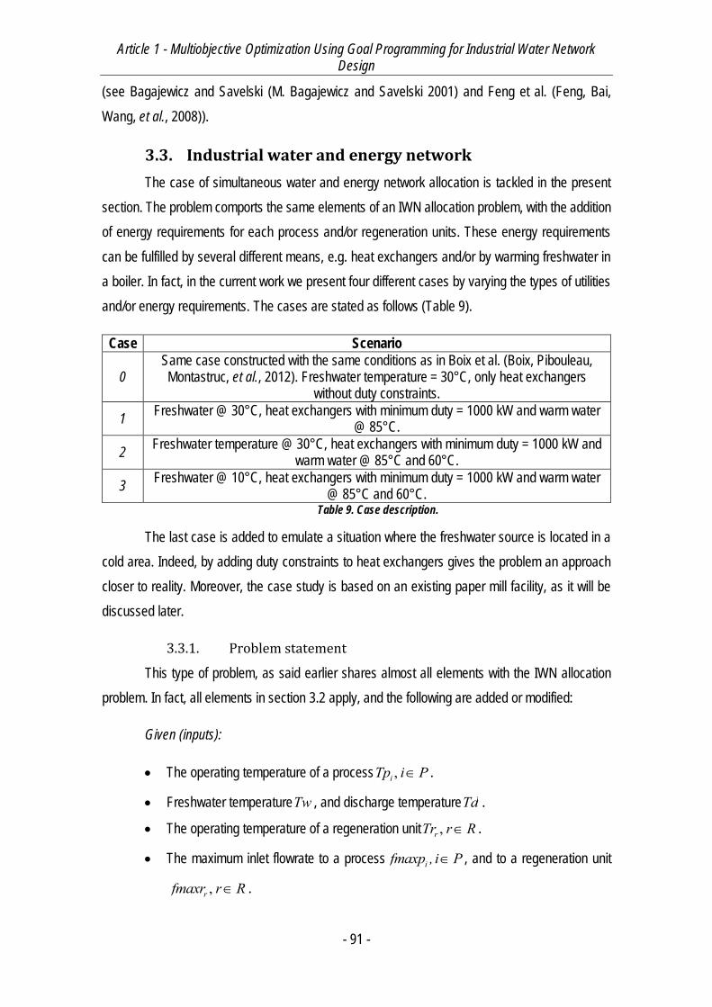
Article 1 - Multiobjective Optimization Using Goal Programming for Industrial Water Network Design
- 91 -
(see Bagajewicz and Savelski (M. Bagajewicz and Savelski 2001) and Feng et al. (Feng, Bai,
Wang, et al., 2008)).
3.3. Industrial water and energy network
The case of simultaneous water and energy network allocation is tackled in the present
section. The problem comports the same elements of an IWN allocation problem, with the addition
of energy requirements for each process and/or regeneration units. These energy requirements
can be fulfilled by several different means, e.g. heat exchangers and/or by warming freshwater in
a boiler. In fact, in the current work we present four different cases by varying the types of utilities
and/or energy requirements. The cases are stated as follows (Table 9).
Case Scenario
0 Same case constructed with the same conditions as in Boix et al. (Boix, Pibouleau, Montastruc, et al., 2012). Freshwater temperature = 30°C, only heat exchangers
without duty constraints.
1 Freshwater @ 30°C, heat exchangers with minimum duty = 1000 kW and warm water
@ 85°C.
2 Freshwater temperature @ 30°C, heat exchangers with minimum duty = 1000 kW and
warm water @ 85°C and 60°C.
3 Freshwater @ 10°C, heat exchangers with minimum duty = 1000 kW and warm water
@ 85°C and 60°C. Table 9. Case description.
The last case is added to emulate a situation where the freshwater source is located in a
cold area. Indeed, by adding duty constraints to heat exchangers gives the problem an approach
closer to reality. Moreover, the case study is based on an existing paper mill facility, as it will be
discussed later.
3.3.1. Problem statement
This type of problem, as said earlier shares almost all elements with the IWN allocation
problem. In fact, all elements in section 3.2 apply, and the following are added or modified:
Given (inputs):
The operating temperature of a process ,iTp i P .
Freshwater temperatureTw , and discharge temperatureTd .
The operating temperature of a regeneration unit ,rTr r R .
The maximum inlet flowrate to a process ifmaxp ,i P , and to a regeneration unit
,rfmaxr r R .

Article 1 - Multiobjective Optimization Using Goal Programming for Industrial Water Network Design
- 92 -
The minimum and maximum duty of the heat exchanger associated to a process or
regeneration unitminQ,maxQ .
-Determine (variables):
The existence of a heat exchanger (i.e. cooler or heater) in a process, a regeneration
unit or the discharge , , , , , , ,i i r ryexp yexp yexr yexr yexd yexd i P r R .
-In order to (objectives):
Minimize total energy consumption
The number of heat exchangers in the network
It is important to note that in the present case study total regenerated water consumption
is not considered as an objective function, in order to be in accordance with the case study of Boix
et al. (Boix, Pibouleau, Montastruc, et al., 2012).
3.3.2. Optimization problem formulation
The objective functions related to this case study, according to the aforementioned, are
1 2,J J and in addition Eq. 12-Eq. 13.
-Total energy consumption:
4 i i i ii P r R
J Qp Qp Qr Qr Qd Qd
Eq. 12
-Number of heat exchangers in the network:
5 i i i ii P r R
J yexp yexp yexr yexr yexd yexd
Eq. 13
In accordance, the resulting optimization problem is the following:
1 2 4 5min ( , , , )J J J J
Subject to:
Eq. 14-Eq. 33, Eq. 35-Eq. 40, Eq. 41-Eq. 46
Prob. 6
(described in the Appendix, at the end of the document)
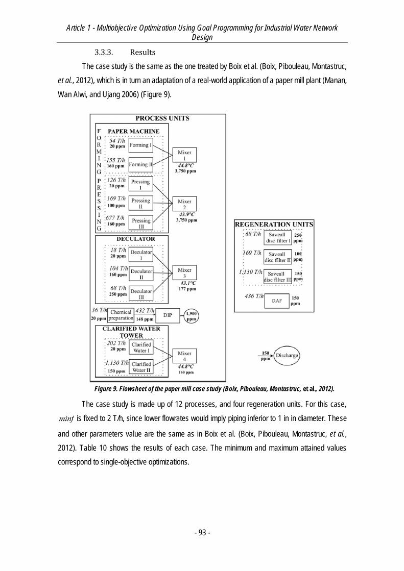
Article 1 - Multiobjective Optimization Using Goal Programming for Industrial Water Network Design
- 93 -
3.3.3. Results
The case study is the same as the one treated by Boix et al. (Boix, Pibouleau, Montastruc,
et al., 2012), which is in turn an adaptation of a real-world application of a paper mill plant (Manan,
Wan Alwi, and Ujang 2006) (Figure 9).
Figure 9. Flowsheet of the paper mill case study (Boix, Pibouleau, Montastruc, et al., 2012).
The case study is made up of 12 processes, and four regeneration units. For this case,
minf is fixed to 2 T/h, since lower flowrates would imply piping inferior to 1 in in diameter. These
and other parameters value are the same as in Boix et al. (Boix, Pibouleau, Montastruc, et al.,
2012). Table 10 shows the results of each case. The minimum and maximum attained values
correspond to single-objective optimizations.
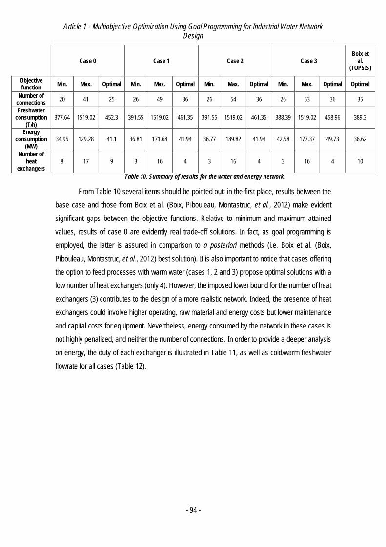
Article 1 - Multiobjective Optimization Using Goal Programming for Industrial Water Network Design
- 94 -
Case 0 Case 1 Case 2 Case 3 Boix et
al. (TOPSIS)
Objective function
Min. Max. Optimal Min. Max. Optimal Min. Max. Optimal Min. Max. Optimal Optimal
Number of connections
20 41 25 26 49 36 26 54 36 26 53 36 35
Freshwater consumption
(T/h) 377.64 1519.02 452.3 391.55 1519.02 461.35 391.55 1519.02 461.35 388.39 1519.02 458.96 389.3
Energy consumption
(MW) 34.95 129.28 41.1 36.81 171.68 41.94 36.77 189.82 41.94 42.58 177.37 49.73 36.62
Number of heat
exchangers 8 17 9 3 16 4 3 16 4 3 16 4 10
Table 10. Summary of results for the water and energy network.
From Table 10 several items should be pointed out: in the first place, results between the
base case and those from Boix et al. (Boix, Pibouleau, Montastruc, et al., 2012) make evident
significant gaps between the objective functions. Relative to minimum and maximum attained
values, results of case 0 are evidently real trade-off solutions. In fact, as goal programming is
employed, the latter is assured in comparison to a posteriori methods (i.e. Boix et al. (Boix,
Pibouleau, Montastruc, et al., 2012) best solution). It is also important to notice that cases offering
the option to feed processes with warm water (cases 1, 2 and 3) propose optimal solutions with a
low number of heat exchangers (only 4). However, the imposed lower bound for the number of heat
exchangers (3) contributes to the design of a more realistic network. Indeed, the presence of heat
exchangers could involve higher operating, raw material and energy costs but lower maintenance
and capital costs for equipment. Nevertheless, energy consumed by the network in these cases is
not highly penalized, and neither the number of connections. In order to provide a deeper analysis
on energy, the duty of each exchanger is illustrated in Table 11, as well as cold/warm freshwater
flowrate for all cases (Table 12).
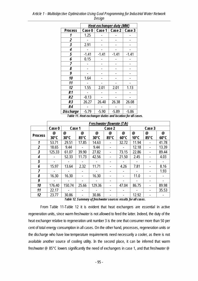
Article 1 - Multiobjective Optimization Using Goal Programming for Industrial Water Network Design
- 95 -
Heat exchanger duty (MW)
Process Case 0 Case 1 Case 2 Case 3
1 1.25 - - -
2 - - - -
3 2.91 - - -
4 - - - -
5 -1.41 -1.41 -1.41 -1.41
6 0.15 - - -
7 - - - -
8 - - - -
9 - - - -
10 1.64 - - -
11 - - - -
12 1.55 2.01 2.01 1.13
R1 - - - -
R2 -0.13 - - -
R3 26.27 26.40 26.38 26.08
R4 - - - -
Discharge -5.79 -5.90 -5.89 -5.86 Table 11. Heat exchanger duties and location for all cases.
Freshwater flowrate (T/h)
Case 0 Case 1 Case 2 Case 3
Process @
30°C @ 30°C
@ 85°C
@ 30°C
@ 85°C
@ 60°C
@ 10°C
@ 85°C
@ 60°C
1 53.71 29.51 17.85 14.63 - 32.72 11.94 - 41.78
2 18.65 9.44 - 9.44 - - 12.18 - 13.39
3 125.33 61.07 39.90 27.82 - 73.15 22.86 - 89.44
4 - 52.33 11.73 42.56 - 21.50 2.45 - 4.03
5 - - - - - - - - -
6 15.97 13.64 2.32 11.71 - 4.26 7.81 - 8.16
7 - - - - - - - - 1.93
8 16.30 16.30 - 16.30 - - 11.0 - -
9 - - - - - - - - -
10 176.40 150.74 25.66 129.36 - 47.04 86.75 - 89.98
11 22.17 - - - - - - - 35.53
12 23.77 30.86 - 30.86 - - 12.92 - - Table 12. Summary of freshwater sources results for all cases.
From Table 11-Table 12 it is evident that heat exchangers are essential in active
regeneration units, since warm freshwater is not allowed to feed the latter. Indeed, the duty of the
heat exchanger relative to regeneration unit number 3 is the one that consumer more than 50 per
cent of total energy consumption in all cases. On the other hand, processes, regeneration units or
the discharge who have low temperature requirements need necessarily a cooler, as there is not
available another source of cooling utility. In the second place, it can be inferred that warm
freshwater @ 85°C lowers significantly the need of exchangers in case 1, and that freshwater @
Article 1 - Multiobjective Optimization Using Goal Programming for Industrial Water Network Design
- 96 -
60°C is preferred and sufficient for the other cases. It is to be noted also that in the base case there
are exchangers with very low duties, thing that is traduced in very little and less efficient heat
exchanger equipment. In addition, it is clear that source freshwater temperature has a very
important impact on the network performance. For instance, the total energy consumed in case 3
is significantly higher than in other cases. Moreover, it is important to note that all cases that involve
warm freshwater sources comport higher number of connections, since it is evident the preference
for the latter than heat exchangers themselves.
4. Conclusions
In this work, it is addressed the IWN allocation problem by multiobjective optimization using
a priori methods, more specifically speaking, goal programming. This method has never been
explored to the case of water and/or energy networks design although it is performing and
particularly adapted to these problems containing binary variables where very few integer solutions
exist in the feasible region. Indeed, usually with a branch-and-Bound methodology, the resolution
of an MINLP or MILP problem is very fastidious, and especially with water network design, because
the binary variables control the solution. Consequently, the size of the tree with traditional methods
becomes very large and the program often returns an infeasible error message before finding a
solution. In this study, goal programming methodology has been successfully applied to the
problem of water and/or energy network design. Its effectiveness has been successfully
demonstrated by comparing the results obtained with other research works where different
multiobjective optimization methods are employed. On the two specific examples studied, namely
a traditional IWN and an IWN with energy, trade-off solutions are obtained and compared with other
solutions. Moreover, on the latter case, different temperature freshwater sources are studied in
order to study the influence of these in heat exchangers.
Since in Boix et al. (Boix, Pibouleau, Montastruc, et al., 2012) the authors employed a
lexicographic methodology based on the epsilon-constraint method and subsequent selection by
TOPSIS procedures, treating four objective functions could constraint the solution space to a few
solutions within the Pareto front for the sake of solution times and practicality. On the other hand,
solutions in this work are obtained within seconds, and several modifications to the case study can
be studied with little difficulty. Nevertheless, the usefulness of a posteriori methods is not
questioned if the totality of the Pareto front is desired. Additionally, several a priori methods can be
used in order to accomplish this task e.g. goal programming coupled with stochastic algorithms.
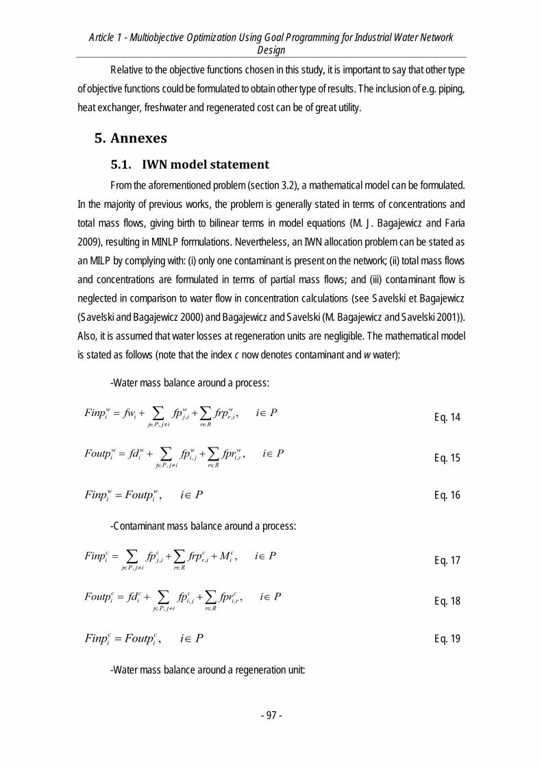
Article 1 - Multiobjective Optimization Using Goal Programming for Industrial Water Network Design
- 97 -
Relative to the objective functions chosen in this study, it is important to say that other type
of objective functions could be formulated to obtain other type of results. The inclusion of e.g. piping,
heat exchanger, freshwater and regenerated cost can be of great utility.
5. Annexes
5.1. IWN model statement
From the aforementioned problem (section 3.2), a mathematical model can be formulated.
In the majority of previous works, the problem is generally stated in terms of concentrations and
total mass flows, giving birth to bilinear terms in model equations (M. J. Bagajewicz and Faria
2009), resulting in MINLP formulations. Nevertheless, an IWN allocation problem can be stated as
an MILP by complying with: (i) only one contaminant is present on the network; (ii) total mass flows
and concentrations are formulated in terms of partial mass flows; and (iii) contaminant flow is
neglected in comparison to water flow in concentration calculations (see Savelski et Bagajewicz
(Savelski and Bagajewicz 2000) and Bagajewicz and Savelski (M. Bagajewicz and Savelski 2001)).
Also, it is assumed that water losses at regeneration units are negligible. The mathematical model
is stated as follows (note that the index c now denotes contaminant and w water):
-Water mass balance around a process:
, ,,
,w w wi i j i r i
j P j i r RFinp fw fp frp i P
Eq. 14
, ,,
,w w w wi i i j i r
j P j i r RFoutp fd fp fpr i P
Eq. 15
,w wi iFinp Foutp i P Eq. 16
-Contaminant mass balance around a process:
, ,,
,c c c ci j i r i i
j P j i r RFinp fp frp M i P
Eq. 17
, ,,
,c c c ci i i j i r
j P j i r RFoutp fd fp fpr i P
Eq. 18
,c ci iFinp Foutp i P Eq. 19
-Water mass balance around a regeneration unit:
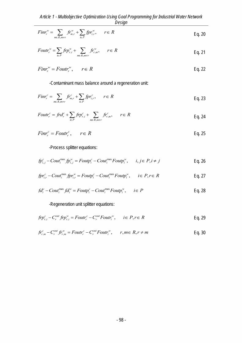
Article 1 - Multiobjective Optimization Using Goal Programming for Industrial Water Network Design
- 98 -
, ,,
,w w wr m r i r
m R m r i PFinr fr fpr r R
Eq. 20
, ,,
,w w wr r i r m
i P m R m rFoutr frp fr r R
Eq. 21
,w wr rFinr Foutr r R Eq. 22
-Contaminant mass balance around a regeneration unit:
, ,,
,c c cr m r i r
m R m r i PFinr fr fpr r R
Eq. 23
, ,,
,c c c cr r r i r m
i P m R m rFoutr frd frp fr r R
Eq. 24
,c cr rFinr Foutr r R Eq. 25
-Process splitter equations:
max max, , , , ,c w c wi j i i j i i ifp Cout fp Foutp Cout Foutp i j P i j Eq. 26
max max, , , ,c w c wi r i i r i i ifpr Cout fpr Foutp Cout Foutp i P r R Eq. 27
max max ,c w c wi i i i i ifd Cout fd Foutp Cout Foutp i P Eq. 28
-Regeneration unit splitter equations:
, , , ,c out w c out wr i r r i r r ifrp C frp Foutr C Foutr i P r R Eq. 29
, , , , ,c out w c out wr m r r m r r ifr C fr Foutr C Foutr r m R r m Eq. 30
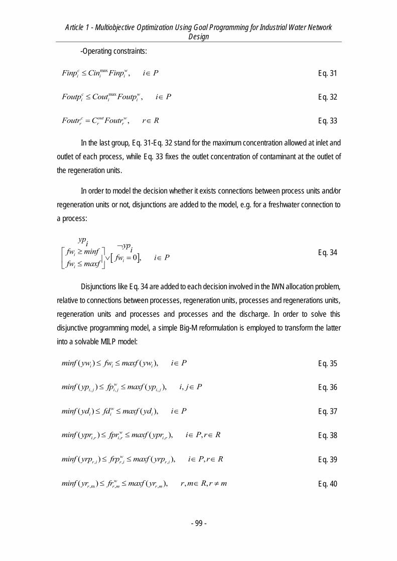
Article 1 - Multiobjective Optimization Using Goal Programming for Industrial Water Network Design
- 99 -
-Operating constraints:
max ,c wi i iFinp Cin Finp i P Eq. 31
max ,c wi i iFoutp Cout Foutp i P Eq. 32
,c out wr r rFoutr C Foutr r R Eq. 33
In the last group, Eq. 31-Eq. 32 stand for the maximum concentration allowed at inlet and
outlet of each process, while Eq. 33 fixes the outlet concentration of contaminant at the outlet of
the regeneration units.
In order to model the decision whether it exists connections between process units and/or
regeneration units or not, disjunctions are added to the model, e.g. for a freshwater connection to
a process:
0 ,ii
i
ypi ypifw minffw i P
fw maxf
Eq. 34
Disjunctions like Eq. 34 are added to each decision involved in the IWN allocation problem,
relative to connections between processes, regeneration units, processes and regenerations units,
regeneration units and processes and processes and the discharge. In order to solve this
disjunctive programming model, a simple Big-M reformulation is employed to transform the latter
into a solvable MILP model:
( ) ( ),i i iminf yw fw maxf yw i P Eq. 35
, , ,( ) ( ), ,wi j i j i jminf yp fp maxf yp i j P Eq. 36
( ) ( ),wi i iminf yd fd maxf yd i P Eq. 37
, , ,( ) ( ), ,wi r i r i rminf ypr fpr maxf ypr i P r R Eq. 38
, , ,( ) ( ), ,wr i r i r iminf yrp frp maxf yrp i P r R Eq. 39
,m , ,( ) ( ), , ,wr r m r mminf yr fr maxf yr r m R r m Eq. 40

Article 1 - Multiobjective Optimization Using Goal Programming for Industrial Water Network Design
- 100 -
In Eq. 35-Eq. 40, , , , ,, , , , , , , , , , ,i i j i i r r i r myw yp yd ypr yrp yr i j P r m R i j r m are
indeed binary variables.
5.2. Industrial water and energy network model statement
The model for the current problem is made of Eq. 14-Eq. 40 and the following, which
represent the addition of energy balances in the network:
-Energy balance around a process unit:
, ,,
, ,,
,
w w wi j i k r i r i i
j P j i r R
w w w wi i i j i r
j P j i r R
Cp fwTw fp Tp frp Tr Qp Qp
Cp Tp fd fp fpr i P
Eq. 41
-Energy balance around a regeneration unit:
, ,,
, ,,
,
w w wm r m i r i r r
m R m r i P
w w w wr r r i r m
i P m R m r
Cp fr Tr fpr Tp Qr Qr
Cp Tr frd frp fr r R
Eq. 42
-Global energy balance around the discharge:
w wi i i
i P i PCp fd Tp Qd Qd Td fw
Eq. 43
In addition, the following equations are added in order to model the disjunction to actually
place a heat exchanger in a process or not:
,+ + +i i iminQ(yexp ) Qp maxQ(yexp ) i P Eq. 44
,i i iminQ(yexp ) Qp maxQ(yexp ) i P Eq. 45
1,i iyexp yexp i P Eq. 46
Eq. 44-Eq. 46 ensure that both positive and negative heats are between stipulated bounds.
In addition, Eq. 46 assure that only cooling or heating is allowed, or neither. For regeneration units
and the discharge, the disjunctions are modeled analogously.

Article 1 - Multiobjective Optimization Using Goal Programming for Industrial Water Network Design
- 101 -
Finally, it is important to highlight that boilers/heaters are modeled as processes without
contaminant load and by prohibiting inlet connections different than freshwater to these processes.
6. Nomenclature
Latin symbols nf: Number of objective functions. w: Weighting vector. z : Reference vector. vz : Nadir vector. rz : Aspiration vector. v : Dummy variable.
d : Positive deviation.
d : Negative deviation. normf : Normalized objective function. minf : Minimum value of the objective function. maxf : Maximum relative value of the objective function.
goal: Goal vector. normgoal : Normalized goal.
A: Decision matrix. R: Ranking in TOPSIS methods. P: Index set of processes. np: Number of processes. R: Index set of regeneration units. nr: Number of regeneration units. C: Index set of components. nc: Number of components.
cM : Contaminant load. maxCin : Maximum concentration allowed at inlet.
maxCout : Maximum concentration allowed at outlet. outC : Outlet concentration.
minf: Minimum flowrate allowed. minf: Maximum flowrate allowed. yw : Existence of freshwater input.
yp : Existence of flow between processes.
ypr : Existence of flow between a process and a regeneration unit.
yr : Existence of flow between regeneration units.
yd : Existence of flow to the discharge.
Fin: Inlet flowrate. Fout: Outlet flowrate. Tp: Operation temperature of a process. Tw: Freshwater temperature. Td: Discharge temperature. Tr: Operating temperature of a regeneration unit. fmaxp: Maximum allowed flowrate to a process. fmaxr: Maximum allowed flowrate to a regeneration unit.

Article 1 - Multiobjective Optimization Using Goal Programming for Industrial Water Network Design
- 102 -
minQ: Minimum allowed duty of a heat exchanger. maxQ: Maximum allowed duty of a heat exchanger. yexp: Existence of a heat exchanger in a process. yexr: Existence of a heat exchanger in a regeneration unit. yexd: Existence of a heat exchanger in the discharge. Qp: Heat flow of a process. Qr: Heat flow of a regeneration unit. Qd: Heat flow of the discharge. fp: Flowrate between processes. frp: Flowrate between a regeneration unit and a process. fd: Flowrate from a process to the discharge. fpr: Flowrate between a process and a regeneration unit. fr: Flowrate between regeneration units frd: Flowrate from a regeneration unit and the discharge Greek symbols
: Sufficiently small positive scalar.
: Upper bound of an objective function.
Article 1 - Multiobjective Optimization Using Goal Programming for Industrial Water Network Design
- 103 -
References
Bagajewicz, M. (2000) A Review of Recent Design Procedures for Water Networks in
Refineries and Process Plants. Computers & chemical engineering. 24 (9), 2093–2113.
Bagajewicz, M. & Savelski, M. (2001) On the Use of Linear Models for the Design of Water
Utilization Systems in Process Plants with a Single Contaminant. Chemical engineering research
and design. 79 (5), 600–610.
Bagajewicz, M.J. & Faria, D.C. (2009) On the Appropriate Architecture of the
Water/Wastewater Allocation Problem in Process Plants Jacek Jeżowski and Jan Thullie (ed.).
Computer Aided Chemical Engineering. 261–20.
Biegler, L.T., Grossmann, I.E. & Westerberg, A.W. (1997) Systematic Methods of Chemical
Process Design. Upper Saddle River, N.J., Prentice Hall PTR.
Boix, M. (2011) Optimisation Multicritère Des Réseaux D’eau. PhD Thesis. Toulouse,
France, Université de Toulouse.
Boix, M., Montastruc, L., Pibouleau, L., Azzaro-Pantel, C., et al. (2011) A Multiobjective
Optimization Framework for Multicontaminant Industrial Water Network Design. Journal of
environmental management. [Online] 92 (7), 1802–1808. Available from:
doi:10.1016/j.jenvman.2011.02.016.
Boix, M., Montastruc, L., Pibouleau, L., Azzaro-Pantel, C., et al. (2010) Multiobjective
Optimization of Industrial Water Networks with Contaminants S. Pierucci and G. Buzzi Ferraris
(ed.). Computer Aided Chemical Engineering. 28859–864.
Boix, M., Pibouleau, L., Montastruc, L., Azzaro-Pantel, C., et al. (2012) Minimizing Water
and Energy Consumptions in Water and Heat Exchange Networks. Applied Thermal Engineering.
[Online] 36442–455. Available from: doi:10.1016/j.applthermaleng.2011.10.062.
Brooke, A., Kendrick, D., Meeraus, A. & Raman, R. (1998) GAMS User’s Guide.
Chang, C.-T. (2011) Multi-Choice Goal Programming with Utility Functions. European
Journal of Operational Research. [Online] 215 (2), 439–445. Available from:
doi:10.1016/j.ejor.2011.06.041.
Chen, A. & Xu, X. (2012) Goal Programming Approach to Solving Network Design Problem
with Multiple Objectives and Demand Uncertainty. Expert Systems with Applications. [Online] 39
(4), 4160–4170. Available from: doi:10.1016/j.eswa.2011.09.118.
Collette, Y. & Siarry, P. (2003) Multiobjective Optimization: Principles and Case Studies.
Springer.
Diwekar, U. (2010) Introduction to Applied Optimization. 2nd edition. New York, Springer.
Article 1 - Multiobjective Optimization Using Goal Programming for Industrial Water Network Design
- 104 -
Dunn, R.F. & El-Halwagi, M.M. (2003) Process Integration Technology Review:
Background and Applications in the Chemical Process Industry. Journal of Chemical Technology
and Biotechnology. 78 (9), 1011–1021.
Duran, M.A. & Grossmann, I.E. (1986) An Outer-Approximation Algorithm for a Class of
Mixed-Integer Nonlinear Programs. Mathematical Programming. [Online] 36 (3), 307–339.
Available from: doi:10.1007/BF02592064.
El-Halwagi, M.M. (1997) Pollution Prevention Through Process Integration: Systematic
Design Tools. [Online]. Academic press. Available from:
http://books.google.fr/books?hl=en&lr=&id=-
8pE0bS130UC&oi=fnd&pg=PP2&dq=pollution+preve,ntion+through+process&ots=TvUSiLpmnY&
sig=APwzQec0TBKFFY6_oycwVMQ0s0s [Accessed: 12 May 2014].
Farmani, R., Walters, G. & Savic, D. (2006) Evolutionary Multi-Objective Optimization of
the Design and Operation of Water Distribution Network: Total Cost Vs. Reliability Vs. Water
Quality. Journal of Hydroinformatics. 8 (3), 165–179.
Feng, X., Bai, J., Wang, H. & Zheng, X. (2008) Grass-Roots Design of Regeneration
Recycling Water Networks. Computers & Chemical Engineering. 32 (8), 1892–1907.
Fonseca, C.M. & Fleming, P.J. (1993) Genetic Algorithms for Multiobjective Optimization:
Formulation, Discussion and Generalization. In: Proceedings of the 5th International Conference
on Genetic Algorithms. [Online]. 1993 San Francisco, CA, USA, Morgan Kaufmann Publishers Inc.
pp. 416–423. Available from: http://dl.acm.org/citation.cfm?id=645513.657757 [Accessed: 12
February 2014].
Goldberg, D. (1989) Genetic Algorithms. Pearson Education.
Gomez, A. (2008) Optimisation Technico-Économique Multi-Objectif De Systèmes De
Conversion D’energie: Cogénération Électricité-Hydrogène À Partir D’un Réacteur Nucléaire De
Ivème Génération. PhD Thesis. Toulouse, France, Université de Toulouse.
Hallale, N. & Fraser, D.M. (2000) Supertargeting for Mass Exchange Networks: Part I:
Targeting and Design Techniques. Chemical Engineering Research and Design. 78 (2), 202–207.
Huang, C.-H., Chang, C.-T., Ling, H.-C. & Chang, C.-C. (1999) A Mathematical
Programming Model for Water Usage and Treatment Network Design. Industrial & Engineering
Chemistry Research. 38 (7), 2666–2679.
IBM (2013) IBM ILOG CPLEX Optimization Studio.
Jacob, J., Viviant, C., Houle, J.F. & Paris, J. (2002) Analyse Et Optimisation Des Réseaux
D’eau Dans Les Procédés De Fabrication Des Pâtes Et Papiers: La Technique Du Pincement À
L’oeuvre. Pulp & paper Canada. 103 (3), 24–27.
Article 1 - Multiobjective Optimization Using Goal Programming for Industrial Water Network Design
- 105 -
Jaszkiewicz, A. & Słowiński, R. (1999) The ‘light Beam Search’ Approach – an Overview
of Methodology Applications. European Journal of Operational Research. [Online] 113 (2), 300–
314. Available from: doi:10.1016/S0377-2217(98)00218-5.
Linnhoff, B. & Vredeveld, R. (1984) Pinch Technology Has Come of Age. Chemical
engineering progress. 80 (7), 33–40.
Manan, Z.A., Wan Alwi, S.R. & Ujang, Z. (2006) Water Pinch Analysis for an Urban System:
A Case Study on the Sultan Ismail Mosque at the Universiti Teknologi Malaysia (utm). Desalination.
194 (1), 52–68.
Mariano-Romero, C.E., Alcocer-Yamanaka, V.H. & Morales, E.F. (2007) Multi-Objective
Optimization of Water-Using Systems. European Journal of Operational Research. 181 (3), 1691–
1707.
Messac, A., Sundararaj, G., Tappeta, R. & Renaud, J. (2000) The Ability of Objective
Functions to Generate Non-Convex Pareto Frontiers. In: 40th Structures, Structural Dynamics, and
Materials Conference and Exhibit. [Online]. American Institute of Aeronautics and Astronautics. p.
Available from: http://arc.aiaa.org/doi/abs/10.2514/6.1999-1211 [Accessed: 10 February 2014].
Miettinen, K. & Hakanen, J. (2009) Why Use Interactive Multi-Objective Optimization in
Chemical Process Design? In: [Online]. World Scientific. p. Available from:
https://jyx.jyu.fi/dspace/handle/123456789/37133 [Accessed: 7 February 2014].
Miettinen, K. & Mäkelä, M.M. (2006) Synchronous Approach in Interactive Multiobjective
Optimization. European Journal of Operational Research. [Online] 170 (3), 909–922. Available
from: doi:10.1016/j.ejor.2004.07.052.
Miettinen, K.M. (1999) Nonlinear Multiobjective Optimization. Springer.
Moghaddam, K.S. (2013) Multi-Objective Preventive Maintenance and Replacement
Scheduling in a Manufacturing System Using Goal Programming. International Journal of
Production Economics. [Online] 146 (2), 704–716. Available from: doi:10.1016/j.ijpe.2013.08.027.
Papalexandri, K.P. & Dimkou, T.I. (1998) A Parametric Mixed-Integer Optimization
Algorithm for Multiobjective Engineering Problems Involving Discrete Decisions. Industrial &
Engineering Chemistry Research. [Online] 37 (5), 1866–1882. Available from:
doi:10.1021/ie970720n.
Rangaiah, G.P. & Bonilla-Petriciolet, A. (2013) Multi-Objective Optimization in Chemical
Engineering: Developments and Applications. 1st edition. Wiley.
Ren, L., Zhang, Y., Wang, Y. & Sun, Z. (2010) Comparative Analysis of a Novel M-TOPSIS
Method and TOPSIS. Applied Mathematics Research eXpress. [Online] Available from:
doi:10.1093/amrx/abm005 [Accessed: 12 February 2014].
Article 1 - Multiobjective Optimization Using Goal Programming for Industrial Water Network Design
- 106 -
Savelski, M.J. & Bagajewicz, M.J. (2000) On the Optimality Conditions of Water Utilization
Systems in Process Plants with Single Contaminants. Chemical Engineering Science. [Online] 55
(21), 5035–5048. Available from: doi:10.1016/S0009-2509(00)00127-5.
Shafiei, S., Domenech, S., Koteles, R. & Paris, J. (2004) System Closure in Pulp and Paper
Mills: Network Analysis by Genetic Algorithm. Journal of Cleaner Production. 12 (2), 131–135.
Srinivas, N. & Deb, K. (1994) Muiltiobjective Optimization Using Nondominated Sorting in
Genetic Algorithms. Evol. Comput. [Online] 2 (3), 221–248. Available from:
doi:10.1162/evco.1994.2.3.221.
Tanyimboh, T., Ward, K., Prasad, T., Jarvis, E., et al. (2010) Multiobjective Optimization
and Multicriteria Decision Making for Water Networks. In: Proceedings of the Computing and
Control in the Water Industry Conference (CCWI 2009). University of Sheffield, UK. [Online]. 2010
pp. 277–283. Available from: http://www.poly.ac.mw/centres/washted/images/pdfs/kanyoza.pdf
[Accessed: 13 May 2014].
UNESCO (2009) Water in a Changing World. Report 3. The United Nations World Water
Development.
Vamvakeridou-Lyroudia, L.S., Walters, G.A. & Savic, D.A. (2005) Fuzzy Multiobjective
Optimization of Water Distribution Networks. Journal of water resources planning and
management. 131 (6), 467–476.
Wächter, A. & Biegler, L.T. (2002) An Interior Point Algorithm for Large-Scale Nonlinear
Optimization with Applications in Process Engineering. Pittsburgh, Pa., Carnegie Mellon University,
Carnegie Mellon University, 2002.
Wächter, A. & Biegler, L.T. (2005) On the Implementation of an Interior-Point Filter Line-
Search Algorithm for Large-Scale Nonlinear Programming. Mathematical Programming. [Online]
10625–57. Available from: doi:10.1007/s10107-004-0559-y.
Yeomans, H. & Grossmann, I.E. (1999) A Systematic Modeling Framework of
Superstructure Optimization in Process Synthesis. Computers & Chemical Engineering. [Online]
23 (6), 709–731. Available from: doi:10.1016/S0098-1354(99)00003-4.
Zhou, A., Qu, B.-Y., Li, H., Zhao, S.-Z., et al. (2011) Multiobjective Evolutionary Algorithms:
A Survey of the State of the Art. Swarm and Evolutionary Computation. [Online] 1 (1), 32–49.
Available from: doi:10.1016/j.swevo.2011.03.001.


- 109 -
Chapitre 3 - Water Exchanges in Eco-Industrial Parks through Multiobjective
Optimization and Game Theory

Article 2 - Water Exchanges in Eco-Industrial Parks through Multiobjective Optimization and Game Theory
- 110 -
Article 2 - Water Exchanges in Eco-Industrial Parks through Multiobjective Optimization and Game Theory
- 111 -
Ramos, Manuel A., Marianne Boix, Didier Aussel, Ludovic Montastruc, Patrick Vilamajo, & Serge
Domenech. 2015. “Water Exchanges in Eco-Industrial Parks through Multiobjective Optimization
and Game Theory.” Computer Aided Chemical Engineering 37: 1997–2002.
Résumé
Cet article permet de faire le lien entre l’article 1 et son application dans le domaine de la conception
des EIP. En effet, après avoir démontré l’utilité de la méthode du goal programming pour la
résolution des problèmes d’optimisation multiobjectif sur le cas des réseaux d’eau, elle va être
appliquée aux EIP. Le cas d’étude reste le même, avec l’incorporation d’unités de régénération
d’eau polluée, qui est en fait le point fort de l’étude. La gestion des unités de régénération est
étudiée selon 3 scénarios différents : i) les usines des entreprises possèdent des unités de
régénération propres choisies parmi 3 types (par rapport à la concentration de sortie) et 3 capacités
différentes, et échangent tout type d’eau (i.e. polluée et régénérée) ; ii) les unités de régénération
sont communes à tout l’EIP, aussi choisies parmi 3 types et 3 capacités ; iii) un scénario mixte
entre i et ii. Les fonctions à minimiser sont les coûts annualisés opératoires de chaque entreprise.
Les résultats de l’étude montrent qu’à travers le goal programming, les résultats obtenus pour la
conception des réseaux sont satisfaisants, mais fournissent dans chaque scénario des solutions
acceptables où une usine est toujours favorisée (au niveau de la fonction objectif) par rapport aux
autres. De plus, il faut noter que les paramètres de la méthode du goal programming ont été choisis
de façon arbitraire pour la résolution de ce cas d’étude. De fait, malgré l’efficacité de cette méthode,
ces paramètres, dépendant toujours des priorités externes d’un décideur, ont une grande influence
sur la configuration du réseau obtenu et font également varier le coût opératoire de chaque
entreprise. Finalement, les concepts de la théorie des jeux semblent être une solution envisageable
pour surmonter ces difficultés de façon à obtenir une unique solution qui satisfasse toutes les
usines simultanément.

Article 2 - Water Exchanges in Eco-Industrial Parks through Multiobjective Optimization and Game Theory
- 112 -
Article 2 - Water Exchanges in Eco-Industrial Parks through Multiobjective Optimization and Game Theory
- 113 -
Water Exchanges in Eco-Industrial Parks
through Multiobjective Optimization and
Game Theory
Manuel Ramos,a Marianne Boix,a Didier Aussel,b Ludovic Montastruc,a Patrick Vilamajo,b
Serge Domenecha
a Laboratoire de Génie Chimique, U.M.R. 5503 CNRS/INP/UPS, Université de Toulouse, 4, Allée
Emile Monso, 31432 Toulouse Cedex 4, France
b Laboratoire PROMES, UPR CNRS 8521, Université de Perpignan, Via Domitia, 66100 Perpignan,
France.
Keywords: Eco-industrial Park, Water Network, Multiobjective Optimization, Goal Programming,
Game theory.
Abstract
The current environmental context makes urgent the development of robust methodologies able to
design innovative industries. Industrial ecology, and most particularly the concept of eco-industrial
parks, aims at proposing at several plants to gather in a same geographical site to share several
fluxes (water, energy, utilities…) in order to decrease environmental impacts of their industrial
activities. A recent literature analysis has shown the emergence of new works devoted to the
application of optimization methodologies to design greener and more efficient eco-industrial parks.
In this work, the method of goal programming is applied for the first time to design optimal
exchanges of water in an academic case of park. Goal programming is employed to deal with
several conflicting objectives: the cost for each plant included in the park. This method is proven to
be reliable in this context because it proposes to obtain one solution instead of a set of optimal
solutions that takes directly into account the preferences of the decision maker. Although the
solution obtained in this study is quite interesting and is a good compromise, the main perspective
of this work is to be extended by being coupled with a game theory approach so that a more
equilibrate solution can be obtained.
Article 2 - Water Exchanges in Eco-Industrial Parks through Multiobjective Optimization and Game Theory
- 114 -
1. Introduction
Over the past ten years, most industrialized countries have invested heavily in
environmental research thanks to a general awareness about natural resources depletion.
Especially in the case of fresh water, there is a real need to reduce its consumption by redefining
and designing industrial networks with a low environmental impact. In response to these
environmental problems, the concept of industrial ecology is born. Frosch and Gallapoulos (Frosch
& Gallopoulos, 1989) initiated the scientific community to look very closely at the gathering of
industries with a common goal of sustainable development. During the last twenty years, many
terms and concepts have emerged in the broad field of industrial ecology. Eco-industrial parks (EIP)
are a particular manifestation of industrial ecology and a definition commonly admitted was given
by Lowe (Lowe, 1997) as: “A community of manufacturing and service businesses seeking
enhanced environmental and economic performance through collaboration in managing
environmental and resource issues including energy, water, and materials. By working together,
the community of businesses seeks a collective benefit that is greater than the sum of the individual
benefits each plant would realize if it optimized its individual performance only.” Since these
preliminary studies, a lot of concrete examples have emerged through the world including the most
famous example of the EIP of Kalundborg in Denmark. Other successful examples even more
numerous are built all over the world. Most of them were built in industrialized countries of North
America, Europe, or Australia but more recently it is in developing countries that many parks are
born (such as China, Brazil and Korea for example).
The approach adopted in this work consists in designing optimal EIP networks (carrying
water or energy) before its manufacturing. Optimization methods are then implemented in this
context so that optimal networks for EIP can be designed. For a most extended bibliographic review
to optimization methods applied to the design of eco industrial parks, the reader can refer to Boix
et al. (Boix, Montastruc, Azzaro-Pantel, et al., 2015). In this study the increasing interest for this
research field during the past few years is highlighted. Figure 1 illustrates the number of studies
published and cited during the fifteen past years with “optimization” and “eco industrial parks”
keywords in the ISI Web of Science database.
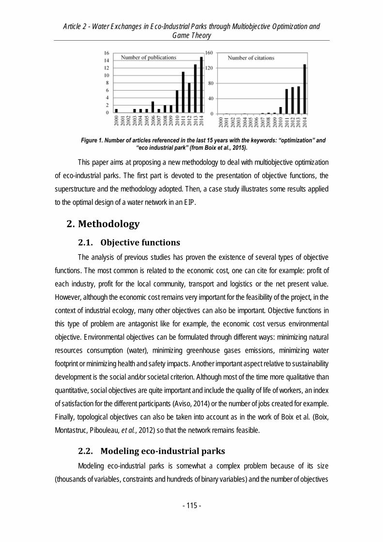
Article 2 - Water Exchanges in Eco-Industrial Parks through Multiobjective Optimization and Game Theory
- 115 -
Figure 1. Number of articles referenced in the last 15 years with the keywords: “optimization” and
“eco industrial park” (from Boix et al., 2015).
This paper aims at proposing a new methodology to deal with multiobjective optimization
of eco-industrial parks. The first part is devoted to the presentation of objective functions, the
superstructure and the methodology adopted. Then, a case study illustrates some results applied
to the optimal design of a water network in an EIP.
2. Methodology
2.1. Objective functions
The analysis of previous studies has proven the existence of several types of objective
functions. The most common is related to the economic cost, one can cite for example: profit of
each industry, profit for the local community, transport and logistics or the net present value.
However, although the economic cost remains very important for the feasibility of the project, in the
context of industrial ecology, many other objectives can also be important. Objective functions in
this type of problem are antagonist like for example, the economic cost versus environmental
objective. Environmental objectives can be formulated through different ways: minimizing natural
resources consumption (water), minimizing greenhouse gases emissions, minimizing water
footprint or minimizing health and safety impacts. Another important aspect relative to sustainability
development is the social and/or societal criterion. Although most of the time more qualitative than
quantitative, social objectives are quite important and include the quality of life of workers, an index
of satisfaction for the different participants (Aviso, 2014) or the number of jobs created for example.
Finally, topological objectives can also be taken into account as in the work of Boix et al. (Boix,
Montastruc, Pibouleau, et al., 2012) so that the network remains feasible.
2.2. Modeling eco-industrial parks
Modeling eco-industrial parks is somewhat a complex problem because of its size
(thousands of variables, constraints and hundreds of binary variables) and the number of objectives

Article 2 - Water Exchanges in Eco-Industrial Parks through Multiobjective Optimization and Game Theory
- 116 -
to take into account. In order to model the network of an EIP, the concept of superstructure is used,
it represents all the possible alternatives to connect each process of the network, this systemic
approach allows to represent process design. Figure 2 shows the superstructure of an EIP including
3 industries and each industry is composed of process and regeneration units.
Figure 2. General superstructure of an EIP including 3 industries
After modeling the superstructure, the next step is to model the network with mass
balances so that mathematical programming methods can be applied. A “black box” approach is
adopted so that each parameter of the different processes is known, for more precision about the
modeling stage, the reader can refer to Boix et al. (Boix, Montastruc, Pibouleau, et al., 2012).
2.3. Multi-objective optimization approaches
Resolution methodologies for multiobjective optimization are generally classified
depending on the number of generated solutions and on the importance of the decision maker
during the resolution. These approaches can be classified into two categories:
Generative approaches: these methods are characterized by the generation of different
solutions and the decision maker has to choose one solution among them. These a posteriori
methods include scalar approaches like weighting method or the epsilon-constraint strategy
coupled with mathematical programming and stochastic methods like genetic algorithm. With these
methods, a Pareto front is built to propose a set of non-dominated solutions to the decision maker.
Preference-based methods: in this case, decision maker preferences are included along
with the resolution and the optimization. These “a priori” approaches like for example, goal
programming or interactive methods like NIMBUS directly include the decision maker preferences
Article 2 - Water Exchanges in Eco-Industrial Parks through Multiobjective Optimization and Game Theory
- 117 -
during the resolution so that one solution is finally obtained. In this work, we propose to adopt the
goal programming approach to solve the case of water allocation in eco industrial parks.
2.4. Characteristics of eco-industrial parks
Boix et al. (Boix, Montastruc, Azzaro-Pantel, et al., 2015) highlighted the lack of studies
dealing with optimization in order to design optimal configuration of an EIP. However, it is important
to develop methodologies able to design an EIP where each industry has a gain compared to the
case where it is individual. Furthermore, each plant included in a park has its own objective (for
example to minimize its costs) and all of these objectives are always antagonists. In this work, a
multiobjective optimization approach is adopted in order to take into account each objective function
associated to each plant of the EIP. This approach has already been applied to the design of
industrial water networks but never with the optimal design of the water network in an EIP which is
a different problem.
The optimization of eco-industrial parks includes several bottlenecks: one of the main
characteristic of this problem is that the structure (represented by the existence or not of
connections between processes and numerically modeled by binary variables) is dominating the
solution. The resulting model is large and of MILP (mixed integer linear programming) type which
constitute a great challenge and it is relatively new to solve this problem with the help of preference-
based approaches. Indeed, previous studies have widely explored generation based approaches
but some numerical problems were encountered especially when problems involve many binary
variables. In most of the cases, the solver does not succeed to return a feasible solution and when
it succeeds to build the Pareto front, it remains a very long and tedious task.
In this work, a goal programming (GP) approach is adopted to obtain one solution that
already includes the preferences of the decision maker. This approach is based on a recent study
(Ramos, Boix, Montastruc, et al., 2014) where it has been proven that GP can be a very reliable
method to design industrial water networks following multiple antagonist objective functions.
Based on an academic example, this paper explores 3 different scenarios of an EIP in
order to point out the difficulties encountered with multiobjective optimization of EIP’s.

Article 2 - Water Exchanges in Eco-Industrial Parks through Multiobjective Optimization and Game Theory
- 118 -
3. Multiobjective optimization through goal
programming
3.1. Presentation of the case study
In this study, an EIP including 3 plants is designed, this academic example has been widely
explored in the literature (Olesen & Polley, 1996; Boix, Montastruc, Pibouleau, et al., 2012). For
this reason, it remains a good example to test and to validate a new methodology because solutions
are well-known. Each plant is composed of 5 process units and the parameters are the same as
those defined in Boix et al. (Boix, Montastruc, Pibouleau, et al., 2012).
Three different scenarios are explored (Figure 3), where the position of the regeneration
unit differs, so that all the configurations are scanned:
- Scenario 1: the three plants exchange water and each plant owns its regeneration unit,
chosen among three available types (depending on the outlet concentration);
- Scenario 2: the three plants exchange water and share one regeneration unit;
- Scenario 3: a mixed scenario where each plant owns its regeneration unit and an
additional unit is shared by the three plants.
It is important to notice that for each above mentioned scenario, three objective functions
are minimized: the total cost of each plant involved in the EIP.
Figure 3. Different configurations of the EIP
In order to show that these objectives are antagonists, table 1 represents the pay-off table
that include the values of two objectives while the third is minimized for scenario 2.
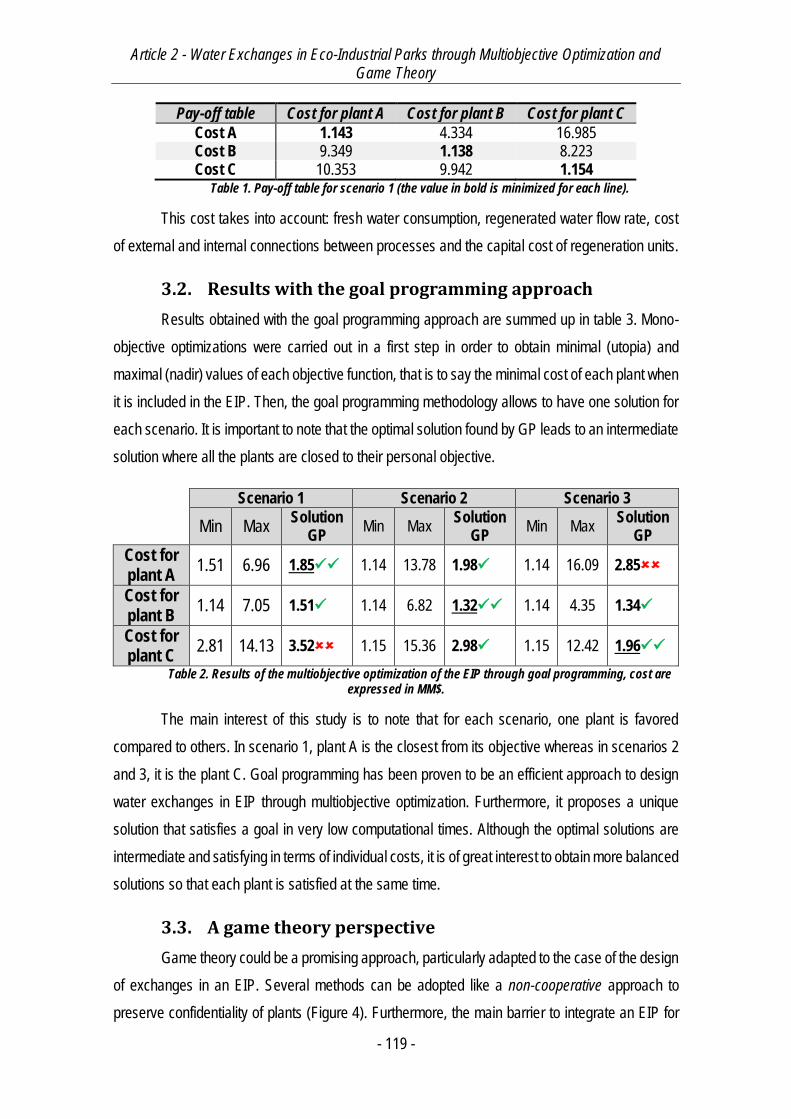
Article 2 - Water Exchanges in Eco-Industrial Parks through Multiobjective Optimization and Game Theory
- 119 -
Pay-off table Cost for plant A Cost for plant B Cost for plant C
Cost A 1.143 4.334 16.985 Cost B 9.349 1.138 8.223 Cost C 10.353 9.942 1.154
Table 1. Pay-off table for scenario 1 (the value in bold is minimized for each line).
This cost takes into account: fresh water consumption, regenerated water flow rate, cost
of external and internal connections between processes and the capital cost of regeneration units.
3.2. Results with the goal programming approach
Results obtained with the goal programming approach are summed up in table 3. Mono-
objective optimizations were carried out in a first step in order to obtain minimal (utopia) and
maximal (nadir) values of each objective function, that is to say the minimal cost of each plant when
it is included in the EIP. Then, the goal programming methodology allows to have one solution for
each scenario. It is important to note that the optimal solution found by GP leads to an intermediate
solution where all the plants are closed to their personal objective.
Scenario 1 Scenario 2 Scenario 3
Min Max Solution
GP Min Max
Solution GP
Min Max Solution
GP
Cost for plant A
1.51 6.96 1.85 1.14 13.78 1.98 1.14 16.09 2.85
Cost for plant B
1.14 7.05 1.51 1.14 6.82 1.32 1.14 4.35 1.34
Cost for plant C
2.81 14.13 3.52 1.15 15.36 2.98 1.15 12.42 1.96
Table 2. Results of the multiobjective optimization of the EIP through goal programming, cost are expressed in MM$.
The main interest of this study is to note that for each scenario, one plant is favored
compared to others. In scenario 1, plant A is the closest from its objective whereas in scenarios 2
and 3, it is the plant C. Goal programming has been proven to be an efficient approach to design
water exchanges in EIP through multiobjective optimization. Furthermore, it proposes a unique
solution that satisfies a goal in very low computational times. Although the optimal solutions are
intermediate and satisfying in terms of individual costs, it is of great interest to obtain more balanced
solutions so that each plant is satisfied at the same time.
3.3. A game theory perspective
Game theory could be a promising approach, particularly adapted to the case of the design
of exchanges in an EIP. Several methods can be adopted like a non-cooperative approach to
preserve confidentiality of plants (Figure 4). Furthermore, the main barrier to integrate an EIP for
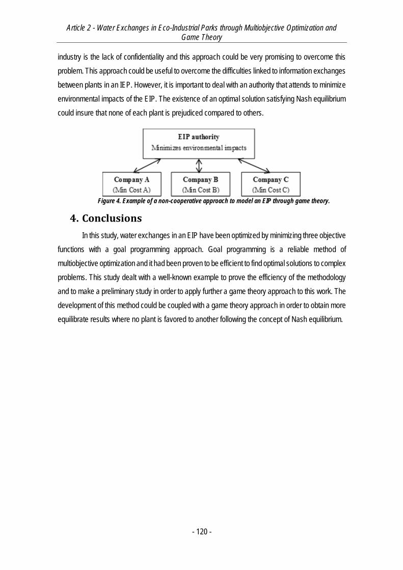
Article 2 - Water Exchanges in Eco-Industrial Parks through Multiobjective Optimization and Game Theory
- 120 -
industry is the lack of confidentiality and this approach could be very promising to overcome this
problem. This approach could be useful to overcome the difficulties linked to information exchanges
between plants in an IEP. However, it is important to deal with an authority that attends to minimize
environmental impacts of the EIP. The existence of an optimal solution satisfying Nash equilibrium
could insure that none of each plant is prejudiced compared to others.
Figure 4. Example of a non-cooperative approach to model an EIP through game theory.
4. Conclusions
In this study, water exchanges in an EIP have been optimized by minimizing three objective
functions with a goal programming approach. Goal programming is a reliable method of
multiobjective optimization and it had been proven to be efficient to find optimal solutions to complex
problems. This study dealt with a well-known example to prove the efficiency of the methodology
and to make a preliminary study in order to apply further a game theory approach to this work. The
development of this method could be coupled with a game theory approach in order to obtain more
equilibrate results where no plant is favored to another following the concept of Nash equilibrium.
Article 2 - Water Exchanges in Eco-Industrial Parks through Multiobjective Optimization and Game Theory
- 121 -
References
Aviso, K.B. (2014) Design of Robust Water Exchange Networks for Eco-Industrial
Symbiosis. Process Safety and Environmental Protection. [Online] 92 (2), 160–170. Available from:
doi:10.1016/j.psep.2012.12.001.
Boix, M., Montastruc, L., Azzaro-Pantel, C. & Domenech, S. (2015) Optimization Methods
Applied to the Design of Eco-Industrial Parks: A Literature Review. Journal of Cleaner Production.
87303–317.
Boix, M., Montastruc, L., Pibouleau, L., Azzaro-Pantel, C., et al. (2012) Industrial Water
Management by Multiobjective Optimization: From Individual to Collective Solution Through Eco-
Industrial Parks. Journal of Cleaner Production. [Online] 22 (1), 85–97. Available from:
doi:10.1016/j.jclepro.2011.09.011.
Frosch, R.A. & Gallopoulos, N.E. (1989) Strategies for Manufacturing. Scientific American.
261 (3), 144–152.
Lowe, E.A. (1997) Creating by-Product Resource Exchanges: Strategies for Eco-Industrial
Parks. Journal of Cleaner Production. [Online] 5 (1–2), 57–65. Available from: doi:10.1016/S0959-
6526(97)00017-6.
Olesen, S.G. & Polley, G.T. (1996) Dealing with Plant Geography and Piping Constraints
in Water Network Design. Process Safety and Environmental Protection. [Online] 74 (4), 273–276.
Available from: doi:10.1205/095758296528626.
Ramos, M.A., Boix, M., Montastruc, L. & Domenech, S. (2014) Multiobjective Optimization
Using Goal Programming for Industrial Water Network Design. Industrial & Engineering Chemistry
Research. 53 (45), 17722–17735.

- 123 -
Chapitre 4 - Water integration in Eco-Industrial Parks Using a Multi-Leader-
Follower Approach

Article 3 - Water integration in Eco-Industrial Parks Using a Multi-Leader-Follower Approach
- 124 -
Article 3 - Water integration in Eco-Industrial Parks Using a Multi-Leader-Follower Approach
- 125 -
Ramos, Manuel A., Marianne Boix, Didier Aussel, Ludovic Montastruc, & Serge Domenech. 2016.
“Water Integration in Eco-Industrial Parks Using a Multi-Leader-Follower Approach.” Computers &
Chemical Engineering 87: 190–207.
Résumé
Cet article représente un des points cruciaux de la thèse. En effet, afin de surmonter les problèmes
liés à la confidentialité entre les entreprises d’un même parc, le concept d’autorité, appelé
également régulateur de l’EIP est introduit. Ainsi, l’autorité du parc a pour objectif de minimiser la
consommation des ressources naturelles dans l’EIP (i.e. l’eau fraîche) tandis que chaque usine
cherche à minimiser son coût opératoire annualisé. De cette façon, l’EIP est modélisé comme un
Multi-leader-single-follower game (MLSFG) dans lequel les usines agissent comme les « leaders
» et l’autorité comme un « follower ». La formulation inverse, c’est-à-dire, Single-leader-multi-
follower game (SLMFG) avec les entreprises en tant que “follower” et l’autorité en “leader” est
également explorée. Dans les deux cas, le niveau (inférieur ou supérieur) au sein duquel sont
modélisées les usines représente un jeu dans lequel les entreprises doivent être en équilibre de
Nash entre elles pour la solution optimale et en même temps être en équilibre de Stackelberg avec
le niveau dans lequel est modélisée l’autorité. Grâce à cette approche, le problème de
confidentialité est géré ainsi que le problème de dépendance d’un décideur externe qui prend des
décisions de façon empirique. Ensuite, dans ce travail, la modélisation des jeux bi-niveaux est
discutée dans le détail. Il est notamment démontré que, dans certaines conditions (situations de
convexité, qualification des contraintes) que le problème du (des) follower (s) est équivalent aux
conditions d’optimalité du premier ordre, dites conditions KKT (conditions de Karush-Kuhn-Tucker).
À partir de ce postulat, une formulation de type « All Equilibrium » (tout à l’équilibre) est présentée
dans laquelle les leaders préconisent aussi les stratégies du follower pour les autres leaders,
conduisant à des modèles plus facilement résolubles. Cependant, d’un point de vue modélisation,
cette transformation rend le problème non linéaire et non convexe à cause de l’introduction des
contraintes de complémentarité qui font partie des conditions de KKT. Dans cet article, les
méthodologies de résolution numérique des différents problèmes d’optimisation sont détaillées,
exploitées et analysées de façon approfondie. Ce travail introduit également un algorithme
d’élimination des faibles flux afin de proposer une structure de réseau simple sans aberrations en
évitant de placer des petits tuyaux. L’algorithme développé permet notamment d’éliminer les
variables discrètes du modèle (liées au nombre de connexions ou tuyaux) qui rendent la résolution
des modèles MLFG très difficile. Le cas d’étude choisi est le même que celui de Boix (Boix, 2011)

Article 3 - Water integration in Eco-Industrial Parks Using a Multi-Leader-Follower Approach
- 126 -
(3 usines incluant 5 procédés chacune) prouvant ainsi l’adaptabilité de la méthodologie développée
sur des cas de grande taille. Dans un premier temps, un EIP sans unité de régénération est étudié
puis, des unités de régénération communes gérées par l’autorité de l’EIP sont introduites. Les
résultats démontrent que la méthodologie garantit un gain relatif positif pour chaque usine par
rapport au cas où elles opèrent de façon autonome, i.e. hors EIP. Le résultat le plus attractif est
celui obtenu avec le modèle SLMFG, dans lequel les gains sont assez significatifs (i.e. 15%15% ) et
la consommation d’eau fraîche reste très faible.

Article 3 - Water integration in Eco-Industrial Parks Using a Multi-Leader-Follower Approach
- 127 -

Article 3 - Water integration in Eco-Industrial Parks Using a Multi-Leader-Follower Approach
- 128 -
Article 3 - Water integration in Eco-Industrial Parks Using a Multi-Leader-Follower Approach
- 129 -
Water integration in Eco-Industrial Parks
Using a Multi-Leader-Follower Approach
Manuel A. Ramosa, Marianne Boix*a, Didier Aussel*b, Ludovic Montastruca, Serge
Domenecha
a Laboratoire de Génie Chimique, U.M.R. 5503 CNRS/INP/UPS, Université de Toulouse, 4, Allée
Emile Monso, 31432 Toulouse Cedex 4, France
b Laboratoire PROMES, UPR CNRS 8521, Université de Perpignan, Via Domitia, 66100 Perpignan,
France
* Corresponding authors: [email protected]; [email protected].
Keywords: Eco-industrial parks, Multi-leader-follower Game, Nash equilibrium, Multi-objective
Optimization, MPCC, and Game Theory.
Abstract
The design and optimization of industrial water networks in eco-industrial parks is studied by
formulating and solving multi-leader-follower game problems. The methodology is explained by
demonstrating its advantages against multi-objective optimization approaches. Several
formulations and solution methods for MLFG are discussed in detail. The approach is validated on
a case study of water integration in EIP without and with regeneration units. In the latter, multi-
leader-single-follower and single-leader-multi-follower games are studied. Each plant’s objective is
to minimize the total annualized cost, while the EIP authority objective is to minimize the
consumption of freshwater within the ecopark. The MLFG is transformed into a MOPEC and solved
using GAMS® as an NLP. Obtained results are compared against the MOO approach and between
different MLFG formulations. The methodology proposed is proved to be very reliable in multi-
criteria scenarios compared to MOO approaches, providing numerical Nash equilibrium solutions
and specifically in EIP design and optimization.
1. Introduction
During the last few decades, industrialization has contributed to rapid depletion of natural
resources such as water and natural gas. Consequently, there is a real need for industries to ensure
minimum natural resources consumption, while maintaining good production levels. In particular,
Article 3 - Water integration in Eco-Industrial Parks Using a Multi-Leader-Follower Approach
- 130 -
industrial development is often linked to the use of high volumes of freshwater (Boix, Montastruc,
Pibouleau, et al., 2011, 2010). In order to work towards global environmental preservation while
increasing business success, the concept of industrial ecology has emerged (Boix, Montastruc,
Azzaro-Pantel, et al., 2015). This concept, which is directly linked to sustainable development, aims
at engaging separate industries, geographically closed enough, in a collective approach so that
exchanges of raw matter, by-products, energy and utilities (Chertow, 2000) are maximized. Indeed,
the most widespread manifestations of these kinds of industrial symbiosis are eco-industrial parks
(EIP). A definition widely accepted of EIP is “an industrial system of planned materials and energy
exchanges that seeks to minimize energy and raw materials use, minimize waste, and build
sustainable economic, ecological and social relationships” (Boix, Montastruc, Azzaro-Pantel, et al.,
2015; Montastruc, Boix, Pibouleau, et al., 2013; Alexander, Barton, Petrie, et al., 2000). As it can
be highlighted, a basic condition for an EIP to be economically viable is to demonstrate that benefits
of each industry involved in it by working collectively is higher than working as a stand-alone facility.
Boix et al. (Boix, Montastruc, Azzaro-Pantel, et al., 2015) highlighted the lack of studies
dealing with optimization in order to design optimal configuration of an EIP. However, it is important
to develop methodologies able to design an EIP where each industry has an effective gain
compared to the case where they operate individually, by also taking into account environmental
concerns. Among EIP design studies, water-using network is the most common type of cooperation
modeled in literature (Boix, Montastruc, Azzaro-Pantel, et al., 2015). In this kind of studies, the case
is often solved as a water-allocation problem through a superstructure-based model where water
has to be distributed, treated and discharged in an optimal way between the process units of each
plant/company involved in the EIP.
Modeling EIPs based on water-exchange networks is somewhat a complex problem, since,
depending on the number of plants and processes, a model with thousands of variables, constraints
and disjunctions has to be solved. On the other hand, it is obvious that the design of EIPs through
mono-objective optimization it is not trivial, since to choice a single objective function is almost
impossible due to the size of the manifold of the possible objective functions. As aforementioned,
the main aim of industrial symbiosis is to minimize pollution and resources utilization while
maximizing each company’s gain. For instance, by using a mono-objective optimization approach
and minimizing the EIP total annualized cost do not necessarily agree with environmental
objectives. Indeed, it is due to the latter that these kind of problems are better tackled with a
multiobjective optimization (MOO) approach (Montastruc, Boix, Pibouleau, et al., 2013; Boix,
Montastruc, Azzaro-Pantel, et al., 2015; Boix & Montastruc, 2011).
Article 3 - Water integration in Eco-Industrial Parks Using a Multi-Leader-Follower Approach
- 131 -
Recently, Boix et al. (Boix, Montastruc, Pibouleau, et al., 2012) developed a multi-objective
optimization strategy based on the -constraint method applied to the case of a water network in
an EIP under several scenarios. The interest of dealing with multiobjective optimization is to build
a Pareto front in which several optimal solutions are available; then, an a posteriori tool of multi-
criteria decision making is further applied. In the aforementioned work, three antagonist objective
functions were taken into account: freshwater consumption, number of connections and total
regenerated water-flowrate. On the other hand, a posterior work of Montastruc et al. (Montastruc,
Boix, Pibouleau, et al., 2013) has explored the flexibility of the designed EIPs by changing
parameters related to processes. The authors have also analyzed different indicators to test the
EIP profitability. Then, a later extension of this work was conducted by Ramos et al. (Ramos, Boix,
Aussel, et al., 2015): they employed a multiobjective optimization approach by minimizing each
plant capital cost by using goal programming (GP). This approach is based on a recent study where
GP has been proven to be a very reliable method to design industrial water networks following
multiple antagonist objective functions (Ramos et al. (Ramos, Boix, Montastruc, et al., 2014)).
Indeed, previous studies have widely explored Pareto front generation approaches but
some numerical problems were encountered especially when a very large number of binary
variables is involved. In most cases, choosing the bounds for generating methods (e.g. ε-constraint
method) is a non-trivial task, and the choice of these bounds is important because if they are not
well chosen the solver may not succeed into obtaining a feasible solution. Furthermore, if a solution
is found it remains a very long and tedious computational task. That is why a GP approach shows
more affinity with EIP design. However, Ramos et al. (Ramos, Boix, Aussel, et al., 2015)
demonstrated that in different scenarios and by tuning different optimization parameters (e.g.
weight factors associated with the objective functions) one company is favored compared to the
others. Although optimal solutions are intermediate and satisfying in terms of individual costs, it is
of great interest to obtain more balanced solutions so that each plant/company is satisfied at the
same time and moreover, by minimizing freshwater consumption in order to insure the
environmental performance of the EIP.
An interesting alternative particularly adapted to the optimal design of EIP is the Game
Theory approach and most particularly the concept of the generalized Nash equilibrium problem
(GNEP). In fact, an EIP can be seen as the congregation of different non-cooperative agents (i.e.
the plants) which aim at minimizing their annualized operating costs and an EIP authority whose
aim is to minimize resources consumption (e.g. freshwater). This kind of non-cooperative game is
very interesting for the concepts of EIP, since the main barrier to integrate an EIP for industry is
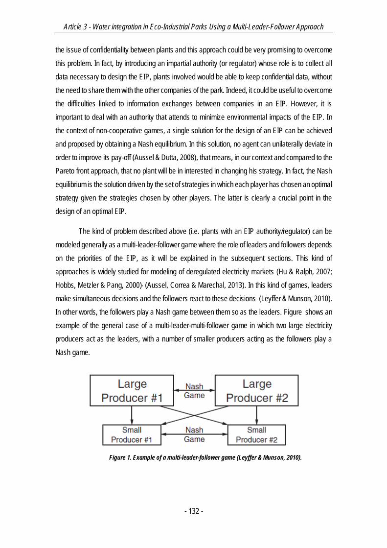
Article 3 - Water integration in Eco-Industrial Parks Using a Multi-Leader-Follower Approach
- 132 -
the issue of confidentiality between plants and this approach could be very promising to overcome
this problem. In fact, by introducing an impartial authority (or regulator) whose role is to collect all
data necessary to design the EIP, plants involved would be able to keep confidential data, without
the need to share them with the other companies of the park. Indeed, it could be useful to overcome
the difficulties linked to information exchanges between companies in an EIP. However, it is
important to deal with an authority that attends to minimize environmental impacts of the EIP. In
the context of non-cooperative games, a single solution for the design of an EIP can be achieved
and proposed by obtaining a Nash equilibrium. In this solution, no agent can unilaterally deviate in
order to improve its pay-off (Aussel & Dutta, 2008), that means, in our context and compared to the
Pareto front approach, that no plant will be in interested in changing his strategy. In fact, the Nash
equilibrium is the solution driven by the set of strategies in which each player has chosen an optimal
strategy given the strategies chosen by other players. The latter is clearly a crucial point in the
design of an optimal EIP.
The kind of problem described above (i.e. plants with an EIP authority/regulator) can be
modeled generally as a multi-leader-follower game where the role of leaders and followers depends
on the priorities of the EIP, as it will be explained in the subsequent sections. This kind of
approaches is widely studied for modeling of deregulated electricity markets (Hu & Ralph, 2007;
Hobbs, Metzler & Pang, 2000), (Aussel, Correa & Marechal, 2013). In this kind of games, leaders
make simultaneous decisions and the followers react to these decisions (Leyffer & Munson, 2010).
In other words, the followers play a Nash game between them so as the leaders. Figure shows an
example of the general case of a multi-leader-multi-follower game in which two large electricity
producers act as the leaders, with a number of smaller producers acting as the followers play a
Nash game.
Figure 1. Example of a multi-leader-follower game (Leyffer & Munson, 2010).
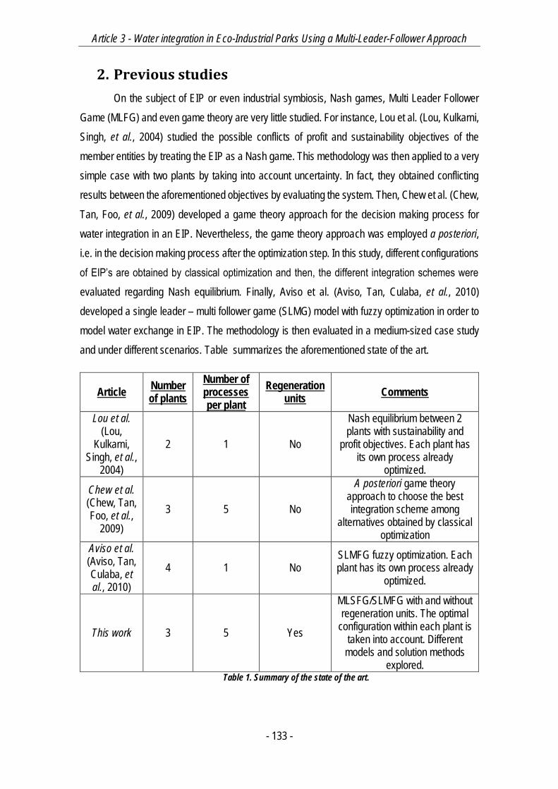
Article 3 - Water integration in Eco-Industrial Parks Using a Multi-Leader-Follower Approach
- 133 -
2. Previous studies
On the subject of EIP or even industrial symbiosis, Nash games, Multi Leader Follower
Game (MLFG) and even game theory are very little studied. For instance, Lou et al. (Lou, Kulkarni,
Singh, et al., 2004) studied the possible conflicts of profit and sustainability objectives of the
member entities by treating the EIP as a Nash game. This methodology was then applied to a very
simple case with two plants by taking into account uncertainty. In fact, they obtained conflicting
results between the aforementioned objectives by evaluating the system. Then, Chew et al. (Chew,
Tan, Foo, et al., 2009) developed a game theory approach for the decision making process for
water integration in an EIP. Nevertheless, the game theory approach was employed a posteriori,
i.e. in the decision making process after the optimization step. In this study, different configurations
of EIP’s are obtained by classical optimization and then, the different integration schemes were
evaluated regarding Nash equilibrium. Finally, Aviso et al. (Aviso, Tan, Culaba, et al., 2010)
developed a single leader – multi follower game (SLMG) model with fuzzy optimization in order to
model water exchange in EIP. The methodology is then evaluated in a medium-sized case study
and under different scenarios. Table summarizes the aforementioned state of the art.
Article Number of plants
Number of processes per plant
Regeneration units
Comments
Lou et al. (Lou,
Kulkarni, Singh, et al.,
2004)
2 1 No
Nash equilibrium between 2 plants with sustainability and
profit objectives. Each plant has its own process already
optimized.
Chew et al. (Chew, Tan, Foo, et al.,
2009)
3 5 No
A posteriori game theory approach to choose the best integration scheme among
alternatives obtained by classical optimization
Aviso et al. (Aviso, Tan, Culaba, et al., 2010)
4 1 No SLMFG fuzzy optimization. Each plant has its own process already
optimized.
This work 3 5 Yes
MLSFG/SLMFG with and without regeneration units. The optimal
configuration within each plant is taken into account. Different
models and solution methods explored.
Table 1. Summary of the state of the art.
Article 3 - Water integration in Eco-Industrial Parks Using a Multi-Leader-Follower Approach
- 134 -
As it can be seen, this work deals with both MLSFG/SLMFG approaches for the design of
EIP, in which at least the former, to the best of authors’ knowledge, is an unexplored area of
research regarding the design of EIP or even in any domain of process engineering.
The aim of this work is to develop an alternative methodology to multi-criteria optimization
generally used in the field of process engineering, by applying the methodology in an industrial
ecology context. First, the MLSFG is formulated and solved in an optimization manner, and
algorithmic, modeling and reformulations issues are discussed alongside. Then, it is demonstrated
the power of such formulations by comparing them with MOO methodologies with a case study of
considerable size where the consideration of regeneration units is included. It is also important to
specify that the optimal design of each plant is taken into account in the model. The latter is a
fundamental point when designing EIP, since by first optimizing each plant and then by optimizing
the EIP like in Lou et al. (Lou, Kulkarni, Singh, et al., 2004) several optimal solutions could be
discarded. In the subsequent sections, the MLFG approach is explained in detail, as well as
different formulations, models for water integration with and without regeneration units and solution
methodologies. Successively, results for each one of the case studies are presented, and
comparisons with respective MOO results are made.
Solving MLFG is a rather difficult task (Leyffer & Munson, 2010; Aussel & Dutta, 2008;
Pang & Fukushima, 2005), and the modeling has to be accomplished very carefully and on the
other side, solution methodologies have to be carefully chosen and tuned. Finally, it is important to
highlight that large-scale MLFG models such as those addressed in this work have never been
treated in literature before, to the best of authors’ knowledge.
3. Multi-leader-follower game approach
In order to obtain a solution for the kind of systems as EIPs are, where heavy interactions
exist and where each entity is biased by their own interests, game theory is a viable tool for
decision-making. As aforementioned, in Nash games, players make simultaneous optimal
decisions given the optimal strategies of other players. Indeed, Nash equilibrium denotes the state
where all the casual forces internal to the system balance each other out (Lou, Kulkarni, Singh, et
al., 2004), and no player can improve its gain by unilaterally changing his strategy. By solving a
Nash game, it is possible to obtain this kind of solution by definition. On the contrary, by considering
the problem as a MOO problem, an ulterior decision-making procedure has to be successfully
applied in order to obtain a solution where all participants are satisfied by the solution, as
demonstrated by Ramos et al. (Ramos, Boix, Montastruc, et al., 2014). If the participant is not
Article 3 - Water integration in Eco-Industrial Parks Using a Multi-Leader-Follower Approach
- 135 -
satisfied with the solution, another solution has to be chosen by the decision maker from the pool
of solutions or another solution has to be generated taking into account that preferences of the
participants are known. In contrast, Nash games do not need to have information on participants’
preferences. It is important to note that obtaining a solution with MOO that satisfies all participants
is a very difficult task, and even impossible for certain cases (Ramos, Boix, Aussel, et al., 2015).
Moreover, the case of MLSFG is impossible to model by MOO if leaders’ optimal responses are
unknown, which is almost always the case.
3.1. Authority/Regulator’s design of an EIP and game theory
approach
The introduction of an authority/regulator to the design of viable water networks in EIP is
an interesting alternative to overcome the confidentiality problem on one hand, and on the other
hand, to solve the problem of equilibrium benefits of the players involved. In fact, the latter can be
modeled as a MLSFG where the leaders are the plants whereas the EIP authority represents the
only follower or as a SLMFG, when the roles are inversed. The choice between these different
formulations depends on the priorities of the EIP.
The design of EIP water network by MLFG consists in near-located plant process plants
that are subjected to regulations implemented in the park. Each plant has its own processes, and
each process requires a specific water both in quantity and quality in order to operate. Moreover,
each process produces a certain amount of wastewater, given its contaminant flowrate and an
upper bound on outlet quality. In this particular case, only one contaminant is taken into account
for the sake of simplicity. Each plant has access to water regeneration units, shared within the EIP.
At this point, it is important to note that in the MLFG approach the choice of leaders and
followers is crucial in the problem formulation. As it will be explained later in terms of modeling and
results, this choice changes completely the nature of the problem: On one hand, it can be assumed
that plants act as followers and the authority as the lone leader (SLMFG) or vice-versa (MLSFG).
It is assumed that in the case of SLMFG the plants aim to minimize their total annualized cost,
given the minimum flowrate consumption in the EIP, determined by the authority. This is in fact the
same game as the one proposed by Aviso et al. (Aviso, Tan, Culaba, et al., 2010). A general
scheme of the SLMFG proposed is shown in Figure 2.

Article 3 - Water integration in Eco-Industrial Parks Using a Multi-Leader-Follower Approach
- 136 -
Leader
EIP authority
Minimize Freshwater consumption
Plant 1Minimize Cost1
Plant NMinimize CostN
Plant 2Minimize Cost2
Followers
Stackelberg Equilibrium
Figure 2. General scheme of the proposed SLMFG.
On the other hand, the game may be formulated as a MLSFG, where the EIP authority
aims to minimize the total freshwater consumption, given the recycle and reuse of wastewater
inside each plant and between plants, which minimizes their individual operating costs. A general
scheme of the MLSFG proposed is shown in Figure 3.
Plant 1Minimize Cost1
EIP authority
Minimize Freshwater consumption
Plant NMinimize CostN
Plant 2Minimize Cost2
Leaders
Follower
Stackelberg Equilibrium
Nash Equilibrium
Figure 3. General scheme of the proposed MLSFG.
By changing the nature of the game as stated above, the priorities of the EIP are shifted.
Indeed, in the latter case plants operating cost is predominant compared to total freshwater
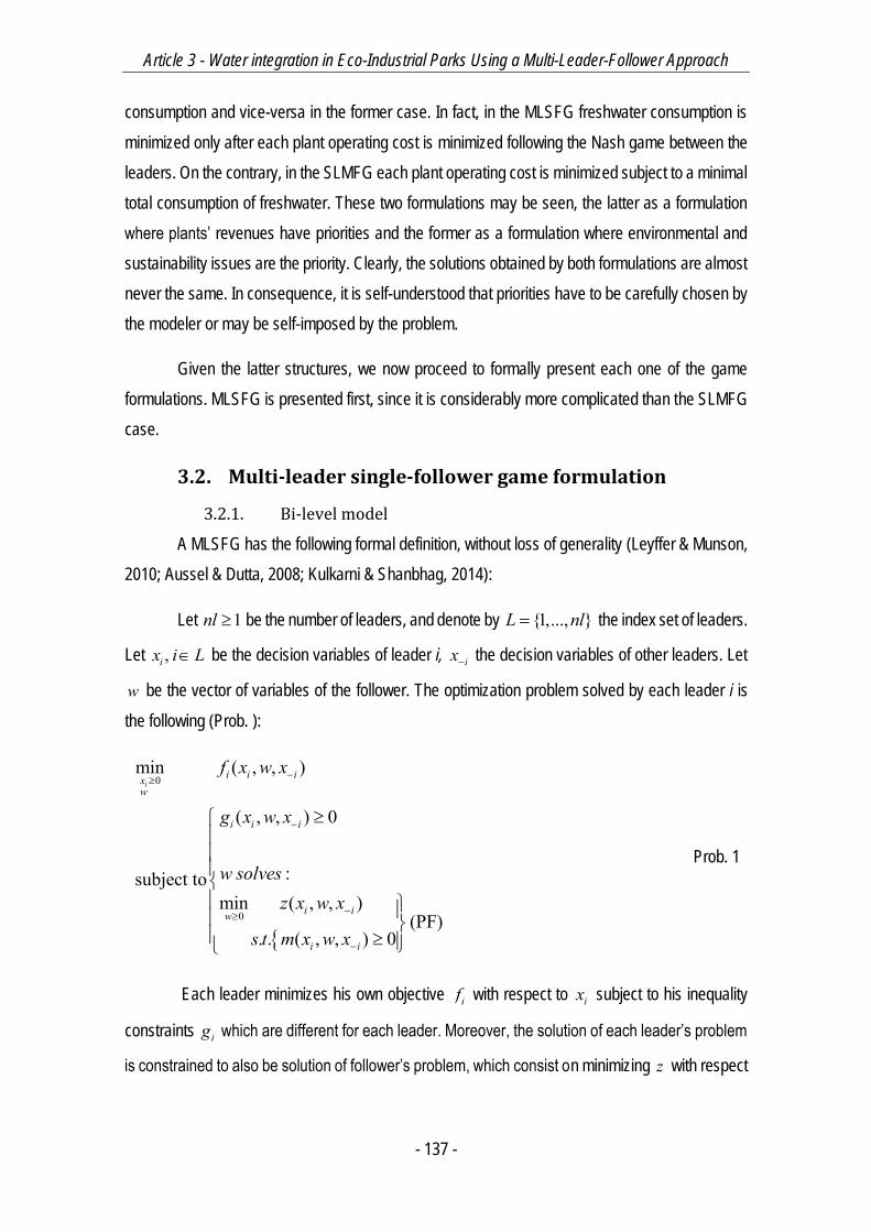
Article 3 - Water integration in Eco-Industrial Parks Using a Multi-Leader-Follower Approach
- 137 -
consumption and vice-versa in the former case. In fact, in the MLSFG freshwater consumption is
minimized only after each plant operating cost is minimized following the Nash game between the
leaders. On the contrary, in the SLMFG each plant operating cost is minimized subject to a minimal
total consumption of freshwater. These two formulations may be seen, the latter as a formulation
where plants’ revenues have priorities and the former as a formulation where environmental and
sustainability issues are the priority. Clearly, the solutions obtained by both formulations are almost
never the same. In consequence, it is self-understood that priorities have to be carefully chosen by
the modeler or may be self-imposed by the problem.
Given the latter structures, we now proceed to formally present each one of the game
formulations. MLSFG is presented first, since it is considerably more complicated than the SLMFG
case.
3.2. Multi-leader single-follower game formulation
3.2.1. Bi-level model
A MLSFG has the following formal definition, without loss of generality (Leyffer & Munson,
2010; Aussel & Dutta, 2008; Kulkarni & Shanbhag, 2014):
Let 1nl be the number of leaders, and denote by {1,..., }L nl the index set of leaders.
Let ,ix i L be the decision variables of leader i, ix the decision variables of other leaders. Let
w be the vector of variables of the follower. The optimization problem solved by each leader i is
the following (Prob. ):
0
0
min ( , , )
( , , ) 0
:subject tomin ( , , )
(PF). . ( , , ) 0
ii i ix
w
i i i
i iw
i i
f x w x
g x w x
w solvesz x w x
s t m x w x
Prob. 1
Each leader minimizes his own objective if with respect to ix subject to his inequality
constraints ig which are different for each leader. Moreover, the solution of each leader’s problem
is constrained to also be solution of follower’s problem, which consist on minimizing z with respect
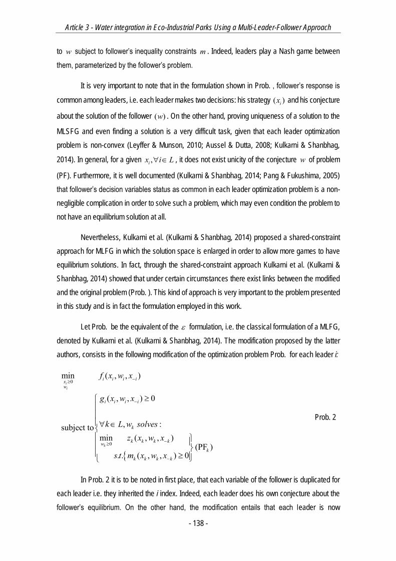
Article 3 - Water integration in Eco-Industrial Parks Using a Multi-Leader-Follower Approach
- 138 -
to w subject to follower’s inequality constraints m . Indeed, leaders play a Nash game between
them, parameterized by the follower’s problem.
It is very important to note that in the formulation shown in Prob. , follower’s response is
common among leaders, i.e. each leader makes two decisions: his strategy ( )ix and his conjecture
about the solution of the follower ( )w . On the other hand, proving uniqueness of a solution to the
MLSFG and even finding a solution is a very difficult task, given that each leader optimization
problem is non-convex (Leyffer & Munson, 2010; Aussel & Dutta, 2008; Kulkarni & Shanbhag,
2014). In general, for a given ,ix i L , it does not exist unicity of the conjecture w of problem
(PF). Furthermore, it is well documented (Kulkarni & Shanbhag, 2014; Pang & Fukushima, 2005)
that follower’s decision variables status as common in each leader optimization problem is a non-
negligible complication in order to solve such a problem, which may even condition the problem to
not have an equilibrium solution at all.
Nevertheless, Kulkarni et al. (Kulkarni & Shanbhag, 2014) proposed a shared-constraint
approach for MLFG in which the solution space is enlarged in order to allow more games to have
equilibrium solutions. In fact, through the shared-constraint approach Kulkarni et al. (Kulkarni &
Shanbhag, 2014) showed that under certain circumstances there exist links between the modified
and the original problem (Prob. ). This kind of approach is very important to the problem presented
in this study and is in fact the formulation employed in this work.
Let Prob. be the equivalent of the formulation, i.e. the classical formulation of a MLFG,
denoted by Kulkarni et al. (Kulkarni & Shanbhag, 2014). The modification proposed by the latter
authors, consists in the following modification of the optimization problem Prob. for each leader i:
0
0
min ( , , )
( , , ) 0
, :subject tomin ( , , )
(PF ). . ( , , ) 0
ii
k
i i i ixw
i i i i
k
k k k kwk
k k k k
f x w x
g x w x
k L w solvesz x w x
s t m x w x
Prob. 2
In Prob. 2 it is to be noted in first place, that each variable of the follower is duplicated for
each leader i.e. they inherited the i index. Indeed, each leader does his own conjecture about the
follower’s equilibrium. On the other hand, the modification entails that each leader is now
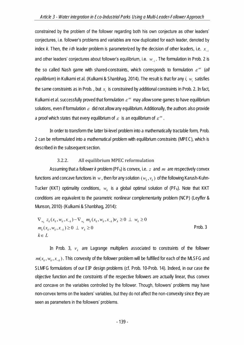
Article 3 - Water integration in Eco-Industrial Parks Using a Multi-Leader-Follower Approach
- 139 -
constrained by the problem of the follower regarding both his own conjecture as other leaders’
conjectures, i.e. follower’s problems and variables are now duplicated for each leader, denoted by
index k. Then, the i-th leader problem is parameterized by the decision of other leaders, i.e. ix
and other leaders’ conjectures about follower’s equilibrium, i.e. iw . The formulation in Prob. 2 is
the so called Nash game with shared-constraints, which corresponds to formulation ae (all
equilibrium) in Kulkarni et al. (Kulkarni & Shanbhag, 2014). The result is that for any i, iw satisfies
the same constraints as in Prob. , but ix is constrained by additional constraints in Prob. 2. In fact,
Kulkarni et al. successfully proved that formulation ae may allow some games to have equilibrium
solutions, even if formulation did not allow any equilibrium. Additionally, the authors also provide
a proof which states that every equilibrium of is an equilibrium of ae .
In order to transform the latter bi-level problem into a mathematically tractable form, Prob.
2 can be reformulated into a mathematical problem with equilibrium constraints (MPEC), which is
described in the subsequent section.
3.2.2. All equilibrium MPEC reformulation
Assuming that a follower k problem (PFk) is convex, i.e. z and m are respectively convex
functions and concave functions in w , then for any solution ( , )k kw v of the following Karush-Kuhn-
Tucker (KKT) optimality conditions, kw is a global optimal solution of (PFk). Note that KKT
conditions are equivalent to the parametric nonlinear complementarity problem (NCP) (Leyffer &
Munson, 2010), (Kulkarni & Shanbhag, 2014):
( , , ) ( , , ) 0 0
( , , ) 0 0k kw k k k k w k k k k k k
k k k k k
z x w x m x w x w
m x w xk L
Prob. 3
In Prob. 3, k are Lagrange multipliers associated to constraints of the follower
( , , )k k km x w x . This convexity of the follower problem will be fulfilled for each of the MLSFG and
SLMFG formulations of our EIP design problems (cf. Prob. 10-Prob. 14). Indeed, in our case the
objective function and the constraints of the respective followers are actually linear, thus convex
and concave on the variables controlled by the follower. Though, followers’ problems may have
non-convex terms on the leaders’ variables, but they do not affect the non-convexity since they are
seen as parameters in the followers’ problems.
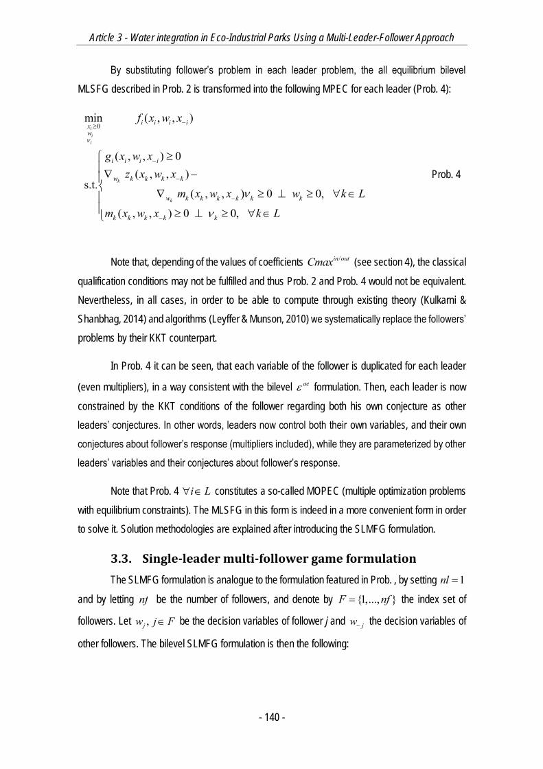
Article 3 - Water integration in Eco-Industrial Parks Using a Multi-Leader-Follower Approach
- 140 -
By substituting follower’s problem in each leader problem, the all equilibrium bilevel
MLSFG described in Prob. 2 is transformed into the following MPEC for each leader (Prob. 4):
0min ( , , )
( , , ) 0( , , )
s.t.( , , ) 0 0,
( , , ) 0 0,
iii
k
k
i i i ixw
i i i i
w k k k k
w k k k k k k
k k k k k
f x w x
g x w xz x w x
m x w x w k L
m x w x k L
Prob. 4
Note that, depending of the values of coefficients /in outCmax (see section 4), the classical
qualification conditions may not be fulfilled and thus Prob. 2 and Prob. 4 would not be equivalent.
Nevertheless, in all cases, in order to be able to compute through existing theory (Kulkarni &
Shanbhag, 2014) and algorithms (Leyffer & Munson, 2010) we systematically replace the followers’
problems by their KKT counterpart.
In Prob. 4 it can be seen, that each variable of the follower is duplicated for each leader
(even multipliers), in a way consistent with the bilevel ae formulation. Then, each leader is now
constrained by the KKT conditions of the follower regarding both his own conjecture as other
leaders’ conjectures. In other words, leaders now control both their own variables, and their own
conjectures about follower’s response (multipliers included), while they are parameterized by other
leaders’ variables and their conjectures about follower’s response.
Note that Prob. 4 i L constitutes a so-called MOPEC (multiple optimization problems
with equilibrium constraints). The MLSFG in this form is indeed in a more convenient form in order
to solve it. Solution methodologies are explained after introducing the SLMFG formulation.
3.3. Single-leader multi-follower game formulation
The SLMFG formulation is analogue to the formulation featured in Prob. , by setting 1nl
and by letting nf be the number of followers, and denote by {1,..., }F nf the index set of
followers. Let ,jw j F be the decision variables of follower j and jw the decision variables of
other followers. The bilevel SLMFG formulation is then the following:
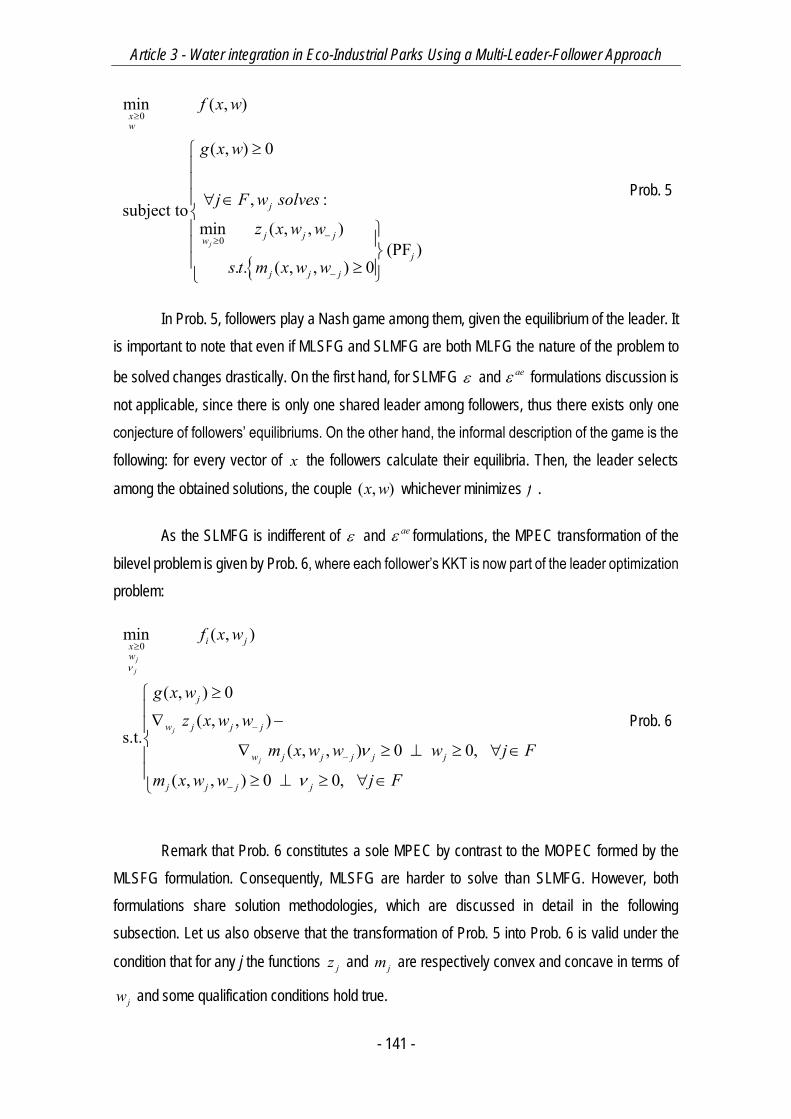
Article 3 - Water integration in Eco-Industrial Parks Using a Multi-Leader-Follower Approach
- 141 -
0
0
min ( , )
( , ) 0
, :subject tomin ( , , )
(PF ). . ( , , ) 0
j
xw
j
j j jwj
j j j
f x w
g x w
j F w solves
z x w w
s t m x w w
Prob. 5
In Prob. 5, followers play a Nash game among them, given the equilibrium of the leader. It
is important to note that even if MLSFG and SLMFG are both MLFG the nature of the problem to
be solved changes drastically. On the first hand, for SLMFG and ae formulations discussion is
not applicable, since there is only one shared leader among followers, thus there exists only one
conjecture of followers’ equilibriums. On the other hand, the informal description of the game is the
following: for every vector of x the followers calculate their equilibria. Then, the leader selects
among the obtained solutions, the couple ( , )x w whichever minimizes f .
As the SLMFG is indifferent of and ae formulations, the MPEC transformation of the
bilevel problem is given by Prob. 6, where each follower’s KKT is now part of the leader optimization
problem:
0min ( , )
( , ) 0
( , , )s.t.
( , , ) 0 0,
( , , ) 0 0,
jj
j
j
i jxw
j
w j j j
w j j j j j
j j j j
f x w
g x wz x w w
m x w w w j F
m x w w j F
Prob. 6
Remark that Prob. 6 constitutes a sole MPEC by contrast to the MOPEC formed by the
MLSFG formulation. Consequently, MLSFG are harder to solve than SLMFG. However, both
formulations share solution methodologies, which are discussed in detail in the following
subsection. Let us also observe that the transformation of Prob. 5 into Prob. 6 is valid under the
condition that for any j the functions jz and jm are respectively convex and concave in terms of
jw and some qualification conditions hold true.
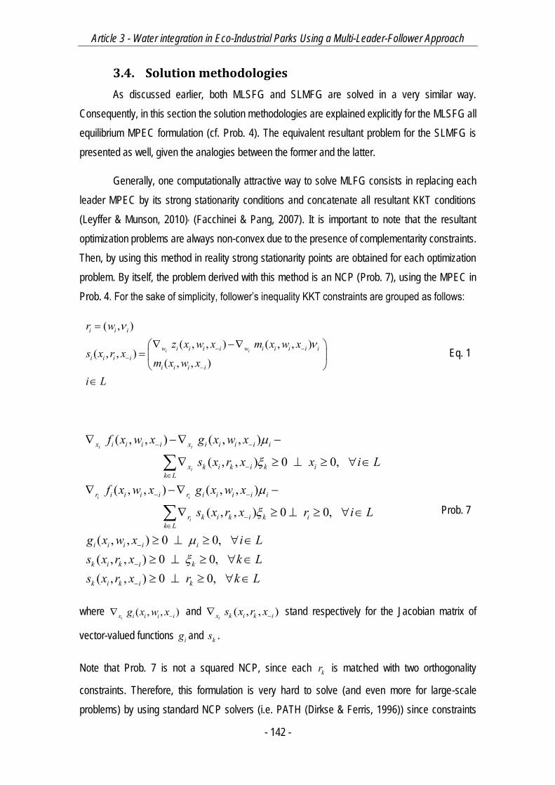
Article 3 - Water integration in Eco-Industrial Parks Using a Multi-Leader-Follower Approach
- 142 -
3.4. Solution methodologies
As discussed earlier, both MLSFG and SLMFG are solved in a very similar way.
Consequently, in this section the solution methodologies are explained explicitly for the MLSFG all
equilibrium MPEC formulation (cf. Prob. 4). The equivalent resultant problem for the SLMFG is
presented as well, given the analogies between the former and the latter.
Generally, one computationally attractive way to solve MLFG consists in replacing each
leader MPEC by its strong stationarity conditions and concatenate all resultant KKT conditions
(Leyffer & Munson, 2010), (Facchinei & Pang, 2007). It is important to note that the resultant
optimization problems are always non-convex due to the presence of complementarity constraints.
Then, by using this method in reality strong stationarity points are obtained for each optimization
problem. By itself, the problem derived with this method is an NCP (Prob. 7), using the MPEC in
Prob. 4. For the sake of simplicity, follower’s inequality KKT constraints are grouped as follows:
( , )( , , ) ( , , )
( , , )( , , )i i
i i i
w i i i i w i i i i ii i i i
i i i i
r wz x w x m x w x
s x r xm x w x
i L
Eq. 1
( , , ) ( , , )
( , , ) 0 0,
( , , ) ( , , )
( , , ) 0 0,
( , , ) 0 0,( , , ) 0 0,( , ,
i i
i
i i
i
x i i i i x i i i i i
x k i k i k ik L
r i i i i r i i i i i
r k i k i k ik L
i i i i i
k i k i k
k i k
f x w x g x w x
s x r x x i L
f x w x g x w x
s x r x r i L
g x w x i Ls x r x k Ls x r x
) 0 0,i kr k L
Prob. 7
where ( , , )ix i i i ig x w x and ( , , )
ix k i k is x r x stand respectively for the Jacobian matrix of
vector-valued functions ig and ks .
Note that Prob. 7 is not a squared NCP, since each kr is matched with two orthogonality
constraints. Therefore, this formulation is very hard to solve (and even more for large-scale
problems) by using standard NCP solvers (i.e. PATH (Dirkse & Ferris, 1996)) since constraints

Article 3 - Water integration in Eco-Industrial Parks Using a Multi-Leader-Follower Approach
- 143 -
violate any classical constraint qualification due to the presence of complementarity conditions
(Leyffer & Munson, 2010).
However, the NCP formulation illustrated in Prob. 7 can be used to derive NLP formulations
of a MLFG. A very interesting alternative which exploits the capacity of modern NLP solvers is the
so-called penalty formulation (Biegler, 2010). This formulation consists in moving the
complementarity constraints to the objective function, which is minimized. The latter is very
convenient for the MLSFG, since it do not exhibit a typical NLP formulation, i.e. no objective
function. Hence, the remaining constraints are well behaved. The formulation for the MLSFG is
illustrated next (Prob. 8), after introducing slacks , , ,i i i i to inequalities:
' ' ' ' ' ' ' ' ' ', , ', ,, ,,
min
( , , ) ( , , )
( , , ) ,
( , , ) ( , , )
s.t. ( , , )
i i
i
i i
i
T T T T Tpen i i i i i i i i i ix r i L
x i i i i x i i i i i
x k i k i k ik L
r i i i i r i i i i i
r k i k i kk L
C x w r
f x w x g x w x
s x r x i L
f x w x g x w x
s x r x
,
( , , ) ,( , , ) ,
0, 0, 0, 0, 0, 0, 0, 0,
i
i i i i i
k i k i k
i i i i i i i i
i L
g x w x i Ls x r x k Lx r i L
Prob. 8
The above formulation is in fact one of the several formulations to solve general MPEC
problems (cf. Biegler (Biegler, 2010) for all possible formulations) and it is the most adequate to
solve MLFG problems and MPECs in general (Biegler, 2010). In addition, Leyffer and Munson
(Leyffer & Munson, 2010) proved that if 0penC and if all variables describe a local solution of
the minimization problem, then the solution is a strong stationarity point of the MLFG. By moving
complementarities to the objective function, most difficulties of the NCP formulation are overcome
including the non-square nature of Prob. 7. The analogous formulation for the SLMFG is described
in Prob. 9, where 0 corresponds to a penalization parameter:
Article 3 - Water integration in Eco-Industrial Parks Using a Multi-Leader-Follower Approach
- 144 -
, ,,
min ' ( , )
( , )( , , ) ,
s.t. 000, 0,
Tj jx r j F
j j j j
j j
C f x w r
g x ws x r r j F
xr j F
Prob. 9
In this work, both NCP and NLP solution methods were tested. However, the NLP
formulation is preferred for the reasons stated above. All problems were modeled in GAMS®
(Brooke, Kendrick, Meeraus, et al., 1998) 24.4.2 and transformed into Prob. 7 through the extended
mathematical programming framework (EMP). The framework uses the solver JAMS to reformulate
Nash games (in MPEC form) into NCPs. Evidently, it is the modeler task to transform the original
MLFG into his MPEC formulation. Then, it is the modeler choice to solve it through Prob. 7 or Prob.
8/Prob. 9 formulation. In the former case, the solver employed has to be capable of solving NCP,
e.g. PATH (Dirkse & Ferris, 1996) and in the latter a standard NLP solver is required. In this work,
a combination of CONOPT, IPOPTH (Wächter & Biegler, 2002) and BARON (Tawarmalani &
Sahinidis, 2005) (if one solver fails to find a solution, then the other is called) was used. In the
context of a penalization scheme like the one in Prob. 8, a global solver like BARON is very useful
to find the solution where 0penC . Moreover, recent work (Zhang & Sahinidis, 2015)
demonstrated the usefulness of BARON in general MPCC problems, using recent versions of it. All
results reported in this work are those corresponding to the solution of Prob. 8/Prob. 9 formulation.
In the following section, the EIP specific model is introduced, with their specific MLFG
formulations and results of each specific case study.
4. EIP problem statement, case studies and results
Water integration in EIP is modeled as an industrial water network (IWN) allocation
problem, according to numerous previous works (Bagajewicz & Faria, 2009; Ramos, Boix,
Montastruc, et al., 2014; Boix, Montastruc, Pibouleau, et al., 2012). Indeed, the way to model a
IWN allocation problem is based on the concept of superstructure (Yeomans & Grossmann, 1999;
Biegler, Grossmann & Westerberg, 1997). From a given number of regeneration units and
processes, all possible connections between them may exist, except recycling to the same unit.
This constraint forbids self-recycles on process and regeneration units, although the latter is often
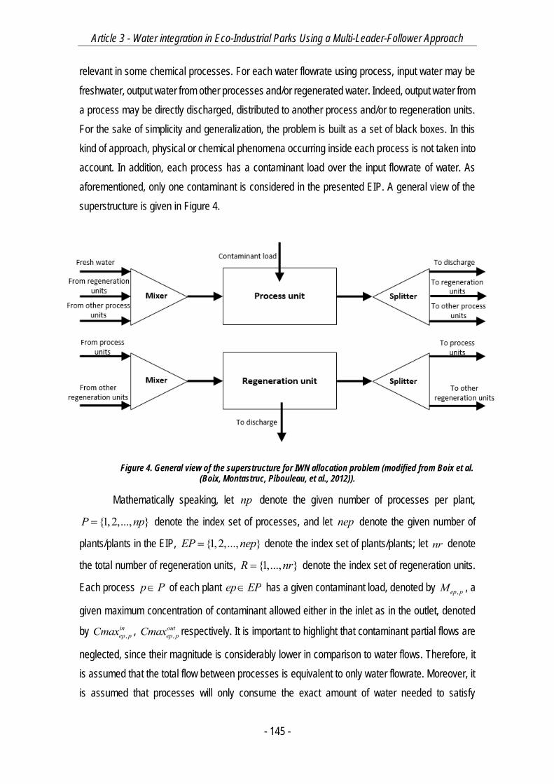
Article 3 - Water integration in Eco-Industrial Parks Using a Multi-Leader-Follower Approach
- 145 -
relevant in some chemical processes. For each water flowrate using process, input water may be
freshwater, output water from other processes and/or regenerated water. Indeed, output water from
a process may be directly discharged, distributed to another process and/or to regeneration units.
For the sake of simplicity and generalization, the problem is built as a set of black boxes. In this
kind of approach, physical or chemical phenomena occurring inside each process is not taken into
account. In addition, each process has a contaminant load over the input flowrate of water. As
aforementioned, only one contaminant is considered in the presented EIP. A general view of the
superstructure is given in Figure 4.
Figure 4. General view of the superstructure for IWN allocation problem (modified from Boix et al. (Boix, Montastruc, Pibouleau, et al., 2012)).
Mathematically speaking, let np denote the given number of processes per plant,
{1,2,..., }P np denote the index set of processes, and let nep denote the given number of
plants/plants in the EIP, {1,2,..., }EP nep denote the index set of plants/plants; let nr denote
the total number of regeneration units, {1,..., }R nr denote the index set of regeneration units.
Each process p P of each plant ep EP has a given contaminant load, denoted by ,ep pM , a
given maximum concentration of contaminant allowed either in the inlet as in the outlet, denoted
by ,inep pCmax , ,
outep pCmax respectively. It is important to highlight that contaminant partial flows are
neglected, since their magnitude is considerably lower in comparison to water flows. Therefore, it
is assumed that the total flow between processes is equivalent to only water flowrate. Moreover, it
is assumed that processes will only consume the exact amount of water needed to satisfy
Article 3 - Water integration in Eco-Industrial Parks Using a Multi-Leader-Follower Approach
- 146 -
concentration constraints. Consequently, processes water outlet will have a concentration
equivalent to ,outep pCmax (cf. Bagajewicz and Faria (Bagajewicz & Faria, 2009) for detailed
explanation). Equivalently, each regeneration unit r R has a given output contaminant
concentration, denoted by outrC . In terms of variables, each process of each plant ,p P ep EP
sends water to process 'p P of plant ' , { ', '} { , }ep EP ep p ep p , taken into account by
variable , , ', 'ep p ep pFpart , receives water, denoted by variable ', ', ,ep p ep pFpart and has an inlet flow of
freshwater, denoted by ,ep pFw . In addition, each process may send polluted water to regeneration
unit r R or receive low contaminant concentration water by the latter, denoted by
, , , ,,ep p r r ep pFproreg Fregpro respectively, or may send water directly to the discharge, denoted
by ,ep pFdis .
Finally, it is to be noted that the original model (e.g. Bagajewicz and Faria (Bagajewicz &
Faria, 2009), Boix et al. (Boix, Montastruc, Pibouleau, et al., 2012) and Ramos et al. (Ramos, Boix,
Montastruc, et al., 2014)) was formulated as a mixed-integer linear program (MILP), since it takes
into account minimum allowable flowrate between processes and/or regeneration units (namely,
the minimum allowed water flowrate was fixed at 2 T/h in Boix et al.8). Nevertheless, in a MLFG
formulation discrete variables are rather impossible to handle (at least for now). In consequence,
in the present article minimum flowrate minf is handled by an elimination algorithm which is
explained afterwards.
4.1. Model without regeneration units formulation
Given the aforementioned notation, the model without regeneration units presented by
Ramos et al. (Ramos, Boix, Montastruc, et al., 2014) for the IWN in EIP is presented below:
-Water mass balance around a process unit p P of a plant ep EP :
, ', ', , , ' ' ,' ' ' '
{ , } { ', '}
ep p ep p ep,p ep p ep ,p ep pep EP p P ep EP p P
Fw Fpart Fpart Fdis
ep p ep p
Eq. 2
-Contaminant mass balance around a process unit p P of a plant ep EP :
Article 3 - Water integration in Eco-Industrial Parks Using a Multi-Leader-Follower Approach
- 147 -
, ', ' ', ', , , , ' ' ,' ' ' '
{ , } { ', '}
out outep p ep p ep p ep,p ep p ep p ep ,p ep p
ep EP p P ep EP p PM Cmax Fpart Cmax Fpart Fdis
ep p ep p
Eq. 3
-Inlet/outlet concentration constraints for a process unit p P of a plant ep EP :
', ' ', ', , , ', ',' ' ' '
{ , } { ', '}
out inep p ep p ep,p ep p ep p ep p ep,p
ep EP p P ep EP p PCmax Fpart Cmax Fw Fpart
ep p ep p
Eq. 4
-Freshwater positivity for a process unit p P of a plant ep EP :
, 0ep pFw Eq. 5
-Flow between processes positivity going from a process unit p P of a plant ep EP to a
process 'p P of a plant ' , { ', '} { , }ep EP ep p ep p :
, , ', ' 0ep p ep pFpart Eq. 6
-Discharge flow positivity for a process unit p P of a plant ep EP :
, 0ep pFdis Eq. 7
From the aforementioned equations, some variables may be eliminated in order to produce
a more succinct model with less variables but equivalent. Indeed, by combining Eq. 2 and Eq. 3 we
obtain:
, ', ' ', ', , , ', ',' ' ' '
,{ , } { ', '}
out outep p ep p ep p ep,p ep p ep p ep p ep,p
ep EP p P ep EP p PM Cmax Fpart Cmax Fw Fpart
ep EP p Pep p ep p
Eq. 8
As ,ep pFdis is now eliminated from the model, his positivity constraint is now expressed
as follows:
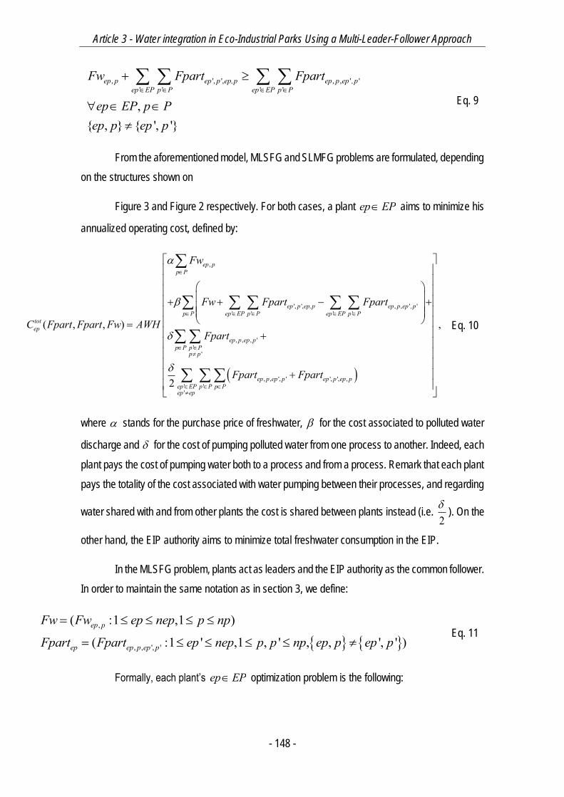
Article 3 - Water integration in Eco-Industrial Parks Using a Multi-Leader-Follower Approach
- 148 -
, ', ', , , ' '' ' ' '
,{ , } { ', '}
ep p ep p ep,p ep p ep ,pep EP p P ep EP p P
Fw Fpart Fpart
ep EP p Pep p ep p
Eq. 9
From the aforementioned model, MLSFG and SLMFG problems are formulated, depending
on the structures shown on
Figure 3 and Figure 2 respectively. For both cases, a plant ep EP aims to minimize his
annualized operating cost, defined by:
,
', ', , , ' '' ' ' '
, , , ''
'
, , ', ' ', ', ,' ''
( , , )
2
ep pp P
ep p ep,p ep p ep ,pp P ep EP p P ep EP p P
totep
ep p ep pp P p P
p p
ep p ep p ep p ep pep EP p P p Pep ep
Fw
Fw Fpart Fpart
C Fpart Fpart Fw AWHFpart
Fpart Fpart
,
Eq. 10
where stands for the purchase price of freshwater, for the cost associated to polluted water
discharge and for the cost of pumping polluted water from one process to another. Indeed, each
plant pays the cost of pumping water both to a process and from a process. Remark that each plant
pays the totality of the cost associated with water pumping between their processes, and regarding
water shared with and from other plants the cost is shared between plants instead (i.e. 2
). On the
other hand, the EIP authority aims to minimize total freshwater consumption in the EIP.
In the MLSFG problem, plants act as leaders and the EIP authority as the common follower.
In order to maintain the same notation as in section 3, we define:
,
, , ', '
( :1 ,1 )
( :1 ' ,1 , ' , , ', ' )ep p
ep ep p ep p
Fw Fw ep nep p np
Fpart Fpart ep nep p p np ep p ep p
Eq. 11
Formally, each plant’s ep EP optimization problem is the following:
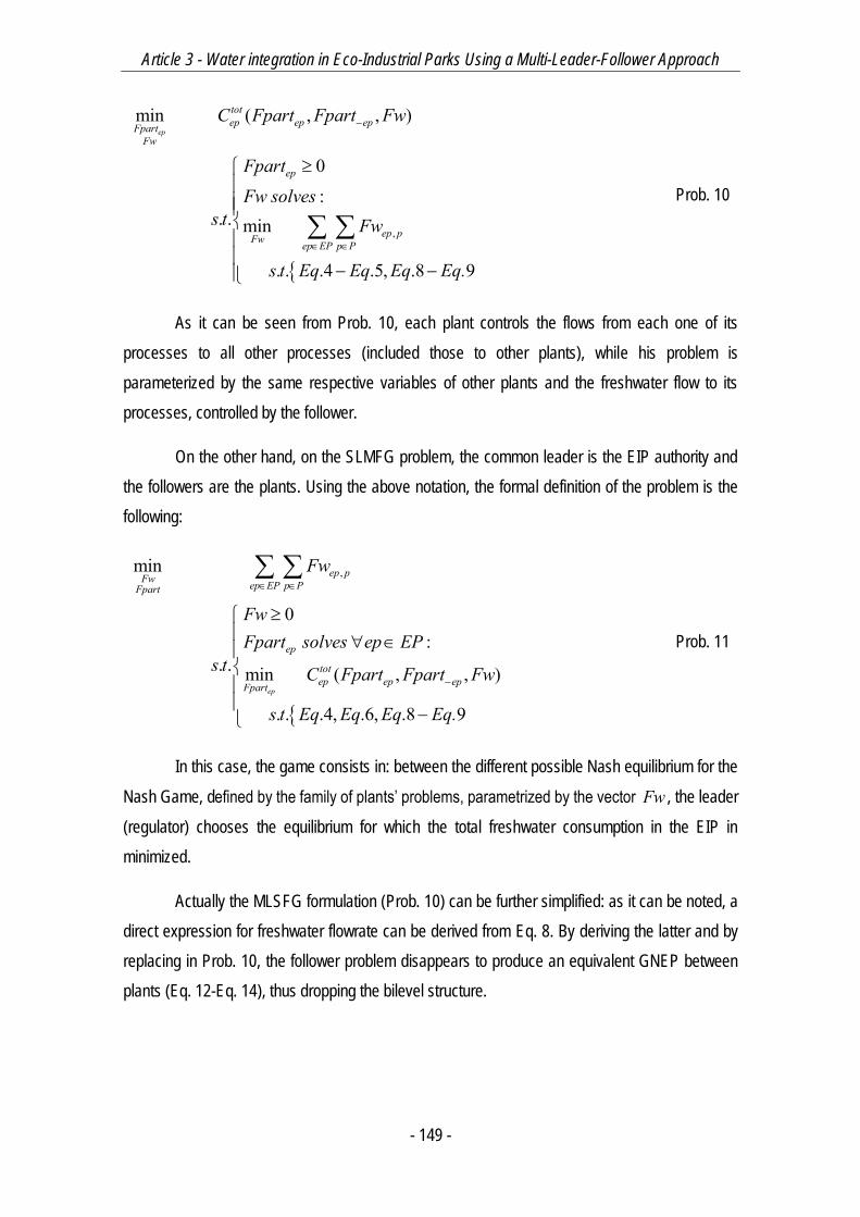
Article 3 - Water integration in Eco-Industrial Parks Using a Multi-Leader-Follower Approach
- 149 -
,
min ( , , )
0
:. . min
. . .4 .5, .8 9
ep
totep ep epFpart
Fw
ep
ep pFw ep EP p P
C Fpart Fpart Fw
FpartFw solves
s t Fw
s t Eq Eq Eq Eq.
Prob. 10
As it can be seen from Prob. 10, each plant controls the flows from each one of its
processes to all other processes (included those to other plants), while his problem is
parameterized by the same respective variables of other plants and the freshwater flow to its
processes, controlled by the follower.
On the other hand, on the SLMFG problem, the common leader is the EIP authority and
the followers are the plants. Using the above notation, the formal definition of the problem is the
following:
,min
0:
. . min ( , , )
. . .4, .6, .8 9ep
ep pFw ep EP p PFpart
ep
totep ep epFpart
Fw
FwFpart solves ep EP
s t C Fpart Fpart Fw
s t Eq Eq Eq Eq.
Prob. 11
In this case, the game consists in: between the different possible Nash equilibrium for the
Nash Game, defined by the family of plants’ problems, parametrized by the vector Fw , the leader
(regulator) chooses the equilibrium for which the total freshwater consumption in the EIP in
minimized.
Actually the MLSFG formulation (Prob. 10) can be further simplified: as it can be noted, a
direct expression for freshwater flowrate can be derived from Eq. 8. By deriving the latter and by
replacing in Prob. 10, the follower problem disappears to produce an equivalent GNEP between
plants (Eq. 12-Eq. 14), thus dropping the bilevel structure.
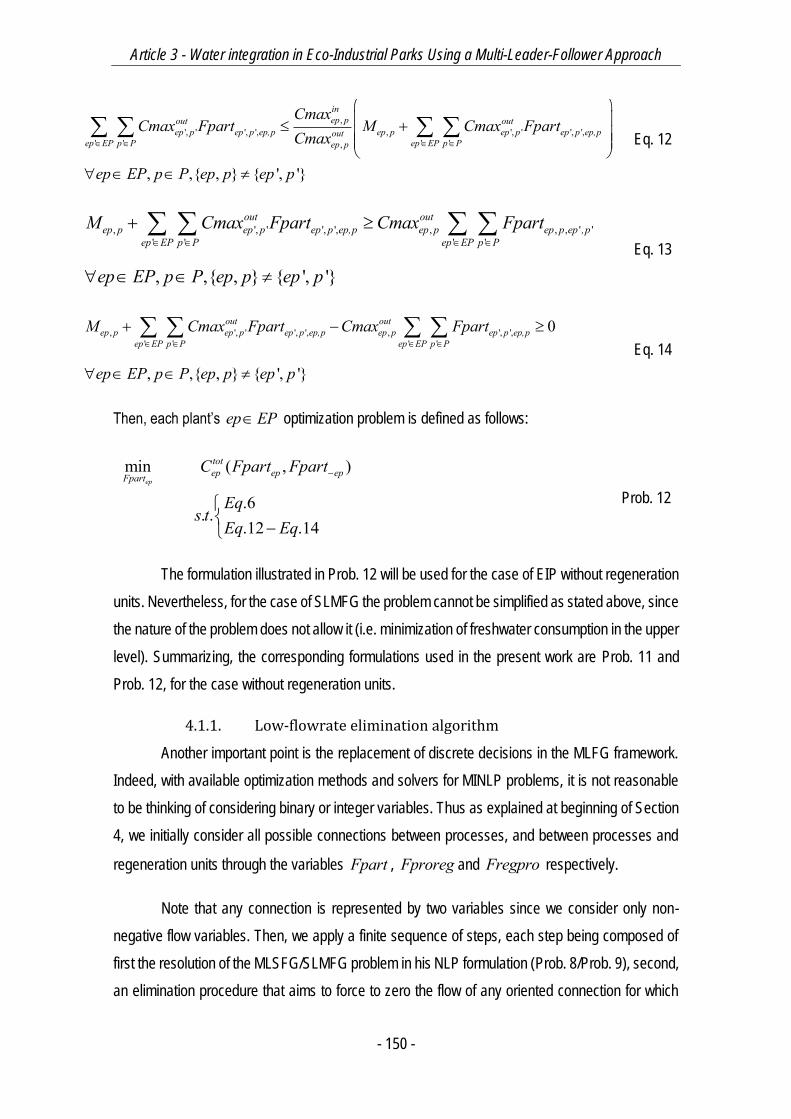
Article 3 - Water integration in Eco-Industrial Parks Using a Multi-Leader-Follower Approach
- 150 -
,', ' ', ', , ', ' ', ',
' ' ' ',
, ,{ , } { ', '}
inep pout out
ep p ep p ep,p ep p ep p ep p ep,poutep EP p P ep EP p Pep p
CmaxCmax Fpart M Cmax Fpart
Cmax
ep EP p P ep p ep p
Eq. 12
, ', ' ', ', , , , ' '' ' ' '
, ,{ , } { ', '}
out outep p ep p ep p ep,p ep p ep p ep ,p
ep EP p P ep EP p PM Cmax Fpart Cmax Fpart
ep EP p P ep p ep p
Eq. 13
, ', ' ', ', , ', ',' ' ' '
0
, ,{ , } { ', '}
out outep p ep p ep p ep,p ep p ep p ep,p
ep EP p P ep EP p PM Cmax Fpart Cmax Fpart
ep EP p P ep p ep p
Eq. 14
Then, each plant’s ep EP optimization problem is defined as follows:
min ( , )
.6. .
.12 .14
ep
totep ep epFpartC Fpart Fpart
Eqs t
Eq Eq
Prob. 12
The formulation illustrated in Prob. 12 will be used for the case of EIP without regeneration
units. Nevertheless, for the case of SLMFG the problem cannot be simplified as stated above, since
the nature of the problem does not allow it (i.e. minimization of freshwater consumption in the upper
level). Summarizing, the corresponding formulations used in the present work are Prob. 11 and
Prob. 12, for the case without regeneration units.
4.1.1. Low-flowrate elimination algorithm
Another important point is the replacement of discrete decisions in the MLFG framework.
Indeed, with available optimization methods and solvers for MINLP problems, it is not reasonable
to be thinking of considering binary or integer variables. Thus as explained at beginning of Section
4, we initially consider all possible connections between processes, and between processes and
regeneration units through the variables Fpart , Fproreg and Fregpro respectively.
Note that any connection is represented by two variables since we consider only non-
negative flow variables. Then, we apply a finite sequence of steps, each step being composed of
first the resolution of the MLSFG/SLMFG problem in his NLP formulation (Prob. 8/Prob. 9), second,
an elimination procedure that aims to force to zero the flow of any oriented connection for which

Article 3 - Water integration in Eco-Industrial Parks Using a Multi-Leader-Follower Approach
- 151 -
step 1 gave a flow lower that a minimum fixed boundminf . This is indeed modeled by big-M
constraints and binary variables in the former classical water integration (Ramos, Boix, Montastruc,
et al., 2014; Bagajewicz & Faria, 2009) model. In this work, we developed an a posteriori algorithm
to add bounds to existing flows and to eliminate low flows. Indeed, the MLFG is solved several
times until all flows are equal or superior to minf . The algorithm is described in detail next, using
as example , , ', 'ep p ep pFpart (all other flows are handled simultaneously and equivalently):
1) The initial MLFG is solved to optimality.
2) For all , ' ,ep ep EP p, p' P,{ep, p} {ep', p'} :
a. If , , ', '34ep p ep pFpart minf , then a lower bound of the flow is imposed that is
the constraint , , ', 'ep p ep pFpart minf is added to the model.
b. If , , ', '34ep p ep pFpart minf , then the flow is fixed , , ', ' 0ep p ep pFpart
c. Else, if all flows , , ', 'ep p ep pFpart minf , then the problem has converged and
no further treatment is required.
3) The bound-modified MLFG problem is tried to be solved to optimality:
a. If optimality is achieved, then go to 2).
b. Else, try solving to optimality with a different solver.
i. If optimality is achieved, then go to 2).
ii. Else, restore initial bounds of the variables of the process whose
constraint/s are infeasible. Go to 3).
In the aforementioned way, low-flowrates are systematically eliminated. It is important to
note that in our numerical experience the algorithm almost never failed by bounding critical flows
thus driving to infeasible models. However, it is evident that the solution obtained does not assure
in any way neither local nor global optimality in terms only of discrete decisions. Nevertheless, it
represents an efficient way to deal with the latter, given the natural complexity of the problem.
4.1.2. Case study, results and discussion
All problems were initialized with the trivial feasible solution where the flows between plants
do not exist, i.e. , , ', ' 0, , ' , , ' ,{ , } { ', '}ep p ep pFpart ep ep EP p p P ep p ep p , and therefore,
processes are only fed with freshwater. It is important to note that this solution represents a feasible
solution (at least for the concentration constraints) that is indeed far from being optimal solution. It
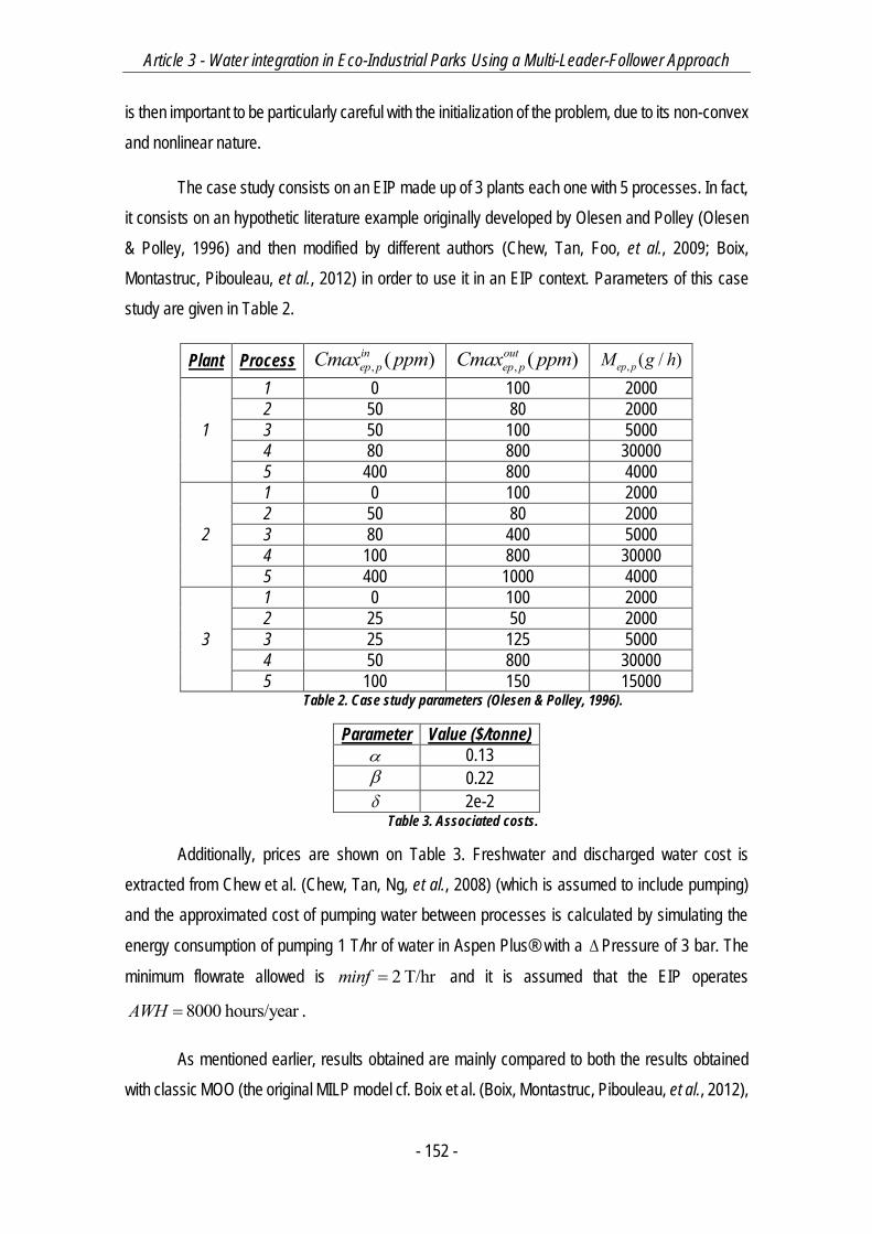
Article 3 - Water integration in Eco-Industrial Parks Using a Multi-Leader-Follower Approach
- 152 -
is then important to be particularly careful with the initialization of the problem, due to its non-convex
and nonlinear nature.
The case study consists on an EIP made up of 3 plants each one with 5 processes. In fact,
it consists on an hypothetic literature example originally developed by Olesen and Polley (Olesen
& Polley, 1996) and then modified by different authors (Chew, Tan, Foo, et al., 2009; Boix,
Montastruc, Pibouleau, et al., 2012) in order to use it in an EIP context. Parameters of this case
study are given in Table 2.
Plant Process , ( )inep pCmax ppm , ( )out
ep pCmax ppm , ( / )ep pM g h
1
1 0 100 2000
2 50 80 2000
3 50 100 5000
4 80 800 30000
5 400 800 4000
2
1 0 100 2000
2 50 80 2000
3 80 400 5000
4 100 800 30000
5 400 1000 4000
3
1 0 100 2000
2 25 50 2000
3 25 125 5000
4 50 800 30000
5 100 150 15000 Table 2. Case study parameters (Olesen & Polley, 1996).
Parameter Value ($/tonne)
0.13
0.22
2e-2 Table 3. Associated costs.
Additionally, prices are shown on Table 3. Freshwater and discharged water cost is
extracted from Chew et al. (Chew, Tan, Ng, et al., 2008) (which is assumed to include pumping)
and the approximated cost of pumping water between processes is calculated by simulating the
energy consumption of pumping 1 T/hr of water in Aspen Plus® with a Pressure of 3 bar. The
minimum flowrate allowed is 2 T/hrminf and it is assumed that the EIP operates
8000 hours/yearAWH .
As mentioned earlier, results obtained are mainly compared to both the results obtained
with classic MOO (the original MILP model cf. Boix et al. (Boix, Montastruc, Pibouleau, et al., 2012),
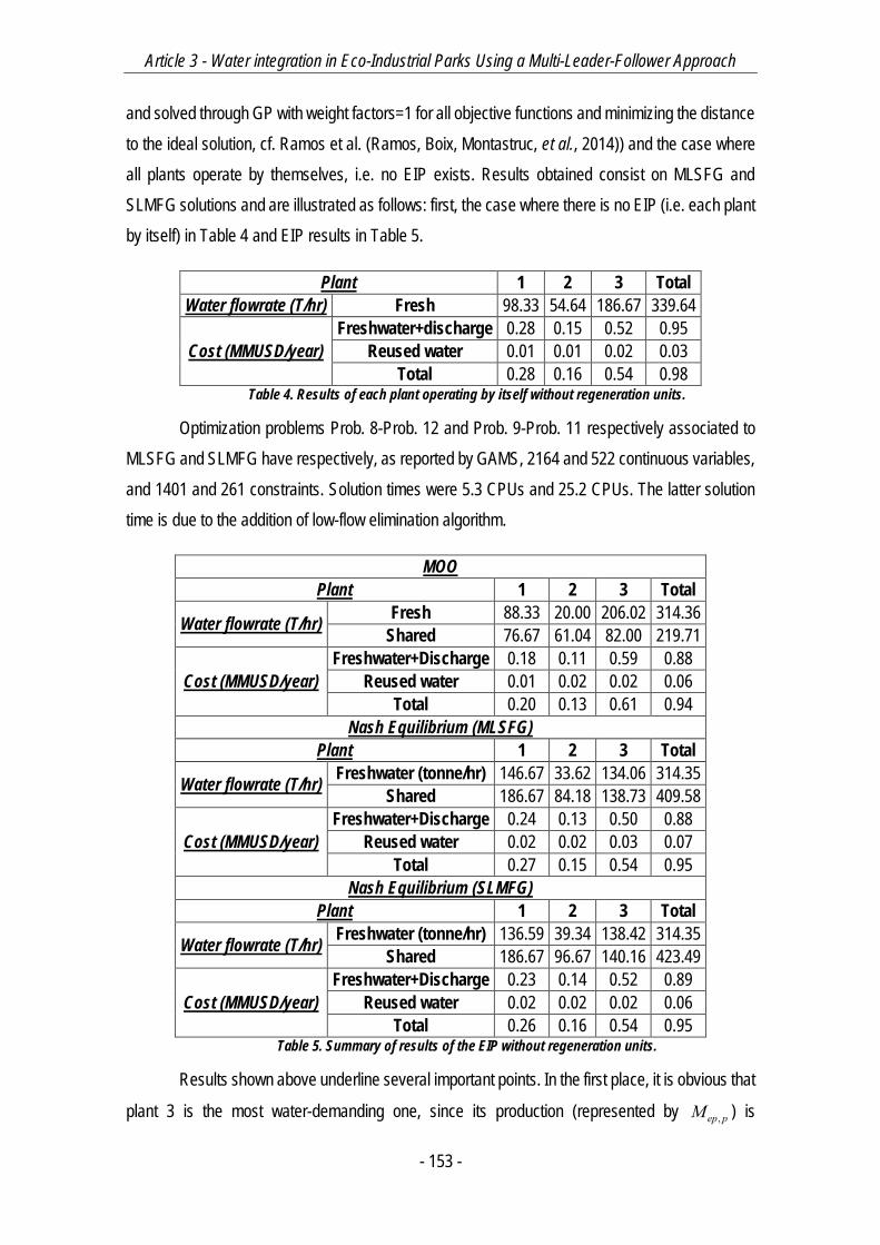
Article 3 - Water integration in Eco-Industrial Parks Using a Multi-Leader-Follower Approach
- 153 -
and solved through GP with weight factors=1 for all objective functions and minimizing the distance
to the ideal solution, cf. Ramos et al. (Ramos, Boix, Montastruc, et al., 2014)) and the case where
all plants operate by themselves, i.e. no EIP exists. Results obtained consist on MLSFG and
SLMFG solutions and are illustrated as follows: first, the case where there is no EIP (i.e. each plant
by itself) in Table 4 and EIP results in Table 5.
Plant 1 2 3 Total
Water flowrate (T/hr) Fresh 98.33 54.64 186.67 339.64
Cost (MMUSD/year)
Freshwater+discharge 0.28 0.15 0.52 0.95
Reused water 0.01 0.01 0.02 0.03
Total 0.28 0.16 0.54 0.98 Table 4. Results of each plant operating by itself without regeneration units.
Optimization problems Prob. 8-Prob. 12 and Prob. 9-Prob. 11 respectively associated to
MLSFG and SLMFG have respectively, as reported by GAMS, 2164 and 522 continuous variables,
and 1401 and 261 constraints. Solution times were 5.3 CPUs and 25.2 CPUs. The latter solution
time is due to the addition of low-flow elimination algorithm.
MOO
Plant 1 2 3 Total
Water flowrate (T/hr) Fresh 88.33 20.00 206.02 314.36
Shared 76.67 61.04 82.00 219.71
Cost (MMUSD/year)
Freshwater+Discharge 0.18 0.11 0.59 0.88
Reused water 0.01 0.02 0.02 0.06
Total 0.20 0.13 0.61 0.94
Nash Equilibrium (MLSFG)
Plant 1 2 3 Total
Water flowrate (T/hr) Freshwater (tonne/hr) 146.67 33.62 134.06 314.35
Shared 186.67 84.18 138.73 409.58
Cost (MMUSD/year)
Freshwater+Discharge 0.24 0.13 0.50 0.88
Reused water 0.02 0.02 0.03 0.07
Total 0.27 0.15 0.54 0.95
Nash Equilibrium (SLMFG)
Plant 1 2 3 Total
Water flowrate (T/hr) Freshwater (tonne/hr) 136.59 39.34 138.42 314.35
Shared 186.67 96.67 140.16 423.49
Cost (MMUSD/year)
Freshwater+Discharge 0.23 0.14 0.52 0.89
Reused water 0.02 0.02 0.02 0.06
Total 0.26 0.16 0.54 0.95 Table 5. Summary of results of the EIP without regeneration units.
Results shown above underline several important points. In the first place, it is obvious that
plant 3 is the most water-demanding one, since its production (represented by ,ep pM ) is
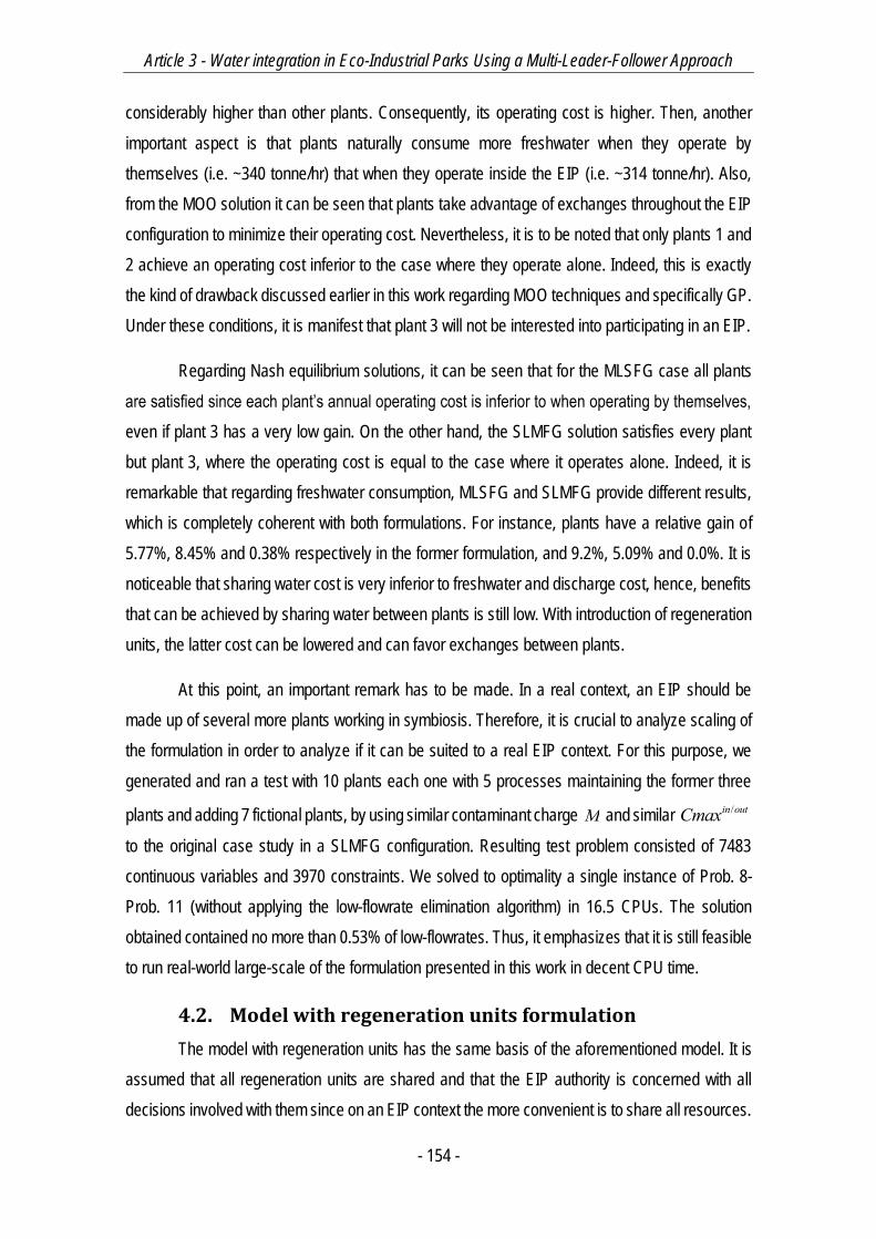
Article 3 - Water integration in Eco-Industrial Parks Using a Multi-Leader-Follower Approach
- 154 -
considerably higher than other plants. Consequently, its operating cost is higher. Then, another
important aspect is that plants naturally consume more freshwater when they operate by
themselves (i.e. ~340 tonne/hr) that when they operate inside the EIP (i.e. ~314 tonne/hr). Also,
from the MOO solution it can be seen that plants take advantage of exchanges throughout the EIP
configuration to minimize their operating cost. Nevertheless, it is to be noted that only plants 1 and
2 achieve an operating cost inferior to the case where they operate alone. Indeed, this is exactly
the kind of drawback discussed earlier in this work regarding MOO techniques and specifically GP.
Under these conditions, it is manifest that plant 3 will not be interested into participating in an EIP.
Regarding Nash equilibrium solutions, it can be seen that for the MLSFG case all plants
are satisfied since each plant’s annual operating cost is inferior to when operating by themselves,
even if plant 3 has a very low gain. On the other hand, the SLMFG solution satisfies every plant
but plant 3, where the operating cost is equal to the case where it operates alone. Indeed, it is
remarkable that regarding freshwater consumption, MLSFG and SLMFG provide different results,
which is completely coherent with both formulations. For instance, plants have a relative gain of
5.77%, 8.45% and 0.38% respectively in the former formulation, and 9.2%, 5.09% and 0.0%. It is
noticeable that sharing water cost is very inferior to freshwater and discharge cost, hence, benefits
that can be achieved by sharing water between plants is still low. With introduction of regeneration
units, the latter cost can be lowered and can favor exchanges between plants.
At this point, an important remark has to be made. In a real context, an EIP should be
made up of several more plants working in symbiosis. Therefore, it is crucial to analyze scaling of
the formulation in order to analyze if it can be suited to a real EIP context. For this purpose, we
generated and ran a test with 10 plants each one with 5 processes maintaining the former three
plants and adding 7 fictional plants, by using similar contaminant charge M and similar /in outCmax
to the original case study in a SLMFG configuration. Resulting test problem consisted of 7483
continuous variables and 3970 constraints. We solved to optimality a single instance of Prob. 8-
Prob. 11 (without applying the low-flowrate elimination algorithm) in 16.5 CPUs. The solution
obtained contained no more than 0.53% of low-flowrates. Thus, it emphasizes that it is still feasible
to run real-world large-scale of the formulation presented in this work in decent CPU time.
4.2. Model with regeneration units formulation
The model with regeneration units has the same basis of the aforementioned model. It is
assumed that all regeneration units are shared and that the EIP authority is concerned with all
decisions involved with them since on an EIP context the more convenient is to share all resources.

Article 3 - Water integration in Eco-Industrial Parks Using a Multi-Leader-Follower Approach
- 155 -
Indeed, early results with these kinds of considerations were not consistent with EIP philosophies.
Therefore, only shared regeneration units are considered, i.e. owned by the EIP.
Model constraints are as follows, consistent with the formulation mentioned earlier in this
section:
-Water mass balance around a process unit p P of a plant ep EP :
, ', ', , ,' '
, , ' ' , , ,' '
{ , } { ', '}
ep p ep p ep,p r ep pep EP p P r R
ep p ep ,p r ep p ep pep EP p P r R
Fw Fpart Fregpro
Fpart Fregpro Fdis
ep p ep p
Eq. 15
-Contaminant mass balance around a process unit p P of a plant ep EP :
, ', ' ', ', , ,' '
, , , ' ' , , ,' '
{ , } { ', '}
out outep p ep p ep p ep,p r r ep p
ep EP p P r R
outep p ep p ep ,p r ep p ep p
ep EP p P r R
M Cmax Fpart C Fregpro
Cmax Fpart Fregpro Fdis
ep p ep p
Eq. 16
-Inlet/outlet concentration constraints for a process unit p P of a plant ep EP :
', ' ', ', , ,' '
, , ', ', , ,' '
{ , } { ', '}
out outep p ep p ep,p r r ep p
ep EP p P r R
inep p ep p ep p ep,p r ep p
ep EP p P r R
Cmax Fpart C Fregpro
Cmax Fw Fpart Fregpro
ep p ep p
Eq. 17
-Contaminant concentration constraints for regeneration unit r R :
, , , , ,out outep p ep p r r r ep p
ep EP p P ep EP p PCmax Fproreg C Fregpro
Eq. 18
-Mass balance around a regeneration unit r R (water and contaminant losses are neglected):
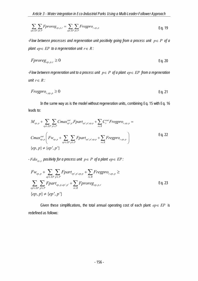
Article 3 - Water integration in Eco-Industrial Parks Using a Multi-Leader-Follower Approach
- 156 -
, , , ,ep p r r ep pep EP p P ep EP p P
Fproreg Fregpro
Eq. 19
-Flow between processes and regeneration unit positivity going from a process unit p P of a
plant ep EP to a regeneration unit r R :
, , 0ep p rFproreg Eq. 20
-Flow between regeneration unit to a process unit p P of a plant ep EP from a regeneration
unit r R :
, , 0r ep pFregpro Eq. 21
In the same way as is the model without regeneration units, combining Eq. 15 with Eq. 16
leads to:
, ', ' ', ', , ,' '
, , ', ', , ,' '
{ , } { ', '}
out outep p ep p ep p ep,p r r ep p
ep EP p P r R
outep p ep p ep p ep,p r ep p
ep EP p P r R
M Cmax Fpart C Fregpro
Cmax Fw Fpart Fregpro
ep p ep p
Eq. 22
- ,ep pFdis positivity for a process unit p P of a plant ep EP :
, ', ', , ,' '
, , ' ' , ,' '
{ , } { ', '}
ep p ep p ep,p r ep pep EP p P r R
ep p ep ,p ep p rep EP p P r R
Fw Fpart Fregpro
Fpart Fproreg
ep p ep p
Eq. 23
Given these simplifications, the total annual operating cost of each plant ep EP is
redefined as follows:
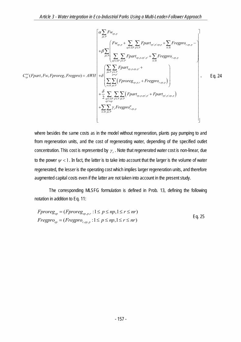
Article 3 - Water integration in Eco-Industrial Parks Using a Multi-Leader-Follower Approach
- 157 -
,
, ', ', , ,' '
, , ' ' , ,' '
, , , ''
'( , , , )
ep pp P
ep p ep p ep,p r ep pep EP p P r R
p Pep p ep ,p r ep p
ep EP p P r R
ep p ep pp P p P
tot p pep
Fw
Fw Fpart Fregpro
Fpart Fregpro
Fpart
C Fpart Fw Fproreg Fregpro AWHFpro
, , , ,
, , ', ' ', ', ,' ''
, ,
,
2
ep p r r ep pr R p P
ep p ep p ep p ep pep EP p P p Pep ep
r r ep pr R p P
reg Fregpro
Fpart Fpart
Fregpro
Eq. 24
where besides the same costs as in the model without regeneration, plants pay pumping to and
from regeneration units, and the cost of regenerating water, depending of the specified outlet
concentration. This cost is represented by r . Note that regenerated water cost is non-linear, due
to the power 1 . In fact, the latter is to take into account that the larger is the volume of water
regenerated, the lesser is the operating cost which implies larger regeneration units, and therefore
augmented capital costs even if the latter are not taken into account in the present study.
The corresponding MLSFG formulation is defined in Prob. 13, defining the following
notation in addition to Eq. 11:
, ,
, ,
( :1 ,1 )
( :1 ,1 )ep ep p r
ep r ep p
Fproreg Fproreg p np r nrFregpro Fregpro p np r nr
Eq. 25
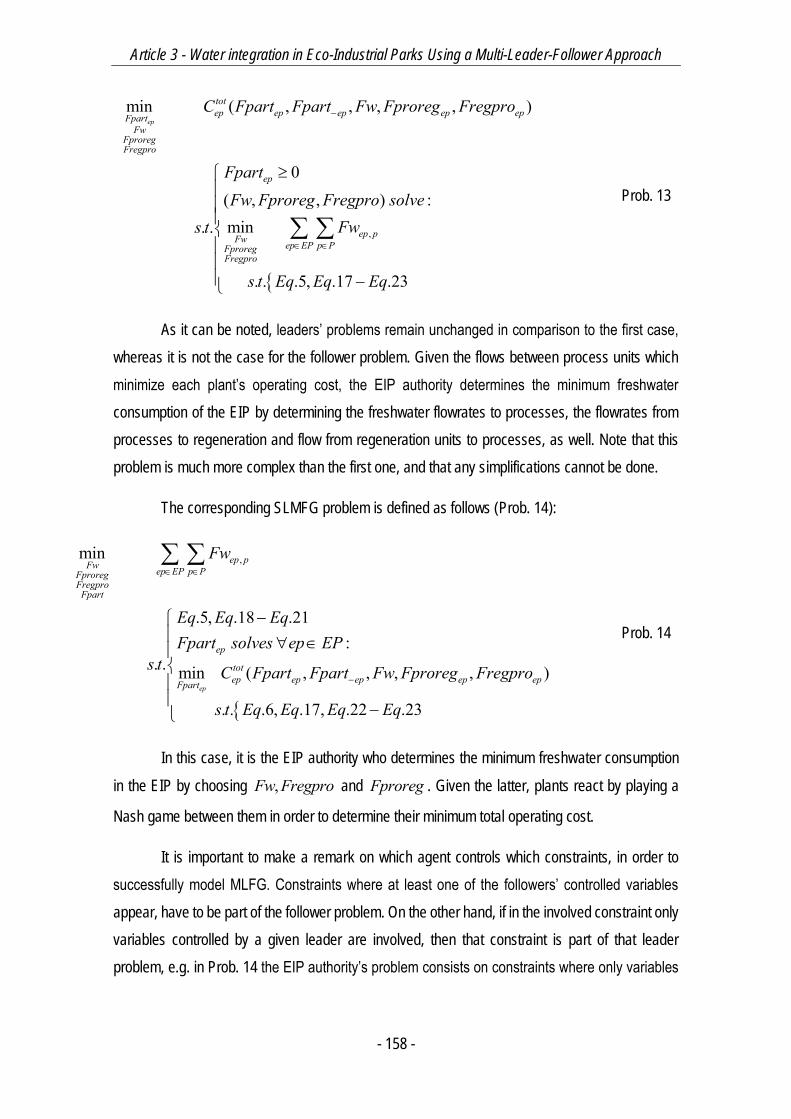
Article 3 - Water integration in Eco-Industrial Parks Using a Multi-Leader-Follower Approach
- 158 -
,
min ( , , , , )
0
( , , ) :min. .
. . .5, .17 .23
ep
totep ep ep ep epFpart
FwFproregFregpro
ep
ep pFw ep EP p PFproregFregpro
C Fpart Fpart Fw Fproreg Fregpro
FpartFw Fproreg Fregpro solve
Fws t
s t Eq Eq Eq
Prob. 13
As it can be noted, leaders’ problems remain unchanged in comparison to the first case,
whereas it is not the case for the follower problem. Given the flows between process units which
minimize each plant’s operating cost, the EIP authority determines the minimum freshwater
consumption of the EIP by determining the freshwater flowrates to processes, the flowrates from
processes to regeneration and flow from regeneration units to processes, as well. Note that this
problem is much more complex than the first one, and that any simplifications cannot be done.
The corresponding SLMFG problem is defined as follows (Prob. 14):
,min
.5, .18 .21:
. . min ( , , , , )
. . .6, .17, .22 .23ep
ep pFw ep EP p PFproregFregproFpart
ep
totep ep ep ep epFpart
Fw
Eq Eq EqFpart solves ep EP
s t C Fpart Fpart Fw Fproreg Fregpro
s t Eq Eq Eq Eq
Prob. 14
In this case, it is the EIP authority who determines the minimum freshwater consumption
in the EIP by choosing ,Fw Fregpro and Fproreg . Given the latter, plants react by playing a
Nash game between them in order to determine their minimum total operating cost.
It is important to make a remark on which agent controls which constraints, in order to
successfully model MLFG. Constraints where at least one of the followers’ controlled variables
appear, have to be part of the follower problem. On the other hand, if in the involved constraint only
variables controlled by a given leader are involved, then that constraint is part of that leader
problem, e.g. in Prob. 14 the EIP authority’s problem consists on constraints where only variables

Article 3 - Water integration in Eco-Industrial Parks Using a Multi-Leader-Follower Approach
- 159 -
controlled by him are involved, i.e. ,Fproreg Fregpro . Finally, the low-flowrate issue was treated
in the same way as in the model without regeneration units.
4.2.1. Case study, results and discussion
All case study parameters of the case without regeneration units still apply to the case with
regeneration units (i.e. Table 2 and Table 3). In addition, regeneration units operating parameters
are illustrated in Table 6. It is assumed that there are 3 different regeneration units which are
distinguished by their capacity to regenerate water, i.e. their outlet concentration on contaminant.
Regeneration unit type Parameter
outrC (ppm) r ($/tonne)
1 15 0.85
2 20 0.695
3 30 0.54 Table 6. Parameters associated with regeneration units.
Remark that regenerated water cost is superior regarding freshwater cost. Nevertheless,
as regenerated water cost is non-linear, it is not always necessarily true that freshwater is cheaper
than regenerated water. Regarding the power , it is assumed that when plants operate by
themselves 0.8 and when they are part of an EIP 0.6 . The latter takes into account the
fact that by sharing regeneration units in the EIP, and by purifying larger volumes of polluted water
capital costs of units would be cheaper. The aforementioned cost-associated parameters were
chosen in order to effectively demonstrate the usefulness of the approach adopted in this work.
Results are shown on the same manner regarding the case without water regeneration
(Table 7, Table 8).
Plant 1 2 3 Total
Water flowrate (tonne/hr) Fresh 98.33 22.00 97.50 217.83
Regenerated 0.00 38.17 111.46 149.63
Cost (MMUSD/year)
Freshwater+discharge 0.28 0.06 0.27 0.61
Reused water 0.01 0.02 0.05 0.08
Regenerated water 0.00 0.08 0.19 0.27
Total 0.28 0.17 0.51 0.96 Table 7. Results of each plant operating by itself with regeneration units.
Optimization problems Prob. 8-Prob. 13 and Prob. 9-Prob. 14 respectively associated to
MLSFG and SLMFG have, as again reported by GAMS, 4272 and 612 continuous variables, and
2397 and 270 constraints. Solution times were 6.5 CPUs and 10.9 CPUs.
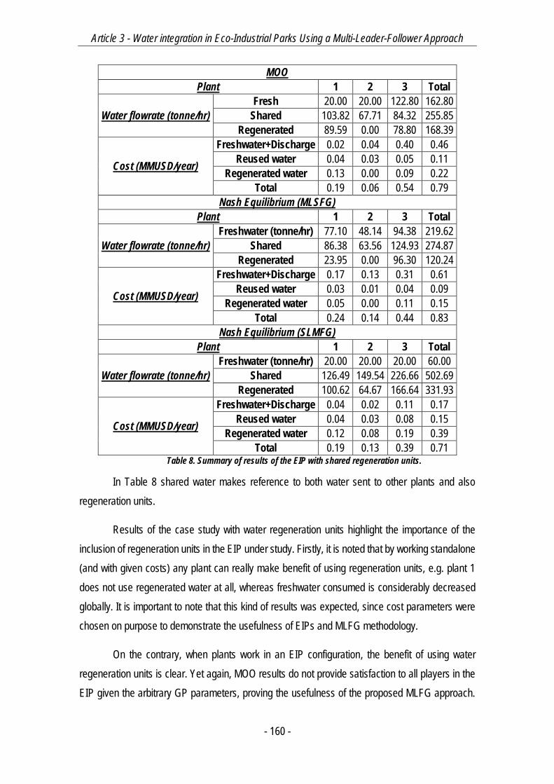
Article 3 - Water integration in Eco-Industrial Parks Using a Multi-Leader-Follower Approach
- 160 -
MOO
Plant 1 2 3 Total
Water flowrate (tonne/hr)
Fresh 20.00 20.00 122.80 162.80
Shared 103.82 67.71 84.32 255.85
Regenerated 89.59 0.00 78.80 168.39
Cost (MMUSD/year)
Freshwater+Discharge 0.02 0.04 0.40 0.46
Reused water 0.04 0.03 0.05 0.11
Regenerated water 0.13 0.00 0.09 0.22
Total 0.19 0.06 0.54 0.79
Nash Equilibrium (MLSFG)
Plant 1 2 3 Total
Water flowrate (tonne/hr)
Freshwater (tonne/hr) 77.10 48.14 94.38 219.62
Shared 86.38 63.56 124.93 274.87
Regenerated 23.95 0.00 96.30 120.24
Cost (MMUSD/year)
Freshwater+Discharge 0.17 0.13 0.31 0.61
Reused water 0.03 0.01 0.04 0.09
Regenerated water 0.05 0.00 0.11 0.15
Total 0.24 0.14 0.44 0.83
Nash Equilibrium (SLMFG)
Plant 1 2 3 Total
Water flowrate (tonne/hr)
Freshwater (tonne/hr) 20.00 20.00 20.00 60.00
Shared 126.49 149.54 226.66 502.69
Regenerated 100.62 64.67 166.64 331.93
Cost (MMUSD/year)
Freshwater+Discharge 0.04 0.02 0.11 0.17
Reused water 0.04 0.03 0.08 0.15
Regenerated water 0.12 0.08 0.19 0.39
Total 0.19 0.13 0.39 0.71 Table 8. Summary of results of the EIP with shared regeneration units.
In Table 8 shared water makes reference to both water sent to other plants and also
regeneration units.
Results of the case study with water regeneration units highlight the importance of the
inclusion of regeneration units in the EIP under study. Firstly, it is noted that by working standalone
(and with given costs) any plant can really make benefit of using regeneration units, e.g. plant 1
does not use regenerated water at all, whereas freshwater consumed is considerably decreased
globally. It is important to note that this kind of results was expected, since cost parameters were
chosen on purpose to demonstrate the usefulness of EIPs and MLFG methodology.
On the contrary, when plants work in an EIP configuration, the benefit of using water
regeneration units is clear. Yet again, MOO results do not provide satisfaction to all players in the
EIP given the arbitrary GP parameters, proving the usefulness of the proposed MLFG approach.
Article 3 - Water integration in Eco-Industrial Parks Using a Multi-Leader-Follower Approach
- 161 -
Regarding the MLSFG results, it is highlighted that all plants have noticeable benefits compared to
the standalone case, where the solution correspond to an equilibrium state between the operating
costs of the three leaders involved, earning respectively 14.53, 13.59 and 14.0%. Total freshwater
consumption is decreased regarding the standalone case, as expected, from 314.355 T/h to 219.62
T/h (which means a decrease of 30%). It is important to note that even if e.g. plant 2 does not use
regenerated water at all, its total operating cost is effectively lowered when other plants use
regenerated water.
Secondly, the SLMFG results demonstrate that minimum freshwater in the EIP is attained
at 60 T/h, by only feeding with freshwater processes which have 0inCmax . Given the latter,
shared and regenerated water are maximized providing all plants a relative gain superior to the
case of MLSFG, i.e. 31.91, 19.39 and 25.1% respectively. By regenerating the maximum amount
of water, its cost is even inferior to that of freshwater, fact which explains the results obtained in
the SLMFG case. However, if this amount is not maximized (i.e. results obtained in the MLSFG
case) plants have lower gains but its solutions are in equilibrium (or at least it corresponds to the
solution which satisfies strong stationarity conditions), according to the structure of the game.
Again, to be precise, both solutions correspond to different kind of games and do not necessarily
correspond to Nash equilibrium but to a solution which satisfies strong stationarity conditions.
An important aspect yet to be addressed is the solution times of the MLFG formulations.
For the EIP with regeneration units’ case, each optimization problem in the form of Prob. 8 is solved
in a matter of seconds to optimality (even if it is solved with BARON to global optimality). By
applying the low-flowrate elimination algorithm, the total solution times of the corresponding
MLSFG and SLMFG are 5.626s and 174s. In fact, the majority of the CPU time is due to achieving
the condition where all low-flowrates are eliminated. Moreover, this can be achieved either in the
first or in the n-th outer iteration.
5. Conclusions
In this work, MLFG formulations for the effective design of EIP were successfully
addressed. Results underline the effectiveness of the proposed methodology, compared to
traditional multi-objective/multi-decision optimization methods, e.g. goal programming. By
formulating the problem in a Nash game manner solutions obtained correspond (if solved to
optimality) at least to the case where each player objective function value matches the value if the
player operates standalone, without having to add additional constraints to the given objective
Article 3 - Water integration in Eco-Industrial Parks Using a Multi-Leader-Follower Approach
- 162 -
functions. Moreover, the solution obtained corresponds most of the times to an equilibrium solution
where all players attain fair gains respectively.
On the other hand, the formulation and proofs provided by Kulkarni et al. (Kulkarni &
Shanbhag, 2014) were numerically proven to be effective and pertinent to MLSFG especially in
cases were traditional formulations do not admit equilibrium. In fact, it is also important to note that
this kind of formulation (to the best of authors’ knowledge) was never modeled and effectively
solved in mathematical modeling environments such as GAMS®. In a parallel way, the
effectiveness of the solution methods adopted for MLFG was proven to be reliable indeed in
medium/large scale problems, solving to optimality this kind of problems in a matter of seconds,
even if solution methods do not solve the Nash equilibrium directly but its strong stationarity
conditions. Although, it is to be highlighted that the given industrial water network models provided
in the present work correspond to a linear model and as a perspective more non-linear models are
yet to be solved. However, given the considerable number of complementarity conditions (which
are very hard to solve) already included in the MLFG framework, non-linear models of industrial
water networks may not pose too much additional efforts. It is furthermore important to notice that
SLMFG are easier to solve than MLSFG and generally multi-leader multi-follower games, since
there is no need to duplicate follower’s conjectures given the nature of a single-leader in the game,
which is numerically speaking very convenient. Given the latter, in this work is successfully
introduced a reliable alternative to solve chemical/process engineering problems with multiple
decision objectives. Moreover, we emphasized that real-world large-scale EIP case studies can be
tackled by the methodologies and formulations presented in this work.
It is also important to underline that the introduction of an EIP regulator plays a major role
in the above quoted improvements of the EIP integration model since it allows considering MLSFG
and SLMFG structures.
Finally, it was also underlined the usefulness of EIPs in the context of industrial symbiosis
to produce more sustainable industrial outcomes. The results obtained show that, by unifying
efforts, wastes are lowered and effective gain can be achieved. As a perspective, simultaneous
energy and water networks will be taken into account with a MLFG approach.
6. Nomenclature
Latin symbols nl = Number of leaders
L = Index set of leaders
Article 3 - Water integration in Eco-Industrial Parks Using a Multi-Leader-Follower Approach
- 163 -
ix = Decision variables of leader i
ix = Decision variables of other leaders
w = Decision variables of the follower
f = Objective function of leader/leaders
g = Inequality constraints of leader/leaders
z = Objective function of the follower m = Inequality constraints of the follower np = Number of processes per plant
P = Index set of processes nep = Number of plants
EP = Index set of plants nr = Number of regeneration units
R = Index set of regeneration units
M = Contaminant load
,in outCmax Cmax = Maximum contaminant concentration allowed in inlet/outlet
of processes outC = Outlet concentration of contaminant in regeneration units
Fpart = Water flow between different processes
Fw = Freshwater inlet flow to processes
Fproreg = Water flow from processes to regeneration units
Fregpro = Water flow from regeneration units to processes
Fdis = Water processes to the discharge
minf = Minimum flowrate allowed
AWH = Annual EIP operating hours Greek symbols = Lagrange multipliers relative to m = Lagrange multipliers relative to g
= Lagrange multipliers relative to s
, , , , = Slacks to inequalities of Prob. 7
= Purchase price of freshwater
= Polluted water discharge cost
= Polluted water pumping cost = Regenerated water cost
= Power associated to
Article 3 - Water integration in Eco-Industrial Parks Using a Multi-Leader-Follower Approach
- 164 -
References
Alexander, B., Barton, G., Petrie, J. & Romagnoli, J. (2000) Process Synthesis and
Optimisation Tools for Environmental Design: Methodology and Structure. Computers & Chemical
Engineering. 24 (2), 1195–1200.
Aussel, D., Correa, R. & Marechal, P. (2013) Spot Electricity Market with Transmission
Losses. Journal of Industrial and Management Optimization. 9 (2), 275–290.
Aussel, D. & Dutta, J. (2008) Generalized Nash Equilibrium Problem, Variational Inequality
and Quasiconvexity. Operations Research Letters. 36 (4), 461–464.
Aviso, K.B., Tan, R.R., Culaba, A.B. & Cruz Jr., J.B. (2010) Bi-Level Fuzzy Optimization
Approach for Water Exchange in Eco-Industrial Parks. Process Safety and Environmental
Protection. [Online] 88 (1), 31–40. Available from: doi:10.1016/j.psep.2009.11.003.
Bagajewicz, M.J. & Faria, D.C. (2009) On the Appropriate Architecture of the
Water/Wastewater Allocation Problem in Process Plants Jacek Jeżowski and Jan Thullie (ed.).
Computer Aided Chemical Engineering. 261–20.
Biegler, L.T. (2010) Nonlinear Programming: Concepts, Algorithms, and Applications to
Chemical Processes. Philadelphia, Society for Industrial and Applied Mathematics : Mathematical
Optimization Society.
Biegler, L.T., Grossmann, I.E. & Westerberg, A.W. (1997) Systematic Methods of Chemical
Process Design. Upper Saddle River, N.J., Prentice Hall PTR.
Boix, M. (2011) Optimisation Multicritère Des Réseaux D’eau. PhD Thesis. Toulouse,
France, Université de Toulouse.
Boix, M. & Montastruc, L. (2011) Eco Industrial Parks for Water and Heat Management.
Computer Aided Chemical Engineering. [Online] 291175–1179. Available from: doi:10.1016/B978-
0-444-54298-4.50014-3.
Boix, M., Montastruc, L., Azzaro-Pantel, C. & Domenech, S. (2015) Optimization Methods
Applied to the Design of Eco-Industrial Parks: A Literature Review. Journal of Cleaner Production.
87303–317.
Boix, M., Montastruc, L., Pibouleau, L., Azzaro-Pantel, C., et al. (2011) A Multiobjective
Optimization Framework for Multicontaminant Industrial Water Network Design. Journal of
environmental management. [Online] 92 (7), 1802–1808. Available from:
doi:10.1016/j.jenvman.2011.02.016.
Boix, M., Montastruc, L., Pibouleau, L., Azzaro-Pantel, C., et al. (2012) Industrial Water
Management by Multiobjective Optimization: From Individual to Collective Solution Through Eco-
Industrial Parks. Journal of Cleaner Production. [Online] 22 (1), 85–97. Available from:
doi:10.1016/j.jclepro.2011.09.011.
Article 3 - Water integration in Eco-Industrial Parks Using a Multi-Leader-Follower Approach
- 165 -
Boix, M., Montastruc, L., Pibouleau, L., Azzaro-Pantel, C., et al. (2010) Multiobjective
Optimization of Industrial Water Networks with Contaminants S. Pierucci and G. Buzzi Ferraris
(ed.). Computer Aided Chemical Engineering. 28859–864.
Brooke, A., Kendrick, D., Meeraus, A. & Raman, R. (1998) GAMS User’s Guide.
Chertow, M.R. (2000) Industrial Symbiosis: Literature and Taxonomy. Annual Review of
Energy and the Environment. [Online] 25 (1), 313–337. Available from:
doi:10.1146/annurev.energy.25.1.313.
Chew, I.M.L., Tan, R., Ng, D.K.S., Foo, D.C.Y., et al. (2008) Synthesis of Direct and Indirect
Interplant Water Network. Industrial & Engineering Chemistry Research. [Online] 47 (23), 9485–
9496. Available from: doi:10.1021/ie800072r.
Chew, I.M.L., Tan, R.R., Foo, D.C.Y. & Chiu, A.S.F. (2009) Game Theory Approach to the
Analysis of Inter-Plant Water Integration in an Eco-Industrial Park. Journal of Cleaner Production.
[Online] 17 (18), 1611–1619. Available from: doi:10.1016/j.jclepro.2009.08.005.
Dirkse, S.P. & Ferris, M.C. (1996) A Pathsearch Damped Newton Method for Computing
General Equilibria. Annals of Operations Research. [Online] 68 (2), 211–232. Available from:
doi:10.1007/BF02209613.
Facchinei, F. & Pang, J.-S. (2007) Finite-Dimensional Variational Inequalities and
Complementarity Problems. Springer Science & Business Media.
Hobbs, B.F., Metzler, C.B. & Pang, J.-S. (2000) Strategic Gaming Analysis for Electric
Power Systems: An Mpec Approach. Power Systems, IEEE Transactions on. 15 (2), 638–645.
Hu, X. & Ralph, D. (2007) Using Epecs to Model Bilevel Games in Restructured Electricity
Markets with Locational Prices. Operations research. 55 (5), 809–827.
Kulkarni, A.A. & Shanbhag, U.V. (2014) A Shared-Constraint Approach to Multi-Leader
Multi-Follower Games. Set-Valued and Variational Analysis. [Online] 22 (4), 691–720. Available
from: doi:10.1007/s11228-014-0292-5.
Leyffer, S. & Munson, T. (2010) Solving Multi-Leader–Common-Follower Games.
Optimisation Methods & Software. 25 (4), 601–623.
Lou, H.H., Kulkarni, M.A., Singh, A. & Huang, Y.L. (2004) A Game Theory Based Approach
for Emergy Analysis of Industrial Ecosystem Under Uncertainty. Clean Technologies and
Environmental Policy. 6 (3), 156–161.
Montastruc, L., Boix, M., Pibouleau, L., Azzaro-Pantel, C., et al. (2013) On the Flexibility
of an Eco-Industrial Park (EIP) for Managing Industrial Water. Journal of Cleaner Production.
[Online] 431–11. Available from: doi:10.1016/j.jclepro.2012.12.039.
Olesen, S.G. & Polley, G.T. (1996) Dealing with Plant Geography and Piping Constraints
in Water Network Design. Process Safety and Environmental Protection. [Online] 74 (4), 273–276.
Available from: doi:10.1205/095758296528626.
Article 3 - Water integration in Eco-Industrial Parks Using a Multi-Leader-Follower Approach
- 166 -
Pang, J.-S. & Fukushima, M. (2005) Quasi-Variational Inequalities, Generalized Nash
Equilibria, and Multi-Leader-Follower Games. Computational Management Science. 2 (1), 21–56.
Ramos, M.A., Boix, M., Aussel, D., Montastruc, L., et al. (2015) Water Exchanges in Eco-
industrial Parks through Multiobjective Optimization and Game Theory. Computer Aided Chemical
Engineering. 371997–2002.
Ramos, M.A., Boix, M., Montastruc, L. & Domenech, S. (2014) Multiobjective Optimization
Using Goal Programming for Industrial Water Network Design. Industrial & Engineering Chemistry
Research. 53 (45), 17722–17735.
Tawarmalani, M. & Sahinidis, N.V. (2005) A Polyhedral Branch-and-Cut Approach to
Global Optimization. Mathematical Programming. 103 (2), 225–249.
Wächter, A. & Biegler, L.T. (2002) An Interior Point Algorithm for Large-Scale Nonlinear
Optimization with Applications in Process Engineering. Pittsburgh, Pa., Carnegie Mellon University,
Carnegie Mellon University, 2002.
Yeomans, H. & Grossmann, I.E. (1999) A Systematic Modeling Framework of
Superstructure Optimization in Process Synthesis. Computers & Chemical Engineering. [Online]
23 (6), 709–731. Available from: doi:10.1016/S0098-1354(99)00003-4.
Zhang, Y. & Sahinidis, N.V. (2015) Global Optimization of Mathematical Programs with
Complementarity Constraints and Application to Clean Energy Deployment. Optimization Letters.
1–16.


- 169 -
Chapitre 5 - Eco-Industrial Park Parameter Evaluation through Design of Experiments over a Multi-leader-follower Game Model Formulation

Article 4 - Eco-Industrial Park Parameter Evaluation through Design of Experiments over a Multi-leader-follower Game Model Formulation
- 170 -

Article 4 - Eco-Industrial Park Parameter Evaluation through Design of Experiments over a Multi-leader-follower Game Model Formulation
- 171 -
Résumé
À partir du modèle MLSFG (celui sans unité de régénération) développé dans l’article précédent,
un plan d’expériences est réalisé afin d’avoir une meilleure compréhension des paramètres
importants des systèmes optimisés. En effet, les effets des paramètres opératoires des usines
(niveaux de production, contraintes de pureté d’eau, politiques de paiement, prix des ressources
naturelles et coût des eaux partagées) sur la conception des EIP et notamment sur le gain relatif
des usines et leur viabilité financière méritent d’être mieux compris. L’EIP précédent est adapté en
considérant uniquement 2 usines avec 5 procédés chacune afin de limiter la taille des
expérimentations. Le plan d’expériences est ensuite utilisé pour l’estimation de modèles
statistiques de régression logistique, méthode des moindres carrés et régression multilinéaire afin
d’estimer la meilleure combinaison des paramètres pour la création fructueuse des EIP. Ce travail
fait apparaitre que les contraintes sur la pureté de l’eau des procédés (entrées et sorties) est le
paramètre le plus important dans la conception des EIP, car c’est le paramètre que restreint le
partage d’eau entre procédés et donc entre usines. Ceci a pour conséquence que si les contraintes
sur les concentrations de polluant en entrée des procédés sont faibles, beaucoup plus d’eau peut
être échangée et donc partagée. Comme cela était pressenti, le prix de l’eau est également un
élément fondamental pour la conception des échanges dans un EIP. Néanmoins, la politique de
paiement des eaux partagées entre usines (« qui paie quoi ») ne s’avère ne pas être un paramètre
significatif pour la viabilité économique des EIP.

Article 4 - Eco-Industrial Park Parameter Evaluation through Design of Experiments over a Multi-leader-follower Game Model Formulation
- 172 -
Article 4 - Eco-Industrial Park Parameter Evaluation through Design of Experiments over a Multi-leader-follower Game Model Formulation
- 173 -
Eco-Industrial Park Parameter Evaluation
through Design of Experiments over a Multi-
leader-follower Game Model Formulation
Manuel A. Ramosa, Marianne Boixa, Ludovic Montastruc*a, Pascal Floqueta, Serge
Domenecha
a Laboratoire de Génie Chimique, U.M.R. 5503 CNRS/INP/UPS, Université de Toulouse, 4, Allée
Emile Monso, 31432 Toulouse Cedex 4, France
* Corresponding author: [email protected]
Keywords: Eco-industrial parks, Multi-leader-follower Game, Bi-level optimization, Logistic
regression, Partial Least Squares.
Abstract
A design of experiments is carried out over a multi-leader-single-follower game (MLSFG)
optimization model for the design of water-sharing Eco-Industrial Parks (EIPs) in order to study the
influence of different parameters over the economic feasibility of the proposed EIP. Several
parameters are taken into account in a case study consisting of 2 plants acting as leaders which
aim to minimize their annualized operating cost and an EIP authority who acts as the common
follower whose aim is to minimize freshwater consumption in the EIP. Logistic, partial-least-squares
and multi-linear regressions are proposed in order to find the impact of the parameters over the
economic EIP feasibility. The MLFSG is transformed into a MOPEC (Multiple Optimization
Problems with Equilibrium Constraints) and solved using GAMS® as a Nonlinear Programming
(NLP) model. The methodology proposed is proven to be very reliable in order to provide insight
regarding the limiting plants parameters in EIP design and economic feasibility.
1. Introduction
Over the past ten years, most industrialized countries have invested heavily in
environmental research thanks to a general awareness about natural resources depletion
(UNESCO, 2009). Especially in the case of fresh water, there is a real need to reduce its
consumption by redefining and designing industrial networks with a low environmental impact. In
Article 4 - Eco-Industrial Park Parameter Evaluation through Design of Experiments over a Multi-leader-follower Game Model Formulation
- 174 -
response to these environmental problems, the concept of industrial ecology is born. Frosch and
Gallapoulos (Frosch & Gallopoulos, 1989) initiated the scientific community to look very closely at
the gathering of industries with a common goal of sustainable development. During the last twenty
years, many terms and concepts have emerged in the broad field of industrial ecology. Eco-
industrial parks (EIP) are a particular manifestation of industrial ecology and a definition commonly
admitted was given by Lowe (Lowe, 1997) as: “A community of manufacturing and service
businesses seeking enhanced environmental and economic performance through collaboration in
managing environmental and resource issues including energy, water, and materials. By working
together, the community of businesses seeks a collective benefit that is greater than the sum of the
individual benefits each company would realize if it optimized its individual performance only.” Since
these preliminary studies, a lot of concrete examples have emerged through the world including
the most famous example of the EIP of Kalundborg in Denmark. Other successful examples even
more numerous are built all over the world. Most of them were built in industrialized countries of
North America, Europe, or Australia but more recently it is in developing countries that many parks
are born (such as China, Brazil and Korea for example).
As it can be highlighted, a basic condition for an EIP to be economically viable is to
demonstrate that benefits of each industry involved in it by working collectively is higher than when
working as a stand-alone facility (Boix, Montastruc, Azzaro-Pantel, et al., 2015).
Boix et al. (Boix, Montastruc, Azzaro-Pantel, et al., 2015) highlighted the lack of studies
dealing with optimization in order to design optimal configuration of an EIP. However, it is important
to develop methodologies able to design an EIP where each industry has an effective gain
compared to the case where they operate individually, by also taking into account environmental
concerns. Among EIP design studies, water-using network is the most common type of cooperation
modeled in literature (Boix, Montastruc, Azzaro-Pantel, et al., 2015). In this kind of studies, the case
is often solved as a water-allocation problem through a superstructure-based model where water
has to be distributed, treated and discharged in an optimal way between the process units of each
enterprise’s plant involved in the EIP. Recently, Boix et al. (Boix, Montastruc, Pibouleau, et al.,
2012) and Ramos et al. (M. Ramos et al. 2015) developed a multi-objective optimization strategy
based on the -constraint method applied to the case of a water network in an EIP under several
scenarios and a goal programming framework respectively. On the other hand, a posterior work of
Montastruc et al. (Montastruc, Boix, Pibouleau, et al., 2013) have explored the flexibility of the
designed EIPs by changing parameters related to processes. The authors have also analyzed
different indicators to test the EIP profitability.
Article 4 - Eco-Industrial Park Parameter Evaluation through Design of Experiments over a Multi-leader-follower Game Model Formulation
- 175 -
An interesting novel approach particularly adapted to the optimal design of EIP is based
on a bi-level multi-leader-single-follower game (MLSFG) approach in which the leaders play a Nash
equilibrium game among them while leaders and followers are in Stackelberg equilibrium between
them (M. A. Ramos et al. 2016). In fact, an EIP can be seen as the congregation of different non-
cooperative agents (i.e. the enterprises’ plants) which aim at minimizing their annualized operating
costs and an EIP authority whose aim is to minimize resources consumption (e.g. freshwater). This
kind of non-cooperative game is very interesting for the concepts of EIP, since the main barrier to
integrate an EIP for industry is the issue of confidentiality between enterprises and this approach
could be very promising to overcome this problem. In fact, by introducing an impartial authority (or
regulator) whose role is to collect all data necessary to design the EIP, enterprises involved would
be able to keep confidential data, without the need to share them with the other companies of the
park.
As demonstrated by Ramos et al. (M. A. Ramos et al. 2016) the pertinence of the approach
is indeed very strong, since several criteria can be evaluated within the model and most importantly,
it is assured that the equilibrium solution will provide economic benefits (or at least no losses) to
enterprises’ plants participating in the EIP. This kind of approach is widely studied for modeling of
deregulated electricity markets (Aussel, Correa & Marechal, 2013). In this kind of games, the
leaders make simultaneous decisions and the followers react to these decisions.
On the other hand, as aforementioned, Montastruc et al. (Montastruc, Boix, Pibouleau, et
al., 2013) discussed the flexibility of EIP related to the influence of each plant production
parameters and constraints, e.g. limits on contaminant concentration and load. This is why the aim
of this work is to develop a statistical study through design of experiments (DoE) of the influence
of different plant operating parameters as well as other parameters related to the EIP in order to
achieve a better comprehension on the importance of the latter in the conception of an EIP. The
study is set up by using the novel MLSFG formulation proposed by Ramos et al. (M. A. Ramos et
al. 2016) in order to deal with several different criteria in a hierarchized model, focusing on the case
study without regeneration units.
First, the MLSFG regulator’s design of an EIP is explained as well as the formulation of the
bi-level optimization problem. Subsequently, the case study is introduced and the DoE and results
associated.
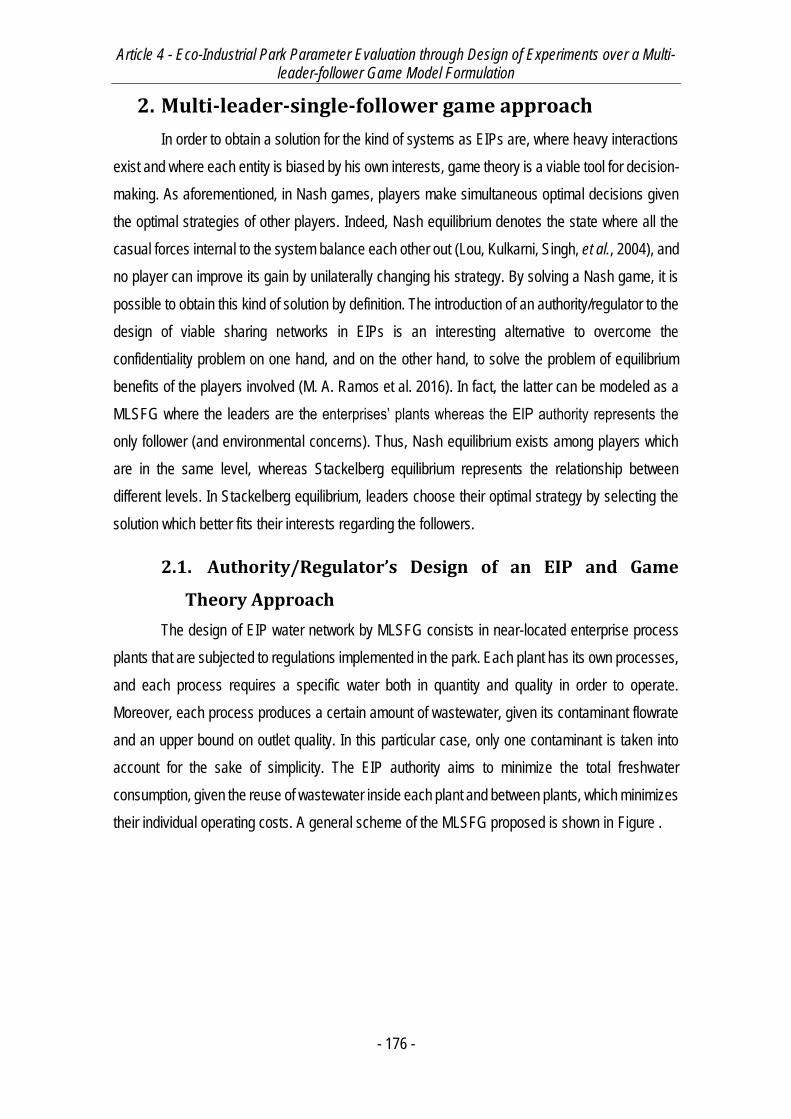
Article 4 - Eco-Industrial Park Parameter Evaluation through Design of Experiments over a Multi-leader-follower Game Model Formulation
- 176 -
2. Multi-leader-single-follower game approach
In order to obtain a solution for the kind of systems as EIPs are, where heavy interactions
exist and where each entity is biased by his own interests, game theory is a viable tool for decision-
making. As aforementioned, in Nash games, players make simultaneous optimal decisions given
the optimal strategies of other players. Indeed, Nash equilibrium denotes the state where all the
casual forces internal to the system balance each other out (Lou, Kulkarni, Singh, et al., 2004), and
no player can improve its gain by unilaterally changing his strategy. By solving a Nash game, it is
possible to obtain this kind of solution by definition. The introduction of an authority/regulator to the
design of viable sharing networks in EIPs is an interesting alternative to overcome the
confidentiality problem on one hand, and on the other hand, to solve the problem of equilibrium
benefits of the players involved (M. A. Ramos et al. 2016). In fact, the latter can be modeled as a
MLSFG where the leaders are the enterprises’ plants whereas the EIP authority represents the
only follower (and environmental concerns). Thus, Nash equilibrium exists among players which
are in the same level, whereas Stackelberg equilibrium represents the relationship between
different levels. In Stackelberg equilibrium, leaders choose their optimal strategy by selecting the
solution which better fits their interests regarding the followers.
2.1. Authority/Regulator’s Design of an EIP and Game
Theory Approach
The design of EIP water network by MLSFG consists in near-located enterprise process
plants that are subjected to regulations implemented in the park. Each plant has its own processes,
and each process requires a specific water both in quantity and quality in order to operate.
Moreover, each process produces a certain amount of wastewater, given its contaminant flowrate
and an upper bound on outlet quality. In this particular case, only one contaminant is taken into
account for the sake of simplicity. The EIP authority aims to minimize the total freshwater
consumption, given the reuse of wastewater inside each plant and between plants, which minimizes
their individual operating costs. A general scheme of the MLSFG proposed is shown in Figure .
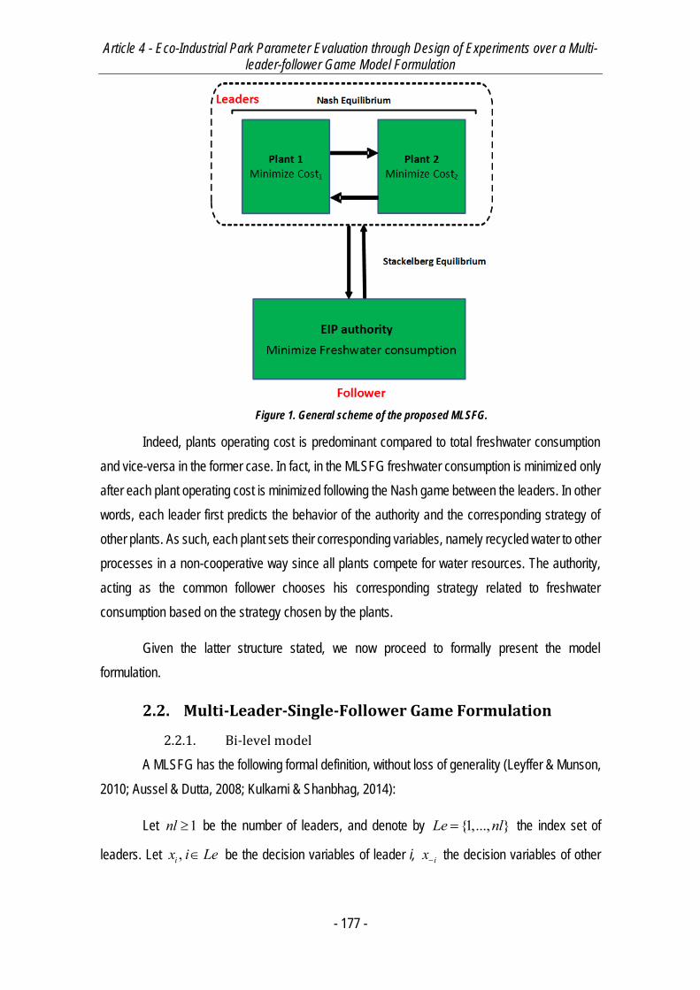
Article 4 - Eco-Industrial Park Parameter Evaluation through Design of Experiments over a Multi-leader-follower Game Model Formulation
- 177 -
Figure 1. General scheme of the proposed MLSFG.
Indeed, plants operating cost is predominant compared to total freshwater consumption
and vice-versa in the former case. In fact, in the MLSFG freshwater consumption is minimized only
after each plant operating cost is minimized following the Nash game between the leaders. In other
words, each leader first predicts the behavior of the authority and the corresponding strategy of
other plants. As such, each plant sets their corresponding variables, namely recycled water to other
processes in a non-cooperative way since all plants compete for water resources. The authority,
acting as the common follower chooses his corresponding strategy related to freshwater
consumption based on the strategy chosen by the plants.
Given the latter structure stated, we now proceed to formally present the model
formulation.
2.2. Multi-Leader-Single-Follower Game Formulation
2.2.1. Bi-level model
A MLSFG has the following formal definition, without loss of generality (Leyffer & Munson,
2010; Aussel & Dutta, 2008; Kulkarni & Shanbhag, 2014):
Let 1nl be the number of leaders, and denote by {1,..., }Le nl the index set of
leaders. Let ,ix i Le be the decision variables of leader i, ix the decision variables of other
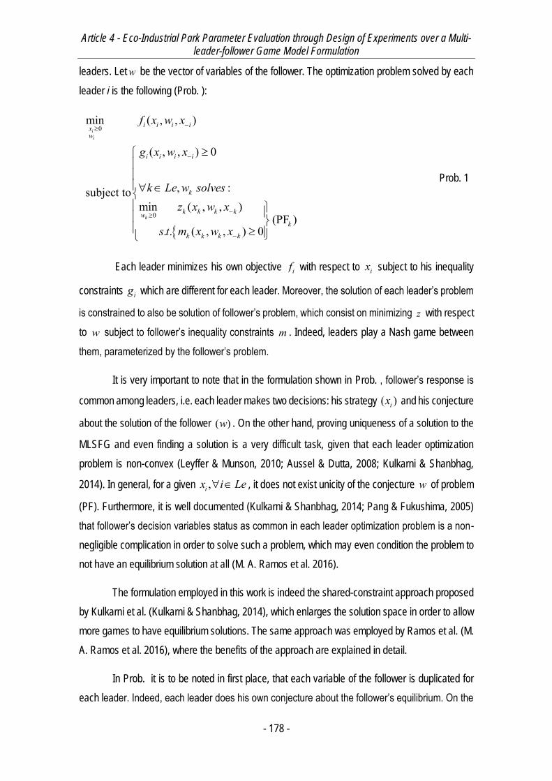
Article 4 - Eco-Industrial Park Parameter Evaluation through Design of Experiments over a Multi-leader-follower Game Model Formulation
- 178 -
leaders. Letw be the vector of variables of the follower. The optimization problem solved by each
leader i is the following (Prob. ):
0
0
min ( , , )
( , , ) 0
, :subject tomin ( , , )
(PF ). . ( , , ) 0
ii
k
i i i ixw
i i i i
k
k k k kwk
k k k k
f x w x
g x w x
k Le w solvesz x w x
s t m x w x
Prob. 1
Each leader minimizes his own objective if with respect to ix subject to his inequality
constraints ig which are different for each leader. Moreover, the solution of each leader’s problem
is constrained to also be solution of follower’s problem, which consist on minimizing z with respect
to w subject to follower’s inequality constraints m . Indeed, leaders play a Nash game between
them, parameterized by the follower’s problem.
It is very important to note that in the formulation shown in Prob. , follower’s response is
common among leaders, i.e. each leader makes two decisions: his strategy ( )ix and his conjecture
about the solution of the follower ( )w . On the other hand, proving uniqueness of a solution to the
MLSFG and even finding a solution is a very difficult task, given that each leader optimization
problem is non-convex (Leyffer & Munson, 2010; Aussel & Dutta, 2008; Kulkarni & Shanbhag,
2014). In general, for a given ,ix i Le , it does not exist unicity of the conjecture w of problem
(PF). Furthermore, it is well documented (Kulkarni & Shanbhag, 2014; Pang & Fukushima, 2005)
that follower’s decision variables status as common in each leader optimization problem is a non-
negligible complication in order to solve such a problem, which may even condition the problem to
not have an equilibrium solution at all (M. A. Ramos et al. 2016).
The formulation employed in this work is indeed the shared-constraint approach proposed
by Kulkarni et al. (Kulkarni & Shanbhag, 2014), which enlarges the solution space in order to allow
more games to have equilibrium solutions. The same approach was employed by Ramos et al. (M.
A. Ramos et al. 2016), where the benefits of the approach are explained in detail.
In Prob. it is to be noted in first place, that each variable of the follower is duplicated for
each leader. Indeed, each leader does his own conjecture about the follower’s equilibrium. On the
Article 4 - Eco-Industrial Park Parameter Evaluation through Design of Experiments over a Multi-leader-follower Game Model Formulation
- 179 -
other hand, the modification entails that each leader is now constrained by the problem of the
follower regarding both his own conjecture as other leaders’ conjectures, i.e. follower’s problems
and variables are now duplicated for each leader, denoted by index k. Then, the i-th leader problem
is parameterized by the decision of other leaders, i.e. ix and other leaders’ conjectures about
follower’s equilibrium, i.e. iw
In order to transform the latter bi-level problem into a mathematically tractable form, Prob.
is reformulated into a mathematical problem with equilibrium constraints (MPEC) following the
same methodology as in Ramos et al. (M. A. Ramos et al. 2016) which is described in the
subsequent sections, after describing the model of the water-sharing network.
2.2.2. EIP problem statement and model
Water integration in EIP is modeled as an industrial water network (IWN) allocation
problem, according to numerous previous works2, (M. A. Ramos et al. 2014),19,20 and based on the
same model employed by Ramos et al. (M. A. Ramos et al. 2016). Indeed, the way to model a IWN
allocation problem is based on the concept of superstructure (Yeomans & Grossmann, 1999;
Biegler, Grossmann & Westerberg, 1997). Note that the present work focuses on an EIP without
water-regeneration units. From a given number and processes, all possible connections between
them may exist, except recycling to the same process. For each water-intensive using process,
input water may be freshwater and/or output water from other processes. In the same way, output
water from a process may be directly discharged and/or distributed to another process. For the
sake of simplicity and generalization, the problem is built as a set of black boxes. In this kind of
approach, physical or chemical phenomena occurring inside each process is not taken into
account. In addition, each process has a contaminant load over the input flowrate of water. As
aforementioned, only one contaminant is considered in the presented EIP. A general view of the
superstructure is given in Figure 4.
Figure 2. General view of the superstructure for IWN allocation problem (M. A. Ramos et al. 2016).
Article 4 - Eco-Industrial Park Parameter Evaluation through Design of Experiments over a Multi-leader-follower Game Model Formulation
- 180 -
Mathematically speaking, let np denote the given number of processes per plant,
{1,2,..., }P np denote the index set of processes, and let nep denote the given number of
plants in the EIP, {1,2,..., }EP nep denote the index set of plants. Each process p P of each
plant ep EP has a given contaminant load, denoted by ,ep pM , a given maximum concentration
of contaminant allowed either in the inlet as in the outlet, denoted by ,inep pCmax , ,
outep pCmax
respectively. It is important to highlight that contaminant partial flows are neglected, since their
magnitude is considerably lower in comparison to water flows. Therefore, it is assumed that the
total flow between processes is equivalent to water flowrate. Moreover, it is assumed that
processes will only consume the exact amount of water needed to satisfy concentration constraints.
Consequently, processes water outlet will have a concentration equivalent to ,outep pCmax (cf.
Bagajewicz and Faria (Bagajewicz & Faria, 2009) for detailed explanation). In terms of variables,
each process of each plant ,p P ep EP sends water to process 'p P of plant
' , { ', '} { , }ep EP ep p ep p , taken into account by variable , , ', 'ep p ep pFpart , receives water,
denoted by variable ', ', ,ep p ep pFpart and has an inlet flow of freshwater, denoted by ,ep pFw . In
addition, each process may send polluted water to directly to the discharge, denoted by ,ep pFdis .
Finally, it is to be noted that the original model (e.g. Bagajewicz and Faria (Bagajewicz &
Faria, 2009), Boix et al. (Boix, Montastruc, Pibouleau, et al., 2012) and Ramos et al. (M. A. Ramos
et al. 2014)) was formulated as a mixed-integer linear program (MILP), since it takes into account
minimum allowable flowrate between processes and/or regeneration units (namely, the minimum
allowed water flowrate was fixed at 2 T/h in Boix et al.8). Nevertheless, in a MLSFG formulation
discrete variables are rather impossible to handle in a deterministic way if discrete decisions are
part of the follower problem, since no continuous optimality conditions exist for these kind of
problems. Note that the solution methodology of MLSFG models includes the reformulation of the
follower problem via his KKT conditions. On the other hand, note that MLSFG are solved in this
work by formulating strong-stationarity conditions on all leaders’ problems, leading to a MOPEC
formulation. Strong-stationarity conditions for non-continuous functions is rather a subject under
research. In consequence, in the present article minimum flowrate minf is handled by an
elimination algorithm which is explained afterwards.
Given the aforementioned notation, the model without regeneration units presented by
Ramos et al. (M. A. Ramos et al. 2016) for the IWN without regeneration units in EIP is presented
Article 4 - Eco-Industrial Park Parameter Evaluation through Design of Experiments over a Multi-leader-follower Game Model Formulation
- 181 -
below. Note that the model is presented in its final form after manipulation (cf. Ramos et al. (M. A.
Ramos et al. 2016) for details):
- Mass balance around a process unit:
, ', ' ', ', , , ', ',' ' ' '
,{ , } { ', '}
out outep p ep p ep p ep,p ep p ep p ep p ep,p
ep EP p P ep EP p PM Cmax Fpart Cmax Fw Fpart
ep EP p Pep p ep p
Eq. 1
-Discharge positivity:
, ', ', , , ' '' ' ' '
,{ , } { ', '}
ep p ep p ep,p ep p ep ,pep EP p P ep EP p P
Fw Fpart Fpart
ep EP p Pep p ep p
Eq. 2
-Inlet/outlet concentration constraints for a process unit:
', ' ', ', , , ', ',' ' ' '
,{ , } { ', '}
out inep p ep p ep,p ep p ep p ep p ep,p
ep EP p P ep EP p PCmax Fpart Cmax Fw Fpart
ep EP p Pep p ep p
Eq. 3
-Freshwater positivity for a process unit:
, 0, ,ep pFw ep EP p P Eq. 4
-Flow between processes positivity
, , ', ' 0, , ' , , ' ,{ , } { ', '}ep p ep pFpart ep ep EP p p P ep p ep p Eq. 5
The respective objective function of each plant ep EP aims to minimize his annualized
operating cost, defined by:
Article 4 - Eco-Industrial Park Parameter Evaluation through Design of Experiments over a Multi-leader-follower Game Model Formulation
- 182 -
,
', ', , , ' '' ' ' '
, , , ''
'
1, , ', ' ', ',
( , , )
2
costep p
p P
costep p ep,p ep p ep ,p
p P ep EP p P ep EP p P
costep p ep p
p P p Pp ptot
ep cost
ep p ep p ep p
fw Fw
dis Fw Fpart Fpart
ex Fpart
C Fpart Fpart Fw AWHexpol Fpart Fpart
,' ''
2, , ', '
' ''
3', ', ,
' ''
,
ep pep EP p P p Pep ep
costep p ep p
ep EP p P p Pep ep
costep p ep p
ep EP p P p Pep ep
pol ex Fpart
pol ex Fpart
Eq. 6
where costfw stands for the purchase price of freshwater, costdis for the cost associated
to polluted water discharge and costex for the cost of pumping polluted water from one process to
another. Indeed, each plant pays the cost of pumping water both to a process and from a process
between processes of the same plant. Then, according to the payment policy adopted in the EIP,
i.e. 1 2 3, ,pol pol pol , shared payment, who sends water pays and who receives water pays
respectively, plants account for the cost of in-coming and out-coming water to other plants. On the
other hand, the EIP authority aims to minimize total freshwater consumption in the EIP.
In the MLSFG problem, plants act as leaders and the EIP authority as the common follower.
In order to maintain the same notation as above, we define:
,
, , ', '
( :1 ,1 )
( :1 ' ,1 , ' , , ', ' )ep p
ep ep p ep p
Fw Fw ep nep p np
Fpart Fpart ep nep p p np ep p ep p
Eq. 7
Formally, each plant ep EP bi-level optimization problem is the following:
Article 4 - Eco-Industrial Park Parameter Evaluation through Design of Experiments over a Multi-leader-follower Game Model Formulation
- 183 -
,
min ( , , )
0
:. . min
. . .1 .4
ep
totep ep epFpart
Fw
ep
ep pFw ep EP p P
C Fpart Fpart Fw
FpartFw solves
s t Fw
s t Eq Eq
Prob. 2
As it can be seen from Prob. 2, each plant controls the flows from each one of its processes
to all other processes (included those to other plants), while his problem is parameterized by the
same respective variables of other plants and the freshwater flow to its processes, controlled by
the follower.
2.2.3. All equilibrium MPEC reformulation
Assuming that a follower k problem (PFk) is convex, i.e. z and m are respectively convex
functions and concave functions in w , then for any solution ( , )k kw v of the following Karush-Kuhn-
Tucker (KKT) optimality conditions, kw is a global optimal solution of (PFk). Note that KKT
conditions are equivalent to the parametric nonlinear complementarity problem (NCP) (Leyffer &
Munson, 2010) ; (Kulkarni & Shanbhag, 2014):
( , , ) ( , , ) 0 0
( , , ) 0 0k kw k k k k w k k k k k k
k k k k k
z x w x m x w x w
m x w xk L
Prob. 3
In Prob. 3, k are Lagrange multipliers associated to constraints of the follower
( , , )k k km x w x .
By substituting follower’s problem in each leader problem, the all-equilibrium bilevel
MLSFG described in Prob. is transformed into the following MPEC for each leader (Prob. 4):
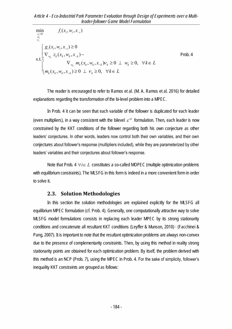
Article 4 - Eco-Industrial Park Parameter Evaluation through Design of Experiments over a Multi-leader-follower Game Model Formulation
- 184 -
0min ( , , )
( , , ) 0( , , )
s.t.( , , ) 0 0,
( , , ) 0 0,
iii
k
k
i i i ixw
i i i i
w k k k k
w k k k k k k
k k k k k
f x w x
g x w xz x w x
m x w x w k L
m x w x k L
Prob. 4
The reader is encouraged to refer to Ramos et al. (M. A. Ramos et al. 2016) for detailed
explanations regarding the transformation of the bi-level problem into a MPEC.
In Prob. 4 it can be seen that each variable of the follower is duplicated for each leader
(even multipliers), in a way consistent with the bilevel ae formulation. Then, each leader is now
constrained by the KKT conditions of the follower regarding both his own conjecture as other
leaders’ conjectures. In other words, leaders now control both their own variables, and their own
conjectures about follower’s response (multipliers included), while they are parameterized by other
leaders’ variables and their conjectures about follower’s response.
Note that Prob. 4 i L constitutes a so-called MOPEC (multiple optimization problems
with equilibrium constraints). The MLSFG in this form is indeed in a more convenient form in order
to solve it.
2.3. Solution Methodologies
In this section the solution methodologies are explained explicitly for the MLSFG all
equilibrium MPEC formulation (cf. Prob. 4). Generally, one computationally attractive way to solve
MLSFG model formulations consists in replacing each leader MPEC by its strong stationarity
conditions and concatenate all resultant KKT conditions (Leyffer & Munson, 2010) ; (Facchinei &
Pang, 2007). It is important to note that the resultant optimization problems are always non-convex
due to the presence of complementarity constraints. Then, by using this method in reality strong
stationarity points are obtained for each optimization problem. By itself, the problem derived with
this method is an NCP (Prob. 7), using the MPEC in Prob. 4. For the sake of simplicity, follower’s
inequality KKT constraints are grouped as follows:
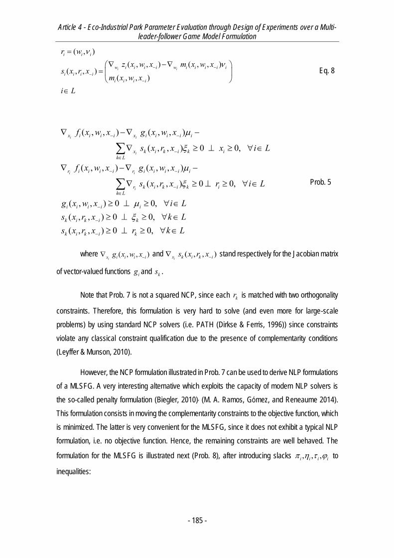
Article 4 - Eco-Industrial Park Parameter Evaluation through Design of Experiments over a Multi-leader-follower Game Model Formulation
- 185 -
( , )( , , ) ( , , )
( , , )( , , )i i
i i i
w i i i i w i i i i ii i i i
i i i i
r wz x w x m x w x
s x r xm x w x
i L
Eq. 8
( , , ) ( , , )
( , , ) 0 0,
( , , ) ( , , )
( , , ) 0 0,
( , , ) 0 0,( , , ) 0 0,( , ,
i i
i
i i
i
x i i i i x i i i i i
x k i k i k ik L
r i i i i r i i i i i
r k i k i k ik L
i i i i i
k i k i k
k i k
f x w x g x w x
s x r x x i L
f x w x g x w x
s x r x r i L
g x w x i Ls x r x k Ls x r x
) 0 0,i kr k L
Prob. 5
where ( , , )ix i i i ig x w x and ( , , )
ix k i k is x r x stand respectively for the Jacobian matrix
of vector-valued functions ig and ks .
Note that Prob. 7 is not a squared NCP, since each kr is matched with two orthogonality
constraints. Therefore, this formulation is very hard to solve (and even more for large-scale
problems) by using standard NCP solvers (i.e. PATH (Dirkse & Ferris, 1996)) since constraints
violate any classical constraint qualification due to the presence of complementarity conditions
(Leyffer & Munson, 2010).
However, the NCP formulation illustrated in Prob. 7 can be used to derive NLP formulations
of a MLSFG. A very interesting alternative which exploits the capacity of modern NLP solvers is
the so-called penalty formulation (Biegler, 2010), (M. A. Ramos, Gomez, and Reneaume 2014).
This formulation consists in moving the complementarity constraints to the objective function, which
is minimized. The latter is very convenient for the MLSFG, since it does not exhibit a typical NLP
formulation, i.e. no objective function. Hence, the remaining constraints are well behaved. The
formulation for the MLSFG is illustrated next (Prob. 8), after introducing slacks , , ,i i i i to
inequalities:

Article 4 - Eco-Industrial Park Parameter Evaluation through Design of Experiments over a Multi-leader-follower Game Model Formulation
- 186 -
' ' ' ' ' ' ' ' ' ', , ', ,, ,,
min
( , , ) ( , , )
( , , ) ,
( , , ) ( , , )
s.t. ( , , )
i i
i
i i
i
T T T T Tpen i i i i i i i i i ix r i L
x i i i i x i i i i i
x k i k i k ik L
r i i i i r i i i i i
r k i k i kk L
C x w r
f x w x g x w x
s x r x i L
f x w x g x w x
s x r x
,
( , , ) ,( , , ) ,
0, 0, 0, 0, 0, 0, 0, 0,
i
i i i i i
k i k i k
i i i i i i i i
i L
g x w x i Ls x r x k Lx r i L
Prob. 6
The above formulation is in fact one of the several formulations to solve general MPEC
problems (cf. Biegler (Biegler, 2010) for all possible formulations) and it is the most adequate to
solve MLSFG problems and MPECs in general (Biegler, 2010). In addition, Leyffer and Munson
(Leyffer & Munson, 2010) proved that if 0penC and if all variables describe a local solution of
the minimization problem, then the solution is a strong stationarity point of the MLSFG. By moving
complementarities to the objective function, most difficulties of the NCP formulation are overcome
including the non-square nature of Prob. 7.
In this work, the NLP formulation is preferred for the reasons stated above. All problems
were modeled in GAMS® (Brooke, Kendrick, Meeraus, et al., 1998) 24.4.2 and transformed into
Prob. 7 through the extended mathematical programming framework (EMP). The framework uses
the solver JAMS (Brooke, Kendrick, Meeraus, et al., 1998) to reformulate Nash games (in MPEC
form) into NCPs. Evidently, it is the modeler task to transform the original MLSFG into his MPEC
formulation. Being an NLP, a combination of CONOPT, IPOPTH (Wächter & Biegler, 2002) and
BARON (Tawarmalani & Sahinidis, 2005) (if one solver fails to find a solution, then the other is
called) was used. In the context of a penalization scheme like the one in Prob. 8, a global solver
like BARON is very useful to find the solution where 0penC . Moreover, recent work (Zhang &
Sahinidis, 2015) demonstrated the usefulness of BARON in general MPCC problems, using recent
versions of it. All results reported in this work are those corresponding to the solution of Prob. 8
formulation.
Article 4 - Eco-Industrial Park Parameter Evaluation through Design of Experiments over a Multi-leader-follower Game Model Formulation
- 187 -
2.3.1. Low-flowrate elimination algorithm
Another important point is the replacement of discrete decisions in the MLSFG framework.
Indeed, with available optimization methods and solvers for MINLP problems, it is not reasonable
to be thinking of considering binary or integer variables. Thus as explained at the beginning, we
initially consider all possible connections between processes.
The algorithm implemented in this work is the same approach as in Ramos et al. (M. A.
Ramos et al. 2016):
4) The initial MLFG is solved to optimality.
5) For all , ' ,ep ep EP p, p' P,{ep, p} {ep', p'} :
a. If , , ', '34ep p ep pFpart minf , then a lower bound of the flow is imposed that is
the constraint , , ', 'ep p ep pFpart minf is added to the model.
b. If , , ', '34ep p ep pFpart minf , then the flow is fixed , , ', ' 0ep p ep pFpart
c. Else, if all flows , , ', 'ep p ep pFpart minf , then the problem has converged and
no further treatment is required.
6) The bound-modified MLFG problem is tried to be solved to optimality:
a. If optimality is achieved, then go to 2).
b. Else, try solving to optimality with a different solver.
i. If optimality is achieved, then go to 2).
Else, restore initial bounds of the variables of the process whose constraint/s are infeasible.
Go to 3).
In the aforementioned algorithm, low-flowrates are systematically eliminated. Note that 3/4
is used as the scalar to determine if the flowrate exists or not. This decision is made in order to
approach almost-feasible flows to their lower bound or above.
In the following section, the EIP specific model is introduced, with their specific MLSFG
formulation and results of the DoE parameters study.
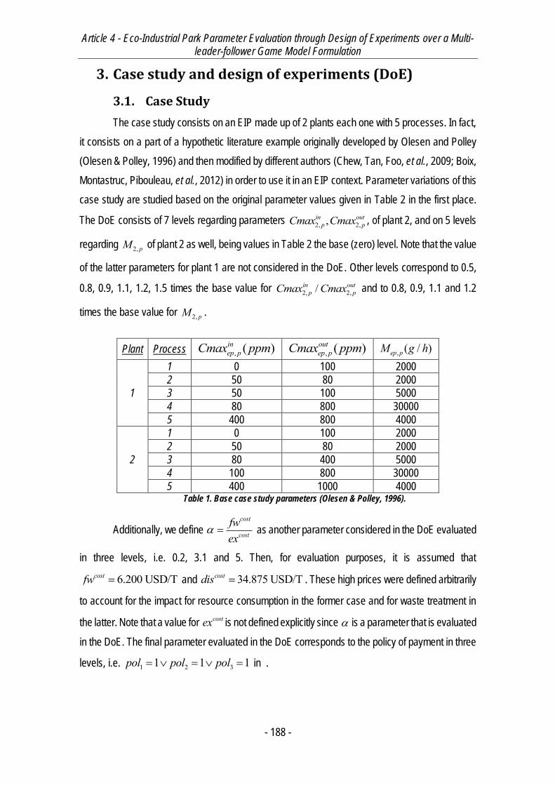
Article 4 - Eco-Industrial Park Parameter Evaluation through Design of Experiments over a Multi-leader-follower Game Model Formulation
- 188 -
3. Case study and design of experiments (DoE)
3.1. Case Study
The case study consists on an EIP made up of 2 plants each one with 5 processes. In fact,
it consists on a part of a hypothetic literature example originally developed by Olesen and Polley
(Olesen & Polley, 1996) and then modified by different authors (Chew, Tan, Foo, et al., 2009; Boix,
Montastruc, Pibouleau, et al., 2012) in order to use it in an EIP context. Parameter variations of this
case study are studied based on the original parameter values given in Table 2 in the first place.
The DoE consists of 7 levels regarding parameters 2, 2,,in outp pCmax Cmax , of plant 2, and on 5 levels
regarding 2, pM of plant 2 as well, being values in Table 2 the base (zero) level. Note that the value
of the latter parameters for plant 1 are not considered in the DoE. Other levels correspond to 0.5,
0.8, 0.9, 1.1, 1.2, 1.5 times the base value for 2, 2,/in outp pCmax Cmax and to 0.8, 0.9, 1.1 and 1.2
times the base value for 2, pM .
Plant Process , ( )inep pCmax ppm , ( )out
ep pCmax ppm , ( / )ep pM g h
1
1 0 100 2000
2 50 80 2000
3 50 100 5000
4 80 800 30000
5 400 800 4000
2
1 0 100 2000
2 50 80 2000
3 80 400 5000
4 100 800 30000
5 400 1000 4000 Table 1. Base case study parameters (Olesen & Polley, 1996).
Additionally, we define cost
cost
fwex
as another parameter considered in the DoE evaluated
in three levels, i.e. 0.2, 3.1 and 5. Then, for evaluation purposes, it is assumed that
6.200 USD/Tcostfw and 34.875 USD/Tcostdis . These high prices were defined arbitrarily
to account for the impact for resource consumption in the former case and for waste treatment in
the latter. Note that a value for costex is not defined explicitly since is a parameter that is evaluated
in the DoE. The final parameter evaluated in the DoE corresponds to the policy of payment in three
levels, i.e. 1 2 31 1 1pol pol pol in .
Article 4 - Eco-Industrial Park Parameter Evaluation through Design of Experiments over a Multi-leader-follower Game Model Formulation
- 189 -
Indeed, these parameters mentioned above seem very influential regarding the economic
feasibility of an EIP. For instance, after careful consideration, the following is extracted as the
hypothesis: in the first place, if 2,inpCmax is increased, freshwater flowrate has to necessarily
decrease – since water purity constraints are easier to satisfy (i.e. they are relaxed) -, and
interconnections between plants/processes should be increased – given the same argument –
which should globally decrease plants operating costs and therefore increasing the overall EIP
satisfaction for enterprises’ plants, given that polluted water cost is less than freshwater cost. In the
second place, if 2,outpCmax is increased, freshwater flow is decreased – since concentration
constraints are easier to satisfy – (cf. Eq. -Eq. 3), but interconnections between plants/processes
decrease, since water will leave a process with a higher concentration, and therefore not being
able to satisfy concentration constraints of other processes. Thus, plants operating costs should
increase given the latter scenario, decreasing overall EIP economic feasibility. Finally, if 2, pM is
increased, the same scenario as if 2,outpCmax is increased should be obtained. On the other hand,
the combined effect of the perturbation of all considered parameters is more difficult to infer in the
same way as and pol . Normally, an increase in could have two interpretations: in one hand,
if costfw is increased, it should have as consequence an augmentation of operating costs, since
freshwater is considered as more expensive than shared water; on the other, if 1costex ,
exchanges should be prioritized and operating costs should decrease.
Additionally, the minimum flowrate allowed is 2 T/hrminf and it is assumed that the
EIP operates 8000 hours/yearAWH .
3.2. Design of Experiments Methodology
For all combination of levels for the parameters of the DoE, the MLSFG model was solved
to optimality following the methodology described before, giving a sample size of 2205. Then, plant
economic satisfaction was checked. For such a purpose, the level of satisfaction epL was defined
as:
*
,tot aloneep ep
ep EIP aloneep ep
C CminL ep EP
Cmin Cmin
Eq. 9
In Eq. 9, *totepC is the value of tot
epC at the optimal solution, aloneepCmin is the minimum
operating cost of plant ep EP when operating outside the EIP and EIPepCmin is the minimum
Article 4 - Eco-Industrial Park Parameter Evaluation through Design of Experiments over a Multi-leader-follower Game Model Formulation
- 190 -
attainable operating cost of plant ep EP when operating inside the EIP. Note that the three latter
values are obtained by carrying on single-objective optimizations of each plant operating by
themselves and inside the EIP respectively.
The aforementioned obtained data has been studied by using various statistical
techniques, in order to pinpoint - in one hand - the major parameters that influence EIP feasibility
and - in the other hand - to model, in the case where the EIP is feasible, i.e. the overall satisfaction
of enterprises’ plants is > 0, measured by the tot epep EP
L L
criterion.
For the EIP feasibility study, all 2205 simulations were included on the DoE built with the
5 variables mentioned above, as well as their interactions and the square terms. The response Y
is a categorical one, i.e. the EIP is economically feasible or not, i.e. 0 01,
totif LY
otherwise
. Binomial
Logistic regression (Hosmer Jr & Lemeshow, 2004), or binomial logit regression, is enforced to
predict the odds of being feasible based on the values of the predictors X (variables). The way to
convert a binary variable to a continuous one is referred to logit transformation:
0 1 1
0 1 1 0 1 1
0 1 1
.....
..... ( ..... )
( 1/ ) ( 1/ ) .....( 0 / ) 1 ( 1/ )
1( 1/ )1 1
p p
p p p p
p p
a a X a X
a a X a X a a X a X
P Y X P Y Xln ln a a X a XP Y X P Y X
eP Y Xe e
Eq. 10
In Eq. 10 ( 1/ )P Y X is the cumulative distribution function (CDF) of the logistic
probability distribution.
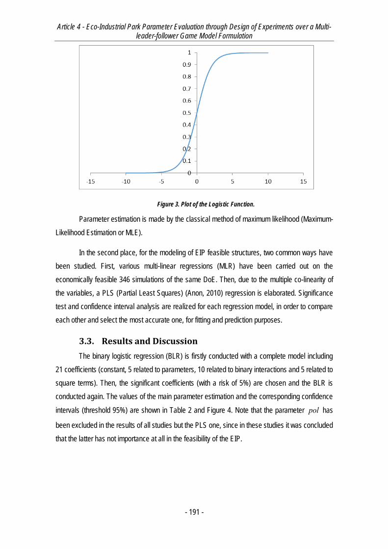
Article 4 - Eco-Industrial Park Parameter Evaluation through Design of Experiments over a Multi-leader-follower Game Model Formulation
- 191 -
Figure 3. Plot of the Logistic Function.
Parameter estimation is made by the classical method of maximum likelihood (Maximum-
Likelihood Estimation or MLE).
In the second place, for the modeling of EIP feasible structures, two common ways have
been studied. First, various multi-linear regressions (MLR) have been carried out on the
economically feasible 346 simulations of the same DoE. Then, due to the multiple co-linearity of
the variables, a PLS (Partial Least Squares) (Anon, 2010) regression is elaborated. Significance
test and confidence interval analysis are realized for each regression model, in order to compare
each other and select the most accurate one, for fitting and prediction purposes.
3.3. Results and Discussion
The binary logistic regression (BLR) is firstly conducted with a complete model including
21 coefficients (constant, 5 related to parameters, 10 related to binary interactions and 5 related to
square terms). Then, the significant coefficients (with a risk of 5%) are chosen and the BLR is
conducted again. The values of the main parameter estimation and the corresponding confidence
intervals (threshold 95%) are shown in Table 2 and Figure 4. Note that the parameter pol has
been excluded in the results of all studies but the PLS one, since in these studies it was concluded
that the latter has not importance at all in the feasibility of the EIP.
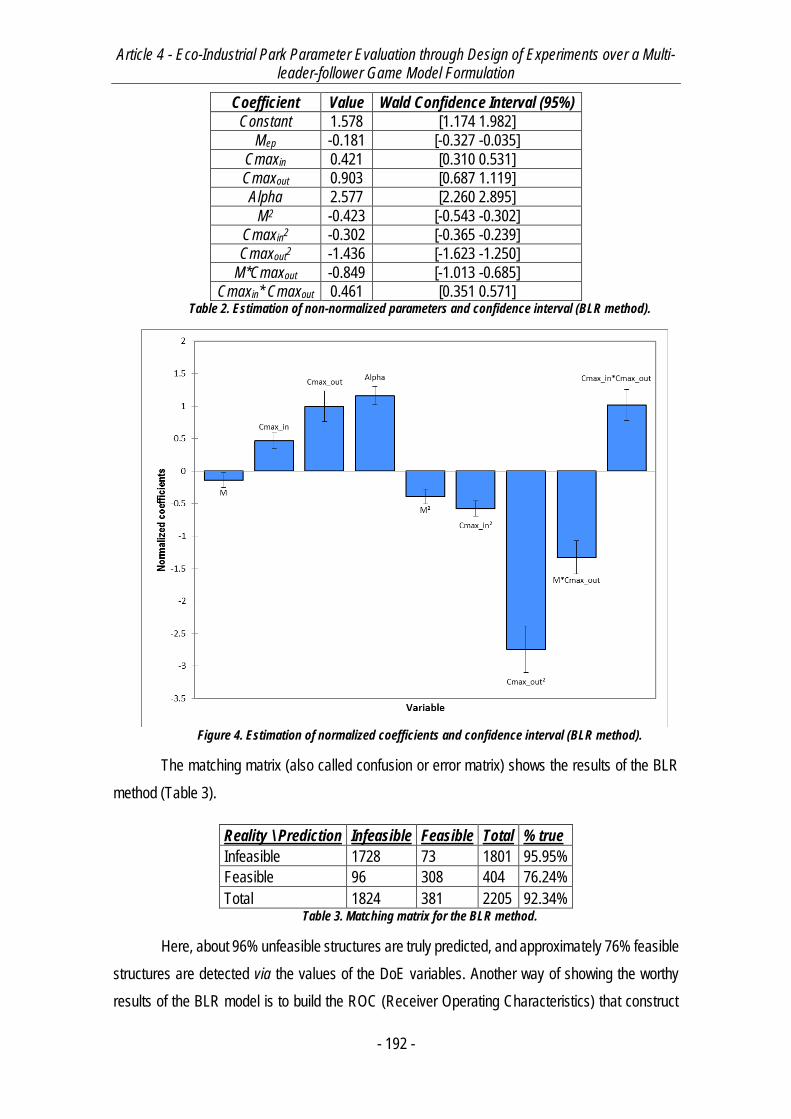
Article 4 - Eco-Industrial Park Parameter Evaluation through Design of Experiments over a Multi-leader-follower Game Model Formulation
- 192 -
Coefficient Value Wald Confidence Interval (95%)
Constant 1.578 [1.174 1.982]
Mep -0.181 [-0.327 -0.035]
Cmaxin 0.421 [0.310 0.531]
Cmaxout 0.903 [0.687 1.119]
Alpha 2.577 [2.260 2.895]
M2 -0.423 [-0.543 -0.302]
Cmaxin2 -0.302 [-0.365 -0.239]
Cmaxout2 -1.436 [-1.623 -1.250]
M*Cmaxout -0.849 [-1.013 -0.685]
Cmaxin* Cmaxout 0.461 [0.351 0.571] Table 2. Estimation of non-normalized parameters and confidence interval (BLR method).
Figure 4. Estimation of normalized coefficients and confidence interval (BLR method).
The matching matrix (also called confusion or error matrix) shows the results of the BLR
method (Table 3).
Reality \ Prediction Infeasible Feasible Total % true
Infeasible 1728 73 1801 95.95%
Feasible 96 308 404 76.24%
Total 1824 381 2205 92.34% Table 3. Matching matrix for the BLR method.
Here, about 96% unfeasible structures are truly predicted, and approximately 76% feasible
structures are detected via the values of the DoE variables. Another way of showing the worthy
results of the BLR model is to build the ROC (Receiver Operating Characteristics) that construct
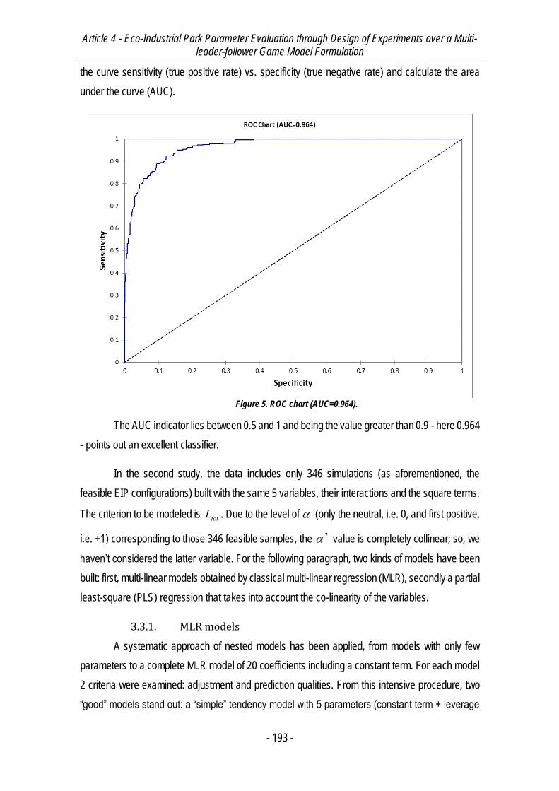
Article 4 - Eco-Industrial Park Parameter Evaluation through Design of Experiments over a Multi-leader-follower Game Model Formulation
- 193 -
the curve sensitivity (true positive rate) vs. specificity (true negative rate) and calculate the area
under the curve (AUC).
Figure 5. ROC chart (AUC=0.964).
The AUC indicator lies between 0.5 and 1 and being the value greater than 0.9 - here 0.964
- points out an excellent classifier.
In the second study, the data includes only 346 simulations (as aforementioned, the
feasible EIP configurations) built with the same 5 variables, their interactions and the square terms.
The criterion to be modeled is totL . Due to the level of (only the neutral, i.e. 0, and first positive,
i.e. +1) corresponding to those 346 feasible samples, the 2 value is completely collinear; so, we
haven’t considered the latter variable. For the following paragraph, two kinds of models have been
built: first, multi-linear models obtained by classical multi-linear regression (MLR), secondly a partial
least-square (PLS) regression that takes into account the co-linearity of the variables.
3.3.1. MLR models
A systematic approach of nested models has been applied, from models with only few
parameters to a complete MLR model of 20 coefficients including a constant term. For each model
2 criteria were examined: adjustment and prediction qualities. From this intensive procedure, two
“good” models stand out: a “simple” tendency model with 5 parameters (constant term + leverage
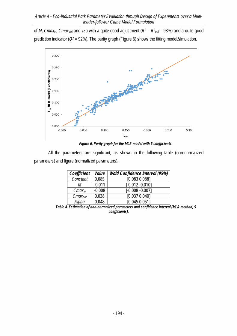
Article 4 - Eco-Industrial Park Parameter Evaluation through Design of Experiments over a Multi-leader-follower Game Model Formulation
- 194 -
of M, Cmaxin, Cmaxout and ) with a quite good adjustment (R2 = R2adj = 93%) and a quite good
prediction indicator (Q2 = 92%). The parity graph (Figure 6) shows the fitting model/simulation.
Figure 6. Parity graph for the MLR model with 5 coefficients.
All the parameters are significant, as shown in the following table (non-normalized
parameters) and figure (normalized parameters).
Coefficient Value Wald Confidence Interval (95%)
Constant 0.085 [0.083 0.088]
M -0.011 [-0.012 -0.010]
Cmaxin -0.008 [-0.008 -0.007]
Cmaxout 0.038 [0.037 0.040]
Alpha 0.048 [0.045 0.051] Table 4. Estimation of non-normalized parameters and confidence interval (MLR method, 5
coefficients).
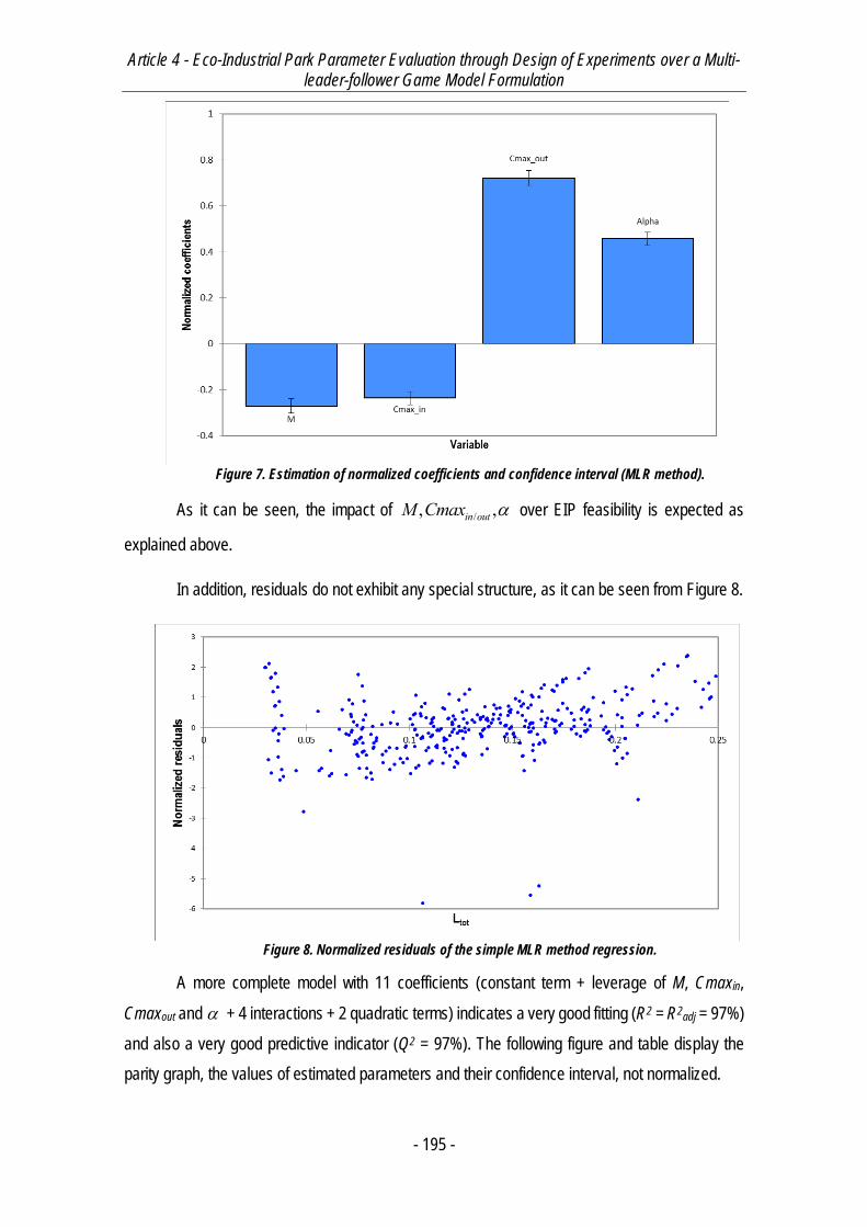
Article 4 - Eco-Industrial Park Parameter Evaluation through Design of Experiments over a Multi-leader-follower Game Model Formulation
- 195 -
Figure 7. Estimation of normalized coefficients and confidence interval (MLR method).
As it can be seen, the impact of /, ,in outM Cmax over EIP feasibility is expected as
explained above.
In addition, residuals do not exhibit any special structure, as it can be seen from Figure 8.
Figure 8. Normalized residuals of the simple MLR method regression.
A more complete model with 11 coefficients (constant term + leverage of M, Cmaxin,
Cmaxout and + 4 interactions + 2 quadratic terms) indicates a very good fitting (R2 = R2adj = 97%)
and also a very good predictive indicator (Q2 = 97%). The following figure and table display the
parity graph, the values of estimated parameters and their confidence interval, not normalized.

Article 4 - Eco-Industrial Park Parameter Evaluation through Design of Experiments over a Multi-leader-follower Game Model Formulation
- 196 -
Figure 9. Parity graph for the MLR model with 11 coefficients.
Coefficient Value Wald Confidence Interval (95%)
Constant 0.089 [0.087 0.091]
M -0.011 [-0.012 -0.010]
Cmaxin -0.004 [-0.005 -0.003]
Cmaxout 0.042 [0.040 0.044]
Alpha 0.050 [0.047 0.052]
M2 -0.002 [-0.002 -0.001]
Cmaxout2 -0.009 [-0.011 -0.008]
M*Cmaxin 0.003 [0.002 0.003]]
M*Cmaxout -0.010 [-0.011 -0.008]
Alpha*Cmaxin -0.003 [-0.004 -0.002]
Alpha*Cmaxout 0.007 [0.005 0.009] Table 5. Estimation of non-normalized parameters and confidence interval (MLR method, 11
coefficients).
By maximizing the aforementioned totL equation with coefficients of Table 5, and by
bounding the variables, an * 0.313totL is obtained. The optimal solution corresponds to the case
where M and inCmax is in their lower level (0.8 and 0.5 respectively), outCmax at its upper bound
(1.5) and at its upper bound. The latter is an expected result, as noted in the Case Study section.
3.3.2. PLS model
A more relevant approach has been performed by using PLS regression (Anon, 2010) that
takes into account the co-linearity of the variables. A PLS model (Tenenhaus, 1998) tries to find
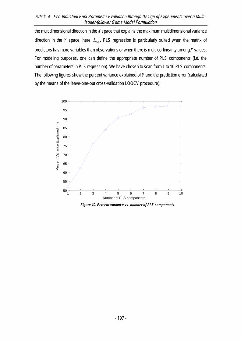
Article 4 - Eco-Industrial Park Parameter Evaluation through Design of Experiments over a Multi-leader-follower Game Model Formulation
- 197 -
the multidimensional direction in the X space that explains the maximum multidimensional variance
direction in the Y space, here totL . PLS regression is particularly suited when the matrix of
predictors has more variables than observations or when there is multi co-linearity among X values.
For modeling purposes, one can define the appropriate number of PLS components (i.e. the
number of parameters in PLS regression). We have chosen to scan from 1 to 10 PLS components.
The following figures show the percent variance explained of Y and the prediction error (calculated
by the means of the leave-one-out cross-validation LOOCV procedure).
Figure 10. Percent variance vs. number of PLS components.
1 2 3 4 5 6 7 8 9 1050
55
60
65
70
75
80
85
90
95
100
Number of PLS components
Perc
ent
Variance E
xpla
ined in y

Article 4 - Eco-Industrial Park Parameter Evaluation through Design of Experiments over a Multi-leader-follower Game Model Formulation
- 198 -
Figure 11. Estimated mean squared predictor error vs. number of PLS components.
It can be seen that a 7 component PLS model offers some good characteristics in terms of
fitting and prediction. The following parity graph confirms this fact.
Figure 12. Parity graph for the PLS model with 7 components.
In the following table non-normalized coefficients for the aforementioned obtained PLS
model are shown.
0 1 2 3 4 5 6 7 8 9 100
0.5
1
1.5
2
2.5
3x 10
-3
Number of components
Est
imat
ed M
ean
Squ
ared
Pre
dict
ion
Erro
r
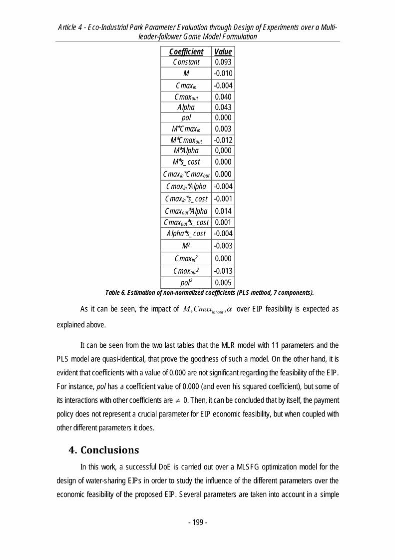
Article 4 - Eco-Industrial Park Parameter Evaluation through Design of Experiments over a Multi-leader-follower Game Model Formulation
- 199 -
Coefficient Value
Constant 0.093
M -0.010
Cmaxin -0.004
Cmaxout 0.040
Alpha 0.043
pol 0.000
M*Cmaxin 0.003
M*Cmaxout -0.012
M*Alpha 0,000
M*s_cost 0.000
Cmaxin*Cmaxout 0.000
Cmaxin*Alpha -0.004
Cmaxin*s_cost -0.001
Cmaxout*Alpha 0.014
Cmaxout*s_cost 0.001
Alpha*s_cost -0.004
M2 -0.003
Cmaxin2 0.000
Cmaxout2 -0.013
pol² 0.005
Table 6. Estimation of non-normalized coefficients (PLS method, 7 components).
As it can be seen, the impact of /, ,in outM Cmax over EIP feasibility is expected as
explained above.
It can be seen from the two last tables that the MLR model with 11 parameters and the
PLS model are quasi-identical, that prove the goodness of such a model. On the other hand, it is
evident that coefficients with a value of 0.000 are not significant regarding the feasibility of the EIP.
For instance, pol has a coefficient value of 0.000 (and even his squared coefficient), but some of
its interactions with other coefficients are 0. Then, it can be concluded that by itself, the payment
policy does not represent a crucial parameter for EIP economic feasibility, but when coupled with
other different parameters it does.
4. Conclusions
In this work, a successful DoE is carried out over a MLSFG optimization model for the
design of water-sharing EIPs in order to study the influence of the different parameters over the
economic feasibility of the proposed EIP. Several parameters are taken into account in a simple
Article 4 - Eco-Industrial Park Parameter Evaluation through Design of Experiments over a Multi-leader-follower Game Model Formulation
- 200 -
modified case study. After reviewing the results of the statistical tools implemented, it is evident
that the most important parameters in a potential EIP environment are those related with process
constraints and those related to the inherent production of each plant. On the other hand, economic
parameters such as who-pays-what are proven to be less significant by the statistical models
obtained. Moreover, it is shown that in early stages of EIP engineering, statistical tools find their
place in order to find limiting plant operating parameters and to propose feasible changes in order
to achieve EIP feasibility.
Also, it is demonstrated how EIPs are very sensible to unilateral changes, which can
produce a variety of scenarios which can be a potential reason to reject EIP cooperation between
different plants. As such, MLSFG models are proven to be models which can aid to overcome these
kinds of impasses.
Finally, it is important to note that flexibility studies in EIPs is yet an unexplored subject
which needs to be addressed soon in order to incentive EIP cooperation and resource related
sustainability.
5. Nomenclature
Latin symbols nl = Number of leaders
Le = Index set of leaders
ix = Decision variables of leader i
ix = Decision variables of other leaders
w = Decision variables of the follower
f = Objective function of leader/leaders
g = Inequality constraints of leader/leaders
z = Objective function of the follower m = Inequality constraints of the follower np = Number of processes per plant
P = Index set of processes nep = Number of plants
EP = Index set of plants
M = Contaminant load
,in outCmax Cmax = Maximum contaminant concentration allowed in inlet/outlet
of processes
Fpart = Water flow between different processes
Fw = Freshwater inlet flow to processes
Fdis = Water processes to the discharge
minf = Minimum flowrate allowed
AWH = Annual EIP operating hours

Article 4 - Eco-Industrial Park Parameter Evaluation through Design of Experiments over a Multi-leader-follower Game Model Formulation
- 201 -
costfw = Freshwater cost costdis = Polluted water discharge cost costex = Polluted water pumping cost
Pol = Binary parameter denoting policy of sharing-water payment L = Level of satisfaction Greek symbols = Lagrange multipliers relative to m = Lagrange multipliers relative to g
= Lagrange multipliers relative to s
, , , , = Slacks to inequalities
= Ratio of freshwater cost to shared water cost
Article 4 - Eco-Industrial Park Parameter Evaluation through Design of Experiments over a Multi-leader-follower Game Model Formulation
- 202 -
References
Aussel, D., Correa, R. & Marechal, P. (2013) Spot Electricity Market with Transmission
Losses. Journal of Industrial and Management Optimization. 9 (2), 275–290.
Aussel, D. & Dutta, J. (2008) Generalized Nash Equilibrium Problem, Variational Inequality
and Quasiconvexity. Operations Research Letters. 36 (4), 461–464.
Bagajewicz, M. & Savelski, M. (2001) On the Use of Linear Models for the Design of Water
Utilization Systems in Process Plants with a Single Contaminant. Chemical engineering research
and design. 79 (5), 600–610.
Bagajewicz, M.J. & Faria, D.C. (2009) On the Appropriate Architecture of the
Water/Wastewater Allocation Problem in Process Plants Jacek Jeżowski and Jan Thullie (ed.).
Computer Aided Chemical Engineering. 261–20.
Biegler, L.T. (2010) Nonlinear Programming: Concepts, Algorithms, and Applications to
Chemical Processes. Philadelphia, Society for Industrial and Applied Mathematics : Mathematical
Optimization Society.
Biegler, L.T., Grossmann, I.E. & Westerberg, A.W. (1997) Systematic Methods of Chemical
Process Design. Upper Saddle River, N.J., Prentice Hall PTR.
Boix, M., Montastruc, L., Azzaro-Pantel, C. & Domenech, S. (2015) Optimization Methods
Applied to the Design of Eco-Industrial Parks: A Literature Review. Journal of Cleaner Production.
87303–317.
Boix, M., Montastruc, L., Pibouleau, L., Azzaro-Pantel, C., et al. (2012) Industrial Water
Management by Multiobjective Optimization: From Individual to Collective Solution Through Eco-
Industrial Parks. Journal of Cleaner Production. [Online] 22 (1), 85–97. Available from:
doi:10.1016/j.jclepro.2011.09.011.
Boix, M., Montastruc, L., Pibouleau, L., Azzaro-Pantel, C., et al. (2010) Multiobjective
Optimization of Industrial Water Networks with Contaminants S. Pierucci and G. Buzzi Ferraris
(ed.). Computer Aided Chemical Engineering. 28859–864.
Brooke, A., Kendrick, D., Meeraus, A. & Raman, R. (1998) GAMS User’s Guide.
Chew, I.M.L., Tan, R.R., Foo, D.C.Y. & Chiu, A.S.F. (2009) Game Theory Approach to the
Analysis of Inter-Plant Water Integration in an Eco-Industrial Park. Journal of Cleaner Production.
[Online] 17 (18), 1611–1619. Available from: doi:10.1016/j.jclepro.2009.08.005.
Dirkse, S.P. & Ferris, M.C. (1996) A Pathsearch Damped Newton Method for Computing
General Equilibria. Annals of Operations Research. [Online] 68 (2), 211–232. Available from:
doi:10.1007/BF02209613.

Article 4 - Eco-Industrial Park Parameter Evaluation through Design of Experiments over a Multi-leader-follower Game Model Formulation
- 203 -
Vincenzo Esposito Vinzi, Wynne W. Chin, Jörg Henseler, & Huiwen Wang (eds.) (2010)
Handbook of Partial Least Squares. [Online]. Berlin, Heidelberg, Springer Berlin Heidelberg.
Available from: http://link.springer.com/10.1007/978-3-540-32827-8 [Accessed: 8 April 2016].
Facchinei, F. & Pang, J.-S. (2007) Finite-Dimensional Variational Inequalities and
Complementarity Problems. Springer Science & Business Media.
Frosch, R.A. & Gallopoulos, N.E. (1989) Strategies for Manufacturing. Scientific American.
261 (3), 144–152.
Hosmer Jr, D.W. & Lemeshow, S. (2004) Applied Logistic Regression. [Online]. John Wiley
& Sons. Available from:
https://books.google.fr/books?hl=en&lr=&id=Po0RLQ7USIMC&oi=fnd&pg=PR5&dq=logistic+regr
ession&ots=DoaTla1jFY&sig=XaeVJ3aN8SMdfbX2X7hPU0bi4Ro [Accessed: 8 April 2016].
Kulkarni, A.A. & Shanbhag, U.V. (2014) A Shared-Constraint Approach to Multi-Leader
Multi-Follower Games. Set-Valued and Variational Analysis. [Online] 22 (4), 691–720. Available
from: doi:10.1007/s11228-014-0292-5.
Leyffer, S. & Munson, T. (2010) Solving Multi-Leader–Common-Follower Games.
Optimisation Methods & Software. 25 (4), 601–623.
Lou, H.H., Kulkarni, M.A., Singh, A. & Huang, Y.L. (2004) A Game Theory Based Approach
for Emergy Analysis of Industrial Ecosystem Under Uncertainty. Clean Technologies and
Environmental Policy. 6 (3), 156–161.
Lowe, E.A. (1997) Creating by-Product Resource Exchanges: Strategies for Eco-Industrial
Parks. Journal of Cleaner Production. [Online] 5 (1–2), 57–65. Available from: doi:10.1016/S0959-
6526(97)00017-6.
Montastruc, L., Boix, M., Pibouleau, L., Azzaro-Pantel, C., et al. (2013) On the Flexibility
of an Eco-Industrial Park (EIP) for Managing Industrial Water. Journal of Cleaner Production.
[Online] 431–11. Available from: doi:10.1016/j.jclepro.2012.12.039.
Olesen, S.G. & Polley, G.T. (1996) Dealing with Plant Geography and Piping Constraints
in Water Network Design. Process Safety and Environmental Protection. [Online] 74 (4), 273–276.
Available from: doi:10.1205/095758296528626.
Pang, J.-S. & Fukushima, M. (2005) Quasi-Variational Inequalities, Generalized Nash
Equilibria, and Multi-Leader-Follower Games. Computational Management Science. 2 (1), 21–56.
Ramos, M.A., Boix, M., Aussel, D., Montastruc, L., et al. (2015) Water Exchanges in Eco-
industrial Parks through Multiobjective Optimization and Game Theory. Computer Aided Chemical
Engineering. 371997–2002.
Ramos, M.A., Boix, M., Aussel, D., Montastruc, L., et al. (2016) Water integration in Eco-
Industrial Parks Using a Multi-Leader-Follower Approach. Computers & Chemical Engineering.
87190–207.
Article 4 - Eco-Industrial Park Parameter Evaluation through Design of Experiments over a Multi-leader-follower Game Model Formulation
- 204 -
Ramos, M.A., Boix, M., Montastruc, L. & Domenech, S. (2014) Multiobjective Optimization
Using Goal Programming for Industrial Water Network Design. Industrial & Engineering Chemistry
Research. 53 (45), 17722–17735.
Ramos, M.A., Gomez, J.M. & Reneaume, J.-M. (2014) Simultaneous Optimal Design and
Control of an Extractive Distillation System for the Production of Fuel Grade Ethanol Using a
Mathematical Program with Complementarity Constraints. Industrial & Engineering Chemistry
Research. 53 (2), 752–764.
Tawarmalani, M. & Sahinidis, N.V. (2005) A Polyhedral Branch-and-Cut Approach to
Global Optimization. Mathematical Programming. 103 (2), 225–249.
Tenenhaus, M. (1998) La Régression Pls: Théorie Et Pratique. Editions TECHNIP.
UNESCO (2009) Water in a Changing World. Report 3. The United Nations World Water
Development.
Wächter, A. & Biegler, L.T. (2002) An Interior Point Algorithm for Large-Scale Nonlinear
Optimization with Applications in Process Engineering. Pittsburgh, Pa., Carnegie Mellon University,
Carnegie Mellon University, 2002.
Yeomans, H. & Grossmann, I.E. (1999) A Systematic Modeling Framework of
Superstructure Optimization in Process Synthesis. Computers & Chemical Engineering. [Online]
23 (6), 709–731. Available from: doi:10.1016/S0098-1354(99)00003-4.
Zhang, Y. & Sahinidis, N.V. (2015) Global Optimization of Mathematical Programs with
Complementarity Constraints and Application to Clean Energy Deployment. Optimization Letters.
1–16.


- 207 -
Chapitre 6 - Optimal design of water exchanges in eco-industrial parks through a game theory approach

Article 5 - Optimal design of water exchanges in eco-industrial parks through a game theory approach
- 208 -

Article 5 - Optimal design of water exchanges in eco-industrial parks through a game theory approach
- 209 -
Ramos, Manuel A., Marianne Boix, Didier Aussel, Ludovic Montastruc, & Serge Domenech. 2016b.
“Optimal Design of Water Exchanges in Eco-Industrial Parks Through a Game Theory Approach.”
Computer Aided Chemical Engineering 38: 1177–1183.
Résumé
Dans cet article complémentaire, d’autres paramètres opératoires sont étudiés dans un modèle
MLSFG. Ce sont notamment les paramètres liés aux capacités des unités de régénération (en
termes de débit d’eau accepté et de capacité à traiter l’eau polluée) qui sont étudiés. En effet, ce
paramètre avait déjà été étudié dans l’étude de Feng et al. (2008) pour la conception des réseaux
d’eau individuels. Il était donc important d’étudier les effets qu’il occasionne dans le cas de la
conception du réseau d’eau d’un EIP qui peut comporter plusieurs unités de régénération
différentes. Plusieurs cas sont considérés, en faisant varier la capacité de régénération maximale
de chaque type d’unité de régénération par rapport à la concentration du polluant en sortie. Il est
alors démontré que chaque usine doit être conçue avec une unité de régénération optimale
nécessitant une étude individuelle préliminaire et le choix de l’unité est un élément crucial pour
l’équilibre économique de l’usine et donc de l’EIP.

Article 5 - Optimal design of water exchanges in eco-industrial parks through a game theory approach
- 210 -
Article 5 - Optimal design of water exchanges in eco-industrial parks through a game theory approach
- 211 -
Optimal design of water exchanges in eco-
industrial parks through a game theory
approach
Manuel Ramos,a Marianne Boix,a Didier Aussel,b Ludovic Montastruc,a Serge Domenecha
a Laboratoire de Génie Chimique, U.M.R. 5503 CNRS/INP/UPS, Université de Toulouse, 4, Allée
Emile Monso, 31432 Toulouse Cedex 4, France
b Laboratoire PROMES, UPR CNRS 8521, Université de Perpignan, Via Domitia, 66100 Perpignan,
France
Keywords: Eco-industrial parks, Multi-leader-follower Game, Nash equilibrium, MPCC, and Game
Theory.
Abstract
The design and optimization of industrial water networks in eco-industrial parks is studied by
formulating and solving multi-leader-follower (MLFG) game models. The methodology is explained
by demonstrating its advantages against multi-objective optimization (MOO) approaches. The
approach is validated on a case study of water integration in EIP with regeneration units. Each
plant’s objective is to minimize the total annualized cost, while the EIP authority objective is to
minimize the consumption of freshwater within the ecopark. On the other hand, flexibility of the
methodology is studied by varying parameters in the case study such as the capacity of the
regeneration units. The MLFG is transformed into a mathematical problem with complementarity
constraints (MPCC) and solved using GAMS® as with a NLP formulation. The methodology
proposed is proved to be very reliable in multi-criteria scenarios compared to MOO approaches,
providing numerical Nash equilibrium solutions and specifically in EIP design and optimization. This
method is proven to be reliable in this context because it proposes to obtain one solution instead
of a set of optimal solutions that takes directly into account the preferences of the decision maker.
1. Introduction
During the last few decades, industrialization has contributed to rapid depletion of natural
resources such as water and natural gas. Consequently, there is a real need for industries to ensure
Article 5 - Optimal design of water exchanges in eco-industrial parks through a game theory approach
- 212 -
minimum natural resources consumption, while maintaining good production levels. In order to work
towards global environmental preservation while increasing business success, the concept of
industrial ecology has emerged. This concept, which is directly linked to sustainable development,
aims at engaging separate industries, geographically closed enough, in a collective approach so
that exchanges of raw matter, by-products, energy and utilities are maximized. Indeed, the most
widespread manifestations of these kinds of industrial symbiosis are eco-industrial parks (EIP). As
it can be inferred, a basic condition for an EIP to be economically viable is to demonstrate that
benefits of each industry involved in it by working collectively is higher than working as a stand-
alone facility.
Recently, Boix et al. (Boix, Montastruc, Azzaro-Pantel, et al., 2015) and Ramos et al.
(Ramos, Boix, Aussel, et al., 2015) highlighted the lack of studies dealing with optimization in order
to design optimal configuration of an EIP. However, it is important to develop methodologies able
to design an EIP where each industry has an effective gain compared to the case where they
operate individually, by also taking into account environmental concerns. In these works (among
others), the authors developed multi-objective optimization strategies such as goal programming.
However, Ramos et al. (Ramos, Boix, Aussel, et al., 2015) demonstrated that in different scenarios
and by tuning different optimization parameters (e.g. weight factors associated with the objective
functions) one company is favored compared to the others using MOO methods. Although optimal
solutions are intermediate and satisfying in terms of individual costs, it is of great interest to obtain
more balanced solutions so that each plant/company is satisfied at the same time and moreover,
by minimizing freshwater consumption in order to insure the environmental performance of the EIP.
An interesting alternative particularly adapted to the optimal design of EIP is the Game
Theory approach and most particularly the concept of multi-leader single-follower game problem
(MLSFG). In fact, an EIP can be seen as the congregation of different non-cooperative agents (the
leaders) which aim at minimizing their annualized operating costs and an EIP authority (the
follower) whose aim is to minimize resources consumption. This kind of non-cooperative game is
very interesting for the concepts of EIP, since the main barrier to integrate an EIP for industry is
the issue of confidentiality between plants and this approach could be very promising to overcome
this problem. In fact, by introducing an impartial authority whose role is to collect all data necessary
to design the EIP, plants involved would be able to keep confidential data, without the need to share
them with the other companies of the park.
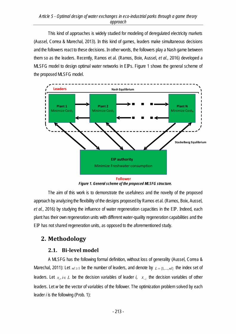
Article 5 - Optimal design of water exchanges in eco-industrial parks through a game theory approach
- 213 -
This kind of approaches is widely studied for modeling of deregulated electricity markets
(Aussel, Correa & Marechal, 2013). In this kind of games, leaders make simultaneous decisions
and the followers react to these decisions. In other words, the followers play a Nash game between
them so as the leaders. Recently, Ramos et al. (Ramos, Boix, Aussel, et al., 2016) developed a
MLSFG model to design optimal water networks in EIPs. Figure 1 shows the general scheme of
the proposed MLSFG model.
Plant 1Minimize Cost1
EIP authority
Minimize Freshwater consumption
Plant NMinimize CostN
Plant 2Minimize Cost2
Leaders
Follower
Stackelberg Equilibrium
Nash Equilibrium
Figure 1. General scheme of the proposed MLSFG structure.
The aim of this work is to demonstrate the usefulness and the novelty of the proposed
approach by analyzing the flexibility of the designs proposed by Ramos et al. (Ramos, Boix, Aussel,
et al., 2016) by studying the influence of water regeneration capacities in the EIP. Indeed, each
plant has their own regeneration units with different water-quality regeneration capabilities and the
EIP has not shared regeneration units, as opposed to the aforementioned study.
2. Methodology
2.1. Bi-level model
A MLSFG has the following formal definition, without loss of generality (Aussel, Correa &
Marechal, 2011): Let 1nl be the number of leaders, and denote by {1,..., }L nl the index set of
leaders. Let ,ix i L be the decision variables of leader i, ix the decision variables of other
leaders. Let w be the vector of variables of the follower. The optimization problem solved by each
leader i is the following (Prob. 1):
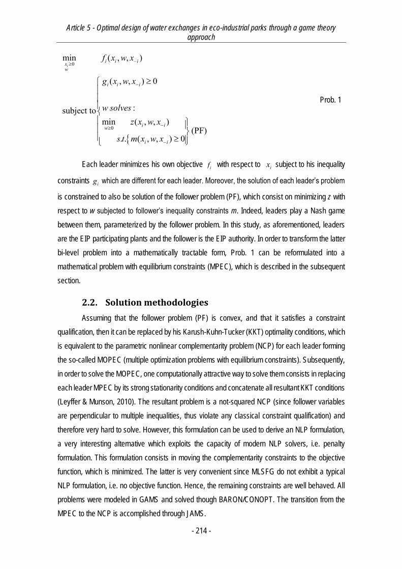
Article 5 - Optimal design of water exchanges in eco-industrial parks through a game theory approach
- 214 -
0
0
min ( , , )
( , , ) 0
:subject tomin ( , , )
(PF). . ( , , ) 0
ii i ix
w
i i i
i iw
i i
f x w x
g x w x
w solvesz x w x
s t m x w x
Prob. 1
Each leader minimizes his own objective if with respect to ix subject to his inequality
constraints ig which are different for each leader. Moreover, the solution of each leader’s problem
is constrained to also be solution of the follower problem (PF), which consist on minimizing z with
respect to w subjected to follower’s inequality constraints m. Indeed, leaders play a Nash game
between them, parameterized by the follower problem. In this study, as aforementioned, leaders
are the EIP participating plants and the follower is the EIP authority. In order to transform the latter
bi-level problem into a mathematically tractable form, Prob. 1 can be reformulated into a
mathematical problem with equilibrium constraints (MPEC), which is described in the subsequent
section.
2.2. Solution methodologies
Assuming that the follower problem (PF) is convex, and that it satisfies a constraint
qualification, then it can be replaced by his Karush-Kuhn-Tucker (KKT) optimality conditions, which
is equivalent to the parametric nonlinear complementarity problem (NCP) for each leader forming
the so-called MOPEC (multiple optimization problems with equilibrium constraints). Subsequently,
in order to solve the MOPEC, one computationally attractive way to solve them consists in replacing
each leader MPEC by its strong stationarity conditions and concatenate all resultant KKT conditions
(Leyffer & Munson, 2010). The resultant problem is a not-squared NCP (since follower variables
are perpendicular to multiple inequalities, thus violate any classical constraint qualification) and
therefore very hard to solve. However, this formulation can be used to derive an NLP formulation,
a very interesting alternative which exploits the capacity of modern NLP solvers, i.e. penalty
formulation. This formulation consists in moving the complementarity constraints to the objective
function, which is minimized. The latter is very convenient since MLSFG do not exhibit a typical
NLP formulation, i.e. no objective function. Hence, the remaining constraints are well behaved. All
problems were modeled in GAMS and solved though BARON/CONOPT. The transition from the
MPEC to the NCP is accomplished through JAMS.
Article 5 - Optimal design of water exchanges in eco-industrial parks through a game theory approach
- 215 -
On the other hand, it is worth noting that typical water-network models exhibit a mixed-
integer linear programming (MILP) model, constraining the minimum water flow between
processes. Nevertheless, the tractability of discrete decisions in MLSFG is yet to be explored. Thus,
a low-flowrate elimination algorithm was employed in order to bind flows and re-iterate until a final
solution is achieved without low-flowrates between processes.
2.3. Modeling EIP water networks
In order to model the water network of an EIP, the concept of superstructure is used, it
represents all the possible alternatives to connect each process of the network, this systemic
approach allows to represent process design. Figure 2 shows the superstructure of an EIP including
3 industries and each industry is composed of process and regeneration units.
Figure 2. General view of the superstructure for water networks in EIP.
After modeling the superstructure, the next step is to model the network with mass
balances so that mathematical programming methods can be applied. A “black box” approach is
adopted so that each parameter of the different processes is known, for more precision about the
modeling stage, the reader can refer to Ramos et al. (Ramos, Boix, Aussel, et al., 2016).
3. Multi-leader single-follower game approach
3.1. Presentation of the case study
In this study, an EIP including 3 companies is designed, which correspond to an academic
example that has been widely explored in the literature (Olesen & Polley, 1996), Boix et al., 2012,
Ramos et al. 2015a and 2015b). For this reason, it remains a good example to test and to validate
a new methodology because solutions are well-known. Each company is composed of 5 process

Article 5 - Optimal design of water exchanges in eco-industrial parks through a game theory approach
- 216 -
units and the parameters are the same as those defined in Ramos et al. (Ramos, Boix, Aussel, et
al., 2016).
Though, different scenarios are studied in the present work, compared to the work of
Ramos et al. (Ramos et al. 2016). In the present work, two different blocks of scenarios are
considered, given that all plants have potentially three different-output-concentration regenerations
units and no shared regeneration units exist:
- Scenario 1: each plant regeneration unit capacity is constrained in two different cases,
namely i) between 10 and 80 each 10 tonne/hr for all plants and ii) the minimum regeneration
capacity needed by each regeneration unit of each plant to operate with minimum freshwater
consumption if they operate by themselves, i.e. 30, 20 and 60 tonne/hr respectively for plant 1, 2
and 3 (which can be inferred from figure 3).
- Scenario 2: The capacity of each potential regeneration unit is a variable controlled by
each plant.
Remark that this do not constraint regenerated water to flow between plants. On the other
hand, regenerated water imported by a plant is paid by the plant to the plant owning the
regeneration unit of which the water comes from.
The economic objective function of each plant represent the cost of freshwater
consumption, wastewater, regenerated water import flowrate (either imported from own or external
regeneration units), shared polluted water to own and other plants processes, and the gain from
selling regenerated water to other plants.
3.2. Results and discussion
Results obtained are always compared to the case where plants operate in a non-EIP
configuration (i.e. by themselves), whose results are illustrated in figure 3.

Article 5 - Optimal design of water exchanges in eco-industrial parks through a game theory approach
- 217 -
Figure 3. Results of the case without an EIP in operation.
Results obtained in both EIP scenarios are summarized in figure 4:
Figure 4. Results obtained by the MLSFG model.
For the variable case the optimal total regeneration capacity obtained for regeneration units
correspond to 268.8 tonne/hr for plant 1, 111 tonne/hr for plant 2 and 0.0 tonne/hr for plant 3. Plants
experience slight gains when regeneration capacity is constrained to low values, which is expected.
As capacities are constrained to higher values, is it possible to observe important gains regarding
all plants, e.g. the case where the maximum capacity of regeneration units is 60 tonne/hr. Evidently,
all plants have considerable gains when the regeneration capacity is enough to supply processes
without consuming freshwater. Furthermore, it can be seen that solutions correspond to equilibrium
Article 5 - Optimal design of water exchanges in eco-industrial parks through a game theory approach
- 218 -
solutions where the plant cannot change their actions unilaterally to their own benefice. In the
second scenario, where capacities are considered as variables, plants compete due to the fact that
they also have the potential to sell regenerated water to other plants. Then, the equilibrium solution
seems to be less advantageous for plants 1 and 2.
4. Conclusions
In this work, MLSFG formulations for the effective design of EIP were successfully
addressed, by studying also different scenarios regarding the water-regeneration capacity. Results
underline the effectiveness of the proposed methodology, compared to traditional multi-objective
optimization methods. By formulating the problem in a MLSFG manner solutions obtained
correspond at least to the case where each player objective function value matches the value if the
player operates standalone, without having to add additional constraints to the given objective
functions. Given the latter, in this work is successfully introduced a reliable alternative to solve
chemical/process engineering problems with multiple decision objectives. It is also important to
underline that the introduction of an EIP regulator plays a major role in the above quoted
improvements of the EIP integration model since it allows considering MLSFG modeling.
Article 5 - Optimal design of water exchanges in eco-industrial parks through a game theory approach
- 219 -
References
Aussel, D., Correa, R. & Marechal, P. (2013) Spot Electricity Market with Transmission
Losses. Journal of Industrial and Management Optimization. 9 (2), 275–290.
Aussel, D., Correa, R. & Marechal, P. (2011) Spot Electricity Market with Transmission
Losses.
Boix, M., Montastruc, L., Azzaro-Pantel, C. & Domenech, S. (2015) Optimization Methods
Applied to the Design of Eco-Industrial Parks: A Literature Review. Journal of Cleaner Production.
87303–317.
Leyffer, S. & Munson, T. (2010) Solving Multi-Leader–Common-Follower Games.
Optimisation Methods & Software. 25 (4), 601–623.
Olesen, S.G. & Polley, G.T. (1996) Dealing with Plant Geography and Piping Constraints
in Water Network Design. Process Safety and Environmental Protection. [Online] 74 (4), 273–276.
Available from: doi:10.1205/095758296528626.
Ramos, M.A., Boix, M., Aussel, D., Montastruc, L., et al. (2015) Water Exchanges in Eco-
industrial Parks through Multiobjective Optimization and Game Theory. Computer Aided Chemical
Engineering. 371997–2002.
Ramos, M.A., Boix, M., Aussel, D., Montastruc, L., et al. (2016) Water integration in Eco-
Industrial Parks Using a Multi-Leader-Follower Approach. Computers & Chemical Engineering.
87190–207.

- 221 -
Chapitre 7 - Utility Network Optimization in Eco-Industrial Parks by
a Multi-Leader Follower Game Methodology

Article 6 - Utility Network Optimization in Eco-Industrial Parks by a Multi-Leader Follower Game Methodology
- 222 -
Article 6 - Utility Network Optimization in Eco-Industrial Parks by a Multi-Leader Follower Game Methodology
- 223 -
Résumé
Ce travail est l’évolution logique de l’article 3 puisque les modèles MLSFG et SLMFG développés
sont appliqués sur un exemple d’EIP de la littérature mettant en œuvre différents types d’échanges
(utilités énergétiques notamment). Dans cet article, une méthodologie systématique est proposée
pour la conception optimale des EIP à partir de données comme les conditions opératoires
pertinentes après une analyse des échanges potentiels. L’obtention des données et des
paramètres est réalisée en utilisant un outil tel qu’un logiciel de simulation des procédés. En effet,
en simulant chaque usine de façon rigoureuse avec ProSim Plus®, pour un cas d’étude d’un EIP
potentiel en Norvège (Zhang, Strømman, Solli, et al., 2008), de nombreuses données ont pu être
extraites. Après l’analyse et la simulation de chaque flowsheet, les échanges potentiels sont
analysés et des entreprises fictives ont été définies à partir de cette étude préliminaire. Les besoins
énergétiques de toutes les opérations unitaires vont alors être déterminants dans la décision
d’implanter ou non des utilités dans le réseau. A partir de cela, un modèle du réseau d’utilités a été
mis en place. Ainsi, les utilités ont été choisies en fonction des températures requises et en
conséquence, les procédés peuvent recevoir uniquement un seul type d’utilité ou un mélange
d’utilités. Certaines utilités tournent en boucle fermée, c’est à dire qu’elles sont renvoyées vers une
chaudière ou un système de refroidissement pour les rendre encore une fois fonctionnelles. Les
usines composant le réseau d’utilités ont pour objectif de minimiser leur coût opératoire (calculé
par rapport aux utilités fraîches et recyclées) et jouent un jeu de Nash entre elles. L’EIP étudié est
composé de 6 entreprises représentant un total de 74 procédés et 16 utilités ont été considérées.
Par ailleurs, l’autorité de l’EIP vise à minimiser les émissions équivalentes de CO2 provenant de
l’utilisation d’utilités fraîches. Les résultats montrent la pertinence de la méthodologie, en
permettant de constater une grande diminution des émissions et d’utilités fraîches utilisées dans
l’EIP. Les résultats économiques des usines sont ainsi assez intéressants, car des gains
significatifs sont atteints (i.e. entre 20-70% environ).

Article 6 - Utility Network Optimization in Eco-Industrial Parks by a Multi-Leader Follower Game Methodology
- 224 -
Article 6 - Utility Network Optimization in Eco-Industrial Parks by a Multi-Leader Follower Game Methodology
- 225 -
Utility Network Optimization in Eco-Industrial
Parks by a Multi-Leader Follower Game
Methodology
Manuel A. Ramosa, Mariona Rocafull, Marianne Boix*a, Didier Aussel*b, Ludovic
Montastruca, Serge Domenecha
a Laboratoire de Génie Chimique, U.M.R. 5503 CNRS/INP/UPS, Université de Toulouse, 4, Allée
Emile Monso, 31432 Toulouse Cedex 4, France
b Laboratoire PROMES, UPR CNRS 8521, Université de Perpignan, Via Domitia, 66100 Perpignan,
France
* Corresponding authors: [email protected].
Keywords: Eco-industrial parks, Multi-leader-follower Game, Nash equilibrium, Utility Network,
MPCC, Game Theory, Process Simulation.
Abstract
A multi-leader-follower game (MLFG) model for the design of the utility network in an eco-industrial
park (EIP) is studied implemented by introducing the concept of environmental authorities. The
methodology also considers the flowsheet simulation of each one of the plants involved in the EIP
in order to obtain utility consumption of each plant by operating by itself. The approach is validated
on a case study of a potential Norwegian EIP. In the latter, multi-leader-single-follower and single-
leader-multi-follower game models are studied. Each plant’s objective is to minimize the total
annualized cost, while the EIP authority objective is to minimize the equivalent CO2 consumption
related to utility consumption within the ecopark. The MLFG is transformed into a MOPEC and
solved using GAMS® as an NLP. The methodology proposed is proved to be very reliable in multi-
criteria scenarios compared to traditional multiobjective optimization approaches, providing
numerical Nash/Stackelberg equilibrium solutions and specifically in EIP design and optimization.
1. Introduction
Due to an increasing depletion of natural resources such as fresh water for instance,
important environmental researches have been developed in the last decades. The environmental
Article 6 - Utility Network Optimization in Eco-Industrial Parks by a Multi-Leader Follower Game Methodology
- 226 -
impact induced by the process industry is linked both to the high volumes involved and to the
diversity of toxic products generated along the processing chain.
Consequently, there is a real need for industries to ensure minimum natural resources
consumption, while maintaining good production levels. In particular, industrial development is
often linked to the use of high volumes of freshwater and other utilities (Boix, Montastruc,
Pibouleau, et al., 2011, 2010). In order to work towards global environmental preservation while
increasing business success, the concept of industrial ecology has emerged (Boix, Montastruc,
Azzaro-Pantel, et al., 2015). This concept, which is directly linked to sustainable development, aims
at engaging separate industries, geographically closed enough, in a collective approach so that
exchanges of raw matter, by-products, energy and utilities (Chertow, 2000) are maximized. Indeed,
the most widespread manifestations of these kinds of industrial symbiosis are eco-industrial parks
(EIP). A definition widely accepted of EIP is “an industrial system of planned materials and energy
exchanges that seeks to minimize energy and raw materials use, minimize waste, and build
sustainable economic, ecological and social relationships” (Boix, Montastruc, Azzaro-Pantel, et al.,
2015; Montastruc, Boix, Pibouleau, et al., 2013; Alexander, Barton, Petrie, et al., 2000). As it can
be highlighted, a basic condition for an EIP to be economically viable is to demonstrate that benefits
of each industry involved in it by working collectively is higher than working as a stand-alone facility.
Among the methodologies to design EIPs in a process engineering framework,
mathematical modeling and optimization is the most practical and most adequate one.
Nevertheless, Boix et al. (Boix, Montastruc, Azzaro-Pantel, et al., 2015) highlighted the lack of
studies dealing with optimization in order to design optimal configuration and design of an EIP.
Thus, it is important to develop methodologies able to design an EIP where each industry has a
plausible gain compared to the case where they operate individually, by also taking into account
environmental concerns. Among EIP design studies, water-using network is the most common type
of cooperation modeled in literature (Boix, Montastruc, Azzaro-Pantel, et al., 2015). In this kind of
studies, the case is often solved as a water-allocation problem through a superstructure-based
model where water has to be distributed, treated and discharged in an optimal way between the
process units of each plant/plant involved in the EIP.
In the majority of these studies, taking process data as a starting point, water-sharing
networks between industries/plants are designed using linear programming (LP) or mixed-integer
linear programming (MILP) models. Furthermore, it is widely known that EIP design entails the
formulation of several objective functions, given that there are completely different interests in play
Article 6 - Utility Network Optimization in Eco-Industrial Parks by a Multi-Leader Follower Game Methodology
- 227 -
e.g. environmental objectives, plants gain and resource consumption (Boix, Montastruc, Pibouleau,
et al., 2012; Chew, Thillaivarrna, Tan, et al., 2011; Lovelady & El-Halwagi, 2009; Rubio-Castro,
Ponce-Ortega, Serna-González, et al., 2012; Tan & Aviso, 2012; El-Halwagi, 1997). Other studies
deal with the energetic integration in EIPs (Chae, Kim, Yoon, et al., 2010) or by taking into account
simultaneously water and energy integration, following also a multi-objective optimization
framework (Boix & Montastruc, 2011; Fichtner, Frank & Rentz, 2004). Moreover, very few studies
deal also with raw matter/products sharing in EIPs, e.g. Kantor et al. (Kantor, Betancourt, Elkamel,
et al., 2015).
On the other hand, regarding modeling and optimization methods, different recent studies
deal with advanced decision-making techniques based on optimization in order to deal with the
design of EIPs, staying based on the water-sharing network design, e.g. Chew et al. (Chew, Tan,
Foo, et al., 2009) developed a game theory approach for the decision making process for water
integration in an EIP. Nevertheless, the game theory approach was employed a posteriori, i.e. in
the decision making process after the optimization step. In this study, different configurations of
EIP’s are obtained by classical optimization and then, the different integration schemes were
evaluated regarding Nash equilibrium. Secondly, Aviso et al. (Aviso, Tan, Culaba, et al., 2010)
developed a single-leader multi-follower game (SLMFG) model with fuzzy optimization in order to
model water exchange in EIP. The methodology is then evaluated in a medium-sized case study
and under different scenarios. Finally, Ramos et al. (Ramos, Boix, Aussel, et al., 2016b) developed
an alternative methodology to multi-criteria optimization generally used in the field of process
engineering, by applying the methodology in an industrial ecology context (water networks), by
using multi-leader-follower game (MLFG) models due to the introduction of an EIP authority in the
model. The latter research compared the obtained results with traditional multi-objective
optimization results and proved that the proposed game theory model methodology was indeed
more effective than traditional multi-objective/multi-decision optimization methods, e.g. goal
programming. Subsequently, Ramos et al. (Ramos, Boix, Aussel, et al., 2016a) studied the
simultaneous water and energy network integration in EIP through a hybrid goal
programming/SLMFG formulation, by generating Pareto fronts for two scenarios and afterwards by
implementing a decision-making tool.
As proved, a MLFG model is a very reliable method to accomplish the design of EIPs.
Indeed, the approach has several demonstrated advantages when compared to traditional
approaches and introduces the concept of environmental authority in an EIP context. On the other
hand, very few studies deal with utility integration in EIPs. In this work, an optimal utility network
Article 6 - Utility Network Optimization in Eco-Industrial Parks by a Multi-Leader Follower Game Methodology
- 228 -
design is address by using MLSFG and SLMFG models. In addition, a general methodology is
introduced in order to further expand on the game theory approaches in EIPs. This work focuses
also on the importance of process engineering in the process of EIP design and integration, by
implementing process simulation in order to obtain process utility consumption data for the
aforementioned model.
2. Methodology
In order to successfully design EIP using the methodology proposed in this work, several
assumptions and aspects have to be taken into account. First of all, it is clear that the plants
involved have to be in feasible geographical vicinity, in order to make matter or energy exchanges
directly (to make piping viable). This, as being the main idea behind an EIP, has as consequence
that supply chain models are not included (at least in the present) in its conception and design.
Second, plants’ processes/plants have to be already in an advanced engineering phase, i.e.
technology selection has already taken place. Therefore, the flowsheet of the processes is already
defined or at least with main unit operations and main operating conditions defined. Thus, the
modeling scale is assumed to be at the level of unit operations. Finally, it is very important to note
that the vital idea behind EIPs is the more sustainable operation of industries, i.e. minimization of
natural resources consumption, by providing a significant economic benefit to the participating
plants. In consequence, EIP optimization models are far from being single-objective classical
optimization problems. Zhang et al. (Zhang, Strømman, Solli, et al., 2008) provided a general
procedure to early planning and design of an EIP. In the present work, we center our approach on
a combination of modern engineering tools, such as process modeling, simulation, mathematical
modeling and optimization.
2.1. General Methodology
Given the aforementioned assumptions, the proposed methodology is as follows:
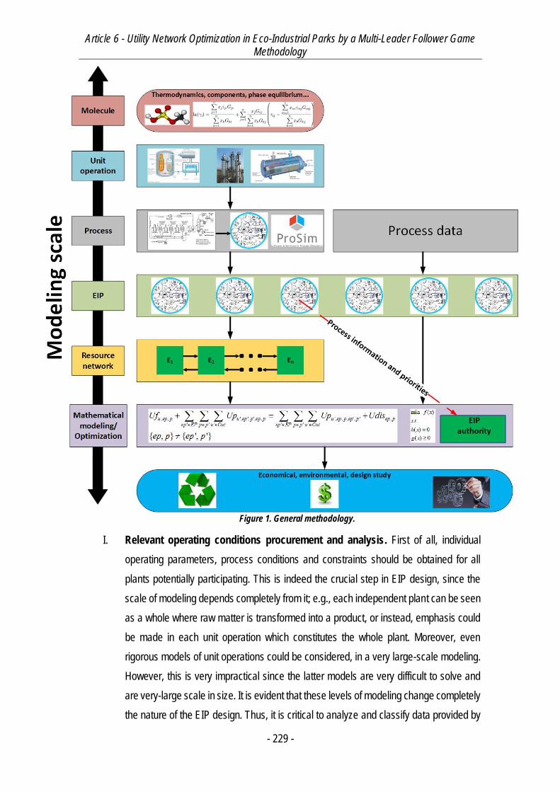
Article 6 - Utility Network Optimization in Eco-Industrial Parks by a Multi-Leader Follower Game Methodology
- 229 -
Figure 1. General methodology.
I. Relevant operating conditions procurement and analysis. First of all, individual
operating parameters, process conditions and constraints should be obtained for all
plants potentially participating. This is indeed the crucial step in EIP design, since the
scale of modeling depends completely from it; e.g., each independent plant can be seen
as a whole where raw matter is transformed into a product, or instead, emphasis could
be made in each unit operation which constitutes the whole plant. Moreover, even
rigorous models of unit operations could be considered, in a very large-scale modeling.
However, this is very impractical since the latter models are very difficult to solve and
are very-large scale in size. It is evident that these levels of modeling change completely
the nature of the EIP design. Thus, it is critical to analyze and classify data provided by
Article 6 - Utility Network Optimization in Eco-Industrial Parks by a Multi-Leader Follower Game Methodology
- 230 -
plants (if it is the case) in order to define beforehand the modeling scale. If data is not
provided by plants, flowsheeting and simulation should be completed in order to obtain
relevant operating conditions of streams and unit operations. This is accomplished by
rigorously simulating all processes unit operations, based on the complete flowsheet
defined by each plant. In this way, process operating conditions and requirements i.e.
energy and raw matter can be obtained in a reliable way. On the other hand, it is a plus
to accomplish individual optimization of each flowsheet and energy integration to obtain
more advanced data. Process simulation software play a crucial role in this step.
II. Type of network definition. With all process data and operating conditions obtained
from the step before, it is subsequently needed to conceive a network suitable for
exchanges in the EIP. In other words, it is about establishing potential networks of raw
matter, waste or energy that may benefit the entire EIP, by highlighting potential sources
and potential sinks. Examples include water-contaminant networks (Boix et al. (Boix,
Montastruc, Pibouleau, et al., 2012, 2011), Ramos et al. (Ramos, Boix, Aussel, et al.,
2015, 2016b)), simultaneous heat and water networks (Boix et al. (Boix & Montastruc,
2011), Ramos et al. (Ramos, Boix, Aussel, et al., 2016a)) and utility networks (this work).
Once defined, it follows the calculation of additional data needed in order to better
understand the potential exchanges. A sensitivity analysis may be also pertinent at this
step.
III. Define a mathematical model for the aforementioned selected network. Indeed,
this step is crucial for the subsequent steps, since it is at this point where the modeling
scale comes into play. Here, several modeling scales may be chosen, depending on the
degree of detail desired. On the other hand, as the degree of detail increases, the larger
the scale of the model and in consequence more difficult to solve. We propose a grey
box approach, where each process of each plant has already fixed operating parameters
obtained from step I. Moreover, the type of models considered in network optimization
in general are often mixed-integer, linear, MILP, or non-linear MINLP problems, which
increases the difficulty of the model. As such, very detailed models such as rigorous
thermodynamic, kinetic, equilibrium models of unit operations should be avoided.
Superstructure-type models are preferred at this stage, where all interconnections
between processes are possible (Yeomans & Grossmann, 1999). It is important to
define at this point design constraints for the network, in order to accomplish a feasible
design of the EIP, e.g. minimum flowrates between processes (Ramos, Boix, Aussel, et
al., 2016b, 2015) and minimum heat exchanger transfer area (Boix & Montastruc, 2011).

Article 6 - Utility Network Optimization in Eco-Industrial Parks by a Multi-Leader Follower Game Methodology
- 231 -
IV. Solve each individual plant problem. At this point, each single-objective optimization
of each plant is accomplished by minimizing their operating and/or capital costs. These
results will provide important data prior to the results of the EIP optimization problem
and will be used to compare the latter obtained results.
V. EIP Solution methodology. At this point, the optimization model is already defined. On
the other hand, it is critical to point out that, as aforementioned, EIP optimization
problems are multi-criteria, or multi-objective optimization problems. As such, this kind
of problems should be solved by advanced decision-making tools as multi-objective
optimization methods (see Ramos et al. (Ramos, Boix, Montastruc, et al., 2014)) or as
in the present work, by using the concept of EIP regulator introduced by Ramos et al.
(Ramos, Boix, Aussel, et al., 2016b) in the context of EIPs and using game theory
optimization models such as multi-leader single-follower game (MLSFG) or single-
leader multi-follower game (SLMFG) formulations. The latter formulations are very
useful in the context of EIP conception and design, since it successfully describe the
distinction between different levels of modeling, i.e. environmental objective functions
and plants profit objective functions, as demonstrated by Ramos et al. (Ramos, Boix,
Aussel, et al., 2016b). At this point, additional modeling takes place by adapting the EIP
model to these game theory models approach. A suitable solution method has to be
selected as well.
VI. Post-optimal analysis. When results are obtained, deep analysis leads to the
understanding and the consequences of the EIP resource-sharing network. At this point,
sustainability objectives must be achieved as well as positive relative gains of each plant
regarding the case where they operate outside the EIP framework. If one or several
plants do not achieve expected profits, then it is crucial to analyze the possible causes
and if possible, provide some changes to the model in order to obtain significant profit
values.
As aforementioned, this work will emphasize on the conception and design of an EIP utility
network. Next, we will describe specifically the methodology of the present work.
2.2. Specific methodology
According to the methodology described earlier, simulations of the potential plants
potentially participating in the EIP were accomplished by using the process simulation software
ProSim Plus® (ProSim, n.d.). With the process operating conditions obtained, we proceeded to
analyze the potential sources and sinks of utility-sharing as well as to select adequate potential
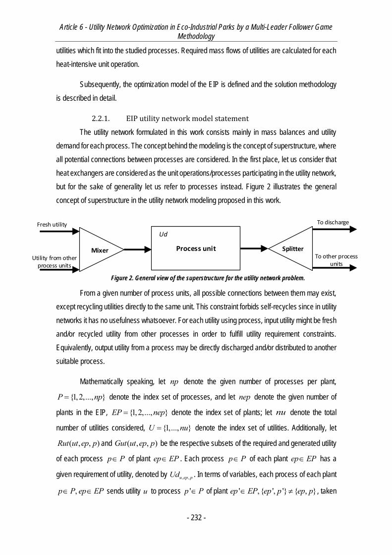
Article 6 - Utility Network Optimization in Eco-Industrial Parks by a Multi-Leader Follower Game Methodology
- 232 -
utilities which fit into the studied processes. Required mass flows of utilities are calculated for each
heat-intensive unit operation.
Subsequently, the optimization model of the EIP is defined and the solution methodology
is described in detail.
2.2.1. EIP utility network model statement
The utility network formulated in this work consists mainly in mass balances and utility
demand for each process. The concept behind the modeling is the concept of superstructure, where
all potential connections between processes are considered. In the first place, let us consider that
heat exchangers are considered as the unit operations/processes participating in the utility network,
but for the sake of generality let us refer to processes instead. Figure 2 illustrates the general
concept of superstructure in the utility network modeling proposed in this work.
Figure 2. General view of the superstructure for the utility network problem.
From a given number of process units, all possible connections between them may exist,
except recycling utilities directly to the same unit. This constraint forbids self-recycles since in utility
networks it has no usefulness whatsoever. For each utility using process, input utility might be fresh
and/or recycled utility from other processes in order to fulfill utility requirement constraints.
Equivalently, output utility from a process may be directly discharged and/or distributed to another
suitable process.
Mathematically speaking, let np denote the given number of processes per plant,
{1,2,..., }P np denote the index set of processes, and let nep denote the given number of
plants in the EIP, {1,2,..., }EP nep denote the index set of plants; let nu denote the total
number of utilities considered, {1,..., }U nu denote the index set of utilities. Additionally, let
( , , )Rut ut ep p and ( , , )Gut ut ep p be the respective subsets of the required and generated utility
of each process p P of plant ep EP . Each process p P of each plant ep EP has a
given requirement of utility, denoted by , ,u ep pUd . In terms of variables, each process of each plant
,p P ep EP sends utility u to process 'p P of plant ' , { ', '} { , }ep EP ep p ep p , taken
Mixer SplitterProcess unit
Fresh utility
Utility from other process units
To discharge
To other process units
Ud

Article 6 - Utility Network Optimization in Eco-Industrial Parks by a Multi-Leader Follower Game Methodology
- 233 -
into account by variable , , , ', 'u ep p ep pUp , receives utility u , denoted by variable , ', ', ,u ep p ep pUp and has
an inlet flow of fresh utility, denoted by , ,u ep pUf . Also, it may send a utility flow directly to the
discharge, denoted by ,ep pUdis . Remark that it is possible to develop a different kind of model, by
taking into account minimum flowrate allowed between processes. However, such a model would
introduce discrete decisions into the model, which in a context of MLSFG/SLMFG models would
be rather very inconvenient to handle.
Given the aforementioned notation, the model statement is as follows:
Constraints.
-Utility mass balance around a process unit p P of a plant ep EP of required utility u Rut
:
, , ', ', ', , ', , , ', ' ,' ' ' ' ' '
{ , } { ', '}
u ep p u ep p ep p u ep p ep p ep pep EP p p u Gut ep EP p p u Gut
Uf Up Up Udis
ep p ep p
Eq. 1
-Utility requirements around a process unit p P of a plant ep EP of required utility u Rut :
, , ', ', ', , , ,' ' '
{ , } { ', '}
u ep p u ep p ep p u ep pep EP p p u Gut
Uf Up Ud
ep p ep p
Eq. 2
-Flow Positivity:
, , 0, , ,u ep pUf u U ep EP p P Eq. 3
, , , ', ' 0, ,{ , '} ,{ , '}
{ , } { ', '}u ep p ep pUp u U ep ep EP p p P
ep p ep p
Eq. 4
, 0, ,ep pUd ep EP p P Eq. 5
Objective functions.
For this kind of problem, let us define the following potential objective functions, which are
very common in previous similar studies (Ramos, Boix, Aussel, et al., 2016b; Boix & Montastruc,
2011; Ramos, Boix, Montastruc, et al., 2014), (Kantor, Betancourt, Elkamel, et al., 2015). In fact,
Article 6 - Utility Network Optimization in Eco-Industrial Parks by a Multi-Leader Follower Game Methodology
- 234 -
these objective functions play a role on the regulator design of EIPs. The objective functions are
divided in two, namely the environmental objective function (Eq. 6) and the objective function of
each one of the plants, i.e. annualized utility cost (Eq. 7). Note that the environmental objective
function may be defined as a simple minimization of fresh resource consumption, but then the
difference between different utility resources and their individual impact on the environment would
not be taken into account. Nonetheless, in other studies (Ramos, Boix, Montastruc, et al., 2014;
Ramos, Boix, Aussel, et al., 2016b; Boix & Montastruc, 2011) minimizing freshwater consumption
is a valid environmental objective function, since only one resource is taken into account.
, ,uttot u u ep pep EP p P u Rut
f Uf
Eq. 6
, , , , , , ''
, , , ', ' , ', ', ,' '2
{ , } { ', '}
u ep p u ep p ep pp P u Rut p P p P u Gut
totep
u ep p ep p u ep p ep pep EP p P p P u Gut
Uf Up
C AWHUp Up
ep p ep p
Eq. 7
In Eq. 3, u represent the CO2 emission rate of each utility u U , in Eq. 4 stands for
the purchase price of fresh utility, for the cost of pumping recycled utility from one process to
another. Indeed, each plant pays the cost of pumping utility flow both to a process and from a
process. Remark that each plant pays the totality of the cost associated with utility pumping
between their own processes, and regarding utility shared with and from other plants the cost is
shared between plants instead (i.e. 2
). Remark that the model stated is linear in its totality (LP).
As aforementioned, a more complex model could be studied, but for the sake of generality and in
order to focus on the general methodology these kind of models were avoided. Finally, note that
the sum of utilities was chosen as the environmental objective function, even if utilities are different
in type. This simplification avoids creating more complicated models where utilities are considered
disaggregated, such as multi-leader multi-follower game formulations.
In the following section, the regulator approach (i.e. MLSFG and SLMFG) to utility networks
in EIPs is presented in detail, and the case study is introduced.
2.2.2. MLSFG and SLMFG optimization models approach
In order to obtain a solution for the kind of systems as EIPs are, where heavy interactions
exist and where each entity is naturally biased by their own interests, game theory is a viable tool

Article 6 - Utility Network Optimization in Eco-Industrial Parks by a Multi-Leader Follower Game Methodology
- 235 -
for decision-making. As aforementioned, in Nash games, players make simultaneous optimal
decisions given the optimal strategies of other players. Indeed, Nash equilibrium denotes the state
where all the casual forces internal to the system balance each other out (Lou, Kulkarni, Singh, et
al., 2004), and no player can improve its gain by unilaterally changing his strategy. By solving a
Nash game, it is possible to obtain this kind of solution by definition as demonstrated by Ramos et
al. (Ramos, Boix, Aussel, et al., 2016b).
The introduction of an authority/regulator to the design of viable utility networks in EIPs is
an interesting alternative to overcome the confidentiality problem on one hand, and on the other
hand, to solve the problem of equilibrium benefits of the players involved (Ramos, Boix, Aussel, et
al., 2016b). In fact, the latter can be modeled as a MLSFG where the leaders are the plants whereas
the EIP authority represents the only follower (and environmental concerns) or as a SLMFG, when
the roles are inversed. Thus, Nash equilibrium exists among players which are in the same level,
whereas Stackelberg equilibrium represents the relationship between different levels. The choice
between these different formulations depends on the priorities of the EIP.
At this point, it is important to note that in this work approach the choice of leaders and
followers is crucial in the problem formulation, as it is explained in detail by Ramos et al. (Ramos,
Boix, Aussel, et al., 2016b) in terms of mathematical modeling and results: On one hand, it can be
assumed that plants act as followers and the authority as the lone leader (SLMFG) or vice-versa
(MLSFG). It is assumed that in the case of SLMFG plants aim to minimize their utility annualized
cost, given the minimum CO2 emissions caused by fresh utility consumption in the EIP, determined
by the authority. A general scheme of the SLMFG proposed is shown in Figure 3.
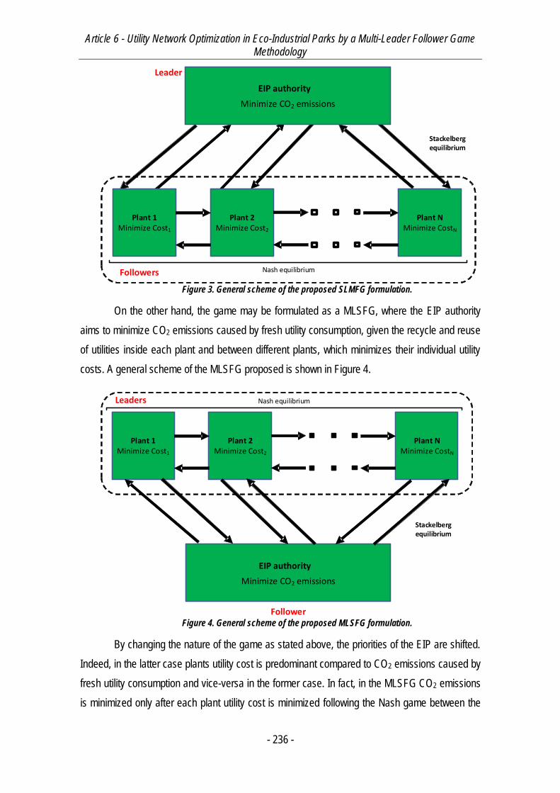
Article 6 - Utility Network Optimization in Eco-Industrial Parks by a Multi-Leader Follower Game Methodology
- 236 -
Leader
EIP authority
Minimize CO2 emissions
Plant 1Minimize Cost1
Plant NMinimize CostN
Plant 2Minimize Cost2
Followers Nash equilibrium
Stackelberg equilibrium
Figure 3. General scheme of the proposed SLMFG formulation.
On the other hand, the game may be formulated as a MLSFG, where the EIP authority
aims to minimize CO2 emissions caused by fresh utility consumption, given the recycle and reuse
of utilities inside each plant and between different plants, which minimizes their individual utility
costs. A general scheme of the MLSFG proposed is shown in Figure 4.
Plant 1Minimize Cost1
EIP authority
Minimize CO2 emissions
Plant NMinimize CostN
Plant 2Minimize Cost2
Leaders
Follower
Stackelberg equilibrium
Nash equilibrium
Figure 4. General scheme of the proposed MLSFG formulation.
By changing the nature of the game as stated above, the priorities of the EIP are shifted.
Indeed, in the latter case plants utility cost is predominant compared to CO2 emissions caused by
fresh utility consumption and vice-versa in the former case. In fact, in the MLSFG CO2 emissions
is minimized only after each plant utility cost is minimized following the Nash game between the
Article 6 - Utility Network Optimization in Eco-Industrial Parks by a Multi-Leader Follower Game Methodology
- 237 -
leaders and vice versa. In consequence, it is self-understood that priorities have to be carefully
chosen by the modeler or may be self-imposed by the problem. Given the latter structures, we now
proceed to formally present each one of the game formulations following Ramos et al. (Ramos,
Boix, Aussel, et al., 2016b).
For the sake of clarity, it is defined:
, ,
, , , ', '
,
( :1 ,1 ,1 )
( :1 ,1 ' ,1 , ' , , ', ' )
( :1 ,1 )
u ep p
ep u ep p ep p
ep p
Uf Uf u nu ep nep p np
Up Up u nu ep nep p p np ep p ep pUdis Udis ep nep p np
Eq. 8
Additionally, by grouping authority variables in x and each plant variables in epy , we
obtain:
( , )( ),ep ep
x Uf Udisy Up ep EP
Eq. 9
Evidently, each plant controls their own flows to their own process as well as for other
plants’ processes, while the authority controls the flow of fresh utilities to each processes of all
plants and their discharge flow.
In the same way, constraints are grouped in the following way either for the SLMFG and
MLSFG formulations:
( , ) { .3, .5}( , , ) { .1, .2}
( , , ) { .4}ep ep ep
ep ep ep
g x y Eq Eql x y y Eq Eqm x y y Eq
Eq. 10
With the aforementioned notation, the corresponding bi-level formulation of the SLMFG is
illustrated in Prob. .
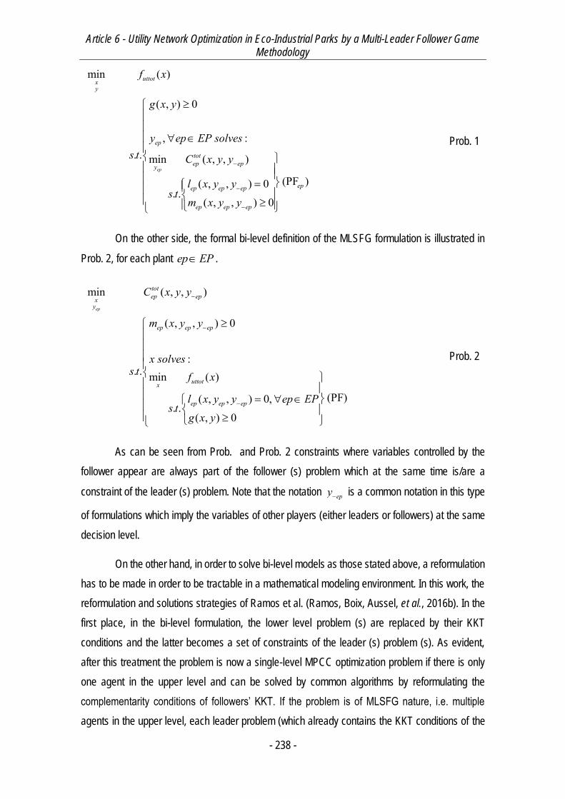
Article 6 - Utility Network Optimization in Eco-Industrial Parks by a Multi-Leader Follower Game Methodology
- 238 -
min ( )
( , ) 0
, :. . min ( , , )
(PF )( , , ) 0. .
( , , ) 0
ep
uttotxy
ep
totep epy
epep ep ep
ep ep ep
f x
g x y
y ep EP solvess t C x y y
l x y ys t
m x y y
Prob. 1
On the other side, the formal bi-level definition of the MLSFG formulation is illustrated in
Prob. 2, for each plant ep EP .
min ( , , )
( , , ) 0
:. . min ( )
(PF)( , , ) 0,. .
( , ) 0
ep
totep epx
y
ep ep ep
uttotx
ep ep ep
C x y y
m x y y
x solvess t f x
l x y y ep EPs t
g x y
Prob. 2
As can be seen from Prob. and Prob. 2 constraints where variables controlled by the
follower appear are always part of the follower (s) problem which at the same time is/are a
constraint of the leader (s) problem. Note that the notation epy is a common notation in this type
of formulations which imply the variables of other players (either leaders or followers) at the same
decision level.
On the other hand, in order to solve bi-level models as those stated above, a reformulation
has to be made in order to be tractable in a mathematical modeling environment. In this work, the
reformulation and solutions strategies of Ramos et al. (Ramos, Boix, Aussel, et al., 2016b). In the
first place, in the bi-level formulation, the lower level problem (s) are replaced by their KKT
conditions and the latter becomes a set of constraints of the leader (s) problem (s). As evident,
after this treatment the problem is now a single-level MPCC optimization problem if there is only
one agent in the upper level and can be solved by common algorithms by reformulating the
complementarity conditions of followers’ KKT. If the problem is of MLSFG nature, i.e. multiple
agents in the upper level, each leader problem (which already contains the KKT conditions of the
Article 6 - Utility Network Optimization in Eco-Industrial Parks by a Multi-Leader Follower Game Methodology
- 239 -
follower) KKT conditions are formulated and concatenated, forming a single-level MPCC. As this
work is oriented towards a systematic methodology to design EIPs rather than the mathematical
methods, the reader is invited to consult the work of Ramos et al. (Ramos, Boix, Aussel, et al.,
2016b) where the detailed solution methodology is explored. Remark the resulting model after
transformation has intrinsic non-linearities characteristic of KKT conditions (i.e. complementarity
conditions).
In this work the NLP formulation of MPCCs (cf. Ramos et al. (Ramos, Boix, Aussel, et al.,
2016b)) is preferred. All problems were modeled in GAMS® (Brooke, Kendrick, Meeraus, et al.,
1998) 24.4.2 and transformed through the extended mathematical programming framework (EMP).
The framework uses the solver JAMS to reformulate general Nash equilibrium games (in MPEC
form) into NCPs. BARON (Tawarmalani & Sahinidis, 2005) with CONOPT as the NLP solver was
used to solve all models. In the context of solving the problems presented in this work, a global
solver like BARON is very useful to find the solution where the minimization of complementarities
is achieved, due to the presence of KKT conditions in the reformulation of both MLSFG and SLMFG
problems.
3. Case study
The case study used in the present work in order to prove the usefulness of the proposed
approach to EIP and utility network design and optimization is based on the EIP suggested by
Zhang et al. (Zhang, Strømman, Solli, et al., 2008). Using the authors’ data and support information
as a reference, flowsheets of the suggested processes and some other processes proposed in this
work were conceived and implemented in process simulation software ProSim Plus®, always trying
to guarantee the maximum similarity to ensure an important degree of reality in the study. Zhang
et al. (Zhang, Strømman, Solli, et al., 2008) specify that some of the modules are already in
existence while others are under construction or conception and design so, it is not an existing
park, but has the potential to become one.
The proposed EIP is located in Mongstad in western Norway. Currently, only the refinery
plant and some gas processes are already existent. Then, the proposed EIP is centered on the
existing refinery. Also, the proximity of a port and some underground storage tanks, are relevant to
search new potential activities. As it is known, the principal refinery products are gasoline, diesel
and other light petroleum-derivate products hence, the principal feedstock is the petroleum.
Environmental policy is becoming more strictly and narrow, especially with CO2 and other
contaminant emissions. In fact, the creation of a combined head and power plant (CHP, as
Article 6 - Utility Network Optimization in Eco-Industrial Parks by a Multi-Leader Follower Game Methodology
- 240 -
proposed by Zhang et al. (Zhang, Strømman, Solli, et al., 2008)) could be an important addition for
the EIP. In addition, this facility may produce the high-pressure steam needed in the refinery and
CO2 that could be also recycled to the refinery. Even so, it would be essential to reduce the CO2
emissions through a CO2 capture process. An additional advantage of building these two facilities
is the low temperature heat produced. Conversely, high temperature waste heat the fjords, which
is not permitted by the authorities.
The main processes were selected to be suited for the present study, i.e. those where the
unit operations, as well as energy exchanges and mass flows, are relevant for the proper
development of the EIP, e.g. the refinery and the power plant and there were omitted modules as
well e.g. water treatment and aquaculture. This decision stems from the fact that, in overview, these
processes do not contribute specially in the utility network optimization. In addition, the chosen
modules generally do not involve complicated processes and can be simulated with traditional unit
operations widely available in commercial process simulators i.e. reactors, distillation columns, etc.
Therefore, the selected processes for this study are coal gasification, CO2 capture, MeOH and
DME synthesis, refinery plant, power plant and air separation processes. Each process is described
in detail subsequently.
3.1. Coal Gasification
This process entails, broadly speaking, the transformation of coal into a synthesis gas (H2
+ CO). The coal gasification is in fact the beginning of the syngas production which consist of coal
gasification, CO2 capture, and fuel synthesis (in this case methanol and DME). Furthermore, this
process allows the option of using the syngas produced as a supplementary fuel in the power plant
to gain the advantages by introducing a duct burner for supplementary firing, as explained by Zhang
et al. (Zhang, Strømman, Solli, et al., 2008).
Since the supplementary information provided by Zhang et al. (Zhang, Strømman, Solli, et
al., 2008), was not complete enough to successfully simulate rigorously all the coal gasification
process, extra sources on the subject were considered. In fact, Preciado et al. (Preciado, Ortiz-
Martinez, Gonzalez-Rivera, et al., 2012) worked on the simulation of gas production from steam
oxygen gasification similar to the coal gasification process studied by Zhang et al. (Zhang,
Strømman, Solli, et al., 2008), based on a Fischer-Tropsch process and other techniques to
separate the sulfur from synthesis gas. Thus, using the known information from both studies it was
possible to successfully simulate the coal gasification process, whose flowsheet is illustrated in
Figure 5.
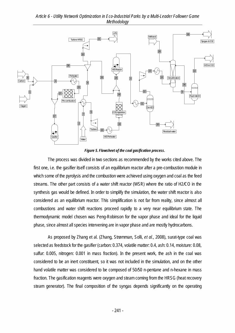
Article 6 - Utility Network Optimization in Eco-Industrial Parks by a Multi-Leader Follower Game Methodology
- 241 -
Figure 5. Flowsheet of the coal gasification process.
The process was divided in two sections as recommended by the works cited above. The
first one, i.e. the gasifier itself consists of an equilibrium reactor after a pre-combustion module in
which some of the pyrolysis and the combustion were achieved using oxygen and coal as the feed
streams. The other part consists of a water shift reactor (WSR) where the ratio of H2/CO in the
synthesis gas would be defined. In order to simplify the simulation, the water shift reactor is also
considered as an equilibrium reactor. This simplification is not far from reality, since almost all
combustions and water shift reactions proceed rapidly to a very near equilibrium state. The
thermodynamic model chosen was Peng-Robinson for the vapor phase and ideal for the liquid
phase, since almost all species intervening are in vapor phase and are mostly hydrocarbons.
As proposed by Zhang et al. (Zhang, Strømman, Solli, et al., 2008), surat-type coal was
selected as feedstock for the gasifier (carbon: 0.374, volatile matter: 0.4, ash: 0.14, moisture: 0.08,
sulfur: 0.005, nitrogen: 0.001 in mass fraction). In the present work, the ash in the coal was
considered to be an inert constituent, so it was not included in the simulation, and on the other
hand volatile matter was considered to be composed of 50/50 n-pentane and n-hexane in mass
fraction. The gasification reagents were oxygen and steam coming from the HRSG (heat recovery
steam generator). The final composition of the syngas depends significantly on the operating
Oxygen
Gasifier
Carbon
6
1
Water
LPS
Residual water
H2S & CO2
2
WS Reactor
7
Syngas & CO2
8
Preheater
WS Preheater
De-H2O
3
11
15
12
22
Pre-combustion
23
Turbine
5
Desulfonation
Methanol
13
Flash MeOH
14
29
COS Hydrolisis
19
10
18
24
Turbine HRSG 21
9
26
27
4
17
16
25
20
28
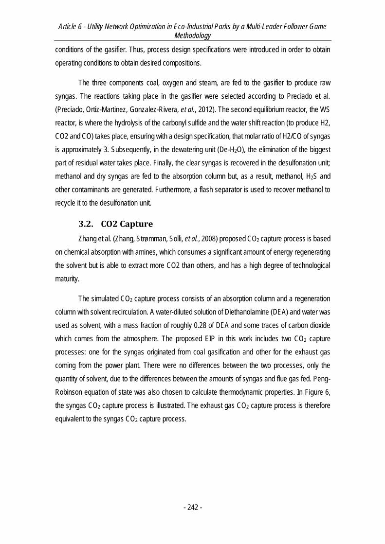
Article 6 - Utility Network Optimization in Eco-Industrial Parks by a Multi-Leader Follower Game Methodology
- 242 -
conditions of the gasifier. Thus, process design specifications were introduced in order to obtain
operating conditions to obtain desired compositions.
The three components coal, oxygen and steam, are fed to the gasifier to produce raw
syngas. The reactions taking place in the gasifier were selected according to Preciado et al.
(Preciado, Ortiz-Martinez, Gonzalez-Rivera, et al., 2012). The second equilibrium reactor, the WS
reactor, is where the hydrolysis of the carbonyl sulfide and the water shift reaction (to produce H2,
CO2 and CO) takes place, ensuring with a design specification, that molar ratio of H2/CO of syngas
is approximately 3. Subsequently, in the dewatering unit (De-H2O), the elimination of the biggest
part of residual water takes place. Finally, the clear syngas is recovered in the desulfonation unit;
methanol and dry syngas are fed to the absorption column but, as a result, methanol, H2S and
other contaminants are generated. Furthermore, a flash separator is used to recover methanol to
recycle it to the desulfonation unit.
3.2. CO2 Capture
Zhang et al. (Zhang, Strømman, Solli, et al., 2008) proposed CO2 capture process is based
on chemical absorption with amines, which consumes a significant amount of energy regenerating
the solvent but is able to extract more CO2 than others, and has a high degree of technological
maturity.
The simulated CO2 capture process consists of an absorption column and a regeneration
column with solvent recirculation. A water-diluted solution of Diethanolamine (DEA) and water was
used as solvent, with a mass fraction of roughly 0.28 of DEA and some traces of carbon dioxide
which comes from the atmosphere. The proposed EIP in this work includes two CO2 capture
processes: one for the syngas originated from coal gasification and other for the exhaust gas
coming from the power plant. There were no differences between the two processes, only the
quantity of solvent, due to the differences between the amounts of syngas and flue gas fed. Peng-
Robinson equation of state was also chosen to calculate thermodynamic properties. In Figure 6,
the syngas CO2 capture process is illustrated. The exhaust gas CO2 capture process is therefore
equivalent to the syngas CO2 capture process.
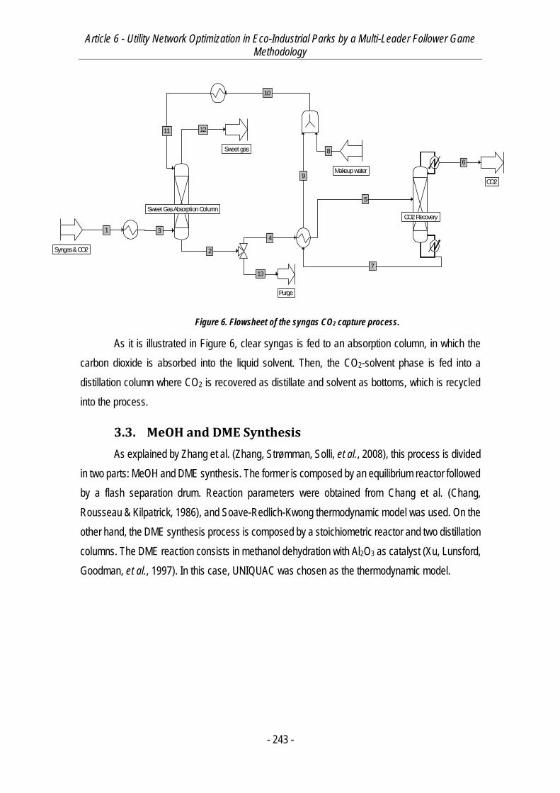
Article 6 - Utility Network Optimization in Eco-Industrial Parks by a Multi-Leader Follower Game Methodology
- 243 -
Figure 6. Flowsheet of the syngas CO2 capture process.
As it is illustrated in Figure 6, clear syngas is fed to an absorption column, in which the
carbon dioxide is absorbed into the liquid solvent. Then, the CO2-solvent phase is fed into a
distillation column where CO2 is recovered as distillate and solvent as bottoms, which is recycled
into the process.
3.3. MeOH and DME Synthesis
As explained by Zhang et al. (Zhang, Strømman, Solli, et al., 2008), this process is divided
in two parts: MeOH and DME synthesis. The former is composed by an equilibrium reactor followed
by a flash separation drum. Reaction parameters were obtained from Chang et al. (Chang,
Rousseau & Kilpatrick, 1986), and Soave-Redlich-Kwong thermodynamic model was used. On the
other hand, the DME synthesis process is composed by a stoichiometric reactor and two distillation
columns. The DME reaction consists in methanol dehydration with Al2O3 as catalyst (Xu, Lunsford,
Goodman, et al., 1997). In this case, UNIQUAC was chosen as the thermodynamic model.
Syngas & CO2
Sweet Gas Absorption Column
Makeup water
CO2
8
9
11
Sweet gas
1 3
2
4
Purge
13
CO2 Recovery
5
6
7
10
12
Article 6 - Utility Network Optimization in Eco-Industrial Parks by a Multi-Leader Follower Game Methodology
- 244 -
Figure 7. MeOH/DME synthesis process flowsheet.
The H2+CO mixture from the CO2 capture is fed to the first reactor where the methanol
synthesis takes place as well as the water gas shift reaction (to produce CO and H2O).
Subsequently, in the flash unit, volatile gases are separated easily from the main liquid products
(MeOH and H2O) and recirculated for better reaction yield. At this point, a methanol is either stored
for commercialization or to feed the second reactor, where the DME synthesis takes place. Finally,
two distillation columns are used to obtain DME and MeOH as final products.
3.4. Refinery
The refinery flowsheet was made up from scratch, since Zhang et al. (Zhang, Strømman,
Solli, et al., 2008) did not included it on their supplementary information.
The objective of the refinery plant is to separate and produce petroleum products from
crude oil, where are included several classes of fuels, asphalt, paraffin wax, lubricants etc. The
procedure for a good distillation of the crude oil is dependent of the composition of the feedstock.
Every refinery has its own proper specifications when it comes to the desired product. In general
H2 + CO
1
Methanol Synthesis / WS
7
Purge
8
MeOH Storage
Turbine
3
4
Waste water
DME
DME Synthesis
10
Purge 220
21
Volatiles Separation
5
6
9
Compressor
2
13
16
18
23
26
DME Separation
MeOH Separation12
17
19
11
22
14
Article 6 - Utility Network Optimization in Eco-Industrial Parks by a Multi-Leader Follower Game Methodology
- 245 -
terms, all the products obtained differ on their boiling point and thus, can be recovered from different
heights of the tower. In order to simulate the fractions of the products it was necessary to divide
the process in atmospheric and vacuum distillation.
The thermodynamic model used in this case was the Peng Robinson’s model as being the
most used when working with petroleum oils, as explained above. General flowsheet of the
conceived refinery is illustrated in Figure 8.
In order to simulate the fractions of the products it was necessary to divide the process in
atmospheric and vacuum distillation. In the atmospheric part a use of two-phase liquid-vapor
separator was needed for the components of light hydrocarbons that are gas at room temperature
and gases such as N2, H2S, CO2, and air. The residue from the two-phase liquid-vapor separator
was the inlet for the first distillation column which was used to separate the naphtha from the
heavier hydrocarbons like diesel and kerosene and immediately afterwards a second distillation
column to divide de diesel from the heavier hydrocarbons (Figure 9)
For the next fraction it was necessary to make vacuum distillation in order to separate the
hydrocarbons from C12 to C22 (as the lightest), C22 to C27 and everything over C29 as residue and
which was considered as asphalt.
Naphtha reforming has an important role in the petro chemistry industry. The core of this
process is consists of three or four fixed-bed adiabatically operated reactors in series. The
feedstock is mixed with a recycled gas stream containing 0.6-0.9 molar fraction of hydrogen which
is heated again. The other product is named reformate which is blended for gasoline purposes and
can be treated accordingly to the desired products of the refinery. Each reactor (Figure 10) was
made for a different process in the refining: the first one was made to simulate the dehydrogenation
(Turaga, Ramanathan, Rajesh, et al., 2003). The next reactor was used to make the isomerization
and the last one was used for the hydrocracking process where the alkanes are broken into lower
alkane chains thanks to catalyst that is usually used and to saturate these lower alkenes chains
hydrogen from the same process is recycled in order to saturate the fractioned alkanes hence the
consummation of hydrogen.

Article 6 - Utility Network Optimization in Eco-Industrial Parks by a Multi-Leader Follower Game Methodology
- 246 -
Figure 8. General flowsheet of the conceived refinery.
HVGO C22 - C27
Petroleum
Diesel
Atmospheric Distilation Train
6
SeparatorCO2 + H2S + Air
LPG + Methane
7
10
11
LVGO C15 - C22
9
Asphalt > C29
Naptha Reforming
5
Light Naphtha
Hydrogen
Heavy Naphtha
2
24
28
Vacuum Distillation Column
12
13
14
15
1
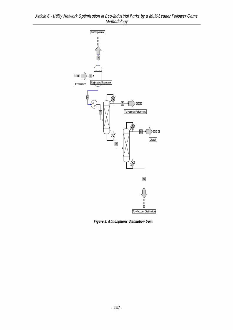
Article 6 - Utility Network Optimization in Eco-Industrial Parks by a Multi-Leader Follower Game Methodology
- 247 -
Figure 9. Atmospheric distillation train.
Light-gas SeparatorPetroleum
1
4
To Naphta Reforming
To Separator
7
Diesel
To Vaccum Distillation
6
9
3
5
8
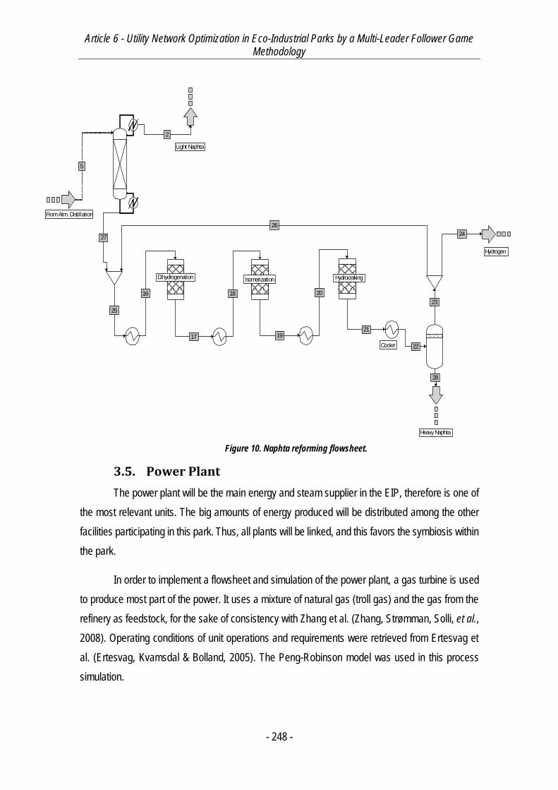
Article 6 - Utility Network Optimization in Eco-Industrial Parks by a Multi-Leader Follower Game Methodology
- 248 -
Figure 10. Naphta reforming flowsheet.
3.5. Power Plant
The power plant will be the main energy and steam supplier in the EIP, therefore is one of
the most relevant units. The big amounts of energy produced will be distributed among the other
facilities participating in this park. Thus, all plants will be linked, and this favors the symbiosis within
the park.
In order to implement a flowsheet and simulation of the power plant, a gas turbine is used
to produce most part of the power. It uses a mixture of natural gas (troll gas) and the gas from the
refinery as feedstock, for the sake of consistency with Zhang et al. (Zhang, Strømman, Solli, et al.,
2008). Operating conditions of unit operations and requirements were retrieved from Ertesvag et
al. (Ertesvag, Kvamsdal & Bolland, 2005). The Peng-Robinson model was used in this process
simulation.
From Atm. Distillation
Dihydrogenation
16
Isomerization
17
18
Hydrocraking
19
20
Cooler
21
22
25
23
26
Light Naphta
Hydrogen
Heavy Naphta
24
28
2
27
5
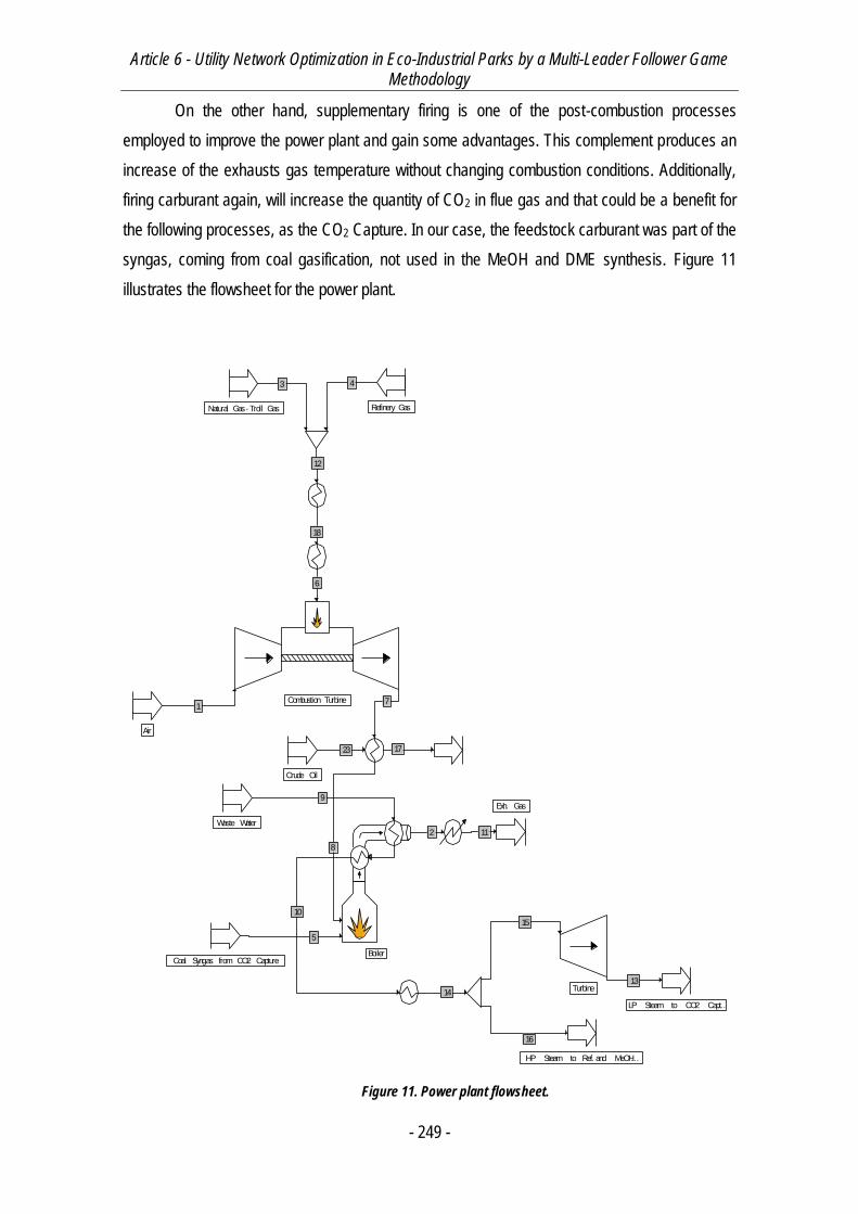
Article 6 - Utility Network Optimization in Eco-Industrial Parks by a Multi-Leader Follower Game Methodology
- 249 -
On the other hand, supplementary firing is one of the post-combustion processes
employed to improve the power plant and gain some advantages. This complement produces an
increase of the exhausts gas temperature without changing combustion conditions. Additionally,
firing carburant again, will increase the quantity of CO2 in flue gas and that could be a benefit for
the following processes, as the CO2 Capture. In our case, the feedstock carburant was part of the
syngas, coming from coal gasification, not used in the MeOH and DME synthesis. Figure 11
illustrates the flowsheet for the power plant.
Figure 11. Power plant flowsheet.
Air
Natural Gas - Troll Gas Refinery Gas
Combustion Turbine
Turbine
Coal Syngas from CO2 Capture
3 4
7
Waste Water
15
HP Steam to Ref. and MeOH …
17
Exh. Gas
LP Steam to CO2 Capt…
16
1
Crude Oil
23
Boiler
5
8
9
6
13
10
14
2 11
12
18
Article 6 - Utility Network Optimization in Eco-Industrial Parks by a Multi-Leader Follower Game Methodology
- 250 -
The mixture of natural gas and refinery gas enters, together with the pre-compressed air
to the gas turbine to produce both energy and exhaust gases. Afterwards, this gas preheats the
crude oil for the refinery plant, and later is fed in the boiler with the syngas to generate the
supplementary firing. Subsequently, the flue gas arrives to the HRSG (boiler) where, though the
introduction of boiled water, an energy exchange takes place. At this stage, the remaining exhaust
gas is recirculated to heat the natural gas, and sent to the CO2 Capture. On the other hand, low-
pressure steam is produced by adding a steam turbine at the end of the process.
3.6. Air Separation
The air separation process present the proposed EIP proposed by Zhang et al. (Zhang,
Strømman, Solli, et al., 2008) was considered as a potential important process for the conception
of the optimal utilities network within the EIP. In consequence, a simple air separation facility is
implemented and simulated in the present study, even though the original authors did not take into
consideration such a process.
Initially three different technologies were contemplated: Pressure swing adsorption
process (PSA), which uses the adsorption with zeolite as an alternative to liquefaction, membrane
technologies, where the gas can be separated by synthetic membranes and it is also a non-
cryogenic process and the cryogenic distillation process, which needs liquefaction to be
implemented. The first two methods are usually used to produce relatively small amounts of air
separation, and on the contrary, the cryogenic distillation process is the most common method in
industry by producing higher amounts of production, ensuring the required purity. Hence, this kind
of process may be very well suited to an EIP.
The air separation module was simulated based on Cornelissen and Hirs (Cornelissen &
Hirs, 1998), using low and high pressure distillation columns (Figure 12). The SRK thermodynamic
model is used.
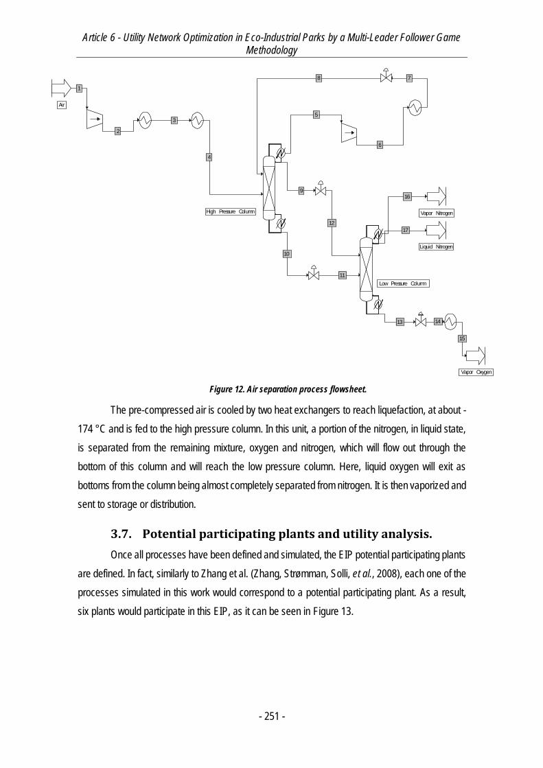
Article 6 - Utility Network Optimization in Eco-Industrial Parks by a Multi-Leader Follower Game Methodology
- 251 -
Figure 12. Air separation process flowsheet.
The pre-compressed air is cooled by two heat exchangers to reach liquefaction, at about -
174 °C and is fed to the high pressure column. In this unit, a portion of the nitrogen, in liquid state,
is separated from the remaining mixture, oxygen and nitrogen, which will flow out through the
bottom of this column and will reach the low pressure column. Here, liquid oxygen will exit as
bottoms from the column being almost completely separated from nitrogen. It is then vaporized and
sent to storage or distribution.
3.7. Potential participating plants and utility analysis.
Once all processes have been defined and simulated, the EIP potential participating plants
are defined. In fact, similarly to Zhang et al. (Zhang, Strømman, Solli, et al., 2008), each one of the
processes simulated in this work would correspond to a potential participating plant. As a result,
six plants would participate in this EIP, as it can be seen in Figure 13.
High Pressure Column
Low Pressure Column
Air
Vapor Nitrogen
Liquid Nitrogen
Vapor Oxygen
1
2
35
4
6
78
9
10
11
12
13 14
15
16
17
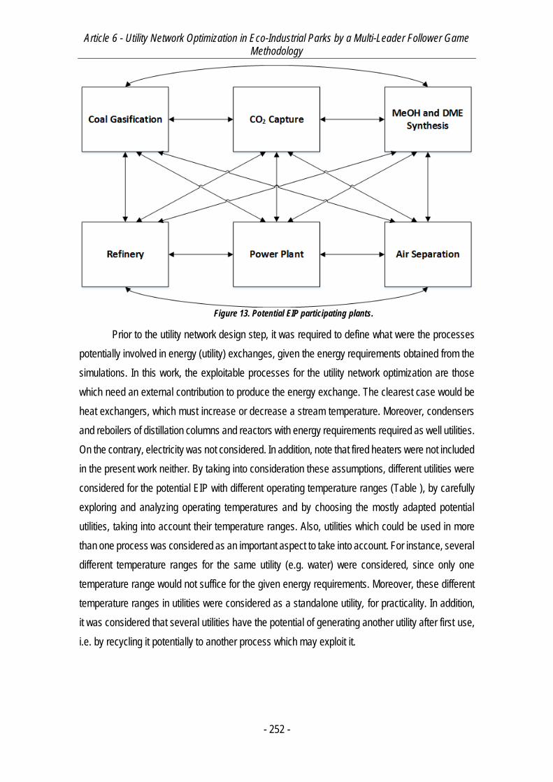
Article 6 - Utility Network Optimization in Eco-Industrial Parks by a Multi-Leader Follower Game Methodology
- 252 -
Figure 13. Potential EIP participating plants.
Prior to the utility network design step, it was required to define what were the processes
potentially involved in energy (utility) exchanges, given the energy requirements obtained from the
simulations. In this work, the exploitable processes for the utility network optimization are those
which need an external contribution to produce the energy exchange. The clearest case would be
heat exchangers, which must increase or decrease a stream temperature. Moreover, condensers
and reboilers of distillation columns and reactors with energy requirements required as well utilities.
On the contrary, electricity was not considered. In addition, note that fired heaters were not included
in the present work neither. By taking into consideration these assumptions, different utilities were
considered for the potential EIP with different operating temperature ranges (Table ), by carefully
exploring and analyzing operating temperatures and by choosing the mostly adapted potential
utilities, taking into account their temperature ranges. Also, utilities which could be used in more
than one process was considered as an important aspect to take into account. For instance, several
different temperature ranges for the same utility (e.g. water) were considered, since only one
temperature range would not suffice for the given energy requirements. Moreover, these different
temperature ranges in utilities were considered as a standalone utility, for practicality. In addition,
it was considered that several utilities have the potential of generating another utility after first use,
i.e. by recycling it potentially to another process which may exploit it.
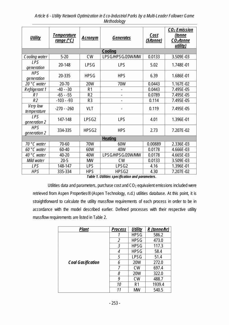
Article 6 - Utility Network Optimization in Eco-Industrial Parks by a Multi-Leader Follower Game Methodology
- 253 -
Utility Temperature
range (°C) Acronym Generates
Cost ($/tonne)
CO2 Emission (tonne
CO2/tonne utility)
Cooling
Cooling water 5-20 CW LPSG/HPSG/20W/MW 0.0133 3.509E-03
LPS generation
20-148 LPSG LPS 5.02 1.748E-01
HPS generation
20-335 HPSG HPS 6.39 1.686E-01
20 °C water 20-70 20W 70W 0.0443 1.167E-02
Refrigerant 1 -40 - -30 R1 - 0.0443 7.495E-05
R1 -65 - -55 R2 - 0.0789 7.495E-05
R2 -103 - -93 R3 - 0.114 7.495E-05
Very low temperature
-270 - -260 VLT - 0.119 7.495E-05
LPS generation 2
147-148 LPSG2 LPS 4.01 1.396E-01
HPS generation 2
334-335 HPSG2 HPS 2.73 7.207E-02
Heating
70 °C water 70-60 70W 60W 0.00889 2.336E-03
60 °C water 60-40 60W 40W 0.0178 4.666E-03
40 °C water 40-20 40W LPSG/HPSG/20W/MW 0.0178 4.665E-03
Mild water 20-5 MW CW 0.0133 3.509E-03
LPS 148-147 LPS LPSG2 4.16 1.396E-01
HPS 335-334 HPS HPSG2 4.30 7.207E-02 Table 1. Utilities specification and parameters.
Utilities data and parameters, purchase cost and CO2 equivalent emissions included were
retrieved from Aspen Properties® (Aspen Technology, n.d.) utilities database. At this point, it is
straightforward to calculate the utility massflow requirements of each process in order to be in
accordance with the model described earlier. Defined processes with their respective utility
massflow requirements are listed in Table 2.
Plant Process Utility R (tonne/hr)
Coal Gasification
1 HPSG 586.2
2 HPSG 473.0
3 HPSG 117.3
4 HPSG 58.4
5 LPSG 51.4
6 20W 272.0
7 CW 697.4
8 20W 322.0
9 CW 488.7
10 R1 1939.4
11 MW 540.5
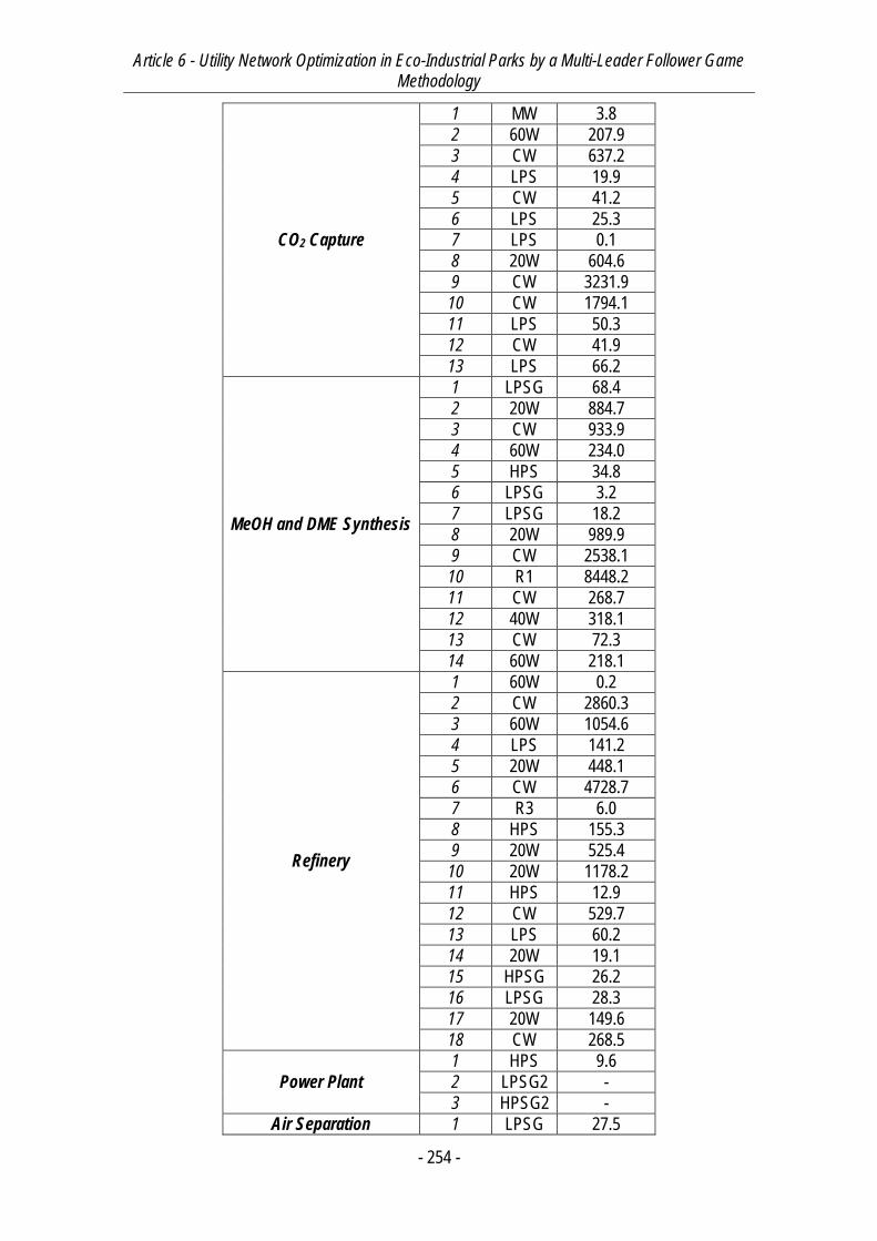
Article 6 - Utility Network Optimization in Eco-Industrial Parks by a Multi-Leader Follower Game Methodology
- 254 -
CO2 Capture
1 MW 3.8
2 60W 207.9
3 CW 637.2
4 LPS 19.9
5 CW 41.2
6 LPS 25.3
7 LPS 0.1
8 20W 604.6
9 CW 3231.9
10 CW 1794.1
11 LPS 50.3
12 CW 41.9
13 LPS 66.2
MeOH and DME Synthesis
1 LPSG 68.4
2 20W 884.7
3 CW 933.9
4 60W 234.0
5 HPS 34.8
6 LPSG 3.2
7 LPSG 18.2
8 20W 989.9
9 CW 2538.1
10 R1 8448.2
11 CW 268.7
12 40W 318.1
13 CW 72.3
14 60W 218.1
Refinery
1 60W 0.2
2 CW 2860.3
3 60W 1054.6
4 LPS 141.2
5 20W 448.1
6 CW 4728.7
7 R3 6.0
8 HPS 155.3
9 20W 525.4
10 20W 1178.2
11 HPS 12.9
12 CW 529.7
13 LPS 60.2
14 20W 19.1
15 HPSG 26.2
16 LPSG 28.3
17 20W 149.6
18 CW 268.5
Power Plant
1 HPS 9.6
2 LPSG2 -
3 HPSG2 -
Air Separation 1 LPSG 27.5

Article 6 - Utility Network Optimization in Eco-Industrial Parks by a Multi-Leader Follower Game Methodology
- 255 -
2 20W 188.2
3 CW 482.5
4 R1 377.2
5 R1 2863.3
6 R2 1835.5
7 R3 2789.9
8 VLT 6049.3
9 VLT 8412.3
10 VLT 9194.9
11 VLT 2436.7
12 VLT 6545.0
13 VLT 8123.5
14 MW 623.5
15 40W 78.9
Total 89531.7 Table 2. Processes utilities requirements.
Note that the power plant has 2 processes which generate exclusively LPS and HPS for
use within the EIP (processes 2 and 3), i.e. they correspond to boilers.
4. Results and discussion
Results are presented for both the SLMFG and MLSFG problems introduced in the
methodology above. On the other hand, in order to fulfill a significant analysis, annualized utility
costs assuming 8200 h/yr as well as fresh utility consumption when plants do not participate in the
utility network are beforehand calculated by optimizing each single-objective plant problem by itself
(described by the model above), in other words, by optimizing the internal utility network.
Nevertheless, a comparison between the results obtained in this work and those obtained by Zhang
et al. (Zhang, Strømman, Solli, et al., 2008) is in fact not possible, since the final objective in both
works is not the same. As a matter of fact, in the work of Zhang et al. (Zhang, Strømman, Solli, et
al., 2008) utility networks are not taken into account at the same level as in the present work,
whereas in the present work no raw matter exchanges are contemplated.
For instance, annualized utility costs and fresh utility consumption are reported in Table 3.
As can be seen, the air separation process is the plant which consumes the great bulk of fresh
utility and on consequence the most elevated utility cost, given that it mainly needs cooling utilities
which cannot be shared with other processes once used without regenerating them.
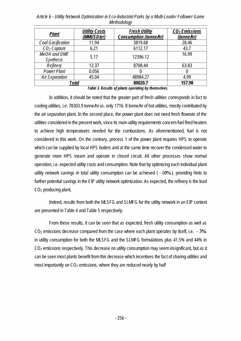
Article 6 - Utility Network Optimization in Eco-Industrial Parks by a Multi-Leader Follower Game Methodology
- 256 -
Plant Utility Costs (MMUSD/yr)
Fresh Utility Consumption (tonne/hr)
CO2 Emissions (tonne/hr)
Coal Gasification 11.94 3819.68 28.46
CO2 Capture 6.21 6112.17 43.7
MeOH and DME Synthesis
5.17 12396.12 16.99
Refinery 12.37 8708.44 63.83
Power Plant 0.056 0 0
Air Separation 45.04 48984.27 4.99
Total 80020.7 157.98 Table 3. Results of plants operating by themselves.
In addition, it should be noted that the greater part of fresh utilities corresponds in fact to
cooling utilities, i.e. 78303.9 tonne/hr vs. only 1716. 8 tonne/hr of hot utilities, mostly contributed by
the air separation plant. In the second place, the power plant does not need fresh flowrate of the
utilities considered in the present work, since its main utility requirements concern fuel fired heaters
to achieve high temperatures needed for the combustions. As aforementioned, fuel is not
considered in this work. On the contrary, process 1 of the power plant requires HPS to operate
which can be supplied by local HPS boilers and at the same time recover the condensed water to
generate more HPS steam and operate in closed circuit. All other processes show normal
operation, i.e. expected utility costs and consumption. Note that by optimizing each individual plant
utility network savings in total utility consumption can be achieved ( 10%10% ), providing hints to
further potential savings in the EIP utility network optimization. As expected, the refinery is the lead
CO2 producing plant.
Indeed, results from both the MLSFG and SLMFG for the utility network in an EIP context
are presented in Table 4 and Table 5 respectively.
From these results, it can be seen that as expected, fresh utility consumption as well as
CO2 emissions decrease compared from the case where each plant operates by itself, i.e. 3%3%
in utility consumption for both the MLSFG and the SLMFG formulations plus 41.5% and 44% in
CO2 emissions respectively. This decrease on utility consumption may seem insignificant, but as it
can be seen most plants benefit from this decrease which incentives the fact of sharing utilities and
most importantly on CO2 emissions, where they are reduced nearly by half
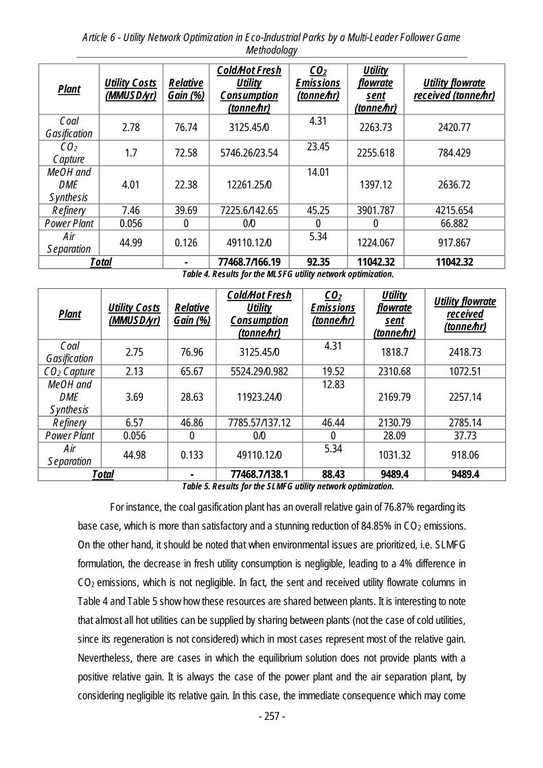
Article 6 - Utility Network Optimization in Eco-Industrial Parks by a Multi-Leader Follower Game Methodology
- 257 -
Plant Utility Costs (MMUSD/yr)
Relative Gain (%)
Cold/Hot Fresh Utility
Consumption (tonne/hr)
CO2 Emissions (tonne/hr)
Utility flowrate
sent (tonne/hr)
Utility flowrate received (tonne/hr)
Coal Gasification
2.78 76.74 3125.45/0 4.31
2263.73 2420.77
CO2 Capture
1.7 72.58 5746.26/23.54 23.45
2255.618 784.429
MeOH and DME
Synthesis 4.01 22.38 12261.25/0
14.01 1397.12 2636.72
Refinery 7.46 39.69 7225.6/142.65 45.25 3901.787 4215.654
Power Plant 0.056 0 0/0 0 0 66.882
Air Separation
44.99 0.126 49110.12/0 5.34
1224.067 917.867
Total - 77468.7/166.19 92.35 11042.32 11042.32 Table 4. Results for the MLSFG utility network optimization.
Plant Utility Costs (MMUSD/yr)
Relative Gain (%)
Cold/Hot Fresh Utility
Consumption (tonne/hr)
CO2 Emissions (tonne/hr)
Utility flowrate
sent (tonne/hr)
Utility flowrate received
(tonne/hr)
Coal Gasification
2.75 76.96 3125.45/0 4.31
1818.7 2418.73
CO2 Capture 2.13 65.67 5524.29/0.982 19.52 2310.68 1072.51
MeOH and DME
Synthesis 3.69 28.63 11923.24/0
12.83 2169.79 2257.14
Refinery 6.57 46.86 7785.57/137.12 46.44 2130.79 2785.14
Power Plant 0.056 0 0/0 0 28.09 37.73
Air Separation
44.98 0.133 49110.12/0 5.34
1031.32 918.06
Total - 77468.7/138.1 88.43 9489.4 9489.4 Table 5. Results for the SLMFG utility network optimization.
For instance, the coal gasification plant has an overall relative gain of 76.87% regarding its
base case, which is more than satisfactory and a stunning reduction of 84.85% in CO2 emissions.
On the other hand, it should be noted that when environmental issues are prioritized, i.e. SLMFG
formulation, the decrease in fresh utility consumption is negligible, leading to a 4% difference in
CO2 emissions, which is not negligible. In fact, the sent and received utility flowrate columns in
Table 4 and Table 5 show how these resources are shared between plants. It is interesting to note
that almost all hot utilities can be supplied by sharing between plants (not the case of cold utilities,
since its regeneration is not considered) which in most cases represent most of the relative gain.
Nevertheless, there are cases in which the equilibrium solution does not provide plants with a
positive relative gain. It is always the case of the power plant and the air separation plant, by
considering negligible its relative gain. In this case, the immediate consequence which may come
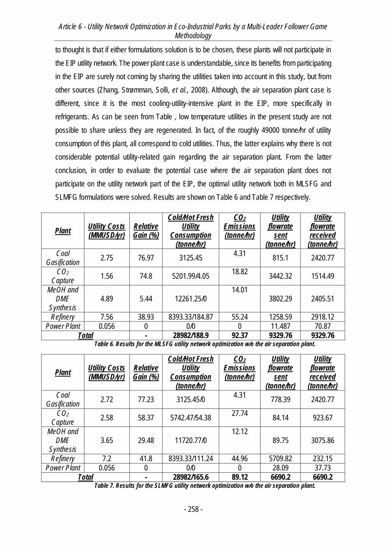
Article 6 - Utility Network Optimization in Eco-Industrial Parks by a Multi-Leader Follower Game Methodology
- 258 -
to thought is that if either formulations solution is to be chosen, these plants will not participate in
the EIP utility network. The power plant case is understandable, since its benefits from participating
in the EIP are surely not coming by sharing the utilities taken into account in this study, but from
other sources (Zhang, Strømman, Solli, et al., 2008). Although, the air separation plant case is
different, since it is the most cooling-utility-intensive plant in the EIP, more specifically in
refrigerants. As can be seen from Table , low temperature utilities in the present study are not
possible to share unless they are regenerated. In fact, of the roughly 49000 tonne/hr of utility
consumption of this plant, all correspond to cold utilities. Thus, the latter explains why there is not
considerable potential utility-related gain regarding the air separation plant. From the latter
conclusion, in order to evaluate the potential case where the air separation plant does not
participate on the utility network part of the EIP, the optimal utility network both in MLSFG and
SLMFG formulations were solved. Results are shown on Table 6 and Table 7 respectively.
Plant Utility Costs (MMUSD/yr)
Relative Gain (%)
Cold/Hot Fresh Utility
Consumption (tonne/hr)
CO2 Emissions (tonne/hr)
Utility flowrate
sent (tonne/hr)
Utility flowrate received
(tonne/hr)
Coal Gasification
2.75 76.97 3125.45 4.31
815.1 2420.77
CO2 Capture
1.56 74.8 5201.99/4.05 18.82
3442.32 1514.49
MeOH and DME
Synthesis 4.89 5.44 12261.25/0
14.01 3802.29 2405.51
Refinery 7.56 38.93 8393.33/184.87 55.24 1258.59 2918.12
Power Plant 0.056 0 0/0 0 11.487 70.87
Total - 28982/188.9 92.37 9329.76 9329.76 Table 6. Results for the MLSFG utility network optimization w/o the air separation plant.
Plant Utility Costs (MMUSD/yr)
Relative Gain (%)
Cold/Hot Fresh Utility
Consumption (tonne/hr)
CO2 Emissions (tonne/hr)
Utility flowrate
sent (tonne/hr)
Utility flowrate received
(tonne/hr)
Coal Gasification
2.72 77.23 3125.45/0 4.31
778.39 2420.77
CO2 Capture
2.58 58.37 5742.47/54.38 27.74
84.14 923.67
MeOH and DME
Synthesis 3.65 29.48 11720.77/0
12.12 89.75 3075.86
Refinery 7.2 41.8 8393.33/111.24 44.96 5709.82 232.15
Power Plant 0.056 0 0/0 0 28.09 37.73
Total - 28982/165.6 89.12 6690.2 6690.2 Table 7. Results for the SLMFG utility network optimization w/o the air separation plant.

Article 6 - Utility Network Optimization in Eco-Industrial Parks by a Multi-Leader Follower Game Methodology
- 259 -
The main difference between the two cases is evidently the fresh cold utility consumption,
since most of the contribution came from the air separation plant. On the other hand, as can be
seen, the air separation plant contribution to hot utility fresh consumption is negligible compared to
cold utility consumption. Relative gains among plants are somewhat similar when compared to the
6-plant potential EIP, specially the SLMFG formulation. Nevertheless, it should be noted that both
MLSFG and SLMFG formulations for the 5-plant potential EIP share the same overall fresh utility
consumption, but it does not correspond to the same solution regarding the equilibrium of the
plants. This phenomenon is completely understandable, since the nature and formulation of the
problem is not the same. In fact, it is expectable to obtain different equilibrium solutions from either
problems. Moreover, it can be seen that CO2 consumption between the two cases is maintained,
due to the small contribution of the air separation plant. Given the relative gains obtained, the most
interesting design of the utility network within the 5 plant EIP will be that corresponding to the
SLMFG formulation.
5. Conclusions and perspectives
In this study, the importance of process engineering in EIP design is successfully
addressed by creating utility sharing networks through process simulation and subsequently by
modeling the problem as a MLFG optimization problem. Process engineering and modeling
provides the necessary unit operation information in order to obtain successful results. These
results obtained highlight the pertinence of Stackelberg/Nash equilibrium models in order to
achieve environmental and economic benefits. In addition, utilities networks are designed with the
proposed methodology generating savings in consumption, by reusing and exploiting them before
discharging. On the other hand, the Stackelberg game structure is demonstrated to influence the
results of the optimal design, which is completely coherent and expected.
As perspectives, we have contemplated on one hand the multi-leader-multi-follower game
modeling of utility networks by defining different environmental authorities according to different
utility consumptions. Indeed, it is evident that environmental impacts measured through life-cycle
analysis rather than CO2 equivalents could bring important improvements to designs obtained. On
the other hand, it is also interesting to propose a model with power suppliers in the upper level e.g.
local energy companies with the consideration of renewable energies which define process of
utilities.

Article 6 - Utility Network Optimization in Eco-Industrial Parks by a Multi-Leader Follower Game Methodology
- 260 -
6. Nomenclature
Latin symbols np = Number of processes per plant
P = Index set of processes nep = Number of plants
EP = Index set of plants nu = Number of plants
U = Index set of plants
Rut Required utility
Gut Generated utility
Ud Utility requirement
Up Utility flow between processes
Uf Fresh utility flow
Udis Utility flow to the discharge
utotf Total CO2 equivalent mass flow totC = Annualized operating cost of plants
x = Decision variables of the authority y = Decision variables of the plants
g = Inequality constraints of the authority
m = Equality constraints of plants
l Inequality constraints of plants
AWH = Annual EIP operating hours Greek symbols
Fresh utility cost
CO2 equivalent emission rate
Recycled utility pumping cost
Article 6 - Utility Network Optimization in Eco-Industrial Parks by a Multi-Leader Follower Game Methodology
- 261 -
References
Alexander, B., Barton, G., Petrie, J. & Romagnoli, J. (2000) Process Synthesis and
Optimisation Tools for Environmental Design: Methodology and Structure. Computers & Chemical
Engineering. 24 (2), 1195–1200.
Aspen Technology (n.d.) Aspen ONE. Cambridge, MA, USA, Aspen Technology.
Aviso, K.B., Tan, R.R., Culaba, A.B. & Cruz Jr., J.B. (2010) Bi-Level Fuzzy Optimization
Approach for Water Exchange in Eco-Industrial Parks. Process Safety and Environmental
Protection. [Online] 88 (1), 31–40. Available from: doi:10.1016/j.psep.2009.11.003.
Boix, M. & Montastruc, L. (2011) Eco Industrial Parks for Water and Heat Management.
Computer Aided Chemical Engineering. [Online] 291175–1179. Available from: doi:10.1016/B978-
0-444-54298-4.50014-3.
Boix, M., Montastruc, L., Azzaro-Pantel, C. & Domenech, S. (2015) Optimization Methods
Applied to the Design of Eco-Industrial Parks: A Literature Review. Journal of Cleaner Production.
87303–317.
Boix, M., Montastruc, L., Pibouleau, L., Azzaro-Pantel, C., et al. (2011) A Multiobjective
Optimization Framework for Multicontaminant Industrial Water Network Design. Journal of
environmental management. [Online] 92 (7), 1802–1808. Available from:
doi:10.1016/j.jenvman.2011.02.016.
Boix, M., Montastruc, L., Pibouleau, L., Azzaro-Pantel, C., et al. (2012) Industrial Water
Management by Multiobjective Optimization: From Individual to Collective Solution Through Eco-
Industrial Parks. Journal of Cleaner Production. [Online] 22 (1), 85–97. Available from:
doi:10.1016/j.jclepro.2011.09.011.
Boix, M., Montastruc, L., Pibouleau, L., Azzaro-Pantel, C., et al. (2010) Multiobjective
Optimization of Industrial Water Networks with Contaminants S. Pierucci and G. Buzzi Ferraris
(ed.). Computer Aided Chemical Engineering. 28859–864.
Brooke, A., Kendrick, D., Meeraus, A. & Raman, R. (1998) GAMS User’s Guide.
Chae, S.H., Kim, S.H., Yoon, S.-G. & Park, S. (2010) Optimization of a Waste Heat
Utilization Network in an Eco-Industrial Park. Applied Energy. [Online] 87 (6), 1978–1988. Available
from: doi:10.1016/j.apenergy.2009.12.003.
Chang, T., Rousseau, R.W. & Kilpatrick, P.K. (1986) Methanol Synthesis Reactions:
Calculations of Equilibrium Conversions Using Equations of State. Industrial & Engineering
Chemistry Process Design and Development. [Online] 25 (2), 477–481. Available from:
doi:10.1021/i200033a021.
Article 6 - Utility Network Optimization in Eco-Industrial Parks by a Multi-Leader Follower Game Methodology
- 262 -
Chertow, M.R. (2000) Industrial Symbiosis: Literature and Taxonomy. Annual Review of
Energy and the Environment. [Online] 25 (1), 313–337. Available from:
doi:10.1146/annurev.energy.25.1.313.
Chew, I.M.L., Tan, R.R., Foo, D.C.Y. & Chiu, A.S.F. (2009) Game Theory Approach to the
Analysis of Inter-Plant Water Integration in an Eco-Industrial Park. Journal of Cleaner Production.
[Online] 17 (18), 1611–1619. Available from: doi:10.1016/j.jclepro.2009.08.005.
Chew, I.M.L., Thillaivarrna, S.L., Tan, R.R. & Foo, D.C.Y. (2011) Analysis of Inter-Plant
Water Integration with Indirect Integration Schemes Through Game Theory Approach: Pareto
Optimal Solution with Interventions. Clean Technologies and Environmental Policy. [Online] 13 (1),
49–62. Available from: doi:10.1007/s10098-010-0280-x.
Cornelissen, R.L. & Hirs, G.G. (1998) Exergy Analysis of Cryogenic Air Separation. Energy
Conversion and Management. [Online] 39 (16–18), 1821–1826. Available from:
doi:10.1016/S0196-8904 (98)00062-4.
El-Halwagi, M.M. (1997) Pollution Prevention Through Process Integration: Systematic
Design Tools. [Online]. Academic press. Available from:
http://books.google.fr/books?hl=en&lr=&id=-
8pE0bS130UC&oi=fnd&pg=PP2&dq=pollution+preve,ntion+through+process&ots=TvUSiLpmnY&
sig=APwzQec0TBKFFY6_oycwVMQ0s0s [Accessed: 12 May 2014].
Ertesvag, I.S., Kvamsdal, H.M. & Bolland, O. (2005) Exergy Analysis of a Gas-Turbine
Combined-Cycle Power Plant with Precombustion CO2 Capture. Energy. 30 (1), 5–39.
Fichtner, W., Frank, M. & Rentz, O. (2004) Inter-Firm Energy Supply Concepts: An Option
for Cleaner Energy Production. Journal of Cleaner Production. [Online] 12 (8–10), 891–899.
Available from: doi:10.1016/j.jclepro.2004.02.036.
Kantor, I., Betancourt, A., Elkamel, A., Fowler, M., et al. (2015) Generalized Mixed-Integer
Nonlinear Programming Modeling of Eco-Industrial Networks to Reduce Cost and Emissions.
Journal of Cleaner Production. [Online] 99160–176. Available from:
doi:10.1016/j.jclepro.2015.03.017.
Lou, H.H., Kulkarni, M.A., Singh, A. & Huang, Y.L. (2004) A Game Theory Based Approach
for Emergy Analysis of Industrial Ecosystem Under Uncertainty. Clean Technologies and
Environmental Policy. 6 (3), 156–161.
Lovelady, E.M. & El-Halwagi, M.M. (2009) Design and Integration of Eco-Industrial Parks
for Managing Water Resources. Environmental Progress & Sustainable Energy. [Online] 28 (2),
265–272. Available from: doi:10.1002/ep.10326.
Montastruc, L., Boix, M., Pibouleau, L., Azzaro-Pantel, C., et al. (2013) On the Flexibility
of an Eco-Industrial Park (EIP) for Managing Industrial Water. Journal of Cleaner Production.
[Online] 431–11. Available from: doi:10.1016/j.jclepro.2012.12.039.
Article 6 - Utility Network Optimization in Eco-Industrial Parks by a Multi-Leader Follower Game Methodology
- 263 -
Preciado, J.E., Ortiz-Martinez, J.J., Gonzalez-Rivera, J.C., Sierra-Ramirez, R., et al. (2012)
Simulation of Synthesis Gas Production from Steam Oxygen Gasification of Colombian Coal Using
Aspen Plus®. Energies. [Online] 5 (12), 4924–4940. Available from: doi:10.3390/en5124924.
ProSim (n.d.) ProSim Plus. ProSim.
Ramos, M.A., Boix, M., Aussel, D., Montastruc, L., et al. (2016a) Simultaneous Water and
Energy Network Optimization in Eco-industrial Parks through a Hybrid Single-Leader-Multi-
Follower Game/Goal Programming Approach.
Ramos, M.A., Boix, M., Aussel, D., Montastruc, L., et al. (2015) Water Exchanges in Eco-
industrial Parks through Multiobjective Optimization and Game Theory. Computer Aided Chemical
Engineering. 371997–2002.
Ramos, M.A., Boix, M., Aussel, D., Montastruc, L., et al. (2016b) Water integration in Eco-
Industrial Parks Using a Multi-Leader-Follower Approach. Computers & Chemical Engineering.
87190–207.
Ramos, M.A., Boix, M., Montastruc, L. & Domenech, S. (2014) Multiobjective Optimization
Using Goal Programming for Industrial Water Network Design. Industrial & Engineering Chemistry
Research. 53 (45), 17722–17735.
Rubio-Castro, E., Ponce-Ortega, J.M., Serna-González, M. & El-Halwagi, M.M. (2012)
Optimal Reconfiguration of Multi-Plant Water Networks into an Eco-Industrial Park. Computers &
Chemical Engineering. [Online] 4458–83. Available from:
doi:10.1016/j.compchemeng.2012.05.004.
Tan, R.R. & Aviso, K.B. (2012) An Inverse Optimization Approach to Inducing Resource
Conservation in Eco-Industrial Parks. In: [Online]. 2012 pp. 775–779. Available from:
http://www.lw20.com/120120812736855.html [Accessed: 12 November 2013].
Tawarmalani, M. & Sahinidis, N.V. (2005) A Polyhedral Branch-and-Cut Approach to
Global Optimization. Mathematical Programming. 103 (2), 225–249.
Turaga, U.T., Ramanathan, R., Rajesh, K.S., Khanrah, A., et al. (2003) Catalytic Naphtha
Reforming: Revisiting Its Importance in the Modern Refinery. Journal of scientific & industrial
research. 62 (10), 963–978.
Xu, M., Lunsford, J.H., Goodman, D.W. & Bhattacharyya, A. (1997) Synthesis of Dimethyl
Ether (DME) from Methanol Over Solid-Acid Catalysts. Applied Catalysis A: General. [Online] 149
(2), 289–301. Available from: doi:10.1016/S0926-860X (96)00275-X.
Yeomans, H. & Grossmann, I.E. (1999) A Systematic Modeling Framework of
Superstructure Optimization in Process Synthesis. Computers & Chemical Engineering. [Online]
23 (6), 709–731. Available from: doi:10.1016/S0098-1354 (99)00003-4.

Article 6 - Utility Network Optimization in Eco-Industrial Parks by a Multi-Leader Follower Game Methodology
- 264 -
Zhang, X., Strømman, A.H., Solli, C. & Hertwich, E.G. (2008) Model-Centered Approach
to Early Planning and Design of an Eco-Industrial Park Around an Oil Refinery. Environmental
science & technology. 42 (13), 4958–4963.


- 267 -
Chapitre 8 - Simultaneous Water and Energy Network Optimization in Eco-
Industrial Parks through a Hybrid Single-Leader-Follower Game/Goal
Programming Approach

Article 7 - Simultaneous Water and Energy Network Optimization in Eco-Industrial Parks through a Hybrid Single-Leader-Follower Game/Goal Programming Approach
- 268 -

Article 7 - Simultaneous Water and Energy Network Optimization in Eco-Industrial Parks through a Hybrid Single-Leader-Follower Game/Goal Programming Approach
- 269 -
Résumé
Cet article s’inscrit dans la continuité de l’article 3 et consiste à regrouper les méthodologies
utilisées dans l’article 1 avec celles de l’article 3. Le point-clé de ce travail est de concevoir
simultanément les réseaux d’eau et d’énergie au sein d’un EIP. La méthode pour la conception du
réseau d’eau est identique à celle de l’article 3 tandis que la partie énergie est récupérée de l’article
1 de même que la méthodologie de GP afin de développer un modèle hybride SLMFG/GP dans
lequel deux autorités environnementales sont introduites, i.e. de gestion de l’eau et de gestion de
l’énergie. De cette façon, les échanges inter-usines d’eau et d’énergie sont favorisés de façon à
maintenir la consommation des ressources naturelles au minimum. D’un point de vue
mathématique, l’approche hybride consiste à transformer le problème du leader en un problème
d’optimisation multiobjectif de façon à intégrer les deux autorités environnementales en laissant les
usines comme followers. Le scénario inverse est également étudié. En conséquence, l’approche
peut être considérée comme une méthodologie d’optimisation multiobjectif a posteriori où un front
de Pareto est obtenu par la résolution d’un modèle SLMFG. Après l’obtention des fronts de Pareto
correspondants aux deux scénarios, des outils d’aide à la décision sont mis en place pour choisir
la solution de compromis, à savoir TOPSIS et AHP (Analytic Hierarchy Process). Ce dernier s’avère
être le plus significatif car il permet la prise de décisions en définissant des niveaux de hiérarchie
parmi les critères. Néanmoins, cet outil d’aide à la décision, a besoin d’une matrice de préférences
des critères, qui est forcément définie par un décideur externe. En revanche, un point fort de la
méthode est sa capacité de prouver la cohérence de la matrice de préférences et informer le
décideur que celles qui ont été choisies doivent être reconsidérées. Les solutions de compromis
obtenues dans les deux scénarios sont satisfaisantes, mais de toute façon il est évident que les
préférences du décideur influencent fortement la solution retenue. En conséquence une approche
multi-leader-multi-follower (MLMFG) est proposée comme perspective et constitue les derniers
travaux rassemblés dans l’article 8 de la thèse.

Article 7 - Simultaneous Water and Energy Network Optimization in Eco-Industrial Parks through a Hybrid Single-Leader-Follower Game/Goal Programming Approach
- 270 -
Article 7 - Simultaneous Water and Energy Network Optimization in Eco-Industrial Parks through a Hybrid Single-Leader-Follower Game/Goal Programming Approach
- 271 -
Simultaneous Water and Energy Network
Optimization in Eco-Industrial Parks through
a Hybrid Single-Leader-Follower Game/Goal
Programming Approach
Manuel A. Ramosa, Marianne Boix*a, Ludovic Montastruca, Didier Aussel*b, Serge
Domenecha
aLaboratoire de Génie Chimique, U.M.R. 5503 CNRS/INP/UPS, Université de Toulouse, 4, Allée
EmileMonso, 31432 Toulouse Cedex 4, France
b Laboratoire PROMES, UPR CNRS 8521, Université de Perpignan, Via Domitia, 66100 Perpignan,
France
* Corresponding authors: [email protected]; [email protected].
Keywords: Eco-industrial parks, Multi-leader-follower Game, Nash equilibrium, Multi-objective
Optimization, MPCC, and Game Theory.
Abstract
The current environmental context makes urgent the development of robust methodologies able to
design innovative industries. Industrial ecology, and most particularly the concept of eco-industrial
parks, aims at proposing at several plants to gather in a same geographical site to share several
fluxes (water, energy, utilities…) in order to decrease environmental impacts of their industrial
activities. A recent literature analysis has shown the emergence of new works devoted to the
application of optimization methodologies to design greener and more efficient eco-industrial parks.
In this work, a hybrid single-leader-multi-follower game/goal programming approach is used to
solve the simultaneous water and energy network optimization problem in an eco-industrial park.
The approach is used in order to deal with several conflicting objectives of the different agents
involved: each plant participating in the park aims to minimize their operating cost while the park
authority aims to minimize both total freshwater and energy consumption. The upper level problem
is treated like a multiobjective optimization problem, while the lower level is a Nash equilibrium

Article 7 - Simultaneous Water and Energy Network Optimization in Eco-Industrial Parks through a Hybrid Single-Leader-Follower Game/Goal Programming Approach
- 272 -
problem. In this way, a Pareto front is obtained from the bi-level structured problem. Both
configurations, plants as leaders, authorities as followers and vice-versa are studied. Subsequently,
a hierarchical decision-making tool is used to obtain a single solution. This method is proven to be
reliable in this context because it proposes to obtain one solution instead of a set of optimal
solutions that takes directly into account the preferences of the decision maker.
1. Introduction
Nowadays, it is commonly admitted in the literature that the rapid and recent
industrialization leads to an increasing depletion of natural resources (water, energy) and has a
great role in global warming (UNESCO, 2009). As a matter of fact, the great majority of involved
processes in industries need water with a given quality at a fixed temperature. Hence, huge
amounts of energy are used in order to cool and/or heat water to reach operating temperatures by
means of cold and heat utilities. There is thus a critical need in reducing both rejects of polluted
water and consumption of primary resources such as water and energy. In this context, preserving
environment while increasing business success is the main goal of industrial ecology. This concept,
which is directly linked to sustainable development, consists in engaging separate industries
geographically linked in a collective approach to competitive advantage involving exchange of raw
matter, by-products, energy and utilities. A primordial feature of an industrial symbiosis is the
collaboration offered by the geographic proximity of the several companies and the most
widespread manifestations of industrial symbioses are Eco-Industrial Parks. A definition widely
accepted of EIP is “an industrial system of planned materials and energy exchanges that seeks to
minimize energy and raw materials use, minimize waste, and build sustainable economic,
ecological and social relationships” (Cheng, Chang & Jiang, 2014; Bagajewicz & Savelski, 2001;
Bagajewicz & Faria, 2009). As it can be highlighted, a basic condition for an EIP to be economically
viable is to demonstrate that benefits of each industry involved in it by working collectively is higher
than working as a stand-alone facility.
Recently, Boix et al. (Boix, Montastruc, Azzaro-Pantel, et al., 2015) and Ramos et al.
(Ramos, Boix, Aussel, et al., 2015) highlighted the lack of studies dealing with optimization in order
to design optimal configuration of an EIP. However, it is important to develop methodologies able
to design environmentally friendly EIP’s while each industry has a real economic gain to increase
competitiveness. Exchanges of materials, water and/or energy through a sharing network between
companies of an EIP are the main way to design an optimal EIP. Furthermore, Reniers et al.
(Reniers, Dullaert & Visser, 2010) showed that water and energy constitute precursor elements to
Article 7 - Simultaneous Water and Energy Network Optimization in Eco-Industrial Parks through a Hybrid Single-Leader-Follower Game/Goal Programming Approach
- 273 -
trigger the collaboration and begin to exchange other materials. Designing eco-industrial parks
needs a lot of rules because it is constituted of several actors (enterprises) working for their
personal objective, and all of these objectives need to be taken into account in the final design
while decreasing environmental effects of the park.
Water and energy allocation problems have been tackled by three main approaches,
including graphical (pinch) methodology (Bagajewicz & Savelski, 2001; Bagajewicz & Faria, 2009;
Ramos, Boix, Montastruc, et al., 2014; Boix & Montastruc, 2011), mathematical programming
(Yeomans & Grossmann, 1999; Biegler, Grossmann & Westerberg, 1997; Olesen & Polley, 1996;
Boix, Montastruc, Pibouleau, et al., 2012) and synthesis of mass exchange networks (Ramos, Boix,
Aussel, et al., 2016; Chew, Tan, Foo, et al., 2009). Besides the mathematical model, resources
allocation problems entail several objective functions which are often antagonist between
themselves, e.g., as discussed above, minimizing resources consumption while maximizing
productivity. In fact, very few studies take into account several objectives simultaneously. Ramos
et al. (Ramos, Boix, Montastruc, et al., 2014) developed a Goal Programming approach to tackle
this problem but they demonstrated that there is no global optimal solution in a mathematical sense,
due to the contradictory nature of the set of objectives involved, i.e. a solution which minimizes all
objectives at the same time does not exist. On the contrary, there are a virtually infinite number of
equally significant solutions (i.e. the Pareto front) which are trade-off solutions between the
objectives. In fact, the best solution (without loss of generality) among the set of solutions should
be identified by a decision maker (DM), in accordance with his own criteria (Boix, Pibouleau,
Montastruc, et al., 2012; Saaty & Peniwati, 2008). In these works (among others), the authors
developed multi-objective optimization strategies such as goal programming. However, Ramos et
al. (Ramos, Boix, Aussel, et al., 2015) demonstrated that in different scenarios and by tuning
different optimization parameters (e.g. weight factors associated with the objective functions) one
company is favored compared to the others using MOO methods. Although optimal solutions are
intermediate and satisfying in terms of individual costs, it is of great interest to obtain more balanced
solutions so that each enterprise/company is satisfied at the same time and moreover, by
minimizing freshwater consumption in order to insure the environmental performance of the EIP.
An interesting alternative particularly adapted to the optimal design of EIP is the Game
Theory approach and most particularly the concept of multi-leader single-follower game problem
(MLSFG). In fact, an EIP can be seen as the congregation of different non-cooperative agents (the
leaders) which aim at minimizing their annualized operating costs and an EIP authority (the
follower) whose aim is to minimize resources consumption. This kind of non-cooperative game is
Article 7 - Simultaneous Water and Energy Network Optimization in Eco-Industrial Parks through a Hybrid Single-Leader-Follower Game/Goal Programming Approach
- 274 -
very interesting for the concepts of EIP, since the main barrier to integrate an EIP for industry is
the issue of confidentiality between enterprises and this approach could be very promising to
overcome this problem. In fact, by introducing an impartial authority whose role is to collect all data
necessary to design the EIP, enterprises involved would be able to keep confidential data, without
the need to share them with the other companies of the park.
This kind of approaches is widely studied for modeling of deregulated electricity markets
(Aussel, Correa & Marechal, 2013). In this kind of games, leaders make simultaneous decisions
and the followers react to these decisions. In other words, the followers play a Nash game between
them so as the leaders. Recently, Ramos et al. (Ramos, Boix, Aussel, et al., 2016) developed a
MLSFG model to design optimal water networks in EIPs.
2. Literature review
In terms of literature review, there are very few works available on the subject of
simultaneous heat and water integration in EIPs. As mentioned earlier, several works exist
regarding water integration, which is not the case of heat integration in EIPs and even less in a
multicriteria environment. For instance, Chae et al. (Chae et al. 2010) developed a framework to
synthetize waste heat utilization networks in EIPs through a mathematical programming
environment. The authors proposed a MILP model for the minimization of the total energy cost
within the EIP, using a classical superstructure heat/sink model which takes also into account
distances between plants in the EIP. Later, Leong et al. (Leong, Tan, and Chew 2014) developed
a procedure for the synthesis of an integrated chilled and cooling water network of an EIP by a
centralized utility hub. Note that in the latter work mathematical modeling and optimization was not
considered. Finally, another relevant work in the subject is that of Cheng et al. (Cheng, Chang, and
Jiang 2014), where the authors developed a systematic design procedure of inter-plant heat
integration through game theory in a sequential optimization strategy, namely, in the first place a
LP model to determine the minimum acceptable total utility cost for the EIP, then a NLP to with
Nash equilibrium constraints to determine heat flows between plants and their fair trade price. In
third place, a MILP model for identifying the minimum number of matches and finally a NLP model
to synthetize a cost-optimal network. In the latter work, is it important to note that Nash equilibrium
constraints are introduced in a classical manner, and not by modeling the problem as a GNEP or
by imposing KKT or strong stationarity conditions on the players participating in the EIP.
Article 7 - Simultaneous Water and Energy Network Optimization in Eco-Industrial Parks through a Hybrid Single-Leader-Follower Game/Goal Programming Approach
- 275 -
3. Problem statement
Simultaneous water and energy integration in EIP is modeled as an industrial water
network (IWN) allocation problem, according to numerous previous works2, (Ramos et al.
2014),19,20with the addition of energy requirements for each process and/or regeneration units as
well as temperature requirements for discharged water (Ramos et al. 2014; Boix and Montastruc
2011). Indeed, the way to model an industrial water and energy network (IWEN) allocation problem
is based on the concept of superstructure (Yeomans and Grossmann 1999; Biegler, Grossmann,
and Westerberg 1997). From a given number of regeneration units and processes, all possible
connections between them may exist, except recycling to the same unit. This constraint forbids
self-recycles on process and regeneration units, although the latter is often relevant in some
chemical processes. For each water using process, input water may be freshwater, output water
from other processes and/or regenerated water in order to fulfill contaminant concentration
constraints. Indeed, output water from a process may be directly discharged, distributed to another
suitable process and/or to regeneration units. In addition, each process has a contaminant load
over the input flowrate of water, as well as water temperature constraints. In consequence, each
process has a potential heat exchanger associated in order to fulfill temperature constraints. For
instance, process operating conditions, i.e. concentration and temperature constraints must be
known a priori, which can be tackled in different ways. For example, one approach consists in
simulating rigorously all processes and interconnections, i.e. the complete process flowsheet and
then using the obtained information to confront the water and energy network, in the form of grey
boxes. In fact, this work deals only with the latter part since the data for the case study is extracted
from a wide-known case study (Olesen and Polley 1996) while a novel study from Ramos et al.
(Ramos et al.) boards the problem starting from the simulation part all the way to the grey box step.
In the grey box kind of approach, physical or chemical phenomena occurring inside each process
is not taken into account. As aforementioned, only one contaminant is considered in the presented
EIP. A general view of the superstructure is given in Figure 4.
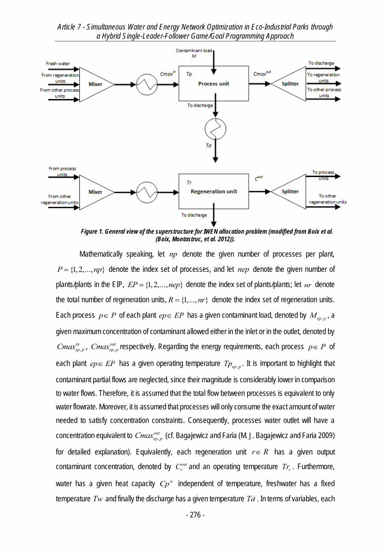
Article 7 - Simultaneous Water and Energy Network Optimization in Eco-Industrial Parks through a Hybrid Single-Leader-Follower Game/Goal Programming Approach
- 276 -
Figure 1. General view of the superstructure for IWEN allocation problem (modified from Boix et al.
(Boix, Montastruc, et al. 2012)).
Mathematically speaking, let np denote the given number of processes per plant,
{1,2,..., }P np denote the index set of processes, and let nep denote the given number of
plants/plants in the EIP, {1,2,..., }EP nep denote the index set of plants/plants; let nr denote
the total number of regeneration units, {1,..., }R nr denote the index set of regeneration units.
Each process p P of each plant ep EP has a given contaminant load, denoted by ,ep pM , a
given maximum concentration of contaminant allowed either in the inlet or in the outlet, denoted by
,inep pCmax , ,
outep pCmax respectively. Regarding the energy requirements, each process p P of
each plant ep EP has a given operating temperature ,ep pTp . It is important to highlight that
contaminant partial flows are neglected, since their magnitude is considerably lower in comparison
to water flows. Therefore, it is assumed that the total flow between processes is equivalent to only
water flowrate. Moreover, it is assumed that processes will only consume the exact amount of water
needed to satisfy concentration constraints. Consequently, processes water outlet will have a
concentration equivalent to ,outep pCmax (cf. Bagajewicz and Faria (M. J. Bagajewicz and Faria 2009)
for detailed explanation). Equivalently, each regeneration unit r R has a given output
contaminant concentration, denoted by outrC and an operating temperature rTr . Furthermore,
water has a given heat capacity wCp independent of temperature, freshwater has a fixed
temperature Tw and finally the discharge has a given temperature Td . In terms of variables, each
Article 7 - Simultaneous Water and Energy Network Optimization in Eco-Industrial Parks through a Hybrid Single-Leader-Follower Game/Goal Programming Approach
- 277 -
process of each plant ,p P ep EP sends water to process 'p P of plant
' , { ', '} { , }ep EP ep p ep p , taken into account by variable , , ', 'ep p ep pFpart , receives water,
denoted by variable ', ', ,ep p ep pFpart and has an inlet flow of freshwater, denoted by ,ep pFw . Also,
each process p P has associated heat duties , ,,ep p ep pQp Qp , for heating and for cooling,
respectively. In addition, each process may send polluted water to regeneration unit r R or
receive low contaminant concentration water by the latter, denoted by
, , , ,,ep p r r ep pFproreg Fregpro respectively, which in turn have associated heat duties ,r rQr Qr
or may send water directly to the discharge, denoted by ,ep pFdis , whose heat duty is denoted by
,ep epQd Qd .
Finally, it is to be noted that the original IWEN models (e.g. Boix et al. (Boix and Montastruc
2011) and Ramos et al. (Ramos et al. 2014)) are formulated as a mixed-integer linear program
(MILP), since it takes into account minimum allowable flowrateminf between processes and/or
regeneration units (namely, the minimum allowed water flowrate was fixed at 2 /minf tonne hr
as in Boix et al.8) and minimum heat exchangers duties. Nevertheless, in a SLMFG formulation
discrete variables are rather impossible to handle in the lower level (at least for the time being). In
consequence, in the present article minimum flowrateminf is handled by an elimination algorithm
which is explained afterwards. On the other hand, heat exchangers are not constrained to have a
minimum allowable heat duty.
3.1. Model statement
Given the aforementioned notation, the considered model is based on the reduced model
of Ramos et al. (Ramos et al. 2016):
-Water mass balance around a process unit p P of a plant ep EP :
, ', ', , ,' '
, , ' ' , , ,' '
{ , } { ', '}
ep p ep p ep,p r ep pep EP p P r R
ep p ep ,p r ep p ep pep EP p P r R
Fw Fpart Fregpro
Fpart Fregpro Fdis
ep p ep p
Eq. 1
-Contaminant mass balance around a process unit p P of a plant ep EP :
Article 7 - Simultaneous Water and Energy Network Optimization in Eco-Industrial Parks through a Hybrid Single-Leader-Follower Game/Goal Programming Approach
- 278 -
, ', ' ', ', , ,' '
, , , ' ' , , ,' '
{ , } { ', '}
out outep p ep p ep p ep,p r r ep p
ep EP p P r R
outep p ep p ep ,p r ep p ep p
ep EP p P r R
M Cmax Fpart C Fregpro
Cmax Fpart Fregpro Fdis
ep p ep p
Eq. 2
-Inlet/outlet concentration constraints for a process unit p P of a plant ep EP :
', ' ', ', , ,' '
, , ', ', , ,' '
{ , } { ', '}
out outep p ep p ep,p r r ep p
ep EP p P r R
inep p ep p ep p ep,p r ep p
ep EP p P r R
Cmax Fpart C Fregpro
Cmax Fw Fpart Fregpro
ep p ep p
Eq. 3
-Contaminant concentration constraints for regeneration unit r R :
, , , , ,out outep p ep p r r r ep p
ep EP p P ep EP p PCmax Fproreg C Fregpro
Eq. 4
-Mass balance around a regeneration unit r R (water and contaminant losses are neglected):
, , , ,ep p r r ep pep EP p P ep EP p P
Fproreg Fregpro
Eq. 5
-Flow between processes and regeneration unit positivity going from a process unit p P of a
plant ep EP to a regeneration unit r R :
, , 0ep p rFproreg Eq. 6
-Flow between regeneration unit to a process unit p P of a plant ep EP from a regeneration
unit r R :
, , 0r ep pFregpro Eq. 7
Article 7 - Simultaneous Water and Energy Network Optimization in Eco-Industrial Parks through a Hybrid Single-Leader-Follower Game/Goal Programming Approach
- 279 -
Combining Eq. 15 with Eq. 16 leads to:
, ', ' ', ', , ,' '
, , ', ', , ,' '
{ , } { ', '}
out outep p ep p ep p ep,p r r ep p
ep EP p P r R
outep p ep p ep p ep,p r ep p
ep EP p P r R
M Cmax Fpart C Fregpro
Cmax Fw Fpart Fregpro
ep p ep p
Eq. 8
- ,ep pFdis positivity for a process unit p P of a plant ep EP :
, ', ', , ,' '
, , ' ' , ,' '
{ , } { ', '}
ep p ep p ep,p r ep pep EP p P r R
ep p ep ,p ep p rep EP p P r R
Fw Fpart Fregpro
Fpart Fproreg
ep p ep p
Eq. 9
-Energy balance around a process unit p P of a plant ep EP :
, ', ', ', ' , ,' '
, , , , ', ', , ,' '
{ , } { ', '}
wep p ep p ep,p ep p r ep p r
ep EP p P r R
wep p ep p ep p ep p ep p ep,p r ep p
ep EP p P r R
Cp Fw Tw Fpart Tp Fregpro Tr
Qp Qp Cp Tp Fw Fpart Fregpro
ep p ep p
Eq. 10
-Energy balance around a regeneration unit r R (water and contaminant losses are neglected):
, , , , ,w w
ep p r ep p r r r r ep pep EP p P ep EP p P
Cp Fproreg Tp Qr Qr Cp Tr Fregpro
Eq. 11
-
Article 7 - Simultaneous Water and Energy Network Optimization in Eco-Industrial Parks through a Hybrid Single-Leader-Follower Game/Goal Programming Approach
- 280 -
Energy balance around each plant ep EP discharge:
, ', ', , ,' '
,
, , ' ' , ,' '
, ', ', , ,' '
ep p ep p ep,p r ep pep EP p P r R
wep ep ep p
p Pep p ep ,p r ep p
ep EP p P r R
ep p ep p ep,p r ep pep EP p P r R
w
Fw Fpart Fregpro
Qd Qd Cp TpFpart Fregpro
Fw Fpart Fregpro
Cp TdFpa
, , ' ' , ,' '
p Pep p ep ,p r ep p
ep EP p P r Rrt Fregpro
Eq. 12
-Heat duties positivity:
, ,0, 0, ,ep p ep pQp Qp ep EP p P Eq. 13
, 0,ep epQd Qd ep EP Eq. 14
, 0,r rQr Qr r R Eq. 15
For this kind of problem, let us define the following potential objective functions, which are
very common in previous studies (Ramos et al. 2016; Boix and Montastruc 2011; Ramos et al.
2014). Furthermore, these objective functions play a role on the regulator design of EIP. The
objective functions are divided in two, namely the two environmental objective functions (Eq. 16)
and the objective function of each one of the plants, i.e. annualized operating cost (Eq. 17).
,
, ,
( , )
( , )
Fwtot ep pep EP p P
Qtot ep p ep pep EP p P
ep ep r rep EP r R
f x y Fw
f x y Qp Qp
Qd Qd Qr Qr
Eq. 16
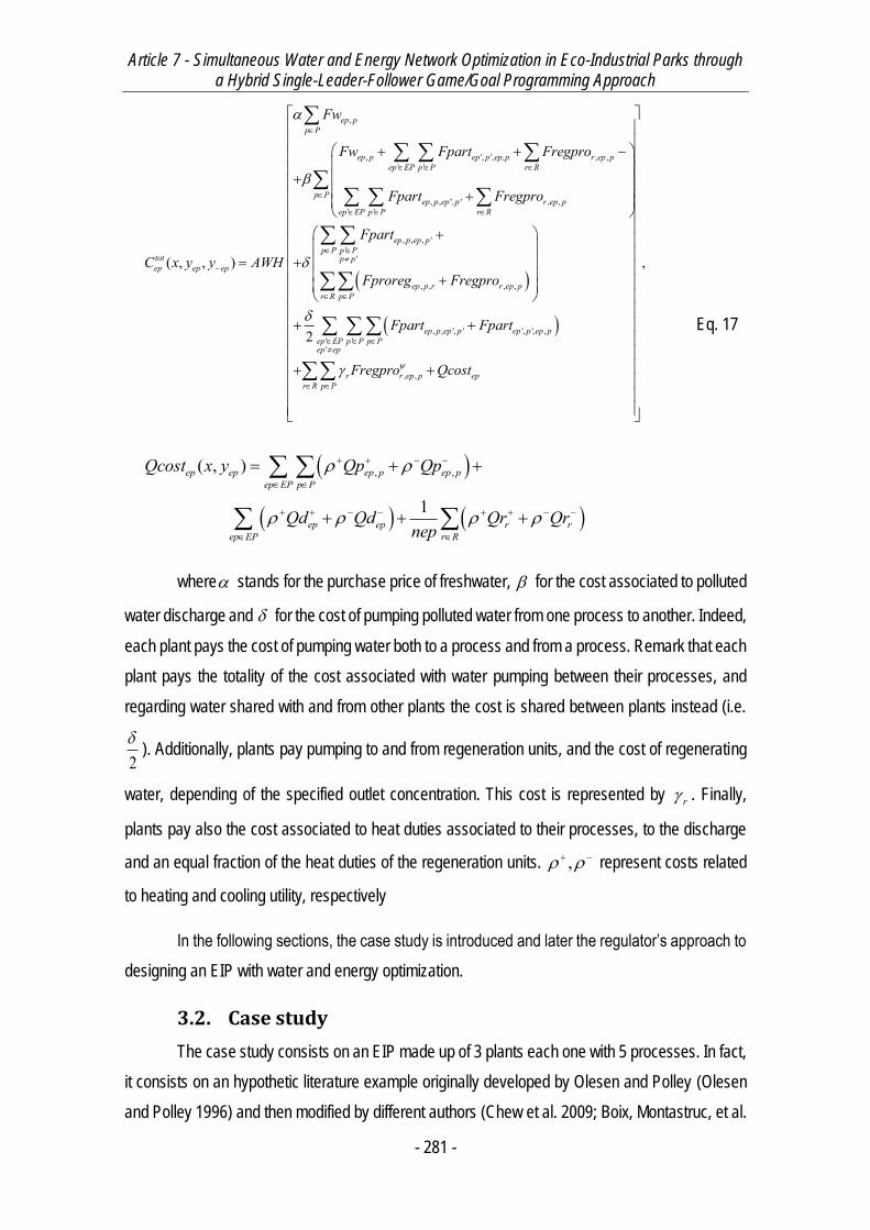
Article 7 - Simultaneous Water and Energy Network Optimization in Eco-Industrial Parks through a Hybrid Single-Leader-Follower Game/Goal Programming Approach
- 281 -
,
, ', ', , ,' '
, , ' ' , ,' '
, , , ''
'
, ,
( , , )
ep pp P
ep p ep p ep,p r ep pep EP p P r R
p Pep p ep ,p r ep p
ep EP p P r R
ep p ep pp P p P
tot p pep ep ep
ep p r
Fw
Fw Fpart Fregpro
Fpart Fregpro
Fpart
C x y y AWHFproreg Freg
, ,
, , ', ' ', ', ,' ''
, ,
,
2
r ep pr R p P
ep p ep p ep p ep pep EP p P p Pep ep
r r ep p epr R p P
pro
Fpart Fpart
Fregpro Qcost
, ,( , )
1
ep ep ep p ep pep EP p P
ep ep r rep EP r R
Qcost x y Qp Qp
Qd Qd Qr Qrnep
Eq. 17
where stands for the purchase price of freshwater, for the cost associated to polluted
water discharge and for the cost of pumping polluted water from one process to another. Indeed,
each plant pays the cost of pumping water both to a process and from a process. Remark that each
plant pays the totality of the cost associated with water pumping between their processes, and
regarding water shared with and from other plants the cost is shared between plants instead (i.e.
2
). Additionally, plants pay pumping to and from regeneration units, and the cost of regenerating
water, depending of the specified outlet concentration. This cost is represented by r . Finally,
plants pay also the cost associated to heat duties associated to their processes, to the discharge
and an equal fraction of the heat duties of the regeneration units. , represent costs related
to heating and cooling utility, respectively
In the following sections, the case study is introduced and later the regulator’s approach to
designing an EIP with water and energy optimization.
3.2. Case study
The case study consists on an EIP made up of 3 plants each one with 5 processes. In fact,
it consists on an hypothetic literature example originally developed by Olesen and Polley (Olesen
and Polley 1996) and then modified by different authors (Chew et al. 2009; Boix, Montastruc, et al.

Article 7 - Simultaneous Water and Energy Network Optimization in Eco-Industrial Parks through a Hybrid Single-Leader-Follower Game/Goal Programming Approach
- 282 -
2012), (Ramos et al. 2016) in order to use it in an EIP context. Parameters of this case study are
given in Table 2.In addition, parameters for temperature constraints are the same as those reported
by Boix et al. (Boix and Montastruc 2011).
Plant Process , ( )inep pCmax ppm , ( )out
ep pCmax ppm , ( / )ep pM g h , ( )ep pTp C
1
1 0 100 2000 40
2 50 80 2000 100
3 50 100 5000 80
4 80 800 30000 60
5 400 800 4000 50
2
1 0 100 2000 90
2 50 80 2000 70
3 80 400 5000 50
4 100 800 30000 40
5 400 1000 4000 100
3
1 0 100 2000 80
2 25 50 2000 60
3 25 125 5000 50
4 50 800 30000 90
5 100 150 15000 70 Table 1. Case study parameters (Olesen and Polley 1996).
In addition, regeneration units operating parameters are illustrated in Table 6. It is assumed
that there are 3 different regeneration units which are distinguished by their capacity to regenerate
water, i.e. their outlet concentration on contaminant.
Regeneration unit type Parameter
( )outrC ppm ( )rTr C
1 15 100
2 20 70
3 30 50 Table 2. Parameters associated with regeneration units.
Also, 15Tw C and 25Td C .
Regarding costs and prices, they were chosen as the same prices as in Ramos et al.
(Ramos et al. 2016), and in addition, heat duties prices are extracted from Aspen Plus (Aspen
Technology) utilities’ properties, namely LP steam and cooling water (Table 3):
Duty ($ / GJ)
Heating (+) 1.9
Cooling (-) 0.212 Table 3. Heat duties cost.
Article 7 - Simultaneous Water and Energy Network Optimization in Eco-Industrial Parks through a Hybrid Single-Leader-Follower Game/Goal Programming Approach
- 283 -
4. Regulator design of an EIP
The introduction of an authority/regulator to the design of viable water and energy networks
in EIP is an interesting alternative to overcome the confidentiality problem on one hand, and on the
other hand, to solve the problem of equilibrium benefits of the players/plants involved. In fact, the
latter can be modeled as a SLMFG, where the leader is the EIP authority and the followers are the
plants.
The design of EIP water and energy network by SLMFG consists in near-located plant
process plants that are subjected to regulations implemented in the park. Each plant has its own
processes, and each process requires a specific water both in quantity and quality and temperature
requirements in order to operate. Moreover, each process produces a certain amount of
wastewater, given its contaminant flowrate and an upper bound on outlet quality. In this particular
case, only one contaminant is taken into account for the sake of simplicity. Each plant has access
to water regeneration units, shared within the EIP.
At this point, it is important to note that in the SLMFG approach the choice of leaders and
followers is crucial in the problem formulation. As it was demonstrated by Ramos et al. (Ramos et
al. 2016), this choice changes completely the nature of the problem. It is assumed that in the case
of SLMFG the plants aim to minimize their total annualized cost, given the compromise of different
environmental objective functions calculated by the EIP authority.
On the other hand, as in Ramos et al. (Ramos et al. 2016) leaders could be the plants and
the follower in lower level, the environmental authority, acting as a single follower or as multiple
entities with different objectives.
4.1. Methodology
In order to deal with a bi-level formulation for the design of optimal water and energy
networks within an EIP, the first important point which emerges is the antagonist nature of the
environmental objectives, i.e. water and energy consumption. The antagonist nature of these two
environmental objectives was further studied in Boix et al. (Boix and Montastruc 2011) and Ramos
et al. (Ramos et al. 2014). In fact, it is the interest of the regulator of the EIP to achieve a
compromise solution between water and energy consumption in the EIP, and on the other side,
plants’ interest is to minimize their operating cost, which are evidently in competition for resources.
Therefore, the EIP authority is actually composed by two different entities, due to the antagonism
between the environmental objectives. Moreover, as explained before, the formulation of the bi-
Article 7 - Simultaneous Water and Energy Network Optimization in Eco-Industrial Parks through a Hybrid Single-Leader-Follower Game/Goal Programming Approach
- 284 -
level problem is very important, since the level assigned to each agent determines its equilibrium
solution.
In this work, the adopted approach is in the first place (scenario 1), to model the EIP
authorities in the upper level as a multiobjective optimization problem rather than two different
entities, where the corresponding objective functions aim to minimize water and energy
consumption in the EIP with plants being modeled separately as independent followers, each one
minimizing their corresponding total annualized operating cost. In the second place (scenario 2),
roles are inversed, treating the competing plants as a single authority in the upper level (a
multiobjective optimization problem) and as followers the environmental authorities.
Being a multiobjective optimization problem, the upper-level problem can be modeled and
solved using different strategies/methodologies (cf. Ramos et al. (Ramos et al. 2014)). For
instance, the most important distinction between these methods is whether a Pareto front or a
single solution is obtained from the optimization step. Then, decision maker’s priorities are
expressed a posteriori in the former case and a priori in the latter. By generating the Pareto front,
the decision maker has the advantage of knowing all the spectrum of non-dominated solutions in
order to make a solution, while by expressing his priorities a priori the decision maker may not base
his choices on all possible non-dominated solutions. However, to generate all the Pareto front is a
non-trivial task and for large-scale models may be even impossible, while obtaining a single solution
can be sufficient in order to make a decision.
Nevertheless, a Pareto front is obtainable in the present work, as demonstrated by earlier
works (cf. Boix et al. (Boix and Montastruc 2011 ; Boix, Pibouleau, et al. 2012) , Ramos et al.
(Ramos et al. 2014)). Then, as the Pareto front is obtained, a Pareto-compromise solution is chosen
among the obtained Pareto non-dominated solutions. One way to find this solution consists in
applying a multi-criteria decision tool, namely TOPSIS. This kind of methods allow the decision-
maker to choose a solution based on his priorities regarding the different criteria. Nevertheless,
TOPSIS only takes into account decisions on one level, i.e. a Pareto-compromise solution is
chosen taking only into account one level objectives (the leader’s). As it, lower-level objectives are
not taken into account when choosing the compromise solution. Thus, for addressing decisions on
both levels a hierarchical decision-making tool was also implanted, i.e. AHP (Analytic Hierarchy
Process) (Saaty and Peniwati 2008). Both scenarios mentioned above (plants on the upper level
and plants on the lower level) were solved with this methodology. Therefore, in the first place,
Pareto fronts are obtained for both problems; then, a compromise solution is found by using
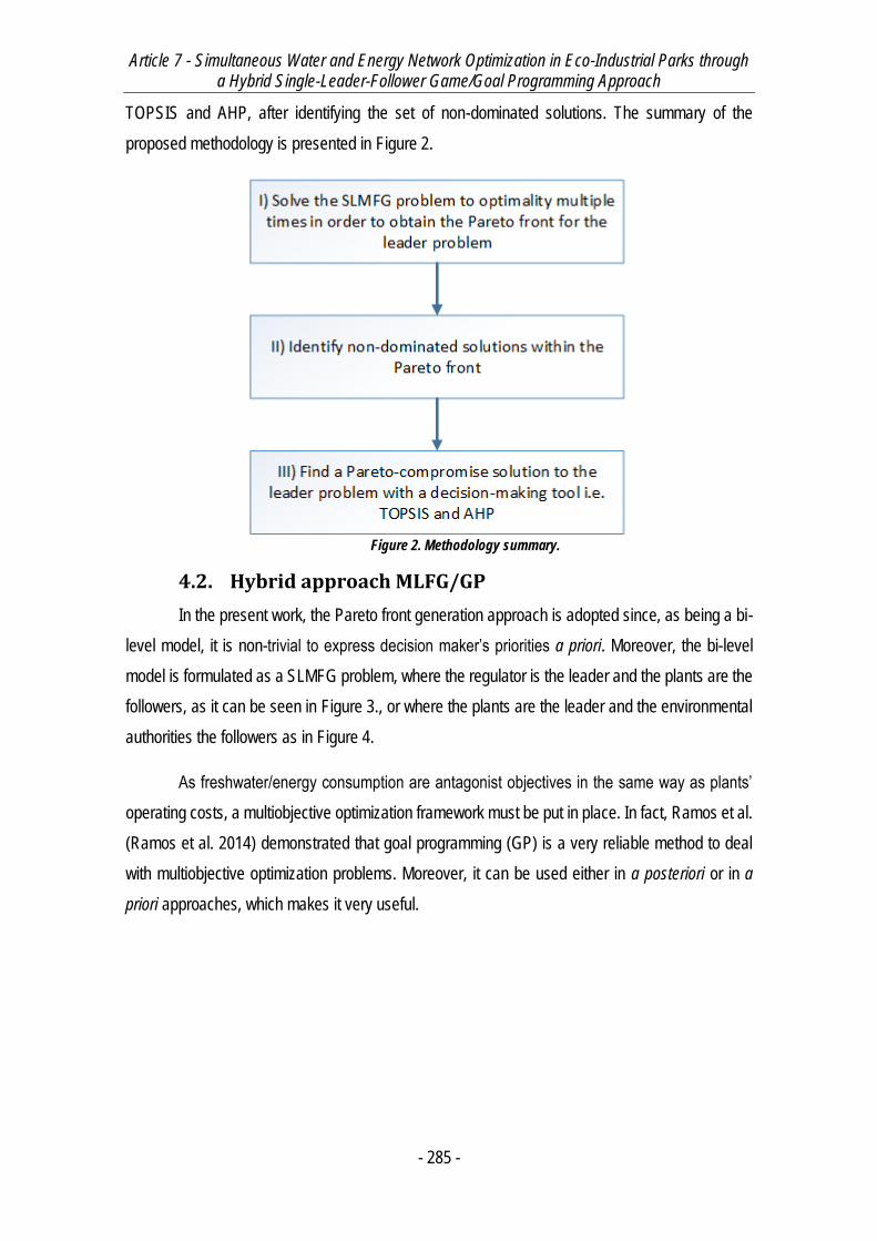
Article 7 - Simultaneous Water and Energy Network Optimization in Eco-Industrial Parks through a Hybrid Single-Leader-Follower Game/Goal Programming Approach
- 285 -
TOPSIS and AHP, after identifying the set of non-dominated solutions. The summary of the
proposed methodology is presented in Figure 2.
Figure 2. Methodology summary.
4.2. Hybrid approach MLFG/GP
In the present work, the Pareto front generation approach is adopted since, as being a bi-
level model, it is non-trivial to express decision maker’s priorities a priori. Moreover, the bi-level
model is formulated as a SLMFG problem, where the regulator is the leader and the plants are the
followers, as it can be seen in Figure 3., or where the plants are the leader and the environmental
authorities the followers as in Figure 4.
As freshwater/energy consumption are antagonist objectives in the same way as plants’
operating costs, a multiobjective optimization framework must be put in place. In fact, Ramos et al.
(Ramos et al. 2014) demonstrated that goal programming (GP) is a very reliable method to deal
with multiobjective optimization problems. Moreover, it can be used either in a posteriori or in a
priori approaches, which makes it very useful.
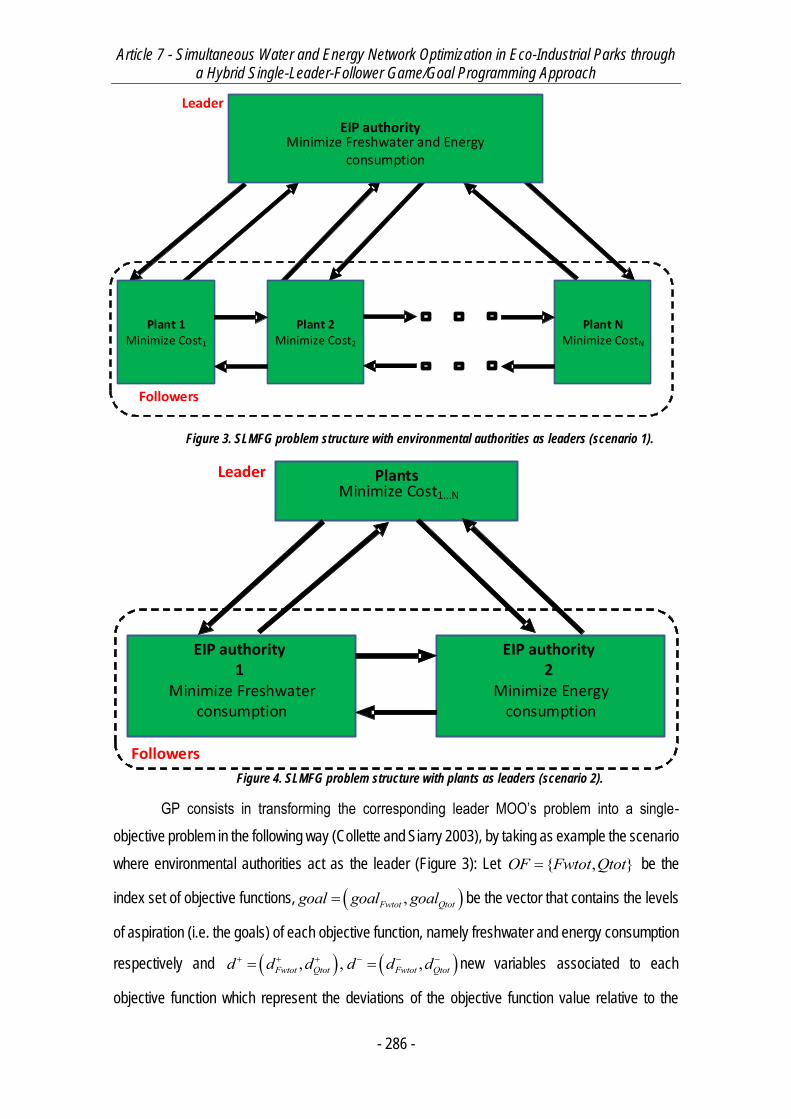
Article 7 - Simultaneous Water and Energy Network Optimization in Eco-Industrial Parks through a Hybrid Single-Leader-Follower Game/Goal Programming Approach
- 286 -
Leader
EIP authorityMinimize Freshwater and Energy
consumption
Plant 1Minimize Cost1
Plant NMinimize CostN
Plant 2Minimize Cost2
Followers
Figure 3. SLMFG problem structure with environmental authorities as leaders (scenario 1).
Leader
Followers
Plants
EIP authority 1
Minimize Freshwater consumption
EIP authority 2
Minimize Energy consumption
Minimize Cost1...N
Figure 4. SLMFG problem structure with plants as leaders (scenario 2).
GP consists in transforming the corresponding leader MOO’s problem into a single-
objective problem in the following way (Collette and Siarry 2003), by taking as example the scenario
where environmental authorities act as the leader (Figure 3): Let { , }OF Fwtot Qtot be the
index set of objective functions, ,Fwtot Qtotgoal goal goal be the vector that contains the levels
of aspiration (i.e. the goals) of each objective function, namely freshwater and energy consumption
respectively and , , ,Fwtot Qtot Fwtot Qtotd d d d d d new variables associated to each
objective function which represent the deviations of the objective function value relative to the
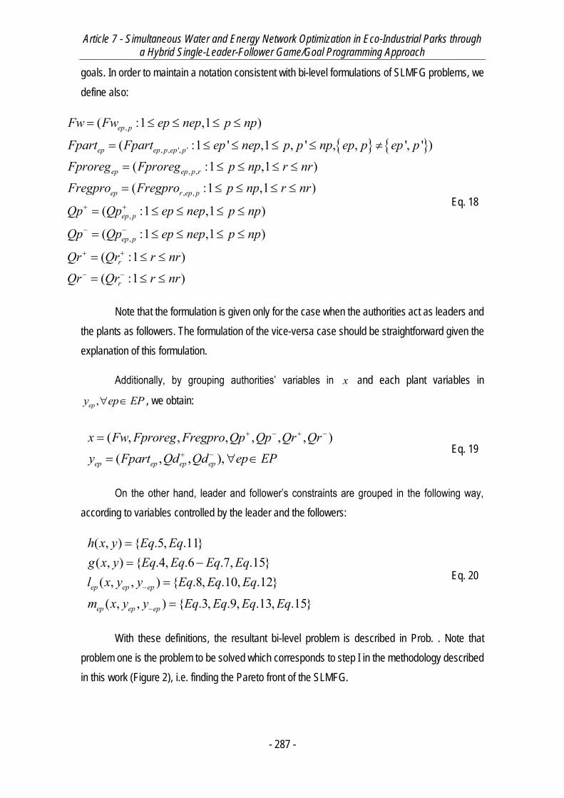
Article 7 - Simultaneous Water and Energy Network Optimization in Eco-Industrial Parks through a Hybrid Single-Leader-Follower Game/Goal Programming Approach
- 287 -
goals. In order to maintain a notation consistent with bi-level formulations of SLMFG problems, we
define also:
,
, , ', '
, ,
, ,
,
( :1 ,1 )
( :1 ' ,1 , ' , , ', ' )
( :1 ,1 )
( :1 ,1 )
( :1 ,1 )
(
ep p
ep ep p ep p
ep ep p r
ep r ep p
ep p
e
Fw Fw ep nep p np
Fpart Fpart ep nep p p np ep p ep pFproreg Fproreg p np r nrFregpro Fregpro p np r nr
Qp Qp ep nep p np
Qp Qp
, :1 ,1 )
( :1 )
( :1 )
p p
r
r
ep nep p np
Qr Qr r nrQr Qr r nr
Eq. 18
Note that the formulation is given only for the case when the authorities act as leaders and
the plants as followers. The formulation of the vice-versa case should be straightforward given the
explanation of this formulation.
Additionally, by grouping authorities’ variables in x and each plant variables in
,epy ep EP , we obtain:
( , , , , , , )( , , ),ep ep ep ep
x Fw Fproreg Fregpro Qp Qp Qr Qry Fpart Qd Qd ep EP
Eq. 19
On the other hand, leader and follower’s constraints are grouped in the following way,
according to variables controlled by the leader and the followers:
( , ) { .5, .11}( , ) { .4, .6 .7, .15}( , , ) { .8, .10, .12}
( , , ) { .3, .9, .13, .15}ep ep ep
ep ep ep
h x y Eq Eqg x y Eq Eq Eq Eql x y y Eq Eq Eqm x y y Eq Eq Eq Eq
Eq. 20
With these definitions, the resultant bi-level problem is described in Prob. . Note that
problem one is the problem to be solved which corresponds to step I in the methodology described
in this work (Figure 2), i.e. finding the Pareto front of the SLMFG.

Article 7 - Simultaneous Water and Energy Network Optimization in Eco-Industrial Parks through a Hybrid Single-Leader-Follower Game/Goal Programming Approach
- 288 -
0
,
0
min
( , ) ,( , ) 0( , ) 0
. . , :
min ( , , )
(PF )( , , ) 0. .
( , , ) 0
ep
i i i i ix i OFd dy
i i i i
ep
totep epy
epep ep ep
ep ep ep
GPof w d d d d
f x y d d goal i OFh x yg x y
s t y ep EP solves
C x y y
l x y ys t
m x y y
Prob. 1
In Prob. , 0, , 1i ii F
w i OF w
correspond to the weights assigned to each
objective function. On the other hand, depending on how it is desired to achieve the goal of each
function, different combinations of ,i id d could be minimized, as it is shown on Table 1.
Case Deviation
value Combination of variables
to minimize
The i-th objective function value is allowed to be greater than or equal to the goal i
Positive id
The i-th objective function value is allowed to be less than or equal to the goal i
Negative id
The i-th objective function value desired has to be equal to the goal i
Null i id d
Table 4. Different combinations of deviations (adapted from Collette et Siarry (Collette and Siarry 2003)).
It is important to highlight that in the two first cases the i-th objective function value is
allowed to go further in the opposite direction, when 0,i id d i OF (Ramos et al. 2014).
In addition, it is important to note that both objective functions were normalized regarding its
maximum and minimum values attained in individual single-objective optimizations.
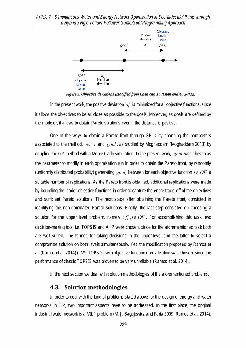
Article 7 - Simultaneous Water and Energy Network Optimization in Eco-Industrial Parks through a Hybrid Single-Leader-Follower Game/Goal Programming Approach
- 289 -
Figure 5. Objective deviations (modified from Chen and Xu (Chen and Xu 2012)).
In the present work, the positive deviation id is minimized for all objective functions, since
it allows the objectives to be as close as possible to the goals. Moreover, as goals are defined by
the modeler, it allows to obtain Pareto solutions even if the distance is positive.
One of the ways to obtain a Pareto front through GP is by changing the parameters
associated to the method, i.e. w and goal , as studied by Moghaddam (Moghaddam 2013) by
coupling the GP method with a Monte Carlo simulation. In the present work, goal was chosen as
the parameter to modify in each optimization run in order to obtain the Pareto front, by randomly
(uniformly distributed probability) generating igoal between for each objective function i OF a
suitable number of replications. As the Pareto front is obtained, additional replications were made
by bounding the leader objective functions in order to capture the entire trade-off of the objectives
and sufficient Pareto solutions. The next stage after obtaining the Pareto front, consisted in
identifying the non-dominated Pareto solutions. Finally, the last step consisted on choosing a
solution for the upper level problem, namely t*,if i OF . For accomplishing this task, two
decision-making tool, i.e. TOPSIS and AHP were chosen, since for the aforementioned task both
are well suited. The former, for taking decisions in the upper-level and the latter to select a
compromise solution on both levels simultaneously. Yet, the modification proposed by Ramos et
al. (Ramos et al. 2014) (LMS-TOPSIS) with objective function normalization was chosen, since the
performance of classic TOPSIS was proven to be very unreliable (Ramos et al. 2014).
In the next section we deal with solution methodologies of the aforementioned problems.
4.3. Solution methodologies
In order to deal with the kind of problems stated above for the design of energy and water
networks in EIP, two important aspects have to be addressed. In the first place, the original
industrial water network is a MILP problem (M. J. Bagajewicz and Faria 2009; Ramos et al. 2014),
Article 7 - Simultaneous Water and Energy Network Optimization in Eco-Industrial Parks through a Hybrid Single-Leader-Follower Game/Goal Programming Approach
- 290 -
where water flows are inferiorly bounded to be, if they exist, at least minf . This is indeed modeled
by big-M constraints and binary variables in the original model. In this work, we developed an a
posteriori algorithm to add bounds to existing flows and to eliminate low flows. Indeed, the problem
is solved several times until all flows are equal or superior to minf . The algorithm is described in
detail next, using as example , , ', 'ep p ep pFpart (all other flows are handled simultaneously and
equivalently) in the same way as in Ramos et al. (Ramos et al. 2016):
7) The initial problem is solved to optimality.
8) For all , ' ,ep ep EP p, p' P,{ep, p} {ep', p'} :
a. If , , ', '34ep p ep pFpart minf , then a lower bound of the flow is imposed that is
the constraint , , ', 'ep p ep pFpart minf is added to the model.
b. If , , ', '34ep p ep pFpart minf , then the flow is fixed , , ', ' 0ep p ep pFpart
c. Else, if all flows , , ', 'ep p ep pFpart minf , then the problem has converged and
no further treatment is required.
9) The bound-modified problem is tried to be solved to optimality:
a. If optimality is achieved, then go to 2).
b. Else, try solving to optimality with a different solver.
i. If optimality is achieved, then go to 2).
ii. Else, restore initial bounds of the variables of the process whose
constraint/s are infeasible. Go to 3).
In the aforementioned way, low-flowrates are systematically eliminated. However, it is
evident that the solution obtained does not assure in any way neither local nor global optimality in
terms only of discrete decisions. Nevertheless, it represents an efficient way to deal with the latter,
given the natural complexity of the problem.
On the other hand, in order to solve bi-level models as those stated in Prob. , the latter has
to be reformulated in order to be tractable in a mathematical modeling environment. In this work,
we follow the reformulation and solutions strategies of Ramos et al. (Ramos et al. 2016). In the first
place, in the bi-level formulation, followers’ problems are replaced by their KKT conditions and the
latter become constraints of the leader’s problem. As evident, after this treatment the problem is
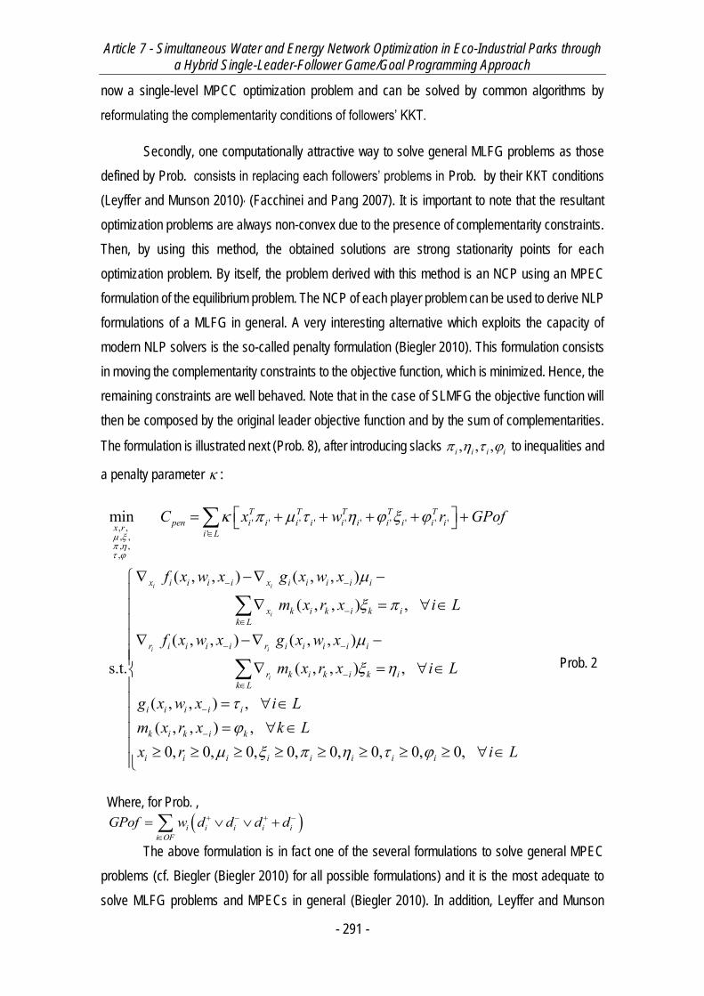
Article 7 - Simultaneous Water and Energy Network Optimization in Eco-Industrial Parks through a Hybrid Single-Leader-Follower Game/Goal Programming Approach
- 291 -
now a single-level MPCC optimization problem and can be solved by common algorithms by
reformulating the complementarity conditions of followers’ KKT.
Secondly, one computationally attractive way to solve general MLFG problems as those
defined by Prob. consists in replacing each followers’ problems in Prob. by their KKT conditions
(Leyffer and Munson 2010), (Facchinei and Pang 2007). It is important to note that the resultant
optimization problems are always non-convex due to the presence of complementarity constraints.
Then, by using this method, the obtained solutions are strong stationarity points for each
optimization problem. By itself, the problem derived with this method is an NCP using an MPEC
formulation of the equilibrium problem. The NCP of each player problem can be used to derive NLP
formulations of a MLFG in general. A very interesting alternative which exploits the capacity of
modern NLP solvers is the so-called penalty formulation (Biegler 2010). This formulation consists
in moving the complementarity constraints to the objective function, which is minimized. Hence, the
remaining constraints are well behaved. Note that in the case of SLMFG the objective function will
then be composed by the original leader objective function and by the sum of complementarities.
The formulation is illustrated next (Prob. 8), after introducing slacks , , ,i i i i to inequalities and
a penalty parameter :
' ' ' ' ' ' ' ' ' ', , ', ,, ,,
min
( , , ) ( , , )
( , , ) ,
( , , ) ( , , )
s.t. ( , , )
i i
i
i i
i
T T T T Tpen i i i i i i i i i ix r i L
x i i i i x i i i i i
x k i k i k ik L
r i i i i r i i i i i
r k i k i
C x w r GPof
f x w x g x w x
m x r x i L
f x w x g x w x
m x r x
,
( , , ) ,( , , ) ,
0, 0, 0, 0, 0, 0, 0, 0,
k ik L
i i i i i
k i k i k
i i i i i i i i
i L
g x w x i Lm x r x k Lx r i L
Where, for Prob. ,
i i i i ii OF
GPof w d d d d
Prob. 2
The above formulation is in fact one of the several formulations to solve general MPEC
problems (cf. Biegler (Biegler 2010) for all possible formulations) and it is the most adequate to
solve MLFG problems and MPECs in general (Biegler 2010). In addition, Leyffer and Munson
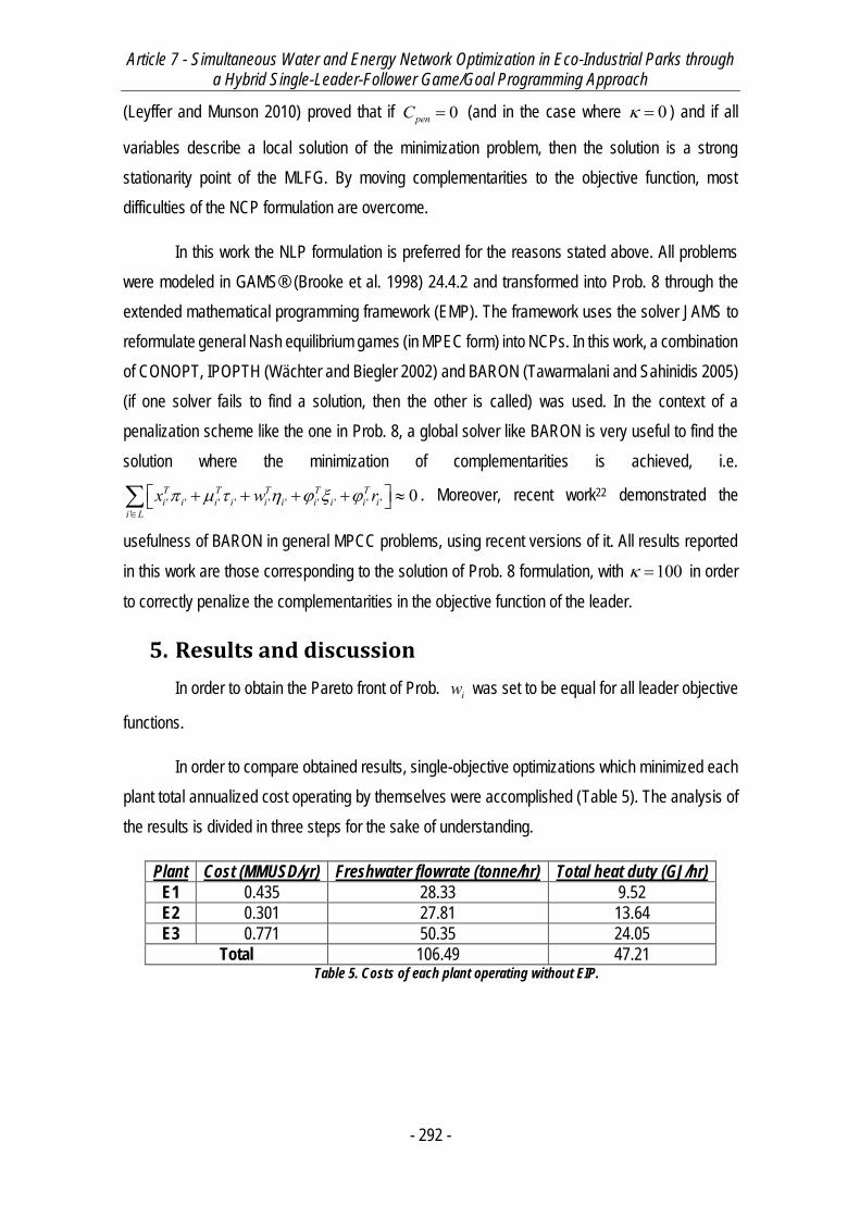
Article 7 - Simultaneous Water and Energy Network Optimization in Eco-Industrial Parks through a Hybrid Single-Leader-Follower Game/Goal Programming Approach
- 292 -
(Leyffer and Munson 2010) proved that if 0penC (and in the case where 0 ) and if all
variables describe a local solution of the minimization problem, then the solution is a strong
stationarity point of the MLFG. By moving complementarities to the objective function, most
difficulties of the NCP formulation are overcome.
In this work the NLP formulation is preferred for the reasons stated above. All problems
were modeled in GAMS® (Brooke et al. 1998) 24.4.2 and transformed into Prob. 8 through the
extended mathematical programming framework (EMP). The framework uses the solver JAMS to
reformulate general Nash equilibrium games (in MPEC form) into NCPs. In this work, a combination
of CONOPT, IPOPTH (Wächter and Biegler 2002) and BARON (Tawarmalani and Sahinidis 2005)
(if one solver fails to find a solution, then the other is called) was used. In the context of a
penalization scheme like the one in Prob. 8, a global solver like BARON is very useful to find the
solution where the minimization of complementarities is achieved, i.e.
' ' ' ' ' ' ' ' ' ''
0T T T T Ti i i i i i i i i i
i Lx w r
. Moreover, recent work22 demonstrated the
usefulness of BARON in general MPCC problems, using recent versions of it. All results reported
in this work are those corresponding to the solution of Prob. 8 formulation, with 100 in order
to correctly penalize the complementarities in the objective function of the leader.
5. Results and discussion
In order to obtain the Pareto front of Prob. iw was set to be equal for all leader objective
functions.
In order to compare obtained results, single-objective optimizations which minimized each
plant total annualized cost operating by themselves were accomplished (Table 5). The analysis of
the results is divided in three steps for the sake of understanding.
Plant Cost (MMUSD/yr) Freshwater flowrate (tonne/hr) Total heat duty (GJ/hr)
E1 0.435 28.33 9.52
E2 0.301 27.81 13.64
E3 0.771 50.35 24.05
Total 106.49 47.21 Table 5. Costs of each plant operating without EIP.
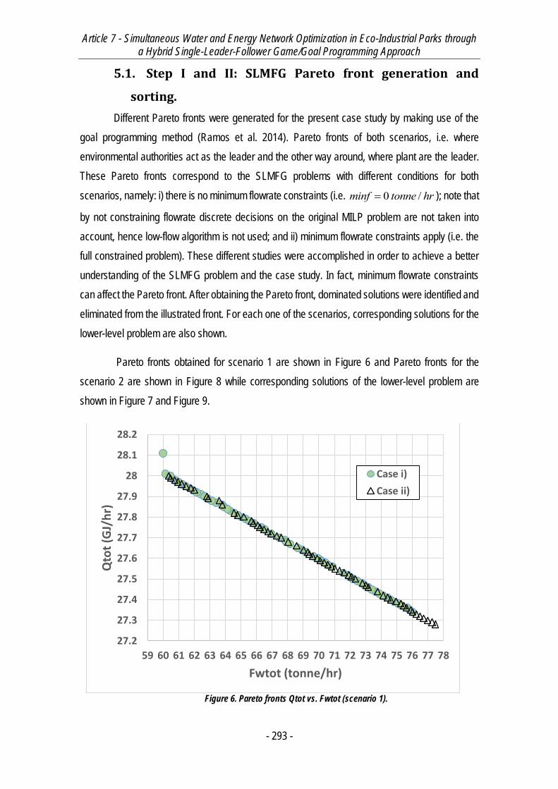
Article 7 - Simultaneous Water and Energy Network Optimization in Eco-Industrial Parks through a Hybrid Single-Leader-Follower Game/Goal Programming Approach
- 293 -
5.1. Step I and II: SLMFG Pareto front generation and
sorting.
Different Pareto fronts were generated for the present case study by making use of the
goal programming method (Ramos et al. 2014). Pareto fronts of both scenarios, i.e. where
environmental authorities act as the leader and the other way around, where plant are the leader.
These Pareto fronts correspond to the SLMFG problems with different conditions for both
scenarios, namely: i) there is no minimum flowrate constraints (i.e. 0 /minf tonne hr ); note that
by not constraining flowrate discrete decisions on the original MILP problem are not taken into
account, hence low-flow algorithm is not used; and ii) minimum flowrate constraints apply (i.e. the
full constrained problem). These different studies were accomplished in order to achieve a better
understanding of the SLMFG problem and the case study. In fact, minimum flowrate constraints
can affect the Pareto front. After obtaining the Pareto front, dominated solutions were identified and
eliminated from the illustrated front. For each one of the scenarios, corresponding solutions for the
lower-level problem are also shown.
Pareto fronts obtained for scenario 1 are shown in Figure 6 and Pareto fronts for the
scenario 2 are shown in Figure 8 while corresponding solutions of the lower-level problem are
shown in Figure 7 and Figure 9.
Figure 6. Pareto fronts Qtot vs. Fwtot (scenario 1).
27.2
27.3
27.4
27.5
27.6
27.7
27.8
27.9
28
28.1
28.2
59 60 61 62 63 64 65 66 67 68 69 70 71 72 73 74 75 76 77 78
Qto
t (G
J/h
r)
Fwtot (tonne/hr)
Case i)
Case ii)
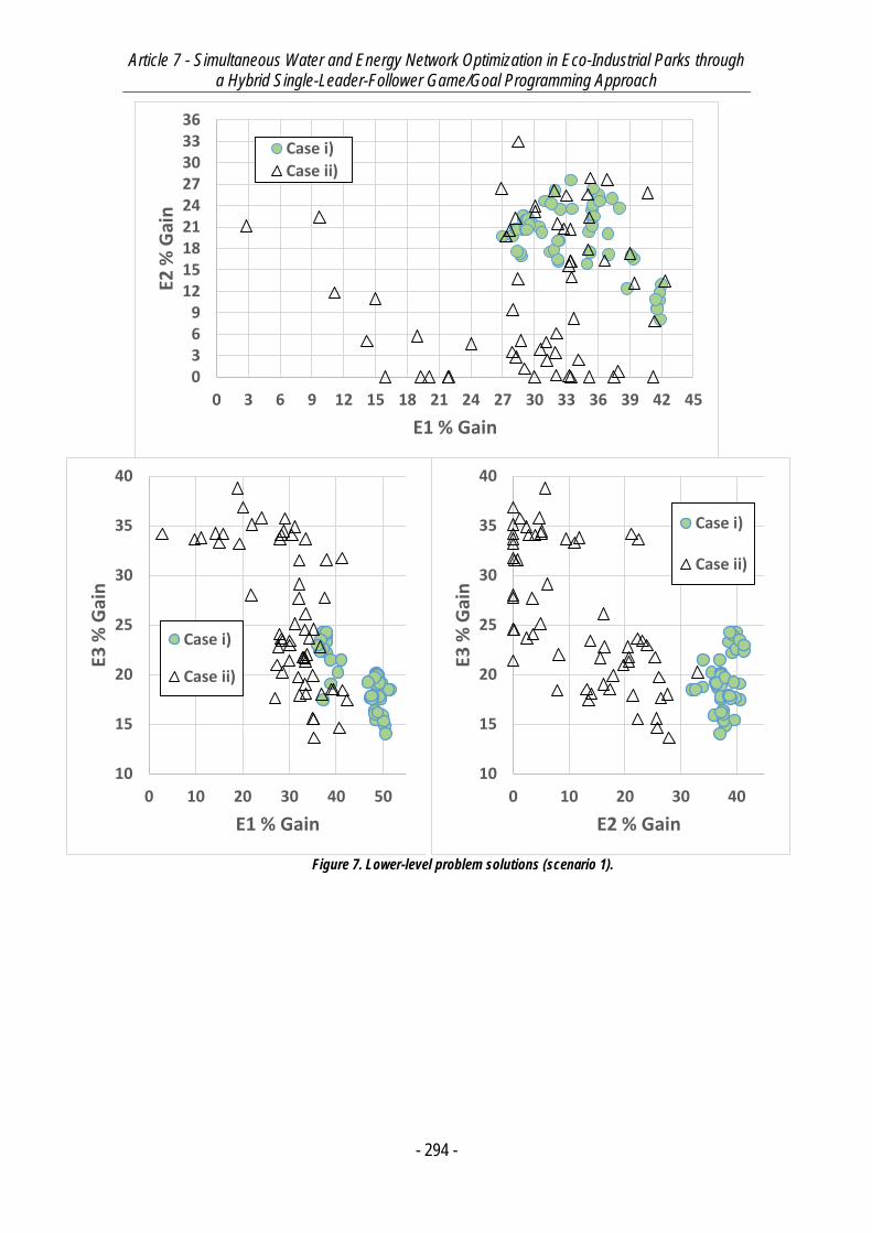
Article 7 - Simultaneous Water and Energy Network Optimization in Eco-Industrial Parks through a Hybrid Single-Leader-Follower Game/Goal Programming Approach
- 294 -
Figure 7. Lower-level problem solutions (scenario 1).
0369
121518212427303336
0 3 6 9 12 15 18 21 24 27 30 33 36 39 42 45
E2 %
Gai
n
E1 % Gain
Case i)
Case ii)
10
15
20
25
30
35
40
0 10 20 30 40 50
E3 %
Gai
n
E1 % Gain
Case i)
Case ii)
10
15
20
25
30
35
40
0 10 20 30 40
E3 %
Gai
n
E2 % Gain
Case i)
Case ii)
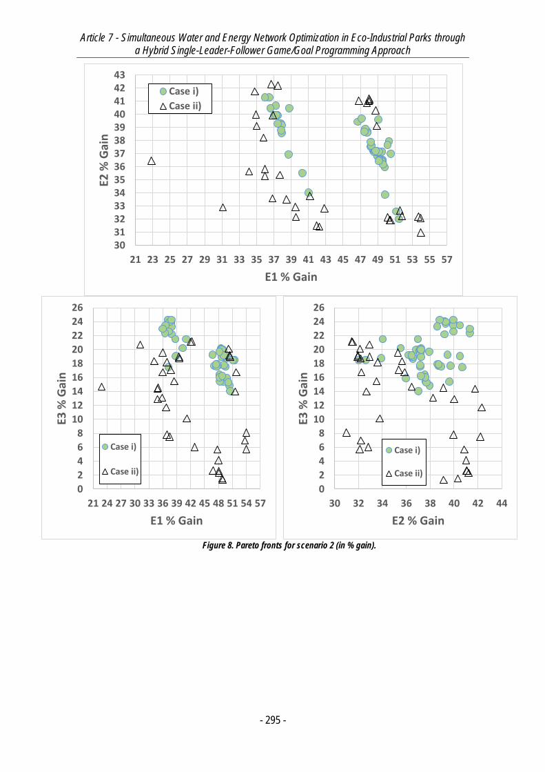
Article 7 - Simultaneous Water and Energy Network Optimization in Eco-Industrial Parks through a Hybrid Single-Leader-Follower Game/Goal Programming Approach
- 295 -
Figure 8. Pareto fronts for scenario 2 (in % gain).
3031323334353637383940414243
21 23 25 27 29 31 33 35 37 39 41 43 45 47 49 51 53 55 57
E2 %
Gai
n
E1 % Gain
Case i)
Case ii)
0
2
4
6
8
10
12
14
16
18
20
22
24
26
21 24 27 30 33 36 39 42 45 48 51 54 57
E3 %
Gai
n
E1 % Gain
Case i)
Case ii)
0
2
4
6
8
10
12
14
16
18
20
22
24
26
30 32 34 36 38 40 42 44
E3 %
Gai
n
E2 % Gain
Case i)
Case ii)
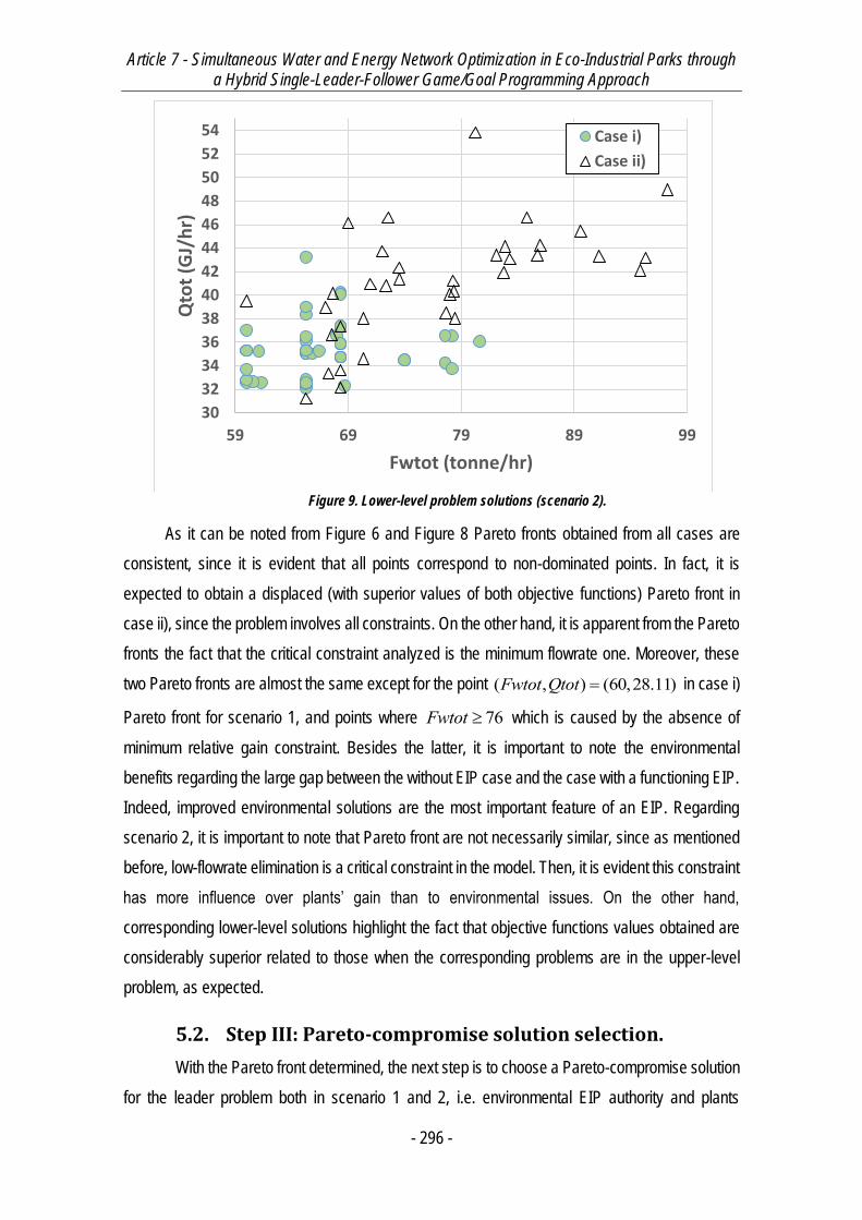
Article 7 - Simultaneous Water and Energy Network Optimization in Eco-Industrial Parks through a Hybrid Single-Leader-Follower Game/Goal Programming Approach
- 296 -
Figure 9. Lower-level problem solutions (scenario 2).
As it can be noted from Figure 6 and Figure 8 Pareto fronts obtained from all cases are
consistent, since it is evident that all points correspond to non-dominated points. In fact, it is
expected to obtain a displaced (with superior values of both objective functions) Pareto front in
case ii), since the problem involves all constraints. On the other hand, it is apparent from the Pareto
fronts the fact that the critical constraint analyzed is the minimum flowrate one. Moreover, these
two Pareto fronts are almost the same except for the point ( , ) (60,28.11)Fwtot Qtot in case i)
Pareto front for scenario 1, and points where 76Fwtot which is caused by the absence of
minimum relative gain constraint. Besides the latter, it is important to note the environmental
benefits regarding the large gap between the without EIP case and the case with a functioning EIP.
Indeed, improved environmental solutions are the most important feature of an EIP. Regarding
scenario 2, it is important to note that Pareto front are not necessarily similar, since as mentioned
before, low-flowrate elimination is a critical constraint in the model. Then, it is evident this constraint
has more influence over plants’ gain than to environmental issues. On the other hand,
corresponding lower-level solutions highlight the fact that objective functions values obtained are
considerably superior related to those when the corresponding problems are in the upper-level
problem, as expected.
5.2. Step III: Pareto-compromise solution selection.
With the Pareto front determined, the next step is to choose a Pareto-compromise solution
for the leader problem both in scenario 1 and 2, i.e. environmental EIP authority and plants
30
32
34
36
38
40
42
44
46
48
50
52
54
59 69 79 89 99
Qto
t (G
J/h
r)
Fwtot (tonne/hr)
Case i)
Case ii)
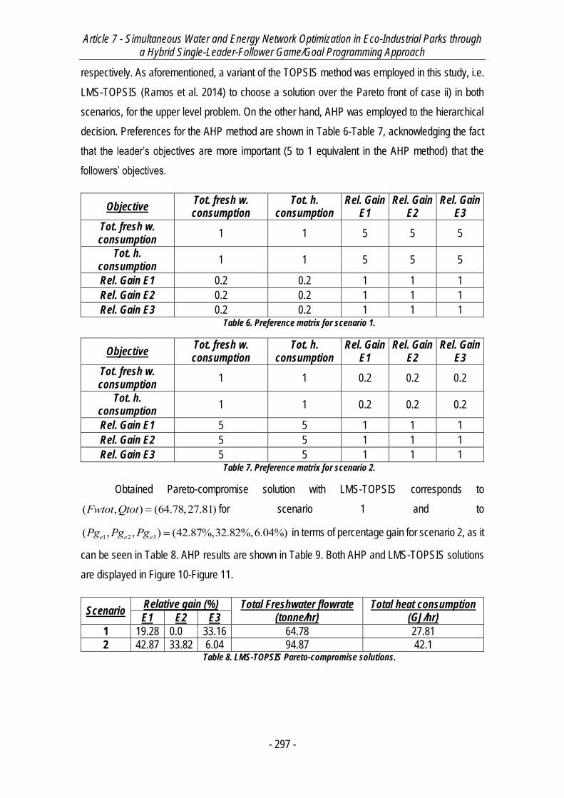
Article 7 - Simultaneous Water and Energy Network Optimization in Eco-Industrial Parks through a Hybrid Single-Leader-Follower Game/Goal Programming Approach
- 297 -
respectively. As aforementioned, a variant of the TOPSIS method was employed in this study, i.e.
LMS-TOPSIS (Ramos et al. 2014) to choose a solution over the Pareto front of case ii) in both
scenarios, for the upper level problem. On the other hand, AHP was employed to the hierarchical
decision. Preferences for the AHP method are shown in Table 6-Table 7, acknowledging the fact
that the leader’s objectives are more important (5 to 1 equivalent in the AHP method) that the
followers’ objectives.
Objective Tot. fresh w. consumption
Tot. h. consumption
Rel. Gain E1
Rel. Gain E2
Rel. Gain E3
Tot. fresh w. consumption
1 1 5 5 5
Tot. h. consumption
1 1 5 5 5
Rel. Gain E1 0.2 0.2 1 1 1
Rel. Gain E2 0.2 0.2 1 1 1
Rel. Gain E3 0.2 0.2 1 1 1 Table 6. Preference matrix for scenario 1.
Objective Tot. fresh w. consumption
Tot. h. consumption
Rel. Gain E1
Rel. Gain E2
Rel. Gain E3
Tot. fresh w. consumption
1 1 0.2 0.2 0.2
Tot. h. consumption
1 1 0.2 0.2 0.2
Rel. Gain E1 5 5 1 1 1
Rel. Gain E2 5 5 1 1 1
Rel. Gain E3 5 5 1 1 1 Table 7. Preference matrix for scenario 2.
Obtained Pareto-compromise solution with LMS-TOPSIS corresponds to
( , ) (64.78,27.81)Fwtot Qtot for scenario 1 and to
1 2 3( , , ) (42.87%,32.82%,6.04%)e e ePg Pg Pg in terms of percentage gain for scenario 2, as it
can be seen in Table 8. AHP results are shown in Table 9. Both AHP and LMS-TOPSIS solutions
are displayed in Figure 10-Figure 11.
Scenario Relative gain (%) Total Freshwater flowrate
(tonne/hr) Total heat consumption
(GJ/hr) E1 E2 E3
1 19.28 0.0 33.16 64.78 27.81
2 42.87 33.82 6.04 94.87 42.1 Table 8. LMS-TOPSIS Pareto-compromise solutions.
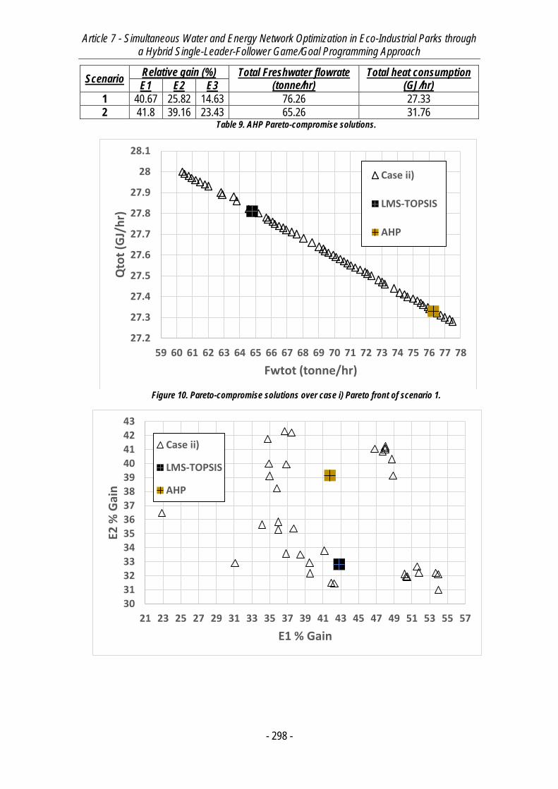
Article 7 - Simultaneous Water and Energy Network Optimization in Eco-Industrial Parks through a Hybrid Single-Leader-Follower Game/Goal Programming Approach
- 298 -
Scenario Relative gain (%) Total Freshwater flowrate
(tonne/hr) Total heat consumption
(GJ/hr) E1 E2 E3
1 40.67 25.82 14.63 76.26 27.33
2 41.8 39.16 23.43 65.26 31.76 Table 9. AHP Pareto-compromise solutions.
Figure 10. Pareto-compromise solutions over case i) Pareto front of scenario 1.
27.2
27.3
27.4
27.5
27.6
27.7
27.8
27.9
28
28.1
59 60 61 62 63 64 65 66 67 68 69 70 71 72 73 74 75 76 77 78
Qto
t (G
J/h
r)
Fwtot (tonne/hr)
Case ii)
LMS-TOPSIS
AHP
3031323334353637383940414243
21 23 25 27 29 31 33 35 37 39 41 43 45 47 49 51 53 55 57
E2 %
Gai
n
E1 % Gain
Case ii)
LMS-TOPSIS
AHP
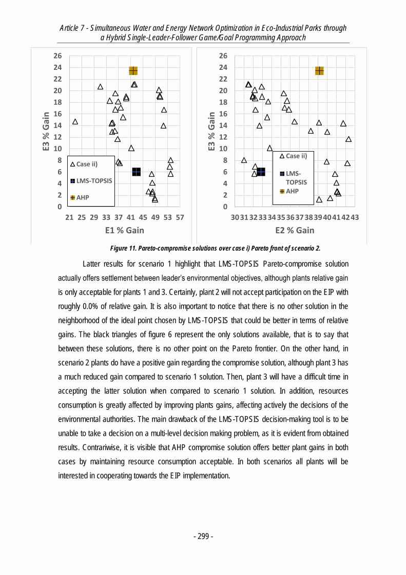
Article 7 - Simultaneous Water and Energy Network Optimization in Eco-Industrial Parks through a Hybrid Single-Leader-Follower Game/Goal Programming Approach
- 299 -
Figure 11. Pareto-compromise solutions over case i) Pareto front of scenario 2.
Latter results for scenario 1 highlight that LMS-TOPSIS Pareto-compromise solution
actually offers settlement between leader’s environmental objectives, although plants relative gain
is only acceptable for plants 1 and 3. Certainly, plant 2 will not accept participation on the EIP with
roughly 0.0% of relative gain. It is also important to notice that there is no other solution in the
neighborhood of the ideal point chosen by LMS-TOPSIS that could be better in terms of relative
gains. The black triangles of figure 6 represent the only solutions available, that is to say that
between these solutions, there is no other point on the Pareto frontier. On the other hand, in
scenario 2 plants do have a positive gain regarding the compromise solution, although plant 3 has
a much reduced gain compared to scenario 1 solution. Then, plant 3 will have a difficult time in
accepting the latter solution when compared to scenario 1 solution. In addition, resources
consumption is greatly affected by improving plants gains, affecting actively the decisions of the
environmental authorities. The main drawback of the LMS-TOPSIS decision-making tool is to be
unable to take a decision on a multi-level decision making problem, as it is evident from obtained
results. Contrariwise, it is visible that AHP compromise solution offers better plant gains in both
cases by maintaining resource consumption acceptable. In both scenarios all plants will be
interested in cooperating towards the EIP implementation.
0
2
4
6
8
10
12
14
16
18
20
22
24
26
21 25 29 33 37 41 45 49 53 57
E3 %
Gai
n
E1 % Gain
Case ii)
LMS-TOPSIS
AHP
0
2
4
6
8
10
12
14
16
18
20
22
24
26
3031323334353637383940414243E3
% G
ain
E2 % Gain
Case ii)
LMS-TOPSISAHP
Article 7 - Simultaneous Water and Energy Network Optimization in Eco-Industrial Parks through a Hybrid Single-Leader-Follower Game/Goal Programming Approach
- 300 -
6. Conclusions
In this work, a hybrid SLMFG/goal programming formulation for the simultaneous design
of water and energy networks in EIP was successfully addressed. The inclusion of different
environmental authorities in order to manage resources has as consequence multiple players at
each level. Thus, the problem is modeled as a SLMFG/goal programming hybrid model where the
upper-level problem is modeled as a MOO problem. With this kind of manipulation, a Pareto front
is generated for each one of the scenarios and a AHP and LMS-TOPSIS decision making tools are
applied to obtain a compromise solution. As such, the multi-agent problem is solved effectively and
compromise solutions between leaders and followers are found in a simple way. The approach is
demonstrated very useful, since all solutions obtained assured important gains in operating costs
in plants by still maintaining environmental impacts low. Moreover, the approach is proved effective
when environmental authorities have conflictual objective functions.
By generating Pareto fronts of the solutions, solid ideas about the feasible space of
solutions is obtained. As such, the proposed methodology is very useful in order to understand the
specter of possible solutions. As solutions are obtained, it is important to highlight that the AHP
method selects the compromise solution by taking into account hierarchy of each one of the
objective functions. Moreover, the coefficient-consistency checking feature comes really useful to
actually select good solutions.
Simultaneous water and energy networks in EIP are not too widely studied in literature,
due to the antagonistic nature of objectives. In this work, the introduction of environmental
regulators plays a major role, since in this way drawbacks of multiobjective optimization are
overcome.
Nevertheless, the proposed approach also exhibits some major drawbacks: first, there is
not an un-biased way to find the overall equilibrium solution between the leaders and the followers.
Indeed, by implementing a decision-making tool, there is always some biasing on the part of the
decision-maker. Moreover, as seen by results of the different scenarios, there is also no way to find
a solution between the two. On the other hand, the Pareto front generation implies running the
optimization problem several ways to find a significant number of solutions. This can be a very
important drawback, since if an EIP with several plants composing it is considered, the solution
times could become prohibitive.
Article 7 - Simultaneous Water and Energy Network Optimization in Eco-Industrial Parks through a Hybrid Single-Leader-Follower Game/Goal Programming Approach
- 301 -
A solution for the first and must important drawback could be the formulation of the problem
as a multi-leader-multi-follower game (MLMFG) model. As such, the need of a decision-making tool
is eliminated and the compromise between solutions is not biased.
Finally, it was also underlined the usefulness of EIPs in the context of industrial symbiosis
to produce more sustainable industrial outcomes. The results obtained show that, by unifying
efforts, wastes are lowered and effective gain can be achieved. As a perspective, simultaneous
energy and water networks will be taken into account with a MLFG approach.
7. Nomenclature
Latin symbols
ix = Decision variables of leader i
ix = Decision variables of other leaders
y = Followers variables
w = Weights on the distances of objective functions of the leader
f = Objective function of the leader
h = Equality constraints of the leader g = Inequality constraints of the leader
m = Inequality constraints of followers
l = Equality constraints of the followers
GPof = Objective function of the goal programming problem
np = Number of processes per plant
P = Index set of processes nep = Number of plants
EP = Index set of plants nr = Number of regeneration units
R = Index set of regeneration units
M = Contaminant load
,in outCmax Cmax = Maximum contaminant concentration allowed in inlet/outlet
of processes
Tp Operating temperature of processes outC = Outlet concentration of contaminant in regeneration units
Tr Operating temperature of regeneration units wCp Water heat capacity
Tw Freshwater temperature
Td Discharge temperature
Fpart = Water flow between different processes
Fw = Freshwater inlet flow to processes ,Qp = Heating (+), cooling (-) processes heat duty
Fproreg = Water flow from processes to regeneration units
Fregpro = Water flow from regeneration units to processes ,Qr = Heating (+), cooling (-) regeneration units heat duty

Article 7 - Simultaneous Water and Energy Network Optimization in Eco-Industrial Parks through a Hybrid Single-Leader-Follower Game/Goal Programming Approach
- 302 -
Fdis = Water processes to the discharge ,Qd = Heating (+), cooling (-) discharge heat duty
minf = Minimum flowrate allowed
AWH = Annual EIP operating hours
Fwtotf = Total freshwater flow
Qtotf = Total heat duty
costQ = Heat duty operating costs ,d = Distance from objective functions to the goal
goal = Level of aspiration of objective functions
OF = Set of objective functions
penC = Penalization objective function
L = Index set of leaders Greek symbols = Lagrange multipliers relative to m = Lagrange multipliers relative to g
= Lagrange multipliers relative to s
, , , , = Slacks to inequalities of Prob. 8
= Purchase price of freshwater
= Polluted water discharge cost
= Polluted water pumping cost = Regenerated water cost
= Power associated to , = Heating (+), cooling (-) duty unit cost
= Penalization parameter for complementarities
Article 7 - Simultaneous Water and Energy Network Optimization in Eco-Industrial Parks through a Hybrid Single-Leader-Follower Game/Goal Programming Approach
- 303 -
References
Aspen Technology (n.d.) Aspen ONE. Cambridge, MA, USA, Aspen Technology.
Aussel, D., Correa, R. & Marechal, P. (2013) Spot Electricity Market with Transmission
Losses. Journal of Industrial and Management Optimization. 9 (2), 275–290.
Bagajewicz, M. & Savelski, M. (2001) On the Use of Linear Models for the Design of Water
Utilization Systems in Process Plants with a Single Contaminant. Chemical engineering research
and design. 79 (5), 600–610.
Bagajewicz, M.J. & Faria, D.C. (2009) On the Appropriate Architecture of the
Water/Wastewater Allocation Problem in Process Plants Jacek Jeżowski and Jan Thullie (ed.).
Computer Aided Chemical Engineering. 261–20.
Biegler, L.T. (2010) Nonlinear Programming: Concepts, Algorithms, and Applications to
Chemical Processes. Philadelphia, Society for Industrial and Applied Mathematics : Mathematical
Optimization Society.
Biegler, L.T., Grossmann, I.E. & Westerberg, A.W. (1997) Systematic Methods of Chemical
Process Design. Upper Saddle River, N.J., Prentice Hall PTR.
Boix, M. & Montastruc, L. (2011) Eco Industrial Parks for Water and Heat Management.
Computer Aided Chemical Engineering. [Online] 291175–1179. Available from: doi:10.1016/B978-
0-444-54298-4.50014-3.
Boix, M., Montastruc, L., Azzaro-Pantel, C. & Domenech, S. (2015) Optimization Methods
Applied to the Design of Eco-Industrial Parks: A Literature Review. Journal of Cleaner Production.
87303–317.
Boix, M., Montastruc, L., Pibouleau, L., Azzaro-Pantel, C., et al. (2012) Industrial Water
Management by Multiobjective Optimization: From Individual to Collective Solution Through Eco-
Industrial Parks. Journal of Cleaner Production. [Online] 22 (1), 85–97. Available from:
doi:10.1016/j.jclepro.2011.09.011.
Boix, M., Montastruc, L., Pibouleau, L., Azzaro-Pantel, C., et al. (2010) Multiobjective
Optimization of Industrial Water Networks with Contaminants S. Pierucci and G. Buzzi Ferraris
(ed.). Computer Aided Chemical Engineering. 28859–864.
Boix, M., Pibouleau, L., Montastruc, L., Azzaro-Pantel, C., et al. (2012) Minimizing Water
and Energy Consumptions in Water and Heat Exchange Networks. Applied Thermal Engineering.
[Online] 36442–455. Available from: doi:10.1016/j.applthermaleng.2011.10.062.
Brooke, A., Kendrick, D., Meeraus, A. & Raman, R. (1998) GAMS User’s Guide.
Chae, S.H., Kim, S.H., Yoon, S.-G. & Park, S. (2010) Optimization of a Waste Heat
Utilization Network in an Eco-Industrial Park. Applied Energy. [Online] 87 (6), 1978–1988. Available
from: doi:10.1016/j.apenergy.2009.12.003.

Article 7 - Simultaneous Water and Energy Network Optimization in Eco-Industrial Parks through a Hybrid Single-Leader-Follower Game/Goal Programming Approach
- 304 -
Chen, A. & Xu, X. (2012) Goal Programming Approach to Solving Network Design Problem
with Multiple Objectives and Demand Uncertainty. Expert Systems with Applications. [Online] 39
(4), 4160–4170. Available from: doi:10.1016/j.eswa.2011.09.118.
Cheng, S.-L., Chang, C.-T. & Jiang, D. (2014) A Game-Theory Based Optimization
Strategy to Configure Inter-Plant Heat Integration Schemes. Chemical Engineering Science.
11860–73.
Chew, I.M.L., Tan, R.R., Foo, D.C.Y. & Chiu, A.S.F. (2009) Game Theory Approach to the
Analysis of Inter-Plant Water Integration in an Eco-Industrial Park. Journal of Cleaner Production.
[Online] 17 (18), 1611–1619. Available from: doi:10.1016/j.jclepro.2009.08.005.
Collette, Y. & Siarry, P. (2003) Multiobjective Optimization: Principles and Case Studies.
Springer.
Facchinei, F. & Pang, J.-S. (2007) Finite-Dimensional Variational Inequalities and
Complementarity Problems. Springer Science & Business Media.
Leong, Y.T., Tan, R.R. & Chew, I.M.L. (2014) Optimization of Chilled and Cooling Water
Systems in a Centralized Utility Hub. Energy Procedia. [Online] 61846–849. Available from:
doi:10.1016/j.egypro.2014.11.979.
Leyffer, S. & Munson, T. (2010) Solving Multi-Leader–Common-Follower Games.
Optimisation Methods & Software. 25 (4), 601–623.
Moghaddam, K.S. (2013) Multi-Objective Preventive Maintenance and Replacement
Scheduling in a Manufacturing System Using Goal Programming. International Journal of
Production Economics. [Online] 146 (2), 704–716. Available from: doi:10.1016/j.ijpe.2013.08.027.
Olesen, S.G. & Polley, G.T. (1996) Dealing with Plant Geography and Piping Constraints
in Water Network Design. Process Safety and Environmental Protection. [Online] 74 (4), 273–276.
Available from: doi:10.1205/095758296528626.
Ramos, M.A., Boix, M., Aussel, D., Montastruc, L., et al. (2015) Water Exchanges in Eco-
industrial Parks through Multiobjective Optimization and Game Theory. Computer Aided Chemical
Engineering. 371997–2002.
Ramos, M.A., Boix, M., Aussel, D., Montastruc, L., et al. (2016) Water integration in Eco-
Industrial Parks Using a Multi-Leader-Follower Approach. Computers & Chemical Engineering.
87190–207.
Ramos, M.A., Boix, M., Montastruc, L. & Domenech, S. (2014) Multiobjective Optimization
Using Goal Programming for Industrial Water Network Design. Industrial & Engineering Chemistry
Research. 53 (45), 17722–17735.
Ramos, M.A., Rocafull, M., Boix, M., Aussel, D., et al. (2016) Utility Network Optimization
in Eco-Industrial Parks by a Multi-Leader Follower Game Methodology.
Article 7 - Simultaneous Water and Energy Network Optimization in Eco-Industrial Parks through a Hybrid Single-Leader-Follower Game/Goal Programming Approach
- 305 -
Reniers, G., Dullaert, W. & Visser, L. (2010) Empirically Based Development of a
Framework for Advancing and Stimulating Collaboration in the Chemical Industry (asc): Creating
Sustainable Chemical Industrial Parks. Journal of Cleaner Production. [Online] 18 (16–17), 1587–
1597. Available from: doi:10.1016/j.jclepro.2010.07.013.
Saaty, T.L. & Peniwati, K. (2008) Group Decision Making: Drawing Out and Reconciling
Differences. RWS Publications.
Tawarmalani, M. & Sahinidis, N.V. (2005) A Polyhedral Branch-and-Cut Approach to
Global Optimization. Mathematical Programming. 103 (2), 225–249.
UNESCO (2009) Water in a Changing World. Report 3. The United Nations World Water
Development.
Wächter, A. & Biegler, L.T. (2002) An Interior Point Algorithm for Large-Scale Nonlinear
Optimization with Applications in Process Engineering. Pittsburgh, Pa., Carnegie Mellon University,
Carnegie Mellon University, 2002.
Yeomans, H. & Grossmann, I.E. (1999) A Systematic Modeling Framework of
Superstructure Optimization in Process Synthesis. Computers & Chemical Engineering. [Online]
23 (6), 709–731. Available from: doi:10.1016/S0098-1354(99)00003-4.
Zhang, Y. & Sahinidis, N.V. (2015) Global Optimization of Mathematical Programs with
Complementarity Constraints and Application to Clean Energy Deployment. Optimization Letters.
1–16.

- 307 -
Chapitre 9 - Multi-Leader Multi-Follower Game Model for Simultaneous
Water and Energy Integration in Eco-Industrial Parks

Article 8 - Multi-Leader Multi-Follower Game Model for Simultaneous Water and Energy Integration in Eco-Industrial Parks
- 308 -

Article 8 - Multi-Leader Multi-Follower Game Model for Simultaneous Water and Energy Integration in Eco-Industrial Parks
- 309 -
Résumé
Suite aux résultats obtenus et aux perspectives adressées à l’issue des articles 3 et 7, il est
important de faire évoluer les méthodes développées vers un modèle dans lequel chaque autorité
de l’EIP est un joueur indépendant devenant alors un modèle de jeu multi-leader-multi-follower
game (MLMFG). Le cas d’étude est le même que celui de l’article 7, où les réseaux d’eau et
d’énergie sont générés simultanément. Le modèle bi-niveaux est conçu avec les gestionnaires
d’eau et énergie comme leaders et les usines comme followers. Ainsi, les usines jouent un jeu de
Nash entre elles et il en va de même pour les gestionnaires de l’EIP. Ces gestionnaires ou
régulateurs choisissent une solution parmi les équilibres des followers avant d’atteindre leur propre
équilibre. Le modèle est transformé mathématiquement de la même façon que dans l’article 3 et
résolu avec la même méthode. Ensuite, les résultats obtenus sont comparés avec ceux de l’article
antérieur en démontrant que le modèle MLMFG fournit des conclusions assez intéressantes pour
les usines et également pour les autorités. Le gain relatif des entreprises est le même (i.e. 30%
environ pour toutes les usines), ce qui constitue un argument solide d’équité pour les convaincre
de participer à la symbiose. Le résultat obtenu après la résolution du problème MLMFG est très
différent de celui obtenu en utilisant la méthode AHP sur l’ensemble des solutions faisables. Pour
démontrer l’aspect décisionnel de la méthode MLMFG, les coefficients de la méthode AHP ont été
identifiés pour retrouver la solution du problème MLMFG parmi l’ensemble des points faisables.
Ainsi il est démontré que les coefficients sont difficiles à déterminer pour un expert malgré la
pertinence de la solution trouvée.

Article 8 - Multi-Leader Multi-Follower Game Model for Simultaneous Water and Energy Integration in Eco-Industrial Parks
- 310 -
Article 8 - Multi-Leader Multi-Follower Game Model for Simultaneous Water and Energy Integration in Eco-Industrial Parks
- 311 -
Multi-Leader Multi-Follower Game Model for
Simultaneous Water and Energy Integration
in Eco-Industrial Parks
Manuel A. Ramosa, Marianne Boix*a, Didier Aussel*b, Ludovic Montastruca, Serge
Domenecha
a Laboratoire de Génie Chimique, U.M.R. 5503 CNRS/INP/UPS, Université de Toulouse, 4, Allée
Emile Monso, 31432 Toulouse Cedex 4, France
b Laboratoire PROMES, UPR CNRS 8521, Université de Perpignan, Via Domitia, 66100 Perpignan,
France
* Corresponding authors: [email protected]; [email protected].
Keywords: Eco-industrial parks, Multi-leader-follower Game, Nash equilibrium, Multi-objective
Optimization, MPCC, and Game Theory.
Abstract
The simultaneous design of water and energy networks in eco-industrial parks (EIP) is addressed
in this work by formulating the problem as a multi-leader-multi-follower game (MLMFG) model.
Plants which participate in the EIP configuration act as followers and play a Nash game among
them, and are in Stackelberg equilibrium with environmental authorities (i.e. water and energy
respectively), which play a Nash game as well and act as leaders. A case study with 3 plants with
5 processes each is modeled and solved in GAMS® by formulating the MLMFG as multiple
optimization problems with equilibrium constraints (MOPEC). Results found highlight the
usefulness of the approach, by providing plants with equitable operating costs gains by maintaining
environmental concerns in equilibrium. Finally, a simple MINLP model is formulated and solved to
find the preference matrix in order to find the obtained solution by an analytical hierarchical process
decision-making method if the obtained solution were to make part of several Pareto solutions. The
preference matrix found is counter-intuitive (i.e. the decision-maker hardly would choose the
obtained MLMFG inside a Pareto front), which highlights the usefulness of the MLMFG
methodology.
Article 8 - Multi-Leader Multi-Follower Game Model for Simultaneous Water and Energy Integration in Eco-Industrial Parks
- 312 -
1. Introduction
During the last few decades, industrialization has contributed to rapid depletion of natural
resources such as water and natural gas. Consequently, there is a real need for industries to ensure
minimum natural resources consumption, while maintaining good production levels. In order to work
towards global environmental preservation while increasing business success, the concept of
industrial ecology has emerged (Boix, Montastruc, Azzaro-Pantel, et al., 2015). This concept, which
is directly linked to sustainable development, aims at engaging separate industries, geographically
closed enough, in a collective approach so that exchanges of raw matter, by-products, energy and
utilities (Chertow, 2000) are maximized. Indeed, the most widespread manifestations of these kinds
of industrial symbiosis are eco-industrial parks (EIP). Recently, Boix et al. (Boix, Montastruc,
Azzaro-Pantel, et al., 2015) and Kastner et al. (Kastner, Lau & Kraft, 2015) highlighted the fact that
there is a lack of systematic methods for EIP design through mathematical modeling. Moreover,
existing works on the subject lacked to present efficient methods to successfully address both
environmental and economic goals, given that it is acknowledged that EIP design problems are in
fact multiobjective optimization (MOO) problems with antagonistic objectives. Recently, Ramos et
al. (Ramos, Boix, Aussel, et al., 2016b) presented a multi-leader-follower game (MLFG) model for
the design of water integration networks in EIP, by modeling the environmental authority, related
to freshwater consumption, as either a leader or a follower. As such, an equilibrium solution can be
obtained. Later, in a logical continuation of our research (Ramos, Boix, Aussel, et al., 2016a), a
second environmental authority related to energy consumption in the EIP was incorporated into the
model, by considering energy exchanges between plants. The problem was modeled as a hybrid
MOO/single-leader-multi-follower game (SLMFG) where the leader is a goal programming
multiobjective optimization problem with either both environmental authorities or the plants
problems. Both scenarios were analyzed, and in such a way, Pareto fronts are obtained.
Subsequently, a decision-making tool, i.e. AHP is employed to find the compromise solution for
each scenario. We identified the methodology as attractive in order to analyze different solutions.
Nevertheless, the solutions obtained between scenarios is significantly different, since there is no
mathematical equilibrium between the players modeled through MOO as the leader. Moreover,
computational times are considerably high, since each SLMFG model has to be solved to optimality
several times in order to obtain the Pareto front, thus, for a large-scale application, the methodology
may not be suited.
Then, as a logical continuation of the aforementioned research, in this paper we present a
multi-leader-multi-follower game (MLMFG) model for the simultaneous integration of water and
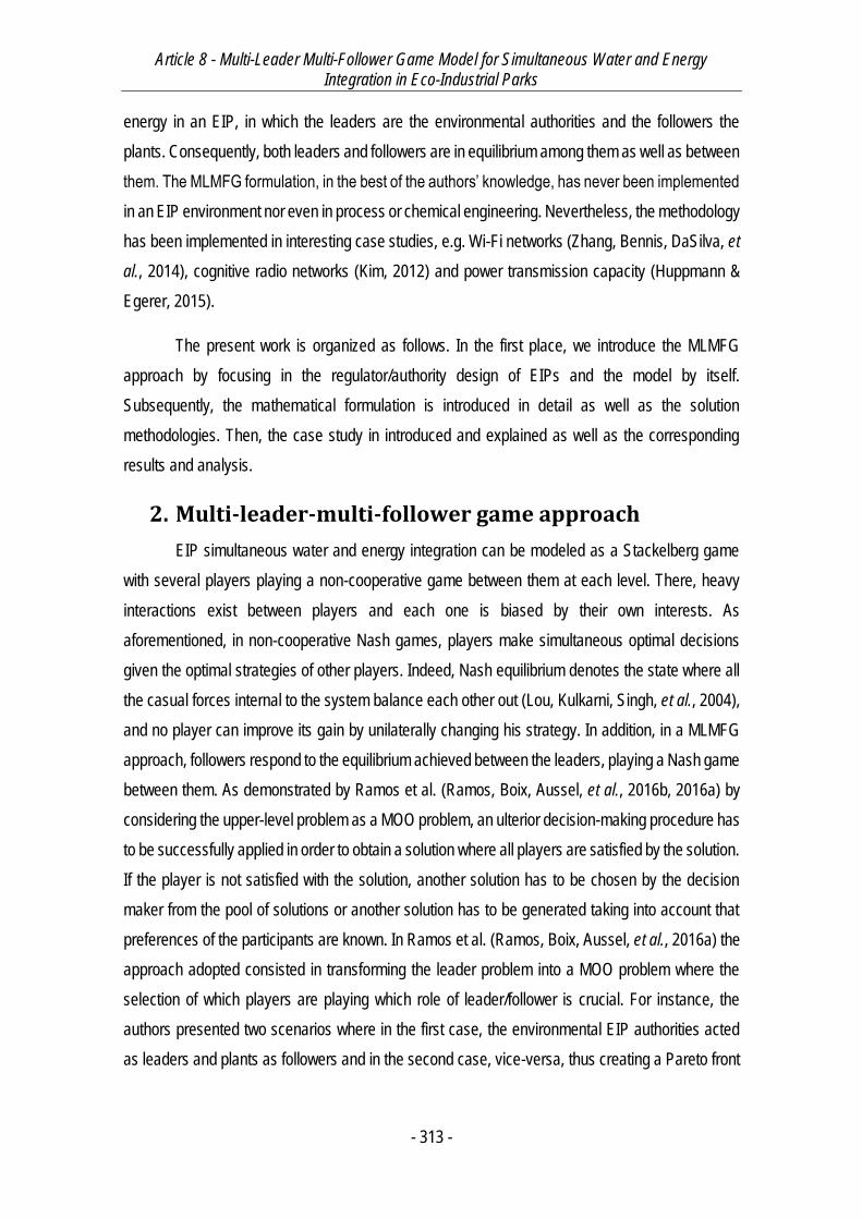
Article 8 - Multi-Leader Multi-Follower Game Model for Simultaneous Water and Energy Integration in Eco-Industrial Parks
- 313 -
energy in an EIP, in which the leaders are the environmental authorities and the followers the
plants. Consequently, both leaders and followers are in equilibrium among them as well as between
them. The MLMFG formulation, in the best of the authors’ knowledge, has never been implemented
in an EIP environment nor even in process or chemical engineering. Nevertheless, the methodology
has been implemented in interesting case studies, e.g. Wi-Fi networks (Zhang, Bennis, DaSilva, et
al., 2014), cognitive radio networks (Kim, 2012) and power transmission capacity (Huppmann &
Egerer, 2015).
The present work is organized as follows. In the first place, we introduce the MLMFG
approach by focusing in the regulator/authority design of EIPs and the model by itself.
Subsequently, the mathematical formulation is introduced in detail as well as the solution
methodologies. Then, the case study in introduced and explained as well as the corresponding
results and analysis.
2. Multi-leader-multi-follower game approach
EIP simultaneous water and energy integration can be modeled as a Stackelberg game
with several players playing a non-cooperative game between them at each level. There, heavy
interactions exist between players and each one is biased by their own interests. As
aforementioned, in non-cooperative Nash games, players make simultaneous optimal decisions
given the optimal strategies of other players. Indeed, Nash equilibrium denotes the state where all
the casual forces internal to the system balance each other out (Lou, Kulkarni, Singh, et al., 2004),
and no player can improve its gain by unilaterally changing his strategy. In addition, in a MLMFG
approach, followers respond to the equilibrium achieved between the leaders, playing a Nash game
between them. As demonstrated by Ramos et al. (Ramos, Boix, Aussel, et al., 2016b, 2016a) by
considering the upper-level problem as a MOO problem, an ulterior decision-making procedure has
to be successfully applied in order to obtain a solution where all players are satisfied by the solution.
If the player is not satisfied with the solution, another solution has to be chosen by the decision
maker from the pool of solutions or another solution has to be generated taking into account that
preferences of the participants are known. In Ramos et al. (Ramos, Boix, Aussel, et al., 2016a) the
approach adopted consisted in transforming the leader problem into a MOO problem where the
selection of which players are playing which role of leader/follower is crucial. For instance, the
authors presented two scenarios where in the first case, the environmental EIP authorities acted
as leaders and plants as followers and in the second case, vice-versa, thus creating a Pareto front
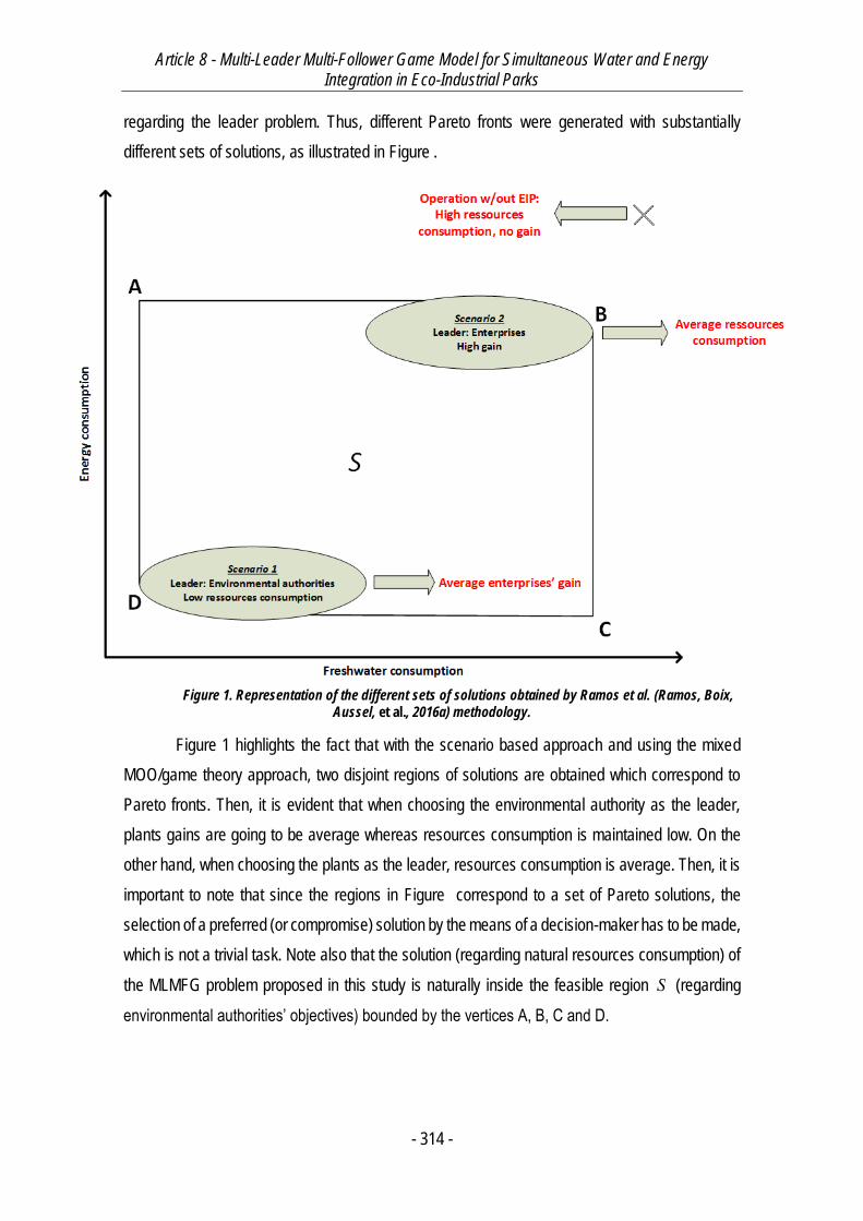
Article 8 - Multi-Leader Multi-Follower Game Model for Simultaneous Water and Energy Integration in Eco-Industrial Parks
- 314 -
regarding the leader problem. Thus, different Pareto fronts were generated with substantially
different sets of solutions, as illustrated in Figure .
Figure 1. Representation of the different sets of solutions obtained by Ramos et al. (Ramos, Boix,
Aussel, et al., 2016a) methodology.
Figure 1 highlights the fact that with the scenario based approach and using the mixed
MOO/game theory approach, two disjoint regions of solutions are obtained which correspond to
Pareto fronts. Then, it is evident that when choosing the environmental authority as the leader,
plants gains are going to be average whereas resources consumption is maintained low. On the
other hand, when choosing the plants as the leader, resources consumption is average. Then, it is
important to note that since the regions in Figure correspond to a set of Pareto solutions, the
selection of a preferred (or compromise) solution by the means of a decision-maker has to be made,
which is not a trivial task. Note also that the solution (regarding natural resources consumption) of
the MLMFG problem proposed in this study is naturally inside the feasible region S (regarding
environmental authorities’ objectives) bounded by the vertices A, B, C and D.
Article 8 - Multi-Leader Multi-Follower Game Model for Simultaneous Water and Energy Integration in Eco-Industrial Parks
- 315 -
2.1. Regulators’ design of an EIP and game theory approach
As aforementioned and demonstrated by Ramos et al. (Ramos, Boix, Aussel, et al.,
2016a), water and energy are different entities who can be in addition non-cooperative and
antagonist between them. Therefore, one way to model the latter synergy in addition to plants’
relationships, is by introducing two non-cooperative regulators who act as leaders and each plant
as a follower acting in a non-cooperative way. The introduction of these regulators to the design of
viable water and energy networks in EIP is an interesting alternative to overcome the confidentiality
problem on one hand, and on the other hand, to solve the problem of equilibrium benefits of the
players involved.
The design of EIP water network by MLMFG consists in near-located plant process plants
that are subjected to regulations implemented in the park. Each plant has its own processes, and
each process requires a specific water both in quantity and quality in order to operate. In addition,
each process also demands a certain heat flow in order to attain a certain temperature on his inlets
conditions. Moreover, each process produces a certain amount of wastewater, given its
contaminant flowrate and an upper bound on outlet quality. In this particular case, only one
contaminant is taken into account for the sake of simplicity. Each plant has access to water
regeneration units, shared within the EIP. Therefore, each stream involved in the process has a
certain temperature which will be determinant for deciding stream sharing between plants. By
modeling the problem with multiple leaders and multiple followers allow to fully account interactions
within the EIP regarding energy and water independently. A general scheme of the proposed
MLMFG approach is illustrated in Figure 2.
Each leader first predicts the behavior of each plant and the corresponding strategy of the
other authority. As such, each authority sets their corresponding variables, namely freshwater and
regenerated water flows for authority 1 and heat flows for all units for authority 2. All plants, acting
as followers choose their corresponding intra-water network and inter-plant sent water based on
the flows (water and energy) determined by the leaders and the strategies of other plants acting in
a non-cooperative way. Thus, the latter structure determines a Stackelberg equilibrium between
authorities and plants and a Nash equilibrium among authorities and among plants.
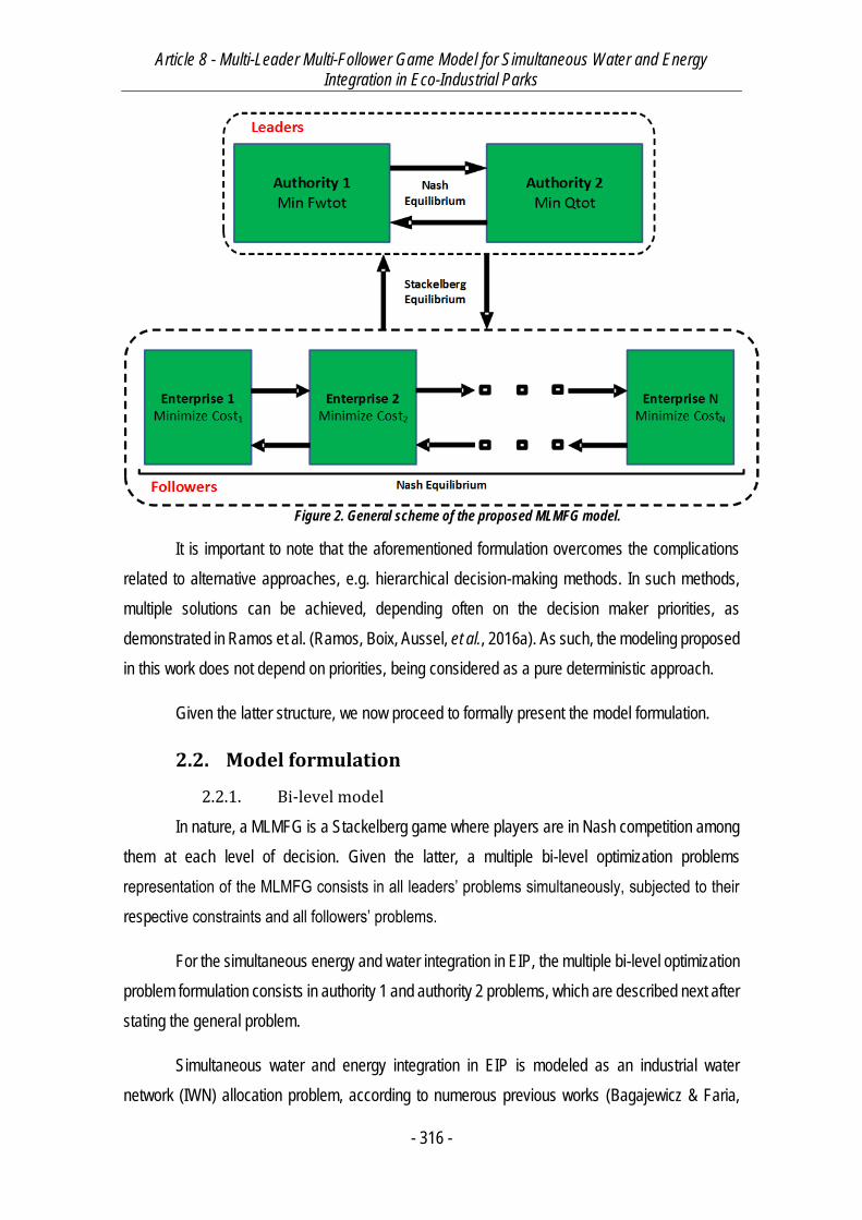
Article 8 - Multi-Leader Multi-Follower Game Model for Simultaneous Water and Energy Integration in Eco-Industrial Parks
- 316 -
Figure 2. General scheme of the proposed MLMFG model.
It is important to note that the aforementioned formulation overcomes the complications
related to alternative approaches, e.g. hierarchical decision-making methods. In such methods,
multiple solutions can be achieved, depending often on the decision maker priorities, as
demonstrated in Ramos et al. (Ramos, Boix, Aussel, et al., 2016a). As such, the modeling proposed
in this work does not depend on priorities, being considered as a pure deterministic approach.
Given the latter structure, we now proceed to formally present the model formulation.
2.2. Model formulation
2.2.1. Bi-level model
In nature, a MLMFG is a Stackelberg game where players are in Nash competition among
them at each level of decision. Given the latter, a multiple bi-level optimization problems
representation of the MLMFG consists in all leaders’ problems simultaneously, subjected to their
respective constraints and all followers’ problems.
For the simultaneous energy and water integration in EIP, the multiple bi-level optimization
problem formulation consists in authority 1 and authority 2 problems, which are described next after
stating the general problem.
Simultaneous water and energy integration in EIP is modeled as an industrial water
network (IWN) allocation problem, according to numerous previous works (Bagajewicz & Faria,
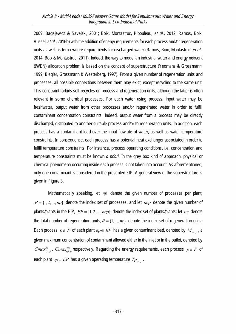
Article 8 - Multi-Leader Multi-Follower Game Model for Simultaneous Water and Energy Integration in Eco-Industrial Parks
- 317 -
2009; Bagajewicz & Savelski, 2001; Boix, Montastruc, Pibouleau, et al., 2012; Ramos, Boix,
Aussel, et al., 2016b) with the addition of energy requirements for each process and/or regeneration
units as well as temperature requirements for discharged water (Ramos, Boix, Montastruc, et al.,
2014; Boix & Montastruc, 2011). Indeed, the way to model an industrial water and energy network
(IWEN) allocation problem is based on the concept of superstructure (Yeomans & Grossmann,
1999; Biegler, Grossmann & Westerberg, 1997). From a given number of regeneration units and
processes, all possible connections between them may exist, except recycling to the same unit.
This constraint forbids self-recycles on process and regeneration units, although the latter is often
relevant in some chemical processes. For each water using process, input water may be
freshwater, output water from other processes and/or regenerated water in order to fulfill
contaminant concentration constraints. Indeed, output water from a process may be directly
discharged, distributed to another suitable process and/or to regeneration units. In addition, each
process has a contaminant load over the input flowrate of water, as well as water temperature
constraints. In consequence, each process has a potential heat exchanger associated in order to
fulfill temperature constraints. For instance, process operating conditions, i.e. concentration and
temperature constraints must be known a priori. In the grey box kind of approach, physical or
chemical phenomena occurring inside each process is not taken into account. As aforementioned,
only one contaminant is considered in the presented EIP. A general view of the superstructure is
given in Figure 3.
Mathematically speaking, let np denote the given number of processes per plant,
{1,2,..., }P np denote the index set of processes, and let nep denote the given number of
plants/plants in the EIP, {1,2,..., }EP nep denote the index set of plants/plants; let nr denote
the total number of regeneration units, {1,..., }R nr denote the index set of regeneration units.
Each process p P of each plant ep EP has a given contaminant load, denoted by ,ep pM , a
given maximum concentration of contaminant allowed either in the inlet or in the outlet, denoted by
,inep pCmax , ,
outep pCmax respectively. Regarding the energy requirements, each process p P of
each plant ep EP has a given operating temperature ,ep pTp .
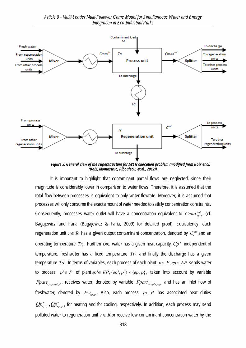
Article 8 - Multi-Leader Multi-Follower Game Model for Simultaneous Water and Energy Integration in Eco-Industrial Parks
- 318 -
Figure 3. General view of the superstructure for IWEN allocation problem (modified from Boix et al. (Boix, Montastruc, Pibouleau, et al., 2012)).
It is important to highlight that contaminant partial flows are neglected, since their
magnitude is considerably lower in comparison to water flows. Therefore, it is assumed that the
total flow between processes is equivalent to only water flowrate. Moreover, it is assumed that
processes will only consume the exact amount of water needed to satisfy concentration constraints.
Consequently, processes water outlet will have a concentration equivalent to ,outep pCmax (cf.
Bagajewicz and Faria (Bagajewicz & Faria, 2009) for detailed proof). Equivalently, each
regeneration unit r R has a given output contaminant concentration, denoted by outrC and an
operating temperature rTr . Furthermore, water has a given heat capacity wCp independent of
temperature, freshwater has a fixed temperature Tw and finally the discharge has a given
temperature Td . In terms of variables, each process of each plant ,p P ep EP sends water
to process 'p P of plant ' , { ', '} { , }ep EP ep p ep p , taken into account by variable
, , ', 'ep p ep pFpart , receives water, denoted by variable ', ', ,ep p ep pFpart and has an inlet flow of
freshwater, denoted by ,ep pFw . Also, each process p P has associated heat duties
, ,,ep p ep pQp Qp , for heating and for cooling, respectively. In addition, each process may send
polluted water to regeneration unit r R or receive low contaminant concentration water by the
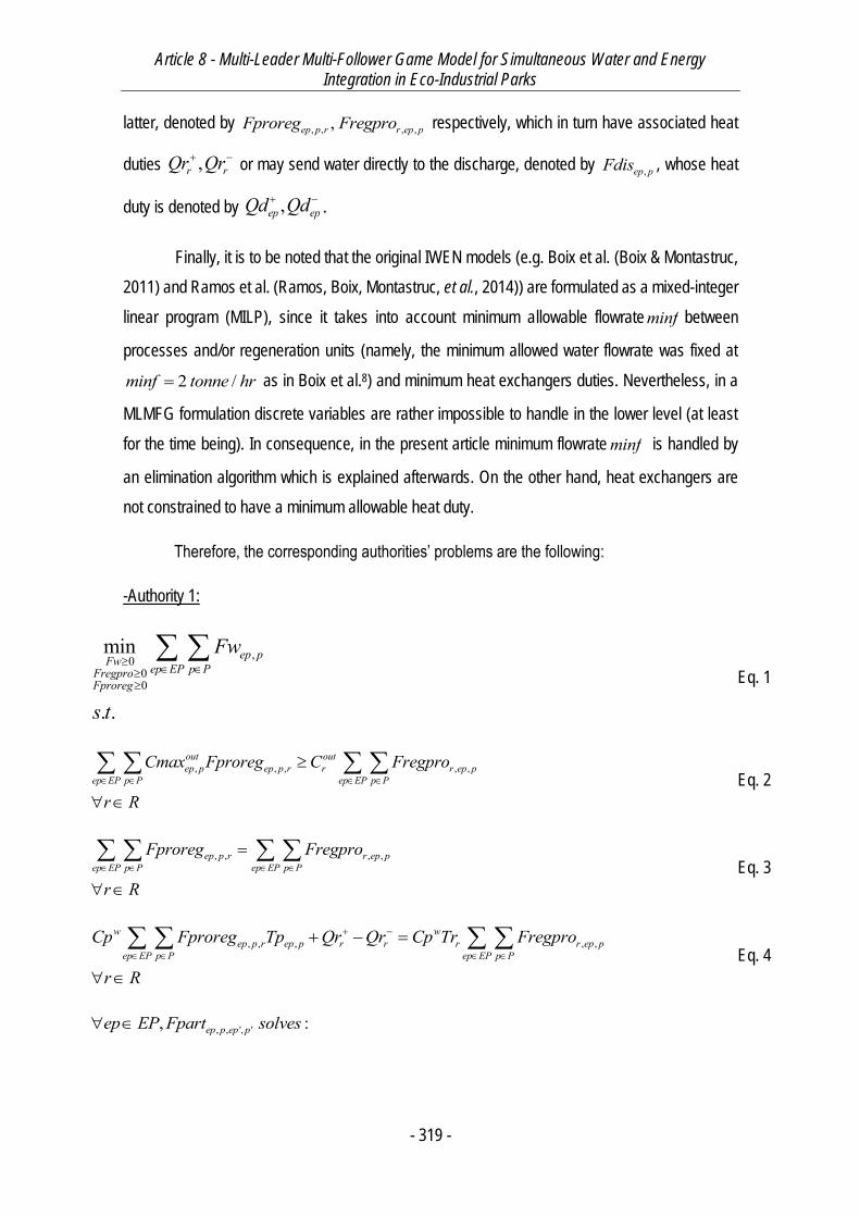
Article 8 - Multi-Leader Multi-Follower Game Model for Simultaneous Water and Energy Integration in Eco-Industrial Parks
- 319 -
latter, denoted by , , , ,,ep p r r ep pFproreg Fregpro respectively, which in turn have associated heat
duties ,r rQr Qr or may send water directly to the discharge, denoted by ,ep pFdis , whose heat
duty is denoted by ,ep epQd Qd .
Finally, it is to be noted that the original IWEN models (e.g. Boix et al. (Boix & Montastruc,
2011) and Ramos et al. (Ramos, Boix, Montastruc, et al., 2014)) are formulated as a mixed-integer
linear program (MILP), since it takes into account minimum allowable flowrateminf between
processes and/or regeneration units (namely, the minimum allowed water flowrate was fixed at
2 /minf tonne hr as in Boix et al.8) and minimum heat exchangers duties. Nevertheless, in a
MLMFG formulation discrete variables are rather impossible to handle in the lower level (at least
for the time being). In consequence, in the present article minimum flowrateminf is handled by
an elimination algorithm which is explained afterwards. On the other hand, heat exchangers are
not constrained to have a minimum allowable heat duty.
Therefore, the corresponding authorities’ problems are the following:
-Authority 1:
Eq. 1
, , , , ,out outep p ep p r r r ep p
ep EP p P ep EP p PCmax Fproreg C Fregpro
r R
Eq. 2
, , , ,ep p r r ep pep EP p P ep EP p P
Fproreg Fregpro
r R
Eq. 3
, , , , ,w w
ep p r ep p r r r r ep pep EP p P ep EP p P
Cp Fproreg Tp Qr Qr Cp Tr Fregpro
r R
Eq. 4
,000
min
. .
ep pFw ep EP p PFregproFproreg
Fw
s t
, , ', ', :ep p ep pep EP Fpart solves
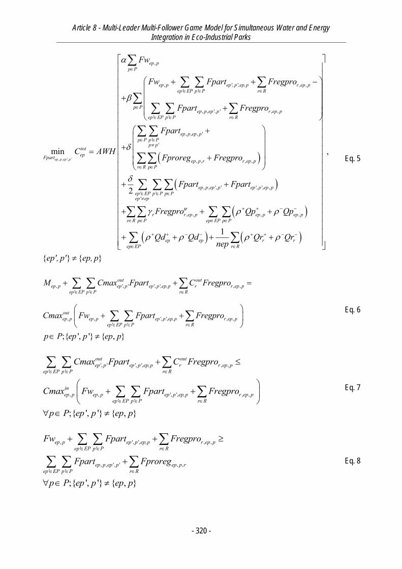
Article 8 - Multi-Leader Multi-Follower Game Model for Simultaneous Water and Energy Integration in Eco-Industrial Parks
- 320 -
, , ', '
,
, ', ', , ,' '
, , ' ' , ,' '
, , , ''
'
,
minep p ep p
ep pp P
ep p ep p ep,p r ep pep EP p P r R
p Pep p ep ,p r ep p
ep EP p P r R
ep p ep pp P p P
p ptotepFpart
ep p
Fw
Fw Fpart Fregpro
Fpart Fregpro
Fpart
C AWHFproreg
, , ,
, , ', ' ', ', ,' ''
, , , ,
2
1
r r ep pr R p P
ep p ep p ep p ep pep EP p P p Pep ep
r r ep p ep p ep pr R p P ep EP p P
ep ep r rep EP r R
Fregpro
Fpart Fpart
Fregpro Qp Qp
Qd Qd Qr Qrnep
,
{ } { }ep', p' ep, p
Eq. 5
Eq. 6
Eq. 7
Eq. 8
, ', ' ', ', , ,' '
, , ', ', , ,' '
;{ ', '} { , }
out outep p ep p ep p ep,p r r ep p
ep EP p P r R
outep p ep p ep p ep,p r ep p
ep EP p P r R
M Cmax Fpart C Fregpro
Cmax Fw Fpart Fregpro
p P ep p ep p
', ' ', ', , ,' '
, , ', ', , ,' '
;{ ', '} { , }
out outep p ep p ep,p r r ep p
ep EP p P r R
inep p ep p ep p ep,p r ep p
ep EP p P r R
Cmax Fpart C Fregpro
Cmax Fw Fpart Fregpro
p P ep p ep p
, ', ', , ,' '
, , ' ' , ,' '
;{ ', '} { , }
ep p ep p ep,p r ep pep EP p P r R
ep p ep ,p ep p rep EP p P r R
Fw Fpart Fregpro
Fpart Fproreg
p P ep p ep p
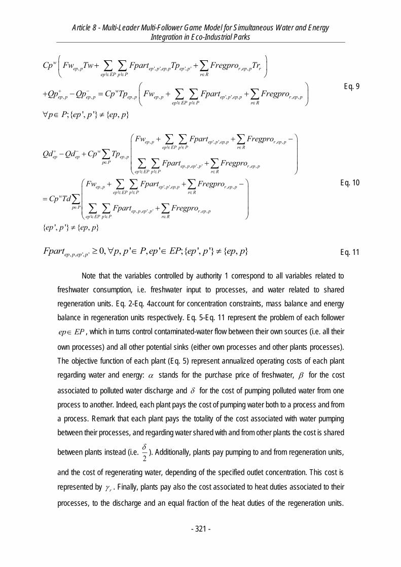
Article 8 - Multi-Leader Multi-Follower Game Model for Simultaneous Water and Energy Integration in Eco-Industrial Parks
- 321 -
Eq. 9
, ', ', , ,' '
,
, , ' ' , ,' '
, ', ', , ,' '
ep p ep p ep,p r ep pep EP p P r R
wep ep ep p
p Pep p ep ,p r ep p
ep EP p P r R
ep p ep p ep,p r ep pep EP p P r R
w
Fw Fpart Fregpro
Qd Qd Cp TpFpart Fregpro
Fw Fpart Fregpro
Cp TdFpa
, , ' ' , ,' '
{ ', '} { , }
p Pep p ep ,p r ep p
ep EP p P r Rrt Fregpro
ep p ep p
Eq. 10
Eq. 11
Note that the variables controlled by authority 1 correspond to all variables related to
freshwater consumption, i.e. freshwater input to processes, and water related to shared
regeneration units. Eq. 2-Eq. 4account for concentration constraints, mass balance and energy
balance in regeneration units respectively. Eq. 5-Eq. 11 represent the problem of each follower
ep EP , which in turns control contaminated-water flow between their own sources (i.e. all their
own processes) and all other potential sinks (either own processes and other plants processes).
The objective function of each plant (Eq. 5) represent annualized operating costs of each plant
regarding water and energy: stands for the purchase price of freshwater, for the cost
associated to polluted water discharge and for the cost of pumping polluted water from one
process to another. Indeed, each plant pays the cost of pumping water both to a process and from
a process. Remark that each plant pays the totality of the cost associated with water pumping
between their processes, and regarding water shared with and from other plants the cost is shared
between plants instead (i.e. 2
). Additionally, plants pay pumping to and from regeneration units,
and the cost of regenerating water, depending of the specified outlet concentration. This cost is
represented by r . Finally, plants pay also the cost associated to heat duties associated to their
processes, to the discharge and an equal fraction of the heat duties of the regeneration units.
, ', ', ', ' , ,' '
, , , , ', ', , ,' '
;{ ', '} { , }
wep p ep p ep,p ep p r ep p r
ep EP p P r R
wep p ep p ep p ep p ep p ep,p r ep p
ep EP p P r R
Cp Fw Tw Fpart Tp Fregpro Tr
Qp Qp Cp Tp Fw Fpart Fregpro
p P ep p ep p
, , ', ' 0, , ' , ' ;{ ', '} { , }ep p ep pFpart p p P ep EP ep p ep p

Article 8 - Multi-Leader Multi-Follower Game Model for Simultaneous Water and Energy Integration in Eco-Industrial Parks
- 322 -
, represent costs related to heating and cooling utility, respectively. Eq. 6-Eq. 9 stand
respectively for water mass balance, concentration constraints, discharged water positivity and
energy balance for each process of each plant, while Eq. 10 represents the discharge energy
balance and Eq. 11 shared flow positivity between processes.
-Authority 2:
, ,000
min
. .
ep p ep p ep ep r rQp ep EP p P ep EP r RQrQd
Qp Qp Qd Qd Qr Qr
s t
Eq. 12
, , , , ,w w
ep p r ep p r r r r ep pep EP p P ep EP p P
Cp Fproreg Tp Qr Qr Cp Tr Fregpro
r R
, , ', ', :ep p ep pep EP Fpart solves
Eq. 5-Eq. 11
The second leader, i.e. the authority 2, has as decision variables all heat flows associated
to processes, regeneration units and discharge. Note that Eq. 4 appears in both leaders’ problems.
2.2.2. All equilibrium MOPEC reformulation
In order to transform the latter multiple bi-level problems into a mathematically tractable
form, bi-level problems 1 and 2 can be reformulated into multiple optimization problems with
equilibrium constraints (MOPEC). Assuming that all followers’ problems are convex, i.e. the
objective functions and constraints are respectively convex functions and concave functions in the
decision variables of the followers, then for any solution set of the followers-problems’ Karush-
Kuhn-Tucker (KKT) optimality conditions,
, , ', ' , , ' , ' ,{ ', '} { , }ep p ep pFpart p p P ep EP ep p ep p is a global optimal solution of the
follower problem. Note that KKT conditions are equivalent to the parametric nonlinear
complementarity problem (NCP) (Leyffer & Munson, 2010) (Kulkarni & Shanbhag, 2014).
Indeed, in our case the objective function and the constraints of the respective followers
are actually linear, thus convex and concave on the variables controlled by the follower. Though,
followers’ problems may have non-convex terms on the leaders’ variables, but they do not affect
the non-convexity since they are seen as parameters in the followers’ problems.
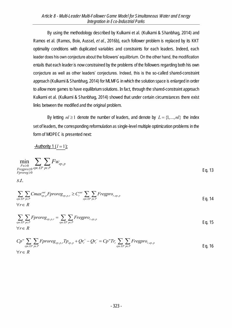
Article 8 - Multi-Leader Multi-Follower Game Model for Simultaneous Water and Energy Integration in Eco-Industrial Parks
- 323 -
By using the methodology described by Kulkarni et al. (Kulkarni & Shanbhag, 2014) and
Ramos et al. (Ramos, Boix, Aussel, et al., 2016b), each follower problem is replaced by its KKT
optimality conditions with duplicated variables and constraints for each leaders. Indeed, each
leader does his own conjecture about the followers’ equilibrium. On the other hand, the modification
entails that each leader is now constrained by the problems of the followers regarding both his own
conjecture as well as other leaders’ conjectures. Indeed, this is the so-called shared-constraint
approach (Kulkarni & Shanbhag, 2014) for MLMFG in which the solution space is enlarged in order
to allow more games to have equilibrium solutions. In fact, through the shared-constraint approach
Kulkarni et al. (Kulkarni & Shanbhag, 2014) showed that under certain circumstances there exist
links between the modified and the original problem.
By letting 1nl denote the number of leaders, and denote by {1,..., }L nl the index
set of leaders, the corresponding reformulation as single-level multiple optimization problems in the
form of MOPEC is presented next:
-Authority 1 ( 1l ):
Eq. 13
, , , , ,out outep p ep p r r r ep p
ep EP p P ep EP p PCmax Fproreg C Fregpro
r R
Eq. 14
, , , ,ep p r r ep pep EP p P ep EP p P
Fproreg Fregpro
r R
Eq. 15
, , , , ,w w
ep p r ep p r r r r ep pep EP p P ep EP p P
Cp Fproreg Tp Qr Qr Cp Tr Fregpro
r R
Eq. 16
,000
min
. .
ep pFw ep EP p PFregproFproreg
Fw
s t
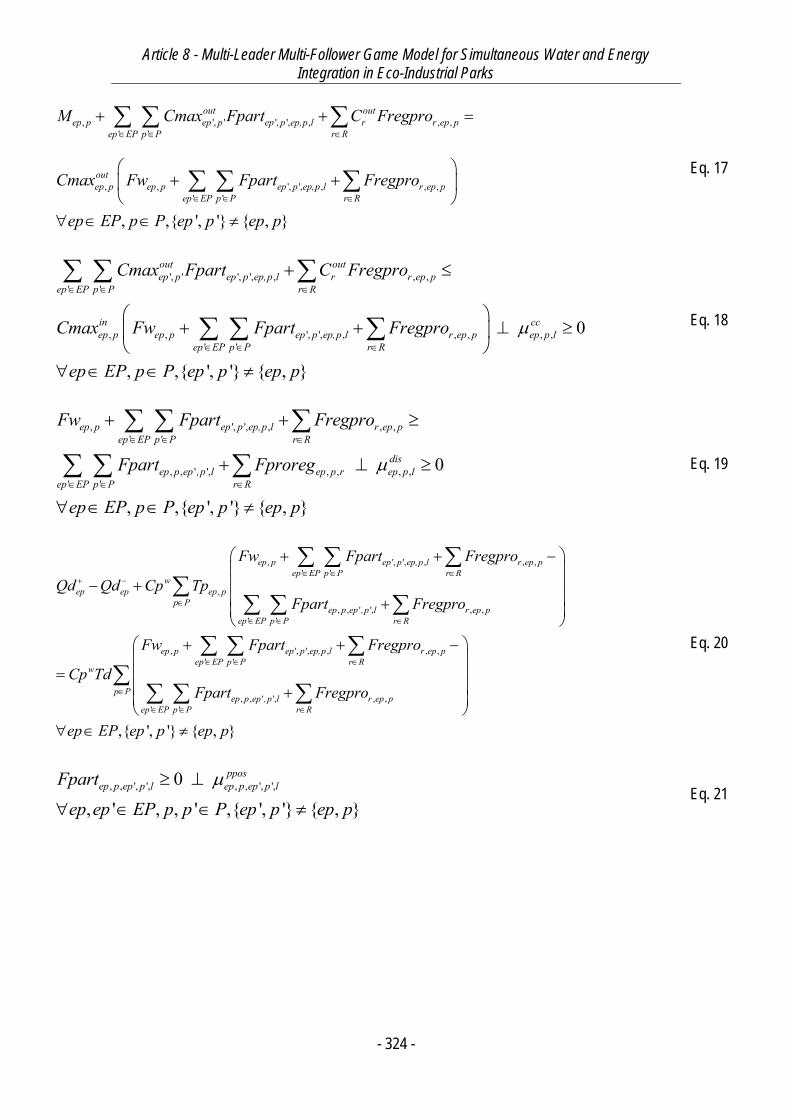
Article 8 - Multi-Leader Multi-Follower Game Model for Simultaneous Water and Energy Integration in Eco-Industrial Parks
- 324 -
, ', ' ', ', , , ,' '
, , ', ', , , ,' '
, ,{ ', '} { , }
out outep p ep p ep p ep,p l r r ep p
ep EP p P r R
outep p ep p ep p ep,p l r ep p
ep EP p P r R
M Cmax Fpart C Fregpro
Cmax Fw Fpart Fregpro
ep EP p P ep p ep p
Eq. 17
', ' ', ', , , ,' '
, , ', ', , , , , ,' '
0
, ,{ ', '} { , }
out outep p ep p ep,p l r r ep p
ep EP p P r R
in ccep p ep p ep p ep,p l r ep p ep p l
ep EP p P r R
Cmax Fpart C Fregpro
Cmax Fw Fpart Fregpro
ep EP p P ep p ep p
Eq. 18
, ', ', , , ,' '
, , ' ', , , , ,' '
0
, ,{ ', '} { , }
ep p ep p ep,p l r ep pep EP p P r R
disep p ep ,p l ep p r ep p l
ep EP p P r R
Fw Fpart Fregpro
Fpart Fproreg
ep EP p P ep p ep p
Eq. 19
, ', ', , , ,' '
,
, , ' ', , ,' '
, ', ', , , ,' '
ep p ep p ep,p l r ep pep EP p P r R
wep ep ep p
p Pep p ep ,p l r ep p
ep EP p P r R
ep p ep p ep,p l r ep pep EP p P r
w
Fw Fpart Fregpro
Qd Qd Cp TpFpart Fregpro
Fw Fpart Fregpro
Cp Td
, , ' ', , ,' '
,{ ', '} { , }
R
p Pep p ep ,p l r ep p
ep EP p P r RFpart Fregpro
ep EP ep p ep p
Eq. 20
, , ', ', , , ', ',0
, ' , , ' ,{ ', '} { , }
pposep p ep p l ep p ep p lFpart
ep ep EP p p P ep p ep p
Eq. 21
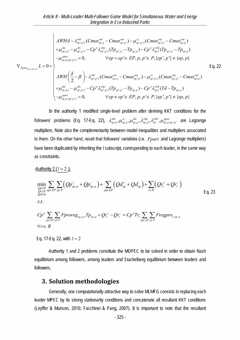
Article 8 - Multi-Leader Multi-Follower Game Model for Simultaneous Water and Energy Integration in Eco-Industrial Parks
- 325 -
, , ', ',
', ', , ', ' ', ', ', ' ,
, , ', ', ', ', ', ' , , ', ' ,
, ,
( ) ( )
( ) ( )
0ep p ep p l
mb out out cc out outep p l ep p ep p ep p l ep p ep p
dis dis w ebp w ebdep p l ep p l ep p l ep p ep p ep l ep p ep p
ep p ep
Fpart
AWH Cmax Cmax Cmax Cmax
Cp Tp Tp Cp Tp Tp
L
', ',
', ', , ', ' ', ', ', ' ,
, , ', ', ', ', ', ' ,
0, ' , , ' ,{ ', '} { , }
( ) ( )2
( )
pposp l
mb out out cc out outep p l ep p ep p ep p l ep p ep p
dis dis w ebp wep p l ep p l ep p l ep p ep p e
ep ep EP p p P ep p ep p
AWH Cmax Cmax Cmax Cmax
Cp Tp Tp Cp
, ,
, , ', ',
( )
0, ' , , ' ,{ ', '} { , }
ebdp l ep p
pposep p ep p l
Td Tp
ep ep EP p p P ep p ep p
Eq. 22
In the authority 1 modified single-level problem after deriving KKT conditions for the
followers’ problems (Eq. 17-Eq. 22), , , , , , , ', ', , , , ,mb cc dis ebp ebd pposep p ep p ep p ep p ep ep p ep p are Lagrange
multipliers. Note also the complementarity between model inequalities and multipliers associated
to them. On the other hand, recall that followers’ variables (i.e. Fpart and Lagrange multipliers)
have been duplicated by inheriting the l subscript, corresponding to each leader, in the same way
as constraints.
-Authority 2 ( 2l ):
, ,000
min
. .
ep p ep p ep ep r rQp ep EP p P ep EP r RQrQd
Qp Qp Qd Qd Qr Qr
s t
Eq. 23
, , , , ,w w
ep p r ep p r r r r ep pep EP p P ep EP p P
Cp Fproreg Tp Qr Qr Cp Tr Fregpro
r R
Eq. 17-Eq. 22, with 2l
Authority 1 and 2 problems constitute the MOPEC to be solved in order to obtain Nash
equilibrium among followers, among leaders and Stackelberg equilibrium between leaders and
followers.
3. Solution methodologies
Generally, one computationally attractive way to solve MLMFG consists in replacing each
leader MPEC by its strong stationarity conditions and concatenate all resultant KKT conditions
(Leyffer & Munson, 2010; Facchinei & Pang, 2007). It is important to note that the resultant
Article 8 - Multi-Leader Multi-Follower Game Model for Simultaneous Water and Energy Integration in Eco-Industrial Parks
- 326 -
optimization problems are always non-convex due to the presence of complementarity constraints.
Then, by using this method in reality strong stationarity points are obtained for each optimization
problem. By itself, the problem derived with this method is an NCP.
Note that the obtained problem is not a squared NCP (cf. Ramos et al. (Ramos, Boix, Aussel, et
al., 2016b)), since each inequality constraint is matched with two complementarity constraints.
Therefore, this formulation is very hard to solve (and even more for large-scale problems) by using
standard NCP solvers (i.e. PATH (Dirkse & Ferris, 1996)) since constraints violate any classical
constraint qualification due to the presence of complementarity conditions (Leyffer & Munson,
2010).
However, the NCP formulation can be used to derive NLP formulations of a MLMFG. A
very interesting alternative which exploits the capacity of modern NLP solvers is the so-called
penalty formulation (Biegler, 2010). This formulation consists in moving the complementarity
constraints to a penalization objective function ( penC ), which is minimized. The latter is very
convenient for the MLMFG, since it does not exhibit a typical NLP formulation, i.e. no explicit single-
objective function, due to its nature as a MOPEC. Hence, the remaining constraints are well
behaved. The above formulation is in fact one of the several formulations to solve general MPEC
problems (cf. Biegler (Biegler, 2010) for all possible formulations) and it is the most adequate to
solve MLMFG problems and MPECs in general (Biegler, 2010). In addition, Leyffer and Munson
(Leyffer & Munson, 2010) proved that if 0penC and if all variables describe a local solution of
the minimization problem, then the solution is a strong stationarity point of the MLMFG. By moving
complementarities to the objective function, most difficulties of the NCP formulation are overcome
including the non-square nature the original NCP.
All problems were modeled in GAMS® (Brooke, Kendrick, Meeraus, et al., 1998) 24.4.2
and transformed into the NLP formulation through the extended mathematical programming
framework (EMP). The framework uses the solver JAMS to reformulate MOPECs into NCPs.
Evidently, it is the modeler task to transform the original MLMFG into his MOPEC formulation. Then,
it is the modeler choice to reformulate and solve it using all available reformulations of MPECs
available in GAMS framework NLPEC. In the case of the NLP reformulation, a standard NLP solver
is required. In this work, BARON (Tawarmalani & Sahinidis, 2005) was chosen as the solver, since
its demonstrated effectiveness in past works (Ramos, Boix, Aussel, et al., 2016b). Moreover, In the
context of a penalization scheme, a global solver like BARON is very useful to find the solution

Article 8 - Multi-Leader Multi-Follower Game Model for Simultaneous Water and Energy Integration in Eco-Industrial Parks
- 327 -
where 0penC . Moreover, recent work (Zhang & Sahinidis, 2015) demonstrated the usefulness
of BARON in general MPEC problems, using recent versions of it. The resulting solved problem
after all reformulations is composed by 3315 constraints and 6087 continuous variables, and it was
solved in 17.6s in an Intel I5 quad-core processor with 8Gb of ram and the subsolvers CPLEX for
MILP and CONOPT for NLP.
Another important point is the manipulation of discrete decisions of the original problem
(cf. Bagajewicz and Savelski (Bagajewicz & Savelski, 2001)) in the MLMFG framework. In order to
deal with allowable minimum flow, we apply a finite sequence of steps, each step being composed
of first the resolution of the MLMFG problem in his NLP formulation, and second, an elimination
procedure that aims to force to zero or to minf (depending on the closeness to minf ) the flow
of any oriented connection for which step 1 gave a flow lower that a minimum fixed bound minf .
This is indeed modeled by big-M constraints and binary variables in the former classical water
integration (Ramos, Boix, Montastruc, et al., 2014; Bagajewicz & Faria, 2009) model. In this work,
we developed an a posteriori algorithm to add bounds to existing flows and to eliminate low flows.
Indeed, the MLMFG is solved several times until all water flows are equal or superior to minf . The
algorithm is described in detail next, using as example , , ', ',ep p ep p lFpart (all other flows are handled
simultaneously and equivalently):
10) The initial MLMFG is solved to optimality.
11) For all , ' , ,ep ep EP p, p' P,l L {ep, p} {ep', p'} :
a. If , , ', ',34ep p ep p lFpart minf , then a lower bound of the flow is imposed that is
the constraint , , ', ',ep p ep p lFpart minf is added to the model.
b. If , , ', ',34ep p ep p lFpart minf , then the flow is fixed , , ', ', 0ep p ep p lFpart
c. Else, if all flows , , ', ',ep p ep p lFpart minf , then the problem has converged and
no further treatment is required.
12) The bound-modified MLMFG problem is tried to be solved to optimality:
a. If optimality is achieved, then go to 2).
b. Else, try solving to optimality with a different solver.
i. If optimality is achieved, then go to 2).
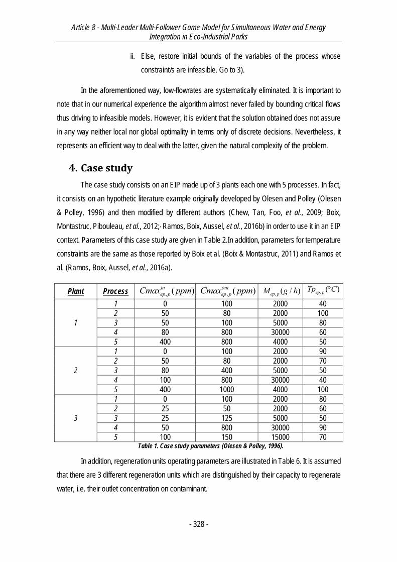
Article 8 - Multi-Leader Multi-Follower Game Model for Simultaneous Water and Energy Integration in Eco-Industrial Parks
- 328 -
ii. Else, restore initial bounds of the variables of the process whose
constraint/s are infeasible. Go to 3).
In the aforementioned way, low-flowrates are systematically eliminated. It is important to
note that in our numerical experience the algorithm almost never failed by bounding critical flows
thus driving to infeasible models. However, it is evident that the solution obtained does not assure
in any way neither local nor global optimality in terms only of discrete decisions. Nevertheless, it
represents an efficient way to deal with the latter, given the natural complexity of the problem.
4. Case study
The case study consists on an EIP made up of 3 plants each one with 5 processes. In fact,
it consists on an hypothetic literature example originally developed by Olesen and Polley (Olesen
& Polley, 1996) and then modified by different authors (Chew, Tan, Foo, et al., 2009; Boix,
Montastruc, Pibouleau, et al., 2012;, Ramos, Boix, Aussel, et al., 2016b) in order to use it in an EIP
context. Parameters of this case study are given in Table 2.In addition, parameters for temperature
constraints are the same as those reported by Boix et al. (Boix & Montastruc, 2011) and Ramos et
al. (Ramos, Boix, Aussel, et al., 2016a).
Plant Process , ( )inep pCmax ppm , ( )out
ep pCmax ppm , ( / )ep pM g h , ( )ep pTp C
1
1 0 100 2000 40
2 50 80 2000 100
3 50 100 5000 80
4 80 800 30000 60
5 400 800 4000 50
2
1 0 100 2000 90
2 50 80 2000 70
3 80 400 5000 50
4 100 800 30000 40
5 400 1000 4000 100
3
1 0 100 2000 80
2 25 50 2000 60
3 25 125 5000 50
4 50 800 30000 90
5 100 150 15000 70 Table 1. Case study parameters (Olesen & Polley, 1996).
In addition, regeneration units operating parameters are illustrated in Table 6. It is assumed
that there are 3 different regeneration units which are distinguished by their capacity to regenerate
water, i.e. their outlet concentration on contaminant.
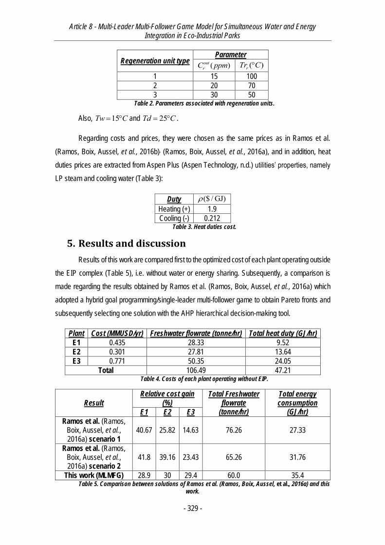
Article 8 - Multi-Leader Multi-Follower Game Model for Simultaneous Water and Energy Integration in Eco-Industrial Parks
- 329 -
Regeneration unit type Parameter
( )outrC ppm ( )rTr C
1 15 100
2 20 70
3 30 50 Table 2. Parameters associated with regeneration units.
Also, 15Tw C and 25Td C .
Regarding costs and prices, they were chosen as the same prices as in Ramos et al.
(Ramos, Boix, Aussel, et al., 2016b), (Ramos, Boix, Aussel, et al., 2016a), and in addition, heat
duties prices are extracted from Aspen Plus (Aspen Technology, n.d.) utilities’ properties, namely
LP steam and cooling water (Table 3):
Duty ($ / GJ)
Heating (+) 1.9
Cooling (-) 0.212 Table 3. Heat duties cost.
5. Results and discussion
Results of this work are compared first to the optimized cost of each plant operating outside
the EIP complex (Table 5), i.e. without water or energy sharing. Subsequently, a comparison is
made regarding the results obtained by Ramos et al. (Ramos, Boix, Aussel, et al., 2016a) which
adopted a hybrid goal programming/single-leader multi-follower game to obtain Pareto fronts and
subsequently selecting one solution with the AHP hierarchical decision-making tool.
Plant Cost (MMUSD/yr) Freshwater flowrate (tonne/hr) Total heat duty (GJ/hr)
E1 0.435 28.33 9.52
E2 0.301 27.81 13.64
E3 0.771 50.35 24.05
Total 106.49 47.21 Table 4. Costs of each plant operating without EIP.
Result Relative cost gain
(%) Total Freshwater
flowrate (tonne/hr)
Total energy consumption
(GJ/hr) E1 E2 E3
Ramos et al. (Ramos, Boix, Aussel, et al., 2016a) scenario 1
40.67 25.82 14.63 76.26 27.33
Ramos et al. (Ramos, Boix, Aussel, et al., 2016a) scenario 2
41.8 39.16 23.43 65.26 31.76
This work (MLMFG) 28.9 30 29.4 60.0 35.4 Table 5. Comparison between solutions of Ramos et al. (Ramos, Boix, Aussel, et al., 2016a) and this
work.
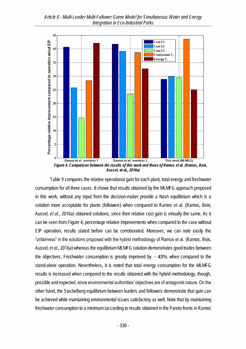
Article 8 - Multi-Leader Multi-Follower Game Model for Simultaneous Water and Energy Integration in Eco-Industrial Parks
- 330 -
Figure 4. Comparison between the results of this work and those of Ramos et al. (Ramos, Boix,
Aussel, et al., 2016a)
Table 9 compares the relative operational gain for each plant, total energy and freshwater
consumption for all three cases. It shows that results obtained by the MLMFG approach proposed
in this work, without any input from the decision-maker provide a Nash equilibrium which is a
solution more acceptable for plants (followers) when compared to Ramos et al. (Ramos, Boix,
Aussel, et al., 2016a) obtained solutions, since their relative cost gain is virtually the same. As it
can be seen from Figure 4, percentage relative improvements when compared to the case without
EIP operation, results stated before can be corroborated. Moreover, we can note easily the
“unfairness” in the solutions proposed with the hybrid methodology of Ramos et al. (Ramos, Boix,
Aussel, et al., 2016a) whereas the equilibrium MLMFG solution demonstrates good trades between
the objectives. Freshwater consumption is greatly improved by 43%43% when compared to the
stand-alone operation. Nevertheless, it is noted that total energy consumption for the MLMFG
results is increased when compared to the results obtained with the hybrid methodology, though,
possible and expected, since environmental authorities’ objectives are of antagonist nature. On the
other hand, the Stackelberg equilibrium between leaders and followers demonstrate that gain can
be achieved while maintaining environmental issues satisfactory as well. Note that by maintaining
freshwater consumption to a minimum (according to results obtained in the Pareto fronts in Ramos
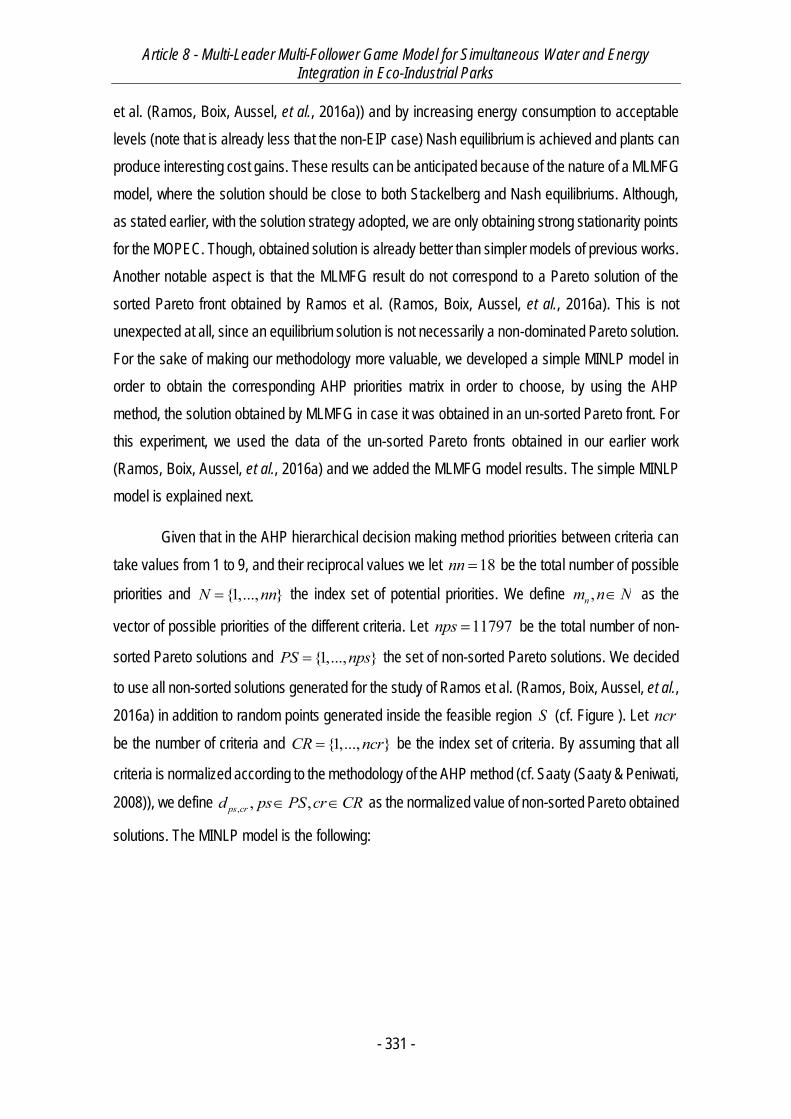
Article 8 - Multi-Leader Multi-Follower Game Model for Simultaneous Water and Energy Integration in Eco-Industrial Parks
- 331 -
et al. (Ramos, Boix, Aussel, et al., 2016a)) and by increasing energy consumption to acceptable
levels (note that is already less that the non-EIP case) Nash equilibrium is achieved and plants can
produce interesting cost gains. These results can be anticipated because of the nature of a MLMFG
model, where the solution should be close to both Stackelberg and Nash equilibriums. Although,
as stated earlier, with the solution strategy adopted, we are only obtaining strong stationarity points
for the MOPEC. Though, obtained solution is already better than simpler models of previous works.
Another notable aspect is that the MLMFG result do not correspond to a Pareto solution of the
sorted Pareto front obtained by Ramos et al. (Ramos, Boix, Aussel, et al., 2016a). This is not
unexpected at all, since an equilibrium solution is not necessarily a non-dominated Pareto solution.
For the sake of making our methodology more valuable, we developed a simple MINLP model in
order to obtain the corresponding AHP priorities matrix in order to choose, by using the AHP
method, the solution obtained by MLMFG in case it was obtained in an un-sorted Pareto front. For
this experiment, we used the data of the un-sorted Pareto fronts obtained in our earlier work
(Ramos, Boix, Aussel, et al., 2016a) and we added the MLMFG model results. The simple MINLP
model is explained next.
Given that in the AHP hierarchical decision making method priorities between criteria can
take values from 1 to 9, and their reciprocal values we let 18nn be the total number of possible
priorities and {1,..., }N nn the index set of potential priorities. We define ,nm n N as the
vector of possible priorities of the different criteria. Let 11797nps be the total number of non-
sorted Pareto solutions and {1,..., }PS nps the set of non-sorted Pareto solutions. We decided
to use all non-sorted solutions generated for the study of Ramos et al. (Ramos, Boix, Aussel, et al.,
2016a) in addition to random points generated inside the feasible region S (cf. Figure ). Let ncr
be the number of criteria and {1,..., }CR ncr be the index set of criteria. By assuming that all
criteria is normalized according to the methodology of the AHP method (cf. Saaty (Saaty & Peniwati,
2008)), we define , , ,ps crd ps PS cr CR as the normalized value of non-sorted Pareto obtained
solutions. The MINLP model is the following:
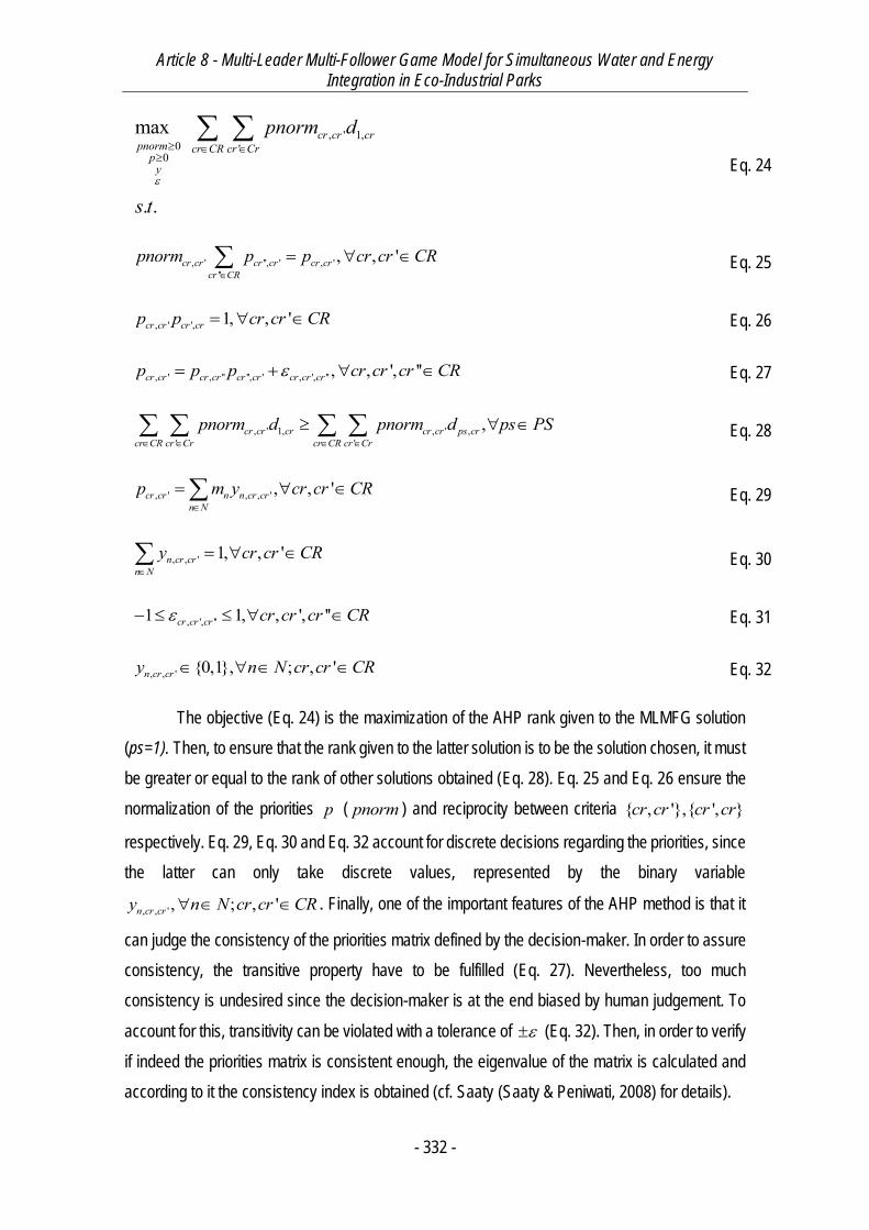
Article 8 - Multi-Leader Multi-Follower Game Model for Simultaneous Water and Energy Integration in Eco-Industrial Parks
- 332 -
, ' 1,0 '
0
max
. .
cr cr crpnorm cr CR cr Crpy
pnorm d
s t
Eq. 24
, ' '', ' , '''
, , 'cr cr cr cr cr crcr CR
pnorm p p cr cr CR
Eq. 25
, ' ', 1, , 'cr cr cr crp p cr cr CR Eq. 26
, ' , '' '', ' , ', '' , , ', ''cr cr cr cr cr cr cr cr crp p p cr cr cr CR Eq. 27
, ' 1, , ' ,' '
,cr cr cr cr cr ps crcr CR cr Cr cr CR cr Cr
pnorm d pnorm d ps PS
Eq. 28
, ' , , ' , , 'cr cr n n cr crn N
p m y cr cr CR
Eq. 29
, , ' 1, , 'n cr crn Ny cr cr CR
Eq. 30
, ', ''1 1, , ', ''cr cr cr cr cr cr CR Eq. 31
, , ' {0,1}, ; , 'n cr cry n N cr cr CR Eq. 32
The objective (Eq. 24) is the maximization of the AHP rank given to the MLMFG solution
(ps=1). Then, to ensure that the rank given to the latter solution is to be the solution chosen, it must
be greater or equal to the rank of other solutions obtained (Eq. 28). Eq. 25 and Eq. 26 ensure the
normalization of the priorities p ( pnorm ) and reciprocity between criteria { , '},{ ', }cr cr cr cr
respectively. Eq. 29, Eq. 30 and Eq. 32 account for discrete decisions regarding the priorities, since
the latter can only take discrete values, represented by the binary variable
, , ', ; , 'n cr cry n N cr cr CR . Finally, one of the important features of the AHP method is that it
can judge the consistency of the priorities matrix defined by the decision-maker. In order to assure
consistency, the transitive property have to be fulfilled (Eq. 27). Nevertheless, too much
consistency is undesired since the decision-maker is at the end biased by human judgement. To
account for this, transitivity can be violated with a tolerance of (Eq. 32). Then, in order to verify
if indeed the priorities matrix is consistent enough, the eigenvalue of the matrix is calculated and
according to it the consistency index is obtained (cf. Saaty (Saaty & Peniwati, 2008) for details).
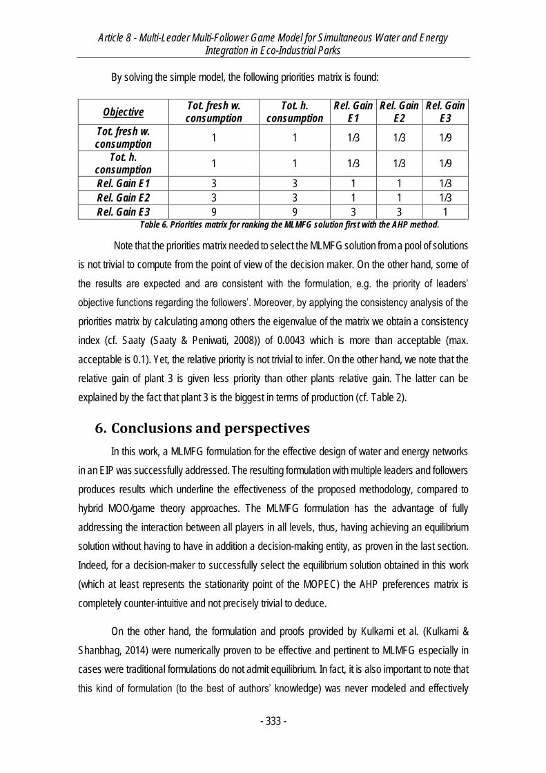
Article 8 - Multi-Leader Multi-Follower Game Model for Simultaneous Water and Energy Integration in Eco-Industrial Parks
- 333 -
By solving the simple model, the following priorities matrix is found:
Objective Tot. fresh w. consumption
Tot. h. consumption
Rel. Gain E1
Rel. Gain E2
Rel. Gain E3
Tot. fresh w. consumption
1 1 1/3 1/3 1/9
Tot. h. consumption
1 1 1/3 1/3 1/9
Rel. Gain E1 3 3 1 1 1/3
Rel. Gain E2 3 3 1 1 1/3
Rel. Gain E3 9 9 3 3 1 Table 6. Priorities matrix for ranking the MLMFG solution first with the AHP method.
Note that the priorities matrix needed to select the MLMFG solution from a pool of solutions
is not trivial to compute from the point of view of the decision maker. On the other hand, some of
the results are expected and are consistent with the formulation, e.g. the priority of leaders’
objective functions regarding the followers’. Moreover, by applying the consistency analysis of the
priorities matrix by calculating among others the eigenvalue of the matrix we obtain a consistency
index (cf. Saaty (Saaty & Peniwati, 2008)) of 0.0043 which is more than acceptable (max.
acceptable is 0.1). Yet, the relative priority is not trivial to infer. On the other hand, we note that the
relative gain of plant 3 is given less priority than other plants relative gain. The latter can be
explained by the fact that plant 3 is the biggest in terms of production (cf. Table 2).
6. Conclusions and perspectives
In this work, a MLMFG formulation for the effective design of water and energy networks
in an EIP was successfully addressed. The resulting formulation with multiple leaders and followers
produces results which underline the effectiveness of the proposed methodology, compared to
hybrid MOO/game theory approaches. The MLMFG formulation has the advantage of fully
addressing the interaction between all players in all levels, thus, having achieving an equilibrium
solution without having to have in addition a decision-making entity, as proven in the last section.
Indeed, for a decision-maker to successfully select the equilibrium solution obtained in this work
(which at least represents the stationarity point of the MOPEC) the AHP preferences matrix is
completely counter-intuitive and not precisely trivial to deduce.
On the other hand, the formulation and proofs provided by Kulkarni et al. (Kulkarni &
Shanbhag, 2014) were numerically proven to be effective and pertinent to MLMFG especially in
cases were traditional formulations do not admit equilibrium. In fact, it is also important to note that
this kind of formulation (to the best of authors’ knowledge) was never modeled and effectively

Article 8 - Multi-Leader Multi-Follower Game Model for Simultaneous Water and Energy Integration in Eco-Industrial Parks
- 334 -
solved in mathematical modeling environments such as GAMS®. In a parallel way, the
effectiveness of the solution methods adopted for MLFG was proven to be reliable indeed in
medium/large scale problems, solving to optimality this kind of problems in a matter of seconds,
even if solution methods do not solve the Nash equilibrium directly but its strong stationarity
conditions.
Finally, it was also underlined the usefulness of EIPs in the context of industrial symbiosis
to produce more sustainable industrial outcomes. The results obtained show that, by unifying
efforts, wastes are lowered and effective gain can be achieved. As perspectives, we consider in
the first place the inclusion of renewable energies within the EIP MLMFG formulation, e.g. as a
market regulator which determines the price of energy originating from renewable sources. Second,
the MLMFG methodology can also be applied to utility networks and conceiving multiple
environmental authorities which minimize the environmental impact of all different utilities.
7. Nomenclature
Latin symbols nl = Number of leaders
L = Index set of leaders np = Number of processes per plant
P = Index set of processes nep = Number of plants
EP = Index set of plants nr = Number of regeneration units
R = Index set of regeneration units
M = Contaminant load
,in outCmax Cmax = Maximum contaminant concentration allowed in inlet/outlet
of processes
Tp Operating temperature of processes outC = Outlet concentration of contaminant in regeneration units
Tr Operating temperature of regeneration units wCp Water heat capacity
Tw Freshwater temperature
Td Discharge temperature
Fpart = Water flow between different processes
Fw = Freshwater inlet flow to processes ,Qp = Heating (+), cooling (-) processes heat duty
Fproreg = Water flow from processes to regeneration units
Fregpro = Water flow from regeneration units to processes ,Qr = Heating (+), cooling (-) regeneration units heat duty
Fdis = Water processes to the discharge

Article 8 - Multi-Leader Multi-Follower Game Model for Simultaneous Water and Energy Integration in Eco-Industrial Parks
- 335 -
,Qd = Heating (+), cooling (-) discharge heat duty
minf = Minimum flowrate allowed
AWH = Annual EIP operating hours
nn = Total number of possible priorities in the AHP method
N = Index set of potential priorities
m = Vector of possible priorities of criteria
nps = Total number of non-sorted Pareto solutions
PS = Set of non-sorted Pareto solutions
S = Feasible region
ncr = Number of criteria
CR = Index set of criteria
d = Normalized value of non-sorted Pareto solutions
pnorm = Normalized priority value
Greek symbols = Purchase price of freshwater
= Polluted water discharge cost
= Polluted water pumping cost = Regenerated water cost
= Power associated to , = Heating (+), cooling (-) duty unit cost cc = Lagrange multiplier of concentration inequality constraints dis = Lagrange multiplier of discharge positivity inequality constraints ppos = Lagrange multiplier of Fpart positivity constraints mb = Lagrange multiplier of mass balance equality constraints mb = Lagrange multiplier of processes mass balance equality constraints ebp = Lagrange multiplier of process energy balance equality constraints ebd = Lagrange multiplier of discharge energy balance equality constraints
= Tolerance for transitivity violation
Article 8 - Multi-Leader Multi-Follower Game Model for Simultaneous Water and Energy Integration in Eco-Industrial Parks
- 336 -
References
Aspen Technology (n.d.) Aspen ONE. Cambridge, MA, USA, Aspen Technology.
Bagajewicz, M. & Savelski, M. (2001) On the Use of Linear Models for the Design of Water
Utilization Systems in Process Plants with a Single Contaminant. Chemical engineering research
and design. 79 (5), 600–610.
Bagajewicz, M.J. & Faria, D.C. (2009) On the Appropriate Architecture of the
Water/Wastewater Allocation Problem in Process Plants Jacek Jeżowski and Jan Thullie (ed.).
Computer Aided Chemical Engineering. 261–20.
Biegler, L.T. (2010) Nonlinear Programming: Concepts, Algorithms, and Applications to
Chemical Processes. Philadelphia, Society for Industrial and Applied Mathematics : Mathematical
Optimization Society.
Biegler, L.T., Grossmann, I.E. & Westerberg, A.W. (1997) Systematic Methods of Chemical
Process Design. Upper Saddle River, N.J., Prentice Hall PTR.
Boix, M. & Montastruc, L. (2011) Eco Industrial Parks for Water and Heat Management.
Computer Aided Chemical Engineering. [Online] 291175–1179. Available from: doi:10.1016/B978-
0-444-54298-4.50014-3.
Boix, M., Montastruc, L., Azzaro-Pantel, C. & Domenech, S. (2015) Optimization Methods
Applied to the Design of Eco-Industrial Parks: A Literature Review. Journal of Cleaner Production.
87303–317.
Boix, M., Montastruc, L., Pibouleau, L., Azzaro-Pantel, C., et al. (2012) Industrial Water
Management by Multiobjective Optimization: From Individual to Collective Solution Through Eco-
Industrial Parks. Journal of Cleaner Production. [Online] 22 (1), 85–97. Available from:
doi:10.1016/j.jclepro.2011.09.011.
Brooke, A., Kendrick, D., Meeraus, A. & Raman, R. (1998) GAMS User’s Guide.
Chertow, M.R. (2000) Industrial Symbiosis: Literature and Taxonomy. Annual Review of
Energy and the Environment. [Online] 25 (1), 313–337. Available from:
doi:10.1146/annurev.energy.25.1.313.
Chew, I.M.L., Tan, R.R., Foo, D.C.Y. & Chiu, A.S.F. (2009) Game Theory Approach to the
Analysis of Inter-Plant Water Integration in an Eco-Industrial Park. Journal of Cleaner Production.
[Online] 17 (18), 1611–1619. Available from: doi:10.1016/j.jclepro.2009.08.005.
Dirkse, S.P. & Ferris, M.C. (1996) A Pathsearch Damped Newton Method for Computing
General Equilibria. Annals of Operations Research. [Online] 68 (2), 211–232. Available from:
doi:10.1007/BF02209613.
Facchinei, F. & Pang, J.-S. (2007) Finite-Dimensional Variational Inequalities and
Complementarity Problems. Springer Science & Business Media.
Article 8 - Multi-Leader Multi-Follower Game Model for Simultaneous Water and Energy Integration in Eco-Industrial Parks
- 337 -
Huppmann, D. & Egerer, J. (2015) National-Strategic Investment in European Power
Transmission Capacity. European journal of operational research : EJOR. 247 (1), 191–203.
Kastner, C.A., Lau, R. & Kraft, M. (2015) Quantitative Tools for Cultivating Symbiosis in
Industrial Parks; a Literature Review. Applied Energy. [Online] 155599–612. Available from:
doi:10.1016/j.apenergy.2015.05.037.
Kim, S. (2012) Multi-Leader Multi-Follower Stackelberg Model for Cognitive Radio
Spectrum Sharing Scheme. Computer Networks. [Online] 56 (17), 3682–3692. Available from:
doi:10.1016/j.comnet.2012.08.004.
Kulkarni, A.A. & Shanbhag, U.V. (2014) A Shared-Constraint Approach to Multi-Leader
Multi-Follower Games. Set-Valued and Variational Analysis. [Online] 22 (4), 691–720. Available
from: doi:10.1007/s11228-014-0292-5.
Leyffer, S. & Munson, T. (2010) Solving Multi-Leader–Common-Follower Games.
Optimisation Methods & Software. 25 (4), 601–623.
Lou, H.H., Kulkarni, M.A., Singh, A. & Huang, Y.L. (2004) A Game Theory Based Approach
for Emergy Analysis of Industrial Ecosystem Under Uncertainty. Clean Technologies and
Environmental Policy. 6 (3), 156–161.
Olesen, S.G. & Polley, G.T. (1996) Dealing with Plant Geography and Piping Constraints
in Water Network Design. Process Safety and Environmental Protection. [Online] 74 (4), 273–276.
Available from: doi:10.1205/095758296528626.
Ramos, M.A., Boix, M., Aussel, D., Montastruc, L., et al. (2016a) Simultaneous Water and
Energy Network Optimization in Eco-industrial Parks through a Hybrid Single-Leader-Multi-
Follower Game/Goal Programming Approach.
Ramos, M.A., Boix, M., Aussel, D., Montastruc, L., et al. (2016b) Water integration in Eco-
Industrial Parks Using a Multi-Leader-Follower Approach. Computers & Chemical Engineering.
87190–207.
Ramos, M.A., Boix, M., Montastruc, L. & Domenech, S. (2014) Multiobjective Optimization
Using Goal Programming for Industrial Water Network Design. Industrial & Engineering Chemistry
Research. 53 (45), 17722–17735.
Saaty, T.L. & Peniwati, K. (2008) Group Decision Making: Drawing Out and Reconciling
Differences. RWS Publications.
Tawarmalani, M. & Sahinidis, N.V. (2005) A Polyhedral Branch-and-Cut Approach to
Global Optimization. Mathematical Programming. 103 (2), 225–249.
Yeomans, H. & Grossmann, I.E. (1999) A Systematic Modeling Framework of
Superstructure Optimization in Process Synthesis. Computers & Chemical Engineering. [Online]
23 (6), 709–731. Available from: doi:10.1016/S0098-1354(99)00003-4.

Article 8 - Multi-Leader Multi-Follower Game Model for Simultaneous Water and Energy Integration in Eco-Industrial Parks
- 338 -
Zhang, H., Bennis, M., DaSilva, L.A. & Han, Z. (2014) Multi-Leader Multi-Follower
Stackelberg Game Among Wi-Fi, Small Cell and Macrocell Networks. In: 2014 IEEE Global
Communications Conference (GLOBECOM). [Online]. December 2014 pp. 4520–4524. Available
from: doi:10.1109/GLOCOM.2014.7037520.
Zhang, Y. & Sahinidis, N.V. (2015) Global Optimization of Mathematical Programs with
Complementarity Constraints and Application to Clean Energy Deployment. Optimization Letters.
1–16.


- 341 -
Chapitre 10 – Conclusions et perspectives

Chapitre 10 – Conclusions et perspectives
- 342 -
Chapitre 10 – Conclusions et perspectives
- 343 -
1. Conclusions
Au cours des dernières années, l'industrialisation croissante a contribué à une
consommation excessive de différentes ressources naturelles telles que l'eau et les ressources
énergétiques. Par conséquent, il existe un réel besoin pour les industries de réduire ces
consommations tout en maintenant des niveaux de production élevés afin d’assurer leur rentabilité
financière. Le concept d'écologie industrielle a ainsi émergé pour proposer des solutions
permettant de préserver l'environnement en consommant de façon optimale tout en augmentant le
niveau de compétitivité des entreprises. Dans ce contexte, les parcs éco-industriels sont
l’application la plus courante de ce concept. Néanmoins, plusieurs problématiques représentent
des verrous mettant en péril la réussite du concept ; ces problèmes sont liés à la conception ainsi
qu’à leur mise en œuvre.
Ce travail de thèse étudie la mise en œuvre d’une méthodologie systématique pour la
modélisation, l’optimisation, la conception, et la mise en œuvre des EIP. D’après les
exemples industriels existants, il est important de remarquer que la majorité d’entre eux ont été
conçus sans faire appel à des procédures mathématiques. De plus, des recherches récentes sur
l’optimisation des EIP mettent en évidence plusieurs problématiques. Dans ce contexte spécifique,
plusieurs objectifs relatifs aux EIP doivent être satisfaits simultanément afin d’obtenir un EIP ayant
le moins d’impact possible sur l’environnement tout en prenant en compte l’aspect financier et la
rentabilité de ce dernier. De plus, les critères choisis sont souvent antagonistes, ce qui conduit à
des modèles pour l’optimisation des EIP, qui sont, par nature, multiobjectif. Les usines incluses
dans un EIP sont en concurrence directe les unes entre les autres vis-à-vis de la consommation
des ressources naturelles. D’autre part, pour convaincre les entreprises de participer à l’EIP, les
coûts individuels doivent être significativement inférieurs au cas où les usines opèrent de façon
indépendante, et les gains économiques doivent être équitables entre les entreprises. Une autre
problématique est directement liée à la confidentialité industrielle : pour la mise en œuvre d’un parc
éco-industriel, les entreprises ne veulent pas forcément partager toutes les informations relatives
aux procédés de production avec les autres entreprises, ce facteur peut être un frein pour la mise
en œuvre d’échanges inter-entreprises optimaux.
Pour répondre à ces problématiques, le problème est abordé en traitant l'allocation des
réseaux d’eau industriels et/ou d’énergie par une approche d’optimisation multiobjectif en
utilisant des méthodes dites « a priori », il s’agit plus spécifiquement, de la méthode du goal
programming. Cette méthode n'avait jamais été explorée pour le cas de la conception des réseaux
Chapitre 10 – Conclusions et perspectives
- 344 -
d'eau et/ou d'énergie. Cette méthode est performante et particulièrement adaptée à résoudre ces
problèmes, qui contiennent des variables discrètes, pour lesquels il n’existe que très peu de
solutions dans la région faisable.
La méthode du goal programming a été appliquée avec succès pour la conception des
réseaux d'eau et/ou d'énergie. Son efficacité a été démontrée en comparant les résultats obtenus
avec ceux d’autres travaux de recherche dans lesquels différentes méthodes d'optimisation
multiobjectif sont employées. Sur les deux exemples spécifiques étudiés, à savoir : un réseau d’eau
industriel traditionnel et un réseau d’eau industriel avec échanges d'énergie, des solutions de
compromis sont comparées avec les autres solutions. Les solutions obtenues sont, dans la
majorité des cas, plus satisfaisantes d’un point de vue environnemental et économique. Le
principal avantage de la méthode développée est également qu’elles sont obtenues en
quelques secondes en comparaison avec les autres méthodes car il n’est pas nécessaire
de construire le front de Pareto.
Un premier résultat important est le fait que les différentes configurations obtenues par
des méthodes d’optimisation multiobjectif sont des solutions très dépendantes des
paramètres fixés par le décideur. Ainsi, chaque scénario étudié conduit à une solution qui
convient davantage à une des trois entreprises impliquées dans l’EIP. C’est à la suite de ces
résultats qu’une approche basée sur la théorie des jeux a été développée dans le but d'obtenir des
solutions plus équilibrées, c’est à dire qu’aucune entreprise n’est favorisée par rapport aux autres
selon le concept d'équilibre de Nash. Avec cette méthode, aucune des entreprises n’a d’intérêt à
changer sa stratégie ou à quitter la symbiose car l’EIP est construit de façon équilibrée lorsque l’on
considère les gains des différentes entreprises.
En conséquence, des formulations de jeux « multi-leader-follower » pour la
conception efficace des EIP ont été développées. Les résultats mettent en évidence une
réelle efficacité de la méthode proposée par rapport aux méthodes d'optimisation
multiobjectif traditionnelles, comme par exemple, le goal programming. En formulant le
problème avec la théorie des jeux, la solution obtenue correspond au moins au cas où le joueur
opère de façon autonome, sans avoir à ajouter des contraintes supplémentaires (sur l’équitabilité
des gains relatifs des usines). En outre, la solution obtenue correspond la plupart du temps à
une solution d'équilibre dans laquelle tous les joueurs atteignent des gains équilibrés. Ainsi,
une formulation efficace pour la résolution des problèmes bi-niveaux lors de la conception des EIP
a été développée et approuvée. Il est également important de noter que ce type de formulation n'a
Chapitre 10 – Conclusions et perspectives
- 345 -
jamais été modélisé, ni résolu dans des environnements de modélisation mathématique tels que
GAMS®. De façon parallèle, les méthodes de résolution adoptées pour les modèles de jeux
multi-leader-follower ont prouvé leur fiabilité sur des problèmes de grande taille. En effet, la
résolution de ce genre de problème est réalisée en quelques secondes. De fait, les modèles de
jeux multi-leader-follower ont été introduits pour résoudre des problèmes dans le domaine du génie
des procédés avec des niveaux de décision multiples. Il est également important de souligner
que la mise en place d'un régulateur dans l’EIP joue un rôle majeur dans les améliorations
citées ci-dessus car elle permet d'envisager des structures de jeux multi-leader-single-
follower et single-leader-multi-follower. Le régulateur fonctionne alors comme une entité qui
gère des informations sensibles de chaque usine, ce qui pallie le problème de confidentialité.
Après avoir défini et étudié la méthodologie basée sur la théorie des jeux, un autre aspect
très important à déterminer est l’influence des différents paramètres sur la faisabilité
économique d’un EIP. Pour cela, un plan d’expériences a été réalisé sur un modèle
d'optimisation multi-leader-single-follower pour la conception de réseaux d'eau. Il a été mis
en évidence que les paramètres les plus importants dans un environnement d’EIP sont ceux
liés aux contraintes sur les procédés et à la production inhérente à chaque usine. Les
modèles statistiques obtenus ont également démontré que la politique instaurée au sein du parc,
sur la distribution des coûts liée aux échanges entre usines n’est pas si importante. En outre, il est
démontré que, dans les premiers stades de la conception des EIP, les outils statistiques trouvent
leur place et permettent de définir quelles sont les limitations des paramètres de fonctionnement
des usines et de proposer des modifications afin d'atteindre la faisabilité de l’EIP considéré. Les
EIP sont très sensibles aux changements unilatéraux, qui peuvent produire une variété de
scénarios et cela pourrait être une des raisons possibles de rejeter la coopération entre les
différentes usines. En tant que tels, les modèles de jeux multi-leader-single-follower se sont révélés
être des modèles qui peuvent aider à surmonter ce genre d’impasse. Ceci a également été
démontré à travers une étude sur la capacité des unités de régénération de l’eau. Ce paramètre
s’avère être très important au moment de décider des contraintes opératoires qui vont surtout
influencer le facteur économique de l’EIP.
Suite aux résultats positifs obtenus au cours de l’implémentation des modèles basés sur
l’équilibre et la théorie de jeux, l'importance des conditions opératoires dans la conception des EIP
est abordée. Après avoir résolu un problème d'optimisation multi-leader-follower pour la
modélisation du réseau de partage d’utilités, ce dernier a été créé à l’aide de la simulation
de procédés. L’utilisation de logiciels de flowsheeting tels que ProSim Plus ou Aspen Plus® fournit
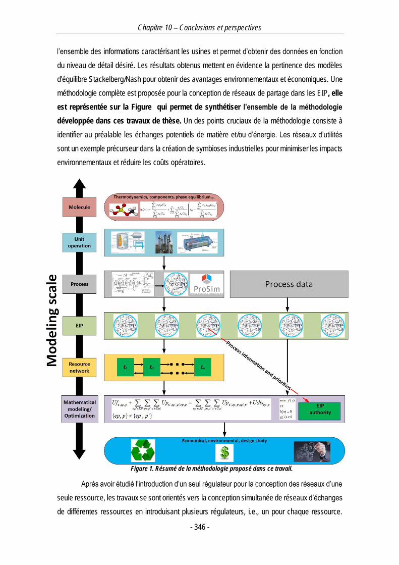
Chapitre 10 – Conclusions et perspectives
- 346 -
l’ensemble des informations caractérisant les usines et permet d’obtenir des données en fonction
du niveau de détail désiré. Les résultats obtenus mettent en évidence la pertinence des modèles
d'équilibre Stackelberg/Nash pour obtenir des avantages environnementaux et économiques. Une
méthodologie complète est proposée pour la conception de réseaux de partage dans les EIP, elle
est représentée sur la Figure qui permet de synthétiser l’ensemble de la méthodologie
développée dans ces travaux de thèse. Un des points cruciaux de la méthodologie consiste à
identifier au préalable les échanges potentiels de matière et/ou d’énergie. Les réseaux d’utilités
sont un exemple précurseur dans la création de symbioses industrielles pour minimiser les impacts
environnementaux et réduire les coûts opératoires.
Figure 1. Résumé de la méthodologie proposé dans ce travail.
Après avoir étudié l’introduction d’un seul régulateur pour la conception des réseaux d’une
seule ressource, les travaux se sont orientés vers la conception simultanée de réseaux d’échanges
de différentes ressources en introduisant plusieurs régulateurs, i.e., un pour chaque ressource.
Chapitre 10 – Conclusions et perspectives
- 347 -
Afin de mener à bien cet objectif, l’intégration d’eau et d’énergie dans les EIP est étudiée en
utilisant une méthode hybride couplant le goal programming et les jeux single-leader-multi-
follower. Les consommations d’eau et d’énergie sont des critères antagonistes qui
influencent fortement l’aspect économique des EIP. En conséquence, le concept de régulateur
gérant la consommation d‘eau est étendu en rajoutant un gestionnaire pour la partie énergétique.
Les résultats obtenus sont différents au sein de chaque scénario étudié, ce qui met en évidence
les inconvénients de l’approche proposée : il est très difficile de trouver une solution de
compromis sans utiliser un outil de décision. La méthode AHP est alors utile dans ce cas précis
puisqu’elle permet de prendre des décisions hiérarchisées (cas du problème multi-niveaux).
Finalement, une formulation de jeu multi-leader-multi-follower pour la conception
efficace des réseaux d'eau et d'énergie dans un EIP a été développée. La formulation
résultante avec plusieurs leaders et plusieurs followers produit des résultats qui soulignent
l'efficacité de la méthode proposée, par rapport aux autres approches hybrides couplant
l’optimisation multiobjectif aux concepts de théorie des jeux. La formulation de jeu multi-leader-
multi-follower a l'avantage d'aborder globalement l'interaction entre tous les acteurs de tous
les niveaux. Ceci permet d’obtenir une solution d'équilibre sans faire appel à une entité de
prise de décisions comme cela a été effectué dans l’article 7. En effet, d’un point de vue du
décideur, il a été démontré que la sélection des coefficients de la matrice de décision pour la
méthode AHP est totalement contre-intuitive. La sélection de la solution parmi l’ensemble des
points de Pareto obtenus dans le dernier article s’avère finalement difficile.
2. Perspectives
Les perspectives de ce travail de thèse concernent plusieurs aspects qui résultent des
observations et des conclusions tirées. À partir des modèles d’équilibre économiques proposés
dans ce travail, l’intérêt d’inclure simultanément plusieurs types d’échanges (matière, énergie,
utilités parmi d’autres) devient très attirant et intéressant, non seulement de par la capacité de ces
modèles à pouvoir représenter ces types d’échanges, mais aussi par la capacité à gérer plusieurs
objectifs simultanément et de les satisfaire de façon équilibrée. Ceci est un des sujets les plus
problématiques dans la conception des EIP. Le modèle pourrait ainsi être adapté pour implémenter
un nombre assez important de régulateurs afin de satisfaire tous les acteurs de la symbiose
proposée.
De plus, il serait aussi intéressant d’inclure des sources d’énergie renouvelables dans les
EIP afin de nourrir la philosophie écologique de ce concept. Ainsi, la source d’énergie renouvelable
Chapitre 10 – Conclusions et perspectives
- 348 -
pourrait être choisie de façon optimale parmi plusieurs sources possibles. On pourrait imaginer que
le (ou un des) gestionnaire(s) de l’EIP inclut ce paramètre dans sa gestion, ce qui rendrait le prix
de la source d’énergie variable, en fonction de la quantité d’échanges inter-entreprises.
Un autre volet important qu’il sera nécessaire d’explorer concerne les aspects liés à la
flexibilité des EIP. Les usines peuvent changer la capacité de production de leurs procédés
plusieurs fois durant leur vie utile de production. En conséquence, les paramètres opératoires
changeront certainement, ce qui affectera négativement le déroulement et le fonctionnement de
l’EIP. Il est donc possible qu’une (ou plusieurs) entreprise(s) ne désire plus participer à la symbiose
car les nouveaux paramètres opératoires ne satisfont plus le critère économique précédemment
évalué. Pour surmonter ce défi, une alternative prometteuse est d’inclure la modélisation de
l’incertitude dans les modèles de jeu multi-leader-follower, puisque la structure de ce type de
formulation permet de l’y inclure. De cette façon, l’EIP serait conçu en tenant compte de potentiels
évènements empêchant le bon déroulement et le fonctionnement des symbioses.
Finalement, les aspects mathématiques qui concernent les modèles de conception des
EIP pourront être développés vers de nombreuses évolutions. En premier lieu, l’insertion des
décisions de type discrètes dans les modèles multi-niveaux reste encore un défi pour la
communauté scientifique. En effet, les problèmes d’optimisation des niveaux inférieurs (i.e.
followers) sont remplacés par leurs conditions d’optimalité du premier ordre (i.e. KKT). Étant donné
que ces conditions ne sont pas valides avec la présence de variables discrètes, de nouvelles
théories/techniques doivent être développées. Néanmoins, l’inclusion de décisions discrètes
pourrait signifier la possibilité de mettre en place des modèles de chaine logistique impliquant des
choix de technologie dans les modèles multi-leader-follower de conception des EIP. En deuxième
lieu, un autre aspect intéressant à explorer serait l’inclusion de la variable temporelle en rendant
les modèles dynamiques. De cette façon, il serait possible de prendre en compte soit des modèles
d’opération en temps réel des usines et des opérations unitaires, soit des modèles de planification
en considérant différentes périodes de temps. Néanmoins, on remarque que les perspectives
concernant les aspects mathématiques posent plusieurs verrous scientifiques, notamment par
rapport à l’échelle de modélisation des problèmes. Tous les modèles proposés sont des problèmes
de grande taille qui, liés à des modèles de jeu multi-leader-follower dont la taille augmente
considérablement et introduisent des non-linéarités, pourraient devenir très compliqués à résoudre,
voire impossible. Il s’agirait de résoudre des problèmes NP-Complets.

Titre : Optimisation Bi-Niveau d’Ecoparcs Industriels pour une Gestion Durable des Ressources
Résumé
Ce travail concerne une méthodologie d'optimisation bi-niveau pour la conception de réseaux de ressources durables dans les parcs éco-industriels (EIP). Différents cas d’étude sont pris en compte afin de minimiser et de maintenir en équilibre les coûts opératoires des usines, tout en minimisant la consommation des ressources naturelles. Tout d'abord, les réseaux d'eau mono-contaminants dans les EIP sont étudiés, où l’influence des paramètres opératoires des usines sont étudiés afin de déterminer ceux qui favorisent la symbiose entre les usines. Ensuite, d'autres études de cas sont abordées en utilisant le méthodologie bi-niveau ainsi que l’introduction des « régulateurs ». En premier lieu, les réseaux d'eau sont étendus pour inclure simultanément les réseaux d'énergie, et d'autre part, les réseaux d’utilités dans un scénario du monde réel. Ce travail a conduit à des améliorations significatives dans la conception des réseaux de ressources dans les EIP, notamment dans le cadre de la prise de décisions multi-critére. En utilisant une approche à bi-niveau multi-leader-multi-follower, les usines pourraient obtenir des gains équitables des coûts opératoires tout en conservant les ressources naturelles au minimum. Mots – clés : Écoparc Industriel, Optimisation bi-niveau, Durabilité, Equilibre de Nash, Théorie des Jeux.
Title: Bilevel Optimization of Eco-Industrial Parks for the Design of Sustainable Resource Networks
Abstract
This work presents a bilevel optimization framework for the design of sustainable resource networks in eco-industrial parks (EIP). Different case studies are taken into account in order to minimize and maintain in equilibrium participating plants operating costs while minimizing resource consumption. First, mono-contaminant water networks in EIP are studied, where also plants operating parameters are studied in order to determine the most important ones to favor the symbiosis between plants. Then, other case studies are approached by using the bilevel and regulatory framework. In the first place, water networks are extended to include simultaneously energy networks, and secondly utility networks in a real-world case scenario. This work led to significant improvements in EIP resource networks design, most notably in the framework of multi-criteria decision making. By using a multi-leader-multi-follower bilevel approach, plants could obtain equitable operating costs gains while still maintaining natural resources to a minimum. Keywords: Eco-Industrial Parks, Bilevel Optimization, Sustainability, Nash Equilibrium, Game Theory