-----,,--- ----------

Doctorat de l'Université Montpellier II

Spécialité: Biologie Intégrative

Procédure de Validation des Acquis de l'Expérience

Présentée par

Marc Pansu

Chimie du sol et cycle du carbone et de l'azote

Soutenue le 28 Janvier 2005Devant le Jury VAE de Montpellier II

---- - ---,--,-----

i Monsie,ur JL Cuq, ConseiLScientifique, Président du juryMadame M Vianey-Liaud, Directeur de la DREDMonsieur M Robert, Ecole doctorale « Information, structures et systèmes»Monsieur M Montero, École doctorale Sciences chimiques et physiques (ED 459)Monsieur M Daignieres, École doctorale "Terre, Eau, Espace" (ED 148)Monsieur C Le Peuch, Ecole doctorale « Sciences Chimiques et Biologiques pour la santé»Monsieur B Jaillard, Ecole doctorale« Biologie des systèmes intégrés, Agronomie,Environnement (ED167) », rapporteurMonsieur JM Navarro, Écoledoctorale« Science etpJ:océdés biologiques et industriets(ED306»)Monsieur Ph Aurier, École doctorale "Économie etGestion"Monsieur P Mangea!, CSE 64MonSieur F Bonhomme, CSE 67Monsieur R Joffre, Cefe-CNRS, rapporteurMonsieur J Calas, Service de formation continueMadame M Frayssinet, conseiller VAB,Madame C Johera, chargé d'accompagement VAE

Sommaire

Première partieles acquis de mon expérience

Lettre de motivation 5

Curriculum Vitae 6

Parcours professionnel 6

Recherche actuelle 7

Valorisation et synthèse........................•......•................................................................... 7

E . .. ';r. 7'xpertise et animation scienujique............................................................•••••..•.•...........

Enseignement 7

Coopération 8

Publications des 5 dernières années ..........•..•..............................•...............••................. 8

Formation .......................••.............•.........................•....................................................... 9

Valorisation et synthèses Il

L'analyse du sol Il

Rubriques encyclopédiques ..........•••..............................................................•...•.•........... Il

Fiche Masson 12

Fiche Balkema 15

Fiche Springer ...............................•...............................................•................................• 17

Expertise et animation scientifique 18

Expertise 18

Animation de séminaires Agropolis.•....•..................•.•...............................••.••..............•. 18

Enseignement 20

Recherche, coopérations 22

Historique 22

Programmes et projets internationaux .....•........•.........................................••................. 22

Partenaires scientifiques .........•...•...........................................•....................................... 22

Deuxième partieModélisation du cycle du carbone et de l'azote dans les sols

Cycle du carbone dans les sols 25

Modèles à 2 et 3 compartiments 25

Cycle du Carbone et propriétés physiques et chimiques du sol 35

Modèle Carbone à 5 compartiments (MOMOS-C) 37

Cycle de l'azote dans les sols, modèle MOMOS-N 45

Influence des racines actives sur le cycle du carbone 57

La Transformation du C des Apports Organiques (TAO-C) 68

Cinétique de transformation du carbone 70

Composition biochimique de l'apport et transformation C 85

La Transformation N des Apports Organiques (TAO-N) 97

Cinétique de transformation de l'azote..........................................•..•............................. 98

Composition biochimique de l'apport et transformation N 111

Le rôle de la biomasse microbienne: nouvelles propositions 123

Modélisation du fonctionnement d'écosystèmes 161

Bilan et perspective 163

Annexes

Al - Institut de Recherchepour le Développement (IRD) 170

A2 - UR-IRD Séquestration C dans les sols tropicaux. 183

A3 - Rapport d'activités 2003 ..•....................••.••••••.•....................................................... 203

A4 - Liste de publications 221

AS - Diplôme ENSCT 229

PREMIERE PARTIE

LES ACQUIS DE MON EXPERIENCE

1jtJ

1

5

Lettre de motivation

Montpellier le Mardi Il Mai 2004

Marc Pansu,Laboratoire MOST, IRD,BP 64 501,34 394 Montpellier Cedex 5Tel: 04 67 41 62 28FAX: 04 67 41 62 94E-mail: pansu@mpl.ird.fr

Monsieur le Président de l'Université Montpellier II

J'ai l'honneur de solliciter auprès de votre université l'obtention d'un Doctorat de l'école

doctorale de Biologie Intégrative selon la loi de Validation des Acquis de l'Expérience

(VAE).

Je vous soumets pour cela mes titres, travaux et publications dans le dossier joint rédigé en

conformité avec la procédure VAE selon la recommandation de ses responsables à

l'Université Montpellier II. Mes motivations pour l'obtention de ce Doctorat sont les

suivantes:

reconnaissance de mes travaux par l'autorité universitaire,

renforcement des possibilités d'encadrement d'étudiants dans notre laboratoire (avec

l'encouragement de mes responsables),

coordination plus aisée de programmes de recherche nationaux et internationaux,

transmission facilitée de mes connaissances en Chimie du sol, particulièrement sur la

modélisation du cycle du carbone et de l'azote, par une formation d'étudiants aptes à

prendre, s'ils le désirent, le relais de mes travaux après mon départ en retraite.

Vous remerciant par avance de la considération que vous voudrez bien accorder à ma

demande, je vous prie d'agréer, Monsieur le Président, l'expression de mes sentiments

respectueux.

Marc Pansu

6

Curriculum Vitae

Marc PANSUDate de naissance : 26-04-1947,Marié, 3 enfants,Ingénieur de Recherche (INR 1), IRD, Montpellier

Parcours professionnel- Depuis 2001 : ingénieur de recherche, UR séquestration du carbone dans les sols tropicaux

(IRD Montpellier) et laboratoire Matière Organique des Sols Tropicaux (MOST, IRD­ClRAD, Montpellier), Recherche pédologique, agronomique et environnementaleparticulièrement sur modélisation cycle C et N, ouvrages analytiques de synthèse« L'analyse du sol»

- 1988-2000 : ingénieur de Recherche, Laboratoire de Comportement des Sols Cultivés, IRDMontpellier, Recherche pédologique et agronomique, développements analytiques, ouvragesanalytiques de synthèse, modélisation cycle Cet N.

- 1984-1988: ingénieur, responsable du Laboratoire Matière Organique (6 Ingénieurs etTechniciens), IRD Bondy, Analyses et recherche analytique sur les matières organiques.

- 1976-1984: ingénieur au laboratoire de Spectrographie, IRD Bondy, développementsanalytiques particulièrement en chimiométrie, éléments trace, et analyse organique.

- 1975-1976: ingénieur au laboratoire IRD d'Adiopodoumé (RCI) d'analyses de sol, eau etvégétaux, encadrement du laboratoire (25 Techniciens et Laborantins).

- 1972-1974: allocataire de recherche au laboratoire de l'Energie Solaire CNRS de Font­Romeu, recherches sur la purification d'oxydes réfractaires au four solaire.

- 1967-1969: assistant-ingénieur au laboratoire de l'ENSEE de Grenoble, recherches suraccumulateurs électrochimiques.

Recherche actuelle- Modélisation du cycle du carbone et de l'azote dans les sols,- Application à la modélisation de la fertilisation organique,- Application à la modélisation du fonctionnement d'écosystèmes,

Valorisation et synthèse- Secrétaire scientifique et premier auteur de livres de synthèse sur « L'analyse du sol» : un

livre en français aux éditions Masson (paris, Milan, Barcelone), un livre en anglais auxéditions Balkema (Lisse, Abingdon, Exton, Tokyo), un livre en français aux éditionsSpringer (Paris, Berlin, Heidelberg, New York, Hong Kong, Londres, Milan, Tokyo), unlivre en anglais à paraître chez Springer.

- auteur de deux rubriques encyclopédiques sur le sol (encyclopédie sur internethttp://webencyclo.com. rubrique « sol », éditions Atlas)

Expertise et animation scientifique- Expert «rewiever» revues scientifiques «Soil Biology & Biochemistry (Elsevier) »,

« Etude et gestion des sols (AFES) », «Nutrient cycling in agro-ecosystems (Kluwer) ».

7

- conférences sur l'analyse du sol et expertise de laboratoires d'analyse au Pérou et en Bolivie(2000),

- membre nommé de la Commission Scientifique Sectorielle 1 de l'IRD : physique et chimiede l'environnement planétaire,

- expertise de dossiers de carrières, jury de concours, évaluation d'unités de recherche,- organisateur de séminaires scientifiques mensuels (troisième Jeudi de chaque mois depuis

2001) sur la communauté scientifique Agropolis de Montpellier (IRD, CIRAD, CNRS,INRA, ENSAM, Université Montpellier II, CNEARC, CEMAGREF, ENGREF). Le thèmedes exposés concerne toutes les disciplines en relation avec l'étude des sols. Une large partconsacrée à la discussion favorise les échanges et coopérations entre scientifiques de lacommunauté.

Enseignement- Participation à l'encadrement de 40 stagiaires au laboratoire de spectrographie de l'IRD

Bondy (dont co-encadrement de 5 thèses), 20 stagiaires au laboratoire Matières Organiquesde l'IRD Bondy (dont co-encadrement d'une thèse), 45 stagiaires au laboratoire LCSC del'IRD Montpellier (dont co-encadrement de 5 thèses et responsable principal de 8stagiaires), 20 stagiaires au laboratoire MOST de l'IRD Montpellier (dont co-encadrementde 3 thèses et responsable principal de 9 stagiaires).

- Organisation et participation à des enseignements pour adultes dans le cadre du CNRS­Formation, Groupement pour l'Avancement des Méthodes Spectroscopiques (GAMS), IRD­formation: chimiométrie, outil informatique en chimie analytique, plans d'expériences,méthodes d'optimisation.

- Conférences à publics scientifiques: universités de Syrie, Bolivie, Pérou, cycle mensuelAgropolis Montpellier.

- Conférences grand public et lycée: tète de la science, festival «L'avenir au naturel»(L'Albenc, Isère).

CoopérationProgrammes et projets internationaux

1998-2003 - Partenaire du programme Européen Tropandes INCO-DC ERBIC18CT98-0263,Fertility management in the tropical andean mountains : agroecological bases for a sustainablefallow agriculture, union de partenaires boliviens, vénézuéliens, espagnols, hollandais etfrançais (IRD, CNRS, Université).2004 - Soumission d'un projet ECOS-Nord France- Vénézuela: Dynamique de la matièreorganique du sol dans les écosystèmes vénézuéliens et son importance dans le controle del'érosion.En prévision: programmes ECO-PNBC et INCO-DEV

Partenaires scientifiques

CEFE-CNRS Montpellier, France,CIRAD Montpellier, France,INRA Montpellier, France,Entreprise Phalippou Frayssinet (Fertilisants organique, Tarn, France),Laboratoire d'Ecologie microbienne des sols tropicaux, IRD SénégalEMBRAPA, Sao Paulo, Brésil;Instituto de Investigaciones Agrobiologicas de Galicia, Santiago de Compostella, Espagne,Instituto de ciencias ambientales y ecologicas, Facultad de ciencias, Merida, Venezuela,

8

Universidad mayor de San Andres, Instituto de Ecologia, La Paz, Bolivie,Plant Research International, location born Zuid Wageningen, Pays Bas,Laboratoire d'écophysiologie végétale, Université de Paris-Sud, Orsay, France

Formation

initiale

- Ingénieur diplômé de l'Ecole Nationale Supérieure de Chimie de Toulouse (ENSCT, 1972),- Admission à l'ENST par la voie du Centre Universitaire d'Education et de Formation des

Adultes (CUEFA Grenoble, 1969),- DEST par CUEFA Grenoble (1968),- BTS par Lycée Technique d'Etat de Vizille (LTEV, 1967),- BT par LTEV (1965).

Stages

- Caractérisation moléculaire de substances naturelles, Faculté de pharmacie Châtenay­Malabry, 1 mois en 1984

- Plans d'expérience et Méthodes d'optimisation, CACEMI (arts et métiers, Paris) 1 semaineen 1984

- Modélisation du cycle du carbone (modèle de Rothamsted, GB), Laboratoire de radio-agronomie CEA Cadarache, 1 semaine en 1986

- Méthodologie de la recherche expérimentale, Université Aix-Marseille, 1 semaine en 1988- Simulation des systèmes complexes, IRD-Université d'Orléans, 2 semaines en1996

Langues

- Langue maternelle : Français- Autres langues: Anglais (écrit et parlé), Espagnol (notions)

Publications des 5 dernières années

Revues à comité de lecture

P. Bottner, M. Pansu et Z. SaHih, 1999. - Modelling the effect of active roots on soil organicmatter turnover, Plant and Soils, 216, 15-25.

L. Thuriès, M. -e. Larré-Larrouy et M. Pansu, 2000. - Evaluation of three incubation designsfor mineralization kinetics of organic materials in soil. Communications in Soi/Science and Plant Analysis, 31, 289-304

L. Thuries, A. Arrufat, M. Dubois, C. Feller, P. Herrmann, M.C. Larre-Larrouy, C; Martin, M.Pansu, J.e. Remy et M. Viel, 2000. - Influence d'une fertilisation organique et de lasolarisation sur la productivité maraîchère et les propriétés d'un sol sableux sous abri.Etude et Gestion des sols, 7, 73-88.

L. Thuriès, M. Pansu, C. Feller, P. Hermann, et J.C. Rémy. 2001 - Kinetics of added organicmatter decomposition in a mediterranean sandy soil. Soil Biology & Biochemistry 33,997-1010.

L. Thuriès, M. Pansu, M.C. Larre-Larrouy et C. Feller. 2002 - Biochemical composition andmineralization kinetics of organic inputs in a sandy soil. Soil Biology & Biochemistry34, 239-250.

9

M. Pansu et L. Thuriès 2003 - Kinetics of C and N mineralization, N immobilization and Nvolatilization of organic inputs in soil. Soil Biology & Biochemistry, 35, 37-48.

M. Pansu, L. Thuriès, M.C. Larré-Larrouy et P. Bottner, 2003 - Predicting N transformationsfrom organic inputs in soil in relation to incubation time and biochemicalcomposition. Soil Biology & Biochemistry, 35, 353-363.

P. Bottner, M. Pansu, R. Callisaya, K. Metselaar, D. Hervé, 2004 - Modelizaciôn de laevolucién de la materia orgânica en suelos en descanso (Altiplano seco boliviano).Ecologia en Bolivia, sous presse.

Marc Pansu, Pierre Bottner, Lina Sarmiento and Klaas Metselaar, 2004 - Comparison of fivesoil organic matter decomposition models using data from a 14C and ISN labeling fieldexperiment, soumis pour publication à Global Biogeochemical Cycles.

Marc Pansu, Klaas Metselaar, Pierre Bottner, and Lina Sarmiento, 2004 - Sensitivity analysisof two types of soil organic matter decomposition models, soumis pour publication àGlobal Biogeochemical Cycles.

Livres

M. Pansu, 1. Gautheyrou et 1.Y. Loyer, 2001 - Soil analysis - sampling, instrumentation andquality control, translated from French by V.A.K. Sarma, Balkema Publishers, 489 p.

M. Pansu et 1. Gautheyrou, 2003 - L'analyse du sol - minéralogique, organique et minérale,Springer-Verlag, 995 p.

Communication à congrès internationaux

L. Thuriès and M. Pansu, 2001. - Classification and modelling of added organic matterdecomposition in a sandy soil. Proceeding of Il th Nworkshop, Reims, France, 9-12Sept. 2001.

M. Pansu, L. Thuriès, M.C. Larré-Larrouy et C. Feller, 2002 - Kinetics of organic inputs insoil carbon model. Proceeding of 17th World Congress ofsoil science, Bangkok, 14-21August 2002, Oral communication 1502, symposium10.

M. Pansu et P. Bottner, 2002 - Modélisation de l'effet des racines actives sur les transferts deC organique dans les sols. Proceeding of congress Gestion de la biomasse, erosion etsequestration du carbone, Agropolis Montpellier, 23-28 Septembre 2002.

L. Thuriès et M. Pansu, 2002 - Classification et modélisation de la décomposition de matièresorganiques ajoutées au sol. Proceeding of congress Gestion de la biomasse, erosion etsequestration du carbone, Agropolis Montpellier, 23-28 Septembre 2002.

Communication à congrès nationaux

M. Pansu and P. Bottner, 2001. - Modélisation de l'effet des racines actives sur les transfertsde carbone organique dans les sols. Actes 3° colloque rhizosphère, Dijon, 26-28 Nov.2001

10

M. Pansu, L. Thuriès, MC Larre-Larrouy et C. Feller, 2002. - Dynamique de minéralisationd'apports organiques dans les modèles carbone du sol. Actes Journées Nationalesd'Etude des Sols AFES, 22-24 Octobre 2002, Orléans.

Information scientifique

M. Pansu, 2000. - Le sol et son analyse. Fréquence Chimie, 28, 2-9.

M. Pansu et F. Doumenge, 2000. - Modélisation des transferts de carbone et d'azote dans lessols, poster tète de la science.

M. Pansu, 2001. - Le sol : formation, fonctions et composition. In Encyclopédie francophonesur Internet Webencyclo http://webencyclo.com. rubrique « sol », editions Atlas

M. Pansu, 2001. - Le sol: méthodes d'analyse. In Encyclopédie francophone sur InternetWebencyclo http://webencyclo.com. rubrique « sol », editions Atlas

Conférences

M. Pansu, 1999. El analysis de sue10. Universités de Lima, Puno, La Paz, Cochabamba. 20transparents, 1 h de conférence + 1 h de discussions. Collaboration avec DominiqueHervé pour la traduction préalable du texte en espagnol et pour la traduction desquestions.

M. Pansu, 1999. Modelling Organic Matter of Soils (MOMOS model). Centro Internationalde la Papa (CIP) Lima, Pérou, Novembre 1999.

M. Pansu et J.P. Rossignol, 2001. Le sol - formation, fonctions, composition, dégradation.Application aux formations en terrasses de la basse vallée de l'Isère. Grand public, 5°Festival « L'avenir au naturel» L'Albenc Isère, 1 Sept. 2001.

M. Pansu, 2001. Le sol- formation, fonctions, composition, dégradation. Public BTS, Fête dela science, 16 Oct. 2001.

Pansu M, 2001. Modélisation de la dynamique des matières organiques des sols, Cyclemensuel Agropolis Montpellier, coordinateur M. Pansu, 15 Mars 2001.

Pansu M, 2002. Cinétique des entrées organiques dans les modèles de décomposition. Cyclemensuel Agropolis Montpellier, coordinateur M. Pansu, 17 Septembre 2002

M. Pansu, 2002. Modélisation de la dynamique des matières organiques dans les sols. Publicscientifique et enseignement supérieur, étudiants INA-PG, 4 Décembre 2002.

M. Pansu, 2003. Modélisation de la transformation des apports organiques dans les sols.Public scientifique et enseignement supérieur, étudiants INA-PG, Décembre 2003.

11

Valorisation et synthèses

L'analyse du solCe livre de synthèse a été entrepris à la demande des Commissions scientifiques 2 et 7 et de laDirection Générale de l'IRD en 1991. Il constitue maintenant un outil de travail performantpour le laboratoire MOST et le laboratoire central d'analyses du CIRAD, notre partenaire àMontpellier.

Auteurs: M. Pansu, J Gautheyrou et JY Loyer (in Memoriam, J.Susini, décédé en 1994), ainsique des collaborateurs pour compléments et corrections,

Secrétaire scientifique: M. Pansu,

Objectif: pour chaque chapitre, il s'agissait de réunir une compilation d'une expenencecollective de laboratoire et d'une analyse bibliographique s'appuyant sur les nonnesinternationales et françaises et comportant souvent de très nombreuses références; ils'agissait aussi de combler une lacune, les ouvrages sur ce thème étant assez peu nombreuxsurtout en Français,

Résultats: deux ouvrages en français et un en anglais sous les références qui suivent.

M. Pansu, J. Gautheyrou et J.Y. Loyer, 2001 -L'analyse du sol - échantillonnage.instrumentation et contrôle, Masson, Paris, Milan, Barcelone, 489 p.

M. Pansu, J. Gautheyrou et J.Y. Loyer, 2001 - Soi! analysis - sampling, instrumentation andquality control, translated from French by V.A.K. Sanna, Balkema Publishers, Lisse,Abington, Exton, Tokyo, 489 p.

M. Pansu et 1. Gautheyrou, 2003 - L'analyse du sol - minéralogique, organique et minérale,Springer, Paris, Berlin, Heidelberg, New York, Hong Kong, Londres, Milan, Tokyo995 p.

Un livre en anglais à paraître chez Springer.

Rubriques encyclopédiques- auteur en 2001 de deux rubriques encyclopédiques sur le sol (Encyclopédie francophone

Webencyclo sur internet http://webencyclo.com. rubrique« sol », éditions Atlas) :

- Le sol: formation, fonctions et composition

- Le sol: méthodes d'analyse

12 NOUVEAUTE'iiii,,' . 0

CO Itü(C Pansu 1Jacques Gautheqrou 1Jeiln-Ym loqer

l'ANAlYSE DU SOl,ECHANTillONNAGE,

A

INSTRUMENTATION ET CONTROlEMarc PANSU,

Jacques GAUTHEYROU,Jean-Yves LOYER

Préface de M. Pinta et A. Herbillon

Recherche1997,512 pages

395 f.

Mieux connaître les outils de l'analyse des solspour mieux les utiliser: tel est l'objectif decetouvrage.Face aux méthodes et techniques d'analyse

de plus en plus nombreuses, ce volume a été ConçuComme un guide qui permettra d'abord de choisir laméthode adaptée au problème et ensuite de la mettreen oeuvre.La première partie est consacrée aux problèmesd'échantillonnage, qu'il s'agisse du choix deséchantillons. de leur prélèvement ou de leurconditionnement etfractionnement.Les questions liées à l'analyse proprement dite et aucontrôle des résultats font l'objet de la seconde partie.Les principales méthodes physico-chimiques,notamment spectroscopiques etchromatographiques, ysont présentées successivement de manière détaillée.Les techniques d'automatisation au laboratoire et decontrôle statistique de la qualité des résultats sontexposées en fin d'ouvrage.Ce manuel de référence dresse l'inventaire des outilsd'échantillonnage, d'analyse et de contrôle dontdisposent aujourd'hui les « sciences du sol ».

LE PUBLIC

Les chimistes spécialisés en physico-chimieanaly- tique. les ingénieurs, les chercheurset les techni- ciens concernés par lessciences du sol que ce soit dans ledomaine de l'agronomie, de la climatologie,de la géologie. de l'environnement, dugénie civil ou de l'industrie minérale etorganique associée au sol.

LES AUTEURS

Marc Pansu et Jacques Gautheyrou sont ingénieursde recherche spécialisés en sciences du sol à l'institutfrançais de recherche scientifique pour ledéveloppement en coopération (OrstomJ.Jean- Yves loyer est pédologue, directeur derecherche à l'Orstom.

ID

13

L'ANALYSE DU SOL

111

1,j~

111

J

1

CONTENU Prélèvement d'échantillons

Premiers tests de terrain

Préparation des échantillons

Matériels de broyage et tamisage

Premiers tests qualitatifs au laboratoire

Balances analytiques

Séparations sur filtres et membranes

Présentation des techniques analytiques

Spectrométrie moléculaire, d'absorption atomique, d'émission

lonométrie

Techniques chromatographiques

Chromatographie en phase gazeuse, en phase liquide

Analyse élémentaire CHN-QS

Automatisation et robotique au laboratoire

Contrôle de qualité des résultats analytiques

BON DE COMMANDE

Je désire commander: ...... exemplaire(s) de L'ANALYSE DU SOL· Échantillonnage, instrumentation et contrôledeM. Pansu, J. Gautheyrou etJ.·Y.Loyer, au prix de 375 F* au lieu de 395 F. (ISBN 2225831 300)

Frais d'envoi: pour 1vol. 20 F (étranger: 30 F), pour chaque volume supplémentaire 10F.

Envoi par avion: nous consulter. Franco de port pour toute commande supérieure à 1000 F .

CUoint mon chèque F libellé à l'ordre de MASSON Éditeur

NOM Prénom ..

Adresse ..

Code postal, Ville Pays ..

·Prix public TTC au 01.12.97

MASSON

à compléter et à retourner à

MASSON Éditeur

5, rue laromiguière -75005Paris

Please send me ..... copies of:

10. Atomic absorption spectrometry

II. Emission spectrometry12. Ionometry

13. Chromatographie techniques

14. Gas chromatography

15. Liquid chromatography

16. Elemental analysis for C, H, N, 0 and S17. Automation and robotics in the laboratory

18. Quality control ofanalytical data

Appendices1. Classification ofanalytical techniques used for soil studies

2. Analytical equipment and techniques bilingual glossary ofabbreviations, symbols and

acronyms

3. Soil chemistry and the international system ofunits (SI)

4. Statistical tables

5. Soil classification and reference base

6. Suppliers ofanalytical equipment and instruments

7. Periodic table of the elements

Index

Private customers living within the EC have to add 6% VAT to their

payment

o Pansu: Soil analysis, Hardback, €85.00 / USS85.00 / i57

------ ---_. _._. _.- -_.--_.--_.- -- ---_. _._.- -_. _._.- -_._.- -----_.- :-.~~- -_.--- -- ~

-ORDEIHORM , '.~h _''. ,-U ) _

C::~' _~.>, .

•24 cm, 500 pp., EUR 85.00/ $85.00/ [57ISBN 90 5410 7162

Sampling, instrumentation

and quality control

by

M.PANSU, J.GAUTHEYROU&J.-Y.LOYER

A translation of L'analyse du sol: Echantillonnage. instrumentation et contrôle, Masson,

Paris, 1998. The objective of this book is to provide a better understanding of soil-analysistools in order to use them more efficiently. Given the increasing number of analytical methods

and techniques, this book has been designed as a guide that will enable first the selection ofthe method appropriate to the problem and, then, its execution. The first part is devoted tosampling problems, which encompass selection, withdrawing, drying and fractionation of

samples. Problems related to the actual analysis and to quality control of the results form the

subject of the second part. Principal physicochemical methods, especially spectroscopie andchromatographie, are sequentially presented in detail. Techniques of laboratory automationand of statistical quality control of the results are explained at the end of the book. This

reference manual presents the list of tools for sampling, analysis and quality control currentlyavailable for "soil science".

SOIL ANALYSIS

CONTENTS:Payment by personal chèque drawn on a bank in the USA, or credit card:

Master Card / VISA / American Express / Diners Club / Eurocard

A.A.Balkema Publisners, P.O. Box 1675, Rotterdam, Netherlands

Tel.: (+31.10) 4145822 Fax: (+ 31.10) 4135 947lntemet: www.Balkema.nl

Card numbej 1 1 1 1 1 1 1 1 OIIIIJ

~.....

Part One: Samplingr. Sampling

2. Preliminary field tests3. Sample preparation

4. Grinding and sieving equipment

5. Preliminary qualitative laboratory tests

6. Analytical balances

7. Separation by paper and membrane filtration

Part Two: Instrumentation and quality control8. Introduction to analyticaltechniques

9. Molecular spectrometry

Expiry date:

Name:

Address:

City & Country:

Signature:

Cvc nurnber 1 1 1 1

A Word about the Cover Illustration

1 have the notion (and 1enjoy persisting with this notion) that the shapesliked by living matter are everywhere the same, true for ail small abjects orlarge geographical areas. In this spirit, 1have desired in these landscapes taconfuse the scale in such a manner that it will be uncertain whether thepainting represents a vast area of mountains or a tiny parcel of land. 1feelthat, having found these rhythms of matter and being provided with anyabject, the painter couId endow that abject with Iife.

Many persans have imagined that because of a disparaging bias 1Iike tashow unfortunate things. How 1 have been misunderstood! 1 had wishedLa reveal ta them that these things they consider ugly or have forgotten tasee are also great wonders.

Jean Dubuffet, commentary on his paintings'Population on the sail, 1952'

and 'Fruits of earth, 1960'.

A Word about the Cover Illustration

I have the notion (and I enjoy persisting with this notion) that the shapesliked by living matter are everywhere the same, true for all small objects orlarge geographical areas. In this spirit, I have desired in these landscapes toconfuse the scale in such a manner that it will be uncertain whether thepainting represents a vast area of mountains or a tiny parcel of land. I feelthat, having found these rhythms of matter and being provided with anyobject, the painter could endow that object with life.

Many persons have imagined that because of a disparaging bias I like toshow unfortunate things. How I have been misunderstood! I had wishedLo reveal to them that these things they consider ugly or have forgotten tosee are also great wonders.

Jean Dubuffet, commentary on his paintings'Population on the soil, 1952'

and 'Fruits of earth, 1960'.

16

Vient de paraÎtre

M. Pansu, J. Gautheyrou, IRD, Montpellier, France

L'analyse du solMinéralogique, organique,minérale

~-..._--_..-_~

2003. XIX, 993 p. Broché 62 €*, ISBN 2-287-59774-3

Rédigé en conformité avec les normes analytiques, partieintégrante de la démarche qualité, cet ouvrage est unguide de référence pour les choix méthodologiques puis

pour la mise en œuvre des nombreuses méthodes, normalisées ou non, de l'analysedu sol.

Il synthétise une multitude d1nformations techniques dans des protocoles, tableaux,formules, modèles de spectres, chromatogrammes et autres diagrammesanalytiques. Les modes opératoires sont diversifiés, depuis les tests les plus simplesjusqu'aux déterminations les plus complexes - physico-chimie structurale des édificesminéralogiques et organiques, éléments échangeables, potentiellement disponibles ettotaux, pesticides et polluants, éléments traces et isotopes.

Outil de base, il sera particulièrement utile aux chercheurs, ingénieurs, techniciens,professeurs et étudiants spécialisés en pédologie, agronomie, sciences de la terre etde l'environnement, ainsi qu'aux disciplines connexes telles que physico-chimieanalytique, géologie, hydrologie, écologie, climatologie, génie civil et industriesassociées aux sols.

BON DE COMMANDE

à retourner àvotre libraire spécialisé

Je désire commander:.... Ex L'analyse du sol 2-287-59774-3 62€*

ou, à défaut, àPrénomNom: ..................................................... : ..............................

Springer-Verlag Adresse : .................................................................................................

Customer Service Books/ .................................................................................................................Haberstr.7 Code postal : ..................... Ville: ........................................................0-69126 Heidelberg/Allemagne

Date: Signature:Tél. : 00800 777 46437(appel gratuit) Mode de règlement: 0 chèque 0 carte de créditFax: 004962213454229e-mail : orders@springer.de n: ................................................... date de validité : ......................

http://www.springer.de MONTANT TOTAL : ...............................................................................

*Prix TTCen France (livres: 5,5% TVA, produits électroniques: 19,6% TVA incl.). Dans d'autres pays, la TVA locale est applicable.Partidpation aux fraisde port : 1 ouvrage 5 € (+ 1,50 € par ouvrage supplémentaire) France métrooo!itaine uniquement

Les prix indiqués et autres détailssont susceptibles d'être modifiéssansavispréalable.

17

Expertise et animation scientifique

E$ertise- Expert « rewiever » revues scientifiques « Soil Biology & Biochemistry (Elsevier) »,

« Etude et gestion des sols (AFES) », « Nutrient cycling in agro-ecosystems (Kluwer) ».- conférences sur l'analyse du sol et expertise de laboratoires d'analyse au Pérou et en Bolivie

(2000),- membre nommé de la Commission Scientifique Sectorielle 1 de l'IRD : physique et chimie

de l'environnement planétaire,- expertise de dossiers de carrières, jury de concours, évaluation d'unités de recherche,

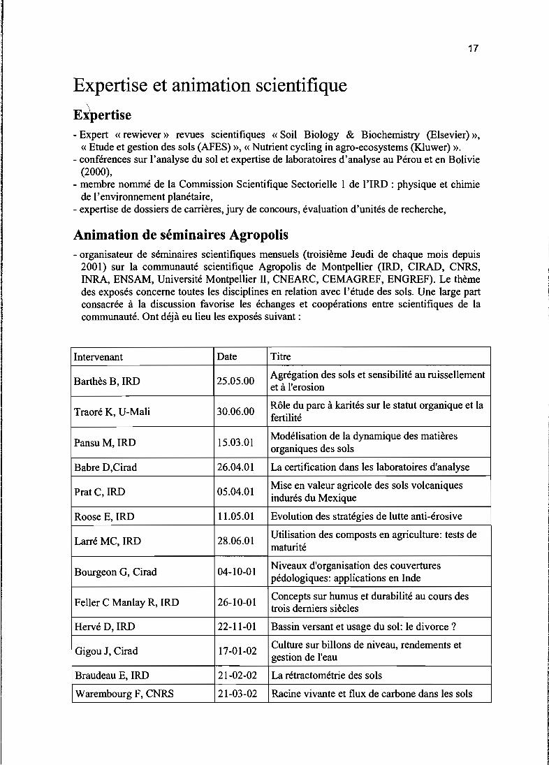
Animation de séminaires Agropolis- organisateur de séminaires scientifiques mensuels (troisième Jeudi de chaque mois depuis

2001) sur la communauté scientifique Agropolis de Montpellier (IRD, CIRAD, CNRS,INRA, ENSAM, Université Montpellier II, CNEARC, CEMAGREF, ENGREF). Le thèmedes exposés concerne toutes les disciplines en relation avec l'étude des sols. Une large partconsacrée à la discussion favorise les échanges et coopérations entre scientifiques de lacommunauté. Ont déjà eu lieu les exposés suivant:

Intervenant Date Titre

Barthès B, IRD 25.05.00Agrégation des sols et sensibilité au ruissellementet à l'erosion

Traoré K, U-Mali 30.06.00Rôle du parc à karités sur le statut organique et lafertilité

Pansu M, IRD 15.03.01Modélisation de la dynamique des matièresorganiques des sols

Babre D,Cirad 26.04.01 La certification dans les laboratoires d'analyse

PratC,IRD 05.04.01Mise en valeur agricole des sols volcaniquesindurés du Mexique

Roose E, IRD 11.05.01 Evolution des stratégies de lutte anti-érosive

Larré MC, IRD 28.06.01Utilisation des composts en agriculture: tests dematurité

Bourgeon G, Cirad 04-10-01Niveaux d'organisation des couverturespédologiques: applications en Inde

Feller C Manlay R, IRD 26-10-01Concepts sur humus et durabilité au cours destrois derniers siècles

Hervé D, IRD 22-11-01 Bassin versant et usage du sol: le divorce?

Gigou J, Cirad 17-01-02Culture sur billons de niveau, rendements etgestion de l'eau

Braudeau E, IRD 21-02-02 La rétractométrie des sols

Warembourg F, CNRS 21-03-02 Racine vivante et flux de carbone dans les sols

18

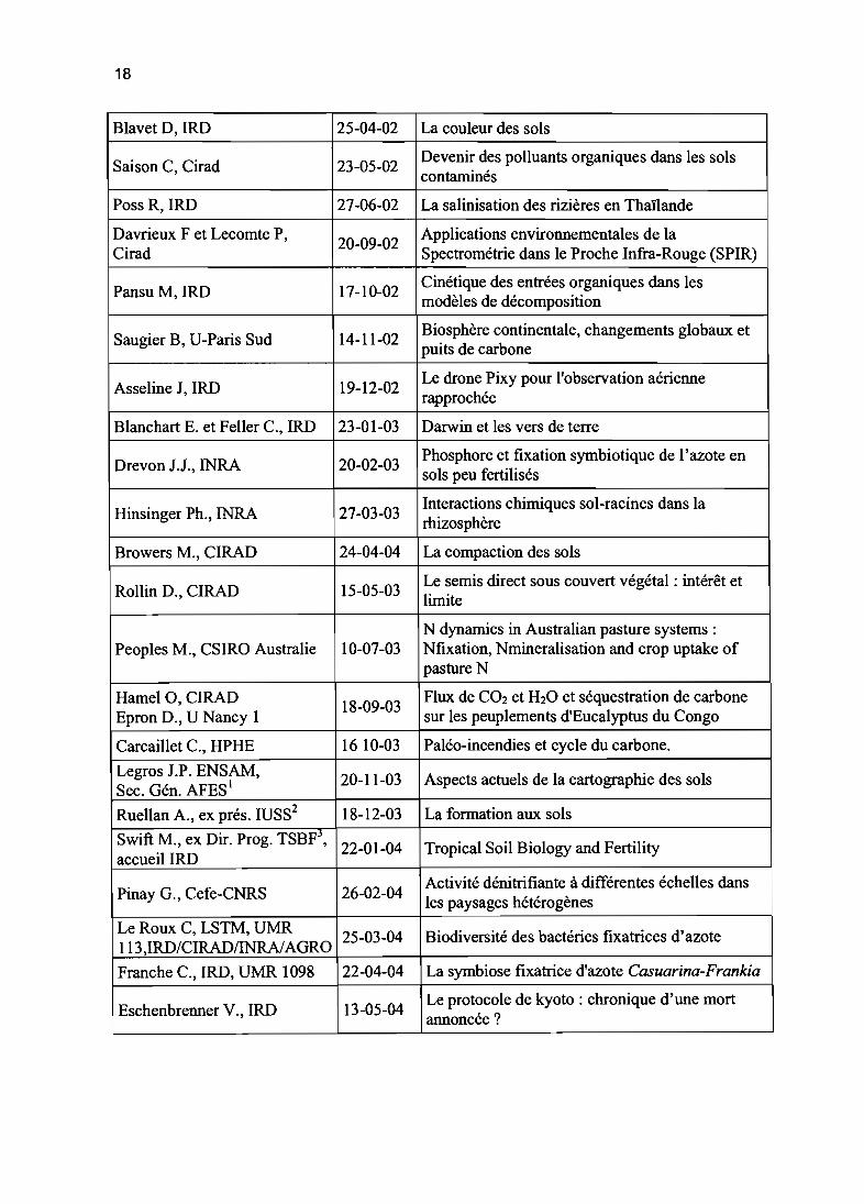
Blavet D, IRD 25-04-02 La couleur des sols

Saison C, Cirad 23-05-02Devenir des polluants organiques dans les solscontaminés

Poss R, IRD 27-06-02 La salinisation des rizières en Thaïlande

Davrieux F et Lecomte P,20-09-02

Applications environnementales de laCirad Spectrométrie dans le Proche Infra-Rouge (SPIR)

Pansu M, IRD 17-10-02Cinétique des entrées organiques dans lesmodèles de décomposition

Saugier B, U-Paris Sud 14-11-02Biosphère continentale, changements globaux etpuits de carbone

Asseline J, IRD 19-12-02Le drone Pixy pour l'observation aériennerapprochée

Blanchart E. et Feller c., IRD 23-01-03 Darwin et les vers de terre

Drevon J.1., INRA 20-02-03Phosphore et fixation symbiotique de l'azote ensols peu fertilisés

Hinsinger Ph., INRA 27-03-03Interactions chimiques sol-racines dans larhizosphère

Browers M., CIRAD 24-04-04 La compaction des sols

RoUin D., CIRAD 15-05-03Le semis direct sous couvert végétal : intérêt etlimite

N dynamics in Australian pasture systems :Peoples M., CSIRO Australie 10-07-03 Nfixation, Nmineralisation and crop uptake of

pasture N

Hamel 0, CIRAD18-09-03

Flux de CO2 et H20 et séquestration de carboneEpron D., U Nancy 1 sur les peuplements d'Eucalyptus du Congo

Carcaillet C., HPHE 16 10-03 Paléo-incendies et cycle du carbone.

Legros J.P. ENSAM,20-11-03 Aspects actuels de la cartographie des sols

Sec. Gén. AFES 1

Ruellan A., ex prés. IUSS2 18-12-03 La formation aux sols

Swift M., ex Dir. Prog. TSBF3,

22-01-04 Tropical Soil Biology and FertilityaccueilIRD

Pinay G., Cefe-CNRS 26-02-04Activité dénitrifiante à différentes échelles dansles paysages hétérogènes

Le Roux C, LSTM, UMR25-03-04 Biodiversité des bactéries fixatrices d'azote

113,IRD/CIRADIINRA/AGRO

Franche C., IRD, UMR 1098 22-04-04 La symbiose fixatrice d'azote Casuarina-Frankia

Eschenbrenner V., IRD 13-05-04Le protocole de kyoto : chronique d'une mortannoncée?

1t

19

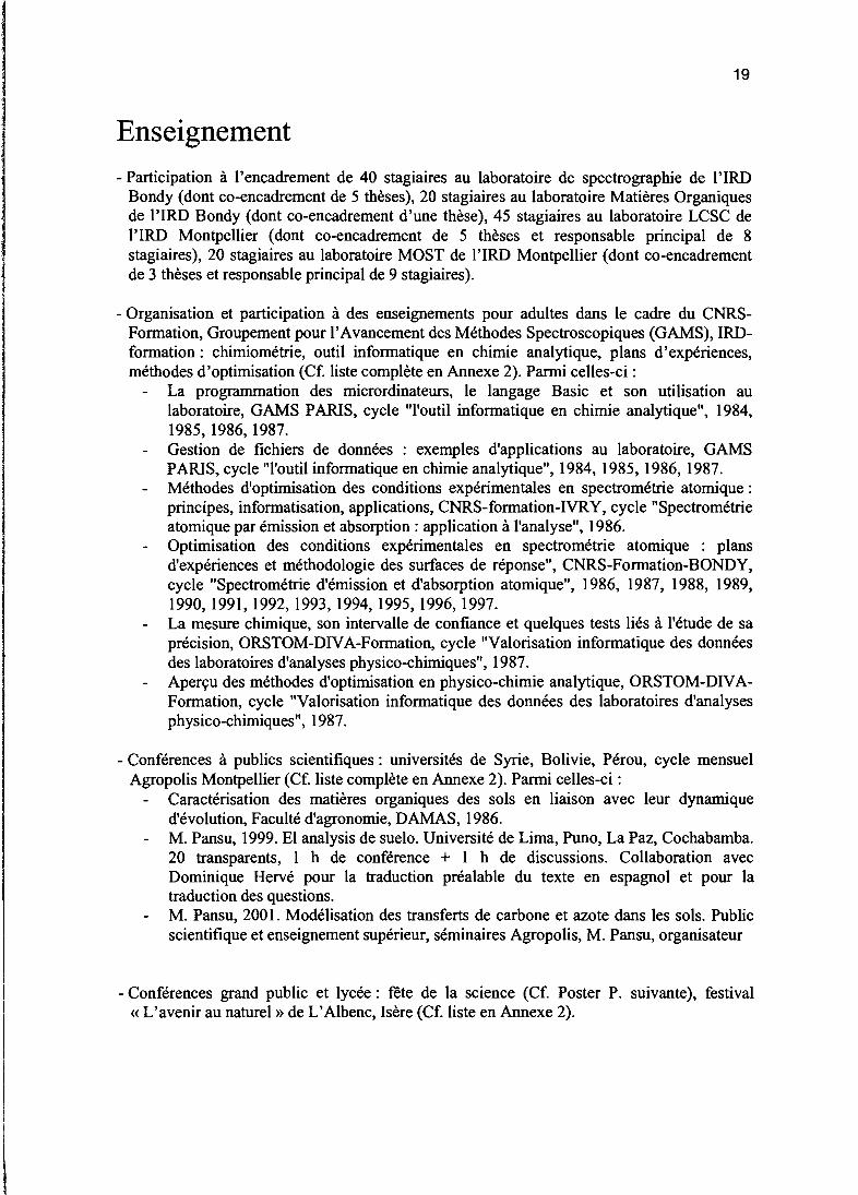
Enseignement

- Participation à l'encadrement de 40 stagiaires au laboratoire de spectrographie de l'IRDBondy (dont co-encadrement de 5 thèses), 20 stagiaires au laboratoire Matières Organiquesde l'IRD Bondy (dont co-encadrement d'une thèse), 45 stagiaires au laboratoire LCSC del'IRD Montpellier (dont co-encadrement de 5 thèses et responsable principal de 8stagiaires), 20 stagiaires au laboratoire MOST de l'IRD Montpellier (dont co-encadrementde 3 thèses et responsable principal de 9 stagiaires).

- Organisation et participation à des enseignements pour adultes dans le cadre du CNRS­Formation, Groupement pour l'Avancement des Méthodes Spectroscopiques (GAMS), IRD­formation: chimiométrie, outil informatique en chimie analytique, plans d'expériences,méthodes d'optimisation (Cf. liste complète en Annexe 2). Parmi celles-ci:

La programmation des micrordinateurs, le langage Basic et son utilisation aulaboratoire, GAMS PARIS, cycle "l'outil informatique en chimie analytique", 1984,1985, 1986, 1987.Gestion de fichiers de données : exemples d'applications au laboratoire, GAMSPARIS, cycle "l'outil informatique en chimie analytique", 1984, 1985, 1986, 1987.Méthodes d'optimisation des conditions expérimentales en spectrométrie atomique:principes, informatisation, applications, CNRS- formation- IVRY, cycle "Spectrométrieatomique par émission et absorption: application à l'analyse", 1986.Optimisation des conditions expérimentales en spectrométrie atomique : plansd'expériences et méthodologie des surfaces de réponse", CNRS-Formation-BONDY,cycle "Spectrométrie d'émission et d'absorption atomique", 1986, 1987, 1988, 1989,1990, 1991, 1992, 1993, 1994, 1995, 1996, 1997.La mesure chimique, son intervalle de confiance et quelques tests liés à l'étude de saprécision, ORSTOM-DIVA-Formation, cycle "Valorisation informatique des donnéesdes laboratoires d'analyses physico-chimiques", 1987.Aperçu des méthodes d'optimisation en physico-chimie analytique, ORSTOM-DIVA­Formation, cycle "Valorisation informatique des données des laboratoires d'analysesphysico-chimiques", 1987.

- Conférences à publics scientifiques: universités de Syrie, Bolivie, Pérou, cycle mensuelAgropolis Montpellier (Cf. liste complète en Annexe 2). Parmi celles-ci:

Caractérisation des matières organiques des sols en liaison avec leur dynamiqued'évolution, Faculté d'agronomie, DAMAS, 1986.M. Pansu, 1999. El analysis de suelo. Université de Lima, Puno, La Paz, Cochabamba.20 transparents, 1 h de conférence + 1 h de discussions. Collaboration avecDominique Hervé pour la traduction préalable du texte en espagnol et pour latraduction des questions.M. Pansu, 2001. Modélisation des transferts de carbone et azote dans les sols. Publicscientifique et enseignement supérieur, séminaires Agropolis, M. Pansu, organisateur

- Conférences grand public et lycée: tète de la science (Cf. Poster P. suivante), festival«L'avenir au naturel» de L'Albenc, Isère (Cf. liste en Annexe 2).

Modél'isation des transferts de carbone et d'azote dans les sols''i<ii\H~I,t.iI:;j,~1>i~i~J,:.'~~~~.jt;'i,*'ii~~î,0j~;;il,:~~âéNf#tflflif'~r·'••rq~!·~,"~,:;~l~;j,j"@M*fîi'~Ii.'1~~.é~~a*~iÎtî~~.:j1~jjhïlbo~~KiitW'iJÜWtià\&:~",;,"

Le carbone et l'azote sont des éléments constitutifs importantsdes êtres vivants. La compréhension de leurs cycles - c'est-à-direles états sous lesquels on les rencontre et les processus biochi­11Jiques qui les font passer d'un état à l'autre - est nécessaire.Etant donné la complexité de ces cycles et leurs interactions, leurmodélisation est une étape incontournable. Le modèle MOMOS(MOdélisation des Matières Organiques dans les Sols), mis aupointpar une équipe de pédologues et chimistes, est un modèlemathematique des cycles du carbone et de l'azote dans les sols.Momos peut s'adapter aux sols du monde entier.

U: J' ·'.Jpplic~;tion

Le modèle Momos peut être utilisé dans les domaines des sciencesdu sol, de l'agronomie, la climatologie, la géologie, l'environne­ment et la qualité des eaux, pour:• mieux comprendre les mécanismes microbiologiques et biochi­

miques dans les sols;• prédire l'évolution des systèmes de culture et écosystèmes,

apporter des corrections;• quantifier les émissions atmosphériques de Co, et N,Q et leurs

conséquences sur les changements globaux de la planète;• prévoir l'entraînement des nitrates dans les nappes phréatiques,

~.- e,'(~".<f.~"r . f~~(, .' .'..1.' "." ;. ',t.! .. ,..: - .'~'~ -'/ "~'.~ '.-"'. '"{ '"'." , - '. ". " ~ , ''',"'r!', .' ; " ~, '.";' " '

',±§~1:{~~~7-i}ç'.,- '~''''!L-!-~~ ,~~ "~~~~ , , <.1 ........~:~~i ~ ~~";' ..:..:'lr:........~~~~.; ...:l.;

,;> ;:~:;~~_~~"':.i.t';.-:;. t ., ". ~~'~.,.';i':~~~~,r_-=""· .'

Le laux de pz carbonique aanosphtriqUll ioOueoce la tempë­IllIW'ede laplaœte, lacroissance des piailleS et ladtalmpositonde lan~ lei pratiquescu1tyrales sont cIonc fortementimpJiq~ dalla 1.. cban&"lllcinq~ de laplaœle.

InsUlut de rltcllercfltlpour le d'v.loDDG",.n'

~.....1

·~i((j.çtQtjollavec l'atmospbère. l'hydrosphère "t la biosphère. ,. .

~O!ai

l~

Cvcr-. de l'azote (N)La minéralisation fournit de l'am­monium (ammonification) qui peutêtre à nouveau consommé par lesmicroorganismes (immobilisation)ou transformé en nitrates (nitrifica­tion). En milieu aéré, les nitratessont essentiels à la croissance desplantes. L'ion nitrate est aussi le .~

moins retenu par le complexe 1d'échange des sols et migre Iacile- jment dans les eaux (hydrosphère), 0

dont il devient l'un des principaux jpolluants, Durant les processus de '"transfo~mation de I:azote minéral ~n Rammonium et en nitrate, une partie gde N peut être perdue sous forme cJ

gazeuse (volatilisation) essentielle- ]ment en protoxyde d'azote, respon- lsable en partie de la pollution atmo- >:sphérique. ~

;".>."i savoir plus ~• S,\lhh Z,endf'~n~u M.(I9YJl

M(odc1l1l1~ (,f\l111 (JI'honrnnn~ ~flGl nr~Al1ic amendmem\Il1..kr (unlllllkd ..·,ll1dIllOI1~50,{ 81(1/('.1;.1 ,~ r.IfO(:I!(fIllWf 2.11. 17~s..l1ti2

• Pansu Mo, SJllih Z.(1 Bonner P. (1'1Jlti)MlXIcliSOlhull dt~ (,)rmcs ducertoue('Ir~,anÎl.luc dansles~l.)Is.

(0111/'/(1 Rtlldw .·I(l1d. 05(1.ritl;" n211~. 401-4(....

• Pmu M..S.,lhh 1..;and Sonnerr (1W8)Mllddlln" ol \lJi1 nilro~en rorms aûcroTlonic amendmcnt :wIJer ccnunllcd wmlilioRl.: SoilBNJIIJI.' & 81«II.tmisfry J(),19-2!-). i

• Bouner P.. Pansu M.fil Sltthl\ S.(I~) 1Mooelljn~ thedIeu of1L1.lVC rOOlS M lOil orpnicm.lIerluroover:Plu"l(m5rJ1l216, l5·2.~

1'1l«.I}"""/J'

...

, .

l_dilJiuJl.....~A.m-.u

ptt. /q .....illi•

8":""'!'~'..re~;'\ ,.... ~,:.,tt""co. ' 'i,- ...r ~.:." " ,,.. .

!;/1.a''''....IfIc-".1 1§ .'~. dual•.

.., ...rt.. ;'" ...y,"11JeJI 4 .Y.l.II'''''.1Hot

.....

.... ,

~,...~.-....

, ."",~

. ~""'-.~'"Hydroapllirc ,#' 1:'~1"..

t~

lI_i/i_;..,

tWc:ram...c

~;~~,~1:~' ~~~,~,.!I~lill.'r!.~:1Jj)

•

~toT~ ..

:~-__e, 1.*

J

+IUIIlHJ,~...

" r t;, ..,,,' 1 ' .. ..

J ,.~,:' Jallirllmme Momas des nllx C ct !Il: .•

Un modèle il compartiments est compost d'un diagramme de lIuxet d'un système d'équations, Momos ost un système de sept ëquations

diffl!rentielles gouverné par douze cœfficients en relation avec lesdonnées climatiques (radiation. tempé rature, pluviométrie). le type de

sol. la végétation et la qua litt biochimique de.llux de nécromasse.

MJJ(Pansu \lIWl. ZaherSalllh (CNRSl.lllCIT': Bouner((:NRS)

Cycle ,-,lu c,;!)I)i",) or9anique (C)Le carbone provenant du gaz carbonique (CO,)atmosphérique alimente la croissance desplantes (photosynthèse) et indirectementd'autres organismes vivants de la planète (bio­sphère). Recueillant ces organismes après leurmort, le sol constitue le "puits de mort" de labiosphère. Il reçoit ainsi la nécromasse labile(facilement décomposable) et la "i'!lirUI!iiiEIIiiii' ïLïa. n. éïcÏlroiimïiiasse sert d'aliment à la_

dont la respiration restituele gaz carbonique à l'atmosphère (minéralisa­tion). Les premiers stades de décompositionfournissent des métabolites labiles alors qu'unefaible partie du carbone est stabilisée sousforme de '''l", "+, ,"" .•, '!I " (humification),Des métabolites labiles sont également appor­tés aux sols par les racines des plantes actives(rhizodéposition).

oN

21

Recherche, coopérations

Historique- Depuis 2001 : ingénieur de recherche, UR séquestration du carbone dans les sols tropicaux

(IRD Montpellier) et laboratoire Matière Organique des Sols Tropicaux (MOST, IRD­ClRAD, Montpellier), Recherche pédologique, agronomique et environnementaleparticulièrement sur modélisation cycle C et N, ouvrages analytiques de synthèse« L'analyse du sol »

- 1988-2000 : ingénieur de Recherche, Laboratoire de Comportement des Sols Cultivés, IRDMontpellier, Recherche pédologique et agronomique, développements analytiques, ouvragesanalytiques de synthèse, modélisation cycle C et N.

- 1984-1988: ingénieur, responsable du Laboratoire Matière Organique (6 Ingénieurs etTechniciens), IRD Bondy, Analyses et recherche analytique sur les matières organiques.

- 1976-1984: ingénieur au laboratoire de Spectrographie, IRD Bondy, développementsanalytiques particulièrement en chimiométrie, éléments trace, et analyse organique.

- 1975-1976 : ingénieur au laboratoire IRD d'Adiopodoumé (RCI) d'analyses de sol, eau etvégétaux, encadrement du laboratoire (25 Techniciens et Laborantins).

- 1972-1974: allocataire de recherche au laboratoire de l'Energie Solaire CNRS de Font­Romeu, recherches sur la purification d'oxydes réfractaires au four solaire.

- 1967-1969: assistant-ingénieur au laboratoire de l'ENSEE de Grenoble, recherches suraccumulateurs électrochimiques.

Programmes et projets internationaux1998-2003 - Partenaire du programme Européen Tropandes INCO-DC ERBICI8CT98-0263,Fertility management in the tropical andean mountains : agroecological bases for a sustainablefallow agriculture, union de partenaires boliviens, vénézuéliens, espagnols, hollandais etfrançais (IRD, CNRS, Université).2004 - Soumission d'un projet ECOS-Nord France- Vénézuela: Dynamique de la matièreorganique du sol dans les écosystèmes vénézuéliens et son importance dans le controle del'érosion.En prévision: programmes ECO-PNBC et INCO-DEV

Partenaires scientifiquesCEFE-CNRS Montpellier, France,ClRAD Montpellier, France,INRA Montpellier, France,Entreprise Phalippou Frayssinet (Fertilisants organique, Tarn, France),Laboratoire d'Ecologie microbienne des sols tropicaux, IRD SénégalEMBRAPA, Sao Paulo, Brésil ;Instituto de Investigaciones Agrobiologicas de Galicia, Santiago de Compostelia, Espagne,Instituto de ciencias ambientales y ecologicas, Facultad de ciencias, Merida, Venezuela,Universidad mayor de San Andres, Instituto de Ecologia, La Paz, Bolivie,Plant Research International, location born Zuid Wageningen, Pays Bas,Laboratoire d'écophysiologie végétale, Université de Paris-Sud, Orsay, France

22

23

DEUXIEME PARTIE

MODELISATION DU CYCLE DU CARBONE

ET DE L'AZOTE

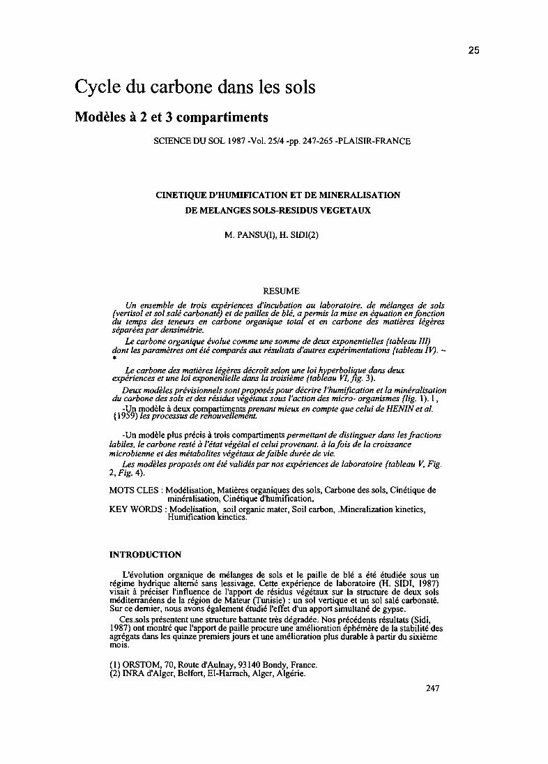
Cycle du carbone dans les sols

Modèles à 2 et 3 compartiments

SCIENCE DU SOL 1987 -Vol. 25/4 -pp. 247-265 -PLAISIR-FRANCE

CINETIQUE D'HUMIFICATION ET DE MINERALISATION

DE MELANGES SOLS-RESIDUS VEGETAUX

M. PANSU(I), H. SIDI(2)

RESUME

Un ensemble de trois expériences d'incubation au laboratoire. de mélanges de sols(vertisol et sol salé carbonaté) et de pailles de blé. apermis la mise en équation en fonctiondu temps des teneurs en carbone organique total et en carbone des matières légèresséparées par densimétrie.

Le carbone organique évolue comme une somme de deux exponentielles (tableau III)dont les paramètres ont été comparés aux résultats d'autres expérimentations (tableau IV). ­•

Le carbone des matières légères décroît selon une loi hyperbolique dans deuxexpériences et une loi exponentielle dans la troisième (tableau VI. Jlg. 3).

Deux modèles prévisionnels sont proposés pour décrire l'humification et la minéralisationdu carbone des sols et des résidus végétaux sous l'action des micro- organismes (lig. 1). l,

-Un modèle à deux çompartiments prenant mieux en compte que celui de HENIN et al.{1959) les processus de renouvellement.

-Un modèle plus précis à trois compartiments permettant de distinguer dans les fractionslabiles, le carbone resté à l'état végétal et celui provenant. à la fois de la croissancemicrobienne et des métabolites végétaux defaible durée de vie.

Les modèles proposés ont été validés par nos expériences de laboratoire (tableau V. Fig.2, Fig. 4).

MOTS CLES : Modélisation, Matières organiques des sols, Carbone des sols, Cinétique deminéralisation, Cinétique d'humification,

KEY WORDS : Modelisation\ soil organic mater, Soil carbon, .Mineralization kinetics,Humification kinetics.

INTRODUCTION

L'évolution organique de mélanges de sols et le paille de blé a été étudiée sous unrégime hydrique alterné sans lessivage. Cette expérience de laboratoire (H. SIDI, 1987)visait à préciser l'influence de l'apport de résidus végétaux sur la structure de deux solsméditerranéens de la région de Mateur (Tunisie) : un sol vertique et un sol salé carbonaté.Sur ce dernier, nous avons également étudié l'effet d'un apport Simultané de gypse.

Ces.sols présentent une structure battante très dégradée. Nos précédents résultats (Sidi,1987) ont montré que l'apport de paille procure une amélioration éphémère de la stabilité desagrégats dans les quinze premiers jours et une amélioration plus durable à partir du sixièmemois.

(1) ORSTOM, 70, Route d'Aulnay, 93140 Bondy, France.(2) INRA d'Alger, Belfort, EI-Harrach, Alger, Algérie.

247

25

M. PANSU, H. SIOI

"

Nos expérJences apportent également de nombreuses mesures sur l'évolution desstocks orgsnlques de ces sols dans des conditions expérimentales contr6l6es.

Il était nécessaire de préciser paralllliement la cinétique des caractéristiquesmesurées relatives aux matlllre8 organiques.

L'analyse des données • carbone organique total. et • matlllres légllres séparéespar densimétrie'. avalent pour but leur mise en équations ol!fl fonction du tempsd'Incubation et la comparaison des résultats avec d'autres. axpérlences du mêmetype.

Nos données ont permis également la prise en compte du paramètre • quantitéde pallie apportée ••

L'ensemble des données nous a permis de proposer et valider des modèles prëvt­slonnels d'évolution des compartiments stables et labiles des matlè'res organlquesdes sola eous l'effet d'apports végétaux~ Nous rappelons ct-deesous les principauxmodèles en usage qui Interviendront dans les discussions 8t qui permettent de situernos propositions, .

Le choix d'un modèle d'évolution Hé Il l'Interprétation de données agronomiquesat. pédologlques dépend du volume et de la natUre. de celles-cl. Alnel dans bien'des' cas, les auteurs se limitent Il des modèles monocompartlmentaux dérivés dumodèle de HENIN et OUPUIS (945). En fonction des cond'Itlon:s expérimentales l8t desmesurllS les auteurs ont été condulta Il modifier le modèLe Initiai selon différentescinétiques de décroissance comme le montrent les quelquea eXlBmples du tableau 1.

Tableau 1 : Clnétlqull de déerolwnce de modèles monocompartlmentaux appliquée aucarbone dea eols. A = contenu carboné exprimé généralement en pourmille massique du sol sec, t est le temps exprimé en année. Ao = valeurde A au temps O. a. = coefficient de décroissance. Dans le seul cas dela décrolseance exponentielle le temps de demi-vie est Indépendant de laquantité de matière li détruire. Dans ce cas également. appelé • mélangeparfait. Je temps moyen de résidence est égal au tempa de renouvelle­ment aolt 1/a..Decreaslng klnetlcs of monocompartlmental models app\led to the aollcarbon. A la carbot! content genera/y expreased ln terma of pour milleof dry soli. t la the tlme expressed ln yaar. Ao Is the value' 01 A at tlme O.a. Is decreaslng coefficient. Only ln cese of' exponentiel d&cay, the ha/f­tlme Is Independent 01 the emount 01 metter ta he de8troyed. Acrass thlssOoCe/led • we/l·mlxèd reservolr. the meen resldence tlme la equal tothe turn-over ttme, n8mely 11«-

Loi dnftiquo Ord.. 0 ordre 1 Ordre 2 Ordro nLin'ot re o.ponondoll.• h)'~orboUquo l'uhl.lnc.e

Modal. -d"'dt~ ŒJ!ill+ ~ ŒJ"(,\)~

Dillonoion aK • -,•••a•• îqu. !lrl T-I trlT-1 t11- nr - 1

T • t ......p.

Evolution A ""-oc Ao ••p(-ot) 1\0(I+,\OD t)-l Ao(l ... (n-I )AO,,-I t) -J In-I

ne>.

Demi-vi. A Ao/20 LOll 2/0 1/0.\0 (2n-1_0 1(a (n-I ),\0"-1)

Exer:aplol dl o1pplica- 1I0F~L\11 ot B01FlN otc ion • .au carbone pour .âmoire RUnlBEKE (1979) FLEURY (197~) Il.\L[St'!.:;T (1982)de. lot. aOIFI" .t 01.

(1986)---...;

L'apparition de mod~lea li plusieurs compartiments de décroissances supposées homo­. gènes est allée d'e pair avec l'augmentetlon du volume des données collect6es et la'quallté de leur analyse statistique.

248

CINETIOUE HUMIFICATION, 'MINERALISATION SOLS

Les compartimenta correspondent trlls rerament Il des constituants organiquesdéfInis ou Il des fraotlons mesurables quantitativement. les donnéea physiques. chl­mlques ou biologiques' permettent cependant de Jellr affecter une cinétique de décrois­sance et d'estImer les flux qui les traversent.

Ainsi, le modèle de HENIN, MONNIER et TURC (1959) permet la prise en comptedes mesures densimétrlques de matières légllres (HENIN et TURC, 1949) Mslmltéesalora Il une fraotlon labile.

Le modèle de JENK1NSON et RAYNER (1977) a été validé li la fols per desmesuras de décrolssancltS de matières végétales. de bIomasse microbienne (JENKIN­SON, 1965) et de detatlons pour estimer les param~tres d'évolution Il long terme du.stock humique d'un sol soumis Il un système cultural donné.

Les modèles de PAUL et VAN VEEN (1978) et JENKINSON 'et LADD (1981)concer­nent des évolutlone Il' plus. court terme. Le preniler 1 été validé surtout par desmesuras de décrolssence de constituants blochlmlquell des plsntes dens les sols, ledeuxième essentiellement par des mesures de biomasse microbienne.

On peut remarquer que, contrairement aux modèle d'évolution globale de toutle carbone (tableau Il, lei loIs cln6tlques d6crlvant la décrolsssnce de chaque compar- .tlm~nt dans les modèles multlcompartlmentaux ci-dessus sont toujours du premier'ordre. .

1. MATERIELS ET METHODES

A) Matériels utilisés et protocole expérimental

Les principales caractéristiques du sol peu évolué' d'lpports.lI tendance vertlqueet du sol ealé carbonaté li hydromorphle de profondeur sont présentées dans letableau Il.

Tableau " : Sol. utilisés pour lei expérlencel. ce = ~ond.Îlctlvlt6 électrique de l'extrait. pite saturée (en mmhol/cm), CaC03 = calcaire total, lei valeurs du ear-

bone organique sont Indlquéel dans le tableau III. .Solls under study. CE = electrlc81 conductlvlty 01 s8tureted extrsct linmmhostcm), CI/COJ = tata/- ca/c;areous, org8nle carbon VI/Ives are Indl­ceted ln Table 1/1,

Compleze absorbanttype c!e 101e et pB argile CE C/II CaC03 Ifa It 1 Ca 1 Hghorizons prélevés B20) % % meq/100g

---------------------- --- ------ --- 13 ----- --- ------ ---alluvial à tendance 7,2 48 0,7 1,2 1, 1 0,3! 15,18 4, ~~

vertique 0-32 cm5al' oarbonaté à hyc!ro 8,0 49 4,7 8,5 28 9,!> 1 t G~ G6,40 7, Clmorphie de.profonc!eur.0~21 om

.. -la pallie dé blé, découpée et ce/ll7rée entre 0,2 et 2 mm a été ajoutée eux

sols Il des doses ëorl'6Spondant li 0 (témoin), 2,7 et 8,1 pour mille de carbonedans le mélarige -sec. Des ajouts d'emmonlac mé'lang6 li l'eau d'humectatlon ont permisde ramener li 15 le rapport CIN de la palllè apportée. .

Les écbantillons de 250' g de sols amendés ou non (témoIns) ont ét6 placésdans des tubes PVC de 7,5 cm de d/am6tre. Intérieur bouchés Il la partie 'n'érleure·par un grillage plastique aurmonté de 2 cm de gravier.

249

<:

N0)

.'.

.........................................._ . "'-_"""'u._,_" "'~~~"""'~~. -~_,.~ __ "•..,~.~ , ...,...,

• .6

r'.M. PANSU, H. 5101

Ces tubes ont été mIs il Incuber è une tempéreture constente de 28·C evecune alternance humectatlon-desslccatlc:'I (teneur en eau ramenée tous les trois jours è80 % de l'humIdIté équlvslente li ls capacttë de rétention au champ) donc ssna pertepar drainage. Les prélèvements ont été effectuéa eux temps : 0, 15, 30, 90, 180, 270jours d'Incubation. Lea essais conduits en double comprenaient donc, 36 tubes pour'chacune des trois expériences notées comme suit :VE = Sol .peu évolu6 d'spport il tendsnce vertfque.SA = Sol salé carbonaté.SG = Sol salé carbonaté amendé è 1 % de gypse.

A la fin de chacune des périodes d'Incubation prévues dans le plan' d'exp6rlenèes,les sols des 18 tubes correspondants ont ét6 prélevés et mis il s6cher avecréunIon des deux répétitions. Après écrasement des mottes, tamisage il 2 mm ethomogénélsstlon les échantlllons ont été prélevés au partIteur et les teneurs encarbone organique mesurées par oxydation avec le mélange sulfochromlque selon laméthode de WALKLEY et BLACK. Les ·teneurs en csrbone des échantillons provensntdu sol non carbonaté ont pu être v6rlflées par combustion sous oxygène il 1 20O"Cet dosage du CO. d6gag6 par coulométrle.

Le coefficient ~e varlatlon 6tabll sur 15 prises 'd'éssal d'un même sol est de1,9 "10 et Iss Intervalles de confiance au niveau de probsblllté 0,95 ont 6té reportéssur la figure II. .' , . ,

Les matIères vég6tales légères sont obtenues par céparatlon denslm6tr1que avecde ('acide phosphorique 2M' (DABIN, 1976). BI"n que moins dense (d = 1,2) qued'autres IIqueura denslm6trlques (HENIN et TURC,. 1949) (MONNIER et el., 1962],l'acide phosphorique est moins dangereux è manipuler, Il détruit !:es carbcnates enfavorisant la IIbératlon de matlères légères séquestrées et permet le dosage dematières organiques acldo-solubles (acides fulvlques libres) contenues dans les solset débris végétaux.

Le carbone de!! particules recueillies dans le surnageant est dosé par combustlonet couJométrle du C01.

B) Outils statistiques et informatiques

Le logiciel SPCLA$ (PANSU, 1983) a permis ('extractIon des donn6es étudiéesselon chacun des troIs plans d'expérience, leur présentation graphique avec leeIntervalles de conf:ance et les premiers essais d'ajustement linéaIres.

L'ajustement non linéaIre des courbes de carbone a été réalisé au moyen dulogicIel STATGRAPHICS (société UNIWARE) qui utilise le méthode anslytlque de l'slgo­rlthme de MAROUAROT (1963) et avec le logiciel OPTIM (CHEVILLOTTE et TOUMA,1987) par la méthode de MAROUARDT et la méthode SIMPLEX des gradients.

Nous avons écrit un programme donnant pour chaque modèle trouvé: les résidusd'ajustement, le cœfflclent de détermination R2, le test F de Flsher-5nedecor, la,probablllté associée Pro de re~s du modèle et l'estimation de l'écart·type s des valeursprédites.

.te calcul des approxtmetïone de dépsrt des modèles non linéaIres est réaliséde la manière suivante : ,

- Estimation de l'exponentielle correspondant au compartiment stable è partirdé 90 jours d'Incubation.

- Déduction des valeurs prédites avec cette exponentielle aux valeurs mesurées'en début d'Incubation. '

- Estlmatlon de l'exponentlelle correspondant au début d'Incubation. 'Il va de sol que pour un même phénomène, plusieurs modèles peuvent convenir.

'Par exemple, lè où BALESDENT (1982) trouve une fonction puissance, JENKINSON (1971]'trouve une somme d'exponentleiles. C'est pourquoi, nous avons toujours essayé plu­sieurs modèles et dans ce qui suit seuls sont IndIqués les ajustements les plusslgnlflcstlfs.250

. CINETIOUE HUMIFICATION, MINERALISATION SOLS

Nous avons programmé les modèles d'ëvelutten en basic sous leur forme matrl·clelle. Nous avons également utlJ/sé un logiciel turbo-pasC81 d'Intégrstlon num,érlqued'équations différentielles (G. PICHON, ORSTOM. com. pers.).

U. EVOLUTION DU CARBONE ORGANIQUE TOTAL

A) Equation trouvée .

Le meJlleur ajuste!"ent de la tel18ur du carbone organique Ct en fonction du tempst que nous ayons pu observer est de Is forme:

Ct= a 'exp(- et t) + b exp(- P t) (1)

dans lesquel les constantes a et b représentent les valeurs en carbone de deuxcompsrtlmenta Instables et stables il l'Instant InitIai alora- que et et P représententrespectivement leura cœfflclents de décrol8Sance. Nous avona réalisé ces ajustementssur les trois séries d'~ssals ayant' reçu les plus forta amendements en patlJe. Lesmesures sont alors moins sujettes il. des fluctuatlons. d'échantillonnage.

Les courbes correspond~nt' aux amendÎlments plus falblea ont été 'déduItes despremières en corlservant les coefficients et et 13 des exponèntlellès et en posant :

Xl = exp(- et t)X2 = exp(- Il t)

Une régression multiple sans co'natante a perrnlos alors d'estimer les coeffIcientsa et b 'des modèles :

Ct ='a Xi + b X2Les paramètres s, b, et, 13 sont reportés dsns le tableau fil avec les tests statls·

tiques d'ajustementa. .

Tableail III: D'croissance du carbone organique total: et, 13, a, b sont les paramètresd. l'~.tlon (1); m et Co représentent l'apport de carbone et la. valeurmesur6e au temps O.Les équations lJC?ur m = 8.1 pour mme sont obtenues par les méthodesnon IIn'a1r:es. Les eutres 'quatlons sont obtanues par le méthode der6gresslon multiple Indlqu~e dans le texte.Decrease of total organlc carbon : et, p, a, b are Ole parameters ofthe equstlon (1) : m and Co correspond ta the csrbon supply .sodthe vslue mesured at tlme O. ,Equations concernlng m = 8,1 pour mll/8 sre obtalned wlth oon·/l08slmethods. The other equatlons are obta/ned wlth the multiple regress/onmethod mentloned 1" the text,

Exp. m Co -0: -B e b R2 FC 3, 3) Pr.. ir°looC '-l/ann6e 0/00 C

VS 8,1 21,05 14, 51 0,015 4,99 15,68 0,94 15,8 0,05 0,67SA 8,1 27,27 16,24 0,007 9,48 17, lI5 O,lIO 60,,6 0,01 0,63sa 8',1 26,30 24, 11 0,074 6,17 20,03 0,98 40,2 0,01 0,56

VB 2,7 15,60 14, 51 0,015 2,23 13,23 0,79 4,0 0,28 0,61IsA 2,7 21,00 16,24 '0,007 5,36 15,33 0,87 6.5 0,16 " 10sa 2,7 20,80 24, 11 0,074 6,39 14,91 0,90 . 9,2 0,10 l, 16

VS 0 12,95 14, 51 0,015 1,57 11,68 0,68 2,2 0,53 0,59IsA 0 17,75 16,24 0,007 3,47 13,97 0,94 15,2 0, 05 0,47Iso 0 17,75 24, 11 0,074 3,68 13,92 1,00 50,9 0,01 D,3D

251

I\J-...l

_~ ......:.... -.:...__J.I -----------';""---"";"";"------_""".... , " ....

M. PANSU, H. SIDI

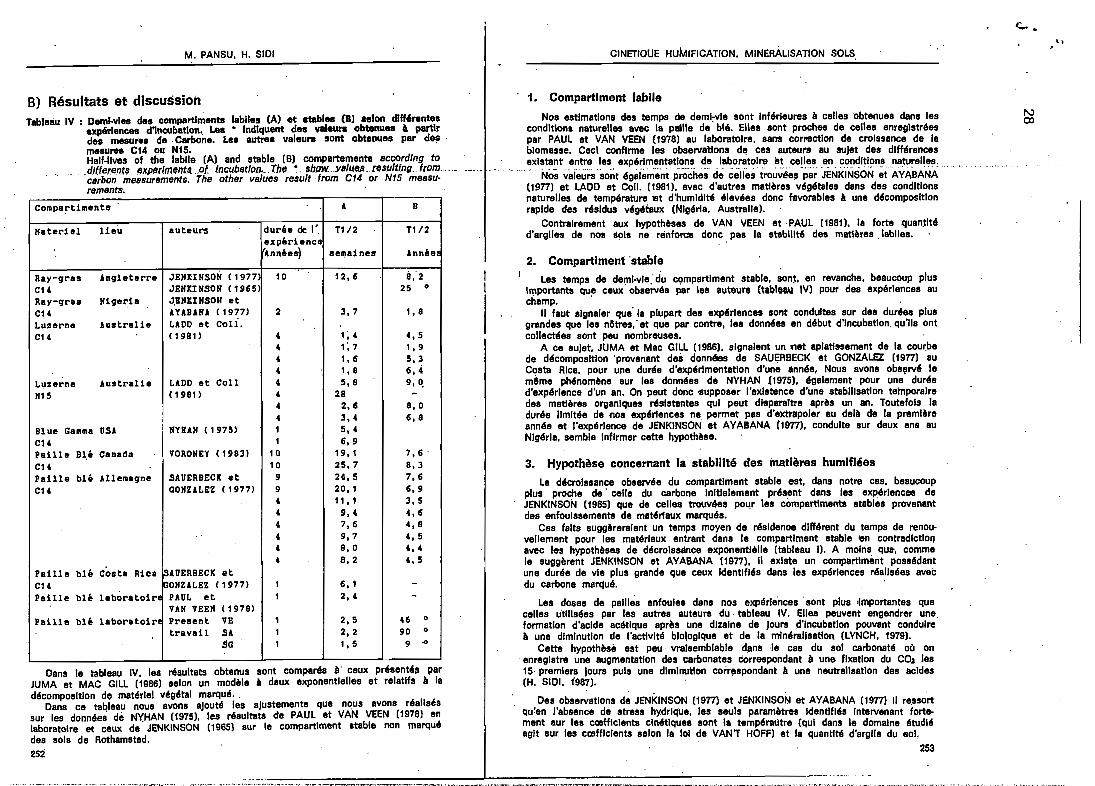
B) Résultats et discussionTableàu IV : DemI-vIes des compartiments labiles (A) et ablbles (B) aelon dlH'rentes

expérIences d'Incubation, Les • IndIquent des valeurs obtenues l partIrdes mesures de· Carbone. Les autrea valeurs sont obtellues par de!,mesures C14 ou N15.Half-ll".es of the labile (A) and stable (B) compartemente accordlng ta

. .d/ftemn.t' exper/meflttl. ..of lncubaUon•..The. • . sh/JW. ..YB/USA. reBu/ting..irom. ... ._...•. " .carbon measurements. The other values result {rom C14 or N15 meesu-rements.

COfllpa~t1l1lents A B

Hateriel lieu auteurs durée de l'. T1/.2 T1I2expérienceAnnées) aelllaines Année:

Ray-gras Angleterre JEIIUNSON (1977 10 12,6 8;2CH JEfllCINSON (1965) 25 0

Ray-grae Nigeria J.EllIIIISOlf etCH AUBANA (1977) 2 3,7 1,8Luzerne Australie LADD et Coli.CH ( 1981) 4 1; 4 4,5

4 1; 7 1, 94 1,6 5.34 1,8 6.4

Luzerne Australie LADD et Coll 4 5.8 9, O.N15 ( 1981) 4 28 -

4 2.ll 8,04 3.4 6,8

Blue Gamma USA IIYRAII (1975) 1 5,4CH 1 6.9Paille B~é Canada VORONEY (19831 10 19.1 7,6'CH 10 25,7 8,3Paille blé Allemagne SAUERBECK et 9 24,5 7,6CU aOKZALEZ (19771 9 20.1 6.9

4 11,1 3,54 9.4 4,64 7.6 4.84 9,7 4,54 8,0 4.44 8,2 4.5

Paille blé Costa Rica IsAlJERBECK etCH ~ONZALEZ (19771 1 6,1 -Paille blé leboratoiN PAUL et 1 2.4 -

VAN VEEII (1978)Paille blé laboratoir' Present VE 1 2,5 46 0

travail SA 1 2,2 90 0

SG 1 1,5 9 -0

08ns le tableau IV, les rés.ultat'S obtanus sont comparés li' ceux présantéll parJUMA et MAC GILL (1986) selon un modèle li daux exponentielles et relatifs li ladécomposItion do matériel végétal marqué..

Dans ce tal:!leau nous avons ajouté les ajustements que nous avons réaliséssur les données de N'(HAN (1975), les résultats ete PAUL et VAN VEEN (1978) enlaboratoIre e( ceux de JENKINSON (1965) sur le compartiment stable non marquédes sols de Rot~amsted.

252

CINETIOUE HUMIFICATION, MINERALISATION SOLS.

1. Compartiment labile

Noa estlmstlons des temps de deml:vle sont Inférieures li celles 'obtenues dans lesconditions naturelles avec \a pllllle de blli. Elles sont proches de celles anreglstréespar PAUL et VAN VEEN (1978) au laboratoire, sans correction de croissance de labIomasse. Ceci confirme les observations dl! ces auteurs au sujet des dlfMrencesexistant entre les expérimentations de laboratoire lit celles en conditions naturelles.

..... Nôsvaiëurssont égaièin'èntproëhes de' cëllë;troûVée~ 'p~~ ïÊNKINSON ~tAYABANA .(1977) et LAOO et Coll. (1981), avec d'autres matières végétales dans des conditionsnaturelles de température tet d'humidité élevées donc favorables li une décompositionrapide des résidus vég,taux (Nlgérla, Australie).

Contrairement aux hypothèses de VAN VEEN et PAUL (19811, la forte quan.tltéd'argiles de nos IIpls ne rlinforœ donc pas ta stabilité des matières. labiles.

2. Compartiment 'stable1 .

Les temps de del:Tll-vle: du cçmpartlrnent stable, son~, en revanche, beaucoup plusImportants que ceux observés par los ll\ltoure (tableau IV) pour des expériences auchamp. '

Il faut sIgnaler que la plupart des expériences sont conduites sur des dur'es plusgrandes que les netres,' et que par contre, les données en début d'Incubation.qu'Ils ontcollectées sont pau nombreuses.

A ce sujet. JUMA et Mac GILL (1986), signaient un '"et aplatl"ement de la courbede décomposition 'provenant dei données de SAUERBECK et GONZALEZ (1977) auCosta Rica, pour une durée d'expérimentation d'une année, Nous avons obsl(lrvé lemême phénomène sur les données de NYHAN (1975), également pour una duréed'expérience d'un an. On peut donc 'llupposer l'exlatence d'une stabilisation temporairedes matières organIques rlislstentes qui peut dlsparaltre après un an. Toutefois ladurée limItée de nos expériences ne permet pas d'extrapoler au delà ete la premièreannée et l'expérIence de JENKINSON' et AYABANA (1977), conduIte sur deux ans auNlgérla, semble Infirmer cette hypothèse.

3. Hypothèse concernant la stabilité des inatières humlfléesLa décroIssance observée du compartiment stable est, dans notre cas, beaucoup

pllJ'S proche de' celle du carbone Inltlalemant présent dans les expérIences deJENKINSON (1965) que de celles trouvées pour les compartiments stables provenantdes enfoulssementa de matériaux marqués.

Ces faits suggèreraJent un temps moyen de résldenoe dlHérent du temps de renou­vellement pour les matériaux entrant dana le compartiment stable ren contradictionavec les hypothèses de décroissance exponentielle (tableau Il. A moins qUIt, commele suggèrent JENKINSON et AYABANA t1977), Il existe un compartlmént possédantune durée de vie plus grande que ceux Identifiés dans les expériences réalisées avecdu carbone marqué. .

Les doses de pallies enfouies dans nos expériences' sont plus .Importantes quecelles utilisées par les autres auteurs du tableau IV. Elles peuvent engendrer une.formation d'acide acétique après une dizaine de jours .d'Incubatlon pouvant conduire11 une diminution de l'activité biologique et de la minéralisation (LYNCH, 1979).

Cette hypothèsè est peu' vraIsemblable d.ans ·Ie cas du sol carbonaté oCl on.enregistre une augmentation des carbonates correspondant li une fixation du COJ les15· premlera joure puis une dlmlnutton correspondant li une neutralisation des acides(H. SIOI, 1987).

Des observations de JENKINSON (1977) et JENKINSON et AYABANA (1977) 1/ re.ssortqu'en J'absence de stress hydrique, les seuls paramètres Identifiés. Intervenant forte­ment aur les cœfflclents cinétiques sont la tempéreùtre (qui dans le domaine étudiéagit sur les cœfflclents selon la 101 de VAN'T HOFF) et la quantité d'argile du BoL

253

<-.

NCD

"

1 __ ••••••.•.

~

," ,

M. PANSU, H. SIDI CI/ilETIQUE HUMIFICATION, MINERALISATION SOLS

Ce dernIer paramètre Intervient sans doute fortement dans' notre expérience puisqueles sols sont très argileux, avec des argiles 2:1 gonflantes alors que l'essai' deJENKINSON et AVABANA a été réalisé sur des sols sableux avec deè atglleskaollnltlques.

Nous allons tenté d'utiliser nos données pour valider des modèles prévisionnelsne différenciant pas carbone apporté et carbone présent stabilisé ou non.

III. VALIDATION DES MODELES A DEUX COMPARTIMENTS

Al Le modèle de HENINet al. (1959) et sa validation par nosmesures de carbone total

Le modèle 1 de HENIN, MONNIER et TURC (1959) reporté dsns la figure 1 distingueles matières organiques labiles A alimentées par les apports végétaux m et lesmatières humlflées B forméas d'un apport provenant des précédentes, et qui seminéralisent beaucoup plus lentement. '

Pour l'ajustement Il nos données, nous avons modifié un peu "expression' des ,équations présentées Initialement.

En effet, m est un apport discontinu avec une échelle de tempa dIfférente' de celledu cœfflc'ent de décroissance.

Les équations de vItesse de décrolseance de chaque compartIment s'exprimentalors par:' '

CompartIment labile A : dIA + mi/dt = - a.(A + rn) (2)COmpartiment stable B : d(B)/dt = ka.!A + rn) - P(B) (3)

svec

t ... tamps (en année)CA + m), (B) .. carbone organlqlJo total des compsitlment'9 A et B (en pour mille):z; .. cœfflclent de destruction des matières labiles (en année-l)

1 k::z cœfflclent Isohumlque ' ,P = cœfflclent de minéralisation des matIères stables (en année-ll)

Li somme des deux expressions obtenues psr Intégration des équations (2) et (3)nous fournit, la formule d'évolutlon du carbone organIque total Ct soIt :

Ct = [Ao(l, - ka/(a. - Pl) ++ [Bo + kAoa./(a. - P)

m(l - ka./(a. - pm EXP (- a.t)+ mka./(a.- pJ] \:"XP (- pt) (4)

et comme p est très petit devant a. :Ct = [Ao(l - k) + m(l - k))' EXP(- «t) + (Bo + kAo + km) EXP(- Pt) (5J

Sous 08tte forme, le' carbone évolue comme une somme de deux expon'entlellessvec des cœfflclent'9 muklpllçstlfs IInéslres en fonction de l'apport. Nous avons testécette linéarité pour chaque expérience 'afin d'obtenir le modèle correspondant Il l'ëque-tlon (5) de la forme: '

Ct == (ao + sim) (EXP(- a. t) + (bo + bim) EXP (-- P tl (S')

N,(0

Les valeurs des psrsmètrea des équations (5) et (5') sont reportées dans letableau V, où R2a et R2b représentent' leB cœfflclents de détermination des deuxsJustements linéaires des cœfflclenta a et b de l'équation (1) en fonction de l'spportm. Les courbes correepondant Il ces équatIons, sont reportées dans la figure 2.

Il ressort du tableau V que la linéarité en fonction des apports el meilleure pour lecompartiment stable. Elle est satisfaISante pour expliquer la décroissance carbonéeselon le modèle de HENIN et al. (1959) dans les expériences VE et SA. Le modèles'sppllqu,e mal par contre Il l'expérience SG.

255

Tableau V : Estfmatfons des paramètres des 6quatlons 5 et 5' correspondant au mod61ede HENIN et al. (1959 : k = bt, Gk = .cart de k avec l'estfmatlonk = f - a1, AD et 80 estIm6s avec k == bl, BAo et GBo == écarts cieAo et Bo avec l'estimation k + Gk.Parsmeters evaluatlons ln equatlons (SJ and (5') correspondlng, to themodel by HENIN et al. (1959)': k = bt, Gk '= d/ff"rence between theev"luBtlon k = 1 - et, Ao Bnd 80 er« eVBluBt"d wlth k = bt, GAoBnd Mo = dlfferences on Ao Bnd 80 wlth dhe evaluat/on k + Bk.

Exp so al R2a bo b1 R2b k 6k Ao 6Ao BD 6Bo

VE 1,36 0,43 0,98 11,11 0,49 1,00 ,0,49 +0,08 2,68 +0,41 10,46 -0,47SA 3,42 0,14 1,00 13,98 0,49 1,00 0,49 -0,23 6, 1J, -a, 13 10,68 +2, 13sa 4,49 0,26 0,11 13,41 0,18 0,98 0,18 -0,04 (20,41 - (-2,4) -

Agure f: Les modèles validés par nos exp,"rlences. Les traita pointillés exprI­ment une possible différence d'ëchel­le de temps entre apports et dé­croissances.1 = modèle de HENIN et al. (1959)correspondant aux équations de vI·tesse (2) et (3) et aux formulesd'évolution du carbone organique(4) et (5).Il = modèle propos' il: deux com­partimenta correapondant aux équa­tions ,(6) et (7).

III = modèle proposé il trois com­partlmenta correspondant aux équa·tlons de vItesse (11), (12) et (13)et la formule matricielle '(14).

The models valldated wlth our experlmsnta. Dotted /Ines show a possibletlme sca/e dlfference between carbon amendments and decay.1 = HENIN et al, modal (1959) correspondlng ta dlf~erentlel equatlon (2)and (3) end organ/c cerbon evolutlon formula (4) and (5).Il = Suggested MO compartment model correspondlng to equatlo,ns (6) and(7).III = Suggested, three compartments model correspondlng to dlfferentlalequatlons (11), (12), (13) and matrlc/al formula (14).

JI1

254

J.:.... -,M. PANSU, H: 8101 CINETIOUE HUMIFICATION, MINERALISATION SOLS

eNoBl Nouvelle présentation 'd'un modèle à deux compartiments

Les paramètres de l'équation (5) (tableau V) montrent que le pourcentage de carboneInstable Initialement présent dans le sol salé carbonaté (SA), est plus grand quedans le aol Il tendance vertlque (VE). L'activité biologique de ce dernier est d'mlleursmolna Importante, comme le montre également la disparition moins rapide des poly.saccharldes (5101, 1987),

L'apport' de gypse semble produlre uns augmentation simultanée des procsssusd'humlflcstlon et de minéralisation et J'expérience SG ne permet pas de valider lemodèle de HENIN et al. (19S9),

Nous proposons une autre présentstlon d'un modèle Il deux compartiments lmodëleIl, figure n prenant mIeux en compte le' renouvellement permsnent (sauf contralnteclimatique majeure) des matières orgsnlques d'un cornpartlmant à l'autre et la possl·blllté de pasaage des spports vers chacun des deux compartiments.

Pa et Pb représenten,t les propcrttons qui passent respectivement dans lea corn-i, psrtlments Instable A el: stable B, soit ile façon discontinue (traits pointillés) au

moment des apports aolt, en permanence lors des processus de renouvellemen't,' Lesvitesses d'ëvolutton de chaque compartiment s'exprIment alors comme suit:Compartiment Instsble A.': d(A]/dt = (mPa) + a(A]Pa + ~[B]Pa - «[A] (6)Compartlm~nt atable B:· d[BJ/dt = (mPb) + a(AJPb + ~[BJPb - ~[BJ (7)

où les parenthllses exprIment une différence d'échelle ds temps et les crochets,les teneurs de choque compartiment en pour mille massique.. Dsns les conditions d'état stable : d(A]/dt _ d[B]/dt = 0salt d'après les deux équations de vitesses :'

[A] = [B] ~Pa/aPb et [B] = [A] «Pb/~Pa

Lea temps de renouvellement Ta et Tb de chaque compartiment A et B a'exprl·ment alors, par Ta == [A]/o:[A] == 1/0: et Tb == 1/~. ,

Les valeurs de csrbone Il l'Instant Initiai permettent d'estimer les proportlona Paet' Pb alors que, les valeurs aptès un Intervslle de tempa at fournissent une estlms.tlonde la somme Pa + Pb proche du cœfflc/ent Isohumlque de HENIN et al,

. Les valeura de Ps et Pb sont respectivement de 0,3 et 0,25 pour l'expérience VE,0,24 et 0,1 pour l'expi§rlence SA, 0,28 et 0,32 pour l'expérience ~G. .

Le calcul des vsleurs prédites par ce modèle (fig, 2) peut s'effectuer par deuxméthodes donnsnt dea résulteta équivalents : Intégration numérique des équations (6)et (7) ou sous forme matricielle de manière anslogue au modèle Il trois compartl.ments prdsent6 cl-aprèa.

Les courbes de la ~Igure 2 montrerit des ajustements cçnfondcs avec ceux dumodèle de HENIN et al. en ce qui concerne les expériences VE' et SA. Le modèleproposé permet un meilleur ajustement des données de l'exoérlence SG.

Les cslculs montrent une molndrs décroissance en fonction du temps pour lecompartiment labile que dan's le modèle précédent, Comme prévu, ce modèle traduitdonc mieux une réalité physique ,: la présilnce de carbone facilement décomposableprovensnt des processus de renouvellement qui accompagnent la minéralisation del'humus même dans les sols l!ivoJués. '

--.---

___ . "':10.1 .....1112

..._'08 1 .n ...1.12

DPlItIINCE : sa

. .__ 120

--'-- ~--

en %0Il . ,_. ----. zo.

! c.T: -;~ %~ --- 1

. 25._----

. c,r.

10-:' ..o 1

_.... ... 108 L •• m.JI12

_____ . .20

-- ..__ .6

EXPERIINCI : lA

~a ~~ 1• 1

!1\ --JZ5

.~-

~. ,. .

lS 1 •• • ft

.,. l _ ..•'., - ...15. .

loi. .0'1 3

Figure 2 : Ajustements réalisés selon les équations (5') (tableau V) du modèle deHENIN et al. (traits pleins) et selon notre modèle Il (figure 1) Il deuxcompartiments (pointillés), Les ajustements sont Identiques pour les expé­rlence~ VE et SA. Les points expérImentaux aont représentés, avec leursIntervalles de confiance au niveau O,9S pour' les' trois amendementS depallie (8,1 pour mille ., 2,7 pour mll/e .. et 0 "..de carbone).

Flttlng wlth the equatlons (S') (table V) of HENIN et al. (1959) model andour model Il ln figure 1, (dottèd /Ines). AdJustments are Identlca/.11I VEand SA expe.rlments. Experimentai points are represented w/th thel, ~S Of.confidence lnteNais fo, the three lJupply of carbon straw : 8,1 pour mille .,2,7 pour mille. and 0 V' '

256

IV. PRISE EN COMPTE· DE LA CINETIOUE D'EVOLUTIONDES MATIERES' ORGANIOUES LEGERESET PROPOSITION D'UN MODELEA TROIS COMPARTIMENTS

Al Cinétique de décroissance des matièrès organiques légaresLe 'carbone dss mstlè'res légères extraites par fractIonnement denslmétrlque en

début d'Incubation, juste sprès Is premlllre humectstlon, est touJours proche de 40 %

.257

" .••'" ~"""'~"''''' ....., .. "'~....~'.~'n"'.• " ".~,,,,~..•~, ....•"

..~t,.

M. PANSU, H. SIDI CINETIQUE HUMIFICATION, MINERALISATION SOLS

cr 1C.T.-MDL

.Z5

U.N:"IINCI 1 la

en %0

\\\\\\

2~ \,......... cr .20

1\

-'-<::=::':: - ~- --·c:r.~M6.L::-----·---------

!

'~ "

~.~ .'aL.a .. _.:.....~~...._.==lfJo 1 3 e 9 1 •• mlll 12

fOl\

J15

Jzo1

C.T. 1

C:r.-M.OLI.251

I!)CN....NCI :IA

en 960

cr--------

-----ëi::M~O~~-------------'

M.OL

,1~ , :r "10• - - • 9 1.....1112

3

avec

du carbone apporté par la pallie. On ne peut donc assimiler ces fractions à lapallie apportée. GRAFIN (1971) décrit le carbolJll des matières légères commeun carbone libre non remanié dans le sol alors que DABIN (1976) s'en tient auterme'. matières organiques légères-.

la décroissance carbonée des matières organiques légères en fonction du tempssuit une 101 hyperbolique pour les expériences VE et SG alofs que la 101 est exponen­tlelle dans l'expérience SA soit :

~pérlences VE et SG : V = Vo/ll + Vort) (8)expérience SA : V = Vo EXP(- rt) (9)

Avec :

t = temps (en année)V' = carbone au temps t des 'matières légères (en pour mille de la masse totale de

. sol sec)

Vo =valeur de V pour t = 0r = Cœfflclent da décrolssanca du carbone des matières légères (exprimé en

année-1 pour mllle-I pour l'équation (8) et année-1 pour l'équation 191 tre­dulsent li la fols sa fixation dans le sol et sa minéralisation.

Dans chaque cas, les ajustements ont été trouvés' en supposant que les valeurs. Vo en début d'Incubation sont les plus précises. •

Des régressions linéaires ont permis alors d'estImer le cœfflclent r du modèley = r t (10)

. 259

~

.zo

C.T.C.T.-M.OL

rx,t"'INCI :VI

en 960

C.T.- - -::.==_='::15

------CT. -M.OL

'M.OL

,1-,-- .L,::::J . T 11001 3 e .1 .....1.12

Décroissance des matières végétaies séparies par densimétrie .IMOL), Valeuraexpérimentales de 3 apports 18.1' pour mille III, 2,7 pour mille. et 0 v) etvaleurs prédites pâr .les équations (8) et .(9) Itableau VI). les courbes enpointillés représentent sur une échelle différente, les' valeurs prédites ducarbone total lCn. et du carbone non séparé par densimétrie lCT - MOL)pour les apports, il 8.1 pour mille de carbone •Decay of plant materlals aeparated by denslmetry Mal. Experimentaivs/ues.of the' tbree supplies (B,1 pour mille •• 2,7 pour mille e, and Ov)end predlcted velues of (B) end (9) equatlons (tsble VI). The dotted curves

represent on e dlfferent sce/e the predlcted vs/ues of total organ/c carbon(CT) and csrbon not sepsreted by denslmetry (CT·MOL) for the suppl/es ofB," pour mille cerbon strew. ' ,

Figure ,3 :

Exp m Equ. V Vo r F( 1 1 5) s Tl/2%oC

VE 0 ( 8) o, 24 39,86 98 0,02 5,4VE 2,7 ( 8) 1,67 6,41 231 0,08 4,9VE 8,1 ( 8) 2,66 1,92 163 0, 1 S 10, 2

SA 0 ( 9) 0,.25 S,Ol 44 0,03 7,2SA 2,7 ( 9) 1, 16 2,77 S3 0, 14 13, 0SA 8, 1 ( 9) 2,25 2,92 144 0,03 12, 3

SG 0 ( 8) 0, 23 38,35 40 0,03 5,9sa 2,7 ( 8) 1, 13 9,13 14 0,24 5,0sa 8, 1 ( 8) 2,19 3,19 ~16 0,03 7,4

--258

Tableau VI : Estimation des paramètres des équations (8) et (9) décrivant la décrois.,sance des matières organiques légères. Tous les ajustements sont slgnl.flcatlfs au niveau 0,99 sauf pour l'apport 2.7 de l'expérience sa,Evaluatlon 'of the parameters ln equatlon (8) end (9) descrlblng thedecrease of IIght organlc materlals, Ali Ilttlng sre slgnlflcsnt st 0.99level exept lor the supply 1 % Irom the SG experlment.

y = llV - ttv». dans Je cas de "équation (8) ety = loS (VIVo), dans. le cas de l'équation (9)

les' paramètres correspondant aux équations (8) et (9) sont présentés dans letableau VI. et les courbes de valeurs prédites dans la ('Igure 3.

......~.

M. PANSU, H. 5101 CINETIQUE HUMIFICATION, MINERALISATION SOLS

m == «[A] (1 - Pa - Pb}/Pam = lJ[B](1 - Pa ~ Pb}/Pb

W~

b) 1

(14)SI = MS'·I

obtenu au moyen' du produit" matrIcIelSI = 1: Iloil M représente la matrice d'évolution du sol :

M IV . 0 0Pa(l - v) a + Pa(1 '- a) Pa (1 - blPb(l - v) . Pb(l - a) b + Pb(l _

Ul aussi, ia méthode matricielle fournIt des ~sultats comparables aux autresméthodes d'Intégration numérique dea équations de vitesses. Les courbas de la fIgure4 repr~sentent l'évolution almultsnée de chaque compartiment et du carbone totalpour les trola Bols avec les plua forta apports de pallie.

En f.lt, la présentstlon que nous donnons correspond égslement Ji une almpllfl-'cation du modèle de JENKINSON et RAYNER (1977) :

- Pour l'évolution Il court terme, noue négligeons la fraction • Chemlcaly stablllsedorganlc matter", dans laquelle les'entrées 1I0nt très faibles. .

- Nous remplaçons les deux compartimenta è olnétlque ,du premier ordre. d6com­posable plant materlal" at • Resistant plant, materlal " par un sel.li compartiment dontla cinétique peut Atre, selon "état du sol! e~ponentlelle ou hyperbolique.

Pendant un Intetvalle de temps ôt l'évolution respective de chaque compartimentpeut être assimilée Il' :

v = EXP(-rat) ou v == 1/(1 + Vorc~t) pour le compsrtlment végétal selon sadécrolsssnce sans E de EXP, décroissance exponentielle ou hyperbolique.a = EXP(- ~t) pour le compartiment Instable.b = EXP(- ~~t) POur le compartiment stable.

Au temps tl = ,t'-I + ~t, "état du sol est décrit par le vecteur:

'[V,] [A], [B]'= teneur carbonée de chaque compartiment (en pour mille de aol secl.Pa, Pb = Proportions de carbone entrant dana lIis compartiments A et B.:1:, 13 = cœfflclents de, décroissance des compartiments A et B (en année-I )

l' == cœfflclent de décroissance hyperbolique du carbone II l'état végétsl (en année-Ipour mllle-I). . .

SI l'évolution des matières légères ast exponentielle. '11 faut remplacer [V]2 par[V] dans les équatlona (11), (12) et (13).

Dans ce cas, le modèle fonctionne de manière analogue è celui proposé pa!,JENKINSON et LADD (1961), pour décrire le renouvellement de la biomasse et desmétabolites aous l'effet d'apports végétaux.' .

La princIpale différence réside: dans· le fait qUI! notre compartiment Instable A ne1 correspond pas il la seule biomasse microbienne mals ausal' aux produits d'origine végé­

tale facilement décomposables dont la vltésse de déc,omposltlon est Bouvent Jugéecomparable (CLARK et PAUL, 1970) (CHAUSSOT et al., 1966). .

SI "on 'ne tient pas compte de le dIfférence d'6cholle de temps spports/humlflcatlon(suppression des parenthèses dans l'équation (11)) on peut comme JENKIN~ON et LADD:calculer l'apport correspondant au maintien des conditions d'état dynamique stsble:

C) Présentation du modèle à 3 compartlménts

On ne peut pas affirmer dans le cas des expériences VI: et SG que les loisde décroissance des matières organiques légères correspondent exactement il unecinétique d'ordre 2. Dans ce cas, comme nous l'Indique le tableau l, les tempsde' demi-vie devraient dépendre de' la quantité de pallie apportée et le cœfflclent Tdevrait Atre constant.

Or, nos cœfflclents r diminuent' lorsque "apport de paille aUgmente, les temps'de demI-vIe restant relativement le paramètre le plus eenstant, Nous pensons quece phénomène peut s'expliquer par une Insuffisance quantitative de microorganismespar rapport il la quantité de pallie enfouIe. LB biomasse microbIenne davlendralt. alorsun factaur limitant. . .

'Ces lois de décroIssance des matières légères' sont néanmoins très dlfféren~es decelles trouvées pour l'ensemble du carbone.

Sl la vitesse de décroissance du carbone des n'latlères légères est égale il celledu carbone de la pallie enfouie, nos résultats sont en contradiction avsc les hypothè­ses de JENKINSON et RAYNER (1977) et VAN VEEN et PAUL (19111) décrivant. la'décroissance' des matières végétales enfouies dans les sols.

. En effet, ces auteurs l'esslmllent il une somme de compartiments plus ou moinsdécomposables il cinétIque exponentielle. Or, nous ne trouvons pas, de résultatSexpérimentaux pouvant vraiment étayer cette hypothèse. Les courbes d'évolution. devégétaux marqués 'enfouls ne nous 'rènselgnant pas sur l'étst du csrbone 'msrqué dsnsle ~ol .au moment oCl " est 'mesuré. Psr amsura, la décomposition d'un végétal peut­elle ralsonneblement 'tre assimilée il ls. somme des lois d'6volutlon en fonctIondu temps de ses constituants biochimiques ? ..

L'Information appertëe par la décroissance de nos matlèrei légères, si I~parfaltesque soient nos. meeuree, est donc p~cleusa dans le débat concernant la clniêtlquede décrolsaa,!ce des vég6taux dans les. sols.

Nous remarquons égaiemént (tableau VI) que les temps de demi-Vie dIJ carbonede ces matières légères est supérIeur au temps de d~ml-vle du csrbone du cern­partlment labile (tableau VI). Ceci confirme notre hypothèse du modèle /1 de lafigure l, c'eat-à-dlre que le totalité dea matières végétales apportées ne peut AtreIdentlflée au eeul comparttment labile de' HENIN et al. (1959). .

B) Discussion

SI l'on retranche des teneura. en carbone total fea valeurs du carbone' des matièresorganiques légèrea, les courbes obtenues (flgure 3), peuvent 'encore êtT& ajustéesil des sommes d'expo(lentlelles comme précédemment.

Pour p~volr. l'évo!utlo(l simultanée du cllrbone libre non remanié. provenant desvégétaux (compartiment V), du carbone d'origine' végétale et microbienne de faIbledurée de vie (compartiment A) et du carbone atable' de l'humus (compertlment B),nous proposons le modèle III de la fillure 1.

Dans le cas: d'une évoll,ltlon byperbollque des matières légères et avec unapport m, les vlteases d'évolution de chaque compsrtlment s'expriment par:d[V]/dt == _f[V]2 (+ ml (11)deAl/dt == Paf[V]2 + Ps«[A] + Pell[B]·- «[A] (12)d[B]/dt == Pbf(V]2 + Pb«[A] + Pb~[Bj - lJ[B] (13)

avec :

== temps (en année)m == apport de carbone végétsl en (pour mille du sol sec). Les plirenthèsss expriment

une possible dlfférsnce d'échelle de temps entre apports et décrol~sances.

260• .. ....,_ .. .. 1

261

ft"",

....""

M. PANSU, H. 5101 CINETIOUE HUM,IFICAi10N. MINERALISATION SOLS,

végétales stabilisées dès leur Incorporation. L'autre différence concerne un renouvelle­ment du carbone labile depuis le carbone stable, même en l'absence d'apport végétal.

Le second mod./e .(N" III figure 1) est plus précta car Il permet de tenir compted'un répartition du carbone dana trois compartimenta : fractions végétales nonremaniées (V), microorganismes et métabolites végétaux labiles (A), matières organl­

'ques Ittables (B).

L'application dea modèles à des études prévisionnelles au champ sur les sols de la'région de MATEUR nécenlters le transposition sur le terl:aln des expérlençes delaboratolrs avec des doses d'amendements organlquea forcément plus limitées.

La posalblllté de slmllier avec nos modèle!! différents apports de pas d,e temps'variables devrait aider à cette transposition. '

Reçu pour publlcatton : MI" tsè7ACCIP~ pour publication : Septembre 1987

REMERCIEMENTS'. Noui ·remerclo.... MON Il''' S. HENIN pour lei Incouragements • ,"IIder et d,pi.ler ~on IIIOd'le;

M...leu... H. CHEVILLOm. J. TOUMA. B. lOUSTALAN, G. PICHON pour leI dllCllllloNl Inlnl'el. et Imlcalel lur lu m'thodl. num"lquel, Meedlmel E, GAVINELLI, 1. ROCHETTE.' M. RICHARD, pour

leur conlelll lri mltl6.. d'Inlly.el chlmlquee It Monlleur P. de BOISSEZON qui 1 dlr/gll ce tre.11I• "ORSTOM.

15

'20

C.T. J25'B

en %0

3

V15t A

20

c:r.B

- l15

en %0

il, ~--- 110•. - 9 L•• ",.bI2

Figure 4: Evolution simultanée des 3 compartiments du modèle III (figure 1) et ducarbone total pour les apports de paille de blé correspondant Il 8,1 pourmille de carbone des expërlences' VE et SG.Simultaneous evolutton of the three compartments of our model III (figure 1)and of total c/lrbon for the suppl/es of 8,1 pour mllle carbon wheat strawfrom the VE and SG experlments,

La validation du modèle esf très satisfaisante po!.!r l'expérience avec apport degypse (SG). Les processus d'humlfJcatlon et de minéralisation sont alors plus rapldes,Les mesures du carborre total des deux autres expé~lences s'ajustent un peu moinsbien aux valeurs prédites.

On rsmarque une décroissance rapide du carbone végétal V accompeçnëe :

- d'une' croissance plus lente du carbone stabilisé en B qui se rapproche ducarbone totel après six mols d'Incubation.

, - une crotesance dana les premiers jours d'Incubation (VE), voire dès le premierJour (SG), du carbone labile A d'origine microbienne et végétale. Ce carbone décroit.ensulte rapidement et devient três peu abondant' aprës 3 mola sans Jamais atteindreune valeur négligeable.

On notera que le maximum de notre compartimelTt A se situe toujours Il unedurée d'Incubation plus faible que le maximum observé (JENKINSON et LADD. 1981)pour la croissance de la biomasse en conditions' nature.lles. Cependant, pour l'expë­rience VE, Il se situe au même endroit que celui noté par VAN VEEN et PAUL (1981)dana des condltlona semblables.

CONCLUSIONS

Les 'deux modèles prévisionnels que nous proposons n'ont été validés que pardes expérIences de laboratoire dans des conditions 'contrëlëes.

Le premier modèle (N" Il figure 1) différencie aeulement Is carbone labile et le car­bone atable du sol, Contrairement au modèle de HENIN et al. (1959), ce dsrnler necomprend pas uniquemerit les frsetlons humlflées maia aussi une partie des fractions262

SOiL HUMIFICATION AND MINERAUZATION KINETICS

A serie of three leborstory ~perlm~nts concernlng the Incubation of mixturesof so/ls {lIertlsol end ce/cereous sel/ne solls] and wheat straws a/lowed to equateas functlon of tlmë total organlc carbon contents and carbon contents of IIght plantmata~/al8 seperated by dens/metry•

The evofutlon of organlc carbofl contents has been , fltted to a sum of byo expo­nentlals (tsble /I/) whose parsmeters have been compBred wlth the results obt,'nedwlth other exper/nients {teble IV],

The cerbo» contents ln I/ght pl,nt m,terl,ls decre,se followlng an hyperbol/c I,wln two experl"!ents and followlng 'Il exponentl,l I,w ln 'the thlrd one {t,ble VI, fig. 3].

Two mode/s are suggestttd to descrlbe the soli carbon and plant resldues humlfl·catloll snd mlneral/zatlon processBS by thtt m/croorgan/sms action' (fig. 1) :

- a two compartment modal whlch takes better account of turnover proce8sesthsn the model worked out by HENIN' et al. {19S9].

- a mora accurate three compa.rtment model whlch al/ows ta dlstlnglilsh ln labilefractions, plant carbon from carbon resultlng both from the mlcroblal growth andshort·l/ved plant metabol/tes.

ïh« 8uggested models have been conf/rmed by our Isboratory experlments {table V,fig. 2, fig. 4}.

263

ûJ.ûJ

M. PANSU, H. SIDI

BIBLIOGRAPHIE

BALESOENT J... 1982. - Etude de la dynamique de l'humlflcatoln de sola de prairiesd'altitude (Haut..Jura) au moyen des datations C'4 des matiêres organiques. ThêseOocteur·lngllnieur, Un/v. Nancy l, 90 pages.

BOIFFIN P. et FLEURY A•• 1974. - Ouelques consllquences agronomiques du retour­, nement des prairies permanentes. Ann. agron., 25 (4). p. 555·573.

BOIFFIN J•• KELI ZAGBAHI J. et SEBILLOTTE M.. 1986. - Systêmes de culture etstatut organique des sols dans le Noyonnala : application du rnodële de Hllnln·Oupuls.Agronomie, 6 (5), p. 437-446. '

CHEVILLOTTE H" TOUMA J.: 1987. - Le logiciel OPTIM: Optimisation d'aJustelJ1entsnon IInllalres, ORS,TOM (à paraltre) ,

CHAUSSOO R•• NJCOLAROOT B., SOULAS G., JOHANNES H., 1988. - Mesure de labiomasse mlc.roblenne dans les soJa cultlv&s. Il. Cln~tlque de mlnllrallsatlon dematIère organ/qua.mh:roblenl'la..mar.qulle..,au,.catbooe, 14. Rev. Ecol. Biol. Sol" 23.(2)~ ,119·153.

CLARK F.E. et PAUL E.A.. 1970. - The mfcroflora of glasstand. Advim. Agron., 22,375-435. "

OAalN B•• 1976. - Mllthode d'extraction et de fractionnement des mati lires humIquesdu sol. Application ê eueloues Iltudes pllc;lologlques '8t allronomlques dans les80ls tropicaux. Cahiers ORSTOM, sMle, pédol., 14 (4], 287-297.

GAAFFIN Ph.• 1971. - Etude Intl!Rrlle de la dllcomposltlon d'apports organlquell' dansle aol. Ann. Agron. 22, 2, 213-239.

HENIN S. et, OUPI,JIS M.. 1945. - Essai de bilan de la matlllre organique du sol., Ann. Agron. 15. 17·29.

HENIN S. et TURC L.. 1949. - Essai de fractionnement des matilires organiques du 1101.C.R. Acad. Agrlc. Fr.• 35 (1). 41-43.

HENIN S.. MONNIER G. et TURC L:. 1959. - Un aSDect de, la dynamique des matièresorganiques du sol. C.R: Acaa:-Scl.'·Fr.; '24&,,'198-141.

HOFMAN G. et VAN RUYMBEKE M., 1979. - Evolution of soli humus content and'calculatlon of global humification cœfflclants on dlfferent organlc mal;ter treatmentsdurlng a 12·year experlment wlth belglan allt solls. Soli Scl.. 129(2), 92·94.

JENKINSON O.s.. 1965. - Studles on the deçomposltlon of plant materlel in sol/.1. Losses of carbon frnm Cl4 labeled, ryegresll. 'Incubated wlth soli ln the fieldSoli set, 18. (1), 105-115. .

JENKINSON D.s.. 1977. - Study on the decomposltlon of plant materlal ln solla. V. TheefAlcts of plant cover and sol/ type on the loss of carbon from 14C labeled reygrassdecomposlng under field conditions J., Soli Scl., 28, 424-434. '

~ENKINSON O.s. et AYABANA A., 1977. - Decomposition of carbon·14 labeled plantmaterlal under tropical conditions. Soli Scl. Soc. Amer. J.• 41. 912·915.

JENKINSON OS. et RAYNEfl J.H•• 1917• ...:. Te turnover of soli organlc matter ln someof the rothamsted cJasslcal experlments. Soli Sel.. 123. (5). 298-303.

JENKINSON ns, et LAPD J.N•• 1981. - Mlcrobl" blomass ln 11011 measurement an~turnover III • Soli Blochemlstry". Marcel Dekker. New-York, S. 415-471-

JUMA N.G. :et McGILL W.B•• 1986. - • Mlcrofloral and faurial InteractIons ln naturaland agro-eoosystems •• MJ, MITCHELL et J.P: NAKAS Ed.• Martlnus 'NIJhoff Publie­hers, 74-136.

LAOD :I.N. et Coll.. 1981. - Mlcroblal blomasll, formed from Cl4• Nl5 labëlad plantmaterlal dacomposlng ln solls 'In the field, Soli Biol. Blochem., 13, 11g:126.

LYNCH J.M.. 1979. - Straw resldùes al substra~ell for growth and product formationby soli mlcro·organlsms, J. Wlley 'St Sons, New-York, 47·58.

MAROUARDT,D.W., 1963. -:- An elgorlthm for, least squares estimation of non IInearparameters. Journal of the society of Industrlal and applled mathematlcs. 11 (2),431-441. '

MONNIER G••,TURC L., JEANSON·LUUSINANG G.. 1962. - Une mllthode de fractIon·nement denslmlltrlque par centrlfugatlorl des matlèras, organiques du sol. Ann.

, Agron., 13 (1], 55·63. .l!64

•• " ., ".....,·w..-....."n",. u." .~,",.""." •.,,,.".... '· ..K....... ·.... ,...• ,··.~'" """."._.d_ ....., ..,_ ,"n""""'''~'N'-,'''"~' '",-.... "-",',,,,' '.""','<'" ~""""""~"'~',... ",'0' _, '......-w..,.,.,~... ,.",-..... ",.,.".""""'"'.,...•• '"',.;r_'.."

CINETIOUE HUMIFICATION. MINERALISATION SOLS

NYHAN J.W., 1975. - Decomposition of carbon.14 labeled plant materlals ln a glass­land soli under fIeld conditions. Soli Sei. Soc. Amer. Proc.. 39. 643-648.

PANSU M., 1983. - SPCLAS, un loglolel basic pour le calcul, le classement et la gestiondes rllsultats d'un laboratOire d'analyses ,physico-chimiques, ORSTOM Bondy, 60' p.

PAUL EA. et VAN VEEN J.A., 1978. - The, use of tracers to determ/ne the dynamlcnature of organlc matter. Trans. llth tnt. Congr. Soli Sol.. Edmonton, Alta, 3, 61.102.

SAUERBECK D. et GONZALEZ MA., 1977. - Field decompositlon of C14 labeledplant reslduits ln varlous solls of the faderai republlc of Germany and Costa Rica.ln Soli organlc matter studles. Proc. Symp. FAO/EIEA, Sept. 1976, Braunschwelg,Germany. " 159-170.

SIOI H•• 1987. - Effet de l'apport de matière organique et de gypse sur la stabllltll'structurale de sols de rIlglon mllâlterrarïéenne (Mateur - TunisIe). Thèse Ooct. Ing.INAPG Paris, 206 p.

STEVENSON FJ .• 1986. - Cycles of soli : carbon. nltrogen; sulfur, mlcronutlents.J. Wlley et, Sons Ed.• New-York. 1-44. .

.~. 'VAWVEEN JA. et PAUL EA.:'-1981: '':::'':'Orgaiiic''"CIÏrbon-dynainÎc ln glassland s01ls.1. Background Information' and computer simulation. Can. J. Soli Scl. 61, 185-201.

VORONEY R.P., 1983. - DecompositIon of plant resldues. Ph. O. Thèsls. University ofSaskatchawan. Saskatoon.

265

.... !'

~

, :..

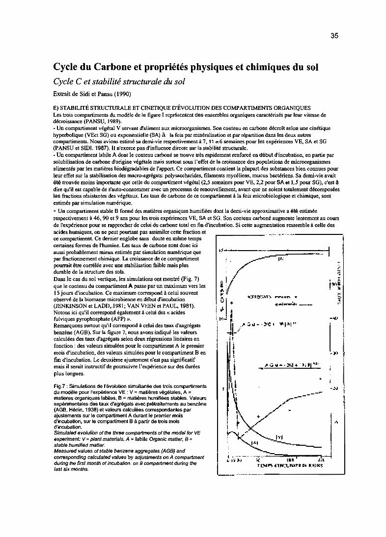
35

Cycle du Carbone et propriétés physiques et chimiques du sol

Cycle C et stabilité structurale du solExtrait de Sidi et Pansu (1990)

-*1....

........9"'1 •

--­~---

/ ....

_~':;"'''.Y..J .. -)i~I"I,

"':.rI I)-.~''''

I~ 1 1

Fig.? : Simulations de l'évolution simultanée des trois compartimentsdu modèle pour l'expérience VE : V =matières végétales, A =matieres organiques labiles, B = matières humifiées stables. Valeursexpérimentales des taux d'agrégats avec prétraitements au benzène(AGB, Hénin. 1938) et valeurs calculées correspondantes parajustements sur le compartiment A durant le premier moisd'incubation, sur le compartiment B à partir de trois moisd'incubation.Simulalad evo/ulion of the three compartments of the model for VEexperiment: V=plant materials. A =labile Organic matter, B =stable humified matter.Measured values of stable benzene aggregates (AGB) andcorresponding calculated values by adjustments on A compartmentduring Ihe first month of incubalion. on B compartment during thelast six months.

E) STABILITÉ STRUCfURALE ET CINETIQUE D'ÉVOLUTION DES COMPARTIMENTS ORGANIQUESLes trois compartiments du modèle de le figure 1 rcpr6scntcnt des ensembles organiques caractérisés par leur vitesse dedécroissance (PANSU, 1989).- Un compartiment végétal V servant d'aliment aux microorganismes. Son contenu en carbone décroît selon une cinétiquehyperbolique (VEct SG) ou exponentielle (SA) à la fois par minéralisation et par répartition dans les deux autrescompartiments. Nous avions estimé sa demi-vie respectivement à 7, 11 et 6 semaines pour les expériences VE, SA et SG(pANSU et SIDI. 1987). II n'exerce pas d'influence directe sur la stabilité structurale.- Un compartiment labile A dont le contenu carboné se trouve très rapidement renforcé en début d'incubation, en partie parsolubilisation de carbone d'origine végétale mais surtout sous l'effet de la croissance des populations de microorganismesalimentés par les matières biodégradables de l'apport. Ce compartiment contient la plupart des substances bien connues pourleur effet sur la stabilisation des macro-agrégats: polysaccharides, filaments mycéliens, mucus bactériens. Sa demi-vie avaitété trouvée moins importante que celle du compartiment végétal (2,5 semaines pour VE, 2,2 pour SA et 1,5 pour SG), c'est àdire qu'il est capable de s'auto-consommer avec un processus de renouvellement, avant que ne soient totalement décomposéesles fractions résistantes des végétaux. Les taux de carbone de ce compartiment à la fois microbiologique et chimique, sontestimés par simulation numérique.

- Un compartiment stable B formé des matières organiques humifiées dont la demi-vie approximative a été estiméerespectivement à 46, 90 et 9 ans pour les trois expériences VE, SA et SG. Son contenu carboné augmente lentement au coursde l'expérience pour se rapprocher de celui du carbone total en fin d'incubation. Si cette augmentation ressemble à celle desacides humiques, on ne peut pourtant pas assimiler cette fraction et c ••• 'To-'-.-'-- ,ce compartiment. Ce dernier englobe sans doute en même tempscertaines formes de l'humine. Les taux de carbone sont donc iciaussi probablement mieux estimés par simulation numérique quepar fractionnement chimique. La croissance de ce compartimentpourrait être corrélée avec une stabilisation faible mais plusdurable de la structure des sols.Dans le cas du sol vertique, les simulations ont montré (Fig. 7)que le contenu du compartiment A passe par un maximum vers les15jours d'incubation. Ce maximum correspond à celui souventobservé de la biomasse microbienne en début d'incubation(JENKINSON et LADD,.1981; VAN VEEN et PAUL, 1981).Notons ici qu'il correspond également à celui des « acidesfulviques pyrophosphate (AFP) ».Remarquons surtout qu'il correspond à celui des taux d'aagrégatsbenzène (AGB). Sur la figure 7, nous avons indiqué les valeurscalculées des taux d'agrégats selon deux régressions linéaires enfonction: des valeurs simulées pour le compartiment A le premiermois d'incubation, des valeurs simulées pour le compartiment B enfm d'incubation. Le deuxième ajustement n'est pas significatifmais il serait instructif de poursuivre l'expérience sur des duréesplus longues.

36

Cycle C et capacité d'échange cationique du solExtrait de Pansu et de Boissezon (1989)

C - Relation avec les variations observées de la Capacité d'échange cationiqueDe nombreux auteurs ont montré l'existence de corrélations entre la capacité d'échange cationique des 50' 5 etleurs teneurs en matière organique, mais l'incorporation de matières organiques ne provoque pas toujours uneaugmentation significative de la capacité d'échange des horizons enrichis (BOISSEZON et BONZON, 1986).Nous avons reporté dans le tableau II, les résultats d'ajustements linéaires entre la capacité d'échange cationiqueet les teneurs en carbone au cours des expériences, d'une part, pour chaque amendement, d'autre part pour chaquetemps d'incubation, toujours selon le modèle:CEC =a + b CT (4)

Tableau Il : Ajustements de capacité d'échanges cationiques de l'horizon A1 correspondant à "équation 4 pourchaque temps d'incubation (tableau de gauche) et pour chaque dose de paille ajoutée (tableau de droite).

TEMPS D'INCUBATION DOSES DE PAILLE DE LUZERNET jours a b r Apporte a b roro1 18,0 0,089 0,93 0 11,1 0,346 0,5715 17,2 0,111 0,89 10,05 15,2 0,166 0,7230 16,6 0,122 0,85 20,1 16,7 0,118 0,8490 15,3 0,163 0,76 30,15 17,5 0,103 0,90180 13,4 0,242 0,57

La capacité d'échange cationique qui est maximum en début d'incubation décroît proportionnellement à ladiminution des teneurs en carbone organique dans l'horizon Al. Néanmoins, les résultats du tableau II indiquentune corrélation de plus en plus significative, pour les doses de paille les plus importantes, mais qui devient moinssignificative lorsque le temps d'incubation s'accroît. La pente des droites de régression varie en sens inverse: ellecroît avec le temps, mais elle est divisée environ, par trois, lorsqu'on passe de l'apport nul à la dose de paille laplus forte. Ceci indique que la CEC des matières organiques résiduelles et des matières humifiées croît avec letemps tandis que la CEC due aux matières végétales ajoutées décroît d'autant moins que la dose de paille ajoutéeest plus importante.Or, notre modèle permet d'évaluer la quantité globale de carbone labile et celle de carbone stabilisé, au cours dela période d'incubation. Il était alors tentant, de calculer des ajustements linéaires de la CEC, non plus enfonction du carbone total, mais en fonction du contenu carbone des deux compartiments "A" labile et "B"stabilisé, selon un modèle du typeCEC = a[A] + b[B] (5)Le tableau III indique les valeurs obtenues pour les deux coefficients "a" et "b", pour les quatre fumures et lescoefficients de détermination correspondants. Les courbes correspondant a ces quatre ajustements sontreprésentées sur la figure 5 :

Tableau III : Ajustements de capacités d'échanges cationiques correspondant à l'Equation (5). sa et sb =écartstypes associés a la détermination des coefficients a et b.

Apport C"t" a Sa b Sb R20 0,472 0,009 0,846 0,002 1,000010,05 0,303 0,014 0,787 0,005 1,000020,1 0,262 0,007 0,740 0,004 1,000030,15 0,237 0,009 0,711 0,006 0,9999Les ajustements sont tous tres hautement significatifs, Le coefficient "b" prend une valeur deux a trOIS fois plusforte que celle du coefficient "a", ce qui indiquerait un nombre de sites d'échange cationique également 2 à 3 foisplus fort, pour les produits humifiés que pour les matières organiques labiles. Le coefficient "a" diminuefortement lorsque la dose de paille ajoutée augmente. Avec l'apport le plus fort, la valeur devient moitié de cellesans apport. Ceci est probablement, en rapport avec la grande hétérogénéité du compartiment A. Celui-cienglobe tout le carbone des matières labiles, qu'il provienne des micro-organismes, de métabolites ou de résidusde végétaux non décomposés. Les matières labiles initialement présentes dans le sol possèdent plus de sitesd'échange que les matières labiles provenant de la paille.Le coefficient "b" diminue très faiblement lorsque la dose de paille ajoutée augmente. Les produitsd'humification récente, provenant de la transformation de la paille, auraient donc un nombre de sites d'échangeslégèrement moins importants que les produits humifiés antérieurement.

•

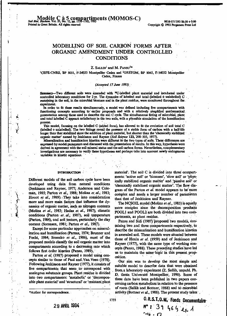
Modèle c: à 5 comnartiments (MOMOS-C)Sol/ Biol. BI«1Iem. VoL '}S. No. 12,pp. 17~1762, f993 ' ,Printedin Great Britain.AUrighlSreserved

0038.0717/93 $6.00+0.00Copyright <C 1993Pergamon PressLtd

,

, lll,,.~ ~~ ',.{

J.~'

,~

.:..;.

, "

"

\,:~".\ f

ott')"t;

" :.

MODELL:INO OF SOIL CARBON FO~,S AFfEROROANIC AMENDMENT UNDER CONTROLLED

CONDITIONS

Z. SALUH1 and M. PANSU2•

ICEFE-CNRS~ OP SoSI. F-34033 Montpellier Cedex and 2ORSTOM. OP S04S. F-34032 Môntpellier, Cedex, France

(Accepted 17 June 1993), '

SuJuDùIry-Two difl'crent sails were B:mended' with ~4(:.litbelled plant material and incubated undercoDtrolled Iaboratory conditions foc 2 yr. Thedynamics of Iabelled and total (Iabel1ed + unlabelledjC 'remajning in the sail, in.the microbial biomass and in the plantresidue, were monitoredthroughout the'

~~r:~ to fit the:se results simultaneo~ly. a model was'defi.ned ùicluding live compartmenü Withfunctioning conœpts according' to èarlier proposaIs and with a relatively simplified mathematical,presentation among those,~ ~o descri~ th~ soil C ~~'.ThesitÎ1u~tan~us fi«;ing of microbi~ p~~and totallabelled C àppears satisfactory ln the two soils, W1th a plausible simulation of the.humiâcationprocess. ' ,,' ',' , ,

nis model, focUSÎng On the Iabe!led C (added form), bas allowed to fit theevolution o.f soil total.C(Iabe1led+unlabelled): The two fittings rev~ the presence of.a stable form of carbon W1th a half-Iüelonger thaa' tbat stabilizèd ~ce" theaddition ofplantmateriaJ,' butshorter than the'chemical1y stabilizcd 'organic matter' l1lIDICd byJ~n and Rayner, (SoU Sc.~ce 1,23. 298-3~3, 1?77). .

Mincralization andhwDification kinetics,were different m the two types of soils. These difl'erences areexpressed by model parameters and diScussed with thepresentation of results. In tbis way, hypothesis werederived inagreement with thesoilmincral status andthesoilcarbon forms, Nevertheless, complementaryinvestigations are necessarY to verify thcse hypotheses andperhaps takeintoaceount newly endogenousvariables in kineticcquations. ' .

INTRODUCI1ON : material'. The soil C is divided into three compart-ments: 'active soil' or 'biomass', 'slow soil' or 'phys­

Diffe~nt models of the soil carbon cycle have been i~y stabilized organic matter' and .'p8.ssîve soil' ordeveloped using data from natural conditions 'èhemically stabilized organic matter'iThe ft0'Y dia­(Jenkinson and Rayner, 1977; Andersonand 'Cole- gram orthe Parton et al. model appears to be'~oreman, 1985; Partoner al.; 1988; Molina et, al.; 1983; complex and needs a largernumber of parametersHouot et al., 1989). '.,They' take ioto consideration' thari that of Jenkinson and' Rayner. 'more and more main factors that inâuenee the dy- ' The NCSOIL model (Molina et al., 1983) isequallynamies of organic matter, ~b, as nitrogen contents more co~plexsince'the' decomposition 'produCts(Molina et al., .983; Hadaser al.; 1987), ctimatic POOLI and poOL2.'are both divided into two com­conditions {parto~' et, al.; 1987), soU ,~perature partments, as plantresidue, ;.. ' .: '.,(Parton, 19~),' and soilJcxt1ire, particularly the clay Pansu and Sidi (1987) 'proposed 'two models, Co~~content (Sorensen, 1981; ,Parton f!t al., 198.'1).' taining two and three eompartments respectively, to

Except for some particular approaches on mineral- describe the mineralization and humification kineticsization and humification,(Parnas, 1974; Brunner and in amended soil. These models were situated betweenFocht, 1984; Iônenko et DJ... .1986), most of' the those of Henin et al. (1959) and of Jenkinson andproposed models c1assify the soil organic matter into Rayner (1977), with the same type of working con­compartmentsaccording ta a decreasing rate which cepis (pansu, 1988). Thèse preœding studies'have 100foUows fust order ~etics (Paos\J, 1989),' . ' us to maintain the saine'ldgic' in this present.prop-

Parton et al: (1987) proposed a model usmg con- osition. .', . "cepts similar ta those of Paul and.Yan Veen (1978)., 'Our aim was to develop the most simple andFoUowing Jenkinson and Rayner (1977), it consistaof suitable model to describe data that were obtainedfive compartmeil~, that seem. to' co~Tesp~)Qd. ~th , from.a laboratory experiment (Z. ,Sallih, unpubI. Ph.analogoussubstance gr:oups. Plant .resldue 15 diVlded ,D. theSis Université Montpellier, 1990). Soine ofinto ,two comp~~ents: 'metabo?ç' ?r ,~decompos- these data h~ve beèn publishOO 'intwo papers con- .able plant pllltenal and structural or ~Istant plan! cerningcarbQnmetabolism" in relation to the presence

of roots (Sallih·tlDd,Bottner~ 1988) and to ,microbial•Author forcorrespondence. ' àctivity(Bottner et al., 1988). The present 'studytakes' ,

17SS . O.R.S.T.,O.M~' fonds Documentaire-29'AYRll1994 N° : '3, ~ t; ~ .~~ A

l''lntë ! n

1-&l Z. SALUH and M. PANSU

into account the results of C evolution in two soifsincubated without plants. In addition, labeUed Cfound both in the light plus coarse organic particleswas measured, and assimilated into non-humifiedplant residue, Thus, to fit our model, we used moredetailed results in comparison to studies carried out ,by Jenkinson and Ladd (1981), who considered themicrobial biomass, and by Van Veen et al. (1985)Whoconsidered bothmicrobial biomass and totallabelledcarbon simultaneously.

MATE1lIA1S AND MF:I1fODS

Soifs

The two soils used had developed under humidMediterranean climatic .conditions in southemFrance. Both' were taken from the Al horizon(0-15 cm) and c1assed aœording to CPCS (1976): :

-soil 1:' a fersiallitic Càlcicsoil reœntly fallowed-soit 2: li typieal biown soil under grassland

(Brachypobium ramosum).

determined following the fumigation-incubationtechnique (Jenkinson and Powlson, 1976), using a K.:factor of 0.41.

The remaining plant material -was separatedfrom the soit using the procedure of Ladd et al.(1977) modified aS below. Soit samples were shakenwith 0.2 mol (N~C03) L-1 (pH 8.3), centrifuged(12,000 rev min-I) and filtered. The ftoating materialwas collected. The filtrate was concentrated andconsidered as the hydrosoluble fraction. The sedi­ment was suspended again and fractionated into twoparts by water sieving through a 50 pm mesh sieve.Within, the fraction > 50 p m, the,sequestrated plantmaterial was separated densimetrically by znS04solution (density 1.4) and then added to,the previousfraction. The total and labelled C of this fraction wasdetermined by dry combustion. This procedure isdetailed by Cortez (1989)., In our study, this fraction (light and coarse matter)

la assumed to be the residual plant carbon.

Mathematical model

1

il(

The major characteristics of each soit are shown io ' Figure 1 shows our present m~el compared. withTable 1. Main differences,between the two Soifs were 'two other models (pansu ~d Sldi, 198~; ~enkinsonorganic matter content, pH value and clay content and Rayner, 1977). ~ccording to three principal typeslUites are prevailing in soil.I, the most clayey one.. of orgamc matter, differences between these models

are:

f

:.<' .1

Experimental proceduré ,

The .experimental procedure wasdescribed by Sal­1ih and Bottner (1988)., Briefty, dried soit samples(5 mm) were split into 'portions of 800 g, mixed with7 g mature uniformly 14C-labelled wheat straw andthen put in pots: The straw contained 1% N and 43%C with aspeeific activity of 2.59 MBQ g-I C; whichcorresponds to 3145pg plant material14Cg-I .soit.The procedure to obtain the labelled .straw wasdescribed ,?y Bottner (1982).. . '

, Pots were kept for > 2 yr under controlled con­ditions in a growth chamber (daylight, 16h at~5 ± 4°C; night 8 h at ïs±3°C). Duiitig tJ:üs period,~il moisture was maintained at75% waç.. Sevensamplings were carried out at days 16, 29, 8~, 121,247, 422 and 690. At each sampling, the wholecontent of 'one pot wu used for the analysis; 6-10sub-samplings were carried out açcording to the typeof analysis. . .

Analytical methods '

Total carbon (organic plus inorganic) and labelledcarbon (14q were measured ~g dry and wet com­bustion (Bottner and Warembourg, 1976).

Carbon of the microbial biomass (C-BM) was

, (1) Plànt rilaterial: the present model separatesthis matter into two compartments; labile(Vd and stable (Va) which may correspondto the compartments 'decomposable plantmaterials (DPM)" and 'resistant plant ma­terials (RPM)' of Jenkinson and Rayner.This approach is in agreement with that ofPaul and Van Veen (1978), Molina et al,(1983) and Parton' et al. (1987), but contraryto our earlier one which grouped thèse twoorganic fractions in one compartment with avariable kinetic 'order.:

(2) Labile organic matter: the present modelmakes a distinction between microbialbiomass (B) and other labile compounds (A):This is not the case in the model or"Jenkinsonand Rayner which takes into aecount oo1ythe microbial compartment (BIO), and inour earlier model which considered the sumof these two eompartments (L).

(3) Stable organic matter: our data do not allowto take into account the 'chemically stabil­ized organic matter' (COM), obtained byJenkinson and Rayner from dating measure­ments: But in short and medium tenn study

Table 1. Main cbaracCeristics of soils used

Panicle slze distributioo (%)

Soils

12

--------------Organic C N2~.2mm 200-SOpm 5O-20pm 2O-2pm <2pm (%) (%)

7 18 24, 21 29 1.2 0.124S 12 11 18 11 2.7 0.2

2.2<0.1

pH{HzO)

7.96.S

1 ..,: ~,.i .,',', . ".'\,.. ~.. : ~,) r

... .::", ...

Modelling of carbon fonns 3957

t~~~,~?~ ,V . 1 PLANT MATERIAL

• input

u .K({ q- "Z<t l ,', . .-.oCl:o Cl: L (A)t>:lc.l;::lt: "

CQ<t;i:E "

)

1.1·

0::W

~;:; ' r--'---'-------'-'I.-'-'-'--'---,

·U.~. C-------.,.---,---J

l'0::o '

.W . ....,..-----1'--.:..;;..--'----,,.;J.....c:Q

<...:l

.~

: Kn ['B] ,

PLANT MATERIAL

, .~

"

..':", '" PB"

B (BIO)

Fig. 1. Flow diagram for the present model compared to the propositions of Pansu and Sidi (1987; PSIIImodel) and lenkinson and Rayner (1977; JR model) . m = Organic input; V,VL'V R =plant material(PSIII) , Labile plant material, Resistant plantmaterial (JR and present model); B = rnicrobial biomassOR and present model); H ,; stable humified' organic matter (present model, .last called B in PSIII, lastcalled 'Physically stabilized Organic Matter POM' in JR); C = chemically stabilized organic matter (COMin JR); A == labile soil organic matter, except microbial biomass and plant fragments (present model);L~labile soilorganic matter, except plant fragments (pSIII model, last called A); PL' PA' Pa, PH'Pc == input proportion in -L, A, B, H, C cornpartments; Ky, Ky L • Ky R; KA'. Ka; K H , K c =kineliccoefficients of decays in the cornpartments V.. VL, VR , A, B,H, C; /1 '= kinetic order 'of decay in V

". conipartment (PSIII). · . ,

l~ Z. SALLIH and M. PANSU

fV1

(.t1

We defined M as the mineralization coefficient ofthe amended soi!. From this, 1 = I:.tP/ = 1 - M is therenewed proportion of soil C.

Calculations were made using Turbo-Pascal Tool­box numerical methods (Borland).

(2)

RESULTS AND DISCUSSION

Study of different measurements

In preceding publications, we described:

-the decrease of added carbon according to thesum of two negatively exponential functions(SalIih and Bottner, .1988).

-'--the dynamic of microbi àl biomass and the respir­. atory quotient (Bottner et al., 1988).

The best fitting for the non-transformed organicmatter (separated by water sieving and densimetry)was obtained using the suffi of two negative exponen-

Cm' Ct=carbon contents of compartments tial terms. Parameters of these equations were sup-km, kt= rate constants of compartments (t -1 )

.plied entering values for VLU, VRO' KYL and KYRPm = proportion of carbon input into m corn- (Fig. 2, Table 2). This type of fitting is different from

partment. that used by Pansu and Sidi (1987) where the lightThe equation of rnineralization of carbon (Cr) is. matter decreased according to an exponential or an

assumed to be: : . hyperbolic function. However, preceding data are·different and 'possibly not so accurate because theywere obtained by densimetry only and from anunlabelled plant materia!. .

where:

of soil biochemical functioning, we can, asMolina et al. (1983) did, not Lake into ac­count the 'passive organic phase'. In ourmodel, the humified compartment (H) isanalogous to that of our preceding modeland similarto the 'physically stabilized or­ganic matter' (POM) named by Jenkinsonand Rayner,

Carbon dynamics vs time 't' is fitted according toa system of five first order differential equations. Forany compartment 'm' among i compartments, this

.evolution is directed by:

dC S .

---!'!. = -k C +P L klCI . (1)dt nt m m/~ 1 .

m, i E[VL,VR,A, B, Hl

seu i SoU 2

690 .422

:, ;I;: \ :I:;\ ;I;-v. r,\ ....§...\ ~ ~

\\\

oqI. ..l--J...-I._----'_--C-.....::J===-''---'-=-''"''-

162985121 247

100

bI) .

8 .

300

>..."C 200

o-e

ï. bI)oo....

690422

-6- Total 14C

•• '0 ' .. ' Plant 14C (VL + VR)- - - - Labil~ 14C (~) .

-'- Humified 14C' (H)-<>-- Microbial biornass 14é (B)

....~

... î':" -. .- '-:-'- '- '-:-'-'1 \ _ '"'''l'.' ·Y· ~ "'" .!:il ...~....... 2

. . .....

o .162985121 247

300

-'ô!Il

>..."C 200

' ïbI)

00....o;!.

bI)

8

100

Time (days) Time (days)

Fig. 2. Simultaneous model fitling of labelled carbon (added form) in the who le soil and in eachcompartrnent (confidence lntervals of experimental data at 95%).

Modelling of carbon forms

The fitting of the model is as good as that ofindividual simulation of total-labelled e (Sallih andBottner, 1988), and microbial biomass (Bottner et al.,1988). A slight discrepancy of the microbial compart­ment fitting is noticed at the end of the experiment insoil 1. However, new experiments are necessary todefine the cause of this deficit: experimental errors ora defect of modellinearity would need a correction ofthe mathematical formulation. .

Concerning the plant C, since renewal proportionP, is zero for, VL and VRcompartments, the fitting isthe same as that obtained by the sum of two exponen­tialterms. The greater Iack offitting was noted at theend of experiment in soill (as for microbial biomass),and at day 84 in soil 2. In each soil, the slope of plantC curve became close to that of total-labelled e whenthe labile fraction is already consumed. Then, the roleof resistant plant e (VR) becomes preponderant inthe evolution of the system..

P,

0.00.00.790.0330.025

sen 2

0.10.000430.1 '.0.0040.0001

K, P, I.V.

Soill

246125

ooo

I.V.

', ..'

Labcllcdcarbon0.05 M 2830.0031 0.0 910.05 0.58 00.006 0.08 00.0004 0.08 0

Total carbonVL 246 0.05 0.0 283 0.1 0.0Va 125 0.0031 0.0 91 '0.00043 0.0A 9 0.05 0.58 220 0.1 . 0.79B 60 0.006 0.12 120 0.004 0.033H 1153 0.00005 . 0.08 2390 0.00002 0.025

I.V. -Initial value of each compartment in mg C 1008-1 dry soil.K,-kinetics constant in day-I.P,- t.urnover proportion.VL a labileplant material.V. a rcsistant plant materiatA ... labile&Oi1 organiç matter (except microbiaJ biolDUland plant

l'rqments). ' . . .

B - microbia1 biomass; .H - bumifled orJaniç matter. -.

CompL

·Table 2. Parametersof the mode!for Iabelled and total carbon oftwosoils

il'i

SoU type and eoolution kinetics" '.

. Important âifferences in the mineralization proéesswere found between the two types of soil. Mineraliz-

Model fùting . ation is more intense in soil 1 than in soil 2; MThep~eters ~f Table 2 and Fig. 2 show- the (mineralization coefficient, equation 2) is 0.26 and'

simultaneous fitting of total-labelled C, plant-labelled .0.15 for the two soils respectively.e (VL +VR) and microbial-labelled e (B).The dottedHowever, at the beginning of the experiment thislines represent the simulation of labile (A) and stable . order was reversed. At this time, more .intensified(H) humified labelled e. These two compartments mineralization occurred in soil 2. Conversion of rate

1" were not measured but must be taken into accountto constant of VL and A compartments in haIf-life,

1

equilibrate thebalance of 'totat71.abellOO c .minus aecording to Jenkinson and Rayner'(1977), .gives a'plant-e·plus microbial e'.value of 2 weeks for soil 1 but only 1. week for soil

. Moreover, the measurement of labelled C in the 2. Thiscould he explained by the recent history of1 hydrosoluble fraction (unpubI. data) isclosely corre- ..each soil. Soil 2 has been developed under grassland.

lated with the simulation of labile carbon. (A) Root input induces more labileorganic matter and a(r =0.89···· for soil i and r =0.73· for soil2), with microfiora adapted to metabolize these substances or

;,', a maximum towards day 15-30. This is clearly earlier '. other labile products Iike the cellulose and polysac­, .) f than the maximum for microbial development. Nev- charides of added plant material. Another expia­

I ertheless, the water-soluble fraction represents 'only nation could 'he in relation to the stabilization of. i, ' about 10% of the simulated labile e, so itwould he labile plant matter que to eiay content (Van Veen and

I

Ji' necessary to search forother labile produets princi- Paul, 19,81) whichis highest in soil 1. .

. pally amongst ·the polysaccharides in the range he- When labile material was completely decayed after" i tween cellulose and simple sugars, ' , 2-3 months, the decrease in mineralization 'rate was

l " In the two soils,the labile compartment (A) de- particularly clear in soil 2. Half-life of the VR CC?m­creased at the same rate as the plant labile corn- partment would he about 7 months in soil 1 but

· pounds. This shows a very rapid incorporation of' >4 yr in sOiI 2. 89, at 'the end of the experiment,l' these compounds into the soil in such a way that it about 18% of the added plant material was not1 . becomes impossible to- distinguish them by graau-.' degraded in soil 7. whereas: only 4%. in soil 1. -'~.. lometry or by densimetry. Bothtypes of labile com- The simulation by the model of the humification

pounds are used to feed the microorganisms which process (li compartment) is notably higherinsoil 1reach their maximum growth afterca 3 months of than in soil 2: This is consistent with former hypoth­incubation, Most of the labilecompounds are con- . eses about the role of clays in humification (Martin'\ . .1. sumed after 6 months, so microbial biomass decreases and Haider, 1986). The isohumic coefficient, calcu-

l gradually. ·llited according to the original deânition of Henin-HumifiOO compounds increaSed progressively and Dupuis (1945) from 'H' compartment simu-

· during the experiment to approach, at the end of the lation, is equal to 0.18 for soil 1 and 0.11 for soil 2.incubation, the lével of tbe remaining tadded e. We note here the importance of the compartmented.Nevertheless, as the degradation of the labile com- simulation in the calculationiof this coefficient,pounds, .the major part'of the humification proeess .because -calculations consideringadded carbon de­seemed to stabilize after 6 months of incubation. crease only, may have 100 to an inverse conclusion

z. SAwH and M. PANSU

concerning humification. Effectively, at the end of theexperiment, the ratio of remaining 1~ to initiaIlyadded 14C is equal to 0.25 in soit 1 and 0.31 in soil2;the isohumic ·coefficient seems to be more importantin sandy soi) than in clay soil.

After 2 yr of incubation, and-in spite of a relativelystabilized curve of global labelled C, we are still farfrom the equilibrium in soit 2, whereas in soit 1, theresidual added C beoomes close to humified carbon.The initiaUy greater C content of soil 2 is originatedprobably from the preponderance of plant C that isincompletely transformed: .

Finally, both mineralization and humification pro­cess are more important in soil 1 (clay soil), andexpress an intense biological functioning, except atthe beginning of the experiment. The model showstbis phenomenon by the parameters that characterizethe microbial biomass. A1thougb global aspects ofmicrobial dynamic curves appear similar in the twosoils, haIf-life of microbial biomass is slightly shorterin soit ] than in soit 2 (about 4 monthsinstead of 6months) and the renewal proportion in soil 1 is morethan twice. This' bigher turnover of the microbialcompartment may suggest an important availabilityof nltrogen in soil l, but this hypotheses must heverified.

Moreover, if humification is less intense in soit 2(sandy soit) than in soit 1(clayey soil), it suggests thatformed humus in soil 2 is more stable; with a half-Iifeof 'H' compartment about 19.yr against only 5yr insoit 1.

1l,

1

2800

2000

2200

3000

·0'". 2600 e-

"l:l

-. 'co<:)o....

2400 U

a

690247 422

Time (days)

UlIIla

:s 300....

.5'7g 200<:)....

Total carbon simulation

Before the model cao be tested in natural con­ditions, we must verify if it is possible to fit thedynamics of total soil C (labelled + unlabelled) with­out major modifications in parameters. This mayaUow to check the validity of the model: does pre­eXisting organic matter in the soil behave in the sameway as added matter?

Parameters of Table 2 and Fig. 3 show the simul­taneous fitting of total C, plant C and microbial C.As above, the simulation of humified total C ofcompartments labile (A) and stable (H) are rep­resented by dotted fines. The model seems satisfac­tory because similar results were obtained allerchanging the initial values of A, B and H compart­ments.

The rate constants are the same as above, exceptthat ofstable compartment (H) whose half-life wouldpalis from 5 to 38 yr in soil 1 and from 19 to 95 yrin soit 2. Thisdifference could be explained by the factthat the very stable compartment (COM) of soitorganic matter bas not been taken into account in thecalculation.

With these data, we tried to estimate the stability .of this compartment; assuming that KH , k~, kt arethe rate constants of humified total, labelled and. 0 .native carbon respectively, the [Hl, [H.] and [H ] aretheir corresponding contents, then the equation of theDow between these compartments is:

kH[H] = kt[HOj +k~[H·] (3)

600

800

1600

1400

-ë5..1200 e-

"'Cl

7.s

. ...1000 U

;

690

Soil1

-6--Tolal C.. ·c· .. Plul C (VL + VR)---- Labile C (A)-'- Humified C (H)-0-- Microbial blomass f (B)

o W/...I....-L.L._----L__--L.__----'-'-=:J-l

16 29 85121 247 422

Time (days)

~ 300 .

'.... ::-- ... ."l:l :

7~ 200<:)....U~a

Fig. 3. Simultaneous modelfittingof total carbon in the wholesoiland in ~c~ compartment (pl~t, labileand microbialcarbon on the lcft scalc, total and humifiedcarbon on the nght scale;confidence antervals

of experimental data at 95%). '.' .

Modelling of carbon forms ~I

Ifwe take for [Hl, [Ht] and [HO], the valuesat theend of the experiment (with simulation or non-ad­dition for [Ho]), equation 3 givesa kt of 0.00003 d-I

for soil 1 and of 0.000019 d- I fcrsoil 2; this corre­sponds to a half-lifeof 63 and of 102 yr for the twosoils respectively, These half-lives are considerablysmaller than that of 1980 years found by Jenkinsonand Rayner for their [COM) compartmenl So it isillusory to try 10estimate thiseompartment from thistype of experimentation, But it seems that it existsli part of soil C with an intermediaryhalf-life m;tween[Hl arid[COM].This couldexplaln the oftenobserveddecrease of native C in.comparison 10 added C, andconfirms some preœding suggestions(Jenkinson andAjanaba, 1977; 'Pansu and Sidi, 1987). However.wemust, he careful with the' estimation of stable com­pounds from a short-term experimenl

Renewal proportions P, are ,àll the same as thoseuscd for 14C, except that of the microbial biomass ofthe soil l, which had 'been increased slightly. ThiswoUJd confirm our preeeding remarb that suggest a ­little anomaly of the model in this soil whichhave anintense biological activity, but complementary inves­tigations will hé necessary to determine precisely this

, ,ob~rvation., On the other band, in soil 2 the fitting of the

microbial biomass by our model seems still moreprecise than the fitting of this only compartment(Bottner et al., 1988). A choice.of high initial valuesof both microbial and labile (A) comparbnents wasnecessary for the realization of the adjusbnenl Thisis in agreement with one of the above hypothesesabout the intense inineralizationactivity at the begin-.Ding or the experiment in this soil from grassland.

The fitting of soil total C is acceptable despite the,relatively important variability of the measurements,especially in soil 2. This variabilitywould confirmtheabove hypothesis about thepresence in this soil of,incompletely decomposed fragments of plant C.

Ii1 spite of, these restrictions; the transposition ofthe model on the soU total C is satisfactory.This gives.a validation to the modei in our experimenl Thenumber and the type of proposed cçmpartmentsappear neèessaryand sufficient to explaingloballythesoil C cycle (added or native).

"1-,

~. .~

. ", 1

. (~

::\

. REFERENCES

Anderson D. W.amiColeman D. C. (1985) Thedynamics. of organic matter 41 grass1and soils. Journal of SOU tmd

.Water Conservation, 40, 211-216.Bottner P. (1982) Biodégradation du matériel végétal en~eu herbacé. Acta OEcologica/OEc%gaGenera/ls 3,

. 155-182.Bottner P. and Warembourg F. (1976) Method for simul­

taneous measurement of total and radioactive carbon insoils, soil extracts and plant materlal. Plant andSoU 45,273-'-277.

Bottner P., Sallih Z. and Billes G. (1988) Root activity andcarbon metabo\ism in soils. Bio/ogy and FertUity of Soifs7,71-78.

Brunner W. and Focht D. (1984) Detenninistic three-half-.order lcinetic model for microbial degradation of added .carbon' substrates in soil, Applied and Enoironmental

. Microbiology 47, 167-112.Cortez J. (1989) Effectofdrying and rewetting on mineral­

ization and distribution of bacterial coastltuentsln soil .fractions. Biology and FertUlty of S~u, 7, 142-151. .

CPCS (1967) Classification des sols. Ecole NationaleSupérieure d'Agronomie (E.N.S.A), 87pp., Grignon.

Hadas A., Molina J. A. E., Feigenbaum S.andClapp C. E.,-(1987) Simulation of Nitrogen-15 immobllization by the

model NCSOIL. SoU Science Society of America Journal '. 51, 102-106.

Henin S.and Dupuis M.(1945) Essaidebilan de la matièreerganique du sol Anna/es Agronomiques 15, 17":'29.

Henin S., Monnier,G..and Turc L. (1959) Un aspect de ladynamique des matières organiques du sol. Comptes

'. Rendus de l'Académie des Sciences-France 248, 138-141.HouotS., Molina J. A. B., ChaussÔd R. and Clapp C. E.

(1989) Simulation by NCSOIL of net mincra1ization insoils from theDeherain and36Parcelles fields at Grignon.

. Soü Science Society of America Joumâl 53, 451-455.Perspectives Ionenko V.l, Batsu1a A. A. and Golovachev Ye. A. (1986)

Thismode1, tested by experimentaldata, is interest- Kinetics of humification. SOoiet Soif Science 18, 33-42. 'ing by its relative. simplicity as only one equation Jenkinson D. S. andAyanaba A. (19TI) Decomposition of

carbon-14 labelled plant material under tropical con­(equation 1)' 'can describe the evolution of every . <litions. Soil Science Society of America Journal 41,compartment. It can also he adapted 10 obtain the , 912-915. . ,more suitable descriptionof the soil C cyèle at a given Jenkiason D. S. and Ladd J. N. (1981) Microbial biomasssituation. For example, the model with two or three in soil; measurement and turnover. In SoU Biochemlstrycompartments (pansu and Sidi,1987) could he de- (E. A. Paul and J. N. Ladd, Eds), Vol. 5, pp. 415-471..

Dekker, New York.scribed by a similar equation' with i = 2 or i = 3 (if . Jenkinson D.·S. and Powlson D. S. (1976) The effect of

. n = 1 for PS III, Fig. 1) and a new definition of the biocidal treatments on metabolism in soil: V. a methodcompartments. The model can he used in predicting for meas\lring soilbiomass. SoU Biology cl 'Bioche~try

di f th " 8, 209-213.stu es 0 e organic pools dynamics for one soil Jenkinson D. S. and Rayner. J. H. (1977) The turnover ~ftype (where organic inputs couldhe estimated as weil . soil.organic matter in some of the Rothamsted classieal

, ' . as k l and PI)' The influence of -climate could be experiments. $Qi! Science 123, 29S-303.

Z. SALLUI and M. PANSU

Ladd J. N., Parsons J. W. and Amato M. (1977) Studiesofnitrogen immobilisation and miDeraJization in cak:areoussoils. L Distribution of immobili.sed nitrogen amongstsoilfractions ofdifferent particlesizcand density. Soil Biology& Biochemistry 9, 309-318.

Martin J. P. and Haider K. (1986) lDfluencc of mineraicolloids on turnover rates of soil organic carbon. SoilScienœ Society ofAmerica 17,283-303.

Molina J. A. E., ClappC. E., ShafferM.J., Chi~ester F. W.and Larsen W. E. (1983) NCSOIL, a model of nitrogenand carbon transformation in soiI: description, cali­bration and behaviour. Soil Scienœ Society of AmericaJounwl47, 85-91.

Pansu M. (1988) Proposition de modèles descriptifs de.1adynamique des matières organiques des sols. (C. R.Journée de pédologie ORSTOM Sep. 1988), CahiersORSTOM Série Pedologie XXIV (4). '

Pansu M. (1989), Cinétique chimique et modèlescompartimentaux: application à rétude de l'évolutiondu stock organique 'des sols. In SEMINFOR 2: LaModaisationÂ3peCt3 Pratiques et Méthodologie, 2" Sémi­""ire Informatique ORSTOM, Sep. 1988. ORSTOM.Paris. -

Pansu M. and SidiH. (1987) CinétiqUe d'humification et deminéralisation de mélangessols-résidus végétaux. Sciencedu Sol25. 247-265. ' .

Parnas H: (1974) Model for decomposition of orianic. material by, microorganisms. Soil Biology cl Biochemistry7. 161-169. . ' ,

" ;

Parton W. J. (1984) Predictingsoit temperature in a short­grass steppe. Soil Scienœ 138, 93-101.

P8rt0n W. J., Stewart J. W. B. and COle. C. V. (1988)Dynamic of C, N. P and S in grassland soils: a model.Blogeochenistry 50 109-131.

Parton W. J., Schimel D. S., Cole C. V. and Ojima D. S.(1987) AnaIysis of factorscontrollingsoil organic,matterlevels in great plains grass1aDds. Soil Science Sodety ofAmerica Joumol51. 1173-1179.

Paul E. A. and Van VeenJ. A. (1978) The useoftraccn todetermine the d~'nature oforganic matter. Trans­actionsofthe llth Intet'lUllionlll Congrus ofSoilScienceEdmonton, Alta 3, 61-102. .

Sallih Z. and Botmer P. (1988) Eff'ect of wheat (Trltialmaestivum) roots on mineralization rates of soil orpnic

" matter. Biology and FertiJùy of Soib 7. 67-70.SorenscnL. H. (1981) CarboD-Ditrogeo relationshipsduring

the humification of ccUuIose in ~i1s contaïning clifl'erent.amounts of clay. So~ Biology cl Biochemistry 13,313-321.

Van Veen J. A. and 'Paul E. A. (1981) Organic carbondynamics in grassland soils. I., Background information

. and computer simulation. Canodian JoumoJ of SoilScience 61; 185-201.

VanV~ J. A., Ladd J. N. and Amato (1985)Turnover ofcarbon and nitrogeci through the microbial biomassin àsandy Ioamand clay soil incubated with l'''C(U)JgIuooseand ('sN]<NH..hSO. under diff'erent moisture regimes•Soil Biology cl BiochemistTy 17. 747-756.

.)

'.

I­r

,l

45

Cycle de l'azote dans les sols, modèle MOMOS-N

I/Iikl 46~pergamon

Soil BioL Biochtm. Vol. 30. No. 1. pp. 19-29. 1998C 1997 Elsevier Sc:icoœ Ltd. AlI rights reserved

Printed in Great BritalnPH: 80038-0717(9'7)00087-4 0038-0717}98 $19.00 + 0.00

MODELLING OF SOIL NITROGEN FORMS AFfERORGANIC AMENDMENTS UNDER CONTROLLED

CONDITIONS~

M.jPANSU,·. z. SALLllP and P. BOTINERJ

'ORSTOM, BP 5045, 911 Avenued'Agropolis, F-34032, MontpellierCedex, France and lCEFE-CNRS,BP 5051, Route deMende, F·34033 MontpellierCedex, France

(Âcœpted 10 Mard 1997)

Summary-This N mode! is derived from the e modd (MOMOS) published by SaUih and Pansu(1993). Both models were fitted to experimental data obtained from an incubation experitnent of 14eand 1~-label1ed plant material in two soils with contrasting characteristics over 2 y under controUedlaboratory conditions. The N model uses the same structure as the e model with fiveorganic compart­ments: labile plant material (v0; stable plant material (vRl; microbial biomass(D); labile humifiedma­terial (A); and stable humified material (H). Two additional compartments are included: exchangeableNR.·N and NOl-N. The transfers of N between the organic compartments are described according tofirst-order kinetics. Nitrogen transferred to the NIl. compartment results from the balance between theoutput and input of aU the organic compartments. Ammonium N output is split between nitrificationand immobilisation into B (77%) and H (23%). Nitrification is controlled bya microbial growth law.The N model uses the parameters defined in the e modd, with a constant multiplying factor for the Nkinetic constants (fn ... 1.4and 1.9 in soil 1 and 2, rcspectivez). The additional parameters definedforinorganic pools are comparablein both sons. The predicted 1eto-I~ ratios of each organic compart­ment agree with the experimental data, showing a rapid incorporation of I~ into microbial biomassand a gradual build-up into stable humified compound!.The model was adjusted to 1~ experimentaldata from five time series(each series containing from 1M to eight sampling occasions), and was vali­dated using five series of corresponding total N data. MOMOS-C and -N formulation is relativelysimple, combining mechanistic first-order kinetic models and growth models. The predictions are inagreement with 16 data sets including differentforms of organic 14e (three series), total e (three series),organic and inorganic I~ and total N. © 1997 Elsevier Science Ltd .

fonds Documentaire ORSTOMCota : ~~~:r. Ex: A

19

INTRODUcnON funetions. The concept itself of defined mineraliz-

Though "azote", the French name for nitrogen able N pools was critically discussed by Broadbentgiven by Lavoisier, means "lifeless" and inert, this (1986) and Sierra (1990).element is a major constituent of living organisms To improve empirical descriptions, mechanistic

models try to integrate the N cycle processes withwhich catalyse key steps in biogeochemical cycling.

the inconvenience of increasing the number of par-Severa! indices, relying on chemical or biologica1 ameters. Process-based models have been regu1arlyfield (Greenwood et al., 1985) or laboratory tests to reviewed: Neeteson and van Veen (1988), Hétier etestimate soil nitrogen avai1ability for plants have al. (1989), Addiscott (1993), Beckie et al. (1994),~ proposed. Kinetic expressions ~or minera1iz- Hansen et al. (1995). Some models describe particu­atton proposed by Stanford and Smith (1972) are lar mechanisms for instance mineralization-immo­~ ~n a poten~aI1y labile N p~~IJ:'o),. which bi1iiatiotÎ'pr~ (van Veen and Frissel, 1981),mmera1izes according to first-order kinetics (k con- nitrjfication (Laudelout et al. 1974) or denitrifica­stant). Mary and Rémy (1979) propo~.k:~d as a . tion (BergStr~rn and Beauchamp, 1993). The Npotentia1 lDÎnera1ization index, but. other equations cycle is described .separately (Jenkinson and Parcy,have been suggested: double exponentia1 ~DS et 1989) or is linked to the- carbon cycle, e.g, McGillal., 1986; Matus anâ Rodrigez, 1994); linear et al. (1981), Molina et al. (1983), van Veen et al.(AddisCQtt, 1983); or parabolic (Broadbent, 1986) (1984). Parton et al. (1987), Bradbury et al. (1993).

'.' - The carbon part of the MOMOS model

.Author for correspondence. (Tel: +046-741-6228; Fax: (MOdélisation de la Matie(c)re Organique des Sols,__-+046-741-629/J;..e-mall: pansu~pP.orstom.fr). Mode11ing of Organic Matter Of Soils) bas aIready

-lliiïiiü.. Il-'-·

20 M. Pansu el al.

been presented in former publications (Pansu andSidi, 1987; SaJlih and Pansu, 1993; Pansu et al.,1996). The C and N parts were built using datafrom Iaboratory incubation experiments performedover 2y with 14C_ and 1~-labelJed plant materiaJ.The N model is Iinked to the C model, which basthe same structure for organic compartments. Theaim was to develop the most simple and suitablemodel to fit theexperimental data.

MATEIIAI.S AND MI11IODS

Data acquisiJion

Data were collected from incubation experiments,condueted under laboratory conditions, with twoMediterranean soils; a fersiallitic calcic soil (soil 1:pH =7.9, organic C = 1.2%, N =0.12%, andclay content =29%), and a typicaJ brown soil (soil2: pH = 6.5; organic C = 2.7'1., N =0.2%, andclay content = ll%)(cpcs' 1967). Theanalyses ofsoils and theexperimental procedure were describedby Sallih and, Bottner (1988), Bottncr et al. (1988)and Sallih and Pansu (1993). Briefl.y, soils wmmixed with 14C_ and I~-labelled mature wheatstraw (Bottner, 1982), incubated over nOd undercontroUed temperature and moisture conditions andsampled on seven occasions. The foUowing analyseswere performed on two replicates:

(1) C and 14C in the whole soil, (2) Cand 14Cin plant debris separated from the soil by physi­cal fractionation, and (3) C and 14C in microbiaJ 'biomass (fumigation-incubation method;Jenkinson and Powlson, 1976); this data wasused to validate the C model (Sallih and Pansu,1993).

N and I~ of: (1) the whole soil; (2) the plantdebris; (3) the microbial biomass; (4) K~04extractable ammonium; and (5) K~04 extracta­hie nitrate. This data isused in the present Nmodel.

For physical fractionation, the simples'wen: firstsbakeo witha 0.2 mol NaBC03ri solution to sep­arate floating material (FO). The sediment was thenfractionated by wet sieving to giYC a >50pm frac.tion. This coane fraction wu ,lCpUated densimetrî­caUy (ZOS04 solution) intoa sandy (FI) and a lightfraction (F2). As for the C model, the sumPO + FI + F2 wu CODSidered as the resi.dual plantmaterial. Ammonium and NO] were extracted fromunfumïgated and fumigated subSamples with a0.5mol K~4 ri solution. Ammonium was separ­ated by steam distillation with MgO; NOï was dis­tillated after reduction by Devarda reagent. ln thedistillates, N wu measured byautomatcd colorime­try and I~ by mass spcctrometry. Total N andI~ in soil and plant material, were determined byautomated colorimetry and mass spectrometry onKjeldhaJ-mineralization distiUates.

Mathematical motkl

MOMOS describes N transformations using thestructure and parameters defined in the C model,with additionaJ N specifie parameters. Figure 1shows the causal diagram and the main flows of Ndescribed by MOMOS. The foUowing abbreviationswere used in Fig. l, the equations and in the textoN, '. aN, nN = organic N, ammonium N, andnitrate N, respectively.

The model fonnulation is relatively simple. Thestate variable oN (Fig. 1) represents the five organiccompartments as subscripts: VL = labile plant ma­terial; VR = resistant plantmaterial; A = labile soilorganic matter; B = microbiaJ biomass; and Hstable hwnified organic matter. As described bySaJlih and Pansu (1993) for carbon, the input of agiven organic compartment m (oN,J indudes a frac­tion (P,J of the outputs of organic compartments(oN~ and immobilization from ammonium (aN).Thisis d.irected by:

do;", =.r.( -k.oN",+P",~kiONI)

+f(m>(aN(I- ktil(k.ü -aN))) (1)

where kit km (time'")are kinetic constants of theor­ganic compartments; Pm is the proportion of Ninput from compartments i into compartment m.These parameters were previously defined by Sallihand Pansu (1993). The multiplying factor f" increase

ilrhNt.I t.z 14K"'~

Fig. 1.Causal diagn.m of tbc N modcL The &tale variableoN iDduda tbc fM orpnic c:ompartmcnls as subscripls.Theyare defiDed in tbc text Va.. labile plant material; Viltl'CIistant plantmaterial; A, labile humified materiaJ; B.mi­<:robial biomass; aDd H, stable humified material. Thestatc variables tlN aDd lIN represenl IJDIDOnium N andnitrate N, respectivdy. Wide urows indic:ale N f1ows.Numbers (1-5) associated with tbc wide arrows represent(1) orpnic N transren bctween tbc live orpnic compart­menls; (2) ammonification; (3) immobilisation or ~N;(4)nitrification; aDd (5)N Joss during nitrification proœss.The function f(m) and tbc constants kb Pb r.. r.. f.. k•••

k02• k~ are defioed in the textand in Table 1.

48 Modelling of nitrogen forms 21

REStJLTS AND DISCUSSION

dnN =(l-k ) knlaNdt. ' .d kn3 +aN

Inorgank N

Measured exchangeable NH..-J~ (Fig. 3) andNltrN (Fig. 7) concentrations were always 10wandvaried irregularly with time. It was possible to simu­late chaotic variations of ammonium by introducinga kinetic constant for ammonium immobilization.The proportion of l~ in NH..-N decreased with

(2) time in both soils, from 1/10 to about 1/50 at theend of experiment. Labelled NIL.-N concentrations

i.e. aN is nitrified, lost or Immobilized; exchange- were of the same order of magnitude in both soils,as well as total Nli4-N.

able ammonium represents the balance between The accumulation of N03-1~ and N03-N wasammonification and these outputs. Nitrate (nN) more regular and could he expressed using linearproduction iS directed by: functions, reflccting zero-order kinetics. A linear

dnN function for nitrification was also found bydt = (1 - kd )knlaN(k,q. ~ aN) Addiscott (1983), while first-ordër kinetic functions

. dnN were calculated by Stanford and Smith (1972), from'when aN ~ kn2, otherwise .dt =O. (3) experiments where inorganic N was regularly

extracted from the same soil sample. Zero-orderkinetics of nitrification were used by Nicolardot etal. (1994) in the NCSOIL model (Molina et al.;,1983) to simulate data from a laboratory incubationexperiment. Zero-order functions which indicate nosubstrate (Nli4-N) limitation for nitrifiers are notrealistic for long-term incubations of unfertilizedsoils, The use of only one nitrification parameter(slope) could simplify the model, but this parameterwas specific for each soil type and was different forlabelled and total N. ,

First-order kinetics (van Veen et al.., 1984; vanwhen aN ~ ka, otherwise dndN

t= 0 (3') . der Linden et al., 1987; Parton et al., 1987;

Bradbury et al., 1993) did not fit the measurednitrate values. Introduction of a state variablebetween aN and nN (arrow 4, Fig. 1), representingnitrite and other intermediates forms, improved thefirst-order kinetic predictions. However, the inter­

(3") Mediate compartment became too large. Integratingthe fixation of ammonium by clays also resulted iria good fit, but the simulated pool of fixed Nli4 wastooimportant.

.Nitrification cao also he described taking intoaccount its control by the 'growth of nitrifiers or byenzyntatic kine~. Several models (Smith, 1979;van Veen and Frissel, 1981; McGill et al.; 1981;Knapp et al., 19~3; Grant et al., 1993) use exclu­sively kinetic equations for microbial growth butthey are rather complex compared to the MOMOS

(4) model. The' growth model of Laudelout et al. (1974)for ammonium nitrification in water, necessitates 10parameters. w1ücb cannot easUy he estimated in soils

Enzymâtic kinetics [equation (3")] become zero­order kinetics, wheJi the Michaelis constant kn3 isnear 0, Le, when nitrification is always at a maxi­mum rate (Vmu: 0:: kn1) . Enzymatic law was usedfor soil nitrification by Franko et al. (l995) andSvendsen et al. (1995). This formulation is valid forconstant enzyme concentrations and does not con-

Equations (3') and (3j imply correspondingmodifications of equation (1). The nitrification kin­etic constants knb kn2 and kn3 are discussed helow.

Calculations were made according Press et al.(1992) by numerical integrations usÎl,lg Euler'smethod and by optimizations of the parameters forthe N part of MOMeS using Powell's method,with the minimized criterion:

The process cao also he described by enzyme kin­etics:

the rate of N transformation compared with that ofC. The flow of aN toward oN (arrow 3, Fig. 1) isdistributed by f{m): f{m) =0 for me {VL , Va, A},j{m) = rb for m = B (rb is the proportion of NH..-Nimmobilized in microbial biomass), f{m) = 1 - rbfor m = H. knJ and kn2 represent two nitrificationrate constants.

The ammonium N (aN) balance is directed by:

d;~ =/,.(1- ~Pi)~kloNI-aN

.where j identifies the number of sampling points, k .is the number of data series and Y/cJ and j", are themeasured and predicted value of each data point,respectively; Pk are weight coeffici~ts for each dataseries. In this workpk values are O.S, 0.3, l, l, 1 fortotal_l~, plant-UN, oN[B])'N, aN_l~, andnN.J~, respectively.

Equation 3 states that the nitrate production. rateis proportional to the mass of depleted substrate(ammonium). Parameters knJ and kn2 are the same

.as in eq.(1); kd represents the fraction of N which islost. Altemately, the more precise law of Monod(1941) cao he used with the Inconvenience of an ad­ditional parameter kn3 giving:

22 M. Pansu et al. 49

Table 1. Parametets used in the model for IabeUed and total nitrogen. k"" k.a. k ll3: nitrificationparameters; k,J volatilisation parameter;'ft: labile fraction of the plant material input; '6 andJ. are au immobillsation parameter and a multiplicativeparameter defined in thetcxt Parameters kl and PI associated with organic compamnents (VL .. labile plant material, Va - resistaDt plant material, A - labilehumified material; B .. microbial biomass; H - stable humified material) arc defincd in SalIih and Pansu (1993)for the carbon model.

For Iabelled N. initial values of compartments A. B,H, NHt, and NO) ..0

Sail 1LabeUed N

Soil2

3'Nitrificationequation

k. 1 (cri)kM(mg kg- I)

k"j (mg kg- I)

kd (no dimension)'6 (no dimension)J. (no dimension)'ft (no dimension)

SSK(equation 4)

3

7.80.6No

830

0.260.70.2

0.10.771.40.5

830

3'

0.0054No

o

880 .

3

6.30.8No

280

3'

0.221.10.34

o0.771.90.5

290

0.009No0.08

310

Total N (nitrification equation 3)

kft l (cri)kM (mg kg- I )

1cJ (no dimcnsîon)'6 (no dimension)f. (no dimension)'. (no dimension)k{H] WI)

A (labile humified material)B (microbial biomass) .H (stable humified material)aN (ammoniumN)nN (nitrate N)

7.81.160.10.771.40.50.00015Initial values (mg kg- I )

o160950

oo

6.32.22o0.771.90.50.00005

o320

1930oo

160.,------------,- 60 160~---------..,..60

120 -rrtT--r---I---...Jl 120 ........-...f----1~--_+1

20

40

• •~f,­~J \~ \

~ '".. -,Il .... ~..~: ~-6

k:=\. .".:: ..~\ '-,.

'...........-................•....

XJ

3c

CD ~..ÊGO

Zs ê 80.:..

~ ~~ f

C»E

40

20

40

. ,. ..,. ,,:; .." ,".,

'\il-., ':....~::-....... -: ... ....... .. .....

--., "•• '\.J

./ ":, '\

'. A • '\~ A '\

40

..~Z.....C»E

."

Fig. 2. Observed and predicted total 1~ and organic compartment-l~, in both soUs: total0-,microbial biomass (B) • - - -, plant material (labile VL + resistant Va> 6,-----, labile humified

material (A) ---'., stable humified material (H) --.

50 Modelling of nitrogen forms 23

40-r-----------r 1,5 40"t----------.,. 1,5

.... A.. ..... .....····Â

o..."""'+........+-'-"-l-''"'''''"l~_+_''_'_+ ...............''_t 0

o 8 i ~ g § ~ ~ ~Tme(days)

...... .. .. .A A

~ g g aTune(days)

..rt' .. .. ..

30 30

1,0 1•~

•• 3 "'a 1 :1• C .li: • CZ • Z

~ • zb20 • .~ :J:.~20

• ......1 •Z • Z • ZI:D • :01'" a • ~E • c, E.. •• •• •, 0,5 0,5,,

10 , 10...A ...

Fig. 3. Observed and prcdicted inorganic l'N in both soi1s: ~)'N (aN)·À-----, N03) 'N (nN)

."

sider the growtb of nitrifying bacteria. If we expressthe Monod (1941) equation in tenns of substrate(Nl4-N) decrease, then knl in formula 3' representsthe growth rate, kn3 is Monod's constant and kn2

depends on the initial population of nitrifying bac­teria and the concentration of substrate. The dimen­sion of knl is time'", while parameters k,a and kn3

express concentrations. Il is assumed tbat for agiven soil, kn l bas the same value for labelled andtotal N03-N. This is not the case for the two otherconstants.

Both equations (3) and (3') gave a similar predic­tion accuracy [SSK equation (4); Table 1]. Howeverequation (3') required tbree parameters instead oftwo for equation (3). A similar precision wasobtained with equation (3") (two parameters). Asthe maximum reaction rate [kn h equation (3")],necessitates separate values for labelled and total-N03-N (nN), we cboosé equation (3).~

~odellin~ labellednJtrogenforms ,

. The parameters k, and Pm [equation (1)} weredefined for the carbon, mode! (Sallih and Pansu,1993). For the N model (Table 1; figs 2 and 3) newkinetic constants were added: kn1; k,a [equation (3)version] and/or knJ [equations (3') and (3")]. It is

assumed tbat microorganisms use NHt preferably 'to NO] for inorganic N iminobilization(Dommergues and Mangenot, 1970; Stevenson,1986). Gazeous N loss during nitrification (N20release) and denitrification (N20 and Nv are regu­lated by kd- Both soils were maintained underaerobic macro-conditions. The N loss (estimated bytotal I~ balance) from soil 2 was not significant,thus kd = O. In soil l, about 10% of the N fluxbetween NHt and NOj (kd =0.1) was lost afterthe onset of nitrification. This difference may beexplained by the higber clay content in soil 1 com­pared with soil 2, creating temporarily- anaerobiemicrosites (Nevison et al., 1996). .

Contrary to Nicolardot et al. (1994) using theNCSOIL model and Yevdokimov and Blagodatsky(1993), the ldnetic constants were not modifiedduring the. incubation lime. For the N model, thekinetic constants of the C mode! were multiplied by

~ f", .for the fivè.organic compartments. The positivevalue of j", (1:4 and 1.9 for soil 1 and 2, respect­ively) indicates that N transformations were fasterthan C transfomiations for aIl organic compart­ments.

For each soil, the parameter rb indicated that77% of the flux of aN to oN compartments (arrow

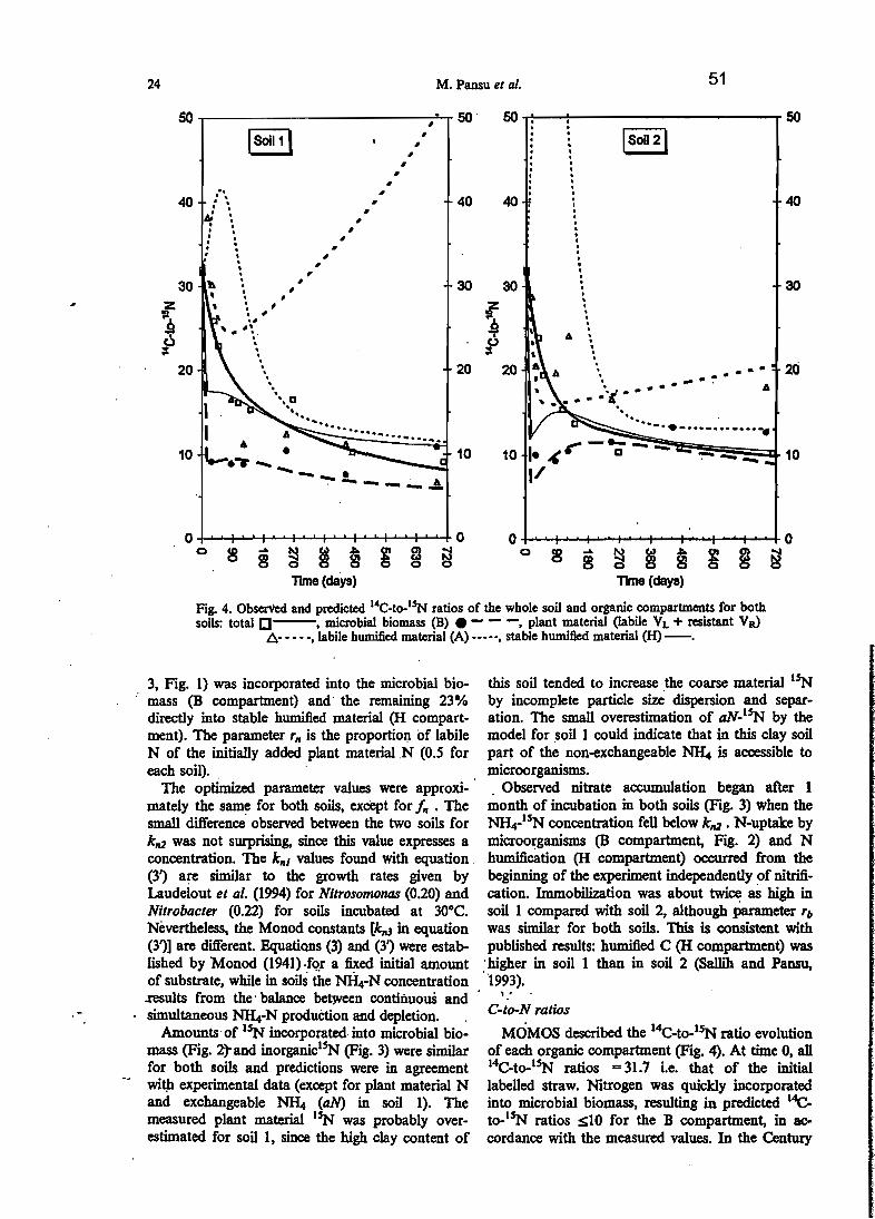
24 M. Pansu et al. 51

50 50 50 50, , ,

Isoilq, ,

1Soli 2 1, , ,, , ,, ,, , ., ., , ,, , ,, ,, . ,"

, ,, , ,40 ' . 40 40 , , 40' , , ., ,

,: ~, ,, ,, , ,

, , , ,, , , ,,, . ,, , ,. , , ,., , ,, ,· , ,30 · # 30 30

,30· , ,, ·. , ·~

. , l!- ·,, , ·l ., l,·, " ·

~.. ~. ,

A ~· p ·· ·.. ·. ·20 . 20 20 · ... 20·, . " .. ... .., , .. .." ' A. , ., ..." a " ......., .. ".,

" .......•...._..........A

, .•...•...A

...... -.......r-~-10 • 10 10 1- ~ a- ~.-.-- 10..... _-

• 1/-- -- ........ ~.!.

~ ~ ~ g a ~l1me(days)

~ 8 gT1me (days)

Fig. 4. ObserVed and predicted 14C_to-l'N ratios of the whole soil and organic compartments for bothsoils: total 0--, microbial biomass (D) • - - -, plant material (labile VL + resistant VlÙ

A' •• - -, labile humified material (A) -----, stable humified material (H)-.

3, Fig. 1) was incorporated into the microbial bio­mass (B compartment) and the remaining 23%directIy into stable humified material (H compart­ment). The parameter r" is the proportion of labileN of the initiaIly added plant materialN (0.5 foreach soil)..

The optimized parameter values were approxi­mately the same for both soils, except for f" . Thesma11 difference' observed between the two soils forkrr2 was not surprising, since this value expresses aconcentration. The k"J values found with equation .(3') are similar 10 the growth rates given byLaudelout et al. (1994) for Nltrosomonas (0.20) andNitrobacter (0.22) for soils incubated at 30°C.Nèvertheless, the Monod constants [kll3 in equation(3')] are different. Equations (3) and (3') were estab­lished by Monod (1941) ..fQ.r a fixed initial amountof substrate, while in soils the~-N concentration.results from the' balance between continuous andsimultaneous NlLt-N production and depletion. ,

Amounts of I~ incorporated into microbial bio­mass (Fig. 2"rand inorganicl~ (Fig. 3) were similarfor both soils and predictions were in agreement

-0 wi$ experimental data (except for plant material Nand exchangeable ~ (aN) in soil 1). Themeasured plant material uN was probably over­estimated for soil 1, since the high clay content of

this soil tended to increase the coarse material I~by incomplete particle size dispersion and separ­ation. The small overestimation of aN_l~ by themodel for soil 1 could indicate that in this clay soilpart of the non-exchangeable NlLt is accessible tomicroorganisms.. Observed nitrate accumulation began after 1

month of incubation in both soils (Fig. 3) when theNRJ-1sN concentration feU below krr2 • N-uptake bymicroorganisms (B compartment, Fig. 2) and Nhumification (li compartment) occurred from thebeginning of the experlment independently of nitrifi­cation. Immobilization was about twice as high insoil 1 compared with soil 2, although parameter rb

was similar for both soils, This is consistent withpublished results: humified C (li compartment) was

.higher in soil 1 than in soil 2 (Sallih and Pansu,'1993).

': .

Cao-N ratios

MOMOS described the 14C-to-l~ ratio evolutionof each organic compartment (Fig. 4). At time 0, aIl14C-to-l~ ratios co 31.7 i.e. that of the initiallabelled straw. Nitrogen was quicldy incorporatedinto microbial biomass, resulting in predicted l"c_to-I~ ratios ~10 for the B compartment, in ac­cordance with the measured values. In the Century

r•52 Modelling of nitrogen fonns 25

150~-------------..40 150~------------r 40

,t

100 ,

il 'Z' 1

~ 'i '

. j ~l!:­r

50

\. \", ,

... .....,'''''.. -- ...., -.. -- ...........................::.~.-:':.::: ..

30 1SN-Input

1100 ,

il ,JI 1 1

20~d 1~

,~ i

,~ ,

r ,50 .,

'.,10

30

10

model (parton et al., 1987) the C-to-N ratio of mi- Some important differences appeared between thecrobial compartment was fixed at a constant value two soils. At the end of the incubation, total .14C_

or8. In contrast, the 14C_to-l~ of the A-compart- to-I~ was lower in soil 1 compared with sail 2,ment was high, mainly due ta. an abundance of This was because: (i) despite the fact that the samelabile C compouads (carbohydrates), the main amount of plant material was initially added toenergy source for microorganisms. The predicted both soils, the proportion of plant debris remaining14C_to-ISN ratio of plant debris deereased to about in soil 2 (Fig. 2) was higher than in soil 1 (near 0);two-thirds of the initial value during the first 3 (ii) the size of labelled microbial biomass remainingmonths; this can be explained by a rapid initial ex- at the end of the experiment was higher in soil 1haustion of labile C' compounds, After this time.: compared with· soil 2. The higher clay content ofthe plant material e-to-N ratio increased con- soil 1 may have had a proteeting effect on microbialstantly. The similarity between predicted and calcu- survival. In soil 2, a high proportion of plant frag­lated plant debris values is acceptable' for soil 2,but ments remained undecomposed and acted as anot for soil 1. This is probably due to the inaccur- nitrogen source for a prolonged period.. while inaey of the fractionation method for clay Soils (soil soil 1 a larger proportion of I~ was incorporated1), as explained above, Except for plant fragments, into humified materials (H compartment) and intoall the labelled C-to-N values approached 10 at the microbial biomass which remained until the laterend of the incubation. Nitrogen was progressively stages of decomposition (B compartment).incorporated into the stable humified H compart-ment, which was the major I~ reservoir at the end .Long-ter'!'. '!ecomposition of the plant res/duesof the experiment. For·the 14C-tO:r~ratio'ofthe . Figure S"shows the predicted transformation oftotal soil, the prediction agrees with the experimen- : the- initial· ~~. input over 20 y, assuming ~ steadyta! data at each sampling occasion for bâih_soils. state organic matter content. During the earlyThus, taking into aecount the propagation of ran- stages of decomposition, the labile plant material N

~ dom errors when calculilting the ratios. the model (VÙ is the major source of' inorganic N.predictions are acceptable except for the remaining Simultaneously, N is transferred to microbial bio­plant debris in ,the clay soil, mass, which becomes the essential source during the

first 2 Y of incubation, Ammonium is reorganizedinto organic compartments with a progressive sto­rage in stable H compartment, which becomes themain müieralization pool aftér 3 or 4 y. Since thisstable compartment decays according first-orderkinetics, the release of inorganic N decreases pro­gressively. The model predicts a NOJ_I~ releasefrom initiallabelled wheat straw over 30 y for soil 1and over more than 40 Yfor soil 2. During the fust10 y in soil 2 the stable plant N (VR compartment)is an important source of inorganic N, whereas insoil 1 this compartment is exhausted after 2 y.

26 M. Pansuet al. 53

1500 200 2500

1801~ ~D-

D

1. aD D-\ 300

\

"IJ 1: 2000

~-

~1801121V\ \

1000 :E' \ af' 3G:I • 1500 \ z

l\ z ~ 200~-\

100~t::. \ ,...

~\ ~ "

:!l- i ~" z \z

"~1000 1>al 1> \E ,

"m

500 • 66 ~ --~ " - \ 100,

" \-,6 ...... 6

500 \.. " ...'"'• -·l"''Of,. " -: "V•• ~ •••• -6. , -..-. 6 ' ... AA-', . . ,-. 6. ~,,-...... .... ..'... ......... ' . ............ .. ...............~....... 00 0 0

0 8 ~

~ ~ § 8 a ~0 8 - ~ ~ Ê s ~ ~g 0 0 !

Time(days) TIme(days)

Fig. 6. Observed and predicted total N in the whole soil and in organic compartmeots for both soUs:total 0-- microbia! biomass (H) • - - -. plant materia! (labile VL + resistant Va) 6, ••• -.

labile humified material (A) • stable humified material (H)-.

Total N predictions were in agreement with the ex­perimental data. As for the C model, total Nallowed to check the validity of the N model builtfrom I~ data. .

High nitrification rates of native soil N wereobserved, particularly in soil 2. At the end of theexperiment, NÜJ)~ amounted to about 35 mgI~ kg-I for each soil (Fig. 3), representing 30% ofadded labelled N and only 2.7 and 1.7% of total N(soil + plant) for soils l'and 2, respectively. TotalNOJ-N was about 130 and 350 mg kg-1 correspond­ing to Il and 18% of total N for soils 1 and 2, re­spectively. The model predictions agreed with the

Modelling of total N forms observed data for both soils, showing high minerai.Predicted and observed total N pools (soil native ization rates of native soil N for soil 2 and lower

N + labelled N) are presented in Figs 6 and 7. The rates for soill. Microbial biomass N was the,majorinitial values of the compartments A, B. H (0 for source of inorganic N and was about twice as higlilabeUed N) were modified as weU as kll2 (which for soil 2 compared with soil 1 at the beginning ofexpresses a concentration). The other parameters the experiment. This ditrerence between the lWofor totalN (Table 1) were the same as for labelled soils has been observed already and predicted for CN. However, for total-N:as for total C, kH constant ., and is probably explained by the recent history ofhad to be reoptimized, Values of kH for the stable. both soils (SaIlih and Pansu, 1993). Despite great

- N compartment'were more aceurate than those of .changes in all labile compartments, variations ofkH for the stable C compartmenr'(Sallih and Pansu. total N and of stable humified N (H compartment)1992), since the N model is more sensitive to kH were not significant during the incubation (Fig. 6).than the C-model. The kH values for stable C andN were lower compared to stable 14C and I~, indi- Conclusioncating that the long-term evolution of these stable The MOMOS N model combines the concept ofcompartments cannot completely be predicted from first-order metics used in Most actual process­short-terra descriptions based on tracer techniques. based models with concepts used in microbial

54Modellingof nitrogen fonns 27

150r------------,. 10 400 -.--------------,. 10

300

100

F à ~ c8~

z~200

z5 .x 5 x

z Z z '*Q

~ ~ ~E ..50 .. ..

100 ...... .... .. ..... ..... .. .. . .. ..... .. .... ... .. '.0 0 0 0

0 ~....

~ ~Jo. a 5 ~

0 8 .... fi,)

~ s a ~ ~~ g 3 ~TIme(days) TIme(days)

Fig. 7. Observed and predicted inorganic total N in bath soils: N}4·N (aN) JI,. •••• -, N03·N (nN).-.,-;,

growth models. Transfers between organic compart­ments and mineralization are explained by fust­order kinetics. This is not surprising, since theseprocesses are associated with a wide range of dlver­sified microbial species. In contrast nitrification,which is associated principally with only two mi­crobial genera, cao be described by a growth fune­tion. Nitrate was not detectable at the beginning ofthe cxperimenl At this stage, when labile organic Ccompounds are avaiJable, Most NHrN is reincorpo­rated into the internaI cycle (three-quarters in mi­crobial biomass and one-quarter in stable humuscompounds).

The MOMOS formulation is reJativeJy simpleand based on data obtained under controUed con­ditions. The model was able to describe the trans­formation of labelled C and N as weil as total Cand N. For each labile organic compartment, themodel used the same parameters Jor C and N(adjusted for N using the cons~t /,J.. For thestable native humified C and N, the kinetlc con­stants kH . Viere· Jower than for the stable .humified14C and !5N materiaI, indicating storage of ç andN into very stable compartments. The N model wasmore sensitive to kH than the C model, indicatingthat the estimation of kH for soil native compoundswas more aeçurate for N than for C. The par­ameters describing the behaviour of the inorganic N

compartments have the same value for labelled andtotal N (except for the nitrification constant kn2,

which expresses a concentration) and they weresimilar for bath soils, except for kn2 and f".Simulated values of 14C_to-1SN in organic compact­ments agreed with experimental data. They showed:(i) a rapid incorporation of N in the microbial bio­mass, with 14C_to-1SN values < 10; (ii) a rapid ex­haustion of N from the labile humifiedcompartment (energetic substrate); and (ili) a pro­gressive incorporation of N in stable humified com­pounds with C-to-N near 10 at the end of theexperiment.

The link between the C model and the N modelwas established by using the same five organic com­partments and by using the same input and outputparameters with a constant multiplicative factor forN kinetic constants.

AcJcnowledgements-The authors wish ta express theirgratitude to' -Professer H. Laudelout (U C Louvain-Ia­Neuve B), and to Dr M. J. WheaJan (University of ExeterllK)for critically reading the manuscript and for Iinguisticcorrections

REFERENCES

Addiscott T. M. (1983) Kinetics and temperature relation­sbips of mineralization and nitrification in Rothamsted

M. Pansu et al.28

soils with differing histories. Journal of Soil Science 34,343-353.

Addiscott T. M. (1993) Simulation modelling and soilbehaviour. Geoderma60, 15-40. '

Beckie H. J., Moulin A. P., Campbell C. A. and Brandt S.A. (1994) Testing effectiveness of four simulation modelsfor estimating nitrates and water in two soils. CanadianJournal ofSoil Science75, 135-143.

Bergstrom D. W. andBeauchamp E. G. (1993) An empiri­cal model of denitrification. Canadian Journal of SoilScience 73, 421-431.

Bottner P. (l9a2) Biodégradation du matériel végétal enmilieu herbacé. Acta OecologicalOecologa Generalis 3,155-182.

Bottner P., Sallih Z. and Billes G. (1988) Root activityand carbon metabolism in soils. Biology andFertility ofSoils 7,71-78.

Bradbury N. J., Whitmore A. P., Hart P. B. S. andJenlcinson D. S. (1993) Modelling the fate of nitrogen incrop and soil in the ycars following application of l'Niabelled fertiliser 10 winter wheat. Journal ofAgricultural Science 111, 363-379.

Broadbent F. E. (1986) Empirical modelling of soil nitro­gen mineraJization. SOU Science 141, 208-213.

CPCS (1967) Classification des Sols. Ecole NationaleSupérieure d'Agronomie, Grignon, France.

Deans J. R., Molina J. A. E. and C1app C. E. (1986)Models for predicting potentially mineralizable nitrogenand decomposition rate constants. Soil Science Societyof America JournalSO, 323-326.

Dommergues, Y. and Mangenot. F. (1970) Cycle del'azote. In Ecologie Microbienne du Sol. Masson, Paris,pp. 155-232.

. Franko U., DeJsch.ligel B. and Schenk: S. (1995)"Simulation of temperature-, water- and nitrogendynamics using the 'model CANDY. EcologicalMadel/ing 81,213-222.

. Grant R. F., Juma N. G. and McGiII W. B. (1993)Simulation of carbon and nitrogen transformations insoil, Soil Biology cl Biochemistry 15, 1317-1338.

Grecnwood D. J., Neeteson J. J. and Draycott A. (1985). Response of potatoes to N fertiliser: dynamic model.Plant and Soil 85, 185-203.

Hansen S., Jensen H. E. and Shaffer M. J. (1995)Developments in modeling nitrogen transformations insoil, In NiJrogen Fertilization in the Environment (p. E.Bacon, Bd.), pp. 83-107, Dekker, New York. .

Hétier J. M., Zuvia M.; Houot S. and Thiéry J. M. (1989)Comparaison de trois mode(c)les choisis pour la simu­lation. du cycle de l'azote dans les agro-syste(c)lnes tro­picaux. Cahiers ORSTOMsérie 'pédologie 15, 443-451.

Jenkinson D. S. and Pany L. C. (1989) The nitrogen cycle. in the broadbalk wheat experiment: a model for the

turnover of nitrogen through the microbial biomass.Soil Biology cl BiochemJstry 21,535-541.

Jenkinson D. S. and. Powlson. D. S. (1976) The effect ofbiocidal treatments on metabolism in soil: V. A methodfor measuring soi! biomass. Soil Biowgy cl Biochemislry8, 209-213.

Knapp ~. B:, EIliott L.·F. and Campbell G. S. (1983)Carbon, nitrogen and. microbial biomass Interrelation­ships during the decomposition of wheat straw: à'

. mechanistic simulation m~e1. Soil. Biowgy ~ ,Blochemistry 15, 45>-461....

Laudelout H., Cheverry C. aid Calvet R. (1994)Modélisation Mathén,atique des ProCUSIU Pédologiques.Acles Editions, Rabat.' .

Laudelout H., Lambert R., Fripiat 1. L. and Pham M.L. (1974) Effet de la température sur la vitessed'oxyda­tion de l'ammonium en nitrate par des cultures mixtesde nitrifiants.' Annales de Microbiowgie (Instttu:Pasteur) 11SB, 75-84.

55Mary B. and Rémy J. C. (1979) Essaid'appréciation de la

capacité de minéralisation de l'azote des sols de grandeculture. 1- Signification des cinétiques deminéralisa­tion de la matie(c)re organique humifiée. AlIIUl1esAgromiques, France 30, 513-527.

Matus F. J. and Rodrigez J. (1994) A simple model forestimating the contribution of nitrogen mineraIization tathe nitrogen supply of crops from a stabilized pool ofsoil organic matter and recent organic input. Plant andSoi/162, 259-271.

McGiII W. B., Hunt H. W., Woodmansee R. G., ReussJ. O. and Paustian K. H. (1981) Formulation, processcontrols, parameters and performance of PHOENIX: amodel of carbon and nitrogen dynamics in grassiandsoils. In Simulation of Nitrogen Belunlour of Soil PlantSystems (MJ. Frissel and J.A. van Veen, Eds), pp. 171­191. Centre for Agricultural Publishing andDocumentation, Wageningen, The Netheriands.

Molina J. A. E., C1app C. E., Shaffer M. J., Chichester F.W. and Larson W. E. (1983) NCSOIL, a model ofnitrogen and carbon transformation in soil: description,calibration and 6ehaviour. Soil Science Society ofAmerica Journal 47, 85-91.

Monod J. (1941) Recherches sur la croissance des culturesbactériennes. The(c)se faculté des sciences Paris,Hermann et Cie, pp. 1-137.

Neeteson J. J. and Van VCiCn J. A. (1988) Mechanisticand practical modelling of nitrogen mineralization-im­mobilization in soils. In Advanc~ in Nitrogen Cycling inAgricultural Ecosystems, Proceedings of the Symposiumheld ln Brisbane (Australia) 11-15 May 1987 (J.R.Wilson, Ed.), pp. 145-155, CAB. International,Wallingford.

Nevison C. D., Esser G. and Holland E. A. (1996) A glo­bal model of changing N 20 emissions from natura! andperturbed soils. Climatic C/umge 32, 327-378.

Nicolardot B., Molina J. A. E. and Allard M. R. (1994) Cand N flux between pools of soil organic matter: modelcalibration with Iong-term incubation data. Soil Biologycl Biochemistry 26, 235-243.

Pansu M. and Sidi H. (1987) Cinétique d'humification etde minéralisation des mélanges sols-r=dus végétaux.Science du Sol 15, 247-265.

Pansu M., SaIlih Z. and Bottner P. (1996) Modélisationdes formes du carbone organiquedans les sols. ComptesRendus Academy of Science, Paris 322, 401-406.

Parton W. J., Schimel D. S., Cole C. V. and Ojima D.S. (1987) Analysis of factors controlling soil organicmatter levels in great plains grasslands. SoU ScienceSociety ofAmerica Joumal 51, 1173-1179.

Press W. H., Teukolsky S. A., Vetterling W. T. andFlannery B. P. (1992) Numerica/ Recipu in Fortran.The Art of Scientific Computing, 2nd edn. CambridgeUniversity Press, Cambridge.

Sallih Z. and Bottaer P. (1988) Effect of wheat (TriJicumaestivum) roots on mineralization rates of soil organicmatter. Biology and Fertillly ofSoils7, 67-70.

Sallih Z. and Pansu M. (1993) ModelJing of soil carbonforms after organic amendment under controlled COD­ditions. Soil Biology cl BiocJremüiry 15, 1755-1762.

Sierra J. (1990) Analysis of soil nitrogen mineralization asestimated by exponentiaJ models. Soil Biology &

• - Biochemistry 22, 1151-1153.Smith O. L. (1979) An analytical model of the decompo­

sition of soil organic matter. Soil Biology clBiochemistry 11, 585-606. .

Stanford G. and Smith S. J. (1972) Nitrogen mineraliz­ation potential of soils. Soil Science Society of AmericaProceedings 36, 465-472.

Stevenson F. J. (1986) Cycles of Soll: Carbon. Nitrogen,Phosphorus. Sulphur and Micronutrienu. Wiley, NewYork.

Modellingof rÏitrogen forms""

"'.

"r,

56Svendsen a, Hansen S. and Jensen H. E. (1995)

Simulation of crop production, water and nitrogen bal­ances in two German agro-ecosystems using the DAISYmodeL Ecological Modelling 81,197-212.

van der Linden A. M. A., van Veen J. A. and Frissel M.J. (1987) ModeUing soil organic matter levels ailer 10Dgtenn applications of crop residues, and farmyard andgreenmanures. Plant andSoil 101, 21-28.

van VeenJ. A. and Frissel M. J. (1981) Simulation modelof the bebaviour of N in soil. In Simulation of NitrogenBelraviour of Soil-Plant Systems (M. J. Frisseland J. A.van Veen Eds), pp. 126-144. Centre for Agricultural

29

Publishing and Documentation, Wageningen, TheNetherlands.

van Veen J. A., Ladd J. N. and Amato M. (1984)Turnover of carbon and nitrogen througb the microbialbiomass in a sandy loam and a clay soil incubated with(14C(U)]g1ucose and [1~hS04 under differentmoisture regimes. Soil Biology & BiocJremistry 17, 747­756.

Yevdokimov J. V. and BlagodatskyS. A. (1993) Nitrogenimmobilization and remineralization by miccoorganismsand nitrogcn uptake by plants: interactions and rate cal­culations. Geomicrobiology Journal 11, 185-193.

Influence des racines actives sur le cycle du carbone

57

PÙUll and Soil 216: 15-25, 1999.Cl 1999 Kluwer Academie Publishers. Printed in the Netherlands.

Modelling the effect of active roots on soil organic matter turnover

15

Pierre Bottner!:", Marc Pansu/ and Zaher Sallih1

ICEFE-CNRS, 1919 Route de Mende F-34293 Montpellier Cedex 5, France and 2lRD HP 5045, 9JJ Avenued'Agropolis, F-34032 Montpellier Cedex 1, France

Reœived 11 March 1999. Accepted in revised fonn 16 August 1999

Key words: Soil organic matter, Decomposition, Carbon mineralisation, Root activity, Rhizosphere, Microbialbiomass, Modelling

Abstract

The aim of this experiment was to study the effect ofliving roots on soil carbon metabolism at different decomposi­tion stages during a long-term incubation. Plant material1abelled with 14C and 15Nwas incubated in two contrastingsoils under controlled laboratory conditions, over two years. Half the samples were cropped with wheat (Triticumaestivum) Il times in succession. At earing time the wheat was harvested, the roots were extracted from the soiland a new crop was started. Thus the soils were continuously occupied by active root systems. The other half ofthe samples was maintained bare, without plants under the same conditions. Over the 2 years, pairs of croppedand bare soils were analysed at eight sampling occasions (total-, plant debris-, and rnicrobial biomass-C and ­14C). A five compartment (labile and recalcitrant plant residues, labile rnicrobial metabolites, microbial biomassand stabilised humified compounds) decomposition model was fitted to the labelled and soil native organic matterdata of the bare and cropped soils. 1\\'0 different phases in the decomposition processes showed a different planteffect. (1) During the initial fast decomposition stage, labile 14C-material stimulated rnicrobial activities and Nimmobilisation, increasing the 14C-microbialbiomass. In the presence of living roots, competition between micro­organisms and plants for inorganic N weakly lowered the measured and predicted total_14C mineralisation andresulted in a lower plant productivity compared to subsequent growths. (2) In contrast, beyond 3-6 months, whenthe labile material was exhausted, during the slow decomposition stage, the presence of living roots stimulated themineralisation of the recalcitrant plant residue-14C in the sandy soil and of the humified-J''C in the clay soil. In thesandy soil, the presence of roots also substantially stimulated decomposition of old soil native humus compounds.During this slow decomposition stage, the measured and predicted plant induced decrease in total_14C and -Cwas essentially explained by the predicted decrease in humus-l''C and -C, The 14C-microbial biomass (MB) partlydecayed or became inactive in the bare soils, whereas in the rooted soils, the labelled MB turnover was accelerated:the MB- 14C was replaced by unlabelled-C from C derived from living roots. At the end of experiment, the MB-Cin the cropped soils was 2.5-3 times higher than in the bare soils. To sustain this biomass and activity, the modelpredicted a daily root derived C input (rhizodeposition), amounting to 5.4 and 3.2% of the plant biomass-C orestimated at 46 and 41% of the daily net assimilated C (shoot + root + rhizodeposition C) in the clay and sandysoil, respectively.

Introduction

There is a substantial body of information reviewedby Wipps (1990) on the amounts and quality ofroot-derived organic compounds released in the rhizo-

• FAX No: +33 (0)4 67412 138.E-mail: bouner@cefe.cnrs-mop.fr

sphere and defined as rhizodeposition. More recentlythe effect of plant below-ground activity on nutrientmobilisation has raised new interest as a response toatmospheric C02 increase (Rogers et al., 1994; VanNoordwijk et al., 1998; Van Veen et al., 1991). Therelease of organic compounds in the rhizosphere isrecognised as a major energy input to the soil, provid-

16

ing an essential driving force for rnicrobial mediatedprocesses: carbon mineralisation-humification, nutri­ent mobilisation, mineralisation and immobilisation,denitrification (Quian et al., 1997) and maintenanceof soil structure. However sorne essential questionson how the root and rhizosphere activity positivelyor negatively affects decomposition (Dormaar, 1990)and how the rhizodeposits are used in the soil, stillremain unanswered. Shields and Paul (1973) and Jen­kinson (1977) demonstrated by field experiments, thatdecomposition of 14C-labelled plant material is sub­stantially lowered in the presence of cultivated plantsor under natural grassland when compared to baresoil. In these field experiments the reduction in thedecomposition rate is essentially explained by themodification of soil water balance by plant transpir­ation, lowering microbial activity, In addition to thisindirect effect, nutrient uptake by plants, modifyingthe soil nutrient balance and subsequent N-mediatedmicrobial processes, is another plant-induced modific­ation. Thus Merckx et al. (1985, 1987) demonstratedthat in N poor soils, the rhizosphere microbial biomasswas controlled by N-limitation, despite the supplYofavailable C derived from the roots. This illustratesthe complexity of the response of soil net C and Nrnineralisation rates to the presence of active roots,resulting from the link between the C and N cyclesand involving (1) the active roots as a net C sourceand net N sink, (2) decomposing dead plant materialas a labile C supply and (3) the stabilised humus asa probable N source. In this system, the microbialbiomass is the key pool linking the C and N cycles.Thus the still controversial question is: how the rootand rhizosphere activity directly affects soil organicmatter decomposition, modifying the energy input andnutrient balance.

In the present work, 14C_ and 15N-labelled plantmaterial was incubated in two contrasting soils over 2years in pots under controlled laboratory conditions.Half of the pots were cropped with wheat, Il timesin succession, whereas the other half was treated asuncropped control bare soils. A carbon decompositionmodel was fitted to the results of both treatments. Theaim was to describe and predict the effect of roots dur­ing a long-term incubation, involving the initial fastphase of fresh labelled plant material decompositionand the later slower phase, when the 14C derived fromthe plant material was stabilised in humus compounds.

59

Materials and methods

Data acquisition

Data were obtained from an incubation experimentcarried out under controlled laboratory conditions andpreviously described by Sallih and Pansu, (1993) andPansu et al. (1998). Briefly, two Mediterranean soilsfrom southem France were selected, differing mainlyby their texture and organic matter content: soil l , aclay soil (C 1.2%; N = 0.12%; clay content = 29%;total sand =27%; pH(H20) =7.9); and soil2, a sandysoil (C = 2.7%; N = 0.20%; clay content = Il%, totalsand = 66%; pH(H20) = 6.5). ACter drying, sieving(5 mm mesh) and homogenisation, the soils were splitinto 18 portions of 800 g dry soi\. Each portion wasmixed with 7 g of mature uniformly 14C_ and 15N_labelled wheat straw (stems + leaves; C = 46%; N= 1.0%; specifie activity 2.59 MBq g-I C), eut inabout 1-2-cm pieces and placed in lOx IOx 12 cmplastic pots. The pots were installed in a ventilatedgrowth chamber with 16 h light (25±4 "C) and 8 hdark (15±3 "C), at ambient atmosphere. Half the potswere cropped Il times in succession with spring wheat(Triticim aestivum, cultivar 'Florence Aurore', sixseedlings to each pot). ACter 1.5-2 months of growth,the plants were harvested close to earing time andthe roots were removed from the soil by sieving andhand sampling. The next culture started 2-5 days aftereach harvest, using 4-7-day-old pre-germinated seed­lings. Thus in the planted pots, the soil was constantlyoccupied by active roots (from seedling to earing).The experiment was performed without fertilisation.The wheat variety (an old cultivar) was chosen forits low nutrient requirement. The other half of thepots remained unplanted. In aIl pots with or withoutplants, soil moisture was maintained at 75± 15% of theWHC by weight adjustrnent. In order to reduce evap­oration, soil surface was covered with a perforatedaluminium sheet covering 80% of the soil surface area.At each remoistening, pots were randomly replaced inthe growing chamber. Pots without plants were treatedin the same ways as pots with plants, especially for thesoil mixing when the roots were removed. Betweenharvest of culture 3 and new seeding for culture 4 andagain between growth 8 and 9, all the pots were keptbare for 80 days without moistening. The soils driedout progressively.

During the 2 years of experiment, eight samplingsof one paired bare and cultivated pots were collee­ted. ACter harvest of plants and removal of roots, the

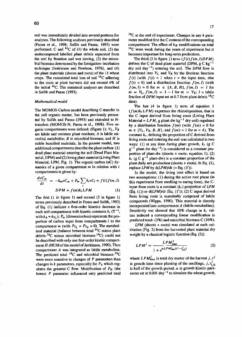
6017

Mashematical model

-kmoCm + Pm LkiOCi + f(l)f(m, 1)

soil was immediately divided into several portions foranalyses. The following analyses previously described(Pansu et al., 1998; Sallih and Pansu, 1993) wereperfonned: C and 14C of (1) the whole soil, (2) theundecomposed labelled plant debris separated fromthe soil by flotation and wet sieving, (3) the micro­bial biomass detennined by the fumigation-incubationtechnique (Jenkinson and Powlson, 1976), and (4)the plant materials (shoots and roots) of the Il wheatcrops. The cumulated total loss of soil 14C adheringto the roots at plant harvests did not exceed 4% ofthe initial 14c. The statistical analyses are describedin Sallih and Pansu (1993).

(2)LPMi = ------;=--,--

where L PMInn is total dry matter of the harvest j,Ii

is growth time since planting of the seedlings, j,I{/2is half of the growth period, a is growth kinetic para­meter set at 0.001 day-I to simulate the wheat growth.

14C at the end of experiment. Changes in any k para­meter modified first the C content of the correspondingcompartment. The effect of kH modifications on total14C were weak during the years of experiment but itbecomes important for long-tenn predictions.

The third (3 in figure 1) tenn (f(t)f(m, I)DP M)defines the C of dead plant material (DPM, g C kg- I

dry soil day") entering the soil. The DPM flow isdistributed into VL and VR by the Boolean functionf(l) (with f(t) = 1 when 1 = the input time, elsef(l) = 0) and a distribution function f(m, 1) (withf(m, l) = 0 for m E (A, B, Hl, f(m, l) = 1 form = VL, f(m,l) = 1 -1 for m = VR; 1 = labilefraction of DPM input set al 0.7 from plant debris 14Cdata).

The last (4 in figure 1) tenn of equation 1(f (m)kr L P M) expresses the rhizodeposition, that isthe C input derived from living roots (Living PlantMaterial = LPM, g plant-dw kg- I dry soil) regulatedby a distribution function f(m) (with f(m) = 0 form E (VL, VR, B, Hl. and f(m) = 1 for m = A). Theconstant kr , defining the proportion of C derived fromliving roots and entering the soil was calculated in twoways: (1) at any time during plant growth, kr (g Cg-I plant-dw day-I) is considered as a constant pro­portion of plant-dw (shoots + roots; equation 1); (2)kr (g C g-I plant-dw) is a constant proportion of theplant daily net production (shoots + roots). In Eq. (1),replace LPM by d(LPM)/dl (= Eq. (1')).

In the model, the living root effect is based ontwo assumptions: (1) during the active root phase (inthis experiment from seedling to earing time), the C­input from roots is a constant (kr ) proportion of LPM(Eq. (1)) or d(LPM)/dt (Eq. (l')); (2) C input derivedfrom living roots is essentially composed of labilecompounds (Wipps, 1990). This material is directlyincorporated into compartment A (labile metabolites).Sensitivity test showed that 10% change in kr val­ues induced a corresponding linear modification inpredicted total- (3%) and microbial biomass-C (10%).

LPM (shoots + roots) was simulated at each cul­tivation (Fig. 2) from the harvested plant material dryweight by a classicallogistic function (Eq. (2)):

LPM~IUj . j

1 + eaLPMmu(rJ-rlfl)

(1)DPM + f(m)krLPM

The MOMOS-Carbon model describing C-transfer inthe soil organic matter, has been previously presen­ted by Sallih and Pansu (1993) and extended to N­transfers (MOMOS-N, Pansu et al., 1998). Five or­ganic compartments were defined: (Figure 1): VL, VRare labile and resistant plant residues; A is labile mi­crobial metabolite; B is microbial biomass; and H isstable humified materials. In the present model, twoadditional compartments describe the plant carbon: (1)dead plant mate rial entering the soil (Dead Plant Ma­terial, DPM) and (2) living plant material (Living PlantMaterial, LPM, Fig. 1). The organic carbon (oC) dy­namics of a given compartment m in relation with icompartments is given by:

doCm

dl

The first (1 in figure 1) and second (2 in figure 1)tenns previously described in Pansu and Sallih, 1993)of Eq. (1) indicate a first-order kinetics decrease ineach soil compartment with kinetic constants ki (T-I,with kA = kYL); Pm (dimensionless) represents the pro­portion of carbon input from compartments i to thecompartment m (with PYL = PYR = 0). The metabol­ised material (balance between total 14C minus plantdebris-l''C minus microbial biomass-J''C) could notbe described with only one first-order kinetic compart­ment H (HUM of the model ofJenkinson, 1990). Thuscompartment A was integrated as labile metabolites.The predicted total 14C and microbial biomass-P'Cwere more sensitive to changes of P parameters thanchanges in k parameters, especially for PA which reg­ulates the greatest C flow. Modification of PH (thelowest P parameter influenced only predicted total

6118

DPM

1\

1ft) f(m,l)

\oC

2

Figure J. The MOMOS-e mode\. Five soil organic carbon (oC) compartments (V[.,labile plant material; VR, resistant plant material; A,labilemetabolites; B, microbial biomass; H, stable humified material). Two plant material compartmenlS (D PM, dead plant material = above groundand rootliner; LP M,living plant material). The numbers correspond to the terms in Eq. (1): l, carbon mineralisation; 2, humification; 3, deadplant materiaI-oC input (litrer); 4, oC input from living roots (rhizodeposition). The parameters are defined in Eq. (I).

••• Soli 1

-So/12

r

~): Il If IrIj j

1 8

~5'a

j.4

1:11

QOo 80 180 270 3CiO 450 540 630 720

TIme(days)

where r identifies the number of sampling points; qis the number of data series and Yqr and Yqr are themeasured and the predicted value of each data pointrespectively; wq are weight coefficients for each dataseries. For these data, wq was set at 0.3, 0.3 and 1 fortotal-, plant material- and mïcrobtal-I''C, respectively.

Results and discussion

Figure 2. Simulated production of plant material over the elevensuccessive wheat growths (see Eq. (2». LPMmax was set to themeasured plant dry weight at each harvest,

Mineralisation and humification of labelled plantmaterial

The daily net plant production was simulated by thedifferential fonn of Bq. (2), giving Bq. (2'):

In the experiment and for the simulation, the dead (la­belled) plant material (DPM) was introduced in thesoil only once, at the beginning of incubation (70%directed into VL and 30% into VR ).

The numerical integration was perfonned usingEuler's method and the parameter optimisation us­ing Powell's method, by minimising the followingcriterion:

d(LPMj) J" ( LPMj)---=-------.:... =aLPM 1- .dt LPM~~

SSK = L w~ L(Yqr - Yqr)2q r

(2')

(3)

The respective pararneters describing the 14C dynam­ics were different for the two bare soils. In contrastwhen the two cultivated soils are compared, the para­meters were similar (Table 1).

The presence of living plants lowered the meas­ured and predicted total 14C mineralisation during thefirst 3 (soil 1) or 6 (soil 2) months (Fig. 3A). Nev­ertheless the retarding effect was weak, especially insoil 1. During the initial decomposition stages, theavailability of labile labelled plant material stimulatedthe microbial activity and N immobilisation (Pansu etal., 1998). This active decomposition stage is illus­trated by (1) high total_14C mineralisation rates (Fig.3A), (2) increasing microbial biomass-U'C, reachingmaximum levels after 3~ months (Fig. 3B) and (3)high microbial metabolic quotients for labelled C02(qC02_14C, Bottner et al., 1988). In the presence ofliving plants, the competition between roots and activemicro-organisms for inorganic N lowered the total_14C

6219

100(a) 100

ao

•,,oP ~:"eo~

ca 4le.5

20

,'.".',.... ......~.

' ..t ....... :.~.~.... " ....

........... •.... lpIant:vll·······1b8re-vC~.~~.

80

80

40

20

10 180 270 3eO 450 lS40 130 720nme(days)

80 180 270 310 450 lS40 130 720nrne(days)

O+--+----+---+--t--__t----<f__-t-----io

O+--t---t-----.,t---;---t-_--+--io

o 0 1 1

o tG 180 270 3&0 410 640 130 720nme(days)

•. .

1 1 1

tG 110 270 310 450 640 130 720Thne(days)

", _----------------lbanHH[--,,",

, - - - - -1plant-Ej-'_"':""!~"'--'

: .: .: .

'Iba~l•,

o..--~---t--_+_--+--_+-__t-__If__­o

10

20

o

•..................... ..

_------1 banHH i-----.;--­,,-'"

10

40,(b)

•,••·,• •

30 • ,p1ant-A!

i'ii ,= •.E~20

i'

Figure3. Measured and predicted 14C distribution (in percent of total initial 14C) in the soil cornpartments in ban: and cultivated soils 1 and 2.

20

Table J. Optimised model parameters for bare and cultivated soils

Compartrnent Bare soil 1 Bare soil2 Culivated soils 1 and 2

kj Pj kj Pj kj Pj

VL 0.05 0.0 0.1 0.0 0.06 0

VR 0.0031 0.0 0.00043 0.0 0.002 0

A 0.05 0.58 0.1 0.79 0.06 0.77

B 0.006 0.08 0.004 0.033 0.006 0.037

H 0.0004 0.08 0.0001 0.025 0.00025 0.02

Kj. kinetic constants (day-l); Pj. proportion of compartment input. For thecultivated soils the parameters were similar.

63

mineralisation rates. This explanation is supported bythe observations of Merckx et al. (1985, 1987) show­ing that in nutrient limited soils the N deficiency inthe rhizosphere reduces the C metabolism. Thus thedepletion of mineral nutrients by plants may limit mi­crobial activity during active decomposition stages.The competition between micro-organisms and plantsoccurring during the initial decomposition stage, alsoresulted in a lower plant productivity (Fig. 2). The dryweight of plant material produced during the three firstgrowths was lower than subsequent growths.

In contrast, beyond 3 or 6 months, the measuredand predicted total_14C mineralisation was signifie­antly increased in both cultivated soils compared tothe bare soils (Fig. 3A). The total_14C remaining in thesoils at the end of the experiment was 18% of the ini­tially added 14C in both cultivated soils, compared to25 and 31% for bare soils 1 and 2, respectively. Thus,during the low activity stages, when the labile 14C_

compounds were exhausted, the presence of activeroots stimulated the mineralisation of the more resist­ant 14C-compounds. A similar stimulation of total_14C

mineralisation was observed by Cheng and Coleman(1990) as evidenced by a higher C(h_14C releaseand interpreted as resulting from a higher microbialmetabolism.

In addition to the total)4C mineralisation, themodel predicts root-induced modifications of sornemeasurable and unmeasurable organic matter com­partments. In bare soils, the plant debris- 14C (VL +VR, Fig. 3A) remaining at the end of experiment was 4and 18% of the initial l4C in soil 1 and 2, respectively.In cultivated soils, this proportion was not signifie­antly modified for soil l, but greatly decreased to 7%for soil 2 (Fig. 3A). Thus, in soil 2 the roots accel­erated the decomposition of the stable labelled plantdebris, explaining partly the plant induced stimulationof total_14C mineralisation.

ln the presence of roots, the model predicts a de­creased accumulation of the stabilised humus-l'[C (Hin Fig. 3B) especially in soil l. At the end of incub­ation, the net 14C accumulation in compartment Hamounted to 8% of the total_14C initially added forboth cultivated soils, compared to 18% and Il% inbare soils 1 and 2, respectively. Thus, in soil l, thelower total_14C remaining at the end of the incuba­tion in the cultivated soil (18%, Fig. 3A) comparedto the bare soil (25%), is essentially explained in themodel by a lower predicted (not measured) accumu­lation of stabilised humified-v'C in compartment H(Fig. 3B). For the bare soils, Sallih and Pansu (1993)explained the higher humification rates (accumulationin H) of the clay soil 1 (18%, Fig. 3B), comparedto the sandy soil 2 (Il%), by the properties of theclays to protect humified compounds (Merckx et al.,1985). The present simulation shows that this protect­ing effect may be counteracted in presence of roots.Thus the roots stimulate the mineralistion of recentlystabilised humus fractions. Similarly, in a comparableexperiment, Zagal (1994) demonstrated that the rootsalso liberated formerly stabilised 15Ncompounds.

In both soils and both treatments, the microbialbiomass-l''C increased during the initial active decom­position stage, in response to the availability of labile14C-material. Beyond this time, when the labile ma­terial was exhausted, the B compartment decreasedslowly for both treatments, showing a typical shapeof the microbial biomass curve (Fig. 3B) observedin many labelling experiments. Nevertheless the pres­ence of roots slightly lowered the measured and pre­dicted microbial biomass- 14c. Bottner et al. (1988)explained the 14Cdecrease induced by the active rootsby a stimulated C turnover in the microbial biomass.In the bare soils, beyond the active decompositionstage, the labelled portion of microbial biomass partlydecayed (explaining the decrease of the curve) and

64

partly became donnant by exhaustion of available 14C_substrate. In the planted systems, part of the microbialbiomass, stimulated by the input of labile C derivedfrom the roots, remained active and 14C was progress­ively replaced by unlabelled C derived from the roots.The qCOZ_14C values (microbial metabolic quotientfor COz_14q calculated by Bottner et al. (1988) forboth systems, revealed that in the rooted soils the la­belled biomass was smaller but more active than inthe bare soils. Thus during the slow decompositionphases, the presence of roots accelerated the turnoverof the portion of microbial biomass which previouslyused the labelled plant material as substrate. In Table1 for soil l, kB (ki for compartrnent B) is sirnilar inbare and cultivated soil, but PB in the planted soil ishalf that of bare soil, illustrating the higher turnover ofC in compartrnent B of the planted soil.

In the Rotharnsted model, Jenkinson (1990) de­scribed the effect of living plants by multiplying thefirst order kinetic constants by a constant factor ('re­tainment' factor). The present experiment shows that(1) the multiplication factor of ki (Table 1) cannot beconstant and (2) the plant effect varied positively ornegatively depending on the decomposition phases, asillustrated by the total 14C Mineralisation and the plantdebris-14C decomposition (Fig. 3A). In bare soils, themodel parameters (ki and Pi, Table 1) varied accord­ing to the soil properties. In contrast for the plantedsoils, the model parameters were found to be sim­ilar for both soils. Thus, the plant effect could not bedescribed by simply multiplying each bare soil para­meter by a constant factor. The solution was to runthe model for both treatrnents and to compare there-optimised parameters of each treatrnent (Table 1).Nevertheless in a strictly mechanistic way, this pro­cedure is not satisfying, since the plant effect couldnot be intrinsically described.

Total carbon trans/ers

Total-C was simulated using: (1) pararneters definedfrom 14C data in cultivated soils (Table 1), (2) ini­tial values of A, B and H compartrnents calculatedin bare soils and (3) optimisation of the k; pararneter.Predicted values agreed closely with the experimentaldata (Fig. 4A, B).

The model predicted large fluctuations in compart­ment A (not measured), which were related to thesuccessive plant growths (Figs. 2 and 4B). Indeed inthe model, the labile C derived from the active roots(rhizosphere activity) was directed into the compart-

21

ment A. Thus A is defined by two origins: (1) labilernicrobial Metabolites derived from the decomposing(labelled) plant material. In both bare soils, thesetransient compounds appear in small amounts essen­tially during the initial active decomposition phase(Fig. 4B), (2) labile material derived from activeroots (rhizodeposits). The second origin is quantitat­ively greater than the first (compare bare to cultivatedsoils, in Fig. 4B), explaining the high fluctuation ofsimulated A related to the successive crops.

In the unplanted soils, the rnicrobial biomass-Cdecreased from the beginning to the end of experi­ment, by a factor of 2.5-3 forboth soils (compartrnentB, Fig. 4B), as a result of the progressive exhaus­tion of labile C (Sallih and Pansu, 1993). In contrast,with plants present, the measured and predicted mi­crobial biomass-C remained at a relatively high leveluntil the end of the experiment, illustrating the supplyto micro-organisms of labile carbon derived from theliving roots (A compartrnent). Nevertheless, the fluc­tuations of B are greatly attenuated compared to A.As a matter of fact, in the model 70% of A is directlymineralised and used as energy source and only 20%is used to build new microbial biomass. At the end ofexperiment, bare soil rnicrobial biomass was 3 timeslower than in the cultivated soils, illustrating the C andenergy input derived from the roots.

The predicted H compartment (the stabilised hu­mus, Fig. 4A) remained relatively stable in soil 1 underboth bare and cultivated soil conditions. In contrast, insoil 2 the predicted H decreased substantially in thepresence of plants. Thus the presence of living rootsstimulated the Mineralisation of the stabilised unla­belled soil native humus. In cultivated soil 2, when thekn value of 0.00025 obtained from the 14C data wasused (as for the other ki and Pi pararneters, Table 1),the predicted H values were too high to properly de­scribe the total-C dynamics. A new optimisation gavekH = 0.0007. Thus in this cultivated soil 2, the para­meters describing the 14Cdynamics could not be usedto describe the unlabelled H compartrnent, indicatingthat roots probably stimulated the Mineralisation of anextra-amount of old stabilised humus whose dynamicsdiffer from those of recently fonned stabilised humus.In soil l , the predicted stimulation of H mineralisa­tion was weaker (Fig. 4A). For both cultivated soils,the H compartment curve declined parallel to total C,illustrating that the dynarnics of total-C are essentiallyexplained by the dynamics of H. This compartmentrepresents the major portion oforganic matter. In cul­tivated soil 2, almost one-third of the total C was lost

2265

20 (a) 40

.. ! --.-.-+ 1

360 450 540 630 720

Tlme (days)

D

..................!bare-Hf·· ..·..··..·..··..··· ..··....···.>

L'..~-..--.~plant-H ..... - ....~ .

10 ---+- -+- --+--t--+-----j

o 90 110 270 380 450 540 830 720

Tlme(days}

25 ·1 bare-H r···· ..... .. ... .. .20

1

151

J 1

0 " 110 270

a

'bare-tot l

-... .....

540 630 720

Tbne (days)4&0

. .

380270180

~'......

90

1

0+--_-+--+--+--1---1-----11-----1o

0.5

3.5

ISoll211 • •1 • 1 Il \ ..

•1 , 1

1 • ". 1 •, • . Il • • 1 • 1 •3 • 1. 1 • 1 &

i: " .. • 1 .1 • '01 ••!~

•• • 1 • 1 • 1 1 • 0

l' 1 0 • 1

-• ,0'

Ipl~.nt-AJ2.5 •

0

• 1 11 • 1

2 • 10

1V o'

1.5

1

540 830 720

Tlme (days)

• 1

• •

......... .......................

l' ·.1 1 •

••.. • 1 1 • • ..'. 1• • 1 • 1.• l , l' 1 ,.. 1 Ir • 1

• 11 ..

'. 1Il

• 1 l' 1

" 1 • 1'. 1 .• ••

1

180 270 HO 45090O+--_-t---I-----1---t---t--t---I

o

2T.15011 11'.• .•, .

••1.5

•'0 : (b) •1) •~ •"0

":'

~Cl

0.8

Figure4. Measured and predicted total carbon distribution (g C kg- 1 dry soil) in the soil compartments in bare and cultivated soils 1 and 2.

66

during the experiment, indicating a high instability un­der the experiment conditions, especially with plants(Fig.4A).

Predicted rhizodeposition

Total N contents of soil 1 and 2 were 0.12 and 0.20%,respectively. Plant production of soill was about halfthat of soil 2 (Fig. 2). Cumulative total N taken upby the plants of the Il growths amounted to 173 and366 mg N kg- 1 dry soil for soils 1 and 2, respect­ively, 14 and 18% of the total soil N. The declinein productivity of both soils at the last growth (Il th,Fig. 2) indicates nutrient exhaustion (this was con­firmed by the l2th growth not used in the calculations).For each growth, LPM (shoots + roots) was simu­lated from the mass of harvested dry plant materialand from a classicallogistic function (formula 2; Fig.2). Parameter kr is the predicted proportion of C,which is derived from living roots and directed intothe soil as labile material. In formula l, kr is definedas a constant proportion of the plant biomass (LPM)and was 0.025 and 0.ül5 g C g-l plant dw day-l,which is 0.054 and 0.032 g C g-l plant-C day-l(plant material-C = 46%) for soils 1 and 2 respect­ively. Thus the model predicts a lower proportion oflabile C released from roots for the more productivesoil 2 than in the less productive soil 1. Neverthe­less, in absolute values, predicted C derived from rootswas comparable for both soils. During the Il growths,10.7 and 13.8 g organic C kg- 1 dry soit were re­leased by plants into soils 1 and 2, respectively. Themodel prediction confirrns results from many pulse­labelling and non-labelled experiments, pointing outan increased below ground translocation and rhizo­sphere activity with decreased N availability (Hanssonet al., 1991). By contrast, Swinnen et al. (1995) in apulse-labelling experiment, found that N fertilisationof a winter wheat had no effect on the proportion of14Cwhich is translocated to the roots, calculated as aproportion of net assimilated 14c. Unlike our results,Liljeroth et al. (1990) found that the proportion of netassimilated 14C recovered in root/soil respiration anddeposited in soil was higher with a high N fertilisa­tion, compared to low N. These contradictory resultsillustrate that, beside the N fertility, other factors alsocontrol below-ground C translocation. Thus, a highersoil compaction in the clay soil 1 also may explainthe higher proportion of 14C released in the soil, sinceBarber and Gun (1974) observed a higher exudationrate in soils with increased physical resistance to roots.

23

In formula (l'), kr was defined as a constant pro­portion of the net daily production and was 0.43 and0.35 g C g-l plant dw or 0.93 and 0.76 g C g-l plant­C for soils 1 and 2, respectively. If in our calculationthe 'assirnilated C' is defined as the sum of shoots­C +roots-C+the organic C released from the roots asrhizodeposition, then the model predicts that the or­ganic C released from the roots represented 48 and43% of this 'assirnilated C'. These values are high,because in the calculation the direct root respiration­C (not measured nor predicted in this experiment)is not included in the 'assirnilated C'. The estimatedproportion of assirnilated C translocated to the rootsis controversial, with a large degree of uncertainty.Approximately 10-30% of the total assimilated C islost by the roots as root respiration and organic Crelease (Van Veen et al., 1991). The estimated rootrespirationlrnicrobial respiration ratio ranges from 111(Warembourgand Billes, 1979) to 114 (Van Veenet al.,1991). When the means of these values are used, thenthe rhizodeposited-C in soils 1 and 2 amounts to 46%and 41%, respectively, in percent of the classicallydefined net assimilated-C (shoot+root+direct root res­piration+root exudation). These values are still high.Except under sterile conditions, the techniques (pulselabelling) seldom allow direct measurement of organicC release from the roots. Microbial respiration can­not therefore be distinguished from root respiration.The fluxes are generally calculated indirectly. Review­ing the carbon economy in the rhizosphere, Wipps(1990) reported that the COz produced by the micro­organisms utilising carbon sources derived from theroots varied from 7% to at least 30% of the totalC fixed by the plant. The author concluded that themajority of below-ground COz respired during thegrowth of wheat, was derived from the respiration ofmicro-organisms degrading root-derived material. Inaddition, the root exudation varies to a large extent, de­pending on the age of the plants (Meharg and Killham,1990; Warembourg 1997). The present experimentwas perforrned only with active root systems (untilearing time), generating mean values calculated fromthe model prediction over the Il growths. Finally, therelatively high kr (Eq. (l'» values may also be partlyexplained by a quantity of fine roots which remainedin the soil after each plant harvest and root extraction,slightly overestimating the input of organic C derivedfrom the living roots. The cumulated soil 14C adheringto the roots at plant harvests did not exceed 4% of theinitial total 14C, but the cumulated proportion of rootsremaining in soil was probably higher.

24

Conclusion

The present experiment investigated the effects of act­ive roots on decomposition of labelled plant material,throughout a complete decomposition cycle, from veryfast to slow stages dominated by donnant organisms.The root effect couId not be described by simple mul­tiplying factors. This illustrates the complexity of theroot effect and the difficulty to parametrise the pro­cess, when multi-compartment models are fitted tomeasured soil carbon pools. Thus the plant effect can­not yet be easily extended to other soil and growthconditions. The generalisation of multi-compartmentmodels supported by measured compartments is stillquestionable. The controversial response of the soilprocesses to the presence of living roots, pointed outby many authors, is in this experiment predicted bytwo main processes:(l) The competition between plants and micro­

organisms for inorganic N explains the negativeeffect of plants on total C mineralisation rates, dur­ing the initial active decomposition stage, whenavailable labile-C stimulates microbial activity.This effect is also reftected by lower plant pro­ductivity and lower plant N uptake during theactive decomposition stages compared to the sub­sequent growths. Nevertheless this root-inducedreduction of decomposition is relatively low.

(2) By contrast, the presence of living roots stimulatesthe total carbon mineralisation during the later de­composition stage. During this phase, the labile-Cresources are exhausted, leading to low mineral­isation rates. In bare soils, part of the microbialbiomass decays, and most of the surviving organ­isms are donnant. In the presence of living roots,the model predicts the mineralisation of an extraamount of stabilised humus or recalcitrant plantdebris. The protecting effect of clays and loamon recently formed labelled humus is partly coun­teracted by the presence of roots, stimulating itsmineralisation. The model also predicts a stim­ulated mineralisation of old soil native stabilisedorganic fractions; they are not govemed by thesame mineralisation rates as the freshly fonnedcompounds derived from the labelled material.The total soil native-C dynamics are essentiallyexplained by the humus compartment, since thisfraction is largely dominant. The presence of rootsled to a progressive replacement of the labelledmicrobial biomass derived from the initial plantmaterial by unlabelled microbial biomass derived

67

from the root deposited carbon. During the slowdecomposition phase, in the bare soils, the biomassdecreased 2.5-to 3-fold by progressive energy ex­haustion. By contrast in the cultivated soils, highbiomass levels were maintained until the end of theexperiment.To maintain this high biomass level in the cultiv­

ated soils and to sustain its activity, the model predictsan input of labile C derived from the roots and relatedto the plant growth. This predicted organic rhizode­position was described as a mean proportion of theliving biomass: (shoots+roots) or as a mean proportionof the daily plant production. At each day, the meanvalue of C released by the roots into the soil amountedto 5.4 and 3.2% of the plant biomass present or 48 and43% of the daily plant 'net production' for soils 1 and2, respectively. These calculated values are relativelyhigh but within the range of sorne published data.

References

Barber D A and Gunn K B 1974 The effect of mechanical forces onthe exudation of organic substances by the roots of cereal plantsgrown under sterile conditions. New Phytol. 73, 39-45.

Bottner P, Sallih Z and Billes G 1988 Root activity and carbonmetabolism in soils. Biol. Fertil. Soils 7, 71-78.

Cheng W X and Coleman D C 1990 Effect of living roots on soilorganic matter decomposition. Soil Biol. Biochem. 22, 781-787.

Donnaar J F (1990) Effect of active roots 00 the decomposition ofsoil organic materials. Biol. Fertil. Soils 10, 121-126.

Hansson A C, Andren 0 and Steen E 1991 Root production offour arable crops in Sweden and its effect on abundance ofsoil organisms. ln Plant Root Growth an Ecological perspective.Ed. D Atkinson. pp 247-266. Blackwell Scientific Publications,Oxford.

Jenkinson D S 1977 Studies on the decomposition of plant materialin soil. V. The effects of plant cover and soil type on the lossof carbon from 14C labelled ryegrass decomposing under fieldconditions. J. Soil Sci. 28, 424-434.

Jenkinson D S 1990 The turnover of organic carbon and nitrogen insoil. Phil. Trans. R. Soc. London B 329, 361-368.

Jenkinson D S and Powlson D S 1976 The effect of biocidal treat­ments on metabolism in soil: V. A method for measuring soilbiomass. Soi1Biol. Biochem. 8, 209-213.

Liljeroth E, van Veen J A and Miller H J 1990 Assimilate trans­location to rhizosphère of two wheat cultivars and subsequentutilisation by microorganisms at IWO soil nitrogen levels. SoilBiol. Biochem. 22,1015-1021.

Meharg A A and Killham K 1990 Carbon distribution within theplant and rhizosphere in laboratory and field-grown Lolium per­enne at different stages of development. Soil Biol. Biochem. 22,471-477.

Merckx R, den Hartog A and van Veen J A 1985 Turnover of root­derived material and related microbial biomass formation in soilsof different texture. Soi1Biol. Biochem. 17: 565-569.

Merckx R, Dijkstra A, den Hartog A and van Veen J A 1987 Pro­duction of root-derived material and associated microbial growthin soil at different nutrient levels. Biol. Fertil. Soils 5, 126-132.

68

Pansu M, Sallih Z and Botmer P 1998 Modelling of soil nitrogenforms after organic arnendment under controlled conditions. SoilBiol. Biochem. JO, 19-29.

Quian J H, Doran J W and Walters D T 1997 Maize plant contribu­tions to root zone available carbon and microbial transformationsofnitrogen. Soil Biol. Biochem. 29,1451-1462.

Rogers H H, Runion G B and Krupa S V 1994 Plant response taatrnospheric C0:2 enrichment, with emphasis on mots and therhizozsphere. Environ. Poilut 83, 155-189.

Sallih Z and Pansu M 1993 Modelling of soil carbon fonns afterorganic arnendment under controUed conditions. Soil Biol. Bio­chem. 25, 1755-1762.

Shields J A and Paul E A 1973 Decomposition of C-labeUed plantmaterial under field conditions. Can. J. Soil Sei. 53, 297-306.

Swinnen J, van Veen J A and Merckx R 1995 Root decay andturnover of rhizodeposits in field-grown winter wheat and springbarley estimated by t4c pulse-Iabelling. Soil Biol. Biochem. 27,211-217.

25

Van Noordwijk M, Martikainen P, Bottner P, Cuevas E, Rooland Cand Dhillion S 1998 Global change and root function. GlobalChange Biol. 4, 759-772.

van Veen J A, Liljeroth E, Lekkerkerk L J A and Van de Geijn S C1991 Carbon fluxes in plant-soil systems al elevated atmosphericC0:2 levels. Ecol. Appl. i, 175-181.

Warembourg F. 1997 The 'rhizosphere effect': a plant strategy forplants to exploit and colonize nutrient Iimited habitats. Bocconea7, 187-193.

Warembourg F and Billes G, 1979. Estimating carbon transfer in therhizosphere. ln The Soil-Root Interface. EdsJ L Harley and R SRussel. pp 183-197. Academie Press,New York, USA.

Wipps J M 1990 Carbon Economy. ln The Rhizosphere. Ed. J MLynch. pp 59-97. Wiley and Sons, Chichester, UK

ZagaI E 1994 Influence of Iight intensity on the distribution of car­bon and consequent elfects on mineralization of soil nitrogen ina barley-soil system. Plant Soill60, 21-31.

Section editor:R Merc1cx

La Transformation du C des Apports Organiques(modèle TAO-C)

69

e: de transformation du carbone

PERGAMON Soil Biology & Biochemistry 33 (200 1) 997-10 10

Soil Biology StBiochemistry

www.elsevier.comllocatelsoilbio

Kinetics of added organic matter decompositionin a Mediterranean sandy soil

L. Thuriès'r'", M. Pansu":", C. Fellera, P. Herrmann'', r..c. Rémy"

a/RD (formerly ORSfOM). BP 5045. 34032Montpellier Cedex J. FrancebJNRA-ENSAM. 2 place P. Yiala 34060 Montpellier Cedex t. France

"Phalippou-Fraysslnet S.A.• Organic fertilizers, BP 42.81270 Labastide-Rouairoux; France

Received 17 December 1999; received in revised form 13 July 2000; accepted 6 December 2000

Abstract

Carbon mineralization kinetics of 17 organic materials were studied in a Mediterranean sandy soil. These added organic matters (ADM)used in the organic fertilizer industry differed in their origin and composition: plant residues from the agri-food industry, animal wastes,manures (plant and animal origin), composts at different composting times and organic fertilizers. The mixtures ADM-soils were incubatedunder aerobic conditions at 28°C during 6 months. Soil moisture was maintained at 75% water holding capacity and respired-eÛ2 wasregularly trapped into alkali media in closed chambers, then checked by HCl titration. Analyses of CÛ2 were performed in triplicate at 17sampling occasions. The mineralized ADM fraction (MADMF) varied according to the ADM origin: from 12-33% of added C for composts,to 65-90% for animal-originated ADM, with many intermediate patterns for plant-originated ADM.

Seven decomposition models from the literature were fitted to actual MADMF: (a) three consecutive models with two lst-order-kineticcompartments and three parameters (ml, humification; m2, exchange; m3,decomposition), (b) three parallel models (m4, with two compact­ments and three parameters; m8, a lst-order plus O-ordermodel with threeparameters; mS,a three-compartment model with four parameters),and (c) m7, a model with one 2nd-order-lcinetic compartment and two parameters. Additionally, m6, a simplified version of mSwas proposed.Models m2 and m7 did not match with actual data or gave a poor fit. By the correlation parameters, the most simple model m4 was choseninstead of the consecutive models ml and m3. Residual sums of squares were a1waysgreater-but not significantly-io m8 than in m4, whichconfirmed the superiority of the models with two 1st-order compartments against 1st-order plus O-order models for incubation times higherthan 100 days. Model mS(most of its parameters being not correlated) gave the best predictions of our data. The proposed m6 version gavepredictions with similar precision as m4 and appeared powerful with only two parameters (very labile and stable fractions of the ADM). Acompromise between the precision of the predictions and the simplicity of the formulae allowed the recommendation of the well-known m4model, and above ail the simpler m6 model. @ 200 1 Elsevier Science Ltd. Ali rights reserved.

Keywords: Decomposition models; Added organic matter; Organic fenilizers; Composted organic amendments; Organic carbon

1. Introduction

The utilization of organic amendments and fertilizers isincreasing with the development of organic farming, and iseven increasing among conventional farmers (Hartz et al.,2(00). Indeed, such products are largely available due to: (a)a social need for healthy food produced under conditionsthat protect the environment and (b) a constant legislative

pressure for recycling of organic wastes. Both manufac­turers and farmers need tools for characterizing and evalu­

ating such organic materials. Furthermore, environmentalscientists need more precise parameters for modelling the

• Corresponding author. Tel.: +33-4-67-41-62-28; fax: +33-4-67-41­62-94.

E-mail address: pansu@mpl.ïnifr(M. Pansu).

decomposition of such added organic matter (AOM,Mueller et al., 1998) in soils. Up to now, many workshave dealt with the carbon and/or nitrogen mineralizationkinetics of crop residues (Janzen and Kucey, 1988; Mary etal., 1993; Recous et al., 1995; Kaboneka et al., 1997) and itsmodelling (Quemada and Cabrera, 1995; Whitmore, 1996;Gilmour et al., 1998; Henriksen and Breland, 1999). Carbonmineralization kinetics have also been studied with manuresand composts (Hébert et al., 1991; Hadas and Portnoy,1994; Paul and Beauchamp, 1994; Serensen and Jensen,1995; Paré et al., 1998; Hartz et al., 2(00), together withmodelling investigations (Levi-Minzi et al., 1990; Saviozziet al., 1993; Kirchmann and Bernal, 1997; Hadas and Port­noy, 1997; N'Dayegamiye et al., 1997; Bernai et al., 1998).Because laboratory techniques and model standardization islacking, these studies are difficult to compare. Laboratory

0038-{)7171011S - see front matter Cl 2001 Elsevier Science Ltd. Al! rights reserved.PlI: S0038-0717(0 1)00003-7

998 L. Thuriès et al. / Soil Biology & Biochemistry 33 (200l) 997-101071

Table 1Major characteristics (C, N, C-to-N ratio. total ashes) and doses of added organic matter (AOM) in g (C or N) kg -1 dry soil, and in equivalent field dose in tonper hectare

AOM origin AOM g kg- I AOM (dry basis) g kg -1 dry soil t ha- I

C N Ashes C:N Added C Added N Field dose'

Plant Coffk 537 20 31 27 4.999 0.184 28Wgrap 529 27 89 20 4.667 0.238 28Dgrap 494 22 71 22 4.605 0.209 28Olîvp 469 20 88 24 4.426 0.186 28Kokoa 437 45 91 10 4.072 0.423 28

Manure Shepm 379 22 281 17 3.230 0.190 28Chicm 376 61 323 6 3.360 0.542 28

Animal Nfeat 545 146 38 4 1.205 0.322 7Featrn 471 152 28 3 1.064 0.343 7Guano 175 156 433 1 0.392 0.350 7

Fertilizer Gnofer 273 95 404 3 0.617 0.215 7Comfer 369 37 255 10 1.735 0.176 14

Compost Compoa 362 29 322 12 2.709 0.218 28Compob 363 25 344 15 3.434 0.233 28Compoe 288 27 404 11 2.505 0.235 28

Compo + 339 26 321 13 3.035 0.229 28Compop 449 25 402 18 2.816 0.156 28

• AOM bulk weight, calculated on 0-20 cm layer. mean soil bulk density «2 mm) = 1.5. refuse (>2 mm) = 5.21 % and 6.68% for the 0-10 cm and10-20 cm layers, respectively.

protocols differ on CO 2 measurement methods, type of soil,incubation time, temperature, soil moisture, AOM amounts,decomposition of AOM alone (specifie mineralization) orsimultaneous addition of mineral-N (mineralization withstandardized total-N content). Most of the models used forpredicting COrC mineralization take into account one (thewhole AOM), two, or more organic compartrnents of theAOM (more or less resistant to microbial attack).

The first objective of this work was to test, under standardlaboratory conditions, the specifie carbon mineralization ofa wide range of AOM in a sandy soil with low organicmatter content. The second objective was to find accuratemodels to describe the carbon-AOM mineralization kineticsunder these standard conditions, the model parameters onlydepending upon AOM quality.

2. Material and methods

2.1. Sail for mineralization test

The incubation test was done with the top-layer (0-20 cm)ofa sandy soil (69.3% sand, 11.5% clay), previously describedby Servat and Callot (1966) and classified as ftuvisol (FAO­UNESCO-ISRIS, 1988) or Udifluvent (USDA, 1975). It wascollected in an experirnental site (Thuriès et al., 2000a) locatedin Théza (Eastern Pyrénées, France). This soil has P~H,o) 6.6,CEC5.5 cmolc + kg " soil, total C andN 4.98 and 0.59 g kg- I

soil, respectively. It was partially air-dried at room tempera­ture (20°C) until it could be crushed and sieved through a2 mm sieve, then air-dried to constant weight.

2.2. Added organic matter (AOM)

Different kinds of AOM from agri-food industry wastesand industrial-processed fertilizers (organic amendmentsand fertilizers) were tested. Their major characteristics areshown in Table 1. The raw materials were from (a) plantorigin: wet and dry grape berry pellicles cakes (Wgrap,Dgrap), coffeecake (Coffk), cocoacake (Kokoa), olivecake(Olivp), (b) animal origin: hydrolyzed feather meal (Featm),native fine feather (Nfeat), guano (Guano), (c) manure origin(plant and animal origin): sheep manure (Shepm), chickenmanure (Chicm) and (d) fertilizers: organic compostedamendments (Compo series), and organic fertilizers (Gnofer,Comfer). The composted organic amendments (Compo) weremade from Shepm and Coffk in periodically-tumed and aera­ted piles, during a 1O-month composting period. Sampleswere taken before the composting process (Compo a), andat 40 (Compo b), 120 (Compo p), and 305 (Compo e) days.Compo + was a mixture of 75% Compo e and 25% Dgrap(used for drying the compost). Gnofer was a guano-basedorganic fertilizer, whereas Comfer was a Compo-based ferti­lizer supplemented with Chïcm. The AOM were air-dried at25°C, then finely ground

2.3. Incubation experiment

Carbon mineralization was measured as respired COrCin closed chambers (28°C ± 1°C, in an incubator) with theexperimental design adapted by Thuriès et al. (200üb). Anexact mass (125-500 mg AOM per container) was

72L Thuriès et al / Soil Biology cre Biochemistry 33 (200/) 997-/0/0 999

Where Cm;a= respired fraction of organic amendment atsampling occasion i and replication a, C02Ga and C02Gaare the amounts ofC evolved from theamended and control iasamples respectively, TAC is total added C expressed in theC02Ga and C02Ga unit, Cm, = mean respired fraction ofAOM at sampling occasion i (n = 3 replicates), MAOMF.and MAOMFc 1are mean mineraiized AOM fractions (cumu~lated values of respired fractions with MAOMFo= O).Theexpression MAOMF is very useful for practical use since itdoes not depend on any unit. For example, a valueMAOMF = 0.4 at 150 days, means (with gross approximateof comparable mineraiization conditions) that for a 10 Mg Cha -1 AOM application, 4 Mg C ha -1 will be mineraiizedduring 5 months after spreading. Hess and Schmidt (1995)pointed out that estimations with non-cumulative data weremore accurate than with cumulative ones. But they used short­term experiments with a great number of sampling occasionswith thesame time interval. Moreover, their estimations by thetwo methods where not rea1lydifferent. Our experiment lastedfor 6 months with very different time intervals betweensampling occasions. The cumulative values are also the mostfrequently used for parameter estimations and corresponddirectly to the analytica1 solutions of differential equations(fable 2). Nevertheless, working with cumulative valuesnecessitate careful data control during the experiments sincevariances are added simultaneously with mean additions. Thepooled variance of Cm; is:

homogeneously incorporated in 50 g air-dried soil. Theseexperimental AOM amounts were chosen to correspond torealistic inputs in field conditions: 7 or 14 t ha -1 for animalproducts or fertilizers, 28 t ha -1 for composts, plant originproducts and manures (fable 1).

The AOM-C ranged from 8 to 102% of initial soit C, andthe AOM-N from 26 to 93% of initial soit N. Identical addedquantities of AOM-N would have led to very 10w inputs of Cfor N-rich fertilizers and unrea1istic high field doses for N­poor amendments. Recous et al. (1995) and Henriksen andBreland (1999) indicated that concentrations of available N(AOM-N + soil inorganic N) less than 1.2% of AOM drymatter significantly reduced the rate of C-mineralization andgrowth of microbial biomass. This risk does not exist in thepresent experiment since AOM-N concentrations alonewere greater than 2% of AOM-dry matter (fable 1). Forour study of specifie AOM mineralization, we did notconsider any mineral N addition simultaneously withAOM addition. During decomposition, the N pathway anddynamics of organic and inorganic N are not the same(pansu et al., 1998b); the addition of mineral-N would notreduce the N heterogeneity linked to AOM addition.

Three replicates per AOM treatment, basal soil respira­tion and blanks were used for the experiment. Samplecontainers were placed in 1.2 1airtight glass jars containinga 50 ml vial with 20 ml aqueous NaOH solution0,25 mol 1- 1 (Titrisol) for CO 2-C trapping and -10 ml deio­nized water (moisture saturated atmosphere) to prevent soitdesiccation. Soil moisture was checked by periodicalweighting and maintained at -75% water holding capacity(- - 30 kPa or 16% dry weight basis) with deionizedwater. For each replicate of AOM, blank and control, 17sampling occasions of CO2-C measurements were done atdays 1,2,3,5,7,10,14,20,28,41,61,90,100,120,130,152 and 180.

sampling occasion i was estimated according to:

Cm. = C02Ga- C02Ga.a TAC

_ 1 ft

Cm, = -, Cm.1 n L.. la

a=1

MAOMF; = MAOMF;_I + Cm;

(1)

(2)

(3)

2.6. Mathematical models

(5)

(4)

where p is the total number of sampling occasions with nsamples. The cumulative confidence intervals must be calcu­lated according to Pansu et al. (l998a):

MAOMF; = MAOMF; ± ~~~ X SCmi fI. v-;;

1 p ft

;, =_"( _- 2Cm; n _ L. L. Cm;a Cm;)

P P ;=1 a=1

Our main objective was to compare the efficiency ofdifferent model formulations (fable 2) in the descriptionof cumulative CO 2-C data. The tested models can be classi­fied in three types: one-compartment model (0 in Table 2),consecutive Ist order compartment models (C in Table 2)and parallel 1st order compartment models (P in Table 2).

The first consecutive two-compartment humification model

2.5. Data calculatian and control

The fraction of added C mineraiized from AOM at a

2.4. Measurements

Organic carbon and total nitrogen of soil and AOM weredetermined by dry combustion (Carlo Erba NA 2000) withcontrol by lost on ignition at 450°C for AOM (NFU 44160,1985).

The respired CO2-C was estimated by precipitating thecarbonates with a solution of BaCh and titrating the remain­ing NaOH (uncarbonated) with HCI 0.25 mol 1- 1

• Soil basalrespiration (control unamended soil) was subtracted fromthe gross respiration to assess the net respiration associatedto AOM mineralization (Bq. 1). The total respired COrCquantities were obtained by summing the COrC respiredbetween sampling occasions (Eq. 2).

1000 L Thuriès et al. / Soil Biology ~ Biochemistry 33 (200/) 997-101073

Table 2Model formulations for remaining AOM fraction (RAOMF = I-MAOMF); CM = compartment model; T = model type (C = consecutive two CM, P =paraIlel 2 or 3 CM. 0 =one CM)

TNo. Name

C ml Consecutive humification, 1storder 2 CM, three parameters

C m2 Exchange 1st order 2 CM

C m3 Consecutive decomposition1st order 2 CM, three

parameters

P m4 Parallel Ist order 2 CM, three

pararneters

FlowAOM = added organic matter

Analytical solution RAOMFat time t

(k,m. - k",R) e-(ka +t,,)1

k,m. + kH - kmR

Pararneters

k.nL k..R: Ist order kineticmineralization constants of labile (L)and resistant (R) compartments ~:humification constant

tH, 10: humification and decompositionconstants. k",: mineralization constant

V." À2: mots of 2nd order lineardilferential equation j{kH, /co. k"J)

/co. k",: decomposition andmineralization constants, PL: labileAOM fraction

k.nL, k.nR: see ml above, PL: see m3above

P mS Parallel Ist order 3 CM, 4

pararneters

P m6 Parallel Ist order 3 CM, 2

pararneters

~~R

L r, RP'L i-r,»,

AOM

P~e -k:'" + (1 - P~ - Ps}e-k.... ' + Ps P~: very labile AOM fraction.~,~:

kinetic constants of very labile and R

fractions. Ps:stable AOM fraction

P~, Ps: see mS above. /, h = constants

(fixed values of k",L and k..R for ailAOM)

o m7 2nd order kinetic model

P mS Ist order plus 0 order model

1 + ta(1 - a)tk: 2nd order kinetic constant. a:fraction of AOM becoming microbialbiomass

PL, k.nL: see m4 above. k..oJ: 0 orderk:inetic constant

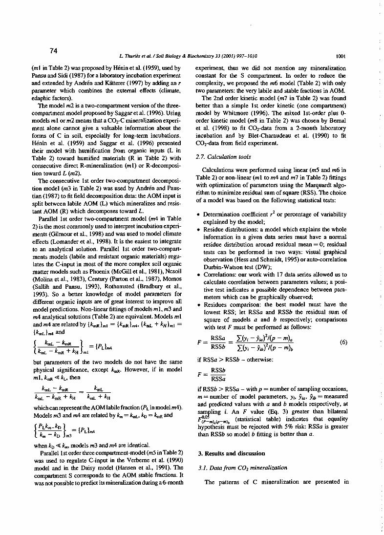
74L Thuriès et al / Soil Biology cl Biochemistry 33 (2001) 997-1010 1001

(ml in Table 2) was proposed by Hénin et al. (1959), used byPansu and Sidi (1987) for a laboratory incubation experimentand extended by Andrén and Klitterer (1997) by adding an rpararneter which combines the external effects (climate,edaphic factors).

The model m2 is a two-compartment version of the three­compartment model proposed by Saggar et al. (1996). Usingmodels ml or m2 means that a COrC mineralization experi­ment alone cannot give a valuable information about theforms of C in soil, especially for long-terrn incubations.Hénin et al. (1959) and Saggar et al. (1996) presentedtheir model with humification from organic inputs (L inTable 2) toward humified materials (R in Table 2) withconsecutive direct R-mineraIization (ml) or R-decomposi­tion toward L (m2).

The consecutive lst order two-compartment decomposi­tion model (m3 in Table 2) was used by Andrén and Paus­tian (1987) to fit field decomposition data: the AOM input issplit between labile AOM (L) which mineralizes and resis­tant AOM (R) which decomposes toward L.

Parallel lst order two-compartment model (m4 in Table2) is the most commonly used to interpret incubation experi­ments (Gilmour et al., 1998) and was used to model climateeffects (Lomander et al., 1998). It is the easiest to integrateto an analytical solution. Parallel lst order two-compart­ments models (labile and resistant organic materials) regu­lates the C-input in most of the more complex soil organicmatter models such as Phoenix (McGil1 et al., 1981), Ncsoil(Molina et al., 1983), Century (Parton et al., 1987), Momos(Sallih and Pansu, 1993), Rotharnsted (Bradbury et al.,1993). So a better knowledge of model parameters fordifferent organic inputs are of great interest to improve allmodel predictions. Non-linear fittings ofmodels ml, m3 andm4 analytical solutions (Table 2) are equivalent. Models mlandm4are relatedby {kmR}ml = {kmR }m4' {kmL + kH}ml ={kmL }m4 and

{ ~ - kmR } = {Pdm4kmL - kmR + kH ml

but parameters of the two models do not have the sarnephysical significance, except k,.,R. However, if in modelml, kmR~ kL, then

which can represent the AOM labile fraction (PLin model m4).Models m3 and m4 are related by km = kmL, ko = kmR and

{PLkm_ko } = {Pdm4km - ko m3

when ko ~ km, models m3 and m4 are identical.Parallel1st oroer three compartment-model (m5 in Table 2)

was used to regulate C-input in the Verberne et al. (1990)model and in the Daisy model (Hansen et al., 1991). Thecompartment S corresponds to the AOM stable fractions. Itwas not possible to predict its mineraIization during a 6-month

experiment, thus we did not mention any mineralizationconstant for the S compartment In oroer to reduce thecomplexity, we proposed the m6 model (Table 2) with onlytwo pararneters: the very labile and stable fractions in AOM.

The 2nd order kinetic model (m7 in Table 2) was foundbetter than a simple lst order kinetic (one compartment)model by Whitmore (1996). The mixed lst-order plus 0­order kinetic model (m8 in Table 2) was chosen by Bernalet al. (1998) to fit COrdata from a 2-month laboratoryincubation and by Blet-Charaudeau et al. (1990) to fitCO2-data from field experiment.

2.7. Calculation tools

Calculations were performed using linear (m5 and m6 inTable 2) or non-linear (ml to m4 and m7 in Table 2) fittingswith optimization of parameters using the Marquardt algo­rithm to minimize residual sum of square (RSS). The choiceof a model was based on the following statistical tests:

• Determination coefficient? or percentage of variabilityexplained by the model;

• Residue distributions: a model which explains the wholeinformation in a given data series must have a normalresidue distribution around residual mean = 0; residualtests can be performed in two ways: visual graphicalobservation (Hess and Schmidt, 1995) or auto-corre1ationDurbin-Watson test (DW);

• Correlations: our work with 17 data series allowed us tocalculate correlation between parameters values; a posi­tive test indicates a possible dependence between para­meters which can be graphically observed;

• Residues comparison: the best model must have thelowest RSS; let RSSa and RSSb the residual sum ofsquare of models a and b respectively; comparisonswith test F must be performed as follows:

F = RSSa = L(Yi - Yùil(p - m)a (6)

RSSb L(Yi - Yib)2/(p - m)b

if RSSa > RSSb - otherwise:

F = RSSbRSSa

if RSSb > RSSa - with p = number of sarnpling occasions,m = number of model parameters, Yi> Yia' Yib = measuredand predicted values with a and b models respectively, atsarnpling i. An F value (Eq. 3) greater than bilateraIF/.po:.mlQ(p-mlb (statistical table) indicates that equalityhypothesis must be rejected with 5% risk: RSSa is greaterthan RSSb so model b fitting is better than a.

3. ResuUs and discussion

3.1. Datafrom COl mineralization

The patterns of C mineralization are presented in

\002 L Thuriès et al. 1 Soil Biology & Biochemistry 33 (2001) 997-101075

..;g .. :g

:g ....

~~~~~-=MN"";"':

'oONOO"Of"'o0'1 ~ - N V'Io'~...;r--:...;

r-­00

lM

. ... ..1 .. .. ..

1 f!

N N r-- r-- 0 ('0") 0'1- 'Olt' V"I N ('0") \oC r--r--:d "':ddcid

... ­- ...ON

.. .·. ..... .. :g ;g

.. .... ..j:gl 1-- •••• :g

'000

1 ci 1

··1 • 1

o1 ....; 1

1 ~ 1

'0~

1 ... 1- '"- '0~...;

8;!; s s s....: N ....:....; ci

e e<>'u...-..c..cCIlU

··· ~

· ..· ..~ .... ;g.. .. ;g

· ..· ..:g .. .. .... :g

li' li' w.I li' w.Iccc c c

~$~~r:: =~ ~~~-=0"':0'0 ON ci cci

ë..li:

~~~~Sf 8Sf s e so-=cid-= 0'0 ~-.ir--=

OIC-V'lOO0'1 r-- 00 r-- N.....:r--:MN~

e- V""I N e- 'Olt' r-- 0-MOV"lM V"I-M vi • ..0 r--: "':;-.i

'"

~~a~~-- - --

~~~~;;:;- - ---

'0

i...E~

'"E

00E

...E~

'"E~ Ë

~E~

'"E

'"E

c'00'Co

~-e

•

•••

-ociV~

Figs. 1-3. Most of AOM from animal origins wererapidly mineralized (Figs. 1 and 3). During 6 months,65% (Chicm), or up to 90% (Guano) of AOM-C wasrespired. Mineralization from plant origin-AOM wasless intensive (Fig. 1) with a large range of mineralizedC: from 29% for Dgrap to more than 56% for Coffk.These discrepancies occurred during the last stages ofincubation (after 2 months). Sorne AOM have uncom­mon patterns. On one hand the Kokoa rnineralizationcurve looks like a fertilizer or an animal-originatedAOM (see Featm in Fig. l) with a large very labilefraction. On the other hand, native fine feather (Nfeatin Fig. 1) was less susceptible to microbial degradation,and behaved like a recalcitrant plant material. Nfeat iscomposed of native proteins arranged in lamella, and isquite recalcitrant to microbial attacks (AOM manufac­turer, unpublished data). Another hypothesis is thepossible presence of antibiotics since Nfeat is derivedfrom intensive duck livestock.

After 6 months of incubation, the C mineralization of theindustrial composts (Compo in Fig. 2) showed a gradientaccording to the time of composting: 33% for the initialmixture to 12% for the most composted material. Thecurve patterns were intermediary between the animal-originAOM and plant-origin ones. The fertilizer with a compostbase (Comfer in Fig. 3) combined the typical fertilizerpattern (strong early mineralization rate) with a more stableone.

The confidence intervals at 152 or 180 days of incu­bation (Figs. 1-3) are the greatest of the experimentsince they are calculated with i = 16 or i = 17 respec­tively (Eq. 5). It is difficult to compare their amplitudeswith other works since the calculation methods are notgiven, and results are very different: for example, verysmall intervals reported by BernaI et al. (1998) andwider ones by Paré et al. (1998).

The highest actual confidence intervals relate to theproducts with strong mineralization: guano-based fertilizerand guano (Fig. 3). In contrast, the third animal product withrapid mineralization (Featrn in Fig. l) gave a better repeat­ability. This feather meal is an industrial product, and hasbeen treated at high temperature (120°C, autoclaved); thisproduct is finely ground and is probably more homogenouswith respect to the C- and N-repartition and active sites forrnicrobial attack,

Models m2 and m7 (Table 2) did not match with thisdata or gave poor fittings (determination coefficients2% < ? < 97%, depending on the AOM). As expected,models ml, m3 and m4 gave the same predictions. The17 data series were weIl predicted with these two-compart­ment models (Figs. 1-3). The determination coefficients (inTable 3 and on each curve) were above 99% for Il series,

3.2. Comparative ml, m2, ml, m4, m7, m8 modelpredictions

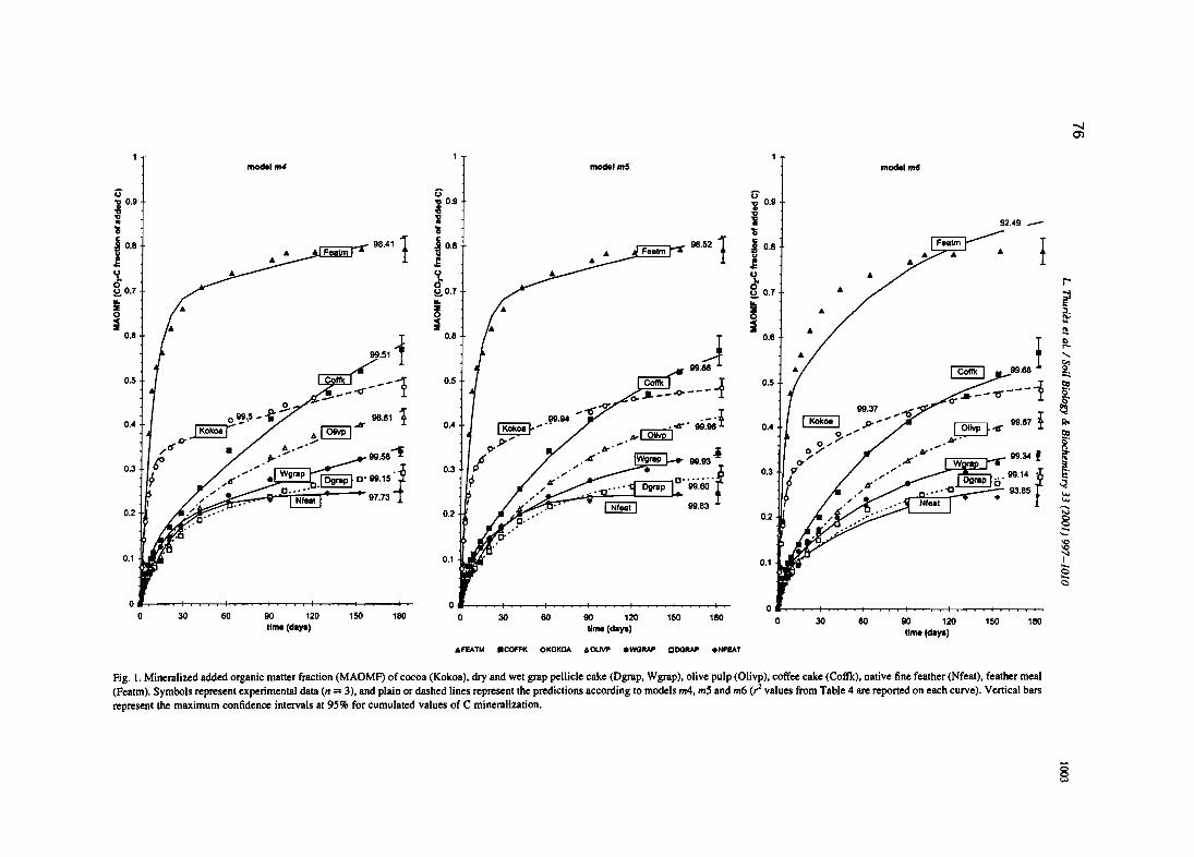
.......0)

modal m4 1 model mS 1 J model me

G' G' G'lM lM lM.., .., ..,l l l 92.49 __'l; 'l; 'l;

j 0.8 98.41 1 ~ 0.8 F 98.52 1 ~ 0.8 l1 • ~ • eelm j •~ ~ ~ r-!:!.0.7 !:!.0.7 !:!. 0.7 r~ ~ ~ ~:~ ~ ~ ~

0.8 1 0.8 J 0.8 f~

99.51 <,

""99.88 99.88 ~

0.5+ 1 Udl!!!!J __-1 0.5 Coflk r 0.5 ~~ __ -« ... .o----'"I 5

o ~--- 0- -- !)j). -- 1 1 99.37 "1S: ~

0.4+' ~9J..5'" ~...r 98.81 0.4 "<okoll~ ... ·98.lM ~...r' 9Ïl:eêI 0.4 1Kokoe 1 ...,1>-......... 1 Ollvp ~"il" 99.87 i Il-

.o-~ ~~ ... A-~ 9-'" A-' ~d' • A .> • poP' A-.... O~o"" A-.... 1\f .~..... 99.561' 15 ~"I{'Wgr8p 98.83~ 0-" .....=.,..,~ 99.34 r ~

0.3 +1 »:" W ra .~ 0.3 IS- ".0"" • J 03" 1:;'1. If'. 9 P IOgraptO·99.15 ,( 1(' .-=----10.. · .. ·· . 0 .=.y ".. Y .• on ""~ft 1 0Cl"" ~ t::

+" ... "...-.....- ~ ,. J.I1.-- - l ,..vv. 1 n.__ li. ;:::,0.2. ~.~ ••• , 0.2+r • ,Jr .• ' 0.2-l1l 8:~

s0.1-11.1U 0.1 -ll,u.- 0.11W ~

S2Cl

01 " 1 1 of 1 1 1 1 1 0•o 30 60 90 120 150 180 0 30 80 90 120 150 180 0 30 80 90 120 150 180

lime (daya) Ume(daya) Ume(daya)

.FEATM .COFFK OKOKOA AOl.IVP .WORAl' ODORAI' .NFEAT

Fig. 1. Mineralized added organic matter fraction (MAOMF) of cocoa (Kokoa), dry and wet grap pellicle cake (Dgrap, Wgrap), olive pulp (Olivp), coffee cake (Coffk), native fine feather (Nfeat), feather meal(Featm). Symbols represent experimental data (n =3), and plain or dashed lines representthe predictions according to models m4, m5 and m6 (r2 values from Table 4 are reported on each curve), Vertical barsrepresent the maximum confidence intervals at 95% for cumulated values of C mineralization.

§

§

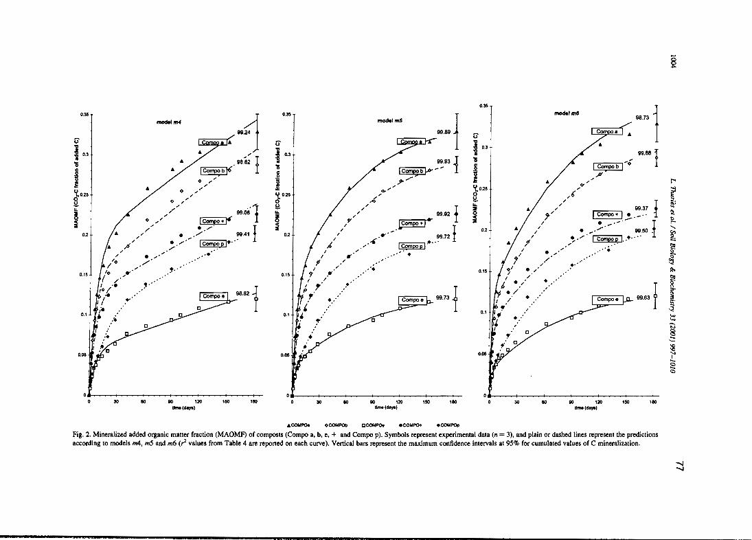
~~Ratas:ir~.~:::::

~~'1'...~c

r-

~::1.~'

~

~<,

~::::

99.88 !

99.63 f

,. -:"1

1~+ l~.~·~: l/.-'- !-'1Compo pl.." ..9.9:50 .

....•. '

,~.'

•",e,../

modelm5

•,/

".".- •." ,

•

0.060.060.05

0.35

0.35 T 1 0.35 1mode' m4 model m5

99.24 99.89 _

G' & - lU1 U 0.3

" 0.3 ;' i 0.3

~ 98.82 l . 99.93 l '5

fi ICO"'bl~ l j ~-- 1 1: 0 .- 11 "..

o ",'" tE «<" '(.0.2e'{0.2S ,," <t 0.2S ,," 8o 0" 0 1'0 -

~ .: '1 l:l. ,," l ~!li ,,/ 99.06 !li ,," 99.92 0

; 0 ,,/ ~ ~ ,,'7 LCornpo+'.... ;/ • .> 1:1 " _ l 0.2

0.2 &./ • .... / 99.41 l 0.2 ,," .. ' 99.72 l-,," • -- ~•. ,. .6,.." ~~...

" /". l '" "

" ." .'. 1 fT •"0 /'".' " " ,

l '" •. ' l " .'.'0" .. ' ..... 0.15

l " 0.15 , •

i« ,.' i,' ," ~' 1Of . P1 •• Corn" 98.82

,>/ ..•. ~ r •... p"b-99.73

~'. .: C ,o.• ~ '.' .: 0.1 J 0.1.. - .

111015080 120.hM (doyal

11030

O. 1 1 1

o111015080 120tl... (doya)

11030O~ 1 1 1 1

o111015080 120-Cdoyal

11030o~ 1 1 1 1

o

&COMPOo OCOMPOb CCOMPOt .COMPO+ .COMPOp

Fig. 2. Mineralized added organic matter fraction (MAOMF) of composts (Compo a, b, e, + and Compo pl.Symbols represent experimental data (n = 3), and plain or dashed Iines represent the predictionsaccording to models m4, m5 and m6 (r2 values from Table 4 are reported on each curve). Vertical bars represent the maximum confidence intervals al 95% for cumulated values of C minerallzation,

-....1-....1

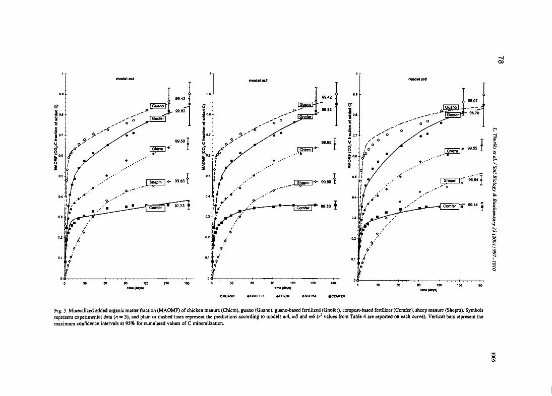
.......00

1 IImodelm4 modelm5 modelm8

oJ T 0.8 0.899.42

-~Al l ), 95.07Û (Gu_no r û Guano Û

! o._ ./>" 99.82 1°._./>"- 99.82

10.8,," ,," _ _ - - ",....._..... 98.70,," " ,,-"Cl,," 0 ~--• " 'l;'l; ,," 0 'l; ,," 0 ",,"

j 0.7

;-.-6"jO.7

".-6" c

"/",, 0j 0.7r-

3-" 3-" ./ 0

~0" 0" ,,/09"7 99.50 t 9"7 99.89 l ~

._.1 l'Nan r· 99.85 !~~ 1 0

::1.Ô 1 1Chlan t·· 1 ).fhlcml"·

Ô ~'u u u j/ ~~o.e

..'iO.5 ~ 0.5.' f:.:1 • ....... . s »

0 1 0 1,..

::i 1.

::i-» ::i <,

0~ ~

O.~ 1 •J S~epm 1·0- 99.83 t •

._~.o- 99.89 l .:

~; 98·~I::::

0.5 0.5 1 tlo5'.-. , ë",.' 0-.- .. - -' " " 0 ~,,<T'

" ,. 0 ,"u.u T ,~

J 0.4 ;-0.4 ;- Il-

99.83 ! 0 ;- tlo

ComfM] -;- Comter • 99.14 ! 5'

~0.3·lI[ ~ 0.3·U: --X ~~ ft' • ~.

~1 1 1 ....

.~ ~ 0'....-..

0.2 -lU..6

0.26 0.2 / N

8""-

'1 ~~

: 10

0.1 ~ " "10

0.1 '-l,~ 9 0.1 1

9 9 <5<5

06 1 1 1

°°30 50 80 120 130 150

°30 50 80 120 150 150 30

-(cIoyIl 1I_lcloyll 50 80 120 130 '501I_(dlYOI

OGUANO eGNOFER .CHICM OSHEPM .COMFER

Fig. 3. Mineralized added organic matter fraction (MAOMF) of chicken manure (Chicm), guano (Guano), guano-based fertilized (Gnofer), compost-based fertilizer (Comfer), sheep manure (Shepm), Symbolsrepresent experimental data (n =3), and plain or dashed lines represent the predictions according to models m4, m5 and m6 (r2 values from Table 4 are reported on each curve), Vertical bars represent themaximum confidence intervals at 95% for cumulated values of C mineralization.

§

791006 L Thuriès et al. / Soil Biology & Biochemistry 33 (200/) 997-1010

Table 4Values of the estimated parameters: PL (no dimension), kmL, kmR (d- I

) in model m4. P'L, Ps (no dimension), k'mL, k'mR (d- I) in models mS and m6.

In model m4. PI. is calculated by difference I-P L. In models mS and m6. PI. is calculated by difference I-P'L-Ps, • =Two exponential models (ml or m4)

gave low k".,. values with associated confidence interval including zero value, low k.nL values close to k".,. values of most products; consequently they could heconsidered as particular cases of models mS with labile L compartment =0; •• = Particular cases of model mS where PH=O. could he fitted with oneexponential term and a constant term with IWoparameters k.nL and Ps (with PL= I-P s); ••• = Particular cases of models mS where Ps =0, then fittings arethose of model m4

AOM origin AOM Model m4 (or ml) Model mS Model m6

PL k.nL k".,. r l (%) P'L k'ml. k'~ Ps r l (%) P'L Ps r l (%)

Plant Coffk 0.114 0.164 0.0041 99.51 0.065 0.449 0.0093 0.330 99.86 0.046 0.425 99.380Wgrap 0.165 0.082 0.0014 99.58 0.089 0.172 0.0126 0.638 99.93 0.065 0.641 99.580Dgrap 0.177 0.053 0.0008 99.15 0.036 0.632 0.0199 0.711 99.80 0.053 0.686 99.470Olivp 0.197 0.044 0.0019 98.81 0.041 0.904 0.0127 0.538 99.96 0.041 0.556 99.780Kokoa 0.333 0.245 0.0016 99.56 0.298 0.293 0.0124 0.495 99.94 0.273 0.495 99.470

Manure Shepm 0.428 0.028 0.0006 99.83 • 0 0.024 0.515 99.80 0.054 0.449 98.940Chicm 0.338 0.375 0.0041 99.50 0.307 0.445 0.0107 0.281 99.89 0.303 0.326 99.650

Animal Nfeat 0.231 0.045 0.0001 99.66 • 0 0.042 0.756 99.62 0.064 0.709 94.870Featm 0.668 0.136 0.0033 98.41 • • 0.668 0.136 0.33 98.41 0.439 0.112 93.000Guano 0.599 0.668 0.0066 99.42 • • • 0.599 0.668 0.0066 0 99.42 0.635 0.146 95.070

Fertilizer Gnofer 0.479 0.227 0.0065 99.82 • • • 0.479 0.227 0.0065 0 99.82 0.386 0.136 98.700Comfer 0.285 0.334 0.0008 97.73 0.217 0.533 0.0362 0.642 99.83 0.259 0.620 99.140

Compost Compoa 0.191 0.130 0.0012 99.24 0.137 0.207 0.0138 0.656 99.89 0.112 0.648 99.020Compob 0.148 0.161 0.0011 98.82 0.102 0.291 0.0134 0.693 99.93 0.093 0.693 99.790Compoe 0.057 0.139 0.0004 98.82 0.037 0.293 0.0116 0.869 99.73 0.032 0.874 99.650Compo + 0.125 0.144 0.0008 99.06 0.087 0.251 0.0135 0.761 99.92 0.076 0.759 99.560Cornpo p 0.102 0.058 0.0007 99.41 0.026 0.400 0.0158 0.794 99.72 0.029 0.786 99.67

between 98 and 99% for four series and between 97 and98% for two series.

Model m8 gave also good predictions; differencesbetween model m8 and models ml, m3 or m4 (Table3) were not significant at 5% level (F values, Eq. 6).Nevertheless, in aIl cases (except the curve for Guano)the trends were the same: F values (Eq. 6, Table 3)greater than 1 indicated that models ml, m3 and m4gave a better prediction than model m8. These modelbehaviors can be easily explained since lst order kineticconstants for the 2nd exponential in models ml, m3 andm4 were found to be relatively smaIl (fable 4). Soresistant organic material (R in Table 2) mineralizationcurves were flattened for small incubation times, likethe straight line of the zero order kinetics in modelm8. Blet-Charaudeau et al. (1990) indicated that 'theuse of the double exponential model is superftuousunless the duration of incubation experiments exceeds100 days'; Bernai et al. (1998) found lst-order plus 0­order kinetics from 70 days incubation experiments. Our180 day experiments began to show a better predictionby the double exponential model but with no significantdifferences. The differences would become more signif­icant for greater incubation times. Our experimentaldata confirmed the superiority of double exponentialmodel compared to 1st-order plus O-order model. Thisis satisfactory in mechanistic terms, since a constant Rmineralization rate even when R = 0 is not realistic.

The comparison between models ml, m2, m3, m4, m7and m8 (Table 2) indicated that the lst order two­compartment models ml, m3 and m4 should be retained.Unfortunately, most of the correlation coefficientsbetween the parameters found with models ml, m3and m4 from these 17 data series were significant. Butgraphical representation (Fig. 4) showed that there wasno evident relationship between the different parameters.Nevertheless, actual data could not allow a real choicebetween the three models. The model m4 can beselected for the relative simplicity of its formula(Table 2). The model m3 kD or model m4 kmR fittedvalues were found small in comparison to km or kmL

fitted values (Table 4). Model m3 PL were foundclose to model m4 PL and the two models were almostidentical: the parallei lst order two-compartment model(m4 in Table 2) can be seen as a m3 decompositionmodel.

3.3. Comparative m4 and mS model predictions

Despite good predictions given by models ml, m3 or m4with determination coefficientshigher than 97% (Figs. 1-3),the residues (predicted minus measured values) were notrandomlydistributed.The DW tests (Table 3) showedsignifi­cant autocorrelation in residues from all data series exceptfor the animal products Guano, Gnofer and Nfeat: two

80L Thuriès et al: 1 Soit Biology & Biochorristry JJ (2001) 997-1010 1007

o _..,..OL--,-,..-----.----,o 0.1 0.2 0.3 0.4 0.5

k H

•m1

•• •

• r=0.470.002. • p=O.06 (ns)

.~··l ·o +------,r'-----.---.----,o 0.1 0.2 0.3 0.4

k H

o.oos

0.006

J 0.004•

m1r=0.68p=0.003 (**)

••• 1

o.a

0.6

0.2

.J 0.4

• •

0.5

m3

••

o.ooa0.006

•0.002 •• r=0.64..-4t. • p=O.OO6 (**)

0+-'----'0---.------,

o

.: 0.004

•

•

r=O.68p=0.003 (**)

0.5

0.5

m3

m4

•

•• ••

• •• r=O.68

0.002. • p=0.003 (**)., .o~~--,------,

o

o.ooa

0.008

0.006

0.002. •., .o~~-----.--~

o

0.006

JO.OO4

.: 0.004

m3o.a

•0.6 r=0.48

~ 0.4 • p=0.052 (ns)~ •

0.2 • •••• •0

.~

0 0.5PL

m4o.a

•0.6r=O.50

~0.4 •• p=0.042 (*)~

0.2 • •••• •0

• \ot

0 0.5PL

1 mS1 mB

o.a •·i•• r=-O.69 o.a

r=-O.a2...0.6 p=0.006 (**) ... 0.6 • p=0.OOO1 (***)~ 0.4 • ~• 0.4 ..• • • •0.2 • 0.2

0 0 .- 4-0 0.5 0 0.5Ps Ps

Fig. 4. Correlation between estimated parameters for models ml, m3, m4, mSand m6.Only significant correlations are shown, other values (model mS) areTkmIJI'S = -0.01 (p =0.96), TkmIUPI. =0.24 (p =0.41), TboMS =0.18 (p =0.54), TUolAJoII =0.11 (p =0.71), Tkm1JPl. = -0.40 (p =0.17).

exponential models cannot describe the whole information inmost of the data.

The use of model m5 improved all predictions with r2

values higher than 99.7% for 14 data series and higherthan 98.4 for the three other data series (animal productswith strong mineralization rates: Guano, Gnofer andFeatm). Tests F (Eq. 6, Table 3) showed a significantimprovement at 5% level for ten data series, at 1% levelfor seven data series included in the former ten series. Theimprovements are shown in Figs. 1-3, especially with abetter fitting of the intermediate points (between 30 and120 days) for nine curves (Kokoa, Coffk, Olivp, Wgrap,Compo a, Compo b, Compo + , Chicm, Cornfer). At the

end of the 6-month incubation, the slopes of mode! m5curves were smaller than model m4 curve slopes, tendingto the asymptotic Iines given by the Ps (mS in Table 2)values (Table 4).

The correlation between the four parameter values ofmodel m5 predictions for the 17 data series were notsignificant except the correlation between p'Land Psvalues; but this correlation did not appear as an evidentrelation (Fig. 4). The model m5 explained the wholeinformation in Il data series as shown by DW autocorre­lation test in residual values (Table 3); in three othercases residual autocorrelation in model m5 were smallerthan in model m4; model m5 did not match for the three

1008 L Thuriès et al. / Sail Biology & Biochemistry 33 (200/) 997-101081

other cases conceming animal products Guano, Gnoferand Nfeat. In products with high mineralization rates,Guano and Gnofer, the stable S compartment was notfound. In the 3rd high mineralization animal product,Featm, models m4 and m5 gave the same predictions. InNfeat the intermediary compartment H was not found.This may be related to the particular biochemical struc­ture of this product.

3.4. Comparative m4, m5 and m6 model predictions

The three-compartment model mS (in Table 2) gave thebest predictions. But this model need four parametersagainst three for the two-compartment models m4. Anexamination of k:.u. and k~ fittings showed less variablevalues in model m5 than kmL and kmR values in models m4(Table 4). For 14 data series (except the animal productsGuano, Gnofer and Featm) the mean k:.u. value was 0.40(±0.21 sd) d- l

, the mean k~ value was 0.014 (±0.OO7)d- l

. There was one extraneous value in k:.u. distribution forOlivp (k:.u. = 0.90). The elimination of Olivp gave normaldistribution (kurtosis and skewness tests, normal probabilityplot) for k:.u.with a mean value = 0.36 (±0.15). There weretwo extraneous values in k~ distribution for Comfer(k~ = 0.036) and Shepm (k~ = 0.(02). Their elimina­tion gave k~ normal distribution with mean k~R

value = 0.014 (±0.OO3). The corresponding half lives ofthe two parallel Ist order compartment models were 1.8days for labile compounds L and 49 days for resistantcompounds R.

Gilmour et al. (1998) reported for different crop residuesincubated at 25°C, the first order rate constants for labilecompartment in the range 0.09-0.43 d- l with a mean valueof 0.21 (±0.02) and for stable compartment in the range0.0026-0.016 d- l with a mean value of 0.008 (±0.OO52).Vanlauwe et al. (1994) found 0.4 and 0.012 d- l for labileand stable kinetic constants respectively, of maize residueincubated at 25°C.

Model m6 predictions with mean mineralization ratevalues (Table 2) 1= -0.4d-1 and r=-0.0I4d-1 andthe pL and Ps fittings are shown in Figs. 1-3. The accordwith data series remained valuable with r2 > 99.5% forseven series, 99 < r2 < 99.5 for five series, 98 < r2 < 99for two series and 93 < r2 < 98 for the three animalproducts Guano, Featm and Nfeat. Tests F (Eq. 6, Table 3)showed no significant difference between model m5 andmodel m6 predictions for five data series. However, signifi­cantly better predictions were found for model m5 comparedto model m6 at 5% risk for one data series and at 1% risk foreight other data series. As mentioned above, the three­compartment models were less appropriate than two­compartment models for the animal products Guano, Gnoferand Nfeat.

Despite satisfactory data fittings, residual checks (Table 3)showed that model m6 did not expIain the whole informationin data series, contrarily to model m5. Durbin Watson tests

gave significant autocorrelation except for one compostedmatter (Compo e).

Precision of model m6 predictions was found close tothe precision of model m4 (or ml or m3) ones. Tests F(Eq, 6, Table 3) showed that predictions with model m6were better than model m4 ones for nine data series, withsignificant difference for three data series only (two at 5%risk and one at 1% risk.). Model m4 predictions werebetter than model m6 ones for eight data series but differ­ences were significant only for five data series (at 1%risk). For nine data series, the model m6 and m4 preci­sions were equivalent.

3.5. Conclusion

This work dealt with the mineralization kinetics ofvarious AOM and not of soil organic matter (SOM). Thehigher proportion of mineralized AOM-C (-65-90%added C) was found in the animal-originated AOM richin N. That from composts was of a lesser importance(-12-33% added C), and depended on their compostingtime. The majority of the plant-originated AOM had anintermediary C mineralization behavior, with a greatdiscrepancy between that of animal-originated AOM andcomposts. The values of the very labile fractions pL,stable fractions Ps (Table 4) and resistant fractions (1­pL-Ps) illustrated these mineralization behaviors.

For the wide variety of AOM tested in this experiment,the COrC mineralization were not predicted very weil bythe single compartment models. Additionally, this data didnot justify the choice for the consecutive models for theirmore complex formulation than parallel ones.

In general, a better simulation was provided by the three­compartment model mS as compared to model m4 (twocompartments); furthermore, the correlations between them5 parameters were less significant than between the m4ones. Model m6 was adapted by simplification of model mS.Under controlled conditions, the mineralization rate of thevery labile compounds was found approximately constant(half life 1.8 days), as was the mineralization rate of theresistant ones (half life 49 days). The simplified model m6gave satisfactory predictions with only two parameters: thevery labile AOM fraction and the very stable one. This didnot affect negatively the quality of the predictions since thepredictions of m6 were not very different than those ofmodel m5, and sometimes better than those of m4. Fromthe eight models tested, m4, m5 and m6 could be recom­mended at this time-scale, The m5 model with four para­meters must be useful in fluctuating conditions, over longertime-scale. The m6 model was powerful and simple enoughto be chosen but the m4 one could not be completelyrejected. This work shows that it is possible to find accurateand simple parameters to describe the C mineralizationkinetics of AOM with very different C mineralizationbehavior.

82L Thuriès er al. 1 Soil Biology &: Biochemisrry 33 (2001) 997-/0/0 1009

Acknowledgements

This work was partly granted by a CIFRE convention.The authors thank the CivamBio (organic farrning Frenchnational association) and Dr M. Viel (R&D Department,Phalippou-Frayssinetf S.A., France) for the AOM choiceand helpful discussions, Dr P. Bottner (Cefe-Cnrs, Montpel­lier, France) for the experimental advice, Dr C.M. Arshad,(Agriculture and Agri-Food Canada, Edmonton, Canada)and Dr M.C. Larré-Larrouy (IRD, Montpellier, France) forcomments on an early version of the manuscript.

References

Andrén, O., Kânerer, T., 1991. ICBM: The introductory carbon balancemodel for exploration of soi! carbon balances. Ecological Applications1, 1226-1236.

Andrén, O., Paustian, K., 1981. Barley straw deeomposition in the field: acomparison ofmodels. Ecology 68,1190-1200.

Bernai, M.P., Sanchez-Monedero, MA, Paredes, C., Roig, A., 1998.Carbon mineralization from organic wastes al different compostingstages during their incubation with soil. Agriculture Ecosystems andEnvironment69,115-189.

Blet-Charaudeau, C., Muller, J., Laudelout, H., 1990. Kinetics of carbondioxide evolution in relation to microbial biomass and temperature, SoilScience Society of America Journal 54, 1324-1328.

Bradbury, N.J., Whitmore, A.P., Hart, P.B.S., Jenkinson, O.S., 1993.Modelling the fate of nitrogen in crop and soi! in the years followingapplication of 15N labelled fertilizer to winter wheal. Journal of Agri­cultural Science 121,363-319.

FAO-UNESCO-ISRIC, 1988. FAO-UNESCO soil map of the world:revised legend. World soi! resources report. Rome, ltaly, 119 pp.

Gilmour, J.T., Mauromoustakos, A., Gale, P.M., Norman, RJ., 1998.Kinetics of crop residue decomposition: variability among crops andyears. Soi! Science Society of America Journal 62, 150-155.

Hadas, A., Portnoy, R., 1994. Nitrogen and carbon mineralization rates ofcomposted manures incubated in soil. Journal ofEnvironmental Quality23,1184-1189.

Hadas, A., Portnoy, R., 1991. Rates of decomposition in soil and release ofavailable nitrogen from caille manure and municipal waste composts.Compost Science and Utilization 5, 48-54.

Hansen, S., Jensen. H.E., Nielsen, N.E., Svendsen, H., 1991. Simulation ofnitrogen dynamics and biomass production in winter wheat using theDanish simulation model Daisy. Fertilizer Research 21, 245-259.

Hartz, T.K., Mitchell. J.P., Giannini, C., 2000. Nitrogen and carbon miner­alization dynamics of manures and composts. Hort Science 35, 209­212.

Hébert, M., Karam, A., Parent, L.E., 1991. Mineralization of nitrogen andcarbon in soils amended with composted manure. Biological Agricul­ture and Horticulture 1, 349-361.

Hénin, S., Monnier, G., Turc, L., 1959. Un aspect de la dynamique desmatières organiques du sol. Comptes Rendus de l'Académie d'Agricul­ture Française 248, 138-141.

Henriksen, T.M., Breland, T.A., 1999. Nitrogen availability effeets oncarbon mineralization, fungal and bacterial growth, and enzyme activ­ities during decomposition of wheat straw in soil. Soi! Biology &Biochemistry 31, 1121-1134.

Hess, T.F., Schmidt, S.K., 1995. lmproved procedure for obtaining statis­tically valid parameter estimates from soi! respiration data. Soi! Biology& Biochemistry 21,1-1.

Janzen, H.H., Kucey, R.M.N., 1988. C, N and S mineralization of cropresidue as influenced by crop species and nutrient regime. Plant andSoil 100,35-41.

Kaboneka, S., Sabbe, W.E., Mauromoustakos, A., 1997. Carbon decompo­sition kinetics and nitrogen mineralization from corn, soybean, andwheat residues. Communications in Soil Science and Plant Analysis28, 1359-1313.

Kirchmann, H., Bernai, M.P., 1991. Organic waste treatment and C stabi­lization efficiency. Soil Biology & Biochemistry 29, 1141-1153.

L.evi-Minzi, R., Riffaldi, R., Saviozzi, A., 1990. Carbon minera1ization insoi! arnended with different organic material. Agriculture, Ecosystemsand Environment31, 325-335.

Lomander, A., Kiitterer, T., Andrén, O., 1998. Modelling the effeets oftemperature and moisture on COz evolution from top- and sub-soilusing a multi-compartment approach. Soil Biology & Biochemistry30, 2023-2030.

Mary, B., Fresneau, C., Morel, J.L., Mariotti, A., 1993. C and N cyclingduring decomposition of mol mucilage, mots and glucose in soil, Soi!Biology & Biochemistry 25, 1005-1014.

McGiII, W.B., Hunt, H.W., Woodmansee, R.G., Reuss, J.O., Paustian,K.H., 1981. Formulation. process controls, parameters and performanceof PHOENIX: a model of carbon and nitrogen dynamics in grasslandsoils, ln: Frissel, M.J., van Veen. J.A. (Eds.). Simulation of NitrogenBehaviour of Soi! Plant Systems. Wageningen, The Netherlands, pp.111-191.

Molina, J.A.E., Clapp, C.E., Shaffer, M.J., Chichester, F.W., Larsen, W.E.,1983. NCSOIL, a model of nitrogen and carbon transformations insoi!s: description, calibration, and behavior. Soil Science Society ofAmerica Joumal 41, 85-91.

Mueller, T., Jensen, L.S., Nielsen, N.E., Magid, J., 1998. Turnover ofcarbon and nitrogen in a sandy loam soil following incorporation ofchopped maize plants, barley straw and blue grass in the field. SoilBiology & Biochemistry 30, 561-511.

N'Dayegamiye, A., Royer, R., Audesse, P., 1991. Nitrogen mineralizationand availability in manure composts from Quebec biological farms.Canadian Journal of Soil Science 11, 345-350.

NFU 44160, 1985. Détermination de la matière organique totale, méthodeparcalcination. In: AFNOR (Ed.), Normes et Réglementation: MatièresFertilisantes et Supports de Culture, Tome l, Normalisation. AFNOR,Paris, France, p. 648.

Pansu, M., Gautheyrou, J., Loyer, J.Y., 1998a. L'analyse du Sol: échantil­lonnage, Instrumentation et Contrôle. Masson, Paris, France, p. 512.

Pansu, M., Sallih, z., Bottner, P., 1998b. Modelling of soi! nitrogen formsafter organic amendments under controlled conditions. Soi! Biology &Biochemistry 30, 19-29.

Pansu, M., Sidi, H., 1981. Cinétique d'humification et de minéralisation demélanges sols-résidus végétaux. Science du sol 25, 241-265.

Paré,T., Dinel, H., Schnitzer, M., Oumontet, S., 1998. Transformations ofcarbon and nitrogen during composting of animal manure and shreddedpaper. Biology and Fertility of Soils 26,113-118.

Parton. WJ., Schimel, O.S., Cole, C.V ~ Ojima, O.S., 1981. Analysis offactors controlling soi! organic matter levels in Great Plains grasslands.Soil Science Society of America Journal51, 1113-1119.

Paul, J.W., Beauchamp, E.G., 1994. Short-term nitrogen dynamics in soilarnended with fresh and composted cattle manures. Canadian Journal ofSoil Science 14,141-155.

Quemada, M., Cabrera, M.L., 1995. Carbon and nitrogen mineralized fromleaves and stems of four coyer crops. Soil Science Society of AmericaJoumal 59,411-411.

Recous, S., Robin, O., Oarwis, O., Mary, B., 1995. Soil inorganic N avail­ability: effeet on maize residue decomposition. Soi! Biology &Biochemistry 21, 1529-1538.

Saggar, S., Parshotarn, A., Sparling, G.P., Feltharn, C.W., Hart, P.B.S.,1996. ··C-Iabelled ryegrass turnover and residence times in soils vary­ing in clay content and mineralogy. Soil Biology & Biochemistry 28,1611-1686.

Sallih, z., Pansu, M., 1993. Modelling of soil carbon forms after organicarnendment under controlled conditions. Soil Biology & Biochemistry25, 1155-1162.

Saviozzi, A., L.evi-Minzi, R., Riffaldi, R., 1993. Mineralization parameters

1010 L Thuriès el aL / Soil Biology c:fc Biochemistry 33 (2001) 997-101083

from organic materials added to soil as a function of their chemicalcomposition. Bioresource Technology 45, 131-135.

Servat, E., Callot, G., 1966. Notice Explicative de la Carte des sols duRoussillon. ENSA-Montpellier, Montpellier, France, p. 68.

Serensen, P., Jensen, E.S., 1995. Mineralization of carbon and nitrogenfrom fresh and anaerobically stored sheep manure in soils of differenttexture. Bio1ogy and Fertility of Soils 19, 29-35.

Thuriès, L., Arrufat, A., Dubois, M., Feller, C., Hemnann, P., Larré­Larrouy, M.-e., Pansu, M., Rémy, J.-e., Viel, M., 2000a. Influenced'une fertilisation organique et de la solarisation sur la productivitémaraîchère elles propriétés d'un sol sableux sous abri. Etude et Gestiondes Sols 7, 215-229.

Thuriès, L., Larré-Larrouy, M.-C., Pansu, M., 2000b. Evaluation ofthree incubation designs for mineralization kinetics of organic

materials in soil. Communications in Soil Science and Plant Analy­sis 31, 289-304.

USDA, 1975. Soil taxonomy. A basic system of soi1 classification formaking and interpreting soil surveys. Agric. Handbook no. 436,USDA, 754 pp.

Van1auwe, B., Dendooven, L., Merckx, R., 1994. Residue fractionation anddecomposition-The significance of the active fraction. Plant and Soil158, 263-274.

Verberne, E.LJ., Hassink, J., de Willingen. P., Groot, JJ.R., van Veen,J.A., 1990. Modelling organic matter dynarnics in different soils. Neth­er1andsJournal of Agricu1tura1 Science 328, 221-238.

Whitrnore, A.P., 1996. Oescribiog the mineralization of carbon added tasoil in crop residues using second-order kinetics. Soil Bio1ogy &Biochemistry 28, 1435-1442.

84

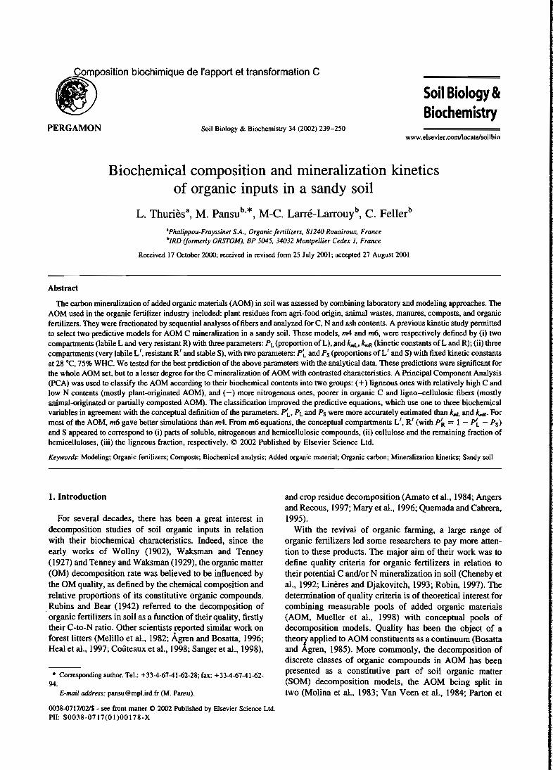
I)'SitiOn biochimique de l'apportet transformation C

PERGAMON Soil Biology & Biochemistry 34 (2002) 239-250

Soil Biology &Biochemistry

www.elsevier.comllocatelsoilbio

Biochemical composition and mineralization kineticsof organic inputs in a sandy soil

L. Thuriès a, M. Pansu":", M-C. Larré-Larrouy'', C. Fellerb

"Phalippou-Frayssinet S.A.• Organic fertilizers, 81240 Rouairoux, Franceb1RD (formerly ORSTOM). BP 5045.34032 Monrpellier Cedex 1. France

Received 17 October 2000; received in revised forrn 25 July 2001; accepted 27 August 2001

Abstract

The carbon mineralization of added organic materials (AOM) in soil was assessed by combining laboratory and modeling approaches. TheAOM used in the organic fertilizer industry included: plant residues from agri-food origin, animal wastes, rnanures, composts, and organicfertilizers, They were fractionated by sequential analyses offibers and analyzed for C, N and ash contents. A previous kinetic study permittedto select two predictive models for AOM C mineralization in a sandy soil. These models, m4 and m6, were respectively defined by (i) twocompartments (labile L and very resistant R) with three parameters: PL (proportion of L), and k..r., k..R (kinetic constants of Land R); (ii) threecompartments (very labile L', resistant R' and stable S), with two parameters: pL and Ps (proportions of L' and S) with fixed lcinetic constantsat 28 "C, 75% WHC. We tested for the best prediction of the above parameters with the analytical data. These predictions were significant forthe whole AOM set, but to a lesser degree for the C mineralization of AOM with contrasted characteristics. A Principal Component Analysis(PCA) was used to classify the AOM according to their biochemical contents into two groups: (+) ligneous ones with relatively high C andlow N contents (mostly plant-originated AOM), and (-) more nitrogenous ones, poorer in organic C and ligno-cellulosic fibers (mostlyanimal-originated or paItially composted AOM). The classification improved the predictive equations, which use one to three biochemicalvariables in agreement with the conceptual definition of the parameters. pL, PL and Ps were more accurately estimated than k..r. and k/fIR. Formost of the AOM, m6 gave better simulations than m4. From m6 equations, the conceptual compartments L', R' (with P~ = 1 - pL - Ps)and S appeared to correspond to (i) parts of soluble, nitrogenous and hemicellulosic compounds, (ii) cellulose and the remaining fraction ofhemicelluloses, (iii) the Iigneous fraction, respectively. © 2002 Published by Elsevier Science Ltd.

Keywords: Modeling; Organic fertilizers; Composts; Biochemical analysis; Added organic material; Organic carbon; Mineralization kinetics; Sandy soil

1. Introduction

For several decades, there has been a great interest indecomposition studies of soil organic inputs in relationwith their biochemical characteristics. lndeed, since theearly works of Wollny (1902), Waksman and Tenney(1927) and Tenney and Waksman (1929), the organic matter(OM) decomposition rate was believed to be influenced bythe OM quality, as defined by the chemical composition andrelative proportions of its constitutive organic compounds.Rubins and Bear (1942) referred to the decomposition oforganic fertilizers in soil as a function of their quality, firstlytheir C-to-N ratio. Other scientists reported similar work onforest litters (Melillo et al., 1982; Âgren and Bosatta, 1996;Real et al., 1997; Coûteaux et al., 1998; Sanger et al., 1998),

.. Corresponding author. Tel.: + 33-4-67-41-{j2-28; fax: + 33-4-67-41-{j2­94.

E-mailaddress:pansu@mpl.ïrd.fr (M. Pansu).

0038.(1717/021$ - see front matter Cl 2002 Published by Elsevier Science Ltd.PlI: S0038-0717(01)00178-X

and crop residue decomposition (Amato et al., 1984; Angersand Recous, 1997; Mary et al., 1996; Quemada and Cabrera,1995).

With the revival of organic farming, a large range oforganic fertilizers led sorne researchers to pay more atten­tion to these products. The major aim of their work was todefine quality criteria for organic fertilizers in relation totheir potential C and/or N rnineralization in soil (Chenebyetal., 1992; Linères and Djakovitch, 1993; Robin, 1997). Thedetermination of quality criteria is of theoretical interest forcombining measurable pools of added organic materials(AOM, Mueller et al., 1998) with conceptual pools ofdecomposition models. Quality has been the object of atheory applied to AOM constituents as a continuum (Bosattaand Agren, 1985). More commonly, the decomposition ofdiscrete classes of organic compounds in AOM has beenpresented as a constitutive part of soil organic matter(SOM) decomposition models, the AOM being split intwo (Molina et al., 1983; Van Veen et al., 1984; Parton et

24086

L Thuriès et al. / Soil Biology JeBiochemistry 34 (2002) 239-250

al., 1987; Sallih and Pansu, 1993; Bradbury et al., 1993) orthree (Hansen et al., 1991; Verberne et al., 1990) compart­ments with a specifie decay rate.

One of the most considered quality criteria was theC-to-N ratio of the AOM (Rubins and Bear, 1942; McGillet al., 1981), but this simple criterion appeared sometimesinadequate for predicting the decomposition kinetics(Recous et al., 1995; Paré et al., 1998). Thus, other qualitycriteria seemed necessary; such criteria can be provided bythe sequential analysis of Van Soest (1963) and Van Soest etal. (1991), which attempts to divide AOM into soluble-,hemicellulose-, cellulose- and lignin-like substances.Nowadays sorne modelers utilize these fractions (Linèresand Djakovitch, 1993; Robin, 1997; Henriksen and Breland,1999a,b,c; Trinsoutrot et al., 2000) or their combinations asthe lignin-to-N ratio (Melillo et al., 1982; Parton et al.,1987).

This study was conducted in conjunction with amanufacturer of organic fertilizers and a French nationalassociation for organic farnùng. The aim was to relate themineralization kinetics of different AOM to their chemical(C, N) and biochemical (soluble, hemicelluloses, cellulose,lignin) characteristics. We thus studied, under laboratoryconditions, the mineralization of raw AOM or their combi­nations into complex admixtures (composts), and modeledtheir kinetics (Thuriès et al., 2001). In the present study, wethen attempted to define the model parameters as a functionof the AOM composition.

When matching measurable OM fractions with concep­tual pools in models of C turnover, Christensen (1996)concluded that the challenge of modelers is to "keepthe balance between structural simplicity, explanatorycapability and predictive power". Our objective was tocombine laboratory and discrete modeling approaches inoroer to find a simple and accurate way of predictingAOM-C mineralization.

2, Materiais and methods

2.1. Added organic materials

Different kinds of AOM from agri-food industry wastesand industrial-processed fertilizers (organic amendmentsand fertilizers) were tested (Table 1). The raw materialswere from (i) plant origin: wet and dry grape berry pelliclecakes (Wgrap, Dgrap), coffeecake (Coffk), cocoacake(Kokoa), olivecake (Olivp) (ii) animal origin: hydrolyzedfeather meal (Featm), native fine feather (Nfeat), guano(Guano) (iii) plant and animal origin: sheep manure(Shepm), chicken manure (Chicm), and (iv) fertilizers:composted organic amendments (Compo series), andorganic fertilizers (Gnofer, Comfer). The compostedorganic amendments (Compo) were made from Shepmand Coffk, periodically turned and aerated during aIQ-month composting period. Samples were taken before

the composting process (Compo a), and at 40 (Compo b),120 (Compo p), and 305 (Compo e) days. Compo + was amixture of75% Compo e and 25% Dgrap (used for loweringmoisture). Gnofer was a guano-based organic fertilizer,whereas Comfer was a Compo-based fertilizer supplemen­ted with Chicm.

The AOM were air-dried, then ground to pass al-mmsieve for a sequential analysis of fibers, or finely ground«200 ~m, in order to reduce the AOM sampling hetero­geneity) for the incubation tests and total C and N analyses.Angers and Recous (1997) found an increase then aslight decrease of C mineralization when the particlesize decreases, in the early and latter incubation stages,respectively.

2.2. Biochemical characterization ofAOM

Each AOM sample (six replicates) was successivelyextracted for NDF (neutral detergent fiber), ADF (aciddetergent fiber) and ADL (acid detergent lignin) by sequen­tial analysis offibers (Table 2), after Van Soest et al. (1991).At each extraction step, the products obtained were filtered,dried at 40 "C, weighed, and either (i) analyzed for C and Nby dry combustion (Fisons NA2ooo), or (ii) dried at 105 "Cfor determining residual moisture, then ignited gradually at525 "C for ash content. The data used in this paper (Table 1)were calculated according to Table 2:

Sol (neutral detergent soluble), Hem (hemicelluloses­like), Cel (cellulose-like), and Lig (lignin-like)represented the different organic fractions (ash free) asdefined by Van Soest (1967),CSoI, NSoh CHem, NHem, Cce., Neeh CUg, and NUg were therespective carbon and nitrogen contents of fractions Sol,Hem, Cel and Lig,AshAOM represented the inorganic part of AOM.

2.3. Mineralization kinetics

The experiment was described in detail in Thuriès et al.(2000). Briefly, 125-500 mg AOM were incorporatedhomogeneously in 50 g air-dried soil «2 mm) andincubated in the dark at 28 "C and 75% WHC. These experi­mental AOM amounts corresponded to realistic inputs underfield conditions: 7 or 14 t ha -1 for animal materials orfertilizers, 28 t ha -1 for plant-originated materials, manures,and composts. Carbon mineralization was measured asrespired CO2-C in closed chambers on 17 sampling occa­sions across a six-month period. The sandy soil used (11.5%clay, 69.3% sand; 4.98 g C kg- 1

) has been classified asfluvisol (FAO-UNESCO-ISRIC, 1988) or Udifluvent(USDA,1975).

Two models for AOM-C mineralization have beenselected after Thuriès et al. (2001): (m4), a parallel Istorder two-compartment model with labile (L) and veryresistant (R) organic compounds, (m6), a simplified parallel

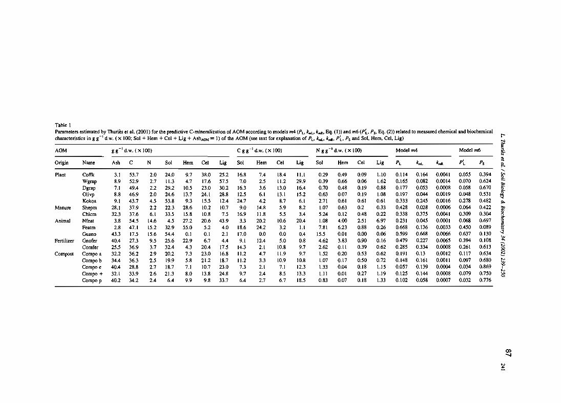
Table 1Parameters estimatedby Thurièset al. (2001) for the predictiveC-minemlizationof AOMaccordingto modelsm4 (PLo k..Lok..a•Eq. (1» and m6(pl. ps•Eq. (2» related to measured chemicaland biochemical

r-characteristics in g g-I d.w. (x 100;Sol + Hem + Cel + Lig + AshAOM = 1) of the AOM(see text for explanationof PLo kod.. k..a• pl. Ps and Sol. Hem. Cel. Lig) rAOM g g-I d.w. (x 1(0) Cg g-I d.w. (X 1(0) N g g-I d.w, (X 1(0) Model m4 Model m6 ~;...Origin Name Ash C N Sol Hem Cel Lig Sol Hem Cel Lig Sol Hem Cel Lig PL k..L k..a pl Ps

~

~<,

Plant Coffk 3.1 53.7 2.0 24.0 9.7 38.0 25.2 16.8 7.4 18.4 11.1 0.29 0.49 0.09 1.10 0.114 0.164 0.0041 0.055 0.394~Wgmp 8.9 52.9 2.7 11.3 4.7 17.6 57.5 7.0 2.5 11.2 29.9 0.39 0.66 0.06 1.62 0.165 0.082 0.0014 0.070 0.624tIo

Dgrap 7.1 49.4 2.2 29.2 10.5 23.0 30.2 16.3 3.6 13.0 16.4 0.70 0.48 0.19 0.88 0.177 0.053 0.0008 0.058 0.670 Q'

Olivp 8.8 46.9 2.0 24.6 13.7 24.1 28.8 12.5 6.1 13.1 15.2 0.63 0.07 0.19 1.08 0.197 0.044 0.0019 0.048 0.531 gKokoa 9.1 43.7 4.5 53.8 9.3 15.5 12.4 24.7 4.2 8.7 6.1 2.71 0.61 0.61 0.61 0.333 0.245 0.0016 0.278 0.482 Il-

Manure Shepm 28.1 37.9 2.2 22.3 28.6 10.2 10.7 9.0 14.8 5.9 8.2 1.07 0.63 0.2 0.33 0.428 0.028 0.0006 0.064 0.422 tIo

Chicm 32.3 37.6 6.1 33.5 15.8 10.8 7.5 16.9 11.8 5.5 3.4 5.24 0.12 0.48 0.22 0.338 0.375 0.0041 0.309 0.304 g'Animal

:>-Nfeat 3.8 54.5 14.6 4.5 27.2 20.6 43.9 3.3 20.2 10.6 20.4 1.08 4.00 2.51 6.97 0.231 0.045 0.0001 0.068 0.697 .-Featm 2.8 47.1 15.2 32.9 55.0 5.2 4.0 18.6 24.2 3.2 1.1 7.81 6.23 0.88 0.26 0.668 0.136 0.0033 0.450 0.089 ~.

Guano 43.3 17.5 15.6 54.4 0.1 0.1 2.1 17.0 0.0 0.0 0.4 15.5 0.01 0.00 0.06 0.599 0.668 0.0066 0.637 0.130 ~

Fenilizer.....

Gnofer 40.4 27.3 9.5 25.6 22.9 6.7 4.4 9.1 12.4 5.0 0.8 4.62 3.83 0.90 0.16 0.479 0.227 0.0065 0.394 0.108 ....Comfer 25.5 36.9 3.7 32.4 4.3 20.4 17.5 14.3 2.1 10.8 9.7 2.62 0.11 0.39 0.62 0.285 0.334 0.0008 0.261 0.613 ~

Compost Compoa 32.2 36.2 2.9 20.2 7.3 23.0 16.8 11.2 4.7 11.9 9.7 1.52 0.20 0.53 0.62 0.191 0.13 0.0012 0.117 0.634 ~Compob 34.4 36.3 2.5 19.9 5.8 21.2 18.7 11.2 3.3 10.9 10.8 1.07 0.17 0.50 0.72 0.148 0.161 0.0011 0.097 0.680 "".....Compoe 40.4 28.8 2.7 18.7 7.1 10.7 23.0 7.3 2.1 7.1 12.3 1.33 0.04 0.18 1.15 0.057 0.139 0.0004 0.034 0.869 '0

1

Compo + 32.1 33.9 2.6 21.3 8.0 13.8 24.8 9.7 2.4 8.5 13.3 1.11 0.01 0.27 1.19 0.125 0.144 0.0008 0.079 0.750 ""'""cCompo p 40.2 34.2 2.4 6.4 9.9 9.8 33.7 6.4 2.7 6.7 18.5 0.83 0.07 0.18 1.33 0.102 0.058 0.0007 0.032 0.776

~

co.......

~....

Table 2Sequentiel procedurefor biochemicalfractionation of the AOM intoNDF. ADF. ADL. after Van Socstet al. (1991)(NDS. ADS= neutraldetergent solution. acid detergent solution. respectively(Van Socst etal., 1991);AOMe,. NDFo• ADFo• ADLo =organicpart of AOM.NDF.ADF and ADLresidues,respectively; W,'= sampleweightona 105"Cbasis;CAOM• NAOM• CNDF. NNDF. CADF• NADF, CADL• NADL= carbonandnitrogencontents of AOM. NDF. ADF. ADL.respectively;Ash; AshNDF• AshADF• AshADL=ash contents of AOM. NDF. ADF. ADL. respectively; Sol. Hem. Cel. Lig = dry massesof soluble. hemicelluloses,cellulose and lignine fractions. respectively; CSoI• NSo/. CHem• NHom• Ccc" Necl• Cu,. Nu, = carbon and nitrogen contents of Sol. Hem. Cel and Lig fractions. respectively; AshAOM=inorganic part of AOM)

Extractions Weight (40 oC) C (%) N (%) Weight (lOS"C) Correction factor/w Ash content (525"C) Fibrousproduct Calculation Final data (%)

WIAOM ClOIaJ NI"" W2AOM /wAOM = W2AOMlwIAOM Ash, AOM WIAOM/wAOM W<I t""C_I/wAOM CAOM rN...v/WAOM NAOM ::l,

AOMe, W,' - Ash, ~'NDS}-. ~I:l,...

Sol WINDF CNDF NNDp W2NDF /wNDF = w2NDF/w'NDF AshNDF NDF wlNDefwNDF "-~NDFo wINDF/wNDF - AshNDF ~

(AOMe, - NDFo)/w" Sol ~(CAOMWIAOM - CNDFWINDF)/W" CSol g(NAOMWIAOM - NNDF WINDF)/W" NSoI

Ro

Hem WIADF CAOP NADF W2ADF /wADF = w2ADF/wIADF AshADF ADF WIADF/wADF[

ADFo WIADF/wADF - AshADF ~1:;'

(NDFo - ADFo)/w<I Hem ~(CNDF WINDF - CADFWIADF)/w<I CIIe.. ~(NNllf WINDF - NADF wIADF)/wÇ\ NIIe.. -.:.

H2S04~ ~Cel WIADI. CADI. NADL /wADL = w2ADLlwIADL AshADL ADL WIADL/wADL '"W2ADL ...

'0ADLo WIADL/wADL - AshADL 1

'"(ADFo - ADLo)/w<I Cel ....<:>

(CADP WIADP - CADLW'ADL)/w<I Ceci(NADF WIADf - NADL wIADLllw" Necl

Lig ADLJw" LigCADLWIADL!w" CL1,NADLWIADL Iw" Nu,Ash,lw" AshAOM

coCO

L Thuriès et al / Sail Biology & Biochemistry 34 (2002) 239-25089

243

3. Results

3.1. Predictions ofCOrC mineralization for the AOM set

where p is the numher of sampling occasions, m the numherof model parameters, Yi, Yia' Yib is the measured andpredicted values with models a and b, respectively, atsampling i. A F value (Eq. (3» higher than bilateralFt~m).(p-m)b (statistical table) implies that the hypothesisof equality must he rejected at p < 0.05: RSSa is greaterthan RSSb, b simulation is thus hetter than a.

When necessary, Principal Component Analysis (PCA)was also used to classify the AOM hefore the simulations.

(3)

otherwise, if

fees = CeUstab,lignin/nitrogen ratio (LigINAOM), C and N inlabile (C1ab, N,ab) and stable (Cstab, Nstab) fractions.

A stepwise regression procedure using partial F-testand sequential F-test, controlled by Mallows Cp statistic(Draper and Smith, 1980) was used in order to removeor to enter biochemical variables in the models describ­ing each parameter of m4 (Eq. (1» and m6 (Eq. (2».The resulting equations (fable 3) were then associated toEq. (1) or Eq. (2) in order to give biochernical prediction ofC-rnineralization with m4 and m6 model, with or withoutclassification.

ln each case, the efficiency of these predictions wasassessed by the residual sum of squares RSS and graphievisualization. The best simulation must have the lowestRSS; let RSSa and RSSb he the residual sum of squaresof simulations a and b, respectively; if RSSa > RSSb.comparisons with F-test must he performed as follows:

F = RSSa = L(Yi - Yui/(p - m)aRSSb L(Yi - Yib)2/(p - m)b

RSSbRSSb > RSSa, F = RSSa

Model m6 is also used to regulate organic inputs in otherSOM models. The complete version utilizes generally fiveparameters: the proportions P~ and Ps (no dimension) ofvery labile and stable compounds, respectively, (P~ isobtained by the difference 1 - P~ - Ps) and the kineticconstants k~L' k~R' and kmS (d- I

) of each compartment.Here, in the simplified version, kmS was set to zero as themineralization of this stable compartment was not notice­able during the six-month experiment. The k~L' and k~values fitted for each AOM (model m5 in Thuriès et al.,2(01) were found less variable than kmL and kmR (m4) andclose to their mean value. The increase from two (m4) tothree (m6) discrete classes of compounds in AOM logicallydisplayed more homogeneous products in each class withanalogous decomposition rate. Thus m6 could be definedwith only two parameters P~ and Ps (k~ and k~R set attheir mean values: k~L = 0.40 d -1 , k~ = 0.012 d-1). TheMAOMF (28 "C, 75% WHC) at a given incubation time twas thus calculated as:

MAOMF = 1 - P~ e-0.41 - (1 - P~ - Ps)e-0.0121 - Ps(2)

lst order three-compartment model with very labile (L'),resistant (R') and stable (S) organic compounds. Morecomplex model including exchanges hetween compart­ments (humification from L to R, decomposition from Rto L) was not retained after statistical analysis.

The three parameters of model m4 are classically used toregulate organic inputs in many SOM models: PL (nodimension) is the proportion of labile compounds inAOM, k«. and kmR (d- I

) are the rnineralization kineticconstants for the compartments Land R, respectively. Thernineralized AOM fraction (MAOMF, cumulative COrCexpressed as a fraction of added C) at a given incubationtime t (d) was:

The values of the parameters (Eqs. (1) and (2» obtained forthe 17 AOM are reported in Table 1.

2.4. Calculations

In the present work, a stepwise regression was used todetermine the relationships hetween the parameters ofEqs. (1) and (2) (fable 1), and the characteristics of themeasured biochernical fractions: CAOM, NAOM, AshAOM,Sol, Hem, Cel, Lig, CSoh NSoh CH•m, NHem, Ceeh NCch CU g,

NLig. The variables synthesized were also taken into accountfrom the former fractions: C-to-N, labile (/ab = Sol + Hem)and stable (stab = Cel + Lig) fractions, labile organic frac­tion flab = lab/(lab + stab) , labile/stable ratio flabr = lab/stab, soluble organic fraction (cellular content) fsol = SoU(lab + stab), soluble/insoluble ratio fsolr = SoU(Hem +Cel + Lig), soluble fraction in labile organic compoundsfsoll = Sol/lab, cellulose fraction in the stable compounds

The hest relationships found hetween the parameters andthe biochemical characteristics (fable 1) were reported inTable 3, Eqs. (4) (Pd, (5) (kmd and (6) (kmR> for m4 and Eqs.(7) (pD and (8) (PR> for m6.

For Il AOM among the 17 tested, the F-tests (Eq. (3),columns 'no' in Table 4) showed that Eqs. (2), (7) and (8)(simplified three-compartment model) gave hetter minerali­zation predictions than Eqs. (1), (4)-(6) (two-compartmentmodel). However, the differences were only significant forfour AOM: Nfeat, Chicm, and Dgrap at p < 0.0 l , CofIk atp < 0.05. The carbon mineralization for six AOM was bestpredicted by Eqs. (1), (4)-(6), but the differences were onlysignificant for three of them: Wgrap and Kokoa at p < 0.01,and Guano at p < 0.05.

Despite the significant predictions of the parameters(85.7 < r2 < 97.1), the modeling of MAOMF withEqs. (1), (4)-(6), or (2), (7) and (8), was not alwayssatisfactory for sorne contrasted N-rich (e.g. Guano) and

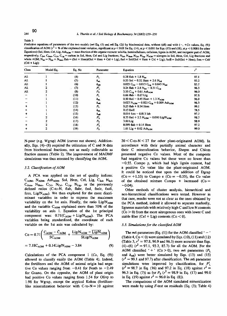
24490

L Thuriès et al: / Soil Bi%gy cl Biochemistry 34 (2002) 239-250

Table 3

Predictive equations of parameters of the two models (m4 Eq. (1) and m6 Eq, (2» by biochemical data. without (ail) and with (-, +Co values. Eq. (9»classification of AOM (r2 = % of the explaioed total variation, sigoificant atp < 0.01 for Eq, (14), atp < 0.001 for Eqs, (15) and (18), atp < 0.0001 forotherEquations) (Sol, Hem. Cel. Lig, AshAOtol = mass fraction of the organic extracts: soluble, hemicelluloses, cellulose.Iignin in AOM. and inorganic pan of AOM.respectively. CSaI, CIIem, Cc.h CÜI = carbon in Sol, Hem. Cel and Lig fractions; NSai• NIIeIII• NCd, Nu., NAOM = nitrogen in Sol, Hem, Cel, Lig fractions andwhole AOM; N iob = NSai + NIIem; f1ab= (Sol + Hem)/(Sol + Hem + Cel + Lig), fsol = SoU(SoI + Hem + Cel + Lig); fsoll = SoU(SoI + Hem). fees = Ceu(Cel + Lig»

Class

AliAliAliAliAli

+++

++

ModelEq. Eq.No Parameter Equation r2

1 (4) PL 0.38 f1ab+ 1.8 Niob 97.11 (5) k.L 0.53 Sol - 0.32 Hem + 2.6 NSai 93.21 (6) k.R 0.025 Ce.t - 0.015 Cu. + 0.045 NSai 85.72 (7) P'L 0.24 f1ab+ 2.8 NSai - 0.31 Cu. 96.32 (8) Ps 3.55 CÜI + 0.61 AshAOM 96.01 (10) PL 0.66 f1ab- 0.67 Lig 97.81 (II) k.L 0.50 fsol - 0.45 Hem + 1.3 NAOM 96.91 (12) k.R 0.023 NA(}M - 0.023 eu. + 0.009 AshAOM 96.31 (13) PL 0.25 f1ab+ 0.54 Hem 99.11 (14) k.L 0.\3 fsoll 78.51 (15) k.R 0.014 fces - 0.0\3 lab 97.72 (16) PL 0.35 fsol + 2.2 NAOM - omo LigINAOM 98.72 (17) Ps 3.60 Lig 98.92 (18) PL 0.099 f1ab+ 0.14 Hem 97.22 (19) Ps 1.61 Lig + 0.62 AshAOM 99.0

3.2. Classification ofAOM

N-poor (e.g. Wgrap) AOM (curves not shown). Addition­ally, Eqs. (4)-(8) required the utilization of C and N datafrom biochemical fractions, not as easily coUectable asfraction masses (Table 2). The improvement of MAOMFsimulations was thus assessed by classifying the AOM.

Calculations of the PCA component 1 (Co, Eq. (9»allowed to classify easily the AOM (Table 4). Indeed,the fertilizers and the AOM of animal origin had nega­tive Co values ranging from -0.41 for Feath to -2.49for Guano. On the opposite, the AOM of plant originhad positive Co values ranging from 1.54 for Olivp to1.98 for Wgrap, except the atypical Kokoa (fertilizer­like mineralization behavior with C-to-N = 10 against

A PCA was applied on the set of quality indices:CAOM' NAOM' AshAOM, Sol, Hem, Cel, Lig, CSoI> NSo),CHom, NHom, CColo Nc." CLig, NLig, or the previouslydefined ratios (Ceto-N, flab, flabr, fsol, fsolr, fsoU,fees, Lig/NAOM)' We then explored for the most discri­minant variables in order to express the maximumvariability on the lst axis. Finally, the ratio Lig/NAOMand the variable CAOM explained more than 70% of thevariability on axis 1. Equation of the lst principalcomponent was: 0.71(CAoM+ Lig/NAOM)' The PCAvariables being standardized, the coordinate of eachvariable on the lst axis was calculated by:

Co = 0.71 (CAOM - ëAOM + Lig/NAO~ - DglNAOM)SCAOM SLlg/NAOM

3.3. Simulations for the classified AOM

The m4 parameters (Eq, (1» for the AOM classified • - '(Table 4, Co < 0) were simulated by Eqs. (10), (11) and (12)(Table 3, r2 = 97.8,96.9 and 96.3) more accurate than Eqs.(4)-(6) (r2 = 97.1, 93.2, 85.7) for all the AOM. For theAOM classified • +' (Co> 0), two m4 parameters (PLand k..0 were better simulated by Eqs. (13) and (15)(r2 = 99.1 and 97.7) after classification. The m6 parametersimulations were improved by classification, for p l

L

(?- = 98.7 in Eq. (16) and 97.2 in Eq. (18) against r 2 =96.3 in Eq. (7» as for P« (r2 = 98.9 in Eq. (17) and 99.0in Eq. (19) against ?- = 96.0 in Eq. (8».

The comparisons of the AOM simulated mineralizationwere made by using F-test on residuals (Eq. (3); Table 4)

20 < C-to-N < 27 for other plant-originated AOM). Inaccordance with their partially animal character andtheir C mineralization behavior, Shepm and Chicmpresented negative Co values. Most of the compostshad negative Co values but these were no lower than-0.55. Compo p, which had high lignin content, hada positive Co value like the plant-originated AOM.lt could be noticed that upon the addition of Dgrap(Co = + 1.55) to Cornpo e (Co = -0.55), the Co valueof the obtained mixture Compo + increased (Co =-0.04).

Other methods of cluster analysis, hierarchical andnon-hierarchical classifications were tested. However inthat case, results were not as clear as the ones obtained bythe PCA method; indeed it allowed to separate markedly,ligneous materials with relatively high C and low N contents(Co> 0) from the more nitrogenous ones with lower C andstable fiber (Cel + Lig) contents (Co < 0).

(9)= 7.l8CAOM+ O.l4Lig/NAOM - 3.84

91L Thuriès et al. / Soil Biology &: Biochemistry 34 (2002) 239-250 245

Table 4Comparison of models m4 (Eq. (1)) and m6 (Eq. (2)) predictions (F-test, Eq. (3)), with ('yes', Eqs. (10)-(19) in Table 3) or without ('no', Eqs. (4)-(8) in Table3) classification of the AOM by means of PCA (Co, Eq. (9)) (symbols represent the level of significance for F-test (Eq. (3»: ••(p < 0.01), .(p < 0.05), ns (no

significann)

Classification No Nolyes Yeslno Nolyes Yeslno Yes

Co m4/m6 m6lm4 m41m4 m41m4 mfv'm6 mfv'm6 m41m6 mfv'm4

Coflk 1.76 3.76 • 3.14 • <1 1.83 ns <1 1.53 ns

Wgrap 1.98 <1 9.42 .. 1.69 ns 6.44 •• <1 2.47 nsDgrap 1.56 4.12 .. 6.65 •• <1 7.50 •• <1 12.10 ..Olivp 1.54 2.05 ns 1.18 ns 5.36 •• 9.33 ••Kokoa -0.31 <1 5.90 .. <1 1.41 ns 22.26 •• 5.32 •Shepm -0.43 <1 1.55 ns <1 1.16 ns <1 2.26 ns 1.70 ns

Chîcm -0.94 4.88 .. <1 4.84 •• <1 2.26 ns 10.45 ..Nfeat 0.48 > 100 .. > 100 •• 2.34 ns > 100 ..Featm -0.41 <1 2.18 ns <1 2.06 ns <1 1.08 ns <1 1.14 nsGuano -2.49 <1 3.64 • 1.83 ns 1.57 ns <1 4.24 ..Gnofer -1.76 <1 1.49 ns 20.97 .. 4.66 •• <1 6.69 ..Comfer -0.52 1.31 ns <1 1.14 ns 1.33 ns 1.31 nsCompoa -0.42 1.93 ns 10.44 •• 7.04 .. 1.93 nsCompob -0.16 1.42 ns 9.08 •• 16.29 •• 2.56 •Compoe -0.55 1.08 ns <1 1.09 ns 7.91 •• 9.30 ••Compo + -0.05 1.10 ns LOI ns 34.37 •• 37.38 ••Compop 1.26 1.82 ns 6.00 •• 50.63 •• 15.37 ••

and graphically (Figs. 1-3) in order to: (i) compare models (2), (16)-(19» (iii) compare m4 (Eqs. (1), (10)-(15» andm4 (Eqs. (1), (4)-(6» and m6 (Eqs. (2), (7) and (8» without m6 (Eqs, (2), (16)-(19» simulations after classification ofAüM classification (see description earlier) (ii) show the AüM.effect of classification on m4 (Eqs. (1), (4)-(6) vs (1), For the model m4, the classification improved the(10)-(15» and m6 simulations (Eqs. (2), (7) and (8) vs simulations for Il AüM (Table 4), but only significantly

time (days)

•

time (days) ., l '

150 ISO

_"-'-'-';'-'-"'I•

o Guano

• Gnofer6 Featm

• Chicm• Kokoa<> Shepm• CornIer

60 90 12030

o 11-~.--If--,~-+~~-+-~~+-~~+-.~r-I~~

o

0.6

0.4

0.2

J

150 ISO1209060

/0.0.0

MAOMF(C02-Cfraction ofaddedC)

o 11-~r-I~~-+-~~+-~~t~~-+-~~+-...--Jo 30

O.S

0.6

0.2

0.4

Fig. 1. Mineralized added organic rnaterial fraction (MAOMF) of the AOM from animal origin (Guano: 0; Featm: 6), manures (Chicm: +; Shepm: 0),fertilizers (Gnofer: .; Comfer: .) or with a fertilizer-like behavior (Kokoa: .). Symbols represent experimental data (n = 3), and lines represent thepredictions according to m4 (Eqs. (1), (10)-(12» and m6 (Eqs. (2), (16) and (17» models after classification of the AOM (Co < 0, Eq. (9)). Vertical barsrepresent the maximum of cumulative confidence intervals al 95%.

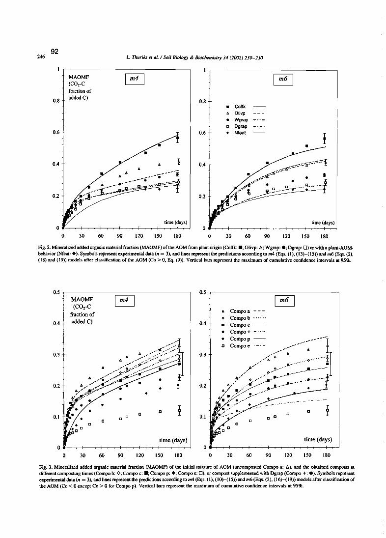
L Thuriès et al / Sail Biology dt Biochemistry 34 (2002) 239-250

180

time (days)

1501209060

• Coffk1\ Olivp

• Wgrap[] Dgrap

• Nfeat

30

0.8

0.6

0.4

0.2

180

time (days)

150120906030

O~~-+~~+-r-T-+~~+-~--+~~+-,........j

o

0.6

0.4

0.2

92246

MAOMF(C02-C

fraction of

0.8addedC)

Fig. 2. Mineralized added organic material fraction (MAOMF) of the AOM from plant origin (Coffk: .; Olivp: 6.; Wgrap: e; Dgrap: D) or with a plant·AOM­behavior (Nfeat: .). Symbols represent experimental data (n = 3), and lines represent the predictions according to m4 (Eqs. (1), (13)-(15» and m6 (Eqs, (2),(18) and (19» models after classification of the AOM (Co > 0, Eq. (9». Vertical bars represent the maximum of cumulative confidence intervals al 95%.

0.5 0.5 rMAOMF a 8(C02-C

fraction of1\ Compoa0 Compob

0.4 added C) 0.4 • Compoc

• Compo+

• Compop,---~--"1.> .>: [] Compoe

0.3 • >::;1;:;:::-1 0.3 "--6 ,,,' "'";:,.'" .s-:

1\ ,/'-;:;::<~::........1\ ~' ,.-"~ ..- ! o ...·"."0/ ." •

0.2 " -II... l 0.26,J' / •1\'" ,.,/' .- ..•.. •f ..'~.. . •

[] ï [][] ï

0.1[]

0.1[][]

[][]

[] [][]

time (days) time (days)0 0

0 30 60 90 120 150 180 0 30 60 90 120 150 180

Fig. 3. Mineralized added organic material fraction (MAOMF) of the initial mixture of AOM (uncomposted Compo a: 6.), and the obtained composts atdifferent composting times (Compo b: 0; Compo c: .; Compo p: .; Compo e: D), or compost supplemented with Dgrap (Compo +: e). Syrnbols representexperimental data (n = 3), and lines represent the predictions according to m4(Eqs. (1), (10)-(15» and m6 (Eqs, (2), (16)-( 19» models after classification ofthe AOM (Co < 0 except Co > 0 for Cornpo pl. Vertical bars represent the maximum of cumulative confidence intervals at 95%.

L Thuriès et al 1 Soil Biology cf< Biochemistry 34 (2002) 239-25093

247

for 7 AOM: Dgrap, Nfeat, Gnofer, Compo a, Compo b,Compo p at p < 0.01, and Coffk at p < 0.05. For 6 AOM,the classification resulted in poorer simulations compared tounclassified data, but only significantly (p < 0.01) forChicm.

For m6, the classification improved the simulations for 12AOM (Table 4), but only significanlly (p < 0.01) for 9AOM: Wgrap, Olivp, Kokoa, Gnofer, Compo a, Compo b,Compo e, Compo +, and Compo p. For 5 AOM, theclassification resulted in poorer simulations compared tounclassified data, but only significanlly (p < 0.01) forDgrap.

After classification, the m6 simulations (Eqs. (2),(16)-(19» were better than the m4 ones (Eqs. (1),(10)-(15» for II AOM, but only significantly for 8AOM: Olivp, Chicm, Nfeat, Compo e, Compo +, Compopat p < 0.01, and Kokoa, Compo b at p < 0.05. Inversely,the m4 simulations were better for 6 AOM, but onlysignificantly (p < 0.01) for 3 AOM: Dgrap, Guano andGnofer.

Fig. 1 shows the C mineralization data and theirsimulations by models m4 (Eqs. (1), (10)-(12» and m6(Eqs. (2), (16) and (17» for AOM classified • - ' (animal­originated AOM and Kokoa). Guano and Gnofer m4simulations were better than m6 ones from 15 to 150 d ofincubation and similar at the beginning and the end of theincubation. Since Guano and Gnofer had very low Ligcontents (Table 1), a three-compartment model wasobviously not necessary to describe their mineralization.However, the calculation of Ps from Eq. (2) gave a lowbut no null value (Table 1); Guano and Gnofer representedborderline cases for m6, but still acceptable since the predic­tions were close to experimental data at the end of incuba­tion. During the first 90 d, Shepm mineralization was bettersimulated with m6, but better with m4 afterwards (ns F-test).The overestimation observed with m6 at the end of theexperiment cou Id be explained by the low content of Ligin Shepm.

Fig. 2 shows the C mineralization data and theirsimulations by models m4 (Eqs. (1), (13)-(15» and m6(Eqs. (2), (18) and (19» for AOM classified • + ' (plant­originated AOM and Nfeat). Good simulations wereobserved with both models for Coffk (ns F-test), and withm6 for Nfeat (*** F-test). The Olivp simulated mineraliza­tion was close to the experimental data with m6 but not withm4 (***F-test). Inversely, Dgrap mineralization was bettersimulated with m4 (***F-test). These differences betweenDgrap and Olivp simulations were difficult to explain sincethe biochemical characteristics of the two AOM werealmost similar (Table 1). The major difference concemedHem, a terrn of Eq. (18). The Wgrap simulations wereslightly underestimated by both models.

The C mineralization data and their simulations forcomposts classified • -' (Eqs. (1), (10)-(12) and (2),(16), (17» and Compo p classified '+', (Eqs. (1),(13)-(15) and (2), (18), (19» are displayed in Fig. 3.

Compo c was added in Fig. 3 for validating the model butit was not used for calculations nor discussed there. For allthe composts, m6 simulations were close to experimentaldata, but slightly overestimated for Compo e (greatly over­estimated with m4. see Section 4.3). Ali the m6 simulationswere better than the m4 ones; however, the latter seemedstill valid for Compo a (ns difference between m4 and m6)and Compo b (with a better m6 prediction, *F-test).

4. Discussions

4.1. Simulations for the AOM set

Equations in Table 3 highlight the relationships betweenthe kinetic parameters and contrasted biochemical charac­teristics of the AOM set. The conceptual labile fraction PL inEq. (1) was mostly linked to the measured labile organicfraction flab (Eq, (4». But PL was not strictly equivalent tothe flab value as it represented 0.38 flab. The three-cornpart­ment model (Eq. (2» defined L' as a part (the most labilecompounds) of compartment L (Eq. (1». As for Plo theconceptual very labile fraction P~ (Eqs. (2) and (7» wasfirst linked to the measured labile organic fraction flab, butto a lesser extent (0.24 flab against 0.38 flab). P~ was alsolinked to the most labile nitrogenous compounds (Nso1 =N1ab - NHem) , like PL was to N1ab (Eq. (4». The very stablefraction Ps (Eqs. (2) and (8» was strongly linked to thecarbon content of ligneous compounds (CLig). Il is generallyaccepted that lignin is one of the least degradable part of anAOM (Melillo et al., 1982; Heal et al., 1997). The weakerrelationship between Ps and AshAOM could be explained bythe high ash contents of sorne humified products (composts,manure, Table 1).

The kinetic constants kmL (Eq. (5» and kmIl. (Eq. (6» wereless strongly linked to the biochemical characteristics. ThekmL and kmR values were positively related to the mostdecomposable compounds (Sol and NSoi for kmL, Cel forkmR) , and negatively to the less decomposable ones (Hemfor kmL• CLig for kmR) in the labile (lab = Sol + Hem) and thestable (Stab = Cel + Lig) fractions, respectively.

4.2. Simulations for the classified AOM

The conceptuallabile fraction PL was always linked to themeasured labile organic fraction flab (0.66 flab in Eq. (10),0.25 flab in Eq. (13), 0.38 flab in Eq. (4). The equationsdiffered in their second terrn: PL was negatively linkedwith Lig in Eq. (10), positively linked to Hem in Eq. (13).The AOM classified ' + ' included mostly plant-originatedAOM, non-composted, and containing hemicellulosicconstitutive parts of plant œil walls.

The conceptual very labile fraction P~ (a part of labilefraction Pd was principally related to the soluble organicfraction fsol (the more labile part of the labile fraction flab)for the AOM classified • - ' (Eq. (16) in Table 3) or to flabfor the AOM classified ' + ' (Eq. (18) in Table 3). For AOM

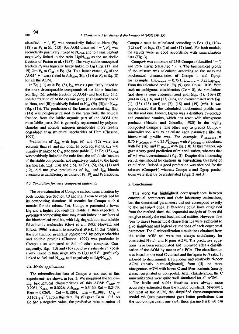
24894

L Thuriès eral:1 SOU Biology & Biochemistry 34 (2002) 239-250

classified ' + " P~ was secondarily linked to Hem (Bq.(18» as Pi. in Eq. (13). For AüM classified ' - " P~ wassecondarily positively linked to NAOM, and to a small extentnegatively linked to the ratio LigINAOM as the metabolicfraction of Parton et al. (1987). The very stable conceptualfraction Ps was logically firstly linked to Lig (Eqs. (17) and19) like r, to CUg in Eq. (8). To a lesser extent, Ps of theAüM' + ' was related to AshAOM(Bq. (19» as Ps in Eq. (8)for all the AüM.

In Eq. (Il) as in Eq. (5), kmL was: (i) positively linked tothe more decomposable compounds of the labile fractionsSol (Bq. (5), soluble fraction of AüM) and fsol (Bq. (Il),soluble fraction of AüM organic part), (ii) negatively linkedto Hem, and (iii) positively linked to NSoI (Bq. (5» or NAOM(Bq. (Il». The prediction of the kinetic constant Jc..L (Bq.(14» was positively related to the ratio fsoIl, the solublefraction from the labile organic part of the AüM (themost labile part). Sol is generally represented by polysac­charidic and soluble nitrogen metabolites more readilydegradable than structural saccharides of Hem (Chesson,1997).

Predictions of kmR with Eqs. (6) and (12) were lessaccurate than PL and kmL ones. In both equations, kmR wasnegatively linked to CUg (the more stable C). In Eq. (15), kmR

was positively linked to the ratio fees, the cellulosic fractionof the stable compounds, and negatively linked to the labilefraction labo Eqs. (14) and (15), as Eqs. (5), (6), (Il) and(12), did not give predictions of kmL and kmR kineticconstants as satisfactory as those of PL,P~ and Ps fractions.

4.3. SimuLation for very composted materiaLs

The overestimation of Compo e carbon mineralization byboth models (see Section 3.3 and Fig. 3) can be explained byits composting duration: ID months for Compo e, 0-6months for the others. Yet, Compo e presented a lowerLig and a higher Sol contents (Table 1) than expected. Aprolonged composting time may result indeed in artifacts ofthe biochemical profiles, with Lig degradation into solublefulvo-humic molecules (Govi et al., 1995; Horwath andElliott, 1996) resistant to microbial attack. In this manner,the Sol fraction generally represented by polysaccharidesand soluble proteins (Chesson, 1997) was particular inCompo e as compared to Sol of other composts. Con­sequently, Eqs. (10) and (16) could overestimate PL (posi­tively linked to flab, negatively to Lig) and P~ (positivelylinked to fsol and NAOM' and negatively to LigINAOM>.

4.4. ModeL applications

The mineralization data of Compo c -not used in thisexperiment- are shown in Fig. 3. We measured the follow­ing biochemical characteristics of this AüM: CAOM=0.2961, NAOM= 0.0226, AshAOM= 0.3460, Sol = 0.2479,Hem = 0.0269, Cel = 0.1804, Lig = 0.1988, CUg =0.1162 g g -1. From this data, Eq. (9) gave Co = -0.5. AsCo had a negative value, the predictive mineralization of

Compo c must be calculated according to Eqs. (1), (10)­(12) (m4) or Eqs. (2), (16) and (17) (m6). For both models,the results were in good accordance with mineralizationdata (Fig. 3).

Compo+ was a mixture of75% Compo e (classified ' - ')and 25% Dgrap (classified ' + '). The biochemical profileof the mixture was calculated according to the measuredbiochemical characteristics of Compo e and Dgrap:for example, Li~po+ = 0.75 Li&ompo e + 0.25 LigDgrap'From the calculated profile, Eq. (9) gave Co = -0.05. Withsuch an ambiguous classification (Co - 0), the simulations(not shown) were underestimated with Eqs. (1), (10)-(12)(m4) or (2), (16) and (17) (m6), and overestimated with Eqs.(1), (13)-(15) (m4) or (2), (18) and (19) (m6). It washypothesized that the calculated biochemical profile wasnot the real one. Indeed, Dgrap was a distillery by-productand contained tannins, which can react with nitrogenousproducts (Metche and Girardin, 1980) in the highlycomposted Compo e. The other way to predict Compo+mineralization was to calculate each parameter like thebiochemical profile was. For example, pGCompo+l =0.75 pGCompo el + 0.25 pGOgrapl with pGCompo el calculatedwith Eq. (16), and PGograpl with Eq. (18). In this manner, m6gave a very good prediction of mineralization, whereas thatof m4 was overestimated (Fig. 3). Despite this interestingresult, one should be cautious in generalizing this kind ofcalculation. Indeed, a good prediction was obtained for themixture (Compo+) whereas Compo e and Dgrap predic­tions were slightly overestimated (Figs. 2 and 3).

S. Conclusions

This work has highlighted correspondences betweenconceptual parameters and their laboratory estimations,but the theoretical parameters did not correspond exactlyto the measured ones. Differences could have originatedfrom the method since the sequential analysis of fibers didnot give exactly the real biochemical entities. However, few(one to three) biochemical characteristics were sufficient togive significant and logical estimations of each conceptualparameter. The C mineralization simulations obtained fromthe entire AüM set were not always satisfactory forcontrasted N-rich and N-poor AüM. The predictive equa­tions have been recalculated and improved after a classifi­cation of the AüM by means of a PCA. The classificationwas based on the total C content and the lignin-to-N ratio. Itallowed to discriminate (i) ligneous and relatively N-poorAüM (mostly plant-originated), from (ii) the morenitrogenous AüM with lower C and fiber contents (mostlyanimal-originated or composts). After classification, the Cmineralizations were quite weIl simulated for aIl AüM.

The labile and stable fractions were always moreaccurately estimated than the kinetic constants. Moreover,for MOSt of the AüM, the simplified three-compartmentmodel m6 (two parameters) gave better predictions thanthe two-compartment one (m4, three parameters): m6 can

L Thuriès et al. / ssu Biology & Biochemistry 34 (2002) 239-25095

249

thus be recommended. Henriksen and Breland (l999a,b,c)defined a three-compartment model with (i) Sol, (ii) Hern +Cel, and (iii) Lig. But Hern is generally defined by a rela­tively large range of molecules more or less degradable(Heal et al., 1997); indeed, Hern represents an heteroge­neous group of linear or branched polysaccharides with adegree of polymerisation of about 100-200 while Cel repre­sents mostly a homopolymer of 13 1-4 n-glucose with adegree of polymerisation of about 14,000 (Breznak andBrune, 1994). From our equations, the contents of thevery labile, resistant and stable compartments could bedefined by: (i) parts of soluble, nitrogenous and hemicellu­losic compounds, (ii) cellulose and the remaining fraction ofhernicelluloses, (iii) the ligneous fraction, respectively.

This study has shown the possibility to simulate AOM-Crnineralization from a simple analytical approach includingsequential extraction and mass measurements. Thecalculations can be easily managed through a spreadsheet.The kinetic constants (0.4 and 0.012 d- t for m6) obtainedunder these experimental conditions (28 "C, 75% WHC)must be adjusted with classicallaws to varying pedoclimaticconditions.

Acknowledgements

This work was partly granted by a CIFRE convention.The authors gratefully acknowledge Prof le. Rémy andProf P. Herrrnann (ENSA-Montpellier, France), Dr M.Viel (Phalippou-Frayssinet S.A., Rouairoux, France), andDr P. Bottner (CEFE-CNRS-Montpellier, France) forhelpful discussions. We thank D. Beunard for technicalassistance with fiber analyses.

References

Àgren, G.l, Bosatta, E., 1996. Quality: a bridge between theory andexperiment in soil organic matter studies. Oikos 76, 522-528.

Amato, M., Jackson, R.B., Butler, J.H.A., Ladd, J.N., 1984. Decompositionof plant material in Australian soils. II. Residual organic I·C and ISNfrom legume plant parts decomposing under field and laboratoryconditions. AusuaIian Journal of Soil Research 22, 331-341.

Angers, O.A., Recous, S., 1997. Decomposition of wheat straw and ryeresidues as affected by particle size. Plant and Soil 189, 197-203.

Bosatta, E., Àgren, G.I., 1985. TheoreticaJ anaJysis of decomposition ofheterogeneous substrates. Soil Biology and Biochemistry 17, 60 1-610.

Bradbury, Nl., Whitrnore, A.P., Hart, P.B.S., Jenkinson, O.S., 1993.Modelling the fate of nitrogen in crop and soil in the years followingapplication of ISN labelled fertilizer to winter whear, Journal ofAgricultural Science 121,363-379.

Breznak, J.A., Brune, A., 1994. Role of microorganisms in the digestion oflignocellulose by termites. Annual Review of Entomology 39,453-487.

Cheneby, O., Nicolardot, B., Linères, M., 1992. Estimation de la valeuragronomique de produits organiques au moyen de cinétiques deminéralisation déterminées au laboratoire. Ministère de l'Agriculture,INRA Dijon.

Chesson, A., 1997. Plant degradation by ruminants: paraJlels with litterdecomposition in soils. In: Cadisch, G., Giller, K.E. (Eds.). Driven by

Nature, Plant Litter Quality and Decomposition. CAB International,Wallingford, pp. 3-30.

Christensen, B.T., 1996. Matching measurable soil organic matter fractionswith conceptual pools in simulation models of carbon turnover: revisionof model structure. In: Powlson, O.S., Smith, P., Smith, J.U. (Eds.).

Evaluation of Soil Organic Matter Models. Springer, Berlin, pp.143-159.

Coûteaux, M.M., McTieman, K.B., Berg, B., Szuberla, O., Oardenne, P.,Bottner, P., 1998. Chemical composition and carbon mineralizationpotential of scots pine needles at different stages of decomposition.Soil Biology and Biochemistry 30, 583-595.

Draper, N.R., Smith, H., 1980. Applied Regression Analysis. 2nd 00.Wiley, New York,

FAO-UNESCO-ISRlC, 1988. FAO-UNESCO Soil Map of the Word:revised legend. World Soil Resources Report. Rome.

Govi, M., Ciavatta, C., Sitti, L., Gessa, C., 1995. Evaluation of thestabilization level of pig organic waste: influence of humic-likecompounds. Communications in Soil Science and Plant Analysis 26,425-439.

Hansen, S., Jensen, H.E., Nielsen, N.E., Svendsen, H., 1991. Simulation ofnitrogen dynamics and biomass production in winter wheat using theOanish simulation model Daisy. Fertilizer Research 27, 245-259.

Heal, O.W., Anderson, J.M., Swift, M.J., 1997. Plant litter qualiry anddecomposition: an historicaJ overview. In: Cadisch, G., Giller, K.E.(Eds.). Oriven by Nature, Plant Litter Quality and Decomposition.CAB International, Wallingford, pp. 47-66.

Henriksen, T.M.• Breland, T.A., 1999a. Nitrogen availability effects oncarbon mineralization, fungal and bacterial growth, and enzymeactivities during decomposition of wheat straw in soil. Soil Biologyand Biochemistry 31,1121-1134.

Henriksen, T.M., Breland, T.A., 1999b. Evaluation of criteria for describingcrop residue degradability in a model of carbon and nitrogen turnover insoil. Soil Biology and Biochemistry 31,1135-1149.

Henriksen, T.M., Breland, T.A., 1999c. Decomposition of erop residues inthe field: evaluation of a simulation model developed from microcosmstudies. Soil Biology and Biochemistry 31, 1423-1434.

Horwath, W.R., Elliott, L.F., 1996. Ryegrass straw component decom­position during mesophilic and thermophilic incubations. Biology andFertility of Soils 21, 227-232.

Linères, M., Ojakovitch, J.L., 1993. Caractérisation de la stabilitébiologique des apports organiques par l'analyse biochimique. In:Decroux, J., Ignazi, J.C., (Eds.), Matières Organiques et Agricultures.Quatrièmes Journées de l'Analyse de Terre et Cinquième Forum de laFertilisation Raisonnée. Gemas-Comifer, Blois, pp. 159-168.

Mary, B., Recous, S., Darwis, O., Robin, O., 1996. Interactions betweendecomposition of plant residues and nitrogen cycling in soil. Plant andSoil 181,71-82.

McGilI, W.B., Hunt, H.W., Woodmansee, R.G., Reuss, J.O., Paustian,K.H., 1981. Formulation, process controls, parameters and performanceof PHOENIX: a model of carbon and nitrogen dynamics in grasslandsoils. In: Frissel, Ml., Van Veen, J.A. (Eds.). Simulation of NitrogenBehaviour of Soil Plant Systems. Centre for AgriculturaJ Publishing andDocumentation, Wageningen, The Netherlands, pp. 171-191.

Melillo, J.M., Aber, J.O., Muratore, J.F., 1982. Nitrogen and lignin controlof hardwood leaf litter decomposition dynamics. Ecology 63, 621-626.

Metche, M., Girardin, M., 1980. Les tanins végétaux. ln: Monties, B. (Ed.),Les Polymères Végétaux, Polymères Pariétaux et Alimentaires nonAzotés. Bordas, Paris, pp. 252-288.

Molina, J.A.E., Clapp, C.E., Shaffer, Ml.•Chichester, F.W., Larson, W.E.,1983. NCSOIL, a model of nitrogen and carbon transfonnations insoils: description, calibration, and behavior. Soil Science Society ofAmerica Journal 47, 85-91.

MueHer, T., Jensen, L.S., Nielsen, N.E., Magid, J., 1998. Turnover ofcarbon and nitrogen in a sandy loam soil following incorporation ofchopped maize plants, barley straw and blue grass in the field. SoilBiology and Biochemistry 30, 561-571.

Paré, T., Dinel, H., Schnitzer, M., Oumontet, S., 1998. Transformations of

25096

L Thuriès et al. 1 Sail Biology & Biochemistry 34 (2002) 239-250

carbon and nitrogen during composting of animal manure and shreddedpaper. Biology and Fertility of Soils 26, 173-178.

Parton, WJ., Schimel, O.S., Cole, C.V., Ojima, O.S., 1987. Analysis offactors controlling soil organic matter levels in Great Plains grasslands.Soil Science Society of America Journal 51, 1173-1179.

Quemada, M., Cabrera, M.L., 1995. Carbon and nitrogen mineralized fromleaves and stems of four cover crops. Soil Science Society of AmericaJoumal 59, 471-477.

Recous, S., Robin, O., Darwis, D., Mary, B., 1995. Soil inorganic Navailability: effect on maize residue decomposition. Soil Biology andBiochemistry 27, 1529-1538.

Robin, O., 1997. Intérêt de la caractérisation biochimique pour l'évaluationde la proportion de matière organique stable après décomposition dansle sol et la classification des produits organominéraux. Agronomie 17,157-171.

Rubins, EJ., Bear, F.E., 1942. Carbon-nitrogen ratios in organic fertilizermaterials in relation to the availability oftheir nitrogen. Soil Science 54,411-423.

Sallih, Z, Pansu, M., 1993. Modelling of soil carbon forms after organicamendment under controlled conditions. Soil Biology and Biochemistry25, 1755-1762.

Sanger, LJ., Cox, P., Splan, P., Whelan, M., Anderson, J.M., 1998.Variability in the quality and potential decomposability of Pinussylvestris litter from sites with different soil characteristics: aciddetergent fibre (ADF) and eatbohydrate signatures. Soil Biology andBiochemistry 30, 455-461.

Tenney, F.G., Waksman, S.A., 1929. Composition of natural organicmaterials and their decomposition in soil: IV. The nature and rapidityof decomposition of the various organic complexes in different plantmaterials, under aerobic conditions. Soil Science 28, 55-84.

Thuriès, L., Larré-Larrouy, M.C., Pansu, M., 2000. Evaluation of threeincubation designs for mineralization kinetics of organic materials insoil. Communications in Soil Science and Plant Analysis 31, 289-304.

Thuriès, L., Pansu, M., Feller, C., Herrmann, P., Rémy, re, 2001. Kineticsof added organic malter decomposition in a Mediterranean sandy soil.Soil Biology and Biochemistry 33, 997-1010.

Trinsoutrot, 1., Recous, S., Bentz, B., Linères, M., Chèneby, O., Nicolardot,B., 2000. Biochemical quality of crop residues and carbon and nitrogenminera1ization kinetics under nonlimiting nitrogen conditions. SoilScience Society of America Journal 64, 918-926.

USDA, 1975. Soil Taxonomy. A Basic System of Soil classification forMaking and Interpreting Soil Surveys. USDA Soil Survey Staff,Washington.

Van Soest, PJ., 1%3. Use of detergents in the analysis offibrous feeds. ILA rapid method for the detennination of fiber and Iignin. Journal of theAOAC 46, 829-835.

Van Soest, PJ., 1%7. Use of detergents in the anaIysis offibrous feeds.IV.Detennination of plant cell-wall constituents, Journal of the AOAC 50,50-55.

Van Soest, PJ., Robertson, J.B., Lewis, B.A., 1991. Symposium:carbohydrate methodology, metabolism, and nuttitional implicationsin dairy cattle, Methods for diatery fiber, neutral detergent fiber, andnonstarch polysaccharides in relation to animal nuttition. Journal ofDairy Science 74, 3583-3597.

Van Veen, J.A., Ladd, J.N., Frissel, MJ., 1984. Modelling C and N turnoverthrough the microbial biomass in soil. Plant and Soil 76, 257-274.

Verberne, E.LJ., Hassink, J., de Willingen, P., Groot, JJ.R., Van Veen,J.A., 1990. Modelling organic malter dynamics in different soils.Netherlands Journal of Agricultural Science 328, 221-238.

Waksman, S.A.•Tenney, F.G., 1927. Composition of natural organic mate­rials and their decomposition in soil: O. Influence of age of plant uponthe rapidity and nature of its decomposition-rye plants. Soil Science24,317-334.

Wollny, E., 1902. La Décomposition des Matières Organiques et lesFormes d'Humus dans leurs Rapports avec l'Agriculture. Translatedfrom the 18% German edition by Henry, E., Berger-Levrault, Paris.

La Transformation de l'azote des Apports Organiques(TAO-N)

97

Cinétique de transformation de l'azote

PERGAMON Soil Biology & Biochemistry 35 (2003) 37-48

Soil Biology &Biochemistry

www.elsevier.com/locare/soilbio

Kinetics of C and N mineralization, N immobilization and Nvolatilization of organic inputs in soil

M. Pansu":", L. Thurièsb

afRO (ORSfOM). BP 64501. 34394 MOIIlpeUier Cedex 5, FroncebpluJlippou-Frayssinet S.A.• Organic Fertilizers, 81240 Rouairoux. France

Received 5 February 2002; received in revised fonn 1 August 2002; accepted 3 September 2002

Abstract

C and N mineralization data for 17 different added organic materials (AOM) in a sandy soil were collected from an incubation experimentconducted under controlled laboratory conditions. 'The AOM originated from plants, animal wastes, rnanures, composts, and organicfertilizers. The C-to-N AOM ratios (7IAOM) ranged from l.l to 27.1. Sequential fibre analyses gave C-to-N ratios of soluble (1'/soi),holocellulosic (1/Hol) and ligneous compounds (7Iu.) ranging from l.l ta 57.2,0.8 ta 65.2, and 3.5 to 25.3, respectively. Very differentpatterns of net AOM-N minera1ization were observed: (i) immobilization for four plant AOM; (ii) moderate minera1ization (4-15% AOM­N) for composts; (iii) marked minera1ization (11-27% AOM-N) for 1 animal AOM, 1manure and 2 organic fertilizers; and (iv) high rates oftransformations with possible gaseous losses for sorne N-rich AOM.

The Transformation of Added Organics (TAO) model proposed here, described AOM-C minera1ization (28 "C, 75% WHC) from threelabile (LI), resistant (R) and stable (S) compartments with the sole parameters P'L and Ps = fractions of very labile and stable compounds ofAOM, respectively. Dividing the C-compartments by their C-to-N estimates supplied the remaining NAOM fraction (RAONF). A Pim

parameter split the TAO nitrogen fraction (TAONF = added N-RAONF) into two compartments, immobilized (imN) and inorganic (inorgN)N. A Pim > 0 value meant that all the TAONF plus a fraction (Pim - 1) of native soil inorganic N was immobilized. Additional Nminera1ization was predicted when necessary from imN by first order kinetics (constant Icremin)' The TAO version with two parameters Pimand kremin allowed us to predict very different patterns of N minera1ization and N immobilization. In a few cases, a further first order kineticlaw (constant k,J was added to predict N volatilization from inorgN. Two hypotheses were tested: (i) "IL', 1/R, 7Is (C-to-N of L', R andS) = 7ISoI,1/Holo "ILi., respectively, (ii) T/L' = 1/R = 7Is= 7IAOM· The first hypothesis was validated by these data, and the second was a goodapproximation of the former one. In ail the cases, predictions were in good agreement with measured values.© 2003 Elsevier Science Ltd, Ali rights reserved.

Keywords: Modelling; Kinetics; Carbon andnitrogen turnover; N minernlization; N immobilization; Organic fertilizers

1. Introduction

Despite a large collection of experimental data, the fateof nitrogen (N) of organic inputs in soils remains difficult tointerpret. Inorganic N can he produced by mineralization orimmobilized by microbial biomass; it can he assimilated byplants, partially fixed within clays, leached in water orvolatilized as NH3, N20 , NO.. or N2• Tracer experirnentsillustrate the complexity of the fluxes (Mary et al., 1998),with a high turnover of ammonium (NHt) largely re­immobilized by microbial biomass (Yevdokimov and

• Corresponding author. Tel.: +33-4674-16100; fax: +33-4674-16294.E-mailaddress:pansu@mpl.ird.fr (M. Pansu).

Blagodatsky, 1993), and partly nitrified according to agrowth law (Pansu et al., 1998a).

In most soil organic matter (SOM) rnodels, N kinetics arederived from those of carbon (C). The initial input materialis generally defined by two (Molina et al., 1983; Van Veenet al., 1984; Parton et al., 1987; Bradbury et al., 1993: Pansuet al., 1998b) or three (Verberne et al., 1990; Hansen et al.,1991) compartments. Sorne mineralization data have beenused directly with SOM models (Hadas and Portnoy, 1994;Jans-Hammermeister and McGill, 1997; Trinsoutrot et al.,2000a) or have been adjusted to different specifie models. Insimplified systems with artificial extraction of inorganic N,a one-compartrnent model has been proposed by Stanfordand Smith (1972). Other functions have been then tested:linear (Addiscott, 1983), parabolic (Broadbent, 1986),

0038-0717/03/$ - see front matter ~ 2003 Elsevier Science LId. Ali rights reserved.PU: 50038-0717(02)00234-1

99

38 M. Pansu, L. Thuriès 1 Soil Biology '" Biochemistry 35 (2003) 37-48

2.3. Data calculation and control

2.2. Incubation experiment

The inorganic N due to AOM at sampling occasion i canbe written:

1 P ft

SfnorgN = ;-=- L L(inorgNia - inorgNi (2)p p ,=1 a=1

(1)

where inorgNia and inorgNj are inorganic N at samplingoccasion i and replication a for sample (soil + AOM) andmean value of soil control, respectively; n = three repli­cates. Net N mineralization gives a mNi positive value,whereas N immobilization gives a negative one. AlI units(Remaining Added Organic C Fraction RAOCF in Eq. (3),inorgNiu' inorgNj, inorgN, and total-N) were expressed as afraction of C input (Mary et al., 1996; Whitmore andHandayanto, 1997; Henriksen and Breland, 1999b; Trinsou­trot et al., 2000b), in order to facilitate the interpretation ofN fluxes from AOM by using C-to-N ratios.

For p sampling occasions with n replicates, the pooledvariance of inorgbl, was:

. N 1~. s-­morg i = - L (morgNia - inorgNf)n a=1

The incubation test using a sandy soil (top 0-20 cmlayer; sand = 69.3%, clay = 11.5%, pH(H20) 6.6,CEC=5.5cmol c+ kg-l, total C=4.98gkg- l, totalN = 0.59 g kg- I

) was previously described by Thurièset al. (2001). 125 to 500 mg AOM in 50 g air-dried soil(AOM-C ranged from 8 to 102% of initial soil C, AOM-Nfrom 26 to 93% of initial soil N) were incubated at 28 "C and75% WHC. CO2-C titrimetric measurements were made on17 sampling occasions during six months. Organic C andtotal N in soil, AOM and soil + AOM mixtures weredetennined by dry combustion on a Fisons Instrumentselemental analyser (Fisons, Crawley, UK).

Inorganic-N measurements were made at days 0, 1,2,5,10, 21, 41, 90, 182 (when soil + AOM or control soilsamples were removed from the incubation) according tothe reference method NF-ISO 14256 (2000): (i) extractionby a KCI 1 mol 1- 1 solution, (ii) filtration through a 0.2-~mmembrane and storage of filtrates at - 20 "C, and (Hi)determination of nitrate + nitrite and ammonium byspectrophotometric methods. In this paper, we consideredtotal inorganic N (= ammonium + nitrate + nitrite). Analiquot of each soil + AOM sample was air dried andanalysed for total N content in order to be able to estimatepossible gaseous losses of N.

et al. (200 1, 2(02). The data used in this paper (Table 1)were: 71AOM, 71Sol> 71Hol> TlLig = C-to-N ratios of AOM,soluble, holocellulosic (= hemicellulosic + cellulosic),and ligneous AOM fractions, respectively.

Different kinds of AOM from agri-food industry wastesand industrial-processed fertilizers (organic amendmentsand fertilizers) were tested (Table 1). The materialsoriginated from (a) plant residues: wet and dry grapeberry peIlicle cakes (Wgrap, Dgrap), coffee cake (Coffk),cocoa cake (Kokoa), olive pulp (Olivp), (b) animal wastes:hydrolysed feather meal (Featm), native fine feather (Nfeat),guano (Guano), (c) animal manures from sheep (Shepm),and chickens (Chicm), and (d) industrial organic fertilizers:composted amendments (Compo series), and combinedfertilizers (Gnofer, Comfer). A full description of theseorganic materials and their biochemical characterization bythe Van Soest et al. (1991) method were given in Thuriès

2. Materials and methods

2.1. Added organic materials (AOM)

exponential plus constant (Bernal et al., 1998), or doubleexponential (Deans et al., 1986; Matus and Rodriguez,1994). In other studies, double exponential expressionsfailed to estimate organic N pools (Dendooven et al., 1997)or were used for C- but not for N-pools (Bloemhof andBerendse, 1995; Trinsoutrot et al., 2000b).

Another option is to propose mechanistic models in orderto follow specifically the decomposition of added organicmatter (AOM) to the SOM part. The model of Bosatta andÂgren (1985) defined a quality theory applied to AOMconstituents as a continuum. In the model of Henriksen andBreland (1999a), AOM was split into three biochemicalcompartments, and then assimilated into five soil compart­ments. Nicolardot et al. (2001) proposed one AOMcompartment assimilated into three soil compartments.From a comparative statistical study on C mineralization,Thuriès et al. (2001) proposed splitting AOM into threecompartments with only two descriptive parameters. In thispaper, we aimed to extend this AOM-C to an AOM-N modelin order to predict the C- and N-transfonnations of AOM.

Although pioneer studies on inorganic-N evolution fromincubation experiments took into account a large diversityof AOM (Rubins and Bear, 1942), most of these can beclassified in two large groups corresponding to homo­geneous materials: (i) plant residues (Nordmeyer andRichter, 1985; Janzen and Kucey, 1988; Jensen, 1994;Bloemhof and Berendse, 1995; Quemada and Cabrera,1995; Kaboneka et al., 1997; Dendooven et al., 1997;Mueller et al., 1998; Trenbath and Diggle, 1998; Henriksenand Breland 1999a,b; Trinsoutrot et al., 2000a.b; Nicolardotet al., 2(01), and (ii) animal manures or composts (Leclerc,1990; Thiénot, 1991; Hébert et al., 1991; Hadas andPortnoy, 1994; Mahimairaja et al., 1995; Jedidi et al.,1995; Serensen and Jensen, 1995; Hadas and Portnoy, 1997;Bernai et al., 1998; Paré et al., 1998). Our objective was tomodel AOM-C and -N transformations of a large collectionof AOM from plant, animal manure or compost origins.

oo.....

Table 1AOM-C application rates in the incubation experiment, TAO-C parameter values (Thuriès et al., 2(01), measured C-to-N data for AOM (7JAOM). soluble ('IJsoI). holocellulosic (11H01), ligneous (l1LI.) AOMfractions. and parameters obtained for TAo-N with Eqs. (4) and (10) hypothèses

AOM origin AOM g kg- 1 soil added C TAo-C C-to-N data TAo-N parameters with e-te- TAO-N parameters with C·to- F test~parameters Eq. N L'. R'. S Eqs. (4)-(6) N AOM Eqs. (5), (6) and (10)

(3) ~pL Fe-

Ps 7JAOM 7JSoI 11H01 l1L1. l'lm kramin k. l'lm kramin k. Eq. (II) Eq. (lIa) r-;;1

Plant Coftk 4.999 0.055 0.394 27.13 57.21 39.35 18.00 1.170 0.00099 0 1.109 0.00064 0 1.001 NS 1::1.

Wgrap 4.667 0.070 0.624 19.64 23.92 21.56 18.46 1.156 0.00209 0 1.136 0.00181 0 1.000 NS ~.

<,

Dgrap 4.605 0.058 0.670 21.99 23.29 39.43 18.56 1.713 0.00522 0 1.514 0.00410 0 1.299 NS ~Olivp 4.426 0.048 0.531 23.78 19.97 65.22 16.00 1.814 0.00419 0 1.505 0.00337 0 1.087 NS ::::Kokoa 4.072 0.278 0.482 9.62 9.14 9.53 9.97 0.981 0.00246 0.00896 0.979 0.00257 0.00890 1.001 NS

~

6'iS"

Manure Shepm 3.230 0.064 0.422 16.99 8.43 14.87 25.27 0.900 0 0 0.871 0 0 1.010 NS ~

Chicm 3.360 0.309 0.304 6.20 2.40 31.59 14.96 0.820 0.00163 0.0120 0.572 0.00404 0.0184 1.054 NS Ro~

Animal wastes Nfeat 1.205 0.068 0.697 3.74 3.07 5.08 3.50 0.835 0.04850 0 0.487 0.00982 0 4.310 * ~Featm 1.064 0.450 0.089 3.10 2.38 4.13 4.17 0.703 0.00466 0.00694 0.611 0.00117 0.00316 1.016 NS~.Guano 0.392 0.637 0.130 1.12 1.10 0.80 6.60 0.497 0.0413 0.05270 0.484 0.04040 0.04840 1.001 NS~

Fertilizer Gnofer 0.617 0.394 0.108 2.87 1.96 3.94 5.08 0.665 0 0 0.601 0 0 1.345 NS b:Comfer 1.735 0.261 0.613 9.87 5.45 8.78 15.66 0.772 0.00208 0 0.601 0.00475 0 1.295 NS N

Compost Compo a 2.709 0.117 0.634 12.40 5.19 13.18 16.17 0.889 0.00054 0 0.787 0.00045 0 1.005 NS ~Compob 3.434 0.097 0.680 14.74 8.00 21.60 14.98 1.084 0.00151 0 1.116 0.00202 0 1.029 NS

....lCompo e 2.505 0.034 0.869 10.66 5.45 15.18 10.70 0.532 0 0 0.448 0 0 1.027 NS 00

Compo + 3.035 0.079 0.750 13.12 8.64 57.89 11.70 1.145 0.00231 0 1.168 0.00246 0 1.005 NSCompo p 2.816 0.032 0.776 14.16 1.40 30.63 18.70 0.760 0.00075 0 0.208 0 0 1.124 NS

Coffk,coffee cake; Wgrap, wet grape berry pelliclecake; Dgrap, dry grape berry pellicle cake; Olivp, olive pulp; Kokoa,cocoa cake; Shepm, sheep manure; Chicm,chicken manure; Nfeat, native fine feather;Featm, feather meal; Guano, bird guano; Gnofer, guano-based industria1 fertilizer; Comfer, compost-based industrial fertilizer; Compo, industrial composted amendments,

VJ'0

101

40 M. Pansu, L Thuriès / Soil Biology & Biochemistry 35 (2003) 37-48

2.4. Mathematical model

with the corresponding confidence interval: inorgN; ±r;r.9~fSinorgN'

In the proposed TAO model (Fig. 1), the fraction Pu« splitsthe TAONf into 2 compartments: immobilized N (imN =Pim TAONF) and mineralized N (inorgN = (1 - P im)TAONf). Additionally, imN could be re-mineralized

Organicproducts

}

Inorganicproducts

Gaseous lassesCO,. N,O, (NO),

otherwise inorgN = initial inorgNAoM and imN = 0 fort = to

When kremin = k; = 0, the system is entirely govemedby the fraction P im , and the two fractions PL and Ps fromC mineralization curves. The curves TAONf, imN andinorgN are thus parallel. If the inorgN slope becomesgreater than the TAONf slope, then k remin must he greaterthan O. If the inorgN' slope becornes lower than theTAONf one, then N losses occur and k; becomes greaterthan zero. A system where Pim , k remin and kv havesimultaneously positive values is in active transformationwith a phase of gaseous N losses from inorgN andmaintenance of inorgN level from imN and organicNAOM' By these transfer processes, losses of inorgN givelosses of total N from AOM. Conversely, a system whereP jm = k remin = k; = 0 is a system where only N mineral­ization occurs from initial AOM without any N immobil­ization or N volatilization. In a system where Pim = l, theAOM organic N is entirely re-organized into SOM whichmineralizes according to the k remin value. In a systemwhere Pim> l, N immobilization is greater than TAONf;this system immobilizes all TAONf plus a part (P jm - 1)of the inorganic N from soil origin (expressed in theAOM-N unit).

Fig. 1. The model TAO (Transformation of Added Organics, Transform­ation des Apports Organiques) for C mineralizarion, N mioeralizaIion, NimmobilizaIion and N volatilization of Added Organic Matters (AOM) insoil: inorgN. inorgaoic N from AOM; imN, immobilized Nfrom AOM (andSoil-Inorg N if n; > 1).

(decomposition of microbial cells) and inorgN could hepartly volatilized according to first order kinetics, thecomplete equations hecome:

inorgN =(1 - Pim)TAONf +LimN k..min dt

-LinorgN kv dt (6)

imN = PimTAONf - JI imN k..min dt for t> to (6a)10

1- PL - Ps e-0.012(1-10) + Ps"1R T'Js

(4)

RAONf = PL e -0.4(/-10) +11L

The transformed (mineralized or immobilized) addedorganic N fraction (TAONF) can then be expressed fromthe total C ( = 1 in this data, all values of C and N expressedas a fraction of initial C content) and C-to-N ratio of AOM(T'JAOM) by:

1TAONf = - - RAONf (5)

T'JAOM

In order to predict C rnineralization, Thuriès et al.(2001) selected two models amongst the seven tested: aparallel first order two-compartment model with threeparameters (m4). and a paralIel first order three-cornpart­ment model with four parameters (mS). Additionally, asimplification of m5 was proposed: the kinetic constantsof very labile (t<m.) and resistant (lc'mR) compartmentscould he considered as being independent of the AOMorigin. Under the controlled conditions of the incubation(28 "C, 75% WHC), the following mean values wereretained: k'mL = 0.4 ± 0.15 d- I (half life Tin. = 1.7 dl,k'mR = 0.012 ± 0.003 d- 1 (Tin. = 58 dl. Thus the pro­posed model m6 needed two parameters only: the fractionPL of very labile cornpounds, and the fraction Ps of verystable ones (with a rnineralization constant fixed to 0 forthis six-rnonth experiment), The fraction of intermediaryresistant compounds was PR = 1 - PL - Ps, and RAOCF(remaining CAOM plus AOM-C transformed into microbialbiomass and humus) at a given time t from input time to(d) can he written:

RAOCF = PL e -0.4(/-10) + (l - PL - Ps)e-0.012(1-10) + Ps(3)

Arnong the 17 AOMs tested in the experirnent, Eq. (3)with PL and Ps values from Table l, allowed us to predictRAOCF with deterrnination coefficients of r 2 > 99.5 forseven series, 99 < r 2 < 99.5 for five series,98 < r 2 < 99 for two series, and 93 < r 2 < 98 for thethree animal AOMs, i.e. Guano. Featm and Nfeat (bestpredicted with m4).

Let 11L. "1R, T'Js he the C-to-N ratios of very labile,resistant and stable AOM-compartments. respectively; theremaining added organic N fraction (RAONF) can heexpressed as:

102

M. Pansu, L Thuriès1Soi! Biology & Biochemistry35 (ZOO3) 37-48 41

(10)

+Ps)

RSS4 and RSS IO being RSS (Bq. (8» with first (Bq. 4) andsecond (Bq. (10» calculations, respectively.

L, R, S being equal to 1]AOM. Eq. (4) becarne:

RAONF = _1_ (PL e -0.4(1-10) + (1 - PL - Ps)e -0.012(1-10)

1]AON

(Il)

(lIa)if RSS IO > RSS 4 ,

if RSS4 > RSS 10

with the other calculations remaining unchanged. Compari­sons of the two methods were made by the test:

F= RSS4

RSS IO

else F = RSS IO

RSS4

Sensitivity analysis showed a linear response of pre­dicted inorgN to change of pararneters Pim, kn:min or kv (datanot shown). The Pim pararneter had the greatest influence oninorgN, especially when Pim was used alone (kn:min =k. = 0). For exarnple, in the Shepm prediction with Pim

alone (Pim = 0.87, Table 1), a random normal distributionof P im with a relative standard deviation of 1% gave arandom normal distribution of inorgN at 210 d with 10%RSD. A less accurate simulation could be perfonned with apositive value for the three parameters (Pim = 0.81,kn:min = 0.()(}2I, k; = 0.016), but the model predictionswere more stable: a 1% RSD for Pim gave 5% and < 1%RSD for inorgN predictions at 90 and 210 cl, respectively.The fluctuations of inorgN predictions to Pim changes werethe greatest for the maximum or minimum values of inorgNcurves. The predictions were less sensitive to kn:min or kv

fluctuations, with the greatest changes at the end of theincubation.

2.5. Model calculations 3. Results

where Yj and Yj were data measurement and prediction ofinorgN, respectively, at sarnpling occasionj. The alternativeconsisted of considering total N data with the minimizedcriterion:

TAONF was then calculated according to Eq. (5). Theprediction of inorgN required the optimization of P im onlyand, if necessary, kremin and/or k; (Bq. (6».1t was perfonnedby Powell's method with the minimized criterion:

3.1. Classification of inputs according to inorganic-Nproduction

Fig. 2 presents N-rich AOM incubation data showing netpositive mineralization flux and positive rates of rnineraliz­ation (slope). After six months of incubation, net mineralizedN represented about 27% oftotal AOM-N for the two organicfertilizers Gnofer (C-to-N = 2.9) and Comfer (C-to­N = 9.9), 22% for Nfeat (animal waste, C-to-N = 3.7), andII % for Shepm (manure = plant + animal origin, C-to­N = 17). The mineralized N decreased whereas Ceto-Nratios increased, but there was no significant relationship. Incontrast with the results ofThiénot (1991) and Corbeels et al.(1999), Shepm did not show a net N immobilization. Thefraction of mineralized N was almost the sarne for the twoorganic fertilizers, and was higher than that for Nfeat andShepm. The expected difference between the two fertilizerswas shown. The guano-based fertilizer (Gnofer) mineralized26% of its N during the first month of incubation, this leve1remaining stable during the following five months. Thecompost-based fertilizer (Cornfer) mineralized about 10% ofits N contact during the first week, the mineralizationincreasing afterwards linearly with the incubation time.

Fig. 3 shows the inorganic N immobilization by N-poorplant debris which has often been observed (Quemada andCabrera, 1995; Trenbath and Diggle, 1998; Mueller et al.,1998; Henriksen and Breland, 1999b; Trinsoutrot et al.,2000b). From this incubation data at 180 cl, the Ceto-Nthreshold for mineralization!immobilization (Whitmoreand Handayanto, 1997) was found to be ca. 19. AlI theAOM in Fig. 3, with C-to-N ranging from 19.6 (Wgrap) to27.1 (Coffk), induced a marked N immobilization. Theparùcular behaviour of Kokoa (Fig. 5), an AOM of plantorigin, couId be partly explained by its low Ceto-N value(Table 1). Negative values of inorgN were observed during

(9)

(8)

(7)

2

RSSt = ~ pi~ (Ykj - Yk/k=1 j

RSS=~(yj-Y/j

The PL and Ps pararneters (Eqs, (3) and (4); Table 1)were given by Thuriès et al. (2001). As a first step, wecalculated RAONF Eq. (4) with nu. TIR, 1]s assimilated toCsto-N data 1]Soh 1]Hoh and 1JLig. respective1y. These datamust be checked (and if necessary 1JHol recalculated)according to the balance Eq. (7):

1 PL PR Ps--=-+-+­1]AON TJl 1]. n;

where k identified the data series (inorgN or total added N)associated with a weight coefficient Pk. The two possibilitieswere tested, and the first (Eq. (8» then retained (similaraccuracy; inorgN measurements more repeatable than totalNones). Although total added N data were not taken intoaccount in the calculations, the predictions obtained were inaccordance with these data. Hence, total added N data wasused to validate the TAO approach.

In a second step, RAONF was calculated without the useof 1JL. 1JR, 1]sdeterminations, C-to-N ratios ofcompartments

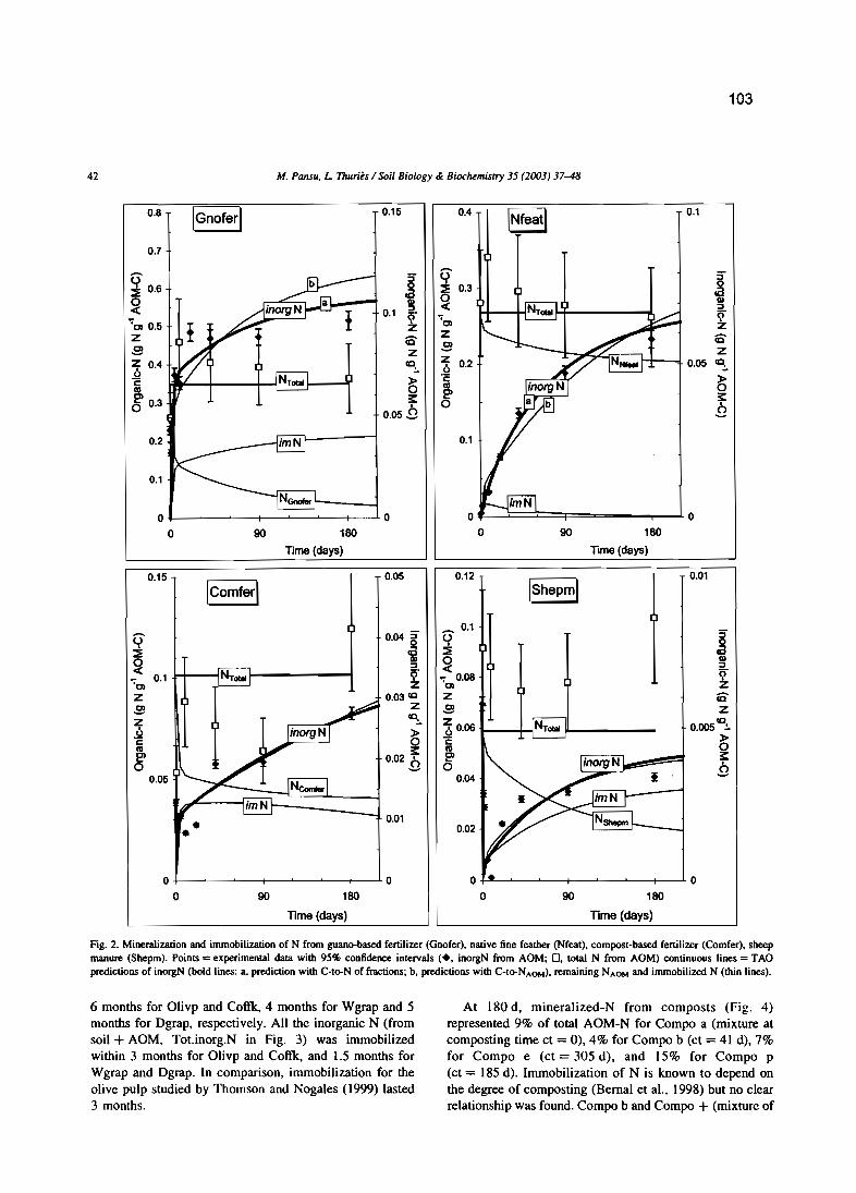
103

42 M. Pansu. L Thuriès 1 SoitBiology &: Biochemistry 35 (2003) 37-48

0.8 0.15 0.4 0.1

0.7

fi~ 0.6

~";"01 0.5Z

S~ 0.4

c::CO~o 0.3

0.2

0.1

90 180

lime (days)

s fi0~ 0.3

~~QI

0.1 :::J

~ ";"01

{è Z

Z SCC:.

Z 0.26

~C

CO

:i: ~

0.0590

0.1

90 180

lime (days)

:r~QI:::J

9"z{èZ

0.05 CC:.

~:i:

9

0.15 0.05 0.12 0.01

t

90 180

nme (days)

0.02

~ 0.1tl~

~";"010.08

Z

S~ 0.06 1-_--+--INToIaI 11- _CIII~o

0.04

0.01

0.04 ~

~:::J

~0.03 CC

Z

~

~0.02

9

90 180

lime (days)

••

O+--~-~-+--~-~-+-----'-O

o

Fig. 2. Mineralization and immobilization of N from guano-based fertilizer (Gnofer), native fine feather (Nfeat), compost-based fertilizer (Comfer), sheepmanure (Shepm). Points = experimental data with 95% confidence intervals (+, inorgN from AOM; 0, total N from AOM) continuous \ines = TAOpredictions of inorgN (bold Iines: a, prediction with C-to-N of fractions; b. predictions with C-to-NAOI•I ) . remaining NAoMand immobilized N (thin \ines).

6 months for Olivp and Coffk, 4 months for Wgrap and 5months for Dgrap, respectively. Ali the inorganic N (fromsoil + AOM, Tot.inorg.N in Fig. 3) was immobilizedwithin 3 months for Olivp and Coffk, and 1.5 months forWgrap and Dgrap. In comparison, immobilization for theolive pulp studied by Thomson and Nogales (1999) lasted3 months.

At 180 d, mineralized-N from composts (Fig. 4)represented 9% of total AOM-N for Compo a (mixture atcomposting time ct = 0), 4% for Compo b (ct = 41 d), 7%for Compo e (ct = 305 d), and 15% for Compo p(ct = 185 d). Immobilization of N is known to depend onthe degree of composting (Bernai et al., 1998) but no clearrelationship was found. Compo b and Compo + (mixture of

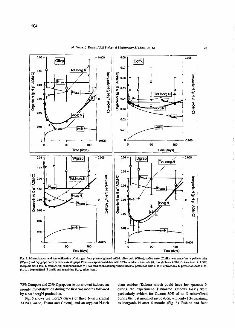
104

M. Pansu, L 'nwriès / Soil Bwlogy 4cBiochemistry 35 (2003) 37-48 43

5'~llJ:l

~Zs-

0 zCl~

~

h

0.005

5'~llJ:l

~ZS-z

0 Cl~

~~

9

0.005

180

l1me (days)

90 180Time(days)

90

+--~~--+--'--~--t----'- ~.005

0.06

IOIiVpl0.005 0.08

ICoffkl0.07

~0.05

fi5'~ ~ 0.06

~llJ:l

':'01 0.04 9" ':'0Z Z 0.05Z S-.9 z .9

~ 0.03 ~Z

0 6 0.04c ~ ëIII IIIEt ~ Et0 9 o 0.03

0.02

0.02

0.010.01

0 ~.005

0 90 180

Time(days)

0.08 0.005 0.06

0.070.05

fi 5'

~~ 0.06 ~~ ~ 0

9" -c 0.04':'00.05 Z ':'00 S- zS z si 0.04 0 ~ i 0.03c

~III C

00.03 h g0.02

0.02

0.010.01

0 ~.005 00 90 180 0

lime (days)

Fig. 3. Mineralization and immobilization of nitrogen from plant-originated AOM: olive pulp (Olivp), coffee cake (Coûk), wet grapeberry pellicle cake(Wgrap) and dry grapeberry pellicle cake (Dgrap). Points = experimental data with 95% confidence intervals (+. inorgN from AOM; O. total (soil + AOM)inorganic N; 0. total N from AOM) continuous lines =TAO predictions of inorgN (bold lines: a, prediction with C-to-N of fractions; b. predictions with C-to­NAOM ) . immobilized N (imN) and remaining NAOM (thin lines).

75% Compo e and 25% Dgrap, curve not shown) induced aninorgN immobilization during the fust two months followedby a net inorgN production.

Fig. 5 shows the inorgN curves of three N-rich animalAOM (Guano, Featm and Chicm), and an atypical N-rich

plant residue (Kokoa) which could have lost gaseous Nduring the experiment. Estimated gaseous losses wereparticularly evident for Guano: 30% of its N mineralizedduring the first month of incubation, with only 1% remainingas inorganic N after 6 months (Fig. 5). Rubins and Bear

105

44 M. Pansu. I.. rhums 1 Sou Bi%gy & Biochemistry 35 (2003) 37-48

0.1 0.015 0.1

- 0.004

o

i::liïz6"

0.002 ZlC.:.

~

~

90 180TIITle (days)

5' fi0a ~III 0::l -c

0.01 ë)"':"

Z 01

6" zz S

lC.:. Z.!olO.05> c

0 al~ 211 0.9

0.005

90 180Time (days)

•o.j--~~----+--~-~---i-----'- 0

o

fi~o-c

':"01

ZSzu 0.05"E

~o

0.015

ICompoel

0.1

ICompo pl0.015

5' g0aIII 0

0.01 ::l -cë)"Z ':"

01

6" zZ 01

lC.:.Z 0.05

> 6"E0 al

~ 210.005.9 0

imN

90 180TIIT18 (<laya)

90 180

Time(days)

Of--~-~-t----'~~--+-----'-O

o

I.._-------iim N:..r--__--;O+--~~-_+-~-~-+_~O

o

Fig. 4. Mineralization and immobilization of N from composts. Points = experimental data with 95% confidence intecvaIs (+, inorgN; D. total N from AOM)continuous Iines = TAO predictions of inorgN (bold Iines: a, prediction with Csto-N offractions; b, predictions with C-to-NAOM),immobilized N (imN) andremaining NAOM (thin lines).

(1942) and Leclerc (1990) showed that 80 and 60-93%guano-No respectively, were transformed in NO)-N inleachates. The removal of NO) by leaching was not studiedin this experimental design. Total gaseous losses estimatedby difference from NTotaI analyses were about 90% of addedN for Guano, and 30% for Chicm. Similar losses for chicken

manure were observed by Mahimairaja et al. (1994) andGagnon and Simard (1999). Gaseous N loss was notdemonstrated for Kokoa (quantified to about 10%, i.e. withinexperimental error) and Featm (about 20%). This experimenthighlighted the stabilization effect of the industrial processused to produce the organic fertilizer Gnofer (Fig. 2) by

106

M. Pansu, L ThuIÜS 1 Sail Biology Je Biochemistry 35 (2003) 37-48 45

IGuanol0.3 0.4 0.15

IFeatm)

fi5"a

~ ~4è::E QI 0.3 4è~

:;,

9" ~QI:l

";'Cl 0.2 Z 9"iê ";'Cl Z

Z Z z êCS

~ S zz Z 10.:..2 0.5 ~ 6 0.2 0.05c

~ë

,.III 0e' III

.9 e' ~0 0 g

0.1

0.1

NF

_

0 0 -0.05

90 180 0 90 180

Time (days) Time (days)

0.2

IChicml0.1 0.15

1Kokoa10.01

5" 5"

~ 0.15s ~

ataDIDI :l

~:l

~ 9"9"':"Cl Z

':"Cl0.1 Z

êC iêz z z zS CD.:. S CD:.Z Z

0.005 ~6 0.1 0.05 ,. .2ë 0 e ~III ~ ët ge' g0 0

0.05

0.05

90 180

Time (days)

90 180

Time (days)

o~-~~~--+---'--~---t-------'- 0

oo'--~~----t-~-~---t---'- 0

o

Fig. 5. Mineralization. immobilization and gaseous losses of N from (i) animal-originated AOM: guano (Guano), fealher meal (Featm), chicken manure(Chicm), and (ii) plant-originated AOM: cocoa cake (Kokoa). Points = experimental data with 95% confidence intervals (•• inorgN; D. total N from AOM)continuous lines = TAO predictions of inorgN (bold (ines), remaining NAOM • immobilized N (imN) and NTouI from AOM (thin \ines).

the addition of N-poor plant residues (Wgrap and Olivp) toGuano. The same effect was observed by Mahimairaja et al.(1994) when mixing chicken manure with wheat straw.These are usefull processes for avoiding N volatilization(compare Gnofer, Fig. 2, and Guano, Fig. 5).

3.2. Predictions made with C-to-N ratios ofbiochemicalfractions

AlI the TAO-inorgN predictions were in good accord­ance with the data (Figs. 2-5). AOM-N transformations

107

46 M. Pansu, L Thuriès 1 Soi/ Biology cf< Biochemistry 35 (2003) 37-48

3.3. Predictions using C-to-N ratios ofAOM

could he predicted for 4 materials using Pim only (Table 1):Shepm, Gnofer, Compo e, Compo p. Let NAOM he theremaining untransfonned N in AOM (NNfeat and NShepm inFig. 2, NCompo e and NCompo p in Fig. 4) and NTolal the Ninput from AOM, at any incubation time the curves wereplotted in accordance with the balance equation:

For 13 of the 17 AOM tested, F tests (Table r, Eqs. (Il)and (l l a) showed RSS IO > RSS4• The predictions with C­to-N ratios of biochemical fractions thus tended to he betterthan predictions made with C-to-NAOM solely, the ditIer­ence being significant for Nfeat only. In the four other cases(RSS4 > RSS IO) , there were no significant ditIerences. TheinorgN predictions by the two methods were plotted in Figs.2-5. The two simulations were almost sirnilar for Comferand for Shepm, but slightly ditIerent for Gnofer and forNfeat (Fig. 2). There was only a significant ditIerence forNfeat hecause the predictions with biochemical fractionswere very close to the data. The two simulations wereidentical for Coffk and for Wgrap and slightly ditIerent forOlivp and for Dgrap (Fig. 3), but the ditIerences were notsignificant and did not modify the predicted duration andamounts of inorgN immobilization. As for composts, thetwo methods gave almost the same predictions except forCompo p (Fig. 4), but the ditIerence was not significant. Forthe four AOM with N-Iosses, the predictions made with thetwo methods were identical (Fig. 5).

N transformations were predicted for 9 AOM, only with thetwo N-parameters Pim and kremin (Table 1): four plantresidues (Fig. 3), the animal residue Nfeat, the fertilizerCornfer (Fig. 2) and three composts (Fig. 4). In these cases,the slope of imN decreased when kremin increased. In thisexperiment, the highest kremin value was found for Nfeatwhich explained the strong decrease of imN for this AOM(Fig. 2); after three months of incubation, the balancerelationship (Eq. (12» became: inorgN = NTolaI - NNfeat.Ali transfonned N was rnineralized.

The four other AOM required the threeTAO parametersPim, kremin and k.: three animal N-rich residues Guano,Featm and Chicrn, and the atypical plant residue Kokoa(Fig. 5). The highest k; value was found for Guano with alsoa high kremin value. Guano presented the highest fraction ofvery labile compounds and a small fraction of stablecompounds (see PL and Ps values, Table 1). It was thusrapidly decomposed (see NOu ano in Fig. 5) into unstable Nforros. Important gaseous N-Iosses occurred from inorgN,this compartrnent being supplied by further mineralizationof imN. By these transfer processes, almost aIl N was lostunder gaseous fonns at the end of the incubation (Fig. 5),although Guano represented the highest N-input.

4.2. Csto-N ratios and transformations ofAOM

Predictions made with 11L, 11R and 11s of the firsthypothesis (Eq. (4» were close to those made with 11AOMof the second hypothesis (Eq. (10». This represented atechnical advantage since the later required C-to-NAOMratios only. Significant correlations were often reportedbetween rnineralized-N and C-to-NAOMratios (Frankenber­gel' and Abdelmagid, 1985; Quemada and Cabrera, 1995;Trinsoutrot et al., 2000a). The model proposed byNicolardot et al. (2001) was also based on C-to-NAOMdata. Although the first hypothesis was more logical (Eq.(4», the correspondences between theoretical and measuredfractions (labile-soluble, resistant-holocellulosic, stable­ligneous) remained to he proved. Chesson (1997) con­sidered the soluble fraction as a sum of polysaccharides(pool' in N) plus soluble proteins of low molecular weight(very rich in N). On the other hand, as lignin is known to hethe least biodegradable plant polymer (Melillo et al., 1982;Heal et al., 1997), ligno-protein N should represent the mostrecalcitrant part of NAOM.

In order to explain how the two hypotheses were linked(Eqs. (4) and (10», one should consider the relationshipsexisting between all the C-to-N values. First, these valueswere linked by the balance Eq. (7). Three significantrelationships were computed from Table 1: 11801 == 0.05 X

11iOM, 11H01 == 211AOM, 11Lig == 1.811AOM - O·0411ioM·From these relationships (curves not shown), 11S01 < 11AOMfor 11AOM < 20 (11s01 $ 5 for 11AOM $ 10, 11Sol $ 10 for11AOM $ 20), otherwise 11801 > 11AOM for 11AOM > 20. Mostsoluble compounds were probably proteinaceous moleculesfor N-rich AOM, and polysaccharides for N-poor ones.

Decomposition of AOM was based on C evolution (Eqs.3 and 4): Ps (Table 1) defined the stable non-transfonnedNAOM'the rate of transformation (slope of NAOMcurve) wasrelated to PL and PR (Table l , PR = 1 - PL - Ps). Thelowest Ps values, for Featrn, Guano and Gnofer, showed thelowest remaining NAOM and a high value of imN (onlyduring the first stage, hefore volatilization for Guano). MostAOM from plant origin, composts and Nfeat displayed highPs values together with high remaining NAOM levels andlow N immobilization. Compo e and Compo p, with thelongest composting times, presented the highest Ps value,high NAOM and low imN levels. The fertilizer Gnoferrnineralized more rapidly than Comfer during the earlystages (PL = 0.39 and 0.26, respectively). During the laterstages, further Gnofer rnineraiization and immobilizationoccurred, resulting from the decomposition of the NGnoferresistant compounds (PR = 0.49, kremin = 0). A moreconstant mineralization of Cornfer from imN (PR= 0.12,kremin = 0.0048) displayed a more regular pattern.

4. Discussion

4.1. Decomposition and immobilization

(12)NTOlllI - NAOM = inorgN + imN

108

M. Pansu, L Thuriès1SOU Bio/ogy &: Biochemistry35 (2003) 37-48 47

The curvature of 'J1Lig predictions was inverse to that of T/SoI

(not shown). For T/AOM < 15, 'J1Lig == T/AOM otherwise forT/AOM > 15, the slope of 'J1Lig predictions decreased, andT/ug tended to == 18. This maximum value occurred withplant-originated AOM of C-to-N == 19-27. It could heindicative of the minimum N content required for stabilizingligno-proteinaceous macromolecules. Trinsoutrot et al.(2000b) reported a lignin C-to-N == 21 for C-to­NAOM == 22-26. The 11H01 values showed the greatestvariability but were generally higher than T/Sol and T/ug, inaccordance with their hemicellulose- and cellulose-likemolecular structures.

For the calculation of the stable N fraction, the twopredictive methods (Eqs. (4) and (lû) used Ps (Eq. (3»first The stable fractions were PsI'J1Lig and PslT/AoM inEqs. (4) and (lO), respectively. Since these two fractionswere not very different, the predicted level of TAONF wassimilar with the two methods. The main differencesconcemed the slopes of the predictive curves govemedby the relative values of P'd'J1L and P'dT/AOM on one hand,P'R/T/R and P'R/T/AOM on the other hand. Although the F-test(Eqs. (l l) and (l la) was only significant for Nfeat (Table1), Figs. 2-5 showed a good agreement with the shape ofmeasured data by the first method ('a' in Figs. 2-4) forsorne AOM: Gnofer, Nfeat, Olivp, Ograp, Compo p. Thefirst hypothesis was therefore validated and the secondhypothesis was a good approximation of the former one inall the cases tested.

4.3. Conclusions

The TAO (Transformation of Added Organics) modelwas proposed in this paper as a predictive tool for Cmineralization, N mineralization, N immobilization, and Nvolatilization from added AOM, without taking into accountthe native SOM. The interest of this work was to relate theTAO-N version to the TAO-C one, which employs the C-to­N ratio of the AOM. The transformed NAOM fraction(TAONF) was higher than the mineralized AOM. In TAO,the split parameter Pim allowed us to partition TAONFbetween mineralized N and immobilized N. A valueP im > 1 indicated a total immobilization of TAONF, plusa further immobilization (Pim - 1) of soi! inorganic N. Thefirstorder kinetic parameter k.emin was used according to theAOM type, for regulating a further mineralization fromimmobilized N. The two parameters Pim and k.emin weresufficient for predicting various properties of a large rangeof organic fertilizers. For sorne AOM with high N content(animal wastes), another first order kinetic parameter k. wassometimes introduced for predicting a volatilization fromNAOM' Ali the predictions were in good agreement with thedata collected from very different AOM: plant residues,manures, animal wastes, organic fertilizers, andamendments.

Ackoowledgements

This work was partly granted by a CIFRE convention.The authors gratefully acknowledge Prs J.e. Rémy andP. Herrmann (ENSA-Montpellier, France), Dr M. Viel(Phalippou-Frayssinet S.A., Rouairoux, France), DrP. Bottner (CNRS Montpellier, France), Ors M.e. Larré­Larrouy and e. Feller (!RD Montpellier, France) for helpfuldiscussions.

References

Addiscotl, T.M.. 1983. Kinetics and temperature relationships ofmineralization and nitrification in Rothamsted soils with differinghistories. Journal of Soil Science 34. 343-353.

Bernai. M.P.• Navarro. A.F., Sanchez-Monedero. MA. Roig, A.• Cegarra,1. 1998. Influence of sewage sludge compost stability and maturity oncarbon and nitrogen mineralization in soil. Soil Biology & Biochem­istty 30, 305- 313.

Bloemhof, H.S., Berendse, F.• 1995. Simulation of the decomposition andnitrogen mineralization of aboveground plant material in twounfertilized grassland ecosystems. Plant and Soil 177. 157-173.

Basana, E.• Àgren. G.I .• 1985. Theoretical ana1ysis of decomposition ofheterogeneous substrates. Soil Biology & Biochemistry 17.601-610.

Bradbury. Nl., Whitmore. A.P., Hart. P.B.S .• Jenkinson, O.S.• 1993.Modelling the fate of nitrogen in crop and soil in the years followingapplication of 15N labelled fertilizer to winter wheat. Journal ofAgricultural Science 121.363-379.

Broadbent, F.E.• 1986. Empirical modelling of soil nitrogen mineralization.Soil Science 141.208-213.

Chesson, A.. 1997. Plant degradation by ruminants: parallels with linerdecomposition in soils. In: Cadish, G.• Giller, K.E. (Eds.), Driven byNature. Plant Liner Quality and Decomposition. CAB International.Wallingford, pp. 47-66.

Corbeels, M., Hofrnan, G., Van Cleemput, O., 1999. Simulation of net Ninunobilization and mineralization on substrate-amended soils by theNCSOIL computer model. Biology and Fertility of Soils 28, 422-430.

Deans, J.R.• Molina. J.A.E .• Clapp, C.E.• 1986. Models for predictingpotentially mineralizable nitrogen and decomposition rate constants.Sail Science Society of America Journal 50, 323-326.

Dendooven, L., Merckx. R., Verstraeten, L.Ml.•V1assak, K.• 1997. Failureof an iterative curve-fitting procedure to successfully estimate IWO

organic N pools. Plant and Sail 195, 121-128.Frankenberger, W.T.• Abdelmagid, H.M., 1985. Kinetic parameters of

nitrogen mineralisation rate of leguminous crops incorporated into soil.Plant and Sail 87. 257 -271.

Gagnon, B.• Simard, R.R., 1999. Nitrogen and phosphorus release from on­farm and industrial composts. Canadian Journal of Soil Science 79.481-489.

Hadas, A.• Portnoy, R.• 1994.Nitrogen and carbon mineralization rates ofcomposted manures incubated in soil. Journal of Environmental Quality23, 1184-1189.

Hadas, A., Portnoy, R.. 1997. Rates of decomposition in soil and release ofavailable nitrogen from cattle manure and municipal waste composts.Compost Science and Utilization 5, 48-54.

Hansen, S.• Jensen, H.E., Nielsen, RE., Svendsen, H., 1991. Simulation ofnitrogen dynamics and biomass production in winter wheat using theDanish simulation model Daisy. Fertilizer Research 27, 245-259.

Heal, O.W.. Anderson, lM., Swift, M.J.• 1997. Plant liner quality anddecomposition: an historical overview. In: Cadish, G., Giller, K.E.(Eds.), Driven by Nature. Plant Litter Qua1ity and Decomposition. CABInternational, Wallingford, pp. 3-30.

48 M. Pansu, L Thuriès / Soi! Bi%gy & Biochemistry 35 (2003) 37-48

109

Hébert, M., Karam,A., Parent, L.E., 1991. Mineralization of nitrogen andcarbon in soils amended with composted manure. Biological Agricul­ture and Horticulture 7, 349-361.

Henriksen, T.M., Breland, T.A., 1999a. Nitrogen availability elfects oncarbon mineralization, fungal and bacterial growth, and enzymeactivities during decomposition of wheat straw in soil. Soil Biology& Biochemistry 31,1121-1134.

Henriksen, T.M., Breland, T.A .• 1999b. Evaluation of criteria for describingerop residue degradability in a model of carbonand nitrogen turnover insoil. Soil Biology & Biochemistry 31, 1135-1\49.

Jans-Hammermeister, D.C., McGill, W.B., 1997. Evaluation of threesimulation models used to describe plant residue decomposition in soil.Ecological Modelling 104, 1-13.

Janzen, H.H., Kucey, R.M.N., 1988. C, N and S minera1ization of cropresidue as inftuenced by crop species and nutrient regime. Plant and Soil100,35-41.

Jedidi, N., Van C1eemput, O., Mhiri, A., 1995. Quantification of nitrogenmineralization and immobilization in soil in the presence of organicamendments. Canadian Journal of Soil Science 75,85-91.

Jensen. E.S., 1994. Mineralization immobilization of nitrogen in soilamended with low C - N ratio plant residues with dilferent particle sizes.Soil Biology & Biochemistry 26, 519-521.

Kaboneka, S.• Sabbe, W.E., Mauromoustakos, A., 1997. Carbon decompo­sition kinetics and nitrogen minera1ization from corn. soybean, andwheat residues. Communications in Soil Science and Plant Analysis 28,1359-1373.

Leclerc, B., 1990. Vitesse de minéralisation de l'azote des fertilisantsorganiques. Proceedings Les journées techniques de l'agriculturebiologique, 12-14 December Avignon, ACB-GRAB, pp. 172-177.

Mahimairaja, S., Belan, N.S., Hedley, MJ.• Macgregor, A.N., 1994. Lassesand transformation of nitrogen during composting of poultry manurewith different amendments-An incubation experiment. BioresourceTechnology 47, 265-273.

Mahimairaja, S., Bolan, N.S., Hedley, MJ., 1995. Denitrification losses ofN from fresb and composted manures. Soil Biology & Biochemistry 27,1223-1225.

Mary, B., Recous, S., Darwis, D., Robin, D., 1996. Interactions betweendecomposition of plant residues and nitrogen cycling in soil. Plant andSoil 181,7\-82.

Mary, B., Recous, S., Robin, D., 1998. A model for calculating nitrogenftuxes in soil using N-15 tracing. Soil Biology & Biochemistry 30,1963-1979.

MalUS, FJ., Rodriguez, J., 1994. A simple model for estimating thecontribution of nitrogen mineralization to the nitrogen supply of cropsfrom a stabilized pool of soil organic matter and recent organic input.Plant and Soil 162, 259-271.

Melillo, J.M., Aber, J.D., Murarore, J.F .• 1982. Nitrogen and lignin controlof hardwood leaf liner decomposition dynamics. Ecology 63, 621 -626.

Molina, J.A.E., C1app, C.E., Shaffer, MJ., Chichester, F.W., Larson, W.E.,1983. NCSOIL, a model of nitrogen and carbon transformations insoils: description, calibration, and behavior. Soil Science Society ofAmerica Journal 47, 85-91.

Mueller, T., Jensen, L.S., Nielsen, N.E., Magid, L, 1998. Turnover ofcarbon and nitrogen in a sandy loam soil following incorporation ofchopped maize plants, barley straw and blue grass in the field. SoilBiology & Biochemistry 30,561-571.

NF-ISO 14256,2000. Dosage des nitrates, des nitrites et de l'ammoniumdans les sols humides par extraction avec une solution de chlorure depotassium. Qualité des Sols. AFNOR, Paris, X31-423-2.

Nicolardot, B., Recous, S., Mary, B., 2001. Simulation of C and Nrnineralisation during crop residue decomposition: a simple dynarnicmodel based on the C:N ratio of the residues. Plant and Soil 228,83-103.

Nordmeyer, H., Richter. J., 1985. Incubation experiments on nitrogenmineralization in loess and sandy soils. Plant and Soil 83,433-445.

Pansu, M., Sallih, Z., Botmer, P., 1998. A process-based model for carbonand nitrogen transfers in soil organic matter. Proceedings of the 16th

World Congress of Soil Science, 20-26 August 1998, Montpellier,France, ISSS-AISS-IBG-SICS-AFES (CD-ROM), Symp. 7, 883-t.pdf,7 pp.

Pansu, M., Sallih, Z.• Bottner, P., 1998b. Modelling of soil nitrogen fonnsafter organic amendments under controlled conditions. Soil Biology &Biochemistry 30, 19-29.

Pare, T., Dinel, H., Schnitzer, M., Durnontet, S., 1998. Transformations ofcarbon and nitrogen du ring composting of animal manure and shreddedpaper. Biology and Fertility of Soils 26,173-178.

Parton, WJ., Schimel, D.S., Cole, C.V., Ojima, D.S., 1987. Analysis offactors controlling soil organic matter levels in Great Plains grasslands.Soil Science Society of America Journal 51, 1173-1179.

Quemada, M., Cabrera, M.L.• 1995. Carbon and nitrogen mineralized fromleaves and stems of four coyer crops. Soil Science Society of AmericaJournal 59, 471-477.

Rubins, EJ., Bear, F.E., 1942. Carbon-nitrogen ratios in organic fertilizermaterials in relation to the availability of their nitrogen. Soil Science 54,411-423.

Serensen, P.• Jensen, E.S., 1995. Mineralization of carbon and nitrogenfrom fresh and anaerobically stored sbeep manure in soils of differenttexture. Biology and Fertility of Soils 19.29-35.

Stanford, G., Smith, SJ., 1972. Nitrogen mineralization potentials of soils.Soil Science Society of America Proceedings 36, 465-472.

Thiénot, F., 199 1. Etude de la minéralisation de l'azote de différentsfertilisants organiques. Proceedings Les journées techniques del'agriculture biologique, 28-29 November, Agen, GRAB·ITAB­CIV AMBIO, pp. 78-83.

Thompson, R.B., Nogales, R., 1999. Nitrogen and carbon rnineralization insoil of vermi-composted and unprocessed dry olive cake (orujo seco)produced from two-stage centrifugation for olive oil extraction. Journalof Environmental Science and Health 34, 917-928.

Thuriês, L., Pansu, M.• Feller, C., Herrmann, P., Rémy, l-e., 2001.Kinetics of added organic matter decomposition in a Mediterraneansandy soil. Soil Biology & Biochemistry 33,997-1010.

Thuriès, L., Pansu, M., Larré-Larrouy, M.-e., Feller, C., 2002. Biochemicalcomposition of organic materials in relation with their mineralization ina sandy soil. Soil Biology & Biochemistry 34, 239-250.

Trenbath, B.R., Diggle, AJ.• 1998. An interpretative model of carbon andnitrogen transformations applied to a residue incubation experiment.Australian Journal of Agricultural Researeh 49, 537 -553.

Trinsoutrot, 1.. Recous, S., Bentz, B., Linères, M., Chèneby, D., Nicolardot,B., 2000a. Biochemical quality of crop residues and carbon andnitrogen mineralization kinetics under nonlimiting nitrogen conditions.Soil Science Society of America Journal 64.918-926.

Trinsoutrot, 1., Recous, S., Mary, B.• Nicolardot, B., 2000b. C and N ftuxesof decomposing C-13 and N-15 Brassica napus L.: elfects of residuecomposition and N content. Soil Biology and Biochemistry 32,1717-1730.

Van Soest, P.J., Robertson, J.B., Lewis, B.A., 1991. Symposium:carbohydrate methodology, metabolism, and nutritional implicationsin dairy cattle. Methods for dietary fiber, neutral detergent fiber, andnonstareh polysaccharides in relation to animal nutrition. Journal ofDairy Science 74, 3583-3597.

Van Veen, lA., Ladd, J.N., Frissel, MJ., 1984. Modelling C and N turnoverthrough the microbial biomass in soil. Plant and Soil 76. 257- 274.

Verberne, E.L.l, Hassink, J.. de Willingen, P., Groot, JJ.R., Van Veen,lA., 1990. Modelling organic maner dynamics in different soils.Netherlands Journal of Agricultural Science 328, 221-238.

Whitrnore, A.P., Handayanto, E., 1997. Simulating the mineralization of Nfrom crop residues in relation to residue quality. In: Cadish, G., Giller,K.E. (Eds.), Driven by Nature, Plant Liner Quality and Decomposition,CAB International. Wallingford, pp. 337-348.

Yevdokimov, LV., Blagodatsky, S.A., 1993. Nitrogen immobilization andrernineralization by microorganisms and nitrogen uptake by plants:Interactions and rate calculations. Geomicrobiology Journal Il,185-193.

110

PERGAMON

Available online at www.sciencedirect.com

eCII!NCI!@DIRECTe

Soil Biology & Biochemistry 35 (2003) 353-363

111

Soil Biology &Biochemistry

www.elsevier.com/locatezsoilbio

Predicting N transformations from organic inputs in soil in relationto incubation time and biochemical composition

M. Pansu":", L. Thuriès'', M.C. Larré-Larrouy", P. Bottner"

alRD (ORSfOM), BP 64501, 34394 Montpellier Cedex 5. France

bphalippou-FrayssiMt S.A., Organic fenilizers, 81240 Rouairoux, France

<Cele-CNRS, 1919 route de Mende 34293 Montpellier Cedex 5. France

Received 24 April 2002; received in revised fonn 22 October 2002; accepted 26 November 2002

Abstract

Seventeen different added organic materials (AOM) in a sandy soil were incubated under controlled laboratory conditions (28 "C, 75%WHC), and examined for C and N mineralisation. The transformation of added organics (T AO) model has been presented in previous workfor predicting C mineralisation. The IWO variables (very labile and stable fractions of AOM) used in TAO have been related to thebiochemical characteristics of the AOM. 11Ietransfonned added organic N fraction (fAONF) was estimated from the remaining CAOMandNAOM linked by the C-to-N ratios. TAONF was split (Pim parameter) into immobilised N (imN) and inorganic N (inorgN). When necessary,an additional N mineralisation of imN was predicted by fust order kinetics (constant Icrcmin)' The TAO version with the two parameters Pim

and Icrcmin allowed us to predict very different dynamics of N mineralisation and N immobilisation from the AOM. ln a few cases, another fustorder kinetic law (constant k,,) was used to predict N volatilisation from inorgN.

Biochemical characteristics of AOM were used for predicting N transformations. First, at each incubation date, inorgN was approximatedto inorgNa = a(N-to-CAOM)+ P by linear regression. The a, P and - {3Ia (C-to-NAOM threshold for mineralisationlimmobilisation) wererelated to time. The TAO expression (1 - Pim)TAONF was then replaced by the proposed approximation inorgNa as a function of incubationtime and C-to-NAOM. Secondly, significant relationships were computed between Icrcmin and organic fibre content of AOM. Finally, a TAOapproximation was proposed for predicting the simultaneous transformations of C and N, only using biochemical data (plus the k; parameterin a few cases of N volatilisation). For ail AOMs, the validity of the approximation and its borderline cases were examined by comparing theIWO TAO versions.© 2003 Elsevier Science Ltd. Ali rights reserved.

Keywords: Modelling; N mineralisation; N immobilisation; Organic residues; Biochemical characteristics

1. Introduction

It is a challenge to develop accurate tools for predicting(i) C sequestration in soil from added organic materials(AOM) and its influence on soil properties, and (ii) nutrient(N, especially) transformations from AOM to meet theoptimum crop N-demand and avoid N-Iosses by volatilis­ation and leaching.

AOM inputs in the decomposition models of soil organicmatter (SOM) are generally defined by two (Molina et al.,1983; Van Veen et al., 1984; Parton et al., 1987; Bradburyet al., 1993;Sallih and Pansu, 1993)orthree (Verberne et al.,1990; Hansen et al., 1991) initial AOM pools. Other

e Corresponding author. Tel.: +33-4674-16228; fax: +33-4674-16294.E-mail address:pansu@mpl.ird.fr (M. Pansu).

mechanistic models considered AOM constituents as acontinuum (Bosatta and Âgren, 1985) or split AOM andtheir decomposition products into SOM compartments(Henriksen and Breland, 1999; Nicolardot et al., 2(01)according to their quality. Indeed, the decomposition ofAOM has been known for a long time to depend upon theirquality (Wollny, 1902), often on their Ceto-N ratio (Jensen,1929: Rubins and Bear, 1942; Nicolardot et al., 2001). Themethod of Van Soest et al. (1991) fractionates AOM intosoluble, hemicelluloses-, cellulose- and lignin-like initialsubstances. To define AOM quality, these fractions can beused directly (Linères and Djakovitch, 1993; Robin, 1997:Henriksen and Breland, 1999; Trinsoutrot et al., 2(00) or incombination (e.g. ligninIN ratio; Melillo et al., 1982).

This paper examines the modelling of C and Ntransformation kinetics of various AOM in a Mediterranean

0038-0717/03/$ - see front matter Ci 2003 Elsevier Science Ltd. Ali rights reserved.doi: 10.1016SOO38-07 17(02)00285-7

112

354 M. Pansu el al. / Soil Biology & Biochemistry 35 (2003) 353-363

sandy soil with low C content. In previous works (Thurièset al., 200 1) comparing several models, a fust order, three­compartment model with four parameters was selected todescribe COrC mineralisation processes. Under controlledconditions (28 "C, 75% WHC), this model was simplifiedwith two parameters only: It (fraction of very labile AOM)and Ps (fraction of stable AOM). New equations thenrelated It and Ps to biochemical characteristics of AOM,and hence predicted CÛ2-C mineralisation from these data(Thuriès et al., 2(02). The C results were then extended tosimulate N transformations, and the transformation of addedorganics (TAO, Transformation des Apports Organiques)model was proposed (Pansu and Thuriès. 2002). The TA0­N model required, in most cases, one or two additionalparameters: Pim (immobilised fraction of transfonned N)and, if necessary, kn.min (fust order kinetic constant of re­mineralisation from immobilised N). In sorne cases, when Nvolatilisation occurred, another first order kinetics (constantkv) was added. The aim of the present work was to simulateboth C and N transformations with AOM biochemical data.

(i) the mass of ash-free fractions of the AOM,labile, flab = (Sol + Hem)/(Sol + Hem + Cel +Lig),soluble, fsol = SoV(Sol + Hem + Cel + Lig), andcellulose-like, fcel = CeV(Sol + Hem + Cel + Lig);

(ii) CAOM, NAOM, Lig, i.e. the C and N contents and thelignin-like fraction of AOM, respectively;

(iii) 1}Soh 11Hoh 1}Lig, i.e. C-to-N ratios of soluble, holocel­lulosic, and ligneous AOM fractions, respectively.

2.3. Incubation experiment

The incubation test using a sandy soil (0-20 cmdepth, sand = 69.3%, clay = 11.5%, pH(Hlo) = 6.6,CEC = 5.5 cmol c" kg-l, total C = 4.98 g kg-l, totalN = 0.59 g kg -1) was previously described in Thurièset al. (200 1). The COrC release (28 ± 1 "C) was measuredin closed chambers (Thuriès et al., 2(00). Organic C, totaland inorganic N (inorgN = ammonium + nitrate + nitrite)of soil, AOM and 'soil + AOM' mixtures were detenninedas reported by Thuriès et al. (200 l , 2(02) and Pansu andThuriès (2002).

2. Materials and methods2.4. Modelling

2.1. Added organic materials (AOM)

Different kinds of AOM from the agri-food industry andindustrially-processed fertilisers (organic amendments andfertilisers) were tested (Table 1). They originated from (i)plant residues: wet and dry grape skin cakes (Wgrap,Dgrap), coffee cake (Coffk), cocoa cake (Kokoa), olive pulp(Olivp); (ii) animal residues: hydrolyzed feather meal(Featm), native fine feather (Nfeat), guano (Guano); (iii)sheep and chicken manures (Shepm, Chicm); (iv) industrialorganic fertilisers: composted amendments (Compo series),and combined fertilisers (Gnofer, Comfer). A morecomplete description of these products was given in Thurièset al. (200 l, 2(02). The AOM were air-dried and ground fortotal C andN analyses, sequential analysis of fibres, and theincubation tests.

At 28 "C and 75% WHC, the selected model (Thurièset al., 200 1) described the remaining AOM-C fraction(RAOCF) as a function of incubation time t, time ofapplication to, fraction of very labile P'L and stable (Ps)compounds, respectively:

RAOCF = PL e -0.4(1-10) + (1 - PL - Ps) e -0.012(1-10) + Ps(1)

If 11L, 1}R, 1}s are the C-to-N ratios of very labile, resistantand stable AOM-compartments, respectively, the remainingadded organic nitrogen fraction (RAONF) is:

1- It - Ps e-0.012(1-10) + Ps1}R 1}s

(2)

2.2. Biochemical characterization ofAOM From Pansu and Thuriès (2002), Bq. (2) can be approxi­mated to:

(4)

(3)Xe -0.012(1-10) + Ps)

RAONF = _1_ (PL e -0.4(1-10) + (1 - pL - Ps)1}AOM

The transfonned (mineralised or immobilised) addedorganic nitrogen fraction (TAONF) was calculated fromthe initial total C of the AOM ( = 1 in this data set, allvalues of C and N being expressed as a fraction of initial Ccontent) and C-to-N of AOM (1}AOM) by:

1TAONF = -- - RAONF

1}AOM

Each AOM sample (six replicates) was successivelyextracted for NDF (neutral detergent fibre), ADF (aciddetergent fibre) and ADL (acid detergent lignin) bysequential analysis of fibres, after Van Soest et al. (1991).At each extraction step, the products obtained were filtered,dried at 40 "C, weighed, and either (i) analysed for C and Nby dry combustion (autoanalyser Fisons NA2(00), or (ii)dried at 105 "C for detennining residual moisture, thenignited gradually at 525 "C for ash content. The contents ofneutral detergent soluble, hemicelluloses-, cellulose-, lig­nin-like compounds and ashes (Sol, Hem. Cel, Lig, Ash,respectively) were then calculated. The data used in thispaper (Table 1) were:

Table 1Biochemicalcharacteristics of added organic rnatters (AOM). PCA = AOM classificationaccording to the principal component analysis method (Thuriès et al., 2(02), k"r=ln and le': are the optimised values ofparametersfrom TAO initial version(Pansu and Thuriès. 2(02). ~mln is recalculated fromEqs. (9) and (10),~ is the reoptimisedvalues of volatilisationparameter in predictionsfrom biochemicaldata, " AOM

~where an adjustment of C-to-NA OM value improved the predictions (see Fig. 3 and Section 4)

Origin AOM PCA Laboratory data (100 g g- 1) C-to-N of fractions C-to.NAOM Initial parameters Re-calculated ~1::

parameters~

le': ~min kb ~Ash C N Sol Hem Cel Lig '1Sol '1"01 '7Li. Direct Mixture Adjust ~min v ......

~::::Plant Coflk + 3.1 53.71 1.98 24.0 9.7 38.0 25.2 57.21 39.35 18.00 27.13 19.61 17.52" 0.00059 0 0.00037 0 bol

Wgrap + 8.9 52.85 2.69 11.3 4.7 17.6 57.5 23.92 21.56 18.46 19.64 14.20 16.37" 0.00178 0 0.00063 0 o'~Dgrap + 7.1 49.40 2.25 29.2 10.5 23.0 30.2 23.29 39.43 18.56 21.99 21.92 21.99 0.00401 0 0.0016 0 '<

Olivp + 8.8 46.86 1.97 24.6 13.7 24.1 28.8 19.97 65.22 16.00 23.78 24.15 21.24" 0.00324 0 0.0024 0 Il-

Kokoa - 9.1 43.68 4.54 53.8 9.3 15.5 12.4 9.14 9.53 9.97 9.62 12.14 14.04" 0.00250 0.00860 0.0012 0 ~Manure Shepm - 28.1 37.91 2.23 22.3 28.6 10.2 10.7 8.43 14.87 25.27 16.99 11.55 16.99 0 0 0.0011 0 ~

Chicm - 32.3 37.59 6.06 33.5 15.8 10.8 7.5 2.40 31.59 14.96 6.20 7.41 6.20 0.00401 0.0183 0.0010 0.00813 ~.Animal Nfeat + 3.8 54.48 14.57 4.5 27.2 20.6 43.9 3.07 5.08 3.50 3.74 3.45 3.74 0.00951 0 0 0 .s

Featm - 2.8 47.13 15.18 32.9 55.0 5.2 4.0 2.38 4.13 4.17 3.10 4.09 3.10 0.00076 0.00274 0.00034 0 ~Guano - 43.3 17.50 15.61 54.4 0.1 0.1 2.1 1.10 0.80 6.60 1.12 1.35 0.82· 0.03410 0.04610 0.00013 0.0201 ;;:;

Fertilizer Gnofer - 40.4 27.28 9.51 25.6 22.9 6.7 4.4 1.96 3.94 5.08 2.87 2.66 2.87 0 0 0.00070 0~Comfer - 25.5 36.88 3.74 32.4 4.3 20.4 17.5 5.45 8.78 15.66 9.87 12.32 9.87 0.00476 0 0.0024 0 ..,

Compost Compo a - 32.2 36.19 2.92 20.2 7.3 23.0 16.8 5.19 13.18 16.17 12.40 16.34 14.67" 0.00050 0 0.0030 0 v,

Compo b - 34.4 36.29 2.46 19.9 5.8 21.2 18.7 8.00 21.60 14.98 14.74 17.92 18.37" 0.00200 0 0.0031 0 tCompo e - 40.4 28.76 2.70 18.7 7.1 10.7 23.0 5.45 15.18 10.70 10.66 10.27 12.95" 0 0 0.0028 0 eCompo + - 32.1 33.92 2.58 21.3 8.0 13.8 24.8 8.64 57.89 11.70 13.12 13.51 16.78" 0.00244 0 0.0028 0Compop + 40.2 34.18 2.41 6.4 9.9 9.8 33.7 1.40 30.63 18.70 14.16 12.25 11.32" 0 0 0.00020 0

....VIVI

->.->.W

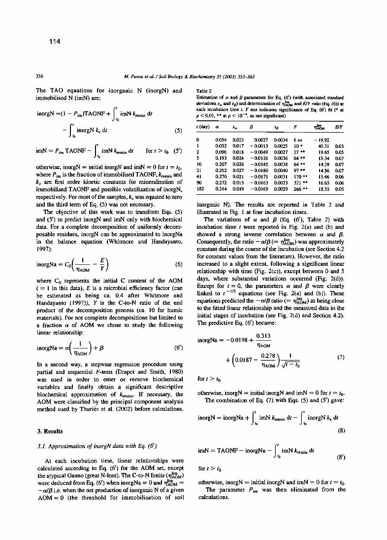
114

356 M. Pansu et aL / Soil Bi%gy & Biochemistry 35 (2003) 353-363

Table 2Estimation of a and fJ parameters for Eq. (6') (with associated standarddeviations Sa and S(3) and determination of 71~'8t.t and ElY ratio (Eq. (6» al

each incubation time t. F tesl indieates signilicance of Eq. (6') lil (. al

P < 0.01••• al p < 10-4, ns not signiâcant)

The TAü equations for inorganic N (inorgN) andirnrnobilised N (irnN) are:

inorgN =(1 - Pim)TAüNF +LirnN k.-enun dt

-LinorgN le" dt (S)t (day) a S" F ElY

(6')

(6)

for t > to (S')

otherwise, inorgN = initial inorgN and irnN = 0 for t = to.The combination of Eq. (7) with Eqs. (S) and (S') gave:

(7)(

0.278) 1+ 0.0187 - -- ---T/AüM .Jt - to

for t > to

. 0 0.313morgNa = -O. 198 + --T/AüM

inorgN = inorgNa +LirnN k.emin dt - LinorgN le" dt

(8)

inorganic N). The results are reported in Table 2 andillustrated in Fig. 1 at four incubation times.

The variations of a and 13 (Eq. (6'), Table 2) withincubation time t were reported in Fig. 2(a) and (b) andshowed a strong inverse correlation between a and 13.Consequently, the ratio - alf3 (= T/~'8M)was approximatelyconstant during the course of the incubation (see Section 4.2for constant values from the literature). However, the ratioincreased to a slight extent, following a significant linearrelationship with time (Fig. 2(c», except between 0 and Sdays, where substantial variations occurred (Fig. 2(d».Except for t = 0, the parameters a and 13 were closelylinked to t -lfl equations (see Fig. 2(a) and (bj). Theseequations predicted the - al13 ratio (= T/~M) as being closeto the fitted linear relationship and the measured data in theinitial stages of incubation (see Fig. 2(d) and Section 4.2).The predictive Eq. (6') became:

0 0.054 0.023 0.0027 0.0034 6 ns -19.921 0.052 0.017 -0.0013 0.0025 10· 40.31 0.032 0.096 0.Ql8 -0.0049 0.0027 27·· 19.65 0.055 0.193 0.024 -0.0126 0.0036 64 •• 15.34 0.0710 0.207 0.026 -0.0145 0.0038 64 •• 14.29 0.0721 0.262 0.027 -0.0180 0.0040 97·· 14.56 0.0741 0.270 0.021 -0.0175 0.0031 170·· 15.46 0.0690 0.272 0.Ql5 -0.0163 0.0023 321·· 16.65 0.06182 0.314 0.019 -0.0169 0.0029 266 •• 18.55 0.05

inorgNa = a(_1_) + 13T/AüM

In a second way, a stepwise regression procedure usingpartial and sequential F-tests (Draper and Smith, 1980)was used in order to enter or remove biochemicalvariables and finally obtain a significant descriptivebiochernical approximation of k.emin' If necessary, theAüM were classified by the principal component analysismethod used by Thuriès et al. (2002) before calculations.

inorgNa = Co(_I- - ~)T/AüM y

where Co represents the initial C content of the AüM( = 1 in this data), E is a rnicrobial efficiency factor (canbe estimated as being ca. 0.4 after Whitmore andHandayanto (1997», y is the C-to-N ratio of the endproduct of the decomposition process (ca. 10 for hurnicmaterials). For not complete decompositions but lirnited toa fraction a of AüM we chose to study the followinglinear relationship:

irnN = Pim TAüNF - LirnN ~nùn dt

otherwise, inorgN = initial inorgN and irnN = 0 for t = to,where Pimis the fraction of irnrnobilised TAüNF, ~nùn andk; are fust order kinetic constants for rnineralisation ofirnrnobilised TAüNF and possible volatilisation of inorgN,respectively. For most of the samples, k; was equated to zeroand the third tenn of Eq. (S) was not necessary.

The objective of this work was to transfonn Eqs. (S)and (S') to predict inorgN and irnN only with biochernicaldata. For a complete decomposition of unifonnly decom­posable residues, inorgN can be approximated to inorgNain the balance equation (Whitmore and Handayanto,1997):

3. Results

otherwise, inorgN = initial inorgN and irnN = 0 for t = to.The parameter Pim was then eliminated from the

calculations.

3.1. Approximation ofinorgN data with Eq. (6')

At each incubation time, linear relationships werecalculated according to Eq. (6') for the AüM set, exceptthe atypical Guano (great N-Ioss). The C-to-N lirnits (T/~M)were deduced from Eq. (6') when inorgNa = 0 and 'l7'l'8M =- alf3 i.e. when the net production of inorganic N of a givenAüM = 0 (the threshold for immobilisation of soit

irnN = TAüNF - inorgNa - LirnN k.enùn dt

for t > to

(8')

115

M. Pansu el aL / Soil Bi%gy & Biochemistry 35 (2003) 353-363 357

~ 0.1 t = 182 d C Gnofer o 0.1 t=90d

i1lOlf1N = 0.34 NIC - 0.0169 C Featm :::E i1lOlf1N = 0.272 NIC - 0.0163~ 0.08 0 0.08

nce

";'00.06Nfeat

";'00.06

~ ~o 0.04 ~ 0.04.s:0 0.02

00.02

0 0O. 0.20 0.30 0.40 O. 0.20 0.30 0.40-0.02 NIC -0.02 NIC

~0.1 t= 21 d ~

0.1 t= 10 dn

~ 0.08 /norgN = 0.262 NIC - 0.0180 c 0 0.08 i1lOlf1N = 0.207 NIC - 0.0145ce";' ";'0 Cc0

0.06

t0.08 t0.04 0.04.s

Cl 00.02 C 0.02

C0 0O. 0.20 0.30 0.40 O. 0.20 0.30 0.40

-0.02 NIC -0.02 NIC

Fig. 1. Estimation (solid line) of N mineralisation by Eq. (6') (NIC = lI1JAOM) at four incubation times.

3.2. Predicting re-mineralisation of immobilised N

Predictions of inorganic N with time Eq. (7) gave sirnilarcurves (not shown) with a high absolute value for the slope(positive for mineralisation, negative for immobilisation)during the first 10 days of incubation, a strong inflexion for

10-30 days and a slight increase for 30-180 days. In a fewcases, the predictions were close to the inorganic Nmeasured data (Gnofer, Featm) and in general they providedapproximate estimates of the total inorganic N production orimmobilisation. In the case of net immobilisation of N,Eq. (7) did not take into account the production of inorganic

0.4 a = ( 0.31 :!: 0.01 ) - ( 0.28:!: 0.02 ) t .112

0.01Il = -(0.020:!:0.OO1) + (0.019:!:0.OO2) t ·112

t (days)0.3

0

tS 0.2 30 60 90 120 150 180 210

co. -0.01

0.1 (a) . ..", l (b)

~= 97.0%"· -0.02 lt (days)0

~=94.6%'"0 30 60 90 120 150 180 210 -0.03

20 50

liiJra@]

40 ~ Il'JAOMliIIl = (0.31 tl 12- 0.28)1(0.020t

l12-0.019)115 B@!I liiJ 30 'ai, (c) :fi 20

(d)

10 ~

1'JAOMlm = (14.2 :!: 0.2) + (0.025:!: 0.002) t ~ 10 .... - -ç' ç'

5 ~ = 98.0% •••0

t(days) -10 5 10 5 20 25 300 -20 !

\l'JAOMlm = 14.2 + 0.025 t 1 t (days)0 30 60 90 120 150 180 210 -30

Fig. 2. Evolution of Eq, (6') parameters (above) and 'l'l'8M (below) as functions of incubation time (from initial input time '0 = 0).

116

358 M. Pansu el al. / SOU Bi%gy &: Biochemistry 35 (2003) 353-363

N from immobilised N; the predicted inorganic N remainedat a negative value whereas a re-mineralisation was oftenobserved. In the case of net mineralisation, Eq. (7) did notsimulate the different shapes of inorganic N releases relatedto the specifie properties of the tested products.

The k,."min values obtained from Eqs. (5) and (5') (Pansuand Thuriès, 2(02) were re-optimized with Eqs. (S) and (S')(Table 1). The relationships between optimised k,."min valuesand biochemical characteristics of the AüM were thenexamined. As pointed out for the C mineralisation studies(Thuriès et al., 2(02), it was difficult to obtain a satisfactoryrelationship for the whole AüM set. The same method ofPrincipal Component Analysis (PCA) was used in order todiscriminate the AüM into two groups: (+) ligneous oneswith relatively high C-to-N ratio, mostly plant-originatedAüM (PCA + in Table 1), and (- ) more nitrogenous ones,with lower C-to-N and ligno-cellulosic fibre contents,mostly animal-originated or partially-composted AüM(pcA - in Table 1). For each group, the kremin valuescould then he fitted to the following equations:

Eqs. (7), (9) and (10) combined with Eqs. (S) and (S'), andEqs. (1), (3) and (4) with the following equations originatedfrom Thuriès et al. (2002). For PCA -

pL = 0.35fsol + 2.2N AOM - O.OIOLigINAoM (II)

Ps = 3.60Lig (12)

or for PCA +

Additionally, the k; value was re-optimized for Nvolatilisation. The k; parameter was not adjusted bybiochemical data since volatilisation c1early occurred ononly two (Guano and Chicm) occasions (k; = 0 for the 15other AÜM). The biochemical predictions were satisfactoryfor seven AüM. For the remaining AüM r in Table 1), acorrection, assuming a possible variability in C and NAOMmeasurements, improved the predictions (see Fig. 3 andSection 4.3). The results are shown in Figs. 4-7 .

krenun = -(0.0034 ± 0.OOO3)ln(flab) (PCA-) (9)

pL = O.099flab + 0.14Hem

Ps = l.6lLig + 0.62AshAOM

(13)

(14)

kmmn = -(O.OOS ± 0.(02)fcel + (0.014 ± 0.(03)fsol(10)

4. Discussion

(PCA+)

with determination coefficients ? = 93.6 and 95.7% forEqs. (9) and (10), respectively.

3.3. Biochemical predictions of C and N transformations

The simultaneous C and N transformations were thenpredicted with the biochemical data only (in g g-1, Table 1):

4.1. About a and 13 values

Except for dO-l, the relationships for Eq. (6') werehighly significant (p < 10-4 for d 2-IS2 in Table 2). For acomplete mineralisation of N-AüM, the slope a Eq. (6')might he equal to l. The value a = 0.31 (at d IS2) indicatesthat about one third of AüM-N was mineralised during theIS2-day experiment, Consequently, 0.69 AüM-N could he

5 - -- -

inorgN

l(days)

(b) Sensltlvlty of InorgN predIctIons to C·to-N value (Ollvp)

0.006

- "Â- •TAO adjustment

-tr-Mbdure measurement

~AOM measurement(a) C-to-N---r--------,

value.

10

15

25 +-t--------j

30

Fig. 3. (a) Values of C-IO-N obtained by: (0) direct measurement on AOM (with 95% confidence intervals, three replicates), (~) measurement fromsoit + AOM sample, (À) model adjustmenl (b) Sensitivity of inorgN predictions vs. changes in C-to-N values following a random normal distribution with

10% RSD (minimum, mean and maximum values in box).

117

M. Pansu el al. 1 Soil Biology de Biochemistry 35 (2003) 353-363 359

+-_~ -+-_~_~_--+-_---LO

0.1

180

imN

80

o~ -==_~~==L~'==:LO

o

iDzoc

~0.05 ~

0.1

s~ ~ 0.3

0.1 1 ;Z .9

0.15 0.4

18080

0.8

02

0.1

0.7

i 0.8

"'coZ 0.5

.9~ 0.4

~ ~--+----+-lo 0.3

t (days) t (days)

iDzoc

io

!;.0.005 2:

0.01

18080

•

+--~~---+-~-~-_+_-...I.~.OO5

0.02

0.08

0.08 ?----l-----'-.......--"'7..-:;;..-----I

0.12

0.01

0.02

0.03

0.05

18080

O+--~-~-_~~~-----t-----I.O

o

0.05

0.15

t(days) t(days)

Fig. 4. Mineralisation and immobilisation of N from guano-based fertiliser (Gnofer), native fine feather (Nfeat). compost-based fertiliser (Comfer), sheepmanure (Shepm). Points. experimental daIa with 95% confidence intervals «+. inorgN from AOM; D. NT_' from AOM); solid lines, TAO biochemicalpredictions of ioorgN (bold Iines), immobilised N (imN) and remainiog NADM (thin Iines).

considered as being stable. The mean value of Ps (the verystable fraction of the AOM, Thuriès et al., 2001) for the 17AOM was 0.53. Thus ca. 0.16 AOM-N could originate fromimmobilisation or from the undecomposed resistant Rfraction (PR = l - pL - Ps)·

The comparison of Eq. (6) and (6') gave an interpretationof {3 values: a being the decomposed fraction, {3 must beequal to -aEIY, then ElY = -{3Ia. The obtained ElYvalues (Table 2) are very close to those given by Whitmoreand Handayanto (1997) with Y ... 10 and E'" 0.4.

4.2. About l1~'ôM values and a,{3, l1~'ôM predictions

In a pioneer study, Jensen (1929) found a C-to-N ratiolimit 'above which no nitrification occurred' reaching about13 in an acid soil and 26 in an alkaline one. In the presentexperiment with a sandy soil (pHH20 = 6.6), the values

l1~'ôM (Table 2) ranged between 14.3 (d 10) and 18.6 (d182). These values were consistent with other found in theliterature. The C-to-N ratio threshold for mineralisation/immobilisation has been variously assumed to be 20-25(Haynes, 1986), about 25 (Whitmore and Handayanto.1997), 24 (Trinsoutrot et al., 2000), about 20 (Stevenson,1986), 17.5 (Hue and Sobieszczyk, 1999), and 11.5 (Gagnonand Simard, 1999).

There was wide variation in the experimental values ofinorganic N at the early incubation times following thequick immobilisation after the addition of AOM at to.Nevertbeless, the parameters a and {3 were very wellpredicted by the t -112 equations as the incubation proceeded(Fig. 2(a) and (bj). From these equations, the ratio -a/{3(= l1~'ôM) was an hyperbole with an asymptote parallel tothe l1~'ôM axis at t == 1, and values very close to theexperimental ones at the early incubation stages (Fig. 2(d».

118

M. Pansu et al / Soil Biology & Biochemistry 35 (2003) 353-363

1llJ::>~.

Zâz

CI .:.

o

rOO5

j

18090

0.06

0.08

fi 0.07

~

0.01

0.02

"':"01

Z 0.05-9

~ 0.04c~o 0.03

-I--~-~-+--~-~-;---------'- _0.005

âZ

CI .:.

0.005

18090

---}---lf:::'-.--=::,..--~c....--+ 0

o-I-------~---+ ___t_-l_o.OO5

o

0.06

0.01

fi 0.05:::ii: 1-+-"1"""l~

"':"... 0.04

Z-9z.2 0.03cIIIE!'o 0.02

360

1(days) t (days)

:;-

~llJ::>~.

ZâZCI

.:.

18090

'f--------::::.....=--f----±--f 0

ol---~-~---+--~-~----+------'- _0.005

o

0.06

0.01

fi 0.05:::ii: H--~~

"':"00.04Z-9

âZ

CI.:. Z

" 0.03C

~0 0.02

0.005

18090

-+-_~_~_-+-_..J. _0.005

0.07

0.02

0.06

imN

q:::ii: 0.06

~"':"... 0.05

Z

~ 0.04 e,i::::;~~~~~=-------I 0

.Illi 0.03

6

t (days) t (days)

Fig. 5. Mineralisationand immobilisationofN fromcrop residees: olive pulp (Olivp),coûee cake (Coffk), wet grape skin cake (Wgrap) and dry grape skin cake(Dgrap). Points, experimental data with 95 % confidence intervals (•• inorgN from AOM; 0, total (AOM + soil) inorganic N; O. NTota.l from AOM); solidliees, TAO biochemical predictions of inorgN (bold Unes),immobilised N (imN) and remaining NAOM (thin lines).

A slight difference appeared at later incubation times (Fig.2(c». In the - a/f3 equation (Fig. 2(d», when 1 -+ 00,

l1~oM -+ 15.5. In reality, after d 10, l1~M increased weaklybut significantly according to the linear relationship inFig. 2(c). The precision found for a and f3 was satisfactory(see confidence intervals of the data in Figs. 4-7) and theproposed Eq. (7) need not be more complicated.

4.3. Sensitivity 10 C-Io-NAOM ratios

Among the biochemical data used in modeUing the Nmineralisation dynamics (Corbeels et al., 1999; Henriksenand Breland, 1999), the importance of C-to-NAOM ratio wasemphasized by Trinsoutrot et al. (2000) and Nicolardot et al.(2001).

In the first TAO version Eqs. (l), (3), (4), (S) and (S'),the fitting of Pim and kremin pennitted correction of

the variability of C and N measurements. As shown inFig. 3(b), the present TAO version was very sensitive to C­to-N values. The error in C-to-N determination is linked tothe propagation of random and systematic errors on C and Nmeasurements (Pansu el al., 2001). The relative variance(RV) is the sum RV on C and RV on N. In this study, eachAOM was measured in triplicate, and the corresponding9S% confidence intervals were plotted in Fig. 3(a). ForDgrap, Shepm, Chicm, Nfeat, Featm, Gnofer and Comfer,the measured C-to-N values gave good predictions. ForCompo a, Compo c and Guano, the adjusted C-to-N valueswere within the confidence intervals of measured C-to-N. Inthe seven other cases, the predictions were not explained bythe random errors. There were probably systematic errorsconfinned by differences between direct AOM measure­ments and the 'soil + AOM' ones [lI(NsoiI+AOM - Nsoivl.They couId originate from two sources. First, the 'soil +

119

180

t(days)

90

o+-'~-~-+-~~~---t---'- -0.002

o90 180t (days)

o +-~~~_--t-_~~_---+-_...L 0

o

M. Pansu el al. 1 Soil Biology & Biochemistry 35 (2003) 353-363 361

Cl 0.1 leompoal 0.015 5" q 0.1 Icompo bl:::i: 0 5"

~ca ::::E 0III

~ 0.004 .a'"

~. !CI z "'Q li"Z iô' z zS êD

0.01 z SIz z Z

10 CD.5.! ~ .Y 0.002 ~c: s c

~III~ 0.05E!' 0.05

0 b 0 h0.005

0

t (days)

0.01

Ne-oP

180

t (days)

90

O-b_r::::..-~-----t--~-~-t------'-O

o

~ 0.1

~"'CIZS

~~ 0.05

o»o.oo~

9

[caIII:l

0.01 c'i"ziô'z

10~

0.015

180

•

90

Icompoel

••

j

o ~::::;:===:;==~im~Nt"=-=-:;:-=-~l 0

o

Cl~ 0.1-c

";"01

zSz~0.05cas

Fig. 6. Mineralisation and immobilisation of N from composts. Points. experimental datawith 95 % confidence intervals (•• inorgN from AOM; 0. NTocal fromAOM); sol id lines, TAO biochemical predictions of inorgN (bold lines), immobilised N (imN) and remaining NAOM (thin lines).

AOM' mixtures were obtained from air-dried materialswhile the direct C and NAOM measurements were made onsamples dried at 40 oc. Even at this low temperature, apartial N volatilisation may occur. Secondly, active N-richsites could induce a micro-heterogeneity in AOM. ForCoffk, Wgrap, Kokoa, Cornpo a, Compo b and Compo p, theC-to-NAOM adjustments by TAO were closer to the valuesmeasured on the 'soil + AOM' mixtures than to thosedetermined on the sole AOM before addition to soil (Fig.3(a».

4.4. Modelling N transformations

Figs. 4-7 displayed biochemical predictions as accurateas those presented in the kinetic adjustment of Figs. 2-5 ofPansu and Thuriès (2002) for Gnofer (Fig. 4), Olivp, Coffk,Wgrap, Dgrap (Fig. 5), Compo a, Compo b, Compo e, and

Compo p (Fig. 6). For Guano, Featm, Chicrn, and Kokoa(Fig. 7), the inorganic N predictions were accurate with bothapproaches, but the biochemical method underestimated Nvolatilisation (too high a value of predicted NT OlaI) . In Pansuand Thuriès (2002), the optimisation method gave k; > 0for these four AOM. This study showed k; > 0 only forGuano and Chicm. Even for these AOM, the presentpredicted volatilisations of N were lower than those inPansu and Thuriès (2002). Total-N was overestimated. TheIcremin values were underestimated (especially for Guano,Table 1) by Eqs. (9) and (10). The transfers of imN toinorgN and to volatile N were thus low. These AOM wereborderline cases for Eqs. (9) and (10).

In Nfeat and Comfer (Fig. 4) the shape of inorganic Nprediction curve differed from the data measured. At d 180the prediction of Nfeat inorgN was correct but the slope ofthe curve was different from the data. The C mineralisation

120

18090

o+--~~~--t-~-~--+-_...J. 0o18090

O~-~-~-_-~~~--t----LO

o

0 0 0

90 180 0 90 180

t(days) t(days)

0.2 IChicml 0.1 0.15

1Kokoaj0.01

~ ! ~ !0.15

11"'", "'", 0.1z z â.g â .!! zz z z 0.005 CI.:..2 0.1 0.05 CI:. .2c

ic i"' •

Ô I!'0

0.05

0.05

362 M. Pansu el al. / Soil Biology '" Biochemistry 35 (2003) 353-363

1.5 0.3 0.4

1Featml0.15

! ~ !~

Il ~:::J Il

~ "",il.

0.3 .,z z

0.2 â .!! 0.1 â"", z~

zz CICI:.

.!!~

c• i~ Ô 0.2

li !JÔ 0.5 0.1 0.05

0.1

t(days) t(days)

Fig. 7. Mineralisation, immobilisation and gaseous losses of N from animal residues guano (Guano), feather meal (Featrn), chicken manure (Chicm) andcropresidue cocoa cake (Kokoa). Points, experimental data with 95% confidence intervals (., inorgN from AOM; D, NT.... from AOM); solid lines, TAObiocbemical predictions of inorgN (bold lines), immobilised N (imN) and remaining NAOM (thin lines), NT.... from AOM.

rate of Nfeat was low (Thuriès el al., 200 1, 2(02) despite ahigh N content. Nfeat had a high Ps fraction and a k.emin

value poorly predicted by Eqs. (9) and (10). The inorgNcurve was more in accordance with the COrC- than withthe inorgN-data. Comfer (Fig. 4) was also a borderline caseof Eqs. (9) and (10). The kremi n value and the regularproduction of inorganic N were underestimated (by 30%during the 1-6 month incubation time).

4.5. Conclusion

as a means of predicting kremin based on biochemicalcharacteristics. In a few cases where N volatilisation clearlyoccurred (Guano and Chicm), TAO needed the inlegrationof the first order volatilisation kinetics (k; constant) of Pansuand Thuriès (2002). Despite sorne cautions linked to thevariability of C and N measurements, a few borderline casesin k.emin determination, and classical corrections needed forfield and soil type conditions, this TAO version appears as avaluable tool for predicting both C and N transformations ofAOM in soil.

Eq. (7) is proposed as a means of estimating theproduction of inorganic N in soil as a function of incubationtime and C-to-NAOM ratio. The threshold for mineralisationlimmobilisation (= 1J~'8M) has been related to the incubationtime. Eq. (7) was used to replace the P im term in theprevious TAO-C and -N kinetic model. The k.emin valueswere then re-optimised and Eqs. (9) and (10) were suggested

Acknowledgemeots

This work was partly granted by a CIFRE convention.The authors gratefully acknowledge Dr C. Feller (IRDMontpellier, France), Dr M. Viel (phalippou-Frayssinet

M. Pansu et al. 1 Soil Biology & Biochemistry 35 (2003) 353-363

121

363

S.A., Rouairoux, France), Prs J.e. Rémy and P. Herrmann(ENSA-Montpellier, France) for helpful discussions.

References

Bosatta, E., Âgren, G.I., 1985. Theoretical analysis of decomposition ofheterogeneous substrates. Soil Biology & Biochemistry 17, 60 1-610.

Bradbury, NJ., Whitmore, A.P., Hart. P.B.S., Jenkinson, O.S., 1993.Modelling the fate of nitrogen in crop and soil in the years foHowingapplication of I~ labelled fertilizer to winter wheal. Journal ofAgriculrural Science 121,363-379.

Corbeels, M., Hofman, G., Van Cleemput, O., 1999. Simulation of net Nimmobilisation and mineralisation in substrate-amended soils by theNCSOIL computer model. Biology and Fertility of Soils 28, 422-430.

Draper, N.R., Smith, H., 1980. Applied Regression Analysis, second ed.,Wiley, New York.

Gagnon, B., Simard, R.R., 1999. Nitrogen and phosphorus release from on­farm and industrial composts. Canadian Journal of Soil Science 79,481-489.

Hansen, S., Jensen, H.E., Nielsen, N.E., Svendsen, H., 199I. Simulation ofnitrogen dyoamics and biomass production in wioter wheat using theDanish simulation model Daisy. Fertilizer Research 27, 245-259.

Haynes, RJ., 1986. Mineral nitrogen in the soif-plant system. In: Haynes,RJ., (Ed.), Mineral Nitrogen in the Soil-Plant System, AcademiePress, Orlando, pp. 52-126.

Henriksen, T.M., Breland, T.A., 1999. Evaluation of criteria for describingcrop residue degradability in a model of carbon and nitrogen turnover insoil. Soil Biology & Biochemistry 31, 1135-1149.

Hue, N.V., Sobieszczyk, B.A., 1999. Nutritional values ofsome biowastesas soil amendments. Compost Science and Utilization 7, 34-41.

Jensen, H.L., 1929. On the inOuenceof the carbon:nitrogen ratios of organicmaterial on the mineralisation of nitrogen. Journal of AgriculruralScience 19,71-82.

Linères, M., Djakovitch, J.L., 1993. Caractérisation de la stabilitébiologique des apports organiques par l'analyse biochimique. 10:Decroux, J., Ignazi, J.c. (Eds.), Matières Organiques et Agricultures,Quatrièmes Journées de l'Analyse de Terre et Cinquième Forum de laFertilisation Raisonnée, Gemas-Comifer, Blois, pp. 159-168.

Melillo,J.M., Aber, J.O., Muratore, J.F., 1982. Nitrogen and Iignin controlof hardwood leaf litrer decomposition dynamics. Ecology 63, 621-626.

Molina. J.A.E., Clapp, C.E., Shaffer, MJ., Chichester, F.W., Larsen, W.E.,1983. NCSOIL, a model of nitrogen and carbon transformations insoils: description, calibration, and behavior. Soil Science Society ofAmerica Joumal47, 85-91.

Nicolardot, B., Recous, S., Mary, B., 2OOI. Simulation of C and Nmineralisation duriog crop residue decomposition: a simple dynamicmodel hased on the C:N ratio of the residues. Plant and Soil83, 83-103.

Pansu, M., Gautheyrou, J., Loyer, J.Y., 2001. Soil Analysis-Sampling,Instrumentation and Quality Control, Balkema, Lisse.

Pansu, M., Thuriès, L., 2003. Kinetics of C and N mineralization, Nimmobilization and N volatilization of organic inputs in a sandy soil.Soil Biology & Biochemistry 35, 37-48.

Parton, WJ., Schimel, O.S., Cole, C.V., Ojima, O.S., 1987. Analysis offactors controlling soil organic matter levels in Great Plains grasslands.Soil Science Society of America Journal 51, 1173-1179.

Robin, O., 1997. Intérêt de la caractérisation biochimique pour l'évaluationde la proportion de matière organique stable après décomposition dansle sol et la classification des produits organominéraux. Agronomie 17,157-17I.

Rubins, E.1., Bear, F.E., 1942. Carbon-nitrogen ratios in organic fertilizermaterials in relation to the availability of their nitrogen. Soil Science 54,411-423.

Sallih, Z., Pansu, M., 1993. Modelling of soil carbon forms after organicamendment under controlled conditions. Soil Biology & Biochemistry25,1755-1762.

Stevenson, FJ., 1986. Cycles of Soil. Carbon, Nitrogen, Phosphorus,Sulfur, Micronutrients, Wiley, New York, 637 pp.

Thuriès, L., Larré-Larrouy, M.-C., Pansu, M., 2000. Evaluation of lhreeincubation designs for mineralization kinetics of organic materials insoil. Communications in Soil Science and Plant Analysis 31, 289-304.

Thuriès, L., Pansu, M., Feller, c., Herrmann, P., Rémy,J.C., 2001. Kineticsof added organic matter decomposition in a Mediterranean sandy soil.Soil Biology & Biochemistry 33, 997-1010.

Thuriès, L., Pansu, M., Larré-Larrouy, M.-C., Feller, c., 2002. Biochemicalcomposition and mineralization kinetics of organic inputs in a sandysoil. Soil Biology & Biochemistry 34, 239-250.

Trinsoutrot, L, Recous, S., Bentz, B., Linères, M., Chèneby, O., Nicolardot,B., 2000. Biochemical quality of crop residues and carbon and nitrogenmineralization kinetics under non-Iimiting nitrogen conditions. SoilScience Society of America Journal 64, 918-926.

Van Soest, P.J., Robertson, J.B., Lewis, B.A., 1991. Symposium:carbohydrate methodology, metabolism, and nutritional implicationsin dairy cattle. Journal of Dairy Science 74, 3583-3597.

Van Veen,J.A., Ladd,J.N., Frissel, MJ., 1984. ModellingC and N rumoverlhrough the microbial biomass in soil. Plant and Soil 76, 257-274.

Verberne, E.L.1., Hassink, J., de Willingen, P., Groot, U.R., Van Veen,J.A., 1990. Modelling organic matter dyoarnics in different soils,Netherlands Journal of Agricultural Science 328, 221-238.

Whitmore. A.P., Handayanto, E., 1997. Simulating the mineralization ofNfrom crop residues in relation to residue quality. In: Cadisch, G., Giller,K.E. (Eds.), Driven by Narure: Plant Litter Quality and Decomposition,CAB International, Wallingford, pp. 337-348.

Wolloy, E., 1902. La Décomposition des Matières Organiques et lesFormes d'Humus dans leurs Rapports avec l'Agriculrure. Translatedfrom the 1896 German edition by E. Henry. Berger-Levrault, Paris.

122

Le rôle de la biomasse microbienne(modèle MOMOS-6)

123

124

Author names and affiliations

Marc Pansu 1, Pierre Bottner', Lina Sarmiento' and Klaas Metselaar"

1 lRD, BP 64501, 34394 Montpellier Cedex 05 France, tel: 33 (0)4 67 41 62 28, E-mail: pansu@mpI.ird.fr

2 CEFE-CNRS 1919, Route de Mende, 34293 Montpellier Cedex 05 France, tel: 33(0)4 67 59 7188, E-mail:

bottner.pierre@wanadoo.fr

3 rCAE, Facultad de Ciencias, Universidad de los Andes, Mérida 5101 Venezuela, E-mail: Isarrnien@ula.ve

4 PRI Wageningen The Netherlands, E-mail: henriette.drenth@wur.nl

Title

Comparison of five soil organic matter decomposition

models using data from a 14C and 15N labeling field

experiment

Running Title

Comparison of five SoU Organic Matter Models

1

125

Abstract. Five alternatives (MOMOS-2 to -6) of the previously published MOMOS model

are tested to predict the dynamics of carbon (C) and nitrogen (N) in soil during the

decomposition of plant necromass. 14C and 15N labeled wheat straw was incubated from

Nov. 13, 1998 to Nov. 11, 2000 in fallow soils of the high Andean Paramo of Venezuela.

The following data were collected: soil moisture, total 14C and 15N and microbial biomass

MB_14C and _1~, daily rainfall, air temperature and total radiation. Soil moisture was

predicted by the SAHEL model. MOMOS-2 to --4 (type 1 models) use kinetic constants and

flow partitioning parameters. MOMOS-2 can be simplified to MOMOS-3 and further to

MOMOS-4, without significant changes in the prediction accuracy for total-i''C and _1~ as

well as for MB_14C and _15N. MOMOS-5 (type 2) uses only kinetic constants: three

MB-inputs (from labile and stable plant material and from humified compounds) and two

MB-outputs (mortality and respiration constants). MOMOS-5 did not significantly change

the total_14C and _1~ predictions but improved markedly MB_14C and _15N predictions.

Thus MOMOS-5 is proposed as an accurate description of decomposition processes based

on field incubations. MOMOS-6 completes MOMOS-5 by integrating a stable humus

compartment (HS) for long tenn simulations. The improvement of the predictions is not

significant for the 2 year experiment, but MOMOS-6 enables to predict a sequestration in

the stable humus compartment of2% of the initially added 14C and 5.4% of the added 15N.

Keywords: decomposition, modeling, tracer experiment, soil organic matter, carbon,

nitrogen, 14C, 15N, microbial biomass, Andes, Venezuela.

2

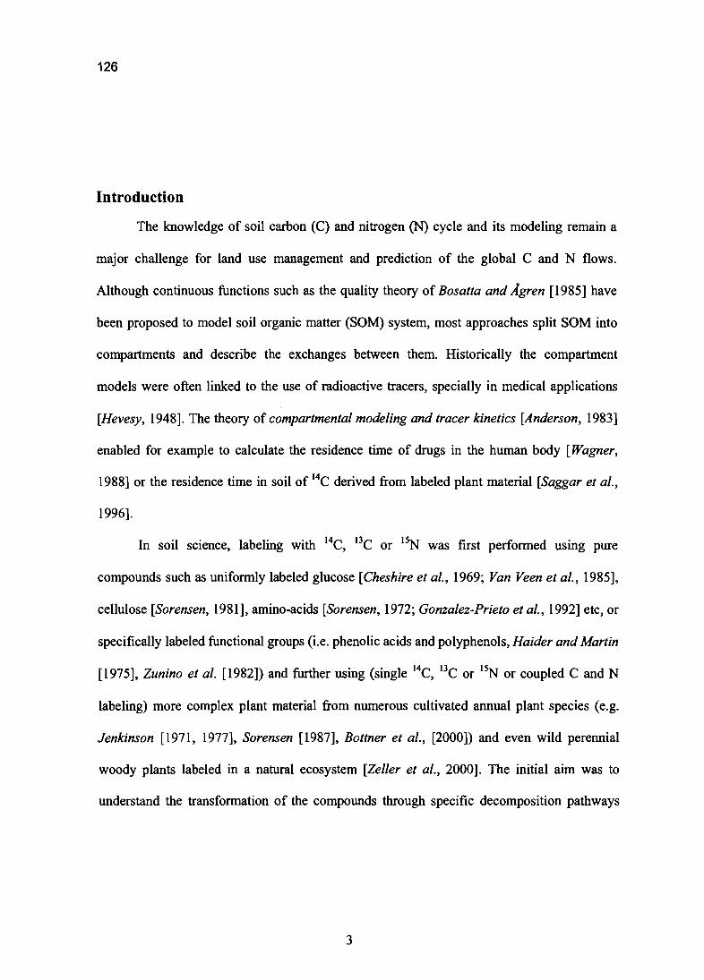
126

Introduction

The knowledge of soil carbon (C) and nitrogen (N) cycle and its modeling remain a

major challenge for land use management and prediction of the global C and N flows.

Although continuous functions such as the quality theory of Bosatta and Âgren [1985] have

been proposed to model soil organic matter (SOM) system, most approaches split SOM into

compartments and describe the exchanges between them. Historically the compartment

models were often linked to the use of radioactive tracers, specially in medical applications

[Hevesy, 1948]. The theory of compartmental mode/ing and tracer kinetics [Anderson, 1983]

enabled for example to calculate the residence rime of drugs in the human body [Wagner,

1988] or the residence time in soil of 14C derived from labeled plant material [Saggar et al.,

1996].

In soil science, labeling with 14C, BC or IsN was first performed using pure

compounds such as uniformly labeled glucose [Cheshire et al., 1969; Van Veen et al., 1985],

cellulose [Sorensen, 1981], amino-acids [Sorensen, 1972; Gonzalez-Prieto et al., 1992] etc, or

specifically labeled functional groups (i.e. phenolic acids and polyphenols, Haider and Martin

[1975], Zunino et al. [1982]) and further using (single 14C, BC or 1~ or coupled C and N

labeling) more complex plant material from numerous cultivated annual plant species (e.g.

Jenkinson [1971, 1977], Sorensen [1987], Bottner et al., [2000]) and even wild perennial

woody plants labeled in a natural ecosystem [Zeller et al., 2000]. The initial aim was to

understand the transformation of the compounds through specifie decomposition pathways

3

127

(i.e. the fate of 14C labeled polyphenols), and further to follow the tracers through identified

and measurable compartments, e.g. soil microbial biomass [Van Veen et al., 1985; Ladd et al.,

1985, 1995; Bottner et al., 1998; Saggar et al., 1999].

A pioneer SOM decomposition model (a simple two compartment model) was

proposed by Hénin et al. [1959]. Among the further published mode1s, many were too

complex to be easily validated, because theoretical compartments were often not measurable.

The numerous physical, chemical and biological SOM fractionation procedures seldom

corresponded to theoretically defined compartments. A major step was achieved when

Jenkinson and Powlson [1976] and Anderson and Domsch [1978] proposed new procedures

to measure the microbial biomass pool (MB), a keystone to describe the SOM system.

However the structural identifiability analysis [Cobelli et al., 1979] of the complex theoretical

schemes remains a difficult task. The models are mainly tested by estimating their predictive

quality using long-tenn experiments. This approach is e.g. explored by Smith et al. [1997]

who compared the following models: Roth-C [Jenkinson, 1990; Jenkinson and Rayner, 1977],

Ncsoil [Molina et al., 1983], Century [Parton et al., 1987], Hurley pasture [Thornley and

Verberne, 1989], Verbeme/MOTOR [Verberne et al., 1990], ITE forest [Thornley, 1991],

Daisy [Hansen et al., 1991], DNDC [Li et al., 1994], Candy [Franko et al., 1995] and SOMM

[Chertov and Komarov, 1997]. The authors identified two groups, but for most of the

compared models the prediction errors did not differ significantly. Thus, the model

performance seems to be independent of their conceptual content, suggesting that sorne of

them may be over-parameterized.

4

128

Data from a former 14C and 1~ labeling experiment perfonned under controlled

laboratory conditions enabled the construction of the initial MOMOS-C [Sa//ih and Pansu,

1993] and -N [Pansu et al., 1998] mode1s. The aim of the present work was to validate and

improve the initial MOMOS model with data from a new 14C and 15N experiment perfonned

in the field under natura1 climatic conditions. This paper compares five new versions derived

from the initial proposal, In comparing the versions, the aim was to test their validity (1)

through successive simplifications of the model structure by suppressing sorne compartments

or sorne decomposition pathways and (2) by focusing the decomposition on the microbial

biomass compartment highlighting its key functional role.

Materials and methods

The site of the experiment

The experiment was conducted at the paramo site of Gavidia (8°35'-8°45' N,

70°52'-70°57' W) in the Andes of Mérida (Mérida State, Venezuela) at an altitude of 3400 m.

The mean annual precipitation is 1329 mm. The mean annual temperature is 8.5 "C differing

on1yby 1.5 "C between the coldest and the warmest months. The experiment was set up in (1)

a 2 year old fallow plot (JO data series) with an estimated soil cover = 0.85 of mainly

perennial herbs and (2) in a 7-year old fallow plot (VI data series) covered by the

characteristic paramo giant rosettes and by sclerophilous shrubs (height = 1 to 1.5 m,

estimated soi1 cover = 0.9). The soil (humitropepts, USA Soi1 Taxonomy) is loamy and well

drained. In the 0-10 cm layer, sand = 54 %, silt = 31 %, clay = 15 %, pH(H20) = 4.5, water

5

129

holding capacity (v/v) = 0.52 (mean values of the two experimental plots), C = 9.4 % (plot

JO) and 8.8 % (plot VI), N = 0.55 % (JO) and 0.56 % (VI). The high organic matter content

explains the high water holding capacity. The cultivation system is based on a long fallow

period used for grazing (generally from 5 to 10 years) altemating with a short (1 to 3 years)

potato and cereal cropping period.

14C and lSN labeled plant material

A low N-requiring old cultivar of spring wheat (Florence Aurore) was grown from

seed to maturity in a labeling chamber with controlled 14C02 atmosphere (0.03 % v/v, 0.86

kBq mg-IC), temperature, radiation and altemate lighting conditions. The plants, which were

cultivated in pure sand, were periodically flooded with a complete nutrient solution containing

Ca('~03h (10 % atomic ratio) as the sole N source. At maturity the wheat was dried at 40°C.

Only the stems and leaves were used in the experiment. They were ground into 2-7 mm long

partic1es and homogeneously mixed. The C content of the stems + leaves equaled

43.0 ± 0.39 % (0.821 ± 0.022 kBq mg" C) and the N content was 1.60 ± 0.05 % ('~ isotopie

ratio = 9.250 ± 0.451 %). The biochemical fractions of the straw [van Soest et al., 1991] were

as follows: neutral detergent soluble = 0.36, hemicelluloses = 0.25, cellulose = 0.26, lignin =

0.03, ashes = 0.10.

Field incubation

For each plot (JO and VI series), homogenized air dried soil, sampled from the 5-10

cm layer, was divided into 40 samples of 150.0 g soil each. 3.260 g of labeled straw were

6

130

homogeneously added to each sample, corresponding to 9.0 % (JO) and 9.6 % (VI) of total C

(soil native C + plant material C) and 5.9 % (JO) and 5.8 (VI) % of total N (soil native N +

plant N). The mixture was placed in 10 x 8 cm sealed polyester bags made from 0.5 mm mesh

tissue. The bags were placed horizontally in the 5-10 cm layer and covered with the upper

0-5 cm layer soil. The experiment lasted from November 13, 1998 to November Il,2000. For

each series, 9 samplings were performed, collecting 4 replicates at each samp1ing (see Fig. 2

and 3 for sampling dates).

Data acquisition

At sampling, the wet sample was homogenized and 3 x 5 g wet soil was dried at

105°C for the measurement of the moisture content. The remaining wet soil was sub-sampled

for analyses of (a) microbial biomass-X; and _l~ (4 field replicates x 2 analysis replicates

for MB_14C, 4 field replicates for MB_I~), and (b) total-14C, (4 x 8 replicates) and _l~ (4 x

2 replicates). Microbial biomass was measured according to the fumigation-extraction method

of Brookes et al. [1985] : 20 g soil, 150 mL 1 mo1('l'2K2S04)L-1 extractant, 14C measurement

on the extracts by liquid scintillation counting (Tricarb 1500, Packard), measurement ofN and

I~ by Kjeldahl procedure and Mass spectrometry (Finnigan delta S), kEc. = 0.45

[Joergensen, 1996], kEN = 0.54 [Joergensen and Muel/er, 1996]. Total C and 14C were

measured simu1taneously using Carmograph 12A (Wôsthoff, Bochum, Germany), according

to Bottner and Warembourg [1976]. Total N and 15N were measured using coupled

CHNlMass spectrometry.

7

131

Climatic parameters (daily precipitation, mean air temperature and total radiation)

were recorded (automatic Campbell weather station) at the site throughout the experiment

period (except for a total of 3 months, when data were statistically generated from records of

other sites located around the studied site).

Predictive models

The five models tested are presented in figure 1. Three compartments are present in all

the models: labile (VL), stable (VS) fractions of necromass (NC = VL +VL) and rnicrobial

biomass (MB). MOMOS-3, -4 and -5 contain a compartment for humified compounds (H).

MOMOS-2 and -6 contain compartrnents for labile (HL) and stable humified compounds

(HS). MOMOS-2 is the model aIready presented by Sallih and Pansu [1993] using data from

a labeling experiment performed under laboratory conditions, with measurements of total 14C,

rnicrobial 14C and not yet decomposed plant fragments 14C. MOMOS-3 results from the

simplification of MOMOS-2, with an equation system analogous to the Roth-C model

(Jenkinson, 1990) but without the inert organic matter (lOM) compartment of Roth-C (not

necessary for this short term 14C and 15N experiment). MOMOS-4 offers a further

simplification of MOMOS-3 with the recycling part of H and MB compartment removed.

MOMOS-5 explores two new modifications: (1) the whole outputs from plant (VL+VS) and

humus (H) compartments are the inputs of MB, (2) the outputs of MB are defmed by a

respiration quotient (qC02) and a rnicrobial mortality rate (kMB). The equation system of

MOMOS-5 is sirnilar to that in the CANDY model [Franko et al., 1995] and to that used by

8

132

Saggar et al. [1996] to calculate 14C turnover and residence times in soils. MOMOS-5 differs

in the following aspects: (1) fractionation ofNC inputs into VL and VS, (2) change ofkinetic

calculation of the microbial respiration (see below, eq. 9 and 10), (3) elimination of the flow

fractionation between necromass and MB used in CANDY (in MOMOS-5 the whole flow

from NC substrate enters into MB). MOMOS-6 attempts to improve MOMOS-5 by

introducing a stable humus compartment (HS), that results from the slow maturation of HL

and supplies the dormant MB with maintenance energy, when the fresh C input is exhausted.

MOMOS-5 and -6 are regulated by l " order kinetic constants (dimension TI) only, without

the dimensionless parameters (efficiency factors) often used in SOM models to fractionate the

flows between the compartments (e.g. Jenkinson and Rayner [1977], Parton et al. [1987],

Franko et al. [1995] or P parameters in MOMOS-2 to -4).

For each model, the substrate (NC) was partitioned over VL and VR on the basis of its

biochemical characteristics using the equations proposed by Thuriès et al. [2001; 2002] which

give for this labeled straw the stable fraction of NC:.fs= 0.107.

The general equation of the models is:

x=Ax (1)

where X is the vector of the state variables (compartments), X is the vector of the

rates variables and A is the parame ter matrix of each model. A and X are written, for

MOMOS-2:

9

133

-kVL 0 0 0 0 VL

0 -kyS 0 0 0 VS

A = PMBk VL PMBk yS (PMB- 1) k MB PMBk HL PMBk HS X = MB (2)

PHLk YL PHLk ys PHLk MB (PHL -1)kHL PHLk HS HL

PHsk VL PHSk yS PHsk MB PHsk HL (PHs-l)kHs HS

for MOMOS-3:

-kVL 0 0 0 VL

0 -kyS 0 0 VSA=

(PMB-l)kMBX = (3)

PMBk VL PMBk yS PMBkH MB

PHkVL PHkys PHkMB (PH-l)kH H

for MOMOS-4:

-k VL 0 0 0 VL

0 -kyS 0 0 VSA= x = (4)

PMBk YL PMBk yS -kMB 0 MB

PHkYL PHkyS 0 -kH H

for MOMOS-5:

-k VL 0 0 0 VL

0 -kyS 0 0 VSA= x = (5)

k YL k yS -(Qco2+k MB) k H MB

0 0 k MB -kH H

for MOMOS-6:

10

134

-kVL 0 0 0 0 VL

0 -kvs 0 0 0 VS

A= kVL k vs -(qc02+kMB ) k HL k HS X = MB (6)

0 0 k MB -(kHL +k HLS ) 0 HL

0 0 0 k HLS -kHS HS

For the labeling experiment described in this paper (one single initial input of dead

matter and an initial amount Co of 14C with a stable fractionJS), the initial conditions are given

by:

VL(O) = (1-fs) Co, VS(O) =JS Co.MB(O) = 0, H(O)=O,

HL(O) = 0, HS(O)=O and CO2(O)=O (7)

At each incubation time, the remaining total 14C evolution è from the n compartments

(n = 4 for MOMOS-3, -4, -5; n = 5 for MOMOS-2, -6) is given by:

n. ~.

C =- L.Jx j

j=1

with c(O)= Co (8)

In the case ofMOMOS-5 and -6, eq. 8 becomes particularly simple:

è =-qC02 MB (9)

where qC02 is the metabolic quotient of the microbial biomass [Anderson and Domsch,

1993]. Another condition is necessary to ensure correct performance of MOMOS-5 and -6:

qC02 must be controlled by the amount of MB. The QC02 should increase when MB is growing

(particularly in response to the initial high supply from VL), and decrease when MB decreases

or becomes inactive (dormant MB). Then è is linked to MB by a 2nd order kinetics. In order

to allow use of MOMOS-5, -6 in different situations, we suggest (1) to introduce a respiratory

11

135

coefficient kœsp (dimension Tl) and (2) to weight the lcresp values by the ratio of the actual

level of MB in the studied soil and its equilibrium value (C~ measured on biologically

stable soil, i.e. long after recent inputs of substrate). For the present labeling experiment

C~B =0.15 g kg", the level of MB_14C_ measured at the end of the experiment. The qC02 is

given by:

MBqC02 = kresp -0­

CMB(10)

MOMOS-2 to -6 are simplified compared with the initial MOMOS-N model

(MOMOS-l, Pansu et al. [1998]). ~- and N03- are combined in a single pool of

inorganic-N, For each of the five models, the N state variables are derived from the C model,

using the C-to-N ratios of the compartments. If T'l is the vector of the C-to-N ratios and y the

vector ofN contents, the simulation of organic N status at a given incubation time is govemed

by:

xy=-

'1

If T'lo is the initial l4C_to_l~ ratio of the substrate, the inorganic 15N (iN) is:

(11)

(12)

In this labeling experiment, the values T'lo, l'Jt (remaining total l4C_to_ remaining total

l~) and l'JMB e4C-to-l~ ofmicrobial biomass) were measured. The l'JVL value is linked to l'Jo

and nvs by:

12

136

(1- fs)

11VL =(1 fS)110 11vs

The 11H or 11HL values are linked to the other data by:

Xn _ H'18 - Cl _ x VL _ xvs _ x MB

111 11VL 11vs 11MB

(13)

(14)

(15)

Thus the only 11 values that have to be estimated are 11vs e4C-to-l~ of the stable

fraction of NC) in MOMOS-3 to -5 or 11vs and 11HS e4C-to-l~ of the stable fraction of

humus) in MOMOS-2 and -6. In order to avoid irregularities in predictions, the values

calculated for 11H or 11HL are smoothed in the interval [11MB, t (110 + 11MB)] with 11HS = 6 11MBJ'5

for MüMOS-6.

During the simulations, the kinetic constants are always corrected by two functions,

one for temperatureftT) and one for moistureftw);ftT) is a law with QlO = 2 for a reference

temperature of 20°C assumed to be valid for these mountain soils [Kiitterer et al., 1998];ftw)

is a linear function of the actual soil moi sture scaled by moisture content at field capacity. For

the 5-10 cm soillayer, the actual moisture was calculated by the SAHEL model [Penning de

Vries et al., 1989]. With the corrective factor ftT) x ftw) in [0,1] interval, the general

formulation (eq. 1) of the models becomes:

13

x = .f{T).f{w) A x

Statistical comparison of model predictive quality

The four vectors of measured data were:

137

(16)

- x t = total 14C (9 sampling occasions (so) during two years of incubation)

n

corresponding to the predicted values xt = LXI';=1

n

- y t = total 1~ (9 so) corresponding to the predicted values yt = L Yi';=1

- XMB = 14C_MB (9 so) corresponding to the predicted values XMB ,

- YMB = 15N_MB (9 so) corresponding to the predicted values YMB'

For each model four residual sums of square (RSS) were calculated for the m so:

m m

RSS xt= L (xt -xtY RSSyt= L (Yt -YtYj=1 j=1

m ID

RSS xMB= L (XMB-XMBY RSSyMB= L (YMB -YMBY (17)j=1 j=1

The smallest RSS corresponds to the best fit. In addition the comparison should take

the number of model parameters (P) into account. The best model has the smallest RSS and

also the smallest p. MûMûS-S has five parameters: kVL, kvs, kMB, kHL and kresp. MûMûS-3

and -4 have six parameters: kVL, kvs, kMB , kH, PMB, PH. However the specifie parameterization

of this experiment take kvs=kH and reduce MûMûS-3 and -4 to five parameter models.

14

138

MOMOS-2 has eight parameters: kVL, kvs, kHL, !<Hs, kMB, PHL, PMB, PHS. But again the

parameterization of this experiment take kVL = kHL, kvs = kHS, PHL=O.77 (value found by

Sallih and Pansu [1993]) and also reduce MOMOS-2 to a five parameter model.

Thus the predictive quality of the models MOMOS 2-5 can be pairwise compared by

the F tests:

{

RSS MOMOS-I IRSS MOMOS-UF -(m-I m-l) -, RSSMOMOs-u/RSSMOMOS-1

if RSSMOMOS-I > RSSMOMOS-u

if RSSMOMOS-u > RSSMOMOS-I

(18)

(u, t E [2-5], t::/; u, m sampling occasions)

for each of the four models applied to each of the four series total- 14C and _I~,

Results

Model parameters

Since there was no significant difference between the results from series JO and VI, all

the predictions for each model are based on only one set ofparameters (the mean value from

JO and VI calculations, table 1).

Total 14C and lSN predictions

The predictions of the five models and the measured JO and VI values are plotted in

figure 2. Tables 2 and 3 compare the predictive quality (eq. 18) of the models for total l''C and

I~, respectively.

15

139

For total 14C the MOMOS-2 and MOMOS-3 predictions were almost identical. For the

other models the predictions were slightly different (Figure 2), but a11 the results were

statistica11y equivalent (Table 2). The MOMOS-5 and -{) predictions were almost the same

during the first nine months, as long as the HS content (MOMOS-6) was low. At the end of

the experiment, MOMOS-6 predicted slightly higher values and closer to the measured data

than MOMOS-5, indicating a 14C-sequestration in the HS compartment.

For total 15N predictions, slight differences appeared between the models (Figure 2),

but they were again a11 statistica11y equivalent (Table 3). The MOMOS-2 to -4 predictions

were overestimated during the first six months of incubation and underestimated during the

last year. The MOMOS-5 and especia11y the MOMOS-6 predictions were the closest to

measured values throughout the whole incubation period. The slight underestimation

observed during the last year could be explained by a slight overestimation of the 15N

measurements: total_15N is defmed in MOMOS as organic-PN, whereas the measurements

inc1ude sma11 amounts of inorganic 15N remaining in the soil.

Predictions of MB-14C and _lsN

The predicted and measured values of MB in JO and VI series are plorted in figure 3.

Tables 4 and 5 compare the predictive quality (eq. 18) of the models for MB_14C and _I~,

respective1y. The MOMOS-2 and -3 predictions were aImost the same and were close to

MOMOS-4 predictions. In a11 cases the results show clearly a significant improvement in MB

predictions by MOMOS-5 compared to those by MOMOS-2 to -4. For MB_14C, the

16

140

improvement was significant at 5% risk in five cases and at 2% risk in one case. For MB_I~,

the improvement was significant at 10% risk in two cases and at 5% in the four other cases.

During the first five months the MOMOS-5 and -6 predictions were again similar. After this

time the MOMOS-6 predictions were slightly closer to the measured values of MB_14C and ­

I~.

Discussion

Comparison of MOMOS-2 and-3

The two models gave similar predictions for total- 14C and MB_14C, as well as for

MB_15N (Fig 2 and 3). The slight but not significant differences observed for tota1_I~

resulted from the estimated C-to-N ratio (Eq.15) of the HL compartment. Thus the two

models are clearly equivalent in predicting total SOM dynamics. MOMOS-3 differs from

MOMOS-2 in that there is no labile humus (HL) compartment (Figure 1), resulting in very

different values of the I" order kinetic constants of VL: kVL = 0.54 (t l/2 = 1,3 days) for

MOMOS-2 and kVL = 0.13 (t l/2 = 5,3 days) for MOMOS-3 (table 1), with for MOMOS-2 the

consequent transfer of labile metabolites to the transient HL compartment. The MOMOS-2

decay rate of HL and VL are identical (km. = kVL). Both VL and HL compartments are

quicklyand almost completely exhausted (after 90-120 days of incubation); at that time MB

reaches its maximum value and begins also to dec1ine, that highlights the role of labile

compounds in the MB dynamics. In MOMOS-3, the VL compartment represents the sum

VL+HL of MOMOS-2 and is exhausted at the same time. Thus MOMOS-3, with an equation

17

141

system analogous to the Roth-C model [Jenkinson, 1990], is a valuable simplification of

MOMOS-2. Nevertheless, the need for the HL compartment was supported from another

labeling experiment [Sallih and Pansu, 1993] performed under controlled laboratory

conditions where, in addition to the MB measurement, the not yet decomposed plant

fragments-PC (NC) remaining in the soil were also measured: HL_14C = total-14C minus

(MB_14C + plant fragments-PC). The HL compartment describes a real transient

decomposition step. Nevertheless in modeling total C and N dynamics from long field

experiments with this type of model , HL can be eliminated. Thus the simplification defined

in MOMOS-3 is justified.

Comparison of MOMOS-3 and -4

MOMOS-4 is a further simplification derived from MOMOS-3 by suppressing the

recycling loop ofMB and H outputs (Figure 1). MOMOS-4 is a parallel decomposition model

in which a part PMB of the flow from VL and VS becomes MB and another part PH becomes

H. In the mathematical description of MOMOS-4, this simplification eliminates the P

parameters (Cf. matrix eq. 3) from the diagonal terms. In the matrix of eq.4, the

corresponding elements become 1st order kinetic constants; aIl the terms above the diagonal

become zero. The calculated MOMOS-3 and -4 parameters are similar, except for the slightly

lower l" order kinetic constants kvs (and kH = Kvs) and kMB in MOMOS-4 values. This is in

accordance with the removal ofthe recycling part in MOMOS-4.

18

142

In table 2, RSS-4 was lower than RSS-3 in one case, and higher in the other cases

(NS). In tables 4, S, 6 RSS-3 was always lower than RSS-4 (NS) indicating more accurate

predictions for MOMOS-3 than for MOMOS-4, but the differences were never significant.

Given the ratios of their RSS (Tables 2, 4, S, and 6), models 3 and 4 yield predictions which

are never significantly different. Consequently MOMOS-4 is preferable because of its simpler

structure.

MOMOS-4 and -5 comparison

In MOMOS-S, the estimated 151 order kinetic constant kVL is higher than in MOMOS-3

and -4 and close to the MOMOS-2 value (table 1). But in MOMOS-S, the VL labile plant

material is entirely assimilated by MB while in MOMOS-2 VL becomes, for the PHL part, HL

labile humus. Consequently, the MOMOS-S and MOMOS-2 to -4 generate different MB

curves. In MOMOS-S, MB increases rapidly, reaching its maximum level after two days of

incubation and decreases equally rapidly after a few days, giving significantly better

predictions than MOMOS-2 to -4 from day 30 until the end of the incubation. In this

experiment, the 1st measurement occurred at day 30, i.e, at the end of the MB initial peak

(Figure 3). Nevertheless, the shape of the MOMOS-S MB curve agrees with literature data:

the response time of the MB to labile organic substrate to the soil is generally in the order

from a few hours [Anderson and Domsch, 1978] to a few days. The maximum size of MB is

often observed from the 151 measurement, i.e. about 7-10 days after the substrate addition

[Henriksen and Breland, 1999; Lundquist et al., 1999; Ocio et al., 1991; Trinsoutrot et al.,

19

143

2000]. An immediate N microbial immobilization was measured from the beginning of the

incubation with various substrates by Pansu and Thuriès, [2003], Pansu et al.[2003] and

Trinsoutrot et al. [2000]. Conversely, for MOMOS-2 to -4 the predicted MB curve increases

slowly, reaching the maximum level after only about two months of incubation. Thus

MOMOS-2 to -4 underestimate MB at the 1st measurements, overestimate it during the

following few months and again underestimate it during the 2nd year. A similar discrepancy

between the predicted and measured MB has already been observed by Sal/ih and Pansu

[1993], using the MOMOS-1 model.

In MOMOS-5 the H compartment has the same input (4m) and output 0cH) kinetic

constants as HL in MOMOS-6. Indeed, H and HL represent labile metabolites, like HL in

MOMOS-2. But HL has two different meanings. The MOMOS-2 HL describes labile

metabolites resulting from decomposing plant material. In MOMOS-5 H describes

metabolites resulting from microbial cadavers or by-products of microbial activity. Both

materials are used (for MOMOS-2 VL) or reused (For MOMOS-5 H) as substrates for

microorganisms, but the MOMOS-2 HL is rapidly used and exhausted (kHL = kVL = 0.54

day") explaining the above mentioned failures in MB predictions. In contrast, the MOMOS-5

H represents a large reserve of 14C, that lasts the whole incubation period 0cH = 0.05 day")

and sustains the relatively high level of MB until the end of the experiment. This agrees with

the conclusions of Mueller et al. [1998]: "a part of the decomposed plant material is

immobilized both in soil MB as well as in a considerable amount of microbial residual

products".

20

144

Improvement of MOMOS-S by MOMOS-6

MOMOS-6 which results from the improvement of MOMOS-S (Fig. 1) yields better

RSS for aIl predicted variables (tables 3 to 6). However MOMOS-6 needs 2 additional

parameters (kHLS and kas) and the improvement over MOMOS-S is not significant. Thus the

largest improvement in predictive quality is achieved in MOMOS-S for this l4C and ISN

experirnent. However the simulation of the dynarnics of soil native total-C and -N (work in

preparation) required the introduction of a stable humus compartment (HS) in order to take

into account the slow sequestration and accumulation of long lasting C. In this two-year

experirnent, MOMOS-6 predicted an amount ofstabilized l4C = 0.18 g kg", i.e. 2.0 % of the

total added l4C, and an arnount of stabilized l~ = 0.018 g kg", i.e. S.4 % of added l~. The

HS compartment is also the most important reservoir of stable N in soil.

Figures. 2 and 3 show the ecological consistency of the improvement of MOMOS-6.

During the second year of incubation, the MOMOS-6 predictions were doser to the measured

data than those by MOMOS-S: for total l''C and _lsN, the MOMOS-6 predictions were higher

than those by MOMOS-S, but for MB_14C and _lsN, the MOMOS-6 predictions were lower

than those by MOMOS-S. When for MOMOS-6 MB_14C and _l~ decreased as a response to

stabilization in HS, total_14C and _lsN increased, reflecting a lower mineralization by

rnicroorganisms. The MOMOS-2 to --4 predictions were less consistent, because an increase

in total- 14C also corresponded to an increase in MB_14C (fraction PMB) and vice versa.

21

145

Conclusion

The five compartment MOMOS-2 model was initially developed on the basis of a

laboratory labeling experiment in which most of the predicted compartments were measured

[Sallih and Pansu, 1993]. In the present field experiment, under natural c1imate conditions,

with less samplings and a simpler procedure of chemical analysis, the aim of this study was to

test the predictive quality of successively simpler versions. The tirst step was to reduce the

number of compartments (MOMOS-2 to -3) and to suppress a recyc1ing processes

(MOMOS-3 to -4). The successive simplifications did not significantly modify the prediction

accuracy for total 14C and 1~, nor for microbial biomass. Thus the simplification of

MOMOS-2 to -3 is considered to be valid, as is the further simplification of MOMOS-3 to

MOMOS-4.

The second step focused on the processes associated with microbial activity. It

allowed to eliminate the dimensionless parameters used for flow partitioning. As a result,

MOMOS-S only uses (1) the three l" order kinetic constants kVL, kvs, and leu which

determine inputs into MB, (2) the 1st order kinetic constant kMB which defmes the production

of microbial cadavers and metabolites, (3) the metabolic quotient qC02 which regulates MB

respiration. The modifications leading to MOMOS-S did not change the accuracy of total 14C

and 15N predictions, but noticeably improved the MB_14C and _1~ predictions throughout the

decomposition steps. The present paper therefore proposes MOMOS-S as the most accurate

among the versions tested for 14C and 15N predictions for tracer experiments during the tirst

years of incubation. Modifications leading to MOMOS-6 were essentially carried out in order

22

146

to be able to modellonger term processes, including those associated with soil native organic

matter. For that purpose, a stable humus compartment (HS) was introduced, resulting from the

slow stabilization of a small fraction of HL (H in MOMOS-5). MOMOS-6 HS includes the

high amount of C and N that is sequestered in the soil native organic matter. This labeling

incubation allowed 14C and I~ sequestration to be quantified for a period oftwo years.

Acknowledgements

TROPANDES INCO-DC program of the European Union (ERBICI8CT98-0263)

supported this work. We are grateful to Prof. T. Carballas, CSIC-lIAG, Santiago de

Compostela Spain, coordinator of the program, to A. Olivo, ICAE Mérida Venezuela, for her

help in the field experiment and to B. Buatois, CEFE-CNRS, Montpellier France and N.

Marquez of the ICAE for the analysis of 14C and I~.

Bibliography

Anderson, D.H., Compartmenta/ modeling and Tracer Kinetics, 302 pp., Springer-Verlag,

Berlin, Heidelberg, New York, Tokyo, 1983.

Anderson, J.P.E., and K.H. Domsch, A physiological method for the quantitative

measurement ofmicrobial biomass in soils, Soi! Biology & Biochemistry, 10, 215-221,

1978.

Anderson, T.H., and K.H. Domsch, The metabolic quotient for CO2 (qC02) as a specifie

activity parameter to assess the effect of environmental conditions such as pH on the

microbial biomass offorests soil, Soi! Biology & Biochemistry, 25, 393-395, 1993.

Bosatta, E., and G.!. Âgren, Theoretical analysis of decomposition of heterogeneous

substrates, Soi! Biology & Biochemistry, 17, 601-610, 1985.

23

147

Bottner, P., and F. Warembourg, Method for simultaneous measurement of total and

radioactive carbon in soils, soil extracts and plant materials, Plant and soif, 45, 273­

277, 1976.

Bottner, P., F. Austrui, J. Cortez, G. Billès, and M.M. Coûteaux, Decomposition of 14C_ and

1~_ labelled plant material, under controlled conditions, in coniferous forest soils

from a north-south climatic sequence in western Europe, Soif Biology & Biochemistry

30,597-610, 1998

Bottner, P., M.M. Coûteaux, lM. Anderson, B. Berg, G. Billes, T. Bolger, J. Casabianca, P.

Romany, and P. Rovira, Decomposition of 13C labelled plant material in a European

65-40° latitudinal transect of coniferous forest soils: simulation of climatic change by

translocation ofsoils, Soif Biology & Biochemistry, 32, 527-543, 2000.

Brookes, P.c., IF. Kragt, O.S. Powlson, and O.S. Jenkinson, Chlorofonn fumigation and the

release of soil nitrogen : the effects of fumigation time and temperature, Soif Biology

& Biochemistry, 17(6),831-835,1985.

Chertov, O.G., and A.S. Komarov, SOMM: A model of soil organic matter dynamics,

Ec%gica/Afode/ling,94, 177-189, 1997.

Cheshire, M.V., C.M. Mundie, and H. Shepherd, Transformation of 14C glucose and starch in

soil, Soif Biology & Biochemistry, 1, 117-130, 1969.

Cobelli, c., A. Lepschy, and G. Romanin-Jacur, Structural Identifiability of Linear

Compartmental Models, in Theoretical Systems Ecology, pp. 239-258, Academie

Press, Inc., 1979.

Franko, U., B. Oelschlâgel, and S. Schenk, Simulation of temperature-, water- and nitrogen

dynamics using the model CANDY, Ecological modelling, 81,213-222, 1995.

24

148

Gonzalez-Prieto, S.1., M. Carballas, and T. Carballas, Incorporation of the degradation

products of 14C,1~-glycine in various forms of organic carbon and nitrogen in two

acid soils, Soi! Biology & Biochemistry, 24, 199-208, 1992.

Haider, K., and lP. Martin, Decomposition of specifically carbon-14 labelled benzoic and

cinnamic acids derivatives in soil, Soi! Sei. Soc. Am. Proc., 39, 657-662, 1975.

Hansen, S., H.E. Jensen, N.E. Nielsen, and H. Svendsen, Simulation ofnitrogen dynamics and

biomass production in winter wheat using the Danish simulation model DAISY,

Fertilizer Resarch, 27, 245-259, 1991.

Hénin, S., G. Monnier, and L. Turc, Un aspect de la dynamique des matières organiques du

sol, Compte rendu de l'académie des sciences - France, 248, 138-141, 1959.

Henriksen, T.M., and T.A. Breland, Nitrogen availability effects on carbon mineralization,

fungal and bacterial growth, and enzyme activities during decomposition of wheat

straw in soil, Soi! Biology & Biochemistry, 31 (8), 1121-1134, 1999.

Hevesy, G., Radioactive indicators. Their application in Biochemistry, Anima/ physiology

and Pathology, Interscience Publishers, New-York, 1948.

Jenkinson, O.S., and O.S. Powlson, The effects ofbiocidal treatments on metabolism in soil.­

V. A method for measuring soil biornass, Soi! Biology & Biochemistry, 8, 209-213,

1976.

Jenkinson, O.S., and J.H. Rayner, The turnover of soil organic matter in sorne of the

Rotharnsted classical experiments, Soi! Science, 123,298-305, 1977.

Jenkinson, O.S., Studies of the decomposition of 14C labelled organic matter in soil, Soi!

Science, 111, 64-69, 1971.

Jenkinson, O.S., Studies on the decomposition of plant material in soil. V. The effects ofplant

coyer and soil type on the loss of carbon from 14C labelled ryegrass decomposing

under field conditions, Journa/ ofSoi! Science, 28, 424-434, 1977.

25

149

Jenkinson, D.S., The turnover of organic carbon and nitrogen in soil, Phil. Trans. R. Soc.

Lond., B. 329,361-368, 1990.

Joergensen, R.G., and T. Mueller, The fumigation-extraction method to estimate soil

microbial biomass: Calibration of the k(EN) value, Soil Biology & Biochemistry, 28,

33-37, 1996.

Joergensen, R.G., The fumigation-extraction method to estimate soil microbial biomass:

Calibration of the k(EC) value, Soil Biology & Biochemistry, 28, 25-31, 1996.

Kâtterer, T., M. Reichstein, O. Andrén, and A. Lomander, Temperature dependance of

organic matter decomposition: a critical review using literature data analyzed with

different models, Biology and Fertilility ofSoils, 27, 258-262, 1998.

Ladd, J.N., M. Arnato, and J.M. Oades, Decomposition of plant material in Australian Soil.

III. Residual organic and microbial biomass C and N from isotope-labelled plant

material and soil organic matter decomposition under field condition, Australian

Journa/ ofSoil Research, 23, 603-611, 1985.

Ladd, J.N., M. Arnato, P.R. Grace, and J.A. van Veen, Simulation of C-14 turnover through

the microbial biomass in soils incubated with 14C-labelled plant residues, Soil Biology

& Biochemistry, 27, 777-783, 1995.

Li, C., S. Frolking, and R.C. Harriss, Mode1ing carbon biogeochemistry in agricultural soils,

G/oba/ Biogeochemica/ Cycles, 8, 237-254, 1994.

Lundquist, E.J., L.E. Jackson, K.M. Scow, and C. Hsu, Change in microbial biomass and

community composition, and soi carbon and nitrogen pools after incorporation of rye

into three Califomia agricultural soils, Soil Biology & Biochemistry, 31, 221-238,

1999.

26

150

Molina, J.A.E., C.E. Clapp, M.J. Shaffer, F.W. Chichester, and W.E. Larson, NCSOIL, a

model of nitrogen and carbon transformations in soil: description, calibration and

behavior, Soi! Science Society ofAmerica Journa/, 47, 85-91, 1983.

Mueller, T., L.S. Jensen, N.E. Nielsen, and J. Magid, Turnover of carbon and nitrogen in a

sandy loam soil following incorporation of chopped maize plants, barley straw and

blue grass in the field, Soi! Biology & Biochemistry, 30,561-571, 1998.

Ocio, lA., P.C. Brookes, and O.S. Jenkinson, Field incorporation of straw and its effects on

soil microbial biomass and soil inorganic N, Soi! Biology & Biochemistry, 23, 171­

176, 1991.

Pansu, M., and L. Thuriès, Kinetics of C and N mineralization, N immobilization and N

volatilization of organic inputs in soil, Soi! Biology & Biochemistry, 35,

doi: 10.1016/S0038-0717(2)00234-1 , 2003.

Pansu, M., L. Thuriès, M.C. Larré-Larrouy, and P. Bottner, Predicting N transformations from

organic inputs in soil in relation to incubation time and biochemical composition, Soi!

Biology & Biochemistry, 35, doi:1O.1016/S0038-0717(02)00285-7, 2003.

Pansu, M., Z. Sallih, and P. Bottner, Modelling of soil nitrogen forms after organic

amendments under controlled conditions, Soi! Biology & Biochemistry, 30, 19-29,

1998.

Parton, W.J., O.S. Schimel, C.V. Cole, and O.S. Ojima, Analysis of factors controHing soil

organic matter levels in great plains grasslands, Soi! Science Society of America

Journa/, 51, 1173-1179, 1987.

Penning de Vries, F.W.T., D.M. Jansen, H.F.M. ten Berge, and A. Bakema, Simulation of

ecophysiological processes of growth in severa/ annual crops, 271 pp., Pudoc,

Wageningen, 1989.

27

151

Saggar, S., A. Parshotam, C. Hedley, and G. Salt, 14C- labelled glucose turnover in New

Zealand soils, Soil Biology & Biochemistry, 31, 2025-2037, 1999.

Saggar, S., A. Parshotam, G.P. Sparling, C.W. Feltharn, and P.B.S. Hart, 14C-labelled

ryegrass turnover and residence times in soils varying in clay content and mineralogy,

Soil Biology & Biochemistry, 28, 1677-1686, 1996.

Sallih, Z., and M. Pansu, Modelling of Soil Carbon Forms After Organic Amendment Under

Controlled Conditions, Soil Biology & Biochemistry, 25, 1755-1762, 1993.

Smith, P., J.u. Smith, D.S. Powlson, W.B. McGill, J.R.M. Arah, O.G. Chertov, K. Coleman,

U. Franko, S. Frolking, D.S. Jenkinson, L.S. Jensen, R.H. Kelly, H. KleinGunnewiek,

A.S. Komarov, C. Li, J.A.E. Molina, T. Mueller, W.J. Parton, J.H.M. Thornley, and

A.P. Whitmore, A comparison of the performance of nine soil organic matter models

using datasets from seven long-term experiments, Geoderma, 81, 153-225, 1997.

Sorensen, L.H., Carbon-nitrogen relationships during the humification of cellulose in soils

containing different amounts ofclay, Soil Biology & Biochemistry, 13,313-321, 1981.

Sorensen, L.H., Organic matter and microbial biomass in a soil incubated in the field for 20

years with 14C-labelled barley straw, Soil Biology & Biochemistry, 19 (1), 39-42,

1987.

Sorensen, L.H., Stabilisation of newly formed amino-acids metabolites III soil by clay

minerals, Soil Science, 114, 121-130, 1972.

Thomley, J.H.M., A transport-resistance model of forest growth and partitioning, Anna/s

Botany, 68, 211-226, 1991.

Thomley, J.H.M., and E.L. Verbeme, A model of nitrogen flows in grassland, Plant Cell

Environment, 12, 863-886, 1989.

28

152

Thuriès, L., M. Pansu, C. Feller, P. Herrmann, and J.C. Rémy, Kinetics of added organic

matter decomposition in a Mediterranean sandy soil, Soi! Biol. Biochem., 33,

claï: 10.1016/S0038-0717(01)QQQQ3-7, 2001.

Thuriès, L., M. Pansu, M.C. Larré-Larrouy, and C. Feller, Biochemical composition and

mineralization kinetics of organic inputs in a sandy soil, Soi! Biol. Biochem., 34,

claï: 10.1016/S0038-0717<OI)QQ178-X, 2002.

Trinsoutrot, 1., S. Recous, B. Mary, and B. Nicolardota, C and N fluxes of decomposing C-13

and N-15 Brassica napus L.: effects of residue composition and N content, Soil

Biology & Biochemistry, 32, 1717-1730,2000.

van Soest, P.J., J.B. Robertson, and B.A. Lewis, Symposium: carbohydrate methodology,

metabolism, and nutritional implications in dairy cattle, Journal ofDairy Science, 74

(10),3583-3597, 1991.

Van Veen, lA., lN. Ladd, and M. Amato, Turnover of carbon and nitrogen through the

microbial biomass in a sandy loam and a clay soil incubated with e4C(U]glucose and

eSNlCNH4)2S04 under different moisture regimes., Soil Biology & Biochemistry, 17

(6),747-756, 1985.

Verberne, E.L., J. Hassink, P. De Willigen, J.J.R. Groot, and J.A. Van Veen, Modelling

organic matter dynamics in different soils, Netherlandjournal ofAgricultural Science,

38,221-238, 1990.

Wagner, J.G., Types ofmean residence times, Biopharmaceutics & Drug Disposition, 9,41­

57,1988.

Zeller, B., M. Colin-Belgrand, E. Dambrine, F. Martin, and P. Bottner, Decomposition of1~_

labelled beech litter and fate of nitrogen derived from litter in a beech forest,

Oecologia, 123,550-559,2000.

29

153

Zunino, F., F. Borie, S. Aguilera, J.P. Martin, and K. Haider, Decomposition of 14C-labeled

glucose, plant and microbial products and phenols in volcanic ash-derived soils of

Chile, Sail Biology & Biochemistry, 14,37-43, 1982.

30

154

Figure captions

Figure 1. Flow diagram's of the five versions of the MOMOS model compared. Ne = total

necromass, VL = labile necromass, VS = stable necromass, MB = microbial biomass,

H = humified compounds (humus), HL = labile humus, HS = stable humus.

Figure 2. Model predictions (lines) and measured data of total-14e and _1~ for the two series

(points + =JO, 0= VI) with pooled 95% confidence interval's (9 sampling occasions

x 4 field replicates x 2 to 8 analysis replicates). Day 0 is November 13, 1998.

Figure 3. Model predictions (lines) and measured data ofMB-14e and _15N for the two series

(points + = JO, 0= VI) with pooled 95% confidence interval's (9 sampling occasions

x 4 field replicates). Day 0 is November 13, 1998.

31

155

Table 1. Estimated values of the parameters for the five tested models: k = 1st order kinetic

constants (day"), P = fraction offlow (dimensionlessjn = estimated 14C_to_l~ ratio.

Parameter kVL kvs hm kHL kH kHS kresp PMB PH PHS T\vs "H "HSModel (kHLS)

MOMOS-2 0.54 0.004 0.01

MOMOS-3 0.13 0.004 0.01

MOMOS-4 0.13 0.002 0.007

MOMOS-5 0.6 0.003 0.45

MOMOS-6 0.6 0.003 0.45 0.00005 0.03 9.9kHLS=0.0003

Table 2. F tests (eq. 18) applied to the comparison of the residual sums of squares (RSS) of

total 14C predictions for the two data series JO (on the left in the columns) and VI (on

the right). Exponent close to F value = MOMOS number with the smallest RSS; NS =

not significant.

Model MOMOS-3 MOMOS-4 MOMOS-5 MOMOS-6

MOMOS-2 1,002.NS 1.132. NS 1,062. NS 1.102. NS 2,172. NS 1.162. NS 1,832. NS 1.006. NS

MOMOS-3 1,063. NS 1.024. NS 2 163. NS 1.023. NS 1,833. NS 1,136. NS,

MOMOS-4 2,054. NS 1.054.NS 1,734. NS 1 106. NS,

MOMOS-S 1 186. NS 1,166. NS,

32

1S6

Table 3. F tests (eq. 18) applied to the comparison of the residual sums of squares (RSS) of

totall~predictions for the two data series JO (on the left in the columns) and VI (on

the right). Exponent close to F value = MOMOS number with the smallest RSS; NS =

not significant.

MOMOS-3 MOMOS-4 MOMOS-S MOMOS-6

MOMOS-2 1,342, NS 1,362, NS 1,362. NS 1,382,NS 1,282, NS 1 145, NS 1,746,NS 1 S36, NS, ,

MOMOS-3 1,023, NS 1,013, NS 1,045, NS 1 775, NS 1,816, NS 2,096, NS,

MOMOS-4 1,065, NS 1,795,NS 1,8S6, NS 4,3S6

MOMOS-S-s 1,746, NS 2,436, NS

Table 4. F tests (eq. 18) applied to the comparison of the residual sums of squares (RSS) of

MB_14C predictions for the two data series JO (on the left in the columns) and VI (on

the right). Exponent close to F value = MOMaS number with the smallest RSS; **,

***, NS = RSS significant difference at 5% and 2% risk and not significant,

respectively.

Model MOMOS-3

MOMOS-2 1 023, NS 1 093, NS, ,

MOMOS-3

MOMOS-4

MOMOS-S

MOMOS-4 MOMOS-S MOMOS-6

131 2, NS 1,202, NS 4,S15, •• S,225, - 6,606 S,806,

1 333, NS 1,223, NS 4435,- S,125, - 6,486 S,696r ,

S,885, •• 6,265'-8,61 6 6,9r

1,466 1,116

33

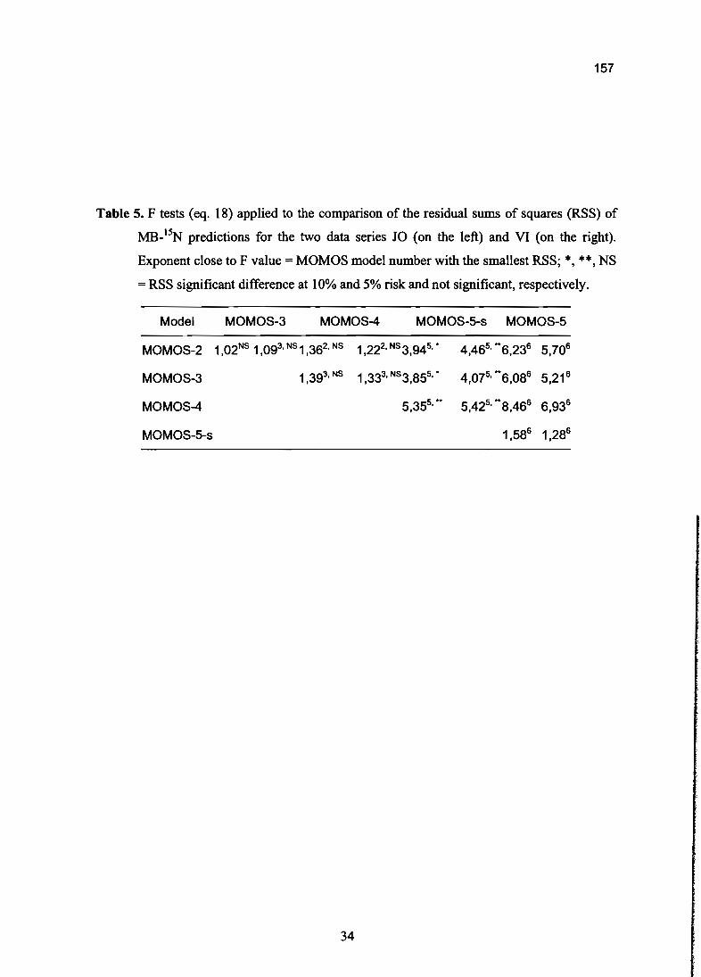
157

Table 5. F tests (eq. 18) applied to the comparison of the residual sums of squares (RSS) of

MB_l~ predictions for the two data series JO (on the left) and VI (on the right).

Exponent close to F value = MOMOS model number with the smallest RSS; ., •• , NS

= RSS significant difference at 10% and 5% risk and not significant, respectively.

Model MOMOS-3 MOMOS-4 MOMOS-5-s MOMOS-5

MOMOS-2 1,02NS1,093, NS 1,362,NS 1 222, NS3 945, • 4465, -6236 5,706, , , ,

MOMOS-3 1,393,NS 1,333, NS3,855, • 4,075, - 6,086 5,21 6

MOMOS-4 5,355, •• 5,425, -8,466 6936,

MOMOS-5-s 1 586 1 286, ,

34

158

tL ~.. .J

MOMOS-4

t .L ~ j

MOMOS-6 e

tt.. L ~ !

_____________________------l

MOMQS-3 e

tL ~ l

MOMQS-S

Figure 1. The five versions of the MOMOS model compared. Ne = total necromass, VL =

labile necromass, VS = stable necromass, MB = microbial biomass, H = humified

compounds, HL= labile humus, HS = stable humus.

35

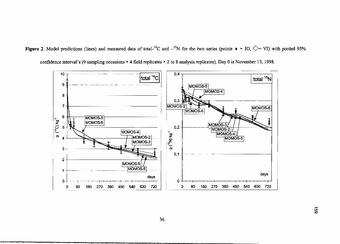
Figure 2. Model predictions (lines) and measured data of total)4C and _lsN for the two series (points + =JO, 0= VI) with pooled 95%

confidence interval's (9 sampling occasions x 4 field replicates x 2 to 8 analysis replicates). Day 0 is November 13, 1998.

total 15N

days

o l ' ! 1 ! ! Il! ! l ' ! l ' '1 ! 1 1

o 90 180 270 360 450 540 630 720

0,2 +-------------e;::::.:::::..:.~ i l 1 ~<...j

0,4 1 1

0,1 +-----~-------------- ---------------1

Cl

~z~~

---- --c=1.W~

--- .__ .. ----- --_.._-------------------_.__._----9

2 l ,_ _ __ ( r -

7 -111111-----------------

days

8 +1------------------

3

1~ ~

~

o 1 ! ' 1 ! ! Il! ! l ' ! l ' ! l ' ! l ' ! 1 !

o 90 180 270 360 450 540 630 720

10 -,----------

----/1Cl 41 ~ .......

_ 6 ln !!lAr'\lAI"'I~ r:: 1

'Cl.:t!

:E 5 -/ 'k ri 1 1•• _ •• __ .1

.....0'1co

36

\l'~''''''''''''''''''~ ",pp .."m III i kW !'iW:U;P4 P. ( QUi W P ,q .M4 4; 4flAP

Figure 3. Model predictions (lines) and measured data of MB}4C and _1~ for the two series (points. =JO, 0= VI) with pooled 95%

confidence interval's (9 sampling occasions x 4 field replicates). Day 0 is November 13, 1998.

____._. -"_·-" __6_-_._

";'c)

~09 1'.u ' __:L UMOMOS-S f--- _ __ _ _

C) O,S ifMOMOS-6i

1M-B-14C] ~ 0,1 0----------- ------------IMB-15NIoC 0,09

C)

O,OS

oco.....

0,7 +I-~---------------------------- --------------

0,6 +If-I---------------

0,5

0,4 1~!".~- ... -

0,3 -1-1--- ~"&.

~ 1f/IMVMV;:)-"! 1~~ ( L0,2 1MOMOS-6 ,

0,1 .J------------------

o • ' , l ' , l ' , l' l" l ' , l ' '1 '1 '

o 90 180 270 360 450 540 630 days

37

0,05 ~-+------------------

0,04

0,03 1/ - \i~ ! ~2 ~

0,02 -u--------~.._.!" ,.

0,01 , \' ,. ~L. .1 :;7

o • ' , l ' , l ' '1 'l" l ' , l ' , l ' , l '

o 90 1S0 270 360 450 540 630 720

Modélisation du fonctionnement d'écosystèmes

161

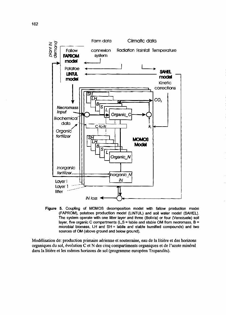
162

Climatic dataFarm data

0connexion Radiation Rainfall Temperature

~Fallow

"0 FAPROM system

-. modeI .. 1

Potatoe .. ,1 ~

LM\I. • SAIe. _

rnodeI modeIKinetic

! corrections

SHIL ., 1 CO2- B

SNecromass '--

Input - -"'\..... L ;9t Organic_C

Biochemical ~

data -/' 11 C-to-N 1 k;

Orgonic1

1

fertilizer SH ,MOMeSL-I 1 1

- BS

1 MadelIl

"- L'- - Organic N

"'-- -lnorganicfertilizer. norganic N

Layer i iNLayer l .--- .-

--- -'

~lifter.i->:

IN toss ~ \....'--'"

Figure 5. Coupling of MOMOS decomposition model with fallow production model(FAPROM), potatoes production model (lINTUL) and soil water model (SAHEL).The system operate with one litter layer and three (Bolivia) or four (Venezuela) soillayer, five organic C compartments (L,S= labile and stable OM trom necromass, B =mierobial biomass, LH and SH = labile and stable humified compounds) and twosources of OM (above ground and belowground).

Modélisation de: productionprimaire aérienneet souterraine, eau de la litière et des horizonsorganiques du sol, évolutionC et N des cinq compartiments organiques et de l'azote minéraldans la litière et les mêmes horizons de sol (programme européenTropandès).

Bilan et perspective

163

164

Photosynthèse

Biomasse aérienne-------, et souterraine 14-----,

Sénéscence

jj 7f\O-CNécromasse

(Ne) .. - - _ ..._. - ~- _. - ...................................... e.~g; ~~ g~g~~; ~~~;~~;~ ~~r

~~~~~~~•.!!'!'••~:::"'!':::~::::::::::~:::::::::::::;::;...of:: :_:.: ~:: :_::::::::::::: :::::

--.:::t:: z::::-:-::~: :.::

......_ , " '..- ;, ·---..·····f'··"'-······ ..········"-l ..····· ··· .. ··~.·................... ::::::::":::::::.:::.::............ e .

"~.""-"""'''.'' .............. ........................"""::::::::::::::::::::.- .

Figure 1. Schéma simplifié du cycle C et N en rapport avec nos travaux (grand carré grisunis =modèles de décomposition MOMOS incluant les entrées en provenance de lasénescence et de la rhizodéposition, petit carré pointillé = nos travaux du modèleTAO-C sur les compartiments d'entrée de la nécromasse, petit carré hachuré =6°proposition MOMOS donnant un rôle central à la biomasse microbienne et à sesparamètres de respiration et mortalité.

La figure 1 permet de situer nos travaux dans l'étude du cycle terrestre du carbone et de

l'azote. La partie grise unie représente les modèles de décomposition, que l'on doit coupler

avec les modèles de production végétale photo-synthétique, production animale et sénescence

pour une simulation plus complète du cycle C et N. Une simulation exhaustive du cycle C

165

réclamerait de prendre en compte aussi les équilibres COl/carbonates dans le cas des sols à

pH alcalin ainsi que les dégagements de méthane des milieux réducteurs. L'approximation de

la figure 1 est valable pour tous les milieux pas trop engorgés et de pH neutre ou acide. Au

niveau de la planète, on considère que les masses énormes de carbone stockées dans les

carbonates terrestres ou océaniques participent peu au cycle du carbone des cycles courts. On

sait que les mécanismes de dissolution/précipitation des carbonates fournissent un bilan nul de

COl (autant de moles adsorbées pour la précipitation que de moles dégagées pour la

dissolution). Les carbonates ne peuvent être un puits ou une source de COl qu'en cas de

changement assez important de l'ambiance physico-chimique (pH, pression partielle de COl,

température) ou biologique (coraux...). D'une façon générale on distingue le cycle du carbone

de la biosphère comme le régulateur à court terme des échanges avec l'atmosphère. Ce cycle

est en cours de perturbation par l'entrée non négligeable dans l'atmosphère depuis la fm du

XIXo siècle, du COl provenant de la combustion des combustibles fossiles, qui s'ajoute au

COl en provenance de la respiration microbienne. La formation des combustibles fossiles

constitue un puits de C étalé sur des millénaires, alors que leur combustion par les activités

humaines est une source de COl pour l'atmosphère en augmentation très rapide. C'est

pourquoi de nombreux programmes de recherche à travers le monde tentent d'évaluer la

réponse de la biosphère à ces changements atmosphériques. Des programmes

complémentaires tentent d'évaluer l'incidence de changements de gestion de la biomasse et

des sols sur la séquestration ou la libération de C atmosphérique. Notre unité de recherche

s'inscrit dans ces programmes dans le cas des sols tropicaux (Cf. Annexe 2).

Le petit carré pointillé de la figure 1 correspond à nos travaux sur le modèle de

Transformation des Apports Organiques (TAO). Ces travaux permettent pour la première fois

de prédire la minéralisation des apports d'après une connaissance élémentaire de leur

composition biochimique (contenu en matières solubles, hémicellulosiques, cellulosique,

ligneuse, minérale et azote). La figure 1 ne comprend que la partie TAO-C du modèle, la

partie TAO-N permet aussi de prédire les transformations plus complexes de l'azote en

provenance de l'apport. En effet, selon ses caractéristiques biochimiques, particulièrement son

rapport CIN, l'apport organique va provoquer une immobilisation de l'azote minéral du sol,

une libération d'azote minéral (pour les plantes mais aussi pour des pertes possibles vers les

nappes phréatiques) ou encore dans certains cas une perte d'azote par volatilisation dans

l'atmosphère. On voit donc tout l'intérêt que présente TAO pour une pratique raisonnée de la

fertilisation organique: éviter les pertes d'azote minéral dans l'atmosphère et l'hydrosphère,

optimiser la croissance des plantes en faisant correspondre les courbes d'absorption d'azote

166

minéral liée à leur croissance et les courbes de fournitures d'azote minéral par TAO-N. Des

travaux complémentaires sont encore nécessaires pour quantifier la réponse du modèle TAO à

des variations édaphiques et climatiques.

Le petit carré hachuré de la figure 1 correspond à nos travaux plus récents sur la comparaison

de modèles de décomposition qui nous ont conduits à la version 6 du modèle MOMOS, le

premier à centrer entièrement la décomposition sur la biomasse microbienne. Jusqu'ici dans

les modèles à compartiments du cycle C, les échanges sont généralement régulés par deux

types de paramètres: des constantes de vitesse (dimension Tl) régulant la sortie des

compartiments, des constantes sans dimension régulant le partage des flux d'entrée des

compartiments avec des sorties multiples de C02. Ces dernières constantes sont souvent

appelées facteur d'efficience: rapport taux de C synthétisé dans un compartiment/taux de C

brûlé en C02. On a pu montrer (autre publication soumise non incluse ici) que les modèles

sont souvent plus sensibles à des fluctuations de ces facteurs d'efficience qu'à des fluctuations

sur les constantes de vitesse (et simultanément aux influences climatiques qui modulent ces

constantes de vitesse). MOMOS-6 comporte uniquement des constantes de vitesse régulant:

(1) les entrées dans la biomasse microbienne depuis les quatre autres compartiments, (2) la

respiration (grandeur mesurable également sur le terrain) et la mortalité de la biomasse

microbienne.

Nous avons précédemment proposé une méthodologie d'utilisation de nos modèles MOMOS

pour la quantification des flux de C à la rhizosphère des plantes actives. Jusqu'ici la plupart

des travaux de quantification de ce type utilisent des expérimentations de cultures de plantes

en atmosphère contrôlée avec marquage isotopique du C02 pour la photosynthèse, puis

mesure du C marqué de la respiration racinaire (difficile à distinguer de la respiration de la

rhisosphère). Notre méthode utilise un marquage préalable du sol par apport de nécromasse

marquée sur sol nu et cultivé. Le modèle est d'abord ajusté sur sol nu avec le traceur

isotopique, puis l'expérience sur sol cultivé permet de quantifier l'apport de C non marqué

depuis les racines vivantes. La nouvelle version MOMOS-6 sera aussi utilisée pour ce type

d'étude (travail en préparation).

La figure 1 est également un schéma très simplificateur du cycle de l'azote. Ne sont pas

représentés de nombreux échanges tels que la fixation symbiotique et non symbiotique, la

volatilisation dans l'atmosphère et l'apport atmosphérique par les pluies ou encore la

rétrogradation d'ammonium dans les feuillets d'argile ou l'entraînement des nitrates par les

eaux. MOMOS-6 couplé avec le modèle SAHEL d'humidité du sol (PR!, Wageningen) et

FAPROM de production végétale des jachères (labo. d'écophysiologie, université d'Orsay)

167

nous a permis de comprendre les processus de restauration de la fertilité par les jachères. Dans

cette simulation, la fixation symbiotique des plantes amélioratrices des jachères est prise en

compte dans les taux d'azote des nécromasses restituées au sol, l'entraînement des nitrates est

pris en compte par une modification du modèle SAHEL. Alors qu'il n'a pas été possible de

déceler des changements significatifs liés à la durée des jachères par les analyses classiques

de C et N au laboratoire, la restauration de la fertilité est simulée par un accroissement du

contenu en C et N des compartiments Biomasse microbienne et Métabolites labiles du modèle

(Fig.1). Le maximum observé de 8-10 ans correspond aux temps de jachère effectivement

pratiqués par les agriculteurs dans ces systèmes de montagne.

Ce travail en cours prend en compte une simulation des compartiments aérien et racinaire des

différentes espèces végétales en compétition pour la lumière, l'eau et l'azote disponible

(modèle FAPROM). Il simule les restitutions organiques et leur transformation dans la litière

et les principaux horizons organiques des sols étudiés. Il prend en compte l'effet des

différences entre les caractéristiques édaphiques des deux sites (Puna bolivienne et Paramo

vénézuélien) ainsi que l'effet des différences de contenus biochimiques des apports sur les

paramètres de fonctionnement du modèle MOMOS-6 (travaux en préparation). L'outil sera

ensuite validé et testé sur d'autres sites pour permettre une meilleure gestion simultanément

de la fertilité des sols et des flux de C au niveau de la planète, conformément aux grands

objectifs de la politique de recherche de l'IRD oùje travaille (Annexe 1).

168

ANNEXES

169

Annexe 1 : IRD

Institut de recherche pour le développementIRD

Un aperçu des grands chantiers de recherche de l'Institut

Une recherche intégrative,de la géosphère et la biosphère

à l'anthroposphère

Avril 2001

Politique scientifique de 1 IRD, Version du 15 mars 2001 1

171

le processus de création d'unités de recherche et d'unités de service à l'IRDa permis de sélectionner quatre vingt dix laboratoires et par là-même d'obtenir,en quelque sorte en retombée de cette évaluation, un descriptif actualisé del'ensemble des compétences de l'organisme.

Un simple regard porté sur cet ensemble fait très clairement apparanre deslignes de force sous-jacentes. Il n'y a rien de surprenant en la matière, dans lamesure où, par nature même, un processus "ascendant" tel que celui qui aété utilisé - demander au milieu de "secréter" des projets à partir de sonexpérience et de son histoire et de les soumettre à une procédure d'évaluationsévère, fondé sur des règles internationalement reconnues - ne peut queconduire à une restructuration cohérente de l'existant. Avec toutefoisl'avantage majeur que nulle critique sérieuse ne peut plus être désormaisportée à cet édifice en phase avancée de reconstruction contrôlée.

Il appartiendra aux instances scientifiques de l'Institut, et en tout premier lieuà son Conseil scientifique, de porter plus loin l'analyse con{oncturelle ainsiamorcée et, à partir de là, de faire des propositions en matiere de politiquescientifique ~ur l'organisme: on attend de ce dernier qu'il suggère des voiesd'évolution a la fois réalistes et audacieuses, permettant à l'IRD de faire denouveaux pas en avant. Une prospective respectueuse de l'existant est en faitun processus de régulation, dont on est en droit d'attendre beaucoup. Il nes'agit pas de bouleverser de façon autoritaire ce que les équipes de l'Institut ­dûment évaluées - savent faire, mais bien de renforcer délibérément les pôlesd'excellence reconnus et de stimuler vers encore plus de compétence etd'efficacité les domaines de qualité encore susceptibles d'être améliorés.

Dans cette perspective prometteuse, il nous a semblé utile de dessiner defaçon explicite le tableau de ce que représente l'IRD aujourd'hui, à partir,précisément, des domaines d'activité de ses actuelles unites. C'est l'objet duprésent document que de fournir cette photographie instantanée del'organisme. Il s'agit bien, au sens technique du terme, d'un " instantané ":l'objet photographié est et demeure en mouvement, et l'image qu'on enproduit ne saurait rendre parfaitement compte, en soi, de sa dynamiqueévolutive. Elle n'en est pas moins précieuse pour permettre d'identifier lestraits spécifiques de l' " être" que l'on cherche à représenter.

Certains se demandent parfois ce qu'est la spécificité à proprement parlerscientifique de l'IRD. Nous ne parlons pas ici de l'ensemble de ses missions,finalisées par sa vocation à être un Institut de recherche au service dudéveloppement. Il s'agit bien, en l'occurrence, de s'attacher à sesparticularités en tant qu'institution de recherche scientifique. le lecteur quiparcourra ces pages avec attention et/ou qui analysera pour son proprecompte le tableau des domaines d'activité de ses quatre vingt dix unités fournien annexe constatera sans difficulté que l'on peut résumer en quelques motsce qui fait la très réelle originalité scientifique de l'Institut.

l'IRD est en fait présent dans deux domaines essentiels de l'analyse del'espace terrestre, qu'il s'agisse de son approche en tant que géosphère, quebiosphère ou qu'anthroposphère: son passé et son devenir. Ses chercheurssont présents dans nombre - si ce n'est la plupart - des grands chantiers quiconcernent la mémoire de la terre: mémoire des climats, mémoire de l'histoireet de la diversification des espèces vivantes, mémoire des peuples, dansl'extrême variété de leurs langues et de leurs cultures. Ils le sont tout autants'agissant de l'évolution de la planète: grandes fluctuations de la croûteterrestre, oscillations et évolutions climatiques majeures, devenir desécosystèmes complexes, grands mouvements de tous ordres affectant lespopulations les plus nombreuses de la planète, phénomènes majeurs en

Politique scientifique de 1 IRD, Version du 15 mars 2001 2

172

termes de santé et de maladies émergentes, etc. Et les chantiers en questionsont tous d'ampleur planétaire en termes de leurs possibles implications.

Travailler au "Sud" - parce que c'est là que résident les peuples "endéveloppement" - est ainsi à la fols une raison d'être de nature" politique"mais aussi une chance scientifique extraordinaire {)Our autant que l'on veuillebien en prendre conscience. Elle nous oblige vis-a-vls des pays partenaires,mais elle nous offre aussi une raison incomparable d'être présents et bienprésents au cœur des problèmes qui sont sans doute parmi les pluspassionnants du siècle commençant. Si nous savons partager cetteopportunité avec nos partenaires du Sud mais aussi avec les institutions derecherche de notre propre pays et, plus généralement, du Nord, n'est-ce pas làune situation à la fois exceptionnelle et particulièrement stimulante? Il est entout cas de notre responsabilité de la cultiver.

Les pages qui suivent illustrent ces quelques propos introductifs.

Politique scientifique de l IRD, Version du 15 mars 2001 3

173

1 - La géosphère

L'IRD contribue à la compréhension des interactions entre les enveloppes solides etfluides qui constituent notre environnement planétaire, depuis la croûte profonde jusqu'àl'atmosphère en passant par la croûte superficielle, les sols, les eaux continentales, lesocéans. Ces interactions, complexes, conditionnent le devenir de la biosphère et del'anthroposphère qui, en retour, sont susceptibles de modifier celui de la géosphère elle­même.

L'IRD est ainsi en mesure, dans cette partie hautement active de la planète, de traiter del'évaluation des ressources mais aussi des risques associés aux phénomènes évoqués.

1 ) Lacroûte terrestre est soumise à la fois à faction de la dynamique profonde de laterre (mouvement des plaques, déformations, transferts de matière depuis les couchesprofondes) et aux processus d'altérations physiques et chimiques de sa surface.

Les principales questions abordées par 1'1 RD sont dès lors:

• la reconstitution de l'histoire et du fonctionnement géodynamiques de régions cibles

• les causes, modes de déclenchement et possibilités de prévision des phénomènesdestructeurs

• l'élaboration de modèles prédictifs, à l'échelle régionale, pour l'exploitation desressources métalliques et énergétiques fossiles

• l'étude des milieux superficiels (aquifères, altération des sols, etc.)

Deux grands chantiers géographiques sont ouverts:

• i) celui du Pacifique Sud-Ouest, où les plaques se rejoignent en un" point triple",lieu où les phénomènes de subduction atteignent une intensité extrême et créentdes risques sismiques et volcaniquesmajeurs

• ii) celui de la partie occidentale du cône sud-américain, où la rencontre de la plaquePacifique et de la plaque américaine comprime le bourrelet des Andes, qui estsoumis de surcroît, en permanence, à une intense érosion et à des altérationssuperficielles physiques et chimiques. Plusieurs grandes villes d'Amérique du Sudsont ainsi sous la menace de risques volcaniques et sismiques majeurs maisd'importantes ressources minérales sont également associées à ces intensesphénomènes tectoniques.

2) Les altérations de la surface de la terre qui résultent des interactions entre sesenveloppes fluides (hydrosphère et atmosphère) se manifestent principalement dans lesol, pellicule superficielle où se concentre la vie. Les interactions des sols avec l'eau desurface, la biosphère (principalement le couvert végétal: plantes et forêts) et le dimatsont au œeur des problématiques de développement, par les ressources qu'ellesconditionnent (agronomie, etc.) mais aussi du fait des risques que l'exploitation humainepeut engendrer vis-à-vis de ces milieux fragiles (pénurie et dégradation de la qualité del'eau, dégradation des sols, désertification, etc.).

En ce qui concerne l'eau, elle est considéréed'un triple point de vue:

i) en tant que ressource renouvelableii) en tant que vecteur (transports liquides, solides, géochimiques)

Politique scientifique de 1 IRD, Version du 15 mars 2001 4

174

iii) en tant qu'agent d'altération et de transformation du sol (interactions avecla géosphère).

La rationalisation de sa gestion (ressources, qualité, usages) est, on le sait, l'unedes conditions absolues du développement durable des pays à faibles revenus.Elle suppose notamment de savoir caractériser et prévoir la variabilité desressources dans l'espace et dans le temps, qui repose sur l'étude locale et lamodélisation régionale des composantes des bassins versants, domaines decompétence reconnue de l'Institut.

Pour ce qui est des sols, ils doivent être étudiés en tenant simultanément comptede l'ensemble des processus physico-chimiques et biologiques qui les engendrentet les modifient en pennanence. L'IRD dispose à ce sujet de bases de donnéespédologiques d'une extrême richesse, que les possibilités nouvelles d'analyse etde traitement numérique permettent de réintégrer utilement dans les études encours.

3) Les interactions des enveloppes terrestres fluides (océan, atmosphère)engendrent des variations du dimat à des échelles temporelles perceptibles parl'homme (de la saison au millénaire): leur étude directe apporte donc de précieusesinformations à des pays dont l'économie, fragile, est particulièrement sensible à cesoscillations. Cependant l'étude des paléo-ctimats (à l'échelle du million d'années) estaussi un moyen de comprendre comment le dmat évolue aujourd'hui en tendance etpeut évoluer dans le futur (la question du réchauffement et de ses composantesanthropiques).

Dans les régions tropicales, la proximité de l'équateur induit de surcroît des phénomènessinguliers (El Nina, la Nina) qui jouent un rôle privilégié dans la dynamique du dimat del'ensemble de la planète.

Les unités d'océanographie physique de l'IRD, qui ont joué un rôle pionnier dans ladécouverte du rôle prépondérant de l'océan tropical dans le dimat, s'attachent àélucider les mécanismes de son couplage intime avec l'atmosphère dans l'océanPacifique et dans l'océan Atlantique. Les impacts de ces variations se marquentprincipalement dans les précipitations, dont la fréquence, l'intensité et le volumedépendent de la circulation atmosphérique à des échelles spatiales locales (lacentaine de kilomètres) et régionales (le millier de kilomètres). Les glaciers andinsconstituent, à cet égard, de précieuses archives des variations des sièclespassés, avant que l'actMté industrielle ne perturbe le système dimatique. Outreces glaciers tropicaux, les coraux, les sédiments continentaux et marins, leursflores et faunes, constituent aussi d'exceptionnels conservatoires dimatiques, surdes périodes couvrant la fin du quatemaire (période holocène).

Ces recherches sont structurées dans des programmes nationaux etintemationaux, auxquels l'IRD s'efforce d'associer étroitement ses partenaires duSud.

Il - La biosphère

Il - La biosphère

Ce n'est qu'au cours des toutes dernières décennies qu'à l'échelle planétaire, au-delàdes clivages identitaires et des particularismes de tous ordres, les hommes ont prisréellement conscience de l'ampleur de la diversité du vivant: de ranimai au végétal, dumicrobe aux grands mammifères terrestres ou marins, du gigantisme fragile des arbres

Politique scientifique de l IRD, Version du 15 mars 2001 5

175

de la forêt amazonienne au milliard de tonnes de chlorophylle produites par lephytoplancton océanique. Avec lJ1 léger décalage temporel (Conférence de Rio surl'environnement et le développement), on a commencé à s'inquiéter sérieusement dudevenir de cette" biodiversité", affectée et menacée par le développement soustoutes ses formes (démographie, industrie, commerce, urbanisation, mouvements depopulations, etc.), et pas seulement, bien entendu, par le développement propre auxpays qu'on désigne sous ce vocable générique. Mais l'inquiétude est dautant plus vivedans les (ou à propos des) pays du Sud que, disposant d'une richesse toute particulièreen la matière (ils recèlent sans doute, à eux tous, les principales ressources de taplanète), ils sont en pennanence confrontés à la tentation, face aux énormes besoinsfinanciers qui sont aujourd'hui les leurs, de la monnayer au plus offrant au risque derapidement la dilapider - et par là même de dilapider une partie significative du.. patrimoine" de l'humanité.

Quatre questionnements majeurs peuvent être identifiés à ce propos; ils sont au <:Xl3lJ"des préoccupations des unités de recherche et de service de l'IRD qui s'intéressentspécifiquement à la biosphère. /1 s'agit :

1) d'une préoccupation d'ordre taxonomique: comment décrire de façon.. systématique" cette biodiversité dont nous ne disposons, tout compte fait, qued'une connaissanceet d'une quantification très partielles?

Le préalable indispensable est l'inventaire des espèces qui composent lesdifférentes biocénoses. Après un travail d'identification (systématique) fondé sur lamorphologie, ces inventaires conduisent à la constitution de collections de micro­organismes, de plantes (herbiers) et d'animaux (nématodes, insectes, poissons,rongeurs). La nécessité de différencier les espèces au niveau génétique etd'analyser leur variabilité intra-spécifique conduit à utiliser en parallèle l'approchebio-systématique et la biologie moléculaire. Plusieurs équipes de l'lADs'investissent dans cette quête, qui peut représenter une fin en elle-même, carmec'est le cas pour les flores des pays tropicaux (Guyane, Polynésie, Afrique) etpour les poissons marins et d'eau douce de ces régions, ou bien être le préalableà la compréhension du fonctionnement d'agro-écosystèmes divers, aquatiques outerrestres. S'interroger sur la notion même d'espèce constitue l'enjeu de plusieursunités de recherche; ceci implique l'exploration des mécanismes de l'évolution desespèces, de leur disparition voire de leur apparition (spéciation).

2) d'une préoccupation de nature physiologique ou fonctionnelle: on peutconsidérer que le gène est la plus petite unité constitutive de la biodiversité.Comment la biodiversité est-elle préservée à différents niveaux d'organisation(génome, espèces, populations, peuplements) ? Ou bien encore, quel rôle joue-t­elle dans la viabilité des écosystèmes? Plus on avance dans l'intégration (du gène àl'écosystème), plus la complexité va croissant. On s'adresse donc, dès que l'onconsidère des populations dans leur milieu, à des systèmes complexes; c'est enleur sein qu'interagissent de nombreux éléments: communautés d'espèces(animales, végétales, micro-organismes), paramètres physico-chimiques du milieu(biotope), activités humaines (usage de tout ou partie des communautés vivantes etdu milieu, impact d'activités connexes (aménagement des territoires et despaysages... ). La question de la résilience de ces écosystèmes, dans leur ensemblemais aussi au niveau de d'lacune de leurs composantes (populations,peuplements..), est cruciale et au cœur de nombreux questionnements scientifiques ­mais aussi d'interrogations politiques. Les projets de plusieurs unités de recherches'intéressent ainsi aux questions de dynamique, de conservation et de valorisation de labiodiversité aquatique, agricole et microbienne.

On peut les présenter en quatre grands domaines :

i) l'étude de la structure et de la dynamique de la biodiversité pour l'amélioration dela conservation, de la gestion et de la valorisation des ressources génétiques:

Politique scientifique de l IRD. Version du 15 mars 2001 6

176

- influence de la structure du génome sur les hybridations interspécifiques ;- mécanismes physiologiques et génétiques de la capacité d'adaptation desespèces (poissons, plantes) à des environnements perturbés (hyper-salinité,pollution, sur-pêche); résistance des graines à la déshydratation et aux bassestempératuresen vue d'améliorer la conservationex situ .. .).- dynamique des flux de gènes spontanés entre espèces cultivées et apparentéessauvages, mais aussi entre variétés cultivées (palmier d'Amérique du sud, manioc,mil et niébé d'Afrique et d'Amériquedu sud, riz, mais du Mexique...);

ii) la recherche biotechnologique de principes actifs ou de molécules valorisables :

- identification de souches de champignons ou de bactéries permettant la bio­dépollution ou la valorisation de sous-produits agro-industriels, y compris dans desmilieux extrêmes;- identification de molécules extraites d'organismes vivants (plantes, animauxmarins...) d'intérêt pharmacologique, cosmétique ou médicinal;

iii) "identification des mécanismes moléculaires et cellulaires qui régulent ledéveloppement des poissons ou des plantes et leurs relations avec leurssymbiotes et parasites :

- compréhension des mécanismes physiologiques et moléculaires qui régulent degrandes fonctions chez diverses organismes vivants (plantes, poissons) ;- l'identification et le clonage de gènes d'intérêt.- la reproduction non-sexuée( apomixie du mais) ;- les interactionsentre les plantes, leurs parasites ou leurs symbiontes.

iv) l'analyse de l'évolution des agro-écosystèmes :

- étude de la structure et de la dynamique de la biodiversité pourl'amélioration de la - conservation, de la gestion et de la valorisation desressources génétiques.- dynamique des sols cultivés à fortes contraintes physico-chimiques (solsacides, salés, basiques) des régions chaudes;- les climats, la physiologie des plantes cultivées et le fonctionnement desag ro-systèmes.

Ces recherches recèlent de nombreux débouchés en tenne d'applications ou d'expertises(définition de stratégies de conservation dynamique et de déploiement des ressourcesgénétiques et des variétés améliorées, identification de souches locales de poissons aptesà l'élevage, etc.).

3) d'unepréoccupation d'ordreéconomique et social: quel rôle cette diversité joue-t-elleet quel intérêt, actuel ou potentiel, représente-t-elle ?

Les ressources renouvelables, liées à la biodiversité exploitable, sont étudiées àla lumière de l'anthropisation, voire de l' artificialisation des milieux terrestres etaquatiques; les contraintes imposées par la .. prédation Il humaine sur des cibles..proies Il sont détenninantes; dans ces ordres d'idée, l'Institut travaille sur dessujets très diversifiés, tels que:

- l'impact des pratiques culturales sur la séquestration du carbone dans les solstropicaux et sur l'élaborationde la fertilité du sol;-l'effet du mode de gestion des agro-systèmes et des pratiques paysannes surl'érosion et le changement d'usage des terres (et réciproquement) ; la pratique dela jachère et celle de la déforestation à des fins d'agriculture font l'objet d'uneattention toute particulière ;

Politique scientifique de l IRD. Version du 15 mars 2001 7

177

- les interactions (déterminantes de la fertilité des sols) entre la faune des solstropicaux, la dynamique physico-chimique de ces derniers et les plantescultivées;- les conflits d'usage;- les transitionsagraireset les dynamiques écologiques;-les stratégies d'exploitation des pêcheurs et leurs interactions avec les espècesocéaniques exploitées (thons tropicaux, sardinelles, anchois... ) et leurenvironnement.

4) d'une préoccupation de nature conjoncturelle et prospective enfin: commentpeut-on mieux observer la biodiversité et en suivre J'évolution ou les modifications?Quels indicateurs (des fonctions combinant plusieurs variables et paramètresmesurables) et quelles méthodologies d'observation sont les plus pertinents(développement des connaissances, conservation, aide à la prise de décision pourla gestion d'activités que fon veut viables à long terme, souci de pourvoir auxbesoins alimentaires des sociétés, prévention et gestion des accidents écologiques,etc.) ? Ces activités qui visent à prédire à partir d'une analyse et d'une représentation(par modélisation) des situations, s'adressent aussi bien aux conséquences desévolutions des techniques d'exploitation qui pourraient être introduites au sud qu'à Bcollecte systématique de données et à l'élaboration d'indicateurs décrivant lesactivités humaines d'exploitation et la réaction des systèmes complexes concernés.Outre l'élaboration d'hypothèses et de théories, les retombées utilisablesimmédiatement pour éclairer la prise de décision en matière de gestion dessystèmes et d'amélioration des productions sont nombreuses.

On peut citer à ce titre les domainesde recherche suivants :

- modélisation écosystèmique des interactions et des dynamiques spatiales desressources renouvelables halieutiques (crevettes marines de Madagascar,poissons migrateurs: thons tropicaux des trois océans, petits pélagiques del'écosystème du Benguela: Afrique du Sud et Namibie, ressources piscicoles desretenuesd'eau et des lacs africains...) ;- pratiques culturales traditionnelles et risques induits par "introduction denouvelles technologies agricoles;- biologie et gestion des populations de ravageurs des cultures (petitsmammifères -rongeurs et insectes d'Afrique de "ouest, d'Amérique centrale etd'Afrique de l'est notamment); modélisation des patho-systèmes des milieuxtropicaux (ex: pathogènes et complexes culturaux maïs-haricots, café-plantesd'ombrage, en Amérique centrale) ;- mise en place à l'échelle régionale d'observatoires et de systèmes d'informationsur les pêches (ex: pêches thonières des océans Atlantique et Indien, pêchescôtières d'Afrique de "ouest et de Madagascar etc.), sur l'évolution qualitative(herbiers en Afrique de l'ouest, Guyane, Nouvelle Calédonie et Polynésie) etquantitative (dynamique des forêts tropicales) du couvert végétal.

III - L'anthroposphère

Illustrant l'impératif de recherche pour les pays du Sud, les travaux programmés ou déjàengagés par les unités de l'IRD se situent à la fois en amont et en aval des actions de

Politique scientifique de 1 IRD, Version du 15 mars 2001 8

178

développement. En aval puisqu'ils s'intéressent aux retombées précises de touteentreprise en direction de la. société. En amont puisque tout programme dedéveloppement devrait passer par une analyse préalable approfondie des modes devie, des représentations qui pennettront ou au oontraire freineront raction projetée.L'histoire passée ne manque pas d'exemples de programmes (irrigation, changementsdans le mode de culbJre, l'éducation ou le système de santé, etc.) qui n'ont pas eu lesrésultats escomptés parce qu'ils ne correspondaient ni à l'attente ri aux possibilitésréelles des populations sur le terrain.

Les recherches en sciences sociales à l'IRD ont beaucoup évolué. Les étudesapprofondies des terroirs qui étaient la. spécificité de l'ORSTOM s'intègrent aujourd'huidans des études d'inspiration comparatiste, rendues plus urgentes par la. globalisationqui homogénéise les problématiques tout en exacerbant les inégalités et lesdyshannonies dans les pays du Sud.

Trois axes principaux illustrent cette nouvelle donne.

1) Problèmes démographiques et de santé

L'IRD suit avec une particulière acuité les évolutions démographiques au moment où Btransition épidémiologique (vers une population moins féconde à l'espérance de vieplus longue) des maladies infectieuses aux maladies chroniques commence à atteindre,bien que fort inégalement, les pays du Sud, en fonction de leur degré d'émergence. ndemeure néanmoins vigilant dans les domaines jadis considérés comme relevant de Bmédecine tropicale, qui bénéficient maintenant des méthodes d'exploration les plusrécentes. Il s'efforce de faciliter sur place, au Sud, l'exploitation des nouveaux outilsgénétiques afin de suivre l'évolution des pathogènes responsables des ~randes

endémies et de comprendre les mutations qui se produisent à un rythme accélére.

L'IRD est particulièrement actif dans le domaine des résistances à la.chimiothérapie, qui risque de se trouver à court dans un proche avenir denouvelles molécules, par exemple dans le domaine du paludisme. Dans d'autresmaladies, accentuées par les bouleversements écologiques qui facilitent lespullulations de rongeurs (leishmanioses) ou les bouleversements des systèmesde surveillance traditionnels (trypanosomoses), il s'agit au contraire d'améliorer lediagnostic précoce ou de trouver, pour la. première fois, des traitements à la foissans danger et efficaces. L'idée d'éradication des maladies a perdu de sapertinence, COITYTle celle d'une méthode unique pour améliorer les performancessanitaires, au profit d'une lutte intégrée qui met en perspective les différentsmoyens connus. L'IRD possède ici un atout majeur: son expérienceentomologique, indispensable pour pondérer, prévoir et apprécier la lutteantivectorielle, composante indépassable du combat contre les grandes endémiesrelevant de ce modede transmission.

L'IRD s'appuie sur 1I1 dispositif de centres de recherche, hérité de la. période desindépendances nationales, qui d'lerche aujourd'hui sa voie entre une fragmentation àl'échelon national et une restructuration à l'échelon de la sous-région. L'IRD valorise làencore sa bonne connaissance des flores et des faunes tropicales, enrichie parl'exploration plus récente des fonds sous-marins, pour participer à la. recherche denouvelles molécules, avec des partenaires industriels, dans le respect des législationsnovatrices et exigeantes qui, actuellement, s'élaborent très rapidement dans ces pays,notamment là où la biodiversité est à la. fois la. plus grande et la. plus menacée, commeen Amérique latine, dans le Pacifique ou à Madagascar.

Dans le cas du Sida, dont il n'est pas nécessaire de souli9ner l'importance dansles pays du Sud, l'IRD participe à "effort sans précédent initié par certains d'entreeux, comme la Thaïlande ou le Sénégal, pour fournir aux populations concernéesdes traitements reflétant l'étatactuel de la recherd1e, et ses chercheurs suivent deprès une expérience modèle qui bouleverse les circuits et les mécanismes

Politique scientifique de l IRD, Version du 15 mars 2001 9

179

traditionnels du rnard'lé des médicaments. C'est l'occasion également de suivre lal'éfonne des systèmes de soins, qu'il s'agisse des hôpitaux ou des dispensairesde villages, après l'abandon d'une idéologie mettant l'accent exclusivement sur lescentres de santé primaire, en poussant l'analyse au niveau local, qui permet demieux percevoir les dysfonctionnements administratifs et techniques.

2) Problèmes posés par les mégapoles

Là encore, l'analyse comparée permet de balayer les multiples problèmes posés par legigantisme des villes et surtout de oonfronter les solutions improvisées ou planifiéesdans les différents oontextes. Les acteurs régionaux et sous-régionaux sont sollicités pardes forces oontradictoires, celles notamment qui correspondent aux demandes de lasociété civile et des divers groupes de pression, en particulier ceux qui relèvent du"développement de substitution n (ententes criminelles, mard'lés d'armes ou toutsimplement corruption). Les multiples problèmes des villes (mobilités de leurs citoyens,transports, surveillance des observatoires urbains) sont également pris en compte. Ladynamique d'un salariat informel qui ne suit pas les schémas de l'économie classiquebénéficie là encore d'une approche comparatiste.

Les migrations entre les villes d'individus ou de groupes souvent organisés enréseaux semi-officiels nécessitent, pour être observées et comprises, la complicitéavec le .. terrain n, instruite par une longue fréquentation des partenaires. Cesmigrations peuvent revêtir des aspects originaux qui défient la catégorisation,comme la djihad économique des Mourides, à cheval sur l'Europe et l'Afrique del'Ouest, et aux Etats-Unis.

3) Problèmes liés à la mondialisation

Soulignons d'abord les conséquences socio-anthropologiques et économiques debouleversements qu'elle induit et dont il est difficile de délimiter les effets puisqu'ils sefont également sentir dans le domaine de la santé, déjà évoqué plus haut.

Un thème majeur, en quelque sorte en miroir de la mondialisation, est celui desrevendications identitaires, avec leurs multiples variantes, en deçà ou au-delà du cadrede la nation traditionnelle: religieuses, nationales, traditionnelles, ou encore ethniques oucommunautaires. Dans cet éventail, le biologique s'associe et se mêle au culturel, et lescritères plus naturalistes, de couleur de peau ou de type de métissage, s'associent àdes critères plus culturels: langue, mythes et histoire. L'archéologie, fût-elle préhistorique,et tout à la fois la linguistique explorent les racines vraies ou prétendues de ces identitéset permettent, en même temps, d'explorer la diversité des systèmes de langue ou deparenté, de contribuer parfois même, par exemple pour la linguistique, à la recherche surl'acquisition du langage (langues amérindiennes) ou de certains comportements sociaux.La recomposition des territoires, particulièrement active dans certaines grandes régionsdu globe comme l'Amazonie (où l'IRD est activement présent), est une autre façond'envisager la dynamique de ces revendications identitaires.

Les recherches en économie ne peuvent ainsi se résumer, dans ce nouveau contexte, àce qu'on appelait hier l'économie du développement, en pleine redéfinition et à larecherche de nouveaux modèles plus prédictifs et plus performants. Elles portent, entreautres, sur une analyse de la pauvreté visant à cemer de plus près une réalité multiformeet à distinguer les points d'ancrqge possibles d'un dispositif destiné à renforcer ou àpermettre l'action régulatrice des Etats nationaux. Elles mettent en évidence la nécessitéde disposer de données actualisées, aussi précises que possible, afin de mettre enplace les dispositifs de taxation et d'indexation nécessaires à des économies nationalesprises dans les filets de la globalisation. La oonnaissance des terroirs permet, là encore,

Politique scientifique de l IRD. Version du 15 mars 2001 10

180

de suivre de façon réaliste les solutions ahematives liées à toutes les formes de la. microfinance.

La recherche en économie de l'IRD est particulièrement attentive aussi à des facteurs nonmarchands, comme les facteurs d'éducation et de santé, selon une perspective prochede la. Banque mondiale, qui encourage aujourd'hui des projets en ce sens. Un axenouveau est la recherche, en sciences de l'éducation, sur les performances de l'école oude l'apprentissage pour permettre aux jeunes de se préparer à une activitéprofessionnelle et de trouver dans la vie la légitime satisfaction de leurs besoins.

IV - Les systèmes complexes

Ce rapide survol des grands domaines de recherche de l'IRD resterait incomplet siquelques mots n'étaient dits

• d'une part des recherches qui empruntent à deux ou trois des domaines ci-dessusévoqués, recherches par nature multidisciplinaires et que l'on peut, pour nombred'entre elles, rattacher au concept d'écosystème

• d'autre part du recours des équipes de l'Institut à des disciplines ou à destechnologies permettant de " prendre du recul" par rapport au tenain : les processusde modélisation et les technologies spatiales.

1) Les écosystèmes sont à la. base de l'alimentation et assurent une part importantedes revenus des pays en développement. Cependant nombre d'entre eux presententaujourd'hui des signes inquiétants de fragilisation ou de surexploitation. Ainsi l'évolutionde l'environnement climatique et ses conséquences sur les ressources en eau peuvent­elles avoir des répercutions directes sur leur durabilité. A l'inverse, mal gérés ousurexploités, les écosystèmes peuvent avoir une influence néfaste sur l'environnementet le dirnat, susceptible d'aller jusqu'à des effets "catastrophiques" (désertification,dégradation irréversible des sols ou des rivages, etc.).

L'objectif poursuivi par les unités de l'IRD est de comprendre le fonctionnement deces écosystèmes naturels, exploités ou exploitables, afin daider à la.rationalisation de leur gestion durable. Ceci implique de connaître leur histoirenaturelle ainsi que leurs interactions avec les variations du milieu environnant(climat, ressource en eau, pression anthropique, etc.).

2) La modélisation des systèmes complexes est un outil en plein essor, qui faitappel à des méthodes mathématiques et à des systèmes informatisés spécifiques.Ces méthodes s'appliquent particulièrement à la. simulation et à l'étude des processusde fonctionnement dynamique de la. biosphère ou encore aux phénomènes interactifsimpliquant simultanément géosphère, biosphère et anthroposphère.

L'IRD a été très actif dans le passé pour l'observation des milieux physiques etdes sociétés des pays du Sud, accumulant ainsi un capital peut-être unique aumonde d'observations répétitives sur ces milieux et ces peuplements. Presquetous les domaines de recherche pratiqués à l'Institut sont impliqués, du dirnat auxépidémies en passant par le plancton et la pêche. L'état de ces données estvariable. Leur gestion pose, de façon générale, des problèmes d'inventaire,d'identification, de localisation, de numérisation, de contrôle de qualité et surtoutd'usage croisé. Le développement de la modélisation devrait permettre de valorisercet exceptionnel conservatoire de données.

Politique scientifique de 1 IRD, Version du 15 mars 2001 11

181

3) Presque tous les champs scientifiques de l'IRD relèvent pour partie de l'observationspatiale. Des laboratoires spécialisés de "télédétecton" ont ainsi été créés, qui offrentdes services et des produits aux programmes de recherche et répondent à desdemandes opérationnelles de nos partenaires. Les sources de données spatiales sesont multipliees ces dernières annees, les techniques, les matériels, les logiciels ontrapidement évolué. Un grand avenir semble aujourd'hui promis à ces procédés,particulièrement adaptés à la surveillance globale des zones tropicales difficiles d'accès.

Politique scientifique de l IRD, Version du 15 mars 2001 12

182

INSTITUT DE RECHERCHEPOUR LE DEVELOPPEMENT(lRD)

183

Dossier de bilanJanvier 2004

(rappeler le numéro et l'intitulé de l'unité)(nom du directeur de l'unité)

Il - BILAN DE L'UNITE

Mémoire, de vingt pages maximum (interligne simple; police" times " ; taille 12), rédigé sur

papier libre qui :

1) rappelle brièvement les objectifs de l'unité;

2) présente le rapport d'activité;

3) précise les prolongements envisagés dans le cadre de l'appel à propositions pour lerenouvellement ou la constitution d'unités de recherche et d'unités de service au titre del'année 2005.

184

Il - BILAN DE L'UNITE 041 :SEQUESTRATION DU CARBONE DANS LES SOLS TROPICAUX

1. Objectifs de l'Unité

L'objectif scientifique général de l'UR041 (sigle UR SeqC) est d'étudier (i) le niveau, ladynamique et les processus de la séquestration du carbone (C) dans les sols pour diversagroécosystèmes tropicaux, et ce, à différentes échelles spatiales, de la parcelle à la régiongéographique ou administrative (phase 1 de l'UR), (ii) l'économie du C séquestré (phase 2 del'UR).Les objectifs scientifiques spécifiques affichés en 2000 par l'UR SeqC, et qui, de fait, ontcomplètement structuré l'activité de l'UR041 depuis 2001, peuvent se résumer ainsi:

1. Mesurer, à l'échelle parcelle, les effets du mode d'usage des terres ou d'alternativesd'itinéraires techniques sur la « séquestration du C dans le sol». Ceci implique desmesures quantitatives des stocks de C dans le sol et de ses variations, des flux de gaz àeffet de serre à la surface du sol (C~ et N20 exprimés en équivalents C-COÛ et, danscertains cas, du C érodé hors parcelle.

2. Analyser, à l'échelle parcelle, les déterminants édaphiques (type de sol, minéralogie,texture, structure), agronomiques (niveau, qualité et localisation des restitutionsorganiques, travail du sol) de cette séquestration et les processus mis en jeu, enparticulier, la forme de C séquestré et la « protection» de ce C contre laminéralisation, avec, en particulier, le rôle spécifique de la faune du sol dans cetteprotection.

3. Modéliser, en laboratoire et à l'échelle parcelle, la dynamique de décomposition de C(et N) restitué au sol ou du C-sol.

4. Spatialiser à différentes échelles le stock de C actuel (phase 1) afin de pouvoir, àl'avenir (annoncé pour phase 2 de l'UR et objectif 5), simuler par modélisation spatio­temporelle, les dynamiques des stocks de C selon différentes alternatives de gestiondes terres à ces mêmes échelles.

5. Evaluer le coûtfbénéfice du C séquestré (annoncé pour phase 2005-2008 de l'UR).

Ces objectifs scientifiques spécifiques avaient été regroupés en 3 axes :

Axe 1. Déterminants et processus de la séquestration du C dans le sol à l'échelleparcelle (objectifs 1,2 et 3).Axe 2. Spatialisation des stocks actuels de C des sols (objectif 4).Axe 3. Economie de la séquestration du C dans les sols tropicaux (objectif S).

Les agrosystèmes sélectionnés initialement l'ont été sur la base des 2 critères suivants :être représentatifs de grands modes de gestion des terres en milieu tropical : pâturages,cultures annuelles ou semi-pérennes (canne, banane), agroforesterie, plantation sylvicole(annoncée seulement pour phase 2 de l'UR),être, a priori, potentiellement « séquestrants » : « semis direct» en cultures annuelles, nonbrûlis de la canne à sucre, restauration des prairies plantées dégradées, pratiques agro­forestières à forts niveaux de restitution organique.

Les trois implantations secondaires initialement choisies (Martinique, Brésil, Kenya)permettaient, a priori :

2

185

d'évaluer le mode d'usage des terres ou les changements d'itinéraires techniques décritsci-dessus sur la séquestration du C à l'échelle parcelle:

• au Brésil: restauration pâturages, non-brûlis de la canne à sucre avant récolte,pratiques de « semis direct »,

• au Kenya: pratiques agro-forestières,• à la Martinique: comparaison de divers modes d'usage des terres.

d'évaluer certains déterminants ou processus de la séquestration du C conune :• à la Martinique : effet du type de sol (texture, minéralogie) et de la faune du

sol.

Un chantier nouveau, Madagascar, qui devrait devenir une implantation en phase 2, afortement émergé à partir de 2003, et quelques autres chantiers très secondaires ont été aussiconsidérés au cours de la phase 1 conune le Bénin (valorisation de données anciennes) ou leBurkina-Faso (acquisition de données en cours sur essais longue durée de Saria).

II. Bilan en résultats scientifiques de l'UR SeqC (2001-2004)

ILA. La définition de la « séquestration du C dans les sols » selon l'UR SeqC

La notion de séquestration du C est directement issue de la problématique de l'effet de serredonc de la diminution de la concentration de gaz à effet de serre (GES) de l'atmosphère, soitpar diminution des émissions soit par augmentation du stockage de ces GES dans différentscompartiments de la planète, entre autres, les écosystèmes continentaux. Par ailleurs, lamajorité des travaux portant sur la « séquestration du C dans les sols » considère le termeséquestration comme strictement équivalent au terme « stockage », ce que nous contestons,car, sinon, aucune nécessité d'avoir deux termes différents pour un même processus. Laréflexion menée dans l'UR SeqC nous a conduit à proposer une définition sensiblementdifférente des définitions habituelles (Bernoux et al., 2004), qui :

ne prend en compte, concernant le C stocké dans le sol que celui issu directement ouindirectement (via la plante) de l'atmosphère (C-C02) et non pas l'ensemble des formesde stockage de C dans le sol qui peuvent avoir d'autres origines, telles que un apport de Cfossile (composts urbains, etc.) ou le C perdu ou déposé à la parcelle lors du cycleérosion-sédimentation (processus de transfert de C dans le paysage et non de fixation enprovenance de 1'atmosphère),considère que la notion de séquestration de C doit être étendue à l'ensemble des flux GES,que ceux-ci soient carbonés (C02, CH4) ou non (N20), mais tous exprimés en« équivalents C- CO2 » en prenant en compte leur potentiel de réchauffement global relatifà C02 (échelle séculaire) : 23 pour CH4 et 296 pour N20.

La «Séquestration du Carbone dans le Sol » ou encore «Séquestration du Carbonedans le système Sol-Plante » pour un agroécosystème donné, en comparaison avec unagroécosystème de référence, et pour une période et une surface données, doit êtreconsidérée comme le résultat du bilan net, exprimé en équivalents (eq.) C-C02 oueqC02, de tous les flux de GES, à l'interface sol-plante-atmosphère du site de mesure.

L'acceptation de cette définition pour la «Séquestration du C dans les sols », due à unchangement d'usage des terres ou une modification des itinéraires techniques, implique doncles mesures suivantes pour l'estimation de bilans de « C séquestré », pour un espace et unedurée donnés:

3

186

variations du stock total de C des sols et, si possible, la part correspondant au C déposé ouérodé et du C soluble (ruisselé et lixivié), afin d'en déduire la part du C séquestré(correspondant strictement à la fixation de C-C02) .variations des flux des autres GES, en particulier CI-4 et N20.

B Tempso A

1 lJ. C f••••••••".v.~.~...n • • • • • _ ••••~...... . 8. C

1 à A C= D·:::~;~::; •lJ. C = Synchronie

.."~u.."'Cl

~o<ii '----t---"1----"-------,r--

t.C-plallte (p.a.)t. C-plante (racine)t.C- litièreeq.t.C-gaz (CH. , N20 )t.C-Solt. C-solublet.C-particuiaire

C~ble

i JSyst Conv . to Syst. Amélioré t.

Figure 1. Flux et compartiments à prendre en comptepour les bilans de C séquestré

Figure 2. Comparaisons des approchesdiachroniques et synchroniques

La figure 1 résume les compartiments et flux à estimer dans l'idéal pour atteindre ces bilansde flux de GES à l'échelle du système sol-plante. La figure 2 explicite l'importance du Cérodé, généralement non pris en compte, dans l'estimation réelle du C séquestré (cf. lIA.).

Mais avant d'entrer dans les résultats détaillés de la séquestration du C, nous avons tentéd'estimer le potentiel de stockage de C d'un sol pour une grande diversité de situationspédologiques tropicales .

II.B. Les différentes approches du bilan de la « séquestration du C » dans les sols

II.B.l. Le potentiel de stockage de C dans les sols tropicaux

Nous présentons ici essentiellement les résultats obtenus à la Martinique, implantation choisiepour permettre d'atteindre ces résultats , puisque sur une superficie très faible on peutrencontrer des systèmes sol-plante très diversifiés, tant sur :

le plan pédologique (minéralogie et texture) avec les grands types minéralogiques de solstropicaux: à argile 1: 1 (kaolinite et halloysite, de type ferrallitique) , à argile 2 :1(smectite, de type vertique), à minéraux amorphes comme les allophanes (de typeandique) (Fig. 3)le plan agronomique, avec des modes d'usage des terres très variés: cultures annuelles,pérennes et cultures prairiales (Fig. 4) .

La figure 3 (thèse en cours Venkatapen) montre, toutes situations agronomiques confondues,que, pour une texture donnée (teneur en argile), (i) les sols à caractère andique marquéprésentent les stocks de C (O-IOOcm) les plus élevés, (ii) pour les autres minéralogies, il existeune corrélation positive entre le stock de C et la texture du sol , résultat bien connu par ailleurs(Feller & Beare 1997).

MARTINIQUE

Envi ron 100SItuation sétud iées

JO 600 10 100

Teneur &ft argiles ('

Figure 3. Effet de la minéralogie et de la texture sur lesstocks de C des principaux types de sols de la Martinique

4

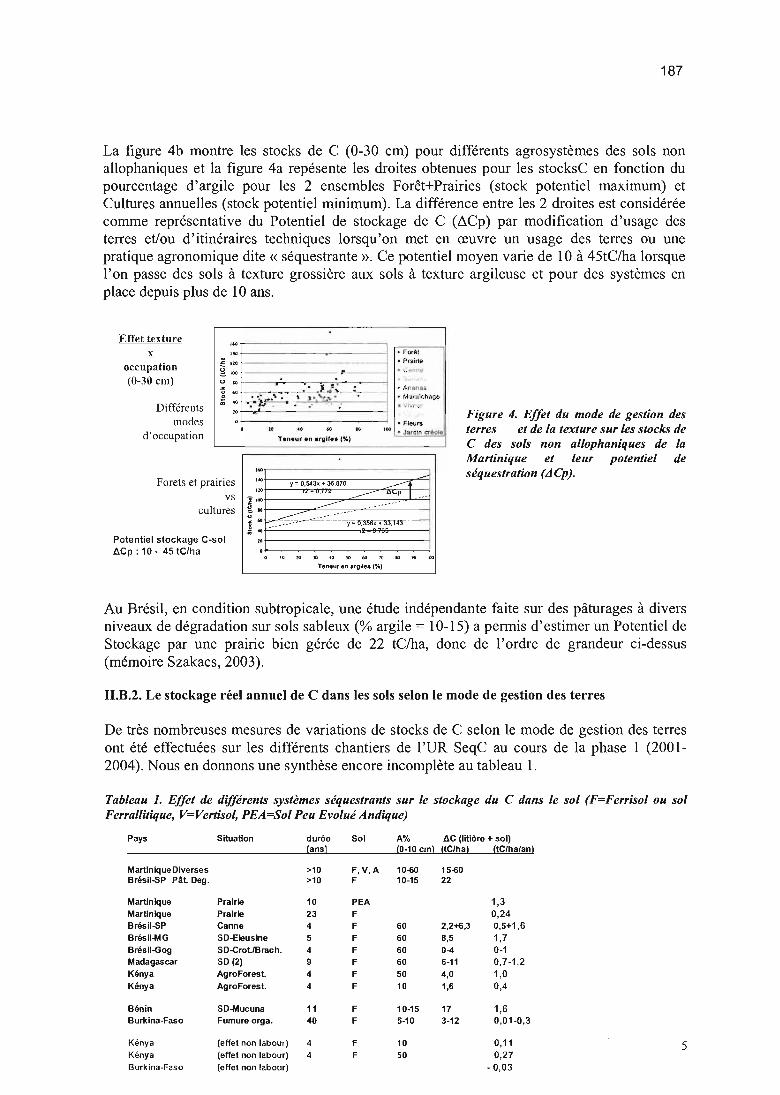
187

La figure 4b montre les stocks de C (0-30 cm) pour différents agrosystèmes des sols nonallophaniques et la figure 4a repésente les droites obtenues pour les stocksC en fonction dupourcentage d'argile pour les 2 ensembles Forêt+Prairies (stock potentiel maximum) etCultures annuelles (stock potentiel minimum). La différence entre les 2 droites est considéréecomme représentative du Potentiel de stockage de C (LlCp) par modification d'usage desterres et/ou d'itinéraires techniques lorsqu'on met en œuvre un usage des terres ou unepratique agronomique dite « séquestrante ». Ce potentiel moyen varie de 10 à 45tClha lorsquel'on passe des sols à texture grossière aux sols à texture argileuse et pour des systèmes enplace depuis plus de 10 ans.

Figure 4. Effet du mode de gestion desterres et de la texture sur les stocks deC des sols non allophaniques de laMartinique et leur potentiel deséquestration (ACp).

,..'" • F oré l

s: '" - • Prairieg '"

- " ,.o;r.4I'

0 " _ _ _.'~ . _ :. .1}~- ;-:--~ • Anen a su ..0

R~"\ ':'''''''''," • M dl"lli(;ht\ge,;; " . .---:-- - : ·-,; r. 1

",• Fleurs, 10 " .. " '" • J lIrdîrl ct 60f0

Teneur en argile. (%)'------- - --

'60

'" Y - O,543x ...36,870 ......------t 1'''' -

--------

u~p

~," -- ~ . . , .

»> ---- --10 »> _.- ---u

J60

•• " ~ •• _. J- Y'" U.,JOOX ... ,J..), l~J..'",,

" ro " " " 60 " '" .. '"Teneur en argiles (%)

Forets et prairiesvs

cultures

Différentsmodes

d'occupation

xoccuQation(0-30 cm)

Potentiel stockage C-soiL\.Cp : 10 - 45 tC/ha

Effet texture

Au Brésil, en condition subtropicale, une étude indépendante faite sur des pâturages à diversniveaux de dégradation sur sols sableux (% argile = 10-15) a permis d'estimer un Potentiel deStockage par une prairie bien gérée de 22 tClha, donc de l'ordre de grandeur ci-dessus(mémoire Szakacs, 2003).

II.B.2. Le stockage réel annuel de C dans les sols selon le mode de gestion des terres

De très nombreuses mesures de variations de stocks de C selon le mode de gestion des terresont été effectuées sur les différents chantiers de l'UR SeqC au cours de la phase 1 (2001­2004). Nous en donnons une synthèse encore incomplète au tableau 1.

Tableau 1. Effet de différents systèmes séquestrants sur le stockage du C dans le sol (F=Ferrisol ou solFerrallitique, V=Vertisol, PEA=Sol Peu Evolué Andique)

Pays Situation durée Sol A% ll.C (litière + sol)(ansl (0-10 cm) (tClha) (tC/ha/an)

MartiniqueOiverses >10 F,V,A 10060 15060Brésil-SP Pât. Oeg. >10 F 10-15 22

Martinique Prairie 10 PEA 1,3Martinique Prairie 23 F 0,24Brésil-SP Canne 4 F 60 2,2+6,3 0,5+1,6Brésll-MG SO-Eleuslne 5 F 60 B,5 1,7Brésil-Gog SO-Crol/Brach. 4 F 60 0-4 0-1Madagascar SO (2) 9 F 60 6-11 0,7-1,2Kénya AgroForest. 4 F 50 4,0 1,0Kénya AgroFores!. 4 F 10 1,6 0,4

Bénin SO-Mucuna 11 F 10-15 17 1,6Bur1<ina-Faso Fumure orga. 40 F 5-10 3-12 0,01--0,3

Kénya (effet non labour) 4 F 10 0,11 5Kénya (effet non labour) 4 F 50 0,27Burkina-Faso (effet non labour) - 0,03

188

Les alternatives séquestrantes testées sont des effets:prairie derrière cultures annuelles (Chevallier et aI.2004),canne à sucre non brûlée avant récolte (thèses de De Luca et Campos),divers systèmes Semis direct (sans labour) dans Couverture Végétale (systèmes SCV)(thèses en cours Metay et Razafimbelo),agroforesterie (Albrecht & Kandji, 2003),faible à forte fumure organique (thèses en cours Hien),

ceci pour des sols à texture grossière ou fine (% argile inférieure à 15 ou supérieure à 50), etpour des durées variant de 4 à 40 ans.

De manière générale on note que, toutes situations agro-pédologiques confondues, lesaccroissements annuels de stocks de C (~C t/haJan) sont compris entre °et 1.7 tC/haJan. Il estprématuré d'aller plus loin actuellement dans la hiérarchisation des facteurs à l'origine de cetaccroissement, entre les déterminants climatiques, pédologiques ou culturaux (en particulier,durée de la pratique et niveau des restitutions organiques au sol), n'ayant pas encore fait lasynthèse de toutes les données.On peut toutefois constater que:

pour les sols argileux, les valeurs les plus élevées (qui doivent se rapprocher du potentielde séquestration) sont comprises entre 1,0 et 1,7 tC/haJan . Pour atteindre la valeurmoyenne du potentiel estimé ci-dessus à environ 45tC/ha, il faudrait donc unaccroissement linéaire durant 45 ou 25 ans respectivement. Autrement dit, le palier où lesstocks de C restent à l'équilibre, se situe après environ 30-40 ans de pratique pour ces solsargileux,pour les sols sableux, les accroissements varient (hors fumure organique) de 0,4 à 1,6tC/haJan et la durée nécessaire pour atteindre le potentiel (l0 tC/ha) se situerait donc entre25 et 7 ans, donc beaucoup plus faible que pour les sols argileux,la fumure organique (sur sol sableux) ne constitue pas une pratique séquestrante trèsintéressante avec des valeurs comprises entre 0,01 (apport annuel de 5t fumier/ha/an) et0,3 (apport annuel de 40t fumier/haJan) tC/haJan. (La dynamique plus précise de cestockage est en cours d'étude),l'effet du seul non travail du sol sur le stockage du C dans le sol (par protection de la MOcontre la minéralisation) est pratiquement nul en sol sableux avec fumure organique (-0,03tC/haJan) mais non négligeable en agroforesterie aussi bien sur des sols sableux (0, IltC/ha/an) qu'argileux (0,27 tC/haJan)

Il.B.3. Le niveau du C érodé et son importance dans l'estimation du C séquestré

Nous avons évoqué ci-dessus que le C érodé ou déposé au niveau d'une parcelle, ne devraitpas entrer dans le bilan de C séquestré dans le sol, car il s'agit d'un simple transfert de C dansl'espace (d'une parcelle à une autre, voire aux sédiments fluviaux, lacustres ou marins) et nond'une capture de C-C02 atmosphérique par le système séquestrant (Feller et al. 2001 ,Bernoux et al. 2004). Or, de fait, notamment dans les études menées en synchronie(comparaison au même moment d'une parcelle sous système séquestrant d'âge X et d'uneparcelle témoin supposée représentée la parcelle X au temps °du système), les valeurs de ~Cmesurées et considérées comme du C séquestré peuvent être entachées d'un erreur due à laprise en compte de C érodé et/ou déposé sur la parcelle pendant l'échelle de temps considéré.Ceci est schématisé sur la figure 2.Supposons que l'on ait suivi l'accroissement de C chaque année sur la parcelle à systèmeséquestrant (approche diachronique), on aurait trouvé ~AC. Mais en fait pour ne pas attendrede nombreuses années que le système se différencie, on utilise une approche synchronique en

6

189

prélevant 2 parcelles différentes déjà différenciées. Il se peut que le résultat ~BC soit égal à~AC, mais bien souvent il peut être supérieur. Une des raisons en est que le « témoin », nerecevant justement pas de MO , soit très sensible aux processus d'érosion et qu'un partie de~BC soit due à une perte par C érodé.Il nous a donc paru essentiel de mener quelques études à ce sujet pour avoir une idée duniveau des pertes les plus probables en C érodé sur des sytèmes conventionnels. Pour cecinous avons eu une triple démarche:

a) faire émerger des données déjà existantes, publiées ou non , par l'organisation en 2003d'un séminaire international sur le sujet et dont les principaux résultats seront publiésdans un N° spécial de la collection « Advances in Soil Science» (Roose et al. , encours),

b) faire la synthèse de données IRD anciennes ou récentes mais non publiées sous cetangle, en particulier celles de notre collègue E. Roose,

c) faire quelques mesures sur nos situations actuelles.La synthèse est en cours (Roose et Barthès, en rédaction), nous en rapportons ici quelquespremiers résultats schématisés sur la figure 5. Toutes situations confondues, le C érodé estglobalement proportionnel à la perte en terre avec les valeurs les plus élevées pour les solsmaintenus « nus» (1,2 à 3 tC/ha/an), puis les sols sous cultures annuelles (0-0,4 tC/ha/an)avec une situation exceptionnelle en Côte d'Ivoire (1,8 tC/ha/an), et des valeurs faibles à trèsfaibles (0-0,2 tC/ha/an) sous forêts, savanes ou cultures paillées.Autrement dit, lorsque l'on considère les cultures annuelles comme le témoin par rapport àune pratique séquestrante (Fig. 2), la valeur ~BC mesurée en mode synchronique supposéeêtre la valeur du C, peut conduire à une surestimation de 0-0 ,4 tC/ha/an (moyenne 0,3) du Créellement séquestré, une valeur non négligeable par rapport aux niveaux espérés pour laséquestration du C.

Erosion du carbone sur une gamme de sols tropicauxsols Ierrauinquee. fenvgl neux el verûso ts. 5 è 70% d'arg ile. pluviosité de 650 .fi2500 mm arr!

Influence de l'érosion: nette surtoul auxfortesérosions

r·O'- (lUe pour~ <0.5)

0

0

--0

~ D

o sols nus

oo 5(} 100 150 200

Erosion(th.1 an·')

a c:utturuannueUes

.. forêts ,savanes,culturespaDl6es

Figure 5. Effet de l'occupation des terres sur le niveau del'érosion et les stocks de C érodé.

II.B. 4. Compléter le bilan du C séquestré par la mesure des flux de CH4 et N20

Nous avons vu en ILl que la notion de séquestration du C devrait prendre en compte aussi lesflux des autres GES que le CO2 (estimé par les variations de stocks de C organique du sol), àsavoir C~ et N20 . Il est en effet important de s'assurer qu'une pratique dite « séquestrante »par rapport au stockage du C dans le sol, ne conduit pas, par ailleurs, à des émissions directesou indirectes accrues d'autres GES, tels que C~ et N20 , les GES dominants avec CO2•

En effet quelques données de la littérature, pour les milieux tempérés (USA), semblentindiquer, par exemple, que la pratique du non labour peut conduire dans 50 % des cas à desémissions plus élevées en N20 que le système conventionnel avec labour (cf. article desynthèse de Six et al., 2002).Etablir des bilans annuels de GES par des mesures directes au champ est extrêmement lourd àfaire et donne des résultats avec une très grande variabilité que l'on ne sait pas toujours bien

7

190

expliquer. Néanmoins il est essentiel de mettre en œuvre ces études mais elles ne peuvent êtreconduites que dans un nombre limité de sites.Une telle approche a été faite ici dans les cas suivants:

effet du non-brûlis de la canne à sucre au Brésil (Etat de Sào Paulo),effet d'un système SCY (rotations riz-crotalaire et soja-bracchiaria) au Brésil (Etat deGoias),effet de jachères traditionnelles et améliorées (agroforesterie) au Kenya.

Nous rapporterons seulement des résultats synthétiques mais encore provisoires, ceux-ci étanten cours de dépouillement.

a) Système SCY au Brésil (thèse en cours Metay)Le stockage de C supplémentaire sur ce site sous l'effet du système SCY testé est del'ordre de 1 tC/ha/an pour les 4 premières années. Ce stockage s'accompagne-t-il ou nonde modification des flux de CH4 et N20?

Les mesures de GES au champ actuellement disponibles correspondent à la période la plusimportante de l'année, de la fin de la saison sèche au début de la saison sèche suivante.C'est au cours de cette période que les risques d'émission de C~ et N20 sont les plusgrands : après apport d'engrais minéral, au début de la décomposition de la plante decouverture (graminée ou légumineuse) ou encore lorsque le sol est engorgé.Outre les mesures de flux de GES à la surface du sol (mesures quotidiennes àhebdomadaires), ont été collectées aussi systématiquement la température et l'humidité dusol, les teneurs en nitrates et la production in situ de CO 2 et N20 pour les horizons 0-10 et10-30 cm) . La teneur en eau associée à la densité apparente et réelle du sol permet lecalcul de la porosité occupée par l'eau en % de la porosité totale (WFPS). On admetgénéralement que les conditions favorables à l'émission de N20 sont des valeurs de WFPSsupérieures à 60 % associées à des teneurs fortes en nitrates .Les résultats obtenus montrent que:Pour N20, le niveau des flux est extrêmement faible et non significativement différententre le système SCY (SO) et le système conventionnel avec labour (OFF). Ainsi, lesémissions sont pratiquement toutes inférieures à 19 N- N20 /jour, valeur considéréecomme la limite inférieure d'une émission significative (Fig. 6). Ceci s'explique par à lafois des valeurs de WFPS pratiquement toujours inférieures à 60 % et de faibles teneurs enNO)' du sol (de 0 à 12 mgN/kg sol). Ceci tient au fait que bien que ces sols soientargileux, ils se comportent pratiquement comme des sols sableux suite à leurmicrostructure très développée et stable dite « en poudre de café ». Pourtant, les valeurs deproduction de N20 in situ ne sont pas négligeables, mais , pratiquement, aucune donnée dela littérature ne fournit de comparaison entre niveau de production in situ et flux à lasurface du sol. Une étude en laboratoire est en cours pour préciser ces différents aspects.

Émissions deN,Omg N.N,O/halj aucours du cyclecultural

ém"<iOR" 9:C3~livC . •..

~ .-- -- .~ .

o • Of ·.·.1 G.----.---"'-o:mtions

IaYorable. i ladénil1ification :WFps, N03

WFPS rareffltnl).60 If.

w rr_ :7.

Bitanprovl!oIre

· 1d. qq I OO Il N4'l~ .n, 1 0

toi, moins que da l!'l l~l1I~t

(lh tllOfl. Ktmp...1

· Pn de diff. tl g l llh~liYti

enll,SO . 'OFf

•Aut1'HmuUft:S C«nIdos.,<l ellll.délectkln (OavW;l lOn)

Figure 6. Niveaux des émissions de N20 en semisdirect sur un sol jerrallitique argileux au Brésil(Cerrados),

8

191

Pour CH4, il n'y a pas non plus de différence significative entre les systèmes SCY etConventionnel.

En conclusion, ces systèmes SCY, sur sols ferrallitiques argileux, permettent le stockage de Cdans le sol (de 0 à 1 tC/ha/an, durée 4 ans). Ce stockage ne s'accompagne pas d'une émissionsupplémentaire de C~ et N20. Le bilan de « C séquestré » (en eq. C-C02) est donc bien de 0à 1 tC/ha/an.

b) Système canne à sucre non brûlée au Brésil (thèses de De Luca, et Campos)Le stockage de C supplémentaire sur ce site sous l'effet du non brûlis de la canne est del'ordre de 1,6 tC/ha/an pour les 3 premières années pour un sol ferrallitique argileux. Cestockage s'accompagne-t-il ou non de modification des flux de C~ et N20?

Dans le cas particulier de ce système, il faut prendre en considération 2 aspects :d'une part les émissions de C~ et N20 au cours du brûlis même de la canne sur lesystème conventionnel (canne brûlée CB). Celles-ci ont été estimées à partir decoefficients de la littératured'autre part , les flux à la surface du sol à l'échelle annuelle pour les 2 systèmes: CB etcanne non brûlée CNB.

Le tableau 2 résume le bilan à l'échelle annuelle (Cerri et al. 2004b). Les résultats sont tousexprimés en eqC-C02.

Tableau 2. Bilan annuel moyen pour 1 hectare de la Situation 1 en kg Ceq (une valeur négative indique unpuits de Cequivalent par rapport à l'atmosphère)

Origine CB CNB /). (CNB-CN)annuel

-1625kg Ceg ha-! an-I

Stockage éphémère (environ -500, noncomptabilisé ici)

Flux annuel de CH4 -39 -18 21Flux annuel de N20 323 460 137Flux de CH4 lors du brûlis 230a -230Flux de N20 lors du brûlis 140b -140

Total -1837

Stockage dans le sol 0-20cmStockage dans la litière

a valeur centrale de l'amplitude de variation 220-240 kg Ceq ; b valeur centrale de l'amplitudede variation 40-240 kg Ceq.

Ces résultats montrent clairement que d'un point de vue bilan GES, le système CNBest plus avantageux par rapport au système CB avec un gain net de -1,84 tCeq par an pour lapériode concernée. Il faut noter que dans ce bilan intervient un évitement d'émission de CH4+ N20 de 0,37 tC/ha/an lors du brûlis immédiat de la canne à sucre. Le « C séquestré» estdonc ici supérieur au C stocké dans le sol.

c) Systèmes agroforestiers au KenyaUne première estimation des flux de N20 a été faite au Kenya pour divers systèmes sur unsol sableux. Les résultats sont dans le tableau 3 :

9

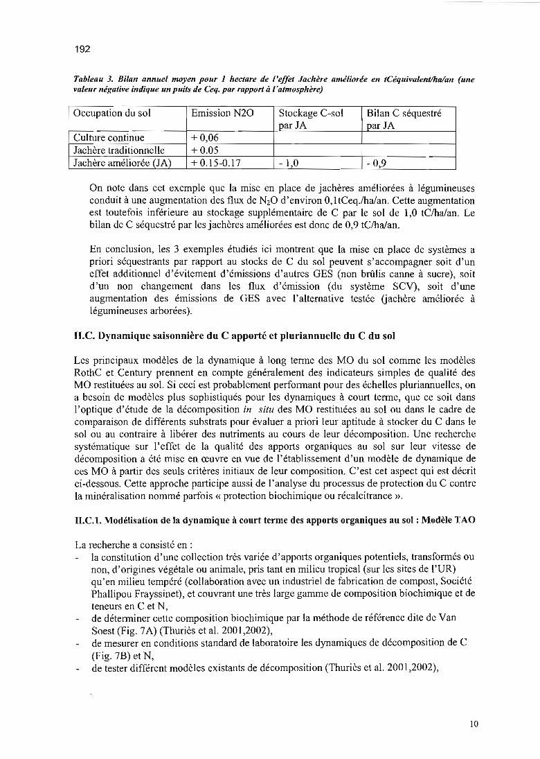
192

Tableau 3. Bilan annuel moyen pour 1 hectare de l'effet Jachère améliorée en tCéquivalent/ha/an (unevaleur négative indique un puits de Ceq. par rapport à l'atmosphère)

Occupation du sol Emission N20 Stockage C-sol Bilan C séquestréparJA parJA

Culture continue +0,06Jachère traditionnelle +0.05Jachère améliorée (lA) + 0.15-0.17 - 1,0 - 0,9

On note dans cet exemple que la mise en place de jachères améliorées à légumineusesconduit à une augmentation des flux de N20 d'environ 0, ltCeq./haJan. Cette augmentationest toutefois inférieure au stockage supplémentaire de C par le sol de 1,0 tC/haJan. Lebilan de C séquestré par les jachères améliorées est donc de 0,9 tC/haJan.

En conclusion, les 3 exemples étudiés ici montrent que la mise en place de systèmes apriori séquestrants par rapport au stocks de C du sol peuvent s'accompagner soit d 'uneffet additionnel d'évitement d'émissions d'autres GES (non brûlis canne à sucre), soitd 'un non changement dans les flux d'émission (du système SCV), soit d'uneaugmentation des émissions de GES avec l'alternative testée (jach ère améliorée àlégumineuses arborées).

II.C. Dynamique saisonnière du C apporté et pluriannuelle du C du sol

Les principaux modèles de la dynamique à long terme des MO du sol comme les modèlesRothC et Century prennent en compte généralement des indicateurs simples de qualité desMO restituées au sol. Si ceci est probablement performant pour des échelles pluriannuelles, ona besoin de modèles plus sophistiqués pour les dynamiques à court terme, que ce soit dansl'optique d'étude de la décomposition in situ des MO restituées au sol ou dans le cadre decomparaison de différents substrats pour évaluer a priori leur aptitude à stocker du C dans lesol ou au contraire à libérer des nutriments au cours de leur décomposition. Une recherchesystématique sur l'effet de la qualité des apports organiques au sol sur leur vitesse dedécomposition a été mise en œuvre en vue de l'établissement d'un modèle de dynamique deces MO à partir des seuls critères initiaux de leur composition. C'est cet aspect qui est décritci-dessous. Cette approche participe aussi de l'analyse du processus de protection du C contrela minéralisation nommé parfois « protection biochimique ou récalcitrance ».

II.C.1. Modélisation de la dynamique à court terme des apports organiques au sol: Modèle TAO

La recherche a consisté en :la constitution d'une collection très variée d'apports organiques potentiels, transformés ounon , d'origines végétale ou animale, pris tant en milieu tropical (sur les sites de l'UR)qu'en milieu tempéré (collaboration avec un industriel de fabrication de compost, SociétéPhallipou Frayssinet), et couvrant une très large gamme de composition biochimique et deteneurs en C et N,de déterminer cette composition biochimique par la méthode de référence dite de VanSoest (Fig. 7A) (Thuriès et al. 200 l ,2002),de mesurer en conditions standard de laboratoire les dynamiques de décomposition de C(Fig. 7B) et N,de tester différent modèles existants de décomposition (Thuriès et al. 2001,2002),

10

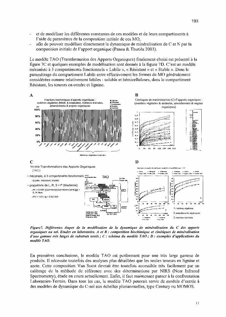
193

et de modéliser les différentes constantes de ces modèles et de leurs compartiments àl'aide de paramètres de la composition initiale de ces MO,afin de pouvoir modéliser directement la dynamique de minéralisation de C et N par lacomposition initiale de l'apport organique (Pansu & Thuriès 2003).

Le modèle TAO (Transformation des Apports Organiques) finalement choisi est présenté à lafigure 7C et quelques exemples de modélisation sont donnés à la figure 7D. C'est un modèlemécaniste à 3 compartiments fonctionnels « Labile », « Résistant» et « Stable ». Dans leparamétrage du compartiment Labile entre effectivement les formes de MO généralementconsidérées comme relativement labiles: soluble et hémicelluloses, dans le compartimentRésistant, les teneurs en cendre et lignine.

A BCinétiques de min érali sation (C) d'apports organ iques :

(matières végétales & animales, amendements & engraisorganiques)

Fractions biochimiques d'apports organiques :matières végétales (Méd~. & tropicalesl, matières animales,

MS amendements & engrais organiques

100%

80%

60%

400/.

20%

• Lignine.Cellulo••DHc.lulo...8Solub..C.ndr••

O.'o.'o.'o.'o.'

o JO 60 90 IZO rso 1110 ZlO

c DQM~ lq uCl rltmpiu de t1llillq un nlu.lin rI nlo6 i-Hllitt p.lIrT\ l)

.QItw.o,poJI(l .c~ .0..-0CacAO_TAO -Oh_TAO -c.o","_fAO - Cl'oIUI_fAO -o.._o_TAO-~_TAO

3

1 matiéres végétales

2 amendementsorganiques

3 matièresanimales

o l--~----....-.J• JCI 10 ICI UO Uli

'.'o'--~~~--"""""

• :tG 60 to no 1~ 110 J'Q

,)U~U

' ,1 2" -~-jyuo

• JO 100 liO 11" lM 114 tu.COO'llflOlio .~p

-b_TAC -p_TAO

""' ...

~1I1t.J(lJI

~tII"~:!002Pwo.t &~ zo:n............. 2OOJ

Modèle Transformations des Apports Organiques(TAO) :

• proportions de L, R, S =t" (biochimie)

- PL ; 0 .099 [(Sol+Hem)/(SoI+Hem+Cel+Lig)J +0.14 Hem

-PS ; 1.61 Lig + 0.62 Ash

Figure 7. Différentes étapes de la modélisation de la dynamique de minéralisation du C des apportsorganiques au soL Etudes en laboratoire. A et B: composition biochimique et cinétiques de minéralisationd'une gamme très larges de substrats testés; C: schéma du modèle TAO; D: exemples d'applications dumodèle TAO.

En premières conclusions, le modèle TAO est performant pour une très large gamme deproduits. Il nécessite toutefois des analyses plus détaillées que les seules teneurs en lignine etazote. Cette composition Van Soest devrait être toutefois accessible très facilement par uncalibrage de la méthode de référence avec des déterminations par NIRS (Near InfraredSpectrometry), étude en cours actuellement. Enfin, il faut maintenant passer à la confrontationLaboratoire-Terrain. Dans tous les cas, le modèle TAO pourrait servir de module d'entrée àdes modèles de dynamique du C-sol aux échelles pluriannuelles, type Century ou MOMOS.

Il

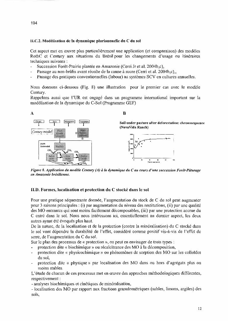
194

II.C.2. Modélisation de la dynamique pluriannuelle du C du sol

Cet aspect met en œuvre plus particulièrement une application (et comparaison) des modèlesRothC et Century aux situations du Brésil pour les changements d'usage ou itinérairestechniques suivants :

Succession Forêt-Prairie plantée en Amazonie (Cerri Jr et al. 2004b,c),Passage au non-brûlis avant récolte de la canne à sucre (Cerri et al. 2004b,c)"Passage des pratiques conventionnelles (labour) au systèmes SCY en cultures annuelles.

Nous donnons ci-dessous (Fig. 8) une illustration pour le premier cas avec le modèleCentury.Rappelons aussi que l'UR est engagé dans un programme international important sur lamodélisation de la dynamique du C-Sol (Programme GEF)

A

SOMSubmodel

B

Soil under pasture after deforestation: chronosequence(NovaVida Ranch)

.;; ....~3/'JOO

ij 2000

'.1-- ---'

Figure 8. Application du modèle Century (A) à la dynamique du C au cours d'une succession Forêt-Pâturageen Amazonie brésilienne.

II.0. Formes, localisation et protection du C stocké dans le sol

Pour une pratique séquestrante donnée, l'augmentation du stock de C du sol peut augmenterpour 3 raisons principales: (i) par augmentation du niveau des restitutions, (ii) par une qualitédes MO entrantes qui sont moins facilement décomposables, (iii) par une protection accrue duC entré dans le sol. Nous nous intéressons ici, essentiellement au dernier aspect, les deuxautres ayant été évoqués plus haut.De la nature, de la localisation et de la protection (contre la minéralisation) du C stocké dansle sol vont dépendre la durabilité de l'effet, considéré comme positif vis-à-vis de l'effet deserre, de l'augmentation du C du sol.Sur le plan des processus de « protection », on peut en envisager de trois types:

protection dite « biochimique» ou récalcitrance des MO à la décomposition,protection dite « physicochimique » ou phénomènes de sorption des MO sur les colloïdesdu sol,protection dite « physique» par localisation des MO dans ou hors d'agrégats plus oumoins stables.

L'étude de chacun de ces processus met en œuvre des approches méthodologiques différentes,respectivement :- analyses biochimiques et cinétiques de minéralisation,- localisation des MO par rapport aux fractions granulométriques (sables, limons, argiles) dessols,

12

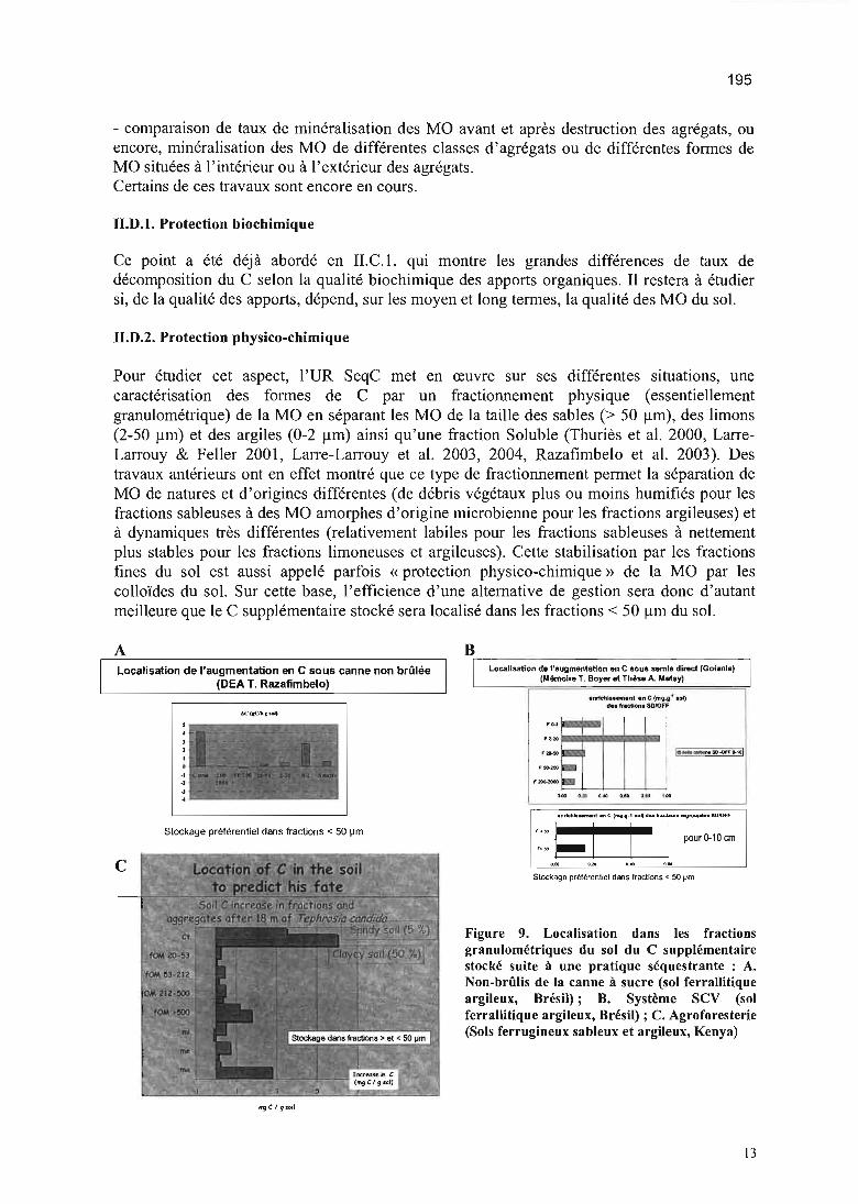
195

- comparaison de taux de minéralisation des MO avant et après destruction des agrégats, ouencore, minéralisation des MO de différentes classes d'agrégats ou de différentes formes deMO situées à l'intérieur ou à l'extérieur des agrégats .Certains de ces travaux sont encore en cours .

II.D.l. Protection biochimique

Ce point a été déjà abordé en II.C.l. qui montre les grandes différences de taux dedécomposition du C selon la qualité biochimique des apports organiques. Il restera à étudiersi, de la qualité des apports, dépend, sur les moyen et long termes, la qualité des MO du sol.

II.D.2. Protection physico-chimique

Pour étudier cet aspect, l'UR SeqC met en œuvre sur ses différentes situations, unecaractérisation des formes de C par un fractionnement physique (essentiellementgranulométrique) de la MO en séparant les MO de la taille des sables (> 50 um), des limons(2-50 um) et des argiles (0-2 um) ainsi qu 'une fraction Soluble (Thuriès et al. 2000, Larre­Larrouy & Feller 2001, Larre-Larrouy et al. 2003, 2004, Razafimbelo et al. 2003). Destravaux antérieurs ont en effet montré que ce type de fractionnement permet la séparation deMO de natures et d'origines différentes (de débris végétaux plus ou moins humifiés pour lesfractions sableuses à des MO amorphes d'origine microbienne pour les fractions argileuses) età dynamiques très différentes (relativement labiles pour les fractions sableuses à nettementplus stables pour les fractions limoneuses et argileuses). Cette stabilisation par les fractionsfines du sol est aussi appelé parfois «protection physico-chimique» de la MO par lescolloïdes du sol. Sur cette base , l'efficience d'une alternative de gestion sera donc d'autantmeilleure que le C supplémentaire stocké sera localisé dans les fractions < 50 um du sol.

ALocalisation de l'augmentation en C sous canne non brOlée

(DEA T. Razafimbelo)

,·J,,•.,-1

-1·Stockage préférentiel dans fraction s < 50 um

c

B

1

Localisation de l'augmentation 8f1 C sous semle direct (Golilnla)

1(Mémoire T. Boyer el Thèse A. Melay)

.nrlchl_.ment en C (mg.;"' 101)<hl. fn~IOf1' SDIOFF

r e-a liE!~ :f ;l .2'Q

,..... lIl:lII 1ïï"'--" !IO .oJI'G- 101

, ...,.,. ..,- ID... .,. .~ ... .., '"

Inrkhi...mIInl ln C (mg ...,. l loI) d•• IrK.lIon....lIOVU,..•• SD,()f'f

""=ttJ pour a-10 cm,."

'-" = .~ ..,Stockage préférentiel de-s fractions < 50 ~m

Figure 9. Localisation dans les fractionsgranulométriques du sol du C supplémentairestocké suite à une pratique séquestrante : A.Non-brûlis de la canne à sucre (sol ferraUitiqueargileux, Brésil); B. Système SCY (solferrallitique argileux, Brésil) ; C. Agroforesterie(Sols ferrugineux sableux et argileux, Kenya)

13

196

Nous rapportons ci-dessous quelques résultats sur : a) l'effet du non brûlis de la canne à sucreau Brésil (Razafimbelo et al. 2003), b) l'effet des systèmes SCY au Brésil (thèse en coursMetay) et c) des systèmes agroforestiers (Kenya) (Fig. 9A, B, C).

Les principales conclusions sont que:dans les systèmes avec mulch, sans travail du sol, et sans apport supplémentaire par lesystème racinaire (cas des Fig. 9A et 9B), le stockage du C se fait essentiellement dans lesfractions fines du sol < SO!J,m,dans les systèmes avec une double entrée de C, sous forme de litière et de racine, commele cas des systèmes agroforestiers, les accumulations se font à la fois dans les fractions >et < à SO!J,m, les fractions < SO!J,m étant d'autant favorisées que le sol est plus argileux.

En terme de processus, et suite à d'autres résultats existant dans la littérature, une deshypothèses (à tester) serait que lorsque les entrées sont uniquement en surface du sol (cas dumulch), la seule incorporation possible de la MO dans le sol est due à la faune du sol (vers ettermites) et que cette incorporation conduirait à une transformation (division +solubilisation/humification) très forte des matières organiques lors du transit intestinal ce quiorienterait une fixation préférentielle des MO sur les colloïdes du sol.

II.D.3. Protection physique au sein des agrégats de sol

Cette étude est largement encore en cours. Nous ne rapportons ici que quelques résultatsprovrsoires.

La démarche complète choisie est basée sur les questions/méthodologies suivantes:globalement, le sol étudié présente-t-il une protection du C vis-à-vis de la minéralisation?et comment cette protection varie selon les alternatives séquestrantes testées? On met enœuvre ici un test de laboratoire pour comparer la minéralisation d'un échantillon de sol« naturel» (non broyé) avec les MO encore protégées et d'un échantillon broyé avec lesMO plus ou moins déprotégées (par destruction des agrégats) selon l'intensité du broyage,les formes de MO à l'extérieur des agrégats sont-elles plus facilement minéralisables queles formes de MO équivalentes à l'intérieur des agrégats? Ceci met en œuvre (i) unfractionnement spécial des MO du sol en distinguant leur localisation par rapport auxagrégats, (ii) des tests de minéralisation en conditions standard de chacune des fractionsséparées,la protection de la MO varie-t-elle selon l'organisation du sol, en d'autres termes, niveaude la protection dans les différentes classes d'agrégats du sol? Ceci met en œuvre les 2approches précédentes mais appliquées aux différentes classes d 'agrégats du sol?enfin, la faune du sol, susceptible de très fortes variations selon le mode de gestion desterres, et en maintenant étant un acteur essentiel des variations de la structure du sol, l'Urmet en œuvre une étude spécifique de l'effet de différentes pratiques sur la faune du sol,des conséquences de l'activité faunique sur la stabilité de la structure, et des conséquencesde cette dernière sur la protection physique du C. Ceci met en œuvre l'étude de laprotection du C (cf. ci-dessus) sur des agrégats d'origine faunique.

a) Protection physique globale du C dans les sols selon le mode de gestionUn exemple peut-être donné dans le cadre de la thèse en cours de T. Razafimbelo (SystèmesSCY, Madagascar) et est illustré sur la figure 10.On constate que:

14

197

le taux de minéralisation à 28 jours est systématiquement plus faible sous Semis direct quesous Labour. Bien que les stocks de C aient été significativement augmentés sous semisdirect (par apports plus importants de MO), il ressort donc qu'il existe toutefois dans cessystèmes une forme de MO plus labile,le niveau de protection du C est faible pour les 2 traitements et la différence entre les 2systèmes est non significative.

Ceci est un exemple où probablement l'effet protection physique intervient peu dans lestsockage du C du sol, contrairement à d'autres situations étudiées comme des prairiesartificielles sur Vertisol aux Antilles (thèse Chevallier 1999, Chevallier et al. 2004).

Protection C - Respirométrie - Effet broyage

....- - S><u1DW'aHl - 9>aJoo.,....t-Il

• 3:lRJ'ltr~'''Hl .l SXrJt:.l-f'aHl

I~.

- -Ub::>.I rU'lb'W".Hl LtrnrQ<ll~.Hl

• UI;1o.t ru'lb..,.•• H'1 '" l.CnIQ<II~.HI

- -SllUl~bHl 9)QJtr0,4 bti

• SllUltq06bHl .l !DaJ trq4b1't

5 Il 15 ~ Z'i Xl....- -Uln.rfO'ltq06bHl .. ~a,lt:l'otfib~

• !.muRJ'ltq06bHl .. l.II:o.raJtrotoIIbl1'l

- - !Ilral tr<ljoll,1-II SXrJ tq06( 11I

• !Ilral tJwlllC " .. SXrJ~(Hl

5 Il ~ :Il 25 :Il....__ Uln.rl'U'lt:ra,olcHl - . lA:nI QJ~': '"

.L.au.tlU'ltro./t c:Hl "'l...a1IOJ~ c:1i

Figure 10. Taux de minéralisation (mgC-C02/gC sol) et protection du C (différences entre courbes « broyé»et « non broyé ») d'un sol ferrallitique argileux à Madagascar, en traitements Labour (parcelles a', b' et c')ou Semis direct (parcelles a, b et c}.

b) Taux de minéralisation des MO particulaires internes et externes aux agrégatsUn travail méthodologique original est en cours pour permettre une séparation de ces deuxformes de MO en utilisant l'eau seulement (et non des liqueurs minérales denses comme c'estle cas dans la littérature) afin d'éviter des artefacts pour les expérimentations deminéralisation ultérieures. Pas de résultats à fournir actuellement.

c) Niveau de protection du C selon différentes classes d 'agrégatsEst en cours d'étude sur des situations agroforestières du Kenya. Pas de résultats à fourniractuellement.

d) Effet de la faune sur la protection physique du CRappelons que la faune du sol joue un effet majeur sur les propriétés physiques des sols(Blanchart et al. 2004a,b) et en particulier l'agrégation (Blanchart et al. 2000, Cabidoche et al.2000, Chevallier et al. 2001), et que la biomasse, la diversité et l'activité faunique estsusceptible de variations très fortes rapidement sous l'effet d'un changement de pratique.

15

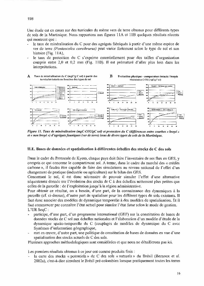
198

Une étude est en cours sur des turricules du même vers de terre obtenus pour différents typesde sols de la Martinique. Nous rapportons aux figures Il A et Il B quelques résultats récentsqui montrent que:

le taux de minéralisation du C pour des agrégats fabriqués à partir d'une même espèce dever de terre (Pontosco/ex corethrurus) peut varier fortement selon le type de sol et sonhistoire (Fig . lIA),le taux de protection du C s'exprime essentiellement pour des tailles d'organisationcompris entre 2,0 et 0,2 mm (Fig. Il B). Il est prématuré d'aller plus loin dans lesinterprétations.

A Taux de minérali sation du C (mgC/g C sol) à partir desturricules intacts en fonction des types de sol

B Protection physique - comparaison intacts 1broyésMinéralisation C-C02 (mgCIg C sol)

~ I· SoljelnC'lllJrc.niml

:~"'J..Aodosol :

: I=E:'!:~=::~2==~1=;;"lM . -" t.1 lM+- . t.1

~-: . . :tv::'::~:=:=:=::'lltU.U •• 'l'U.UlI

BdlttànIUine '2• Sol aha1lcl)'Sitc-­

---::

.l'--_~~~---l

• , Il IS • lS •

I=:;d :t--·/--=..=::.-------1 I:S:~1/

• 1 l' U • lJ •

Caruvdlc ~ . Sol rouge lJ. rrcnmo.

~-

--------

.

,V

Figure Il. Taux de minéralisation (mgC-C02/gC sol) et protection du C (différences entre courbes « broyé»et « non broyé »] d'agrégats fauniques (ver de terre) issus de divers types de sols de la Martinique.

II.E. Bases de données et spatialisation à différentes échelles des stocks de C des sols

Dans le cadre du Protocole de Kyoto, chaque pays doit faire l'inventaire de ses flux en GES, ycompris ce qui concerne le compartiment sol. A terme, dans le cadre du marché des « créditscarbone », il faudra être capable de faire des simulations au niveau national de l'effet d'unchangement de pratique (industrie ou agriculture) sur le bilan des GES .Concernant le sol, il est donc nécessaire de pouvoir simuler l'effet d'une alternativeséquestrante donnée sur l'évolution des stocks de C à des échelles nettement plus petites quecelles de la parcelle : de l'exploitation jusqu'à la région administrative.Pour obtenir ce résultat, on a besoin, d'une part, de la connaissance des dynamiques à laparcelle (cf. ci-dessus), d'autre part de spatialiser pour les différent types de sols existants. Ilfaut donc associer des modèles de dynamique temporelle à des modèles de spatialisation. Et ilfaut commencer par connaître l'état actuel pour simuler l'état futur selon le mode de gestion.L'URSeqC:

participe, d'une part , d'un programme international (GEF) sur la constitution de bases dedonnées stocks de C sol aux échelles nationales et l'élaboration d'un modèle d'étude de ladynamique spatio-temporelle du C (couplages de modèles de dynamique du C avecSystèmes d'information géographique,met en œuvre, d'autre part, une politique de constitution de bases de données en vue d'unespatialisation des stocks actuels de C des sols.

Plusieurs approches méthodologiques sont considérées et que nous ne détaillerons pas ici.

Les premiers résultats obtenus à ce jour ont comme produits finis:la carte des stocks « potentiels» de C des sols « naturels» du Brésil (Bernoux et al.2002a), c'est-à-dire simulant le Brésil pré-colombien lorsque pratiquement toutes les terres

16

199

étaient sous végétations naturelles (Fig. 12A). Ceci permettra très prochainement, commeproduit dérivé, la carte des stocks actuels du Brésil,la carte (encore provisoire) des stocks de C de la Martinique (Fig . 12B) (thèse en coursVenkatapen).

Pour le futur, l'accent sera mis sur le Brésil , avec la simulation des changements de stocks deC aux échelles nationales pour des alternatives majeures comme le non-brûlis de la canne àsucre et/ou l'extension des pratiques de semis direct.

A BEstimation des stocks C (0-100 cm) dans les sols

de la Martinique

C . 1OdtS- kg C m-". '.5- 2_ 2-2.5_ :Hi - J_3 - J.5_ 3.5 - 4

.. • ...54..5·5_ 5·'_6·'

_ 7-10_10-45 lPo-lOlSg -

1 milliard oe tonnes

Corbon. (1/'"')

30·70_ 70 -90_90-110

110 · 130_ 130 - 160_ 160 ·200

-10,5 Mt C au lieu de 15MtC- variations de 50 à 180au lieu de 75 à 125 IC/ha

Figure 12. Cartes des stocks «potentiels» de C des sols du Brésil (A) et des stocks actuels (1980) de laMartinique (B).

Certains milieux nécessitent des approches de spatialisation particulières comme la zone dessavanes d'Afrique sub-saharienne où le paysage est organisé en « terroirs ». C'est donc à cetteéchelle qu'il st intéressant d'estimer les stocks et les flux de C ou autres nutriments (Manlayet al. 2002a,b,c, 2004a,b,c)

H.F. Economie du « C séquestré»

Dans notre projet d'UR, nous avions annoncé que cette partie (Axe 3) ne serait probablementpas abordée au cours de la première phase de l'UR, ce qui, en effet n'a pu l'être.Toutefois, une première estimation (ayant donné lieu à publication) a été faite par l'UR SeqCde ce que représente réellement le marché mondial du C « Gestion agricole et forestière desterres (LULUCF) dans le cadre du Mécanisme de Développement Propre (MDP) du Protocolede Kyoto (Bernoux et al. 2002).Il ressort que si, a priori , ce marché (hors USA) représente des crédits pour 605 Mt C02 eq.pour l'ensemble des 45 pays de la Non-Annexe 1 (globalement les pays du Sud), le marché leplus probable ne serait que de 109,5 MtC02 eq., ce qui représente pour des valeurs de 8 à 10euros/tC02, une enveloppe totale de 876 à 1095 millions euros, valeur à comparer avec lesomme de 51 milliards euros consacrés en 2002 par l'OCDE dans son programme de« Official Development Assistance ». Toutefois ces projets MDP sont avant tout une vitrinede coopération « politico-socio-environnernental et politiquement correct» pour les pays etentreprises concernés, et, un positionnement sur un marché qui sera probablement en forteexpansion, pas uniquement au niveau des fonds publics nationaux ou internationaux maisaussi des fonds privés, comme cela est déjà en cours. L'UR SeqC est d'ailleurs engagé auBrésil dans un de ces processus avec un projet de coopération quadripartite entre: un trèsgroupe de sucriers, une société de consultance, l'université de Sao Paulo et l'IRD.

17

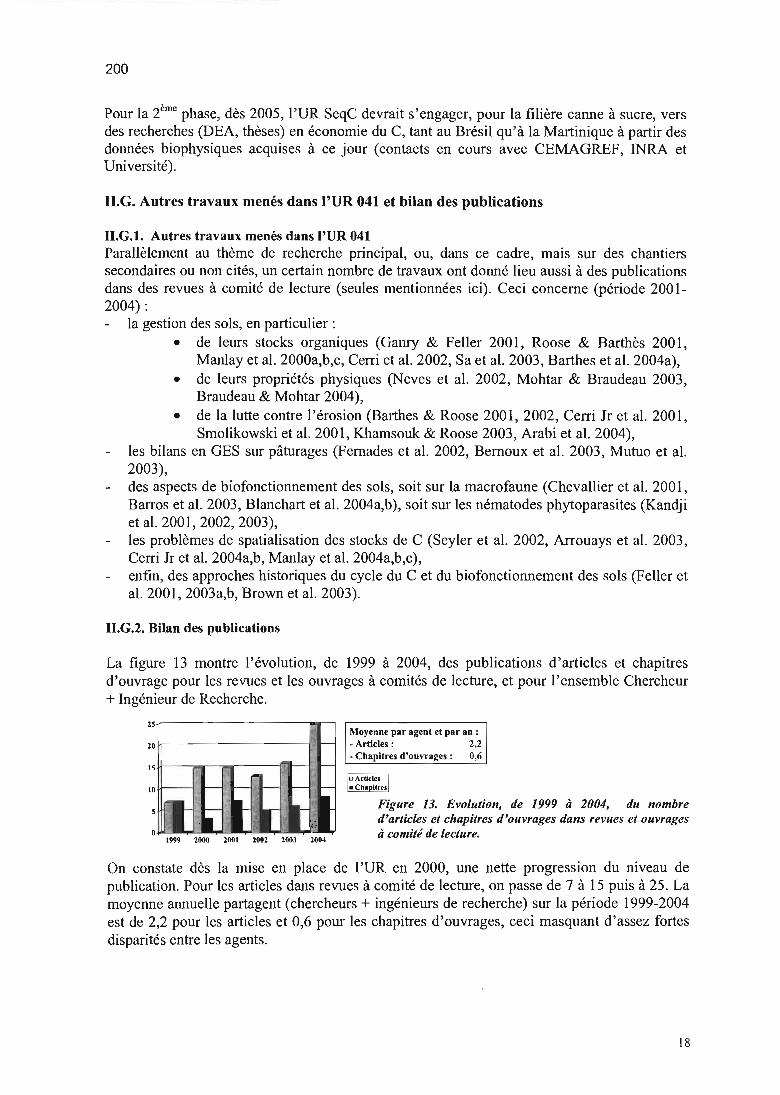
200

Pour la 2ème phase, dès 2005, l'UR SeqC devrait s'engager, pour la filière canne à sucre, versdes recherches (DEA, thèses) en économie du C, tant au Brésil qu'à la Martinique à partir desdonnées biophysiques acquises à ce jour (contacts en cours avec CEMAGREF, [NRA etUniversité).

II.G. Autres travaux menés dans l'UR 041 et bilan des publications

II.G.1. Autres travaux menés dans l'UR 041Parallèlement au thème de recherche principal, ou, dans ce cadre, mais sur des chantierssecondaires ou non cités, un certain nombre de travaux ont donné lieu aussi à des publicationsdans des revues à comité de lecture (seules mentionnées ici). Ceci concerne (période 2001­2004) :

la gestion des sols, en particulier:• de leurs stocks organiques (Ganry & Feller 2001, Roose & Barthès 200 l ,

Manlay et al. 2000a,b,c, Cerri et al. 2002, Sa et al. 2003, Barthes et al. 2004a),• de leurs propriétés physiques (Neves et al. 2002, Mohtar & Braudeau 2003,

Braudeau & Mohtar 2004),• de la lutte contre l'érosion (Barthes & Roose 2001, 2002, Cerri Jr et al. 2001,

Smolikowski et al. 2001, Khamsouk & Roose 2003, Arabi et al. 2004),les bilans en GES sur pâturages (Fernades et al. 2002, Bernoux et al. 2003, Mutuo et al.2003),des aspects de biofonctionnement des sols, soit sur la macrofaune (Chevallier et al. 200 1,Barros et al. 2003, Blanchart et al. 2004a,b), soit sur les nématodes phytoparasites (Kandjiet al. 2001, 2002, 2003),les problèmes de spatialisation des stocks de C (Seyler et al. 2002, Arrouays et al. 2003,Cerri Jr et al. 2004a,b, Manlay et al. 2004a,b,c),enfin, des approches historiques du cycle du C et du biofonctionnement des sols (Feller etal. 2001, 2003a,b, Brown et al. 2003).

II.G.2. Bilan des publications

La figure 13 montre l'évolution, de 1999 à 2004, des publications d'articles et chapitresd'ouvrage pour les revues et les ouvrages à comités de lecture, et pour l'ensemble Chercheur+ Ingénieur de Recherche.

25...r---------...,..----,

20>l-----------j : I--i

15~- _,__--_r.:11__j

1999 2000 2001 2002 2003 2004

Moyenne par agent et par an :- Articles: 2,2- Chapitres d'ouvrages: 0,6

Figure 13. Evolution, de 1999 à 2004, du nombred'articles et chapitres d'ouvrages dans revues et ouvragesà comité de lecture.

On constate dès la mise en place de l'UR en 2000, une nette progression du niveau depublication. Pour les articles dans revues à comité de lecture, on passe de 7 à 15 puis à 25. Lamoyenne annuelle partagent (chercheurs + ingénieurs de recherche) sur la période 1999-2004est de 2,2 pour les articles et 0,6 pour les chapitres d'ouvrages, ceci masquant d'assez fortesdisparités entre les agents.

18

201

III. Prolongements envisagés

Il a été décidé en Conseil d'Unité de ne pas poursuivre sous sa forme actuelle l'UR SeqC maisde s'intégrer à une nouvelle UR« Séquestration du C et Biofonctionnement des sols. Effetdu mode de gestion des agroécosystèmes (SeqBio) », résultat de la fusion de l'UR SeqC etde l'UR IBIS.

Ce projet est la concrétisation des collaborations établies, durant la période 2001-2004, entreles UR «Séquestration du Carbone » (R041, Directeur C. Feller) et Ibis « Interactionsbiologiques dans les sols des systèmes anthropisés tropicaux » (R083 , IL. Chotte).

Le nouveau projet conserve la même thématique large que le projet initial de l'UR SeqC, ma isen mettant un accent très fort sur les processus biologiques (apport de l'UR Ibis) à la base dustockage de la MO dans les sols et des flux de GES.

Les recherches conduites dans l'UR SeqBio auront pour objectif de valider, parmi lespratiques de gestion de ressources organiques dans les agro-écosystèmes, celles quiparticipent à la maîtrise des flux [L\ sortie = f(L\ stock, L\ entrée)] de carbone et d'azote,permettant à la fois une production agricole optimale et un contrôle de l'émission des gaz àeffet de serre.

Pour atteindre cet objectif, les opérations de recherche conduites dans l'UR s'attacheront àapporter des réponses aux questions suivantes:

Quels sont les modes de gestion des ressources organiques qui favorisent le stockagede la MO (donc du C) dans le sol?

Ces pratiques sont-elles adaptées à une maîtrise de l'émission des gaz à effet deserre?

Les réponses apportées à ces questions participeront à la validation des modalités de gestiondes matières organiques et pourront, à chaque fois que possible, être à l'origine deproposition(s) innovante(s) pour la gestion des ressources naturelles dans les agrosystèmes.

Dans ce projet, une attention particulière sera accordée:

aux acteurs microbiologiques responsables des processus de décomposition desressources organiques (sol, matières exogènes)

aux caractéristiques biotiques et abiotiques de leur environnement immédiat (notiond'habitat microbien)

aux interactions entre ces communautés microbiennes et les autres composantesbiotiques du sol (macrofaune, mésofaune, racines)

aux réponses différentes (dans le temps et l'espace) de ces composants biotiques etabiotiques aux pratiques de gestions des ressources organiques,

La prise en considération de l'ensemble de ces aspects et l'étude de leur impact à l'échelle deparcelle permettra ensuite une meilleure estimation des flux à l'échelle des terroirs, micro­régions constitue aussi une originalité du projet.

La réunion de ces deux URs sur une ligne directrice commune" maîtrise des flux [L\ sortie = f(L\ stock, L\ Entrée)] de carbone et d'azote" doit permettre de poursuivre et d'élargir lesthématiques initiées par ces URs en exploitant des chantiers communs.

19

202

203

Activités 2003 à Février 2004Marc Pansu

1. Positionnement institutionnel

Laboratoire MOST et UR-041, IRD

En 2003, mes activités se sont poursuivies au sein de l'UR 041 - Séquestration du

carbone dans les sols tropicaux (IRD) et du laboratoire MOST (Matière organique des sols

tropicaux, IRD-Cirad) sur deux directions principales:

- modèles de décomposition des matières organiques des sols (Cf. 2.1, 2.2, 2.3 ci­

dessous) et de fonctionnement de systèmes écologiques (Cf. 2.4);

- dynamique de décomposition des apports organiques (compartiments d'entrée des

matières organiques des sols, Cf. 2.5)

Mon activité s'inscrit essentiellement dans l'axe 1 de l'UR 041: déterminants

(écologiques et agronomiques), processus et dynamique de la séquestration du C dans les sols

et l'émission de GES. Au sein du laboratoire MOST, je suis plus particulièrement chargé de

modélisation du cycle C et N dans les sols (Cf. 2). Je m'occupe aussi de qualité et

standardisation de méthodes de laboratoire (collaboration fiches AFNOR), d'ouvrages de

synthèse sur «L'analyse du sol» (Cf. 3), d'expertise scientifique auprès de revues

internationales, de formation de stagiaires, de rédaction de projets de recherche (Cf.6) ainsi

que d'animation et communication scientifique (Cf. 4 et 5).

Coopérations: (partenaires)

IRD, UR 041 (Montpellier) et IBIS (Sénégal)

CEFE-CNRS Montpellier, France,

CIRAD Montpellier, France,

Laboratoire d'écologie microbienne des sols tropicaux, IRD-IBIS, Sénégal

Entreprise Phalippou Frayssinet (Fertilisants organique, Tarn, France),

EMBRAPA, Sao Paulo, Brésil ;

Instituto de Investigaciones Agrobiologicas de Galicia, Santiago de Compostella, Espagne,

Instituto de ciencias ambientales y ecologicas, Facultad de ciencias, Merida, Venezuella,

Universidad mayor de San Andres, Instituto de Ecologia, La Paz, Bolivie,

204

Plant Research International, location born Zuid Wageningen, Pays Bas,

Laboratoired'écophysiologie végétale, Université de Paris-Sud, Orsay, France

2. Travaux de recherche (modélisation du cycle C et N)

2.1. Rappel sur le modèle Momos

in(nN

CO, GazeousN,O.JOSS...}

/.

IniLoC_oN~ C. N Input" ... ...

r.

\ 6\

\\

\ , 1 \

~---t-----~ 1 \

iniLaN kn1 kn2

1t,

Figure 1. MOMOS : a process-based modelfor carbon and nitrogen transfers in soilorganic matter (Pansu et al.,1988). OrganicC and N represents five compartments: VLand VR = labile and resistant necromass, A= labile metabolites, B= microbial biomass,H = stable humified compounds. Boldarrows indicate the processes of masstransfers: 1) mineralization, 2) humification,3) input from necromass, 5)ammonification, 6) reorganisation, 7)nitrification, 8) N-volatilization

Les études actuelles sont réalisées sur la base du modèle de décomposition MOMOS

(Modelling Organic Matter of Soil, Modélisation des Matières Organiques du Sol, Fig"),

résultat d'une collaboration établie entre l'IRD et le Centre d'Ecologie Fonctionnelle et

Evolutive du CNRS à Montpellier.

Ce modèle de décomposition, établi enconditions de laboratoire, a aussi permis de

faire progresser le sujet controversé de l'influence des racines vivantes sur le cycle des

matières organiques dans les sols (Fig. 2, Bottner, Pansu et Sallih, Plant and Soil;1999 ;

Pansu et Bottner, 2001, Actes colloque Rhizosphère, Dijon; Pansu et Bottner, 2002, actes

congrès C et érosion, Montpellier).

Figure 2. Modification of MOMOS-C takinginto account the effect of active roots onsoil organic matter turnover (Bottner andPansu, 1999). Symbols are the same asin Fig. 1, except arrows 3) input fromdead plant material (DPM) and 4) inputfrom living plant materials (LPM,exsudation).

2

205

2.2. Développements actuels du modèle

MOMOS-4

MOMOS-6

tL. ~.. .1

tL. ~ j

MOMOS-3

MOMOS-S

t1 CIrroIIct ... ~................ c::IcIa •.....:

Figure 3. Flow diagram's of the five versions of the MOMOS model compared. Ne = totalnecromass, VL = labile necromass, VS = stable necromass, MB = microbial biomass,H = humified compounds (humus), HL = labile humus, HS = stable humus.

Sur la base des expériences de traceurs isotopiques 14e et ISN, cinq versions du

modèle MOMOS ont été comparées (Fig. 3). Les expériences concernaient des suivis in situ

d'incubation de mélanges sols-pailles marquées pendant deux ans selon la technique

« soilbags » avec collecte des données: humidité du sol, 14e et ISN totaux, biomasse3

206

microbienne 14C et 15N, pluviométrie, température de l'air et radiation totale. L'humidité du

sol était prédite par le modèle SAHEL couplé avec les différentes versions de MOMOS. Les

versions MOMOS-2 à 4 (modèles de type 1) utilisent les paramètres classiques des modèles

du cycle C et N : constantes de vitesse du premier ordre et fractions de partition des flux. Les

versions MOMOS-5 et -6 (type 2) utilisent seulement des constantes de vitesse et donnent un

rôle central à la biomasse microbienne (BM) et à son coefficient respiratoire, deux variables

dont la mesure est maintenant bien définie dans les sols. Les principaux résultats montrent:

(1) la simplification de MOMOS-2 en MOMOS-3 (type modèle Roth-C de nos collègues

anglais) par suppression d'un compartiment est valide, (2) la simplification de MOMOS-3 en

MOMOS-4 par suppression de processus de recyclage est également valide, (3) MüMOS-5

améliore significativement la prédiction de BM_14C et _1~ et peut etre proposé pour la

prédiction à court terme, (4) MOMOS-6 est proposé pour la prédiction à long tenne par

l'intégration d'un compartiment humus stable. Pour cette expérience, il permet de prédire une

séquestration de 2% du 14C ajouté et de 5,4% du 15N ajouté. Ces travaux viennent de faire

l'objet de la soumission d'une publication (Pansu et al., 2004a).

2.3. Analyse de sensibilité des modèles

Pour la proposition d'un nouveau modèle (type 2) les conclusions de 2.2 (justesse)

devaient être complétées par une analyse de sensibilité comparative des deux types de

modèles: robustesse, répétabilité, cohérence écologique de la variation des fonctions de

réponse avec celle des divers paramètres. Les principaux résultats montrent: (1) les modèles

de type 1 (MOMOS-2 à -4, fig. 3) sont surtout sensibles aux paramètres de fractionnement

des flux, particulièrement le facteur d'efficience de l'humification, (2) les modèles de type 2

(MOMOS-5 à -6, fig.3) sont sensibles en premier lieu au taux de mortalité et au taux de

respiration de BM, en second lieu aux taux d'entrée des compartiments labiles dans BM, (3)

les fonctions de réponse MB-C et -N sont moins sensibles aux changements de paramètres

dans les modèles de type 2 (Fig.4) que dans ceux de type 1, malgré l'équation plus complexe

de BM dans le type 2, (4) les variations comparatives des fonctions de réponse sont plus

consistantes avec leur définition écologique dans les modèles de type 2 que dans ceux de

type 1. Ces résultats viennent de faire l'objet de la soumission d'une autre publication (Pansu

et al., 2004b).

4

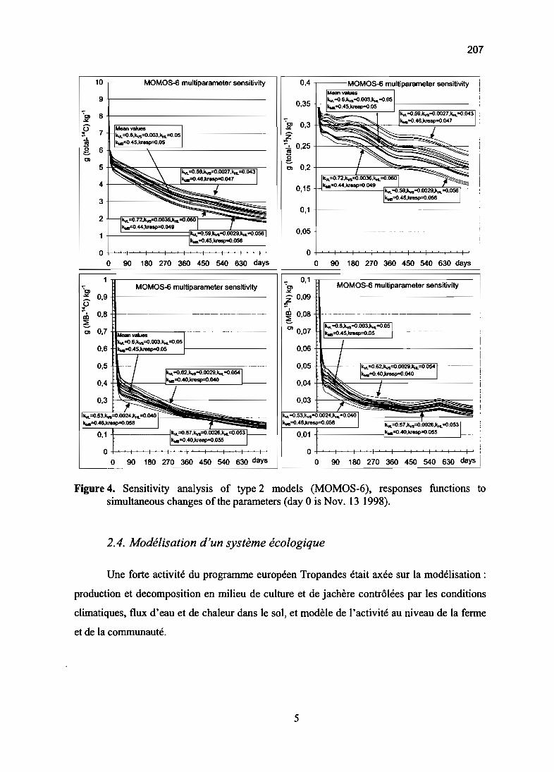
207

O+-"-~f_'_..L....j_~'_I_~_+_~+-"~+-"--'-I'-'-~

o 90 180 270 360 450 540 630 days

0,35

0,4 -,------MOM05-6 multiparameter sensitivity

.... I::::.~OO3·""-~·05I _ÎIW~.45.kresp=O.05

0,1 +--------------~--

O+-'--'-I~'_I_~+_'~f_'__'_+~_+_''-'-t_'_~

o 90 180 270 360 450 540 630 days

0,05

--MOM05-6 multiparameter sensitivity10

9

~ 8

Ô 7::.Ss 6Cl

5

4

3

2

MOMOS-6 multiparameter sensitivity

i

90 180 270 360 450 540 630 days i

0,05 +t\o--J/--.--1i<:;o:W;:;;;;o.iOO29:~l.054I

0,04

0,06 ++--+------------

0,03 +---::",-;

0,01 t--------r:~~~~~-----1

O+-'-~f_'__'_+~_+_~+_'__'_If_'__'_+~_+_~+_'

o

0,1 ...---------------

~i 0,09

~ 0,08

Cl 0,07

1 ! ,

MOM05-6 multiparameter sensitivity

o +--'--'-t~c.+~_t_'_~f_'__'_+~_+_''-'-t_'_..L....j_~

o 90 180

~~0,9

Ô::

0,8eb~

L...- . ._I_·_·6_~0_~_a~_s_· 1 L- ----'

Figure4. Sensitivity analysis of type 2 models (MOMOS-6), responses functions tosimultaneous changes of the parameters (day 0 is Nov. 13 1998).

2.4. Modélisation d'un système écologique

Une forte activité du programme européen Tropandes était axée sur la modélisation:

production et decomposition en milieu de culture et de jachère contrôlées par les conditions

climatiques, flux d'eau et de chaleur dans le sol, et modèle de l'activité au niveau de la ferme

et de la communauté.

5

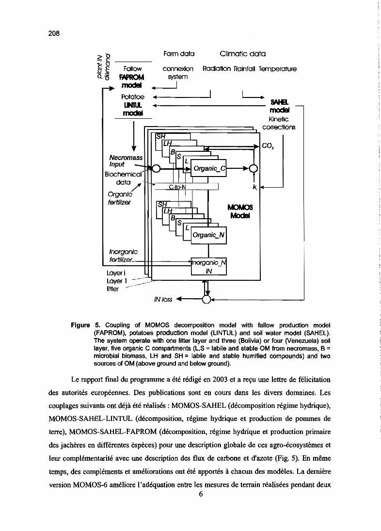
208

Farm data Climatic data

connexion Radiation Rainfall Temperaturesystem

1

FallowFIYROMmodal...... •Potatoe • 1 1 •lN\l. • SAIe. _

modal modal

lKinetic

correctionsISN 1

LII B 1 cO2

Necromass '- 18JLtnput - - Organic cl :'9Biochemical- ~ Ji -1data -

/..

C-t l-N 1 k,Organte 1

fertilizer

L7~ Il =-~OrganiC_NI

tnorganiefertilizer

.norganlc NILayeri iNLayer 1 _._~:--_.

litter ---- ~IN tcss~

"' '-"

Figure 5. Coupling of MOMOS decomposition model with fallow production model(FAPROM), potatoes production model (L1NTUL) and soil water model (SAHEL).The system operate with one litter layer and three (Bolivia) or four (Venezuela) soillayer, five organic C compartments (L,S = labile and stable OM from necromass, B =microbial biomass, LH and SH = labile and stable humified compounds) and twosources of OM (above ground and below ground).

Le rapport final du programme a été rédigé en 2003 et a reçu une lettre de félicitation

des autorités européennes. Des publications sont en cours dans les divers domaines. Les

couplages suivants ont déjà été réalisés: MOMOS-SAHEL (décomposition régime hydrique),

MOMOS-SAHEL-LINTUL (décomposition, régime hydrique et production de pommes de

terre), MOMOS-SAHEL-FAPROM (décomposition, régime hydrique et production primaire

des jachères en différentes èspèces) pour une description globale de ces agro-écosystèmes et

leur complémentarité avec une description des flux de carbone et d'azote (Fig. 5). En même

temps, des compléments et améliorations ont été apportés à chacun des modèles. La dernière

version MOMOS-6 améliore l'adéquation entre les mesures de terrain réalisées pendant deux6

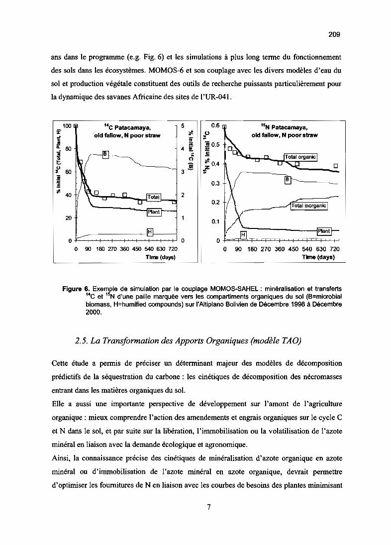
209

ans dans le programme (e.g, Fig. 6) et les simulations à plus long terme du fonctionnement

des sols dans les écosystèmes. MOMOS-6 et son couplage avec les divers modèles d'eau du

sol et production végétale constituent des outils de recherche puissants particulièrement pour

la dynamique des savanes Africaine des sites de l'UR-041.

100 14C Patacamaya, 5 0.6 15N Patacamaya,% :>l!old fallow, N poor straw 0 0 old fallow 1 N poor strawi :r ~

• ;::;: ~0.5iL 80 4 !t -l ;: B

0;;l! 04"iD 0u Z'

: 60 3- ......l B~ 0.3~

40 20.2 -------1fôtal inorganicJ

20 0.1

H H ~0 0 0

0 90 180 270 360 450 540 630 720 0 90 180 270 360 450 540 630 720Tlme (days) lime (days)

Figure 6. Exe~le de simulation par le couplage MOMaS-SAHEL: minéralisation et transferts14C et 1 N d'une paille marquée vers les compartiments organiques du sol (B=microbialbiomass, H=humified compounds) sur l'Altiplano Bolivien de Décembre 1998 à Décembre2000.

2.5. La Transformation des Apports Organiques (modèle TAO)

Cette étude a permis de préciser un déterminant majeur des modèles de décomposition

prédictifs de la séquestration du carbone : les cinétiques de décomposition des nécromasses

entrant dans les matières organiques du sol.

Elle a aussi une importante perspective de développement sur l'amont de l'agriculture

organique: mieux comprendre l'action des amendements et engrais organiques sur le cycle C

et N dans le sol, et par suite sur la libération, l'immobilisation ou la volatilisation de l'azote

minéral en liaison avec la demande écologique et agronomique.

Ainsi, la connaissance précise des cinétiques de minéralisation d'azote organique en azote

minéral ou d'immobilisation de l'azote minéral en azote organique, devrait permettre

d'optimiser les fournitures de N en liaison avec les courbes de besoins des plantes minimisant

7

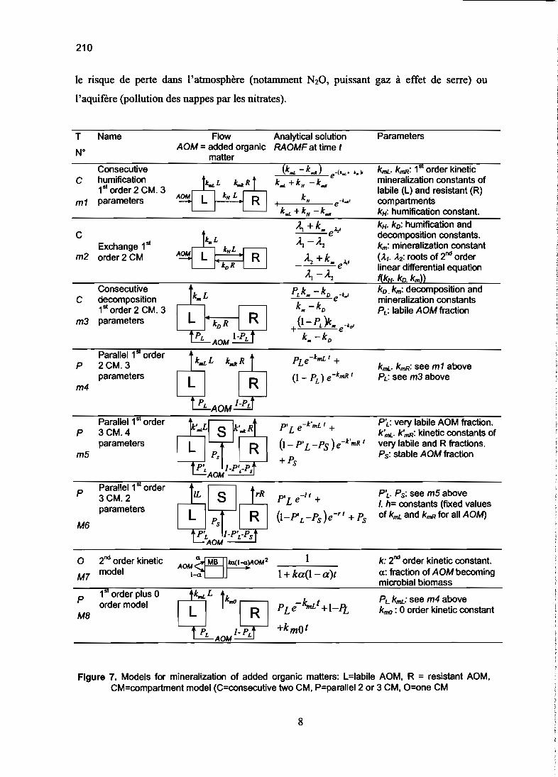
210

le risque de perte dans l'atmosphère (notamment N20, puissant gaz à effet de serre) ou

l'aquifère (pollution des nappes par les nitrates).

T Name Flow Analytical solution Parameters

N°AOM =added organic RAOMFat time t

matterConsecutive (kaL -k.. ) e-(l.. + lN' kmL. kmR: 1st order kinetic

C humification kaL +kH -k.. mineralization constants of151 order 2 CM. 3 labile (L) and resistant (R)

m1 parameters 1k H e- l ..' compartments

kaL+kH-k.. kH: humification constant.

~ +k. eJ.,' kH• ko: humification andC decomposition constants.

Exchange 1stl, -l2 km: mineralization constant

m2 order 2 CM _ l2 +k. e.l,' (Â.,. Â.2: roots of 2nd orderlinear differential equation

li -l2 f(kH• ko.km»Consecutive PLie -leD -1' ko. km: decomposition and

C decomposition • e • mineralization constants151order 2 CM. 3 le -le PL: labile AOM fraction• D

m3 parameters +(1- PJk. e-1o'le. -leD

Parallel 1st order PLe-kmL 1 +P 2CM.3 kmL. kmR: see m1 above

parameters (l - PL ) e-kmR 1 PL: see m3 abovem4

Parallel 1st order P'L e-k'mL 1 + P'L: very labile AOM fraction.P 3CM.4 k'mL. k'mR: kinetic constants of

parameters (1- PIL-Ps ) e-k'mR 1 very labile and R fractions.mS

+PsPs: stable AOM fraction

Parallel 1st orderP P'L' Ps: see mS above3CM.2 P'L e-11 + 1. h= constants (fixed valuesparameters

(l-P'L-Ps )e-rl + Ps of kmL and kmR for ail AOM)M6

0 2nd order kinetic ~21 k: 2nd order kinetic constant.AOM MB m(1~)AOM

M7 model 1-« 1+ ka(l-a)t a: fraction of AOM becomingmicrobial biomass

P1st order plus 0

~t~PLkmL: see m4 above

order model -k"uJM8

LP, Il;] PLe +l-Jt kmO : 0 orcier kinetic constant

+kmotAOM

Figure 7. Models for mineralization of added organic matters: L=labiie AOM, R = resistant AOM,CM=compartment model (C=consecutive two CM, P=parallel 2 or 3 CM, O=one CM

8

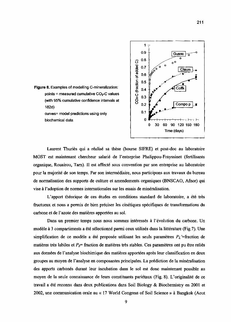
211

Figure 8. Examples of modelling C-mineralization:

points = measured cumulative COrC values

(with 95% cumulative confidence intervals at

182d)

curves= model predictions using only

biochemical data

1

0.9

Û 0.8"0

0.7G)"0"0ni 0.6'0c:

0.50tsni 0.4~o

0.31

'"0o 0.2

0.1

00

o 0

00 1Chicm 1· ...' .....

.y"

.•...

Lcompo p 1.••....•.....30 60 90 120 150 180

lime (days)

Laurent Thuriès qui a réalisé sa thèse (bourse SIFRE) et post-doc au laboratoire

MOST est maintenant chercheur salarié de l'entreprise Phalippou-Frayssinet (fertilisants

organique, Rouairou, Tarn). Il est affecté sous convention par son entreprise au laboratoire

pour la majorité de son temps. Par son intermédiaire, nous participons aux travaux du bureau

de normalisation des supports de culture et amendements organiques (BNSCAO, Afnor) qui

vise à l'adoption de normes internationales sur les essais de minéralisation.

L'apport théorique de ces études en conditions standard de laboratoire, a été très

fructueux et nous a permis de bien préciser les cinétiques spécifiques de transformations du

carbone et de l'azote des matières apportées au sol.

Dans un premier temps nous nous sommes intéressés à l'évolution du carbone. Un

modèle à 3 compartiments a été sélectionné parmi ceux utilisés dans la littérature (Fig.7). Une

simplification de ce modèle a été proposée utilisant les seuls paramètres PL '=fraction de

matières très labiles et Ps= fraction de matières très stables. Ces paramètres ont pu être reliés

aux données de l'analyse biochimique des matières apportées après leur classification en deux

groupes au moyen de l'analyse en composantes principales. La prédiction de la minéralisation

des apports carbonés durant leur incubation dans le sol est donc maintenant possible au

moyen de la seule connaissance de leurs constituants pariétaux (Fig. 8). L'originalité de ce

travail a été reconnu dans deux publications dans Soil Biology & Biochemistry en 2001 et

2002, une communication orale au « 17 World Congress of Soil Science» à Bangkok (Aout

9

212

2002), communications au congrès « Gestion de la Biomasse, Erosion et Sequestration du

Carbone» (Montpellier, Septembre 2002) et aux « Journées nationales pour l'étude des sols»

d'Orléans (Octobre 2002).

AOMinput

k,.",., imN

kvinorgNGaseous !ossesCOz, NzO, (NO).

Organicproducts

Inorganicproducts

Figure 9. The model TAO (Transformation of Added Organics, Transformation des ApportsOrganiques) for C mineralization, N mineralization. N immobilization and Nvolatilization of Added Organic Matters (AOM) in soil: inorgN = inorganic N tromAOM. imN= immobilized N trom AOM(and Soillnorganic N if P;m>1).

L'étape suivante consistait à modéliser les transformations de l'azote qui

accompagnent la minéralisation du carbone lors de la décomposition des matières apportées

au sol. Ces transformations sont plus complexes avec une production d'ammonium qui peut

être soit nitrifié soit réimmobilisé dans le sol par l'intermédiaire de la biomasse microbienne.

Des phénomènes de volatilisation en NH3, N20, NOx et N2 peuvent aussi se produire. La

prédiction simultanée des transformation du carbone et de l'azote spécifiques aux matières

apportées au sol est maintenant possible au moyen du modèle TAO (Transformation ofAdded

Organics, Transformation des Apports Organiques; Fig. 9) mis au point au laboratoire

MOST.

Comme pour la minéralisation du carbone, les transformations de l'azote

(minéralisation, immobilisation, volatilisation) en provenance de matières organiques diverses

ont été simulées par notre modèle avec une précision très encourageante (Fig. 10). Deux

10

213

publications internationales sont sorties cette année dans Soil Biology & Biochemistry (Pansu

et Thuriès, 2003; Pansu et al., 2003).

0.06

louvpl0.005

1Icompo el 0.015

éj 0.05 s-Û

5"~ 0 0

0 ca 1 ca-c Dl ~ 0.1 Dl

::J 0 :J'7 0.04 <:> -c 0.01 0

01 Z Zz 6" ';01

S Z cczZ 0.03 0 ~ s z0 10.:-'2 » z »III 0 ue'

~'20.05 0

0 0.02 co 0.005 :s:::~ 90 .- •0.01

imN0 -0.005 0 0

0 90 180 0 90 180

Time (days) Time (days)

1.5 - 0.3 0.8

1Gnoferl0.15

s-0 0.7ca

~CIl Û::Jc;;' ~ 0.6 s-a z

~0

-c iê CI'7 02 '7 0.1 CIl

Z ::JCI CI 0.5 <:ïZ ce Z ZS

~S 6"z Z 0.4 Z.2 .:: ~ occ .è'" '"E!' E!' 0.3 ~a a

0.5 0.1 0.05 .::!J

0.2

0.1

0 0

90 180 90 180

lime (days) lime (days)

Figure 10. Examples of modelling N transformations:• Experimental data for inorganic N (with 95% confidence intervals)o Experimental data for total N {with 95% confidence intervalslines = predicted values using only biochemical data and incubation time {imN=re­immobilized N. inoryN=produced inorganic NNotes: -for OUvp: total immobilization of inorgN (soil+input) during 3 rnonths, netimmobilization during 6 months,-for Compo e: immediate immobilization of % initial inorgN, then regular Nmineralization,-for Guano: high turnover with gaseous losses-for Gnofer: suppression of gaseous N loss in this Guano based fertilizer.

La collaboration avec Phalippou-Frayssinet se poursuit par l'étude de différentes

variables, notamment la texture des sols, sur les cinétiques de transformation des apports.

11

214

Nous démarrons aussi un programme d'analyse des apports organiques par spectrométrie de

proche infra-rouge (SPIR, near infrared spectrometry, NIRS), avec l'objectif à long terme de

relier la Transformation des Apports Organiques (modèle TAO) à leur spectre dans le proche

infra-rouge. Trois stages étudiants ont été accueillis cette année au laboratoire sur ces

objectifs (Cf. 5 ci-dessous). Un quatrième stage concernait une formation au modèle TAO en

vue de son transfert au laboratoire d'Ecologie Microbienne des sols tropicaux (UR IBIS- IRD,

Dakar. M. Saidou Sall, directeur de ce laboratoire, a été accueilli une semaine en 2003 dans

ce but au laboratoire MOST et devrait effectuer à nouveau un stage en 2004.

3. Ouvrages de synthèse« L'analyse du sol»

Les ouvrages parus sont maintenant salués par la communauté scientifique et

constituent des outils de travail performants par exemple pour le laboratoire MOST et le

laboratoire central d'analyses du CIRAD, notre partenaire à Montpellier.

Le premier volume est disponible sous la référence :

M. Pansu, 1. Gautheyrou, J.Y. Loyer, 1998. - L'analyse du sol - Echantillonnage,

instrumentation et contrôle, Masson, 512 p.

Le volume anglais est disponible sous la référence:

M. Pansu, 1. Gautheyrou et J.Y. Loyer, 2001. - Soil Analysis - Samp/ing

instrumentation, quality control, translated by V.A.K. Sarma, Balkema publishers, 489 p.

Le dernier volume est disponible sous la référence:

M. Pansu et J. Gautheyrou, 2003. - L'analyse du sol - minéralogique, organique et

minérale, Springer-verlag, Paris, Berlin, Heidelberg, New York, Hong Kong, Londres, Milan,

Tokyo, 993 p.

Nous reproduisons ci-après le texte de sa présentation (quatrième de couverture et

bons de commande) :

Marc Pansu et Jacques GautheyrouL'analyse du sol - minéralogique, organique et minérale

Rédigé en conformité avec les normes analytiques. partie intégrante de la démarchequalité, cet ouvrage est un guide de référence pour les choix méthodologiques puis pourla mise en œuvre des nombreuses méthodes, normalisées ou non, de l'analyse du sol. Ilsynthétise une multitude d'informations techniques dans des protocoles, tableaux,formules, modèles de spectres, chromatogrammes et autres diagrammes analytiques.Les modes opératoires sont diversifiés, depuis les tests les plus simples jusqu'auxdéterminations les plus complexes - physico-chimie structurale des édificesminéralogiques et organiques, éléments échangeables, potentiellement disponibles ettotaux, pesticides et polluants, éléments traces et isotopes. C'est un outil de base pourles chercheurs, ingénieurs, techniciens, professeurs et étudiants spécialisés en

12

215

pédologie, agronomie, sciences de la terre et de l'environnement, et pour les disciplinesconnexes telles que physico-chimie analytique, géologie, hydrologie, écologie,climatologie, génie civil et industries associées aux sols.

Ci-dessous un récent compte rendu de lecture publié par l'Union des Professeurs de

Physique et Chimie, également disponible sur le site:

http://www.udppc.asso.fr/nouveautes/fourniss/livresllli200312.htm#2916

L'analyse du sol - minéralogique, organique et minérale, Pansu, M. et Gautheyrou,J., Springer-Verlag

Analyser un sol est un problème complexe : d'abord les composés à identifier et 1 oudoser sont nombreux. Ensuite certains paramètres transversaux sont utiles (ounécessaires), comme par exemple l'azote total. Enfin les techniques d'analyse sontextrêmement diverses, et sont empruntées à tous les domaines de la physico-chimie. Cetouvrage regroupe toutes les analyses de sols existantes, depuis la physique pure(granulométrie) jusqu'à la chimie-chimie (azote Kjeldahl) : aucun domaine de la physico­chimie n'est laissé de côté, un regard sur le sommaire suffit pour s'en persuader. A telpoint qu'on comprend vite que les auteurs ont collaboré avec des pédologues, desbiologistes, des analystes ... ne pouvant être spécialistes de tous ces domaines. Lesmodes opératoires proposés, détaillés et utilisables immédiatement, s'appuient sur unebibliographie solide (cf. le dosage des carbonates par acidimétrie, p 598), et sur lesnombreuses nonnes en vigueur dans ce domaine (voir pH Ca et pH K p. 565, parexemple). De très bonnes tables sont disponibles, regroupant souvent des données peuusuelles (consulter p. 25, p. 596, ...). Les limites des différentes méthodes sont mises enrelief (par exemple dosage des nitrates et nitrites par UV ou par colorimétrie, p 778). Etles paramètres importants sont soulignés efficacement : la polarité des solvantsd'extraction est un point central pour le dosage des lipides, bien mis en valeur (p. 472).Les auteurs ne se sont pas limités aux grands classiques (pH, potentiel redox) : lesdosages par électrodes spécifiques sont détaillées, commentées, critiquées (lire parexemple p.780 à propos de NH4+, ou bien p. 784 à propos de N03-). Ce livre seracertainement une référence dans le domaine du sol. C'est un outil extrêmement complet,très transversal, aisé à utiliser. A mettre à la disposition de toutes les équipes dechimistes, physiciens, biologistes... qui travaillent sur les sols. Le seul défaut de cetouvrage de référence est sans doute son poids (1,7 kg), qui le rend difficile à emmenerpartout avec soi. Mais trimballons-nous le Chemical Handbook ?BaUDOT, HélèneUnion des Professeurs de Physique et Chimie

Le principe d'une traduction en anglais de ce livre a également été accepté par

l'éditeur Springer et sa réalisation est à l'étude.

4. Animation de la recherche

Animateur de séminaires scientifiques mensuels (troisième Jeudi de chaque mois) sur

la communauté scientifique Agropolis (IRD, CIRAn, CNRS, INRA, ENSAM, Université

Montpellier II, CNEARC, CEMAGREF, ENGREF). Le thème des exposés concerne toutes

les disciplines en relation avec l'étude des sols. D'abord accueillis dans les locaux de l'IRD,

ils sont maintenant intégrés dans le programme d'Agropolis sous l'égide de l'IFR Ecosystem

13

216

et se déroulent principalement dans les locaux plus spacieux d'Agropolis International. Ont

déjà eu lieu les exposés suivants :

Intervenant Date TitreBarthès B, IRD 2S.0S.00 Agrégation des sols et sensibilité au ruissellement et à

l'erosionTraoré K, U-Mali 30.06.00 Rôle du parc à karités sur le statut organique et la fertilitéPansu M, IRD IS.03.01 Modélisation de la dynamique des matières organiques

des solsBabre D,Cirad 26.04.01 La certification dans les laboratoires d'analysePratC,IRD OS.04.01 Mise en valeur agricole des sols volcaniques indurés du

MexiqueRoose E, IRD 11.0S.01 Evolution des stratégies de lutte anti-érosiveLarré MC, IRD 28.06.01 Utilisation des composts en agriculture: tests de maturitéBourgeon G, Cirad 04-10-01 Niveaux d'organisation des couvertures pédologiques:

applications en IndeFeller C Manlay R, 26-10-01 Concepts sur humus et durabilité au cours des troisIRD derniers sièclesHervé D,!RD 22-11-01 Bassin versant et usage du sol: le divorce?Gigou J, Cirad 17-01-02 Culture sur billons de niveau, rendements et gestion de

l'eauBraudeau E, IRD 21-02-02 La rétractométrie des solsWarembourg F, CNRS 21-03-02 Racine vivante et flux de carbone dans les solsBlavet D, IRD 2S-04-02 La couleur des solsSaison C, Cirad 23-0S-02 Devenir des polluants organiques dans les sols contaminésPoss R, IRD 27-06-02 La salinisation des rizières en ThaïlandeDavrieux F et 20-09-02 Applications environnementales de la Spectrométrie dansLecomte P, Cirad le Proche Infra-Rouge (SPIR)Pansu M, IRD 17-10-02 Cinétique des entrées organiques dans les modèles de

décompositionSaugier B, Univ-Paris 14-11-02 Biosphère continentale, changements globaux et puits deSud carboneAsseline J, !RD 19-12-02 Le drone Pixy pour l'observation aérienne rapprochéeBlanchart E. et Feller 23-01-03 Darwin et les vers de terreC.,IRDDrevon 1.J., INRA 20-02-03 Phosphore et fixation symbiotique de l'azote en sols peu

fertilisésHinsinger Ph., INRA 27-03-03 Interactions chimiques sol-racines dans la rhizosphèreBrowers M., CIRAD 24-04-04 La compaction des solsRollin D.. CIRAD lS-OS-03 Le semis direct sous couvert végétal : intérêt et limitePeoples M., CSIRO 10-07-03 N dynamics in Australian pasture systems: Nfixation,Australie Nmineralisation and crop uptake of pasture NHamel 0, CIRAD 18-09-03 Flux de CO2 et H20 et séquestration de carbone sur lesEpron D., U Nancy 1 peuplements d'Eucalyptus du CongoCarcaillet C. HPHE 16 10-03 Paléo-incendies et cycle du carbone.Legros 1.P. ENSAM, 20-11-03 Aspects actuels de la cartographie des solsSec. Gén. AFES 1

14

217

AFES - Association Française d Etude des Sols,2 IUSS = International Union of Soil Science,3 TSBF = programme international Tropical Soil Biology and Fertility

Ruellan A., ex prés. 18-12-03 La formation aux solsIUSS2

Swift M., ex Dir. Prog. 22-01-04 Biological Management of Soil Fertility in AfricaTSBF3

1 - ,

5. Expertise, communication, formation

- Expert « rewiever» revues « Soit Biology & Biochernistry (Elsevier) », « Etude et

gestion des sols (AFES) », « Nutrient cycling in agro-ecosystems (Kluwer) ».

- Formation et encadrement de quatre stagiaires:

+ Léo Cayeux (DUT Génie Biologique, IUT) sur la caractérisation de matières

premières végétales, avec calibrage de la spectrométrie proche infrarouge (SPIR) à

partir des résultats des méthodes classiques de dosage des constituants pariétaux et

des polyphénols totaux.

+ Fabien Petit (Elève-ingénieur chimiste ENSlACET, Toulouse) sur le calibrage de

spectres proche infrarouge (SPIR) de matières premières végétales d'origine

tropicale, basé sur l'analyse conventionnelle de leur contenu en constituants

pariétaux (méthode Van Soest).

+ Loïc Legourrierec (Elève-ingénieur chimiste, ENSCM, Montpellier) sur l'étude de

l'influence de la texture, de la minéralogie et de la teneur en matière organique du

sol sur les dynamiques de minéralisation du carbone et de l'azote provenant

d'apports organiques en conditions contrôlées (incubation de 13 sols).

+ Saidou Sall, Directeur du laboratoire d'Ecologie Microbienne des Sols Tropicaux

(UR mIS, Sénégal) : application du modèle TAO a une étude de décomposition de

nécromasse végétale doublement marquée 14C et 15N.

- Participation à la rédaction du rapport fmal du programme européen Tropandes.

6. Projets

Soumission au programme national ECCO-PNBC d'un projet coordonné auprès des

partenaires MOST-IRD, MOST-CIRAD, INERA Burkina et LEMST Sénégal intitulé

« Transformations organiques et fertilité des sols de la zone soudanienne en liaison avec les

changements de pratiques culturales». Son objectif est d'évaluer les potentialités de stockage

15

218

de matière organique et de transfert entre compartiments organiques, ainsi que leur

déterminisme, dans les sols des régions centre et sud-ouest du Burkina Faso. L'évolution des

réservoirs de carbone et d'azote du sol devrait être appréhendée sur la base d'une importante

collecte de données de terrain et de laboratoire, en faisant notamment ressortir les modes de

gestion des agrosystèmes (restitutions organiques au sol) et les caractéristiques climatiques.

Les données collectées seraient utilisées pour modéliser les transferts entre compartiments

(apports et restitutions, biomasse microbienne, compartiments humifiés), au moyen

notamment des modèles TAO (transformation des apports) et MOMOS (dynamique des

compartiments du sol), avec couplage à un modèle de prédiction de 1'humidité du sol

(SAHEL). A terme, on viserait à l'intégration des données dans un modèle global du cycle de

l'eau, du carbone et de l'azote, en liaison avec le fonctionnement microbien des systèmes,

auquel une attention particulière serait portée. La rédaction du projet a été rapide en 2003 du

fait de la date très tardive de l'appel d'offre. Ses évaluateurs ont souligné sa pertinence

scientifique, mais ils n'ont pas retenu son financement pour 2003 et nous encouragent à le

soumettre à nouveau en 2004 ; probablement en élargissant le nombre de partenaires.

Parmi les autres projets possibles se trouvent deux. thèmes très attractifs

scientifiquement pour compléter nos recherches sur le modèle MOMOS par (1) la datation du

carbone (ou de ses fractions) qui s'accumule sur le paramo vénézuelien, (2) la reprise des

données 14C et ISN d'un précédent programme européen pour valider et étendre le modèle

MOMOS à différentes conditions édaphiques et climatiques. Ces travaux. pourraient être

réalisés dans le cadre des projets ECOS-Nord de coopération scientifique France-Venezuela.

Un autre projet à murir probablement dans le cadre des projets européens INCO-DEV devrait

concerner une étude comparative du fonctionnement des savanes Ouest-Africaines et

Vénézueliennes sous l'effet de différents systèmes de gestion.

Références 2003 à février 2004

Revues internationales

Marc Pansu et Laurent Thuriès, 2003 - Kinetics of C and N mineralization, N immobilizationand N volatilization of organic inputs in soil. Soi! Biology & Biochemistry, 35, 37-48.

Marc Pansu, Laurent Thuriès, Marie-Christine Larré-Larrouy et Pierre Bottner, 2003 ­Predicting N transformations from organic inputs in soil in relation to incubation timeand biochemical composition. Soi! Biology & Biochemistry, 35, 353-363.

16

219

Pierre Bottner, Marc Pansu, Ruben Callisaya, Klaas Metselaar, Dominique Hervé, 2003 ­Modelizaciôn de la evoluciôn de la materia orgànica en suelos en descanso (Altiplanoseco boliviano), Ecologia en Bolivia, sous presse.

Marc Pansu, Pierre Bottner, Lina Sarmiento and Klaas Metselaar, 2004 - Comparison of fivesoil organic matter decomposition models using data from a 14C and ISN labeling fieldexperiment, soumis pour publication à Global Biogeochemical Cycles.

Marc Pansu, Klaas Metselaar, Pierre Bottner, and Lina Sarmiento, 2004 - Sensitivity analysisof two types of soil organic matter decomposition models, soumis pour publication àGlobal Biogeochemical Cycles.

Ouvrage

M. Pansu et J. Gautheyrou, 2003 - L'analyse du sol- minéralogique, organique et minérale,Springer-Verlag, Paris, Berlin, Heidelberg, New York, Hong-Kong, Londres, Milan,Tokyo, 995 p.

Rapports

INCO-DC ERBICI8CT98-0263, 2003. Final report of Tropandes program. T. Carballas ed.,CESGA, Santiago de Compostella, Spain.

Cayeux L., 2003 (encadrement L. Thuriès et M. Pansu). Caractérisation de matières premièresvégétales: calibrage de la méthode « Near Infra Red Spectroscopy» (NIRS) à partirdes résultats des méthodes classiques de dosage des constituants pariétaux et despolyphénols totaux. Mémoire de DUT Génie biologique, Option Industriesalimentaires et biologiques, Université Montpellier II.

Petit F., 2003 (encadrement L. Thuriès et M. Pansu). Caractérisation de matières premièresvégétales par méthodes biochimique et spectroscopique (NIRS). Rapport de stage de1C année, Ecole Nationale Supérieure d'Ingénieurs en Arts Chimiques etTechnologiques, Toulouse, 71 p.

17

220

221

Publications M. Pansu

Revues à comité de lecture

P. Guillet, Coz J., Sannier C., Barathe 1., Mustapha A., Pansu M., J.Itard, 1979 - Etude de lasensibilité à quelques insecticides, OMS 1998, OMS 1821, OMS 2, OMS 185, OMS595, OMS 570 de glossines d'élevage, Cah. ORSTOM, Ser. Ent. Med. et Parasito.XVII,81-87.

M. Pansu, M.H. Dhouibi, M. Pinta, 1981 - Détermination des traces de pyréthrinoïdes dansles substats biologiques par chromatographie en phase gazeuse, Analusis, 9, 55-59.

M. Pansu, S. Tostain, M. Pinta, 1981 - Etude par chromatographie en phase gazeuse de lavariabilité des acides gras des graines de mil, Journal ofchromatography, 204, 377­383.

M. Pansu, M.N. Al Salti, H. Aubert, J. Gry, 1981 - Contribution à l'étude de l'activitésystémique du carbofuran par chromatographie en phase gazeuse, Phytiatriephytopharmacie, 30, 203-214.

M. Pansu et F. Abo, 1985 - Application d'un progiciel de chimiométrie (SPCLAS) à l'étude del'incidence du Bore et du Manganèse sur la fertilisation du blé (triticum aestivum L.),Analusis, 13,443-451.

M.Pansu et H.Sidi, 1987 - Cinétique d'humification et de minéralisation des mélanges sols­résidus végétaux, Sciences du sol, 25, 4, 247-265.

M.Pansu, 1988 - Proposition de modèles descriptifs de la dynamique des matières organiquesdes sols, Cah. ORSTOMSer. Pédol., XXIV, 4,361-362.

H. Sidi et M. Pansu, 1990 - Effets d'apports organiques et de gypse sur la stabilité structuralede deux sols méditerranéens, Science du Sol, 28, 237-255.

M. Pansu, 1991 - Détermination de quelques paramètres caractéristiques de la cinétiqued'humification et de minéralisation des amendements organiques dans les sols, Cah.Orstom Ser. Pédol., XXVI, 2: 131-144.

Z. SalIih et M. Pansu, 1993 - Modelling of soil carbon fonns after organic amendments undercontrolled conditions. Soi! Biology & Biochemistry, 25, 1755-1762.

M. Pansu, Z. Sallih et P. Bottner, 1996. - Modélisation des formes du carbone organique dansles sols. Compte Rendus de l'Acad. des Sciences, Série Ila, 322, 401-406.

M. Pansu, Z. SalIih et P. Bottner, 1998 - Modelling of soil nitrogen fonns after organicamendments under controlled conditions. Soi! Biology & Biochemistry, 30, 19-29.

P. Bottner, M. Pansu et Z. Sallih, 1999. - Modelling the effect of active roots on soil organicmatter turnover, Plant and Soils, 216, 15-25.

222

L. Thuriès, M. -CO Larré-Larrouy et M. Pansu, 2000. - Evaluation of three incubation designsfor mineralization kinetics of organic materials in soil. Communications in Soi!Science and Plant Analysis, 31, 289-304

L. Thuries, A. Arrufat, M. Dubois, C. Feller, P. Hemnann, M.C. Larre-Larrouy, C; Martin,M. Pansu, J.C. Remy et M. Viel, 2000. - Influence d'une fertilisation organique et dela solarisation sur la productivité maraîchère et les propriétés d'un sol sableux sousabri. Etude et Gestion des sols, 7, 73-88.

L. Thuriès, M. Pansu, C. Feller, P. Hermann, et lC. Rémy. 2001 - Kinetics of added organicmatter decomposition in a mediterranean sandy sail. Soil Biology & Biochemistry 33,997-1010.

L. Thuriès, M. Pansu, M.C. Larre-Larrouy et C. Feller. 2002 - Biochemical composition andmineralization kinetics of organic inputs in a sandy sail. Soil Biology & Biochemistry34, 239-250.

M. Pansu et L. Thuriès 2003 - Kinetics of C and N mineralization, N immobilization and Nvolatilization of organic inputs in sail. Soil Biology & Biochemistry, 35, 37-48.

M. Pansu, L. Thuriès, M.C. Larré-Larrouy et P. Bottner, 2003 - Predicting N transformationsfrom organic inputs in soil in relation to incubation time and biochemicalcomposition. Soil Biology & Biochemistry, 35, 353-363.

P. Bottner, M. Pansu, R. Callisaya, K. Metselaar, D. Hervé, 2003 - Modelizaci6n de laevoluci6n de la materia orgànica en suelos en descanso (Altiplano seco boliviano).Ecologia Boliviana, sous presse.

Marc Pansu, Pierre Bottner, Lina Sarmiento and Klaas Metselaar, 2004 - Comparison of fivesoil organic matter decomposition models using data from a 14C and l~ labeling fieldexperiment, soumis pour publication à Global Biogeochemical Cycles.

Marc Pansu, Klaas Metselaar, Pierre Bottner, and Lina Sarmiento, 2004 - Sensitivity analysisof two types of soil organic matter decomposition models, soumis pour publication àGlobal Biogeochemical Cycles.

Livres

M. Pansu, 1 Gautheyrou et lY. Loyer, 1998 - L'analyse du sol - échantillonnage,instrumentation et contrôle, Masson, 512 p.

M. Pansu, J. Gautheyrou et J.Y. Loyer, 2001 - Soi! analysis - sampling, instrumentation andqua/ity control, translated from French by V.A.K. Sanna, Balkema Publishers, 489 p.

M. Pansu et J. Gautheyrou, 2003 - L'analyse du sol - minéralogique, organique et minérale,Springer-Verlag, 995 p.

Communication à congrès internationaux

2

223

M. Pansu, Sallih Z. et Bottner P., 1998. - A process-based model for carbon and nitrogentransfers in soil organic matter. Un modèle mécaniste des flux de C et N dans lamatière organique du sol. Actes 16° Congrès mondial de science du sol, Montpellieraoût 1998.

L. Thuriès and M. Pansu, 2001. - Classification and modelling of added organic matterdecomposition in a sandy soil. Proceeding of 11 Nworkshop, Reims, France, 9-12Sept. 2001.

M. Pansu, L. Thuriès, M.C. Larré-Larrouy et C. Feller, 2002 - Kinetics of organic inputs insoil carbon model. Proceeding of 17th World Congress ofsoil science, Bangkok, 14-21August 2002, Oral communication 1502, symposiumlO.

M. Pansu et P. Bottner, 2002 - Modélisation de l'effet des racines actives sur les transferts deC organique dans les sols. Proceeding of congress Gestion de la biomasse, erosion etsequestration du carbone, Agropolis Montpellier, 23-28 Septembre 2002.

L. Thuriès et M. Pansu, 2002 - Classification et modélisation de la décomposition de matièresorganiques ajoutées au sol. Proceeding of congress Gestion de la biomasse, erosion etsequestration du carbone, Agropolis Montpellier, 23-28 Septembre 2002.

Communication à congrès nationaux

M. Pansu et F. Abo, 1986 - L'outil informatique au service des analyses chimiques etagronomiques, Actes 26ème semaine scientifique de Latakié-Syrie.

M. Pansu, 1987 - La gestion des données des laboratoires d'analyses physico-chimiques.Exemple d'application: MIDAS, Actes SEMINFOR1 "premier séminaire informatiqueORSTOM', 203-219.

M.Pansu, 1988 - Cinétique chimique et modèles compartimentaux : application à l'étude del'évolution du stock organique des sols. In actes séminaire SEMINFOR "Iamodélisation: aspects pratiques et méthodologie", ORSTOM Coll. et séminaires, 46­61.

M. Pansu et P. de Boissezon, 1990 - Dynamique du carbone organique dans les mélangessols-résidus végétaux; influence sur la capacité d'échange cationique. Actes GEMOS(Groupe d'étude des matières organiques des sols), INRA-Bordeaux 18-19 avril1989).

M. Pansu, 1990 - Modélisation appliquée à l'étude du stock organique et de la stabilitéstructurale de sols méditerranéens, Actes séminaire de Tiaret (Algérie) "Les solscéréaliers", Tiaret, sept 1989.

M. Pansu, R. Gavinelli et P. Espiau, 1990 - Etude de précision appliquée à la détermination del'acidité d'échange des sols, Actes Journées des laboratoires 18..20 septembre 1990ORSTOM Bondy.

3

224

M. Pansu, Z. Sallib et P. Bottner, 1991 - Cinétique d'évolution des formes du carboneorganique dans les sols. In actes séminaire SEMINFOR5 "Statistiques impliquées",ORSTOM Coll. et séminaires.

M. Pansu, 1994 - Modélisation des formes du carbone organique dans les sols. Actes 4emesjournées d'études des sols-AFES (Association Française d'Etude des Sols), Lille 19­21 avri11994.

M. Pansu and P. Bottner, 2001. - Modélisation de l'effet des racines actives sur les transfertsde carbone organique dans les sols. Actes 3° colloque rhizosphère, Dijon, 26-28 Nov.2001

M. Pansu, L. Thuriès, MC Larre-Larrouy et C. Feller, 2002. - Dynamique de minéralisationd'apports organiques dans les modèles carbone du sol. Actes Journées Nationalesd'Etude des Sols AFES, 22-24 Octobre 2002, Orléans.

Publications IRD, logiciels

M. Pansu, 1983 - SPCLAS - Un logiciel basic pour le calcul, le classement, la gestion desrésultats d'un laboratoire d'analyses physico-chimiques, ORSTOM (60 p.).

M. Pansu, 1985 - Le logiciel SPCLAS, Fiches techniques Agence Nationale du logiciel­Vandoeuvre les Nancy.

M. Pansu 1985 - OPTIMI - Optimisation des mesures par utilisation de plans d'expériences etméthodologie des surfaces de réponse, Fiches techniques Agence Nationale duLogiciel-Vandoeuvre les Nancy. In Logiciels pour la chimie, Société Française dechimie.

M. Pansu 1985, HUMUS - Extension du logiciel SPCLAS à la gestion personnalisée d'unlaboratoire, Fiches techniques Agence nationale du Logiciel-Vandoeuvre les Nancy.

M. Pansu et B. Loustalan, 1990 - Le logiciel MIDAS: Management Informatique desDonnées Analytiques : manuel d'utilisation (70 pages) et disquettes programmescompilés, aide en ligne et exemples, LogORSTOM.

M. Pansu, 1992 - Les sucres neutres dans les sols: opportunité et tentatives d'amélioration deleur détermination, Document ORSTOM Montpellier, n04 : 24 p.

Rapports, conférences, information scientifique

Programmes et expertise

P. Bottner, M.M. Couteaux, D. Hervé et M. Pansu, 2003 - INCO-DC ERBIC18CT98-0263,.Final report of Tropandes program. T. Carballas ed., CESGA, Santiago deCompostella, Spain, Part 5 And 7.

4

225

M. Pansu et D. Hervé, 2000. - El analysis de suelo en laboratorios de Pern y Bolivia (Lima,Puno, La Paz, Cochabamba). IRD et Consortium pour le développement del'écorégion andine (CONDESAN), 18 p.

Rapports divers

M. Pansu, 1985, 1986, et 1987 - Rapports d'activités du laboratoire "Matières organiques",ORSTOM-BONDY.

M. Pansu, 1986 - Influence de la préparation des échantillons sur la précision des analyses desols, ORSTOM-BONDY.

M. Pansu, 1986 - Plan d'essai de précision inter-laboratoires ORSTOM, Comité des moyensanalytiques-ORSTOM

P. Baujard et M. Pansu, 1987 - Analyse des problèmes liés à l'utilisation dudibromochloropropane dans les sols de la zône sahélienne Ouest-Africaine, Labo denématologie ORSTOM-DAKAR-SENEGAL.

M. Pansu et Y.Jacob, 1988 - Installation d'une unité d'analyses de résidus de nématicides aulaboratoire de nématologie ORSTOM-DAKAR.

M. Pansu, 1990 - Compte rendu de mission à l'LN.E.S. agro-vétérinaire de Tiaret (Algérie),17-22 Mars 1990.

M. Pansu, N.Elissa, 1990 - Cinétique de dégradation de solutions diluées de deltaméthrine enrelation avec leur pouvoir insecticide.

M. Pansu, 1990 - Modélisation de l'évolution des compartiments organiques des sols, Rapportd'activités Juillet 1990.

M. Pansu, 1991- 2000. - 10 Rapports de secrétariat de l'ouvrage" Analyse du sol".

M. Pansu, 1999. - Rapport de mission Pérou et Bolivie du 6 au 29 Novembre 1999, 15 p., 4photos (avec traduction en espagnol pour les partenaires)

Conférences

-La programmation des micrordinateurs, le langage Basic et son utilisation au laboratoire,GAMS PARIS, cycle "l'outil informatique en chimie analytique", 1984, 1985, 1986,1987.

-Gestion de fichiers de données : exemples d'applications au laboratoire, GAMS PARIS,cycle "l'outil informatique en chimie analytique", 1984, 1985, 1986, 1987.

-Méthodes d'optimisation des conditions expérimentales en spectrométrie atomique:principes, informatisation, applications, CNRS- formation- IVRY, cycle "Spectrométrieatomique par émission et absorption: application à l'analyse", 1986.

-Optimisation des conditions expérimentales en spectrométrie atomique : plans d'expérienceset méthodologie des surfaces de réponse", CNRS-Formation-BONDY, cycle

5

226

"Spectrométrie d'émission et d'absorption atomique", 1986, 1987, 1988, 1989, 1990,1991, 1992, 1993, 1994, 1995, 1996, 1997.

-Caractérisation des matières organiques des sols en liaison avec leur dynamique d'évolution,Faculté d'agronomie, DAMAS, 1986.

-Utilisation du logiciel de gestion de bases de données DBASE III, ORSTOM-DIVA­formation BONDY, 1986, 1987.

-Initiation à la programmation en langage BASIC, ORSTOM-DIVA-formation BONDY,1986, 1987.

-La mesure chimique, son intervalle de confiance et quelques tests liés à l'étude de saprécision, ORSTOM-DIVA-Formation, cycle "Valorisation informatique des donnéesdes laboratoires d'analyses physico-chimiques", 1987.

-Aperçu des méthodes d'optimisation en physico-chimie analytique, ORSTOM-DIVA­Formation, cycle "Valorisation informatique des données des laboratoires d'analysesphysico-chimiques", 1987.

-Gestion de l'information physico-chimique: exemples d'application, ORSTOM-DIVA­Formation, cycle "Valorisation informatique des données des laboratoires d'analysesphysico-chimiques, 1987.

M. Pansu, 1999. El analysis de suelo. Université de Lima, Puno, La Paz, Cochabamba. 20transparents, 1 h de conférence + 1 h de discussions. Collaboration avec DominiqueHervé pour la traduction préalable du texte en espagnol et pour la traduction desquestions.

M. Pansu, 2001. Le sol - formation, fonctions, composition, dégradation. Grand public, 5°Festival« L'avenir au naturel» L'Albenc Isère, 1 Sept. 2001.

M. Pansu, 2001. Le sol- formation, fonctions, composition, dégradation. Public BTS, Fête dela science, 16 Oct. 2001.

M. Pansu, 2001. Modélisation des transferts de carbone et azote dans les sols. Publicscientifique et enseignement supérieur, séminaires Agropolis, M. Pansu, organisateur

M. Pansu, 2002. Modélisation de la transformation des apports de carbone dans les sols.Public scientifique et enseignement supérieur, étudiants INA-PG, 4 Décembre 2002.

Information scientifique,

M. Pansu, 2000. - Le sol et son analyse. Fréquence Chimie, 28, 2-9.

M. Pansu et F. Doumenge, 2000. - Modélisation des transferts de carbone et d'azote dans lessols, poster tète de la science.

M. Pansu, 2001. - Le sol : formation, fonctions et composition. In Encyclopédie francophonesur Internet Webencyclo http://webencyclo.com. rubrique « sol », editions Atlas

6

227

M. Pansu, 2001. - Le sol: méthodes d'analyse. In Encyclopédie francophone sur InternetWebencyclo http://webencyclo.com. rubrique « sol », editions Atlas

7

228

Annexe 5 : diplôme

~ ' . • "1,.

N° ._lL........

":,r.

• j

Le Rcaeut,

RÉPU~LIQgE FRANÇAISE

MINlS'l"ÈRE DE L'ÉDUCATION NATIONALE - tJAlIU<IIJlÎX»..IHI.1l1D:...8AI1.QlW._...__.. , ':. POLYTECHNIQUE

1

DIPLÔME D'INCÉ-NIEURDE 't 'ÉCOL E NATIONALE SUPÉRIEUIlE

D_L "'Cgu l..Oq. 51'"

J:1, J'artüJe II dll dImt dM Ii jtlll1lier 1947,

dlJivrons Je pritmt dipMJm li M.allJluur..Ha=....PABSIL ....,..

LE DII.i!.CTEUI. ET LES PllOPESSEUI.S DE L'ÉCOLB NA.TIONALB SUPÉI.1EUD

Di..._e...JL1..1LLI._.H_.::UL.JU...2..-'I'\lwS!Lll1I__---:-_.,.,.-- ,

«rliftmt flll M.91lJ.l~Jl~J~~1!_...... ...-----~_

ni li .DlLU. {11h01 _ _ , le ..u Ayril 1947 .._ ....:..:::.5:.·

a Jll6i aWfJII«ès lu lpnMtJts prumfts POlir J',)ttntitln dM IJ;pa. Ii'~'-'---'~"=

................!::EC9!t!_~~~_.~~~ ...!E CB~"ifE r . .~ ,_.....,.__.__