approches générales de résolution pour les problèmes multi

Universite de Montreal& Universite de Technologie de Troyes (co-tutelle)

Approches generales de resolution pour les problemes

multi-attributs de tournees de vehicules et confection

d’horaires

parThibaut VIDAL

Departement d’informatique et de recherche operationnelleFaculte des arts et des sciences

These presenteeen vue de l’obtention du grade de

Philosophiæ Doctor (Ph.D.) en Informatique

Mars, 2013

Cette these a ete evaluee par un jury compose des personnes suivantes:

Teodor Gabriel CRAINIC, Directeur de rechercheMichel GENDREAU, Co-directeurChristian PRINS, Co-directeurDaniele VIGO, RapporteurRichard EGLESE, RapporteurJean-Yves POTVIN, ExaminateurCaroline PRODHON, ExaminateurMarc SEVAUX, Examinateur.

Universite de Montreal& Universite de Technologie de Troyes (co-tutelle)

Cette these intitulee:

Approches generales de resolution pour les problemes

multi-attributs de tournees de vehicules et confection

d’horaires

presentee par:

Thibaut VIDAL

a ete evaluee par un jury compose des personnes suivantes:

Teodor Gabriel CRAINIC, Directeur de rechercheMichel GENDREAU, Co-directeurChristian PRINS, Co-directeurDaniele VIGO, RapporteurRichard EGLESE, RapporteurJean-Yves POTVIN, ExaminateurCaroline PRODHON, ExaminateurMarc SEVAUX, Examinateur.

These acceptee le: 10 Decembre 2012

RESUME

Le probleme de tournees de vehicules (VRP) implique de planifier les itineraires d’une flotte de

vehicules afin de desservir un ensemble de clients a moindre cout. Ce probleme d’optimisation

combinatoire NP-difficile apparait dans de nombreux domaines d’application, notamment en

logistique, telecommunications, robotique ou gestion de crise dans des contextes militaires et

humanitaires. Ces applications amenent differents contraintes, objectifs et decisions supplementaires ;

des “attributs” qui viennent completer les formulations classiques du probleme. Les nombreux VRP

Multi-Attributs (MAVRP) qui s’ensuivent sont le support d’une litterature considerable, mais

qui manque de methodes generalistes capables de traiter efficacement un eventail significatif de

variantes. Par ailleurs, la resolution de problemes riches, combinant de nombreux attributs, pose

d’importantes difficultes methodologiques.

Cette these contribue a relever ces defis par le biais d’analyses structurelles des problemes,

de developpements de strategies metaheuristiques, et de methodes unifiees. Nous presentons tout

d’abord une etude transversale des concepts a succes de 64 meta-heuristiques pour 15 MAVRP

afin d’en cerner les “strategies gagnantes”. Puis, nous analysons les problemes et algorithmes

d’ajustement d’horaires en presence d’une sequence de taches fixee, appeles problemes de timing.

Ces methodes, developpees independamment dans differents domaines de recherche lies au transport,

ordonnancement, allocation de ressource et meme regression isotonique, sont unifies dans une revue

multidisciplinaire.

Un algorithme genetique hybride efficace est ensuite propose, combinant l’exploration large des

methodes evolutionnaires, les capacites d’amelioration agressive des metaheuristiques a voisinage,

et une evaluation bi-critere des solutions considerant cout et contribution a la diversite de la

population. Les meilleures solutions connues de la litterature sont retrouvees ou ameliorees pour le

VRP classique ainsi que des variantes avec multiples depots et periodes. La methode est etendue

aux VRP avec contraintes de fenetres de temps, duree de route, et horaires de conducteurs. Ces

applications mettent en jeu de nouvelles methodes d’evaluation efficaces de contraintes temporelles

relaxees, des phases de decomposition, et des recherches arborescentes pour l’insertion des pauses

des conducteurs. Un algorithme de gestion implicite du placement des depots au cours de recherches

locales, par programmation dynamique, est aussi propose. Des etudes experimentales approfondies

demontrent la contribution notable des nouvelles strategies au sein de plusieurs cadres meta-

heuristiques.

Afin de traiter la variete des attributs, un cadre de resolution heuristique modulaire est

presente ainsi qu’un algorithme genetique hybride unifie (UHGS). Les attributs sont geres par des

composants elementaires adaptatifs. Des experimentations sur 26 variantes du VRP et 39 groupes

d’instances demontrent la performance remarquable de UHGS qui, avec une unique implementation

et parametrage, egalise ou surpasse les nombreux algorithmes dedies, issus de plus de 180 articles,

revelant ainsi que la generalite ne s’obtient pas forcement aux depends de l’efficacite pour cette

classe de problemes. Enfin, pour traiter les problemes riches, UHGS est etendu au sein d’un cadre

de resolution parallele cooperatif a base de decomposition, d’integration de solutions partielles, et

de recherche guidee.

vi

L’ensemble de ces travaux permet de jeter un nouveau regard sur les MAVRP et les problemes

de timing, leur resolution par des methodes meta-heuristiques, ainsi que les methodes generalistes

pour l’optimisation combinatoire.

Mots clefs : Recherche operationnelle, Optimisation Combinatoire, Logistique, Transport, Pro-

bleme de Tournees de Vehicules, Ordonnancement, Heuristique, Metaheuristique, Algorithmes

Genetiques, Algorithmes Paralleles

ABSTRACT

The Vehicle Routing Problem (VRP) involves designing least cost delivery routes to service a

geographically-dispersed set of customers while taking into account vehicle-capacity constraints.

This NP-hard combinatorial optimization problem is linked with multiple applications in logistics,

telecommunications, robotics, crisis management in military and humanitarian frameworks, among

others. Practical routing applications are usually quite distinct from the academic cases, encom-

passing additional sets of specific constraints, objectives and decisions which breed further new

problem variants. The resulting “Multi-Attribute” Vehicle Routing Problems (MAVRP) are the

support of a vast literature which, however, lacks unified methods capable of addressing multiple

MAVRP. In addition, some rich VRPs, i.e. those that involve several attributes, may be difficult

to address because of the wide array of combined and possibly antagonistic decisions they require.

This thesis contributes to address these challenges by means of problem structure analysis, new

metaheuristics and unified method developments. The “winning strategies” of 64 state-of-the-art

algorithms for 15 different MAVRP are scrutinized in a unifying review. Another analysis is targeted

on “timing” problems and algorithms for adjusting the execution dates of a given sequence of tasks.

Such methods, independently studied in different research domains related to routing, scheduling,

resource allocation, and even isotonic regression are here surveyed in a multidisciplinary review.

A Hybrid Genetic Search with Advanced Diversity Control (HGSADC) is then introduced,

which combines the exploration breadth of population-based evolutionary search, the aggressive-

improvement capabilities of neighborhood-based metaheuristics, and a bi-criteria evaluation of

solutions based on cost and diversity measures. Results of remarkable quality are achieved on classic

benchmark instances of the capacitated VRP, the multi-depot VRP, and the periodic VRP. Further

extensions of the method to VRP variants with constraints on time windows, limited route duration,

and truck drivers’ statutory pauses are also proposed. New route and neighborhood evaluation

procedures are introduced to manage penalized infeasible solutions w.r.t. to time-window and

duration constraints. Tree-search procedures are used for drivers’ rest scheduling, as well as advanced

search limitation strategies, memories and decomposition phases. A dynamic programming-based

neighborhood search is introduced to optimally select the depot, vehicle type, and first customer

visited in the route during local searches. The notable contribution of these new methodological

elements is assessed within two different metaheuristic frameworks.

To further advance general-purpose MAVRP methods, we introduce a new component-based

heuristic resolution framework and a Unified Hybrid Genetic Search (UHGS), which relies on

modular self-adaptive components for addressing problem specifics. Computational experiments

demonstrate the groundbreaking performance of UHGS. With a single implementation, unique

parameter setting and termination criterion, this algorithm matches or outperforms all current

problem-tailored methods from more than 180 articles, on 26 vehicle routing variants and 39

benchmark sets. To address rich problems, UHGS was included in a new parallel cooperative

solution framework called“Integrative Cooperative Search (ICS)”, based on problem decompositions,

partial solutions integration, and global search guidance.

viii

This compendium of results provides a novel view on a wide range of MAVRP and timing

problems, on efficient heuristic searches, and on general-purpose solution methods for combinatorial

optimization problems.

Keywords : Operations Research, Combinatorial Optimization, Logistics, Transportation, Vehicle

Routing Problem, Scheduling, Heuristic, Metaheuristic, Genetic Algorithms, Parallel Algorithms

TABLE DES MATIERES

RESUME . . . . . . . . . . . . . . . . . . . . . . . . . . . . . . . . . . . . . . . . . . . . . v

ABSTRACT . . . . . . . . . . . . . . . . . . . . . . . . . . . . . . . . . . . . . . . . . . . vii

TABLE DES MATIERES . . . . . . . . . . . . . . . . . . . . . . . . . . . . . . . . . . . ix

LISTE DES TABLEAUX . . . . . . . . . . . . . . . . . . . . . . . . . . . . . . . . . . . xv

LISTE DES FIGURES . . . . . . . . . . . . . . . . . . . . . . . . . . . . . . . . . . . . . xix

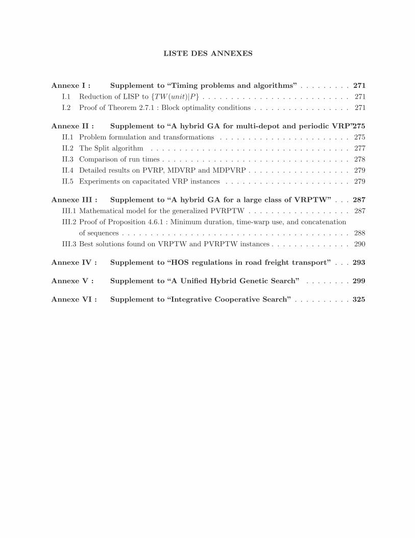
LISTE DES ANNEXES . . . . . . . . . . . . . . . . . . . . . . . . . . . . . . . . . . . . xxi

LISTE DES SIGLES . . . . . . . . . . . . . . . . . . . . . . . . . . . . . . . . . . . . . .xxiii

REMERCIEMENTS . . . . . . . . . . . . . . . . . . . . . . . . . . . . . . . . . . . . . . xxv

AVANT-PROPOS . . . . . . . . . . . . . . . . . . . . . . . . . . . . . . . . . . . . . . . .xxvii

INTRODUCTION . . . . . . . . . . . . . . . . . . . . . . . . . . . . . . . . . . . . . . . 1

0.1 Contexte et defis . . . . . . . . . . . . . . . . . . . . . . . . . . . . . . . . . . . . . 1

0.2 Objectifs, demarche et contributions . . . . . . . . . . . . . . . . . . . . . . . . . . 3

0.3 Detail des contributions . . . . . . . . . . . . . . . . . . . . . . . . . . . . . . . . . 5

0.4 Structure du document . . . . . . . . . . . . . . . . . . . . . . . . . . . . . . . . . . 10

PARTIE I ANALYSE STRUCTURELLE DES PROBLEMES

ET DES METHODES 11

CHAPITRE 1 :METAHEURISTIQUES POUR LES PROBLEMES DE TOUR-

NEES DE VEHICULES MULTI-ATTRIBUTS, REVUE ET SYN-

THESE DE LA LITTERATURE . . . . . . . . . . . . . . . . . . . . 13

1.1 Fil conducteur et contributions . . . . . . . . . . . . . . . . . . . . . . . . . . . . . 13

1.2 Article I : Metaheuristics for multi-attribute vehicle routing problems, a survey and

synthesis . . . . . . . . . . . . . . . . . . . . . . . . . . . . . . . . . . . . . . . . . . 13

1.3 Introduction . . . . . . . . . . . . . . . . . . . . . . . . . . . . . . . . . . . . . . . . 14

1.4 Heuristics for the CVRP . . . . . . . . . . . . . . . . . . . . . . . . . . . . . . . . . 15

1.4.1 Constructive heuristics . . . . . . . . . . . . . . . . . . . . . . . . . . . . . . 17

1.4.2 Local-improvement heuristics . . . . . . . . . . . . . . . . . . . . . . . . . . 18

1.4.3 Metaheuristics . . . . . . . . . . . . . . . . . . . . . . . . . . . . . . . . . . 20

x

1.4.4 Relative performance of CVRP heuristics . . . . . . . . . . . . . . . . . . . 25

1.5 MAVRP: Classification and State-of-the-Art Heuristics . . . . . . . . . . . . . . . . 28

1.5.1 Three main classes of attributes . . . . . . . . . . . . . . . . . . . . . . . . 29

1.5.2 Heuristics for VRP variants with ASSIGN attributes . . . . . . . . . . . . . 31

1.5.3 Heuristics for VRP variants with SEQ attributes . . . . . . . . . . . . . . . 32

1.5.4 Heuristics for VRP variants with EVAL attributes . . . . . . . . . . . . . . 33

1.6 A Synthesis of “Winning”MAVRP Strategies . . . . . . . . . . . . . . . . . . . . . 35

1.7 Conclusions and Perspectives . . . . . . . . . . . . . . . . . . . . . . . . . . . . . . 44

CHAPITRE 2 :UNE SYNTHESE UNIFICATRICE DES PROBLEMES ET AL-

GORITHMES DE “TIMING” . . . . . . . . . . . . . . . . . . . . . . 47


2.2 Article II : A unifying view on timing problems and algorithms . . . . . . . . . . . 47

2.3 Introduction . . . . . . . . . . . . . . . . . . . . . . . . . . . . . . . . . . . . . . . . 48

2.4 Problem statement . . . . . . . . . . . . . . . . . . . . . . . . . . . . . . . . . . . . 49

2.5 Timing issues and major application fields . . . . . . . . . . . . . . . . . . . . . . . 50

2.6 Features : classification and reductions . . . . . . . . . . . . . . . . . . . . . . . . . 53

2.6.1 Classification and notations . . . . . . . . . . . . . . . . . . . . . . . . . . . 53

2.6.2 Feature reductions . . . . . . . . . . . . . . . . . . . . . . . . . . . . . . . . 55

2.7 Single-dimensional features . . . . . . . . . . . . . . . . . . . . . . . . . . . . . . . 56

2.7.1 Makespan, deadlines and weighted execution dates . . . . . . . . . . . . . . 56

2.7.2 Release dates and time windows . . . . . . . . . . . . . . . . . . . . . . . . 57

2.7.3 Separable convex costs . . . . . . . . . . . . . . . . . . . . . . . . . . . . . . 58

2.7.4 Separable costs and multiple time windows . . . . . . . . . . . . . . . . . . 61

2.7.5 State-of-the-art: single-dimensional features . . . . . . . . . . . . . . . . . . 62

2.8 Two-dimensional features . . . . . . . . . . . . . . . . . . . . . . . . . . . . . . . . 63

2.8.1 Total duration and total idle time . . . . . . . . . . . . . . . . . . . . . . . 63

2.8.2 No wait and idle time . . . . . . . . . . . . . . . . . . . . . . . . . . . . . . 65

2.8.3 Flexible processing times . . . . . . . . . . . . . . . . . . . . . . . . . . . . 66

2.8.4 Time-dependent processing times . . . . . . . . . . . . . . . . . . . . . . . . 68

2.8.5 Time lags . . . . . . . . . . . . . . . . . . . . . . . . . . . . . . . . . . . . . 69

2.8.6 Separable costs by pairs of variables . . . . . . . . . . . . . . . . . . . . . . 71

2.9 Conclusion on “stand-alone” timing methods . . . . . . . . . . . . . . . . . . . . . . 71

2.10 Timing re-optimization . . . . . . . . . . . . . . . . . . . . . . . . . . . . . . . . . . 72

2.10.1 Problem statement: Serial timing . . . . . . . . . . . . . . . . . . . . . . . . 73

2.10.2 Breakpoints and concatenations . . . . . . . . . . . . . . . . . . . . . . . . . 74

2.10.3 Re-optimization “by concatenation” . . . . . . . . . . . . . . . . . . . . . . . 75

2.10.4 General literature on the topic . . . . . . . . . . . . . . . . . . . . . . . . . 76

2.10.5 Re-optimization algorithms . . . . . . . . . . . . . . . . . . . . . . . . . . . 78

2.10.6 Summary and perspectives on re-optimization . . . . . . . . . . . . . . . . . 84

2.11 General conclusion . . . . . . . . . . . . . . . . . . . . . . . . . . . . . . . . . . . . 84

xi

PARTIE II METAHEURISTIQUES POUR LES PROBLEMES

DE TOURNEES DE VEHICULES 87

CHAPITRE 3 :UN ALGORITHME GENETIQUE HYBRIDE POUR LES PRO-

BLEMES DE TOURNEES DE VEHICULES MULTI-DEPOTS

ET PERIODIQUES . . . . . . . . . . . . . . . . . . . . . . . . . . . . 89


3.2 Article III : A hybrid genetic algorithm for multi-depot and periodic vehicle routing

problems . . . . . . . . . . . . . . . . . . . . . . . . . . . . . . . . . . . . . . . . . . 89

3.3 Introduction . . . . . . . . . . . . . . . . . . . . . . . . . . . . . . . . . . . . . . . . 90

3.4 Problem Statement . . . . . . . . . . . . . . . . . . . . . . . . . . . . . . . . . . . . 91

3.5 Literature Review . . . . . . . . . . . . . . . . . . . . . . . . . . . . . . . . . . . . 92

3.6 The Hybrid Genetic Search with Adaptive Diversity Control Meta-heuristic . . . . 94

3.6.1 Search space . . . . . . . . . . . . . . . . . . . . . . . . . . . . . . . . . . . 94

3.6.2 Solution representation . . . . . . . . . . . . . . . . . . . . . . . . . . . . . 95

3.6.3 Evaluation of individuals . . . . . . . . . . . . . . . . . . . . . . . . . . . . 96

3.6.4 Parent Selection and Crossover . . . . . . . . . . . . . . . . . . . . . . . . . 97

3.6.5 Education . . . . . . . . . . . . . . . . . . . . . . . . . . . . . . . . . . . . . 99

3.6.6 Population management and search guidance . . . . . . . . . . . . . . . . . 101

3.7 Computational Experiments . . . . . . . . . . . . . . . . . . . . . . . . . . . . . . . 103

3.7.1 Calibration of the HGSADC algorithm . . . . . . . . . . . . . . . . . . . . . 103

3.7.2 Results on periodic and multi-depot VRPs . . . . . . . . . . . . . . . . . . 104

3.7.3 Results on the capacitated VRP . . . . . . . . . . . . . . . . . . . . . . . . 106

3.7.4 Sensitivity analysis of algorithmic components . . . . . . . . . . . . . . . . 106

3.8 Conclusions and Research Perspectives . . . . . . . . . . . . . . . . . . . . . . . . . 108

CHAPITRE 4 :UN ALGORITHME GENETIQUE HYBRIDE POUR UNE GRANDE

FAMILLE DE PROBLEMES DE TOURNEES DE VEHICULES

AVEC FENETRES DE TEMPS . . . . . . . . . . . . . . . . . . . . 111


4.2 Article IV : A hybrid genetic algorithm for a large class of vehicle routing problems

with time windows . . . . . . . . . . . . . . . . . . . . . . . . . . . . . . . . . . . . 111

4.3 Introduction . . . . . . . . . . . . . . . . . . . . . . . . . . . . . . . . . . . . . . . . 112

4.4 Problem Statement . . . . . . . . . . . . . . . . . . . . . . . . . . . . . . . . . . . . 113

4.5 Literature Review . . . . . . . . . . . . . . . . . . . . . . . . . . . . . . . . . . . . 114

4.6 The HGSADC Methodology . . . . . . . . . . . . . . . . . . . . . . . . . . . . . . . 116

4.6.1 Search space . . . . . . . . . . . . . . . . . . . . . . . . . . . . . . . . . . . 117


4.6.3 The diversity and cost objective for evaluating individuals . . . . . . . . . . 119

4.6.4 Parent selection and crossover . . . . . . . . . . . . . . . . . . . . . . . . . . 119

4.6.5 Neighbourhood search for VRPTW education and repair . . . . . . . . . . 119

xii

4.6.6 Population management and search guidance . . . . . . . . . . . . . . . . . 123

4.6.7 Decomposition phases . . . . . . . . . . . . . . . . . . . . . . . . . . . . . . 124


4.7.1 Parameter calibration . . . . . . . . . . . . . . . . . . . . . . . . . . . . . . 125

4.7.2 Comparison of performances . . . . . . . . . . . . . . . . . . . . . . . . . . 126

4.7.3 Sensitivity analysis on method components . . . . . . . . . . . . . . . . . . 132

4.8 Conclusions . . . . . . . . . . . . . . . . . . . . . . . . . . . . . . . . . . . . . . . . 133

CHAPITRE 5 :UNE ETUDE EMPIRIQUE DES RELAXATIONS DE FENETRES

DE TEMPS . . . . . . . . . . . . . . . . . . . . . . . . . . . . . . . . . 135


5.2 Article V : Empirical studies on time-window relaxations in vehicle routing heuristics135

5.3 Introduction . . . . . . . . . . . . . . . . . . . . . . . . . . . . . . . . . . . . . . . . 136

5.4 Problem statement and notations . . . . . . . . . . . . . . . . . . . . . . . . . . . . 137

5.5 Time-window relaxations in VRPTW heuristics . . . . . . . . . . . . . . . . . . . . 138

5.6 Move evaluation methods and their computational complexity . . . . . . . . . . . . 138

5.6.1 No infeasible solution . . . . . . . . . . . . . . . . . . . . . . . . . . . . . . 139

5.6.2 Early/Late and Late service . . . . . . . . . . . . . . . . . . . . . . . . . . . 140

5.6.3 Returns in time . . . . . . . . . . . . . . . . . . . . . . . . . . . . . . . . . . 141

5.6.4 Flexible service and travel times . . . . . . . . . . . . . . . . . . . . . . . . 142

5.7 Empirical comparison of relaxations . . . . . . . . . . . . . . . . . . . . . . . . . . 143

5.7.1 Performance of relaxations with regards to distance minimization . . . . . . 143

5.7.2 Performance of relaxations with regards to fleet minimization . . . . . . . . 144

5.8 Conclusions . . . . . . . . . . . . . . . . . . . . . . . . . . . . . . . . . . . . . . . . 146

CHAPITRE 6 :GESTION IMPLICITE DES PLACEMENTS DE DEPOT DANS

LES HEURISTIQUES ET META-HEURISTIQUES A BASE DE

RECHERCHE LOCALE . . . . . . . . . . . . . . . . . . . . . . . . . 147


6.2 Article VI : Implicit depot choice and positioning in vehicle routing heuristics . . . 147

6.3 Introduction . . . . . . . . . . . . . . . . . . . . . . . . . . . . . . . . . . . . . . . . 148

6.4 Vehicle routing problems and variants . . . . . . . . . . . . . . . . . . . . . . . . . 149

6.5 Compound neighborhoods with implicit depot positioning and vehicle choices . . . 151

6.6 Split algorithm with vehicle choices, depot assignments and rotations . . . . . . . . 154

6.7 Two meta-heuristic applications . . . . . . . . . . . . . . . . . . . . . . . . . . . . . 156

6.7.1 An iterated local search application . . . . . . . . . . . . . . . . . . . . . . 156

6.7.2 A hybrid genetic search application . . . . . . . . . . . . . . . . . . . . . . . 157

6.8 Computational experiments . . . . . . . . . . . . . . . . . . . . . . . . . . . . . . . 159

6.8.1 Impact of compound neighborhoods . . . . . . . . . . . . . . . . . . . . . . 160

6.8.2 Addressing a rich problem – the MDVFMP . . . . . . . . . . . . . . . . . . 167

6.9 Conclusions . . . . . . . . . . . . . . . . . . . . . . . . . . . . . . . . . . . . . . . . 167

xiii

PARTIE III RESOLUTION DE PROBLEMES RICHES ET

APPROCHES GENERALISTES 169

CHAPITRE 7 :PROBLEMES DE TOURNEES DE VEHICULES ET D’HORAIRES

DE CONDUCTEURS . . . . . . . . . . . . . . . . . . . . . . . . . . . 171


7.2 Article VII : Hours of service regulations in road freight transport – an optimiza-

tion-based international assessment . . . . . . . . . . . . . . . . . . . . . . . . . . . 171

7.3 Introduction . . . . . . . . . . . . . . . . . . . . . . . . . . . . . . . . . . . . . . . . 172

7.4 Hours of service regulations . . . . . . . . . . . . . . . . . . . . . . . . . . . . . . . 173

7.4.1 United States . . . . . . . . . . . . . . . . . . . . . . . . . . . . . . . . . . . 173

7.4.2 Canada . . . . . . . . . . . . . . . . . . . . . . . . . . . . . . . . . . . . . . 174

7.4.3 European Union . . . . . . . . . . . . . . . . . . . . . . . . . . . . . . . . . 174

7.4.4 Australia . . . . . . . . . . . . . . . . . . . . . . . . . . . . . . . . . . . . . 175

7.4.5 Discussion . . . . . . . . . . . . . . . . . . . . . . . . . . . . . . . . . . . . . 176

7.5 Problem statement and related work . . . . . . . . . . . . . . . . . . . . . . . . . . 177

7.6 An optimization method for combined vehicle routing and truck driver scheduling 179



7.6.3 Generation of new individuals . . . . . . . . . . . . . . . . . . . . . . . . . . 181

7.6.4 Population management . . . . . . . . . . . . . . . . . . . . . . . . . . . . . 182

7.6.5 Truck driver scheduling for route evaluations . . . . . . . . . . . . . . . . . 182

7.6.6 Addressing the challenge of computational efficiency . . . . . . . . . . . . . 183

7.7 Computational experiments . . . . . . . . . . . . . . . . . . . . . . . . . . . . . . . 185

7.7.1 Comparison with best known solutions . . . . . . . . . . . . . . . . . . . . . 186

7.7.2 An international comparison of hours of service regulations . . . . . . . . . 187

7.8 Conclusions . . . . . . . . . . . . . . . . . . . . . . . . . . . . . . . . . . . . . . . . 192

CHAPITRE 8 :RESOLUTION GENERALISTE DE PROBLEMES DE TOUR-

NEES DE VEHICULES MULTI-ATTRIBUTS . . . . . . . . . . . 193


8.2 Article VIII : A unified solution framework for multi-attribute vehicle routing problems193

8.3 Introduction . . . . . . . . . . . . . . . . . . . . . . . . . . . . . . . . . . . . . . . . 194

8.4 Problem Statement and General Methodology . . . . . . . . . . . . . . . . . . . . . 195

8.4.1 Vehicle routing problems, notations and attributes . . . . . . . . . . . . . . 196

8.4.2 General-purpose solution approaches for MAVRPs. . . . . . . . . . . . . . . 196

8.4.3 Proposed component-based framework . . . . . . . . . . . . . . . . . . . . . 199

8.5 Unified Local Search for Vehicle Routing Problems . . . . . . . . . . . . . . . . . . 200

8.5.1 Route-evaluation components . . . . . . . . . . . . . . . . . . . . . . . . . . 200

8.5.2 Route-evaluation operators for several attributes . . . . . . . . . . . . . . . 201

8.5.3 Unified local search procedure . . . . . . . . . . . . . . . . . . . . . . . . . . 208

xiv

8.6 Unified Hybrid Genetic Search . . . . . . . . . . . . . . . . . . . . . . . . . . . . . 209

8.6.1 General algorithmic structure . . . . . . . . . . . . . . . . . . . . . . . . . . 209

8.6.2 Unified solution representation and Split . . . . . . . . . . . . . . . . . . . . 210


8.6.4 Selection and Crossover . . . . . . . . . . . . . . . . . . . . . . . . . . . . . 212

8.6.5 Education and Repair . . . . . . . . . . . . . . . . . . . . . . . . . . . . . . 213

8.6.6 Population management . . . . . . . . . . . . . . . . . . . . . . . . . . . . . 213

8.6.7 Decomposition Phases . . . . . . . . . . . . . . . . . . . . . . . . . . . . . . 214


8.8 Conclusions and Perspectives . . . . . . . . . . . . . . . . . . . . . . . . . . . . . . 217

CHAPITRE 9 :UNE APPROCHE PARALLELE COOPERATIVE A BASE DE

DECOMPOSITION ET INTEGRATION POUR LES PROBLEMES

DE TOURNEES DE VEHICULES MULTI-ATTRIBUTS . . . . 219


9.2 Article IX : Integrative Cooperative Search for Multi-Attribute Vehicle Routing

Problems . . . . . . . . . . . . . . . . . . . . . . . . . . . . . . . . . . . . . . . . . 219

9.3 Introduction . . . . . . . . . . . . . . . . . . . . . . . . . . . . . . . . . . . . . . . . 220

9.4 Motivation and Inspiration . . . . . . . . . . . . . . . . . . . . . . . . . . . . . . . 221

9.5 ICS Fundamental Concepts and Structure . . . . . . . . . . . . . . . . . . . . . . . 224

9.5.1 The ICS idea . . . . . . . . . . . . . . . . . . . . . . . . . . . . . . . . . . . 224

9.5.2 The ICS Method . . . . . . . . . . . . . . . . . . . . . . . . . . . . . . . . . 226

9.6 Application to the MDPVRP . . . . . . . . . . . . . . . . . . . . . . . . . . . . . . 230

9.6.1 The multi-depot periodic vehicle routing problem . . . . . . . . . . . . . . . 230

9.6.2 ICS for the MDPVRP . . . . . . . . . . . . . . . . . . . . . . . . . . . . . . 231

9.7 Experimental Results and Analyses . . . . . . . . . . . . . . . . . . . . . . . . . . . 234

9.8 Conclusions . . . . . . . . . . . . . . . . . . . . . . . . . . . . . . . . . . . . . . . . 238

CONCLUSION . . . . . . . . . . . . . . . . . . . . . . . . . . . . . . . . . . . . . . . . . 239

BIBLIOGRAPHIE . . . . . . . . . . . . . . . . . . . . . . . . . . . . . . . . . . . . . . . 243

LISTE DES TABLEAUX

1 Acronyms . . . . . . . . . . . . . . . . . . . . . . . . . . . . . . . . . . . . . . xxiii

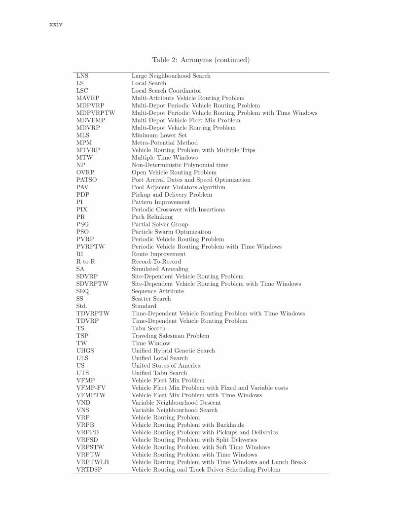
2 Acronyms (continued) . . . . . . . . . . . . . . . . . . . . . . . . . . . . . . . xxiv

1.1 Best performing metaheuristics for CVRP on Golden et al. (1998b) instances 27

1.2 Some frequently encountered attributes in the literature . . . . . . . . . . . . 30

1.3 Main metaheuristic concepts used in the 64 winning methods . . . . . . . . . 35

1.4 Fundamental metaheuristic features . . . . . . . . . . . . . . . . . . . . . . . 36

1.5 Successful metaheuristics for CVRP and MAVRPs with ASSIGN attributes . 37

1.6 Successful metaheuristics for MAVRPs with SEQ and EVAL attributes . . . 38

2.1 Classification of timing features and notations . . . . . . . . . . . . . . . . . . 54

2.2 Re-optimization operators . . . . . . . . . . . . . . . . . . . . . . . . . . . . . 75

2.3 Complexity of algorithms and re-optimization operators for common timing

problems

. . . . . . . . . . . . . . . . . . . . . . . . . . . . . . . . . . . . . . . . . . . . 85

3.1 Calibration Results . . . . . . . . . . . . . . . . . . . . . . . . . . . . . . . . . 104

3.2 HGSADC performance on PVRP instances . . . . . . . . . . . . . . . . . . . 104

3.3 HGSADC performance on MDVRP instances . . . . . . . . . . . . . . . . . . 105

3.4 Sensitivity analysis on main HGSADC components . . . . . . . . . . . . . . . 107

3.5 Comparison of population-diversity management mechanisms . . . . . . . . . 107

4.1 Performance of HGSADC on a selection of 200-customer VRPTW instances

for various γTW and γWT settings . . . . . . . . . . . . . . . . . . . . . . . . 126

4.2 Results on Cordeau et al. (2001a) PVRPTW instances . . . . . . . . . . . . . 127

4.3 Results on Pirkwieser and Raidl (2009b) PVRPTW instances without duration

constraints, distances truncated to the first digit . . . . . . . . . . . . . . . . 128

4.4 Results on Cordeau et al. (2001a) MDVRPTW instances . . . . . . . . . . . 128

4.5 Results on Cordeau and Laporte (2001) SDVRPTW instances. . . . . . . . . 129

4.6 Results on Solomon and Desrosiers (1988) VRPTW instances . . . . . . . . . 129

4.7 Results on Gehring and Homberger (1999) large-scale VRPTW instances . . 130

4.8 Results on new large-scale PVRPTW, MDVRPTW, and SDVRPTW instances.131

4.9 Sensitivity analysis on the role of diversity and cost objective, time window-

infeasible solutions, and decomposition phases. . . . . . . . . . . . . . . . . . 132

5.1 Infeasible solutions in state of the art VRPTW heuristics . . . . . . . . . . . 138

5.2 Distance minimization on the VRPTW benchmark instances of Solomon (1987)144

5.3 Fleet minimization on the VRPTW benchmark instances of Solomon (1987) . 145

6.1 Impact of implicit rotations within ILS – CVRP instances . . . . . . . . . . . 162

6.2 Impact of implicit rotations within HGSADC – CVRP instances . . . . . . . 163

xvi

6.3 Impact of implicit rotations and depot choices within ILS – MDVRP instances.164

6.4 Impact of implicit rotations and depot choices within HGSADC – MDVRP

instances. . . . . . . . . . . . . . . . . . . . . . . . . . . . . . . . . . . . . . . 165

6.5 Performance of HGSADC – MDVFMP instances . . . . . . . . . . . . . . . . 166

7.1 Comparison of the regulations . . . . . . . . . . . . . . . . . . . . . . . . . . . 176

7.2 Method performance on Goel (2009) instances - EU (No split) . . . . . . . . 186

7.3 Method performance on Goel (2009) instances - EU (All) . . . . . . . . . . . 187

7.4 Best solutions found for modified Goel (2009) instances . . . . . . . . . . . . 188

7.5 Schedule characteristics . . . . . . . . . . . . . . . . . . . . . . . . . . . . . . 190

7.6 Average risk indices . . . . . . . . . . . . . . . . . . . . . . . . . . . . . . . . 191

8.1 Attributes addressed by some well-known rich VRP solvers . . . . . . . . . . 197

8.2 Route-evaluation component functionalities . . . . . . . . . . . . . . . . . . . 201

8.3 List of acronyms for benchmark instances and methods . . . . . . . . . . . . 214

8.4 Performance analysis on several VRP variants with various objectives . . . . 215

8.5 Performance analysis on several VRP variants with various objectives (continued)216

9.1 Average performance of ICS versions and sequential algorithms . . . . . . . . 236

9.2 Performance of GUTS-ICS . . . . . . . . . . . . . . . . . . . . . . . . . . . . 236

9.3 Performance of HGSADC-ICS2+ with encapsulated population-based solvers 236

II.1 Scaling factors for computation times . . . . . . . . . . . . . . . . . . . . . . 279

II.2 Results on Cordeau et al. (1997) PVRP instances . . . . . . . . . . . . . . . . 282

II.3 Results on Cordeau et al. (1997) MDVRP instances . . . . . . . . . . . . . . 283

II.4 Results on new MDPVRP instances . . . . . . . . . . . . . . . . . . . . . . . 284

II.5 Results for Christofides et al. (1979) and Golden et al. (1998a) CVRP instances285

II.6 Behaviour of HGSADC on CVRP instances, when run times increase . . . . . 286

III.1 HGSADC best solutions on Pirkwieser and Raidl (2009b) PVRPTW instances.

Distances truncated to the first digit.

. . . . . . . . . . . . . . . . . . . . . . . . . . . . . . . . . . . . . . . . . . . . 290

III.2 HGSADC best solutions on Gehring and Homberger (1999) large-scale VRPTW

instances.

. . . . . . . . . . . . . . . . . . . . . . . . . . . . . . . . . . . . . . . . . . . . 291

IV.1 Detailed results for Goel (2009) instances and European Union regulations . 294

IV.2 Detailed results for modified Goel (2009) instances and U.S. and Canadian

regulations . . . . . . . . . . . . . . . . . . . . . . . . . . . . . . . . . . . . . 295

IV.3 Detailed results for modified Goel (2009) instances and European Union

regulations . . . . . . . . . . . . . . . . . . . . . . . . . . . . . . . . . . . . . 296

IV.4 Detailed results for modified Goel (2009) instances and Australian regulations

and without regulations . . . . . . . . . . . . . . . . . . . . . . . . . . . . . . 297

xvii

V.1 Results on the VRPB, instances of Goetschalckx and Jacobs-Blecha (1989) . 302

V.2 Results on the CCVRP, instances of Christofides et al. (1979) . . . . . . . . . 303

V.3 Results on the CCVRP, instances of Golden et al. (1998b) . . . . . . . . . . . 303

V.4 Results on the VRPSDP, instances of Salhi and Nagy (1999) . . . . . . . . . 304

V.5 Results on the VRPSDP, instances of Montane and Galvao (2006) . . . . . . 304

V.6 Results on the VFMP-F, only fixed vehicle costs, instances of Golden (1984) 305

V.7 Results on the VFMP-V, only variable vehicle costs, instances of Golden (1984)305

V.8 Results on the VFMP-FV, fixed and variable vehicle costs, instances of Golden

(1984) . . . . . . . . . . . . . . . . . . . . . . . . . . . . . . . . . . . . . . . . 306

V.9 Results on the LDVRP, instances of Christofides et al. (1979) . . . . . . . . . 306

V.10 Results for the LDVRP, instances of Golden et al. (1998b) . . . . . . . . . . . 307

V.11 Results on the GVRP, instances of Bektas et al. (2011) . . . . . . . . . . . . 308

V.12 Results on the GVRP, instances of Bektas et al. (2011) (continued) . . . . . . 309

V.13 Results on the GVRP, instances of Bektas et al. (2011) (continued) . . . . . . 310

V.14 Results on the OVRP, instances of Christofides et al. (1979) and Fisher (1994) 311

V.15 Results on the OVRP, instances of Golden et al. (1998b) . . . . . . . . . . . . 311

V.16 Results on the OVRPTW, instances of Solomon and Desrosiers (1988) . . . . 312

V.17 Results on the TDVRPTW. Scenario 1 for time-dependent travel times. Ins-

tances of Solomon and Desrosiers (1988). . . . . . . . . . . . . . . . . . . . . 313

V.18 Results on the VFMPTW, minimization of duration, type A fleet, instances of

Liu and Shen (1999) . . . . . . . . . . . . . . . . . . . . . . . . . . . . . . . . 314

V.19 Results on the VFMPTW, minimization of duration, type B fleet, instances of

Liu and Shen (1999) . . . . . . . . . . . . . . . . . . . . . . . . . . . . . . . . 315

V.20 Results on the VFMPTW, minimization of duration, type C fleet, instances of

Liu and Shen (1999) . . . . . . . . . . . . . . . . . . . . . . . . . . . . . . . . 316

V.21 Results on the VFMPTW, minimization of distance, type A fleet, instances of

Liu and Shen (1999) . . . . . . . . . . . . . . . . . . . . . . . . . . . . . . . . 317

V.22 Results on the VFMPTW, minimization of distance, type B fleet, instances of

Liu and Shen (1999) . . . . . . . . . . . . . . . . . . . . . . . . . . . . . . . . 318

V.23 Results on the VFMPTW, minimization of distance, type C fleet, instances of

Liu and Shen (1999) . . . . . . . . . . . . . . . . . . . . . . . . . . . . . . . . 319

V.24 Results on the type 1 VRPSTW (only lateness) with α = 100, hierarchical

objective involving first the minimization of the Fleet Size ”Fleet”, then the

number of customers serviced outside of their time windows ”TW”, then the

overall lateness ”L”, and finally distance ”Dist”. Instances of Solomon and

Desrosiers (1988) . . . . . . . . . . . . . . . . . . . . . . . . . . . . . . . . . . 320

V.25 Results on the type 1 VRPSTW (only lateness) with α = 1. Minimization of

the sum of distance and lateness under a fleet size limit. Instances of Solomon

and Desrosiers (1988). . . . . . . . . . . . . . . . . . . . . . . . . . . . . . . . 321

xviii

V.26 Results on the type 2 VRPSTW (earliness and lateness) with α = 100, hierar-

chical objective involving first the minimization of the Fleet Size “Fleet”, then

the number of customers serviced outside of their time windows “TW”, then

the overall earliness plus lateness “E+L”, and finally distance “Dist”. Instances

of Solomon and Desrosiers (1988) . . . . . . . . . . . . . . . . . . . . . . . . . 322

V.27 Results on the type 2 VRPSTW (earliness and lateness) with α = 1. Minimi-

zation of the sum of distance, earliness and lateness under a fleet size limit.

Instances of Solomon and Desrosiers (1988) . . . . . . . . . . . . . . . . . . . 323

V.28 Results on the new MDPVRPTW instances. . . . . . . . . . . . . . . . . . . 324

VI.1 MDPVRP instances . . . . . . . . . . . . . . . . . . . . . . . . . . . . . . . . 325

VI.2 Performance of GUTS-ICS . . . . . . . . . . . . . . . . . . . . . . . . . . . . 325

VI.3 Performance of HGSADC-ICS1 with shared populations . . . . . . . . . . . . 326

VI.4 Performance of HGSADC-ICS1+ with shared populations . . . . . . . . . . . 326

VI.5 Performance of HGSADC-ICS2 with encapsulated population-based solvers . 326

LISTE DES FIGURES

1 Organisation des contributions. Trois axes de recherche complementaires pour

progresser vers des methodes generalistes pour les problemes de tournees

multi-attributs . . . . . . . . . . . . . . . . . . . . . . . . . . . . . . . . . . . 4

1.1 2-opt and Or-exchange illustration. The deleted/inserted arcs are indicated

with dotted/bold lines. . . . . . . . . . . . . . . . . . . . . . . . . . . . . . . . 19

1.2 2-opt* and CROSS-exchange illustration. The deleted/inserted arcs are indica-

ted with dotted/bold lines. . . . . . . . . . . . . . . . . . . . . . . . . . . . . 19

1.3 State-of-the-art CVRP methods: solution quality and scaled computation time 28

2.1 Hierarchy of timing features . . . . . . . . . . . . . . . . . . . . . . . . . . . . 56

2.2 Illustrative example with six activities: cost functions and durations . . . . . 59

2.3 Comparison between Garey et al. (1988) algorithm (left part of the figure),

and Best and Chakravarti (1990) algorithm (right part of the figure) . . . . . 60

2.4 The PAV algorithm illustrated on timing problems . . . . . . . . . . . . . . . 61

2.5 Duration minimization under multiple time-window constraints . . . . . . . . 64

2.6 Feasibility checking under time-windows and idle-time constraints . . . . . . 65

2.7 Sequence invariants in 2-opt* and relocate moves . . . . . . . . . . . . . . . . 72

3.1 From a MDPVRP solution to the individual chromosome representation . . . 96

3.2 The PIX crossover . . . . . . . . . . . . . . . . . . . . . . . . . . . . . . . . . 99

3.3 Population entropy and error gap to the BKS for the diversity management

strategies on MDPVRP instance pr03 . . . . . . . . . . . . . . . . . . . . . . 108

4.1 Illustration of waiting times and time warps . . . . . . . . . . . . . . . . . . . 118

4.2 Example of “swap” move in N1 . . . . . . . . . . . . . . . . . . . . . . . . . . 121

6.1 Solution improvements using compound moves . . . . . . . . . . . . . . . . . 152

6.2 Moves assimilated to recombinations of sequences . . . . . . . . . . . . . . . . 153

6.3 Advanced Split requirements . . . . . . . . . . . . . . . . . . . . . . . . . . . 154

6.4 ILS performance – Avg Gap to BKS (%) – with different parameter settings . 160

7.1 General behavior of the hybrid genetic algorithm with adaptive diversity control

for the VRTDSP . . . . . . . . . . . . . . . . . . . . . . . . . . . . . . . . . . 179

7.2 From individual to solution representation . . . . . . . . . . . . . . . . . . . . 180

7.3 Truck driver scheduling procedure for a route with four locations . . . . . . . 183

7.4 Common subsequences through 2opt move evaluations . . . . . . . . . . . . . 184

7.5 Costs vs. risks . . . . . . . . . . . . . . . . . . . . . . . . . . . . . . . . . . . 191

8.1 Moves assimilated to recombinations of sequences . . . . . . . . . . . . . . . . 200

8.2 UHGS structure and relationships with problem attributes . . . . . . . . . . 210

xx

8.3 Solution representation as a giant tour per AAR, illustration of the Split

procedure and its reverse Merge operation . . . . . . . . . . . . . . . . . . . . 211

9.1 The Central-Memory Multi-Search Cooperative Scheme . . . . . . . . . . . . 224

9.2 The ICS Methodology Idea . . . . . . . . . . . . . . . . . . . . . . . . . . . . 225

9.3 The Integrative Cooperative Search Structure . . . . . . . . . . . . . . . . . . 227

9.4 Solution Quality versus Computational Effort . . . . . . . . . . . . . . . . . . 237

II.1 Illustration of a Split graph and shortest-path solution . . . . . . . . . . . . . 278

LISTE DES ANNEXES

Annexe I : Supplement to “Timing problems and algorithms” . . . . . . . . . 271

I.1 Reduction of LISP to {TW (unit)|P} . . . . . . . . . . . . . . . . . . . . . . . . . . 271

I.2 Proof of Theorem 2.7.1 : Block optimality conditions . . . . . . . . . . . . . . . . . 271

Annexe II : Supplement to “A hybrid GA for multi-depot and periodic VRP”275

II.1 Problem formulation and transformations . . . . . . . . . . . . . . . . . . . . . . . 275

II.2 The Split algorithm . . . . . . . . . . . . . . . . . . . . . . . . . . . . . . . . . . . 277

II.3 Comparison of run times . . . . . . . . . . . . . . . . . . . . . . . . . . . . . . . . . 278

II.4 Detailed results on PVRP, MDVRP and MDPVRP . . . . . . . . . . . . . . . . . . 279

II.5 Experiments on capacitated VRP instances . . . . . . . . . . . . . . . . . . . . . . 279

Annexe III : Supplement to “A hybrid GA for a large class of VRPTW” . . . 287

III.1 Mathematical model for the generalized PVRPTW . . . . . . . . . . . . . . . . . . 287

III.2 Proof of Proposition 4.6.1 : Minimum duration, time-warp use, and concatenation

of sequences . . . . . . . . . . . . . . . . . . . . . . . . . . . . . . . . . . . . . . . . 288

III.3 Best solutions found on VRPTW and PVRPTW instances . . . . . . . . . . . . . . 290

Annexe IV : Supplement to “HOS regulations in road freight transport” . . . 293

Annexe V : Supplement to “A Unified Hybrid Genetic Search” . . . . . . . . 299

Annexe VI : Supplement to “Integrative Cooperative Search” . . . . . . . . . . 325

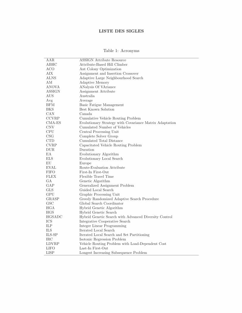
LISTE DES SIGLES

Table 1: Acronyms

AAR ASSIGN Attribute ResourceABHC Attribute-Based Hill ClimberACO Ant Colony OptimizationAIX Assignment and Insertion CrossoverALNS Adaptive Large Neighbourhood SearchAM Adaptive MemoryANOVA ANalysis Of VArianceASSIGN Assignment AttributeAUS AustraliaAvg AverageBFM Basic Fatigue ManagementBKS Best Known SolutionCAN CanadaCCVRP Cumulative Vehicle Routing ProblemCMA-ES Evolutionary Strategy with Covariance Matrix AdaptationCNV Cumulated Number of VehiclesCPU Central Processing UnitCSG Complete Solver GroupCTD Cumulated Total DistanceCVRP Capacitated Vehicle Routing ProblemDUR DurationEA Evolutionary AlgorithmELS Evolutionary Local SearchEU EuropeEVAL Route-Evaluation AttributeFIFO First-In First-OutFLEX Flexible Travel TimeGA Genetic AlgorithmGAP Generalized Assignment ProblemGLS Guided Local SearchGPU Graphic Processing UnitGRASP Greedy Randomized Adaptive Search ProcedureGSC Global Search CoordinatorHGA Hybrid Genetic AlgorithmHGS Hybrid Genetic SearchHGSADC Hybrid Genetic Search with Advanced Diversity ControlICS Integrative Cooperative SearchILP Integer Linear ProgrammingILS Iterated Local SearchILS-SP Iterated Local Search and Set PartitioningIRC Isotonic Regression ProblemLDVRP Vehicle Routing Problem with Load-Dependent CostLIFO Last-In First-OutLISP Longest Increasing Subsequence Problem

xxiv

Table 2: Acronyms (continued)

LNS Large Neighbourhood SearchLS Local SearchLSC Local Search CoordinatorMAVRP Multi-Attribute Vehicle Routing ProblemMDPVRP Multi-Depot Periodic Vehicle Routing ProblemMDPVRPTW Multi-Depot Periodic Vehicle Routing Problem with Time WindowsMDVFMP Multi-Depot Vehicle Fleet Mix ProblemMDVRP Multi-Depot Vehicle Routing ProblemMLS Minimum Lower SetMPM Metra-Potential MethodMTVRP Vehicle Routing Problem with Multiple TripsMTW Multiple Time WindowsNP Non-Deterministic Polynomial timeOVRP Open Vehicle Routing ProblemPATSO Port Arrival Dates and Speed OptimizationPAV Pool Adjacent Violators algorithmPDP Pickup and Delivery ProblemPI Pattern ImprovementPIX Periodic Crossover with InsertionsPR Path RelinkingPSG Partial Solver GroupPSO Particle Swarm OptimizationPVRP Periodic Vehicle Routing ProblemPVRPTW Periodic Vehicle Routing Problem with Time WindowsRI Route ImprovementR-to-R Record-To-RecordSA Simulated AnnealingSDVRP Site-Dependent Vehicle Routing ProblemSDVRPTW Site-Dependent Vehicle Routing Problem with Time WindowsSEQ Sequence AttributeSS Scatter SearchStd. StandardTDVRPTW Time-Dependent Vehicle Routing Problem with Time WindowsTDVRP Time-Dependent Vehicle Routing ProblemTS Tabu SearchTSP Traveling Salesman ProblemTW Time WindowUHGS Unified Hybrid Genetic SearchULS Unified Local SearchUS United States of AmericaUTS Unified Tabu SearchVFMP Vehicle Fleet Mix ProblemVFMP-FV Vehicle Fleet Mix Problem with Fixed and Variable costsVFMPTW Vehicle Fleet Mix Problem with Time WindowsVND Variable Neighbourhood DescentVNS Variable Neighbourhood SearchVRP Vehicle Routing ProblemVRPB Vehicle Routing Problem with BackhaulsVRPPD Vehicle Routing Problem with Pickups and DeliveriesVRPSD Vehicle Routing Problem with Split DeliveriesVRPSTW Vehicle Routing Problem with Soft Time WindowsVRPTW Vehicle Routing Problem with Time WindowsVRPTWLB Vehicle Routing Problem with Time Windows and Lunch BreakVRTDSP Vehicle Routing and Truck Driver Scheduling Problem

REMERCIEMENTS

Cette these est le resultat d’une combinaison de travail, de confiance, de rencontres imprevues,

d’enthousiasme, et de circonstances. Tout aurait ete totalement different sans l’aide considerable

de nombreux proches, amis et collegues. Je tiens a remercier, en particulier,

• Mes directeurs, au nombre de trois : Teodor Gabriel Crainic, Michel Gendreau et Christian

Prins. Je vous remercie pour m’avoir donne la chance de faire cette these, pour votre confiance

sans faille, votre soutien, votre engagement, et tout l’enseignement que vous m’avez transmis.

• Le Conseil de Recherches en Sciences Naturelles et en Genie du Canada (CRSNG), le Fonds

Quebecois de la Recherche sur la Nature et les Technologies (FQRNT) et le conseil Regional

de la region Champagne-Ardenne pour le soutien financier.

• Le CIRRELT et le LOSI, des environnements de recherche accueillants et dynamiques, ainsi

que le RQCHP et Calcul Canada, qui m’ont mis a disposition des ressources informatiques

providentielles.

• Richard Eglese, Jean-Yves Potvin, Caroline Prodhon, Marc Sevaux et Daniele Vigo, membres

du jury. C’etait un honneur de vous presenter cette these. Merci pour votre participation et

votre temps, ainsi que les commentaires, suggestions et corrections detaillees.

• Julien Moncel et Denis Naddef : c’est grace a une discussion providentielle, il y a quelques

annees a Grenoble, le jour de la cloture des inscriptions pour le master recherche, que j’ai

finalement emprunte une carriere academique.

• Amis doctorants des deux cotes de l’ocean et d’ailleurs : une dedicace speciale a Elivelton,

Karine, Sixtine, Phuong, Sanjay a Montreal, Atefeh, Julien et Slim a Troyes, Renaud de

Nantes, Anand, Puca, Vinicius, Marcos de Niteroi, Diego a Gardanne, et bien d’autres encore.

• L’equipe administrative et technique : une dedicace speciale a Lucie, Nath, Johanne, Josee,

Vero et Marie-Jo pour avoir releve les defis administratifs avec autant de bonne humeur.

Daniel, Luc et Pierre, a qui le systeme informatique du CIRRELT obeit au doigt et a l’oeil,

capables de reparer les cataclysmes que mes taches en panne ont parfois cause a la grille de

calcul.

• De nombreux amis et collegues, en particulier, mais sans se limiter a, Nadia Lahrichi, Walter

Rei, Asvin Goel, Jean-Francois Cordeau, Gilbert Laporte, Jean-Yves Potvin, Patrice Marcotte,

Michel Toulouse, Caroline Prodhon, Nacima Labadie, Christophe et Andrea Duhamel, Murat

Afsar, Sandra Ngueveu, Nabil Absi, Dominique Feillet et Frederic Semet. Votre enthousiasme

m’a amene a avancer avec encore plus d’entrain.

• Ma famille pour ce constant soutien tout au long de ces trois annees, ma mere qui a surement

trouve un moyen pour me transformer en futur amateur de science des les premieres annees.

Enfin Sophie, venue vivre a Montreal puis a Troyes, qui m’a soutenu jour apres jour, malgre

le froid, les mauvais jours et le travail considerable de ces trois annees. Merci du fond du

coeur.

AVANT-PROPOS

La recherche d’un plus court chemin, la confection de tournees et d’horaires, le placement

d’objets 2D (puzzles) sont autant de problemes que le cerveau humain resout jour apres jour de

maniere suffisamment efficace pour ses besoins (Vickers et al. 2004, Dry et al. 2006). Ce sont

cependant des problemes d’optimisation combinatoire, pour lesquels le nombre de solutions croıt

de maniere extremement rapide, exponentielle au moins, avec la taille des donnees : nombre de

destinations, activites ou objets. Le nombre total de sequences possibles pour visiter 80 lieux est

80! (≈ 7.10118), un nombre beaucoup plus grand que le nombre d’atomes (≈ 1080) estime dans

l’univers. Ainsi, le dicton populaire “a chaque probleme une solution”, passe sous silence la difficulte

a localiser une bonne solution (ainsi d’ailleurs que le caractere indecidable de certains problemes).

Le developpement rapide de la theorie de la complexite algorithmique a conduit a jeter depuis

les annees 1970 un nouveau regard sur un grand nombre de problemes d’optimisation combinatoire

qualifies de “Nondeterministic Polynomial time” (NP) (Garey and Johnson 1979). De maniere

simpliste, la caracteristique de ces problemes est qu’il est relativement aise de verifier l’optimalite

d’une solution, mais excessivement difficile de trouver la solution optimale. L’existence ou la non

existence d’algorithmes de resolution efficaces “polynomiaux” (pour lesquels le nombre d’operations

elementaires de calcul est une fonction polynomiale de la taille des donnees d’entree) pour les

problemes NP constitue une question celebre, toujours non resolue a l’heure actuelle, mais pour

laquelle une reponse positive est rarement envisagee. La conjecture precedente ne signifie cependant

pas que tout effort de resolution est vain, mais plutot que les methodes exactes actuelles pour ces

problemes atteignent inevitablement leurs limites sur certains jeux de donnees de grande taille.

Toutefois, dans le monde industriel au sein de systemes complexes et de grande taille, dans le

domaine de la logistique, de la production manufacturiere, ou des reseaux d’approvisionnement entre

autres, la resolution efficace et precise de tels problemes NP de grande taille est liee a des enjeux

economiques majeurs. Le XXIeme siecle est ainsi un age d’or pour la science informatique, ou des

enjeux considerables de recherche et d’application restent a relever afin de mieux guider la prise de

decision. Cette these vient rajouter une pierre a l’edifice en proposant de nouvelles methodologies de

resolution approchee (heuristiques et meta-heuristiques) efficaces pour les problemes de tournees de

vehicules, une classe importante de problemes d’optimisation combinatoire. Elle s’inscrit dans cette

dynamique generale de recherche qui touche a la fois a des questions methodologiques fondamentales

et a des applications pratiques indispensables. Ameliorer la gestion de ces problemes permet certes

d’augmenter la competitivite economique, mais aussi de progresser vers des systemes de transport

plus intelligents et ecologiques en adequation avec les besoins de la societe.

INTRODUCTION

0.1 Contexte et defis

Les problemes d’optimisation combinatoire visent a trouver une meilleure solution au sein

d’un ensemble fini et discret, mais generalement tres large, d’alternatives. Les applications sont

nombreuses en mathematiques appliquees, aide a la decision, informatique et bio-informatique,

intelligence artificielle, sciences economiques, ainsi que de nombreuses autres disciplines. Ces

problemes sont aussi au coeur des systemes industriels, qui dans un contexte d’integration, de

globalisation et de recherche de perfectionnement, cherchent a prendre les meilleures decisions

malgre la presence de donnees approximatives, d’objectifs et contraintes antagonistes, et d’une

multitude de solutions.

Le recherche d’une solution exacte “optimale” est souvent impossible pour des instances de

problemes de grande taille. Afin toutefois d’obtenir de bonnes solutions, de nombreuses approches

heuristiques et metaheuristiques ont ete proposees dans la litterature. Ces metaheuristiques sont

des strategies de recherche “globales”, qui ne donnent pas de garantie de performance mais visent a

guider l’exploration des solutions pour augmenter les chances de trouver une solution de qualite.

Certaines exploitent des concepts de recherche simples : perturber legerement pour trouver un

meilleur arrangement, eviter de repasser sur les memes solutions. D’autres s’inspirent de phenomenes

de notre environnement : selection naturelle, insectes sociaux et intelligence collective, minimisation

d’energie libre et equilibre de cristallisation...

Les metaheuristiques ont permis d’aboutir a des algorithmes tres efficaces pour de nombreux

problemes combinatoires classiques comme les problemes de voyageur de commerce, de tournees de

vehicules, d’affectation quadratique, de sac a dos, de couverture d’ensemble, entre autres. Malheu-

reusement, les applications pratiques correspondent rarement a ces cas academiques, presentant

generalement des contraintes ou objectifs particuliers, des attributs supplementaires qui conduisent

a de nouvelles variantes de problemes. Cette multitude de nouvelles variantes amene un defi me-

thodologique de taille, car on ne connait pas de methode systematique efficace pour ces problemes,

et des concepts qui apparaissaient comme prometteurs sur plusieurs attributs se revelent parfois

etre inefficaces lorsque ces attributs sont combines ensemble, ou lorsque des problemes proches

sont consideres, si bien que des developpements specialises sont necessaires dans la plupart des cas.

Cette these vise a contribuer a l’avancement des methodes heuristiques et metaheuristiques pour

les problemes d’optimisation combinatoire multi-attributs, en portant une attention particuliere

sur une classe de problemes tres importante : le probleme de tournees de vehicules (Vehicle

Routing Problem – VRP) et ses variantes. Le VRP vise a planifier les meilleurs itineraires d’une

flotte de vehicules afin de desservir n clients disperses geographiquement. Meme en presence

d’un seul vehicule, le nombre de solutions possibles, assimilable au nombre de permutations

n!, est considerable. Une amelioration meme mineure des solutions peut avoir des consequences

economiques et environnementales colossales, le secteur de la logistique et du transport representant

en France pour l’annee 2007 un chiffre d’affaires de 150 milliards d’euros ainsi que 34% des emissions

de dioxyde de carbone impliquees dans le phenomene de rechauffement climatique (Ministere de

2

l’ecologie, du developpement durable, des transports et du logement, France 2007, 2010). Par

ailleurs, les modeles mathematiques de VRP apparaissent au-dela des domaines du transport

et de la logistique, au sein de problemes de production, de disposition d’atelier, d’organisation

hospitaliere, de telecommunications, de robotique, de maintenance, de reponse a des situations de

crise dans des contextes militaires et humanitaires...

Une requete sur Scopus avec la clef “vehicle routing” sur une periode de cinq ans, allant de 2007

a 2011, aboutit a 1258 publications referencees dont 648 articles de conferences et 566 articles de

journaux. Cette impressionnante dynamique de recherche est en grande partie la consequence du

grand nombre de variantes emergentes. Les attributs du VRP visent a mieux gerer les specificites

des cas d’applications en considerant des objectifs varies (distance, cout, satisfaction client, impact

environnemental, resilience, risque, equite...), en prenant en compte des caracteristiques fines du

systeme (heures de livraison, contraintes de chargement, pauses et temps de travail, largeur des

routes, embouteillages...), la nature des donnees (imprecision, agregation, incertitude, dynamisme...)

ou en integrant plusieurs ensembles de decisions afin d’obtenir une meilleure solution globale (gestion

de production, d’inventaire, localisation de noeuds de distribution...).

Les problemes de tournees de vehicules multi-attributs (MAVRP) ainsi rencontres amenent des

defis methodologiques majeurs, de par leur difficulte et leur tres grande variete. Beaucoup de ces

defis de recherche font echo a des questionnements fondamentaux en optimisation combinatoire.

On vise notamment a developper de nouvelles methodes metaheuristiques qui utilisent d’avantage

la connaissance accumulee au cours de la recherche afin de mieux la guider ; exploitent la structure

particuliere des problemes rencontres (et notamment la quasi-convexite de l’espace des solutions, c.f.

Reeves 1998) ; etablissent un equilibre subtil entre recherche intensifiee autour de caracteristiques de

solutions de haute qualite et l’exploration de caracteristiques inconnues ; utilisent des formulations

de problemes, au travers de relaxations de contraintes ou de differentes representations de solutions,

afin qu’il soit plus aise de progresser vers de meilleures solutions ; tirent profit d’hybridations entre

differentes methodologies et de recherches paralleles simultanees, entre autres...

De plus, certains problemes combinant plusieurs attributs et qualifies de problemes riches (Hartl

et al. 2006), sont particulierement difficiles a traiter du fait de la variete des decisions combinees,

parfois antagonistes. La plupart des methodes actuelles pour ces problemes sont basees sur une

resolution iterative de problemes projetes considerant des sous-ensembles de decisions. Chaque

decision n’est alors prise qu’en presence d’une vision tres incomplete ou approximative du probleme,

ce qui conduit frequemment a des solutions de mauvaise qualite. L’integration des decisions est un

enjeu de recherche majeur dans ce cadre.

Aussi, le nombre de combinaisons envisageables d’attributs, et donc de variantes de VRP,

est en soi combinatoire. Etudier chaque nouveau probleme de maniere independante n’est pas

une demarche scientifiquement acceptable dans ce cadre. Identifier le niveau de generalite des

methodes proposees est un challenge important, qui requiert des developpements theoriques ou

des experimentations sur une vaste gamme de problemes. Or, dans le cas des MAVRP, le nombre

d’algorithmes academiques capables de resoudre plus de cinq variantes se comptent sur les doigts

de la main, si bien qu’il est indispensable de mettre au point des methodes unifiees pour traiter

une gamme de problemes et ainsi ouvrir la porte a des experimentations a plus grande echelle.

3

Enfin, d’un point de vue applicatif, la necessite de developper un algorithme specialise pour

chaque nouvelle variante“exotique”engendre un delai de developpement souvent beaucoup trop long

pour les besoins industriels, limitant l’impact des nouvelles technologies en matiere d’optimisation.

Le developpement de methodes generalistes ou rapidement adaptables est capital pour la pratique.

Cependant, le choix du niveau de generalite de la methode est critique, car certains travaux

theoriques (Wolpert 1997, Droste et al. 2002) viennent illustrer une idee generale selon laquelle

aucun algorithme ne peut etre meilleur sur tout probleme, et que toute amelioration est le fruit de

l’exploitation de connaissance particuliere. A l’inverse, une methode trop specifique perdrait tout

son interet applicatif. Determiner le niveau de generalite et cibler la bonne classe de variantes est

ainsi un challenge en soi, qui doit etre releve avant meme de pouvoir developper une methodologie

unifiee performante.

0.2 Objectifs, demarche et contributions

L’objectif principal de cette these est de proposer de nouvelles metaheuristiques generalistes

pour gerer efficacement la variete et les combinaisons d’attributs des problemes de tournees de

vehicules et d’optimisation combinatoire. Plusieurs developpements intermediaires sont necessaires

a cette fin, visant a mieux comprendre la structure des problemes, introduire de nouvelles strategies

metaheuristiques efficaces, et enfin aboutir a des methodologies generalistes. Le developpement et

les contributions de cette these sont ainsi organises en trois axes complementaires.

La premier axe de recherche vise ainsi a aboutir a une meilleure vision d’ensemble des attributs,

problemes, et methodes. Deux contributions principales sont presentees dans ce cadre. Une premiere

synthese de la litterature repertorie les attributs des problemes de tournees de vehicules et les

methodes de resolution heuristiques, analyse en detail les concepts des 64 meilleures methodes

pour 15 MAVRP differents, et mene a une meilleur comprehension des concepts a succes. Une

seconde analyse, pluridisciplinaire, cible les sous-problemes d’ajustement temporel des taches

(timing), qui apparaissent frequemment au sein de problemes riches de tournees de vehicules ou

d’ordonnancement non regulier. Ce dernier etat de l’art, unique en son genre pour cette famille de

problemes, vient mettre en relation des methodes issues de nombreux domaines, ordonnancement de

projet ou de production, optimisation de reseaux et de tournees, allocation de ressource, regression

statistique, et identifie les meilleures approches pour une grande variete d’attributs.

Le deuxieme axe de recherche vise a proposer de nouvelles methodologies heuristiques efficaces

sur un large eventail de problemes de tournees de vehicules. Nous ciblons une classe particuliere de

metaheuristiques, les algorithmes genetiques hybrides (HGA), car ces methodes a base de popula-

tions, croisements, et recherche locales, qui favorisent l’emergence et la diffusion de fragments de

solutions elites, sont susceptibles d’etre particulierement efficaces sur des problemes d’optimisation

combinatoire “biens structures” comme le VRP ou les fragments de bonnes solutions ont une grande

probabilite d’etre presents dans les meilleures solutions. De ce fait, nous proposons un nouvel HGA

avec controle adaptatif de diversite. La specificite de cet algorithme reside dans une evaluation

bi-critere des solutions, qui prend en compte a la fois leur qualite mais aussi leur contribution a la

diversite. Les meilleurs resultats de la litterature sont obtenus pour des problemes fondamentaux

4

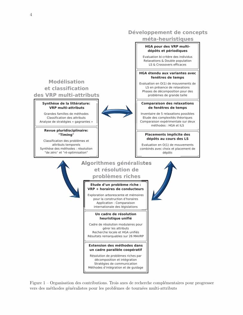
Figure 1 – Organisation des contributions. Trois axes de recherche complementaires pour progresservers des methodes generalistes pour les problemes de tournees multi-attributs

5

comme le VRP ainsi que ses variantes avec depots multiples, periodes de planification multiples,

et fenetre de temps. D’autres developpements amenent a mieux tirer profit des relaxations de

contraintes de fenetres de temps, et a gerer implicitement certaines decisions, comme le placement

et le choix des depots, par des methodes programmation dynamique.

Le dernier axe de recherche s’appuie sur les contributions precedentes pour progresser vers

des methodes efficaces et generalistes pour les problemes de tournees de vehicules multi-attributs.

Nous resolvons tout d’abord un MAVRP particulierement difficile, qui prend en compte les regles

precises de la legislation concernant les horaires et pauses des conducteurs. Cette methodologie nous

permet de qualifier l’impact des regles de la legislation sur la performance economique du transport

et la fatigue des conducteurs. Puis, un cadre de resolution heuristique modulaire est introduit,

ainsi qu’un algorithme genetique hybride unifie pour les MAVRP. Avec une seule implementation

et jeu de parametres, cet algorithme egalise ou surpasse toutes les meilleures methodes dediees

de la litterature pour 26 variantes classiques du VRP. Enfin, un cadre de resolution parallele

cooperatif a base de decomposition, d’integration de solutions et de guidage est propose pour

resoudre efficacement des problemes de tournees de vehicules et d’optimisation combinatoire riches.

La Figure 1 illustre de facon symbolique les liens etroits entre les axes de recherche consideres,

et situe dans ce cadre les differentes contributions et chapitres de la these. Les developpements

methodologiques de cette these sont systematiquement appuyes de developpements algorithmiques

et d’experimentations sur des jeux de donnees issues de la litterature, qui permettent de comparer

les methodes proposees a de nombreux autres algorithmes de la litterature et d’examiner l’apport

de differentes strategies. Les differentes contributions, ainsi que les liens qui les unissent, sont

decrites plus en detail dans la prochaine section.

0.3 Detail des contributions

Axe I : Analyse des attributs et methodes. Une revue de litterature et analyse detaillee des

heuristiques pour les VRP multi-attributs (MAVRP) est tout d’abord conduite dans le Chapitre 1.

Cette revue repond au besoin de classifier et organiser les attributs relativement a leur impact sur

les methodologies de resolution. Trois grandes categories d’attributs sont identifiees : les attributs

Assign, qui impactent les choix d’affectation des routes et ressources aux clients, les attributs Seq,

qui changent la structure et la nature des routes, et les attributs Eval, qui impactent l’evaluation

du cout ou de la faisabilite des sequences, incluant eventuellement la resolution de sous-problemes

inherents aux routes fixees, comme la recherche d’un placement geometrique des objets ou la

determination des horaires.

D’autre part, les concepts principaux de 64 metaheuristiques, selectionnees pour leur remar-

quable performance sur 15 MAVRP classiques avec differents attributs, sont finement etudies au

cours d’une analyse transversale. Il apparait notamment dans cette revue que les meilleures me-

thodes heuristiques ne tiennent pas leur performance d’une unique idee “gagnante”, mais sont plutot

le resultat d’un equilibre et d’une complementarite de concepts, incluant par exemple plusieurs

espaces de recherche, des procedures de modifications de solutions avec differents degres d’impacts,

differentes memoires a plus ou moins long terme, etc... Aucune methodologie metaheuristique ne

6

s’illustre comme etant une meilleure strategie sur l’ensemble des problemes. Toutefois, les methodes

a base de voisinage, comme les recherches tabou et variantes de recuit simule, ont ete generalement

plus etudiees et exploitees dans le passe (Osman 1993, Gendreau et al. 1994, Cordeau et al. 1997),

alors que le succes des methodes evolutionnaires a base de populations est plus recent (Prins

2004, Reimann et al. 2004), conduisant a de nombreuses perspectives de recherche prometteuses.

Certaines “strategies gagnantes” identifiees seront par la suite exploitees et perfectionnees dans

cette these lors du developpement specifique d’algorithmes specialises ou generalistes pour les

VRPs.

Enfin, comme le souligne cette revue de litterature, de nombreux attributs de type Eval,

impactant seulement l’evaluation des sequences, sont lies a des considerations temporelles sur les

horaires de service. La resolution efficace des sous-problemes de determination d’horaires est alors

la clef pour resoudre les MAVRP associees. Ces sous-problemes, que nous appelons problemes de

timing, se retrouvent dans d’autres domaines de la litterature, dans des problemes de transport, de

plus courts chemins, d’ordonnancement de projet ou de production, d’allocation de ressources, ou

de regression isotonique en statistique. Cependant, quasiment aucun lien n’avait ete etabli entre

ces problemes traites dans plusieurs domaines, si bien que des algorithmes efficaces similaires ont

ete redecouverts de nombreuses fois dans la litterature.

Afin d’etablir l’etat de l’art pour ces problemes, decisif pour nos applications, une synthese

de litterature pluridisciplinaire sur les problemes de timing est proposee dans le Chapitre 2. Les

attributs temporels sont classifies, et des algorithmes de resolution efficaces issus de nombreux

domaines de recherche sont identifies et analyses. Cette analyse considere non-seulement la resolu-

tion sequentielle de problemes de timing en “partant de zero”, mais aussi la resolution de series de

sous-problemes successifs au sein de recherches locales ou de methodes de branchement par des

methodes de re-optimisation. La bibliotheque de methodes efficaces ainsi identifiee est un atout

considerable pour la resolution de problemes riches de tournees de vehicules multi-attributs ou

d’ordonnancement non reguliers, car dans bien des cas cette richesse se manifeste exclusivement

au travers de la resolution de ces sous-problemes temporels. Cette analyse vient ainsi completer

et clore notre premiere partie de recherche, dediee a l’analyse de la structure des attributs, des

problemes, et des methodes de la litterature.

Axe II : Developpements metaheuristiques. Nous introduisons de nouveaux developpements

methodologiques afin d’etendre des concepts a succes issus des metaheuristiques evolutionnaires,

introduire de nouveaux concepts prometteurs pour les variantes du VRP, et ainsi contribuer

au deuxieme defi enonce dans ce plan de these. Dans ce cadre, le Chapitre 3 propose un nouvel

algorithme genetique hybride a controle adaptatif de diversite (Hybrid Genetic Search with Advanced

Diversity Control – HGSADC ) tres efficace pour les VRP multi-periodes (PVRP) et multi-depots

(MDVRP) eventuellement combines, ainsi que pour le VRP classique. Cette metaheuristique

combine l’exploration large des methodes evolutionnaires a base de populations, les capacites

d’amelioration agressive des metaheuristiques a voisinage, les relaxations de contraintes pour

cibler les frontieres de non-faisabilite, et des methodes avancees de gestion de la diversite dans

la population. HGSADC reinterprete le concept de survie du plus apte, mettant en place une

7

evaluation bi-critere des individus qui considere a la fois la qualite des solutions, mais aussi leur

contribution a la diversite. Cette strategie permet de preserver la variete des elements de solutions

au sein de la population et de reduire les risques de convergence prematuree pour explorer des

regions prometteuses de l’espace de recherche. De vastes experimentations demontrent la grande

performance de cette methode, en terme d’efficacite de calcul et de qualite de solution, identifiant

soit les meilleures solutions de la litterature ou les solutions optimales quand elles sont connues,

soit de nouvelles meilleures solutions pour tous les jeux de tests connus et etudies depuis des annees

sur les trois classes de problemes. Finalement, une comparaison experimentale des strategies de

gestion de population et d’evaluation des individus, sur plusieurs problemes, revele la contribution

importante des methodes proposees.

Les attributs etudies dans le Chapitre 3 font partie de la categorie Assign, impactant les choix

d’affectation. Afin d’etendre la methode HGSADC a d’autres types d’attributs, notamment ceux

de type Eval, et d’etudier ses concepts principaux sur une plus grande variete de problemes,

le Chapitre 4 presente l’application de cette metaheuristique au VRP avec fenetres de temps

(VRP with time windows : VRPTW). Cette application donne lieu a de nouveaux developpements

methodologiques, concernant notamment l’exploitation de solutions irrealisables ne respectant

pas certaines contraintes sur les routes (fenetres de temps, capacites et durees), et l’exploration

efficace de voisinages avec des methodes de pre-evaluation sur les segments de routes. Le concept

de relaxation des contraintes temporelles de Nagata et al. (2010) est utilise. Celui-ci permet de

payer des penalites pour des “retours dans le temps” en cas d’arrivee tardive a un client. Nous

proposons une maniere simple et efficace dans ce cadre pour evaluer en temps constant amorti

O(1) les solutions intermediaires irrealisables produites par des mouvements de recherche locale a

base d’un nombre borne d’echanges d’arcs. Les meilleurs resultats de la litterature sont obtenus

sur les problemes-tests classiques pour des variantes de VRP avec n’importe quelle combinaison

d’attributs de fenetres de temps, contraintes de durees, compatibilites vehicules-clients, depots

multiples et periodes de planification multiples.

L’application de HGSADC aux problemes avec fenetres de temps, dans le Chapitre 4, a souleve

des questions de recherche liees a l’utilisation efficace de solutions irrealisables et aux choix de

relaxation effectue dans les recherches locales et les heuristiques en general. Cette utilisation de

solutions irrealisables avait deja ete identifiee comme un concept “gagnant” des metaheuristiques

etudiees dans le Chapitre 1, cependant peu d’elements theoriques ou empiriques de la litterature

venaient jusqu’alors appuyer ces conjectures. De ce fait, le Chapitre 5 presente une analyse empirique

des relaxations de contraintes de fenetres de temps au sein de methodes de recherche locale pour le

VRPTW. Les resultats, produits pour deux types d’objectifs (minimisation de la distance totale

et minimisation de la taille de flotte) confirment l’utilite de solutions irrealisables au cours de la

recherche. Aussi, plusieurs alternatives de relaxation sont comparees : arrivees tardives penalisees,

arrivees en avance, retours dans le temps, ou accelerations des services et des deplacements. Des

differences notables sont observees. Les resultats experimentaux montrent que l’approche de“retours

dans le temps” (Nagata et al. 2010), utilisee et generalisee lors de l’application d’HGSADC aux

VRP avec fenetres de temps, permet d’obtenir a la fois de meilleures solutions, et de les trouver

plus rapidement.

8

Enfin, l’etude des problemes avec depots multiples a souleve des questions methodologiques

quand a l’exploration, combinee ou non, de differentes alternatives d’affectation aux depots et

de choix de sequences. Dans le Chapitre 3 nous avions traite le MDVRP comme sous-probleme

du PVRP en separant la representation de solution et les voisinages en relation aux ressources

d’affectation (decomposition sur les periodes de planification ou les depots) et en creant des

operateurs (croisement, recherche locale) specifiques aux choix d’affectations. Le Chapitre 6 decrit

une nouvelle methode efficace, basee sur la programmation dynamique, pour evaluer de maniere

combinee et en temps amorti O(1) le choix optimal du depot, du type de vehicule, et du pre-

mier client de la sequence a etre visite apres le depot (rotation optimale) lors de methodes de

recherche locale et de Split. Cette methodologie permet non seulement d’evaluer efficacement un

plus grand nombre d’alternatives combinees d’affectation et de sequence, mais aussi de releguer

les decisions d’affectation au sein de sous-probleme d’evaluation de tournees, afin de ne plus avoir

a considerer explicitement cet aspect combinatoire au sein des voisinages de recherche locale et

des representations de solution. Ces approches sont implantees et testees au sein de deux cadres

metaheuristiques, une recherche locale iteree, et la methode HGSADC, sur des VRP multi-depots

avec flotte illimitee, homogene ou heterogene. Les experiences mettent en valeur la contribution

importante des methodes proposees au sein des deux types de metaheuristiques.

Axe III : Resolution de problemes riches et algorithmes generalistes. Les derniers cha-

pitres de cette these se consacrent a la resolution de VRP riches combinant de nombreux attributs,

comme le probleme de tournees de vehicules et horaires de conducteurs combines, et au deve-

loppement de nouvelles methodes heuristiques generalistes pour traiter une grande variete de

problemes.

Le Chapitre 7 presente tout d’abord une application a un probleme riche de tournees de

vehicules et horaires de conducteurs (VRP and truck driver scheduling : VRTDSP). En effet,

de nombreux pays ont etabli des legislations complexes sur les sequences de temps de conduite

et de pause (European Union 2002, 2006, National Transport Commission 2008c,b, Transport

Canada 2005, Federal Motor Carrier Safety Administration 2011). Ne pas prendre en compte ces

contraintes conduirait a des solutions totalement irrealistes dans le cadre du transport longue-

distance. Toutefois, les VRP combines avec des contraintes de legislation sont des problemes riches

particulierement difficile a resoudre. Ils amenent parfois plus de quinze regles supplementaires sur

les horaires, ou plusieurs types de taches sont discernees : conduite, travail hors conduite, repos

hebdomadaire, repos journalier, pause... et peuvent etre parfois etendues ou coupees dans des cas

exceptionnels. Le sous-probleme meme de placement des pauses, pour une sequence de visite choisie,

est en soi un probleme tres difficile, dont la polynomialite est a ce jour une question ouverte pour

la plupart des legislations.

Selon la classification du Chapitre 1, ces attributs sur les horaires impactent exclusivement

l’evaluation des routes (type Eval). Une extension de HGSADC est proposee pour resoudre cette

famille de problemes pour les regles de l’Union Europeenne, des Etats-Unis, du Canada, et de

l’Australie. Des methodes d’evaluation de routes efficaces, basees sur une exploration arborescente

des combinaisons de taches et pauses en presence de relaxations des contraintes de fenetres de

9

temps, sont utilisees. Par ailleurs, dans notre cadre, le probleme meme de placement des pauses

est un probleme complexe. Des methodes polynomiales quadratiques (en fonction du nombre de

clients) permettent de le resoudre pour le cas des Etats-Unis, tandis que pour les autres pays

la complexite (et polynomialite) du problemes est toujours une question ouverte. Dans ce cadre

ou chaque evaluation de route est complexe et couteuse en temps de calcul, nous introduisons

des techniques d’acceleration de recherche, basees sur des restrictions de voisinage ainsi que des

memoires sur les evaluations de routes et sur les sous-sequences de visites sont utilisees a la maniere

des methodes de re-optimisation pour les problemes de timing L’algorithme ainsi obtenu ameliore

les solutions existantes de la litterature pour le VRTDSP avec regles europeennes. Enfin, il permet

de traiter les differentes legislations en une seule implementation, ouvrant ainsi la porte a une

comparaison internationale de l’effet des regles sur les couts, les horaires, et la fatigue estimee

des conducteurs. En particulier, nos experimentations indiquent que les regles europeennes sont

les plus sures, tandis que les regles Canadiennes sont les plus profitables economiquement. Les

regles Australiennes, par contre, semblent etre dominees a la fois en termes de risque et d’efficacite

economique. Ces observations demontrent l’interet pratique direct des methodes developpees, qui

peuvent etre utile aux acteurs de la chaine logistique pour leurs besoins d’optimisation, et aux

organismes decisionnaires et syndicats pour evaluer l’impact de nouveaux choix de regles sur le

transport longue-distance.

En outre, cette these contribue a la resolution generaliste de la grande variete de VRP multi-

attributs, par le biais d’un cadre modulaire de resolution heuristique, et une implementation

metaheuristique generaliste, appelee Unified Hybrid Genetic Search (UHGS). Ces contributions

sont decrites dans le Chapitre 8. Proposer une telle methode generaliste pour les MAVRP ne

signifiait pas ignorer les caracteristiques specifiques des problemes, car il etait necessaire dans tous

les cas de prendre en compte les contraintes, decisions supplementaires et objectifs specifiques, mais

impliquait plutot de restreindre les procedures dediees a des elements minimes et modulaires de la

methode. Ainsi, alors que les algorithmes modulaires et librairies de composants de la litterature

pour l’optimisation combinatoire etaient auparavant principalement dedies a la multiplicite des

methodes (differents modules pour differentes strategies heuristiques), le cadre propose gere

la multiplicite des variantes de problemes grace a des composants de resolution elementaires

s’adaptant automatiquement aux attributs consideres. UHGS se base donc sur des procedures dont

l’implantation est independante du probleme : operateurs de recherche locale unifies, croisement,

segmentation de routes (Split generalise), gestion de diversite. Les traitements specifiques au

probleme sont confines dans des composants modulaires qui fournissent les fonctions necessaires aux

choix d’affectation, de sequence, et aux evaluations efficaces de routes, et sont automatiquement

selectionnes et adaptes relativement aux attributs du probleme. Des etudes experimentales de

grande ampleur sur 26 variantes fondamentales de VRP et 39 ensembles de problemes de test

de la litterature, un total de 1008 instances, demontrent la performance remarquable de UHGS

qui, avec une unique implementation et parametrage, egalise ou surpasse les meilleures methodes

dediees de la litterature. De plus, toutes les solutions optimales connues pour ces problemes ont

ete retrouvees. Ces developpements demontrent que la generalite ne s’obtient pas forcement aux

depends de l’efficacite pour cette classe de problemes.

10

Finalement, pour gerer efficacement non seulement la variete mais aussi la difficulte inherente

aux combinaisons des attributs, et afin de progresser plus en avant vers la resolution de VRP

riches contenant plusieurs types d’attributs decisionnels, les metaheuristiques precedentes ont

ete etendues au sein d’un cadre de resolution parallele cooperative a base de decompositions

et recompositions successives de solutions, appele Integrative Cooperative Search (ICS). Cette

contribution est presentee dans le Chapitre 9. L’idee fondamentale d’ICS est de combiner les idees

de decomposition, de simplification intelligente et opportuniste, et de recherche cooperative. Les

decompositions visent a generer des problemes avec un nombre d’attributs reduits, pour lequel

des methodes de resolution efficaces, comme UHGS, peuvent etre utilisees aux mieux de leurs

capacites. Les solutions issues de ces sous-problemes plus simples sont integrees par des algorithmes

dedies afin de reconstituer des solutions completes et ainsi traiter le probleme initial. Les differents

composants cooperent ensemble par le biais d’une memoire centrale enrichie de mecanismes de

guidage. Ce developpement methodologique permet de produire des solutions de plus grande qualite

sur les problemes traites auparavant, combinant attributs periodiques et multi-depots. De plus,

cette application a souleve plusieurs considerations methodologiques impliquant notamment la

reconstitution de solutions completes a partir de solutions partielles, et l’exploitation efficace de

memoires pour guider la recherche future. De nombreuses experimentations ont ete developpees

pour analyser l’impact de differentes strategies alternatives a ce sujet. Ces contributions s’appliquent

avec succes aux problemes de tournees de vehicules multi-attributs, et sont applicables en toute

generalite a une large gamme de problemes d’optimisation combinatoire.

0.4 Structure du document

La structure de ce document concorde avec la demarche de recherche annoncee. La premiere

partie, Chapitres 1 et 2, presente les contributions en terme d’analyse de problemes et methodes : les

heuristiques pour les MAVRP, et la synthese des problemes de timing. La deuxieme partie, au sein

des Chapitres 3 a 6, detaille les differentes contributions methodologiques pour les metaheuristiques,

la methode HGSADC, son application aux variantes du VRPTW, ainsi que l’etude des relaxations

des contraintes de fenetres de temps et des choix de rotation de sequences et d’affectation implicites.

La derniere partie, Chapitres 7 a 9, decrit l’extension de HGSADC aux problemes riches de

VRTDSP, le nouveau cadre de resolution general pour les MAVRP et le traitement des problemes

riches avec la methode ICS.

Premiere partie

ANALYSE STRUCTURELLE DES

PROBLEMES ET DES METHODES

11

CHAPITRE 1

METAHEURISTIQUES POUR LES PROBLEMES DE TOURNEES DE

VEHICULES MULTI-ATTRIBUTS, REVUE ET SYNTHESE DE LA

LITTERATURE

1.1 Fil conducteur et contributions

Les attributs des problemes de tournees de vehicules sont des caracteristiques et contraintes

additionnelles qui visent a mieux prendre en compte les specificites des applications reelles. Les

variantes engendrees sont le support d’une litterature fournie, qui comporte une large variete

d’heuristiques. Ce chapitre passe en revue les principaux types d’attributs, et decrit les heuristiques

et meta-heuristiques classiques pour les problemes de tournees de vehicules multi-attributs. Puis, il

analyse de maniere fine les concepts et “strategies gagnantes” de 64 meta-heuristiques remarquable-

ment efficaces sur plusieurs attributs. Cette analyse transversale est une etape importante pour

progresser vers des methodes efficaces pour une large gamme de problemes.

1.2 Article I : Metaheuristics for multi-attribute vehicle routing problems, a survey

and synthesis

Ce chapitre a ete accepte pour publication sous forme d’article de journal : Vidal,

T., Crainic, T.G., Gendreau, M., Prins, C. (2012). Metaheuristics for multi-attribute

vehicle routing problems, a survey and synthesis. European Journal of Operational

Research, Forthcoming.

Abstract: The attributes of Vehicle Routing Problems are additional characteristics or constraints

that aim to better take into account the specificities of real applications. The variants thus formed

are supported by a well-developed literature, including a large variety of heuristics. This article

first reviews the main classes of attributes, providing a survey of heuristics and meta-heuristics for

Multi-Attribute Vehicle Routing Problems (MAVRP). It then takes a closer look at the concepts

of 64 remarkable meta-heuristics, selected objectively for their outstanding performance on 15

classic MAVRP with different attributes. This cross-analysis leads to the identification of “winning

strategies” in designing effective heuristics for MAVRP. This is an important step in the development

of general and efficient solution methods for dealing with the large range of vehicle routing variants.

Keywords: Vehicle routing, multi-attribute problems, heuristics, meta-heuristics, survey, analysis,

algorithmic design principles.

14

1.3 Introduction

Vehicle routing problems have been the subject of intensive research for more than 50 years, due

to their great scientific interest as difficult combinatorial optimization problems and their importance

in many application fields, including transportation, logistics, communications, manufacturing,

military and relief systems, and so on. The “traditional” Capacitated Vehicle Routing Problem

(CVRP) involves designing least cost delivery routes to service a geographically-dispersed customer

set, while respecting vehicle-capacity constraints. This NP-hard optimization problem combines

the characteristics of a Multiple Knapsack Problem aiming to assign loads to capacitated vehicles,

and a Travelling Salesman Problem (TSP) that aims to find the best route for each vehicle, i.e.,

the least costly sequence of visits for the customers assigned to it.

The extremely broad range of actual applications where routing issues are found leads to the

definition of many VRP variants with additional characteristics and constraints, that we call

attributes, aiming to capture a higher level of system detail or decision choices, including but not

limited to richer system structures (e.g., several depots, vehicle fleets, and commodities), customer

requirements (e.g., multi-period visits and within-period time windows), vehicle operation rules (e.g.,

load placement, route restrictions on total distance or time, and driver work rules), and decision

context (e.g., traffic congestion and planning over extended time horizons). These attributes

complement the traditional CVRP formulations and lead to a variety of Multi-Attribute Vehicle

Routing Problems (MAVRPs), making up a vast research, development, and literature domain.

The dimensions of most problem instances of interest hinders the applicability of exact methods,

while the few software systems presented as general heuristic solvers are increasingly challenged by

the growing variety of attributes. Finally, some MAVRPs combining multiple attributes together,

the so-called rich VRPs, may be especially difficult to solve because of the compound, and possibly

antagonist, decisions they involve.

Thousands of heuristics, meta-heuristics, and solution concepts tailored to some specific

MAVRPs have been proposed in the literature. The vehicle routing domain, vast and difficult to

classify, has been historically articulated around several streams of research dedicated to a number

of major attributes. Such diverse research lines would be justified if the nature of the various

problem settings would call for radically different solution approaches. Yet, MAVRPs naturally

share many common features, and most heuristic strategies developed for specific problems can

be applied to a broader range of VRP variants. The identification of such fundamental design

elements for MAVRP metaheuristics is of primary interest to progress toward more generalist and

efficient VRP algorithms, thus providing the means to quickly address various application cases

and rich VRP settings without extensive problem-tailored algorithmic developments.

To respond to these challenges, we introduce a unifying synthesis and analysis of MAVRP

solution methods, providing the means to identify the main concepts of successful heuristics and

metaheuristics. The analysis is based on two main ideas. On the one hand, we analyse from a

general perspective detached from the particular characteristics of the attributes. On the other

hand, we adopt a synthetic approach to deal with the abundance of contributions. Thus, in

15

particular, the scope of the analysis has been limited to settings with complete and exact data,

demands on nodes (no arc-routing settings), and a single objective.

We identified, classified, and analysed fifteen notable MAVRPs, which have been the object of

a consistent body of well-acknowledged research resulting in a considerable number of heuristic

methods and a number of common benchmark sets of test instances. The simple classification we

use is method-oriented rather than application-oriented, i.e. attributes are discerned relatively

to their impact on the resolution approaches rather than relatively to the real-life constraint or

objective it originates from. We then selected three to five of the most efficient heuristics, in terms

of average solution quality, for each of these MAVRP variants with different kinds of attributes. The

resulting sixty-four methods were then analysed in detail, resulting in the identification of broad

concepts and main algorithmic-design principles, an objective synthesis of “winning strategies”,

perspectives and major research challenges.

The article unfolds in three main parts. Section 1.4 recalls the “traditional” CVRP and reviews

the fundamental elements of heuristics developed to address it. Most of these elements are also found

in the next sections when analysing heuristics for multi-attribute problems. Section 1.5 introduces

an attribute-classification system and presents the selected MAVRPs and the corresponding subset

of selected high-performance heuristics, thus providing the necessary material for our unifying

analysis of state-of-the-art MAVRP heuristics in Section 1.6. Section 1.7 concludes with a discussion

of a number of challenges for the field and possible research perspectives.

1.4 Heuristics for the CVRP

The CVRP was introduced in the seminal article by Dantzig and Ramser (1959) under the

name “Truck Dispatching Problem”. It was only several years later, following the publication of

the article by Christofides (1976), that the current name of the problem became widespread. Like

numerous previous articles, we define the CVRP as follows.

Let G = (V, E) be a complete undirected graph with |V| = n + 1 nodes. The node v0 ∈ Vrepresents a depot, where a fleet of m identical vehicles is based, and where the product to be

distributed is stored. The other nodes vi ∈ V\{v0}, for i ∈ {1, . . . , n}, represent the customers,

characterized by demands for non-negative amounts of product qi. Edges (i, j) ∈ E represent the

possibility of travelling directly from a node (customer or depot) vi ∈ V to a different node vj ∈ Vfor a transportation cost of cij . The objective of the CVRP is to find a set of m or less vehicle

routes, i.e. sequences of deliveries to customers, such that all customers are visited exactly one

time, the total cumulated demand on any route does not exceed a capacity limit Q, the total length

of each route is limited to a value T , and the total transportation cost is minimized. Applications

considering an unlimited fleet can be modeled by setting m = n as at most one vehicle per customer

is needed.

The CVRP has been the subject of intensive research since the 1960s. Numerous exact methods,

heuristics, and metaheuristics have been presented in the literature, as illustrated by various surveys

(see Baldacci et al. 2007, Cordeau et al. 2007, Gendreau et al. 2008b, Eksioglu et al. 2009, Potvin

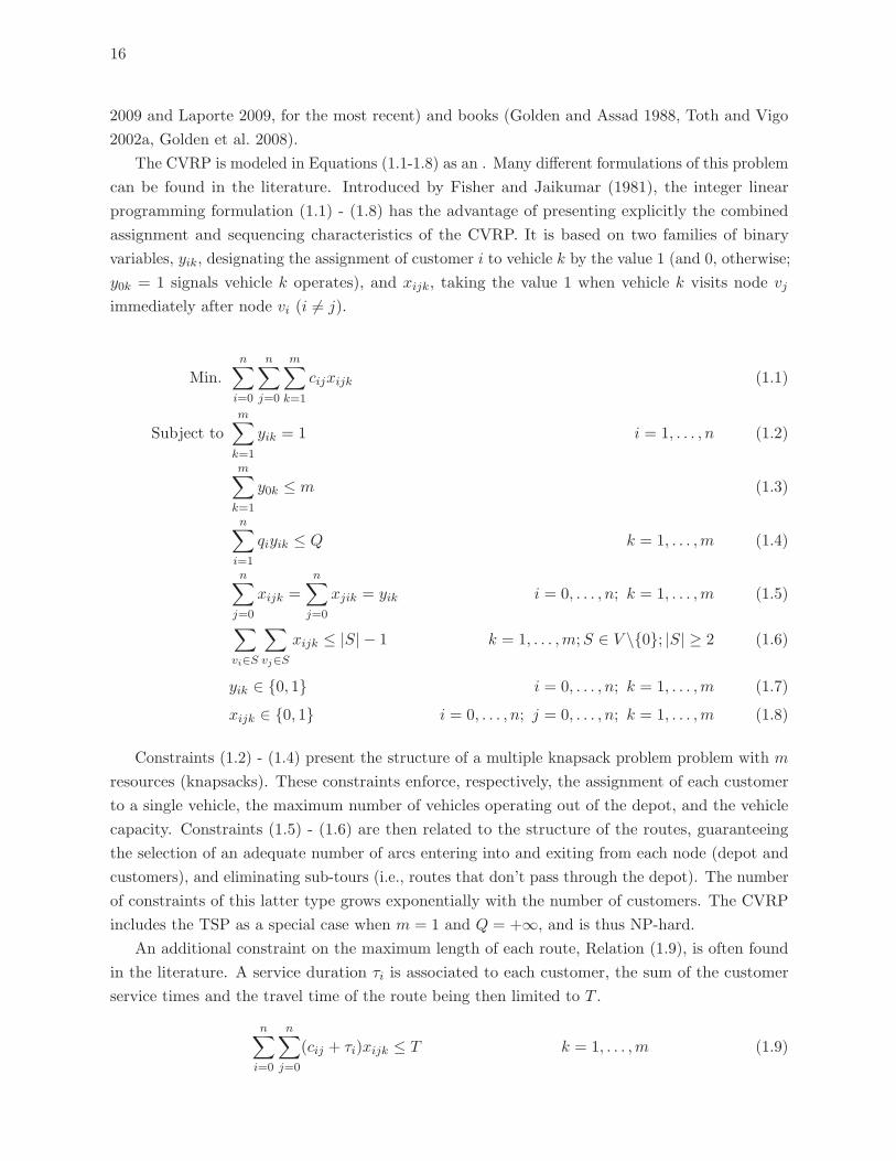
16

2009 and Laporte 2009, for the most recent) and books (Golden and Assad 1988, Toth and Vigo

2002a, Golden et al. 2008).

The CVRP is modeled in Equations (1.1-1.8) as an . Many different formulations of this problem

can be found in the literature. Introduced by Fisher and Jaikumar (1981), the integer linear

programming formulation (1.1) - (1.8) has the advantage of presenting explicitly the combined

assignment and sequencing characteristics of the CVRP. It is based on two families of binary

variables, yik, designating the assignment of customer i to vehicle k by the value 1 (and 0, otherwise;

y0k = 1 signals vehicle k operates), and xijk, taking the value 1 when vehicle k visits node vj

immediately after node vi (i �= j).

Min.

n∑i=0

n∑j=0

m∑k=1

cijxijk (1.1)

Subject to

m∑k=1

yik = 1 i = 1, . . . , n (1.2)

m∑k=1

y0k ≤ m (1.3)

n∑i=1

qiyik ≤ Q k = 1, . . . ,m (1.4)

n∑j=0

xijk =n∑

j=0

xjik = yik i = 0, . . . , n; k = 1, . . . ,m (1.5)

∑vi∈S

∑vj∈S

xijk ≤ |S| − 1 k = 1, . . . ,m;S ∈ V \{0}; |S| ≥ 2 (1.6)

yik ∈ {0, 1} i = 0, . . . , n; k = 1, . . . ,m (1.7)

xijk ∈ {0, 1} i = 0, . . . , n; j = 0, . . . , n; k = 1, . . . ,m (1.8)

Constraints (1.2) - (1.4) present the structure of a multiple knapsack problem problem with m

resources (knapsacks). These constraints enforce, respectively, the assignment of each customer

to a single vehicle, the maximum number of vehicles operating out of the depot, and the vehicle

capacity. Constraints (1.5) - (1.6) are then related to the structure of the routes, guaranteeing

the selection of an adequate number of arcs entering into and exiting from each node (depot and

customers), and eliminating sub-tours (i.e., routes that don’t pass through the depot). The number

of constraints of this latter type grows exponentially with the number of customers. The CVRP

includes the TSP as a special case when m = 1 and Q = +∞, and is thus NP-hard.

An additional constraint on the maximum length of each route, Relation (1.9), is often found

in the literature. A service duration τi is associated to each customer, the sum of the customer

service times and the travel time of the route being then limited to T .

n∑i=0

n∑j=0

(cij + τi)xijk ≤ T k = 1, . . . ,m (1.9)

17

Only relatively small CVRPs can currently be consistently solved to optimality. The largest

symmetric instances solved by Fukasawa et al. (2006) and Baldacci et al. (2008b) have a maximum of

135 customers. Some exact methods for asymmetric problems have also been proposed in Fischetti

et al. (1994) and Pessoa et al. (2008). Because of this, heuristics and metaheuristics constitute a very

active research domain in the literature. These approaches for the classic CVRP are surveyed in the

following, discerning some main categories of methods: constructive heuristics, local improvement

heuristics, metaheuristics, hybrid methods, and parallel and cooperative metaheuristics.

1.4.1 Constructive heuristics

Mainly proposed between the 1960s and the 1980s, a large number of heuristics attempted to

produce solutions constructively. One key characteristic of these heuristics is that they operate in

a greedy manner, producing a set of definitive decisions (e.g., customer insertion or the merging of

two routes) that cannot be reversed afterwards.

The savings method of Clarke and Wright (1964) is the best-known example of a constructive

heuristic. Starting from an initial solution s0 in which each customer is served by a different route,

the heuristic searches for and merges two route extremities i and j, maximizing the distance saved

sij = ci0 + c0j − cij , under the condition that the merged route is feasible. The original method

has been revised and improved several times, notably by Gaskell (1967) and Yellow (1970) who

parametrized the original equation to give more, or less, importance to the distance to the depot

(sij = ci0 + c0j − λcij with λ ≥ 0), thus correcting a flaw in the original method, which produced

routes with a high “circular” tendency. Mole and Jameson (1976) and Solomon (1987) further

generalize these constructive procedures, considering customer insertions into the routes and using

additional parameters and simple local-improvement procedures.

Another constructive heuristic, called “sweep” (Gillett and Miller 1974), is remarkable in its

simplicity. The approach explores the customers circularly, in increasing polar angle around the

depot. Each customer is successively inserted in this order at the end of the current route. If this

insertion is infeasible because of the route constraints, then a new route is initiated. At the end of

this construction phase, Gillett and Miller (1974) proposed to apply a λ-opt improvement heuristic

(see Section 1.4.2) to post-optimize each route separately.

Other heuristics perform the assignment and sequencing in two separate phases. The “route-first

cluster-second” approach (Newton and Thomas 1974, Bodin and Berman 1979, Beasley 1983) first

constructs a giant circuit that visits all customers, like a TSP solution. This giant tour is then cut

into several routes from the depot. The segmentation problem can be solved exactly as a shortest

path problem in an acyclic graph.

Proposed by Fisher and Jaikumar (1981), the “cluster-first route-second” approach, first creates

customer clusters, and then optimizes the order of visits for each cluster as a TSP subproblem.

The creation of the clusters is performed by solving a Generalized Assignment Problem (GAP)

for the customers, around m locations chosen to represent zones with a high customer density.

A linear estimate of the route costs is used as the objective function of the GAP. This approach

is strongly linked to the visual solution approach of human planners. In addition, the priority

given to the assignment allows capacity constraints to be better dealt with for highly constrained

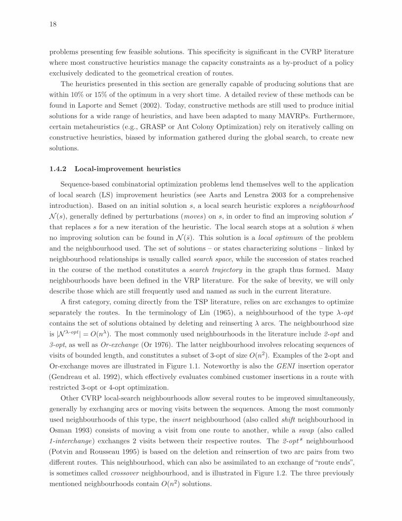
18

problems presenting few feasible solutions. This specificity is significant in the CVRP literature

where most constructive heuristics manage the capacity constraints as a by-product of a policy

exclusively dedicated to the geometrical creation of routes.

The heuristics presented in this section are generally capable of producing solutions that are

within 10% or 15% of the optimum in a very short time. A detailed review of these methods can be

found in Laporte and Semet (2002). Today, constructive methods are still used to produce initial

solutions for a wide range of heuristics, and have been adapted to many MAVRPs. Furthermore,

certain metaheuristics (e.g., GRASP or Ant Colony Optimization) rely on iteratively calling on

constructive heuristics, biased by information gathered during the global search, to create new

solutions.

1.4.2 Local-improvement heuristics

Sequence-based combinatorial optimization problems lend themselves well to the application

of local search (LS) improvement heuristics (see Aarts and Lenstra 2003 for a comprehensive

introduction). Based on an initial solution s, a local search heuristic explores a neighbourhood

N (s), generally defined by perturbations (moves) on s, in order to find an improving solution s′

that replaces s for a new iteration of the heuristic. The local search stops at a solution s when

no improving solution can be found in N (s). This solution is a local optimum of the problem

and the neighbourhood used. The set of solutions – or states characterizing solutions – linked by

neighbourhood relationships is usually called search space, while the succession of states reached

in the course of the method constitutes a search trajectory in the graph thus formed. Many

neighbourhoods have been defined in the VRP literature. For the sake of brevity, we will only

describe those which are still frequently used and named as such in the current literature.

A first category, coming directly from the TSP literature, relies on arc exchanges to optimize

separately the routes. In the terminology of Lin (1965), a neighbourhood of the type λ-opt

contains the set of solutions obtained by deleting and reinserting λ arcs. The neighbourhood size

is |N λ-opt | = O(nλ). The most commonly used neighbourhoods in the literature include 2-opt and

3-opt, as well as Or-exchange (Or 1976). The latter neighbourhood involves relocating sequences of

visits of bounded length, and constitutes a subset of 3-opt of size O(n2). Examples of the 2-opt and

Or-exchange moves are illustrated in Figure 1.1. Noteworthy is also the GENI insertion operator

(Gendreau et al. 1992), which effectively evaluates combined customer insertions in a route with

restricted 3-opt or 4-opt optimization.

Other CVRP local-search neighbourhoods allow several routes to be improved simultaneously,

generally by exchanging arcs or moving visits between the sequences. Among the most commonly

used neighbourhoods of this type, the insert neighbourhood (also called shift neighbourhood in

Osman 1993) consists of moving a visit from one route to another, while a swap (also called

1-interchange) exchanges 2 visits between their respective routes. The 2-opt* neighbourhood

(Potvin and Rousseau 1995) is based on the deletion and reinsertion of two arc pairs from two

different routes. This neighbourhood, which can also be assimilated to an exchange of “route ends”,

is sometimes called crossover neighbourhood, and is illustrated in Figure 1.2. The three previously

mentioned neighbourhoods contain O(n2) solutions.

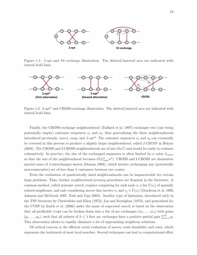
19

Figure 1.1: 2-opt and Or-exchange illustration. The deleted/inserted arcs are indicated withdotted/bold lines.

Figure 1.2: 2-opt* and CROSS-exchange illustration. The deleted/inserted arcs are indicated withdotted/bold lines.

Finally, the CROSS-exchange neighbourhood (Taillard et al. 1997) exchanges two (one being

potentially empty) customer sequences s1 and s2, thus generalizing the three neighbourhoods

introduced previously, insert, swap, and 2-opt*. The customer sequences s1 and s2 can eventually

be reversed in this process to produce a slightly larger neighbourhood, called I-CROSS in Braysy

(2003). The CROSS and I-CROSS neighbourhoods are of size O(n4) and would be costly to evaluate

exhaustively. In practice, the size of the exchanged sequences is often limited by a value Lmax,

so that the size of the neighbourhood becomes O(L2maxn

2). CROSS and I-CROSS are themselves

special cases of λ-interchanges moves (Osman 1993), which involve exchanging any (potentially

non-consecutive) set of less than λ customers between two routes.

Even the evaluation of quadratically sized neighbourhoods can be impracticable for certain

large problems. Thus, further neighbourhood pruning procedures are frequent in the literature. A

common method, called granular search, requires computing for each node vi a list Γ(vi) of spatially

related neighbours, and only considering moves that involve vi and vj ∈ Γ(vi) (Gendreau et al. 1992,

Johnson and McGeoch 1997, Toth and Vigo 2003). Another type of limitation, introduced early in

the TSP literature by Christofides and Eilon (1972), Lin and Kernighan (1973), and generalized for

the CVRP by Irnich et al. (2006) under the name of sequential search, is based on the observation

that all profitable λ-opt can be broken down into a list of arc exchanges (φ1, . . . , φλ) with gains

(g1, . . . , gλ), such that all subsets of k ≤ λ first arc exchanges have a positive partial gain∑k

i=1 gi.

This observation allows to rapidly eliminate a lot of unpromising neighbour solutions.

Of critical concern is the efficient serial evaluation of moves, route feasibility and costs, which

represents the bottleneck of most local searches. Several techniques can lead to computational effort

20

reductions. The management of judicious variables on subsequences of visits (e.g. partial demands

or distances), in particular, can lead to incremental move evaluations in amortized O(1) time.

Similar approaches are used with success on other MAVRPs (c.f. Section 1.6). Memory structures

may also be used to store route evaluations or move evaluations within tables or hashtables.

Large neighbourhoods, with an exponential number of solutions, have also been widely studied

and used in the literature. The procedure of Lin and Kernighan (1973) is a remarkably effective

method for optimizing a TSP sequence. Like the ejection chains strategy developed by Glover

(1992, 1996) and extensively applied to the CVRP by Rego (2001), this procedure attempts to find

a cycle that alternates existing and non-existing arcs in the current solution, so that the solution

obtained by replacing existing arcs in a cycle with the non-existing arcs is feasible and improving.

Such a method can be viewed as an incomplete investigation of a λ-opt neighbourhood with large

λ values. Closely related to the previous concepts, the cyclical transfers of Thompson and Psaraftis

(1993) explore a large neighbourhood obtained by moving k customers within b routes. The search

for an improving neighbour solution is formulated as a negative-cost cycle detection problem in an

auxiliary graph. Although NP-hard, this latter subproblem can be solved effectively by means of

heuristics.

Other ruin-and-recreate neighbourhoods (Shaw 1998) operate deletions and reinsertions of

customer visits within customer sequences. Methods of this kind vary in the nature of their

destruction and reconstruction operators, and may exploit heuristic methods, constraint program-

ming, or integer programming for reconstruction. Finally, generalizing the work of Sarvanov and

Doroshko (1981) for the TSP, De Franceschi et al. (2006) and Toth (2008) propose neighbourhoods

based on fixing some customers and re-assigning unfixed customers between fixed ones, which are

explored by solving an integer-programming model. Other large neighbourhoods and exploration

techniques are reviewed in Ahuja et al. (2002) and Pisinger and Ropke (2010). Additional literature

reviews on local-search methods for the VRP can be found in Van Breedam (1995), Thompson

and Psaraftis (1993), Kindervater and Savelsbergh (1997), Laporte and Semet (2002), Braysy and

Gendreau (2005a) and Funke et al. (2005). Local search constitutes an essential building block of

metaheuristics for the CVRP, described in the next section.

1.4.3 Metaheuristics

The term“metaheuristic”was first coined by Glover (1986) to designate a broad class of heuristic

methods that continue the search beyond the first encountered local optimum. A somewhat crude

but telling definition characterizes metaheuristics as heuristics guiding other heuristics.

Metaheuristics constitute a core research domain in combinatorial optimization as illustrated

by many literature reviews (e.g., Osman and Laporte 1996, Blum and Roli 2003, Gendreau and

Potvin 2005) and books (e.g., Corne et al. 1999, Glover and Kochenberger 2003, Dreo et al. 2003,

Gendreau and Potvin 2010). The CVRP is a testing ground particularly appreciated for such

methods, as illustrated by the reviews of Gendreau et al. (2002), Cordeau et al. (2005), Gendreau

et al. (2008b), Laporte (2009) and Potvin (2009). We distinguish between so-called neighbourhood-

centred methods, which generally proceed by iteratively exploring the neighbourhoods of a single

incumbent solution, population-based strategies evolving a set of solutions by generating one of

21

several “new” solutions out of combinations of existing ones, and approaches that either combine

elements of different metaheuristics, the so-called hybrids, or harness the exploration capabilities of

several solution methods exploiting their interaction, the parallel and cooperative search methods.

1.4.3.1 Neighbourhood-centred search

Simulated Annealing (SA) (Kirkpatrick et al. 1983, Cerny 1985) overcomes the limitation

of local-improvement heuristics, the rapid attraction to a local optimum, by accepting solution-

deterioration moves with a probability governed by a statistical process, the so-called temperature

parameter. The higher the temperature, the more likely it is to accept a deteriorating move.

Temperature evolves dynamically during the search relatively to a cooling scheme, first favouring a

vast exploration and frequent degradations, then gradually accepting fewer and fewer degradations

to intensify the search for good-quality solutions. For the CVRP, efficient deterministic “Record-

to-Record” (R-to-R) variants (Dueck 1993, Li et al. 2005) accept any neighbor solution which is

not much worse than the incumbent solution, and prevent degradations that are too significant

relatively to the best-found solution s∗, subject to re-starting the search from s∗.Tabu search (Glover 1986, 1989, 1990, Glover and Laguna 1998) associates a search trajectory

centred on the choice the best neighbour of the incumbent solution, with learning capabilities,

generally represented as short-, medium- and long-term memories on solution elements, which

replace or significantly complement the randomization used in other metaheuristics. The method

is thus escaping from local optima when the best neighbor solution is not improving. This decision

process is enhanced by two mechanisms, the first aiming to avoid cycling and relying on short-term

memories to reject solutions that contain recently examined tabu elements, the second accepting

solutions that fulfil some aspiration criteria such as “the best solution in value or containing a given

solution element”. Of central importance are the medium- and long-term memories used to manage

significant trajectory-inflecting procedures known as intensification, e.g., focusing the search around

elite solutions while promoting high-quality elements, and diversification, e.g., moving the search

to an under-explored area of the search space, promoting infrequent elements, and so on. The

challenge of balancing diversification and intensification is still a key research question in the

literature.

Tabu search led to very effective CVRP metaheuristics, including TABUROUTE (Gendreau

et al. 1994), Adaptive Memory (AM) variants (Taillard 1993, Rochat and Taillard 1995, Tarantilis

2005), and the Unified Tabu Search (UTS) (Cordeau et al. 1997, 2001a). In TABUROUTE

and UTS, diversification and intensification occur through penalties (incentives, respectively) on

frequently (rarely) encountered solution elements, while AM approaches regularly redirect the

search to a region around a new solution built out of promising fragments from a memory.

Concepts from tabu search have inspired other metaheuristics. Long-term memories for

penalizing frequent solution elements can also be viewed as a basis of Guided Local Search

(Voudouris and Tsang 1999), applied by Kilby et al. (1999), Tarantilis et al. (2007), Kytojoki et al.

(2007), and Zachariadis and Kiranoudis (2010a) to the CVRP. In this case, modifying the search

space by means of penalties is a primary tool for escaping from local optima. Similarly, aspiration

22

criteria take a preponderant role in the Attribute Based Hill Climber (ABHC) method (Whittley

and Smith 2004, Derigs and Kaiser 2007).

Variable neighbourhood Search (VNS) (Mladenovic and Hansen 1997, Hansen et al. 2010)

exploits the fact that a local optimum is defined for a given neighbourhood. Thus, changing

the nature of the neighbourhood during the search, or at least some of its parameters, provide

the means for further solution improvements. The order of neighbourhood evaluations and the

solution acceptance criteria can be either deterministic or probabilistic. For the CVRP, additional

solution perturbation mechanisms and long-term memories inspired from tabu search are sometimes

employed (Kytojoki et al. 2007, Fleszar et al. 2009, Chen et al. 2010). Metaheuristic hybrids (see

Section 1.4.3.3) based on VNS are thus frequent.

In the same spirit, the Adaptive Large neighbourhood Search (ALNS) by Pisinger and Ropke

(2007) exploits the benefits of varied neighbourhoods based on ruin-and-recreate moves (Shaw

1998). The frequency of use of these neighbourhoods is adapted throughout the search relatively

to their past performance. Finally, the Iterated Local Search (ILS) (see Lourenco et al. 2010, for a

recent review) applies successively a local-improvement phase, which ends up in a local optima,

and a perturbation phase to escape from the local optima. Scaling appropriately the strength of

the perturbation operator is a crucial point of the method. Prins (2009a) provides a simple and

efficient application of ILS to the CVRP, where several solutions are iteratively produced from the

same incumbent solution by means of improvement and perturbation mechanisms, the best one

being selected for the next iteration.

1.4.3.2 Population-based methods

Population-based methods are often inspired from natural mechanisms. Genetic Algorithms

(GA) and Evolutionary Algorithms (EA) were introduced during the late 1950s, and developed in

their current form in Holland (1975). These algorithms interpret genetic laws and natural selection

to evolve a population of individuals assimilated to solutions, through elitist selection, crossover,

and mutation operators. With EA, it is also common to simultaneously make the search strategies

(e.g., operator parameters) evolve with the solutions. Traditional GA and EA have a tendency

to progress too slowly, however, and have thus been enhanced with various mechanisms, such as

local search, which is also sometimes called an “education operator”. The algorithms thus obtained

are sometimes called “genetic local searches” (Muhlenbein et al. 1988) or “memetic algorithms”

(Moscato 1989, Moscato and Cotta 2010).

Some of these enhanced genetic methods performed remarkably well on classical CVRP bench-

mark instances (Prins 2004, Alba and Dorronsoro 2006, Marinakis et al. 2006, Nagata et al. 2010,

Vidal et al. 2012a). We refer to Potvin (2009) for a thorough coverage of the field. It is noteworthy

that many successful genetic algorithms for the CVRP use a giant-tour solution representation

without trip delimiters (Prins 2004), along with clustering procedures (Beasley 1983) to optimally

Split a tour into routes. This strategy, based on route-first cluster-second constructive procedures,

enables to reduce the number of alternative solutions (there are less giant tours than VRP solutions)

and rely on very simple genetic crossover operators working on permutations. In addition, an

23

adequate management or promotion of population diversity appears to be of critical importance

(Prins 2004, Sorensen and Sevaux 2006, Vidal et al. 2012a).

The Path Relinking (PR) and Scatter Search (SS) metaheuristics (Glover 1977, Resende et al.

2010) are other population methods based on solution recombinations. These methods promote

strategic recombination over randomization, and differ essentially from the GA-type of methods in

the manner in which solutions are crossed and in the size of the solution pool, which is generally

smaller. Recombinations in PR involve an initial solution sDEP and a guiding solution sGD, both

selected from an elite solution population. Characteristics of sGD are progressively inserted in

sDEP in order to create a trajectory connecting these two solutions, potentially containing new

improving solutions. On the other hand, the recombinations operators used in SS can involve more

than two solutions. Path relinking was applied to the CVRP by Ho and Gendreau (2006).

Ant Colony Optimization (ACO) approaches (Dorigo and Stutzle 2004) were inspired by the

social behaviour of ants foraging for food and are for now the swarm-type of method most used in

optimization. ACO was applied to the CVRP by Bullnheimer et al. (1999), Bell and Mc Mullen

(2004), Doerner et al. (2004), Reimann et al. (2004) and Yu et al. (2009), among others. The

individual behaviour of ants is embodied by constructive heuristics, exploiting information on the

search history (i.e., pheromones). Other swarm-inspired methods were proposed for the CVRP

by Marinakis and Marinaki (2011) (bee colonies) and Marinakis and Marinaki (2010) (particle

swarms). All these methods are exploiting some form of learning, as are neural networks (Ghaziri

1996, Vakhutinsky and Golden 1994, Creput and Koukam 2008), and artificial immune systems

(Masutti 2008), to name a few. These algorithms are often combined with local-improvement

procedures, thus complicating the task to estimate the proper impact of collective intelligence

paradigms on the search performance.

1.4.3.3 Hybrid metaheuristics

Hybrid metaheuristics blend concepts from various solution methodologies, metaheuristic classes

most often, to take advantage of their respective strengths. The blending may take the form

of a juxtaposition of methods (e.g., two algorithms called on consecutively) or an indissociable

inclusion of elements from one method into a fully-functional different metaheuristic (e.g., tabu

search-inspired memories in VNS). Hybrids may exclusively combine metaheuristic concepts, or also

involve algorithmic ideas and modules from mathematical programming, constraint programming,

tree-search procedures, and so on.

Although much effort has been recently put into properly defining the scope of hybrid meta-

heuristics (Raidl et al. 2010, Blum et al. 2011), the term remains very general and covers very

different strategies. One can indeed argue that metaheuristics, described as heuristics guiding other

heuristics, are hybrid in nature. This shows the shortcomings of a too-encompassing definition or,

even, of trying to find a precise definition. Within the scope of this paper, we identify hybridisation

as a strong concept in metaheuristic design, rather than a well-defined class of methods, aiming to

take advantage of the synergy among different solution-method ideas to explore a broad variety of

solution strategies, often yielding superior results.

24

A large variety of hybrid methods has thus been proposed for the CVRP. Several approaches

involve combined neighbourhood-centred search concepts, such as SA+tabu (Osman 1993),

GRASP+ILS (Prins 2009a), ILS+VND (Chen et al. 2010), tabu+ILS (Cordeau and Maischberger

2012), among others. Hybridization schemes of this kind are frequent in recent local search-

based methods, which are frequently enriched with restart procedures (a main characteristic of

GRASP), probabilistic acceptance of deteriorating moves (a main characteristic of SA), variable

neighbourhoods (VNS), or long-term memories and penalties on solutions attributes (GLS).

Population- and neighbourhood-search hybrids are also widespread. The wide majority of

population-based approaches for the CVRP actually integrates some kind of local-search components,

and can be characterized as hybrid. Furthermore, two of the three most efficient current CVRP

metaheuristics (Nagata and Braysy 2009b, Vidal et al. 2012a) combine GA and LS. Other advanced

hybridization schemes involve combined GA+tabu (Perboli et al. 2008), or combined population-

based concepts such as GA+PSO (Marinakis and Marinaki 2010) and PR+PSO (Marinakis et al.

2010).

Finally, a number of metaheuristics for the CVRP integrate integer or constraint programming

components to recombine promising elements of solutions into complete solutions (Rochat and

Taillard 1995, Tarantilis 2005, Alvarenga et al. 2007, Groer et al. 2011), or to explore large

neighbourhoods based on ruin-and-recreate (Shaw 1998, De Franceschi et al. 2006, Salari et al. 2010).

One actually observes a trend towards proposing matheuristics for VRP, combining metaheuristic

and mathematical programming components, and explicitly using the model formulation in defining

elements of the method (Doerner and Schmid 2010).

1.4.3.4 Parallel and cooperative metaheuristics

Parallel metaheuristics (Toulouse et al. 1996, Alba 2005, Crainic and Toulouse 2010) are

concerned with the efficient exploitation of simultaneous work (often on several processors) to solve

a given problem instance, and have proved of great interest for routing problems (Crainic 2008).

Several types of parallelism may be distinguished according to how parallelism is obtained, how

communications among the tasks are defined, as well as how the global search is conducted. In

the most straightforward classification, low-level parallelism involves decomposing parts of the

algorithm into independent tasks, thus providing the means to exploit parallel resources without

changing the general behaviour of the method. To be efficient, such a strategy must target the

computationally expensive “bottleneck” procedures, which most frequently are the evaluation of

moves in neighbourhood-centred methods, and crossover, selection, and evaluation in population-

based ones. To our knowledge, although many papers are concerned with the development of such

strategies for metaheuristics in general, few studies on low-level procedures have been directly

focused on the CVRP. A notable exception is the recent work of Schulz (2011), considering the

efficient solving of CVRPs on Graphic Processing Units (GPU). In this case, the change in hardware

has direct implications on the resolution methodology.

In contrast, metaheuristics based on high-level parallelism either partition the set of decisions,

leading to problem decompositions, or conduct multiple concurrent searches on one or several

search spaces. The simplest method of the latter kind, noted as parallel independent multi-search,

25

involves to gather the best final solution of a set of methods not linked by any communication

or information exchange. This parallel implementation of the multi-start strategy can offer very

interesting performances for the CVRP. Yet, to fully profit from parallelism, more advanced

cooperation schemes integrate mechanisms to share information during the course of the methods

and, in the most advanced settings, to create new information out of the exchanged data. Thus, the

nature of the information shared, the frequency of the communications, and the scope (utilisation)

of the received information are the main characteristics of cooperation strategies.

For the CVRP, as for most combinatorial optimization cases, the most efficient parallel meta-

heuristics are built on asynchronous communications, triggered individually by the cooperating

algorithms, and often taking the form of exchanges of solutions or elements of solutions. Most

multi-search strategies are based on either adaptive (Rochat and Taillard 1995, Badeau et al.

1997) or central memory (Rego 2001, Jin et al. 2012, Cordeau and Maischberger 2012, Groer et al.

2011) principles. The former gathers promising solution fragments and constructs new solutions

out of such fragments. Tabu searches improve these new solutions, and return the best found

solutions to the memory. In central memory-based cooperation, participating solution methods,

which may be metaheuristics, exact algorithms, or any other method, exchange solutions and,

possibly, various other data, through a common data repository (the “central memory”). Thus, all

information is always available on request to any of the cooperating processes and, moreover, can

be used to generate new relevant information, e.g., new solutions, performance measures on solution

components, promising areas of the search space, and so on. Currently, tabu search threads (in a

hybrid setting for Cordeau and Maischberger 2012) cooperate in most central-memory methods

proposed for the CVRP, while Groer et al. (2011) also added integer programming solvers.

Other parallel strategies arose in the field of evolutionary computation. According to fine-grained

parallel ideas, individuals are arrayed according to some geometrical form (2-dimensional toroidal

grid in Alba and Dorronsoro 2006) and interact only with the (four, in this case) individuals directly

connected to. This sets up a diffusion mechanism of good individual characteristics throughout

the population. GA cooperation is generally built according to a coarse-grained strategy, where

populations evolve separately and cooperate through migrations of elite solutions (e.g., Dorronsoro

et al. 2007).

Doerner et al. (2006) performed extensive sensitivity analyses on several cooperative ACO

metaheuristics that communicate synchronously through exchanges of solutions, ants, or pheromones.

Experiments reproduce the results obtained for the parallel strategies for other metaheuristics,

and show that parallel methods tend to outperform sequential ones, that sharing populations

of elite solutions is more relevant than solely broadcasting the global best solution, and that

episodic re-initializations of pheromone matrices contribute towards a better search. Furthermore,

exploiting the spatial decomposition of Reimann et al. (2004) in a parallel context leads to increased

speed-ups.

1.4.4 Relative performance of CVRP heuristics

Two main sets of instances have been widely used in the literature to compare the performance of

heuristics in the last 30 years of research on the CVRP. The 14 benchmark instances of Christofides

26

et al. (1979) include between 50 and 199 customers, which are spatially randomly distributed for the

first 10 instances, and otherwise clustered. The 20 large-scale instances (pr01-pr20) of Golden et al.

(1998b), include between 200 and 483 customers and present geometric symmetries. Comparisons of

VRP approaches are often based on the quality of the solutions in presence of similar computational

effort. Nowadays, many metaheuristics reach systematically the best known solution (BKS) on

almost all instances from Christofides et al. (1979). A comparison of state-of-the-art metaheuristics

based on this benchmark tends to be less statistically significant, as only slight differences on 3

or 4 instances are now reported. To state the best performing methods, we therefore rely on the

larger scale instances of Golden et al. (1998b), for which the results of well-performing approaches

remain significantly different.

We start by emphasizing a number of good practices for reporting results and establishing a fair

comparison between CVRP heuristics. We also refer to Barr et al. (1995) for further discussions

and insights. A performance report must contain at least an estimate of the solution quality and

CPU time of the proposed method, as well as the computing environment: programming language,

processor, operating system, compiler and compiler options. Any performance analysis should be

presented with a minimum of statistical information. As such, for non-deterministic algorithms,

the average solution quality and CPU time on several runs for each problem instance should be

reported, as well as the standard deviation to assess both quality and robustness. For deterministic

algorithms, we suggest either to use a large-enough set of instances, or shuffle the customer indices

to perform several different runs. A heuristic must also not require any other information than the

problem instance. Using exterior knowledge, e.g, an optimal solution to trigger termination, or

some best known characteristics as a starting point (fleet size for example in presence of a fleet

minimization objective), is not a fair practice.

The most standard search-effort measure in the CVRP literature considers the total CPU time,

and thus not only the time to reach the best solution. Other conventions should be clearly stated.

The factors of Dongarra (2011) are commonly used to assess the relative speed of two processors by

scaling the CPU time of two algorithms run on different machines. These factors must be used with

caution however, mostly to compare order of magnitudes, since differences in operating systems,

compilers, and memory organization have a huge impact on the measures. The best alternative

remains to compare on the same computer whenever possible. Reporting the best solutions of the

method on K runs may also provide valuable insights on the potential of solution improvement. In

that case, K must be specified, and the computation effort of the assimilated multi-start method is

the CPU time for all runs. Similarly, the effort of a parallel method is evaluated as the sum of

the CPU times on all threads and processors. The communication overhead, approximated as the

difference between the real wall-clock time and the CPU time should also be reported.

Table 1.1 provides a brief comparative analysis of the performance of the best CVRP heuristics

on the instances of Golden et al. (1998b). The solution quality is measured as the average Gap (%)

to the current Best Known Solutions (BKS) in the literature for each instance. The CPU time

is indicated in column “T”. The scaled computational effort T# = nruns × ncpu × T × f(cpu) is

also reported, where f(cpu) stands for the CPU speed factor relatively to a Pentium IV 3.0 GHz

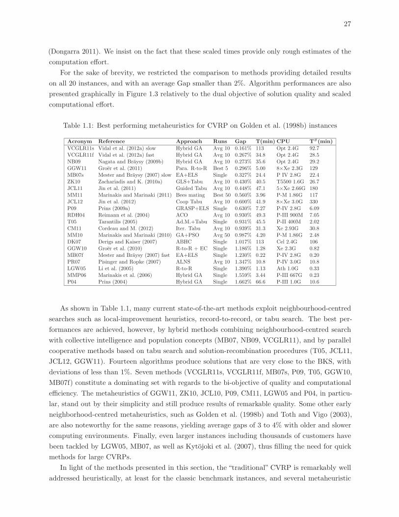
27

(Dongarra 2011). We insist on the fact that these scaled times provide only rough estimates of the

computation effort.

For the sake of brevity, we restricted the comparison to methods providing detailed results

on all 20 instances, and with an average Gap smaller than 2%. Algorithm performances are also

presented graphically in Figure 1.3 relatively to the dual objective of solution quality and scaled

computational effort.

Table 1.1: Best performing metaheuristics for CVRP on Golden et al. (1998b) instances

Acronym Reference Approach Runs Gap T(min) CPU T#(min)

VCGLR11s Vidal et al. (2012a) slow Hybrid GA Avg 10 0.161% 113 Opt 2.4G 92.7VCGLR11f Vidal et al. (2012a) fast Hybrid GA Avg 10 0.267% 34.8 Opt 2.4G 28.5NB09 Nagata and Braysy (2009b) Hybrid GA Avg 10 0.273% 35.6 Opt 2.4G 29.2GGW11 Groer et al. (2011) Para. R-to-R Best 5 0.296% 5.00 8×Xe 2.3G 129MB07s Mester and Braysy (2007) slow EA+ELS Single 0.327% 24.4 P IV 2.8G 22.4ZK10 Zachariadis and K. (2010a) GLS+Tabu Avg 10 0.430% 40.5 T5500 1.6G 26.7JCL11 Jin et al. (2011) Guided Tabu Avg 10 0.448% 47.1 5×Xe 2.66G 180MM11 Marinakis and Marinaki (2011) Bees mating Best 50 0.560% 3.96 P-M 1.86G 117JCL12 Jin et al. (2012) Coop Tabu Avg 10 0.600% 41.9 8×Xe 3.0G 330P09 Prins (2009a) GRASP+ELS Single 0.630% 7.27 P-IV 2.8G 6.09RDH04 Reimann et al. (2004) ACO Avg 10 0.930% 49.3 P-III 900M 7.05T05 Tarantilis (2005) Ad.M.+Tabu Single 0.931% 45.5 P-II 400M 2.02CM11 Cordeau and M. (2012) Iter. Tabu Avg 10 0.939% 31.3 Xe 2.93G 30.8MM10 Marinakis and Marinaki (2010) GA+PSO Avg 50 0.987% 4.20 P-M 1.86G 2.48DK07 Derigs and Kaiser (2007) ABHC Single 1.017% 113 Cel 2.4G 106GGW10 Groer et al. (2010) R-to-R + EC Single 1.186% 1.28 Xe 2.3G 0.82MB07f Mester and Braysy (2007) fast EA+ELS Single 1.230% 0.22 P-IV 2.8G 0.20PR07 Pisinger and Ropke (2007) ALNS Avg 10 1.347% 10.8 P-IV 3.0G 10.8LGW05 Li et al. (2005) R-to-R Single 1.390% 1.13 Ath 1.0G 0.33MMP06 Marinakis et al. (2006) Hybrid GA Single 1.559% 3.44 P-III 667G 0.23P04 Prins (2004) Hybrid GA Single 1.662% 66.6 P-III 1.0G 10.6

As shown in Table 1.1, many current state-of-the-art methods exploit neighbourhood-centred

searches such as local-improvement heuristics, record-to-record, or tabu search. The best per-

formances are achieved, however, by hybrid methods combining neighbourhood-centred search

with collective intelligence and population concepts (MB07, NB09, VCGLR11), and by parallel

cooperative methods based on tabu search and solution-recombination procedures (T05, JCL11,

JCL12, GGW11). Fourteen algorithms produce solutions that are very close to the BKS, with

deviations of less than 1%. Seven methods (VCGLR11s, VCGLR11f, MB07s, P09, T05, GGW10,

MB07f) constitute a dominating set with regards to the bi-objective of quality and computational

efficiency. The metaheuristics of GGW11, ZK10, JCL10, P09, CM11, LGW05 and P04, in particu-

lar, stand out by their simplicity and still produce results of remarkable quality. Some other early

neighborhood-centred metaheuristics, such as Golden et al. (1998b) and Toth and Vigo (2003),

are also noteworthy for the same reasons, yielding average gaps of 3 to 4% with older and slower

computing environments. Finally, even larger instances including thousands of customers have

been tackled by LGW05, MB07, as well as Kytojoki et al. (2007), thus filling the need for quick

methods for large CVRPs.

In light of the methods presented in this section, the “traditional” CVRP is remarkably well

addressed heuristically, at least for the classic benchmark instances, and several metaheuristic

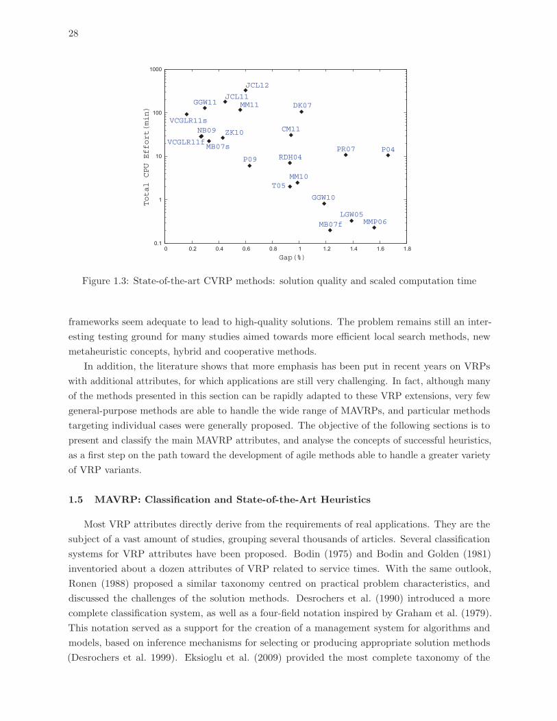
28

0.1

1

10

100

1000

0 0.2 0.4 0.6 0.8 1 1.2 1.4 1.6 1.8

Total CPU Effort(min)

Gap(%)

VCGLR11s

VCGLR11f

NB09

GGW11

MB07s

ZK10

JCL11MM11

JCL12

P09 RDH04

T05

CM11

MM10

DK07

GGW10

MB07f

PR07

LGW05MMP06

P04

Figure 1.3: State-of-the-art CVRP methods: solution quality and scaled computation time

frameworks seem adequate to lead to high-quality solutions. The problem remains still an inter-

esting testing ground for many studies aimed towards more efficient local search methods, new

metaheuristic concepts, hybrid and cooperative methods.

In addition, the literature shows that more emphasis has been put in recent years on VRPs

with additional attributes, for which applications are still very challenging. In fact, although many

of the methods presented in this section can be rapidly adapted to these VRP extensions, very few

general-purpose methods are able to handle the wide range of MAVRPs, and particular methods

targeting individual cases were generally proposed. The objective of the following sections is to

present and classify the main MAVRP attributes, and analyse the concepts of successful heuristics,

as a first step on the path toward the development of agile methods able to handle a greater variety

of VRP variants.

1.5 MAVRP: Classification and State-of-the-Art Heuristics

Most VRP attributes directly derive from the requirements of real applications. They are the

subject of a vast amount of studies, grouping several thousands of articles. Several classification

systems for VRP attributes have been proposed. Bodin (1975) and Bodin and Golden (1981)

inventoried about a dozen attributes of VRP related to service times. With the same outlook,

Ronen (1988) proposed a similar taxonomy centred on practical problem characteristics, and

discussed the challenges of the solution methods. Desrochers et al. (1990) introduced a more

complete classification system, as well as a four-field notation inspired by Graham et al. (1979).

This notation served as a support for the creation of a management system for algorithms and

models, based on inference mechanisms for selecting or producing appropriate solution methods

(Desrochers et al. 1999). Eksioglu et al. (2009) provided the most complete taxonomy of the

29

MAVRP literature, integrating most common variants as well as several general observations on

the nature of the articles. This taxonomy was accompanied by bibliometric data, illustrating the

growth in the number of articles, the main authors, subjects, and journals. In addition to the

previously listed taxonomies, other papers proposed thematic literature reviews of routing problems

(Assad 1988, Desrosiers et al. 1995, Braysy et al. 2008b,c, Andersson et al. 2010). The annotated

bibliographies by Laporte and Osman (1995) and Gendreau et al. (2008b) are also noteworthy,

providing pointers towards hundreds of articles dealing with MAVRPs and other related problems.

Unlike scheduling, however, where the classification system of Graham et al. (1979) is still used

and updated, none of the previously-listed classification systems has been used on a large scale in

the vehicle routing literature. This is probably connected to the large variety of attributes, which

makes all exhaustive taxonomies extremely difficult. In addition, most of the previous classifications

are application-oriented, based on the actual origin of the different types of constraints (related to,

e.g., particular vehicle, network, driver or customers requirements). Moreover, even though these

classification systems permitted the organization of the different attributes and contributions, few

hints were given as to what heuristic concepts to privilege for the different types of attributes. Thus,

the objective of the next section is to fill this gap with a new classification which, even though

rather simple, emphasizes the relationships between problem attributes and recent heuristics.

1.5.1 Three main classes of attributes

To analyse the concepts of MAVRP heuristics, we distinguish three main classes of attributes,

relative to their impact on three aspects of the problem that must imperatively be dealt with by

solvers: the Assignment of customers and routes to resources (ASSIGN), the Sequence choices

(SEQ), and the Evaluation of fixed sequences (EVAL). This simple classification is intimately

connected with the resolution methodologies, as dealing with these three problem aspects leads

to a complete solution method. Please note that an attribute may impact several aspects of the

problem, and thus possibly appear in several categories.

ASSIGN attributes impact the assignment of limited resources, e.g., vehicles, vehicle types,

depots, and service periods over a planning horizon, to customer services and routes. Most common

ASSIGN attributes include multiple depots, heterogeneous fleets, multiple periods, split deliveries,

site dependencies, inventory, location and profits collection. Furthermore, two main sub-families

of ASSIGN attributes may be distinguished. Some variants of the VRP, e.g., multiple depot or

heterogeneous VRP, are concerned with the assignment of resources to routes. In these settings, an

entire route can potentially be re-assigned. In other cases, such as the VRP with multiple periods

(PVRP) or inventory routing, the assignment issues are performed on resources to customers, and

re-assigning a full route is likely to be infeasible due to the independent assignment constraints.

SEQ attributes directly impact the nature and structure of the routes. In a backhaul setting, for

example, the route is a compound of two sequences of linehaul and backhaul services, respectively.

In presence of multiple trips or intermediate facilities, the routes pass several times at depots, while

in the generalized VRP, groups of customers are defined, and only one visit per group is performed.

In truck-and-trailer problems, the routes involve sections with and without trailer. Finally, some

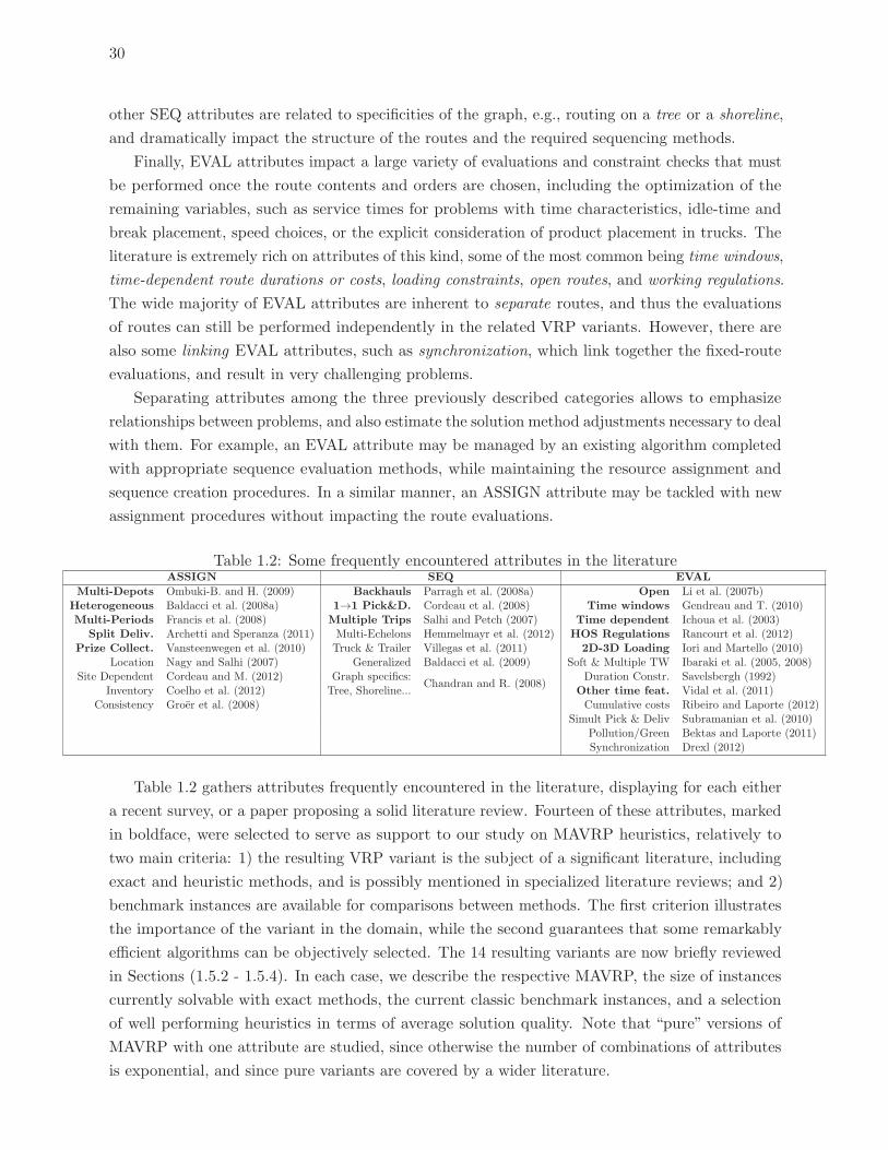
30

other SEQ attributes are related to specificities of the graph, e.g., routing on a tree or a shoreline,

and dramatically impact the structure of the routes and the required sequencing methods.

Finally, EVAL attributes impact a large variety of evaluations and constraint checks that must

be performed once the route contents and orders are chosen, including the optimization of the

remaining variables, such as service times for problems with time characteristics, idle-time and

break placement, speed choices, or the explicit consideration of product placement in trucks. The

literature is extremely rich on attributes of this kind, some of the most common being time windows,

time-dependent route durations or costs, loading constraints, open routes, and working regulations.

The wide majority of EVAL attributes are inherent to separate routes, and thus the evaluations

of routes can still be performed independently in the related VRP variants. However, there are

also some linking EVAL attributes, such as synchronization, which link together the fixed-route

evaluations, and result in very challenging problems.

Separating attributes among the three previously described categories allows to emphasize

relationships between problems, and also estimate the solution method adjustments necessary to deal

with them. For example, an EVAL attribute may be managed by an existing algorithm completed

with appropriate sequence evaluation methods, while maintaining the resource assignment and

sequence creation procedures. In a similar manner, an ASSIGN attribute may be tackled with new

assignment procedures without impacting the route evaluations.

Table 1.2: Some frequently encountered attributes in the literatureASSIGN SEQ EVAL

Multi-Depots Ombuki-B. and H. (2009) Backhauls Parragh et al. (2008a) Open Li et al. (2007b)Heterogeneous Baldacci et al. (2008a) 1→1 Pick&D. Cordeau et al. (2008) Time windows Gendreau and T. (2010)Multi-Periods Francis et al. (2008) Multiple Trips Salhi and Petch (2007) Time dependent Ichoua et al. (2003)

Split Deliv. Archetti and Speranza (2011) Multi-Echelons Hemmelmayr et al. (2012) HOS Regulations Rancourt et al. (2012)Prize Collect. Vansteenwegen et al. (2010) Truck & Trailer Villegas et al. (2011) 2D-3D Loading Iori and Martello (2010)

Location Nagy and Salhi (2007) Generalized Baldacci et al. (2009) Soft & Multiple TW Ibaraki et al. (2005, 2008)Site Dependent Cordeau and M. (2012) Graph specifics:

Chandran and R. (2008)Duration Constr. Savelsbergh (1992)

Inventory Coelho et al. (2012) Tree, Shoreline... Other time feat. Vidal et al. (2011)Consistency Groer et al. (2008) Cumulative costs Ribeiro and Laporte (2012)

Simult Pick & Deliv Subramanian et al. (2010)Pollution/Green Bektas and Laporte (2011)Synchronization Drexl (2012)

Table 1.2 gathers attributes frequently encountered in the literature, displaying for each either

a recent survey, or a paper proposing a solid literature review. Fourteen of these attributes, marked

in boldface, were selected to serve as support to our study on MAVRP heuristics, relatively to

two main criteria: 1) the resulting VRP variant is the subject of a significant literature, including

exact and heuristic methods, and is possibly mentioned in specialized literature reviews; and 2)

benchmark instances are available for comparisons between methods. The first criterion illustrates

the importance of the variant in the domain, while the second guarantees that some remarkably

efficient algorithms can be objectively selected. The 14 resulting variants are now briefly reviewed

in Sections (1.5.2 - 1.5.4). In each case, we describe the respective MAVRP, the size of instances

currently solvable with exact methods, the current classic benchmark instances, and a selection

of well performing heuristics in terms of average solution quality. Note that “pure” versions of

MAVRP with one attribute are studied, since otherwise the number of combinations of attributes

is exponential, and since pure variants are covered by a wider literature.

31

1.5.2 Heuristics for VRP variants with ASSIGN attributes

Multiple depots. The multi-depot VRP (MDVRP) deals with a number of depots d > 1.

Each vehicle is assigned to a single depot, which is generally both the origin and the destination

of the vehicle’s route. Some variants, called “non-fixed” problems, relax this latter requirement.

Furthermore, in the classical MDVRP, no limit on supply at depots is considered. Recent elements of

literature review can be found in Ombuki-Berman and Hanshar (2009) and Vidal et al. (2012a). The

best exact method (Baldacci and Mingozzi 2009) can solve problem instances up to 75 customers,

as well as a few instances with up to 199 customers. When considering metaheuristics, the best

solutions on the classic instances presented in Cordeau et al. (1997) were produced by the ALNS

of Pisinger and Ropke (2007), the fuzzy logic-guided hybrid GA of Lau et al. (2010), the ILS and

set covering approach of Subramanian (2012), the Hybrid Genetic Search with Advanced Diversity

Control (HGSADC) of Vidal et al. (2012a), and the parallel UTS of Cordeau and Maischberger

(2012).

Heterogeneous fleet. Customers are assigned to vehicle types with different characteristics:

capacity, maximum route times, fixed costs, and variable costs in terms of the distance. When the

number of vehicles is not constrained, the problem is usually referred to as the Vehicle Fleet Mix

Problem (VFMP), otherwise the more difficult version is called Heterogeneous VRP (HVRP) (see

Baldacci et al. 2008a, for a review). The exact algorithm of Baldacci and Mingozzi (2009) solves

most problem instances with 75 customers or less, as well as some instances with 100 customers.

The state-of-the-art metaheuristics, evaluated on the HVRP instances of Taillard (1999) and Li

et al. (2007a), are of various kinds: tabu search (Brandao 2011), hybrid GA (Prins 2009b), or ILS

and VNS (Penna et al. 2011) with set covering phases (Subramanian et al. 2012).

Multiple periods. A time dimension is introduced in the Periodic VRP (PVRP) as route

planning is to be performed over a horizon of several periods. Each customer requires a total

number of services according to some acceptable combinations of visit periods called patterns. The

assignment of customer visits is thus subject to compatibility constraints with the patterns. The

PVRP is reviewed in Francis et al. (2008). Exact methods (Baldacci et al. 2011a) are able to solve

some instances with up to 100 customers and 6 time periods. Benchmark instances for PVRP

metaheuristics are gathered in Cordeau et al. (1997). Several efficient neighbourhood-centred

searches have been designed, such as UTS (Cordeau et al. 1997, 2001a) and its parallel extension

(Cordeau and Maischberger 2012), the VNS of Hemmelmayr et al. (2009), and the hybrid record-

to-record and integer programming matheuristic of Gulczynski et al. (2011). The population-based

approach of Alegre et al. (2007), dedicated to large temporal horizons, focuses on assignment

optimization, while using constructive methods to create routes. Also, the HGSADC of Vidal et al.

(2012a) produces the current best solutions by combining the GA search breadth with efficient LS,

relaxations schemes, and diversity management procedures.

The PVRP has led to several other notable problem extensions (Groer et al. 2008, Gulczynski

et al. 2011). The issue of service consistency, i.e., visiting regular customers on each period at

similar time and with the same driver, has received a notable attention. Recent methods dealing

with this attribute are based on record-to-record travel (Groer et al. 2008), tabu search (Tarantilis

et al. 2012), and ALNS (Kovacs et al. 2012). All these methods optimize a template of visits to

32

frequent customers, which remains the same on every day, in which some additional non-frequent

deliveries are inserted.

Split deliveries. Customer demands can be satisfied by several vehicles, each moving a partial

load. This variant is called VRP with split deliveries (VRPSD), as reviewed in Gulczynski et al.

(2008) and Archetti and Speranza (2011). Instances with up to 50 customers (Belenguer et al. 2000,

Lee et al. 2006) can be exactly solved. Recent metaheuristics have been evaluated with two different

fleet-size policies on the benchmark instances of Archetti et al. (2006), Belenguer et al. (2000) and

Chen et al. (2007). In the first setting, the fleet size is unlimited, and state-of-the-art methods rely

on hybrid GA with giant-tour representation (Boudia et al. 2007), Attribute Based Hill Climber

(ABHC) (Derigs et al. 2009), and integer programming optimization with tabu search (Archetti

et al. 2008). In the second setting, a solution with minimum number of vehicles is imposed, and

the best performances are achieved by the scatter search of Mota et al. (2007) and the tabu search

with vocabulary building of Aleman and Hill (2010).

Prize collection. For several customers, service is optional but rewarded with a prize. Hence,

customers must be implicitly distributed among two subsets, following whether their service is

omitted or performed. Several objectives were dealt with in the literature, notably the optimization

of a weighted sum of route lengths and prizes (Dell’Amico et al. 1995), or the maximization of

the prizes under a route length constraint, usually called the team orienteering problem (see the

reviews of Feillet et al. 2005 and Vansteenwegen et al. 2010). Exact methods can solve instances

with up to 100 customers (Boussier et al. 2006). Most efficient metaheuristics, evaluated on the

instance set of Chao et al. (1996), rely on population concepts. Ke et al. (2008) proposed a hybrid

ACO method with a local search. Souffriau et al. (2010) introduced a path relinking method, in

which elements of the solution set undergo an ageing process. Bouly et al. (2009) introduced a

hybrid GA based on giant-tour solution representation, which is hybridized later on with PSO in

Dang et al. (2011). Finally, Archetti et al. (2006) proposed a hybrid tabu search and VNS.

1.5.3 Heuristics for VRP variants with SEQ attributes

Backhauls. Customers are separated into two groups: delivery customers (i.e., linehaul

customers) and pickup customers (i.e., backhaul customers). All routes mixing both groups of

customers must serve all linehaul customers before the first backhaul customer, thus leading to

different route structures. We refer to Toth and Vigo (2002b) and Parragh et al. (2008a) for

detailed reviews on the VRPB. The classic instances were first introduced in Goetschalckx and

Jacobs-Blecha (1989) and Toth and Vigo (1997). Some of these, with a maximum 100 customers,

were solved exactly in Toth and Vigo (1997) and Mingozzi et al. (1999). The best metaheuristics,

on the instance sets of Goetschalckx and Jacobs-Blecha (1989), include the ALNS of Ropke and

Pisinger (2006a); the tabu search of Brandao (2006), which, as Zachariadis and Kiranoudis (2012),

uses long-term memories to direct the search toward inadequately exploited characteristics; and

finally the ACO of Gajpal and Abad (2009), which concurrently evolves two ant families to work

on assignment and sequences.

Pickups & Deliveries. Each service is characterized by a pair of locations designating the

pickup and delivery spots. All pickups must be made before the deliveries. This type of problem is

33

dealt with in numerous literature reviews as a one-to-one Pickup and Delivery Problem (PDP)

(Desaulniers et al. 2002, Berbeglia et al. 2007, Cordeau et al. 2008, Berbeglia et al. 2010) or simply

as VRP with Pickup and Deliveries (VRPPD) (Parragh et al. 2008a,b). This problem is often

coupled with time-window constraints. Ropke et al. (2007) solved exactly instances involving up to

96 requests. The classic benchmark instances have been introduced in Li and Lim (2001). Efficient

neighbourhood-centred metaheuristics have been proposed, including the ALNS of Ropke and

Pisinger (2006b) and the two-phase method of Bent and Van Hentenryck (2006), which combines

simulated annealing (SA) to reduce the number of routes with large neighbourhood search (LNS)

to optimize the distance. These methods were recently outperformed by the memetic algorithm of

Nagata and Kobayashi (2011), which exploits a well-designed crossover focused on transmitting

parent characteristics without introducing too many new arcs in the offspring. For problem variants

arising from the domain of transportation on demand, the so-called dial-a-ride problems, UTS

(Cordeau and Laporte 2003) and the VNS of Parragh et al. (2010) produce solutions of good

quality.

Multiple trips. During its tour, a vehicle can reach several times the depot to load or unload.

By doing so, the global constraints on the routes, such as the maximum duration, are still considered.

The exact method of Mingozzi et al. (2012) can solve some instances of multi-trip VRP (MTVRP)

with up to 120 customers. Three algorithms produce on average the largest number of feasible

solutions, or the solutions with least amount of infeasibility on the classic instances of Taillard

et al. (1996). The original tabu search and adaptive memory approach of Taillard (1993) remain

still competitive. In addition, good results have been obtained with the adaptive memory-based

search of Olivera and Viera (2007), and by Alonso et al. (2008), who generalized UTS to a PVRP

with multiple trips and vehicle-customer compatibility constraints.

1.5.4 Heuristics for VRP variants with EVAL attributes

Time windows. The VRP with time windows (VRPTW) is certainty the most extensively

studied VRP variant to date. Time windows are associated to customer visits and depot, each

arc being characterized by a route duration. Waiting time is allowed upon an early arrival to a

customer, while a late arrival is forbidden. Recent literature reviews can be found in Braysy and

Gendreau (2005b,a) and Gendreau and Tarantilis (2010). The classic VRPTW instances were

introduced in Solomon (1987) and Gehring and Homberger (1999). Most efficient exact methods

(Kallehauge et al. 2006, Jepsen et al. 2008, Baldacci et al. 2011c) can solve most instances with up

to 100 customers, and a few instances with up to 1000 customers. However, exact resolution is

highly dependent upon the characteristics of the instance and the width of time windows. Actual

state-of-the-art VRPTW metaheuristics are of various kinds. The guided EA of Repoussis et al.

(2009b) combines evolution, ruin-and-recreate mutations, and guided local search. Prescott-Gagnon

et al. (2009) proposed a LNS combined with branch-and-price for solution reconstruction. The

HGA proposed by Nagata et al. (2010) uses a particularly effective crossover operator. This latter

method, as well as the path relinking of Hashimoto and Yagiura (2008) and HGSADC of Vidal

et al. (2013), apply time-constraint relaxations during the search to benefit from infeasible solutions

in the search space.

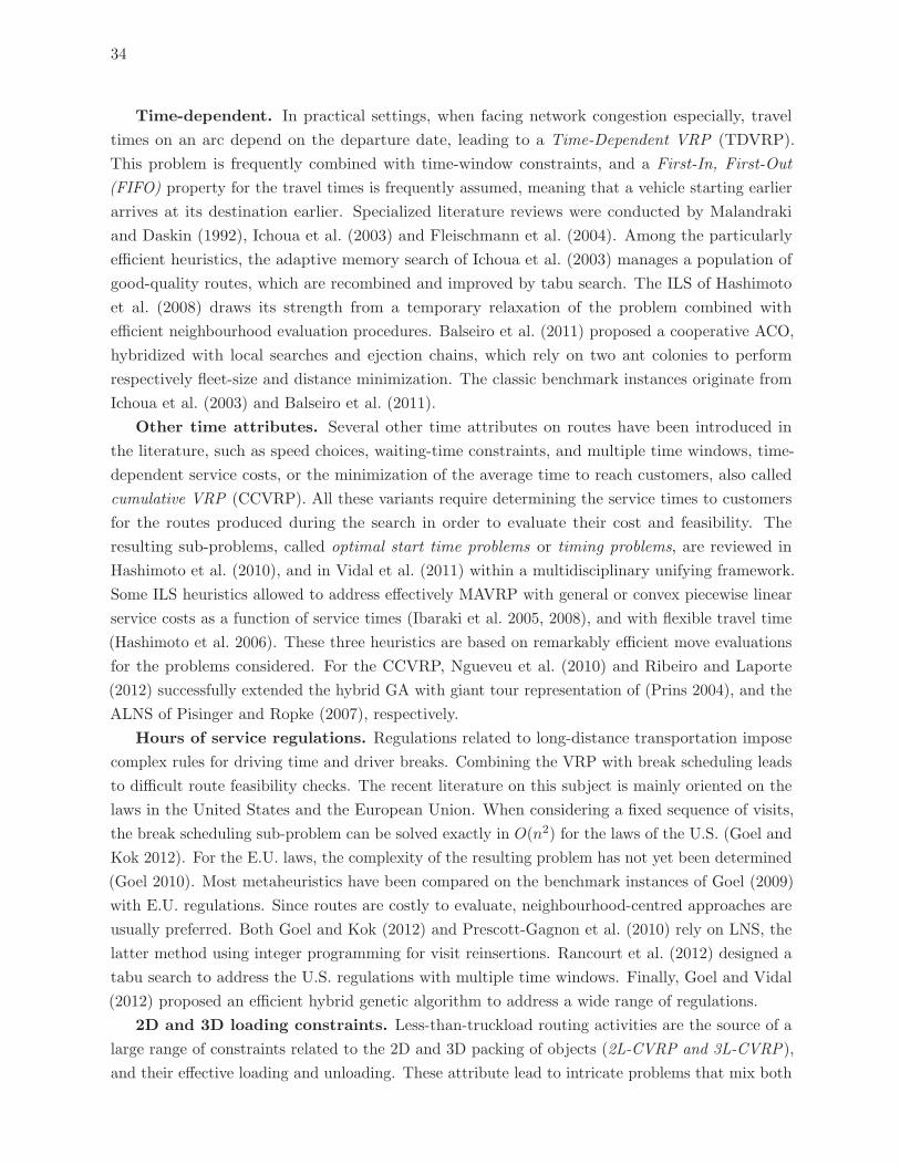
34

Time-dependent. In practical settings, when facing network congestion especially, travel

times on an arc depend on the departure date, leading to a Time-Dependent VRP (TDVRP).

This problem is frequently combined with time-window constraints, and a First-In, First-Out

(FIFO) property for the travel times is frequently assumed, meaning that a vehicle starting earlier

arrives at its destination earlier. Specialized literature reviews were conducted by Malandraki

and Daskin (1992), Ichoua et al. (2003) and Fleischmann et al. (2004). Among the particularly

efficient heuristics, the adaptive memory search of Ichoua et al. (2003) manages a population of

good-quality routes, which are recombined and improved by tabu search. The ILS of Hashimoto

et al. (2008) draws its strength from a temporary relaxation of the problem combined with

efficient neighbourhood evaluation procedures. Balseiro et al. (2011) proposed a cooperative ACO,

hybridized with local searches and ejection chains, which rely on two ant colonies to perform

respectively fleet-size and distance minimization. The classic benchmark instances originate from

Ichoua et al. (2003) and Balseiro et al. (2011).

Other time attributes. Several other time attributes on routes have been introduced in

the literature, such as speed choices, waiting-time constraints, and multiple time windows, time-

dependent service costs, or the minimization of the average time to reach customers, also called

cumulative VRP (CCVRP). All these variants require determining the service times to customers

for the routes produced during the search in order to evaluate their cost and feasibility. The

resulting sub-problems, called optimal start time problems or timing problems, are reviewed in

Hashimoto et al. (2010), and in Vidal et al. (2011) within a multidisciplinary unifying framework.

Some ILS heuristics allowed to address effectively MAVRP with general or convex piecewise linear

service costs as a function of service times (Ibaraki et al. 2005, 2008), and with flexible travel time

(Hashimoto et al. 2006). These three heuristics are based on remarkably efficient move evaluations

for the problems considered. For the CCVRP, Ngueveu et al. (2010) and Ribeiro and Laporte

(2012) successfully extended the hybrid GA with giant tour representation of (Prins 2004), and the

ALNS of Pisinger and Ropke (2007), respectively.

Hours of service regulations. Regulations related to long-distance transportation impose

complex rules for driving time and driver breaks. Combining the VRP with break scheduling leads

to difficult route feasibility checks. The recent literature on this subject is mainly oriented on the

laws in the United States and the European Union. When considering a fixed sequence of visits,

the break scheduling sub-problem can be solved exactly in O(n2) for the laws of the U.S. (Goel and

Kok 2012). For the E.U. laws, the complexity of the resulting problem has not yet been determined

(Goel 2010). Most metaheuristics have been compared on the benchmark instances of Goel (2009)

with E.U. regulations. Since routes are costly to evaluate, neighbourhood-centred approaches are

usually preferred. Both Goel and Kok (2012) and Prescott-Gagnon et al. (2010) rely on LNS, the

latter method using integer programming for visit reinsertions. Rancourt et al. (2012) designed a

tabu search to address the U.S. regulations with multiple time windows. Finally, Goel and Vidal

(2012) proposed an efficient hybrid genetic algorithm to address a wide range of regulations.

2D and 3D loading constraints. Less-than-truckload routing activities are the source of a

large range of constraints related to the 2D and 3D packing of objects (2L-CVRP and 3L-CVRP),

and their effective loading and unloading. These attribute lead to intricate problems that mix both

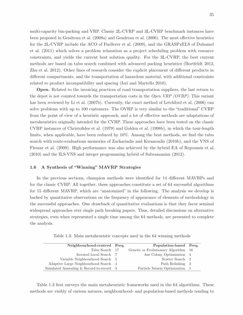
35

multi-capacity bin-packing and VRP. Classic 2L-CVRP and 3L-CVRP benchmark instances have

been proposed in Gendreau et al. (2008a) and Gendreau et al. (2006). The most effective heuristics

for the 2L-CVRP include the ACO of Fuellerer et al. (2009), and the GRASPxELS of Duhamel

et al. (2011) which solves a problem relaxation as a project scheduling problem with resource

constraints, and yields the current best solution quality. For the 3L-CVRP, the best current

methods are based on tabu search combined with advanced packing heuristics (Bortfeldt 2012,

Zhu et al. 2012). Other lines of research consider the explicit placement of different products in

different compartments, and the transportation of hazardous material, with additional constraints

related to product incompatibility and spacing (Iori and Martello 2010).

Open. Related to the invoicing practices of road transportation suppliers, the last return to

the depot is not counted towards the transportation costs in the Open VRP (OVRP). This variant

has been reviewed by Li et al. (2007b). Currently, the exact method of Letchford et al. (2006) can

solve problems with up to 100 customers. The OVRP is very similar to the “traditional” CVRP

from the point of view of a heuristic approach, and a lot of effective methods are adaptations of

metaheuristics originally intended for the CVRP. These approaches have been tested on the classic

CVRP instances of Christofides et al. (1979) and Golden et al. (1998b), in which the tour-length

limits, when applicable, have been reduced by 10%. Among the best methods, we find the tabu

search with route-evaluations memories of Zachariadis and Kiranoudis (2010b), and the VNS of

Fleszar et al. (2009). High performance was also achieved by the hybrid EA of Repoussis et al.

(2010) and the ILS-VNS and integer programming hybrid of Subramanian (2012).

1.6 A Synthesis of “Winning” MAVRP Strategies

In the previous sections, champion methods were identified for 14 different MAVRPs and

for the classic CVRP. All together, these approaches constitute a set of 64 successful algorithms

for 15 different MAVRP, which are “anatomized” in the following. The analysis we develop is

backed by quantitative observations on the frequency of appearance of elements of methodology in

the successful approaches. One drawback of quantitative evaluations is that they favor seminal

widespread approaches over single path breaking papers. Thus, detailed discussions on alternative

strategies, even when represented a single time among the 64 methods, are presented to complete

the analysis.

Table 1.3: Main metaheuristic concepts used in the 64 winning methods

Neighbourhood-centred Freq. Population-based Freq.Tabu Search 17 Genetic or Evolutionary Algorithm 16

Iterated Local Search 7 Ant Colony Optimization 4Variable Neighbourhood Search 5 Scatter Search 2

Adaptive Large Neighbourhood Search 4 Path Relinking 2Simulated Annealing & Record-to-record 3 Particle Swarm Optimization 1

Table 1.3 first surveys the main metaheuristic frameworks used in the 64 algorithms. These

methods are visibly of various natures, neighbourhood- and population-based methods tending to

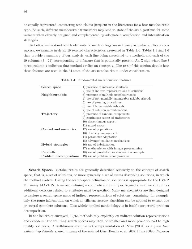
36

be equally represented, contrasting with claims (frequent in the literature) for a best metaheuristic

type. As such, different metaheuristic frameworks may lead to state-of-the-art algorithms for some

variants when cleverly designed and complemented by adequate diversification and intensification

strategies.

To better understand which elements of methodology make these particular applications a

success, we examine in detail 19 selected characteristics, presented in Table 1.4. Tables 1.5 and 1.6

then provide a summary of our analysis, each line being associated to a method, and each of the

19 columns (3 - 21) corresponding to a feature that is potentially present. An X sign where line i

meets column j indicates that method i relies on concept j. The rest of this section details how

these features are used in the 64 state-of-the-art metaheuristics under consideration.

Table 1.4: Fundamental metaheuristic features

Search space 1) presence of infeasible solutions2) use of indirect representations of solutions

Neighbourhoods 3) presence of multiple neighbourhoods4) use of polynomially enumerable neighbourhoods5) use of pruning procedures6) use of large neighbourhoods7) use of solution recombinations

Trajectory 8) presence of random components9) continuous aspect of trajectories10) discontinuous aspect11) mixed aspect

Control and memories 12) use of populations13) diversity management14) parameter adaptation15) advanced guidance mechanisms

Hybrid strategies 16) use of hybridization17) matheuristics with integer programming

Parallelism 18) use of parallelism or cooperation conceptsProblem decompositions 19) use of problem decompositions

Search Space. Metaheuristics are generally described relatively to the concept of search

space, that is, a set of solutions, or more generally a set of states describing solutions, in which

the method evolves. Basing the search-space definition on solutions is appropriate for the CVRP.

For many MAVRPs, however, defining a complete solution goes beyond route description, as

additional decisions related to attributes must be specified. Many metaheuristics are then designed

to explore a search space made of indirect representations of solutions, containing, for example,

only the route information, on which an efficient decoder algorithm can be applied to extract one

or several complete solutions. This widely applied methodology is in itself a structural problem

decomposition.

In the heuristics surveyed, 12/64 methods rely explicitly on indirect solution representations

and decoders. The resulting search spaces may then be smaller and more prone to lead to high

quality solutions. A well-known example is the representation of Prins (2004) as a giant tour

without trip delimiters, used in many of the selected GAs (Boudia et al. 2007, Prins 2009b, Ngueveu

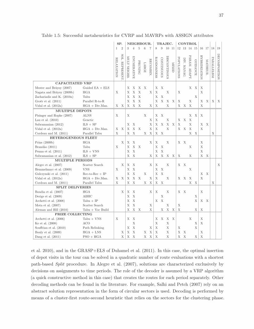
37

Table 1.5: Successful metaheuristics for CVRP and MAVRPs with ASSIGN attributes

SP. NEIGHBOUR. TRAJEC. CONTROL

1 2 3 4 5 6 7 8 9 10 11 12 13 14 15 16 17 18 19

RELAXATIO

N

SOL.REPRESENT.

MULT

NEIG

HB.

ENUMERATIV

E

PRUNIN

G

LARGE

RECOMBIN

.

RANDOMNESS

CONTIN

UOUS

DISCONTIN

OUS

MIX

ED

POPULATIO

NS

DIV

.MANAG.

PARAM.ADAPT.

GUID

ANCE

HYBRID

IZATIO

N

MATHEUR.

PARALLELISM

DECOMPOSIT

ION

CAPACITATED VRP

Mester and Braysy (2007) Guided EA + ELS X X X X X X X X X

Nagata and Braysy (2009b) HGA X X X X X X X X X

Zachariadis and K. (2010a) Tabu X X X X X X

Groer et al. (2011) Parallel R-to-R X X X X X X X X X X X X X

Vidal et al. (2012a) HGA + Div.Man. X X X X X X X X X X X X

MULTIPLE DEPOTS

Pisinger and Ropke (2007) ALNS X X X X X X X X

Lau et al. (2010) Genetic X X X X X X

Subramanian (2012) ILS + SP X X X X X X X X X X X


Cordeau and M. (2011) Parallel Tabu X X X X X X X X X X

HETEROGENEOUS FLEET

Prins (2009b) HGA X X X X X X X X X

Brandao (2011) Tabu X X X X X X X X

Penna et al. (2011) ILS + VNS X X X X X

Subramanian et al. (2012) ILS + SP X X X X X X X X X X X

MULTIPLE PERIODS

Alegre et al. (2007) Scatter Search X X X X X X X X X

Hemmelmayr et al. (2009) VNS X X X X X X

Gulczynski et al. (2011) Rec-to-Rec + IP X X X X X X X


Cordeau and M. (2011) Parallel Tabu X X X X X X X X X X

SPLIT DELIVERIES

Boudia et al. (2007) HGA X X X X X X X X X

Derigs et al. (2009) ABHC X X X X

Archetti et al. (2008) Tabu + IP X X X X X X X

Mota et al. (2007) Scatter Search X X X X X

Aleman and Hill (2010) Tabu + Voc Build X X X X X X X X X X

PRIZE COLLECTING

Archetti et al. (2006) Tabu + VNS X X X X X X X X X

Ke et al. (2008) ACO X X X X X

Souffriau et al. (2010) Path Relinking X X X X X X X

Bouly et al. (2009) HGA + LNS X X X X X X X X X X

Dang et al. (2011) PSO + HGA X X X X X X X X X X X

et al. 2010), and in the GRASP+ELS of Duhamel et al. (2011). In this case, the optimal insertion

of depot visits in the tour can be solved in a quadratic number of route evaluations with a shortest

path-based Split procedure. In Alegre et al. (2007), solutions are characterized exclusively by

decisions on assignments to time periods. The role of the decoder is assumed by a VRP algorithm

(a quick constructive method in this case) that creates the routes for each period separately. Other

decoding methods can be found in the literature. For example, Salhi and Petch (2007) rely on an

abstract solution representation in the form of circular sectors is used. Decoding is performed by

means of a cluster-first route-second heuristic that relies on the sectors for the clustering phase.

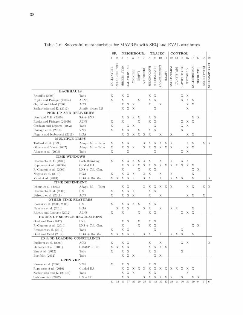
38

Table 1.6: Successful metaheuristics for MAVRPs with SEQ and EVAL attributes

SP. NEIGHBOUR. TRAJEC. CONTROL

1 2 3 4 5 6 7 8 9 10 11 12 13 14 15 16 17 18 19

RELAXATIO

N

SOL.REPRESENT.

MULT

NEIG

HB.

ENUMERATIV

E

PRUNIN

G

LARGE

RECOMBIN

.

RANDOMNESS

CONTIN

UOUS

DISCONTIN

OUS

MIX

ED

POPULATIO

NS

DIV

.MANAG.

PARAM.ADAPT.

GUID

ANCE

HYBRID

IZATIO

N

MATHEUR.

PARALLELISM

DECOMPOSIT

ION

BACKHAULS

Brandao (2006) Tabu X X X X X X X

Ropke and Pisinger (2006a) ALNS X X X X X X X X

Gajpal and Abad (2009) ACO X X X X X X X

Zachariadis and K. (2012) Attrib. driven LS X X X X X

PICK-UP AND DELIVERIES

Bent and V.H. (2006) SA + LNS X X X X X X X X

Ropke and Pisinger (2006b) ALNS X X X X X X X X

Cordeau and Laporte (2003) Tabu X X X X X X

Parragh et al. (2010) VNS X X X X X X X

Nagata and Kobayashi (2011) HGA X X X X X X X X X X

MULTIPLE TRIPS

Taillard et al. (1996) Adapt. M. + Tabu X X X X X X X X X X X X X

Olivera and Viera (2007) Adapt. M. + Tabu X X X X X X X X X X X X

Alonso et al. (2008) Tabu X X X X X

TIME WINDOWS

Hashimoto et Y. (2008) Path Relinking X X X X X X X X X X X

Repoussis et al. (2009b) Guided EA X X X X X X X X X X X X X X

P.-Gagnon et al. (2009) LNS + Col. Gen. X X X X X X

Nagata et al. (2010) HGA X X X X X X X X X

Vidal et al. (2013) HGA + Div.Man. X X X X X X X X X X X X X

TIME DEPENDENT

Ichoua et al. (2003) Adapt. M. + Tabu X X X X X X X X X X X X

Hashimoto et al. (2008) ILS X X X X X X

Balseiro et al. (2011) ACO X X X X X X X X X

OTHER TIME FEATURES

Ibaraki et al. (2005, 2008) ILS X X X X X X X

Ngueveu et al. (2010) HGA X X X X X X X X X

Ribeiro and Laporte (2012) ALNS X X X X X X X X

HOURS OF SERVICE REGULATIONS

Goel and Kok (2012) LNS X X X X X

P.-Gagnon et al. (2010) LNS + Col. Gen. X X X X X X

Rancourt et al. (2012) Tabu X X X X X

Goel and Vidal (2012) HGA + Div.Man. X X X X X X X X X X X X

2D & 3D LOADING CONSTRAINTS

Fuellerer et al. (2009) ACO X X X X X X X X

Duhamel et al. (2011) GRASP + ELS X X X X X X X X

Zhu et al. (2012) Tabu X X X X X X

Bortfeldt (2012) Tabu X X X X X

OPEN VRP

Fleszar et al. (2009) VNS X X X X X

Repoussis et al. (2010) Guided EA X X X X X X X X X X X X X X

Zachariadis and K. (2010b) Tabu X X X X X X

Subramanian (2012) ILS + SP X X X X X X X X X X X

31 12 60 57 26 20 29 56 42 35 12 28 14 30 29 39 9 6 6

39

Finally, multiple structurally different search spaces, relying on different (representations, decoder)

pairs, may efficiently reduce the risks of getting trapped in a local optimum.

Another main characteristic of the search space comes from the potential use of infeasible

solutions. Since the early literature on tabu search with the strategic oscillation concept (Glover

1986, Glover and Hao 2011), studies report that a controlled exploitation of infeasible solutions

may enhance the search, by allowing it to transition more easily between structurally different

feasible solutions. Furthermore, the use of infeasible solutions may contribute toward improving

the robustness of the method, which is less dependent upon the availability of a feasible initial

solution (finding a feasible solution is often in itself a NP-hard problem).

About half of the selected MAVRP heuristics (31/64) rely on penalized infeasible solutions in

the search space, which violate either the route constraints (load, duration, or time windows), the

fleet size limit, or do not service all customers. Moreover, iteratively decrementing the fleet size

limit while relaxing route constraints provides the means to address the “fleet size minimization”

objective without relying on complex route elimination procedures. Elements of sensitivity analyses

on the role of infeasible solutions in the context of PVRP and MDVRP can be found in Vidal

et al. (2012a). In the methods surveyed, relaxations of route constraints are usually privileged over

fleet-size relaxations, as it can be difficult to progress from a solution with too many routes to a

feasible solution.

Neighbourhoods. With the exception of some methods that use exclusively large neigh-

bourhoods, and the GA of Lau et al. (2010) which appears to rely exclusively on crossover and

random mutation, all mentioned MAVRP heuristics are based on at least one type of enumerable

neighbourhood using the arc exchanges described in Section 1.4.2. The size of these enumerable

neighbourhoods is usually O(n2) in practice. Exponentially large neighbourhoods are also frequently

used (20/64). Besides ruin-and-recreate neighbourhoods or perturbation mechanisms that are

well represented in recent methods, cyclic transfers or ejection chains are also used (Ibaraki et al.

2005), as well as variants of the Sarvanov-Doroshko IP refinement heuristic (Gulczynski et al.

2011). Finally, 29/64 methods combine solutions, or fragments of solutions, into new solutions,

thus transmitting good sequence elements as the evolutionary, genetic, scatter search and path

relinking algorithms do. Not only GA and EA use these mechanisms. Consider for example the

adaptive memory approaches of Taillard et al. (1996), Ichoua et al. (2003) and Olivera and Viera

(2007), which operate recombinations of solution fragments, and the set covering based approach

of Groer et al. (2011) involving recombinations of routes issued from multiple solutions.

Almost all the methods surveyed (60/64) rely on multiple neighbourhoods, either successively,

or in a compound way. The successive exploration of multiple neighbourhoods makes the basis

of the VNS methodology, and is recognized as an important success factor for metaheuristics

in general, especially on complex problems with multiple constraints and characteristics such as

MAVRPs. The methods of Archetti et al. (2006) and Parragh et al. (2010) push very far the

concept of neighbourhood variation by exploiting structurally-different, enumerative and large,

neighbourhoods. Other VNS for MAVRPs may gradually increase the size of the enumerative

neighbourhoods by varying the number of arcs to be exchanged (Hemmelmayr et al. 2009), but,

strictly speaking, do not involve structural neighbourhood differences.

40

Searching efficiently these neighbourhoods is critical for performance, as it generally makes

for the biggest part of the computation effort. Therefore, many techniques aim at pruning the

neighbourhoods (26/64 algorithms), or at enumerating them more efficiently. Move restrictions

based on customer neighbourhood lists (granular search of Toth and Vigo (2003)) are frequently

used (Ibaraki et al. 2005, Mester and Braysy 2007, Olivera and Viera 2007, Hashimoto and Yagiura

2008, Vidal et al. 2012a), as well as neighbourhood limitation strategies based on recently modified

solution features (Nagata and Braysy 2008, 2009b, Nagata et al. 2010, Nagata and Kobayashi

2011). In the presence of EVAL attributes, re-optimization information developed on subsequences

of successive customers can increase the efficiency of neighbour evaluations (Kindervater and

Savelsbergh 1997, Cordeau and Laporte 2003, Nagata et al. 2010, Vidal et al. 2013). Lower bounds,

multi-phase (feasibility-first or cost-first for example) or approximate evaluations of neighbours

can be used to reduce complexity (Ichoua et al. 2003, Bortfeldt 2012).

Memories of previous computations, aimed at reducing computational redundancy without

changing the method behaviour, are also frequently used. Although such procedures may be viewed

as a matter of algorithmic engineering, and thus not necessarily mentioned, they are critical to

reach a good performance, especially on problems for which route evaluations are costly such as

the 2L- or 3L-CVRP, or the VRP with break scheduling. Most common memories of this kind are

dedicated to manage move informations (Cordeau and Laporte 2003, Alegre et al. 2007, Zachariadis

and Kiranoudis 2010a, Vidal et al. 2012a) and route evaluations (Duhamel et al. 2011). Addressing

all the attributes of the problem with well-designed neighbourhood-centred searches is, and should

remain, a primary concern when addressing complex MAVRPs.

Search trajectories. The inclusion of random components in the various algorithm choices,

mentioned explicitly in 56/64 methods, is a dominant characteristic of search trajectories. Ran-

domisation is a prerequisite of asymptotic convergence properties of metaheuristics such as SA or

GA. In practice, however, it is mostly used as a simple and efficient way to avoid cyclic behaviour

and increase the diversity of solutions. Only a few current methods for MAVRPs are deterministic.

For example, although tabu search has been first built on deterministic arguments (Glover 1986),

recent applications involve random diversification operations, or tabu lists whose sizes vary proba-

bilistically. Adding random noise to the objective function, as in Pisinger and Ropke (2007), is

another way to exploit randomization to diversify the search.

The amount of change from one solution to the next is also characteristic of the methods. In

neighbourhood-centred methods, successive solutions tend to be in close proximity, sharing many

common elements. This kind of trajectory can be qualified as continuous, unlike the trajectories

of most population-based metaheuristics with crossovers, which are discontinuous, and display a

“jumpy” behaviour between successive solutions. Finally, mixed trajectories, combining continuous

search and jumps, aim to profit from both kinds of exploration.

We identified 42/64 methods that use mostly a continuous trajectory, and 35/64 methods

that often use discontinuous trajectories. Twelve algorithms use mixed trajectories, with large

continuous search phases as well as regular jumps. These are neighbourhood-centred metaheuristics

that include mechanisms to change abruptly the search region by “jumping” to an elite solution

(e.g., Archetti et al. 2006, Groer et al. 2011), during GRASP restarts (Duhamel et al. 2011), or

41

when complete solutions are reconstituted from fragments or separate routes (Taillard et al. 1996,

Ichoua et al. 2003, Olivera and Viera 2007). Note that, ruin-and-recreate LNS and perturbation

moves were included among the continuous class. Our main motivation is that the effective amount

of arcs that are actually changed from one LNS iteration to the next can remain rather small, and

such moves are generally operated in a spirit of single solution improvement.

Memories and control. The judicious acquisition, management, and exploitation of knowl-

edge on the problem and on the past search history is a complex task that belongs to the core

of metaheuristics. Glover (1986) described three types of memories in the case of tabu search:

short-term memories (e.g., tabu lists), which allow the search to be influenced locally in order to

evade local optima, and medium- and long-term memories (e.g., memories on solutions elements),

which are used to direct the overall exploration of the search space. These kind of memories have

since been developed into various forms, and exploited for many means in other metaheuristics,

including those surveyed for MAVRPs.

In particular, 28/64 of the selected metaheuristics bring into play populations as memories to

manage promising or good-quality solutions, solution representations, routes, or solutions fragments.

This is naturally the case for GA-based methods, path relinking, and scatter search, as well as

metaheuristics relying on adaptive (Taillard et al. 1996, Ichoua et al. 2003, Olivera and Viera

2007) or central memory cooperation (Cordeau and Maischberger 2012, Groer et al. 2011). The

populations of solution elements are used as the support for recombination procedures, including

through set covering formulations, yielding new incumbent solutions.

Usually, a mix of diverse and high-quality elements is stored, thus aiming to find a balance

between exploring new solution elements and focusing on champion features. Maintaining both

diversity and elitism simultaneously in a population is a difficult task, as the aggressive local-

improvement procedures, used in most efficient metaheuristics, tend to strongly drive the population

towards a few local optima, resulting in premature convergence. Population-diversity management

has thus been shown to be a key success factor in achieving good performance for MAVRPs (Prins

2004, Goel and Vidal 2012, Vidal et al. 2012a). It is especially critical in addressing rich VRPs

combining several attributes, as finding new high-quality solutions on such intricate problems seems

to require a good diversity of solution elements.

Half of the above-mentioned methods operate diversity management procedures, relying usually

on a distance metric between individuals for both measuring diversity and driving the population

management. For MAVRPs, this metric is usually based on solution differences in the objective

space (Prins 2004, Ngueveu et al. 2010) or similarities in the route sequences (Prins 2009b, Vidal

et al. 2012a), or are designed specifically for the attributes considered (those of the ASSIGN

category especially, e.g., Alegre et al. 2007, Vidal et al. 2012a). Diversity can then be controlled

by different means. Lau et al. (2010) rely on fuzzy logic to adapt search parameters relatively to

population diversity and quality measures. Prins (2004), as well as several other recent genetic

algorithms with population management (Sorensen and Sevaux 2006), impose distance constraints

for acceptance in the population. Souffriau et al. (2010) implement ageing concepts to discard too

“old” solutions from the pool. Finally, HGSADC (Vidal et al. 2012a) does not consider diversity as

a constraint, but as an integral part of the objective that competes with solution quality during

42

individual evaluations. Empirical studies show that the latter mechanism leads to a higher solution

diversity and quality.

Population management parameters are not the only ones to be adapted throughout the

search. Parameter adaptation tends to be widespread in the methods analysed (30/64) to drive

the infeasibility penalties (Cordeau et al. 1997, Vidal et al. 2012a), mutation or crossover rates

(Repoussis et al. 2009b, Lau et al. 2010), or other algorithm strategies such as the frequency of use

of operators and neighbourhoods (Ropke and Pisinger 2006a, Pisinger and Ropke 2007). Evolving

search parameters directly within the genetic material of individuals is a common practice in EAs,

while general metaheuristics adaptation is a main focus of hyper-heuristics (Burke et al. 2010).

More advanced forms of guidance, aiming to explicitly collect, analyse, and exploit knowledge

on the past search to orient the future trajectories, are used in 29/64 methods. In MAVRP

metaheuristics, the information is usually built as statistics on solution features, arcs, sets of arcs,

routes, or problem specific attributes. The search context, e.g., the value of the incumbent solution

and, eventually, the evolution of the value of the best solution (overall or for the current phase of

the search), the value of particular counters resulting from the search history, and so on, is also

part of the knowledge which is built.

This body of information, once collected and analysed, serves as support for guidance actions.

The purpose of such actions is generally to either intensify the search, by focusing on promising

solution features, or diversify it towards under-explored areas of the search space. Various methods

are used in the methods surveyed to undertake such intensification and diversification actions,

such as, penalties or incentives on solution attributes (see Cordeau and Laporte 2003, Derigs

et al. 2009, Repoussis et al. 2009b, 2010, among others), “jumps” toward elite solutions or new

solutions recombined from elite elements (Taillard et al. 1996, Ichoua et al. 2003, Brandao 2006,

Olivera and Viera 2007), target solutions in path relinking (Hashimoto et al. 2008, Souffriau

et al. 2010), neighbourhood choices governed by pheromone matrices (Ke et al. 2008, Fuellerer

et al. 2009, Balseiro et al. 2011), or history-based ruin-and-recreate operators (Ropke and Pisinger

2006a, Pisinger and Ropke 2007, Ribeiro and Laporte 2012). Guidance actions may be undertaken

continuously, as part of the fundamental search pattern of the metaheuristic (e.g., path relinking

or TABUROUTE and UTS incorporating dynamically adjusted penalties on solution stagnation or

infeasibility elements), or discreetly through a purposeful move.

Balancing intensification and diversification is particularly important for MAVRPs, where many

problem features may be exploited in order to drive the search more efficiently. It is thus well-known

that statistically frequent features of high-quality solutions are more likely to appear in the global

optimum, thus explaining partly the recent success for MAVRP of population-based metaheuristics

(Jones 1995), which favour the apparition and transmission of good solution elements, called building

blocks in Holland (1975). Similarly, concepts of identification and combination of statistically

promising solution attributes appeared with tabu search under the name of vocabulary building

(Glover and Laguna 1998, Aleman and Hill 2010). Problem knowledge can thus be exploited

in many ways in MAVRPs to intensify the search around relevant solution elements. Much of

this same information can also be used for diversification, as it does, and should not play second

fiddle. Indeed, as MAVRP search spaces, although sometimes metaphorically described as globally

43

convex “big valleys” (Boese 1995, Kubiak 2007), remain nonetheless rugged and some near-optimal

solutions may be substantially different from the global optimum, diversification procedures play a

critical role in search efficiency.

Finally, among the papers surveyed, many sensitivity analyses on parameters seek a good balance

between intensification and diversification, through modifications of diversity management, tabu

lists, temperature controls in SA, pheromone matrices, thresholds choices in R-to-R, neighbourhood

choices in LNS or VNS, and so on. However, due to the balance that must be established, such

parameters are subject to correlations, and advanced calibration methods, meta-calibration (De

Landgraaf et al. 2007) or other statistical methods (Nannen and Eiben 2007) that address all

parameters together may be necessary.

Hybridization. The metaheuristics surveyed rely to a large extent (39/64) on hybridization.

By decreasing order of appearance, we report genetic algorithms and ACO methods combined

with local search, sometimes using large neighbourhoods; tabu search methods combined with

diversification operators based on solution recombinations (Ichoua et al. 2003, Olivera and Viera

2007); and hybrid neighbourhood-centred methods combining SA and LNS (Gajpal and Abad

2009), tabu search and VNS (Archetti et al. 2006), or ILS with VNS (Penna et al. 2011). Nine

hybrid matheuristics involve mathematical programming components. These components are

used to handle attributes of the problem, such as loading constraints (Fuellerer et al. 2009) or

split deliveries (Archetti et al. 2008). In other cases, exact methods are used to search large

neighbourhoods (Bent and Van Hentenryck 2006, Prescott-Gagnon et al. 2010, Gulczynski et al.

2011), or recombine solution elements (Groer et al. 2011).

Parallelism and cooperation. With the exception of multi-start methods which can be

considered as a straightforward form of parallelism, 6/64 efficient methods relying on advanced

parallelism and cooperation mechanisms were identified. Most such methods involve neighbourhood-

centred heuristics, tabu search in particular, that communicate through an adaptive memory of

elements of solutions (Ichoua et al. 2003) or through a central memory of complete solutions

(Cordeau and Maischberger 2012, Groer et al. 2011). Integer programming solvers are used in Groer

et al. (2011) to recreate solutions from the routes present in memory. In Balseiro et al. (2011),

cooperation is based on pheromone exchanges between two ant colonies which simultaneously

optimize travel times and fleet size.

It should finally be mentioned that more advanced cooperative metaheuristics are emerging

for rich MAVRPs. In particular, Le Bouthillier and Crainic (2005a) introduced an advanced

cooperative method for the VRPTW based on central memory. The method was complemented in

Le Bouthillier and Crainic (2005b) with advanced guidance features. It served then as a building

block of the Integrative Cooperative Search (ICS) framework (Crainic et al. 2009, Lahrichi et al.

2012), which relies on a structural problem decomposition among several such central memories.

Each central memory involves several partial solvers that cooperate to produce partial solutions

of the sub-problems, while integrators take on the role of reconstituting complete solutions from

partial solutions picked in the partial memories. A global search coordinator is in charge of guiding

the overall search as well as modifying the parameters and procedures.

44

Problem Decompositions. MAVRPs lend themselves well to various decomposition ap-

proaches, centred on assignments or geometry (Ostertag 2008, Bent and Van Hentenryck 2010),

temporal aspects (Bent and Van Hentenryck 2010), or on solution attribute subsets (Crainic et al.

2009, Lahrichi et al. 2012). Among the methods analysed, Ichoua et al. (2003), Fuellerer et al.

(2009) and Vidal et al. (2013) separate temporarily the routes of an elite solution using geometrical

arguments, the different customer sets corresponding to sub-problems that are solved separately.

Such decompositions thus makes it possible to improve the assignments of an elite solution in a

view of intensification. Structural problem decompositions, involving successive or simultaneous

solutions of sub-problems presenting less attributes, are also used. Alegre et al. (2007) apply to

the PVRP a scatter search to optimize the assignment to periods, while a simple CVRP heuristic

is repeatedly used for route creation. Decompositions become essential to handle rich MAVRPs

but, in this context, the sequential approaches that independently solve problem characteristics

consecutively are not sufficient to attain high-quality solutions. A clever management of the

successive decompositions, sub-problem resolutions, and full solution reconstructions becomes thus

essential.

1.7 Conclusions and Perspectives

This unifying survey and synthesis responds to the considerable challenge related to the

abundance of VRP variants and to the relatively few general classifications and analyses of these

problems and solution methods. The survey underlines that, while few general and efficient

metaheuristics were proposed in the literature for this important class of problems, MAVRPs

naturally share many common features, and most heuristic strategies developed for specific problems

can be applied to a broader range of VRP variants. Hence, we conducted this analysis from a

general perspective detached from the particular characteristics of the VRP attributes, and adopted

a synthetic approach providing the means to cope with the abundance of contributions. We

analysed in detail sixty-four successful metaheuristics for fifteen well-studied MAVRPs, identifying

the main concepts and algorithmic-design principles, and highlighting the winning strategies of

many efficient metaheuristics for a wide variety of variants.

When considering state-of-the-art methods, we observed recurrent notions such as mix, vari-

ability, hybridisation, cooperation, diversity, multiplicity, as well as balance, equilibrium, trade-off.

It appears that most successful metaheuristics are not determined by a single factor but are the

result of a good balance between several elements of methodology: the use of different search

spaces, variable neighbourhoods, mixed continuous and discontinuous search, short-, medium- and

long-term memories, trade-off between diversification and intensification, cooperation and collective

intelligence, hybridisation, and so on. In brief, in cooperation and diversity lies strength. The

performance of those methods indicates that each element plays an important role. On the one

hand, long-term memories, jumps, recombinations and, generally, advanced guidance mechanisms

providing diversification and, when relevant, population-diversity management methods have the

potential to make the search progress in the general “big rugged valley” of MAVRPs. On the other

45

hand, short and medium-term memories and well-designed solution-improvement methods provide

the aggressive search capabilities to complete the refinement of solutions.

We also observed that a clever implementation of algorithms is a necessary condition to yield

competitive and scalable methods. Neighbourhood-pruning procedures (granularity, sequential

searches) or memories on already evaluated routes, route segments, and moves, are necessary

in many cases. Furthermore, one may notice that many algorithms rely on randomization and

dedicate most of their computing time to evaluating various potential choices, without taking

much advantage of history and already performed computations that may in many cases be

profitably used. More intelligent guidance schemes have thus the potential to lead to performance

improvements.

The research avenues for developing efficient MAVRP heuristics are numerous. We conclude

the paper by summing up some open research questions.

In the previous sections, we identified a number of search-space, neighbourhoods, and trajectory

choices leading to successful MAVRP metaheuristics. One may then ask to what extent these

choices should depend upon the variant of the problem, and whether it is possible to identify

desirable search spaces and neighbourhoods for some broad MAVRP classes. Of a similar nature

are studies related to the definition of population-diversity metrics (e.g., what type of distance for

MAVRPs) and management methods, and whether it should it be dependent upon the particular

problem setting. Designing adequate and general neighbourhood pruning procedures for MAVRPs

is another important issue of similar nature, which may also be stated in terms of making current

mechanisms, e.g., granular and sequential search, efficiently applicable to a large variety of attributes

and problem settings. Such algorithmic developments and proof-of-concept studies make up a very

challenging research area.

The integration of diversification and the appropriate balance between intensification and

diversification are critical factors for efficient MAVRP metaheuristics. This area is closely related

to the development of advanced mechanisms to extract knowledge out of the explored search-space

areas and to globally guide the metaheuristics. Links to the fields of hyper-heuristics and landscape

analysis should also be more thoroughly explored.

As this survey illustrates, a number of metaheuristic families, tabu search, adaptive large

neighbourhood search, and hybrid genetic algorithms, in particular, are widely acknowledged for

their performance on a variety of MAVRPs. Given how differently these metaheuristics define and

explore the search space, they are very likely to lead to extremely effective hybrid algorithms and

parallel cooperative methods. This is an extremely rich and promising research field, particularly

given the trend toward problem settings including a continuously increasing number of attributes

and solution methods capable of addressing these attributes simultaneously.

To conclude, more general-purpose solvers, capable of handling a wide range of MAVRPs, are

necessary to efficiently address practical routing applications in a timely manner. Many research

questions have been answered by personalizing algorithms for each particular variant and by

case-by-case improvements. However, solving generically (e.g., using a single solver and parameter

set) a wide range of MAVRPs requires a better understanding of the problem foundations and the

methods. This unifying survey and synthesis is a step toward reaching these goals.

CHAPITRE 2

UNE SYNTHESE UNIFICATRICE DES PROBLEMES ET ALGORITHMES DE

“TIMING”


Ce chapitre presente une revue de litterature et synthese pluridisciplinaire visant a etudier

les problemes de determination d’horaires d’activites sous un ordre d’execution fixe, que nous

appelons problemes de timing, ainsi que les methodes de resolution efficaces developpees a cet

effet dans la litterature. Les modeles de timing apparaissent frequemment comme sous-problemes

lors de la resolution de problemes de tournees de vehicules multi-attributs ou d’ordonnancement

non-reguliers, ainsi que dans d’autres problemes de reseaux, d’allocation de ressources, ou de

statistiques. Cette analyse considere non-seulement la resolution sequentielle de problemes de

timing en “partant de zero”, mais aussi la resolution de series de sous-problemes successifs au sein

de recherches locales ou de methodes de branchement par des methodes de re-optimisation. La

bibliotheque de methodes efficaces ainsi identifiee est un atout pour la resolution d’une vaste gamme

de problemes d’optimisation combinatoire riches faisant intervenir des attributs temporels, car tres

souvent la difficulte de ces problemes est inherente la gestion de ces dernieres caracteristiques.

2.2 Article II : A unifying view on timing problems and algorithms

Un article base sur ce chapitre a ete soumis pour publication : Vidal, T., Crainic,

T.G., Gendreau, M., Prins, C. (2012) A Unifying View on Timing Problems and Al-

gorithms. Computers & Operations Research, submitted for publication.

Abstract: Timing problems involve the choice of task execution dates within a predetermined

processing sequence, and under various additional constraints or objectives such as time win-

dows, time-dependent costs and so on. Their efficient solving is critical in branch and bound

and neighborhood search methods for vehicle routing, scheduling with idle times, as well as in

various applications in network optimization and statistical inference. Timing related problems

have been studied for years, yet research on this subject suffers from a lack of consensus, and most

knowledge is scattered among operations research and applied mathematics domains. This article

introduces a classification for timing problems and features, as well as a unifying multidisciplinary

analysis of timing algorithms. In relation to frequent application cases within branching schemes

or neighborhood searches, the efficient resolution of series of similar timing subproblems is also

analyzed. A dedicated formalism of re-optimization “by concatenation” is introduced to that extent.

The knowledge developed through this analysis is valuable for modeling work and algorithmic

design, for a wide range of combinatorial optimization problems with time characteristics, including

rich vehicle routing settings and emerging non-regular scheduling applications, among others.

48

Keywords: Timing problems; scheduling; routing; statistical inference; branch and bound; neigh-

borhood search.

2.3 Introduction

Time-related constraints and objectives appear in a variety of flavors within scheduling, project

management, data transmission, routing, network optimization and numerous other fields. Several

problem settings in these domains involve the allocation and arrangement of elementary activities

under time requirements, such as tasks, visits to customers, production of objects, and so on.

They may thus be seen as a combination of three issues (Desrosiers et al. 1995): the repartition of

activities among resources, called resource allocation, the choice of an execution order for activities

on each resource, called sequencing, and finally the adjustment of activity execution dates with

respect to this order, called scheduling or timing. We will favor the name timing in this paper, as

the word scheduling is already employed for various other settings in the literature.

In most situations, the combinatorial aspect of resource allocation and sequencing issues leads

to NP-hard problem settings. Most heuristic and exact solution approaches perform a search

through a large number of sequence and resource allocation alternatives, using repeatedly a timing

algorithm to produce adequate execution dates, filter feasible solutions and evaluate costs. In all

these cases, the timing algorithm is called extensively, and thus its complexity impacts dramatically

the performance of the solution method, making the difference between successful algorithmic

approaches and failure.

Timing problems therefore are the cornerstone of many algorithms. Yet, the literature dedicated

to this subject remains scarce and scattered. Most developments on timing are made in relation

to particular fields such as project planning, shortest path, routing, scheduling, and statistical

inference, which bring into play, quite unexpectedly, the same formulations. Few relationships

between domains have been actually exploited and, thus, close concepts and solution methods

are independently developed within different formalisms, being rarely assessed in a more general

context. The large number of problem variants arising from real-life settings bring forth additional

challenges related to the variety of timing problems that must be dealt with. Among typical

features we find target execution dates, (possibly multiple) time windows on activities, penalized

lateness and earliness, speed decisions, time-dependent activity durations and costs, congestion,

learning issues, and so on and so forth. Although efficient timing algorithms have been designed for

some of these characteristics taken separately, problems involving combinations of characteristics

become much more complex, and there is generally no systematic way to evolve concepts developed

for the separate problems into a methodology for the new ones.

This paper contributes to the timing field, by means of a multidisciplinary review and analysis

of timing features, problems, and algorithmic approaches. A large assortment of problems, often

treated independently in the literature under various names, are identified and classified in relation

to their structure. Successful solution methods and solving concepts are inventoried and analyzed.

In the most noticeable cases, this analysis led to identify more than 26 algorithms from different

49

research fields as similar implementations of three main general approaches (Sections 2.7.3-2.7.4).

Not only does this review gather the keys for a stand-alone resolution of a large variety of timing

problems, but it also analyzes the efficient resolution of timing problems within the context of global

search methods, e.g. neighborhood-based heuristics and branch-and-bound-based approaches. For

these applications, managing global information through the successive resolution of similar timing

instances can lead to dramatic reductions of the overall computational effort. To this extent, a

re-optimization framework is introduced in the second part of this paper. The body of knowledge

developed in this paper is critical for both modeling work and algorithmic design, enabling to point

out relationships between problems and their respective complexities. A portfolio of state-of-the-art

timing algorithms is identified, which will prove useful to build more generalist solvers for many

variants of difficult combinatorial optimization problems. To our knowledge, no such unifying

review and methodological analysis of this rich body of issues has been performed in the past.

The remainder of this paper is organized as follows: Section 2.4 formally defines timing

problems, while Section 2.5 presents examples of applications. Section 2.6 provides a detailed

classification of the main timing features encountered in the literature as well as notations. Our

methodological analysis of timing problems and their independent resolution is then organized in

Sections 2.7, 2.8, and 2.9 relatively to the previous classification. Section 2.10 finally introduces

a re-optimization framework that encompasses state-of-the-art approaches for solving series of

related timing instances. Section 2.11 highlights a number of challenging avenues of research in the

timing field, and concludes.

2.4 Problem statement

In this paper, the term activities is used to represent, independently of the field of application,

elementary operations that must be managed. The term date always stands for a point in time,

whereas the words duration or time are employed for relative values (e.g., processing time). Without

loss of generality, objective minimization is considered.

Definition 2.4.1 (General timing problem) Let A = (a1, . . . , an) be a sequence of n activities

with processing times p1, . . . , pn. The execution dates of these activities t = (t1, . . . , tn) constitute

the decision variables of the timing problem, and are required to follow a total order with respect to

the subscripts, such that ti ≤ ti+1 for i ∈ {1, . . . , n-1}.Additional so-called features complete the

description of the problem, providing the means to address particular settings. Let m be the number

of such features. A feature F x for x ∈ {1, . . . ,m} corresponds to the specification of a set of mx

characteristic functions fxy (t) for each y ∈ {1, . . . ,mx}. A role is associated to each feature F x,

either as “objective” (F x ∈ Fobj) or as “constraint” (F x ∈ Fcons). The general timing problem

aims to find a feasible timing solution t = (t1, . . . , tn), respecting order and features constraints

(Equations 2.2-2.3), and minimizing the weighted sum of contributions from all feature objectives

50

(Equation 2.1).

mint=(t1,...,tn)∈�n+

∑Fx∈Fobj

αx

∑1≤y≤mx

fxy (t) (2.1)

s.t. ti + pi ≤ ti+1 1 ≤ i < n (2.2)

fxy (t) ≤ 0 F x ∈ Fcons , 1 ≤ y ≤ mx (2.3)

Two illustrative examples of features follow. The feature deadlines D, for example, completes

the model with mD = n additional parameters, representing latest execution dates di for activities,

and involve the characteristic functions fDi (t) = (ti − di)+ (i = 1, . . . , n), where a+ denotes

max(a, 0). When D takes the role of a constraint, fDi (t) = (ti − di)+ ≤ 0 ⇔ ti ≤ di yields the

standard formulation of deadlines, while a role as objective leads to standard tardiness optimization

criteria. The feature time-lags TL involves up to mtl = n2 additional parameters δij on minimum

elapsed time between the execution dates of activity pairs. The characteristic functions are

ftlij (t) = (tj − δij − ti)+.

Timing problems can be viewed as shifting activity execution dates on a single resource, without

never changing the processing order. This issue is equivalent to idle-time insertion when processing

times are fixed. Most basic versions of timing are straightforward to solve, while various features

arising from application cases can lead to dramatic increases in problem difficulty. Traditionally, in

the scheduling domain, some constraints and objectives, such as due dates, are based on activity

completion dates Ci = ti+pi. Without loss of generality, these problems are reformulated to involve

only execution dates. It must also be noted that features have been defined independently from

their role as constraint or objective for two main reasons. First, many algorithms are concerned

with the effective calculation of some quantities, like total duration for example, that enable

to tackle related constraints or objectives in the same way. Secondly, since constraints can be

transformed into objectives by Lagrangian relaxation, it is sometimes artificial to discriminate

problems involving a given feature either as constraint or objective. Our study will thus be targeted

on features, independently of their role, the latter being specified only when relevant to the method.

To emphasize the relations with practical problem settings, Section 2.5 now details some major

problems in the fields of operations research and applied mathematics leading to underlying timing

structures.

2.5 Timing issues and major application fields

Production and project scheduling. The development of just-in-time policies leads to chal-

lenging non-regular scheduling settings for which earliness or idle times are a major concern.

Time-dependent processing times and costs (Alidaee and Womer 1999, Cheng 2004, Gawiejnowicz

2008), especially, represent very active areas of research (Kanet and Sridharan 2000). In the

earliness and tardiness (E/T) scheduling problem, for example, a sequence of activities (a1, . . . , an)

is given with target execution dates di and processing times pi, as well as penalty factors for

earliness εi and tardiness τi. The goal is to determine the sequence of activities and their execution

dates on a single machine, such that linear penalties incurred for early or late processing are

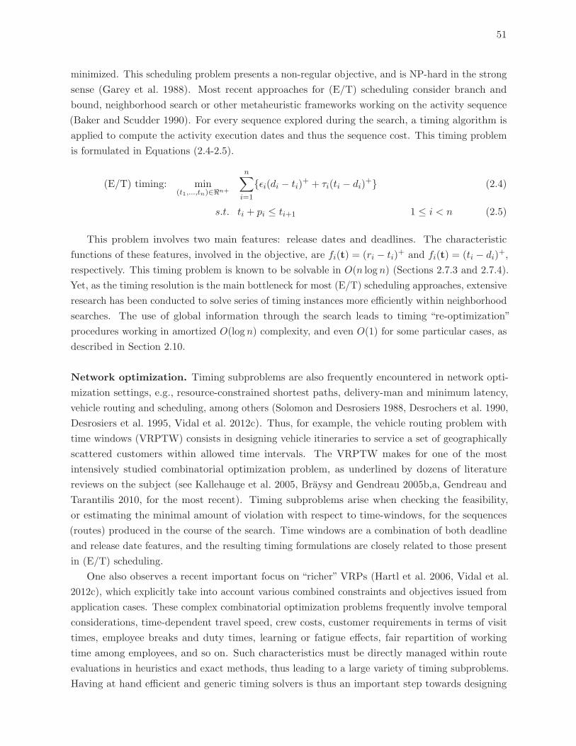
51

minimized. This scheduling problem presents a non-regular objective, and is NP-hard in the strong

sense (Garey et al. 1988). Most recent approaches for (E/T) scheduling consider branch and

bound, neighborhood search or other metaheuristic frameworks working on the activity sequence

(Baker and Scudder 1990). For every sequence explored during the search, a timing algorithm is

applied to compute the activity execution dates and thus the sequence cost. This timing problem

is formulated in Equations (2.4-2.5).

(E/T) timing: min(t1,...,tn)∈�n+

n∑i=1

{εi(di − ti)+ + τi(ti − di)

+} (2.4)

s.t. ti + pi ≤ ti+1 1 ≤ i < n (2.5)

This problem involves two main features: release dates and deadlines. The characteristic

functions of these features, involved in the objective, are fi(t) = (ri − ti)+ and fi(t) = (ti − di)

+,

respectively. This timing problem is known to be solvable in O(n log n) (Sections 2.7.3 and 2.7.4).

Yet, as the timing resolution is the main bottleneck for most (E/T) scheduling approaches, extensive

research has been conducted to solve series of timing instances more efficiently within neighborhood

searches. The use of global information through the search leads to timing “re-optimization”

procedures working in amortized O(log n) complexity, and even O(1) for some particular cases, as

described in Section 2.10.

Network optimization. Timing subproblems are also frequently encountered in network opti-

mization settings, e.g., resource-constrained shortest paths, delivery-man and minimum latency,

vehicle routing and scheduling, among others (Solomon and Desrosiers 1988, Desrochers et al. 1990,

Desrosiers et al. 1995, Vidal et al. 2012c). Thus, for example, the vehicle routing problem with

time windows (VRPTW) consists in designing vehicle itineraries to service a set of geographically

scattered customers within allowed time intervals. The VRPTW makes for one of the most

intensively studied combinatorial optimization problem, as underlined by dozens of literature

reviews on the subject (see Kallehauge et al. 2005, Braysy and Gendreau 2005b,a, Gendreau and

Tarantilis 2010, for the most recent). Timing subproblems arise when checking the feasibility,

or estimating the minimal amount of violation with respect to time-windows, for the sequences

(routes) produced in the course of the search. Time windows are a combination of both deadline

and release date features, and the resulting timing formulations are closely related to those present

in (E/T) scheduling.

One also observes a recent important focus on “richer” VRPs (Hartl et al. 2006, Vidal et al.

2012c), which explicitly take into account various combined constraints and objectives issued from

application cases. These complex combinatorial optimization problems frequently involve temporal

considerations, time-dependent travel speed, crew costs, customer requirements in terms of visit

times, employee breaks and duty times, learning or fatigue effects, fair repartition of working

time among employees, and so on. Such characteristics must be directly managed within route

evaluations in heuristics and exact methods, thus leading to a large variety of timing subproblems.

Having at hand efficient and generic timing solvers is thus an important step towards designing

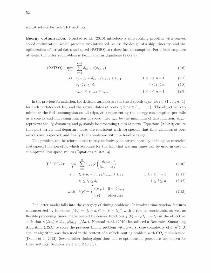
52

robust solvers for rich VRP settings.

Energy optimization. Norstad et al. (2010) introduce a ship routing problem with convex

speed optimization, which presents two interlaced issues: the design of a ship itinerary, and the

optimization of arrival dates and speed (PATSO) to reduce fuel consumption. For a fixed sequence

of visits, the latter subproblem is formulated in Equations (2.6-2.9).

(PATSO): mint,v

n−1∑i=1

di,i+1 c(vi,i+1) (2.6)

s.t. ti + pi + di,i+1/vi,i+1 ≤ ti+1 1 ≤ i ≤ n− 1 (2.7)

ri ≤ ti ≤ di 1 ≤ i ≤ n (2.8)

vmin ≤ vi,i+1 ≤ vmax 1 ≤ i ≤ n− 1 (2.9)

In the previous formulation, the decision variables are the travel speeds vi,i+1 for i ∈ {1, . . . , n−1}for each port-to-port leg, and the arrival dates at ports ti for i ∈ {1, . . . , n}. The objective is to

minimize the fuel consumption on all trips, c(v) representing the energy consumption per mile

as a convex and increasing function of speed. Let vopt be the minimum of this function. di,i+1

represents the leg distances, and pi stands for processing times at ports. Equations (2.7-2.9) ensure

that port arrival and departure dates are consistent with leg speeds, that time windows at port

arrivals are respected, and finally that speeds are within a feasible range.

This problem can be reformulated to rely exclusively on arrival dates by defining an extended

cost/speed function c(v), which accounts for the fact that waiting times can be used in case of

sub-optimal low speed values (Equations 2.10-2.13).

(PATSO-2): mint

n∑i=1

di,i+1c

(di,i+1

ti+1 − ti

)(2.10)

s.t. ti + pi + di,i+1/vmax ≤ ti+1 1 ≤ i ≤ n− 1 (2.11)

ri ≤ ti ≤ di 1 ≤ i ≤ n (2.12)

with c(v) =

⎧⎨⎩c(vopt) if v ≤ vopt

c(v) otherwise(2.13)

The latter model falls into the category of timing problems. It involves time-window features

characterized by functions fi(t) = (ti − di)+ + (ri − ti)

+ with a role as constraints, as well as

flexible processing times characterized by convex functions fi(t) = ci(ti+1 − ti) in the objective,

such that ci(Δti) = di,i+1c(di,i+1/Δti). Norstad et al. (2010) introduced a Recursive Smoothing

Algorithm (RSA) to solve the previous timing problem with a worst case complexity of O(n2). A

similar algorithm was then used in the context of a vehicle routing problem with CO2 minimization

(Demir et al. 2012). Several other timing algorithms and re-optimization procedures are known for

these settings (Sections 2.8.3 and 2.10.5.6).

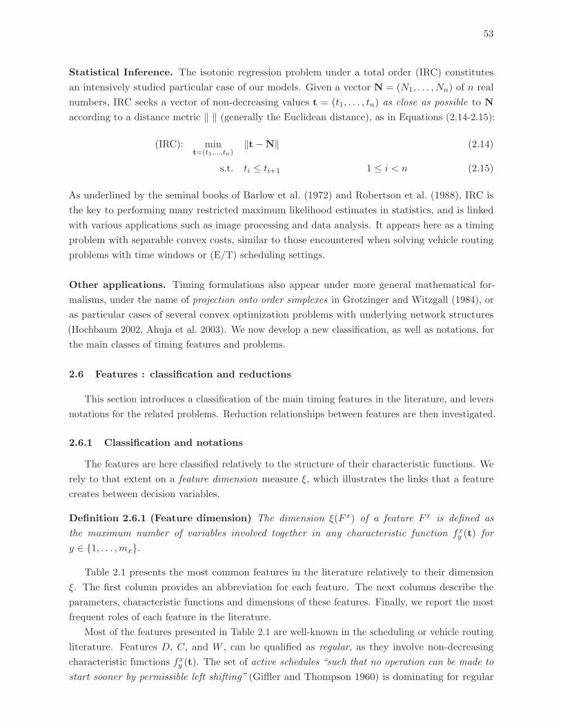
53

Statistical Inference. The isotonic regression problem under a total order (IRC) constitutes

an intensively studied particular case of our models. Given a vector N = (N1, . . . , Nn) of n real

numbers, IRC seeks a vector of non-decreasing values t = (t1, . . . , tn) as close as possible to N

according to a distance metric ‖ ‖ (generally the Euclidean distance), as in Equations (2.14-2.15):

(IRC): mint=(t1,...,tn)

‖t−N‖ (2.14)

s.t. ti ≤ ti+1 1 ≤ i < n (2.15)

As underlined by the seminal books of Barlow et al. (1972) and Robertson et al. (1988), IRC is

the key to performing many restricted maximum likelihood estimates in statistics, and is linked

with various applications such as image processing and data analysis. It appears here as a timing

problem with separable convex costs, similar to those encountered when solving vehicle routing

problems with time windows or (E/T) scheduling settings.

Other applications. Timing formulations also appear under more general mathematical for-

malisms, under the name of projection onto order simplexes in Grotzinger and Witzgall (1984), or

as particular cases of several convex optimization problems with underlying network structures

(Hochbaum 2002, Ahuja et al. 2003). We now develop a new classification, as well as notations, for

the main classes of timing features and problems.

2.6 Features : classification and reductions

This section introduces a classification of the main timing features in the literature, and levers

notations for the related problems. Reduction relationships between features are then investigated.

2.6.1 Classification and notations

The features are here classified relatively to the structure of their characteristic functions. We

rely to that extent on a feature dimension measure ξ, which illustrates the links that a feature

creates between decision variables.

Definition 2.6.1 (Feature dimension) The dimension ξ(F x) of a feature F x is defined as

the maximum number of variables involved together in any characteristic function fxy (t) for

y ∈ {1, . . . ,mx}.

Table 2.1 presents the most common features in the literature relatively to their dimension

ξ. The first column provides an abbreviation for each feature. The next columns describe the

parameters, characteristic functions and dimensions of these features. Finally, we report the most

frequent roles of each feature in the literature.

Most of the features presented in Table 2.1 are well-known in the scheduling or vehicle routing

literature. Features D, C, and W , can be qualified as regular, as they involve non-decreasing

characteristic functions fxy (t). The set of active schedules “such that no operation can be made to

start sooner by permissible left shifting” (Giffler and Thompson 1960) is dominating for regular

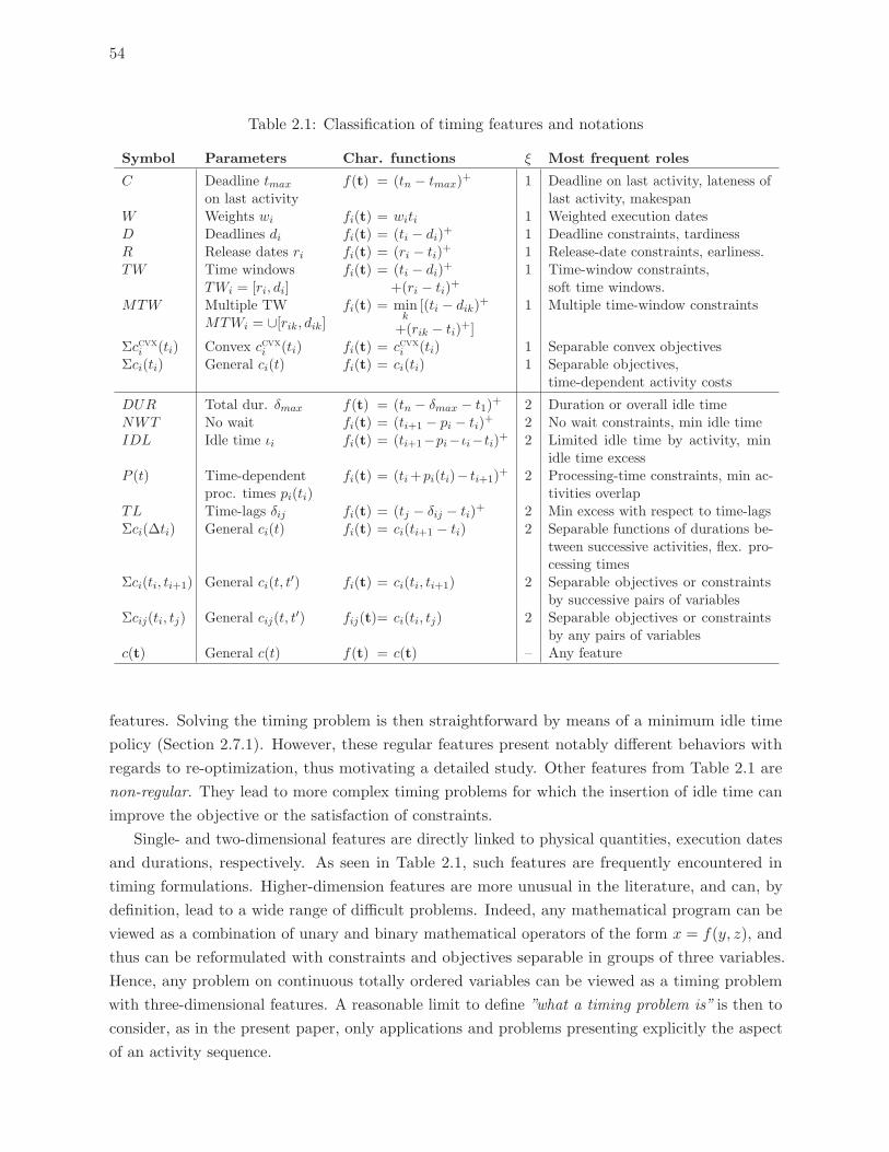
54

Table 2.1: Classification of timing features and notations

Symbol Parameters Char. functions ξ Most frequent roles

C Deadline tmax

on last activityf(t) = (tn − tmax)

+ 1 Deadline on last activity, lateness oflast activity, makespan

W Weights wi fi(t) = witi 1 Weighted execution datesD Deadlines di fi(t) = (ti − di)

+ 1 Deadline constraints, tardinessR Release dates ri fi(t) = (ri − ti)

+ 1 Release-date constraints, earliness.TW Time windows

TWi = [ri, di]fi(t) = (ti − di)

+

+(ri − ti)+

1 Time-window constraints,soft time windows.

MTW Multiple TWMTWi = ∪[rik, dik]

fi(t) = mink

[(ti − dik)+

+(rik − ti)+]

1 Multiple time-window constraints

Σccvxi (ti) Convex ccvxi (ti) fi(t) = ccvxi (ti) 1 Separable convex objectivesΣci(ti) General ci(t) fi(t) = ci(ti) 1 Separable objectives,

time-dependent activity costs

DUR Total dur. δmax f(t) = (tn − δmax − t1)+ 2 Duration or overall idle time

NWT No wait fi(t) = (ti+1 − pi − ti)+ 2 No wait constraints, min idle time

IDL Idle time ιi fi(t) = (ti+1−pi−ιi−ti)+ 2 Limited idle time by activity, minidle time excess

P (t) Time-dependentproc. times pi(ti)

fi(t) = (ti+pi(ti)− ti+1)+ 2 Processing-time constraints, min ac-

tivities overlapTL Time-lags δij fi(t) = (tj − δij − ti)

+ 2 Min excess with respect to time-lagsΣci(Δti) General ci(t) fi(t) = ci(ti+1 − ti) 2 Separable functions of durations be-

tween successive activities, flex. pro-cessing times

Σci(ti, ti+1) General ci(t, t′) fi(t) = ci(ti, ti+1) 2 Separable objectives or constraints

by successive pairs of variablesΣcij(ti, tj) General cij(t, t

′) fij(t)= ci(ti, tj) 2 Separable objectives or constraintsby any pairs of variables

c(t) General c(t) f(t) = c(t) – Any feature

features. Solving the timing problem is then straightforward by means of a minimum idle time

policy (Section 2.7.1). However, these regular features present notably different behaviors with

regards to re-optimization, thus motivating a detailed study. Other features from Table 2.1 are

non-regular. They lead to more complex timing problems for which the insertion of idle time can

improve the objective or the satisfaction of constraints.

Single- and two-dimensional features are directly linked to physical quantities, execution dates

and durations, respectively. As seen in Table 2.1, such features are frequently encountered in

timing formulations. Higher-dimension features are more unusual in the literature, and can, by

definition, lead to a wide range of difficult problems. Indeed, any mathematical program can be

viewed as a combination of unary and binary mathematical operators of the form x = f(y, z), and

thus can be reformulated with constraints and objectives separable in groups of three variables.

Hence, any problem on continuous totally ordered variables can be viewed as a timing problem

with three-dimensional features. A reasonable limit to define ”what a timing problem is” is then to

consider, as in the present paper, only applications and problems presenting explicitly the aspect

of an activity sequence.

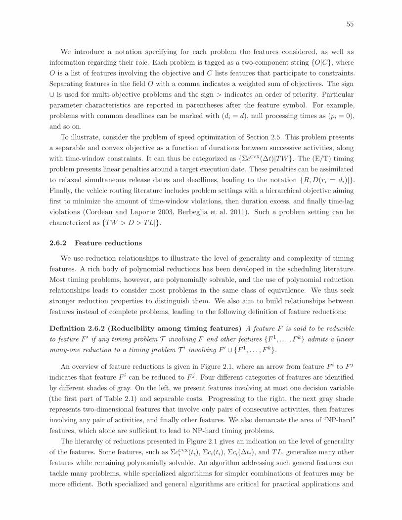
55

We introduce a notation specifying for each problem the features considered, as well as

information regarding their role. Each problem is tagged as a two-component string {O|C}, whereO is a list of features involving the objective and C lists features that participate to constraints.

Separating features in the field O with a comma indicates a weighted sum of objectives. The sign

∪ is used for multi-objective problems and the sign > indicates an order of priority. Particular

parameter characteristics are reported in parentheses after the feature symbol. For example,

problems with common deadlines can be marked with (di = d), null processing times as (pi = 0),

and so on.

To illustrate, consider the problem of speed optimization of Section 2.5. This problem presents

a separable and convex objective as a function of durations between successive activities, along

with time-window constraints. It can thus be categorized as {Σccvx(Δt)|TW}. The (E/T) timing

problem presents linear penalties around a target execution date. These penalties can be assimilated

to relaxed simultaneous release dates and deadlines, leading to the notation {R,D(ri = di)|}.Finally, the vehicle routing literature includes problem settings with a hierarchical objective aiming

first to minimize the amount of time-window violations, then duration excess, and finally time-lag

violations (Cordeau and Laporte 2003, Berbeglia et al. 2011). Such a problem setting can be

characterized as {TW > D > TL|}.

2.6.2 Feature reductions

We use reduction relationships to illustrate the level of generality and complexity of timing

features. A rich body of polynomial reductions has been developed in the scheduling literature.

Most timing problems, however, are polynomially solvable, and the use of polynomial reduction

relationships leads to consider most problems in the same class of equivalence. We thus seek

stronger reduction properties to distinguish them. We also aim to build relationships between

features instead of complete problems, leading to the following definition of feature reductions:

Definition 2.6.2 (Reducibility among timing features) A feature F is said to be reducible

to feature F ′ if any timing problem T involving F and other features {F 1, . . . , F k} admits a linear

many-one reduction to a timing problem T ′ involving F ′ ∪ {F 1, . . . , F k}.

An overview of feature reductions is given in Figure 2.1, where an arrow from feature F i to F j

indicates that feature F i can be reduced to F j . Four different categories of features are identified

by different shades of gray. On the left, we present features involving at most one decision variable

(the first part of Table 2.1) and separable costs. Progressing to the right, the next gray shade

represents two-dimensional features that involve only pairs of consecutive activities, then features

involving any pair of activities, and finally other features. We also demarcate the area of “NP-hard”

features, which alone are sufficient to lead to NP-hard timing problems.

The hierarchy of reductions presented in Figure 2.1 gives an indication on the level of generality

of the features. Some features, such as Σccvxi (ti), Σci(ti), Σci(Δti), and TL, generalize many other

features while remaining polynomially solvable. An algorithm addressing such general features can

tackle many problems, while specialized algorithms for simpler combinations of features may be

more efficient. Both specialized and general algorithms are critical for practical applications and

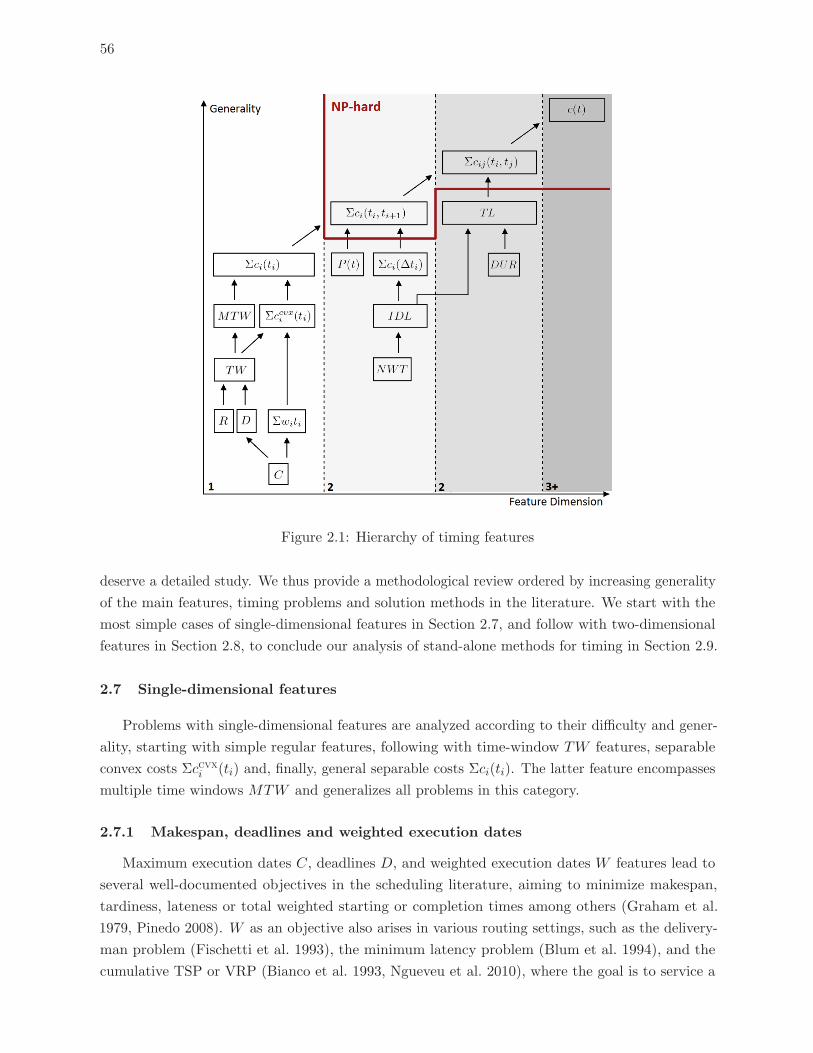
56

Figure 2.1: Hierarchy of timing features

deserve a detailed study. We thus provide a methodological review ordered by increasing generality

of the main features, timing problems and solution methods in the literature. We start with the

most simple cases of single-dimensional features in Section 2.7, and follow with two-dimensional

features in Section 2.8, to conclude our analysis of stand-alone methods for timing in Section 2.9.

2.7 Single-dimensional features

Problems with single-dimensional features are analyzed according to their difficulty and gener-

ality, starting with simple regular features, following with time-window TW features, separable

convex costs Σccvxi (ti) and, finally, general separable costs Σci(ti). The latter feature encompasses

multiple time windows MTW and generalizes all problems in this category.

2.7.1 Makespan, deadlines and weighted execution dates

Maximum execution dates C, deadlines D, and weighted execution dates W features lead to

several well-documented objectives in the scheduling literature, aiming to minimize makespan,

tardiness, lateness or total weighted starting or completion times among others (Graham et al.

1979, Pinedo 2008). W as an objective also arises in various routing settings, such as the delivery-

man problem (Fischetti et al. 1993), the minimum latency problem (Blum et al. 1994), and the

cumulative TSP or VRP (Bianco et al. 1993, Ngueveu et al. 2010), where the goal is to service a

57

set of customer as early as possible. These features are regular, as any backward shift of execution

date is beneficial for both feasibility and objective value. A very simple algorithm follows, which

will be referred to as the “minimum idle time policy”: For each activity ai of A in the sequence

order, schedule ai at its earliest possible execution date. If ai cannot be scheduled, declare problem

infeasibility and stop. If all activities have been successfully scheduled, declare problem feasibility.

An optimal solution is thus retrieved in n searches of the earliest feasible execution date, leading

to a O(n) complexity.

2.7.2 Release dates and time windows

Release dates and time-window features appear frequently in vehicle routing and scheduling

applications. Time-window features generalize release dates R and deadlines D, as any release date

ri or deadline di can be transformed into a time window with an infinite value on the right [ri,+∞]

or the left [−∞, di]. Two main issues are often considered regarding these features. The first

involves stating the feasibility of a sequence of activities under time-window constraints, whereas

the second problem involves the minimization of infeasibility with respect to the time windows,

and thus involves characteristic functions fi(t) = (ti − di)+ + (ri − ti)

+ in the objective.

Feasibility problem. Solving the feasibility problem {|TW} is straightforward, as the minimum

idle time policy, presented in Section 2.7.1, is dominating in this respect. For a sequence of n

activities (a1, . . . , an), the algorithm starts with t1 = r1, then chooses each subsequent activity

execution date to minimize idle time: ti+1 = max(ti + pi, ri+1). Hence, feasibility can be checked in

O(n) from scratch. Yet, more efficient feasibility checking procedures are available to solve series

of timing instances in local-search context. These procedures are presented in Section 2.10.

Infeasibility minimization. Many real-case applications allow lateness or earliness, the so-called

soft time-window settings, as a way to gain flexibility. Relaxations are also very frequently used in

heuristics, as managing intermediate infeasible solutions contributes to improve the capabilities

of exploration. Different conventions for soft time windows have been reported in the literature,

relative to earliness allowance and the way infeasibility is penalized. Several contributions, such as

Taillard et al. (1997) and Cordeau et al. (2001a), focus on the problem {D|R}, where late activities

are allowed with penalties, but not early activities. This case falls within the scope of regular

features (Section 2.7.1), and choosing for each activity the earliest execution date is optimal. The

problem can thus be solved with linear complexity O(n).

However, when early activities are allowed, as in {TW |} (Garey et al. 1988, Baker and Scudder

1990, Koskosidis et al. 1992, Balakrishnan 1993, Ibaraki et al. 2005), the objective function is

no longer non-decreasing. Supposing that activity ai is finished earlier than the beginning of

the time-window of ai+1, a choice must be made whether to insert idle time to reach ai+1, or

pay a penalty to better satisfy the time windows of remaining activities. The resulting timing

setting can thus become more complex. As an example, we show in Appendix I.1 that the problem

of minimizing the number of time-window infeasibilities, {TW (unit)|}, generalizes the Longest

Increasing Subsequence Problem (LISP). LISP has been the subject of extensive research, and

58

admits a computational lower bound of Ω(n log n) in the comparison tree model (Fredman 1975). It

should be noted that{TW |} is also special case of separable piecewise linear convex cost functions.

Sections 2.7.3 and 2.7.4 provide general efficient algorithms to address this wide range of problems,

leading to an O(n log n) algorithm for soft time-window relaxations.

2.7.3 Separable convex costs

Separable convex costs Σccvxi include a wide range of problem settings as particular cases. The

feature TW , and thus R, D, and C, can be reduced to Σccvxi (ti), as any time-window constraint

can be formulated as a piecewise convex cost by associating arbitrary large costs to both sides of

the feasibility interval. This feature also encompasses various other settings from the literature

such as earliness-tardiness scheduling (Baker and Scudder 1990), isotonic regression problems with

respect to a total order (Barlow et al. 1972, Robertson et al. 1988), extensions of team orienteering

problems (Feillet et al. 2005) in which the profit value can decrease with time (Erkut and Zhang

1996), various convex penalty functions for time-window infeasibility (Sexton and Bodin 1985a,b,

Ioachim et al. 1998, Ibaraki et al. 2005) and time-dependent convex processing costs (Tagmouti

et al. 2007), among others. The timing problem {Σccvxi (ti)|} is formulated in Equations (2.16-2.17).

Functions ccvxi (ti) are supposed to take infinite value for ti < 0.

min(t1,...,tn)∈�n

n∑i=1

ccvxi (ti) (2.16)

s.t. ti + pi ≤ ti+1 1 ≤ i < n (2.17)

Many methods have been proposed for this setting. We study, in this subsection, approaches

specially designed for separable convex cost functions. Dynamic programming based algorithms,

relying on fundamentally different concepts, are grouped in Section 2.7.4.

We base our analysis of algorithms for {Σccvxi (ti)|} on a set of optimality conditions using

the active set formalism (Chakravarti 1989, Best and Chakravarti 1990, Best et al. 2000). The

necessary and sufficient conditions we propose are more general than those developed previously in

the literature, being applicable to any set of proper convex cost functions, including non-smooth

cases.

Definition 2.7.1 (Activity blocks and prefix blocks) A block B is defined as a sequence

of activities (aB(1), . . . , aB(|B|)) processed consecutively such that ti + pi = ti+1 for all i ∈{B(1), . . . , B(|B|) − 1}. For k ∈ {B(1), . . . , B(|B|) − 1}, we also define the prefix block Bk =

(aB(1), . . . , ak). Let pij for 1 ≤ i ≤ j ≤ n be the cumulative processing duration of activities

(ai, . . . , aj). The execution cost CB of a block B as a function of its first activity execution

date tB(1) is given in Equation (2.18).

CB(tB(1)) = cB(1)(tB(1)) +

B(|B|)∑i=B(1)+1

ci(tB(1) + pB(1)i−1) (2.18)

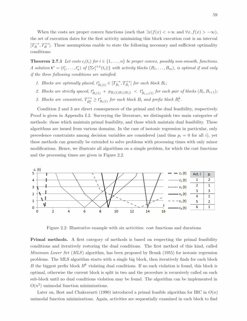
59

When the costs are proper convex functions (such that ∃x|f(x) < +∞ and ∀x, f(x) > −∞),

the set of execution dates for the first activity minimizing this block execution cost is an interval

[T−∗B , T+∗

B ]. These assumptions enable to state the following necessary and sufficient optimality

conditions:

Theorem 2.7.1 Let costs ci(ti) for i ∈ {1, . . . , n} be proper convex, possibly non-smooth, functions.

A solution t∗ = (t∗1, . . . , t∗n) of {Σccvxi (ti)|} with activity blocks (B1, . . . , Bm), is optimal if and only

if the three following conditions are satisfied:

1. Blocks are optimally placed, t∗Bi(1)∈ [T−∗

Bi, T+∗

Bi] for each block Bi;

2. Blocks are strictly spaced, t∗Bi(1)+ pBi(1)Bi(|Bi|) < t∗Bi+1(1)

for each pair of blocks (Bi, Bi+1);

3. Blocks are consistent, T+∗Bk

i

≥ t∗Bi(1)for each block Bi and prefix block Bk

i .

Condition 2 and 3 are direct consequences of the primal and the dual feasibility, respectively.

Proof is given in Appendix I.2. Surveying the literature, we distinguish two main categories of

methods: those which maintain primal feasibility, and those which maintain dual feasibility. These

algorithms are issued from various domains. In the case of isotonic regression in particular, only

precedence constraints among decision variables are considered (and thus pi = 0 for all i), yet

these methods can generally be extended to solve problems with processing times with only minor

modifications. Hence, we illustrate all algorithms on a simple problem, for which the cost functions

and the processing times are given in Figure 2.2.

Figure 2.2: Illustrative example with six activities: cost functions and durations

Primal methods. A first category of methods is based on respecting the primal feasibility

conditions and iteratively restoring the dual conditions. The first method of this kind, called

Minimum Lower Set (MLS ) algorithm, has been proposed by Brunk (1955) for isotonic regression

problems. The MLS algorithm starts with a single big block, then iteratively finds for each block

B the biggest prefix block Bk violating dual conditions. If no such violation is found, this block is

optimal, otherwise the current block is split in two and the procedure is recursively called on each

sub-block until no dual conditions violation may be found. The algorithm can be implemented in

O(n2) unimodal function minimizations.

Later on, Best and Chakravarti (1990) introduced a primal feasible algorithm for IRC in O(n)

unimodal function minimizations. Again, activities are sequentially examined in each block to find

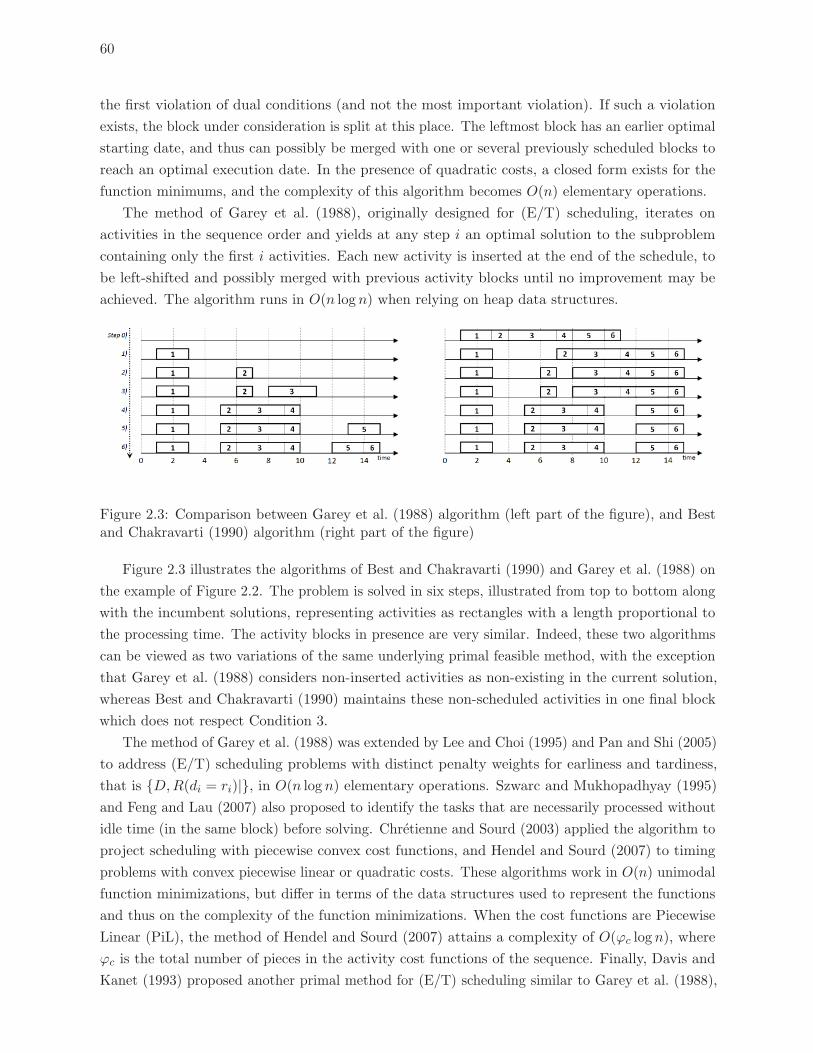
60

the first violation of dual conditions (and not the most important violation). If such a violation

exists, the block under consideration is split at this place. The leftmost block has an earlier optimal

starting date, and thus can possibly be merged with one or several previously scheduled blocks to

reach an optimal execution date. In the presence of quadratic costs, a closed form exists for the

function minimums, and the complexity of this algorithm becomes O(n) elementary operations.

The method of Garey et al. (1988), originally designed for (E/T) scheduling, iterates on

activities in the sequence order and yields at any step i an optimal solution to the subproblem

containing only the first i activities. Each new activity is inserted at the end of the schedule, to

be left-shifted and possibly merged with previous activity blocks until no improvement may be

achieved. The algorithm runs in O(n log n) when relying on heap data structures.

Figure 2.3: Comparison between Garey et al. (1988) algorithm (left part of the figure), and Bestand Chakravarti (1990) algorithm (right part of the figure)

Figure 2.3 illustrates the algorithms of Best and Chakravarti (1990) and Garey et al. (1988) on

the example of Figure 2.2. The problem is solved in six steps, illustrated from top to bottom along

with the incumbent solutions, representing activities as rectangles with a length proportional to

the processing time. The activity blocks in presence are very similar. Indeed, these two algorithms

can be viewed as two variations of the same underlying primal feasible method, with the exception

that Garey et al. (1988) considers non-inserted activities as non-existing in the current solution,

whereas Best and Chakravarti (1990) maintains these non-scheduled activities in one final block

which does not respect Condition 3.

The method of Garey et al. (1988) was extended by Lee and Choi (1995) and Pan and Shi (2005)

to address (E/T) scheduling problems with distinct penalty weights for earliness and tardiness,

that is {D,R(di = ri)|}, in O(n logn) elementary operations. Szwarc and Mukhopadhyay (1995)

and Feng and Lau (2007) also proposed to identify the tasks that are necessarily processed without

idle time (in the same block) before solving. Chretienne and Sourd (2003) applied the algorithm to

project scheduling with piecewise convex cost functions, and Hendel and Sourd (2007) to timing

problems with convex piecewise linear or quadratic costs. These algorithms work in O(n) unimodal

function minimizations, but differ in terms of the data structures used to represent the functions

and thus on the complexity of the function minimizations. When the cost functions are Piecewise

Linear (PiL), the method of Hendel and Sourd (2007) attains a complexity of O(ϕc logn), where

ϕc is the total number of pieces in the activity cost functions of the sequence. Finally, Davis and

Kanet (1993) proposed another primal method for (E/T) scheduling similar to Garey et al. (1988),

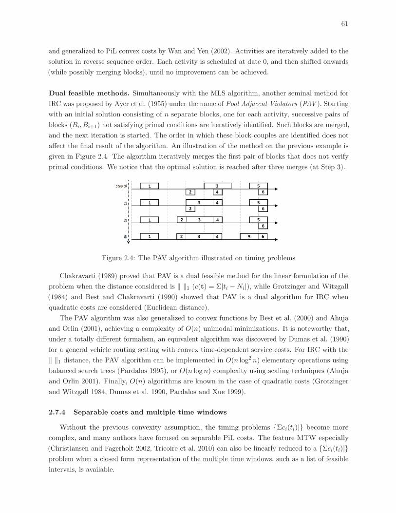
61

and generalized to PiL convex costs by Wan and Yen (2002). Activities are iteratively added to the

solution in reverse sequence order. Each activity is scheduled at date 0, and then shifted onwards

(while possibly merging blocks), until no improvement can be achieved.

Dual feasible methods. Simultaneously with the MLS algorithm, another seminal method for

IRC was proposed by Ayer et al. (1955) under the name of Pool Adjacent Violators (PAV ). Starting

with an initial solution consisting of n separate blocks, one for each activity, successive pairs of

blocks (Bi, Bi+1) not satisfying primal conditions are iteratively identified. Such blocks are merged,

and the next iteration is started. The order in which these block couples are identified does not

affect the final result of the algorithm. An illustration of the method on the previous example is

given in Figure 2.4. The algorithm iteratively merges the first pair of blocks that does not verify

primal conditions. We notice that the optimal solution is reached after three merges (at Step 3).

Figure 2.4: The PAV algorithm illustrated on timing problems

Chakravarti (1989) proved that PAV is a dual feasible method for the linear formulation of the

problem when the distance considered is ‖ ‖1 (c(t) = Σ|ti −Ni|), while Grotzinger and Witzgall

(1984) and Best and Chakravarti (1990) showed that PAV is a dual algorithm for IRC when

quadratic costs are considered (Euclidean distance).

The PAV algorithm was also generalized to convex functions by Best et al. (2000) and Ahuja

and Orlin (2001), achieving a complexity of O(n) unimodal minimizations. It is noteworthy that,

under a totally different formalism, an equivalent algorithm was discovered by Dumas et al. (1990)

for a general vehicle routing setting with convex time-dependent service costs. For IRC with the

‖ ‖1 distance, the PAV algorithm can be implemented in O(n log2 n) elementary operations using

balanced search trees (Pardalos 1995), or O(n logn) complexity using scaling techniques (Ahuja

and Orlin 2001). Finally, O(n) algorithms are known in the case of quadratic costs (Grotzinger

and Witzgall 1984, Dumas et al. 1990, Pardalos and Xue 1999).

2.7.4 Separable costs and multiple time windows

Without the previous convexity assumption, the timing problems {Σci(ti)|} become more

complex, and many authors have focused on separable PiL costs. The feature MTW especially

(Christiansen and Fagerholt 2002, Tricoire et al. 2010) can also be linearly reduced to a {Σci(ti)|}problem when a closed form representation of the multiple time windows, such as a list of feasible

intervals, is available.

62

In presence of non-negative and Lower Semi-Continuous (LSC) costs (ci(ti) ≤ limε→0min{ci(ti+ε), c(ti− ε)} at every discontinuity point), the timing problem {Σci(ti)|} can be efficiently solved by

dynamic programming. A large range of backward and forward approaches has thus been proposed

in the routing and scheduling literature (Yano and Kim 1991, Sourd 2005, Ibaraki et al. 2005,

Hendel and Sourd 2006, Ibaraki et al. 2008).

Solving {Σci(ti)|} by forward dynamic programming involves the forward minimum cost function

Fi(t), which evaluates the minimum cost to execute the sequence of activities (a1, . . . , ai) while

starting the last activity before t (ti ≤ t). Fi(t) functions can be computed by means of Equation

(2.19), starting from the case i = 1 with a single activity where F1(t) = minx≤t

c1(x). The optimal

solution value of the timing problem is z∗ = Fn(+∞), and the optimal activity execution dates can

be retrieved from the Fi(t) functions.

Fi(t) = min0≤x≤t

{ci(x) + Fi−1(x− pi−1)} 1 < i ≤ n (2.19)

The symmetric way to solve this problem by backward programming involves the backward

minimum cost function Bi(t), which evaluates the minimum cost to execute the sequence of

activities (ai, . . . , an), while executing the first activity ai after t (ti ≥ t). Bi(t) functions are

computed by backward recursion, starting with Bn(t) = minx≥t

cn(x) and using Equation (2.20). The

optimal solution value of the timing problem is z∗ = B1(−∞).

Bi(t) = minx≥t

{ci(x) +Bi+1(x+ pi)} 1 ≤ i < n (2.20)

These methods can be implemented in O(nϕc), where ϕc stands for the total number of pieces

in the activity cost functions ci. When the costs are also convex, the use of efficient tree data

structures leads to a complexity of O(ϕc logϕc) (Ibaraki et al. 2008), matching the best available

approaches in O(n logn) for the particular cases related to IRC, (E/T) scheduling, and soft time

windows. Finally, besides their good complexity for solving independent timing problems, these

dynamic programming open the way to efficient re-optimization procedures for solving series of

similar timing instances. These latter methods are surveyed in Section 2.10.

2.7.5 State-of-the-art: single-dimensional features

We introduced and analyzed in this section the main single-dimensional features from the

literature, independently of the field of application. Single-dimensional features are related to many

prominent problems such as LISP and IRC, which have been the subject of extensive research.

Various algorithms were examined and state-of-the-art methods for each particular feature and

problem were identified. In the particular case of {Σccvxi (ti)|}, 26 methods from various fields,

such as routing, scheduling and isotonic regression, were classified into three main families: primal,

dual, and dynamic programming methods.

Efficient linear methods are known for the most general problem of this category, {Σccvxi (ti)|},in presence of either convex or LSC and piecewise linear cost functions. Linear complexity is the

best possible complexity when addressing the problem from scratch. As illustrated in Section 2.10,

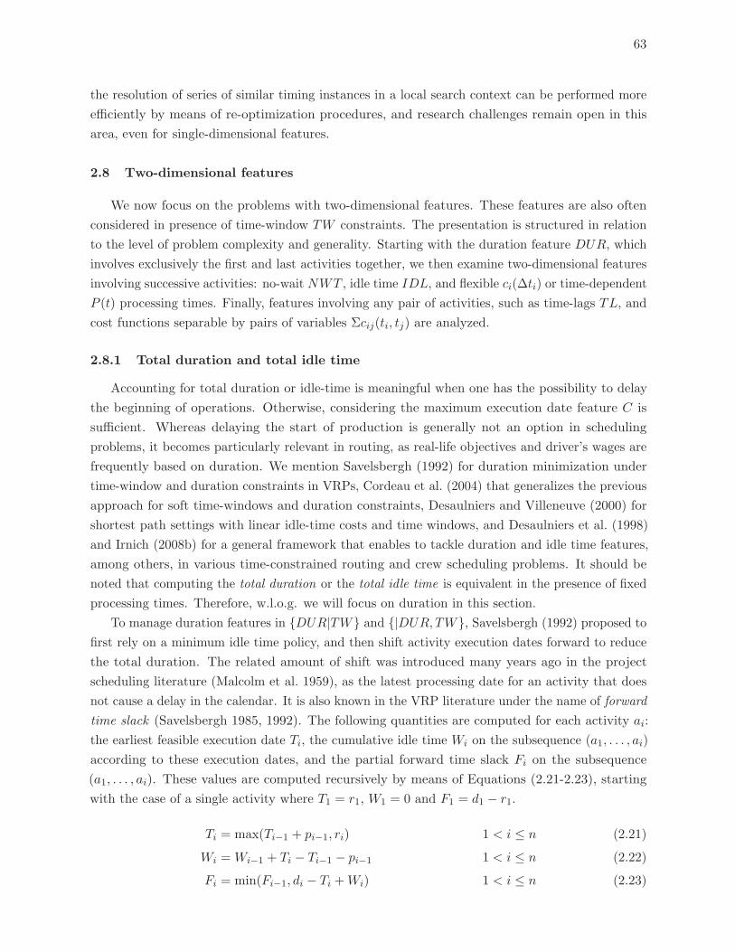
63

the resolution of series of similar timing instances in a local search context can be performed more

efficiently by means of re-optimization procedures, and research challenges remain open in this

area, even for single-dimensional features.

2.8 Two-dimensional features

We now focus on the problems with two-dimensional features. These features are also often

considered in presence of time-window TW constraints. The presentation is structured in relation

to the level of problem complexity and generality. Starting with the duration feature DUR, which

involves exclusively the first and last activities together, we then examine two-dimensional features

involving successive activities: no-wait NWT , idle time IDL, and flexible ci(Δti) or time-dependent

P (t) processing times. Finally, features involving any pair of activities, such as time-lags TL, and

cost functions separable by pairs of variables Σcij(ti, tj) are analyzed.

2.8.1 Total duration and total idle time

Accounting for total duration or idle-time is meaningful when one has the possibility to delay

the beginning of operations. Otherwise, considering the maximum execution date feature C is

sufficient. Whereas delaying the start of production is generally not an option in scheduling

problems, it becomes particularly relevant in routing, as real-life objectives and driver’s wages are

frequently based on duration. We mention Savelsbergh (1992) for duration minimization under

time-window and duration constraints in VRPs, Cordeau et al. (2004) that generalizes the previous

approach for soft time-windows and duration constraints, Desaulniers and Villeneuve (2000) for

shortest path settings with linear idle-time costs and time windows, and Desaulniers et al. (1998)

and Irnich (2008b) for a general framework that enables to tackle duration and idle time features,

among others, in various time-constrained routing and crew scheduling problems. It should be

noted that computing the total duration or the total idle time is equivalent in the presence of fixed

processing times. Therefore, w.l.o.g. we will focus on duration in this section.

To manage duration features in {DUR|TW} and {|DUR, TW}, Savelsbergh (1992) proposed to

first rely on a minimum idle time policy, and then shift activity execution dates forward to reduce

the total duration. The related amount of shift was introduced many years ago in the project

scheduling literature (Malcolm et al. 1959), as the latest processing date for an activity that does

not cause a delay in the calendar. It is also known in the VRP literature under the name of forward

time slack (Savelsbergh 1985, 1992). The following quantities are computed for each activity ai:

the earliest feasible execution date Ti, the cumulative idle time Wi on the subsequence (a1, . . . , ai)

according to these execution dates, and the partial forward time slack Fi on the subsequence

(a1, . . . , ai). These values are computed recursively by means of Equations (2.21-2.23), starting

with the case of a single activity where T1 = r1, W1 = 0 and F1 = d1 − r1.

Ti = max(Ti−1 + pi−1, ri) 1 < i ≤ n (2.21)

Wi =Wi−1 + Ti − Ti−1 − pi−1 1 < i ≤ n (2.22)

Fi = min(Fi−1, di − Ti +Wi) 1 < i ≤ n (2.23)

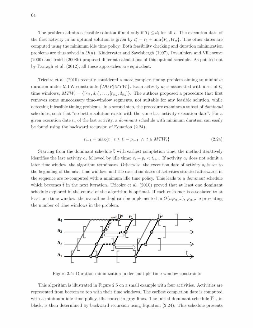
64

The problem admits a feasible solution if and only if Ti ≤ di for all i. The execution date of

the first activity in an optimal solution is given by t∗1 = r1 +min{Fn,Wn}. The other dates are

computed using the minimum idle time policy. Both feasibility checking and duration minimization

problems are thus solved in O(n). Kindervater and Savelsbergh (1997), Desaulniers and Villeneuve

(2000) and Irnich (2008b) proposed different calculations of this optimal schedule. As pointed out

by Parragh et al. (2012), all these approaches are equivalent.

Tricoire et al. (2010) recently considered a more complex timing problem aiming to minimize

duration under MTW constraints {DUR|MTW}. Each activity ai is associated with a set of ki

time windows, MTWi = {[ri1, di1], . . . , [riki , diki ]}. The authors proposed a procedure that first

removes some unnecessary time-window segments, not suitable for any feasible solution, while

detecting infeasible timing problems. In a second step, the procedure examines a subset of dominant

schedules, such that “no better solution exists with the same last activity execution date”. For a

given execution date tn of the last activity, a dominant schedule with minimum duration can easily

be found using the backward recursion of Equation (2.24).

ti−1 = max{t | t ≤ ti − pi−1 ∧ t ∈MTWi} (2.24)

Starting from the dominant schedule t with earliest completion time, the method iteratively

identifies the last activity ai followed by idle time: ti + pi < ti+1. If activity ai does not admit a

later time window, the algorithm terminates. Otherwise, the execution date of activity ai is set to

the beginning of the next time window, and the execution dates of activities situated afterwards in

the sequence are re-computed with a minimum idle time policy. This leads to a dominant schedule

which becomes t in the next iteration. Tricoire et al. (2010) proved that at least one dominant

schedule explored in the course of the algorithm is optimal. If each customer is associated to at

least one time window, the overall method can be implemented in O(nϕmtw), ϕmtw representing

the number of time windows in the problem.

Figure 2.5: Duration minimization under multiple time-window constraints

This algorithm is illustrated in Figure 2.5 on a small example with four activities. Activities are

represented from bottom to top with their time windows. The earliest completion date is computed

with a minimum idle time policy, illustrated in gray lines. The initial dominant schedule t0 , in

black, is then determined by backward recursion using Equation (2.24). This schedule presents

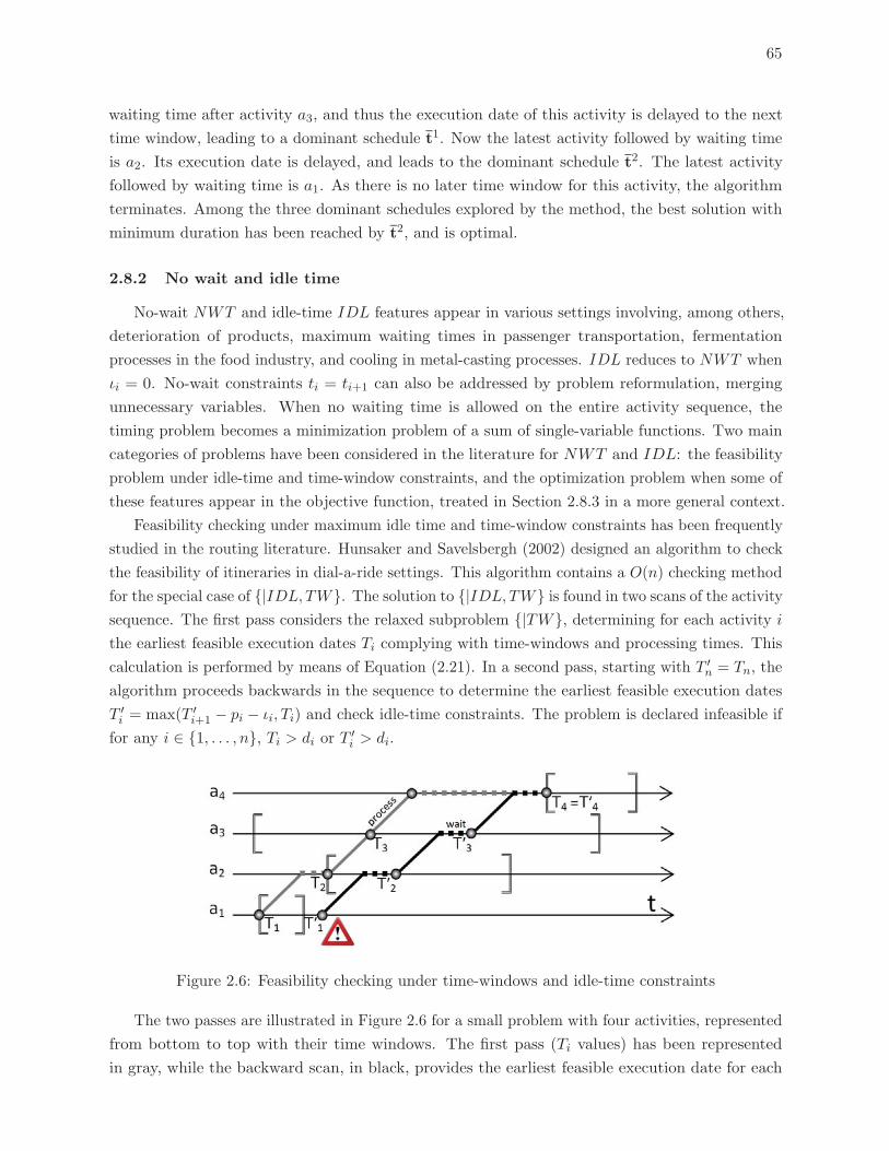
65

waiting time after activity a3, and thus the execution date of this activity is delayed to the next

time window, leading to a dominant schedule t1. Now the latest activity followed by waiting time

is a2. Its execution date is delayed, and leads to the dominant schedule t2. The latest activity

followed by waiting time is a1. As there is no later time window for this activity, the algorithm

terminates. Among the three dominant schedules explored by the method, the best solution with

minimum duration has been reached by t2, and is optimal.

2.8.2 No wait and idle time

No-wait NWT and idle-time IDL features appear in various settings involving, among others,

deterioration of products, maximum waiting times in passenger transportation, fermentation

processes in the food industry, and cooling in metal-casting processes. IDL reduces to NWT when

ιi = 0. No-wait constraints ti = ti+1 can also be addressed by problem reformulation, merging

unnecessary variables. When no waiting time is allowed on the entire activity sequence, the

timing problem becomes a minimization problem of a sum of single-variable functions. Two main

categories of problems have been considered in the literature for NWT and IDL: the feasibility

problem under idle-time and time-window constraints, and the optimization problem when some of

these features appear in the objective function, treated in Section 2.8.3 in a more general context.

Feasibility checking under maximum idle time and time-window constraints has been frequently

studied in the routing literature. Hunsaker and Savelsbergh (2002) designed an algorithm to check

the feasibility of itineraries in dial-a-ride settings. This algorithm contains a O(n) checking method

for the special case of {|IDL, TW}. The solution to {|IDL, TW} is found in two scans of the activity

sequence. The first pass considers the relaxed subproblem {|TW}, determining for each activity i

the earliest feasible execution dates Ti complying with time-windows and processing times. This

calculation is performed by means of Equation (2.21). In a second pass, starting with T ′n = Tn, the

algorithm proceeds backwards in the sequence to determine the earliest feasible execution dates

T ′i = max(T ′

i+1 − pi − ιi, Ti) and check idle-time constraints. The problem is declared infeasible if

for any i ∈ {1, . . . , n}, Ti > di or T′i > di.

Figure 2.6: Feasibility checking under time-windows and idle-time constraints

The two passes are illustrated in Figure 2.6 for a small problem with four activities, represented

from bottom to top with their time windows. The first pass (Ti values) has been represented

in gray, while the backward scan, in black, provides the earliest feasible execution date for each

66

activity T ′i . As shown in the figure, this value exceeds the time window of activity a1 (T ′

1 > d1),

and thus the timing problem illustrated is infeasible.

2.8.3 Flexible processing times

Resource allocation, time-resource trade-offs, and project crashing problems have been thor-

oughly studied in the operations research literature, since they are critical in many applications,

including energy optimization (see Section 2.5), project scheduling, portfolio selection, production

economics, optimization of search effort, advertising, and so on and so forth (Kelley and Walker

1959, Talbot 1982, Ibaraki and Katoh 1988, Patriksson 2008). The processing time or resource

allocation in all these problems can be increased or reduced at a cost. We refer to this feature

as “flexible processing times” Σci(Δti). The characteristic function of this feature is a general

separable function of successive execution time differences ti+1 − ti. As such, it generalizes both

NWT and IDL.

When only NWT, IDL, and Σci(Δti) features are encountered, the timing problem {Σci(Δti)|}(Equations 2.25-2.27) can be decomposed along ti+1 − ti values, and the independent minimization

of every ci(Δti) leads to the optimal solution where ti+1 − ti = argminΔti Σci(Δti).

When the ci functions are convex and in presence of an additional constraint on the total

duration, the problem {Σci(Δti)|DUR} can be reformulated (Equations 2.28-2.30) as a Simple

Resource Allocation Problem (SRA) by setting t0 = 0 w.l.o.g. and using the change of variables

xi = ti+1 − ti.

min(t1,...,tn)∈�n+

n−1∑i=1

ci(ti+1 − ti) (2.25)

s.t. tn − t1 ≤ dmax (2.26)

ti + pi ≤ ti+1 1 ≤ i < n (2.27)


n−1∑i=1

ci(xi) (2.28)

s.t.

n−1∑i=1

xi ≤ dmax (2.29)

xi ∈ [pi,+∞] 1 ≤ i < n (2.30)

Non-linear resource allocation problems have been the subject of hundreds of papers. Two

main families of methods for this problem are generally discerned. Lagrangian methods (Charnes

and Cooper 1958, Everett 1963, Srikantan 1963) seek to iteratively progress towards the optimal

value of the single dual variable associated to Equation (2.29) while respecting primal feasibility.

Pegging algorithms (Sanathanan 1971, Luss and Gupta 1975, Kodialam and Luss 1998) relax the

constraints of Equations (2.29-2.30), iteratively solving the relaxed problems and fixing the values

of variables that do not satisfy primal constraints. A third approach originates from concepts

67

originally developed for the discrete problem version. Hochbaum (1994) proposes a greedy algorithm

with arbitrary increments coupled with scaling techniques, yielding the best known computational

complexity for this problem, O(n log n log(dmax/εn)), where ε is the target precision. The method

increments progressively the xi variable yielding the least reduced cost, leading to the optimum of

this convex problem. Finally, a dynamic programming approach has been introduced in Karush

(1962), which iteratively characterizes the best cost as a function of the resource consumption

(total time in our case).

In particular, relationships can be established between these approaches and the three classes

of methods surveyed in Section 2.7.3 for timing problems with separable convex costs. Pegging

algorithms work similarly to the dual feasible methods of Section 2.7.3, such as PAV or the algorithm

of Dumas et al. (1990), by iteratively solving relaxed problems and re-introducing the constraints.

These constraints are here re-introduced by setting variables to constraint bounds, rather than

joining pairs of activities (merging blocks) as in the PAV algorithm. The equivalent to the primal

methods of Section 2.7.3 is less immediate. The greedy method of Hochbaum (1994) is one of this

kind, but requires advanced scaling techniques to solve the continuous case. Also, even though

most authors opted to optimize the single Lagrangian variable μ associated to Equation (2.29)

rather than the primal variables, a consequence of the KKT conditions is that optimizing μ is

equivalent to choosing iteratively the slope for each ci(xi) and, in fact, iteratively fixing primal

variables. Thus, Lagrangian approaches for this problem were eventually qualified by Patriksson

(2008) as explicitly dual but also implicitely primal.

Adding time-window constraints to the model of Equations (2.25-2.27) leads to other timing

settings, which can no longer be assimilated to resource allocation problems. In the special case

of Norstad et al. (2010), a timing problem {Σccvxi (Δti)|TW} is addressed with the objective

z(t) =∑n

i=1 di,i+1c(ti+1−tidi,i+1

)and non-increasing and convex c(Δt) functions. In presence of such

functions, removing time-window constraints leads to optimal solutions presenting a constant

ratio ti+1−tidi,i+1

for all i, and thus constant speed on all legs. The recursive smoothing algorithm

(RSA) exploits this property by maintaining this ratio constant on subsequences and progressively

re-introducing violated time-window constraints. The overall method works in O(n2) elementary

operations once the minimum of each function c(Δt) is given. It is noteworthy that this method

is another example of a dual feasible algorithm based on the relaxation and re-introduction of

constraints, conceptually similar to PAV and pegging methods.

In more general settings, when flexible processing times are combined with single-dimensional

features such as time windows or time-dependent activity costs, the problem can become more

difficult. Sourd (2005) and Hashimoto et al. (2006) have independently studied {Σci(Δti),Σci(ti)|}(Equation 2.31) with piecewise linear functions in the context of (E/T) scheduling and vehicle

routing, and report its NP-hardness.

min(t1,...,tn)∈�n+

n∑i=1

ci(ti) +n−1∑i=1

c′i(ti+1 − ti) (2.31)

When the functions ci and c′i are PiL with integer breakpoints, a dynamic programming

algorithm is proposed to solve the problem in O(T 2), where T represents an upper bound on the

68

schedule durations. Note that this dynamic programming algorithm can be viewed as an extension

of the resource allocation algorithm of Karush (1962). The method can be implemented with a

forward dynamic programming function Fi(t) (Equations 2.32-2.33), which evaluates the minimum

cost to process the subsequence of activities (a1, . . . , ai), starting the last activity exactly at time t

(ti = t). The resulting optimal cost is given by z∗ = mint Fn(t).

F1(t) = c1(t) (2.32)

Fi(t) = ci(t) + min0≤x≤t

{Fi−1(x) + c′i−1(t− x)} 1 < i ≤ n (2.33)

A polynomial dynamic programming algorithm working in O(n(ϕc + ϕc × ϕ′c)) exists for the

case where the functions c′i(Δt) are PiL and convex (Sourd 2005, Hashimoto et al. 2006). ϕc

and ϕ′c represent the total number of pieces in the cost functions ci and c

′i, and ϕc stands for the

number of convex pieces in the cost functions ci. Efficient re-optimization procedures have also

been proposed (Section 2.10). Finally, DUR involved in the objective can be seen as a special case

of Σci(Δti) where cdur

i (Δti) = Δti. Since MTW is also reducible to Σci(ti), the previous algorithm

thus provides an alternative way to solve {DUR|MTW} or {|DUR,MTW} in O(n+nϕmtw), where

ϕmtw represents the total number of time windows.

2.8.4 Time-dependent processing times

In several application settings, activity processing times may vary as a function of the execution

dates. In machine and project scheduling for example, learning, deterioration effects and other

time-dependencies can have a large impact (see Alidaee and Womer 1999, Cheng 2004). Network

congestion is a major concern for vehicle routing and data transmission (Van Woensel et al. 2008,

Kok et al. 2009) and, thus, the time-dependent processing-time feature P (t) appears in various

network optimization problems: shortest path (Cooke and Halsey 1966, Dreyfus 1969, Halpern

1977), traveling salesman (Malandraki and Dial 1996), vehicle routing (Beasley 1981, Malandraki

and Daskin 1992, Ichoua et al. 2003, Donati et al. 2008, Hashimoto et al. 2008), and so on.

The literature on the subject can generally be separated between discrete and continuous

settings. Discrete optimization models generally involve time-space networks which are less likely

to present the timing issues studied in this article, whereas several continuous models have led to

explicit timing problems with P (t) features, as in Ichoua et al. (2003), Fleischmann et al. (2004),

Donati et al. (2008), and Hashimoto et al. (2008). These models involve constraints of the type

ti + pi(ti) ≤ ti+1 within a timing formulation with other additional features. A FIFO assumption

on functions pi can be made:

FIFO assumption: ∀i x ≥ y =⇒ x+ pi(x) ≥ y + pi(y) (2.34)

FIFO implies that any delay in an activity execution date results in a delay in its completion date.

The assumption is meaningful in several settings, e.g. vehicle routing, as two vehicles that behave

similarly on the same route are supposed to remain in the same arrival order, whatever congestion

happens (Ichoua et al. 2003).

69

Time-dependent processing-time features are generally assumed to result in more complex

timing problems. However, one should clearly identify the source of the difficulty, which is frequently

imputable to the calculation and access to pij(t) throughout the search, and not necessarily to the

timing problem solving method. Assuming that pij(t) can be evaluated in constant time and under

FIFO, {D|R,P (t)} is still solvable in O(n) by means of a minimum idle time policy (Fleischmann

et al. 2004). In the same spirit, Donati et al. (2008) apply the time-slack approach of Savelsbergh

(1992) to {|TW,P (t)}. Still, dedicated methodologies are necessary for other settings such as

{DUR|TW,P (t)} and for re-optimization procedures (Section 2.10).

A general time-dependent timing problem {Σci(ti)|P (t)}, Equations (2.35-2.36), is addressed in

Hashimoto et al. (2008). All functions considered are PiL, non-negative and lower semicontinuous.

min(t1,...,tn)∈Rn+

n∑i=1

ci(ti) (2.35)

s.t. ti + pi(ti) ≤ ti+1 1 ≤ i < n (2.36)

The authors propose a dynamic programming approach, which extends the method of Section

2.7.4. It involves the functions Fi(t), which represent the minimum cost to process the subsequence

of activities (a1, . . . , ai) while starting the last activity before t (ti ≤ t). These functions can be

computed by means of Equations (2.37-2.38), and the optimal solution cost is given by Fn(+∞).

F1(t) = min0≤x≤t

c1(x) (2.37)

Fi(t) = min0≤x≤t

{ci(x) + minx′+pi(x′)≤x

Fi−1(x′)} 1 < i ≤ n (2.38)

Under the assumption of Equation (2.39), which is slightly weaker than FIFO, the method can

be implemented in O(n(ϕc + ϕp)), where ϕc and ϕp are the total number of pieces in cost and

processing-time functions. This method for {Σci(ti)|P (t)} thus presents the same quadratic

complexity as in the case without time dependency (Section 2.7.4). When the previous assumption

does not hold, the dynamic programming method of Hashimoto et al. (2008) is not polynomial,

and the question remains open whether {Σci(ti)|P (t)} is polynomially solvable.

(HYI) assumption: ∀i x+ pi(x) = y + pi(y) =⇒ x+ pi(x) = z + pi(z) ∀z ∈ [x, y] (2.39)

2.8.5 Time lags

The two-dimensional features surveyed in the previous sections involved linking constraints

and objectives between the first and last tasks, in the case of DUR, or between pairs of successive

variables in the case of NWT and IDL. We now review the time-lag TL feature, which brings into

play a time difference tj − ti between any two activity execution dates ti and tj . This feature is

thus a generalization of NWT , IDL and DUR.

To the best of our knowledge, early research on time lags has been conducted by Mitten

(1959) for flowshop scheduling problems. This feature has been used since to model many problem

characteristics in various domains, such as the deterioration of food or chemical products, glue

70

drying, customer requirements in some dial-a-ride problems, elevator dispatching, quarantine

durations, and so on. Time-lag scheduling problems on a single machine have also been shown by

Brucker et al. (1999) to generalize all shop, multi-purpose machines, and multi-processor scheduling

problems. Hence, timing problems with TL are likely to be difficult.

The most basic problem with TL feature relates to feasibility checking under time-lag constraints

of the form ti + δij ≤ tj . When δij ≥ 0, the constraint is called positive time lag, and corresponds

to a minimum delay between activities ai and aj , whereas δij ≤ 0 corresponds to a negative time

lag, and involves a maximum delay of −δij between the activities aj and ai. Equality constraints

ti + δij = tj involve both positive and negative time lags. The resulting timing problem {|TL}can be seen as a special case of project scheduling on a chain of activities, and the METRA

potential method (MPM) of Roy (1959, 1962) can be applied. In MPM, the time-lag constraints

are represented on a graph G = (V,A), where each activity ai is associated with a node vi ∈ V ,

and each arc (vi, vj), associated with a weight wij , represents a temporal constraint of the form

tj − ti ≥ wij . The feasibility of {|TL} is equivalent to the non-existence of a positive length cycle

in this graph (Bartusch et al. 1988, Dechter et al. 1991). The algorithm of Floyd-Warshall can be

employed to solve this problem in O(n3), but the longest-path procedure of Hurink and Keuchel

(2001), also in O(n3), is shown to provide faster results in practice. Potts and Whitehead (2007)

also considered a coupled-operation scheduling problem with only n/2 time-lag constraints, and

timing feasibility is checked in O(n2). The authors underlined the computational burden of such

timing algorithms, which strongly degrades the performance of neighborhood searches or branch

and bound procedures.

Hunsaker and Savelsbergh (2002) studied a case of {|TL, TW} timing in the context of dial-a-ride

problems. Activities represent customer requests on pick-up and deliveries services, which occur by

pairs, such that any pick-up always precedes its corresponding delivery in the sequence. Each such

pair of activities is linked by a single positive time-lag constraint. The total number of time-lag

constraints is thus n/2. The problem also involves time windows and maximum idle times for each

activity. The authors claim that the resulting feasibility problem can be solved in three passes on

the sequence of activities with linear complexity. Yet, the algorithm presents a small flaw, which

is straightforward to correct (Tang et al. 2010), but leads to a O(n logn) complexity (Haugland

and Ho 2010). A O(n) complexity is finally achieved in Firat and Woeginger (2011) by means of a

reduction to a shortest path problem on a weighted interval graph.

The same setting is also addressed in Gschwind and Irnich (2012). The authors describe a

labeling procedure based on |Mi| resources for each pickups and each delivery activity ai. Mi

stands for the current number of open pickups at ai. This labeling procedure provides another way

to check the feasibility of a fixed activity sequence {|TL, TW} in O(n2). Also, it enables to evaluate

the feasibility of an extended sequence with one additional activity an+1 in O(Mn+1) given the

information on the original sequence. Such forward extension function is critical when solving

shortest path problems with underling timing features.

Cordeau and Laporte (2003) and Berbeglia et al. (2011) consider a dial-a-ride setting with

an additional duration constraint on the entire trip duration. The authors solve heuristically a

Lagrangian relaxation of the problem with a hierarchical objective. Total trip duration infeasibility

71

is minimized, then time-window infeasibility and, finally, time-lag infeasibility, that is the timing

problem {DUR > D > TL|R}. The algorithm first minimizes duration and time-window infeasibility

as in Section 2.8.1, then iteratively delays some pick-up services to reduce time-lag infeasibility

without increasing any other violation. A computational complexity of O(n2) is achieved. It was

observed (Private Communication 2010), however, that the previous approach only guarantees

optimality under an additional assumption that we call LIFO, which requires that for any 1 ≤i < j < k < l ≤ n, no activities ai, aj , ak, al present “entangled” time-lag constraints of the form

tk − ti ≤ δik and tl − tj ≤ δjl. The LIFO assumption is frequently enforced in the vehicle routing

literature, especially when transporting passengers, or in presence of complex loading constraints.

In this case, the last object or customer received in the vehicle is the first one to leave. Without this

assumption, the difficulty of many problems with time lags strongly increases, and no specialized

efficient algorithm is actually known for {DUR > D > TL|R} and similar problems.

2.8.6 Separable costs by pairs of variables

Separable costs by pairs of variables Σcij(ti, tj) generalize all problems combining single or

two-dimensional features. The timing problem with this feature alone is NP-hard, as it includes

{Σci(ti),Σci(Δti)|} as special case (see Section 2.8.2). When the objective function is convex, the

problem {Σccvxij (tj − ti),Σccvx

i (ti)|} given in Equations (2.40-2.41), is equivalent to the convex

cost dual network flow problem for which weakly polynomial algorithms are available (Ahuja et al.

2003).

mint=(t1,...,tn)∈�n+

∑(i,j)∈Q

ccvxij (tj − ti) +∑

1≤i≤n

ccvxi (ti) (2.40)

s.t. ti + pi ≤ ti+1 1 ≤ i < n (2.41)

2.9 Conclusion on “stand-alone” timing methods

In contrast to single-dimensional features, which appeared as fairly well addressed in Section 2.7

by means of a few algorithms and concepts, two-dimensional features lead to more diverse problem

structures and algorithms. Several simple cases with duration minimization or time-dependent

processing times can be solved in linear time, but other problems with time-lag features actually

require O(n3) algorithms to be solved exactly. Although polynomial, the latter methods can be

impracticable in the context of local searches or branch-and-bound approaches.

Many practical timing settings result in models with linear constraints and linear or separable

convex objectives. For these problems, the linear and convex programming theory ensures weakly

polynomial solvability, and provides general solution methods (Khachiyan 1979, Karmarkar 1984,

Hochbaum and Shanthikumar 1990). Some general problems, however, such as {Σci(ti),Σci(Δti)|}with PiL functions, are NP-hard, while for other problems, such as {Σci(ti)|P (t)} with general

piecewise linear functions P (t), the existence or non-existence of polynomial algorithm is still open.

Timing settings thus lead to a rich variety of problem structures and complexities.

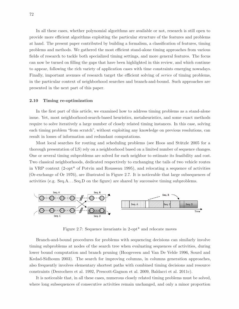
72

In all these cases, whether polynomial algorithms are available or not, research is still open to

provide more efficient algorithms exploiting the particular structure of the features and problems

at hand. The present paper contributed by building a formalism, a classification of features, timing

problems and methods. We gathered the most efficient stand-alone timing approaches from various

fields of research to tackle both specialized timing settings, and more general features. The focus

can now be turned on filling the gaps that have been highlighted in this review, and which continue

to appear, following the rich variety of application cases with time constraints emerging nowadays.

Finally, important avenues of research target the efficient solving of series of timing problems,

in the particular context of neighborhood searches and branch-and-bound. Such approaches are

presented in the next part of this paper.

2.10 Timing re-optimization

In the first part of this article, we examined how to address timing problems as a stand-alone

issue. Yet, most neighborhood-search-based heuristics, metaheuristics, and some exact methods

require to solve iteratively a large number of closely related timing instances. In this case, solving

each timing problem “from scratch”, without exploiting any knowledge on previous resolutions, can

result in losses of information and redundant computations.

Most local searches for routing and scheduling problems (see Hoos and Stutzle 2005 for a

thorough presentation of LS) rely on a neighborhood based on a limited number of sequence changes.

One or several timing subproblems are solved for each neighbor to estimate its feasibility and cost.

Two classical neighborhoods, dedicated respectively to exchanging the tails of two vehicle routes

in VRP context (2-opt* of Potvin and Rousseau 1995), and relocating a sequence of activities

(Or-exchange of Or 1976), are illustrated in Figure 2.7. It is noticeable that large subsequences of

activities (e.g. Seq.A. . . Seq.D on the figure) are shared by successive timing subproblems.

Figure 2.7: Sequence invariants in 2-opt* and relocate moves

Branch-and-bound procedures for problems with sequencing decisions can similarly involve

timing subproblems at nodes of the search tree when evaluating sequences of activities, during

lower bound computation and branch pruning (Hoogeveen and Van De Velde 1996, Sourd and

Kedad-Sidhoum 2003). The search for improving columns, in columns generation approaches,

also frequently involves elementary shortest paths with combined timing decisions and resource

constraints (Desrochers et al. 1992, Prescott-Gagnon et al. 2009, Baldacci et al. 2011c).

It is noticeable that, in all these cases, numerous closely related timing problems must be solved,

where long subsequences of consecutive activities remain unchanged, and only a minor proportion

73

of problem parameters (reduced cost values for column generation) is impacted. Several authors

thus propose to keep meaningful data on the global search process to save computations and solve

more efficiently these series of similar timing problems. Neighborhood searches have actually largely

benefited from these techniques, as move evaluations (and thus the resolution of timing problems)

take the largest part of the computational effort. These re-optimization methodologies therefore

can lead to dramatic reductions in the computational burden of algorithms.

We now formally define serial timing problems in Section 2.10.1, and present a general framework

for re-optimization methods based on sequence concatenations in Sections 2.10.2-2.10.3. Links

with related re-optimization methodologies are analyzed in Section 2.10.4, before reviewing or

introducing efficient concatenation-based re-optimization methods for each major timing feature

and related problems in Section 2.10.5.

2.10.1 Problem statement: Serial timing

This section formally defines serial timing problems. Sequence-dependent processing times are

also considered here, in relation to a large range of vehicle routing applications, which heavily rely

on re-optimization methods.

Definition 2.10.1 (Serial timing) Let T be an incumbent timing problem with n activities

(a1, . . . , an), sequence-dependent processing-times pij, and additional features with their data and

characteristic functions fxi (t). Features are separated into two sets Fobj and Fcons following

their role as objective or constraint (see Section 2.4). N permutation functions σk : {1, . . . , n} →{1, . . . , n} for k ∈ {1, . . . , N}, are also given. The serial timing problem involves to solve the timing

subproblems T k of Equations (2.42-2.44), for k ∈ {1, . . . , N}.

(T ‖) : mint=(∞,...,\)∈�\+

∑Fx∈Fobj

αx

∑1≤y≤mx

fxy (t) (2.42)

s.t. tσk(i) + pσk(i)σk(i+1) ≤ tσk(i+1) 1 ≤ i < n (2.43)

fxy (t) ≤ 0 F x ∈ Fcons , 1 ≤ y ≤ mx (2.44)

To efficiently solve the previous problem, several types of re-optimization approaches have been

developed in the literature to take advantage of the information developed during the successive

subproblem solving. One such approach involves re-arranging previously developed schedules

in relation to the new settings. For network-flow or shortest-path formulations especially, re-

optimization methods related to a change of arcs or costs in the network have been thoroughly

studied (Goto and Sangiovanni-Vincentelli 1978, Pallottino 2003, Frangioni and Manca 2006, Miller-

Hooks and Yang 2005). Most timing problems can also be formulated as linear programs, on which

sensitivity analysis and warm start following a problem modification have been studied for long, and

can be tackled by means of a primal-dual simplex algorithm. Finally, a last methodology, on which

we focus in the following, is based on the simple observation that a permutation of activities can

be assimilated to a concatenation of some subsequences of consecutive activities. Hence, keeping

information on subsequences (e.g., dynamic programming data) can lead to significant speed up in

74

solving (Kindervater and Savelsbergh 1997, Cordone 2000). We introduce in the next sections a

framework for these concatenation properties and the re-optimization approaches that follow.

2.10.2 Breakpoints and concatenations

We first introduce some vocabulary, and then emphasize the links between operations on

sequences of activities, such as activity relocations or changes of order relations, and properties of

the resulting permutation functions. These observations lead to efficient re-optimization approaches

“by concatenation”.

Definition 2.10.2 (Permutation breakpoints) Let σ : {1, . . . , n} → {1, . . . , n} be a permuta-

tion. Any integer b such that σ(b) + 1 �= σ(b+ 1) and 1 ≤ i < n is called a breakpoint of σ, and

corresponds to non consecutive values in the permutation representation.

Let b(σ) denote the number of breakpoints of σ, and bσ1 , . . . , bσb(σ) denote these breakpoints in

increasing order. For instance, the permutation σ0 : {1, 2, 3, 4, 5, 6} → {4,5,3, 1,2, 6} has three

breakpoints (indicated in boldface): bσ01 = 2, bσ0

2 = 3, and bσ03 = 5. We now show the links between

classical operations on activity sequences and the resulting permutation function properties in

terms of breakpoints:

Lemma 2.10.1 (Order changes) Let A′ be an activity sequence obtained from A by changing l

order relations and σA→A′ the associated permutation function, then b(σA→A′) = l.

Lemma 2.10.2 (Activity relocations) Let A′ be an activity sequence obtained from A by relo-

cating l activities and σA→A′ the associated permutation function, then b(σA→A′) ≤ 3l.

Any change of the order relationship results in exactly one breakpoint, while any relocation

of activity can be assimilated to at most three changes of order relations, and thus yields three

breakpoints. Situations where k order relations or activities are changed from one timing problem

T to another problem T ′ occur frequently in the context of neighborhood searches working on

sequences of activities and solving timing subproblems to evaluate cost or feasibility of each

new sequence. The interest of breakpoints is highlighted in the following proposition. Although

straightforward, it provides the basis of re-optimization methods working by concatenation.

Proposition 2.10.1 Let σ : {1, . . . , n} → {1, . . . , n} be a permutation with breakpoints bσ1 , . . . , bσb(σ).

Let A be a sequence of n activities. Then, A′ = σ(A) corresponds to the concatenation of exactly

b(σ) + 1 subsequences of consecutive activities in A, as presented in Equation 2.45. A dummy

breakpoint bσ0 = 1 stands for the beginning of the sequence.

A′ =⊕

l=0,...,b(σ)−1

(aσ(bσl +1), . . . , aσ(bσl+1)) (2.45)

Any bounded number of operations transforming an activity sequence A into A′ (relocationof activities, or changes of order relations) thus involves a permutation function with a bounded

number of breakpoints, such that A′ can be seen as a concatenation of a bounded number of

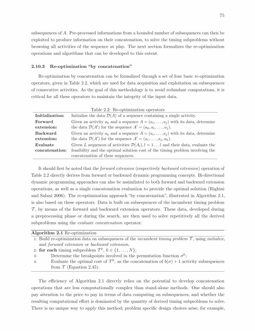
75

subsequences of A. Pre-processed informations from a bounded number of subsequences can then be

exploited to produce information on their concatenation, to solve the timing subproblems without

browsing all activities of the sequence at play. The next section formalizes the re-optimization

operations and algorithms that can be developed to this extent.

2.10.3 Re-optimization “by concatenation”

Re-optimization by concatenation can be formalized through a set of four basic re-optimization

operators, given in Table 2.2, which are used for data acquisition and exploitation on subsequences

of consecutive activities. As the goal of this methodology is to avoid redundant computations, it is

critical for all these operators to maintain the integrity of the input data.

Table 2.2: Re-optimization operators

Initialization: Initialize the data D(A) of a sequence containing a single activity.

Forwardextension:

Given an activity ak and a sequence A = (ai, . . . , aj) with its data, determinethe data D(A′) for the sequence A′ = (ak, ai, . . . , aj).

Backwardextension:

Given an activity ak and a sequence A = (ai, . . . , aj) with its data, determinethe data D(A′) for the sequence A′ = (ai, . . . , aj , ak).

Evaluateconcatenation:

Given L sequences of activities D(Al), l = 1 . . . l and their data, evaluate thefeasibility and the optimal solution cost of the timing problem involving theconcatenation of these sequences.

It should first be noted that the forward extension (respectively backward extension) operation of

Table 2.2 directly derives from forward or backward dynamic programming concepts. Bi-directional

dynamic programming approaches can also be assimilated to both forward and backward extension

operations, as well as a single concatenation evaluation to provide the optimal solution (Righini

and Salani 2006). The re-optimization approach “by concatenation”, illustrated in Algorithm 2.1,

is also based on these operators. Data is built on subsequences of the incumbent timing problem

T , by means of the forward and backward extension operators. These data, developed during

a preprocessing phase or during the search, are then used to solve repetitively all the derived

subproblems using the evaluate concatenation operator.

Algorithm 2.1 Re-optimization

1: Build re-optimization data on subsequences of the incumbent timing problem T , using initialize,and forward extension or backward extension.

2: for each timing subproblem T k, k ∈ {1, . . . , N};3: Determine the breakpoints involved in the permutation function σk;4: Evaluate the optimal cost of T k, as the concatenation of b(σ) + 1 activity subsequences

from T (Equation 2.45).

The efficiency of Algorithm 2.1 directly relies on the potential to develop concatenation

operations that are less computationally complex than stand-alone methods. One should also

pay attention to the price to pay in terms of data computing on subsequences, and whether the

resulting computational effort is dominated by the quantity of derived timing subproblems to solve.

There is no unique way to apply this method; problem specific design choices arise, for example,

76

when determining the nature of the data, the subsequences on which it is computed, as well as the

phases dedicated to data computation.

We therefore illustrate an application in neighborhood search for routing problems with time

constraints on routes. In this context, a local search improvement procedure based on sequence

changes leads to a number of timing subproblems proportional to the number of neighborhood

solutions to explore. The number of derived timing subproblems is often N = Ω(n2) in the VRP or

scheduling literature, and the derived activity sequences do not involve the concatenation of more

than k = 2, 3 or 4 subsequences of the original problem.

The overall complexity of a neighborhood exploration, when solving each timing subproblem

independently, isNc(T ), c(T ) being the computational complexity of one stand-alone timing solution

procedure. A straightforward re-optimization approach consists in exhaustively computing the data

for each of the n(n−1) subsequences of consecutive activities from T , and then use it to evaluate all

moves. Data computation is straightforward to perform in O(n2c(I)+n2c(F/B)). c(I) and c(F/B)

stand for the computational complexity of initialization, and forward or backward extension,

respectively. The overall complexity of the new neighborhood exploration procedure is thus

O(n2c(I) + n2c(F/B) +Nc(EC)), c(EC) being the complexity for evaluating the concatenation of

less than 4 subsequences. Assuming that N = Ω(n2), the computational complexity of neighborhood

evaluation becomes O(N [c(I) + c(F/B) + c(EC)]) for re-optimization methods instead of Nc(T )

for independent solving. Re-optimization operators being less computationally complex than

stand-alone methods, the resulting approach is likely to lead to reduced computational effort.

Concatenation operators involving more than two sequences are not actually available or not

computationally suitable for efficient re-optimization for some settings such as {|MTW} and most

problems with two-dimensional features. In this case, forward and backward propagation may

be used along with concatenations of two subsequences only to perform the timing subproblem

evaluations. Such an example is given by the lexicographic search of Savelsbergh (1985), which

enables to evaluate timing subproblems associated to well-known neighborhoods for vehicle routing

problems exclusively by means of concatenation of two subsequences. Designing efficient evaluation

orders in such contexts becomes a problem dependent issue, clearly impacted by the complexity of

the operators at hand, and the nature of the permutations involved.

Finally, if the concatenation of many subsequences can be operated efficiently, but data creation

constitutes the bottleneck in terms of computational effort, the subset of subsequences involved

can be restricted to O(n4/3) or O(n8/7), using the hierarchical approach of Irnich (2008a).

The relevant data to compute can also be tailored relatively to the neighborhoods at play. For

example, the 2-opt* move presented in Figure 2.7 involves only the concatenation of subsequences

containing the first or last activity, which we call prefix or suffix subsequences. The number of such

subsequences requiring data computation is thus reduced to O(n).

2.10.4 General literature on the topic

A large range of vehicle routing and scheduling problems are addressed using local search on

sequences. Serial timing issues thus frequently arise in these fields.

77

Following the seminal work of Savelsbergh (1985, 1992), Kindervater and Savelsbergh (1997)

proposed a framework to manage several constraints on vehicle routes, such as precedence constraints,

time windows, collection and deliveries under capacity constraints. Several of these constraints are

explicitly, or can be assimilated to, timing features. To perform efficient feasibility checking, the

authors develop global variables on partial routes, which are used in concatenation operations to

evaluate moves consisting of a constant number of edge exchanges. Move evaluations are performed

in lexicographic order to allow calculation of the global variables through the search.

Cordone (2000) and Duhamel (2001) report similar concepts of global data management on

subsequences and concatenation operators. Although these methodologies are essentially dedicated

to the VRPTW, they explore different possibilities related to the concept of macro-nodes. Indeed,

when the information developed on subsequences has the same structure as the problem data on

activities, subsequences of activities can be replaced by equivalent single activities during timing

resolution. Concatenation concepts in this case enable to temporarily reduce the problem size

by collapsing nodes into “macro-nodes”, opening the way to algorithms based on aggregation of

activities and multi-level approaches (Bean et al. 1987, Walshaw 2002, Elhallaoui et al. 2005).

Campbell and Savelsbergh (2004) presented a compilation of efficient insertion heuristics for

many vehicle routing problems with additional characteristics such as shift time limits, variable

delivery quantities, fixed and variable delivery times, and multiple routes per vehicle. These

methods iteratively create solutions by adding customers to the routes. The authors show that by

managing global data on the routes, the cost of feasibility of customer insertions can be evaluated

in amortized O(1) for many of these settings.

A rich body of dynamic programming-based timing algorithms is also presented in Ibaraki et al.

(2005), Hashimoto et al. (2006, 2008), Hashimoto (2008), Ibaraki et al. (2008), and Hashimoto

et al. (2010). Forward and backward propagation is used, with an additional “connect” operator to

manage concatenation of two subsequences, thus leading to efficient re-optimization approaches by

concatenation for several timing problems involving Piecewise Linear (PiL) functions.

The framework of Desaulniers et al. (1998) models many constraints and objectives on sequences

of activities as resources that are subject to window constraints, and are extended from one activity

to the next by means of resource extension functions (REFs). This framework proved extremely

efficient to model many crew scheduling and routing problems and solve them by column generation

(Desaulniers et al. 2005). It has also been recently extended by Irnich (2008a,b) to perform

efficient neighborhood search under various constraints on routes, such as load dependent costs,

simultaneous pickup and deliveries, maximum waiting and duty times. To that extent, REFs

“generalized to segments” are built on subsequences to characterize their resource consumption.

Inverse REFs are defined to give an upper bound on the resource consumptions that allow the

sequence to be processed. Developing this data on subsequences enables then to evaluate efficiently

the cost or feasibility of local search moves. This framework, however, requires rather restrictive

conditions: the existence of REFs that can be generalized to subsequences and inversed. These

conditions are satisfied only by a limited subset of the timing problems and features introduced

previously, such as {|TW}, {|MTW} or {DUR|TW}.

78

Several general methodologies thus exist in the literature to tackle timing problems within a

neighborhood search context. However, these approaches are restricted by the types of concate-

nations allowed, the assumptions made on features, or the applicability of the models to a wide

range of constraints. The timing formalism we propose and its generalization to re-optimization

procedures by concatenation, following the concepts of Kindervater and Savelsbergh (1997), is less

specialized and thus can encompass a wider range of timing settings and methods. As shown in the

next sections, this framework unifies previous successful concepts, and provides a line of thought

for the development of efficient algorithms for various timing problems. It can also be viewed as a

generalization of Irnich (2008a,b) concepts applied to timing problems. Indeed, generalized REFs

and their inverse provide, when they exist, the suitable data for re-optimization.

2.10.5 Re-optimization algorithms

We now review and analyze re-optimization approaches for main timing features and problems.

As in the first part of this paper, the analysis is organized by increasing order of complexity and

feature dimensions, starting with single-dimensional features in Sections 2.10.5.1 to 2.10.5.5, and

finishing with two-dimensional features in Sections 2.10.5.6 to 2.10.5.8. For each timing setting

we describe the re-optimization data, as well as the operators that can be used for forward and

backward data computation and for evaluating the concatenation of several subsequences. These

operators can be used within Algorithm 2.1 to develop efficient re-optimization approaches by

concatenation.

2.10.5.1 Constant activity costs & cumulative resources.

In presence of constant activity costs or, more generally, in presence of a cumulated resource

such as distance, load or time with a global constraint, evaluating the total cost of a solution from

scratch would involve to browse each activity and cumulate the costs, or the resource consumption,

resulting in an O(n) complexity. To perform more efficient evaluations, a simple re-optimization

approach involves applying Algorithm 2.1 with the following data and operators.

Data. Partial cost C(Ai) (or resource consumed) by each subsequence Ai.

Data computation. Cumulating the cost (or resource consumption) on the subsequence.

Evaluate concatenation. Cumulating the partial costs (or resource consumptions) on

subsequences: C(A1 ⊕ · · · ⊕Ak) =∑C(Ai).

The evaluation of the concatenation of a bounded number of subsequences can thus be performed

in a bounded number of operations, leading to O(1) complexity for move evaluation when the

data is available. Data can be processed in amortized constant time for each move during a local

search procedure for many classic neighborhoods, using a lexicographic order (Kindervater and

Savelsbergh 1997) for move evaluation, or developed in a preprocessing phase for a complexity of

O(n2), which is often dominated by the neighborhood size.

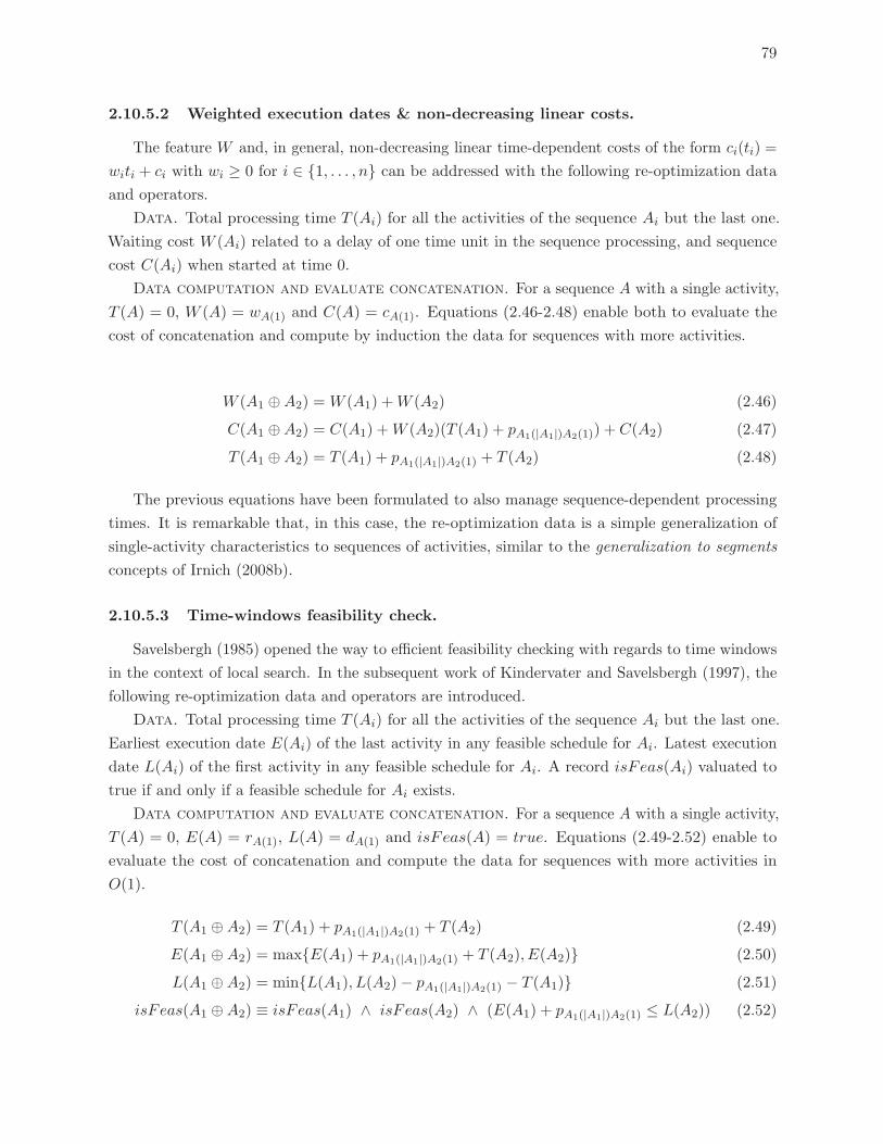
79

2.10.5.2 Weighted execution dates & non-decreasing linear costs.

The feature W and, in general, non-decreasing linear time-dependent costs of the form ci(ti) =

witi + ci with wi ≥ 0 for i ∈ {1, . . . , n} can be addressed with the following re-optimization data

and operators.

Data. Total processing time T (Ai) for all the activities of the sequence Ai but the last one.

Waiting cost W (Ai) related to a delay of one time unit in the sequence processing, and sequence

cost C(Ai) when started at time 0.

Data computation and evaluate concatenation. For a sequence A with a single activity,

T (A) = 0, W (A) = wA(1) and C(A) = cA(1). Equations (2.46-2.48) enable both to evaluate the

cost of concatenation and compute by induction the data for sequences with more activities.

W (A1 ⊕A2) =W (A1) +W (A2) (2.46)

C(A1 ⊕A2) = C(A1) +W (A2)(T (A1) + pA1(|A1|)A2(1)) + C(A2) (2.47)

T (A1 ⊕A2) = T (A1) + pA1(|A1|)A2(1) + T (A2) (2.48)

The previous equations have been formulated to also manage sequence-dependent processing

times. It is remarkable that, in this case, the re-optimization data is a simple generalization of

single-activity characteristics to sequences of activities, similar to the generalization to segments

concepts of Irnich (2008b).

2.10.5.3 Time-windows feasibility check.

Savelsbergh (1985) opened the way to efficient feasibility checking with regards to time windows

in the context of local search. In the subsequent work of Kindervater and Savelsbergh (1997), the

following re-optimization data and operators are introduced.

Data. Total processing time T (Ai) for all the activities of the sequence Ai but the last one.

Earliest execution date E(Ai) of the last activity in any feasible schedule for Ai. Latest execution

date L(Ai) of the first activity in any feasible schedule for Ai. A record isFeas(Ai) valuated to

true if and only if a feasible schedule for Ai exists.


T (A) = 0, E(A) = rA(1), L(A) = dA(1) and isFeas(A) = true. Equations (2.49-2.52) enable to

evaluate the cost of concatenation and compute the data for sequences with more activities in

O(1).

T (A1 ⊕A2) = T (A1) + pA1(|A1|)A2(1) + T (A2) (2.49)

E(A1 ⊕A2) = max{E(A1) + pA1(|A1|)A2(1) + T (A2), E(A2)} (2.50)

L(A1 ⊕A2) = min{L(A1), L(A2)− pA1(|A1|)A2(1) − T (A1)} (2.51)

isFeas(A1 ⊕A2) ≡ isFeas(A1) ∧ isFeas(A2) ∧ (E(A1) + pA1(|A1|)A2(1) ≤ L(A2)) (2.52)

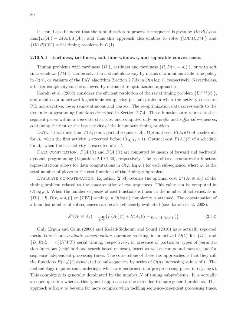
80

It should also be noted that the total duration to process the sequence is given by DUR(Ai) =

max{E(Ai) − L(Ai), T (Ai), and thus this approach also enables to solve {|DUR,TW} and

{DUR|TW} serial timing problems in O(1).

2.10.5.4 Earliness, tardiness, soft time-windows, and separable convex costs.

Timing problems with tardiness {D|}, earliness and tardiness {R,D(ri = di)|}, or with soft

time windows {TW |} can be solved in a stand-alone way by means of a minimum idle time policy

in O(n), or variants of the PAV algorithm (Section 2.7.3) in O(n log n), respectively. Nevertheless,

a better complexity can be achieved by means of re-optimization approaches.

Ibaraki et al. (2008) considers the efficient resolution of the serial timing problem {Σccvx(t)|},and attains an amortized logarithmic complexity per sub-problem when the activity costs are

PiL non-negative, lower semicontinuous and convex. The re-optimization data corresponds to the

dynamic programming functions described in Section 2.7.4. These functions are represented as

segment pieces within a tree data structure, and computed only on prefix and suffix subsequences,

containing the first or the last activity of the incumbent timing problem.

Data. Total duty time T (Ai) on a partial sequence Ai. Optimal cost F (Ai)(t) of a schedule

for Ai, when the first activity is executed before t(tAi(1) ≤ t). Optimal cost B(Ai)(t) of a schedule

for Ai, when the last activity is executed after t.

Data computation. F (Ai)(t) and B(Ai)(t) are computed by means of forward and backward

dynamic programming (Equations 2.19-2.20), respectively. The use of tree structures for function

representations allows for data computations in O(ϕc logϕc) for each subsequence, where ϕc is the

total number of pieces in the cost functions of the timing subproblem.

Evaluate concatenation. Equation (2.53) returns the optimal cost Z∗(A1 ⊕ A2) of the

timing problem related to the concatenation of two sequences. This value can be computed in

O(logϕc). When the number of pieces of cost functions is linear in the number of activities, as in

{D|}, {R,D(ri = di)|} or {TW |} settings, a O(log n) complexity is attained. The concatenation of

a bounded number of subsequences can be also efficiently evaluated (see Ibaraki et al. 2008).

Z∗(A1 ⊕A2) = mint≥0

{F (A1)(t) +B(A2)(t+ pA1(|A1|)A2(1))} (2.53)

Only Ergun and Orlin (2006) and Kedad-Sidhoum and Sourd (2010) have actually reported

methods with an evaluate concatenation operator working in amortized O(1) for {D|} and

{D,R(di = ri)|NWT} serial timing, respectively, in presence of particular types of permuta-

tion functions (neighborhood search based on swap, insert as well as compound moves), and for

sequence-independent processing times. The cornerstone of these two approaches is that they call

the functions B(A2)(t) associated to subsequences by series of O(n) increasing values of t. The

methodology requires some orderings, which are performed in a pre-processing phase in O(n log n).

This complexity is generally dominated by the number N of timing subproblems. It is actually

an open question whereas this type of approach can be extended to more general problems. This

approach is likely to become far more complex when tackling sequence-dependent processing times,

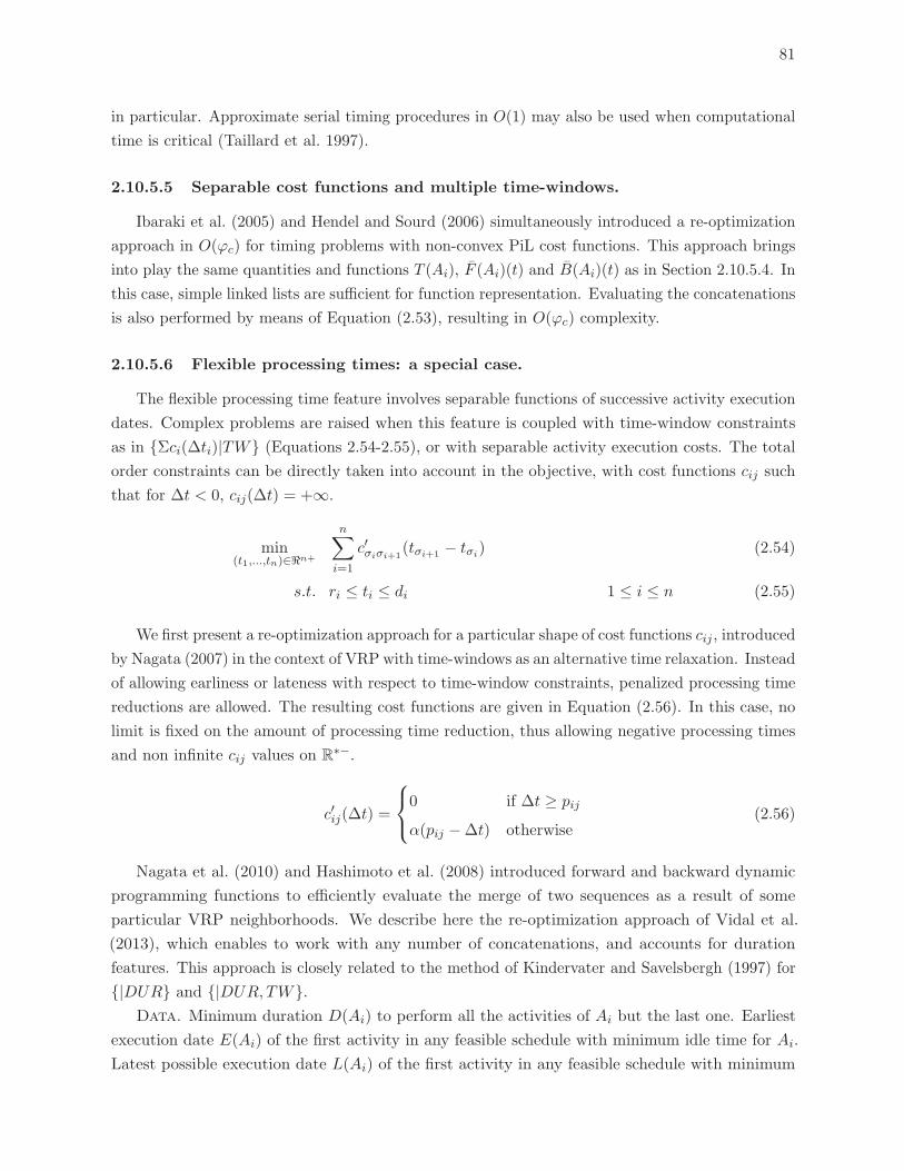
81

in particular. Approximate serial timing procedures in O(1) may also be used when computational

time is critical (Taillard et al. 1997).

2.10.5.5 Separable cost functions and multiple time-windows.

Ibaraki et al. (2005) and Hendel and Sourd (2006) simultaneously introduced a re-optimization

approach in O(ϕc) for timing problems with non-convex PiL cost functions. This approach brings

into play the same quantities and functions T (Ai), F (Ai)(t) and B(Ai)(t) as in Section 2.10.5.4. In

this case, simple linked lists are sufficient for function representation. Evaluating the concatenations

is also performed by means of Equation (2.53), resulting in O(ϕc) complexity.

2.10.5.6 Flexible processing times: a special case.

The flexible processing time feature involves separable functions of successive activity execution

dates. Complex problems are raised when this feature is coupled with time-window constraints

as in {Σci(Δti)|TW} (Equations 2.54-2.55), or with separable activity execution costs. The total

order constraints can be directly taken into account in the objective, with cost functions cij such

that for Δt < 0, cij(Δt) = +∞.

min(t1,...,tn)∈�n+

n∑i=1

c′σiσi+1(tσi+1 − tσi) (2.54)

s.t. ri ≤ ti ≤ di 1 ≤ i ≤ n (2.55)

We first present a re-optimization approach for a particular shape of cost functions cij , introduced

by Nagata (2007) in the context of VRP with time-windows as an alternative time relaxation. Instead

of allowing earliness or lateness with respect to time-window constraints, penalized processing time

reductions are allowed. The resulting cost functions are given in Equation (2.56). In this case, no

limit is fixed on the amount of processing time reduction, thus allowing negative processing times

and non infinite cij values on R∗−.

c′ij(Δt) =

⎧⎨⎩0 if Δt ≥ pij

α(pij −Δt) otherwise(2.56)

Nagata et al. (2010) and Hashimoto et al. (2008) introduced forward and backward dynamic

programming functions to efficiently evaluate the merge of two sequences as a result of some

particular VRP neighborhoods. We describe here the re-optimization approach of Vidal et al.

(2013), which enables to work with any number of concatenations, and accounts for duration

features. This approach is closely related to the method of Kindervater and Savelsbergh (1997) for

{|DUR} and {|DUR, TW}.Data. Minimum duration D(Ai) to perform all the activities of Ai but the last one. Earliest

execution date E(Ai) of the first activity in any feasible schedule with minimum idle time for Ai.

Latest possible execution date L(Ai) of the first activity in any feasible schedule with minimum

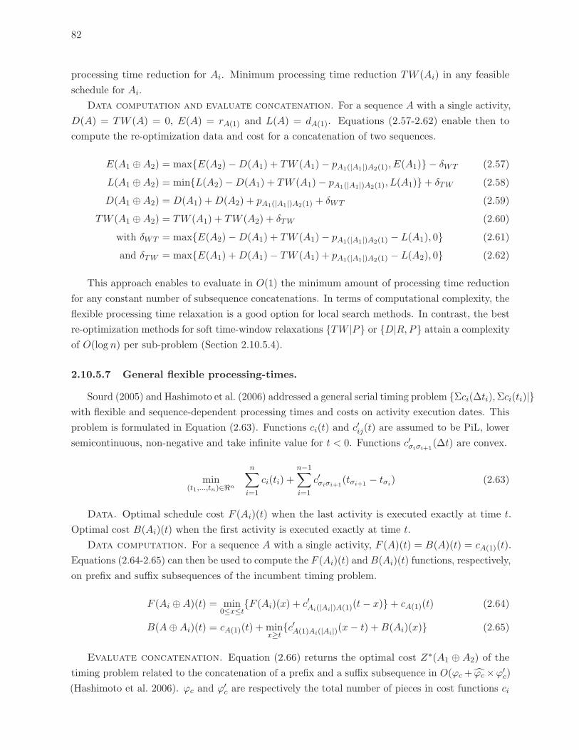
82

processing time reduction for Ai. Minimum processing time reduction TW (Ai) in any feasible

schedule for Ai.


D(A) = TW (A) = 0, E(A) = rA(1) and L(A) = dA(1). Equations (2.57-2.62) enable then to

compute the re-optimization data and cost for a concatenation of two sequences.

E(A1 ⊕A2) = max{E(A2)−D(A1) + TW (A1)− pA1(|A1|)A2(1), E(A1)} − δWT (2.57)

L(A1 ⊕A2) = min{L(A2)−D(A1) + TW (A1)− pA1(|A1|)A2(1), L(A1)}+ δTW (2.58)

D(A1 ⊕A2) = D(A1) +D(A2) + pA1(|A1|)A2(1) + δWT (2.59)

TW (A1 ⊕A2) = TW (A1) + TW (A2) + δTW (2.60)

with δWT = max{E(A2)−D(A1) + TW (A1)− pA1(|A1|)A2(1) − L(A1), 0} (2.61)

and δTW = max{E(A1) +D(A1)− TW (A1) + pA1(|A1|)A2(1) − L(A2), 0} (2.62)

This approach enables to evaluate in O(1) the minimum amount of processing time reduction

for any constant number of subsequence concatenations. In terms of computational complexity, the

flexible processing time relaxation is a good option for local search methods. In contrast, the best

re-optimization methods for soft time-window relaxations {TW |P} or {D|R,P} attain a complexity

of O(log n) per sub-problem (Section 2.10.5.4).

2.10.5.7 General flexible processing-times.

Sourd (2005) and Hashimoto et al. (2006) addressed a general serial timing problem {Σci(Δti),Σci(ti)|}with flexible and sequence-dependent processing times and costs on activity execution dates. This

problem is formulated in Equation (2.63). Functions ci(t) and c′ij(t) are assumed to be PiL, lower

semicontinuous, non-negative and take infinite value for t < 0. Functions c′σiσi+1(Δt) are convex.


n∑i=1

ci(ti) +

n−1∑i=1

c′σiσi+1(tσi+1 − tσi) (2.63)

Data. Optimal schedule cost F (Ai)(t) when the last activity is executed exactly at time t.

Optimal cost B(Ai)(t) when the first activity is executed exactly at time t.

Data computation. For a sequence A with a single activity, F (A)(t) = B(A)(t) = cA(1)(t).

Equations (2.64-2.65) can then be used to compute the F (Ai)(t) and B(Ai)(t) functions, respectively,

on prefix and suffix subsequences of the incumbent timing problem.

F (Ai ⊕A)(t) = min0≤x≤t

{F (Ai)(x) + c′Ai(|Ai|)A(1)(t− x)}+ cA(1)(t) (2.64)

B(A⊕Ai)(t) = cA(1)(t) + minx≥t

{c′A(1)Ai(|Ai|)(x− t) +B(Ai)(x)} (2.65)

Evaluate concatenation. Equation (2.66) returns the optimal cost Z∗(A1 ⊕ A2) of the

timing problem related to the concatenation of a prefix and a suffix subsequence in O(ϕc + ϕc ×ϕ′c)

(Hashimoto et al. 2006). ϕc and ϕ′c are respectively the total number of pieces in cost functions ci

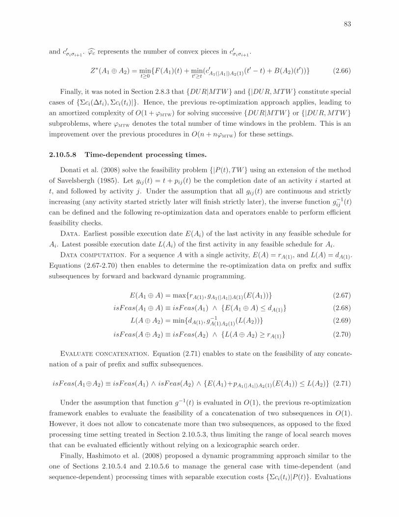
83

and c′σiσi+1. ϕc represents the number of convex pieces in c′σiσi+1

.

Z∗(A1 ⊕A2) = mint≥0

{F (A1)(t) + mint′≥t

(c′A1(|A1|)A2(1)(t′ − t) +B(A2)(t

′))} (2.66)

Finally, it was noted in Section 2.8.3 that {DUR|MTW} and {|DUR,MTW} constitute special

cases of {Σci(Δti),Σci(ti)|}. Hence, the previous re-optimization approach applies, leading to

an amortized complexity of O(1 +ϕmtw) for solving successive {DUR|MTW} or {|DUR,MTW}subproblems, where ϕmtw denotes the total number of time windows in the problem. This is an

improvement over the previous procedures in O(n+ nϕmtw) for these settings.

2.10.5.8 Time-dependent processing times.

Donati et al. (2008) solve the feasibility problem {|P (t), TW} using an extension of the method

of Savelsbergh (1985). Let gij(t) = t + pij(t) be the completion date of an activity i started at

t, and followed by activity j. Under the assumption that all gij(t) are continuous and strictly

increasing (any activity started strictly later will finish strictly later), the inverse function g−1ij (t)

can be defined and the following re-optimization data and operators enable to perform efficient

feasibility checks.

Data. Earliest possible execution date E(Ai) of the last activity in any feasible schedule for

Ai. Latest possible execution date L(Ai) of the first activity in any feasible schedule for Ai.

Data computation. For a sequence A with a single activity, E(A) = rA(1), and L(A) = dA(1).

Equations (2.67-2.70) then enables to determine the re-optimization data on prefix and suffix

subsequences by forward and backward dynamic programming.

E(A1 ⊕A) = max{rA(1), gA1(|A1|)A(1)(E(A1))} (2.67)

isFeas(A1 ⊕A) ≡ isFeas(A1) ∧ {E(A1 ⊕A) ≤ dA(1)} (2.68)

L(A⊕A2) = min{dA(1), g−1A(1)A2(1)

(L(A2))} (2.69)

isFeas(A⊕A2) ≡ isFeas(A2) ∧ {L(A⊕A2) ≥ rA(1)} (2.70)

Evaluate concatenation. Equation (2.71) enables to state on the feasibility of any concate-

nation of a pair of prefix and suffix subsequences.

isFeas(A1⊕A2) ≡ isFeas(A1) ∧ isFeas(A2) ∧ {E(A1)+pA1(|A1|)A2(1)(E(A1)) ≤ L(A2)} (2.71)

Under the assumption that function g−1(t) is evaluated in O(1), the previous re-optimization

framework enables to evaluate the feasibility of a concatenation of two subsequences in O(1).

However, it does not allow to concatenate more than two subsequences, as opposed to the fixed

processing time setting treated in Section 2.10.5.3, thus limiting the range of local search moves

that can be evaluated efficiently without relying on a lexicographic search order.

Finally, Hashimoto et al. (2008) proposed a dynamic programming approach similar to the

one of Sections 2.10.5.4 and 2.10.5.6 to manage the general case with time-dependent (and

sequence-dependent) processing times with separable execution costs {Σci(ti)|P (t)}. Evaluations

84

of concatenations of pairs of subsequences A1 and A2 are performed in O(ϕc + ϕp), where ϕc and

ϕp denote respectively the total number of pieces in the cost and processing-time functions.

2.10.6 Summary and perspectives on re-optimization

Table 2.3 summarizes the complexity of stand-alone resolution and re-optimization operations

for the main timing settings in the literature. The leftmost column lists the problems, while the

next block of columns present stand-alone approaches and their complexity. Following to the

right, the next columns are dedicated to summarize re-optimization approaches, the complexity of

forward and backward data construction, “F/B”, the complexity of concatenation of two, “C2”,

and more than two subsequences, “C3+”, if available. Column “Sd” finally indicates whether

the re-optimization approach enables to tackle problems with sequence-dependent parameters.

Additional assumptions on the problems are listed in the last column.

Re-optimization has clearly proven useful to address more efficiently several timing settings,

reducing in many case the computational complexity by a factor of n or ϕc. Still, the complexity

gain remains smaller in some particular cases. Solving the timing problem {D|R} from scratch, for

example, can be done in O(n) but the best re-optimization approach attains only a complexity of

O(logn). This latter timing problem takes a prominent role in many VRP heuristics that allow

time-constraints relaxations. Whether a O(1) re-optimization algorithm exists for {D|R} remains

an open question. In addition, no re-optimization algorithm is available, to our knowledge, for

several problems such as {DUR|MTW}, {|DUR,MTW}, {DUR|TW,P (t)}, {|TL, TW} and

{DUR > D > TL|R}. Finally, another promising research path concerns the study of re-

optimization data and concatenation operators involving more than two subsequences and their

application to sequence-dependent problems. Such operators are still missing in several cases such

as {Σci(ti)|P (t)} or {Σccvxi (Δti),Σci(ti)|}, but are necessary to achieve high-performance local

searches in many combinatorial optimization problems with time features.

2.11 General conclusion

In this chapter, a rich body of problems with time characteristics and totally ordered variables

has been identified and classified. Many algorithms from different fields of research were analyzed

to identify key problem features and main solution concepts. As timing subproblems frequently

arise in the context of local search, both the stand-alone resolution of problems, and the efficient

resolution of series of problems by means of re-optimization approaches were analyzed. A general

re-optimization framework based on decomposition and recombination of sequences was introduced,

and links to other re-optimization approaches were highlighted.

A subset of timing methods, originating from various research fields, and constituting the

actual state-of-the-art for timing problems with different features, has been identified. These

algorithms are a keystone for addressing many rich combinatorial optimization problems with time

characteristics, for which the timing sub-problem represents the core of the originality and difficulty.

Having a library of timing algorithms at hand opens also the door to further developments on

more generic solvers that relegate the problem difficulties to known subproblems and methods.

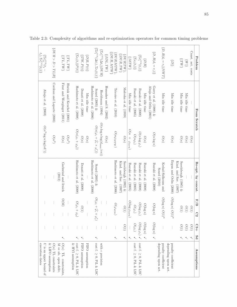
85

Table 2.3: Complexity of algorithms and re-optimization operators for common timing problemsPro

blem

Fro

mScra

tchRe-opt.

byconcat.

F/B

C2

C3+

Sd

Assu

mptio

ns

Const.

act.

costs

—O(n)

—O(1)

O(1)

�{W

|}Min

idle

time

O(n)

—O(1)

O(1)

�{|T

W}

Min

idle

time

O(n)

Savelsb

ergh(1985)

&Kind.an

dSav.(1997)

O(1)

O(1)

�

{D|}

Min

idle

time

O(n)

Ergunan

dOrlin

(2006)

O(lo

gn)O(1)*

—penalty

coeffi

cient

dep

endingupon

act.

{D,R

(di=ri )|N

WT}

Min

idle

time

O(n)

Kedad

-Sidhou

man

dSou

rd(2010)

O(lo

gn)O(1)*

—penalty

coeffi

cient

dep

endingupon

act.

{D,R

(di=ri )|}

Garey

etal.

(1988)&

Ahuja

andOrlin

(2001)

O(n

logn)

Ibarak

iet

al.(2008)

O(lo

gn)

O(lo

gn)

�

{D|R

}Min

idle

time

O(n)

Ibarak

iet

al.(2008)

O(lo

gn)

O(lo

gn)

�{Σccvx

i(ti )|}

Ibarakiet

al.(2008)

O(n

logϕc )

Ibarak

iet

al.(2008)

O(lo

gϕc )

O(lo

gϕc )�

costf.≥

0,PiL

&LSC

{Σci (ti )|}

Ibarakiet

al.(2005)

O(nϕc )

Ibarak

iet

al.(2005)

O(ϕ

c )O(ϕ

c )�

costf.≥

0,PiL

&LSC

{|MTW

}Min

idle

time

O(n

+ϕmtw)

Ibarak

iet

al.(2005)

O(lo

gϕmtw)

—�

{DUR|TW

},

{|DUR,TW

}Malcolm

etal.

(1959)O(n)

Savelsb

ergh(1992)

&Kind.an

dSav.(1997)

O(1)

O(1)

�

{DUR|M

TW

},{|D

UR,M

TW

}Trico

ireet

al.(2010)

O(nϕM

TW)

Hash

imoto

etal.

(2006)O(ϕ

mtw)

—�

{|IDL,TW

}Hunsak

eran

dS.(2002)

O(n)

——

——

{Σccvx

i(Δti )|D

UR}

Hochbaum

(1994)

O(n

lognlog(d

max /εn

))—

——

—with

εprecision

{Σccvx

i(Δti ),Σ

ci (ti )|}

Sourd

(2005)&

Hashim

oto

etal.

(2006)O(n(ϕ

c+ϕc ×

ϕ′c ))

Sou

rd(2005)

&Hash

imoto

etal.

(2006)O(ϕ

c+ϕc ×

ϕ′c )

—�

costf.≥

0,PiL

&LSC

{D|R,P

(t)}Min

idle

time

O(n)

——

——

FIFO

assumption

{|TW,P

(t)}Donatiet

al.(2008)

O(n)

Donatiet

al.(2008)

O(1)

—�

FIFO

assumption

{Σci (ti )|P

(t)}Hashim

oto

etal.

(2008)O(n(ϕ

c+ϕp ))

Hash

imoto

etal.

(2008)O(ϕ

c+ϕp )

—�

costf.≥

0,PiL

&LSC

&HYIassu

mption

{|TL,TW

}Hurin

kandKeuchel

(2001)O(n

3)—

——

—

{|TL,TW

}Firat

andWoegin

ger(2011)

O(n)

Gsch

windan

dIrn

ich(2012)

O(M

)—

—�

O(n)

TL

constra

ints,

M⇔

nb.op

endeliv

.

{DUR>D>TL|R

}Cord

eauan

dLap

orte(2003)

O(n

2)—

——

—O(n)TLcon

straints

&LIFO

assumption

{Σccvx

ij(tj −

ti ),Σccvx

i(ti )|}

Ahuja

etal.

(2003)O(n

3lognlog(nU))

——

——

Uisan

upper

bou

ndof

execu

tiondates

86

Many interesting avenues of research arise as a result of this work. First of all, for several timing

features studied in this article, more efficient stand-alone, re-optimization methods and complexity

lower bounds should be investigated (Section 2.10.6). The impact of sequence-dependency on re-

optimization is also another interesting concern, as sequence-dependency constitutes a fundamental

delimitation between routing-related problems and scheduling settings. Identifying precisely its

impact on re-optimization procedures would lead to better insights on local search-based methods

for these two important classes of problems. Finally, even if the focus of this paper was on time

characteristics, other cumulative resources such as loads, energy or workforce, lead to similar

features and models. The work performed on timing can thus prove useful for an even broader

range of applications.

Deuxieme partie

METAHEURISTIQUES POUR LES

PROBLEMES DE TOURNEES DE

VEHICULES

87

CHAPITRE 3

UN ALGORITHME GENETIQUE HYBRIDE POUR LES PROBLEMES DE

TOURNEES DE VEHICULES MULTI-DEPOTS ET PERIODIQUES


En relation aux concepts etudies dans les deux revues de litterature, des etudes experimentales

poussees sont developpees afin de proposer des concepts meta-heuristiques performants pour les

variantes du VRP, et ainsi contribuer au deuxieme defi enonce dans le plan de these. Ces travaux ont

abouti a la creation d’un algorithme genetique hybride a controle adaptatif de diversite (HGSADC)

extremement efficace pour les VRP periodiques, multi-depots eventuellement combinees, ainsi que

le VRP classique. Cet algorithme hybride combine l’exploration large des methodes evolutionnaires

a base de populations, les capacites d’amelioration agressive des meta-heuristiques a voisinage, les

relaxations de contraintes pour cibler les frontieres de non-faisabilite, et des methodes avancees de

gestion de la diversite dans la population. HGSADC reinterprete le concept de survie du plus apte,

en evaluant les individus non pas seulement en relation a la qualite de la solution associee, mais

aussi en relation a leur contribution dans la diversite de la population. Cette strategie permet de

preserver la variete de l’information presente dans la population sous forme de materiel genetique,

et de reduire les risques de convergence prematuree, pour explorer de vastes regions prometteuses

de l’espace de recherche. Des etudes experimentales approfondies sur des variantes de VRP avec

multiple depots et multiple periodes montrent la grande performance de la methode, en termes

de qualite de solution et efficacite de calcul. Pour tous les jeux de tests de la litterature sur ces

problemes, HGSADC retrouve soit les meilleures solutions de la litterature, y compris celles qui

sont prouvees optimales, ou de meilleures solutions. Les meilleurs resultats de la litterature sont

aussi obtenus pour le VRP classique.

3.2 Article III : A hybrid genetic algorithm for multi-depot and periodic vehicle

routing problems

Ce chapitre a fait l’objet d’une publication sous forme d’article de journal : Vidal,

T., Crainic, T. G., Gendreau, M., Lahrichi, N., & Rei, W. (2012). A Hybrid Genetic

Algorithm for Multi-Depot and Periodic Vehicle Routing Problems. Operations Re-

search, 60(3), 611–624.

Abstract: We propose an algorithmic framework that successfully addresses three vehicle routing

problems: the multi-depot VRP, the periodic VRP, and the multi-depot periodic VRP with

capacitated vehicles and constrained route duration. The meta-heuristic combines the explo-

ration breadth of population-based evolutionary search, the aggressive-improvement capabilities

of neighborhood-based meta-heuristics, and advanced population-diversity management schemes.

Extensive computational experiments show that the method performs impressively, in terms of

90

computational efficiency and solution quality, identifying either the best known solutions, including

the optimal ones, or new best solutions for all currently available benchmark instances for the three

problem classes. The proposed method also proves extremely competitive for the capacitated VRP.

Keywords: Multi-depot multi-period vehicle routing problems, hybrid population-based meta-

heuristics, adaptive population diversity management

3.3 Introduction

Vehicle Routing Problem (VRP) formulations are used to model an extremely broad range of

issues in many application fields, transportation, supply chain management, production planning,

and telecommunications, to name but a few (Toth and Vigo 2002a, Hoff et al. 2010). Not

surprisingly, starting with the seminal work of Dantzig and Ramser (1959), routing problems make

up an extensively and continuously studied field, as illustrated by numerous conferences, survey

articles (e.g., Cordeau et al. 2007, Laporte 2009), and books (Toth and Vigo 2002a, Golden et al.

2008).

Surveying the literature one notices, however, that not all problem classes have received an

equal nor adequate degree of attention. This is the case for the problems with multiple depots and

periods. A second general observation is that most methodological developments target a particular

problem variant, the capacitated VRP (CVRP) or the VRP with time windows (VRPTW ), for

example, very few contributions aiming to address a broader set of problem settings. This also

applies to the problem classes targeted in this paper.

Our objective is to contribute toward addressing these two challenges. We propose an algorithmic

framework that successfully addresses three VRP variants: the multi-depot VRP, MDVRP, the

periodic VRP, PVRP, and the multi-depot periodic VRP, MDPVRP, with capacitated vehicles

and constrained route duration. The literature on these problems is relatively scarce (Francis et al.

2008) despite their relevance to many applications, e.g., raw material supply (Alegre et al. 2007),

refuse collection (Beltrami and Bodin 1974, Russell and Igo 1979, Teixeira et al. 2004, Coene et al.

2010), food collection or distribution (Golden and Wasil 1987, Parthanadee and Logendran 2006),

and maintenance operations (Hadjiconstantinou and Baldacci 1998, Blakeley et al. 2003).

We propose a meta-heuristic that combines the exploration breadth of population-based

evolutionary search, the aggressive-improvement capabilities of neighborhood-based meta-heuristics,

and advanced population-diversity management schemes. The method, that we name Hybrid

Genetic Search with Adaptive Diversity Control (HGSADC ), performs impressively in terms of

both solution quality and computational efficiency. HGSADC outperforms the state-of-the-art

methods for the three problem classes on all currently available benchmark instances, identifying

either the best known solutions, including the optimal ones, or new best solutions. Moreover, with

very limited adaptation, HGSADC proves to be extremely competitive for the CVRP.

The two main contributions of this article are: 1) A new meta-heuristic, which is highly effective

for four important vehicle routing problem classes, the MDVRP, the PVRP, the MDPVRP, and the

CVRP. The method is built on general components that are applicable, provided minor adjustments,

91

to an even wider range of VRP variants. 2) New population-diversity management mechanisms to

allow a broader access to reproduction, while preserving the characteristics of elite solutions. In

this respect, we revisit the traditional survival-of-the-fittest paradigm to enhance the evaluation of

individuals by making it rely on both solution cost and diversity (distance-to-the-others) measures.

Thus, diversity appears as an integral part of the objective, which contrasts with classical diversity-

management procedures that have traditionally imposed diversity constraints for the acceptance of

solutions in the population. Empirical studies show that these new mechanisms do not only avoid

premature population convergence efficiently, but also lead to higher quality solutions in reduced

computation time when compared to traditional approaches. It must be emphasized that the

proposed population-diversity management mechanisms could be applied to almost any problem

that one can solve using population-based evolutionary search methods.

The paper is organized as follows. Section 3.4 states the notation and formal definition of the

three classes of VRPs we address, while the relevant literature is surveyed in Section 3.5. The

proposed meta-heuristic is detailed in Section 3.6, its performances are analyzed in Section 3.7,

and we conclude in Section 3.8.

3.4 Problem Statement

We formally state the MDVRP, PVRP, and MDPVRP, introducing the notation used in this

paper and the transformation of the MDPVRP into a PVRP, which supports the algorithmic

developments.

The CVRP can be defined as follows. Let G = (V,A) be a complete graph with |V| = n+ 1

vertices, divided in two sets V = Vdep ∪ Vcst. The unique vertex v0 ∈ Vdep represents the depot

where the product to be distributed is kept and a fleet of m identical vehicles with capacity Q is

based. Vertices vi ∈ Vcst stand for customers i, i = 1, . . . , n, requiring service and characterized

by a non-negative demand qi and a service duration τi. Arcs aij ∈ A, i, j ∈ V represent the

direct-travel possibility from vi to vj with travel time equal to cij . The duration of a vehicle route

is computed as the total travel and service time required to serve the customers, and is limited to

T . The goal is to design a set of vehicle routes servicing all customers, such that vehicle-capacity

and route-duration constraints are respected, and the total travel time is minimized.

Several depots, d, are available to service customers in the Multi-Depot VRP, m representing

the number of vehicles available at each depot. In this case, vertices v0, . . . , vd make up the set

Vdep, while the remaining vertices Vcst stand for customers. A time dimension is introduced in the

Periodic VRP as route planning is to be performed over a horizon of t periods. Each customer i is

characterized by a service frequency fi, representing the number of visits to be performed during

the t periods, and a list Li of possible visit-period combinations, called patterns. The PVRP aims

to select a pattern for each customer and construct the associated routes to minimize the total

cost over all periods. Finally, the Multi-Depot Periodic VRP extends the two previous problem

settings, asking for the selection of a depot and a visit pattern for each customer, with services in

different periods to the same customer being required to originate at the same depot. The CVRP

is NP-Hard and so are the three problem classes that generalize it and are addressed in this paper.

92

The MDPVRP reduces to a PVRP when d = 1 and to a MDVRP when t = 1. Furthermore, the

three problem settings share similar mathematical structures. We take advantage of this property

and, in the spirit of the problem transformation from MDVRP to PVRP of Cordeau et al. (1997),

we transform a MDPVRP with d depots and t periods into an equivalent PVRP with d× t periods

corresponding to (depot, period) couples. (Appendix II.1 details these mathematical structures and

problem transformations). This transformation provides the means to address the three problem

classes with the same solution method and reduces the number of problem characteristics. Of

course, the method must be computationally efficient to deal with the increased number of periods

and the corresponding increase in problem dimension. As the computational results displayed in

Section 3.7 show, we achieve this goal.

3.5 Literature Review

This section provides a brief literature review of contributions for the PVRP, the MDVRP, and

the MDPVRP. The purpose of this review is twofold. First, to present the most recently proposed

meta-heuristic algorithms, particularly population-based ones, for the considered problems. Second,

to distinguish the leading solution approaches for the three problem settings.

Some population and neighborhood-based meta-heuristics already exist in the PVRP literature.

Drummond et al. (2001) proposed an island-based parallel evolutionary method, which evolves

individuals representing schedules (patterns), the fitness of each individual being obtained by

constructing routes for each period with a savings heuristic. Alegre et al. (2007) proposed a scatter

search procedure designed especially for PVRPs with a large number of periods. As in Drummond

et al. (2001), the core of the method is dedicated to the improvement of visit schedules, while a

neighborhood-based improvement procedure is used to design routes for each period. Contrasting

with the two previous methods, Matos and Oliveira (2004) proposed an ant colony optimization

(ACO) approach that first optimizes routes, then schedules. This ACO method addresses the

PVRP as a VRP, where each customer is duplicated as many times as indicated by its frequency,

the resulting routes being then distributed to periods by solving a graph coloring problem.

Until recently, however, the most successful contributions to this problem were based on the

serial exploration of neighborhoods. The local search approach of Chao et al. (1995) was the

first to use deteriorating moves to escape from poor local optima, and also allow relaxation of

vehicle-capacity limits to enhance the exploration of the solution space. The tabu search proposed

by Cordeau et al. (1997) introduced an innovative guidance scheme, which collects statistics on

customer assignments to periods and vehicle routes in order to penalize recurring assignments

within the solutions obtained and, thus, gradually diversify the search. For a long period of time,

this method stood as the state-of-the-art solution approach for both the PVRP and the MDVRP,

as well as, in its Unified Tabu Search (UTS ) version (Cordeau et al. 2001a), for a number of

other VRP variants. To date, however, the best PVRP results have been produced by the variable

neighborhood search (VNS) of Hemmelmayr et al. (2009) and the record-to-record travel approach

of Gulczynski et al. (2011), the latter combining local search and an integer-programming-based

93

large neighborhood search. Finally, one should notice the VNS algorithm with multilevel refinement

strategy of Pirkwieser and Raidl (2010a), specifically tailored for large-size instances.

Population-based meta-heuristics proposed for the MDVRP often took advantage of geometric

aspects of the problem. Thus, Thangiah and Salhi (2001) represented solutions as circles in the 2D

space, whereas Ombuki-Berman and Hanshar (2009) introduced a mutation operator that targeted

the depot assignment to “borderline” customers (i.e., which are close to several depots). Lau et al.

(2010) explored a different genetic-algorithm idea by using diversity measures and fuzzy logic to

adapt the mutation and crossover rates during the search. Finally, a parallel ACO approach was

proposed by Yu et al. (2011).

As underlined in Ombuki-Berman and Hanshar (2009), various neighborhood-based single-

trajectory searches have been proposed in the MDVRP literature. The most successful approach

remains the adaptive large neighborhood search (ALNS) method of Pisinger and Ropke (2007),

which implements the ruin-and-recreate paradigm with an adaptive selection of operators.

In the case of the MDPVRP, most proposed algorithms do not consider all characteristics

simultaneously, but rather apply a successive-optimization approach. Thus, the method developed

by Hadjiconstantinou and Baldacci (1998) starts by first assigning all customers to a particular

depot. Given these a priori assignments, customer visits are then successively inserted among

available periods to obtain feasible visit combinations. The depot-period VRP subproblems

obtained are then separately solved using a tabu search algorithm. Finally, a last phase attempts to

improve the solution by modifying some period or depot assignments. The overall solution strategy

then repeats this sequence of heuristics for a fixed number of iterations. Other such approaches

were proposed by Kang et al. (2005) and Yang and Chu (2000), where schedules for each depot

and period are first determined, followed by the design of the corresponding routes.

We are aware of only two methods that aim to address problems similar to the MDPVRP as a

whole. Parthanadee and Logendran (2006) implemented a tabu search method for a complex variant

of the MDPVRP with backorders. The authors also study the impact of interdependent operations

between depots, where the depot assignment of a customer may vary according to the periods

considered. Significant gains are reported on small test instances when such operations are applied.

Crainic et al. (2009) introduced the Integrative Cooperative Search (ICS) framework, which relies

on problem decomposition by attributes, concurrent resolution of subproblems, integration of the

elite partial solutions yielded by the subproblems, and adaptive search-guidance mechanisms. The

authors used the MDPVRP with time windows to illustrate the methodology with very promising

results, but did not report results for the problems addressed in this paper. Moreover, ICS targets

complex problem settings and we provide a simpler way to treat the MDPVRP.

A number of exact methods were also proposed for one or another of the problems we address.

Noteworthy are the recent contributions of Baldacci and Mingozzi (2009) and Baldacci et al. (2011a)

addressing the MDVRP and the PVRP. Exact methods are limited in the size of instances they

may handle, but these particular approaches have proven quite successful in solving to optimality

several instances that are used as a test bed for the algorithm we propose.

This brief review supports the general statement made previously that no satisfactory method

has yet been proposed for the three problem settings. Furthermore, the contributions to the

94

MDPVRP literature are very scarce, those addressing all the problem characteristics simultaneously

being scarcer still. Most solution methods proposed address the periodic and multi-depot VRP

settings, with neighborhood-based methods yielding, until now, the best results on standard

benchmark instances. However, evolutionary methods have proven recently to be efficient on the

standard VRP (Prins 2004, Nagata and Braysy 2009b) and on a number of other variants, e.g., the

VRPTW (Braysy et al. 2004a). Noteworthy is the contribution of Prins (2004), who introduced

an important methodological element, namely the solution representation for the VRP as a TSP

tour without delimiters along with a polynomial time algorithm to partition the sequence of

customers into separate routes. This approach was later applied by Lacomme et al. (2005) and Chu

et al. (2006) to the periodic capacitated arc routing problem, which shares a number of common

characteristics with the PVRP. We adopt this solution representation for the population-based

method we propose to efficiently address the periodic and multi-depot problems, as well as the

MDPVRP as a whole. This methodology is described in the next section.

3.6 The Hybrid Genetic Search with Adaptive Diversity Control Meta-heuristic

The Hybrid Genetic Search with Adaptive Diversity Control (HGSADC ) meta-heuristic we

propose is based on the Genetic Algorithm (GA) paradigm introduced by Holland (1975) but

includes a number of advanced features, in terms of solution evaluation, offspring generation and

improvement, and population management, which contribute to its originality and high performance

level.

The general scheme of the meta-heuristic we propose is displayed in Algorithm 1. The method

evolves a population of individuals, managing feasible and infeasible solutions, which are kept in two

separate groups (subpopulations). It applies successively a number of operators to select two parent

individuals and combine them, yielding a new individual (offspring), which is first enhanced using

local search procedures (education and repair), and then included in the appropriate subpopulation

in relation to its feasibility. Of particular interest is the evaluation mechanism we propose, which

is used to select both parents for mating (Line 3 of Algorithm 1) and individuals to survive to the

next generation (Line 8). The mechanism takes into account not only the solution cost (Section

3.6.1), which is often the norm, but also the contribution the individual makes to the diversity of

the gene pool. It thus contributes to maintain a high level of diversity among individuals, and

plays an important role in the overall performance of the proposed methodology.

We initiate the description of HGADSC with the definition of the search space, Section 3.6.1,

followed by the representation and evaluation of individuals, Sections 3.6.2 and 3.6.3, respectively.

We then proceed with detailed discussions of parent selection and crossover, Section 3.6.4, education

and repair, Section 3.6.5, and population management, Section 3.6.6.

3.6.1 Search space

The meta-heuristic literature indicates that allowing a controlled exploration of infeasible

solutions may enhance the performance of the search, which may more easily transition between

structurally different feasible solutions (Glover and Hao 2011). We thus define the search space S

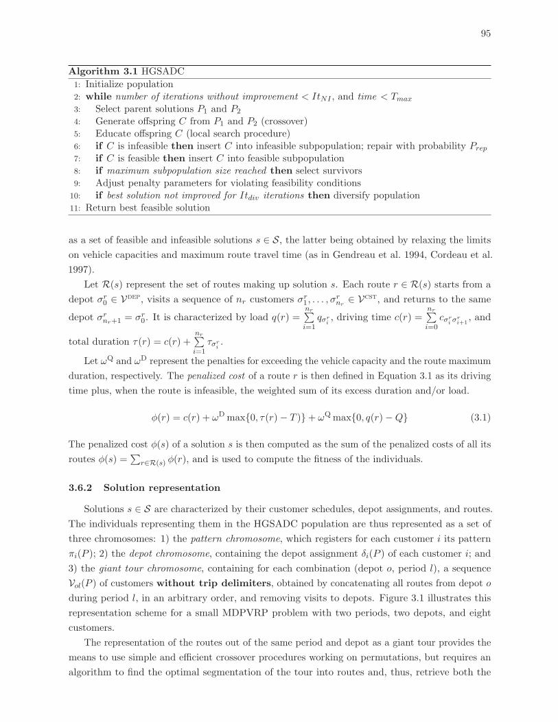
95

Algorithm 3.1 HGSADC

1: Initialize population2: while number of iterations without improvement < ItNI , and time < Tmax

3: Select parent solutions P1 and P2

4: Generate offspring C from P1 and P2 (crossover)5: Educate offspring C (local search procedure)6: if C is infeasible then insert C into infeasible subpopulation; repair with probability Prep

7: if C is feasible then insert C into feasible subpopulation8: if maximum subpopulation size reached then select survivors9: Adjust penalty parameters for violating feasibility conditions

10: if best solution not improved for Itdiv iterations then diversify population11: Return best feasible solution

as a set of feasible and infeasible solutions s ∈ S, the latter being obtained by relaxing the limits

on vehicle capacities and maximum route travel time (as in Gendreau et al. 1994, Cordeau et al.

1997).

Let R(s) represent the set of routes making up solution s. Each route r ∈ R(s) starts from a

depot σr0 ∈ Vdep, visits a sequence of nr customers σr1, . . . , σrnr

∈ Vcst, and returns to the same

depot σrnr+1 = σr0. It is characterized by load q(r) =nr∑i=1

qσri, driving time c(r) =

nr∑i=0

cσri σ

ri+1

, and

total duration τ(r) = c(r) +nr∑i=1

τσri.

Let ωQ and ωD represent the penalties for exceeding the vehicle capacity and the route maximum

duration, respectively. The penalized cost of a route r is then defined in Equation 3.1 as its driving

time plus, when the route is infeasible, the weighted sum of its excess duration and/or load.

φ(r) = c(r) + ωDmax{0, τ(r)− T )}+ ωQmax{0, q(r)−Q} (3.1)

The penalized cost φ(s) of a solution s is then computed as the sum of the penalized costs of all its

routes φ(s) =∑

r∈R(s) φ(r), and is used to compute the fitness of the individuals.

3.6.2 Solution representation

Solutions s ∈ S are characterized by their customer schedules, depot assignments, and routes.

The individuals representing them in the HGSADC population are thus represented as a set of

three chromosomes: 1) the pattern chromosome, which registers for each customer i its pattern

πi(P ); 2) the depot chromosome, containing the depot assignment δi(P ) of each customer i; and

3) the giant tour chromosome, containing for each combination (depot o, period l), a sequence

Vol(P ) of customers without trip delimiters, obtained by concatenating all routes from depot o

during period l, in an arbitrary order, and removing visits to depots. Figure 3.1 illustrates this

representation scheme for a small MDPVRP problem with two periods, two depots, and eight

customers.

The representation of the routes out of the same period and depot as a giant tour provides the

means to use simple and efficient crossover procedures working on permutations, but requires an

algorithm to find the optimal segmentation of the tour into routes and, thus, retrieve both the

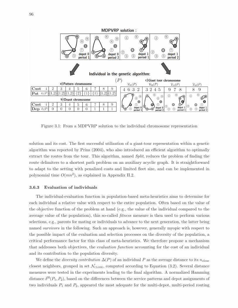
96

Figure 3.1: From a MDPVRP solution to the individual chromosome representation

solution and its cost. The first successful utilization of a giant-tour representation within a genetic

algorithm was reported by Prins (2004), who also introduced an efficient algorithm to optimally

extract the routes from the tour. This algorithm, named Split, reduces the problem of finding the

route delimiters to a shortest path problem on an auxiliary acyclic graph. It is straightforward

to adapt to the setting with penalized costs and limited fleet size, and can be implemented in

polynomial time O(mn2), as explained in Appendix II.2.

3.6.3 Evaluation of individuals

The individual-evaluation function in population-based meta-heuristics aims to determine for

each individual a relative value with respect to the entire population. Often based on the value of

the objective function of the problem at hand (e.g., the value of the individual compared to the

average value of the population), this so-called fitness measure is then used to perform various

selections, e.g., parents for mating or individuals to advance to the next generation, the latter being

named survivors in the following. Such an approach is, however, generally myopic with respect to

the possible impact of the evaluation and selection processes on the diversity of the population, a

critical performance factor for this class of meta-heuristics. We therefore propose a mechanism

that addresses both objectives, the evaluation function accounting for the cost of an individual

and its contribution to the population diversity.

We define the diversity contribution Δ(P ) of an individual P as the average distance to its nclose

closest neighbors, grouped in set Nclose, computed according to Equation (3.2). Several distance

measures were tested in the experiments leading to the final algorithm. A normalized Hamming

distance δH(P1, P2), based on the differences between the service patterns and depot assignments of

two individuals P1 and P2, appeared the most adequate for the multi-depot, multi-period routing

97

problems we address. This distance is computed according to Equation (3.3), where 1(cond) is a

valuation function that returns 1 if the condition cond is true, 0, otherwise.

Δ(P ) =1

nclose

∑P2∈Nclose

δH(P, P2) (3.2)

δH(P1, P2) =1

2n

∑i=1,...,n

(1(πi(P1) �= πi(P2)) + 1(δi(P1) �= δi(P2)) (3.3)

Let fit(P ) and dc(P ) in {1, . . . , nbIndiv} stand for the rank of an individual P in a subpopulation

of size nbIndiv, with respect to its penalized cost φ(P ) and diversity contribution Δ(P ), respectively.

The biased fitness function BF (P ) we propose combines the cost and diversity ranks, and is given

by Equation (3.4), where nbElit is the number of elite individuals one desires to survive to the

next generation.

BF (P ) = fit(P ) +

(1− nbElit

nbIndiv

)dc(P ), (3.4)

The ranks and biased-fitness measures are continuously updated for the two subpopulations

and are used to evaluate the quality of an individual during parent (Section 3.6.4) and survivor

(Section 3.6.6) selections. The biased-fitness is thus an adaptive mechanism aiming to balance the

drive for the best individual (elitism) and the possible loss of information usually associated with

this drive. This concern for continuous and “early” (parent selection) population-diversity control

complements the periodic population-management mechanism introduced in Section 3.6.6.

3.6.4 Parent Selection and Crossover

The offspring generation scheme of HGADSC selects two parents, P1 and P2, and yields a

single individual C. Parent selection is performed through a binary tournament, which twice

randomly (with uniform probability) picks two individuals from the complete population, grouping

the feasible and infeasible subpopulations, and keeps the one with the best biased fitness. Feasible

and infeasible individuals may thus be selected to undergo crossover in order to lead the search

close to the borders of feasibility, where we expect to find high quality solutions.

We propose a new periodic crossover with insertions (PIX ) dedicated to periodic routing

problems and designed to transmit good sequences of visits, while enabling pattern, depot, and

route recombinations. We aimed for a versatile crossover, which would allow for both a wide

exploration of the search space and small refinements of “good” solutions. The possibility for the

offspring to inherit genetic material from its parents in nearly equal proportions is required to

provide the crossover with the former capability, while copying most of one parent along with small

parts of the other provides the latter. To ensure PIX has both capabilities meant avoiding a priori

determined rules on how much genetic material the offspring inherits from each parent, as well as

rules based on simple random selection of individual characteristics.

Algorithm 2 displays the detailed pseudo-code for the PIX crossover procedure, which is

illustrated in Figure 3.2 on a problem with two periods and two depots, and described in the rest of

this section. The crossover begins in Step 0 by determining the period and depot inheritance rule.

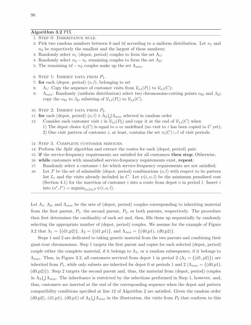
98

Algorithm 3.2 PIX

1: Step 0: Inheritance rule.

2: Pick two random numbers between 0 and td according to a uniform distribution. Let n1 andn2 be respectively the smallest and the largest of these numbers;

3: Randomly select n1 (depot, period) couples to form the set Λ1;4: Randomly select n2 − n1 remaining couples to form the set Λ2;5: The remaining td− n2 couples make up the set Λmix.

6: Step 1: Inherit data from P1.

7: for each (depot, period) (o, l), belonging to set8: Λ1: Copy the sequence of customer visits from Vo,l(P1) to Vo,l(C);9: Λmix: Randomly (uniform distribution) select two chromosome-cutting points αkl and βkl;

copy the αkl to βkl substring of Vo,l(P1) to Vo,l(C).

10: Step 2: Inherit data from P2.

11: for each (depot, period) (o, l) ∈ Λ2⋃

Λmix selected in random order12: Consider each customer visit i in Vo,l(P2) and copy it at the end of Vo,l(C) when

1) The depot choice δi(C) is equal to o or undefined (no visit to i has been copied to C yet);2) One visit pattern of customer i, at least, contains the set πi(C) ∪ l of visit periods.

13: Step 3. Complete customer services.

14: Perform the Split algorithm and extract the routes for each (depot, period) pair;15: if the service-frequency requirements are satisfied for all customers then stop; Otherwise,16: while customers with unsatisfied service-frequency requirements exist, repeat:17: Randomly select a customer i for which service-frequency requirements are not satisfied;18: Let F be the set of admissible (depot, period) combinations (o, l) with respect to its pattern

list Li and the visits already included in C. Let ψ(i, o, l) be the minimum penalized cost(Section 4.1) for the insertion of customer i into a route from depot o in period l. Insert iinto (o∗, l∗) = argmin(o,l)∈F ψ(i, o, l).

Let Λ1, Λ2, and Λmix be the sets of (depot, period) couples corresponding to inheriting material

from the first parent, P1, the second parent, P2, or both parents, respectively. The procedure

then first determines the cardinality of each set and, then, fills them up sequentially by randomly

selecting the appropriate number of (depot, period) couples. We assume for the example of Figure

3.2 that Λ1 = {(d1,p2)}, Λ2 = {(d1,p1)}, and Λmix = {(d0,p1), (d0,p2)}.Steps 1 and 2 are dedicated to taking genetic material from the two parents and combining their

giant-tour chromosomes. Step 1 targets the first parent and copies for each selected (depot, period)

couple either the complete material, if it belongs to Λ1, or a random subsequence, if it belongs to

Λmix. Thus, in Figure 3.2, all customers serviced from depot 1 in period 2 (Λ1 = {(d1, p2)}) areinherited from P1, while only subsets are inherited for depot 0 at periods 1 and 2 (Λmix = {(d0,p1),(d0,p2)}). Step 2 targets the second parent and, thus, the material from (depot, period) couples

in Λ2⋃Λmix. The inheritance is restricted by the selections performed in Step 1, however, and,

thus, customers are inserted at the end of the corresponding sequence when the depot and pattern

compatibility conditions specified at line 12 of Algorithm 2 are satisfied. Given the random order

(d0,p2), (d1,p1), (d0,p1) of Λ2⋃Λmix in the illustration, the visits from P2 that conform to this

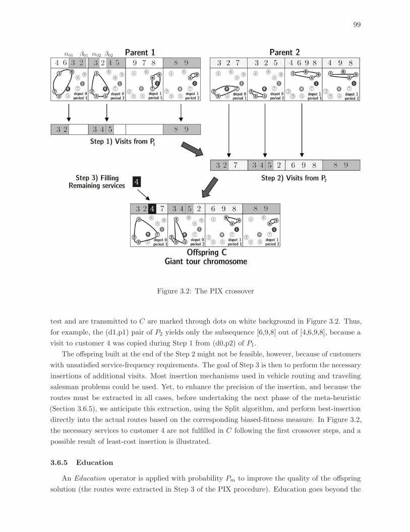
99

Figure 3.2: The PIX crossover

test and are transmitted to C are marked through dots on white background in Figure 3.2. Thus,

for example, the (d1,p1) pair of P2 yields only the subsequence [6,9,8] out of [4,6,9,8], because a

visit to customer 4 was copied during Step 1 from (d0,p2) of P1.

The offspring built at the end of the Step 2 might not be feasible, however, because of customers

with unsatisfied service-frequency requirements. The goal of Step 3 is then to perform the necessary

insertions of additional visits. Most insertion mechanisms used in vehicle routing and traveling

salesman problems could be used. Yet, to enhance the precision of the insertion, and because the

routes must be extracted in all cases, before undertaking the next phase of the meta-heuristic

(Section 3.6.5), we anticipate this extraction, using the Split algorithm, and perform best-insertion

directly into the actual routes based on the corresponding biased-fitness measure. In Figure 3.2,

the necessary services to customer 4 are not fulfilled in C following the first crossover steps, and a

possible result of least-cost insertion is illustrated.

3.6.5 Education

An Education operator is applied with probability Pm to improve the quality of the offspring

solution (the routes were extracted in Step 3 of the PIX procedure). Education goes beyond the

100

classical genetic-algorithm concepts of random mutation and enhancement through hill-climbing

techniques, as it includes several local-search procedures based on neighborhoods for the VRP. A

Repair phase eventually completes the Education operator when the educated offspring is infeasible.

Two sets of local-search procedures are defined. The nine route improvement (RI) procedures

are dedicated to optimize each VRP subproblem separately, whereas the pattern improvement (PI)

procedure relies on a quick and simple move to improve the visit assignments of customers by

changing their patterns and depots. These local searches are called in the RI, PI, RI sequence.

Route Improvement. Let r(u) stand for the route containing vertex u in the given (depot,

period) routing subproblem, and (u1, u2) identify the partial route from u1 to u2. Define the

neighborhood of vertex u, customer or depot, as the hn closest vertices, where h ∈ [0, 1] is a

granularity threshold restricting the search to nearby vertices (Toth and Vigo 2003). Let v be

a neighbor of u, and x and y the successors of u in r(u) and v in r(v), respectively. The Route

Improvement phase iterates, in random order, over each vertex u and each of its neighbors v, and

evaluate the following moves:

• (M1) If u is a customer visit, remove u and place it after v;

• (M2) If u and x are customer visits, remove them, then place u and x after v;

• (M3) If u and x are customer visits, remove them, then place x and u after v;

• (M4) If u and v are customer visits, swap u and v;

• (M5) If u, x, and v are customer visits, swap u and x with v;

• (M6) If u, x, v, and y are customer visits, swap u and x with v and y;

• (M7) If r(u) = r(v), replace (u, x) and (v, y) by (u, v) and (x, y);

• (M8) If r(u) �= r(v), replace (u, x) and (v, y) by (u, v) and (x, y);

• (M9) If r(u) �= r(v), replace (u, x) and (v, y) by (u, y) and (x, v).

The first three moves correspond to insertions, while moves M4 to M6 are generally called

swaps. These moves can be applied indifferently on the same or different routes. Move M7 is a

2-opt intra-route move, while moves M8 and M9 are 2-opt* inter-route moves. Moves are examined

in random order, the first yielding an improvement being implemented. The Route-Improvement

phase stops when all possible moves have been successively tried without success.

Pattern Improvement. Let o and p be the depot and pattern, respectively, of customer i in

the current solution. The Pattern-Improvement procedure iterates on customers in random order

and computes, for each customer i, depot o, and pattern p ∈ Li, Ψ(i, o, p) =∑

l∈p ψ(i, o, l), theminimum cost to satisfy the visit requirements of i from the depot o according to the visit pattern

p. If a (i, o, p) combination exists such that Ψ(i, o, p) < Ψ(i, o, p), then all visits to customer i are

removed, and a new visit is inserted in the best location in each sequence corresponding to depot

o and period l ∈ p. The procedure stops when all customers have been successively considered

without a modification.

The Pattern-Improvement procedure is significantly faster when the optimal position and

insertion cost of each customer is stored for each route. It is also worth noting that, sometimes,

the current pattern and depot choices are kept, but a better insertion of customers is found. The

101

resulting move is then, in fact, a combination of intra-period M1 insertions. This may prove

particularly interesting for the exceptional case when the move was not attempted in RI because

of proximity conditions. The Pattern-Improvement phase thus fulfills the double role of changing

the patterns and attempting moves between distant vertices.

The individual yielded by the RI, PI, RI education sequence may be feasible, in which case,

we call it naturally feasible, or infeasible, and it is inserted into the appropriate subpopulation.

Infeasible individuals are subject to the Repair procedure with probability Prep. When Repair is

successful, the resulting individual is added to the feasible subpopulation (the infeasible one is not

deleted from the infeasible subpopulation). Repair consists in temporarily multiplying the penalty

parameters by 10 and re-starting the RI, PI, RI sequence. When the resulting individual is still

infeasible, penalty parameters are temporarily multiplied by 100 and the sequence is started again.

This significant increase of penalties aims at redirecting the search toward feasible solutions.

3.6.6 Population management and search guidance

The population management mechanism complements the selection, crossover, and education

operators in identifying and propagating the characteristics of good solutions, enhancing the popula-

tion diversity, and providing the means for a thorough and efficient search. The two subpopulations

dedicated to feasible and infeasible individuals are independently managed to contain between μ

and μ+ λ individuals, the former representing the minimum subpopulation size, and the latter the

generation size. Any incoming individual is directly included in the appropriate subpopulation

with respect to its feasibility, and thus acceptance in the population is systematically granted. Any

subpopulation reaching its maximum size will undergo a survivors selection phase to discard λ

individuals and thus return to its minimum size. Four main components thus constitute the general

behavior of the population: initialization, adjustment of the penalties for infeasible individuals,

diversification, and selection of survivors.

Initialization. To initialize the subpopulations, 4μ individuals are created by randomly choosing

a pattern and a depot for each customer and producing for each period the associated service

sequence in random order. These initial individuals undergo education, repair with probability

0.5, and are inserted into the appropriate subpopulation in relation to their feasibility. Survivor

selection is activated, as described later on, when a subpopulation reaches the maximum size.

At the end of initialization, one of the two subpopulations may be incomplete, with less than μ

individuals.

Penalty parameter adjustment. The penalty parameters are initially set to ωD = 1 and

ωQ = c/q, where c represents the average distance between two customers and q is the average

demand. The parameters are then dynamically adjusted during the execution of the algorithm, to

favor the generation of naturally-feasible individuals as defined in Section 3.6.5. Let ξREF be a

target proportion of naturally-feasible individuals, and ξQ and ξD the proportion in the last 100

generated individuals of naturally-feasible one with respect to vehicle capacity and route duration,

respectively. The following adjustment is then performed every 100 iterations, where par = q, d:

102

• if ξPAR ≤ ξREF − 0.05, then ωPAR = ωPAR × 1.2;

• if ξPAR ≥ ξREF + 0.05, then ωPAR = ωPAR × 0.85.

Diversification is called when Itdiv iterations occurs without improving the best solution. It is

performed by eliminating all but the best μ/3 individuals of each subpopulation, and creating 4μ

new individuals as in the initialization phase. This process introduces a significant amount of new

genetic material, which revives the search further, even when the population has lost most of its

diversity.

Diversity and selection of survivors. A major challenge in population-based algorithms is

avoiding premature convergence of the population. The issue is even more challenging when, as

in our case, education compounds the parent selection tendency to favor individuals with good

characteristics, thus reducing the genetic material diversity in the population. The mechanism

we propose aims to address this challenge by simultaneously identifying and preserving the most

promising solution characteristics, and ensuring the diversity of both subpopulations.

The first component of this mechanism is made up of the definition of the biased-fitness function

and the explicit consideration of diversity during parents selection (Section 3.6.3). The second takes

place whenever one of the two subpopulations reaches the maximum size μ+ λ. Named Survivor

selection, the procedure determines the μ individuals that will go on to the next generation, such

that the population diversity, in terms of visit patterns, is preserved and elite individuals in terms

of cost are protected. The λ discarded individuals are thus either clones (Prins 2004) or bad with

respect to cost and contribution to diversity as measured by their biased fitness.

Let a clone be an individual P2 with either the same pattern and depot assignments as another

individual P1, i.e., δH(P1, P2) = 0, or the same solution cost. The procedure successively eliminates,

first, clones, and then, bad individuals, as described in Algorithm 3. Proposition 3.6.1 formalizes

the elitism property of the Survivor-selection procedure.

Algorithm 3.3 Survivor selection

1: for i = 1 . . . λ2: X ← all individuals having a clone3: if X �= ∅ then remove P ∈ X with maximum Biased Fitness4: else remove P in the subpopulation with maximum Biased Fitness5: Update distance and Biased Fitness measures

Proposition 3.6.1 An individual P �∈ X, among the nbElit best individuals of the subpopulation

in terms of cost, will not be removed from the subpopulation by the Survivor-selection procedure.

Proof Let J be the individual with the worst cost in the subpopulation, i.e., fit(J) = nbIndiv,

and thus BF (J) ≥ nbIndiv + 1. P belongs to the best nbElit solutions in terms of cost, thus

BF (P ) ≤ nbElit+ (1− nbElitnbIndiv )(nbIndiv) ≤ nbIndiv. Individual P will not be removed as J has a

worst biased fitness. �

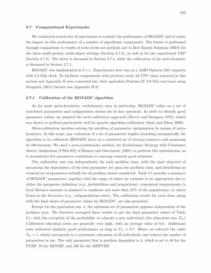
103

3.7 Computational Experiments

We conducted several sets of experiments to evaluate the performance of HGSADC and to assess

the impact on this performance of a number of algorithmic components. The former is performed

through comparisons to results of state-of-the-art methods and to Best Known Solutions (BKS) for

the three multi-period, multi-depot settings (Section 3.7.2), as well as for the capacitated VRP

(Section 3.7.3). The latter is discussed in Section 3.7.4, while the calibration of the meta-heuristic

is discussed in Section 3.7.1.

HGSADC was implemented in C++. Experiments were run on a AMD Opteron 250 computer

with 2.4 Ghz clock. To facilitate comparisons with previous work, all CPU times reported in this

section and Appendix II were converted into their equivalent Pentium IV 3.0 Ghz run times using

Dongarra (2011) factors (see Appendix II.3).

3.7.1 Calibration of the HGSADC algorithm

As for most meta-heuristics, evolutionary ones in particular, HGSADC relies on a set of

correlated parameters and configuration choices for its key operators. In order to identify good

parameter values, we adopted the meta-calibration approach (Mercer and Sampson 1978), which

was shown to perform particularly well for genetic-algorithm calibration (Smit and Eiben 2009).

Meta-calibration involves solving the problem of parameter optimization by means of meta-

heuristics. In this scope, any evaluation of a set of parameters implies launching automatically the

algorithm to be calibrated (HGSADC here) on a restricted set of training instances and measuring

its effectiveness. We used a meta-evolutionary method, the Evolutionary Strategy with Covariance

Matrix Adaptation (CMA-ES) of Hansen and Ostermeier (2001) to perform this optimization, as

it necessitates few parameter evaluations to converge towards good solutions.

The calibration was run independently for each problem class, with the dual objective of

measuring the dependency of the best parameter set upon the problem class, and identifying an

eventual set of parameters suitable for all problem classes considered. Table 3.1 provides a summary

of HGSADC parameters, together with the range of values we estimate to be appropriate due to

either the parameter definition (e.g., probabilities and proportions), conceptual requirements (a

local distance measure is assumed to implicate not more than 25% of the population), or values

found in the literature (e.g., subpopulations sizes). The calibration results for each class, along

with the final choice of parameter values for HGSADC, are also presented.

Except for the generation size λ, the optimum set of parameters appears independent of the

problem type. We therefore averaged these results to get the final parameter values of Table

3.1, with the exception of the probability to educate a new individual (the education rate Pm).

Calibrated education rates are generally very high, with an average value of 0.8. Additional

tests indicated similarly good performance as long as Pm ≥ 0.7. Hence we selected the value

Pm = 1, which corresponds to a systematic education of all individuals, and reduces the number of

parameters in use. The only parameter that is problem dependent is λ, which is set to 40 for the

PVRP, 70 for MDVRP, and 100 for the MDPVRP.

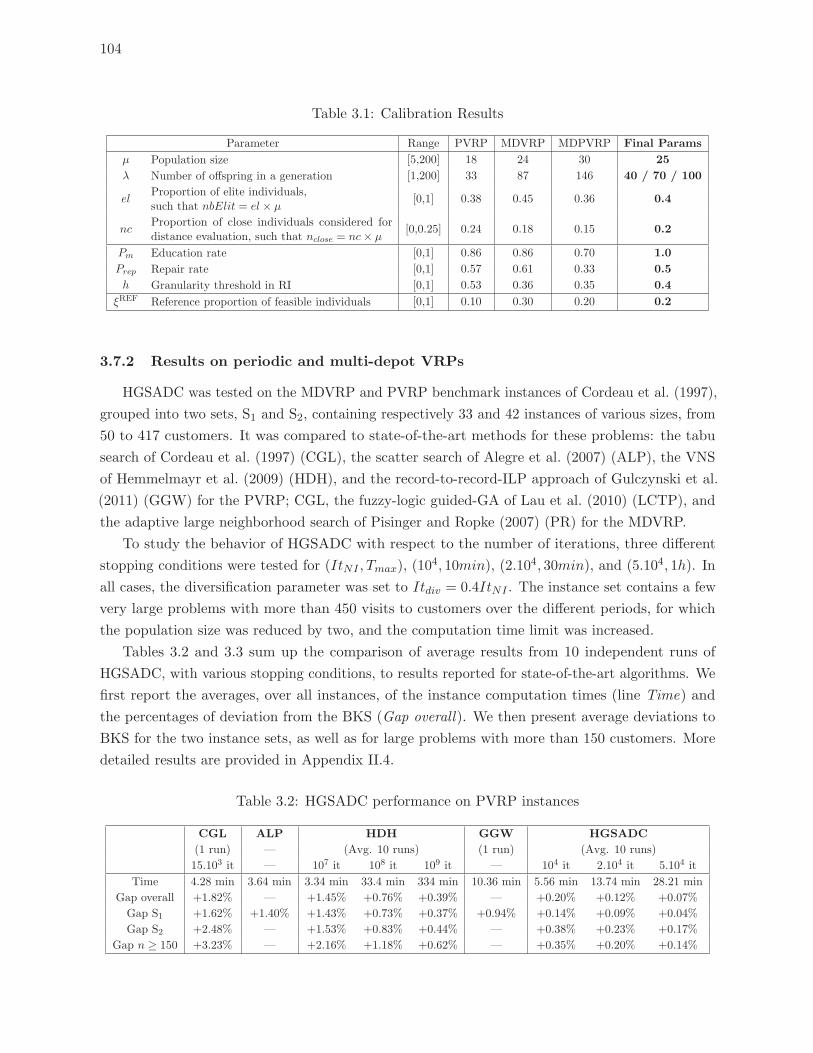
104

Table 3.1: Calibration Results

Parameter Range PVRP MDVRP MDPVRP Final Params

μ Population size [5,200] 18 24 30 25

λ Number of offspring in a generation [1,200] 33 87 146 40 / 70 / 100

elProportion of elite individuals,such that nbElit = el × μ

[0,1] 0.38 0.45 0.36 0.4

ncProportion of close individuals considered fordistance evaluation, such that nclose = nc× μ

[0,0.25] 0.24 0.18 0.15 0.2

Pm Education rate [0,1] 0.86 0.86 0.70 1.0

Prep Repair rate [0,1] 0.57 0.61 0.33 0.5

h Granularity threshold in RI [0,1] 0.53 0.36 0.35 0.4

ξREF Reference proportion of feasible individuals [0,1] 0.10 0.30 0.20 0.2

3.7.2 Results on periodic and multi-depot VRPs

HGSADC was tested on the MDVRP and PVRP benchmark instances of Cordeau et al. (1997),

grouped into two sets, S1 and S2, containing respectively 33 and 42 instances of various sizes, from

50 to 417 customers. It was compared to state-of-the-art methods for these problems: the tabu

search of Cordeau et al. (1997) (CGL), the scatter search of Alegre et al. (2007) (ALP), the VNS

of Hemmelmayr et al. (2009) (HDH), and the record-to-record-ILP approach of Gulczynski et al.

(2011) (GGW) for the PVRP; CGL, the fuzzy-logic guided-GA of Lau et al. (2010) (LCTP), and

the adaptive large neighborhood search of Pisinger and Ropke (2007) (PR) for the MDVRP.

To study the behavior of HGSADC with respect to the number of iterations, three different

stopping conditions were tested for (ItNI , Tmax), (104, 10min), (2.104, 30min), and (5.104, 1h). In

all cases, the diversification parameter was set to Itdiv = 0.4ItNI . The instance set contains a few

very large problems with more than 450 visits to customers over the different periods, for which

the population size was reduced by two, and the computation time limit was increased.

Tables 3.2 and 3.3 sum up the comparison of average results from 10 independent runs of

HGSADC, with various stopping conditions, to results reported for state-of-the-art algorithms. We

first report the averages, over all instances, of the instance computation times (line Time) and

the percentages of deviation from the BKS (Gap overall). We then present average deviations to

BKS for the two instance sets, as well as for large problems with more than 150 customers. More

detailed results are provided in Appendix II.4.

Table 3.2: HGSADC performance on PVRP instances

CGL ALP HDH GGW HGSADC

(1 run) — (Avg. 10 runs) (1 run) (Avg. 10 runs)

15.103 it — 107 it 108 it 109 it — 104 it 2.104 it 5.104 it

Time 4.28 min 3.64 min 3.34 min 33.4 min 334 min 10.36 min 5.56 min 13.74 min 28.21 min

Gap overall +1.82% — +1.45% +0.76% +0.39% — +0.20% +0.12% +0.07%

Gap S1 +1.62% +1.40% +1.43% +0.73% +0.37% +0.94% +0.14% +0.09% +0.04%

Gap S2 +2.48% — +1.53% +0.83% +0.44% — +0.38% +0.23% +0.17%

Gap n ≥ 150 +3.23% — +2.16% +1.18% +0.62% — +0.35% +0.20% +0.14%

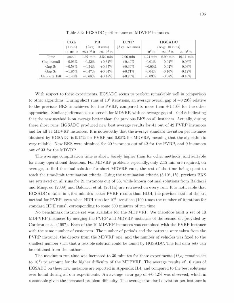
105

Table 3.3: HGSADC performance on MDVRP instances

CGL PR LCTP HGSADC

(1 run) (Avg. 10 runs) (Avg. 50 runs) (Avg. 10 runs)

15.103 it 25.103 it 50.103 it — 104 it 2.104 it 5.104 it

Time small 1.97 min 3.54 min 2.06 min 4.24 min 8.99 min 19.11 min

Gap overall +0.96% +0.52% +0.34% +0.49% -0.01% -0.04% -0.06%

Gap S1 +0.58% +0.54% +0.35% +0.39% +0.00% -0.02% -0.03%

Gap S2 +1.85% +0.47% +0.34% +0.71% -0.04% -0.10% -0.12%

Gap n ≥ 150 +1.40% +0.68% +0.45% +0.70% -0.03% -0.08% -0.10%

With respect to these experiments, HGSADC seems to perform remarkably well in comparison

to other algorithms. During short runs of 104 iterations, an average overall gap of +0.20% relative

to the previous BKS is achieved for the PVRP, compared to more than +1.40% for the other

approaches. Similar performance is observed for MDVRP, with an average gap of −0.01% indicating

that the new method is on average better than the previous BKS on all instances. Actually, during

these short runs, HGSADC produced new best average results for 41 out of 42 PVRP instances

and for all 33 MDVRP instances. It is noteworthy that the average standard deviation per instance

obtained by HGSADC is 0.15% for PVRP and 0.05% for MDVRP, meaning that the algorithm is

very reliable. New BKS were obtained for 20 instances out of 42 for the PVRP, and 9 instances

out of 33 for the MDVRP.

The average computation time is short, barely higher than for other methods, and suitable

for many operational decisions. For MDVRP problems especially, only 2.15 min are required, on

average, to find the final solution for short MDVRP runs, the rest of the time being spent to

reach the time-limit termination criteria. Using the termination criteria (5.104, 1h), previous BKS

are retrieved on all runs for 21 instances out of 33, while known optimal solutions from Baldacci

and Mingozzi (2009) and Baldacci et al. (2011a) are retrieved on every run. It is noticeable that

HGSADC obtains in a few minutes better PVRP results than HDH, the previous state-of-the-art

method for PVRP, even when HDH runs for 109 iterations (100 times the number of iterations for

standard HDH runs), corresponding to some 300 minutes of run time.

No benchmark instance set was available for the MDPVRP. We therefore built a set of 10

MDPVRP instances by merging the PVRP and MDVRP instances of the second set provided by

Cordeau et al. (1997). Each of the 10 MDVRP instances was combined with the PVRP instance

with the same number of customers. The number of periods and the patterns were taken from the

PVRP instance, the depots from the MDVRP one, and the number of vehicles was fixed to the

smallest number such that a feasible solution could be found by HGSADC. The full data sets can

be obtained from the authors.

The maximum run time was increased to 30 minutes for these experiments (ItNI remains set

to 104) to account for the higher difficulty of the MDPVRP. The average results of 10 runs of

HGSADC on these new instances are reported in Appendix II.4, and compared to the best solutions

ever found during all our experiments. An average error gap of +0.42% was observed, which is

reasonable given the increased problem difficulty. The average standard deviation per instance is

106

now 0.26%, illustrating the increased irregularity of the search space. Keeping the best solution of

the 10 runs leads to significantly better solutions, with an average error gap of +0.13%, but requires

more computational resources. This approach corresponds to the well-known independent-search

strategy for parallel meta-heuristics (Crainic and Toulouse 2010). More sophisticated parallel-search

strategies, based on cooperation, in particular, could be used to improve the exploration of the

search space and reach better results.

3.7.3 Results on the capacitated VRP

The CVRP is a special case of multi-depot periodic problems, when d = 1 and t = 1. HGSADC

can thus be used to address the CVRP with very minor changes in the distance measure and the

parameters, even though its operators were designed for multi-period settings.

Detailed results of experiments on 34 well-known CVRP instances from the literature are

reported in Appendix II.5. Very competitive results to state-of-the-art methods were obtained in

similar computation times. An overall gap to the BKS of 0.10% was thus observed, which is equal

to the performance of the best, highly specialized, algorithm in the literature (Nagata and Braysy

2009b). We also retrieved 12 new best known solutions for Golden et al. (1998a) instances. The

diversity management method we propose seems to compensate for the lack of problem-tailored

operators, and opens several promising avenues of research.

3.7.4 Sensitivity analysis of algorithmic components

A second set of experiments targeted the analysis of the impact on the performance of the

proposed meta-heuristic of various algorithmic components. Sensitivity analysis was thus performed

on “traditional” hybrid genetic components by “removing” each of them in turn.

The “No-Education” version was obtained by setting the probability of offspring education

Pm to 0, which also meant that no repair was performed. Local-search improvement methods

are thus exclusively used to produce the initial population. In the “No-Population” version,

λ = 1, μ = 0, and nbElite = 1. Thus, only one individual appears in each subpopulation, the

population management mechanism then behaving as a steady-state population management

where the offspring replaces the parent only if it improves. The crossover either combines an

individual with itself, or both feasible and infeasible individuals. Only one parent was selected

by binary tournament for the “No-Crossover” version, underwent education and was inserted into

the population. The parent selection was performed only in the feasible subpopulation for the

“No-Infeasible” algorithm, a constant high penalty value being enforced through the search. Finally,

setting the repair probability Prep to 0 yielded the “No-Repair” version. The results are reported

in Table 3.4, each column corresponding to the average time and gap to BKS of HGSADC without

the respective component.

It is noticeable that all these algorithmic components play an important role in the good

performance of the proposed meta-heuristic, the most crucial being education followed by population,

crossover, infeasible solutions, and repair to a lesser extent.

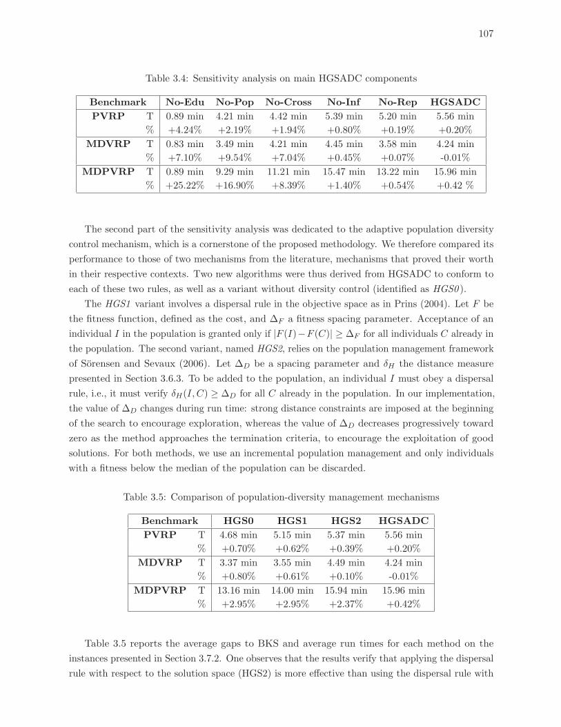
107

Table 3.4: Sensitivity analysis on main HGSADC components

Benchmark No-Edu No-Pop No-Cross No-Inf No-Rep HGSADC

PVRP T 0.89 min 4.21 min 4.42 min 5.39 min 5.20 min 5.56 min

% +4.24% +2.19% +1.94% +0.80% +0.19% +0.20%

MDVRP T 0.83 min 3.49 min 4.21 min 4.45 min 3.58 min 4.24 min

% +7.10% +9.54% +7.04% +0.45% +0.07% -0.01%

MDPVRP T 0.89 min 9.29 min 11.21 min 15.47 min 13.22 min 15.96 min

% +25.22% +16.90% +8.39% +1.40% +0.54% +0.42 %

The second part of the sensitivity analysis was dedicated to the adaptive population diversity

control mechanism, which is a cornerstone of the proposed methodology. We therefore compared its

performance to those of two mechanisms from the literature, mechanisms that proved their worth

in their respective contexts. Two new algorithms were thus derived from HGSADC to conform to

each of these two rules, as well as a variant without diversity control (identified as HGS0 ).

The HGS1 variant involves a dispersal rule in the objective space as in Prins (2004). Let F be

the fitness function, defined as the cost, and ΔF a fitness spacing parameter. Acceptance of an

individual I in the population is granted only if |F (I)−F (C)| ≥ ΔF for all individuals C already in

the population. The second variant, named HGS2, relies on the population management framework

of Sorensen and Sevaux (2006). Let ΔD be a spacing parameter and δH the distance measure

presented in Section 3.6.3. To be added to the population, an individual I must obey a dispersal

rule, i.e., it must verify δH(I, C) ≥ ΔD for all C already in the population. In our implementation,

the value of ΔD changes during run time: strong distance constraints are imposed at the beginning

of the search to encourage exploration, whereas the value of ΔD decreases progressively toward

zero as the method approaches the termination criteria, to encourage the exploitation of good

solutions. For both methods, we use an incremental population management and only individuals

with a fitness below the median of the population can be discarded.

Table 3.5: Comparison of population-diversity management mechanisms

Benchmark HGS0 HGS1 HGS2 HGSADC

PVRP T 4.68 min 5.15 min 5.37 min 5.56 min

% +0.70% +0.62% +0.39% +0.20%

MDVRP T 3.37 min 3.55 min 4.49 min 4.24 min

% +0.80% +0.61% +0.10% -0.01%

MDPVRP T 13.16 min 14.00 min 15.94 min 15.96 min

% +2.95% +2.95% +2.37% +0.42%

Table 3.5 reports the average gaps to BKS and average run times for each method on the

instances presented in Section 3.7.2. One observes that the results verify that applying the dispersal

rule with respect to the solution space (HGS2) is more effective than using the dispersal rule with

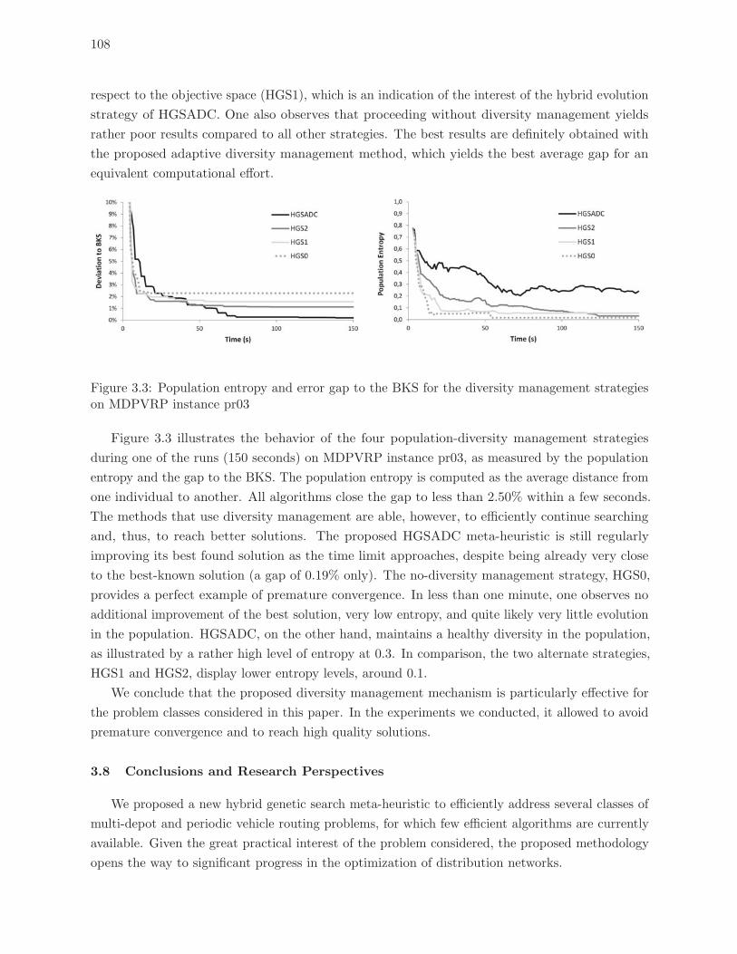
108

respect to the objective space (HGS1), which is an indication of the interest of the hybrid evolution

strategy of HGSADC. One also observes that proceeding without diversity management yields

rather poor results compared to all other strategies. The best results are definitely obtained with

the proposed adaptive diversity management method, which yields the best average gap for an

equivalent computational effort.

Figure 3.3: Population entropy and error gap to the BKS for the diversity management strategieson MDPVRP instance pr03

Figure 3.3 illustrates the behavior of the four population-diversity management strategies

during one of the runs (150 seconds) on MDPVRP instance pr03, as measured by the population

entropy and the gap to the BKS. The population entropy is computed as the average distance from

one individual to another. All algorithms close the gap to less than 2.50% within a few seconds.

The methods that use diversity management are able, however, to efficiently continue searching

and, thus, to reach better solutions. The proposed HGSADC meta-heuristic is still regularly

improving its best found solution as the time limit approaches, despite being already very close

to the best-known solution (a gap of 0.19% only). The no-diversity management strategy, HGS0,

provides a perfect example of premature convergence. In less than one minute, one observes no

additional improvement of the best solution, very low entropy, and quite likely very little evolution

in the population. HGSADC, on the other hand, maintains a healthy diversity in the population,

as illustrated by a rather high level of entropy at 0.3. In comparison, the two alternate strategies,

HGS1 and HGS2, display lower entropy levels, around 0.1.

We conclude that the proposed diversity management mechanism is particularly effective for

the problem classes considered in this paper. In the experiments we conducted, it allowed to avoid

premature convergence and to reach high quality solutions.

3.8 Conclusions and Research Perspectives

We proposed a new hybrid genetic search meta-heuristic to efficiently address several classes of

multi-depot and periodic vehicle routing problems, for which few efficient algorithms are currently

available. Given the great practical interest of the problem considered, the proposed methodology

opens the way to significant progress in the optimization of distribution networks.

109

The paper introduces several methodological contributions, in particular, in the crossover and

education operators, the management of infeasible solutions, the individual evaluation procedure

driven both by solution cost and the contribution to population diversity and, more generally, the

adaptive population management mechanism that enhances diversity, allows a broader access to

reproduction, and preserves the memory of what characterizes good solutions represented by the

elite individuals. The combination of these concepts provides the capability of the proposed Hybrid

Genetic Search with Adaptive Diversity Control meta-heuristic to reach high quality solutions

on the literature benchmarks. The method actually identifies either the best known solutions,

including the optimal ones, or new best solutions for all benchmark instances, thus outperforming

the current state-of-the-art meta-heuristics for each particular problem class. Moreover, with

minimal adjustments, it obtains comparable results to the best methods for the CVRP.

Among the many interesting avenues of research, we mention the interest to explore the impact

of the adaptive diversity control mechanism for other classes of problems, and to validate its good

performance using theoretical models. We also plan to generalize the methodology to problems

with additional attributes, and thus progress toward addressing rich VRP problem settings, as

well as real world applications.

CHAPITRE 4

UN ALGORITHME GENETIQUE HYBRIDE POUR UNE GRANDE FAMILLE

DE PROBLEMES DE TOURNEES DE VEHICULES AVEC FENETRES DE

TEMPS


Les attributs etudies dans le precedent chapitre faisaient partie de la categorie des attributs de

type Assign, impactant les choix d’affectation. Ce chapitre etudie l’extension de la methodologie

HGSADC a un autre type d’attribut : les fenetres de temps pour les services aux clients. Cet attribut

est de type Eval selon la classification du Chapitre 1. De nouvelles methodes d’evaluation de

voisinages de recherche locale sont introduites pour evaluer efficacement des solutions irrealisables

ne respectant pas certaines contraintes sur les routes (fenetres de temps, capacite et duree). Aussi,

pour traiter des problemes de grande taille comprenant jusque 4500 services sur 10 jours, des phases

de decomposition sont utilisees. La methode ainsi obtenue produit des resultats remarquables sur

une vaste gamme de problemes de tournees de vehicules avec fenetres de temps, contraintes de

duree de routes, multiple depots et multiple periodes, surpassant toutes les methodes precedentes

de la la litterature pour ces problemes.

4.2 Article IV : A hybrid genetic algorithm for a large class of vehicle routing

problems with time windows

Ce chapitre a fait l’objet d’une publication sous forme d’article de journal : Vidal,

T., Crainic, T.G., Gendreau, M., Prins, C. (2012). A hybrid genetic algorithm for a

large class of vehicle routing problems with time windows. Computers & Operations

Research, 40(1), 475–489.

Abstract: The paper presents an efficient Hybrid Genetic Search with Advanced Diversity Control

for a large class of time-constrained vehicle routing problems, introducing several new features to

manage the temporal dimension. New move evaluation techniques are proposed, accounting for

penalized infeasible solutions with respect to time-window and duration constraints, and allowing

to evaluate moves from any classical neighbourhood based on arc or node exchanges in amortized

constant time. Furthermore, geometric and structural problem decompositions are developed to

address efficiently large problems. The proposed algorithm outperforms all current state-of-the-art

approaches on classical literature benchmark instances for any combination of periodic, multi-depot,

site-dependent, and duration-constrained vehicle routing problem with time windows.

Keywords: Vehicle routing problems, time windows, hybrid genetic algorithm, diversity manage-

ment, neighbourhood search, decomposition

112

4.3 Introduction

Vehicle routing problems (VRP) with time constraints and requirements relative to customer

assignments to vehicle types, depots, or planning periods constitute a class of difficult optimization

problems. These settings are linked with numerous practical applications including logistics, goods

transportation, refuse collection, maintenance operations, and relief supply (see Golden et al. 2008,

for a large variety of application cases). Much has already been dedicated to specific VRP with

additional “attributes” such as time windows, multiple depots, or delivery-period choices. As

illustrated by numerous reviews (Braysy and Gendreau 2005b,a, Francis et al. 2008, Gendreau

et al. 2008b, Gendreau and Tarantilis 2010, for the most recent), almost every prominent meta-

heuristic paradigm, including evolutionary methods, ant colony optimization, tabu search, simulated

annealing, other improved local search approaches or ruin-and-recreate, has been applied to at

least one of the previous settings. Yet, besides highly problem-tailored methods, the literature

critically lacks good generalist approaches able to efficiently address a wide range of problem

variants, and VRP combining several problem attributes (also called multi-attribute VRP in Crainic

et al. 2009 and rich VRP in Hartl et al. 2006) still constitute major challenges for both research

and applications. Within these settings, it is well known that imposing time-window constraints

on customer services (and depot availability) raises significant challenges related to the smaller

proportion of feasible solutions, the increased computation burden required to evaluate moves in

neighbourhood search, and the antagonist influence of temporal and spatial characteristics.

This paper introduces a new Hybrid Genetic Search with Advanced Diversity Control (HGSADC ),

that addresses some of these challenges. In particular, it addresses efficiently a wide range of

large-scale vehicle routing problems with time windows (VRPTW ), route-duration constraints, and

additional attributes involving requirements for customer assignments to particular vehicles types,

depots or planning periods. The main characteristic of HGSADC stands in a different approach

to population diversity management, the contribution of a particular individual to the diversity

of the population appearing as a proper objective to be optimized (Vidal et al. 2012a). We also

introduce a number of new algorithmic features targeting specifically the temporal characteristics

of the problems. We thus propose simple move evaluation procedures that accommodate penalized

infeasibility with regard to duration and time-window constraints, and work in amortized O(1) for

any neighbourhood based on a bounded number of arc exchanges or node relocations. We also

develop neighbourhood pruning procedures based on the temporal dimension, and decomposition

principles to address efficiently large problem instances involving up to 1000 customers and 4500

services. The resulting algorithm is simple and efficient, outperforming all existing approaches on

classical benchmarks for the VRPTW, its variants with multiple depots (MDVRPTW ), multiple

periods (PVRPTW ), and vehicle-site dependencies (SDVRPTW ).

The main contributions of this paper are thus 1) a generalization of the concept of HGSADC

to a large class of VRPTW variants presenting mixed temporal and geometrical characteristics; 2)

new procedures to efficiently search neighbourhoods when considering infeasible solutions with

regards to duration and time-window constraints; 3) decomposition principles within the genetic

113

framework allowing to address efficiently large instances; and 4) a state-of-the-art meta-heuristic

for four classes of vehicle routing problems with time windows.

The remainder of this paper is organized as follows: Section 4.4 states the notation and formally

defines the problems. Summarized elements of the literature are presented in Section 4.5. The

proposed meta-heuristic is described in Section 4.6, while extensive computational experiments are

reported in Section 4.7. Section 4.8 concludes.

4.4 Problem Statement

We first formally state the VRPTW. A general PVRPTW is then defined, including other

notable variants, such as the MDVRPTW and the SDVRPTW, as special cases. Route-duration

constraints are included in all cases but do not appear in the acronyms.

Let G = (V ,A) be a complete directed graph. Vertex v0 ∈ V represents a single depot, where a

fleet of m identical vehicles with capacity Q is located, and a product to be delivered is kept. Each

other vertex vi ∈ Vcst, with Vcst = V\{v0} and i ∈ {1, . . . , n}, stands for a customer to be serviced,

characterized by a non-negative demand qi, a service duration τi, as well as an interval of allowable

visit times [ei, li], called time window. By definition, q0 = τ0 = 0. Arcs (i, j) ∈ A represent the

possibility to travel from vi to vj with a distance cij and a duration δij . A feasible route r is defined

as a circuit in G that starts and ends at v0, such that the total demand of customers in r is smaller

than or equal to Q. While performing its route, a vehicle may stop and wait in order to reach the

next customer within its time window, but the route duration, computed as the difference between

the start time and the return time at v0, is limited to D. The VRPTW aims to construct up to m

vehicle routes, to visit each customer vertex once within its time window, while minimizing the

total distance.

In the generalized PVRPTW, route planning is performed for a horizon of t periods. Distances

cijl and durations δijl can be dependent upon the period. Each customer vi is characterized by a

frequency fi, representing the total number of services requested on the planning horizon, and a

list Li of allowable visit combinations, called patterns. The objective is to select a pattern for each

customer, and construct the associated routes to minimize the total distance over all periods. A

mathematical integer programming formulation of this problem is given in Appendix III.1.

We also consider two related problem classes. The MDVRPTW involves d > 1 depots. It is

also generally assumed that any route originates and returns to the same depot. This problem

was shown to constitute a special case of the generalized PVRPTW (Cordeau et al. 1997), where

depots are assimilated to periods (t = d), any customer vi ∈ Vcst has a frequency fi = 1 and can

be serviced in any period Li = {{1}, . . . , {t}}, and δ0il and c0il values are set in each period to

correctly account for the distance to the assimilated depots. The SDVRPTW involves w vehicle

types, with compatibility constraints between customers and vehicles. Each customer vi ∈ Vcst

can be serviced only by a subset Ri ∈ {1 . . . w} of vehicle types. As shown in Cordeau and Laporte

(2001), this problem constitutes another particular case of PVRPTW, where each vehicle type is

assimilated to a different period (t = w) and Li = {{k} : k ∈ Ri}.

114

It was shown in Vidal et al. (2012a), that any VRP with multiple depots and periods (MDPVRP)

can be transformed into an equivalent PVRP, by associating a different period to each (period, depot)

pair from the former problem. In the same spirit, we can transform a problem combining multi-

depot, site-dependent, multi-period, and time-window attributes into a PVRPTW, by associating

a period for each (depot, period, vehicle type) in the original problem. This transformation thus

enables to address all the previous VRPTW variants and their combinations by means of a single

algorithm for the PVRPTW. The inherent difficulty related to combined (depot, period, vehicle

type) choices leads to a large number of periods in the new problem. The proposed algorithm has

thus been designed to successfully tackle large PVRPTW instances.

4.5 Literature Review

We initiate this review surveying proposed meta-heuristics for the VRPTW, which is one of

the most intensively studied NP-hard combinatorial optimization problems in the last thirty years.

Exact methods are still not able to address most large-size applications, and their performance

strongly varies with the time-window characteristics. Heuristic and meta-heuristic approaches

have thus been the methodology of choice (see Braysy and Gendreau 2005b,a, Gendreau and

Tarantilis 2010, for extensive reviews), and have been mostly evaluated and compared on standard

benchmark instances introduced by Solomon (1987) and Gehring and Homberger (1999) relative

to their computational efficiently and the quality of the solutions obtained. Most authors have

focused on primarily minimizing fleet size, and then distance, but a few exceptions exist (Alvarenga

et al. 2007, Labadi et al. 2008). As a consequence, state-of-the-art VRPTW heuristics are generally

based on two stages, dedicated first to minimizing fleet size and then distance.

Most successful approaches involve local search improvement procedures based on arc- and

node-exchange neighbourhoods, and are coupled with various other concepts listed in the following:

• Evolution strategies (Alvarenga et al. 2007, Mester and Braysy 2005, Hashimoto et al. 2008,

Labadi et al. 2008, Repoussis et al. 2009b, Nagata et al. 2010);

• Solutions recombinations (Alvarenga et al. 2007, Hashimoto et al. 2008, Labadi et al. 2008,

Repoussis et al. 2009b, Nagata et al. 2010);

• Ruin and recreate (Pisinger and Ropke 2007, Prescott-Gagnon et al. 2009, Repoussis et al.

2009b);

• Ejection chains (Lim and Zhang 2007, Nagata and Braysy 2009a, Nagata et al. 2010);

• Guidance and memories (Mester and Braysy 2005, Le Bouthillier and Crainic 2005b, Repoussis

et al. 2009b);

• Parallel and cooperative search (Le Bouthillier and Crainic 2005a,b);

• Mathematical programming hybrids (Prescott-Gagnon et al. 2009).

The most competitive result are currently offered by the hybrid genetic algorithm of Nagata

et al. (2010). The method combines powerful route minimization procedures, with a very effective

edge assembly crossover, and extremely efficient local search procedures. The Iterated Local Search

115

(ILS) of Ibaraki et al. (2008), the Adaptive Large Neighbourhood Search (ALNS) of Pisinger and

Ropke (2007), and the Unified Tabu Search (UTS) of Cordeau et al. (1997, 2001a, 2004) are also

worth mentioning. These methods stand out in terms of simplicity and wider applicability, as both

have been extended to address various VRP variants.

Variants of the VRPTW, combining time windows with multi-period, multi-depot, or site

dependency, arise in many practical applications such as maintenance operations (Weigel and

Cao 1999, Blakeley et al. 2003), refuse collection (Teixeira et al. 2004, Sahoo et al. 2005), or

product distribution (Golden and Wasil 1987, Prive et al. 2005, Jang et al. 2006, Chiu et al. 2006,

Parthanadee and Logendran 2006). Although the interest in these problem settings is growing,

a somewhat restricted number of contributions have been proposed in the literature addressing

them. Most of these implemented some form of neighbourhood-based meta-heuristic search. UTS

(Cordeau et al. 2001a, Cordeau and Laporte 2001, Cordeau et al. 2004) is currently the only method

addressing all variants considered in this paper. UTS exploits long-term memories to penalize

frequently-encountered solution features. A parallel variant of this approach has been recently

proposed by Cordeau and Maischberger (2012).

Specific to the PVRPTW, Pirkwieser and Raidl (2008) propose a Variable Neighborhood Search

(VNS), further enhanced by means of multi-start strategies, column generation hybridizations,

or multi-level strategies in (Pirkwieser and Raidl 2009a,b, 2010b). Yu and Yang (2011) propose

a coarse-grained parallel Ant Colony Optimization (ACO) algorithm, and Nguyen et al. (2011)

develop a hybrid genetic approach. The latter method combines the strength of population-based

search, and Tabu and VNS improvement methods applied to the offspring. For the MDVRPTW,

we report the hybrid Tabu search and savings approach of Tamashiro et al. (2010), the parallel VNS

approaches of Polacek et al. (2004, 2008), and a genetic algorithm and ACO hybrid by Ostertag

(2008). Noteworthy is also the approach of Chiu et al. (2006), which considers total duty time

minimization (including waiting times). Other than UTS, a single hybrid Tabu search and VNS

approach by Belhaiza (2010) may be reported for the SDVRPTW.

The literature is extremely scarce on VRPTW variants combining multiple features. We

mention the Tabu search of Parthanadee and Logendran (2006) able to address multi-depot

periodic VRPTW (MDPVRPTW). Crainic et al. (2009) introduced the Integrative Cooperative

Search (ICS) framework to target highly complex combinatorial optimization settings. ICS is

a central-memory cooperative multi-search involving problem decompositions by decision sets,

integration of elite partial solutions yielded by the subproblems, and adaptive guidance mechanisms.

A MDPVRPTW application was presented, but no definitive results have been published yet.

We conclude this section focusing on the design of efficient local-search methods, because

most methods presented in this section dedicate the greatest part of their computational effort

to the serial exploration of neighbourhoods, basically edge exchanges. Efficient move evaluation

procedures are thus determining for both algorithmic speed and scalability.

Many methods rely on search spaces that include infeasible solutions with respect to time-

window constraints, aiming to explore a wider diversity of structurally different feasible solutions.

Several relaxation alternatives have been proposed in the literature. Cordeau et al. (2001a) and

Repoussis et al. (2009b), among others, allow penalized late services to customers, while Ibaraki

116

et al. (2008) also allow penalized early services. Using such relaxations however leads to less

efficient move-evaluation procedures, working in O(n) or O(log n) (Ibaraki et al. 2008). A different

relaxation was recently used by Hashimoto et al. (2008) and Nagata et al. (2010). An assumption

is made that upon a late arrival, a penalized return in time can be employed to reach the time

window. The authors demonstrated that several classical neighbourhood moves can be evaluated

in amortized O(1) in this relaxation scheme. However, neither intra-route moves, nor duration

constraints are actually managed in O(1).

This review clearly underlines several gaps in the actual state of the art. Thus, for example,

while population-based methods have shown their worth on the classic VRPTW, there is a lack of

really efficient methods of this type for more complex variants such as PVRPTW, MDVRPTW,

SDVRPTW and their combinations. Also, most current efficient methods for VRPTW are intricate,

hard to reproduce, and largely rely on specific problem-tailored procedures. Hence, there is a need

for more general and simple methods, broadly applicable to a large variety of practical settings

with combined features. Finally, the temporal aspects lead to important challenges regarding

infeasible-solution management and neighbourhood-evaluation procedures, which have a strong

impact on the efficiency and scalability of VRPTW meta-heuristics. The concepts developed in

this paper contribute towards addressing these issues.

4.6 The HGSADC Methodology

This section describes the proposed Hybrid Genetic Search with Adaptive Diversity Control

algorithm for time window-constrained VRP variants. For matters of presentation clarity, we

describe the approach for the VRPTW and PVRPTW, the latter encompassing the MDVRPTW,

SDVRPTW and other problems as special cases.

HGSADC (Vidal et al. 2012a) is a hybrid meta-heuristic combining the exploration capabilities

of genetic algorithms with efficient local search-based improvement procedures and diversity

management mechanisms. In HGSADC, population diversity is considered as an objective to be

optimized along with solution quality through individual evaluations and selections. The general

behavior of HGSADC is sketched in Algorithm 4.1.

The method evolves feasible and infeasible solutions in two separate subpopulations. Genetic

operators are iteratively applied to select two parents from the subpopulations (Line 3 of Algorithm

4.1), combine them into an offspring (Line 4), which undergoes a local search-based Education,

is Repaired if infeasible, and is finally inserted into the suitable subpopulation (Lines 5-7). Each

subpopulation is managed separately to trigger a Survivor Selection phase when a maximum size

is reached, adapt infeasibility penalties, and call a Diversification mechanism (after each Itdiv

successive iterations without improvement, Lines 8-10) whenever the search stagnates. In this

application, structural and geometrical decompositions phases are also performed (after each Itdec

iterations, Line 11) to tackle large problems, the subproblems being addressed by means of recursive

calls to HGSADC. The method terminates when ItNI successive iterations have been performed

without improvement.

117

Algorithm 4.1 HGSADC

1: Initialize population2: while number of iterations without improvement < ItNI , and

time < Tmax

3: Select parent solutions P1 and P2

4: Create offspring C from P1 and P2 (crossover)5: Educate C (local search procedure)6: if C infeasible then

Insert C into infeasible subpopulation,Repair with probability Prep

7: if C feasible thenInsert C into feasible subpopulation

8: if maximum subpopulation size reached thenSelect survivors

9: if best solution not improved for Itdiv iterations, thenDiversify population

10: Adjust penalty parameters for infeasibility11: if number of iterations = k × Itdec where k ∈ N

∗, thenDecompose the master problemUse HGSADC on each subproblemReconstitute three solutions, and insert them in the population

12: Return best feasible solution

The main components of the method are described in the following subsections. The search

space is presented in Section 4.6.1. Sections 4.6.2-4.6.4 briefly recall the solution representation,

individual evaluation, selection, and crossover operators which, as the population management of

Section 4.6.6, remain unchanged from Vidal et al. (2012a). We then detail, in Section 4.6.5, the new

neighbourhood-based evaluation procedures within Education and Repair, specifically developed

for the temporal characteristics of the problems. Finally, Section 4.6.7 presents structural and

geometrical problem decompositions that enable to address efficiently large instances. All these

components together lead to a highly efficient algorithm for VRPTW variants.

4.6.1 Search space

The efficient exploitation of penalized infeasible solutions is known to contribute significantly

to the performance of heuristics (Glover and Hao 2011, Vidal et al. 2012a). The search space of

HGSADC involves infeasible solutions with respect to route constraints: load, duration, and time

windows. The fleet-size limit is always respected, as a solution with too many vehicles may require

sophisticated and computationally costly route-reduction methods to be repaired. Time windows

are relaxed following the lines of Nagata (2007). Upon a late arrival to a customer, one pays for

a “time warp” to reach the end of the time window. This choice of relaxation is motivated by

the availability of efficient penalty evaluation procedures within neighbourhood searches (Section

4.6.5).

Figure 4.1 (inspired by Nagata et al. 2010) illustrates the previous assumptions on a route with

five stops, which are represented from bottom to top with their time windows. The time dimension

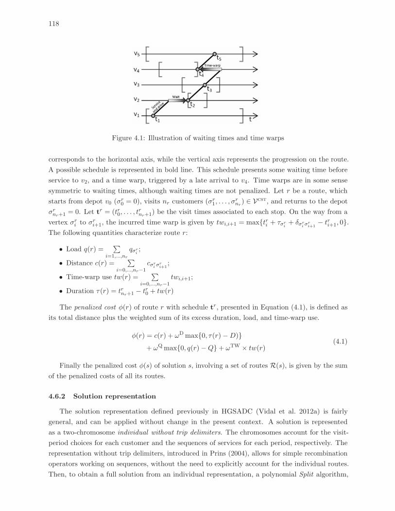
118

Figure 4.1: Illustration of waiting times and time warps

corresponds to the horizontal axis, while the vertical axis represents the progression on the route.

A possible schedule is represented in bold line. This schedule presents some waiting time before

service to v2, and a time warp, triggered by a late arrival to v4. Time warps are in some sense

symmetric to waiting times, although waiting times are not penalized. Let r be a route, which

starts from depot v0 (σr0 = 0), visits nr customers (σr1, . . . , σrnr) ∈ Vcst, and returns to the depot

σrnr+1 = 0. Let tr = (tr0, . . . , trnr+1) be the visit times associated to each stop. On the way from a

vertex σri to σri+1, the incurred time warp is given by twi,i+1 = max{tri + τσri+ δσr

i σri+1

− tri+1, 0}.The following quantities characterize route r:

• Load q(r) =∑

i=1,...,nr

qσri;

• Distance c(r) =∑

i=0,...,nr−1cσr

i σri+1

;

• Time-warp use tw(r) =∑

i=0,...,nr−1twi,i+1;

• Duration τ(r) = trnr+1 − tr0 + tw(r)

The penalized cost φ(r) of route r with schedule tr, presented in Equation (4.1), is defined as

its total distance plus the weighted sum of its excess duration, load, and time-warp use.

φ(r) = c(r) + ωDmax{0, τ(r)−D)}+ ωQmax{0, q(r)−Q}+ ωTW × tw(r)

(4.1)

Finally the penalized cost φ(s) of solution s, involving a set of routes R(s), is given by the sum

of the penalized costs of all its routes.


The solution representation defined previously in HGSADC (Vidal et al. 2012a) is fairly

general, and can be applied without change in the present context. A solution is represented

as a two-chromosome individual without trip delimiters. The chromosomes account for the visit-

period choices for each customer and the sequences of services for each period, respectively. The

representation without trip delimiters, introduced in Prins (2004), allows for simple recombination

operators working on sequences, without the need to explicitly account for the individual routes.

Then, to obtain a full solution from an individual representation, a polynomial Split algorithm,

119

based on a shortest path procedure, is applied for each period to optimally partition the sequence

of customers into routes. In our context, we use a Split algorithm that respects the maximum

number of routes (Chu et al. 2006), and includes in the auxiliary graph penalized infeasible routes

r regarding duration, load, and time-window constraints, and such that q(r) ≤ 2Q. Reversely,

any PVRPTW solution, represented by its routes for each period, can be transformed into an

individual by removing visits to the depot.

4.6.3 The diversity and cost objective for evaluating individuals

Any individual P in the population is characterized by its solution cost φ(P ) (Section 4.6.1),

and its diversity contribution Δ(P ) defined as the average distance from P to its closest neighbours

Nclose in the subpopulation (Equation 4.2).

Δ(P ) =1

|Nclose|∑

P2∈Nclose

δ(P, P2) (4.2)

For the PVRPTW and SDVRPTW, we rely on a Hamming distance δ measuring the proportion

of customers with identical patterns or vehicle type assignments, as in Vidal et al. (2012a). For the

VRPTW and MDVRPTW, experiments led to choose the broken pairs distance (see Prins 2009b),

which evaluates the amount of common arcs.

The evaluation, biased fitness, BF (P ) of an individual P (Equation 4.3) is then a “diversity and

cost objective” that involves both the rank fit(P ) of P in the subpopulation with regards to solution

cost φ(P ), and its rank dc(P ) in terms of diversity contribution Δ(P ) (Equation 4.2). BF (P )

depends upon the actual number of individuals in the subpopulation Nindiv, and a parameter Nelite

ensuring elitism properties during survivor selection. This trade-off between diversity and elitism

is critical for a thorough and efficient search.

BF (P ) = fit(P ) +

(1− Nelite

Nindiv

)dc(P ) (4.3)

4.6.4 Parent selection and crossover

An iteration of HGSADC corresponds to the generation of a new individual by a succession

of genetic operations. Two parents are first selected by binary tournament in the union of both

feasible and infeasible populations, and used as input to the crossover operator. The PIX crossover

(Vidal et al. 2012a) is used for the PVRPTW. PIX enables to inherit good sequences of visits

from both parents, and also to recombine visit patterns. For the VRPTW, we rely on the simple

Ordered Crossover (OX) (see Prins 2004, for instance). These crossovers allow both small solution

refinement and more important structural changes.

4.6.5 Neighbourhood search for VRPTW education and repair

An offspring resulting from the crossover operator undergoes the Split procedure to extract

its routes. A neighbourhood search-based improvement operator, called education, is then sys-

tematically applied, followed by a repair phase, called with probability Prep, when the resulting

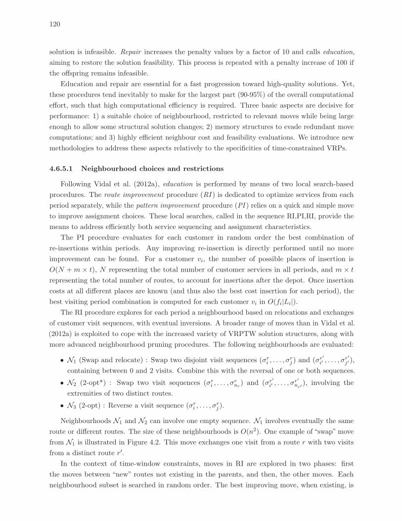
120

solution is infeasible. Repair increases the penalty values by a factor of 10 and calls education,

aiming to restore the solution feasibility. This process is repeated with a penalty increase of 100 if

the offspring remains infeasible.

Education and repair are essential for a fast progression toward high-quality solutions. Yet,

these procedures tend inevitably to make for the largest part (90-95%) of the overall computational

effort, such that high computational efficiency is required. Three basic aspects are decisive for

performance: 1) a suitable choice of neighbourhood, restricted to relevant moves while being large

enough to allow some structural solution changes; 2) memory structures to evade redundant move

computations; and 3) highly efficient neighbour cost and feasibility evaluations. We introduce new

methodologies to address these aspects relatively to the specificities of time-constrained VRPs.

4.6.5.1 Neighbourhood choices and restrictions

Following Vidal et al. (2012a), education is performed by means of two local search-based

procedures. The route improvement procedure (RI ) is dedicated to optimize services from each

period separately, while the pattern improvement procedure (PI ) relies on a quick and simple move

to improve assignment choices. These local searches, called in the sequence RI,PI,RI, provide the

means to address efficiently both service sequencing and assignment characteristics.

The PI procedure evaluates for each customer in random order the best combination of

re-insertions within periods. Any improving re-insertion is directly performed until no more

improvement can be found. For a customer vi, the number of possible places of insertion is

O(N +m × t), N representing the total number of customer services in all periods, and m × t

representing the total number of routes, to account for insertions after the depot. Once insertion

costs at all different places are known (and thus also the best cost insertion for each period), the

best visiting period combination is computed for each customer vi in O(fi|Li|).The RI procedure explores for each period a neighbourhood based on relocations and exchanges

of customer visit sequences, with eventual inversions. A broader range of moves than in Vidal et al.

(2012a) is exploited to cope with the increased variety of VRPTW solution structures, along with

more advanced neighbourhood pruning procedures. The following neighbourhoods are evaluated:

• N1 (Swap and relocate) : Swap two disjoint visit sequences (σri , . . . , σrj ) and (σr

′i′ , . . . , σ

r′j′ ),

containing between 0 and 2 visits. Combine this with the reversal of one or both sequences.

• N2 (2-opt*) : Swap two visit sequences (σri , . . . , σrnr) and (σr

′i′ , . . . , σ

r′nr′ ), involving the

extremities of two distinct routes.

• N3 (2-opt) : Reverse a visit sequence (σri , . . . , σrj ).

Neighbourhoods N1 and N2 can involve one empty sequence. N1 involves eventually the same

route or different routes. The size of these neighbourhoods is O(n2). One example of “swap” move

from N1 is illustrated in Figure 4.2. This move exchanges one visit from a route r with two visits

from a distinct route r′.In the context of time-window constraints, moves in RI are explored in two phases: first

the moves between “new” routes not existing in the parents, and then, the other moves. Each

neighbourhood subset is searched in random order. The best improving move, when existing, is

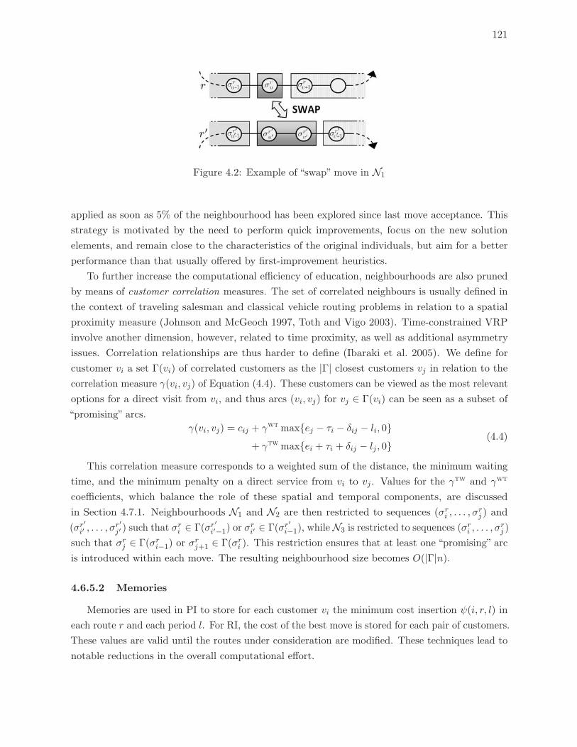
121

Figure 4.2: Example of “swap” move in N1

applied as soon as 5% of the neighbourhood has been explored since last move acceptance. This

strategy is motivated by the need to perform quick improvements, focus on the new solution

elements, and remain close to the characteristics of the original individuals, but aim for a better

performance than that usually offered by first-improvement heuristics.

To further increase the computational efficiency of education, neighbourhoods are also pruned

by means of customer correlation measures. The set of correlated neighbours is usually defined in

the context of traveling salesman and classical vehicle routing problems in relation to a spatial

proximity measure (Johnson and McGeoch 1997, Toth and Vigo 2003). Time-constrained VRP

involve another dimension, however, related to time proximity, as well as additional asymmetry

issues. Correlation relationships are thus harder to define (Ibaraki et al. 2005). We define for

customer vi a set Γ(vi) of correlated customers as the |Γ| closest customers vj in relation to the

correlation measure γ(vi, vj) of Equation (4.4). These customers can be viewed as the most relevant

options for a direct visit from vi, and thus arcs (vi, vj) for vj ∈ Γ(vi) can be seen as a subset of

“promising” arcs.

γ(vi, vj) = cij + γwtmax{ej − τi − δij − li, 0}+ γtwmax{ei + τi + δij − lj , 0}

(4.4)

This correlation measure corresponds to a weighted sum of the distance, the minimum waiting

time, and the minimum penalty on a direct service from vi to vj . Values for the γtw and γwt

coefficients, which balance the role of these spatial and temporal components, are discussed

in Section 4.7.1. Neighbourhoods N1 and N2 are then restricted to sequences (σri , . . . , σrj ) and

(σr′

i′ , . . . , σr′j′ ) such that σri ∈ Γ(σr

′i′−1) or σ

ri′ ∈ Γ(σr

′i−1), while N3 is restricted to sequences (σri , . . . , σ

rj )

such that σrj ∈ Γ(σri−1) or σrj+1 ∈ Γ(σri ). This restriction ensures that at least one “promising” arc

is introduced within each move. The resulting neighbourhood size becomes O(|Γ|n).

4.6.5.2 Memories

Memories are used in PI to store for each customer vi the minimum cost insertion ψ(i, r, l) in

each route r and each period l. For RI, the cost of the best move is stored for each pair of customers.

These values are valid until the routes under consideration are modified. These techniques lead to

notable reductions in the overall computational effort.

122

4.6.5.3 Move evaluations

When infeasible solutions are used, evaluating moves implies to compute the change in total

arc costs, as well as the variation of duration, load, and time-window infeasibility of the routes.

Calculation of cost and load variation is straightforward to perform in amortized O(1) for moves

based on a constant number of arc exchanges (Kindervater and Savelsbergh 1997). Nagata et al.

(2010) also provided the means to compute infeasibility in O(1) for some neighbourhoods, including

2-opt*, inter-route swaps, and inter-route inserts. This method can not address as efficiently intra-

route moves or more complex neighborhoods, however, and does not actually manage duration

features. We thus introduce new procedures to evaluate combined duration and time-window

infeasibility in amortized O(1). The proposed approach is widely applicable to any classical

neighbourhood based on a constant number of arc exchanges or sequence relocations.

We first observe that any such move can be viewed as a separation of routes into subsequences,

which are then concatenated into new routes. This simple property is formalized in Kindervater

and Savelsbergh (1997), Irnich (2008a), and Vidal et al. (2011). In the example of Figure

4.2, the move produces indeed two new routes, (σr0, . . . , σri−1) ⊕ (σr

′i′ , σ

r′j′ ) ⊕ (σrj+1, . . . , σ

rnr) and

(σr′

0 , . . . , σr′i′−1) ⊕ (σri ) ⊕ (σr

′j′+1, . . . , σ

r′nr′ ), where ⊕ represents the concatenation operator. Our

move evaluation approach follows from this observation, and uses induction on the concatenation

operation to develop suitable re-optimization data on subsequences of consecutive visits in the

incumbent solution.

For each such subsequence σ, containing visits to depots or customers, we compute the minimum

duration D(σ), minimum time-warp use TW (σ), earliest E(σ) and latest visit L(σ) to the first

vertex allowing a schedule with minimum duration and minimum time-warp use, as well as the

cumulated distance C(σ) and load Q(σ). This data is straightforward to compute for a sequence

σ0 involving a single vertex vi, as D(σ0) = τi, TW (σ0) = 0, E(σ0) = ei, L(σ0) = li, C(σ

0) = 0

and Q(σ0) = qi. Proposition 4.6.1 then enables to compute the same data on concatenations of

sequences. Equations (4.5 - 4.10) are frequently used in the VRP literature to calculate loads and

costs. The other statements, which target the temporal aspects of the problem, are proven in III.2.

Proposition 4.6.1 (Concatenation of two sequences) Let σ = (σi, . . . , σj) and σ′ = (σ′i′ , . . . , σ

′j′)

be two subsequences of visits. The concatenated subsequence σ⊕ σ′ is characterized by the following

data:

D(σ ⊕ σ′) = D(σ) +D(σ′) + δσjσ′i′+ΔWT (4.5)

TW (σ ⊕ σ′) = TW (σ) + TW (σ′) + ΔTW (4.6)

E(σ ⊕ σ′) = max{E(σ′)−Δ, E(σ)} −ΔWT (4.7)

L(σ ⊕ σ′) = min{L(σ′)−Δ, L(σ)}+ΔTW (4.8)

C(σ ⊕ σ′) = C(σ) + C(σ′) + cσjσ′i′

(4.9)

Q(σ ⊕ σ′) = Q(σ) +Q(σ′) (4.10)

123

where Δ = D(σ)− TW (σ) + δσjσ′i′, ΔWT = max{E(σ′)−Δ− L(σ), 0} and ΔTW = max{E(σ) +

Δ− L(σ′), 0}.

The neighbourhood evaluation procedure we propose relies on Proposition 4.6.1 to first develop

data on relevant consecutive visit subsequences (and their reversal) in a preprocessing phase, and

then to evaluate the penalties and costs of routes issued from the moves. Classical neighbourhoods

in the literature correspond to a concatenation of less than five subsequences. Hence, given the

data on subsequences, any move evaluation is performed in constant time. As shown in Vidal

et al. (2011), this property stands for any move issued from a constant number of arc exchanges or

customer visit relocations.

Experiments showed that, for some problem instances with long routes with more than 50

customers, data preprocessing on all O(n2) subsequences can play a non negligible role in the

overall computation effort. The 1-level or 2-level strategy of Irnich (2008a) can be employed to

limit this preprocessing to O(n4/3) or O(n8/7) subsequences, while maintaining the constant time

evaluation of moves. To make it even simpler, we limited the preprocessing to “prefix” (and “suffix”)

subsequences containing the first (the last) customer of a route, and subsequences of size smaller

than 20. This data enables to evaluate inter-route moves in constant time, and allows an evaluation

of intra-route moves as a concatenation of less than 7 subsequences for the instances considered.

4.6.6 Population management and search guidance

The main components of HGSADC regarding population management remain unchanged from

Vidal et al. (2012a). The two subpopulations are set up to contain between μ and μ+λ individuals.

To initialize the populations, 4μ individuals are created by randomly choosing the patterns and

routes, using Education and, when infeasible, Repair. These individuals are then included in

the appropriate subpopulations, which then evolve through iterative generation, education, and

selections of individuals. Any solution produced by the education and repair operators is transformed

into an individual by removing visits to depots (Section 4.6.2), and is included in the appropriate

subpopulation with respect to its feasibility. It can thus be selected for mating immediately after

education. Any subpopulation reaching the size μ+ λ undergoes a survivor-selection phase, where

λ individuals are discarded. Let a “clone” be an individual with the same solution cost, or null

distance to another with respect to the metric defined in Section 4.6.3. Survivor selection removes

iteratively λ times the worst clone in terms of biased fitness (Equation 4.3), or the worst individual

when no clone exists. The use of the biased fitness for survivor selection promotes both elitism and

innovation during the search (Vidal et al. 2012a).

The proportion of feasible solutions following education with regards to duration, capacity,

and time-window constraints is monitored during the search on the last 100 generated individuals.

Penalty coefficients ωD, ωQ, and ωTW (Section 4.6.1) are also adjusted each 100 iterations. Let

parameter ξREF stand for the target proportion of feasible individuals. If the proportion of

feasible individuals relatively to one type of constraint (duration, load or time-window) falls below

ξREF − 5% (or, rises to more than ξREF + 5%), then the corresponding penalty is increased (or,

decreased).

124

A diversification phase finally occurs whenever Itdiv = 0.4ItNI iterations are performed without

improving the best solution. Diversification retains the best μ/3 individuals of each subpopulation,

to be completed with 4μ new individuals as in the Initialization phase, thus introducing new genetic

material.

All these components contribute towards a more thorough search, and complement advanta-

geously the aggressive local improvement abilities of education and repair operators.

4.6.7 Decomposition phases

Variants of vehicle routing problems with time windows lend themselves well to various

decomposition approaches, mostly based on geometry (Taillard 1993, Reimann et al. 2004, Ostertag

2008, Bent and Van Hentenryck 2010), temporal aspects (Bent and Van Hentenryck 2010), or

problem structure (Crainic et al. 2009), which enable to address large instances more efficiently.

We introduce a simple decomposition framework for population-based methods, which takes

full advantage of their associated pool of solutions. The approach proceeds in four steps: 1)

features from one elite solution are exploited to define subproblems; 2) initial individuals for the

subproblems are created from the genetic material of the complete problem population; 3) the

algorithm, here HGSADC, is called to address these subproblems; 4) a set of complete solutions is

finally reconstructed.

We rely on simple route-based geometrical decompositions in the VRPTW case. For the

PVRPTW, fixing assignments to periods naturally decomposes the problem. It is worth noticing that

the “integration” of partial solutions into solutions of the complete problem is here straightforward,

as it simply involves gathering the routes. Also, any improvement in any subproblem leads to

an improvement of the elite complete solution, as subproblems are built from the features of this

solution.

In the current implementation, decomposition phases occur every Itdec iterations, and are only

used on problems with more than 120 customers. The elite solution is randomly selected from

the 25% best feasible individuals (or infeasible if no feasible solution has been found). In the

VRPTW case, routes from this elite solution are swept circularly around the depot by polar angle

of barycentre, and included in a set Rdec. Each time the number of customers in routes from

Rdec becomes larger than 120, or when all the routes have been swept, a VRPTW subproblem

is created with the customers from Rdec and the set is emptied. Subproblems of this size can be

very efficiently handled by HGSADC. In the case of the PVRPTW, we fix the periods of service,

leading to a subproblem for each period.

Initial populations of subproblem solutions are created from the complete solutions population,

by retaining from the route chromosomes of complete individuals only the services that occur in

the subproblem at the right period. For the PVRTPW, visits from solutions with patterns different

from those of the elite solution can be missing. These visits are completed by means of a least

cost insertion heuristic. HGSADC is then run on each of these subproblems until Itdec/2 iterations

without improvement are performed. Combining the best solution of each subproblem yields an

elite solution, to be added to the population of the complete problem. The same process is repeated

with the second and the third best solutions to produce two additional elite individuals.

125


Extensive computational experiments were performed to analyze the impact of the parameter

settings (Section 4.7.1), assess HGSADC performance when compared to state-of-the-art methods

for each problem (Section 4.7.2), and evaluate the role of the new decomposition phases (Section

4.7.3). The algorithm is coded in C++, compiled with “g++ -O3”, and run on a Intel Xeon 2.93

Ghz processor.

We rely on a variety of classical benchmark instance sets: Solomon and Desrosiers (1988)

and Gehring and Homberger (1999) VRPTW instances, Cordeau et al. (2001a) and Cordeau and

Laporte (2001) instances for PVRPTW, MDVRPTW, SDVRPTW with duration constraints and

the PVRPTW instances of Pirkwieser and Raidl (2009b) without duration constraints. These

instances involve from 48 to 1008 customers, up to 9 depots, 10 periods, and 6 vehicle types. It

should be noted that the distances of Pirkwieser and Raidl (2009b) instances have been truncated

to the first digit by previous authors. We used this convention exclusively in this case to perform a

fair comparison. We also introduce new larger-dimension instances for PVRPTW, MDVRPTW,

and SDVRPTW, involving 360 to 960 customers, and up to 4608 total services, following the

generation procedure of Cordeau et al. (1997, 2001a). These instances are available upon request.

Finally, the traditional objective for VRPTW is fleet minimization in priority, and then route

length minimization. To apply HGSADC with this objective, we first constrain the fleet size to a

large value of 100, and iteratively interrupt the run and reduce the fleet size whenever a feasible

solution is found. As soon as HGSADC fails to find a feasible solution, we return to the last feasible

fleet value and perform a final run. It is noteworthy that both objectives are here addressed in

single-stage-single-algorithm mode contrasting with current state-of-the-art VRPTW methods,

which generally rely on two distinct procedures and concepts.

4.7.1 Parameter calibration

The parameter values from Vidal et al. (2012a) were shown to perform well on a large range of

VRP variants. In order to study the applicability and generality of the HGSADC framework with

limited changes, we voluntarily limited the role of parameter tuning, to focus exclusively on the

new ones, related to the neighbourhood evaluation procedures (γwt, γtw), and the decomposition

phases. The remaining parameter values are imported from Vidal et al. (2012a), where an extensive

meta-calibration approach had been used to produce good parameter values on closely related

PVRP and MDVRP problems. Thus, Nelite = 8 and |Nclose| = 3 ; Prep = 0.5 and |Γ| = 40 ;

(μ, λ) = (25, 40) and ξREF = 0.2 (Section 4.6.6). Finally, the termination criteria ItNI = 5000

is used to compare with other authors in similar run times, while Itdec = 2000 to balance the

computation time dedicated to decomposition phases and the regular run.

The nature of VRPTW solutions tends to strongly vary in relation to the distribution and

tightness of time windows. For some problems, high-quality solutions involve some long arcs and

relatively small waiting times, while for less tightly constrained problems, closer to the classical

VRP, long arcs become very unlikely. The parameters γTW and γWT , balancing the role of

geometrical and temporal aspects during neighbourhood pruning, are thus critical, and need to

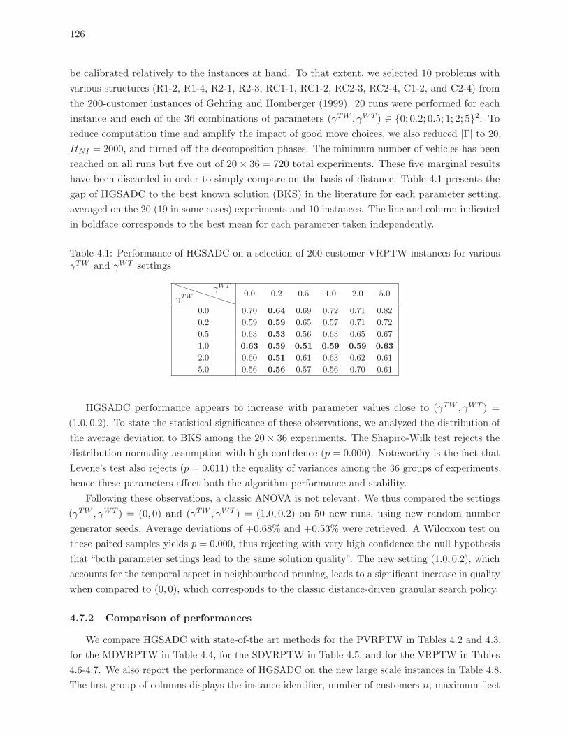
126

be calibrated relatively to the instances at hand. To that extent, we selected 10 problems with

various structures (R1-2, R1-4, R2-1, R2-3, RC1-1, RC1-2, RC2-3, RC2-4, C1-2, and C2-4) from

the 200-customer instances of Gehring and Homberger (1999). 20 runs were performed for each

instance and each of the 36 combinations of parameters (γTW , γWT ) ∈ {0; 0.2; 0.5; 1; 2; 5}2. To

reduce computation time and amplify the impact of good move choices, we also reduced |Γ| to 20,

ItNI = 2000, and turned off the decomposition phases. The minimum number of vehicles has been

reached on all runs but five out of 20× 36 = 720 total experiments. These five marginal results

have been discarded in order to simply compare on the basis of distance. Table 4.1 presents the

gap of HGSADC to the best known solution (BKS) in the literature for each parameter setting,

averaged on the 20 (19 in some cases) experiments and 10 instances. The line and column indicated

in boldface corresponds to the best mean for each parameter taken independently.

Table 4.1: Performance of HGSADC on a selection of 200-customer VRPTW instances for variousγTW and γWT settings

γTWγWT

0.0 0.2 0.5 1.0 2.0 5.0

0.0 0.70 0.64 0.69 0.72 0.71 0.82

0.2 0.59 0.59 0.65 0.57 0.71 0.72

0.5 0.63 0.53 0.56 0.63 0.65 0.67

1.0 0.63 0.59 0.51 0.59 0.59 0.63

2.0 0.60 0.51 0.61 0.63 0.62 0.61

5.0 0.56 0.56 0.57 0.56 0.70 0.61

HGSADC performance appears to increase with parameter values close to (γTW , γWT ) =

(1.0, 0.2). To state the statistical significance of these observations, we analyzed the distribution of

the average deviation to BKS among the 20× 36 experiments. The Shapiro-Wilk test rejects the

distribution normality assumption with high confidence (p = 0.000). Noteworthy is the fact that

Levene’s test also rejects (p = 0.011) the equality of variances among the 36 groups of experiments,

hence these parameters affect both the algorithm performance and stability.

Following these observations, a classic ANOVA is not relevant. We thus compared the settings

(γTW , γWT ) = (0, 0) and (γTW , γWT ) = (1.0, 0.2) on 50 new runs, using new random number

generator seeds. Average deviations of +0.68% and +0.53% were retrieved. A Wilcoxon test on

these paired samples yields p = 0.000, thus rejecting with very high confidence the null hypothesis

that “both parameter settings lead to the same solution quality”. The new setting (1.0, 0.2), which

accounts for the temporal aspect in neighbourhood pruning, leads to a significant increase in quality

when compared to (0, 0), which corresponds to the classic distance-driven granular search policy.

4.7.2 Comparison of performances

We compare HGSADC with state-of-the art methods for the PVRPTW in Tables 4.2 and 4.3,

for the MDVRPTW in Table 4.4, for the SDVRPTW in Table 4.5, and for the VRPTW in Tables

4.6-4.7. We also report the performance of HGSADC on the new large scale instances in Table 4.8.

The first group of columns displays the instance identifier, number of customers n, maximum fleet

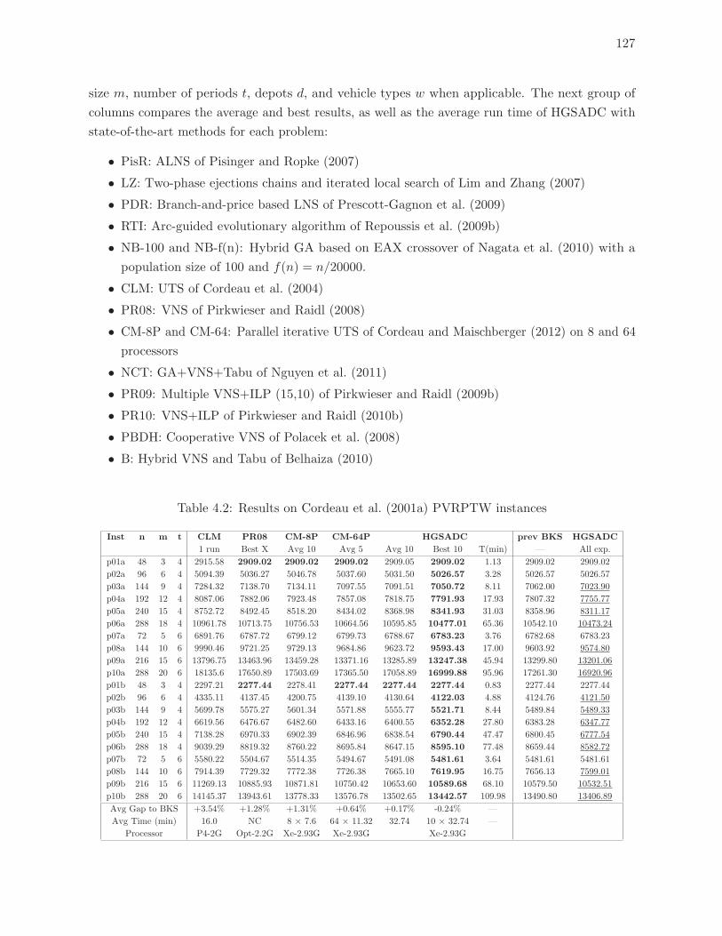
127

size m, number of periods t, depots d, and vehicle types w when applicable. The next group of

columns compares the average and best results, as well as the average run time of HGSADC with

state-of-the-art methods for each problem:

• PisR: ALNS of Pisinger and Ropke (2007)

• LZ: Two-phase ejections chains and iterated local search of Lim and Zhang (2007)

• PDR: Branch-and-price based LNS of Prescott-Gagnon et al. (2009)

• RTI: Arc-guided evolutionary algorithm of Repoussis et al. (2009b)

• NB-100 and NB-f(n): Hybrid GA based on EAX crossover of Nagata et al. (2010) with a

population size of 100 and f(n) = n/20000.

• CLM: UTS of Cordeau et al. (2004)

• PR08: VNS of Pirkwieser and Raidl (2008)

• CM-8P and CM-64: Parallel iterative UTS of Cordeau and Maischberger (2012) on 8 and 64

processors

• NCT: GA+VNS+Tabu of Nguyen et al. (2011)

• PR09: Multiple VNS+ILP (15,10) of Pirkwieser and Raidl (2009b)

• PR10: VNS+ILP of Pirkwieser and Raidl (2010b)

• PBDH: Cooperative VNS of Polacek et al. (2008)

• B: Hybrid VNS and Tabu of Belhaiza (2010)

Table 4.2: Results on Cordeau et al. (2001a) PVRPTW instances

Inst n m t CLM PR08 CM-8P CM-64P HGSADC prev BKS HGSADC

1 run Best X Avg 10 Avg 5 Avg 10 Best 10 T(min) — All exp.

p01a 48 3 4 2915.58 2909.02 2909.02 2909.02 2909.05 2909.02 1.13 2909.02 2909.02

p02a 96 6 4 5094.39 5036.27 5046.78 5037.60 5031.50 5026.57 3.28 5026.57 5026.57

p03a 144 9 4 7284.32 7138.70 7134.11 7097.55 7091.51 7050.72 8.11 7062.00 7023.90

p04a 192 12 4 8087.06 7882.06 7923.48 7857.08 7818.75 7791.93 17.93 7807.32 7755.77

p05a 240 15 4 8752.72 8492.45 8518.20 8434.02 8368.98 8341.93 31.03 8358.96 8311.17

p06a 288 18 4 10961.78 10713.75 10756.53 10664.56 10595.85 10477.01 65.36 10542.10 10473.24

p07a 72 5 6 6891.76 6787.72 6799.12 6799.73 6788.67 6783.23 3.76 6782.68 6783.23

p08a 144 10 6 9990.46 9721.25 9729.13 9684.86 9623.72 9593.43 17.00 9603.92 9574.80

p09a 216 15 6 13796.75 13463.96 13459.28 13371.16 13285.89 13247.38 45.94 13299.80 13201.06

p10a 288 20 6 18135.6 17650.89 17503.69 17365.50 17058.89 16999.88 95.96 17261.30 16920.96

p01b 48 3 4 2297.21 2277.44 2278.41 2277.44 2277.44 2277.44 0.83 2277.44 2277.44

p02b 96 6 4 4335.11 4137.45 4200.75 4139.10 4130.64 4122.03 4.88 4124.76 4121.50

p03b 144 9 4 5699.78 5575.27 5601.34 5571.88 5555.77 5521.71 8.44 5489.84 5489.33

p04b 192 12 4 6619.56 6476.67 6482.60 6433.16 6400.55 6352.28 27.80 6383.28 6347.77

p05b 240 15 4 7138.28 6970.33 6902.39 6846.96 6838.54 6790.44 47.47 6800.45 6777.54

p06b 288 18 4 9039.29 8819.32 8760.22 8695.84 8647.15 8595.10 77.48 8659.44 8582.72

p07b 72 5 6 5580.22 5504.67 5514.35 5494.67 5491.08 5481.61 3.64 5481.61 5481.61

p08b 144 10 6 7914.39 7729.32 7772.38 7726.38 7665.10 7619.95 16.75 7656.13 7599.01

p09b 216 15 6 11269.13 10885.93 10871.81 10750.42 10653.60 10589.68 68.10 10579.50 10532.51

p10b 288 20 6 14145.37 13943.61 13778.33 13576.78 13502.65 13442.57 109.98 13490.80 13406.89

Avg Gap to BKS +3.54% +1.28% +1.31% +0.64% +0.17% -0.24% —

Avg Time (min) 16.0 NC 8 × 7.6 64 × 11.32 32.74 10 × 32.74 —

Processor P4-2G Opt-2.2G Xe-2.93G Xe-2.93G Xe-2.93G

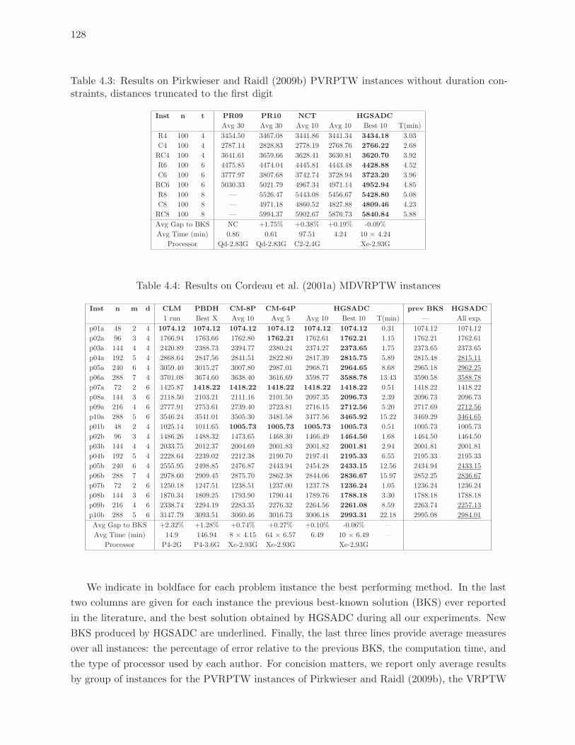
128

Table 4.3: Results on Pirkwieser and Raidl (2009b) PVRPTW instances without duration con-straints, distances truncated to the first digit

Inst n t PR09 PR10 NCT HGSADC

Avg 30 Avg 30 Avg 10 Avg 10 Best 10 T(min)

R4 100 4 3454.50 3467.08 3441.86 3441.34 3434.18 3.03

C4 100 4 2787.14 2828.83 2778.19 2768.76 2766.22 2.68

RC4 100 4 3641.61 3659.66 3628.41 3630.81 3620.70 3.92

R6 100 6 4475.85 4474.04 4445.81 4443.48 4428.88 4.52

C6 100 6 3777.97 3807.68 3742.74 3728.94 3723.20 3.96

RC6 100 6 5030.33 5021.79 4967.34 4971.14 4952.94 4.85

R8 100 8 — 5526.47 5443.08 5456.67 5428.80 5.08

C8 100 8 — 4971.18 4860.52 4827.88 4809.46 4.23

RC8 100 8 — 5994.37 5902.67 5876.73 5840.84 5.88

Avg Gap to BKS NC +1.75% +0.38% +0.19% -0.09%

Avg Time (min) 0.86 0.61 97.51 4.24 10 × 4.24

Processor Qd-2.83G Qd-2.83G C2-2.4G Xe-2.93G

Table 4.4: Results on Cordeau et al. (2001a) MDVRPTW instances

Inst n m d CLM PBDH CM-8P CM-64P HGSADC prev BKS HGSADC


p01a 48 2 4 1074.12 1074.12 1074.12 1074.12 1074.12 1074.12 0.31 1074.12 1074.12

p02a 96 3 4 1766.94 1763.66 1762.80 1762.21 1762.61 1762.21 1.15 1762.21 1762.61

p03a 144 4 4 2420.89 2388.73 2394.77 2380.24 2374.27 2373.65 1.75 2373.65 2373.65

p04a 192 5 4 2868.64 2847.56 2841.51 2822.80 2817.39 2815.75 5.89 2815.48 2815.11

p05a 240 6 4 3059.40 3015.27 3007.80 2987.01 2968.71 2964.65 8.68 2965.18 2962.25

p06a 288 7 4 3701.08 3674.60 3638.40 3616.69 3598.77 3588.78 13.43 3590.58 3588.78

p07a 72 2 6 1425.87 1418.22 1418.22 1418.22 1418.22 1418.22 0.51 1418.22 1418.22

p08a 144 3 6 2118.50 2103.21 2111.16 2101.50 2097.35 2096.73 2.39 2096.73 2096.73

p09a 216 4 6 2777.91 2753.61 2739.40 2723.81 2716.15 2712.56 5.20 2717.69 2712.56

p10a 288 5 6 3546.24 3541.01 3505.30 3481.58 3477.56 3465.92 15.22 3469.29 3464.65

p01b 48 2 4 1025.14 1011.65 1005.73 1005.73 1005.73 1005.73 0.51 1005.73 1005.73

p02b 96 3 4 1486.26 1488.32 1473.65 1468.30 1466.49 1464.50 1.68 1464.50 1464.50

p03b 144 4 4 2033.75 2012.37 2004.69 2001.83 2001.82 2001.81 2.94 2001.81 2001.81

p04b 192 5 4 2228.64 2239.02 2212.38 2199.70 2197.41 2195.33 6.55 2195.33 2195.33

p05b 240 6 4 2555.95 2498.85 2476.87 2443.94 2454.28 2433.15 12.56 2434.94 2433.15

p06b 288 7 4 2978.60 2909.45 2875.70 2862.38 2844.06 2836.67 15.97 2852.25 2836.67

p07b 72 2 6 1250.18 1247.51 1238.51 1237.00 1237.78 1236.24 1.05 1236.24 1236.24

p08b 144 3 6 1870.34 1809.25 1793.90 1790.44 1789.76 1788.18 3.30 1788.18 1788.18

p09b 216 4 6 2338.74 2294.19 2283.35 2276.32 2264.56 2261.08 8.59 2263.74 2257.13

p10b 288 5 6 3147.79 3093.51 3060.46 3016.73 3006.18 2993.31 22.18 2995.08 2984.01

Avg Gap to BKS +2.32% +1.28% +0.74% +0.27% +0.10% -0.06% —

Avg Time (min) 14.9 146.94 8 × 4.15 64 × 6.57 6.49 10 × 6.49 —

Processor P4-2G P4-3.6G Xe-2.93G Xe-2.93G Xe-2.93G

We indicate in boldface for each problem instance the best performing method. In the last

two columns are given for each instance the previous best-known solution (BKS) ever reported

in the literature, and the best solution obtained by HGSADC during all our experiments. New

BKS produced by HGSADC are underlined. Finally, the last three lines provide average measures

over all instances: the percentage of error relative to the previous BKS, the computation time, and

the type of processor used by each author. For concision matters, we report only average results

by group of instances for the PVRPTW instances of Pirkwieser and Raidl (2009b), the VRPTW

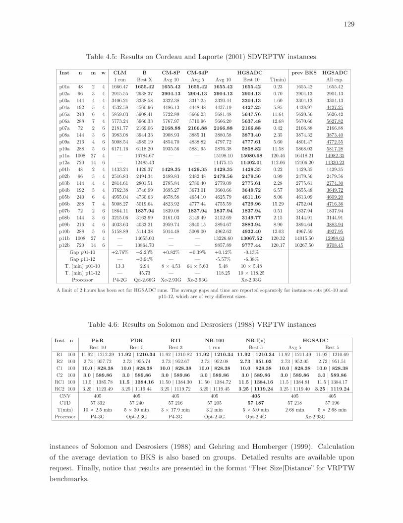
129

Table 4.5: Results on Cordeau and Laporte (2001) SDVRPTW instances.

Inst n m w CLM B CM-8P CM-64P HGSADC prev BKS HGSADC


p01a 48 2 4 1666.47 1655.42 1655.42 1655.42 1655.42 1655.42 0.23 1655.42 1655.42

p02a 96 3 4 2915.55 2938.37 2904.13 2904.13 2904.13 2904.13 0.70 2904.13 2904.13

p03a 144 4 4 3406.21 3338.58 3322.38 3317.25 3320.44 3304.13 1.60 3304.13 3304.13

p04a 192 5 4 4532.58 4560.96 4486.13 4448.48 4437.19 4427.25 5.85 4438.97 4427.25

p05a 240 6 4 5859.03 5908.41 5722.89 5666.23 5681.48 5647.76 11.64 5620.56 5626.42

p06a 288 7 4 5773.24 5966.33 5767.97 5710.96 5666.20 5637.48 12.68 5670.66 5627.82

p07a 72 2 6 2181.77 2169.06 2168.88 2166.88 2166.88 2166.88 0.42 2166.88 2166.88

p08a 144 3 6 3983.08 3944.33 3908.93 3885.31 3880.58 3873.40 2.35 3874.32 3873.40

p09a 216 4 6 5008.54 4985.19 4854.70 4838.82 4797.72 4777.61 5.60 4801.47 4772.55

p10a 288 5 6 6171.16 6118.20 5935.56 5881.95 5876.38 5858.82 11.58 5868.03 5817.28

p11a 1008 27 4 — 16784.67 — — 15198.10 15080.68 120.46 16418.21 14982.35

p12a 720 14 6 — 12485.43 — — 11475.15 11402.01 112.06 12106.20 11330.23

p01b 48 2 4 1433.24 1429.37 1429.35 1429.35 1429.35 1429.35 0.22 1429.35 1429.35

p02b 96 3 4 2516.83 2494.34 2489.83 2482.48 2479.56 2479.56 0.99 2479.56 2479.56

p03b 144 4 4 2814.61 2801.51 2785.84 2780.40 2779.09 2775.61 2.28 2775.61 2774.30

p04b 192 5 4 3762.38 3746.99 3695.27 3673.01 3660.66 3649.72 6.57 3655.48 3649.72

p05b 240 6 4 4955.04 4730.63 4678.58 4654.10 4625.79 4611.16 8.06 4613.09 4609.20

p06b 288 7 4 5008.27 5019.64 4823.92 4777.44 4755.59 4729.96 15.29 4752.04 4716.36

p07b 72 2 6 1864.11 1837.94 1839.08 1837.94 1837.94 1837.94 0.51 1837.94 1837.94

p08b 144 3 6 3215.06 3163.99 3161.03 3149.49 3152.69 3149.77 2.15 3144.91 3144.91

p09b 216 4 6 4033.63 4033.21 3959.74 3940.15 3894.67 3883.94 8.90 3894.64 3883.94

p10b 288 5 6 5158.89 5114.38 5014.48 5009.00 4962.62 4932.40 12.03 4967.59 4927.95

p11b 1008 27 4 — 14655.00 — — 13226.60 13067.52 120.32 14015.50 12998.63

p12b 720 14 6 — 10864.70 — — 9857.89 9777.44 120.17 10267.50 9708.45

Gap p01-10 +2.76% +2.23% +0.82% +0.39% +0.12% -0.13%

Gap p11-12 — +3.94% — — -5.57% -6.38%

T. (min) p01-10 13.3 2.94 8 × 4.53 64 × 5.60 5.48 10 × 5.48

T. (min) p11-12 — 45.73 — — 118.25 10 × 118.25

Processor P4-2G Qd-2.66G Xe-2.93G Xe-2.93G Xe-2.93G

A limit of 2 hours has been set for HGSADC runs. The average gaps and time are reported separately for instances sets p01-10 andp11-12, which are of very different sizes.

Table 4.6: Results on Solomon and Desrosiers (1988) VRPTW instances

Inst n PisR PDR RTI NB-100 NB-f(n) HGSADC

Best 10 Best 5 Best 3 1 run Best 5 Avg 5 Best 5

R1 100 11.92 | 1212.39 11.92 | 1210.34 11.92 | 1210.82 11.92 | 1210.34 11.92 | 1210.34 11.92 | 1211.49 11.92 | 1210.69R2 100 2.73 | 957.72 2.73 | 955.74 2.73 | 952.67 2.73 | 952.08 2.73 | 951.03 2.73 | 952.05 2.73 | 951.51C1 100 10.0 | 828.38 10.0 | 828.38 10.0 | 828.38 10.0 | 828.38 10.0 | 828.38 10.0 | 828.38 10.0 | 828.38C2 100 3.0 | 589.86 3.0 | 589.86 3.0 | 589.86 3.0 | 589.86 3.0 | 589.86 3.0 | 589.86 3.0 | 589.86RC1 100 11.5 | 1385.78 11.5 | 1384.16 11.50 | 1384.30 11.50 | 1384.72 11.5 | 1384.16 11.5 | 1384.81 11.5 | 1384.17RC2 100 3.25 | 1123.49 3.25 | 1119.44 3.25 | 1119.72 3.25 | 1119.45 3.25 | 1119.24 3.25 | 1119.40 3.25 | 1119.24CNV 405 405 405 405 405 405 405

CTD 57 332 57 240 57 216 57 205 57 187 57 218 57 196

T(min) 10 × 2.5 min 5 × 30 min 3 × 17.9 min 3.2 min 5 × 5.0 min 2.68 min 5 × 2.68 min

Processor P4-3G Opt-2.3G P4-3G Opt-2.4G Opt-2.4G Xe-2.93G

instances of Solomon and Desrosiers (1988) and Gehring and Homberger (1999). Calculation

of the average deviation to BKS is also based on groups. Detailed results are available upon

request. Finally, notice that results are presented in the format “Fleet Size|Distance” for VRPTW

benchmarks.

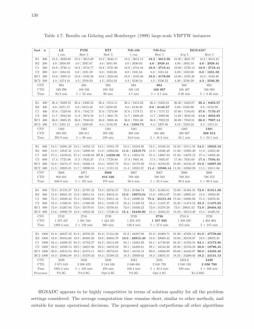
130

Table 4.7: Results on Gehring and Homberger (1999) large-scale VRPTW instances

Inst n LZ PDR RTI NB-100 NB-f(n) HGSADC

1 run Best 5 Best 3 1 run Best 5 Avg 5 Best 5

R1 200 18.2 | 3639.60 18.2 | 3615.69 18.2 | 3640.11 18.2 | 3615.15 18.2 | 3612.36 18.20 | 3621.72 18.2 | 3613.16R2 200 4.0 | 2950.09 4.0 | 2937.67 4.0 | 2941.99 4.0 | 2930.04 4.0 | 2929.41 4.00 | 2933.19 4.0 | 2929.41C1 200 18.9 | 2726.11 18.9 | 2718.77 18.9 | 2721.90 18.9 | 2718.44 18.9 | 2718.41 18.90 | 2720.13 18.9 | 2718.41C2 200 6.0 | 1834.24 6.0 | 1831.59 6.0 | 1833.36 6.0 | 1831.64 6.0 | 1831.64 6.00 | 1832.08 6.0 | 1831.59RC1 200 18.0 | 3205.51 18.0 | 3192.56 18.0 | 3224.63 18.0 | 3182.48 18.0 | 3178.68 18.00 | 3195.26 18.0 | 3180.48RC2 200 4.3 | 2574.10 4.3 | 2559.32 4.3 | 2554.33 4.3 | 2536.54 4.3 | 2536.22 4.30 | 2538.29 4.3 | 2536.20CNV 694 694 694 694 694 694 694

CTD 169 296 168 556 169 163 168 143 168 067 168 407 168 092

Time 93.2 min 5 × 53 min 90 min 4.7 min 5 × 4.1 min 8.40 min 5 × 8.40 min

R1 400 36.4 | 8489.53 36.4 | 8420.52 36.4 | 8514.11 36.4 | 8413.23 36.4 | 8403.24 36.40 | 8423.07 36.4 | 8402.57R2 400 8.0 | 6271.57 8.0 | 6213.48 8.0 | 6258.82 8.0 | 6149.49 8.0 | 6148.57 8.00 | 6168.98 8.0 | 6152.92C1 400 37.6 | 7229.04 37.6 | 7182.75 37.6 | 7273.90 37.6 | 7179.71 37.6 | 7175.72 37.60 | 7184.65 37.6 | 7170.47C2 400 11.7 | 3942.93 11.9 | 3874.58 11.7 | 3941.70 11.7 | 3898.02 11.7 | 3899.00 11.68 | 3916.83 11.6 | 3952.95RC1 400 36.0 | 8005.25 36.0 | 7940.65 36.0 | 8088.46 36.0 | 7931.66 36.0 | 7922.23 36.00 | 7942.81 36.0 | 7907.14RC2 400 8.5 | 5431.15 8.6 | 5269.09 8.4 | 5516.59 8.4 | 5293.74 8.4 | 5297.86 8.52 | 5233.33 8.5 | 5215.21CNV 1382 1385 1381 1381 1381 1382 1381

CTD 393 695 389 011 395 936 388 548 388 466 388 697 388 013


R1 600 54.5 | 18381.28 54.5 | 18252.13 54.5 | 18781.79 54.5 | 18194.38 54.5 | 18186.24 54.50 | 18111.58 54.5 | 18023.18R2 600 11.0 | 12847.31 11.0 | 12808.59 11.0 | 12804.60 11.0 | 12319.75 11.0 | 12330.49 11.00 | 12385.20 11.0 | 12352.38C1 600 57.4 | 14103.61 57.4 | 14106.03 57.3 | 14236.86 57.4 | 14054.70 57.4 | 14067.34 57.40 | 14078.12 57.4 | 14058.46C2 600 17.4 | 7725.86 17.5 | 7632.37 17.4 | 7729.80 17.4 | 7601.94 17.4 | 7605.07 17.40 | 7635.68 17.4 | 7594.41RC1 600 55.0 | 16274.17 55.0 | 16266.14 55.0 | 16767.72 55.0 | 16179.39 55.0 | 16183.95 55.00 | 16156.47 55.0 | 16097.05RC2 600 11.5 | 10935.91 11.7 | 10990.85 11.4 | 11311.81 11.4 | 10591.87 11.4 | 10586.14 11.50 | 10568.26 11.5 | 10511.86CNV 2068 2071 2066 2067 2067 2068 2068

CTD 802 681 800 797 816 326 789 420 789 592 789 353 786 373


R1 800 72.8 | 31755.57 72.8 | 31797.42 72.8 | 32734.57 72.8 | 31486.74 72.8 | 31492.81 72.80 | 31385.55 72.8 | 31311.38R2 800 15.0 | 20601.22 15.0 | 20651.81 15.0 | 20618.21 15.0 | 19873.04 15.0 | 19914.97 15.00 | 19995.82 15.0 | 19933.39C1 800 75.4 | 25026.42 75.4 | 25093.38 75.2 | 25911.44 75.3 | 24990.42 75.2 | 25151.83 75.50 | 24898.96 75.4 | 24876.38C2 800 23.4 | 11598.81 23.5 | 11569.39 23.4 | 11835.72 23.4 | 11438.52 23.4 | 11447.27 23.38 | 11474.16 23.3 | 11475.05RC1 800 72.0 | 31267.84 72.0 | 33170.01 72.0 | 33795.61 72.0 | 31020.22 72.0 | 31278.28 72.0 | 29655.52 72.0 | 29404.32RC2 800 15.6 | 16992.79 15.8 | 16852.38 15.5 | 17536.54 15.4 | 16438.90 15.4 | 16484.31 15.50 | 16513.49 15.4 | 16495.82CNV 2742 2745 2739 2739 2738 2741.8 2739

CTD 1 372 427 1 391 344 1 424 321 1 352 478 1 357 695 1 339 235 1 334 963

Time 1269.4 min 5 × 129 min 360 min 126.8 min 5 × 27.6 min 215 min 5 × 215 min

R1 1000 91.9 | 48827.23 91.9 | 49702.32 91.9 | 51414.26 91.9 | 48287.98 91.9 | 48369.71 91.90 | 47928.13 91.9 | 47759.66R2 1000 19.0 | 30164.60 19.0 | 30495.26 19.0 | 30804.79 19.0 | 28913.40 19.0 | 29003.42 19.00 | 29159.07 19.0 | 29076.45C1 1000 94.4 | 41699.32 94.3 | 41783.27 94.2 | 43111.60 94.1 | 41683.29 94.1 | 41748.60 94.42 | 41550.55 94.1 | 41572.86C2 1000 29.3 | 16589.74 29.5 | 16657.06 29.3 | 16810.22 29.1 | 16498.61 29.1 | 16534.36 28.90 | 16723.59 28.8 | 16796.45RC1 1000 90.0 | 44818.54 90.0 | 45574.11 90.0 | 46753.61 90.0 | 44743.18 90.0 | 44860.60 90.00 | 44448.97 90.0 | 44333.40RC2 1000 18.3 | 25064.88 18.5 | 25470.33 18.4 | 25588.52 18.3 | 23939.62 18.3 | 24055.31 18.24 | 24209.03 18.2 | 24131.13CNV 3429 3432 3428 3424 3424 3424.6 3420

CTD 2 071 643 2 096 823 2 144 830 2 040 661 2 045 720 2 040 193 2 036 700

Time 1865.4 min 5 × 162 min 450 min 186.4 min 5 × 35.3 min 349 min 5 × 349 min

Processor P4-3G P4-2.8G Opt-2.3G P4-3G Opt-2.4G Xe-2.93G

HGSADC appears to be highly competitive in terms of solution quality for all the problem

settings considered. The average computation time remains short, similar to other methods, and

suitable for many operational decisions. The proposed approach outperforms all other algorithms

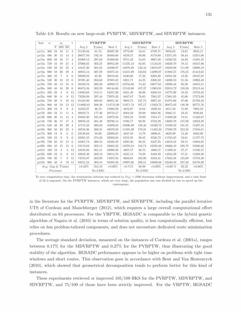
131

Table 4.8: Results on new large-scale PVRPTW, MDVRPTW, and SDVRPTW instances.

Inst n m t PVRPTW MDVRPTW SDVRPTW

P MD SD Avg 5 T(min) Best 5 Avg 5 T(min) Best 5 Avg 5 T(min) Best 5

pr11a 360 24 10 11 4 21120,94 61,74 20937,29 6772,00 16,81 6720,71 9958,05 13,91 9924,11

pr12a 480 30 13 14 4 26677,56 192,16 26483,68 8259,57 30,00 8179,80 12371,95 30,44 12251,66

pr13a 600 38 16 17 4 31909,12 297,03 31808,00 9751,22 54,85 9667,20 14562,53 44,93 14491,25

pr14a 720 44 19 21 4 37066,65 302,25 36954,39 11235,13 65,65 11124,01 16620,70 70,12 16547,86

pr15a 840 50 22 25 4 41847,30 301,05 41699,07 13078,26 132,44 13013,97 19283,90 111,09 19090,19

pr16a 960 58 26 29 4 48855,14 307,29 48375,16 14415,89 133,63 14299,87 21803,57 176,25 21413,65

pr17a 360 22 7 8 6 28889,82 65,28 28818,04 6340,66 17,23 6304,30 10581,02 12,20 10547,07

pr18a 520 30 10 12 6 37491,40 263,63 37385,82 8381,71 44,25 8308,32 14009,53 21,56 13963,49

pr19a 700 38 13 16 6 49103,78 300,39 48993,72 10734,60 74,42 10677,61 18998,48 95,29 18855,51

pr20a 880 48 16 20 6 60474,34 302,59 60144,66 12142,60 107,37 11963,91 22655,72 150,56 22513,44

pr21a 420 22 4 6 12 54562,68 213,11 54257,26 6321,20 28,00 6260,53 13775,90 16,22 13758,32

pr22a 600 30 6 8 12 73226,99 297,44 72978,33 8047,87 76,05 7985,37 17661,05 45,00 17572,09

pr23a 780 38 8 10 12 91424,98 300,02 90951,34 9984,75 137,72 9937,43 21974,90 97,06 21793,32

pr24a 960 48 10 12 12 114892,01 308,38 114712,30 11971,74 197,17 11923,72 26875,82 148,26 26775,76

pr11b 360 18 8 9 4 16102,27 86,18 15992,20 4852,67 18,04 4839,44 8011,50 15,89 7962,22

pr12b 480 24 11 11 4 20822,71 177,36 20753,17 6084,33 29,09 6063,26 9566,13 33,45 9508,68

pr13b 600 30 14 14 4 25050,30 291,83 24972,94 7282,25 70,99 7254,17 11609,39 74,81 11562,67

pr14b 720 36 17 17 4 29976,52 301,40 29790,14 8796,77 98,92 8732,29 13693,79 157,09 13623,28

pr15b 840 48 20 20 4 41715,58 300,02 41609,04 10496,39 129,48 10439,72 15589,83 191,21 15437,52

pr16b 960 56 23 23 4 49558,36 306,31 49470,50 11565,39 170,31 11483,22 17920,79 252,35 17834,61

pr17b 360 18 6 6 6 23138,63 94,09 22989,05 4847,58 15,78 4806,01 8629,90 13,20 8562,99

pr18b 520 24 9 9 6 32201,55 274,33 32093,04 6555,95 39,45 6526,72 11525,05 53,61 11477,72

pr19b 700 32 12 12 6 42467,74 300,53 42332,28 8295,30 80,55 8227,25 14918,54 92,15 14894,65

pr20b 880 42 15 15 6 53119,63 302,15 52863,23 10378,54 150,74 10325,80 18666,10 228,78 18566,66

pr21b 420 18 4 4 12 43195,88 261,51 43098,26 4887,57 36,75 4866,57 11309,41 27,17 11246,57

pr22b 600 24 6 6 12 58942,49 303,13 58814,76 6537,15 73,28 6488,50 14354,29 57,21 14288,26

pr23b 780 30 7 8 12 74755,07 302,99 74357,84 8603,85 163,99 8523,41 17635,56 125,08 17576,39

pr24b 960 40 8 10 12 94551,24 303,18 94395,56 10997,66 298,51 10890,08 23420,33 227,26 23176,90

Avg. Gap & T(min) +0.42% 254.19 +0.00% +0.71% 88.98 +0.00% +0.60 % 92.22 +0.00%

Processor Xe-2.93G Xe-2.93G Xe-2.93G

To save computation time, the termination criterion was reduced to ItNI = 2500 iterations without improvement, and a time limitof 5h is imposed. On the PVRPTW instances, which are very large, the population size was divided by two to speed up the

convergence.

in the literature for the PVRPTW, MDVRPTW, and SDVRPTW, including the parallel iterative

UTS of Cordeau and Maischberger (2012), which requires a large overall computational effort

distributed on 64 processors. For the VRPTW, HGSADC is comparable to the hybrid genetic

algorithm of Nagata et al. (2010) in terms of solution quality, is less computationally efficient, but

relies on less problem-tailored components, and does not necessitate dedicated route minimization

procedures.

The average standard deviation, measured on the instances of Cordeau et al. (2001a), ranges

between 0.17% for the MDVRPTW and 0.27% for the PVRPTW, thus illustrating the good

stability of the algorithm. HGSADC performance appears to be higher on problems with tight time

windows and short routes. This observation goes in accordance with Bent and Van Hentenryck

(2010), which showed that geometrical decomposition tends to perform better for this kind of

instances.

These experiments retrieved or improved 105/109 BKS for the PVRPTW, MDVRPTW, and

SDVRPTW, and 75/109 of those have been strictly improved. For the VRPTW, HGSADC

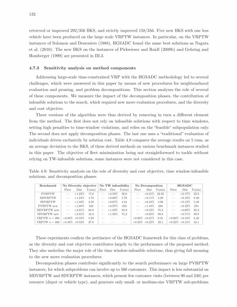
132

retrieved or improved 292/356 BKS, and strictly improved 158/356. Five new BKS with one less

vehicle have been produced on the large scale VRPTW instances. In particular, on the VRPTW

instances of Solomon and Desrosiers (1988), HGSADC found the same best solutions as Nagata

et al. (2010). The new BKS on the instances of Pirkwieser and Raidl (2009b) and Gehring and

Homberger (1999) are presented in III.3.

4.7.3 Sensitivity analysis on method components

Addressing large-scale time-constrained VRP with the HGSADC methodology led to several

challenges, which were answered in this paper by means of new procedures for neighbourhood

evaluation and pruning, and problem decompositions. This section analyses the role of several

of these components. We measure the impact of the decomposition phases, the contribution of

infeasible solutions to the search, which required new move evaluation procedures, and the diversity

and cost objective.

Three versions of the algorithm were thus derived by removing in turn a different element

from the method. The first does not rely on infeasible solutions with respect to time windows,

setting high penalties to time-window violations, and relies on the “feasible” subpopulation only.

The second does not apply decomposition phases. The last one uses a “traditional” evaluation of

individuals driven exclusively by solution cost. Table 4.9 compares the average results on 5 runs, as

an average deviation to the BKS, of these derived methods on various benchmark instances studied

in this paper. The objective of fleet minimization being not straightforward to tackle without

relying on TW-infeasible solutions, some instances were not considered in this case.

Table 4.9: Sensitivity analysis on the role of diversity and cost objective, time window-infeasiblesolutions, and decomposition phases.

Benchmark No Diversity objective No TW infeasibility No Decomposition HGSADC

Fleet Dist T(min) Fleet Dist T(min) Fleet Dist T(min) Fleet Dist T(min)

PVRPTW — +1.23% 17.6 — +0.59% 26.0 — +0.21% 22.56 — +0.17% 33.2

MDVRPTW — +1.24% 4.73 — +0.80% 5.79 — +0.11% 5.29 — +0.10% 6.49

SDVRPTW — +1.33% 3.59 — +0.67% 4.84 — +0.10% 4.06 — +0.12% 5.48

PVRPTW new — +1.68% 232 — +0.97% 252 — +1.45% 238 — +0.42% 254

MDVRPTW new — +3.91% 62.9 — +1.83% 85.9 — +0.52% 78.3 — +0.60% 92.2

SDVRPTW new — +2.91% 44.3 — +1.56% 74.2 — +0.65% 99.6 — +0.71% 89.9

VRPTW n = 200 +0.00% +0.55% 5.93 — — — +0.00% +0.21% 6.21 +0.00% +0.18% 8.40

VRPTW n = 400 +0.48% +0.53% 27.9 — — — +0.32% +0.22% 29.1 +0.22% +0.15% 34.1

These experiments confirm the pertinence of the HGSADC framework for this class of problems,

as the diversity and cost objective contributes largely to the performance of the proposed method.

They also underline the major role of the time window-infeasible solutions, thus giving full meaning

to the new move evaluation procedures.

Decomposition phases contribute significantly to the search performance on large PVRPTW

instances, for which subproblems can involve up to 560 customers. This impact is less substantial on

MDVRPTW and SDVRPTW instances, which present few customer visits (between 90 and 240) per

resource (depot or vehicle type), and generate only small- or medium-size VRPTW sub-problems.

133

In this latter case, VRPTW routes were already efficiently optimized by the algorithm, without

the need for decomposition, solution improvements being more likely to come from combined route

and assignment optimizations.

4.8 Conclusions

We presented a new Hybrid Genetic Search with Advanced Diversity Control to efficiently

address a large class of VRPTW variants, including MDVRPTW, PVRPTW, and SDVRPTW.

Several new features were introduced to efficiently evaluate and prune neighbourhoods, and

decompose large instances. Their important contribution to the performance of the algorithm in

terms of solution quality and computing efficiency, as well as that of the HGSADC methodology

combining cost and contribution-to-diversity factors in evaluating and selecting individuals, has

been demonstrated by extensive sensitivity analysis.

Comprehensive computational experiments and comparisons to state-of-the-art methods showed

that the proposed algorithm performs impressively, in terms of both solution quality and computa-

tional efficiency, outperforming all current state-of-the-art methods for the considered problems,

and producing numerous new best known solutions on classical literature benchmark instances.

Among the future developments we intend to undertake, there is the development of more

advanced mixed structural and spatial decompositions, in order to decompose a PVRPTW into

smaller PVRPTW subproblems thus providing the means to keep on working on service assignments

during the decomposition phases. We also plan to keep on generalizing the method, progressing

towards VRP variants with even more attributes and “rich” settings.

CHAPITRE 5

UNE ETUDE EMPIRIQUE DES RELAXATIONS DE FENETRES DE TEMPS


L’application de HGSADC aux problemes avec fenetres de temps, dans le chapitre precedent, a

souleve des interrogations methodologiques sur l’utilisation efficace de solutions irrealisables et aux

choix de relaxation effectue dans les recherches locales. Cette utilisation de solutions irrealisables

avait deja ete identifiee comme un concept recurrent des heuristiques etudiees au cours du Chapitre

1, cependant peu d’elements theoriques ou empiriques de la litterature venaient jusqu’alors appuyer

ces conjectures. De ce fait, ce chapitre presente une analyse empirique des relaxations de contraintes

de fenetres de temps au sein de methodes de recherche locale pour le VRPTW. Les resultats

experimentaux montrent que l’approche de “retours dans le temps” (Nagata et al. 2010), utilisee

precedemment et generalisee pour l’application de HGSADC aux variantes avec fenetres de temps,

permet d’obtenir de meilleures solutions en un temps de calcul moindre.

5.2 Article V : Empirical studies on time-window relaxations in vehicle routing

heuristics

Ce chapitre a fait l’objet d’une publication sous forme d’article de conference interna-

tionale : Vidal, T., Crainic, T.G., Gendreau, M., Prins, C. (2012). Empirical studies

on time-window relaxations in vehicle routing heuristics. Proceedings of the XVIth

CLAIO / XLIVth SBPO conference, Rio de Janeiro, Brazil.

Abstract: The contribution of infeasible solutions in heuristic searches for vehicle routing problems

does not make, up to date, a consensus in the metaheuristics community. On one hand, infeasible

solutions may allow to transition between structurally different feasible solutions, thus enhancing

the search. On the other hand they also lead to more complex move evaluation procedures and to

wider search spaces. Choices of constraint relaxations may thus dramatically impact the method

performance, both in terms of speed and solution quality. This paper analyzes the impact of infea-

sible solutions on heuristic searches through various empirical studies on local search improvement

procedures for the vehicle routing problem with time windows (VRPTW). As a result of these

analyses, relaxations appear clearly to have a positive impact on the solution quality. Especially,

the time-window relaxation scheme of Nagata et al. (2010) clearly contributes to increase the

performance of neighborhood searches for this problem.

Keywords: Constraint relaxations, neighborhood search, vehicle routing, time windows

136

5.3 Introduction

The vehicle routing problem with time-windows (VRPTW) is one of the most intensively studied

NP-hard combinatorial optimization problems in transportation logistics, due to its major practical

applications and its remarkable difficulty, most exact methods being still rarely able to solve

instances of more than 100 customers. As a result, a wide range of heuristics and metaheuristics

(see the surveys of Braysy and Gendreau 2005b,a, Gendreau and Tarantilis 2010) have been

proposed to address real-life settings.

Most efficient metaheuristics rely on some sort of local search-based improvement procedure,

dedicating a large part of the computation effort to the serial exploration of neighborhoods. Efficient

move evaluations are thus critical for algorithmic performance and scalability. Furthermore, even

finding a feasible solution to the VRPTW is a NP-hard problem (Savelsbergh 1985). Hence, any

method built on the postulate that an initial feasible solution can be rapidly found, e.g. by a

constructive procedure, may fail on tightly-constrained problem instances.

The use of intermediate infeasible solutions with relaxed time-window constraints appears in this

context as an alternative to guarantee the availability of some initial solutions. Several relaxation

schemes have been proposed through the years, such as penalized late arrival to customers (Taillard

et al. 1997), early and late arrival (Ibaraki et al. 2005), or penalized returns in time (Nagata et al.

2010). It is frequently conjectured that infeasible solutions enable to better transition during the

search between structurally different feasible solutions (Cordeau et al. 2001a, Vidal et al. 2013). In

particular, a clever management of penalties may enable to focus the search towards borders of

feasibility, a place where high quality solutions are more susceptible to appear (Glover and Hao

2011). However, relaxations can also lead to more complex move evaluations (Ibaraki et al. 2005,

Vidal et al. 2011) and larger search spaces. Hence, it becomes necessary to determine whether 1)

the use of infeasible solutions contributes significantly to the search 2) if one relaxation scheme

is more suitable to progress towards good feasible solutions, and 3) to quantify the additional

computational burden related to infeasibility evaluations on practical problems.

This paper contributes towards answering these questions by means of dedicated experimental

analyses. Four local-search improvement procedures, differing only by their relaxation scheme,

are compared on the well-known benchmark instances of Solomon (1987). Sensitivity analyses

are conducted to assess on the computational effort related to relaxations, on the contributions

of relaxations in the search performance, relatively to different objectives and initial solution

procedures. As a result of these analyses, the “return in time” relaxation of Nagata et al. (2010)

appears to contribute to reach higher quality solutions, mitigates the dependency upon a good

initial solution, with only a minor impact on the algorithm speed.

The paper is organized as follows. A review of relaxation schemes for the VRPTW is conducted

in Section 5.5, followed by a presentation of state-of-the-art neighborhood evaluation procedures

for each relaxation in Section 5.6. Empirical analysis on the impact of relaxations are performed in

Section 5.7, and finally Section 5.8 concludes.

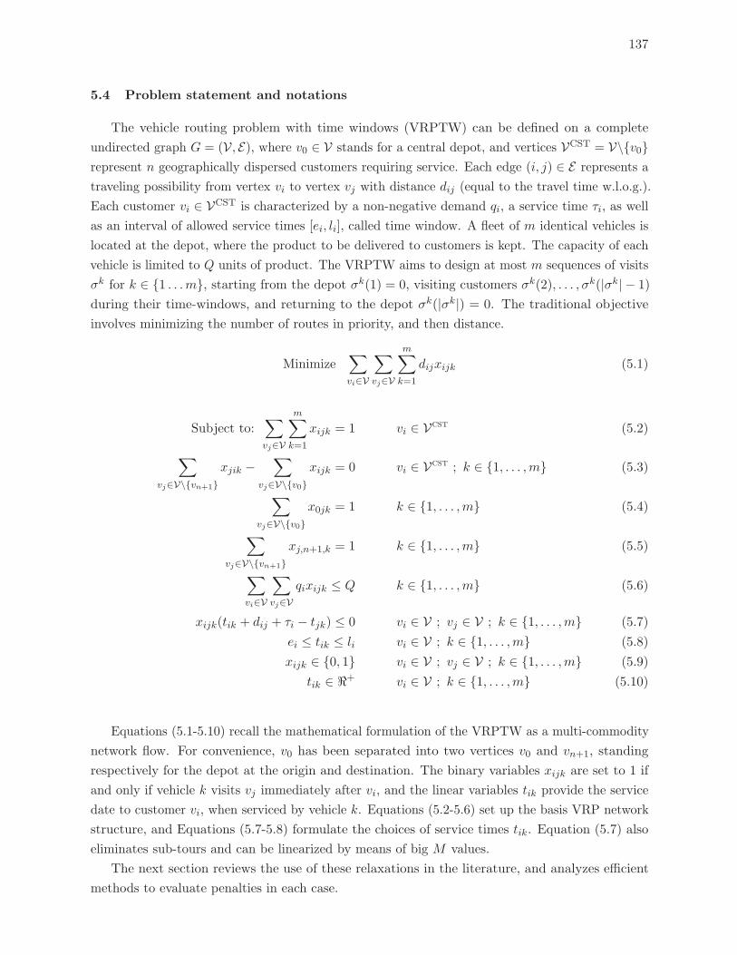
137

5.4 Problem statement and notations

The vehicle routing problem with time windows (VRPTW) can be defined on a complete

undirected graph G = (V , E), where v0 ∈ V stands for a central depot, and vertices VCST = V\{v0}represent n geographically dispersed customers requiring service. Each edge (i, j) ∈ E represents a

traveling possibility from vertex vi to vertex vj with distance dij (equal to the travel time w.l.o.g.).

Each customer vi ∈ VCST is characterized by a non-negative demand qi, a service time τi, as well

as an interval of allowed service times [ei, li], called time window. A fleet of m identical vehicles is

located at the depot, where the product to be delivered to customers is kept. The capacity of each

vehicle is limited to Q units of product. The VRPTW aims to design at most m sequences of visits

σk for k ∈ {1 . . .m}, starting from the depot σk(1) = 0, visiting customers σk(2), . . . , σk(|σk| − 1)

during their time-windows, and returning to the depot σk(|σk|) = 0. The traditional objective

involves minimizing the number of routes in priority, and then distance.

Minimize∑vi∈V

∑vj∈V

m∑k=1

dijxijk (5.1)

Subject to:∑vj∈V

m∑k=1

xijk = 1 vi ∈ Vcst (5.2)

∑vj∈V\{vn+1}

xjik −∑

vj∈V\{v0}xijk = 0 vi ∈ Vcst ; k ∈ {1, . . . ,m} (5.3)

∑vj∈V\{v0}

x0jk = 1 k ∈ {1, . . . ,m} (5.4)

∑vj∈V\{vn+1}

xj,n+1,k = 1 k ∈ {1, . . . ,m} (5.5)

∑vi∈V

∑vj∈V

qixijk ≤ Q k ∈ {1, . . . ,m} (5.6)

xijk(tik + dij + τi − tjk) ≤ 0 vi ∈ V ; vj ∈ V ; k ∈ {1, . . . ,m} (5.7)

ei ≤ tik ≤ li vi ∈ V ; k ∈ {1, . . . ,m} (5.8)

xijk ∈ {0, 1} vi ∈ V ; vj ∈ V ; k ∈ {1, . . . ,m} (5.9)

tik ∈ �+ vi ∈ V ; k ∈ {1, . . . ,m} (5.10)

Equations (5.1-5.10) recall the mathematical formulation of the VRPTW as a multi-commodity

network flow. For convenience, v0 has been separated into two vertices v0 and vn+1, standing

respectively for the depot at the origin and destination. The binary variables xijk are set to 1 if

and only if vehicle k visits vj immediately after vi, and the linear variables tik provide the service

date to customer vi, when serviced by vehicle k. Equations (5.2-5.6) set up the basis VRP network

structure, and Equations (5.7-5.8) formulate the choices of service times tik. Equation (5.7) also

eliminates sub-tours and can be linearized by means of big M values.

The next section reviews the use of these relaxations in the literature, and analyzes efficient

methods to evaluate penalties in each case.

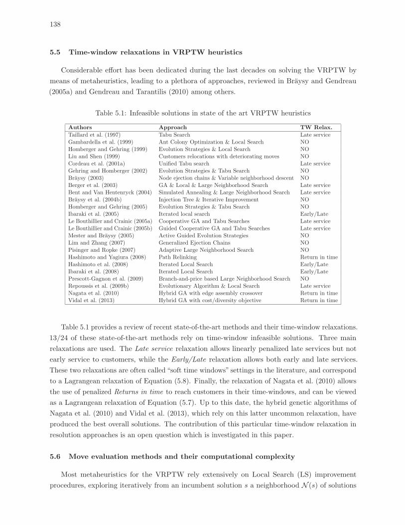
138

5.5 Time-window relaxations in VRPTW heuristics

Considerable effort has been dedicated during the last decades on solving the VRPTW by

means of metaheuristics, leading to a plethora of approaches, reviewed in Braysy and Gendreau

(2005a) and Gendreau and Tarantilis (2010) among others.

Table 5.1: Infeasible solutions in state of the art VRPTW heuristics

Authors Approach TW Relax.

Taillard et al. (1997) Tabu Search Late serviceGambardella et al. (1999) Ant Colony Optimization & Local Search NOHomberger and Gehring (1999) Evolution Strategies & Local Search NOLiu and Shen (1999) Customers relocations with deteriorating moves NOCordeau et al. (2001a) Unified Tabu search Late serviceGehring and Homberger (2002) Evolution Strategies & Tabu Search NOBraysy (2003) Node ejection chains & Variable neighborhood descent NOBerger et al. (2003) GA & Local & Large Neighborhood Search Late serviceBent and Van Hentenryck (2004) Simulated Annealing & Large Neighborhood Search Late serviceBraysy et al. (2004b) Injection Tree & Iterative Improvement NOHomberger and Gehring (2005) Evolution Strategies & Tabu Search NOIbaraki et al. (2005) Iterated local search Early/LateLe Bouthillier and Crainic (2005a) Cooperative GA and Tabu Searches Late serviceLe Bouthillier and Crainic (2005b) Guided Cooperative GA and Tabu Searches Late serviceMester and Braysy (2005) Active Guided Evolution Strategies NOLim and Zhang (2007) Generalized Ejection Chains NOPisinger and Ropke (2007) Adaptive Large Neighborhood Search NOHashimoto and Yagiura (2008) Path Relinking Return in timeHashimoto et al. (2008) Iterated Local Search Early/LateIbaraki et al. (2008) Iterated Local Search Early/LatePrescott-Gagnon et al. (2009) Branch-and-price based Large Neighborhood Search NORepoussis et al. (2009b) Evolutionary Algorithm & Local Search Late serviceNagata et al. (2010) Hybrid GA with edge assembly crossover Return in timeVidal et al. (2013) Hybrid GA with cost/diversity objective Return in time

Table 5.1 provides a review of recent state-of-the-art methods and their time-window relaxations.

13/24 of these state-of-the-art methods rely on time-window infeasible solutions. Three main

relaxations are used. The Late service relaxation allows linearly penalized late services but not

early service to customers, while the Early/Late relaxation allows both early and late services.

These two relaxations are often called “soft time windows” settings in the literature, and correspond

to a Lagrangean relaxation of Equation (5.8). Finally, the relaxation of Nagata et al. (2010) allows

the use of penalized Returns in time to reach customers in their time-windows, and can be viewed

as a Lagrangean relaxation of Equation (5.7). Up to this date, the hybrid genetic algorithms of

Nagata et al. (2010) and Vidal et al. (2013), which rely on this latter uncommon relaxation, have

produced the best overall solutions. The contribution of this particular time-window relaxation in

resolution approaches is an open question which is investigated in this paper.

5.6 Move evaluation methods and their computational complexity

Most metaheuristics for the VRPTW rely extensively on Local Search (LS) improvement

procedures, exploring iteratively from an incumbent solution s a neighborhood N (s) of solutions

139

defined relatively to a limited number of movements on the sequences of visits, called moves. In

practice, move evaluations make for the largest part of the overall computation effort in recent

heuristics, and therefore must be very efficient.

It is well-known in the literature (Kindervater and Savelsbergh 1997, Irnich 2008a, Vidal

et al. 2011, 2013) that any classical VRP move based on a bounded number of edge exchanges

or vertices relocations, such as Relocate, Swap, 2-opt, 2-opt*, or CROSS exchanges, can be

assimilated to a recombination of a bounded number of subsequences of consecutive visits (and

reverse subsequences for 2-opt) from the incumbent solution. Since local-search neighborhoods

generally involve recurrent subsequences of visits, the management of meaningful information on

subsequences can save redundant computations and increase the local search performance.

Keeping track of partial demands and distances, for example, on each O(n2) subsequence from

the incumbent solution, provides the means to evaluate the demand and distance of any recombined

route with a bounded number of sums. This opens the way to O(1) time load-feasibility checks and

distance computations during the local search, compared to O(n) for a straightforward method

that browses the routes and cumulates loads and distances.

In the literature, the sequence information is either pre-processed before move exploration and

updated whenever a route change is performed, or computed on the fly if a lexicographic order is

used for move evaluations (Savelsbergh 1985, 1992). In addition, pre-processing can be limited to

the O(Lmaxn) subsequences that contain either the first node of the route, the last node, or of

less than Lmax nodes, while still allowing for efficient inter-route Relocate, Swap, 2-opt*, and

CROSS exchanges. We opted in this paper to rely on pre-processing, since the computational

effort required to manage the information on subsequences is generally negligible when compared

to the effort required by move evaluations, and because it allows for a random exploration of local

search moves which increases the solution variety.

In a similar manner, preprocessing meaningful information on subsequences can contribute

to reduce the computational complexity of time-window feasibility checks or, when applicable,

time-penalties evaluations on the routes issued from the local search moves. Still, as reviewed in

the following, not all relaxation schemes allow for efficient move evaluation techniques, and some

relaxations result in non-trivial sub-problems for determining service times (called timing problems

in Vidal et al. 2011) on each new route.

5.6.1 No infeasible solution

When no infeasible solution is used, checking route feasibility within a local search can be

efficiently done with the approach of Savelsbergh (1985, 1992) and Kindervater and Savelsbergh

(1997). For any subsequence σ, the sum of travel and service times T (σ), the earliest possible

sequence completion time E(σ), and the latest feasible starting date L(σ) are pre-processed. These

values can be obtained by induction on the concatenation operation, starting with the base case of

a sequence σ0 = (vi) containing a single visit where T (σ0) = τi, E(σ0) = ei + τi and L(σ0) = li,

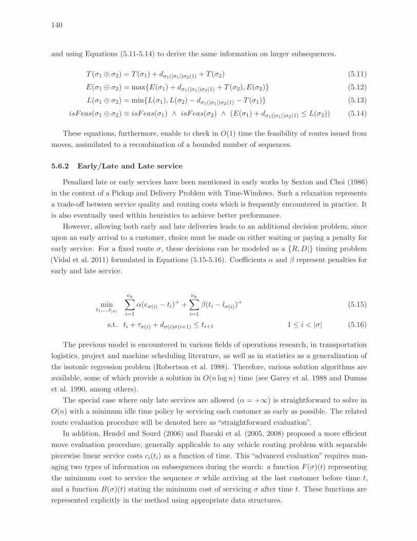
140

and using Equations (5.11-5.14) to derive the same information on larger subsequences.

T (σ1 ⊕ σ2) = T (σ1) + dσ1(|σ1|)σ2(1) + T (σ2) (5.11)

E(σ1 ⊕ σ2) = max{E(σ1) + dσ1(|σ1|)σ2(1) + T (σ2), E(σ2)} (5.12)

L(σ1 ⊕ σ2) = min{L(σ1), L(σ2)− dσ1(|σ1|)σ2(1) − T (σ1)} (5.13)

isFeas(σ1 ⊕ σ2) ≡ isFeas(σ1) ∧ isFeas(σ2) ∧ (E(σ1) + dσ1(|σ1|)σ2(1) ≤ L(σ2)) (5.14)

These equations, furthermore, enable to check in O(1) time the feasibility of routes issued from

moves, assimilated to a recombination of a bounded number of sequences.

5.6.2 Early/Late and Late service

Penalized late or early services have been mentioned in early works by Sexton and Choi (1986)

in the context of a Pickup and Delivery Problem with Time-Windows. Such a relaxation represents

a trade-off between service quality and routing costs which is frequently encountered in practice. It

is also eventually used within heuristics to achieve better performance.

However, allowing both early and late deliveries leads to an additional decision problem, since

upon an early arrival to a customer, choice must be made on either waiting or paying a penalty for

early service. For a fixed route σ, these decisions can be modeled as a {R,D|} timing problem

(Vidal et al. 2011) formulated in Equations (5.15-5.16). Coefficients α and β represent penalties for

early and late service.

mint1,...,t|σ|

nk∑i=1

α(eσ(i) − ti)+ +

nk∑i=1

β(ti − lσ(i))+ (5.15)

s.t. ti + τσ(i) + dσ(i)σ(i+1) ≤ ti+1 1 ≤ i < |σ| (5.16)

The previous model is encountered in various fields of operations research, in transportation

logistics, project and machine scheduling literature, as well as in statistics as a generalization of

the isotonic regression problem (Robertson et al. 1988). Therefore, various solution algorithms are

available, some of which provide a solution in O(n logn) time (see Garey et al. 1988 and Dumas

et al. 1990, among others).

The special case where only late services are allowed (α = +∞) is straightforward to solve in

O(n) with a minimum idle time policy by servicing each customer as early as possible. The related

route evaluation procedure will be denoted here as “straightforward evaluation”.

In addition, Hendel and Sourd (2006) and Ibaraki et al. (2005, 2008) proposed a more efficient

move evaluation procedure, generally applicable to any vehicle routing problem with separable

piecewise linear service costs ci(ti) as a function of time. This “advanced evaluation” requires man-

aging two types of information on subsequences during the search: a function F (σ)(t) representing

the minimum cost to service the sequence σ while arriving at the last customer before time t,

and a function B(σ)(t) stating the minimum cost of servicing σ after time t. These functions are

represented explicitly in the method using appropriate data structures.

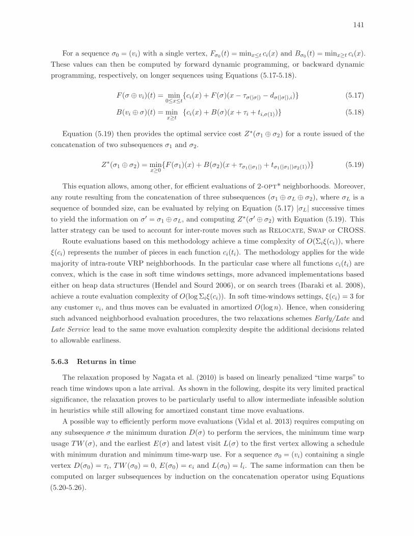
141

For a sequence σ0 = (vi) with a single vertex, Fσ0(t) = minx≤t ci(x) and Bσ0(t) = minx≥t ci(x).

These values can then be computed by forward dynamic programming, or backward dynamic

programming, respectively, on longer sequences using Equations (5.17-5.18).

F (σ ⊕ vi)(t) = min0≤x≤t

{ci(x) + F (σ)(x− τσ(|σ|) − dσ(|σ|),i)} (5.17)

B(vi ⊕ σ)(t) = minx≥t

{ci(x) +B(σ)(x+ τi + ti,σ(1))} (5.18)

Equation (5.19) then provides the optimal service cost Z∗(σ1 ⊕ σ2) for a route issued of the

concatenation of two subsequences σ1 and σ2.

Z∗(σ1 ⊕ σ2) = minx≥0

{F (σ1)(x) +B(σ2)(x+ τσ1(|σ1|) + tσ1(|σ1|)σ2(1))} (5.19)

This equation allows, among other, for efficient evaluations of 2-opt* neighborhoods. Moreover,

any route resulting from the concatenation of three subsequences (σ1 ⊕ σL ⊕ σ2), where σL is a

sequence of bounded size, can be evaluated by relying on Equation (5.17) |σL| successive times

to yield the information on σ′ = σ1 ⊕ σL, and computing Z∗(σ′ ⊕ σ2) with Equation (5.19). This

latter strategy can be used to account for inter-route moves such as Relocate, Swap or CROSS.

Route evaluations based on this methodology achieve a time complexity of O(Σiξ(ci)), where

ξ(ci) represents the number of pieces in each function ci(ti). The methodology applies for the wide

majority of intra-route VRP neighborhoods. In the particular case where all functions ci(ti) are

convex, which is the case in soft time windows settings, more advanced implementations based

either on heap data structures (Hendel and Sourd 2006), or on search trees (Ibaraki et al. 2008),

achieve a route evaluation complexity of O(log Σiξ(ci)). In soft time-windows settings, ξ(ci) = 3 for

any customer vi, and thus moves can be evaluated in amortized O(log n). Hence, when considering

such advanced neighborhood evaluation procedures, the two relaxations schemes Early/Late and

Late Service lead to the same move evaluation complexity despite the additional decisions related

to allowable earliness.

5.6.3 Returns in time

The relaxation proposed by Nagata et al. (2010) is based on linearly penalized “time warps” to

reach time windows upon a late arrival. As shown in the following, despite its very limited practical

significance, the relaxation proves to be particularly useful to allow intermediate infeasible solution

in heuristics while still allowing for amortized constant time move evaluations.

A possible way to efficiently perform move evaluations (Vidal et al. 2013) requires computing on

any subsequence σ the minimum duration D(σ) to perform the services, the minimum time warp

usage TW (σ), and the earliest E(σ) and latest visit L(σ) to the first vertex allowing a schedule

with minimum duration and minimum time-warp use. For a sequence σ0 = (vi) containing a single

vertex D(σ0) = τi, TW (σ0) = 0, E(σ0) = ei and L(σ0) = li. The same information can then be

computed on larger subsequences by induction on the concatenation operator using Equations

(5.20-5.26).

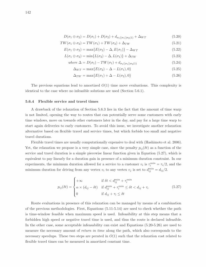
142

D(σ1 ⊕ σ2) = D(σ1) +D(σ2) + dσ1(|σ1|)σ2(1) +ΔWT (5.20)

TW (σ1 ⊕ σ2) = TW (σ1) + TW (σ2) + ΔTW (5.21)

E(σ1 ⊕ σ2) = max{E(σ2)−Δ, E(σ1)} −ΔWT (5.22)

L(σ1 ⊕ σ2) = min{L(σ2)−Δ, L(σ1)}+ΔTW (5.23)

where Δ = D(σ1)− TW (σ1) + dσ1(|σ1|)σ2(1) (5.24)

ΔWT = max{E(σ2)−Δ− L(σ1), 0} (5.25)

ΔTW = max{E(σ1) + Δ− L(σ2), 0} (5.26)

The previous equations lead to amortized O(1) time move evaluations. This complexity is

identical to the case where no infeasible solutions are used (Section 5.6.1).

5.6.4 Flexible service and travel times

A drawback of the relaxation of Section 5.6.3 lies in the fact that the amount of time warp

is not limited, opening the way to routes that can potentially serve some customers with early

time windows, move on towards other customers later in the day, and pay for a large time warp to

start again deliveries to early customers. To avoid this issue, we investigate another relaxation

alternative based on flexible travel and service times, but which forbids too small and negative

travel durations.

Flexible travel times are usually computationally expensive to deal with (Hashimoto et al. 2006).

Yet, the relaxation we propose is a very simple case, since the penalty pij(δt) as a function of the

service and travel duration is a simple piecewise linear function given in Equation (5.27), which is

equivalent to pay linearly for a duration gain in presence of a minimum duration constraint. In our

experiments, the minimum duration allowed for a service to a customer vi is τmini = τi/2, and the

minimum duration for driving from any vertex vi to any vertex vj is set to dminij = dij/2.

pij(δt) =

⎧⎪⎪⎪⎨⎪⎪⎪⎩+∞ if δt < dmin

ij + τmini

α× (dij − δt) if dminij + τmin

i ≤ δt < dij + τi

0 if dij + τi ≤ δt

(5.27)

Route evaluations in presence of this relaxation can be managed by means of a combination

of the previous methodologies. First, Equations (5.11-5.14) are used to check whether the path

is time-window feasible when maximum speed is used. Infeasibility at this step means that a

forbidden high speed or negative travel time is used, and thus the route is declared infeasible.

In the other case, some acceptable infeasability can exist and Equations (5.20-5.26) are used to

measure the necessary amount of return in time along the path, which also corresponds to the

necessary speedups. These two steps are perated in O(1) such that the relaxation cost related to

flexible travel times can be measured in amortized constant time.

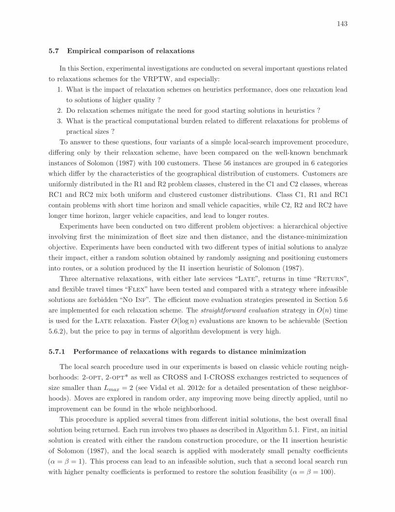
143

5.7 Empirical comparison of relaxations

In this Section, experimental investigations are conducted on several important questions related

to relaxations schemes for the VRPTW, and especially:

1. What is the impact of relaxation schemes on heuristics performance, does one relaxation lead

to solutions of higher quality ?

2. Do relaxation schemes mitigate the need for good starting solutions in heuristics ?

3. What is the practical computational burden related to different relaxations for problems of

practical sizes ?

To answer to these questions, four variants of a simple local-search improvement procedure,

differing only by their relaxation scheme, have been compared on the well-known benchmark

instances of Solomon (1987) with 100 customers. These 56 instances are grouped in 6 categories

which differ by the characteristics of the geographical distribution of customers. Customers are

uniformly distributed in the R1 and R2 problem classes, clustered in the C1 and C2 classes, whereas

RC1 and RC2 mix both uniform and clustered customer distributions. Class C1, R1 and RC1

contain problems with short time horizon and small vehicle capacities, while C2, R2 and RC2 have

longer time horizon, larger vehicle capacities, and lead to longer routes.

Experiments have been conducted on two different problem objectives: a hierarchical objective

involving first the minimization of fleet size and then distance, and the distance-minimization

objective. Experiments have been conducted with two different types of initial solutions to analyze

their impact, either a random solution obtained by randomly assigning and positioning customers

into routes, or a solution produced by the I1 insertion heuristic of Solomon (1987).

Three alternative relaxations, with either late services “Late”, returns in time “Return”,

and flexible travel times “Flex” have been tested and compared with a strategy where infeasible

solutions are forbidden “No Inf”. The efficient move evaluation strategies presented in Section 5.6

are implemented for each relaxation scheme. The straightforward evaluation strategy in O(n) time

is used for the Late relaxation. Faster O(logn) evaluations are known to be achievable (Section

5.6.2), but the price to pay in terms of algorithm development is very high.

5.7.1 Performance of relaxations with regards to distance minimization

The local search procedure used in our experiments is based on classic vehicle routing neigh-

borhoods: 2-opt, 2-opt* as well as CROSS and I-CROSS exchanges restricted to sequences of

size smaller than Lmax = 2 (see Vidal et al. 2012c for a detailed presentation of these neighbor-

hoods). Moves are explored in random order, any improving move being directly applied, until no

improvement can be found in the whole neighborhood.

This procedure is applied several times from different initial solutions, the best overall final

solution being returned. Each run involves two phases as described in Algorithm 5.1. First, an initial

solution is created with either the random construction procedure, or the I1 insertion heuristic

of Solomon (1987), and the local search is applied with moderately small penalty coefficients

(α = β = 1). This process can lead to an infeasible solution, such that a second local search run

with higher penalty coefficients is performed to restore the solution feasibility (α = β = 100).

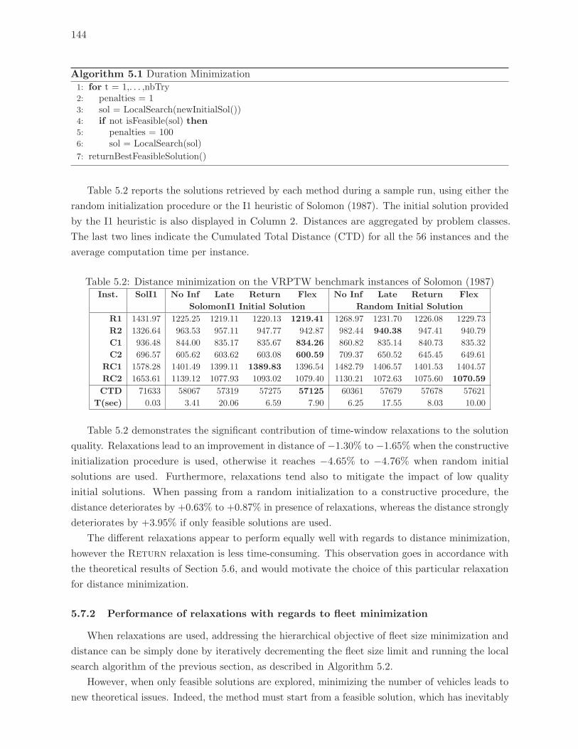
144

Algorithm 5.1 Duration Minimization1: for t = 1,. . . ,nbTry2: penalties = 13: sol = LocalSearch(newInitialSol())4: if not isFeasible(sol) then5: penalties = 1006: sol = LocalSearch(sol)

7: returnBestFeasibleSolution()

Table 5.2 reports the solutions retrieved by each method during a sample run, using either the

random initialization procedure or the I1 heuristic of Solomon (1987). The initial solution provided

by the I1 heuristic is also displayed in Column 2. Distances are aggregated by problem classes.

The last two lines indicate the Cumulated Total Distance (CTD) for all the 56 instances and the

average computation time per instance.

Table 5.2: Distance minimization on the VRPTW benchmark instances of Solomon (1987)Inst. SolI1 No Inf Late Return Flex No Inf Late Return Flex

SolomonI1 Initial Solution Random Initial Solution

R1 1431.97 1225.25 1219.11 1220.13 1219.41 1268.97 1231.70 1226.08 1229.73

R2 1326.64 963.53 957.11 947.77 942.87 982.44 940.38 947.41 940.79

C1 936.48 844.00 835.17 835.67 834.26 860.82 835.14 840.73 835.32

C2 696.57 605.62 603.62 603.08 600.59 709.37 650.52 645.45 649.61

RC1 1578.28 1401.49 1399.11 1389.83 1396.54 1482.79 1406.57 1401.53 1404.57

RC2 1653.61 1139.12 1077.93 1093.02 1079.40 1130.21 1072.63 1075.60 1070.59

CTD 71633 58067 57319 57275 57125 60361 57679 57678 57621

T(sec) 0.03 3.41 20.06 6.59 7.90 6.25 17.55 8.03 10.00

Table 5.2 demonstrates the significant contribution of time-window relaxations to the solution

quality. Relaxations lead to an improvement in distance of −1.30% to −1.65% when the constructive

initialization procedure is used, otherwise it reaches −4.65% to −4.76% when random initial

solutions are used. Furthermore, relaxations tend also to mitigate the impact of low quality

initial solutions. When passing from a random initialization to a constructive procedure, the

distance deteriorates by +0.63% to +0.87% in presence of relaxations, whereas the distance strongly

deteriorates by +3.95% if only feasible solutions are used.

The different relaxations appear to perform equally well with regards to distance minimization,

however the Return relaxation is less time-consuming. This observation goes in accordance with

the theoretical results of Section 5.6, and would motivate the choice of this particular relaxation

for distance minimization.

5.7.2 Performance of relaxations with regards to fleet minimization

When relaxations are used, addressing the hierarchical objective of fleet size minimization and

distance can be simply done by iteratively decrementing the fleet size limit and running the local

search algorithm of the previous section, as described in Algorithm 5.2.

However, when only feasible solutions are explored, minimizing the number of vehicles leads to

new theoretical issues. Indeed, the method must start from a feasible solution, which has inevitably

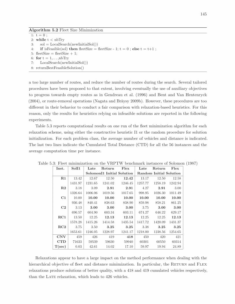
145

Algorithm 5.2 Fleet Size Minimization1: t = 0 ;2: while t < nbTry3: sol = LocalSearch(newInitialSol())4: if isFeasible(sol) then fleetSize = fleetSize - 1; t = 0 ; else t = t+1 ;5: fleetSize = fleetSize + 1;6: for t = 1,. . . ,nbTry7: LocalSearch(newInitialSol())

8: returnBestFeasibleSolution()

a too large number of routes, and reduce the number of routes during the search. Several tailored

procedures have been proposed to that extent, involving eventually the use of auxiliary objectives

to progress towards empty routes as in Gendreau et al. (1996) and Bent and Van Hentenryck

(2004), or route-removal operations (Nagata and Braysy 2009b). However, these procedures are too

different in their behavior to conduct a fair comparison with relaxation-based heuristics. For this

reason, only the results for heuristics relying on infeasible solutions are reported in the following

experiments.

Table 5.3 reports computational results on one run of the fleet minimization algorithm for each

relaxation scheme, using either the constructive heuristic I1 or the random procedure for solution

initialization. For each problem class, the average number of vehicles and distance is indicated.

The last two lines indicate the Cumulated Total Distance (CTD) for all the 56 instances and the

average computation time per instance.

Table 5.3: Fleet minimization on the VRPTW benchmark instances of Solomon (1987)Inst. SolI1 Late Return Flex Late Return Flex

SolomonI1 Initial Solution Random Initial Solution

R1 13.42 12.67 12.50 12.42 13.17 12.50 12.58

1431.97 1231.65 1241.02 1246.45 1257.77 1258.19 1242.94

R2 3.18 3.09 2.91 2.91 4.27 2.91 3.00

1326.64 1006.06 1019.56 1017.65 998.95 1026.30 1011.49

C1 10.00 10.00 10.00 10.00 10.00 10.00 10.00

936.48 840.41 838.63 838.90 859.98 858.21 861.25

C2 3.13 3.00 3.00 3.00 3.75 3.00 3.00

696.57 604.90 603.34 603.11 674.27 646.22 629.17

RC1 13.50 12.25 12.13 12.13 12.25 12.25 12.13

1578.28 1415.26 1414.58 1435.54 1417.72 1420.09 1431.37

RC2 3.75 3.50 3.25 3.25 3.38 3.25 3.25

1653.61 1246.05 1228.97 1241.17 1218.00 1238.56 1254.65

CNV 459 426 419 418 450 420 421

CTD 71633 59539 59630 59940 60301 60550 60314

T(sec) 0.03 42.61 14.02 17.10 59.97 19.94 24.89

Relaxations appear to have a large impact on the method performance when dealing with the

hierarchical objective of fleet and distance minimization. In particular, the Return and Flex

relaxations produce solutions of better quality, with a 418 and 419 cumulated vehicles respectively,

than the Late relaxation, which leads to 426 vehicles.

146

Return and Flex relaxations are also less dependent upon the availability of a good initial

solution. Indeed, the cumulated fleet size reaches 420 and 421 vehicles when a random initial

solution is used, whereas with a Late relaxation the fleet size increases to 450 vehicles. A potential

explanation is that infeasible insertions at the beginning of routes are likely to result in massive

penalties in the Late relaxation scheme, leading to imbalanced insertion capacities within the

routes, thus reducing the ability to progress towards feasible solutions in tightly constrained settings

with few routes.

5.8 Conclusions

In this paper, four simple neighborhood search procedures, differing only by their relaxation

scheme, have been tested on the vehicle routing problem with time windows. Experimental results

demonstrate the positive contribution of time-window relaxations in the method performance for

two different objectives, as well as their ability to mitigate the impact of low quality starting

solutions. The relaxation of Nagata et al. (2010), especially, based on the concept of returns in

time, yields the best results in terms of both solution quality and computation efficiency, and thus

appear as a promising option for VRPTW metaheuristics.

Finally, as a perspective of research, this study will be completed by comparison of relaxations

within an iterated local search and the hybrid genetic algorithm of Vidal et al. (2013), thus providing

the means to challenge the previous observations on more advanced metaheuristic procedures.

CHAPITRE 6

GESTION IMPLICITE DES PLACEMENTS DE DEPOT DANS LES

HEURISTIQUES ET META-HEURISTIQUES A BASE DE RECHERCHE

LOCALE


L’application de HGSADC aux problemes avec depots multiples, en Section 3 a permis de

soulever des questions methodologiques quand a l’exploration, combinee ou non, de differentes

alternatives d’affectation aux depots et de choix de sequences. Ce chapitre presente une methode

efficace de programmation dynamique pour evaluer en temps O(1) amorti le placement et le

choix optimal des depots dans les routes, lors de methodes de recherche locale et de Split. Cette

approche permet d’une part d’explorer des alternatives combinees d’affectation et de sequence et

donc d’augmenter la gamme des mouvements consideres. D’autre part les decisions d’affectation

peuvent etre ainsi releguees au sein de sous-problemes d’evaluation de routes, afin de ne plus avoir

a considerer explicitement cet aspect combinatoire au sein des voisinages de recherche locale et

des representations de solution. Ces approches sont implantees et testees au sein de deux cadres

meta-heuristiques, une recherche locale iteree, et la methode HGSADC, sur des VRP multi-depots

avec flotte illimitee, homogene ou heterogene. Les experiences mettent en valeur la contribution

importante des methodes proposees au sein des deux types de meta-heuristiques.

6.2 Article VI : Implicit depot choice and positioning in vehicle routing heuristics


T.G., Gendreau, M., Prins, C. (2012) Implicit depot assignments and rotations in

vehicle routing heuristics. European Journal of Operational Research, submitted for

publication.

Abstract: Vehicle routing variants with multiple depots and mixed fleet present intricate com-

binatorial aspects related to sequencing choices, vehicle type choices, depot choices, and depot

positioning. This paper introduces a dynamic programming methodology for efficiently evaluating

compound neighborhoods combining sequence-based moves with an optimal choice of vehicle and

depot, and an optimal determination of the first customer to be visited in the route, called rotation.

The assignment choices, making the richness of the problem, are thus no more addressed in the

solution structure, but implicitly determined during each move evaluation. Two meta-heuristics

relying on these concepts, an iterated local search and a hybrid genetic algorithm, are presented.

Extensive computational experiments demonstrate the remarkable performance of these methods

on classic benchmark instances for multi-depot vehicle routing problems with and without fleet

mix, as well as the notable contribution of the implicit depot choice and positioning methods to

the search performance. The proposed concepts are fairly general, and widely applicable to many

148

other vehicle routing variants.

Keywords: Vehicle routing, multi-depot, fleet mix, dynamic programming, local search, genetic

algorithms

6.3 Introduction

Vehicle Routing Problems (VRP) with combined assignment choices, such as multi-depot and

mixed-fleet settings, appear prominently in many applications related to transportation, production

planning, robotics, maintenance, health care or emergency relief. These combinatorial optimization

problems require two levels of decisions, related respectively to the sequencing of visits to customers

into routes, and the assignment of customers to some global resources, such as depots or vehicle

types. Heuristics and meta-heuristics that rely on separate optimization procedures for addressing

each aspect, e.g. separate families of local searches, large neighborhoods or crossovers to work

on the order of visits, the depot choices or the vehicle types, may overlook a wide range of

potential solution refinements involving joint changes in the sequencing and assignment decisions,

e.g. swapping two customers and in the meantime changing the vehicle or the depot assigned

to the routes. Thus, most advanced meta-heuristics combine these decisions within purposeful

optimization procedures to achieve notable performance gains (see Prins 2009b, for example),

though the number of combined solution changes tends to become computationally expensive to

investigate.

To contribute towards addressing this challenge, this paper proposes a new bidirectional dynamic

programming approach to optimally manage the choices of vehicle, depot, and first customer visited

in a route, the so-called optimal rotation, directly at the level of route evaluations in vehicle routing

heuristics. We thus introduce a new Local Search (LS) in which the neighborhoods are solely

based on customer-visits relocations and arc exchanges, while dynamic programming-based route

evaluation functions produce optimal depot placements, choices and rotations for each alternative

route. Since several advanced meta-heuristics for vehicle routing problems requires a Split algorithm

to optimally segment a solution represented as a giant tour into several routes, we also derive an

advanced Split algorithm with compound vehicle assignments, depot choices and rotations. The

proposed enhanced procedures work with the same computational complexity as the classic ones

from the literature. Thus, the additional capability we introduce does not lead to any additional

computational overhead.

As a proof of concept, these methodologies are integrated and tested within two meta-heuristics:

a simple multi-start Iterated Local Search (ILS) similar to the one of Prins (2009a) for the

capacitated VRP, and a more elaborate Hybrid Genetic Search with Advanced Diversity Control

(HGSADC) similar to the one of Vidal et al. (2012a,b, 2013). Two specific problems are investigated,

the multi-depot fleet mix problem requiring combined decisions on assignments to vehicles types

and depot along with sequencing choices, and the classic multi-depot VRP. Extensive computational

experiments, on small- and large-scale benchmark instances with up to 960 customers demonstrate

149

the remarkable performance of the proposed meta-heuristics, as well as the notable contribution of

the combined neighborhoods to the search performance.

To facilitate the presentation, we first introduce in Section 6.4 the problems, notations and

variants considered in our experiments. Sections 6.5 and 6.6 describe the proposed methodology

for optimally managing depot, vehicle choices and rotations within route evaluations, and presents

the advanced Split method. The integration of these procedures into a neighborhood-based and a

population-based meta-heuristic is discussed in Section 6.7. The computational experiments are

reported in Section 6.8, and Section 6.9 concludes.

6.4 Vehicle routing problems and variants

Vehicle Routing Problems (VRP) aim to design least cost vehicle routes to service geographically

dispersed customers (Toth and Vigo 2002a, Cordeau et al. 2007, Golden et al. 2008, Laporte 2009,

Vidal et al. 2012c). Emphasis is still growing on this family of problems after 50 years of research,

mostly because of their major economic impact in many application fields, but also because of the

considerable amount of problem variants that must be dealt with to adequately address practical

settings. Practical applications, indeed, lead to a variety of problem attributes that complement the

classic VRP model, and seek to account for customer requirements (e.g., schedules, consistency),

network and vehicle characteristics (mixed fleet, multiple depots), and driver’s needs (working hour

regulations, lunch breaks) among others.

Two attributes especially, mixed-fleet and multi-depot, are recurrent in many large-scale logistics

applications. The problem combining these attributes, known as the Multi-Depot Vehicle Fleet

Mix Problem (MDVFMP), can be defined as follows. Let G = (V, E) with V = Vdep ∪ Vcst be a

complete undirected graph, in which the d nodes vo ∈ Vdep represent depots with infinite capacity,

and the n nodes vi ∈ Vcst stand for customers. Each customer vi is characterized by a demand for

a non-negative amount of product qi. The edges (i, j) ∈ E represent the possibility of traveling

between customers vi and vj for a total travel distance of cij . Finally, w types of vehicles are

available in unlimited quantity, any vehicle k being characterized by a base acquisition/depreciation

cost ek, a per-distance-unit cost uk, and a capacity Qk. As such, the minimum cost Φ(x, q) to

perform a route with distance x and total demand q is given in Equation (6.1).

Φ(x, q) = mink∈{1,...,w}/q≤Qk

{ek + ukx} (6.1)

The MDVFMP aims to find a set of routes, as well as their assignment to vehicles and depots,

to service each customer once and minimize the total cost. Each route assigned to any vehicle

k shall start and end at the same depot location and carry less than qk of units of products. A

mathematical formulation is given in Equations (6.2-6.10). In this model, F represents a fleet

containing a large number of vehicles of each type. The binary variable yio represents the depot

assignment decision, taking value 1 if and only if customer vi is assigned to depot vo. The binary

variable xijko takes value 1 if and only if customer vj is serviced immediately after vi by vehicle k

from depot o. The objective, presented in Equation (6.2), includes the base cost of ek of any used

vehicle k, and the distance-based cost ukcij . Equations (6.3-6.5) ensure that exactly one depot

150

is chosen for each customer. Equation (6.6) ensures the conservation of the flow. Equation (6.7)

enforces the capacity limits for the vehicles, and sub-tours are eliminated by Equation (6.8).

Minimize∑k∈F

∑vo∈Vdep

(∑vi∈V

ekxoiko +∑

(vi,vj)∈Eukcijxijko) (6.2)

Subject to:∑

vo∈Vdep

yio = 1 vi ∈ Vcst (6.3)

∑vi∈V

∑k∈F

xijko − yio = 0 vj ∈ Vcst ; vo ∈ Vdep (6.4)

∑vj∈V

xojko′ = 0 vo ∈ Vdep ; vo′ ∈ Vdep ; vo �= vi ; k ∈ F (6.5)

∑vj∈V

xjiko −∑vj∈V

xijko = 0 vi ∈ V ; vo ∈ Vdep ; k ∈ F (6.6)

∑vi∈V

∑vj∈V

qixijko ≤ Qk vo ∈ Vdep ; k ∈ F (6.7)

∑vi∈S

∑vj∈S

xijko ≤ |S| − 1 S ∈ Vcst ; |S| ≥ 2 ; vo ∈ Vdep ; k ∈ F (6.8)

xijko ∈ {0, 1} vi ∈ V; vj ∈ V ; vo ∈ Vdep ; k ∈ F (6.9)

yiko ∈ {0, 1} vi ∈ V ; vo ∈ Vdep ; k ∈ F (6.10)

The MDVFMP includes several prominent problems as special cases, such as the Vehicle Fleet

Mix Problem (VFMP) when d = 1, the Multi-Depot VRP (MDVRP) when w = 1, and the

Capacitated VRP (CVRP) when (w, d) = (1, 1). The MDVFMP is also NP-hard as a generalization

of the CVRP.

Contributions explicitly targeted on the MDVFMP are not frequent in the literature, and we

are currently aware of a single meta-heuristic from Salhi and Sari (1997). This neighborhood-based

method relies on the same concepts as the Variable Neighborhood Search, and proceeds by changing

the neighborhoods by increasing size whenever a local optimum is encountered. Advanced moves

that change both the assignment and the sequencing are used once several simpler neighborhoods

have been exhausted. The MDVFMP is also a sub-problem of the settings encountered by Irnich

(2000), Dondo and Cerda (2007) and Goel and Gruhn (2008), although a limited fleet has been

considered in most cases along with some other problem attributes.

In contrast, the literature dedicated to its two immediate sub-problems, the MDVRP and the

VFMP, is much more furnished. An extensive survey of all methods for these two sub-problems is

outside the scope of this section, and we refer to Ombuki-Berman and Hanshar (2009), Vidal et al.

(2012c) and Subramanian et al. (2012) to that extent. Several meta-heuristics produce solutions

of remarkable quality. For the MDVRP, the current state of the art results are produced by the

Hybrid Genetic Search with Advanced Diversity Control (HGSADC) of Vidal et al. (2012a), which

relies on efficient crossover and LS-improvement procedures to create new individuals. Of particular

interest is the individual evaluation used in HGSADC, which relies on both solution quality and

151

contribution to the population diversity. High-quality solutions have also been generated by the

Adaptive Large Neighborhood Search (ALNS) of Pisinger and Ropke (2007), the parallel iterated

tabu search heuristic of Cordeau and Maischberger (2012) and the hybrid iterated local search and

integer programming approach of Subramanian (2012).

For the VFMP, state-of-the-art heuristics are based either on ILS and integer programming

(Subramanian et al. 2012, Subramanian 2012), tabu search (Brandao 2009), variable neighborhood

search (Imran et al. 2009), or hybrid genetic algorithms (Liu et al. 2009, Prins 2009b). The

previously-mentioned meta-heuristics enable to adequately address large scale problem instances,

while smaller-size instances may be manageable with exact methods. The integer programming

approach of Baldacci and Mingozzi (2009) especially, based on a set partitioning formulation, has

demonstrated its ability to solve most MDVRP and VFMP instances with up to 100 customers.

It should finally be noted that most successful hybrid genetic algorithms for the previous

problems (Liu et al. 2009, Prins 2009b, Vidal et al. 2012a,b, 2013) rely on a solution representation

as a giant tour without trip delimiters that does not consider the route segmentation. Such

a representation reduces the search space and allows for the use of simple crossovers based on

permutations, but requires a Split algorithm to optimally segment the tour into routes whenever a

full solution is needed (Prins 2004). This latter splitting problem is generally solved as a shortest

path problem on an acyclic auxiliary directed graph (Beasley 1983). For the CVRP, the VFMP and

the MDVRP, advanced Split algorithms with supplementary capabilities have been proposed, in

order to combine the segmentation choices with decisions on vehicle type-to-customer assignments

(Prins 2009b), depot selections (Kansou and Yassine 2010), or potential route inversions or rotations

(Prins et al. 2009). These enhanced procedures were shown to contribute significantly to solution

quality, however, although implicit depot choice and positioning has been studied in the context

of Split algorithms, no such methodology has been to this date proposed in the context of LS.

The next section contributes to fill this gap in the state of the art, by introducing a new dynamic

programming-based approach to efficiently explore compound LS neighborhoods with sequence

changes, optimal vehicle, depot choices and route rotations.

6.5 Compound neighborhoods with implicit depot positioning and vehicle choices

When dealing with vehicle routing variants with combined assignment choices – for example to

depots, days, drivers or vehicle types –, the success of heuristics is often linked to their capacity to

tightly integrate decisions together. Any change in the routes, especially, may influence the best

way to assign these routes to vehicles, depots, or intervals in drivers schedules, or to rotate the

route, such that the exploration of compound neighborhoods is often a key to find new combined

choices that could otherwise look unfavorable when examined separately.

Figure 6.5 displays three euclidean problem instances where these situations arise. Customers

are represented with diamonds, while depots are represented by larger squares. For the VRP

instance illustrated on the right, the vehicle capacity is Q = 3 and any customer vi for i ∈ {3, . . . , 7}requests one unit of product. All solutions illustrated on the top of this figure are not the global

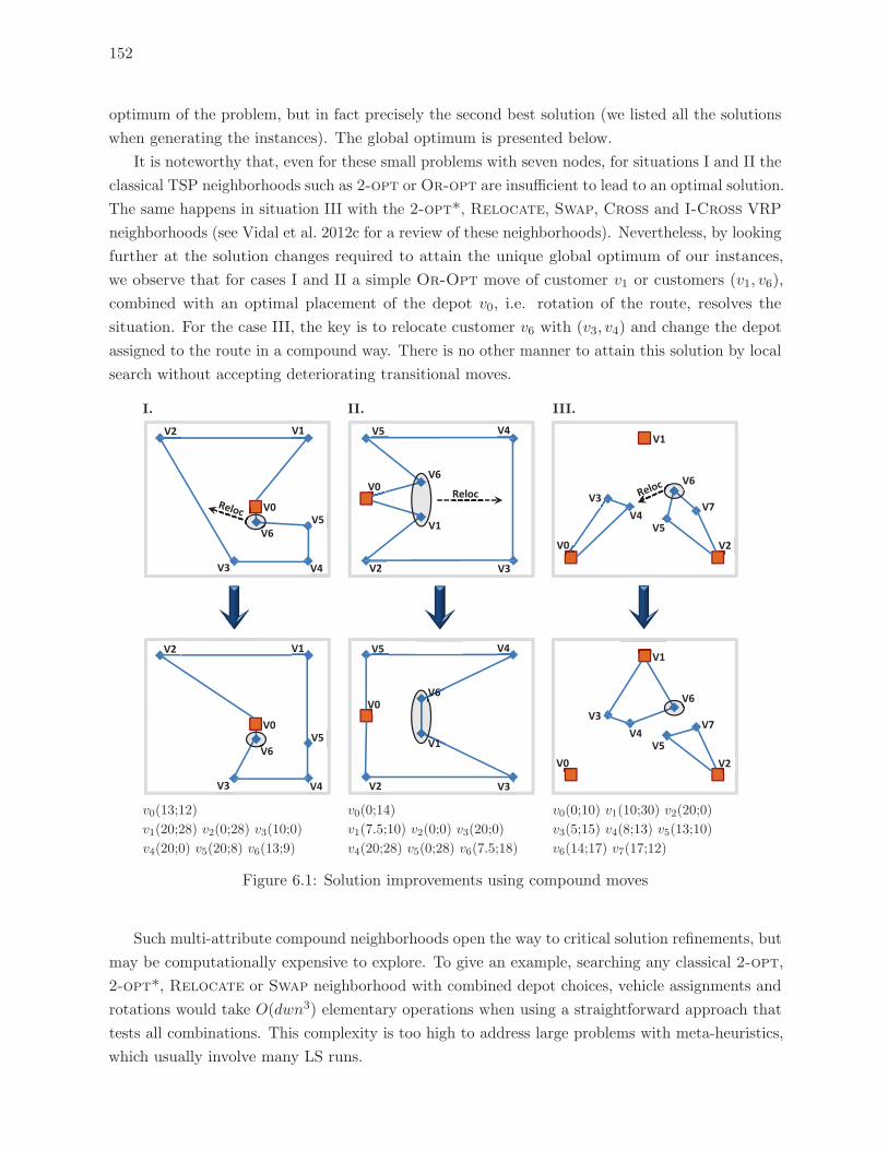
152

optimum of the problem, but in fact precisely the second best solution (we listed all the solutions

when generating the instances). The global optimum is presented below.

It is noteworthy that, even for these small problems with seven nodes, for situations I and II the

classical TSP neighborhoods such as 2-opt or Or-opt are insufficient to lead to an optimal solution.

The same happens in situation III with the 2-opt*, Relocate, Swap, Cross and I-Cross VRP

neighborhoods (see Vidal et al. 2012c for a review of these neighborhoods). Nevertheless, by looking

further at the solution changes required to attain the unique global optimum of our instances,

we observe that for cases I and II a simple Or-Opt move of customer v1 or customers (v1, v6),

combined with an optimal placement of the depot v0, i.e. rotation of the route, resolves the

situation. For the case III, the key is to relocate customer v6 with (v3, v4) and change the depot

assigned to the route in a compound way. There is no other manner to attain this solution by local

search without accepting deteriorating transitional moves.

I. II. III.

1

V0

V0

V0

V1 V1

V2

V2

V3 V4

V5 V6

V1

V2 V3

V4 V5

V4

V6

V3

V5

V6

V7 Reloc

V0

V0

V0

V1 V1

V2

V2

V3 V4

V5 V6

V1

V2 V3

V4 V5

V4

V6

V3

V5

V6

V7

v0(13;12) v0(0;14) v0(0;10) v1(10;30) v2(20;0)

v1(20;28) v2(0;28) v3(10;0) v1(7.5;10) v2(0;0) v3(20;0) v3(5;15) v4(8;13) v5(13;10)

v4(20;0) v5(20;8) v6(13;9) v4(20;28) v5(0;28) v6(7.5;18) v6(14;17) v7(17;12)

Figure 6.1: Solution improvements using compound moves

Such multi-attribute compound neighborhoods open the way to critical solution refinements, but

may be computationally expensive to explore. To give an example, searching any classical 2-opt,

2-opt*, Relocate or Swap neighborhood with combined depot choices, vehicle assignments and

rotations would take O(dwn3) elementary operations when using a straightforward approach that

tests all combinations. This complexity is too high to address large problems with meta-heuristics,

which usually involve many LS runs.

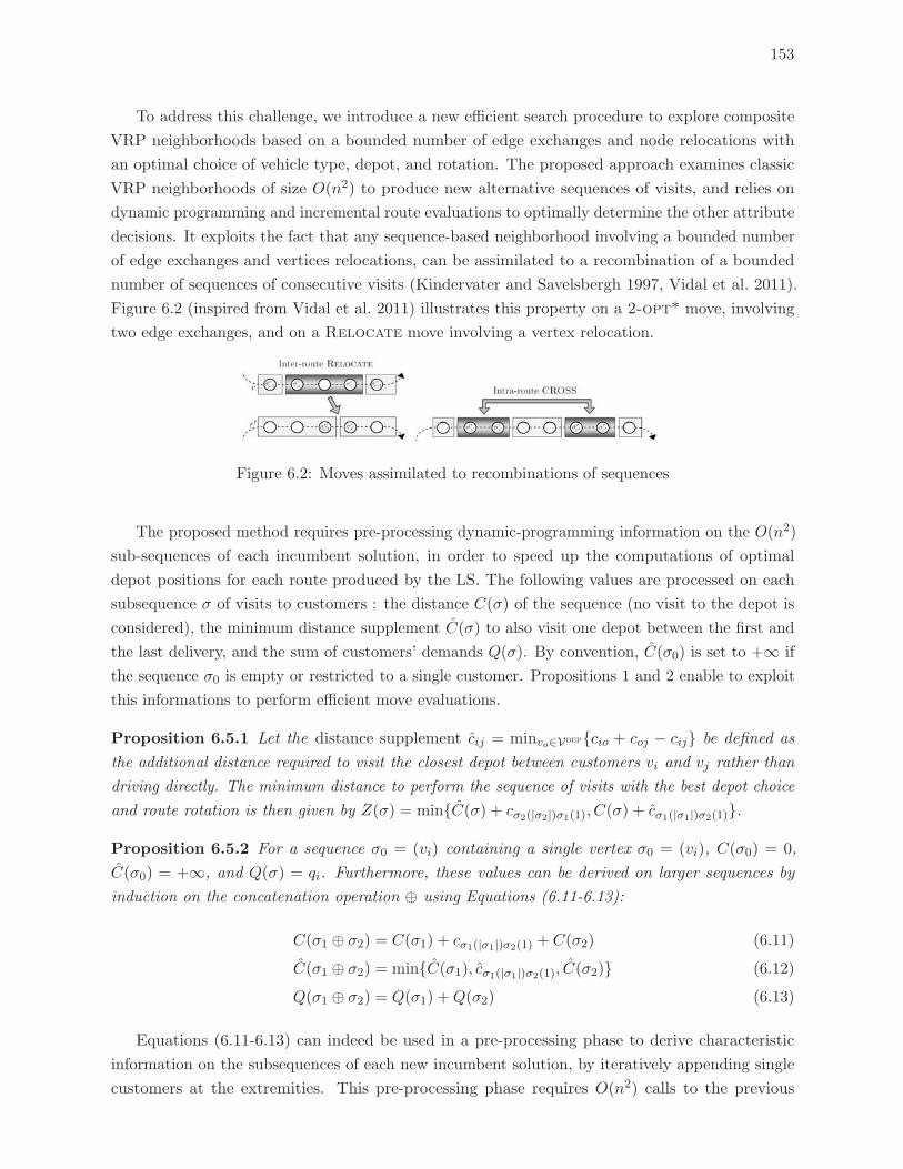
153

To address this challenge, we introduce a new efficient search procedure to explore composite

VRP neighborhoods based on a bounded number of edge exchanges and node relocations with

an optimal choice of vehicle type, depot, and rotation. The proposed approach examines classic

VRP neighborhoods of size O(n2) to produce new alternative sequences of visits, and relies on

dynamic programming and incremental route evaluations to optimally determine the other attribute

decisions. It exploits the fact that any sequence-based neighborhood involving a bounded number

of edge exchanges and vertices relocations, can be assimilated to a recombination of a bounded

number of sequences of consecutive visits (Kindervater and Savelsbergh 1997, Vidal et al. 2011).

Figure 6.2 (inspired from Vidal et al. 2011) illustrates this property on a 2-opt* move, involving

two edge exchanges, and on a Relocate move involving a vertex relocation.

Figure 6.2: Moves assimilated to recombinations of sequences

The proposed method requires pre-processing dynamic-programming information on the O(n2)

sub-sequences of each incumbent solution, in order to speed up the computations of optimal

depot positions for each route produced by the LS. The following values are processed on each

subsequence σ of visits to customers : the distance C(σ) of the sequence (no visit to the depot is

considered), the minimum distance supplement C(σ) to also visit one depot between the first and

the last delivery, and the sum of customers’ demands Q(σ). By convention, C(σ0) is set to +∞ if

the sequence σ0 is empty or restricted to a single customer. Propositions 1 and 2 enable to exploit

this informations to perform efficient move evaluations.

Proposition 6.5.1 Let the distance supplement cij = minvo∈Vdep{cio + coj − cij} be defined as

the additional distance required to visit the closest depot between customers vi and vj rather than

driving directly. The minimum distance to perform the sequence of visits with the best depot choice

and route rotation is then given by Z(σ) = min{C(σ) + cσ2(|σ2|)σ1(1), C(σ) + cσ1(|σ1|)σ2(1)}.

Proposition 6.5.2 For a sequence σ0 = (vi) containing a single vertex σ0 = (vi), C(σ0) = 0,

C(σ0) = +∞, and Q(σ) = qi. Furthermore, these values can be derived on larger sequences by

induction on the concatenation operation ⊕ using Equations (6.11-6.13):

C(σ1 ⊕ σ2) = C(σ1) + cσ1(|σ1|)σ2(1) + C(σ2) (6.11)

C(σ1 ⊕ σ2) = min{C(σ1), cσ1(|σ1|)σ2(1), C(σ2)} (6.12)

Q(σ1 ⊕ σ2) = Q(σ1) +Q(σ2) (6.13)

Equations (6.11-6.13) can indeed be used in a pre-processing phase to derive characteristic

information on the subsequences of each new incumbent solution, by iteratively appending single

customers at the extremities. This pre-processing phase requires O(n2) calls to the previous

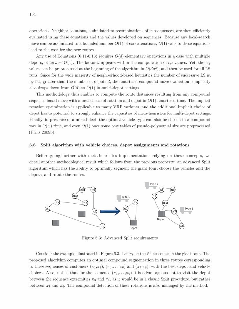
154

operations. Neighbor solutions, assimilated to recombinations of subsequences, are then efficiently

evaluated using these equations and the values developed on sequences. Because any local-search

move can be assimilated to a bounded number O(1) of concatenations, O(1) calls to these equations

lead to the cost for the new routes.

Any use of Equations (6.11-6.13) requires O(d) elementary operations in a case with multiple

depots, otherwise O(1). The factor d appears within the computation of cij values. Yet, the cij

values can be preprocessed at the beginning of the algorithm in O(dn2), and then be used for all LS

runs. Since for the wide majority of neighborhood-based heuristics the number of successive LS is,

by far, greater than the number of depots d, the amortized compound move evaluation complexity

also drops down from O(d) to O(1) in multi-depot settings.

This methodology thus enables to compute the route distances resulting from any compound

sequence-based move with a best choice of rotation and depot in O(1) amortized time. The implicit

rotation optimization is applicable to many VRP variants, and the additional implicit choice of

depot has to potential to strongly enhance the capacities of meta-heuristics for multi-depot settings.

Finally, in presence of a mixed fleet, the optimal vehicle type can also be chosen in a compound

way in O(w) time, and even O(1) once some cost tables of pseudo-polynomial size are preprocessed

(Prins 2009b).

6.6 Split algorithm with vehicle choices, depot assignments and rotations

Before going further with meta-heuristics implementations relying on these concepts, we

detail another methodological result which follows from the previous property: an advanced Split

algorithm which has the ability to optimally segment the giant tour, choose the vehicles and the

depots, and rotate the routes.

π1

π2 π3

π4

π5 π6

π7

π8

π1

π2 π3

Type 2

π4

π5 π6

π7

π8

Type 1

Type 1

Depot

Depot

Figure 6.3: Advanced Split requirements

Consider the example illustrated in Figure 6.3. Let πi be the ith customer in the giant tour. The

proposed algorithm computes an optimal compound segmentation in three routes corresponding

to three sequences of customers (π1,π2), (π3,. . . ,π6) and (π7,π8), with the best depot and vehicle

choices. Also, notice that for the sequence (π3,. . . ,π6) it is advantageous not to visit the depot

between the sequence extremities π3 and π6, as it would be in a classic Split procedure, but rather

between π3 and π4. The compound detection of these rotations is also managed by the method.

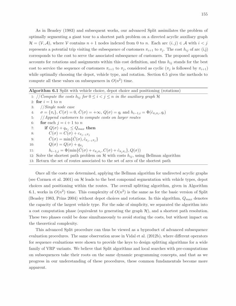
155

As in Beasley (1983) and subsequent works, our advanced Split assimilates the problem of

optimally segmenting a giant tour to a shortest path problem on a directed acyclic auxiliary graph

H = (V,A), where V contains n+ 1 nodes indexed from 0 to n. Each arc (i, j) ∈ A with i < j

represents a potential trip visiting the subsequence of customers πi+1 to πj . The cost hij of arc (i,j)

corresponds to the cost to serve the associated subsequence of customers. The proposed approach

accounts for rotations and assignments within this cost definition, and thus hij stands for the best

cost to service the sequence of customers πi+1 to πj , considered as cyclic (πj is followed by πi+1)

while optimally choosing the depot, vehicle type, and rotation. Section 6.5 gives the methods to

compute all these values on subsequences in O(n2) time.

Algorithm 6.1 Split with vehicle choice, depot choice and positioning (rotations)

1: //Compute the costs hij for 0 ≤ i < j ≤ n in the auxiliary graph H2: for i = 1 to n3: //Single node case4: σ = {πi}, C(σ) = 0, C(σ) = +∞, Q(σ) = qi and hi−1,i = Φ(cπiπi , qi)5: //Append customers to compute costs on larger routes6: for each j = i+ 1 to n7: if Q(σ) + qπj ≤ Qmax then8: C(σ) = C(σ) + cπj−1πj

9: C(σ) = min{C(σ), cπj−1πj}10: Q(σ) = Q(σ) + qπj

11: hi−1,j = Φ(min{C(σ) + cπjπi , C(σ) + cπjπi}, Q(σ))12: Solve the shortest path problem on H with costs hij , using Bellman algorithm13: Return the set of routes associated to the set of arcs of the shortest path

Once all the costs are determined, applying the Bellman algorithm for undirected acyclic graphs

(see Cormen et al. 2001) on H leads to the best compound segmentation with vehicle types, depot

choices and positioning within the routes. The overall splitting algorithm, given in Algorithm

6.1, works in O(n2) time. This complexity of O(n2) is the same as for the basic version of Split

(Beasley 1983, Prins 2004) without depot choices and rotations. In this algorithm, Qmax denotes

the capacity of the largest vehicle type. For the sake of simplicity, we separated the algorithm into

a cost computation phase (equivalent to generating the graph H), and a shortest path resolution.

These two phases could be done simultaneously to avoid storing the costs, but without impact on

the theoretical complexity.

This advanced Split procedure can thus be viewed as a byproduct of advanced subsequence

evaluation procedures. The same observation arose in Vidal et al. (2012b), where different operators

for sequence evaluations were shown to provide the keys to design splitting algorithms for a wide

family of VRP variants. We believe that Split algorithms and local searches with pre-computations

on subsequences take their roots on the same dynamic programming concepts, and that as we

progress in our understanding of these procedures, these common fundamentals become more

apparent.

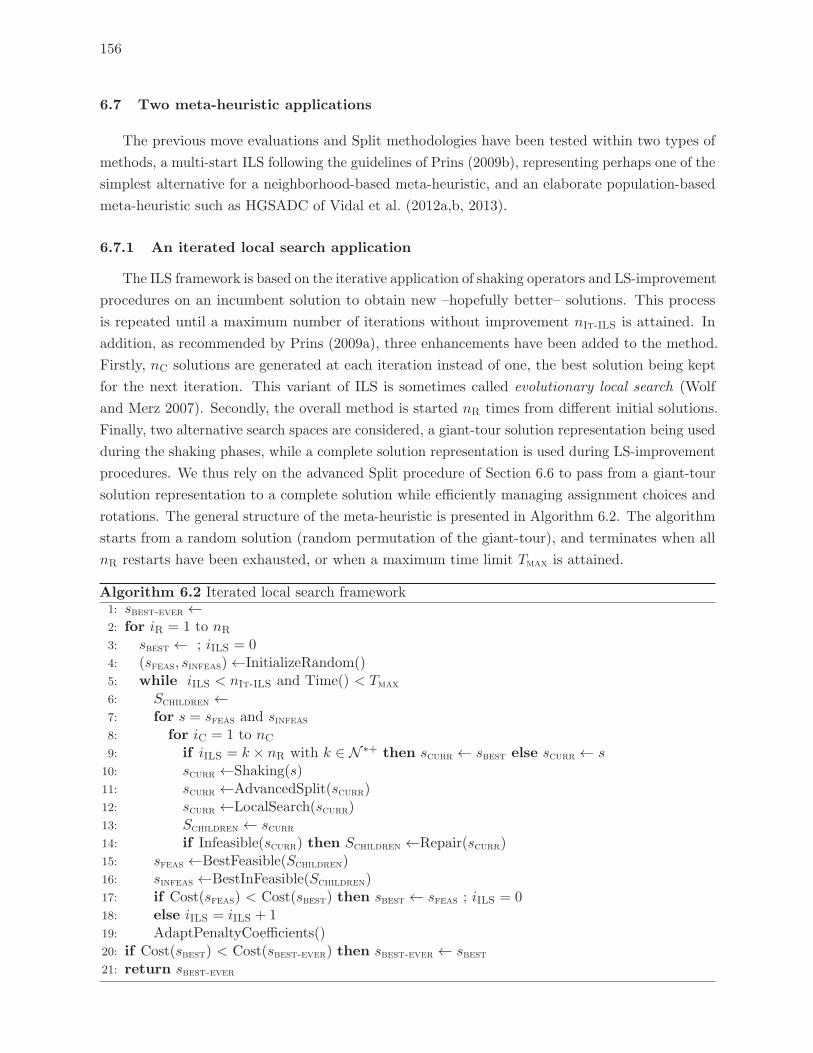
156

6.7 Two meta-heuristic applications

The previous move evaluations and Split methodologies have been tested within two types of

methods, a multi-start ILS following the guidelines of Prins (2009b), representing perhaps one of the

simplest alternative for a neighborhood-based meta-heuristic, and an elaborate population-based

meta-heuristic such as HGSADC of Vidal et al. (2012a,b, 2013).

6.7.1 An iterated local search application

The ILS framework is based on the iterative application of shaking operators and LS-improvement

procedures on an incumbent solution to obtain new –hopefully better– solutions. This process

is repeated until a maximum number of iterations without improvement nIt-ILS is attained. In

addition, as recommended by Prins (2009a), three enhancements have been added to the method.

Firstly, nC solutions are generated at each iteration instead of one, the best solution being kept

for the next iteration. This variant of ILS is sometimes called evolutionary local search (Wolf

and Merz 2007). Secondly, the overall method is started nR times from different initial solutions.

Finally, two alternative search spaces are considered, a giant-tour solution representation being used

during the shaking phases, while a complete solution representation is used during LS-improvement

procedures. We thus rely on the advanced Split procedure of Section 6.6 to pass from a giant-tour

solution representation to a complete solution while efficiently managing assignment choices and

rotations. The general structure of the meta-heuristic is presented in Algorithm 6.2. The algorithm

starts from a random solution (random permutation of the giant-tour), and terminates when all

nR restarts have been exhausted, or when a maximum time limit Tmax is attained.

Algorithm 6.2 Iterated local search framework1: sbest-ever ←2: for iR = 1 to nR3: sbest ← ; iILS = 04: (sfeas, sinfeas) ←InitializeRandom()5: while iILS < nIt-ILS and Time() < Tmax6: Schildren ←7: for s = sfeas and sinfeas8: for iC = 1 to nC9: if iILS = k × nR with k ∈ N ∗+ then scurr ← sbest else scurr ← s

10: scurr ←Shaking(s)11: scurr ←AdvancedSplit(scurr)12: scurr ←LocalSearch(scurr)13: Schildren ← scurr14: if Infeasible(scurr) then Schildren ←Repair(scurr)15: sfeas ←BestFeasible(Schildren)16: sinfeas ←BestInFeasible(Schildren)17: if Cost(sfeas) < Cost(sbest) then sbest ← sfeas ; iILS = 018: else iILS = iILS + 119: AdaptPenaltyCoefficients()20: if Cost(sbest) < Cost(sbest-ever) then sbest-ever ← sbest21: return sbest-ever

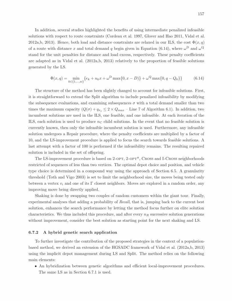
157

In addition, several studies highlighted the benefits of using intermediate penalized infeasible

solutions with respect to route constraints (Cordeau et al. 1997, Glover and Hao 2011, Vidal et al.

2012a,b, 2013). Hence, both load and distance constraints are relaxed in our ILS, the cost Φ(x, q)

of a route with distance x and total demand q begin given in Equation (6.14), where ωD and ωQ

stand for the unit penalties for distance and load excess, respectively. These penalty coefficients

are adapted as in Vidal et al. (2012a,b, 2013) relatively to the proportion of feasible solutions

generated by the LS.

Φ(x, q) = mink∈{1,...,w}

{ek + ukx+ ωDmax{0, x−D)}+ ωQmax{0, q −Qk}} (6.14)

The structure of the method has been slightly changed to account for infeasible solutions. First,

it is straightforward to extend the Split algorithm to include penalized infeasibility by modifying

the subsequence evaluations, and examining subsequences σ with a total demand smaller than two

times the maximum capacity (Q(σ) + qπj ≤ 2×Qmax – Line 7 of Algorithm 6.1). In addition, two

incumbent solutions are used in the ILS, one feasible, and one infeasible. At each iteration of the

ILS, each solution is used to produce nC child solutions. In the event that no feasible solution is

currently known, then only the infeasible incumbent solution is used. Furthermore, any infeasible

solution undergoes a Repair procedure, where the penalty coefficients are multiplied by a factor of

10, and the LS-improvement procedure is applied to focus the search towards feasible solutions. A

last attempt with a factor of 100 is performed if the infeasibility remains. The resulting repaired

solution is included in the set of offspring.

The LS-improvement procedure is based on 2-opt, 2-opt*, Cross and I-Cross neighborhoods

restricted of sequences of less than two vertices. The optimal depot choice and position, and vehicle

type choice is determined in a compound way using the approach of Section 6.5. A granularity

threshold (Toth and Vigo 2003) is set to limit the neighborhood size, the moves being tested only

between a vertex vi and one of its Γ closest neighbors. Moves are explored in a random order, any

improving move being directly applied.

Shaking is done by swapping two couples of random customers within the giant tour. Finally,

experimental analyses that adding a probability of Recall, that is, jumping back to the current best

solution, enhances the search performance by letting the method focus further on elite solution

characteristics. We thus included this procedure, and after every nR successive solution generations

without improvement, consider the best solution as starting point for the next shaking and LS.

6.7.2 A hybrid genetic search application

To further investigate the contribution of the proposed strategies in the context of a population-

based method, we derived an extension of the HGSADC framework of Vidal et al. (2012a,b, 2013)

using the implicit depot management during LS and Split. The method relies on the following

main elements:

• An hybridization between genetic algorithms and efficient local-improvement procedures.

The same LS as in Section 6.7.1 is used.

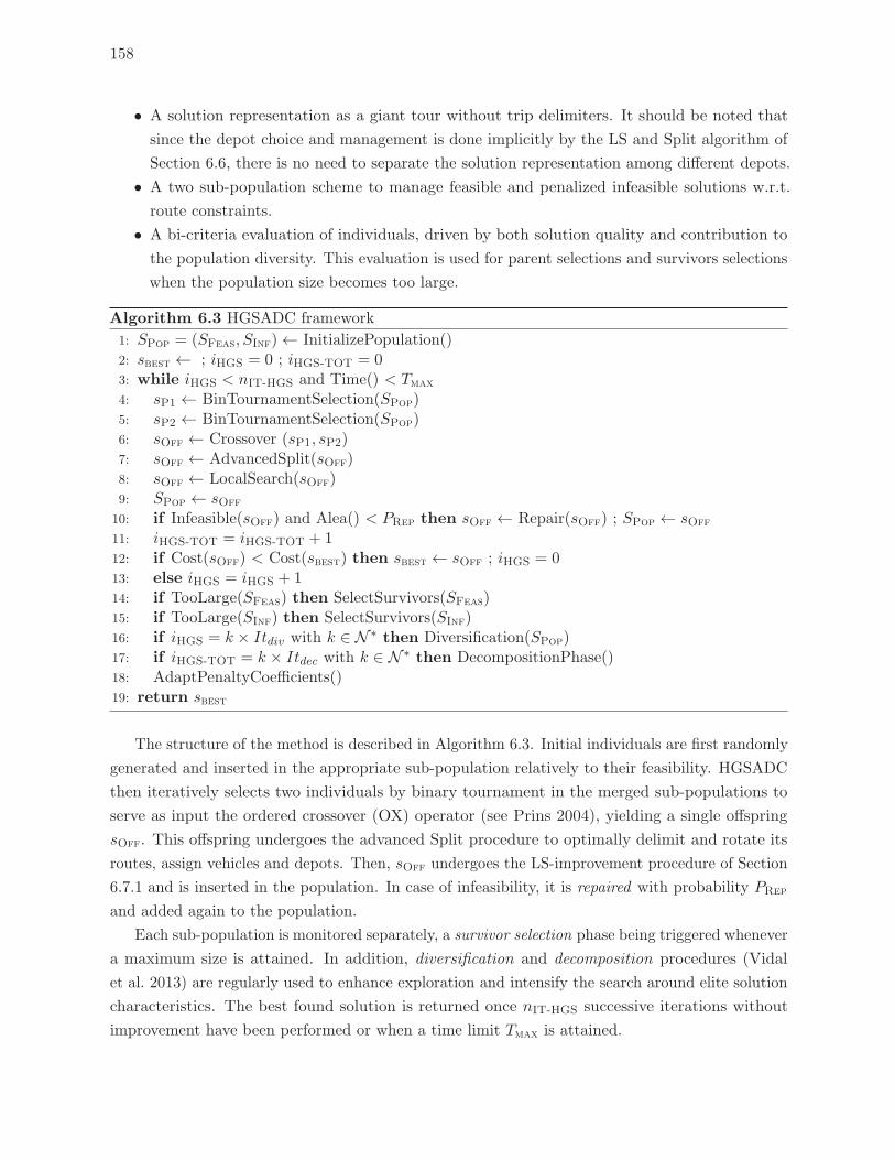
158

• A solution representation as a giant tour without trip delimiters. It should be noted that

since the depot choice and management is done implicitly by the LS and Split algorithm of

Section 6.6, there is no need to separate the solution representation among different depots.

• A two sub-population scheme to manage feasible and penalized infeasible solutions w.r.t.

route constraints.

• A bi-criteria evaluation of individuals, driven by both solution quality and contribution to

the population diversity. This evaluation is used for parent selections and survivors selections

when the population size becomes too large.

Algorithm 6.3 HGSADC framework

1: SPop = (SFeas, SInf) ← InitializePopulation()2: sbest ← ; iHGS = 0 ; iHGS-TOT = 03: while iHGS < nIT-HGS and Time() < Tmax4: sP1 ← BinTournamentSelection(SPop)5: sP2 ← BinTournamentSelection(SPop)6: sOff ← Crossover (sP1, sP2)7: sOff ← AdvancedSplit(sOff)8: sOff ← LocalSearch(sOff)9: SPop ← sOff

10: if Infeasible(sOff) and Alea() < PRep then sOff ← Repair(sOff) ; SPop ← sOff

11: iHGS-TOT = iHGS-TOT + 112: if Cost(sOff) < Cost(sbest) then sbest ← sOff ; iHGS = 013: else iHGS = iHGS + 114: if TooLarge(SFeas) then SelectSurvivors(SFeas)15: if TooLarge(SInf) then SelectSurvivors(SInf)16: if iHGS = k × Itdiv with k ∈ N ∗ then Diversification(SPop)17: if iHGS-TOT = k × Itdec with k ∈ N ∗ then DecompositionPhase()18: AdaptPenaltyCoefficients()19: return sbest

The structure of the method is described in Algorithm 6.3. Initial individuals are first randomly

generated and inserted in the appropriate sub-population relatively to their feasibility. HGSADC

then iteratively selects two individuals by binary tournament in the merged sub-populations to

serve as input the ordered crossover (OX) operator (see Prins 2004), yielding a single offspring

sOff. This offspring undergoes the advanced Split procedure to optimally delimit and rotate its

routes, assign vehicles and depots. Then, sOff undergoes the LS-improvement procedure of Section

6.7.1 and is inserted in the population. In case of infeasibility, it is repaired with probability PRep

and added again to the population.

Each sub-population is monitored separately, a survivor selection phase being triggered whenever

a maximum size is attained. In addition, diversification and decomposition procedures (Vidal

et al. 2013) are regularly used to enhance exploration and intensify the search around elite solution

characteristics. The best found solution is returned once nIT-HGS successive iterations without

improvement have been performed or when a time limit Tmax is attained.

159

6.8 Computational experiments

Extensive computational experiments are conducted to analyze the contribution of the compound

neighborhoods within the ILS and HGSADC metaheuristics, and compare these methods with

state-of-the-art algorithms from the literature. Three main VRP variants are considered: the

CVRP and the MDVRP, two seminal problems covered by a huge literature, and the multi-depot

vehicle fleet mix problem (MDVFMP), a good example of rich problem with compound attributes.

The goal, with the ILS experiments, is not to put forward a new champion method, but rather to

test the impact of the new compound neighborhoods on a simple LS-based metaheuristic.

Five sets of benchmark instances are used for the tests. For the CVRP, we rely on the classic

benchmark instances of Christofides et al. (1979) (Set A) and Golden et al. (1998b) (Set B). Set A

includes ten instances with uniformly geographically distributed customers, and four instances with

clustered customers. Set B ranges from 200 to 483 customers and displays geometric symmetries.

Three sets of instances (Sets C-E) are used for multi-depot settings. These instances present a

mix of uniformly distributed customers and clustered customers. Sets C and D of Cordeau et al.

(1997) include 33 MDVRP instances with 50 to 360 customers and two to nine depots. The last

Set E, of fourteen large-scale instances, has been introduced in Vidal et al. (2013) for the MDVRP

with time windows, and is used for the MDVRP by removing time-window constraints. This set

involves 360 to 960 customers and four to twelve depots. MDVFMP instances were also derived,

as in Salhi and Sari (1997), by keeping the same customer locations and demands, and generating

five types of vehicles vk such that Qk = (0.4 + 0.2k) ∗ Q, ek = 70 + 10k and uk = 0.7 + 0.1k for

k ∈ {1, . . . , 5}, Q standing for the vehicle capacity in the original instance. An unlimited fleet is

considered in all experiments.

The run time limit for the methods has been set to Tmax = 20 min on the medium-scale

instance sets (Sets A to D) and Tmax = 5 h for the larger instances (Set E). The parameter setting

of HGSADC is kept the same as in Vidal et al. (2012a,b, 2013), since an extensive parameter

calibration had already been conducted for multi-depot settings. The termination criteria of ILS

has been set to nIt-ILS = 25000/nC, so as to generate 25000 non-improving children before stopping,

and the number of restarts is set to nR = 5 to compare with HGSADC and other authors using

similar computational effort. The two remaining free parameters, nC and nR were simultaneously

calibrated. Several possible values of each parameter were selected, and the method was run 30

times for each configuration on a subset of instances, using different random seeds. For each

parameter configuration, the gap to the Best Known Solutions (BKS) in the literature, averaged

on all test instances, is reported in Figure 6.4.

As observed in Figure 6.4, the combination of parameters (nC, nR) = (10, 200) yields the

solutions of highest quality. These values were kept for all computational experiments. The

algorithm has been coded in C++, compiled with “g++ -O3”, and run on an Opteron 250 2.4

GHz CPU for the medium-scale instances (Sets A to D), and an Opteron 275 2.2 GHz CPU for

large-scale instances (Set E).

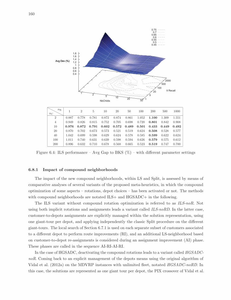
160

1 2 5 10 20 50 15

20100

5002000

0.4 0.6 0.8

1 1.2 1.4 1.6 1.8

Avg Dev (%)

0.75 0.7 0.65 0.6 0.55 0.5 0.45

NbChilds

It Recall

Avg Dev (%)

nC

nR 1 2 5 10 20 50 100 200 500 1000

2 0.887 0.778 0.781 0.872 0.874 0.861 1.052 1.100 1.309 1.551

4 0.949 0.826 0.815 0.752 0.705 0.698 0.720 0.801 0.842 0.908

10 0.976 0.872 0.791 0.602 0.572 0.489 0.501 0.433 0.449 0.492

20 0.870 0.702 0.673 0.573 0.521 0.519 0.624 0.508 0.528 0.577

40 1.042 0.699 0.598 0.629 0.624 0.578 0.585 0.599 0.622 0.624

100 1.011 0.740 0.631 0.639 0.598 0.594 0.626 0.579 0.575 0.612

200 0.896 0.632 0.710 0.678 0.568 0.665 0.523 0.519 0.747 0.700

Figure 6.4: ILS performance – Avg Gap to BKS (%) – with different parameter settings

6.8.1 Impact of compound neighborhoods

The impact of the new compound neighborhoods, within LS and Split, is assessed by means of

comparative analyses of several variants of the proposed meta-heuristics, in which the compound

optimization of some aspects – rotations, depot choices – has been activated or not. The methods

with compound neighborhoods are notated ILS+ and HGSADC+ in the following.

The ILS variant without compound rotation optimization is referred to as ILS-noR. Not

using both implicit rotations and assignments leads a variant called ILS-noRD. In the latter case,

customer-to-depots assignments are explicitly managed within the solution representation, using

one giant-tour per depot, and applying independently the classic Split procedure on the different

giant-tours. The local search of Section 6.7.1 is used on each separate subset of customers associated

to a different depot to perform route improvements (RI), and an additional LS-neighborhood based

on customer-to-depot re-assignments is considered during an assignment improvement (AI) phase.

These phases are called in the sequence AI-RI-AI-RI.

In the case of HGSADC, deactivating the compound rotations leads to a variant called HGSADC-

noR. Coming back to an explicit management of the depots means using the original algorithm of

Vidal et al. (2012a) on the MDVRP instances with unlimited fleet, notated HGSADC-noRD. In

this case, the solutions are represented as one giant tour per depot, the PIX crossover of Vidal et al.

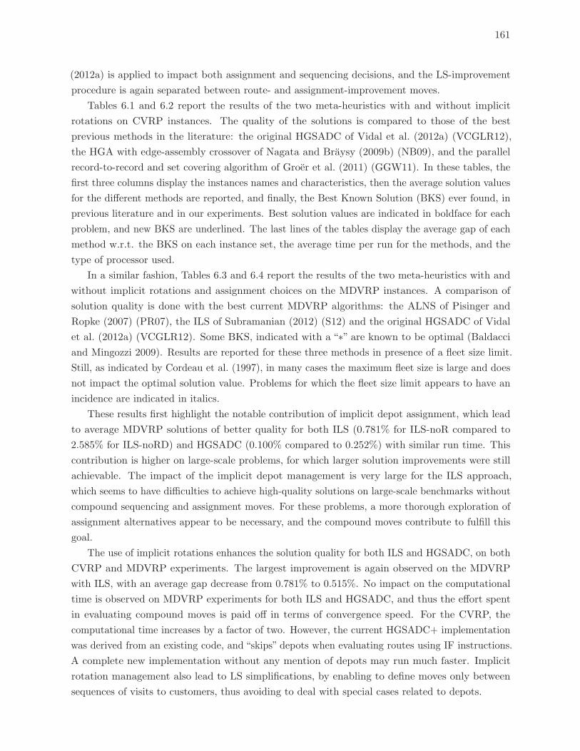
161

(2012a) is applied to impact both assignment and sequencing decisions, and the LS-improvement

procedure is again separated between route- and assignment-improvement moves.

Tables 6.1 and 6.2 report the results of the two meta-heuristics with and without implicit

rotations on CVRP instances. The quality of the solutions is compared to those of the best

previous methods in the literature: the original HGSADC of Vidal et al. (2012a) (VCGLR12),

the HGA with edge-assembly crossover of Nagata and Braysy (2009b) (NB09), and the parallel

record-to-record and set covering algorithm of Groer et al. (2011) (GGW11). In these tables, the

first three columns display the instances names and characteristics, then the average solution values

for the different methods are reported, and finally, the Best Known Solution (BKS) ever found, in

previous literature and in our experiments. Best solution values are indicated in boldface for each

problem, and new BKS are underlined. The last lines of the tables display the average gap of each

method w.r.t. the BKS on each instance set, the average time per run for the methods, and the

type of processor used.

In a similar fashion, Tables 6.3 and 6.4 report the results of the two meta-heuristics with and

without implicit rotations and assignment choices on the MDVRP instances. A comparison of

solution quality is done with the best current MDVRP algorithms: the ALNS of Pisinger and

Ropke (2007) (PR07), the ILS of Subramanian (2012) (S12) and the original HGSADC of Vidal

et al. (2012a) (VCGLR12). Some BKS, indicated with a “∗” are known to be optimal (Baldacci

and Mingozzi 2009). Results are reported for these three methods in presence of a fleet size limit.

Still, as indicated by Cordeau et al. (1997), in many cases the maximum fleet size is large and does

not impact the optimal solution value. Problems for which the fleet size limit appears to have an

incidence are indicated in italics.

These results first highlight the notable contribution of implicit depot assignment, which lead

to average MDVRP solutions of better quality for both ILS (0.781% for ILS-noR compared to

2.585% for ILS-noRD) and HGSADC (0.100% compared to 0.252%) with similar run time. This

contribution is higher on large-scale problems, for which larger solution improvements were still

achievable. The impact of the implicit depot management is very large for the ILS approach,

which seems to have difficulties to achieve high-quality solutions on large-scale benchmarks without

compound sequencing and assignment moves. For these problems, a more thorough exploration of

assignment alternatives appear to be necessary, and the compound moves contribute to fulfill this

goal.

The use of implicit rotations enhances the solution quality for both ILS and HGSADC, on both

CVRP and MDVRP experiments. The largest improvement is again observed on the MDVRP

with ILS, with an average gap decrease from 0.781% to 0.515%. No impact on the computational

time is observed on MDVRP experiments for both ILS and HGSADC, and thus the effort spent

in evaluating compound moves is paid off in terms of convergence speed. For the CVRP, the

computational time increases by a factor of two. However, the current HGSADC+ implementation

was derived from an existing code, and “skips” depots when evaluating routes using IF instructions.

A complete new implementation without any mention of depots may run much faster. Implicit

rotation management also lead to LS simplifications, by enabling to define moves only between

sequences of visits to customers, thus avoiding to deal with special cases related to depots.

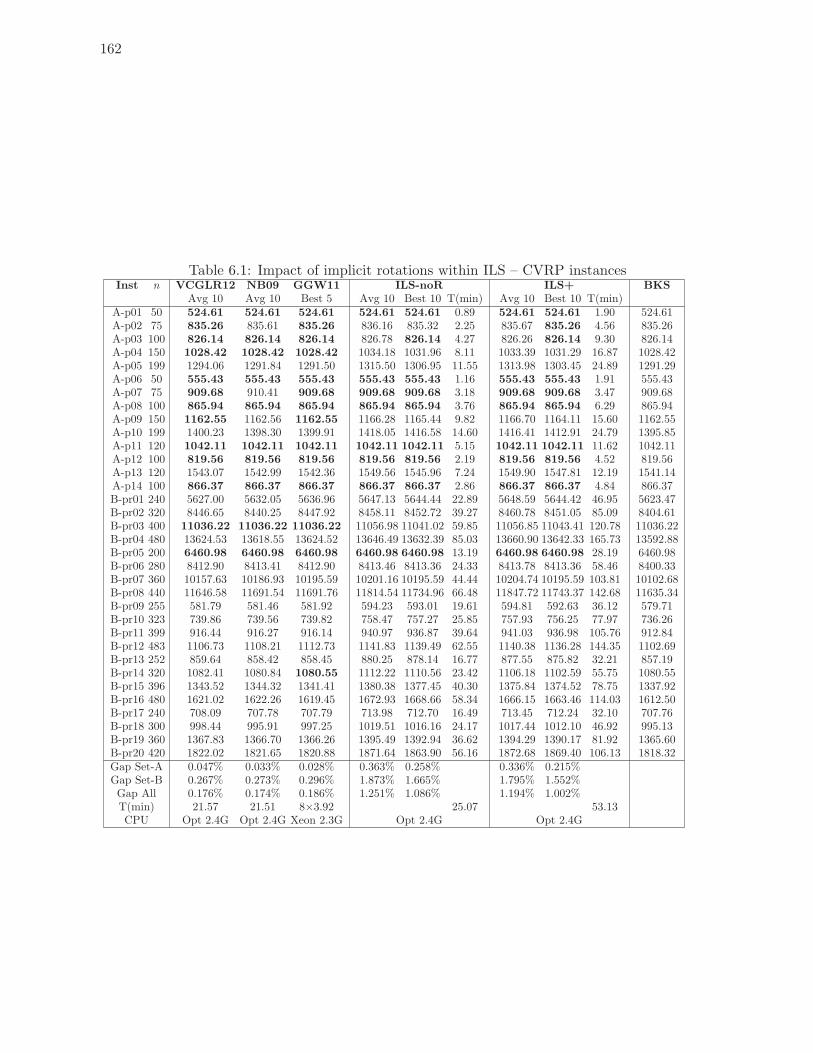
162

Table 6.1: Impact of implicit rotations within ILS – CVRP instancesInst n VCGLR12 NB09 GGW11 ILS-noR ILS+ BKS

Avg 10 Avg 10 Best 5 Avg 10 Best 10 T(min) Avg 10 Best 10 T(min)A-p01 50 524.61 524.61 524.61 524.61 524.61 0.89 524.61 524.61 1.90 524.61A-p02 75 835.26 835.61 835.26 836.16 835.32 2.25 835.67 835.26 4.56 835.26A-p03 100 826.14 826.14 826.14 826.78 826.14 4.27 826.26 826.14 9.30 826.14A-p04 150 1028.42 1028.42 1028.42 1034.18 1031.96 8.11 1033.39 1031.29 16.87 1028.42A-p05 199 1294.06 1291.84 1291.50 1315.50 1306.95 11.55 1313.98 1303.45 24.89 1291.29A-p06 50 555.43 555.43 555.43 555.43 555.43 1.16 555.43 555.43 1.91 555.43A-p07 75 909.68 910.41 909.68 909.68 909.68 3.18 909.68 909.68 3.47 909.68A-p08 100 865.94 865.94 865.94 865.94 865.94 3.76 865.94 865.94 6.29 865.94A-p09 150 1162.55 1162.56 1162.55 1166.28 1165.44 9.82 1166.70 1164.11 15.60 1162.55A-p10 199 1400.23 1398.30 1399.91 1418.05 1416.58 14.60 1416.41 1412.91 24.79 1395.85A-p11 120 1042.11 1042.11 1042.11 1042.11 1042.11 5.15 1042.11 1042.11 11.62 1042.11A-p12 100 819.56 819.56 819.56 819.56 819.56 2.19 819.56 819.56 4.52 819.56A-p13 120 1543.07 1542.99 1542.36 1549.56 1545.96 7.24 1549.90 1547.81 12.19 1541.14A-p14 100 866.37 866.37 866.37 866.37 866.37 2.86 866.37 866.37 4.84 866.37B-pr01 240 5627.00 5632.05 5636.96 5647.13 5644.44 22.89 5648.59 5644.42 46.95 5623.47B-pr02 320 8446.65 8440.25 8447.92 8458.11 8452.72 39.27 8460.78 8451.05 85.09 8404.61B-pr03 400 11036.22 11036.22 11036.22 11056.98 11041.02 59.85 11056.85 11043.41 120.78 11036.22B-pr04 480 13624.53 13618.55 13624.52 13646.49 13632.39 85.03 13660.90 13642.33 165.73 13592.88B-pr05 200 6460.98 6460.98 6460.98 6460.98 6460.98 13.19 6460.98 6460.98 28.19 6460.98B-pr06 280 8412.90 8413.41 8412.90 8413.46 8413.36 24.33 8413.78 8413.36 58.46 8400.33B-pr07 360 10157.63 10186.93 10195.59 10201.16 10195.59 44.44 10204.74 10195.59 103.81 10102.68B-pr08 440 11646.58 11691.54 11691.76 11814.54 11734.96 66.48 11847.72 11743.37 142.68 11635.34B-pr09 255 581.79 581.46 581.92 594.23 593.01 19.61 594.81 592.63 36.12 579.71B-pr10 323 739.86 739.56 739.82 758.47 757.27 25.85 757.93 756.25 77.97 736.26B-pr11 399 916.44 916.27 916.14 940.97 936.87 39.64 941.03 936.98 105.76 912.84B-pr12 483 1106.73 1108.21 1112.73 1141.83 1139.49 62.55 1140.38 1136.28 144.35 1102.69B-pr13 252 859.64 858.42 858.45 880.25 878.14 16.77 877.55 875.82 32.21 857.19B-pr14 320 1082.41 1080.84 1080.55 1112.22 1110.56 23.42 1106.18 1102.59 55.75 1080.55B-pr15 396 1343.52 1344.32 1341.41 1380.38 1377.45 40.30 1375.84 1374.52 78.75 1337.92B-pr16 480 1621.02 1622.26 1619.45 1672.93 1668.66 58.34 1666.15 1663.46 114.03 1612.50B-pr17 240 708.09 707.78 707.79 713.98 712.70 16.49 713.45 712.24 32.10 707.76B-pr18 300 998.44 995.91 997.25 1019.51 1016.16 24.17 1017.44 1012.10 46.92 995.13B-pr19 360 1367.83 1366.70 1366.26 1395.49 1392.94 36.62 1394.29 1390.17 81.92 1365.60B-pr20 420 1822.02 1821.65 1820.88 1871.64 1863.90 56.16 1872.68 1869.40 106.13 1818.32Gap Set-A 0.047% 0.033% 0.028% 0.363% 0.258% 0.336% 0.215%Gap Set-B 0.267% 0.273% 0.296% 1.873% 1.665% 1.795% 1.552%Gap All 0.176% 0.174% 0.186% 1.251% 1.086% 1.194% 1.002%T(min) 21.57 21.51 8×3.92 25.07 53.13CPU Opt 2.4G Opt 2.4G Xeon 2.3G Opt 2.4G Opt 2.4G

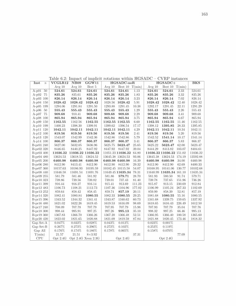
163

Table 6.2: Impact of implicit rotations within HGSADC – CVRP instancesInst n VCGLR12 NB09 GGW11 HGSADC-noR HGSADC+ BKS

Avg 10 Avg 10 Best 5 Avg 10 Best 10 T(min) Avg 10 Best 10 T(min)A-p01 50 524.61 524.61 524.61 524.61 524.61 1.13 524.61 524.61 2.33 524.61A-p02 75 835.26 835.61 835.26 835.26 835.26 1.83 835.26 835.26 3.32 835.26A-p03 100 826.14 826.14 826.14 826.14 826.14 3.23 826.14 826.14 7.02 826.14A-p04 150 1028.42 1028.42 1028.42 1028.56 1028.42 5.91 1028.42 1028.42 12.40 1028.42A-p05 199 1294.06 1291.84 1291.50 1293.88 1291.45 10.38 1292.17 1291.45 22.11 1291.29A-p06 50 555.43 555.43 555.43 555.43 555.43 1.29 555.43 555.43 2.26 555.43A-p07 75 909.68 910.41 909.68 909.68 909.68 2.29 909.68 909.68 3.41 909.68A-p08 100 865.94 865.94 865.94 865.94 865.94 3.75 865.94 865.94 6.67 865.94A-p09 150 1162.55 1162.56 1162.55 1162.55 1162.55 6.60 1162.55 1162.55 11.46 1162.55A-p10 199 1400.23 1398.30 1399.91 1399.62 1396.54 17.17 1398.12 1395.85 28.33 1395.85A-p11 120 1042.11 1042.11 1042.11 1042.11 1042.11 4.29 1042.11 1042.11 10.34 1042.11A-p12 100 819.56 819.56 819.56 819.56 819.56 2.41 819.56 819.56 5.20 819.56A-p13 120 1543.07 1542.99 1542.36 1542.86 1542.86 5.79 1542.52 1541.14 10.17 1541.14A-p14 100 866.37 866.37 866.37 866.37 866.37 3.41 866.37 866.37 5.83 866.37B-pr01 240 5627.00 5632.05 5636.96 5625.75 5623.47 25.65 5625.22 5623.47 62.00 5623.47B-pr02 320 8446.65 8440.25 8447.92 8447.92 8447.92 39.04 8444.29 8413.82 103.07 8404.61B-pr03 400 11036.22 11036.22 11036.22 11051.23 11036.22 64.80 11036.22 11036.22 151.02 11036.22B-pr04 480 13624.53 13618.55 13624.52 13645.38 13624.53 93.06 13645.38 13624.53 174.19 13592.88B-pr05 200 6460.98 6460.98 6460.98 6460.98 6460.98 16.39 6460.98 6460.98 34.00 6460.98B-pr06 280 8412.90 8413.41 8412.90 8412.90 8412.90 29.32 8412.90 8412.90 62.69 8400.33B-pr07 360 10157.63 10186.93 10195.59 10182.45 10115.58 54.07 10168.95 10141.06 130.77 10102.68B-pr08 440 11646.58 11691.54 11691.76 11649.45 11635.34 78.31 11640.99 11635.34 161.10 11635.34B-pr09 255 581.79 581.46 581.92 581.86 579.71 28.70 581.93 580.50 91.74 579.71B-pr10 323 739.86 739.56 739.82 739.01 737.43 81.40 739.78 737.65 151.96 736.26B-pr11 399 916.44 916.27 916.14 915.41 913.69 111.23 915.87 913.15 230.69 912.84B-pr12 483 1106.73 1108.21 1112.73 1107.36 1104.96 177.02 1106.99 1105.24 267.33 1102.69B-pr13 252 859.64 858.42 858.45 859.74 857.19 20.11 859.99 858.39 52.81 857.19B-pr14 320 1082.41 1080.84 1080.55 1082.33 1080.55 29.25 1081.68 1080.55 55.16 1080.55B-pr15 396 1343.52 1344.32 1341.41 1343.87 1340.62 60.73 1341.68 1339.75 159.65 1337.92B-pr16 480 1621.02 1622.26 1619.45 1619.53 1616.09 98.69 1618.65 1616.43 226.49 1612.50B-pr17 240 708.09 707.78 707.79 707.95 707.79 15.98 707.93 707.79 35.04 707.76B-pr18 300 998.44 995.91 997.25 997.26 995.13 35.10 998.32 997.25 66.46 995.13B-pr19 360 1367.83 1366.70 1366.26 1367.20 1366.48 52.51 1366.95 1366.40 100.58 1365.60B-pr20 420 1822.02 1821.65 1820.88 1821.09 1819.59 87.84 1821.88 1820.45 173.46 1818.32Gap Set-A 0.047% 0.033% 0.028% 0.043% 0.012% 0.023% 0.001%Gap Set-B 0.267% 0.273% 0.296% 0.272% 0.102% 0.253% 0.119%Gap All 0.176% 0.174% 0.186% 0.178% 0.065% 0.158% 0.070%T(min) 21.57 21.51 8×3.92 37.31 77.09CPU Opt 2.4G Opt 2.4G Xeon 2.3G Opt 2.4G Opt 2.4G

164

Table 6.3: Impact of implicit rotations and depot choices within ILS – MDVRP instances.Inst n d PR07 VCGLR12 S12 ILS-noRD ILS-noR ILS+ BKS

Avg 10 Avg 10 Avg 10 Avg 10 Best 10 T(min) Avg 10 Best 10 T(min) Avg 10 Best 10 T(min)C-p01 50 4 576.87 576.87 576.87 576.87 576.87 0.53 576.87 576.87 0.50 576.87 576.87 0.49 576.87∗C-p02 50 4 473.53 473.53 473.53 473.53 473.53 0.81 473.67 473.53 1.21 473.63 473.53 1.41 473.53∗C-p03 75 2 641.19 641.19 641.19 641.19 641.19 0.96 641.08 640.65 0.99 641.08 640.65 1.00 640.65∗C-p04 100 2 1006.09 1001.24 1001.04 1001.84 999.21 2.57 1002.12 999.21 1.88 1000.01 999.21 1.81 999.21∗C-p05 100 2 752.34 750.03 750.21 750.03 750.03 2.09 750.92 750.03 2.84 750.72 750.03 2.81 750.03C-p06 100 3 883.01 876.50 876.50 878.65 876.50 2.06 879.82 876.50 1.63 877.43 876.50 1.60 876.50∗C-p07 100 4 889.36 882.24 881.97 886.85 884.66 2.29 886.72 881.97 1.72 885.71 881.97 1.71 881.97∗C-p08 249 2 4421.03 4397.71 4393.70 4426.63 4401.79 19.65 4424.72 4401.17 15.54 4392.96 4382.91 14.85 4372.78C-p09 249 3 3892.50 3863.45 3864.22 3903.12 3891.91 19.30 3899.90 3882.66 14.69 3889.82 3878.25 12.75 3858.66C-p10 249 4 3666.85 3634.03 3634.72 3679.20 3660.30 19.92 3657.40 3635.52 14.43 3651.73 3635.71 12.45 3631.11C-p11 249 5 3573.23 3546.95 3546.15 3588.35 3560.27 19.52 3586.44 3565.95 14.73 3574.43 3557.57 12.94 3546.06C-p12 80 2 1319.13 1318.95 1318.95 1318.95 1318.95 1.09 1318.95 1318.95 1.35 1318.95 1318.95 1.51 1318.95∗C-p13 80 2 1318.95 1318.95 1318.95 1318.95 1318.95 0.98 1318.95 1318.95 1.24 1318.95 1318.95 1.23 1318.95C-p14 80 2 1360.12 1360.12 1360.12 1360.12 1360.12 0.98 1360.12 1360.12 1.34 1360.12 1360.12 1.17 1360.12C-p15 160 4 2519.64 2505.42 2505.42 2505.42 2505.42 4.18 2507.46 2505.42 3.82 2505.42 2505.42 3.25 2505.42C-p16 160 4 2573.95 2572.23 2572.23 2572.23 2572.23 3.32 2572.23 2572.23 3.15 2572.23 2572.23 3.17 2572.23C-p17 160 4 2709.09 2709.09 2710.21 2716.89 2709.09 3.43 2711.32 2709.09 3.48 2710.21 2709.09 3.03 2709.09C-p18 240 6 3736.53 3702.85 3702.85 3713.02 3702.85 13.98 3731.55 3714.56 9.82 3711.32 3702.85 10.32 3702.85C-p19 240 6 3838.76 3827.06 3827.55 3828.29 3827.06 7.95 3834.44 3827.06 7.06 3831.98 3827.06 7.32 3827.06C-p20 240 6 4064.76 4058.07 4058.07 4064.76 4058.07 9.26 4088.92 4058.07 8.70 4069.80 4058.07 8.02 4058.07C-p21 360 9 5501.58 5474.84 5474.84 5525.93 5490.11 20.00 5540.82 5506.26 32.59 5530.58 5496.40 20.00 5474.84C-p22 360 9 5722.19 5702.16 5705.84 5719.73 5702.16 19.66 5724.26 5714.46 19.99 5717.64 5702.16 18.63 5702.16C-p23 360 9 6092.66 6078.75 6078.75 6118.29 6078.75 20.00 6129.08 6112.46 30.04 6124.99 6112.46 20.00 6078.75D-pr01 48 4 861.32 861.32 861.32 861.32 861.32 1.02 861.32 861.32 1.18 861.32 861.32 1.12 861.32D-pr02 96 4 1308.17 1307.34 1308.53 1299.08 1297.44 3.96 1296.25 1296.25 3.03 1296.25 1296.25 2.82 1296.25D-pr03 144 4 1810.66 1803.80 1804.09 1804.55 1803.80 6.61 1803.81 1803.80 5.79 1803.81 1803.80 5.66 1803.80D-pr04 192 4 2073.16 2058.31 2060.93 2054.15 2042.45 11.41 2047.99 2042.45 8.13 2044.26 2042.45 8.09 2042.45D-pr05 240 4 2350.31 2335.81 2338.12 2377.66 2342.77 20.00 2333.43 2326.50 12.77 2330.19 2326.35 11.41 2324.12D-pr06 288 4 2695.74 2680.95 2685.23 2684.11 2675.71 20.00 2679.96 2673.00 18.72 2670.77 2668.76 18.06 2663.56D-pr07 72 6 1089.56 1089.56 1089.56 1075.53 1075.12 1.85 1075.12 1075.12 1.64 1075.12 1075.12 1.55 1075.12D-pr08 144 6 1675.74 1664.99 1665.08 1667.48 1660.16 6.44 1660.21 1658.71 4.32 1658.68 1658.23 4.30 1658.23D-pr09 216 6 2144.84 2133.52 2135.37 2159.27 2147.68 18.88 2144.57 2136.67 8.88 2139.08 2131.70 8.85 2131.70D-pr10 288 6 2905.43 2885.39 2882.41 2861.08 2826.91 20.00 2819.33 2812.39 20.38 2815.00 2810.25 17.96 2805.53E-pr11 360 4 – – – 5144.80 5096.71 164.31 5071.03 5029.61 70.36 5026.89 4999.04 72.89 4994.67E-pr12 480 4 – – – 6593.86 6522.94 281.29 6446.22 6424.10 149.53 6418.54 6391.48 168.58 6367.67E-pr13 600 4 – – – 8100.34 8054.60 300.02 7791.39 7746.68 261.83 7743.51 7689.19 293.95 7645.29E-pr14 720 4 – – – 9681.79 9588.94 300.03 9279.51 9211.41 300.02 9239.96 9184.68 300.06 9101.67E-pr15 840 4 – – – 11390.61 11235.84 300.03 10817.77 10782.85 300.02 10762.94 10726.17 300.03 10598.70E-pr16 960 4 – – – 13025.41 12720.01 300.04 12196.66 12143.63 300.03 12128.21 12062.69 300.02 11919.71E-pr17 360 6 – – – 4901.09 4880.87 172.32 4817.03 4797.91 68.73 4792.53 4772.62 80.47 4761.70E-pr18 520 6 – – – 6869.04 6770.66 300.02 6585.97 6536.84 186.31 6562.69 6531.79 176.90 6504.36E-pr19 700 6 – – – 9362.54 9170.60 300.03 8804.79 8770.25 300.02 8775.67 8736.22 300.01 8639.44E-pr20 880 6 – – – 10730.24 10553.01 300.03 10040.07 10000.46 300.02 9980.76 9946.18 300.03 9825.50E-pr21 420 12 – – – 4839.75 4712.22 295.36 4632.10 4613.14 99.47 4605.51 4596.09 109.73 4582.62E-pr22 600 12 – – – 6651.39 6466.61 300.03 6230.97 6193.52 283.34 6207.59 6181.67 264.14 6141.63E-pr23 780 12 – – – 9041.86 8778.31 300.04 8176.64 8119.01 300.01 8128.24 8078.99 300.02 8014.10E-pr24 960 12 – – – 11547.32 11020.10 300.06 10134.47 10067.97 300.03 10054.52 10040.63 300.04 9909.49Gap/T Set-C 0.413% 0.049% 0.049% 0.378% 0.148% 8.46 0.429% 0.157% 8.38 0.268% 0.093% 7.02Gap/T Set-D 1.171% 0.747% 0.795% 0.778% 0.298% 11.02 0.250% 0.096% 8.48 0.133% 0.046% 7.98Gap/T Set-E – – – 7.501% 5.495% 279.54 1.740% 1.193% 229.98 1.194% 0.745% 233.35Gap/T All – – – 2.585% 1.772% 89.75 0.781% 0.453% 74.41 0.515% 0.277% 74.64

T(min) Set-CD 3.95 5.18 10.45 – – 9.23 – – 8.41 – – 7.31CPU P-IV 3G Opt 2.4G I7 2.9G Opt 2.2 & Opt 2.4G Opt 2.2 & Opt 2.4G Opt 2.2 & Opt 2.4G

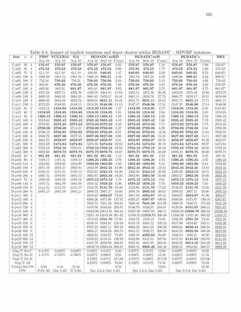
165

Table 6.4: Impact of implicit rotations and depot choices within HGSADC – MDVRP instances.Inst n d PR07 VCGLR12 S12 HGSADC-noRD HGSADC-noR HGSADC+ BKS

Avg 10 Avg 10 Avg 10 Avg 10 Best 10 T(min) Avg 10 Best 10 T(min) Avg 10 Best 10 T(min)C-p01 50 4 576.87 576.87 576.87 576.87 576.87 0.65 576.87 576.87 1.10 576.87 576.87 1.09 576.87∗C-p02 50 4 473.53 473.53 473.53 473.53 473.53 0.90 473.53 473.53 1.77 473.53 473.53 1.69 473.53∗C-p03 75 2 641.19 641.19 641.19 640.92 640.65 1.47 640.65 640.65 2.56 640.65 640.65 2.53 640.65∗C-p04 100 2 1006.09 1001.24 1001.04 1000.18 999.21 3.48 1001.04 1001.04 3.59 1000.66 999.21 3.43 999.21∗C-p05 100 2 752.34 750.03 750.21 750.03 750.03 2.84 750.03 750.03 5.12 750.03 750.03 4.89 750.03C-p06 100 3 883.01 876.50 876.50 876.50 876.50 1.99 876.50 876.50 3.31 876.50 876.50 3.02 876.50∗C-p07 100 4 889.36 882.24 881.97 883.83 881.97 3.02 881.97 881.97 3.75 881.97 881.97 3.75 881.97∗C-p08 249 2 4421.03 4397.71 4393.70 4386.59 4384.15 17.83 4382.51 4375.49 26.36 4383.63 4375.49 19.93 4372.78C-p09 249 3 3892.50 3863.45 3864.22 3864.85 3859.17 16.48 3865.11 3859.76 27.73 3860.77 3859.17 19.51 3858.66C-p10 249 4 3666.85 3634.03 3634.72 3639.61 3631.11 18.43 3631.71 3631.11 23.54 3631.71 3631.11 17.71 3631.11C-p11 249 5 3573.23 3546.95 3546.15 3553.28 3546.06 13.13 3547.47 3546.06 17.31 3547.37 3546.06 17.14 3546.06C-p12 80 2 1319.13 1318.95 1318.95 1318.95 1318.95 1.57 1318.95 1318.95 2.77 1318.95 1318.95 2.85 1318.95∗C-p13 80 2 1318.95 1318.95 1318.95 1318.95 1318.95 1.91 1318.95 1318.95 2.94 1318.95 1318.95 2.85 1318.95C-p14 80 2 1360.12 1360.12 1360.12 1360.12 1360.12 1.88 1360.12 1360.12 2.38 1360.12 1360.12 2.53 1360.12C-p15 160 4 2519.64 2505.42 2505.42 2505.42 2505.42 4.42 2505.42 2505.42 7.66 2505.42 2505.42 7.79 2505.42C-p16 160 4 2573.95 2572.23 2572.23 2572.23 2572.23 5.28 2572.23 2572.23 7.71 2572.23 2572.23 7.75 2572.23C-p17 160 4 2709.09 2709.09 2710.21 2709.09 2709.09 5.27 2709.09 2709.09 8.29 2709.09 2709.09 8.31 2709.09C-p18 240 6 3736.53 3702.85 3702.85 3702.85 3702.85 8.81 3702.85 3702.85 13.48 3702.85 3702.85 14.01 3702.85C-p19 240 6 3838.76 3827.06 3827.55 3827.06 3827.06 9.90 3827.06 3827.06 15.34 3827.06 3827.06 15.11 3827.06C-p20 240 6 4064.76 4058.07 4058.07 4058.07 4058.07 9.55 4058.07 4058.07 16.55 4058.07 4058.07 16.20 4058.07C-p21 360 9 5501.58 5474.84 5474.84 5476.36 5474.84 19.83 5474.84 5474.84 29.18 5474.84 5474.84 20.07 5474.84C-p22 360 9 5722.19 5702.16 5705.84 5702.16 5702.16 19.94 5702.16 5702.16 33.19 5702.16 5702.16 20.00 5702.16C-p23 360 9 6092.66 6078.75 6078.75 6078.75 6078.75 19.97 6078.75 6078.75 38.69 6080.43 6078.75 20.00 6078.75D-pr01 48 4 861.32 861.32 861.32 861.32 861.32 1.12 861.32 861.32 2.10 861.32 861.32 2.05 861.32D-pr02 96 4 1308.17 1307.34 1308.53 1296.25 1296.25 2.70 1296.25 1296.25 4.74 1296.25 1296.25 4.67 1296.25D-pr03 144 4 1810.66 1803.80 1804.09 1803.80 1803.80 4.93 1803.80 1803.80 8.54 1803.80 1803.80 8.84 1803.80D-pr04 192 4 2073.16 2058.31 2060.93 2043.09 2042.45 10.99 2042.45 2042.45 13.24 2042.45 2042.45 12.84 2042.45D-pr05 240 4 2350.31 2335.81 2338.12 2325.91 2324.12 16.40 2326.30 2324.12 25.88 2325.09 2324.12 19.51 2324.12D-pr06 288 4 2695.74 2680.95 2685.23 2664.85 2663.56 19.26 2663.88 2663.56 34.66 2664.57 2663.56 20.00 2663.56D-pr07 72 6 1089.56 1089.56 1089.56 1075.12 1075.12 1.78 1075.12 1075.12 3.01 1075.12 1075.12 3.04 1075.12D-pr08 144 6 1675.74 1664.99 1665.08 1658.52 1658.23 6.36 1658.23 1658.23 7.73 1658.23 1658.23 7.85 1658.23D-pr09 216 6 2144.84 2133.52 2135.37 2132.70 2131.70 10.39 2132.96 2131.70 17.23 2132.95 2131.70 15.65 2131.70D-pr10 288 6 2905.43 2885.39 2882.41 2809.72 2807.17 18.60 2808.19 2805.53 38.64 2808.63 2807.11 20.00 2805.53E-pr11 360 4 – – – 5018.62 4994.67 73.02 5001.94 4994.67 88.13 5004.67 4994.67 81.90 4994.67E-pr12 480 4 – – – 6396.26 6371.96 127.92 6392.27 6367.67 109.81 6389.08 6375.87 139.18 6367.67E-pr13 600 4 – – – 7683.73 7651.43 250.91 7668.48 7645.29 215.08 7668.70 7648.71 175.03 7645.29E-pr14 720 4 – – – 9185.56 9163.63 293.97 9136.79 9106.37 294.81 9129.58 9101.67 296.51 9101.67E-pr15 840 4 – – – 10682.96 10614.31 300.44 10627.80 10607.65 300.11 10638.93 10598.70 296.53 10598.70E-pr16 960 4 – – – 12071.44 12016.08 301.22 11948.52 11919.71 300.38 11948.39 11921.00 300.32 11919.71E-pr17 360 6 – – – 4772.85 4761.70 77.00 4765.72 4762.19 73.01 4766.29 4761.70 73.10 4761.70E-pr18 520 6 – – – 6539.55 6504.81 158.53 6518.19 6504.72 192.22 6517.60 6504.62 162.11 6504.36E-pr19 700 6 – – – 8707.25 8667.11 290.42 8669.38 8641.05 296.36 8669.61 8639.44 296.34 8639.44E-pr20 880 6 – – – 9883.17 9834.39 300.74 9845.57 9826.77 300.28 9845.52 9825.50 300.26 9825.50E-pr21 420 12 – – – 4603.04 4583.67 75.69 4595.10 4582.62 88.00 4596.54 4586.41 88.90 4582.62E-pr22 600 12 – – – 6183.22 6154.31 198.82 6162.68 6147.01 207.01 6157.81 6141.63 233.83 6141.63E-pr23 780 12 – – – 8101.79 8050.99 289.35 8037.81 8021.97 283.35 8032.95 8014.10 294.29 8014.10E-pr24 960 12 – – – 10049.78 10004.94 300.01 9938.18 9909.49 300.48 9926.27 9910.02 300.57 9909.49Gap/T Set-C 0.413% 0.049% 0.049% 0.056% 0.012% 8.20 0.027% 0.012% 12.80 0.023% 0.003% 10.09Gap/T Set-D 1.171% 0.747% 0.795% 0.037% 0.006% 9.25 0.026% 0.000% 15.58 0.025% 0.006% 11.45Gap/T Set-E – – – 0.729% 0.275% 217.00 0.270% 0.026% 217.79 0.257% 0.020% 217.06Gap/T All – – – 0.252% 0.089% 70.62 0.100% 0.014% 74.45 0.093% 0.009% 72.03

T(min) Set-CD 3.95 5.18 10.45 – – 8.52 – – 13.64 – – 10.50CPU P-IV 3G Opt 2.4G I7 2.9G Opt 2.2 & Opt 2.4G Opt 2.2 & Opt 2.4G Opt 2.2 & Opt 2.4G

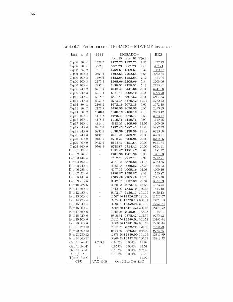
166

Table 6.5: Performance of HGSADC – MDVFMP instances

Inst n d SS97 HGSADC+ BKS– Avg 10 Best 10 T(min)

C-p01 50 4 1526.7 1477.73 1477.73 1.87 1477.73C-p02 50 4 992.8 957.73 957.73 2.44 957.73C-p03 75 2 1611.1 1569.67 1569.67 3.37 1569.67C-p04 100 2 2361.9 2292.64 2292.64 4.64 2292.64C-p05 100 2 1498.4 1453.64 1453.64 7.42 1453.64C-p06 100 3 2277.5 2208.66 2208.66 5.34 2208.66C-p07 100 4 2297.1 2198.91 2198.91 5.19 2198.91C-p08 249 2 6718.6 6448.26 6441.36 20.00 6441.36C-p09 249 3 6211.4 6021.41 5998.70 20.00 5998.70C-p10 249 4 6018.7 5817.81 5807.53 20.00 5807.53C-p11 249 5 6030.8 5773.28 5770.42 19.74 5770.42C-p12 80 2 2108.2 2072.18 2072.18 3.60 2072.18C-p13 80 2 2126.8 2096.39 2096.39 3.56 2096.39C-p14 80 2 2160.1 2160.12 2160.12 4.18 2160.12C-p15 160 4 4116.2 3973.47 3973.47 9.61 3973.47C-p16 160 4 4178.9 4119.76 4119.76 9.93 4119.76C-p17 160 4 4344.1 4323.09 4309.09 13.95 4309.09C-p18 240 6 6217.0 5887.43 5887.43 19.80 5887.43C-p19 240 6 6233.6 6130.36 6130.36 19.47 6130.36C-p20 240 6 6493.1 6481.23 6469.21 20.00 6469.21C-p21 360 9 9184.6 8710.75 8709.26 20.00 8709.26C-p22 360 9 9332.0 9164.65 9151.64 20.00 9151.64C-p23 360 9 9706.6 9728.87 9714.41 20.00 9714.41D-pr01 48 4 – 1181.47 1181.47 2.09 1181.47D-pr02 96 4 – 1901.39 1901.39 6.81 1901.39D-pr03 144 4 – 2712.71 2712.71 9.97 2712.71D-pr04 192 4 – 3371.35 3370.85 24.15 3370.85D-pr05 240 4 – 4068.98 4066.52 28.20 4066.52D-pr06 288 4 – 4677.35 4669.16 62.08 4669.16D-pr07 72 6 – 1550.87 1550.87 3.56 1550.87D-pr08 144 6 – 2705.46 2705.46 10.73 2705.46D-pr09 216 6 – 3642.57 3637.39 28.84 3637.39D-pr10 288 6 – 4980.33 4973.74 48.63 4973.74E-pr11 360 4 – 7342.40 7323.10 150.65 7323.10E-pr12 480 4 – 9472.47 9436.13 251.09 9436.13E-pr13 600 4 – 11567.96 11526.27 291.36 11526.27E-pr14 720 4 – 13824.41 13778.18 300.01 13778.18E-pr15 840 4 – 16393.71 16352.74 301.06 16352.74E-pr16 960 4 – 18509.70 18471.52 300.46 18471.52E-pr17 360 6 – 7048.26 7025.01 168.08 7025.01E-pr18 520 6 – 9810.34 9775.42 245.35 9775.42E-pr19 700 6 – 13312.76 13280.04 301.52 13280.04E-pr20 880 6 – 15683.36 15631.64 301.52 15631.64E-pr21 420 12 – 7087.02 7072.79 170.80 7072.79E-pr22 600 12 – 9804.69 9776.65 288.99 9776.65E-pr23 780 12 – 12878.26 12840.99 301.05 12840.99E-pr24 960 12 – 16360.55 16343.33 300.02 16343.33Gap/T Set-C 2.769% 0.067% 0.000% 11.92Gap/T Set-D – 0.053% 0.000% 22.51Gap/T Set-E – 0.282% 0.000% 262.28Gap/T All – 0.128% 0.000% 88.75

T(min) Set-C 4.10 – – 11.92CPU VAX 4000 Opt 2.2 & Opt 2.4G

167

These experiments finally illustrate the good performance of the proposed HGSADC+ meta-

heuristic, which matches or outperforms other current state-of-the-art CVRP and MDVRP with an

average gap to BKS of 0.158% for the CVRP, and 0.093% for the MDVRP. In all cases, HGSADC

variants produce solutions of better quality than ILS. As a counterpart, ILS is simpler and in

general faster. All known optimal solutions have been retrieved. Run times remains moderate on

medium-scale instances, of a magnitude comparable to those of other methods in the literature.

The standard deviation of solution costs from HGSADC+ is small (0.069%, 0.071% for the CVRP

and MDVRP), thus showing that high-quality solutions are produced in a consistent manner.

6.8.2 Addressing a rich problem – the MDVFMP

A second set of experiments has been conducted to investigate the performance of the proposed

HGSADC+ on a rich vehicle routing variant, the MDVFMP. The literature is scarce on this

particular problem. We compare the proposed method to the variable neighborhood heuristic of

Salhi and Sari (1997) (SS97) and to the best known solution founds during multiple runs. Table

6.5 reports the results of the methods on the modified MDVRP instances, using the same format

as previously.

As highlighted in Table 6.5, major solution improvements were still achievable on these instances.

The average gap obtained with HGSADC+ is 0.067%, compared to 2.769% for SS97. Still, it

should be noted that SS97 was executed on an old system and processor, and that extended runs

on modern computers may lead to decreased gaps. Nevertheless, HGSADC+ demonstrate its

ability to find the best known solutions in a consistent manner on this difficult problem: for 14/23

instances of set C with 50 to 240 customers the best known solution has been reached on all 10

runs, and the overall standard deviation of solution costs remains very small (0.089%).

6.9 Conclusions

In this paper, an efficient dynamic programming methodology was introduced for managing com-

pound customer-to-depots assignments, rotations and vehicles choices within neighborhood searches

for vehicle routing. Two meta-heuristics based on these concepts, an ILS and a HGSADC, have been

proposed. These approaches produce solutions of remarkable quality on classic CVRP, MDVRP

and MDVFMP benchmark instances with unlimited fleet. Extensive experiments demonstrate the

notable contribution of the proposed implicit depot management to the search performance. The

implicit rotations have a smaller but noticeable impact, and may simplify several aspects of LS

implementations. The proposed methodology is general, and broadly applicable to many VRP

variants.

Promising avenues of research involves generalizing the approach to other multi-attribute VRPs,

possibly with limited fleet. Finally, this research is part of a general effort aiming to identify

efficiently manageable subproblems to reduce the size of solution spaces, and similar subproblems and

management methods may be investigated on other VRP variants and combinatorial optimization

settings.

Troisieme partie

RESOLUTION DE PROBLEMES

RICHES ET APPROCHES

GENERALISTES

169

CHAPITRE 7

PROBLEMES DE TOURNEES DE VEHICULES ET D’HORAIRES DE

CONDUCTEURS


Les derniers chapitres de cette these se consacrent a la resolution de VRP riches combinant

de nombreux attributs et au developpement de nouvelles methodes heuristiques generalistes pour

traiter une grande variete de problemes.

Ce chapitre presente tout d’abord une application de HGSADC au VRTDSP, un probleme riche

particulierement difficile, qui requiert la determination simultanee de routes et de combinaisons de

pauses legalement acceptables pour les conducteurs. Les regles de la legislation sont tres complexes,

et ne pas les prendre en compte dans les methodes de resolution conduirait inevitablement a des

solutions irrealistes pour le transport de longue distance. Par ailleurs, le methodologie proposee

dans ce chapitre permet de resoudre le VRTDSP pour une grande variete de legislations, permet-

tant ainsi de conduire une comparaison internationale experimentale de l’impact des reglements

gouvernementaux sur la competitivite economique, les horaires, et la fatigue des conducteurs.

Nous montrons en particulier que les regles de l’Union Europeenne sont les plus sures, tandis que

les regles du Canada sont les plus avantageuses economiquement. Les regles de l’Australie sont

dominees a la fois en termes de cout et surete par les autres regles. Finalement, les Etats-Unis

fournissent une alternative intermediaire entre cout et surete, les recents changements de regles a

venir en 2013 tendant vers plus de securite.

7.2 Article VII : Hours of service regulations in road freight transport – an optimiza-

tion-based international assessment

Un article base sur ce chapitre a ete soumis pour publication : Goel, A., Vidal., T.

Hours of service regulations in road freight transport – an optimization-based inter-

national assessment. Transportation Science, submitted for publication.

Abstract: Driver fatigue is internationally recognized as a significant factor in approximately 15

to 20% of commercial road transport crashes. In their efforts to increase road safety and improve

working conditions of truck drivers, governments world wide are enforcing stricter limits on the

amount of working and driving time without rest. This paper describes an effective optimization

algorithm for minimizing transportation costs for a fleet of vehicles considering business hours

of customers and complex hours of service regulations. The algorithm combines the exploration

capacities of population-based metaheuristics, the quick improvement abilities of local search, with

efficient tree search procedures for checking compliance with hours of service regulations. The

proposed approach can be used to assess the impact of different hours of service regulations from a

carrier-centric point of view. Extensive computational experiments conducted for various sets of

172

regulations in the United States, Canada, the European Union, and Australia are conducted to

provide an international assessment of the impact of different rules on transportation costs and

accident risks. Our experiments demonstrate that European Union rules lead to the highest safety,

while Canadian regulations are the most competitive in terms of economic efficiency. Australian

regulations appear to have unnecessarily high risk rates with respect to operating costs. The recent

rule change in the United States reduces accident risk rates with a moderate increase in operating

costs.

Keywords: Hours of Service Regulations; Fatigue; Road Safety; Truck Driver Scheduling; Vehicle

Routing and Scheduling.

7.3 Introduction

Driver fatigue is a significant factor in approximately fifteen to twenty percent of commercial

road transport crashes (Williamson et al. 2001, European Transport Safety Council 2001, Federal

Motor Carrier Safety Administration 2008). In Europe it is estimated that one out of two long

haul drivers has fallen asleep while driving (European Transport Safety Council 2001). One out of

five long distance road transport drivers in Australia reported at least one fatigue related incident

on their last trip and one out of three drivers reported breaking road rules on at least half of their

trips (Williamson et al. 2001). A survey among truck drivers in the United States revealed that

one out of six truck drivers has dozed at wheel in the month prior to the survey, and less than one

out of two truck drivers reported that delivery schedules are always realistic (McCartt et al. 2008).

Undoubtedly, fatigue is a threat to road safety and companies must give drivers enough time for

breaks and rest periods during their trips.

In their efforts to increase road safety and improve working conditions, governments world wide

are adopting stricter regulations concerning driving and working hours of truck drivers. These

regulations impose maximum limits on the amount of driving and working within certain time

periods and minimum requirements on the number and duration of break and rest periods which

must be taken by drivers. Compulsory break and rest periods have a significant impact on total

travel durations, which are typically more than twice as long as the pure driving time required

in long distance haulage. Consequently, motor carriers must take applicable hours of service

regulations into account when generating routes and truck driver schedules. Not doing so would

inevitably result in unrealistic schedules, large delays, violations of regulations and reduced road

safety.

In this paper, a hybrid genetic algorithm is introduced for the problem of determining a set of

routes for a fleet of vehicles, such that each customer is visited within given time windows, that

each driver can comply with applicable hours of service regulations, and that transportation costs

are minimized. The proposed optimization method is specifically designed to efficiently handle

explicit schedule generation during route evaluations and can be applied for various hours of service

regulations world wide. Extensive computational experiments on benchmark instances developed

for vehicle routing and truck driver scheduling in the European Union demonstrate the remarkable

173

performance of the method in comparison to previous approaches. In particular, 103/112 best

known solutions for these instances were either obtained or improved, and 72/112 were strictly

improved. This shows that our approach can provide a valuable tool for transport operators to

minimize costs and likewise give drivers enough time for recuperation.

Furthermore, policy makers, unions, and transport companies can use our approach to assess

the impact of regulations or agreements to find the best trade-off between road safety, working

conditions of truck drivers as well as speed and costs of transportation. In this paper we assess

and compare of hours of service regulations in the United States, Canada, the European Union,

and Australia with regards to operating costs and accident risks. Specific subsets of rules such as

split breaks and rests or extended driving times and reduced rests in the European Union as well

as the impact of the recent rule change in the United States are analyzed.

7.4 Hours of service regulations

This section presents the hours of service regulations in the United States, Canada, the

European Union, and Australia. For the sake of conciseness only the most important rules for a

planning horizon of six days (i.e. Monday to Saturday) are described. For more details about these

regulations the reader is referred to Federal Motor Carrier Safety Administration (2011), Transport

Canada (2005), European Union (2006, 2002) and National Transport Commission (2008a,b,c).

7.4.1 United States

In December 2011, the Federal Motor Carrier Safety Agency published new hours of service

regulations in the United States. These regulations distinguish between on-duty time and off-duty

time. On-duty time refers to all time a driver is working and includes driving activities as well as

other work such as loading and unloading. Off-duty time refers to any time during which a driver

is not performing any work.

The regulations limit the maximum amount of accumulated driving time between two rest

periods to 11 hours. After accumulating 11 hours of driving, the driver must be off duty for

10 consecutive hours before driving again. The regulations prohibit a driver from driving after

14 hours have elapsed since the end of the last rest period. However, a driver may conduct other

work after 14 hours have elapsed since the end of the last rest period. Furthermore, a driver must

not drive after accumulating 60 hours of on-duty time within a period of 7 days. Alternatively,

a driver must not drive after accumulating 70 hours of on-duty time within a period of 8 days.

For the sake of conciseness, however, this second option is not considered in the remainder of this

paper.

Above rules are the same as in the previous regulations. The new regulations, furthermore,

include new rules which will become effective in July 2013. According to these new rules a truck

driver must not drive if 8 hours or more have elapsed since the end of the last off-duty period of at

least 30 minutes.

174

7.4.2 Canada

Canadian hours of service regulations are described in Transport Canada (2005) and interpreted

in Canadian Council of Motor Transport Administrators (2007). Two sets of regulations exist, one

of which applies to driving conducted south of latitude 60◦ N and one to driving north of latitude

60◦ N. In this paper we focus on the subset of regulations applicable for driving south of latitude

60◦ N, because this is the area of major economic concern. On- and off-duty times are defined as

described above for U.S. hours of service regulations. The regulations demand that a driver must

not drive after accumulating 13 hours of driving time, after accumulating 14 hours of on-duty time,

or after 16 hours of time have elapsed since the end of the last period of at least 8 consecutive

hours of off-duty time. In any of these cases the driver may only commence driving again after

taking another period of at least 8 consecutive hours of off-duty time.

Furthermore, the regulations impose restrictions on the maximum amount of on-duty time and

the minimum amount of off-duty time during a day. According to the regulations a day means a

24-hour period that begins at some time designated by the motor carrier. For simplicity and w.l.o.g.

let us assume in the remainder that this time is midnight. The regulations demand that a driver

does not drive for more than 13 hours in a day and that a driver accumulates at least 10 hours

of off-duty time in a day. At least 2 of these hours must not be part of a period of 8 consecutive

hours of off-duty time as required by the provisions described in the previous paragraph. However,

if a period of more than 8 consecutive hours of off-duty time is scheduled, the amount exceeding

the 8th hour may contribute to these 2 hours. Off-duty periods of less than 30 minutes do not

count toward the minimum off-duty time requirements. Eventually, the regulations demand that a

driver does not drive after accumulating 70 hours of on-duty time within a period of 7 days.

7.4.3 European Union

In the European Union, truck drivers must comply with regulation (EC) No 561/2006 and the

national implementations of Directive 2002/15/EC.

Regulation (EC) No 561/2006 distinguishes between four driver activities: rest periods, breaks,

driving time, and other work. Rest periods are periods during which a driver may freely dispose

of her or his time and have the purpose of giving drivers enough time to sleep. Breaks are short

periods exclusively used for recuperation during which a driver must not carry out any work.

Driving time refers to the time during which a driver is operating a vehicle and includes any time

during which the vehicle is temporarily stationary due to reasons related to driving, e.g. traffic

jams. Other work refers to any work except for driving and includes time spent for loading or

unloading, cleaning and technical maintenance, customs, and so on.

Regulation (EC) No 561/2006 demands that a driver takes a break of at least 45 minutes after

accumulating 412 hours of driving. A daily rest period of at least 11 hours must be completed within

24 hours after the end of the previous rest period, and the accumulated driving time between two

rest periods shall not exceed 9 hours. Furthermore, the driving time in a week must not exceed 56

hours, and the accumulated driving and working time in a week must not exceed 60 hours.

175

The basic set of rules described above are sufficient to comply with regulation (EC) No 561/2006.

The regulation, furthermore, allows a driver to take break and rest periods in two parts. A break

period may be taken in two parts if the first part is a period of at least 15 minutes and the second

part is a period of at least 30 minutes. A rest period may be taken in two parts if the first part is

a period of at least 3 hours and the second part is a period of at least 9 hours. If a rest period

is taken in two parts, the second part must be completed within 24 hours after the end of the

previous rest period. Within a planning horizon of one week a driver is allowed to reduce the

duration of at most three rest periods to 9 hours. Furthermore, the amount of driving between two

rest periods may be extended twice a week to at most 10 hours.

According to Directive 2002/15/EC, a truck driver must not work for more than 6 hours without

taking at least 30 minutes of break time. If a truck driver works for more than 9 hours at least

45 minutes of break time must be taken. The break time may be taken in several periods of at

least 15 minutes each. The directive, furthermore, applies additional rules for night work. However,

these rules not are not considered in the scope of this paper because they differ throughout the

member states of the European Union.

7.4.4 Australia

In Australia, motor carriers accredited in the National Heavy Vehicle Accreditation Scheme may

operate according to the Basic Fatigue Management Standard (National Transport Commission

2008b). Motor carriers without accreditation must comply with the standard hours option of the

Australian Heavy Vehicle Driver Fatigue described in National Transport Commission (2008c).

Standard Hours

Australian motor carriers without accreditation must comply with the following constraints on

driver schedules:

1. In any period of 512 hours a driver must not work for more than 51

4 hours and must have at

least 15 continuous minutes of rest time.

2. In any period of 8 hours a driver must not work for more than 712 hours and must have at

least 30 minutes rest time in blocks of not less than 15 continuous minutes.




least 7 continuous hours of stationary rest time.

5. In any period of 7 days a driver must not work for more than 72 hours and must have at


When evaluating whether a truck driver schedule complies with these provisions, the duration

of each work period is rounded up to the nearest multiple of 15 minutes and the duration of each

rest period is rounded down to the nearest multiple of 15 minutes.

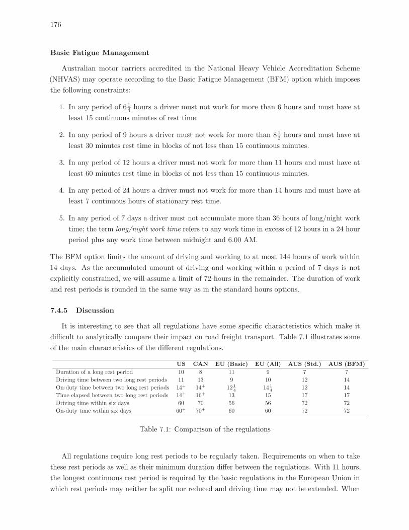
176

Basic Fatigue Management

Australian motor carriers accredited in the National Heavy Vehicle Accreditation Scheme

(NHVAS) may operate according to the Basic Fatigue Management (BFM) option which imposes

the following constraints:


least 15 continuous minutes of rest time.







5. In any period of 7 days a driver must not accumulate more than 36 hours of long/night work

time; the term long/night work time refers to any work time in excess of 12 hours in a 24 hour

period plus any work time between midnight and 6.00 AM.

The BFM option limits the amount of driving and working to at most 144 hours of work within

14 days. As the accumulated amount of driving and working within a period of 7 days is not

explicitly constrained, we will assume a limit of 72 hours in the remainder. The duration of work

and rest periods is rounded in the same way as in the standard hours options.

7.4.5 Discussion

It is interesting to see that all regulations have some specific characteristics which make it

difficult to analytically compare their impact on road freight transport. Table 7.1 illustrates some

of the main characteristics of the different regulations.

US CAN EU (Basic) EU (All) AUS (Std.) AUS (BFM)

Duration of a long rest period 10 8 11 9 7 7

Driving time between two long rest periods 11 13 9 10 12 14

On-duty time between two long rest periods 14+ 14+ 12 14 14 1

4 12 14

Time elapsed between two long rest periods 14+ 16+ 13 15 17 17

Driving time within six days 60 70 56 56 72 72

On-duty time within six days 60+ 70+ 60 60 72 72

Table 7.1: Comparison of the regulations

All regulations require long rest periods to be regularly taken. Requirements on when to take

these rest periods as well as their minimum duration differ between the regulations. With 11 hours,

the longest continuous rest period is required by the basic regulations in the European Union in

which rest periods may neither be split nor reduced and driving time may not be extended. When

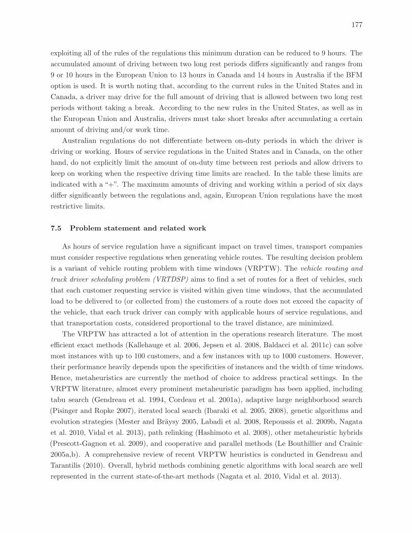
177

exploiting all of the rules of the regulations this minimum duration can be reduced to 9 hours. The

accumulated amount of driving between two long rest periods differs significantly and ranges from

9 or 10 hours in the European Union to 13 hours in Canada and 14 hours in Australia if the BFM

option is used. It is worth noting that, according to the current rules in the United States and in

Canada, a driver may drive for the full amount of driving that is allowed between two long rest

periods without taking a break. According to the new rules in the United States, as well as in

the European Union and Australia, drivers must take short breaks after accumulating a certain

amount of driving and/or work time.

Australian regulations do not differentiate between on-duty periods in which the driver is

driving or working. Hours of service regulations in the United States and in Canada, on the other

hand, do not explicitly limit the amount of on-duty time between rest periods and allow drivers to

keep on working when the respective driving time limits are reached. In the table these limits are

indicated with a “+”. The maximum amounts of driving and working within a period of six days

differ significantly between the regulations and, again, European Union regulations have the most

restrictive limits.

7.5 Problem statement and related work

As hours of service regulation have a significant impact on travel times, transport companies

must consider respective regulations when generating vehicle routes. The resulting decision problem

is a variant of vehicle routing problem with time windows (VRPTW). The vehicle routing and

truck driver scheduling problem (VRTDSP) aims to find a set of routes for a fleet of vehicles, such

that each customer requesting service is visited within given time windows, that the accumulated

load to be delivered to (or collected from) the customers of a route does not exceed the capacity of

the vehicle, that each truck driver can comply with applicable hours of service regulations, and

that transportation costs, considered proportional to the travel distance, are minimized.

The VRPTW has attracted a lot of attention in the operations research literature. The most

efficient exact methods (Kallehauge et al. 2006, Jepsen et al. 2008, Baldacci et al. 2011c) can solve

most instances with up to 100 customers, and a few instances with up to 1000 customers. However,

their performance heavily depends upon the specificities of instances and the width of time windows.

Hence, metaheuristics are currently the method of choice to address practical settings. In the

VRPTW literature, almost every prominent metaheuristic paradigm has been applied, including

tabu search (Gendreau et al. 1994, Cordeau et al. 2001a), adaptive large neighborhood search

(Pisinger and Ropke 2007), iterated local search (Ibaraki et al. 2005, 2008), genetic algorithms and

evolution strategies (Mester and Braysy 2005, Labadi et al. 2008, Repoussis et al. 2009b, Nagata

et al. 2010, Vidal et al. 2013), path relinking (Hashimoto et al. 2008), other metaheuristic hybrids

(Prescott-Gagnon et al. 2009), and cooperative and parallel methods (Le Bouthillier and Crainic

2005a,b). A comprehensive review of recent VRPTW heuristics is conducted in Gendreau and

Tarantilis (2010). Overall, hybrid methods combining genetic algorithms with local search are well

represented in the current state-of-the-art methods (Nagata et al. 2010, Vidal et al. 2013).

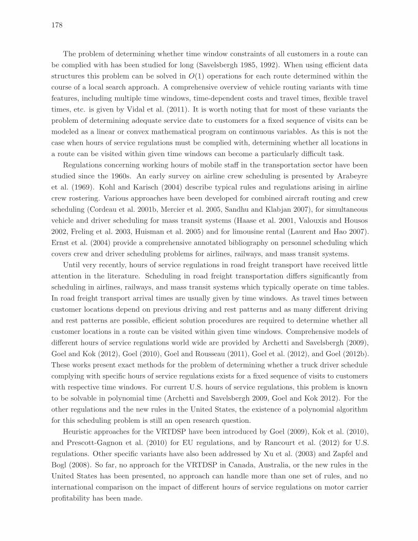
178

The problem of determining whether time window constraints of all customers in a route can

be complied with has been studied for long (Savelsbergh 1985, 1992). When using efficient data

structures this problem can be solved in O(1) operations for each route determined within the

course of a local search approach. A comprehensive overview of vehicle routing variants with time

features, including multiple time windows, time-dependent costs and travel times, flexible travel

times, etc. is given by Vidal et al. (2011). It is worth noting that for most of these variants the

problem of determining adequate service date to customers for a fixed sequence of visits can be

modeled as a linear or convex mathematical program on continuous variables. As this is not the

case when hours of service regulations must be complied with, determining whether all locations in

a route can be visited within given time windows can become a particularly difficult task.

Regulations concerning working hours of mobile staff in the transportation sector have been

studied since the 1960s. An early survey on airline crew scheduling is presented by Arabeyre

et al. (1969). Kohl and Karisch (2004) describe typical rules and regulations arising in airline

crew rostering. Various approaches have been developed for combined aircraft routing and crew

scheduling (Cordeau et al. 2001b, Mercier et al. 2005, Sandhu and Klabjan 2007), for simultaneous

vehicle and driver scheduling for mass transit systems (Haase et al. 2001, Valouxis and Housos

2002, Freling et al. 2003, Huisman et al. 2005) and for limousine rental (Laurent and Hao 2007).

Ernst et al. (2004) provide a comprehensive annotated bibliography on personnel scheduling which

covers crew and driver scheduling problems for airlines, railways, and mass transit systems.

Until very recently, hours of service regulations in road freight transport have received little

attention in the literature. Scheduling in road freight transportation differs significantly from

scheduling in airlines, railways, and mass transit systems which typically operate on time tables.

In road freight transport arrival times are usually given by time windows. As travel times between

customer locations depend on previous driving and rest patterns and as many different driving

and rest patterns are possible, efficient solution procedures are required to determine whether all

customer locations in a route can be visited within given time windows. Comprehensive models of

different hours of service regulations world wide are provided by Archetti and Savelsbergh (2009),

Goel and Kok (2012), Goel (2010), Goel and Rousseau (2011), Goel et al. (2012), and Goel (2012b).

These works present exact methods for the problem of determining whether a truck driver schedule

complying with specific hours of service regulations exists for a fixed sequence of visits to customers

with respective time windows. For current U.S. hours of service regulations, this problem is known

to be solvable in polynomial time (Archetti and Savelsbergh 2009, Goel and Kok 2012). For the

other regulations and the new rules in the United States, the existence of a polynomial algorithm

for this scheduling problem is still an open research question.

Heuristic approaches for the VRTDSP have been introduced by Goel (2009), Kok et al. (2010),

and Prescott-Gagnon et al. (2010) for EU regulations, and by Rancourt et al. (2012) for U.S.

regulations. Other specific variants have also been addressed by Xu et al. (2003) and Zapfel and

Bogl (2008). So far, no approach for the VRTDSP in Canada, Australia, or the new rules in the

United States has been presented, no approach can handle more than one set of rules, and no

international comparison on the impact of different hours of service regulations on motor carrier

profitability has been made.

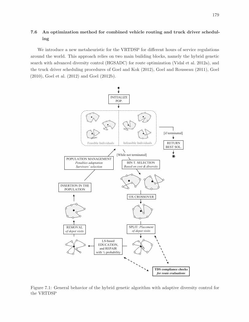
179

7.6 An optimization method for combined vehicle routing and truck driver schedul-

ing

We introduce a new metaheuristic for the VRTDSP for different hours of service regulations

around the world. This approach relies on two main building blocks, namely the hybrid genetic

search with advanced diversity control (HGSADC) for route optimization (Vidal et al. 2012a), and

the truck driver scheduling procedures of Goel and Kok (2012), Goel and Rousseau (2011), Goel

(2010), Goel et al. (2012) and Goel (2012b).

00

Figure 7.1: General behavior of the hybrid genetic algorithm with adaptive diversity control forthe VRTDSP

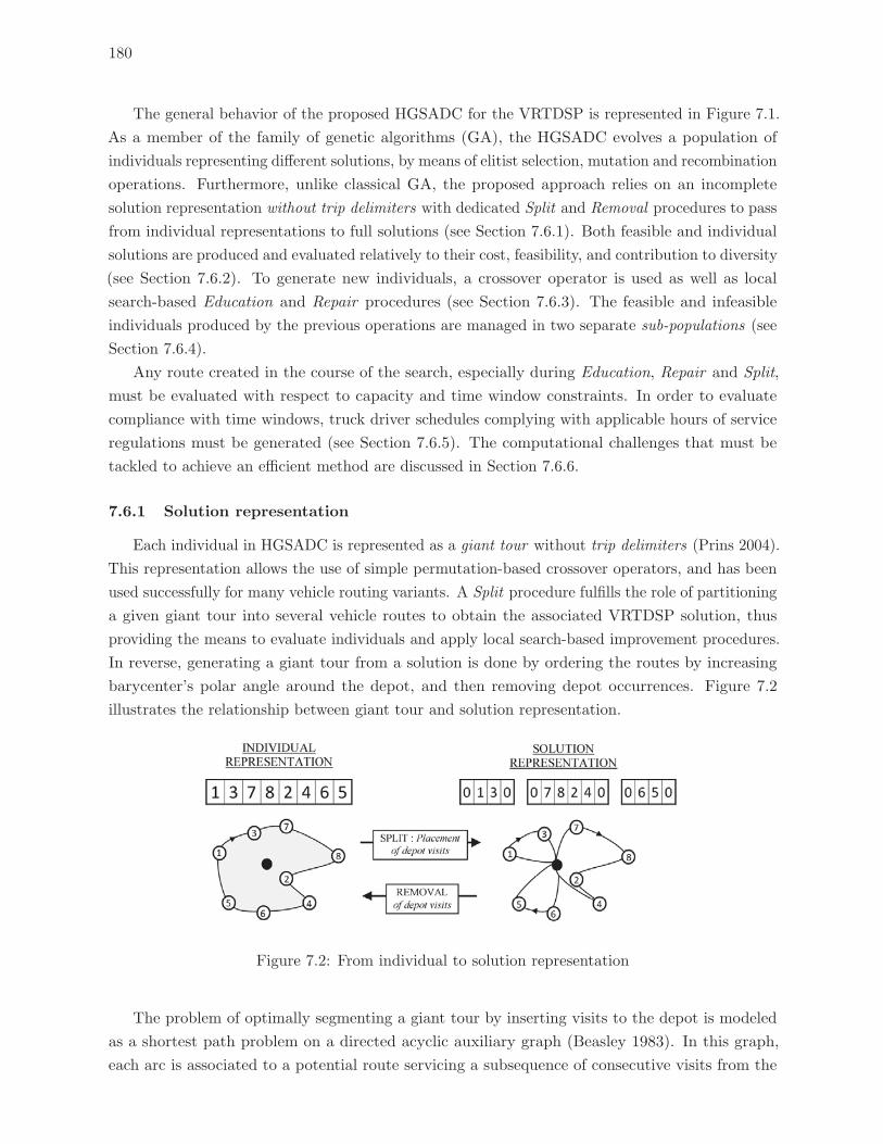
180

The general behavior of the proposed HGSADC for the VRTDSP is represented in Figure 7.1.

As a member of the family of genetic algorithms (GA), the HGSADC evolves a population of

individuals representing different solutions, by means of elitist selection, mutation and recombination

operations. Furthermore, unlike classical GA, the proposed approach relies on an incomplete

solution representation without trip delimiters with dedicated Split and Removal procedures to pass

from individual representations to full solutions (see Section 7.6.1). Both feasible and individual

solutions are produced and evaluated relatively to their cost, feasibility, and contribution to diversity

(see Section 7.6.2). To generate new individuals, a crossover operator is used as well as local

search-based Education and Repair procedures (see Section 7.6.3). The feasible and infeasible

individuals produced by the previous operations are managed in two separate sub-populations (see

Section 7.6.4).

Any route created in the course of the search, especially during Education, Repair and Split,

must be evaluated with respect to capacity and time window constraints. In order to evaluate

compliance with time windows, truck driver schedules complying with applicable hours of service

regulations must be generated (see Section 7.6.5). The computational challenges that must be

tackled to achieve an efficient method are discussed in Section 7.6.6.


Each individual in HGSADC is represented as a giant tour without trip delimiters (Prins 2004).

This representation allows the use of simple permutation-based crossover operators, and has been

used successfully for many vehicle routing variants. A Split procedure fulfills the role of partitioning

a given giant tour into several vehicle routes to obtain the associated VRTDSP solution, thus

providing the means to evaluate individuals and apply local search-based improvement procedures.

In reverse, generating a giant tour from a solution is done by ordering the routes by increasing

barycenter’s polar angle around the depot, and then removing depot occurrences. Figure 7.2

illustrates the relationship between giant tour and solution representation.

Figure 7.2: From individual to solution representation

The problem of optimally segmenting a giant tour by inserting visits to the depot is modeled

as a shortest path problem on a directed acyclic auxiliary graph (Beasley 1983). In this graph,

each arc is associated to a potential route servicing a subsequence of consecutive visits from the

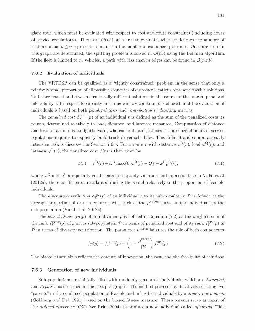
181

giant tour, which must be evaluated with respect to cost and route constraints (including hours

of service regulations). There are O(nb) such arcs to evaluate, where n denotes the number of

customers and b ≤ n represents a bound on the number of customers per route. Once arc costs in

this graph are determined, the splitting problem is solved in O(nb) using the Bellman algorithm.

If the fleet is limited to m vehicles, a path with less than m edges can be found in O(mnb).


The VRTDSP can be qualified as a “tightly constrained” problem in the sense that only a

relatively small proportion of all possible sequences of customer locations represent feasible solutions.

To better transition between structurally different solutions in the course of the search, penalized

infeasibility with respect to capacity and time window constraints is allowed, and the evaluation of

individuals is based on both penalized costs and contribution to diversity metrics.

The penalized cost φcostP (p) of an individual p is defined as the sum of the penalized costs its

routes, determined relatively to load, distance, and lateness measures. Computation of distance

and load on a route is straightforward, whereas evaluating lateness in presence of hours of service

regulations requires to explicitly build truck driver schedules. This difficult and computationally

intensive task is discussed in Section 7.6.5. For a route r with distance ϕD(r), load ϕQ(r), and

lateness ϕL(r), the penalized cost φ(r) is then given by

φ(r) = ϕD(r) + ωQmax{0, ϕQ(r)−Q}+ ωLϕL(r), (7.1)

where ωQ and ωL are penalty coefficients for capacity violation and lateness. Like in Vidal et al.

(2012a), these coefficients are adapted during the search relatively to the proportion of feasible

individuals.

The diversity contribution φdivP (p) of an individual p to its sub-population P is defined as the

average proportion of arcs in common with each of the μclose most similar individuals in the

sub-population (Vidal et al. 2012a).

The biased fitness fP(p) of an individual p is defined in Equation (7.2) as the weighted sum of

the rank fcostP (p) of p in its sub-population P in terms of penalized cost and of its rank fdivP (p) in

P in terms of diversity contribution. The parameter μelite balances the role of both components.

fP(p) = fcostP (p) +

(1− μelite

|P|

)fdivP (p) (7.2)

The biased fitness thus reflects the amount of innovation, the cost, and the feasibility of solutions.

7.6.3 Generation of new individuals

Sub-populations are initially filled with randomly generated individuals, which are Educated,

and Repaired as described in the next paragraphs. The method proceeds by iteratively selecting two

“parents” in the combined population of feasible and infeasible individuals by a binary tournament

(Goldberg and Deb 1991) based on the biased fitness measure. These parents serve as input of

the ordered crossover (OX) (see Prins 2004) to produce a new individual called offspring. This

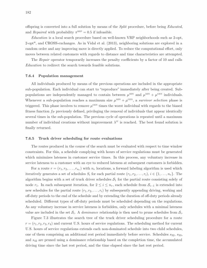
182

offspring is converted into a full solution by means of the Split procedure, before being Educated,

and Repaired with probability πrep = 0.5 if infeasible.

Education is a local search procedure based on well-known VRP neighborhoods such as 2-opt,

2-opt*, and CROSS-exchanges. As in Vidal et al. (2013), neighboring solutions are explored in a

random order and any improving move is directly applied. To reduce the computational effort, only

moves between related customers with regards to distance and time characteristics are attempted.

The Repair operator temporarily increases the penalty coefficients by a factor of 10 and calls

Education to redirect the search towards feasible solutions.

7.6.4 Population management

All individuals produced by means of the previous operations are included in the appropriate

sub-population. Each individual can start to “reproduce” immediately after being created. Sub-

populations are independently managed to contain between μmin and μmin + μgen individuals.

Whenever a sub-population reaches a maximum size μmin + μgen, a survivor selection phase is

triggered. This phase involves to remove μgen times the worst individual with regards to the biased

fitness function fP previously defined, privileging the removal of individuals that appear identically

several times in the sub-population. The previous cycle of operations is repeated until a maximum

number of individual creations without improvement λit is reached. The best found solution is

finally returned.

7.6.5 Truck driver scheduling for route evaluations

The routes produced in the course of the search must be evaluated with respect to time window

constraints. For this, a schedule complying with hours of service regulations must be generated

which minimizes lateness in customer service times. In this process, any voluntary increase in

service lateness to a customer with an eye to reduced lateness at subsequent customers is forbidden.

For a route r = (r1, r2, . . . , rnr) with nr locations, a forward labeling algorithm is used which

iteratively generates a set of schedules Si for each partial route (r1, r2, . . . , ri), i ∈ {1, . . . , nr}. Thealgorithm begins with a set of truck driver schedules S1 for the partial route consisting solely of

node r1. In each subsequent iteration, for 2 ≤ i ≤ nr, each schedule from Si−1 is extended into

new schedules for the partial route (r1, r2, . . . , ri) by subsequently appending driving, working and

off-duty periods to the end of the schedule and by extending the duration of off-duty periods already

scheduled. Different types of off-duty periods must be scheduled depending on the regulations.

As any voluntary increase in service lateness is forbidden, only schedules with a minimal lateness

value are included in the set Si. A dominance relationship is then used to prune schedules from Si.

Figure 7.3 illustrates the search tree of the truck driver scheduling procedure for a route

r = (r1, r2, r3, r4) and current U.S. hours of service regulations. The scheduling method for current

U.S. hours of service regulations extends each non-dominated schedule into two child schedules,

one of them comprising an additional rest period immediately before service. Schedules s32, s33,

and s42 are pruned using a dominance relationship based on the completion time, the accumulated

driving time since the last rest period, and the time elapsed since the last rest period.

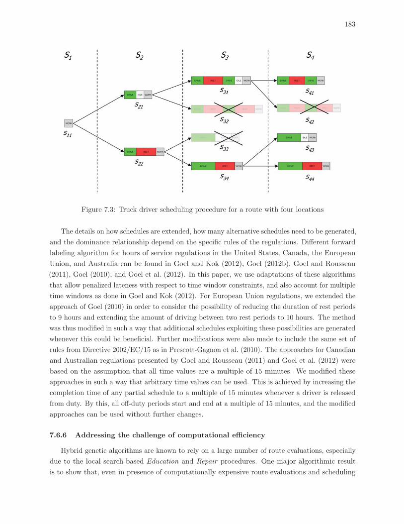
183

Figure 7.3: Truck driver scheduling procedure for a route with four locations

The details on how schedules are extended, how many alternative schedules need to be generated,

and the dominance relationship depend on the specific rules of the regulations. Different forward

labeling algorithm for hours of service regulations in the United States, Canada, the European

Union, and Australia can be found in Goel and Kok (2012), Goel (2012b), Goel and Rousseau

(2011), Goel (2010), and Goel et al. (2012). In this paper, we use adaptations of these algorithms

that allow penalized lateness with respect to time window constraints, and also account for multiple

time windows as done in Goel and Kok (2012). For European Union regulations, we extended the

approach of Goel (2010) in order to consider the possibility of reducing the duration of rest periods

to 9 hours and extending the amount of driving between two rest periods to 10 hours. The method

was thus modified in such a way that additional schedules exploiting these possibilities are generated

whenever this could be beneficial. Further modifications were also made to include the same set of

rules from Directive 2002/EC/15 as in Prescott-Gagnon et al. (2010). The approaches for Canadian

and Australian regulations presented by Goel and Rousseau (2011) and Goel et al. (2012) were

based on the assumption that all time values are a multiple of 15 minutes. We modified these

approaches in such a way that arbitrary time values can be used. This is achieved by increasing the

completion time of any partial schedule to a multiple of 15 minutes whenever a driver is released

from duty. By this, all off-duty periods start and end at a multiple of 15 minutes, and the modified

approaches can be used without further changes.

7.6.6 Addressing the challenge of computational efficiency

Hybrid genetic algorithms are known to rely on a large number of route evaluations, especially

due to the local search-based Education and Repair procedures. One major algorithmic result

is to show that, even in presence of computationally expensive route evaluations and scheduling

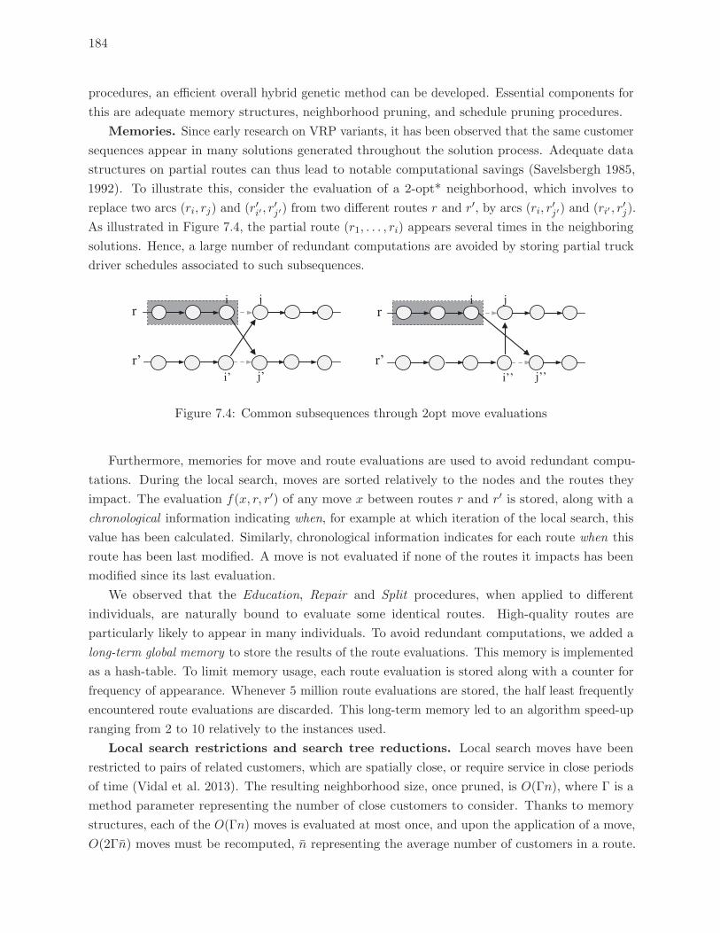
184

procedures, an efficient overall hybrid genetic method can be developed. Essential components for

this are adequate memory structures, neighborhood pruning, and schedule pruning procedures.

Memories. Since early research on VRP variants, it has been observed that the same customer

sequences appear in many solutions generated throughout the solution process. Adequate data

structures on partial routes can thus lead to notable computational savings (Savelsbergh 1985,

1992). To illustrate this, consider the evaluation of a 2-opt* neighborhood, which involves to

replace two arcs (ri, rj) and (r′i′ , r′j′) from two different routes r and r′, by arcs (ri, r

′j′) and (ri′ , r

′j).

As illustrated in Figure 7.4, the partial route (r1, . . . , ri) appears several times in the neighboring

solutions. Hence, a large number of redundant computations are avoided by storing partial truck

driver schedules associated to such subsequences.

v’’

r

r’

j i

i’ j’ v’’

r

r’

j i

i’’ j’’

Figure 7.4: Common subsequences through 2opt move evaluations

Furthermore, memories for move and route evaluations are used to avoid redundant compu-

tations. During the local search, moves are sorted relatively to the nodes and the routes they

impact. The evaluation f(x, r, r′) of any move x between routes r and r′ is stored, along with a

chronological information indicating when, for example at which iteration of the local search, this

value has been calculated. Similarly, chronological information indicates for each route when this

route has been last modified. A move is not evaluated if none of the routes it impacts has been

modified since its last evaluation.

We observed that the Education, Repair and Split procedures, when applied to different

individuals, are naturally bound to evaluate some identical routes. High-quality routes are

particularly likely to appear in many individuals. To avoid redundant computations, we added a

long-term global memory to store the results of the route evaluations. This memory is implemented

as a hash-table. To limit memory usage, each route evaluation is stored along with a counter for

frequency of appearance. Whenever 5 million route evaluations are stored, the half least frequently

encountered route evaluations are discarded. This long-term memory led to an algorithm speed-up

ranging from 2 to 10 relatively to the instances used.

Local search restrictions and search tree reductions. Local search moves have been

restricted to pairs of related customers, which are spatially close, or require service in close periods

of time (Vidal et al. 2013). The resulting neighborhood size, once pruned, is O(Γn), where Γ is a

method parameter representing the number of close customers to consider. Thanks to memory

structures, each of the O(Γn) moves is evaluated at most once, and upon the application of a move,

O(2Γn) moves must be recomputed, n representing the average number of customers in a route.

185

The total number of route evaluations during a local search is thus O(Γn + αimp(n)Γn), where

αimp(n) is the number of moves before reaching a local optimum.

Fast route evaluations are crucial for the overall running time of the HGSADC. As the search

tree generated during route evaluations may grow very large for some of the regulations, various

techniques for limiting its size have been applied. For Canadian and Australian regulations, Goel

and Rousseau (2011) and Goel et al. (2012) presented heuristic forward labeling methods which

only generate a small subset of all possible partial schedules, thus reducing the size of the search

tree significantly. In the European Union, the possibility of reducing the duration of rest periods

and extending the amount of driving time between rest periods results in a dramatic increase in

the size of the search tree. To speed up route evaluations in this case, the size of the search tree

has been reduced using a combination of two techniques. First, we use a heuristic dominance

relationship which does not take into account the number of reduced rests and extended driving

periods. Second, the number of different schedules in Si at each iteration i of the truck driver

scheduling method is limited to at most Γ′ = 5. To do so, the set of non-dominated partial schedules

Si is ordered by completion time, and only the schedules at positions 1+ �(j− 1)(|Si|− 1)/(Γ′− 1)�for all 1 ≤ j ≤ Γ′ are kept.

All these elements lead to rapid Split and local search-based Education procedures for the

VRTDSP, and thus enable to efficiently apply the HGSADC framework to this difficult problem.

7.7 Computational experiments

Extensive computational experiments have been conducted to evaluate the performance of the

proposed algorithm, and to assess the impact of different hours of service regulations world wide.

These experiments are based on the 56 benchmark instances for the VRTDSP proposed by Goel

(2009), which are derived from the VRPTW benchmarks of Solomon (1987). The instances are

grouped into six classes. In classes R1 and R2 customers are randomly distributed in a square

region. In classes C1 and C2 customers are clustered, and in classes RC1 and RC2 the customer

distribution is mixed. In all instances, 100 customers with a demand of at most 50 units must be

served. In the R1, C1, and RC1 classes the capacity of each vehicle is 200 units, in the R2 and

RC2 classes the capacity of each vehicle is 1000 units, and in the C2 class the capacity of each

vehicle is 700 units. The average size of time windows per instance ranges from less than 7 hours

to more than 107 hours. The service time at every customer is set to one hour. The planning

horizon is 144 hours and the maximum required driving time (without compulsory breaks and

rests) to go from one point in the square region to another is approximately one day.

To demonstrate the performance of the proposed method, the solutions obtained by HGSADC

on these original instances were compared with the solutions of the best current methods. To

assess the impact of different hours of service regulations world wide, we also derived a modified

instance set to improve realism. As time window requirements of customers are usually tied to

business hours and most customers cannot be visited in the night, we removed the time between

8.00 PM and 8.00 AM from time windows in the original VRTDSP instances. However, to maintain

feasibility of the instances, the night time of time windows with a duration of 24 hours or less

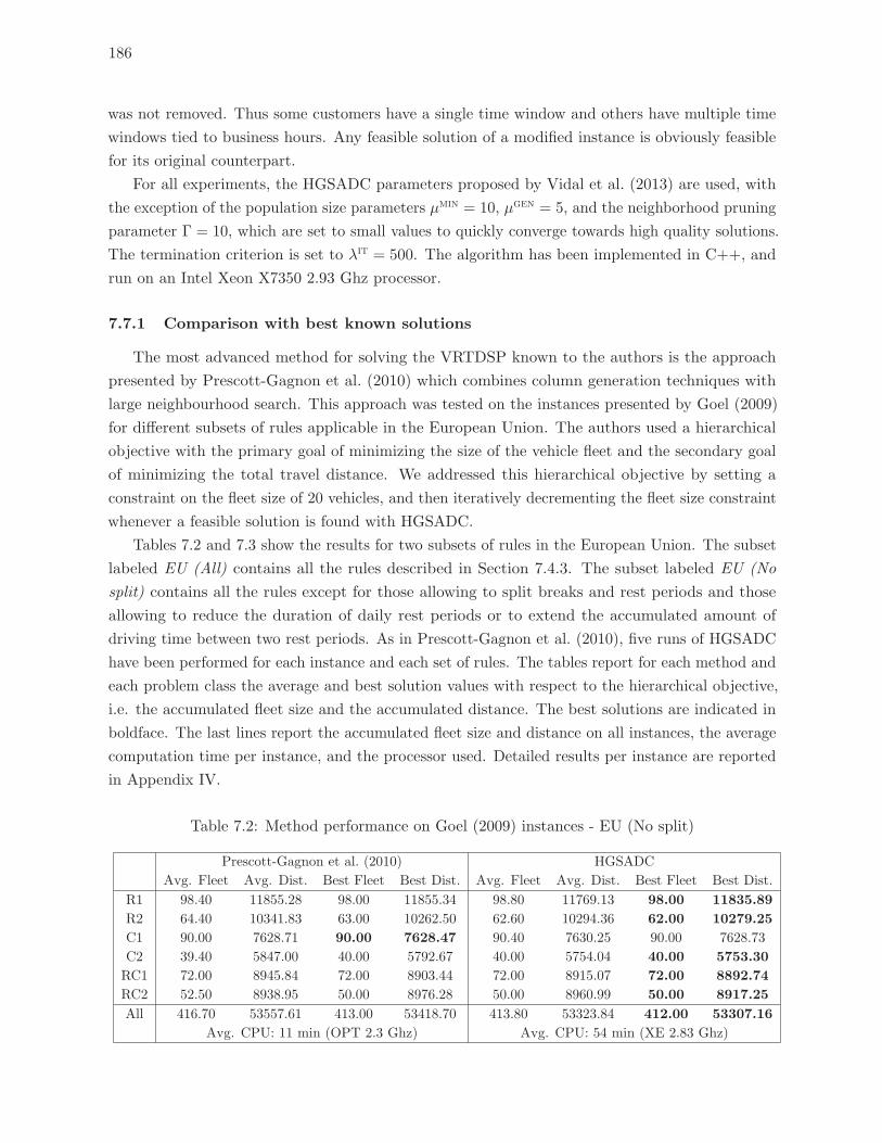
186

was not removed. Thus some customers have a single time window and others have multiple time

windows tied to business hours. Any feasible solution of a modified instance is obviously feasible

for its original counterpart.

For all experiments, the HGSADC parameters proposed by Vidal et al. (2013) are used, with

the exception of the population size parameters μmin = 10, μgen = 5, and the neighborhood pruning

parameter Γ = 10, which are set to small values to quickly converge towards high quality solutions.

The termination criterion is set to λit = 500. The algorithm has been implemented in C++, and

run on an Intel Xeon X7350 2.93 Ghz processor.

7.7.1 Comparison with best known solutions

The most advanced method for solving the VRTDSP known to the authors is the approach

presented by Prescott-Gagnon et al. (2010) which combines column generation techniques with

large neighbourhood search. This approach was tested on the instances presented by Goel (2009)

for different subsets of rules applicable in the European Union. The authors used a hierarchical

objective with the primary goal of minimizing the size of the vehicle fleet and the secondary goal

of minimizing the total travel distance. We addressed this hierarchical objective by setting a

constraint on the fleet size of 20 vehicles, and then iteratively decrementing the fleet size constraint

whenever a feasible solution is found with HGSADC.

Tables 7.2 and 7.3 show the results for two subsets of rules in the European Union. The subset

labeled EU (All) contains all the rules described in Section 7.4.3. The subset labeled EU (No

split) contains all the rules except for those allowing to split breaks and rest periods and those

allowing to reduce the duration of daily rest periods or to extend the accumulated amount of

driving time between two rest periods. As in Prescott-Gagnon et al. (2010), five runs of HGSADC

have been performed for each instance and each set of rules. The tables report for each method and

each problem class the average and best solution values with respect to the hierarchical objective,

i.e. the accumulated fleet size and the accumulated distance. The best solutions are indicated in

boldface. The last lines report the accumulated fleet size and distance on all instances, the average

computation time per instance, and the processor used. Detailed results per instance are reported

in Appendix IV.

Table 7.2: Method performance on Goel (2009) instances - EU (No split)

Prescott-Gagnon et al. (2010) HGSADC

Avg. Fleet Avg. Dist. Best Fleet Best Dist. Avg. Fleet Avg. Dist. Best Fleet Best Dist.

R1 98.40 11855.28 98.00 11855.34 98.80 11769.13 98.00 11835.89

R2 64.40 10341.83 63.00 10262.50 62.60 10294.36 62.00 10279.25

C1 90.00 7628.71 90.00 7628.47 90.40 7630.25 90.00 7628.73

C2 39.40 5847.00 40.00 5792.67 40.00 5754.04 40.00 5753.30

RC1 72.00 8945.84 72.00 8903.44 72.00 8915.07 72.00 8892.74

RC2 52.50 8938.95 50.00 8976.28 50.00 8960.99 50.00 8917.25

All 416.70 53557.61 413.00 53418.70 413.80 53323.84 412.00 53307.16

Avg. CPU: 11 min (OPT 2.3 Ghz) Avg. CPU: 54 min (XE 2.83 Ghz)

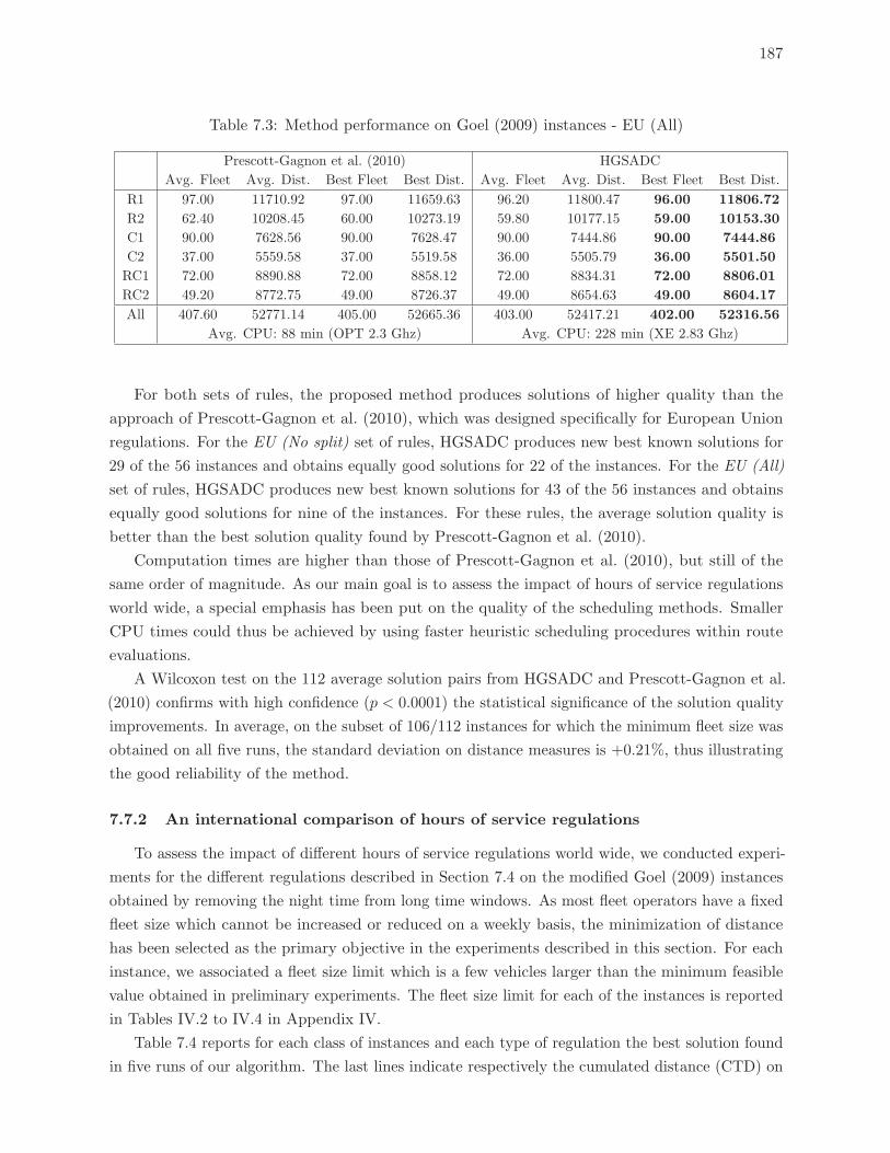
187

Table 7.3: Method performance on Goel (2009) instances - EU (All)

Prescott-Gagnon et al. (2010) HGSADC

Avg. Fleet Avg. Dist. Best Fleet Best Dist. Avg. Fleet Avg. Dist. Best Fleet Best Dist.

R1 97.00 11710.92 97.00 11659.63 96.20 11800.47 96.00 11806.72

R2 62.40 10208.45 60.00 10273.19 59.80 10177.15 59.00 10153.30

C1 90.00 7628.56 90.00 7628.47 90.00 7444.86 90.00 7444.86

C2 37.00 5559.58 37.00 5519.58 36.00 5505.79 36.00 5501.50

RC1 72.00 8890.88 72.00 8858.12 72.00 8834.31 72.00 8806.01

RC2 49.20 8772.75 49.00 8726.37 49.00 8654.63 49.00 8604.17

All 407.60 52771.14 405.00 52665.36 403.00 52417.21 402.00 52316.56

Avg. CPU: 88 min (OPT 2.3 Ghz) Avg. CPU: 228 min (XE 2.83 Ghz)

For both sets of rules, the proposed method produces solutions of higher quality than the

approach of Prescott-Gagnon et al. (2010), which was designed specifically for European Union

regulations. For the EU (No split) set of rules, HGSADC produces new best known solutions for

29 of the 56 instances and obtains equally good solutions for 22 of the instances. For the EU (All)

set of rules, HGSADC produces new best known solutions for 43 of the 56 instances and obtains

equally good solutions for nine of the instances. For these rules, the average solution quality is

better than the best solution quality found by Prescott-Gagnon et al. (2010).

Computation times are higher than those of Prescott-Gagnon et al. (2010), but still of the

same order of magnitude. As our main goal is to assess the impact of hours of service regulations

world wide, a special emphasis has been put on the quality of the scheduling methods. Smaller

CPU times could thus be achieved by using faster heuristic scheduling procedures within route

evaluations.

A Wilcoxon test on the 112 average solution pairs from HGSADC and Prescott-Gagnon et al.

(2010) confirms with high confidence (p < 0.0001) the statistical significance of the solution quality

improvements. In average, on the subset of 106/112 instances for which the minimum fleet size was

obtained on all five runs, the standard deviation on distance measures is +0.21%, thus illustrating

the good reliability of the method.

7.7.2 An international comparison of hours of service regulations

To assess the impact of different hours of service regulations world wide, we conducted experi-

ments for the different regulations described in Section 7.4 on the modified Goel (2009) instances

obtained by removing the night time from long time windows. As most fleet operators have a fixed

fleet size which cannot be increased or reduced on a weekly basis, the minimization of distance

has been selected as the primary objective in the experiments described in this section. For each

instance, we associated a fleet size limit which is a few vehicles larger than the minimum feasible

value obtained in preliminary experiments. The fleet size limit for each of the instances is reported

in Tables IV.2 to IV.4 in Appendix IV.

Table 7.4 reports for each class of instances and each type of regulation the best solution found

in five runs of our algorithm. The last lines indicate respectively the cumulated distance (CTD) on

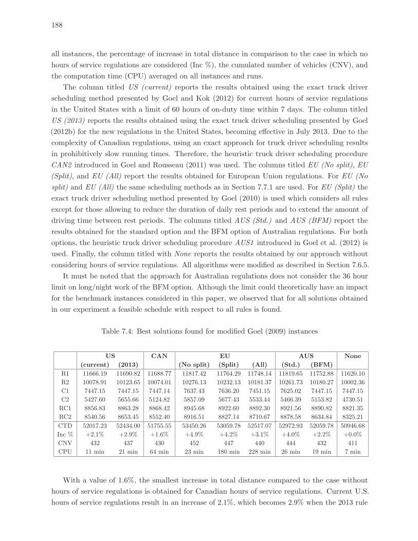
188

all instances, the percentage of increase in total distance in comparison to the case in which no

hours of service regulations are considered (Inc %), the cumulated number of vehicles (CNV), and

the computation time (CPU) averaged on all instances and runs.

The column titled US (current) reports the results obtained using the exact truck driver

scheduling method presented by Goel and Kok (2012) for current hours of service regulations

in the United States with a limit of 60 hours of on-duty time within 7 days. The column titled

US (2013) reports the results obtained using the exact truck driver scheduling presented by Goel

(2012b) for the new regulations in the United States, becoming effective in July 2013. Due to the

complexity of Canadian regulations, using an exact approach for truck driver scheduling results

in prohibitively slow running times. Therefore, the heuristic truck driver scheduling procedure

CAN2 introduced in Goel and Rousseau (2011) was used. The columns titled EU (No split), EU

(Split), and EU (All) report the results obtained for European Union regulations. For EU (No

split) and EU (All) the same scheduling methods as in Section 7.7.1 are used. For EU (Split) the

exact truck driver scheduling method presented by Goel (2010) is used which considers all rules

except for those allowing to reduce the duration of daily rest periods and to extend the amount of

driving time between rest periods. The columns titled AUS (Std.) and AUS (BFM) report the

results obtained for the standard option and the BFM option of Australian regulations. For both

options, the heuristic truck driver scheduling procedure AUS1 introduced in Goel et al. (2012) is

used. Finally, the column titled with None reports the results obtained by our approach without

considering hours of service regulations. All algorithms were modified as described in Section 7.6.5.

It must be noted that the approach for Australian regulations does not consider the 36 hour

limit on long/night work of the BFM option. Although the limit could theoretically have an impact

for the benchmark instances considered in this paper, we observed that for all solutions obtained

in our experiment a feasible schedule with respect to all rules is found.

Table 7.4: Best solutions found for modified Goel (2009) instances

US CAN EU AUS None

(current) (2013) (No split) (Split) (All) (Std.) (BFM)

R1 11666.19 11690.82 11688.77 11817.42 11764.29 11748.14 11819.65 11752.88 11620.10

R2 10078.91 10123.65 10074.01 10276.13 10232.13 10181.37 10261.73 10180.27 10002.36

C1 7447.15 7447.15 7447.14 7637.43 7636.20 7451.15 7625.02 7447.15 7447.15

C2 5427.60 5655.66 5124.82 5857.09 5677.43 5533.44 5466.39 5153.82 4730.51

RC1 8856.83 8863.28 8868.42 8945.68 8922.60 8892.30 8921.56 8890.82 8821.35

RC2 8540.56 8653.45 8552.40 8916.51 8827.14 8710.67 8878.58 8634.84 8325.21

CTD 52017.23 52434.00 51755.55 53450.26 53059.78 52517.07 52972.93 52059.78 50946.68

Inc % +2.1% +2.9% +1.6% +4.9% +4.2% +3.1% +4.0% +2.2% +0.0%

CNV 432 437 430 452 447 440 444 432 411

CPU 11 min 21 min 64 min 23 min 180 min 228 min 26 min 19 min 7 min

With a value of 1.6%, the smallest increase in total distance compared to the case without

hours of service regulations is obtained for Canadian hours of service regulations. Current U.S.

hours of service regulations result in an increase of 2.1%, which becomes 2.9% when the 2013 rule

189

change is enforced. In the European Union a similar increase of 3.1% is obtained when exploiting

all rules of the regulations. The regulations give a strong incentive of exploiting the possibilities

of reducing the duration of rest periods to 9 hours and extending the driving time between rest

periods to 10 hours. Without these optional rules, the total distance increases by 4.2% if the

possibility of taking break and rest periods in two parts is exploited and by 4.9% otherwise. One

might think that the intention of European lawmakers was to give motor carriers the possibility

of reacting on unforeseeable traffic conditions by allowing to reduce the duration of rest period

and to extend the driving time between rest periods on some days of the week. However, if this

was the case, these optional rules are unlikely to fulfill this purpose as economic pressure can force

motor carriers to exploit these options on a regular basis and not only in the case of unexpected

delays. Australian motor carriers without accreditation have with 4.0% the highest increase in

total distance. As travel distances only increase by 2.2% when using the BFM option, there is a

strong incentive for Australian motor carriers to be accredited for the BFM option.

To further analyze the impact of hours of service regulations, we determined for each of

the routes of the best solutions a schedule with minimal duration using the iterative dynamic

programming approach of Goel (2012a). Table 7.5 reports for each set of solutions the cumulated

schedule duration (csd), the average percentage of on-duty time with respect to the schedule

duration (od), and the average amount of on-duty time between two long rest periods (obr). Time

values are reported in hours and minutes (hh:mm).

As illustrated in Table 7.5, schedule characteristics appear to be consistent with the properties

of the regulations. The impact of hours of service regulations on the total schedule duration,

average on-duty ratio, and duty time between rests periods is evidenced. Exploiting the optional

rules in the European Union leads to reduced schedule durations and to increased on-duty ratios

and on-duty time between rests. Similar observations can be made when comparing AUS (Std.)

with AUS (BFM) regulations, and US (2013) with US (current). Overall, the highest on-duty ratio

(45.98%) is achieved for Canadian regulations followed by the current regulations in the United

States (45.01%). On-duty ratios for the new regulations in the United States (43.41%), European

Union regulations (43.19%) and the rules of the BFM option in Australia (43.02%) are comparable.

It is also worth noting that hours of service regulations do not have a high impact on distances

for the C1 class. Analyzing the schedules, we observe that only one third of the time spent by

the drivers in the solutions for the C1 class is on-duty time. Consequently, there is plenty of time

available that potentially can be used for taking breaks and rest periods. For the C2 class, on the

other hand, we obtain a high on-duty ratio of 58.98% and an average amount of on-duty time per

vehicle above 72 hours when not considering hours of service constraints. As the average amount

of on-duty time exceeds the weekly limits of the regulations and as less time can be used for taking

breaks and rest periods, the impact of hours of service regulations is the highest for the C2 class.

Although the fleet size is not considered in the objective function, fleet sizes differ in the

solutions as a result of minimizing the total distance. The largest increase in fleet size compared to

the case without regulations is obtained for the instances in the C2 class. For most other instances

and most of the regulations, at most one additional vehicle is required. Again, CAN, US (current),

and AUS (BFM) regulations lead to the smallest fleet sizes.

190

Table 7.5: Schedule characteristics

US CAN EU AUS None


R1 csd 7701:17 7781:22 7614:30 8493:44 8226:12 7897:22 8791:03 8203:23 6976:20

od 45.72% 45.31% 46.30% 41.81% 43.04% 44.79% 40.40% 43.13% 50.34%

obr 9:01 8:56 9:04 7:56 8:20 8:46 7:47 8:19

R2 csd 6676:13 6866:41 6654:21 7487:26 7296:31 7051:50 7652:05 7482:32 6423:20

od 46.50% 45.34% 46.64% 41.99% 42.97% 44.31% 41.05% 41.76% 48.10%

obr 9:23 8:59 9:27 8:29 8:33 9:05 8:01 8:09

C1 csd 7110:20 7152:27 6973:48 7572:27 7476:26 7308:34 7404:59 7237:57 7054:48

od 33.55% 33.35% 34.21% 32.01% 32.41% 32.65% 32.70% 32.96% 33.82%

obr 6:42 6:33 6:57 6:11 6:14 6:26 5:17 5:22

C2 csd 4025:31 4645:37 3564:01 4945:59 4875:29 4508:54 4631:22 3814:39 2951:55

od 46.71% 41.45% 51.06% 39.75% 39.59% 42.17% 40.77% 47.86% 58.98%

obr 10:37 9:31 11:10 8:32 9:03 9:32 9:05 10:31

RC1 csd 5022:03 5201:13 5052:00 5784:08 5673:59 5204:16 5816:18 5391:15 4607:28

od 51.09% 49.36% 50.84% 44.67% 45.45% 49.44% 44.34% 47.72% 55.54%

obr 9:42 9:27 9:25 8:17 8:21 9:08 8:03 8:48

RC2 csd 5386:09 5535:45 5347:53 6075:56 5952:10 5541:58 6058:10 5639:57 4753:37

od 46.47% 45.62% 46.85% 42.43% 43.01% 45.77% 42.43% 44.71% 51.74%

obr 9:36 9:26 9:28 8:34 8:41 9:19 8:34 8:56

All csd 5986:56 6197:11 5867:46 6726:37 6583:28 6252:09 6725:39 6294:57 5461:15

od 45.01% 43.41% 45.98% 40.44% 41.08% 43.19% 40.28% 43.02% 49.75%

obr 9:10 8:48 9:15 7:60 8:12 8:43 7:48 8:21

To evaluate the impact of hours of service regulations on road safety we used the fatigue and

risk index calculator available from Health and Safety Executive (2006). This calculator can be

used to estimate the average risk of the occurrence of an accident given a specific work schedule

and is described in Spencer et al. (2006). The risk indices are calculated from separate components

considering the amount of sleep loss that is likely to accumulate throughout the course of a work

schedule, the effect of start time and length of the individual daily shifts, and the break patterns

within these shifts. When using the calculator to assess the risk associated to the solutions obtained

by our method, we interpreted any off-duty period of at least 7 hours duration as the end of a

daily shift and specified the required input accordingly. Table 7.6 shows the average risk indices

obtained for the different hours of service regulations. The indices represent the estimated relative

accident risk and an index of two represents a twice as high average accident risk as an index of

one. We normalized the risk indices with respect to the average risk associated to the EU (No

split) rule set.

For European Union rules we observe that the possibility of taking breaks and rest periods

in two parts and the respective reduction in the minimum duration of rest periods has only little

impact on the average risk. When exploiting all optional rules in the European Union, the risk

is 3% higher compared to the basic set of rules. Looking at the individual risk components it

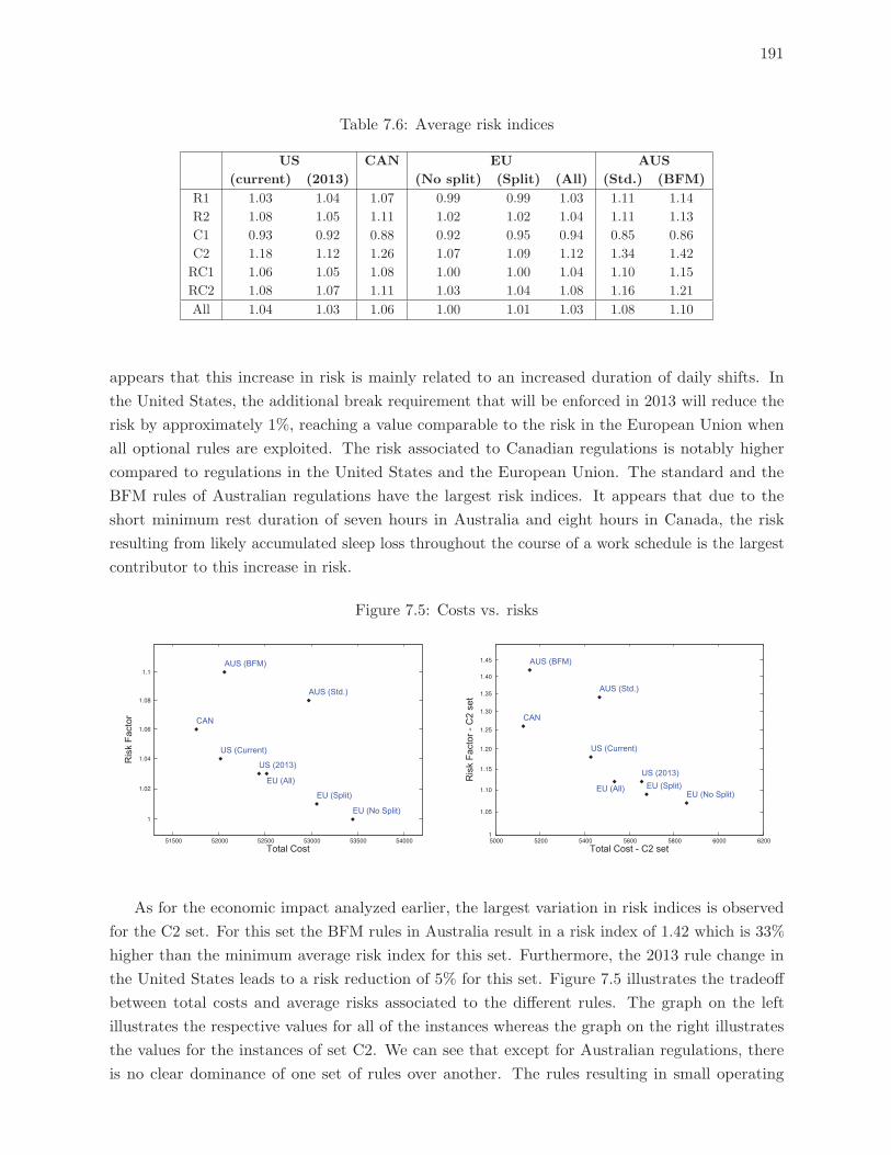
191

Table 7.6: Average risk indices

US CAN EU AUS


R1 1.03 1.04 1.07 0.99 0.99 1.03 1.11 1.14

R2 1.08 1.05 1.11 1.02 1.02 1.04 1.11 1.13

C1 0.93 0.92 0.88 0.92 0.95 0.94 0.85 0.86

C2 1.18 1.12 1.26 1.07 1.09 1.12 1.34 1.42

RC1 1.06 1.05 1.08 1.00 1.00 1.04 1.10 1.15

RC2 1.08 1.07 1.11 1.03 1.04 1.08 1.16 1.21

All 1.04 1.03 1.06 1.00 1.01 1.03 1.08 1.10

appears that this increase in risk is mainly related to an increased duration of daily shifts. In

the United States, the additional break requirement that will be enforced in 2013 will reduce the

risk by approximately 1%, reaching a value comparable to the risk in the European Union when

all optional rules are exploited. The risk associated to Canadian regulations is notably higher

compared to regulations in the United States and the European Union. The standard and the

BFM rules of Australian regulations have the largest risk indices. It appears that due to the

short minimum rest duration of seven hours in Australia and eight hours in Canada, the risk

resulting from likely accumulated sleep loss throughout the course of a work schedule is the largest

contributor to this increase in risk.

Figure 7.5: Costs vs. risks

1

1.02

1.04

1.06

1.08

1.1

51500 52000 52500 53000 53500 54000

Ris

k Fa

ctor

Total Cost

US (Current)

US (2013)

CAN

EU (No Split)

EU (Split)

AUS (Std.)

AUS (BFM)

EU (All)

1

1.05

1.10

1.15

1.20

1.25

1.30

1.35

1.40

1.45

5000 5200 5400 5600 5800 6000 6200

Ris

k Fa

ctor

- C

2 se

t

Total Cost - C2 set

US (Current)

US (2013)

CAN

EU (No Split)EU (Split)

AUS (Std.)

AUS (BFM)

EU (All)

As for the economic impact analyzed earlier, the largest variation in risk indices is observed

for the C2 set. For this set the BFM rules in Australia result in a risk index of 1.42 which is 33%

higher than the minimum average risk index for this set. Furthermore, the 2013 rule change in

the United States leads to a risk reduction of 5% for this set. Figure 7.5 illustrates the tradeoff

between total costs and average risks associated to the different rules. The graph on the left

illustrates the respective values for all of the instances whereas the graph on the right illustrates

the values for the instances of set C2. We can see that except for Australian regulations, there

is no clear dominance of one set of rules over another. The rules resulting in small operating

192

costs are associated with a higher risk index and rules associated with a small risk index have

higher operating costs. Australian rules, however, appear to result in unnecessarily high risk levels

in relation to the economic impact of these regulations. Apparently, the break requirements of

Australian regulations are not sufficient to compensate the negative impact of short rest periods

on associated risk values.

7.8 Conclusions

In this paper we proposed a hybrid genetic search with advanced diversity control (HGSADC)

for solving the combined vehicle routing and truck driver scheduling problem. By combining the

exploration capacities of population-based approaches, the quick improvement abilities of local

search, along with efficient procedures for checking compliance with hours of service regulations, the

proposed approach outperforms all current methods designed for this difficult family of problems.

Our approach is the first which is not specifically designed for a particular set of rules and can be

a valuable tool for transport operators world wide.

We conducted extensive experiments to assess the impact of hours of service regulations in the

United States, Canada, the European Union, and Australia. The results indicate that Australian

regulations have unnecessarily high risk levels with respect to the resulting operating costs. For the

other regulations, average accident risk rates appear to be negatively correlated to operating costs.

European Union rules lead to the highest safety, while in terms of economic efficiency Canadian

regulations are the most competitive. The recent rule change in the United States will bring a

reduction in accident risks. The largest decrease in the associated accident risk of the new rules

can be observed for the set of instances in which the previous rules had the largest associated risk

indices.

Our optimization-based approach can be used to realistically assess the impact of hours of

service regulations from a carrier-centric point of view. The decision whether the economic impact

of hours of service regulations is justified by improved road safety is a question that has to be

discussed and answered by society, policy makers, transport operators, and truck drivers. Our

optimization-based approach to analyze the impact of hours of service regulations can be an

important building block in such a discussion.

Where transport operators can choose among alternative rule sets our approach can bring

important insight concerning the best choice of rules to operate under. Our experiments indicate

that accreditation for the BFM option can bring significant advantages for transport operators

in Australia. Furthermore, we observed that there are strong economic incentives for European

operators to exploit all optional rules of the regulations, in particular, reducing the duration of

rest periods and extending driving times.

CHAPITRE 8

RESOLUTION GENERALISTE DE PROBLEMES DE TOURNEES DE

VEHICULES MULTI-ATTRIBUTS


Ce chapitre propose de nouvelles methodes pour la resolution generaliste d’une grande variete de

problemes de tournees de vehicules multi-attributs. Un cadre modulaire de resolution heuristique est

decrit, ainsi qu’une implementation de meta-heuristique generaliste efficace, appelee Unified Hybrid

Genetic Search (UHGS). UHGS se base sur des procedures dont l’implantation est independante

du probleme : operateurs de recherche locale unifies, croisement, Split generalise, gestion de

diversite. Les traitements specifiques au probleme sont confines dans des composants modulaires

qui fournissent les fonctions necessaires aux choix d’affectation, de sequence, et aux evaluations

efficaces de routes, et sont automatiquement selectionnes et adaptes relativement aux attributs du

probleme. Des etudes experimentales de grande ampleur sur 26 variantes fondamentales de VRP,

39 jeux de test et au total 1008 instances, illustrent la performance remarquable de la methode

qui, avec une unique implementation et parametrage, egalise ou surpasse les meilleures methodes

dediees de la litterature issues de plus de 180 articles. La generalite n’altere ainsi pas forcement la

performance pour cette classes de problemes.

8.2 Article VIII : A unified solution framework for multi-attribute vehicle routing

problems


T.G., Gendreau, M., Prins, C. A Unified Solution Framework for Multi-Attribute

Vehicle Routing Problems. Operations Research, submitted for publication.

Abstract: Vehicle routing problem attributes are extra characteristics and decisions that comple-

ment the academic problem formulations and aim to properly account for real-life application needs.

Hundreds of methods have been introduced in recent years for specific attributes, but the develop-

ment of a single, general-purpose algorithm, which is both efficient and applicable to a wide family of

variants remains a considerable challenge. Yet, such a development is critical for understanding the

proper impact of attributes on resolution approaches, and to answer the needs of actual applications.

This paper contributes towards addressing these challenges with a component-based design for

heuristics, targeting multi-attribute vehicle routing problems, and an efficient general-purpose solver.

The proposed Unified Hybrid Genetic Search metaheuristic relies on problem-independent unified

local search, genetic operators, and advanced diversity management methods. Problem specifics

are confined to a limited part of the method and are addressed by means of assignment, sequencing,

and route-evaluation components, which are automatically selected and adapted and provide the

fundamental opertors to manage attribute specificities. Extensive computational experiments on

194

26 prominent vehicle routing variants and 39 benchmark instance sets demonstrate the remarkable

performance of the method, which matches or outperforms the current state-of-the-art problem-

tailored algorithms, and reveals that generality does not necessarily alter efficiency for these settings.

Keywords: Vehicle routing; multiple attributes; general-purpose solver; component-based design.

8.3 Introduction

General-purpose solvers for combinatorial optimization are algorithms that can be used to

address large classes of problem settings without requiring extensive adaptations, user involvement

and expertise. The development of such solvers is critical to the understanding of the impact of

problem characteristics on the performance of solution methods, as well as to the capability to

efficiently address new problem settings and applications displaying particular sets of characteristic

combinations. One thus aims for high-performance general-purpose solvers, achieving a subtle

balance between generality of scope and specificity in exploiting particular problem characteristics,

to identify high-quality solutions for the broadest set of problem settings possible within limited

computation time. Such developments are very challenging, however. Indeed, a number of

theoretical results indicate that high generality is paid for in terms of performance (Wolpert 1997),

while dedicated algorithms cannot address problem variants without extensive adaptation.

We focus on vehicle routing problems (VRPs), one of the major classes of combinatorial

optimization problems with an extremely broad range of applications yielding a very large number

of variants born of the requirement to manage a wide variety of characteristics and decisions,

called attributes in Vidal et al. (2012c), to account for the particular customer, vehicle, driver, and

network settings and to combine routing considerations with other tactical or strategic choices. The

number of VRP attributes that need to be jointly considered is continuously increasing, yielding a

considerable variety of Multi-Attribute Vehicle Routing Problems (MAVRPs).

The current state-of-the-art and knowledge does not offer the means to use exact solution

methods for combinatorial optimization as general-purpose solvers for MAVRPs. Actually, such

solvers cannot even efficiently address realistic-scale instances of most MAVRPs of interest. Con-

sequently, literally hundreds of papers were published recently, proposing supposedly different

solution methods for VRP variants with diverse combinations of sets of attributes. As for the most

general vehicle routing metaheuristics proposed in the literature (Cordeau et al. 1997, 2001a, Ropke

and Pisinger 2006a,b, Subramanian 2012), they usually address a single difficult compound problem

formulation including several variants as special cases, but still require extensive adaptation when

the main problem settings is modified. The field thus lacks an efficient general-purpose MAVRP

solver and building one represents a considerable research challenge.

Our objective is to address this challenge and propose a unique general-purpose solver providing

high performance in terms of solution quality and computational efficiency for a very broad and

diverse set of multi-attribute vehicle routing problem settings. Furthermore, the methodology

195

we use in setting up this solver may points to promising developments in related fields such as

scheduling.

We thus introduce a component-based heuristic solution framework, most of which is general in

purpose, the specifics of each problem setting being confined to a very limited part of the method.

The framework relies on adaptive assignment, sequencing, and route-evaluation components to

interface with problem-specific knowledge. These components are automatically selected and

adapted to address the problem attributes. We then use this framework to derive efficient general-

purpose Unified Local Search (ULS) and Unified Hybrid Genetic Search (UHGS) methods for

MAVRPs. ULS is built out of the route-evaluation components. It is designed for efficiency

through information storage and addresses a very large set of MAVRPs with state-of-the-art move

evaluations. The proposed UHGS exploits a giant-tour solution representation with a unified Split

procedure, relies on route constraint relaxations to orient the search towards feasibility frontiers,

harnesses the improvement capabilities of ULS to educate new individuals, and considers the

diversity contribution of an individual as a proper component of its fitness to enhance exploration.

Extensive computational experiments demonstrate the remarkable performance of UHGS on

the classical VRP as well as on MAVRP with multiple periods, multiple depots, vehicle-site

dependencies, soft, multiple, and general time windows, backhauls, cumulative or load-dependent

costs, simultaneous pickup and delivery, fleet mix, time dependency, service site choice, driving

and working hour regulations, and many of their combinations. With a single implementation and

parameter setting for all the 26 different VRP variants and the 39 sets of benchmark instances

considered, UHGS matches or outperforms all current state-of-the-art problem-tailored algorithms

in the literature, thus showing that generality does not alter efficiency for this class of problems.

The contributions of this work are the following: 1) A component-based heuristic design is

proposed for multi-attribute vehicle routing problems, which efficiently isolates problem-specific

adaptations from the generic framework; 2) A general-purpose local search is built on these principles,

its computational complexity matching the state-of-the-art approaches on many MAVRPs despite

its high generality; 3) A unified solution representation, Split algorithm, and genetic operators

are introduced; 4) A Unified Hybrid Genetic Search is built from these components, addressing a

large set of variants with a single implementation and set of parameters, and yielding solutions of

remarkable quality on prominent VRP variants and benchmark instance sets.

This paper is structured as follows. Section 8.4 states the problem, reviews the main classes of

general-purpose MAVRP solvers, and introduces the proposed component-based heuristic design.

Section 8.5 details the ULS and its route-evaluation operators. Section 8.6 describes the UHGS.

Computational experiments on a wide range of problems are reported in Section 8.7. Section 8.8

concludes.

8.4 Problem Statement and General Methodology

Vehicle routing problems have been studied for more than 50 years, serving as support for a

vast literature, including numerous surveys (see Gendreau et al. 2008b, Andersson et al. 2010,

Vidal et al. 2012c, among others), books (Toth and Vigo 2002a, Golden et al. 2008), and overall

196

more than a thousand dedicated journal articles (Eksioglu et al. 2009). The research effort on the

topic is still growing today, because of its major economic impact, the large difficulty of many

settings, and the considerable variety of attributes combinations encountered in practice.

8.4.1 Vehicle routing problems, notations and attributes

The classical Capacitated Vehicle Routing Problem (CVRP) can be stated as follows. Let

G = (V , E) be a complete undirected graph with |V| = n+ 1 vertices, vertex v0 ∈ V representing a

depot, where a fleet of m identical vehicles with capacity Q is based, the other vertices vi ∈ V\{v0}for i ∈ {1, . . . , n} representing customers characterized by a demand for qi units of product. Edges

(i, j) ∈ E illustrate the possibility to travel from a customer vi to a customer vj for a cost dij

(assimilated to the distance). The CVRP requires designing up to m cycles (vehicle routes) starting

and ending at a depot v0 in order to service each customer once.

Many VRP variants with attributes have emerged due to the requirements of practical ap-

plications. These particular versions aim at better accounting for customer requirements (e.g.,

time-dependent service costs, time windows, multiple planning periods), network and vehicle

characteristics (multiple depots, congestion, heterogeneous fleet, vehicle-site dependencies), driver

needs (working hour regulations, lunch breaks), or at better integrating the decisions in a tactical

or strategic planning (inventory or location routing). The large variety of actual settings, char-

acteristics and VRP attributes is addressed by a vast literature, including hundreds of methods

targeting various attribute combinations. For the purpose of conciseness, we do not include a

detailed literature review on all VRP variants addressed in this paper. Comprehensive surveys can

be found in Gendreau et al. (2008b), Golden et al. (2008), Andersson et al. (2010), and Vidal et al.

(2012c).

Following Vidal et al. (2012c), three main categories of attributes are discerned in this paper.

ASSIGN attributes are problem particularities requiring decisions on the assignment of customers

to some globally constrained ASSIGN Attribute Resources (AARs), for example, depots, days or

vehicle types. SEQ attributes are problem characteristics that explicitly impact the structure and

geometry of the routes such as, backhaul trips, multiple trips, or multi-echelon attributes. Finally,

EVAL attributes affect the way routes are evaluated. This latter class of attributes encompasses

advanced route costs or feasibility evaluations, as well as the eventual optimization of additional

decisions on routes (e.g., service dates, waiting times, packing of objects in the vehicle) when the

sequence of visits if fixed. Each family of attributes thus impacts the resolution methodologies in a

very different way.

8.4.2 General-purpose solution approaches for MAVRPs.

Three main approaches for achieving generality may be identified when analyzing the literature

on general-purpose MAVRP solvers that we identify as rich solvers and modeling and solution

frameworks, examined in this subsection, and component-based frameworks, which are the topic of

the next one.

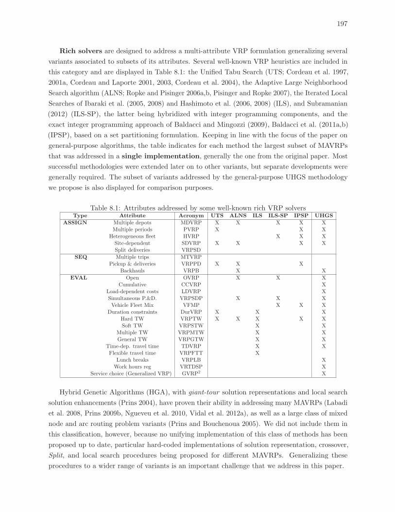
197

Rich solvers are designed to address a multi-attribute VRP formulation generalizing several

variants associated to subsets of its attributes. Several well-known VRP heuristics are included in

this category and are displayed in Table 8.1: the Unified Tabu Search (UTS; Cordeau et al. 1997,

2001a, Cordeau and Laporte 2001, 2003, Cordeau et al. 2004), the Adaptive Large Neighborhood

Search algorithm (ALNS; Ropke and Pisinger 2006a,b, Pisinger and Ropke 2007), the Iterated Local

Searches of Ibaraki et al. (2005, 2008) and Hashimoto et al. (2006, 2008) (ILS), and Subramanian

(2012) (ILS-SP), the latter being hybridized with integer programming components, and the

exact integer programming approach of Baldacci and Mingozzi (2009), Baldacci et al. (2011a,b)

(IPSP), based on a set partitioning formulation. Keeping in line with the focus of the paper on

general-purpose algorithms, the table indicates for each method the largest subset of MAVRPs

that was addressed in a single implementation, generally the one from the original paper. Most

successful methodologies were extended later on to other variants, but separate developments were

generally required. The subset of variants addressed by the general-purpose UHGS methodology

we propose is also displayed for comparison purposes.

Table 8.1: Attributes addressed by some well-known rich VRP solversType Attribute Acronym UTS ALNS ILS ILS-SP IPSP UHGS

ASSIGN Multiple depots MDVRP X X X X XMultiple periods PVRP X X X

Heterogeneous fleet HVRP X X XSite-dependent SDVRP X X X XSplit deliveries VRPSD

SEQ Multiple trips MTVRPPickup & deliveries VRPPD X X X

Backhauls VRPB X X

EVAL Open OVRP X X XCumulative CCVRP X

Load-dependent costs LDVRP XSimultaneous P.&D. VRPSDP X X XVehicle Fleet Mix VFMP X X X

Duration constraints DurVRP X X XHard TW VRPTW X X X X XSoft TW VRPSTW X X

Multiple TW VRPMTW X XGeneral TW VRPGTW X X

Time-dep. travel time TDVRP X XFlexible travel time VRPFTT X

Lunch breaks VRPLB XWork hours reg VRTDSP X

Service choice (Generalized VRP) GVRP2 X

Hybrid Genetic Algorithms (HGA), with giant-tour solution representations and local search

solution enhancements (Prins 2004), have proven their ability in addressing many MAVRPs (Labadi

et al. 2008, Prins 2009b, Ngueveu et al. 2010, Vidal et al. 2012a), as well as a large class of mixed

node and arc routing problem variants (Prins and Bouchenoua 2005). We did not include them in

this classification, however, because no unifying implementation of this class of methods has been

proposed up to date, particular hard-coded implementations of solution representation, crossover,

Split, and local search procedures being proposed for different MAVRPs. Generalizing these

procedures to a wider range of variants is an important challenge that we address in this paper.

198

Each rich solver included in Table 8.1 relies on a “rich” multi-attribute VRP formulation, a

periodic VRP with time windows (UTS), a pick-up and delivery problem with time windows

(ALNS), a VRP with general time windows, time-dependent, and flexible travel-times (ILS), or

a heterogeneous pickup-and-delivery problem with time windows (ILS-SP). Yet, relying on such

formulations to achieve generality presents two main limitations. First, problems become more

intricate and difficult to address as the number of attributes one must consider simultaneously

grows. Second, all the features of the general model are still present when particular variants, with

less attributes, are considered, resulting in loss of efficiency through wasted computations induced

by deactivated attributes and, sometimes, higher complexity for some algorithm components. The

methodology we propose avoids these pitfalls.

Modeling and solution frameworks seek to capture the general properties of the attributes

to transform them into machine-readable components. Thus, the framework of Desaulniers et al.

(1998) formulates a number of classes of attributes as resources (e.g., load, distance, time), which

are extended to successive customer visits through resource extension functions (REFs) subject to

interval constraints. This framework was applied to various crew scheduling and routing problem

variants, the resulting formulations being then solved efficiently by column generation (Desaulniers

et al. 2005).

It is well known that the performance of many heuristics for MAVRPs is directly linked to the

capability of efficiently evaluating new routes produced during the search. Hence, a large body

of literature focuses on reducing the complexity of route evaluation in presence of difficult EVAL

attributes (Savelsbergh 1985, 1992, Garcia 1996, Kindervater and Savelsbergh 1997, Campbell

and Savelsbergh 2004). These approaches share the common characteristic that they develop

meaningful information on subsequences of successive visits (partial routes) to speed up evaluations

of new routes. Using this methodology, time windows, simultaneous pickups and deliveries, and

load-dependent costs attributes can be efficiently managed in the course of local searches, leading

to notable gains in computational complexity.

Merging these two avenues of research, Irnich (2008b) considered forward and backward

extension of resources, as well as the management of generalized resources extension functions on

subsequences of visits to perform efficient route evaluations. This extended REF methodology was

combined with sequential search concepts, leading to a unified solution approach (Irnich 2008a).

Yet, strong properties on REFs inversion and generalization to segments are required for the

framework to apply.

Finally, Puranen (2011) introduced a domain model able to express VRP variants and transform

them into a routing metamodel workable by optimization methods. The routing metamodel is

based on the concepts of actors, activities, resources, and capabilities. It exploits both the

concept of resource extension functions, and a generalization called mapping-ordering constraints.

The methodology covers the complete resolution process flow, from the domain model, to the

routing metamodel and its resolution. However, few computational experiments were presented to

demonstrate the capabilities of the approach.

199

8.4.3 Proposed component-based framework

As underlined in this review, a few unifying methodologies have been proposed for multi-

attribute VRPs. However, these approaches are limited in the classes, properties and number of

attributes they manage. Modeling and solution frameworks (Desaulniers et al. 1998, Irnich 2008a,b,

Puranen 2011) do provide remarkable formalisms for many attributes, but in counterpart require

strong properties to be efficiently applied, such as the existence of REFs which are invertible and

generalizable to segments.

In this paper, we investigate a different approach towards general-purpose MAVRP resolution

inspired from component-based design. Indeed, even a general-purpose solver must ultimately

account for the specific attributes, objectives, and constraints of the particular problem setting

at hand. Yet, to achieve a high level of generality, these problem attributes must be confined to

restricted components of the algorithm, defined relatively to a subset of functionalities. These

components should be polymorphic (Meyer 1997), meaning that they can be implemented differently

as required by problem specifics, but their functionalities can always be used in the same manner,

independently of the problem, and without requiring the knowledge of what is inside the component.

The implementation of components requires a library of basic attribute-dependent operators, out

of which the algorithm can automatically select the necessary operators relatively to the problem

specification. Furthermore, components can be designed to offer the possibility to integrate

attribute-specific strategies, opening the way, for example, to efficient route-evaluation procedures

managing meaningful data on sequences.

It is worth noticing that related designs have been used in the combinatorial optimization

literature to build general-purpose heuristic solvers or software libraries (e.g., Fink and Voss 2003,

Cahon et al. 2004), hyper-heuristics (Burke et al. 2010), and cooperative methods (Crainic and

Toulouse 2010). Component-based heuristic approaches are rare in the VRP literature (Du and

Wu 2001, Groer et al. 2010). While polymorphism has been efficiently used to generate adaptable

resolution strategies, i.e., configurable metaheuristics or local-search strategies, it has not yet

provided the means to address the challenge of the broad variability in problem settings. Moreover,

although hyper-heuristics and cooperative methods achieve more robust solving by making several

basic methods adapt or cooperate, they are still dependent upon the availability of these basic

problem-tailored methods.

We restrict in this paper the scope of the proposed approach to the VRP class in order to keep

the length of the paper within acceptable limits and discus in detail its main components and

logic. Indeed, similarly to several other combinatorial optimization problems, MAVRPs present

a particular structure combining decisions on assignment (and partitioning), sequencing, and

fixed-sequence optimization and evaluation. Consequently, as indicated in Section 8.4.1, we identify

three categories of attributes, defined relatively to their impact on the heuristic resolution: ASSIGN

attributes requiring the assignment of routes and customers to global resources (depots, days,

vehicle types), SEQ attributes determining the structure of the network and the sequences of visits,

and EVAL attributes modifying the solution evaluations. We introduce three adaptive components,

which account for these attributes, providing the following functionalities:

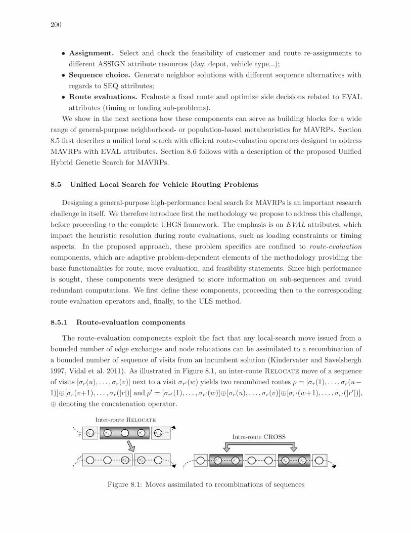
200

• Assignment. Select and check the feasibility of customer and route re-assignments to

different ASSIGN attribute resources (day, depot, vehicle type...);

• Sequence choice. Generate neighbor solutions with different sequence alternatives with

regards to SEQ attributes;

• Route evaluations. Evaluate a fixed route and optimize side decisions related to EVAL

attributes (timing or loading sub-problems).

We show in the next sections how these components can serve as building blocks for a wide

range of general-purpose neighborhood- or population-based metaheuristics for MAVRPs. Section

8.5 first describes a unified local search with efficient route-evaluation operators designed to address

MAVRPs with EVAL attributes. Section 8.6 follows with a description of the proposed Unified

Hybrid Genetic Search for MAVRPs.

8.5 Unified Local Search for Vehicle Routing Problems

Designing a general-purpose high-performance local search for MAVRPs is an important research

challenge in itself. We therefore introduce first the methodology we propose to address this challenge,

before proceeding to the complete UHGS framework. The emphasis is on EVAL attributes, which

impact the heuristic resolution during route evaluations, such as loading constraints or timing

aspects. In the proposed approach, these problem specifics are confined to route-evaluation

components, which are adaptive problem-dependent elements of the methodology providing the

basic functionalities for route, move evaluation, and feasibility statements. Since high performance

is sought, these components were designed to store information on sub-sequences and avoid

redundant computations. We first define these components, proceeding then to the corresponding

route-evaluation operators and, finally, to the ULS method.

8.5.1 Route-evaluation components

The route-evaluation components exploit the fact that any local-search move issued from a

bounded number of edge exchanges and node relocations can be assimilated to a recombination of

a bounded number of sequence of visits from an incumbent solution (Kindervater and Savelsbergh

1997, Vidal et al. 2011). As illustrated in Figure 8.1, an inter-route Relocate move of a sequence

of visits [σr(u), . . . , σr(v)] next to a visit σr′(w) yields two recombined routes ρ = [σr(1), . . . , σr(u−1)]⊕[σr(v+1), . . . , σr(|r|)] and ρ′ = [σr′(1), . . . , σr′(w)]⊕[σr(u), . . . , σr(v)]⊕[σr′(w+1), . . . , σr′(|r′|)],⊕ denoting the concatenation operator.

Figure 8.1: Moves assimilated to recombinations of sequences

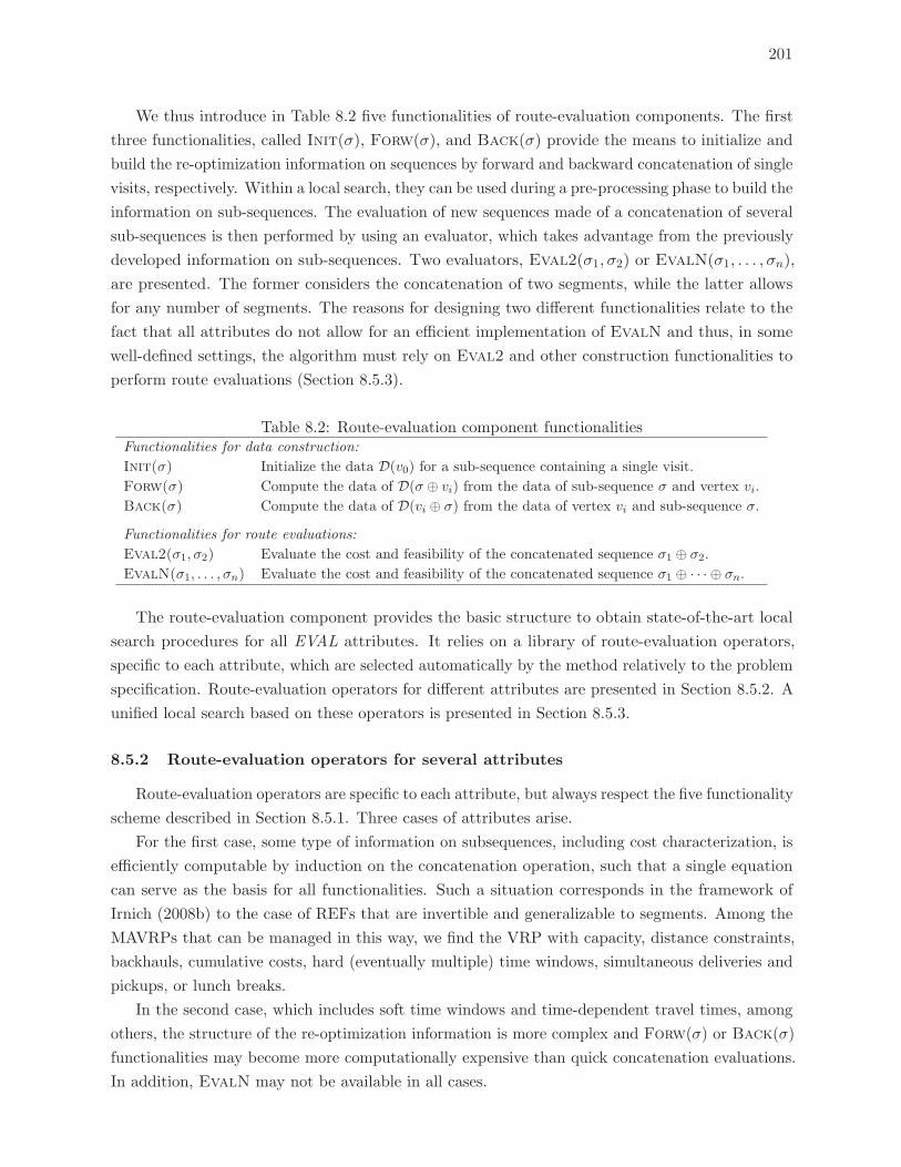
201

We thus introduce in Table 8.2 five functionalities of route-evaluation components. The first

three functionalities, called Init(σ), Forw(σ), and Back(σ) provide the means to initialize and

build the re-optimization information on sequences by forward and backward concatenation of single

visits, respectively. Within a local search, they can be used during a pre-processing phase to build the

information on sub-sequences. The evaluation of new sequences made of a concatenation of several

sub-sequences is then performed by using an evaluator, which takes advantage from the previously

developed information on sub-sequences. Two evaluators, Eval2(σ1, σ2) or EvalN(σ1, . . . , σn),

are presented. The former considers the concatenation of two segments, while the latter allows

for any number of segments. The reasons for designing two different functionalities relate to the

fact that all attributes do not allow for an efficient implementation of EvalN and thus, in some

well-defined settings, the algorithm must rely on Eval2 and other construction functionalities to

perform route evaluations (Section 8.5.3).

Table 8.2: Route-evaluation component functionalitiesFunctionalities for data construction:

Init(σ) Initialize the data D(v0) for a sub-sequence containing a single visit.

Forw(σ) Compute the data of D(σ ⊕ vi) from the data of sub-sequence σ and vertex vi.

Back(σ) Compute the data of D(vi ⊕ σ) from the data of vertex vi and sub-sequence σ.

Functionalities for route evaluations:

Eval2(σ1, σ2) Evaluate the cost and feasibility of the concatenated sequence σ1 ⊕ σ2.

EvalN(σ1, . . . , σn) Evaluate the cost and feasibility of the concatenated sequence σ1 ⊕ · · · ⊕ σn.

The route-evaluation component provides the basic structure to obtain state-of-the-art local

search procedures for all EVAL attributes. It relies on a library of route-evaluation operators,

specific to each attribute, which are selected automatically by the method relatively to the problem

specification. Route-evaluation operators for different attributes are presented in Section 8.5.2. A

unified local search based on these operators is presented in Section 8.5.3.

8.5.2 Route-evaluation operators for several attributes

Route-evaluation operators are specific to each attribute, but always respect the five functionality

scheme described in Section 8.5.1. Three cases of attributes arise.

For the first case, some type of information on subsequences, including cost characterization, is

efficiently computable by induction on the concatenation operation, such that a single equation

can serve as the basis for all functionalities. Such a situation corresponds in the framework of

Irnich (2008b) to the case of REFs that are invertible and generalizable to segments. Among the

MAVRPs that can be managed in this way, we find the VRP with capacity, distance constraints,

backhauls, cumulative costs, hard (eventually multiple) time windows, simultaneous deliveries and

pickups, or lunch breaks.

In the second case, which includes soft time windows and time-dependent travel times, among

others, the structure of the re-optimization information is more complex and Forw(σ) or Back(σ)

functionalities may become more computationally expensive than quick concatenation evaluations.

In addition, EvalN may not be available in all cases.

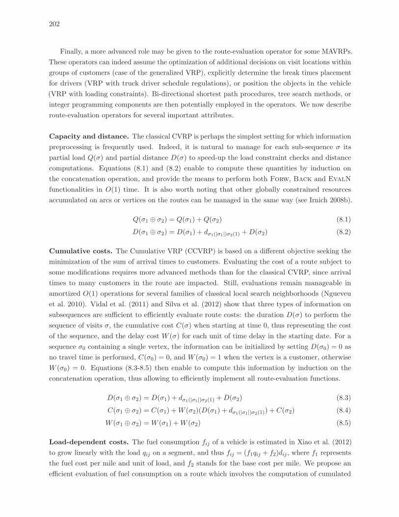
202

Finally, a more advanced role may be given to the route-evaluation operator for some MAVRPs.

These operators can indeed assume the optimization of additional decisions on visit locations within

groups of customers (case of the generalized VRP), explicitly determine the break times placement

for drivers (VRP with truck driver schedule regulations), or position the objects in the vehicle

(VRP with loading constraints). Bi-directional shortest path procedures, tree search methods, or

integer programming components are then potentially employed in the operators. We now describe

route-evaluation operators for several important attributes.

Capacity and distance. The classical CVRP is perhaps the simplest setting for which information

preprocessing is frequently used. Indeed, it is natural to manage for each sub-sequence σ its

partial load Q(σ) and partial distance D(σ) to speed-up the load constraint checks and distance

computations. Equations (8.1) and (8.2) enable to compute these quantities by induction on

the concatenation operation, and provide the means to perform both Forw, Back and EvalN

functionalities in O(1) time. It is also worth noting that other globally constrained resources

accumulated on arcs or vertices on the routes can be managed in the same way (see Irnich 2008b).

Q(σ1 ⊕ σ2) = Q(σ1) +Q(σ2) (8.1)

D(σ1 ⊕ σ2) = D(σ1) + dσ1(|σ1|)σ2(1) +D(σ2) (8.2)

Cumulative costs. The Cumulative VRP (CCVRP) is based on a different objective seeking the

minimization of the sum of arrival times to customers. Evaluating the cost of a route subject to

some modifications requires more advanced methods than for the classical CVRP, since arrival

times to many customers in the route are impacted. Still, evaluations remain manageable in

amortized O(1) operations for several families of classical local search neighborhoods (Ngueveu

et al. 2010). Vidal et al. (2011) and Silva et al. (2012) show that three types of information on

subsequences are sufficient to efficiently evaluate route costs: the duration D(σ) to perform the

sequence of visits σ, the cumulative cost C(σ) when starting at time 0, thus representing the cost

of the sequence, and the delay cost W (σ) for each unit of time delay in the starting date. For a

sequence σ0 containing a single vertex, the information can be initialized by setting D(σ0) = 0 as

no travel time is performed, C(σ0) = 0, and W (σ0) = 1 when the vertex is a customer, otherwise

W (σ0) = 0. Equations (8.3-8.5) then enable to compute this information by induction on the

concatenation operation, thus allowing to efficiently implement all route-evaluation functions.

D(σ1 ⊕ σ2) = D(σ1) + dσ1(|σ1|)σ2(1) +D(σ2) (8.3)

C(σ1 ⊕ σ2) = C(σ1) +W (σ2)(D(σ1) + dσ1(|σ1|)σ2(1)) + C(σ2) (8.4)

W (σ1 ⊕ σ2) =W (σ1) +W (σ2) (8.5)

Load-dependent costs. The fuel consumption fij of a vehicle is estimated in Xiao et al. (2012)

to grow linearly with the load qij on a segment, and thus fij = (f1qij + f2)dij , where f1 represents

the fuel cost per mile and unit of load, and f2 stands for the base cost per mile. We propose an

efficient evaluation of fuel consumption on a route which involves the computation of cumulated

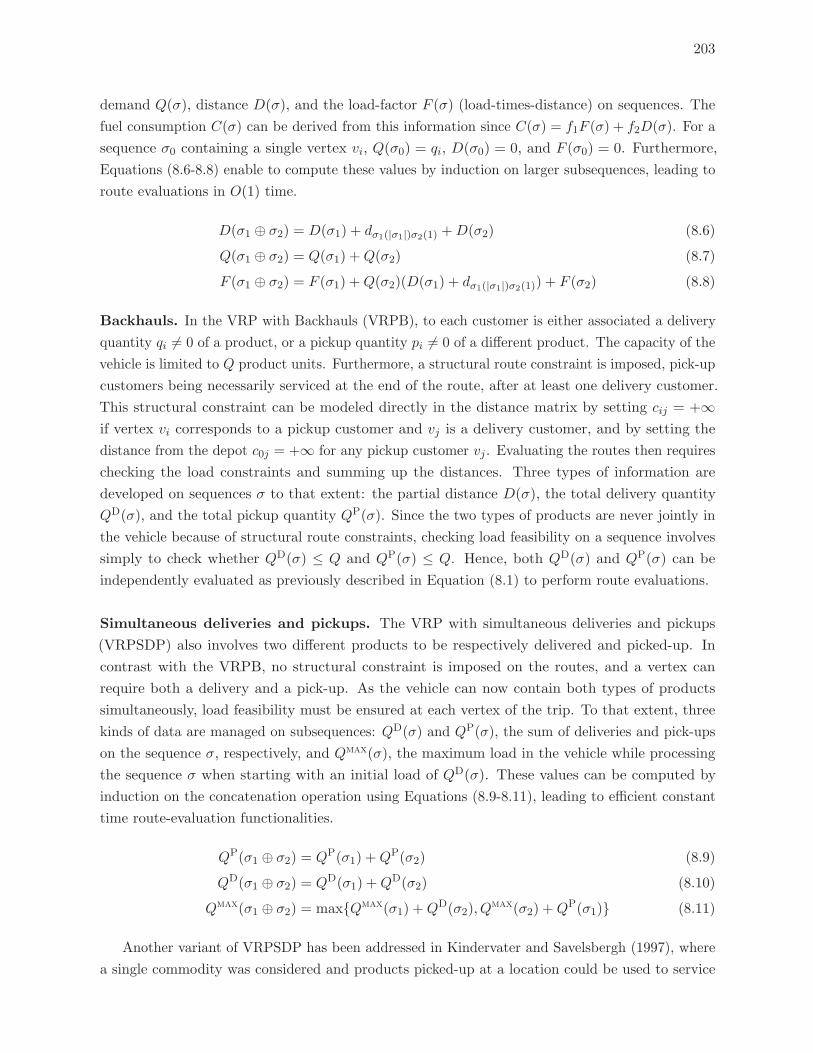
203

demand Q(σ), distance D(σ), and the load-factor F (σ) (load-times-distance) on sequences. The

fuel consumption C(σ) can be derived from this information since C(σ) = f1F (σ) + f2D(σ). For a

sequence σ0 containing a single vertex vi, Q(σ0) = qi, D(σ0) = 0, and F (σ0) = 0. Furthermore,

Equations (8.6-8.8) enable to compute these values by induction on larger subsequences, leading to

route evaluations in O(1) time.

D(σ1 ⊕ σ2) = D(σ1) + dσ1(|σ1|)σ2(1) +D(σ2) (8.6)

Q(σ1 ⊕ σ2) = Q(σ1) +Q(σ2) (8.7)

F (σ1 ⊕ σ2) = F (σ1) +Q(σ2)(D(σ1) + dσ1(|σ1|)σ2(1)) + F (σ2) (8.8)

Backhauls. In the VRP with Backhauls (VRPB), to each customer is either associated a delivery

quantity qi �= 0 of a product, or a pickup quantity pi �= 0 of a different product. The capacity of the

vehicle is limited to Q product units. Furthermore, a structural route constraint is imposed, pick-up

customers being necessarily serviced at the end of the route, after at least one delivery customer.

This structural constraint can be modeled directly in the distance matrix by setting cij = +∞if vertex vi corresponds to a pickup customer and vj is a delivery customer, and by setting the

distance from the depot c0j = +∞ for any pickup customer vj . Evaluating the routes then requires

checking the load constraints and summing up the distances. Three types of information are

developed on sequences σ to that extent: the partial distance D(σ), the total delivery quantity

QD(σ), and the total pickup quantity QP(σ). Since the two types of products are never jointly in

the vehicle because of structural route constraints, checking load feasibility on a sequence involves

simply to check whether QD(σ) ≤ Q and QP(σ) ≤ Q. Hence, both QD(σ) and QP(σ) can be

independently evaluated as previously described in Equation (8.1) to perform route evaluations.

Simultaneous deliveries and pickups. The VRP with simultaneous deliveries and pickups

(VRPSDP) also involves two different products to be respectively delivered and picked-up. In

contrast with the VRPB, no structural constraint is imposed on the routes, and a vertex can

require both a delivery and a pick-up. As the vehicle can now contain both types of products

simultaneously, load feasibility must be ensured at each vertex of the trip. To that extent, three

kinds of data are managed on subsequences: QD(σ) and QP(σ), the sum of deliveries and pick-ups

on the sequence σ, respectively, and Qmax(σ), the maximum load in the vehicle while processing

the sequence σ when starting with an initial load of QD(σ). These values can be computed by

induction on the concatenation operation using Equations (8.9-8.11), leading to efficient constant

time route-evaluation functionalities.

QP(σ1 ⊕ σ2) = QP(σ1) +QP(σ2) (8.9)

QD(σ1 ⊕ σ2) = QD(σ1) +QD(σ2) (8.10)

Qmax(σ1 ⊕ σ2) = max{Qmax(σ1) +QD(σ2), Qmax(σ2) +QP(σ1)} (8.11)

Another variant of VRPSDP has been addressed in Kindervater and Savelsbergh (1997), where

a single commodity was considered and products picked-up at a location could be used to service

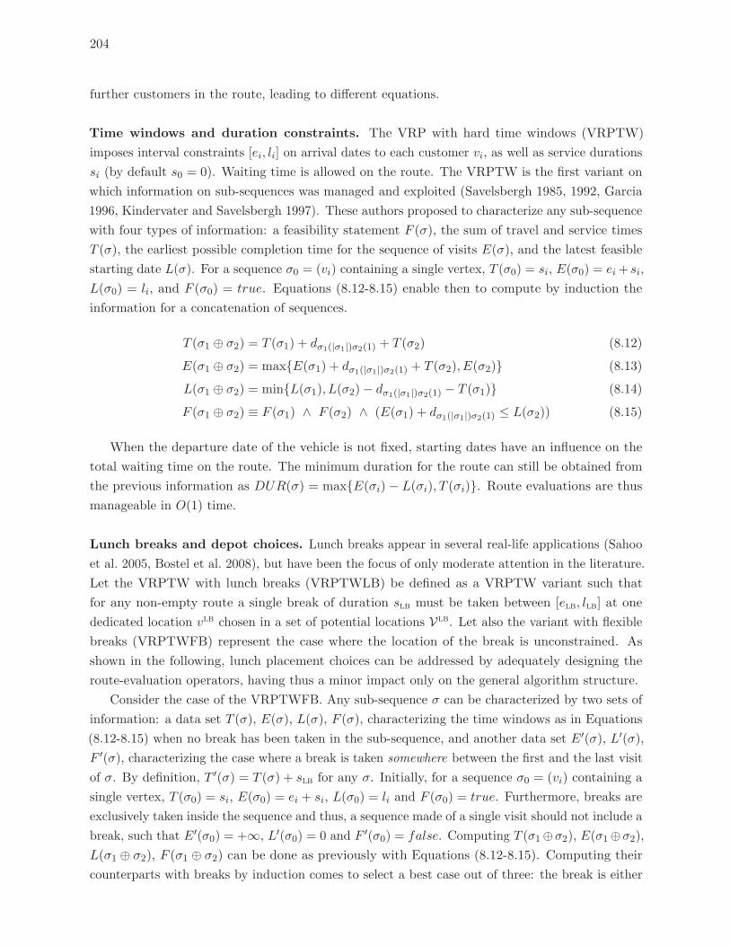
204

further customers in the route, leading to different equations.

Time windows and duration constraints. The VRP with hard time windows (VRPTW)

imposes interval constraints [ei, li] on arrival dates to each customer vi, as well as service durations

si (by default s0 = 0). Waiting time is allowed on the route. The VRPTW is the first variant on

which information on sub-sequences was managed and exploited (Savelsbergh 1985, 1992, Garcia

1996, Kindervater and Savelsbergh 1997). These authors proposed to characterize any sub-sequence

with four types of information: a feasibility statement F (σ), the sum of travel and service times

T (σ), the earliest possible completion time for the sequence of visits E(σ), and the latest feasible

starting date L(σ). For a sequence σ0 = (vi) containing a single vertex, T (σ0) = si, E(σ0) = ei+ si,

L(σ0) = li, and F (σ0) = true. Equations (8.12-8.15) enable then to compute by induction the

information for a concatenation of sequences.

T (σ1 ⊕ σ2) = T (σ1) + dσ1(|σ1|)σ2(1) + T (σ2) (8.12)

E(σ1 ⊕ σ2) = max{E(σ1) + dσ1(|σ1|)σ2(1) + T (σ2), E(σ2)} (8.13)

L(σ1 ⊕ σ2) = min{L(σ1), L(σ2)− dσ1(|σ1|)σ2(1) − T (σ1)} (8.14)

F (σ1 ⊕ σ2) ≡ F (σ1) ∧ F (σ2) ∧ (E(σ1) + dσ1(|σ1|)σ2(1) ≤ L(σ2)) (8.15)

When the departure date of the vehicle is not fixed, starting dates have an influence on the

total waiting time on the route. The minimum duration for the route can still be obtained from

the previous information as DUR(σ) = max{E(σi)− L(σi), T (σi)}. Route evaluations are thus

manageable in O(1) time.

Lunch breaks and depot choices. Lunch breaks appear in several real-life applications (Sahoo

et al. 2005, Bostel et al. 2008), but have been the focus of only moderate attention in the literature.

Let the VRPTW with lunch breaks (VRPTWLB) be defined as a VRPTW variant such that

for any non-empty route a single break of duration slb must be taken between [elb, llb] at one

dedicated location vlb chosen in a set of potential locations Vlb. Let also the variant with flexible

breaks (VRPTWFB) represent the case where the location of the break is unconstrained. As

shown in the following, lunch placement choices can be addressed by adequately designing the

route-evaluation operators, having thus a minor impact only on the general algorithm structure.

Consider the case of the VRPTWFB. Any sub-sequence σ can be characterized by two sets of

information: a data set T (σ), E(σ), L(σ), F (σ), characterizing the time windows as in Equations

(8.12-8.15) when no break has been taken in the sub-sequence, and another data set E′(σ), L′(σ),F ′(σ), characterizing the case where a break is taken somewhere between the first and the last visit

of σ. By definition, T ′(σ) = T (σ) + slb for any σ. Initially, for a sequence σ0 = (vi) containing a

single vertex, T (σ0) = si, E(σ0) = ei + si, L(σ0) = li and F (σ0) = true. Furthermore, breaks are

exclusively taken inside the sequence and thus, a sequence made of a single visit should not include a

break, such that E′(σ0) = +∞, L′(σ0) = 0 and F ′(σ0) = false. Computing T (σ1⊕σ2), E(σ1⊕σ2),

L(σ1 ⊕ σ2), F (σ1 ⊕ σ2) can be done as previously with Equations (8.12-8.15). Computing their

counterparts with breaks by induction comes to select a best case out of three: the break is either

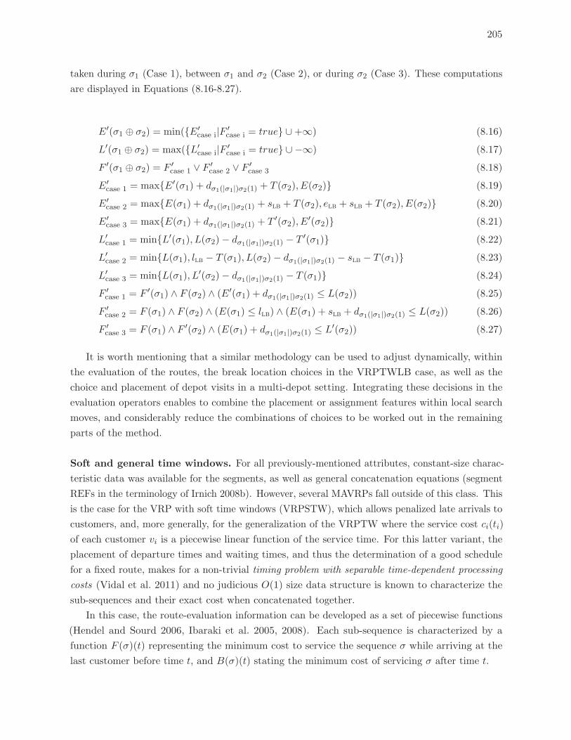
205

taken during σ1 (Case 1), between σ1 and σ2 (Case 2), or during σ2 (Case 3). These computations

are displayed in Equations (8.16-8.27).

E′(σ1 ⊕ σ2) = min({E′case i|F ′

case i = true} ∪+∞) (8.16)

L′(σ1 ⊕ σ2) = max({L′case i|F ′

case i = true} ∪ −∞) (8.17)

F ′(σ1 ⊕ σ2) = F ′case 1 ∨ F ′

case 2 ∨ F ′case 3 (8.18)

E′case 1 = max{E′(σ1) + dσ1(|σ1|)σ2(1) + T (σ2), E(σ2)} (8.19)

E′case 2 = max{E(σ1) + dσ1(|σ1|)σ2(1) + slb + T (σ2), elb + slb + T (σ2), E(σ2)} (8.20)

E′case 3 = max{E(σ1) + dσ1(|σ1|)σ2(1) + T ′(σ2), E′(σ2)} (8.21)

L′case 1 = min{L′(σ1), L(σ2)− dσ1(|σ1|)σ2(1) − T ′(σ1)} (8.22)

L′case 2 = min{L(σ1), llb − T (σ1), L(σ2)− dσ1(|σ1|)σ2(1) − slb − T (σ1)} (8.23)

L′case 3 = min{L(σ1), L′(σ2)− dσ1(|σ1|)σ2(1) − T (σ1)} (8.24)

F ′case 1 = F ′(σ1) ∧ F (σ2) ∧ (E′(σ1) + dσ1(|σ1|)σ2(1) ≤ L(σ2)) (8.25)

F ′case 2 = F (σ1) ∧ F (σ2) ∧ (E(σ1) ≤ llb) ∧ (E(σ1) + slb + dσ1(|σ1|)σ2(1) ≤ L(σ2)) (8.26)

F ′case 3 = F (σ1) ∧ F ′(σ2) ∧ (E(σ1) + dσ1(|σ1|)σ2(1) ≤ L′(σ2)) (8.27)

It is worth mentioning that a similar methodology can be used to adjust dynamically, within

the evaluation of the routes, the break location choices in the VRPTWLB case, as well as the

choice and placement of depot visits in a multi-depot setting. Integrating these decisions in the

evaluation operators enables to combine the placement or assignment features within local search

moves, and considerably reduce the combinations of choices to be worked out in the remaining

parts of the method.

Soft and general time windows. For all previously-mentioned attributes, constant-size charac-

teristic data was available for the segments, as well as general concatenation equations (segment

REFs in the terminology of Irnich 2008b). However, several MAVRPs fall outside of this class. This

is the case for the VRP with soft time windows (VRPSTW), which allows penalized late arrivals to

customers, and, more generally, for the generalization of the VRPTW where the service cost ci(ti)

of each customer vi is a piecewise linear function of the service time. For this latter variant, the

placement of departure times and waiting times, and thus the determination of a good schedule

for a fixed route, makes for a non-trivial timing problem with separable time-dependent processing

costs (Vidal et al. 2011) and no judicious O(1) size data structure is known to characterize the

sub-sequences and their exact cost when concatenated together.

In this case, the route-evaluation information can be developed as a set of piecewise functions

(Hendel and Sourd 2006, Ibaraki et al. 2005, 2008). Each sub-sequence is characterized by a

function F (σ)(t) representing the minimum cost to service the sequence σ while arriving at the

last customer before time t, and B(σ)(t) stating the minimum cost of servicing σ after time t.

206

For a sequence σ0 = (vi) with a single vertex, Fσ0(t) = minx≤t ci(x) and Bσ0(t) = minx≥t ci(x).

The construction operator Forw relies on forward dynamic programming (Equation 8.28) to build

explicitly the information for the concatenation of a sequence σ with a vertex vi. In reverse, the

functionality Back is based on backward dynamic programming (Equation 8.29). Equation (8.30)

provides the cost Z∗(σ1 ⊕ σ2) of the concatenated sequence σ1 ⊕ σ2 when F (σ1)(t) and B(σ2)(t)

are available, thus leading to an efficient Eval2 functionality.

F (σ ⊕ vi)(t) = min0≤x≤t

{ci(x) + F (σ)(x− sσ(|σ|) − dσ(|σ|),i)} (8.28)

B(vi ⊕ σ)(t) = minx≥t

{ci(x) +B(σ)(x+ si + di,σ(1))} (8.29)

Z∗(σ1 ⊕ σ2) = minx≥0

{F (σ1)(x) +B(σ2)(x+ sσ1(|σ1|) + dσ1(|σ1|)σ2(1))} (8.30)

In our implementations, the data structures F (σ)(t) and B(σ)(t) are managed as linked lists of

function pieces characterized by interval, origin value and slope. The data construction functionali-

ties Forw(σ), Back(σ) and Eval2 work in O(Σiξ(ci)) time, ξ(ci) representing the number of

pieces of a piecewise cost function ci. However the EvalN functionality is not efficiently manage-

able. In the particular case where all functions ci(t) are convex, more advanced implementations

based either on heaps (Hendel and Sourd 2006) or on search trees (Ibaraki et al. 2008) achieve a

complexity of O(log Σiξ(ci)) for both Eval2 and EvalN.

Other time features. The literature contains various other EVAL attributes related to time, such

as duration constraints, multiple time windows, time-dependent trip durations, flexible travel times,

and minimum and maximum intervals of time between pairs of services. We refer to Vidal et al.

(2011) for a comprehensive review and analysis of state-of-the-art algorithms for the underlying

timing sub-problems for route evaluations, and their incremental resolution during local searches.

These approaches were used to generate UHGS route-evaluation operators for the related problems

with time characteristics.

Service site choices. In the Generalized Vehicle Routing Problem (GVRP), each request vi is

associated to a set of λi alternative locations Li = {li1, . . . , li|λi|}. Exactly one location of each

set must be serviced. As illustrated in Baldacci et al. (2009), the GVRP is relevant for several

practical applications and directly generalizes other variants of vehicle routing.

Recent metaheuristics for this problem (Moccia et al. 2012) include local-search procedures

on the order of services that do not consider explicitly in the neighborhoods the locations to be

serviced. Evaluating a sequence of services then becomes finding the associated shortest sequence

of visits to locations, leading to a shortest path problem.

Again, efficient route evaluations require to store for each sequence of services appropriate data

to speed-up the shortest path computation. In this case, the information to be stored for a sequence

σ is the shortest path S(σ)[i, j] between the ith location of σ(1) and the jth location of σ(|σ|),where i ∈ {1, . . . , λσ(1)} and j ∈ {1, . . . , λσ(|σ|)}. For a sequence σ0 = (vi) containing a single

service, S(σ0)[x, x] = 0 for any x ∈ {1, . . . , λi} and S(σ0)[x, y] = +∞ if x �= y. Equation (8.31)

207

enables then to develop this information on larger subsequences by induction on the concatenation

operation.

S(σ1 ⊕ σ2)[i, j] = min1≤x≤λσ1(|σ1|),1≤y≤λσ2(1)

S(σ1)[i, x] + dxy + S(σ2)[y, j]

∀i ∈ {1, . . . , λσ1(1)}, ∀j ∈ {1, . . . , λσ2(|σ2|)}(8.31)

Equation (8.31) provides the means to perform efficiently in O(λ2) operations all route-evaluation

functionalities, λ standing for the maximum number of locations associated to a service. This

complexity is notably better than the complexity of computing each shortest path from scratch,

which would be O(nrλ2) operations for a route containing nr services.

Hours of service regulations. Governments worldwide impose complex regulations on truck-

driver schedules to limit the amount of work and driving within intervals of time and impose a

minimum frequency and duration for break and rest periods. Because of their large impact on

driving times, these regulations should be accounted for when optimizing the routes, leading to

combined vehicle routing and truck-driver scheduling problems (VRTDSP). However, even checking

the existence of a feasible placement of breaks for a fixed sequence of visits makes for a highly

complex problem which is known to be solvable in a quadratic time for United States hours of

service regulations (Goel and Kok 2012), while no polynomial algorithm is known for many other

cases, with European Union, Canadian, and Australian rules.

Despite this high complexity, most efficient methods for the VRTDSP integrate break scheduling

feasibility checks directly in the local search (Prescott-Gagnon et al. 2010, Goel and Vidal 2012), and

thus during each route evaluation. In the proposed methodology, these break-scheduling procedures

are used inside the route-evaluation operators. A set of schedule alternatives is maintained for each

subsequence of consecutive visits. The schedule information is extended to larger subsequences

by appending new driving and break activities at the end of the schedules, and selecting only a

relevant subset by means of dominance relationships. Our current implementation is exclusively

based on forward operators, and thus Eval2(σ1,σ2) is performed by iteratively completing the

schedule of σ1 with services of σ2.

Summary. As reviewed in this section, efficient route-evaluation operators relative to different

VRP attributes may require to develop radically different information on sequences, and use more

or less complex evaluation procedures. Still, all previously-mentioned approaches respect the same

five functionalities scheme, based on the forward or backward propagation of labels (or, generally,

of any information to characterize the sequences), and the evaluation of the concatenation of two

or more sequences using the information developed on sequences. As shown in the following, this

library of route-evaluation operators provides the means to create a general-purpose state-of-the-art

local search for many MAVRPs.

208

8.5.3 Unified local search procedure

The five functionalities of the route-evaluation component can be used to build any local search

method with moves involving a bounded number of edge exchanges and node relocations, since

all these moves can be evaluated as a recombination of partial subsequences from the incumbent

solution. The general ULS process is illustrated in Algorithm 8.1. To efficiently evaluate moves, ULS

manages information on subsequences of consecutive visits (and reverse subsequences in presence

of moves that impact the route orientation), using the Init, Forw, and Back route construction

functionalities. This information is built during a pre-processing phase at the beginning of the

local search, and is then updated whenever any route is modified. Moves are then evaluated by

means of Eval2 and EvalN.

Algorithm 8.1 Unified local search based on route-evaluation operators

1: Detect the good combination of evaluation operators relatively to the problem attributes2: Build re-optimization data on subsequences using the Init, Forw and Back operators.3: while some improving moves exist in the neighborhood N4: for each move μi in N5: for each route rμj produced by the move6: Determine the k sub-sequences [σ1, . . . , σk] that are concatenated to produce rμj7: if k = 2, then NewCost(r) = Eval2(σ1,σ2)8: else if k > 2, then NewCost(r) = EvalN(σ1,. . . ,σk)9: if AcceptCriteria(μi) then perform the move μ and update the re-optimization data

on for each route rμj using the Init, Forw and Back operators.

In the specific implementation of this paper, the neighbor solutions issued from moves are

explored in random order, using the acceptance criterion of Vidal et al. (2013) and terminating

whenever no improving move can be found in the whole neighborhood. As in Vidal et al. (2013),

the classical 2-opt*, and 2-opt neighborhoods are used, as well as the inter-route and intra-route

Cross and I-Cross neighborhoods, restricted to subsequences of length smaller than Lmax = 2

and including relocate moves as special cases. Only moves involving neighbor vertices in terms of

distance and time characteristics (Toth and Vigo 2003, Vidal et al. 2013) are attempted, leading

to a neighborhood size of O(L2maxΓn) instead of O(L2

maxn2), where Γ stands for the number of

neighbor vertices per vertex.

It should be noted that all inter-route moves such as Cross, I-Cross and 2-opt*, require

either Eval2(σ1, σ2) or EvalN(σ1, σL, σ2), where σL is a sequence of size bounded by Lmax. When

no efficient EvalN is available, in presence of attributes such as soft and general time windows

for example, this first family of inter-route moves can still be evaluated efficiently as EvalN(σ1,

σL, σ2) can be replaced by less than Lmax successive calls to Forw to yield the information on

σ′ = σ1 ⊕ σL, with a final call to Eval2(σ′, σ2). Intra-route Cross and I-Cross and 2-opt moves

require calling EvalN on a set of 3 to 5 subsequences. If no efficient EvalN is available, the

same reasoning for replacement can still be used, but in this case the number of necessary calls to

Forw becomes linear in the route size since the size of intermediate subsequences is not bounded.

However, since intra-route moves are usually in minority, this increased number of operations did

not impact the method speed.

209

The good combination of route-evaluation operators is automatically determined relatively

to the problem attributes according to the component-based framework of Section 8.4.3, and

thus the route-evaluation operators allow to use advanced move evaluation techniques which were

until now considered as problem-specific in a unified framework for MAVRPs. The resulting

unified local search is efficient and applicable to many VRP variants. It can be extended into

any generic neighborhood-based metaheuristic such as tabu search, iterated local search, or

variable neighborhood search. Relatively to the recent advances in genetic algorithms and diversity

management for vehicle routing, we opted to combine this procedure with the approach of Vidal

et al. (2012a) to obtain a Unified Hybrid Genetic Search (UHGS). Such integration requires

addressing several additional challenges, related to the design of a generic solution representation,

genetic operators, and population management methods. The next section explains how to address

them.

8.6 Unified Hybrid Genetic Search

The proposed UHGS is an extension of the Hybrid Genetic Search with Advanced Diversity

Control of Vidal et al. (2012a), and aims to address MAVRPs in a unified manner by means

of the proposed component-based design. The method stands out from previous works since

all its elements (solution representation, genetic operators, local searches) are fully generic and

detached from the attributes of the problem, relying on the subset of adaptive assignment and

route-evaluation components to make the interface with problem-specific knowledge (Section 8.4.3).

Note that in this work, only single-echelon problems with a route structure, e.g., a single sequence,

are addressed, thus allowing to rely on a unique sequencing component based on standard VRP

neighborhoods (Section 8.5.3). This Section briefly recalls the general structure of UHGS, then

details in turn each element of the unified method.

8.6.1 General algorithmic structure

UHGS combines four main optimization methodologies: 1) hybridization of genetic algorithms

with local search procedures; 2) the use of penalized infeasible solutions, managed through two

distinct sub-populations during the search; 3) a solution representation without trips delimiters

(Prins 2004) with an optimal Split procedure for delimiter computation; 4) an advanced population

management method with diversity-and-cost objective for solution evaluation.

The structure of UHGS is illustrated in Figure 8.2. UHGS iteratively selects two individuals in

the merged sub-populations to serve as input of a crossover operator, yielding a single offspring.

After going through the Split procedure to compute trip delimiters, the offspring is Educated by

means of a local search, Repaired with probability Prep when infeasible, and transfered to the

suitable sub-population. Each sub-population is managed separately to trigger a Survivor Selection

procedure when reaching a maximum size. Diversification procedures and decomposition phases

are regularly used to further enhance the diversity and intensify the search around elite solution

characteristics. The algorithm terminates when Itmax successive iterations (individual generations)

have been performed without improving the best solution, or when a time limit Tmax is reached.

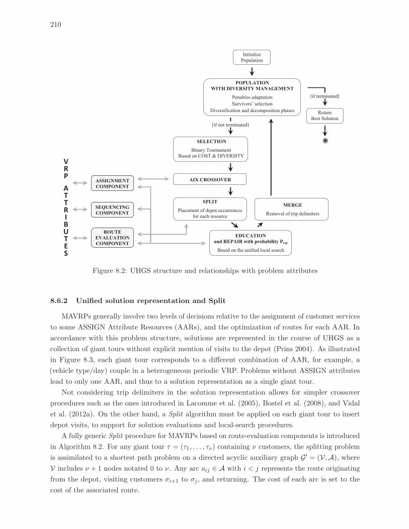
210

ROUTE EVALUATION COMPONENT

POPULATION WITH DIVERSITY MANAGEMENT

Penalties adaptation Survivors’ selection

Diversification and decomposition phases

V R P A T T R I B U T E S

SELECTION a

Binary Tournament Based on COST & DIVERSITY

AIX CROSSOVER

SPLIT

Placement of depot occurrences for each resource

EDUCATION and REPAIR with probability Prep

Based on the unified local search

SEQUENCING COMPONENT

MERGE

Removal of trip delimiters

[if terminated]

[if not terminated]

Return Best Solution

Initialize Population

ASSIGNMENT COMPONENT

Figure 8.2: UHGS structure and relationships with problem attributes

8.6.2 Unified solution representation and Split

MAVRPs generally involve two levels of decisions relative to the assignment of customer services

to some ASSIGN Attribute Resources (AARs), and the optimization of routes for each AAR. In

accordance with this problem structure, solutions are represented in the course of UHGS as a

collection of giant tours without explicit mention of visits to the depot (Prins 2004). As illustrated

in Figure 8.3, each giant tour corresponds to a different combination of AAR, for example, a

(vehicle type/day) couple in a heterogeneous periodic VRP. Problems without ASSIGN attributes

lead to only one AAR, and thus to a solution representation as a single giant tour.

Not considering trip delimiters in the solution representation allows for simpler crossover

procedures such as the ones introduced in Lacomme et al. (2005), Bostel et al. (2008), and Vidal

et al. (2012a). On the other hand, a Split algorithm must be applied on each giant tour to insert

depot visits, to support for solution evaluations and local-search procedures.

A fully generic Split procedure for MAVRPs based on route-evaluation components is introduced

in Algorithm 8.2. For any giant tour τ = (τ1, . . . , τν) containing ν customers, the splitting problem

is assimilated to a shortest path problem on a directed acyclic auxiliary graph G′ = (V ,A), where

V includes ν + 1 nodes notated 0 to ν. Any arc aij ∈ A with i < j represents the route originating

from the depot, visiting customers σi+1 to σj , and returning. The cost of each arc is set to the

cost of the associated route.

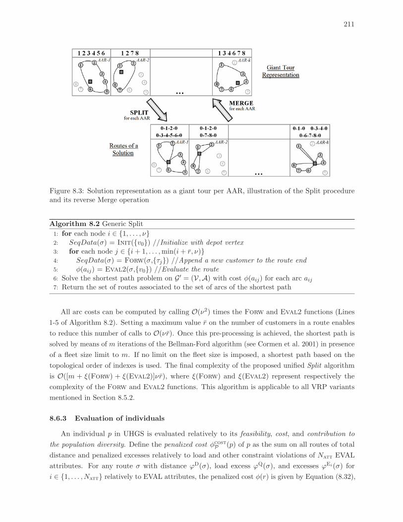
211

Figure 8.3: Solution representation as a giant tour per AAR, illustration of the Split procedureand its reverse Merge operation

Algorithm 8.2 Generic Split

1: for each node i ∈ {1, . . . , ν}2: SeqData(σ) = Init({v0}) //Initialize with depot vertex3: for each node j ∈ {i+ 1, . . . ,min(i+ r, ν)}4: SeqData(σ) = Forw(σ,{τj}) //Append a new customer to the route end5: φ(aij) = Eval2(σ,{v0}) //Evaluate the route6: Solve the shortest path problem on G′ = (V,A) with cost φ(aij) for each arc aij7: Return the set of routes associated to the set of arcs of the shortest path

All arc costs can be computed by calling O(ν2) times the Forw and Eval2 functions (Lines

1-5 of Algorithm 8.2). Setting a maximum value r on the number of customers in a route enables

to reduce this number of calls to O(νr). Once this pre-processing is achieved, the shortest path is

solved by means of m iterations of the Bellman-Ford algorithm (see Cormen et al. 2001) in presence

of a fleet size limit to m. If no limit on the fleet size is imposed, a shortest path based on the

topological order of indexes is used. The final complexity of the proposed unified Split algorithm

is O([m + ξ(Forw) + ξ(Eval2)]νr), where ξ(Forw) and ξ(Eval2) represent respectively the

complexity of the Forw and Eval2 functions. This algorithm is applicable to all VRP variants

mentioned in Section 8.5.2.


An individual p in UHGS is evaluated relatively to its feasibility, cost, and contribution to

the population diversity. Define the penalized cost φcostP (p) of p as the sum on all routes of total

distance and penalized excesses relatively to load and other constraint violations of Natt EVAL

attributes. For any route σ with distance ϕD(σ), load excess ϕQ(σ), and excesses ϕEi(σ) for

i ∈ {1, . . . , Natt} relatively to EVAL attributes, the penalized cost φ(r) is given by Equation (8.32),

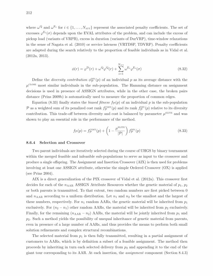
212

where ωQ and ωEi for i ∈ {1, . . . , Natt} represent the associated penalty coefficients. The set of

excesses ϕEi(σ) depends upon the EVAL attributes of the problem, and can include the excess of

pickup load (variants of VRPB), excess in duration (variants of DurVRP), time-window relaxations

in the sense of Nagata et al. (2010) or service lateness (VRTDSP, TDVRP). Penalty coefficients

are adapted during the search relatively to the proportion of feasible individuals as in Vidal et al.

(2012a, 2013).

φ(r) = ϕD(r) + ωQϕQ(r) +

Natt∑i=1

ωEiϕEi(σ) (8.32)

Define the diversity contribution φdivP (p) of an individual p as its average distance with the

μclose most similar individuals in the sub-population. The Hamming distance on assignment

decisions is used in presence of ASSIGN attributes, while in the other case, the broken pairs

distance (Prins 2009b) is automatically used to measure the proportion of common edges.

Equation (8.33) finally states the biased fitness fP(p) of an individual p in the sub-population

P as a weighted sum of its penalized cost rank fcostP (p) and its rank fdivP (p) relative to its diversity

contribution. This trade-off between diversity and cost is balanced by parameter μelite and was

shown to play an essential role in the performance of the method.

fP(p) = fcostP (p) +

(1− μelite

|P|

)fdivP (p) (8.33)

8.6.4 Selection and Crossover

Two parent individuals are iteratively selected during the course of UHGS by binary tournament

within the merged feasible and infeasible sub-populations to serve as input to the crossover and

produce a single offspring. The Assignment and Insertion Crossover (AIX) is then used for problems

involving at least one ASSIGN attribute, otherwise the simple Ordered Crossover (OX) is applied

(see Prins 2004).

AIX is a direct generalization of the PIX crossover of Vidal et al. (2012a). This crossover first

decides for each of the nAAR ASSIGN Attribute Resources whether the genetic material of p1, p2

or both parents is transmitted. To that extent, two random numbers are first picked between 0

and nAAR according to a uniform distribution. Let n1 and n2 be the smallest and the largest of

these numbers, respectively. For n1 random AARs, the genetic material will be inherited from p1

exclusively. For (n2 − n1) other random AARs, the material will be inherited from p2 exclusively.

Finally, for the remaining (nAAR − n2) AARs, the material will be jointly inherited from p1 and

p2. Such a method yields the possibility of unequal inheritance of genetic material from parents,

even in presence of a large number of AARs, and thus provides the means to perform both small

solution refinements and complex structural recombinations.

The selected material from p1 is then fully transmitted, resulting in a partial assignment of

customers to AARs, which is by definition a subset of a feasible assignment. The method then

proceeds by inheriting in turn each selected delivery from p2 and appending it to the end of the

giant tour corresponding to its AAR. At each insertion, the assignment component (Section 8.4.3)

213

is called to check whether this inheritance of a customer still allows for completion into a feasible

assignment relatively to ASSIGN attributes. If this latter property in not fulfilled, then the delivery

is not transmitted to the offspring.

Finally, as the previous constraints can lead to an incomplete offspring, missing visits to

customers are inserted in turn in a random order to the best location relatively to the penalized

route cost. Good insertion procedures require the knowledge of the depot occurrences, and thus

this final step of AIX is completed after using the unified Split algorithm (Section 8.6.2).

8.6.5 Education and Repair

An offspring issued from the crossover undergoes the Split procedure, and is then improved by

means of an Education operator based on two local searches. First, the local search procedure of

Section 8.5.3 is applied independently for each AAR to perform Route Improvements (RI). Second,

an Assignment Improvement (AI) procedure is designed to optimize on assignment decisions.

Finally, RI is applied a last time.

The AI procedure is the generalization of the pattern improvement procedure of Vidal et al.

(2012a). AI tentatively removes all services to a customer, and chooses the best combination of

insertion locations in the AARs for reinsertion. AI relies on the assignment component to list the

tentative combinations of resource assignments, and evaluates each insertion position by means of

the route-evaluation component. Any insertion is thus assimilated to a call to EvalN(σ1, σ0, σ2)

where σ0 contains a single vertex. Customer re-assignments are exhaustively tried in random

order, the best re-assignment position being systematically chosen. AI stops when no improving

re-assignment can be found.

The solutions issued from Education are directly accepted in the appropriate sub-population

relatively to their feasibility. Furthermore, any infeasible solution with penalty (see Section 8.6.3) is

Repaired with probability Prep. The Repair operator temporarily increases the penalty coefficients

by a factor of 10 and calls Education to redirect the search towards feasible solutions.

8.6.6 Population management

Sub-populations are independently managed to always contain between μmin and μmin + μgen

individuals, by triggering a survivor selection phase each time a sub-population reaches a maximum

size of μmin + μgen. Survivor selection consists in iteratively removing μgen times the worst

individual with regards to the biased fitness of Section 8.6.3, privileging first the removal of clone

individuals with null distance to at least another individual. To regularly introduce new genetic

material, these population management mechanisms are completed by diversification phases (Vidal

et al. 2012a, 2013) which take place after each Itdiv successive iterations without improvement of

the best solution, and consist in retaining the best μ/3 individuals and replacing the others by new

individuals. This advanced population management procedure coupled with the diversity-based

evaluation of individuals plays a main role in the success of the overall algorithm.

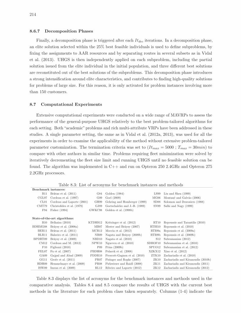
214

8.6.7 Decomposition Phases

Finally, a decomposition phase is triggered after each Itdec iterations. In a decomposition phase,

an elite solution selected within the 25% best feasible individuals is used to define subproblems, by

fixing the assignments to AAR resources and by separating routes in several subsets as in Vidal

et al. (2013). UHGS is then independently applied on each subproblem, including the partial

solution issued from the elite individual in the initial population, and three different best solutions

are reconstituted out of the best solutions of the subproblems. This decomposition phase introduces

a strong intensification around elite characteristics, and contributes to finding high-quality solutions

for problems of large size. For this reason, it is only activated for problem instances involving more

than 150 customers.


Extensive computational experiments were conducted on a wide range of MAVRPs to assess the

performance of the general-purpose UHGS relatively to the best problem-tailored algorithms for

each setting. Both“academic”problems and rich multi-attribute VRPs have been addressed in these

studies. A single parameter setting, the same as in Vidal et al. (2012a, 2013), was used for all the

experiments in order to examine the applicability of the method without extensive problem-tailored

parameter customization. The termination criteria was set to (Itmax = 5000 ; Tmax = 30min) to

compare with other authors in similar time. Problems requiring fleet minimization were solved by

iteratively decrementing the fleet size limit and running UHGS until no feasible solution can be

found. The algorithm was implemented in C++ and run on Opteron 250 2.4GHz and Opteron 275

2.2GHz processors.

Table 8.3: List of acronyms for benchmark instances and methodsBenchmark instances:

B11 Bektas et al. (2011) G84 Golden (1984) LS99 Liu and Shen (1999)

CGL97 Cordeau et al. (1997) G09 Goel (2009) MG06 Montane and Galvao (2006)

CL01 Cordeau and Laporte (2001) GH99 Gehring and Homberger (1999) SD88 Solomon and Desrosiers (1988)

CMT79 Christofides et al. (1979) GJ89 Goetschalckx and J.-B. (1989) SN99 Salhi and Nagy (1999)

F94 Fisher (1994) GWKC98 Golden et al. (1998b)

State-of-the-art algorithms:

B10 Belhaiza (2010) KTDHS12 Kritzinger et al. (2012) RT10 Repoussis and Tarantilis (2010)

BDHMG08 Braysy et al. (2008a) MB07 Mester and Braysy (2007) RTBI10 Repoussis et al. (2010)

BER11 Bektas et al. (2011) MCR12 Moccia et al. (2012) RTI09a Repoussis et al. (2009a)

BLR11 Balseiro et al. (2011) NB09 Nagata and Braysy (2009b) RTI09b Repoussis et al. (2009b)

BPDRT09 Braysy et al. (2009) NBD10 Nagata et al. (2010) S12 Subramanian (2012)

CM12 Cordeau and M. (2012) NPW10 Ngueveu et al. (2010) SDBOF10 Subramanian et al. (2010)

F10 Figliozzi (2010) P09 Prins (2009b) SPUO12 Subramanian et al. (2012)

FEL07 Fu et al. (2007) PBDH08 Polacek et al. (2008) XZKX12 Xiao et al. (2012)

GA09 Gajpal and Abad (2009) PDDR10 Prescott-Gagnon et al. (2010) ZTK10 Zachariadis et al. (2010)

GG11 Groer et al. (2011) PR07 Pisinger and Ropke (2007) ZK10 Zachariadis and Kiranoudis (2010b)

HDH09 Hemmelmayr et al. (2009) PR08 Pirkwieser and Raidl (2008) ZK11 Zachariadis and Kiranoudis (2011)

ISW09 Imran et al. (2009) RL12 Ribeiro and Laporte (2012) ZK12 Zachariadis and Kiranoudis (2012)

Table 8.3 displays the list of acronyms for the benchmark instances and methods used in the

comparative analysis. Tables 8.4 and 8.5 compare the results of UHGS with the current best

methods in the literature for each problem class taken separately. Columns (1-4) indicate the

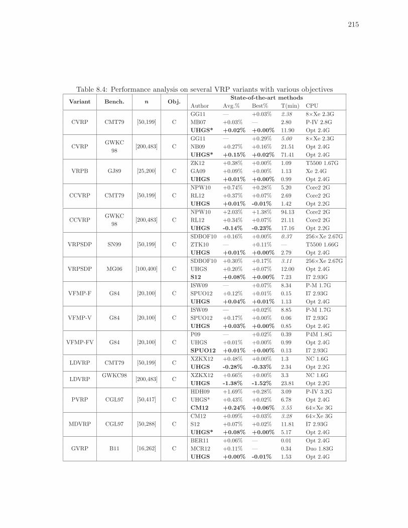
215

Table 8.4: Performance analysis on several VRP variants with various objectives

Variant Bench. n Obj.State-of-the-art methods

Author Avg.% Best% T(min) CPU

CVRP CMT79 [50,199] C

GG11 — +0.03% 2.38 8×Xe 2.3G

MB07 +0.03% — 2.80 P-IV 2.8G

UHGS* +0.02% +0.00% 11.90 Opt 2.4G

CVRPGWKC

[200,483] C

GG11 — +0.29% 5.00 8×Xe 2.3G

98NB09 +0.27% +0.16% 21.51 Opt 2.4G

UHGS* +0.15% +0.02% 71.41 Opt 2.4G

VRPB GJ89 [25,200] C

ZK12 +0.38% +0.00% 1.09 T5500 1.67G

GA09 +0.09% +0.00% 1.13 Xe 2.4G

UHGS +0.01% +0.00% 0.99 Opt 2.4G

CCVRP CMT79 [50,199] C

NPW10 +0.74% +0.28% 5.20 Core2 2G

RL12 +0.37% +0.07% 2.69 Core2 2G

UHGS +0.01% -0.01% 1.42 Opt 2.2G

CCVRPGWKC

[200,483] C

NPW10 +2.03% +1.38% 94.13 Core2 2G

98RL12 +0.34% +0.07% 21.11 Core2 2G

UHGS -0.14% -0.23% 17.16 Opt 2.2G

VRPSDP SN99 [50,199] C

SDBOF10 +0.16% +0.00% 0.37 256×Xe 2.67G

ZTK10 — +0.11% — T5500 1.66G

UHGS +0.01% +0.00% 2.79 Opt 2.4G

VRPSDP MG06 [100,400] C

SDBOF10 +0.30% +0.17% 3.11 256×Xe 2.67G

UHGS +0.20% +0.07% 12.00 Opt 2.4G

S12 +0.08% +0.00% 7.23 I7 2.93G

VFMP-F G84 [20,100] C

ISW09 — +0.07% 8.34 P-M 1.7G

SPUO12 +0.12% +0.01% 0.15 I7 2.93G

UHGS +0.04% +0.01% 1.13 Opt 2.4G

VFMP-V G84 [20,100] C

ISW09 — +0.02% 8.85 P-M 1.7G

SPUO12 +0.17% +0.00% 0.06 I7 2.93G

UHGS +0.03% +0.00% 0.85 Opt 2.4G

VFMP-FV G84 [20,100] C

P09 — +0.02% 0.39 P4M 1.8G

UHGS +0.01% +0.00% 0.99 Opt 2.4G

SPUO12 +0.01% +0.00% 0.13 I7 2.93G

LDVRP CMT79 [50,199] CXZKX12 +0.48% +0.00% 1.3 NC 1.6G

UHGS -0.28% -0.33% 2.34 Opt 2.2G

LDVRPGWKC98

[200,483] CXZKX12 +0.66% +0.00% 3.3 NC 1.6G

UHGS -1.38% -1.52% 23.81 Opt 2.2G

PVRP CGL97 [50,417] C

HDH09 +1.69% +0.28% 3.09 P-IV 3.2G

UHGS* +0.43% +0.02% 6.78 Opt 2.4G

CM12 +0.24% +0.06% 3.55 64×Xe 3G

MDVRP CGL97 [50,288] C

CM12 +0.09% +0.03% 3.28 64×Xe 3G

S12 +0.07% +0.02% 11.81 I7 2.93G

UHGS* +0.08% +0.00% 5.17 Opt 2.4G

GVRP B11 [16,262] C

BER11 +0.06% — 0.01 Opt 2.4G

MCR12 +0.11% — 0.34 Duo 1.83G

UHGS +0.00% -0.01% 1.53 Opt 2.4G

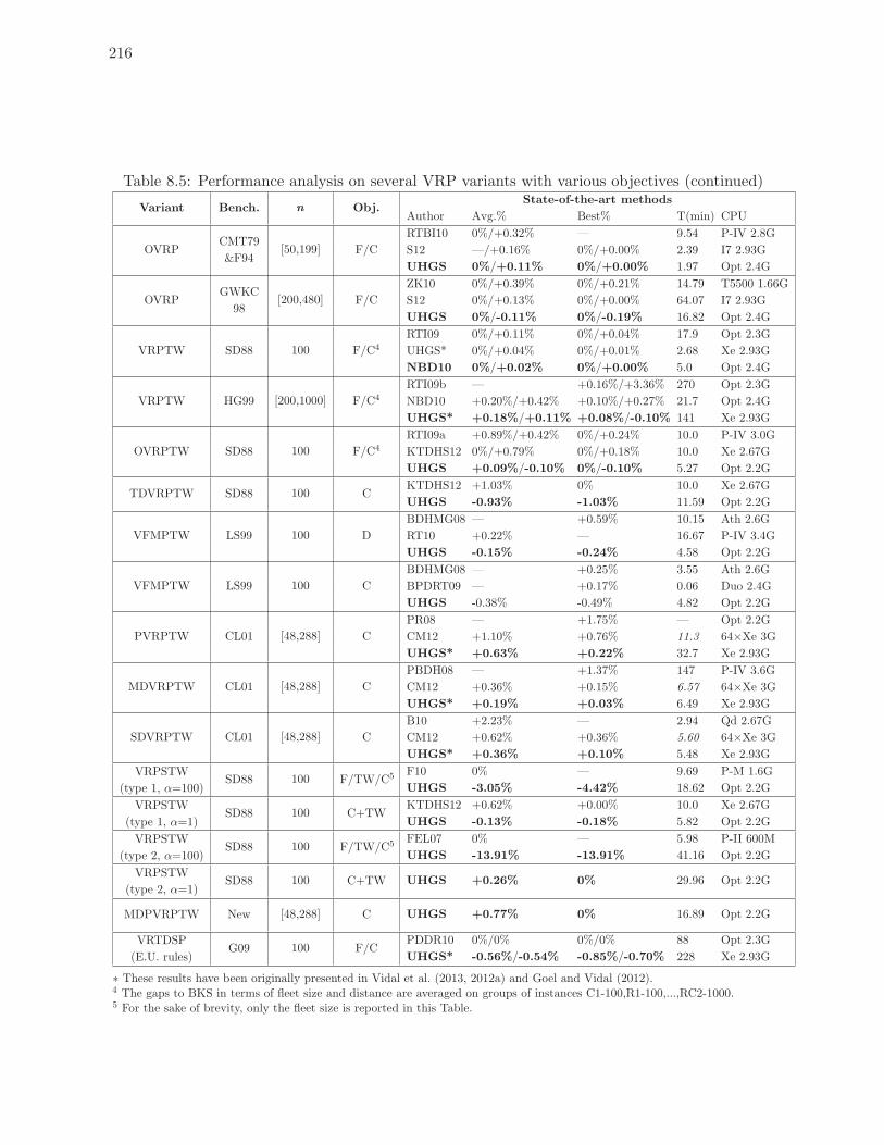
216

Table 8.5: Performance analysis on several VRP variants with various objectives (continued)

Variant Bench. n Obj.State-of-the-art methods

Author Avg.% Best% T(min) CPU

OVRPCMT79

[50,199] F/C

RTBI10 0%/+0.32% — 9.54 P-IV 2.8G

&F94S12 —/+0.16% 0%/+0.00% 2.39 I7 2.93G

UHGS 0%/+0.11% 0%/+0.00% 1.97 Opt 2.4G

OVRPGWKC

[200,480] F/C

ZK10 0%/+0.39% 0%/+0.21% 14.79 T5500 1.66G

98S12 0%/+0.13% 0%/+0.00% 64.07 I7 2.93G

UHGS 0%/-0.11% 0%/-0.19% 16.82 Opt 2.4G

VRPTW SD88 100 F/C4

RTI09 0%/+0.11% 0%/+0.04% 17.9 Opt 2.3G

UHGS* 0%/+0.04% 0%/+0.01% 2.68 Xe 2.93G

NBD10 0%/+0.02% 0%/+0.00% 5.0 Opt 2.4G

VRPTW HG99 [200,1000] F/C4

RTI09b — +0.16%/+3.36% 270 Opt 2.3G

NBD10 +0.20%/+0.42% +0.10%/+0.27% 21.7 Opt 2.4G

UHGS* +0.18%/+0.11% +0.08%/-0.10% 141 Xe 2.93G

OVRPTW SD88 100 F/C4

RTI09a +0.89%/+0.42% 0%/+0.24% 10.0 P-IV 3.0G

KTDHS12 0%/+0.79% 0%/+0.18% 10.0 Xe 2.67G

UHGS +0.09%/-0.10% 0%/-0.10% 5.27 Opt 2.2G

TDVRPTW SD88 100 CKTDHS12 +1.03% 0% 10.0 Xe 2.67G

UHGS -0.93% -1.03% 11.59 Opt 2.2G

VFMPTW LS99 100 D

BDHMG08 — +0.59% 10.15 Ath 2.6G

RT10 +0.22% — 16.67 P-IV 3.4G

UHGS -0.15% -0.24% 4.58 Opt 2.2G

VFMPTW LS99 100 C

BDHMG08 — +0.25% 3.55 Ath 2.6G

BPDRT09 — +0.17% 0.06 Duo 2.4G

UHGS -0.38% -0.49% 4.82 Opt 2.2G

PVRPTW CL01 [48,288] C

PR08 — +1.75% — Opt 2.2G

CM12 +1.10% +0.76% 11.3 64×Xe 3G

UHGS* +0.63% +0.22% 32.7 Xe 2.93G

MDVRPTW CL01 [48,288] C

PBDH08 — +1.37% 147 P-IV 3.6G

CM12 +0.36% +0.15% 6.57 64×Xe 3G

UHGS* +0.19% +0.03% 6.49 Xe 2.93G

SDVRPTW CL01 [48,288] C

B10 +2.23% — 2.94 Qd 2.67G

CM12 +0.62% +0.36% 5.60 64×Xe 3G

UHGS* +0.36% +0.10% 5.48 Xe 2.93G

VRPSTWSD88 100 F/TW/C5 F10 0% — 9.69 P-M 1.6G

(type 1, α=100) UHGS -3.05% -4.42% 18.62 Opt 2.2G

VRPSTWSD88 100 C+TW

KTDHS12 +0.62% +0.00% 10.0 Xe 2.67G

(type 1, α=1) UHGS -0.13% -0.18% 5.82 Opt 2.2G

VRPSTWSD88 100 F/TW/C5 FEL07 0% — 5.98 P-II 600M

(type 2, α=100) UHGS -13.91% -13.91% 41.16 Opt 2.2G

VRPSTWSD88 100 C+TW UHGS +0.26% 0% 29.96 Opt 2.2G

(type 2, α=1)

MDPVRPTW New [48,288] C UHGS +0.77% 0% 16.89 Opt 2.2G

VRTDSPG09 100 F/C

PDDR10 0%/0% 0%/0% 88 Opt 2.3G

(E.U. rules) UHGS* -0.56%/-0.54% -0.85%/-0.70% 228 Xe 2.93G

∗ These results have been originally presented in Vidal et al. (2013, 2012a) and Goel and Vidal (2012).4 The gaps to BKS in terms of fleet size and distance are averaged on groups of instances C1-100,R1-100,...,RC2-1000.5 For the sake of brevity, only the fleet size is reported in this Table.

217

variant considered, the origin of the benchmark instances, the number n of customers in these

instances, and the objective function (“C” standing for distance, “D” for duration, i.e., the time

elapsed between departure and return, “T” for travel time, “F” for fleet size, “TW” for time-window

violations). Hierarchical objectives are presented by decreasing order of priority, separated with

the sign “/”. The last column reports, for each state-of-the-art method, the gap of an average or

single run with respect to the current Best Known Solutions (BKS), the gap of the best solution

produced by the method, the average run time to achieve these results (for parallel methods, the

computation time on a single CPU is reported in italics as well as the number of CPUs), and

the type of processor used. The algorithm yielding the best result quality, for each benchmark

instances set and problem class, is indicated in boldface. Table 8.4 also includes the results from

previous HGSADC applications on the PVRP, MDVRP, CVRP, and VRTDSP with European

Union regulations (Vidal et al. 2013, 2012a, Goel and Vidal 2012) since UHGS works identically

when instantiated on these problems. Detailed results are reported in Appendix V.

As reported in Tables 8.4 and 8.5, UHGS produces high-quality solutions for all problems and

benchmark sets, from pure academic problems such as the CVRP to a large variety of VRP variants

and rich settings. In addition to its high generality and its potential to address many MAVRPs,

UHGS matches or outperforms the wide majority of problem-tailored approaches on each separate

benchmark and problem class. The average standard deviation of solutions, measured separately

for each single objective problem, ranges between 0.002% (GVRP) and 0.66% (MDPVRPTW),

thus showing that the metaheuristic produces high-quality solutions in a consistent manner. The

average run time remains in most cases smaller than 10 minutes for average-sized problems (100 to

200 customers), being thus adequate for daily or weekly planning. Overall, 954 BKS out of 1008

have been either retrieved or improved during these experiments, and 550 BKS out of 1008 have

been strictly improved.

8.8 Conclusions and Perspectives

A new unified local search and a Unified Hybrid Genetic Search (UHGS) relying on a component-

based design have been introduced to address a large variety of difficult VRP variants. The methods

rely on adaptive assignment, sequencing, and route-evaluation components to address problem

specifics. These components serve as the basis to generate generic local-search improvement, Split,

and genetic operators. Furthermore, the use of individual fitness measures based on both diversity

and quality, and advanced population management schemes provides the means for a thorough

and efficient search. The remarkable performance of UHGS has been demonstrated on a wide

range of problems. On 26 VRP variants and 39 sets of benchmark instances, UHGS matches or

outperforms the current state-of-the-art problem-tailored algorithms. Overall, 954 of the 1008

best known solutions have been either retrieved or improved. Hence, it appears that the proposed

heuristic design is particularly efficient for dealing with MAVRPs and, furthermore, that generality

does not necessarily play against performance for the considered classes of VRP variants.

This general-purpose solver opens the way to experimentations and sensitivity analyses of

local search and metaheuristic components on a wide range of structurally different problems.

218

Perspectives of research involve the generalization of the method towards a wider variety of

ASSIGN and SEQ attributes, multi-objective and stochastic settings. Further methodological

analyses should also be conducted to fully identify the compatibility relationships and complexity

implications of attribute combinations.

CHAPITRE 9

UNE APPROCHE PARALLELE COOPERATIVE A BASE DE

DECOMPOSITION ET INTEGRATION POUR LES PROBLEMES DE

TOURNEES DE VEHICULES MULTI-ATTRIBUTS


Finalement, pour gerer efficacement non seulement la variete mais aussi la difficulte inherente

aux combinaisons des attributs, et afin de progresser plus en avant vers la resolution de VRP

riches contenant plusieurs types d’attributs decisionnels, les meta-heuristiques precedentes ont

ete etendues au sein d’un cadre de resolution parallele cooperative a base de decomposition

et recompositions successives de solutions, appele Integrative Cooperative Search (ICS). L’idee

fondamentale de ICS est de combiner les idees de decomposition, simplification intelligente et

opportuniste, et de recherche cooperative. Le mecanisme de decomposition vise a generer des

problemes avec un nombre d’attributs reduits, pour lequel des methodes de resolution efficaces,

comme UHGS, peuvent etre utilisees aux mieux de leurs capacites. Les solutions issues de ces

problemes plus simples sont integrees au sein d’une cadre de recherche cooperatif pour traiter le

probleme initial. Cette application permet de produire des solutions de plus grande qualite sur

les problemes traites auparavant, et souleve plusieurs considerations methodologiques impliquant

notamment la reconstitution de solutions completes a partir de solutions partielles, et l’exploitation

efficace de memoires pour guider la recherche future.

9.2 Article IX : Integrative Cooperative Search for Multi-Attribute Vehicle Routing

Problems

La methodologie ICS a fait l’objet d’un article commun soumis pour publication :

Lahrichi, N., Crainic, T.G., Gendreau, M., Rei, W., Crisan, G.C., Vidal, T. (2012).

An Integrative Cooperative Search Framework for Multi-Decision-Attribute Combi-

natorial Optimization. INFORMS Journal on Computing, submitted for publication.

Plusieurs co-auteurs ont contribue dans ce travail. Mon role a ete d’appliquer le

concept ICS aux VRP riches, en proposant et experimentant des choix de solvers

partiels, de modes de communication, de methodes d’integration et de guidage effi-

caces pour ces problemes.

Abstract: We introduce the Integrative Cooperative Search (ICS), a multi-thread cooperative

search method for multi-attribute combinatorial optimization problems. ICS musters the combined

capabilities of a number of independent exact or meta-heuristic solution methods. A number of

these methods work on sub-problems defined by suitably selected subsets of decision-set attributes of

the problem, while others combine the resulting partial solutions into complete ones and, eventually,

improve them. All these methods cooperate through an adaptive search-guidance mechanism, using

220

the central-memory cooperative search paradigm. Extensive numerical experiments explore the

behavior of ICS and how the interest of the method through an application to the multi-depot,

periodic vehicle routing problem, for which ICS improves the results of the current state-of-the-art

methods.

Keywords: Multi-attribute combinatorial optimization, integrative cooperative search, meta-

heuristics, decision-set decomposition, multi-depot, periodic vehicle routing

9.3 Introduction

Combinatorial optimization problems prominently appear in many theoretical and real-life

settings. A large number of methodological developments targeted these problems proposing exact,

heuristic, and meta-heuristic solution methods. Parallel computing enhanced these optimization

methods providing the means to accelerate the resolution process and, for meta-heuristics, to obtain

higher-quality solutions for a broad range of problems (Crainic and Nourredine 2005, Crainic and

Toulouse 2010).

Yet, although solution methods become more powerful, the combinatorial problems one faces

grow continuously in size and difficulty, as defined by the number of interacting characteristics

defining their feasibility structures and optimality criteria. Such increasingly larger sets of charac-

teristics severely challenge our methodological capability to efficiently address the corresponding

problem settings. Thus, the general approach when addressing such multi-attribute, also informally

known as rich, problem settings is to either simplify them, or to sequentially solve a series of

restricted ones where part of the overall problem might be fixed, ignored, or both (Section 9.4

further discusses the issue).

It is well-known, however, that such approaches lead to sub-optimal solutions. Moreover, one

observes in many application settings, including vehicle routing, network design, and carrier service

network design, the need to comprehensively address the associated combinatorial optimization

formulations to simultaneously account for “all” relevant attributes. The current literature does

not offer a satisfactory answer to this challenge in terms of methods able to efficiently address

multi-attribute problem settings and provide good solutions. The goal of this paper is to contribute

toward addressing this challenge.

We focus on decision-based characteristics, or decision-set attributes, i.e., the sets of decisions

defining the particular problem setting, and introduce the Integrative Cooperative Search (ICS ), a

multi-thread cooperative search method for multi-attribute combinatorial optimization problems.

ICS musters the combined capabilities of a number of independent solution methods, exact or

meta-heuristic. A number of these methods work on sub-problems defined by suitably selected

subsets of decision-set attributes of the problem, while others combine the resulting partial solutions

into complete ones and, eventually, improve them. These methods cooperate through an adaptive

search-guidance mechanism, using the central-memory cooperative search paradigm. Our goal is to

present and discuss the ICS concept, its structure, main building blocks, and operating principles,

as well as to present a proof-of-concept of its efficiency.

221

The main contributions of this paper are to: 1) Introduce and formally describe a new meta-

heuristic solution framework for multi-attribute combinatorial optimization problems; ICS is general,

flexible, and scalable in the number of attributes defining the problem at hand; 2) Define and exploit

a functional decomposition of such problems along decisional attributes; 3) Show the interest of

ICS through an application to a well-known multi-attribute case, the multi-depot, periodic vehicle

routing problem (MDPVRP), for which ICS improves the results of the current state-of-the-art

methods, and discuss how to apply the methodology to other combinatorial optimization problem

classes; 4) Experimentally examine the role and impact of various ICS components.

This paper is organized as follows. Section 9.4 discusses the motivation for our work, and

identifies the sources of inspiration for the methodology we propose. Section 9.5 introduces the

fundamental concepts underlining the Integrative Cooperative Search methodology, particularly

the decision-set attribute-based decomposition and the ICS algorithmic structure. We illustrate

these concepts and methods through an application to the MDPVRP in Section 9.6. Extensive

experiments are presented and discussed in Section 9.7. We finally conclude.

9.4 Motivation and Inspiration

We aim to address extended versions of classical combinatorial-optimization problems, which

are NP-hard in their basic forms. When real-world cases are considered, “new” characteristics have

to be considered while searching for feasible solutions of high quality. These characteristics take

usually the form of a broad set of conditions defining the solution feasibility or optimality, or both,

and may generally be represented through sets of decision variables. The resulting set of decisions

is then much broader than for the classical problem settings usually found in the literature, each

new group of decisions compounding the difficulty of the problem and complicating the solution

process, particularly when one aims to address them simultaneously.

Two examples to illustrate, selected from two major problem classes of significant methodological

interest and widely encountered in actual applications. Network design aims to select among a set

of possible facilities on arcs, nodes, or both, such that the demand for utilization of the resulting

network is satisfied at minimum total cost accounting for the cost of both selecting the facilities

and using the network. Many particular design and location-decision problem settings have been

defined during the years, the vast majority focusing on the facility-selection and demand-flow

decisions (Magnanti and Wong 1984, Grotschel et al. 1995, Drezner and Hamacher 2004, Crainic

2000). Crainic et al. (2006) describe a realistic setting of a wireless network design problem, where

the decision set includes not only decisions of the selection of base stations to cover a given territory,

but also on selecting the number of antennae for each of these, as well as their height, power, tilt,

and orientation.

A similar richness of attributes may be increasingly observed in the vehicle routing field (where

the “rich” qualification was first linked to a VRP setting; Hartl et al. 2006). There exists an

extensive literature on the Capacitated Vehicle Routing Problem (CVRP), which aims to construct

cost-efficient routes to deliver the demand of a given set of customers with a fleet of vehicles of

limited capacity operating out of a unique depot (Toth and Vigo 2002a, Golden et al. 2008). An

222

even greater volume of contributions address extensions of the CVRP reflecting the extreme variety

of actual applications, including but not limited to multiple depots, vehicle fleets, or commodities,

customer requirements for multi-period visits or within-period time windows, route restrictions on

total distance or time, and so on and so forth (Vidal et al. 2012c). Several of these generalizations

yielded problem classes of their own, the Vehicle Routing Problem with Time Windows (VRPTW)

being probably the most well known of these.

Most generalizations found in the literature either add decisional features, e.g., selecting the

number of antennae in addition of the location and number of stations in the wireless network

design problem, or are concerned with adding characteristics to particular problem elements, e.g.,

the timing concerns in the VRPTW sequence of customer visits. While not making problems easier,

the latter type of generalization may be addressed within particular algorithmic components, e.g.,

route generation and sequencing. Adding an extra characteristic to the definition of this group of

problem elements might require a more involved algorithmic component (Vidal et al. 2011), but

does not change fundamentally the nature of the problem.

Adding more decision sets to the problem, on the other hand, makes it significantly harder to

address and, thus, the general approach when addressing such multi-attribute problems is to either

simplify them, or to sequentially solve a series of particular cases, where part of the overall problem

is fixed or ignored, or both (e.g. Golden et al. 2002, Hadjiconstantinou and Baldacci 1998, Hartl

et al. 2006, Homberger and Gehring 1999, 2005). It is well-known that this leads to sub-optimal

solutions. Moreover, one observes in many application settings, including vehicle routing, network

design, and carrier service network design, the need to comprehensively address the corresponding

combinatorial formulation accounting for “all” relevant decision-set attributes simultaneously.

Among the few exceptions to the state of the literature described above, we single out the

Multi-Depot Periodic VRP (MDPVRP) problem class, with or without time windows, encompassing

decisions on selecting patterns of multi-period visits for customers, as well as on assigning each

customer to a depot for each of its selected visits. This multi-decision-set problem was considered

until quite recently as difficult to address as a whole. New exact (Baldacci and Mingozzi 2009,

Baldacci et al. 2011a) and meta-heuristic (Vidal et al. 2012a) contributions have re-defined the state-

of-the-art for this class of problems. We have selected the MDPVRP to illustrate the performance

of the methodology we propose to take advantage of this new set of best-known solutions (BKS).

So, how to proceed to build a method, which is general, scalable, and efficient, to address

multi-attribute combinatorial optimization problems in a comprehensive manner? We were inspired

by three major methodological concepts, decomposition, simplification, and cooperative search.

Decomposition is a fundamental technique in mathematical programming and parallel/distributed

computing. Proceeding through various strategies, e.g., projection and relaxation in mathematical

programming, its main objective is to transform a difficult-to-address formulation into a number

of much simpler ones. All such methods encompass three main mechanisms. The first defines

how the problem is transformed and how derived sub-problems are specified. The second spec-

ifies the information exchanged among the sub-problems. The third brings together the results

obtained working on the sub-problems to create complete solutions to the original problem and,

eventually, continues the decomposition-based algorithm. A so-called master problem (actually,

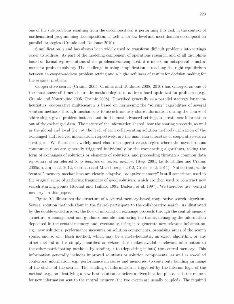
223

one of the sub-problems resulting from the decomposition) is performing this task in the context of

mathematical-programming decomposition, as well as for low-level and most domain-decomposition

parallel strategies (Crainic and Toulouse 2010).

Simplification is and has always been widely used to transform difficult problems into settings

easier to address. As part of the modeling component of operations research, and of all disciplines

based on formal representations of the problems contemplated, it is indeed an indispensable instru-

ment for problem solving. The challenge in using simplification is reaching the right equilibrium

between an easy-to-address problem setting and a high-usefulness of results for decision making for

the original problem.

Cooperative search (Crainic 2005, Crainic and Toulouse 2008, 2010) has emerged as one of

the most successful meta-heuristic methodologies to address hard optimization problems (e.g.,

Crainic and Nourredine 2005, Crainic 2008). Described generally as a parallel strategy for meta-

heuristics, cooperative multi-search is based on harnessing the “solving” capabilities of several

solution methods through mechanisms to asynchronously share information during the course of

addressing a given problem instance and, in the most advanced settings, to create new information

out of the exchanged data. The nature of the information shared, how the sharing proceeds, as well

as the global and local (i.e., at the level of each collaborating solution method) utilization of the

exchanged and received information, respectively, are the main characteristics of cooperative-search

strategies. We focus on a widely-used class of cooperative strategies where the asynchronous

communications are generally triggered individually by the cooperating algorithms, taking the

form of exchanges of solutions or elements of solutions, and proceeding through a common data

repository, often referred to as adaptive or central memory (Rego 2001, Le Bouthillier and Crainic

2005a,b, Jin et al. 2012, Cordeau and Maischberger 2012, Groer et al. 2011). Notice that, while

“central”-memory mechanisms are clearly adaptive, “adaptive memory” is still sometimes used in

the original sense of gathering fragments of good solutions, which are then used to construct new

search starting points (Rochat and Taillard 1995, Badeau et al. 1997). We therefore use “central

memory” in this paper.

Figure 9.1 illustrates the structure of a central-memory-based cooperative search algorithm.

Several solution methods (four in the figure) participate to the collaborative search. As illustrated

by the double-ended arrows, the flow of information exchange proceeds through the central-memory

structure, a management-and-guidance module monitoring the traffic, managing the information

deposited in the central memory and, eventually, using it to generate new relevant information,

e.g., new solutions, performance measures on solution components, promising areas of the search

space, and so on. Each method, which may be a meta-heuristic, an exact algorithm, or any

other method and is simply identified as solver, thus makes available relevant information to

the other participating methods by sending it to (depositing it into) the central memory. This

information generally includes improved solutions or solution components, as well as so-called

contextual information, e.g., performance measures and memories, to contribute building an image

of the status of the search. The sending of information is triggered by the internal logic of the

method, e.g., on identifying a new best solution or before a diversification phase, as is the request

for new information sent to the central memory (the two events are usually coupled). The required

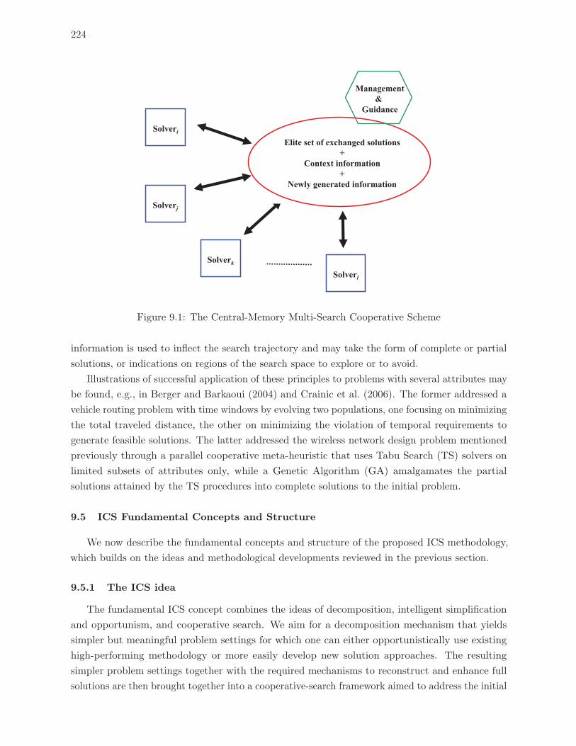
224

Solveri

Solverk

Elite set of exchanged solutions +

Context information +

Newly generated information

Solverj

Solverl

Management &

Guidance

Figure 9.1: The Central-Memory Multi-Search Cooperative Scheme

information is used to inflect the search trajectory and may take the form of complete or partial

solutions, or indications on regions of the search space to explore or to avoid.

Illustrations of successful application of these principles to problems with several attributes may

be found, e.g., in Berger and Barkaoui (2004) and Crainic et al. (2006). The former addressed a

vehicle routing problem with time windows by evolving two populations, one focusing on minimizing

the total traveled distance, the other on minimizing the violation of temporal requirements to

generate feasible solutions. The latter addressed the wireless network design problem mentioned

previously through a parallel cooperative meta-heuristic that uses Tabu Search (TS) solvers on

limited subsets of attributes only, while a Genetic Algorithm (GA) amalgamates the partial

solutions attained by the TS procedures into complete solutions to the initial problem.

9.5 ICS Fundamental Concepts and Structure

We now describe the fundamental concepts and structure of the proposed ICS methodology,

which builds on the ideas and methodological developments reviewed in the previous section.

9.5.1 The ICS idea

The fundamental ICS concept combines the ideas of decomposition, intelligent simplification

and opportunism, and cooperative search. We aim for a decomposition mechanism that yields

simpler but meaningful problem settings for which one can either opportunistically use existing

high-performing methodology or more easily develop new solution approaches. The resulting

simpler problem settings together with the required mechanisms to reconstruct and enhance full

solutions are then brought together into a cooperative-search framework aimed to address the initial

225

formulation. Figure 9.2 illustrates the main elements of the methodology and their interconnection

links.

Original problem Complete solvers

Complete solution set

Partial problems Partial solvers

Partial solution sets

DECOMPOSITION

GUIDANCE

SHARING CONTEXT DATA

Integration solvers

INTEGRATION

Figure 9.2: The ICS Methodology Idea

Decomposition is the first item that needs to be addressed, in particular, the problem dimensions

along which it is to be applied and the mechanisms to reconstruct complete solutions to the initial

problem. Given our objective of opportunist simplification for an intelligent use within a cooperative-

search framework, we propose a structural problem decomposition along sets of decisions variables.

Let x ∈ X be the set of decision variables of the problem at hand, and let δ be a set of indices

identifying a particular subset of x. The decision-set attribute decomposition then identifies |Δ|sets of decision variables, and defines a partial-problem formulation Πδ(xδ) for each decision set

xδ, δ ∈ Δ, by fixing the corresponding variables to suitably selected values xδ (and appropriately

adjusted constraints, if needed). Notice that this definition of decomposition does not change the

dimensionality of the partial problems with respect to that of the original setting. Actually, any

solution to any partial problem constructed according to this definition may be considered for the

complete formulation.

The selection of the decision sets is specific to each application case. Thus, in particular, defining

Δ according to spatio-temporal characteristics of the problem elements (e.g., node coordinates

in a space-time network representation) yields the well known data-decomposition procedure

used in a number of parallel and sequential solution methods. The choice for ICS is governed

by the objective of opportunistic simplification indicated above and, thus, decision variables are

clustered to yield known or identifiable optimization problem settings. Thus, for example, fixing

the customer-to-depot assignments in the MDPVRP illustration of Section 9.6 yields a PVRP,

while fixing the patterns for all customers yields a MDVRP.

Notice that the proposed decomposition does not require the sets δ ∈ Δ to induce a partition

of the feasible domain. Furthermore, with respect to the mathematical programming literature,

the decision-set decomposition may be viewed as a multiple simultaneous projection (Geoffrion

1970a,b) performed through variable fixing. Further notice that there is no a priori limit on the

number of sets. Actually, the decomposition process should aim for a “best” compromise between

226

the ease of addressing each partial problem and the difficulty in building complete solutions to the

original problem from the solutions to the partial problems.

Indeed, decomposition very often needs to be coupled with integration providing an efficient way

to use the solutions obtained by addressing the partial problems to build a complete solution to the

initial formulation. This functionality makes up the second main element of the ICS methodology.

Integration is generally not an easy task, however. Integration solvers need to address three,

possibly contradictory, challenges: 1) solution quality, 2) transmission of critical features (which

may be incompatible) from the partial solutions, and 3) computational efficiency. Thus, the simple

integrator consisting in transferring directly to the complete-solution set a solution (feasible or not)

to a partial problem achieves the latter but fails in most cases to achieve the first two goals. Even

when this simple integrator achieves solution quality, it is generally due to a good partial solution

and not through combining, and respecting critical features of, several partial solutions, as often

required by decomposition schemes. More advanced methods are thus required and evolutionary

methods, genetic algorithms and path relinking, in particular, have proved their flexibility and

stability in combining solution characteristics to yield high-quality solutions, often at the price of

higher computational efforts. A formal definition of integration problems for meta-heuristics is

provided by Crainic et al. (2012).

We complete the ICS concept with a third main element, a purposeful-evolution mechanism

geared to produce high-quality complete solutions while avoiding a heavy-handed control of the

process (which has been shown to be unproductive for most meta-heuristics). We build upon

the central-memory cooperative search meta-heuristic paradigm presented above, integrating a

dynamically adaptive guidance mechanism based on monitoring the activities of the partial solvers,

the partial and complete solutions produced, and the context information shared by the solvers.

The ICS methodology, its structure, elements, and operational mechanisms are detailed next.

9.5.2 The ICS Method

ICS implements the decision-set attribute decomposition described in the previous section, and

takes the form of a self-adaptive cooperative meta-heuristic concurrently evolving and combining

several populations, one corresponding to solutions to the original problem, each of the others

addressing specific dimensions of the problem resulting from the decision-set attributes used to

decompose the problem.

Figure 9.3 illustrates the structure and components of ICS as inspired by the central-memory

cooperative search meta-heuristic paradigm. Following the initial decomposition of the original

problem into partial problems through decision-variable fixing as defined previously, each partial

problem is addressed by one or several solution methods within a Partial Solver Group (PSG),

two of which are illustrated in Figure 9.3. Concurrently with PSG activities, integrators select

partial solutions from PSGs (represented by full arrows in the figure), combine them to create

complete ones, which are then sent (short slashed arrow) to the Complete Solver Group (CSG).

(All solutions are “complete” in our setting; we use the terms “partial” and “complete” solution,

however, to indicate the solver group of origin.) The latter could enhance these solutions, when

appropriate solvers are available, but its main task is to extract out of the complete-solution set

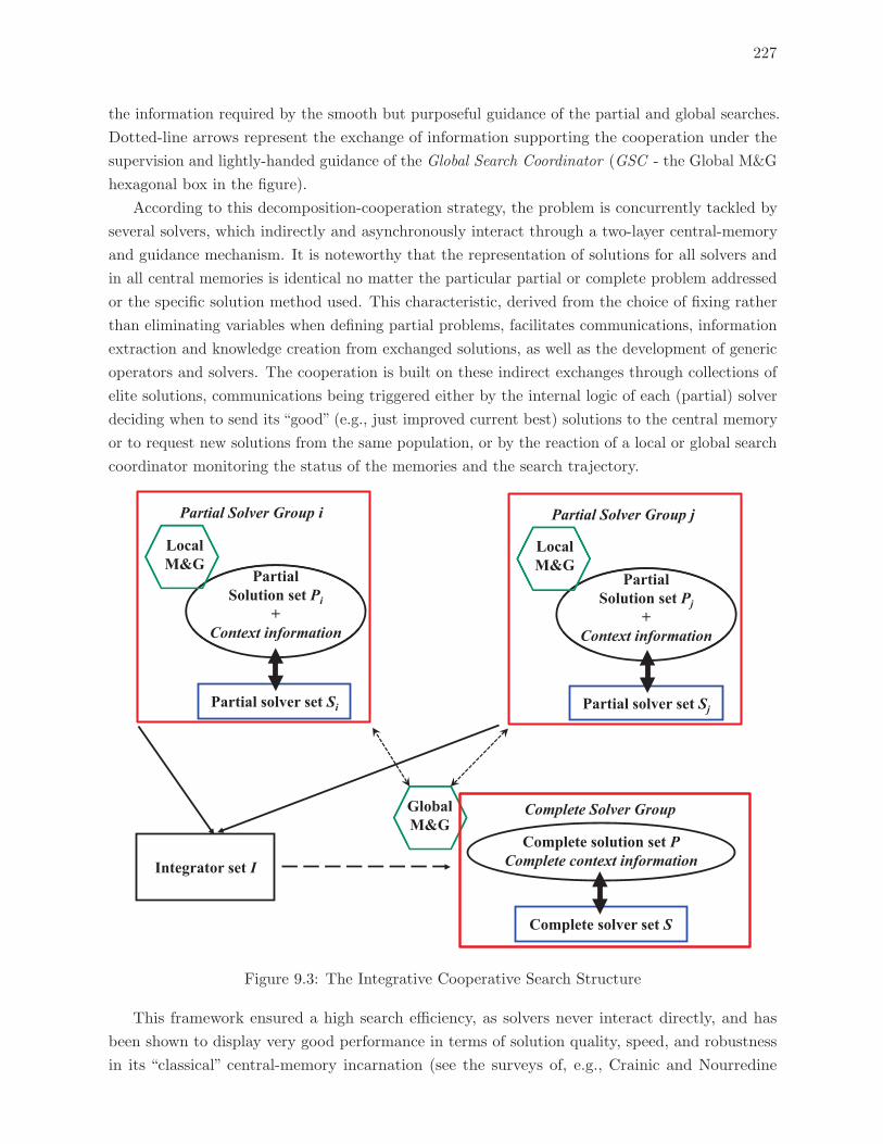
227

the information required by the smooth but purposeful guidance of the partial and global searches.

Dotted-line arrows represent the exchange of information supporting the cooperation under the

supervision and lightly-handed guidance of the Global Search Coordinator (GSC - the Global M&G

hexagonal box in the figure).

According to this decomposition-cooperation strategy, the problem is concurrently tackled by

several solvers, which indirectly and asynchronously interact through a two-layer central-memory

and guidance mechanism. It is noteworthy that the representation of solutions for all solvers and

in all central memories is identical no matter the particular partial or complete problem addressed

or the specific solution method used. This characteristic, derived from the choice of fixing rather

than eliminating variables when defining partial problems, facilitates communications, information

extraction and knowledge creation from exchanged solutions, as well as the development of generic

operators and solvers. The cooperation is built on these indirect exchanges through collections of

elite solutions, communications being triggered either by the internal logic of each (partial) solver

deciding when to send its “good” (e.g., just improved current best) solutions to the central memory

or to request new solutions from the same population, or by the reaction of a local or global search

coordinator monitoring the status of the memories and the search trajectory.

Partial Solution set Pj

+Context information

Integrator set I

Partial solver set Sj

Partial Solver Group j

LocalM&G

Partial Solution set Pi

+Context information

Partial solver set Si

Partial Solver Group i

LocalM&G

Complete solver set S

GlobalM&G

Complete Solver Group

Complete solution set PComplete context information

Figure 9.3: The Integrative Cooperative Search Structure

This framework ensured a high search efficiency, as solvers never interact directly, and has

been shown to display very good performance in terms of solution quality, speed, and robustness

in its “classical” central-memory incarnation (see the surveys of, e.g., Crainic and Nourredine

228

2005, Crainic 2008). ICS expands this concept to include Partial Solvers and Integrators into the

cooperation, as well as a richer set of tasks for the Search Coordinators. We now examine each

component in more details.

Partial Solver Group. Each PSG investigates a partial problem obtained through the decision-

set decomposition procedure. It thus focuses on a particular subset of the original decision variables,

the values of the other ones being fixed, directly or indirectly, through communications with the

Global Search Coordinator. The PSG i is composed of a set of Partial Solvers Si that work with

complete solutions, but may modify only the values for the decision subset they are assigned to.

Partial Solvers construct Pi, the corresponding set (population) of elite partial solutions.

Each PSG operates according to the central-memory cooperative search paradigm. Thus,

Partial Solvers may be simple constructive methods (providing initial solutions), metaheuristics

or exact methods tailored to the subset of attributes they are dedicated to, or post-optimization

methods. The type of solvers depends only on the available methods to efficiently address the

particular problem. The number of solvers depends on the availability of appropriate solution

methods and the choice of the analyst. ICS does not impose any actual limit, but the usual

concerns related to an efficient implementation of parallel methods (e.g., computer architecture,

communication protocol and latency, programming language, etc.) also apply in this context.

Communications and exchanges among Partial Solvers are performed through the central-

memory mechanism made up of the population of elite solutions, context information, and the Local

Search Coordinator (LSC ) providing supervision, management, communications, and guidance

functionalities. The actual Partial Solvers involved in cooperation and the corresponding cooperation

mechanism are application specific and, thus, so is the local context information. The latter may

consist in simple pointers to the best solutions and a relative order of the elements in the population,

or may be enriched with memories related to, e.g., solution elements, solutions, performance

measures for the Partial Solvers involved, and partial solution structures (see, e.g., Le Bouthillier

and Crainic 2005b, Jin et al. 2012), to be used in guiding the Partial Solvers and the search

trajectory of the group.

Communications between the central memory and the Partial Solvers is generally initiated by

the latter to deposit or request, or both, solutions and context information. Guidance instructions

issued by the local or global search coordinators may reverse this general policy. Indeed, the LSC

may include functionalities to monitor the performance of the Partial Solvers and act when this

performance becomes locally unsatisfactory (e.g., a given Partial Solver did not send any solution

for a given time or all its latest solutions received by the LSC are weak compared to the best

solutions in memory). The LSC could then, for example, force a Partial Solver to restart from a

suitable solution in memory, modify the search parameters, or even change the solution method.

Similar behavior could also be triggered by messages from the GSC that monitors the progress

of the global search. We discuss in more depth the role of the GSC later in this section, but want to

emphasize that a thorough exploration of the original problem solution space would often require

the modification of the focus of particular Partial Solver Groups. The modification will generally

proceed through changes to the xδ values defining the search space of given Πδ(xδ) PSGs, but

could also involve the definition of the Δ partition. This modification is communicated to the

229

corresponding LSC that, in turn, will instruct Partial Solvers, as well as work on the solutions and

context information (initialize or modify values) in memory.

Integrators select solutions in the populations of one or more PSGs, combine them to yield

complete solutions, and transmit some or all of these new solutions to the Complete Solver Group.

Integrators are defined by the particular rules and procedures used to perform these tasks. Similarly

to the Partial Solvers, Integrators can be very simple procedures selecting partial solutions to pass

directly to the CSG, or comprehensive exact or heuristic solution methods.

Integrators play an essential role in the ICS methodology. While Partial Solvers address a

single aspect of the original problem, with a number of attributes fixed, Integrators build complete

solutions by mixing partial solutions with promising features from these various populations. The

selection operators thus need to take into account this objective by picking up not only the currently

best solution in a given population, but rather a small number of diverse elite solutions. Similarly,

in order to contribute to the progress of the global search, the usual quality and diversity criteria

should guide the choice of complete solutions to be sent to the CSG (when the Integrator yields

more than a single solution). More than one Integrator can be involved in an ICS implementation.

Using different solution methodologies would then contribute toward the diversity objective.

Complete Solver Group and Global Search Coordinator. The CSG is the component of

ICS where complete solutions are kept, and sometimes enhanced (e.g., Crainic et al. 2006), and

from where the final solution to the original problem is obtained once the stopping conditions are

verified.

The CSG is organized similarly to the PSGs, but the complete-solver set is optional or could

hold a few methods only. Indeed, in most applications of interest for ICS, methods targeting the

respective problem, if they exist, would be inadequate in computing efficiency or solution quality,

or both. ICS is intended to replace them and, in such cases, the inclusion of solvers would not

be warranted. On the other hand, post-optimization techniques may profitably be used to locally

enhance solutions (e.g., customer sequencing for VRP or flow distribution for network design).

Post-optimization methods could therefore belong to the complete-solver set.

Most importantly, it is the CSG that produces the complete context information required by

the GSC for the global guidance of the search. Indeed, the purposeful-evolution objective of ICS

requires the monitoring and guidance of the progress of the search. This is the main role of the

Global Search Coordinator. More specifically, the GSC monitors the evolution of the complete

solution set, and those of the partial populations, as well as the behavior of the solver groups

and integrators. This activity enables it to build and maintain the context information of the

global search. This later may include various performance measures (e.g., the cost or elaborate

functions that reflect multiple characteristics) and indicators (e.g., membership to a specific class

of solutions, or information on the solver that yielded it) for each solution in the complete solution

set. It may also include an image of the global search through statistical information (memories)

on the evolution of solutions in the complete and partial populations, the contribution of solutions

and their components (e.g., routes or arcs in VRP) to the evolution of the search, the relative

performances of Partial Solvers and Integrators, etc.

230

The complete context information provides the means to detect undesired situations, e.g., loss

of diversity in the partial or complete elite population, stagnation in the improvement of the best

solution quality, awareness that some zones of the solution space - defined by particular values for

particular decision sets - have been scarcely explored, if at all, and the search should be diversified

in that direction, and so on. Thresholds on such global performance measures trigger guidance

operations for ICS performed by sending “instructions” to Partial Solvers and Integrators. The

particular type of guidance is application specific, but instructions may modify the values xδ

of the fixed attributes for a specific Partial Solver to orient the search toward a different area,

change the attribute subset under investigation (i.e., change the decomposition of the decision-set

attributes), or modify/replace the solution method in a Partial Solver or Integrator. The last two

types of instructions significantly modify the structure of the global search and should reflect major

observations in the behavior of the method, e.g., a solver is constantly under-performing compared

to the others. Their usage should therefore be rather infrequent.

The first type of instructions, on the contrary, is the core guidance mechanism of the method

and is implemented in the application discussed later on in this paper. In their simplest form,

instructions take the form of a particular solution or solution subset being sent to re-initialize a

particular partial population (re-initialization may be complete or partial, retaining in the latter

case a few very good and diverse solutions) and thus re-start the Partial Solver searches. Additional

context information (e.g., the promising arc patterns of Le Bouthillier and Crainic 2005b) may

complete the guiding instructions, to further inflect the search trajectory toward regions that

appear promising from the point of view of the global search.

This general ICS framework can be applied to any multi-attribute combinatorial problem class

for which a decision set decomposition may be defined. The next section illustrates the application

of the ICS methodology to such a problem class.

9.6 Application to the MDPVRP

We illustrate the ICS methodology with an application to the multi-depot periodic vehicle

routing problem (MDPVRP). Our aim is double. First, to document the instantiation of ICS

components and general method on a well-known multi-attribute problem and, second, to evaluate

the performance of the method. We first briefly recall the MDPVRP setting and then detail the

ICS application.

9.6.1 The multi-depot periodic vehicle routing problem

Briefly, see Vidal et al. (2012a) for a full description, the MDPVRP (Mingozzi 2005) is defined

on a multi-period planning horizon, each customer requiring service several times during this

planning horizon according to one of a particular set of pre-defined visit patterns (i.e., lists of

periods when visits may occur). Service is provided out of a set of depot, operating in all periods,

by a homogeneous fleet of limited-capacity vehicles. The distribution of the fleet among depots is

known and the same for all periods. The MDPVRP aims to select a depot and a visit pattern for

231

each customer, with services in different periods to the same customer being required to originate

at the same depot, such that the total cost of distribution is minimized.

The literature, we refer the reader to Vidal et al. (2012a) for a detailed review, shows a richer

set of contributions for two restrictions of the MDPVRP, the periodic VRP (PVRP) where service

proceeds out of a single depot, and the multi-depot VRP (MDVRP) where the planning horizon

has a single period only. Most contributions to the MDPVRP did not consider all attributes

simultaneously, but rather applied a successive-optimization approach (e.g., Hadjiconstantinou

and Baldacci 1998, Kang et al. 2005, Yang and Chu 2000). We are aware of only two methods

that address problems similar to the MDPVRP with a comprehensive approach. Parthanadee

and Logendran (2006) implemented a tabu search method for a complex variant of the MDPVRP

with backorders. Vidal et al. (2012a) proposed a hybrid genetic methodology, named Hybrid

Genetic Search with Adaptive Diversity Control (HGSADC ), combining the exploration capability

of population-based evolutionary search, the aggressive-improvement capabilities of neighborhood-

based meta-heuristics to enhance (educate) solution newly created by genetic operators, and

advanced population-diversity management mechanisms to evaluate and select solutions. HGSADC

is the current state-of-the-art method for the MDPVRP, as well as for the PVRP and the MDVRP.

We therefore use HGSADC as solver in our ICS implementation for the MDPVRP and give more

details in the next subsection.

9.6.2 ICS for the MDPVRP

To apply ICS to a given problem, we have to specify the decision-set attributes for the

decomposition, the state of the art algorithms making up the solvers to address the resulting partial

problems, the organization of each Partial Solver Group, the integrators to reconstruct solutions,

and finally the Complete Solver Group and the coordination mechanisms.

We are opportunistic in this implementation and decompose the MDPVRP along the depot and

period decision sets to create two partial problems, managed through two PSGs called PSG-fixDep

and PSG-fixPat, respectively, which complement the CSG dedicated to the complete MDPVRP.

The partial problem addressed in the PSG-fixDep group is a set of independent PVRPs optimizing

pattern assignment and routing decisions, given customer-to-depot assignments. (The depot-

specific PVRPs can be optimized independently when depot assignments are fixed.) Symmetrically,

the second partial problem, addressed in PSG-fixPat, is a multiple MDVRP optimizing depot

assignment and routing decisions for each period given pattern-to-customer selections. Notice that,

fixing the pattern-to-customer selections simplifies the problem, but does not lead to a separable

formulation as previously, since the depot assignment for each customer must be consistent among

different periods.

Solver Groups. Two algorithms are used in this implementation, namely, GUTS, a generalized

version of the Unified Tabu Search (UTS) of Cordeau et al. (2001a) and the Hybrid Genetic Search

with Adaptive Diversity Control (HGSADC) of Vidal et al. (2012a). UTS is a tabu search-based

meta-heuristic implementing advanced insertion neighborhoods and allowing the exploration of

infeasible solutions by dynamically adjusted penalties on violation of vehicle capacity and route

duration constraints. We implemented a generalized version, GUTS, which can be used either as

232

complete or partial solver by fixing the appropriate attributes. HGSADC harnesses the strength of

local-search improvement procedures and the exploration capacities of population-based methods,

including advanced crossover operators and diversity management mechanisms. A new evaluation of

individuals driven by both solution quality and contribution to the population diversity is proposed

to further promote innovation within selection and population management procedures. This

strategy was shown to be highly successful on periodic and multi-depot problems. We therefore

rely on it to manage individuals in the elite sets of partial and complete solver groups with the

same parameters as in Vidal et al. (2012a).

As illustrated in Algorithm 9.1, both GUTS and HGSADC can be used to work on a solution

Sini received from an elite set with fixed depot or pattern assignments. These solvers are designed to

use pattern-change, depot-change, and inter-route movements, as well as intra-route optimization,

but only on the solution components they are allowed to work on. In the case of GUTS, Sini is

simply considered an initial solution to be enhanced by the algorithm. In the case of HGSADC,

initial individuals are generated as in Vidal et al. (2012a), considering the allowed pattern and

depot assignment alternatives, to create an initial population to which Sini is added. These two

algorithms are then run until Itend = 5000 successive iterations (number of local-search moves in

the case of GUTS or number of generated individuals for HGSADC) have been performed without

improvement of the best solution. When this threshold is reached, the solver restarts from a new

solution from the elite set. Any improving solution is sent to the elite set if it remains the best for

at least Itcomm = 200 successive iterations, and thus the elite set only receives solutions known to

require some effort for further improvement. Furthermore, the solver receives after each Itcomm

iterations a new solution selected from the elite set. This solution becomes the new starting solution

of GUTS and it is included in the population of HGSADC, if it improves upon the current best

solution of the solver. The solutions sent to the solvers are selected from the elite sets by binary

tournament, using the individual evaluation function of Vidal et al. (2012a). To avoid sending the

same solution multiple times, any solution which a solver has worked on until the termination

criteria is marked with a flag, and cannot be received again by the same solver. A solution, which

has been considered by all types of solvers without success, remains in the elite set for the purpose

of integration, migration, and bookkeeping only.

Various combinations of GUTS and HGSADC, or parts thereof, yield different Partial Solver

Groups. Preliminary experiments showed that“pure”cooperation, involving only GUTS or HGSADC

solvers, outperforms “mixed” ones. The speed and quality of the evolution performed by HGSADC

is the main reason behind this observation, as including one more HGSADC was experimentally

shown to be in all cases more profitable than one additional GUTS. We thus investigate in Section

9.7 different versions of ICS, one with only neighborhood-based solvers (UTS) in the solver groups,

and the other with HGSADC only. For the latter implementation, two different strategies have

been evaluated. The first is the previously described encapsulated setting, where HGSADC is

used with a dedicated population to improve single solutions, exchanging solutions (“migrating”

individuals) with the elite set. The second is the sharing setting, where the elite set directly serves

as population for all HGSADC solvers involved in the cooperation. In this latter case, flags are not

used to mark solutions, and the role of the partial solver simply comes to iteratively receiving a

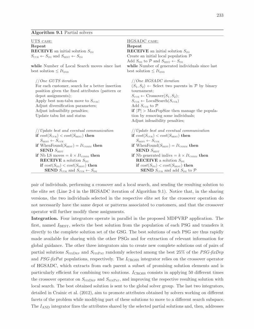
233

Algorithm 9.1 Partial solvers

UTS case:

RepeatRECEIVE an initial solution Sini

Scur ← Sini and Sbest ← Sini

while Number of Local Search moves since lastbest solution ≤ Itend

//One GUTS iterationFor each customer, search for a better insertionposition given the fixed attributes (pattern ordepot assignments);Apply best non-tabu move to Scur;Adjust diversification parameters;Adjust infeasibility penalties;Update tabu list and status

//Update best and eventual communicationif cost(Scur) < cost(Sbest) thenSbest ← Scur

if WhenFound(Sbest) = Itcomm thenSEND Sbest

if Nb LS moves = k × Itcomm thenRECEIVE a solution Sini

if cost(Sini) < cost(Sbest) thenSEND Scur and Scur ← Sini

HGSADC case:

RepeatRECEIVE an initial solution Sini

Create an initial local population PAdd Sini to P and Sbest ← Sini

while Number of generated individuals since lastbest solution ≤ Itend

//One HGSADC iteration(S1, S2) ← Select two parents in P by binarytournament;Scur ← Crossover(S1, S2);Scur ← LocalSearch(Scur)Add Scur to Pif |P| > MaxPopSize then manage the popula-tion by removing some individuals;Adjust infeasibility penalties;

//Update best and eventual communicationif cost(Scur) < cost(Sbest) thenSbest ← Scur

if WhenFound(Sbest) = Itcomm thenSEND Sbest

if Nb generated indivs = k × Itcomm thenRECEIVE a solution Sini

if cost(Sini) < cost(Sbest) thenSEND Scur and add Sini to P

pair of individuals, performing a crossover and a local search, and sending the resulting solution to

the elite set (Line 2-4 in the HGSADC iteration of Algorithm 9.1). Notice that, in the sharing

versions, the two individuals selected in the respective elite set for the crossover operation do

not necessarily have the same depot or patterns associated to customers, and that the crossover

operator will further modify these assignments.

Integration. Four integrators operate in parallel in the proposed MDPVRP application. The

first, named IBEST, selects the best solution from the population of each PSG and transfers it

directly to the complete solution set of the GSG. The best solutions of each PSG are thus rapidly

made available for sharing with the other PSGs and for extraction of relevant information for

global guidance. The other three integrators aim to create new complete solutions out of pairs of

partial solutions SfixDep and SfixPat randomly selected among the best 25% of the PSG-fixDep

and PSG-fixPat populations, respectively. The ICROSS integrator relies on the crossover operator

of HGSADC, which extracts from each parent a subset of promising solution elements and is

particularly efficient for combining two solutions. ICROSS consists in applying 50 different times

the crossover operator on SfixDep and SfixPat, and improving the respective resulting solution with

local search. The best obtained solution is sent to the global solver group. The last two integrators,

detailed in Crainic et al. (2012), aim to promote attributes obtained by solvers working on different

facets of the problem while modifying part of these solutions to move to a different search subspace.

The IAND integrator fixes the attributes shared by the selected partial solutions and, then, addresses

234

the resulting restricted formulation by means of HGSADC, to return the best solution. The IPEN

integrator modifies the original complete formulation by adding cost incentives to direct HGSADC

toward the depot-to-customer assignments of SfixPat and the pattern-to-customer assignments of

SfixDep.

Global Solver Group and Search Coordination. The Global Search Coordinator assumes

the fourfold role of collecting statistical information on the past search, monitoring the status of

the solver groups, triggering migration of individuals when necessary, and building new guiding

solutions to orient the search towards promising features. The statistical information is developed

on (client, depot, pattern) triplets entering the complete solution set, by monitoring the number

of occurrences (frequency) of each triplet in the population as well as in the best, average and

worst sub-populations (Le Bouthillier and Crainic 2005b), and finally the best cost of a solution

containing any given triplet.

The GSC monitors the elite sets to check whether more than five non-flagged individuals are

available (UTS and encapsulated-HGSADC implementations), and whether improving solutions

have been received during the Itcontrol = 2000 last solutions. If one of these two criteria is not

fulfilled, the GSC sends three solutions to the corresponding elite set. The three solutions are either

randomly selected (equiprobably) from the complete solution set, or are three guiding solutions,

as defined in the next paragraph. In the shared-HGSADC implementations, this migration is

preceded by a reset of the population, where all the solutions are replaced by new initial random

solutions. It should be noted that the solutions to be migrated do not necessarily have the same

values for the fixed attributes, and thus the solver groups process individuals with identical sets of

fixed attributes, but potentially different attribute values.

The GSC generates guiding solutions by selecting promising triplets to create feasible pattern

and depot customer assignments. “Promising” is based on the complete search history and is meant

as appearing in at least one solution with a cost difference of less than 3% with respect to the best

found solution. Once these patterns and depots are selected, complete solutions with routes are

generated by local search, to serve as initial population (HGSADC implementations) or solution

(UTS implementations) and be optimized with the solver of choice. The termination criterion for

GUTS or HGSADC is here set to It′end

= 2000 iterations without improvement. Since creating

such an individual is time consuming, guiding individuals are generated by the GSC in background,

and stored in a temporary pool of guiding individuals. These solutions significantly contribute to

inflect the search trajectory towards different alternatives of assignment combinations.

We experimented with two settings of the CSG, with and without a complete-solver set. The

same two algorithms, GUTS and HGSADC, are used in the former case, targeting the full MDPVRP.

The results are presented next.

9.7 Experimental Results and Analyses

Extensive experimental analyses were conducted to 1) assess the performance of ICS when

compared to state-of-the-art sequential methods and, 2) investigate several implementation alter-

natives, including the choice of solver type (GUTS vs. HGSADC) and of cooperation strategy in

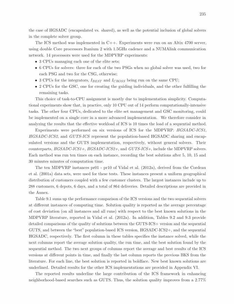
235

the case of HGSADC (encapsulated vs. shared), as well as the potential inclusion of global solvers

in the complete solver group.

The ICS method was implemented in C++. Experiments were run on an Altix 4700 server,

using double Core processors Itanium 2 with 1.5GHz cadence and a NUMAlink communication

network. 14 processors were used for the MDPVRP experiments:

• 3 CPUs managing each one of the elite sets;

• 6 CPUs for solvers: three for each of the two PSGs when no global solver was used, two for

each PSG and two for the CSG, otherwise;

• 3 CPUs for the integrators, IBEST and ICROSS being run on the same CPU;

• 2 CPUs for the GSC, one for creating the guiding individuals, and the other fulfilling the

remaining tasks.

This choice of task-to-CPU assignment is mostly due to implementation simplicity. Computa-

tional experiments show that, in practice, only 10 CPU out of 14 perform computationally-intensive

tasks. The other four CPUs, dedicated to the elite set management and GSC monitoring, could

be implemented on a single core in a more advanced implementation. We therefore consider in

analyzing the results that the effective workload of ICS is 10 times the load of a sequential method.

Experiments were performed on six versions of ICS for the MDPVRP. HGSADC-ICS1,

HGSADC-ICS2, and GUTS-ICS represent the population-based HGSADC sharing and encap-

sulated versions and the GUTS implementation, respectively, without general solvers. Their

counterparts, HGSADC-ICS1+, HGSADC-ICS2+, and GUTS-ICS+, include the MDPVRP solvers.

Each method was run ten times on each instance, recording the best solutions after 5, 10, 15 and

30 minutes minutes of computation time.

The ten MDPVRP instances pr01 - pr10 of Vidal et al. (2012a), derived from the Cordeau

et al. (2001a) data sets, were used for these tests. These instances present a uniform geographical

distribution of customers coupled with a few customer clusters. The largest instances include up to

288 customers, 6 depots, 6 days, and a total of 864 deliveries. Detailed descriptions are provided in

the Annex.

Table 9.1 sums up the performance comparison of the ICS versions and the two sequential solvers

at different instances of computing time. Solution quality is reported as the average percentage

of cost deviation (on all instances and all runs) with respect to the best known solutions in the

MDPVRP literature, reported in Vidal et al. (2012a). In addition, Tables 9.2 and 9.3 provide

detailed comparisons of the quality of solutions between the GUTS-ICS+ version and the sequential

GUTS, and between the “best” population-based ICS version, HGSADC-ICS2+, and the sequential

HGSADC, respectively. The first column in these tables specifies the instance solved, while the

next columns report the average solution quality, the run time, and the best solution found by the

sequential method. The two next groups of columns report the average and best results of the ICS

versions at different points in time, and finally the last column reports the previous BKS from the

literature. For each line, the best solution is reported in boldface. New best known solutions are

underlined. Detailed results for the other ICS implementations are provided in Appendix VI.

The reported results underline the large contribution of the ICS framework in enhancing

neighborhood-based searches such as GUTS. Thus, the solution quality improves from a 2.77%

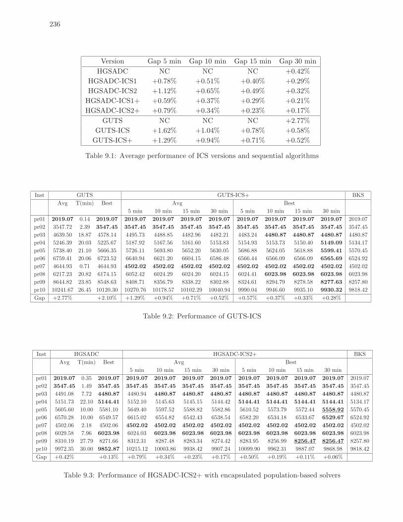
236

Version Gap 5 min Gap 10 min Gap 15 min Gap 30 min

HGSADC NC NC NC +0.42%

HGSADC-ICS1 +0.78% +0.51% +0.40% +0.29%

HGSADC-ICS2 +1.12% +0.65% +0.49% +0.32%

HGSADC-ICS1+ +0.59% +0.37% +0.29% +0.21%

HGSADC-ICS2+ +0.79% +0.34% +0.23% +0.17%

GUTS NC NC NC +2.77%

GUTS-ICS +1.62% +1.04% +0.78% +0.58%

GUTS-ICS+ +1.29% +0.94% +0.71% +0.52%

Table 9.1: Average performance of ICS versions and sequential algorithms

Inst GUTS GUTS-ICS+ BKS

Avg T(min) Best Avg Best

5 min 10 min 15 min 30 min 5 min 10 min 15 min 30 min

pr01 2019.07 0.14 2019.07 2019.07 2019.07 2019.07 2019.07 2019.07 2019.07 2019.07 2019.07 2019.07

pr02 3547.72 2.39 3547.45 3547.45 3547.45 3547.45 3547.45 3547.45 3547.45 3547.45 3547.45 3547.45

pr03 4639.50 18.87 4578.14 4495.73 4488.85 4482.96 4482.21 4483.24 4480.87 4480.87 4480.87 4480.87

pr04 5246.39 20.03 5225.67 5187.92 5167.56 5161.60 5153.83 5154.93 5153.73 5150.40 5149.09 5134.17

pr05 5738.40 21.10 5666.35 5726.11 5693.80 5652.20 5630.05 5686.88 5624.05 5618.88 5599.41 5570.45

pr06 6759.41 20.06 6723.52 6640.94 6621.20 6604.15 6586.48 6566.44 6566.09 6566.09 6565.69 6524.92

pr07 4644.93 0.71 4644.93 4502.02 4502.02 4502.02 4502.02 4502.02 4502.02 4502.02 4502.02 4502.02

pr08 6217.23 20.82 6174.15 6052.42 6024.29 6024.20 6024.15 6024.41 6023.98 6023.98 6023.98 6023.98

pr09 8644.82 23.85 8548.63 8408.71 8356.79 8338.22 8302.88 8324.61 8294.79 8278.58 8277.63 8257.80

pr10 10241.67 26.45 10120.30 10270.76 10178.57 10102.29 10040.94 9990.04 9946.60 9935.10 9930.32 9818.42

Gap +2.77% +2.10% +1.29% +0.94% +0.71% +0.52% +0.57% +0.37% +0.33% +0.28%

Table 9.2: Performance of GUTS-ICS

Inst HGSADC HGSADC-ICS2+ BKS



pr01 2019.07 0.35 2019.07 2019.07 2019.07 2019.07 2019.07 2019.07 2019.07 2019.07 2019.07 2019.07

pr02 3547.45 1.49 3547.45 3547.45 3547.45 3547.45 3547.45 3547.45 3547.45 3547.45 3547.45 3547.45

pr03 4491.08 7.72 4480.87 4480.94 4480.87 4480.87 4480.87 4480.87 4480.87 4480.87 4480.87 4480.87

pr04 5151.73 22.10 5144.41 5152.10 5145.63 5145.15 5144.42 5144.41 5144.41 5144.41 5144.41 5134.17

pr05 5605.60 10.00 5581.10 5649.40 5597.52 5588.82 5582.86 5610.52 5573.79 5572.44 5558.92 5570.45

pr06 6570.28 10.00 6549.57 6615.02 6554.82 6542.43 6538.54 6582.20 6534.18 6533.67 6529.67 6524.92

pr07 4502.06 2.18 4502.06 4502.02 4502.02 4502.02 4502.02 4502.02 4502.02 4502.02 4502.02 4502.02

pr08 6029.58 7.96 6023.98 6024.03 6023.98 6023.98 6023.98 6023.98 6023.98 6023.98 6023.98 6023.98

pr09 8310.19 27.79 8271.66 8312.31 8287.48 8283.34 8274.42 8283.95 8256.99 8256.47 8256.47 8257.80

pr10 9972.35 30.00 9852.87 10215.12 10003.86 9938.42 9907.24 10099.90 9962.31 9887.07 9868.98 9818.42

Gap +0.42% +0.13% +0.79% +0.34% +0.23% +0.17% +0.50% +0.19% +0.11% +0.06%

Table 9.3: Performance of HGSADC-ICS2+ with encapsulated population-based solvers

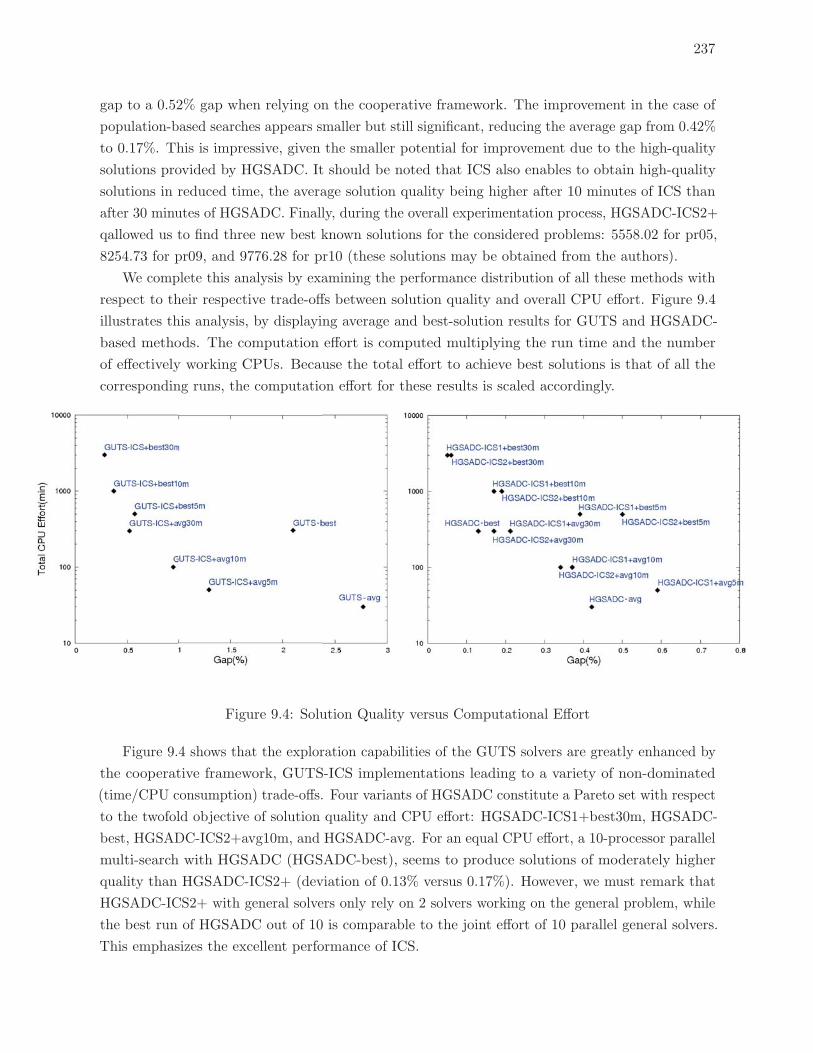
237

gap to a 0.52% gap when relying on the cooperative framework. The improvement in the case of

population-based searches appears smaller but still significant, reducing the average gap from 0.42%

to 0.17%. This is impressive, given the smaller potential for improvement due to the high-quality

solutions provided by HGSADC. It should be noted that ICS also enables to obtain high-quality

solutions in reduced time, the average solution quality being higher after 10 minutes of ICS than

after 30 minutes of HGSADC. Finally, during the overall experimentation process, HGSADC-ICS2+

qallowed us to find three new best known solutions for the considered problems: 5558.02 for pr05,

8254.73 for pr09, and 9776.28 for pr10 (these solutions may be obtained from the authors).

We complete this analysis by examining the performance distribution of all these methods with

respect to their respective trade-offs between solution quality and overall CPU effort. Figure 9.4

illustrates this analysis, by displaying average and best-solution results for GUTS and HGSADC-

based methods. The computation effort is computed multiplying the run time and the number

of effectively working CPUs. Because the total effort to achieve best solutions is that of all the

corresponding runs, the computation effort for these results is scaled accordingly.

Figure 9.4: Solution Quality versus Computational Effort

Figure 9.4 shows that the exploration capabilities of the GUTS solvers are greatly enhanced by

the cooperative framework, GUTS-ICS implementations leading to a variety of non-dominated

(time/CPU consumption) trade-offs. Four variants of HGSADC constitute a Pareto set with respect

to the twofold objective of solution quality and CPU effort: HGSADC-ICS1+best30m, HGSADC-

best, HGSADC-ICS2+avg10m, and HGSADC-avg. For an equal CPU effort, a 10-processor parallel

multi-search with HGSADC (HGSADC-best), seems to produce solutions of moderately higher

quality than HGSADC-ICS2+ (deviation of 0.13% versus 0.17%). However, we must remark that

HGSADC-ICS2+ with general solvers only rely on 2 solvers working on the general problem, while

the best run of HGSADC out of 10 is comparable to the joint effort of 10 parallel general solvers.

This emphasizes the excellent performance of ICS.

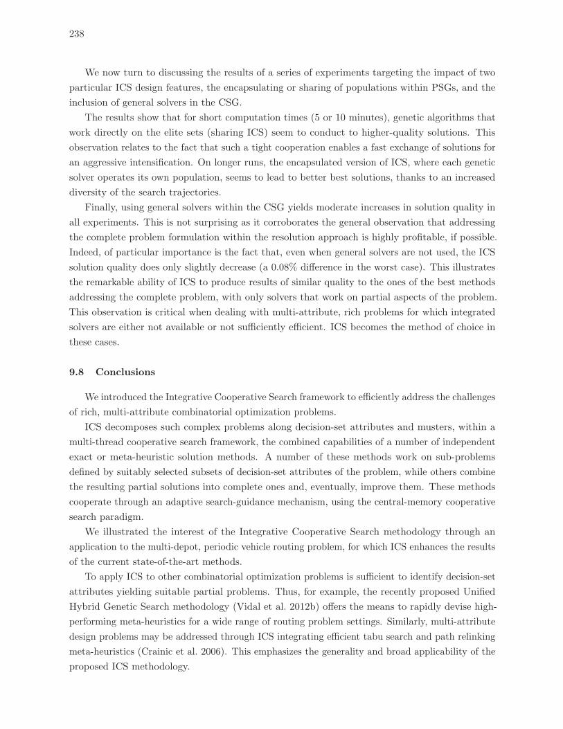
238

We now turn to discussing the results of a series of experiments targeting the impact of two

particular ICS design features, the encapsulating or sharing of populations within PSGs, and the

inclusion of general solvers in the CSG.

The results show that for short computation times (5 or 10 minutes), genetic algorithms that

work directly on the elite sets (sharing ICS) seem to conduct to higher-quality solutions. This

observation relates to the fact that such a tight cooperation enables a fast exchange of solutions for

an aggressive intensification. On longer runs, the encapsulated version of ICS, where each genetic

solver operates its own population, seems to lead to better best solutions, thanks to an increased

diversity of the search trajectories.

Finally, using general solvers within the CSG yields moderate increases in solution quality in

all experiments. This is not surprising as it corroborates the general observation that addressing

the complete problem formulation within the resolution approach is highly profitable, if possible.

Indeed, of particular importance is the fact that, even when general solvers are not used, the ICS

solution quality does only slightly decrease (a 0.08% difference in the worst case). This illustrates

the remarkable ability of ICS to produce results of similar quality to the ones of the best methods

addressing the complete problem, with only solvers that work on partial aspects of the problem.

This observation is critical when dealing with multi-attribute, rich problems for which integrated

solvers are either not available or not sufficiently efficient. ICS becomes the method of choice in

these cases.

9.8 Conclusions

We introduced the Integrative Cooperative Search framework to efficiently address the challenges

of rich, multi-attribute combinatorial optimization problems.

ICS decomposes such complex problems along decision-set attributes and musters, within a

multi-thread cooperative search framework, the combined capabilities of a number of independent

exact or meta-heuristic solution methods. A number of these methods work on sub-problems

defined by suitably selected subsets of decision-set attributes of the problem, while others combine

the resulting partial solutions into complete ones and, eventually, improve them. These methods

cooperate through an adaptive search-guidance mechanism, using the central-memory cooperative

search paradigm.

We illustrated the interest of the Integrative Cooperative Search methodology through an

application to the multi-depot, periodic vehicle routing problem, for which ICS enhances the results

of the current state-of-the-art methods.

To apply ICS to other combinatorial optimization problems is sufficient to identify decision-set

attributes yielding suitable partial problems. Thus, for example, the recently proposed Unified

Hybrid Genetic Search methodology (Vidal et al. 2012b) offers the means to rapidly devise high-

performing meta-heuristics for a wide range of routing problem settings. Similarly, multi-attribute

design problems may be addressed through ICS integrating efficient tabu search and path relinking

meta-heuristics (Crainic et al. 2006). This emphasizes the generality and broad applicability of the

proposed ICS methodology.

CONCLUSION

Les contributions de cette these concernent a la fois l’analyse et la synthese des problemes de

tournees de vehicules multi-attributs et de timing, ainsi que l’amelioration et le developpement

de nouvelles methodes dediees et generalistes, qui ont le potentiel d’etre etendues a de nombreux

autres problemes d’optimisation combinatoire.

Le developpement de syntheses et d’analyses de concepts au sein de revues de litterature

unificatrices, dans les chapitres 1 et 2, a permis de poser un nouveau regard sur les problemes de

tournees de vehicules multi-attributs, ainsi que sur un vaste domaine de recherche lie aux problemes

de timing, riche en problematiques et perspectives. Des liens ont ete etablis entre la structure des

problemes et les methodes de resolution. Ainsi, pour le VRP, trois types d’attributs (Assign, Seq

et Eval) ont ete differencies en considerant leur impact sur les methodes de resolution heuristique.

Par ailleurs, les strategies gagnantes de 64 metaheuristiques ont ete analysees en detail. Pour les

problemes de timing, l’etude de la structure des problemes, eventuellement par le biais de leurs

conditions d’optimalite (cas des “couts convexes separables”), a conduit a classifier de nombreux

algorithmes de differents domaines comme autant de variations de trois principes fondamentaux, lies

au respect des contraintes primales, duales, ou a des concepts de programmation dynamique. Cette

vaste analyse pluridisciplinaire de la litterature a permis d’identifier une librairie d’algorithmes

efficaces pour resoudre les problemes de timing pour des attributs varies de maniere independante,

et de maniere groupee par des methodes de re-optimisation dans des contextes de recherche locale.

Ces methodes donnent la clef pour gerer les caracteristiques temporelles difficiles de nombreux

problemes de tournees de vehicules riches et d’ordonnancement non-regulier.

Les Chapitres 3 a 6 ont decrit de nouvelles methodologies heuristiques efficaces pour plusieurs

problemes de tournees de vehicules fondamentaux. Un algorithme genetique hybride (HGSADC)

efficace a ete propose, combinant l’exploration large des methodes evolutionnaires a base de

populations, les capacites d’amelioration agressive des meta-heuristiques a voisinage, les relaxations

de contraintes pour cibler les frontieres de non-faisabilite, et des methodes avancees de gestion

de population et d’evaluation des individus considerant a la fois des criteres de qualite et de

contribution a la diversite. HGSADC s’est avere etre particulierement efficace sur les jeux de

tests classiques de la litterature, sur des problemes fondamentaux comme le VRP classique, et

d’autres variantes avec depots multiples et contraintes de periodes de visites, obtenant toutes

les solutions optimales connues et retrouvant ou ameliorant toutes les meilleures solutions de

la litterature pour ces problemes. Par ailleurs, une extension de cet algorithme aux problemes

de tournees de vehicules avec fenetres de temps et contraintes de duree de route a donne lieu

a d’autres contributions methodologiques, concernant l’exploitation efficaces de relaxation de

contraintes temporelles et l’utilisation d’approches de decomposition. De nouvelles methodes ont

ete proposees pour evaluer en temps constant amorti O(1) les solutions intermediaires irrealisables

vis-a-vis des contraintes temporelles, produites par des mouvements de recherche locale. Des etudes

experimentales approfondies ont mis en valeur la contribution majeure des nouvelles strategies

d’evaluation des individus et de gestion de population, l’apport des methodes de decomposition, et

l’impact positif des solutions intermediaires irrealisables et dans la methodologie HGSADC, ainsi

240

que dans des approches simples de descente par recherche locale et de recherche locale iteree. De

plus, une methode simple de programmation dynamique a ete proposee pour choisir en temps O(1)

le meilleur depot et son placement dans les routes. Cette approche ouvre la porte a des evaluations

efficaces de familles de mouvements combines, et permet de releguer les decisions d’affectation au

sein de sous-probleme d’evaluation de routes afin de ne plus avoir a considerer explicitement cet

aspect combinatoire au sein des voisinages de recherche locale et des representations de solution.

Les Chapitres 7 a 9 ont exploite les analyses et developpements methodologiques precedents

pour progresser vers des methodes efficaces et generalistes pour les problemes de tournees de

vehicules multi-attributs. Dans ce cadre, une famille de problemes riches particulierement difficiles,

les problemes combines de tournees de vehicules et optimisation des horaires de conducteurs, a ete

consideree. Ces problemes combines ont ete traites efficacement en couplant l’algorithme genetique

hybride avec des strategies avancees d’evaluation des routes basees sur des recherches arborescentes et

des memoires. Un cadre de resolution modulaire a par ailleurs ete propose, et applique pour produire

un algorithme genetique hybride unifie pour les MAVRP. Tandis que les algorithmes modulaires

et librairies de composants de la litterature pour l’optimisation combinatoire etaient auparavant

principalement dedies a la multiplicite des methodes (differents modules pour differentes strategies

heuristiques), le cadre propose a permis de gerer la multiplicite des variantes de problemes grace a

des composants de resolution elementaires s’adaptant automatiquement aux attributs consideres.

L’algorithme UHGS bati sur ces principes, teste sur 26 variantes fondamentales de VRP avec une

unique implementation et parametrage, egalise ou surpasse toutes les meilleures methodes dediees

de la litterature issues de plus de 180 articles. Cet algorithme est une contribution fondamentale

a la fois d’un point de vue pratique et methodologique, de tels algorithmes generalistes etant

necessaires pour mettre a l’epreuve des concepts de resolution sur une vaste gamme de problemes,

mais aussi pour repondre rapidement aux besoins des cas application pratiques. De plus, afin

de traiter plus efficacement le challenge des combinaisons d’attributs et des problemes riches, les

meta-heuristiques precedentes ont ete etendues au sein d’un cadre de resolution parallele cooperative

a base de decomposition et integration successives de solutions (ICS-UHGS). Cette application a

donne lieu a des developpements concernant la gestion efficace des problemes partiels obtenus par

projection, de l’integration des solutions, et du guidage de la recherche. Les experimentations ont

demontre la contribution importante du cadre parallele cooperatif, des methodes d’integration et

de guidage, et ont illustre la capacite d’ICS-UHGS a traiter efficacement un probleme riche en

utilisant exclusivement des algorithmes de resolution sur des projections, ouvrant ainsi la porte a de

nouvelles perspectives pour la resolution efficace de problemes riches d’optimisation combinatoire.

Enfin, le fort potentiel d’impact pratique des methodologies developpees dans cette these a

ete demontre a plusieurs reprises. Le Chapitre 7, plus particulierement, a utilise ces methodes

d’optimisation pour quantifier l’impact des legislations sur les temps de conduite, et ainsi comparer

et evaluer l’impact de differentes legislations autour du monde sur la competitivite economique, les

horaires, et la fatigue des conducteurs. Il apparait notamment que les regles de l’Union Europeenne

sont les plus sures, tandis que les regles du Canada sont les plus avantageuses economiquement. Les

regles de l’Australie sont dominees en termes de cout et surete par les autres regles. Finalement, les

regles des Etats-Unis sont une alternative intermediaire entre cout et surete, les recents changements

241

de regles a venir en 2013 tendant vers plus de securite. Ces observations demontrent l’interet

pratique direct des methodes proposees, qui peuvent apporter une aide precieuse non seulement aux

acteurs des chaines logistiques a des fins d’optimisation, mais aussi aux organismes decisionnaires

afin de mesurer l’impact reel de choix de regles sur le transport longue-distance. Enfin, il faut noter

que les methodes heuristiques proposees ont ete testees sur de nombreux ensembles de problemes,

dont un bon nombre sont issus de cas d’applications pratiques et de jeux de donnees reels. La

grande generalite et performance de UHGS en fait un outil unique, dans la litterature scientifique

sur les tournees de vehicules, pour repondre rapidement et efficacement aux besoins d’applications

industrielles. Cette these a ainsi conduit a de nouvelles contributions cruciales en termes d’analyse,

de synthese, et de nouvelles methodologies de resolution pour gerer a la fois la difficulte, la variete

et la combinaison des problemes. Les implications academiques et pratiques de ces travaux sont

manifestes au vu de l’ampleur des experimentations et varietes de problemes traites. Les questions

et les pistes de recherches ouvertes sont, en consequence, nombreuses.

En particulier, l’etude unificatrice de la classe de problemes de timing a permis d’identifier des

breches dans l’etat de l’art. Des algorithmes plus performants pourraient etre recherches pour des

problemes de timing avec contraintes de laps de temps minimum ou maximum, duree d’execution

dependant du temps et contrainte de duree, entre autres. Les bornes inferieures de complexite

sont rares et particulierement utiles, ainsi que le serait une extension de la methodologie a des

problemes multi-objectifs ou stochastiques.

Concernant les MAVRP, certains problemes riches apparaissent comme particulierement difficiles,

notamment les variantes avec synchronisation de flux (rencontres, echanges de marchandises), les

variantes stochastiques avec des recours complexes faisant eventuellement changer l’itineraire de

plusieurs vehicules, ou les problemes impliquant plusieurs modes de transport.

Plusieurs methodologies developpees dans cette these, et en particulier l’evaluation multicritere

des individus impliquant qualite et contribution a la diversite ainsi que le cadre de resolution

heuristique modulaire generaliste, ont vocation a etre etendues et testees sur d’autres problemes

d’optimisation combinatoire. Des etudes supplementaires pourraient etre conduites sur les differentes

mesures de distance et de diversite utilisees dans les methodes de population, et il serait pertinent

d’etudier si les attributs ont un impact significatif sur le meilleur choix de mesure.

La prochaine generation de metaheuristiques pourrait tirer parti de voisinages plus larges et

structurellement differents, permettant d’integrer au mieux au niveau de la recherche locale des

decisions combinees sur differents attributs des problemes. Un progres pourrait etre effectue vers des

metaheuristiques plus “intelligentes” et moins randomisees, qui profitent au mieux de l’historique

de la recherche et d’informations locales, pour aiguiller au mieux la recherche future et trouver un

equilibre subtil entre diversification et intensification correctement ciblee. Aussi, nous avons observe

dans cette these que le succes sur les MAVRP n’est pas reellement lie a un cadre metaheuristique

particulier, mais a une combinaison de concepts a succes. Il existe des methodes performantes de

plusieurs types, incluant la recherche tabou, la recherche voisinage large, recherche locale iteree,

methode a base de population et croisements... Etant donne la maniere tres differente avec laquelle

ces methodes explorent l’espace des solutions, il est tres probable que des heuristiques hybrides tres

242

efficaces puissent etre generees, le defi majeur a ce niveau restant cependant de trouver le meilleur

compromis entre simplicite des concepts et performance.

Finalement, beaucoup de progres restent a venir vis-a-vis de la resolution generaliste de

problemes de tournees de vehicules. Entre autres, l’utilisation de langages formels de modelisation

peut etre consideree, ainsi que des approches plus systematiques pour gerer la combinaison de

modules specifiques aux attributs et la generation des voisinages de recherche locale relativement a

la structure du graphe et la nature des solutions. Ayant montre qu’une unique methode peut etre

performante sur une vaste gamme de problemes, nous esperons que plus d’articles futurs visent

non seulement a introduire de nouveaux elements methodologiques, mais aussi a mieux examiner

leur potentiel d’application a des plusieurs variantes de VRP. Les algorithmes unifies produits

dans cette these – ILS, UHGS, ICS – ont le potentiel d’etre une aide considerable pour mener a

bien ces pistes de recherche en permettant d’introduire de nouveaux elements methodologiques et

d’examiner leur impact sur une vaste gamme de problemes.

BIBLIOGRAPHIE

Aarts, E.H.L., J.K. Lenstra, eds. 2003. Local search in combinatorial optimization. Princeton Univ Pr.

Ahuja, R, D Hochbaum, J Orlin. 2003. Solving the convex cost integer dual network flow problem.

Management Science 49(7) 950–964.

Ahuja, Ravindra K., James B. Orlin. 2001. A Fast Scaling Algorithm for Minimizing Separable Convex

Functions Subject to Chain Constraints. Operations Research 49(5).

Ahuja, R.K., O. Ergun, J.B. Orlin, A.P. Punnen. 2002. A survey of very large-scale neighborhood search

techniques. Discrete Applied Mathematics 123(1-3) 75–102.

Alba, E. 2005. Parallel metaheuristics : a new class of algorithms. Wiley-Interscience, Hoboken, NJ.

Alba, E., B. Dorronsoro. 2006. Computing nine new best-so-far solutions for Capacitated VRP with a

cellular Genetic Algorithm. Information Processing Letters 98(6) 225–230.

Alegre, J., M. Laguna, J. Pacheco. 2007. Optimizing the periodic pick-up of raw materials for a manufacturer

of auto parts. European Journal of Operational Research 179(3) 736–746.

Aleman, R.E., R.R. Hill. 2010. A tabu search with vocabulary building approach for the vehicle routing

problem with split demands. International Journal of Metaheuristics 1(1) 55–80.

Alidaee, B., N.K. Womer. 1999. Scheduling with time dependent processing times : review and extensions.

Journal of the Operational Research Society 50(7) 711–720.

Alonso, F., M. J. Alvarez, J. E. Beasley. 2008. A tabu search algorithm for the periodic vehicle routing

problem with multiple vehicle trips and accessibility restrictions. Journal of the Operational Research

Society 59(7) 963–976.

Alvarenga, G.B., G.R. Mateus, G. De Tomi. 2007. A genetic and set partitioning two-phase approach for

the vehicle routing problem with time windows. Computers & Operations Research 34(6) 1561–1584.

Andersson, H., A. Hoff, M. Christiansen, G. Hasle, A. Lokketangen. 2010. Industrial aspects and literature

survey : Combined inventory management and routing. Computers & Operations Research 37(9)

1515–1536.

Arabeyre, J.P., J. Fearnley, F.C. Steiger, W. Teather. 1969. The Airline Crew Scheduling Problem : A

Survey. Transportation Science 3(2) 140–163.

Archetti, C., A. Hertz, M. G. Speranza. 2006. Metaheuristics for the team orienteering problem. Journal of

Heuristics 13(1) 49–76.

Archetti, C., M. Savelsbergh. 2009. The trip scheduling problem. Transportation Science 43(4) 417–431.

Archetti, C., M.G. Speranza. 2011. Vehicle routing problems with split deliveries. International Transactions

in Operational Research, Forthcoming .

Archetti, C., M.G. Speranza, M.W.P. Savelsbergh. 2008. An optimization-based heuristic for the split

delivery vehicle routing problem. Transportation Science 42(1) 22–31.

Assad, A.A. 1988. Modeling and Implementation Issues in Vehicle Routing. B.L. Golden, A.A. Assad, eds.,

Vehicle Routing : Methods and Studies. North-Holland Amsterdam, 7–45.

Ayer, M., H.D. Brunk, G.M. Ewing, W.T. Reid, E. Silverman. 1955. An empirical distribution function for

sampling with incomplete information. The Annals of Mathematical Statistics 26(4) 641–647.

Badeau, P., F. Guertin, M. Gendreau, J.-Y. Potvin, E.D. Taillard. 1997. A parallel tabu search heuristic

for the vehicle routing problem with time windows. Transportation Research Part C : Emerging

Technologies 5(2) 109–122.

244

Baker, K.R., G.D. Scudder. 1990. Sequencing with earliness and tardiness penalties : a review. Operations

Research 38(1) 22–36.

Balakrishnan, N. 1993. Simple heuristics for the vehicle routeing problem with soft time windows. Journal

of the Operational Research Society 44(3) 279–287.

Baldacci, R., E. Bartolini, G. Laporte. 2009. Some applications of the generalized vehicle routing problem.


Baldacci, R., E. Bartolini, A. Mingozzi, A. Valletta. 2011a. An Exact Algorithm for the Period Routing

Problem. Operations Research 59(1) 228–241.

Baldacci, R., M. Battarra, D. Vigo. 2008a. Routing a heterogeneous fleet of vehicles. B. Golden, S. Raghavan,

E. Wasil, eds., The Vehicle Routing Problem : Latest Advances and New Challenges. Springer, New

York, 3–27.

Baldacci, R., N. Christofides, A. Mingozzi. 2008b. An exact algorithm for the vehicle routing problem based

on the set partitioning formulation with additional cuts. Mathematical Programming 115(2) 351–385.

Baldacci, R., A. Mingozzi. 2009. A unified exact method for solving different classes of vehicle routing

problems. Mathematical Programming 120(2) 347–380.

Baldacci, R., A. Mingozzi, R.W. Calvo. 2011b. An exact method for the capacitated location-routing

problem. Operations Research 59(5) 1284–1296.

Baldacci, R., A. Mingozzi, R. Roberti. 2011c. New route relaxation and pricing strategies for the vehicle

routing problem. Operations Research 59(5) 1269–1283.

Baldacci, R., P. Toth, D. Vigo. 2007. Recent advances in vehicle routing exact algorithms. 4OR 5(4)

269–298.

Balseiro, S.R., I. Loiseau, J. Ramonet. 2011. An Ant Colony algorithm hybridized with insertion heuristics

for the Time Dependent Vehicle Routing Problem with Time Windows. Computers & Operations

Research 38(6) 954–966.

Barlow, R.E., D.J. Bartholomew, J.M. Bremner, H.D. Brunk. 1972. Statistical inference under order

restrictions : The theory and application of isotonic regression. Wiley New York.

Barr, R.S., B.L. Golden, J.P. Kelly, M.G.C. Resende, W.R. Stewart JR. 1995. Designing and reporting on

computational experiments with heuristic methods. Journal of Heuristics 1(1) 9–32.

Bartusch, M., R.H. Mohring, F.J. Radermacher. 1988. Scheduling project networks with resource constraints

and time windows. Annals of Operations Research 16(1) 199–240.

Bean, J.C., J.R. Birge, R.L. Smith. 1987. Aggregation in dynamic programming. Operations Research 35(2)

215–220.

Beasley, J.E. 1981. Adapting the savings algorithm for varying inter-customer travel times. Omega 9(6)

658–659.

Beasley, J.E. 1983. Route first–cluster second methods for vehicle routing. Omega 11(4) 403–408.

Bektas, T., G. Erdogan, S. Ropke. 2011. Formulations and branch-and-cut algorithms for the generalized

vehicle routing problem. Transportation Science 45(3) 299–316.

Bektas, T., G. Laporte. 2011. The pollution-routing problem. Transportation Research Part B : Methodological

45(8) 1232–1250.

Belenguer, J. M., M. C. Martinez, E. Mota. 2000. A Lower Bound for the Split Delivery Vehicle Routing

Problem. Operations Research 48(5) 801–810.

Belhaiza, S. 2010. Hybrid Variable Neighborhood - Tabu Search Algorithm for the Site Dependent Vehicle

Routing Problem with Time Windows. Tech. rep., GERAD, Montreal, Canada.

245

Bell, J., P. Mc Mullen. 2004. Ant colony optimization techniques for the vehicle routing problem. Advanced

Engineering Informatics 18(1) 41–48.

Beltrami, E.J., L.D. Bodin. 1974. Networks and vehicle routing for municipal waste collection. Networks

4(1) 65–94.

Bent, R., P. Van Hentenryck. 2006. A two-stage hybrid algorithm for pickup and delivery vehicle routing

problems with time windows. Computers & Operations Research 33(4) 875–893.

Bent, R., P. Van Hentenryck. 2010. Spatial, temporal, and hybrid decompositions for large-scale vehicle

routing with time windows. D. Cohen, ed., Proceedings of CP’10 , LNCS , vol. 6308. Springer Berlin

Heidelberg, 99–113.

Bent, Russell, Pascal Van Hentenryck. 2004. A Two-Stage Hybrid Local Search for the Vehicle Routing

Problem with Time Windows. Transportation Science 38(4) 515–530.

Berbeglia, G., J.-F. Cordeau, I. Gribkovskaia, G. Laporte. 2007. Static pickup and delivery problems : a

classification scheme and survey. Top 15(1) 1–31.

Berbeglia, G., J.-F. Cordeau, G. Laporte. 2010. Dynamic pickup and delivery problems. European Journal

of Operational Research 202(1) 8–15.

Berbeglia, G., J.-F. Cordeau, G. Laporte. 2011. A Hybrid Tabu Search and Constraint Programming

Algorithm for the Dynamic Dial-a-Ride Problem. INFORMS Journal on Computing .

Berger, J, M Barkaoui. 2004. A parallel hybrid genetic algorithm for the vehicle routing problem with time

windows. Computers & Operations Research 31(12) 2037–2053.

Berger, J., M. Barkaoui, O. Braysy. 2003. A route-directed hybrid genetic approach for the vehicle routing

problem with time windows. INFOR 41(2) 179–194.

Bertsekas, D.P., A. Nedi, A.E. Ozdaglar. 2003. Nonlinear Programming . Athena Scientific, Nashua, NH.

Best, M.J., N. Chakravarti. 1990. Active set algorithms for isotonic regression, a unifying framework.

Mathematical Programming 47(1-3) 425–439.

Best, M.J, N. Chakravarti, V.A. Ubhaya. 2000. Minimizing separable convex functions subject to simple

chain constraints. SIAM Journal on Optimization 10(3) 658–672.

Bianco, L., A. Mingozzi, S. Ricciardelli. 1993. The traveling salesman problem with cumulative costs.

Networks 23(2) 81–91.

Blakeley, F., B. Bozkaya, B. Cao, W. Hall, J. Knolmajer. 2003. Optimizing periodic maintenance operations

for Schindler Elevator Corporation. Interfaces 33(1) 67–79.

Blum, A., P. Chalasani, D. Coppersmith, B. Pulleyblank, P. Raghavan, M. Sudan. 1994. The minimum

latency problem. Proceedings of the twenty-sixth annual ACM symposium on Theory of computing .

ACM, New York, USA, 163–171.

Blum, C., J. Puchinger, G. Raidl, A. Roli. 2011. Hybrid metaheuristics in combinatorial optimization : A

survey. Applied Soft Computing 11(6) 4135–4151.

Blum, C., A. Roli. 2003. Metaheuristics in Combinatorial Optimization : Overview and Conceptual

Comparison. ACM Computing Surveys (CSUR) 35(3) 268–308.

Bodin, L., B. Golden. 1981. Classification in vehicle routing and scheduling. Networks 11(2) 97–108.

Bodin, L. D. 1975. A taxonomic structure for vehicle routing and scheduling problems. Computers & Urban

Society 1(1) 11–29.

Bodin, L.D., L. Berman. 1979. Routing and scheduling of school buses by computer. Transportation Science

13(2) 113.

Boese, K.D. 1995. Cost versus distance in the traveling salesman problem. Tech. rep.

246

Bortfeldt, A. 2012. A hybrid algorithm for the capacitated vehicle routing problem with three-dimensional

loading constraints. Computers & Operations Research 39(9) 2248–2257.

Bostel, N., P. Dejax, P. Guez, F. Tricoire. 2008. Multiperiod planning and routing on a rolling horizon for

field force optimization logistics. Bruce Golden, S. Raghavan, Edward Wasil, eds., The Vehicle Routing

Problem : Latest Advances and New Challenges, vol. 43. Springer, New York, 503–525.

Boudia, M., C. Prins, M. Reghioui. 2007. An Effective Memetic Algorithm with Population Management for

the Split Delivery Vehicle Routing Problem. Hybrid Metaheuristics, LNCS , vol. 4771. Springer Berlin


Bouly, H., D.-C. Dang, A. Moukrim. 2009. A memetic algorithm for the team orienteering problem. 4OR

8(1) 49–70.

Boussier, S., D. Feillet, M. Gendreau. 2006. An exact algorithm for team orienteering problems. 4OR 5(3)

211–230.

Brandao, J. 2006. A new tabu search algorithm for the vehicle routing problem with backhauls. European

Journal of Operational Research 173(2) 540–555.

Brandao, J. 2009. A deterministic tabu search algorithm for the fleet size and mix vehicle routing problem.

European Journal of Operational Research 195(3) 716–728.

Brandao, J. 2011. A tabu search algorithm for the heterogeneous fixed fleet vehicle routing problem.

Computers & Operations Research 38(1) 140–151.

Braysy, O. 2003. A Reactive Variable Neighborhood Search for the Vehicle-Routing Problem with Time

Windows. INFORMS Journal on Computing 15(4) 347–368.

Braysy, O., W. Dullaert, M. Gendreau. 2004a. Evolutionary algorithms for the vehicle routing problem with

time windows. Journal of Heuristics 10(6) 587–611.

Braysy, O., W. Dullaert, G. Hasle, D. Mester, M. Gendreau. 2008a. An Effective Multirestart Deterministic

Annealing Metaheuristic for the Fleet Size and Mix Vehicle-Routing Problem with Time Windows.

Transportation Science 42(3) 371–386.

Braysy, O., M. Gendreau. 2005a. Vehicle routing problem with time windows, Part I : Route construction

and local search algorithms. Transportation Science 39(1) 104–118.

Braysy, O., M. Gendreau. 2005b. Vehicle routing problem with time windows, Part II : Metaheuristics.


Braysy, O., M. Gendreau, G. Hasle, A. Lokketangen. 2008b. A Survey of Heuristics for the Vehicle Routing

Problem Part I : Basic Problems and Supply Side Extensions. Tech. rep., SINTEF, Norway.

Braysy, O., M. Gendreau, G. Hasle, A. Lokketangen. 2008c. A Survey of Heuristics for the Vehicle Routing

Problem Part II : Demand Side Extensions. Tech. rep., SINTEF, Norway.

Braysy, O., G. Hasle, W. Dullaert. 2004b. A multi-start local search algorithm for the vehicle routing

problem with time windows. European Journal of Operational Research 159(3) 586–605.

Braysy, O., P.P. Porkka, W. Dullaert, P.P. Repoussis, C.D. Tarantilis. 2009. A well-scalable metaheuristic

for the fleet size and mix vehicle routing problem with time windows. Expert Systems with Applications

36(4) 8460–8475.

Brucker, P., T. Hilbig, J. Hurink. 1999. A branch and bound algorithm for a single-machine scheduling

problem with positive and negative time-lags. Discrete Applied Mathematics 94(1-3) 77–99.

Brunk, H. D. 1955. Maximum Likelihood Estimates of Monotone Parameters. The Annals of Mathematical

Statistics 26(4) 607–616.

Bullnheimer, B., R.F. Hartl, C. Strauss. 1999. An improved ant system algorithm for the vehicle routing

problem. Annals of Operations Research 89 319–328.

247

Burke, E.K., M. Hyde, G. Kendall, G. Ochoa, E. Ozcan, J.R. Woodward. 2010. A classification of hyper-

heuristic approaches. M. Gendreau, J.-Y. Potvin, eds., Handbook of Metaheuristics. Springer US,

449–468.

Cahon, S., N. Melab, E.-G. Talbi. 2004. ParadisEO : A framework for the reusable design of parallel and

distributed metaheuristics. Journal of Heuristics 10(3) 357–380.

Campbell, A.M., M. Savelsbergh. 2004. Efficient insertion heuristics for vehicle routing and scheduling

problems. Transportation science 38(3) 369–378.

Canadian Council of Motor Transport Administrators. 2007. Commercial Vehicle Drivers Hours of Service

Regulations – Application Guide.

Chakravarti, N. 1989. Isotonic Median Regression : A Linear Programming Approach. Mathematics of

Operations Research 14(2) 303–308.

Chandran, B., S. Raghavan. 2008. Modeling and Solving the Capacitated Vehicle Routing Problem on Trees.

B. Golden, S. Raghavan, E. Wasil, eds., The Vehicle Routing Problem : Latest Advances and New

Challenges. Springer, New York, 616–622.

Chao, I., B. Golden, E.A. Wasil. 1996. The team orienteering problem. European Journal of Operational

Research 88(3) 464–474.

Chao, I.M., B.L. Golden, E. Wasil. 1995. An improved heuristic for the period vehicle routing problem.

Networks 26(1) 25–44.

Charnes, A., W.W. Cooper. 1958. The theory of search : optimum distribution of search effort. Management

Science 5(1) 44–50.

Chen, P., H.-K. Huang, X.-Y. Dong. 2010. Iterated variable neighborhood descent algorithm for the

capacitated vehicle routing problem. Expert Systems with Applications 37(2) 1620–1627.

Chen, S., B. Golden, E. Wasil. 2007. The split delivery vehicle routing problem : Applications, algorithms,

test problems, and computational results. Networks 49(4) 318–329.

Cheng, T. 2004. A concise survey of scheduling with time-dependent processing times. European Journal of

Operational Research 152(1) 1–13.

Chiu, H.N., Y.S. Lee, J.H. Chang. 2006. Two approaches to solving the multi-depot vehicle routing problem

with time windows in a time-based logistics environment. Production Planning & Control 17(5)

480–493.

Chretienne, P., F. Sourd. 2003. PERT scheduling with convex cost functions. Theoretical Computer Science

292(1) 145–164.

Christiansen, M., K. Fagerholt. 2002. Robust ship scheduling with multiple time windows. Naval Research

Logistics 49(6) 611–625.

Christofides, N. 1976. The Vehicle Routing Problem. RAIRO Operations Research 10(2) 55–70.

Christofides, N., S. Eilon. 1972. Algorithms for Large-Scale Travelling Salesman Problems. Operational

Research Quarterly 23(4) 511.

Christofides, N., A. Mingozzi, P. Toth. 1979. The vehicle routing problem. N. Christofides, A. Mingozzi,

P. Toth, C. Sandi, eds., Combined Optimization. Wiley, Chichester, UK, 315–338.

Chu, F., N. Labadi, C. Prins. 2006. A Scatter Search for the periodic capacitated arc routing problem.


Clarke, G., J. W. Wright. 1964. Scheduling of Vehicles from a Central Depot to a Number of Delivery Points.


248

Coelho, L.C., J.-F. Cordeau, G. Laporte. 2012. Thirty Years of Inventory-Routing. Tech. rep., CIRRELT,

Montreal, Canada.

Coene, S., A. Arnout, F.C.R Spieksma. 2010. On a periodic vehicle routing problem. Journal of the

Operational Research Society 61(12) 1719–1728.

Cooke, K.L., E. Halsey. 1966. The shortest route through a network with time-dependent internodal transit

times. Journal of Mathematical Analysis and Applications 14 493–498.

Cordeau, J.-F., M. Gendreau, A. Hertz, G. Laporte, J.S. Sormany. 2005. New heuristics for the vehicle

routing problem. A. Langevin, D. Riopel, eds., Logistics systems : design and optimization. Springer,

279–297.

Cordeau, J.-F., M. Gendreau, G. Laporte. 1997. A tabu search heuristic for periodic and multi-depot vehicle

routing problems. Networks 30(2) 105–119.

Cordeau, J.-F., G. Laporte. 2001. A tabu search algorithm for the site dependent vehicle routing problem

with time windows. INFOR 39(3) 292–298.

Cordeau, J.-F., G. Laporte. 2003. A tabu search heuristic for the static multi-vehicle dial-a-ride problem.

Transportation Research Part B : Methodological 37(6) 579–594.

Cordeau, J.-F., G. Laporte, A. Mercier. 2001a. A unified tabu search heuristic for vehicle routing problems

with time windows. Journal of the Operational Research Society 52(8) 928–936.

Cordeau, J.-F., G. Laporte, A. Mercier. 2004. Improved tabu search algorithm for the handling of route

duration constraints in vehicle routing problems with time windows. Journal of the Operational

Research Society 55(5) 542– 546.

Cordeau, J.-F., G. Laporte, S. Ropke. 2008. Recent models and algorithms for one-to-one pickup and

delivery problems. Bruce Golden, S. Raghavan, Edward Wasil, eds., The Vehicle Routing Problem :

Latest Advances and New Challenges. Springer, New York, 327–357.

Cordeau, J.-F., G. Laporte, M.W.P. Savelsbergh, D. Vigo. 2007. Vehicle Routing. C. Barnhart, G. Laporte,

eds., Transportation. Elsevier, North-Holland, Amsterdam, 367–428.

Cordeau, J.-F., M. Maischberger. 2012. A Parallel Iterated Tabu Search Heuristic for Vehicle Routing

Problems. Computers & Operations Research 39(9) 2033–2050.

Cordeau, J.-F., G. Stojkovic, F. Soumis, J. Desrosiers. 2001b. Benders Decomposition for Simultaneous

Aircraft Routing and Crew Scheduling. Transportation Science 35(4) 375–388.

Cordone, R. 2000. A note on time windows constraints in routing problems. Tech. rep., Department of

Electronics and Information, Polytechnic of Milan.

Cormen, T.H., C. Stein, R.L. Rivest, C.E. Leiserson. 2001. Introduction to Algorithms. McGraw-Hill Higher

Education.

Corne, D., M. Dorigo, F. Glover. 1999. New ideas in optimisation. McGraw-Hill, Maidenhead, UK, England.

Crainic, Teodor Gabriel. 2000. Service network design in freight transportation. European Journal of


Crainic, T.G. 2005. Parallel computation, co-operation, tabu search. C. Rego, B. Alidaee, eds., Metaheuristic

Optimization Via Memory and Evolution : Tabu Search and Scatter Search. Kluwer Academic Publishers,

Norwell, MA, 283–302.

Crainic, T.G. 2008. Parallel solution methods for vehicle routing problems. B.L. Golden, S. Raghavan, E.A.

Wasil, eds., The Vehicle Routing Problem : Latest Advances and New Challenges . Springer, New York,

171–198.

Crainic, T.G., G.C. Crisan, M. Gendreau, N. Lahrichi, W. Rei. 2009. Multi-thread integrative cooperative

optimization for rich combinatorial problems. Proceedings of IPDPS ’09 .

249

Crainic, T.G., B. Di Chiara, M. Nonato, L. Tarricone. 2006. Tackling electrosmog in completely configured

3G networks by parallel cooperative meta-heuristics. IEEE Wireless Communications 13(6) 34–41.

Crainic, T.G., N. El Hachemi, M. Gendreau, N. Lahrichi, W. Rei, T. Vidal. 2012. Solution Integration in

Combinatorial Optimization : Applications to Cooperative Search and Multi-Attribute Vehicle Routing.

Tech. rep., CIRRELT, Montreal, QC, Canada.

Crainic, T.G., H. Nourredine. 2005. Parallel Meta-Heuristics Applications. E. Alba, ed., Parallel Metaheu-

ristics. John Wiley & Sons, Hoboken, NJ, 1–49.

Crainic, T.G., M. Toulouse. 2008. Explicit and Emergent Cooperation Schemes for Search Algorithms.

V. Maniezzo, R. Battiti, J.-P. Watson, eds., Learning and Intelligent Optimization, LNCS , vol. 5315.

Springer-Verlag, Berlin, Heidelberg, 95–109.

Crainic, T.G., M. Toulouse. 2010. Parallel Meta-heuristics. M. Gendreau, J.-Y. Potvin, eds., Handbook of

Metaheuristics. Springer US, Boston, MA, 497–541.

Creput, J.-C., A. Koukam. 2008. The memetic self-organizing map approach to the vehicle routing problem.

Soft Computing 12(11) 1125–1141.

Dang, D.-C., R. Guibadj, A. Moukrim. 2011. A PSO-Based Memetic Algorithm for the Team Orienteering

Problem. Applications of Evolutionary Computation, LNCS , vol. 6625. Springer Berlin Heidelberg,

471–480.

Dantzig, G.B., J.H. Ramser. 1959. The truck dispatching problem. Management Science 6(1) 80–91.

Davis, J.S., J.J. Kanet. 1993. Single-machine scheduling with early and tardy completion costs. Naval

Research Logistics 40 85–101.

De Franceschi, R., M. Fischetti, P. Toth. 2006. A new ILP-based refinement heuristic for vehicle routing

problems. Mathematical Programming 105(2) 471–499.

De Landgraaf, W.A., AE Eiben, V Nannen. 2007. Parameter calibration using meta-algorithms. Proceedings

of CEC’07 . IEEE, 71–78.

Dechter, R, I. Meiri, J. Pearl. 1991. Temporal constraint networks. Artificial Intelligence 49 61–95.

Dell’Amico, M., F. Maffioli, P. Varbrand. 1995. On prize-collecting tours and the asymmetric travelling

salesman problem. International Transactions in Operational Research 2(3) 297–308.

Demir, E., T. Bektas, G. Laporte. 2012. An adaptive large neighborhood search heuristic for the Pollution-

Routing Problem. European Journal of Operational Research 223(2) 346–359.

Derigs, U., R. Kaiser. 2007. Applying the attribute based hill climber heuristic to the vehicle routing problem.


Derigs, U., B. Li, U. Vogel. 2009. Local search-based metaheuristics for the split delivery vehicle routing

problem. Journal of the Operational Research Society 1356–1364.

Desaulniers, G., J. Desrosiers, A. Erdmann, M.M. Solomon, F. Soumis. 2002. VRP with pickup and delivery.

P. Toth, D. Vigo, eds., The Vehicle Routing Problem. SIAM, Philadelphia, PA, USA, 225–242.

Desaulniers, G., J. Desrosiers, I. Ioachim, M.M. Solomon, F. Soumis, D. Villeneuve. 1998. A unified

framework for deterministic time constrained vehicle routing and crew scheduling problems. T.G.

Crainic, G. Laporte, eds., Fleet Management and Logistics. Kluwer Academic Publishers, Boston, MA,

129–154.

Desaulniers, G., J. Desrosiers, M.M. Solomon, eds. 2005. Column generation. Springer.

Desaulniers, G., D. Villeneuve. 2000. The Shortest Path Problem with Time Windows and Linear Waiting

Costs. Transportation Science 34(3) 312–319.

250

Desrochers, M., J. Desrosiers, M. Solomon. 1992. A new Optimization Algorithm for the Vehicle Routing

Problem with Time Windows. Operations Research 40(2) 342–354.

Desrochers, M, C.V. Jones, J.K. Lenstra, M.W.P. Savelsbergh, L. Stougie. 1999. Towards a model and

algorithm management system for vehicle routing and scheduling problems. Decision support systems

25(2) 109–133.

Desrochers, M., J.K. Lenstra, M.W.P. Savelsbergh. 1990. A classification scheme for vehicle routing and

scheduling problems. European Journal of Operational Research 46(3) 322–332.

Desrosiers, J., Y. Dumas, M.M. Solomon, F. Soumis. 1995. Time Constrained Routing and Scheduling.

M. Ball, T. L. Magnanti, C.L. Monma, G.L. Nemhauser, eds., Network Routing . North-Holland

Amsterdam, 35–139.

Doerner, K.F., R.F. Hartl, S. Benkner, M. Lucka. 2006. Parallel cooperative savings based ant colony

optimization : multiple search and decomposition approaches. Parallel processing letters 16(3) 351.

Doerner, K.F., R.F. Hartl, G. Kiechle, M. Lucka, M. Reimann. 2004. Parallel ant systems for the capacitated

vehicle routing problem. J. Gottlieb, G. Raidl, eds., Evolutionary Computation in Combinatorial

Optimization, LNCS , vol. 3004. Springer Berlin Heidelberg, 72–83.

Doerner, K.F., V. Schmid. 2010. Survey : Matheuristics for Rich Vehicle Routing Problems. Hybrid

Metaheuristics, LNCS , vol. 6373. Springer Berlin Heidelberg, 206–221.

Donati, A., R. Montemanni, N. Casagrande, A.E. Rizzoli, L.M. Gambardella. 2008. Time dependent vehicle

routing problem with a multi ant colony system. European Journal of Operational Research 185(3)

1174–1191.

Dondo, R., J. Cerda. 2007. A cluster-based optimization approach for the multi-depot heterogeneous

fleet vehicle routing problem with time windows. European Journal of Operational Research 176(3)

1478–1507.

Dongarra, J. 2011. Performance of various computers using standard linear equations software. Tech. rep.,

University of Tennessee.

Dorigo, M., T. Stutzle. 2004. Ant colony optimization. Cambridge, MIT Press.

Dorronsoro, B., D. Arias, F. Luna, A.J. Nebro, E. Alba. 2007. A grid-based hybrid cellular genetic algorithm

for very large scale instances of the CVRP. W. Smari, ed., Proceedings of HPCS’07 . Prague, Czech

Republic, 759–765.

Dreo, J., A. Petrowski, P. Siarry, E. Taillard. 2003. Metaheuristiques pour l’optimisation difficile. Eyrolles.

Drexl, M. 2012. Synchronization in vehicle routing – a survey of VRPs with multiple synchronization

constraints. Transportation Science 46(3) 297–316.

Dreyfus, SE. 1969. An appraisal of some shortest-path algorithms. Operations Research 17(3) 395–412.

Drezner, Z, HW Hamacher. 2004. Facility location : applications and theory . Springer Verlag, Berlin.

Droste, S., T. Jansen, I. Wegener. 2002. Optimization with randomized search heuristics – the (A)NFL

theorem, realistic scenarios, and difficult functions. Theoretical Computer Science 287(1) 131–144.

Drummond, L.M.A., L.S. Ochi, D.S. Vianna. 2001. An asynchronous parallel metaheuristic for the period

vehicle routing problem. Future Generation Computer Systems 17(4) 379–386.

Dry, M., M.D. Lee, D. Vickers, P. Hughes. 2006. Human performance on visually presented traveling

salesperson problems with varying numbers of nodes. Journal of Problem Solving 1(1) 20–32.

Du, T.C., J.-L. Wu. 2001. Using object-oriented paradigm to develop an evolutional vehicle routing system.

Computers in Industry 44(3) 229–249.

251

Dueck, G. 1993. New optimization heuristics : The great deluge algorithm and the record-to-record travel.

Journal of Computational Physics 104(1) 86–92.

Duhamel, C. 2001. Un Cadre Formel pour les Methodes par Amelioration Iterative - Application a deux

problemes d’Optimisation dans les reseaux. Ph.D. thesis, Universite Blaise Pascal, Clermont-Ferrand.

Duhamel, C., P. Lacomme, A. Quilliot, H. Toussaint. 2011. A multi-start evolutionary local search for the

two-dimensional loading capacitated vehicle routing problem. Computers & Operations Research 38(3)

617–640.

Dumas, Y., F. Soumis, J. Desrosiers. 1990. Optimizing the Schedule for a Fixed Vehicle Path with Convex

Inconvenience Costs. Transportation Science 24(2) 145–152.

Eksioglu, B., A.V. Vural, A. Reisman. 2009. The vehicle routing problem : A taxonomic review. Computers

& Industrial Engineering 57(4) 1472–1483.

Elhallaoui, I., D. Villeneuve, F. Soumis, G. Desaulniers. 2005. Dynamic Aggregation of Set-Partitioning

Constraints in Column Generation. Operations Research 53(4) 632–645.

Ergun, O., J. Orlin. 2006. Fast neighborhood search for the single machine total weighted tardiness problem.

Operations Research Letters 34(1) 41–45.

Erkut, E., J. Zhang. 1996. The Maximum Collection Problem with Time-Dependent Rewards. Naval

Research Logistics 43(5) 749–763.

Ernst, A.T., H. Jiang, M. Krishnamoorthy, B. Owens, D. Sier. 2004. An Annotated Bibliography of Personnel

Scheduling and Rostering. Annals of Operations Research 127(1) 21–144.

European Transport Safety Council. 2001. The Role of Driver Fatigue in Commercial Road Transport

Crashes. ETSC Review.

European Union. 2002. Directive 2002/15/EC of the European Parliament and of the Council of 11 March

2002 on the organisation of the working time of persons performing mobile road transport activities.

Official Journal of the European Communities L 80 35–39.

European Union. 2006. Regulation (EC) No 561/2006 of the European Parliament and of the Council of 15

March 2006 on the harmonisation of certain social legislation relating to road transport and amending

Council Regulations (EEC) No 3821/85 and (EC) No 2135/98 and repealing Co. Official Journal of

the European Union L 102, 11.04.2006.

Everett, H. 1963. Generalized Lagrange multiplier method for solving problems of optimum allocation of

resources. Operations Research 11(3) 399–417.

Federal Motor Carrier Safety Administration. 2008. Hours of Service of Drivers. Federal Register Vol. 73,

No. 224, p. 69569 - 69586.

Federal Motor Carrier Safety Administration. 2011. Hours of Service of Drivers. Federal Register Vol. 76,

No. 248, p. 81134 - 81188.

Feillet, D., P. Dejax, M. Gendreau. 2005. Traveling Salesman Problems with Profits. Transportation Science

39(2) 188–205.

Feng, G., H.C. Lau. 2007. Efficient algorithms for machine scheduling problems with earliness and tardiness

penalties. Annals of Operations Research 159(1) 83–95.

Figliozzi, M.A. 2010. An iterative route construction and improvement algorithm for the vehicle routing

problem with soft time windows. Transportation Research Part C : Emerging Technologies 18(5)

668–679.

Fink, A., S. Voss. 2003. HOTFRAME : A Heuristic Optimization Framework. S. Voss, D.L. Woodruff, eds.,

Optimization Software Class Libraries . Operations Research/Computer Science Interfaces Series, Vol.

18, Springer, 81–154.

252

Firat, M., G.J. Woeginger. 2011. Analysis of the dial-a-ride problem of Hunsaker and Savelsbergh. Operations

Research Letters 39(1) 32–35.

Fischetti, M., G. Laporte, S. Martello. 1993. The Delivery Man Problem and Cumulative Matroids. Operations

Research 41(6) 1055–1064.

Fischetti, M., P. Toth, D. Vigo. 1994. A branch-and-bound algorithm for the capacitated vehicle routing

problem on directed graphs. Operations Research 42(5) 846–859.

Fisher, M.L. 1994. Optimal solution of vehicle routing problems using minimum k-trees. Operations Research

42(4) 626–642.

Fisher, M.L., R. Jaikumar. 1981. A generalized assignment heuristic for vehicle routing. Networks 11(2)

109–124.

Fleischmann, B., M. Gietz, S. Gnutzmann. 2004. Time-Varying Travel Times in Vehicle Routing. Transpor-

tation Science 38(2) 160–173.

Fleszar, K., I. Osman, K. Hindi. 2009. A variable neighbourhood search algorithm for the open vehicle

routing problem. European Journal of Operational Research 195(3) 803–809.

Francis, P.M., K.R. Smilowitz, M. Tzur. 2008. The period vehicle routing problem and its extensions.

B. Golden, S. Raghavan, E. Wasil, eds., The Vehicle Routing Problem : Latest Advances and New

Challenges. Springer, New York, 73–102.

Frangioni, A., A. Manca. 2006. A Computational Study of Cost Reoptimization for Min-Cost Flow Problems.

INFORMS Journal on Computing 18(1) 61–70.

Fredman, M.L. 1975. On computing the length of longest increasing subsequences. Discrete Mathematics

11(1) 29–35.

Freling, R., D. Huisman, A.P.M. Wagelmans. 2003. Models and algorithms for integration of vehicle and

crew scheduling. Journal of Scheduling 6(1) 63–85.

Fu, Z., R. Eglese, L.Y.O. Li. 2007. A unified tabu search algorithm for vehicle routing problems with soft

time windows. Journal of the Operational Research Society 59(5) 663–673.

Fuellerer, G., K.F. Doerner, R.F. Hartl, M. Iori. 2009. Ant colony optimization for the two-dimensional

loading vehicle routing problem. Computers & Operations Research 36(3) 655–673.

Fukasawa, R., H. Longo, J. Lysgaard, M.P. Aragao, M. Reis, E. Uchoa, R.F. Werneck. 2006. Robust

branch-and-cut-and-price for the capacitated vehicle routing problem. Mathematical Programming

106(3) 491–511.

Funke, B., T. Grunert, S. Irnich. 2005. Local search for vehicle routing and scheduling problems : Review

and conceptual integration. Journal of Heuristics 11(4) 267–306.

Gajpal, Y., P. Abad. 2009. Multi-ant colony system (MACS) for a vehicle routing problem with backhauls.


Gambardella, L.M., E. Taillard, G. Agazzi. 1999. MACS-VRPTW : A multiple ant colony system for vehicle

routing problems with time windows. F. Glover D. Corne, M. Dorigo, ed., New Ideas in Optimization.

McGraw-Hill, 63–76.

Garcia, B.-L. 1996. Une approche generique des methodes par amelioration iterative. Application a la

resolution de problemes d’optimisation dans les reseaux. Ph.D. thesis, Laboratoire d’Informatique de

l’Universite Blaise Pascal, Clermont-Ferrand, France.

Garey, M R, D S Johnson. 1979. Computers and lntractability : A Guide to the Theory of NP–Completeness .

Garey, M.R., R.E. Tarjan, G.T. Wilfong. 1988. One-processor scheduling with symmetric earliness and

tardiness penalties. Mathematics of Operations Research 13(2) 330–348.

253

Gaskell, T.J. 1967. Bases for vehicle fleet scheduling. Operational Research Quarterly 18(3) 281–295.

Gawiejnowicz, S. 2008. Time-dependent scheduling . Springer, New York.

Gehring, H., J. Homberger. 1999. A parallel hybrid evolutionary metaheuristic for the vehicle routing

problem with time windows. Proceedings of EURO-GEN’99 . 57–64.

Gehring, H., J. Homberger. 2002. Parallelization of a two-phase metaheuristic for routing problems with

time windows. Journal of heuristics 8(2) 251–276.

Gendreau, M., A. Hertz, G. Laporte. 1992. New insertion and postoptimization procedures for the traveling

salesman problem. Operations Research 40(6) 1086–1094.

Gendreau, M., A. Hertz, G. Laporte. 1994. A tabu search heuristic for the vehicle routing problem.

Management Science 40(10) 1276–1290.

Gendreau, M., M. Iori, G. Laporte, S. Martello. 2006. A Tabu Search Algorithm for a Routing and Container

Loading Problem. Transportation Science 40(3) 342–350.

Gendreau, M., M. Iori, G. Laporte, S. Martello. 2008a. A Tabu search heuristic for the vehicle routing

problem with two-dimensional loading constraints. Networks 51(1) 4–18.

Gendreau, M., G. Laporte, J.-Y. Potvin. 2002. Metaheuristics for the capacitated VRP . SIAM, Philadelphia,

USA, 129–154.

Gendreau, M., G. Laporte, R. Seguin. 1996. A Tabu Search Heuristic for the Vehicle Routing Problem with

Stochastic Demands and Customers. Operations Research 44(3) 469–477.

Gendreau, M., J.-Y. Potvin. 2005. Metaheuristics in Combinatorial Optimization. Annals of Operations

Research 140(1) 189–213.

Gendreau, M., J.-Y. Potvin, eds. 2010. Handbook of Metaheuristics. International Series in Operations

Research & Management Science, Springer.

Gendreau, M., J.Y. Potvin, O. Braysy, G. Hasle, A. Lokketangen. 2008b. Metaheuristics for the vehicle

routing problem and its extensions : A categorized bibliography. B. Golden, S. Raghavan, E. Wasil, eds.,

The Vehicle Routing Problem : Latest Advances and New Challenges. Springer, New York, 143–169.

Gendreau, M., C.D. Tarantilis. 2010. Solving large-scale vehicle routing problems with time windows : The

state-of-the-art. Tech. rep., CIRRELT.

Geoffrion, A.M. 1970a. Elements of Large-Scale Mathematical Programming : Part I : Concepts. Management

Science 16(11) 652–675.

Geoffrion, AM. 1970b. Elements of large-scale mathematical programming. Part II : Synthesis of algorithms

and bibliography. Management Science 16(11) 676–691.

Ghaziri, H. 1996. Supervision in the self-organizing feature map : Application to the vehicle routing problem.

I.H. Osman, J.P. Kelly, eds., Meta-heuristics : Theory & applications. Kluwer, Boston, 651–660.

Giffler, B., G.L. Thompson. 1960. Algorithms for Solving Production-Scheduling Problems. Operations

Research 8(4) 487–503.

Gillett, B.E., L.R. Miller. 1974. A heuristic algorithm for the vehicle-dispatch problem. Operations Research

22(2) 340–349.

Glover, F. 1977. Heuristics for integer programming using surrogate constraints. Decision Sciences 8

156–166.

Glover, F. 1986. Future paths for integer programming and links to artificial intelligence. Computers &


Glover, F. 1989. Tabu Search – Part I. ORSA Journal on Computing 1(3) 190–206.

254

Glover, F. 1990. Tabu Search – Part II. ORSA Journal on Computing 2(1) 4–32.

Glover, F. 1992. New ejection chain and alternating path methods for traveling salesman problems. O. Balci,

R. Sharda, S. Zenios, eds., Computer Science and Operations Research : New Developments in Their

Interfaces. Pergamon Press, 449–509.

Glover, F. 1996. Ejection chains, reference structures and alternating path methods for traveling salesman

problems. Discrete Applied Mathematics 65(1-3) 223–253.

Glover, F., J.-K. Hao. 2011. The case for strategic oscillation. Annals of Operations Research 183(1)

163–173.

Glover, F., M. Laguna. 1998. Tabu search. Kluwer Academic Publishers, Boston, MA.

Glover, F.W., G.A. Kochenberger, eds. 2003. Handbook of Metaheuristics. Springer.

Goel, A. 2009. Vehicle Scheduling and Routing with Drivers’ Working Hours. Transportation Science 43(1)

17–26.

Goel, A. 2010. Truck driver scheduling in the European Union. Transportation Science 44(4) 429–441.

Goel, A. 2012a. The Canadian minimum duration truck driver scheduling problem. Computers & Operations

Research 39(10) 2359–2367.

Goel, A. 2012b. Truck driver scheduling in the United States and the 2013 rule change. Tech. rep., Zaragoza

Logistics Center.

Goel, A., C. Archetti, M. Savelsbergh. 2012. Truck driver scheduling in Australia. Computers & Operations

Research 39(5) 1122–1132.

Goel, A., V. Gruhn. 2008. A general vehicle routing problem. European Journal of Operational Research

191(3) 650–660.

Goel, A., L. Kok. 2012. Truck driver scheduling in the United States. Transportation Science 46(3) 317–326.

Goel, A., T. Vidal. 2012. Hours of service regulations in road freight transport : an optimization-based

international assessment. Tech. rep., CIRRELT.

Goel, Asvin, L.M. Rousseau. 2011. Truck Driver Scheduling in Canada. Journal of Scheduling, Articles in

Advance .

Goetschalckx, M., C. Jacobs-Blecha. 1989. The vehicle routing problem with backhauls. European Journal


Goldberg, D.E., K. Deb. 1991. A comparative analysis of selection schemes used in genetic algorithms.

Foundations of Genetic Algorithms 69–93.

Golden, B. 1984. The fleet size and mix vehicle routing problem. Computers & Operations Research 11(1)

49–66.

Golden, B., S. Raghavan, E. Wasil, eds. 2008. The Vehicle Routing Problem : Latest Advances and New

Challenges. Springer, New York.

Golden, B.L., A.A. Assad. 1988. Vehicle routing : methods and studies. North-Holland Amsterdam.

Golden, B.L., A.A. Assad, E.A. Wasil. 2002. Routing vehicles in the real world : applications in the solid

waste, beverage, food, dairy, and newspaper industries. SIAM, Philadelphia, PA, USA, 245–286.

Golden, B.L., E.A. Wasil. 1987. Computerized Vehicle Routing in the Soft Drink Industry. Operations

Research 35(1) 6–17.

Golden, B.L., E.A. Wasil, J.P. Kelly, I.M. Chao. 1998a. Metaheuristics in vehicle routing. T.G. Crainic,

G. Laporte, eds., Fleet Management and Logistics. Kluwer Academic Publishers, Boston, MA, 33–56.

255

Golden, B.L., E.A. Wasil, J.P. Kelly, I.M. Chao. 1998b. The impact of metaheuristics on solving the vehicle

routing problem : algorithms, problem sets, and computational results. T.G. Crainic, G. Laporte, eds.,

Fleet management and logistics. Kluwer Academic Publishers, Boston, MA, 33–56.

Goto, S., A. Sangiovanni-Vincentelli. 1978. A new shortest path updating algorithm. Networks 8(4) 341–372.

Graham, R.L., E.L. Lawler, J.K. Lenstra, A.H.G Rinnooy Kan. 1979. Optimization and approximation in

deterministic sequencing and scheduling : a survey. Annals of Discrete Mathematics 5 287–326.

Groer, C., B. Golden, E. Wasil. 2008. The Consistent Vehicle Routing Problem. Manufacturing & Service

Operations Management 11(4) 630–643.

Groer, C., B. Golden, E. Wasil. 2010. A Library of Local Search Heuristics for the Vehicle Routing Problem.

Mathematical Programming Computation 2(2) 79–101.

Groer, C., B. Golden, E. Wasil. 2011. A Parallel Algorithm for the Vehicle Routing Problem. INFORMS

Journal on Computing 23(2) 315–330.

Grotschel, M., C.L. Monma, M. Stoer. 1995. Design of survivable networks. M. Ball, T. Magnanti, C. Monma,

G. Nemhauser, eds., Network Models, Handbooks in Operations Research and Management Science,

vol. 7. North-Holland Amsterdam, 617–672.

Grotzinger, S.J., C. Witzgall. 1984. Projections onto Order Simplexes. Applied Mathematics and Optimization

270(12) 247–270.

Gschwind, T., S. Irnich. 2012. Effective Handling of Dynamic Time Windows and Synchronization with

Precedences for Exact Vehicle Routing. Tech. rep., Johannes Gutenberg University, Mainz, Germany.

Gulczynski, D., B. Golden, E. Wasil. 2011. The period vehicle routing problem : New heuristics and real-world

variants. Transportation Research Part E : Logistics and Transportation Review 47(5) 648–668.

Gulczynski, D.J., B. Golden, E. Wasil. 2008. Recent Developments in Modeling and Solving the Split

Delivery Vehicle Routing Problem. Z. Chen, S. Raghavan, eds., Tutorials in Operations Research.

INFORMS, Hanover, MD, 170–180.

Haase, K., G. Desaulniers, J. Desrosiers. 2001. Simultaneous Vehicle and Crew Scheduling in Urban Mass

Transit Systems. Transportation Science 35(3) 286–303.

Hadjiconstantinou, E., R. Baldacci. 1998. A multi-depot period vehicle routing problem arising in the

utilities sector. Journal of the Operational Research Society 49(12) 1239–1248.

Halpern, J. 1977. Shortest route with time dependent length of edges and limited delay possibilities in nodes.

Zeitschrift fur Operations Research 21(3) 117–124.

Hansen, N., A. Ostermeier. 2001. Completely Derandomized Self-Adaptation in Evolution Strategies.

Evolutionary Computation 9(2) 159–195.

Hansen, P., N. Mladenovic, J.A. Moreno Perez. 2010. Variable neighbourhood search : methods and

applications. Annals of Operations Research 175(1) 367–407.

Hartl, R.F., G. Hasle, G.K. Janssens. 2006. Special issue on Rich Vehicle Routing Problems. Central

European Journal of Operations Research 14(2) 103–104.

Hashimoto, H. 2008. Studies on Local Search-Based Approaches for Vehicle Routing and Scheduling

Problems. Ph.D. thesis, Kyoto University.

Hashimoto, H., T. Ibaraki, S. Imahori, M. Yagiura. 2006. The vehicle routing problem with flexible time

windows and traveling times. Discrete Applied Mathematics 154(16) 2271–2290.

Hashimoto, H., M. Yagiura. 2008. A Path Relinking Approach with an Adaptive Mechanism to Control

Parameters for the Vehicle Routing Problem with Time Windows. J. Hemert, C. Cotta, eds., Evolu-

tionary Computation in Combinatorial Optimization, LNCS , vol. 4972. Springer Berlin Heidelberg,

254–265.

256

Hashimoto, H., M. Yagiura, T. Ibaraki. 2008. An iterated local search algorithm for the time-dependent

vehicle routing problem with time windows. Discrete Optimization 5(2) 434–456.

Hashimoto, H., M. Yagiura, S. Imahori, T. Ibaraki. 2010. Recent progress of local search in handling the

time window constraints of the vehicle routing problem. 4OR 8(3) 221–238.

Haugland, D., S. Ho. 2010. Feasibility Testing for Dial-a-Ride Problems. B. Chen, ed., Algorithmic Aspects

in Information and Management , LNCS , vol. 6124. Springer Berlin / Heidelberg, 170–179.

Health and Safety Executive. 2006. http ://www.hse.gov.uk/research/rrhtm/rr446.htm.

Hemmelmayr, V.C., J.-F. Cordeau, T.G. Crainic. 2012. An adaptive large neighborhood search heuristic for

Two-Echelon Vehicle Routing Problems arising in city logistics. Computers & Operations Research

39(12) 3215–3228.

Hemmelmayr, V.C., K.F. Doerner, R.F. Hartl. 2009. A variable neighborhood search heuristic for periodic

routing problems. European Journal of Operational Research 195(3) 791–802.

Hendel, Y., F. Sourd. 2006. Efficient neighborhood search for the one-machine earliness-tardiness scheduling

problem. European Journal of Operational Research 173(1) 108–119.

Hendel, Y., F. Sourd. 2007. An improved earliness-tardiness timing algorithm. Computers & Operations

Research 34(10) 2931–2938.

Ho, S.C., M. Gendreau. 2006. Path relinking for the vehicle routing problem. Journal of Heuristics 12(1-2)

55–72.

Hochbaum, D. 2002. Solving integer programs over monotone inequalities in three variables : A framework for

half integrality and good approximations. European Journal of Operational Research 140(2) 291–321.

Hochbaum, D.S. 1994. Lower and upper bounds for the allocation problem and other nonlinear optimization

problems. Mathematics of Operations Research 19(2) 390–409.

Hochbaum, D.S., J.G. Shanthikumar. 1990. Convex separable optimization is not much harder than linear

optimization. Journal of the ACM (JACM) 37(4) 843–862.

Hoff, A., H. Andersson, M. Christiansen, G. Hasle, A. Lø kketangen. 2010. Industrial aspects and literature

survey : Fleet composition and routing. Computers & Operations Research 37(12) 2041–2061.

Holland, J.H. 1975. Adaptation in natural and artificial systems. an introductory analysis with applications

to biology, control and artificial intelligence. Ann Arbor : The University of Michigan Press.

Homberger, J., H. Gehring. 1999. Two evolutionary metaheuristics for the vehicle routing problem with

time windows. INFOR 37(3) 297–318.

Homberger, J., H. Gehring. 2005. A two-phase hybrid metaheuristic for the vehicle routing problem with

time windows. European Journal Of Operational Research 162(1) 220–238.

Hoogeveen, J.A., S.L. Van De Velde. 1996. A branch-and-bound algorithm for single-machine earliness-

tardiness scheduling with idle time. INFORMS Journal on Computing 8(4) 402–412.

Hoos, H.H., T. Stutzle. 2005. Stochastic local search : Foundations and applications . Morgan Kaufmann.

Huisman, Dennis, Richard Freling, Albert P. M. Wagelmans. 2005. Multiple-Depot Integrated Vehicle and

Crew Scheduling. Transportation Science 39(4) 491–502.

Hunsaker, B., M.W.P. Savelsbergh. 2002. Efficient feasibility testing for dial-a-ride problems. Operations


Hurink, J., J. Keuchel. 2001. Local search algorithms for a single-machine scheduling problem with positive

and negative time-lags. Discrete Applied Mathematics 112(1-3) 179–197.

257

Ibaraki, T., S. Imahori, M. Kubo, T. Masuda, T. Uno, M. Yagiura. 2005. Effective Local Search Algorithms

for Routing and Scheduling Problems with General Time-Window Constraints. Transportation Science

39(2) 206–232.

Ibaraki, T., S. Imahori, K. Nonobe, K. Sobue, T. Uno, M. Yagiura. 2008. An iterated local search algorithm

for the vehicle routing problem with convex time penalty functions. Discrete Applied Mathematics

156(11) 2050–2069.

Ibaraki, T., N. Katoh. 1988. Resource allocation problems : algorithmic approaches. MIT Press, Cambridge,

MA, USA.

Ichoua, S., M. Gendreau, J.Y. Potvin. 2003. Vehicle dispatching with time-dependent travel times. European


Imran, A., S. Salhi, N.A. Wassan. 2009. A variable neighborhood-based heuristic for the heterogeneous fleet

vehicle routing problem. European Journal of Operational Research 197(2) 509–518.

Ioachim, I., S. Gelinas, F. Soumis, J. Desrosiers. 1998. A dynamic programming algorithm for the shortest

path problem with time windows and linear node costs. Networks 31(3) 193–204.

Iori, M., S. Martello. 2010. Routing problems with loading constraints. Top 18(1) 4–27.

Irnich, S. 2000. A multi-depot pickup and delivery problem with a single hub and heterogeneous vehicles.


Irnich, S. 2008a. A Unified Modeling and Solution Framework for Vehicle Routing and Local Search-Based

Metaheuristics. INFORMS Journal on Computing 20(2) 270–287.

Irnich, S. 2008b. Resource extension functions : properties, inversion, and generalization to segments. OR

Spectrum 30 113–148.

Irnich, S., B. Funke, T. Grunert. 2006. Sequential search and its application to vehicle-routing problems.


Jang, W., H.H. Lim, T.J. Crowe, G. Raskin, T.E. Perkins. 2006. The Missouri Lottery Optimizes Its

Scheduling and Routing to Improve Efficiency and Balance. Interfaces 36(4) 302–313.

Jepsen, M., B. Petersen, S. Spoorendonk, D. Pisinger. 2008. Subset-Row Inequalities Applied to the

Vehicle-Routing Problem with Time Windows. Operations Research 56(2) 497–511.

Jin, J., T.G. Crainic, A. Lokketangen. 2011. A Guided Cooperative Parallel Tabu Search for the Capacitated

Vehicle Routing Problem. Proceedings of NIK’11 . 49–60.

Jin, J., T.G. Crainic, A. Lokketangen. 2012. A parallel multi-neighborhood cooperative Tabu search for

Capacitated Vehicle Routing Problem. European Journal of Operational Research 222(3) 441–451.

Johnson, D.S., L.A. McGeoch. 1997. The traveling salesman problem : A case study in local optimization.

E.H.L. Aarts, J.K. Lenstra, eds., Local search in Combinatorial Optimization. Princeton Univ Pr,

215–310.

Jones, T. 1995. Fitness distance correlation as a measure of problem difficulty for genetic algorithms.

Proceedings ICGA’95 . Morgan Kaufmann, San Francisco, CA, USA, 184–192.

Kallehauge, B., J. Larsen, O. Madsen. 2006. Lagrangian duality applied to the vehicle routing problem with

time windows. Computers & Operations Research 33(5) 1464–1487.

Kallehauge, B., J. Larsen, O.B.G. Madsen, M.M. Solomon. 2005. Vehicle routing problem with time windows.

G. Desaulniers, J. Desrosiers, M.M. Solomon, eds., Column Generation. Springer, New York, 67–98.

Kanet, J.J., V Sridharan. 2000. Scheduling with inserted idle time : problem taxonomy and literature review.


258

Kang, K.H., Y.H. Lee, B.K. Lee. 2005. An Exact Algorithm for Multi Depot and Multi Period Vehicle

Scheduling Problem. Computational Science and Its Applications – ICCSA 2005 3483 350–359.

Kansou, A., A. Yassine. 2010. New upper bounds for the multi-depot capacitated arc routing problem.

International Journal of Metaheuristics 1(1) 81–95.

Karmarkar, N. 1984. A New Polynomial-Time algorithm for Linear Programming. Combinatorica 4(4)

373–395.

Karush, W. 1962. A general algorithm for the optimal distribution of effort. Management Science 9(1)

50–72.

Ke, L., C. Archetti, Z. Feng. 2008. Ants can solve the team orienteering problem. Computers & Industrial

Engineering 54(3) 648–665.

Kedad-Sidhoum, S., F. Sourd. 2010. Fast neighborhood search for the single machine earliness-tardiness

scheduling problem. Computers & Operations Research 37(8) 1464–1471.

Kelley, J.E., M.R. Walker. 1959. Critical-path planning and scheduling. Proceedings of Eastern joint

Computer conference. ACM Press, New York, New York, USA, 160–173.

Khachiyan, L.G. 1979. A polynomial algorithm in linear programming. Soviet Mathematics Doklady 20

191–194.

Kilby, P., P. Prosser, P. Shaw. 1999. Guided local search for the vehicle routing problem with time windows.

Meta-Heuristics : Advances and Trends in Local Search Paradigms for Optimization. Kluwer Academic

Publishers, 321–361.

Kindervater, G.A.P., M.W.P. Savelsbergh. 1997. Vehicle routing : Handling edge exchanges. E.H.L. Aarts,

J.K. Lenstra, eds., Local Search in Combinatorial Optimization. Princeton Univ Pr, 337–360.

Kirkpatrick, S., C.D. Gelatt, M.P. Vecchi. 1983. Optimization by simulated annealing. Science 220(4598)

671–680.

Kodialam, M.S., H. Luss. 1998. Algorithms for separable nonlinear resource allocation problems. Operations

Research 46(2) 272–284.

Kohl, N., S. Karisch. 2004. Airline Crew Rostering : Problem Types , Modeling , and Optimization. Annals

of Operations Research 127(1) 223–257.

Kok, A.L., E.W. Hans, J.M.J. Schutten. 2009. Vehicle routing under time-dependent travel times : the

impact of congestion avoidance. Tech. rep., University of Twente.

Kok, A.L., C.M. Meyer, H. Kopfer, J.M.J. Schutten. 2010. A dynamic programming heuristic for the vehicle

routing problem with time windows and European Community social legislation. Transportation

Science 44(4) 442–454.

Koskosidis, Y A, W B Powell, M M Solomon. 1992. An Optimization-Based Heuristic for Vehicle Routing

and Scheduling with Soft Time Window Constraints. Transportation Science 26(2) 69–85.

Kovacs, A.A., S.N. Parragh, R.F. Hartl. 2012. A template based adaptive large neighborhood search for the

consistent vehicle routing problem.

Kritzinger, S., F. Tricoire, K.F. Doerner, R.F. Hartl, T. Stutzle. 2012. A Unified Framework for Routing

Problems with a Fixed Fleet Size. Tech. rep., Johannes Kepler University, Linz, Austria.

Kubiak, M. 2007. Distance measures and fitness-distance analysis for the capacitated vehicle routing problem.

Metaheuristics : Progress in Complex Systems Optimization, vol. 39. Springer, New York, 345–364.

Kytojoki, J., T. Nuortio, O. Braysy, M. Gendreau. 2007. An efficient variable neighborhood search heuristic

for very large scale vehicle routing problems. Computers & Operations Research 34(9) 2743–2757.

259

Labadi, N., C. Prins, M. Reghioui. 2008. A memetic algorithm for the vehicle routing problem with time

windows. RAIRO Operations Research 42(3) 415–431.

Lacomme, P., C. Prins, W. Ramdane-Cherif. 2005. Evolutionary algorithms for periodic arc routing problems.


Lahrichi, N., T.G. Crainic, M. Gendreau, W. Rei, G.C. Crisan, T. Vidal. 2012. An Integrative Cooperative

Search Framework for Multi-Decision-Attribute Combinatorial Optimization. Tech. rep., CIRRELT.

Laporte, G. 2009. Fifty Years of Vehicle Routing. Transportation Science 43(4) 408–416.

Laporte, G., I.H. Osman. 1995. Routing problems : A bibliography. Annals of Operations Research 61(1)

227–262.

Laporte, G., F. Semet. 2002. Classical heuristics for the Capacitated VRP . SIAM, Philadelphia, PA, USA,

109–128.

Lau, H.C.W., T.M. Chan, W.T. Tsui, W.K. Pang. 2010. Application of Genetic Algorithms to Solve the

Multidepot Vehicle Routing Problem. IEEE Transactions on Automation Science and Engineering

7(2) 383–392.

Laurent, B., J.-K. Hao. 2007. Simultaneous vehicle and driver scheduling : A case study in a limousine

rental company. Computers & Industrial Engineering 53(3) 542–558.

Le Bouthillier, A., T.G. Crainic. 2005a. A cooperative parallel meta-heuristic for the vehicle routing problem

with time windows. Computers & Operations Research 32(7) 1685–1708.

Le Bouthillier, A., T.G. Crainic. 2005b. A guided cooperative search for the vehicle routing problem with

time windows. Intelligent Systems, IEEE 20(4) 36–42.

Lee, C., M. Epelman, C. White III, Y.A. Bozer. 2006. A shortest path approach to the multiple-vehicle

routing problem with split pick-ups. Transportation Research Part B : Methodological 40(4) 265–284.

Lee, C.Y., J.Y. Choi. 1995. A genetic algorithm for job sequencing problems with distinct due dates and

general early-tardy penalty weights. Computers & Operations Research 22(8) 857–869.

Letchford, A.N., J. Lysgaard, R.W. Eglese. 2006. A branch-and-cut algorithm for the capacitated open

vehicle routing problem. Journal of the Operational Research Society 58(12) 1642–1651.

Li, F., B. Golden, E. Wasil. 2005. Very large-scale vehicle routing : new test problems, algorithms, and

results. Computers & Operations Research 32(5) 1165–1179.

Li, F., B. Golden, E. Wasil. 2007a. A record-to-record travel algorithm for solving the heterogeneous fleet

vehicle routing problem. Computers & Operations Research 34(9) 2734–2742.

Li, F., B. Golden, E. Wasil. 2007b. The open vehicle routing problem : Algorithms, large-scale test problems,

and computational results. Computers & Operations Research 34(10) 2918–2930.

Li, H., A. Lim. 2001. A metaheuristic for the pickup and delivery problem with time windows. Proceedings

of ICTAI’01 . IEEE Comput. Society, 160–167.

Lim, A., X. Zhang. 2007. A two-stage heuristic with ejection pools and generalized ejection chains for the

vehicle routing problem with time windows. INFORMS Journal on Computing 19(3) 443–57.

Lin, S. 1965. Computer solutions of the traveling salesman problem. Bell System Technical Journal 44(10)

2245–2269.

Lin, S., B.W. Kernighan. 1973. An effective heuristic algorithm for the traveling-salesman problem. Operations

Research 21(2) 498–516.

Liu, F.-H., S.-Y. Shen. 1999. The fleet size and mix vehicle routing problem with time windows. Journal of

the Operational Research Society 50(7) 721–732.

260

Liu, S., W. Huang, H. Ma. 2009. An effective genetic algorithm for the fleet size and mix vehicle routing

problems. Transportation Research Part E : Logistics and Transportation Review 45(3) 434–445.

Lourenco, H.R., O.C. Martin, T. Stutzle. 2010. Iterated Local Search : Framework and Applications.

M. Gendreau, J.-Y. Potvin, eds., Handbook of Metaheuristics. Springer, Boston, MA, 363–397.

Luss, H., S.K. Gupta. 1975. Allocation of effort resources among competing activities. Operations Research

23(2) 360–366.

Magnanti, T.L., R.T. Wong. 1984. Network design and transportation planning : Models and algorithms.


Malandraki, C., M.S. Daskin. 1992. Time dependent vehicle routing problems : Formulations, properties

and heuristic algorithms. Transportation Science 26(3) 185–200.

Malandraki, C., R.B. Dial. 1996. A restricted dynamic programming heuristic algorithm for the time

dependent traveling salesman problem. European Journal of Operational Research 90(1) 45–55.

Malcolm, D.G., J.H. Roseboom, C.E. Clark, W. Fazar. 1959. Application of a technique for research and

development program evaluation. Operations Research 7(5) 646–669.

Marinakis, Y., M. Marinaki. 2010. A Hybrid Genetic - Particle Swarm Optimization Algorithm for the

Vehicle Routing Problem. Expert Systems with Applications 37(2) 1446–1455.

Marinakis, Y., M. Marinaki. 2011. Bumble Bees Mating Optimization Algorithm for the Vehicle Routing

Problem. Handbook of Swarm Intelligence. Springer Berlin Heidelberg, 347–369.

Marinakis, Y., M. Marinaki, G. Dounias. 2010. A hybrid particle swarm optimization algorithm for the

vehicle routing problem. Engineering Applications of Artificial Intelligence 23(4) 463–472.

Marinakis, Y., A. Migdalas, P.M. Pardalos. 2006. A new bilevel formulation for the vehicle routing problem

and a solution method using a genetic algorithm. Journal of Global Optimization 38(4) 555–580.

Masutti, T. 2008. A neuro-immune algorithm to solve the capacitated vehicle routing problem. Artificial

Immune Systems, LNCS , vol. 5132. Springer Berlin Heidelberg, 210–219.

Matos, A.C., R.C. Oliveira. 2004. An Experimental Study of the Ant Colony System for the Period Vehicle

Routing Problem, LNCS , vol. 3172. Springer Berlin Heidelberg, 286–293.

McCartt, A.T., L.A. Hellinga, M.G. Solomon. 2008. Work schedules of long-distance truck drivers before

and after 2004 hours-of-service rule change. Traffic injury prevention 9(3) 201–10.

Mercer, R.E., J.R. Sampson. 1978. Adaptive search using a reproductive metaplan. Kybernetes 7(3) 215–228.

Mercier, A., J.-F. Cordeau, F. Soumis. 2005. A computational study of Benders decomposition for the

integrated aircraft routing and crew scheduling problem. Computers & Operations Research 32(6)

1451–1476.

Mester, D., O. Braysy. 2005. Active guided evolution strategies for large-scale vehicle routing problems with

time windows. Computers & Operations Research 32(6) 1593–1614.

Mester, D., O. Braysy. 2007. Active-guided evolution strategies for large-scale capacitated vehicle routing

problems. Computers & Operations Research 34(10) 2964–2975.

Meyer, B. 1997. Object-oriented software construction. Prentice Hall, Englewood Cliffs, USA.

Miller-Hooks, E., B. Yang. 2005. Updating Paths in Time-Varying Networks Given Arc Weight Changes.


Mingozzi, A. 2005. The Multi-depot Periodic Vehicle Routing Problem. Lectures Notes in Computer Science

347–350.

Mingozzi, A., S. Giorgi, R. Baldacci. 1999. An exact method for the vehicle routing problem with backhauls.


261

Mingozzi, A, R Roberti, P Toth. 2012. An exact algorithm for the multi-trip vehicle routing problem.

INFORMS Journal on Computing, Articles in Advance .

Ministere de l’ecologie – du developpement durable – des transports et du logement – France. 2007. Le

Compte des Transports. Tech. Rep. tome 1, Ministere De L’Ecologie, Du Developpement Durable, Des

Transports Et Du Logement.

Ministere de l’ecologie – du developpement durable – des transports et du logement – France. 2010.

L’Environnement en France. Tech. rep.

Mitten, L.G. 1959. Sequencing n Jobs on Two Machines with Arbitrary Time Lags. Management Science

5(3) 293–298.

Mladenovic, N., P. Hansen. 1997. Variable neighborhood search. Computers & Operations Research 24(11)

1097–1100.

Moccia, L., J.-F. Cordeau, G. Laporte. 2012. An incremental tabu search heuristic for the generalized vehicle

routing problem with time windows. Journal of the Operational Research Society 63(2) 232–244.

Mole, R.H., S.R. Jameson. 1976. A Sequential Route-Building Algorithm Employing a Generalised Savings

Criterion. Operational Research Quarterly 27(2) 503–511.

Montane, F.A.T., R.D. Galvao. 2006. A tabu search algorithm for the vehicle routing problem with

simultaneous pick-up and delivery service. Computers & Operations Research 33(3) 595–619.

Moscato, P. 1989. On Evolution, Search, Optimization, Genetic Algorithms and Martial Arts : Towards

Memetic Algorithms. Tech. rep., California Institute of Technology, Pasadena, California USA.

Moscato, P., C. Cotta. 2010. A Modern Introduction to Memetic Algorithms. M. Gendreau, J.-Y. Potvin,

eds., Handbook of Metaheuristics, vol. 146. Springer, Boston, MA, 141–183.

Mota, E., V. Campos, A. Corberan. 2007. A new metaheuristic for the vehicle routing problem with split

demands. Evolutionary Computation in Combinatorial Optimization, LNCS , vol. 4446. Springer Berlin


Muhlenbein, H., M. Gorges-Schleuter, O. Kramer. 1988. Evolution algorithms in combinatorial optimization.

Parallel Computing 7(1) 65–85.

Nagata, Y. 2007. Effective memetic algorithm for the vehicle routing problem with time windows : Edge

assembly crossover for the VRPTW. Proceedings of the Seventh Metaheuristics International Conference,

Montreal, Canada (on CD-ROM).

Nagata, Y., O. Braysy. 2008. Efficient local search limitation strategies for vehicle routing problems.

J. Hemert, C. Cotta, eds., Evolutionary Computation in Combinatorial Optimization, LNCS , vol. 4972.

Springer Berlin Heidelberg, 48–60.

Nagata, Y., O. Braysy. 2009a. A powerful route minimization heuristic for the vehicle routing problem with

time windows. Operations Research Letters 37(5) 333–338.

Nagata, Y., O. Braysy. 2009b. Edge Assembly-Based Memetic Algorithm for the Capacitated Vehicle

Routing Problem. Networks 54(4) 205–215.

Nagata, Y., O. Braysy, W. Dullaert. 2010. A penalty-based edge assembly memetic algorithm for the vehicle

routing problem with time windows. Computers & Operations Research 37(4) 724–737.

Nagata, Y., S. Kobayashi. 2011. A memetic algorithm for the pickup and delivery problem with time

windows using selective route exchange crossover. Proceedings of PPSN’11 , LNCS , vol. 6238. Springer

Berlin Heidelberg, 536–545.

Nagy, G., S. Salhi. 2007. Location-routing : Issues, models and methods. European Journal of Operational

Research 177(2) 649–672.

262

Nannen, V., A.E. Eiben. 2007. Efficient relevance estimation and value calibration of evolutionary algorithm

parameters. Proceedings of CEC’07 . IEEE, 103–110.

National Transport Commission. 2008a. Heavy Vehicle Driver Fatique Reform – Advanced Fatigue Manage-

ment explained. Information Bulletin.

National Transport Commission. 2008b. Heavy Vehicle Driver Fatique Reform – Basic Fatigue Management

explained. Information Bulletin.

National Transport Commission. 2008c. Heavy Vehicle Driver Fatique Reform – Standard Hours explained.

Information Bulletin.

Newton, R.M., W.H. Thomas. 1974. Bus routing in a multi-school system. Computers & Operations Research

1(2) 213–222.

Ngueveu, S.U., C. Prins, R. Wolfler Calvo. 2010. An effective memetic algorithm for the cumulative

capacitated vehicle routing problem. Computers & Operations Research 37(11) 1877–1885.

Nguyen, P.K., T.G. Crainic, M. Toulouse. 2011. A Hybrid Genetic Algorithm for the Periodic Vehicle

Routing Problem with Time Windows. Tech. rep., CIRRELT.

Norstad, I., K. Fagerholt, G. Laporte. 2010. Tramp ship routing and scheduling with speed optimization.

Transportation Research Part C : Emerging Technologies .

Olivera, A., O. Viera. 2007. Adaptive memory programming for the vehicle routing problem with multiple

trips. Computers & Operations Research 34(1) 28–47.

Ombuki-Berman, B., F. Hanshar. 2009. Using genetic algorithms for multi-depot vehicle routing. F.B.

Pereira, J. Tavares, eds., Bio-inspired Algorithms for the Vehicle Routing Problem. Springer, 77–99.

Or, I. 1976. Traveling salesman-type combinatorial problems and their relation to the logistics of regional

blood banking. Ph.D. thesis, Northwestern University, Evanston, IL.

Osman, I.H. 1993. Metastrategy simulated annealing and tabu search algorithms for the vehicle routing

problem. Annals of Operations Research 41(1-4) 421–451.

Osman, I.H., G. Laporte. 1996. Metaheuristics : A bibliography. Annals of Operations Research 63(5)

511–623.

Ostertag, A. 2008. Decomposition strategies for large scale multi depot vehicle routing problems. Ph.D.

thesis, Universitat Wien.

Pallottino, S. 2003. A new algorithm for reoptimizing shortest paths when the arc costs change. Operations


Pan, Y., L. Shi. 2005. Dual Constrained Single Machine Sequencing to Minimize Total Weighted Completion

Time. IEEE Transactions on Automation Science and Engineering 2(4) 344–357.

Pardalos, P. 1995. Efficient computation of an isotonic median regression. Applied Mathematics Letters 8(2)

67–70.

Pardalos, P.M., G Xue. 1999. Algorithms for a class of isotonic regression problems. Algorithmica 23(3)

211–222.

Parragh, S.N., J.-F. Cordeau, K.F. Doerner, R.F. Hartl. 2012. Models and algorithms for the heterogeneous

dial-a-ride problem with driver-related constraints. OR Spectrum 34(3) 593–633.

Parragh, S.N., K.F. Doerner, R.F. Hartl. 2008a. A survey on pickup and delivery problems Part I :

Transportation between customers and depot. Journal fur Betriebswirtschaft 58(1) 21–51.

Parragh, S.N., K.F. Doerner, R.F. Hartl. 2008b. A survey on pickup and delivery problems Part II :

Transportation between pickup and delivery locations. Journal fur Betriebswirtschaft 58(2) 81–117.

263

Parragh, S.N., K.F. Doerner, R.F. Hartl. 2010. Variable neighborhood search for the dial-a-ride problem.


Parthanadee, P., R. Logendran. 2006. Periodic product distribution from multi-depots under limited supplies.

IIE Transactions 38(11) 1009–1026.

Patriksson, M. 2008. A survey on the continuous nonlinear resource allocation problem. European Journal


Penna, P.H.V., A. Subramanian, L.S. Ochi. 2011. An Iterated Local Search heuristic for the Heterogeneous

Fleet Vehicle Routing Problem. Journal of Heuristics, forthcoming .

Perboli, G., F. Pezzella, R. Tadei. 2008. EVE-OPT : a hybrid algorithm for the capacitated vehicle routing

problem. Mathematical Methods of Operations Research 68(2) 361–382.

Pessoa, A., M.P. de Aragao, E. Uchoa. 2008. Robust branch-cut-and-price algorithms for vehicle routing

problems. B. Golden, S. Raghavan, E. Wasil, eds., The Vehicle Routing Problem : Latest Advances and

New Challenges. Springer, Boston, MA, 297–325.

Pinedo, M. 2008. Scheduling : theory, algorithms, and systems. Prentice Hall.

Pirkwieser, S., G.R. Raidl. 2008. A variable neighborhood search for the periodic vehicle routing problem

with time windows. Proceedings of the 9th EU Meeting on Metaheuristics for Logistics and Vehicle

Routing, Troyes, France .

Pirkwieser, S., G.R. Raidl. 2009a. A Column Generation Approach for the Periodic Vehicle Routing Problem

with Time Windows. Proceedings of the International Network Optimization Conference 2009 . Pisa,

Italy.

Pirkwieser, S., G.R. Raidl. 2009b. Multiple Variable Neighborhood Search Enriched with ILP Techniques for

the Periodic Vehicle Routing Problem with Time Windows. M. Blesa, C. Blum, L. Di Gaspero, A. Roli,

M. Sampels, A. Schaerf, eds., Hybrid Metaheuristics, LNCS , vol. 5818. Springer Berlin / Heidelberg,

45–59.

Pirkwieser, S., G.R. Raidl. 2010a. Multilevel variable neighborhood search for periodic routing problems.

P. Cowling, P. Merz, eds., Evolutionary Computation in Combinatorial Optimisation, LNCS , vol. 6022.

Springer Berlin / Heidelberg, 226–238.

Pirkwieser, S., R. Raidl. 2010b. Matheuristics for the Periodic Vehicle Routing Problem with Time Windows.

Proceedings of the 3rd International Workshop on model-based metaheuristics (Metaheuristics 2010).

Vienna, Austria.

Pisinger, D., S. Ropke. 2007. A general heuristic for vehicle routing problems. Computers & Operations

Research 34(8) 2403–2435.

Pisinger, D., S. Ropke. 2010. Large neighborhood search. M. Gendreau, J.-Y. Potvin, eds., Handbook of

Metaheuristics. Springer, Boston, MA, 399–419.

Polacek, M., S. Benkner, K.F. Doerner, R.F. Hartl. 2008. A cooperative and adaptive variable neighborhood

search for the multi depot vehicle routing problem with time windows. BuR-Business Research. 1(2)

207–218.

Polacek, M., R.F. Hartl, K. Doerner, M. Reimann. 2004. A Variable Neighborhood Search for the Multi

Depot Vehicle Routing Problem with Time Windows. Journal of Heuristics 10(6) 613–627.

Potts, C.N., J.D. Whitehead. 2007. Heuristics for a coupled-operation scheduling problem. Journal of the

Operational Research Society 58(10) 1375–1388.

Potvin, J.-Y. 2009. State-of-the Art Review : Evolutionary Algorithms for Vehicle Routing. INFORMS

Journal on Computing 21(4) 518–548.

264

Potvin, J.-Y., J.-M. Rousseau. 1995. An Exchange Heuristic for Routeing Problems with Time Windows.


Prescott-Gagnon, E., G. Desaulniers, M. Drexl, L.-M. Rousseau. 2010. European Driver Rules in Vehicle

Routing with Time Windows. Transportation Science 44(4) 455–473.

Prescott-Gagnon, E., G. Desaulniers, L.M. Rousseau. 2009. A branch-and-price-based large neighborhood

search algorithm for the vehicle routing problem with time windows. Networks 54(4) 190–204.

Prins, C. 2004. A Simple and Effective Evolutionary Algorithm for the Vehicle Routing Problem. Computers

& Operations Research 31(12) 1985–2002.

Prins, C. 2009a. A GRASP - Evolutionary Local Search Hybrid for the Vehicle Routing Problem. F.B.

Pereira, J. Tavares, eds., Bio-Inspired Algorithms for the Vehicle Routing Problem. Springer Berlin


Prins, C. 2009b. Two memetic algorithms for heterogeneous fleet vehicle routing problems. Engineering

Applications of Artificial Intelligence 22(6) 916–928.

Prins, C., S. Bouchenoua. 2005. A memetic algorithm solving the VRP, the CARP, and more general routing

problems with nodes, edges and arcs. W. Hart, N. Krasnogor, J. Smith, eds., Recent advances in

memetic algorithms. Studies in Fuzziness and Soft Computing, Springer, 65–85.

Prins, C., N. Labadi, M. Reghioui. 2009. Tour splitting algorithms for vehicle routing problems. International

Journal of Production Research 47(2) 507–535.

Prive, J., J. Renaud, F. Boctor, G. Laporte. 2005. Solving a vehicle-routing problem arising in soft-drink

distribution. Journal of the Operational Research Society 57(9) 1045–1052.

Puranen, T. 2011. Metaheuristics Meet Metamodels - A Modeling Language and a Product Line Architecture

for Route Optimization Systems. Ph.D. thesis, University of Jyvaskyla, Finland.

Raidl, R., J. Puchinger, C. Blum. 2010. Metaheuristic Hybrids. M. Gendreau, J.-Y. Potvin, eds., Handbook

of Metaheuristics. Springer US, Boston, MA, 469–496.

Rancourt, M.E., J.-F. Cordeau, G. Laporte. 2012. Long-Haul Vehicle Routing and Scheduling with Working

Hour Rules. Transportation Science, Articles in Advance .

Reeves, Colin R. 1998. Fitness Landscapes. E.K. Burke, G. Kendall, eds., Search methodologies : introductory

tutorials in optimization and decision support techniques. Springer, Berlin, 587–610.

Rego, C. 2001. Node-ejection chains for the vehicle routing problem : Sequential and parallel algorithms.

Parallel Computing 27(3) 201–222.

Reimann, M., K.F. Doerner, R.F. Hartl. 2004. D-Ants : Savings Based Ants divide and conquer the vehicle

routing problem. Computers & Operations Research 31(4) 563–591.

Repoussis, P.P., C.D. Tarantilis. 2010. Solving the Fleet Size and Mix Vehicle Routing Problem with

Time Windows via Adaptive Memory Programming. Transportation Research Part C : Emerging

Technologies 18(5) 695–712.

Repoussis, P.P., C.D. Tarantilis, O. Braysy, G. Ioannou. 2010. A hybrid evolution strategy for the open

vehicle routing problem. Computers & Operations Research 37(3) 443–455.

Repoussis, P.P., C.D. Tarantilis, G. Ioannou. 2009a. An Evolutionary Algorithm for the Open Vehicle

Routing Problem with Time Windows. F.B. Pereira, J. Tavares, eds., Bio-inspired Algorithms for the

Vehicle Routing Problem. Studies in Computational Intelligence, Springer, 55–75.

Repoussis, P.P., C.D. Tarantilis, G. Ioannou. 2009b. Arc-Guided Evolutionary Algorithm for the Vehicle

Routing Problem With Time Windows. IEEE Transactions on Evolutionary Computation 13(3)

624–647.

265

Resende, M.G.C., C.C. Ribeiro, F. Glover, R. Marti. 2010. Scatter search and path-relinking : Fundamentals,

advances, and applications. M. Gendreau, J.-Y. Potvin, eds., Handbook of Metaheuristics. Springer

US, Boston, MA, 87–107.

Ribeiro, G.M., G. Laporte. 2012. An Adaptive Large Neighborhood Search Heuristic for the Cumulative

Capacitated Vehicle Routing Problem. Computers & Operations Research 39(3) 728–735.

Righini, G, M Salani. 2006. Symmetry helps : Bounded bi-directional dynamic programming for the

elementary shortest path problem with resource constraints. Discrete Optimization 3(3) 255–273.

Robertson, T., F.T. Wright, R.L. Dykstra. 1988. Order Restricted Statistical Inference. Wiley Series in

Probability and Statistics, John Wiley & Sons, New York.

Rochat, Y., E.D. Taillard. 1995. Probabilistic Diversification and Intensification in Local Search for Vehicle

Routing. Journal of Heuristics 1(1) 147–167.

Rockafellar, R.T. 1970. Convex analysis. Princeton Univ Press.

Ronen, D. 1988. Perspectives on practical aspects of truck routing and scheduling. European Journal of


Ropke, S., J.F. Cordeau, G. Laporte. 2007. Models and branch-and-cut algorithms for pickup and delivery

problems with time windows. Networks 49(4) 258–272.

Ropke, S., D. Pisinger. 2006a. A unified heuristic for a large class of Vehicle Routing Problems with

Backhauls. European Journal of Operational Research 171(3) 750–775.

Ropke, S., D. Pisinger. 2006b. An adaptive large neighborhood search heuristic for the pickup and delivery

problem with time windows. Transportation Science 40(4) 455–472.

Roy, B. 1959. Contribution de la theorie des graphes a l’etude de certains problemes lineaires. Comptes

rendus de l’academie des sciences de Paris 248 2437–2439.

Roy, B. 1962. Graphes et ordonnancement. Revue Francaise de Recherche Operationnelle 25 323–333.

Russell, R., W. Igo. 1979. An assignment routing problem. Networks 9(1) 1–17.

Sahoo, S., S. Kim, B.-I. Kim, B. Kraas, A. Popov Jr. 2005. Routing Optimization for Waste Management.

Interfaces 35(1) 24–36.

Salari, M., P. Toth, A. Tramontani. 2010. An ILP improvement procedure for the Open Vehicle Routing

Problem. Computers & Operations Research 37(12) 2106–2120.

Salhi, S., G. Nagy. 1999. A cluster insertion heuristic for single and multiple depot vehicle routing problems

with backhauling. Journal of the Operational Research Society 50(10) 1034–1042.

Salhi, S., R. J. Petch. 2007. A GA Based Heuristic for the Vehicle Routing Problem with Multiple Trips.

Journal of Mathematical Modelling and Algorithms 6(4) 591–613.

Salhi, S., M. Sari. 1997. A multi-level composite heuristic for the multi-depot vehicle fleet mix problem.


Sanathanan, L. 1971. On an allocation problem with multistage constraints. Operations Research 19(7)

1647–1663.

Sandhu, R., D. Klabjan. 2007. Integrated Airline Fleeting and Crew-Pairing Decisions. Operations Research

55(3) 439–456.

Sarvanov, V.I., N.N. Doroshko. 1981. The approximate solution of the travelling salesman problem by a local

algorithm with scanning neighborhoods of factorial cardinality in cubic time (in Russian). Software :

Algorithms and Programs 31, Mathematical Institute of the Belorussian Academy of Sciences, Minsk

11–13.

266

Savelsbergh, M.W.P. 1985. Local Search in Routing Problems with Time Windows. Annals of Operations

Research 4(1) 285–305.

Savelsbergh, M.W.P. 1992. The Vehicle Routing Problem with Time Windows : Minimizing Route Duration.

ORSA Journal on Computing 4(2) 146–154.

Schulz, C. 2011. Efficient Local Search on the GPU Investigations on the Vehicle Routing Problem. SINTEF

Report 2011-05-24 .

Sexton, T.R., L.D. Bodin. 1985a. Optimizing single vehicle many-to-many operations with desired delivery

times : I. Scheduling. Transportation Science 19(4) 378–410.

Sexton, T.R., L.D. Bodin. 1985b. Optimizing single vehicle many-to-many operations with desired delivery

times : II. Routing. Transportation Science 19(4) 411–435.

Sexton, T.R., Y.-M. Choi. 1986. Pickup and delivery of partial loads with ”soft” time windows. American

Journal of Mathematical and Management Sciences 6(3-4) 369–398.

Shaw, P. 1998. Using constraint programming and local search methods to solve vehicle routing problems,

LNCS , vol. 1520. Springer Berlin Heidelberg, 417–431.

Silva, M.M., A. Subramanian, T. Vidal, L.S. Ochi. 2012. A simple and effective metaheuristic for the

Minimum Latency Problem. European Journal of Operational Research 221(3) 513–520.

Smit, S.K., A.E. Eiben. 2009. Comparing Parameter Tuning Methods for Evolutionary Algorithms. Procee-

dings of the 2009 IEEE Congress on Evolutionary Computation. IEEE Press, 399–406.

Solomon, M.M. 1987. Algorithms for the vehicle routing and scheduling problems with time window

constraints. Operations Research 35(2) 254–265.

Solomon, M.M., J. Desrosiers. 1988. Time Window Constrained Routing and Scheduling Problems. Trans-

portation Science 22(1) 1–13.

Sorensen, K., M. Sevaux. 2006. MAPM : memetic algorithms with population management. Computers &


Souffriau, W., P. Vansteenwegen, G. Vanden Berghe, D. Van Oudheusden. 2010. A Path Relinking approach

for the Team Orienteering Problem. Computers & Operations Research 37(11) 1853–1859.

Sourd, F. 2005. Optimal timing of a sequence of tasks with general completion costs. European Journal of


Sourd, F., S. Kedad-Sidhoum. 2003. The one-machine problem with earliness and tardiness penalties.

Journal of Scheduling 6(6) 533–549.

Spencer, M.B., K.A. Robertson, S. Folkard. 2006. The development of a fatigue / risk index for shiftworkers.

Tech. rep., Health and Safety Executive, UK.

Srikantan, K.S. 1963. A problem in optimum allocation. Operations Research 11(2) 265–273.

Subramanian, A. 2012. Heuristic, Exact and Hybrid Approaches for Vehicle Routing Problems. Ph.D. thesis,

Universidade Federal Fluminense, Niteroi, Brazil.

Subramanian, A., L.M.A. Drummond, C. Bentes, L.S. Ochi, R. Farias. 2010. A parallel heuristic for the

Vehicle Routing Problem with Simultaneous Pickup and Delivery. Computers & Operations Research

37(11) 1899–1911.

Subramanian, A., P.H.V. Penna, E. Uchoa, L.S. Ochi. 2012. A Hybrid Algorithm for the Heterogeneous

Fleet Vehicle Routing Problem. European Journal of Operational Research 221(2) 285–295.

Szwarc, W., S.K. Mukhopadhyay. 1995. Optimal timing schedules in earliness-tardiness single machine

sequencing. Naval Research Logistics 42(7) 1109–1114.

267

Tagmouti, M., M. Gendreau, J.-Y. Potvin. 2007. Arc routing problems with time-dependent service costs.


Taillard, E. 1993. Parallel iterative search methods for vehicle routing problems. Networks 23(8) 661–673.

Taillard, E. 1999. A heuristic column generation method for the heterogeneous fleet VRP. RAIRO Operations

Research 33(1) 1–14.

Taillard, E., P. Badeau, M. Gendreau, F. Guertin, J.-Y. Potvin. 1997. A tabu search heuristic for the vehicle

routing problem with soft time windows. Transportation Science 31(2) 170–186.

Taillard, E., G. Laporte, M. Gendreau. 1996. Vehicle Routeing with Multiple Use of Vehicles. Journal of the

Operational Research Society 47(8) 1065.

Talbot, F.B. 1982. Resource-Constrained Project Scheduling with Time-Resource Tradeoffs : The Non-

preemptive Case. Management Science 28(10) 1197–1210.

Tamashiro, H., M. Nakamura, T. Okazaki, D. Kang. 2010. A Tabu Search Approach combined with

An Extended Saving Method for Multi-depot Vehicle Routing Problems with Time Windows. Soft

Computing 15(1) 31–39.

Tang, J., Y. Kong, H. Lau, A.W.H. Ip. 2010. A note on “Efficient feasibility testing for dial-a-ride problems”.

Operations Research Letters 38(5) 405–407.

Tarantilis, C.D. 2005. Solving the vehicle routing problem with adaptive memory programming methodology.


Tarantilis, C.D., F. Stavropoulou, P.P. Repoussis. 2012. A template-based Tabu Search algorithm for the

Consistent Vehicle Routing Problem. Expert Systems with Applications 39(4) 4233–4239.

Tarantilis, C.D., E.E. Zachariadis, C.T. Kiranoudis. 2007. A guided tabu search for the heterogeneous

vehicle routeing problem. Journal of the Operational Research Society 59(12) 1659–1673.

Teixeira, J., A.P. Antunes, J.P. De Sousa. 2004. Recyclable waste collection planning - a case study. European


Thangiah, S.R., S. Salhi. 2001. Genetic clustering : an adaptive heuristic for the multidepot vehicle routing

problem. Applied Artificial Intelligence 15(4) 361–383.

Thompson, P.M., H.N. Psaraftis. 1993. Cyclic transfer algorithms for multivehicle routing and scheduling

problems. Operations Research 41(5) 935–946.

Toth, P. 2008. An integer linear programming local search for capacitated vehicle routing problems. B. Golden,

S. Raghavan, E. Wasil, eds., The Vehicle Routing Problem : Latest Advances and New Challenges.

Springer, New York, 275–295.

Toth, P., D. Vigo. 1997. An exact algorithm for the vehicle routing problem with backhauls. Transportation

Science 31(4) 372–385.

Toth, P., D. Vigo, eds. 2002a. The vehicle routing problem. Society for Industrial Mathematics, Philadelphia,

PA, USA.

Toth, P., D. Vigo. 2002b. VRP with Backhauls. P. Toth, D. Vigo, eds., The Vehicle Routing Problem. SIAM,

Philadelphia, PA, USA, 195–224.

Toth, P., D. Vigo. 2003. The Granular Tabu Search and Its Application to the Vehicle-Routing Problem.

INFORMS Journal on Computing 15(4) 333–346.

Toulouse, M., T.G. Crainic, M. Gendreau. 1996. Communication Issues in Designing Cooperative Multi-

Thread Parallel Searches. I.H. Osman, J.P. Kelly, eds., Meta-heuristics : Theory & Applications.

Kluwer Academic Publishers, Norwell, MA, 501–522.

Transport Canada. 2005. Commercial Vehicle Drivers Hours of Service Regulations. SOR/2005-313.

268

Tricoire, F., M. Romauch, K.F. Doerner, R.F. Hartl. 2010. Heuristics for the multi-period orienteering

problem with multiple time windows. Computers & Operations Research 37(2) 351–367.

Vakhutinsky, A.I., B.L. Golden. 1994. Solving vehicle routing problems using elastic nets. Proceedings of

ICNN’94 7(2) 4535–4540.

Valouxis, C., E. Housos. 2002. Combined bus and driver scheduling. Computers & Operations Research

29(3) 243–259.

Van Breedam, A. 1995. Improvement heuristics for the vehicle routing problem based on simulated annealing.


Van Woensel, T., L. Kerbache, H. Peremans, N. Vandaele. 2008. Vehicle routing with dynamic travel times :

A queueing approach. European Journal of Operational Research 186(3) 990–1007.

Vansteenwegen, P., W. Souffriau, D.V. Oudheusden. 2010. The orienteering problem : A survey. European


Cerny, V. 1985. Thermodynamical approach to the traveling salesman problem : An efficient simulation

algorithm. Journal of optimization theory and applications 45(1) 41–51.

Vickers, D, T Mayo, M Heitmann, M Lee, P Hughes. 2004. Intelligence and individual differences in

performance on three types of visually presented optimisation problems. Personality and Individual

Differences 36(5) 1059–1071.

Vidal, T., T.G. Crainic, M. Gendreau, N. Lahrichi, W. Rei. 2012a. A Hybrid Genetic Algorithm for

Multi-Depot and Periodic Vehicle Routing Problems. Operations Research 60(3) 611–624.

Vidal, T., T.G. Crainic, M. Gendreau, C. Prins. 2011. A Unifying View on Timing Problems and Algorithms.

Tech. rep., CIRRELT.

Vidal, T., T.G. Crainic, M. Gendreau, C. Prins. 2012b. A Unified Solution Framework for Multi-Attribute

Vehicle Routing Problems. Tech. rep., CIRRELT.

Vidal, T., T.G. Crainic, M. Gendreau, C. Prins. 2012c. Heuristics for Multi-Attribute Vehicle Routing

Problems : A Survey and Synthesis. European Journal of Operational Research, Forthcoming .

Vidal, T., T.G. Crainic, M. Gendreau, C. Prins. 2013. A hybrid genetic algorithm with adaptive diversity

management for a large class of vehicle routing problems with time-windows. Computers & Operations

Research 40(1) 475–489.

Villegas, J.G., C. Prins, C. Prodhon, A.L. Medaglia, N. Velasco. 2011. A GRASP with evolutionary path

relinking for the truck and trailer routing problem. Computers & Operations Research 38(9) 1319–1334.

Voudouris, C., E. Tsang. 1999. Guided local search and its application to the traveling salesman problem.


Walshaw, C. 2002. A multilevel approach to the travelling salesman problem. Operations Research 50(5)

862–877.

Wan, G., B.P.-C. Yen. 2002. Tabu search for single machine scheduling with distinct due windows and

weighted earliness/tardiness penalties. European Journal of Operational Research 142(2) 271–281.

Weigel, D., B. Cao. 1999. Applying GIS and OR techniques to solve Sears technician-dispatching and

home-delivery problems. Interfaces 29(1) 112–130.

Whittley, I.M., G.D. Smith. 2004. The attribute based hill climber. Journal of Mathematical Modelling and

Algorithms 3(2) 167–178.

Williamson, A., S. Sadural, A. Feyer, R. Friswell. 2001. Driver Fatigue : A Survey of Long Distance Heavy

Vehicle Drivers in Australia. Tech. rep., National Road Transport Commission.

269

Wolf, S., P. Merz. 2007. Evolutionary local search for the super-peer selection problem and the p-hub

median problem. T. Bartz-Beielstein, M.J. Belsa Aguilera, C. Blum, B. Naujoks, A. Roli, G. Rudolph,

M. Sampels, eds., Hybrid Metaheuristics, LNCS , vol. 4771. Springer Berlin Heidelberg, 1–15.

Wolpert, D.H. 1997. No free lunch theorems for optimization. IEEE Transactions on Evolutionary

Computation 1(1) 67–82.

Xiao, Y., Q. Zhao, I. Kaku, Y. Xu. 2012. Development of a fuel consumption optimization model for the

capacitated vehicle routing problem. Computers & Operations Research 39(7) 1419–1431.

Xu, Hang, Zhi-Long Chen, Srinivas Rajagopal, Sundar Arunapuram. 2003. Solving a Practical Pickup and

Delivery Problem. Transportation Science 37(3) 347–364.

Yang, W.T., L.C. Chu. 2000. A heuristic algorithm for the multi-depot periodic Vehicle Routing Problem.

Journal of Information & Optimization Sciences 22 359–367.

Yano, C.A., Y.-D. Kim. 1991. Algorithms for a class of single-machine weighted tardiness and earliness

problems. European Journal of Operational Research 52(2) 167–178.

Yellow, P.C. 1970. A Computational Modification to the Savings Method of Vehicle Scheduling. Operational

Research Quarterly 21(2) 281–283.

Yu, B., Z. Yang, B. Yao. 2009. An improved ant colony optimization for vehicle routing problem. European


Yu, B., Z.-Z. Yang, J.-X. Xie. 2011. A parallel improved ant colony optimization for multi-depot vehicle

routing problem. Journal of the Operational Research Society 62(1) 183–188.

Yu, B., Z.Z. Yang. 2011. An ant colony optimization model : The period vehicle routing problem with time

windows. Transportation Research Part E : Logistics and Transportation Review 47(2) 166–181.

Zachariadis, E.E., C.T. Kiranoudis. 2010a. A strategy for reducing the computational complexity of local

search-based methods for the vehicle routing problem. Computers & Operations Research 37(12)

2089–2105.

Zachariadis, E.E., C.T. Kiranoudis. 2010b. An open vehicle routing problem metaheuristic for examining

wide solution neighborhoods. Computers & Operations Research 37(4) 712–723.

Zachariadis, E.E., C.T. Kiranoudis. 2011. A local search metaheuristic algorithm for the vehicle routing

problem with simultaneous pick-ups and deliveries. Expert Systems with Applications 38(3) 2717–2726.

Zachariadis, E.E., C.T. Kiranoudis. 2012. An effective local search approach for the Vehicle Routing Problem

with Backhauls. Expert Systems with Applications 39(3) 3174–3184.

Zachariadis, E.E., C.D. Tarantilis, C.T. Kiranoudis. 2010. An adaptive memory methodology for the vehicle

routing problem with simultaneous pick-ups and deliveries. European Journal of Operational Research

202(2) 401–411.

Zapfel, G, M Bogl. 2008. Multi-period vehicle routing and crew scheduling with outsourcing options.

International Journal of Production Economics 113(2) 980–996.

Zhu, W., H. Qin, A. Lim, L. Wang. 2012. A two-stage tabu search algorithm with enhanced packing

heuristics for the 3L-CVRP and M3L-CVRP. Computers & Operations Research 39(9) 2178–2195.

Annexe I

SUPPLEMENT TO “TIMING PROBLEMS AND ALGORITHMS”

I.1 Reduction of LISP to {TW (unit)|P}

Given a vector N = (N1, . . . , Nn) of n real numbers, LISP aims to find the maximum length L of

a non-decreasing subsequence of numbers: L = max{k|1 ≤ i1 < · · · < ik ≤ n and Ni1 ≤ ... ≤ Nik}.From a LISP instance, we construct the following instance T of {TW (unit)|}, with n activities

such that for i ∈ {1, . . . , n}, ei = li = Ni and pi = 0. This instance is created in n elementary

algorithmic operations.

Let z∗(T ) be the optimal solution cost of T . This solution naturally initiates as many activities

as possible without penalties, within a non-decreasing order of execution dates. Hence, the activities

achieved without penalty correspond to the LISP subsequence sought in the original problem,

whose length is L∗ = n − z∗(T ). Hence, LISP admits a many-one reduction to {TW (unit)|}.Conversely, {TW (unit)|} generalizes LISP.

I.2 Proof of Theorem 2.7.1: Block optimality conditions

We first recall the corresponding timing problem, stated in Equations (I.1-I.2).


n∑i=1

ci(ti) (I.1)

s.t. ti + pi ≤ ti+1 1 ≤ i < n (I.2)

The functions ci(t) : � → � are assumed to be convex, but not necessarily smooth. We note

δci(t) the subdifferential of ci at t, which is necessarily a non-empty interval, as a byproduct of

the convexity assumption and the space of definition. We first recall two useful properties on

subdifferentials from Rockafellar (1970), to follow with the proof of Theorem (2.7.1).

Proposition I.2.1 Let f1, . . . , fm be subdifferentiable functions on �n, then:

δ(f1(x) + · · ·+ fm(x)) ⊃ δf1(x) + · · ·+ δfm(x) ∀x (I.3)

Theorem I.2.1 Let f1, . . . , fm be a set of proper convex functions on �n having at least one

common point in the relative interior of their domains ri(dom(fi)), then:

δ(f1(x) + · · ·+ fm(x)) = δf1(x) + · · ·+ δfm(x) ∀x ∈⋂ri(dom(fi)) (I.4)

Constraint qualifications hold as the constraints are linear, and any solution with idle time

between each activity is feasible, thus taking place in the relative interior of the polytope. Hence,

strong duality applies, leading to the following necessary and sufficient optimality conditions. A

solution t∗ = (t∗1, . . . , t∗n) of Problem (I.1-I.2) is optimal if and only if a set of Lagrangian multipliers

272

(λ∗1, . . . , λ∗n−1) exists, such that conditions (I.5) are satisfied (Bertsekas et al. 2003, Propositions

5.7.1 and 6.4.2).

⎧⎪⎪⎪⎪⎪⎪⎪⎪⎪⎪⎪⎨⎪⎪⎪⎪⎪⎪⎪⎪⎪⎪⎪⎩

t∗i−1 + pi−1 ≤ t∗i i = 2, . . . , n

0 ∈ δc1(t∗1) + λ∗1

0 ∈ δci(t∗i ) + λ∗i − λ∗i−1 i = 2, . . . , n− 1

0 ∈ δcn(t∗n)− λ∗n−1

λ∗i−1(t∗i−1 + pi−1 − t∗i ) = 0 i = 2, . . . , n

λ∗i ≥ 0 i = 1, . . . , n

(I.5)

Solution t∗ can be represented as a succession of blocks of activities (B1, . . . , Bm), such that

activities within each block are processed without idle time, and the last activities of blocks are

followed by non-zero idle time. The previous definition, combined with primal feasibility, yields

t∗Bj(|Bj |) + pBj(|Bj |) < t∗Bj(|Bj |)+1, and thus λ∗Bj(|Bj |) = 0 for j ∈ {1, . . . ,m− 1}. Conditions (I.5) arethus equivalent to primal feasibility (equivalent to the first condition of (2.7.1) combined with the

definition of blocks) and the following independent systems of equations for each block:

∀j ∈ {1, . . . ,m}

⎧⎪⎪⎪⎪⎪⎪⎨⎪⎪⎪⎪⎪⎪⎩

i) 0 ∈ δcBj(1)(t∗Bj(1)

) + λ∗Bj(1)

ii) 0 ∈ δci(t∗Bj(1)

+ pBj(1)i−1) + λ∗i − λ∗i−1 i = Bj(1) + 1, . . . , Bj(|Bj |)− 1

iii) 0 ∈ δcBj(|Bj |)(t∗Bj(1)

+ pBj(1)Bj(|Bj |−1)))− λ∗Bj(|Bj |)−1

iv) λ∗i ≥ 0 i = Bj(1), . . . , Bj(|Bj |)(I.6)

Necessary condition proof. For 1 ≤ i ≤ j ≤ n, let pij be the cumulative processing duration of

activities ai to aj . Relying on Proposition (I.2.1), one can sum i) , ii) and iii) of (I.6), leading to:

0 ∈ δcBj(1)(t∗Bj(1)

) +

Bj(|Bj |)∑i=Bj(1)+1

δci(t∗Bj(1)

+ pBj(1)i−1) ⇒ 0 ∈ δCBj (t∗Bj(1)

) , (I.7)

and thus, following the definition of the optimal block execution cost of Equation (2.18), t∗Bi(1)∈

[T−∗Bi, T+∗

Bi]. Any optimal solution thus verifies the first statement of Theorem (2.7.1). Finally, for

any block Bj and prefix block Bkj , summing i) , ii) and iii) for j ∈ {Bj(1) + 1, . . . , k} leads to:

− λ∗k ∈ δcBj(1)(t∗Bj(1)

) +

k∑i=Bj(1)+1

δci(t∗Bj(1)

+ pBj(1)i−1) ⇒ −λ∗k ∈ δCBj (t∗Bk

j (1)) , (I.8)

which can be reformulated as T+∗Bk

j

≥ t∗Bj(1)and implies the last statement of Theorem (2.7.1).

Sufficient condition proof. Consider a solution t = (t1, . . . , tn) with its blocks (B1, . . . , Bm),

respecting conditions of Theorem (2.7.1). Following block definitions and primal feasibility, it

only remains to prove that Conditions (I.6) are respected for each block. We choose the following

273

Lagrangian multipliers, which are non-negative as T+∗Bk

i

≥ tBi(1) ⇒ ∃x ≤ 0 ∈ δCBij(tBj(1))):

∀j ∈ {1, . . . ,m}

⎧⎨⎩λ∗i = −min(x ∈ δCBi

j(tBj(1))) i = Bj(1) + 1, . . . , Bj(|Bj |)− 1

λ∗Bj(|Bj |) = 0(I.9)

Proposition (I.2.1) then involves that for i ∈ {1, . . . ,m} and j ∈ {Bj(1) + 1, . . . , Bj(|Bj |)− 1};

− λ∗i ∈ δCBij(tBj(1)) = δcBj(1)(tBj(1)) +

i∑k=Bj(1)+1

δck(tBj(1) + pBj(1)k−1) (I.10)

In the case where i = Bj(1), Equation (I.10) proves statement i) of (I.6). Also, λ∗Bj(1)∈

δ(−cBj(1))(tBj(1)), and we can combine this statement with Equation (I.10) for i = Bj(1)+ 1, using

Proposition I.2.1), leading to:

λ∗Bj(1)+1 − λ∗Bj(1)∈ δ(−cBj(1))(tBj(1)) + δcBj(1)(tBj(1)) + δcBj(1)+1(tBj(1) + pBj(1))

= δcBj(1)+1(tBj(1) + pBj(1))(I.11)

The remaining statements of Equation ii) and Equation iii) in (I.6) are proven by recurrence.

Assuming that for a given i ∈ {Bj(1) + 1, . . . , Bj(|Bj |)− 1}, λ∗i−1 − λ∗i ∈ δci(tBj(1) + pBj(1)i), then

λ∗i − λ∗i+1 = −λ∗i+1 + λ∗i−1 − (λ∗i−1 − λ∗i )

∈ δcBj(1)(tBj(1)) +

i+1∑k=Bj(1)

δck(tBj(1) + pBj(1)k−1) + δ(−cBj(1))(tBj(1))

+

i−1∑k=Bj(1)

δ(−ck)(tBj(1) + pBj(1)k−1) + δ(−ci)(tBj(1) + pBj(1)i−1)

⊂ δci+1(tBj(1) + pBj(1)i)

(I.12)

All the sufficient optimality conditions are thus satisfied by solution t = (t1, . . . , tn). �

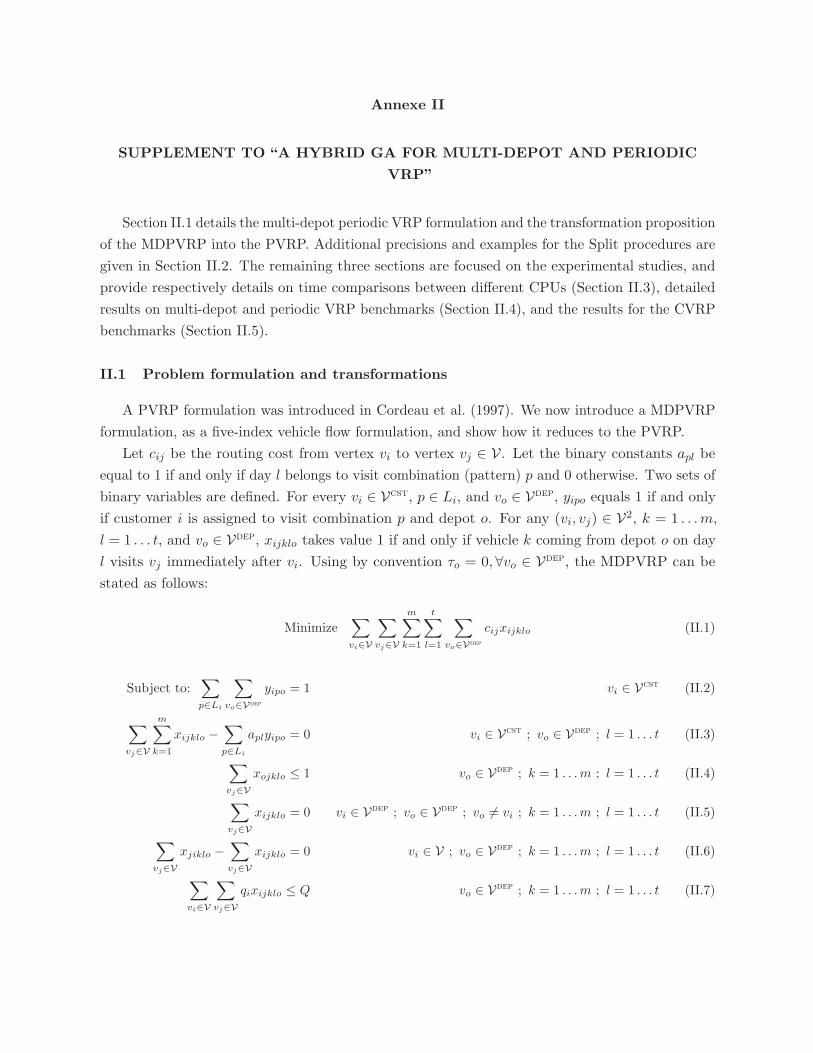
Annexe II

SUPPLEMENT TO “A HYBRID GA FOR MULTI-DEPOT AND PERIODIC

VRP”

Section II.1 details the multi-depot periodic VRP formulation and the transformation proposition

of the MDPVRP into the PVRP. Additional precisions and examples for the Split procedures are

given in Section II.2. The remaining three sections are focused on the experimental studies, and

provide respectively details on time comparisons between different CPUs (Section II.3), detailed

results on multi-depot and periodic VRP benchmarks (Section II.4), and the results for the CVRP

benchmarks (Section II.5).

II.1 Problem formulation and transformations

A PVRP formulation was introduced in Cordeau et al. (1997). We now introduce a MDPVRP

formulation, as a five-index vehicle flow formulation, and show how it reduces to the PVRP.

Let cij be the routing cost from vertex vi to vertex vj ∈ V. Let the binary constants apl be

equal to 1 if and only if day l belongs to visit combination (pattern) p and 0 otherwise. Two sets of

binary variables are defined. For every vi ∈ Vcst, p ∈ Li, and vo ∈ Vdep, yipo equals 1 if and only

if customer i is assigned to visit combination p and depot o. For any (vi, vj) ∈ V2, k = 1 . . .m,

l = 1 . . . t, and vo ∈ Vdep, xijklo takes value 1 if and only if vehicle k coming from depot o on day

l visits vj immediately after vi. Using by convention τo = 0, ∀vo ∈ Vdep, the MDPVRP can be

stated as follows:

Minimize∑vi∈V

∑vj∈V

m∑k=1

t∑l=1

∑vo∈Vdep

cijxijklo (II.1)

Subject to:∑p∈Li

∑vo∈Vdep

yipo = 1 vi ∈ Vcst (II.2)

∑vj∈V

m∑k=1

xijklo −∑p∈Li

aplyipo = 0 vi ∈ Vcst ; vo ∈ Vdep ; l = 1 . . . t (II.3)

∑vj∈V

xojklo ≤ 1 vo ∈ Vdep ; k = 1 . . .m ; l = 1 . . . t (II.4)

∑vj∈V

xijklo = 0 vi ∈ Vdep ; vo ∈ Vdep ; vo �= vi ; k = 1 . . .m ; l = 1 . . . t (II.5)

∑vj∈V

xjiklo −∑vj∈V

xijklo = 0 vi ∈ V ; vo ∈ Vdep ; k = 1 . . .m ; l = 1 . . . t (II.6)

∑vi∈V

∑vj∈V

qixijklo ≤ Q vo ∈ Vdep ; k = 1 . . .m ; l = 1 . . . t (II.7)

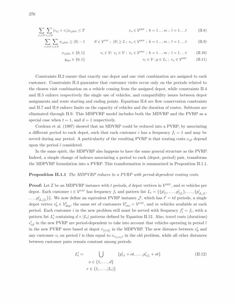
276

∑vi∈V

∑vj∈V

(cij + τi)xijklo ≤ T vo ∈ Vdep ; k = 1 . . .m ; l = 1 . . . t (II.8)

∑vi∈S

∑vj∈S

xijklo ≤ |S| − 1 S ∈ Vcst ; |S| ≥ 2 ; vo ∈ Vdep ; k = 1 . . .m ; l = 1 . . . t (II.9)

xijklo ∈ {0, 1} vi ∈ V; vj ∈ V ; vo ∈ Vdep ; k = 1 . . .m ; l = 1 . . . t (II.10)

yipo ∈ {0, 1} vi ∈ V ; p ∈ Li ; vo ∈ Vdep (II.11)

Constraints II.2 ensure that exactly one depot and one visit combination are assigned to each

customer. Constraints II.3 guarantee that customer visits occur only on the periods related to

the chosen visit combination on a vehicle coming from the assigned depot, while constraints II.4

and II.5 enforce respectively the single use of vehicles, and compatibility issues between depot

assignments and route starting and ending points. Equations II.6 are flow conservation constraints

and II.7 and II.8 enforce limits on the capacity of vehicles and the duration of routes. Subtours are

eliminated through II.9. This MDPVRP model includes both the MDVRP and the PVRP as a

special case when t = 1, and d = 1 respectively.

Cordeau et al. (1997) showed that an MDVRP could be reduced into a PVRP, by associating

a different period to each depot, such that each customer i has a frequency fi = 1 and may be

served during any period. A particularity of the resulting PVRP is that routing costs cijl depend

upon the period l considered.

In the same spirit, the MDPVRP also happens to have the same general structure as the PVRP.

Indeed, a simple change of indexes associating a period to each (depot, period) pair, transforms

the MDPVRP formulation into a PVRP. This transformation is summarized in Proposition II.1.1.

Proposition II.1.1 The MDPVRP reduces to a PVRP with period-dependent routing costs.

Proof: Let I be an MDPVRP instance with t periods, d depot vertices in Vdep, and m vehicles per

depot. Each customer i ∈ Vcst has frequency fi and pattern list Li = {{pi11, . . . , pi1fi}, . . . , {pi|Li|1,

. . . , pi|Li|fi}}. We now define an equivalent PVRP instance J , which has t′ = td periods, a single

depot vertex v′0 ∈ V ′dep, the same set of customers V ′

cus = Vcst, and m vehicles available at each

period. Each customer i in the new problem still must be served with frequency f ′i = fi, with a

pattern list L′i containing d× |Li| patterns defined by Equation II.12. Also, travel costs (durations)

c′ijl in the new PVRP are period-dependent to take into account that vehicles operating in period l

in the new PVRP were based at depot v�l/d in the MDPVRP. The new distance between v′0 and

any customer vi on period l is thus equal to cv�l/d�i in the old problem, while all other distances

between customer pairs remain constant among periods.

L′i =

⋃o ∈ {1, . . . , d}r ∈ {1, . . . , |Li|}

{pir1 + ot, . . . , pirfi + ot} (II.12)

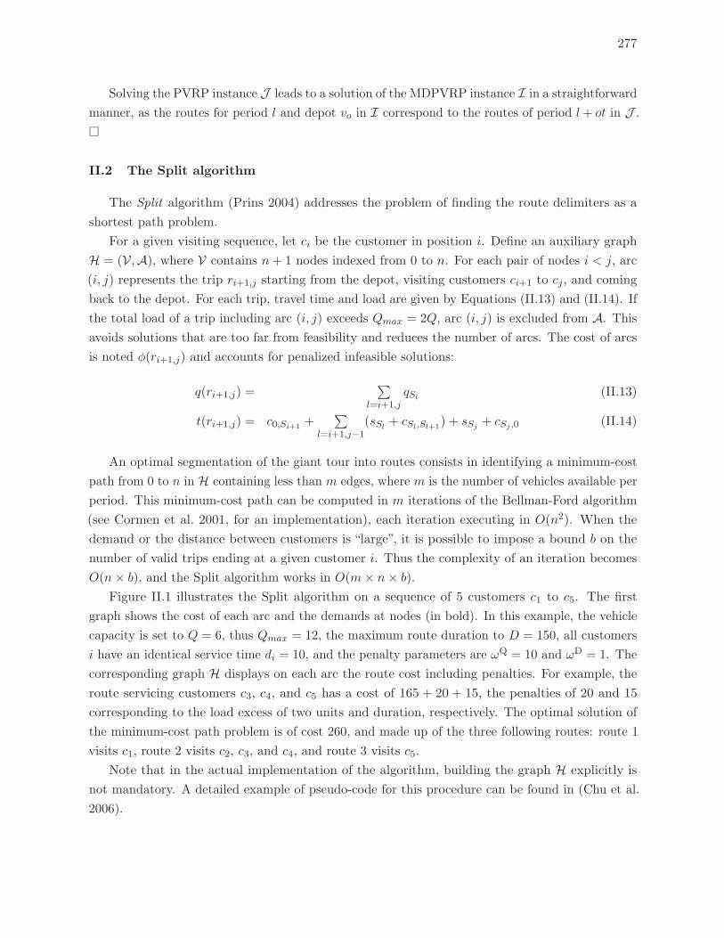
277

Solving the PVRP instance J leads to a solution of the MDPVRP instance I in a straightforward

manner, as the routes for period l and depot vo in I correspond to the routes of period l+ ot in J .

�

II.2 The Split algorithm

The Split algorithm (Prins 2004) addresses the problem of finding the route delimiters as a

shortest path problem.

For a given visiting sequence, let ci be the customer in position i. Define an auxiliary graph

H = (V,A), where V contains n+ 1 nodes indexed from 0 to n. For each pair of nodes i < j, arc

(i, j) represents the trip ri+1,j starting from the depot, visiting customers ci+1 to cj , and coming

back to the depot. For each trip, travel time and load are given by Equations (II.13) and (II.14). If

the total load of a trip including arc (i, j) exceeds Qmax = 2Q, arc (i, j) is excluded from A. This

avoids solutions that are too far from feasibility and reduces the number of arcs. The cost of arcs

is noted φ(ri+1,j) and accounts for penalized infeasible solutions:

q(ri+1,j) =∑

l=i+1,j

qSl(II.13)

t(ri+1,j) = c0,Si+1 +∑

l=i+1,j−1

(sSl+ cSl,Sl+1

) + sSj + cSj ,0 (II.14)

An optimal segmentation of the giant tour into routes consists in identifying a minimum-cost

path from 0 to n in H containing less than m edges, where m is the number of vehicles available per

period. This minimum-cost path can be computed in m iterations of the Bellman-Ford algorithm

(see Cormen et al. 2001, for an implementation), each iteration executing in O(n2). When the

demand or the distance between customers is “large”, it is possible to impose a bound b on the

number of valid trips ending at a given customer i. Thus the complexity of an iteration becomes

O(n× b), and the Split algorithm works in O(m× n× b).

Figure II.1 illustrates the Split algorithm on a sequence of 5 customers c1 to c5. The first

graph shows the cost of each arc and the demands at nodes (in bold). In this example, the vehicle

capacity is set to Q = 6, thus Qmax = 12, the maximum route duration to D = 150, all customers

i have an identical service time di = 10, and the penalty parameters are ωQ = 10 and ωD = 1. The

corresponding graph H displays on each arc the route cost including penalties. For example, the

route servicing customers c3, c4, and c5 has a cost of 165 + 20 + 15, the penalties of 20 and 15

corresponding to the load excess of two units and duration, respectively. The optimal solution of

the minimum-cost path problem is of cost 260, and made up of the three following routes: route 1

visits c1, route 2 visits c2, c3, and c4, and route 3 visits c5.

Note that in the actual implementation of the algorithm, building the graph H explicitly is

not mandatory. A detailed example of pseudo-code for this procedure can be found in (Chu et al.

2006).

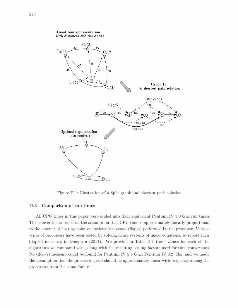
278

Figure II.1: Illustration of a Split graph and shortest-path solution

II.3 Comparison of run times

All CPU times in this paper were scaled into their equivalent Pentium IV 3.0 Ghz run times.

This conversion is based on the assumption that CPU time is approximately linearly proportional

to the amount of floating point operations per second (flop/s) performed by the processor. Various

types of processors have been tested by solving dense systems of linear equations, to report their

(flop/s) measures in Dongarra (2011). We provide in Table II.1 these values for each of the

algorithms we compared with, along with the resulting scaling factors used for time conversions.

No (flop/s) measure could be found for Pentium IV 2.8 Ghz, Pentium IV 3.2 Ghz, and we made

the assumption that the processor speed should be approximately linear with frequency among the

processors from the same family.

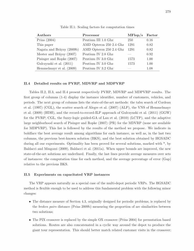
279

Table II.1: Scaling factors for computation times

Authors Processor MFlop/s Factor

Prins (2004) Pentium III 1.0 Ghz 250 0.16

This paper AMD Opteron 250 2.4 Ghz 1291 0.82

Nagata and Braysy (2009b) AMD Opteron 250 2.4 Ghz 1291 0.82

Mester and Braysy (2007) Pentium IV 2.8 Ghz — 0.92

Pisinger and Ropke (2007) Pentium IV 3.0 Ghz 1573 1.00

Gulczynski et al. (2011) Pentium IV 3.0 Ghz 1573 1.00

Hemmelmayr et al. (2009) Pentium IV 3.2 Ghz — 1.08

II.4 Detailed results on PVRP, MDVRP and MDPVRP

Tables II.2, II.3, and II.4 present respectively PVRP, MDVRP and MDPVRP results. The

first group of columns (1-4) display the instance identifier, number of customers, vehicles, and

periods. The next group of columns lists the state-of-the-art methods: the tabu search of Cordeau

et al. (1997) (CGL), the scatter search of Alegre et al. (2007) (ALP), the VNS of Hemmelmayr

et al. (2009) (HDH), and the record-to-record-ILP approach of Gulczynski et al. (2011) (GGW)

for the PVRP; CGL, the fuzzy-logic guided-GA of Lau et al. (2010) (LCTP), and the adaptive

large neighborhood search of Pisinger and Ropke (2007) (PR) for the MDVRP (none are available

for MDPVRP). This list is followed by the results of the method we propose. We indicate in

boldface the best average result among algorithms for each instance, as well as, in the last two

columns, the previous best-known solution (BKS), and the best solution obtained by HGSADC

during all our experiments. Optimality has been proved for several solutions, marked with *, by

Baldacci and Mingozzi (2009), Baldacci et al. (2011a). When upper bounds are improved, the new

state-of-the-art solutions are underlined. Finally, the last lines provide average measures over sets

of instances: the computation time for each method, and the average percentage of error (Gap)

relative to the previous BKS.

II.5 Experiments on capacitated VRP instances

The VRP appears naturally as a special case of the multi-depot periodic VRPs. The HGSADC

method is flexible enough to be used to address this fundamental problem with the following minor

changes:

• The distance measure of Section 4.3, originally designed for periodic problems, is replaced by

the broken pairs distance (Prins 2009b) measuring the proportion of arc similarities between

two solutions;

• The PIX crossover is replaced by the simple OX crossover (Prins 2004) for permutation based

solutions. Routes are also concatenated in a cyclic way around the depot to produce the

giant tour representation. This should better match related customer visits in the crossover;

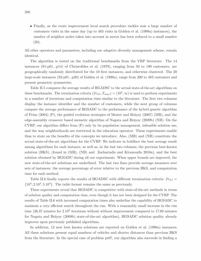
280

• Finally, as the route improvement local search procedure tackles now a large number of

customers visits in the same day (up to 483 visits in Golden et al. (1998a) instances), the

number of neighbor nodes taken into account in moves has been reduced to a small number

(20).

All other operators and parameters, including our adaptive diversity management scheme, remain

identical.

The algorithm is tested on the traditional benchmarks from the VRP literature. The 14

instances (S1-p01...p14) of Christofides et al. (1979), ranging from 50 to 199 customers, are

geographically randomly distributed for the 10 first instances, and otherwise clustered. The 20

large-scale instances (S2-p01...p20) of Golden et al. (1998a), range from 200 to 483 customers and

present geometric symmetries.

Table II.5 compares the average results of HGADSC to the actual state-of-the-art algorithms on

these benchmarks. The termination criteria (ItNI , Tmax) = (104,∞) is used to perform experiments

in a number of iterations and computation time similar to the literature. The first two columns

display the instance identifier and the number of customers, while the next group of columns

compare the average performance of HGSADC to the performance of the hybrid genetic algorithm

of Prins (2004) (P), the guided evolution strategies of Mester and Braysy (2007) (MB), and the

edge-assembly crossover based memetic algorithm of Nagata and Braysy (2009b) (NB). On the

CVRP, our algorithm differs from (P) only by its population management, infeasible solution use,

and the way neighborhoods are restricted in the education operator. These experiments enable

thus to state on the benefits of the concepts we introduce. Also, (MB) and (NB) constitute the

actual state-of-the-art algorithms for the CVRP. We indicate in boldface the best average result

among algorithms for each instance, as well as, in the last two columns, the previous best-known

solution (BKS), (found in (MB), (NB) and Zachariadis and Kiranoudis 2010a), and the best

solution obtained by HGSADC during all our experiments. When upper bounds are improved, the

new state-of-the-art solutions are underlined. The last two lines provide average measures over

sets of instances: the average percentage of error relative to the previous BKS, and computation

time for each method.

Table II.6 finally reports the results of HGADSC with different termination criteria: ItNI =

{104, 2.104, 5.104}. The table format remains the same as previously.

These experiments reveal that HGSADC is competitive with state-of-the-art methods in terms

of solution quality and computation time, even though it has not been designed for the CVRP. The

results of Table II.6 with increased computation times also underline the capability of HGSADC to

maintain a very efficient search throughout the run. With a reasonably small increase in the run

time (26.37 minutes for 2.104 iterations without without improvement compared to 17.69 minutes

for Nagata and Braysy (2009b) state-of-the-art algorithm), HGSADC solution quality already

improves upon previously published algorithms.

In addition, 12 new best known solutions are reported on Golden et al. (1998a) instances.

All these solutions present equal numbers of vehicles and shorter distances than previous BKS

from the literature. In the special case of problem pr07, our algorithm also succeeds in finding a

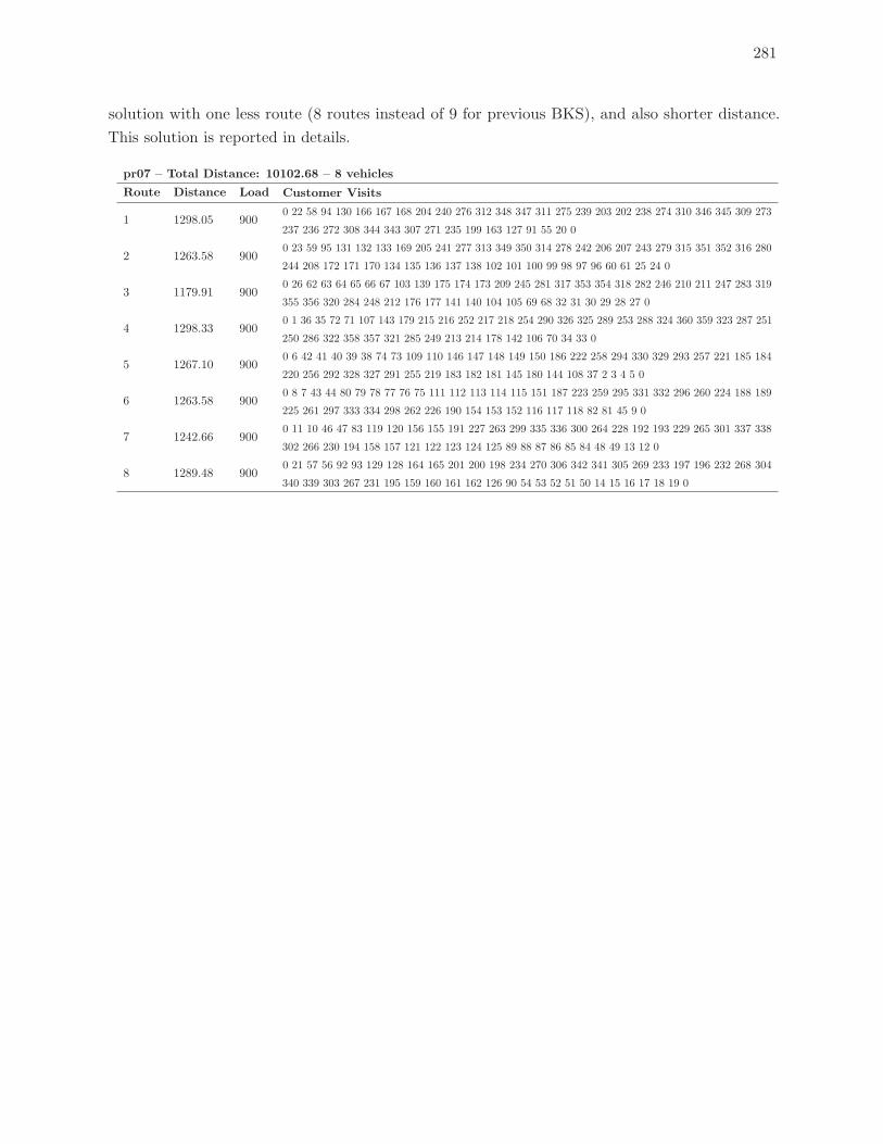
281

solution with one less route (8 routes instead of 9 for previous BKS), and also shorter distance.

This solution is reported in details.

pr07 – Total Distance: 10102.68 – 8 vehicles

Route Distance Load Customer Visits

1 1298.05 9000 22 58 94 130 166 167 168 204 240 276 312 348 347 311 275 239 203 202 238 274 310 346 345 309 273

237 236 272 308 344 343 307 271 235 199 163 127 91 55 20 0

2 1263.58 9000 23 59 95 131 132 133 169 205 241 277 313 349 350 314 278 242 206 207 243 279 315 351 352 316 280

244 208 172 171 170 134 135 136 137 138 102 101 100 99 98 97 96 60 61 25 24 0

3 1179.91 9000 26 62 63 64 65 66 67 103 139 175 174 173 209 245 281 317 353 354 318 282 246 210 211 247 283 319

355 356 320 284 248 212 176 177 141 140 104 105 69 68 32 31 30 29 28 27 0

4 1298.33 9000 1 36 35 72 71 107 143 179 215 216 252 217 218 254 290 326 325 289 253 288 324 360 359 323 287 251

250 286 322 358 357 321 285 249 213 214 178 142 106 70 34 33 0

5 1267.10 9000 6 42 41 40 39 38 74 73 109 110 146 147 148 149 150 186 222 258 294 330 329 293 257 221 185 184

220 256 292 328 327 291 255 219 183 182 181 145 180 144 108 37 2 3 4 5 0

6 1263.58 9000 8 7 43 44 80 79 78 77 76 75 111 112 113 114 115 151 187 223 259 295 331 332 296 260 224 188 189

225 261 297 333 334 298 262 226 190 154 153 152 116 117 118 82 81 45 9 0

7 1242.66 9000 11 10 46 47 83 119 120 156 155 191 227 263 299 335 336 300 264 228 192 193 229 265 301 337 338

302 266 230 194 158 157 121 122 123 124 125 89 88 87 86 85 84 48 49 13 12 0

8 1289.48 9000 21 57 56 92 93 129 128 164 165 201 200 198 234 270 306 342 341 305 269 233 197 196 232 268 304

340 339 303 267 231 195 159 160 161 162 126 90 54 53 52 51 50 14 15 16 17 18 19 0

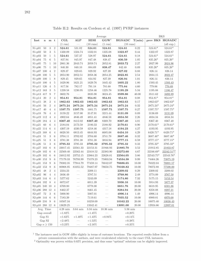
282

Table II.2: Results on Cordeau et al. (1997) PVRP instances

Average BKS

Inst n m t CGL ALP HDH GGW1 HGSADC T(min) prev BKS HGSADC

(1 run) — (10 runs) (1 run) (10 runs) — (all exp.)

S1-p01 50 3 2 524.61 531.02 524.61 524.61 524.61 0.22 524.61* 524.61*

S1-p02 50 3 5 1330.09 1324.74 1332.01 1335.08 1322.87 0.44 1322.87 1322.87

S1-p03 50 1 5 524.61 537.37 528.97 524.61 524.61 0.18 524.61* 524.61*

S1-p04 75 6 5 837.94 845.97 847.48 838.47 836.59 1.05 835.26* 835.26*

S1-p05 75 1 10 2061.36 2043.74 2059.74 2052.81 2033.72 2.27 2027.99 2024.96

S1-p06 75 1 10 840.30 840.10 884.69 838.47 842.48 0.89 835.26* 835.26*

S1-p07 100 4 2 829.37 829.65 829.92 827.39 827.02 0.88 826.14 826.14

S1-p08 100 5 5 2054.90 2052.51 2058.36 2054.25 2022.85 2.54 2034.15 2022.47

S1-p09 100 1 8 829.45 829.65 834.92 827.39 826.94 1.01 826.14 826.14

S1-p10 100 4 5 1629.96 1621.21 1629.76 1645.42 1605.22 1.80 1593.45 1593.43

S1-p11 126 4 5 817.56 782.17 791.18 781.68 775.84 4.60 779.06 770.89

S1-p12 163 3 5 1239.58 1230.95 1258.46 1225.78 1195.29 5.34 1195.88 1186.47

S1-p13 417 9 7 3602.76 — 3835.90 3624.45 3599.86 40.00 3511.62 3492.89

S1-p14 20 2 4 954.81 954.81 954.81 954.81 954.81 0.08 954.81* 954.81*

S1-p15 38 2 4 1862.63 1862.63 1862.63 1862.63 1862.63 0.17 1862.63* 1862.63*

S1-p16 56 2 4 2875.24 2875.24 2875.24 2875.24 2875.24 0.32 2875.24* 2875.24*

S1-p17 40 4 4 1597.75 1597.75 1601.75 1597.75 1597.75 0.27 1597.75* 1597.75*

S1-p18 76 4 4 3159.22 3157.00 3147.91 3215.44 3131.09 0.89 3136.69 3131.09

S1-p19 112 4 4 4902.64 4846.49 4851.41 4846.58 4834.50 2.26 4834.34 4834.34

S1-p20 184 4 4 8367.40 8412.02 8367.40 8369.70 8367.40 4.01 8367.40 8367.40

S1-p21 60 6 4 2184.04 2173.58 2180.33 2188.92 2170.61 0.90 2170.61* 2170.61*

S1-p22 114 6 4 4307.19 4330.59 4218.46 4317.18 4194.23 4.27 4193.95 4193.95

S1-p23 168 6 4 6620.50 6813.45 6644.93 6685.08 6434.10 4.29 6420.71* 6420.71*

S1-p24 51 3 6 3704.11 3702.02 3704.60 3741.78 3687.46 0.32 3687.46* 3687.46*

S1-p25 51 3 6 3781.38 3781.38 3781.38 3816.94 3777.15 0.59 3777.15* 3777.15*

S1-p26 51 3 6 3795.32 3795.33 3795.32 3795.32 3795.32 0.33 3795.32* 3795.32*

S1-p27 102 6 6 23017.45 22561.33 22153.31 21946.93 21885.70 3.52 21912.85 21833.87

S1-p28 102 6 6 22569.40 22562.44 22418.52 22383.90 22272.60 4.67 22246.69* 22242.51*2

S1-p29 102 6 6 24012.92 23752.15 22864.23 22628.81 22564.05 3.86 22543.75* 22543.76*

S1-p30 153 9 6 77179.33 76793.99 75579.23 75003.94 74534.38 9.99 74464.26 73875.19

S1-p31 153 9 6 79382.35 77944.79 77459.14 76842.07 76686.65 10.00 76322.04 76001.57

S1-p32 153 9 6 80908.95 81055.52 79487.97 78650.75 78168.82 10.00 78072.88 77598.00

S2-p01 48 2 4 2234.23 — 2209.11 — 2209.02 0.29 2209.02 2209.02

S2-p02 96 4 4 3836.49 — 3787.51 — 3768.86 2.49 3774.09 3767.50

S2-p03 144 6 4 5277.62 — 5243.09 — 5174.80 7.32 5175.15 5153.54

S2-p04 192 8 4 6072.67 — 6011.39 — 5936.16 10.00 5914.93 5877.37

S2-p05 240 10 4 6769.80 — 6778.00 — 6651.76 20.00 6618.95 6581.86

S2-p06 288 12 4 8462.37 — 8461.45 — 8284.94 20.00 8258.08 8207.21

S2-p07 72 3 6 5000.90 — 5007.01 — 4996.14 1.49 4996.14 4996.14

S2-p08 144 6 6 7183.39 — 7119.61 — 7035.52 10.00 6989.81 6970.68

S2-p09 216 9 6 10507.34 — 10259.09 — 10162.22 20.00 10075.40 10038.43

S2-p10 288 12 6 13629.25 — 13342.41 — 13091.00 20.00 12924.66 12897.01

Avg. Time 4.28 min 3.64 min 3.34 min 10.36 min 5.56 min

Gap overall +1.82% — +1.45% — +0.20%

Gap S1 +1.62% +1.40% +1.43% +0.94% +0.14%

Gap S2 +2.48% — +1.53% — +0.38%

Gap n ≥ 150 +3.23% — +2.16% — +0.35%

1 The instances used in GGW differ slightly in terms of customer locations. The reported results follow from aprivate communication with the authors, and were recalculated relatively to the exact CGL instances.

2 Optimality was proven within 0.02% precision, and thus some “optimal” solutions can be slightly improved.

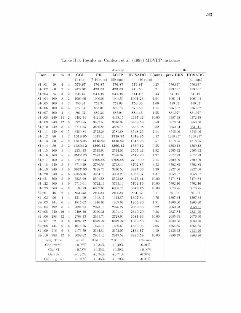
283

Table II.3: Results on Cordeau et al. (1997) MDVRP instances

Average BKS

Inst n m d CGL PR LCTP HGSADC T(min) prev BKS HGSADC

(1 run) (5-10 runs) (50 runs) (10 runs) — (all exp.)

S1-p01 50 4 4 576.87 576.87 576.87 576.87 0.23 576.87* 576.87*

S1-p02 50 2 4 473.87 473.53 473.53 473.53 0.21 473.53* 473.53*

S1-p03 75 3 2 645.15 641.19 641.19 641.19 0.43 641.19 641.19

S1-p04 100 8 2 1006.66 1006.09 1001.59 1001.23 1.94 1001.04 1001.04

S1-p05 100 5 2 753.34 752.34 752.08 750.03 1.06 750.03 750.03

S1-p06 100 6 3 877.84 883.01 882.73 876.50 1.14 876.50* 876.50*

S1-p07 100 4 4 891.95 889.36 887.94 884.43 1.55 881.97* 881.97*

S1-p08 249 14 2 4482.44 4421.03 4438.15 4397.42 10.00 4387.38 4372.78

S1-p09 249 12 3 3920.85 3892.50 3916.32 3868.59 9.50 3873.64 3858.66

S1-p10 249 8 4 3714.65 3666.85 3669.76 3636.08 9.82 3650.04 3631.11

S1-p11 249 6 5 3580.84 3573.23 3581.88 3548.25 7.14 3546.06 3546.06

S1-p12 80 5 2 1318.95 1319.13 1318.95 1318.95 0.52 1318.95* 1318.95*

S1-p13 80 5 2 1318.95 1318.95 1318.95 1318.95 0.57 1318.95 1318.95

S1-p14 80 5 2 1360.12 1360.12 1360.12 1360.12 0.55 1360.12 1360.12

S1-p15 160 5 4 2534.13 2519.64 2514.06 2505.42 1.92 2505.42 2505.42

S1-p16 160 5 4 2572.23 2573.95 2578.37 2572.23 1.97 2572.23 2572.23

S1-p17 160 5 4 2720.23 2709.09 2709.09 2709.09 2.14 2709.09 2709.09

S1-p18 240 5 6 3710.49 3736.53 3728.44 3702.85 4.52 3702.85 3702.85

S1-p19 240 5 6 3827.06 3838.76 3840.53 3827.06 4.20 3827.06 3827.06

S1-p20 240 5 6 4058.07 4064.76 4063.26 4058.07 4.37 4058.07 4058.07

S1-p21 360 5 9 5535.99 5501.58 5525.68 5476.41 10.00 5474.84 5474.84

S1-p22 360 5 9 5716.01 5722.19 5733.13 5702.16 10.00 5702.16 5702.16

S1-p23 360 5 9 6139.73 6092.66 6098.75 6078.75 10.00 6078.75 6078.75

S2-p01 48 2 4 861.32 861.32 861.32 861.32 0.17 861.32 861.32

S2-p02 96 4 4 1314.99 1308.17 1312.85 1307.34 0.76 1307.34 1307.34

S2-p03 144 6 4 1815.62 1810.66 1809.69 1803.80 1.91 1806.60 1803.80

S2-p04 192 8 4 2094.24 2073.16 2076.27 2059.36 5.22 2060.93 2058.31

S2-p05 240 10 4 2408.10 2350.31 2391.42 2340.29 9.56 2337.84 2331.20

S2-p06 288 12 4 2768.13 2695.74 2728.94 2681.93 10.00 2685.35 2676.30

S2-p07 72 3 6 1092.12 1089.56 1089.56 1089.56 0.34 1089.56 1089.56

S2-p08 144 6 6 1676.26 1675.74 1666.60 1665.05 2.05 1664.85 1664.85

S2-p09 216 9 6 2176.79 2144.84 2152.05 2134.17 6.10 2136.42 2133.20

S2-p10 288 12 6 3089.62 2905.43 2919.59 2886.59 10.00 2889.49 2868.26

Avg. Time small 3.54 min 2.06 min 4.24 min

Gap overall +0.96% +0.34% +0.49% -0.01%

Gap S1 +0.58% +0.35% +0.39% +0.00%

Gap S2 +1.85% +0.34% +0.71% -0.04%

Gap n ≥ 150 +1.40% +0.45% +0.70% -0.03%

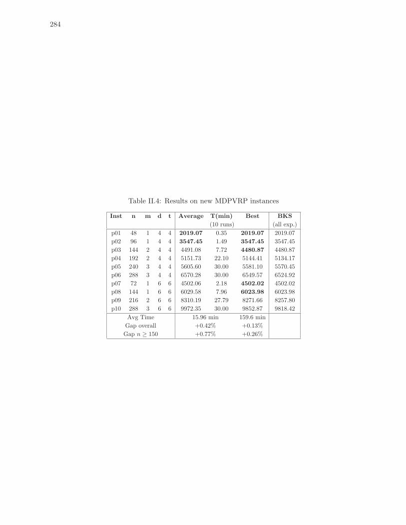
284

Table II.4: Results on new MDPVRP instances

Inst n m d t Average T(min) Best BKS

(10 runs) (all exp.)

p01 48 1 4 4 2019.07 0.35 2019.07 2019.07

p02 96 1 4 4 3547.45 1.49 3547.45 3547.45

p03 144 2 4 4 4491.08 7.72 4480.87 4480.87

p04 192 2 4 4 5151.73 22.10 5144.41 5134.17

p05 240 3 4 4 5605.60 30.00 5581.10 5570.45

p06 288 3 4 4 6570.28 30.00 6549.57 6524.92

p07 72 1 6 6 4502.06 2.18 4502.02 4502.02

p08 144 1 6 6 6029.58 7.96 6023.98 6023.98

p09 216 2 6 6 8310.19 27.79 8271.66 8257.80

p10 288 3 6 6 9972.35 30.00 9852.87 9818.42

Avg Time 15.96 min 159.6 min

Gap overall +0.42% +0.13%

Gap n ≥ 150 +0.77% +0.26%

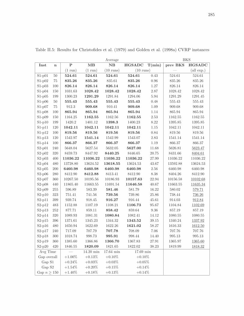
285

Table II.5: Results for Christofides et al. (1979) and Golden et al. (1998a) CVRP instances

Average BKS

Inst n P MB NB HGSADC T(min) prev BKS HGSADC

(1 run) (1 run) (10 runs) (10 runs) — (all exp.)

S1-p01 50 524.61 524.61 524.61 524.61 0.43 524.61 524.61

S1-p02 75 835.26 835.26 835.61 835.26 0.96 835.26 835.26

S1-p03 100 826.14 826.14 826.14 826.14 1.27 826.14 826.14

S1-p04 150 1031.63 1028.42 1028.42 1028.42 2.87 1028.42 1028.42

S1-p05 199 1300.23 1291.29 1291.84 1294.06 5.94 1291.29 1291.45

S1-p06 50 555.43 555.43 555.43 555.43 0.48 555.43 555.43

S1-p07 75 912.3 909.68 910.41 909.68 1.09 909.68 909.68

S1-p08 100 865.94 865.94 865.94 865.94 1.14 865.94 865.94

S1-p09 150 1164.25 1162.55 1162.56 1162.55 2.53 1162.55 1162.55

S1-p10 199 1420.2 1401.12 1398.3 1400.23 8.22 1395.85 1395.85

S1-p11 120 1042.11 1042.11 1042.11 1042.11 1.15 1042.11 1042.11

S1-p12 100 819.56 819.56 819.56 819.56 0.84 819.56 819.56

S1-p13 120 1542.97 1541.14 1542.99 1543.07 2.83 1541.14 1541.14

S1-p14 100 866.37 866.37 866.37 866.37 1.19 866.37 866.37

S2-p01 240 5648.04 5627.54 5632.05 5627.00 11.68 5626.81 5623.47

S2-p02 320 8459.73 8447.92 8440.25 8446.65 20.75 8431.66 8404.61

S2-p03 400 11036.22 11036.22 11036.22 11036.22 27.99 11036.22 11036.22

S2-p04 480 13728.80 13624.52 13618.55 13624.53 43.67 13592.88 13624.53

S2-p05 200 6460.98 6460.98 6460.98 6460.98 2.56 6460.98 6460.98

S2-p06 280 8412.90 8412.88 8413.41 8412.90 8.38 8404.26 8412.90

S2-p07 360 10267.50 10195.56 10186.93 10157.63 22.94 10156.58 10102.68

S2-p08 440 11865.40 11663.55 11691.54 11646.58 40.67 11663.55 11635.34

S2-p09 255 596.89 583.39 581.46 581.79 16.22 580.02 579.71

S2-p10 323 751.41 741.56 739.56 739.86 25.86 738.44 736.26

S2-p11 399 939.74 918.45 916.27 916.44 45.61 914.03 912.84

S2-p12 483 1152.88 1107.19 1108.21 1106.73 95.67 1104.84 1102.69

S2-p13 252 877.71 859.11 858.42 859.64 9.36 857.19 857.19

S2-p14 320 1089.93 1081.31 1080.84 1082.41 14.12 1080.55 1080.55

S2-p15 396 1371.61 1345.23 1344.32 1343.52 39.15 1340.24 1337.92

S2-p16 480 1650.94 1622.69 1622.26 1621.02 58.27 1616.33 1612.50

S2-p17 240 717.09 707.79 707.78 708.09 7.06 707.76 707.76

S2-p18 300 1018.74 998.73 995.91 998.44 14.40 995.13 995.13

S2-p19 360 1385.60 1366.86 1366.70 1367.83 27.91 1365.97 1365.60

S2-p20 420 1846.55 1820.09 1821.65 1822.02 38.23 1819.99 1818.32

Avg Time — 14.20 min 17.64 min 17.69 min

Gap overall +1.00% +0.13% +0.10% +0.10%

Gap S1 +0.24% +0.03% +0.03% +0.05%

Gap S2 +1.54% +0.20% +0.15% +0.14%

Gap n ≥ 150 +1.40% +0.18% +0.13% +0.14%

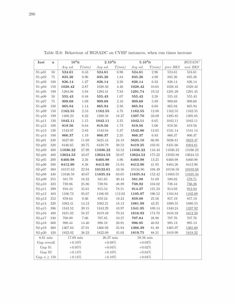
286

Table II.6: Behaviour of HGSADC on CVRP instances, when run times increase

Inst n 104it 2.104it 5.104it HGSADC

Avg sol. T(min) Avg sol. T(min) Avg sol. T(min) prev BKS new BKS

S1-p01 50 524.61 0.43 524.61 0.96 524.61 2.96 524.61 524.61

S1-p02 75 835.26 0.96 835.26 1.84 835.26 4.98 835.26 835.26

S1-p03 100 826.14 1.27 826.14 2.30 826.14 6.33 826.14 826.14

S1-p04 150 1028.42 2.87 1028.56 4.46 1028.42 10.65 1028.42 1028.42

S1-p05 199 1294.06 5.94 1294.41 7.83 1291.74 19.52 1291.29 1291.45

S1-p06 50 555.43 0.48 555.43 1.07 555.43 3.28 555.43 555.43

S1-p07 75 909.68 1.09 909.68 2.10 909.68 5.89 909.68 909.68

S1-p08 100 865.94 1.14 865.94 2.38 865.94 6.68 865.94 865.94

S1-p09 150 1162.55 2.53 1162.55 4.78 1162.55 12.00 1162.55 1162.55

S1-p10 199 1400.23 8.22 1398.58 18.37 1397.70 33.09 1395.85 1395.85

S1-p11 120 1042.11 1.15 1042.11 2.35 1042.11 6.65 1042.11 1042.11

S1-p12 100 819.56 0.84 819.56 1.73 819.56 5.06 819.56 819.56

S1-p13 120 1543.07 2.83 1543.04 5.37 1542.86 12.65 1541.14 1541.14

S1-p14 100 866.37 1.19 866.37 2.35 866.37 6.83 866.37 866.37

S2-p01 240 5627.00 11.68 5625.44 24.18 5625.10 66.90 5626.81 5623.47

S2-p02 320 8446.65 20.75 8438.79 39.52 8419.25 103.91 8431.66 8404.61

S2-p03 400 11036.22 27.99 11036.22 53.52 11036.22 116.43 11036.22 11036.22

S2-p04 480 13624.53 43.67 13624.53 50.67 13624.53 175.22 13592.88 13624.53

S2-p05 200 6460.98 2.56 6460.98 4.96 6460.98 13.25 6460.98 6460.98

S2-p06 280 8412.90 8.38 8412.90 15.94 8412.90 41.95 8404.26 8412.90

S2-p07 360 10157.63 22.94 10132.61 43.56 10134.90 108.49 10156.58 10102.68

S2-p08 440 11646.58 40.67 11635.34 63.65 11635.34 152.42 11663.55 11635.34

S2-p09 255 581.79 16.22 581.65 30.44 581.08 51.69 580.02 579.71

S2-p10 323 739.86 25.86 739.94 48.89 738.92 104.02 738.44 736.26

S2-p11 399 916.44 45.61 915.54 78.51 914.37 131.23 914.03 912.84

S2-p12 483 1106.73 95.67 1106.93 112.03 1105.97 196.52 1104.84 1102.69

S2-p13 252 859.64 9.36 859.24 19.24 859.08 25.56 857.19 857.19

S2-p14 320 1082.41 14.12 1082.21 18.13 1081.99 43.35 1080.55 1080.55

S2-p15 396 1343.52 39.15 1343.29 43.97 1341.95 109.14 1340.24 1337.92

S2-p16 480 1621.02 58.27 1619.49 79.24 1616.92 174.70 1616.33 1612.50

S2-p17 240 708.09 7.06 707.85 10.27 707.84 28.98 707.76 707.76

S2-p18 300 998.44 14.40 998.18 20.91 996.95 40.83 995.13 995.13

S2-p19 360 1367.83 27.91 1366.92 35.94 1366.39 81.49 1365.97 1365.60

S2-p20 420 1822.02 38.23 1822.09 45.03 1819.75 88.31 1819.99 1818.32

6.61 min 17.69 min 26.37 min 58.56 min

Gap overall +0.10% +0.08% +0.03%

Gap S1 +0.05% +0.04% +0.02%

Gap S2 +0.14% +0.10% +0.04%

Gap n ≥ 150 +0.14% +0.10% +0.04%

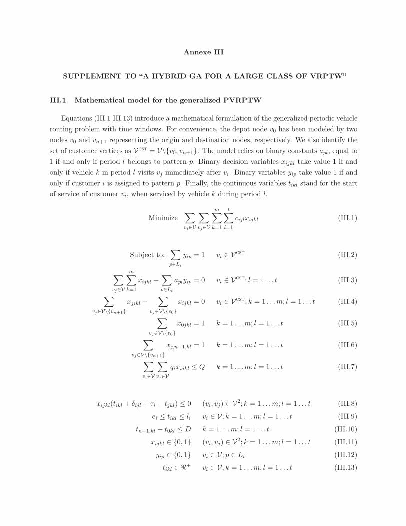
Annexe III

SUPPLEMENT TO “A HYBRID GA FOR A LARGE CLASS OF VRPTW”

III.1 Mathematical model for the generalized PVRPTW

Equations (III.1-III.13) introduce a mathematical formulation of the generalized periodic vehicle

routing problem with time windows. For convenience, the depot node v0 has been modeled by two

nodes v0 and vn+1 representing the origin and destination nodes, respectively. We also identify the

set of customer vertices as Vcst = V\{v0, vn+1}. The model relies on binary constants apl, equal to

1 if and only if period l belongs to pattern p. Binary decision variables xijkl take value 1 if and

only if vehicle k in period l visits vj immediately after vi. Binary variables yip take value 1 if and

only if customer i is assigned to pattern p. Finally, the continuous variables tikl stand for the start

of service of customer vi, when serviced by vehicle k during period l.

Minimize∑vi∈V

∑vj∈V

m∑k=1

t∑l=1

cijlxijkl (III.1)

Subject to:∑p∈Li

yip = 1 vi ∈ Vcst (III.2)

∑vj∈V

m∑k=1

xijkl −∑p∈Li

aplyip = 0 vi ∈ Vcst; l = 1 . . . t (III.3)

∑vj∈V\{vn+1}

xjikl −∑

vj∈V\{v0}xijkl = 0 vi ∈ Vcst; k = 1 . . .m; l = 1 . . . t (III.4)

∑vj∈V\{v0}

x0jkl = 1 k = 1 . . .m; l = 1 . . . t (III.5)

∑vj∈V\{vn+1}

xj,n+1,kl = 1 k = 1 . . .m; l = 1 . . . t (III.6)

∑vi∈V

∑vj∈V

qixijkl ≤ Q k = 1 . . .m; l = 1 . . . t (III.7)

xijkl(tikl + δijl + τi − tjkl) ≤ 0 (vi, vj) ∈ V2; k = 1 . . .m; l = 1 . . . t (III.8)

ei ≤ tikl ≤ li vi ∈ V; k = 1 . . .m; l = 1 . . . t (III.9)

tn+1,kl − t0kl ≤ D k = 1 . . .m; l = 1 . . . t (III.10)

xijkl ∈ {0, 1} (vi, vj) ∈ V2; k = 1 . . .m; l = 1 . . . t (III.11)

yip ∈ {0, 1} vi ∈ V; p ∈ Li (III.12)

tikl ∈ �+ vi ∈ V; k = 1 . . .m; l = 1 . . . t (III.13)

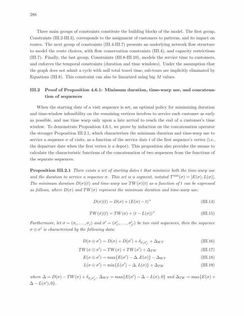
288

Three main groups of constraints constitute the building blocks of the model. The first group,

Constraints (III.2-III.3), corresponds to the assignment of customers to patterns, and its impact on

routes. The next group of constraints (III.4-III.7) presents an underlying network flow structure

to model the route choices, with flow conservation constraints (III.4), and capacity restrictions

(III.7). Finally, the last group, Constraints (III.8-III.10), models the service time to customers,

and enforces the temporal constraints (duration and time windows). Under the assumption that

the graph does not admit a cycle with null total travel time, sub-tours are implicitly eliminated by

Equations (III.8). This constraint can also be linearized using big M values.

III.2 Proof of Proposition 4.6.1: Minimum duration, time-warp use, and concatena-

tion of sequences

When the starting date of a visit sequence is set, an optimal policy for minimizing duration

and time-window infeasibility on the remaining vertices involves to service each customer as early

as possible, and use time warp only upon a late arrival to reach the end of a customer’s time

window. To demonstrate Proposition 4.6.1, we prove by induction on the concatenation operator

the stronger Proposition III.2.1, which characterizes the minimum duration and time-warp use to

service a sequence σ of visits, as a function of the service date t of the first sequence’s vertex (i.e.,

the departure date when the first vertex is a depot). This proposition also provides the means to

calculate the characteristic functions of the concatenation of two sequences from the functions of

the separate sequences.

Proposition III.2.1 There exists a set of starting dates t that minimize both the time-warp use

and the duration to service a sequence σ. This set is a segment, notated T min(σ) = [E(σ), L(σ)].

The minimum duration D(σ)(t) and time-warp use TW (σ)(t) as a function of t can be expressed

as follows, where D(σ) and TW (σ) represent the minimum duration and time-warp use:

D(σ)(t) = D(σ) + (E(σ)− t)+ (III.14)

TW (σ)(t) = TW (σ) + (t− L(σ))+ (III.15)

Furthermore, let σ = (σi, . . . , σj) and σ′ = (σ′i′ , . . . , σ

′j′) be two visit sequences, then the sequence

σ ⊕ σ′ is characterized by the following data:

D(σ ⊕ σ′) = D(σ) +D(σ′) + δσjσ′i′+ΔWT (III.16)

TW (σ ⊕ σ′) = TW (σ) + TW (σ′) + ΔTW (III.17)

E(σ ⊕ σ′) = max{E(σ′)−Δ, E(σ)} −ΔWT (III.18)

L(σ ⊕ σ′) = min{L(σ′)−Δ, L(σ)}+ΔTW (III.19)

where Δ = D(σ)− TW (σ) + δσjσ′i′, ΔWT = max{E(σ′)−Δ− L(σ), 0} and ΔTW = max{E(σ) +

Δ− L(σ′), 0}.

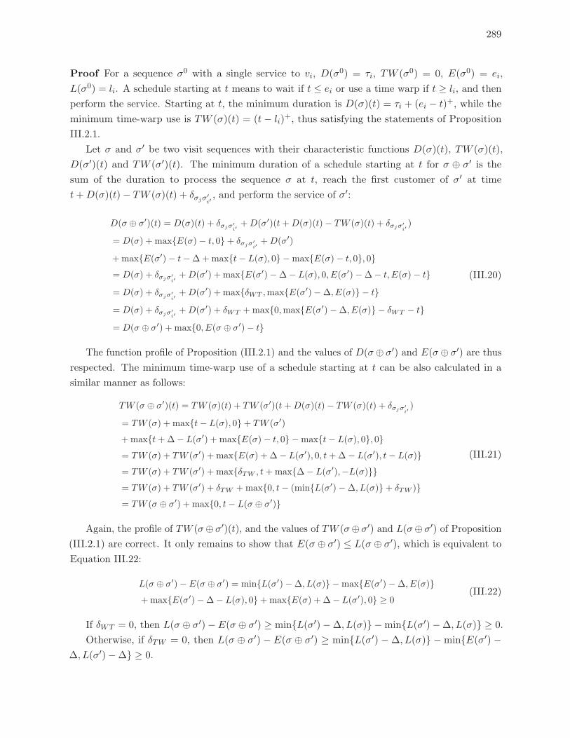
289

Proof For a sequence σ0 with a single service to vi, D(σ0) = τi, TW (σ0) = 0, E(σ0) = ei,

L(σ0) = li. A schedule starting at t means to wait if t ≤ ei or use a time warp if t ≥ li, and then

perform the service. Starting at t, the minimum duration is D(σ)(t) = τi + (ei − t)+, while the

minimum time-warp use is TW (σ)(t) = (t − li)+, thus satisfying the statements of Proposition

III.2.1.

Let σ and σ′ be two visit sequences with their characteristic functions D(σ)(t), TW (σ)(t),

D(σ′)(t) and TW (σ′)(t). The minimum duration of a schedule starting at t for σ ⊕ σ′ is the

sum of the duration to process the sequence σ at t, reach the first customer of σ′ at time

t+D(σ)(t)− TW (σ)(t) + δσjσ′i′, and perform the service of σ′:

D(σ ⊕ σ′)(t) = D(σ)(t) + δσjσ′i′+D(σ′)(t+D(σ)(t)− TW (σ)(t) + δσjσ′

i′)

= D(σ) + max{E(σ)− t, 0}+ δσjσ′i′+D(σ′)

+ max{E(σ′)− t−Δ+max{t− L(σ), 0} −max{E(σ)− t, 0}, 0}= D(σ) + δσjσ′

i′+D(σ′) + max{E(σ′)−Δ− L(σ), 0, E(σ′)−Δ− t, E(σ)− t}

= D(σ) + δσjσ′i′+D(σ′) + max{δWT ,max{E(σ′)−Δ, E(σ)} − t}

= D(σ) + δσjσ′i′+D(σ′) + δWT +max{0,max{E(σ′)−Δ, E(σ)} − δWT − t}

= D(σ ⊕ σ′) + max{0, E(σ ⊕ σ′)− t}

(III.20)

The function profile of Proposition (III.2.1) and the values of D(σ⊕ σ′) and E(σ⊕ σ′) are thus

respected. The minimum time-warp use of a schedule starting at t can be also calculated in a

similar manner as follows:

TW (σ ⊕ σ′)(t) = TW (σ)(t) + TW (σ′)(t+D(σ)(t)− TW (σ)(t) + δσjσ′i′)

= TW (σ) + max{t− L(σ), 0}+ TW (σ′)

+ max{t+Δ− L(σ′) + max{E(σ)− t, 0} −max{t− L(σ), 0}, 0}= TW (σ) + TW (σ′) + max{E(σ) + Δ− L(σ′), 0, t+Δ− L(σ′), t− L(σ)}= TW (σ) + TW (σ′) + max{δTW , t+max{Δ− L(σ′),−L(σ)}}= TW (σ) + TW (σ′) + δTW +max{0, t− (min{L(σ′)−Δ, L(σ)}+ δTW )}= TW (σ ⊕ σ′) + max{0, t− L(σ ⊕ σ′)}

(III.21)

Again, the profile of TW (σ⊕ σ′)(t), and the values of TW (σ⊕ σ′) and L(σ⊕ σ′) of Proposition(III.2.1) are correct. It only remains to show that E(σ ⊕ σ′) ≤ L(σ ⊕ σ′), which is equivalent to

Equation III.22:

L(σ ⊕ σ′)− E(σ ⊕ σ′) = min{L(σ′)−Δ, L(σ)} −max{E(σ′)−Δ, E(σ)}+max{E(σ′)−Δ− L(σ), 0}+max{E(σ) + Δ− L(σ′), 0} ≥ 0

(III.22)

If δWT = 0, then L(σ ⊕ σ′)− E(σ ⊕ σ′) ≥ min{L(σ′)−Δ, L(σ)} −min{L(σ′)−Δ, L(σ)} ≥ 0.

Otherwise, if δTW = 0, then L(σ ⊕ σ′) − E(σ ⊕ σ′) ≥ min{L(σ′) −Δ, L(σ)} −min{E(σ′) −Δ, L(σ′)−Δ} ≥ 0.

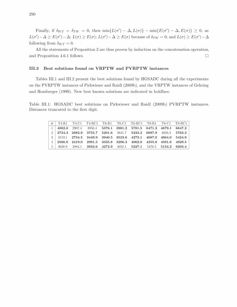
290

Finally, if δWT = δTW = 0, then min{L(σ′) − Δ, L(σ)} − min{E(σ′) − Δ, E(σ)} ≥ 0, as

L(σ′)−Δ ≥ E(σ′)−Δ; L(σ) ≥ E(σ); L(σ′)−Δ ≥ E(σ) because of δTW = 0; and L(σ) ≥ E(σ′)−Δ

following from δWT = 0.

All the statements of Proposition 2 are thus proven by induction on the concatenation operation,

and Proposition 4.6.1 follows. �

III.3 Best solutions found on VRPTW and PVRPTW instances

Tables III.1 and III.2 present the best solutions found by HGSADC during all the experiments

on the PVRPTW instances of Pirkwieser and Raidl (2009b), and the VRPTW instances of Gehring

and Homberger (1999). New best known solutions are indicated in boldface.

Table III.1: HGSADC best solutions on Pirkwieser and Raidl (2009b) PVRPTW instances.Distances truncated to the first digit.

# T4-R1 T4-C1 T4-RC1 T6-R1 T6-C1 T6-RC1 T8-R1 T8-C1 T8-RC1

1 4082.0 2907.4 3956.4 5376.1 3981.2 5781.5 6471.3 4679.1 6847.2

2 3724.3 2882.9 3755.7 5201.6 3841.7 5333.3 6097.9 4933.3 5763.3

3 3153.1 2734.5 3449.9 3940.5 3523.6 4273.1 4687.0 4664.0 5424.9

4 2566.0 2419.0 2991.5 3335.8 3206.3 4062.0 4355.8 4591.6 4929.5

5 3638.9 2884.1 3932.6 4272.9 4052.1 5227.1 5476.5 5134.2 6203.4

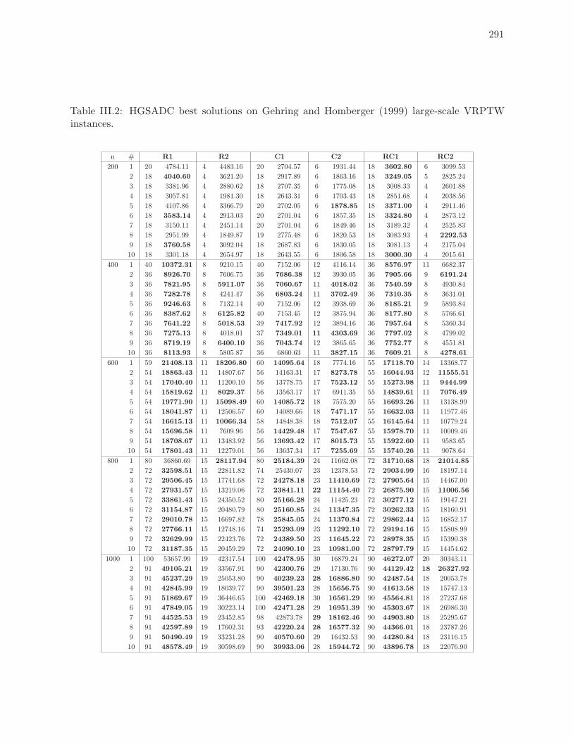
291

Table III.2: HGSADC best solutions on Gehring and Homberger (1999) large-scale VRPTWinstances.

n # R1 R2 C1 C2 RC1 RC2

200 1 20 4784.11 4 4483.16 20 2704.57 6 1931.44 18 3602.80 6 3099.53

2 18 4040.60 4 3621.20 18 2917.89 6 1863.16 18 3249.05 5 2825.24

3 18 3381.96 4 2880.62 18 2707.35 6 1775.08 18 3008.33 4 2601.88

4 18 3057.81 4 1981.30 18 2643.31 6 1703.43 18 2851.68 4 2038.56

5 18 4107.86 4 3366.79 20 2702.05 6 1878.85 18 3371.00 4 2911.46

6 18 3583.14 4 2913.03 20 2701.04 6 1857.35 18 3324.80 4 2873.12

7 18 3150.11 4 2451.14 20 2701.04 6 1849.46 18 3189.32 4 2525.83

8 18 2951.99 4 1849.87 19 2775.48 6 1820.53 18 3083.93 4 2292.53

9 18 3760.58 4 3092.04 18 2687.83 6 1830.05 18 3081.13 4 2175.04

10 18 3301.18 4 2654.97 18 2643.55 6 1806.58 18 3000.30 4 2015.61

400 1 40 10372.31 8 9210.15 40 7152.06 12 4116.14 36 8576.97 11 6682.37

2 36 8926.70 8 7606.75 36 7686.38 12 3930.05 36 7905.66 9 6191.24

3 36 7821.95 8 5911.07 36 7060.67 11 4018.02 36 7540.59 8 4930.84

4 36 7282.78 8 4241.47 36 6803.24 11 3702.49 36 7310.35 8 3631.01

5 36 9246.63 8 7132.14 40 7152.06 12 3938.69 36 8185.21 9 5893.84

6 36 8387.62 8 6125.82 40 7153.45 12 3875.94 36 8177.80 8 5766.61

7 36 7641.22 8 5018.53 39 7417.92 12 3894.16 36 7957.64 8 5360.34

8 36 7275.13 8 4018.01 37 7349.01 11 4303.69 36 7797.02 8 4799.02

9 36 8719.19 8 6400.10 36 7043.74 12 3865.65 36 7752.77 8 4551.81

10 36 8113.93 8 5805.87 36 6860.63 11 3827.15 36 7609.21 8 4278.61

600 1 59 21408.13 11 18206.80 60 14095.64 18 7774.16 55 17118.70 14 13368.77

2 54 18863.43 11 14807.67 56 14163.31 17 8273.78 55 16044.93 12 11555.51

3 54 17040.40 11 11200.10 56 13778.75 17 7523.12 55 15273.98 11 9444.99

4 54 15819.62 11 8029.37 56 13563.17 17 6911.35 55 14839.61 11 7076.49

5 54 19771.90 11 15098.49 60 14085.72 18 7575.20 55 16693.26 11 13138.99

6 54 18041.87 11 12506.57 60 14089.66 18 7471.17 55 16632.03 11 11977.46

7 54 16615.13 11 10066.34 58 14848.38 18 7512.07 55 16145.64 11 10779.24

8 54 15696.58 11 7609.96 56 14429.48 17 7547.67 55 15978.70 11 10009.46

9 54 18708.67 11 13483.92 56 13693.42 17 8015.73 55 15922.60 11 9583.65

10 54 17801.43 11 12279.01 56 13637.34 17 7255.69 55 15740.26 11 9078.64

800 1 80 36860.69 15 28117.94 80 25184.39 24 11662.08 72 31710.68 18 21014.85

2 72 32598.51 15 22811.82 74 25430.07 23 12378.53 72 29034.99 16 18197.14

3 72 29506.45 15 17741.68 72 24278.18 23 11410.69 72 27905.64 15 14467.00

4 72 27931.57 15 13219.06 72 23841.11 22 11154.40 72 26875.90 15 11006.56

5 72 33861.43 15 24350.52 80 25166.28 24 11425.23 72 30277.12 15 19147.21

6 72 31154.87 15 20480.79 80 25160.85 24 11347.35 72 30262.33 15 18160.91

7 72 29010.78 15 16697.82 78 25845.05 24 11370.84 72 29862.44 15 16852.17

8 72 27766.11 15 12748.16 74 25293.09 23 11292.10 72 29194.16 15 15808.99

9 72 32629.99 15 22423.76 72 24389.50 23 11645.22 72 28978.35 15 15390.38

10 72 31187.35 15 20459.29 72 24090.10 23 10981.00 72 28797.79 15 14454.62

1000 1 100 53657.99 19 42317.54 100 42478.95 30 16879.24 90 46272.07 20 30343.11

2 91 49105.21 19 33567.91 90 42300.76 29 17130.76 90 44129.42 18 26327.92

3 91 45237.29 19 25053.80 90 40239.23 28 16886.80 90 42487.54 18 20053.78

4 91 42845.99 19 18039.77 90 39501.23 28 15656.75 90 41613.58 18 15747.13

5 91 51869.67 19 36446.65 100 42469.18 30 16561.29 90 45564.81 18 27237.68

6 91 47849.05 19 30223.14 100 42471.28 29 16951.39 90 45303.67 18 26986.30

7 91 44525.53 19 23452.85 98 42873.78 29 18162.46 90 44903.80 18 25295.67

8 91 42597.89 19 17602.31 93 42220.24 28 16577.32 90 44366.01 18 23787.26

9 91 50490.49 19 33231.28 90 40570.60 29 16432.53 90 44280.84 18 23116.15

10 91 48578.49 19 30598.69 90 39933.06 28 15944.72 90 43896.78 18 22076.90

Annexe IV

SUPPLEMENT TO “HOS REGULATIONS IN ROAD FREIGHT TRANSPORT”

Table IV.1 presents detailed results of our experiments conducted on the Goel (2009) instances.

The table shows the average fleet size and distance as well as the best fleet size and distance

obtained from the five HGSADC runs. Tables IV.2, IV.3, and IV.4 present detailed results of our

experiments on the modified instances with multiple time windows. The tables report the average

distance and fleet size as well as the best distance and fleet size obtained from the five HGSADC

runs, for regulations in North America, Europe, and Australia, as well as the results obtained

without hours of service constraints.

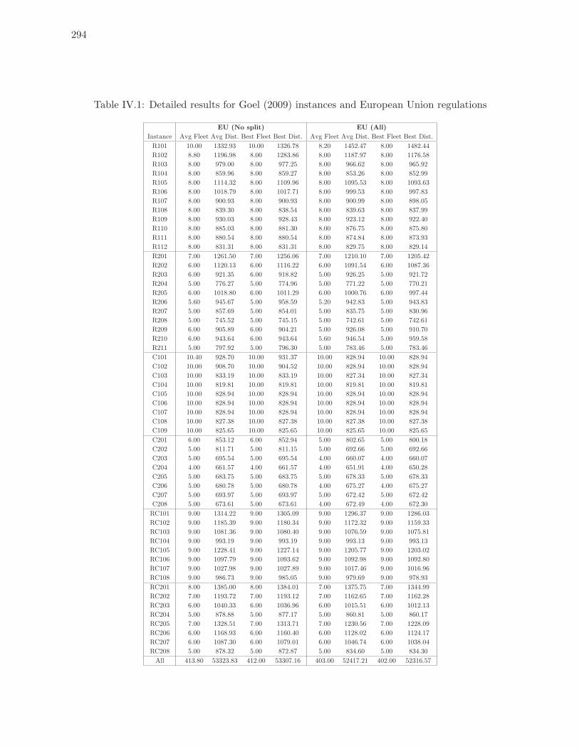
294

Table IV.1: Detailed results for Goel (2009) instances and European Union regulations

EU (No split) EU (All)

Instance Avg Fleet Avg Dist. Best Fleet Best Dist. Avg Fleet Avg Dist. Best Fleet Best Dist.

R101 10.00 1332.93 10.00 1326.78 8.20 1452.47 8.00 1482.44

R102 8.80 1196.98 8.00 1283.86 8.00 1187.97 8.00 1176.58

R103 8.00 979.00 8.00 977.25 8.00 966.62 8.00 965.92

R104 8.00 859.96 8.00 859.27 8.00 853.26 8.00 852.99

R105 8.00 1114.32 8.00 1109.96 8.00 1095.53 8.00 1093.63

R106 8.00 1018.79 8.00 1017.71 8.00 999.53 8.00 997.83

R107 8.00 900.93 8.00 900.93 8.00 900.99 8.00 898.05

R108 8.00 839.30 8.00 838.54 8.00 839.63 8.00 837.99

R109 8.00 930.03 8.00 928.43 8.00 923.12 8.00 922.40

R110 8.00 885.03 8.00 881.30 8.00 876.75 8.00 875.80

R111 8.00 880.54 8.00 880.54 8.00 874.84 8.00 873.93

R112 8.00 831.31 8.00 831.31 8.00 829.75 8.00 829.14

R201 7.00 1261.50 7.00 1256.06 7.00 1210.10 7.00 1205.42

R202 6.00 1120.13 6.00 1116.22 6.00 1091.54 6.00 1087.36

R203 6.00 921.35 6.00 918.82 5.00 926.25 5.00 921.72

R204 5.00 776.27 5.00 774.96 5.00 771.22 5.00 770.21

R205 6.00 1018.80 6.00 1011.29 6.00 1000.76 6.00 997.44

R206 5.60 945.67 5.00 958.59 5.20 942.83 5.00 943.83

R207 5.00 857.69 5.00 854.01 5.00 835.75 5.00 830.96

R208 5.00 745.52 5.00 745.15 5.00 742.61 5.00 742.61

R209 6.00 905.89 6.00 904.21 5.00 926.08 5.00 910.70

R210 6.00 943.64 6.00 943.64 5.60 946.54 5.00 959.58

R211 5.00 797.92 5.00 796.30 5.00 783.46 5.00 783.46

C101 10.40 928.70 10.00 931.37 10.00 828.94 10.00 828.94

C102 10.00 908.70 10.00 904.52 10.00 828.94 10.00 828.94

C103 10.00 833.19 10.00 833.19 10.00 827.34 10.00 827.34

C104 10.00 819.81 10.00 819.81 10.00 819.81 10.00 819.81

C105 10.00 828.94 10.00 828.94 10.00 828.94 10.00 828.94

C106 10.00 828.94 10.00 828.94 10.00 828.94 10.00 828.94

C107 10.00 828.94 10.00 828.94 10.00 828.94 10.00 828.94

C108 10.00 827.38 10.00 827.38 10.00 827.38 10.00 827.38

C109 10.00 825.65 10.00 825.65 10.00 825.65 10.00 825.65

C201 6.00 853.12 6.00 852.94 5.00 802.65 5.00 800.18

C202 5.00 811.71 5.00 811.15 5.00 692.66 5.00 692.66

C203 5.00 695.54 5.00 695.54 4.00 660.07 4.00 660.07

C204 4.00 661.57 4.00 661.57 4.00 651.91 4.00 650.28

C205 5.00 683.75 5.00 683.75 5.00 678.33 5.00 678.33

C206 5.00 680.78 5.00 680.78 4.00 675.27 4.00 675.27

C207 5.00 693.97 5.00 693.97 5.00 672.42 5.00 672.42

C208 5.00 673.61 5.00 673.61 4.00 672.49 4.00 672.30

RC101 9.00 1314.22 9.00 1305.09 9.00 1296.37 9.00 1286.03

RC102 9.00 1185.39 9.00 1180.34 9.00 1172.32 9.00 1159.33

RC103 9.00 1081.36 9.00 1080.40 9.00 1076.59 9.00 1075.81

RC104 9.00 993.19 9.00 993.19 9.00 993.13 9.00 993.13

RC105 9.00 1228.41 9.00 1227.14 9.00 1205.77 9.00 1203.02

RC106 9.00 1097.79 9.00 1093.62 9.00 1092.98 9.00 1092.80

RC107 9.00 1027.98 9.00 1027.89 9.00 1017.46 9.00 1016.96

RC108 9.00 986.73 9.00 985.05 9.00 979.69 9.00 978.93

RC201 8.00 1385.00 8.00 1384.01 7.00 1375.75 7.00 1344.99

RC202 7.00 1193.72 7.00 1193.12 7.00 1162.65 7.00 1162.28

RC203 6.00 1040.33 6.00 1036.96 6.00 1015.51 6.00 1012.13

RC204 5.00 878.88 5.00 877.17 5.00 860.81 5.00 860.17

RC205 7.00 1328.51 7.00 1313.71 7.00 1230.56 7.00 1228.09

RC206 6.00 1168.93 6.00 1160.40 6.00 1128.02 6.00 1124.17

RC207 6.00 1087.30 6.00 1079.01 6.00 1046.74 6.00 1038.04

RC208 5.00 878.32 5.00 872.87 5.00 834.60 5.00 834.30

All 413.80 53323.83 412.00 53307.16 403.00 52417.21 402.00 52316.57

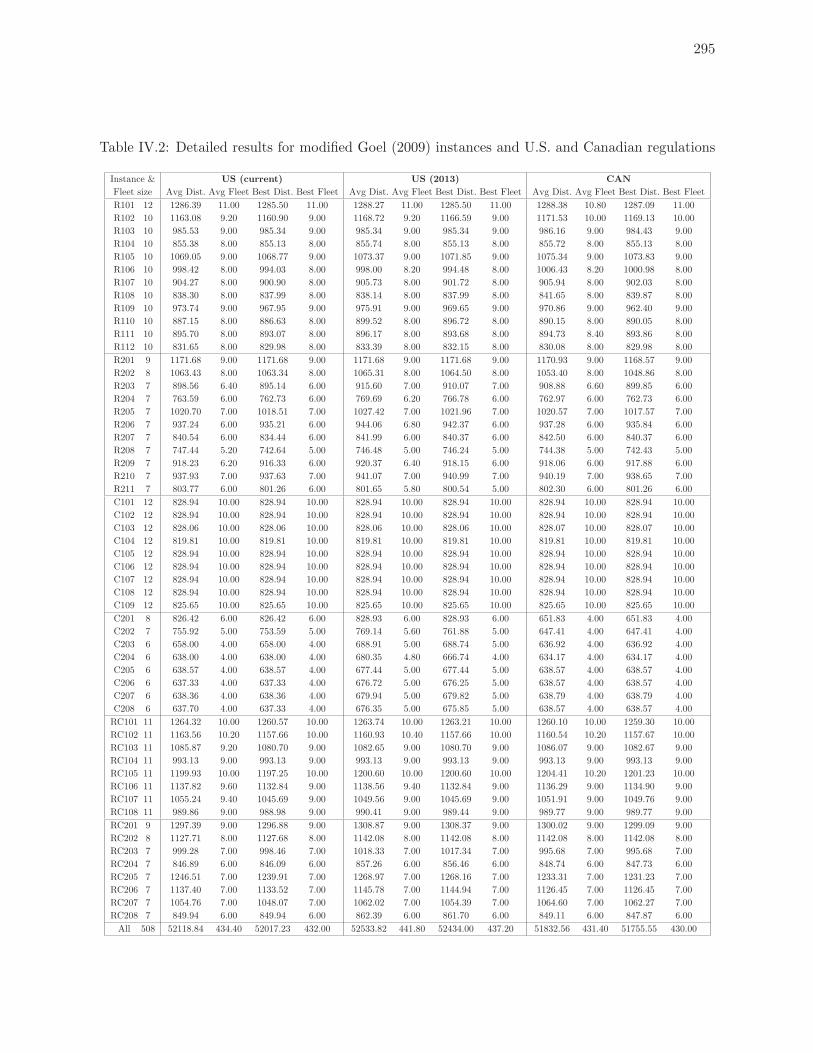
295

Table IV.2: Detailed results for modified Goel (2009) instances and U.S. and Canadian regulations

Instance & US (current) US (2013) CAN

Fleet size Avg Dist. Avg Fleet Best Dist. Best Fleet Avg Dist. Avg Fleet Best Dist. Best Fleet Avg Dist. Avg Fleet Best Dist. Best Fleet

R101 12 1286.39 11.00 1285.50 11.00 1288.27 11.00 1285.50 11.00 1288.38 10.80 1287.09 11.00

R102 10 1163.08 9.20 1160.90 9.00 1168.72 9.20 1166.59 9.00 1171.53 10.00 1169.13 10.00

R103 10 985.53 9.00 985.34 9.00 985.34 9.00 985.34 9.00 986.16 9.00 984.43 9.00

R104 10 855.38 8.00 855.13 8.00 855.74 8.00 855.13 8.00 855.72 8.00 855.13 8.00

R105 10 1069.05 9.00 1068.77 9.00 1073.37 9.00 1071.85 9.00 1075.34 9.00 1073.83 9.00

R106 10 998.42 8.00 994.03 8.00 998.00 8.20 994.48 8.00 1006.43 8.20 1000.98 8.00

R107 10 904.27 8.00 900.90 8.00 905.73 8.00 901.72 8.00 905.94 8.00 902.03 8.00

R108 10 838.30 8.00 837.99 8.00 838.14 8.00 837.99 8.00 841.65 8.00 839.87 8.00

R109 10 973.74 9.00 967.95 9.00 975.91 9.00 969.65 9.00 970.86 9.00 962.40 9.00

R110 10 887.15 8.00 886.63 8.00 899.52 8.00 896.72 8.00 890.15 8.00 890.05 8.00

R111 10 895.70 8.00 893.07 8.00 896.17 8.00 893.68 8.00 894.73 8.40 893.86 8.00

R112 10 831.65 8.00 829.98 8.00 833.39 8.00 832.15 8.00 830.08 8.00 829.98 8.00

R201 9 1171.68 9.00 1171.68 9.00 1171.68 9.00 1171.68 9.00 1170.93 9.00 1168.57 9.00

R202 8 1063.43 8.00 1063.34 8.00 1065.31 8.00 1064.50 8.00 1053.40 8.00 1048.86 8.00

R203 7 898.56 6.40 895.14 6.00 915.60 7.00 910.07 7.00 908.88 6.60 899.85 6.00

R204 7 763.59 6.00 762.73 6.00 769.69 6.20 766.78 6.00 762.97 6.00 762.73 6.00

R205 7 1020.70 7.00 1018.51 7.00 1027.42 7.00 1021.96 7.00 1020.57 7.00 1017.57 7.00

R206 7 937.24 6.00 935.21 6.00 944.06 6.80 942.37 6.00 937.28 6.00 935.84 6.00

R207 7 840.54 6.00 834.44 6.00 841.99 6.00 840.37 6.00 842.50 6.00 840.37 6.00

R208 7 747.44 5.20 742.64 5.00 746.48 5.00 746.24 5.00 744.38 5.00 742.43 5.00

R209 7 918.23 6.20 916.33 6.00 920.37 6.40 918.15 6.00 918.06 6.00 917.88 6.00

R210 7 937.93 7.00 937.63 7.00 941.07 7.00 940.99 7.00 940.19 7.00 938.65 7.00

R211 7 803.77 6.00 801.26 6.00 801.65 5.80 800.54 5.00 802.30 6.00 801.26 6.00

C101 12 828.94 10.00 828.94 10.00 828.94 10.00 828.94 10.00 828.94 10.00 828.94 10.00

C102 12 828.94 10.00 828.94 10.00 828.94 10.00 828.94 10.00 828.94 10.00 828.94 10.00

C103 12 828.06 10.00 828.06 10.00 828.06 10.00 828.06 10.00 828.07 10.00 828.07 10.00

C104 12 819.81 10.00 819.81 10.00 819.81 10.00 819.81 10.00 819.81 10.00 819.81 10.00

C105 12 828.94 10.00 828.94 10.00 828.94 10.00 828.94 10.00 828.94 10.00 828.94 10.00

C106 12 828.94 10.00 828.94 10.00 828.94 10.00 828.94 10.00 828.94 10.00 828.94 10.00

C107 12 828.94 10.00 828.94 10.00 828.94 10.00 828.94 10.00 828.94 10.00 828.94 10.00

C108 12 828.94 10.00 828.94 10.00 828.94 10.00 828.94 10.00 828.94 10.00 828.94 10.00

C109 12 825.65 10.00 825.65 10.00 825.65 10.00 825.65 10.00 825.65 10.00 825.65 10.00

C201 8 826.42 6.00 826.42 6.00 828.93 6.00 828.93 6.00 651.83 4.00 651.83 4.00

C202 7 755.92 5.00 753.59 5.00 769.14 5.60 761.88 5.00 647.41 4.00 647.41 4.00

C203 6 658.00 4.00 658.00 4.00 688.91 5.00 688.74 5.00 636.92 4.00 636.92 4.00

C204 6 638.00 4.00 638.00 4.00 680.35 4.80 666.74 4.00 634.17 4.00 634.17 4.00

C205 6 638.57 4.00 638.57 4.00 677.44 5.00 677.44 5.00 638.57 4.00 638.57 4.00

C206 6 637.33 4.00 637.33 4.00 676.72 5.00 676.25 5.00 638.57 4.00 638.57 4.00

C207 6 638.36 4.00 638.36 4.00 679.94 5.00 679.82 5.00 638.79 4.00 638.79 4.00

C208 6 637.70 4.00 637.33 4.00 676.35 5.00 675.85 5.00 638.57 4.00 638.57 4.00

RC101 11 1264.32 10.00 1260.57 10.00 1263.74 10.00 1263.21 10.00 1260.10 10.00 1259.30 10.00

RC102 11 1163.56 10.20 1157.66 10.00 1160.93 10.40 1157.66 10.00 1160.54 10.20 1157.67 10.00

RC103 11 1085.87 9.20 1080.70 9.00 1082.65 9.00 1080.70 9.00 1086.07 9.00 1082.67 9.00

RC104 11 993.13 9.00 993.13 9.00 993.13 9.00 993.13 9.00 993.13 9.00 993.13 9.00

RC105 11 1199.93 10.00 1197.25 10.00 1200.60 10.00 1200.60 10.00 1204.41 10.20 1201.23 10.00

RC106 11 1137.82 9.60 1132.84 9.00 1138.56 9.40 1132.84 9.00 1136.29 9.00 1134.90 9.00

RC107 11 1055.24 9.40 1045.69 9.00 1049.56 9.00 1045.69 9.00 1051.91 9.00 1049.76 9.00

RC108 11 989.86 9.00 988.98 9.00 990.41 9.00 989.44 9.00 989.77 9.00 989.77 9.00

RC201 9 1297.39 9.00 1296.88 9.00 1308.87 9.00 1308.37 9.00 1300.02 9.00 1299.09 9.00

RC202 8 1127.71 8.00 1127.68 8.00 1142.08 8.00 1142.08 8.00 1142.08 8.00 1142.08 8.00

RC203 7 999.28 7.00 998.46 7.00 1018.33 7.00 1017.34 7.00 995.68 7.00 995.68 7.00

RC204 7 846.89 6.00 846.09 6.00 857.26 6.00 856.46 6.00 848.74 6.00 847.73 6.00

RC205 7 1246.51 7.00 1239.91 7.00 1268.97 7.00 1268.16 7.00 1233.31 7.00 1231.23 7.00

RC206 7 1137.40 7.00 1133.52 7.00 1145.78 7.00 1144.94 7.00 1126.45 7.00 1126.45 7.00

RC207 7 1054.76 7.00 1048.07 7.00 1062.02 7.00 1054.39 7.00 1064.60 7.00 1062.27 7.00

RC208 7 849.94 6.00 849.94 6.00 862.39 6.00 861.70 6.00 849.11 6.00 847.87 6.00

All 508 52118.84 434.40 52017.23 432.00 52533.82 441.80 52434.00 437.20 51832.56 431.40 51755.55 430.00

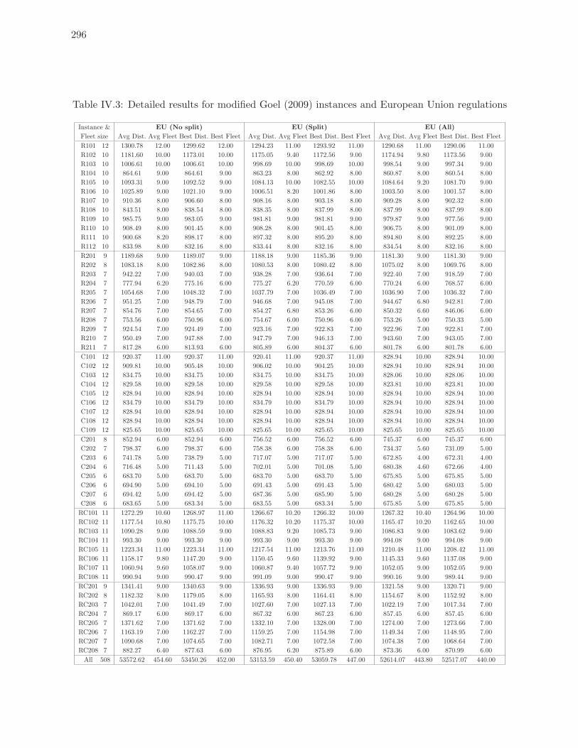
296

Table IV.3: Detailed results for modified Goel (2009) instances and European Union regulations

Instance & EU (No split) EU (Split) EU (All)


R101 12 1300.78 12.00 1299.62 12.00 1294.23 11.00 1293.92 11.00 1290.68 11.00 1290.06 11.00

R102 10 1181.60 10.00 1173.01 10.00 1175.05 9.40 1172.56 9.00 1174.94 9.80 1173.56 9.00

R103 10 1006.61 10.00 1006.61 10.00 998.69 10.00 998.69 10.00 998.54 9.00 997.34 9.00

R104 10 864.61 9.00 864.61 9.00 863.23 8.00 862.92 8.00 860.87 8.00 860.54 8.00

R105 10 1093.31 9.00 1092.52 9.00 1084.13 10.00 1082.55 10.00 1084.64 9.20 1081.70 9.00

R106 10 1025.89 9.00 1021.10 9.00 1006.51 8.20 1001.86 8.00 1003.50 8.00 1001.57 8.00

R107 10 910.36 8.00 906.60 8.00 908.16 8.00 903.18 8.00 909.28 8.00 902.32 8.00

R108 10 843.51 8.00 838.54 8.00 838.35 8.00 837.99 8.00 837.99 8.00 837.99 8.00

R109 10 985.75 9.00 983.05 9.00 981.81 9.00 981.81 9.00 979.87 9.00 977.56 9.00

R110 10 908.49 8.00 901.45 8.00 908.28 8.00 901.45 8.00 906.75 8.00 901.09 8.00

R111 10 900.68 8.20 898.17 8.00 897.32 8.00 895.20 8.00 894.80 8.00 892.25 8.00

R112 10 833.98 8.00 832.16 8.00 833.44 8.00 832.16 8.00 834.54 8.00 832.16 8.00

R201 9 1189.68 9.00 1189.07 9.00 1188.18 9.00 1185.36 9.00 1181.30 9.00 1181.30 9.00

R202 8 1083.18 8.00 1082.86 8.00 1080.53 8.00 1080.42 8.00 1075.02 8.00 1069.76 8.00

R203 7 942.22 7.00 940.03 7.00 938.28 7.00 936.64 7.00 922.40 7.00 918.59 7.00

R204 7 777.94 6.20 775.16 6.00 775.27 6.20 770.59 6.00 770.24 6.00 768.57 6.00

R205 7 1054.68 7.00 1048.32 7.00 1037.79 7.00 1036.49 7.00 1036.90 7.00 1036.32 7.00

R206 7 951.25 7.00 948.79 7.00 946.68 7.00 945.08 7.00 944.67 6.80 942.81 7.00

R207 7 854.76 7.00 854.65 7.00 854.27 6.80 853.26 6.00 850.32 6.60 846.06 6.00

R208 7 753.56 6.00 750.96 6.00 754.67 6.00 750.96 6.00 753.26 5.00 750.33 5.00

R209 7 924.54 7.00 924.49 7.00 923.16 7.00 922.83 7.00 922.96 7.00 922.81 7.00

R210 7 950.49 7.00 947.88 7.00 947.79 7.00 946.13 7.00 943.60 7.00 943.05 7.00

R211 7 817.28 6.00 813.93 6.00 805.89 6.00 804.37 6.00 801.78 6.00 801.78 6.00

C101 12 920.37 11.00 920.37 11.00 920.41 11.00 920.37 11.00 828.94 10.00 828.94 10.00

C102 12 909.81 10.00 905.48 10.00 906.02 10.00 904.25 10.00 828.94 10.00 828.94 10.00

C103 12 834.75 10.00 834.75 10.00 834.75 10.00 834.75 10.00 828.06 10.00 828.06 10.00

C104 12 829.58 10.00 829.58 10.00 829.58 10.00 829.58 10.00 823.81 10.00 823.81 10.00

C105 12 828.94 10.00 828.94 10.00 828.94 10.00 828.94 10.00 828.94 10.00 828.94 10.00

C106 12 834.79 10.00 834.79 10.00 834.79 10.00 834.79 10.00 828.94 10.00 828.94 10.00

C107 12 828.94 10.00 828.94 10.00 828.94 10.00 828.94 10.00 828.94 10.00 828.94 10.00

C108 12 828.94 10.00 828.94 10.00 828.94 10.00 828.94 10.00 828.94 10.00 828.94 10.00

C109 12 825.65 10.00 825.65 10.00 825.65 10.00 825.65 10.00 825.65 10.00 825.65 10.00

C201 8 852.94 6.00 852.94 6.00 756.52 6.00 756.52 6.00 745.37 6.00 745.37 6.00

C202 7 798.37 6.00 798.37 6.00 758.38 6.00 758.38 6.00 734.37 5.60 731.09 5.00

C203 6 741.78 5.00 738.79 5.00 717.07 5.00 717.07 5.00 672.85 4.00 672.31 4.00

C204 6 716.48 5.00 711.43 5.00 702.01 5.00 701.08 5.00 680.38 4.60 672.66 4.00

C205 6 683.70 5.00 683.70 5.00 683.70 5.00 683.70 5.00 675.85 5.00 675.85 5.00

C206 6 694.90 5.00 694.10 5.00 691.43 5.00 691.43 5.00 680.42 5.00 680.03 5.00

C207 6 694.42 5.00 694.42 5.00 687.36 5.00 685.90 5.00 680.28 5.00 680.28 5.00

C208 6 683.65 5.00 683.34 5.00 683.55 5.00 683.34 5.00 675.85 5.00 675.85 5.00

RC101 11 1272.29 10.60 1268.97 11.00 1266.67 10.20 1266.32 10.00 1267.32 10.40 1264.96 10.00

RC102 11 1177.54 10.80 1175.75 10.00 1176.32 10.20 1175.37 10.00 1165.47 10.20 1162.65 10.00

RC103 11 1090.28 9.00 1088.59 9.00 1088.83 9.20 1085.73 9.00 1086.83 9.00 1083.62 9.00

RC104 11 993.30 9.00 993.30 9.00 993.30 9.00 993.30 9.00 994.08 9.00 994.08 9.00

RC105 11 1223.34 11.00 1223.34 11.00 1217.54 11.00 1213.76 11.00 1210.48 11.00 1208.42 11.00

RC106 11 1158.17 9.80 1147.20 9.00 1150.45 9.60 1139.92 9.00 1145.33 9.60 1137.08 9.00

RC107 11 1060.94 9.60 1058.07 9.00 1060.87 9.40 1057.72 9.00 1052.05 9.00 1052.05 9.00

RC108 11 990.94 9.00 990.47 9.00 991.09 9.00 990.47 9.00 990.16 9.00 989.44 9.00

RC201 9 1341.41 9.00 1340.63 9.00 1336.93 9.00 1336.93 9.00 1321.58 9.00 1320.71 9.00

RC202 8 1182.32 8.00 1179.05 8.00 1165.93 8.00 1164.41 8.00 1154.67 8.00 1152.92 8.00

RC203 7 1042.01 7.00 1041.49 7.00 1027.60 7.00 1027.13 7.00 1022.19 7.00 1017.34 7.00

RC204 7 869.17 6.00 869.17 6.00 867.32 6.00 867.23 6.00 857.45 6.00 857.45 6.00

RC205 7 1371.62 7.00 1371.62 7.00 1332.10 7.00 1328.00 7.00 1274.00 7.00 1273.66 7.00

RC206 7 1163.19 7.00 1162.27 7.00 1159.25 7.00 1154.98 7.00 1149.34 7.00 1148.95 7.00

RC207 7 1090.68 7.00 1074.65 7.00 1082.71 7.00 1072.58 7.00 1074.38 7.00 1068.64 7.00

RC208 7 882.27 6.40 877.63 6.00 876.95 6.20 875.89 6.00 873.36 6.00 870.99 6.00

All 508 53572.62 454.60 53450.26 452.00 53153.59 450.40 53059.78 447.00 52614.07 443.80 52517.07 440.00

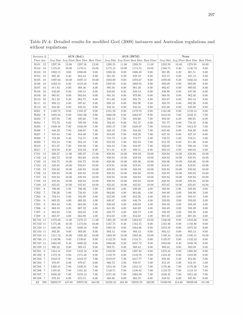
297

Table IV.4: Detailed results for modified Goel (2009) instances and Australian regulations andwithout regulations

Instance & AUS (Std.) AUS (BFM) None


R101 12 1297.58 12.00 1297.56 12.00 1288.55 11.00 1288.55 11.00 1282.59 10.40 1278.95 10.00

R102 10 1178.81 10.00 1176.51 10.00 1175.12 10.00 1174.74 10.00 1160.75 9.40 1156.73 9.00

R103 10 1002.15 9.60 1000.08 9.00 1000.56 9.00 1000.43 9.00 981.99 8.20 981.51 9.00

R104 10 865.46 8.40 864.44 8.00 861.23 8.20 859.19 8.00 855.15 8.00 855.13 8.00

R105 10 1097.66 10.00 1097.12 10.00 1082.89 9.00 1078.67 9.00 1059.69 8.20 1056.52 8.00

R106 10 1023.13 8.80 1018.23 9.00 1007.05 8.20 1003.94 8.00 988.09 8.00 983.06 8.00

R107 10 911.82 8.00 908.46 8.00 905.50 8.00 901.29 8.00 902.87 8.00 900.03 8.00

R108 10 842.69 8.00 838.54 8.00 840.62 8.00 838.54 8.00 838.96 8.00 837.99 8.00

R109 10 985.61 9.00 983.94 9.00 981.34 9.00 976.66 9.00 968.59 9.00 962.40 9.00

R110 10 911.32 8.20 904.75 8.00 911.69 8.00 904.75 8.00 885.87 8.00 885.54 8.00

R111 10 899.12 8.00 897.61 8.00 898.18 8.00 893.96 8.00 893.70 8.00 892.26 8.00

R112 10 834.56 8.00 832.41 8.00 832.16 8.00 832.16 8.00 831.00 8.00 829.98 8.00

R201 9 1188.74 9.00 1188.27 9.00 1181.50 9.00 1179.79 9.00 1161.66 8.00 1159.14 8.00

R202 8 1085.24 8.00 1081.06 8.00 1068.09 8.00 1062.97 8.00 1044.94 7.60 1042.41 7.00

R203 7 937.05 7.00 935.60 7.00 926.13 7.00 922.60 7.00 892.50 6.20 890.85 6.00

R204 7 773.79 6.00 769.50 6.00 764.33 6.00 761.57 6.00 761.77 6.00 758.45 6.00

R205 7 1039.16 7.00 1038.09 7.00 1031.57 7.00 1028.97 7.00 1016.61 7.00 1013.37 7.00

R206 7 948.23 7.00 946.67 7.00 945.10 7.00 944.03 7.00 935.86 6.00 934.38 6.00

R207 7 855.64 7.00 854.40 7.00 854.03 7.00 852.28 7.00 827.18 6.00 827.18 6.00

R208 7 758.39 5.40 752.71 5.00 755.75 5.20 753.77 5.00 733.72 5.00 733.51 5.00

R209 7 924.24 7.00 924.18 7.00 922.83 7.00 922.83 7.00 913.79 6.00 911.96 6.00

R210 7 951.07 7.00 948.92 7.00 943.44 7.00 942.97 7.00 932.08 7.00 930.48 7.00

R211 7 823.50 6.20 822.33 6.00 811.91 6.20 808.51 6.00 802.52 5.80 800.63 5.00

C101 12 920.37 11.00 920.37 11.00 828.94 10.00 828.94 10.00 828.94 10.00 828.94 10.00

C102 12 904.72 10.00 904.69 10.00 828.94 10.00 828.94 10.00 828.94 10.00 828.94 10.00

C103 12 834.75 10.00 834.75 10.00 828.06 10.00 828.06 10.00 828.06 10.00 828.06 10.00

C104 12 823.81 10.00 823.81 10.00 819.81 10.00 819.81 10.00 819.81 10.00 819.81 10.00

C105 12 828.94 10.00 828.94 10.00 828.94 10.00 828.94 10.00 828.94 10.00 828.94 10.00

C106 12 828.94 10.00 828.94 10.00 828.94 10.00 828.94 10.00 828.94 10.00 828.94 10.00

C107 12 828.94 10.00 828.94 10.00 828.94 10.00 828.94 10.00 828.94 10.00 828.94 10.00

C108 12 828.94 10.00 828.94 10.00 828.94 10.00 828.94 10.00 828.94 10.00 828.94 10.00

C109 12 825.65 10.00 825.65 10.00 825.65 10.00 825.65 10.00 825.65 10.00 825.65 10.00

C201 8 706.26 5.00 706.26 5.00 639.40 4.00 639.40 4.00 588.88 3.00 588.88 3.00

C202 7 730.26 5.00 728.82 5.00 664.66 4.00 664.66 4.00 588.88 3.00 588.88 3.00

C203 6 703.14 5.00 702.99 5.00 652.60 4.00 652.20 4.00 593.41 3.00 593.41 3.00

C204 6 669.32 4.00 669.32 4.00 646.87 4.00 646.70 4.00 593.03 3.00 593.03 3.00

C205 6 664.34 5.00 664.08 5.00 626.63 4.00 626.63 4.00 588.49 3.00 588.49 3.00

C206 6 669.16 4.20 667.32 4.00 641.26 4.00 640.89 4.00 588.49 3.00 588.49 3.00

C207 6 662.62 5.00 662.62 5.00 628.72 4.00 628.72 4.00 588.29 3.00 588.29 3.00

C208 6 665.87 4.60 664.98 4.00 654.62 4.00 654.62 4.00 601.05 3.00 601.05 3.00

RC101 11 1270.83 11.00 1270.15 11.00 1265.29 10.00 1263.82 10.00 1246.06 9.80 1243.20 9.00

RC102 11 1175.26 10.20 1173.04 10.00 1167.75 9.40 1164.55 9.00 1162.36 9.80 1156.30 9.00

RC103 11 1091.86 9.20 1088.18 9.00 1085.24 9.00 1084.06 9.00 1072.22 9.00 1072.22 9.00

RC104 11 993.30 9.00 993.30 9.00 993.14 9.00 993.13 9.00 993.13 9.00 993.13 9.00

RC105 11 1211.72 10.00 1208.22 10.00 1203.59 10.00 1203.38 10.00 1188.34 10.00 1186.15 10.00

RC106 11 1146.96 9.60 1139.01 9.00 1142.78 9.60 1134.71 9.00 1135.07 9.00 1132.52 9.00

RC107 11 1062.89 9.40 1060.22 9.00 1060.66 9.20 1057.72 9.00 1053.60 9.40 1049.76 9.00

RC108 11 990.22 9.00 989.44 9.00 989.75 9.00 989.44 9.00 989.44 9.00 988.09 9.00

RC201 9 1344.55 9.00 1342.10 9.00 1310.98 9.00 1307.20 9.00 1270.16 8.60 1266.50 9.00

RC202 8 1172.76 8.00 1171.30 8.00 1142.78 8.00 1142.78 8.00 1104.42 8.00 1103.98 8.00

RC203 7 1042.57 7.00 1042.57 7.00 1019.07 7.00 1017.77 7.00 958.40 5.20 954.86 5.00

RC204 7 870.87 6.00 870.67 6.00 860.73 5.80 859.57 5.00 812.18 5.00 812.18 5.00

RC205 7 1360.45 7.00 1339.21 7.00 1254.43 7.00 1243.12 7.00 1170.36 7.00 1170.36 7.00

RC206 7 1165.65 7.00 1161.43 7.00 1140.71 7.00 1138.82 7.00 1119.73 7.00 1118.13 7.00

RC207 7 1086.28 7.00 1078.14 7.00 1071.50 7.00 1062.89 7.00 1056.45 7.00 1051.32 7.00

RC208 7 876.44 6.00 873.15 6.00 868.36 6.00 862.70 6.00 849.52 6.00 847.86 6.00

All 508 53093.57 447.80 52972.93 444.00 52168.24 434.80 52059.78 432.00 51030.98 414.60 50946.68 411.00

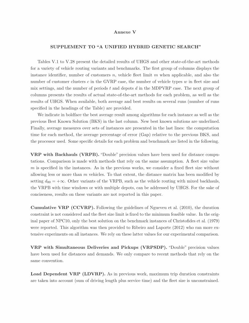
Annexe V

SUPPLEMENT TO “A UNIFIED HYBRID GENETIC SEARCH”

Tables V.1 to V.28 present the detailed results of UHGS and other state-of-the-art methods

for a variety of vehicle routing variants and benchmarks. The first group of columns displays the

instance identifier, number of customers n, vehicle fleet limit m when applicable, and also the

number of customer clusters c in the GVRP case, the number of vehicle types w in fleet size and

mix settings, and the number of periods t and depots d in the MDPVRP case. The next group of

columns presents the results of actual state-of-the-art methods for each problem, as well as the

results of UHGS. When available, both average and best results on several runs (number of runs

specified in the headings of the Table) are provided.

We indicate in boldface the best average result among algorithms for each instance as well as the

previous Best Known Solution (BKS) in the last column. New best known solutions are underlined.

Finally, average measures over sets of instances are presented in the last lines: the computation

time for each method, the average percentage of error (Gap) relative to the previous BKS, and

the processor used. Some specific details for each problem and benchmark are listed in the following.

VRP with Backhauls (VRPB). “Double” precision values have been used for distance compu-

tations. Comparison is made with methods that rely on the same assumption. A fleet size value

m is specified in the instances. As in the previous works, we consider a fixed fleet size without

allowing less or more than m vehicles. To that extent, the distance matrix has been modified by

setting d00 = +∞. Other variants of the VRPB, such as the vehicle routing with mixed backhauls,

the VRPB with time windows or with multiple depots, can be addressed by UHGS. For the sake of

conciseness, results on these variants are not reported in this paper.

Cumulative VRP (CCVRP). Following the guidelines of Ngueveu et al. (2010), the duration

constraint is not considered and the fleet size limit is fixed to the minimum feasible value. In the orig-

inal paper of NPC10, only the best solution on the benchmark instances of Christofides et al. (1979)

were reported. This algorithm was then provided to Ribeiro and Laporte (2012) who ran more ex-

tensive experiments on all instances. We rely on these latter values for our experimental comparison.

VRP with Simultaneous Deliveries and Pickups (VRPSDP). “Double” precision values

have been used for distances and demands. We only compare to recent methods that rely on the

same convention.

Load Dependent VRP (LDVRP). As in previous work, maximum trip duration constraints

are taken into account (sum of driving length plus service time) and the fleet size is unconstrained.

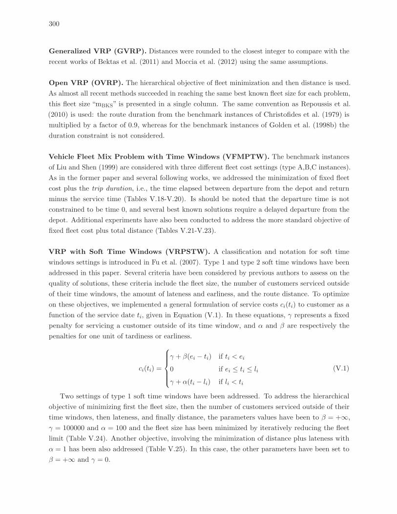
300

Generalized VRP (GVRP). Distances were rounded to the closest integer to compare with the

recent works of Bektas et al. (2011) and Moccia et al. (2012) using the same assumptions.

Open VRP (OVRP). The hierarchical objective of fleet minimization and then distance is used.

As almost all recent methods succeeded in reaching the same best known fleet size for each problem,

this fleet size “mBKS” is presented in a single column. The same convention as Repoussis et al.

(2010) is used: the route duration from the benchmark instances of Christofides et al. (1979) is

multiplied by a factor of 0.9, whereas for the benchmark instances of Golden et al. (1998b) the

duration constraint is not considered.

Vehicle Fleet Mix Problem with Time Windows (VFMPTW). The benchmark instances

of Liu and Shen (1999) are considered with three different fleet cost settings (type A,B,C instances).

As in the former paper and several following works, we addressed the minimization of fixed fleet

cost plus the trip duration, i.e., the time elapsed between departure from the depot and return

minus the service time (Tables V.18-V.20). Is should be noted that the departure time is not

constrained to be time 0, and several best known solutions require a delayed departure from the

depot. Additional experiments have also been conducted to address the more standard objective of

fixed fleet cost plus total distance (Tables V.21-V.23).

VRP with Soft Time Windows (VRPSTW). A classification and notation for soft time

windows settings is introduced in Fu et al. (2007). Type 1 and type 2 soft time windows have been

addressed in this paper. Several criteria have been considered by previous authors to assess on the

quality of solutions, these criteria include the fleet size, the number of customers serviced outside

of their time windows, the amount of lateness and earliness, and the route distance. To optimize

on these objectives, we implemented a general formulation of service costs ci(ti) to customer as a

function of the service date ti, given in Equation (V.1). In these equations, γ represents a fixed

penalty for servicing a customer outside of its time window, and α and β are respectively the

penalties for one unit of tardiness or earliness.

ci(ti) =

⎧⎪⎪⎪⎨⎪⎪⎪⎩γ + β(ei − ti) if ti < ei

0 if ei ≤ ti ≤ li

γ + α(ti − li) if li < ti

(V.1)

Two settings of type 1 soft time windows have been addressed. To address the hierarchical

objective of minimizing first the fleet size, then the number of customers serviced outside of their

time windows, then lateness, and finally distance, the parameters values have been to β = +∞,

γ = 100000 and α = 100 and the fleet size has been minimized by iteratively reducing the fleet

limit (Table V.24). Another objective, involving the minimization of distance plus lateness with

α = 1 has been also addressed (Table V.25). In this case, the other parameters have been set to

β = +∞ and γ = 0.

301

Furthermore, two settings of type 2 soft time windows have been addressed. The hierarchical

objective has been addressed by setting β = 100, γ = 100000 and α = 100 (Table V.26). We also

provide results for the objective seeking to minimize the sum of distance, earliness and lateness by

setting β = 1, γ = 0 and α = 1 (Table V.27).

Time-Dependent VRP with Time Windows (TDVRPTW). The same setting as Kritzinger

et al. (2012) is considered, involving the minimization of the total time dependent travel time. The

same convention as the authors is used, and thus all routes are constrained to start at time 0, waiting

time being allowed only at a customer location upon an early arrival. We consider the same fleet size

limits as in Kritzinger et al. (2012). The benchmark instances of Solomon and Desrosiers (1988) are

used. In the scope of this thesis, only the results for the first scenario travel time scenarios of Ichoua

et al. (2003) are reported in Table V.17. The complete results are available in the published article

journal associated to this paper. The planning horizon is divided into three parts of 20%, 60% and

20%, respectively, as in Ichoua et al. (2003). The arc category matrix of Balseiro et al. (2011) is used.

Multi-Depot Periodic VRP with Time Windows (MDPVRPTW). The set of MDPVRP

instances from Vidal et al. (2012a), originally issued from the combination of multi-depot and

periodic instances of Cordeau et al. (1997, 2001a), has been completed with the time windows

values from Cordeau et al. (2001a). Experiments have been conducted to set the fleet size value

close to the minimum fleet size. The corresponding values of m are reported, along with the results,

in Table V.28.

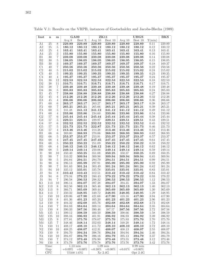
302

Table V.1: Results on the VRPB, instances of Goetschalckx and Jacobs-Blecha (1989)

Inst n m GA09 ZK11 UHGS BKSAvg 8 Best X Avg 10 Best 10 Avg 10 Best 10 T(min)

A1 25 8 229.89 229.89 229.89 229.89 229.89 229.89 0.11 229.89A2 25 5 180.12 180.12 180.12 180.12 180.12 180.12 0.12 180.12A3 25 4 163.41 163.41 163.41 163.41 163.41 163.41 0.13 163.41A4 25 3 155.80 155.80 155.80 155.80 155.80 155.80 0.16 155.80B1 30 7 239.08 239.08 239.08 239.08 239.08 239.08 0.14 239.08B2 30 5 198.05 198.05 198.05 198.05 198.05 198.05 0.15 198.05B3 30 3 169.37 169.37 169.37 169.37 169.37 169.37 0.18 169.37C1 40 7 250.56 250.56 250.56 250.56 250.56 250.56 0.22 250.56C2 40 5 215.02 215.02 215.02 215.02 215.02 215.02 0.24 215.02C3 40 5 199.35 199.35 199.35 199.35 199.35 199.35 0.23 199.35C4 40 4 195.37 195.37 195.37 195.37 195.37 195.37 0.24 195.37D1 38 12 322.53 322.53 322.53 322.53 322.53 322.53 0.18 322.53D2 38 11 316.71 316.71 316.71 316.71 316.71 316.71 0.17 316.71D3 38 7 239.48 239.48 239.48 239.48 239.48 239.48 0.19 239.48D4 38 5 205.83 205.83 205.83 205.83 205.83 205.83 0.24 205.83E1 45 7 238.88 238.88 238.88 238.88 238.88 238.88 0.27 238.88E2 45 4 212.26 212.26 212.26 212.26 212.26 212.26 0.32 212.26E3 45 4 206.66 206.66 206.66 206.66 206.66 206.66 0.36 206.66F1 60 6 263.17 263.17 263.27 263.17 263.17 263.17 0.38 263.17F2 60 7 265.21 265.21 265.66 265.21 265.21 265.21 0.39 265.21F3 60 5 241.48 241.12 241.12 241.12 241.12 241.12 0.49 241.12F4 60 4 233.86 233.86 234.60 233.86 233.86 233.86 0.54 233.86G2 57 6 245.44 245.44 245.44 245.44 245.44 245.44 0.38 245.44G3 57 5 229.51 229.51 229.97 229.51 229.51 229.51 0.43 229.51G4 57 6 232.52 232.52 232.52 232.52 232.52 232.52 0.45 232.52G5 57 5 221.73 221.73 222.87 221.73 221.73 221.73 0.46 221.73G6 57 4 213.46 213.46 214.38 213.46 213.46 213.46 0.54 213.46H1 68 6 269.00 268.93 270.06 268.93 268.93 268.93 0.62 268.93H2 68 5 253.37 253.37 253.91 253.37 253.37 253.37 0.57 253.37H3 68 4 247.45 247.45 247.45 247.45 247.45 247.45 0.64 247.45H4 68 5 250.22 250.22 251.09 250.22 250.22 250.22 0.59 250.22H5 68 4 246.12 246.12 246.12 246.12 246.12 246.12 0.62 246.12H6 68 5 249.14 249.14 250.06 249.14 249.14 249.14 0.59 249.14I1 90 10 350.40 350.25 351.08 350.25 350.37 350.25 0.89 350.25I2 90 7 310.32 309.94 309.98 309.94 309.94 309.94 0.85 309.94I3 90 5 294.84 294.51 294.79 294.51 294.51 294.51 0.99 294.51I4 90 6 296.13 295.99 297.91 295.99 295.99 295.99 0.92 295.99I5 90 7 301.83 301.24 303.49 301.24 301.24 301.24 0.82 301.24J1 94 10 335.12 335.01 335.78 335.01 335.01 335.01 0.83 335.01J2 94 8 310.42 310.42 312.51 310.42 310.42 310.42 0.84 310.42J3 94 6 279.34 279.22 280.43 279.22 279.22 279.22 0.93 279.22J4 94 7 296.58 296.53 298.32 296.53 296.53 296.53 1.12 296.53K1 113 10 396.14 394.07 397.38 394.07 394.35 394.07 1.33 394.07K2 113 8 362.56 362.13 365.46 362.13 362.13 362.13 1.40 362.13K3 113 9 366.71 365.69 369.44 365.69 365.69 365.69 1.30 365.69K4 113 7 350.32 348.95 349.72 348.95 348.95 348.95 1.29 348.95L1 150 10 420.06 417.90 421.68 417.90 418.16 417.90 3.94 417.90L2 150 8 401.36 401.23 405.20 401.23 401.23 401.23 2.96 401.23L3 150 9 404.32 402.68 405.76 402.68 402.68 402.68 2.73 402.68L4 150 7 384.83 384.64 388.14 384.64 384.64 384.64 2.35 384.64L5 150 8 390.33 387.56 390.46 387.57 387.56 387.56 2.72 387.56M1 125 11 399.12 398.59 400.50 398.59 398.66 398.59 1.58 398.59M2 125 10 398.16 396.92 401.91 396.92 396.93 396.92 2.39 396.92M3 125 9 377.81 375.70 378.07 375.70 375.93 375.70 2.70 375.70M4 125 7 348.46 348.14 352.03 348.14 348.20 348.14 1.72 348.14N1 150 11 408.17 408.10 411.72 408.10 408.10 408.10 2.72 408.10N2 150 10 408.25 408.07 412.31 408.07 408.13 408.07 2.55 408.07N3 150 9 394.70 394.34 398.76 394.34 394.94 394.34 2.46 394.34N4 150 10 394.87 394.79 396.16 394.79 395.13 394.79 2.37 394.79N5 150 7 374.12 373.48 376.90 373.48 373.55 373.48 3.12 373.48N6 150 8 374.79 373.76 379.78 373.76 373.76 373.76 3.42 373.76

Time 1.13 min 1.09 min 0.99 minGap +0.09% +0.00% +0.38% +0.00% +0.01% +0.00%CPU T5500 1.67G Xe 2.4G Opt 2.4G

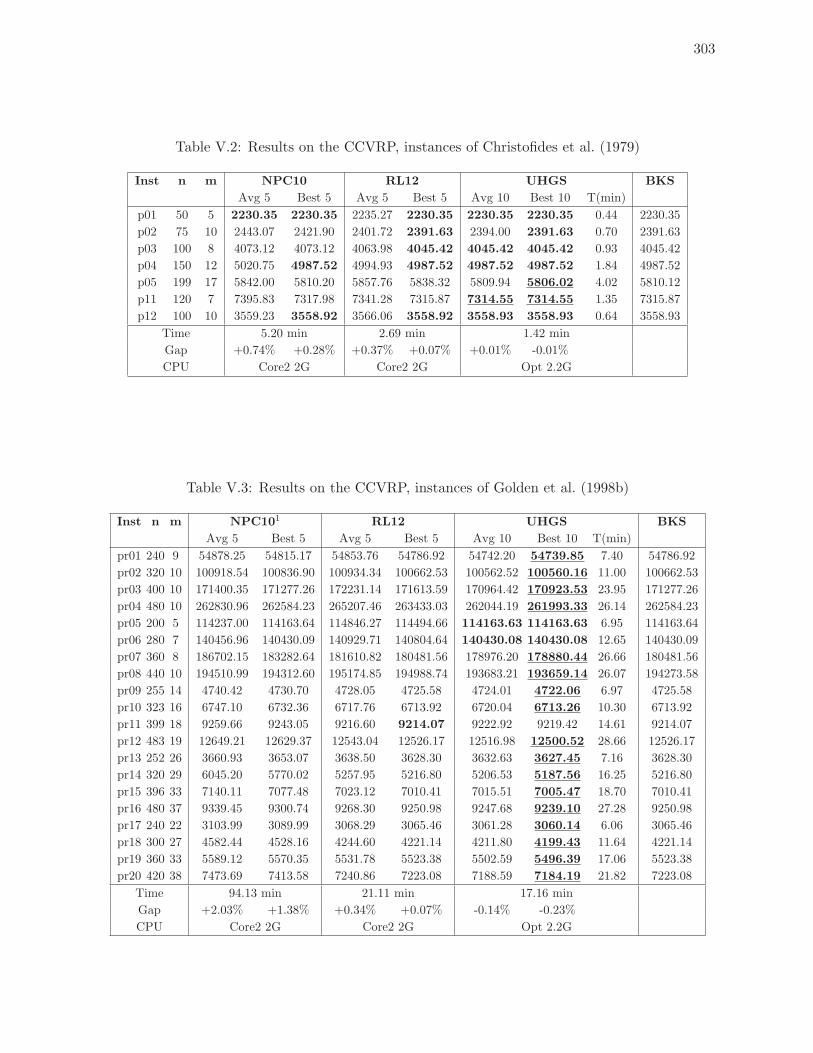
303

Table V.2: Results on the CCVRP, instances of Christofides et al. (1979)

Inst n m NPC10 RL12 UHGS BKS

Avg 5 Best 5 Avg 5 Best 5 Avg 10 Best 10 T(min)

p01 50 5 2230.35 2230.35 2235.27 2230.35 2230.35 2230.35 0.44 2230.35

p02 75 10 2443.07 2421.90 2401.72 2391.63 2394.00 2391.63 0.70 2391.63

p03 100 8 4073.12 4073.12 4063.98 4045.42 4045.42 4045.42 0.93 4045.42

p04 150 12 5020.75 4987.52 4994.93 4987.52 4987.52 4987.52 1.84 4987.52

p05 199 17 5842.00 5810.20 5857.76 5838.32 5809.94 5806.02 4.02 5810.12

p11 120 7 7395.83 7317.98 7341.28 7315.87 7314.55 7314.55 1.35 7315.87

p12 100 10 3559.23 3558.92 3566.06 3558.92 3558.93 3558.93 0.64 3558.93

Time 5.20 min 2.69 min 1.42 min

Gap +0.74% +0.28% +0.37% +0.07% +0.01% -0.01%

CPU Core2 2G Core2 2G Opt 2.2G

Table V.3: Results on the CCVRP, instances of Golden et al. (1998b)

Inst n m NPC101 RL12 UHGS BKS

Avg 5 Best 5 Avg 5 Best 5 Avg 10 Best 10 T(min)

pr01 240 9 54878.25 54815.17 54853.76 54786.92 54742.20 54739.85 7.40 54786.92

pr02 320 10 100918.54 100836.90 100934.34 100662.53 100562.52 100560.16 11.00 100662.53

pr03 400 10 171400.35 171277.26 172231.14 171613.59 170964.42 170923.53 23.95 171277.26

pr04 480 10 262830.96 262584.23 265207.46 263433.03 262044.19 261993.33 26.14 262584.23

pr05 200 5 114237.00 114163.64 114846.27 114494.66 114163.63 114163.63 6.95 114163.64

pr06 280 7 140456.96 140430.09 140929.71 140804.64 140430.08 140430.08 12.65 140430.09

pr07 360 8 186702.15 183282.64 181610.82 180481.56 178976.20 178880.44 26.66 180481.56

pr08 440 10 194510.99 194312.60 195174.85 194988.74 193683.21 193659.14 26.07 194273.58

pr09 255 14 4740.42 4730.70 4728.05 4725.58 4724.01 4722.06 6.97 4725.58

pr10 323 16 6747.10 6732.36 6717.76 6713.92 6720.04 6713.26 10.30 6713.92

pr11 399 18 9259.66 9243.05 9216.60 9214.07 9222.92 9219.42 14.61 9214.07

pr12 483 19 12649.21 12629.37 12543.04 12526.17 12516.98 12500.52 28.66 12526.17

pr13 252 26 3660.93 3653.07 3638.50 3628.30 3632.63 3627.45 7.16 3628.30

pr14 320 29 6045.20 5770.02 5257.95 5216.80 5206.53 5187.56 16.25 5216.80

pr15 396 33 7140.11 7077.48 7023.12 7010.41 7015.51 7005.47 18.70 7010.41

pr16 480 37 9339.45 9300.74 9268.30 9250.98 9247.68 9239.10 27.28 9250.98

pr17 240 22 3103.99 3089.99 3068.29 3065.46 3061.28 3060.14 6.06 3065.46

pr18 300 27 4582.44 4528.16 4244.60 4221.14 4211.80 4199.43 11.64 4221.14

pr19 360 33 5589.12 5570.35 5531.78 5523.38 5502.59 5496.39 17.06 5523.38

pr20 420 38 7473.69 7413.58 7240.86 7223.08 7188.59 7184.19 21.82 7223.08

Time 94.13 min 21.11 min 17.16 min

Gap +2.03% +1.38% +0.34% +0.07% -0.14% -0.23%

CPU Core2 2G Core2 2G Opt 2.2G

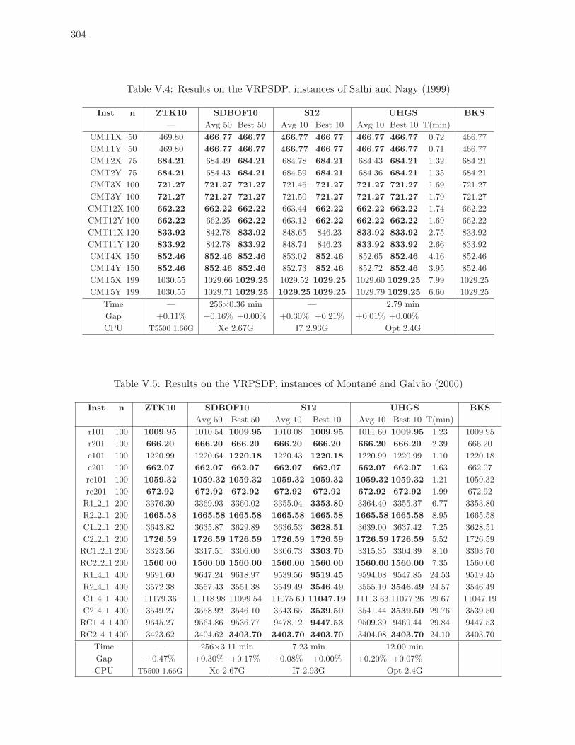
304

Table V.4: Results on the VRPSDP, instances of Salhi and Nagy (1999)

Inst n ZTK10 SDBOF10 S12 UHGS BKS

— Avg 50 Best 50 Avg 10 Best 10 Avg 10 Best 10 T(min)

CMT1X 50 469.80 466.77 466.77 466.77 466.77 466.77 466.77 0.72 466.77

CMT1Y 50 469.80 466.77 466.77 466.77 466.77 466.77 466.77 0.71 466.77

CMT2X 75 684.21 684.49 684.21 684.78 684.21 684.43 684.21 1.32 684.21

CMT2Y 75 684.21 684.43 684.21 684.59 684.21 684.36 684.21 1.35 684.21

CMT3X 100 721.27 721.27 721.27 721.46 721.27 721.27 721.27 1.69 721.27

CMT3Y 100 721.27 721.27 721.27 721.50 721.27 721.27 721.27 1.79 721.27

CMT12X 100 662.22 662.22 662.22 663.44 662.22 662.22 662.22 1.74 662.22

CMT12Y 100 662.22 662.25 662.22 663.12 662.22 662.22 662.22 1.69 662.22

CMT11X 120 833.92 842.78 833.92 848.65 846.23 833.92 833.92 2.75 833.92

CMT11Y 120 833.92 842.78 833.92 848.74 846.23 833.92 833.92 2.66 833.92

CMT4X 150 852.46 852.46 852.46 853.02 852.46 852.65 852.46 4.16 852.46

CMT4Y 150 852.46 852.46 852.46 852.73 852.46 852.72 852.46 3.95 852.46

CMT5X 199 1030.55 1029.66 1029.25 1029.52 1029.25 1029.60 1029.25 7.99 1029.25

CMT5Y 199 1030.55 1029.71 1029.25 1029.25 1029.25 1029.79 1029.25 6.60 1029.25

Time — 256×0.36 min — 2.79 min

Gap +0.11% +0.16% +0.00% +0.30% +0.21% +0.01% +0.00%

CPU T5500 1.66G Xe 2.67G I7 2.93G Opt 2.4G

Table V.5: Results on the VRPSDP, instances of Montane and Galvao (2006)

Inst n ZTK10 SDBOF10 S12 UHGS BKS

— Avg 50 Best 50 Avg 10 Best 10 Avg 10 Best 10 T(min)

r101 100 1009.95 1010.54 1009.95 1010.08 1009.95 1011.60 1009.95 1.23 1009.95

r201 100 666.20 666.20 666.20 666.20 666.20 666.20 666.20 2.39 666.20

c101 100 1220.99 1220.64 1220.18 1220.43 1220.18 1220.99 1220.99 1.10 1220.18

c201 100 662.07 662.07 662.07 662.07 662.07 662.07 662.07 1.63 662.07

rc101 100 1059.32 1059.32 1059.32 1059.32 1059.32 1059.32 1059.32 1.21 1059.32

rc201 100 672.92 672.92 672.92 672.92 672.92 672.92 672.92 1.99 672.92

R1 2 1 200 3376.30 3369.93 3360.02 3355.04 3353.80 3364.40 3355.37 6.77 3353.80

R2 2 1 200 1665.58 1665.58 1665.58 1665.58 1665.58 1665.58 1665.58 8.95 1665.58

C1 2 1 200 3643.82 3635.87 3629.89 3636.53 3628.51 3639.00 3637.42 7.25 3628.51

C2 2 1 200 1726.59 1726.59 1726.59 1726.59 1726.59 1726.59 1726.59 5.52 1726.59

RC1 2 1 200 3323.56 3317.51 3306.00 3306.73 3303.70 3315.35 3304.39 8.10 3303.70

RC2 2 1 200 1560.00 1560.00 1560.00 1560.00 1560.00 1560.00 1560.00 7.35 1560.00

R1 4 1 400 9691.60 9647.24 9618.97 9539.56 9519.45 9594.08 9547.85 24.53 9519.45

R2 4 1 400 3572.38 3557.43 3551.38 3549.49 3546.49 3555.10 3546.49 24.57 3546.49

C1 4 1 400 11179.36 11118.98 11099.54 11075.60 11047.19 11113.63 11077.26 29.67 11047.19

C2 4 1 400 3549.27 3558.92 3546.10 3543.65 3539.50 3541.44 3539.50 29.76 3539.50

RC1 4 1 400 9645.27 9564.86 9536.77 9478.12 9447.53 9509.39 9469.44 29.84 9447.53

RC2 4 1 400 3423.62 3404.62 3403.70 3403.70 3403.70 3404.08 3403.70 24.10 3403.70

Time — 256×3.11 min 7.23 min 12.00 min

Gap +0.47% +0.30% +0.17% +0.08% +0.00% +0.20% +0.07%

CPU T5500 1.66G Xe 2.67G I7 2.93G Opt 2.4G

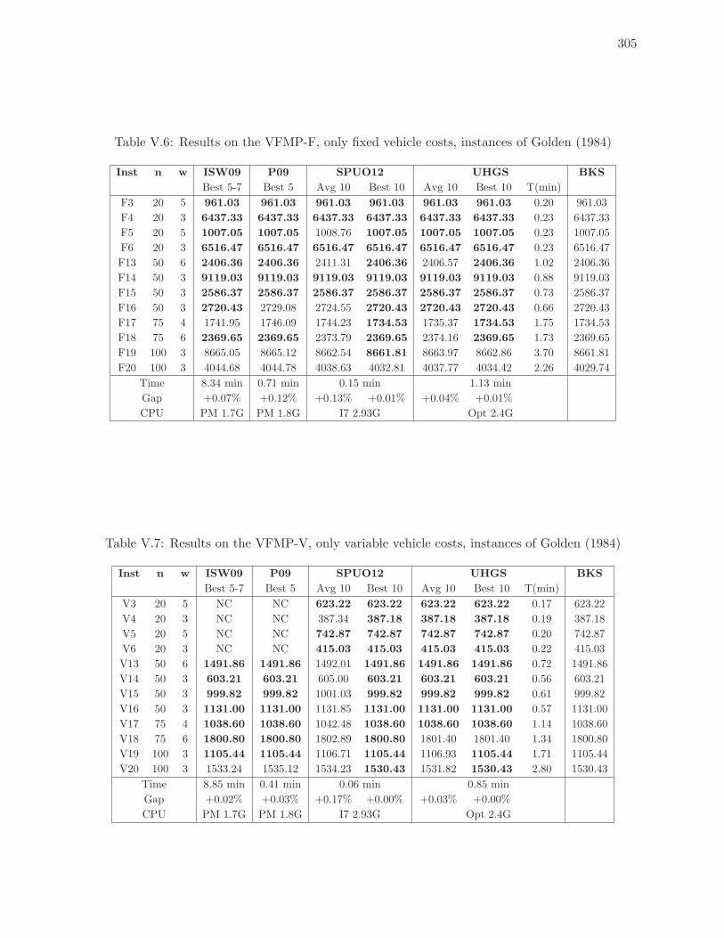
305

Table V.6: Results on the VFMP-F, only fixed vehicle costs, instances of Golden (1984)

Inst n w ISW09 P09 SPUO12 UHGS BKS

Best 5-7 Best 5 Avg 10 Best 10 Avg 10 Best 10 T(min)

F3 20 5 961.03 961.03 961.03 961.03 961.03 961.03 0.20 961.03

F4 20 3 6437.33 6437.33 6437.33 6437.33 6437.33 6437.33 0.23 6437.33

F5 20 5 1007.05 1007.05 1008.76 1007.05 1007.05 1007.05 0.23 1007.05

F6 20 3 6516.47 6516.47 6516.47 6516.47 6516.47 6516.47 0.23 6516.47

F13 50 6 2406.36 2406.36 2411.31 2406.36 2406.57 2406.36 1.02 2406.36

F14 50 3 9119.03 9119.03 9119.03 9119.03 9119.03 9119.03 0.88 9119.03

F15 50 3 2586.37 2586.37 2586.37 2586.37 2586.37 2586.37 0.73 2586.37

F16 50 3 2720.43 2729.08 2724.55 2720.43 2720.43 2720.43 0.66 2720.43

F17 75 4 1741.95 1746.09 1744.23 1734.53 1735.37 1734.53 1.75 1734.53

F18 75 6 2369.65 2369.65 2373.79 2369.65 2374.16 2369.65 1.73 2369.65

F19 100 3 8665.05 8665.12 8662.54 8661.81 8663.97 8662.86 3.70 8661.81

F20 100 3 4044.68 4044.78 4038.63 4032.81 4037.77 4034.42 2.26 4029.74

Time 8.34 min 0.71 min 0.15 min 1.13 min

Gap +0.07% +0.12% +0.13% +0.01% +0.04% +0.01%

CPU PM 1.7G PM 1.8G I7 2.93G Opt 2.4G

Table V.7: Results on the VFMP-V, only variable vehicle costs, instances of Golden (1984)



V3 20 5 NC NC 623.22 623.22 623.22 623.22 0.17 623.22

V4 20 3 NC NC 387.34 387.18 387.18 387.18 0.19 387.18

V5 20 5 NC NC 742.87 742.87 742.87 742.87 0.20 742.87

V6 20 3 NC NC 415.03 415.03 415.03 415.03 0.22 415.03

V13 50 6 1491.86 1491.86 1492.01 1491.86 1491.86 1491.86 0.72 1491.86

V14 50 3 603.21 603.21 605.00 603.21 603.21 603.21 0.56 603.21

V15 50 3 999.82 999.82 1001.03 999.82 999.82 999.82 0.61 999.82

V16 50 3 1131.00 1131.00 1131.85 1131.00 1131.00 1131.00 0.57 1131.00

V17 75 4 1038.60 1038.60 1042.48 1038.60 1038.60 1038.60 1.14 1038.60

V18 75 6 1800.80 1800.80 1802.89 1800.80 1801.40 1801.40 1.34 1800.80

V19 100 3 1105.44 1105.44 1106.71 1105.44 1106.93 1105.44 1.71 1105.44

V20 100 3 1533.24 1535.12 1534.23 1530.43 1531.82 1530.43 2.80 1530.43


Gap +0.02% +0.03% +0.17% +0.00% +0.03% +0.00%


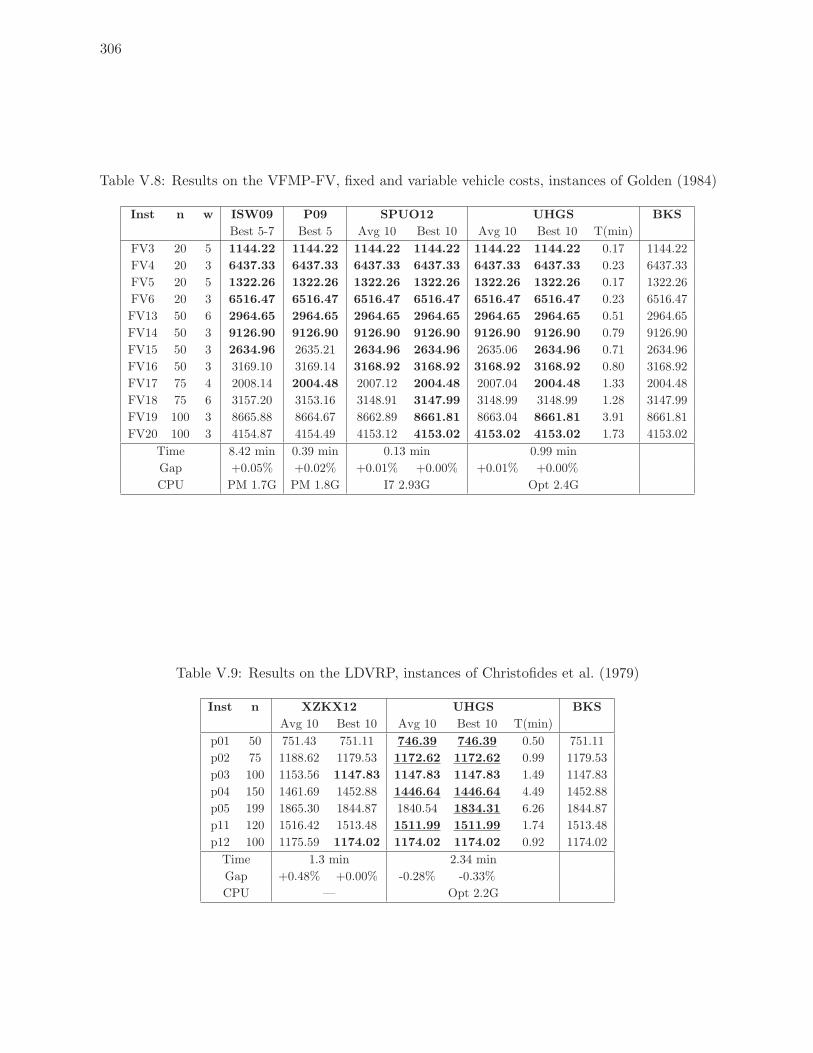
306

Table V.8: Results on the VFMP-FV, fixed and variable vehicle costs, instances of Golden (1984)



FV3 20 5 1144.22 1144.22 1144.22 1144.22 1144.22 1144.22 0.17 1144.22

FV4 20 3 6437.33 6437.33 6437.33 6437.33 6437.33 6437.33 0.23 6437.33

FV5 20 5 1322.26 1322.26 1322.26 1322.26 1322.26 1322.26 0.17 1322.26

FV6 20 3 6516.47 6516.47 6516.47 6516.47 6516.47 6516.47 0.23 6516.47

FV13 50 6 2964.65 2964.65 2964.65 2964.65 2964.65 2964.65 0.51 2964.65

FV14 50 3 9126.90 9126.90 9126.90 9126.90 9126.90 9126.90 0.79 9126.90

FV15 50 3 2634.96 2635.21 2634.96 2634.96 2635.06 2634.96 0.71 2634.96

FV16 50 3 3169.10 3169.14 3168.92 3168.92 3168.92 3168.92 0.80 3168.92

FV17 75 4 2008.14 2004.48 2007.12 2004.48 2007.04 2004.48 1.33 2004.48

FV18 75 6 3157.20 3153.16 3148.91 3147.99 3148.99 3148.99 1.28 3147.99

FV19 100 3 8665.88 8664.67 8662.89 8661.81 8663.04 8661.81 3.91 8661.81

FV20 100 3 4154.87 4154.49 4153.12 4153.02 4153.02 4153.02 1.73 4153.02


Gap +0.05% +0.02% +0.01% +0.00% +0.01% +0.00%


Table V.9: Results on the LDVRP, instances of Christofides et al. (1979)

Inst n XZKX12 UHGS BKS

Avg 10 Best 10 Avg 10 Best 10 T(min)

p01 50 751.43 751.11 746.39 746.39 0.50 751.11

p02 75 1188.62 1179.53 1172.62 1172.62 0.99 1179.53

p03 100 1153.56 1147.83 1147.83 1147.83 1.49 1147.83

p04 150 1461.69 1452.88 1446.64 1446.64 4.49 1452.88

p05 199 1865.30 1844.87 1840.54 1834.31 6.26 1844.87

p11 120 1516.42 1513.48 1511.99 1511.99 1.74 1513.48

p12 100 1175.59 1174.02 1174.02 1174.02 0.92 1174.02

Time 1.3 min 2.34 min

Gap +0.48% +0.00% -0.28% -0.33%

CPU — Opt 2.2G

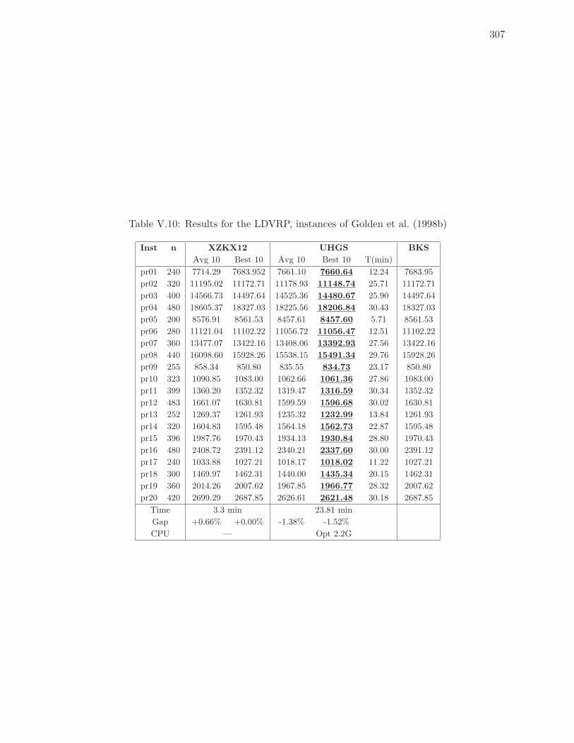
307

Table V.10: Results for the LDVRP, instances of Golden et al. (1998b)

Inst n XZKX12 UHGS BKS

Avg 10 Best 10 Avg 10 Best 10 T(min)

pr01 240 7714.29 7683.952 7661.10 7660.64 12.24 7683.95

pr02 320 11195.02 11172.71 11178.93 11148.74 25.71 11172.71

pr03 400 14566.73 14497.64 14525.36 14480.67 25.90 14497.64

pr04 480 18605.37 18327.03 18225.56 18206.84 30.43 18327.03

pr05 200 8576.91 8561.53 8457.61 8457.60 5.71 8561.53

pr06 280 11121.04 11102.22 11056.72 11056.47 12.51 11102.22

pr07 360 13477.07 13422.16 13408.06 13392.93 27.56 13422.16

pr08 440 16098.60 15928.26 15538.15 15491.34 29.76 15928.26

pr09 255 858.34 850.80 835.55 834.73 23.17 850.80

pr10 323 1090.85 1083.00 1062.66 1061.36 27.86 1083.00

pr11 399 1360.20 1352.32 1319.47 1316.59 30.34 1352.32

pr12 483 1661.07 1630.81 1599.59 1596.68 30.02 1630.81

pr13 252 1269.37 1261.93 1235.32 1232.99 13.84 1261.93

pr14 320 1604.83 1595.48 1564.18 1562.73 22.87 1595.48

pr15 396 1987.76 1970.43 1934.13 1930.84 28.80 1970.43

pr16 480 2408.72 2391.12 2340.21 2337.60 30.00 2391.12

pr17 240 1033.88 1027.21 1018.17 1018.02 11.22 1027.21

pr18 300 1469.97 1462.31 1440.00 1435.34 20.15 1462.31

pr19 360 2014.26 2007.62 1967.85 1966.77 28.32 2007.62

pr20 420 2699.29 2687.85 2626.61 2621.48 30.18 2687.85

Time 3.3 min 23.81 min

Gap +0.66% +0.00% -1.38% -1.52%

CPU — Opt 2.2G

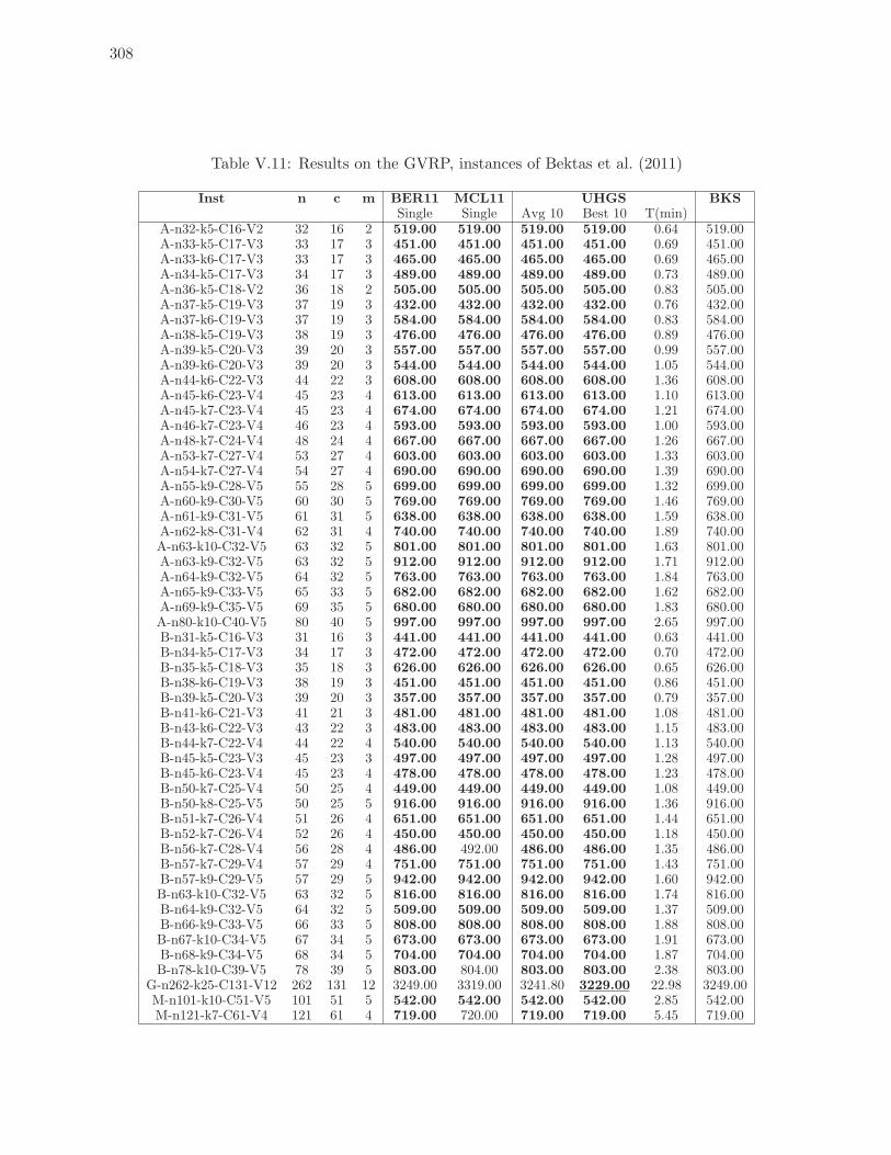
308

Table V.11: Results on the GVRP, instances of Bektas et al. (2011)

Inst n c m BER11 MCL11 UHGS BKSSingle Single Avg 10 Best 10 T(min)

A-n32-k5-C16-V2 32 16 2 519.00 519.00 519.00 519.00 0.64 519.00A-n33-k5-C17-V3 33 17 3 451.00 451.00 451.00 451.00 0.69 451.00A-n33-k6-C17-V3 33 17 3 465.00 465.00 465.00 465.00 0.69 465.00A-n34-k5-C17-V3 34 17 3 489.00 489.00 489.00 489.00 0.73 489.00A-n36-k5-C18-V2 36 18 2 505.00 505.00 505.00 505.00 0.83 505.00A-n37-k5-C19-V3 37 19 3 432.00 432.00 432.00 432.00 0.76 432.00A-n37-k6-C19-V3 37 19 3 584.00 584.00 584.00 584.00 0.83 584.00A-n38-k5-C19-V3 38 19 3 476.00 476.00 476.00 476.00 0.89 476.00A-n39-k5-C20-V3 39 20 3 557.00 557.00 557.00 557.00 0.99 557.00A-n39-k6-C20-V3 39 20 3 544.00 544.00 544.00 544.00 1.05 544.00A-n44-k6-C22-V3 44 22 3 608.00 608.00 608.00 608.00 1.36 608.00A-n45-k6-C23-V4 45 23 4 613.00 613.00 613.00 613.00 1.10 613.00A-n45-k7-C23-V4 45 23 4 674.00 674.00 674.00 674.00 1.21 674.00A-n46-k7-C23-V4 46 23 4 593.00 593.00 593.00 593.00 1.00 593.00A-n48-k7-C24-V4 48 24 4 667.00 667.00 667.00 667.00 1.26 667.00A-n53-k7-C27-V4 53 27 4 603.00 603.00 603.00 603.00 1.33 603.00A-n54-k7-C27-V4 54 27 4 690.00 690.00 690.00 690.00 1.39 690.00A-n55-k9-C28-V5 55 28 5 699.00 699.00 699.00 699.00 1.32 699.00A-n60-k9-C30-V5 60 30 5 769.00 769.00 769.00 769.00 1.46 769.00A-n61-k9-C31-V5 61 31 5 638.00 638.00 638.00 638.00 1.59 638.00A-n62-k8-C31-V4 62 31 4 740.00 740.00 740.00 740.00 1.89 740.00A-n63-k10-C32-V5 63 32 5 801.00 801.00 801.00 801.00 1.63 801.00A-n63-k9-C32-V5 63 32 5 912.00 912.00 912.00 912.00 1.71 912.00A-n64-k9-C32-V5 64 32 5 763.00 763.00 763.00 763.00 1.84 763.00A-n65-k9-C33-V5 65 33 5 682.00 682.00 682.00 682.00 1.62 682.00A-n69-k9-C35-V5 69 35 5 680.00 680.00 680.00 680.00 1.83 680.00A-n80-k10-C40-V5 80 40 5 997.00 997.00 997.00 997.00 2.65 997.00B-n31-k5-C16-V3 31 16 3 441.00 441.00 441.00 441.00 0.63 441.00B-n34-k5-C17-V3 34 17 3 472.00 472.00 472.00 472.00 0.70 472.00B-n35-k5-C18-V3 35 18 3 626.00 626.00 626.00 626.00 0.65 626.00B-n38-k6-C19-V3 38 19 3 451.00 451.00 451.00 451.00 0.86 451.00B-n39-k5-C20-V3 39 20 3 357.00 357.00 357.00 357.00 0.79 357.00B-n41-k6-C21-V3 41 21 3 481.00 481.00 481.00 481.00 1.08 481.00B-n43-k6-C22-V3 43 22 3 483.00 483.00 483.00 483.00 1.15 483.00B-n44-k7-C22-V4 44 22 4 540.00 540.00 540.00 540.00 1.13 540.00B-n45-k5-C23-V3 45 23 3 497.00 497.00 497.00 497.00 1.28 497.00B-n45-k6-C23-V4 45 23 4 478.00 478.00 478.00 478.00 1.23 478.00B-n50-k7-C25-V4 50 25 4 449.00 449.00 449.00 449.00 1.08 449.00B-n50-k8-C25-V5 50 25 5 916.00 916.00 916.00 916.00 1.36 916.00B-n51-k7-C26-V4 51 26 4 651.00 651.00 651.00 651.00 1.44 651.00B-n52-k7-C26-V4 52 26 4 450.00 450.00 450.00 450.00 1.18 450.00B-n56-k7-C28-V4 56 28 4 486.00 492.00 486.00 486.00 1.35 486.00B-n57-k7-C29-V4 57 29 4 751.00 751.00 751.00 751.00 1.43 751.00B-n57-k9-C29-V5 57 29 5 942.00 942.00 942.00 942.00 1.60 942.00B-n63-k10-C32-V5 63 32 5 816.00 816.00 816.00 816.00 1.74 816.00B-n64-k9-C32-V5 64 32 5 509.00 509.00 509.00 509.00 1.37 509.00B-n66-k9-C33-V5 66 33 5 808.00 808.00 808.00 808.00 1.88 808.00B-n67-k10-C34-V5 67 34 5 673.00 673.00 673.00 673.00 1.91 673.00B-n68-k9-C34-V5 68 34 5 704.00 704.00 704.00 704.00 1.87 704.00B-n78-k10-C39-V5 78 39 5 803.00 804.00 803.00 803.00 2.38 803.00

G-n262-k25-C131-V12 262 131 12 3249.00 3319.00 3241.80 3229.00 22.98 3249.00M-n101-k10-C51-V5 101 51 5 542.00 542.00 542.00 542.00 2.85 542.00M-n121-k7-C61-V4 121 61 4 719.00 720.00 719.00 719.00 5.45 719.00

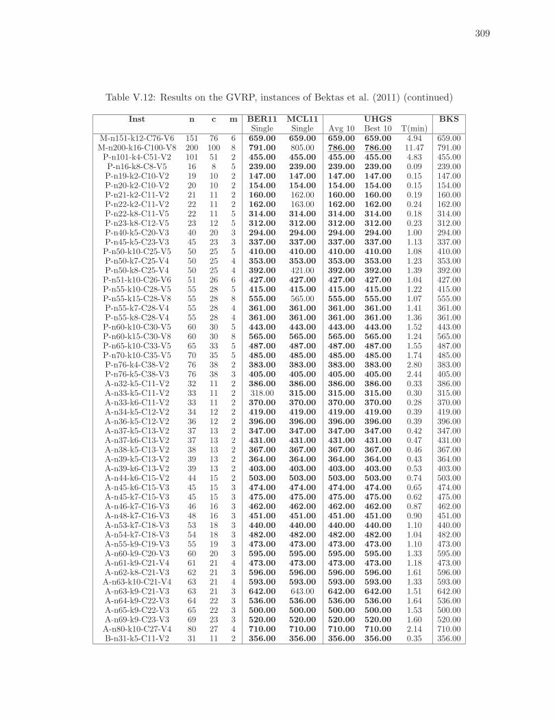
309

Table V.12: Results on the GVRP, instances of Bektas et al. (2011) (continued)


M-n151-k12-C76-V6 151 76 6 659.00 659.00 659.00 659.00 4.94 659.00M-n200-k16-C100-V8 200 100 8 791.00 805.00 786.00 786.00 11.47 791.00P-n101-k4-C51-V2 101 51 2 455.00 455.00 455.00 455.00 4.83 455.00P-n16-k8-C8-V5 16 8 5 239.00 239.00 239.00 239.00 0.09 239.00P-n19-k2-C10-V2 19 10 2 147.00 147.00 147.00 147.00 0.15 147.00P-n20-k2-C10-V2 20 10 2 154.00 154.00 154.00 154.00 0.15 154.00P-n21-k2-C11-V2 21 11 2 160.00 162.00 160.00 160.00 0.19 160.00P-n22-k2-C11-V2 22 11 2 162.00 163.00 162.00 162.00 0.24 162.00P-n22-k8-C11-V5 22 11 5 314.00 314.00 314.00 314.00 0.18 314.00P-n23-k8-C12-V5 23 12 5 312.00 312.00 312.00 312.00 0.23 312.00P-n40-k5-C20-V3 40 20 3 294.00 294.00 294.00 294.00 1.00 294.00P-n45-k5-C23-V3 45 23 3 337.00 337.00 337.00 337.00 1.13 337.00P-n50-k10-C25-V5 50 25 5 410.00 410.00 410.00 410.00 1.08 410.00P-n50-k7-C25-V4 50 25 4 353.00 353.00 353.00 353.00 1.23 353.00P-n50-k8-C25-V4 50 25 4 392.00 421.00 392.00 392.00 1.39 392.00P-n51-k10-C26-V6 51 26 6 427.00 427.00 427.00 427.00 1.04 427.00P-n55-k10-C28-V5 55 28 5 415.00 415.00 415.00 415.00 1.22 415.00P-n55-k15-C28-V8 55 28 8 555.00 565.00 555.00 555.00 1.07 555.00P-n55-k7-C28-V4 55 28 4 361.00 361.00 361.00 361.00 1.41 361.00P-n55-k8-C28-V4 55 28 4 361.00 361.00 361.00 361.00 1.36 361.00P-n60-k10-C30-V5 60 30 5 443.00 443.00 443.00 443.00 1.52 443.00P-n60-k15-C30-V8 60 30 8 565.00 565.00 565.00 565.00 1.24 565.00P-n65-k10-C33-V5 65 33 5 487.00 487.00 487.00 487.00 1.55 487.00P-n70-k10-C35-V5 70 35 5 485.00 485.00 485.00 485.00 1.74 485.00P-n76-k4-C38-V2 76 38 2 383.00 383.00 383.00 383.00 2.80 383.00P-n76-k5-C38-V3 76 38 3 405.00 405.00 405.00 405.00 2.44 405.00A-n32-k5-C11-V2 32 11 2 386.00 386.00 386.00 386.00 0.33 386.00A-n33-k5-C11-V2 33 11 2 318.00 315.00 315.00 315.00 0.30 315.00A-n33-k6-C11-V2 33 11 2 370.00 370.00 370.00 370.00 0.28 370.00A-n34-k5-C12-V2 34 12 2 419.00 419.00 419.00 419.00 0.39 419.00A-n36-k5-C12-V2 36 12 2 396.00 396.00 396.00 396.00 0.39 396.00A-n37-k5-C13-V2 37 13 2 347.00 347.00 347.00 347.00 0.42 347.00A-n37-k6-C13-V2 37 13 2 431.00 431.00 431.00 431.00 0.47 431.00A-n38-k5-C13-V2 38 13 2 367.00 367.00 367.00 367.00 0.46 367.00A-n39-k5-C13-V2 39 13 2 364.00 364.00 364.00 364.00 0.43 364.00A-n39-k6-C13-V2 39 13 2 403.00 403.00 403.00 403.00 0.53 403.00A-n44-k6-C15-V2 44 15 2 503.00 503.00 503.00 503.00 0.74 503.00A-n45-k6-C15-V3 45 15 3 474.00 474.00 474.00 474.00 0.65 474.00A-n45-k7-C15-V3 45 15 3 475.00 475.00 475.00 475.00 0.62 475.00A-n46-k7-C16-V3 46 16 3 462.00 462.00 462.00 462.00 0.87 462.00A-n48-k7-C16-V3 48 16 3 451.00 451.00 451.00 451.00 0.90 451.00A-n53-k7-C18-V3 53 18 3 440.00 440.00 440.00 440.00 1.10 440.00A-n54-k7-C18-V3 54 18 3 482.00 482.00 482.00 482.00 1.04 482.00A-n55-k9-C19-V3 55 19 3 473.00 473.00 473.00 473.00 1.10 473.00A-n60-k9-C20-V3 60 20 3 595.00 595.00 595.00 595.00 1.33 595.00A-n61-k9-C21-V4 61 21 4 473.00 473.00 473.00 473.00 1.18 473.00A-n62-k8-C21-V3 62 21 3 596.00 596.00 596.00 596.00 1.61 596.00A-n63-k10-C21-V4 63 21 4 593.00 593.00 593.00 593.00 1.33 593.00A-n63-k9-C21-V3 63 21 3 642.00 643.00 642.00 642.00 1.51 642.00A-n64-k9-C22-V3 64 22 3 536.00 536.00 536.00 536.00 1.64 536.00A-n65-k9-C22-V3 65 22 3 500.00 500.00 500.00 500.00 1.53 500.00A-n69-k9-C23-V3 69 23 3 520.00 520.00 520.00 520.00 1.60 520.00A-n80-k10-C27-V4 80 27 4 710.00 710.00 710.00 710.00 2.14 710.00B-n31-k5-C11-V2 31 11 2 356.00 356.00 356.00 356.00 0.35 356.00

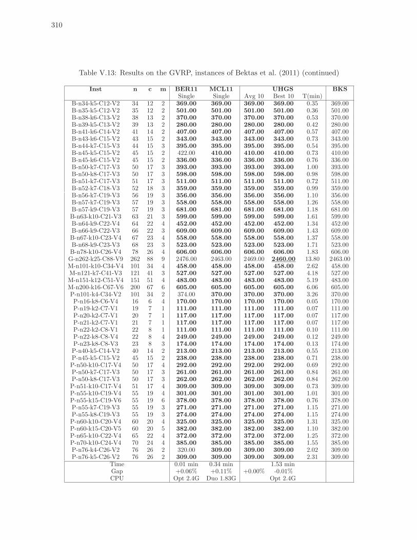
310

Table V.13: Results on the GVRP, instances of Bektas et al. (2011) (continued)


B-n34-k5-C12-V2 34 12 2 369.00 369.00 369.00 369.00 0.35 369.00B-n35-k5-C12-V2 35 12 2 501.00 501.00 501.00 501.00 0.36 501.00B-n38-k6-C13-V2 38 13 2 370.00 370.00 370.00 370.00 0.53 370.00B-n39-k5-C13-V2 39 13 2 280.00 280.00 280.00 280.00 0.42 280.00B-n41-k6-C14-V2 41 14 2 407.00 407.00 407.00 407.00 0.57 407.00B-n43-k6-C15-V2 43 15 2 343.00 343.00 343.00 343.00 0.73 343.00B-n44-k7-C15-V3 44 15 3 395.00 395.00 395.00 395.00 0.54 395.00B-n45-k5-C15-V2 45 15 2 422.00 410.00 410.00 410.00 0.73 410.00B-n45-k6-C15-V2 45 15 2 336.00 336.00 336.00 336.00 0.76 336.00B-n50-k7-C17-V3 50 17 3 393.00 393.00 393.00 393.00 1.00 393.00B-n50-k8-C17-V3 50 17 3 598.00 598.00 598.00 598.00 0.98 598.00B-n51-k7-C17-V3 51 17 3 511.00 511.00 511.00 511.00 0.72 511.00B-n52-k7-C18-V3 52 18 3 359.00 359.00 359.00 359.00 0.99 359.00B-n56-k7-C19-V3 56 19 3 356.00 356.00 356.00 356.00 1.10 356.00B-n57-k7-C19-V3 57 19 3 558.00 558.00 558.00 558.00 1.26 558.00B-n57-k9-C19-V3 57 19 3 681.00 681.00 681.00 681.00 1.18 681.00B-n63-k10-C21-V3 63 21 3 599.00 599.00 599.00 599.00 1.61 599.00B-n64-k9-C22-V4 64 22 4 452.00 452.00 452.00 452.00 1.34 452.00B-n66-k9-C22-V3 66 22 3 609.00 609.00 609.00 609.00 1.43 609.00B-n67-k10-C23-V4 67 23 4 558.00 558.00 558.00 558.00 1.37 558.00B-n68-k9-C23-V3 68 23 3 523.00 523.00 523.00 523.00 1.71 523.00B-n78-k10-C26-V4 78 26 4 606.00 606.00 606.00 606.00 1.83 606.00G-n262-k25-C88-V9 262 88 9 2476.00 2463.00 2469.00 2460.00 13.80 2463.00M-n101-k10-C34-V4 101 34 4 458.00 458.00 458.00 458.00 2.62 458.00M-n121-k7-C41-V3 121 41 3 527.00 527.00 527.00 527.00 4.18 527.00M-n151-k12-C51-V4 151 51 4 483.00 483.00 483.00 483.00 5.19 483.00M-n200-k16-C67-V6 200 67 6 605.00 605.00 605.00 605.00 6.06 605.00P-n101-k4-C34-V2 101 34 2 374.00 370.00 370.00 370.00 3.26 370.00P-n16-k8-C6-V4 16 6 4 170.00 170.00 170.00 170.00 0.05 170.00P-n19-k2-C7-V1 19 7 1 111.00 111.00 111.00 111.00 0.07 111.00P-n20-k2-C7-V1 20 7 1 117.00 117.00 117.00 117.00 0.07 117.00P-n21-k2-C7-V1 21 7 1 117.00 117.00 117.00 117.00 0.07 117.00P-n22-k2-C8-V1 22 8 1 111.00 111.00 111.00 111.00 0.10 111.00P-n22-k8-C8-V4 22 8 4 249.00 249.00 249.00 249.00 0.12 249.00P-n23-k8-C8-V3 23 8 3 174.00 174.00 174.00 174.00 0.13 174.00P-n40-k5-C14-V2 40 14 2 213.00 213.00 213.00 213.00 0.55 213.00P-n45-k5-C15-V2 45 15 2 238.00 238.00 238.00 238.00 0.71 238.00P-n50-k10-C17-V4 50 17 4 292.00 292.00 292.00 292.00 0.69 292.00P-n50-k7-C17-V3 50 17 3 261.00 261.00 261.00 261.00 0.84 261.00P-n50-k8-C17-V3 50 17 3 262.00 262.00 262.00 262.00 0.84 262.00P-n51-k10-C17-V4 51 17 4 309.00 309.00 309.00 309.00 0.73 309.00P-n55-k10-C19-V4 55 19 4 301.00 301.00 301.00 301.00 1.01 301.00P-n55-k15-C19-V6 55 19 6 378.00 378.00 378.00 378.00 0.76 378.00P-n55-k7-C19-V3 55 19 3 271.00 271.00 271.00 271.00 1.15 271.00P-n55-k8-C19-V3 55 19 3 274.00 274.00 274.00 274.00 1.15 274.00P-n60-k10-C20-V4 60 20 4 325.00 325.00 325.00 325.00 1.31 325.00P-n60-k15-C20-V5 60 20 5 382.00 382.00 382.00 382.00 1.10 382.00P-n65-k10-C22-V4 65 22 4 372.00 372.00 372.00 372.00 1.25 372.00P-n70-k10-C24-V4 70 24 4 385.00 385.00 385.00 385.00 1.55 385.00P-n76-k4-C26-V2 76 26 2 320.00 309.00 309.00 309.00 2.02 309.00P-n76-k5-C26-V2 76 26 2 309.00 309.00 309.00 309.00 2.31 309.00

Time 0.01 min 0.34 min 1.53 minGap +0.06% +0.11% +0.00% -0.01%CPU Opt 2.4G Duo 1.83G Opt 2.4G

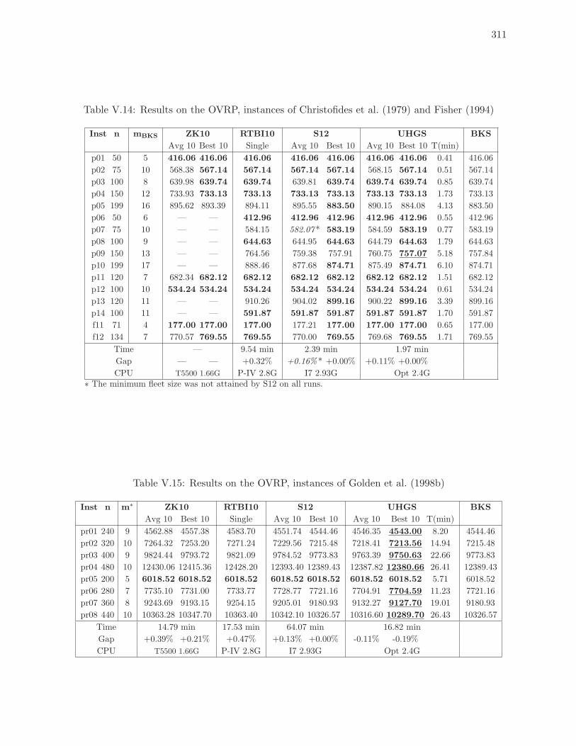
311

Table V.14: Results on the OVRP, instances of Christofides et al. (1979) and Fisher (1994)

Inst n mBKS ZK10 RTBI10 S12 UHGS BKS

Avg 10 Best 10 Single Avg 10 Best 10 Avg 10 Best 10 T(min)

p01 50 5 416.06 416.06 416.06 416.06 416.06 416.06 416.06 0.41 416.06

p02 75 10 568.38 567.14 567.14 567.14 567.14 568.15 567.14 0.51 567.14

p03 100 8 639.98 639.74 639.74 639.81 639.74 639.74 639.74 0.85 639.74

p04 150 12 733.93 733.13 733.13 733.13 733.13 733.13 733.13 1.73 733.13

p05 199 16 895.62 893.39 894.11 895.55 883.50 890.15 884.08 4.13 883.50

p06 50 6 — — 412.96 412.96 412.96 412.96 412.96 0.55 412.96

p07 75 10 — — 584.15 582.07* 583.19 584.59 583.19 0.77 583.19

p08 100 9 — — 644.63 644.95 644.63 644.79 644.63 1.79 644.63

p09 150 13 — — 764.56 759.38 757.91 760.75 757.07 5.18 757.84

p10 199 17 — — 888.46 877.68 874.71 875.49 874.71 6.10 874.71

p11 120 7 682.34 682.12 682.12 682.12 682.12 682.12 682.12 1.51 682.12

p12 100 10 534.24 534.24 534.24 534.24 534.24 534.24 534.24 0.61 534.24

p13 120 11 — — 910.26 904.02 899.16 900.22 899.16 3.39 899.16

p14 100 11 — — 591.87 591.87 591.87 591.87 591.87 1.70 591.87

f11 71 4 177.00 177.00 177.00 177.21 177.00 177.00 177.00 0.65 177.00

f12 134 7 770.57 769.55 769.55 770.00 769.55 769.68 769.55 1.71 769.55

Time — 9.54 min 2.39 min 1.97 min

Gap — — +0.32% +0.16%* +0.00% +0.11% +0.00%

CPU T5500 1.66G P-IV 2.8G I7 2.93G Opt 2.4G∗ The minimum fleet size was not attained by S12 on all runs.

Table V.15: Results on the OVRP, instances of Golden et al. (1998b)

Inst n m∗ ZK10 RTBI10 S12 UHGS BKS

Avg 10 Best 10 Single Avg 10 Best 10 Avg 10 Best 10 T(min)

pr01 240 9 4562.88 4557.38 4583.70 4551.74 4544.46 4546.35 4543.00 8.20 4544.46

pr02 320 10 7264.32 7253.20 7271.24 7229.56 7215.48 7218.41 7213.56 14.94 7215.48

pr03 400 9 9824.44 9793.72 9821.09 9784.52 9773.83 9763.39 9750.63 22.66 9773.83

pr04 480 10 12430.06 12415.36 12428.20 12393.40 12389.43 12387.82 12380.66 26.41 12389.43

pr05 200 5 6018.52 6018.52 6018.52 6018.52 6018.52 6018.52 6018.52 5.71 6018.52

pr06 280 7 7735.10 7731.00 7733.77 7728.77 7721.16 7704.91 7704.59 11.23 7721.16

pr07 360 8 9243.69 9193.15 9254.15 9205.01 9180.93 9132.27 9127.70 19.01 9180.93

pr08 440 10 10363.28 10347.70 10363.40 10342.10 10326.57 10316.60 10289.70 26.43 10326.57


Gap +0.39% +0.21% +0.47% +0.13% +0.00% -0.11% -0.19%

CPU T5500 1.66G P-IV 2.8G I7 2.93G Opt 2.4G

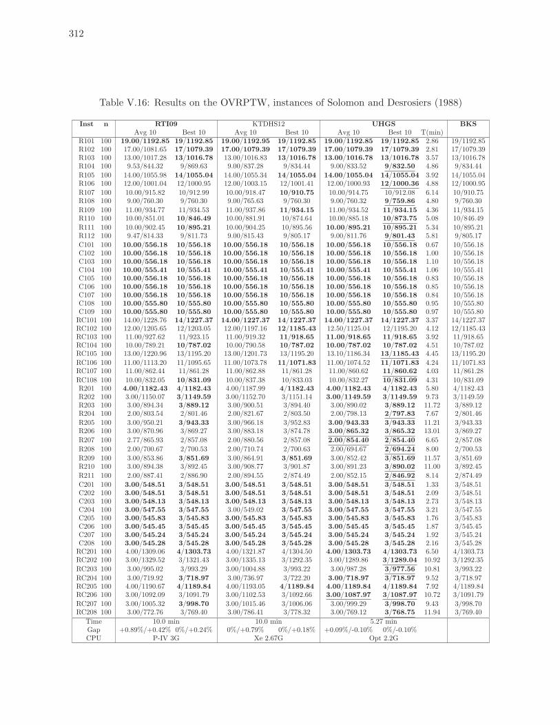
312

Table V.16: Results on the OVRPTW, instances of Solomon and Desrosiers (1988)

Inst n RTI09 KTDHS12 UHGS BKSAvg 10 Best 10 Avg 10 Best 10 Avg 10 Best 10 T(min)

R101 100 19.00/1192.85 19/1192.85 19.00/1192.95 19/1192.85 19.00/1192.85 19/1192.85 2.86 19/1192.85R102 100 17.00/1081.65 17/1079.39 17.00/1079.39 17/1079.39 17.00/1079.39 17/1079.39 2.81 17/1079.39R103 100 13.00/1017.28 13/1016.78 13.00/1016.83 13/1016.78 13.00/1016.78 13/1016.78 3.57 13/1016.78R104 100 9.53/844.32 9/869.63 9.00/837.28 9/834.44 9.00/833.52 9/832.50 4.86 9/834.44

R105 100 14.00/1055.98 14/1055.04 14.00/1055.34 14/1055.04 14.00/1055.04 14/1055.04 3.92 14/1055.04R106 100 12.00/1001.04 12/1000.95 12.00/1003.15 12/1001.41 12.00/1000.93 12/1000.36 4.88 12/1000.95

R107 100 10.00/915.82 10/912.99 10.00/918.47 10/910.75 10.00/914.75 10/912.08 6.14 10/910.75R108 100 9.00/760.30 9/760.30 9.00/765.63 9/760.30 9.00/760.32 9/759.86 4.80 9/760.30

R109 100 11.00/934.77 11/934.53 11.00/937.86 11/934.15 11.00/934.52 11/934.15 4.36 11/934.15R110 100 10.00/851.01 10/846.49 10.00/881.91 10/874.64 10.00/885.18 10/873.75 5.08 10/846.49

R111 100 10.00/902.45 10/895.21 10.00/904.25 10/895.56 10.00/895.21 10/895.21 5.34 10/895.21R112 100 9.47/814.33 9/811.73 9.00/815.43 9/805.17 9.00/811.76 9/801.43 5.81 9/805.17

C101 100 10.00/556.18 10/556.18 10.00/556.18 10/556.18 10.00/556.18 10/556.18 0.67 10/556.18C102 100 10.00/556.18 10/556.18 10.00/556.18 10/556.18 10.00/556.18 10/556.18 1.00 10/556.18C103 100 10.00/556.18 10/556.18 10.00/556.18 10/556.18 10.00/556.18 10/556.18 1.10 10/556.18C104 100 10.00/555.41 10/555.41 10.00/555.41 10/555.41 10.00/555.41 10/555.41 1.06 10/555.41C105 100 10.00/556.18 10/556.18 10.00/556.18 10/556.18 10.00/556.18 10/556.18 0.83 10/556.18C106 100 10.00/556.18 10/556.18 10.00/556.18 10/556.18 10.00/556.18 10/556.18 0.85 10/556.18C107 100 10.00/556.18 10/556.18 10.00/556.18 10/556.18 10.00/556.18 10/556.18 0.84 10/556.18C108 100 10.00/555.80 10/555.80 10.00/555.80 10/555.80 10.00/555.80 10/555.80 0.95 10/555.80C109 100 10.00/555.80 10/555.80 10.00/555.80 10/555.80 10.00/555.80 10/555.80 0.97 10/555.80RC101 100 14.00/1228.76 14/1227.37 14.00/1227.37 14/1227.37 14.00/1227.37 14/1227.37 3.37 14/1227.37RC102 100 12.00/1205.65 12/1203.05 12.00/1197.16 12/1185.43 12.50/1125.04 12/1195.20 4.12 12/1185.43RC103 100 11.00/927.62 11/923.15 11.00/919.32 11/918.65 11.00/918.65 11/918.65 3.92 11/918.65RC104 100 10.00/789.21 10/787.02 10.00/790.58 10/787.02 10.00/787.02 10/787.02 4.51 10/787.02RC105 100 13.00/1220.96 13/1195.20 13.00/1201.73 13/1195.20 13.10/1186.34 13/1185.43 4.45 13/1195.20

RC106 100 11.00/1113.20 11/1095.65 11.00/1073.78 11/1071.83 11.00/1074.52 11/1071.83 4.24 11/1071.83RC107 100 11.00/862.44 11/861.28 11.00/862.88 11/861.28 11.00/860.62 11/860.62 4.03 11/861.28

RC108 100 10.00/832.05 10/831.09 10.00/837.38 10/833.03 10.00/832.27 10/831.09 4.31 10/831.09R201 100 4.00/1182.43 4/1182.43 4.00/1187.99 4/1182.43 4.00/1182.43 4/1182.43 5.80 4/1182.43R202 100 3.00/1150.07 3/1149.59 3.00/1152.70 3/1151.14 3.00/1149.59 3/1149.59 9.73 3/1149.59R203 100 3.00/894.34 3/889.12 3.00/900.51 3/894.40 3.00/890.02 3/889.12 11.72 3/889.12R204 100 2.00/803.54 2/801.46 2.00/821.67 2/803.50 2.00/798.13 2/797.83 7.67 2/801.46

R205 100 3.00/950.21 3/943.33 3.00/966.18 3/952.83 3.00/943.33 3/943.33 11.21 3/943.33R206 100 3.00/870.96 3/869.27 3.00/883.18 3/874.78 3.00/865.32 3/865.32 13.01 3/869.27

R207 100 2.77/865.93 2/857.08 2.00/880.56 2/857.08 2.00/854.40 2/854.40 6.65 2/857.08

R208 100 2.00/700.67 2/700.53 2.00/710.74 2/700.63 2.00/694.67 2/694.24 8.00 2/700.53

R209 100 3.00/853.86 3/851.69 3.00/864.91 3/851.69 3.00/852.42 3/851.69 11.57 3/851.69R210 100 3.00/894.38 3/892.45 3.00/908.77 3/901.87 3.00/891.23 3/890.02 11.00 3/892.45

R211 100 2.00/887.41 2/886.90 2.00/894.55 2/874.49 2.00/852.15 2/846.92 8.14 2/874.49

C201 100 3.00/548.51 3/548.51 3.00/548.51 3/548.51 3.00/548.51 3/548.51 1.33 3/548.51C202 100 3.00/548.51 3/548.51 3.00/548.51 3/548.51 3.00/548.51 3/548.51 2.09 3/548.51C203 100 3.00/548.13 3/548.13 3.00/548.13 3/548.13 3.00/548.13 3/548.13 2.73 3/548.13C204 100 3.00/547.55 3/547.55 3.00/549.02 3/547.55 3.00/547.55 3/547.55 3.21 3/547.55C205 100 3.00/545.83 3/545.83 3.00/545.83 3/545.83 3.00/545.83 3/545.83 1.76 3/545.83C206 100 3.00/545.45 3/545.45 3.00/545.45 3/545.45 3.00/545.45 3/545.45 1.87 3/545.45C207 100 3.00/545.24 3/545.24 3.00/545.24 3/545.24 3.00/545.24 3/545.24 1.92 3/545.24C208 100 3.00/545.28 3/545.28 3.00/545.28 3/545.28 3.00/545.28 3/545.28 2.16 3/545.28RC201 100 4.00/1309.06 4/1303.73 4.00/1321.87 4/1304.50 4.00/1303.73 4/1303.73 6.50 4/1303.73RC202 100 3.00/1329.52 3/1321.43 3.00/1335.13 3/1292.35 3.00/1289.86 3/1289.04 10.92 3/1292.35

RC203 100 3.00/995.02 3/993.29 3.00/1004.88 3/993.22 3.00/987.28 3/977.56 10.81 3/993.22

RC204 100 3.00/719.92 3/718.97 3.00/736.97 3/722.20 3.00/718.97 3/718.97 9.52 3/718.97RC205 100 4.00/1190.67 4/1189.84 4.00/1193.05 4/1189.84 4.00/1189.84 4/1189.84 7.92 4/1189.84RC206 100 3.00/1092.09 3/1091.79 3.00/1102.53 3/1092.66 3.00/1087.97 3/1087.97 10.72 3/1091.79

RC207 100 3.00/1005.32 3/998.70 3.00/1015.46 3/1006.06 3.00/999.29 3/998.70 9.43 3/998.70RC208 100 3.00/772.76 3/769.40 3.00/786.41 3/778.32 3.00/769.12 3/768.75 11.94 3/769.40

Time 10.0 min 10.0 min 5.27 minGap +0.89%/+0.42% 0%/+0.24% 0%/+0.79% 0%/+0.18% +0.09%/-0.10% 0%/-0.10%CPU P-IV 3G Xe 2.67G Opt 2.2G

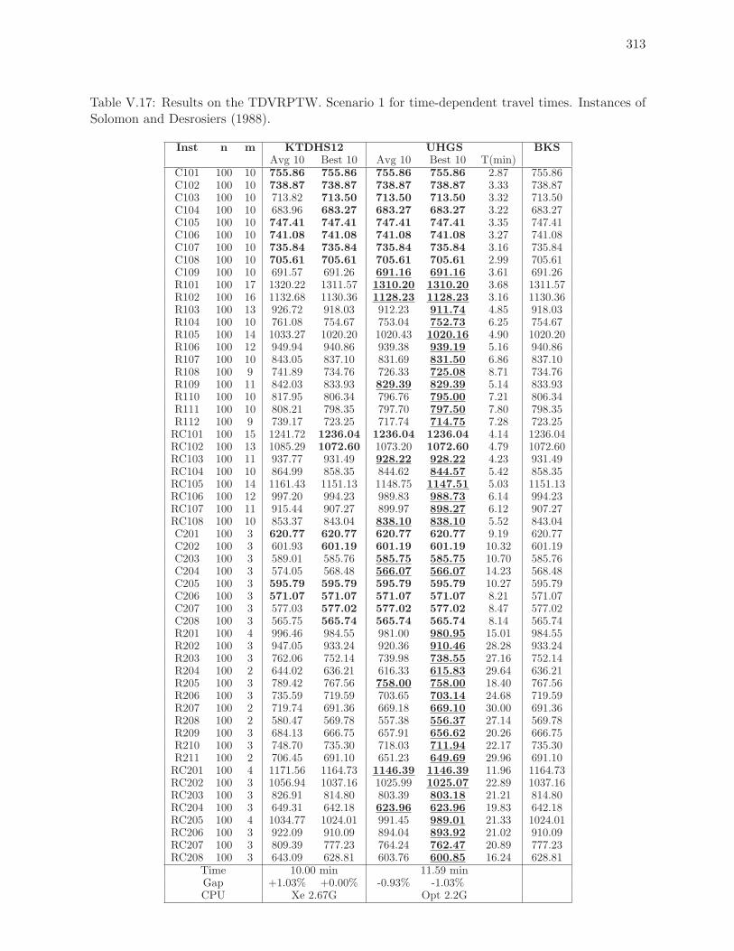
313

Table V.17: Results on the TDVRPTW. Scenario 1 for time-dependent travel times. Instances ofSolomon and Desrosiers (1988).

Inst n m KTDHS12 UHGS BKSAvg 10 Best 10 Avg 10 Best 10 T(min)

C101 100 10 755.86 755.86 755.86 755.86 2.87 755.86C102 100 10 738.87 738.87 738.87 738.87 3.33 738.87C103 100 10 713.82 713.50 713.50 713.50 3.32 713.50C104 100 10 683.96 683.27 683.27 683.27 3.22 683.27C105 100 10 747.41 747.41 747.41 747.41 3.35 747.41C106 100 10 741.08 741.08 741.08 741.08 3.27 741.08C107 100 10 735.84 735.84 735.84 735.84 3.16 735.84C108 100 10 705.61 705.61 705.61 705.61 2.99 705.61C109 100 10 691.57 691.26 691.16 691.16 3.61 691.26R101 100 17 1320.22 1311.57 1310.20 1310.20 3.68 1311.57R102 100 16 1132.68 1130.36 1128.23 1128.23 3.16 1130.36R103 100 13 926.72 918.03 912.23 911.74 4.85 918.03R104 100 10 761.08 754.67 753.04 752.73 6.25 754.67R105 100 14 1033.27 1020.20 1020.43 1020.16 4.90 1020.20R106 100 12 949.94 940.86 939.38 939.19 5.16 940.86R107 100 10 843.05 837.10 831.69 831.50 6.86 837.10R108 100 9 741.89 734.76 726.33 725.08 8.71 734.76R109 100 11 842.03 833.93 829.39 829.39 5.14 833.93R110 100 10 817.95 806.34 796.76 795.00 7.21 806.34R111 100 10 808.21 798.35 797.70 797.50 7.80 798.35R112 100 9 739.17 723.25 717.74 714.75 7.28 723.25RC101 100 15 1241.72 1236.04 1236.04 1236.04 4.14 1236.04RC102 100 13 1085.29 1072.60 1073.20 1072.60 4.79 1072.60RC103 100 11 937.77 931.49 928.22 928.22 4.23 931.49RC104 100 10 864.99 858.35 844.62 844.57 5.42 858.35RC105 100 14 1161.43 1151.13 1148.75 1147.51 5.03 1151.13RC106 100 12 997.20 994.23 989.83 988.73 6.14 994.23RC107 100 11 915.44 907.27 899.97 898.27 6.12 907.27RC108 100 10 853.37 843.04 838.10 838.10 5.52 843.04C201 100 3 620.77 620.77 620.77 620.77 9.19 620.77C202 100 3 601.93 601.19 601.19 601.19 10.32 601.19C203 100 3 589.01 585.76 585.75 585.75 10.70 585.76C204 100 3 574.05 568.48 566.07 566.07 14.23 568.48C205 100 3 595.79 595.79 595.79 595.79 10.27 595.79C206 100 3 571.07 571.07 571.07 571.07 8.21 571.07C207 100 3 577.03 577.02 577.02 577.02 8.47 577.02C208 100 3 565.75 565.74 565.74 565.74 8.14 565.74R201 100 4 996.46 984.55 981.00 980.95 15.01 984.55R202 100 3 947.05 933.24 920.36 910.46 28.28 933.24R203 100 3 762.06 752.14 739.98 738.55 27.16 752.14R204 100 2 644.02 636.21 616.33 615.83 29.64 636.21R205 100 3 789.42 767.56 758.00 758.00 18.40 767.56R206 100 3 735.59 719.59 703.65 703.14 24.68 719.59R207 100 2 719.74 691.36 669.18 669.10 30.00 691.36R208 100 2 580.47 569.78 557.38 556.37 27.14 569.78R209 100 3 684.13 666.75 657.91 656.62 20.26 666.75R210 100 3 748.70 735.30 718.03 711.94 22.17 735.30R211 100 2 706.45 691.10 651.23 649.69 29.96 691.10RC201 100 4 1171.56 1164.73 1146.39 1146.39 11.96 1164.73RC202 100 3 1056.94 1037.16 1025.99 1025.07 22.89 1037.16RC203 100 3 826.91 814.80 803.39 803.18 21.21 814.80RC204 100 3 649.31 642.18 623.96 623.96 19.83 642.18RC205 100 4 1034.77 1024.01 991.45 989.01 21.33 1024.01RC206 100 3 922.09 910.09 894.04 893.92 21.02 910.09RC207 100 3 809.39 777.23 764.24 762.47 20.89 777.23RC208 100 3 643.09 628.81 603.76 600.85 16.24 628.81

Time 10.00 min 11.59 minGap +1.03% +0.00% -0.93% -1.03%CPU Xe 2.67G Opt 2.2G

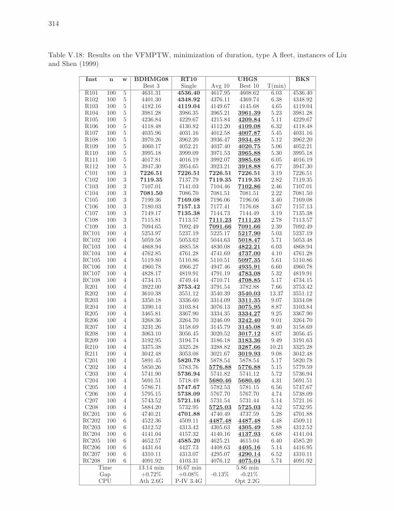
314

Table V.18: Results on the VFMPTW, minimization of duration, type A fleet, instances of Liuand Shen (1999)

Inst n w BDHMG08 RT10 UHGS BKSBest 3 Single Avg 10 Best 10 T(min)

R101 100 5 4631.31 4536.40 4617.95 4608.62 6.03 4536.40R102 100 5 4401.30 4348.92 4376.11 4369.74 6.38 4348.92R103 100 5 4182.16 4119.04 4149.67 4145.68 4.65 4119.04R104 100 5 3981.28 3986.35 3965.21 3961.39 5.23 3981.28R105 100 5 4236.84 4229.67 4215.84 4209.84 5.11 4229.67R106 100 5 4118.48 4130.82 4112.20 4109.08 6.32 4118.48R107 100 5 4035.96 4031.16 4012.58 4007.87 5.45 4031.16R108 100 5 3970.26 3962.20 3936.47 3934.48 5.12 3962.20R109 100 5 4060.17 4052.21 4037.40 4020.75 5.06 4052.21R110 100 5 3995.18 3999.09 3971.53 3965.88 5.30 3995.18R111 100 5 4017.81 4016.19 3992.07 3985.68 6.05 4016.19R112 100 5 3947.30 3954.65 3923.21 3918.88 6.77 3947.30C101 100 3 7226.51 7226.51 7226.51 7226.51 3.19 7226.51C102 100 3 7119.35 7137.79 7119.35 7119.35 2.82 7119.35C103 100 3 7107.01 7141.03 7104.46 7102.86 2.46 7107.01C104 100 3 7081.50 7086.70 7081.51 7081.51 2.22 7081.50C105 100 3 7199.36 7169.08 7196.06 7196.06 3.40 7169.08C106 100 3 7180.03 7157.13 7177.41 7176.68 3.67 7157.13C107 100 3 7149.17 7135.38 7144.73 7144.49 3.19 7135.38C108 100 3 7115.81 7113.57 7111.23 7111.23 2.78 7113.57C109 100 3 7094.65 7092.49 7091.66 7091.66 2.39 7092.49RC101 100 4 5253.97 5237.19 5225.17 5217.90 5.03 5237.19RC102 100 4 5059.58 5053.62 5044.63 5018.47 5.71 5053.48RC103 100 4 4868.94 4885.58 4830.08 4822.21 6.03 4868.94RC104 100 4 4762.85 4761.28 4741.69 4737.00 4.10 4761.28RC105 100 4 5119.80 5110.86 5110.51 5097.35 5.61 5110.86RC106 100 4 4960.78 4966.27 4947.46 4935.91 6.60 4960.78RC107 100 4 4828.17 4819.91 4791.19 4783.08 5.32 4819.91RC108 100 4 4734.15 4749.44 4710.71 4708.85 5.17 4734.15R201 100 4 3922.00 3753.42 3791.54 3782.88 7.66 3753.42R202 100 4 3610.38 3551.12 3540.39 3540.03 13.37 3551.12R203 100 4 3350.18 3336.60 3314.09 3311.35 9.07 3334.08R204 100 4 3390.14 3103.84 3076.13 3075.95 8.87 3103.84R205 100 4 3465.81 3367.90 3334.35 3334.27 9.25 3367.90R206 100 4 3268.36 3264.70 3246.09 3242.40 9.01 3264.70R207 100 4 3231.26 3158.69 3145.79 3145.08 9.40 3158.69R208 100 4 3063.10 3056.45 3020.52 3017.12 8.07 3056.45R209 100 4 3192.95 3194.74 3186.18 3183.36 9.49 3191.63R210 100 4 3375.38 3325.28 3288.82 3287.66 10.21 3325.28R211 100 4 3042.48 3053.08 3021.67 3019.93 9.08 3042.48C201 100 4 5891.45 5820.78 5878.54 5878.54 5.17 5820.78C202 100 4 5850.26 5783.76 5776.88 5776.88 5.15 5779.59C203 100 4 5741.90 5736.94 5741.82 5741.12 5.72 5736.94C204 100 4 5691.51 5718.49 5680.46 5680.46 4.31 5691.51C205 100 4 5786.71 5747.67 5782.53 5781.15 6.56 5747.67C206 100 4 5795.15 5738.09 5767.70 5767.70 4.74 5738.09C207 100 4 5743.52 5721.16 5731.54 5731.44 5.14 5721.16C208 100 4 5884.20 5732.95 5725.03 5725.03 4.52 5732.95RC201 100 6 4740.21 4701.88 4740.49 4737.59 5.28 4701.88RC202 100 6 4522.36 4509.11 4487.48 4487.48 4.48 4509.11RC203 100 6 4312.52 4313.42 4305.63 4305.49 5.88 4312.52RC204 100 6 4141.04 4157.32 4140.16 4137.93 6.68 4141.04RC205 100 6 4652.57 4585.20 4625.21 4615.04 6.40 4585.20RC206 100 6 4431.64 4427.73 4408.63 4405.16 5.14 4416.95RC207 100 6 4310.11 4313.07 4295.07 4290.14 6.52 4310.11RC208 100 6 4091.92 4103.31 4076.12 4075.04 5.74 4091.92

Time 13.14 min 16.67 min 5.86 minGap +0.72% +0.08% -0.13% -0.21%CPU Ath 2.6G P-IV 3.4G Opt 2.2G

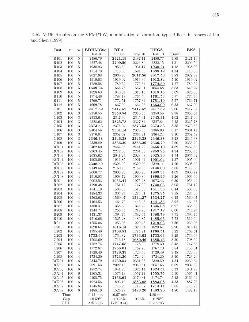
315

Table V.19: Results on the VFMPTW, minimization of duration, type B fleet, instances of Liuand Shen (1999)




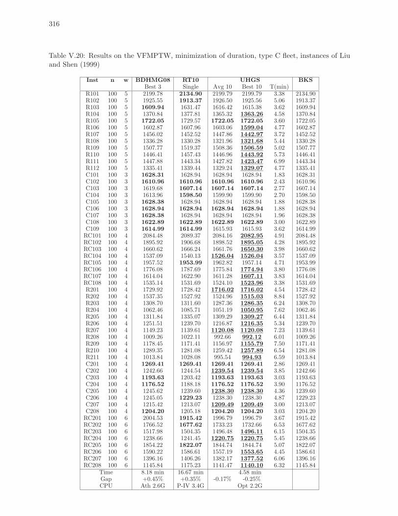
316

Table V.20: Results on the VFMPTW, minimization of duration, type C fleet, instances of Liuand Shen (1999)




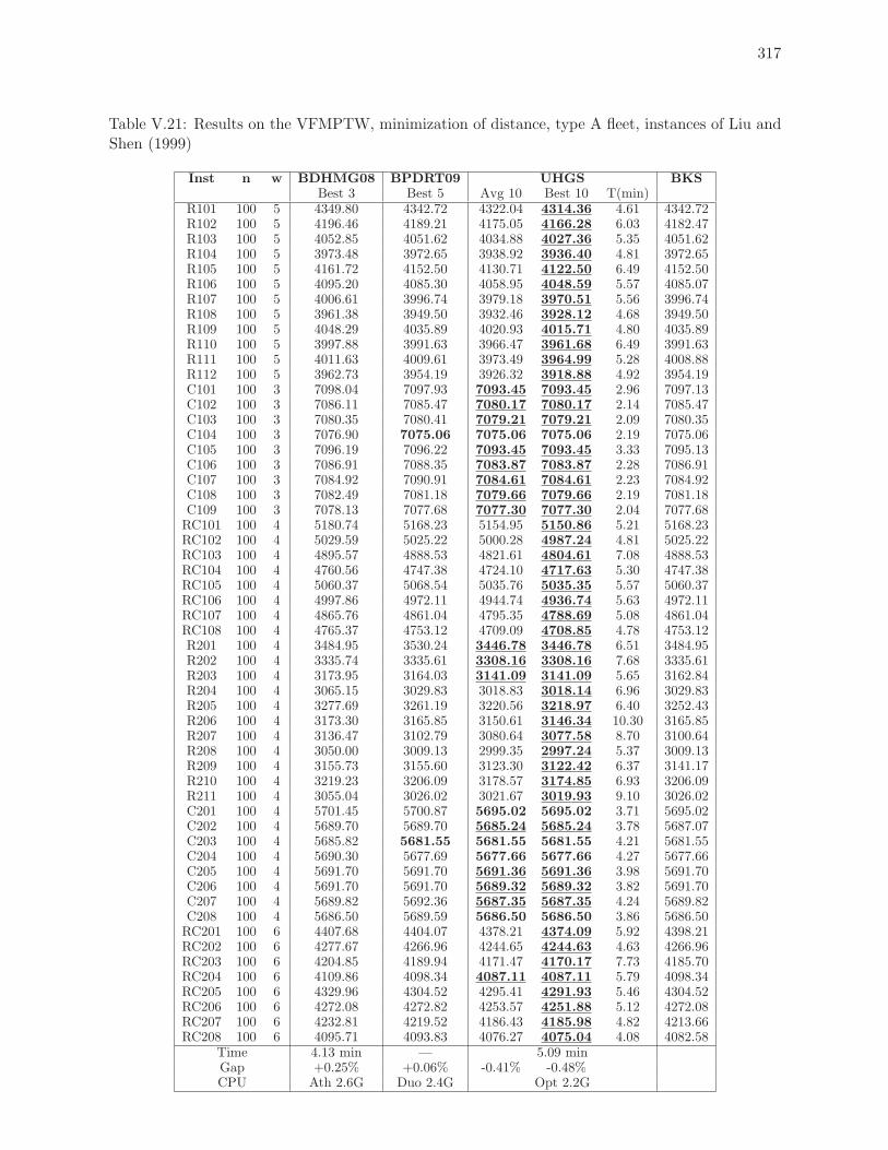
317

Table V.21: Results on the VFMPTW, minimization of distance, type A fleet, instances of Liu andShen (1999)

Inst n w BDHMG08 BPDRT09 UHGS BKSBest 3 Best 5 Avg 10 Best 10 T(min)


Time 4.13 min — 5.09 minGap +0.25% +0.06% -0.41% -0.48%CPU Ath 2.6G Duo 2.4G Opt 2.2G

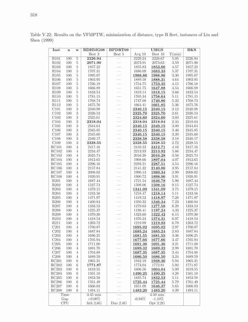
318

Table V.22: Results on the VFMPTW, minimization of distance, type B fleet, instances of Liu andShen (1999)


R101 100 5 2226.94 — 2229.24 2228.67 5.05 2226.94R102 100 5 2071.90 — 2073.91 2073.63 3.59 2071.90R103 100 5 1857.22 — 1855.83 1853.66 4.57 1857.22R104 100 5 1707.31 — 1686.09 1683.33 5.37 1707.31R105 100 5 1995.07 — 1988.86 1988.86 3.30 1995.07R106 100 5 1903.95 — 1889.58 1888.31 4.64 1903.95R107 100 5 1766.18 — 1754.75 1753.35 4.15 1766.18R108 100 5 1666.89 — 1651.75 1647.88 4.54 1666.89R109 100 5 1833.54 — 1819.14 1818.15 3.66 1833.54R110 100 5 1781.15 — 1765.34 1758.64 5.11 1781.15R111 100 5 1768.74 — 1747.08 1740.86 5.32 1768.74R112 100 5 1675.76 — 1664.41 1661.85 5.36 1675.76C101 100 3 2340.98 — 2340.15 2340.15 3.12 2340.98C102 100 3 2326.53 — 2325.70 2325.70 2.61 2326.53C103 100 3 2325.61 — 2324.60 2324.60 3.03 2325.61C104 100 3 2318.04 — 2318.04 2318.04 2.44 2318.04C105 100 3 2344.64 — 2340.15 2340.15 3.00 2344.64C106 100 3 2345.85 — 2340.15 2340.15 3.46 2345.85C107 100 3 2345.60 — 2340.15 2340.15 3.20 2345.60C108 100 3 2340.17 — 2338.58 2338.58 3.18 2340.17C109 100 3 2328.55 — 2328.55 2328.55 2.72 2328.55RC101 100 4 2417.16 — 2416.23 2412.71 4.16 2417.16RC102 100 4 2234.47 — 2213.93 2213.92 5.86 2234.47RC103 100 4 2025.74 — 2016.28 2016.28 3.50 2025.74RC104 100 4 1912.65 — 1908.66 1897.04 4.07 1912.65RC105 100 4 2296.16 — 2293.21 2287.51 4.54 2296.16RC106 100 4 2157.84 — 2141.32 2140.86 3.95 2157.84RC107 100 4 2008.02 — 1990.13 1989.34 2.99 2008.02RC108 100 4 1920.91 — 1900.72 1898.96 3.91 1920.91R201 100 4 1687.44 — 1721.54 1646.78 5.96 1687.44R202 100 4 1527.74 — 1509.06 1508.16 9.15 1527.74R203 100 4 1379.15 — 1341.09 1341.09 3.75 1379.15R204 100 4 1243.56 — 1218.47 1218.14 5.11 1243.56R205 100 4 1471.97 — 1419.52 1418.97 7.28 1471.97R206 100 4 1400.84 — 1350.32 1346.34 7.23 1400.84R207 100 4 1333.53 — 1279.63 1277.58 6.28 1333.53R208 100 4 1225.37 — 1198.41 1197.24 4.33 1225.37R209 100 4 1370.30 — 1323.60 1322.42 6.15 1370.30R210 100 4 1418.54 — 1376.24 1374.31 6.97 1418.54R211 100 4 1263.72 — 1219.99 1219.93 6.79 1263.72C201 100 4 1700.87 — 1695.02 1695.02 2.97 1700.87C202 100 4 1687.84 — 1685.24 1685.24 2.83 1687.84C203 100 4 1696.25 — 1681.55 1681.55 3.36 1696.25C204 100 4 1705.94 — 1677.66 1677.66 3.47 1705.94C205 100 4 1711.00 — 1691.36 1691.36 3.21 1711.00C206 100 4 1691.70 — 1689.32 1689.32 2.99 1691.70C207 100 4 1704.88 — 1687.35 1687.35 3.44 1704.88C208 100 4 1689.59 — 1686.50 1686.50 3.24 1689.59RC201 100 6 1965.31 — 1942.19 1938.36 5.94 1965.31RC202 100 6 1771.87 — 1773.04 1772.81 5.92 1771.87RC203 100 6 1619.55 — 1606.56 1604.04 5.99 1619.55RC204 100 6 1501.10 — 1490.25 1490.25 4.28 1501.10RC205 100 6 1853.58 — 1835.74 1832.53 5.11 1853.58RC206 100 6 1761.49 — 1725.44 1725.44 5.79 1761.49RC207 100 6 1666.03 — 1651.09 1646.37 5.65 1666.03RC208 100 6 1494.11 — 1483.20 1483.20 4.39 1494.11

Time 3.45 min — 4.50 minGap +0.00% — -0.94% -1.10%CPU Ath 2.6G Duo 2.4G Opt 2.2G

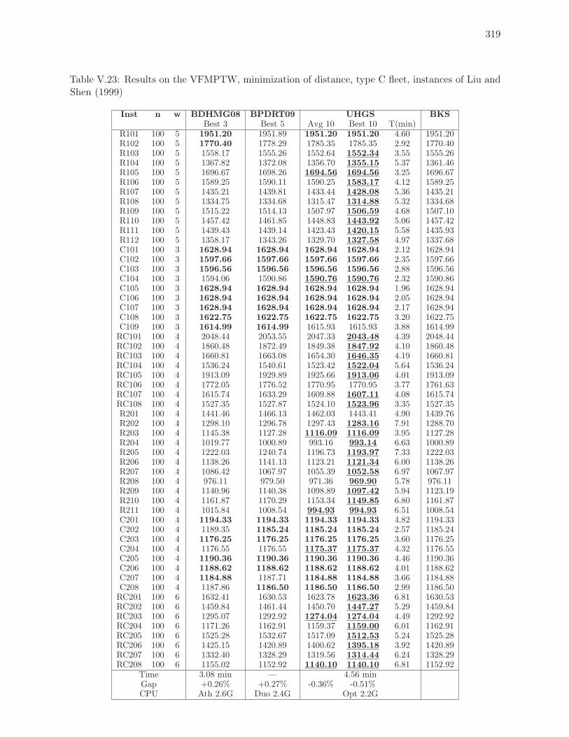
319

Table V.23: Results on the VFMPTW, minimization of distance, type C fleet, instances of Liu andShen (1999)



Time 3.08 min — 4.56 minGap +0.26% +0.27% -0.36% -0.51%CPU Ath 2.6G Duo 2.4G Opt 2.2G

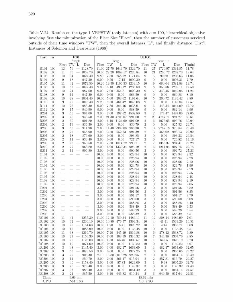
320

Table V.24: Results on the type 1 VRPSTW (only lateness) with α = 100, hierarchical objectiveinvolving first the minimization of the Fleet Size ”Fleet”, then the number of customers servicedoutside of their time windows ”TW”, then the overall lateness ”L”, and finally distance ”Dist”.Instances of Solomon and Desrosiers (1988)

Inst n F10 UHGSSingle Avg 10 Best 10

Fleet TW L Dist Fleet TW L Dist Fleet TW L Dist T(min)R101 100 12 56 — 1128.70 11.00 27.70 1644.70 1329.70 11 27 1720.97 1331.85 11.78R102 100 11 46 — 1058.70 10.00 22.20 1069.17 1226.84 10 21 1206.72 1252.78 18.64R103 100 10 34 — 1027.40 9.80 7.50 258.62 1171.84 9 5 90.68 1208.63 11.05R104 100 9 18 — 947.30 9.00 0.50 17.15 1009.30 9 0 0.00 1007.31 7.79R105 100 11 42 — 1073.50 10.20 19.50 1106.53 1239.15 10 9 680.04 1381.88 13.74R106 100 10 33 — 1047.40 9.90 8.10 433.32 1236.89 9 6 358.86 1259.11 12.59R107 100 10 24 — 987.60 9.00 7.00 354.81 1029.30 9 7 343.45 1042.96 11.24R108 100 9 14 — 947.20 9.00 0.00 0.00 963.50 9 0 0.00 960.88 8.10R109 100 10 28 — 1001.40 10.00 5.00 208.62 1194.64 10 5 200.72 1183.42 8.80R110 100 9 29 — 1013.40 9.20 9.50 461.42 1043.08 9 0 0.00 1118.84 12.57R111 100 10 26 — 983.30 9.00 7.80 385.46 1038.01 9 6 443.34 1047.09 12.72R112 100 9 17 — 940.90 9.00 0.00 0.00 988.59 9 0 0.00 982.14 9.96R201 100 3 56 — 984.00 3.00 2.00 197.62 1502.80 3 2 174.47 1497.06 27.05R202 100 3 40 — 943.50 2.00 21.30 4703.07 991.60 2 20 4757.71 991.27 30.61R203 100 2 30 — 901.80 2.00 6.10 1124.60 991.09 2 6 1076.65 995.76 30.04R204 100 2 19 — 836.30 2.00 0.00 0.00 830.79 2 0 0.00 825.52 26.74R205 100 3 36 — 911.90 2.00 14.40 2998.08 983.30 2 14 2767.13 973.84 26.49R206 100 2 25 — 956.90 2.00 3.50 652.23 994.39 2 3 465.02 993.13 29.92R207 100 2 18 — 876.60 2.00 0.00 0.00 893.85 2 0 0.00 893.33 29.54R208 100 2 11 — 833.40 2.00 0.00 0.00 727.17 2 0 0.00 726.82 14.16R209 100 2 26 — 950.50 2.00 7.30 1814.72 990.71 2 7 1386.37 994.41 29.28R210 100 2 29 — 963.80 2.00 6.00 1339.34 995.19 2 6 1264.94 997.75 29.75R211 100 2 14 — 906.80 2.00 0.00 0.00 900.56 2 0 0.00 892.72 27.23C101 100 — — — — 10.00 0.00 0.00 828.94 10 0 0.00 828.94 2.32C102 100 — — — — 10.00 0.00 0.00 828.94 10 0 0.00 828.94 2.28C103 100 — — — — 10.00 0.00 0.00 828.06 10 0 0.00 828.06 2.12C104 100 — — — — 10.00 0.00 0.00 824.78 10 0 0.00 824.78 1.96C105 100 — — — — 10.00 0.00 0.00 828.94 10 0 0.00 828.94 2.73C106 100 — — — — 10.00 0.00 0.00 828.94 10 0 0.00 828.94 2.56C107 100 — — — — 10.00 0.00 0.00 828.94 10 0 0.00 828.94 2.48C108 100 — — — — 10.00 0.00 0.00 828.94 10 0 0.00 828.94 2.19C109 100 — — — — 10.00 0.00 0.00 828.94 10 0 0.00 828.94 2.05C201 100 — — — — 3.00 0.00 0.00 591.56 3 0 0.00 591.56 5.82C202 100 — — — — 3.00 0.00 0.00 591.56 3 0 0.00 591.56 8.35C203 100 — — — — 3.00 0.00 0.00 591.17 3 0 0.00 591.17 9.79C204 100 — — — — 3.00 0.00 0.00 590.60 3 0 0.00 590.60 8.08C205 100 — — — — 3.00 0.00 0.00 588.88 3 0 0.00 588.88 6.40C206 100 — — — — 3.00 0.00 0.00 588.49 3 0 0.00 588.49 6.53C207 100 — — — — 3.00 0.00 0.00 588.29 3 0 0.00 588.29 6.54C208 100 — — — — 3.00 0.00 0.00 588.32 3 0 0.00 588.32 6.51RC101 100 11 44 — 1255.30 11.00 12.10 789.34 1486.11 11 12 808.44 1486.99 7.01RC102 100 10 32 — 1230.10 10.30 10.80 476.57 1399.34 10 4 41.41 1539.29 10.51RC103 100 10 25 — 1154.60 10.00 1.20 18.41 1320.22 10 1 4.18 1333.71 8.03RC104 100 10 12 — 1083.90 10.00 0.00 0.00 1135.48 10 0 0.00 1135.48 5.57RC105 100 11 38 — 1219.70 10.90 7.20 345.49 1516.88 10 6 278.42 1538.72 6.89RC106 100 10 27 — 1150.30 10.00 7.60 308.59 1310.32 10 7 344.38 1307.76 8.85RC107 100 10 28 — 1123.00 10.00 1.50 65.46 1300.57 10 1 64.05 1325.19 9.70RC108 100 10 10 — 1071.60 10.00 0.00 0.00 1139.82 10 0 0.00 1139.82 6.97RC201 100 3 48 — 1147.40 3.00 3.00 482.47 1663.69 3 3 482.47 1663.69 32.65RC202 100 3 35 — 1073.50 3.00 0.00 0.00 1377.25 3 0 0.00 1365.65 26.22RC203 100 3 29 — 906.30 2.10 13.80 3013.28 929.95 2 0 0.00 1064.14 30.49RC204 100 2 14 — 850.70 2.00 2.00 261.17 915.94 2 2 257.81 916.79 29.27RC205 100 3 40 — 1158.40 3.00 1.00 87.83 1623.09 3 1 9.38 1605.20 32.78RC206 100 3 40 — 978.40 3.00 0.00 0.00 1149.37 3 0 0.00 1146.32 24.48RC207 100 3 33 — 986.40 3.00 0.00 0.00 1061.49 3 0 0.00 1061.14 24.51RC208 100 2 21 — 885.50 2.00 6.40 946.83 910.34 2 6 949.50 917.64 22.51

Time 9.69 min 18.62 minCPU P-M 1.6G Opt 2.2G

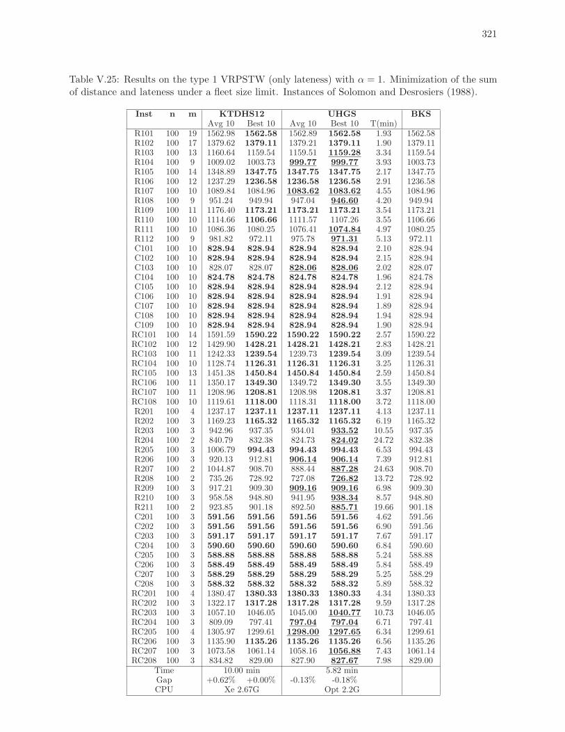
321

Table V.25: Results on the type 1 VRPSTW (only lateness) with α = 1. Minimization of the sumof distance and lateness under a fleet size limit. Instances of Solomon and Desrosiers (1988).

Inst n m KTDHS12 UHGS BKSAvg 10 Best 10 Avg 10 Best 10 T(min)


Time 10.00 min 5.82 minGap +0.62% +0.00% -0.13% -0.18%CPU Xe 2.67G Opt 2.2G

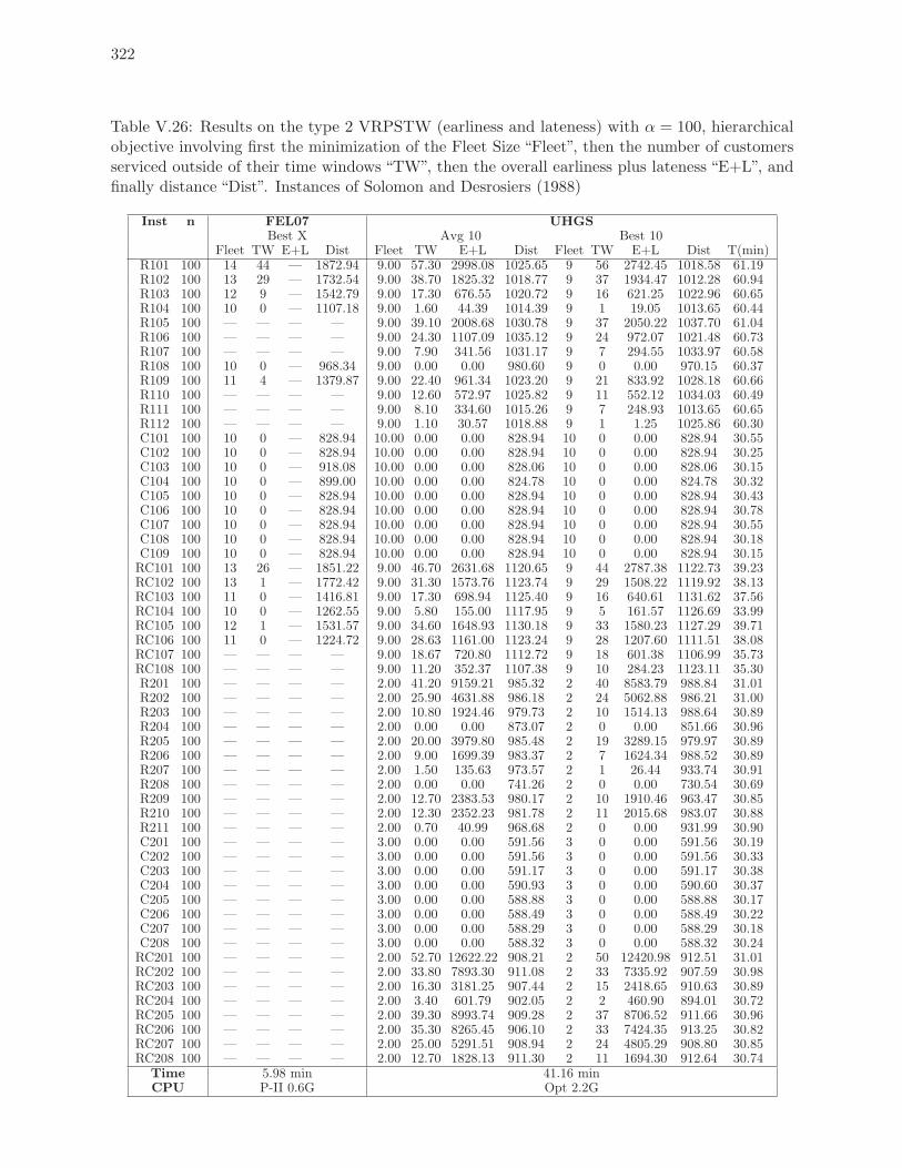
322

Table V.26: Results on the type 2 VRPSTW (earliness and lateness) with α = 100, hierarchicalobjective involving first the minimization of the Fleet Size “Fleet”, then the number of customersserviced outside of their time windows “TW”, then the overall earliness plus lateness “E+L”, andfinally distance “Dist”. Instances of Solomon and Desrosiers (1988)

Inst n FEL07 UHGSBest X Avg 10 Best 10

Fleet TW E+L Dist Fleet TW E+L Dist Fleet TW E+L Dist T(min)R101 100 14 44 — 1872.94 9.00 57.30 2998.08 1025.65 9 56 2742.45 1018.58 61.19R102 100 13 29 — 1732.54 9.00 38.70 1825.32 1018.77 9 37 1934.47 1012.28 60.94R103 100 12 9 — 1542.79 9.00 17.30 676.55 1020.72 9 16 621.25 1022.96 60.65R104 100 10 0 — 1107.18 9.00 1.60 44.39 1014.39 9 1 19.05 1013.65 60.44R105 100 — — — — 9.00 39.10 2008.68 1030.78 9 37 2050.22 1037.70 61.04R106 100 — — — — 9.00 24.30 1107.09 1035.12 9 24 972.07 1021.48 60.73R107 100 — — — — 9.00 7.90 341.56 1031.17 9 7 294.55 1033.97 60.58R108 100 10 0 — 968.34 9.00 0.00 0.00 980.60 9 0 0.00 970.15 60.37R109 100 11 4 — 1379.87 9.00 22.40 961.34 1023.20 9 21 833.92 1028.18 60.66R110 100 — — — — 9.00 12.60 572.97 1025.82 9 11 552.12 1034.03 60.49R111 100 — — — — 9.00 8.10 334.60 1015.26 9 7 248.93 1013.65 60.65R112 100 — — — — 9.00 1.10 30.57 1018.88 9 1 1.25 1025.86 60.30C101 100 10 0 — 828.94 10.00 0.00 0.00 828.94 10 0 0.00 828.94 30.55C102 100 10 0 — 828.94 10.00 0.00 0.00 828.94 10 0 0.00 828.94 30.25C103 100 10 0 — 918.08 10.00 0.00 0.00 828.06 10 0 0.00 828.06 30.15C104 100 10 0 — 899.00 10.00 0.00 0.00 824.78 10 0 0.00 824.78 30.32C105 100 10 0 — 828.94 10.00 0.00 0.00 828.94 10 0 0.00 828.94 30.43C106 100 10 0 — 828.94 10.00 0.00 0.00 828.94 10 0 0.00 828.94 30.78C107 100 10 0 — 828.94 10.00 0.00 0.00 828.94 10 0 0.00 828.94 30.55C108 100 10 0 — 828.94 10.00 0.00 0.00 828.94 10 0 0.00 828.94 30.18C109 100 10 0 — 828.94 10.00 0.00 0.00 828.94 10 0 0.00 828.94 30.15RC101 100 13 26 — 1851.22 9.00 46.70 2631.68 1120.65 9 44 2787.38 1122.73 39.23RC102 100 13 1 — 1772.42 9.00 31.30 1573.76 1123.74 9 29 1508.22 1119.92 38.13RC103 100 11 0 — 1416.81 9.00 17.30 698.94 1125.40 9 16 640.61 1131.62 37.56RC104 100 10 0 — 1262.55 9.00 5.80 155.00 1117.95 9 5 161.57 1126.69 33.99RC105 100 12 1 — 1531.57 9.00 34.60 1648.93 1130.18 9 33 1580.23 1127.29 39.71RC106 100 11 0 — 1224.72 9.00 28.63 1161.00 1123.24 9 28 1207.60 1111.51 38.08RC107 100 — — — — 9.00 18.67 720.80 1112.72 9 18 601.38 1106.99 35.73RC108 100 — — — — 9.00 11.20 352.37 1107.38 9 10 284.23 1123.11 35.30R201 100 — — — — 2.00 41.20 9159.21 985.32 2 40 8583.79 988.84 31.01R202 100 — — — — 2.00 25.90 4631.88 986.18 2 24 5062.88 986.21 31.00R203 100 — — — — 2.00 10.80 1924.46 979.73 2 10 1514.13 988.64 30.89R204 100 — — — — 2.00 0.00 0.00 873.07 2 0 0.00 851.66 30.96R205 100 — — — — 2.00 20.00 3979.80 985.48 2 19 3289.15 979.97 30.89R206 100 — — — — 2.00 9.00 1699.39 983.37 2 7 1624.34 988.52 30.89R207 100 — — — — 2.00 1.50 135.63 973.57 2 1 26.44 933.74 30.91R208 100 — — — — 2.00 0.00 0.00 741.26 2 0 0.00 730.54 30.69R209 100 — — — — 2.00 12.70 2383.53 980.17 2 10 1910.46 963.47 30.85R210 100 — — — — 2.00 12.30 2352.23 981.78 2 11 2015.68 983.07 30.88R211 100 — — — — 2.00 0.70 40.99 968.68 2 0 0.00 931.99 30.90C201 100 — — — — 3.00 0.00 0.00 591.56 3 0 0.00 591.56 30.19C202 100 — — — — 3.00 0.00 0.00 591.56 3 0 0.00 591.56 30.33C203 100 — — — — 3.00 0.00 0.00 591.17 3 0 0.00 591.17 30.38C204 100 — — — — 3.00 0.00 0.00 590.93 3 0 0.00 590.60 30.37C205 100 — — — — 3.00 0.00 0.00 588.88 3 0 0.00 588.88 30.17C206 100 — — — — 3.00 0.00 0.00 588.49 3 0 0.00 588.49 30.22C207 100 — — — — 3.00 0.00 0.00 588.29 3 0 0.00 588.29 30.18C208 100 — — — — 3.00 0.00 0.00 588.32 3 0 0.00 588.32 30.24RC201 100 — — — — 2.00 52.70 12622.22 908.21 2 50 12420.98 912.51 31.01RC202 100 — — — — 2.00 33.80 7893.30 911.08 2 33 7335.92 907.59 30.98RC203 100 — — — — 2.00 16.30 3181.25 907.44 2 15 2418.65 910.63 30.89RC204 100 — — — — 2.00 3.40 601.79 902.05 2 2 460.90 894.01 30.72RC205 100 — — — — 2.00 39.30 8993.74 909.28 2 37 8706.52 911.66 30.96RC206 100 — — — — 2.00 35.30 8265.45 906.10 2 33 7424.35 913.25 30.82RC207 100 — — — — 2.00 25.00 5291.51 908.94 2 24 4805.29 908.80 30.85RC208 100 — — — — 2.00 12.70 1828.13 911.30 2 11 1694.30 912.64 30.74

Time 5.98 min 41.16 minCPU P-II 0.6G Opt 2.2G

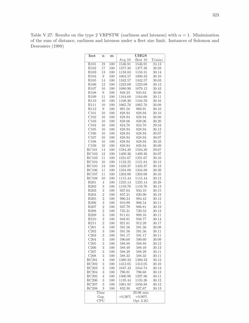
323

Table V.27: Results on the type 2 VRPSTW (earliness and lateness) with α = 1. Minimizationof the sum of distance, earliness and lateness under a fleet size limit. Instances of Solomon andDesrosiers (1988)

Inst n m UHGSAvg 10 Best 10 T(min)

R101 19 100 1546.91 1546.91 24.13R102 17 100 1377.38 1377.38 26.93R103 13 100 1158.83 1158.31 30.14R104 9 100 1004.57 1000.33 30.10R105 14 100 1342.57 1342.57 30.03R106 12 100 1223.09 1223.09 30.12R107 10 100 1080.90 1079.12 30.43R108 9 100 948.23 945.64 30.08R109 11 100 1164.68 1164.68 30.11R110 10 100 1108.30 1104.59 30.16R111 10 100 1065.76 1065.76 30.08R112 9 100 991.50 969.91 30.10C101 10 100 828.94 828.94 30.10C102 10 100 828.94 828.94 30.08C103 10 100 828.06 828.06 30.20C104 10 100 824.78 824.78 29.34C105 10 100 828.94 828.94 30.12C106 10 100 828.94 828.94 30.07C107 10 100 828.94 828.94 30.07C108 10 100 828.94 828.94 30.33C109 10 100 828.94 828.94 30.09RC101 14 100 1584.20 1584.20 29.67RC102 12 100 1409.36 1409.36 30.07RC103 11 100 1231.67 1231.67 30.16RC104 10 100 1123.25 1121.84 30.12RC105 13 100 1433.37 1433.37 30.18RC106 11 100 1334.89 1334.89 30.39RC107 11 100 1203.06 1203.06 30.45RC108 10 100 1115.44 1115.44 30.12R201 4 100 1235.14 1235.14 30.28R202 3 100 1159.76 1159.76 30.13R203 3 100 937.04 934.10 30.15R204 2 100 837.21 820.90 30.18R205 3 100 996.24 994.43 30.12R206 3 100 910.99 906.54 30.11R207 2 100 937.79 906.81 30.19R208 2 100 735.31 730.52 30.13R209 3 100 911.61 909.16 30.11R210 3 100 948.91 938.77 30.14R211 2 100 921.81 912.39 30.17C201 3 100 591.56 591.56 30.09C202 3 100 591.56 591.56 30.11C203 3 100 591.17 591.17 30.11C204 3 100 590.60 590.60 30.09C205 3 100 588.88 588.88 30.12C206 3 100 588.49 588.49 30.13C207 3 100 588.29 588.29 30.11C208 3 100 588.32 588.32 30.11RC201 4 100 1380.33 1380.33 30.12RC202 3 100 1312.05 1312.05 30.10RC203 3 100 1047.43 1044.74 30.13RC204 3 100 796.91 796.68 30.13RC205 4 100 1300.98 1297.86 30.11RC206 3 100 1135.44 1135.26 30.12RC207 3 100 1061.92 1056.88 30.12RC208 3 100 832.30 827.67 30.13

Time 29.96 minGap +0.26% +0.00%CPU Opt 2.2G

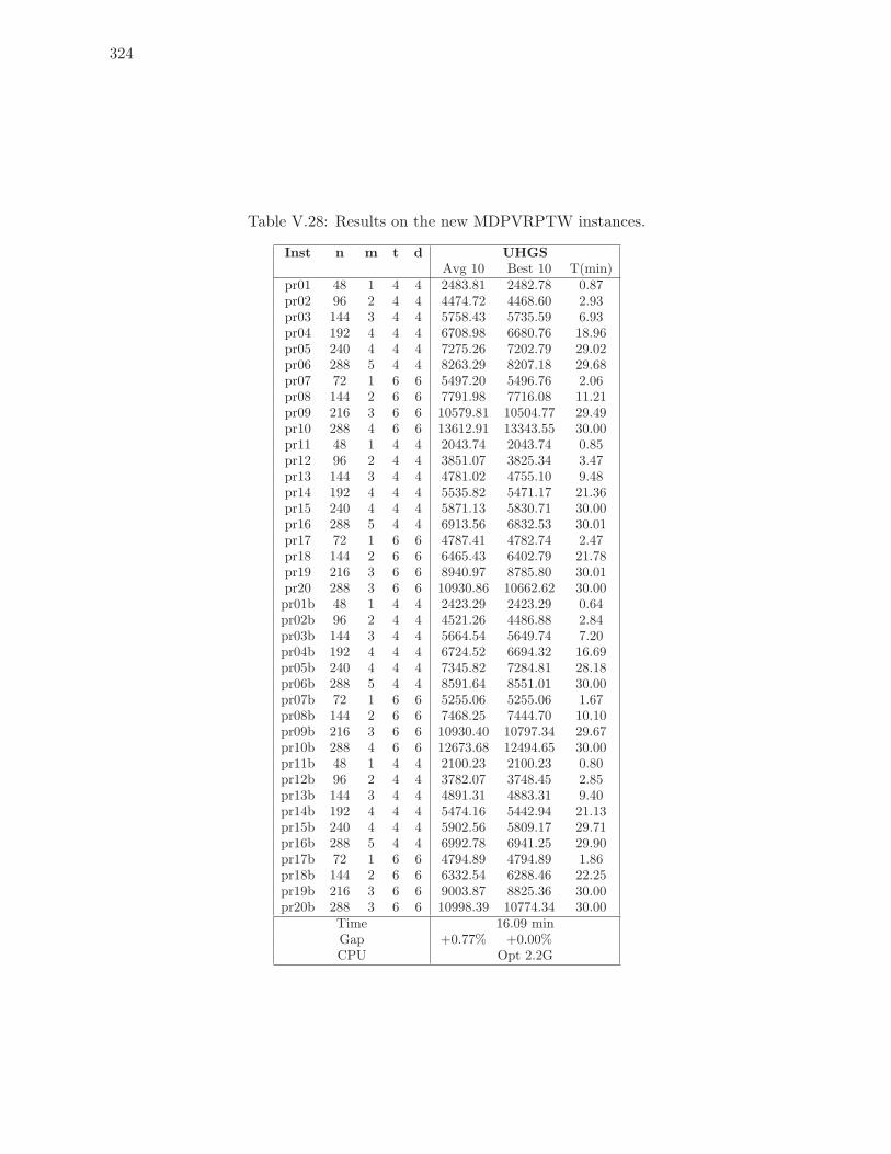
324

Table V.28: Results on the new MDPVRPTW instances.

Inst n m t d UHGSAvg 10 Best 10 T(min)

pr01 48 1 4 4 2483.81 2482.78 0.87pr02 96 2 4 4 4474.72 4468.60 2.93pr03 144 3 4 4 5758.43 5735.59 6.93pr04 192 4 4 4 6708.98 6680.76 18.96pr05 240 4 4 4 7275.26 7202.79 29.02pr06 288 5 4 4 8263.29 8207.18 29.68pr07 72 1 6 6 5497.20 5496.76 2.06pr08 144 2 6 6 7791.98 7716.08 11.21pr09 216 3 6 6 10579.81 10504.77 29.49pr10 288 4 6 6 13612.91 13343.55 30.00pr11 48 1 4 4 2043.74 2043.74 0.85pr12 96 2 4 4 3851.07 3825.34 3.47pr13 144 3 4 4 4781.02 4755.10 9.48pr14 192 4 4 4 5535.82 5471.17 21.36pr15 240 4 4 4 5871.13 5830.71 30.00pr16 288 5 4 4 6913.56 6832.53 30.01pr17 72 1 6 6 4787.41 4782.74 2.47pr18 144 2 6 6 6465.43 6402.79 21.78pr19 216 3 6 6 8940.97 8785.80 30.01pr20 288 3 6 6 10930.86 10662.62 30.00pr01b 48 1 4 4 2423.29 2423.29 0.64pr02b 96 2 4 4 4521.26 4486.88 2.84pr03b 144 3 4 4 5664.54 5649.74 7.20pr04b 192 4 4 4 6724.52 6694.32 16.69pr05b 240 4 4 4 7345.82 7284.81 28.18pr06b 288 5 4 4 8591.64 8551.01 30.00pr07b 72 1 6 6 5255.06 5255.06 1.67pr08b 144 2 6 6 7468.25 7444.70 10.10pr09b 216 3 6 6 10930.40 10797.34 29.67pr10b 288 4 6 6 12673.68 12494.65 30.00pr11b 48 1 4 4 2100.23 2100.23 0.80pr12b 96 2 4 4 3782.07 3748.45 2.85pr13b 144 3 4 4 4891.31 4883.31 9.40pr14b 192 4 4 4 5474.16 5442.94 21.13pr15b 240 4 4 4 5902.56 5809.17 29.71pr16b 288 5 4 4 6992.78 6941.25 29.90pr17b 72 1 6 6 4794.89 4794.89 1.86pr18b 144 2 6 6 6332.54 6288.46 22.25pr19b 216 3 6 6 9003.87 8825.36 30.00pr20b 288 3 6 6 10998.39 10774.34 30.00

Time 16.09 minGap +0.77% +0.00%CPU Opt 2.2G

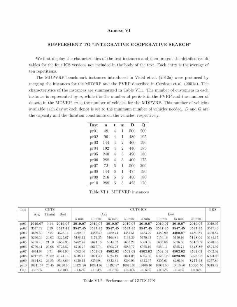
Annexe VI

SUPPLEMENT TO “INTEGRATIVE COOPERATIVE SEARCH”

We first display the characteristics of the test instances and then present the detailed result

tables for the four ICS versions not included in the body of the text. Each entry is the average of

ten repetitions.

The MDPVRP benchmark instances introduced in Vidal et al. (2012a) were produced by

merging the instances for the MDVRP and the PVRP described in Cordeau et al. (2001a). The

characteristics of the instances are summarized in Table VI.1. The number of customers in each

instance is represented by n, while t is the number of periods in the PVRP and the number of

depots in the MDVRP. m is the number of vehicles for the MDPVRP. This number of vehicles

available each day at each depot is set to the minimum number of vehicles needed. D and Q are

the capacity and the duration constraints on the vehicles, respectively.

Inst n t m D Q

pr01 48 4 1 500 200

pr02 96 4 1 480 195

pr03 144 4 2 460 190

pr04 192 4 2 440 185

pr05 240 4 3 420 180

pr06 288 4 3 400 175

pr07 72 6 1 500 200

pr08 144 6 1 475 190

pr09 216 6 2 450 180

pr10 288 6 3 425 170

Table VI.1: MDPVRP instances

Inst GUTS GUTS-ICS BKS



pr01 2019.07 0.14 2019.07 2019.07 2019.07 2019.07 2019.07 2019.07 2019.07 2019.07 2019.07 2019.07

pr02 3547.72 2.39 3547.45 3547.45 3547.45 3547.45 3547.45 3547.45 3547.45 3547.45 3547.45 3547.45

pr03 4639.50 18.87 4578.14 4492.07 4483.49 4482.74 4481.51 4483.29 4480.90 4480.87 4480.87 4480.87

pr04 5246.39 20.03 5225.67 5188.12 5171.35 5168.81 5163.29 5170.63 5156.16 5156.16 5148.06 5134.17

pr05 5738.40 21.10 5666.35 5762.78 5674.16 5644.62 5633.24 5663.68 5635.88 5626.66 5616.02 5570.45

pr06 6759.41 20.06 6723.52 6716.27 6615.74 6603.22 6585.77 6575.16 6559.11 6555.71 6548.86 6524.92

pr07 4644.93 0.71 4644.93 4502.06 4502.02 4502.02 4502.02 4502.02 4502.02 4502.02 4502.02 4502.02

pr08 6217.23 20.82 6174.15 6038.41 6024.40 6024.19 6024.08 6024.00 6023.98 6023.98 6023.98 6023.98

pr09 8644.82 23.85 8548.63 8430.12 8356.94 8322.31 8306.93 8323.97 8305.61 8286.66 8277.93 8257.80

pr10 10241.67 26.45 10120.30 10421.26 10324.62 10192.87 10071.34 10106.10 10092.50 10018.80 10006.50 9818.42

Gap +2.77% +2.10% +1.62% +1.04% +0.78% +0.58% +0.69% +0.55% +0.43% +0.36%

Table VI.2: Performance of GUTS-ICS

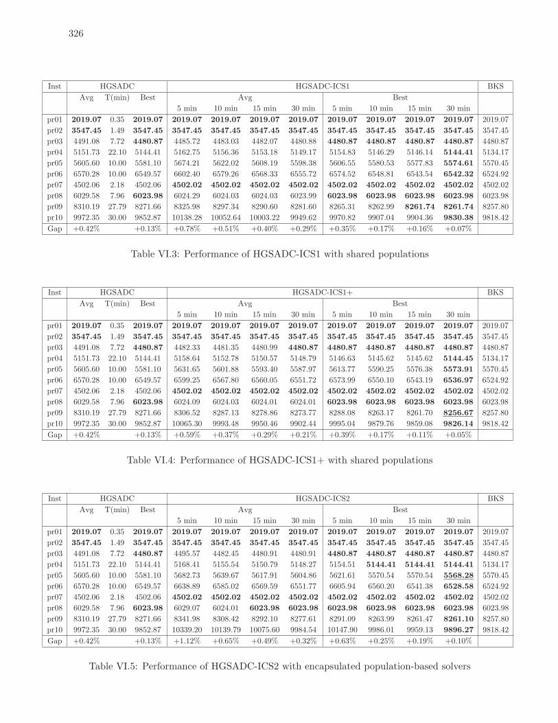
326

Inst HGSADC HGSADC-ICS1 BKS



pr01 2019.07 0.35 2019.07 2019.07 2019.07 2019.07 2019.07 2019.07 2019.07 2019.07 2019.07 2019.07

pr02 3547.45 1.49 3547.45 3547.45 3547.45 3547.45 3547.45 3547.45 3547.45 3547.45 3547.45 3547.45

pr03 4491.08 7.72 4480.87 4485.72 4483.03 4482.07 4480.88 4480.87 4480.87 4480.87 4480.87 4480.87

pr04 5151.73 22.10 5144.41 5162.75 5156.36 5153.18 5149.17 5154.83 5146.29 5146.14 5144.41 5134.17

pr05 5605.60 10.00 5581.10 5674.21 5622.02 5608.19 5598.38 5606.55 5580.53 5577.83 5574.61 5570.45

pr06 6570.28 10.00 6549.57 6602.40 6579.26 6568.33 6555.72 6574.52 6548.81 6543.54 6542.32 6524.92

pr07 4502.06 2.18 4502.06 4502.02 4502.02 4502.02 4502.02 4502.02 4502.02 4502.02 4502.02 4502.02

pr08 6029.58 7.96 6023.98 6024.29 6024.03 6024.03 6023.99 6023.98 6023.98 6023.98 6023.98 6023.98

pr09 8310.19 27.79 8271.66 8325.98 8297.34 8290.60 8281.60 8265.31 8262.99 8261.74 8261.74 8257.80

pr10 9972.35 30.00 9852.87 10138.28 10052.64 10003.22 9949.62 9970.82 9907.04 9904.36 9830.38 9818.42

Gap +0.42% +0.13% +0.78% +0.51% +0.40% +0.29% +0.35% +0.17% +0.16% +0.07%

Table VI.3: Performance of HGSADC-ICS1 with shared populations

Inst HGSADC HGSADC-ICS1+ BKS



pr01 2019.07 0.35 2019.07 2019.07 2019.07 2019.07 2019.07 2019.07 2019.07 2019.07 2019.07 2019.07

pr02 3547.45 1.49 3547.45 3547.45 3547.45 3547.45 3547.45 3547.45 3547.45 3547.45 3547.45 3547.45

pr03 4491.08 7.72 4480.87 4482.33 4481.35 4480.99 4480.87 4480.87 4480.87 4480.87 4480.87 4480.87

pr04 5151.73 22.10 5144.41 5158.64 5152.78 5150.57 5148.79 5146.63 5145.62 5145.62 5144.45 5134.17

pr05 5605.60 10.00 5581.10 5631.65 5601.88 5593.40 5587.97 5613.77 5590.25 5576.38 5573.91 5570.45

pr06 6570.28 10.00 6549.57 6599.25 6567.80 6560.05 6551.72 6573.99 6550.10 6543.19 6536.97 6524.92

pr07 4502.06 2.18 4502.06 4502.02 4502.02 4502.02 4502.02 4502.02 4502.02 4502.02 4502.02 4502.02

pr08 6029.58 7.96 6023.98 6024.09 6024.03 6024.01 6024.01 6023.98 6023.98 6023.98 6023.98 6023.98

pr09 8310.19 27.79 8271.66 8306.52 8287.13 8278.86 8273.77 8288.08 8263.17 8261.70 8256.67 8257.80

pr10 9972.35 30.00 9852.87 10065.30 9993.48 9950.46 9902.44 9995.04 9879.76 9859.08 9826.14 9818.42

Gap +0.42% +0.13% +0.59% +0.37% +0.29% +0.21% +0.39% +0.17% +0.11% +0.05%

Table VI.4: Performance of HGSADC-ICS1+ with shared populations

Inst HGSADC HGSADC-ICS2 BKS



pr01 2019.07 0.35 2019.07 2019.07 2019.07 2019.07 2019.07 2019.07 2019.07 2019.07 2019.07 2019.07

pr02 3547.45 1.49 3547.45 3547.45 3547.45 3547.45 3547.45 3547.45 3547.45 3547.45 3547.45 3547.45

pr03 4491.08 7.72 4480.87 4495.57 4482.45 4480.91 4480.91 4480.87 4480.87 4480.87 4480.87 4480.87

pr04 5151.73 22.10 5144.41 5168.41 5155.54 5150.79 5148.27 5154.51 5144.41 5144.41 5144.41 5134.17

pr05 5605.60 10.00 5581.10 5682.73 5639.67 5617.91 5604.86 5621.61 5570.54 5570.54 5568.28 5570.45

pr06 6570.28 10.00 6549.57 6638.89 6585.02 6569.59 6551.77 6605.94 6560.20 6541.38 6528.58 6524.92

pr07 4502.06 2.18 4502.06 4502.02 4502.02 4502.02 4502.02 4502.02 4502.02 4502.02 4502.02 4502.02

pr08 6029.58 7.96 6023.98 6029.07 6024.01 6023.98 6023.98 6023.98 6023.98 6023.98 6023.98 6023.98

pr09 8310.19 27.79 8271.66 8341.98 8308.42 8292.10 8277.61 8291.09 8263.99 8261.47 8261.10 8257.80

pr10 9972.35 30.00 9852.87 10339.20 10139.79 10075.60 9984.54 10147.90 9986.01 9959.13 9896.27 9818.42

Gap +0.42% +0.13% +1.12% +0.65% +0.49% +0.32% +0.63% +0.25% +0.19% +0.10%

Table VI.5: Performance of HGSADC-ICS2 with encapsulated population-based solvers

approches générales de résolution pour les problèmes multi

Documents