annexe 12 rapport de chantier de ginger-cebtp
TRANSCRIPT

RAPPORT E2016/027DE – 16ALS21010
Annexe 12 Rapport de chantier de
Ginger-CEBTP
JANVIER 2016
Dossier : EST2.F.067
DIRECTION REGIONALE GRAND NORD
Agence de STRASBOURG Téléphone : 03 88 81 20 50 13 rue de l’Electricité Télécopie : 03 88 81 21 50 67800 HOENHEIM Email : [email protected]
GEODERIS Réalisation de sondages carottés équipés en piézomètres et réalisation de diagraphies gamma-ray MISSION D'INVESTIGATIONS GEOTECHNIQUES
LOCHWILLER (67) – Lotissement Weingarten


GINGER CEBTP Agence de Strasbourg
Affaire : LOCHWILLER (67) – Lotissement Weingarten
Dossier : EST2.F.067 Indice 1 du 06/01/2016 Page 3/10
SOMMAIRE
1 PLANS DE SITUATION ............................................................................................. 4
1.1 EXTRAIT DE CARTE IGN ............................................................................................................. 4
1.2 IMAGE AERIENNE DE LA ZONE CONCERNEE ......................................................................... 4
2 CONTEXTE DE L’ETUDE .......................................................................................... 5
2.1 DONNEES GENERALES .............................................................................................................. 5
22..11..11 GGéénnéérraalliittééss .................................................................................................................................................................................................................................................. 55
22..11..22 DDooccuummeennttss ccoommmmuunniiqquuééss .................................................................................................................................................................................................... 55
2.2 NATURE ET OBJECTIFS DE LA MISSION GINGER CEBTP ..................................................... 5
3 SONDAGES ET ESSAIS REALISES ........................................................................ 6
3.1 PREAMBULE ................................................................................................................................ 6
3.2 IMPLANTATION ET NIVELLEMENT ............................................................................................ 6
3.3 SONDAGES IN SITU .................................................................................................................... 6
33..33..11 SSoonnddaaggeess ccaarroottttééss ééqquuiippééss eenn ppiiéézzoommèèttrree .................................................................................................................................................. 66
33..33..22 SSoonnddaaggee ddeessttrruuccttiiff ééqquuiippéé eenn ppiiéézzoommèèttrree ...................................................................................................................................................... 77
3.4 REALISATION DES SONDAGES EQUIPES EN PIEZOMETRES ............................................... 7
33..44..11 SSoonnddaaggeess ccaarroottttééss ééqquuiippééss eenn ppiiéézzoommèèttrreess .............................................................................................................................................. 77
33..44..22 SSoonnddaaggee ddeessttrruuccttiiff ééqquuiippéé eenn ppiiéézzoommèèttrree ...................................................................................................................................................... 99
33..44..33 MMaattéérriieell uuttiilliisséé .......................................................................................................................................................................................................................................... 99
33..44..44 AAllééaass rreennccoonnttrrééss lloorrss dduu cchhaannttiieerr ............................................................................................................................................................................ 1100
33..44..55 MMéétthhooddee ddee ddéévveellooppppeemmeenntt ddeess ppiiéézzoommèèttrreess .................................................................................................................................... 1100
3.5 REALISATION DES DIAGRAPHIES GAMMA-RAY ................................................................... 10
ANNEXES
ANNEXE 1 – PLAN D’IMPLANTATION DES SONDAGES
ANNEXE 2 – SONDAGES CAROTTES EQUIPES EN PIEZOMETRES
ANNEXE 3 – SONDAGE DESTRUCTIF EQUIPE EN PIZOMETRE
ANNEXE 4 – RAPPORTS REALISES PAR LES SONDEURS DES SONDAGES CAROTTES EQUIPES EN PIEZOMETRES
ANNEXE 5 – RAPPORT REALISE PAR LES SONDEURS DU SONDAGE DESTRUCTIF EQUIPE EN PIEZOMETRE
ANNEXE 6 – FICHE TECHNIQUE DE LA MACHINE INNOVA UTILISEE
ANNEXE 7 – LITHOLOGIES DETAILLEES DES SONDAGES CAROTTES REALISEES PAR GEODERIS
ANNEXE 8 – DIAGRAPHIES GAMMA-RAY DES SONDAGES

GINGER CEBTP Agence de Strasbourg
Affaire : LOCHWILLER (67) – Lotissement Weingarten
Dossier : EST2.F.067 Indice 1 du 06/01/2016 Page 4/10
11 PPLLAANNSS DDEE SSIITTUUAATTIIOONN
11..11 EExxttrraaiitt ddee ccaarrttee IIGGNN
Source : CartoExplorer 3
11..22 IImmaaggee aaéérriieennnnee ddee llaa zzoonnee ccoonncceerrnnééee
Source : www.google.fr/maps
Site étudié

GINGER CEBTP Agence de Strasbourg
Affaire : LOCHWILLER (67) – Lotissement Weingarten
Dossier : EST2.F.067 Indice 1 du 06/01/2016 Page 5/10
22 CCOONNTTEEXXTTEE DDEE LL’’EETTUUDDEE
22..11 DDoonnnnééeess ggéénnéérraalleess
22..11..11 GGéénnéérraalliittééss
Nom de l’opération : Réalisation de sondages carottés équipés en piézomètres et réalisation de
diagraphies gamma-ray
Localisation : LOCHWILLER (67) – Lotissement Weingarten
Commune : LOCHWILLER (67)
Client : GEODERIS
22..11..22 DDooccuummeennttss ccoommmmuunniiqquuééss
Les documents qui nous ont été communiqués et qui ont été utilisés dans le cadre de ce rapport sont les
suivants :
- Cahier des charges établi par GEODERIS.
22..22 NNaattuurree eett oobbjjeeccttiiffss ddee llaa mmiissssiioonn GGIINNGGEERR CCEEBBTTPP
La mission de GINGER CEBTP est conforme au contrat n°EST2.F.0149 et concernait la réalisation de
quatre forages carottés à équiper de tubes piézométriques ainsi que la réalisation de diagraphies
Gamma-Ray de ces forages.
Le lotissement Weingarten est le siège, depuis plusieurs années, de désordres aux terrains, aux
infrastructures et au bâti, liés à un phénomène de surrection des sols. Cette situation trouve son origine
dans des réactions de gonflement d’anhydrite, qui se transforme en gypse en présence d’eau. Un forage
géothermique fuyard serait l’élément déclencheur auquel s’ajouteraient ensuite des infiltrations d’eau
météorique.
L’objectif des quatre forages était de :
• fournir une description précise des couches sédimentaires en présence ;
• fournir une évaluation de l’extension spatiale des zones concernées actuellement par les
transformations minéralogiques et de leur intensité ;
• permettre la réalisation de diagraphies ;
• permettre d’effectuer des prélèvements d’eau à des fins d’analyses chimiques ;
• permettre de prélever des échantillons de sols/roches en vue d’essais de caractérisation et
géotechniques en laboratoire.

GINGER CEBTP Agence de Strasbourg
Affaire : LOCHWILLER (67) – Lotissement Weingarten
Dossier : EST2.F.067 Indice 1 du 06/01/2016 Page 6/10
33 SSOONNDDAAGGEESS EETT EESSSSAAIISS RREEAALLIISSEESS
33..11 PPrrééaammbbuullee
Les moyens de reconnaissance et d’essais ont été définis par GEODERIS lors de la consultation.
Il était prévu la réalisation de 4 forages carottés, équipés en piézomètres, de longueurs suivantes :
• Sondage SC4 : 20 m,
• Sondage SC5 : 35 m,
• Sondage SC6 : 40 m,
• Sondage SC7 : 50 m.
Il était également prévu la réalisation de diagraphies gamma-ray de tous les forages.
33..22 IImmppllaannttaattiioonn eett nniivveelllleemmeenntt
L’implantation des sondages in situ figure sur le plan joint en annexe 1. Elle a été définie par GEODERIS
et réalisée par GINGER CEBTP en fonction des accès et en présence de GEODERIS.
Les coordonnées des têtes de sondages ont été relevées en X, Y et Z par GEODERIS.
33..33 SSoonnddaaggeess iinn ssiittuu
33..33..11 SSoonnddaaggeess ccaarroottttééss ééqquuiippééss eenn ppiiéézzoommèèttrree
Les sondages suivants ont été réalisés :
Type de sondage Quantité Noms Prof. / TN Altitude NGF
Sondages carottés battus en diamètre extérieur
114 mm et rotatifs en en diamètre extérieur 122 mm 4
SC4
SC5
SC6
SC7
43.4 m
33.0 m
35.2 m
43.4 m
+220.310 m
+230.050 m
+225.804 m
+243.511 m
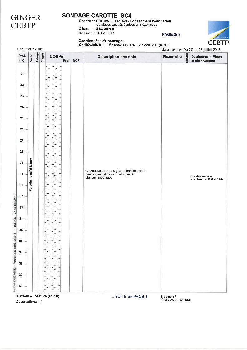
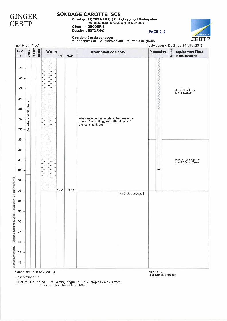
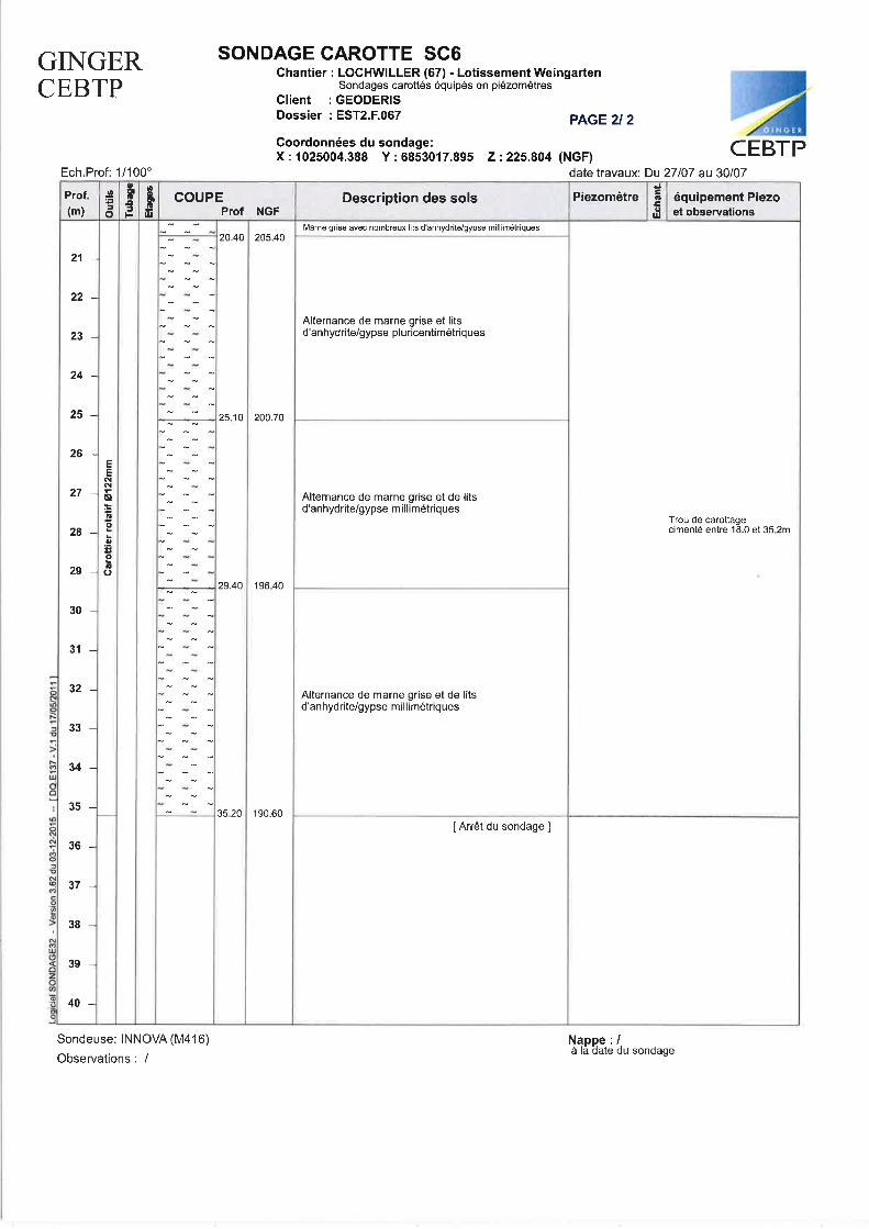
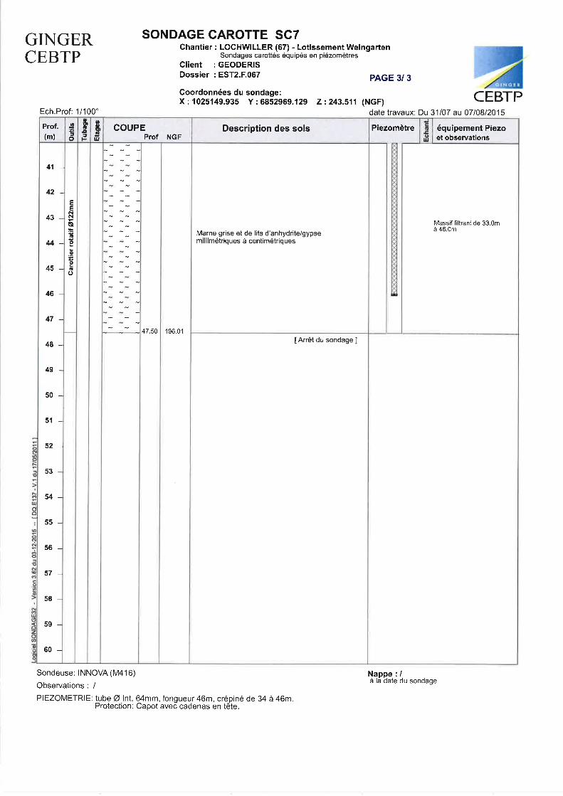
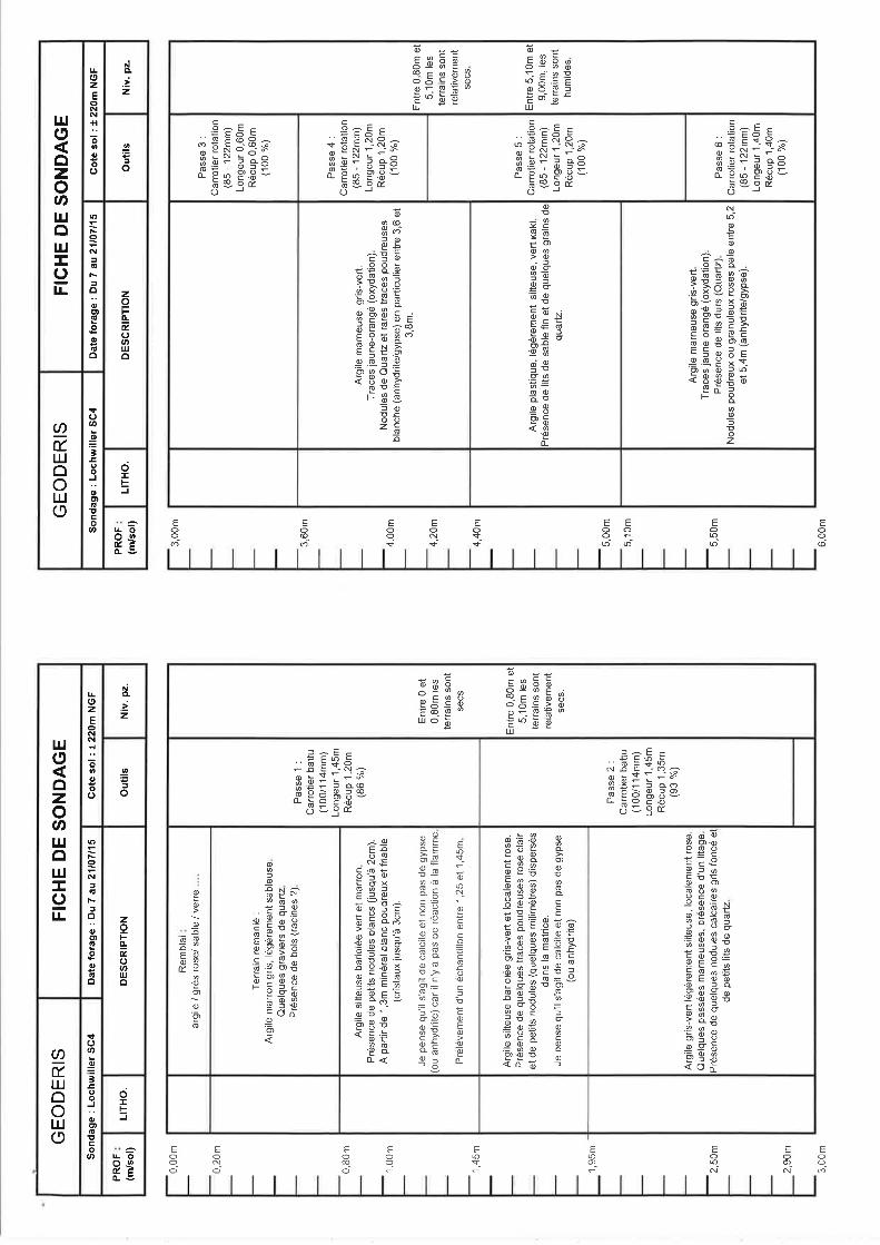
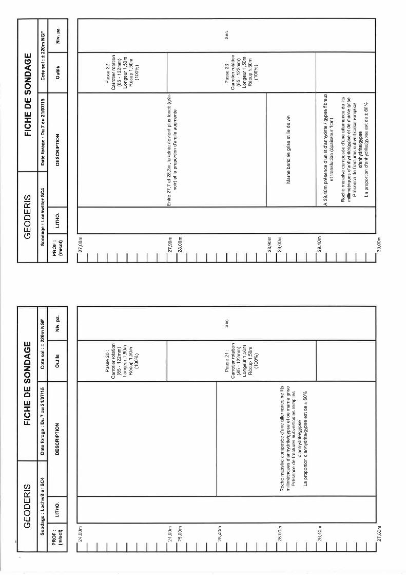
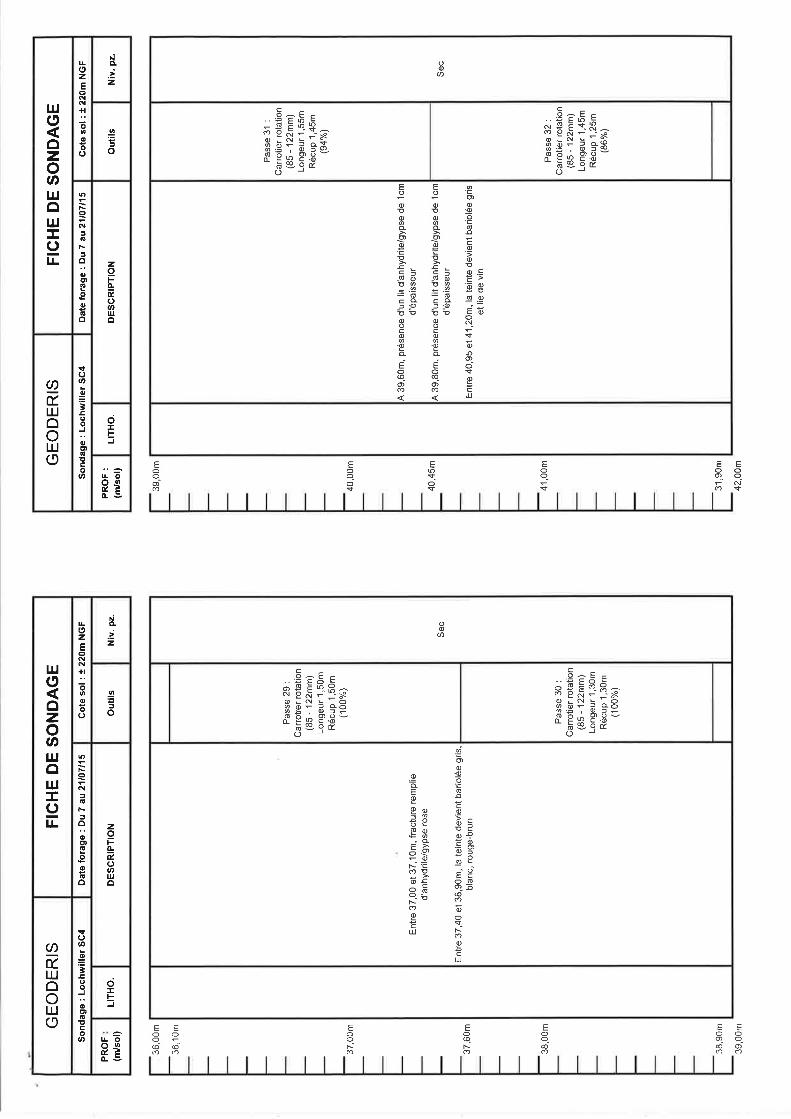
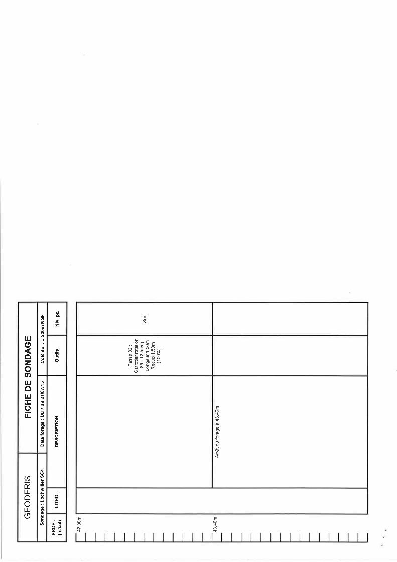
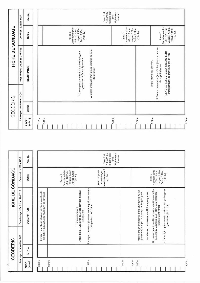
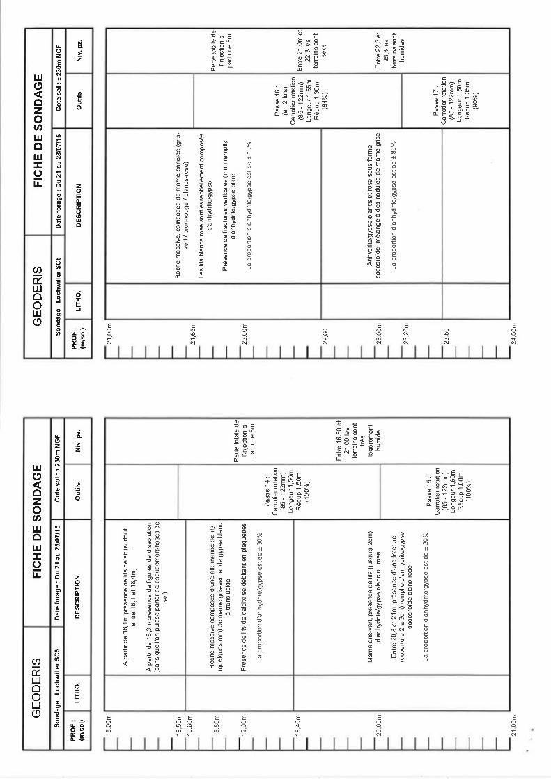
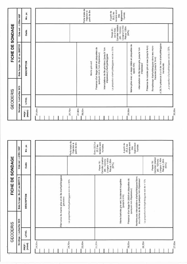
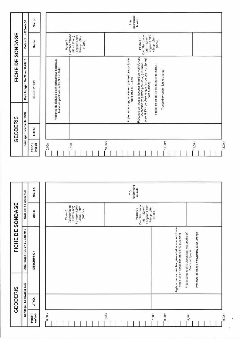
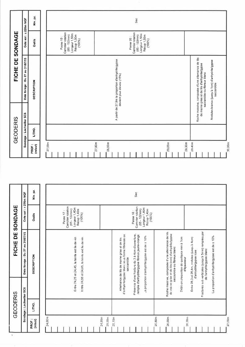
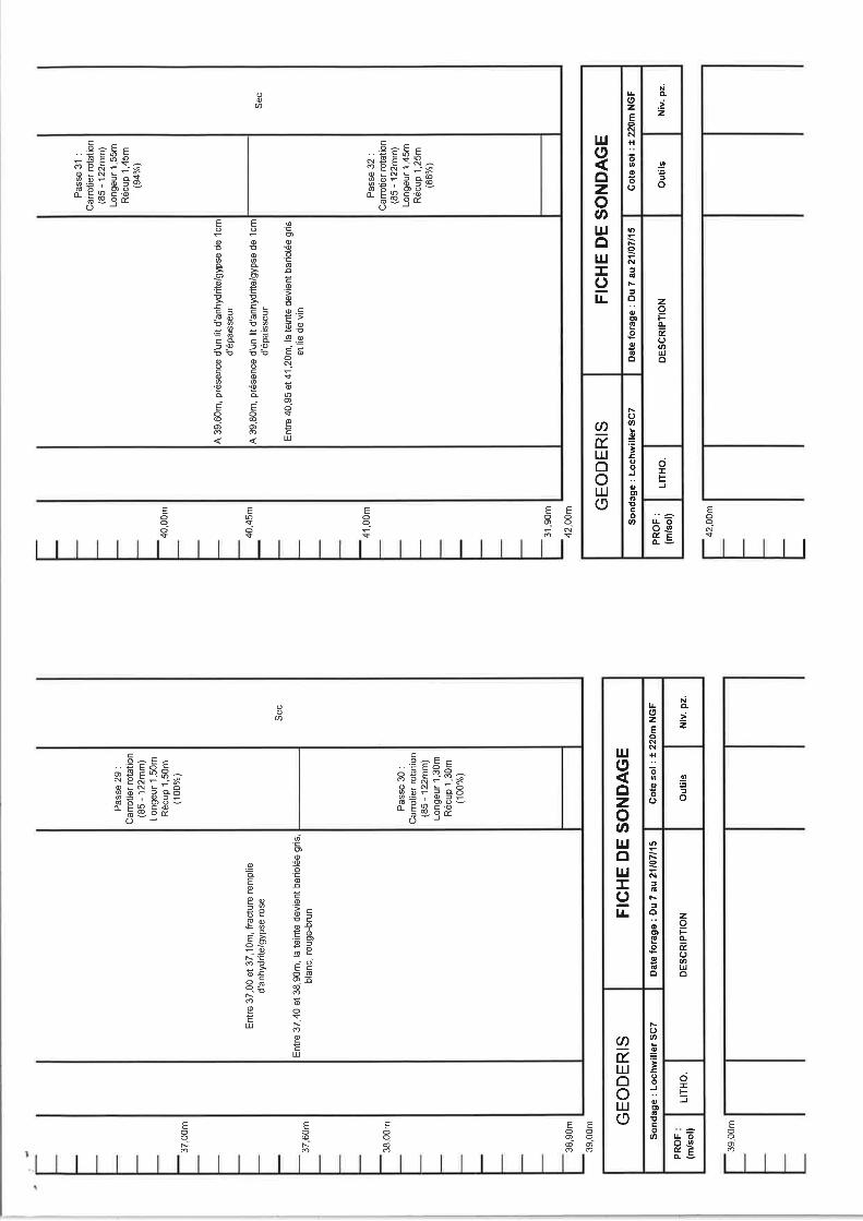
Les coupes lithologiques simplifiées des sondages carottés sont présentées en annexe 2. Les levés
géologiques ont été réalisés par GEODERIS.
GINGER CEBTP Agence de Strasbourg
Affaire : LOCHWILLER (67) – Lotissement Weingarten
Dossier : EST2.F.067 Indice 1 du 06/01/2016 Page 7/10
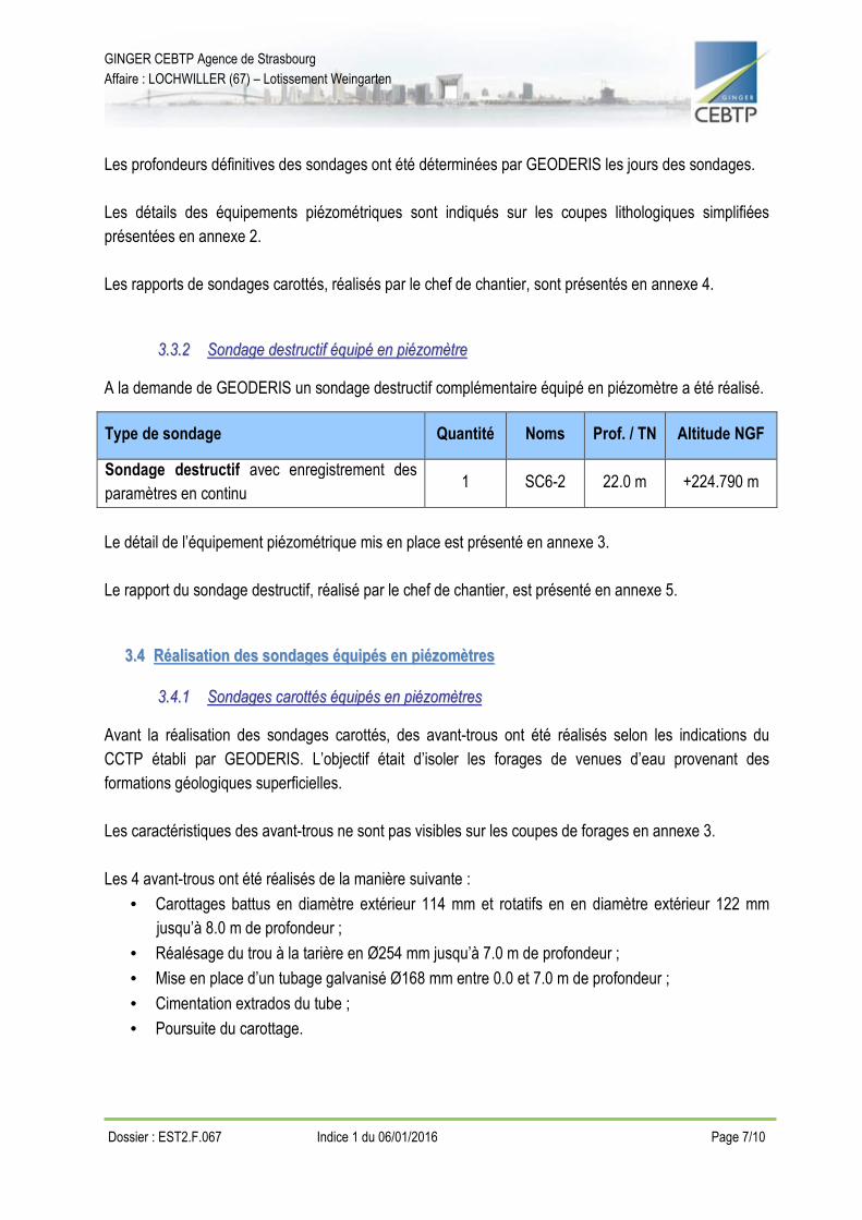
Les profondeurs définitives des sondages ont été déterminées par GEODERIS les jours des sondages.
Les détails des équipements piézométriques sont indiqués sur les coupes lithologiques simplifiées
présentées en annexe 2.
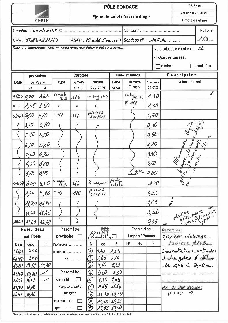
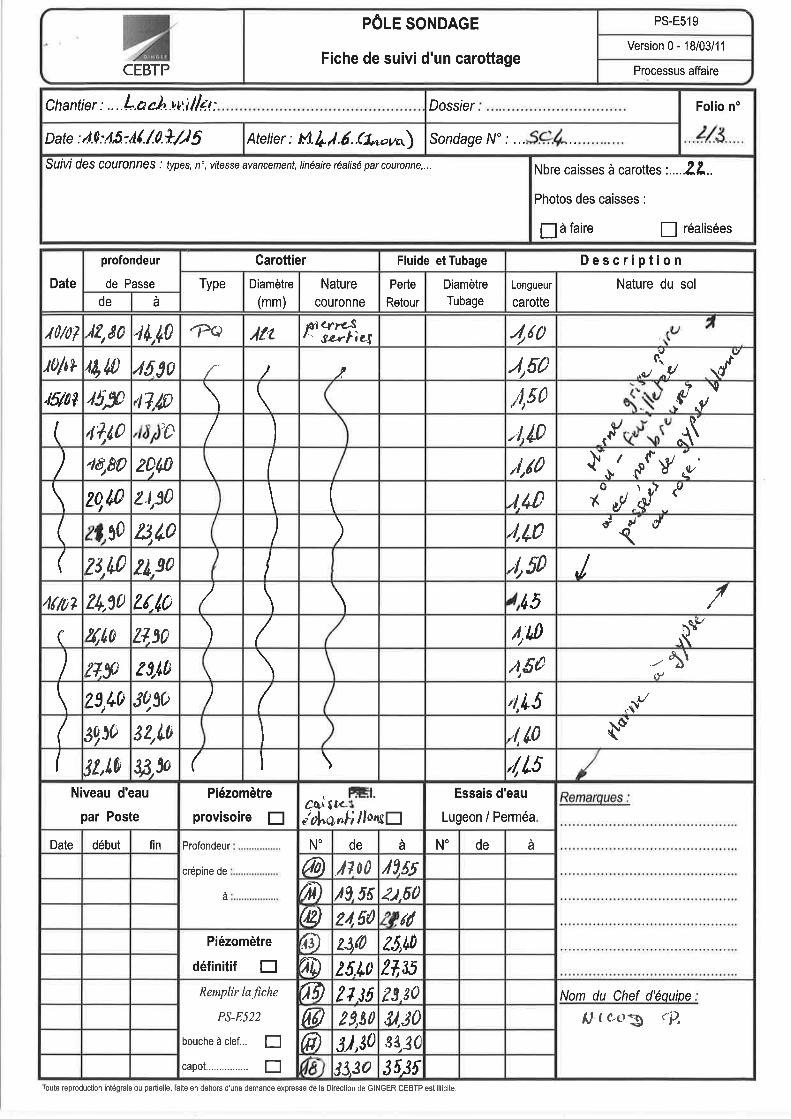
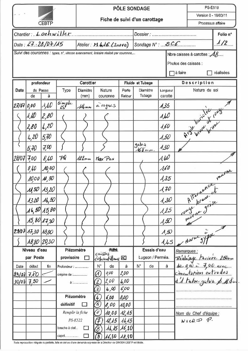
Les rapports de sondages carottés, réalisés par le chef de chantier, sont présentés en annexe 4.
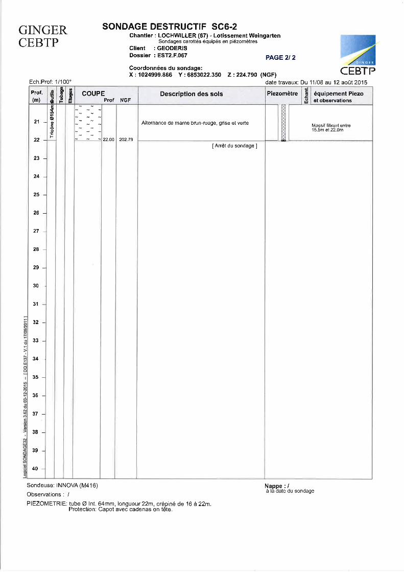
33..33..22 SSoonnddaaggee ddeessttrruuccttiiff ééqquuiippéé eenn ppiiéézzoommèèttrree
A la demande de GEODERIS un sondage destructif complémentaire équipé en piézomètre a été réalisé.
Type de sondage Quantité Noms Prof. / TN Altitude NGF
Sondage destructif avec enregistrement des
paramètres en continu 1 SC6-2 22.0 m +224.790 m
Le détail de l’équipement piézométrique mis en place est présenté en annexe 3.
Le rapport du sondage destructif, réalisé par le chef de chantier, est présenté en annexe 5.
33..44 RRééaalliissaattiioonn ddeess ssoonnddaaggeess ééqquuiippééss eenn ppiiéézzoommèèttrreess
33..44..11 SSoonnddaaggeess ccaarroottttééss ééqquuiippééss eenn ppiiéézzoommèèttrreess
Avant la réalisation des sondages carottés, des avant-trous ont été réalisés selon les indications du
CCTP établi par GEODERIS. L’objectif était d’isoler les forages de venues d’eau provenant des
formations géologiques superficielles.
Les caractéristiques des avant-trous ne sont pas visibles sur les coupes de forages en annexe 3.
Les 4 avant-trous ont été réalisés de la manière suivante :
• Carottages battus en diamètre extérieur 114 mm et rotatifs en en diamètre extérieur 122 mm
jusqu’à 8.0 m de profondeur ;
• Réalésage du trou à la tarière en Ø254 mm jusqu’à 7.0 m de profondeur ;
• Mise en place d’un tubage galvanisé Ø168 mm entre 0.0 et 7.0 m de profondeur ;
• Cimentation extrados du tube ;
• Poursuite du carottage.

GINGER CEBTP Agence de Strasbourg
Affaire : LOCHWILLER (67) – Lotissement Weingarten
Dossier : EST2.F.067 Indice 1 du 06/01/2016 Page 8/10
La figure ci-dessous présente un schéma des ouvrages réalisés :
Les piézomètres ont été mis en place selon la méthode suivante :
• Mise en place du tubage de l’avant-trou ;
• Réalisation des carottages jusqu’à la profondeur indiquée par GEODERIS ;
• Réalésage du trou de forage au tricône Ø154 mm pour les sondages SC5, SC6 et SC7 (pas le
SC4) ;
• Cimentation du trou de forage jusqu’à la profondeur de la base du piézomètre fixée par
GEODERIS ;
• Mise en place des tubes piézométriques ;
• Mise en œuvre du massif filtrant et du bouchon de sobranite aux profondeurs fixées par
GEODERIS ;
• Cimentation du piézomètre jusqu’à la surface ;
• Mise en place du capot orange avec cadenas (ou de la bouche-à-clef pour le sondage SC5).

GINGER CEBTP Agence de Strasbourg
Affaire : LOCHWILLER (67) – Lotissement Weingarten
Dossier : EST2.F.067 Indice 1 du 06/01/2016 Page 9/10
Remarques :
• les caractéristiques des piézomètres (niveaux crépinés et pleins, profondeur) sont indiquées sur
les coupes de forage présentées en annexe 2,
• les lithologies détaillées établies par GEODERIS sont présentées en annexe 7.
33..44..22 SSoonnddaaggee ddeessttrruuccttiiff ééqquuiippéé eenn ppiiéézzoommèèttrree
A la demande de GEODERIS un sondage complémentaire, non prévu initialement, a été réalisé. Il s’agit
d’un sondage destructif, avec enregistrements des paramètres de forage, équipé en piézomètre.
Aucun avant-trou n’a été réalisé pour ce sondage.
La réalisation du sondage s’est déroulée selon la méthode suivante :
• Réalisation du sondage destructif au tricône Ø154mm jusqu’à 22.0 m de profondeur ;
• Mise en place des tubes piézométriques Ø75mm jusqu’à 22.0 m de profondeur ;
• Mise en œuvre du massif filtrant entre 15.5 m et 22.0 m de profondeur,
• Mise en œuvre du bouchon de sobranite entre 13.0 m et 15.5 m de profondeur ;
• Cimentation du piézomètre jusqu’à la surface ;
• Mise en place du capot orange avec cadenas.
Les caractéristiques du piézomètre (niveaux crépiné et plein, profondeur) sont indiquées sur la coupe de
forage présentée en annexe 3.
33..44..33 MMaattéérriieell uuttiilliisséé
Le matériel suivant a été utilisé :
• Foreuse INNOVA (fiche technique présentée en annexe 6) ;
• Pompe à eau ;
• Compresseur ;
• Carottier battu LS Ø114mm ;
• Carottier rotatif PQ Ø122mm ;
• Tricône Ø152mm ;
• Caisses à carottes ;
• Tubes galvanisé Ø154/168mm pour les avant-trous ;
• Tubes piézométriques en PVC pleins et crépinés Ø75mm ;
• Bouchons de fonds piézométriques ;
• 4 Capots orange avec cadenas d’artillerie ;

GINGER CEBTP Agence de Strasbourg
Affaire : LOCHWILLER (67) – Lotissement Weingarten
Dossier : EST2.F.067 Indice 1 du 06/01/2016 Page 10/10
• 1 bouche-à-clef ;
• Sacs de gravette pour les massifs filtrants ;
• Sacs de sobranite ;
• Sacs de coulis de ciment ;
• Compresseur pour le développement des piézomètres.
33..44..44 AAllééaass rreennccoonnttrrééss lloorrss dduu cchhaannttiieerr
Aucun aléa particulier n’a été rencontré lors du chantier.
33..44..55 MMéétthhooddee ddee ddéévveellooppppeemmeenntt ddeess ppiiéézzoommèèttrreess
Les piézomètres ont été soufflés au compresseur comme prévu initialement au contrat. A la demande de
GEODERIS, l’eau présente dans les piézomètres a également été évacuée à l’aide d’une pompe.
33..55 RRééaalliissaattiioonn ddeess ddiiaaggrraapphhiieess ggaammmmaa--rraayy
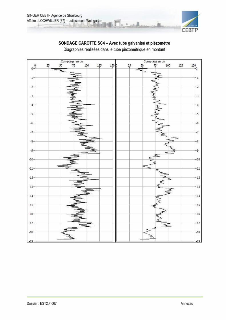
Les diagraphies gamma-ray ont été réalisées dans le sondage SC4 avant et après la pose du piézomètre
et du tube galvanisé pour vérifier les différences de signaux obtenus. Ces différences se sont avérées
minimes. Il a donc été convenu avec GEODERIS de réaliser les diagraphies après la réalisation
définitives des autres sondages.
Il également été réalisé des diagraphies dans le sondage existant avec inclinomètre.
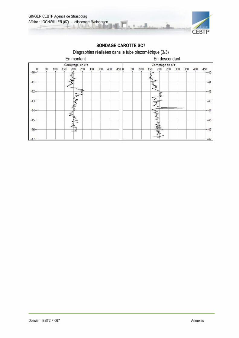
Les résultats des diagraphies sont présentés en annexe 8.
GINGER CEBTP Agence de Strasbourg
Affaire : LOCHWILLER (67) – Lotissement Weingarten
Dossier : EST2.F.067 Annexes
ANNEXE 1 – PLAN D’IMPLANTATION DES SONDAGES

GINGER CEBTP Agence de Strasbourg
Affaire : LOCHWILLER (67) – Lotissement Weingarten
Dossier : EST2.F.067 Annexes
PLAN D’IMPLANTATION DES SONDAGES
SC4 SC5
SC7
SC6
SC6-2
GINGER CEBTP Agence de Strasbourg
Affaire : LOCHWILLER (67) – Lotissement Weingarten
Dossier : EST2.F.067 Annexes
ANNEXE 2 – SONDAGES CAROTTES EQUIPES EN PIEZOMETRES
- Coupes lithologiques simplifiées,
- Détails des équipements piézométriques.


GINGER CEBTP Agence de Strasbourg
Affaire : LOCHWILLER (67) – Lotissement Weingarten
Dossier : EST2.F.067 Annexes
ANNEXE 3 – SONDAGE DESTRUCTIF EQUIPE EN PIZOMETRE
- Coupe lithologique très simplifiée,
- Détails de l’équipement piézométrique.

GINGER CEBTP Agence de Strasbourg
Affaire : LOCHWILLER (67) – Lotissement Weingarten
Dossier : EST2.F.067 Annexes
ANNEXE 4 – RAPPORTS REALISES PAR LES SONDEURS DES SONDAGES
CAROTTES EQUIPES EN PIEZOMETRES


GINGER CEBTP Agence de Strasbourg
Affaire : LOCHWILLER (67) – Lotissement Weingarten
Dossier : EST2.F.067 Annexes
ANNEXE 5 – RAPPORT REALISE PAR LES SONDEURS DU SONDAGE DESTRUCTIF
EQUIPE EN PIEZOMETRE

GINGER CEBTP Agence de Strasbourg
Affaire : LOCHWILLER (67) – Lotissement Weingarten
Dossier : EST2.F.067 Annexes
ANNEXE 6 – FICHE TECHNIQUE DE LA MACHINE INNOVA UTILISEE

��� ������� Fiche : PS-E230Fiche : GG-MPS-018
16 allée Prométhée, Les Propylées III Version 0 du 06/12/2012 01/01/04 Vers. 1
28000 CHARTRES Processus : Infra et Moyens
TYPE D'ATELIER : SONDEUSE GEOTECHNIQUE
MARQUE : EMCI MODELE : INOVA
M 410 : n° de série 06-274, mise en service Août 2007
M 416 : n° de série xxxx, mise en service xxxx
Utilisations :
Forage à la tarière hélicoïdale
Forage en roto-percussion
Carottage en vibro-percussion et en rotation
Destructif en rotation ou au marteau fond de trou
5.60 m
2.30 m
1.80 m 5.25 m
Caractéristiques Principales :
Moteur : 100 ch Deutz diesel insonorisé Tête de rotation : 400 daN.m - 370 tr/mn
Capacité d'enfoncement : 3000 kg et de traction : 7000 kg Rotopercussion : 1200 cps/min, 240 joules
Treuil manœuvre : 2000 kg - 50 m/mn
Mât : 5,25 m Course : 3,40 m
Pompe : ORION double 120 l/mn à 40 bars
Accessoires : frein de tiges double, capacité 200 mm
extracteur hydraulique
Dimensions :
Poids : 6200 kg Largeur : 1,80 m
Longueur transport : 5,25 m Longueur travail : 5,25 m Hauteur transport : 2,30 m Hauteur travail : 5,60 m
Performances indicatives :
Sondeuse de grande capacité, montée sur chenillard METALLIQUE vitesse de déplacement 3,5 km/h.
- 40 m en tarière 114 mm - 80 m en destructif 100 mm
- 100 m au mft 90 mm - 80 m au carottier à câble type HQ
GINGER CEBTP Agence de Strasbourg
Affaire : LOCHWILLER (67) – Lotissement Weingarten
Dossier : EST2.F.067 Annexes
ANNEXE 7 – LITHOLOGIES DETAILLEES DES SONDAGES CAROTTES REALISEES
PAR GEODERIS


GINGER CEBTP Agence de Strasbourg
Affaire : LOCHWILLER (67) – Lotissement Weingarten
Dossier : EST2.F.067 Annexes
ANNEXE 8 – DIAGRAPHIES GAMMA-RAY DES SONDAGES
GINGER CEBTP Agence de Strasbourg
Affaire : LOCHWILLER (67) – Lotissement Weingarten
Dossier : EST2.F.067 Annexes
SONDAGE CAROTTE SC4 – Avec tube galvanisé et piézomètre
Diagraphies réalisées dans le tube piézométrique en montant

GINGER CEBTP Agence de Strasbourg
Affaire : LOCHWILLER (67) – Lotissement Weingarten
Dossier : EST2.F.067 Annexes
SONDAGE CAROTTE SC4 – Avec tube galvanisé et piézomètre
Diagraphies réalisées dans le tube piézométrique en descendant

GINGER CEBTP Agence de Strasbourg
Affaire : LOCHWILLER (67) – Lotissement Weingarten
Dossier : EST2.F.067 Annexes
SONDAGE CAROTTE SC4 – Sans tube galvanisé
Diagraphies réalisées dans le trou de carottage en descendant (1/3)

GINGER CEBTP Agence de Strasbourg
Affaire : LOCHWILLER (67) – Lotissement Weingarten
Dossier : EST2.F.067 Annexes
SONDAGE CAROTTE SC4 - Sans tube galvanisé
Diagraphies réalisées dans le trou de carottage en descendant (2/3)

GINGER CEBTP Agence de Strasbourg
Affaire : LOCHWILLER (67) – Lotissement Weingarten
Dossier : EST2.F.067 Annexes
SONDAGE CAROTTE SC4 - Sans tube galvanisé
Diagraphies réalisées dans le trou de carottage en descendant (3/3)

GINGER CEBTP Agence de Strasbourg
Affaire : LOCHWILLER (67) – Lotissement Weingarten
Dossier : EST2.F.067 Annexes
SONDAGE CAROTTE SC5
Diagraphies réalisées dans le tube piézométrique en descendant (1/2)

GINGER CEBTP Agence de Strasbourg
Affaire : LOCHWILLER (67) – Lotissement Weingarten
Dossier : EST2.F.067 Annexes
SONDAGE CAROTTE SC5
Diagraphies réalisées dans le tube piézométrique en descendant (2/2)

GINGER CEBTP Agence de Strasbourg
Affaire : LOCHWILLER (67) – Lotissement Weingarten
Dossier : EST2.F.067 Annexes
SONDAGE CAROTTE SC5
Diagraphies réalisées dans le tube piézométrique en montant (1/2)

GINGER CEBTP Agence de Strasbourg
Affaire : LOCHWILLER (67) – Lotissement Weingarten
Dossier : EST2.F.067 Annexes
SONDAGE CAROTTE SC5
Diagraphies réalisées dans le tube piézométrique en montant (2/2)

GINGER CEBTP Agence de Strasbourg
Affaire : LOCHWILLER (67) – Lotissement Weingarten
Dossier : EST2.F.067 Annexes
SONDAGE CAROTTE SC6
Diagraphies réalisées dans le tube piézométrique
En montant En descendant

GINGER CEBTP Agence de Strasbourg
Affaire : LOCHWILLER (67) – Lotissement Weingarten
Dossier : EST2.F.067 Annexes
SONDAGE CAROTTE SC7
Diagraphies réalisées dans le tube piézométrique (1/3)
En montant En descendant

GINGER CEBTP Agence de Strasbourg
Affaire : LOCHWILLER (67) – Lotissement Weingarten
Dossier : EST2.F.067 Annexes
SONDAGE CAROTTE SC7
Diagraphies réalisées dans le tube piézométrique (2/3)
En montant En descendant
GINGER CEBTP Agence de Strasbourg
Affaire : LOCHWILLER (67) – Lotissement Weingarten
Dossier : EST2.F.067 Annexes
SONDAGE CAROTTE SC7
Diagraphies réalisées dans le tube piézométrique (3/3)
En montant En descendant

GINGER CEBTP Agence de Strasbourg
Affaire : LOCHWILLER (67) – Lotissement Weingarten
Dossier : EST2.F.067 Annexes
SONDAGE DESTRUCTIF SC6-2
Diagraphies réalisées dans le tube piézométrique
En montant En descendant

GINGER CEBTP Agence de Strasbourg
Affaire : LOCHWILLER (67) – Lotissement Weingarten
Dossier : EST2.F.067 Annexes
SONDAGE AVEC INCLINOMETRE
Diagraphies réalisées en montant dans le tube inclinométrique
GINGER CEBTP Agence de Strasbourg
Affaire : LOCHWILLER (67) – Lotissement Weingarten
Dossier : EST2.F.067 Annexes
Agence de Strasbourg
13 rue de l’Electricité 67800 HOENHEIM
Tél. : 03.88.81.20.50
Fax. : 03.88.81.21.50
LE RESEAU
CONTACT
www.groupe-cebtp.com


RAPPORT E2016/027DE – 16ALS21010
Annexe 13 Analyses minéralogiques -
Caractérisation géotechnique - GeoRessources
Rapport final
Juin 2016
ASGA - GeoRessources GR.CA.GEO.PSI.RPRE.15.0524.B 1/20
Analyses minéralogiques Caractérisation géotechnique
(forages sur la commune de Lochwiller - 67)
GEODERIS
Rapport final
juin 2016
Ce document comporte 20 pages
(hors couverture et annexes)
Rédaction Vérification Approbation
Nom C. AUVRAY E. FOURREAU D. GRGIC
Qualité Ingénieur de Recherche Assistant Ingénieur Maître de conférence - HdR
Visa

GEODERIS
ASGA - GeoRessources GR.CA.GEO.PSI.RPRE.15.0524.B 2/20
Sommaire
1- CADRE DE L'ETUDE................................................................................................4
2- PREPARATION DES ECHANTILLONS ...................................................................4
3- CONDUITE DES MESURES ET DES ESSAIS .........................................................4
3.1- Analyses minéralogiques...........................................................................................4
3.2- Essais géotechniques ...............................................................................................5
4- RESULTATS .............................................................................................................9
4.1- Analyses minéralogiques...........................................................................................9
4.2- Essais géotechniques .............................................................................................13
5- CONCLUSIONS ......................................................................................................20

GEODERIS
ASGA - GeoRessources GR.CA.GEO.PSI.RPRE.15.0524.B 3/20
Liste des figures
Figure 1 - Représentation des limites d'Atterberg ......................................................................6
Figure 2 - Représentation schématique de la cellule œdométrique ...............................................7
Figure 3 - SC4-7 Evolution du déplacement mesuré en fonction du temps (pression injection = 0.10MPa et pression de confinement = 0.33kN) ................................................................16
Figure 4 - SC4-7 Augmentation de la force axiale - Détermination du potentiel de gonflement .....16
Figure 5 - SC4-7 Détermination du potentiel de gonflement......................................................16
Figure 6 - SC4-20 Evolution du déplacement mesuré en fonction du temps (pression injection = 0.16MPa et pression de confinement = 0.52kN) ................................................................16
Figure 7 - SC4-20 Evolution de la force axiale ........................................................................16
Figure 8 - SC7-16 Evolution du déplacement mesuré en fonction du temps (pression injection = 0.45kN et pression de confinement = 1.50MPa) ................................................................17
Figure 9 - SC7-16 Augmentation de la force axiale - Détermination du potentiel de gonflement ...17
Figure 10 - SC7-16 Détermination du potentiel de gonflement ..................................................17
Figure 11 - SC5-18 Evolution du déplacement mesuré en fonction du temps (pression injection = 0.25MPa et pression de confinement = 0.90kN) ................................................................18
Figure 12 - SC5-18 Augmentation de la force axiale - Détermination du potentiel de gonflement .18
Figure 13 - SC5-18 Détermination du potentiel de gonflement ..................................................18
Figure 14 - SC6-17 Evolution du déplacement mesuré en fonction du temps (pression injection = 0.18MPa et pression de confinement = 0.70kN) ................................................................19
Figure 15 - SC6-17 Augmentation de la force axiale - Détermination du potentiel de gonflement .19
Figure 16 - SC6-17 Détermination du potentiel de gonflement ..................................................19
Liste des tableaux
Tableau 1 - Identification des espèces minérales - Sondage SC4........................................................9
Tableau 2 - Identification des espèces minérales - Sondage SC5 ...............................................10
Tableau 3 - Identification des espèces minérales - Sondage SC6 ...............................................11
Tableau 4 - Identification des espèces minérales - Sondage SC7 ...............................................12
Tableau 5 - Paramètres physiques - Sondage SC4....................................................................13
Tableau 6 - Paramètres physiques - Sondage SC5....................................................................14
Tableau 7 - Paramètres physiques - Sondage SC6....................................................................14
Tableau 8 - Paramètres physiques - Sondage SC6....................................................................15
Tableau 9 - Evolution de la phase anhydre avant et après essais œdométriques ..........................20
GEODERIS
ASGA - GeoRessources GR.CA.GEO.PSI.RPRE.15.0524.B 4/20
1- CADRE DE L'ETUDE
A la demande de GEODERIS « Demande de prestations pour la réalisation d'analyses minéralogiques et d'essais géotechniques sur des carottes issues de forages de Lochwiller (67) " référencé "CAHIER DES CHARGES E2015/025DIO - 15ALS21010" en date du 02/07/2015, l’ASGA-GeoRessources a réalisé :
Analyses minéralogiques : détermination de la part volumique de chaque phase rencontrées ;
Essais géotechniques : évaluation de la teneur en eau, de la masse volumique humide et sèche ; évaluation de la porosité ; évaluation des limites d'Atterberg, évaluation de la valeur au bleu de méthylène des phases argileuses ; essais œdométriques
Ce document présente la totalité des résultats minéralogiques, l'ensemble des paramètres physiques et les résultats des essais œdométriques.
2- PREPARATION DES ECHANTILLONS
Les analyses minéralogiques nécessitent deux types de préparation :
la fabrication d'une lame mine pour réaliser un comptage des espèces minérales
la fabrication d'une poudre et l’extraction de la fraction inférieure à 2µm afin de pouvoir réaliser des diffractions des rayons X (DRX). Cette technique permet : i) de déterminer la fraction argileuse et ii) de réaliser une détermination semi-quantitative des espèces minérales.
Les essais géotechniques (paramètres physiques, essais oedométriques) nécessitent la préparation d'une poudre et d'échantillons cylindriques d'un diamètre de 38mm et d'un élancement de 20mm.
3- CONDUITE DES MESURES ET DES ESSAIS
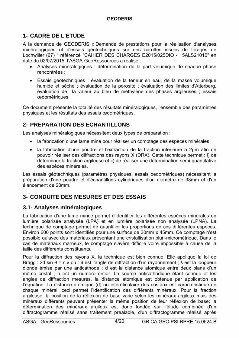
3.1- Analyses minéralogiques
La fabrication d'une lame mince permet d'identifier les différentes espèces minérales en lumière polarisée analysée (LPA) et en lumière polarisée non analysée (LPNA). La technique de comptage permet de quantifier les proportions de ces différentes espèces. Environ 600 points sont identifiés pour une surface de 30mm x 45mm. Ce comptage n'est possible qu'avec des matériaux présentant une cristallisation pluri-micrométrique. Dans le cas de matériaux marneux, le comptage s'avère difficile voire impossible à cause de la taille des différents constituants.
Pour la diffraction des rayons X, la technique est bien connue. Elle applique la loi de Bragg : 2d sin θ = n.λ où : θ est l’angle de diffraction d’un rayonnement ; λ est la longueur d’onde émise par une anticathode ; d est la distance atomique entre deux plans d’un même cristal ; n est un numéro entier. La source anticathodique étant connue et les angles de diffraction mesurés, la distance atomique est obtenue par application de l’équation. La distance atomique (d) ou interéticulaire des cristaux est caractéristique de chaque minéral, ceci permet l’identification des différents minéraux. Pour la fraction argileuse, la position de la réflexion de base varie selon les minéraux argileux mais des minéraux différents peuvent présenter la même position de leur réflexion de base; la détermination des minéraux argileux est donc fondée sur l'étude combinée d'un diffractogramme réalisé sans traitement préalable, d'un diffractogramme réalisé après

GEODERIS
ASGA - GeoRessources GR.CA.GEO.PSI.RPRE.15.0524.B 5/20
saturation par l'éthylène-glycol, et par l'étude d'un diffractogramme réalisé après chauffage à 490°C pendant deux heures.
3.2- Essais géotechniques
Identification physique :
Teneur en eau :
La teneur en eau est mesurée par différence de masse d'un échantillon avant et après passage à l'étuve.
Elle est déterminée suivant la norme NF P 94-410-1 :
d
w
mm=w (1)
avec :
mw = m2 - m3
md = m3 - m1
où :
mw est la masse d’eau ;
md est la masse de matériau sec ;
m2 est la masse de la prise d’essai et de son contenant avant le passage à l’étuve ;
m1 est la masse du contenant ;
m3 est la masse de la prise d’essai et de son contenant après le passage à l’étuve.
La teneur en eau est exprimée en pourcentage et l’intervalle est de 0,1. Pour que cette mesure soit valide, le conditionnement des sondages et des éprouvettes entre chaque manipulation doit être parfaitement étanche afin de conserver les conditions hydriques naturelles du matériau.
Masses volumiques :
Les masses volumiques sèches et naturelles sont déterminées sur un échantillon géométriquement « parfait » c’est-à-dire un cylindre ou un prisme. Dans le cas contraire, ces paramètres sont déterminés par pesée hydrostatique sur des morceaux. Pour la masse volumique des grains indispensable au calcul de la porosité, l’échantillon est sous forme de poudre : nous prélevons donc un échantillon représentatif de la zone étudiée. Les procédures utilisées pour la détermination de ces paramètres sont les normes AFNOR NF P94-410-1 / -2.
Porosité apparente :
La porosité apparente est calculée à partir de la masse volumiques sèche et de la masse volumique des grains en fonction de la norme AFNOR NF P94-410-3. La taille des pores atteints avec cette mesure ne peut excéder quelques millimètres.

GEODERIS
ASGA - GeoRessources GR.CA.GEO.PSI.RPRE.15.0524.B 6/20
Limites d'Atterberg :
On détermine les teneurs en eau pondérales correspondant à des états particuliers du matériau :
- limite de liquidité (wL) : teneur en eau du matériau remanié au point de transition entre les états liquide et plastique.
- limite de plasticité (wp) : teneur en eau du matériau remanié au point de transition entre les états plastique et solide.
Il en est déduit l'indice de plasticité (Ip) : différence entre les limites de liquidité et de plasticité. Cet indice définit l'étendue du domaine plastique et il est utilisé avec la teneur en eau naturelle dans la détermination de l'indice de consistance (Ic) : rapport défini par la formule : Ic = (wL - w) / Ip, où w est la teneur en eau du matériau dans son état naturel et ne comportant pas d'éléments supérieurs à 400 µm. N'oublions pas non plus qu'il peut être mesuré une limite de retrait (wR).
Les teneurs en eau sont exprimées en pourcentage, l'indice de plasticité est un nombre sans dimension.
Etat solide Etat plastique Etat liquide
teneurs en eau 0 w R w p wL
Ip
Figure 1 - Représentation des limites d'Atterberg
Cette procédure répond à la norme NF P95 0-51, elle est destinée à la détermination des deux limites d'Atterberg et s'applique aux matériaux dont les éléments passent à travers le tamis de dimension nominale d'ouverture de maille 400 µm.
Valeur au bleu de méthylène des phases argileuses :
L'essai consiste à mesurer par dosage la quantité de bleu de méthylène pouvant s'adsorber sur la prise d'essai. Cette valeur est rapportée par proportionnalité directe à la fraction 0/50 mm du matériau. La valeur de bleu est directement liée à la surface spécifique des particules constituant le matériau, laquelle est avant tout régie par l'importance et l'activité des minéraux argileux présents dans la fraction fine.
Le dosage s'effectue en ajoutant successivement différentes quantités de bleu de méthylène et en contrôlant l'adsorption après chaque ajout. Pour ce faire, on prélève une goutte de la suspension que l'on dépose sur un papier filtre, ce qui provoque la création d'une tache. L'adsorption maximale est atteinte lorsqu'une auréole bleu clair persistante se produit à la périphérie de la tache.
Cette valeur est déterminée en suivant la norme NF P94-068.

GEODERIS
ASGA - GeoRessources GR.CA.GEO.PSI.RPRE.15.0524.B 7/20
Caractérisation hydromécanique :
La réalisation d’essais œdométriques sur des échantillons de roches, et en particulier de roches peu perméables requiert un dispositif expérimental qui permet :
1 – d'assurer un ajustement du diamètre de l’échantillon, par rapport au diamètre interne de la cellule (déformation radiale nulle) et un effritement superficiel minimal de l’éprouvette lors de sa mise en place dans le corps de cellule indéformable,
2 – de maintenir une contrainte axiale stable au cours de chacun des paliers,
3 – de maintenir une pression interstitielle stable au cours de chacun des paliers,
4 – d'optimiser les conditions de drainage aux deux extrémités de l'éprouvette afin de limiter le temps d'essai,
5 – d'avoir une précision et une plage de mesure des déformations axiales adaptées au protocole fixé pour les phases de déchargement en contrainte axiale à pression interstitielle constante et les phases de chargement en pression interstitielle à contrainte axiale constante, et à la déformation maximale de l’éprouvette au cours de l’essai (déformation totale obtenue sous l’état de contrainte effective maximal).
Afin de faciliter l’introduction des éprouvettes dans les corps de cellule indéformable et pour limiter leur effritement superficiel, les bords des corps de cellule sont biseautés (Figure 2).
Figure 2 - Représentation schématique de la cellule œdométrique
De plus, pour obtenir un ajustement optimal entre le diamètre des éprouvettes et le diamètre interne des corps de cellules indéformables, les éprouvettes seront réalisées en trois étapes. Dans un premier temps, les éprouvettes seront carottées puis rectifiées, avec un carottier permettant d'obtenir des éprouvettes de diamètre supérieur à 38 mm (carottier diamanté permettant d'obtenir des éprouvettes d'un diamètre approximatif de 40 mm). Dans un second temps, un ajustement plus précis sera réalisé à l'aide de papier de verre afin d'obtenir un diamètre légèrement supérieur au diamètre interne des corps de cellules. Les éprouvettes seront ensuite introduites en force dans le corps de cellule à l'aide d'une presse. L'enfoncement sera réalisé manuellement (guidage de la presse en déplacement) à très faible vitesse. Une rotule est placée entre l'éprouvette et la presse afin de faciliter sa

GEODERIS
ASGA - GeoRessources GR.CA.GEO.PSI.RPRE.15.0524.B 8/20
mise en place dans le corps de cellule. Cette technique permet d'obtenir un effritement minimal des éprouvettes tout en assurant un bon ajustement du diamètre des éprouvettes avec le diamètre interne du corps de cellule.
Le protocole retenu est le suivant :
Potentiel de gonflement : On laisse se déformer axialement l'échantillon (les déplacements radiaux sont bloqués par l'anneau œdométrique) puis après stabilisation, on augmente la force axiale pour revenir à la hauteur initiale de l'échantillon.
a - Chargement axial équivalent à la profondeur de prélèvement - Attente de la stabilité en déplacement axial.
b - Injection en amont et aval du fluide avec une pression d'injection pouvant correspondre à celle in situ.
c - Enregistrement de l'augmentation du déplacement axiale avec un capteur de déplacement ayant une sensibilité de 0,001mm. Attente de la stabilité du déplacement
d - Augmentation de la force pour retrouver la hauteur initiale de l'échantillon.
La difficulté de ces mesures est fortement liée à la nature hétérogène du matériau. Une attention particulière sera faite sur la représentativité entre l'analyse minéralogique et la pression de gonflement mesurée. Nous préconisons une seconde analyse minéralogique sur l'échantillon après l'essai œdométrique afin de vérifier l'évolution géochimique du matériau.
GEODERIS
ASGA - GeoRessources GR.CA.GEO.PSI.RPRE.15.0524.B 9/20
4- RESULTATS
4.1- Analyses minéralogiques
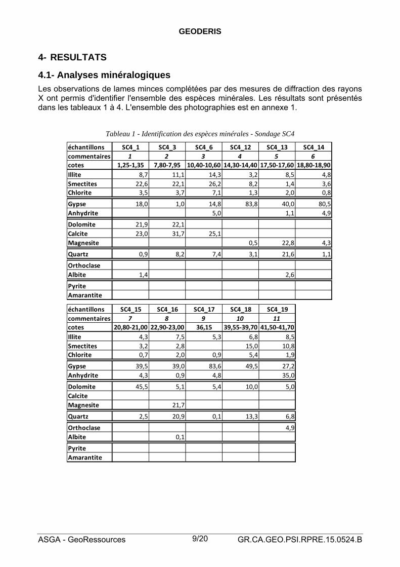
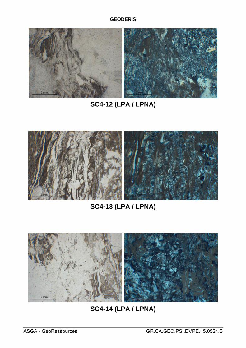
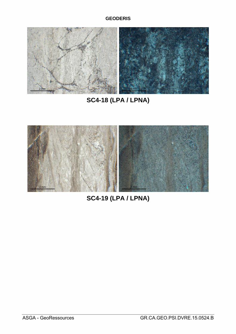
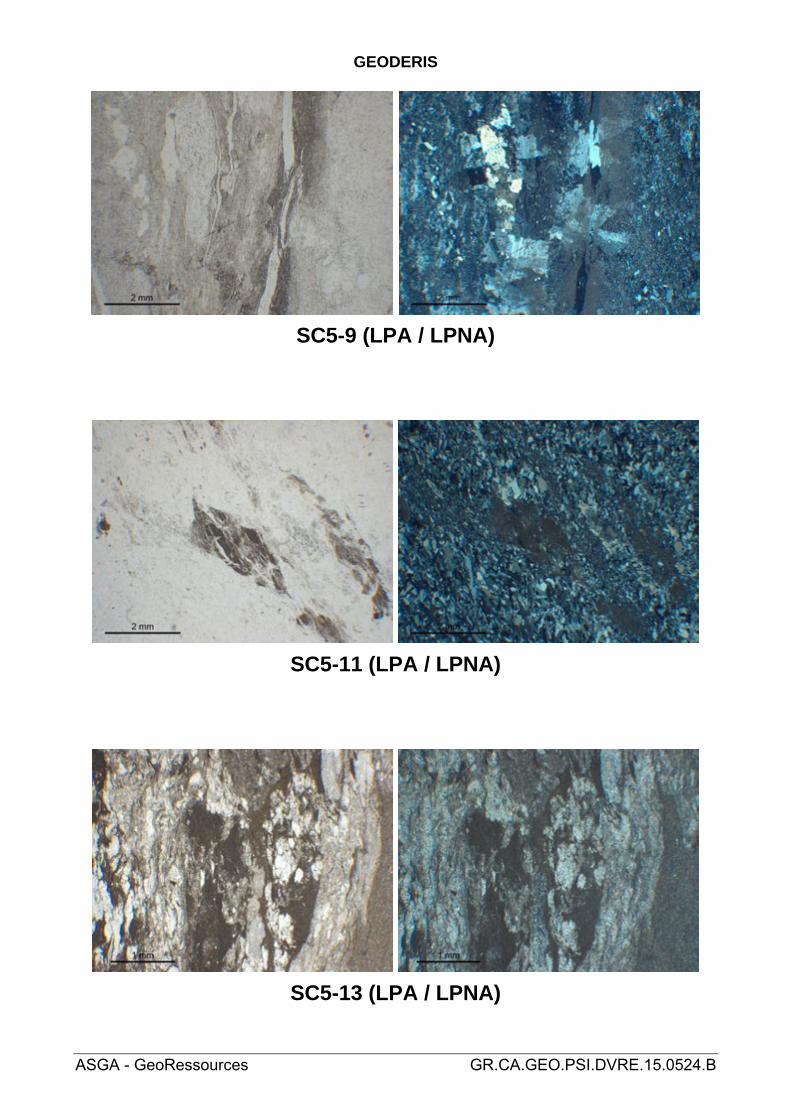
Les observations de lames minces complétées par des mesures de diffraction des rayons X ont permis d'identifier l'ensemble des espèces minérales. Les résultats sont présentés dans les tableaux 1 à 4. L'ensemble des photographies est en annexe 1.
Tableau 1 - Identification des espèces minérales - Sondage SC4
échantillons SC4_1 SC4_3 SC4_6 SC4_12 SC4_13 SC4_14
commentaires 1 2 3 4 5 6
cotes 1,25‐1,35 7,80‐7,95 10,40‐10,60 14,30‐14,40 17,50‐17,60 18,80‐18,90
Illite 8,7 11,1 14,3 3,2 8,5 4,8
Smectites 22,6 22,1 26,2 8,2 1,4 3,6
Chlorite 3,5 3,7 7,1 1,3 2,0 0,8
Gypse 18,0 1,0 14,8 83,8 40,0 80,5
Anhydrite 5,0 1,1 4,9
Dolomite 21,9 22,1
Calcite 23,0 31,7 25,1
Magnesite 0,5 22,8 4,3
Quartz 0,9 8,2 7,4 3,1 21,6 1,1
Orthoclase
Albite 1,4 2,6
Pyrite
Amarantite
échantillons SC4_15 SC4_16 SC4_17 SC4_18 SC4_19
commentaires 7 8 9 10 11cotes 20,80‐21,00 22,90‐23,00 36,15 39,55‐39,70 41,50‐41,70
Illite 4,3 7,5 5,3 6,8 8,5
Smectites 3,2 2,8 15,0 10,8Chlorite 0,7 2,0 0,9 5,4 1,9
Gypse 39,5 39,0 83,6 49,5 27,2
Anhydrite 4,3 0,9 4,8 35,0
Dolomite 45,5 5,1 5,4 10,0 5,0
Calcite
Magnesite 21,7
Quartz 2,5 20,9 0,1 13,3 6,8
Orthoclase 4,9
Albite 0,1
Pyrite
Amarantite

GEODERIS
ASGA - GeoRessources GR.CA.GEO.PSI.RPRE.15.0524.B 10/20
Ces résultats suscitent plusieurs commentaires qui sont précisés ci-dessous : 1 Gypse granulaire en remplacement de clastes sédimentaires - Nodules gypseux2 Microcristaux isolés dans la matrice - Nodules gypseux 3 Microcristaux et macrocristaux en forme de tablettes. Remplacement probable
car la densité des cristaux suit les laminations sédimentaires. Les nodules sont constitués à 99% de gypse
4 Nodules formés de macrocristaux allongés + gypse microcristallin en remplacement de lamines sédimentaires
5 Nodules formés de macrocristaux. Fractures remplies de cristaux allongés déformés (croissance des cristaux pendant l'ouverture des fractures, "crack and seal").
6 Nodules cristallins 7 Nodules en croissance dans un sédiment laminé. 8 Lamines macrocristallines massives pouvant correspondre à des nodules
amalgamés. Présence de structures "crack and seal" 9 Nodules macrocristallins montrant une frange externe microcristalline
correspondant au remplacement du sédiment encaissant. 10 Gypse microcristallin en remplacement du sédiment. Possible aggradation des
cristaux. Quelques "Crack and seal". 11 Seul exemple de possible gypse "primaire". Lamines de gypse microcristallin en
forme de feuillets fins.
Tableau 2 - Identification des espèces minérales - Sondage SC5
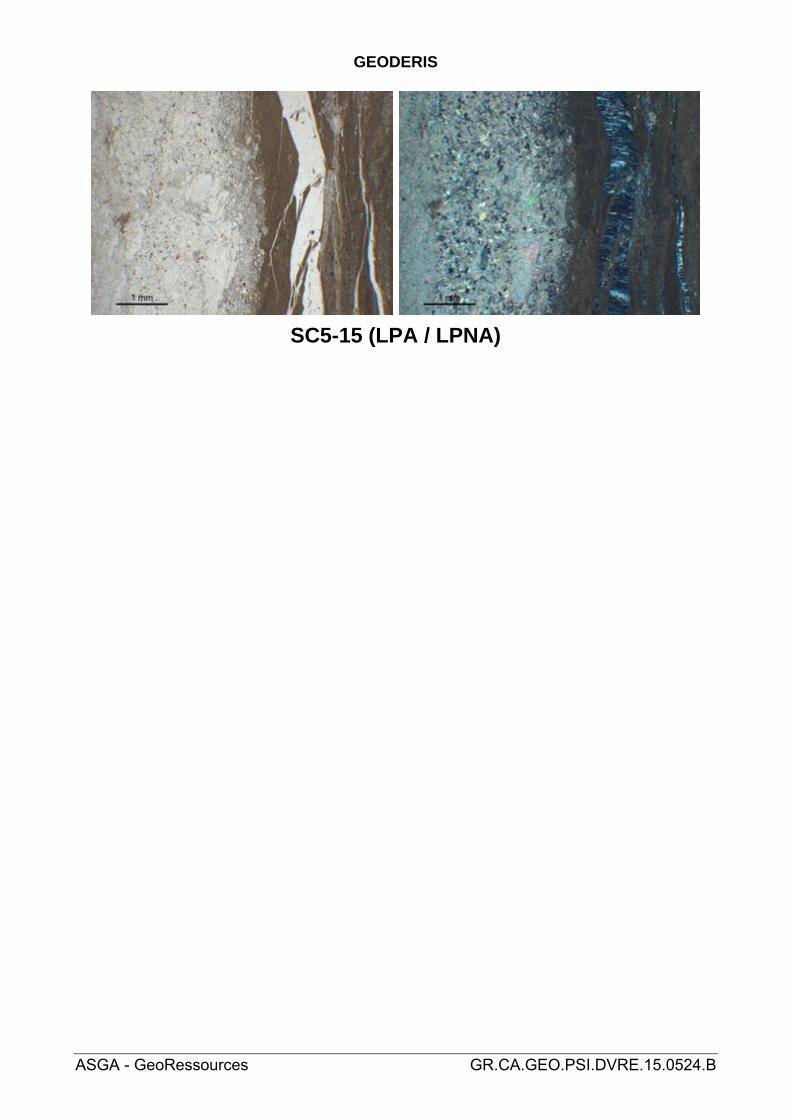
échantillons SC5_2 SC5_4 SC5_6 SC5_9 SC5_11 SC5_13 SC5_15
commentaires 12 13 14 15 16 17 18
cotes 6,90‐7,10 11,05‐11,20 17,70‐17,90 19,30‐19,45 23,30‐23,40 29,80‐29,90 32,70‐32,80
Illite 16,2 7,4 10,7 1,8 2,5 5,2 15,5
Smectites 32,3 25,6 25,0 2,6 7,4 13,2
Chlorite 5,4 2,2 1,6 1,0 1,8 2,2 2,0
Gypse 1,2 84,5 83,2 2,3 32,9
Anhydrite 2,5 1,2 0,7 1,4 52,0 12,8
Dolomite 27,2 19,8 40,1 5,4 7,8 2,2
Calcite 7,4 39,8 6,4
Magnesite 2,7 16,8
Quartz 7,0 2,5 8,1 4,5 0,7 11,8 14,3
Orthoclase 4,3 7,0
Albite 1,5 2,0 2,2
Pyrite 2,0
Amarantite
Les commentaires associés à ces résultats sont : 12 Cristaux automorphes : concentration de cristaux fins (100µm max) dans une
lamines et des fractures sub-verticales, cristaux très fins (20µm) disséminés dans l'encaissant.
13 Très petits cristaux (silts) disséminés dans l'encaissant. 14 Un nodule de gypse (mosaïque cristalline) et très rares petits cristaux (silts)

GEODERIS
ASGA - GeoRessources GR.CA.GEO.PSI.RPRE.15.0524.B 11/20
disséminés dans l'encaissant. 15 Gypse sous plusieurs formes: microcristallin en remplacement de sédiment
(peut-être d'anhydrite également), mosaïque cristalline dans les nodules, mosaïque cristalline dans les fractures horizontales
16 Macrocristaux en tablettes allongées et organisés en 2 directions apparentes. L'une parallèle aux laminations sédimentaires et l'autres app. à 90°.
17 Gypse en macrocristaux renfermant des inclusions d'anhydrite, en remplacement de l'anhydrite originelle. "Crack-and-seal" dans les fractures horizontales.
18 Gypse automorphe dans les fractures (rare "crack-and seal") et en replacement plus diffus de l'anhydrite.
Tableau 3 - Identification des espèces minérales - Sondage SC6
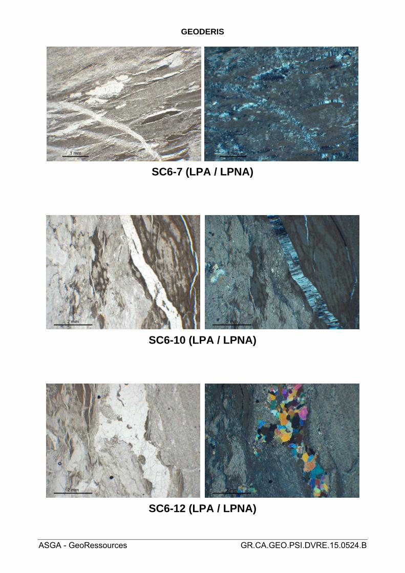
échantillons SC6_1 SC6_4 SC6_6 SC6_7 SC6_10 SC6_12 SC6_14
commentaires 19 20 21 22 23 24 25
cotes 3,60‐3,70 10,40‐10,50 17,30‐17,40 21,90‐22,00 24,90‐25,10 29,90‐30,10 31,80‐31,90
Illite 5,6 11,8 7,3 9,4 4,2 6,4 12,2
Smectites 17,8 28,3 10,6 7,3 1,3 6,3 26,3
Chlorite 2,0 7,0 1,5 2,5 1,3 1,8 3,1
Gypse 64,3 50,9 11,4 13,0 22,7
Anhydrite 1,2 74,1 48,2 6,5
Dolomite 35,6 35,2 3,0 1,9 1,2 3,2 11,1
Calcite 37,7 9,1
Magnesite 6,9 18,0 3,2 11,5
Quartz 1,3 7,7 6,3 10,0 3,4 9,6 18,1
Orthoclase
Albite
Pyrite
Amarantite
Les commentaires sont précisés ci-dessous : 19 Gypse dans de nombreuses petites fractures. 20 Gypse macrocristallin dans petits nodules et fines fractures verticales. 21 Gypse macrocristallin dans petits nodules et fractures horizontales. Gypse
microcristallin en remplacement d'anhydrite fibreuse dans la majeure partie de la lame. Pas d'inclusions d'anhydrite dans les fractures.
22 Gypse macrocristallin dans les fractures (quelques "crack-and-seal"), et en flammes se développant en remplacement du sédiment et d'anhydrite fibreuse.
23 Gypse macrocristallin dans les fractures ("crack-and-seal"), et plus rarement dans des nodules avec inclusions d'anhydrite. Egalement en remplacement très incomplet d'anhydrite.
24 Gypse dans de nombreuses petites fractures ("crack-and-seal"). 25 Gypse macrocristallin en "crack-and-seal" dans fractures fines principalement
horizontales, et en remplacement de sédiment et peut-être d'anhydrite.
GEODERIS
ASGA - GeoRessources GR.CA.GEO.PSI.RPRE.15.0524.B 12/20
Tableau 4 - Identification des espèces minérales - Sondage SC7
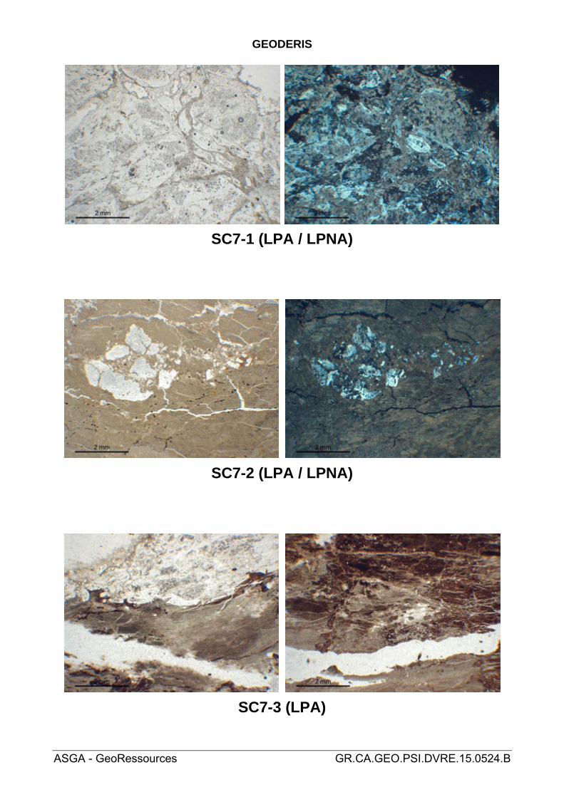
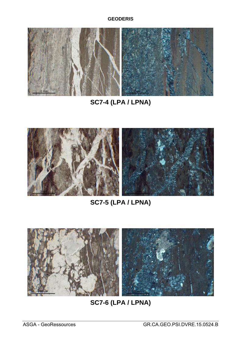
échantillons SC7_1 SC7_2 SC7_3 SC7_4 SC7_5 SC7_6 SC7_7 SC7_8
commentaires 26 27 28 29 30 31 32 33
cotes 12,80‐12,90 26,25‐26,40 34,70‐34,85 39,20‐39,35 41,05‐41,25 42,95‐43,10 44,95‐45,10 45,80‐45,88
Illite 4,5 21,0 11,1 10,3 12,2 6,8 4,8 9,3
Smectites 2,4 27,0 27,2 13,3 14,1 4,1 8,9 8,2
Chlorite 1,2 12,0 2,2 2,1 3,1 1,3 2,4 1,7
Gypse 4,3 25,7 37,5 66,0 17,0 24,6
Anhydrite 2,7 3,8 2,6 2,9 12,7 28,9 13,6
Dolomite 7,7 6,4 3,2 12,0 15,4 19,4
Calcite 43,1 13,8 20,9
Magnesite 5,0 3,5 4,0 2,2 14,7
Quartz 46,0 10,5 27,4 29,5 17,6 5,1 18,9 7,5
Orthoclase 5,8
Albite 2,2 2,2 1,5
Pyrite
Amarantite 1,0
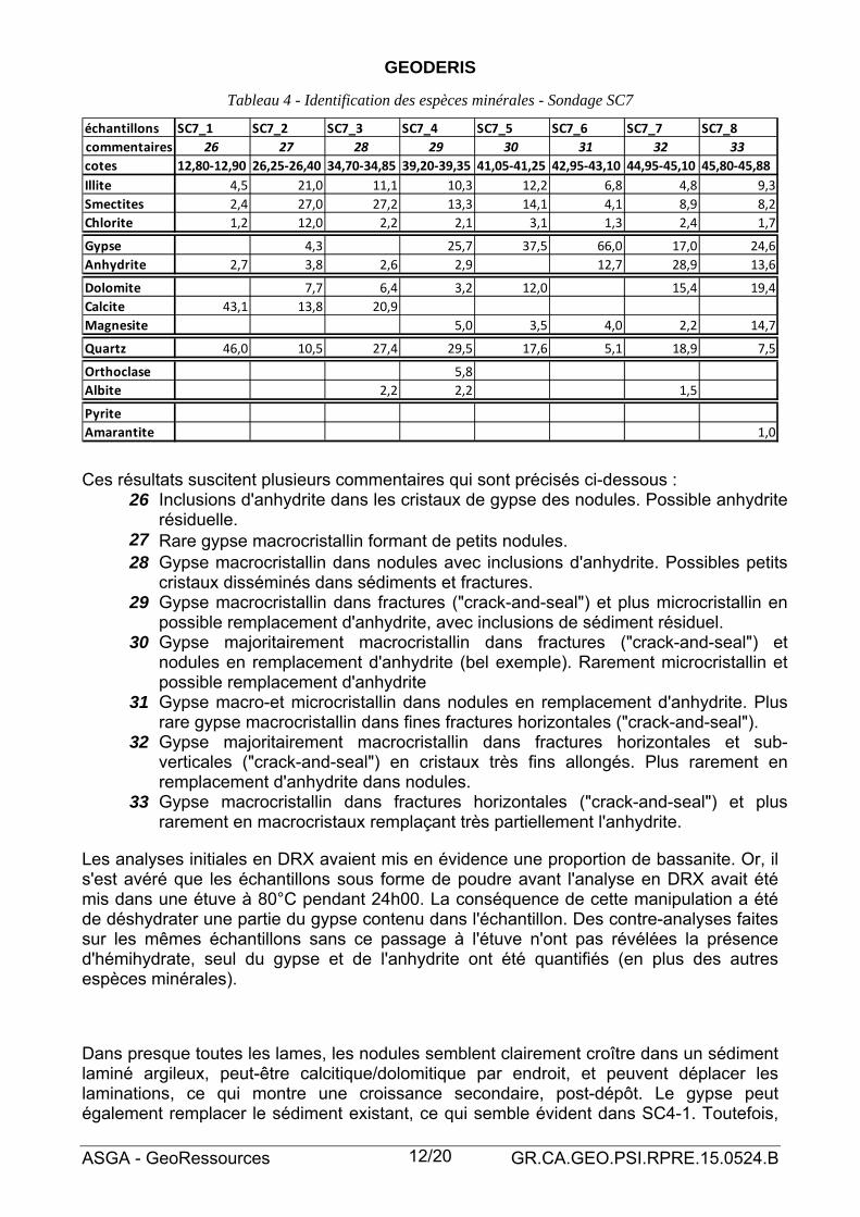
Ces résultats suscitent plusieurs commentaires qui sont précisés ci-dessous : 26 Inclusions d'anhydrite dans les cristaux de gypse des nodules. Possible anhydrite
résiduelle. 27 Rare gypse macrocristallin formant de petits nodules. 28 Gypse macrocristallin dans nodules avec inclusions d'anhydrite. Possibles petits
cristaux disséminés dans sédiments et fractures. 29 Gypse macrocristallin dans fractures ("crack-and-seal") et plus microcristallin en
possible remplacement d'anhydrite, avec inclusions de sédiment résiduel. 30 Gypse majoritairement macrocristallin dans fractures ("crack-and-seal") et
nodules en remplacement d'anhydrite (bel exemple). Rarement microcristallin et possible remplacement d'anhydrite
31 Gypse macro-et microcristallin dans nodules en remplacement d'anhydrite. Plus rare gypse macrocristallin dans fines fractures horizontales ("crack-and-seal").
32 Gypse majoritairement macrocristallin dans fractures horizontales et sub-verticales ("crack-and-seal") en cristaux très fins allongés. Plus rarement en remplacement d'anhydrite dans nodules.
33 Gypse macrocristallin dans fractures horizontales ("crack-and-seal") et plus rarement en macrocristaux remplaçant très partiellement l'anhydrite.
Les analyses initiales en DRX avaient mis en évidence une proportion de bassanite. Or, il s'est avéré que les échantillons sous forme de poudre avant l'analyse en DRX avait été mis dans une étuve à 80°C pendant 24h00. La conséquence de cette manipulation a été de déshydrater une partie du gypse contenu dans l'échantillon. Des contre-analyses faites sur les mêmes échantillons sans ce passage à l'étuve n'ont pas révélées la présence d'hémihydrate, seul du gypse et de l'anhydrite ont été quantifiés (en plus des autres espèces minérales).
Dans presque toutes les lames, les nodules semblent clairement croître dans un sédiment laminé argileux, peut-être calcitique/dolomitique par endroit, et peuvent déplacer les laminations, ce qui montre une croissance secondaire, post-dépôt. Le gypse peut également remplacer le sédiment existant, ce qui semble évident dans SC4-1. Toutefois,

GEODERIS
ASGA - GeoRessources GR.CA.GEO.PSI.RPRE.15.0524.B 13/20
dans les nodules il est probable qu’il soit précoce. Il montre une forme cristalline granulaire et en tablettes, voire rarement fibreuse. La lame SC4-19 est la seule qui montre une forme de gypse qui pourrait être syn-sédimentaire, avec une biréfringence dans des couleurs d’ordre supérieur. Les cristaux plus fins allongés sont localisés dans des lamines, non des nodules. Dans les fractures, le gypse est plus tardif. Les formes en « crack and seal » montrent une croissance pendant l’écartement des épontes des joints.
En résumé, il faut retenir que les nodules et lamines sont précoces. Ils sont probablement tous initialement en anhydrite mais beaucoup sont remplacées par du gypse. Des inclusions d’anhydrite sont également visibles dans le gypse des nodules.
4.2- Essais géotechniques
Identification physique :
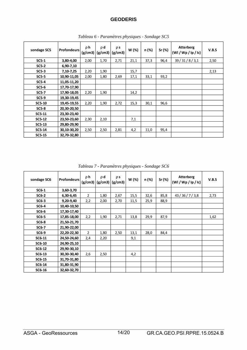
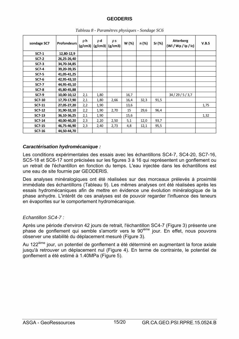
L'ensemble des résultats est présenté dans les tableaux 5 à 8. La signification des symboles dans ces tableaux est la suivante : h ; d et s : masses volumiques "naturelle", sèche et des grains W : teneur en eau "naturelle" n : porosité calculée Sr : degré de saturation Atterberg : limite d'Atterberg avec Wl = limite de liquidité, Wp = limite de plasticité, lp = indice de plasticité, lc = Indice de consistance V.B.S. : valeur au bleu de méthylène
Les différents bordereaux de mesures pour les limites d'Atterberg et les valeurs au bleu de méthylène sont respectivement en annexe 2 et 3.
Tableau 5 - Paramètres physiques - Sondage SC4
sondage SC4 Profondeursh
(g/cm3)
d (g/cm3)
s (g/cm3)
W (%) n (%) Sr (%)Atterberg
(Wl / Wp / Ip / Ic)V.B.S
SC4‐1 1,25‐1,35 2,00 1,70 17,7
SC4‐2 3,40‐3,60 1,90 1,50 2,67 24,3 43,8 83,3 39 / 32 / 7 / 2,1 3,74
SC4‐4 7,50‐7,60 1,90 1,50 2,62 23,1 42,7 81,2 38 / 32 / 6 / 2,5 3,36
SC4‐3 7,80‐7,95
SC4‐7 9,65‐9,80
SC4‐5 10,00‐10,10 2,10 1,80 2,44 12,7 26,2 87,3
SC4‐6 10,40‐10,60
SC4‐12 14,30‐14,40
SC4‐20 14,80‐15,00
SC4‐13 17,50‐17,60
SC4‐8 17,80‐17,90 2,20 2,00 2,56 9,3 21,9 85,2
SC4‐14 18,80‐18,90
SC4‐15 20,80‐21,00
SC4‐9 21,00‐21,10 2,30 2,00 10,1
SC4‐16 22,90‐23,00
SC4‐10 28,80‐28,90 2,30 2,10 2,60 7,9 19,2 86,4
SC4‐17 36,15
SC4‐11 39,55‐39,65 2,30 2,00 2,60 9,8 23,1 85,1
SC4‐18 39,55‐39,70
SC4‐19 41,50‐41,70
GEODERIS
ASGA - GeoRessources GR.CA.GEO.PSI.RPRE.15.0524.B 14/20
Tableau 6 - Paramètres physiques - Sondage SC5
sondage SC5 Profondeursh
(g/cm3)
d (g/cm3)
s (g/cm3)
W (%) n (%) Sr (%)Atterberg
(Wl / Wp / Ip / Ic)V.B.S
SC5‐1 3,80‐4,00 2,00 1,70 2,71 21,1 37,3 96,4 39 / 31 / 8 / 3,1 2,50
SC5‐2 6,90‐7,10
SC5‐3 7,10‐7,25 2,20 1,90 15,7 2,13
SC5‐5 10,90‐11,05 2,00 1,80 2,69 17,1 33,1 93,2
SC5‐4 11,05‐11,20
SC5‐6 17,70‐17,90
SC5‐7 17,90‐18,05 2,20 1,90 14,2
SC5‐9 19,30‐19,45
SC5‐10 19,45‐19,55 2,20 1,90 2,72 15,3 30,1 96,6
SC5‐8 20,30‐20,50
SC5‐11 23,30‐23,40
SC5‐12 23,50‐23,60 2,30 2,10 7,1
SC5‐13 29,80‐29,90
SC5‐14 30,10‐30,20 2,50 2,50 2,81 4,2 11,0 95,4
SC5‐15 32,70‐32,80
Tableau 7 - Paramètres physiques - Sondage SC6
sondage SC6 Profondeursh
(g/cm3)
d (g/cm3)
s (g/cm3)
W (%) n (%) Sr (%)Atterberg
(Wl / Wp / Ip / Ic)V.B.S
SC6‐1 3,60‐3,70
SC6‐2 6,30‐6,45 2 1,80 2,67 15,5 32,6 85,8 43 / 36 / 7 / 3,8 2,73
SC6‐3 9,20‐9,40 2,2 2,00 2,70 11,5 25,9 88,9
SC6‐4 10,40‐10,50
SC6‐6 17,30‐17,40
SC6‐5 17,85‐18,00 2,2 1,90 2,71 13,8 29,9 87,9 1,62
SC6‐8 21,50‐21,70
SC6‐7 21,90‐22,00
SC6‐9 22,20‐22,30 2 1,80 2,50 13,1 28,0 84,4
SC6‐11 24,50‐24,60 2,4 2,20 9,1
SC6‐10 24,90‐25,10
SC6‐12 29,90‐30,10
SC6‐13 30,30‐30,40 2,6 2,50 4,2
SC6‐15 31,70‐31,80
SC6‐14 31,80‐31,90
SC6‐16 32,60‐32,70
GEODERIS
ASGA - GeoRessources GR.CA.GEO.PSI.RPRE.15.0524.B 15/20
Tableau 8 - Paramètres physiques - Sondage SC6
sondage SC7 Profondeursh
(g/cm3)
d (g/cm3)
s (g/cm3)
W (%) n (%) Sr (%)Atterberg
(Wl / Wp / Ip / Ic)V.B.S
SC7‐1 12,80‐12,9
SC7‐2 26,25‐26,40
SC7‐3 34,70‐34,85
SC7‐4 39,20‐39,35
SC7‐5 41,05‐41,25
SC7‐6 42,95‐43,10
SC7‐7 44,95‐45,10
SC7‐8 45,80‐45,88
SC7‐9 10,00‐10,12 2,1 1,80 16,7 34 / 29 / 5 / 3,7
SC7‐10 17,70‐17,90 2,1 1,80 2,66 16,4 32,3 91,5
SC7‐11 27,05‐27,20 2,2 1,90 13,6 1,75
SC7‐12 31,90‐32,10 2,2 1,90 2,70 15 29,6 96,4
SC7‐13 36,10‐36,25 2,1 1,90 15,6 1,32
SC7‐14 40,00‐40,20 2,3 2,20 2,50 5,1 12,0 93,7
SC7‐15 46,75‐46,90 2,3 2,40 2,73 4,8 12,1 95,5
SC7‐16 44,50‐44,70
Caractérisation hydromécanique :
Les conditions expérimentales des essais avec les échantillons SC4-7, SC4-20, SC7-16, SC5-18 et SC6-17 sont précisées sur les figures 3 à 16 qui représentent un gonflement ou un retrait de l'échantillon en fonction du temps. L'eau injectée dans les échantillons est une eau de site fournie par GEODERIS.
Des analyses minéralogiques ont été réalisées sur des morceaux prélevés à proximité immédiate des échantillons (Tableau 9). Les mêmes analyses ont été réalisées après les essais hydromécaniques afin de mettre en évidence une évolution minéralogique de la phase anhydre. L'intérêt de ces analyses est de pouvoir regarder l'influence des teneurs en évaporites sur le comportement hydromécanique.
Echantillon SC4-7 :
Après une période d'environ 42 jours de retrait, l'échantillon SC4-7 (Figure 3) présente une phase de gonflement qui semble s'amortir vers le 90ième jour. En effet, nous pouvons observer une stabilité du déplacement mesuré (Figure 3).
Au 122ième jour, un potentiel de gonflement a été déterminé en augmentant la force axiale jusqu'à retrouver un déplacement nul (Figure 4). En terme de contrainte, le potentiel de gonflement a été estimé à 1.40MPa (Figure 5).

GEODERIS
ASGA - GeoRessources GR.CA.GEO.PSI.RPRE.15.0524.B 16/20
‐0,1
‐0,08
‐0,06
‐0,04
‐0,02
0
0,02
0,04
0 20 40 60 80 100 120 140 160
jours
(mm)
0
0,1
0,2
0,3
0,4
0,5
0,6
0,7
0 20 40 60 80 100 120 140 160
jours
(kN)
Figure 3 - SC4-7 Evolution du déplacement mesuré en fonction du temps (pression injection = 0.10MPa
et pression de confinement = 0.33kN)
Figure 4 - SC4-7 Augmentation de la force axiale - Détermination du potentiel de gonflement
0,20
0,40
0,60
0,80
1,00
1,20
1,40
1,60
0 0,01 0,02 0,03 0,04 0,05 0,06 0,07 0,08
déplacement (mm)
contrainte (MPa)
Figure 5 - SC4-7 Détermination du potentiel de gonflement
Echantillon SC4-20 :
Pour l'échantillon SC4-20 (Figures 6 et 7), nous avons pu observer un début de gonflement après 42 jours de retrait, cependant ce gonflement s'est arrêté très rapidement et depuis les mesures de déplacement étant stables, nous ne pouvons plus y associer de retrait ou de gonflement. Il semblerait donc que cet échantillon n'est pas de potentiel de gonflement.
0
0,05
0,1
0,15
0,2
0,25
0 20 40 60 80 100 120 140
jours
(mm)
0
0,1
0,2
0,3
0,4
0,5
0,6
0,7
0 20 40 60 80 100 120 140
jours
(kN)
Figure 6 - SC4-20 Evolution du déplacement mesuré en fonction du temps (pression injection = 0.16MPa
et pression de confinement = 0.52kN)
Figure 7 - SC4-20 Evolution de la force axiale
GEODERIS
ASGA - GeoRessources GR.CA.GEO.PSI.RPRE.15.0524.B 17/20
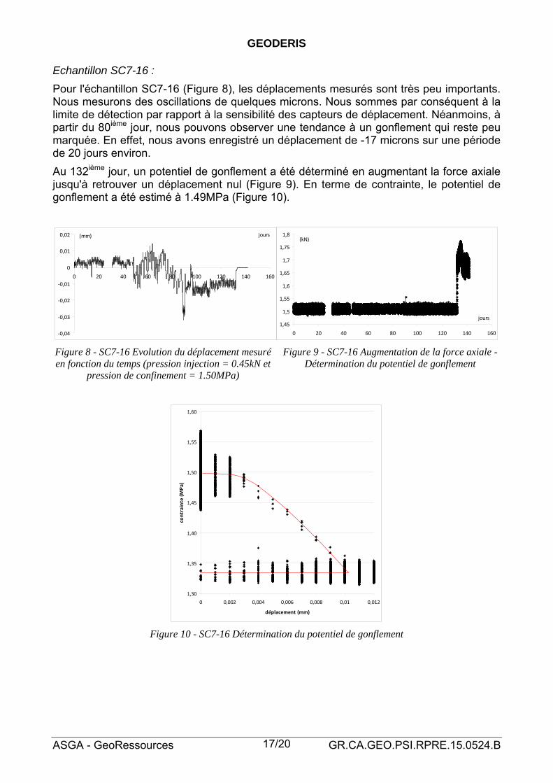
Echantillon SC7-16 :
Pour l'échantillon SC7-16 (Figure 8), les déplacements mesurés sont très peu importants. Nous mesurons des oscillations de quelques microns. Nous sommes par conséquent à la limite de détection par rapport à la sensibilité des capteurs de déplacement. Néanmoins, à partir du 80ième jour, nous pouvons observer une tendance à un gonflement qui reste peu marquée. En effet, nous avons enregistré un déplacement de -17 microns sur une période de 20 jours environ.
Au 132ième jour, un potentiel de gonflement a été déterminé en augmentant la force axiale jusqu'à retrouver un déplacement nul (Figure 9). En terme de contrainte, le potentiel de gonflement a été estimé à 1.49MPa (Figure 10).
‐0,04
‐0,03
‐0,02
‐0,01
0
0,01
0,02
0 20 40 60 80 100 120 140 160
jours(mm)
1,45
1,5
1,55
1,6
1,65
1,7
1,75
1,8
0 20 40 60 80 100 120 140 160
jours
(kN)
Figure 8 - SC7-16 Evolution du déplacement mesuré en fonction du temps (pression injection = 0.45kN et
pression de confinement = 1.50MPa)
Figure 9 - SC7-16 Augmentation de la force axiale - Détermination du potentiel de gonflement
1,30
1,35
1,40
1,45
1,50
1,55
1,60
0 0,002 0,004 0,006 0,008 0,01 0,012
déplacement (mm)
contrainte (MPa)
Figure 10 - SC7-16 Détermination du potentiel de gonflement

GEODERIS
ASGA - GeoRessources GR.CA.GEO.PSI.RPRE.15.0524.B 18/20
Echantillon SC5-18 :
A partir du 58ième jour (Figure 11), l'échantillon présente une phase de gonflement rapide qui s'amorti vers le 70ième jour. Jusqu'au 98ième jour, le déplacement est stabilisé.
Au 99ième jour, un potentiel de gonflement a été déterminé en augmentant la force axiale jusqu'à retrouver un déplacement nul (Figure 12). En terme de contrainte, le potentiel de gonflement a été estimé à 1.13MPa (Figure 13).
‐0,05
‐0,04
‐0,03
‐0,02
‐0,01
0
0,01
0 20 40 60 80 100 120
jours(mm)
0,8
0,9
1
1,1
1,2
1,3
1,4
1,5
1,6
0 20 40 60 80 100 120
jours
(kN)
Figure 11 - SC5-18 Evolution du déplacement
mesuré en fonction du temps (pression injection = 0.25MPa et pression de confinement = 0.90kN)
Figure 12 - SC5-18 Augmentation de la force axiale - Détermination du potentiel de gonflement
0,70
0,80
0,90
1,00
1,10
1,20
0 0,01 0,02 0,03 0,04 0,05
déplacement (mm)
contrainte (MPa)
Figure 13 - SC5-18 Détermination du potentiel de gonflement
Echantillon SC6-17 :
Pour l'échantillon SC6-17 (Figure 14), nous avons observé un déplacement négatif dès la mise en place de l'essai. Cette phase précoce de gonflement est peu probable : nous attribuons plutôt ce comportement à une phase d'équilibre de l'échantillon dans la cellule c'est-à-dire à une reprise des jeux mécaniques lors du montage de la cellule œdométrique. La phase de gonflement semble plutôt commencer au 50ième jour. Le potentiel de gonflement a été déterminé au 100ième jour à 1.50MPa (Figures 15 et 16).

GEODERIS
ASGA - GeoRessources GR.CA.GEO.PSI.RPRE.15.0524.B 19/20
‐0,06
‐0,05
‐0,04
‐0,03
‐0,02
‐0,01
0
0 20 40 60 80 100 120jours(mm)
0,60
0,70
0,80
0,90
1,00
1,10
0 20 40 60 80 100
jours
(kN)
Figure 14 - SC6-17 Evolution du déplacement
mesuré en fonction du temps (pression injection = 0.18MPa et pression de confinement = 0.70kN)
Figure 15 - SC6-17 Augmentation de la force axiale - Détermination du potentiel de gonflement
0,50
0,60
0,70
0,80
0,90
1,00
1,10
1,20
1,30
1,40
1,50
1,60
1,70
0 0,01 0,02 0,03 0,04 0,05 0,06
déplacement (mm)
contrainte (MPa)
Figure 16 - SC6-17 Détermination du potentiel de gonflement
GEODERIS
ASGA - GeoRessources GR.CA.GEO.PSI.RPRE.15.0524.B 20/20
5- CONCLUSIONS
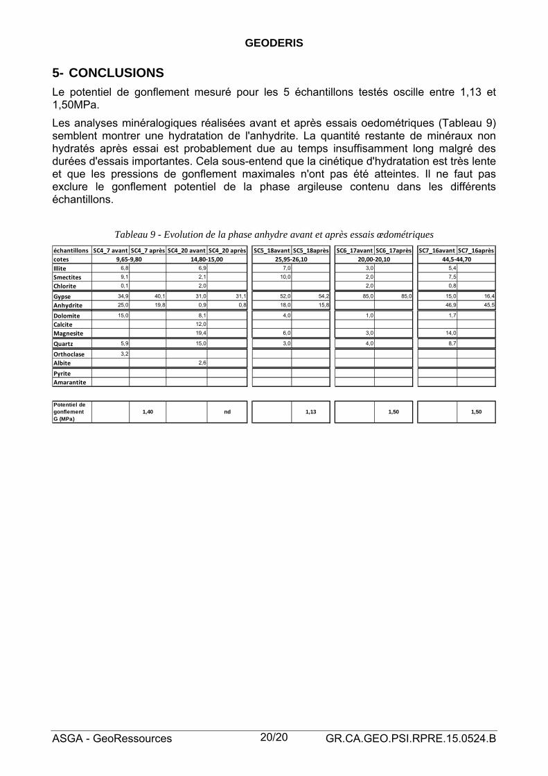
Le potentiel de gonflement mesuré pour les 5 échantillons testés oscille entre 1,13 et 1,50MPa.
Les analyses minéralogiques réalisées avant et après essais oedométriques (Tableau 9) semblent montrer une hydratation de l'anhydrite. La quantité restante de minéraux non hydratés après essai est probablement due au temps insuffisamment long malgré des durées d'essais importantes. Cela sous-entend que la cinétique d'hydratation est très lente et que les pressions de gonflement maximales n'ont pas été atteintes. Il ne faut pas exclure le gonflement potentiel de la phase argileuse contenu dans les différents échantillons.
Tableau 9 - Evolution de la phase anhydre avant et après essais œdométriques
échantillons SC4_7 avant SC4_7 après SC4_20 avant SC4_20 après SC5_18avant SC5_18après SC6_17avant SC6_17après SC7_16avant SC7_16après
cotes
Illite 6,8 6,9 7,0 3,0 5,4
Smectites 9,1 2,1 10,0 2,0 7,5
Chlorite 0,1 2,0 2,0 0,8
Gypse 34,9 40,1 31,0 31,1 52,0 54,2 85,0 85,0 15,0 16,4
Anhydrite 25,0 19,8 0,9 0,8 18,0 15,8 46,9 45,5
Dolomite 15,0 8,1 4,0 1,0 1,7
Calcite 12,0
Magnesite 19,4 6,0 3,0 14,0
Quartz 5,9 15,0 3,0 4,0 8,7
Orthoclase 3,2
Albite 2,6
Pyrite
Amarantite
Potentiel de gonflement G (MPa)
1,40 nd 1,13 1,50 1,50
44,5‐44,7025,95‐26,10 20,00‐20,109,65‐9,80 14,80‐15,00

GEODERIS
ASGA - GeoRessources GR.CA.GEO.PSI.DVRE.15.0524.B
Annexe 1 Photographies au microscope optique

GEODERIS
ASGA - GeoRessources GR.CA.GEO.PSI.DVRE.15.0524.B
SC4-01 (LPA / LPNA)
SC4-03 (LPA / LPNA)
SC4-06 (LPA / LPNA)
GEODERIS
ASGA - GeoRessources GR.CA.GEO.PSI.DVRE.15.0524.B
SC4-12 (LPA / LPNA)
SC4-13 (LPA / LPNA)
SC4-14 (LPA / LPNA)

GEODERIS
ASGA - GeoRessources GR.CA.GEO.PSI.DVRE.15.0524.B
SC4-15 (LPA / LPNA)
SC4-16 (LPA / LPNA)
SC4-17 (LPA / LPNA)
GEODERIS
ASGA - GeoRessources GR.CA.GEO.PSI.DVRE.15.0524.B
SC4-18 (LPA / LPNA)
SC4-19 (LPA / LPNA)

GEODERIS
ASGA - GeoRessources GR.CA.GEO.PSI.DVRE.15.0524.B
SC5-2 (LPA / LPNA)
SC5-4 (LPA)
SC5-6 (LPA)
GEODERIS
ASGA - GeoRessources GR.CA.GEO.PSI.DVRE.15.0524.B
SC5-9 (LPA / LPNA)
SC5-11 (LPA / LPNA)
SC5-13 (LPA / LPNA)
GEODERIS
ASGA - GeoRessources GR.CA.GEO.PSI.DVRE.15.0524.B
SC5-15 (LPA / LPNA)

GEODERIS
ASGA - GeoRessources GR.CA.GEO.PSI.DVRE.15.0524.B
SC6-1 (LPA)
SC6-4 (LPA / LPNA)
SC6-6 (LPA / LPNA)
GEODERIS
ASGA - GeoRessources GR.CA.GEO.PSI.DVRE.15.0524.B
SC6-7 (LPA / LPNA)
SC6-10 (LPA / LPNA)
SC6-12 (LPA / LPNA)
GEODERIS
ASGA - GeoRessources GR.CA.GEO.PSI.DVRE.15.0524.B
SC7-1 (LPA / LPNA)
SC7-2 (LPA / LPNA)
SC7-3 (LPA)
GEODERIS
ASGA - GeoRessources GR.CA.GEO.PSI.DVRE.15.0524.B
SC7-4 (LPA / LPNA)
SC7-5 (LPA / LPNA)
SC7-6 (LPA / LPNA)

GEODERIS
ASGA - GeoRessources GR.CA.GEO.PSI.DVRE.15.0524.B
SC7-7 (LPA / LPNA)
SC7-8 (LPA / LPNA)

GEODERIS
ASGA - GeoRessources GR.CA.GEO.PSI.RPRE.15.0524.B
Annexe 2 Limites d'Atterberg

GEODERIS
ASGA - GeoRessources GR.CA.GEO.PSI.RPRE.15.0524.B
DETERMINATION DES LIMITES D'ATTERBERG
Limite de liquidité à la coupelle-Limite de plasticité au rouleauConforme à la norme : NF P 94-051Procédure d'essai : MS1 - 10
Identification appareillage : Coupelle de Casagrande automatique (modèle Controls) X
Coupelle de Casagrande manuelle type W.F.
N° balance H3 et H2
Date : 03/09/2015 RemarqueN° d'étude : 15.0524
Nom de l'étude : GEODERIS
Sondage : SC4-2
Profondeur :
Mesure n° 1 2 3 4 5 6 7 8
Nombre de coups (N) 15 17 19 28 40
Teneur en eau (%) 41,0 40,6 39,9 37,8 37,4
15 015 20025 025 20035 035 200
1 2 3 4
31,5 31,8
Limite de liquidité : wL = 39
Limite de plasticité : wP = 32 IP = 7
w (%) = 24,3 IC = 2,1
Indice de consistanceTeneur en eau du sol
Limite de plasticité
PROCES-VERBAL D'ESSAI
Limite de liquidité à la coupelle de Casagrande
Indice de plasticité
Mesure n°
Teneur en eau (%)
HydroGéomécanique Multi-échelleUniversité de Lorraine - ENSGUMR 7359 GéoRessources
3536373839404142434445
10 100
Nombre de chocs de la coupelle (N)
Tene
ur e
n ea
u (%
)
15 25 3520 4030 50

GEODERIS
ASGA - GeoRessources GR.CA.GEO.PSI.RPRE.15.0524.B
DETERMINATION DES LIMITES D'ATTERBERG
Limite de liquidité à la coupelle-Limite de plasticité au rouleauConforme à la norme : NF P 94-051Procédure d'essai : MS1 - 10
Identification appareillage : Coupelle de Casagrande automatique (modèle Controls) X
Coupelle de Casagrande manuelle type W.F.
N° balance H3 et H2
Date : 03/09/2015 RemarqueN° d'étude : 15.0524
Nom de l'étude : GEODERIS
Sondage : SC4-4
Profondeur :
Mesure n° 1 2 3 4 5 6 7 8
Nombre de coups (N) 22 20 16 26 33
Teneur en eau (%) 39,2 39,0 40,0 38,3 36,3
15 015 20025 025 20035 035 200
1 2 3 4
32,2 31,7
Limite de liquidité : wL = 38
Limite de plasticité : wP = 32 IP = 6
w (%) = 23,1 IC = 2,5
Indice de consistanceTeneur en eau du sol
Limite de plasticité
PROCES-VERBAL D'ESSAI
Limite de liquidité à la coupelle de Casagrande
Indice de plasticité
Mesure n°
Teneur en eau (%)
HydroGéomécanique Multi-échelleUniversité de Lorraine - ENSGUMR 7359 GéoRessources
3536373839404142434445
10 100
Nombre de chocs de la coupelle (N)
Tene
ur e
n ea
u (%
)
15 25 3520 4030 50

GEODERIS
ASGA - GeoRessources GR.CA.GEO.PSI.RPRE.15.0524.B
DETERMINATION DES LIMITES D'ATTERBERG
Limite de liquidité à la coupelle-Limite de plasticité au rouleauConforme à la norme : NF P 94-051Procédure d'essai : MS1 - 10
Identification appareillage : Coupelle de Casagrande automatique (modèle Controls) X
Coupelle de Casagrande manuelle type W.F.
N° balance H3 et H2
Date : 03/09/2015 RemarqueN° d'étude : 15.0524
Nom de l'étude : GEODERIS
Sondage : SC5-1
Profondeur :
Mesure n° 1 2 3 4 5 6 7 8
Nombre de coups (N) 14 21 23 29 37
Teneur en eau (%) 40,9 39,2 39,4 38,4 37,5
15 015 20025 025 20035 035 200
1 2 3 4
31,0 31,2
Limite de liquidité : wL = 39
Limite de plasticité : wP = 31 IP = 8
w (%) = 14,9 IC = 3,1
Indice de consistanceTeneur en eau du sol
Limite de plasticité
PROCES-VERBAL D'ESSAI
Limite de liquidité à la coupelle de Casagrande
Indice de plasticité
Mesure n°
Teneur en eau (%)
HydroGéomécanique Multi-échelleUniversité de Lorraine - ENSGUMR 7359 GéoRessources
3536373839404142434445
10 100
Nombre de chocs de la coupelle (N)
Tene
ur e
n ea
u (%
)
15 25 3520 4030 50
GEODERIS
ASGA - GeoRessources GR.CA.GEO.PSI.RPRE.15.0524.B
DETERMINATION DES LIMITES D'ATTERBERG
Limite de liquidité à la coupelle-Limite de plasticité au rouleauConforme à la norme : NF P 94-051Procédure d'essai : MS1 - 10
Identification appareillage : Coupelle de Casagrande automatique (modèle Controls) X
Coupelle de Casagrande manuelle type W.F.
N° balance H3 et H2
Date : 08/09/2015 RemarqueN° d'étude : 15.0524
Nom de l'étude : GEODERIS
Sondage : SC6-2
Profondeur :
Mesure n° 1 2 3 4 5 6 7 8
Nombre de coups (N) 15 25 24 31
Teneur en eau (%) 45,1 43,5 42,9 42,2
15 015 20025 025 20035 035 200
1 2 3 4
36,0 35,2
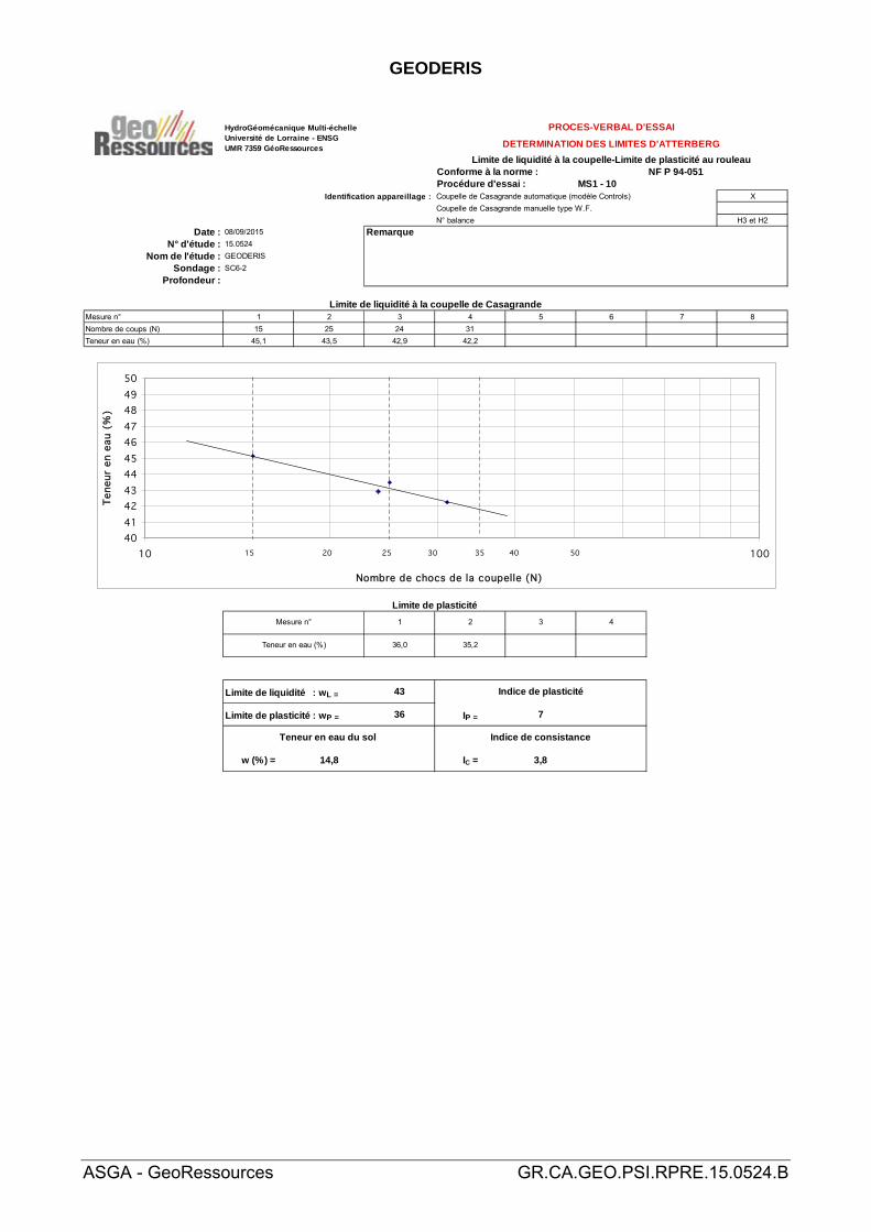
Limite de liquidité : wL = 43
Limite de plasticité : wP = 36 IP = 7
w (%) = 14,8 IC = 3,8
Indice de consistanceTeneur en eau du sol
Limite de plasticité
PROCES-VERBAL D'ESSAI
Limite de liquidité à la coupelle de Casagrande
Indice de plasticité
Mesure n°
Teneur en eau (%)
HydroGéomécanique Multi-échelleUniversité de Lorraine - ENSGUMR 7359 GéoRessources
4041424344454647484950
10 100
Nombre de chocs de la coupelle (N)
Tene
ur e
n ea
u (%
)
15 25 3520 4030 50

GEODERIS
ASGA - GeoRessources GR.CA.GEO.PSI.RPRE.15.0524.B
DETERMINATION DES LIMITES D'ATTERBERG
Limite de liquidité à la coupelle-Limite de plasticité au rouleauConforme à la norme : NF P 94-051Procédure d'essai : MS1 - 10
Identification appareillage : Coupelle de Casagrande automatique (modèle Controls) X
Coupelle de Casagrande manuelle type W.F.
N° balance H3 et H2
Date : 08/09/2015 RemarqueN° d'étude : 15.0524
Nom de l'étude : GEODERIS
Sondage : SC7-9
Profondeur :
Mesure n° 1 2 3 4 5 6 7 8
Nombre de coups (N) 14 17 24 26 33
Teneur en eau (%) 36,4 35,3 34,3 33,9 33,5
15 015 20025 025 20035 035 200
1 2 3 4
29,3 29,2
Limite de liquidité : wL = 34
Limite de plasticité : wP = 29 IP = 5
w (%) = 16,4 IC = 3,7
Indice de consistanceTeneur en eau du sol
Limite de plasticité
PROCES-VERBAL D'ESSAI
Limite de liquidité à la coupelle de Casagrande
Indice de plasticité
Mesure n°
Teneur en eau (%)
HydroGéomécanique Multi-échelleUniversité de Lorraine - ENSGUMR 7359 GéoRessources
3031323334353637383940
10 100
Nombre de chocs de la coupelle (N)
Tene
ur e
n ea
u (%
)
15 25 3520 4030 50

GEODERIS
ASGA - GeoRessources GR.CA.GEO.PSI.RPRE.15.0524.B
Annexe 3 Valeurs au bleu de méthylène
GEODERIS
ASGA - GeoRessources GR.CA.GEO.PSI.RPRE.15.0524.B
DATE
OPERATEUR
N° D'ETUDE
NOM DE L'ETUDE Remarque :
21/08/2015
Teneur en eau initiale
REFERENCES DE L'ECHANTILLON
PTH PTS Ptare w%Masse
échantillon humide
Masse échantillon sec
Volume de solution de bleu
V.B.S.
(g) (g) (g) (g) (g) (cm^3)
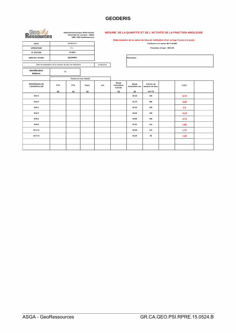
SC4-2 84,16 315 3,74
SC4-4 87,75 295 3,36
SC5-1 62,10 155 2,5
SC5-3 56,25 120 2,13
SC6-2 54,86 150 2,73
SC6-5 67,91 110 1,62
SC7-11 62,68 110 1,75
SC7-13 64,45 85 1,32
Identificationbalance
GEODERIS
H3
Procédure d'essai : MS1-08
15.0524
E.L.
HydroGéomécanique Multi-échelleUniversité de Lorraine - ENSG
UMR 7359 GéoRessources
MESURE DE LA QUANTITE ET DE L'ACTIVITE DE LA FRACTION ARGILEUSE
Détermination de la valeur de bleu de méthylène d'un sol par l'essai à la tache
Date de préparation de la solution de bleu de méthylène
Conforme à la norme NF P 94-06828/08/2015


RAPPORT E2016/027DE – 16ALS21010
Annexe 14 Avis du Dr-Ing E. Pimentel
« Expertise on the damages occurring in the community of
Lochwiller (Alsace) »
15.04.2016

Chair of Underground Construction P.O. Box 133 Stefano-Franscini-Platz 5 CH-8093 Zürich
Expertise on the damages occurring in the community of Lochwiller (Alsace, France)
Bericht 164201 – Zürich, 15.04.2016

2/18
3/18
Table of contents
1 Objective and goal ..................................................................................................... 4
2 Problem description and investigations .................................................................. 4
3 Geology ...................................................................................................................... 9
4 Comparable study cases .......................................................................................... 9
5 Aspects related to the swelling of anhydritic rock .................................................. 9
6 Causes and mechanisms ........................................................................................ 11
7 Recommendations .................................................................................................. 13
References ..................................................................................................................... 17

4/18
1 Objective and goal
The company Geoderis in Metz, France, asked the Chair for Underground Construction with the email from 04. February of this year to prepare an expertise on performed in-vestigations and propositions concerning the swelling problems occurring in the village of Lochwiller, which is located 28 km to the north-west of Strasbourg in France. In the present expertise the two reports prepared by Geoderis (Kimmel et al. 2014 and Kim-mel et al. 2016) are revised and recommendations concerning further investigations and mitigation works presented. A meeting in the offices of Geoderis in Metz and a visit of the site was done on 3rd March 2016.
The essential findings and conclusions of the study performed by Geoderis (see re-ports mentioned above) concerning the interpretation of the geology, including the ori-entation of the Gipskeuper as well as the identification of sections with different stages of swelling, can be confirmed. The extent of these sections results from the interpreta-tion of the exploratory drillings and is plausible. As mentioned in the reports, the cause for the damages is the geothermal drilling on the Kandel property, which disturbed the hydrogeological conditions in the Gipskeuper formation in the vicinity of the borehole. However, one unresolved issue is the course of the groundwater table between the pi-ezometers SC7 and SC5.
The following sections describe the problem at hand and the essential investigations performed (section 2) as well as the geology (section 3). Section 4 summarises similar cases where damage occurred due to geothermal borings in Gipskeuper and describes the applied mitigation works. Some processes and their characteristics related to the swelling of anhydrite and which are deemed relevant for this study (for a better inter-pretation of the results and thus to understand the limitations concerning a prediction of the swelling process) are discussed in section 5. Section 6 focuses on the main causes for the damages and discusses which mechanisms may now prevail in situ. The last section (section 7) lists recommendations for further investigations as well as for miti-gation works.
2 Problem description and investigations
The western border of an older part of Lochwiller holds the residences (from South to North) of the families Schellinger, Schorr, Matjeka, Salin and Ott (see Fig. 1). Bordering these houses the new settlement “Weingarten” was constructed since 2006 on an area which was previously used as a vegetable orchard.
Since 2008, houses from both the older part of Lochwiller as well as the new settlement have experienced various forms of damage. Furthermore, the infrastructure surround-ing the new settlement (e.g. roads, rainwater sewers and drainage pipes as well as streetlamps) was damaged. The cause for these damages was investigated by the company Geoderis and presented in the reports mentioned above (Kimmel et al. 2014

5/18
and Kimmel et al. 2016). The following paragraphs give a short summary of the most important events and findings. Detailed information can be found in the respective re-ports.
In February 2008 a geothermal borehole was drilled on the Kandel property down to a depth of 140 m (see Figs. 1 and 2). Within these works, a pressurized aquifer was en-countered at a depth of 64 m on 19th February 2008. The next day (20th February 2008) the water level within the borehole had risen from a depth of 64 m to 11 m (Ba-bot et al. 2008). After installation of the U-tubes down to 140 m, the gap in the borehole could not be backfilled completely. Roughly one month later, the neighbouring house Schorr experienced some leakage. House Schorr is located at a distance of 18.5 m from the borehole and lies at a lower altitude (13.5 m lower) than house Kandel (see Figs. 1 and 2). In a well located on the Schorr property an elevation of the water level by 5 m was observed. Roughly one month later the geothermal borehole was attempt-ed to be sealed with resin. Due to insufficient verticality of the borehole, solely the up-per section of the borehole could be sealed (two injections were performed at depths of 9 m and 14 m), thus merely inhibiting further leakage in the house Schorr.
The first signs of heaving were observed on cobblestone of the Schorr property in 2008. Since then, a series of steadily increasing damages occurred on a number of houses.
Figure 1. Location of the houses mentioned in the text (copy from Kimmel et al. 2014)

6/18
Figure 2. Sketch of the situation surrounding the Schorr property after the geothermal boring (copy from Babot et al. 2008)
Since 2011 differential levelling measurements were performed. These clearly indicate heaving mechanisms which affect the entire settlement (to a different extent). The max-imal heave measured within a period of 6 months (March 2013 to October 2013) amounted to 25 cm whereas within a period of 16 months (October 2011 to February 2013) a heave of up to 47 cm was measured (Kimmel et al. 2014). This corresponds to an average heave rate of 3 to 4 cm per month. The measured heave is presented in Kimmel et al (2014) as isocurves (Fig. 3). The company Archimed GE performed geo-detic measurements (altimetry and planimetry) of the ground surface every two months from May to October 2013 on survey points positioned in March 2013. Fig. 4 indicates the measured displacement vectors within the x-y-plane for a time span from 7th March to 28th October 2013. According to this, displacements of 13 cm were measured within 7.5 months in the vicinity of the house Belhadj-Kobloth.
Furthermore, two inclinometers were installed (I1 and I2 in Fig. 1). These indicate an inclination towards West which led in both cases to displacements of the inclinometer head by about 2 cm after 4.5 months. The inclination of I2 occurred nearly linearly over the top 12 m whereas the origin of the inclination of I1 cannot be identified (despite the depth of 20 m).
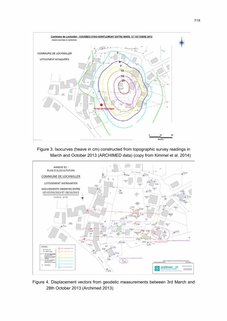
7/18
Figure 3. Isocurves (heave in cm) constructed from topographic survey readings in March and October 2013 (ARCHIMED data) (copy from Kimmel et al. 2014)
Figure 4. Displacement vectors from geodetic measurements between 3rd March and 28th October 2013 (Archimed 2013)

8/18
Additionally, four exploratory boreholes were drilled with core recovery and converted to piezometers (SC4, SC5, SC6 and SC7 in Fig. 1). Selected bore cores were then used for swelling tests in oedometers with a constant axial load. The mineralogy of the bore cores was determined on leftover material from the oedometer samples as well as on other cores. Water was sampled from the piezometers for chemical analysis and de-termination of age. The measured water table in the piezometers SC4, SC5 and SC7 is presented in Fig. 5.
Figure 5. Geological and hydrogeological west-east cross-section - Assumed extent of the swelling and the weathered zone (yellow strata: gypsum, orange: basanite, red: anhydrite, *: intensity of swelling from water temperature measurements) (copy from Kimmel et al. 2016)

9/18
3 Geology
Lochwiller is located on the left bank of the Rheingraben. The known geological for-mations encountered here are clay layers and Triassic layers: middle and lower Gipskeuper, Lettenkohle and Muschelkalk. The Triassic layers dip in Northeast direc-tion with an inclination of 10°. The upper clay layers lie parallel to the topography (hill) and feature a thickness of roughly 2 m. They are characterised on the one hand by a small permeability, on the other hand by a strong sensitivity to water, i.e. the strength of the clay decreases when it comes into contact with water. The layers of the Gipskeuper can be divided into three sections, based on their swelling potential (from top to bot-tom): a leached section, a fully swollen section and unaltered Gipskeuper. In the leached and swollen layers a complete transformation from anhydrite to gypsum al-ready took place. These sections are referred to as the “altered zone” in the report. The difference between the swollen and the leached layer is that the latter experienced ad-ditional dissolution of gypsum due to water circulation. The border between the swollen and the unaltered Gipskeuper is referred to as the “anhydrite level”.
4 Comparable study cases
Comparable damage cases in connection with geothermal borings have been reported from Staufen and Böblingen in Germany (Engesser et al. 2010 and Koch et al. 2015). Similar to Lochwiller, the geothermal boring of 2007 in Staufen punctured a deeper ly-ing pressurized aquifer which resulted in a watering of the above lying Gipskeuper con-taining anhydrite. The maximal measured heave rate was 1.1 cm/month. In the case of Böblingen the water infiltrated through the geothermal borehole to the anhydritic Gipskeuper below. In both cases a number of houses were damaged due to the heave and the heave process is so far not completed.
In Staufen the boreholes (EWS1 to EWS7) were sealed via postgrouting and water is now being pumped continuously since 2010 in order to lower the groundwater level within the anhydritic layer. So far these measures merely led to a retardation of the heave process.
In Böblingen the boreholes (EWS1 and EWS2) were postgrouted multiple times be-tween 27th October 2014 and 28th January 2015. Measurements performed via satel-lites show a retardation of the swelling process here as well.
5 Aspects related to the swelling of anhydritic rock
Swelling of anhydritic rock occurs due to transformation of anhydrite to gypsum. How-ever, the mineralogical analysis of the bore cores indicates sulphate to be present in the form of basanite (CaSO4 x 0.5H2O) as well, in addition to anhydrite (CaSO4) and
10/18
gypsum (CaSO4 x 2H2O). Basanite is metastable and usually not encountered in situ, with the exception of very arid regions (cf. Pagliai & Stoops 2010).
During sample preparation for X-ray diffractometry (abbr. XRD) the samples need to be dried. If this occurs at temperatures above ca. 60°C, it is possible that the gypsum (or a part of it) transforms to basanite through loss of bound water molecules. This can also occur during sample preparation of thin sections (generation of heat during polishing). Neither our investigations with Gipskeuper of the Belchen- and Chienbergtunnels, nor the investigations in Staufen and Böblingen showed the presence of basanite (Engesser et al. 2010 und Koch et al. 2015)1. Therefore, it is strongly assumed that the measured amount of basanite was in fact originally gypsum. The correction of the re-sults need to be performed by considering the stoichiometry of the different minerals, i.e. the mass of 1.5 water molecules need to be added to a basanite molecule in order to obtain the mass of a corresponding gypsum molecule.
The properties of the swelling behaviour of anhydritic rock presented in the report of Kimmel et al (2014) stem from research performed by Nagra (National Cooperative for the Disposal of Radioactive Waste) and are based on results of a limited number of ex-periments. Therefore, they cannot be assumed to be generally applicable. Further re-search needs to be taken into consideration, such as e.g. Pimentel (2003a), who measured swelling pressures higher than 8 MPa on samples from the Gipskeuper sur-rounding the Freudensteintunnel. He also measured swelling strains over 30% with samples which were axially loaded with 3 MPa. These swelling strains cannot be at-tributed solely to the anhydrite to gypsum transformation, since the anhydrite content was ca. 20%. Based on observations he made on a number of samples, Pimentel in-troduced a concept of cracking due to gypsum crystallisation (Pimentel 2003b, 2007) where a gypsum crystal can cause the surrounding structure to fracture. The swelling of anhydrite in situ can therefore be accompanied by the formation of cracks or fissures which lead to new water routing through the rock and thus increase the surface of an-hydrite in contact with water. This in return leads to further anhydrite dissolution and gypsum precipitation due to supersaturation of the dissolved sulphates in the pore with respect to gypsum. The gypsum crystals will form mainly in the existing pore space and thus begin to fill the pores. When these are filled, further gypsum precipitation will occur primarily in the direction of smallest stress (as long as this stress is not too high, cf.
1 During first investigations performed by the authors, basanite was identified with XRD on samples from the Belchentunnel, however upon repetition with an improved sample preparation procedure it was found that no basanite was in the samples and the previously measured amount of basanite corresponded to the amount of gypsum measured during the re-run (cf. An-agnostou et al. 2016).
11/18
Serafeimidis et al. 2014) and cause a crack or fissure in the rock perpendicular to that direction. This leads to newly formed larger pores and the increase in total volume will be markedly higher than the theoretical increase in volume of the single molecules (i.e. from anhydrite to gypsum). Thus, it is not possible to predict the swelling strains based solely on the mineralogical composition of the rock. Furthermore, it is not possible to assume a maximal swelling pressure based one the experiments performed by Georesources, i.e. to apply an axial load on a sample in an oedometer cell, induce swelling by inundating the sample with water and after swelling apply an axial load high enough to reverse the deformation. This can only work if the processes are reversible as in the case of elastic material behaviour. The best way to obtain the maximal swell-ing pressure is by running swelling tests under completely constrained conditions (c.f. Pimentel 2007).
It needs to be pointed out, however, that the upscaling of laboratory results from swell-ing experiments to the scale of a geotechnical structure in situ is a so far unsolved problem in geotechnical engineering. This concerns the interpretation of maximal swell-ing stresses, swelling strains as well as the development of the involved processes (ki-netics) in terms of time. The reason for these uncertainties can be attributed to the nat-ural heterogeneity of the Gipskeuper before swelling, the formation of cracks and fis-sures and changes in water circulation and water chemistry in the rock (among other factors).
Due to the above mentioned uncertainties, it is not possible to predict the course of the swelling process over time as well as the effect of potential mitigation measures (also not after performing additional laboratory investigations). An extrapolation of the results from in situ measurements merely allows an estimation of the behaviour to be expected in the near future (e.g. heaves or displacements).
6 Causes and mechanisms
Prior to the boring performed on the Kandel property, no signs of damage were ob-served in the affected area. Therefore, the above mentioned leakage in the house Schorr as well as the damages on other houses and the measured heave can only be related to the 140 m deep boring on the Kandel property. Following the boring, the wa-ter infiltrated the unaltered Gipskeuper and thus triggered the swelling mechanism, which led to the damages (starting with the leakage and heave of the cobblestone on the Schorr property). The attempt to seal the boring may not have been beneficial, since merely the upper section of the borehole was injected and thus nearly the entire length of the borehole within the Gipskeuper remained filled with pressurized water from the lower layer. This may have led to “favourable” groundwater infiltration in the unaltered Gipskeuper. It needs to be noted that the maximal swelling stress expected

12/18
from Gipskeuper exceeds the in situ stress from the overburden (which is ca. 1 MPa at an overburden of 40 m).
The estimated extent of the currently active zone within the unaltered Gipskeuper is il-lustrated in Fig. 5. This estimation is based on the interpretation of the borehole profiles as well as on measurements of the displacements at the surface and is considered plausible. A more accurate knowledge of the active swelling zones in greater depth re-quires displacement measurements of the ground, i.e. within the Gipskeuper.
The anhydrite level runs more or less parallel to the ground surface and not to the strat-ification (Fig. 5). Therefore, it is assumed that - in the past - the water which caused the formation of the altered Gipskeuper section originated from the surface. The upper lay-er of clay then formed on top of the Gipskeuper and served as a protective layer against further leaching and swelling. This layer is now being damaged by the swelling process (vertical cracks along the surface).
The displacement measurements at the surface indicate that the higher part of the set-tlement experiences the largest vertical heave as well as horizontal displacement.
These horizontal displacements may occur due to the following reasons: (a) the anhy-drite layer did so far not swell evenly, but preferentially in one area (i.e. near the south-eastern corner of house Belhadj-Kabloth) thus creating a “hill” with some radial defor-mation around the area of strongest activity; (b) since the horizontal stress in situ is smaller or similar to the vertical stress, swelling may occur in horizontal direction as well; (c) the vertical heave can cause sliding of the top layers of the slope. Such a slid-ing exerts an earth pressure on structures, which is particularly assumed to cause the damage of the house Schmitz (see Fig. 1). Due to the uneven heave, in combination with the above mentioned horizontal displacements of the ground, cracks develop along the surface (an indication for vertical cracks of the surface can be found next to the house Amann and along the street “impasse Koelberg”), allowing water from pre-cipitation to infiltrate both into the upper layers (thus soften the soil and cause or accel-erate landslides) as well as into the lower Gipskeuper. Softening of the upper layers in-creases the earth pressure on the structures (especially when strong rainfalls occur) which, therefore, results in additional damage to some houses. This could also affect some of the older houses at the foot of the slope. Furthermore, the vertical cracks along the surface as well as the damages to the rainwater sewers facilitate the infiltra-tion of rain water in the leached Gipskeuper and subsequently into the unaltered Gipskeuper, leading to a stronger development of the swelling process. This could ex-plain the connection between the amount of rain water and the rate of deformation, i.e. the percolation of rain water can cause landslides and / or accelerate the swelling pro-cess. However, these mechanisms cannot be recorded and identified alone with dis-placement measurements on the surface. The only way to identify the active mecha-nisms is with deformation measurements in the ground.

13/18
The groundwater table between the piezometers SC4 and SC5 may be supplied by the geothermal boring. It is questionable whether the measured water level of SC7 belongs to the same aquifer as that in SC5 and how the course of the groundwater table runs between these two piezometers. If they are in fact connected, the main source for the groundwater is actually rain water (and not primarily from the geothermal drilling, as so far assumed), with a main seepage flow from east to west. Based on this assumption, the water level in SC5 would need to be higher than that in SC4.
Dissolution (i.e. leaching) of gypsum occurs in the already swollen section of the Gipskeuper under the influence of seepage flow. This was seen e.g. at the Schanztun-nel in Germany, where seepage flow occurred parallel to the tunnel axis. After roughly 110 years the swollen Gipskeuper contained no more gypsum, whereas 10 m below the invert the rock still contained anhydrite. For the moment - and as long as there is no strong seepage flow in the unaltered zone - leaching of gypsum is considered a sec-ondary problem.
A termination of the entire swelling process can only be expected when either the swelling potential is completely exhausted or when the new aquifer experiences no fur-ther water supply and the free water in the aquifer is drained. The former can last for decades (no final statement can be made concerning the expected duration of the swelling process) and range over the entire anhydritic Gipskeuper and thus affect the majority of Lochwiller. The damages could be so severe, that an extensive part of the village may necessitate demolition. Since the swelling process in the unaltered Gipskeuper is triggered by the water in the new aquifer, a complete sealing of all water routing towards the new aquifer and drainage of the aquifer would be necessary. Each measure toward an effective reduction of the water supply of the new aquifer could re-tard the swelling processes. As indicated previously, there is a causal connection be-tween the ground water from the geothermal borehole, rainfall and the swelling heave. As discussed above, the infiltration of rain water into the unaltered section of the Gipskeuper can be accelerated by the cracks occurring due to swelling heave of the surface. An increase in water infiltration will, in return, favour the swelling process. In order to undermine this vicious cycle, as much water as possible (groundwater as well as rain water) needs to be withheld from the unaltered zone.
7 Recommendations
In Kimmel et al. 2014 the following recommendations were proposed:
• taking urgent measures concerning the sealing of the underground pipework, to eliminate all surface water intake;
• a perfect sealing of the boreholes, to control the influx of deep groundwater, by performing a re-drilling and concreting under high pressure;
14/18
• evaluation of the remaining anhydrite and the nature of the groundwater, in order to confirm the origin of the swelling process by drilling down to the base of Gipskeuper (approx. 40m);
• the resumption of levelling measurements and an extension of the network of measurements, which appears to be insufficient to date;
• identification of similar geological configurations as vigilance for future projects in this very sensitive subsurface environment.
We generally agree with these recommendations. As seen in comparable study cases (cf. section 4) the immediate measures need to focus on the mitigation of further swell-ing. By applying, observing and assessing the efficiency of the mitigation measures, the heave rate can be slowed down (i.e. buying more time) and additional in situ infor-mation can be gained for the planning of further measures (e.g. concepts for additional monitoring, drainage and/or further grouting). However, a complete suppression of the active swelling processes can most likely not be achieved, as was also seen in various cases of damage in tunnelling (e.g. Belchen- and Chienbergtunnels in Switzerland). Furthermore it is not possible to predict the evolution of the swelling process and the ul-timate effect of the mitigation measures (cf. section 5).
The following paragraphs elaborate the above mentioned measures and contain sug-gestions for additional possible measures.
a) A sealing of the geothermal boring via grouting needs to occur consequently below the anhydritic Gipskeuper, i.e. in the layers of the Lettenkohle and Muschelkalk. A sealing of the borehole above these layers (i.e. within the Gipskeuper) would not be advantageous, since the new aquifer could then still be supplied with groundwater from the borehole. However, this necessitates grouting under the high water pressures pre-vailing at that depth (ca. 5 bars at 50 m water column or more). For this reason the use of a packer is recommended. The packer would need to be placed and inflated in the old borehole within the section of the Lettenkohle. This requires the precise location of the old borehole within the Lettenkohle or a complete radial overcut of the borehole.
b) In addition to the restoration of damaged rainwater collecting pipes, all further defect pipelines (such as sewers or drinking water pipelines) should always be repaired immediately. Furthermore, all open cracks in the terrain should be filled and sealed with clayey material, so that rain water flows unhindered into the rainwater collecting pipes (i.e. without any infiltration in the ground).
c) An additional retardation of the swelling process can be accomplished by drain-ing the free water in the new aquifer. Due to the topography this can only be achieved by pumping the water. In order to dimension an efficient pumping system, this measure should only be started after grouting of the bore hole is completed and the course of the groundwater table in the new aquifer is known (see “e”).
15/18
d) In order to gain a better understanding of the various deformation processes (e.g. the identification of the active swelling zones in the rock mass or the distinction between horizontal displacements due to swelling or due to landslide) as well as to de-termine the effectiveness of the sealing measures from an early stage on, displace-ment measurements in all three directions (x/y/z) need to be collected at a greater depth. It is therefore recommended to incorporate at least three TRIVEC-borings in the above mentioned measuring program. The TRIVEC system is a combination of one micrometer and two inclinometers and enables measuring deformations in all three di-rections at every meter of the entire bore hole (Amstad et al. 1988). The TRIVEC-borings should pierce the entire unaltered Gipskeuper (while avoiding water to infiltrate the Gipskeuper) and reach all the way into the Lettenkohle. It would be advantageous, if the flushing of the borings were performed with the use of swelling inhibitors. The recommended positions for the TRIVEC-borings TV1 to TV3 are sketched in Fig. 1.
e) Due to the importance of the (uncertain) course of the groundwater table be-tween the piezometers SC7 and SC5 and the consequences this groundwater table could imply for the selection and dimensioning of the measures, this assumed course needs to be confirmed. This can be achieved by drilling additional bore holes and de-veloping them to piezometers. In order to investigate the so far uncertain hydraulic connection between the existing piezometers, at least one additional piezometer (SC8) is necessary between SC7 and SC5 (see Fig. 1). A hydraulic connection can be identi-fied by pouring tracers e.g. in SC7 and measuring the arrival of the tracers in the sur-rounding piezometers (assuming that a hydraulic gradient exists between SC7 and the surrounding piezometers). This allows the identification and estimation of seepage flow in the ground. Should seepage flow be detected, it needs to be determined whether the flow runs along preferential layers, in order to design sealing or drainage measures more efficiently.
f) Further exploratory drillings in the older part of the town will facilitate an exact mapping of anhydrite level, i.e. the identification of leached, unleached and intact Gipskeuper, and therefore determine under which buildings the swelling potential is exhausted. It is crucial, however, that the Lettenkohle is not punctured by these bor-ings. Since the leached Gipskeuper is more porous than the intact Gipskeuper, the former does not behave as an impermeable layer and does not prohibit water circula-tion.
f) Due to the questionable identification of basanite during the mineralogical anal-ysis (XRD), the repetition of XRD on at least one sample is recommended, whereas the sample may not be subjected to temperatures >60°C during sample preparation. When the assumption, that the basanite occurred due to faulty sample preparation, is verified and the amount of gypsum corresponds to the erroneously measured basanite, the other (existing) results can be corrected considering the stoichiometry of the different minerals (cf. section 5).

16/18
g) Additional swelling tests under completely constrained conditions would give an indication of the maximal swelling pressure and thus add to a thorough characterisation of the ground and resolve uncertainties from a scientific point of view. However, it is expected that the maximal swelling pressure is far higher than the pressure from the overburden. Since a restraining counter pressure (as is common, e.g., in tunnelling where heavy anchoring or a stiff lining is applied) is not an applicable measure in this case, the determination of the maximal swelling pressure with laboratory experiments will not provide a practical relevance for the planning of further mitigation measures.
h) Buildings, which show severe damage and where the safety is endangered, should be rehabilitated immediately. As long as the swelling process cannot be stopped, and thus no new equilibrium reached, no further building should be construct-ed in the active swelling zone. Even with a retardation of the swelling process it is only a matter of time, until new buildings are subjected to damage. This also applies to re-mediation measures on existing buildings.
Zürich, 12.05.2016
Dr.-Ing. Erich Pimentel MSc ETH Civ Eng Tara Wanninger-Huber
17/18
References
Amstad Ch., Koeppel J., Kovári K. (1988): TRIVEC-measurements in geotechnical en-gineering. Proc. 2nd Int. Symp. on Field Measurements in Geomechanics. Eds. Sakurai, Balkema. Rotterdam, p. 17-32.
Anagnostou G., Serafeimidis K., Pimentel E., Wanninger-Huber T., Vrakas A. (2015): Modelling of anhydritic swelling claystones. Forschungsprojekt FGU 2010/007 auf An-trag der Arbeitsgruppe Tunnelforschung (AGT), 1539.
Archimed GE (2013): Rapport d’Auscultation n°04 du 14/11/2013 – Commune de Lochwiller - Lotissement Weingarten.
Babot Y., Schomburgk S. Elsass P. (2008): Expertise des venues d’eau chez Monsieur schorr 13 rue de l’Etang à Lochwiller (67) – Visite du 02 juin 2008. BRGM/ALSNT08N13, juin 2008
Engesser W., Ruch C., Wirsing G. (2010): Geologische Untersuchungen von Bau-grundhebungen im Bereich des Erdwärmesondenfeldes beim Rathaus in der histori-schen Altstadt von Staufen i. Br. Sachstandbericht Az.: 94-4763//10-563, Landesamt für Geologie, Rohstoffe und Bergbau (LGRB), Freiburg.
Kimmel M., Frank C., Hadadou R. (2014): Avdice on the causes of damage occurring in the community of Lochwiller (67). Geoderis, Report E2014/003DE – 14ALS3301.
Kimmel M., Hadadou R. (2016): Evaluation of the residual swelling potential of evapo-rites to the right of the Weingarten residential area in Lochwiller (Lower Rhine) – Pro-ject Version. Geoderis, Report E2016/027DE_PROJECT – 16ALS21010.
Koch A., Martin M., Prestel R., Ruch C., Sage A., Trapp Ch. (2015): Geologische Un-tersuchungen von Baugrundhebungen im nordöstlichen Stadtgebiet von Böblingen (Hebungsgebiet “Nord”). Sachstandbericht Az.: 95-4764//15-7202, Landesamt für Geo-logie, Rohstoffe und Bergbau (LGRB), Freiburg.
Pagliai M., Stoops G. (2010): Physical and biological surface crusts and seals in Inter-pretation of micromorphological features of soils and regoliths. Eds. Stoops G., Mar-celino V., Mees F., Elsevier, Ch. 19, p. 419-435.
Pimentel E. (2003a): Langzeitschwellversuche an Probenmaterial aus dem Freuden-steintunnel. Zwischenbericht für den Zeitraum 0.1.01.2001–01.10.2003. Bericht des Lehrstuhls der Universität Karlsruhe, erstattet an die DB Projekte Süd GmbH.
Pimentel E. (2003b): Swelling behavior of sedimentary rocks under consideration of micromechanical aspects and its consequences on structure design. Geotechnical Measurements and Modelling. Proc. intern. symp. Karlsruhe, Germany, 23-26 Sept. 2003: pp. 367-374. Lisse: Balkema.

18/18
Pimentel E. (2007): A laboratory testing technique and a model for the swelling behav-ior of anhydritic rock. The second half century of rock mechanics; 11th Congress of the International Society for Rock Mechanics (ISRM), Lisbon; Volume 1, 143-146; Taylor & Francis Group London.
Serafeimidis, K., Anagnostou, G., Vrakas, A. (2014): Scale effects in relation to swell-ing pressure in anhydritic claystones. Int. Symp. on Geomechanics from micro to mac-ro. University of Cambridge.