a gelindo et teresina -...
TRANSCRIPT


A Gelindo et Teresina


Ceux qui ont commence a apprendre enchaınent les formules, mais
n’en savent pas encore le sens ; car il faut qu’elles murissent avec
nous. Or c’est la une chose qui demande du temps.
Aristote, Ethique a Nicomaque.
〈〈 Prendre son vol 〉〉 chaque jour ! Au moins un moment qui peut
etre bref, pourvu qu’il soit intense. Chaque jour un 〈〈 exercice
spirituel 〉〉 — seul ou en compagnie d’un homme qui lui aussi veut
s’ameliorer.
Exercices spirituels. Sortir de la duree. S’efforcer de depouiller tes
propres passions, les vanites [. . . ] Depouiller la pitie et la haine.
Aimer tous les hommes libres. S’eterniser en se depassant.
Georges Friedmann, La Puissance et la Sagesse ().


Table des Matieres
Remerciements . . . . . . . . . . . . . . . . . .
Introduction . . . . . . . . . . . . . . . . . . .
Un peu d’histoire . . . . . . . . . . . . . . . . .
L’analyse harmonique des fonctions sur les espaces hyperboliques . .
Presentation des resultats . . . . . . . . . . . . . . .
Bibliographie pour l’introduction . . . . . . . . . . . .
Analyse harmonique des formes differentielles sur l’espace hyper-
bolique reel (Harmonic analysis for differential forms on real hyper-
bolic spaces) . . . . . . . . . . . . . . . . . . .
(Cette prepublication comprend sa propre table des matieres, p. , une bibliographie,
p. , un index des notations, p. , et un index des sujets, p. .)


Remerciements
Je souhaite remercier vivement les personnes suivantes de participer au jury de
ma these :
— Jean-Louis Clerc, qui me fait l’honneur et la sympathie de presider le jury ;
— Erik van den Ban et Francois Rouviere, qui ont accepte la penible tache d’etre
rapporteurs ;
— Pierre-Yves Gaillard, Noel Lohoue et Robert Stanton, qui contribuent a ce
jury en tant qu’examinateurs.
C’est avec un enthousiasme sincere que je voudrais egalement exprimer a Jean-
Philippe Anker ma profonde gratitude. Je sais que sa modestie legendaire en souffrira,
mais je tiens a rendre hommage au directeur de these competent, disponible, encou-
rageant et amical qu’il fut pour moi durant ces quatre annees d’apprentissage de
la pensee mathematique (cf., a ce propos, l’epigraphe d’Aristote). Si je ne fus sans
doute pas le disciple reve, Jean-Philippe excella en revanche dans sa charge de Maıtre,
c’est-a-dire dans la mise a disposition genereuse de son savoir. J’ai parfois quelque
scrupule a penser que ce don restera, par nature, sans reciproque.
Mon travail de these a pu profiter de diverses conversations fructueuses avec,
notamment, Pierre-Yves Gaillard, Toshiyuki Kobayashi, Robert Stanton et tout par-
ticulierement Roberto Camporesi. Qu’ils en soient chaleureusement remercies.
Je veux aussi souligner les excellentes conditions de travail dont j’ai beneficie au
sein de l’Institut Elie Cartan. Grace a l’amitie de quelques-uns et a la gentillesse
de beaucoup d’autres, l’insertion dans cette micro-communaute me fut grandement
facilitee. Je pense notamment a Jean-Philippe Anker, Jean-Louis Clerc, Christelle
Defosse, Jean-Claude Fort, Didier Gemmerle, Dominique Manchon, Nathalie Pierache,
Elisabeth Rouy, Andre Stef, Gerald Tenenbaum, Charles Torossian et, last but not
least, au futur grand bridgeur et neanmoins ami, Alain Fuser.
La formation de l’esprit et de l’ame d’un jeune chercheur ne resulte pas que
d’une confrontation active et repetee avec l’objet de ses recherches. Participent tout

autant au developpement d’un imaginaire createur la contemplation des œuvres d’art
et les interactions complexes et passionnantes avec des etres doues de pensee et de
sentiments. Il n’y a aucun sens a remercier de tels etres de leur amitie ou de leur amour
— pas plus que de remercier un artiste d’avoir cree ; j’aimerais cependant adresser
une pensee tres affectueuse a toutes celles et tous ceux qui m’ont fait don d’une part
d’eux-memes. En premier lieu, ma famille, et notamment mes parents, dont le soutien
est genereux et sans conditions depuis toujours. Mais egalement Agnes et Didier,
Bertrand, Catherine, Etienne, Francis, Francois, Fred, Helene et Vincent, Isabelle et
Christian, Marie, Nicolas, Sara et Joel, ainsi que les passeurs aupres desquels j’ai
trouve l’inspiration de la Muse Euterpe, Jean-Michel, Mederic et Pierre.
Enfin, je songe avec reconnaissance a certains professeurs de mathematiques qui,
depuis 1988, m’ont donne le gout de cette science amusante et ensorcelante, et m’ont
encourage a en explorer modestement quelques arcanes.

Introduction
Un peu d’histoire
L’analyse harmonique est nee au milieu du dix-huitieme siecle du desir de resoudre
l’equation aux derivees partielles
∂2y
∂x2=
1
c2
∂2y
∂t2
fournie par le probleme de 〈〈 la corde vibrante 〉〉. Des mathematiciens tels que d’Alem-
bert, Euler, Bernoulli et Parseval decouvrirent peu a peu que la solution d’une telle
equation differentielle pouvait s’exprimer a l’aide de series trigonometriques. Il fallut
cependant attendre le debut du siecle suivant pour qu’avec Fourier et ses travaux sur
la diffusion de la chaleur soit correctement formalise le principe de la decomposition
d’une fonction en serie ou integrale de fonctions trigonometriques 〈〈 elementaires 〉〉.
Rappelons qu’une fonction convenable sur l’intervalle [−π, π] se decompose en series
de Fourier comme
f(x) =∑
n∈Z
einxf(n), (0.1)
ou f(n) = 12π
∫ π
−πdx e−inxf(x), et qu’une fonction definie sur la droite reelle se
decompose sous certaines conditions comme
f(x) =
∫
R
dy e2iπxy f(y), (0.2)
ou la fonction y 7→ f(y) =∫
Rdx e−2iπxyf(x) est la transformation de Fourier de f .
Ce furent les premiers exemples d’une theorie qui n’allait cesser de se developper.
Il est desormais bien connu que sous le principe de decomposition introduit par
Fourier se cache l’action d’un groupe G — respectivement le cercle R/2πZ et la droite
R dans les exemples ci-dessus — sur l’espace L2(G) des fonctions de carre integrable
sur G. Dans ce sens, les fonctions x 7→ einx (n ∈ Z) et x 7→ e2iπxy (y ∈ C) peuvent
etre vues commes les caracteres respectifs des groupes abeliens R/2πZ et R, c’est-
a-dire les homomorphismes (continus) de ces groupes dans le corps multiplicatif C∗.
Ainsi les decompositions (0.1) et (0.2) se generalisent-elles a tous les groupes abeliens
finis ou localement compacts. Par exemple, si G est un groupe abelien localement
compact, et si G designe l’ensemble des caracteres unitaires (i.e. de norme 1) de
G [1], la transformation de Fourier d’une fonction f sur G se definit par
f(χ) =
∫
G
dx χ(x)f(x) (0.3)
pour tout χ ∈ G, dx etant une mesure de Haar normalisee sur G. Weil a montre en
1940 qu’il existe une mesure de Haar dν(χ) sur G, appelee couramment mesure de
Plancherel, telle que pour toute f ∈ C(G) ∩ L1(G) verifiant f ∈ L1(G),
f(x) =
∫
G
dν(χ) χ(x)f(χ). (0.4)
La formule de Plancherel(-Parseval) ‖f‖2L2(G) = ‖f‖2
L2(G)en decoule, et ainsi la
transformation de Fourier s’etend en une bijection de L2(G; dx) sur L2(G; dν(χ)).
Lorsque le groupe G n’est plus commutatif, il devient necessaire de considerer des
generalisations pluridimensionnelles des caracteres : les representations du groupe.
Une representation (continue) π d’un groupe localement compact G sur un espace
de Hilbert H est un homomorphisme (continu) de G dans le groupe GL(H). Ainsi
les caracteres precedemment introduits sont-ils des representations de dimension un,
la dimension d’une representation etant par definition la dimension (complexe) de
l’espace de Hilbert qui lui est associe. Une representation (π,H) sera dite unitaire
si chaque π(x) est un endomorphisme unitaire, et irreductible si H ne contient
pas de sous-espaces π(G)-invariants non triviaux. Mautner et Segal ont demontre
(independamment) en 1950 la formule de Plancherel pour la classe relativement
generale des groupes localement compacts 〈〈 unimodulaires 〉〉 et 〈〈 de type I 〉〉 (nous
ne desirons pas expliciter ici ces notions). Notamment, la formule d’inversion (0.4)
reste valable, sachant que f(π) est une matrice et que G designe alors l’ensemble des
(classes d’equivalence de) representations unitaires continues irreductibles de G.
Cependant, cette belle theorie reste abstraite dans la mesure ou elle ne decrit ni la
partie du dual unitaire G (si toutefois G est lui-meme connu) intervenant dans (0.4),
[1] En realite, G est egalement un groupe abelien localement compact (appele dual unitaire de
G).

ni la mesure de Plancherel dν(π). Il a fallu pres de vingt-cinq ans a Harish-Chandra
pour parvenir a les rendre explicites dans le cas des groupes de Lie (i.e. munis d’une
structure de variete differentiable) (essentiellement) semi-simples, ses efforts culmi-
nant dans les articles memorables [HC75, HC76a, HC76b]. Ce type de groupe entre
dans la categorie etudiee par Mautner et Segal, et de nombreux groupes de matrices
en fournissent des exemples classiques, comme les groupes speciaux lineaires, certains
groupes d’isometries associes a une forme quadratique, les groupes symplectiques, etc.
Nous n’insistons pas davantage sur la theorie generale de l’analyse harmonique
et ses liens avec la theorie des representations. Pour un historique plus detaille et
de nombreuses references, voir le tres bel expose [Kna96a, Kna96b]. Nous allons
maintenant nous concentrer sur le cadre semi-simple, et plus exactement sur l’un de
ses aspects particuliers.
L’analyse harmonique des fonctions sur les espaces hyperboliques [2]
Supposons dorenavant que G est un groupe de Lie reel semi-simple, connexe, non
compact et de centre fini, et soit K un sous-groupe compact maximal de G. Il est
bien connu qu’il existe alors un sous-groupe abelien A ' Rr de G tel que G ' KAK :
c’est la decomposition de Cartan de G, et l’entier r est appele rang reel de G. De
plus, le quotient G/K est une variete riemannienne, symetrique (en un certain sens
geometrique), de type non compact (i.e. de courbure de Ricci negative) et de rang r
(ce qui signifie que r est la dimension maximale des sous-varietes plates totalement
geodesiques de G/K). La decomposition de l’espace L2(G/K) resulte alors de celle
de L2(G) etablie par Harish-Chandra, en remarquant simplement qu’une fonction sur
G/K s’identifie a une fonction K-invariante a droite sur G [3]. Introduisons quelques
notations afin d’etre plus explicite.
Pour simplifier, placons-nous tout de suite dans le cadre auquel nous nous res-
treindrons presque toujours dans notre travail de these, celui ou G/K est de rang
un. Ainsi A ' at, t ∈ R, et G/K est necessairement l’un des quatre espaces hyper-
boliques Hn(R), Hn(C), Hn(H), H2(O) ; par exemple, Hn(R) ' SOe(n, 1)/SO(n),
Hn(C) ' SU(n, 1)/S(U(n)×U(1)). Par ailleurs, nous savons que G est diffeomorphe
[2] Les references classiques pour ce qui suit sont [Hel78, Hel84, Hel94], [Far82], [Koo84], [GV88].[3] En fait, la formule de Plancherel sur L2(G/K) preceda la formule de Plancherel sur L2(G)
d’une dizaine d’annees.

au produit KAN , ou N est un sous-groupe nilpotent (ou abelien dans le cas reel) de
G (c’est une decomposition d’Iwasawa de G). Notons H la projection de G = KAN
sur A definie par H(g) = t si g = katn, k la projection de G = KAN sur K, g
et a ' R les algebres de Lie respectives de G et A, gC et aC leurs complexifiees, et
soit M le centralisateur de A dans K. Le quotient K/M s’identifie naturellement
(comme variete) au bord de l’espace hyperbolique G/K, i.e. a la sphere unite dans
Fn si G/K = Hn(F).
Nous allons d’abord donner dans ce nouveau contexte l’analogue des caracteres
x 7→ e2iπxy et x 7→ χ(x) intervenant respectivement dans (0.2) et (0.4). Nous avons
mentionne plus haut que la generalisation de la notion de caractere (unitaire) au cadre
non abelien etait celle de representation (unitaire, irreductible). Cependant, seules
certaines representations de G vont intervenir dans la definition de la transformation
de Fourier sur G/K et jouer un role pour la formule de Plancherel. Voyons lesquelles.
Soit P = MAN (P est un sous-groupe, dit parabolique, de G), et pour λ ∈ a∗C' C,
definissons un caractere χλ de P par
χλ(matn) = eiλt.
On obtient alors une representation πλ de G en 〈〈 induisant 〉〉 le caractere χλ de P au
groupe tout entier. Sans entrer dans les details d’une telle construction, disons que
πλ agit sur l’espace L2(K/M) par :
πλ(x)f(kM) = e−(iλ+ρ)H(x−1k)f(k(x−1k)M),
ou ρ = d2 (n + 1)− 1 si G/K = Hn(F) et d = dimR F (en realite, ρ a une signification
algebrique). Les representations πλ sont appelees series principales spheriques de G ;
elles sont unitaires si λ est reel, et generiquement irreductibles.
Nous pouvons maintenant definir la transformation de Fourier d’une fonction f sur
G/K : pour kM ∈ K/M , λ ∈ C, on pose
H(f)(λ, kM) =
∫
G
dx πλ(x)1K/M(kM) f(x)
=
∫
G
dx e−(iλ+ρ)H(x−1k)f(x), (0.5)
ou dx est une mesure de Haar sur G convenablement normalisee (mais l’integration
peut aussi se faire sur G/K). Remarquons que kM 7→ H(f)(λ, kM) ∈ C∞(K/M) si
par exemple on suppose f ∈ C∞c (G/K). Le theoreme de Plancherel s’enonce alors de
la maniere suivante.

Theoreme 0.1. Normalisons la mesure d(kM) sur K/M de telle sorte que le volume
total soit egal a 1. Alors :
(i) Il existe une mesure dν(λ) sur R telle qu’on ait la formule d’inversion
f(x) =
∫
K/M
d(kM)
∫ ∞
0
dν(λ)e(iλ−ρ)H(x−1k)H(f)(λ, kM) (0.6)
pour toute fonction f ∈ C∞c (G/K).
(ii) La transformation de Fourier H s’etend en une isometrie bijective de L2(G/K)
sur L2([0,∞[×K/M ; dν(λ)d(kM)).
La mesure de Plancherel dν(λ) est bien connue : elle s’exprime sous la forme
dν(λ) = cst dλ |c(λ)|−2,
ou c est la fonction de Harish-Chandra explicitement donnee par la formule de
Gindikin-Karpelevic en termes de fonctions Γ d’Euler :
c(λ) =Γ(dn − 1)
Γ(dn−12 )
Γ(iλ)
Γ(iλ + d(n−1)2 )
Γ( iλ2 + d(n−1)
4 )
Γ( iλ2 + d(n−1)
4 + d−12 )
,
et ou dλ designe la mesure de Lebesgue sur R.
Diverses methodes permettent d’aboutir a la demonstration du Theoreme 0.1. L’une
d’elles consiste a se ramener a l’analyse spherique sur G/K, c’est-a-dire a l’analyse de
Fourier des fonctions radiales (ou bi-K-invariantes) sur G. Cette demarche presente
en outre l’interet d’avoir de nombreuses applications, telles que la resolution d’equa-
tions aux derivees partielles classiques (equations des ondes, de la chaleur, etc.) ou
la 〈〈 formule des traces 〉〉 de Selberg. Pour finir ce paragraphe, nous en donnons les
principaux resultats.
Considerons donc dorenavant les fonctions bi-K-invariantes sur G, i.e. telles que
f(k1xk2) = f(x) (∀x ∈ G,∀k1, k2 ∈ K).
De telles fonctions sont egalement appelees radiales, puisque la decomposition de
Cartan G = KAK permet de se restreindre a des calculs sur A ' R. Si F (G) est un
espace fonctionnel sur G, nous noterons F (G)\ le sous-espace constitue des fonctions
bi-K-invariantes.

En premier lieu, nous devons donner l’analogue des 〈〈 noyaux de Poisson 〉〉 x 7→e−(iλ+ρ)H(x−1k) intervenant dans la definition de la transformation de Fourier (0.5).
Ce seront des coefficients matriciels des series principales spheriques πλ introduites
precedemment : pour λ ∈ C et x ∈ G, on pose
ϕλ(x) =(πλ(x)1,1
)L2(K/M)
=
∫
K/M
d(kM)e−(iλ+ρ)H(x−1k)
=
∫
K
dk e−(iλ+ρ)H(x−1k), (0.7)
les mesures de Haar sur les groupes compacts K et M etant normalisees de telle sorte
que le volume total soit egal a 1. Les fonctions ϕλ sont appelees fonctions spheriques
sur G/K. Il est facile de remarquer qu’elles verifient l’equation differentielle
∆ϕλ = −(λ2 + ρ2)ϕλ, (0.8)
ou ∆ est le Laplacien des fonctions sur G/K [4]. De plus, les fonctions spheriques
possedent les proprietes suivantes :
(i) ϕ−λ = ϕλ ;
(ii) ϕλ(x−1) = ϕλ(x) ;
(iii) ϕλ ∈ C∞(G)\ ;
(iv) ϕ±λ est l’unique solution normalisee (ϕλ(e) = 1) de (0.8) ;
(v) ϕλ est la transformee de Poisson Pλ(f)(xK) = (πλ(x)1, f) d’une fonction sur
le bord K/M (la fonction f ≡ 1) ;
(vi) ϕλ(at) = φ( dn
2−1, d
2−1)
λ (t), ou φ(α,β)λ designe la fonction hypergeometrique de
Jacobi d’indices α et β, et est definie comme l’unique solution analytique,
paire et normalisee (φ(0) = 1) de l’equation differentielle
d2φ
dt2+ (2α + 1) coth t + (2β + 1) th tdφ
dt+ λ2 + (α + β + 1)2φ = 0.
La transformation de Fourier spherique d’une fonction f ∈ C∞c (G)\ se definit alors
de la facon suivante : pour λ ∈ C,
H(f)(λ) =
∫
G
dx ϕλ(x−1)f(x) =
∫
G
dx ϕλ(x)f(x) ∈ C. (0.9)
[4] C’est un fait coutumier que d’etudier l’analyse harmonique a travers le spectre d’operateurs
differentiels.

Il est ici important de remarquer que, grace a la radialite des fonctions considerees
et a la propriete (vi) ci-dessus, l’analyse spherique sur les espaces hyperboliques
se ramene a l’analyse de Jacobi de fonctions d’une variable reelle, dont la theorie
complete fut developpee par Flensted-Jensen et Koornwinder dans les annees 1970
(cf. [Koo84] pour un expose d’ensemble). En quelque sorte, on peut 〈〈 oublier 〉〉 la
structure algebrique sous-jacente pour se ramener a des manipulations analytiques
qui presentent l’avantage d’etre 〈〈 transparentes 〉〉. Voici maintenant le theoreme de
Plancherel.
Theoreme 0.2.
(i) Avec les notations du Theoreme 0.1, on a la formule d’inversion
f(x) =
∫ ∞
0
dν(λ)ϕλ(x)H(f)(λ) (∀x ∈ G) (0.10)
pour toute fonction f ∈ C∞c (G)\.
(ii) La transformation de Fourier spherique H s’etend en une isometrie bijective
de L2(G)\ sur L2([0,∞[; dν(λ)).
Nous voulons donner egalement le theoreme de Paley-Wiener pour cette trans-
formation. Pour R > 0, notons C∞R (G)\ le sous-espace de C∞
c (G)\ dont les elements
sont a support inclus dans la boule fermee B(o, R) de G/K, et PWR(C) l’espace des
fonctions h entieres et paires sur C, verifiant de plus la condition
∀N ∈ N, supλ∈C
|h(λ)|(1 + |λ|)Ne−R| Im λ| < +∞.
Theoreme 0.3. La transformation de Fourier spherique H est un isomorphisme de
C∞R (G)\ sur PWR(C).
Lorsqu’on s’interesse a certaines E.D.P. classiques sur G/K, il est commode d’uti-
liser la factorisation
H = F A,
ou F est la transformation de Fourier euclidienne definie par
F(f)(λ) =
∫
R
dt eiλtf(t),
et A est la transformation d’Abel definie sur Cc(G)\ par
A(f)(t) = e−ρt
∫
N
dn f(nat) = eρt
∫
N
dn f(atn),

et dont on connaıt (par differents travaux) une expression explicite.
Apres ce rapide tour d’horizon de l’analyse harmonique sur les espaces hyper-
boliques, nous en venons maintenant au sujet de notre etude.
Presentation des resultats
Le travail realise dans cette these donne une generalisation des notions et des
resultats principaux de l’analyse harmonique L2 sur l’espace hyperbolique reel Hn(R)
lorsqu’on considere des formes differentielles plutot que des fonctions. L’analyse de
Fourier sur un fibre vectoriel homogene au-dessus de l’espace hyperbolique reel —
ou plus generalement de n’importe quel espace symetrique riemannien de type non
compact G/K — presente evidemment un interet en soi, mais l’etude particuliere
du fibre le plus naturel et le plus 〈〈 simple 〉〉, celui des formes differentielles, possede
(au moins) deux avantages : l’un est de pouvoir exposer de maniere assez concrete
le contenu de cette etude, notamment pour le lecteur familiarise avec le cas des
fonctions, et l’autre reside dans les rapports etroits qu’entretient le sujet etudie avec
d’autres domaines tels que la (g, K)-cohomologie, la geometrie riemannienne ou la
physique mathematique.
De nombreux auteurs ont contribue a une meilleure connaissance de l’analyse har-
monique sur des fibres au-dessus d’espaces symetriques de type non compact G/K.
La plupart des travaux explorent certains aspects particuliers de la theorie dans
des cadres plus ou moins generaux, comme la transformation de Poisson et l’etude
des operateurs differentiels invariants ([Gai86, Gai88], [Olb94], [vdV94], [Yan94]),
la theorie des fonctions spheriques ([War72], [Rad76], [Min92]), ou la resolution
d’equations aux derivees partielles classiques ([BOS94]). Seuls [Shi90, Shi94] et
[Cam97a, Cam97b] exposent une theorie complete — mais necessairement moins
detaillee.
Dans le cas du fibre des formes differentielles sur l’espace hyperbolique reel,
les progres les plus remarquables concernent egalement la transformation de Pois-
son et/ou les operateurs differentiels invariants ([Don81], [Gai86], [Str89], [vdV93],
[Ale95], [CH96]), ainsi que le calcul de la mesure de Plancherel ([vdV93], [CH94])
— avec souvent, cependant, des restrictions importantes sur le degre des formes
differentielles. Dans ce contexte egalement, l’unique etude globale est due a Badert-
scher et Reimann ([BR89]) mais elle ne concerne que les 1-formes (i.e. les champs

de vecteurs) sur Hn(R). C’est le desir de generaliser [BR89] a des formes de degre
quelconque qui a en realite motive ce travail de these, et nous en venons maintenant
a la presentation de nos resultats.
Nous conservons les memes notations et conventions que dans le paragraphe
precedent, mais nous fixons dorenavant G = SOe(n, 1), K = SO(n) et donc G/K =
Hn(R), sauf mention contraire.
Nous commencons par remarquer que l’espace Γ ΛpHn(R) des p-formes differentielles
sur Hn(R) (0 6 p 6 n) s’identifie de maniere naturelle et bien connue a l’espace
Γ(G, K, τp) des fonctions f : G → ΛpC
n de type τp (a droite), c’est-a-dire telles que
f(xk) = τp(k−1)f(x) (∀x ∈ G,∀k ∈ K),
ou τp = Λp Ad∗ designe la representation coadjointe de K sur Λp(gC/kC)∗ ' ΛpC
n
(notons que τp est unitaire et equivalente a la representation standard de K sur
ΛpC
n). Lorsque p = 0 (cas des fonctions, auquel nous ferons souvent reference par le
terme cas scalaire), on retrouve simplement le fait que l’on considere des fonctions K-
invariantes a droite sur G. Nous remplacerons 〈〈 Γ 〉〉 par les autres prefixes classiques
〈〈 C 〉〉, 〈〈 C∞〉〉, 〈〈 Cc 〉〉, 〈〈 L2
〉〉, etc. lorsque nous considererons des fonctions de type τp
respectivement continues, C∞, continues a support compact, de carre integrable, etc.
L’espace L2(G, K, τp) est de Hilbert pour le produit scalaire hermitien
(f, g) =
∫
G
dx(f(x), g(x)
)ΛpCn .
Enfin, une derniere remarque preliminaire est que l’operateur ∗ de Hodge induit un
isomorphisme Γ ΛpHn(R) ' Γ Λn−pHn(R) (cf. par exemple [War83]), et, partant,
qu’il nous suffira desormais de restreindre notre etude aux valeurs p 6n2 . Par com-
modite, nous supposerons egalement p > 1 dans la suite de cet expose.
Notre objectif principal est donc de decomposer l’espace L2(G, K, τp) en com-
posantes 〈〈 irreductibles 〉〉 sous l’action de G, et d’obtenir ainsi le theoreme de Plan-
cherel pour la transformation de Fourier sur cet espace. Nous y parviendrons de deux
facons : d’une part, en particularisant au K-type τp le theoreme de Plancherel du a
Harish-Chandra pour L2(G). C’est l’approche 〈〈 abstraite 〉〉 (algebrique) du probleme,
qui utilise essentiellement la theorie des representations des groupes G et K. Elle a
l’avantage d’etre a la fois instructive et relativement rapide, mais l’inconvenient d’etre

(trop) peu explicite. La seconde facon de proceder consiste a developper d’abord une
theorie analytique spherique (i.e. determiner l’analogue des fonctions spheriques ϕλ
sur G/K, et enoncer le theoreme de Plancherel pour la transformation de Fourier
spherique), d’ou decouleront ensuite les resultats escomptes. Nous verrons alors de
maniere frappante que les formules obtenues par cette approche sont aussi transpa-
rentes — quoiqu’un peu plus compliquees — que celles que nous avons rappelees dans
le paragraphe precedent dans le cas des fonctions.
Commencons donc par exposer ce que nous avons appele l’approche abstraite. Le
point de depart est le theoreme de Harish-Chandra (cf. par exemple [Wal92], Ch. 14)
L2(G) '∫ ⊕
G
dν(π)Hπ ⊗H∗π, (0.11)
qui donne la decomposition de L2(G) en integrale directe d’espaces de Hilbert 〈〈 ele-
mentaires 〉〉 sous l’action de la representation bireguliere B de G definie par
B(x, y)f(z) = f(x−1zy).
L’equivalence (0.11) est realisee via la transformation de Fourier
f 7→ f(π) =
∫
G
dx π(x)f(x).
Si π1, π2 sont deux representations de G, notons HomG(Hπ1,Hπ2
) l’espace des G-
homomorphismes de Hπ1dans Hπ2
, c’est-a-dire des operateurs T : Hπ1→ Hπ2
tels
que
T π1(x) = π2(x) T (∀x ∈ G)
(on dit alors que T entrelace π1 avec π2). En remarquant que L2(G, K, τp) s’identifie
a L2(G) ⊗ HτpK (K agissant a droite sur L2(G)), (0.11) implique
L2(G, K, τp) '∫ ⊕
G
dν(π)Hπ ⊗ H∗π ⊗ Hτp
K
'∫ ⊕
G
dν(π)Hπ ⊗ HomK(Hπ,Hτp). (0.12)
Grace a cette ecriture, nous voyons que seules les representations π ∈ G telles
que HomK(Hπ,Hτp) 6= 0 interviendront effectivement dans la decomposition de
L2(G, K, τp). Par ailleurs, les travaux de Harish-Chandra montrent que l’on peut se
restreindre en rang un a ne considerer que deux types de representations de G : les
series principales (minimales) et les series discretes. Rappelons quelques definitions
et faits elementaires a ce sujet.
Soit M le centralisateur de A dans K (ici, M ' SO(n−1)). Pour σ ∈ M et λ ∈ C,
on definit une representation du sous-groupe parabolique P = MAN de G par
(σ ⊗ eiλ ⊗ 1)(matn) = eiλtσ(m),
et on pose πσ,λ = IndGP (σ ⊗ eiλ ⊗ 1), ce qui fournit une representation du groupe G
sur l’espace
Hσ,λ =L2(G, P, σ ⊗ eiλ ⊗ 1)
:=f : G → Hσ : f(xmatn) = e−(iλ+ρ)tσ(m)−1f(x), f|K ∈ L2(K),
(rappelons que ρ = n−12 ) l’action se faisant par translations a gauche :
πσ,λ(x)f(y) = f(x−1y).
Remarquons que l’operation de restriction f 7→ f|K induit un isomorphisme de K-
modules entre Hσ,λ|K et l’espace L2(K, M, σ) des fonctions L2 de type σ sur K, sur
lequel πσ,λ agit par
πσ,λ(x)f(k) = e−(iλ+ρ)H(x−1k) f(k(x−1k)) (x ∈ G, k ∈ K).
Les representations πσ,λ, appelees series principales de G, sont unitaires si λ ∈ R, et
pour σ ∈ M fixee, irreductibles pour des valeurs 〈〈 generiques 〉〉 de λ.
Une representation π de G sur Hπ est une serie discrete de G si l’une des condi-
tions equivalentes suivantes est verifiee :
(i) il existe un coefficient matriciel(π(·)u, v
)Hπ
non nul de π dans L2(G) ;
(ii) tous les coefficients matriciels de π sont dans L2(G) ;
(iii) π se plonge dans la representation (bi-)reguliere de G sur L2(G).
Avec ces notations, la decomposition (0.12) devient
L2(G, K, τp) '∫ ⊕
W\(M×a∗)
dν(σ, λ) Hσ,λ ⊗ HomK(Hσ,λ,Hτp)
⊕∑
⊕
Gd
dπ Hπ ⊗ HomK(Hπ,Hτp), (0.13)

ou W est le groupe de Weyl W (g, a) ' ±1, Gd la partie discrete de G, et dπ le
poids de π ∈ Gd.
Designons respectivement par L2(G, K, τp)c et L2(G, K, τp)d les parties continue et
discrete dans le membre de droite de (0.13). La description exacte de L2(G, K, τp)c
va s’obtenir grace a la loi de reciprocite de Frobenius :
HomK(Hσ,λ,Hτp) = HomK(L2(K, M, σ),Hτp
) ' HomM (Hσ,Hτp).
Or nous avons les faits suivants :
(i) τp est irreductible si p < n2 et τn
2= τ+
n2
⊕ τ−n2
, cette decomposition en facteurs
irreductibles inequivalents correspondant a la decomposition de Hτ n2
en sous-
espaces propres pour l’operateur de Hodge ;
(ii) soit σp la representation standard de M ' SO(n − 1) sur ΛpC
n−1. Alors,
comme en (i), σp est (unitaire,) irreductible si p < n−12 et σn−1
2
= σ+n−1
2
⊕σ−n−1
2
;
(iii) la restriction de τp a M s’ecrit
τp|M =
σp ⊕ σp−1 si 1 6 p < n−12 ,
σ+p ⊕ σ−
p ⊕ σp−1 si p = n−12 ,
2 τ±p |M ∼ 2 σp ∼ 2 σp−1 si p = n
2 .
Par consequent, HomK(Hσ,λ,Hτp) 6= 0 si et seulement si σ = σp−1, σp ou σ =
σp−1, σ±p (si p = n−1
2 ). De plus, quitte a considerer les sous-representations τ±n2
, cet
espace est toujours de dimension un. Ainsi, lorsque par exemple p < n−12 , en etudiant
l’action du groupe de Weyl W sur les series principales, on obtient
L2(G, K, τp)c =
∫ ⊕
R+
dνp−1(λ)Hσp−1,λ ⊕∫ ⊕
R+
dνp(λ) Hσp,λ
et un resultat analogue dans les autres cas.
D’autre part, la description de L2(G, K, τp)d resulte en grande partie d’un calcul du a
Borel ([Bor85]), que nous reprenons et precisons dans l’Appendice A de notre travail :
Proposition 0.4.
L2(G, K, τp)d =
0 si p 6= n
2 ,Hπ+ ⊕ Hπ− si p = n
2 ,
ou π+ et π− sont les series discretes de G possedant un caractere infinitesimal trivial.
De plus, Hπ± est exactement le sous-espace L2(G, K, τ±n2
)∆ constitue des fonctions
de type τ±n2
sur G qui sont L2 et harmoniques.
Nous en arrivons finalement au resultat suivant (Theoreme 3.2).

Theoreme 0.5 (Theoreme de Plancherel abstrait pour L2(G, K, τp)). L’es-
pace L2(G, K, τp) des p-formes differentielles L2 sur l’espace hyperbolique reel Hn(R)
se decompose comme suit.
• Pour p 6= n−12 , n
2 :
L2(G, K, τp) =∑
⊕q=p−1,p
∫ ⊕
R+
dνq(λ)Hσq,λ.
• Pour p = n−12 :
L2(G, K, τp) =
∫ ⊕
R+
dνp−1(λ)Hσp−1,λ
⊕∫ ⊕
R+
dν+p (λ) Hσ+
p ,λ ⊕∫ ⊕
R+
dν−p (λ) Hσ−
p ,λ.
• Pour p = n2 :
L2(G, K, τp) = Hπ+ ⊕ Hπ− ⊕ 2
∫ ⊕
R+
dνq(λ) Hσq,λ (q = p − 1 ou p),
ou π+ et π− sont les series discretes de G possedant un caractere infinitesimal trivial
et constituent la partie harmonique de L2(G, K, τ±p ).
La distinction de trois cas dans l’enonce precedent reviendra sans cesse par la
suite. Desormais, nous dirons que p est generique si 1 6 p < n−12 , et special dans les
cas p = n−12 , n
2 .
Nous consacrons la suite de cette introduction au developpement de l’approche
analytique 〈〈 concrete 〉〉 du theoreme de Plancherel, par le biais de l’analyse spherique.
La notion de radialite (bi-K-invariance) des fonctions sur G correspondant au cas
p = 0 est ici remplacee par celle de τ -radialite, pour τ ∈ τ1, . . . , τn−1
2
, τ±n2
. Fixons
desormais τ dans cet ensemble.
Nous dirons qu’une fonction F : G → EndHτ est τ -radiale si elle verifie
F (k1xk2) = τ(k2)−1F (x)τ(k1)
−1 (x ∈ G, k1, k2 ∈ K).
Remarquons que si F est τp-radiale, pour tout ξ ∈ Hτp , la fonction x 7→ F (x)ξ est de
type τp sur G et s’identifie donc a une p-forme sur G/K. L’espace des fonctions τ -
radiales sur G sera note Γ(G, K, τ, τ), etant entendu que nous remplacerons 〈〈 Γ 〉〉 par

〈〈 C 〉〉, 〈〈 Cc 〉〉, 〈〈 C∞〉〉, etc. si necessaire. Le produit scalaire hermitien sur L2(G, K, τ, τ)
est donne par
(F, H) =
∫
G
dx trF (x)H(x)∗.
Il resulte par ailleurs des travaux de plusieurs auteurs que, muni du produit de
convolution
(F ∗ H)(x) =
∫
G
dy F (y)H(xy−1),
l’espace C(∞)c (G, K, τ, τ) devient une algebre commutative, ce qui est une propriete
essentielle pour en developper l’analyse.
Les faits suivants sont egalement de premiere importance : d’une part, en vertu de
la decomposition de Cartan de G, une fonction τ -radiale est entierement determinee
par sa restriction a A, et meme a A+ ' R+. D’autre part, il est facile de constater
que
∀at ∈ A, F (at) ∈ EndM Hτ .
Puisque τ |M se decompose sans multiplicite, le lemme de Schur implique que F (at)
est scalaire sur chaque sous-espace M -invariant de Hτ . On peut ainsi ecrire :
F (at) =
(fp−1(t) Idσp−1
0
0 fp(t) Idσp
),
F (at) =
fp−1(t) Idσp−10 0
0 f+p (t) Id
σ+p
0
0 0 f−p (t) Id
σ−p
,
F (at) = f(t) Idτ±n/2
,
lorsque p est respectivement generique, egal a n−12 ou a n
2 . Les fonctions (a valeurs
complexes) fp−1, fp, f±p , f introduites ci-dessus seront appelees composantes scalaires
de F (nous reprenons en cela le vocabulaire de [BR89]) et comme nous l’avons si-
gnale, elles determinent completement une fonction τ -radiale. De plus, lorsque p est
generique ou p = n2 , les composantes scalaires sont paires ; si p = n−1
2 , fp−1 est paire
mais f±p (−t) = f∓
p (t) (ces proprietes refletent l’action du groupe de Weyl W sur A).
La prochaine notion essentielle que nous voulons introduire est celle de fonction
τ -spherique, qui nous permettra ensuite de definir et d’etudier la transformation de
Fourier spherique. Comme dans le cas scalaire, les fonctions τ -spheriques seront des
transformees de Poisson particulieres.
Soit D(G, K, τ) l’algebre des operateurs differentiels invariants (a gauche) agissant
sur C∞(G, K, τ). Introduisons les notations classiques d, d∗ et ∆ = dd∗ + d∗d pour
designer respectivement la differentielle exterieure, la codifferentielle exterieure et le
Laplacien des p-formes sur la variete Hn(R). Un resultat du a Gaillard ([Gai92])
decrit explicitement les generateurs de D(G, K, τ) :
D(G, K, τ) =
C[dd∗, d∗d] si τ = τp avec p generique,C[dd∗, ∗d] si τ = τn−1
2
,
C[∆|C∞(G,K,τ±n/2
)] si τ = τ±n2
.
En particulier, D(G, K, τ) est toujours commutative (mais ce fait decoule aussi d’argu-
ments plus generaux).
Nous dirons qu’une fonction τ -radiale Φ sur G est τ -spherique si, pour tout ξ ∈ Hτ ,
Φ(·)ξ est une fonction propre de D(G, K, τ), i.e. s’il existe un caractere X de D(G, K, τ)
tel que
∀D ∈ D(G, K, τ), D Φ(·)ξ = X(D) Φ(·)ξ.
Ouvrons une large parenthese sur la transformation de Poisson des formes sur le
bord K/M de G/K. Pour p generique, λ ∈ C et ω ∈ C∞(G, P, σp ⊗ eiλ ⊗ 1) (i.e. ω
est une p-forme sur G/P = K/M), soit
φqp(λ, x, ω) = P q
p πσp,λ(x−1)ω pour q = p, p + 1,
ou P qp est la projection orthogonale (K-equivariante) de Hσp,λ sur Hτq
, c’est-a-dire
un generateur de HomK(Hσp,λ,Hτq ), et est definie par
P qp (ω) =
√dim τq
dim σp
∫
K
dk τq(k)ω(k).
Alors φqp(λ, ·, ω) ∈ C∞(G, K, τq), et comme l’application
C∞(G, P, σp ⊗ eiλ ⊗ 1) → C∞(G, K, τq)
ω 7→ φqp(λ, ·, ω)
est lineaire, continue et G-equivariante, φqp(λ, ·, ω) est la transformee de Poisson de
ω. Lorsque p = n−12 ou p = n
2 , en considerant σ±(n−1)/2 et τ±
n/2, on obtient de maniere
analogue des transformees de Poisson φqp,± et φq,±
p .
Des calculs (fastidieux) montrent qu’en fait, ces transformees de Poisson sont des
fonctions propres pour les generateurs de D(G, K, τ), et en particulier pour le Lapla-
cien ∆ (cf. Propositions 4.5 et 4.7.) : on a en effet
∆φ(λ, ·, ω) = λ2 + (ρ − p)2φ(λ, ·, ω)
pour chacune des fonctions φ = φqp, φ
qp,±, φq,±
p . [5]
Expliquons maintenant comment nous construisons les fonctions τ -spheriques sur
G. Pour p generique, notons Jqp = (P q
p )∗ le plongement isometrique K-equivariant de
Hτqdans Hσp,λ|K ' L2(K, M, σp) defini par
Jqpξ =
√dim τq
dim σpPσp τq(·)−1ξ,
ou Pσpdesigne la projection orthogonale de Hτq
sur Hσp. De meme, notons Jq
p,± et
Jq,±p les variantes dans les cas speciaux.
Fixons dorenavant le degre p d’une forme sur G/K obtenue comme transformee de
Poisson d’une forme de degre q sur le bord. D’apres les resultats precedents, q ne
peut prendre que les valeurs p−1 ou p. Nous mettons en garde le lecteur du fait que,
par cette convention, les indices p et q seront echanges dans les expressions. Pour
λ ∈ C et x ∈ G, posons
(i) si p est generique et q = p − 1, p :
Φpq(λ, x) = P p
q πσq,λ(x−1) Jpq ;
(ii) si p = n−12 :
Φp
p−1(λ, x) = P pp−1 πσp−1,λ(x−1) Jp
p−1,
Φpp,±(λ, x) = P p
p,± πσ±p ,λ(x−1) Jp
p,±;
(iii) si p = n2 :
Φ±(λ, x) = P p,±p−1 πσp−1,λ(x−1) Jp,±
p−1
= P p,±p πσp,λ(x−1) Jp,±
p .
Puisque Φpq(λ, x)ξ = φp
q(λ, x, Jpq ξ), on en deduit que Φp
q(λ, ·) est une fonction τp-
spherique sur G (de meme pour les variantes). En realite, les fonctions Φ(λ, ·) definies
ci-dessus fournissent toutes les fonctions τ -spheriques sur G. Plus precisement, on a
le resume suivant (cf §5.2).
[5] A l’aide du Theoreme 0.5, on en deduit aussitot le spectre L2 du Laplacien ∆.

Theoreme 0.6. Soit Φ une fonction τ -radiale normalisee (i.e. Φ(e) = Id), et soit
Σ(G, K, τ, τ) l’ensemble des fonctions τ -spheriques sur G.
(I) Soit p generique. Alors :
(i) Φ = Φpp−1(λ, ·) ⇐⇒
∆Φ = λ2 + [ρ − (p − 1)]2Φ,dΦ = 0;
(ii) Φ = Φpp(λ, ·) ⇐⇒
∆Φ = λ2 + (ρ − p)2Φ,d∗Φ = 0;
(iii) Σ(G, K, τp, τp) = Φpq(λ, ·) : q = p − 1, p et λ ∈ C/ ± 1.
(II) Soit p = n−12 . Alors :
(i) Φ = Φpp−1(λ, ·) ⇐⇒
∆Φ = (λ2 + 1)Φ,dΦ = 0;
(ii) Φ = Φpp,±(λ, ·) ⇐⇒
∗dΦ = ±ip
2−1 λ Φ,dd∗Φ = 0,
(=⇒ ∆Φ = λ2 Φ) ;
(iii) Σ(G, K, τp, τp) = Φpp−1(λ, ·),Φp
p,±(λ, ·) : λ ∈ C/ ± 1.(III) Soit p = n
2 . Alors :
(i) Φ = Φ±(λ, ·) ⇐⇒ ∆Φ = (λ2 + 14 )Φ ;
(ii) Σ(G, K, τ±p , τ±
p ) = Φ±(λ, ·) : λ ∈ C/ ± 1.De plus, Φ ∈ L2(G, K, τ, τ)∆ ⇐⇒ τ = τ±
n2
et Φ = Φ±( i2 , ·) = Φ±(− i
2 , ·).
L’argument principal intervenant dans la demonstration de ce theoreme est le fait
remarquable que, comme dans le cas scalaire, les fonctions τ -spheriques que nous
avons definies — ou plus precisement, leurs composantes scalaires — s’expriment en
termes de fonctions de Jacobi φ(α,β)λ . Prenons un exemple : lorsque p est generique,
les composantes scalaires ϕp−1(λ, ·) et ϕp(λ, ·) de Φpp−1(λ, ·) s’ecrivent :
ϕp−1(λ, t) = np φ
( n2−1,− 1
2)
λ (t) − n−pp (ch t)φ
( n2
,− 12)
λ (t),
ϕp(λ, t) = φ( n
2,− 1
2)
λ (t),
tandis que celles de Φpp(λ, ·) sont :
ϕp−1(λ, t) = φ( n
2,− 1
2)
λ (t),
ϕp(λ, t) = nn−pφ
( n2−1,− 1
2)
λ (t) − pn−p (ch t)φ
( n2
,− 12)
λ (t).
Par ailleurs, nous obtenons egalement l’expression des fonctions τ -spheriques comme
integrales d’Eisenstein : (toujours dans le cas generique)
Φpq(λ, x) =
dim τp
dimσq
∫
K
dk e−(iλ+ρ)H(xk)τp(k) Pσq τp(k(xk))−1
(expression qui generalise celle du cas scalaire (0.7)).
Nous voila maintenant pares pour definir la transformation de Fourier (τ -)sphe-
rique. Cette transformation de Fourier des fonctions τ -radiales est naturellement
definie comme la transformation de Gelfand de l’algebre commutative Cc(G, K, τ, τ).
Un resultat (general) de notre Appendice B (Lemme B.1) montrant que tout caractere
de Gelfand de cette algebre s’ecrit
H(F )(Φ) =1
dim τ
∫
G
dx trF (x)Φ(x−1)
pour F ∈ Cc(G, K, τ, τ) et Φ ∈ Σ(G, K, τ, τ), nous sommes amenes a definir deux
transformations de Fourier τ -spheriques dans le cas generique
Hpq(F )(λ) =
1
Cpn
∫
G
dx trF (x)Φpq(λ, x−1) (q = p − 1, p),
et de la meme facon trois transformations Hpp−1,Hp
p,± dans le cas p = n−12 , et deux
transformations H± dans le cas p = n2 .
Par les remarques que nous avons faites plus haut, toutes ces transformations de
Fourier spheriques se ramenent grosso modo a des transformations de Jacobi. En
utilisant les resultats de Flensted-Jensen et Koornwinder, nous en deduisons les
theoremes de Plancherel vises. Par commodite, nous laissons de cote le cas p = n−12 ,
ou les expressions sont similaires au cas generique.
Theoreme 0.7 (Theoreme de Plancherel pour L2(G, K, τp, τp)). Avec les no-
tations precedentes,
(I) Soit p generique. Alors il existe deux mesures de Plancherel dνp−1(λ) et dνp(λ)
sur R telles que :
(i) la transformation de Fourier des fonctions F ∈ C∞c (G, K, τp, τp) s’inverse par
la formule
F (x) =∑
q=p−1,p
∫ ∞
0
dνp−1(λ)Hpq(F )(λ) Φp
q(λ, x);
(ii) la transformation de Fourier τp-spherique s’etend en une isometrie bijective
entre espaces L2.
(II) Soit p = n2 . Alors il existe une mesure de Plancherel dν(λ) sur R telle que :

(i) la transformation de Fourier des fonctions F± ∈ C∞c (G, K, τ±
p , τ±p ) s’inverse
par la formule
F±(x) =
∫ ∞
0
dν(λ)H±(F±)(λ) Φ±(λ, x) + 21−2n nH±(F±)( i2 ) Φ±( i
2 , x);
(ii) la transformation de Fourier τ±p -spherique s’etend en une isometrie bijective
entre espaces L2.
De plus, nous avons egalement obtenu la description de l’image de la transformation
de Fourier τ -spherique, aussi bien dans le cadre des fonctions C∞ a support compact
(theoreme de Paley-Wiener) que dans celui des espaces de Schwartz. Les mesures
de Plancherel sont calculees explicitement (et nous retrouvons ainsi les resultats de
[vdV93] et [CH94]). Par exemple, dans le cas generique,
dνp−1(λ) =2
π
np
λ2 + [ρ − (p − 1)]2dλ
|c(λ)|2 ,
dνp(λ) =2
π
n(n − p)
λ2 + (ρ − p)2dλ
|c(λ)|2 ,
ou la fonction c de Harish-Chandra est donnee par
c(λ) =2nΓ(n
2 + 1)√π
Γ(iλ)
Γ(iλ + n+12 )
.
Definissons maintenant la transformation de Fourier d’une fonction de type τ sur
G. Si π ∈ G est une representation intervenant dans la decomposition abstraite de
L2(G, K, τ) (cf. Theoreme 0.5), nous posons
H(f)(π) =1
dim τ
∫
G
dx π(x) Jτπf(x), (0.14)
(ou Jτπ est un generateur bien choisi de HomK(Hτ ,Hπ)) qui generalise a l’evidence
la definition (0.5) donnee dans le cas scalaire, lorsque π est une serie principale : en
effet, dans le cas generique nous obtenons en considerant π = πσq,λ :
Hpq(f)(λ, k) =
1
Cpn
∫
G
dx πσq,λ(x)Jpq f(x)(k),
=1√
Cpn Cq
n−1
∫
G
dx e−(iλ+ρ)H(x−1k)Pσq τp(k(x−1k))−1f(x),
et Hpq(f)(λ, ·) est un element de C∞(K, M, σq) des que f ∈ C∞
c (G, K, τp). Bien
entendu, les definitions sont similaires dans les cas speciaux. L’analyse spherique
developpee precedemment conduit alors au resultat suivant (nous laissons de nouveau
de cote le cas p = n−12 ).

Theoreme 0.8 (Theoreme de Plancherel pour L2(G, K, τp)). Avec les notations
precedentes,
(I) Soit p generique. Alors :
(i) la transformation de Fourier des fonctions f ∈ C∞c (G, K, τp) s’inverse par la
formule
f(x) = Cpn
∑
q=p−1,p
∫ ∞
0
dνq(λ)P pq πσq,λ(x−1)Hp
q(f)(λ, ·);
(ii) la transformation de Fourier s’etend en une isometrie bijective entre espaces
L2.
(II) Soit p = n2 et soit q = p − 1 ou q = p. Alors :
(i) la transformation de Fourier des fonctions f± ∈ C∞c (G, K, τ±
p ) s’inverse par
la formule
f±(x) = Cn/2n
∫ ∞
0
dν(λ) P± πσq,λ(x−1)H(f)(λ, ·)
+ 21−2n n P± πσq,− i2(x−1)H±(f±)( i
2 , ·)
;
(ii) la transformation de Fourier s’etend en une isometrie bijective entre espaces
L2, et la formule de Plancherel s’ecrit
‖f±‖2
L2 = (Cn/2n )2
∫ ∞
0
dν(λ) ‖H±(f±)(λ, ·)‖2L2(K,M,σq)
+ 21−2n n ‖H±(f±)(π±)‖2Hπ±
,
ou π± designent les series discretes du Theoreme 0.5.
En particulier, on retrouve le Theoreme de Plancherel abstrait 0.5, puisque
L2(G, K, τn2) = L2(G, K, τ+
n2
) ⊕ L2(G, K, τ−n2
).
Notons que, dans le cas p = n2 , le theoreme de Plancherel n’est pas une consequence
immediate de la formule d’inversion ; sa demonstration necessite en particulier d’uti-
liser le plongement des series discretes π± dans la serie principale non unitaire πσq,− i2
afin d’identifier certains produits scalaires.
Le theoreme precedent complete la liste des resultats classiques que nous escomp-
tions de l’analyse harmonique des formes differentielles sur l’espace hyperbolique reel

(au theoreme de Paley-Wiener pres). Nous donnons dans les deux derniers para-
graphes (7 et 8) des applications de la theorie spherique, principalement :
— la generalisation de la transformation d’Abel au fibre des formes differentielles
sur Hn(R), avec notamment des expressions explicites pour cette transforma-
tion ainsi que pour son inverse ;
— l’expression explicite du noyau de la chaleur associe au Laplacien des formes
differentielles sur Hn(R) (sans toutefois donner d’estimation de son comporte-
ment) ;
— le calcul rapide d’invariants geometrico-topologiques appeles invariants de
Novikov-Shubin, qui avaient d’abord ete determines d’une autre facon dans
[Lot92].
Nous avons ensuite consacre deux appendices a des resultats generaux, dont le
cadre depasse celui que nous avons fixe jusqu’a present.
L’Appendice A reformule et precise un resultat de [Bor85] qui decrit quelles series
discretes interviennent dans la decomposition du fibre L2 des formes differentielles
sur un espace symetrique riemannien de type non compact G/K general (i.e. de rang
quelconque).
L’Appendice B est dedie a la theorie 〈〈 abstraite 〉〉 des fonctions spheriques sur ce
que nous appelons un triplet de Gelfand (G, K, τ). Rappelons que, lorsque (G, K) est
une paire de Gelfand, i.e. lorsque l’algebre Cc(G)\ est commutative pour le produit de
convolution, il est bien connu qu’on peut developper une theorie abstraite des fonc-
tions spheriques (jusqu’a la formule de Plancherel) en donnant notamment plusieurs
caracterisations equivalentes des fonctions spheriques. Nous generalisons ces resultats
au cadre suivant : G est un groupe localement compact unimodulaire, K un sous-
groupe compact de G et τ une representation unitaire irreductible quelconque de K
tels que l’algebre Cc(G, K, τ, τ) soit commutative pour le produit de convolution —
dans ce cas, nous disons que (G, K, τ) est un triplet de Gelfand. Deitmar ([Dei90]) a
fourni une classe importante d’exemples de ce type parmi les espaces symetriques non
compacts G/K, en montrant par exemple que la condition precedente est equivalente
au fait que τ|M se decompose en facteurs irreductibles sans multiplicite.
De plus, lorsque G est un groupe de Lie semi-simple, connexe, non compact et de
centre fini, et K un sous-groupe compact maximal de G (ainsi G/K est un es-
pace symetrique de type non compact general), nous donnons une caracterisation
supplementaire des fonctions τ -spheriques, nous montrons que toutes les fonctions τ -
spheriques sur G peuvent se definir a partir des series principales de G, et nous relions
leur comportement asymptotique a la fonction c (generalisee) de Harish-Chandra,
retrouvant ainsi un phenomene connu dans le cas scalaire.
En guise de conclusion, nous mentionnons qu’il nous paraıt raisonnable d’envisager
des resultats similaires a ceux que nous avons developpes dans cette these lorsqu’on
considere les espaces hyperboliques complexe et quaternionique au lieu de l’espace
hyperbolique reel. Nous venons seulement d’initier les recherches dans cette direction.
L’obtention d’un theoreme de Plancherel 〈〈 abstrait 〉〉, ainsi que la determination du
spectre du Laplacien sur les formes constituent nos premiers objectifs. La complexite
apparente de certains calculs ne permet pas de nous avancer davantage en ce qui
concerne l’approche analytique 〈〈 concrete 〉〉 de la theorie.
Bibliographie pour l’introduction
[Ale95] D. R. Alexandru. Cohomologie Lp et formes harmoniques sur les es-
paces homogenes et hyperboliques. These, Universite Paris-Sud, Orsay,
.
[Bor85] A. Borel. The L2-cohomology of negatively curved Riemannian sym-
metric spaces. Ann. Acad. Scient. Fenn. Series A.I. Math. 10 (),
95–105.
[BOS94] T. P. Branson, G. Olafsson, et H. Schlichtkrull. A bundle-valued
Radon transform, with applications to invariant wave equations. Quart.
J. Math. Oxford (2) 45 (), 429–461.
[BR89] E. Badertscher et H. M. Reimann. Harmonic analysis for vector fields
on hyperbolic spaces. Math. Z. 202 (), 431–456.
[Cam97a] R. Camporesi. The Helgason Fourier transform for homogeneous vector
bundles over Riemannian symmetric spaces. Pacific J. Math. 179 (),
263–300.
[Cam97b] R. Camporesi. The spherical transform for homogeneous vector bundles
over Riemannian symmetric spaces. J. Lie Theory 7 (), 29–60.
[CH94] R. Camporesi et A. Higuchi. The Plancherel measure for p-forms in
real hyperbolic spaces. J. Geom. Phys. 15 (), 57–94.
[CH96] R. Camporesi et A. Higuchi. On the eigenfunctions of the Dirac op-
erator on spheres and real hyperbolic spaces. J. Geom. Phys. 20 (),
1–18.
[Dei90] A. Deitmar. Invariant operators on higher K-types. J. reine angew.
Math. 412 (), 97–107.
[Don81] H. Donnelly. The differential form spectrum of hyperbolic space.
Manuscripta Math. 33 (), 365–385.
[Far82] J. Faraut. Analyse harmonique sur les paires de Guelfand et les espaces
hyperboliques. Dans J.-L. Clerc et al., editeurs, Analyse harmonique
sur les groupes de Lie, Les cours du C.I.M.P.A., pp. 315–437, Nice, .
[Gai86] P.-Y. Gaillard. Transformation de Poisson de formes differentielles. Le
cas de l’espace hyperbolique. Comment. Math. Helv. 61 (), 581–616.
[Gai88] P.-Y. Gaillard. Eigenforms of the Laplacian on real and complex hy-
perbolic spaces. J. Funct. Anal. 78 (), 99–115.
[Gai92] P.-Y. Gaillard. Invariant syzygies and semisimple groups. Advances in
Math. 92 (), 27–46.
[GV88] R. Gangolli et V. S. Varadarajan. Harmonic analysis of spheri-
cal functions on real reductive groups. Ergebnisse Math. Grenzgeb. 101.
Springer Verlag, .
[HC75] Harish-Chandra. Harmonic analysis on real reductive groups I. The
theory of the constant term. J. Funct. Anal. 19 (), 104–204.
[HC76a] Harish-Chandra. Harmonic analysis on real reductive groups II. Wave
packets in the Schwartz space. Invent. Math. 36 (), 1–55.
[HC76b] Harish-Chandra. Harmonic analysis on real reductive groups III. The
Maass-Selberg relations and the Plancherel formula. Ann. of Math. 104
(), 117–201.
[Hel78] S. Helgason. Differential Geometry, Lie groups and Symmetric Spaces.
Academic Press, New York, .

[Hel84] S. Helgason. Groups and Geometric Analysis ; Integral Geometry, In-
variant Differential Operators and Spherical Functions. Academic Press,
New York, .
[Hel94] S. Helgason. Geometric Analysis on Symmetric Spaces. Mathemati-
cal surveys and monographs 39. Amer. Math. Soc., Providence, Rhode
Island, .
[Kna96a] A. W. Knapp. Group representations and harmonic analysis from Euler
to Langlands, Part I. Notices A.M.S. 43 (avril ), 410–415.
[Kna96b] A. W. Knapp. Group representations and harmonic analysis from Euler
to Langlands, Part II. Notices A.M.S. 43 (mai ), 537–549.
[Koo84] T. H. Koornwinder. Jacobi functions and analysis on noncompact
semisimple Lie groups. Dans R. Askey et al., editeurs, Special functions,
group theoretical aspects and applications, pp. 1–85. Reidel, Dordrecht,
.
[Lot92] J. Lott. Heat kernels on covering spaces and topological invariants. J.
Differential Geometry 35 (), 471–510.
[Min92] K. Minemura. Invariant differential operators and spherical sections on
a homogeneous vector bundle. Tokyo J. Math. 15 (), 231–245.
[Olb94] M. Olbrich. Die Poisson-Transformation fur homogene Vektorbundel.
These, Humboldt Universitat, Berlin, .
[Rad76] C. Rader. Spherical functions on a semi-simple Lie group. Lecture notes
in representation theory, Rutgers University, .
[Shi90] N. Shimeno. Eigenspaces of invariant differential operators on a homo-
geneous line bundle on a Riemannian symmetric space. J. Fac. Sci. Univ.
Tokyo Sect. IA Math. 37 (), 210–234.
[Shi94] N. Shimeno. The Plancherel formula for spherical functions with a one-
dimensional K-type on a simply connected simple Lie group of Hermitean
type. J. Funct. Anal. 121 (), 330–388.
[Str89] R. S. Strichartz. Harmonic analysis as spectral theory of Laplacians.
J. Funct. Anal. 87 (), 54–148.

[vdV93] H. van der Ven. Vector valued Poisson transforms on Riemannian sym-
metric spaces of rank one. These, Universiteit Utrecht, .
[vdV94] H. van der Ven. Vector valued Poisson transforms on Riemannian sym-
metric spaces of rank one. J. Funct. Anal. 119 (), 358–400.
[Wal92] N. R. Wallach. Real Reductive Groups II. Academic Press, New York,
.
[War72] G. Warner. Harmonic analysis on semisimple Lie groups I & II.
Grundlehren Math. Wiss. 188 & 189. Springer Verlag, .
[War83] F. W. Warner. Foundations of differentiable manifolds and Lie groups.
Graduate texts in Mathematics 94. Springer Verlag, .
[Yan94] A. Yang. Vector-valued Poisson transforms on Riemannian symmetric
spaces. These, M.I.T., Cambridge, . A paraıtre dans Trans. Amer.
Math. Soc. sous le titre 〈〈 Poisson transforms on vector bundles 〉〉.


Harmonic Analysis for Differential Forms
on Real Hyperbolic Spaces
Emmanuel Pedon
Institut Elie Cartan
Universite Henri–Poincare (Nancy I), B.P. 239
54 506 Vandœuvre–les–Nancy cedex, France
e-mail: [email protected]
Abstract. We present the L2 harmonic analysis for differential formson the real hyperbolic space Hn(R). The classical notions and resultsfor functions on Hn(R) are generalized: Poisson transforms, sphericalfunctions, spherical Fourier transform, Fourier transform. Some basicapplications are derived: study of the Abel transform and exact expres-sion for the heat kernel. Two appendices are dedicated to more generalresults: a description of discrete series of representations occuring in theL2 decomposition of differential forms on general Riemannian symmet-ric spaces of noncompact type G/K and a matrix-valued generalizationof the spherical function theory for Gelfand pairs.
1991 Mathematics Subject Classification.
Primary: 22E30, 33C80, 43A85, 58A10;
Secondary: 22E46, 33C45, 43A90, 58C40, 58G05, 58G11.


Contents
1 Introduction . . . . . . . . . . . . . . . . . . . . . . . . . . . . . . . . . . . . . . . . . . . . . . . . . . . . . . . . . . . . . 42
2 Differential forms on real hyperbolic spaces . . . . . . . . . . . . . . . . . . . . . . . . . . 46
2.1 Structure of real hyperbolic spaces . . . . . . . . . . . . . . . . . . . . . . . . . . . . . . . . . . . . 46
Generalities . . . . . . . . . . . . . . . . . . . . . . . . . . . . . . . . . . . . . . . . . . . . . . . . . . . . . . . . . . 46
Normalizations . . . . . . . . . . . . . . . . . . . . . . . . . . . . . . . . . . . . . . . . . . . . . . . . . . . . . . . 47
2.2 The space L2(G, K, τp) . . . . . . . . . . . . . . . . . . . . . . . . . . . . . . . . . . . . . . . . . . . . . . . 48
2.3 Invariant differential operators . . . . . . . . . . . . . . . . . . . . . . . . . . . . . . . . . . . . . . . . 49
The algebra D(G, K, τp) . . . . . . . . . . . . . . . . . . . . . . . . . . . . . . . . . . . . . . . . . . . . . . 49
The Hodge-Kodaira decomposition of L2(G, K, τp) . . . . . . . . . . . . . . . . . . . . 50
3 The abstract Plancherel Theorem for L2(G, K, τp) . . . . . . . . . . . . . . . . . . . . 51
3.1 Presentation . . . . . . . . . . . . . . . . . . . . . . . . . . . . . . . . . . . . . . . . . . . . . . . . . . . . . . . . . . 51
3.2 Principal series representations decomposing L2(G, K, τp) . . . . . . . . . . . . . 54
3.3 Discrete series representations decomposing L2(G, K, τp) . . . . . . . . . . . . . . 58
3.4 The explicit abstract Plancherel Theorem for L2(G, K, τp) . . . . . . . . . . . . . 59
4 Eigenforms for the algebra D(G, K, τp) . . . . . . . . . . . . . . . . . . . . . . . . . . . . . . . . . 61
4.1 Poisson transforms . . . . . . . . . . . . . . . . . . . . . . . . . . . . . . . . . . . . . . . . . . . . . . . . . . . 61
4.2 Action of D(G, K, τp) on Poisson transforms . . . . . . . . . . . . . . . . . . . . . . . . . . . 65
The algebraic method . . . . . . . . . . . . . . . . . . . . . . . . . . . . . . . . . . . . . . . . . . . . . . . . 65
The analytic method . . . . . . . . . . . . . . . . . . . . . . . . . . . . . . . . . . . . . . . . . . . . . . . . . 68

5 Spherical functions associated with ∧pHn(R) . . . . . . . . . . . . . . . . . . . . . . . . . 80
5.1 Radial functions . . . . . . . . . . . . . . . . . . . . . . . . . . . . . . . . . . . . . . . . . . . . . . . . . . . . . . 80
Generic case . . . . . . . . . . . . . . . . . . . . . . . . . . . . . . . . . . . . . . . . . . . . . . . . . . . . . . . . . . 82
Special case p = n−12 . . . . . . . . . . . . . . . . . . . . . . . . . . . . . . . . . . . . . . . . . . . . . . . . . 83
Special case p = n2 . . . . . . . . . . . . . . . . . . . . . . . . . . . . . . . . . . . . . . . . . . . . . . . . . . . . 84
5.2 Construction and description of spherical functions . . . . . . . . . . . . . . . . . . . . 85
Generic case . . . . . . . . . . . . . . . . . . . . . . . . . . . . . . . . . . . . . . . . . . . . . . . . . . . . . . . . . . 85
Special case p = n−12 . . . . . . . . . . . . . . . . . . . . . . . . . . . . . . . . . . . . . . . . . . . . . . . . . 97
Special case p = n2 . . . . . . . . . . . . . . . . . . . . . . . . . . . . . . . . . . . . . . . . . . . . . . . . . . . 103
6 Fourier analysis on Γ ∧p Hn(R) . . . . . . . . . . . . . . . . . . . . . . . . . . . . . . . . . . . . . . . . 106
6.1 (Spherical) Fourier transform of radial functions . . . . . . . . . . . . . . . . . . . . . 106
Generic case . . . . . . . . . . . . . . . . . . . . . . . . . . . . . . . . . . . . . . . . . . . . . . . . . . . . . . . . . 106
Special case p = n−12 . . . . . . . . . . . . . . . . . . . . . . . . . . . . . . . . . . . . . . . . . . . . . . . . 119
Special case p = n2 . . . . . . . . . . . . . . . . . . . . . . . . . . . . . . . . . . . . . . . . . . . . . . . . . . . 125
6.2 Construction of radial functions starting from differential forms . . . . . . 128
6.3 An abstract approach of the Fourier transform . . . . . . . . . . . . . . . . . . . . . . . 130
6.4 Fourier transform of differential forms . . . . . . . . . . . . . . . . . . . . . . . . . . . . . . . 132
Generic case . . . . . . . . . . . . . . . . . . . . . . . . . . . . . . . . . . . . . . . . . . . . . . . . . . . . . . . . . 132
Special case p = n−12 . . . . . . . . . . . . . . . . . . . . . . . . . . . . . . . . . . . . . . . . . . . . . . . . 136
Special case p = n2 . . . . . . . . . . . . . . . . . . . . . . . . . . . . . . . . . . . . . . . . . . . . . . . . . . . 137

7 Abel transform of radial functions associated with ∧pHn(R) . . . . . . . 143
7.1 Explicit expressions for the Abel transform . . . . . . . . . . . . . . . . . . . . . . . . . . 144
Generic case . . . . . . . . . . . . . . . . . . . . . . . . . . . . . . . . . . . . . . . . . . . . . . . . . . . . . . . . . 144
Special case p = n−12 . . . . . . . . . . . . . . . . . . . . . . . . . . . . . . . . . . . . . . . . . . . . . . . . 146
Special case p = n2 . . . . . . . . . . . . . . . . . . . . . . . . . . . . . . . . . . . . . . . . . . . . . . . . . . . 147
7.2 Inversion of the Abel transform . . . . . . . . . . . . . . . . . . . . . . . . . . . . . . . . . . . . . . 148
Generic case . . . . . . . . . . . . . . . . . . . . . . . . . . . . . . . . . . . . . . . . . . . . . . . . . . . . . . . . . 148
Special case p = n−12 . . . . . . . . . . . . . . . . . . . . . . . . . . . . . . . . . . . . . . . . . . . . . . . . 150
Special case p = n2 . . . . . . . . . . . . . . . . . . . . . . . . . . . . . . . . . . . . . . . . . . . . . . . . . . . 152
8 The heat kernel on ∧pHn(R) . . . . . . . . . . . . . . . . . . . . . . . . . . . . . . . . . . . . . . . . . . 153
8.1 Preliminary: an operator-valued spherical Fourier transform . . . . . . . . . 153
8.2 The heat equation on ∧pHn(R) . . . . . . . . . . . . . . . . . . . . . . . . . . . . . . . . . . . . . . 155
Generic case . . . . . . . . . . . . . . . . . . . . . . . . . . . . . . . . . . . . . . . . . . . . . . . . . . . . . . . . . 155
Special case p = n−12 . . . . . . . . . . . . . . . . . . . . . . . . . . . . . . . . . . . . . . . . . . . . . . . . 156
Special case p = n2 . . . . . . . . . . . . . . . . . . . . . . . . . . . . . . . . . . . . . . . . . . . . . . . . . . . 156
8.3 Explicit expressions for the heat kernel on ∧pHn(R) . . . . . . . . . . . . . . . . . 157
8.4 The Novikov-Shubin invariants . . . . . . . . . . . . . . . . . . . . . . . . . . . . . . . . . . . . . . 158
Appendix A. Discrete series in L2 ∧p (G/K) . . . . . . . . . . . . . . . . . . . . . . . . . . . . 160
Appendix B. Abstract theory of τ-spherical functions . . . . . . . . . . . . . . . . 164
B.1 Unimodular locally compact groups . . . . . . . . . . . . . . . . . . . . . . . . . . . . . . . . . . 165
B.2 Semisimple connected noncompact Lie groups with finite centre . . . . . . 173
Bibliography . . . . . . . . . . . . . . . . . . . . . . . . . . . . . . . . . . . . . . . . . . . . . . . . . . . . . . . . . . . . . . 181
Index of Notation . . . . . . . . . . . . . . . . . . . . . . . . . . . . . . . . . . . . . . . . . . . . . . . . . . . . . . . . 189
Index of Subjects . . . . . . . . . . . . . . . . . . . . . . . . . . . . . . . . . . . . . . . . . . . . . . . . . . . . . . . . . 195

1 Introduction
Harmonic analysis on Riemannian symmetric spaces of noncompact type G/K con-
stitutes a nice chapter of the contemporary representation theory of semisimple Lie
groups. Since its first developments in the 1950’s with Harish-Chandra, it has been
studied intensively during the last decades — mainly by Helgason — and is now
in some sense ‘complete’ (nowadays, the efforts seem rather led toward the pseudo-
Riemannian case). Nice surveys are presented in [Hel84, Hel94], and, for the rank-one
case, in [Far82], [Koo84] and [Ank93].
A natural extension of this theory should be its study on (homogeneous) vector
bundles over G/K. Several directions have already been investigated in that context:
[Shi90, Shi94] and [Cam97a, Cam97b] are the first attempts to generalize the whole
harmonic analysis on G/K to bundles over it, but some independent parts of the the-
ory have been examined more intensively, such as vector-valued Poisson transforms
([Gai86, Gai88], [Olb94], [Ven93, Ven94], [Yan94]), the spherical functions theory
([War72], [Rad76], [Min92]), or a vector-valued Radon transform applied to differen-
tial equations ([BOS94]).
One of the most interesting and natural examples is the bundle of differential
forms on G/K, because of its obvious connections with cohomology theory, geome-
try, topology and theoretical physics (see e.g. [VZ84], [Bor85], [Lot92], [CH94]). In
particular, when G/K = SOe(n, 1)/SO(n) is the real hyperbolic space Hn(R), no-
table progresses have been made, concerning again Poisson transforms and differential
operators ([Don81], [Gai86], [Str89], [CH96], [BOS94], [Ale95]) and the calculation of
the Plancherel measure ([Ven93] and [CH94]). But the first thorough study of Fourier
analysis in this setting is due to Badertscher and Reimann [BR89], who considered
the case of vector fields (i.e. 1-forms) on Hn(R).
The purpose of this paper is precisely to generalize their work, namely to realize
the Fourier decomposition of the space L2 ∧p Hn(R) of square-integrable differential
forms of degree p on the n-dimensional real hyperbolic space — in other words: to
obtain an explicit Plancherel theorem for L2 ∧p Hn(R). As a matter of fact, we
globally follow the spirit of [BR89], although we adopt sometimes a more theoretical
point of view. Unsurprisingly, our results have strong similarities with those concern-
ing functions (0-forms) and vector fields (1-forms), the most impressive (and heavy
with consequences) being maybe the expression of the spherical functions in terms
1 Introduction —
of the so-called Jacobi functions. These analogies make easier the understanding
of what happens for p-forms of arbitrary degree, even though the final presentation
might look lengthy or delicate to handle — especially because we were led to treat
separately at each step three classes of values of p, as we shall see soon.
We come now to the organization of our paper. From now on, we will suppose
G = SOe(n, 1), K = SO(n) and G/K = Hn(R), except where indicated.
In Section 2, we first recall the basic (and standard) notation: structure of G, nor-
malization of measures, identification between L2∧pHn(R) and the space L2(G, K, τp)
of square-integrable functions f : G → ∧pCn of right type τp, i.e. such that
f(gk) = τp(k)−1f(g) (∀g ∈ G, ∀k ∈ K),
where τp = ∧p Ad∗ denotes the coadjoint representation of K on ∧p(gC/kC)∗ ' ∧pCn.
Then, an obvious remark is that the Hodge duality allows us to restrict our study to
the degrees 0 6 p 6 n2 , and we conclude the section by presenting two results concern-
ing differential operators: Gaillard’s beautiful description of the algebra D(G, K, τp)
of left-invariant operators acting on C∞ ∧p Hn(R) ' C∞(G, K, τp), and the Hodge-
de Rham decomposition of L2(G, K, τp).
In Section 3, we develop an ‘abstract approach’ to the Plancherel theorem for the
space L2(G, K, τp) based on Harish-Chandra’s famous Plancherel theorem for L2(G).
Precisely, we show that if p < n−12 , resp. p = n−1
2 , L2(G, K, τp) decomposes as the
direct integral of two, resp. three inequivalent principal series of G, while if p = n2 ,
L2(G, K, τp) decomposes as the direct integral of two equivalent principal series plus
two discrete series representations of G. This latter exceptional fact is a consequence
of a more general result due to Borel and developed in Appendix A.
In Section 4, we introduce in a natural way Poisson transforms on C∞ ∧p Hn(R)
and we prove that they are precisely eigenforms for the generators of D(G, K, τp). This
result is obtained by two complementary methods, one algebraic and one analytic,
the first leading also to the complete description of the L2 spectra of the Hodge-de
Rham and Bochner Laplacians.
Section 5 is devoted to the study of what we call τ -spherical functions, when τ is
one of the irreducible representations τ1, . . . , τn−12
, τ±n2. These are τ -radial functions,
i.e. matrix-valued functions F : G → EndHτ such that
F (k1gk2) = τ(k2)−1F (g)τ(k1)
−1 (∀g ∈ G, ∀k1, k2 ∈ K),

— 1 Introduction
which are furthermore eigenfunctions (in a certain sense) for the algebra D(G, K, τp)
— they can be also defined differently, see Appendix B. We first observe that τ -radial
functions F are completely determined (according to the nature of τ) by one, two
or three scalar functions — that we call, following [BR89], scalar components of F .
Then, we produce τ -spherical functions on G by using the Poisson transforms we
considered in Section 4, and a central result of our paper is that the scalar compo-
nents of τ -spherical functions are exactly (linear combinations of) ‘generalized’ Jacobi
functions (i.e. particular hypergeometric functions). This result was strongly sought
for, since we knew that spherical functions are exactly Jacobi functions when p = 0.
As a corollary, the set of τ -spherical functions on G is completely determined.
Another fortunate consequence is that the τ -spherical Fourier analysis is closely
related to Jacobi analysis. At this point, we can then use the general theory developed
by Flensted-Jensen and Koornwinder (see [Koo84]) to obtain an inversion formula
and the Plancherel theorem for the spherical transform, as well as a Paley-Wiener
theorem and an isomorphism between Schwartz spaces. This makes up the first
part of Section 6. Then, using classical arguments, we show that the knowledge of
the spherical transform suffices to derive the inversion formula and the Plancherel
theorem for the Fourier transform of differential forms on Hn(R). These results
were, in a way, the main goal of our work, and they almost settle, up to a conjectural
Paley-Wiener theorem, the basic Fourier analysis on the space L2(G, K, τp).
In the last two sections, we present some interesting applications. In Section 7,
we obtain explicit expressions for the Abel transform of τ -radial functions and for
its inverse as combinations of differential and integral operators, generalizing again
the well-known case p = 0. We also prove that the spherical transform is still the
composition of the Abel transform followed by the Euclidean Fourier transform. This
fact is used later in Section 8 to get explicit expressions for the heat kernel on the
bundle ∧pHn(R) [1]. The last immediate application we give is the calculation of
the Novikov-Shubin invariants of closed oriented real hyperbolic manifolds. This
geometrical result had been first established in [Lot92].
Finally, we have added two appendices to our work. In Appendix A, we determine
the discrete series contribution to L2∧p (G/K), for any Riemannian symmetric space
[1] In the case of bundles over odd dimensional real hyperbolic spaces, other classical P.D.E.’s
(Maxwell, Dirac and spinor wave equations) have been studied in [BOS94].

1 Introduction —
of noncompact type G/K — this characterization appeared first in [Bor85], but we
present here an alternative proof which was explained to us by Jean-Philippe Anker,
and which looks simpler in our opinion. We give also a related result, concerning the
eigenvalue description of the Laplacian on L2 ∧p (G/K).
In Appendix B, we develop an ‘abstract theory’ for τ -spherical functions on what
we call a Gelfand triple (G, K, τ). Let G be a unimodular locally compact group, K
a compact subgroup of G and τ an irreducible unitary representation of K. Then
we say that (G, K, τ) is a Gelfand triple if the convolution algebra Cc(G, K, τ, τ)
of continuous compactly supported τ -radial functions on G is commutative. This
object is intended then to be a natural generalization of the notion of Gelfand pairs,
and includes as an example certain homogeneous vector bundles G ×K Hτ over a
general noncompact Riemannian symmetric space G/K (and, in particular our bundle
∧pHn(R)). The main result consists in establishing in this setting the analogues of the
classical characterizations of spherical functions on Gelfand pairs (see e.g. [Far82] or
[Ank93]). As a consequence, the spherical Fourier transform of τ -radial functions can
be interpreted as the Gelfand transform of the commutative algebra Cc(G, K, τ, τ).
Let us mention that a similar theory has been carried out simultaneously in [Cam97b].
In addition, we describe explicitely the set of τ -spherical functions on a semisimple,
connected, noncompact Lie group G with finite centre, and we relate their asymptotic
behaviour to matrix-valued Harish-Chandra’s c functions.
The work I present here constitutes my Ph.D. thesis, which was supervised by
J.-Ph. Anker. I would like to express him my sincere gratitude for his guidance and
constant encouragement, and it is obvious that his contribution to this work was
essential. I am grateful to Roberto Camporesi for having read carefully parts of this
manuscript and for his help in the proof of Proposition 6.26. I would like also to
thank Pierre-Yves Gaillard, Toshiyuki Kobayashi and Robert Stanton for interesting
conversations, as well as Mogens Flensted-Jensen and all the staff at the Mittag-
Leffler Institute, where a substantial part of this work was done during the month of
September 1995 thanks to the perfect organization.
Lastly, I mention that I am currently working on the adaptation of this paper —
as far as possible — to the cases of complex and quaternionic hyperbolic spaces.

2 Differential forms on real hyperbolic spaces
2.1 Structure of real hyperbolic spaces
Generalities
On (Rn+1)2 = (Rn × R)2, define the Lorentz form L by:
L(x, y) = x1y1 + · · · + xnyn − xn+1yn+1.
The real hyperbolic space Hn(R) is, by definition, the hyperboloid x ∈ Rn+1 :
L(x, x) = −1, xn+1 > 0 equipped with the metric induced by ds2 = dx21 + · · · +
dx2n − dx2
n+1, so that it is a Riemannian manifold with constant sectional curvature
−1. As usual, we shall view Hn(R) as the symmetric space of noncompact type and
of rank one G/K, where G = SOe(n, 1) and K ' SO(n) ⊂ G is the stabilizer of the
point (0, . . . , 0, 1) ∈ Rn+1.
The Lie algebra g of G decomposes as g = k⊕p, where k = so(n) is the Lie algebra
of K, and p ' Rn its orthogonal complement with respect to the Killing form B(· , ·).In p =
(0 y
ty 0
), y ∈ Rn
, consider the element:
C0 =
0 0 10 0 01 0 0
↔
1←→
n−1↔
1
. (2.1)
a = R C0 is a maximal abelian subspace of p. If
at = exp(tC0) =
ch t 0 sh t0 In−1 0
sh t 0 ch t
,
then A = at, t ∈ R is a (closed) Lie subgroup of G, with Lie algebra a. Any
element g ∈ G can be written g = k1atk2, with k1, k2 ∈ K, and a unique t > 0 (this
is the Cartan decomposition of G ).
Let ad : g → End(g) be the adjoint representation of g. adC0 is a diagonal-
izable endomorphism whose eigenvalues are 0 and ±1; if n denotes the eigenspace
corresponding to the eigenvalue +1, then:

2.1 Structure of real hyperbolic spaces —
(i) n =
0 ty 0
−y 0 y
0 ty 0
, y ∈ Rn−1
' Rn−1;
(ii) g = k ⊕ a ⊕ n (Iwasawa decomposition of g);
(iii) exp is a diffeomorphism from n onto its image N , which is an abelian subgroup
of G, normalized by A.
(iv) G is diffeomorphic to KAN , ANK or NAK (Iwasawa decompositions of G).
When using the decomposition G ' KAN , we shall denote by H the Iwasawa
projection on A such that H(katn) = t, and by k, resp. n the projections on
K, resp. N .
Normalizations
We choose the different Haar measures on the groups in the following way:
• on K: we normalize dk so that∫
Kdk = 1 (K is compact).
• on A: since A = at, t ∈ R, we take dt to be the Lebesgue measure on R.
• on M := ZK(A): M ' SO(n − 1) is compact, then dm is normalized so that∫M
dm = 1.
• on N : identifying N and n via the exponential map, and using the identifi-
cation given in (i) above, the measure dn on N is the Lebesgue measure on
Rn−1 [1].
• on G: according to the Iwasawa decomposition we may choose,
dg = e2ρtdk dt dn = dt dn dk = e−2ρtdn dt dk,
where ρ = n−12 is the half-sum of the positive roots of (g, a).
The measure on Hn(R) is given by dx = dt dn, since G/K ' AN · o, where o = eK
is the origin of the hyperbolic space. Geometrically, this measure corresponds to the
product dσ · (sh t)n−1dt of the respective measures on the unit sphere Sn−1 and on
R+ when one writes the decomposition in geodesical polar coordinates G/K ' p 'K/M × a+.
Remark: In Section 5, we will change the normalization of the measure on Hn(R).
[1] Note that this choice of measure is not the one generally adopted in the literature since
Harish-Chandra’s works. Here, the measure is defined so that it matches the normalization
of the sectional curvature on G/K we have made previously.
— 2 Differential forms on real hyperbolic spaces
2.2 The space L2(G, K, τp)
Let 0 6 p 6 n. A differential p-form on Hn(R) is a section of the vector bundle
∧pE, where E = T ∗C(Hn(R)) is the complexified cotangent bundle of Hn(R). We
shall write
Γ ∧p Hn(R) = differential p-forms on Hn(R),Γ ∧ Hn(R) = differential forms on Hn(R) of any degree,
and shall replace ‘Γ’ by ‘C’, ‘Cc’, ‘C∞’, ‘C∞c ’, ‘L2’, if the sections considered are re-
spectively continuous, continuous with compact support, smooth, smooth with com-
pact support, square-integrable. The Riemannian metric on Hn(R) given previously
induces a (local) Hermitian scalar product (· , ·)x on the fibre ∧pEx of ∧pE at the
point x ∈ Hn(R). Then, endowed with the (global) Hermitian scalar product
(ω1, ω2) =
∫
Hn(R)
dx (ω1(x), ω2(x))x,
L2 ∧p Hn(R) is a Hilbert space.
If τ is a unitary finite dimensional representation of K on a Hilbert space Hτ , we
say that a function f : G → Hτ is of (right) type τ if it verifies the relation
f(gk) = τ(k)−1f(g) (∀g ∈ G, ∀k ∈ K). (2.2)
(In other words, f is a section of the homogeneous bundle G×K Hτ over G/K.) We
shall denote by Γ(G, K, τ) the space of functions of type τ on G and, as above, shall
change ‘Γ’ for ‘C’, ‘Cc’, ‘C∞’, ‘C∞c ’, ‘L2’ when needed.
Let τp be the standard representation of K on the p-th exterior algebra ∧pCn of Cn.
Then τp is equivalent to the p-th exterior product ∧p Ad∗ of the coadjoint represen-
tation Ad∗ of K on p∗C, and this allows us to identify by a well-known procedure (see
for example [Wal73]) a p-form on Hn(R) with a function of type τp on G.
Thereafter, we shall always use the identification
Γ ∧p Hn(R) ≡ Γ(G, K, τp).
Note that the scalar product on L2(G, K, τ) is given by
(f1, f2
)=
∫
G
dg(f1(g), f2(g)
)Hτ
.

2.3 Invariant differential operators —
2.3 Invariant differential operators
We denote by D(G, K, τ) the algebra of (left-)invariant differential operators acting
on C∞(G, K, τ).
The algebra D(G, K, τp)
We recall now a result, due to Gaillard, which describes the algebra D(G, K,∧Ad∗)
of (left-)invariant differential operators acting on C∞ differential forms (of any degree
0 6 p 6 n) on the real hyperbolic space Hn(R).
Using standard notations, we denote respectively by d, ∗ and d∗ the (exterior) dif-
ferential map, the Hodge operator and the (exterior) codifferential map on differential
forms. Recall the following essential facts (see e.g. [War83]):
(i) d : C∞ ∧p Hn(R) → C∞ ∧p+1 Hn(R);
(ii) ∗ : Γ ∧p Hn(R) → Γ ∧n−p Hn(R) and ∗∗ = (−1)p(n−p) Id; the Hodge duality
will permit us to restrict our study to p-forms for 0 6 p 6 n/2;
(iii) d∗ : C∞ ∧p Hn(R) → C∞ ∧p−1 Hn(R), d∗ = (−1)n(p+1)+1∗d∗ on C∞ p-forms
and d∗ is the L2 adjoint of d for the Riemannian metric on Hn(R);
(iv) ∆ = dd∗ + d∗d is the Hodge-de Rham Laplacian on C∞ ∧ Hn(R).
Let p0, . . . , pn be the projections from Γ ∧ Hn(R) onto its homogeneous compo-
nents of degree 0, . . . , n.
Theorem 2.1 ([Gai92], Theorem 3.1). D(G, K,∧Ad∗) is the associative algebra
with unit element generated by p0, . . . , pn, ∗ and d.
Corollary 2.2. Let 0 6 p 6 n/2. Then:
(i) when p < n−12 , D(G, K, τp) is generated by dd∗ and d∗d;
(ii) when p = n−12 , D(G, K, τp) is generated by ∗d and dd∗;
(iii) when p = n2 , D(G, K, τp) is generated by ∗ and d∗d, and D(G, K, τ±
p ) is gen-
erated by the sole Laplacian ∆ restricted to C∞(G, K, τ±p ).
In particular, D(G, K, τp) is commutative except for p = n2 (but, in this case, D(G, K,
τ±n/2) is commutative).
(For convenience, the definition of τ±n/2 will be given in Section 3.)

— 2 Differential forms on real hyperbolic spaces
The Hodge-Kodaira decomposition of L2(G, K, τp)
We recall in our context a famous result of global analysis on Riemannian manifolds
(see [Rha73]). Let L2(G, K, τp)∆ be the space of p-forms ω on Hn(R) that are L2
and harmonic, i.e. such that ∆ω = 0.
Theorem 2.3. For all integers 0 6 p 6 n, the Hilbert space L2(G, K, τp) of square-
integrable p-forms on Hn(R) decomposes into the following orthogonal direct sum:
L2(G, K, τp) = d(C∞c (G, K, τp−1))
⊥⊕ d∗(C∞
c (G, K, τp+1))⊥⊕ L2(G, K, τp)∆.
Notice that L2(G, K, τp)∆ = 0, except for n even and p = n2 . In the latter case,
this space corresponds exactly to the contribution of the discrete series representa-
tions which decompose the space L2(G, K, τp). We examine this point in detail in
next section.

3 The abstract Plancherel Theorem for L2(G, K, τp)
3.1 Presentation
As a semisimple connected real Lie group with finite centre, G = SOe(n, 1) is a uni-
modular ‘type I’ group, and the abstract Plancherel theorem for L2(G) (due indepen-
dently to Mautner and Segal) gives the decomposition of this space into irreducible
components under the action of the biregular representation of G: if G denotes the
unitary dual of G,
L2(G) '∫ ⊕
G
dν(π)Hπ ⊗H∗π, (3.1)
where Hπ stands for the Hilbert space of the representation π ∈ G, H∗π for its dual
space and dν for the Plancherel measure (⊗ means Hilbert completion) [1]. The
equivalence in (3.1) is realized by the Fourier transform:
f 7→ f(π) =
∫
G
dx π(x)f(x).
The masterpiece of Harish-Chandra, culminating with [HC75, HC76a, HC76b],
consisted in making (3.1) explicit in the context of Lie groups that are ‘essentially’
semisimple (see the definition of the Harish-Chandra class in [HC75]), giving notably
a description of representations π occuring effectively in (3.1) and a formula for the
Plancherel measure dν (cf. for instance [HC75, HC76a, HC76b] or [Wal92] for precise
statements).
In this section, our goal is to obtain in the same manner the decomposition of the
space L2 ∧p Hn(R) ' L2(G, K, τp) into irreducible factors.
Recall first that a linear map T : Hπ1→ Hπ2
between the spaces of two representa-
tions π1, π2 of a group G, such that
T π1(x) = π2(x) T (∀x ∈ G) (3.2)
is called an intertwining operator. The space of intertwining operators from Hπ1 to
Hπ2 is denoted by HomG(Hπ1 ,Hπ2), the subscript G referring then to the group on
which the equivariant property (3.2) holds.
[1] As a reference for this result in the general setting, we mention [Wal92], Chapter 14.
— 3 The abstract Plancherel Theorem for L2(G, K, τp)
As it has been remarked by several authors (see e.g. [AS77], [Bor85], [BOS94]),
(3.1) provides an analogous decomposition of any module L2(G, K, τ) induced from
a finite dimensional unitary representation τ of K:
L2(G, K, τ) = L2(G) ⊗ HτK
'∫ ⊕
G
dν(π) Hπ ⊗ H∗π ⊗ HτK
'∫ ⊕
G
dν(π) Hπ ⊗ HomK(Hπ,Hτ ), (3.3)
where the upper index K stands for the space of K-invariant vectors, K acting here
on the right on L2(G). We point out the fact that HomK(Hπ,Hτ ) is necessarily
finite dimensional, since every irreducible unitary representation of G is admissible.
As mentioned before, the support of the Plancherel measure dν in (3.3) is not all
of the set G; when G is of real rank one, only two particular types of representations
of G do occur: the so-called principal series and discrete series. We recall briefly the
definition of these two classes of representations.
For more complete results about (generalized) principal series representations, we
refer to [Kna86], Chapter VII. We recall here their construction when G is of real
rank one.
Let M be the centralizer of A in K (when G = SOe(n, 1), M ' SO(n − 1)), and
let P = MAN be the usual (minimal) parabolic subgroup of G (associated with A
and N). Given an irreducible unitary (then finite dimensional) representation σ of
M on Hσ and λ ∈ C, one can construct a representation σ ⊗ eiλ ⊗ 1 of P on Hσ by
putting:
(σ ⊗ eiλ ⊗ 1)(matn) = eiλtσ(m).
The principal series representations πσ,λ are, by definition, the representations in-
duced from P to G:
πσ,λ = IndGP (σ ⊗ eiλ ⊗ 1).
Concretely, πσ,λ acts on the space
Hσ,λ = L2(G, MAN, σ ⊗ eiλ ⊗ 1)
:= f : G → Hσ : f(gmatn) = e−(iλ+ρ)tσ(m)−1f(g), f|K ∈ L2(K)

3.1 Presentation —
by left translations: πσ,λ(g)f(h) = f(g−1h) — notice the ρ-shift —, where ρ is the
half-sum of the positive roots of the pair (g, a) and equals n−12 when G = SOe(n, 1).
The restriction map f 7→ f|K induces a bijective isometry from Hσ,λ onto the space
L2(K, M, σ) of L2 functions on K of (right) type σ, on which πσ,λ acts by
πσ,λ(g)f(k) = e−(iλ+ρ)H(g−1k) f(k(g−1k)) (g ∈ G, k ∈ K).
Notice that πσ,λ is admissible (and unitary if λ is real); in particular, πσ,λ|K =
IndKM (σ) — which acts precisely on L2(K, M, σ) by left translations — is always uni-
tary. Moreover, the unitary principal series representations are irreducible (except
maybe for λ = 0: see [HC76b], Lemma 13.3), and elements of the Weyl group W (g, a)
can produce intertwining operators between such representations (see Bruhat’s the-
orem in [Kna86], Theorem 7.2).
We recall now the definition of discrete series representations (see e.g. [Kna86]).
If π is a unitary representation of G on the space Hπ endowed with a Hermitian
scalar product (· , ·), a matrix coefficient of π is a function on G of the form (π(·)u, v),
where u, v ∈ Hπ. When π is moreover irreducible, the following three conditions are
equivalent:
(i) there exists a (nonzero) matrix coefficient of π which belongs to L2(G);
(ii) all matrix coefficients of π belong to L2(G);
(iii) π can be embedded in the (left or right) regular representation of G on L2(G).
If one of these conditions is satisfied, there exists a positive real number dπ such that
∫
G
dx (π(x)u1, v1)(π(x)u2, v2) = d−1π (u1, u2)(v1, v2) (u1, u2, v1, v2 ∈ Hπ).
In this case, π is called a discrete series representation of G, and dπ is its formal
degree.
It is well-known ([HC66], §39) that if G is semisimple, connected, with finite centre
and contains a maximal compact subgroup K such that rankG = rankK, then G has
discrete series representations; this fact corresponds to the existence of a compact
Cartan subgroup of G (or, equivalently, of a compact Cartan subalgebra of g), which
is a necessary and sufficient condition for the existence of discrete series [2].
[2] Recall that here, the (complex) rank of a Lie group is the common dimension of the Cartan
subalgebras of its Lie algebra.
— 3 The abstract Plancherel Theorem for L2(G, K, τp)
Remark: in our context, the unique case where G = SOe(n, 1) has discrete se-
ries representations occurs when n is even. Indeed, one has in this case rankG =
rankK = n/2, while rankG = (n + 1)/2 and rankK = (n − 1)/2 when n is odd.
We are now able to make the decomposition (3.3) a little bit more explicit. In
the case of a real rank one Lie group, Harish-Chandra’s Plancherel Theorem (see for
example [HC76b], [Bor85] or [Wal92], Theorem 13.4.1) allows us to develop (3.3) as:
L2(G, K, τp) '∫ ⊕
W\(M×a∗)
dν(σ, λ) Hσ,λ ⊗ HomK(Hσ,λ,Hτp)
⊕∑⊕
Gd
dπ Hπ ⊗ HomK(Hπ,Hτp), (3.4)
where W is the Weyl group W (g, a) and Gd denotes the discrete part of G [3]. In
the sequel, we shall denote by L2(G, K, τp)c (respectively by L2(G, K, τp)d) the con-
tinuous (respectively discrete) part of L2(G, K, τp). In order to reduce as much
as possible the decomposition (3.4), we must now determine whenever the spaces
HomK(Hσ,λ,Hτp) and HomK(Hπ,Hτp
) are nontrivial.
3.2 Principal series representations decomposing L2(G, K, τp)
Recall that, since the principal series πσ,λ are induced representations from MAN
to G, Hσ,λ ' L2(K, M, σ) as a K-module. Thus, the variable λ disappears and
HomK(Hσ,λ,Hτp) ' HomK(Hτp
, L2(K, M, σ)) ' HomM (Hσ,Hτp), the last equiva-
lence coming from the Frobenius reciprocity law: the multiplicity of τp in πσ,λ|K is
equal to the multiplicity of σ in τp|M . This explains why we need now to decom-
pose τp and τp|M into irreducible components. For the following facts, we refer, for
instance, to [BD85] or [IT78].
K-decomposition of τp
(i) τp is irreducible if p 6= n/2.
(ii) τn2
= τ+n2⊕ τ−
n2, the two factors being irreducible and inequivalent; they corre-
spond to the decomposition ∧n2 Cn = ∧
n2+Cn ⊕∧
n2−Cn of Hτ n
2into eigenspaces
for the Hodge operator ∗. Precisely,
∗ = ±i(n2 )2 Id =
± Id for n2 even
±i Id for n2 odd
on ∧n2± C
n. (3.5)
[3] In (3.4), dπ is just a weight in L2(Gd), the multiplicity being implicit in HomK(Hπ, Hτp).

3.2 Principal series representations decomposing L2(G, K, τp) —
(iii) The Hodge operator ∗ induces an equivalence τp ∼ τn−p. We can therefore
restrict to 0 6 p 6 n/2.
Determination of the dominant weights
Choose a Cartan subalgebra tC of kC (when n is odd, one can take for tC a Cartan
subalgebra of mC) and denote by (ei)ni=1 the canonical basis of p ' Rn.
• case n = 2m + 1 odd:
(i) elements of tC[4]: Ts =
0 (0 ism
−ism 0
)
. . . (0 is1
−is1 0
)
0
,
where s = (s1, . . . , sm) ∈ Cm;
(ii) positive roots: αj ± αk (j < k), αl, where αj ∈ t∗C is defined by αj(Ts) = sj ;
(iii) positive Weyl chamber: Ts ∈ t∗C : sj ∈ R, s1 > s2 > . . . > sm > 0;(iv) sum of positive roots: 2δG = (n − 2)α1 + (n − 4)α2 + · · · + αm;
(v) weights of τ1: ±αk, 0; corresponding vectors: en−2k+1 ± i en−2k+2, e1;
(vi) dominant weight of τp (0 6 p 6 m): µp = α1 + · · · + αp.
• case n = 2m even:
(i) elements of tC[4]: Ts =
(0 ism
−ism 0
)
. . . (0 is1
−is1 0
)
0
,
where s = (s1, . . . , sm) ∈ Cm;
(ii) positive roots: αj ± αk (j < k), where αj ∈ t∗C is defined by αj(Ts) = sj ;
(iii) positive Weyl chamber: Ts ∈ t∗C : sj ∈ R, s1 > . . . > sm−1 > |sm|;(iv) sum of positive roots: 2δG = (n − 2)α1 + (n − 4)α2 + · · · + 2αm−1;
(v) weights of τ1: ±αk; corresponding vectors: en−2k+1 ± i en−2k+2;
[4] The unusual looking of these matrices is due to the choice of the parametrization of elements
at ∈ A we made in §2.

— 3 The abstract Plancherel Theorem for L2(G, K, τp)
(vi) dominant weight of τp (0 6 p 6 m − 1): µp = α1 + · · · + αp;
(vii) dominant weight of τ±m: µ±
m = α1 + · · · + αm−1 ± αm.
M-decomposition of τp
Let σp be the standard representation of M on ∧p(Ce2 ⊕ · · · ⊕ Cen) ' ∧pCn−1. For
the decomposition of τp|M , we distinguish three cases:
p 6= n−12 , n
2 : the decomposition is obtained using the ‘branching law’ (see
[Boe63], [IT78] or [BS79]):
∧pC
n = e1 ∧(∧p−1C
n−1) ⊕ ∧pC
n−1,
τp|M = σp−1 ⊕ σp.
The factors occuring in the decomposition are irreducible and inequivalent.
p = n−12 : τp|M = σp−1 ⊕σ+
p ⊕σ−p is a decomposition into irreducible inequiva-
lent factors (σp = σ+p ⊕σ−
p is the decomposition into eigenspaces for the Hodge
operator).
p = n2 : τp|M = τ+
p |M∼⊕ τ−
p |M = σp−1
∼⊕ σp are two decompositions into
irreducible equivalent factors.
It follows that HomK(Hσ,λ,Hτp) ' HomM (Hσ,Hτp
) is nontrivial if and only if
σ = σp−1, σp (or σp−1 and σ±p if p = n−1
2 ). Moreover, this space is one dimensional,
except for p = n2 or p = n−1
2 and σ = σp, in which cases it is two dimensional (but
we can always reduce to the multiplicity free case by considering the subrepresenta-
tions τ±n/2 or σ±
(n−1)/2). We now apply these results to the continuous part in (3.4),
distinguishing three cases.
(i) case p 6= n−12 , n
2
In this case, the continuous part of L2(G, K, τp) reduces to:∫ ⊕
W\(σp−1,σp×a∗)
dν(σ, λ)Hσq,λ.
But we can go a little further: we know that W = W (g, a) can be realized as the
quotient M ′/M , where M ′ ' S(±1 × O(n − 1)) is the normalizer of A in K;
thus, W ' ±1. The nontrivial element w = m′M of W acts on a principal series
representation πσ,λ by
w · πσ,λ = πw·σ,−λ, where w · σ(m) = σ(m′−1mm′),
and with m′ =
(−I2 0
0 In−1
).
3.2 Principal series representations decomposing L2(G, K, τp) —
Since w preserves the highest weights of σp−1 and σp, we have here w ·σq ∼ σq. This
shows that the integral over W\(σp−1, σp × a∗) can be reduced to an integral over
σp−1, σp × R+, and so we get:
L2(G, K, τp)c '∑
⊕q=p−1,p
∫ ⊕
R+
dνq(λ) Hσq,λ. (3.6)
(ii) case p = n−12
We adapt the preceding argument to the case of the three representations σp−1, σ+p
and σ−p . Looking at the highest weights, one sees that the nontrivial Weyl group
element w preserves σp−1 and exchanges σ+p and σ−
p . Thus the contribution of the
series πσp,λ reduces to a direct integral over σ+p , σ−
p × R+, or equivalently over
σ±p × R. πσ+
p ,λ and πσ−p ,−λ are indeed equivalent, although σ+
p et σ−p are not (see
[Kna86]: ‘Bruhat theory’, §VII.3). We finally get:
L2(G, K, τp)c '∫ ⊕
R+
dνp−1(λ) Hσp−1,λ (3.7)
⊕∫ ⊕
R+
dν+p (λ) Hσ+
p ,λ ⊕∫ ⊕
R+
dν−p (λ) Hσ−
p ,λ.
(iii) case p = n2
We have already noticed the equivalences: τ+p |M ∼ τ−
p |M ∼ σp−1 ∼ σp. Thus, one
can write:
L2(G, K, τ±p )c '
∫ ⊕
R+
dνq(λ) Hσq,λ (q = p − 1 or p), (3.8)
L2(G, K, τp)c = L2(G, K, τ+p )c ⊕ L2(G, K, τ−
p )c
' 2
∫ ⊕
R+
dνq(λ) Hσq,λ (q = p − 1 or p). (3.9)

— 3 The abstract Plancherel Theorem for L2(G, K, τp)
3.3 Discrete series representations decomposing L2(G, K, τp)
In this subsection, we describe the discrete series contribution to L2(G, K, τp) by
specializing general results given in Appendix A. As a matter of fact, our setting
(G/K = Hn(R), p = n2 ), although most simple, provides quite an interesting illus-
tration and served as an important inspiration for the statement of Corollary A.3.
Fix p = n2 and let hC be the compact Cartan subalgebra of gC whose elements are
of the type
Hs =
(0 isp
−isp 0
)
. . . (0 is1
−is1 0
)
0
, s = (s1, . . . , sp) ∈ Cp;
Here, RG = RK ∪ Rp, with RK = ±αj ± αk, 1 6 j < k 6 p (compact roots) and
Rp = ±αj , 1 6 j 6 p (noncompact roots). Then R+G = tj ± tk, j < k ∪ tj, and
the half-sums of positive roots δG and δK can be written as
δG = (p − 12 )α1 + (p − 3
2 )α2 + · · · + 32αp−1 + 1
2αp,
δK = (p − 1)α1 + (p − 2)α2 + · · · + αp−1.
If Sp denotes the permutation group of p elements,
WG = ±1po Sp,
WK = ±1peven o Sp,
where ±1peven = (ε1, . . . , εp) : εi = ±1,
∏i εi = +1. Hence,
WG · δG =ν1α1 + · · · + νpαp : |ν1|, . . . , |νp| = 1
2 , 32 , . . . , p − 1
2,
WK\WG · δG = WK · δG, WK · rm(δG) for any m ∈ 1, . . . , p,
where rm denotes the reflection tm 7→ −tm. Thus we have exactly two discrete
series representations in L2(G, K, τp), with Harish-Chandra parameters Λ+ = δG
and Λ− = rp(δG) (according to the choices w1 = Id, w2 = rp made in Appendix A).
We put π± = πΛ± .

3.4 The explicit abstract Plancherel Theorem for L2(G, K, τp) —
Since τ±n2
has highest weight α1+· · ·+αp−1±αp, Corollary A.3 yields the following
result in our case.
Proposition 3.1. Let L2(G, K, τn2)∆ be the space of L2 harmonic n
2 -forms on the
real hyperbolic space Hn(R) and Hπ± be the space of the discrete series representation
π±. Then
L2(G, K, τn2)∆ = L2(G, K, τ+
n2)∆ ⊕ L2(G, K, τ−
n2)∆,
with precisely L2(G, K, τ±n2)∆ ' Hπ± .
3.4 The explicit abstract Plancherel Theorem for L2(G, K, τp)
We now have at our disposal all necessary ingredients to make formula (3.4) explicit.
Theorem 3.2 (Abstract Plancherel Theorem). The space L2(G, K, τp) of L2
differential p-forms on the real hyperbolic space Hn(R) decomposes as follows.
• For p 6= n−12 , n
2 :
L2(G, K, τp) =∑
⊕q=p−1,p
∫ ⊕
R+
dνq(λ)Hσq,λ.
• For p = n−12 :
L2(G, K, τp) =
∫ ⊕
R+
dνp−1(λ)Hσp−1,λ
⊕∫ ⊕
R+
dν+p (λ) Hσ+
p ,λ ⊕∫ ⊕
R+
dν−p (λ) Hσ−
p ,λ.
• For p = n2 :
L2(G, K, τp) = Hπ+ ⊕ Hπ− ⊕ 2
∫ ⊕
R+
dνq(λ)Hσq,λ (q = p − 1 or p),
where π+ and π− are the discrete series of G with trivial infinitesimal character and
constitute the harmonic part of L2(G, K, τ±p ).
Proof : it suffices to use formulæ (3.6), (3.7), (3.9) and the previous proposition. X

— 3 The abstract Plancherel Theorem for L2(G, K, τp)
Remarks:
1. There exists another method to determine the discrete part of L2(G, K, τp), which
works only for G/K = Hn(R), contrary to Theorem A.2. Klimyk & Gavrilik [KG76,
KG79] and Thieleker [Thi73, Thi74, Thi77] have studied the unitary dual of G =
SOe(n, 1). It can be derived from their works that there are exactly two discrete series
π± that occur in the decomposition of L2(G, K, τp) for p = n/2 (and none else), and
that they can be embedded into the (nonunitary) principal series representation πσ,λ
with parameters σ = σn2 −1 ∼ σn
2and λ = −i/2 (this is actually the way discrete series
arise in our analytic approach to the Plancherel theorem in Section 6) — note that
this embedding is also explicitely mentioned in [BS80]. On the other hand, Gaillard
has shown in [Gai86] that the sum π+ ⊕ π− coincides with L2(G, K, τn2)∆. To get
the precise identification Hπ± = L2(G, K, τ±n2)∆, one looks then at the occurrence of
the K-type τ±n2
in these representations.
2. Harish-Chandra showed ([HC76b]) that the Plancherel measure dνσ(λ) is always
absolutely continuous with respect to the Lebesgue measure dλ: dνσ(λ) = dλ µσ(λ),
with
µσ(λ)−1 Id = cst cσ(λ)∗ cσ(λ),
for a certain matrix-valued function cσ. Miatello ([Mia79]) calculated it for real
rank-one linear Lie groups. Recall that Hirai ([Hir66]) was actually the first one
who obtained the Plancherel formula for G = SOe(n, 1). Using the latter article,
Camporesi & Higuchi ([CH94]) wrote down the Plancherel measure for L2 p-forms
on Hn(R) — see also [Ven93] for a direct calculation of the cσ-function in the same
setting (but only in the case p 6= n±12 , n
2 ). In Section 6 we will deduce the Plancherel
measure from the Plancherel formula for the Jacobi transform.
3. For notational reasons, the definition of the Fourier transform for differential forms
on Hn(R) is postponed to Section 6.

4 Eigenforms for the algebra D(G, K, τp)
Let π be a representation of G on a Hilbert space Hπ whose restriction to K is
unitary and contains τp with multiplicity one. Consider the orthogonal projection
Pτpπ of Hπ onto the isotypic component Hτp
, which commutes with the action of π|K .
According to Definition (2.2), for all v ∈ Hπ, the function φ : G → Hτpdefined by
φ(g) = P τpπ π(g−1)v (4.1)
is of type τp; in other words, it is a p-form on G/K. We shall see that, when π is a
representation occuring in the decomposition of L2(G, K, τp), the form φ defined by
(4.1) is a Poisson transform of a differential form on the boundary of the hyperbolic
space, and, in addition, an eigenform for the algebra D(G, K, τp).
4.1 Poisson transforms
In §3.2, we have seen that the decomposition of the representation τp|M into (inequiv-
alent) irreducible factors varies with p [1]:
τp|M ∼
σp if p = 0,σp−1 ⊕ σp if 0 < p < n−1
2 ,σp−1 ⊕ σ+
p ⊕ σ−p if p = n−1
2 ,2 σp−1 ∼ 2 σp ∼ 2 τ±
p |M if p = n2 .
As a consequence,
(i) for p 6 n2 − 1 and q 6 n−1
2 with q = p, p + 1: τq ⊂ IndKM σp with multiplicity
1;
(ii) for p = n2 , n
2 − 1 and q = n2 : τq ⊂ IndK
M σp with multiplicity 2;
(iii) for p = q = n−12 : τq ⊂ IndK
M σ±p with multiplicity 1, thus τq ⊂ IndK
M σp with
multiplicity 2.
Let us realize these embeddings — that we will denote by Jqp — of τq into IndK
M σp.
Remember first (see §3.1) that, as a K-module, the space L2(G, P, σp ⊗ eiλ ⊗ 1) of
the principal series πσp,λ is identified to the space L2(K, M, σp) of L2 p-forms on the
boundary G/P ' K/M ' Sn−1 of the symmetric space G/K ' Hn(R).
In accordance with facts (i), (ii) and (iii) above, we must distinguish several cases,
depending on the dimension of the space HomK(Hτq, L2(K, M, σp)).
[1] As already observed, we can restrict our study to p 6 n2 thanks to the Hodge duality.

— 4 Eigenforms for the algebra D(G, K, τp)
Proposition 4.1. For 0 6 p < n and 0 6 q 6 n with q− p = 0, 1, denote by Pσpthe
projection of Hτq' ∧qCn onto the isotypic component Hσp
' ∧pCn−1, and put:
Jqp : Hτq
' ∧qC
n −→ Hσp,λ|K ' L2(K, M, σp)
Jqp (ξ, ·) = cp,q Pσp
τq(·)−1ξ, (4.2)
where cp,q is the constant defined by
cp,q =√
dim τq
dim σp=
√n
n−q if p = q,√
nq if p + 1 = q.
(4.3)
Then:
(i) Jqp is an isometric embedding of τq into IndK
M σp;
(ii) the duality relation
Jqp (ξ, ·) = (−1)p(n−q)∗Jn−q
n−p−1(∗ξ, ·) (4.4)
allows restriction to p, q 6 n2 ;
(iii) when p 6 n2 − 1 and q 6 n−1
2 , HomK(Hτq, L2(K, M, σp)) is one dimensional,
and Jqp is a generator;
(iv) when p = n2 , n
2 − 1 and q = n2 , HomK(Hτq
, L2(K, M, σp)) is two dimensional.
If ξ = ξ+ + ξ− ∈ Hτ+q⊕ Hτ−
q, then
Jqp (ξ, ·) = Jq,+
p (ξ+, ·) + Jq,−p (ξ−, ·), (4.5)
where Jq,+p and Jq,−
p are two (orthogonal) isometric K-homomorphisms which
embed respectively Hτ+q
and Hτ−q
into L2(K, M, σp), and are defined by
Jq,±p (ξ±, ·) =
√2 Pσp
τ±q (·)−1ξ±; (4.6)
(v) when p = n−12 and q = n±1
2 , HomK(Hτq, L2(K, M, σp)) is two dimensional,
and
Jqp = 1√
2(Jq
p,+ + Jqp,−), (4.7)
where Jqp,± is an isometric K-homomorphism which embeds Hτq
into L2(K,
M, σ±p ) and is defined by
Jqp,±(ξ, ·) = 2
√n
n+1 Pσ±pτq(·)−1ξ. (4.8)
Proof : assertion (i) is trivial; the normalization constants come from Schur’s or-
thogonality relations, and we have cp,q =√
Cqn/Cp
n−1, where Cqn = n!/(q!(n − q)!).

4.1 Poisson transforms —
(ii) The proof of (4.4) follows from the following observations:
cn−p−1,n−q = cp,q;
if ξ ∈ ∧qCn, τn−q(·)−1∗ξ = ∗τq(·)−1ξ;
if ξ ∈ ∧qCn, ∗Pσn−p−1(∗ξ) = (−1)p(n−q)Pσp(ξ).
The proof of the third point is short but rather technical. We give it when q = p,
for example. Recall that the vector ξ ∈ ∧pCn can be written as ξ = eα + e1 ∧ eβ ,
with eα ∈ ∧pCn−1 and eβ ∈ ∧p−1Cn−1. Both sides of the aimed relation vanish on
∗(e1 ∧ eβ). On the contrary, if eα = ei1 ∧ . . . ∧ eipwith 2 6 i1 6 . . . 6 ip 6 n, then:
∗eα = ε
(i1 ... ip 1 j2 ... jn−p
1 ... ... ... ... ... n
)e1 ∧ ej2 ∧ . . . ∧ ejn−p
= (−1)p ε
(1 i1 ... ip j2 ... jn−p
1 2 ... ... ... ... n
)e1 ∧ ej2 ∧ . . . ∧ ejn−p
,
ε being the signature of the considered permutations. Thus,
∗Pσn−p−1(∗eα) = (−1)p ε
(i1 ... ip j2 ... jn−p
2 ... ... ... ... n
)∗(ej2 ∧ . . . ∧ ejn−p
)
= (−1)p(−1)p(n−p−1)eα
= (−1)p(n−p)Pσp(eα).
Assertion (iii) is clear.
For (iv), one has to take into account the decomposition τq = τ+q ⊕τ−
q . Recall that
the operator ∗ exchanges isometrically the orthogonal submodules e1 ∧∧q−1Cn−1 and
∧qCn−1; let us describe the projectors:
for q even:√
2Pτ±q
= Id±∗√2
is an isometry from e1 ∧∧q−1Cn−1 (resp. ∧qCn−1)
on ∧q±Cn. Reciprocally,
√2Pσq−1 (resp.
√2Pσq
) is an isometry from ∧q±Cn on
e1 ∧∧q−1Cn−1 (resp. on ∧qCn−1);
for q odd: the same argument holds with√
2Pτ±q
= Id∓i∗√2
.
Thus, we can construct the embeddings Jq,±p with (4.6), and then Jq
p with (4.5).
In (v), we use the decomposition σp = σ+p ⊕ σ−
p to give the definitions (4.8) and
(4.7) [2]. Let us point out that (Jp+1p,+ , Jp+1
p,− ) is a basis of HomK(Hτp+1 , L2(K, M, σp)).
[2] Notice that, according to the equivalence IndKM σ+
p ∼ IndKM σ−
p , one has the identity Jqp,+(ξ, k)
= m′Jqp,−(ξ, km′), where m′ is a representative in M ′ of the nontrivial element of the Weyl
group W (g, a) and was defined p. 56.

— 4 Eigenforms for the algebra D(G, K, τp)
But, if we define Jp+1p = (−1)p∗Jp
p∗ according to (4.4), then (Jp+1p , Jp
p∗) is another
basis, which will turn out to be useful for the proof of (4.18) when p = n−12 . X
Now, fix 0 6 p 6 n−12 , 0 6 q 6 n
2 (with q − p = 0, 1), λ ∈ C, ω ∈ C∞(G, P, σp ⊗eiλ ⊗ 1), and put
φqp(λ, g, ω) = P q
p πσp,λ(g−1)ω, (4.9)
φq,±p (λ, g, ω) = P q,±
p πσp,λ(g−1)ω, for q = n2 , (4.10)
where (in a generic meaning) P qp := (Jq
p )∗ is the K-equivariant orthogonal projec-
tion of Hσp,λ onto Hτq(in other words, it is a generator of HomK(Hσp,λ, Hτq
)).
Concretely,
P qp (ω) = cp,q
∫
K
dk τq(k)ω(k).
(Note that, using Schur’s lemma, P qp Jq
p = Id on Hτq.) In the same way, when
p = n−12 and ω± ∈ C∞(G, P, σ±
p ⊗ eiλ ⊗ 1), we put:
φqp,±(λ, g, ω±) = P q
p,± πσ±p ,λ(g−1)ω±. (4.11)
Naturally, we have the following relations:
φqp = φq,+
p + φq,−p , for p = n
2 , (4.12)
φqp(λ, g, ω) = 1√
2φq
p,+(λ, g, ω+) + φqp,−(λ, g, ω−), (4.13)
for p = n−12 , ω = ω+ + ω−.
Thus, in all cases, φqp(λ, ·, ω) is a C∞ differential q-form on G/K which is defined as
a transform of the C∞ p-form ω on the boundary G/P of G/K. Since the map
φqp(λ, ·, ·) : C∞(G, P, σp ⊗ eiλ ⊗ 1) → C∞(G, K, τq)
ω 7→ φqp(λ, ·, ω)
is continous, linear and G-equivariant, we shall call it Poisson transform on C∞(G, P,
σp ⊗ eiλ ⊗ 1).

4.2 Action of D(G, K, τp) on Poisson transforms —
Remarks:
1. Let us give explicit expressions for the Poisson transforms. For instance, if p <n−1
2 ,
φqp(λ, g, ω) = cp,q
∫
K
dk e−(iλ+ρ)H(xk)τq(k)ω(k(xk)).
2. The definition of our Poisson transforms coincides, up to the constant cp,q, with
the ones given in [Olb94], [Ven94] and [Yan94], when applied to our particular bundle.
4.2 Action of D(G, K, τp) on Poisson transforms
The aim of this section is to show that the Poisson transforms φqp (resp. φq
p,±, φq,±p )
defined above are eigenforms for the invariant differential operators of D(G, K, τ(±)q ).
For this purpose, we will follow two different approaches: the first one is algebraic,
and will give the action of the Casimir operator Ω on the Poisson transforms; the
second one is analytic, and will lead to all differential equations associated with the
invariant differential operators, after having described the action of d and d∗ on φqp
(resp. φqp,±, φq,±
p ). However, intermediate results in the algebraic method are also
useful later on, and we develop both aspects of the solution.
The algebraic method
Remind that the Casimir element of the universal enveloping algebra U(g) of g is
defined by: Ω =∑
gijXiXj , where (Xi) is any basis of g and (gij) is the inverse of
the matrix with coefficients gij = B(Xi, Xj) (where B denotes the Killing form on
g). In particular, if (Yi) and (Zi)are the respective standard basis of p ' Rn and
k = so(n), one has:
B(Yi, Yj) = 2(n − 1)δij , B(Zi, Zj) = −2(n − 1)δij and B(Yi, Zj) = 0.
In order to recover the standard normalization of the scalar product on p correspond-
ing to a sectional curvature equal to −1 for Hn(R), we put 〈· , ·〉= 12(n−1)B(· , ·), and
we keep the same notation for the Casimir associated with this bilinear form, so that
Ω = Ωp − Ωk =∑
Y 2i −
∑Z2
j . (4.14)
Finally, with this choice we have some traditional identifications (‘Kuga’s formula’,
see [BW80], Theorem II.2.5(iii)): if, following the notation of Harish-Chandra, we
— 4 Eigenforms for the algebra D(G, K, τp)
define
f(X1 . . . Xm : x : Y1 . . . Yn) =
∂
∂s1
∣∣∣0· · · ∂
∂sm
∣∣∣0
∂
∂t1
∣∣∣0· · · ∂
∂tn
∣∣∣0f(exp s1X1 · · · exp smXm · x · exp t1Y1 · · · exp tnYn),
where X1, . . . , Xm, Y1, . . . , Yn ∈ g, then for any function f ∈ C∞(G, K, τp):
f(g : Ω) = f(Ω : g) = −∆f(g), (4.15)
f(g : Ωp) = −∆pf(g) (∆p is Bochner’s Laplacian),
f(g : Ωk) = τp(Ωk)f(g),
Ωk inducing in this way a constant differential operator of order 0.
Let 0 6 p, q 6 n such that q − p = 0, 1. We want to compute (generically)
φqp(λ, g : Ω, ω) = P q
p πσp,λ(Ω) πσp,λ(g−1)ω.
It is well-known that Ω is a central operator in the enveloping algebra of g and that
πσp,λ(Ω) is a scalar operator acting by a constant. More precisely, we have (see e.g.
[Kna86], Proposition 8.22 and Lemma 12.28):
πσp,λ(Ω) =− 〈λ, λ〉 − 〈ρ, ρ〉 + 〈µσp
, µσp+ 2δM 〉
Id,
where µσpis the dominant weight of σp and δM the half-sum of the positive roots in
mC with respect to a Cartan subalgebra. Hence:
φqp(λ, g : Ω, ω) = −(λ2 + ρ2)+ 〈µσp
, µσp+ 2δM 〉φq
p(λ, g, ω). (4.16)
Since M ' SO(n − 1), we can deduce the values of µσpand δM from the results
we gave for the representation τp of K ' SO(n) in Paragraph 3.2. They give
〈µσp, µσp
+ 2δM 〉= p(n − 1 − p).
Notice that this last expression is also true for p = (n ± 1)/2 and σ = σ±p ; on the
other hand, when q = n/2, φq,±p verifies (4.16) as well. Thus we have proved the
following

4.2 Action of D(G, K, τp) on Poisson transforms —
Proposition 4.2. The differential forms φ = φqp(λ, ·, ω), φq
p,±(λ, ·, ω), φq,±p (λ, ·, ω)
defined by (4.9), (4.10) and (4.11) verify the differential equation:
φ(λ, g : Ω, ω) = −λ2 + (ρ − p)2φ(λ, g, ω).
Remark: Kuga’s formula (4.15) for p-forms on Hn(R) is in fact a corollary of an-
other famous result, namely Weitzenbock’s formula. This formula is true for any
Riemannian manifold and takes the following form (see e.g. [Poo81], Theorem 4.22):
with our notation, for any C∞ p-form f on the manifold,
∆f = ∆pf + Tpf,
where Tp is an operator of order 0. When the manifold has a constant sectional
curvature κ, Weitzenbock’s formula becomes ([Poo81], Proposition 4.24):
∆f = ∆pf + κp(n − p)f.
With the same kind of calculations as before, we can quickly find again the formula
for the real hyperbolic space, using the action of the Casimir Ω on p-forms and Kuga’s
formula (4.15): we have
f(g : Ω) = f(g : Ωp) − f(g : Ωk),
with
f(g : Ωk) = − 〈µτp, µτp
+ 2δK〉 f(g)
= −p(n − p)f(g). (4.17)
This is of course still valid when p = n/2 and τ = τ±p , and we can state:
Proposition 4.3 (Weitzenbock’s formula). Let f be a C∞ differential p-form on
the real hyperbolic space Hn(R). Then
f(g : Ω) = f(g : Ωp) + p(n − p)f(g).
(See also [BOS94], Proposition 3.1, for the statement of Weitzenbock’s formula in the
general setting of vector bundles over a homogeneous space G/H.)
— 4 Eigenforms for the algebra D(G, K, τp)
Corollary 4.4 (Comparison of the L2 spectra of the Hodge-de Rham and
Bochner Laplacians). For 0 6 p 6 n, denote by spec ∆p (resp. spec(∆p)p) the L2
spectrum of the Hodge-de Rham (resp. Bochner) Laplacian on p-forms on Hn(R).
Then:
spec ∆p =
[(n−12 − p)2,+∞[ if p 6 n−1
2 ,0 ∪ [ 14 ,+∞[ if p = n
2 ,[(n+1
2 − p)2,+∞[ if p > n+12 ;
spec(∆p)p =
[(n−12 )2 + p, +∞[ if p 6 n−1
2 ,
n2
4 ∪ [n2+14 ,+∞[ if p = n
2 ,[(n+1
2 )2 − p,+∞[ if p > n+12 .
In particular, for 0 < p < n, inf spec(∆p)p > (n−12 )2 > inf spec ∆p.
Proof : the assertions follow easily from the two previous propositions. The number
(n−12 )2 in the final frame corresponds to the value of the infimum of the spectrum of
(∆p)0 = ∆0. X
Remarks:
1. The L2 spectrum of the Hodge-de Rham Laplacian on forms on the real hyperbolic
space had already been computed by Donnelly ([Don81]).
2. The inequality inf spec ∆p < inf spec ∆0 = (n−12 )2 results also from the domination
of the heat semi-group on L2 ∧p Hn(R) by the heat semi-group on L2Hn(R). This
result is valid in a rather general context and is usually known as ‘Kato’s inequality’
— see [HSU77] for complements.
The analytic method
The aimed result is the following.
Proposition 4.5. The differential forms φqp, φq,±
p and φqp,± defined respectively by
(4.9), (4.10) and (4.11) verify the following differential equations:
(i) for 0 6 p 6 n−12 , 0 6 q 6 n
2 and q − p = 0, 1:
dφpp(λ, ·, ω) =
√p+1n−p (ρ − p − iλ)φp+1
p (λ, ·, ω), (4.18)
dφp+1p (λ, ·, ω) = 0, (4.19)
d∗φpp(λ, ·, ω) = 0, (4.20)
d∗φp+1p (λ, ·, ω) =
√n−pp+1 (ρ − p + iλ)φp
p(λ, ·, ω); (4.21)
4.2 Action of D(G, K, τp) on Poisson transforms —
(ii) in the particular case p = n−12 :
dφpp,±(λ, ·, ω) = −iλ φp+1
p,± (λ, ·, ω), (4.22)
dφp+1p,± (λ, ·, ω) = 0, (4.23)
d∗φpp,±(λ, ·, ω) = 0, (4.24)
d∗φp+1p,± (λ, ·, ω) = iλ φp
p,±(λ, ·, ω); (4.25)
(iii) in the particular case q = n2 :
dφq,±q (λ, ·, ω) = − 1
2
√n+2
n ( 12 + iλ)φq+1
q (λ, ·, ω), (4.26)
dφq,±q−1(λ, ·, ω) = ± 1
2 i3q2+2√
n+2n ( 1
2 + iλ)φq+1q (λ, ·, ∗ω) (4.27)
d∗φq,±q (λ, ·, ω) = ± 1
2 i3q2√
n+2n ( 1
2 + iλ)φq−1q−1(λ, ·, ∗ω), (4.28)
d∗φq,±q−1(λ, ·, ω) = 1
2
√n+2
n ( 12 + iλ)φq−1
q−1(λ, ·, ω). (4.29)
The following lemma will allow us to show only half of the results of the previous
proposition.
Lemma 4.6 (Duality). The operator ∗ acts on the differential forms φqp, φq,±
p and
φqp,± in the following way:
(i) for 0 6 p 6 n−12 , 0 6 q 6 n
2 and q − p = 0, 1:
∗φqp(λ, ·, ω) = (−1)pqφn−q
n−p−1(λ, ·, ∗ω); (4.30)
(ii) in the particular case p = n−12 :
∗φqp,±(λ, ·, ω) = ±ip(p+2q)φn−q
p,± (λ, ·, ω); (4.31)
(iii) in the particular case q = n2 :
∗φq,±p (λ, ·, ω) = (−1)pqφq,±
n−p−1(λ, ·, ∗ω); (4.32)
Moreover, the relations (4.30), (4.31), (4.32) are verified for q = p if and only
if they are verified for q = p + 1.
Proof of Lemma 4.6: let us show that if (4.30) is true for q = p, then (4.30) is true
for q = p + 1. If p′ = n − p − 1,
∗φp+1p (λ, ·, ω) = (−1)pp′∗φn−p′
n−p′−1(λ, ·, ∗∗ω)
= (−1)(p+1)p′∗∗φp′
p′(λ, ·, ∗ω)
= (−1)(p+1)p′
(−1)p′(n−p′)φp′
p′(λ, ·, ∗ω)
= φp′
p′(λ, ·, ∗ω).
— 4 Eigenforms for the algebra D(G, K, τp)
Reciprocally:
∗φpp(λ, ·, ω) = (−1)pp′∗φp
p(λ, ·, ∗∗ω)
= (−1)pp′∗∗φn−pn−p−1(λ, ·, ∗ω)
= (−1)pφn−pn−p−1(λ, ·, ∗ω).
To show (4.30), it suffices now to prove (4.30) for q = p (for instance). Let ξ ∈∧n−pCn. On the one hand,
(∗φp
p(λ, g, ω), ξ)∧n−pCn =
(∗∗φp
p(λ, g, ω), ∗ξ)∧pCn
= (−1)p(n−p)(P p
p πσp,λ(g−1)ω, ∗ξ)∧pCn
= (−1)p(n−p)(πσp,λ(g−1)ω, Jp
p (∗ξ, ·))L2(K,M,σp)
.
On the other hand,
(φn−p
n−p−1(λ, g, ∗ω), ξ)∧n−pCn
=(Pn−p
n−p−1 πσn−p−1,λ(g−1)∗ω, ξ)∧n−pCn
=(πσn−p−1,λ(g−1)∗ω, Jn−p
n−p−1(ξ, ·))L2(K,M,σn−p−1)
.
Consider the operator
E : L2(K, M, σn−p−1) −→ L2(K, M, σp)
ω 7−→ ∗ω
E is well-defined: ∗ω(km) = ∗σn−p−1(m−1)ω(k) = σp(m
−1)∗ω(k);
E is an isometry: |∗ω(k)| = |ω(k)|; E intertwines πσn−p−1,λ with πσp,λ:
∗πσn−p−1,λ(g)ω(k) = e−(iλ+ρ)H(g−1k)∗ω(k(g−1k)) = πσp,λ(g)∗ω(k).
It suffices then to use the duality formula (4.4) to complete the proof of (4.30).
The proofs of (4.31) and (4.32) can be done exactly in the same manner; for (4.31),
one uses the additional identity ∗ξ± = ±ip(p+2)ξ± for any vector ξ± ∈ ∧p±Cn−1 when
p = (n − 1)/2 (see (3.5)). X
Proof of Proposition 4.5:
We start by noting that, thanks to the previous lemma, equations (4.18), (4.19),
(4.22), (4.23), (4.26) and (4.27) are respectively equivalent to equations (4.21), (4.20),
(4.25), (4.24), (4.29) and (4.28).

4.2 Action of D(G, K, τp) on Poisson transforms —
For example, let us show (4.19) ⇒ (4.20) (the reciprocal implication is obtained in
the same way).
d∗φpp(λ, ·, ω) = (−1)n(p+1)+1∗d∗φp
p(λ, ·, ω)
= (−1)(n+1)(p+1)∗dφn−pn−p−1(λ, ·, ∗ω)
= 0.
Similarly (4.18) ⇒ (4.21) (the proof of the reciprocal is also omitted).
d∗φp+1p (λ, ·, ω) = (−1)np+1∗d∗φp+1
p (λ, ·, ω)
= (−1)np+1∗dφn−p−1n−p−1(λ, ·, ∗ω)
= (−1)np+1√
n−pp+1 (ρ − n + p + 1 − iλ)∗φn−p
n−p−1(λ, ·, ∗ω)
= (−1)np√
n−pp+1 (ρ − p + iλ)φp
p(λ, ·, ∗∗ω)
=√
n−pp+1 (ρ − p + iλ)φp
p(λ, ·, ω).
The other equivalences are shown using the same kind of calculations, with the par-
ticularity, however, that all equations of case (iii) are equivalent, because of (3.5).
Before to prove the non-equivalent equations case by case, we recall the expressions
of the differential and codifferential maps on forms on the hyperbolic space.
Denote by (ej)nj=1 the canonical orthonormal basis of p ' Rn and by (εj)
nj=1 the dual
basis of p∗. Then, for any p and any f ∈ C∞(G, K, τp):
df(g) =n∑
j=1
εj ∧ f(g : ej),
d∗f(g) = −n∑
j=1
iejf(g : ej),
where iejis the interior product by the vector ej .
Remark: in the sequel, thanks to the duality lemma, we will not need the expression
of d∗.

— 4 Eigenforms for the algebra D(G, K, τp)
• Proof of (4.19) in the cases 0 6 p < n, p 6= n2 − 1, n−3
2
(dφp+1
p (λ, g, ω), ξ)∧p+2Cn =
n∑
j=1
(ej ∧φp+1
p (g : ej), ξ)∧p+2Cn
=
n∑
j=1
(φp+1
p (g : ej), iejξ)∧p+1Cn
=n∑
j=1
(P p+1
p πσp,λ(−ej) πσp,λ(g−1)ω, iejξ)∧p+1Cn
=n∑
j=1
(πσp,λ(g−1)ω, πσp,λ(ej) Jp+1
p (iejξ, ·)
)L2(K,M,σp)
=(πσp,λ(g−1)ω, Tξ
)L2(K,M,σp)
,
where T : ξ 7→ ∑j πσp,λ(ej) Jp+1
p (iejξ, ·) is a K-homomorphism from ∧p+2Cn to
L2(K, M, σp). Indeed,
πσp,λ(k) T τp+2(k−1)ξ = πσp,λ(k)
∑
j
πσp,λ(ej) Jp+1p (iej
(τp+2(k−1)ξ), ·)
= πσp,λ(k) ∑
j
πσp,λ(ej) Jp+1p (τp+1(k
−1)iτ1(k)ejξ, ·)
=∑
j
πσp,λ(k) πσp,λ(ej) πσp,λ(k−1) Jp+1p (iτ1(k)ej
ξ, ·)
=∑
j
πσp,λ(τ1(k)ej) Jp+1p (iτ1(k)ej
ξ, ·). (4.33)
The definition of Tξ being independent of the orthonormal basis (ej) considered, we
can replace τ1(k)ej by∑
l τ1(k)lj el; the right-hand side of (4.33) is then equal to
n∑
l=1
πσp,λ(el) Jp+1p (iel
ξ, ·) = Tξ.
Now, HomK(∧p+2Cn, L2(K, M, σp)) = 0, so T ≡ 0.

4.2 Action of D(G, K, τp) on Poisson transforms —
• Proof of (4.18) in the cases 0 6 p < n, p 6= n2 − 1, n−1
2
(dφp
p(λ, g, ω), ξ)∧p+1Cn =
n∑
j=1
(ej ∧φp
p(g : ej), ξ)∧p+1Cn
=
n∑
j=1
(φp
p(g : ej), iejξ)∧pCn
=n∑
j=1
(P p
p πσp,λ(−ej) πσp,λ(g−1)ω, iejξ)∧pCn
=n∑
j=1
(πσp,λ(g−1)ω, πσp,λ(ej) Jp
p (iejξ, ·)
)L2(K,M,σp)
=(πσp,λ(g−1)ω, Tξ
)L2(K,M,σp)
,
where T : ξ 7→ ∑j πσp,λ(ej) Jp
p (iejξ, ·) is a K-homomorphism from ∧p+1Cn to
L2(K, M, σp) — this can be shown as in the proof of (4.19). Here, HomK(∧p+1Cn,
L2(K, M, σp)) is one dimensional and generated by Jp+1p . Thus, T = c Jp+1
p , where
c is a constant to be determined. In this view, we evaluate the expressions of T and
Jp+1p on ξ = e1 ∧ . . . ∧ ep+1 and k = e. On the one hand,
Tξ(e) =√
nn−p
p+1∑
j=1
(−1)j−1 d
dt
∣∣∣t=0
e−(iλ+ρ)H(exp−tej)
×Pσpτp(k(exp−tej)
−1)e1 ∧ . . . ∧ ej ∧ . . . ∧ ep+1.
d
dt
∣∣∣t=0
H(exp−tej) is the projection of −ej onto a along k ⊕ n, so
d
dt
∣∣∣t=0
H(exp−tej) =
−e1 if j = 1,0 if j > 1;
d
dt
∣∣∣t=0
k(exp−tej)−1 is the projection of ej onto k along a ⊕ n, so
d
dt
∣∣∣t=0
k(exp−tej)−1 =
0 if j = 1,
0 ... −1 ... 0...
......
1 ... 0 ... 0...
......
0 ... 0 ... 0
←j
↑j
if j > 1.

— 4 Eigenforms for the algebra D(G, K, τp)
To understand this last fact, remind that if one defines the subspaces q ⊂ p,
l ⊂ k and n ⊂ g by p = q⊥⊕ a, k = l
⊥⊕ m and n = θ(n), one has l ⊕ q = n ⊕ n
[3], so that ej ∈ q decomposes in a unique way into the sum of an element of
n and of an element of l:
ej =
0 ... 0 ... 0...
......
0 ... 0 ... 1...
......
0 ... 1 ... 0
=
0 ... 1 ... 0...
......
−1 ... 0 ... 1...
......
0 ... 1 ... 0
+
0 ... −1 ... 0...
......
1 ... 0 ... 0...
......
0 ... 0 ... 0
.
Hence,
Tξ(e) =√
nn−p
(iλ + ρ)Pσp
(e2 ∧ . . . ∧ ep+1)
+
p+1∑
j=2
(−1)j−1Pσp(ej ∧ e2 ∧ . . . ∧ ej ∧ . . . ∧ ep+1)
=√
nn−p
(iλ + ρ)e2 ∧ . . . ∧ ep+1 −
p+1∑
j=2
e2 ∧ . . . ∧ ep+1
=√
nn−p (iλ + ρ − p)e2 ∧ . . . ∧ ep+1.
On the other hand, Jp+1p (ξ, e) =
√n
p+1 e2 ∧ . . . ∧ ep+1. This implies that:
c =√
p+1n−p (iλ + ρ − p).
Finally,
(dφp
p(λ, g, ω), ξ)∧p+1Cn =
(πσp,λ(g−1)ω, Tξ
)L2(K,M,σp)
=√
p+1n−p (ρ − p − iλ)
(πσp,λ(g−1)ω, Jp+1
p ξ)L2(K,M,σp)
=√
p+1n−p (ρ − p − iλ)
(P p+1
p πσp,λ(g−1)ω, ξ)∧p+1Cn
=(√
p+1n−p (ρ − p − iλ)φp+1
p (λ, g, ω), ξ)∧p+1Cn .
• Proof of (4.19) in the case n even, p = n2 − 1
[3] In fact, the orthogonal complement of m⊕ a in g is the direct sum of any two factors choosed
among n, n, q and l.

4.2 Action of D(G, K, τp) on Poisson transforms —
As before, we have:
(dφp+1
p (λ, g, ω), ξ)∧p+2Cn= · · · =
(πσp,λ(g−1)ω, Tξ
)L2(K,M,σp)
,
where T : ξ 7→ ∑j πσp,λ(ej) Jp+1
p (iejξ, ·) is a K-homomorphism from ∧p+2Cn to
L2(K, M, σp). But, here, HomK(∧p+2Cn, L2(K, M, σp)) = CJpp∗, so T = c Jp
p∗ for a
constant c to be determined. Let us evaluate this equality on ξ = e1 ∧ . . . ∧ ep+2 and
on k = e:
Tξ(e) =√
2
p+2∑
j=1
(−1)j−1 d
dt
∣∣∣t=0
e−(iλ+ρ)H(exp−tej)
× Pσpτp+1(k(exp−tej))
−1e1 ∧ . . . ∧ ej ∧ . . . ∧ ep+2
=√
2
(iλ + ρ)Pσp(e2 ∧ . . . ∧ ep+2) −
p+2∑
j=2
Pσp(e2 ∧ . . . ∧ ep+2)
= 0.
But Jpp (∗ξ, e) =
√2n
n+2ep+3 ∧ . . . ∧ en, so that c = 0, and dφp+1p = 0.
• Proof of (4.19) in the case n odd, p = n−32
(dφp+1
p (λ, g, ω), ξ)∧p+2Cn= · · · =
(πσp,λ(g−1)ω, Tξ
)L2(K,M,σp)
,
where T : ξ 7→ ∑j πσp,λ(ej) Jp+1
p (iejξ, ·) is a K-homomorphism from ∧p+2Cn to
L2(K, M, σp). Since HomK(∧p+2Cn, L2(K, M, σp)) = CJp+1p ∗, T = c Jp+1
p ∗, for a
constant c to be precised. If ξ = ep+2 ∧ . . . ∧ en and k = e, one shows that:
Tξ(e) = 0,
Jp+1p (∗ξ, e) =
√2n
n−1 e2 ∧ . . . ∧ ep+1,
hence c = 0 and dφp+1p = 0.
• Proof of (4.18) in the case n even, p = n2 − 1
(dφp
p(λ, g, ω), ξ)∧p+1Cn= · · · =
(πσp,λ(g−1)ω, Tξ
)L2(K,M,σp)
,
where T : ξ 7→ ∑j πσp,λ(ej) Jp
p (iejξ, ·) is a K-homomorphism from ∧p+1Cn to
L2(K, M, σp). Here, HomK(∧p+1Cn, L2(K, M, σp)) is two dimensional, and gener-
ated by Jp+1p and Jp+1
p+1 . So T = c1Jp+1p + c2J
p+1p+1 , for some constants c1 and c2. We

— 4 Eigenforms for the algebra D(G, K, τp)
first evaluate this equality on ξ = e1 ∧ . . . ∧ ep+1 and on k = e. We find:
Tξ(e) =√
2nn+2 ( 1
2 + iλ)e2 ∧ . . . ∧ ep+1,
Jp+1p (ξ, e) =
√2 e2 ∧ . . . ∧ ep+1,
and Jp+1p+1 (ξ, e) = 0,
from which we deduce c1 =√
nn+2 ( 1
2 + iλ). We now also evaluate T on ξ =
ej1 ∧ . . . ∧ ejp+1 , with 1 < j1 < . . . < jp+1 6 n, and on k = e:
Tξ(e) = 0,
Jp+1p (ξ, e) = 0,
and ∗Jp+1p+1 (ξ, e) =
√2∗ξ,
so that we get c2 = 0. It follows that T =√
nn+2 ( 1
2 + iλ)Jp+1p , and we conclude as
before.
• Proof of (4.18) in the case n odd, p = n−12
(dφp
p(λ, g, ω), ξ)∧p+1Cn= · · · =
(πσp,λ(g−1)ω, Tξ
)L2(K,M,σp)
,
where T : ξ 7→ ∑j πσp,λ(ej) Jp
p (iejξ, ·) is a K-homomorphism from ∧p+1Cn to
L2(K, M, σp). Here, HomK(∧p+1Cn, L2(K, M, σp)) is two dimensional, generated by
Jp+1p and Jp
p∗. Thus T = c1Jp+1p + c2J
pp∗, for some constants c1 et c2. Evaluating on
ξ = e1 ∧ . . . ∧ ep+1 and k = e, we get:
Tξ(e) =√
2nn−1 iλ e2 ∧ . . . ∧ ep+1,
Jn+1
2p (ξ, e) =
√2n
n−1 e2 ∧ . . . ∧ ep+1,
and Jpp (∗ξ, e) =
√2n
n−1 ep+2 ∧ . . . ∧ en,
so that c1 = iλ and c2 = 0. The conclusion is immediate.
The calculations we just carried out prove equations (4.18) and (4.19) in case (i), and
easily adapt to cases (ii) and (iii) to obtain (4.22), (4.23) and (4.26). As remarked
previously, this suffices to complete the proof of Proposition 4.5. X

4.2 Action of D(G, K, τp) on Poisson transforms —
Corollary 4.7 (Action of invariant differential operators on Poisson trans-
forms). For a given q 6 n/2, let us describe the action of the generators of the
algebra D(G, K, τq) on Poisson transforms of degree q:
(i) if q < n−12 :
dd∗φqq(λ, ·, ω) = 0, (4.34)
d∗dφqq(λ, ·, ω) = λ2 + (ρ − q)2φq
q(λ, ·, ω), (4.35)
dd∗φqq−1(λ, ·, ω) = λ2 + (ρ − q + 1)2φq
q−1(λ, ·, ω), (4.36)
d∗dφqq−1(λ, ·, ω) = 0; (4.37)
(ii) if q = n−12 :
∗dφqq,±(λ, ·, ω) = ±iq
2−1λ φqq,±(λ, ·, ω), (4.38)
dd∗φqq,±(λ, ·, ω) = 0, (4.39)
∗dφqq−1(λ, ·, ω) = 0, (4.40)
dd∗φqq−1(λ, ·, ω) = (λ2 + 1)φq
q−1(λ, ·, ω); (4.41)
(iii) if q = n2 :
∆φq,±p (λ, ·, ω) = (λ2 + 1
4 )φq,±p (λ, ·, ω) (p = q − 1, q), (4.42)
∗φqq(λ, ·, ω) = (−1)qφq
q−1(λ, ·, ∗ω), (4.43)
d∗dφqq(λ, ·, ω) = −(λ2 + 1
4 )φqq−1(λ, ·, ∗ω), (4.44)
∗φqq−1(λ, ·, ω) = φq
q(λ, ·, ∗ω), (4.45)
d∗dφqq−1(λ, ·, ω) = 0. (4.46)
In particular, each Poisson transform φ = φqp, φ
q,±p , φp
p,± verifies the following
differential equation:
∆φ(λ, ·, ω) = λ2 + (ρ − p)2φ(λ, ·, ω). (4.47)
In this way, we find again the result obtained in Proposition 4.2.
Proof : remind that the generators of the algebra D(G, K, τp) had been described
in Corollary 2.2. To get the differential equations above, it then suffices to use

— 4 Eigenforms for the algebra D(G, K, τp)
Proposition 4.5. We give the detail of the calculation in the most technical case, that
is to show (4.42).
On the one hand, according to (4.26) and (4.21),
d∗dφq,±q (λ, ·, ω) = − 1
2
√n+2
n ( 12 + iλ)d∗φq+1
q (λ, ·, ω)
= 12 (λ2 + 1
4 )φqq(λ, ·, ω).
On the other hand, using (4.28) and (4.18),
dd∗φq,±q (λ, ·, ω) = ± 1
2 iq2√
n+2n ( 1
2 + iλ)dφq−1q−1(λ, ·, ∗ω)
= ± 12 iq
2√
n+2n (λ2 + 1
4 )φqq−1(λ, ·, ∗ω).
Hence:
∆φq,±q (λ, ·, ω) = 1
2 (λ2 + 14 )φq
q(λ, ·, ω) ± iq2
φqq−1(λ, ·, ∗ω).
But (4.32) implies:
iq2
φqq−1(λ, ·, ∗ω) = iq
2
(−1)q∗φq,+q (λ, ·, ω) + φq,−
q (λ, ·, ω)= iq
2+2qiq2φq,+
q (λ, ·, ω) − φq,−q (λ, ·, ω)
= φq,+q (λ, ·, ω) − φq,−
q (λ, ·, ω).
As a consequence,
∆φq,±q (λ, ·, ω)
= 12 (λ2 + 1
4 )φq,+q (λ, ·, ω) + φq,−
q (λ, ·, ω) ± (φq,+q (λ, ·, ω) − φq,−
q (λ, ·, ω))= (λ2 + 1
4 )φq,±q (λ, ·, ω).
The same argument works for φq,±q−1. X
Remark: as mentioned in the introduction, several authors have studied Poisson
transforms in our context, and some results of this section can be partially found in
previous works: Gaillard ([Gai86], Theorem 2’(c)) was the first to get the differential
equations verified by the function φpp(λ, ·) (see also [Gai88]); van der Ven ([Ven93],
Section 9) described plainly the eigenspaces of the basic differential operators as im-
ages of the Poisson transforms Φpq(λ, ·) — but only in the generic case p < n−1
2 .
Strichartz ([Str89], Section 7) obtained also that some Poisson transforms are eigen-
forms for the Laplacian, with the same eigenvalues as ours. Schuster [Sch87] showed

4.2 Action of D(G, K, τp) on Poisson transforms —
that eigenforms for the Laplacian are eigenforms for some mean value operators. Fi-
nally (only in the case n odd), one can find in [BOS94], Corollary 4.4, differential
equations for Fourier transforms of forms that are related to some equations in our
Corollary 4.7.
5 Spherical functions associated with ∧pHn(R)
5.1 Radial functions
It is well-known (see [Hel84, Hel94]) that the Fourier analysis of functions — i.e. of 0-
forms — on Riemannian symmetric spaces of noncompact type G/K can be reduced
to the spherical case, that is to the Fourier analysis of left K-invariant functions
on G/K (or bi-K-invariant functions on G). One can proceed in the same way for
differential p-forms on Hn(R) — and more generally for sections of homogeneous
vector bundles on G/K (see [Cam97a, Cam97b]) —, by considering the analogue of
bi-K-invariant functions.
Let κ1 and κ2 be two irreducible unitary (finite dimensional) representations of
K on the Hilbert spaces Hκ1and Hκ2
. We will say that a function F : G →Hom(Hκ1
,Hκ2) is of left type κ1 and of right type κ2 — or more simply of type
(κ1, κ2) — if
F (k1gk2) = κ2(k−12 )F (g)κ1(k
−11 ) (∀g ∈ G, ∀k1, k2 ∈ K).
When κ1 = κ2 = τ , we will say that F is τ -radial . In our context, it is natural to
consider τp-radial (or τ±p -radial, when p = n/2) functions on G. Let us remark the
following facts:
(i) if F is τp-radial, for all ξ ∈ Hτp, the map g 7→ F (g)ξ is of (right) type τp, and
is thus identified to a p-form on G/K;
(ii) a τp-radial (resp. τ±n/2-radial) function F is uniquely determined by any of the
functions of type τp (resp. τ±n/2) g 7→ F (g)ξ, as long as ξ 6= 0;
(iii) thanks to the Cartan decomposition G = KAK, a τp-radial (resp. τ±n/2-radial)
function is determined by its restriction to the subgroup A (and even to A+
' R+) of G.
We shall denote by Γ(G, K, τ, τ) the space of τ -radial functions on G and, as usual,
shall replace ‘Γ’ by ‘C’, ‘Cc’, ‘C∞’, ‘C∞c ’ or ‘L2’ when needed. The L2 inner product
on τp-radial functions is defined by:
(F, H
)=
∫
G
dg(F (g), H(g)
)HS
:=
∫
G
dg trF (g)H(g)∗, (5.1)

5.1 Radial functions —
where H(g)∗ = tH(g) denotes the adjoint endomorphism of H(g) and the subscript
‘HS’ stands for ‘Hilbert-Schmidt’.
In this paragraph, we want to study a particular class of τ -radial functions: the
τ -spherical functions. As already observed in the previous sections, our results will
depend on the (ir)reducibility of the representations τp and σp. This is why we shall
divide, from now on, our study in three parts: we refer to the expression special cases
for the cases where n is odd and p = n−12 or n even and p = n
2 , and to the expression
generic case for all other possibilities (1 6 p 6 n2 − 1) — for simplicity, we will not
deal with the well-known case p = 0.
Before getting to the heart of the matter, we recall a general result due essentially
to Deitmar (see [Dei90], Theorem 3, Corollary 1 and Proposition 3).
Proposition 5.1. Let G be a semisimple, connected, noncompact Lie group with
finite centre, and K a maximal compact subgroup of G. For any irreducible unitary
representation τ of K, let us equip the space C(∞)c (G, K, τ, τ) with the following
convolution product:
(F ∗ H)(x) =
∫
G
dy F (y−1x)H(y) =
∫
G
dy F (y)H(xy−1). (5.2)
Then the following assertions are equivalent:
(a) the K-type τ appears with multiplicity 6 1 in any irreducible unitary (and
even admissible) representation of G;
(b) τ|M is multiplicity free;
(c) equipped with the convolution product (5.2), C(∞)c (G, K, τ, τ) is a commutative
algebra;
(d) D(G, K, τ) is a commutative algebra.
Moreover, the algebra U(g)K is commutative if and only if g = o(n, 1) or su(n, 1),
and in this case the previous conditions are satisfied for every τ ∈ K.
This result implies immediately the commutativity of C(∞)c (G, K, τ, τ) for τ = τp
(p < n/2) and τ = τ±n2. It gives also another proof of the commutativity of D(G, K, τ),
for the same representations τ (see Corollary 2.2).
Remark: let us try to shed some light on the confusion prevailing in the literature
about the contents of Proposition 5.1.
— 5 Spherical functions associated with ∧pHn(R)
1. The link existing between the commutativity of the algebra Cc(G, K, τ, τ) and
the multiplicity of τ in any irreducible unitary representation of G goes back to
Godement [God52]. More exactly, assuming only that G is a unimodular locally
compact group, Godement showed the equivalence (a) ⇔ (c) for the algebra Lo(τ)
of K-central functions f ∈ Cc(G) verifying χτ ∗ f = f ∗ χτ = f , where χτ (k) =
dim(τ) tr τ(k). On the other hand, Lo(τ) and Cc(G, K, τ, τ) are isomorphic (see
[War72], vol. II, Section 6).
2. A quick and elegant proof of (a) for G = SOe(n, 1) or SU(n, 1) (as well as
U(n, 1), SO(n + 1), etc.) has been given by Koornwinder [Koo82], by showing that
(G × K, diagK) is a Gelfand pair.
3. Cooper [Coo75] was the first to show that U(g)K can be identified to the product
of the centres Z(g) · Z(k) (and is, for that reason, commutative) when g = o(n, 1),
su(n, 1) or u(n, 1). Another proof of this result has been obtained by Benabdallah
[Ben83] and Sezionale Basilicato [SB83] by exhibiting explicitly a system of generators
of U(g)K . A third kind of proof (shorter) has been proposed by Johnson [Joh89] and
Knop [Kno90]. Finally, one may also consult [Tir92], where other results on the
structure of U(g)K are stated.
Generic case
We have seen above that τp-radial functions F are determined by their restriction
F|A to the subgroup A of G. But, since A and M commute, for all m ∈ M and all
a ∈ A,
τp(m)F (a) = F (am−1) = F (m−1a) = F (a)τp(m),
which shows that F|A is a M -endomorphism of ∧pCn. Since τp|M is multiplic-
ity free in the generic case, Schur’s lemma implies that F|A is scalar on each M -
irreducible component of ∧pCn, and we know that such nontrivial subspaces are
either Hσp' ∧pCn−1 or Hσp−1
' e1 ∧∧p−1Cn−1, the representations σp−1 and σp
being inequivalent. Thus,
F (at) ei1 ∧ ei2 ∧ . . . ∧ eip=
fp−1(t) ei1 ∧ ei2 ∧ . . . ∧ eip
if i1 = 1,fp(t) ei1 ∧ ei2 ∧ . . . ∧ eip
if i1 > 1,
where the functions fp, fp−1 : R → C defined by this expression are even, for the
nontrivial element w = m′M of the Weyl group W (g, a) verifies m′−1atm′ = a−t and
5.1 Radial functions —
stabilizes the M -invariant subspaces Hσpand Hσp−1 (see §3.2). The functions fp−1
and fp will be called the scalar components of F , and we will remember that they
determine completely F .
As announced in Section 2, p. 47, we now change the normalization of the Haar
measure on G, in order to adopt the notations of [Koo84], which we will use contin-
ually in the sequel.
If dg denotes the Haar measure on G introduced in Section 2, we put
dx = 2n−2π−n2 Γ(n
2 )dg
— the same notation dx will be kept for the measure on Hn(R) if there is no ambiguity
—, so that we have the following integral formula for the Cartan decomposition of
G: ∫
G
dx f(x) =
∫
K
dk1
∫ ∞
0
dt (2 sh t)n−1
∫
K
dk2 f(k1atk2). (5.3)
(From now on, to be coherent, x will be the variable of the group G.) We can reduce
then the definition (5.1) to an integral over A+ (that is, over [0,∞[) by using formula
(5.3): since
trF (k1atk2)H(k1atk2)∗ = trF (at)H(at)
∗,
and since the operators F (at) and H(at) are scalar on the two M -invariant subspaces
of ∧pCn, one gets an expression depending only on the scalar components:
(F, H
)=
∫ ∞
0
dt (2 sh t)n−1Cp−1n−1fp−1(t)hp−1(t) + Cp
n−1fp(t)hp(t). (5.4)
Special case p = n−12
The difference with the generic case is that σp is no more irreducible: σp = σ+p ⊕σ−
p ,
and the restriction of τp to M splits into three inequivalent components: τp|M =
σp−1 ⊕ σ+p ⊕ σ−
p . It follows that the restriction F|A of a τp-radial function F to A is
scalar on each subspace e1 ∧∧p−1Cn−1, ∧p+Cn−1 and ∧p
−Cn−1. Proceeding as in the
generic case, one can see that to F correspond now three complex-valued functions
fp−1, f+p , f−
p on R, which verify the conditions:
fp−1 is even, f+p (t) = f−
p (−t) (∀t ∈ R).
Indeed, if w = m′M is the nontrivial element of the Weyl group W (g, a), the operator
τp(m′) fixes the subspace Hσp−1 of Hτp
(as in the generic case), but exchanges the

— 5 Spherical functions associated with ∧pHn(R)
subspaces Hσ+p
and Hσ−p
(see §3.2). Thus, for ξ+ ∈ Hσ+p, on the one hand F (a−t)ξ
+ =
f+p (−t)ξ+, and on the other hand:
F (a−t)ξ+ = F (m′−1atm
′)ξ+ = τp(m′)−1F (at)τp(m
′)ξ+ = f−p (t)ξ+.
(The calculation with an element ξ− ∈ Hσ−p
gives the same result.)
We define the convolution product and the scalar product as in (5.2) and (5.1).
Note that (5.1) becomes:
(F, H
)=
∫ ∞
0
dt (2 sh t)n−1Cp−1n−1fp−1(t)hp−1(t) + 1
2Cpn−1f
+p (t)h+
p (t) (5.5)
+ 12Cp
n−1f−p (t)h−
p (t).
Special case p = n2
When p = n2 , τp is no more irreducible. More precisely, we recall the decompositions
of τn2:
K-decomposition of ∧n2 Cn
∧n
2 Cn = ∧n2+Cn ⊕ ∧
n2−Cn,
τn2 |K = τ+
n2⊕ τ−
n2;
(decomposition into inequivalent irreducible factors.)
M -decomposition of ∧n2 Cn
∧n2 Cn = e1 ∧∧n
2 −1Cn−1∼⊕ ∧n
2 Cn−1 = ∧n2+Cn
∼⊕ ∧
n2−Cn,
τn2 |M = σn
2 −1
∼⊕ σn
2= τ+
n2|M
∼⊕ τ−
n2|M .
(decomposition into irreducible factors, all equivalent.)
If we consider τn2-radial functions F , we obtain M -endomorphisms of ∧n
2 Cn, when
restricting to A. Thus, F has four non canonically defined scalar components, which
is awkward. Therefore, we will consider instead τ±n2-radial functions F± which, by
virtue of the M -decomposition above, will have only one scalar component f± on
∧n2±Cn.
The scalar product on L2(G, K, τ±n2, τ±
n2) is then simply given by
(F±, H±)
= 12 Cn/2
n
∫ ∞
0
dt (2 sh t)n−1f±(t)h±(t).

5.2 Construction and description of spherical functions —
5.2 Construction and description of spherical functions
We are now interested in a special class of τ -radial functions on G, the so-called
τ -spherical functions. It is well-known that spherical functions play an essential role
in the development of general harmonic analysis theory. For example, the spheri-
cal analysis on Riemannian noncompact symmetric spaces is based on the abstract
spherical function theory on Gelfand pairs. Recall that (G, K) is called a Gelfand
pair if
(i) G is a locally compact group, K a compact subgroup of G, and
(ii) the convolution algebra Cc(G)\ = Cc(G, K, 1, 1) of continuous bi-K-invariant
functions on G with compact support is commutative.
In our Appendix B, we extend this notion as follows:
(i) G is a unimodular locally compact group, K a compact subgroup of G, and
(ii)’ τ is an irreducible unitary representation of K such that the convolution al-
gebra Cc(G, K, τ, τ) is commutative.
We say then that (G, K, τ) is a Gelfand triple, and we develop in this setting a
generalization of the spherical function theory on Gelfand pairs.
Now, let τ ∈ τ1, τ2, . . . , τn−12
, τ±n2. Since (SOe(n, 1), SO(n), τ) is a Gelfand triple
by Proposition 5.1, we shall use in this section some results of Appendix B. We incite
then the reader to have a look at this appendix before proceeding further — we
point out in particular Theorem B.2, Lemma B.7, Proposition B.9, Theorem B.12,
Proposition B.14 and Proposition B.15.
Generic case
With the notations of Section 4, we put, for λ ∈ C:
Φpq(λ, ·) : G −→ End(∧p
Cn),
Φpq(λ, x) = P p
q πσq,λ(x−1) Jpq , (5.6)
for p − q = 0, 1 [1]. Then Φpq(λ, ·) is τp-spherical by Proposition B.9. We know also
by Theorem B.12 that it is an eigenfunction for the algebra D(G, K, τp). But we can
[1] In Section 4 we defined two differential forms φpp and φp+1
p on G/K with respective degrees
p and p + 1 starting from a p-form on the boundary K/M . Here, our point of view is rather
to obtain, for a fixed integer p, the two τp-spherical functions constructed with forms on the
boundary of degree p or p − 1. This is why we will exchange, from now on, the roles of the
indices p and q.

— 5 Spherical functions associated with ∧pHn(R)
have more precise information by remarking that Φpq(λ, x)ξ = φp
q(λ, x, ω) if ω denotes
the q-form on K/M defined by ω = Jpq (ξ, ·). Thus Φp
q verifies certain differential
equations of Corollary 4.7, and in particular:
Φ = Φpp(λ, ·) verifies
∆Φ = λ2 + (ρ − p)2Φ,d∗Φ = 0,
(5.7)(5.8)
and Φ = Φpp−1(λ, ·) verifies
∆Φ = λ2 + [ρ − (p − 1)]2Φ,dΦ = 0.
(5.9)(5.10)
Remarks:
1. When there is no ambiguity, we may drop the variable λ in the expression Φpq .
2. As matrix blocks of the representation πσq,λ, the functions Φpq arise naturally as
generalizations of ‘scalar’ spherical functions (p = 0), which are matrix coefficients.
3. The unitarity of πσq,λ for λ ∈ R gives the identity πσq,λ(x)∗ = πσq,λ(x−1) for all
λ ∈ R and, by analytic continuation, πσq,λ(x)∗ = πσq,λ(x−1) for all λ ∈ C. As a
consequence, Φpq(λ, x)∗ = Φp
q(λ, x−1) for all λ ∈ C.
4. On the other hand, the action of the Weyl group W on the principal series πσq,λ
implies that the functions λ 7→ Φpq(λ, x) are even. Indeed, when λ is real and if w
is the nontrivial Weyl group element, πwσq,wλ = πσq,λ (see [Kna86], §VII.4). Thus
Φpq(−λ, ·) = Φp
q(wλ, ·) = Φpq(λ, ·) for real λ first, and then for all complex λ by analytic
continuation.
Recall that Φpq(λ, ·) admits the following representation as Eisenstein integral (see
Proposition B.14):
Φpq(λ, x) =
dim τp
dimσq
∫
K
dk e−(iλ+ρ)H(xk)τp(k) Pσq τp(k(xk))−1.
Our goal in this section is to examine the effect of differential equations (5.7) to
(5.10) on the scalar components of the functions Φpq(λ, ·) and to point out that — as
in the case p = 0, see [Koo84] — they can be expressed in a simple way in terms of
Jacobi functions.
Before stating next result, notice that equations (5.7) and (5.9) are formally equiv-
alent; for instance, one gets the second one from the first one by replacing λ2 by
λ2 − n + 2p.

5.2 Construction and description of spherical functions —
Lemma 5.2. Let p be generic. The differential equation (5.7) verified by Φ =
Φpp(λ, ·) corresponds to the following equations for its scalar components ϕp−1(λ, ·),
ϕp(λ, ·):
(i) on the subspace e1 ∧∧p−1Cn−1 of ∧pCn,
d2
dt2ϕp−1(λ, t) + (n − 1)(coth t)
d
dtϕp−1(λ, t) + (ρ2 + λ2 − n + 2p)ϕp−1(λ, t)
− 2(n − p)(sh t)−2ϕp−1(λ, t) + 2(n − p)(sh t)−1(coth t)ϕp(λ, t) = 0; (5.11)
(ii) on the subspace ∧pCn−1 of ∧pCn,
d2
dt2ϕp(λ, t) + (n − 1)(coth t)
d
dtϕp(λ, t) + (ρ2 + λ2)ϕp(λ, t)
− 2p(sh t)−2ϕp(λ, t) + 2p(sh t)−1(coth t)ϕp−1(λ, t) = 0. (5.12)
In the same way, the differential equation (5.9) corresponds, for the scalar components
ϕp−1(µ, ·), ϕp(µ, ·) of Φ = Φpp−1(λ, ·), to two differential equations of order 2, obtained
from the previous ones by replacing λ2 by λ2 + n − 2p.
Proof : in Section 4, we introduced the subspaces n = θ(n), q, l of g and we reminded
the identity n ⊕ n = q ⊕ l. Let us denote by Xj , θXj , Yj and Zj (j = 2, . . . , n) the
respective basis elements in n, n = θ(n), q and l:
Xj =
0 ... 1 ... 0...
......
−1 ... 0 ... 1...
......
0 ... 1 ... 0
, θXj =
0 ... 1 ... 0...
......
−1 ... 0 ... −1...
......
0 ... −1 ... 0
,
Yj =Xj − θXj
2=
0 ... 0 ... 0...
......
0 ... 0 ... 1...
......
0 ... 1 ... 0
= ej , Zj =
Xj + θXj
2=
0 ... 1 ... 0...
......
−1 ... 0 ... 0...
......
0 ... 0 ... 0
,
the nonzero coefficients figuring in the j-th lines and columns.
Using Kuga’s formula (4.15) and the formula giving the action of Ωk on τp-spherical
functions Φ = Φpp (4.17), we get:
∆Φ(x) = −Φ(x : Ωp) − p(n − p)Φ(x).

— 5 Spherical functions associated with ∧pHn(R)
We have then to compute explicitly the value of
Φ(x : Ωp) = Φ(x : C20 ) +
n∑
j=2
Φ(x : Y 2j ),
where C0 was defined in (2.1). As we can restrict to x = at ∈ A, and as
(Ad a−t)Zj = 12e−tXj + 1
2etθXj
= (ch t)Zj − (sh t)Yj ,
one deduces the expression of Yj in (Ad a−t)l ⊕ l:
Yj = −(sh t)−1(Ad a−t · Zj) + (coth t)Zj .
Then, in the enveloping algebra,
Y 2j = (sh t)−2(Ad a−t · Zj)
2 + (coth t)2Z2j
− 2(sh t)−1(coth t)(Ad a−t · Zj)Zj + (coth t)C0,
since [(Ad a−t · Zj), Zj ] = −(sh t)[Yj , Zj ] = (sh t)C0. Therefore,
∆Φ(at) = −Φ(at : C20 ) −
n∑
j=2
Φ(at : Y 2j ) − p(n − p)Φ(at)
= − d2
dt2Φ(at) − (n − 1)(coth t)
d
dtΦ(at) − (sh t)−2Φ(at)
n∑
j=2
τp(Zj)2
− (coth t)2n∑
j=2
τp(Zj)2Φ(at)
+ 2(sh t)−1(coth t)n∑
j=2
τp(Zj)Φ(at)τp(Zj) − p(n − p)Φ(at). (5.13)
The first step consists in describing the action of τ1(Zj) on the basis elements ei:
τ1(Zj) :
e1 7−→ −ej ,ej 7−→ e1,ei 7−→ 0 if i 6= 1, j.
Let us distinguish two cases:

5.2 Construction and description of spherical functions —
if ξ = e1 ∧ ei2 ∧ . . . ∧ eip∈ e1 ∧∧p−1Cn−1:
τp(Zj)ξ =
−ej ∧ ei2 ∧ . . . ∧ eip
if j 6∈ i2, . . . , ip,0 if j = ir for some r > 2.
There are then (n − 1) − (p − 1) = n − p ‘non-nullity’ cases for τp(Zj)ξ, and
τp(Zj)Φ(at)τp(Zj)ξ = −τp(Zj)ϕp(t)ej ∧ ei2 ∧ . . . ∧ eip
= −ϕp(t)ξ.
if ξ = ei1 ∧ ei2 ∧ . . . ∧ eip∈ ∧pCn−1 (with i1 > 2):
τp(Zj)ξ =
e1 ∧ iej(ξ) if j = ir for some r > 1,
0 else.
There are here p ‘non-nullity’ cases for τp(Zj)ξ, and
τp(Zj)Φ(at)τp(Zj)ξ = (−1)r−1τp(Zj)ϕp−1(t)e1 ∧ ei1 ∧ . . . ∧ eir∧ . . . ∧ eip
= (−1)rϕp−1(t)ej ∧ ei1 ∧ . . . ∧ eir∧ . . . ∧ eip
= −ϕp−1(t)ξ.
To sum up,
n∑
j=2
τp(Zj)Φ(at)τp(Zj) =
−(n − p)ϕp(t) Id on e1 ∧∧p−1Cn−1,−p ϕp−1(t) Id on ∧pCn−1.
(5.14)
One can make τp(Zj)2 explicit in a similar way or, more simply, use the relation
n∑
j=2
τp(Zj)2 = τp(Ωl) = τp(Ωk) − τp(Ωm),
with
τp(Ωk) = −p(n − p) Id,
and τp(Ωm) =
σp−1(Ωm) = −(p − 1)(n − p) Id on e1 ∧∧p−1Cn−1,σp(Ωm) = −p(n − 1 − p) Id on ∧pCn−1,
since σq(Ωl) is the analogue in ∧qCn−1 of the operator τp(Ωk) in ∧pCn. As a conse-
quence,
τp(Ωl) =
−(n − p) Id on e1 ∧∧p−1Cn−1,−p Id on ∧pCn−1.
(5.15)
Putting (5.14) and (5.15) in (5.13), one obtains the announced expressions (5.11) and
(5.12) of (5.7) on e1 ∧∧p−1Cn−1 and ∧pCn−1. X

— 5 Spherical functions associated with ∧pHn(R)
Lemma 5.3. Let p be generic. The equation (5.10) corresponds, for the scalar com-
ponents ϕp−1(λ, ·), ϕp(λ, ·) of Φ = Φpp−1(λ, ·), to the equation
d
dtϕp(λ, t) = −p(coth t)ϕp(λ, t) + p(sh t)−1ϕp−1(λ, t). (5.16)
Similarly, the equation (5.8) is equivalent to the following equation for scalar compo-
nents ϕp−1(λ, ·), ϕp(λ, ·) of Φ = Φpp(λ, ·):
d
dtϕp−1(λ, t) = −(n − p)(coth t)ϕp−1(λ, t) + (n − p)(sh t)−1ϕp(λ, t). (5.17)
Proof : (5.10) means∑n
j=1 ej ∧Φ(x : ej)ξ = 0 for all x ∈ G and all ξ ∈ ∧pCn.
Restricting as always to x = at ∈ A,
dΦ(at)ξ = e1 ∧Φ(at : C0)ξ +n∑
j=2
ej ∧Φ(at : Yj)ξ
= e1 ∧d
dtΦ(at)ξ − (sh t)−1
n∑
j=2
ej ∧Φ(Zj : at)ξ + (coth t)n∑
j=2
ej ∧Φ(at : Zj)ξ
= e1 ∧d
dtΦ(at)ξ + (sh t)−1
n∑
j=2
ej ∧Φ(at)τp(Zj)ξ (5.18)
− (coth t)n∑
j=2
ej ∧ τp(Zj)Φ(at)ξ.
The expression of (5.18) on ξ = e1 ∧ η ∈ e1 ∧∧p−1Cn−1 is:
dΦ(at)ξ =d
dtϕp−1(t)e1 ∧ e1 ∧ η
− (sh t)−1ϕp(t)
n∑
j=2
ej ∧ ej ∧ η + (sh t)−1ϕp−1(t)
n∑
j=2
ej ∧ e1 ∧ e1 ∧ iej(η)
+ (coth t)ϕp(t)
n∑
j=2
ej ∧ ej ∧ η − (coth t)ϕp−1(t)n∑
j=2
ej ∧ e1 ∧ e1 ∧ iej(η).
All the exterior products vanish, and:
dΦ(at)ξ = 0. (5.19)

5.2 Construction and description of spherical functions —
Now, the expression of (5.18) on a vector ξ ∈ ∧pCn−1 gives:
dΦ(at)ξ =d
dtϕp(t)e1 ∧ ξ + (sh t)−1ϕp−1(t)
n∑
j=2
ej ∧ e1 ∧ iej(ξ)
− (coth t)ϕp(t)n∑
j=2
ej ∧ e1 ∧ iej(ξ).
But ej ∧ e1 ∧ iej(ξ) = −e1 ∧ ξ. Hence:
dΦ(at)ξ = d
dtϕp(t) + p(coth t)ϕp(t) − p(sh t)−1ϕp−1(t)e1 ∧ ξ. (5.20)
When dΦ = 0, (5.19) is useless, but (5.20) implies (5.16).
To prove the second formula (5.17), we use duality arguments. Define the τn−p-radial
function Φ by:
Φ(x) = (−1)p(n−p)∗Φ(x)∗.
Then, if the scalar components of Φ are ϕp−1 and ϕp, the scalar components of Φ are
ϕp and ϕp−1. Moreover, an easy calculation shows that dΦ(x) = (−1)np∗d∗Φ(x)∗.Thus d∗Φ = 0 if and only if dΦ = 0. We can then use results (5.19) and (5.20), and
exchange ϕp with ϕp−1 and p with n − p. X
As claimed before, we shall see now that the scalar components of τp-spherical
functions are (linear combinations of) Jacobi functions. We recall some facts about
these special functions (for complements, see [Koo84], §2.1).
Let α ∈ C r −1,−2, . . ., β ∈ C and λ ∈ C. Put
γ = γ(α, β) = α + β + 1. (5.21)
The Jacobi function φ(α,β)λ is, by definition, the hypergeometric function
φ(α,β)λ (t) = 2F1(
γ+iλ2 , γ−iλ
2 ;α + 1;− sh2 t) (t ∈ R). (5.22)
Consider the weight
ζα,β(t) = (2 sh t)2α+1(2 ch t)2β+1, (5.23)
as well as the differential operator of the second order (‘Jacobi Laplacian’)
Lα,β =d2
dt2+
ζ ′α,β(t)
ζα,β(t)
d
dt
=d2
dt2+ (2α + 1) coth t + (2β + 1) th t d
dt. (5.24)

— 5 Spherical functions associated with ∧pHn(R)
Then φ = φ(α,β)±λ is the unique analytic solution on R of the equation
(Lα,β + λ2 + γ2)φ = 0 (5.25)
which is even and verifies φ(0) = 1.
Remark: the (scalar) spherical functions ϕλ on hyperbolic spaces Hn(F) (for F =
R, C, H) and H2(O) are closely related to the Jacobi functions φ(α,β)λ . Indeed, one
has
ϕλ(at) = φ( dn
2 −1, d2−1)
λ ,
where d = dimR F.
Now, in the definition of a Jacobi function φ(α,β)λ , we add two more parameters
l, m ∈ Z, and put (see [Koo84], formula (4.15)):
φ(α,β)λ,l,m(t) = (sh t)l(ch t)mφ
(α+l,β+m)λ (t). (5.26)
One easily checks that φ = φ(α,β)λ,l,m is (the unique, even and verifying φ(0) = 1 when
l = 0) solution of the equation:
d2φ
dt2+ (2α + 1) coth t + (2β + 1) th tdφ
dt
+ −(2α + l)l(sh t)−2 + (2β + m)m(ch t)−2 + λ2 + (α + β + 1)2φ = 0.(5.27)
The functions φ(α,β)λ,l,m are called modified (or associated) Jacobi functions.
We shall express now the scalar components of Φpq(λ, ·) in terms of Jacobi func-
tions. Gaillard ([Gai86], Lemme fondamental) obtained equivalent expressions in
terms of hypergeometric functions for Φpp(λ, ·) by carrying out a calculation in polar
coordinates. It had been also remarked by Camporesi and Higuchi ([CH94]) that
some differential forms verifying particular differential equations (which are the ana-
logue of the equations verified by our τp-spherical functions) are expressed by means
of hypergeometric functions. In this article, the authors determine these eigenforms
as the analytic continuation of forms verifying the same equations on the compact
dual of Hn(R) — that is, the sphere Sn —, and compute them by a calculation in
polar coordinates.
5.2 Construction and description of spherical functions —
Theorem 5.4. Let p be generic. The scalar components ϕp−1(λ, ·), ϕp(λ, ·) of Φ =
Φpp(λ, ·) can be expressed in terms of the Jacobi functions defined in (5.22) and (5.26):
ϕp−1(λ, t) = φ( n
2 ,− 12 )
λ (t), (5.28)
ϕp(λ, t) = nn−pφ
( n2 −1,− 1
2 )
λ (t) − pn−pφ
( n2 ,− 3
2 )
λ,0,1 (t). (5.29)
Similarly, the scalar components ϕp−1(λ, ·), ϕp(λ, ·) of Φ = Φpp−1(λ, ·) are exactly:
ϕp−1(λ, t) = np φ
( n2 −1,− 1
2 )
λ (t) − n−pp φ
( n2 ,− 3
2 )
λ,0,1 (t), (5.30)
ϕp(λ, t) = φ( n
2 ,− 12 )
λ (t). (5.31)
Proof : let us show first (5.31) and (5.30). The differential equation (5.16) can be
written as
2p(sh t)−1(coth t)ϕp−1(λ, t) = 2(coth t)d
dtϕp(λ, t) + 2p(1 + (sh t)−2)ϕp(λ, t).
Substituting this expression in (5.12) and replacing λ2 by µ2 + n − 2p:
d2
dt2ϕp(µ, t) + (n + 1)(coth t)
d
dtϕp(µ, t) + µ2 + n + (n−1
2 )2ϕp(µ, t) = 0,
that is to say:
d2
dt2ϕp(µ, t) + (n + 1)(coth t)
d
dtϕp(µ, t) + µ2 + (ρ + 1)2ϕp(µ, t) = 0,
which is exactly the equation (5.25) with α = n2 , β = − 1
2 and λ = µ. Since ϕp(λ, ·) is
C∞, even and verifies ϕp(λ, 0) = 1, we have shown (5.31). To deduce the expression
of ϕp−1, we need two ‘technical’ results.
Lemma 5.5. In the particular case β = − 12 , one has the following formulæ:
(a)
(− 1
sh t
d
dt
)φ
(α,− 12 )
λ (t) = c(α)λ φ
(α+1,− 12 )
λ (t), where c(α)λ =
(α+ 12 )2+λ2
2(α+1) .
(b)1
2(α + 1)(sh t)
d
dtφ
(α+1,− 12 )
λ (t) = −(ch t) φ(α+1,− 1
2 )
λ (t) + φ(α,− 1
2 )
λ (t).
Proof of (a): consider the ‘shifted’ Jacobi operator (5.24)
Lα,− 12
=d2
dt2+ (2α + 1)(coth t)
d
dt+
(α +
1
2
)2
.

— 5 Spherical functions associated with ∧pHn(R)
φ(α,− 1
2 )
λ is then the unique C∞ solution on R of the equation
Lα,− 12
φ(α,− 1
2 )
λ (t) = −λ2φ(α,− 1
2 )
λ (t),
with the additional conditions of being even and of verifying φ(α,− 1
2 )
λ (0) = 1. From
the ‘shift’ relation
(− 1
sh tddt
) Lα,− 1
2= Lα+1,− 1
2
(− 1
sh tddt
),
we get the identity:
(− 1
sh tddt
)φ
(α,− 12 )
λ (t) = c(α)λ φ
(α+1,− 12 )
λ (t),
where
c(α)λ =
(− 1
sh tddt
)∣∣t=0
φ(α,− 1
2 )
λ (t)
= 2 ch(0) ddz
∣∣z=0 2F1(
12α + 1
2 + iλ, 12α + 1
2 − iλ;α + 1; z)
=(α+
12 )2+λ2
2(α+1) .
The last equality follows from the elementary formula
ddz 2F1(a, b; c; z) = ab
c 2F1(a + 1, b + 1; c + 1; z).
Proof of (b): it suffices to differentiate both sides of (a) with respect to t. X
We come back to the proof of Theorem 5.4. Starting from (5.16) and, knowing
that ϕp(λ, ·) = φ( n
2 ,− 12 )
λ , we use formula (b) in the previous lemma with α = n2 − 1.
Then
ϕp−1(λ, t) = (ch t)φ( n
2 ,− 12 )
λ (t) + 1p (sh t)
d
dtφ
( n2 ,− 1
2 )
λ (t)
= (ch t)φ( n
2 ,− 12 )
λ (t) + 1p (sh t)
−n(coth t)φ
( n2 ,− 1
2 )
λ (t) +n
sh tφ
( n2 −1,− 1
2 )
λ (t)
= np φ
( n2 −1,− 1
2 )
λ (t) − n−pp (ch t)φ
( n2 ,− 1
2 )
λ (t).
This proves (5.30). One can use the same argument to prove (5.28) and (5.29) or,
more simply, proceed by duality. X

5.2 Construction and description of spherical functions —
Corollary 5.6. Let p be generic. Put ∆1 = d∗d and ∆2 = dd∗. Then:
(i) the following conditions are equivalent for a normalized τp-radial function:
Φ(x) = Φpp(λ, x), resp. Φ(x) = Φp
p−1(λ, x) for all x ∈ G and for some λ ∈ C;
∆Φ = λ2 + (ρ− p)2Φ and d∗Φ = 0, resp. ∆Φ = λ2 + [ρ− (p− 1)]2Φ and
dΦ = 0;
∆1Φ = λ2 + (ρ − p)2Φ and ∆2Φ = 0, resp. ∆2Φ = λ2 + [ρ − (p − 1)]2Φand ∆1Φ = 0;
(ii) Σ(G, K, τp, τp) = Φpq(λ, ·) : q = p − 1, p and λ ∈ C/ ± 1.
(iii) there are no nonzero τp-radial functions which are harmonic and L2 in the
generic case.
Proof of (i): according to Theorem 5.4, the scalar components of Φpq are uniquely
determined as solutions of certain differential equations coming from the differential
equations given in the second condition. The third condition is a rewriting with the
differential operators preserving the degree p (see Corollary 4.7).
Proof of (ii): it is the consequence of a general result (see Proposition B.15 and the
following remark), but it has a simple proof in our setting, which is based on the
following result.
Lemma 5.7. Each element D ∈ D(G, K, τp) can be written in a unique way
D = a Id +∑
j>0
bj∆j1 +
∑
j>0
cj∆j2.
Moreover, the characters of the algebra D(G, K, τp) are of two types:
X1(D) = a +∑
j>0
bjνj1 , X2(D) = a +
∑
j>0
cjνj2 ,
where ν1 and ν2 are two arbitrary scalars.
Proof : we know (Corollary 2.2) that D(G, K, τp) is generated by ∆1 and ∆2. Since
∆1∆2 = 0 = ∆2∆1 (5.32)
is the only relation between the generators, each element D ∈ D(G, K, τp) is expressed
as claimed, and each character X of D(G, K, τp) is of the form
X(D) = a +∑
j>0
bjνj1 +
∑
j>0
cjνj2 , (5.33)

— 5 Spherical functions associated with ∧pHn(R)
where ν1 = X(∆1) and ν2 = X(∆2) are scalars subjected to the sole condition (5.32),
i.e. ν1ν2 = 0. Thus, one (at least) of the complex numbers ν1, ν2 is always zero in
(5.33), and X can only be of the type X1 or X2. X
Combining Lemma 5.7 and Lemma B.13, one obtains that there are exactly two
τp-spherical functions, which are necessarily Φpp(λ, ·) and Φp
p−1(λ, ·). (By the way,
notice that the corresponding characters are given by X(∆1) = λ2 + (ρ − p)2, resp.
X(∆2) = λ2 + [ρ − (p − 1)]2.)
Proof of (iii): according to (i) above, the harmonic τp-radial functions have to be
found out among the functions Φpq(±i(ρ − q), ·) and it is natural to wonder if they
could be L2.
The answer follows from the asymptotic behaviour of the Jacobi functions ([Koo84],
relation (2.19)):
φ( n
2 ,− 12 )
λ (t) ∼t→+∞
c(λ) e(iλ−n+12 )t, for Im(λ) < 0
(and the same behaviour with −λ instead of λ when Im(λ) > 0) [2]. As a consequence,
the components ϕp−1, ϕp of Φpp(±i(ρ − p), ·) behave at infinity as follows:
ϕp−1(t) ∼t→+∞
cst e−(p+1)t,
ϕp(t) ∼t→+∞
cst e−pt,
and we have similar estimates for the components of Φpp−1(±i(ρ − [p − 1]), ·). Hence
Φpq(±i(ρ − q), at) ∼
t→+∞cst e−qt.
Using (5.4), one gets then
‖Φpq(±i(ρ − q), ·)‖2
L2 ∼ cst lims→+∞
∫ s
0
dt e(n−1)te−2qt
∼ cst lims→+∞
∫ s
0
dt e2(ρ−q)t.
Therefore, ‖Φpq(±i(ρ − q), ·)‖2
L2 < +∞ if and only if q > ρ = n−12 and — by duality
— q < n+12 , which excludes only the case n even and q = n/2, that we will deal with
later.
This concludes the proof of Corollary 5.6. X
[2] The function λ 7→ c(λ) will be defined in (6.11).

5.2 Construction and description of spherical functions —
Special case p = n−12
Now, fix p = n−12 . Similarly to the generic case, and with the notations of Section 4,
we define, for λ ∈ C:
Φpp−1(λ, ·) : G −→ End(∧p
Cn),
Φpp−1(λ, x) = P p
p−1 πσp−1,λ(x−1) Jpp−1, (5.34)
and Φpp,±(λ, ·) : G −→ End(∧p
Cn),
Φpp,±(λ, x) = P p
p,± πσ±p ,λ(x−1) Jp
p,±. (5.35)
The functions Φpp−1(λ, ·), Φp
p,±(λ, ·) are τp-spherical by Proposition B.9, and they
verify — as Poisson transforms — some differential equations given in Corollary 4.7.
Precisely:
Φ = Φpp−1(λ, ·) verifies
∆Φ = (λ2 + 1)Φ,dΦ = 0,
(5.36)(5.37)
and Φ = Φpp,±(λ, ·) verifies
d∗Φ = 0,∗dΦ = ±ip
2−1λ Φ,∆Φ = λ2 Φ.
(5.38)(5.39)(5.40)
(Here, certain equations coming from Corollary 4.7 have been replaced by simpler
and equivalent equations.) (5.40) is given for information only, since it is obviously
implied by the previous two.
Remarks:
1. Proposition B.14 gives the following integral expressions:
Φpp−1(λ, x) = 2
∫
K
dk e−(iλ+ρ)H(xk)τp(k) Pσp−1 τp(k(xk))−1,
Φpp,±(λ, x) = 4n
n+1
∫
K
dk e−(iλ+ρ)H(xk)τp(k) Pσ±p τp(k(xk))−1.
2. The unitarity of the occuring principal series implies also the relation Φpq(,±)(λ, x)∗
= Φpq(,±)(λ, x−1), but the action of the Weyl group gives now the relation Φp
p,±(λ, x)
= Φpp,∓(−λ, x) — while Φp
p−1(·, x) is still an even function.
Our aim is again to make explicit the scalar components of the τp-spherical func-
tions defined above. The difference with the generic case is that, a priori , the restric-
tions to A of the τp-spherical functions do not verify the condition Φ(a−t) = Φ(at), i.e.
their scalar components are not necessarily all even (see Section 5.1). The following
result shows that it is however the case for Φpp−1(λ, ·).
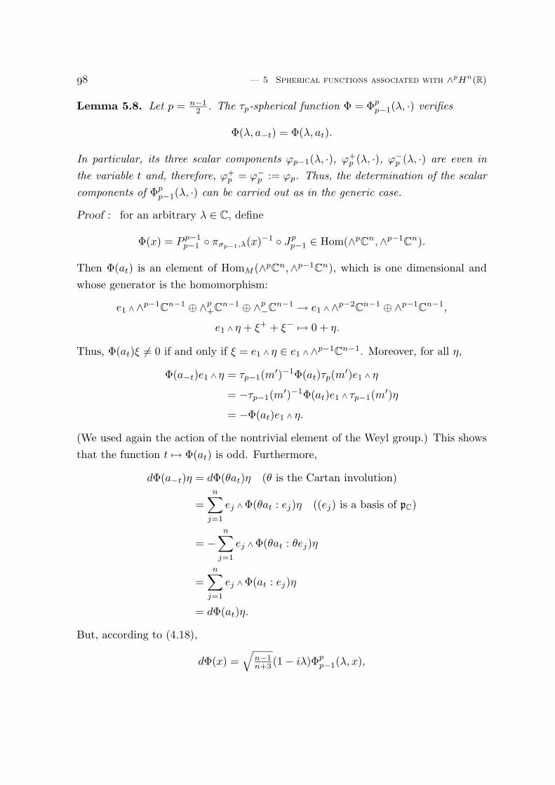
— 5 Spherical functions associated with ∧pHn(R)
Lemma 5.8. Let p = n−12 . The τp-spherical function Φ = Φp
p−1(λ, ·) verifies
Φ(λ, a−t) = Φ(λ, at).
In particular, its three scalar components ϕp−1(λ, ·), ϕ+p (λ, ·), ϕ−
p (λ, ·) are even in
the variable t and, therefore, ϕ+p = ϕ−
p := ϕp. Thus, the determination of the scalar
components of Φpp−1(λ, ·) can be carried out as in the generic case.
Proof : for an arbitrary λ ∈ C, define
Φ(x) = P p−1p−1 πσp−1,λ(x)−1 Jp
p−1 ∈ Hom(∧pC
n,∧p−1C
n).
Then Φ(at) is an element of HomM (∧pCn,∧p−1Cn), which is one dimensional and
whose generator is the homomorphism:
e1 ∧∧p−1C
n−1 ⊕ ∧p+C
n−1 ⊕ ∧p−C
n−1 → e1 ∧∧p−2C
n−1 ⊕ ∧p−1C
n−1,
e1 ∧ η + ξ+ + ξ− 7→ 0 + η.
Thus, Φ(at)ξ 6= 0 if and only if ξ = e1 ∧ η ∈ e1 ∧∧p−1Cn−1. Moreover, for all η,
Φ(a−t)e1 ∧ η = τp−1(m′)−1Φ(at)τp(m
′)e1 ∧ η
= −τp−1(m′)−1Φ(at)e1 ∧ τp−1(m
′)η
= −Φ(at)e1 ∧ η.
(We used again the action of the nontrivial element of the Weyl group.) This shows
that the function t 7→ Φ(at) is odd. Furthermore,
dΦ(a−t)η = dΦ(θat)η (θ is the Cartan involution)
=n∑
j=1
ej ∧Φ(θat : ej)η ((ej) is a basis of pC)
= −n∑
j=1
ej ∧Φ(θat : θej)η
=
n∑
j=1
ej ∧Φ(at : ej)η
= dΦ(at)η.
But, according to (4.18),
dΦ(x) =√
n−1n+3 (1 − iλ)Φp
p−1(λ, x),

5.2 Construction and description of spherical functions —
which shows that Φpp−1(λ, a−t) = Φp
p−1(λ, at) for λ 6= −i, and thus for all λ ∈C by holomorphic continuation. (More generally, one can see that Φp
p−1(λ, θx) =
Φpp−1(λ, x).)
This condition implies that all scalar components of Φpp−1(λ, ·) are even (and not only
ϕp−1(λ, ·)) and, since we know that ϕ+p (λ, t) = ϕ−
p (λ,−t), we are done. X
If the determination of the scalar components of Φpp−1(λ, ·) is done as in the generic
case, thanks to the identity ϕ+p = ϕ−
p , it is not the case for the spherical function
Φpp,±(λ, ·), and the calculations are more delicate, as we shall see now.
Lemma 5.9. Let p = n−12 . Denote by ϕp the average of ϕ+
p and ϕ−p (i.e. the even
part of ϕ+p ). Then:
(i) the equation (5.38) corresponds to the following equation for the scalar com-
ponents ϕp−1(λ, ·), ϕ+p (λ, ·) and ϕ−
p (λ, ·) of Φpp,±(λ, ·):
d
dtϕp−1(λ, t) + n+1
2 (coth t)ϕp−1(λ, t) = n+12 (sh t)−1ϕp(λ, t); (5.41)
(ii) the equation (5.39) corresponds to the following equations for the scalar com-
ponents ϕp−1(λ, ·), ϕ+p (λ, ·) and ϕ−
p (λ, ·) of Φpp,±(λ, ·):
12ϕ
+p (λ, t) − ϕ−
p (λ, t) = ∓i 2λn+1 (sh t)ϕp−1(λ, t), (5.42)
d
dtϕ+
p (λ, t) + n−12 coth t ± iλϕ+
p (λ, t) = n−12 (sh t)−1ϕp−1(λ, t), (5.43)
d
dtϕ−
p (λ, t) + n−12 coth t ∓ iλϕ−
p (λ, t) = n−12 (sh t)−1ϕp−1(λ, t). (5.44)
Proof of (i): set, for short, Φ(x) = Φpp,±(λ, x) and ϕ(t) = ϕ(λ, t). By restricting to
x = at,
(d∗Φ)(at)ξ = e1 ∧d
dt(∗Φ)(at)ξ + (sh t)−1
n∑
j=2
ej ∧ ∗Φ(at)τp(Zj)ξ (5.45)
− (coth t)
n∑
j=2
ej ∧ τp+1(Zj)∗Φ(at)ξ.
Since one has the expressions
∗Φ(at)ξ =
ϕp−1(t)∗η if ξ = e1 ∧ η ∈ e1 ∧∧p−1Cn−1,±ip(p+2)ϕ±
p (t)e1 ∧ ξ if ξ ∈ ∧p±Cn−1,

— 5 Spherical functions associated with ∧pHn(R)
one finds that (5.45) gives ‘0 = 0’ on ξ ∈ ∧p±Cn−1. On the contrary, if ξ = e1 ∧ η,
(d∗Φ)(at)ξ =d
dtϕp−1(t)e1 ∧ ∗η − (sh t)−1
n∑
j=2
ej ∧ ∗Φ(at)ej ∧ η (5.46)
− (coth t)n∑
j=2
ϕp−1(t)ej ∧ τp+1(Zj)∗η.
Simplify the second term in the right-hand side of (5.46):
∗Φ(at)ej ∧ η = ip(p+2)ϕ+p (t)e1 ∧(ej ∧ η)+ − ip(p+2)ϕ−
p (t)e1 ∧(ej ∧ η)−,
where(ej ∧ η)± = 1
2ej ∧ η ± 12 ip(p+2)∗(ej ∧ η)
= 12ej ∧ η ± 1
2 ip2+2iej
(∗η).
Henceej ∧ ∗Φ(at)ej ∧ η = 1
2 ip(p+2)ϕ+p (t) − ϕ−
p (t)ej ∧ e1 ∧ ej ∧ η
− 12ϕ
+p (t) + ϕ−
p (t)ej ∧ e1 ∧ iej(∗η),
so thatn∑
j=2
ej ∧ ∗Φ(at)ej ∧ η = n+12 ϕp(t)e1 ∧ ∗η.
Simplify the third term in the right-hand side of (5.46):
ej ∧ τp+1(Zj)∗η = −ej ∧ ej ∧ ie1(∗η) + ej ∧ e1 ∧ iej(∗η),
which impliesn∑
j=2
ejτp+1(Zj)∗η = −n+12 e1 ∧ ∗η.
To sum up, if ξ = e1 ∧ η,
(d∗Φ)(at)ξ = ddtϕp−1(t) − n+1
2 (sh t)−1ϕp(t) + n+12 (coth t)ϕp−1(t)e1 ∧ ∗η, (5.47)
and one gets (5.41).
Proof of (ii): to make easier the calculations, consider the equation
dΦ = ±ip2−1λ ∗Φ, (5.48)

5.2 Construction and description of spherical functions —
which is equivalent to (5.39). As seen in the generic case,
dΦ(at)ξ = e1 ∧d
dtΦ(at)ξ + (sh t)−1
n∑
j=2
ej ∧Φ(at)τp(Zj)ξ (5.49)
− (coth t)n∑
j=2
ej ∧ τp(Zj)Φ(at)ξ.
Consider first the case where ξ = e1 ∧ η ∈ e1 ∧∧p−1Cn−1. It is easy to see that (5.49)
gives:
dΦ(at)ξ = −(sh t)−1n∑
j=2
ej ∧Φ(at)ej ∧ η,
with
Φ(at)ej ∧ η = ϕ+p (t)(ej ∧ η)+ + ϕ−
p (t)(ej ∧ η)−,
where, as in the proof of (i),
(ej ∧ η)± = 12ej ∧ η ± 1
2 ip2+2iej
(∗η),
so that
ej ∧Φ(at)ej ∧ η = ip2+2 1
2ϕ+p (t) − ϕ−
p (t)ej ∧ iej(∗η).
Thus, (5.49) becomes:
dΦ(at)ξ = n+12 ip
2
(sh t)−1 12ϕ
+p (t) − ϕ−
p (t)∗η. (5.50)
And, since in the right hand-side of (5.48) one has
∗Φ(at)ξ = ϕp−1(t)∗(e1 ∧ η) = ϕp−1(t)∗η,
one deduces (5.42).
Consider now the case where ξ ∈ ∧p±Cn−1. (5.49) becomes then:
dΦ(at)ξ = ddtϕ
±p (t) − n−1
2 (sh t)−1ϕp−1(t) + n−12 (coth t)ϕ±
p (t)e1 ∧ ξ. (5.51)
Finally, as
∗Φ(at)ξ = ϕ±p (t)∗ξ = ±ip(p+2)ϕ±
p (t)e1 ∧ ξ,
one obtains equations (5.43) and (5.44), concluding the proof of the lemma. X

— 5 Spherical functions associated with ∧pHn(R)
Remarks:
1. Summing equations (5.43) and (5.44), and combining the result with (5.42), one
obtains a differential equation relating ϕp−1 and ϕp (as in the generic case):
d
dtϕp(λ, t) + n−1
2 (coth t)ϕp(λ, t) = n−12 (sh t)−1 − 2λ2
n+1 sh tϕp−1(λ, t). (5.52)
2. Substracting (5.44) to (5.43) and combining the result with (5.42), one finds again
(5.41).
Using the two previous lemmas, we can give the expression of the scalar compo-
nents of Φpp−1(λ, ·) and Φp
p,±(λ, ·) in terms of (modified) Jacobi functions.
Theorem 5.10. Let p = n−12 . The scalar components ϕp−1(λ, ·), ϕ+
p (λ, ·), ϕ−p (λ, ·)
of Φ = Φpp−1(λ, ·) can be expressed in terms of the Jacobi functions defined by (5.22)
and (5.26):
ϕp−1(λ, t) = 2nn−1φ
( n2 −1,− 1
2 )
λ (t) − n+1n−1φ
( n2 ,− 3
2 )
λ,0,1 (t), (5.53)
ϕ±p (λ, t) = φ
( n2 ,− 1
2 )
λ (t). (5.54)
The scalar components ϕp−1(λ, ·), ϕ+p (λ, ·), ϕ−
p (λ, ·) of Φ = Φpp,±(λ, ·) can be ex-
pressed in a similar way:
ϕp−1(λ, t) = φ( n
2 ,− 12 )
λ (t), (5.55)
ϕ+p (λ, t) = 2n
n+1φ( n
2 −1,− 12 )
λ (t) − n−1n+1φ
( n2 ,− 3
2 )
λ,0,1 (t) ∓ i 2λn+1φ
( n2 −1,− 1
2 )
λ,1,0 (t), (5.56)
ϕ−p (λ, t) = 2n
n+1φ( n
2 −1,− 12 )
λ (t) − n−1n+1φ
( n2 ,− 3
2 )
λ,0,1 (t) ± i 2λn+1φ
( n2 −1,− 1
2 )
λ,1,0 (t). (5.57)
Proof : the components of Φpp−1(λ, ·) are determined exactly as in the generic case
(Theorem 5.5).
For Φpp,±(λ, ·), one replaces ϕp in (5.52) by its expression given in (5.41). One then
obtains immediatly (5.55), and can deduce (as in the generic case) the expression of
ϕp:
ϕp(λ, t) = 2nn+1φ
( n2 −1,− 1
2 )
λ (t) − n−1n+1φ
( n2 ,− 3
2 )
λ,0,1 (t). (5.58)
As ϕp is the even part of ϕ+p , we are just left with the determination of the odd part,
which we get from (5.42), since ϕp−1 is known. This argument gives (5.56), which is
equivalent to (5.57) by using the identity ϕ−p (λ, t) = ϕ+
p (λ,−t). X
The following result is obtained as in the generic case.

5.2 Construction and description of spherical functions —
Corollary 5.11. Let p = n−12 . Then:
(i) the following conditions are equivalent for a normalized τp-radial function:
Φ(x) = Φpp,±(λ, x), resp. Φ(x) = Φp
p−1(λ, x) for all x ∈ G and for some λ ∈ C;
dΦ = ±ip2−1λ ∗Φ and d∗Φ = 0, resp. ∆Φ = (λ2 + 1)Φ and dΦ = 0;
∗dΦ = ±ip2−1λ Φ and dd∗Φ = 0, resp. dd∗Φ = (λ2 + 1)Φ and ∗dΦ = 0;
(ii) Σ(G, K, τp, τp) = Φpp−1(λ, ·),Φp
p,±(λ, ·) : λ ∈ C/ ± 1.(iii) there are no nonzero τp-radial functions which are harmonic and L2 in the
special case p = n−12 .
Special case p = n2
In the sequel, σ will denote either σp−1 or σp, since these representations are equiv-
alent when p = n/2. Imitating again (5.6), we put, for λ ∈ C:
Φ±(λ, ·) : G −→ End(∧n2±C
n),
Φ±(x) = P± πσ,λ(x−1) J±, (5.59)
where J± = Jn2 ,±n2 (−1) is the isometric embedding from ∧
n2±Cn into L2(K, M, σ) defined
by (4.6) and P± = (J±)∗. The function Φ±(λ, ·) is then τ±n2-spherical and, since
Φ±(λ, e) = Id, it is the unique solution of the differential equation
∆Φ = (λ2 + 14 )Φ. (5.60)
(See Corollary 4.7, equation (4.42).)
Remarks:
1. As in the other cases, one has the integral formula :
Φ±(λ, x) = 2
∫
K
dk e−(iλ+ρ)H(xk)τ±(k) Pσ τ±(k(xk)−1).
2. Again, one has the identities Φ±(λ, x)∗ = Φ±(λ, x−1) and Φ±(λ, x) = Φ±(−λ, x).
Denote by ϕ±(λ, ·) the unique scalar component of Φ±(λ, ·). It is a normalized
(ϕ±(λ, 0) = 1) even solution of the differential equation:
d2
dt2φ(t) + (n − 1)(coth t)
d
dtφ(t) +
n
sh2 t(ch t − 1)φ(t) + (λ2 + ρ2)φ(t) = 0, (5.61)
which comes from (5.60) (the proof is similar to the one in Lemma 5.2). This is why
we easily obtain the following statement.
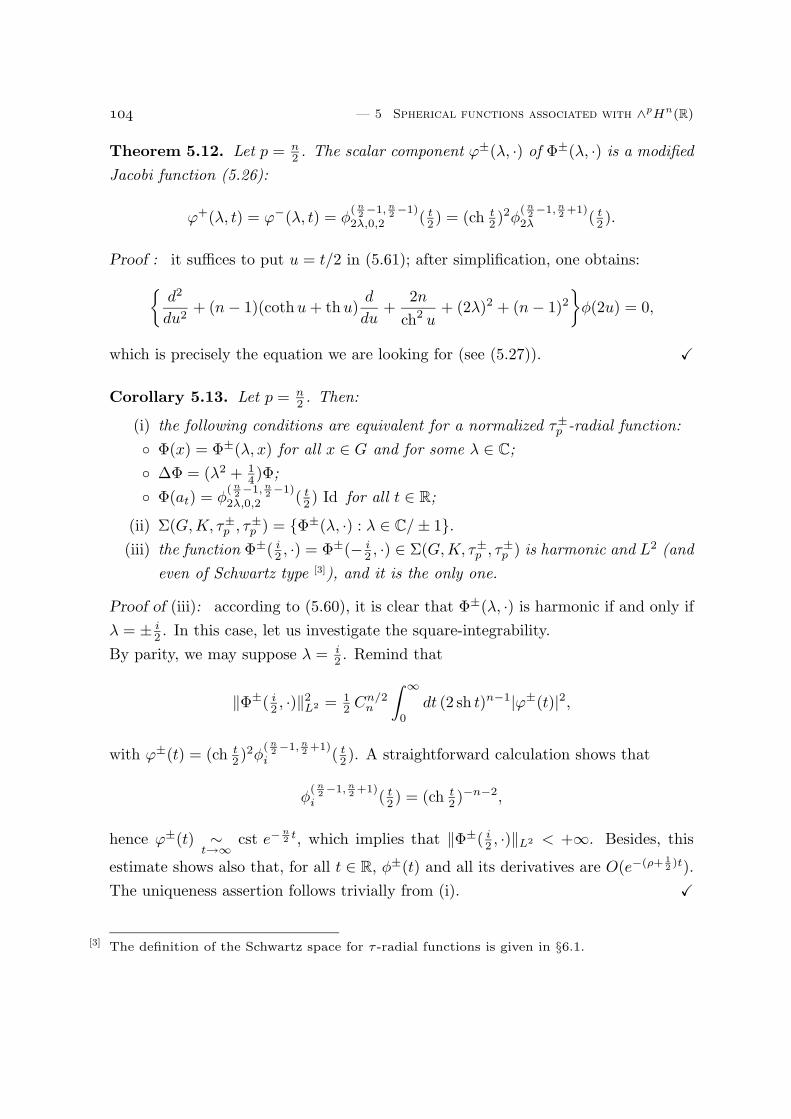
— 5 Spherical functions associated with ∧pHn(R)
Theorem 5.12. Let p = n2 . The scalar component ϕ±(λ, ·) of Φ±(λ, ·) is a modified
Jacobi function (5.26):
ϕ+(λ, t) = ϕ−(λ, t) = φ( n
2 −1, n2 −1)
2λ,0,2 ( t2 ) = (ch t
2 )2φ( n
2 −1, n2 +1)
2λ ( t2 ).
Proof : it suffices to put u = t/2 in (5.61); after simplification, one obtains:
d2
du2+ (n − 1)(cothu + thu)
d
du+
2n
ch2 u+ (2λ)2 + (n − 1)2
φ(2u) = 0,
which is precisely the equation we are looking for (see (5.27)). X
Corollary 5.13. Let p = n2 . Then:
(i) the following conditions are equivalent for a normalized τ±p -radial function:
Φ(x) = Φ±(λ, x) for all x ∈ G and for some λ ∈ C;
∆Φ = (λ2 + 14 )Φ;
Φ(at) = φ( n
2 −1, n2 −1)
2λ,0,2 ( t2 ) Id for all t ∈ R;
(ii) Σ(G, K, τ±p , τ±
p ) = Φ±(λ, ·) : λ ∈ C/ ± 1.(iii) the function Φ±( i
2 , ·) = Φ±(− i2 , ·) ∈ Σ(G, K, τ±
p , τ±p ) is harmonic and L2 (and
even of Schwartz type [3]), and it is the only one.
Proof of (iii): according to (5.60), it is clear that Φ±(λ, ·) is harmonic if and only if
λ = ± i2 . In this case, let us investigate the square-integrability.
By parity, we may suppose λ = i2 . Remind that
‖Φ±( i2 , ·)‖2
L2 = 12 Cn/2
n
∫ ∞
0
dt (2 sh t)n−1|ϕ±(t)|2,
with ϕ±(t) = (ch t2 )2φ
( n2 −1, n
2 +1)i ( t
2 ). A straightforward calculation shows that
φ( n
2 −1, n2 +1)
i ( t2 ) = (ch t
2 )−n−2,
hence ϕ±(t) ∼t→∞
cst e−n2 t, which implies that ‖Φ±( i
2 , ·)‖L2 < +∞. Besides, this
estimate shows also that, for all t ∈ R, φ±(t) and all its derivatives are O(e−(ρ+ 12 )t).
The uniqueness assertion follows trivially from (i). X
[3] The definition of the Schwartz space for τ-radial functions is given in §6.1.
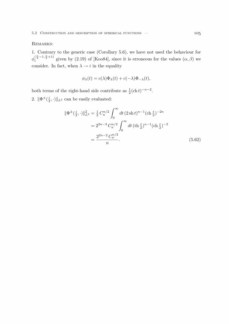
5.2 Construction and description of spherical functions —
Remarks:
1. Contrary to the generic case (Corollary 5.6), we have not used the behaviour for
φ( n
2 −1, n2 +1)
i given by (2.19) of [Koo84], since it is erroneous for the values (α, β) we
consider. In fact, when λ → i in the equality
φλ(t) = c(λ)Φλ(t) + c(−λ)Φ−λ(t),
both terms of the right-hand side contribute as 12 (ch t)−n−2.
2. ‖Φ±( i2 , ·)‖L2 can be easily evaluated:
‖Φ±( i2 , ·)‖2
L2 = 12 Cn/2
n
∫ ∞
0
dt (2 sh t)n−1(ch t2 )−2n
= 22n−3 Cn/2n
∫ ∞
0
dt (th t2 )n−1(ch t
2 )−2
=22n−2 C
n/2n
n. (5.62)

6 Fourier analysis on Γ ∧p Hn(R)
6.1 (Spherical) Fourier transform of radial functions
Generic case
Let F ∈ C∞c (G, K, τp, τp). The (τp-spherical) Fourier transform H(F ) of F is the
couple (Hpp−1(F ),Hp
p(F )) of functions defined on C by :
Hpq(F )(λ) =
1
Cpn
∫
G
dx trF (x)Φpq(λ, x−1) (q = p, p − 1)
=1
Cpn
(F, Φp
q(λ, ·−1)∗)
(q = p, p − 1). (6.1)
Recall that H is nothing else but the Gelfand transform of the commutative algebra
C∞c (G, K, τp, τp) (see Appendix B).
The aim of this section is to show that, as in the scalar case (p = 0), the spherical
Fourier transform reduces essentially to a Jacobi transform. This will allow us to use
the powerful Jacobi analysis developed by Flensted-Jensen and Koornwinder in the
1970’s (we shall often refer to the survey [Koo84]), and notably the Paley-Wiener
and Plancherel theorems.
Before stating next result, we recall that the Jacobi transform J (α,β)(f) of a
complex-valued function f on R is defined by:
J (α,β)(f)(λ) =
∫ ∞
0
dt ζα,β(t)φ(α,β)λ (t)f(t), (6.2)
where the weight ζα,β was defined in (5.23).
Proposition 6.1. Let p be generic and let F ∈ C∞c (G, K, τp, τp) with scalar compo-
nents fp−1, fp. Then:
(i) the spherical Fourier transforms can be expressed in terms of Jacobi trans-
forms:
Hpp(F )(λ) = − 1
4nJ ( n
2 ,− 12 )
( 1
sh tf ′
p(t) + p(coth t)fp(t) −p
sh tfp−1(t)
)(λ), (6.3)
Hpp−1(F )(λ) = − 1
4nJ ( n
2 ,− 12 )
( 1
sh tf ′
p−1(t) + (n − p)(coth t)fp−1(t) (6.4)
− n − p
sh tfp(t)
)(λ);
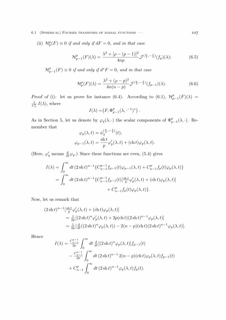
6.1 (Spherical) Fourier transform of radial functions —
(ii) Hpp(F ) ≡ 0 if and only if dF = 0, and in that case
Hpp−1(F )(λ) =
λ2 + [ρ − (p − 1)]2
4npJ ( n
2 ,− 12 )(fp)(λ); (6.5)
Hpp−1(F ) ≡ 0 if and only if d∗F = 0, and in that case
Hpp(F )(λ) =
λ2 + (ρ − p)2
4n(n − p)J ( n
2 ,− 12 )(fp−1)(λ). (6.6)
Proof of (i): let us prove for instance (6.4). According to (6.1), Hpp−1(F )(λ) =
1Cp
nI(λ), where
I(λ) =(F,Φp
p−1(λ, ·−1)∗)
.
As in Section 5, let us denote by ϕq(λ, ·) the scalar components of Φpp−1(λ, ·). Re-
member that
ϕp(λ, t) = φ( n
2 ,− 12 )
λ (t),
ϕp−1(λ, t) =sh t
pϕ′
p(λ, t) + (ch t)ϕp(λ, t).
(Here, ϕ′q means d
dtϕq.) Since these functions are even, (5.4) gives
I(λ) =
∫ ∞
0
dt (2 sh t)n−1Cp−1n−1fp−1(t)ϕp−1(λ, t) + Cp
n−1fp(t)ϕp(λ, t)
=
∫ ∞
0
dt (2 sh t)n−1Cp−1n−1fp−1(t)[
sh tp ϕ′
p(λ, t) + (ch t)ϕp(λ, t)]
+ Cpn−1fp(t)ϕp(λ, t).
Now, let us remark that
(2 sh t)n−1[ sh tp ϕ′
p(λ, t) + (ch t)ϕp(λ, t)]
= 12p [(2 sh t)nϕ′
p(λ, t) + 2p(ch t)(2 sh t)n−1ϕp(λ, t)]
= 12p [ d
dt ((2 sh t)nϕp(λ, t)) − 2(n − p)(ch t)(2 sh t)n−1ϕp(λ, t)].
Hence
I(λ) =Cp−1
n−1
2p
∫ ∞
0
dt ddt [(2 sh t)nϕp(λ, t)]fp−1(t)
− Cp−1n−1
2p
∫ ∞
0
dt (2 sh t)n−1 2(n − p)(ch t)ϕp(λ, t)fp−1(t)
+ Cpn−1
∫ ∞
0
dt (2 sh t)n−1ϕp(λ, t)fp(t).

— 6 Fourier analysis on Γ ∧p Hn(R)
But, since
∫ ∞
0
dt ddt [(2 sh t)nϕp(λ, t)]fp−1(t) = −
∫ ∞
0
dt (2 sh t)nϕp(λ, t)]f ′p−1(t),
we get
I(λ) =
∫ ∞
0
dt (2 sh t)n+1ϕp(λ, t)[− Cp−1
n−1
4p sh tf′p−1(t) −
Cp−1n−1
(n−p) ch t
4p(sh t)2 fp−1(t) +Cp
n−1
4(sh t)2 fp
]
= −Cp
n−1
4
∫ ∞
0
dt (2 sh t)n+1 ϕp(λ,t)sh t
[f ′
p−1(t)
n−p + (coth t)fp−1(t) − fp(t)sh t
].
Now, since ϕp(λ, t) = φ( n
2 ,− 12 )
λ (t), dividing I(λ) by Cpn gives exactly (6.4).
Proof of (ii): suppose now dF = 0. Then Lemma 5.3 can be applied to F , which
means
fp−1 = sh tp f ′
p + (ch t)fp, (6.7)
f ′p−1 = sh t
p [f ′′p + (p + 1)(coth t)f ′
p + p fp].
Hencef ′
p−1(t) + (n − p)(coth t)fp−1(t) − n−psh t fp(t)
= sh tp [L fp(t) + p(n + 1 − p)fp(t)].
(L = Ln2 ,− 1
2is the Jacobi Laplacian defined in (5.24).) As a consequence,
Hpp−1(F )(λ) = − 1
4np
∫ ∞
0
dt (2 sh t)n+1[L fp(t) + p(n + 1 − p)fp(t)]φ( n
2 ,− 12 )
λ (t).
But L is self-adjoint for the scalar product (f, g) =∫ ∞0
dt (2 sh t)n+1f(t)g(t) and,
furthermore,
[L + p(n + 1 − p)]φ( n
2 ,− 12 )
λ = −[λ2 + (ρ + 1)2 + p(n + 1 − p)]φ( n
2 ,− 12 )
λ
= −[λ2 + [ρ − (p − 1)]2]φ( n
2 ,− 12 )
λ .
Thus we obtain (6.5). On the other hand, (6.7) shows also that Hpp(F ) ≡ 0 if dF = 0.
Conversely, suppose Hpp(F ) ≡ 0. Since Hp
p is a Jacobi transform, which is injective
([Koo84], Theorem 2.1), the expression between parantheses in (6.3) vanishes, and
this means exactly that dF = 0.
The case d∗F = 0 can be worked out similarly. X
6.1 (Spherical) Fourier transform of radial functions —
We now deal with the problem of inverting H. The first step will be to give an
inversion formula for τp-radial functions which belong to a particular subspace of
C∞c (G, K, τp, τp), namely to
Vp = d(C∞c (G, K, τp, τp−1)) ⊕ d∗(C∞
c (G, K, τp, τp+1)). (6.8)
Indeed, if F ∈ Vp, the spherical Fourier transforms of F are given by formulæ (6.5)
and (6.6). Thus, given Hpp−1(F ) and Hp
p(F ), one obtains the scalar components fp−1
and fp of F by inverting J ( n2 ,− 1
2 ). Precisely, using [Koo84], Theorem 2.3,
fp−1(t) =1
2π
∫ ∞
0
4n(n − p)
λ2 + (ρ − p)2dλ
|c(λ)|2Hpp(F )(λ)φ
( n2 ,− 1
2 )
λ (t), (6.9)
fp(t) =1
2π
∫ ∞
0
4np
λ2 + [ρ − (p − 1)]2dλ
|c(λ)|2Hpp−1(F )(λ)φ
( n2 ,− 1
2 )
λ (t), (6.10)
where c denotes Harish-Chandra’s function defined by formula (2.18) of [Koo84]:
c(λ) = c( n2 ,− 1
2 )(λ) = 2n+1
2 −iλ Γ(n2 + 1)
Γ( 12 (iλ + n+1
2 ))
Γ(iλ)
Γ( 12 (iλ + n+3
2 ))
=2nΓ(n
2 + 1)√π
Γ(iλ)
Γ(iλ + n+12 )
. (6.11)
Define now the Plancherel measures as follows:
for the component Hpp−1, we put:
dνp−1(λ) =2
π
np
λ2 + [ρ − (p − 1)]2dλ
|c(λ)|2 ; (6.12)
for the component Hpp, we put:
dνp(λ) =2
π
n(n − p)
λ2 + (ρ − p)2dλ
|c(λ)|2 . (6.13)
In order to describe the singularities of the Plancherel measures, we need the explicit
expression of |c(λ)|−2, which is equal to [c(λ)c(−λ)]−1 when λ is real. By standard
calculations relying on well-known properties of the Γ function (see e.g. the details
in the special case p = n2 ), we derive from (6.11) the following expressions:
when n is odd,
[c(λ)c(−λ)]−1 =[(n + 1
2
)(n + 1
2+ 1
). . . (n − 1)n
]−2
λ2
n−12∏
k=1
(λ2 + k2).
— 6 Fourier analysis on Γ ∧p Hn(R)
[c(λ)c(−λ)]−1 is then polynomial, hence entire.
when n is even,
[c(λ)c(−λ)]−1 = 2−2n [(n2 )!]−2 π2 thπλ
πλλ2
n2∏
k=1
(λ2 + (k − 1
2 )2).
Here, [c(λ)c(−λ)]−1 is meromorphic, and its (simple) poles belong to the set
±i(ρ + 1 + k), k ∈ N.From the previous expressions, we deduce the list of (simple) poles of dνp−1:
for n odd: ρ is an integer, and 1 6 ρ− (p− 1) 6 n−12 (for 1 6 p 6 n−1
2 ), then
dνp−1 is polynomial;
for n even: ρ is a half-integer, and 12 6 ρ−(p−1) 6 n−1
2 (for 1 6 p 6 n2 ), then
the poles of dνp−1 range through the set ±i(ρ+1+k), k ∈ N∪±i[ρ−(p−1)].
In the same way, we describe the singularities of dνp:
for n odd: ρ is an integer, and 0 6 ρ − p 6 n−32 (for 1 6 p 6 n−1
2 ), then dνp
is polynomial.
for n even: ρ is a half-integer, and − 12 6 ρ − p 6 n−3
2 (for 1 6 p 6 n2 ). The
division by the quantity λ2 +(ρ−p)2 cancels one of the factors in the product
(when k − 12 = ρ − p) that does not compensate any more the singularities of
th πλπλ = 2
π
∑∞k=1
1λ2+(k− 1
2 )2
at λ = ±i(ρ − p). The (simple) poles of dνp then range through the set
±i(ρ + 1 + k), k ∈ N ∪ ±i(ρ − p).
Remark: we recover (up to normalizing constants) the expressions of the Plancherel
measures established in [CH94], as well as the ones we can deduce from [Ven93],
Example 3.4.
Proposition 6.2 (Intermediate inversion formula). Let p be generic. The
spherical Fourier transform H = (Hpp−1,Hp
p) of τp-radial functions F ∈ Vp is in-
verted by the following formula:
F (x) =
∫ ∞
0
dνp−1(λ)Hp
p−1(F )(λ) Φpp−1(λ, x) + dνp(λ)Hp
p(F )(λ) Φpp(λ, x)
. (6.14)

6.1 (Spherical) Fourier transform of radial functions —
Proof : it suffices to prove (6.14) for F|A , or, equivalently, (6.9) and (6.10) for its
scalar components fp−1 and fp. Moreover, it suffices also to consider the following
two cases.
• First case: F = dH
Then Hpp(F ) ≡ 0. Since the component ϕp(λ, ·) of Φp
p−1(λ, ·) is φ( n
2 ,− 12 )
λ , we have
formula (6.10). On the other hand, differentiating both sides of (6.10) with respect
to t, and using the identities dF = 0 = dΦpp−1, we get:
f ′p = p
sh tfp−1 − p(coth t)fp,
ϕ′p = p
sh tϕp−1 − p(coth t)ϕp.
Now, replacing these expressions in the differentiated version of (6.10), and using
again (6.10), we obtain precisely (6.9).
• Second case: F = d∗H
Then Hpp−1(F ) ≡ 0. The argument is similar to the one used in the first case and
leads to (6.9) and (6.10). X
Remark: our motivation to introduce the subspace Vp is that the inversion for-
mula (6.14) can’t be directly stated for F ∈ C∞c (G, K, τp, τp), for Vp is dense in
L2(G, K, τp, τp) (for p 6= n2 , by a variant of Theorem 2.3), but not in C∞
c (G, K, τp, τp).
Actually, let us mention that the proof of the inversion formula for p = 1 in [BR89]
(Theorem 7.1) is incomplete, precisely because the authors seem to have misapplied
the Hodge-Kodaira Theorem to V1.
Theorem 6.3 (Plancherel). Let p be generic. Define the space
L2(R;µ1, µ2)even = L2(R, µ1)even ⊕ L2(R, µ2)even,
where
L2(R, µ)even = h : R → R even and such that∫ ∞0
µ(λ) |h(λ)|2 < +∞.
Then:

— 6 Fourier analysis on Γ ∧p Hn(R)
(i) Plancherel formula: for F ∈ Vp,
‖F‖2L2 =
∫
G
dx ‖F (x)‖2HS
=
∫ ∞
0
dt (2 sh t)n−1Cp−1
n−1|fp−1(t)|2 + Cpn−1|fp(t)|2
= Cpn
∫ ∞
0
dνp−1(λ)|Hp
p−1(F )(λ)|2 + dνp(λ)|Hpp(F )(λ)|2
. (6.15)
(ii) The spherical Fourier transform H of τp-radial functions extends to a bijective
isometry from
L2(G, K, τp, τp) ' L2(R;Cp−1n−1(2 sh t)n−1dt, Cp
n−1(2 sh t)n−1dt)even
onto L2(R;Cpn dνp−1, C
pn dνp)even.
Proof of (i): we use classical arguments. Put F ∗(x) = F (x−1)∗; apply the inversion
formula (6.14) to the function F ∗ F ∗ at x = e, and take traces.
On the one hand,
tr(F ∗ F ∗)(e) =
∫
G
dx trF (x)F (x)∗ = ‖F‖2L2 .
On the other hand, since Hpq(F1 ∗ F2) = Hp
q(F1) · Hpq(F2) by definition,
(F ∗ F ∗)(e) =
∫ ∞
0
dνp−1(λ)Hp
p−1(F )(λ)Hpp−1(F
∗)(λ) Id∧pCn
+dνp(λ)Hpp(F )(λ)Hp
p(F∗)(λ) Id∧pCn
.
Moreover, as tr(A∗B∗) = tr(AB) and Φpq(λ, x−1) = Φp
q(λ, x)∗,
Cpn Hp
q(F∗)(λ) =
∫
G
dx tr(F (x−1)∗Φpq(λ, x−1))
=
∫
G
dx tr(F (x−1)Φpq(λ, x))
=
∫
G
dx tr(F (x)Φpq(λ, x−1))
= Cpn Hp
q(F )(λ).
Hence, since λ ∈ R,
trF ∗ F ∗(e) = Cpn
∫ ∞
0
dνp−1(λ)|Hp
p−1(F )(λ)|2 + dνp(λ)|Hpp(F )(λ)|2
.

6.1 (Spherical) Fourier transform of radial functions —
The intermediate formula is trivially obtained by using (5.4).
Proof of (ii): (i) implies that H is an isometry; the injectivity of H is obvious by
Proposition 6.1, and to establish the surjectivity, one uses Proposition 6.1, the Paley-
Wiener theorem for the Jacobi transform (see [Koo84], Theorem 2.1, recalled below),
the density of PW (C) into L2(R, dνq) and the density of Vp into L2(G, K, τp, τp)
(Hodge-Kodaira Theorem, see Theorem 2.3). X
The last step consists in stating a Paley-Wiener theorem and an inversion formula
for general functions F ∈ C∞c (G, K, τp, τp). These results will be proved simultane-
ously.
Theorem 6.4 (Inversion formula). Let p be generic. The inversion formula
(6.14) still holds for functions F ∈ C∞c (G, K, τp, τp).
For R > 0, define the set PWR(C)even of entire functions h on C which are even
and verify the condition:
∀N ∈ N, ∃CN > 0 : ∀λ ∈ C, |h(λ)| 6 CN (1 + |λ|)−NeR| Im λ|.
Then the Paley-Wiener theorem for J asserts that J is a topological linear iso-
morphism [1] between PWR(C)even and the space C∞([−R, +R])even of C∞ even
functions on R with support in [−R, +R].
Now, for R > 0, we denote by C∞R (G, K, τp, τp) the subspace of functions in
C∞c (G, K, τp, τp) whose support is included in the closed ball B(o, R) of the hyperbolic
space Hn(R) (recall that d(k1atk2, o) = t > 0 in the Cartan decomposition of G, and
Supp(F ) ⊂ B(o, R) ⇔ Supp(F|A) ⊂ [−R, +R]).
Theorem 6.5 (Paley-Wiener). Let p be generic. For q = p − 1 or p, put λq :=
i(ρ − q) and for R > 0, define
PWR =(hp−1, hp) ∈ PWR(C)2even : hp−1(±λp−1) = hp(±λp)
.
Then H : F 7→ (Hpp−1(F ),Hp
p(F )) is a topological linear isomorphism from C∞R (G, K,
τp, τp) onto PWR.
[1] In the sequel, ‘topological linear isomorphism’ will always mean ‘bi-continuous isomorphism
between vector spaces endowed with a Frechet topology’.

— 6 Fourier analysis on Γ ∧p Hn(R)
Proof of Theorems 6.4 and 6.5:
• First step : using formulæ (6.3) and (6.4), we can see that each Fourier transform
Hpq maps continuously C∞
R (G, K, τp, τp) into PWR(C)even. Indeed, the quantities
between braces in (6.3) and (6.4) are exactly ‘scalar expressions’ of either dF or d∗F ,
and belong then to the space C∞R (R)odd. Thus, dividing by sh t is well-defined and
yields C∞R (R)even functions. According to the Paley-Wiener theorem for J ( n
2 ,− 12 ),
Hpq(F ) ∈ PWR(C)even and Hp
q is a continous map. The fact that Hpp−1(F )(±λp−1) =
Hpp(F )(±λp) is implied by the following result.
Lemma 6.6. Let p be generic. Then Φpp−1(±λp−1, ·) ≡ Φp
p(±λp, ·).
Proof : this is due to the fact (Proposition 4.5) that these two functions verify
the same differential equation dΦ = 0 (or, equivalently, d∗Φ = 0) with the same
normalization. X
• Second step : conversely, let h = (hp−1, hp) ∈ PWR. We put
Fh(x) =∑
q
∫ ∞
0
dνq(λ) hq(λ)Φpq(λ, x). (6.16)
(The map h 7→ Fh is the classical wave packet transform.) It is clear that Fh is
τp-radial, and that its scalar components fp−1, fp live in C∞(R)even if hp−1, hp are
entire. Let us prove the support preserving property for the scalar component fp−1
(the method is similar for fp).
We have
fp−1(t) =2
π
∫ ∞
0
dλ
|c(λ)|2 np
λ2 + [ρ − (p − 1)]2hp−1(λ)φ
( n2 ,− 1
2 )
λ (t)
+n(n − p)
λ2 + (ρ − p)2hp(λ)φ
( n2 ,− 1
2 )
λ (t)
,
where φ( n
2 ,− 12 )
λ = np φ
( n2 −1,− 1
2 )
λ − n−pp φ
( n2 ,− 3
2 )
λ,0,1 (see Theorem 5.4). Now, we use the
development (given in [Koo84], relation (2.17))
φ(α,β)λ (t) = c(α,β)(λ)Φ
(α,β)λ (t) + c(α,β)(−λ)Φ
(α,β)−λ (t),
where Φ(α,β)λ (t) (defined for λ /∈ −i N∗) has a ‘Harish-Chandra type’ expansion:
Φ(α,β)λ (t) = e[iλ−(α+β+1)]t
+∞∑
m=0
Γm(λ)e−mt
6.1 (Spherical) Fourier transform of radial functions —
(see ibid., relation (6.6)). In our case, this gives rise to the developments
φλ(t) = c(λ)Φλ(t) + c(−λ)Φ−λ(t),
φλ(t) = c(λ)Φλ(t) + c(−λ)Φ−λ(t),
where we dropped the upper indices (α, β) = (n2 ,− 1
2 ). Notice that the previ-
ous lemma implies that φλp−1 = φλpand, as a consequence, that c(λp−1)Φλp−1 =
c(λp)Φλp. In other words,
Φλp−1=
c(λp)
c(λp−1)Φλp
= −ρ − p + 1
pΦλp
. (6.17)
Now,
fp−1(t) =2
π
∫ ∞
−∞
dλ
c(−λ)
np
λ2 + [ρ − (p − 1)]2hp−1(λ)Φλ(t)
+n(n − p)
λ2 + (ρ − p)2hp(λ)Φλ(t)
:=
∫ ∞
−∞dλ I(λ, t).
Since c(−λ)−1Φλ and c(−λ)−1Φλ have only poles on the negative part of the imag-
inary axis, the integrand I(λ, t) has two (simple) poles in the upper half-plane, at
λ = λp and λ = λp−1. In order to apply the residue theorem, we integrate the mero-
morphic function λ 7→ I(λ, t) on the square contour with vertices r, r+ir,−r+ir,−r,
for a positive real number r. As soon as r > ρ − p + 1, one gets∫ r
−r
dλ I(λ, t) = 2iπResλ=λp
I(λ, t) + Resλ=λp−1 I(λ, t)
+
∫ r+ir
−r+ir
dλ I(λ, t).
Using the Paley-Wiener type condition for h and the asymptotics estimates for the
functions Φλ and Φλ, one sees that∫ r+ir
−r+irdλ I(λ, t) −→
r→+∞0 if t > R. Hence, since
hp−1(λp−1) = hp(λp), and using (6.17), one gets, for t > R,
fp−1(t) =4i√
π
2nΓ(n2 + 1)
−Γ(ρ − p + 1 + n+1
2 )
Γ(ρ − p + 1)
np
2i(ρ − p + 1)
ρ − p + 1
p
+Γ(ρ − p + n+1
2 )
Γ(ρ − p)
n(n − p)
2i(ρ − p)
hp(λp) Φλp
(t)
=
√π
2n−1Γ(n2 + 1)
Γ(n − p)
Γ(ρ − p)
−n − p
ρ − p
np
ρ − p + 1
ρ − p + 1
p
+n(n − p)
ρ − p
hp(λp) Φλp
(t)
= 0.
Thus, we have proved that if h ∈ PWR, Fh ∈ C∞R (G, K, τp, τp).

— 6 Fourier analysis on Γ ∧p Hn(R)
• Third step : it remains to show that H(Fh) = h to conclude the proof of the
Paley-Wiener theorem for H and to extend the validity of the inversion formula to
the whole space C∞R (G, K, τp, τp). We begin with noticing that it suffices to show
that (H(Fh),H(G)
)=
(h,H(G)
)
for all G ∈ L2 [2], and even for all G ∈ Vp (by density). Then, using the Plancherel
theorem above and the definition of Fh, we have:
(H(Fh),H(G)
)=
(Fh, G
)
=
∫
G
dx trFh(x)G(x)∗
=∑
q
∫ ∞
0
dνq(λ)hq(λ)
∫
G
dx trΦpq(λ, x)G(x)∗
= Cpn
∑
q
∫ ∞
0
dνq(λ) hq(λ)Hpq(G)(λ)
=(h,H(G)
).
Q.E.D. X
Remarks:
1. With h = (hp−1, hp) ∈ PWR, associate Fh by (6.16). Then the scalar components
fp−1, fp of Fh are also given by the following expressions:
fp−1(t) = J ( n2 ,− 1
2 )−1( 4n(n − p)
λ2 + (ρ − p)2hp
)(t) (6.18)
− (ch t)J ( n2 ,− 1
2 )−1( 4n(n − p)
λ2 + [ρ − (p − 1)]2hp−1
)(t)
+ J ( n2 −1,− 1
2 )−1( λ2 + (n−1
2 )2
λ2 + [ρ − (p − 1)]2hp−1
)(t),
fp(t) = J ( n2 ,− 1
2 )−1( 4np
λ2 + [ρ − (p − 1)]2hp−1
)(t) (6.19)
− (ch t)J ( n2 ,− 1
2 )−1( 4np
λ2 + (ρ − p)2hp
)(t)
+ J ( n2 −1,− 1
2 )−1( λ2 + (n−1
2 )2
λ2 + (ρ − p)2hp
)(t).
[2] The scalar products are taken in the space L2(R; Cpndνp−1, Cp
ndνp)even.

6.1 (Spherical) Fourier transform of radial functions —
2. Theorem 6.5 is a special case of Campoli’s Paley-Wiener theorem for real rank
one semisimple Lie groups: see [Cam80], §§2.3.1, 2.3.2 and especially 3.2.1. In par-
ticular, Campoli described the image of a Fourier transform defined on the alge-
bra of K-central functions f ∈ C∞c (G) verifying the K-finiteness condition f =
χτ∗f∗χτ , where τ ∈ K and χτ (k) := (dim τ) tr τ(k), and this algebra is isomorphic
to C∞c (G, K, τ, τ) (see our remark following Theorem 5.1). Recall also that Campoli’s
results have been extended to higher rank real reductive groups by Arthur ([Art83],
Theorems 3.3 and 4.1), and the generalization to the case of reductive symmetric
spaces G/H has been obtained recently by van den Ban and Schlichtkrull (see the
announcement in [BFJS97]).
An alternative proof of Theorems 6.3, 6.4 and 6.5 can be given, by working out
spherical analysis in Schwartz spaces. This approach has the advantage to avoid the
use of the Hodge-Kodaira decomposition for L2(G, K, τp, τp) — then of the subspace
Vp we have introduced. We believe that this second technique is worthwhile, since it
could be the unique way (or, at least, the easiest) to extend our results to more general
homogeneous vector bundles over G/K (where the Hodge-Kodaira decomposition has
no analogue).
Following Harish-Chandra, let us define the (L2) Schwartz space for τp-radial
functions on G:
S(G, K, τp, τp) =F ∈ C∞(G, K, τ, τ) : ∀D1, D2 ∈ U(g), ∀N ∈ N,
supt>0
‖F (D1 : at : D2)‖End Hτp(1 + t)Neρ t < +∞
.
Proceeding as in [GV88], §6.1, we can endow S(G, K, τp, τp) with a Frechet topology,
so that
C∞c (G, K, τp, τp) = S(G, K, τp, τp), (6.20)
and S(G, K, τp, τp) = L2(G, K, τp, τp). (6.21)
Note that it is equivalent to say that F ∈ S(G, K, τp, τp) or that its scalar components
live in the space (ch t)−ρ S(R)even, where S(R) is the classical Schwartz space on R.
Theorem 6.7. Let p be generic. The spherical Fourier transform H of τp-radial
functions is a topological linear isomorphism between
S(G, K, τp, τp) ' (ch t)−ρ S(R)even ⊕ (ch t)−ρ S(R)even
— 6 Fourier analysis on Γ ∧p Hn(R)
and S(R)even ⊕ S(R)even.
Proof : we remark first that Proposition 6.1 is still valid in the Schwartz set-
ting. Hpq(F ) is then the Jacobi transform of an expression which lives in the space
(ch t)−ρ−1 S(R)even. Now, let us recall that there exists an Abel transform A(α,β)
such that
J (α,β) = F A(α,β),
where F denotes the usual Euclidean Fourier transform (the reader will find the
definitions of A(α,β) and F in §7.1). According to [Koo84], §6, we have the topological
isomorphism
A(α,β) : (ch t)−σ S(R)even'−→ (ch t)−σ+α+β+1 S(R)even
for α > β > − 12 and σ > α + β + 1. Hence
J ( n2 ,− 1
2 ) : (ch t)−ρ−1 S(R)evenA( n
2,− 1
2)
−→'
S(R)evenF−→'
S(R)even, (6.22)
so that H maps continuously S(G, K, τp, τp) into S(R)even⊕S(R)even. The injectivity
of H is obvious from Proposition 6.1, and it remains to show the surjectivity.
Let (hp−1, hp) ∈ S(R)even ⊕ S(R)even and put
gq = −4nJ ( n2 ,− 1
2 )−1(hq) ∈ (ch t)−ρ−1 S(R)even.
We have to solve the following system:
(S)
(sh t)gp = f ′
p + p(coth t)fp − psh tfp−1,
(sh t)gp−1 = f ′p−1 + (n − p)(coth t)fp−1 − n−p
sh t fp.
Since hp−1 and hp are independent, we can suppose first hp ≡ 0, i.e. gp ≡ 0. Then,
as in the proof of Proposition 6.1 (and with the same notation), (S) gives
L + p(n − p + 1)fp = p gp−1,
hence
J ( n2 ,− 1
2 )(fp)(λ) =4np
λ2 + (ρ − p + 1)2hp−1.
Thus, if we put
fp = J ( n2 ,− 1
2 )−1( 4np
λ2 + (ρ − p + 1)2hp−1
)∈ (ch t)−ρ−1 S(R)even (by (6.22)),

6.1 (Spherical) Fourier transform of radial functions —
and since
fp−1 =sh t
pf ′
p + (ch t)fp ∈ (ch t)−ρ S(R)even,
we have F ∈ S(G, K, τp, τp), verifying Hpp−1(F ) = hp−1, and furthermore dF = 0,
Hpp(F ) = 0 (by Proposition 6.1).
Similarly, if we assume now hp−1 ≡ 0, i.e. gp−1 ≡ 0, we can take as solutions of (S):
fp−1 = J ( n2 ,− 1
2 )−1( 4n(n − p)
λ2 + (ρ − p)2hp
)∈ (ch t)−ρ−1 S(R)even,
and fp =sh t
n − pf ′
p−1 + (ch t)fp−1 ∈ (ch t)−ρ S(R)even,
so that F ∈ S(G, K, τp, τp), verifying Hpp(F ) = hp, d∗F = 0, and Hp
p−1(F ) = 0.
Finally, we obtain the general solution of (S) by superposing the expressions of the
two particular cases we have considered. X
Corollary 6.8. The previous result implies the following statements:
(i) the inversion formula (6.14) and the Plancherel formula (6.15) for F ∈ S(G,
K, τp, τp), and, by restriction, for F ∈ C∞c (G, K, τp, τp);
(ii) Theorem 6.3 (ii) (Plancherel Theorem);
(iii) Theorem 6.5 (Paley-Wiener Theorem).
Proof :
(i) is easy.
(ii) follows from (6.21).
(iii) is given by the first and second steps in the proof of Theorem 6.5, since (i) is
known. X
Special case p = n−12
Let F ∈ C∞c (G, K, τp, τp). Analogously to (6.1), its (spherical) Fourier transform
H(F ) is the triple (Hpp−1(F ),Hp
p,+(F ),Hpp,−(F )) of functions defined on C by:
Hpp−1(F )(λ) =
1
Cpn
(F,Φp
p−1(λ, ·−1)∗), (6.23)
Hpp,±(F )(λ) =
1
Cpn
(F,Φp
p,±(λ, ·−1)∗)
. (6.24)
We shall first make these expressions more explicit.

— 6 Fourier analysis on Γ ∧p Hn(R)
Proposition 6.9. Let p = n−12 and let F ∈ C∞
c (G, K, τp, τp) with scalar components
fp−1, f+p , f−
p . Recall that we have put fp = 12 (f+
p + f−p ) and fp = 1
2 (f+p − f−
p ). Then:
(i) the spherical Fourier transforms can be expressed in terms of Jacobi trans-
forms:
Hpp−1(F )(λ) = − 1
4nJ ( n
2 ,− 12 )
( 1
sh tf ′
p−1(t) + n+12 (coth t)fp−1(t) (6.25)
− n+12 (sh t)−1fp(t)
)(λ),
Hpp,±(F )(λ) = − 1
4nJ ( n
2 ,− 12 )
( 1
sh tf ′
p(t) + n−12 (coth t)fp(t) (6.26)
− n−12 (sh t)−1fp−1(t)
)(λ) ± iλ
4nJ ( n
2 ,− 12 )
( fp
sh t
)(λ).
(ii) Hpp,±(F ) ≡ 0 if and only if dF = 0, and in that case
Hpp−1(F )(λ) =
λ2 + 1
2n(n − 1)J ( n
2 ,− 12 )(f±
p )(λ); (6.27)
Hpp−1(F ) ≡ 0 if and only if d∗F = 0, and in that case
Hpp,±(F )(λ) =
λ2
2n(n + 1)J ( n
2 ,− 12 )(fp−1)(λ) ± iλ
4nJ ( n
2 ,− 12 )
( fp
sh t
)(λ). (6.28)
Proof : we globally proceed as in the generic case (Proposition 6.1). In particular,
the proof of (6.27) is identical to the one of (6.4), since the scalar components ϕ±p (λ, ·)
of Φpp−1(λ, ·) are equal.
Let us deal now with (6.26). Recall from Section 5 that the scalar components of
Φpp,±(λ, ·) are given by
ϕp−1(λ, t) = φ( n
2 ,− 12 )
λ (t),
ϕp(λ, t) = 2 sh tn+1 ϕ′
p−1(λ, t) + (ch t)ϕp−1(λ, t),
ϕ+p (λ, t) = ϕp(λ, t) ∓ 2iλ
n+1 (sh t)ϕp−1(λ, t),
ϕ−p (λ, t) = ϕp(λ, t) ± 2iλ
n+1 (sh t)ϕp−1(λ, t).
Let I±(λ) = Cpn Hp
p,±(F )(λ) =(F,Φp
p,±(λ, ·−1)∗). Using (5.5), and since
ϕp−1(λ, ·) is even, ϕ±p (λ,−t) = ϕ∓
p (λ, t),
6.1 (Spherical) Fourier transform of radial functions —
we have
I±(λ) =
∫ ∞
0
dt (2 sh t)n−1Cp−1n−1 fp−1(t)ϕp−1(λ, t)
+ 12Cp
n−1 f+p (t)ϕ−
p (λ, t) + 12Cp
n−1 f−p (t)ϕ+
p (λ, t).
In other terms, I±(λ) = Jp−1(λ) + J+p,±(λ) + J−
p,±(λ), where
Jp−1(λ) = Cp−1n−1
∫ ∞
0
dt (2 sh t)n−1fp−1(t)ϕp−1(λ, t),
J+p,±(λ) = 1
2Cpn−1
∫ ∞
0
dt (2 sh t)n−1f+p (t)
[2
n+1 (sh t)ϕ′p−1(λ, t)
+ (ch t)ϕp−1(λ, t) ± 2iλn+1 (sh t)ϕp−1(λ, t)
],
J−p,±(λ) = 1
2Cpn−1
∫ ∞
0
dt (2 sh t)n−1f−p (t)
[2
n+1 (sh t)ϕ′p−1(λ, t)
+ (ch t)ϕp−1(λ, t) ∓ 2iλn+1 (sh t)ϕp−1(λ, t)
].
Then
J+p,±(λ) + J−
p,±(λ)
= 12Cp
n−1
∫ ∞
0
dt (2 sh t)n−1[f+p (t) + f−
p (t)][
2n+1 (sh t)ϕ′
p−1(λ, t)
+ (ch t)ϕp−1(λ, t)]
± Cpn−1
iλn+1
∫ ∞
0
dt (2 sh t)n−1[f+p (t) − f−
p (t)](sh t)ϕp−1(λ, t).
Since f+p + f−
p = 2fp, we can see, as in the proof of Proposition 6.1, that the first
integral in the last expression, added to Jp−1(λ), gives the quantity
−Cp
n−1
4 J ( n2 ,− 1
2 )(
1sh t
2
n−1f ′p(t) + (coth t)fp(t) − (sh t)−1fp−1(t)
),
while the second integral is
±Cpn−1
iλ2(n+1)J
( n2 ,− 1
2 )((sh t)−1fp(t)
)(λ).
(Note that the quotient (sh t)−1fp(t) is well-defined at t = 0 since the two functions
are odd.) Putting these calculations together, we get the expression of I±(λ), hence
(6.26).

— 6 Fourier analysis on Γ ∧p Hn(R)
The rest of the proposition is left to the reader, since the arguments are identical
to the ones in the proof of Proposition 6.1. X
In order to state the main results of this subsection (Paley-Wiener and Plancherel
theorems, inversion formula), we proceed as in the generic case.
First, we establish a intermediate inversion formula for the spherical transform,
that is to say when F is in the subspace Vp defined by (6.8). This is done by
inverting the expressions (6.27) and (6.28) thanks to the inversion formula for the
Jacobi transform:
fp(t) =1
2π
∫ ∞
0
2n(n − 1)
λ2 + 1
dλ
|c(λ)|2Hpp−1(F )(λ)φ
( n2 ,− 1
2 )
λ (t), (6.29)
fp−1(t) =1
2π
∫ ∞
0
2n(n + 1)
λ2
dλ
|c(λ)|21
2Hp
p,+(F )(λ) (6.30)
+ Hpp,−(F )(λ)φ( n
2 ,− 12 )
λ (t),
fp(t) =1
2πsh t
∫ ∞
0
4n
iλ
dλ
|c(λ)|21
2Hp
p,+(F )(λ) (6.31)
−Hpp,−(F )(λ)φ( n
2 ,− 12 )
λ (t),
where Harish-Chandra’s c-function was defined in (6.11). These formulæ suffice to
express completely F , since f±p = fp ± fp.
We define now the Plancherel measures as in (6.12) and (6.13):
dνp−1(λ) =n(n − 1)
π(λ2 + 1)
dλ
|c(λ)|2 , dνp(λ) =n(n + 1)
πλ2
dλ
|c(λ)|2 .
Since the method is identical to the one given in the generic case, we give now the
main results, without proofs (except for the Paley-Wiener theorem). We keep the
same notations.
Theorem 6.10 (Inversion formula). Let p = n−12 . The spherical Fourier trans-
form H = (Hpp−1,Hp
p,+,Hpp,−) of τp-radial functions F ∈ C∞
c (G, K, τp, τp) is inverted
by the following formula:
F (x) =
∫ ∞
0
dνp−1(λ)Hp
p−1(F )(λ)Φpp−1(λ, x)
+1
2dνp(λ)[Hp
p,+(F )(λ)Φpp,+(λ, x) + Hp
p,−(F )(λ)Φpp,−(λ, x)]
.

6.1 (Spherical) Fourier transform of radial functions —
Theorem 6.11 (Plancherel). Let p = n−12 . Define the space
L2(R;µ1, µ2, µ2) =(h1, h+2 , h−
2 ) : h1 is even, h±2 (−λ) = h∓
2 (λ),
h(±)i ∈ L2(R, µi), i = 1, 2.
Then:
(i) Plancherel formula: for F ∈ Vp,
‖F‖2L2 =
∫
G
dx ‖F (x)‖2HS
=
∫ ∞
0
dt (2 sh t)n−1Cp−1
n−1|fp−1(t)|2
+ 12Cp
n−1|f+p (t)|2 + 1
2Cpn−1|f−
p (t)|2
= Cpn
∫ ∞
0
dνp−1(λ) |Hp
p−1(F )(λ)|2
+ 12dνp(λ)(|Hp
p,+(F )(λ)|2 + Hpp,−(F )(λ)|2)
= Cpn
∫ ∞
0
dνp−1(λ) |Hp
p−1(F )(λ)|2 + dνp(λ) |Hpp,±(F )(λ)|2
.
(ii) The spherical Fourier transform H of τp-radial functions extends to a bijective
isometry from
L2(G, K, τp, τp)
' L2(R;Cp−1n−1(2 sh t)n−1dt,
Cp
n−1
2 (2 sh t)n−1dt,Cp
n−1
2 (2 sh t)n−1dt)
onto L2(R;Cpn dνp−1,
12Cp
n dνp,12Cp
n dνp).
Theorem 6.12 (Paley-Wiener). Let p = n−12 . For R > 0, define
PWR =(hp−1, hp,+, hp,−) ∈ PWR(C)even × PWR(C) × PWR(C) :
hp,±(λ) = hp,∓(−λ), hp−1(±i) = hp,±(0).
Then H : F 7→ (Hpp−1(F ),Hp
p,+(F ),Hpp,−(F )) is a topological linear isomorphism
between C∞R (G, K, τp, τp) and PWR.
Proof of Theorem 6.12 (sketch): it is similar to the one given in the generic case,
except for the details of the step consisting in showing the implication h ∈ PWR ⇒Fh ∈ C∞
R (G, K, τp, τp).

— 6 Fourier analysis on Γ ∧p Hn(R)
The wave packet of a function h ∈ PWR is here expressed as:
Fh(x) =
∫ ∞
0
dνp−1(λ)hp−1(λ)Φp
p−1(λ, x)
+1
2dνp(λ)[hp,+(λ)Φp
p,+(λ, x) + hp,−(λ)Φpp,−(λ, x)]
.
We want to prove that fp−1(t) = 0 as soon as t > R (the same argument works for
f±p ). Proceeding as in the proof of Theorem 6.5 (and with the same notations), we
have
fp−1(t) =1
π
∫ ∞
0
dλ
|c(λ)|2n(n − 1)
λ2 + 1hp−1(λ)φλ(t)
+1
2
n(n + 1)
λ2[hp,+(λ) + hp,−(λ)]φλ(t)
=1
π
∫ ∞
−∞
dλ
c(−λ)
n(n − 1)
λ2 + 1hp−1(λ)Φλ(t)
+1
2
n(n + 1)
λ2[hp,+(λ) + hp,−(λ)]Φλ(t)
.
The pathological point is the following: when moving the integration contour (as in
Theorem 6.5), we get two poles for the integrand, at λ = 0 and λ = i. But, while the
second one is only due to the contribution of the quantity (λ2 + 1)−1, the first arises
because of the product [c(−λ)λ2]−1. Indeed,
c(−λ)−1 =
√π
2nΓ(n2 + 1)
(n−1)/2∏
k=0
(−iλ + k),
and the function λ 7→ [c(−λ)λ2]−1 has a simple pole at λ = 0. Hence, remarking
that Φi = − 2n−1Φ0, when t > R we get
fp−1(t) = 2iπ −2n
c(−i)Resλ=i
1
λ2 + 1+
n(n + 1)
2Resλ=0[c(−λ)λ2]−1
hp,±(0)Φ0(t)
=
√π
2nΓ(n2 + 1)
(n−12 )! −n(n + 1) + n(n + 1)hp,±(0)Φ0(t)
= 0. X
As in the generic case, Theorems 6.10, 6.11 and 6.12 can be derived from analysis
in the Schwartz spaces setting. More precisely, we can prove the following result.
6.1 (Spherical) Fourier transform of radial functions —
Theorem 6.13. Let p = n−12 . The spherical Fourier transform H is a topological
linear isomorphism between
S(G, K, τp, τp) ' (fp−1, f+p , f−
p )∈(ch t)−ρS(R)even ⊕ (ch t)−ρS(R) ⊕ (ch t)−ρS(R) :
f±p (−t) = f∓
p (t)
and the space
(h1, h+2 , h−
2 ) ∈ S(R)even ⊕ S(R) ⊕ S(R) : h±2 (−λ) = h∓
2 (λ).
Special case p = n2
For F± ∈ C∞c (G, K, τ±
n2, τ±
n2), we put, similarly to (6.1),
H±(F±)(λ) =2
Cn/2n
(F±,Φ±(λ, ·−1)∗
). (6.32)
Since one can restrict to A, (6.32) becomes:
H±(F±)(λ) =
∫ ∞
0
dt (2 sh t)n−1f±(t)ϕ±(λ, t), (6.33)
which shows that H+ and H− have the same analytic expression, since ϕ+ = ϕ−.
Let us now rewrite (6.33):
H±(F±)(λ) =
∫ ∞
0
dt (2 sh t)n−1(ch t2 )2f±(t)φ
( n2 −1, n
2 +1)
2λ ( t2 )
=1
8
∫ ∞
0
d( t2 ) (2 sh t
2 )n−1(2 ch t2 )n+3 f±(t)
(ch t2 )2
φ( n
2 −1, n2 +1)
2λ ( t2 )
=1
8J ( n
2 −1, n2 +1)
(f±(2·)ch2
)(2λ).
Thus, the spherical Fourier transform is exactly a Jacobi transform (the division by
the factor (ch t2 )2 does not introduce any singularity, nor change in the size of the
support of f±). This is why we obtain immediately the following theorem.
Theorem 6.14 (Paley-Wiener). Let p = n2 . The spherical Fourier transform
H± is a topological linear isomorphism from C∞R (G, K, τ±
p , τ±p ) ' C∞
R (R)even onto
PWR(C)even.
Remark: contrary to Theorems 6.5 and 6.12, in the definition of the Paley-Wiener
space there are no conditions of equality between values of the functions at certain
— 6 Fourier analysis on Γ ∧p Hn(R)
points. As was shown in [Cam80], Theorem 3.3.1, this simplification occurs for any
rank one group G, as soon as the representation τ|M is irreducible.
To state the inversion formula for the scalar component f±, it suffices again to
use Theorem 2.3 of [Koo84]. But, this time, a discrete term appears in the formula:
f±(t) = 8 ch2 t2
1
2π
∫ ∞
0
d(2λ)
|c(2λ)|2H±(F±)(λ)φ
( n2 −1, n
2 +1)
2λ ( t2 )
+d(i)H±(F±)( i2 )φ
( n2 −1, n
2 +1)i ( t
2 )
, (6.34)
where, with the notations of [Koo84], d(i) = −iRes2λ=i[c(2λ)c(−2λ)]−1. In terms
of representation theory, this discrete part comes from the contribution of the two
discrete series discussed in Section 3 and Appendix A. From an analytic point of
view, the discrete part is due to the existence of a pole near the origin (λ = i/2) for
the function λ 7→ [c(2λ)c(−2λ)]−1 (i.e. for the Plancherel measure); let us see why.
Harish-Chandra’s c-function is here given by:
c(λ) = c( n2 −1, n
2 +1)(λ) = 2n+1−iλ Γ(n2 )Γ(iλ)
Γ( iλ+n+12 )Γ( iλ−1
2 ).
(See [Koo84], formula (2.18).) Hence
[c(λ)c(−λ)]−1 = 2−2n−2[(n2 −1)!]−2 Γ( iλ
2 + n+12 )Γ(− iλ
2 + n+12 )Γ( iλ
2 − 12 )Γ(− iλ
2 − 12 )
Γ(iλ)Γ(−iλ).
Using the ‘complements formula’, as well as the usual properties of the Γ function,
one has:
Γ( iλ2 − 1
2 )Γ(− iλ2 − 1
2 ) =Γ( iλ
2 + 12 )
iλ2 − 1
2
Γ(− iλ2 + 1
2 )
− iλ2 − 1
2
=π
ch πλ2
1
(λ2 )2 + ( 1
2 )2,
andΓ( iλ
2 + n+12 )Γ(− iλ
2 + n+12 )
Γ(iλ)Γ(−iλ)
= [(λ2 )2 + (n
2 − 12 )2] . . . [(λ
2 )2 + ( 12 )2]
Γ( iλ2 + 1
2 )Γ(− iλ2 + 1
2 )
Γ(iλ)Γ(−iλ)
= [(λ2 )2 + (n
2 − 12 )2] . . . [(λ
2 )2 + ( 12 )2]
π
ch πλ2
λ sh πλ
π
= 2λ sh πλ2
n/2∏
k=1
[(λ2 )2 + (k − 1
2 )2].
6.1 (Spherical) Fourier transform of radial functions —
Finally, one obtains the following expression:
[c(2λ)c(−2λ)]−1 = 2−2n [(n2 − 1)!]−2 π2 thπλ
πλλ2
n/2∏
k=2
[λ2 + (k − 12 )2].
We deduce then that the poles of λ 7→ [c(2λ)c(−2λ)]−1 are simple and belong to the
set ± i2 ∪ ±i(ρ + 1 + k), k ∈ N. The first two of them give rise to the discrete
measure d(i) = −iRes2λ=i[c(2λ)c(−2λ)]−1 in (6.34). We now compute this term
explicitly. Using the Eulerian expansion
thπλ
πλ=
2
π2
1
λ2 + 14
+∞∑
k=2
1
λ2 + (k − 12 )2
,
one finds
Resλ= i2
thπλ
πλ=
2
π2Resλ= i
2
1
λ2 + 14
= − 2i
π2.
On the other hand,∏n/2
k=2[(i2 )2 + (k − 1
2 )2] = (n2 )!(n
2 − 1)!. Hence, d(i) = 2−2n−2 n.
Since [c(2λ)c(−2λ)]−1 = |c(2λ)|−2 when λ is real, we can now define the continu-
ous part of the Plancherel measure by
dν(λ) =4
π
d(2λ)
|c(2λ)|2 , (λ ∈ R).
Theorem 6.15 (Inversion formula). Let p = n2 . The spherical Fourier trans-
form H of τ±p -radial functions F± ∈ C∞
c (G, K, τ±p , τ±
p ) is inverted by the following
formula:
F±(x) =
∫ ∞
0
dν(λ)H±(F±)(λ)Φ±(λ, x) + 21−2n nH±(F±)( i2 )Φ±( i
2 , x).
The proof follows from the previous considerations; one should keep in mind the
identity Φ±(λ, at) = (ch t2 )2φ
( n2 −1, n
2 +1)
2λ ( t2 ) Id. X
Remark: we shall stress the link between the discrete term in the inversion formula
and the contribution of the discrete series in Section 6.4.

— 6 Fourier analysis on Γ ∧p Hn(R)
Theorem 6.16 (Plancherel). Let p = n2 .
(i) Plancherel formula: for F± ∈ C∞c (G, K, τ±
p , τ±p ),
‖F±‖2L2 =
1
2Cn/2
n
∫ ∞
0
dν(λ) |H±(F±)(λ)|2 (6.35)
+ 21−2n n |H±(F±)( i2 )|2
.
(ii) H± extends to a bijective isometry from the space
L2(G, K, τ±p , τ±
p ) ' L2(R; 12Cn/2
n (2 sh t)n−1dt)even
onto the space L2(R; 12C
n/2n dν)even
⊥⊕ C · Φ±( i
2 , ·).
Moreover, this result is adaptable in an obvious manner to functions F = F+ +F− ∈C∞
c (G, K, τp, τp), if one defines H(F ) = 12H+(F+) + H−(F−).
Remark: one can check the exactness of (6.35) by testing this equality on the spher-
ical function Φ±( i2 , ·). Its L2 norm has been calculated in (5.62). On the other hand,
since
H±(Φ±( i2 , ·))( i
2 ) =22n−1
nand H±(Φ±( i
2 , ·))(λ) = 0 ∀λ ∈ R,
we see that (6.35) holds.
As in the two other cases, an alternative analysis in the Schwartz setting gives
the following result (remind Corollary 5.13 (iii)).
Theorem 6.17. Let p = n2 . The spherical Fourier transform H± is a topological
linear isomorphism between
S(G, K, τ±p , τ±
p ) ' (ch t)−ρ S(R)even
and the space S(R)even ⊕ C · Φ±( i2 , ·).
6.2 Construction of radial functions starting from differential forms
Our ultimate goal is to give the essential results (inversion formula, Plancherel theo-
rem) for the Fourier transform of differential forms on Hn(R). This will be made by
applying the spherical theory described in the preceding section to certain well-chosen
τ -radial functions (τ ∈ τ1, . . . , τn−12
, τ±n2).
First, we show that there are two natural ways to construct τ -radial functions starting
from functions of type τ .

6.2 Construction of radial functions starting from differential forms —
Lemma 6.18. Let f be a function of type τ . Define:
F (x) =
∫
G
dy f(y) ⊗ f(yx−1), (6.36)
F#(x, y) =
∫
K
dk f(xky) ⊗ ξ) τ(k), (ξ ∈ Hτ fixed). (6.37)
Then:
(i) F is a τ -radial function verifying
trF (e) = ‖f‖2;
(ii) for all x ∈ G, F#(x, ·) is a τ -radial function verifying
trF#(x, e) =(f(x), ξ
)Hτ
.
Proof : F is τ -radial, since
F (k1xk2) =
∫
G
dy f(y) ⊗ f(yk−12 x−1k−1
1 )
=
∫
G
dy f(yk2) ⊗ f(yx−1k−11 )
= τ(k2)−1F (x)τ(k1)
−1.
Moreover,
trF (e) =
∫
G
dy trf(y) ⊗ f(y)
=
∫
G
dy(f(y), f(y)
)Hτ
= ‖f‖2.
We have used here the identification between the vector ξ ⊗ η of Hτ ⊗ Hτ and the
operator v 7→ (v, η)ξ of EndHτ .
The proof of (ii) is trivial. X
— 6 Fourier analysis on Γ ∧p Hn(R)
6.3 An abstract approach of the Fourier transform
In the next paragraph, we will define concretely the Fourier transform of differential
forms. We give here a theoretical justification of this definition. Again, let τ ∈τ1, . . . , τn−1
2, τ±
n2.
Recall that the equivalence (3.1)
L2(G) '∫ ⊕
G
dν(π) Hπ ⊗H∗π
is given by the Fourier transform
f 7−→ f(π) =
∫
G
dx π(x)f(x). (6.38)
In accordance with the abstract Plancherel formula (Theorem 3.2), let us now define
the Fourier transform f(π) ∈ Hπ ⊗ HomK(Hπ,Hτ ) when f belongs to (a dense
subspace of) L2(G, K, τ) = L2(G) ⊗ HτK .
First, let f ∈ C∞c (G) ⊗ Hτ : f =
∑i fi ⊗ ξi, where, for each i, fi ∈ C∞
c (G). In
particular, fi(π) is defined by (6.38), and we are led to put:
f(π) :=∑
i
fi(π) ⊗ ξi
=∑
i
∫
G
dx π(x)fi(x)⊗ ξi
=
∫
G
dx π(x) ⊗∑
i
fi(x)ξi
=
∫
G
dx π(x) ⊗ f(x).
Here, f(π) ∈ L2(Hπ) ⊗ Hτ = Hπ ⊗H∗π ⊗ Hτ
[3]. Let us next check that f(π) ∈Hπ ⊗ (H∗
π ⊗Hτ )K ' Hπ ⊗ HomK(Hπ,Hτ )) if f ∈ C∞c (G, K, τ), or equivalently that
v 7→∫
G
dx(π(x)v, w
)Hπ
f(x)
[3] L2(Hπ) denotes the space of Hilbert-Schmidt operators on Hπ — see [Kna86], Theorem 10.2.

6.3 An abstract approach of the Fourier transform —
defines a K-homomorphism f(π, w) from Hπ into Hτ , for every w ∈ Hπ: for any
k ∈ K,
f(π, w)π(k)v =
∫
G
dx(π(xk)v, w
)Hπ
f(x)
=
∫
G
dx(π(x)v, w
)Hπ
f(xk−1)
= τ(k)f(π, w)v.
Let us restrict now to the representations π ∈ G with the K-type τ , which contribute
actually to the decomposition of L2(G, K, τ). Recall that τ occurs then exactly once
in π, that Jτπ denotes a selected embedding of Hτ into Hπ and that P τ
π = (Jτπ )∗ is
the corresponding orthogonal projection of Hπ onto Hτ . Thus
f(π) ∈ Hπ ⊗ HomK(Hπ,Hτ ) = Hπ ⊗C P τπ ' Hπ.
In order to identify f(π) as an element of Hπ, we compute the trace of f(π, w)Jτπ ∈
EndHτ :
trf(π, w) Jτπ =
∑
j
(f(π, w) Jτ
πξj , ξj
)Hτ
=
∫
G
dx∑
j
(π(x) Jτ
πξj , w)Hπ
(f(x), ξj
)Hτ
=
∫
G
dx∑
j
(f(x), ξj
)Hτ
(P τ
π π(x)−1w, ξj
)Hτ
=
∫
G
dx(f(x), P τ
π π(x)−1w)Hτ
=(∫
G
dx π(x) Jτπf(x), w
)Hπ
.
Consequently,
f(π) =1
dim τ
∫
G
dx π(x) Jτπf(x) ⊗P τ
π (6.39)
as an element of Hπ ⊗HomK(Hπ,Hτ ).
Remark: when π = πσ,λ is a principal series representation, Jτπ maps Hτ into
L2(K, M, σ). Hence π acts in the compact picture, and f(π) is an element of
L2(K, M, σ).

— 6 Fourier analysis on Γ ∧p Hn(R)
6.4 Fourier transform of differential forms
Generic case
Let f be a differential p-form on Hn(R). Its Fourier transform H(f) is the pair
(Hpp−1(f),Hp
p(f)) of L2(K, M, σq)-valued functions of λ ∈ R (possibly λ ∈ C) defined
according to (6.39) by:
Hpq(f)(λ, k) =
1
Cpn
∫
G
dx Ψpq(λ, x, k)f(x),
(whenever the integral converges) where Ψpq(λ, x, k) : Hτp
→ Hσqis the homomor-
phism defined by:
Ψpq(λ, x, k)ξ = πσq,λ(x) Jp
q ξ(k)
= cq,p e−(iλ+ρ)H(x−1k)Pσqτp(k(x−1k))−1ξ,
with cq,p as in (4.3). Notice that the integration can be performed on G/K = Hn(R),
since the function x 7→ Ψpq(λ, x, k)f(x) is K-invariant on the right. Notice also
that Hpq(f)(λ, ·) belongs actually to C∞(K, M, σq) if, for instance, f is smooth with
compact support.
Remarks:
1. Here is the link between the Poisson type kernels Ψpq and the τp-spherical functions
Φpq :
Φpq(λ, x)ξ = P p
q πσq,λ(x−1)Jpq ξ
= cq,p
∫
K
dk τp(k)πσq,λ(x−1)Jpq ξ(k)
= cq,p
∫
K
dk τp(k) Ψpq(λ, x−1, k).
2. We recall that Jpq ξ means actually Jp
q (ξ, ·). Similarly, we will write, for short,
Hpq(f)(λ) := Hp
q(f)(λ, ·) when there is no ambiguity — we have introduced in Sec-
tion 6.1 the same notation for the spherical transform, but a τ -spherical function is
always denoted with a capital letter, while a function of type τ is always denoted
with a lower case one.

6.4 Fourier transform of differential forms —
Theorem 6.19 (Inversion formula). Let p be generic. The Fourier transform
H = (Hpp−1,Hp
p) of differential p-forms f ∈ C∞c (G, K, τp) is inverted by the following
formula:
f(x) = Cpn
∑
q=p−1,p
∫ ∞
0
dνq(λ) P pq πσq,λ(x−1)Hp
q(f)(λ). (6.40)
Proof : notice that it suffices to prove (6.40) at x = e. Indeed, if L stands for left
translation, one has:
f(x) = L(x−1)f(e),and Hp
q(L(x−1)f)(λ) = πσq,λ(x−1)Hpq(f)(λ). (6.41)
Now, with f ∈ C∞c (G, K, τp) and ξ ∈ Hτp
, one associates a function F# by (6.37),
with the property that trF#(e, e) =(f(e), ξ
)∧pCn . On the other hand, according to
(6.14),
trF#(e, e) = Cpn
∑
q
∫ ∞
0
dνq(λ)Hpq(F
#(e, ·))(λ),
with
Cpn Hp
q(F#(e, ·))(λ) =
∫
G
dy trF#(e, y)Φpq(λ, y−1)
=
∫
G
dy
∫
K
dk tr(f(ky) ⊗ ξ)τp(k)Φpq(λ, y−1).
But τp(k)Φpq(λ, y−1) = Φp
q(λ, y−1k−1). As a consequence,
Cpn Hp
q(F#(e, ·))(λ) =
∫
G
dy tr(f(y) ⊗ ξ)Φpq(λ, y−1)
=
∫
G
dy(Φp
q(λ, y−1)f(y), ξ)∧pCn
= cq,p
∫
K
dk(∫
G
dy τp(k)Ψpq(λ, y, k)f(y), ξ
)∧pCn
= cq,p Cpn
∫
K
dk(τp(k)Hp
q(f)(λ, k), ξ)∧pCn .
Thus, we obtain first:
f(e) = cq,p Cpn
∑
q
∫
K
dk
∫ ∞
0
dνq(λ) τp(k)Hpq(f)(λ, k),
— 6 Fourier analysis on Γ ∧p Hn(R)
and next, using (6.41):
f(x) = cq,p Cpn
∑
q
∫
K
dk
∫ ∞
0
dνq(λ) τp(k) πσq,λ(x−1)Hpq(f)(λ)(k)
= Cpn
∑
q
∫ ∞
0
dνq(λ)P pq πσq,λ(x−1)Hp
q(f)(λ).
The theorem is proved. X
Remark: one can also obtain the inversion formula (6.40) by using a more classical
path (see e.g. [Hel94], [BR89], [Cam97a]). First, one writes the relation
Φpq(λ, y−1x) = P p
q πσq,λ(x−1) πσq,λ(y) Jpq
= P pq πσq,λ(x−1) Ψp
q(λ, x, ·).Then, one defines the following convolution product: if f ∈ Cc(G, K, τp) and F ∈C(G, K, τp, τp),
(f ∗ F )(x) =
∫
G
dy F (y−1x)f(y).
Then, it can be shown that the following inversion formula holds:
f(x) =∑
q=p−1,p
∫ ∞
0
dνq(λ)f ∗ Φpq(λ, ·)(x),
and, since
f ∗ Φpq(λ, ·)(x) = Cp
n P pq πσq,λ(x−1)Hp
q(f)(λ), (6.42)
(6.40) follows.
Theorem 6.20 (Plancherel). Let p be generic.
(i) Plancherel formula: for f ∈ C∞c (G, K, τp),
‖f‖2L2 = (Cp
n)2∑
q=p−1,p
∫ ∞
0
dνq(λ) ‖Hpq(f)(λ)‖2
L2(K,M,σq).
(ii) The Fourier transform H of differential p-forms extends to a bijective isometry
from L2(G, K, τp) onto ⊕q=p−1,pL2(R+, (Cp
n)2dνq;L2(K, M, σq)).
Proof : with f ∈ C∞c (G, K, τp), one associates by (6.36) F ∈ C∞
c (G, K, τp, τp) with
trF (e) = ‖f‖2L2(G,K,τp). On the other hand, according to (6.14),
trF (e) = Cpn
∑
q
∫ ∞
0
dνq(λ)Hpq(F )(λ),

6.4 Fourier transform of differential forms —
with
Hpq(F )(λ) =
1
Cpn
∫
G
dx trF (x)Φpq(λ, x−1)
=1
Cpn
∫
G
dx
∫
G
dy trf(y) ⊗ f(yx−1) P pq πσq,λ(x)Jp
q .
Here, ξ ⊗ η is viewed as the operator v 7→ (v, η)ξ; therefore, for any operator T ,
tr(ξ ⊗ η T ) = tr(ξ ⊗ T ∗η) = (ξ, T ∗η) = (Tξ, η).
This implies
trf(y) ⊗ f(yx−1) P pq πσq,λ(x) Jp
q =
(P p
q πσq,λ(x)Jpq f(y), f(yx−1)
)∧pCn
=(P p
q πσq,λ(x−1y) Jpq f(y), f(x)
)∧pCn
=(πσq,λ(y)Jp
q f(y), πσq,λ(x) Jpq f(x)
)L2(K,M,σq)
. (6.43)
Finally, since λ ∈ R,
Hpq(F )(λ) = Cp
n ‖Hpq(f)(λ)‖2
L2(K,M,σq).
The surjectivity statement follows from a classical argument of density (see [Hel94],
Ch. III, §2). X
Remark: we have not obtained a Paley-Wiener theorem for the Fourier transform of
differential forms. However, we conjecture the following result, which is the analogue
of Helgason’s Paley-Wiener theorem in the scalar case ([Hel94], Ch. III, Theorem 5.1).
For R > 0, denote by PWR(C;C∞(K, M, σq)) the space of entire functions: C →C∞(K, M, σq) verifying an exponential type condition:
∀D ∈ U(k), ∀N ∈ N, ∃CD,N > 0 such that
∀(λ, k) ∈ C × K, |h(λ, k : D)| 6 CD,N (1 + |λ|)−NeR| Im λ|.
Now, let PW 0R be the set of couples (hp−1, hp) ∈ ⊕q=p−1,pPWR(C;C∞(K, M, σq))
verifying furthermore the two following relations [4]:
P pq πσq,λ(x−1)hq(λ, ·) = P p
q πσq,−λ(x−1) hq(−λ, ·), (∀λ ∈ C,∀x ∈ G)
P pp πσp,±i(ρ−p)(x
−1) hp(±i(ρ − p), ·)= P p
p−1 πσp−1,±i(ρ−p+1)(x−1)hp−1(±i(ρ − p + 1), ·) (∀x ∈ G).
[4] The first one is suggested by (6.42) and the Weyl group invariance of the τp-spherical func-
tions. The second one has the same signification as in Theorem 6.5 and comes also from
(6.42).

— 6 Fourier analysis on Γ ∧p Hn(R)
Then C∞R (G, K, τp) should be isomorphic to PW 0
R.
Special case p = n−12
Since the proofs are similar to the ones of the generic case, we simply give here the
results. We fix p = n−12 .
Let f be a p-form on Hn(R). We define its Fourier transform H(f) as the triple
(Hpp−1(f),Hp
p,+(f),Hpp,−(f)) of L2(K, M, σ
(±)q )-valued functions of λ ∈ C as in the
generic case:
Hpp−1(f)(λ, k) =
1
Cpn
∫
G
dx Ψpp−1(λ, x, k)f(x),
Hpp,±(f)(λ, k) =
1
Cpn
∫
G
dx Ψpp,±(λ, x, k)f(x),
where Ψpp−1(λ, x, k) is defined as in the generic case and Ψp
p,±(λ, x, k) : Hτp→ Hσ±
p
is the homomorphism defined by:
Ψpp,±(λ, x, k)ξ = πσ±
p ,λ(x) Jpp,±ξ(k)
=√
4nn+1 e−(iλ+ρ)H(x−1k)Pσ±
pτp(k(x−1k))−1ξ.
Note that the integrations can be performed on G/K = Hn(R).
Remark: as in the generic case, one has an integral formula relating Ψ and Φ.
Theorem 6.21 (Inversion formula). Let p = n−12 . The Fourier transform H =
(Hpp−1,Hp
p,+,Hpp,−) of differential p-forms f ∈ C∞
c (G, K, τp) is inverted by the fol-
lowing formula:
f(x) = Cpn
∫ ∞
0
dνp−1(λ)P p
p−1 πσp−1,λ(x−1)Hpp−1(f)(λ) (6.44)
+ 12dνp(λ)
[P p
p,+ πσ+p ,λ(x−1)Hp
p,+(f)(λ) + P pp,− πσ−
p ,λ(x−1)Hpp,−(f)(λ)
].
Theorem 6.22 (Plancherel). Let p = n−12 .
(i) Plancherel formula: for f ∈ C∞c (G, K, τp),
‖f‖2L2 = (Cp
n)2∫ ∞
0
dνp−1(λ) ‖Hp
p−1(f)(λ)‖2L2(K,M,σp−1)
+ 12dνp(λ)
[‖Hp
p,+(f)(λ)‖2L2(K,M,σ+
p )+ ‖Hp
p,−(f)(λ)‖2L2(K,M,σ−
p )
].
6.4 Fourier transform of differential forms —
(ii) The Fourier transform H of differential p-forms extends to a bijective isometry
from L2(G, K, τp) onto the Hilbert sum
L2(R+, (Cpn)2dνp−1;L
2(K, M, σp−1)) ⊕ L2(R+, 12 (Cp
n)2dνp; L2(K, M, σ+
p ))
⊕ L2(R+, 12 (Cp
n)2dνp;L2(K, M, σ−
p )).
Remark: one can note the particularity we already observed in the abstract ap-
proach of the L2 decomposition of n−12 -forms (see §3), remarking that dν+
p = dν−p =
12dνp.
Special case p = n2
Here we fix p = n2 , and σq will denote arbitrarily one of the equivalent representations
σp−1, σp.
Let f± be a function of type τ±p . Its Fourier transform is the L2(K, M, σq)- valued
function of λ ∈ C defined by
H(±)(f (±))(λ, k) =2
Cn/2n
∫
G
dx Ψ±(λ, x, k)f±(x),
where Ψ±(λ, x, k) : Hτ±p
→ Hσq(q = p − 1 or q = p) is the homomorphism defined
by:Ψ±(λ, x, k)ξ± = πσq,λ(x)J±ξ±(k)
=√
2 e−(iλ+ρ)H(x−1k)Pσqτ±p (k(x−1k))−1ξ±.
(Again, the integration can be done on G/K = Hn(R).)
Remark: as in the previous cases, we have an integral formula relating Φ± and Ψ±.
Now, define Ψ(λ, x, k) ∈ Hom(Hτp,Hσq
) by the condition:
Ψ(λ, x, k)|Hτ±p
= Ψ±(λ, x, k).
If f is a C∞ compactly supported p-form, f is a sum f = f+ + f−, with f± ∈C∞
c (G, K, τ±p ). We naturally define then the Fourier transform H(f) of f by
H(f)(λ, k) = 12H
+(f+)(λ, k) + 12H
−(f−)(λ, k)
=1
Cn/2n
∫
G
dx Ψ(λ, x, k)f(x).
The following result can be shown exactly as in the generic case, first for H±, and
then for H.
— 6 Fourier analysis on Γ ∧p Hn(R)
Theorem 6.23 (Inversion formula). Let p = n2 and q = p − 1 or p. The Fourier
transform H of differential p-forms f ∈ C∞c (G, K, τp) is inverted by the following
formula:
f(x) = Cn/2n
2
∫ ∞
0
dν(λ)P± πσq,λ(x−1)H(f)(λ) (6.45)
+ 21−2n n[P+ πσq,− i
2(x−1)H+(f+)(− i
2 ) + P− πσq,− i2(x−1)H−(f−)(− i
2 )]
.
We come now to the Plancherel theorem, which, in the case p = n2 , is not an
immediate consequence of the inversion formula. In fact, we will need the celebrated
subrepresentation theorem in order to relate scalar products associated with discrete
series on one hand and principal series on the other hand.
Proceeding as in the generic case (proof of Theorem 6.20), we easily establish first
the formula:
‖f‖2L2 = (Cn/2
n )2
2
∫ ∞
0
dν(λ) ‖H(f)(λ)‖2L2(K,M,σq)
+ 21−2n n[(H+(f+)( i
2 ),H+(f+)(− i2 )
)L2(K,M,σq)
+(H−(f−)( i
2 ),H−(f−)(− i2 )
)L2(K,M,σq)
], (6.46)
which comes from (6.43). Using the notations of §3.3 and following (6.39), if f± ∈C∞
c (G, K, τ±p ), we put
H±(f±)(π±) =1
dim τ±p
∫
G
dx π±(x) Jτ±
p
π± f±(x).
Claim.(H±(f±)( i
2 , ·),H±(f±)(− i2 , ·)
)L2(K,M,σq)
= ‖H±(f±)(π±)‖2H
π±.
Showing this assertion will take some preparation.
With each discrete series representation π±, we associate a τ±p -spherical function
Φπ± defined by (B.13):
Φπ±(x) = Pτ±
p
π± π±(x−1) Jτ±
p
π± ,
where Jτ±
p
π± is a selected embedding of Hτ±p
into Hπ± (recall that τ±p occurs only once
in π± by Theorem A.2), and Pτ±
p
π± = (Jτ±
p
π± )∗ the corresponding projection of Hπ±
onto Hτ±p
.
6.4 Fourier transform of differential forms —
Proposition 6.24. Φπ± = Φ±(ε i2 , ·), where Φ±(ε i
2 , ·) is the τ±p -spherical function
associated with the nonunitary principal series representation πσq,ε i2
for q = p− 1 or
q = p and ε = ±1.
Proof : on the one hand, Φπ± is harmonic by Corollary A.3 (recall that π±(Ω) = 0).
Hence it is a square integrable harmonic τ±p -spherical function.
On the other hand, we know by Corollary 5.13 that the only τ±p -spherical functions
verifying these conditions are precisely Φ±( i2 , ·) = Φ±(− i
2 , ·). X
In the sequel, H(K) denotes the subspace of K-finite vectors in a representation
space H.
Proposition 6.25. H(K)π+ ⊕ H
(K)π− is a (unitary) (g, K)-submodule of H
(K)
σq,− i2
(or,
equivalently, a unitary quotient of H(K)
σq, i2
).
Proof : since Φπ± = Φ±(ε i2 , ·), the proof of Corollary 5.14 shows that −n
2 is a leading
exponent [5] of Φπ± . Let us write it −n2 = iλ0−ρ with λ0 = i
2 and let us check that it
is also a leading exponent for π±. Suppose π± has a leading exponent iλ− ρ greater
than −n2 : then iλ − iλ0 ∈ N∗ i.e. iλ ∈ 1
2 + N. Since π± is a discrete series, all its
leading exponents iλ−ρ must verify the L2 condition Re(iλ−ρ) < −ρ = −n−12 . But
if iλ ∈ 12 + N, Re(iλ− ρ) > −n
2 > −ρ, which ensures that iλ0 − ρ = −n2 is actually a
leading exponent for π±.
By the subrepresentation theorem (Theorem 8.37 of [Kna86]), this implies that
H(K)π± is a (unitary) (g, K)-submodule of the (nonunitary) principal series module
L2(G, MAN, σ ⊗ eiλ0 ⊗ 1)(K) for some σ ∈ M . But, if w denotes as in §3 the
nontrivial element of W (g, a), one has
L2(G, MAN, σ ⊗ eiλ0 ⊗ 1) ' L2(G, w−1MANw, σ ⊗ eiλ0 ⊗ 1)
' L2(G, MAN, wσ ⊗ eiwλ0 ⊗ 1)
' L2(G, MAN, σ ⊗ e−iλ0 ⊗ 1).
Hence H(K)π± is infinitesimally equivalent to a submodule of H
(K)
σ,− i2
for some σ ∈ M .
On the other hand, we know that π± contains the K-type τ±p with multiplicity one,
and that σq is the only possible σ ∈ M for which τ±p may occur in Hσ,− i
2|K '
L2(K, M, σ).
[5] See [Kna86], §VIII.8.

— 6 Fourier analysis on Γ ∧p Hn(R)
Lastly, we recall the existence of a natural duality between Hσq,− i2
and Hσq, i2
(see
(8.114) of [Kna86]) which gives the second part of the assertion. X
Remark: a different proof of Proposition 6.25 can be found in [BS80].
We now come to the justification of our claim.
Proposition 6.26.(H±(f±)( i
2 , ·),H±(f±)(− i2 , ·)
)L2(K,M,σq)
= ‖H±(f±)(π±)‖2H
π±.
Proof : in order to lighten notations, set σ = σq and (τ, π) = (τ+p , π+) or (τ−
p , π−).
By the preceding proposition, there exists a (g, K)-embedding Jπσ,− i
2
of H(K)π into
H(K)
σ,− i2
. As usual, we select isometric embeddings Jτσ and Jτ
π of Hτ into L2(K, M, σ)
and Hπ. Since HomK(Hτ , L2(K, M, σ)) is one dimensional, we have
Jτσ = Jπ
σ,− i2 Jτ
π
up to a nonzero constant that we can include in Jπσ,− i
2
. Consider the corresponding
projectors P τσ = (Jτ
σ )∗ of L2(K, M, σ) onto Hτ , P τπ = (Jτ
π )∗ of Hπ onto Hτ , and
Pπσ, i
2
= (Jπσ,− i
2
)∗ of H(K)
σ, i2
onto H(K)π . Let us check that
H(f)(− i2 ) = Jσ,− i
2H(f)(π), (6.47)
H(f)(π) = Pπσ, i
2H(f)( i
2 ), (6.48)
for every K-finite f ∈ C∞c (G, K, τ). The K-finiteness assumption serves to reduce
expressions to the finite dimensional setting and avoid globalization problems for
Jσ,− i2
or Pπσ, i
2
.
On one hand,
(dim τ)H(f)(− i2 ) =
∫
G
dx πσ,− i2(x) Jτ
σf(x)
=
∫
G
dx πσ,− i2(x) Jπ
σ,− i2
Jτπf(x)
=
∫
G
dx Jπσ,− i
2π(x) Jτ
πf(x)
= (dim τ) Jπσ,− i
2H(f)(π).
6.4 Fourier transform of differential forms —
On the other hand,
(dim τ)Pπσ, i
2H(f)( i
2 ) =
∫
G
dx Pπσ, i
2πσ, i
2(x) Jτ
σf(x)
=
∫
G
dx π(x)Pπσ, i
2Jτ
σf(x)
=
∫
G
dx π(x)Jτπf(x)
= (dim τ)H(f)(π)
since
Pπσ, i
2 Jτ
σ = Jτπ .
This identity is established as follows. The left-hand side is a K-homomorphism of
Hτ into Hπ, hence a multiple of Jτπ :
Pπσ, i
2 Jτ
σ = c Jτπ .
One obtains c = 1 by applying P τπ :
c Id = c P τπ Jτ
π
= P τπ Pπ
σ, i2 Jτ
σ
= (Jπσ,− i
2 Jτ
π )∗ Jτσ
= P τσ Jτ
σ
= Id .
Finally, (6.47) and (6.48) lead to
(H(f)( i
2 ),H(f)(− i2 )
)L2(K,M,σ)
=(H(f)( i
2 ), Jσ,− i2H(f)(π)
)L2(K,M,σ)
=(Pπ
σ, i2H(f)( i
2 ),H(f)(π))Hπ
= ‖H(f)(π)‖2Hπ
,
and this resulting identity extends to all f ∈ C∞c (G, K, τ) by density. X
Note : the idea of the proof of the preceding result was kindly communicated to me
by Roberto Camporesi. His original proof was based on the fact that the intertwining
operator Pπσ, i
2
is in fact a Szego map, which can be precisely determined by a variant
of the subrepresentation theorem used in Proposition 6.25 (for details, see [KW76]
and [KW80]).

— 6 Fourier analysis on Γ ∧p Hn(R)
Finally, (6.46) and Proposition 6.26 lead to the following statement, which is in
accordance with the abstract decomposition given in Theorem 3.2.
Theorem 6.27 (Plancherel). Let p = n2 .
(i) Plancherel formula: for f ∈ C∞c (G, K, τp) and q = p − 1 or q = p,
‖f‖2L2 = (Cn/2
n )2
2
∫ ∞
0
dν(λ) ‖H(f)(λ)‖2L2(K,M,σq)
+ 21−2n n[‖H+(f+)(π+)‖2
H+π
+ ‖H−(f−)(π−)‖2H
−π
].
(ii) The Fourier transform H of differential p-forms extends to a bijective isometry
from L2(G, K, τp) onto 2 L2(R+, (Cn/2n )2dν;L2(K, M, σq))
⊥⊕ Hπ+
⊥⊕ Hπ− .

7 Abel transform of radial functions associated with ∧pHn(R)
Our aim in this section is to study the Abel transform of τ -radial functions, when
τ = τp (1 6 p 6 n−12 ) or τ = τ±
n2. For a given function F ∈ Cc(G, K, τ, τ), we define
its Abel transform A(F ) by [1]
A(F )(t) = eρt
∫
N
dn F (atn) = e−ρt
∫
N
dn F (nat) ∈ EndM Hτ (t ∈ R). (7.1)
As in the case of scalar radial functions (i.e. p = 0, see [Koo84]), we will show
that the spherical Fourier transform H is simply the composition F A of the Abel
transform A followed by the Euclidean Fourier transform F . Moreover, using a
similar factorization for the Jacobi transform, we will get explicit expressions of the
Abel transform in terms of differential and integral operators, and, as a consequence,
an inversion formula [2]. These results will be helpful in Section 8, where we shall
express the heat kernel for differential forms on Hn(R).
We recall that the Abel transform is a special instance of the so-called Radon
transform, which can be defined in our setting by
R(f)(x) = eρH(x)
∫
N
dn f(xn)
for any f ∈ Cc(G, K, τ). Let us mention that the vector-valued Radon transform has
been studied in [BOS94] when G has one conjugacy class of Cartan subgroups.
[1] This transform was introduced and studied by Harish-Chandra ([HC57, HC58a, HC58b,
HC66], etc.). See also the historical reference [God52], §16. It can be defined for general
τ-radial (or K-central) functions on a semisimple Lie group, is often denoted by f 7→ Ff , and
is sometimes called the Harish-Chandra transform, although this vocable is more traditionaly
used for the spherical Fourier transform.[2] In the case of rank one semisimple Lie groups, other methods lead also to the inversion of
the Abel transform of radial functions: see [Tak63], [LR82] and [Rou83].
— 7 Abel transform of radial functions associated with ∧pHn(R)
7.1 Explicit expressions for the Abel transform
We consider separately the usual three cases.
Generic case
Let F ∈ C∞c (G, K, τp, τp). Since A(F )(t) ∈ EndM Hτp
, we put, for q = p − 1, p,
A(F )(t) := Apq(F )(t) Id on Hσq
, (7.2)
where Apq(F ) ∈ C∞
c (R)even can be viewed as a ‘partial Abel transform’. In other
words, Apq(F )(t) = (1/Cq
n−1) trA(F )(t) Pσq.
We begin by showing the relation existing between the spherical Fourier transform
and the Abel transform of F . With the usual notations,
Hpq(F )(λ) =
1
Cpn
∫
G
dx trF (x)Φpq(λ, x−1)
=c2q,p
Cpn
∫
G
dx
∫
K
dk e−(iλ+ρ)H(x−1k) trF (x) τp(k) Pσq τ(k(x−1k)−1)
=1
Cqn−1
∫
G
dx e−(iλ+ρ)H(x−1) trF (x) Pσq τ(k(x−1)−1).
But, if x = n(x) at k(x) ∈ NAK, then x−1 = k(x−1) a−t n(x−1) ∈ KAN , with
k(x−1)−1 = k(x). Thus, since dx = e−2ρt dn dt dk in the decomposition G = NAK,
Hpq(F )(λ) =
1
Cqn−1
∫
N
dn
∫
Rdt
∫
K
dk e(iλ−ρ)t trF (natk) Pσq τ(k)
=1
Cqn−1
∫
Rdt eiλt trA(F )(t) Pσq
=
∫
Rdt eiλt Ap
q(F )(t)
= (F Apq)(F )(λ), (7.3)
where F is the Euclidean Fourier transform defined by F(f)(λ) =∫
R dt eiλtf(t).
The next result gives a precise expression for the transforms Apq in terms of the so-
called Weyl fractional integral operators (see [Koo84], Section 5.3). We first introduce
some notations and recall some basic facts.
For Re m > 0 and ε > 0, define the Weyl operator Wεm by
Wεm(f)(t) =
1
Γ(m)
∫ ∞
t
d(ch εs) (ch εs − ch εt)m−1f(s). (7.4)

7.1 Explicit expressions for the Abel transform —
Then Wεm Wε
m′ = Wεm+m′ and Wε
m maps C∞c (R)even into itself. Moreover, since
Wεm = (− d
d(ch εt) )j Wε
m+j = Wεm+j (− d
d(ch εt) )j for j ∈ N and Rem > −j, the Weyl
transform has an analytic continuation to all complex m, Wεm has inverse Wε
−m and
it is a bijection of C∞c (R)even onto itself.
Now, for complex α, β with α 6= −1,−2, . . ., we define an operator on C∞c (R)even
by
A(α,β) = 2m1−m2
2 πm1+m2
2 W1m12
W2m22
, (7.5)
where m1 = 2(α − β) and m2 = 2β + 1. We shall call this operator the scalar Abel
transform. Then, the Jacobi transform defined in (6.2) is the composition
J (α,β) = F A(α,β). (7.6)
(cf. [Koo84], Section 5.)
Remark: when p = 0, J (α,β) and A(α,β) are respectively the spherical Fourier
transform and the Abel transform of radial functions on the hyperbolic spaces Hn(F),
with α = dn2 − 1 and β = d
2 − 1 (d = dimR F).
Proposition 7.1. Let p be generic. If F ∈ C∞c (G, K, τp, τp) has scalar components
fp−1 and fp, then
(i) the partial Abel transforms of F can be expressed in terms of scalar Abel
transforms:
App(F )(t) = − 1
4nA( n
2 ,− 12 )
( 1
sh sf ′
p(s) + p(coth s)fp(s) −p
sh sfp−1(s)
)(t), (7.7)
App−1(F )(t) = − 1
4nA( n
2 ,− 12 )
( 1
sh sf ′
p−1(s) + (n − p)(coth s)fp−1(s) (7.8)
− n − p
sh sfp(s)
)(t),
where A( n2 ,− 1
2 ) = (2π)n+1
2 W1n+1
2
;
(ii) App(F ) ≡ 0 if and only if dF = 0, and in that case
App−1(F )(t) =
1
4np
− d2
dt2+ [ρ − (p − 1)]2
A( n
2 ,− 12 )(fp)(t); (7.9)
App−1(F ) ≡ 0 if and only if d∗F = 0, and in that case
App(F )(t) =
1
4n(n − p)
− d2
dt2+ (ρ − p)2
A( n
2 ,− 12 )(fp−1)(t). (7.10)
— 7 Abel transform of radial functions associated with ∧pHn(R)
Proof : straightforward; one uses the relations (7.3), (7.6) and the expressions of the
spherical Fourier transforms given in Proposition 6.1. X
Special case p = n−12
Similarly to the previous case, if one defines Apq(,±)(F )(t) := 1
Cq
n−1trA(F )(t)P
σ(±)q
,one gets the relation
Hpq(,±)(F ) = (F Ap
q(,±))(F ). (7.11)
On the other hand, using the expression of the spherical Fourier transform in terms
of the Jacobi transform (Proposition 6.9), one finally obtains:
Proposition 7.2. Let p = n−12 . If F ∈ C∞
c (G, K, τp, τp) has scalar components
fp−1, f+p and f−
p , and if fp = 12 (f+
p − f−p ), then
(i) the partial Abel transforms of F can be expressed in terms of scalar Abel
transforms:
App−1(F )(t) = − 1
4nA( n
2 ,− 12 )
( 1
sh sf ′
p−1(s) + n+12 (coth s)fp−1(s) (7.12)
− n+12 (sh s)−1fp(s)
)(t),
App,±(F )(t) = − 1
4nA( n
2 ,− 12 )
( 1
sh sf ′
p(s) + n−12 (coth s)fp(s) (7.13)
− n−12 (sh s)−1fp−1(s)
)(t) ∓ 1
4n
d
dtA( n
2 ,− 12 )
( fp
sh
)(t),
where A( n2 ,− 1
2 ) = (2π)n+1
2 W1n+1
2
.
(ii) App,±(F ) ≡ 0 if and only if dF = 0, and in that case
App−1(F )(t) =
1
2n(n − 1)
− d2
dt2+ 1
A( n
2 ,− 12 )(fp)(t); (7.14)
App−1(F ) ≡ 0 if and only if d∗F = 0, and in that case
App,±(F )(t) = − 1
2n(n + 1)
d2
dt2A( n
2 ,− 12 )(fp−1)(t) ∓
1
4n
d
dtA( n
2 ,− 12 )
( fp
sh
)(t).
(7.15)

7.1 Explicit expressions for the Abel transform —
Special case p = n2
Let p = n2 , q = p or q = p − 1, and let F± ∈ C∞
c (G, K, τ±p , τ±
p ). Again, if we put
trA(F±)(t) Pσq = trA(F±)(t) :=
Cqn−1
2A±(F±)(t),
we obtain
H±(F±) = (F A±)(F±). (7.16)
Now, we know (see Section 6) that H±(F±)(λ) = 2−3J ( n
2 −1, n2 +1)
( f±(2·)ch2
)(2λ).
An easy calculation leads then to the following result.
Proposition 7.3. Let p = n2 . If F± ∈ C∞
c (G, K, τ±p , τ±
p ) has scalar component f±,
then
A±(F±)(t) =1
16
A( n
2 −1, n2 +1)
(f±(2·)ch2
)( t2 ), (7.17)
where A( n2 −1, n
2 +1) = 2−n+7
2 πn−1
2 W1−2 W2
n+32
.
Remark: the three previous propositions are still valid when F is a τ -radial function
in the Schwartz space (introduced first in §6.1)
S(G, K, τ, τ) =F ∈ C∞(G, K, τ, τ) : ∀D1, D2 ∈ U(g), ∀N ∈ N,
supt>0
‖F (D1 : at : D2)‖End Hτ(1 + t)Neρ t < +∞
,
where
f(X1 . . . Xm : x : Y1 . . . Yn) =
∂
∂s1
∣∣∣0· · · ∂
∂sm
∣∣∣0
∂
∂t1
∣∣∣0· · · ∂
∂tn
∣∣∣0f(exp s1X1 · · · exp smXm · x · exp t1Y1 · · · exp tnYn),
for any X1, . . . , Xm, Y1, . . . , Yn ∈ g. Indeed, recall from [Koo84],§6 that:
A(α,β) : (ch t)−σ S(R)even'−→ (ch t)−σ+α+β+1 S(R)even
for α > β > − 12 and σ > α + β + 1.

— 7 Abel transform of radial functions associated with ∧pHn(R)
7.2 Inversion of the Abel transform
Since the partial Abel transforms are a combination of differential operators and
Weyl operators — which are themselves either integral or differential —, it is quite
easy to get inversion formulæ. We shall give them also in the Schwartz setting.
Generic case
According to Proposition 7.1, it suffices to determine the inverses of the scalar Abel
transform A( n2 ,− 1
2 ) and of the differential operator − d2
dt2 + (ρ − q)2.
Lemma 7.4.
(I) Let f ∈ C∞c (R)even or f ∈ S(R)even. Then the inverse of A( n
2 ,− 12 ) is given by
A( n2 ,− 1
2 )−1(f)(t) = (2π)−
n+12 W1
−n+12
(f)(t)
=
(2π)−n+1
2
(− d
d(ch t)
)n+12
f(t) if n is odd;
2−n+1
2 π−n2 −1
∫ ∞
t
ds√ch s − ch t
(− d
ds
)(− d
d(ch s)
)n2
f(s) if n is even;
(II) Suppose q 6= ρ. Then
(i) the operator − d2
dt2 + (ρ − q)2 is an automorphism of S(R)even;
(ii) the operator − d2
dt2 + (ρ − q)2 is an isomorphism between C∞c (R)even and the
subspace of functions h ∈ C∞c (R)even verifying the three equivalent conditions
(a) F(h)(±λq) = 0;
(b)
∫
Rdt e±(ρ−q)t h(t) = 0;
(c)
∫
Rdt ch(ρ − q)t h(t) = 0,
where λq = i(ρ − q) as in Theorem 6.5;
(iii) when defined, the inverse of − d2
dt2 + (ρ − q)2 is the integral operator
Tq(h)(t) =1
2(ρ − q)
∫
Rds e−(ρ−q)|s|h(s + t).
Proof : for (I), one uses the fact that the Weyl operator Wε−j is simply the differential
operator (− dd(ch εt) )
j when j is a positive integer. In the second formula, we have
written W1−n+1
2
as W112
W1−1 W1
−n2
in order to use again this property.

7.2 Inversion of the Abel transform —
The statements in (II) follow from the fact that ddt + c (c 6= 0) is inverted by the
operator Rc given by
Rc(h)(t) =
∫ ∞0
ds e−csh(t − s) if c > 0,
−∫ ∞0
ds ecsh(t + s) if c < 0.
Note that (i) is also obvious when one considers the Fourier transform of ddt + c. X
Theorem 7.5. Let p be generic. Suppose F ∈ C∞c (G, K, τp, τp) or F ∈ S(G, K, τp,
τp) and denote by gp−1 = App−1(F ), gp = Ap
p(F ) the scalar components of A(F ).
Then we have the following inversion formulæ:
fp−1(t) = 4n(n − p) A( n2 ,− 1
2 )−1 Tp(gp)(t)
+ 4np ( sh tp
ddt + ch t) A( n
2 ,− 12 )−1
Tp−1(gp−1)(t),
fp(t) = 4np A( n2 ,− 1
2 )−1 Tp−1(gp−1)(t)
+ 4n(n − p) ( sh tn−p
ddt + ch t) A( n
2 ,− 12 )−1
Tp(gp)(t),
the explicit expressions of A( n2 ,− 1
2 )−1and Tq having been determined in Lemma 7.4.
As a consequence, the Abel transform A = (App−1,Ap
p) is a topological linear isomor-
phism
(i) from S(G, K, τp, τp) onto S(R)even ⊕ S(R)even, and
(ii) (for every R > 0) from C∞R (G, K, τp, τp) onto the subspace of couples (hp−1, hp)
∈ C∞R (R)even ⊕ C∞
R (R)even verifying the condition
F(hp−1)(±λp−1) = F(hp)(±λp) (λq = i(ρ − q)),
i.e.∫
R dt e±(ρ−p+1)t hp−1(t) =∫
R dt e±(ρ−p)t hp(t).
Moreover, if F is (co)closed, the inversion formulæ can be simplified:
• if dF = 0,
fp(t) = 4np A( n2 ,− 1
2 )−1 Tp−1(gp−1)(t),
fp−1(t) = ( sh tp
ddt + ch t)fp(t);
• if d∗F = 0,
fp−1(t) = 4n(n − p) A( n2 ,− 1
2 )−1 Tp(gp)(t),
fp(t) = ( sh tn−p
ddt + ch t)fp−1(t).
— 7 Abel transform of radial functions associated with ∧pHn(R)
Proof : suppose for instance F ∈ S(G, K, τp, τp). Arguments are then similar to the
ones that work for the inversion of H (Theorem 6.7). If gq = Apq(F ), Proposition 7.1
shows that we have to solve the system
f ′
p + p(coth s)fp − psh sfp−1 = −4n(sh s)A( n
2 ,− 12 )−1
(gp)(s),
f ′p−1 + (n − p)(coth s)fp−1 − n−p
sh s fp = −4n(sh s)A( n2 ,− 1
2 )−1(gp−1)(s).
Suppose first gp ≡ 0 (i.e. dF = 0). Then we get
L + p(n − p + 1)fp = −4npA( n2 ,− 1
2 )−1(gp−1)(s), (7.18)
where L = Ln2 ,− 1
2was defined in (5.24). Using (5.55) of [Koo84], we see that
A( n2 ,− 1
2 ) L =(
d2
ds2 − (n+12 )2
) A( n
2 ,− 12 ),
so that (7.18) yields
(d2
ds2 − (ρ − p + 1)2)A( n
2 ,− 12 )(fp) = −4np gp−1(s),
hence the inversion formula when dF = 0. The case gp−1 ≡ 0 (i.e. d∗F = 0) is
handled in a similar way, and the general solution is the superposition of the two
particular ones.
Furthermore A is continuous for the Schwartz topologies, using the relation H = FAand Theorem 6.7 (it is also a consequence of Harish-Chandra’s work in the group case:
[HC66], §18). X
Special case p = n−12
When p = n−12 , the method is globally the same as in the generic case. We recall the
easy following facts:
the operator − d2
dt2 is an isomorphism from C∞c (R)even, resp. S(R)even onto the
subspace of C∞c (R)even, resp. S(R)even of functions h verifying the equivalent
conditions(i) F(h) = 0 = (F(h))′(0),
(ii)
∫
Rdt h(t) = 0 =
∫
Rdt t h(t);
when defined, the inverse of − d2
dt2 is given by −∫ ∞0
ds s h(t + s).
We have then the following result.

7.2 Inversion of the Abel transform —
Theorem 7.6. Let p = n−12 . Suppose F ∈ C∞
c (G, K, τp, τp) or F ∈ S(G, K, τp, τp)
and denote by gp−1 = App−1(F ), g±p = Ap
p,±(F ) the scalar components of A(F ). Put
gp = 12 (g+
p +g−p ) and gp = 12 (g+
p −g−p ). Then we have the following inversion formulæ:
fp−1(t) = 2n(n + 1)A( n2 ,− 1
2 )−1∫ ∞
t
ds (t − s) gp(s)(s)
+ 2n(n − 1) ( 2 sh tn−1
ddt + ch t) A( n
2 ,− 12 )−1
Tp−1(gp−1)(t),
fp(t) = 2n(n − 1) A( n2 ,− 1
2 )−1 Tp−1(gp−1)(t)
+ 2n(n + 1) ( 2 sh tn+1
ddt + ch t)A( n
2 ,− 12 )−1
∫ ∞
t
ds (t − s) gp(s),
fp(t) = 4n(sh t)A( n2 ,− 1
2 )−1∫ ∞
t
ds gp(s),
and f±p = fp ± fp.
As a consequence, the Abel transform A = (App−1,Ap
p,+,App,−) is a topological linear
isomorphism
(i) from S(G, K, τp, τp) onto the subspace of triples (hp−1, h+p , h−
p ) ∈ S(R)even ⊕S(R) ⊕ S(R) verifying the conditions
h±p (−t) = h∓
p (t), (7.19)∫
Rdt h+
p (t) =
∫
Rdt h−
p (t) =
∫
Rdt t h+
p (t) + h−p (t) = 0. (7.20)
(ii) (for every R > 0) from C∞R (G, K, τp, τp) onto the subspace of triples (hp−1, h
+p ,
h−p ) ∈ C∞
R (R)even ⊕ C∞R (R) ⊕ C∞
R (R) verifying (7.19) and (7.20) above, and
the additional condition
F(hp−1)(±i) = F(h±p )(0),
i.e.∫
R dt (ch t) hp−1(t) =∫
R dt h±p (t).
Moreover, if F is (co)closed, the inversion formulæ can be simplified:
• if dF = 0,
f+p (t) = f−
p (t) = 2n(n − 1) A( n2 ,− 1
2 )−1 Tp−1(gp−1)(t),
fp−1(t) = ( 2 sh tn−1
ddt + ch t)f±
p (t);
— 7 Abel transform of radial functions associated with ∧pHn(R)
• if d∗F = 0,
fp−1(t) = 2n(n + 1)A( n2 ,− 1
2 )−1∫ ∞
t
ds (t − s)gp(s),
fp(t) = 4n(sh t)A( n2 ,− 1
2 )−1∫ ∞
t
ds gp(s),
fp(t) = ( 2 sh tn+1
ddt + ch t)fp−1(t).
Special case p = n2
Here, the scalar Abel transform A( n2 −1, n
2 +1) is inverted by:
A( n2 −1, n
2 +1)−1(f)(t) = 2
n+72 π−n−1
2 W2−n+3
2
W12 (f)(t)
= 2n+7
2 πn2
∫ ∞
t
ds√ch 2s − ch 2t
(− d
ds
)(− d
d(ch 2s)
)n2 +1
∫ ∞
s
d(ch r)(ch r − ch s)f(r).
(We have used the factorization W2−n+3
2
= W2−n
2 −1 W2−1 W2
12
.)
Now, the following result easily follows.
Theorem 7.7 (Inversion formula). Let p = n2 .
(I) Suppose first F± ∈ C∞c (G, K, τ±
p , τ±p ) and denote by g± the scalar component of
A±(F±). Then we have the inversion formula:
F±(at) = 16 (ch 2t)2A( n
2 −1, n2 +1)−1(
g±(2·))
(2t) Id . (7.21)
As a consequence, the Abel transform A± is a topological linear isomorphism from
C∞R (G, K, τ±
p , τ±p ) ' C∞
R (R)even onto C∞R (R)even for every R > 0.
(II) Suppose now F± ∈ S(G, K, τ±p , τ±
p ). Then the discrete term
21−2n nH±(F±)( i2 ) Φ±( i
2 , at) = 21−2n nH±(F±)( i2 ) (ch t
2 )−n Idτ±p
,
which generates the discrete part S(G, K, τ±p , τ±
p )d = KerA± of S(G, K, τ±p , τ±
p ), has
to be added to the right-hand side of (7.21). As a consequence, A± is a topological
linear isomorphism from the continuous part
S(G, K, τ±p , τ±
p )c = C · Φ±( i2 , ·)⊥
onto S(R)even.
Proof of (II): it has been shown by Harish-Chandra ([HC66], Selberg’s conjecture)
that the kernel of the Abel transform is exactly the discrete part of the Schwartz
space. Thus the assertions in (II) follow from Theorems 6.15 & 6.17. X

8 The heat kernel on ∧pHn(R)
Fourier analysis was developed at the origin in order to solve some classical ‘P.D.E.’s’,
such as the wave equation or the heat equation. In this section, we will deal with the
latter. First, we will express the heat kernel for differential forms on Hn(R) by using
the inversion formula for the spherical Fourier transform established in Section 6; and,
secondly, we will get explicit expressions by using the inversion formula for the Abel
transform established in Section 7. A third part will be devoted to the calculation
of certain topological invariants, the so-called Novikov-Shubin invariants, which are
defined in terms of the heat kernel on L2 forms — they have already been determined
in [Lot92], but this is also an immediate consequence of our work.
The definition of the heat kernel requires some preliminaries.
8.1 Preliminary: an operator-valued spherical Fourier transform
For convenience, suppose p generic (all calculations will be easily adaptable to the
other two cases). For F ∈ Cc(G, K, τp, τp), let
Hpq(F )(λ) =
∫
G
dx Φpq(λ, x−1) F (x) ∈ EndHτp
be the operator-valued spherical Fourier transform on Cc(G, K, τp, τp).
Lemma 8.1. The operator-valued and scalar spherical Fourier transforms are related
by the (equivalent) formulæ:
Hpq(F )(λ) = Hp
q(F )(λ) Id,
Hpq(F )(λ) =
1
Cpn
tr Hpq(F )(λ).
Proof : for all k ∈ K, using the fact that P pq ∈ HomK(L2(K, M, σq),Hτp
),
τp(k) Hpq(F )(λ) τp(k
−1) =
∫
G
dx τp(k) P pq πσq,λ(x) Jp
q F (x) τp(k−1)
=
∫
G
dx P pq πσq,λ(kx) Jp
q F (kx)
= Hpq(F )(λ).
Thus, Schur’s lemma implies that Hpq(F )(λ) is a multiple (depending on λ) of the
identity on Hτp. Taking traces, we see immediately that this multiple is precisely
Hpq(F )(λ). X

— 8 The heat kernel on ∧pHn(R)
The next result is primordial for defining the heat kernel. If f ∈ Cc(G, K, τp)
and F ∈ Cc(G, K, τp, τp), the convolution product of f with F is the function in
Cc(G, K, τp) defined by
(f ∗ F )(x) =
∫
G
dy F (y−1x)f(y).
Proposition 8.2. If f ∈ Cc(G, K, τp) and F ∈ Cc(G, K, τp, τp), we have:
Hpq(f ∗ F )(λ, k) = Hp
q(F )(λ) · Hpq(f)(λ, k).
Proof : let us drop the variable k in the Fourier transform of functions of type τp.
We have:
(dim τp)Hpq(f ∗ F )(λ) =
∫
G
dx πσq,λ(x) Jpq
(∫
G
dy F (y−1x)f(y))
=
∫
G
dy πσq,λ(y) I(λ) f(y), (8.1)
where I(λ) =∫
Gdx πσq,λ(x) Jp
q F (x). But, for all k ∈ K, the obvious relation
πσq,λ(k) I(λ) = I(λ) τp(k) shows that I(λ) has to be a multiple (depending on λ)
of the generator Jpq of HomK(Hτp
, L2(K, M, σq)):
I(λ) = cst(λ) Jpq .
On the other hand, the identities P pq I(λ) = Hp
q(F )(λ) = cst(λ) Id imply, by the
previous lemma, that cst(λ) = Hpq(F )(λ). Therefore, (8.1) becomes:
(dim τp)Hpq(f ∗ F )(λ) = Hp
q(F )(λ)
∫
G
dy πσq,λ(y) Jpq f(y)
= (dim τp)Hpq(F )(λ) · Hp
q(f)(λ, k),
and the proposition is proved. X

8.2 The heat equation on ∧pHn(R) —
8.2 The heat equation on ∧pHn(R)
We recall first the definition of the Schwartz space for functions of type τ on G:
S(G, K, τ) =f ∈ C∞(G, K, τ) : ∀D1, D2 ∈ U(g), ∀N ∈ N,
supx∈G
‖f(D1 : x : D2)‖Hτ(1 + d(o, x))Neρ d(o,x) < +∞
,
which is similar to the one given for τ -radial functions on G (see §7.1).
Generic case
Let f ∈ S(G, K, τp) [1]. The heat equation for p-forms on Hn(R) is the differential
problem
∂
∂tu(t, x) = −∆x u(t, x),
limt→0
u(t, x) = f(x),(8.2)
for all t > 0 and x ∈ G, with u(t, ·) ∈ S(G, K, τp). Here, ∆x means unsurprisingly
that the Laplacian is applied to the function u(t, ·). Taking the Fourier transform
Hpq (q = p, p − 1) of each side of the equalities, we get
∂
∂tHp
q(u)(t, λ, k) = −λ2 + (ρ − q)2Hpq(u)(t, λ, k),
limt→0
Hpq(u)(t, λ, k) = Hp
q(f)(λ, k),(8.3)
whose solution is well-known:
Hpq(u)(t, λ, k) = e−tλ2+(ρ−q)2 Hp
q(f)(λ, k).
Now, we define the heat kernel on S ∧p Hn(R) as the element Ht ∈ S(G, K, τp, τp)
such that Hpq(Ht)(λ) = e−tλ2+(ρ−q)2. Using the inversion formula for τp-radial
functions, the heat kernel is exactly:
Ht(x) =∑
q=p−1,p
∫ ∞
0
dνq(λ) e−tλ2+(ρ−q)2 Φpq(λ, x) (x ∈ G, t > 0). (8.4)
Hence, applying Proposition 8.2 (trivially extended to the Schwartz setting), the
solution of the heat equation (8.2) can be written as:
u(t, x) = (f ∗ Ht)(x).
[1] The initial condition may be taken in other function spaces, like L2(G, K, τp),...

— 8 The heat kernel on ∧pHn(R)
Special case p = n−12
If p = n−12 , the previous argument leads to define the heat kernel as the element
Ht ∈ S(G, K, τp, τp) such that:
Hpp−1(Ht)(λ) = e−t(λ2+1),
Hpp,+(Ht)(λ) = Hp
p,−(Ht)(λ) = e−tλ2
,
which implies — by Proposition 6.9 — that the scalar components h+p and h−
p of Ht
are equal, and so we come back to the generic case [2]. For x ∈ G and t > 0, the heat
kernel is exactly given by:
Ht(x) =
∫ ∞
0
dνp−1(λ) e−t(λ2+1) Φpp−1(λ, x)
+1
2
∫ ∞
0
dνp(λ) e−tλ2Φpp,+(λ, x) + Φp
p,−(λ, x). (8.5)
Special case p = n2
Here, we define the continuous part of the heat kernel (H±t )c ∈ S(G, K, τ±
p , τ±p ) for
x ∈ G and t > 0 by:
(H±t )c(x) =
∫ ∞
0
dν(λ) e−t(λ2+ 14 ) Φ±(λ, x). (8.6)
But, as we want to solve the heat equation in the whole Schwartz context, we must
add the discrete part
H±d (x) = 21−2n n Φ±( i
2 , x) (8.7)
(which does not depend on t), since (6.45) shows that
f± 7→21−2n n f± ∗ Φ±( i2 , ·)
= 21−2n n Cn/2n P± πσq,− i
2(··)−1 H±(f±)(− i
2 )
is the projector of L2(G, K, τ±p ) onto the space of the discrete series Hπ± .
[2] Note that this implies also that the partial Abel transforms App,+(Ht) and Ap
p,−(Ht) are equal.

8.3 Explicit expressions for the heat kernel on ∧pHn(R) —
8.3 Explicit expressions for the heat kernel on ∧pHn(R)
The point is now to proceed with the usual method to express the heat kernel, that
is to say to use the factorization relation H = F A established in Section 7 or, more
precisely its inverse. We remind the classical (and basic) fact
F−1(e−t(λ2+c))(r) = 1√4πt
e−c t− r2
4t
for r ∈ R and any complex constant c, so that we know precisely the expressions of
the Abel transforms of the heat kernel. For instance, in the generic case,
Apq(Ht)(r) = 1√
4πte−t(ρ−q)2− r2
4t .
Hence, by applying Theorems 7.5, 7.6 and 7.7, we get rather explicit expressions for
Ht. Note that, in our setting, we must add a discrete term to the inversion formula
when p = n2 . Namely,
Ht(ar) = (H+t )c(ar) + (H−
t )c(ar) + H+d (ar) + H−
d (ar),
with
(H±t )c(ar) = 16(ch 2t)2
(A( n
2 −1, n2 +1)−1
( 1√4πt
e−t4− r2
t ))(2t) Idτ±
n2
,
and H±d (ar) = 21−2n n Φ±( i
2 , ar)
= 21−2n n (ch r2 )−n Idτ±
n2
.
Another method can give us slightly simpler expressions for the heat kernel. It
consists in remarking that dd∗Ht and d∗dHt are respectively closed and coclosed.
Therefore, we can use the (simpler) inversion formulæ for the Abel transform we
obtained with these assumptions. Then, it suffices to notice that, by definition,
Ht(x) = −∫ ∞
t
dr (dd∗Hr + d∗dHr)(x),
[+21−2n n Φ+( i
2 , x) + Φ−( i2 , x) if p = n
2
]
since limt→∞ Ht(x) = 0, resp. limt→∞(Ht)c(x) = 0 by (8.4), (8.5), resp. by (8.6).
— 8 The heat kernel on ∧pHn(R)
Remark: getting sharp estimates for the heat semi-group on Riemannian symmetric
spaces of the noncompact type (and more general Riemannian manifolds) has been
an intensive subject of study: among many references, let us mention in the rank-one
case [LR82], [Ank88], [DM88], [LR96], and in the general case [Ank92], [CGM93],
[AJ]. As far as we know, nothing similar is known for the case of bundles over these
spaces. We believe that our results of Section 7.2 can be used to produce such
estimates.
8.4 The Novikov-Shubin invariants
The Novikov-Shubin invariant of a closed oriented differentiable manifold M is a real
(positive) number αp(M) related to the decay at infinity of the heat kernel e−t∆p on
the L2 p-forms on the universal covering of M . More precisely, with our notations,
αp(M) = supβp : trHt(e) =t→+∞
O(t−βp/2).
The invariance property of αp(M) with respect to the differentiable structure of M
was proved in [NS86] and [ES]. Lott improved considerably this result by showing
that αp(M) is in fact defined for all closed oriented topological manifolds, and is a
topological invariant (see [Lot92]). In the same article was shown the following result
— using [Mia79, Mia80] —, for which we are able to give a quick proof.
Proposition 8.3. Let M be a (closed oriented) real hyperbolic manifold, with uni-
versal covering Hn(R). Then
αp(M) =
+∞ if p 6= n±12 , n
2 ,
1 if p = n±12 ,
0 if p = n2 .
Proof : first, it is obvious that αp(M) = 0 when p = n2 , using (8.7). Suppose now p
generic (the proof is similar in the last case). Using (8.4), we have
Ht(e) =∑
q
e−t(ρ−q)2∫ ∞
0
dνq(λ) e−tλ2
Id .
Call ηq(t) the integral in the last expression. Assume t > 0 and put µ = t12 λ. Then,
using the expression of dνq given in Section 6, we get
ηq(t) = cst
∫ ∞
0
dµt−
12 e−µ2
µ2t−1 + (ρ − q)2|c(µt−12 )|2
.

8.4 The Novikov-Shubin invariants —
Now, we recall from Section 6 that (for real values of µ)
if n is odd, |c(µt−12 )|−2 = cst µ2t−1
∏(n−1)/2k=1 (µ2t−1 + k2);
if n is even, |c(µt−12 )|−2 = cst th(πµt−
12 )
µt−12
µ2t−1∏n/2
k=1(µ2t−1 + (k − 1
2 )2).
In both cases, |c(µt−12 )|−2 ∼ cst t−1 as t → +∞. Hence ηq(t) ∼ cst t−
12 , and it
follows that
trHt(e) ∼t→+∞
cst t−12
∑
q
e−t(ρ−q)2 ∼t→+∞
cst t−12 e−t(ρ−p)2 . X

Appendix A. Discrete series in L2 ∧p (G/K)
In this appendix we describe the discrete series contribution to the space L2 ∧p
(G/K) ≡ L2(G, K, τp) of square-integrable differential forms of degree p on a general
Riemannian symmetric space G/K of noncompact type. We believed that this result
was folklore, i.e. known to specialists but not explicitly written down in the literature,
until Pierre Pansu pointed out recently to Jean-Philippe Anker the reference [Bor85].
Nevertheless, for the sake of simplicity and completeness, it may be worth in our
opinion to devote this appendix to the elementary presentation we came up with.
Our arguments are fundamentally the same as in [Bor85] and were borrowed for the
most part from [BW80], Ch. II.
We need some basic informations about discrete series, which are due to Harish-
Chandra and Schmid, and can be found for instance in [Kna86], §IX.7. Recall that
G has discrete series if and only if G and K have equal rank. Thus let t ⊂ k ⊂ g be a
Cartan subalgebra. Denote by RK = R(kC, tC) ⊂ RG = R(gC, tC) and by WK ⊂ WG
the corresponding root systems and Weyl groups. Fix a positive subsystem R+K
in RK or, equivalently, a positive Weyl chamber h+K with respect to K in h = it.
There are r = |WG|/|WK | positive subsystems in RG which are compatible with R+K ,
i.e. whose intersection with RK coincides with R+K . Let R+
G be one of them and let
h+G be the corresponding positive G-chamber in h. We have h+
K = ∪16j6r wj · h+G for
distinguished representatives w1 = Id, w2, . . . , wr of WK\WG in WG. As usual δK
and δG denote the half-sums of roots in R+K and R+
G respectively.
Proposition A.1. Given Λ ∈ (h∗)+G such that Λ + δG is analytically integral and
1 6 j 6 r, there exists a discrete series representation πwj ·Λ of G with the following
properties:
(a) πwj ·Λ has infinitesimal character χΛ(D) = γ(D)(Λ), where γ denotes as usual
the Harish-Chandra homomorphism;
App. A Discrete series in L2 ∧p (G/K) —
(b) πwj ·Λ contains with multiplicity one the K-type with highest weight µminj =
wj · (Λ + δG) − 2δK ;
(c) if µ is the highest weight of another K-type in πwj ·Λ, then µ−µminj belongs to
the positive root lattice wj · Q+G generated by wj · R+
G.
Moreover all discrete series of G are obtained this way and they are characterized,
up to equivalence, by their Harish-Chandra parameter wj · Λ.
We can now state the main result about discrete series occurring in L2 ∧p (G/K).
Theorem A.2. Let n be the dimension of G/K.
(i) There are no discrete series in L2 ∧p (G/K) when p 6= n2 .
(ii) The discrete series contribution to L2∧n2 (G/K) consists of
∑⊕16j6r πwj ·δG
i.e.
of all discrete series of G with trivial infinitesimal character, each occurring
with multiplicity one.
A closely related result is the L2 eigenvalue description for the Hodge-de Rham
Laplacian ∆ on G/K.
Corollary A.3. ∆ has no eigenvalue on L2 ∧p (G/K), except 0 (with infinite multi-
plicity) when p = n2 . In this case the square integrable harmonic forms on G/K con-
sist exactly of the discrete series contribution to L2∧n2 (G/K). More precisely πwj ·δG
is realized in L2(G, K, τn2) on the null space for the Casimir operator Ω acting
on L2(G, K, τµj), where τµj
is the multiplicity free irreducible subrepresentation of τn2
with highest weight µj = wj · 2δG − 2δK .
Proof of Theorem A.2: recall the abstract Plancherel decomposition
L2(G, K, τp) = L2(G, K, τp)d ⊕ L2(G, K, τp)c
already encountered in Section 3, where the discrete part
L2(G, K, τp)d ' ∑⊕π∈Gd
dπ Hπ ⊗ HomK(Hπ,∧ppC) (A.1)
consists of discrete series of G, and the continuous part
L2(G, K, τp)c ' ∑⊕MAN⊂MAN$G
∑⊕σ∈M
d
∫ ⊕
a∗
dν(σ, λ) (A.2)
× L2(G, MAN, σ ⊗ eiλ ⊗ 1) ⊗ HomK
(L2(K, K ∩ M, σ),∧ppC
)
— App. A Discrete series in L2 ∧p (G/K)
of generalized principal series of G. The proof therefore reduces to a K-type com-
parison between discrete series of G on one hand and the (co)adjoint representation
τp of K on ∧ppC (≡ ∧pp∗C) on the other hand.
Let πwj ·Λ be a discrete series representation of G. Observe first that Λ belongs
to δG + P+G , where P+
G = N µ1 + . . . + N µ` is the positive weight lattice attached
to R+G. Since Λ is integral and lies in the positive Weyl chamber (h∗)+G, we have
indeed Λ = n1µ1 + . . . + n`µ` with coefficients nj ∈ N∗. On the other hand it is well
known that µ1 + . . . + µ` = δG. Thus Λ′ = Λ − δG = (n1 − 1)µ1 + . . . + (n` − 1)µ`
belongs to P+G , as claimed. Observe moreover that, according to Proposition A.1,
the K-types in πwj ·Λ have highest weights µ ∈ wj · 2δG − 2δK + wj · Λ′ + wj · Q+G,
µminj = wj · 2δG − 2δK + wj · Λ′ occurring with multiplicity one.
Consider next the representation τp and let us restrict to p 6 n2 , as one can
always do by duality. Since pC decomposes into 1-dimensional root subspaces (gC)α,
the weights of τp are all possible sums of p distinct noncompact roots α ∈ RG r RK .
In particular µj =∑
α∈(wj ·R+G
)rR+K
α = wj · 2δG − 2δK occurs only in τn2, where it is
clearly a multiplicity free highest weight, and all other highest weights in τp belong
to µj − wj · Q+G.
It follows from these considerations that πwj ·Λ and τp have no K-type in common,
except when Λ = δG and p = n2 , where the only joint factor is the multiplicity free
K-type τµjwith highest weight µj . This concludes the proof of Theorem A.2. X
Proof of Corollary A.3: recall that −∆ is realized by the action of the Casimir
operator Ω on C∞(G, K, τp) (this fact is referred to as Kuga’s formula in [BW80]).
It is well known that Ω acts by scalars on the various components in (A.1) and (A.2),
specifically:
(i) π(Ω) = 0 for discrete series representations π = πwj ·δG;
(ii) π(Ω) = (|Λσ|2 −|δG|2 −|λ|2) Id for generalized principal series representations
π = πσ,λ, where Λσ is a Harish-Chandra parameter for σ.
As a consequence, ∆ ≡ 0 on L2∧p (G/K)d ≡ L2(G, K, τp)d while ∆ has no eigenvalue
on L2 ∧p (G/K)c ≡ L2(G, K, τp)c. Furthermore, by decomposing τn2
into irreducible
subrepresentations and analyzing the resulting factors L2(G, K, τ) as in the proof
of Theorem A.2, we see that L2(G, K, τn2)d =
∑⊕16j6r L2(G, K, τµj
)d and that each
factor L2(G, K, τµj)d reduces exactly to the discrete series πwj ·δG
. This concludes
the proof of Corollary A.3. X

App. A Discrete series in L2 ∧p (G/K) —
Remark: the positivity of ∆ on L2∧p(G/K) ≡ L2(G, K, τp) could have been used in
the proof of Theorem A.2 in order to exclude the discrete series representations πwj ·Λ
with Λ 6= δG. Indeed πwj ·Λ(−Ω) = (|δG|2 − |Λ|2) Id, with
|δG|2 − |Λ|2
= 0 if Λ = δG,< 0 otherwise.

Appendix B. Abstract theory of τ-spherical functions
Let G be a unimodular locally compact group, K a compact subgroup, and τ an
irreducible representation of K (that is necessarily finite dimensional and can be
assumed to be unitary). A function F : G → EndHτ is said τ -radial if it verifies the
property:
F (k1xk2) = τ(k−12 )F (x)τ(k−1
1 ) (∀x ∈ G, ∀k1, k2 ∈ K).
We say that the triple (G, K, τ) is a Gelfand triple if the convolution algebra Cc(G, K,
τ, τ) of continuous τ -radial functions on G with compact support is commutative.
This is a natural generalization of the classical notion of a Gelfand pair, which cor-
responds to the particular case where τ is the trivial representation of K. When
G is a semisimple, connected, noncompact Lie group with finite centre and K is a
maximal compact subgroup, Proposition 5.1 (due to Deitmar mainly) gives several
characterizations of those τ for which (G, K, τ) is a Gelfand triple. In particular,
notice that (SOe(n, 1), SO(n), τ) is such a triple when τ = τp (p 6= n2 ) or τ = τ±
n2.
Our main aim in this appendix consists in characterizing in several ways τ -
spherical functions among τ -radial functions for a Gelfand triple, namely as:
(i) characters of the convolution algebra Cc(G, K, τ, τ);
(ii) solutions of a functional equation;
(iii) eigenfunctions with respect to convolution with Cc(G, K, τ, τ),
and if G is a semisimple Lie group (with the assumptions recalled above),
(iv) eigenfunctions (in a certain sense) for the algebra D(G, K, τ) of left-invariant
differential operators acting on smooth sections of the homogeneous vector
bundle G ×K Hτ over the Riemannian symmetric space of noncompact type
G/K.
B.1 Unimodular locally compact groups —
We obtain thus a perfect generalization of the standard spherical function theory in
the ‘scalar case’, i.e. when τ is trivial (see [Far82], [Ank93], [Hel94]) or one dimensional
(see [Shi90, Shi94]). In particular, the τ -spherical Fourier transform appears this way
as the Gelfand transform of the commutative algebra Cc(G, K, τ, τ). At the end of
the appendix, assuming again that G is semisimple, noncompact, etc., we show that
all τ -spherical functions are associated with principal series representations of G, and
we relate their asymptotic behaviour to generalized Harish-Chandra c-functions.
Generalized spherical functions have been studied earlier in the literature. Several
authors ([God52], [War72], [Rad76], [GV88], [Min92], [Cam97a, Cam97b]) considered
τ -spherical functions of trace type, which are scalar variants of ours, and may look
better suited to the non-commutative setting.
Olbrich [Olb94] considered τ -spherical functions according to (iv) above and estab-
lished remarkable properties of them, even in the non-commutative case. For in-
stance, he showed that one can restrict to representations of D(G, K, τ) associated
with the principal series of G, and that τ -spherical functions are then Eisenstein inte-
grals — a fact that we shall point out in Section B.2 in our particular setting. The link
between generalized spherical functions and Eisenstein integrals has been studied in
a more general (but still commutative) setting — see [HOW96]. Finally, Camporesi
[Cam97b] has also developed a theory similar to ours, as came out recently.
B.1 Unimodular locally compact groups
In this section, we only assumes that (G, K, τ) is a Gelfand triple. We denote
by C(G; EndHτ ) the space of continuous functions on G with values in EndHτ ;
Cc(G; EndHτ ) is defined similarly. Cc(G; EndHτ ) is an algebra for the convolution
product
(F ∗ H)(x) =
∫
G
dy F (y−1x)H(y) =
∫
G
dy F (y)H(xy−1).
To justify the definition of τ -spherical functions, we begin with the following result.
Lemma B.1. Each continuous character χ of the algebra Cc(G, K, τ, τ) can be de-
fined by a function Φ ∈ C(G, K, τ, τ) in the following way:
χ(F ) =1
dim τ
∫
G
dx trF (x)Φ(x−1). (B.1)

— App. B Abstract theory of τ -spherical functions
Proof : the first step consists in remarking that such a character χ extends naturally
to a linear form on Cc(G; EndHτ ) by setting χ(F ) = χ(F \), where \ is the ‘radial-
ization operator’, i.e. the canonical projection of Cc(G; EndHτ ) onto Cc(G, K, τ, τ)
defined by
F \(x) =
∫∫
K×K
dk1 dk2 τ(k2)F (k1xk2)τ(k1).
Now, χ is a continuous linear form on Cc(G; EndHτ ) ' Cc(G) ⊗ EndHτ ; therefore,
by a classical result, there exists an EndHτ -valued Radon measure µ on G such that
χ(F ) =∫
GtrF (x)dµ(x). Furthermore, µ can be chosen in the following way
dµ(x) = 1dim τ Φ(x−1)dx,
with Φ ∈ C(G, K, τ, τ). Let us explain why (we exclude the trivial case χ ≡ 0).
We start from the fact that
χ(F1∗F \2) = χ(F1)χ(F \
2) = χ(F1)χ(F2), (B.2)
for any F1 ∈ Cc(G, K, τ, τ) and any F2 ∈ Cc(G; EndHτ ). That is,
tr∫
G
dµ(z) (F1∗F \2)(z) = χ(F1)χ(F2).
But one can always choose F1 such that χ(F1) = dim τ . So, (B.2) gives:
χ(F2) =1
dim τ
∫
G
trdµ(z)
∫
G
dx F1(x−1z)F \
2(x)
=1
dim τ
∫
G
dx tr(µ∗F1)(x−1)F2(x)\.
But since ∫
G
dx trH1(x−1)H\
2(x) =
∫
G
dx trH1(x−1)H2(x)
for any H1 ∈ Cc(G, K, τ, τ) and any H2 ∈ Cc(G; EndHτ ), we finally get
χ(F2) =1
dim τ
∫
G
dx tr(µ∗F1)\(x−1)F2(x),
=1
dim τ
∫
G
dx trF2(x)Φ(x−1),
with Φ = (µ∗F1)\ ∈ C(G, K, τ, τ). X

B.1 Unimodular locally compact groups —
We will say that Φ ∈ C(G, K, τ, τ) is a τ -spherical function on G if it is nonzero
and if the map χΦ : F 7→ 1dim τ
∫G
dx trF (x)Φ(x−1) defines a (necessarily nonzero
and continuous) character of Cc(G, K, τ, τ) — note that Φ is automatically C∞ if G
is a Lie group (in the proof of the previous lemma, F1 can be taken in C∞c ). We will
denote by Σ(G, K, τ, τ) the set of τ -spherical functions on G.
We are now able to state the main result of this section.
Theorem B.2. Let Φ ∈ C(G, K, τ, τ) with Φ(e) = Id. Then the following conditions
are equivalent:
(i) Φ is τ -spherical;
(ii) Φ verifies one of the three equivalent functional equations:
∫
K
dk τ(k)Φ(xky) =tr Φ(y)
dim τΦ(x) (∀x, y ∈ G), (B.3)
∫
K
dk Φ(xky)τ(k) =tr Φ(x)
dim τΦ(y) (∀x, y ∈ G), (B.4)
∫
K
dk trτ(k)Φ(xky) =tr Φ(x) · tr Φ(y)
dim τ(∀x, y ∈ G); (B.5)
(iii) Φ is an eigenfunction for the convolution product with Cc(G, K, τ, τ), i.e. there
exists a character λ of Cc(G, K, τ, τ) such that for all F ∈ Cc(G, K, τ, τ),
F ∗ Φ = Φ ∗ F = λ(F ) Φ.
The above theorem is a consequence of several intermediate results. In particular,
the equivalence between (i) and (ii) can be established in a slightly more general
context, as will become clear in the following statement.
Proposition B.3. Let Φ ∈ C(G; EndHτ ) such that tr Φ(x0) 6= 0 for some x0 ∈ G.
Then Φ is τ -spherical if and only if Φ verifies the functional equations (B.3), (B.4)
and (B.5). Moreover, in this case, Φ(e) = Id and Φ verifies the additional functional
equation:
∫∫
K×K
dk1 dk2 τ(k1)Φ(xk1k2y)τ(k2) =1
(dim τ)2Φ(x)Φ(y); (B.6)
Proof : We begin with the easiest part, namely: if Φ ∈ Σ(G, K, τ, τ), then Φ verifies
(B.3), (B.4) and (B.5).

— App. B Abstract theory of τ -spherical functions
Let F1, F2 ∈ Cc(G; EndHτ ). Then χΦ(F \1 ∗ F \
2) = χΦ(F \1)χΦ(F \
2), hence
0 =
∫∫
G×G
dx dy trF \1(x−1y)F \
2(x)Φ(y−1)
− 1
dim τ
∫
G
dy trF \1(y)Φ(y−1)
∫
G
dx trF \2(x)Φ(x−1)
=
∫∫
G×G
dx dy
trF \1(y)F \
2(x)Φ(y−1x−1)
− 1
dim τtrF \
1(y)Φ(y−1) trF \2(x)Φ(x−1)
.
Using the definition of the operator \ and making a change of variables, we see that
the integrand can be replaced by∫∫
K×K
dk1 dk2
trF1(y)τ(k1)τ(k2)F2(x)Φ(y−1k1k2x
−1)
− 1
dim τtrF1(y)Φ(y−1) trF2(x)Φ(x−1)
.
Thus, Φ is τ -spherical if and only if, for all F1, F2 ∈ Cc(G; EndHτ ),∫∫
G×G
dx dy
∫
K
dk trF1(y)τ(k)F2(x)Φ(y−1kx−1)
=1
dim τ
∫
G
dy trF1(y)Φ(y−1)∫
G
dx trF2(x)Φ(x−1). (B.7)
If Φ is τ -spherical, using (B.7) and the fact that (F1, F2) 7→∫
Gdx trF1(x)F2(x
−1)is a non-degenerated bilinear form on L2(G; EndHτ ), we get on the one hand:
∫
G
dy
∫
K
dk Φ(y−1kx)F1(y)τ(k) = χΦ(F1) Φ(x) (B.8)
for all F1 ∈ Cc(G; EndHτ ) and all x ∈ G; similarly, (B.7) implies∫
G
dx
∫
K
dk τ(k)F2(x)Φ(ykx−1) = χΦ(F2) Φ(y) (B.9)
for all F2 ∈ Cc(G; EndHτ ) and all y ∈ G. Now, taking traces in both sides of (B.8),
we obtain∫
G
dy tr(F1(y)
∫
K
dk τ(k)Φ(y−1kx) =1
dim τ
∫
G
dy trF1(y)Φ(y−1) tr Φ(x),
hence (B.3). (B.4) follows similarly from (B.9), and (B.5) is a trivial consequence of
(B.3) or (B.4).
We shall now prove the converse, using three lemmas.
B.1 Unimodular locally compact groups —
Lemma B.4. Let Φ ∈ C(G; EndHτ ) such that tr Φ(x0) 6= 0 for some x0 ∈ G. If Φ
verifies (B.3) and (B.4), then Φ is τ -radial.
Proof : this is obvious: using respectively (B.3) and (B.4), we see that for any
k1, k2 ∈ K, and for any x ∈ G,
tr Φ(x0) · Φ(xk2) = tr Φ(x0) · τ(k−12 )Φ(x), tr Φ(x0) · Φ(k1x) = tr Φ(x0) · Φ(x)τ(k−1
1 ),
and the condition of nonzero trace is sufficient to conclude. X
Lemma B.5. A continuous τ -radial function F on G is entirely determined by the
associated scalar function f(x) = trF (x). More precisely,
F (x) = dim τ
∫
K
dk τ(k) trF (kx) = dim τ
∫
K
dk τ(k) trF (xk) (∀x ∈ G).
Proof : this is another easy fact, using Schur’s orthogonality relations for τ (see
[War72], vol. II, §6.1.1 for details). X
Lemma B.6. The conditions (B.3), (B.4), (B.5), (B.7), (B.8) and (B.9) are all
equivalent for a continuous τ -radial function Φ.
Proof : for instance, (B.3) is equivalent to the equation∫
G
dy
∫
K
dk trΦ(ykx)F1(y)τ(k) =1
dim τtr Φ(x)
∫
G
dy trF1(y)Φ(y)
for all F1 ∈ Cc(G; EndHτ ). But it is straightforward to see that, for a fixed y,
the function x 7→∫
Kdk Φ(ykx)F1(y)τ(k) is τ -radial. Hence, applying the previous
lemma, we see that (B.3) is equivalent to (B.8). X
As a consequence of these three lemmas, we get that if Φ ∈ C(G; EndHτ ) is
such that tr Φ(x0) 6= 0 for some x0 ∈ G and if Φ verifies (B.3) and (B.4), then Φ is
τ -spherical. Indeed, Φ is τ -radial by Lemma B.4, hence Φ verifies (B.7), which is also
equivalent to the fact that Φ is τ -spherical.
Remark: the condition that tr Φ(x0) 6= 0 for some x0 ∈ G is not surprising: it
corresponds to the fact that φ 6≡ 0 when one identifies τ -radial functions on G with
K-central functions on G of type τ by φ(x) = tr Φ(x) and by Lemma B.5 (actually,
such functions φ are precisely the τ -spherical functions of trace type that we have
mentioned in the introduction to this appendix).

— App. B Abstract theory of τ -spherical functions
Lemma B.7. If Φ is τ -radial, continuous, nonzero and verifies (B.3) or (B.4), then
Φ is normalized, i.e. Φ(e) = Id.
Proof : suppose for example that Φ verifies (B.3) (the proof is similar in the other
case). By τ -radiality, we have:∫
K
dk Φ(ykxk−1) =tr Φ(x)
dim τΦ(y). (B.10)
Choosing x = e in (B.10), we see that
Φ(y) =tr Φ(e)
dim τΦ(y),
for all y ∈ G. Since Φ is nonzero, we conclude first that
tr Φ(e) = dim τ. (B.11)
Now, choose y = e in (B.10); this gives the relation∫
K
dk Φ(kxk−1) =tr Φ(x)
dim τΦ(e). (B.12)
But, if we set Ψ(x) =∫
Kdk Φ(kxk−1), we note that Ψ(x) intertwines τ(k′) with
itself, for any k′ ∈ K. Thus, by Schur’s lemma, we conclude that Ψ(x) = c(x) Id,
where c(x) is a constant only depending on x ∈ G. We then take the trace of both
sides of (B.12), which gives the relation c(x) dim τ = tr Ψ(x) = tr Φ(x). Finally, using
(B.11), necessarily c(e) = 1 and Φ(e) = Ψ(e) = Id. X
To complete the proof of Proposition B.3, it remains to establish (B.6). But it is
an easy consequence of Lemma B.5 applied to (B.3) or (B.4). X
We proceed with the proof of Theorem B.2 by showing the last characterization
of τ -spherical functions.
Proposition B.8. Let Φ ∈ C(G, K, τ, τ) such that Φ(e) = Id. Then Φ is τ -spherical
if and only if Φ is a convolution eigenfunction with respect to Cc(G, K, τ, τ). More-
over, in this case, the eigenvalue is λ(F ) = χΦ(F ), for each F ∈ Cc(G, K, τ, τ).
Proof : suppose Φ is τ -spherical. Then, for all x ∈ G,
(F ∗ Φ)(x) =
∫
G
dy F (y)Φ(xy−1)
=
∫
G
dy
∫
K
dk τ(k)F (yk)Φ(xy−1)
=
∫
G
dy
∫
K
dk τ(k)F (y)Φ(xky−1).

B.1 Unimodular locally compact groups —
But (B.9) holds, so that
(F ∗ Φ)(x) = χΦ(F ) Φ(x).
Conversely, suppose that for each F ∈ Cc(G, K, τ, τ), there exists a complex number
λ(F ) such that F ∗ Φ = λ(F ) Φ. Then
λ(F ) dim τ = tr(F ∗ Φ)(e)
=
∫
G
dy trF (y)Φ(y−1).
This shows that F 7→ λ(F ) = χΦ(F ) is a character of Cc(G, K, τ, τ). Hence Φ is
τ -spherical. X
We give now a natural construction of τ -spherical functions on a Gelfand triple.
Proposition B.9. Let π be an admissible representation of G such that τ occurs
with multiplicity one in π|K . Define, for x ∈ G,
Φτπ(x) = P τ
π π(x−1) Jτπ , (B.13)
where P τπ is the projection of Hπ onto the τ -isotypical component Hπ(τ) ' Hτ and
Jτπ = (P τ
π )∗. Then Φτπ is a τ -radial function on G verifying Φτ
π(e) = Id and the
functional equation (B.3). Hence Φτπ is τ -spherical.
Proof : put P = P τπ , J = Jτ
π and Φ = Φτπ for short. Let (ξi) be a basis of Hτ , and
set
Ψ(x, y) :=
∫
K
dk τ(k)Φ(xky)
(the left-hand side of (B.3)). We compute the matrix coefficients of Ψ(x, y):
Ψ(x, y)i,j =
∫
K
dk [τ(k)Φ(xky)]i,j
=∑
l
∫
K
dk τ(k)i,l Φ(xky)l,j
=∑
l
∫
K
dk(τ(k)ξl, ξi
)Hτ
(π(k−1)π(x−1)Jξj , π(y−1)∗Jξl
)Hπ
.
We use then (a consequence of) Schur’s orthogonality relations (since π(k) is unitary):
∫
K
dk(π(k)u1, v1
)Hπ
(τ(k−1)v2, u2
)Hτ
= 1dim τ
(Pu1, u2
)Hτ
(v2, Pv1
)Hτ
,
— App. B Abstract theory of τ -spherical functions
for u1, u2 ∈ Hπ and v1, v2 ∈ Hτ . Hence we get
Ψ(x, y)i,j = 1dim τ
∑
l
(ξl, P π(y−1)∗ Jξl
)Hτ
(P π(x−1) Jξj , ξi
)Hτ
= 1dim τ
∑
l
(Φ(y)ξl, ξl
)Hτ
(Φ(x)ξj , ξi
)Hτ
= 1dim τ [tr Φ(y)] Φ(x)i,j .
Thus, applying Theorem B.2, Φ is τ -spherical. X
Let us indicate how the spherical Fourier transform on a Gelfand triple (that is,
the Fourier transform for τ -radial functions on G) arises naturally as the Gelfand
transform of the algebra Cc(G, K, τ, τ). This is a consequence of the general theory
of commutative Banach algebras (see [Rud91]).
Recall first that, by definition, the set Σ(G, K, τ, τ) of τ -spherical functions can be
viewed as the so-called ‘Gelfand spectrum’ of Cc(G, K, τ, τ). We define the spherical
Fourier transform H on Cc(G, K, τ, τ) to be the Gelfand transform on Cc(G, K, τ, τ):
If F ∈ Cc(G, K, τ, τ), for all Φ ∈ Σ(G, K, τ, τ),
HF (Φ) := χΦ(F ) =1
dim τ
∫
G
dx trF (x)Φ(x−1). (B.14)
Let us endow Σ(G, K, τ, τ) with the topology of uniform convergence on compact
sets, so that we can define the algebra C(Σ(G, K, τ, τ)) of continuous functions on the
set of τ -spherical functions. Then, using the fact that HF (Φ) = χΦ(F ), the following
result is easily obtained.
Proposition B.10. H : F 7→ HF is an algebra homomorphism from Cc(G, K, τ, τ)
into C(Σ(G, K, τ, τ)).
Now, let Σ1(G, K, τ, τ) be the Gelfand spectrum of the Banach algebra L1(G, K,
τ, τ); it is clear that this set can be identified with the subset of bounded τ -spherical
functions. The weak topology induced by duality on Σ1(G, K, τ, τ) is called the
Gelfand topology. Then, we have:
Proposition B.11. On Σ1(G, K, τ, τ), the topology of uniform convergence on com-
pact sets coincides with the Gelfand topology. As a corollary, H is an injective alge-
bra homomorphism from L1(G, K, τ, τ) into the set C0(Σ1(G, K, τ, τ)) of continuous
functions on Σ1(G, K, τ, τ) vanishing at infinity.

B.2 Semisimple connected noncompact Lie groups with finite centre —
Remarks:
1. One could also generalize that part of the classical abstract spherical function
theory dealing with the Bochner theorem, the Plancherel theorem and the inversion
formula for H. . . We have not investigated this subject here, concentrating our efforts
on the ‘concrete’ theory (Sections 5 and 6). For some known results, see [Cam97a,
Cam97b].
2. All the results we have established here (in particular, Theorem B.2) still hold
when Cc(G, K, τ, τ) is not commutative. But the present approach yields too poor of
a theory and one must consider finite dimensional representations of Cc(G, K, τ, τ)
instead of characters, as was done in [Olb94] for the algebra D(G, K, τ) when G is a
semisimple Lie group.
B.2 Semisimple connected noncompact Lie groups with finite centre
Assume now that (G, K, τ) is a Gelfand triple with G a semisimple, connected, non-
compact Lie group with finite centre and K a maximal compact subgroup. We have
then an additional characterization of τ -spherical functions on G.
Theorem B.12. Let Φ ∈ C∞(G, K, τ, τ) with Φ(e) = Id. Then characterizations
(i), (ii) and (iii) of Theorem B.2 are all equivalent to
(iv) Φ is an eigenfunction for the algebra D(G, K, τ), in the sense that there exists
a character XΦ of D(G, K, τ) such that
DΦ(·)ξ = XΦ(D)Φ(·)ξ
for any D ∈ D(G, K, τ) and for one nonzero ξ ∈ Hτ (hence for all ξ ∈ Hτ ).
More precisely, the eigenvalue is XΦ(D) = 1dim τ trD Φ(e) for each D.
Proof : suppose first that Φ is τ -spherical: Φ is smooth and, by Proposition B.8,
F ∗ Φ = χΦ(F ) Φ for F ∈ Cc(G, K, τ, τ). Since elements D of D(G, K, τ) are left G-
invariant operators, it is easily seen that D(F ∗Φ) = F ∗DΦ = χΦ(F ) DΦ. Evaluating
at x = e and taking traces, it follows that∫
G
dy trF (y)DΦ(y−1) =1
dim τ
∫
G
dy tr(F (y)trDΦ(e)Φ(y−1)
),
and, in particular,
DΦ =trDΦ(e)
dim τΦ. (B.15)

— App. B Abstract theory of τ -spherical functions
The map XΦ : D 7→ 1dim τ trDΦ(e) is clearly a character of D(G, K, τ): by applying
(B.15),
XΦ(D1 D2) =1
dim τtr
( 1
dim τtrD2Φ(e)D1Φ(e)
)
= XΦ(D1) XΦ(D2).
To prove the converse, we first state a lemma.
Lemma B.13. To each character X of the algebra D(G, K, τ) corresponds at most
one normalized τ -radial function Φ such that:
DΦ = X(D)Φ, ∀D ∈ D(G, K, τ). (B.16)
Proof : we use classical arguments (see [Hel84] for the case of functions on G/K).
Suppose there exists two normalized functions Φ1,Φ2 ∈ C∞(G, K, τ, τ) verifying
(B.16) for the same character X.
Put Φ = Φ1 − Φ2; then DΦ(e) = 0 for all D ∈ D(G, K, τ). Let us show that this
implies that DΦ(e) = 0 for all differential operators D ∈ U(g).
One has, for all D ∈ U(g) and k ∈ K,
DΦ(e) = Φ(e : D)
= τ(k)Φ(k : D : k−1)τ(k)−1
= τ(k)Φ(e : (Ad k)D)τ(k)−1
Therefore, trDΦ(e) = trD\Φ(e), where D\ ∈ U(g)K is defined by:
D\ =
∫
K
dk (Ad k)D.
But U(g)K and EndHτ ⊗ U(g)K coincide on C∞(G, K, τ), so we can see D\ as
an element of D(G, K, τ). Hence tr DΦ(e) = trD\Φ(e) = 0 for all D ∈ U(g). This
implies that tr Φ ≡ 0. Indeed, it can be easily shown that Φ is analytic, as a solution
of the elliptic differential equation
ΩpΦ = τ(Ωk) + X(Ω)Φ
involving the Casimir operator Ω. Using Lemma B.5, we finally get that Φ ≡ 0. X
If we suppose now that there exists X such that DΦ = X(D)Φ for each D, using
again the fact that D(F ∗ Φ) = F ∗ DΦ, we see that D(F ∗ Φ) = X(D)(F ∗ Φ).

B.2 Semisimple connected noncompact Lie groups with finite centre —
From the uniqueness shown in the lemma, we deduce that F ∗Φ has to be a complex
multiple λ(F )Φ of Φ. Moreover, evaluating in x = e and taking traces, we obtain:
tr(F ∗ Φ)(e) =
∫
G
dy trF (y)Φ(y−1) = λ(F ) dim τ,
from which we conclude that λ(F ) = χΦ(F ). X
Remark: Theorem B.12 can be stated in the more general setting of reductive
groups.
We devote the end of this appendix to collect some information about τ -spherical
functions on a Gelfand triple (G, K, τ) when G is a semisimple Lie group (with
the usual other assumptions). More precisely, we show that the set Σ(G, K, τ, τ)
is entirely constituted of τ -spherical functions attached (in the meaning of (B.13))
to (minimal) principal series representations, and we relate their asymptotics with
matrix-valued Harish-Chandra’s c-functions. This material is essentially borrowed
from [War72], [Wal75], [Ven94], [Olb94] and [Yan94], and is presented here for the
sake of completeness.
Let us recall first some standard notation. If g = k ⊕ p is the decomposition of
g into eigenspaces for the Cartan involution θ, choose a maximal abelian subspace
a in p, set A = exp a, log = exp−1 and M = ZK(a). Let P = MAN be a minimal
parabolic subgroup of G (recall that the number of choices of such P depends on
the dimension of a, i.e. on the rank of G/K). Then G = KAN is an Iwasawa
decomposition of G, and we shall write an element
G 3 x = k(x) expH(x) n(x).
Let S be the restricted root system of the pair (g, a) and S+P the subsystem of positive
roots associated with P (i.e. with N). As usual, we put
ρ = ρP =1
2
∑
α∈S+P
mα α,
and seta∗+ = λ ∈ a∗C :〈λ, α〉> 0 ∀α ∈ S+
P ,a∗− = λ ∈ a∗C :〈λ, α〉< 0 ∀α ∈ S+
P .
— App. B Abstract theory of τ -spherical functions
Set also N = θ(N). Finally, dk is the Haar measure on K normalized by∫
Kdk = 1,
and dn is the measure on N induced by the Lebesgue measure on n = θ(n).
As in Section 3, the (minimal) principal series representations of G are defined as
follows: for (σ, Hσ) ∈ M and λ ∈ a∗C,
πσ,λ := IndGMAN (σ ⊗ exp iλ ⊗ 1)
acts on the Hilbert space
Hσ,λ = L2(G, MAN, σ ⊗ exp iλ ⊗ 1)
:= f : G → Hσ : f(xman) = e−(iλ+ρ)(log a)σ(m)−1f(x), f|K ∈ L2(K)
by left translations, and on Hσ,λ|K ' L2(K, M, σ) by
πσ,λ(x)f(k) = e−(iλ+ρ)(H(x−1k)) f(k(x−1k)) (x ∈ G, k ∈ K).
We use now the definition (B.13) to produce τ -spherical functions associated with
a principal series representation of G.
Recall first that the principal series πσ,λ are admissible, and, for a fixed σ, ir-
reducible for ‘generic’ values of λ. Since the decomposition of πσ,λ|K into K-types
does not depend on λ, Deitmar’s criterion (Theorem 5.1) applies and we see that
σ ∈ M can only occur in τ|M with multiplicity 6 1. In the sequel, we denote by Mτ
the subset of M constituted of those representations σ which occur with multiplicity
one in τ|M . Thus, for σ ∈ Mτ , HomK(Hτ ,Hσ,λ) ' HomK(Hτ , L2(K, M, σ)) is one
dimensional, and
ξ 7→ Jτσ ξ =
√dim τdim σ Pσ τ(·)−1ξ
(Pσ denotes the projection onto the σ-isotypical component of Hτ ) defines an (iso-
metric) generator of this space. Similarly, P τσ = (Jτ
σ )∗ is a generator of the one
dimensional space HomK(Hσ,λ,Hτ ) and is defined by
P τσ (f) =
√dim τdim σ
∫
K
dk τ(k) f(k).
Now, for σ ∈ Mτ and λ ∈ a∗C, set
Φτσ(λ, ·) : G −→ EndHτ
Φτσ(λ, x) = P τ
σ πσ,λ(x−1) Jτσ .
Then Φτσ(λ, ·) is τ -spherical on G by Proposition B.9 and admits the following rep-
resentation as Eisenstein integral:
B.2 Semisimple connected noncompact Lie groups with finite centre —
Proposition B.14. For σ ∈ Mτ and λ ∈ a∗C,
Φτσ(λ, x) =
dim τ
dimσ
∫
K
dk e−(iλ+ρ)(H(xk))τ(k) Pσ τ(k(xk)−1). (B.17)
In particular, Φτσ is holomorphic is the variable λ.
Proof : we have:
(Φτ
σ(λ, x)ξ, η)Hτ
=(πσ,λ(x)−1 Jτ
σ (ξ, ·), Jτσ (η, ·)
)L2(K,M,σ)
= dim τdim σ
∫
K
dk e−(iλ+ρ)H(xk)(Pστ(k(xk))−1ξ, Pστ(k)−1η
)Hσ
= dim τdim σ
∫
K
dk e−(iλ+ρ)H(xk)(τ(k) Pστ(k(xk))−1ξ, η
)Hτ
,
since Pσ is self-adjoint. X
The following result shows that all τ -spherical functions on G are associated with
principal series.
Proposition B.15. Σ(G, K, τ, τ) = Φτσ(λ, ·) : σ ∈ Mτ , λ ∈ a∗C.
Proof : it is a consequence of a more general result due to Olbrich [Olb94]. Assuming
that D(G, K, τ) is not necessarily commutative, Olbrich proved that Φτσ(λ, ·) is the
unique (normalized) τ -spherical function such that
D Φτσ(λ, ·)ξ = Xσ,λ(D) Φτ
σ(λ, ·)ξ (∀D ∈ D(G, K, τ), ∀ξ ∈ Hτ ),
where Xσ,λ is a finite dimensional representation of D(G, K, τ) related to πσ,λ, and
to which one can always restrict. He showed also that the functions Φτσ(λ, ·), when
σ and λ vary, exhaust all τ -spherical functions on G if Xσ,λ is irreducible. In our
commutative case, Xσ,λ is a character of D(G, K, τ), and Theorem B.12 shows also
that it is actually defined by
Xσ,λ(D) = 1dim τ trD Φτ
σ(λ, ·)(e), ∀D ∈ D(G, K, τ). X

— App. B Abstract theory of τ -spherical functions
Remarks:
1. The previous result is not optimal, since the action of the Weyl group W (g, a)
on principal series provides some identifications between the τ -spherical functions
Φτσ(λ, ·). For examples, see Section 5.
2. The reason of our restriction to consider only τ -spherical functions associated
with a minimal principal series representation of G is that they are sufficient, ow-
ing to the subrepresentation theorem, to work out the spherical Fourier analysis on
L2(G, K, τ, τ).
Let us introduce now a generalized Harish-Chandra c-function, and give some of
its properties (see [Wal75] for proofs).
Proposition B.16. Define, for τ ∈ K and λ ∈ a∗C,
Cτ (λ) :=
∫
N
dn e−(iλ+ρ)(H(n))τ(k(n)).
Then:
(i) Cτ (λ) ∈ EndM Hτ ;
(ii) Cτ (λ) is absolutely convergent for Im λ ∈ a∗−;
(iii) Cτ is holomorphic in the domain Im λ ∈ a∗− and has a meromorphic contin-
uation to a∗C;
(iv) Cτ (λ) is invertible for ‘generic’ λ;
(v) the matrix coefficients of Cτ (λ) are expressible in terms of Euler Gamma
functions.
The following result gives the limit behaviour of Φτσ(λ, a) (a ∈ A), as was done
similarly for the vector-valued Poisson transform in [Ven94], [Olb94] and [Yan94]. By
‘aP→ ∞’, we mean that α(log a) → +∞ for all α ∈ S+
P .
Theorem B.17. For Im λ ∈ a∗−, put
cτσ(λ) := c−1
0
dim τ
dimσCτ (λ) Pσ,
where c0 =∫
Ndn e−2ρ(H(n)). Then
lima
P→∞e(ρ−iλ)(log a)Φτ
σ(−λ, a) = cτσ(λ)
B.2 Semisimple connected noncompact Lie groups with finite centre —
for Im λ ∈ a∗−.
Proof (sketch): We start with the integral formula (B.17). With the standard
change-of-variables formula
dk = c−10 e−2ρ(H(n))dn,
we get
Φ(λ, x) = cτ,σ c−10
∫
N
dn e−2ρ(H(n))e−(iλ+ρ)(H(xk(n))
× τ(k(n)) Jτσ (k(xk(n))),
where cτ,σ =√
dim τdim σ . But since
H(ak(n)) = H(ana−1) + log a − H(n),
k(ak(n)) = k(ana−1),
we have that
Φ(λ, a) = cτ,σ c−10 e−(iλ+ρ)(log a)
∫
N
dn e−(iλ+ρ)(H(ana−1))
× e(iλ−ρ)(H(n))τ(k(n)) Jτσ (k(ana−1)).
Letting aP→ ∞, we get ana−1 P→ e. To exchange limit and integration, one can adapt
the classical (but technical) arguments due to Harish-Chandra [HC58a] in the scalar
case τ = 1 (see also [Hel84], §IV.6 or [GV88], §4.7). Thus
lima
P→∞e(ρ+iλ)(log a)Φτ
σ(λ, a) = c2τ,σ c−1
0 Cτ (−λ) Pσ
for Imλ ∈ a∗+, or equivalently
lima
P→∞e(ρ−iλ)(log a)Φτ
σ(−λ, a) = cτσ(λ)
for Imλ ∈ a∗−. X

— App. B Abstract theory of τ -spherical functions
Remarks:
1. The minus sign in Φτσ(−λ, a) must not be surprising: if we restrict our definition
of Φτσ to τ = 1 (scalar case), then Φ1
1(−λ, a) = ϕ−λ(a−1) = ϕλ(a), where
ϕλ(x) =(π1,λ(x)1, 1
)L2(K)
=
∫
K
dk e−(iλ+ρ)(H(x−1k))
is the standard spherical function, and we recover then the classical behaviour of this
function.
2. Proceeding with the study of the function cτσ, one can derive for instance from
[War72] a ‘Harish-Chandra expansion’ for Φτσ(λ, a) and the relation between cτ
σ and
the Plancherel measure on L2(G, K, τ, τ). There is also an expression of cτσ in terms
of Knapp-Stein intertwining operators (see [Ven94] and [Olb94]).
In the case of the bundle we have considered throughout this paper, we see that
cτσ(λ) is scalar on the one, two or three subspace(s) of Hτ|M , and these scalar compo-
nents have been completely determined in Section 6 by using the reduction to Jacobi
analysis.

Bibliography
[AJ] J.–Ph. Anker and L. Ji. Heat kernel and Green function estimates on
noncompact symmetric spaces I & II. Preprint, Universite Henri–Poincare
(Nancy).
[Ale95] D. R. Alexandru. Cohomologie Lp et formes harmoniques sur les es-
paces homogenes et hyperboliques. Thesis, Universite Paris–Sud, Orsay,
.
[Ank88] J.–Ph. Anker. Le noyau de la chaleur sur les espaces symetriques
U(p, q)/U(p) × U(q). In P. Eymard and J.-P. Pier, editors, Harmonic
Analysis, Proceeding, Luxembourg, 1987, Lecture Notes in Math. 1359,
pp. 60–82. Springer Verlag, Berlin, .
[Ank92] J.–Ph. Anker. Sharp estimates for some functions of the Laplacian on
noncompact symmetric spaces. Duke Math. J. 65 (), 257–297.
[Ank93] J.–Ph. Anker. Analyse spherique et formule des traces sur les espaces
hyperboliques. Cours de D.E.A., Institut Elie Cartan Nancy, .
[Art83] J. Arthur. A Paley–Wiener theorem for real reductive groups. Acta
Math. 150 (), 1–89.
[AS77] M. F. Atiyah and W. Schmid. A geometric construction of the discrete
series for semisimple Lie groups. Invent. Math. 42 (), 1–62.
[BD85] T. Brocker and T. tom Dieck. Representations of compact Lie groups.
Springer Verlag, Berlin, .
[Ben83] A.-I. Benabdallah. Generateurs de l’algebre U(G)K , avec G = SO(m)
ou SOo(1, m − 1) et K = SO(m − 1). Bull. Soc. Math. Fr. 111 (),
303–326.
[BFJS97] E. P. van den Ban, M. Flensted-Jensen, and H. Schlichtkrull. Har-
monic analysis on semisimple symmetric spaces: a survey of some general

results. In T. N. Bailey and A. W. Knapp, editors, Representation
Theory and Automorphic Forms, volume 61 of Proc. Symp. Pure Math.,
pp. 191–217, A.M.S., Providence, Rhode Island, .
[Boe63] H. Boerner. Representations of Groups. North–Holland, Amsterdam,
.
[Bor85] A. Borel. The L2–cohomology of negatively curved Riemannian sym-
metric spaces. Ann. Acad. Scient. Fenn. Series A.I. Math. 10 (),
95–105.
[BOS94] T. P. Branson, G. Olafsson, and H. Schlichtkrull. A bundle–
valued Radon transform, with applications to invariant wave equations.
Quart. J. Math. Oxford (2) 45 (), 429–461.
[BR89] E. Badertscher and H. M. Reimann. Harmonic analysis for vector
fields on hyperbolic spaces. Math. Z. 202 (), 431–456.
[BS79] M. W. Baldoni-Silva. Branching theorems for semisimple Lie groups
of real rank one. Rend. Sem. Mat. Univ. Padova 61 (), 229–250.
[BS80] M. W. Baldoni-Silva. The embeddings of the discrete series in the
principal series for semisimple Lie groups of real rank one. Trans. Amer.
Math. Soc. 261 (), 303–369.
[BW80] A. Borel and N. R. Wallach. Continuous cohomology, discrete sub-
groups, and representations of reductive Lie groups. Ann. Math. Study
94. Princeton University Press, .
[Cam80] O. Campoli. Paley–Wiener type theorems for rank one semisimple Lie
groups. Rev. Un. Mat. Argentina 29 (), 197–221.
[Cam97a] R. Camporesi. The Helgason Fourier transform for homogeneous vector
bundles over Riemannian symmetric spaces. Pacific J. Math. 179 (),
263–300.
[Cam97b] R. Camporesi. The spherical transform for homogeneous vector bundles
over Riemannian symmetric spaces. J. Lie Theory 7 (), 29–60.
[CGM93] M. G. Cowling, S. Giulini, and S. Meda. Lp − −Lq estimates for
functions of the Laplace–Beltrami operator on noncompact symmetric
spaces I. Duke Math. J. 72 (), 109–150.

[CH94] R. Camporesi and A. Higuchi. The Plancherel measure for p–forms in
real hyperbolic spaces. J. Geom. Phys. 15 (), 57–94.
[CH96] R. Camporesi and A. Higuchi. On the eigenfunctions of the Dirac
operator on spheres and real hyperbolic spaces. J. Geom. Phys. 20 (),
1–18.
[Coo75] A. Cooper. The classifying ring of groups whose classifying ring is
commutative. Thesis, M.I.T., Cambridge, .
[Dei90] A. Deitmar. Invariant operators on higher K–types. J. reine angew.
Math. 412 (), 97–107.
[DM88] E. B. Davies and N. Mandouvalos. Heat kernel bounds on hyperbolic
space and Kleinian groups. Proc. London Math. Soc. 57 (), 182–208.
[Don81] H. Donnelly. The differential form spectrum of hyperbolic space.
Manuscripta Math. 33 (), 365–385.
[ES] D. Efremov and M. Shubin. Spectrum distribution function and varia-
tional principle for automorphic operators on hyperbolic space. Seminaire
EDP 1988–1989, Expose VIII, Ecole Polytechnique, Paris.
[Far82] J. Faraut. Analyse harmonique sur les paires de Guelfand et les espaces
hyperboliques. In J.-L. Clerc et al., editors, Analyse harmonique sur
les groupes de Lie, Les cours du C.I.M.P.A., pp. 315–437, Nice, .
[Gai86] P.-Y. Gaillard. Transformation de Poisson de formes differentielles. Le
cas de l’espace hyperbolique. Comment. Math. Helv. 61 (), 581–616.
[Gai88] P.-Y. Gaillard. Eigenforms of the Laplacian on real and complex hy-
perbolic spaces. J. Funct. Anal. 78 (), 99–115.
[Gai92] P.-Y. Gaillard. Invariant syzygies and semisimple groups. Advances in
Math. 92 (), 27–46.
[God52] R. Godement. A theory of spherical functions I. Trans. Amer. Math.
Soc. 73 (), 496–556.
[GV88] R. Gangolli and V. S. Varadarajan. Harmonic analysis of spheri-
cal functions on real reductive groups. Ergebnisse Math. Grenzgeb. 101.
Springer Verlag, .
[HC57] Harish-Chandra. A formula for semisimple Lie groups. Amer. J. of
Math. 79 (), 733–760.
[HC58a] Harish-Chandra. Spherical functions on a semisimple Lie group I.
Amer. J. of Math. 80 (), 241–310.
[HC58b] Harish-Chandra. Spherical functions on a semisimple Lie group II.
Amer. J. of Math. 80 (), 553–613.
[HC66] Harish-Chandra. Discrete series for semisimple Lie groups II. Explicit
determination of the characters. Acta Math. 116 (), 1–111.
[HC75] Harish-Chandra. Harmonic analysis on real reductive groups I. The
theory of the constant term. J. Funct. Anal. 19 (), 104–204.
[HC76a] Harish-Chandra. Harmonic analysis on real reductive groups II. Wave
packets in the Schwartz space. Invent. Math. 36 (), 1–55.
[HC76b] Harish-Chandra. Harmonic analysis on real reductive groups III. The
Maass-Selberg relations and the Plancherel formula. Ann. of Math. 104
(), 117–201.
[Hel84] S. Helgason. Groups and Geometric Analysis; Integral Geometry, In-
variant Differential Operators and Spherical Functions. Academic Press,
New York, .
[Hel94] S. Helgason. Geometric Analysis on Symmetric Spaces. Mathemati-
cal surveys and monographs 39. Amer. Math. Soc., Providence, Rhode
Island, .
[Hir66] T. Hirai. The Plancherel formula for the Lorentz group of n–th order.
Proc. Japan Acad. 42 (), 323–326.
[HOW96] J.-S. Huang, T. Oshima, and N. Wallach. Dimensions of spaces of
generalized spherical functions. Amer. J. Math. 118 (), 637–652.
[HSU77] H. Hess, R. Schrader, and D. A. Uhlenbrock. Domination of semi-
groups and generalization of Kato’s inequality. Duke Math. J. 44 (),
893–904.
[IT78] A. Ikeda and Y. Taniguchi. Spectra and eigenforms of the Laplacian
on Sn and Pn(C). Osaka J. Math. 15 (), 515–546.

[Joh89] K. D. Johnson. The centralizer of a Lie algebra in an enveloping algebra.
J. reine angew. Math. 395 (), 196–201.
[KG76] A. U. Klimyk and A. M. Gavrilik. The representations of the groups
U(n, 1) and SO0(n, 1). Preprint ITP–76–39–E, Institute for Theoretical
Physics, Kiev (In Russian), .
[KG79] A. U. Klimyk and A. M. Gavrilik. Representation matrix elements
and Clebsch–Gordan coefficients of the semisimple Lie groups. J. Math.
Phys. 20 (), 1624–1642.
[Kna86] A. W. Knapp. Representation theory of semisimple groups. An overview
based on examples. Princeton University Press, .
[Kno90] F. Knop. Der Zentralisator einer Liealgebra in einer einhullenden Alge-
bra. J. reine angew. Math. 406 (), 5–9.
[Koo82] T. H. Koornwinder. A note on the multiplicity free reduction of certain
orthogonal and unitary groups. Indag. Math. 44 (), 215–218.
[Koo84] T. H. Koornwinder. Jacobi functions and analysis on noncompact
semisimple Lie groups. In R. Askey et al., editors, Special functions,
group theoretical aspects and applications, pp. 1–85. Reidel, Dordrecht,
.
[KW76] A. W. Knapp and N. R. Wallach. Szego kernels associated with discrete
series. Inventiones math. 34 (), 163–200.
[KW80] A. W. Knapp and N. R. Wallach. Correction and Addition to Szego
kernels associated with discrete series. Inventiones math. 62 (), 341–
346.
[Lot92] J. Lott. Heat kernels on covering spaces and topological invariants. J.
Diff. Geom. 35 (), 471–510.
[LR82] N. Lohoue and Th. Rychener. Die Resolvente von ∆ auf sym-
metrischen Raumen vom nichtkompakten Typ. Comment. Math. Helv.
57 (), 445–468.
[LR96] G. Lorang and B. Roynette. Etude d’une fonctionnelle liee au pont
de Bessel. Ann. Inst. Henri Poincare Section B (Prob. Stat.) 32 (),
107–133.

[Mia79] R. J. Miatello. On the Plancherel measure for linear Lie groups of rank
one. Manuscripta Math. 29 (), 249–276.
[Mia80] R. J. Miatello. The Minakshisundaram–Pleijel coefficients for the
vector–valued heat kernel on compact locally symmetric spaces of nega-
tive curvature. Trans. Amer. Math. Soc. 260 (), 1–33.
[Min92] K. Minemura. Invariant differential operators and spherical sections on
a homogeneous vector bundle. Tokyo J. Math. 15 (), 231–245.
[NS86] S. Novikov and M. Shubin. Morse inequalities and von Neumann in-
variants of non–simply–connected manifolds. Uspekhi Mat. Nauk 41, 5
(), 222–223. In Russian.
[Olb94] M. Olbrich. Die Poisson–Transformation fur homogene Vektorbundel.
Thesis, Humboldt Universitat, Berlin, .
[Poo81] W. A. Poor. Differential geometric structures. Mc Graw–Hill, .
[Rad76] C. Rader. Spherical functions on a semi–simple Lie group. Lecture notes
in representation theory, Rutgers University, .
[Rha73] G. de Rham. Varietes Differentiables. Hermann, Paris, third edition,
.
[Rou83] F. Rouviere. Sur la transformation d’Abel des groupes de Lie semisim-
ples de rang un. Ann. Scuola Norm. Sup. Pisa Ser. IV 10 (), 263–
290.
[Rud91] W. Rudin. Functional Analysis. Mc Graw–Hill, second edition, .
[SB83] I. Sezionale Basilicato. Structure de U(g)k pour certains groupes
classiques. C. R. Acad. Sc. Paris, Serie I 297 (), 13–16.
[Sch87] R. Schuster. On mean value operators for differential forms in real
hyperbolic spaces. Pr. Nauk. Politech. Szczecin. 323 (), 109–131.
[Shi90] N. Shimeno. Eigenspaces of invariant differential operators on a homo-
geneous line bundle on a Riemannian symmetric space. J. Fac. Sci. Univ.
Tokyo Sect. IA Math. 37 (), 210–234.

[Shi94] N. Shimeno. The Plancherel formula for spherical functions with a one–
dimensional K–type on a simply connected simple Lie group of Hermitean
type. J. Funct. Anal. 121 (), 330–388.
[Str89] R. S. Strichartz. Harmonic analysis as spectral theory of Laplacians.
J. Funct. Anal. 87 (), 54–148.
[Tak63] R. Takahashi. Sur les representations unitaires des groupes de Lorentz
generalises. Bull. Soc. Math. France 91 (), 289–433.
[Thi73] E. A. Thieleker. On the quasi–simple irreducible representations of the
Lorentz groups. Trans. Amer. Math. Soc. 179 (), 465–505.
[Thi74] E. A. Thieleker. The unitary representations of the generalized Lorentz
groups. Trans. Amer. Math. Soc. 199 (), 327–367.
[Thi77] E. A. Thieleker. On the integrable and square–integrable representa-
tions of Spin(1, 2m). Trans. Amer. Math. Soc. 230 (), 1–40.
[Tir92] J. Tirao. On the centralizer of K in the universal enveloping algebra of
SO(n, 1) and SU(n, 1). In J. Tirao and N. R. Wallach, editors, New
Developments in Lie theory and their applications, Progress in mathe-
matics 105, pp. 179–186. Birkhauser, Boston, Mass., .
[Ven93] H. van der Ven. Vector valued Poisson transforms on Riemannian sym-
metric spaces of rank one. Thesis, Universiteit Utrecht, .
[Ven94] H. van der Ven. Vector valued Poisson transforms on Riemannian sym-
metric spaces of rank one. J. Funct. Anal. 119 (), 358–400.
[VZ84] D. A. Vogan, Jr. and G. J. Zuckerman. Unitary representations with
non–zero cohomology. Compositio Math. 53 (), 51–90.
[Wal73] N. R. Wallach. Harmonic Analysis on Homogeneous Spaces. Dekker,
New York, .
[Wal75] N. R. Wallach. On Harish–Chandra’s generalized C–functions. Amer.
J. Math. 97 (), 386–403.
[Wal92] N. R. Wallach. Real Reductive Groups II. Academic Press, New York,
.

[War72] G. Warner. Harmonic analysis on semisimple Lie groups I & II.
Grundlehren Math. Wiss. 188 & 189. Springer Verlag, .
[War83] F. W. Warner. Foundations of differentiable manifolds and Lie groups.
Graduate Texts in Mathematics 94. Springer Verlag, .
[Yan94] A. Yang. Vector–valued Poisson transforms on Riemannian symmetric
spaces. Thesis, M.I.T., Cambridge, . To appear in Trans. Amer.
Math. Soc. as ‘Poisson transforms on vector bundles’.

Index of Notation
⊗, 51
(· , ·) — scalar product
on L2(G, K, τ), 48
on L2(G, K, τ, τ)
for τ = τp (p generic), 83
for τ = τp (p = n−12 ), 84
for τ = τ(±)p (p = n
2 ), 84
for general τ , 80
on L2 ∧p Hn(R), 48
∗ — Hodge operator, 49
∗ — convolution product on Cc(G, K, τ, τ), 81
∗ — convolution product on Cc(G, K, τ) × Cc(G, K, τ, τ), 154
A, 46
a, 46
A(F ) — Abel transform of τ -radial functions, 143
A(α,β)(f) — ‘scalar’ Abel transform, 118, 145
App−1(F ),Ap
p(F ) — partial Abel transform of τp-radial functions (p generic), 144
App−1(F ),Ap
p,±(F ) — partial Abel transform of τn−12
-radial functions, 146
A±(F±) — partial Abel transform of τ±n2-radial functions, 147
at, 46
c(λ) = c(α,β)(λ) — Harish-Chandra’s c-function for the Jacobi transform, 109
χ(F ) — character of the algebra Cc(G, K, τ, τ), 165
C(G, K, τ), 48
C(G, K, τ, τ), 80
Cc(G, K, τ), 48
Cc(G, K, τ, τ), 80
C∞(G, K, τ), 48

C∞(G, K, τ, τ), 80
C∞c (G, K, τ), 48
C∞c (G, K, τ, τ), 80
C ∧p Hn(R), 48
Cc ∧p Hn(R), 48
C∞ ∧p Hn(R), 48
C∞c ∧p Hn(R), 48
Cqn — binomial coefficient, 62
cp,q, 62
C0 — generator of a, 46
d — exterior differential map, 49
d∗ — exterior codifferential map, 49
∆ — Hodge-de Rham Laplacian on C∞ ∧ Hn(R), 49
∆p — Bochner’s Laplacian, 66
δG — sum of positive roots, 55
dg — Haar measure on G, 47
D(G, K, τ) — algebra of invariant differential operators acting on C∞(G, K, τ), 49
D(G, K, τp), 49
dk — Haar measure on K, 47
dm — Haar measure on M , 47
dn — Haar measure on N , 47
dνp−1, dνp — Plancherel measures on L2(G, K, τp)c or L2(G, K, τp, τp)c (p generic),
57, 109
dνp−1, dν(±)p — Plancherel measures on L2(G, K, τp)c or L2(G, K, τp, τp)c (p = n−1
2 ),
57, 122
dνq = dν(±) — Plancherel measure on L2(G, K, τp)c or L2(G, K, τp, τp)c (p = n2 ), 57,
127
dt — Haar measure on A, 47
dx
measure on G (second normalization), 83
measure on Hn(R), 47
dπ — formal degree of the discrete series representation π, 53
F#(x, y), 129

f(D1 : g : D2), 66
F — euclidean Fourier transform, 144
fp−1, fp — scalar components of a τp-radial function (p generic), 82
fp−1, f±p — scalar components of a τp-radial function (p = n−1
2 ), 83
f± — scalar component of a τ±p -radial function (p = n
2 ), 84
G, 46, 160, 164
g, 46
G/K, 46, 160
G ×K Hτ , 48, 164
Γ(G, K, τ), 48
Γ(G, K, τ, τ), 80
Γ ∧ Hn(R) — bundle of differential forms on Hn(R), 48
Γ ∧p Hn(R) — bundle of differential p-forms on Hn(R), 48
(G, K, τ) — Gelfand triple, 164
G — unitary dual of G, 51
Gd — discrete part of G, 54
H — Iwasawa projector on A, 47
Hn(R) — Real hyperbolic space, 46
H(K), 139
HomG(Hπ1 ,Hπ2) — space of intertwining operators, 51
Hpp−1(f),Hp
p(f) — Fourier transform of differential p-forms (p generic), 132
Hpp−1(f),Hp
p,±(f) — Fourier transform of differential p-forms (p = n−12 ), 136
H±(f±) — Fourier transform of differential p-forms (p = n2 ), 137
H±(f±)(π±), 138
Hpp−1(F ),Hp
p(F ) — τp-spherical Fourier transform (p generic), 106
Hpp−1(F ),Hp
p,±(F ) — τp-spherical Fourier transform (p = n−12 ), 119
H±(F±) — τ±p -spherical Fourier transform (p = n
2 ), 125
Ht(x) — heat kernel on Γ ∧p Hn(R) (p generic), 155
Ht(x) — heat kernel on Γ ∧p Hn(R) (p = n−12 ), 156
H±t (x) — heat kernel on Γ ∧p Hn(R) (p = n
2 ), 156
J± = Jn2 ,±n2 (−1), 103
J (α,β) — Jacobi transform, 106
Jqp,±, 62
Jqp , 62
Jq,±p , 62
K, 46, 160, 164
k, 46
k — Iwasawa projector on K, 47
L = L(·, ·) — Lorentz form, 46
L2(G, K, τ), 48
L2(G, K, τ, τ), 80
L2(G, K, τp)c — continuous part of L2(G, K, τp), 54
L2(G, K, τp)d — discrete part of L2(G, K, τp), 54
L2(G, MAN, σ ⊗ eiλ ⊗ 1) = L2(G, P, σ ⊗ eiλ ⊗ 1) = Hσ,λ, 52
L2(K, M, σ), 53
L2(G, K, τp), 48
L2(G, K, τp)∆, 50
L2 ∧p Hn(R), 48
Lα,β — Jacobi Laplacian, 91
M = ZK(A), 52
m′, 56
N , 47
n, 46
n — Iwasawa projector on N , 47
o — origin of Hn(R), 47
Ω — Casimir operator on C∞(G), 65
Ωk, 65
Ωp, 65
P = MAN — (minimal) parabolic subgroup, 52
p, 46
P± = Pn2 ,±
n2 (−1), 103
ϕp−1(λ, ·), ϕp(λ, ·) — scalar components of a τp-spherical function on G (p generic),
87
ϕp−1(λ, ·), ϕ(±)p (λ, ·) — scalar components of a τp-spherical function on G (p = n−1
2 ),
98, 99
ϕ±(λ, ·) — scalar component of a τ±p -spherical function on G (p = n
2 ), 103
φ(α,β)λ — Jacobi function, 91
φ(α,β)λ,l,m — modified Jacobi function, 92
Φpp−1(λ, ·),Φp
p(λ, ·) — τp-spherical functions on G (p generic), 85
φqp — Poisson transform, 64
Φpp−1(λ, ·),Φp
p,±(λ, ·) — τp-spherical functions on G (p = n−12 ), 97
φq,±p — Poisson transform, 64
Φ±(λ, ·) — τ±p -spherical functions on G (p = n
2 ), 103
φqp,± — Poisson transform, 64
(π,Hπ) — (usually a) discrete series representation of G, 53
π± = πΛ± — discrete series occuring in L2(G, K, τn2)d, 58
(πσ,λ,Hσ,λ) — principal series representation of G, 52
(πσ,λ, L2(K, M, σ)) — principal series representation of G in the ‘compact’ picture,
53
P qp,±, 64
P qp , 64
P q,±p , 64
Pσp, 62
Ψpp−1,Ψ
pp — Poisson type kernels (p generic), 132
Ψpp−1,Ψ
pp,± — Poisson type kernels (p = n−1
2 ), 136
Ψ(±) — Poisson type kernels (p = n2 ), 137
PWR(C)even — Paley-Wiener space, 113
PWR — Paley-Wiener space, 113, 123
ρ, 47, 53
S(G, K, τ) — Schwartz space for functions of type τ , 155
S(G, K, τ, τ) — τ -spherical Schwartz space, 117, 147
S(R) — Schwartz space on R, 117
(σ, Hσ) — representation of M , 52
Σ(G, K, τ, τ) — set of τ -spherical functions on G, 167

(σ ⊗ eiλ ⊗ 1,Hσ) — representation of P , 52
σ±n−1
2
, 56
(σp,Hσp) — standard representation of M on ∧pCn−1, 56
Sn−1 — unit sphere in Rn, 47
(τ, Hτ ) — representation of K, 48
τ±n2, 54
(τp,Hτp) — standard representation of K on ∧pCn, 48
Tq, 148
Vp, 109
W = W (g, a) — Weyl group, 54, 56
w = m′M — nontrivial element of W = W (g, a), 56
Wεm — Weyl fractional integral operator, 144
ζα,β , 91

Index of Subjects
Abel transform
‘scalar’ Abel transform, 118, 145
of τ -radial functions, 143
partial Abel transform of τ -radial functions
for τ = τp (p generic), 144
for τ = τn−12
, 146
for τ = τ±n2, 147
Asymptotic behaviour of τ -spherical functions, 178
Branching law, 56
Bundle
of differential (p-)forms on Hn(R), 48
over G/K, associated with a K-representation, 48
Cartan decomposition of G, 46
integral formula, 83
Casimir operator
Ω, 65
Ωk, 65
Ωp, 65
Codifferential map d∗, 49
Convolution product
on Cc(G, K, τ) × Cc(G, K, τ, τ), 154
on Cc(G, K, τ, τ), 81
Differential form, 48
Differential map d, 49
Discrete series representation of G, see Representation of G
Fourier transform of τ -radial functions
for τ = τp (p generic), 106

for τ = τn−12
, 119
for τ = τ±n2, 125
for a Gelfand triple (G, K, τ), 172
operator-valued, 153
Fourier transform of differential p-forms
for p generic, 132
for p = n−12 , 136
for p = n2 , 137
Fourier transform on L2(G) (G general), 51
Function of (right) type σ on K, 53
Function of (right) type τ on G, 48
Function of type (κ1, κ2) on G, 80
Gelfand transform on Cc(G, K, τ, τ), 172
Gelfand triple, 85, 164
Generic case for p, 81
Harish-Chandra’s c-function
for the Jacobi transform, 109
matrix-valued, 178
Harish-Chandra’s Plancherel theorem, see Plancherel theorem
Heat equation on Γ ∧p Hn(R), 155
Heat kernel on Γ ∧p Hn(R)
for p = n−12 , 156
for p = n2 , 156
for generic p, 155
Hodge operator ∗, 49
Hodge-Kodaira decomposition of L2(G, K, τp), 50
Inversion formula
for the τp-spherical Fourier transform (p generic), 113
for the τn−12
-spherical Fourier transform, 122
for the τ±n2-spherical Fourier transform, 127
for the Abel transform of τp-radial functions (p generic), 149
for the Abel transform of τn−12
-radial functions, 151
for the Abel transform of τ±n2-radial functions, 152

for the Fourier transform of differential p-forms (p generic), 133
for the Fourier transform of differential p-forms (p = n−12 ), 136
for the Fourier transform of differential p-forms (p = n2 ), 138
Iwasawa decompositions of G, 47
Iwasawa projectors H, k, n, 47
Jacobi function
φ(α,β)λ , 91
(modified) φ(α,β)λ,l,m, 92
Jacobi transform J (α,β), 106
Kato’s inequality, 68
Kuga’s formula, 66
Laplacian
L2 spectra of the Hodge-de Rham and Bochner Laplacians on Hn(R), 67
Bochner’s Laplacian ∆p, 66
Hodge-de Rham Laplacian ∆, 49
Jacobi Laplacian Lα,β , 91
Lorentz form, 46
Matrix coefficient of a representation, 53
Measure
on A, 47
on G: dg, 47
on G: dx, 83
on Hn(R), 47
on K, 47
on M , 47
on N , 47
Novikov-Shubin invariants, 158
Paley-Wiener theorem
for the τp-spherical Fourier transform (p generic), 113
for the τn−12
-spherical Fourier transform, 123
for the τ±n2-spherical Fourier transform, 125
Parabolic subgroup, 52
Plancherel measure
on L2(G) (G general), 51
on L2(G, K, τ)c or L2(G, K, τ, τ)c
for τ = τp (p generic), 57, 109
for τ = τn−12
, 57, 122
for τ = τ(±)n2
, 57, 127
Plancherel theorem
‘abstract’ Plancherel theorem for L2(G, K, τp), 59
for L2(G, K, τp) (p generic), 134
for L2(G, K, τp, τp) (p generic), 111
for L2(G, K, τn−12
), 136
for L2(G, K, τn−12
, τn−12
), 123
for L2(G, K, τn2), 142
for L2(G, K, τn2, τn
2), 128
Harish-Chandra’s Plancherel theorem, 54
Mautner-Segal’s ‘abstract’ Plancherel theorem, 51
Poisson transforms φqp, φ
q,±p , φq
p,±, 64
Principal series representation of G, see Representation of G
τ -radial function on G, 80
Real hyperbolic space, 46
Representation
of A: eiλ, 52
of G: discrete series π, 53
of G: discrete series π± occuring in L2(G, K, τn2)d, 58
of G: discrete series occuring in L2(G, K, τp)d for general G/K, 161
of G: principal series πσ,λ, 52
of K: τ , 48
of K: τp, 48
of M : σ, 52
of M : σp, 56
of P : σ ⊗ eiλ ⊗ 1, 52
Riemannian metric on Hn(R), 46
Scalar components
of a τp-radial function (p generic), 83
of a τp-radial function (p = n−12 ), 83

of a τ±p -radial function (p = n
2 ), 84
Scalar product
on L2(G, K, τ), 48
on L2(G, K, τ, τ)
for τ = τp (p generic), 83
for τ = τp (p = n−12 ), 84
for τ = τ(±)p (p = n
2 ), 84
for general τ , 80
on L2 ∧p Hn(R), 48
Schwartz space
for τ -radial functions, 117, 147
for functions of type τ , 155
Schwartz spaces isomorphism for the τ -spherical transform
for τ = τp (p generic), 117
for τ = τn−12
, 125
for τ = τ±n2, 128
Special cases for p, 81
τ -spherical function on G
associated with principal series, 176
for τ = τp (p generic), 85
for τ = τn−12
, 97
for τ = τ±n2, 103
for a Gelfand triple, 167, 171
τ -spherical Fourier transform, see Fourier transform of τ -radial functions
Type (κ1, κ2), see Function of type (κ1, κ2) on G
Type σ, see Function of type σ on K
Type τ , see Function of (right) type τ on G
Wave packet transform, 114
Weitzenbock’s formula
for Hn(R), 67
for Riemannian manifolds, 67
Weyl fractional integral operator Wεm, 144
Weyl group W = W (g, a), 54, 56