AN

NALESDE

L’INSTIT

UTFOUR

IER

ANNALESDE

L’INSTITUT FOURIER

André VOROS

Zeta functions for the Riemann zerosTome 53, no 3 (2003), p. 665-699.

<http://aif.cedram.org/item?id=AIF_2003__53_3_665_0>

© Association des Annales de l’institut Fourier, 2003, tous droitsréservés.

L’accès aux articles de la revue « Annales de l’institut Fourier »(http://aif.cedram.org/), implique l’accord avec les conditionsgénérales d’utilisation (http://aif.cedram.org/legal/). Toute re-production en tout ou partie cet article sous quelque forme que cesoit pour tout usage autre que l’utilisation à fin strictement per-sonnelle du copiste est constitutive d’une infraction pénale. Toutecopie ou impression de ce fichier doit contenir la présente mentionde copyright.

cedramArticle mis en ligne dans le cadre du

Centre de diffusion des revues académiques de mathématiqueshttp://www.cedram.org/

665

ZETA FUNCTIONS FOR THE RIEMANN ZEROS

by André VOROS

1. Introduction.

This work proposes to investigate certain meromorphic functionsdefined by Dirichlet series over the nontrivial zeros ~p~ of the Riemann zetafunction (((s), and to thoroughly compile their explicit analytical features.If the Riemann zeros are listed in pairs as usual,

positive and non-decreasing,

then the Dirichlet series to be mainly studied read as

extended to meromorphic functions of a E C, and parametrized by v -

with emphasis on two cases, v = 4 and especially v = 0. Their analysis willsimultaneously yield some results for the variant series

Those Zeta functions are "secondary": arising from the nontriv-ial zeros of a classic zeta function (here, ~(s)); and "generalized": they

Keywords: Riemann zeta function - Riemann zeros - Dirichlet series - Hadamardfactorization - Meromorphic functions - Mellin transform.Math. classification: IlMxx - 30B40 - 30B50.

666

admit an auxiliary shift parameter just like the Hurwitz zeta function

(((s, a) def + a)-S). Such "(-Zeta" functions have occasionally ap-peared in the literature, but mostly through particular cases or under veryspecific aspects. On the other hand, their abundance of general explicitproperties seems to have been largely ignored, although it can be revealedby quite elementary means (as we will do). And with regard to the Riemannzeros, reputed to be highly elusive quantities, those properties constituteadditional explicit information: this is enough to motivate a more compre-hensive treatment (and bibliography) of the subject. The present work justaims to do that, in a self-contained and very concrete way, as a kind of "All

you ever wanted to know about (-Zeta functions..." handbook (withoutprejudice to the usefulness of any single result by itself).

We begin by developing the background and our motivations in

greater detail.

First, if a Selberg zeta function is used in place of ((s) from the start(assuming the simplest setting of a compact hyperbolic surface X here),then the f -rk 2 +-!I become the eigenvalues of the (positive) Laplacian on X,and the Zeta functions (2) turn into bona fide spectral (Minakshisundaram-Pleijel) zeta functions, for which numerous explicit results have indeed beendisplayed (with the help of Selberg trace formulae: cf. [32] for v &#x3E; ~, [35]

[7], [38] for v = 0).

Some transposition of those results to the Riemann case can then be

expected, in view of the formal analogies between the trace formulae forSelberg zeta functions on the one hand, and the Weil "explicit formula"for ((s) on the other hand [19]. Indeed, a few symmetric functions over theRiemann zeros that resemble spectral functions have been well described,mainly I ([10], [18], [23] chap.II). Zeta functions like (2) havealso been considered, but almost solely to establish their meromorphiccontinuation to the whole a-plane - apart from the earliest occurrencewe found: a mention by Guinand [17] (see also [8]) of the series (- Z(sl2, v = 0)) on one side of a functional relation (equation (79) below)arising as an instance of a generalized Poisson summation formula. Later,Delsarte introduced that function again (as 0(s) in [12]) to describe itspoles qualitatively, displaying (only) its principal polar part at s = 1, as(27r)-1/(8 - 1)2; Kurokawa [24] made the same study at v = ~, not onlyfor ((s) but also for Dedekind zeta functions and Selberg zeta functionsfor PSL2(Z) [or congruence subgroups] (then, Zeta functions like (2) occurwithin the parabolic components) ; and Matiyasevitch [27] discussed the

667

special values 9n * 2 Z (n, -1 ), (n E N*). Extensions in the style of theLerch zeta function have also been studied ([16], [23] chap.VI).

Independently, Deninger [13] and Schr6ter-Soul6 [34] considered adifferent Hurwitz-type family (we keep their factor (27r)s just to avoidmultiple notations), I

mainly to evaluate 8sç(s, x)s-o (as equation (101) below); earlier, Matsuoka[29], then Lehmer [26] had focused upon the sums

Here we easily recover ~(s, x) from the other Zeta function (3) (but not thereverse), as

The present work proposes a broader, and unified, description for allthose (-Zeta functions, with a wealth of explicit results comparable to usualspectral zeta functions [38].

Tools for the purpose could also be borrowed from spectral theory(trace formulae, etc.), but the objects under scrutiny are more singularhere (the Zeta functions for the Riemann zeros manifest double poles, vssimple poles in the Selberg case); this then imposes so many adaptationsupon the classic procedures that a self-contained treatment of the Riemanncase alone is actually simpler. Even then, we cannot get maximally explicitoutputs for all cases at once (e.g., Weil’s «explicit formulae diverges forv ~), and our analysis has to develop gradually.

So, we begin (Section 2) by setting up a minimal abstract framework,sufficient to handle v) (with a permanent distinction between proper-ties in the half-planes 1~ and {Re o~ &#x3E; ~} respectively). We nextobtain a first batch of explicit results for the case v = 4 (Section 3), thenfor general values of v (Section 4). Specializing to the case v = 0 in Sec-tion 5, we reach an almost explicit meromorphic continuation formula for

into the half-plane fRe a 2 ~, which immediately implies manymore properties of that function, and is generalizable to L-series and othernumber-theoretical zeta functions. In Section 6 we exploit the latter results

668

to sharpen the descriptions of both Hurwitz-type functions and

3 (a, a). Section 7 provides a summary of the results; essentially, a Tablecollects the main formulae for v = 0 and ~, also referring to the main textlike an index. (Which text can in some sense be viewed, and simply used,as a set of "notes" for this Table !) Finally, Appendices A and B treatsome subsidiary issues: a meromorphic continuation method for the Mellintransforms of Section 2, and certain numerical aspects.

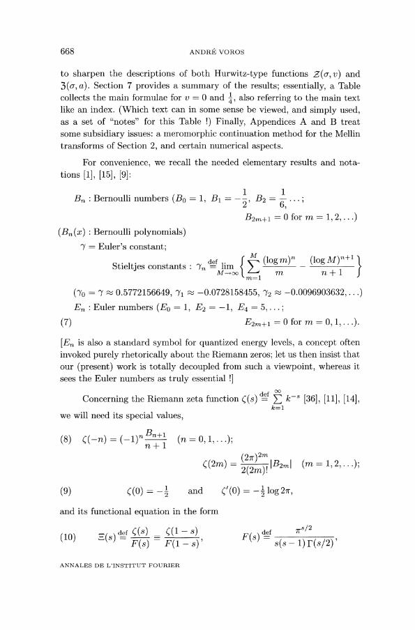
For convenience, we recall the needed elementary results and nota-tions ~1~, [15], [9]:

Bn : Bernoulli numbers I

(Bn (x) : Bernoulli polynomials)7 = Euler’s constant;

Stieltjes constants :

En : Euler numbers

~En is also a standard symbol for quantized energy levels, a concept ofteninvoked purely rhetorically about the Riemann zeros; let us then insist thatour (present) work is totally decoupled from such a viewpoint, whereas itsees the Euler numbers as truly essential !]

Concerning the Riemann zeta function I

we will need its special values,

and its functional equation in the form

669

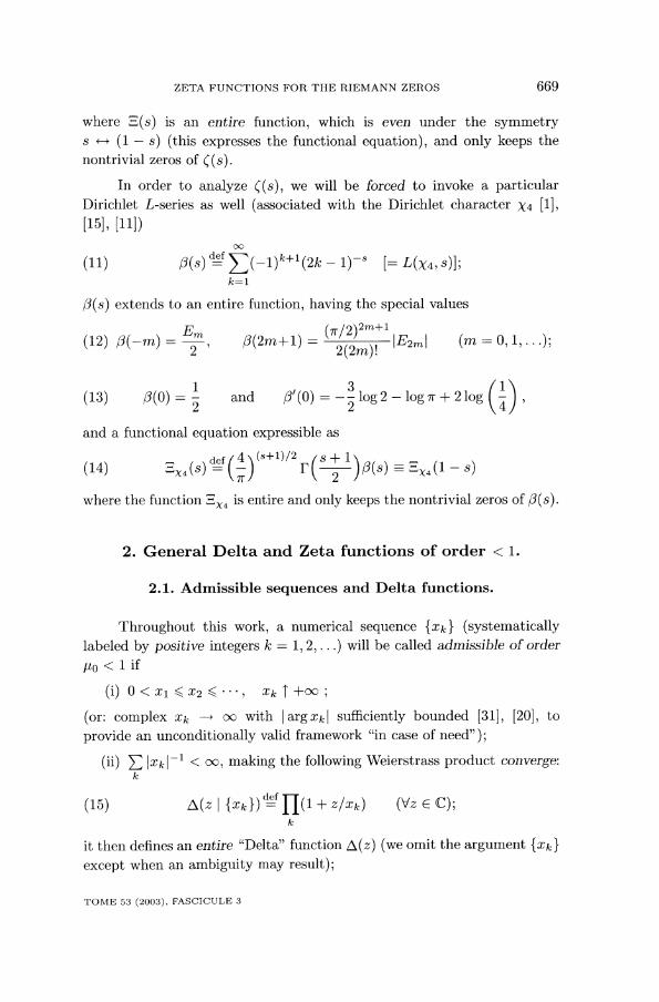
where 3(8) is an entire function, which is even under the symmetrys H (1 - s) (this expresses the functional equation), and only keeps thenontrivial zeros

In order to analyze ((s), we will be forced to invoke a particularDirichlet L-series as well (associated with the Dirichlet character x4 [1],

13(s) extends to an entire function, having the special values

and a functional equation expressible as

where the function 3X4 is entire and only keeps the nontrivial zeros of (3( s).

2. General Delta and Zeta functions of order 1.

2.1. Admissible sequences and Delta functions.

Throughout this work, a numerical sequence fxkl (systematicallylabeled by positive integers k = 1, 2,...) will be called admissible of orderuO 1 if

(or: complex Xk -7 oo with I sufficiently bounded [31], [20], to

provide an unconditionally valid framework "in case of need" ) ;

making the following Weierstrass product converge:

it then defines an entire "Delta" function A(z) (we omit the argument except when an ambiguity may result);

670

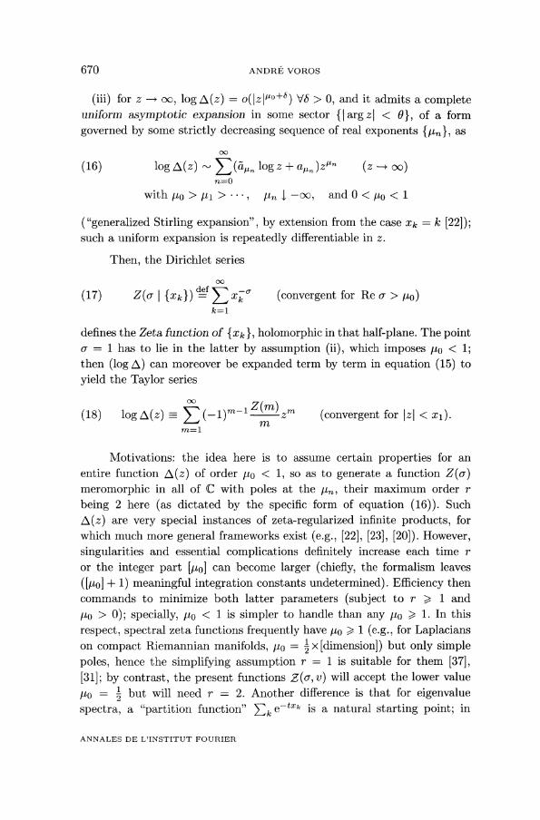
(iii) for , and it admits a completeuniform asymptotic expansion in some sector t arg z~ I 0 1, of a formgoverned by some strictly decreasing sequence of real exponents 1/t.1, as

("generalized Stirling expansion", by extension from the case ~~ = 1~ [22]);such a uniform expansion is repeatedly differentiable in z.

Then, the Dirichlet series

(convergent for Re a &#x3E; po)

defines the Zeta function of holomorphic in that half-plane. The pointa = 1 has to lie in the latter by assumption (ii), which imposes po 1;then (log A) can moreover be expanded term by term in equation (15) toyield the Taylor series

Motivations: the idea here is to assume certain properties for an

entire function A(z) of order po 1, so as to generate a function

meromorphic in all of C with poles at the pn, their maximum order r

being 2 here (as dictated by the specific form of equation (16)). SuchA(z) are very special instances of zeta-regularized infinite products, forwhich much more general frameworks exist (e.g., [22], [23], [20]). However,singularities and essential complications definitely increase each time ror the integer part [po] can become larger (chiefly, the formalism leaves([Mo] + 1 ) meaningful integration constants undetermined). Efficiency thencommands to minimize both latter parameters (subject to r &#x3E; 1 and

Jlo &#x3E; 0); specially, po 1 is simpler to handle than any Jlo 1. In this

respect, spectral zeta functions frequently have 1 (e.g., for Laplacianson compact Riemannian manifolds, po = 1/2 x [dimension]) but only simplepoles, hence the simplifying assumption r = 1 is suitable for them [37],[31]; by contrast, the present functions will accept the lower value

po = 2 but will need r - 2. Another difference is that for eigenvaluespectra, a "partition function" Ek is a natural starting point; in

671

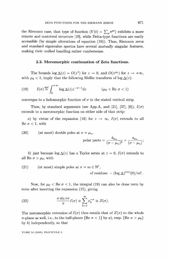
the Riemann case, that type of function ( exhibits a more

remote and contrived structure [10], while Delta-type functions are easilyaccessible (by simple alterations of equation (10)). Thus, Riemann zerosand standard eigenvalue spectra have several mutually singular features,making their unified handling rather cumbersome.

2.2. Meromorphic continuation of Zeta functions.

The bounds log A(z) = for z - 0, and for z - +oo,with po l, imply that the following Mellin transform of log A (z):

converges to a holomorphic function of a in the stated vertical strip.

Then, by standard arguments (see App.A, and [21], [37], [6]), extends to a meromorphic function on either side of that strip:

a) by virtue of the expansion (16) for z -7 oo, extends to all

Re a 1, with

(20) (at most) double poles at a = M,,,

b) just because log A(z) has a Taylor series at z = 0, 1(a) extends toall Re at &#x3E; po, with

(21) (at most) simple poles at a = m E N*,of residues

Now, for po 1, the integral (19) can also be done term byterm after inserting the expansion (15), giving

The meromorphic extension of then entails that of to the whole

a-plane as well, i.e., to the half-planes 1~ by a), resp. &#x3E; po)by b) independently, so that

672

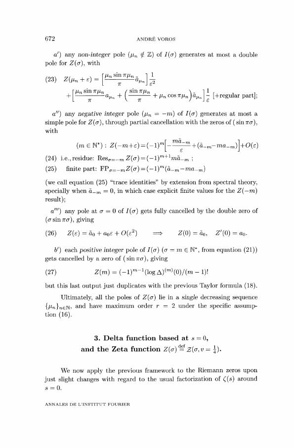
a’) any non-integer pole (Jln tJ- Z) of I(a) generates at most a doublepole for Z(~), with

a") any negative integer pole -m) of I(a) generates at most asimple pole for Z (a), through partial cancellation with the zeros of ( sin with

(we call equation (25) "trace identities" by extension from spectral theory,specially when a-~ == 0, in which case explicit finite values for the Z(-m)result) ;

a"’) any pole at a = 0 of gets fully cancelled by the double zero of

(a- sin giving

b’) each positive integer pole of I(a) (a = m E N*, from equation (21))gets cancelled by a zero of ( sin 7ra), giving

but this last output just duplicates with the previous Taylor formula (18).

Ultimately, all the poles of lie in a single decreasing sequenceand have maximum order r = 2 under the specific assump-

tion (16).

3. Delta function based at s = 0,

and the Zeta function

We now apply the previous framework to the Riemann zeros uponjust slight changes with regard to the usual factorization of ~(s) arounds=0.

673

3.1. Basic facts and notations.

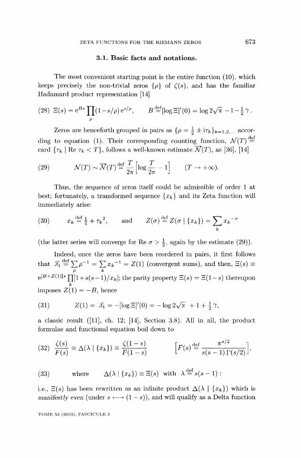
The most convenient starting point is the entire function (10), whichkeeps precisely the non-trivial zeros {p} of ~(s), and has the familiarHadamard product representation [14]

Zeros are henceforth grouped in pairs g accor-

ding to equation ( 1 ) . Their corresponding counting function,card Re Tk T}, follows a well-known estimate Ar(T), as [36], [14]

Thus, the sequence of zeros itself could be admissible of order 1 atbest; fortunately, a transformed sequence and its Zeta function will

immediately arise:

(the latter series will converge for Re a &#x3E; 2 , again by the estimate (29)).Indeed, once the zeros have been reordered in pairs, it first follows

that (convergent sums), and then, 3(s) ==

; the parity property .,

imposes hence

a classic result ([11], ch. 12; [14], Section 3.8). All in all, the productformulae and functional equation boil down to

i.e., E(s) has been rewritten as an infinite product I fxkl) which ismanifestly even (under s ~--~ (1 - s) ), and will qualify as a Delta function

674

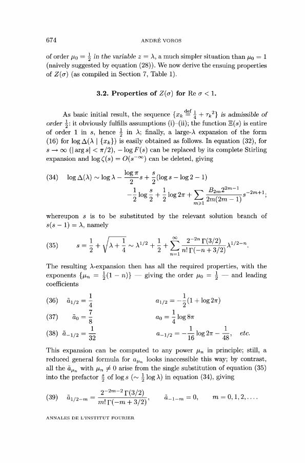
of order [to = 2 in the variable z = A, a much simpler situation than po = 1(naively suggested by equation (28)). We now derive the ensuing propertiesof (as compiled in Section 7, Table 1).

3.2. Properties of Z(a) for Re a 1.

As basic initial result, the sequence ~~~ is admissible of

order 2: it obviously fulfills assumptions (i)-(ii); the function is entire

of order 1 in s, hence -1 in A; finally, a large-A expansion of the form

(16) for log A (A I is easily obtained as follows. In equation (32), fors - oo (~ arg s~ can be replaced by its complete Stirlingexpansion and log ~ ( s ) = O(s-OO) can be deleted, giving

whereupon s is to be substituted by the relevant solution branch of

s ( s - 1) = A, namely

The resulting A-expansion then has all the required properties, with theexponents (pn = 2 (1 - - giving the order lio = 2 and leadingcoefficients

This expansion can be computed to any power pn in principle; still, areduced general formula for aJ-Ln looks inaccessible this way; by contrast,all the aJ-Ln with 0 arise from the single substitution of equation (35)into the prefactor 1 of log s (~ 2 log A) in equation (34), giving

675

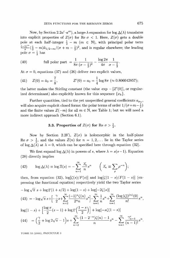
Now, by Section 2.2a’-a"’), a large-A expansion for log A(A) translatesinto explicit properties of for Re a 1. Here, gets a double

pole at each half-integer 2 - m (m e N), with principal polar term, and is regular elsewhere; the leading

pole o~ = 2 has

full polar part

At cr = 0, equations (37) and (26) deliver two explicit values,

the latter makes the Stirling constant (the value exp - [Z’(0)], or regular-ized determinant) also explicitly known for this sequence fxkl.

Further quantities, tied to the yet unspecified general coefficients will also acquire explicit closed forms: the polar terms of order and the finite values Z(-m) for all nz e N, see Table 1; but we will need amore indirect approach (Section 6.1).

3.3. Properties of Z(a) for Re a &#x3E; 2.

Now by Section 2.2b’), is holomorphic in the half-planeRe a &#x3E; 2 , and the values Z(n) for n = 1, 2,... lie in the Taylor seriesof log A(A) at A = 0, which can be specified here through equation (32).

We first expand log A(A) in powers of s, where A = s(s -1). Equation(28) directly implies

then, from equation (32), log[((s)IF(s)] and log[((1 - s)/F(1 - s)] (ex-pressing the functional equation) respectively yield the two Taylor series

676

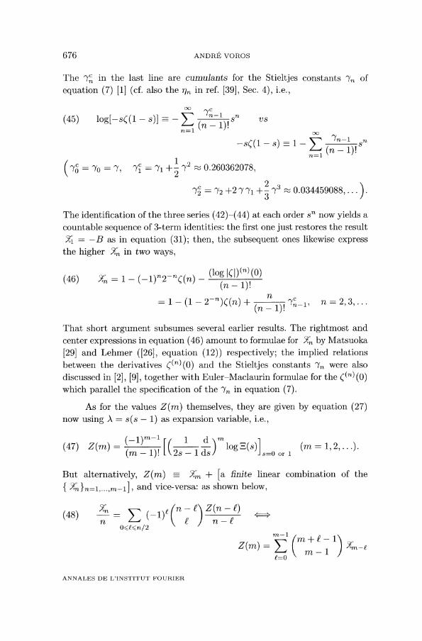
The ’Yn in the last line are cumulants for the Stieltjes constants ’Yn ofequation (7) [1] (cf. also the qn in ref. [39], Sec. 4), i.e.,

The identification of the three series (42)-(44) at each order sn now yields acountable sequence of 3-term identities: the first one just restores the result

-B as in equation (31); then, the subsequent ones likewise expressthe higher ~ in turo ways,

That short argument subsumes several earlier results. The rightmost andcenter expressions in equation (46) amount to formulae for ~ by Matsuoka[29] and Lehmer ([26], equation (12)) respectively; the implied relationsbetween the derivatives ((’)(0) and the Stieltjes constants ’Yn were also

discussed in [2], [9], together with Euler-Maclaurin formulae for the ((n) (0)which parallel the specification of the ’in in equation (7).

As for the values Z(m) themselves, they are given by equation (27)now 1) as expansion variable, i.e.,

But alternatively, finite linear combination of the

, and vice-versa: as shown below,

677

The X, being already knownfrom equations (31) and (46), Z(m) then reduces to an explicit affine

combination (over the rationals) of B - ~(n), and eitheror ~~-1 for 1 n m (see Table 1), as stated earlier by

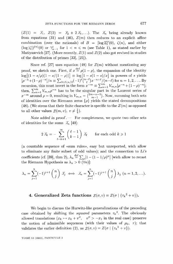
Matiyasevich [27]. (More recently, Z(I) and Z(2) also got revived in studiesof the distribution of primes [33], [25]).

Since ref. [27] uses equation (48) for Z(m) without mentioning anyproof, we sketch one. First, the expansion of the identity

recursion, this must invert in the formhas to be the singular part in the Laurent series of

x-m around p = 0, resulting in I . Now, summing both setsof identities over the Riemann zeros {p} yields the stated decompositions(48). (We stress that their finite character is specific to the Z (m) as opposedto all other values v), v i= ~).

Note added in proof. - For completeness, we quote two other setsof identities for the sums X, [40]:

(a countable sequence of «sum rules», easy but unreported, wich allowto eliminate any finite subset of odd values); and the connection to Li’scoefficients (cf. [39], thm 2), [wich allow to recastthe Riemann Hypothesis as An &#x3E; 0 (Vn)]:

4. Generalized Zeta functions

We begin to discuss the Hurwitz-like generalizations of the precedingcase obtained by shifting the squared parameters The obviouslyallowed translations ( in the real case) preservethe notion of admissible sequences (with their values of po, r); that

validates the earlier definition

678

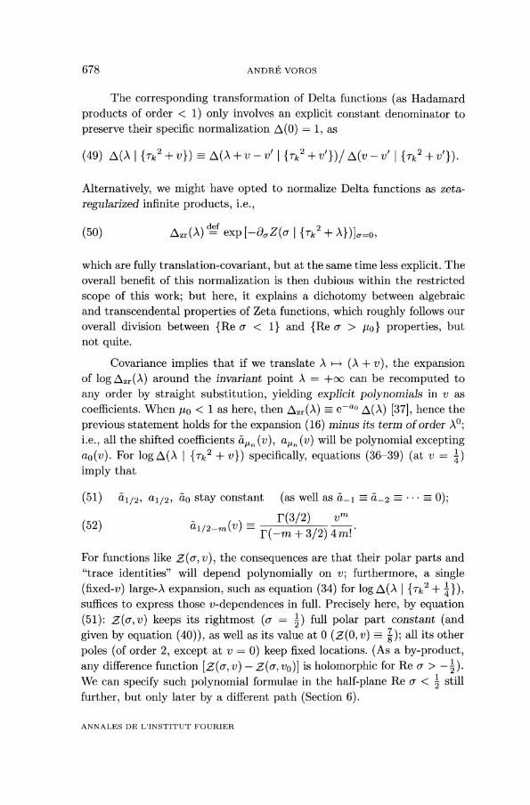
The corresponding transformation of Delta functions (as Hadamardproducts of order 1) only involves an explicit constant denominator topreserve their specific normalization A(0) = 1, as

Alternatively, we might have opted to normalize Delta functions as zeta-regularized infinite products, i.e.,

which are fully translation-covariant, but at the same time less explicit. Theoverall benefit of this normalization is then dubious within the restricted

scope of this work; but here, it explains a dichotomy between algebraicand transcendental properties of Zeta functions, which roughly follows ouroverall division between 1 ~ and &#x3E; po) properties, butnot quite.

Covariance implies that if we translate A - (A + v), the expansionof logAzr(A) around the invariant point A = +oo can be recomputed toany order by straight substitution, yielding explicit polynomials in v ascoefficients. When po 1 as here, then Azr (A) * e -ao A(A) [37], hence theprevious statement holds for the expansion (16) minus its term of order À 0;i.e., all the shifted coefficients aJ-Ln (v), (v) will be polynomial exceptingao(v). For log A (A I ITk2 + VI) specifically, equations (36-39) (at v = ~)imply that

(51) ~i/2, aI/2, ao stay constant (as well as 6-1 d-2 0);

For functions like ,~(~, v), the consequences are that their polar parts and"trace identities" will depend polynomially on v; furthermore, a single(fixed-v) large-A expansion, such as equation (34) for log A(A -t- 4 ~),suffices to express those v-dependences in full. Precisely here, by equation(51): keeps its rightmost (~ = 2 ) full polar part constant (andgiven by equation (40)), as well as its value at 0 (.~(0, v) 8 all its otherpoles (of order 2, except at v = 0) keep fixed locations. (As a by-product,any difference function .Z (6, v ) - Z ( 6, vo ) ] is holomorphic for Re a &#x3E; - 2 ) .We can specify such polynomial formulae in the half-plane Re a 2 stillfurther, but only later by a different path (Section 6).

679

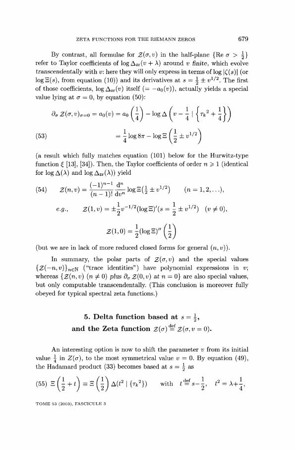
By contrast, all formulae for in the half-plane &#x3E; 2refer to Taylor coefficients of A) around v finite, which evolvetranscendentally with v: here they will only express in terms of log 1(( s) (orlog 3(s), from equation (10)) and its derivatives at The first

of those coefficients, itself (= -ao (v) ), actually yields a specialvalue lying at a = 0, by equation (50):

(a result which fully matches equation (101) below for the Hurwitz-typefunction ~ [13], [34]). Then, the Taylor coefficients of order n &#x3E; 1 (identicalfor log A ( A) and yield

(but we are in lack of more reduced closed forms for general (n, v)).In summary, the polar parts of and the special values

("trace identities") have polynomial expressions in v;

whereas (n :~ 0) plus a~ ,~(o, v) at n = 0 1 are also special values,but only computable transcendentally. (This conclusion is moreover fullyobeyed for typical spectral zeta functions.)

5. Delta function based at s 29and the Zeta function z(a, v = 0).

An interesting option is now to shift the parameter v from its initial

value -1 in Z(a), to the most symmetrical value v = 0. By equation (49),the Hadamard product (33) becomes based at s = 2 as

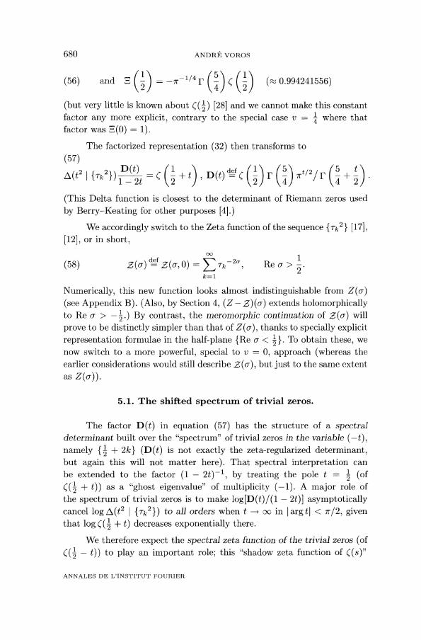
680

(but very little is known about ((~) [28] and we cannot make this constantfactor any more explicit, contrary to the special where that

factor was E(0) = 1).The factorized representation (32) then transforms to

(This Delta function is closest to the determinant of Riemann zeros usedby Berry-Keating for other purposes [4].)

We accordingly switch to the Zeta function of the sequence [17],[12], or in short,

Numerically, this new function looks almost indistinguishable from

(see Appendix B). (Also, by Section 4, (Z - Z)(a) extends holomorphicallyto Re a &#x3E; 20131/2.) By contrast, the meromorphic continuation of will

prove to be distinctly simpler than that of Z (a), thanks to specially explicitrepresentation formulae in the half-plane 2 ~. To obtain these, wenow switch to a more powerful, special to v = 0, approach (whereas theearlier considerations would still describe ,~(~), but just to the same extentas Z(a~)).

5.1. The shifted spectrum of trivial zeros.

The factor D(t) in equation (57) has the structure of a spectraldeterminant built over the "spectrum" of trivial zeros in the variable (-t),namely I’ 2 + (D(t) is not exactly the zeta-regularized determinant,but again this will not matter here). That spectral interpretation canbe extended to the factor (1 - 2t) -1, by treating the pole t - 2 (of~ ( 2 ~ t) ) as a "ghost eigenvalue" of multiplicity ( -1 ) . A major role ofthe spectrum of trivial zeros is to make 2t)] asymptoticallycancel log A(t2 I to all orders when t ~ oc in arg t( I 7r / 2, giventhat log 2 ~- t) decreases exponentially there.

We therefore expect the spectral zeta function of the trivial zeros (of~( 2 - t)) to play an important role; this "shadow zeta function of ~(s)"

681

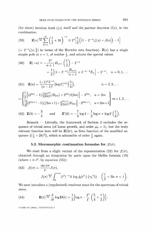
(for short) involves both ~(s) itself and the partner function ~3(s), in thecombination

(= 2-S((s, 4 ) in terms of the Hurwitz zeta function). Z(s) has a singlesimple pole at s = 1, of residue -1, and admits the special values

Remarks Literally, the framework of Section 2 excludes the se-quence of trivial zeros (of linear growth, and order po = 1), but the trulyrelevant function here will be as Zeta function of the modified se-

quence {(1/2 + 2k)2}, which is admissible of order -1 again.

5.2. Meromorphic continuation formulae for

We start from a slight variant of the representation (22) for obtained through an integration by parts upon the Mellin formula (19)(where z = t2, by equation (55)):

We next introduce a (regularized) resolvent trace for the spectrum of trivialzeros,

682

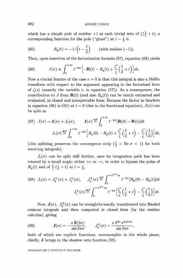
which has a simple pole of residue -f-1 at each trivial zero of

corresponding function for the pole ( "ghost" ) at t = 2 is

Then, upon insertion of the factorization formula (57), equation (63) yields

Now a crucial feature of the case v = 0 is that this integral is also a Mellintransform with respect to the argument appearing in the factorized formof ((s) (namely the variable t, in equation (57)). As a consequence, thecontribution to J from R(t) (and also Rg(t)) can be neatly extracted andevaluated, in closed and interpretable form. Because the factor in bracketsin equation (66) is O(t) at t = 0 (due to the functional equation), can

be split as

( this splitting preserves the convergence strip {1/2 Re a 1 } for both

resulting integrals).

Jr(a) can be split still further, once its integration path has beenrotated by a small angle: either or -~, in order to bypass the poles of

Rg (t) and of

Now, can be straightforwardly transformed into Hankelcontour integrals and then computed in closed form (by the residue

calculus), giving

both of which are explicit functions, meromorphic in the whole plane;chiefly, J brings in the shadow zeta function (59).

683

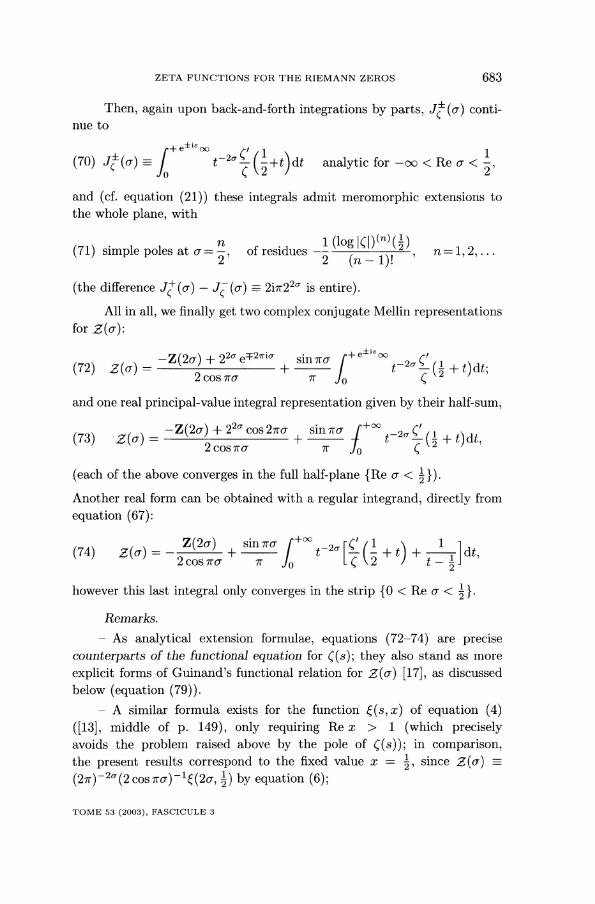
Then, again upon back-and-forth integrations by parts, J/ (a) conti-nue to

and (cf. equation (21)) these integrals admit meromorphic extensions tothe whole plane, with

(71) simple poles at

(the difference

All in all, we finally get two complex conjugate Mellin representationsfor

and one real principal-value integral representation given by their half-sum,

(each of the above converges in the full half-plane ~}).Another real form can be obtained with a regular integrand, directly fromequation (67):

however this last integral only converges in the strip 10 Re at ~}.Remarks.

- As analytical extension formulae, equations (72-74) are precisecounterparts of the functional equation for ((s); they also stand as moreexplicit forms of Guinand’s functional relation for [17], as discussedbelow (equation (79)).

- A similar formula exists for the function ~(s, x) of equation (4)([13], middle of p. 149), only requiring Re x &#x3E; 1 (which preciselyavoids the problem raised above by the pole of ((s)); in comparison,the present results correspond to the fixed value x - ~, since

by equation (6);

684

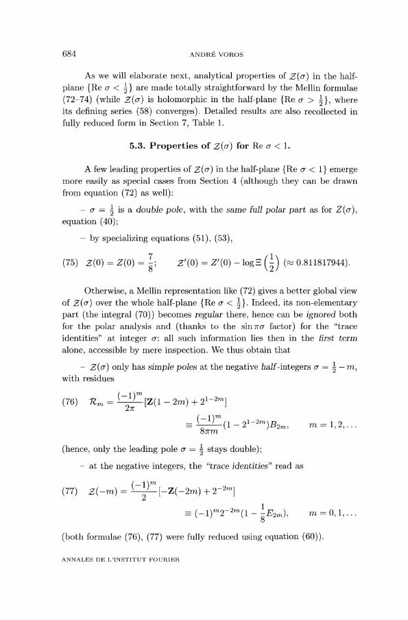
As we will elaborate next, analytical properties of in the half-

plane ~} are made totally straightforward by the Mellin formulae(72-74) (while is holomorphic in the half-plane &#x3E; 2 !I, whereits defining series (58) converges). Detailed results are also recollected infully reduced form in Section 7, Table 1.

5.3. Properties of for Re a 1.

A few leading properties of Z (a) in the half-plane 1~ emergemore easily as special cases from Section 4 (although they can be drawnfrom equation (72) as well):

- r == - is a double pole, with the same full polar part as for Z(a),equation (40);

- by specializing equations (51), (53),

Otherwise, a Mellin representation like (72) gives a better global viewof Z (a) over the whole half-plane ~}. Indeed, its non-elementarypart (the integral (70)) becomes regular there, hence can be ignored bothfor the polar analysis and (thanks to the sinJ1a factor) for the "trace

identities" at integer a : all such information lies then in the first term

alone, accessible by mere inspection. We thus obtain that

- only has simple poles at the negative half-integers a = 2 - m,with residues

(hence, only the leading pole a - -1 stays double);- at the negative integers, the "trace identities" read as

(both formulae (76), (77) were fully reduced using equation (60)).

685

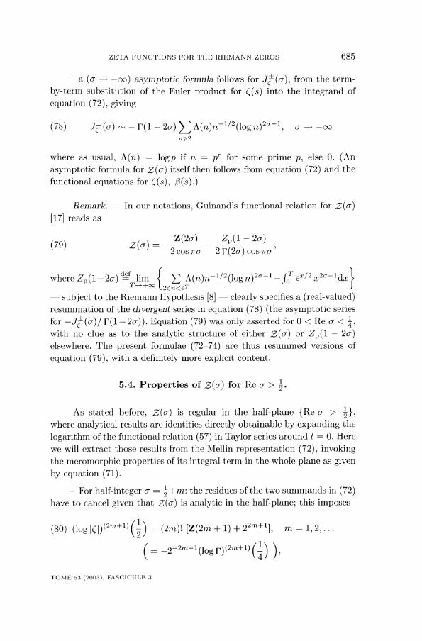
- a (6 -&#x3E; -oo) asymptotic formula follows for J±(o7), from the term-by-term substitution of the Euler product for S(s) into the integrand ofequation (72), giving

where as usual, = logp if n = ~r for some prime p, else 0. (Anasymptotic formula for Z(a) itself then follows from equation (72) and thefunctional equations for ((s), (3(s).)

Remark. 2013 In our notations, Guinand’s functional relation for

[17] reads as

where

subject to the Riemann Hypothesis [8] - clearly specifies a (real-valued)resummation of the divergent series in equation (78) (the asymptotic seriesfo Equation (79) was only asserted for (

with no clue as to the analytic structure of either Z (a) or 2p ( 1 - 2a)elsewhere. The present formulae (72-74) are thus resummed versions ofequation (79), with a definitely more explicit content.

5.4. Properties of for Re a &#x3E; 2"

As stated before, z(J) is regular in the half-plane &#x3E; ~},where analytical results are identities directly obtainable by expanding the

logarithm of the functional relation (57) in Taylor series around t = 0. Herewe will extract those results from the Mellin representation (72), invokingthe meromorphic properties of its integral term in the whole plane as givenby equation (71).

- For half-integer a = 2 -f-m: the residues of the two summands in (72)have to cancel given that is analytic in the half-plane; this imposes

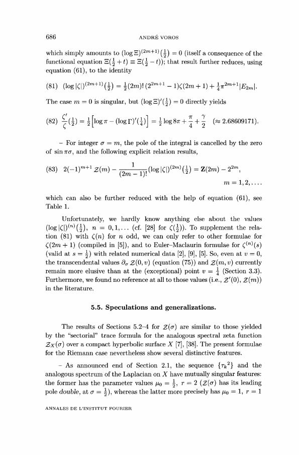
686

which simply amounts to (log u) ~2"2+1&#x3E; ( 2 ) = 0 (itself a consequence of thefunctional equation 3(~ + t) - u( 2 - t)); that result further reduces, usingequation (61), to the identity

The case m = 0 is singular, but ( directly yields

- For integer = m, the pole of the integral is cancelled by the zeroof sin Jra, and the following explicit relation results,

which can also be further reduced with the help of equation (61), seeTable 1.

Unfortunately, we hardly know anything else about the values

(log (n) (-!), n = 0,1,... (cf. [28] for ((~)). To supplement the rela-tion (81) with ((n) for n odd, we can only refer to other formulae for

((2m + 1) (compiled in [5]), and to Euler-Maclaurin formulae for ~~n~ (s)(valid at s = 2 ) with related numerical data [2], [9], [5]. So, even at v = 0,the transcendental values 8a v) (equation (75) ) v) currentlyremain more elusive than at the (exceptional) point v = 4 (Section 3.3).Furthermore, we found no reference at all to those values (i.e., Z’(O), z (rn) )in the literature.

5.5. Speculations and generalizations.

The results of Sections 5.2-4 for Z(cr) are similar to those yieldedby the "sectorial" trace formula for the analogous spectral zeta functionZx (a) over a compact hyperbolic surface X [7], [38]. The present formulaefor the Riemann case nevertheless show several distinctive features.

- As announced end of Section 2.1, the sequence and the

analogous spectrum of the Laplacian on X have mutually singular features:the former has the parameter values po = 2 , r = 2 has its leadingpole double, at a = 2 ), whereas the latter more precisely has Jlo = 1, r = 1

687

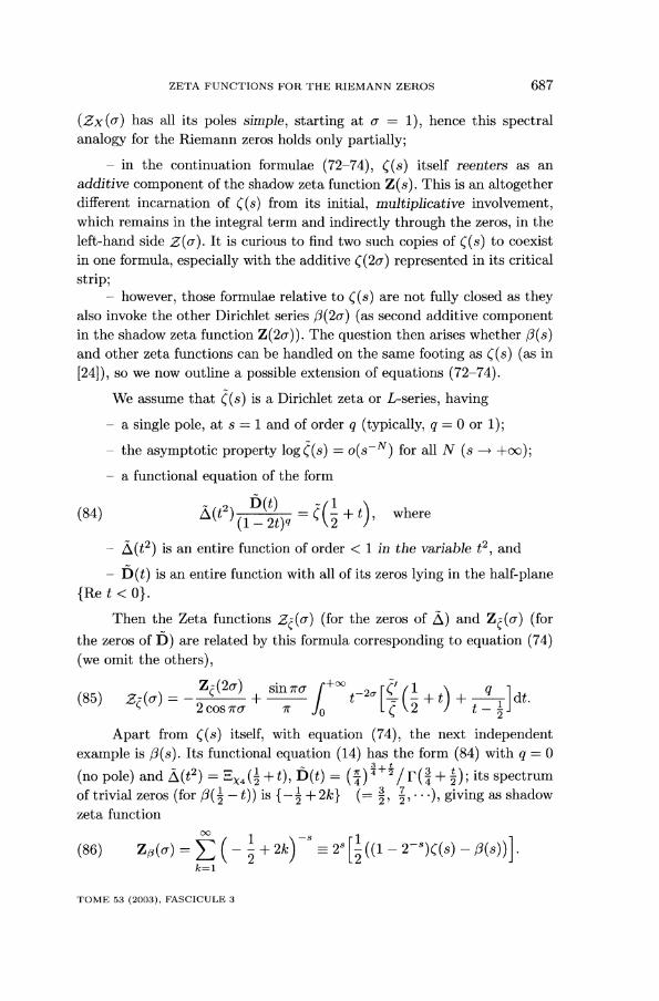
(Zx (a) has all its poles simple, starting at a = 1), hence this spectralanalogy for the Riemann zeros holds only partially;

- in the continuation formulae (72-74), ((s) itself reenters as an

additive component of the shadow zeta function Z(s). This is an altogetherdifferent incarnation of ~(s) from its initial, multiplicative involvement,which remains in the integral term and indirectly through the zeros, in theleft-hand side It is curious to find two such copies of ~(s) to coexistin one formula, especially with the additive ((2a) represented in its criticalstrip;

- however, those formulae relative to ((s) are not fully closed as theyalso invoke the other Dirichlet series (3(2a) (as second additive componentin the shadow zeta function Z(2a)). The question then arises whether (3(s)and other zeta functions can be handled on the same footing as ~(s) (as in[24]), so we now outline a possible extension of equations (72-74).

We assume that ~(s) is a Dirichlet zeta or L-series, having- a single pole, at s = 1 and of order q (typically, q = 0 or 1);- the asymptotic property .- a functional equation of the form

- p(t2) is an entire function of order 1 in the variable t2, and- D (t) is an entire function with all of its zeros lying in the half-plane

Then the Zeta functions zj(a) (for the zeros of 0) and (forthe zeros of D) are related by this formula corresponding to equation (74)(we omit the others),

Apart from ((s) itself, with equation (74), the next independentexample is (3(s). Its functional equation (14) has the form (84) with q = 0

(no pole) and its spectrumof trivial zeros ( , giving as shadowzeta function

688

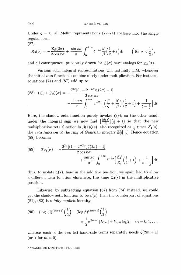
Under q - 0, all Mellin representations (72-74) coalesce into the singleregular form

and all consequences previously drawn for Z (a) have analogs for

Various such integral representations will naturally add, wheneverthe initial zeta functions combine nicely under multiplication. For instance,equations (74) and (87) add up to

Here, the shadow zeta function purely invokes ~(s); on the other hand,under the integral sign we now find so that the new

multiplicative zeta function is (3(s)((s), also recognized as 4 times Z4(s),the zeta function of the ring of Gaussian integers Z[i] [6]. Hence equation(88) becomes

thus, to isolate ~(s), here in the additive position, we again had to allowa different zeta function elsewhere, this time Z4 (s) in the multiplicativeposition.

Likewise, by subtracting equation (87) from (74) instead, we couldget the shadow zeta function to be 0(s); then the counterpart of equations(81), (82) is a fully explicit identity,

whereas each of the two left-hand-side terms separately needs ((2m + 1)for m = 0).

689

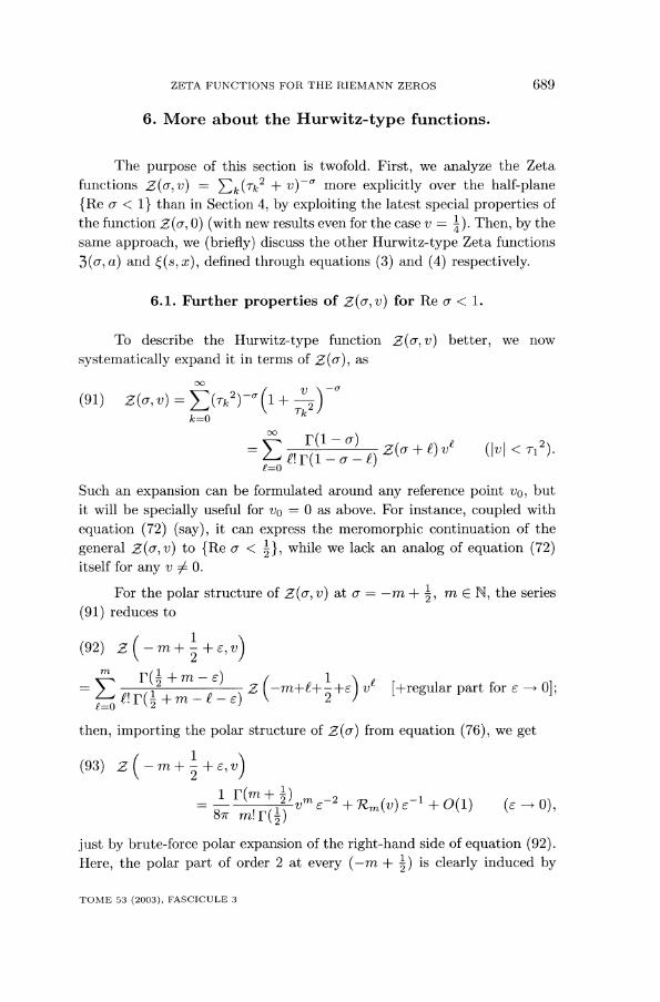
6. More about the HurvcTitz-type functions.

The purpose of this section is twofold. First, we analyze the Zetafunctions .~(~, v) _ E k ( Tk 2 + v) -0" more explicitly over the half-plane

1 ~ than in Section 4, by exploiting the latest special properties ofthe function 0) (with new results even for the case v = ~). Then, by thesame approach, we (briefly) discuss the other Hurwitz-type Zeta functions3 (a, a) and ~ (s, x), defined through equations (3) and (4) respectively.

6.1. Further properties of Z(a, v) for Re a 1.

To describe the Hurwitz-type function better, we now

systematically expand it in terms of ,~(~), as

Such an expansion can be formulated around any reference point vo, butit will be specially useful for vo - 0 as above. For instance, coupled withequation (72) (say), it can express the meromorphic continuation of the

general to (Re a 2 1 1, while we lack an analog of equation (72)itself for any v # 0.

For the polar structure of v) at a = -m + -1 rn G N, the series(91) reduces to

then, importing the polar structure of from equation (76), we get

just by brute-force polar expansion of the right-hand side of equation (92).Here, the polar part of order 2 at every (-m + 2 ) is clearly induced by

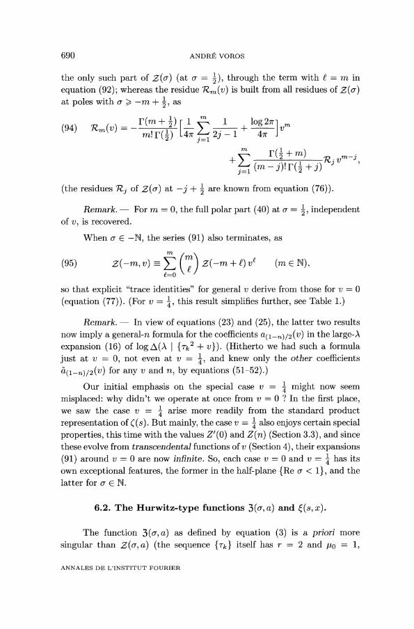
690

the only such part of (at a = -1), through the term with = m inequation (92); whereas the residue is built from all residues of

at poles with a &#x3E; -m + -1, as

(the residues 7Z~ of are known from equation (76)).

Remarks For m = 0, the full polar part (40) at a = -1, independentof v, is recovered.

When o- E -N, the series (91) also terminates, as

1 V

so that explicit "trace identities" for general v derive from those for v = 0

(equation (77)). (For v - -1, this result simplifies further, see Table 1.)

In view of equations (23) and (25), the latter two resultsnow imply a general-n formula for the coefficients a(,-n)/2(V) in the large-Aexpansion (16) of . (Hitherto we had such a formulajust at v - 0, not even at v - 4 , and knew only the other coefficientsa(1-n)/2(v) for any v and n, by equations (51-52).)

Our initial emphasis on the special might now seem

misplaced: why didn’t we operate at once from v = 0 ? In the first place,we saw the arise more readily from the standard productrepresentation of ~(s). But mainly, the case v = 4 also enjoys certain specialproperties, this time with the values Z’(0) and Z(n) (Section 3.3), and sincethese evolve from transcendental functions of v (Section 4), their expansions(91) around v = 0 are now infinite. So, each case v = 0 has its

own exceptional features, the former in the half-plane 1~, and thelatter for a G N.

6.2. The Hurwitz-type functions 3(a, a) and ~(s, x).

The function as defined by equation (3) is a priori more

singular than (the sequence itself has r = 2 and po = 1,

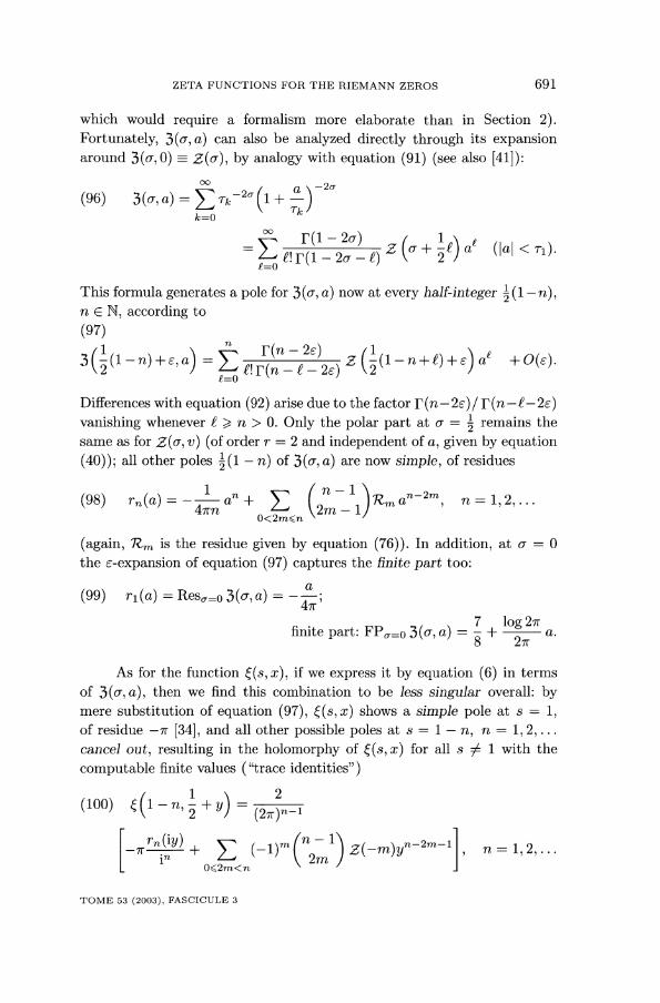
691

which would require a formalism more elaborate than in Section 2).Fortunately, 3(a, a) can also be analyzed directly through its expansionaround 3(a, 0) == .~(~), by analogy with equation (91) (see also [41]):

This formula generates a pole for 3 (a, a) now at every n according to

Differences with equation (92) arise due to the factor r(n-2~)/ vanishing whenever £ &#x3E; n &#x3E; 0. Only the polar part at a = 2 remains thesame as for v) (of order r = 2 and independent of a, given by equation(40)); all other poles 1/2 ( 1 - n) of 3 (a, a) are now simple, of residues

(again, is the residue given by equation (76)). In addition, at a = 0the E-expansion of equation (97) captures the finite part too:

As for the function ~(s, x), if we express it by equation (6) in termsof 3 (a, a), then we find this combination to be less singular overall: bymere substitution of equation (97), ~(s, x) shows a simple pole at s = 1,of residue - 7 [34], and all other possible poles n = 1, 2, ...cancel out, resulting in the holomorphy of ~(s, x) for 1 with the

computable finite values ("trace identities" )

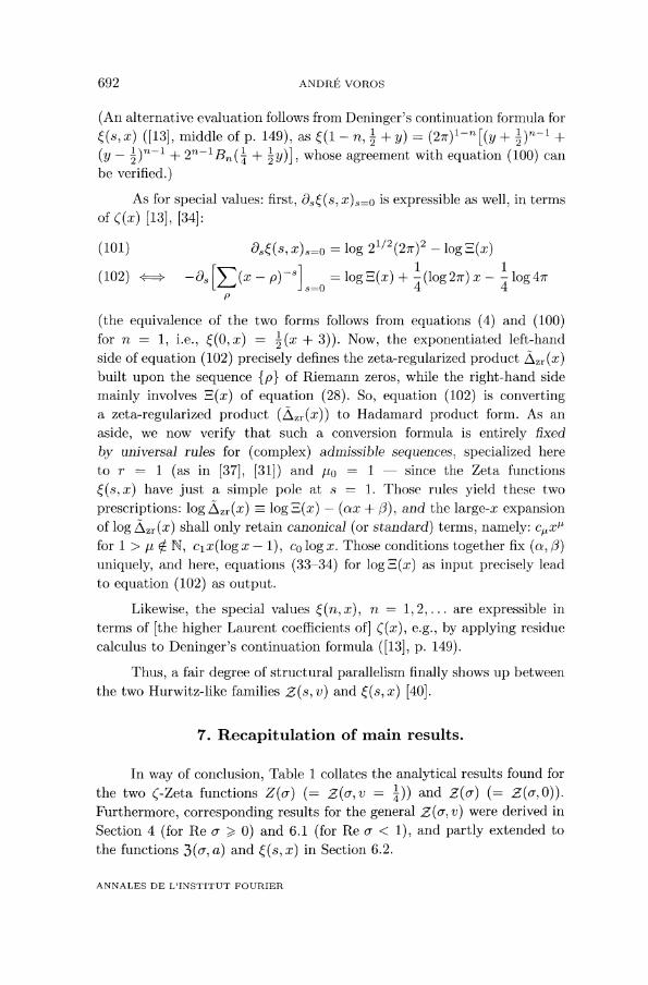
692

(An alternative evaluation follows from Deninger’s continuation formula for

whose agreement with equation (100) canbe verified.)

As for special values: first, 8sç(s, x)s=o is expressible as well, in termsof ((x) [13], [34]:

r

(the equivalence of the two forms follows from equations (4) and (100)for n = 1, i.e., ~(0, x) = -1 (x + 3)). Now, the exponentiated left-handside of equation (102) precisely defines the zeta-regularized product built upon the sequence ~p~ of Riemann zeros, while the right-hand sidemainly involves E(x) of equation (28). So, equation (102) is convertinga zeta-regularized product to Hadamard product form. As an

aside, we now verify that such a conversion formula is entirely fixed

by universal rules for (complex) admissible sequences, specialized hereto r = 1 (as in [37], [31]) and po = 1 - since the Zeta functions

~(s, x) have just a simple pole at s = 1. Those rules yield these twoprescriptions: log 3(x) - (ax + (3), and the large-x expansionof log Lizr (x) shall only retain canonical (or standard) terms, namely: for 1 &#x3E; /-L tJ- N, clx(log x - 1), co log x. Those conditions together fix (a, (3)uniquely, and here, equations (33-34) for log 3(x) as input precisely leadto equation (102) as output.

Likewise, the special values ~(n, x), n = 1,2,... are expressible interms of [the higher Laurent coefficients of] ((x), e.g., by applying residuecalculus to Deninger’s continuation formula ([13], p. 149).

Thus, a fair degree of structural parallelism finally shows up betweenthe two Hurwitz-like families v) and ~(s, x) [40].

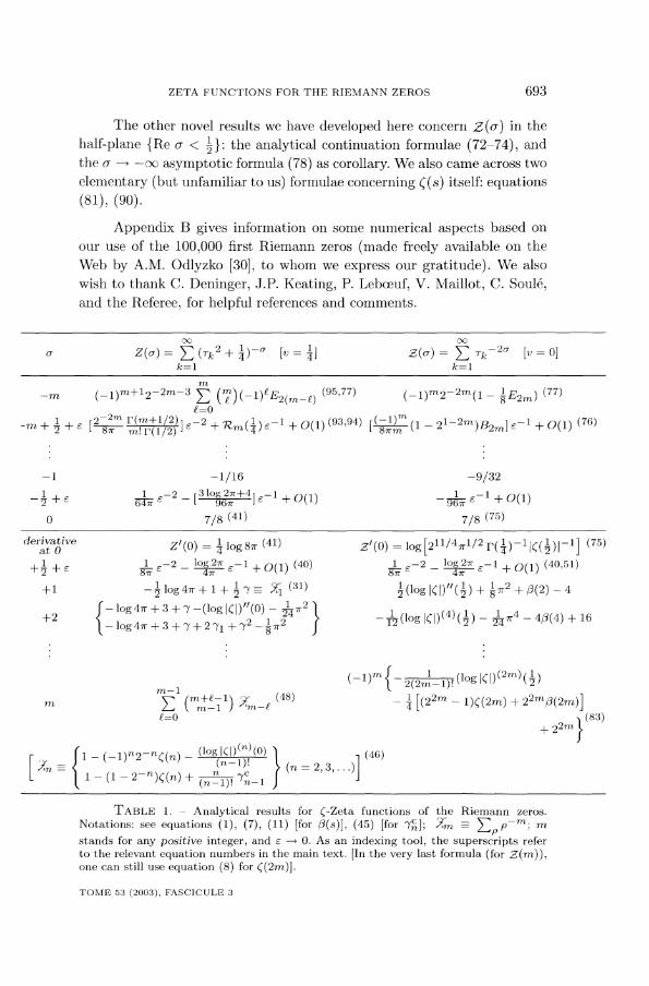
7. Recapitulation of main results.

In way of conclusion, Table 1 collates the analytical results found forthe two (-Zeta functions (= Z(a, v = 4 )) and (= Z(cr,0)).Furthermore, corresponding results for the general were derived in

Section 4 (for Re a &#x3E; 0) and 6.1 (for Re a 1), and partly extended tothe functions 3(a, a) and ~ (s, x) in Section 6.2.

693

The other novel results we have developed here concern Z(o,) in thehalf-plane 2 ~: the analytical continuation formulae (72-74), andthe a -7 -00 asymptotic formula (78) as corollary. We also came across twoelementary (but unfamiliar to us) formulae concerning ~(s) itself: equations(81), (90).

Appendix B gives information on some numerical aspects based onour use of the 100,000 first Riemann zeros (made freely available on theWeb by A.M. Odlyzko [30], to whom we express our gratitude). We alsowish to thank C. Deninger, J.P. Keating, P. Leboeuf, V. Maillot, C. SoUI6,and the Referee, for helpful references and comments.

TABLE 1. - Analytical results for (-Zeta functions of the Riemann zeros.

Notations: see equations (1), (7), (11) [for ¡3(s)], (45) [for m

stands for any positive integer, and 6 - 0. As an indexing tool, the superscripts referto the relevant equation numbers in the main text. [In the very last formula (for .~’(m)),one can still use equation (8) for ~(2?7~)].

694

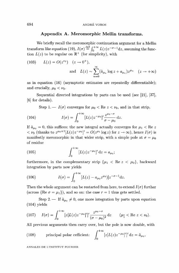
Appendix A. Meromorphic Mellin transforms.

We briefly recall the meromorphic continuation argument for a Mellintransform like equation (19), def Jo+oo assuming the func-tion L(z) to be regular on R+ (for simplicity), with

as in equation (16) (asymptotic estimates are repeatedly differentiable);and crucially, po vo.

Sequential directed integrations by parts can be used (see [21], [37],[6] for details).

Step 1. - converges for po Re z vo, and in that strip,

If = 0, this suffices: the new integral actually converges for Re z

vo (thanks to = 0 (z/" log z) for z - oc), hence I (a) ismanifestly meromorphic in that wider strip, with a simple pole at a = /-Loof residue

furthermore, in the complementary strip (pi Re z pol, backwardintegration by parts now yields

Then the whole argument can be restarted from here, to extend further

(across (Re a = lil I), and so on: the case r = 1 thus gets settled.

Step 2. - If 0, one more integration by parts upon equation(104) yields

All previous arguments then carry over, but the pole is now double, with

principal polar cefficient:

695

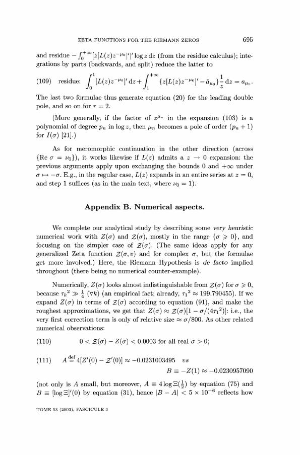
and residue log z dz (from the residue calculus); inte-grations by parts (backwards, and split) reduce the latter to

The last two formulae thus generate equation (20) for the leading doublepole, and so on for r = 2.

(More generally, if the factor of in the expansion (103) is a

polynomial of degree p~ in log z, then pn becomes a pole of order (pn + 1)for [21].)

As for meromorphic continuation in the other direction (acrossRe a - vo 1), it works likewise if L(z) admits a z ~ 0 expansion: theprevious arguments apply upon exchanging the bounds 0 and +oo undera - -~. E.g., in the regular case, L(z) expands in an entire series at z = 0,and step 1 suffices (as in the main text, where vo = 1).

Appendix B. Numerical aspects.

We complete our analytical study by describing some very heuristicnumerical work with Z (a) and mostly in the range (a &#x3E; 01, andfocusing on the simpler case of ,~(~). (The same ideas apply for anygeneralized Zeta function and for complex ~, but the formulae

get more involved.) Here, the Riemann Hypothesis is de facto impliedthroughout (there being no numerical counter-example).

Numerically, Z(a) looks almost indistinguishable from for a &#x3E; 0,because T~2 » 4 (Vk) (an empirical fact; already, 712 ~ 199.790455). If weexpand in terms of according to equation (91), and make theroughest approximations, we get that Z(a) = cr/(4Ti~)]: i.e., thevery first correction term is only of relative size ~ ~/800. As other relatednumerical observations:

(not only is A small, but moreover, A - 4 log ’-7 (-!) by equation (75) andby equation i reflects how

696

little the function log E(s) deviates from the parabolic shape As(l 2013 s) overthe interval [0, 1~ ) .

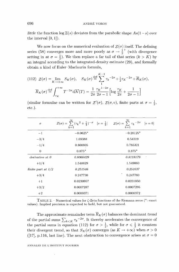
We now focus on the numerical evaluation of Z (a) itself. The definingseries (58) converges more and more poorly as ~ ~ 2 + (with divergencesetting in at a = 2 ) . We then replace a far tail of that series (k &#x3E; K) byan integral according to the integrated-density estimate (29), and formallyobtain a kind of Euler-Maclaurin formula,

(similar formulae can be written for 3’((T), -7(a, v), finite parts at = 2 ,etc.).

TABLE 2. - Numerical values for (-Zeta functions of the Riemann zeros (*: exactvalues). Implied precision is expected to hold, but not guaranteed.

The approximate remainder term RK (a) balances the dominant trendof the partial sums ] . It thereby accelerates the convergence of

.... ,

the partial sums in equation (112) for a &#x3E; 1/2, while it counters

their divergent trend, so that converges (as K - +00) when a &#x3E; 0

([17], p.116, last line). The next obstruction to convergence arises at a = 0

697

but is of another type: SK(a) displays erratic fluctuations in K (roughlyof the order TK-2a(loglogTK)1/2, according to [30], equation (2.5.7)), andthose numerically blow up indeed (as K - when a x 0. Further

convergence now requires to perform a damping of those fluctuations (asargued previously for "chaotic" spectra [3]). Here, a Cesaro averaging

(defined by (S) K def appears to work well initially (resultscan be verified at a = 0), but not very far down: already -0.25,the fluctuations of (S) K (a) itself retain a standard deviation &#x3E; 10-3 up toK = 105. So, instead of pursuing ever more severe (and unproven, after all)numerical regularizations as at decreases below 2 , we advocate the switchto the continuation formulae (72-73) for numerical work as well. Thus, wefirst tested equation (73) against equation (112) for Z(+~), then used it toevaluate Z(- 4 plus equation (91) with v = 4 (3 terms sufficed) to obtain

Table 2 gives a summary of the numerical results we obtained. (Wefound no earlier analogs, except for the other special sums Zn in [29], [26].)

BIBLIOGRAPHY

[1] M. ABRAMOWITZ and I.A. STEGUN, Handbook of Mathematical Functions,chap. 23, Dover, New York, 1965.

[2] T.M. APOSTOL, Formulas for Higher Derivatives of the Riemann Zeta Function,Math. Comput., 44 (1985), 223-232.

[3] N.L. BALAZS, C. SCHMIT and A. VOROS, Spectral Fluctuations and Zeta

Functions, J. Stat. Phys., 46 (1987), 1067-1090.

[4] M.V. BERRY and J.P. KEATING, A new asymptotic representation for 03B6(1/2 + it)and quantum spectral determinants, Proc. R. Soc. Lond., A437 (1992), 151-173.

[5] J.M. BORWEIN, D.M. BRADLEY and R.E. CRANDALL, Computational strategiesfor the Riemann Zeta Function, J. Comput. Appl. Math., 121 (2000), 247-296,and refs. therein.

[6] P. CARTIER, An Introduction to Zeta Functions, in: From Number Theory toPhysics, M. Waldschmidt, P. Moussa, J.-M. Luck and C. Itzykson eds., Springer-Verlag (1992), 1-63.

[7] P. CARTIER and A. VOROS, Une nouvelle interprétation de la formule des tracesde Selberg, C. R. Acad. Sci. Paris, 307, Série I (1988), 143-148, and in: TheGrothendieck Festschrift (vol. 2), eds. P. Cartier et al., Progress in Mathematics,Birkhäuser (1990), 1-67.

[8] I.C. CHAKRAVARTY, The Secondary Zeta-functions, J. Math. Anal. Appl., 30(1970), 2802014294.

[9] B.K. CHOUDHURY, The Riemann zeta-function and its derivatives, Proc. R. Soc.Lond., A450 (1995), 477-499, and refs. therein.

[10] H. CRAMÉR, Studien über die Nullstellen der Riemannschen Zetafunktion,Math. Z., 4 (1919), 104-130.

698

[11] H. DAVENPORT, Multiplicative Number Theory (3rd ed., revised by H.L. Mont-gomery), Graduate Texts in Mathematics, 74, Springer-Verlag, 2000.

[12] J. DELSARTE, Formules de Poisson avec reste, J. Anal. Math. (Jerusalem), 17(1966), 419-431 (Section 7).

[13] C. DENINGER, Local L-factors of motives and regularized determinants, Invent.Math., 107 (1992), 135-150 (Thm 3.3 and Section 4).

[14] H.M. EDWARDS, Riemann’s Zeta Function, Academic Press, 1974.

[15] A. ERDÉLYI (ed.), Higher Transcendental Functions (Bateman ManuscriptProject), vols. I chap. 1 and III chap. 17, McGraw-Hill, New York, 1953.

[16] A. FUJII, The zeros of the Riemann zeta function and Gibbs’s phenomenon,Comment. Math. Univ. St. Paul. (Japan), 32 (1983), 229-248.

[17] A.P. GUINAND, A summation formula in the theory of prime numbers, Proc.London Math. Soc., Series 2, 50 (1949), 107-119 (Section 4(A)).

[18] A.P. GUINAND, Fourier reciprocities and the Riemann zeta-function, Proc.London Math. Soc., Series 2, 51 (1950), 401-414.

[19] D.A. HEJHAL, The Selberg trace formula and the Riemann zeta function, DukeMath. J., 43 (1976), 441-481.

[20] G. ILLIES, Regularized products and determinants, Commun. Math. Phys., 220(2001), 69-94.

[21] P. JEANQUARTIER, Transformation de Mellin et développements asymptotiques,Enseign. Math. II. Ser., 25 (1979), 285-308.

[22] J. JORGENSON and S. LANG, Basic analysis of regularized series and products,Lecture Notes in Mathematics, 1564, Springer-Verlag, 1993.

[23] J. JORGENSON and S. LANG, Explicit formulas for regularized products andseries, Lecture Notes in Mathematics, 1593, Springer-Verlag, 1994, and refs.therein.

[24] N. KUROKAWA, Parabolic components of zeta functions, Proc. Japan Acad., 64,Ser. A (1988), 21-24, and Special values of Selberg zeta functions, in: AlgebraicK-theory and algebraic number theory (Proceedings, Honolulu 1987), M.R.Stein and R. Keith Dennis eds., Contemp. Math., 83, Amer. Math. Soc. (1989),133-149.

[25] P. LEB0152UF, Prime correlations and their fluctuations, preprint (LPTMS, Orsay,2002), submitted to Ann. Henri Poincaré, (Special Issue, Proceedings of TH-2002 Conference, Paris, July 2002).

[26] D.H. LEHMER, The Sum of Like Powers of the Zeros of the Riemann ZetaFunction, Math. Comput., 50 (1988), 265-273, and refs. therein.

[27] Yu.V. MATIYASEVICH, A relationship between certain sums over trivial andnontrivial zeros of the Riemann zeta-function, Mat. Zametki, 45 (1989), 65-70, [Translation: Math. Notes (Acad. Sci. USSR), 45 (1989), 131-135].

[28] Y. MATSUOKA, On the values of the Riemann zeta function at half integers,Tokyo J. Math., 2 (1979), 371-377.

[29] Y. MATSUOKA, A note on the relation between generalized Euler constants andthe zeros of the Riemann zeta function, J. Fac. Educ. Shinshu Univ., 53 (1985),81-82, and A sequence associated with the zeros of the Riemann zeta function,Tsukuba J. Math., 10 (1986), 249-254.

[30] A.M. ODLYZKO, The 1020-th zero of the Riemann zeta function and 175 millionof its neighbors, AT &#x26; T report (1992), unpublished, available on Web sitehttp://www.research.att.com/~amo/.

[31] J.R. QUINE, S.H. HEYDARI and R.Y. SONG, Zeta regularized products, Trans.Amer. Math. Soc., 338 (1993), 213-231.

699

[32] B. RANDOL, On the analytic continuation of the Minakshisundaram-Pleijel zetafunction for compact Riemann surfaces, Trans. Amer. Math. Soc., 201 (1975),241-246.

[33] M. RUBINSTEIN and P. SARNAK, Chebyshev’s bias, Exp. Math., 3 (1994), 173-197.

[34] M. SCHRÖTER and C. SOULÉ, On a result of Deninger concerning Riemann’szeta function, in: Motives, Proc. Symp. Pure Math., 55, Part 1 (1994), 745-747.

[35] F. STEINER, On Selberg’s zeta function for compact Riemann surfaces, Phys.Lett. B, 188 (1987), 447-454.

[36] E.C. TITCHMARSH, The Theory of the Riemann Zeta-function (2nd ed., revisedby D.R. Heath-Brown), Oxford Univ. Press, 1986.

[37] A. VOROS, Spectral functions, special functions and the Selberg zeta function,Commun. Math. Phys., 110 (1987), 439-465.

[38] A. VOROS, Spectral zeta functions, in: Zeta Functions in Geometry (Proceed-ings, Tokyo 1990), N. Kurokawa and T. Sunada eds., Advanced Studies in PureMathematics, 21, Math. Soc. Japan (Kinokuniya, Tokyo, 1992), 327-358.

[39] (added in proof) E. BOMBIERI and J.C. LAGARIAS, Complements to Li’sCriterion for the Riemann Hypothesis, J. Number Theory, 77 (1999), 274-287[the Stieltjes constants 03B3n are normalized differently therein].

[40] (added in proof) A. VOROS, More zeta functions for the Riemann zeros, Saclaypreprint T03/078 (June 2003).

[41] (added in proof) M. HIRANO, N. KUROKAWA and M. NAKAYAMA, Half Zetafunctions, preprint 2003. To appear in J. Ramanujan Math. Soc., 18. [Weunderstand that their polar parts for our function should not have termswith 03B3 either (N. Kurokawa, private communication).]

Manuscrit recu le 25 avril 2001,revise le 27 septembre 2002,accept6 le 12 novembre 2002.

Andr6 VOROS,CEA, Service de Physique Th6orique de SaclayCNRS URA 2306F-91191 Gif-sur-Yvette Cedex (France).voros@spht. saclay. cea. fr

and

Universite Paris 7Institut de Math6matiques de Jussieu-ChevaleretCNRS UMR 75862 place JussieuF-75251 Paris Cedex 05 (France).