universitÉ de la rochelle lab. de maths & applications
TRANSCRIPT
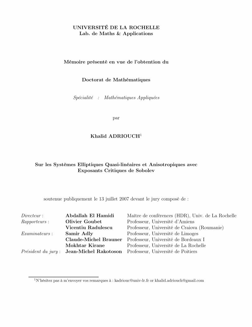
UNIVERSITÉ DE LA ROCHELLELab. de Maths & Applications
Mémoire présenté en vue de l’obtention du
Doctorat de Mathématiques
Spécialité : Mathématiques Appliquées
par
Khalid ADRIOUCH1
Sur les Systèmes Elliptiques Quasi-linéaires et Anisotropiques avecExposants Critiques de Sobolev
soutenue publiquement le 13 juillet 2007 devant le jury composé de :
Directeur : Abdallah El Hamidi Maître de conférences (HDR), Univ. de La RochelleRapporteurs : Olivier Goubet Professeur, Université d’Amiens
Vicentiu Radulescu Professeur, Université de Craiova (Roumanie)Examinateurs : Samir Adly Professeur, Université de Limoges
Claude-Michel Brauner Professeur, Université de Bordeaux IMokhtar Kirane Professeur, Université de La Rochelle
Président du jury : Jean-Michel Rakotoson Professeur, Université de Poitiers
1N’hésitez pas à m’envoyer vos remarques à : [email protected] or [email protected]
Remerciements
Comme le veut la tradition, je vais tenter de satisfaire au difficile exercice de la pagedes remerciements. Non qu’exprimer ma gratitude envers les personnes en qui j’aitrouvé un soutien soit contre ma nature, bien au contraire. La difficulté tient plutôtdans le fait de n’oublier personne. C’est pourquoi, je remercie par avance ceux dontle nom n’apparaît pas dans cette page et qui m’ont aidé d’une manière ou d’uneautre. Ils se reconnaîtront. Pour les autres, non merci. Ils se reconnaîtront aussi...
Cette thèse n’aurait jamais vu le jour sans la confiance, la patience et la générositéde mon directeur de thèse Abdallah El Hamidi que je tiens à remercier vivement.Je voudrais aussi le remercier pour le temps et la patience qu’il m’a accordé toutau long de ces années, d’avoir cru en mes capacités. De plus, les conseils qu’il m’adivulgué en période de rédaction ont toujours été clairs et succincts, me facilitantgrandement la tâche et me permettant d’aboutir à la production de cette thèse.
Je tiens à remercier vivement Mokhtar Kirane pour ses conseils précieux durantles discussions que j’avais avec lui soit dans son bureau ou par téléphone depuis laMalaisie qui m’ont toujours été utiles. Ses qualités scientifiques et humaines, sonencouragement et ses remarques ont largement contribué à l’aboutissement de cettethèse. Qu’il trouve ici l’expression de ma profonde gratitude.
Je remercie les professeurs Olivier Goubet et Vicentu Radulescu de m’avoir faitl’honneur d’être les rapporteurs de cette thèse. J’éprouve un profond respect pourleur travail et leur parcours, ainsi que pour leurs qualités humaines. Je les remercieaussi pour leur participation au jury de thèse. Ils ont également contribué par leursnombreuses remarques et suggestions à améliorer la qualité de ce mémoire, et je leuren suis reconnaissant.
Mes remerciements s’adressent ensuite aux professeurs : Samir Adly, Claude-MichelBrauner, Mokhtar Kirane et Jean-Michel Rakotoson, d’avoir accepté de participerà mon jury de thèse.
Enfin, je remercie mes parents ; Lhoucine et Halima, mes frères ; Rédouane et Ous-sama, mes soeurs ; Fatima et Soumiya et mes camarades ; Amine et Hassan de leursoutien constant tout au long des années de la thèse.
2
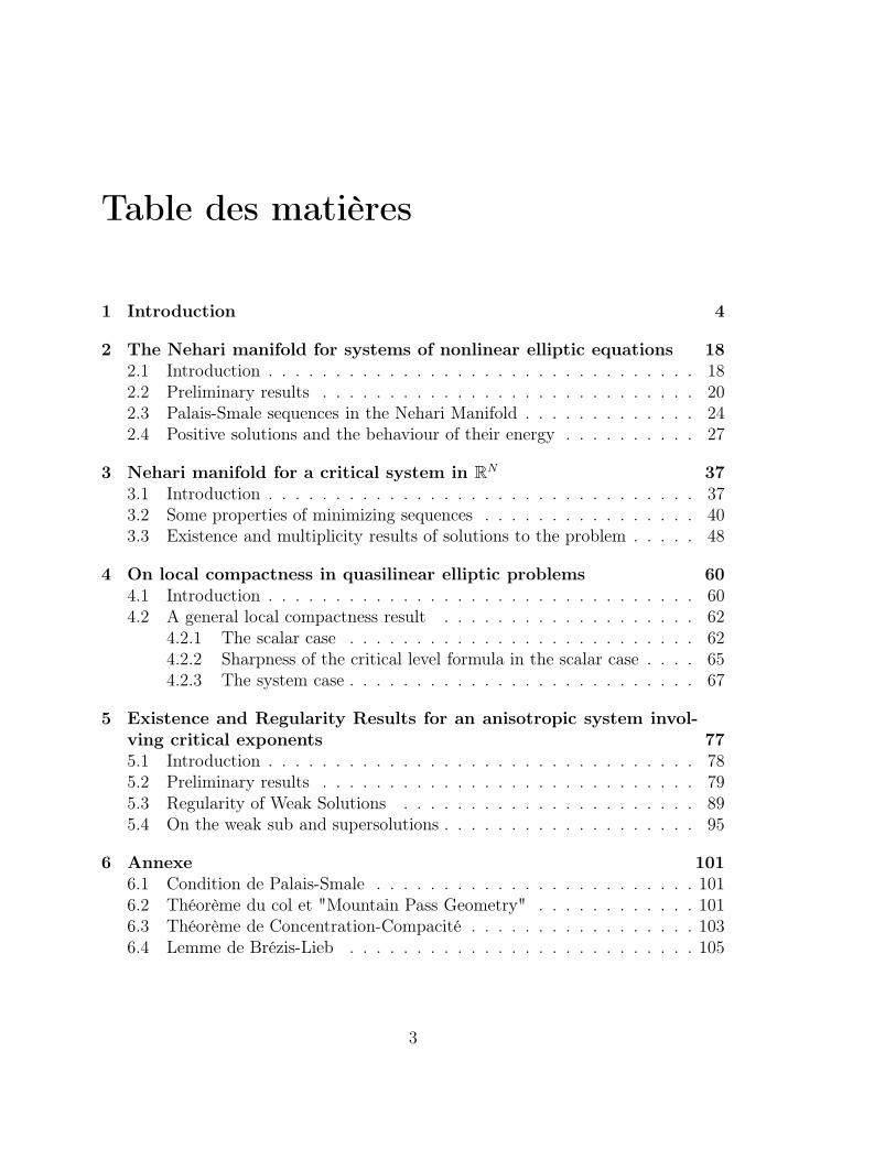
Table des matières
1 Introduction 4
2 The Nehari manifold for systems of nonlinear elliptic equations 182.1 Introduction . . . . . . . . . . . . . . . . . . . . . . . . . . . . . . . . 182.2 Preliminary results . . . . . . . . . . . . . . . . . . . . . . . . . . . . 202.3 Palais-Smale sequences in the Nehari Manifold . . . . . . . . . . . . . 242.4 Positive solutions and the behaviour of their energy . . . . . . . . . . 27
3 Nehari manifold for a critical system in RN 373.1 Introduction . . . . . . . . . . . . . . . . . . . . . . . . . . . . . . . . 373.2 Some properties of minimizing sequences . . . . . . . . . . . . . . . . 403.3 Existence and multiplicity results of solutions to the problem . . . . . 48
4 On local compactness in quasilinear elliptic problems 604.1 Introduction . . . . . . . . . . . . . . . . . . . . . . . . . . . . . . . . 604.2 A general local compactness result . . . . . . . . . . . . . . . . . . . 62
4.2.1 The scalar case . . . . . . . . . . . . . . . . . . . . . . . . . . 624.2.2 Sharpness of the critical level formula in the scalar case . . . . 654.2.3 The system case . . . . . . . . . . . . . . . . . . . . . . . . . . 67
5 Existence and Regularity Results for an anisotropic system invol-ving critical exponents 775.1 Introduction . . . . . . . . . . . . . . . . . . . . . . . . . . . . . . . . 785.2 Preliminary results . . . . . . . . . . . . . . . . . . . . . . . . . . . . 795.3 Regularity of Weak Solutions . . . . . . . . . . . . . . . . . . . . . . 895.4 On the weak sub and supersolutions . . . . . . . . . . . . . . . . . . . 95
6 Annexe 1016.1 Condition de Palais-Smale . . . . . . . . . . . . . . . . . . . . . . . . 1016.2 Théorème du col et "Mountain Pass Geometry" . . . . . . . . . . . . 1016.3 Théorème de Concentration-Compacité . . . . . . . . . . . . . . . . . 1036.4 Lemme de Brézis-Lieb . . . . . . . . . . . . . . . . . . . . . . . . . . 105
3
Chapitre 1
Introduction
Le but de cette thèse est de présenter des résultats récents concernant l’existence etla multiplicité des solutions positives de certaines classes de systèmes d’équationsaux dérivées partielles elliptiques non linéaires faisant intervenir l’opérateur (p, q)-Laplacien du type suivant :
∆pu = f(x, u, v), dans Ω∆qv = g(x, u, v), dans Ω
(0.1)
et des systèmes anisotropiques de la forme suivante :
N∑
i=1
∂
∂xi
(∣∣∣∣∂u
∂xi
∣∣∣∣pi−2
∂u
∂xi
)= f(x, u, v), dans Ω
N∑
i=1
∂
∂xi
(∣∣∣∣∂v
∂xi
∣∣∣∣qi−2
∂v
∂xi
)= g(x, u, v), dans Ω
(0.2)
où ∆pu = ∇ · (|∇u|p−2∇u) et ∆qv = ∇ · (|∇v|p−2∇v) avec p > 1, q > 1, pi > 1et qi > 1 , Ω est un ouvert non vide de RN . D’autre part, les fonctions f et g sontde Caratheodory et sont soumises à certaines conditions de croissance pour garantirque la fonction d’Euler-Lagrange associée est bien définie sur un produit cartésiend’espaces de Sobolev adéquats.Les systèmes d’équations non-linéaires elliptiques et anisotropiques présentent quelq-ues nouveaux et intéressants phénomènes qu’on ne rencontre dans les cas scalaires.En général, les systèmes sont couplés, et même fortement couplés. Alors, les notionsde superlinéarité ou sous-linéarité et même d’exposants critiques, au sens de Sobolev,doivent prendre en considération la nature de tels couplages.L’opérateur p−Laplacien apparaît aussi bien en mathématiques pures ; par exempleen géométrie riemannienne, qu’en mathématiques appliquées. En effet, il intervientdans de nombreux domaines en sciences expérimentales : problèmes de réaction-diffusion non linéaires, dynamique des populations, écoulements de fluides non-newtoniens, écoulements dans les milieux poreux, élasticité non linéaire, extraction
4
§ 1. Introduction 5
de pétrole [23], etc · · ·
Dans la littérature on trouve de nombreux travaux dédiés à l’étude théorique detels équations et systèmes d’équations. En fait, l’étude de ce type de problèmesa effectivement commencé au milieu des années 1980 par M. Ôtani [50] en unedimension puis par F. de Thélin [58] en dimension N , qui ont obtenu les premiersrésultats sur une équation de la forme −∆pu = λuγ−1. Ce dernier auteur [58] etW. M. Ni & J. Serrin [57] ont démontré indépendamment l’existence et l’unicité dessolutions radiales dans RN , plus tard Ôtani [49] a généralisé ce résultat à des ouvertsquelconques. En 1987, F. De Thélin [59] a étendu ces résultats pour des équations detype ∆pu = g(x, u) où la fonction g est contrôlée par des fonctions polynomiales parrapport à u. On peut citer certains précurseurs de l’analyse des problèmes elliptiquesaux valeurs propres G. Barles [10], S. Sakaguchi [56] et A. Anane [8], qui ont étudiéles équations du type :
−∆pu = λ|u|p−2u dans Ω domaine borné.
Plus tard en 1990, P. Lindqvist [43] a établi différents résultats sur ce type d’équa-tions qui font suite à l’article de A. Anane [8]. Par ailleurs, il y a d’autres résultatssur l’unicité qui ont été énoncés par J. I. Dìaz et J. E. Saa [24] en 1987 pour deséquations de la forme −∆pu = f(x, u) sous la condition r 7→ f(x,r)
rp−1 est décroissante.Le problème de bifurcation à la première valeur propre a été abordé par R. F. Maná-sevich et M. A. Del Pino [46], tandis que les problèmes de non résonance associésau p−Laplacien étaient étudiés par A. Anane et J. P. Gossez [9]. Plus tard, le casnon borné de ces équations a été abordé par P. Drábek [25], Drábek et Y. X. Huang[26] et A. Bechah, K. Chaïb et F. de Thélin [11], où les questions d’existence etd’unicité ont été résolues aussi bien pour des problèmes de valeurs propres que pourdes problèmes non-linéaires.Le cas des systèmes présente un nouveau défi et entraîne plusieurs complications liéesau couplage. Les systèmes variationnels peuvent être traîtés en utilisant la théoriedes points critiques, puisque les solutions faibles de ces systèmes sont précisémentles points critiques des fonctionnelles d’Euler-Lagrange associées. Les espaces où cesfonctionnelles sont étudiées dépendent des conditions aux bords que les solutionsdoivent satisfaire. Cette méthode est appelée la méthode directe pour le calcul desvariations, dont les origines remontent à Gauss et Thomson au milieu du 19ème
siècle et qui a été utilisée par Dirichlet et Riemann pour résoudre le problème deDirichlet pour l’équation de Laplace. Cependant, en 1870 Weierstrass avait montréque la démonstration comportait des "trous" et manquait de rigueur mathématiqueet a été alors abandonnée. Il faut attendre le début du 20ème lorsque Hilbert a res-suscité la méthode et développé la théorie nécessaire pour la justifier et depuis elleété connue sous le nom de principe de Dirichlet. De nos jours, les mêmes méthodessont toujours utilisées pour résoudre des problèmes aux bords pour des classes plusgénérales d’équations et de systèmes elliptiques. Dans le cas simple du problème de
§ 1. Introduction 6
Dirichlet pour l’équation de Laplace, le point critique est un minimum de la fonc-tionnelle associée. Dans les années 1930, Ljusternik et Schnierelmann ont développéune théorie des points critiques de type min-max pour des fonctionnelles présentantune symétrie Z2. Plus tard, en 1973 Ambrosetti et Rabinowitz [7] ont établi plu-sieurs résultats sur les points critiques du type min-max pour des fonctionnelles sanssymétrie. On peut distinguer deux sortes de systèmes variationnels : ceux qui sontdu type gradient, s’il existe une fonction F : Ω × R × R −→ R de classe C1 telleque :
f =∂F
∂uet g =
∂F
∂v, (0.3)
et ceux du type hamiltonien s’il existe une fonction H : Ω × R × R −→ R de classeC1 telle que :
f =∂H
∂vet g =
∂H
∂u, (0.4)
où les fonctions f et g sont définies dans (0.1) et (0.2).En ce qui concerne le système du type gradient (0.1) satisfaisant (0.3), on chercheles points critiques de la fonctionnelle
I(u, v) =1
p
∫
Ω
|∇u|pdx+1
q
∫
Ω
|∇v|qdx−∫
Ω
F (x, u, v)dx
qui sont solutions faibles du système (0.1). La fonctionnelle I est définie dans l’espaceproduit W = W 1,p
0 (Ω)×W 1,q0 (Ω). On supposera que la fonction F doit satisfaire les
conditions de croissance suivantes :
|Fu(x, u, v)| ≤ C(|u|γ + |u|α|v|β+1) p. p. dans Ω (0.5)
|Fv(x, u, v)| ≤ C(|v|δ + |u|α+1|v|β) p. p. dans Ω (0.6)
avec les conditions de sous-criticalité ou de criticalité (au sens de Sobolev)
α+ 1
p∗+β + 1
q∗< 1 ou
α + 1
p∗+β + 1
q∗= 1,
où p∗ = NpN−p
, q∗ = NqN−q
et 1 < p, q < N sont les exposants critiques des injections
de Sobolev W 1,p0 (Ω) ⊂ Lp
∗(Ω) et W 1,q
0 (Ω) ⊂ Lq∗(Ω). Les exposants γ et δ vérifient
1 < γ < p∗−1 et 1 < δ < q∗−1. Le fait d’imposer que F soit de classe C1 et qu’ellesatisfait les conditions (0.5) et (0.6) entraînent que I est aussi de classe C1.C’est en 1990 où F. de Thélin [60] avait initié les travaux sur les systèmes faisantintervenir le p−Laplacien où il a montré l’existence et l’unicité de la première valeurpropre du système
−∆pu = λ|u|α−1u|v|β+1 dans Ω−∆qv = λ|u|α+1|v|β−1v dans Ω
§ 1. Introduction 7
sous la condition de criticalité α+1p∗
+ β+1q∗
= 1. Le cas d’un système variationnel a ététraité par P. Felmer, R. F. Manásevich et F. de Thélin [34] où les auteurs ont étudiél’existence et l’unicité de la solution positive d’un système variationnel du type :
−∆pu =∂H
∂u(x, u, v) dans Ω
−∆qv =∂H
∂v(x, u, v) dans Ω,
généralisant ainsi les résultats obtenus dans le cas scalaire par J. I. Dìaz et J. E.Saa [24]. Plus tard, ces résultats ont été étendus au cas du système dérivant d’unpotentiel par F. de Thélin et J. Vélin [62], J. Chabrowski [19] et L. Boccardo andD. G. de Figueiredo [14] et ont commencé une approche du cas non variationnelen imposant des conditions sur la croissance des non-linéarités. Dans tout ce quiprécède, les auteurs ont étudié ces systèmes dans des domaines bornés, pour cequi est des problèmes non bornés de RN ont été abordés par J. Fleckinger, R. F.Manásevich, N. M. Stavrakakis et F. de Thélin [34] et A. Bechah, K. Chaïb et F. deThélin [11]. Notons que l’étude des systèmes de p−Laplaciens dans RN ont été inspirépar l’étude générale faite par M. F. Bidaut-Véron [13] sur les Laplaciens classiques etpar P. Clément, J. Fleckinger, R. F. Manásevich et F. de Thélin [21] et P. Clément, R.Manásevich et E. Mitidieri [22] qui ont étudié la question de l’existence des solutionspour les systèmes (p, q)−Laplacien purement non variationnels du type (0.1).
Actuellement, de nombreux travaux de recherche sont en cours sur les systèmes, enparticulier les quatres chapitres de la présente thèse [1, 2, 3, 4]. L’historique qu’onvient de tracer ci-dessus est bien entendu loin d’être exhaustif.Une des motivations de cette thèse est le fait que certains résultats sur les systèmeselliptiques faisant intervenir le p−Laplacien dans les domaines bornés ou non bornésméritaient d’être complétés et que dans certains travaux on imposait des conditionssur les exposants qui ne sont pas "naturelles" pour garantir l’existence ou la non-existence des solutions. La deuxième motivation est de généraliser certains résultatsobtenus par T. Aubin et H. Brézis & L. Nirenberg concernant le niveau critiquegarantissant la compacité des suites minimisantes de Palais-Smale au cas d’équationsscalaires plus générales et ensuite des systèmes elliptiques faisant intervernir le (p, q)-Laplacien.Notre troisième travail a été motivé par la difficulté de démontrer des résultats demultiplicité dans le cas critique en domaine non borné.Notre dernier travail a été motivé par un récent résultat important, dû à A. El Ha-midi et J. M. Rakotoson [32] où ils ont généralisé le fameux principe de concentration-compacité de P. L. Lions au cas des opérateurs anisotropiques.
Dans le reste de cette introduction, nous décrivons brièvement les travaux présentésdans cette thèse.
§ 1. Introduction 8
Chapitre 2 : Dans leur article [6], A. Ambrosetti, H. Brézis et G. Cerami étudientl’existence et la multiplicité de l’équation suivante :
−∆u = fλ(u), x ∈ Ωu = 0 x ∈ ∂Ω,
avec fλ est une fonction présentant une sous linéarité de type concave-convexe, enparticulier fλ(u) = λ|u|p−1u + |u|q−1u sous la condition 1 < p < 2 < q < 2∗. Ils ontmontré, en utilisant la méthode des sous et sur solutions, l’existence d’une solutionpositive correspondant aux petites valeurs de λ > 0 et l’existence d’une deuxièmesolution avec le théorème du col. Ensuite, ils ont également démontré l’existenced’une infinité de solutions si la fonction fλ est impaire. Ce résultat a été généraliséet amélioré par A. El Hamidi [29] au problème de Dirichlet et mixte suivant :
−∆pu = λ|u|q−1u+ |u|r−1u, x ∈ Ω
ε|∇u|p−2 ∂u∂ν
+ a(x)|u|p−2u = 0, x ∈ ∂Ω,(0.7)
avec 1 < q < p < r < p∗ et ε ∈ 0, 1. En utilisant la méthode de Nehari, introduitepar Nehari en 1960. Cette méthode est équivalente à la méthode de stratificationsphérique introduite plus tard par S. I. Pohozaev. A. El Hamidi a étudié la fonc-tionnelle énergie modifiée Eλ définie sur R ×W 1,p
0 (Ω) par :
Eλ(t, u) := Eλ(tu),
où Eλ est la fonctionelle d’Euler-Lagrange associée au problème (0.7). Il a étudiéla restriction E1
λ et E2λ de Eλ à la variété de Nehari, qui est en fait constitutée
de deux ensembles disjoints dès que 0 < λ < λ, et a ensuite démontré que lessuites minimisantes de Ei
λ, i ∈ 1, 2, sont de Palais-Smale et convergent vers deuxdifférentes solutions positives de l’équation (0.7). La première solution a une énergienégative tandis que la deuxième solution a une énergie qui change de signe en λ0 ∈(0, λ).
Dans l’article [1], on a étudié le système elliptique variationnel sous critique suivant :
−∆pu = λ|u|p1−2u+ (α+ 1)|u|α−1u|v|β+1 dans Ω,
−∆qv = µ|v|q−2v + (β + 1)|u|α+1|v|β−1v dans Ω,(0.8)
avec 1 < p1 < p < N , 1 < β + 1 < q < N , α+1p
+ β+1q
> 1 et α+1p∗
+ β+1q∗
< 1.On a adopté les mêmes arguments développés par A. El Hamidi dans son article[29]. A la lumière du résultat de Y. Bozhkov and E. Mitidieri [16], on a introduit lafonctionnelle énergie modifiée définie par :
Iλ,µ(s, u, t, v) = Iλ,µ(su, tv)
§ 1. Introduction 9
où Iλ,µ est la fonctionnelle d’Euler-Lagrange associée au système (0.8). En explorantla variété de Nehari associée à Iλ,µ définie par tous les couples (su, tv) 6= (0, 0)
vérifiant ∂Iλ,µ(s, u, t, v)/∂s = ∂Iλ,µ(s, u, t, v)/∂t = 0, on a démontré que cette variétéest encore composée de deux parties disjointes N 1
λ,µ et N 2λ,µ dès que (λ, µ) appartient
à un sous ensemble spécifique D de R2. L’étude de la restriction de la fonctionnelleIλ,µ à N 1
λ,µ et N 2λ,µ nous a permis ensuite de prouver que les suites minimisantes
dans les deux parties de la variété de Nehari sont de Palais-Smale et convergent versles deux solutions positives du système (0.8). En ce qui concerne le signe de leursénergies, notons que la première est d’une énergie négative tandis que l’énergie de laseconde change de signe selon une fonction continue λ0(µ) dont le graphe est situédans l’ensemble D.
Chapitre 3 : Dans cette partie, on s’interessera à l’étude du système (0.8) dans lecas non borné et vérifiant la condition critique α+1
p∗+ β+1
q∗= 1. Notons que, par
rapport au Chapitre 1, nous perdons la compacité des injections W 1,p(Ω) ⊂ Lp∗(Ω)
et W 1,q(Ω) ⊂ Lq∗(Ω). Dans la littérature, le principe de compacité par concentration
de P. L. Lions [45] et le principe de compacité par concentration de Bianchi et al.[12] sont largement utilisés pour remédier à la perte de compacité des suites dePalais-Smale. Signalons que la décomposition de Struwe est aussi utile dans le casdes domaines bornés et les variètés compactes. J. Vélin et F. de Thélin [62] ontétudié le problème suivant :
−∆p = u|u|α−1|v|β+1, dans Ω
−∆q = |u|α+1|v|β−1v, dans Ω.
Ils ont démontré un résultat d’existence de solutions sous l’hypothèse α+1p∗
+ β+1q∗
< 1
et un résultat de non existence dans le cas α+1p∗
+ β+1q∗
= 1 et le domaine Ω eststrictement étoilé en utilisant l’identité de Pohozaev [53]. Ensuite le système critiquesuivant
−∆p = u|u|α−1|v|β+1 + f, dans Ω
−∆q = |u|α+1|v|β−1v + g, dans Ω.
u = v = 0, sur ∂Ω
avec α+1p∗
+ β+1q∗
= 1, a été discuté par J. Chabrowski [19] dans le cas p = q et J. Velin[63] pour le cas p 6= q et ont montré l’existence d’au moins une solution positivesous l’hypotèse f ∈ W−1,p′(Ω) \ 0 et g ∈W−1,q′(Ω) \ 0 et ‖f‖−1,p′, ‖g‖−1,q′ < k.Dans notre article [3], on s’est intéressé au système suivant
§ 1. Introduction 10
−∆pu = a(x)|u|p1−2u+ u|u|α−1|v|β+1, dans Ω
−∆qv = b(x)|v|q−2v + |u|α+1|v|β−1v, dans Ω
u = v = 0, sur ∂Ω,
dans le cas de Ω = RN et α+1p∗
+ β+1q∗
= 1, l’existence d’au moins une solution positivea été prouvé par contre pour ce qui est de la seconde solution positive comme dansl’article [1] on a pu la récupérer que pour 0 ≤ µ < µ1 (µ1 est la première valeurpropre de −∆qv = µ|v|q−2v) et λ suffisamment près de 0 en utilisant un théorèmede convergence des gradients des suites minimisantes de Palais-Smale développé parA. El Hamidi et J. M. Rakotoson [31].
Chapitre 3 : L’une des difficultés majeures en analyse des problèmes elliptiques va-riationnels non linéaires faisant intervenir des non linéarités critiques est de récupérerla compacité des suites de Palais-Smale de la fonctionnelle d’Euler-Lagrange asso-ciée. Ce problème a été discuté par Brézis et Nirenberg dans leur fameux article[17]. Le principe de la compacité par concentration dû à P. L. Lions est largementutilisé pour surmonter ce type de problème. Il existe d’autres méthodes, basées surla convergence presque partout du gradient des suites de Palais-Smale, qui nouspermettent de récupérer la compacité. On peut citer par exemple l’article de L.Boccardo et F. Murat [15], J. M. Rakotoson [55] pour les domaines bornés et A. ElHamidi et J. M. Rakotoson [31] pour les domaines arbitraires.
Les auteurs dans [17] ont étudié le problème de valeur propre avec une perturbationcritique :
−∆u = λu+ u2∗−1, dans Ω,u > 0, dans Ω,u = 0, sur ∂Ω,
avec Ω est un domaine borné de RN , N ≥ 3 à bord régulier, 2∗ = 2NN−2
est l’exposantcritique de Sobolev de l’injection W 1,2(Ω) ⊂ Lp(Ω) et λ est un paramètre positif.Les auteurs ont introduit une condition importante sur le niveau correspondant àl’énergie des suites de Palais-Smale qui garantit leur compacité relative. En fait, soit(un) une suite de Palais-Smale pour la fonctionnelle d’Euler-Lagrange :
Iλ(u) =1
2
∫
Ω
|∇u|2 − λ
2
∫
Ω
|∇u|2 − 1
2∗
∫
Ω
|∇u|2∗.
Ils ont montré que si une suite (un) de (PS)c satisfait :
limn→+∞
Iλ(un) <1
NS
N2 , (0.9)
§ 1. Introduction 11
alors (un) est relativement compacte, ce qui entraîne l’existence des points cri-tiques non triviaux de Iλ. Ici, S est la meilleur constante de Sobolev de l’injectionW 1,2
0 (Ω) ⊂ L2∗(Ω). Dans ce chapitre, on donne une généralisation du condition (0.9)à l’équation semi-linéaire suivante :
(Pλ)
−∆pu = λf(x, u) + |u|p∗−2u, dans Ω,
u|Γ = 0, et ∂u∂ν|Σ = 0,
(0.10)
avec Ω est un domaine borné de RN , N ≥ 3 avec un bord régulier ∂Ω = Γ ∪ Σ etΓ Σ sont des sous-variétés régulières de ∂Ω de dimension (N − 1) avec des mesurespositives telles que Γ∩Σ = ∅. Ici, ∂
∂νdénote la différentielle normale extérieure et f
est une perturbation sous critique de |u|p∗−1. On a démontré que si une suite (un)de (PS)c telle que
c < c∗ ≡ infu∈N0
I0(u) + infv∈Nλ∪0
Iλ(v), (0.11)
alors (un) est relativement compacte. Ici le niveau c∗ est critique parce qu’on aréussit à construire une suite de (PS)c∗ qui n’est pas relativement compacte. Lesensembles Nλ et N0 dénotent respectivement les variétés de Nehari relatives auxproblèmes (Pλ) et (P0).
Ensuite, dans la secondes partie du chapitre 2, on donne une condition analogue à(0.9) et (0.11) pour un sysème général avec des exposants critiques :
−∆p = λf(x, u) + u|u|α−1|v|β+1, dans Ω
−∆q = µg(x, v) + |u|α+1|v|β−1v, dans Ω
avec α+1p∗
+ β+1q∗
= 1 et des conditions aux bords de Dirichlet ou mixtes, où f et gsont des perturbations sous critiques de |u|p∗−1 et |v|q∗−1 respectivement. On dénotepar p∗ = Np
N−p et q∗ = NqN−q sont respectivement les exposants critiques relatives
aux injections de Sobolev W 1,p(Ω) ⊂ Lr(Ω) et W 1,q(Ω) ⊂ Lr(Ω). Notre approchefournit une condition générale basée sur la variété de Nehari, qui peut être étendueà une classe plus large de problèmes non linéaires critiques. L’optimalité de notrerésultat est établie dans le cas spécial p = q et obtenue par la constuction d’unesuite de Palais-Smale qui n’est pas relativement compacte, cependant la questionest encore ouverte dans le cas p 6= q. D. G. de Figueiredo [35], D. G. de Figueiredoet P. Felmer [36] et L. Boccardo et D. G. de Figueiredo [14] ont étudié une largeclasse de systèmes non linéaires elliptiques.
Chapitre 5 : Cette partie sera consacrée à l’étude d’un système anisotropique non-

§ 1. Introduction 12
linéaire de la forme :
N∑
i=1
∂
∂xi
(∣∣∣∣∂u
∂xi
∣∣∣∣pi−2
∂u
∂xi
)= λa(x)|up−2|u+ u|u|α−1|v|β+1, dans Ω
N∑
i=1
∂
∂xi
(∣∣∣∣∂v
∂xi
∣∣∣∣qi−2
∂v
∂xi
)= µb(x)|v|q−2v + |u|α+1|v|β−1v, dans Ω,
u = v = 0, sur ∂Ω
(0.12)
avec
pi, qi > 1,N∑
1
i = 1
pi> 1,
N∑
i=1
1
qi> 1 et
α + 1
p∗+β + 1
q∗= 1
où
p∗ =N
N∑
i=1
1
pi− 1
, et q∗ =N
N∑
i=1
1
qi− 1
.
Ici, p∗ et q∗ sont respectivement les exposants critiques effectifs associés aux opéra-teurs
N∑
i=1
∂
∂xi
(∣∣∣∣∂
∂xi
∣∣∣∣pi−2
∂
∂xi
)et
N∑
i=1
∂
∂xi
(∣∣∣∣∂
∂xi
∣∣∣∣qi−2
∂
∂xi
).
Ce chapitre est motivé par les récents résultats de I. Fragalà et al. [38], C. O. Alveset A. El Hamidi [5] et A. El Hamidi et J. M. Rakotoson [30, 31]. En effet, les auteursdans [38] ont considéré le même opérateur différentiel anisotropique comme (0.12)dans le cas sclaire et ont établi des résultats d’existence et de régularité dans le cassous critique ainsi qu’un résultat de non existence dans les domaines étoilés a étémontré.Les auteurs dans [32] ont généralisé le principe de la compacité par concentrationde P. L. Lions [45] au cas anisotropique. En utilisant ce principe généralisé, ils ontmontré que la meilleur constant de Sobolev dans un certain cas critique est atteinte.Dans l’article [4] on a généralisé les résultats d’existence et de régularité des solutionspositives obtenus par de C. O. Alves et A. El Hamidi [5] au cas du système (0.12)dans un domaine borné de RN , en utilisant les méthodes mini-max.

Bibliographie
[1] K. Adriouch and A. El Hamidi, The Nehari manifold for systems of nonlinearelliptic equations, Nonlinear Anal. TMA 64 (2006), 2149 - 2167.
[2] K. Adriouch and A. El Hamidi, On local compactness in quasilinear ellipticproblems, Diff. & Int. Equ. Vol. 20, No 1 (2007), 77-92.
[3] K. Adriouch and A. El Hamidi, Existence of positive solutions to a criticalsystem of nonlinear elliptic equations in RN , submitted.
[4] K. Adriouch and A. El Hamidi, Existence and regularity results of positive so-lutions for an anisotropic system with a critical exponent in a bounded domain,in preparation.
[5] C. O. Alves and A. El Hamidi, Existence of solution for an anisotropic equationwith critical exponent, to appear.
[6] A. Ambrosetti, H. Brézis and G. Cerami, Combined effects of concave andconvex nonlinearities in some elliptic problems, J. Func. Anal. Vol. 122, Iss.2 , (1994) 519–543.
[7] A. Ambrosetti and P. Rabinowitz, Dual variational methods in critical pointtheory and applications, J. Func. Anal., 14 (1973) 349–381.
[8] A. Anane, Simplicité et isolation de la première valeur propre du p−Laplacienavec poids, C. R. Acad. Sci. Paris Sém. I Math., 305 (16) : 725–728, 1987.
[9] A. Anane and J. P. Gossez, Strongly nonlinear elliptic problems near resonance :a variational approach, Comm. Par. Diff. Equ., 15 (8), (1990) 1141–1159.
[10] G. Barles, Remarks on uniqueness results of the first eigenvalue of thep−Laplacien , Ann. Fac. Sci. Toul., 9 (11) : 65–75, 1988.
[11] A. Bechah, K. Chaïb and F. de Thélin, Existence and uniqueness of positivesolution for subhomogeneous elliptic problems in RN , Rev. Mat. Apl., 21 (1-2)(2000) 1-17.
[12] G. Bianchi, J. Chabrowski and A. Szulkin, On symmetric solutions of an ellipticequationwith a nonlinearity involving critical Sobolev exponent, Nonlin. Anal.T. M. A., 25 (1995), no. 1, 41-59.
[13] M-F. Bidaut-Véron and T. Raoux, Propriétés locales des solutions d’un systèmeelliptique non linéaire, C. R. Acad. Sci. Paris Sér. I Math. 320 (1995), no. 1,35–40.
13
§ 1. Introduction 14
[14] L. Boccardo and D. G. de Figueiredo, Some remarks on a system of quasilinearelliptic equations NoDEA : Nonlin. Diff. Equ. and Appl., 2002 - Springer.
[15] L. Boccardo and F. Murat, Almost everywhere convergence of the gradientsof solutions to elliptic and parabolic equations, Nonlinear Anal. T. M. A. 19,(1992), no 2, 519–543.
[16] Y. Bozhkov and Mitidieri, Existence of multiple solutions for quasilinear sys-tems via fibering method, J. Diff. Equ., 190 (2003), no. 1, 239–267.
[17] H. Brézis and L. Nirenberg, Positive solutions of nonlinear elliptic equationsinvolving critical Sobolev exponents, Comm. Pure Appl. Math. 36 (1983), no. 4,437–477.
[18] K. J. Brown, Y. Zhang, The Nehari manifold for a semilinear elliptic equationwith a sign-changing weight function. J. Diff. Equ., 193 (2003), no. 2, 481–499.
[19] J. Chabrowski, On multiple solutions for nonhomogeneous system of ellipticequations, Rev. Mat. Univ. Complut. Madrid, 9 (1), (1996) 207–234.
[20] P. Clément, D. G. de Figueiredo and E. Mitidieri, Positive solutions of semili-near elliptic systems, Comm. Partial Differential Equations 17 (1992), no. 5-6,923–940.
[21] P. Clément, J. Fleckinger, R. F. Manásevich and F. de Thélin, Existence ofpositive solutions for a nonvartional quasilinear elliptic system , J . Diff. Equ.,166 (2), (2000) 455–477.
[22] P. Clément, R. Manásevich and E. Mitidieri, Positive solutions for a quasilinearsystem via blow up, Comm. Partial Differential Equations 18 (1993), no. 12,2071–2106.
[23] J. I. Dìaz, Nonlinear partial differential equations and free boundaries, ResearchNotes in Math., Pitman ( Advanced Publishing Program), Boston, Vol. I (106)(1985).
[24] J. I. Dìaz and J. E. Saa, Existence et unicité de solutions positives pour certaineséquations elliptiques quasilinéaires, C. R. Acad. Sci. Paris, 305 Série I (1987)521–524.
[25] P. Drábek, Nonlinear eigenvalue problem for p−Laplacian in RN , Math. Nachr.,173 (1995) 131–139.
[26] P. Drábek and Y. X. Huang, Bifurcation problems for the p−Laplacian in RN ,
Amer. Math. Soc., 349 (1), (1997) 171–188.
[27] P. Drábek and S. I. Pohozaev, Positive solutions for the p-Laplacian : applica-tion of the fibering method, Proc. Roy. Soc. Edinburgh Sect. A 127 (1997), no.4, 703–726.
[28] I. Ekeland, On the Variational Principle. J. Math. Anal. Appl. 47 (1974) 324–353.
[29] A. El Hamidi, Multiple solutions with changing sign energy to a nonlinear el-liptic equation, Commun. Pure Appl. Anal. Vol 3, No 2 (2004) 253-265.
§ 1. Introduction 15
[30] A. El Hamidi and J. M. Rakotoson, On a perturbed anisotropic equation with acritical exponent, Ricerche Di Matematica, volume 55 No 1 (2006) 55–69.
[31] A. El Hamidi and J.M. Rakotoson, Compactness and quasilinear problems withcritical exponents, Diff. Int. Equ. 18 (2005), no. 1 30–42.
[32] A. El Hamidi and J.M. Rakotoson, Extremal functions for the anisotropic So-bolev inequalities, to appear in Annales of Inst. Henri Poincaré.
[33] P. L. Felmer, Periodic solutions of superquadratic Hamiltonian systems, J. Diff.Equ., 17 (1992) 923–940.
[34] P. L. Felmer, R. F. Manásevich and F. de Thélin, Existence and uniquenessof positive solutions for certain quasilinear elliptic systems, Comm. Part. Diff.Equ., 17 (11-12), (1992) 2013–2029.
[35] D. G. de Figueiredo, Nonlinear Elliptic Systems, An. Acad. Brasil. Ciênc. 72(2000), no. 4, 453–469.
[36] D. G. de Figueiredo and P. L. Felmer, On Superquadratic Elliptic Systems,Trans. Amer. Math. Soc., Vol. 343, No. 1. (May, 1994), pp. 99-116.
[37] J. Fleckinger, R. F. Manásevich, N. M. Stavrakakis and F. de Thélin, Principaleigenvalues for some quasilinear elliptic equations on R
N , Adv. Diff. Equ., 2(6), (1997) 981–1003.
[38] I. Fragala, F. Gazzola, B. Kawohl, Existence and nonexsistence results for ani-sotropic quasilinear elliptic equation. Ann. I. H. Poincaré AN 21 (2004) 715–734.
[39] J. P. Garcìa Azorero and I. Peral, Existence and nonuniqueness for thep−Laplacian : nonlinear eigenvalues, Comm. Part. Diff. Equ., 12 No. 12, (1987)1389–1430.
[40] Z. M. Guo, Some existence and multiplicity results for a class of quasilinearelliptic eigenvalue problems, Nonlin. Analysis T. M. A., 18 (10), (1992) 957–971.
[41] J. Hulshof and R. C. A. M. van der Vorst, Differential systems with stronglyindefinite variational structure, J. Funct. Anal. 114 (1993), no. 1, 32–58.
[42] O. Kavian, Introduction à la théorie des points critiques, applications aux pro-blèmes elliptiques, Math. et Appl. 13, Springer-Verlag, 1993.
[43] P. Lindqvist, On the equation div(|∇u|p−2∇u) + λ|u|p−2u = 0, Proc. Amer.Math. Soc., 109, N 1 (1990) 157–164.
[44] P. Lindqvist, Note on a nonlinear eigenvalue problem, Rocky Mountain J. Math.23 (1993), no. 1, 281–288.
[45] P. L. Lions, The concentration-compactness principle in the calculus of varia-tions, The limit case I, II, Rev. Mat. Iberoamericana 1 (1985), 145-201 and45-121.
[46] R. F. Manásevich and M. A. Del Pino, Global Birfurcation from the eigenvaluesof the p−Laplacian. J. Diff. Equ., 92 (2), (1991) 226–251.
§ 1. Introduction 16
[47] G. Mancini and E. Mitidieri, Positive solutions of some coercive-anticoerciveelliptic systems, Ann. Fac. Sci. Toul., 8 (3), (1986) 257—292.
[48] E. Mitidieri, Nonexistence of positive solutions of semilinear elliptic systems inRN , Differential Integral Equations 9 (1996), no. 3, 465–479.
[49] M. Ôtani, Existence and nonexistence of nontrivial solution of some nonlineardegenerate elliptic equations, J. Func. Anal., 76 (1),(1988), 140–159 .
[50] M. Ôtani, On certain second order ordinary differential equations associatedwith Sobolev-Poincaré-type inequalities, Nonlinear Anal. 8 (11), (1984), 1255–1270.
[51] R. S. Palais and S. Smale, A generalized Morse theory, Bull. Amer. Math. Soc.70 (1964), 165–171.
[52] L. A. Peletier and R.C.A.M. Van der Vorst, Existence and non-existence ofpositive solutions of nonlinear elliptic systems and the biharmoniq equation, ,Diff. Int. Equ., 5 (1992) 747–767.
[53] S. I. Pohozaev, Eigenfunctions of the equation ∆u + λf(u) = 0, Sov. Math.Dokl., (1965) 1408–1411.
[54] P. H. Rabinowitz, Some minimax theorems and applications to nonlinear partialdifferential equations, in Nonlinear Analysis : a collection of papers in honor ofErich Rothe, Academic Press, New York (1978) 161–177.
[55] J. M. Rakotoson, Quasilinear elliptic problems with measure as data, Diff. Int.Equ., Vol 4 (1991), no. 3, 449–457.
[56] S. Sakaguchi, Concavity properties of solutions to some degenerate quasilinearelliptic Dirichlet problems, Ann. Scuola Norm. Sup. Pisa Cl. Sci., 14 (4) : 403–421, 1987.
[57] W. M. Ni J. Serrin, Existence and nonexistence theorems for ground statesof quasilinear partial differential equations of the anomalous case, Acad. Naz.Lincei 77, 231–287, 1986.
[58] F. de Thélin, Quelques résultats d’existence et de nonexistence pour une EDPelliptique nonlinéaire, C. R. Acad. Sci. Paris. 229 Série I, 18 : 839–844, 1984.
[59] F. de Thélin, Résultats d’existence et de non-existence pour la solution positiveet bornée d’une EDP elliptique non-linéaire, Ann. Fac. Sc. Toulouse. 8 (3) (1987)375–389.
[60] F. de Thélin, Première valeur propre d’un système elliptique non linéaire, C. R.Acad. Sci. Paris Sér. I Math. 311 (1990), no. 10, 603–606.
[61] M. Struwe, Variational methods. Applications to nonlinear partial differentialequations and Hamiltonian systems, Springer-Verlag, (1996).
[62] F. de Thélin and J. Velin, Existence and non-existence of nontrivial solutionsfor some nonlinear elliptic systems, Rev. Matemática de la Universidad Com-plutense de Madrid 6 (1993), 153–154.
[63] J. Vélin, Existence results for some nonlinear elliptic system with lack of com-pactness. Nonlinear Anal. 52 (2003), no. 3, 1017–1034.
[64] M. Willem, Minimax theorems. Progress in Nonlinear Differential Equationsand their Applications, 24. Birkhäuser Boston, Inc., Boston, MA, (1996).
17
Chapitre 2
The Nehari manifold for systems of
nonlinear elliptic equations
AbstractThis paper deals with existence and multiplicity results of nonlocal positive solutionsto the following system
−∆pu = λ|u|p1−2u+ (α + 1)u|u|α−1|v|β+1,
−∆qv = µ|v|q−2v + (β + 1)|u|α+1|v|β−1v,
together with Dirichlet or mixed boundary conditions, under some hypotheses on theparameters p, p1, α, β and q. More precisely, the system considered corresponds to aperturbed eigenvalue equation combined with a second equation having concave andconvex nonlinearities. The study is based on the extraction of Palais-Smale sequencesin the Nehari manifold. The behaviour of the energy corresponding to these positivesolutions, with respect to the real parameters λ and µ, is established.
2.1 Introduction
In this work, we consider the system of quasilinear elliptic equations
−∆pu = λ|u|p1−2u+ (α + 1)u|u|α−1|v|β+1,
−∆qv = µ|v|q−2v + (β + 1)|u|α+1|v|β−1v,(1.1)
together with Dirichlet or mixed boundary conditions
u|Γ1 = 0 and ∂u∂ν|Σ1 = 0,
v|Γ2 = 0 and ∂v∂ν|Σ2 = 0,
(1.2)
where, Ω is a bounded domain in RN , with smooth boundary ∂Ω = Γi∩Σi, where Γi
are smooth (N−1)-dimensional submanifolds of ∂Ω with positive measures such that
18

§ 2. The Nehari manifold for systems of nonlinear elliptic equations 19
Γi ∩Σi = ∅, i ∈ 1, 2. ∆p is the p-Laplacian and ∂∂ν
is the outer normal derivative.It is clear that when Γ1 = Γ2 = ∂Ω, one deals with homogeneous Dirichlet boundaryconditions.Our aim here is to establish nonlocal existence and multiplicity results, with respectto the real parameters λ and µ, for Problem (1.1). Along this work, the followingassumptions will hold
1 < p1 < p < N, q > 1, α > 1, β > 1, (1.3)
α + 1
p∗+β + 1
q∗< 1, (1.4)
α + 1
p+β + 1
q> 1 and
β + 1
q< 1, (1.5)
where
p∗ =Np
N − p, q∗ =
Nq
N − q
are the critical exponents for the p-Laplacian and q-Laplacian respectively. Theseassumptions mean that we are concerned with a subcritical and super-homogeneoussystem where the first equation is concave-convex and the second equation is only aperturbation of an eigenvalue equation. Also, the following assumptions concerningthe real parameters λ and µ will hold
λ > 0, µ < µ1,
where µ1 is the first eigenvalue of −∆q in Ω.Problem (1.1), together with (1.2), is posed in the framework of the Sobolev spaceW = W 1,p
Γ1(Ω) ×W 1,q
Γ2(Ω), where
W 1,pΓ1
(Ω) = u ∈W 1,p(Ω) : u|Γ1 = 0, W 1,qΓ2
(Ω) = u ∈W 1,q(Ω) : u|Γ2 = 0,
are respectively the closure of C10 (Ω∩Γ1,R) with respect to the norm of W 1,p(Ω) and
C10 (Ω ∩ Γ2,R) with respect to the norm of W 1,q(Ω). We can refer the reader to [9]
for a complete description of this space in the case p = 2. Notice that meas(Γi) > 0,i = 1, 2, imply that the Poincaré inequality is still available in W 1,p
Γ1(Ω) and W 1,q
Γ2(Ω),
so W can be endowed with the norm
||(u, v)|| = ||∇u||p + ||∇v||q
and (W, || . ||) is a reflexive and separable Banach space.Semilinear and quasilinear scalar elliptic equations with concave and convex nonli-nearities are widely studied, we can refer the reader to [1, 4, 10, 18] and to the surveyarticle [5]. For the nonlinear elliptic systems, we refer to [2, 3, 6, 8, 11, 14, 20, 21]and to the survey article [13]. In [15], the authors studied the existence of positivesolutions to a perturbed eigenvalue problem involving the p-Laplacian operator. In
§ 2. The Nehari manifold for systems of nonlinear elliptic equations 20
[6], the authors have generalized the results of [15] to a perturbed eigenvalue sys-tem involving p and q-Laplacian operators. Recently, in [10] the first author hasconsidered a semilinear elliptic equation with concave and convex nolinearities, andshowed nonlocal existence and multiplicity results with respect to the parameter viathe extraction of Palais-Smale sequences in the Nehari manifold.In this paper, we extend this method to the system (1.1) where one equation containsconcave and convex nonlinearities and the other one is simply a perturbation of aneigenvalue equation. We show that Problem (1.1) has at least two positive solutionswhen the pair of parameters (λ, µ) belongs to a subset of R2 which will be specifiedbelow.For solutions of (1.1) we understand critical points of the Euler-Lagrange functionalI ∈ C1(W,R) given by
I(u, v) =1
pP (u) − λ
p1
P1(u) +1
q(Q(v) − µQ1(v)) −R(u, v),
where P (u) = ||∇u||pp, P1(u) = ||u||p1p1, Q(v) = ||∇v||qq, Q1(v) = ||v||qq and R(u, v) =∫Ω|u|α+1|v|β+1dx.
Consider the "Nehari" manifold [16] associated to Problem (1.1) given by
N = (u, v) ∈ (W 1,pΓ1
(Ω) \ 0)×W 1,qΓ2
(Ω) \ 0) / D1I(u, v)(u) = D2I(u, v)(v) = 0,
where D1I and D2I are the derivatives of I with respect to the first variable andthe second variable respectively.An interesting and useful characterization of N , [15, 18, 22, 10, 7] is the following
N = (su, tv) / (s, u, t, v) ∈ Z∗ and ∂sI(su, tv) = ∂tI(su, tv) = 0,
where Z∗ = (R\0)×(W 1,pΓ1
(Ω)\0)×(R\0)×(W 1,qΓ2
(Ω)\0) and I is consideredas a functional of four variables (s, u, t, v) in Z := R ×W 1,p
Γ1(Ω) × R ×W 1,q
Γ2(Ω). For
this reason, we introduce the modified Euler-Lagrange functional I defined on Z by
I(s, u, t, v) := I(su, tv).
2.2 Preliminary results
In this work, we are interested by nontrivial positive solutions u 6= 0 and v 6= 0 toProblem (1.1). Since the functional I is even in s and t, we limit our study for s > 0,t > 0 and for (u, v) ∈ (W 1,p
Γ1(Ω) \ 0) × (W 1,q
Γ2(Ω) \ 0).
Lemma 2.2.1. For every (u, v) ∈ (W 1,pΓ1
(Ω) \ 0) × (W 1,qΓ2
(Ω) \ 0) there exists a
unique λ(u, v) > 0 such that the real-valued function (s, t) ∈ (0,+∞)2 7→ I(s, u, t, v)has exactly two critical points (resp. one critical point) for 0 < λ < λ(u, v) (resp.λ = λ(u, v)). This functional has no critical point for λ > λ(u, v).
§ 2. The Nehari manifold for systems of nonlinear elliptic equations 21
Proof. Let (u, v) be an arbitrary element in (W 1,pΓ1
(Ω)\0)×(W 1,qΓ2
(Ω)\0). Then
I(s, u, t, v) =sp
pP (u) − λ
p1sp1P1(u) +
tq
q(Q(v) − µQ1(v)) − sα+1tβ+1R(u, v).
A direct computation gives ∂tI(s, u, t, v) = 0 if and only if
t = t(s) =
[(β + 1)
R(u, v)
Q(v) − µQ1(v)
] 1q−(β+1)
sα+1
q−(β+1) , (2.6)
and
I(s, u, t(s), v) =sp
pP (u) − λ
p1sp1P1(u) −
sr
rA(u, v),
where
A(u, v) = (α + 1)(β + 1)α+1
q−(β+1)R(u, v)
qq−(β+1)
(Q(v) − µQ1(v))β+1
q−(β+1)
and r = (α+1)qq−(β+1)
. It is easy to verify that r > p. Now consider the function s ∈(0,+∞) 7→ I(s, u, t(s), v) and let us write
∂sI(s, u, t(s), v) := sp1−1Fλ,µ(s, u, v).
where Fλ,µ(s, u, v) := P (u)sp−p1−λP1(u)−A(u, v)sr−p1. The function s ∈ (0,+∞) 7→Fλ,µ(s, u, v) is increasing on (0, sµ(u, v)), decreasing on (sµ(u, v),+∞) and attainsits unique maximum for s = sµ(u, v), where
sµ(u, v) =
[p− p1
r − p1
P (u)
A(u, v)
] 1r−p
. (2.7)
So, the function s ∈ (0,+∞) 7→ Fλ,µ(s, u, v) has two positive zeros (resp. one positivezero) if Fλ,µ(sµ(u, v), u, v) > 0 (resp. Fλ,µ(sµ(u, v), u, v) = 0) and has no zero ifFλ,µ(sµ(u, v), u, v) < 0. On the other hand, a direct computation leads to
Fλ,µ(sµ(u, v), u, v) =r − p
r − p1
[p− p1
r − p1
P (u)
A(u, v)
] p−p1r−p1
P (u) − λP1(u).
Then, Fλ,µ(sµ(u, v), u, v) > 0 (resp. Fλ,µ(sµ(u, v), u, v) < 0) if λ < λ(u, v) (resp.λ > λ(u, v)) and Fλ(u,v),µ(sµ(u, v), u, v) = 0, where
λ(u, v) = cP (u)
r−p1r−p
P1(u)A(u, v)p−p1r−p
and c =r − p
r − p1
[p− p1
r − p1
] p−p1r−p
. (2.8)
Therefore, if λ ∈ (0, λ(u, v)), the function s ∈ (0,+∞) 7→ ∂sI(s, u, t(s), v) has twopositive zeros denoted by s1(u, v, λ, µ) and s2(u, v, λ, µ) verifying 0 < s1(u, v, λ, µ) <

§ 2. The Nehari manifold for systems of nonlinear elliptic equations 22
sµ(u, v) < s2(u, v, λ, µ). Since Fλ,µ(s1(u, v, λ, µ), u, v) = Fλ,µ(s2(u, v, λ, µ), u, v) = 0,∂sFλ,µ(s, u, v) > 0 for 0 < s < sµ(u, v) and ∂sFλ,µ(s, u, v) < 0 for s > sµ(u, v) itfollows that
∂ssI(s1(u, v, λ, µ), u, t(s1(u, v, λ, µ)), v) > 0, (2.9)
∂ssI(s2(u, v, λ, µ), u, t(s2(u, v, λ, µ)), v) < 0. (2.10)
This implies that the real-valued function s ∈ (0,+∞) 7→ I(s, u, t(s), v) achievesits unique local minimum at s = s1(u, v, λ, µ) and its unique local maximum ats = s2(u, v, λ, µ), which ends the proof.
Hereafter, we will denote ti(u, v, λ, µ) := t(si(u, v, λ, µ)), i = 1, 2. At this stage, weintroduce the characteristic value
λ(µ) := inf λ(u, v), (u, v) ∈ (W 1,pΓ1
(Ω) \ 0) × (W 1,qΓ2
(Ω) \ 0) .
We claim that λ(µ) is great than a positive constant which depends only on µ, p,p1, q, α, β and Ω. Indeed, using the Hölder inequality, we get
R(u, v) ≤ |Ω|δ||u||α+1p∗ ||v||β+1
q∗ ,
where δ > 1 is such that 1p∗
+ 1q∗
+ 1δ
= 1. Using the continuous embedding W 1,qΓ2
(Ω) ⊂Lq
∗(Ω) we get
A(u, v) ≤ c1P∗(u)
rp∗
(µ1 − µ)β+1
q−(β+1)
,
where P∗(u) = ||u||p∗p∗ and c1 = c1(p, p1, q, α, β,Ω). Using again the continuous em-beddings W 1,p
Γ1(Ω) ⊂ Lp1(Ω) and W 1,p
Γ1(Ω) ⊂ Lp
∗(Ω) we obtain
λ(u, v) ≥ c2(µ1 − µ)β+1
q−(β+1)p−p1r−p ,
where c2 = c2(p, p1, q, α, β,Ω) and then
λ(µ) ≥ c2(µ1 − µ)β+1
q−(β+1)p−p1r−p ,
which achieves the claim. Now let us introduce
D := (λ, µ) ∈ (0,+∞) × (−∞, µ1) : λ < λ(µ).For every (λ, µ) ∈ D, the functionals (u, v) ∈ (W 1,p
Γ1(Ω) \ 0) × (W 1,q
Γ2(Ω) \ 0) 7→
I(si(u, v, λ, µ), u, ti(u, v, λ, µ), v) i = 1, 2, are well defined and one can show easilythat they are bounded below. Hence, for every (λ, µ) ∈ D, we define
α1(λ, µ) := infI(s1(u, v, λ, µ), u, t1(u, v, λ, µ), v), (u, v) ∈ W (2.11)
α2(λ, µ) := infI(s2(u, v, λ, µ), u, t2(u, v, λ, µ), v), (u, v) ∈ W (2.12)
§ 2. The Nehari manifold for systems of nonlinear elliptic equations 23
whereW := (W 1,p
Γ1(Ω) \ 0) × (W 1,q
Γ2(Ω) \ 0).
Our aim in the sequel is to show that α1(λ, µ) and α2(λ, µ) are in fact critical valuesof the Euler-Lagrange functional I for every (λ, µ) ∈ D. We start with the following
Lemma 2.2.2. Let (un, vn) ∈ W be a minimizing sequence of (2.11) (resp. of (2.12))and let (U1
n, V1n ) := (s1(un, vn, λ, µ)un, t1(un, vn, λ, µ)vn)
(resp. (U2n, V
2n ) := (s2(un, vn, λ, µ)un, t2(un, vn, λ, µ)vn)). Then it holds :
(i) lim supn→+∞
||(U1n, V
1n )|| <∞ (resp. lim sup
n→+∞||(U2
n, V2n )|| <∞).
(ii) lim infn→+∞
||(U1n, V
1n )|| > 0 (resp. lim inf
n→+∞||(U2
n, V2n )|| > 0).
Proof. We show the assertion (i), let (un, vn) ∈ W be a minimizing sequence of(2.11). Since ∂sI(s1(un, vn, λ, µ), un, t1(un, vn, λ, µ), vn) = 0 and∂tI(s1(un, vn, λ, µ), un, t1(un, vn, λ, µ), vn) = 0, it follows that
P (U1n) − λP1(U
1n) − (α+ 1)R(U1
n, V1n ) = 0, (2.13)
Q(V 1n ) − µQ1(V
1n ) − (β + 1)R(U1
n, V1n ) = 0. (2.14)
Suppose that there is a subsequence, still denoted by (U1n, V
1n ), such that
limn→+∞ ||(U1n, V
1n )|| = ∞. We will distinguish three cases :
Case a) limn→+∞ ||∇U1n||p = ∞ and ||∇V 1
n ||q is bounded. By (2.14) we get thatR(U1
n, V1n ) is bounded. On the other hand, using the continuous embeddingW 1,p
Γ1(Ω) ⊂
Lp1(Ω), we have P1(U1n) = on (P (U1
n)) , as n goes to +∞. By (2.13) we getR(U1n, V
1n ) =
1α+1
(1 + on(1))P (U1n) as n goes to +∞ and hence limn→+∞R(U1
n, V1n ) = +∞, which
cannot hold true.Case b) limn→+∞ ||∇V 1
n ||q = ∞ and ||∇U1n||p is bounded. By (2.13) we getR(U1
n, V1n )
bounded. If 0 < µ < µ1, using the Sobolev and Young inequalities, for every ε ∈(0, 1), there is a positive constant Cε such that
||V 1n ||qq ≤
ε
µ||∇V 1
n ||qq + Cε,
which gives (β+1)R(U1n, V
1n )+µCε ≥ (1−ε)Q(V 1
n ). Then limn→+∞R(U1n, V
1n ) = +∞,
which is impossible. If µ < 0, then Q(V 1n ) − µQ1(V
1n ) = (β + 1)R(U1
n, V1n ) ≥ Q(V 1
n )so limn→+∞R(U1
n, V1n ) = +∞, which is also impossible.
Case c) limn→+∞ ||∇U1n||p = limn→+∞ ||∇V 1
n ||q = ∞. As in the first case, we have
R(U1n, V
1n ) =
1
α + 1(1 + on(1))P (U1
n), as n goes to + ∞.
Then I(U1n, V
1n ) = 1
α+1
(α+1p
+ β+1q
− 1 + on(1))P (U1
n) as n goes to +∞. Hence,
using the hypothese (1.5), limn→+∞ I(U1n, V
1n ) = +∞, which is impossible. Conse-
quently, lim supn→+∞ ||(U1n, V
1n )|| <∞. We show in the same way that lim supn→+∞
||(U2n, V
2n )|| <∞.
§ 2. The Nehari manifold for systems of nonlinear elliptic equations 24
Now, we show the assertion (ii), let (un, vn) ∈ W be a minimizing sequence of(2.11). Suppose that there is a subsequence, still denoted by (U1
n, V1n ), such that
limn→+∞ ||(U1n, V
1n )|| = 0. By (2.13) we get limn→+∞ I(U1
n, V1n ) = 0 and this can not
hold true because I(U1n, V
1n ) < 0 for every n.
Similarly, let (un, vn) ∈ W be a minimizing sequence of (2.12). Suppose that thereis a subsequence, still denoted by (U2
n, V2n ), such that
limn→+∞ ||(U2n, V
2n )|| = 0. If p > α + 1, by (2.10) , we have
∂ssI(U2n, V
2n ) = (p− 1)P (U2
n) − λ(p1 − 1)P1(U2n) − α(α+ 1)R(U2
n, V2n ) < 0
Then (p−1)P (U2n)−λ(p−1)P1(U
2n)−αpR(U2
n , V2n ) < 0, which implies that (p−(α+
1))R(U2n, V
2n ) < 0 and this is impossible. Finally, if p ≤ α+1, then (p− p1)P (U2
n) <(α + 1)2R(U2
n, V2n ). Since α+1
p∗+ β+1
q∗< 1 and α+1
p+ β+1
q> 1, then there exist p and
q satisfying p < p < p∗, q < q < q∗ and
α + 1
p+β + 1
q= 1. (2.15)
Therefore,
R(U2n, V
2n ) ≤ c(Ω, p, q)||U2
n||α+1p ||V 2
n ||β+1q
≤ c′(Ω, p, q)||∇U2n||α+1
p ||∇V 2n ||β+1
q
and consequently, (p−p1) ≤ c′(Ω, p, q)(α+1)2||∇U2n||α+1−p
p ||∇V 2n ||β+1
q which convergesto 0 as n goes to +∞. This contradicts the fact p > p1, which ends the proof.
2.3 Palais-Smale sequences in the Nehari Manifold
It is interesting to notice that for every γ > 0, δ > 0, it holds
I
(γs,
u
γ, δt,
v
δ
)= I(s, u, t, v),
∂tI
(γs,
u
γ, δt,
v
δ
)=
1
δ∂tI(s, u, t, v),
∂sI
(γs,
u
γ, δt,
v
δ
)=
1
γ∂sI(s, u, t, v),
∂ssI
(γs,
u
γ, δt,
v
δ
)=
1
γ2∂ssI(s, u, t, v).
§ 2. The Nehari manifold for systems of nonlinear elliptic equations 25
This implies that
s1(u, v, λ, µ) =1
γs1
(u
γ,v
δ, λ, µ
), ∀ δ > 0, (3.16)
s2(u, v, λ, µ) =1
γs2
(u
γ,v
δ, λ, µ
), ∀ δ > 0, (3.17)
t1(u, v, λ, µ) =1
δt1
(u
γ,v
δ, λ, µ
), ∀ γ > 0, (3.18)
t2(u, v, λ, µ) =1
δt2
(u
γ,v
δ, λ, µ
), ∀ γ > 0. (3.19)
It follows that
α1(λ, µ) = inf(u,v)∈Sp×Sq
I(s1(u, v, λ, µ), u, t1(u, v, λ, µ), v), (3.20)
α2(λ, µ) = inf(u,v)∈Sp×Sq
I(s2(u, v, λ, µ), u, t2(u, v, λ, µ), v), (3.21)
where Sp and Sq are the unit spheres of W 1,pΓ1
(Ω) and W 1,qΓ2
(Ω) respectively. Makeprecise that Sp × Sq is a 2-codimensional and complete submanifold of W , we willdenote it in the sequel by S.
Lemma 2.3.1. Let (λ, µ) ∈ D and let (un, vn) ∈ S be a minimizing sequence of(3.20) (resp. of (3.21)). Then (s1(un, vn, λ, µ)un, t1(un, vn, λ, µ)vn),(resp. (s2(un, vn, λ, µ)un, t2(un, vn, λ, µ)vn)) is a Palais-Smale sequence for the func-tional I.
Proof. Let (λ, µ) ∈ D and consider a minimizing sequence (un, vn) ∈ S of (3.20).Let us set
Un = s1(un, vn, λ, µ)un,
Vn = t1(un, vn, λ, µ)vn.
The sequence (Un, Vn) is clearly bounded in W . On the other hand, the gradient(resp. the Hessian determinant) of I with respect to s and t at (s, t) = (s1(un, vn, λ, µ),t1(un, vn, λ, µ)) is equal to zero (resp. is strictly negative). So, the implicit functiontheorem implies that that s1(un, vn, λ, µ) and t1(un, vn, λ, µ) are C1 with respect to(u, v), since I is.We introduce now the functional I defined on S by
I(u, v) = I(s1(u, v, λ, µ), u, t1(u, v, λ, µ), v),
thenα1(λ, µ) = inf
(u,v)∈S
I(u, v) = limn→+∞
I(un, vn).
§ 2. The Nehari manifold for systems of nonlinear elliptic equations 26
Applying the Ekeland variational principle [12, 17, 19, 22] on the complete manifold(S, || . ||) to the functional I we get
I ′(un, vn)(ϕn, ψn) ≤1
n||(ϕn, ψn)||, ∀(ϕn, ψn) ∈ T(un,vn)S,
where T(un,vn)S denotes the tangent space to S at the point (un, vn). Recall thatT(un,vn)S = TunSp × TvnSq, where TunSp (resp. TvnSq) is the tangent space to Sp
(resp. Sq) at the point un (resp. vn).Set
An := (un, vn, λ, µ), and Bn := (s1(un, vn, λ, µ), un, t1(un, vn, λ, µ), vn).
For every (ϕn, ψn) ∈ TunSp × TvnSq, one has
I ′(un, vn)(ϕn, ψn) = D1I(Bn)(ϕn) +D2I(Bn)(ψn)
where
D1I(Bn)(ϕn) = ∂us1(An)(ϕn)∂sI(Bn) + ∂uI(Bn)(ϕn) + ∂ut1(An)(ϕn)∂tI(Bn)
= ∂uI(Bn)(ϕn).
Similarly, one hasD2I(Bn)(ψn) = ∂v I(Bn)(ψn).
Furthermore, consider the "fiber" maps
π : W 1,pΓ1
(Ω) \ 0 −→ R × Sp
u 7−→(||∇u||p, u
||∇u||p
):= (π1(u), π2(u)),
π : W 1,qΓ2
(Ω) \ 0 −→ R × Sq
v 7−→(||∇v||q, v
||∇v||q
):= (π1(v), π2(v)).
Applying the Hölder inequality we get, for every (u, ϕ) ∈ (W 1,pΓ1
(Ω) \ 0)×W 1,pΓ1
(Ω)
and (v, ψ) ∈ (W 1,qΓ2
(Ω) \ 0) ×W 1,qΓ2
(Ω), the following estimates
|π′1(u)(ϕ)| ≤ ||∇ϕ||p, |π′
2(u)(ϕ)| ≤ 2||∇ϕ||p||∇u||p
,
|π′1(v)(ψ)| ≤ ||∇ψ||q, |π′
2(v)(ψ)| ≤ 2||∇ψ||q||∇v||q
.
On one hand, from Lemma (2.2.2), there is a positive constant K such that s1(An) ≥K and t1(An) ≥ K, for every integer n. On the other hand, for every (ϕ, ψ) ∈W ,
D1I(Un, Vn)(ϕ) = ϕ1n∂sI(Bn) + ∂uI(Bn)(ϕ
2n) + ϕ1
n∂tI(Bn)
= ∂uI(Bn)(ϕ2n).
§ 2. The Nehari manifold for systems of nonlinear elliptic equations 27
where ϕ1n = π′
1(un)(ϕ) and ϕ2n = π′
2(un)(ϕ). Then the following estimates hold true :|ϕ1n| ≤ ||∇ϕ||p and ||∇ϕ2
n||p ≤ 2K||∇ϕ||p. In the same manner, we get
D2I(Un, Vn)(ψ) = ψ1n∂sI(Bn) + ∂v I(Bn)(ψ
2n) + ψ1
n∂tI(Bn)
= ∂v I(Bn)(ψ2n).
where ψ1n = π′
1(vn)(ψ) and ψ2n = π′
2(vn)(ψ), with the estimates |ψ1n| ≤ ||∇ψ||q and
||∇ψ2n||q ≤ 2
K||∇ψ||q. Therefore
|D1I(Un, Vn)(ϕ)| ≤ 1
n||∇ϕ2
n||p
≤ 2
nK||∇ϕ||p
and
|D2I(Un, Vn)(ψ)| ≤ 1
n||∇ψ2
n||q
≤ 2
nK||∇ψ||q.
We conclude easily thatlim
n→+∞||I ′(Un, Vn)||∗ = 0,
where I ′(Un, Vn)(ϕ, ψ) = D1I(Un, Vn)(ϕ) +D2I(Un, Vn)(ψ) and || ||∗ is the norm onthe dual space of W .The arguments are similar if (un, vn) ∈ S is a minimizing sequence of (3.21). Hence,the lemma is proved.
Remark. For every (u, v) ∈ W and (λ, µ) ∈ D, one has I(s, u, t, v) = I(s, |u|, t, |v|),si(|u|, |v|, λ, µ) = si(u, v, λ, µ), i ∈ 1, 2 and consequently ti(|u|, |v|, λ, µ) = ti(u, v, λ, µ),i ∈ 1, 2. Therefore, every minimizing sequence (un, vn) ∈ Sp×Sq of (3.20) or (3.21)can be considered as a sequence satisfying un ≥ 0 and vn ≥ 0 in Ω.
2.4 Positive solutions and the behaviour of their
energy
Theorem 2.4.1. Let (λ, µ) ∈ D. Then Problem (1.1) has at least two nontrivialsolutions (U i, V i), i ∈ 1, 2, such that U i ≥ 0 and V i ≥ 0 in Ω and U i 6= 0, V i 6= 0,for i ∈ 1, 2.Proof. We will use the notations of the previous lemmas. Let (λ, µ) ∈ D and considera nonnegative minimizing sequence (un, vn) ∈ S of (3.20). It is known from Lemma(2.3.1) that
limn→+∞
I(Un, Vn) = α1(λ, µ),
limn→+∞
||I ′(Un, Vn)||∗ = 0
§ 2. The Nehari manifold for systems of nonlinear elliptic equations 28
and that (Un, Vn) is bounded in W . Passing if necessary to a subsequence, there areU1 ∈W 1,p
Γ1(Ω) and V 1 ∈W 1,q
Γ2(Ω) such that
Un U1 in W 1,pΓ1
(Ω),
Un → U1 in Lp1(Ω) and Lp(Ω),
Vn V 1 in W 1,qΓ2
(Ω),
Vn → V 1 in Lq1(Ω) and Lq(Ω),
where p and q are specified in (2.15). At this stage, we use the well known inequali-ties : ∀(x, y) ∈ RN
|x− y|γ ≤ C(|x|γ−2x− |y|γ−2y
)· (x− y), if γ ≥ 2,
|x− y|2 ≤ C(|x| − |y|)2−γ(|x|γ−2x− |y|γ−2y
)· (x− y), if γ < 2.
where · denotes the scalar product in RN .In the case p ≥ 2, we obtain
P (Un − U1) ≤ C
∫
Ω
(|∇Un|p−2∇Un − |∇U1|p−2∇U1
)· (∇Un −∇U1)
= C(D1I(Un, Vn)(Un − U1) −D1I(U1, V 1)(Un − U1) +
Cλ
∫
Ω
(|Un|p1−2Un − |U1|p1−2U
)(Un − U1) +
C(α+ 1)
∫
Ω
(Un|Un|α−1|Vn|β+1 − U1|U1|α−1|V 1|β+1
)(Un − U1).
Since limn→+∞ ||I ′(Un, Vn)||∗ = 0, (Vn) is bounded, and using the fact that Un → U1
in Lp1(Ω) and in Lp(Ω), Vn → V 1 in in Lq(Ω), we conclude, by the Hölder inequality,that P (Un − U1) → 0, as n goes to +∞, which means that
Un −→ U1 in W 1,pΓ1
(Ω).
In the case p < 2, a direct computation gives
||∇Un −∇U1||2p ≤ C(||∇Un||2−pp + ||∇U1||2−pp
)×∫
Ω
(|∇Un|p−2∇Un − |∇U1|p−2∇U1
)· (∇Un −∇U1).
Since ||∇Un −∇U1||p is bounded, the same arguments used above show that Un →U1 in W 1,p
Γ1(Ω), as n goes to +∞. In a similar way we get Vn → V 1 in W 1,q
Γ2(Ω),
as n goes to +∞.Moreover, it is clear that (U1, V 1) is a nontrivial solution of Problem (1.1) verifyingU1 ≥ 0 and V 1 ≥ 0 in Ω and U1 6= 0, V 1 6= 0. On the other hand, there is asubsequence of (un, vn), still denoted by (un, vn) such that
Un := s1(un, vn, λ, µ)un −→ U1 in W 1,pΓ1
(Ω),
Vn := t1(un, vn, λ, µ)vn −→ V 1 in W 1,qΓ2
(Ω).
§ 2. The Nehari manifold for systems of nonlinear elliptic equations 29
According to Lemma (2.2.2), let (s1, t1) ∈ (0,+∞)2 such that
s1(un, vn, λ, µ) −→ s1 in R,
t1(un, vn, λ, µ) −→ t1 in R,
un −→ u1 = U1
s1in W 1,p
Γ1(Ω),
vn −→ v1 = V 1
t1in W 1,q
Γ2(Ω),
with u1 = U1
s1∈ Sp, v1 = V 1
t1∈ Sq, s1 = s1(u
1, v1, λ, µ) and t1 = t1(u1, v1, λ, µ).
Therefore, ∂ssI(s1(u1, v1, λ, µ), u1, t1(u
1, v1, λ, µ), v1) > 0.Proceeding in the same manner with a nonnegative minimizing sequence (un, vn) ∈ S
of (3.21), we obtain a second nontrivial solution (U2, V 2) of (1.1) verifying U2 ≥ 0and V 2 ≥ 0 in Ω and U2 6= 0, V 2 6= 0.Now, we have to show that (U1, V 1) 6= (U2, V 2). Let (s2, t2) ∈ (0,+∞)2 such that
s2(un, vn, λ, µ) −→ s2 in R,
t2(un, vn, λ, µ) −→ t2 in R,
un −→ u2 = U2
s2in W 1,p
Γ1(Ω),
vn −→ v2 = V 2
t2in W 1,q
Γ2(Ω),
with u2 = U2
s2∈ Sp, v2 = V 2
t2∈ Sq, s2 = s2(u
2, v2, λ, µ) and t2 = t2(u2, v2, λ, µ). The-
refore, ∂ssI(s2(u2, v2, λ, µ), u2, t2(u
2, v2, λ, µ), v2) < 0. Hence (U1, V 1) 6= (U2, V 2),which ends the proof.
In the sequel, for every (λ, µ) ∈ D, the functions (u1, v1) and (u2, v2) will be denotedby (u1(λ, µ), v1(λ, µ)) and (u2(λ, µ), v2(λ, µ)) respectively. Similarly, the solutions(U i, V i), i ∈ 1, 2, will be denoted by (U i(λ, µ), V i(λ, µ)), i ∈ 1, 2.Theorem 2.4.2. Let (λ, µ) ∈ D. Then
(i) I(U1, V 1) < 0 for λ ∈]0, λ(µ)[,
(ii)
I(U2, V 2) > 0 for λ ∈ ]0, λ0(µ)[,
I(U2, V 2) < 0 for λ ∈ ]λ0(µ), λ(µ)[,
where
λ0(µ) :=p1
r
(r
p
) r−p1r−p
λ(µ).
§ 2. The Nehari manifold for systems of nonlinear elliptic equations 30
Proof. In this proof, µ will be fixed in (−∞, µ1), so we will omit the dependence onµ in the expressions which will follow. However, the dependece on λ will be specified.In particular, the Euler-Lagrange functional I will be denoted by Iλ.(ii) Let (u, v) be an arbitrary element of W . We denote
Iλ(s, u, t(s), v) =sp
pP (u) − λ
p1
sp1P1(u) −sr
rA(u, v),
and writeIλ(s, u, t(s), v) = sp1Gλ(s, u, v),
where
Gλ(s, u, v) = sp−p1P (u)
p− λ
P1(u)
p1− sr−p1
A(u, v)
r.
It follows that
∂sIλ(s, u, t(s), v) = p1sp1−1Gλ(s, u, v) + sp1∂sGλ(s, u, v),
with
∂sGλ(s, u, v) = sp−p1−1
p− p1
pP (u) − r − p1
rsr−pA(u, v)
.
The real valued function s 7−→ Gλ(s, u, v) is increasing on ]0, s0(u, v)[, decreasingon ]s0(u, v),+∞[ and attains its unique maximum for s = s0(u, v), where
s0(u, v) =
(r
p
) 1r−p
sµ(u, v), (4.22)
and sµ(u, v) is defined in (2.7). On the other hand, a direct computation gives
Gλ(s0(u, v), u, v) =
(p− p1
r − p1
P (u)
A(u, v)
) r−p1r−p
R(u, v) − λP1(u).
Similarly, Gλ(s0(u, v), u, v) > 0 (resp. Gλ(s0(u, v), u, v) < 0) if λ < λ0(u, v) (resp.λ > λ0(u, v)) and Gλ0(u,v)(s0(u, v), u, v) = 0, where
λ0(u, v) =p1
r
(r
p
) r−p1r−p
λ(u, v), (4.23)
with λ(u, v) given by (2.8). Thus, we get
Iλ(s0(u, v), u, t(s0(u, v)), v) > 0 if λ < λ0(u, v),
Iλ(s0(u, v), u, t(s0(u, v)), v) = 0 if λ = λ0(u, v),
Iλ(s0(u, v), u, t(s0(u, v)), v) < 0 if λ > λ0(u, v).
(4.24)
§ 2. The Nehari manifold for systems of nonlinear elliptic equations 31
First, since the function]0, 1[ −→ R
t 7−→ ln t1−t
is increasing, then for every real numbers x, y such that 0 < x < y < 1, one has
ln
[1
x
]>
1 − x
1 − yln
[1
y
]= ln
[(1
y
) 1−x1−y
],
and consequently
0 < x
(1
y
) 1−x1−y
< 1.
In the particular case x = p1/r and y = p/r we get
0 <p1
r
(r
p
) r−p1r−p
< 1,
and therfore 0 < λ0(u, v) < λ(u, v).Moreover, for every (u, v) ∈ W , one has Gλ0(u,v)(s, u, v) < 0 for s ∈]0,+∞[\s0(u, v)and Gλ0(u,v)(s0(u, v), u, v) = 0. Hence, the real valued function s 7−→ Iλ0(u,v)(s, u, t(s), v),(s > 0), attains its unique maximum at s = s0(u, v) and we obtain the followinginteresting identity
s2(u, v, λ0(u, v), µ) = s0(u, v). (4.25)
We will sett0(u, v) := t2(u, v, λ0(u, v), µ).
On the other hand, it is clear that the functional λ0(u, v) is weakly lower semi-continuous on W . Thus, the value
λ0 := inf(u,v)∈W
λ0(u, v) (4.26)
is achieved on W . Since λ0(u, v) is 0-homogeneous in u and v, we can assume thatthere is some (u∗, v∗) ∈ Sp × Sq such that λ0 = λ0(u
∗, v∗).Now, let λ be such that 0 < λ < λ0. Then, for every (u, v) ∈ W one has 0 < λ <
λ0(u, v) and consequently Iλ(s0(u, v), u, t(s0(u, v)), v) > 0 holds from (4.24). But,s 7−→ Iλ(s, u, t(s), v), (s > 0) attains its unique maximum for s = s2(u, v, λ), henceIλ(s2(u, v, λ), u, t2(u, v, λ), v) > 0, for every (u, v) ∈ W . In particular, we have
Iλ(s2(u2(λ), v2(λ), λ), u2(λ), t2(u
2(λ), v2(λ), λ), v2(λ)) > 0,
i.e. Iλ(U2(λ), V 2(λ)) > 0.
§ 2. The Nehari manifold for systems of nonlinear elliptic equations 32
If λ = λ0, then
Iλ0(U2(λ0), V
2(λ0)) = Iλ0(s2(u
2(λ0), v2(λ0), λ0), u
2(λ0), t2(u2(λ0), v
2(λ0), λ0), v2(λ0))
= inf(u,v)∈Sp×Sq
Iλ0(s2(u, v, λ0), u, t2(u, v, λ0), v)
≤ Iλ0(s2(u
∗, v∗), u∗, t2(u∗, v∗), v∗)
= Iλ0(u∗,v∗)(s0(u∗, v∗), u∗, t0(u
∗, v∗), v∗)
= 0
which implies that Iλ0(U2(λ0), V
2(λ0)) ≤ 0. In addition, it is known from (4.24) that
Iλ0(s0(u, v), u, t0(u, v), v) ≥ 0,
Iλ0(s1(u, v, λ0), u, t1(u, v, λ0), v) < 0,
for every (u, v) ∈ W . Then
s0(u, v) > s1(u, v, λ0), ∀(u, v) ∈ W .
It follows that
Iλ0(s2(u
2(λ0), v2(λ0), λ0), u
2(λ0), t2(u2(λ0), v
2(λ0), λ0), v2(λ0)) ≥
Iλ0(s0(u
1(λ0), v1(λ0)), u
1(λ0), t0(u1(λ0), v
1(λ0)), v1(λ0)) ≥ 0.
Hence,
Iλ0(U2(λ0), V
2(λ0)) = Iλ0(s2(u
2(λ0), v2(λ0), λ0), u
2(λ0), t2(u2(λ0), v
2(λ0), λ0), v2(λ0))
= 0.
Finally, assume that λ0 < λ < λ. Since, for every s ∈]0,+∞[ and (u, v) ∈ W , thereal valued function λ 7−→ Iλ(s, u, t(s), v) is decreasing, it follows that
Iλ(s, u, t(s), v) < Iλ0(s, u, t(s), v), for every s > 0 and (u, v) ∈ W . (4.27)
In addition, we have
Iλ(s2(u2(λ), v2(λ), λ), u2(λ), t2(u
2(λ), v2(λ), λ), v2(λ)) =
inf(u,v)∈Sp×Sq
Iλ(s2(u, v, λ), u, t2(u, v, λ), v) ≤
Iλ(s2(u∗, v∗, λ), u∗, t2(u
∗, v∗, λ), v∗) <
Iλ0(s2(u
∗, v∗, λ), u∗, t2(u∗, v∗, λ), v∗)
where the last inequality follows from (4.27). Moreover, the real valued functions 7−→ Iλ0
(s, u∗, t(s), v∗), (s > 0), achieves its unique maximum at s = s0(u∗, v∗).
§ 2. The Nehari manifold for systems of nonlinear elliptic equations 33
Thus,
Iλ0(s2(u
∗, v∗, λ), u∗, t2(u∗, v∗, λ), v∗) ≤ Iλ0
(s0(u∗, v∗), u∗, t0(u
∗, v∗), v∗)
= Iλ0(u∗,v∗)(s0(u∗, v∗), u∗, t0(u
∗, v∗), v∗)
= 0.
Hence Iλ(s2(u2(λ), v2(λ), λ), u2(λ), t2(u
2(λ), v2(λ), λ), v2(λ)) < 0, which ends theproof.
The following result shows the subtle link existing between the characteristic va-lue λ0 defined by (4.26) and Problem (1.1).
Theorem 2.4.3. If (u, v) is a solution of (4.26) then (s0(u, v)u, t0(u, v)v) is a so-
lution of the system (1.1) when λ = λ0.
Proof. Let (u, v) be a solution of (4.26). In order to simplify the notations, we setU := s0(u, v)u and V := t0(u, v)v. Thus, for λ = λ0 = λ0(u, v) we have :
Iλ0,µ(U, V ) =
s0(u, v)p
pP (u) − λ0
s0(u, v)p1
p1P1(u) −
s0(u, v)r
rA(u, v)
and for every ϕ ∈W 1,p0 (Ω) :
D1Iλ0,µ(U, V )(ϕ) =
1
pP ′(U)(ϕ) − λ0
p1P ′
1(U)(ϕ) − 1
rD1A(U, V )(ϕ),
where
P ′(U)(ϕ) = s0(u, v)p−1P ′(u)(ϕ),
P ′1(U)(ϕ) = s0(u, v)
p1−1P ′1(u)(ϕ),
D1A(U, V )(ϕ) = s0(u, v)r−1D1A(u, v)(ϕ).
We calculate now,
λ0P′1(U)(ϕ) = λ0(u, v)s0(u, v)
p1−1P ′1(u)(ϕ)
=p1
r
(r
p
) r−p1r−p
(p− p1
r − p1
) p−p1r−p P (u)
P1(u)
(P (u)
A(u, v)
) p−1r−p
× r − p
r − p1
(r
p
) p1−1r−p
(p− p1
r − p1
P (u)
A((u, v)
) p1−1r−p
P ′1(u)(ϕ)
=r − p
r − p1
p1
r
r
p
(p− p1
r − p1
) p−1r−p(r
p
) p−1r−p P (u)
P1(u)
P (u)
A(u, v)
p−1r−p
P ′1(u)(ϕ)
=r − p
r − p1
p1
p
P (u)
P1(u)
((r
p
) 1r−p(p− p1
r − p1
) 1r−p P (u)
A(u, v)
)p−1
P ′1(u)(ϕ)
=p1
p
r − p
r − p1P (u)s0(u, v)
p−1P′1(u)(ϕ)
P1(u).
§ 2. The Nehari manifold for systems of nonlinear elliptic equations 34
In addition, one has
D1A(U, V )(ϕ) = s0(u, v)r−1D1(u, v)(ϕ)
=
(r
p
p− p1
r − p1
P (u)
A(u, v)
) p−1r−p r
p
p− p1
r − p1
P (u)
A(u, v)D1A(u, v)(ϕ)
=r
p
p− p1
r − p1P (u)s0(u, v)
p−1D1A(u, v)(ϕ)
A(u, v).
Consequently, we obtain
D1Iλ0,µ(U, V )(ϕ) =
[P ′(u)(ϕ)
P (u)− r − p
r − p1
P ′1(u)(ϕ)
P1(u)− p− p1
r − p1
D1A(u, v)(ϕ)
A(u, v)
]
× P (u)s0(u, v)p−1
p
= K
(r − p1
r − p
P ′(u)(ϕ)
P (u)− P ′
1(u)(ϕ)
P1(u)− p− p1
r − p
D1A(u, v)(ϕ)
A(u, v)
),
where K := r−pr−p1
P (u)ps0(u, v)
p−1. On the other hand, a direct computation gives :
D1λ0(u, v)(ϕ) = λ0
(r − p1
r − p
P ′(u)(ϕ)
P (u)− P ′
1(u)(ϕ)
P1(u)− p− p1
r − p
D1A(u, v)(ϕ)
A(u, v)
),
which is equal to zero by assumption. Hence D1Iλ0,µ(U, V )(ϕ) = 0 since it is pro-
portional to D1λ0(u, v)(ϕ).Moreover, for every ψ ∈ W 1,q
0 (Ω), we get
D2λ0(u, v)(ψ) = −p− p1
r − p1λ0(u, v)
D2A(u, v)(ψ)
A(u, v),
which is also equal to zero by assumption. This implies that D2A(u, v)(ψ) = 0, sinceλ0(u, v) = λ0 6= 0. Then
D2Iλ0,µ(U, V )(ψ) = −s0(u, v)
r
rD2A(u, v)(ψ) = 0.
which implies that (s0(u, v)u, t0(u, v)v) is well a solution of the problem (1.1) withλ = λ0.
Acknowledgments
The authors are very grateful to Prof. Claudianor O. Alves for the interesting dis-cussions and references on this subject.
Bibliographie
[1] C. O. Alves, A. El Hamidi, Nehari manifold and existence of positive solutionsto a class of quasilinear problems. Nonlinear Analysis, Theory, Methods andApplications. 60 (2005) 611–624.
[2] C. O. Alves, D. G. de Figueiredo, Nonvariational elliptic systems. Current de-velopments in partial differential equations (Temuco, 1999). Discrete Contin.Dyn. Syst. 8 (2002), no. 2, 289–302.
[3] C. O. Alves, D. C. de Morais Filho, M. A. S. Souto, On systems of ellipticequations involving subcritical or critical Sobolev exponents. Nonlinear Anal. T.M. A. 42 (2000) no. 5, 771–787.
[4] A. Ambrosetti, H. Brézis, G. Cerami, Combined effects of concave and convexnonlinearities in some elliptic problems. J. Funct. Anal. 122 (1994), no. 2, 519–543.
[5] A. Ambrosetti, J. Garcia Azorero, I. Peral, Existence and multiplicity results forsome nonlinear elliptic equations : a survey. Rend. Mat. Appl. (7) 20 (2000),167–198.
[6] Y. Bozhkov, E. Mitidieri, Existence of multiple solutions for quasilinear systemsvia fibering method. J. Differential Equations 190 (2003), no. 1, 239–267.
[7] K. J. Brown, Y. Zhang, The Nehari manifold for a semilinear elliptic equationwith a sign-changing weight function. J. Differential Equations 193 (2003), no.2, 481–499.
[8] P. Clément, D. G. de Figueiredo, E. Mitidieri, Positive solutions of semilinearelliptic systems. Comm. Partial Differential Equations 17 (1992), no. 5-6, 923–940.
[9] E. Colorado, I. Peral, Semilinear elliptic problems with mixed Dirichlet-Neumann boundary conditions. J. Funct. Anal. 199 (2003), no. 2, 468–507.
[10] A. El Hamidi, Multiple solutions with changing sign energy to a nonlinear el-liptic equation. Commun. Pure Appl. Anal. Vol 3, No 2 (2004) 253-265.
[11] A. El Hamidi, Existence results to elliptic systems with nonstandard growthconditions. J. Math. Anal. Appl. 300 (2004), no. 1, 30–42.
[12] I. Ekeland, On the Variational Principle. J. Math. Anal. Appl. 47 (1974) 324–353.
35
[13] D. G. de Figueiredo, Nonlinear elliptic systems. An. Acad. Brasil. Ciênc. 72(2000), no. 4, 453–469.
[14] D. G. de Figueiredo, P. Felmer, On superquadratic elliptic systems. Trans. Amer.Math. Soc. 343 (1994), no. 1, 99–116.
[15] P. Drabek, S. Pohozaev, Positive solutions for the p-Laplacian : application ofthe fibering method. Proc. Roy. Soc. Edinburgh Sect. A 127 (1997) 703–726.
[16] Z. Nehari, On a class of nonlinear second-order differential equations. Trans.Amer. Math. Soc. 95 (1960) 101–123.
[17] M. Struwe, Variational methods. Applications to nonlinear partial differentialequations and Hamiltonian systems. Springer-Verlag, (1996)
[18] G. Tarantello, On nonhomogeneous elliptic equations involving critical Sobolevexponent. Ann. Inst. H. Poincaré Anal. Non Linéaire 9 (1992), no. 3, 281–304.
[19] P. H. Rabinowitz, Minimax methods in critical point theory with applicationsto differential equations. Reg. Conf. Ser. Math. 65 (1986), 1–100.
[20] J. Vélin, Existence results for some nonlinear elliptic system with lack of com-pactness. Nonlinear Anal. 52 (2003), no. 3, 1017–1034.
[21] F. de Thélin, J. Vélin, Existence and nonexistence of nontrivial solutions forsome nonlinear elliptic systems. Rev. Mat. Univ. Complut. Madrid 6 (1993),no. 1, 153–194.
[22] M. Willem, Minimax theorems. Progress in Nonlinear Differential Equationsand their Applications, 24. Birkhäuser Boston, Inc., Boston, MA, (1996)
36
Chapitre 3
Nehari manifold for a critical system
in RN
AbstractIn this paper, we are interested in existence and multiplicity results of non localsolutions to the following critical system :
−∆pu = λa(x)|u|p1−2u+ u|u|α−1|v|β+1 in R
N ,−∆qv = µb(x)|v|q−2v + |u|α+1|v|β−1v in RN ,
under some conditions for the parameters a , b , p, p1, α, β, q, λ and µ in the criticalcase : α+1
p∗+ β+1
q∗= 1. We show these results by developing variational tools. The
study consists in the extraction of Palais-Smale sequences in the Nehari manifold. Acompactness principle due to A. El Hamidi and J-M. Rokotoson allows us to obtainconvergence results for the gradients in our unbounded case.
3.1 Introduction
We consider the system of quasilinear elliptic equations :
−∆pu = λa(x)|u|p1−2u+ u|u|α−1|v|β+1 in RN ,−∆qv = µb(x)|v|q−2v + |u|α+1|v|β−1v in RN ,
(1.1)
We are interested in establishing nonlocal existence and multiplicity results for Pro-blem (1.1). Of course nonlocal solutions means with respect to the real parameters λand µ. Throughout this paper, the following assumptions will hold :
a ≥ 0, a 6≡ 0, a ∈ Lp∗
p∗−p1 (RN) and b ≥ 0, b 6≡ 0, b ∈ LNq (RN), (1.2)
1 < p1 < p < N, 1 < q < N, α > −1, β > −1, (1.3)
α + 1
p∗+β + 1
q∗= 1, (1.4)
37
§ 3 Nehari manifold for a critical system in RN 38
q > β + 1, (1.5)
where
p∗ =Np
N − p, q∗ =
Nq
N − q,
are the critical exponents for the p-Laplacian and q-Laplacian respectively. Theseassumptions mean that we are concerned with a critical system where the first equa-tion is concave-convex and the second equation is only a critical perturbation of aneigenvalue equation. Also, the following assumptions concerning the real parametersλ and µ will hold
λ > 0, µ < µ1,
where µ1 is the first eigenvalue of the equation
−∆qv = µb(x)v|v|q−2 in RN .
Thus
µ1 = infψ∈D1,q(RN )\0
∫RN |∇ψ|q dx∫
RN b(x)|ψ|q dx,
where the space D1,q(RN) is the closure of D(RN) with respect to the norm
‖u‖D1,q(RN ) :=
(∫
RN
|∇u|qdx)1
q
.
One can prove that µ1 > 0 and µ1 is achieved. Indeed, on one hand, by integrabilityof b, we claim that the functional
Qb : D1,q(RN) −→ R
v 7−→∫
RN
b(x)|v|q dx·
is weakly continuous. It is clear that the functional Qb is well defined since q∗/q andN/q are conjugate exponents. Now, let un u in D1,q(RN) weakly. We are goingto prove that |un|q |u|q in Lq
∗/q(RN). Since ‖ |un|q ‖q∗/q = ‖un‖qq∗ is bounded wecan assume, up to a subsequence, that |un|q v in Lq
∗/q(RN). The claim is completeif we show that v = |u|q because then the limit does not depend of the subsequence.Choose any increasing sequence (Kn)n∈N of open relatively subsets, with regularboundaries, of RN covering RN : RN = ∪∞
n=0Kn. By using the compact/continuousembeddings
D1,q(Kn) → Lq(Kn) ⊂ L1(Kn)
un u =⇒ un −→ u =⇒ |un|q −→ |u|q
andLq
∗/q(Kn) ⊂ L1(Kn)
§ 3 Nehari manifold for a critical system in RN 39
|un|q v =⇒ |un|q v.
Thus, v = |u|q a.e. on each Kn. Using the diagonal process of Cantor, we concludethat v = |u|q a.e. in R
N and the claim is achieved.On the other hand, let (ψn) be a minimizing nonnegative sequence of µ1, (withQb(ψn) = 1, which is possible by homogeneity arguments), there is a nonnegativefunction ψ ∈ D1,q(RN) such that, up to a subsequence,
ψn ψ in D1,q(RN) weakly.
Using the claim proved above, we get as n→ +∞
Qb(ψn) → Qb(ψ) = 1.
But, ∫
RN
|∇ψ|q dx ≤ lim infn→+∞
∫
RN
|∇ψn|q dx = µ1
then µ1 is acicheied by ψ. Finally, suppose that µ1 = 0, then∫
R|∇ψ|q dx = 0 wich
implies that ψ is a constant function which is positive since Qb(ψ) = 1. But positiveconstant functions do not belong to D1,q(RN). Notice that ψ satisfies, in the weaksense, the equation
−∆qψ = µ1b(x)ψ|ψ|q−2 in RN .
We denote by Sp (resp. Sq) the best Sobolev’s constant for the continuous embeddingD1,p(RN) → Lp
∗(RN) (resp. D1,q(RN) → Lq
∗(RN)).
Problem (1.1) is well posed in the framework of the spaceW := D1,p(RN)×D1,q(RN),where
D1,p(RN) = u ∈ Lp∗
(RN) : |∇u| ∈ Lp(RN),D1,q(RN) = v ∈ Lq
∗
(RN) : |∇v| ∈ Lq(RN),
which are, as mentioned above, respectively the closure of D(RN) with respect tothe norms of
‖u‖1,p : =
(∫
RN
|∇u|pdx) 1
p
,
‖v‖1,q : =
(∫
RN
|∇u|qdx) 1
q
.
The space W is endowed by the following norm :
‖(u, v)‖ = ‖u‖1,p + ‖v‖1,q
which gives to (W, ‖.‖) Banach space properties, reflexivity and separability.
§ 3 Nehari manifold for a critical system in RN 40
For solutions of (1.1) we mean critical points of the Euler-Lagrange functional I ∈C1(W,R) given by
I(u, v) := (α + 1)
(1
pP (u) − λ
p1
P1,a(u)
)+β + 1
qQ(v) − µQb(v) − R(u, v),
where
P (u) = ‖u‖pp, P1,a(u) =
∫
RN
a(x)|u|p1dx,
Q(v) = ‖v‖qq, Qb(v) =
∫
RN
b(x)|v|qdx,
R(u, v) =
∫
RN
|u|α+1|v|β+1dx.
Remark that the functional I is bounded neither above nor below on W . For thisreason we introduce the Nehari manifold corresponding to I, which contains allcritical points of I and on which I is bounded below, as we will see in the sequel.For each (u, v) ∈ (D1,p(RN)\0)×(D1,q(RN)\0), the Nehari manifold associatedto the functional I is defined by
Nλ,µ := (u, v) ∈ (D1,p(RN) \ 0) × (D1,p(RN) \ 0) : I ′(u, v)(u, v) = 0.
This manifold can be characterized as follows
Nλ,µ = (s, u, t, v) ∈ Z∗ : ∂sI(su, tv) = 0 and ∂tI(su, tv) = 0,
where Z∗ = (R \ 0) ×(D1,p(RN) \ 0
)× (R \ 0) ×
(D1,q(RN) \ 0
)and I is
considered as a functional of four variables (s, u, t, v) ∈ Z := R × D1,p(RN ) × R ×D1,q(RN). This suggests the introduction of the modified Euler-Lagrange functionalI defined on Z by
I(s, u, t, v) := I(su, tv).
3.2 Some properties of minimizing sequences
Troughout this paper, we will be interested by positive solutions ; u > 0 and v > 0to the problem (1.1). As the functional I is even in s and t we can limit our studyfor s > 0, t > 0 and (u, v) ∈ W := (D1,p(RN) \ 0) × (D1,q(RN) \ 0). In the firstlemma, we establish some properties of the modified functional (s, t) 7→ I(s, ., t, .) :
Lemma 3.2.1. For every (u, v) ∈ W , and for all µ < µ1 there exists a unique
λ(u, v, µ) > 0 such that the real-valued function (s, t) ∈ (0,+∞)2 7→ I(s, u, t, v) hasexactly two critical points (resp. one critical point) for 0 < λ < λ(u, v, µ) (resp.λ = λ(u, v, µ)). This functional has no critical point for λ > λ(u, v, µ).
§ 3 Nehari manifold for a critical system in RN 41
Proof. Let (u, v) ∈ W , (s, t) ∈ (0,+∞)2 and µ < µ1 be arbitrary elements. Wehave
I(s, u, t, v) = (α+ 1)
(sp
pP (u) − λ
p1
sp1P1,a(u)
)− sα+1tβ+1R(u, v)
+ (β + 1)tq
q(Q(v) − µQb(v))
Then ∂tI(s, u, t, v) = 0 if and only if
t = t(s) =
[R(u, v)
Q(v) − µQb(v)
] 1q−(β+1)
sα+1
q−(β+1) , (2.6)
and consequently
I(s, u, t(s), v) = (α + 1)
(sp
pP (u) − λ
p1sp1P1,a(u) −
sr
rA(u, v)
),
where
A(u, v) =R(u, v)
qq−(β+1)
(Q(v) − µQb(v))β+1
q−(β+1)
and r = (α+1)qq−(β+1)
> p. Let us write ∂sI(s, u, t(s), v) = sp1−1F (s, u, v), where F (s, u, v) :=
P (u)sp−p1 − λP1,a(u)−A(u, v)sr−p1. The function s ∈ (0,+∞) 7→ Fλ,µ(s, u, v) is in-creasing on (sµ(u, v),+∞) and attains its unique maximum for s = sµ(u, v), where
sµ(u, v) =
[p− p1
r − p1
P (u)
A(u, v)
] 1r−p
. (2.7)
Thus, the function s ∈ (0,+∞) 7→ Fλ,µ(s, u, v) has two positive zeros (resp. onepositive zero) if Fλ,µ(sµ(u, v), u, v) > 0 (resp. Fλ,µ(sµ(u, v), u, v) = 0) and has nozero if Fλ,µ(sµ(u, v), u, v) < 0. On the other hand, a direct computation leads to
Fλ,µ(sµ(u, v), u, v) =r − p
r − p1
[p− p1
r − p1
P (u)
A(u, v)
]p−p1r−p1
P (u)− λP1,a(u).
Then, Fλ,µ(sµ(u, v), u, v) > 0 (resp. Fλ,µ(sµ(u, v), u, v) < 0) if λ < λ(u, v) (resp.λ > λ(u, v)) and Fλ(u,v),µ(sµ(u, v), u, v) = 0, where
λ(u, v) = cP (u)
r−p1r−p
P1,a(u)A(u, v)p−p1r−p
and c =r − p
r − p1
[p− p1
r − p1
]p−p1r−p
. (2.8)
Therefore, if λ ∈ (0, λ(u, v)), the function s ∈ (0,+∞) 7→ ∂sI(s, u, t(s), v) has twopositive zeros denoted by s1(u, v, λ, µ) and s2(u, v, λ, µ) verifying 0 < s1(u, v, λ, µ) <
§ 3 Nehari manifold for a critical system in RN 42
sµ(u, v) < s2(u, v, λ, µ). Since Fλ,µ(s1(u, v, λ, µ), u, v) = Fλ,µ(s2(u, v, λ, µ), u, v) = 0,∂sFλ,µ(s, u, v) > 0 for 0 < s < sµ(u, v) and ∂sFλ,µ(s, u, v) < 0 for s > sµ(u, v) itfollows that
∂ssI(s1(u, v, λ, µ)u, t1(u, v, λ, µ), v) > 0, (2.9)
∂ssI(s2(u, v, λ, µ), u, t2(u, v, λ, µ), v) < 0. (2.10)
This implies that the real-valued function s ∈ (0,+∞) 7→ I(s, u, t(s), v) achievesits unique local minimum at s = s1(u, v, λ, µ) and its unique local maximum ats = s2(u, v, λ, µ), which ends the proof.
Hereafter, we will denote ti(u, v, λ, µ) = t(si(u, v, λ, µ)), i = 1, 2. Notice that forevery (u, v) ∈ W , µ < µ1 and λ ∈ (0, λ(u, v, µ)), the points (s1(u, v, λ, µ), u, t1(u, v, λ, µ), v)and (s2(u, v, λ, µ), u, t2(u, v, λ, µ), v) belong to the Nehari manifold Nλ,µ.At this stage, we introduce the characteristic value, for all µ < µ1,
λ(µ) := inf(u, v) ∈ Wu 6= 0, v 6= 0
λ(u, v, µ).
We consider the spaces
Lp1a (RN) :=u : RN −→ R, measurable :
∫RN a(x)|u(x)|p1dx < +∞
,
Lqb(RN) :=
u : RN −→ R, measurable :
∫RN b(x)|u(x)|qdx < +∞
,
endowed with their seminorms
‖u‖p1,a :=(∫
RN a(x)|u(x)|p1dx)1/p1
‖u‖q,b :=(∫
RN b(x)|u(x)|qdx)1/q
.
It is clear that, under these notations, the embeddings D1,p(RN) ⊂ Lp1a (RN) andD1,q(RN) ⊂ Lqb(R
N) are continuous.
Remark 3.2.1. Let (un)n be a sequence in D1,p(RN), then we have the assertion :
un u in D1,p(RN) weakly =⇒ limn→+∞
‖un − u‖p1,a = 0.
We will write this property by
un u in D1,p(RN) weakly =⇒ un → u in Lp1a (RN) strongly,
and that the embedding D1,p(RN) → Lp1a (RN) is compact.Similarly,
vn v in D1,q(RN) weakly =⇒ vn → v in Lqb(RN) strongly,
that is, the embedding D1,q(RN) → Lqb(RN) is compact.
§ 3 Nehari manifold for a critical system in RN 43
Indeed, fix (un)n ⊂ D1,p(RN) and a real number ε > 0. It is clear that there is a
constant C > 0 such that ‖un − u‖p∗ ≤ C, for every n ∈ N. Since a ∈ Lp∗
p∗−p1 (RN),there is a compact K(a, ε,N) ⊂ RN such that
‖a‖L
p∗
p∗−p1 (RN\K)≤ (ε/C)p1.
On the other hand, by standard compact Sobolev embeddings, there is n1 ∈ N suchthat ∫
K
a(x)|un − u|p1dx ≤ εp1, ∀n ≥ n1.
Therefore, using the Hölder inequality, we get
∫
RN
a(x)|un − u|p1dx ≤ 2εp1, ∀n ≥ n1,
which ends the claim. The argumentation is the same for the sequence (vn)n ⊂D1,q(RN).
We prove that λ(µ) is greater than a nonnegative constant which depends only onµ, p, p1, q, α and β. Indeed, using the Hölder inequality, we get
R(u, v) ≤ ‖u‖α+1p∗ ‖v‖β+1
q∗ .
On the other hand we have, also by the Hölder inequality
P1,a(u) :=
∫
RN
a(x)|u|p1dx ≤ ‖a‖ p∗
p∗−p1
‖u‖p1p∗.
Using the continuous embedding D1,q(RN) ⊂ Lq∗(RN), we obtain
A(u, v) ≤ c1P∗(u)
rp∗
(µ− µ1)β+1
q−(β+1)
,
where P∗(u) = ‖u‖p∗p∗ and c1 = c1(b, p, p1, q, α, β). Then, using the continuous em-beddings D1,p(RN) ⊂ Lp1a (RN) and D1,p(RN) ⊂ Lp
∗(RN) we obtain
λ(u, v, µ) ≥ c2(µ− µ1)β+1
q−(β+1)p−p1r−p ,
where c2 = c(a, b, p, p1, q, α, β) and Lp1a (RN) := u measurable / a|u|p1 ∈ L1(RN).Consequently
λ(µ) ≥ c2(µ− µ1)β+1
q−(β+1)
p−p1r−p ,
which achieves the claim. We now introduce the subset of R2 defined by
D := (λ, µ) ∈ (0,+∞) × (−∞, µ1) : λ < λ(µ).
§ 3 Nehari manifold for a critical system in RN 44
For every (λ, µ) ∈ D and (u, v) ∈ (D1,p(RN) \ 0) × (D1,q(RN) \ 0), we have∂sI(s1(u, v), u, t1(u, v), v) = 0 and (resp. ∂sI(s2(u, v), u, t2(u, v), v) = 0) , it followsthat the functional (u, v) 7→ I(s1(u, v), u, t1(u, v), v) (resp. (u, v) 7→ I(s2(u, v), u, t2(u, v), v))is bounded below on (u, v) ∈ (D1,p(RN) \ 0) × (D1,q(RN) \ 0). Thus, for every(λ, µ) ∈ D, we define
α1(λ, µ) = infI(s1(u, v), u, t1(u, v), v) : (u, v) ∈ W, (2.11)
α2(λ, µ) = infI(s2(u, v), u, t2(u, v), v) : (u, v) ∈ W. (2.12)
Remark 3.2.2. It is interesting to notice that for every γ > 0, and δ > 0, it holdsthat
I(γs,u
γ, δt,
v
δ) = I(s, u, t, v),
∂tI(γs,u
γ, δt,
v
δ) =
1
δ∂tI(s, u, t, v),
∂sI(γs,u
γ, δt,
v
δ) =
1
γ∂sI(s, u, t, v) and
∂ssI(γs,u
γ, δt,
v
δ) =
1
γ2∂ssI(s, u, t, v).
It follows that
s1(u, v, λ, µ) =1
γs1
(u
γ,v
δ, λ, µ
), ∀ δ > 0, (2.13)
s2(u, v, λ, µ) =1
γs2
(u
γ,v
δ, λ, µ
), ∀ δ > 0, (2.14)
t1(u, v, λ, µ) =1
δt1
(u
γ,v
δ, λ, µ
), ∀ γ > 0, (2.15)
t2(u, v, λ, µ) =1
δt2
(u
γ,v
δ, λ, µ
), ∀ γ > 0. (2.16)
Therefore,
α1(λ, µ) = inf(u, v) ∈ Sp × Sq
I(s1(u, v), u, t1(u, v), v), (2.17)
α2(λ, µ) = inf(u, v) ∈ Sp × Sq
I(s2(u, v), u, t2(u, v), v), (2.18)
where Sp and Sq are the unit spheres of D1,p(RN) and D1,q(RN) respectively. Specifythat Sp×Sq is a 2-codimensional and complete submanifold of W , and we will denoteit by S.
Our aim in this part is to show that α1(λ, µ) is in fact a critical value of the Euler-Lagrange functional I for every (λ, µ) ∈ D. We start with characterizing the mini-mizing sequences of α1(λ, µ) and α2(λ, µ), for every (λ, µ) ∈ D.
§ 3 Nehari manifold for a critical system in RN 45
Lemma 3.2.2. Let (un, vn) ∈ S be a minimizing sequence of (2.17) (resp. of (2.18))and let (U1
n, V1n ) := (s1(un, vn, λ, µ)un, t1(un, vn, λ, µ)vn)
(resp. (U2n, V
2n ) := (s2(un, vn, λ, µ)un, t2(un, vn, λ, µ)vn)). Then it holds :
(i) lim supn→+∞
||(U1n, V
1n )|| <∞ (resp. lim sup
n→+∞||(U2
n, V2n )|| <∞).
(ii) lim infn→+∞
||(U1n, V
1n )|| > 0 (resp. lim inf
n→+∞||(U2
n, V2n )|| > 0).
Proof. We start by checking the point (i), let (un, vn) ∈ S be a minimizing sequenceof (2.17). Since ∂sI(s1(un, vn, λ, µ), un, t1(un, vn, λ, µ), vn)
= 0 and ∂tI(s1(un, vn, λ, µ), un, t1(un, vn, λ, µ), vn) = 0, it follows that
P (U1n) − λP1,a(U
1n) − R(U1
n, V1n ) = 0,
Q(V 1n ) − µQb(V
1n ) − R(U1
n, V1n ) = 0.
Suppose that there exists a subsequence of (U1n, V
1n ), still denoted by (U1
n, V1n ), such
thatlim
n→+∞‖(U1
n, V1n )‖ = ∞.
We can distinguish three cases :case a) limn→+∞ ‖∇U1
n‖p = ∞ and ‖∇V 1n ‖q is bounded. By (2.19) we get R(U1
n, V1n )
is bounded. On the other hand, the continuous embedding of D1,p(RN) ⊂ Lp1a (RN)enables us to have P1,a(U
1n) = o(P (U1
n)), as n goes to +∞. By (2.19) we getR(U1
n, V1n ) = (1+o(1))P (U1
n), as n goes to +∞ and consequently limn→+∞R(U1n, V
1n ) =
+∞, which leads to a contradiction.case b) limn→+∞ ‖∇V 1
n ‖q = ∞ and ‖∇U1n‖p is bounded. We obtain by (2.19) the fact
R(U1n, V
1n ) is bounded. On the other hand, if 0 < µ < µ1, by Sobolev and Young’s
inequalities, for ε ∈ (0, 1), there is a constant Cε > 0 such that
‖V 1n ‖qq ≤
ε
µ‖∇V 1
n ‖qq + Cε
which gives R(U1n, V
1n ) + µCε ≥ (1 − ε)Q(V 1
n ). Then limn→+∞R(U1n, V
1n ) = +∞,
which is impossible. If µ ≤ 0, then Q(V 1n ) − µQb(V
1n ) = R(U1
n, V1n ) ≥ Q(V 1
n ) solimn→+∞R(U1
n , V1n ) = +∞, which can not hold not.
case c) limn→+∞ ‖∇U1n‖p = limn→+∞ ‖∇V 1
n ‖q = ∞. As in the first case, we have
R(U1n, V
1n ) = (1 + o(1))P (U1
n), asn goes to + ∞.
Then I(U1n, V
1n ) = (α+1
p+ β+1
q− 1 + on(1))P (U1
n) as n goes to +∞. Hence, limn→+∞
I(U1n, V
1n ) = +∞, which contradicts the hypothesis I(U1
n, V1n ) ≤ 0 for every n ∈ N.
The first assertion for (2.18) follows by the same arguments.Now, let us show the second assertion of the lemma. Let (un, vn) ∈ S be a minimizingsequence of (2.17). Suppose that there is a a subsequence, still denoted by (U1
n, V1n ),
§ 3 Nehari manifold for a critical system in RN 46
such that limn→+∞ ‖(U1n, V
1n )‖ = 0. By (2.19), we get limn→+∞ I(U1
n, V1n ) = 0 and
this can not hold true because I(U1n, V
1n ) ≤ 0 for every n ∈ N.
Similarly, let (un, vn) ∈ S be a minimizing sequence of (2.18). Suppose that thereis a subsequence, still denoted by (U2
n, V2n ), such that limn→+∞ ‖(U2
n, V2n )‖ = 0. If
p > α+ 1, by (2.10), we have
∂ssI(U2n, V
2n ) = (α + 1)((p− 1)P (U2
n) − λ(p1 − 1)P1,a(U2n) − αR(U2
n, V2n )) < 0.
Then (p − 1)P (U2n) − λ(p1 − 1)P1,a(U
2n) − αpR(U2
n, V2n ) < 0, which implies that
(p − (α + 1))R(U2n, V
2n ) < 0 and this is impossible. Finally, if p ≤ α + 1, then
(p− p1)P (U2n) < (α + 1 + p)R(U2
n, V2n ). Since α+1
p∗+ β+1
q∗= 1, then
R(U2n, V
2n ) ≤ ‖U2
n‖α+1p∗ ‖V 2
n ‖β+1q∗
≤ c(p, q)‖∇U2n‖α+1
p ‖∇V 2n ‖β+1
q ,
and consequently, (p− p1) ≤ c(α, p, q)‖∇U2n‖α+1−p
p ‖∇V 2n ‖β+1
q , which converges to 0s n goes to +∞. This contradicts the fact p > p1, which ends the proof.
Lemma 3.2.3. Let (un, vn) ⊂ S be a minimizing sequence of α1(λ, µ) (resp. forα2(λ, µ)), then the sequences (U1
n, V1n ) and (resp. (U2
n, V2n )) is a Palais-Smale for the
functional I, where (U1n, V
1n ) and (U2
n, V2n ) are defined bellow.
Proof. Let (λ, µ) ∈ D and (un, vn) ∈ S be a minimizing sequence of (2.17). Let usset
Un = s1(un, vn, λ, µ)un,
Vn = t1(un, vn, λ, µ)vn.
By the previous lemma, it is clear that the sequence (Un, Vn) is bounded in W . Onthe other hand, the functional (s, t) 7→ I(., s, ., t) has null gradient and its Hessiandeterminant is strictly positive. So, the implicit functions theorem allows to confirmthat the functions (u, v) 7→ s1(u, v, λ, µ) and (u, v) 7→ t1(u, v, λ, µ) are C1(W,R),since (u, v) 7→ I(., u, ., v) is.We introduce now the functional I defined on S by
I(u, v) = I(s1(u, v, λ, µ), u, t1(u, v, λ, µ), v),
Thenα1(λ, µ) = inf
(u,v)∈S
I(u, v) = limn→+∞
I(un, vn).
By the Ekland variational principle on the complete manifold (S, ‖.‖) to the func-tional I we get
I ′(un, vn)(ϕn, ψn) ≤1
n‖(ϕn, ψn)‖, ∀(ϕn, ψn) ∈ T(un,vn)S,
§ 3 Nehari manifold for a critical system in RN 47
where T(un,vn)S designs the tangent space to S at the point (un, vn). We know thatthe space T(un,vn)S = TunSp × TvnSq where TunSp and TvnSq are respectively thetangent spaces to Sp and Sq at the respective points un and vn.In order to reduce the notations, we set
An := (un, vn, λ, µ), and Bn := (s1(un, vn, λ, µ), un, t1(un, vn, λ, µ), vn).
For every (ϕn, ψn) ∈ TunSp × TvnSq, one has
I ′(un, vn)(ϕn, ψn) = D1I(Bn)(ϕn) +D2I(Bn)(ψn)
where
D1I(Bn)(ϕn) = ∂ss1(An)(ϕn)∂sI(Bn) + ∂uI(Bn)(ϕn) + ∂ut1(An)(ϕn)∂tI(Bn)
= ∂uI(Bn)(ϕn).
With the same manner, one has
D2I(Bn)(ψn) = ∂v I(Bn)(ψn).
Furthermore, consider the following "fiber" maps
π : D1,p(RN) \ 0 → R × Sp
u 7→(‖u‖p,
u
‖u‖p
):= (π1(u), π2(u)),
π : D1,q(RN) \ 0 → R × Sq
v 7→(‖v‖q,
v
‖v‖q
):= (π1(v), π2(v)).
Applying the Hölder inequality we get
|π′1(u)(ϕ)| ≤ ‖ϕ‖p, |π′
2(u)(ϕ)| ≤ 2‖ϕ‖p‖u‖p
, ∀(u, ϕ) ∈(D1,p(RN) \ 0
)×D1,p(RN)
and
|π′1(v)(ψ)| ≤ ‖ψ‖q, |π′
2(v)(ψ)| ≤ 2‖ψ‖q‖v‖q
, ∀(v, ψ) ∈(D1,q(RN) \ 0
)×D1,q(RN).
From Lemma 3.2.2, there exists a nonnegative constant K such that s1(An) ≥ Kand t1(An) ≥ K for any integer n. On the other hand, for every (ϕ, ψ) ∈W
D1I(Un, Vn)(ϕ) = ϕ1n∂sI(Bn) + ∂uI(Bn)(ϕ
2n) + ϕ1
n∂tI(Bn)
= ∂uI(Bn)(ϕ2n),
§ 3 Nehari manifold for a critical system in RN 48
where ϕ1n = π′
1(un)(ϕ) and ϕ2n = π′
2(un)(ϕ). Then we have the following estimates|ϕ1n| ≤ ‖ϕ‖p and ‖ϕ2
n‖p ≤ 2K‖ϕ‖p. In the same way, we get
D2I(Un, Vn)(ψ) = ψ1n∂sI(Bn) + ∂v I(Bn)(ψ
2n) + ψ1
n∂tI(Bn)
= ∂v I(Bn)(ψ2n),
where ψ1n = π′
2(vn)(ψ) and ψ2n = π′
1(vn)(ψ). Then we have the following estimates|ψ1n| ≤ ‖ψ‖p and ‖ψ2
n‖p ≤ 2K‖ψ‖q. Therefore
|D1I(Un, Vn)(ϕ)| ≤ 1
n‖ϕ2
n‖p
≤ 2
nK‖ϕ‖p
and
|D2I(Un, Vn)(ψ)| ≤ 1
n‖ψ2
n‖p
≤ 2
nK‖ψ‖q
Finally, we havelim
n→+∞‖I ′(Un, Vn)‖W ∗ = 0,
where I ′(Un, Vn)(ϕ, ψ) = D1I(Un, Vn)(ϕ) + D2I(Un, Vn)(ψ) and ‖ ‖W ∗ designs thenorm of the dual space of W , which achieves the first claim. The second one followswith similar arguments.
3.3 Existence and multiplicity results of solutions
to the problem
In this section, we will show that there is at least one solution to the system (1.1)and two solutions in the case p = q obtained by considering minimizing sequencesof (2.17) and (2.18) under some supplementary conditions on (λ, µ) which belongsto D. We begin by stating the following lemma, due to A. El Hamidi and J.M.Rakotoson [8]
Lemma 3.3.1. [8] Let Ψ be a Caratheodory function from RN × R × RN into RN
satisfying the usual Leray-Lions growth and monotonicity conditions. Let (un) be a
bounded sequence of W 1,ploc (RN) =
v ∈ Lploc(R
N ), |∇v| ∈ Lploc(RN), with 1 < p <
+∞, (fn) be a bounded sequence of L1loc(R
N) and (gn) be a sequence of W−1,p′
loc (RN)tending strongly to zero.Assume that (un) satisfies :
(H1)
∫
RN
Ψ(x, un(x),∇un(x)
)· ∇ϕdx =
∫
RN
fnϕdx+ < gn, ϕ >,
§ 3 Nehari manifold for a critical system in RN 49
∀ϕ ∈W 1,pcomp(R
N) =v ∈W 1,p(RN), with compact support
, ϕ bounded.
Then
1. there exists a function u such that un(x) → u(x) a.e. in RN ,
2. u ∈ W 1,ploc (RN),
3. there exists a subsequence, still denoted (un), such that
∇un(x) → ∇u(x) a.e. in RN .
At this stage, we state and show the following
Lemma 3.3.2. Let (λ, µ) ∈ D and (un, vn)n ⊂ W be a (P.S)c sequences of I suchthat
c := limn∈+∞
I(un, vn) < inf(u,v)∈N0,0
I0,0(u, v) + α1(λ, µ). (3.19)
Then the sequence (un, vn) is relatively compact.
Proof. Let (λ, µ) ∈ D and (un, vn)n ⊂ W be a (P.S)c sequence of I satisfying thecondition (3.19).On one hand, We claim that (un, vn) is bounded in W . Since (un, vn) is Palais-Smalesequence of I, then we have
I(un, vn) = c+ on(1) (3.20)
P (un) − λP1,a(un) = R(un, vn) + o(‖un‖p∗) (3.21)
Q(vn) − µQb(vn) = R(un, vn) + o(‖vn‖q∗) (3.22)
Then we can apply the result of the lemma 3.2.2 to prove that (un, vn) is boundedin W . At this stage, we can assume, up to a subsequence, that
un u in D1,p(RN ),
vn v in D1,q(RN),
un → u a.e. in RN ,
vn → v a.e. in RN .
It is clear that (u, v) ∈ Nλ,µ ∪ (0, 0).Notice that I ′(un, vn)(ϕ, 0) −→ 0 and I ′(un, vn)(0, ψ) −→ 0 for every (ϕ, ψ) ∈D1,p(RN) × D1,q(RN) imply the hypothesis (H1) for the sequences (un)n and (vn)n,in the special case where Ψ corresponds to the p−Laplacian or the q−Laplacianrespectively. Consequently, Lemma 3.3.1 show that, up to subsequences :
∇un −→ ∇u a.e. in RN ,
∇vn −→ ∇v a.e. in RN .
§ 3 Nehari manifold for a critical system in RN 50
Let us set xn := un − u and yn := vn − v. Using the Brézis-Lieb lemma [4], so weobtain the following decompositions
P (xn) = P (un) − P (u) + on(1),
Q(yn) = Q(vn) −Q(v) + on(1),
P1,a(xn) = P1,a(un) − P1,a(u) + on(1),
Qb(yn) = Qb(vn) −Qb(v) + on(1),
R(xn, yn) = R(un, vn) − R(u, v) + on(1).
Using the compactness of the embeddings D1,p(RN) → Lp1a (RN ), and D1,q(RN ) →Lqb(R
N) we get P1,a(xn) = on(1) and Qb(yn) = on(1).It follows that
P (xn) = R(xn, yn) + on(1),
Q(yn) = R(xn, yn) + on(1),
I0,0(xn, yn) = c− I(u, v) + on(1).
Notice that the Nehari Manifold associated to I0,0 is given by
N0,0 = (s0(u, v)u, t0(u, v)v); (u, v) ∈ W, u 6= 0, v 6= 0 ,where
s0(u, v) =
[P (u)Q(v)
r(β+1)q(α+1)
R(u, v)r
α+1
] 1r−p
and t0(u, v) = t(s0(u, v)),
and s → t(s) is defined by (2.6). Let l be the common limit of P (xn), Q(yn) andR(xn, yn). Suppose that l 6= 0, we get then
I0,0(s0(xn, yn)xn, t0(xn, yn)yn) = (α+ 1)
(1
p− 1
r
)K(xn, yn) (3.23)
≥ inf(u,v)∈N0,0
I0,0(u, v), (3.24)
where
K(xn, yn) =
[P (xn)
(α+1)Q(yn)(β+1) p
q
R(xn, yn)p
] r(α+1)(r−p)
,
which tends to l as n tends to +∞.Therefore
limn→+∞
I0,0(s0(xn, yn)xn, t0(xn, yn)yn) = l(α + 1)
(1
p− 1
r
).
On the other hand,
limn→+∞
Iλ,µ(xn, yn) = l
(α + 1
p+β + 1
q− 1
)
= l(α + 1)
(1
p− 1
r
).
§ 3 Nehari manifold for a critical system in RN 51
Hence, we obtain
l(α + 1)
(1
p− 1
r
)= c− I(u, v),
and consequently
c ≥ inf(u,v)∈N0,0
I(u, v) + I(u, v)
≥ inf(u,v)∈N0,0
I0,0(u, v) + α1(λ, µ),
which contradicts the hypothesis (3.19), then l = 0, which achieves the proof.
Theorem 3.3.1. The system (1.1) has at least one solution, for every (λ, µ) ∈ D.
Proof. Using the Hölder inequality in R(u, v), we get
inf(u,v)∈N0,0
I0,0(u, v) = inf(u,v)∈S
(α + 1)
(1
p− 1
r
)[P (u)(α+1)Q(v)(β+1) p
q
R(u, v)p
] r(α+1)(r−p)
≥ (α + 1)
(1
p− 1
r
)[SpS
p(β+1)q(α+1)q
] rr−p
> 0, (3.25)
where Sp and Sq are the best Sobolev constants in the embeddings D1,p(RN) ⊂Lp
∗(RN ) and D1,q(RN) ⊂ Lq
∗(RN ) respectively. Consequently,
∀ (λ, µ) ∈ D, α1(λ, µ) < inf(u,v)∈N0,0
I(u, v) + α1(λ, µ)
We set U1n := s1(un, vn, λ, µ)un and V 1
n := t1(un, vn, λ, µ)vn, where (un, vn) is aminimizing sequence of (2.11). By Lemma 3.2.3 the sequence (U1
n, V1n ) is of Palais-
smale type whose level is α1(λ, µ)). Then, according to Lemma 3.3.2 there is asubsequence, still denoted (U1
n, V1n ), and (U1, V 1) such that
(U1n, V
1n ) −→ (U1, V 1) strongly in W.
Now, since limn→+∞ ‖I ′(U1n, V
1n )‖W ∗ = 0, we have for every (ϕ, ψ) ∈W
∫RN |∇U1
n|p−2∇U1n.∇ϕdx = λ
∫RN Anϕdx+
∫RN X
1nϕdx+ on(1),
∫RN |∇V 1
n |q−2∇V 1n .∇ψ dx = µ
∫RN Bnψ dx+
∫RN Y
1nψ dx+ on(1),
(3.26)
where An := a |U1n|p1−2U1
n, Bn := b |V 1n |q−2V 1
n , X1n := |U1
n|α−1U1n|V 1
n |β+1 and Y 1n :=
|U1n|α+1|V 1
n |β−1V 1n . On one hand, the continuity of the embeddings D1,p(RN) ⊂
Lp1a (RN) and D1,q(RN) ⊂ Lqb(RN) implies that
∫RN Anϕdx −→
∫RN a|U1|p1−2U1ϕdx
and∫
RN Bnψ dx −→∫
RN b|V 1|q−2V 1ψ dx as n tends to +∞. On the other hand, sinceAnϕ −→ a|U1|p1−2U1ϕ and Bnψ −→ b|V 1|q−2V 1ψ a.e. in R
N as n goes to +∞, theinequalities
∫RN Anϕdx ≤ ‖un‖αp∗‖vn‖β+1
q∗ ‖ϕ‖p∗,∫
RN Bnψ dx ≤ ‖un‖α+1p∗ ‖vn‖βq∗‖ψ‖q∗
§ 3 Nehari manifold for a critical system in RN 52
and the Lebesgue theorem imply that we can pass to the limit under integral signin (3.26) to obtain for all (ϕ, ψ) ∈W
∫RN |∇U1|p−2∇U1.∇ϕdx = λ
∫RN a|U1|p1−2U1ϕdx+
∫RN X
1ϕdx,
∫RN b|∇V 1|q−2∇V 1.∇ψ dx = µ
∫RN b|V 1|q−2V 1ψ dx+
∫RN Y
1ψ dx,
where X1 := |U1|α−1U1|V 1|β+1 and Y 1 := |U1|α+1|V 1|β−1V 1. Hence (U1, V 1) is aweak solution to the problem (1.1).
Remark 3.3.1. In the scalar case, we obtain the analogous of Theorem 3.3.2 withthe same arguments. We note here in this special case, direct computations give
infu∈N0
I0(u) =1
NS
Npp and inf
u∈Nλ∪0Iλ(u) = 0,
which generalize the famous Brézis-Nirenberg condition for the entire space.
Proposition 3.3.1. Let p = q > 1 and (λ, µ) be in D. Then,
inf(u,v)∈N0,0
I0,0(u, v) =p
N − pS
Npp .
Proof. Assume that p = q > 1, then
p∗ = α + β + 2 and (α + 1)
(1
p− 1
r
)=
p
N − p.
By the inequality (3.25), we conclude that
inf(u,v)∈N0,0
I0,0(u, v) ≥p
N − pS
Npp .
On the other hand, let (un) ⊂ D1,p(RN) be a minimizing sequence of Sp. Then usingthe identity (3.23), we get
inf(u,v)∈N0,0
I0,0(u, v) ≤ I0,0(s0(un, un)un, t0(un, un)un)
=p
N − p
[P (un)
P∗(un)p
p∗
] rp∗
(α+1)(r−p)
=p
N − p
[P (un)
P∗(un)p
p∗
]Np
,
making tend n to +∞ the right hand of the last quantity goes to pN−pS
Npp , which
achieves the proof.
§ 3 Nehari manifold for a critical system in RN 53
Theorem 3.3.2. If p = q > 1, the system (1.1) has another nontrivial nonnegativesolution different from the solution established in Theorem 3.3.1.
We start by stating and showing the following
Lemma 3.3.3. Let p > 1, q > 1, (λ, µ) ∈ D and (un, vn) in W be a Palais-Smalesequence for Iλ,µ such that (un, vn) (u, v). Then there exists a constant K > 0depending on p, p1, a and N such that
I(u, v) ≥ −Kλp
p−p1 .
Proof. Let (un, vn) ∈ W be a Palais-Smale sequence for I converging weakly to (u, v)in W . It is clear that (u, v) ∈ Nλ,µ∪(0, 0) and if u = 0 or v = 0 then (u, v) = (0, 0).If (u, v) = (0, 0), the proof is achieved. We assume now that (u, v) ∈ Nλ,µ.Since (un, vn) is a Palais-Smale sequence, then
P (un) − λP1,a(un) = R(un, vn) + on(1),Q(vn) − µQb(vn) = R(un, vn) + on(1).
It follows that
I(un, vn) = (α+ 1)
((1
p− 1
r
)P (un) − λ
(1
p1− 1
r
)P1,a(un)
)+ on(1).
We introduce the following function
f(t, u) := (α+ 1)
(tp(
1
p− 1
r
)P (u) − tp1λ
(1
p1− 1
r
)P1,a(u)
).
Then
∂f
∂t(t, u) = 0 ⇐⇒ t = t(u) :=
λp1(
(1p1
− 1r
)
p((
1p− 1
r
) P1,a(u)
P (u)
1p−p1
,
and
f(t(u), u) = −λp
p−p1
(1 − p1
p
)(p1
p
) p1p−p1
(1p1
− 1r
) p1p−p1
(1p− 1
r
) pp−p1
P1,a(u)p
p−p1
P (u)p1
p−p1
.
If Sp1 denotes the best constant of the continuous embedding D1,p(RN) ⊂ Lp1a (RN),we get
∀u ∈ D1,p(RN) \ 0, P1,a(u)p
p−p1
P (u)p1
p−p1
≤ ‖a‖p
p−p1
Lp∗
p∗−p1
Spp1
p−p1p .
§ 3 Nehari manifold for a critical system in RN 54
So there exists a constant K > 0 such that
∀u ∈ D1,p(RN) \ 0, f(t, u) ≥ f(t(u), u) ≥ −Kλp
p−p1 .
Therefore, for every (u, v) ∈ Nλ,µ, one has
I(u, v) = f(t(u), u) ≥ −Kλp
p−p1 + on(1),
which ends the proof.
Lemma 3.3.4. If p = q > 1 and (λ, µ) ∈ D, then the functional I satisfies the
Palais-Smale condition on the interval
(−∞, N
p∗S
Npp −Kλ
pp−p1
).
Proof. Let (un, vn) be a Palais-Smale sequence such that
limn→∞
I(un, vn) = c <N
p∗S
Npp −Kλ
pp−p1 .
By Standard arguments one can prove that (un, vn) is bounded in W , so one canextract a subsequence of (un, vn), still denoted (un, vn), such that
(un, vn) (u, v) in W,
un → u in Lp1a (RN),
vn → v in Lqb(RN),
un(x) → u(x) a.e x in RN
vn(x) → v(x) a.e x in RN .
Let xn := un − u and yn =: vn − v, applying again Lemma 3.3.1, we get ∇xn → 0and ∇yn → 0 almost everywhere in R
N . So by Brézis-Lieb lemma, it follows
P (xn) = P (un) − P (u) + on(1),
Q(yn) = Q(vn) −Q(v) + on(1),
R(xn, yn) = R(un, vn) − R(u, v) + on(1).
So
P (xn) = R(xn, yn) + on(1),
Q(yn) = R(xn, yn) + on(1),
I0,0(xn, yn) = c− I(u, v) + on(1).
Let l be the common limit of P (xn), P (yn) and R(xn, yn). If l 6= 0, we get
I0,0(s0(xn, yn)xn, t0(xn, yn)yn) =N
p∗K(xn, yn),
≥ infw∈N0,0
I0,0(w),
§ 3 Nehari manifold for a critical system in RN 55
where
K(xn, yn) =
[P (xn)
α+1p P (yn)
β+1p
R(xn, yn)
]Np
.
Direct computations show that
K(xn, yn) → l,
solimn→∞
I0,0(s0(xn, yn)xn, t0(xn, yn)yn) =N
p∗l.
On the other hand we have
limn→+∞
I0,0(xn, yn) = l
(α+ 1
p+β + 1
p− 1
),
=N
p∗l.
Hence, we obtainN
p∗l = c− I(u, v).
Using the lemma 3.3.3 , we have
c =N
p∗l + I(u, v),
≥ N
p∗l −Kλ
pp−p1 ,
which cannot hold true, and l = 0.
Lemma 3.3.5. Let p = q > 1. There exists v ∈W 1,p(RN) and λ∗ > 0 such that for(λ, µ) ∈ (0, λ∗) × (0,+∞), we have
sups≥0
Iλ,µ(sv, sv) <N
p∗l −Kλ
pp−p1 .
In particular,
α2(λ, µ) <N
p∗l −Kλ
pp−p1 .
Proof. Let’s consider the following family of functions given by
wε = CNε(N−p)/p2(ε+ |x|p′)(p−N)/p
§ 3 Nehari manifold for a critical system in RN 56
which attains the best constant Sp of the Sobolev embedding W 1,p(RN) ⊂ Lp∗(RN).
Let φ ∈ C∞0 (RN ) such that φ(x) = 1 in a neighborhood of the origin. We define
uε(x) = φ(x)wε(x). Taking vε = uε
‖uε‖p∗and using the following estimates
P (vε) =
Sp
2p/N − Cε(p−1)/p + o(ε(p−1)/p) +O(ε(N−p)/p) if N ≥ p2,
Sp
2p/N − Cε(p−1)/pf(ε) +O(ε(N−p)/p) if N < p2,
where C is a positive constant and limε→0 f(ε) = +∞. Let δ2 > 0 be such that
N
p∗S
Npp −Kλ
pp−p1 > 0, ∀λ ∈ (0, δ2).
Iλ,µ(svε, svε) =sp
p(p∗P (vε) − (β + 1)µQb(vε)) −
α + 1
p1
λsp1P1,a(vε) − sp∗
P∗(vε),
≤ spp∗
pP (vε) −
α + 1
p1λsp1P1,a(vε) − sp
∗
P∗(vε),
≤ spp∗
pP (vε) −
α + 1
p1
λsp1P1,a(vε) − sp∗ ≡ J(s, vε).
As the function s 7→ J(s, vε) is continuous, lims→+∞ J(s, vε) = −∞, and
sups≥0
spp∗
pP (vε) −
α+ 1
p1λsp1P1,a(vε) − sp
∗
> 0,
then there exists s0 ∈ (0,+∞) such that :
sup0≤s≤s0
J(s, vε) <N
p∗S
Npp −Kλ
pp−p1 , ∀λ ∈ (0, δ2).
If N ≥ p2, we have
J(s, vε) ≤ P (vε)sp − sp
∗ − α + 1
p1λsp10 P1,a(vε),
≤ Sp
2pN
sp − sp∗ − Cε(p−1)/p + o(ε(p−1)/p) +O(ε(N−p)/p)
− α + 1
p1λsp10 P1,a(vε).
Therefore, for all λ ∈ (0, δ3)
sups≥s0
J(s, vε) ≤N
2p∗S
Npp − Cε(p−1)/p + o(ε(p−1)/p) +O(ε(N−p)/p) −Kλ
pp−p1 ,
§ 3 Nehari manifold for a critical system in RN 57
where δ3 =(
(α+1)sp10 P1,a(vε)
2Kp1
)p−p1p1 .
AsN − p
p− p− 1
p≥ (p− 1)2
p> 0,
one can fix ε > 0 such that
−Cε(p−1)/p + o(ε(p−1)/p) +O(ε(N−p)/p) < 0.
If we set λ∗ = minδ2, δ3, we obtain
sups≥0
Iλ,µ(svε, svε) ≤ sups≥0
J(s, vε) <N
p∗S
Npp −Kλ
pp−p1 , ∀λ ∈ (0, λ∗),
and finally
α2(λ, µ) <N
p∗S
Npp −Kλ
pp−p1 , ∀λ ∈ (0, λ∗).
The case N < p2 can be proved by following the same steps.
Theorem 3.3.3. If p = q > 1 and (λ, µ) ∈ D+ ≡ D ∩ ((0, λ∗) × (0,+∞)). ThenProblem (1.1) has at least two nonnegative solutions.
Proof. The first solution (U1, V 1) corresponding to the level α1(λ, µ) has beenproved in the above. Now, to obtain the second solution, we take the minimizingsequence (U2
n, V2n ) ≡ (s2(un, vn, λ, µ))un, t2(un, vn, λ, µ))vn) such that
I(U2n, V
2n ) → α2(λ, µ), ‖I ′(U2
n , V2n )‖∗ → 0 as n→ +∞.
Notice that If (λ, µ) ∈ D+, one has
α2(λ, µ) <N
p∗S
Npp −Kλ
pp−p1 .
Then, we can extract a subsequence of (U2n , V
2n ), still denoted (U2
n, V2n ), and two
nonnegative and nontrivial functions belonging to W such that
U2n → U2 in W 1,p(Ω), as n→ +∞
V 2n → V 2 in W 1,q(Ω), as n→ +∞.
So (U2, V 2) is a solution of Problem (1.1) satisfying
∂ssI(U2, V 2) < 0 and ∂ssI(U1, V 1) > 0,
which imply (U1, V 1) 6= (U2, V 2).
Bibliographie
[1] K. Adriouch and A. El Hamidi, The Nehari manifold for systems of nonlinearelliptic equations, Nonlinear Anal. TMA 64 (2006) 2149-2167.
[2] K. Adriouch and A. El Hamidi, On local compactness in quasilinear ellipticproblems, Differential Integral Equations 20 (2007) 77-92.
[3] C. O. Alves and A. El Hamidi, Existence of solution for an anisotropic equationwith critical exponent, Nonlinear Anal. TMA 4 (2005) 611-624.
[4] H. Brézis, E. Lieb, A Relation between pointwise convergence and convergenceof functionals, Proc. Amer. Math. Soc. 88 (1983) 486-490.
[5] P. Clément, D. G. de Figueiredo, E. Mitidieri, Positive solutions of semilinearelliptic systems. Comm. Partial Differential Equations 17 (1992) 923-940.
[6] A. El Hamidi, Existence results to elliptic systems with nonstandard growthconditions. J. Math. Anal. Appl. 300 (2004) 30-42.
[7] A. El Hamidi, Multiple solutions with changing sign energy to a nonlinear el-liptic equation. Commun. Pure Appl. Anal. Vol 3, No 2 (2004) 253-265.
[8] A. El Hamidi, J.M. Rakotoson, Compactness and quasilinear problems withcritical exponents, Differential Integral Equations 18 (2005) 1201-1220.
[9] J. V. Gonçalves, C. O. Alves Existence of positive solutions for m-Laplacianequations in RN involving critical Sobolev exponents. Nonlinear Analysis, TMA32 (1998) 53-70.
[10] P. Linqvist On a nonlinear eigenvalue problem. Fall School in Analysis (Jyväs-kylä, 1994) 33-54.
[11] P. H. Rabinowitz, Minimax methods in critical point theory with applicationsto differential equations. Reg. Conf. Ser. Math. 65 (1986) 1-100.
[12] M. Struwe, Variational methods. Applications to nonlinear partial differentialequations and Hamiltonian systems. Springer-Verlag, (1996).
[13] G. Talenti, Best constants in Sobolev inequality, Annali di Mat. 110 (1976)353-372.
[14] G. Tarantello, On nonhomogeneous elliptic equations involving critical Sobolevexponent. Ann. Inst. H. Poincaré Anal. Non Linéaire 9 (1992) 281-304.
[15] J. Velin, Existence results for some nonlinear elliptic system with lack of com-pactness. Nonlinear Anal. 52 (2003) 1017-1034.
58
[16] M. Willem, Minimax theorems. Progress in Nonlinear Differential Equationsand their Applications, 24. Birkhäuser Boston, Inc., Boston, MA, (1996)
59

Chapitre 4
On local compactness in quasilinear
elliptic problems
AbstractOne of the major difficulties in nonlinear elliptic problems involving critical nonli-nearities is the compactness of Palais-Smale sequences. In their celebrated work [7],Brézis and Nirenberg introduced the notion of critical level for these sequences inthe case of a critical perturbation of the Laplacian homogeneous eigenvalue problem.In this paper, we give a natural and general formula of the critical level for a largeclass of nonlinear elliptic critical problems. The sharpness of our formula is establi-shed by the construction of suitable Palais-Smale sequences which are not relativelycompact.
4.1 Introduction
In nonlinear elliptic variational problems involving critical nonlinearities, one ofthe major difficulties is to recover the compactness of Palais-Smale sequences ofthe associated Euler-Lagrange functional. Such questions were first studied, in ourknowledge, by Brézis and Nirenberg in their well-known work [7]. The concentration-compactness principle due to Lions [12] is widely used to overcome these difficulties.Other methods, based on the convergence almost everywhere of the gradients ofPalais-Smale sequences, can be also used to recover the compactness. We refer thereader to the papers by Boccardo and Murat [5] and by J. M. Rakotoson [14] forbounded domains. For arbitray domains, we refer to the recent work by A. El Hamidiand J. M. Rakotoson [9].In [7], the authors studied the critical perturbation of the eigenvalue problem :
−∆u = λu+ u2∗−1 in Ω,u > 0 in Ω,u = 0 on ∂Ω,
(1.1)
60
§ 4. On local compactness in quasilinear elliptic problems 61
where Ω is a bounded domain in RN , N ≥ 3, with smooth boundary, 2∗ = 2NN−2
is theSobolev critical exponent of the embedding W 1,2(Ω) ⊂ Lp(Ω), and λ is a positive pa-rameter. The authors introduced an important condition on the level correspondingto the energy of Palais-Smale sequences which guarantees their relative compactness.Indeed, let (un) be a Palais-Smale sequence for the Euler-Lagrange functional
Iλ(u) =1
2
∫
Ω
|∇u|2 − λ
2
∫
Ω
|u|2 − 1
2∗
∫
Ω
|u|2∗.
More precisely, the authors showed that if
limn→+∞
Iλ(un) <1
NS
N2 (1.2)
then (un) est relatively compact, which implies the existence of nontrivial criticalpoints of Iλ. Here, S denotes the best Sobolev constant in the embedding W 1,2
0 (Ω) ⊂L2∗(Ω). In this work, we begin by giving the generalization of condition (1.2) for thequasilinear equation
−∆pu = λf(x, u) + |u|p∗−2u in Ω,
u|Γ = 0 and ∂u∂ν|Σ = 0,
(1.3)
where Ω is a bounded domain in RN , N ≥ 3, with smooth boundary ∂Ω = Γ ∪ Σ,where Γ and Σ are smooth (N − 1)-dimensional submanifolds of ∂Ω with positivemeasures such that Γ ∩ Σ = ∅. ∆p is the p-Laplacian and ∂
∂νis the outer normal
derivative. Here, f is a subcritical perturbation of |u|p∗−1.The sharpness of our result is estabished by the construction of suitable Palais-Smalesequences (corresponding to the critical level) which are not relatively compact.Then we give the analogous condition to (1.2) for a general system with criticalexponents
−∆pu = λf(x, u) + u|u|α−1|v|β+1 in Ω
−∆qv = µg(x, v) + |u|α+1|v|β−1v in Ω
together with Dirichlet or mixed boundary conditions, where f and g are subcriticalperturbations of |u|p∗−1 and |v|q∗−1 respectively, p∗ = Np
N−p (resp. q∗ = NqN−q ) is the
critical exponent of the Sobolev embedding W 1,p(Ω) ⊂ Lr(Ω) (resp. W 1,q(Ω) ⊂Lr(Ω)). Our approach provides a general condition based on the Nehari manifold,which can be extended to a large class of critical nonlinear problems. In this work,we confine ourselves to systems involving (p, q)−Laplacian operators and criticalnonlinearities. The sharpness of our result is estabished, in the special case p = q, bythe construction of suitable Palais-Smale sequences which are not relatively compact.The question of sharpness corresponding to the case p 6= q is still open.For a more complete description of nonlinear elliptic systems, we refer the readerto the papers by De Figueiredo [10] and by De Figueiredo & Felmer [11] and thereferences therein.
§ 4. On local compactness in quasilinear elliptic problems 62
4.2 A general local compactness result
For the reader’s convenience, we start with the scalar case and to render the paperselfcontained we will recall or show some well-known facts.
4.2.1 The scalar case
Let Ω ⊂ RN , N ≥ 3, be a bounded domain with smooth boundary ∂Ω. Let f(x, u) :
Ω × R → R be a function which is measurable in x, continuous in u and satisfyingthe growth condition at infinity
|f(x, u)| = o(up∗−1) as u→ +∞, uniformly in x. (2.4)
This situation occurs, for example, in the special cases f(x, u) = u or f(x, u) = uq−1,1 < q < p∗.Consider the problem
−∆pu = λf(x, u) + |u|p∗−2u in Ω,
u|Γ = 0 and ∂u∂ν|Σ = 0,
(2.5)
where Ω is a bounded domain in RN , N ≥ 3, with smooth boundary ∂Ω = Γ ∪ Σ,where Γ and Σ are smooth (N − 1)-dimensional submanifolds of ∂Ω with positivemeasures such that Γ ∩ Σ = ∅. Problem (2.5) is posed in the framework of theSobolev space
W 1,pΓ (Ω) = u ∈W 1,p(Ω) : u|Γ = 0,
which is the closure of C10(Ω ∩ Γ,R) with respect to the norm of W 1,p(Ω). Notice
that meas(Γ) > 0 implies that the Poincaré inequality is still available in W 1,pΓ (Ω),
so it can be endowed with the norm
||u|| = ||∇u||pand (W 1,p
Γ (Ω), || . ||) is a reflexive and separable Banach space. The associated Euler-Lagrange functional is given by
Jλ(u) :=1
p||∇u||pp −
1
p∗||u||p∗p∗ − λ
∫
Ω
F (x, u(x)) dx
the corresponding Euler-Lagrange functional, where F (x, u) :=∫ u0f(x, s) ds.
We recall here that the Nahari manifold associated to the functional Jλ is given by :
NJλ= u ∈W 1,p
Γ (Ω) \ 0 : J ′λ(u)(u) = 0,
and it is clear that NJλcontains all nontrivial critical points of Jλ. This manifold
can be characterized more explicitely by the following
NJλ=
tu, (t, u) ∈ (R \ 0) × (W 1,p
Γ (Ω) \ 0) :d
dtJλ(tu) = 0
,
§ 4. On local compactness in quasilinear elliptic problems 63
where t 7→ Jλ(tu) is a function defined from R to itself, for every u given in W 1,pΓ (Ω)\
0. We define the critical level associated to Problem (2.5) by :
c∗(λ) := infw∈NJ0
J0(w) + infw∈NJλ
∪0Jλ(w). (2.6)
At this stage, we can state and show our first result
Theorem 4.2.1. Let λ ∈ R and (un) be a Palais-Smale sequence of Jλ such that
limn→+∞
Jλ(un) < c∗(λ). (2.7)
Then (un) is relatively compact.
Proof. Let λ ∈ R and (un) be a Palais-Smale sequence for Jλ of level c ∈ R ((PS)cfor short) satisfying the condition (2.7). We claim that (un) is bounded in W 1,p
Γ (Ω).Indeed, on has one hand
1
p||∇un||pp −
1
p∗||un||p
∗
p∗ − λ
∫
Ω
F (x, un) dx = c+ on(1), (2.8)
and
||∇un||pp − ||un||p∗
p∗ − λ
∫
Ω
f(x, un)un dx = on(||∇un||p). (2.9)
Then,(
1
p− 1
p∗
)||un||p
∗
p∗ +λ
p
∫
Ω
f(x, un)un dx−λ∫
Ω
F (x, un) dx = c+on(1)+on(||∇un||p).
Now, let ε > 0, using the growth condition (2.4), there exists c1(ε) > 0 such that
|f(x, u)| ≤ ε|u|p∗−1+c1 and |F (x, u)| ≤ ε
p∗|u|p∗+c1, a.e. x ∈ Ω and for every u ∈ R.
Applying the Hölder and the Young inequalities to the last relations, it follows
||un||p∗
p∗ ≤ ε||∇un||p + c2(|Ω|, λ, ε). (2.10)
Combining (2.10) and (2.8), we deduce that (un) is in fact bounded in W 1,pΓ (Ω). So
passing, if necessary to a subsequence, we can consider that
un u in W 1,pΓ (Ω),
un → u a.e. in Ω.
On the other hand, the growth condition (2.4) implies also that, for almost everyx ∈ Ω, the functions s 7→ F (x, s) and s 7→ sf(x, s) satisfy the conditions of theBrézis-Lieb Lemma (see Theorem 2 in [6]). Thus, we get the identities
∫
Ω
F (x, vn) dx =
∫
Ω
F (x, un) −∫
Ω
F (x, u) + on(1),∫
Ω
f(x, vn)vn dx =
∫
Ω
f(x, un)un −∫
Ω
f(x, u)u+ on(1).

§ 4. On local compactness in quasilinear elliptic problems 64
Moreover, let ε > 0, there is c1(ε) > 0 such that∣∣∣∣∫
Ω
f(x, vn)vn dx
∣∣∣∣ ≤ ε||vn||p∗
p∗ + c1||vn||1.
Let C > 0 (which is independent of n and ε), such that ||vn||p∗
p∗ ≤ C. Since (vn)converges strongly to 0 in L1(Ω), there is n0(ε) ∈ N such that ||vn||1 ≤ ε/c1, forevery n ≥ n0(ε), and consequently
|∫
Ω
f(x, vn)vn dx| ≤ ε(1 + C), ∀n ≥ n0(ε).
In the same way, rewriting F (x, vn) =∫ vn
0f(x, s) ds and using the same arguments
as above, we deduce that∫
Ω
F (x, vn) dx = on(1) (2.11)∫
Ω
f(x, vn)vn dx = on(1). (2.12)
Applying once again the Brézis-Lieb Lemma, we conclude that u ∈ NJλ∪ 0 and
||vn||p − ||vn||p∗
p∗ = on(1), (2.13)
J0(vn) :=1
p||vn||p −
1
p∗||vn||p
∗
p∗ = c− Jλ(u) + on(1). (2.14)
A direct computation gives
NJ0 =t0(u)u : u ∈W 1,p
Γ (Ω) \ 0,
where
t0(u) :=
(||u||p||u||p∗p∗
) 1p∗−p
.
Now, let b be the common limit of ||vn||p and ||vn||p∗
p∗. Suppose that b 6= 0. On onehand we have
J0(t0(vn)vn) =
(1
p− 1
p∗
)( ||vn||p||vn||pp∗
) p∗
p∗−p
≥ infw∈NJ0
J0(w).
Then
limn→+∞
J0(t0(vn)vn) =b
N≥ inf
w∈NJ0
J0(w).
§ 4. On local compactness in quasilinear elliptic problems 65
On the other hand, the identity (2.14) leads to
b
N= c− Jλ(u).
It follows then
c ≥ infw∈NJ0
J0(w) + Jλ(u)
≥ infw∈NJ0
J0(w) + infw∈NJλ
∪0Jλ(w),
which contradicts the condition (2.7). This achives the proof.
4.2.2 Sharpness of the critical level formula in the scalar case
To show the sharpness of the critical level formula (2.7), it suffices to carry outa Palais-Smale sequence for Jλ of level c∗(λ) which contains no convergent subse-quence.Consider, for a given ε > 0, the extremal function
Φε(x) = CNεN−p
p2
(ε+ |x|
pp−1
)p−Np
with CN :=
(N
(N − p
p− 1
)p−1)(N−p)/p2
which attains the best constant S of the Sobolev embedding
D1,p(RN) → Lp∗
(RN).
Without loss of generality, we can consider that 0 ∈ Σ. Moreover, the set ∂Ω satisfiesthe following property (see more details in Adimurthi, Pacella and Yadava [1]) :There exist δ > 0, an open neighborhood V of 0 and a diffeomorphismΨ : Bδ(0) −→ V which has a jacobian determinant equal to one at 0, withΨ(B+
δ ) = V ∩ Ω, where B+δ = Bδ(0) ∩ x ∈ RN : xN > 0.
Let ϕ ∈ C∞0 (RN ) such that ϕ ≡ 1 in a neighborhood of the origin.
We define the sequence defined by
ψn(x) := ϕ(x)Φ1/n(x), for n ∈ N∗. (2.15)
It is well known that the sequence (ψn) ⊂ W 1,pΓ (Ω) is a Palais-Smale sequence for
J0 of level infw∈NJ0J0(w), which satisfies
ψn → 0 a.e. in Ω,
∇ψn → 0 a.e. in Ω,
||ψn||p∗
p∗ −→[N inf
w∈NJ0
J0(w)
]p/N:= ℓ as n −→ +∞,
||∇ψn||pp −→[N inf
w∈NJ0
J0(w)
]p/N:= ℓ as n −→ +∞.
§ 4. On local compactness in quasilinear elliptic problems 66
Now, let (un) be a Palais-Smale sequence of Jλ of level infw∈NJλ∪0 Jλ(w). We will
not go into further details concerning which subcritical terms f(u) allow the exis-tence of such sequences, but in the litterature, this occurs for various classes ofsubcritical terms. Applying Theorem 4.2.1, there exists a subsequence, still denotedby (un), which converges to some u ∈W 1,p
Γ (Ω). Then
||un + ψn||p∗ ≤ C,
un + ψn → u a.e. in Ω,
||∇un + ∇ψn||p ≤ C,
∇un + ∇ψn → ∇u a.e. in Ω.
where C a positive constant independent of n. We apply the Brézis-Lieb Lemma tothe sequence (un + ψn) and get
||un + ψn||p∗
p∗ = ||(un − u) + ψn||p∗
p∗ + ||u||p∗p∗ + on(1).
Moreover, one has
−||un−u||p∗ +||ψn||p∗−ℓ1/p∗ ≤ ||(un−u)+ψn||p∗−ℓ1/p
∗ ≤ ||un−u||p∗ +||ψn||p∗−ℓ1/p∗
which implies that||(un − u) + ψn||p∗ − ℓ1/p
∗
= on(1).
Therefore, we conclude that
||un + ψn||p∗
p∗ = ||u||p∗p∗ + ℓ+ on(1).
The same argumets applied to the sequence (∇un + ∇ψn) give
||∇un + ∇ψn||pp = ||∇u||pp + ℓ+ on(1).
Finally, using the fact that
|ψn|p∗ ∗ ℓ δ0 weakly ∗ in M+(Ω) (2.16)
|∇ψn|p ∗ ℓ δ0 weakly ∗ in M+(Ω) (2.17)
where δ0 is the Dirac measure concentrated at the origin and M+(Ω) is the space ofpositive finite measures [20]), we get that the sequence (un + ψn) is a Palais-Smalesequence of Jλ of level c∗(λ).We hence constructed a Palais-Smale sequence (un + ψn) of Jλ of level c∗(λ) whichcan not be relatively compact in W 1,p
Γ (Ω). This justifies the sharpness of the criticallevel formula (2.7).
Remark 4.2.1. If we are interested by the homogeneous Dirichlet conditions, i.e. ifΣ = ∅, the same arguments developed above are still valid, it suffices to assume thatthe origin 0 ∈ Ω and consider ϕ ∈ C∞
0 (Ω) such that ϕ ≡ 1 in a neighborhood of theorigin.
§ 4. On local compactness in quasilinear elliptic problems 67
4.2.3 The system case
Now, consider the system
−∆pu = λf(x, u) + u|u|α−1|v|β+1,
−∆qv = µg(x, v) + |u|α+1|v|β−1v,(2.18)
together with Dirichlet or mixed boundary conditions
u|Γ1 = 0 and ∂u∂ν|Σ1 = 0,
v|Γ2 = 0 and ∂v∂ν|Σ2 = 0,
(2.19)
where, Ω is a bounded domain in RN , N ≥ 3, with smooth boundary ∂Ω = Γi ∪Σi,where Γi and Σi are smooth (N − 1)-dimensional submanifolds of ∂Ω with positivemeasures such that Γi ∩ Σi = ∅, i ∈ 1, 2. ∆p is the p-Laplacian and ∂
∂νis the
outer normal derivative. Also, it is clear that when Γ1 = Γ2 = ∂Ω, one deals withhomogeneous Dirichlet boundary conditions. We assume here that
1 < p < N, 1 < q < N, (2.20)
and the critical conditionα + 1
p∗+β + 1
q∗= 1. (2.21)
Indeed, this condition represents the maximal growth such that the integrability ofthe product term |u|α+1|v|β+1 (which will appear in the Euler-Lagrange functional)can be guaranteed by suitable Hölder estimates.The functions f and g are two caratheodory functions which satisfy the growthconditions
|f(x, u)| = o(up∗−1) as u→ +∞, uniformly in x, (2.22)
|g(x, v)| = o(vq∗−1) as v → +∞, uniformly in x. (2.23)
Problem (2.18), together with (2.19), is posed in the framework of the Sobolev spaceW = W 1,p
Γ1(Ω) ×W 1,q
Γ2(Ω), where
W 1,pΓ1
(Ω) = u ∈W 1,p(Ω) : u|Γ1 = 0, W 1,qΓ2
(Ω) = u ∈W 1,q(Ω) : u|Γ2 = 0,
which are respectively the closure of C10 (Ω ∩ Γ1,R) with respect to the norm of
W 1,p(Ω) andC10 (Ω∩Γ2,R) with respect to the norm ofW 1,q(Ω). Notice thatmeas(Γi) >
0, i = 1, 2, imply that the Poincaré inequality is still available in W 1,pΓ1
(Ω) andW 1,q
Γ2(Ω), so W can be endowed with the norm
||(u, v)|| = ||∇u||p + ||∇v||q
§ 4. On local compactness in quasilinear elliptic problems 68
and (W, || . ||) is a reflexive and separable Banach space. The associated Euler-Lagrange functional Iλ,µ ∈ C1(W,R) is given by
Iλ,µ(u, v) = (α+1)
(P (u)
p− λ
∫
Ω
F (x, u)
)+(β+1)
(Q(v)
q− µ
∫
Ω
G(x, v)
)−R(u, v),
where P (u) = ||∇u||pp, Q(v) = ||∇v||qq, F (x, u) =∫ u0f(x, s) ds, G(x, v) =
∫ v0g(x, t) dt,
and R(u, v) =∫Ω|u|α+1|v|β+1dx. Notice that R(u, v) ≤ ||u||α+1
p∗ ||v||β+1q∗ < +∞.
Consider the Nehari manifold associated to Problem (2.18) given by
Nλ,µ = (u, v) ∈W \ (0, 0) / D1Iλ,µ(u, v)(u) = D2Iλ,µ(u, v)(v) = 0,
where D1Iλ,µ and D2Iλ,µ are the derivative of Iλ,µ with respect to the first variableand the second variable respectively.An interesting and useful characterization of Nλ,µ is the following
Nλ,µ = (su, tv) / (s, u, t, v) ∈ Z∗ and ∂sIλ,µ(su, tv) = ∂tIλ,µ(su, tv) = 0,
where
Z∗ = (s, u, t, v); (s, t) ∈ R2, (u, v) ∈W 1,p
Γ1(Ω) ×W 1,q
Γ2(Ω), (su, tv) 6= (0, 0)
and Iλ,µ is considered as a functional of four variables (s, u, t, v) in Z := R ×W 1,p
Γ1(Ω) × R ×W 1,q
Γ2(Ω).
Definition 4.2.1. Let λ and µ be two real parameters. A sequence (un, vn) ∈ W isa Palais-Smale sequence of the functional Iλ,µ if
• there exists c ∈ R such that limn→+∞
Iλ,µ(un, vn) = c (2.24)
• DIλ,µ(un, vn) converges strongly in the dual W ′ of W (2.25)
where DIλ,µ(un, vn) denotes the Gâteaux derivative of Iλ,µ.
The last condition (2.25) implies that
D1Iλ,µ(un, vn)(un) = o (||un||p∗) (2.26)
D2Iλ,µ(un, vn)(vn) = o (||vn||q∗). (2.27)
where D1Iλ,µ(un, vn) (resp. D2Iλ,µ(un, vn)) denotes the Gâteaux derivative of Iλ,µwith respect to its first (resp. second) variable.
We introduce the critical level corresponding to Problem (2.18) by
c∗(λ, µ) := infw∈N0,0
I0,0(w) + infw∈Nλ,µ∪(0,0)
Iλ,µ(w). (2.28)
Then we have the following
§ 4. On local compactness in quasilinear elliptic problems 69
Theorem 4.2.2. Let λ and µ be two real parameters and (un, vn) be a Palais-Smalesequence of Iλ,µ such that
c := limn→+∞
Iλ,µ(un, vn) < c∗(λ, µ). (2.29)
Then (un, vn) relatively compact.
Proof. Let λ and µ be two real parameters and (un, vn) be a Palais-Smale sequenceof Iλ,µ satisfying the condition (2.29). We claim that (un, vn) is bounded in W .Indeed, on one hand conditions (2.24), (2.26) and (2.27) can be rewritten as thefollowing
Iλ,µ(un, vn) = c+ on(1) (2.30)
P (un) − λ
∫
Ω
f(x, un)un dx = R(un, vn) + o (||un||p∗) (2.31)
Q(vn) − µ
∫
Ω
f(x, vn)vn dx = R(un, vn) + o (||vn||q∗). (2.32)
Using (2.21), one gets
R(un, vn) =α + 1
p∗
(P (un) − λ
∫
Ω
f(x, un)un
)+ o (||un||p∗)
+β + 1
q∗
(Q(vn) − µ
∫
Ω
g(x, vn)vn
)+ o (||vn||q∗). (2.33)
Suppose that there is a subsequence, still denoted by (un, vn) in W which is unboun-ded, i.e. ||∇un||p + ||∇vn||q tends to +∞ as n goes to +∞.If
limn→+∞
||∇un||p = +∞,
then using (2.22) one has∫
Ω
|f(x, un)un| = o (P (un)),∫
Ω
|F (x, un)| = o (P (un)),
since (2.22) implies that for every ε > 0, there exists c1(ε) > 0 such that
|f(x, s)| ≤ ε|s|p∗−1 + c1 and |F (x, s)| ≤ ε
p∗|s|p∗ + c1, a.e. x ∈ Ω, ∀ s ∈ R.
Similarly, iflim
n→+∞||∇vn||q = +∞,
§ 4. On local compactness in quasilinear elliptic problems 70
then using (2.23) it follows∫
Ω
|g(x, vn)vn| = o (Q(vn)),∫
Ω
|G(x, vn)| = o (Q(vn)).
On one hand, suppose that
limn→+∞
||∇un||p = limn→+∞
||∇vn||q = +∞.
Substituting (2.33) in (2.30), we obtain
c+ on(1) = (α + 1)
(1
p− 1
p∗+ o (P (un))
p∗−pp
)P (un)
+ (β + 1)
(1
q− 1
q∗+ o (Q(vn))
q∗−qq
)Q(vn) −→n→+∞ + ∞
which can not hold true. On the other hand, suppose that
limn→+∞
||∇un||p = +∞ and the sequence ||∇vn||q is bounded,
then (2.31) implies that R(un, vn) is unbounded while (2.32) implies, on the contrary,that R(un, vn) is bounded. The case
limn→+∞
||∇vn||q = +∞ and the sequence ||∇un||p is bounded,
leads to a contradiction with the same argument, which achieves the claim.At this stage, we can assume, up to a subsequence, that
un u in W 1,pΓ1
(Ω),
vn v in W 1,qΓ2
(Ω),
un → u a.e. in Ω,
vn → v a.e. in Ω.
It is clear that(u, v) ∈ Nλ,µ ∪ (0, 0).
Let us setXn = un − u and Yn = vn − v.
Using again the growth conditions (2.22) and (2.23), we show easily that the func-tions, which are defined on Ω × R : (x, s) 7→ sf(x, s), (x, s) 7→ sg(x, s), (x, s) 7→
§ 4. On local compactness in quasilinear elliptic problems 71
F (x, s) and (x, s) 7→ G(x, s) satisfy the conditions of the Brézis-Lieb lemma [6].Then, we have the decompositions
∫
Ω
F (x,Xn) =
∫
Ω
F (x, un) −∫
Ω
F (x, u) + on(1),∫
Ω
f(x,Xn)Xn =
∫
Ω
f(x, un)un −∫
Ω
f(x, u)u+ on(1),∫
Ω
G(x, Yn) =
∫
Ω
G(x, vn) −∫
Ω
G(x, v) + on(1),∫
Ω
g(x, Yn)Yn =
∫
Ω
g(x, vn)vn −∫
Ω
g(x, v)v + on(1).
Moreover, let ε > 0, then there is c1(ε) > 0 such that∣∣∣∣∫
Ω
f(x,Xn)Xn dx
∣∣∣∣ ≤ ε||Xn||p∗
p∗ + c1||Xn||1.
Let C be a positive constant such that ||Xn||p∗
p∗ ≤ C. Since Xn converges to 0 inL1(Ω), there exists n0(ε) ∈ N verifying ||Xn||1 ≤ ε/c1, for every n ≥ n0(ε), thus
∣∣∣∣∫
Ω
f(x,Xn)Xn dx
∣∣∣∣ ≤ ε(1 + C), ∀n ≥ n0(ε).
In the same manner, writing F (x,Xn) =∫ Xn
0f(x, s) ds and using the same argu-
ments as above, we get∫
Ω
F (x,Xn) = on(1) and∫
Ω
f(x,Xn)Xn = on(1).
Similarly, it follows that∫
Ω
G(x, Yn) = on(1) and∫
Ω
g(x, Yn)Yn = on(1).
Applying a slightly modified version of the Brézis-Lieb lemma [13], one has
R(Xn, Yn) = R(un, vn) − R(u, v) + on(1).
It follows that
P (Xn) − R(Xn, Yn) = on(1),
Q(Yn) − R(Xn, Yn) = on(1),
I0,0(Xn, Yn) = c− Iλ,µ(u, v) + on(1).
Notice that the Nehari manifold associated to I0,0 is given by
N0,0 =(s0(u, v)u, t0(u, v)v); (u, v) ∈W 1,p
Γ1(Ω) ×W 1,q
Γ2(Ω), u 6≡ 0, v 6≡ 0
,

§ 4. On local compactness in quasilinear elliptic problems 72
where
s0(u, v) =
[P (u)Q(v)
r(β+1)q(α+1)
R(u, v)r
α+1
] 1r−p
, t0(u, v) = t(s0(u, v)),
and
r =(α + 1)q
q − (β + 1)> p, t(s) =
[R(u, v)
Q(v)
] rq(α+1)
srq .
Let ℓ be the common limit of P (Xn), Q(Yn) and R(Xn, Yn). We claim that ℓ = 0.By contradiction, suppose that ℓ 6= 0, then on one hand we get
I0,0(s0(Xn, Yn)Xn, t0(Xn, Yn)Yn) = (α + 1)
(1
p− 1
r
)K(Xn, Yn), (2.34)
≥ infw∈N0,0
I0,0(w),
where
K(Xn, Yn) =
[P (Xn)
(α+1)Q(Yn)(β+1) p
q
R(Xn, Yn)p
] r(α+1)(r−p)
.
A direct computation shows that
limn→+∞
K(Xn, Yn) = ℓ,
therefore
limn→+∞
I0,0(s0(Xn, Yn)Xn, t0(Xn, Yn)Yn) = ℓ(α + 1)
(1
p− 1
r
).
On the other hand,
limn→+∞
I0,0(Xn, Yn) = ℓ
(α+ 1
p+β + 1
q− 1
)
= ℓ(α+ 1)
(1
p− 1
r
).
Hence, we obtain
ℓ(α + 1)
(1
p− 1
r
)= c− Iλ,µ(u, v),
and consequently
c ≥ infw∈N0,0
I0,0(w) + Iλ,µ(u, v)
≥ infw∈N0,0
I0,0(w) + infw∈Nλ,µ∪(0,0)
Iλ,µ(w).
This leads to a contradiction with (2.29), then ℓ = 0, which achieves the proof.
§ 4. On local compactness in quasilinear elliptic problems 73
Remark 4.2.2. 1) In the scalar case, we obtain the analogous of Theorem 4.2.2,the proof follows easily with the same arguments. We note here that if we considerthe special case (1.1), direct computations show that
infw∈N0
I0(w) =1
NS
N2 and inf
w∈Nλ∪0Iλ(w) = 0,
which recovers the famous Brézis-Nirenberg condition (1.2).2) It is clear that our condition (2.7) or (2.29) can be extended to a large class ofquasilinear or semilinear differential operators : Leray-Lions type operators, fourth-order operators.3) Using the Hölder inequality in the denominator R(u, v), we get
inf(u,v)∈N0,0
I0,0(u, v) ≥ (α + 1)
(1
p− 1
r
)[SpS
p(β+1)q(α+1)q
] rr−p
, (2.35)
where Sp (resp. Sq) denotes the best Sobolev constant in the embedding W 1,pΓ1
(Ω) ⊂Lp
∗(Ω) (resp. W 1,q
Γ2(Ω) ⊂ Lq
∗(Ω)).
We end this note by the following interesting relation arising in the special casep = q and Γ1 = Γ2.
Proposition 4.2.1. Assume that p = q > 1. Then,
inf(u,v)∈N0,0
I0,0(u, v) =p
N − pS
Npp .
Proof. In the special case p = q, direct computations give
p∗ = α + β + 2 and (α + 1)
(1
p− 1
r
)=
p
N − p.
Then, using (2.35), we conclude that
inf(u,v)∈N0,0
I0,0(u, v) ≥p
N − pS
Npp .
On the other hand, let (un) ⊂W 1,pΓ1
(Ω) be a minimizing sequence of Sp. Then usingthe identity (2.34), we get
infw∈N0,0
I0,0(w) ≤ I0,0(s0(un, un)un, t0(un, un)un) =p
N − p
[ ||∇un||pp||un||pp∗
] rp∗
(α+1)(r−p)
=p
N − p
[ ||∇un||pp||un||pp∗
]Np
.
It is clear that the last quantity goes top
N − pS
Npp as n + ∞, which achieves the
proof.
§ 4. On local compactness in quasilinear elliptic problems 74
Remark 4.2.3. For the sharpness of the critical level (2.29), we define the se-quence ψn(x) := ϕ(x)Φ1/n(x) as in (2.15). We consider then a Palais-Smale sequence(un, vn) for Jλ,µ of level infw∈Nλ,µ∪(0,0) Iλ,µ(w). Following the same argumets deve-loped in the scalar case and using Proposition 4.2.1, we prove that the sequence(un + ψn, vn + ψn) is a Palais-Smale sequence for Jλ,µ of level c∗(λ, µ) and whichcan not be relatively compact in W . This implies the sharpness of the critical levelformula (2.29).
Bibliographie
[1] Admurthi, F. Pacella & S.L. Yadava, Interaction between the geometry of theboundary and positive solutions of a semilinear Neumann problem with criticalnonlinearity, J. funct. Analysis 113 (1993), 318-350.
[2] C. O. Alves, A. El Hamidi, Nehari manifold and existence of positive solutionsto a class of quasilinear problems, Nonlinear Anal. 60 (2005), no. 4, 611–624.
[3] C. O. Alves, D. G. de Figueiredo, Nonvariational elliptic systems. Current de-velopments in partial differential equations (Temuco, 1999). Discrete Contin.Dyn. Syst. 8 (2002), no. 2, 289–302.
[4] A. Ambrosetti, H. Brézis, G. Cerami, Combined effects of concave and convexnonlinearities in some elliptic problems, J. Funct. Anal. 122 (1994), no. 2, 519–543.
[5] L. Boccardo, F. Murat, Almost everywhere convergence of the gradients of solu-tions to elliptic and parabolic equations, Nonlinear Analysis, 19 (1992) 581–597.
[6] H. Brézis, E. Lieb, A Relation Between Pointwise Convergence of Functionsand Convergence of Functionals, Proc. Amer. Math. Soc. 88 (1983), 486–490.
[7] H. Brézis, L. Nirenberg, Positive Solutions of Nonlinear Elliptic Equations In-volving Critical Sobolev Exponents, Comm. Pure App. Math. 36 (1983) 437–477.
[8] A. El Hamidi, Existence results to elliptic systems with nonstandard growthconditions, J. Math. Anal. Appl. 300 (2004), no. 1, 30–42.
[9] A. El Hamidi, J. M. Rakotoson, Compactness and quasilinear problems withcritical exponents, Diff. Int. Equ. 18 (2005) 1201–1220.
[10] D. G. de Figueiredo, Nonlinear elliptic systems, An. Acad. Brasil. Ciênc. 72(2000), no. 4, 453–469.
[11] D. G. de Figueiredo, P. Felmer, On superquadratic elliptic systems, Trans. Amer.Math. Soc. 343 (1994), no. 1, 99–116.
[12] P. L. Lions, The concentration-compactness principle in the calculus of varia-tions. The limit case, I, II, Rev. Mat. Iberoamericana, 1, 145-201 and 45-121,(1985).
[13] D. C. de Morais Filho, M. A. S. Souto, Systems of p-Laplacean equations invol-ving homogeneous nonlinearities with critical Sobolev exponent degrees, Comm.Partial Differential Equations 24 (1999), no. 7-8, 1537–1553.
75
[14] J. M. Rakotoson, Quasilinear elliptic problems with measure as data, Diff. Int.Equa., Vol 4 N 3 (1991) 449–457.
[15] M. Struwe, Variational methods. Applications to nonlinear partial differentialequations and Hamiltonian systems, Springer-Verlag, (1996)
[16] G. Tarantello, On nonhomogeneous elliptic equations involving critical Sobolevexponent, Ann. Inst. H. Poincaré Anal. Non Linéaire 9 (1992), no. 3, 281–304.
[17] P. H. Rabinowitz, Minimax methods in critical point theory with applicationsto differential equations, Reg. Conf. Ser. Math. 65 (1986), 1–100.
[18] J. Vélin, Existence results for some nonlinear elliptic system with lack of com-pactness, Nonlinear Anal. 52 (2003), no. 3, 1017–1034.
[19] J. Vélin, F. de Thélin, Existence and nonexistence of nontrivial solutions forsome nonlinear elliptic systems, Rev. Mat. Univ. Complut. Madrid 6 (1993),no. 1, 153–194.
[20] M. Willem, Minimax theorems, Progress in Nonlinear Differential Equationsand their Applications, 24. Birkhäuser Boston, Inc., Boston, MA, (1996)
76
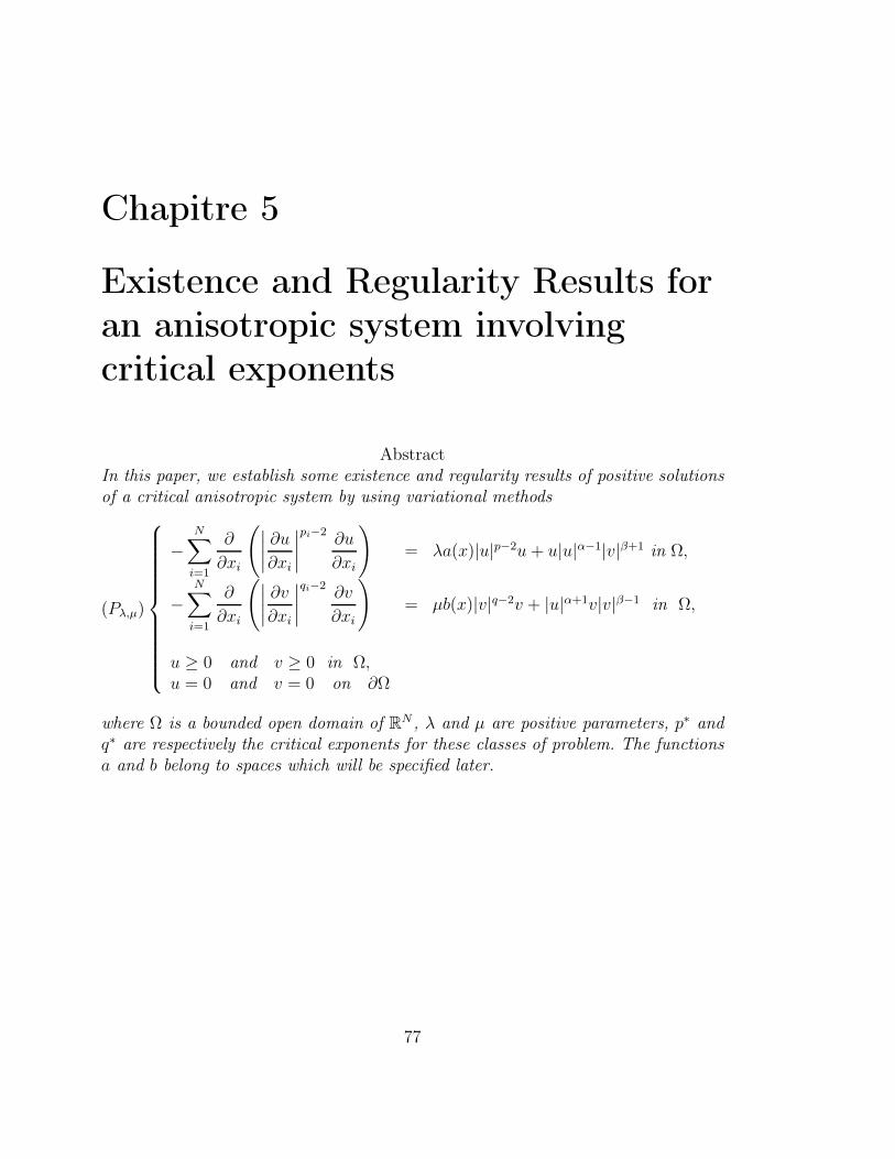
Chapitre 5
Existence and Regularity Results for
an anisotropic system involving
critical exponents
AbstractIn this paper, we establish some existence and regularity results of positive solutionsof a critical anisotropic system by using variational methods
(Pλ,µ)
−N∑
i=1
∂
∂xi
(∣∣∣∣∂u
∂xi
∣∣∣∣pi−2
∂u
∂xi
)= λa(x)|u|p−2u+ u|u|α−1|v|β+1 in Ω,
−N∑
i=1
∂
∂xi
(∣∣∣∣∂v
∂xi
∣∣∣∣qi−2
∂v
∂xi
)= µb(x)|v|q−2v + |u|α+1v|v|β−1 in Ω,
u ≥ 0 and v ≥ 0 in Ω,u = 0 and v = 0 on ∂Ω
where Ω is a bounded open domain of RN , λ and µ are positive parameters, p∗ andq∗ are respectively the critical exponents for these classes of problem. The functionsa and b belong to spaces which will be specified later.
77

§ 5. Existence and Regularity Results for an anisotropic system ... 78
5.1 Introduction
In this paper, we are interested in existence results of nonlocal solutions to thefollowing critical system :
−N∑
i=1
∂
∂xi
(∣∣∣∣∂u
∂xi
∣∣∣∣pi−2
∂u
∂xi
)= λa(x)|u|p−2u+ u|u|α−1|v|β+1 in Ω,
−N∑
i=1
∂
∂xi
(∣∣∣∣∂v
∂xi
∣∣∣∣qi−2
∂v
∂xi
)= µb(x)|v|q−2v + |u|α+1v|v|β−1 in Ω,
u ≥ 0 and v ≥ 0 in Ω,u = 0 and v = 0 on ∂Ω
(1.1)
where Ω is a bounded domain in RN , λ ≥ 0, µ ≥ 0 are real parameters and theexponents pi, α, qi, β satisfy the following conditions
pi > 1, qi > 1,N∑
i=1
1
pi> 1,
N∑
i=1
1
qi> 1
andα + 1
p∗+β + 1
q∗= 1,
where p∗ and q∗ are defined by
p∗ :=N
N∑
i=1
1
pi− 1
and q∗ :=N
N∑
i=1
1
qi− 1
.
We assume in the sequel that
maxp1, p2, · · · , pN < p∗ and maxq1, q2, · · · , qN < q∗,
p∗ and q∗ are the effective critical exponents associated to the operatorsN∑
i=1
∂
∂xi
(∣∣∣∣∂
∂xi
∣∣∣∣pi−2
∂
∂xi
)and
N∑
i=1
∂
∂xi
(∣∣∣∣∂
∂xi
∣∣∣∣qi−2
∂
∂xi
),
respectively [8, 7].
The functions a and b are assumed to be nontrivial, nonnegative , a ∈ Lp∗
p∗−p (Ω) and
b ∈ Lq∗
q∗−q (Ω).In this work, we deal with the nonlocal existence, with respect to λ and µ, of nonne-gative, nontrivial solutions to Problem (1.1). Consider the Euler-Lagrange functionalassociated to Problem (1.1) defined by
I(u, v) := (α + 1)
(N∑
i=1
Pi(u)
pi− λ
pPa(u)
)+ (β + 1)
(N∑
i=1
Qi(v)
qi− µ
qQb(v)
)−R(u, v),
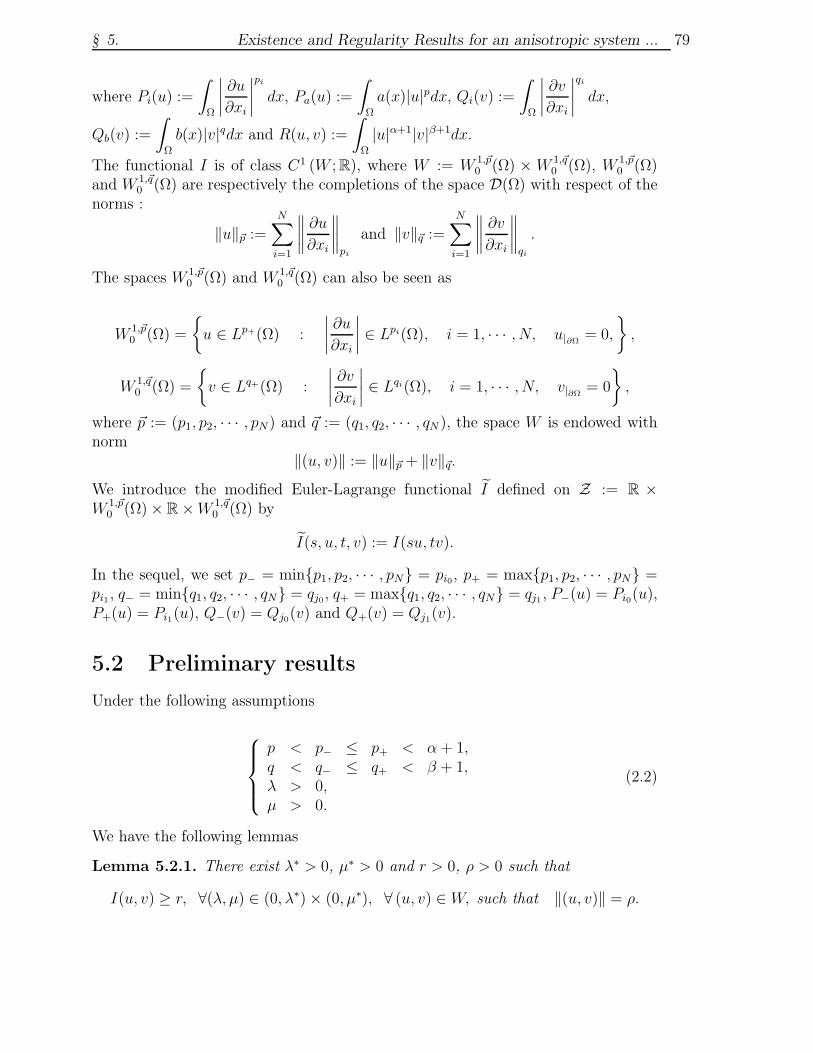
§ 5. Existence and Regularity Results for an anisotropic system ... 79
where Pi(u) :=
∫
Ω
∣∣∣∣∂u
∂xi
∣∣∣∣pi
dx, Pa(u) :=
∫
Ω
a(x)|u|pdx, Qi(v) :=
∫
Ω
∣∣∣∣∂v
∂xi
∣∣∣∣qi
dx,
Qb(v) :=
∫
Ω
b(x)|v|qdx and R(u, v) :=
∫
Ω
|u|α+1|v|β+1dx.
The functional I is of class C1 (W ; R), where W := W 1,~p0 (Ω) ×W 1,~q
0 (Ω), W 1,~p0 (Ω)
and W 1,~q0 (Ω) are respectively the completions of the space D(Ω) with respect of the
norms :
‖u‖~p :=
N∑
i=1
∥∥∥∥∂u
∂xi
∥∥∥∥pi
and ‖v‖~q :=
N∑
i=1
∥∥∥∥∂v
∂xi
∥∥∥∥qi
.
The spaces W 1,~p0 (Ω) and W 1,~q
0 (Ω) can also be seen as
W 1,~p0 (Ω) =
u ∈ Lp+(Ω) :
∣∣∣∣∂u
∂xi
∣∣∣∣ ∈ Lpi(Ω), i = 1, · · · , N, u|∂Ω= 0,
,
W 1,~q0 (Ω) =
v ∈ Lq+(Ω) :
∣∣∣∣∂v
∂xi
∣∣∣∣ ∈ Lqi(Ω), i = 1, · · · , N, v|∂Ω= 0
,
where ~p := (p1, p2, · · · , pN) and ~q := (q1, q2, · · · , qN ), the space W is endowed withnorm
‖(u, v)‖ := ‖u‖~p + ‖v‖~q.We introduce the modified Euler-Lagrange functional I defined on Z := R ×W 1,~p
0 (Ω) × R ×W 1,~q0 (Ω) by
I(s, u, t, v) := I(su, tv).
In the sequel, we set p− = minp1, p2, · · · , pN = pi0, p+ = maxp1, p2, · · · , pN =pi1 , q− = minq1, q2, · · · , qN = qj0, q+ = maxq1, q2, · · · , qN = qj1 , P−(u) = Pi0(u),P+(u) = Pi1(u), Q−(v) = Qj0(v) and Q+(v) = Qj1(v).
5.2 Preliminary results
Under the following assumptions
p < p− ≤ p+ < α + 1,q < q− ≤ q+ < β + 1,λ > 0,µ > 0.
(2.2)
We have the following lemmas
Lemma 5.2.1. There exist λ∗ > 0, µ∗ > 0 and r > 0, ρ > 0 such that
I(u, v) ≥ r, ∀(λ, µ) ∈ (0, λ∗) × (0, µ∗), ∀ (u, v) ∈W, such that ‖(u, v)‖ = ρ.
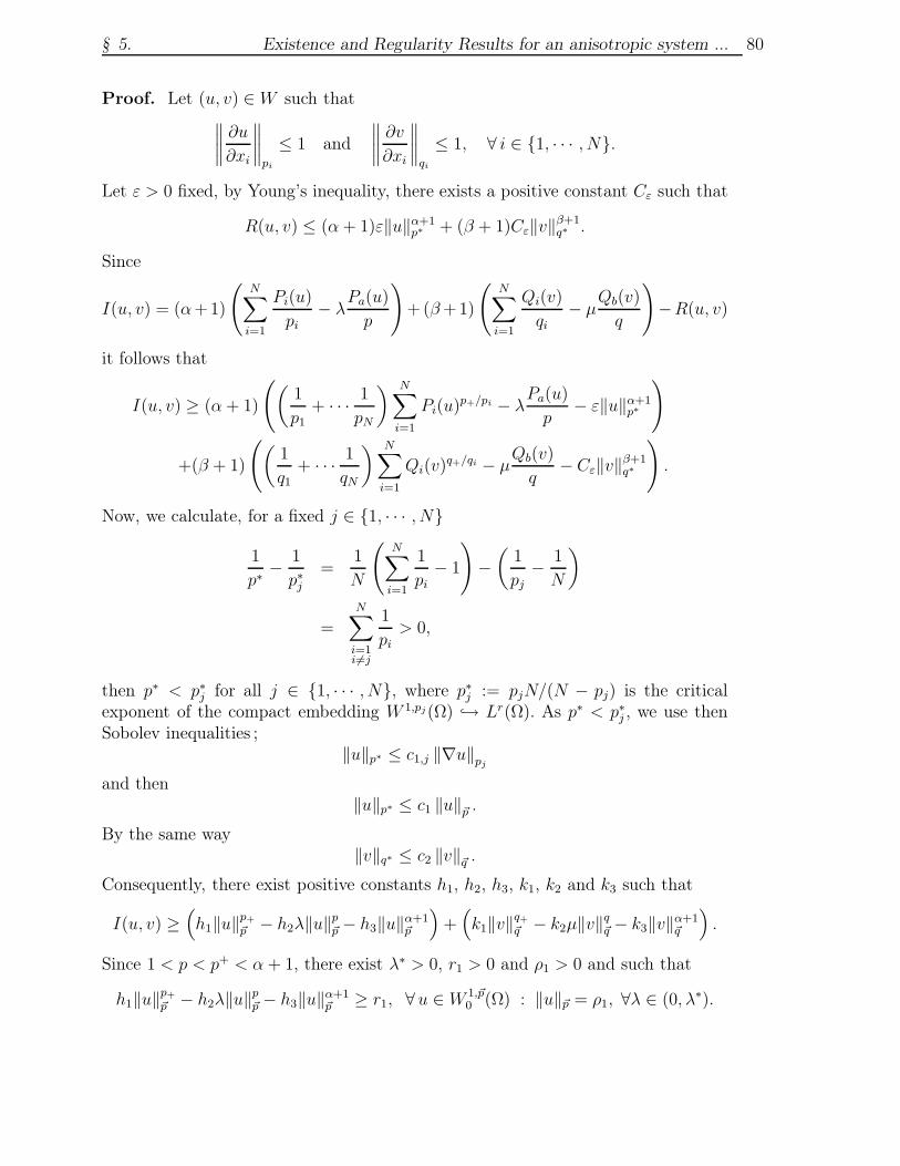
§ 5. Existence and Regularity Results for an anisotropic system ... 80
Proof. Let (u, v) ∈W such that∥∥∥∥∂u
∂xi
∥∥∥∥pi
≤ 1 and
∥∥∥∥∂v
∂xi
∥∥∥∥qi
≤ 1, ∀ i ∈ 1, · · · , N.
Let ε > 0 fixed, by Young’s inequality, there exists a positive constant Cε such that
R(u, v) ≤ (α+ 1)ε‖u‖α+1p∗ + (β + 1)Cε‖v‖β+1
q∗ .
Since
I(u, v) = (α+1)
(N∑
i=1
Pi(u)
pi− λ
Pa(u)
p
)+(β+1)
(N∑
i=1
Qi(v)
qi− µ
Qb(v)
q
)−R(u, v)
it follows that
I(u, v) ≥ (α+ 1)
((1
p1+ · · · 1
pN
) N∑
i=1
Pi(u)p+/pi − λ
Pa(u)
p− ε‖u‖α+1
p∗
)
+(β + 1)
((1
q1+ · · · 1
qN
) N∑
i=1
Qi(v)q+/qi − µ
Qb(v)
q− Cε‖v‖β+1
q∗
).
Now, we calculate, for a fixed j ∈ 1, · · · , N
1
p∗− 1
p∗j=
1
N
(N∑
i=1
1
pi− 1
)−(
1
pj− 1
N
)
=
N∑
i=1i6=j
1
pi> 0,
then p∗ < p∗j for all j ∈ 1, · · · , N, where p∗j := pjN/(N − pj) is the criticalexponent of the compact embedding W 1,pj(Ω) → Lr(Ω). As p∗ < p∗j , we use thenSobolev inequalities ;
‖u‖p∗ ≤ c1,j ‖∇u‖pj
and then‖u‖p∗ ≤ c1 ‖u‖~p .
By the same way‖v‖q∗ ≤ c2 ‖v‖~q .
Consequently, there exist positive constants h1, h2, h3, k1, k2 and k3 such that
I(u, v) ≥(h1‖u‖p+~p − h2λ‖u‖p~p − h3‖u‖α+1
~p
)+(k1‖v‖q+~q − k2µ‖v‖q~q − k3‖v‖α+1
~q
).
Since 1 < p < p+ < α + 1, there exist λ∗ > 0, r1 > 0 and ρ1 > 0 and such that
h1‖u‖p+~p − h2λ‖u‖p~p − h3‖u‖α+1~p ≥ r1, ∀u ∈W 1,~p
0 (Ω) : ‖u‖~p = ρ1, ∀λ ∈ (0, λ∗).
§ 5. Existence and Regularity Results for an anisotropic system ... 81
Similarly, Since 1 < q < q+ < β + 1, there exist µ∗ > 0, r2 > 0 and ρ2 > 0 and suchthat
k1‖v‖q+~q − k2µ‖v‖q~q − k3‖v‖β+1~q ≥ r2, ∀ v ∈W 1,~q
0 (Ω) : ‖v‖~q = ρ2, ∀µ ∈ (0, µ∗).
Therefore, for all (u, v) ∈ W such that ‖(u, v)‖ = ρ := ρ1 + ρ2 and for all (λ, µ) ∈(0, λ∗) × (0, µ∗), one has
I(u, v) ≥ r := r1 + r2 > 0,
which achieves the proof.
Lemma 5.2.2. The functional I is bounded from below in
Bρ(0) = (u, v) ∈W ; ‖(u, v)‖ ≤ ρ.
Moreover,inf
(u,v)∈Bρ(0)I(u, v) < 0, ∀(λ, µ) ∈ (0, λ∗) × (0, µ∗). (2.3)
Proof. It is easy to check that I is bounded from below in Bρ(0). To prove (2.3),fix (φ, ψ) ∈ W and let s > 0 and t > 0. Then
I(sφ, tψ) ≤ (α+1)
(N∑
i=1
spiPi(φ)
pi− λsp
Pa(φ)
p
)+(β+1)
(N∑
i=1
tqiQi(ψ)
qi− µtp
Qb(ψ)
q
).
As p < p− and q < q−, the last inequality implies for s0 and t0 sufficiently small
I(s0φ, t0ψ) < 0 and (s0φ, t0ψ) ∈ Bρ(0)
from where follows the lemma.
For every (λ, µ) ∈ (0, λ∗) × (0, µ∗), we introduce
α(λ, µ) := inf(u,v)∈Bρ(0)
I(u, v).
Applying Ekeland’s principle to the functional I on the metric space (Bρ(0), d)endowed with the metric d given by
d ((u1, v1), (u2, v2)) = ‖(u1 − u2, v1 − v2)‖ = ‖u1 − u2‖~p + ‖v1 − v2‖~q,
there exists a sequence (un, vn) ⊂ Bρ(0) such that
I(un, vn) −→ α(λ, µ) as n→ +∞ (2.4)
and
I(u, v) − I(un, vn) ≤1
n‖(u− un, v − vn)‖, for all (u, v) 6= (un, vn). (2.5)

§ 5. Existence and Regularity Results for an anisotropic system ... 82
Using the differentiability of I over W , from the previous inequality it follows that
I ′(un, vn) −→ 0, as n→ +∞. (2.6)
From (2.5) and (2.6)
I(un, vn) −→ α(λ, µ) and I ′(un, vn) −→ 0, as n→ +∞, (2.7)
then (un, vn) is a bounded (PS)α(λ,µ) sequence to I. Hereafter, we will denote by(u∗, v∗) ∈W the weak limit of (un, vn), up to a subsequence. Moreover, by definitionof I we can assume that the sequence (un, vn) is a sequence of nonnegative functions.
Theorem 5.2.1. The weak limit (u∗, v∗) of (un, vn) satisfies
I ′(u∗, v∗) = 0 and (u∗, v∗) ∈ W , for all (λ, µ) ∈ (0, λ∗) × (0, µ∗).
Proof. Using the properties of (un, vn), one can easily show that
I(un, vn) −1
p∗D1I(un, vn)un −
1
q∗D1I(un, vn)vn = α(λ, µ) + on(1),
where D1I(un, vn) and D2I(un, vn) are respectively the first and second partial Gâ-teaux derivatives in u and v of the functional I. Thus
α(λ, µ) + on(1) = (α + 1)
(N∑
i=1
(1
pi− 1
p∗
)Pi(un) − λ
(1
p− 1
p∗
)Pa(un)
)
+(β + 1)
(N∑
i=1
(1
qi− 1
q∗
)Qi(vn) − µ
(1
q− 1
q∗
)Qb(vn)
). (2.8)
As it is said befeore, one has
un u∗ in W 1,~p0 (Ω),
un −→ u∗ in Lp(Ω),
vn v∗ in W 1,~q0 (Ω),
vn −→ v∗ in Lq(Ω).
By the relation (2.8) and using the compact embeddings of W 1,~p0 (Ω) → Lp(Ω) and
W 1,~q0 (Ω) → Lq(Ω), we obtain
α(λ, µ) + on(1) ≥ −K1‖un‖pp −K2‖vn‖qq
where K1 and K2 are two positive constants. Then we get, as n goes to +∞ :
0 > α(λ, µ) > −K1‖u∗‖pp −K2‖v∗‖qq,
§ 5. Existence and Regularity Results for an anisotropic system ... 83
and consequently u∗ 6= 0 and v∗ 6= 0. Finally, we use the result due to El Hamidiand Rakotoson [6] and obtain
∇un(x) −→ ∇u∗(x) a.e. in Ω,
∇vn(x) −→ ∇v∗(x) a.e. in Ω.
Therefore, the weak limit (u∗, v∗) is a nonnegative and nontrivial solution to (1.1).
Under the following assumptions
p < α + 1q < β + 1
maxp+, q+ < minp, qλ ≥ 0µ ≥ 0
(2.9)
We have the following lemmas
Lemma 5.2.3. For every λ > 0 and µ > 0, the functional I satisfies the followingproperties :a) There exist r > 0 and ρ > 0 such that
I(u, v) ≥ r, ∀ (u, v) ∈W, such that ‖(u, v)‖ = ρ.
b) There exists (eλ,µ, fλ,µ) ∈W such that ‖(eλ,µ, fλ,µ)‖ ≥ ρ such that
I(eλ,µ, fλ,µ) < 0.
Proof.a) Using the same arguments in the proof of Lemma 5.2.1, we have for every (u, v) ∈W and ‖(u, v)‖ ≤ 1, there exist positive constants h1, h2, h3, k1, k2 and k3 suchthat
I(u, v) ≥(h1‖u‖p+~p − h2λ‖u‖p~p − h3‖u‖α+1
~p
)+(k1‖v‖q+~q − k2µ‖v‖q~q − k3‖v‖α+1
~q
).
As p+ < p < α+ 1 and q+ < q < β + 1, there exist r1, r2, ρ1 > 0 and ρ2 > 0 suchthat
h1‖u‖p+~p − h2λ‖u‖p~p − h3‖u‖α+1~p ≥ r1, for all ‖u‖~p ≤ ρ1
andk1‖v‖q+~q − k2µ‖v‖q~q − k3‖v‖α+1
~q ≥ r2, for all ‖v‖~q ≤ ρ2.
Let us introduce ρ := minρ1, ρ2, so if ‖(u, v)‖ = ρ then we have either ‖u‖~p ≤ρ ≤ ρ1 and ‖v‖~q ≤ ρ ≤ ρ2. Consequently, if ‖(u, v)‖ = ρ we have I(u, v) ≥ r :=r1 + r2.
§ 5. Existence and Regularity Results for an anisotropic system ... 84
b) Let (ϕ, ψ) ∈W such that ϕ 6= 0, ψ 6= 0 and R(ϕ, ψ) 6= 0 then
I(sϕ, sψ) = (α + 1)
(N∑
i=1
spi
piPi(ϕ) − λ
sp
pPa(ϕ)
)− sα+β+2R(ϕ, ψ)
+ (β + 1)
(N∑
i=1
sqi
qiQi(ψ) − µ
sq
qQb(ψ)
).
We know that α + β + 2 > maxp+, q+, then for s sufficiently large, we have
I(sϕ, sψ) < 0.
By a lemma in [6], the equation∂I
∂s(su, sv) = 0 has only one solution sλ,µ > 0
such that∂I
∂s(sλ,µu, sλ,µv) = 0. and sλ,µ satisfies the condition
I(sλ,µϕ, sλ,µψ) = maxs≥0
I(sϕ, sψ).
By considering (uλ,µ, vλ,µ) := (sλ,µϕ, sλ,µψ) we have the following results :
(i) I(uλ,µ, vλ,µ) = maxs≥0
I(suλ,µ, svλ,µ)
(ii) I(uλ,µ, vλ,µ) −→ 0 as λ→ +∞ or µ→ +∞.
Let us show (i). The function I(suλ,µ, svλ,µ) has a unique maximum value at somepoint s0 > 0. Since uλ,µ 6= 0 and vλ,µ 6= 0, we have
(α + 1)λsp0Pa(uλ,µ) + (β + 1)µsq0Qb(vλ,µ) + (α + β + 2)sα+β+20 R(uλ,µ, vλ,µ)
N∑
i=1
[(α + 1)Pi(uλ,µ)spi0 + (β + 1)Qi(vλ,µ)s
qi0 ]
= 1.
On the other hand (uλ,µ, vλ,µ) satisfies
(α + 1)λPa(uλ,µ) + (β + 1)µQb(vλ,µ) + (α + β + 2)R(uλ,µ, vλ,µ)N∑
i=1
[(α + 1)Pi(uλ,µ) + (β + 1)Qi(vλ,µ)]
= 1.
We study the variation of the function
θ : s 7→ (α + 1)λspPa(uλ,µ) + (β + 1)µsqQb(vλ,µ) + (α + β + 2)sα+β+2R(uλ,µ, vλ,µ)N∑
i=1
[(α + 1)Pi(uλ,µ)spi + (β + 1)Qi(vλ,µ)s
qi]
§ 5. Existence and Regularity Results for an anisotropic system ... 85
The function θ is of the form θ(s) = sa
Bsb+Csc with B > 0, C > 0, a > b > 0 anda > c > 0. For every s > 0 we have
θ′(s) =B(a− b)sa+b−1 + C(a− c)sa+c−1
(Bsb + Csc)2> 0,
then the function θ is increasing on (0,+∞). Therefore it follows that s0 = 1.We show the claim (ii), notice that
spλ,µPa(ϕ)N∑
i=1
[(α + 1)Pi(ϕ)spi
λ,µ + (β + 1)Qi(ψ)sqiλ,µ]
≤ 1
λ,
andsqλ,µQb(ψ)
N∑
i=1
[(α + 1)Pi(ϕ)spi
λ,µ + (β + 1)Qi(ψ)sqiλ,µ]
≤ 1
µ.
Thus,
spλ,µPa(ϕ)N∑
i=1
[(α + 1)Pi(ϕ)spi
λ,µ + (β + 1)Qi(ψ)sqiλ,µ]
−→ 0 as λ −→ +∞
and
sqλ,µQb(ψ)N∑
i=1
[(α + 1)Pi(ϕ)spi
λ,µ + (β + 1)Qi(ψ)sqiλ,µ]
−→ 0 as µ −→ +∞,
as the function θ satisfies : θ(0) = 0, θ is continuous on R+ and increasing thenθ(s) → 0 ⇐⇒ s→ 0. Thus, we have either
sλ,µ −→ 0 as λ→ +∞ or µ → +∞.
Recalling that
0 ≤ I(uλ,µ, vλ,µ) ≤ (α+ 1)
N∑
i=1
spi
λ,µ
piPi(ϕ) + (β + 1)
sqiλ,µqiQi(ψ) − sα+β+2
λ,µ R(ϕ, ψ)
it follows that
I(uλ,µ, vλ,µ) −→ 0 as λ→ +∞ or µ→ +∞,
§ 5. Existence and Regularity Results for an anisotropic system ... 86
which proves the claim.
Hereafter, we fix (eλ,µ, fλ,µ) with eλ,µ = s∗λ,µuλ,µ and fλ,µ = s∗λ,µvλ,µ such that
‖(eλ,µ, fλ,µ)‖ ≥ r and I(eλ,µ, fλ,µ) < 0.
Lemma 5.2.4. If cλ,µ is the minimax value obtained by the Mountain Pass Theoremapplied to the functional I, then we get
cλ,µ −→ 0 as λ −→ +∞ or µ −→ +∞.
Proof. The maximum value cλ,µ is given by
cλ,µ = inf(γ,ξ)∈Γ
maxs∈[0,1]
I(γ(s), ξ(s)),
where the set of all paths linking (0, 0) and (eλ,µ, fλ,µ) is defined by
Γ =
(γ, ξ) ∈ C(W ; R), (γ(0), ξ(0)) = (0, 0) and (γ(1), ξ(1)) = (eλ,µ, fλ,µ).
Let’s consider γ(s) = seλ,µ and ξ(s) = sfλ,µ, so then (γ, ξ) ∈ Γ and
maxs∈[0,1]
I(γ(s), ξ(s)) = maxs≥0
I(suλ,µ, svλ,µ) = I(uλ,µ, vλ,µ)
then0 ≤ cλ,µ ≤ I(uλ,µ, vλ,µ),
from wherecλ,µ −→ 0 as λ −→ +∞ or µ −→ +∞,
which ends the proof.
Hereafter, we shall denote by S~p > 0 and S~q > 0 the positive constants, see [7] :
S~p = infu∈D1,~p(RN ),‖u‖p∗=1
N∑
i=1
1
pi
∥∥∥∥∂u
∂xi
∥∥∥∥pi
pi
and
S~q = infv∈D1,~q(RN ),‖v‖q∗=1
N∑
i=1
1
qi
∥∥∥∥∂v
∂xi
∥∥∥∥qi
qi
.
The following lemma is an immediate consequence of the last one, that is,
§ 5. Existence and Regularity Results for an anisotropic system ... 87
Lemma 5.2.5. There exists λ∗ > 0 and µ∗ > 0 such that for all (λ, µ) ∈ [λ∗,+∞[×[µ∗,+∞[we have
0 < cλ,µ < d1 min
(S
α+1p+
~p Sβ+1q+
~q
) 1d1
,
(S
α+1p+
~p Sβ+1q−
~q
) 1d2
,
(S
α+1p−
~p Sβ+1q+
~q
) 1d3
,
(S
α+1p−
~p Sβ+1q−
~q
) 1d4
where d1 = α+1p+
+β+1q+
−1, d2 = α+1p+
+β+1q−
−1, d3 = α+1p−
+β+1q+
−1 and d4 = α+1p−
+β+1q−
−1.
Related to the Mountain Pass level cλ,µ, there exists a sequence (un, vn) ⊂ W satis-fying
I(un, vn) −→ cλ,µ and I ′(un, vn) −→ 0 in W ∗.
Using standard arguments, we have that (un, vn) is bounded in W , hence we canassume that there exists (u, v) ∈W such that
un u in W 1,~p0 (Ω)
andvn v in W 1,~q
0 (Ω).
Lemma 5.2.6. The weak limit (u, v) is such that u 6= 0 and v 6= 0.
Proof. By applying the result of A. El Hamidi and Rakotoson in [5], we prove thatwe can extract a subsequence of (un, vn), still denoted (un, vn), such that
∇un(x) −→ ∇u(x) a.e. in Ω,
and∇vn(x) −→ ∇v(x) a.e. in Ω,
then I ′(u, v) = 0.To prove now that u 6= 0 and v 6= 0, we assume by contradiction that u = 0 and weset xn := un and yn := vn − v. Using similar arguments as above, we get
N∑
i=1
Pi(un) − λPa(un) = R(un, vn) + on(1)
N∑
i=1
Qi(vn) − µQb(vn) = R(un, vn) + on(1).
(2.10)
Using Brézis-Lieb Lemma [3], we obtain
N∑
i=1
Pi(xn) = R(xn, yn) + on(1), (2.11)
N∑
i=1
Qi(yn) = R(xn, yn) + on(1), (2.12)
I0,0(xn, yn) = cλ,µ − I(0, v) + on(1). (2.13)
§ 5. Existence and Regularity Results for an anisotropic system ... 88
On the other hand, we have
I(0, v) = (β + 1)
(N∑
i=1
1
qiQi(v) − µ
1
qQb(v)
),
withN∑
i=1
Qi(v) − µQb(v) = 0.
Therefore
I(0, v) = (β + 1)N∑
i=1
(1
qi− 1
q
)Qi(v),
and consequently I(0, v) ≥ 0, since q+ < q. Now, if limn→+∞
R(xn, yn) = L then it
follows by (2.11) and (2.12) that
N∑
i=1
Pi(xn) −→ L andN∑
i=1
Qi(yn) −→ L.
Then
I0,0(xn, yn) = (α+ 1)N∑
i=1
(1
pi− 1
p∗
)Pi(xn) + (β + 1)
N∑
i=1
(1
qi− 1
q∗
)Qi(yn) + on(1),
and
limn→+∞
I0,0(xn, yn) ≥[(α + 1)
(1
p+
− 1
p∗
)+ (β + 1)
(1
q+− 1
q∗
)]L.
By the relation (2.13) we get
cλ,µ = limn→+∞
I0,0(xn, yn) + I(0, v)
≥ limn→+∞
I0,0(xn, yn)
≥[(α + 1)
(1
p+
− 1
p∗
)+ (β + 1)
(1
q+− 1
q∗
)]L
=
(α + 1
p++β + 1
q+− 1
)L.
We use the same arguments as in [2] and [7], to prove that we have either
S~p‖xn‖p+p∗ ≤N∑
i=1
∥∥∥∥∂xn∂xi
∥∥∥∥pi
pi
if ‖xn‖p∗ ≤ 1 (2.14)
S~q‖yn‖q+q∗ ≤N∑
i=1
∥∥∥∥∂yn∂xi
∥∥∥∥qi
qi
if ‖yn‖p∗ ≤ 1 (2.15)
§ 5. Existence and Regularity Results for an anisotropic system ... 89
or
S~p‖xn‖p−p∗ ≤N∑
i=1
∥∥∥∥∂xn∂xi
∥∥∥∥pi
pi
if ‖xn‖p∗ ≥ 1
S~q‖yn‖q−q∗ ≤N∑
i=1
∥∥∥∥∂yn∂xi
∥∥∥∥qi
qi
if ‖yn‖p∗ ≥ 1.
From the previous inequalities, if ‖xn‖p∗ ≤ 1 and ‖yn‖p∗ ≤ 1 we obtain
R(xn, yn) ≤ ‖xn‖α+1p∗ ‖yn‖β+1
q∗
≤(
1
S~p
N∑
i=1
Pi(xn)
)α+1p+(
1
S~q
N∑
i=1
Qi(yn)
)β+1q+
as n→ +∞ we have
L ≥(S
α+1p+
~p Sβ+1q+
~q
) 1α+1p+
+β+1q+
−1
and
cλ,µ ≥ (α + 1
p+
+β + 1
q+− 1)
(S
α+1p+
~p Sβ+1q+
~q
) 1α+1p+
+β+1q+
−1
.
Then
cλ,µ ≥ d1 min
(S
α+1p+
~p Sβ+1q+
~q
) 1d1
,
(S
α+1p+
~p Sβ+1q−
~q
) 1d2
,
(S
α+1p−
~p Sβ+1q+
~q
) 1d3
,
(S
α+1p−
~p Sβ+1q−
~q
) 1d4
,
which cannot hold true. Thus L = 0 and cλ,µ = I(0, v) > 0, in this case limλ→+∞
cλ,µ =
I(0, v) > 0 which leads to a contradiction with the fact that limλ→+∞
cλ,µ = 0. Then
u 6= 0 and v 6= 0.
5.3 Regularity of Weak Solutions
In this section, we show that every weak solution (u, v) ∈W 1,~p0 (Ω)×W 1,~q
0 (Ω) of thefollowing problem
(P )
−N∑
i=1
∂
∂xi
(∣∣∣∣∂u
∂xi
∣∣∣∣pi−2
∂u
∂xi
)= f(x, u, v) in Ω,
−N∑
i=1
∂
∂xi
(∣∣∣∣∂v
∂xi
∣∣∣∣qi−2
∂v
∂xi
)= g(x, u, v) in Ω,
u ≥ 0 and v ≥ 0 in Ω,u = 0 and v = 0 on ∂Ω
is a a strong solution, under some hypothesis on the functions f and g.
§ 5. Existence and Regularity Results for an anisotropic system ... 90
Lemma 5.3.1. Suppose that the functions f and g satisfy the following growthconditions :(h1) There exist c1, c2 ≥ 0 and p ∈ (1, p∗) such that
|f(x, u, v)| ≤ c1up−1 + c2u
αvβ+1, ∀u ≥ 0 and v ≥ 0,
(h2) There exist c′1, c′2 ≥ 0 and q ∈ (1, p∗) such that
|g(x, u, v)| ≤ c′1vq−1 + c′2u
α+1vβ, ∀u ≥ 0 and v ≥ 0.
Then every weak solution (u, v) ∈ W 1,~p0 (Ω) ×W 1,~q
0 (Ω) of (Pλ,µ) belongs to Lr(Ω) ×Ls(Ω) for all 1 ≤ r < +∞ and 1 ≤ s < +∞.
Proof. We will use similar arguments developed by Fragala, Gazzola and Kawohl[8].Let (u, v) be a weak solution to (P ). The assertion that (u, v) ∈ Lr(Ω) × Ls(Ω) forall 1 ≤ r < +∞ and 1 ≤ s < +∞ may be equivalently reformulated as
(u, v) ∈ L(1+a)p∗(Ω) × L(1+b)q∗(Ω) for all (a, b) ∈ R+∗ × R
+∗ . (3.16)
To prove (3.16) it is enough to show that (ua+1, vb+1) ∈ W 1,~p0 (Ω) ×W 1,~q
0 (Ω), whichis equivalent to
limL→+∞
N∑
i=1
(∫
Ω
|∂xi(umin[ua, L]|pidx
) 1pi
< +∞, (3.17)
limL→+∞
N∑
i=1
(∫
Ω
|∂xi(vmin[vb, L]|qidx
) 1qi
< +∞. (3.18)
For each L there exist indexes j and k such that
N∑
i=1
(∫
Ω
|∂i(u · min[ua, L]|pi dx
) 1pi ≤ C
(∫
Ω
|∂j(u · min[ua, L]|pjdx
) 1pj
, (3.19)
N∑
i=1
(∫
Ω
|∂i(v · min[vb, L]|qidx) 1
qi ≤ C ′
(∫
Ω
|∂k(v · min[vb, L]|qkdx) 1
qk
(3.20)
where C and C ′ are positive constants independent of L.For these indexes j and k, and for every L > 0, set φL := min[uapj , Lpj ] and ψL :=vmin[vbqk , Lqk ] such that (φL, ψL) ∈W 1,~p
0 (Ω)×W 1,~q0 (Ω). Note that for every 1 ≤ i ≤
N and for almost every x ∈ Ω,
|∂iu|pi−2∂iu∂iφL ≥ min[uapj , Lpj ]|∂iu|pi,
|∂iv|qi−2∂iv∂iψL ≥ min[vbqk , Lqk]|∂iv|qi,
§ 5. Existence and Regularity Results for an anisotropic system ... 91
|∂i(u · min[ua, L])|pi ≤ (a+ 1) min[uapi, Lpi]|∂iu|pi, (3.21)
and|∂i(v · min[vb, L])|qi ≤ (b+ 1) min[vbqi, Lqi]|∂iv|qi. (3.22)
As (u, v) is a weak solution to (P ), we rewrite, for every k ≥ 1, Ω ≡ Ω1,k ∪ Ω2,k ∪Ω3,k ∪ Ω4,k, where
Ω1,k := x ∈ Ω such that u < k and v < k,
Ω2,k := x ∈ Ω such that u < k and v ≥ k,Ω3,k := x ∈ Ω such that u ≥ k and v < k,Ω4,k := x ∈ Ω such that u ≥ k and v ≥ k.
Then we have
N∑
i=1
∫
Ω
min[uapj , Lpj ]|∂iu|pidx ≤N∑
i=1
∫
Ω
|∂iu|pi−2∂iu∂iφLdx =
∫
Ω
f(x, u, v)φLdx,
and
N∑
i=1
∫
Ω
min[vbqk, Lqk ]|∂iv|qidx ≤N∑
i=1
∫
Ω
|∂iv|qi−2∂iv∂iψLdx =
∫
Ω
g(x, u, v)ψLdx.
Using (h1), for L ≥ ka ≥ 1, it follows that
|f(x, u, v)|φL ≤ Ck,1 in Ω1 (3.23)
|g(x, u, v)|ψL ≤ Ck,2 in Ω1 (3.24)
hence ∫
Ω1
f(x, u, v)φLdx ≤ Ck,1 = Ck,1|Ω|,
∫
Ω2,k
f(x, u, v)φLdx ≤∫
Ω2
[c1u
p + c2uα+1vβ+1
]min[uapj , Lpj ]dx,
≤ C2,k + c2
∫
Ω2
uα+1vβ+1 min[uapj , Lpj ]dx,
≤ C2,k + c2
(∫
Ω2,k
(uα+1 min[uapj , Lpj ])p∗/(α+1)dx
)α+1p∗
×
×(∫
Ω2,k
vq∗
dx
)β+1q∗
≤ C2,k + εkC′2,k
§ 5. Existence and Regularity Results for an anisotropic system ... 92
where εk tends to 0 as k tends to +∞.∫
Ω3,k
f(x, u, v)φLdx ≤ c1
∫
Ω3,k
up∗
min[uapj , Lpj ]dx+
∫
Ω3,k
uα+1vβ+1 min[uapj , Lpj ]dx
≤ c1
(∫
Ω3,k
up∗
dx
) p∗−pjp∗
·∫
Ω3,k
(upj · min[uapj , Lpj ])p∗/pjdx
+ c2
∫
Ω3,k
up∗
min[uapj , Lpj ]vβ+1dx
≤ ε′k
(∫
Ω
(u · min[ua, L])p∗
dx
)pj/p∗
+ c2
(∫
Ω3,k
up∗−pjupj · (min[uapj , Lpj ])p
∗/(α+1)dx
)α+1p∗
×(∫
Ω3,k
vq∗
dx
)β+1q∗
≤ ε′k
(∫
Ω
(u · min[ua, L])p∗
dx
)pj/p∗
+ c2‖u‖(α+1)(p∗−pj)/p∗
p∗,Ω3,k‖v‖β+1
q∗,Ω3,k×
×(∫
Ω3,k
(upj · (min[uapj , Lpj ])p
∗/(α+1)) p∗
pj dx
) (α+1)pj
p∗2
≤ ε′k
(∫
Ω
(u · min[ua, L])p∗
dx
)pj/p∗
+ ε′′k‖v‖β+1q∗ ×
×(∫
Ω
(u · min[ua, L])p∗
dx
) (α+1)pj
p∗2
≤ ε′k
[N∑
i=1
(∫
Ω
|∂i(u · min[ua, L])|pidx
)1/pi]pj
+ ε′′k
[N∑
i=1
(∫
Ω
|∂i (u · min[ua, L]) |pidx
) 1pi
](α+1)pi/p∗
§ 5. Existence and Regularity Results for an anisotropic system ... 93
where ε′k and ε′′k tend to 0 as k goes to +∞.∫
Ω4,k
f(x, u, v)φLdx ≤∫
Ω4,k
[c1u
p + c2uα+1vβ+1
]min[uapj , Lpj ]dx
≤ ε′k
(∫
Ω
(u · min[ua, L])p∗
dx
)pj/p∗
+ c2‖u‖(α+1)(p∗−pj)/p∗
p∗,Ω4,k×
× ‖v‖β+1q∗,Ω4,k
(∫
Ω3,k
(upj · (min[uapj , Lpj ])p
∗/(α+1)) p∗
pj dx
) (α+1)pj
p∗2
≤ ε1k
(∫
Ω
(u · min[ua, L])p∗
dx
)pj/p∗
+
+ ε2k
(∫
Ω
(u · min[ua, L])p∗
dx
) (α+1)pj
p∗2
≤ ε1k
[N∑
i=1
(∫
Ω
|∂i(u · min[ua, L])|pidx
)1/pi]pj
+
+ ε2k
[N∑
i=1
(∫
Ω
|∂i (u · min[ua, L]) |pidx
) 1pi
](α+1)pi/p∗
where ε1k and ε2
k tend to 0 as k goes to +∞.Inserting (3.19) and (3.20) in the last inequalities, we then obtain,
∫
Ω
|∂j(u · min[ua, L])|pjdx ≤ C ′k + εk,1
∫
Ω
|∂j(u · min[ua, L])|pjdx
+ εk,2
[∫
Ω
|∂i (u · min[ua, L]) |pidx
](α+1)/p∗
.
Choosing k sufficiently large, that are εk,1 and εk,2 sufficiently small, the last in-
equality ensures that the integral∫
Ω
|∂j(u · min[ua, L])|pjdx is bounded for L large
enough, from where follows (3.17). By the same way we can prove (3.18), and we canconclude then that every weak solution (u, v) ∈ W 1,~p
0 (Ω) ×W 1,~q0 (Ω) of (P ) belongs
to Lr(Ω) × Ls(Ω), for all r ≥ 1 and s ≥ 1.
Proposition 5.3.1. Under the conditions (h1) and (h2), every nonnegative solution(u, v) ∈W 1,~p
0 (Ω) ×W 1,~q0 (Ω) of (P ) belongs to L∞(Ω) × L∞(Ω).
Proof. For u ≥ 0 and v ≥ 0 such that (u, v) is a solution of (P), we set Aτ =x ∈ Ω, u(x) ≥ τ and Bτ = x ∈ Ω, v(x) ≥ τ, |Aτ | and |Bτ | their Lebesguemeasures. Recall that Cavalieri principle, based on Fubini theorem, gives :
∫ +∞
k
|Aτ |dτ =
∫
Ω
(u− k)+dx, for all k ≥ 0
§ 5. Existence and Regularity Results for an anisotropic system ... 94
and ∫ +∞
k
|Bτ |dτ =
∫
Ω
(v − k)+dx, for all k ≥ 0.
Let ϕk = (u − k)+, for k > 0 fixed. Choosing this function as a test function,combining the Cavalieri principle and Hölder inequality, one gets
N∑
i=1
Pi(ϕk) =
∫
Ω
(λaup−1 + uαvβ+1)ϕkdx
≤ c1λ
∫
Ω
|u|p−1ϕkdx+ c2
∫
Ω
|u|α|v|β+1ϕkdx
≤ c
(∫
[u≤1]
ϕkdx+
∫
[u≤1]
|v|β+1ϕkdx+
∫
[u≥1]
|u|α|v|β+1ϕkdx
),
≤ c(|Ak|1−
1p∗ + |Ak|(1−
α+1p∗ )(1− 1
p∗ ))‖ϕk‖p∗ . (3.25)
Since limn→+∞
‖ϕk‖p∗ = 0, then for k ≥ k0 > 0, ‖ϕk‖p∗ ≤ 1. Relations (2.14) and (3.25)
give
S~p‖ϕk‖p+
p∗ ≤N∑
i=1
Pi(ϕk)
≤ c(|Ak|1−
1p∗ + |Ak|(1−
α+1p∗ )(1− 1
p∗ ))‖ϕk‖p∗.
Thus, for every k ≤ k0, we have :
‖ϕk‖p∗ ≤ c(|Ak|1−
1p∗ + |Ak|(1−α+1
p∗ )(1− 1p∗ )) 1
p+−1
≤ c(|Ak|(1−
1p∗ )
1p+−1 + |Ak|(1−α+1
p∗ )(1− 1p∗ )
1p+−1
). (3.26)
Using Cavalieri’s principle, Hölder inequality and Relation (3.26), one has for allk ≥ k0 :
∫ +∞
k
|Aτ |dτ =
∫
Ω
(u− k)+dx
≤ |Ak|1−1
p∗ ‖ϕk‖p∗
≤ c
(|Ak|1+
1p∗
p∗−1
p+−1 + |Ak|1+θ), (3.27)
where θ := − 1
p∗+
(1 − α + 1
p∗
)(1 − 1
p∗
)1
p+ − 1> 0.
Sinceγ :=
1
p∗p∗ − 1
p+ − 1≥ θ,
§ 5. Existence and Regularity Results for an anisotropic system ... 95
then ∫ +∞
k
|Aτ |dτ ≤ c+ |Ak|1+γ .
This inequality is of Gronwall type, which shows that there exists cλ > 0 such that
‖u‖∞ ≤ cλ.
One can prove by exactly the same way the fact that there exists cµ > 0 such that‖v‖∞ ≤ cµ.
5.4 On the weak sub and supersolutions
In this section, we will use some classical tools concerning sub and super solutionsfor a class of systems involving the anisotropic operators considered above. Noticethat the standard laplacian operator and the anisotropic operator were studied res-pectively in [12] and [2].Let us consider the following problem
−N∑
i=1
∂
∂xi
(∣∣∣∣∂u
∂xi
∣∣∣∣pi−2
∂u
∂xi
)= f(x, u, v) in Ω
−N∑
i=1
∂
∂xi
(∣∣∣∣∂v
∂xi
∣∣∣∣qi−2
∂v
∂xi
)= g(x, u, v) in Ω,
u ≥ 0 and v ≥ 0 in Ω,u = 0 and v = 0 on ∂Ω
(4.28)
where Ω is a smooth and bounded domain in RN , both f , g : Ω × R × R → R are
Carathéodory satisfying the following property that for each fixed A > 0, there existC1 > 0 and C2 > 0 such that
(H)
|f(x, s, t)| ≤ C1, ∀ (x, s, t) ∈ Ω × [−A,A] × [−A,A]|g(x, s, t)| ≤ C2, ∀ (x, s, t) ∈ Ω × [−A,A] × [−A,A].
Definition 5.4.1. The couple (u, v) ∈W is a (weak) sub-solution to (4.28) if u ≤ 0and v ≤ 0 on ∂Ω and for all (ϕ, ψ) ∈ D(Ω)×D(Ω) with ϕ(x) ≥ 0 and ψ(x) ≥ 0 forall x ∈ Ω, we have simultaneously
N∑
i=1
∫
Ω
∣∣∣∣∂u
∂xi
∣∣∣∣pi−2
∂u
∂xi
∂ϕ
∂xidx−
∫
Ω
f(x, u, v)ϕdx ≤ 0
N∑
i=1
∫
Ω
∣∣∣∣∂v
∂xi
∣∣∣∣pi−2
∂v
∂xi
∂ψ
∂xidx−
∫
Ω
g(x, u, v)ψdx ≤ 0.
Similarly, (u, v) ∈W is a (weak) super-solution to (4.28) if in the above the reverseinequalities hold.
§ 5. Existence and Regularity Results for an anisotropic system ... 96
Theorem 5.4.1. Suppose (H) holds, (u, v) ∈W is sub-solution while (u, v) ∈W isa super-solution to Problem (4.28) and assume that there exist c, c, c′, c′ ∈ R thereholds c ≤ u ≤ u ≤ c and c′ ≤ v ≤ v ≤ c′ almost everywhere in Ω. Then, thereexists a weak solution (u, v) ∈W 1,~p
0 (Ω)×W 1,~q0 (Ω) of (4.28), satisfying the condition
u ≤ u ≤ u and v ≤ v ≤ v almost everywhere in Ω.
Proof. Let F (x, u, v) =∫ u0f(x, s, v)ds and G(x, u, v) =
∫ v0g(x, u, t)dt denote res-
pectively primitives of f and g. Let us define J : W 1,~p0 (Ω) × W 1,~q
0 (Ω) → R theEuler-Lagrange functional associated to (4.28) given by
J(u, v) :=
N∑
i=1
∫
Ω
(1
pi
∣∣∣∣∂u
∂xi
∣∣∣∣pi
+1
qi
∣∣∣∣∂v
∂xi
∣∣∣∣qi)
dx−∫
Ω
(F (x, u, v) +G(x, u, v)dx
We introduce the closed and convex subset M of W 1,~p0 (Ω) ×W 1,~q
0 (Ω) defined by
M =
(u, v) ∈W 1,~p0 (Ω) ×W 1,~q
0 (Ω) : u ≤ u ≤ u and v ≤ v ≤ v a.e. in Ω.
Since u, v, u and v ∈ L∞ by assumption, also M ∈ L∞×L∞ and consequently thereexists c > 0 and c > 0 such that |F (x, u(x), v(x)| ≤ c and |G(x, u(x), v(x)) ≤ c| forall (u, v) ∈ M and for almost all x ∈ Ω. Consequently
J(u, v) ≥N∑
i=1
∫
Ω
(1
pi
∣∣∣∣∂u
∂xi
∣∣∣∣pi
+1
qi
∣∣∣∣∂v
∂xi
∣∣∣∣qi)
dx− 2cmeas(Ω)
on M, which implies that J is coercive on M. We claim now that the functional Jis weakly lower semi-continuous on M. Indeed, let (un, vn), (u, v) ⊂ M such thatun u in W 1,~p
0 (Ω) and vn W 1,~q0 (Ω). We may assume that, up to a subsequence,
un → u and vn → v pointwise almost everywhere ; moreover |F (x, un(x)vn(x)| ≤ cand|G(x, un(x)vn(x)| ≤ c uniformly. Hence we may appeal to Lebesgue’s theoremon dominated convergence which implies that
∫
Ω
F (x, un, vn)dx −→∫
Ω
F (x, u, v)dx and∫
Ω
G(x, un, vn)dx −→∫
Ω
G(x, u, v)dx, as n tends to + ∞,
these end the claim, since the functionals
u ∈W 1,~p0 (Ω) 7→
N∑
i=1
∫
Ω
1
pi
∣∣∣∣∂u
∂xi
∣∣∣∣pi
dx
and
v ∈W 1,~q0 (Ω) 7→
N∑
i=1
∫
Ω
1
qi
∣∣∣∣∂v
∂xi
∣∣∣∣pi
dx
§ 5. Existence and Regularity Results for an anisotropic system ... 97
are clearly weakly lower semi-continuous on the whole space. As the space W isreflexive then there exists (u, v) ∈ M such that J(u, v) = inf
(w,s)∈MJ(w, s). We claim
that (u, v) solves weakly Problem (4.28), that is J ′(u, v) = 0. Indeed, fix (ϕ, ψ) ∈D(Ω) ×D(Ω) and ε > 0 and consider the couple (uε, vε) ∈ M defined on Ω by :
uε(x) =
u(x) if u(x) + εϕ(x) ≥ u(x),u(x) + εϕ(x) if u(x) ≤ u(x) + εϕ(x) ≤ u(x),u(x) if u(x) + εϕ(x) ≤ u(x).
and
vε(x) =
v(x) if v(x) + εψ(x) ≥ v(x),v(x) + εψ(x) if v(x) ≤ v(x) + εψ(x) ≤ v(x),v(x) if v(x) + εψ(x) ≤ v(x).
The functions uε and vε can be characterised by uε = (u+ εϕ)− (ϕε−ϕε) and vε =
(v+εψ)−(ψε−ψε), where ϕε = max0, u+εϕ−u ≥ 0, ϕε
= −min0, u+εϕ−u ≥ 0,ψε = max0, v + εψ − v ≥ 0 and ψ
ε= −min0, v + εψ − v ≥ 0. Note that ϕε,
ϕε, ψε and ψ
ε∈ W ∩ L∞(Ω) × L∞(Ω). Since (u, v) minimizes J on M and J is
differentiable, then
0 ≤ D1(u, v)(uε − u) = εD1J(u, v)(ϕ) +D1J(u, v)(ϕε) −D1J(u, v)(ϕε),
where D1J(u, v) denotes the first derivative in u of J , so that
D1J(u, v)(ϕ) ≤ 1
ε
(D1J(u, v)(ϕε) −D1J(u, v)(ϕ
ε)). (4.29)
Using the fact that (u, v) is a super-solution to (4.28), we get
D1J(u, v)(ϕε) = D1J(u, v)(ϕε) + [D1J(u, v) −D1J(u, v)] (ϕε)
≥ [D1J(u, v) −D1J(u, v)] (ϕε)
=
N∑
i=1
∫
Ωε
(∣∣∣∣∂u
∂xi
∣∣∣∣pi−2
∂u
∂xi−∣∣∣∣∂u
∂xi
∣∣∣∣pi−2
∂u
∂xi
)∂
∂xi(u− u+ εϕ)dx−
−∫
Ωε
[f(x, u, v) − f(x, u, v)
](u− u+ εϕ)dx
≥ εN∑
i=1
∫
Ωε
(∣∣∣∣∂u
∂xi
∣∣∣∣pi−2
∂u
∂xi−∣∣∣∣∂u
∂xi
∣∣∣∣pi−2
∂u
∂xi
)∂
∂xi(ϕ)dx−
− ε
∫
Ωε
|f(x, u, v) − f(x, u, v)| |ϕ|dx
where Ωε = x ∈ Ω : u(x) + εϕ(x) ≥ u(x) and v(x) + εψ(x) ≥ v(x). Notice thatmeas(Ωε) −→ 0 as ε→ 0. Thus,
D1J(u, v)(ϕε) ≥ o(ε),
§ 5. Existence and Regularity Results for an anisotropic system ... 98
where o(ε)/ε −→ 0 as ε→ 0. Similarly, we conclude that
D1J(u, v)(ϕε) ≤ o(ε),
and consequently, with (4.29), we get
D1J(u, v)(ϕ) ≥ 0
for every ϕ ∈ D(Ω). This implies, by reversing the sign of ϕ, that D1J(u, v)(ϕ) = 0for every ϕ ∈ D(Ω). Using the density of D(Ω) inW 1,~p
0 (Ω). The proof ofD2J(u, v)(ψ) =0 where D2J(u, v) is the seconde derivative of J in the seconde variable, follows thesame steps as in the above.
Bibliographie
[1] K. Adriouch and A. El Hamidi, The Nehari manifold for systems of nonlinearelliptic equations, Nonlinear Anal. TMA 64 (2006), 2149–2167.
[2] C.O. Alves and A. El Hamidi, Existence of solutions for an anisotropic equationwith critical exponent, (submitted).
[3] H. Brézis, E. Lieb, A Relation Between Pointwise Convergence of Functionsand Convergence of Functionals, Proc. Amer. Math. Soc. 88 (1983), 486–490.
[4] I. Ekeland, On the variational principle, J. Math. Anal. Appl. 47 (1947) 324–353.
[5] A. El Hamidi and J. M. Rakotoson, On a perturbed anisotropic equation with acritical exponent, Ricerche di Matematica Manuscript .
[6] A. El Hamidi and J.M. Rakotoson, Compactness and quasilinear problems withcritical exponents, Diff. Int. Equ., 18 (2005), 1201–1220.
[7] A. El Hamidi and J.M. Rakotoson, Extremal functions for the anisotropic So-bolev inequalities, Ann. I. H. Poincaré, AN, (to appear).
[8] I. Fragala, F. Gazzola, B. Kawohl, Existence and nonexsistence results for ani-sotropic quasilinear elliptic equation. Ann. I. H. Poincaré AN 21 (2004) 715–734.
[9] S.M. Nikol’skii, On embedding, continuation and approximation theorems fordifferentiable functions of several variables. Russian Math. Surv., 16 (1961),55–104.
[10] J. Rakosnik, Some remarks to anisotropic Sobolev spaces I, Beiträ ge zur Ana-lysis 13 (1979), 55–68.
[11] J. Rakosnik, Some remarks to anisotropic Sobolev spaces II.Beiträ ge zur Ana-lysis, 15 (1981), 127–140.
[12] M. Struwe, Variational methods. Applications to nonlinear partial differentialequations and Hamiltonian systems. Springer-Verlag (1996)
[13] G. Talenti, Best constant in Sobolev inequality Ann. Mat. Pura Appl., 4 (1976),353–372.
[14] M. Troisi, Teoremi di inclusione per spazi di Sobolev non isotropi, RicercheMat. 18 (1969), 3–24.
99
§ 6. Annexe : Théorèmes Minimax 100
[15] L. Ven’-tuan, On embedding theorems for spaces of functions with partial deri-vatives of various degrees of summability, Vestnik Leningrad Univ., 16 (1961),pp. 23–37 (in Russian) .

Chapitre 6
Annexe
Dans cette partie, on va rappeler quelques définitions, théorèmes et outils essentielsque nous utilisons au cours de cette thèse.
6.1 Condition de Palais-Smale
Pour exprimer la compacité de certaines suites minimisantes, on a souvent recoursà la condition de Palais-Smale (en abrégé (PS)).
Définition 6.1.1. Soit W un espace de Banach et J : W → R une fonction declasse C1. On dit que la suite (un) ⊂ W est une suite de Palais-Smale s’il existec ∈ R tel que
J(un) → c dans R et J ′(un) → 0 dans W ′.
On dit que J vérifie la condition de Palais-Smale au niveau c ∈ R si toute suite(un)n de Palais-Smale pour la fonctionnelle J (de niveau c) contient une sous-suite(unk
)k convergente.
On dispose généralement de deux théorèmes importants permettant la constructionde suites de Palais-Smale : le théorème du col, dû à Ambrosetti-Rabinowitz et leprincipe variationnel d’Ekeland.
6.2 Théorème du col et "Mountain Pass Geometry"
Théorème 6.2.1. Soient W un espace de Banach et I ∈ C1(W,R). Supposons qu’ilexiste u0 ∈ W , u1 ∈W et un voisinage ouvert Ω de u0 tel que u1 /∈ Ω et
c0 := maxI(u0), I(u1) < c1 := max∂Ω
I(v).
SoitH = h ∈ C([0, 1],W ) : h(0) = u0, h(1) = u1,
101
§ 6. Annexe : Théorèmes Minimax 102
c := infh∈H
sups∈[0,1]
I(h(s)).
Alors,inf∂ΩI(v) ≤ c < +∞,
et pour tout ε ∈ (0, c1 − c0] et pour chaque h ∈ H tel que
maxs∈[0,1]
I(h(s)) ≤ c+ ε,
il existe v ∈W satisfaisant :i. c− ε ≤ I(v) ≤ c + εii. dist(v, h([0, 1]) ≤ √
εiii. ‖I ′(v)‖ ≤ √
ε.
Un autre théorème minimax de type géométrique démontré par P. H. Rabinowitz.
Théorème 6.2.2. ( Point selle géométrique)Supposons que W = U⊕V un espace de Banach et U et V deux sous-espaces fermés,tels que dimU < +∞. Pour un ρ > 0, on considère les ensembles suivants :
M := u ∈ U : ‖u‖ ≤ ρ , M0 := u ∈ U : ‖u‖ = ρ .
On définit l’espace suivant
H := h ∈ C(M,W ) : h|M0 = id ,
et soit I ∈ C1(W,R) telle que
c0 := maxu∈M0
I(u) < c1 := infv∈V
I(v).
Soitc := inf
h∈Hmaxs∈M
I(h(s)).
Si c1 ≤ c, alors pour tout ε ∈]0, c1 − c0] et pour tout h ∈ H tel que
maxs∈M
I(h(s)) ≤ c + ε,
il existe u ∈W tel que
1. c− ε ≤ I(u) ≤ maxs∈M
I(h(s))
2. dist(u, h(M)
)≤ √
ε
3. ‖I ′(u)‖ ≤ √ε.
§ 6. Annexe : Théorèmes Minimax 103
Principe Variationnel d’Ekeland
En général, une fonctionnelle bornée et semi-continue inférieurement J n’atteint pasnécessairement son infimum. Par exemple, la fonction analytique f(x) = arctanxn’atteint ni son infimum ni son supremum sur la droite réelle.
Théorème 6.2.3. Soit (M, d) un espace métrique complet et soit J : M → R∪+∞semi-continue inférieurement, bornée inférieurement et 6≡ +∞. Alors pour chaqueε, δ > 0 et tout u ∈M avec
J(u) ≤ infM
+ε,
il existe un élément v ∈M minimisant strictement la fonctionnelle
Jv(w) ≡ J(w) +ε
δd(v, w).
En plus on aJ(v) ≤ J(u) dès que d(u, v) ≤ δ.
Comme corollaire du principe d’Ekeland, on a
Corollaire Si W est un espace de Banach et J ∈ C1(W ) bornée inférieurement alorsil existe une suite minimisante (vn) pour J dans W telle que
J(vn) −→ infWJ, DJ(vn) −→ 0 dans W ′ quand n→ ∞.
Niveau critique
Pour résoudre le problème de Yamabe, en géométrie riemannienne, Thierry Aubin aintroduit la notion de niveau critique associée au problème de Yamabe, notée c∗, eta montré que si une suite minimisante de l’énergie correspondante a un niveau plusbas que le niveau critique alors le problème de Yamabe possède des solutions.Dans un article de Brézis et Nirenberg, les auteurs ont montré que si (un) ⊂W estune suite de Palais-Smale pour la fonctionnelle J telle que J(un) −→ c < c∗ quandn tend vers +∞, alors (un) est relativement compacte. Le niveau c∗ est appelécritique dans le sens où l’on peut construire une suite (wn) ⊂ W de Palais-Smale,avec J(wn) → c∗, qui n’admet aucune sous-suite convergente dans W .
6.3 Théorème de Concentration-Compacité
Cette méthode introduite par P. L. Lions est la méthode la plus générale pour traîterles problèmes de minimisation qui interviennent dans les domaines les plus variés(équations aux dérivées partielles, calculs des variations, analyse harmonique, etc...).
§ 6. Annexe : Théorèmes Minimax 104
Définition 6.3.1. Soit Ω un ouvert de RN , on définit les ensembles suivants :
K(Ω) := u ∈ C(Ω) : u est à support compact de Ω
BC(Ω) :=
u ∈ C(Ω) ‖u‖∞ := sup
x∈Ω|u(x)| <∞
.
L’espace C0(Ω) est l’adhérence de K(Ω) pour la norme uniforme. Une mesure finiedéfinie sur Ω est une application linéaire continue sur C0(Ω). La norme d’une mesurefinie µ est définie par
‖µ‖ := supu ∈ C0(Ω)‖u‖∞ = 1
| < µ, u > |.
On dénote par M(Ω) (resp. M+(Ω)) l’espace de mesures finies (resp. mesures finiespositives) sur Ω. Une suite de mesures finies (µn) converge faiblement vers µ dansM(Ω), dans ce cas on écrit
µn µ,
si on a< µn, u >−→< µ, u >, ∀ u ∈ C0(Ω).
Théorème 6.3.1. (lemme de concentration-compacité)Soit (un) ⊂ D1,2(RN) une suite telle que
un u dans D1,2(RN),
|∇(un − u)|2 µ dans M(RN),
|un − u|2∗ ν dans M(RN),
un → u p.p. dans RN
et on définit
µ∞ := limR→∞
limn→∞
∫
|x|≥R
|∇un|2, ν∞ := limR→∞
limn→∞
∫
|x|>R
|un|2∗
.
On a alors– ‖ν‖2/2∗ ≤ S−1‖µ‖,– ν
2/2∗
∞ ≤ S−1µ∞,– lim
n→∞‖∇un‖2
2 = ‖∇u‖22 + ‖µ‖ + µ∞
– limn→∞
‖un‖2∗
2∗ = ‖u‖2∗
2∗ + ‖ν‖ + ν∞.
En outre, si u = 0 et ‖ν‖2/2∗ = S−1‖µ‖, alors µ et ν sont concerntrées en un seulpoint.

§ 6. Annexe : Théorèmes Minimax 105
6.4 Lemme de Brézis-Lieb
Théorème 6.4.1. (Lemme de Brézis-Lieb) Soit j : C −→ C une fonction continuetelle que j(0) = 0 et vérifie la condition suivante :Pour tout ε > 0 suffisamment petit il existe deux fonctions continues et positives ϕεet ψε telles que
(P ) ∀ a, b ∈ C, |j(a+ b) − j(a)| ≤ εϕε(a) + ψε(b).
Supposons que j satisfait l’hypothèse du dessus et soit fn = f + gn une suite defonctions mesurables de Ω vers C telles que :i) gn → 0 presque partout,ii) j(f) ∈ L1,iii) il existe une constante C indépendante de ε et n telle que
∫ϕε(gn(x))dµ(x) ≤
C <∞,iv)
∫ψε(f(x)) dµ(x) < ∞ pour tout ε > 0, où µ est la mesure de Lebesgues dans
RN .Alors quand n→ ∞,
∫|j(f + gn) − j(gn) − j(f)| dµ→ 0.
Proposition 6.4.1. Les fonctionelles considérées dans les chapitres § 1, 2, 3 et 4de la forme s 7→ sf(x, s) ou s 7→ F (x, s) =
∫ s0f(x, t)dt satisfont les conditions du
lemme de Brézis-Lieb où f est une fonctionnelle de Carathéodory et vérifie pour toutε > 0 il existe Cε > 0 vérifiant
|f(x, u)| ≤ ε|u|p∗−1 + Cε,
uniformément en x ∈ RN .
Preuve. Soit ε > 0, alors
|(a+ b)f(x, a+ b) − af(x, a)| ≤ |(a+ b)f(a+ b)| + |af(a)|< ε|a+ b|p∗ + Cε|a+ b| + ε|a|p∗ + Cε|a|< εc(p)
[|a|p∗ + |b|p∗
]+ ε|a|p∗ + 2Cε|a| + Cε|b|
< ε[(c(p) + 1)|a|p∗ + (2Cε/ε)|a|
]+ ε|b|p∗ + Cε|b|.
Avec les mêmes notations du lemme de Brézis-Lieb, on prend
ϕε(a) = (c(p) + 1)|a|p∗ + (2Cε/ε)|a|ψε(b) = ε|b|p∗ + Cε|b|,
§ 6. Annexe : Théorèmes Minimax 106
D’où la relation (P ) du lemme de Brézis-Lieb. D’autre part, pour ε > 0
|F (x, a+ b) − F (x, a)| =
∣∣∣∣∫ a+b
a
f(x, t)dt
∣∣∣∣
≤∫ a+b
a
[ε|t|p∗−1 + Cε
]dt
<ε
p∗∣∣|a+ b|p∗ − |a|p∗
∣∣+ Cε|b|
<ε
p∗(c(p) + 1)|a|p∗ +
εc(p)
p∗|b|p∗ + Cε|b|.
Donc
ϕε(a) =1
p∗(c(p) + 1)|a|p∗
et ψε(b) =εc(p)
p∗|b|p∗ + Cε|b|.