ts remerciemen - math.webgirand.eumath.webgirand.eu/pdf/0-main.pdf2016. 2. ts remerciemen il...
TRANSCRIPT
ANNÉE 2016
THÈSE / UNIVERSITÉ DE RENNES 1
sous le s eau de l'Université Bretagne Loire
pour le grade de
DOCTEUR DE L'UNIVERSITÉ DE RENNES 1
Mention : Mathématiques et appli ations
É ole do torale MATISSE
présentée par
Arnaud Girand
préparée à l'unité de re her he 6625 du CNRS : IRMAR
Institut de Re her he Mathématique de Rennes
UFR de Mathématiques
Équations
d'isomonodromie,
solutions algébriques
et dynamique.
Thèse soutenue à Rennes
le 31 août 2016
devant le jury omposé de :
Serge Cantat / Dire teur de re her hes
CNRS, Université de Rennes 1 / dire teur de thèse
Guy Casale / Maître de onféren es
Université de Rennes 1/ examinateur
Bertrand Deroin / Chargé de re her hes
CNRS, É ole Normale Supérieure / examinateur
Lu ia Di Vizio / Dire tri e de re her hes
CNRS, Université de Versailles Saint Quentin /
examinatri e
Oleg Lisovyy / Maître de onféren es
Université de Tours / rapporteur
Frank Loray / Dire teur de re her hes
CNRS, Université de Rennes 1 / dire teur de thèse
Emmanuel Paul Professeur Université
Paul Sabatier (Toulouse) / rapporteur

Last modied: O tober 21, 2016.
2

Remer iements
Il n'est pas impossible que les remer iements onstituent la partie la plus di ile à é rire
d'un tapus rit de thèse ; il s'agit en tout as de la partie qui tou hera le le torat le plus
vaste . . .
Il est de outume de ommen er par remer ier ses dire teurs de thèse, et je ne vois
au une raison de déroger à l'usage. Serge Cantat et Frank Loray ont a ompagné mes
travaux pendant trois ans (plus epsilon) ave un grand professionnalisme et une patien e à
l'épreuve des balles. Ils ont ha un à leur façon façonné mon développement mathématique,
et je pense (et espère) que ela se ressent dans le présent do ument. Mais au delà des
mathématiques que j'ai appris à leur onta t, Serge et Frank ont été un point d'an rage
et un soutien dont je leur suis redevable et re onnaissant. Travailler de ette façon durant
trois ans ave les mêmes personnes demande un ertain degré de ompatibilité, et je suis
heureux de l'avoir trouvé hez eux
1
.
Je souhaite aussi remer ier haleureusement Oleg Lisovyy et Emmanuel Paul d'avoir
a epté d'endosser le rle de rapporteurs. Tous deux ont été de bon onseil et jamais avares
d'en ouragement à mon endroit et je suis honoré du temps qu'il ont dédié à l'évaluation
de mes travaux. Je remer ie également Guy Casale, Bertrand Deroin et Lu ia Di Vizio
d'avoir fait le dépla ement
2
et pris le temps de s'intéresser à mes travaux. Bertrand et
Guy ont toujours été à mon é oute pendant es trois ans de thèse, et j'ai appris beau oup
à leur onta t ; ils m'ont également oert plusieurs opportunités de venir exposer mes
mathématiques à divers endroits dont je leur suis très re onnaissant.
Une thèse est un pro essus ontinu de développement qui ne se fait ependant pas
uniquement au onta t de ses dire teurs de thèse ; à e propos il me semble né essaire de
mentionner les Gentils Organisateurs de l'ANR Iso-Galois, qui m'ont permis de voir du
pays et d'apprendre de belles maths, ainsi que tout le (fort a ueillant) groupe gravitant
autour. Mer i don à Viktoria Heu, Loï Teyssier et Amaury Bittman de Strasbourg,
Charlotte Hardouin, Yohann Genzmer, Stéphane Lamy et Ja ques Sauloy de Toulouse, à
Karamoko Diarra de Bamako, à Ja quesArthur Weil de Limoges ainsi qu'aux itinérants
Thomas Dreyfus, Martin Klimes et Gaël Cousin à qui je souhaite de s'établir rapidement.
I would also like to thank Masa-Hiko Saito, from Kobe, who took a keen interest to my
work sin e the very beginning and was always ex eedingly supportive.
Un des avantages majeurs de préparer une thèse à l'IRMAR est de pouvoir le faire
au onta t de ses résidents, dont la ompagnie et la ulture mathématique m'ont été
pré ieuses. Je souhaiterais don saluer mes deux familles adoptives : l'équipe de géométrie
analytique, ave Dominique qui a le mérite de m'avoir supporté plus longtemps que la
moyenne et d'avoir été un grand père mathématique de première qualité, Fred pour ses
onnaissan es sur la rationalité par haîne et sa freditude, JeanMarie pour m'avoir aidé
à survivre en milieu administrativement hostile, Bert, Christophe, Max et Vi tor grâ e à
1
En espérant que la ré iproque soit vraie.
2
Même si Guy est venu de moins loin.
3

qui le 7e étage est (et restera) un endroit très bien fréquenté où l'on peut dis uter de tout
sauf d'homotopie de rang supérieur ; et l'équipe de théorie ergodique et ses repas du lundi
midi au Diapason, ave Ludo pour les hef-boutonnades, Vin ent, Juan et Sebastien qui
ont maintes fois prouvé que l'on pouvait faire des dessins en ourbure négative sur une
nappe en papier, Anna, Barbara, François et Rémi qui ont tous à leur façon ontribué à
e que je me sente bien dans e laboratoire. Je n'oublie pas non plus eux ave qui je ne
partageais pas une équipe mais ave qui j'ai eu de nombreuses dis ussions intéressantes
3
:
Delphine, Xavier, Mi hel, Matthieu, Felix, Lionel, Mihai, Anne, Benjamin, Eri , Ni olas,
Karel, San . . . J'en oublie sans doute, mais 'est plutt bon signe quant à la qualité humaine
et mathématique du laboratoire, non ?
J'ai eu la han e d'enseigner pendant trois ans à l'ENS Rennes
4
, ave une équipe
formidable. Mer i don à Benoît
5
, Mi hel, Karine, Arnaud, Jeremy et Thibaut qui m'ont
permis de me sentir entouré et soutenu pendant ette période (et désolé de vous avoir
abandonné pendant la réda tion de e tapus rit).
Et puis il y a bien sur le groupe des do torants et exdo torants de l'IRMAR, dont je
devrais réussir à me souvenir
6
à for e de les avoir haperonné pour aller manger (au point de
me demander si la famine ne les guette d'i i quelques jours) : Axel, Olivier, Yvan, Vin ent,
Charles, Cé ile, Basile, Gwezheneg, Tristan, Ma , José, Alex, Türkhu, Elise, Kodjo, Maria,
Christian, Federi o, Andrew, Florian, Tristan, Camille, Ri hard, Renan, Blandine, Hélène,
Julie, Coralie, Adrien, Marine, Cyril, Maxime, Salomé, Benoît et Clément. Bien sur,
je garde une pla e spé iale dans ette énumération dithyrambique pour mes obureaux
passés (Sandrine), présents (Damien et Néstor) et honoraires (Mer edes). Mention spé iale
aux do torants d'algèbre et géométrie dont j'ai organisé le séminaire pendant deux ans et
qui m'ont impressionné par leur motivation et leur enthousiasme.
Aussi merveilleux qu'il soit, e laboratoire s'eondrerait
7
en vingt se ondes sans le
travail de son équipe administrative ; il serait don malhonnête de ne pas remer ier Marie
Aude, Chantal, Hélène, Nelly, Ni ole, Emmanuelle, Xhensila, Carole, MarieAnni k ou
Véronique ainsi que nos informati iens Patri k et Olivier et nos bibliothé aires Marie
Anni k, Maryse et Dominique.
Enn, je on lus omme il est de outume par remer ier ma famille et bellefamille,
eux qui ont pu être là omme eux qui n'ont pas pu. Je dirai sobrement que je ne serai
pas là où je suis sans eux
8
. Et bien sur Ophélie, par e que.
3
Par ordre dé roissant d'étage pour les onnaisseurs
4
Flambant neuve !
5
Envers qui j'ai une ardoise de afé déraisonnable.
6
Non ontra tuel !
7
Figurativement ou littéralement selon le as.
8
En parti ulier, si j'ai bien ompris, mes parents.
4
Contents
Résumé en français 9
I1 Déformations isomonodromiques, groupe modulaire . . . . . . . . . . . . . . 11
I1.1 Déformations isomonodromiques de sphères épointées . . . . . . . . . 11
I1.2 Systèmes de Garnier . . . . . . . . . . . . . . . . . . . . . . . . . . . 16
I1.3 Variété des ara tères d'une surfa e épointée . . . . . . . . . . . . . . 17
I1.4 A tion du groupe modulaire . . . . . . . . . . . . . . . . . . . . . . . 21
I1.5 Quelques avan ées ré entes . . . . . . . . . . . . . . . . . . . . . . . 23
I1.6 Solutions algébriques de systèmes de Garnier obtenues à l'aide de
quintiques planes . . . . . . . . . . . . . . . . . . . . . . . . . . . . . 25
I2 Convolution intermédiaire de Katz . . . . . . . . . . . . . . . . . . . . . . . 31
I2.1 Pro édé général . . . . . . . . . . . . . . . . . . . . . . . . . . . . . . 32
I2.2 Appli ation à l'étude des orbites sous l'a tion de Mod(0, n) . . . . . 37
I2.3 Résultats originaux relatifs aux onvolutions intermédiaires . . . . . 39
I Algebrai Garniers solutions obtained using plane quinti urves 41
1 A lassi ation result 43
1.1 Preliminary remarks . . . . . . . . . . . . . . . . . . . . . . . . . . . . . . . 45
1.1.1 The CorletteSimpson theorem . . . . . . . . . . . . . . . . . . . . . 45
1.1.2 The ZariskiVan Kampen method . . . . . . . . . . . . . . . . . . . 46
1.2 Proof of Theorem A . . . . . . . . . . . . . . . . . . . . . . . . . . . . . . . 51
1.2.1 Understanding the list . . . . . . . . . . . . . . . . . . . . . . . . . . 51
1.2.2 Large singularities . . . . . . . . . . . . . . . . . . . . . . . . . . . . 54
1.2.3 Eliminating groups . . . . . . . . . . . . . . . . . . . . . . . . . . . . 59
1.2.4 Remaining quinti urves and their fundamental group . . . . . . . . 65
2 Mapping lass group orbits 73
2.1 Restri ting a plane onne tion to generi lines . . . . . . . . . . . . . . . . . 73
2.1.1 General method . . . . . . . . . . . . . . . . . . . . . . . . . . . . . . 73
2.1.2 Mapping lass group orbits . . . . . . . . . . . . . . . . . . . . . . . 76
2.2 Proof of Theorem B . . . . . . . . . . . . . . . . . . . . . . . . . . . . . . . 77
5

2.2.1 Orbits under the pure mapping lass group . . . . . . . . . . . . . . 78
2.2.2 Extended orbits . . . . . . . . . . . . . . . . . . . . . . . . . . . . . . 79
3 First family of solutions 83
3.1 Setup and main results . . . . . . . . . . . . . . . . . . . . . . . . . . . . . . 83
3.1.1 Topology of the omplement of a parti ular plane quinti . . . . . . 83
3.1.2 Main results . . . . . . . . . . . . . . . . . . . . . . . . . . . . . . . . 85
3.1.3 Isomonodromi deformations . . . . . . . . . . . . . . . . . . . . . . 87
3.1.4 LotkaVolterra foliations . . . . . . . . . . . . . . . . . . . . . . . . . 88
3.2 Proof of Theorem C . . . . . . . . . . . . . . . . . . . . . . . . . . . . . . . 88
3.2.1 A rank two bre bundle . . . . . . . . . . . . . . . . . . . . . . . . . 89
3.2.2 A rank one proje tive bundle . . . . . . . . . . . . . . . . . . . . . . 90
3.2.3 Logarithmi at onne tions . . . . . . . . . . . . . . . . . . . . . . . 91
3.2.4 Trivialisations . . . . . . . . . . . . . . . . . . . . . . . . . . . . . . . 92
3.2.5 Monodromy representation . . . . . . . . . . . . . . . . . . . . . . . 94
3.3 Algebrai Garnier solutions . . . . . . . . . . . . . . . . . . . . . . . . . . . 95
3.3.1 Painlevé VI solutions . . . . . . . . . . . . . . . . . . . . . . . . . . . 95
3.3.2 Restri tion to generi lines . . . . . . . . . . . . . . . . . . . . . . . . 98
3.3.3 Rational parametrisations . . . . . . . . . . . . . . . . . . . . . . . . 99
3.4 LotkaVolterra foliations . . . . . . . . . . . . . . . . . . . . . . . . . . . . . 103
3.4.1 Proof of Theorem E . . . . . . . . . . . . . . . . . . . . . . . . . . . 105
3.4.2 Invariant urves . . . . . . . . . . . . . . . . . . . . . . . . . . . . . . 106
3.5 Proof of Theorem D . . . . . . . . . . . . . . . . . . . . . . . . . . . . . . . 107
3.5.1 First ase: λ0 and λ1 are not linearly dependant over Z . . . . . . . 107
3.5.2 Se ond ase: there exists (p, q) in Z2 \ (0, 0) su h that pλ0+ qλ1 = 0108
4 Se ond family of solutions 111
4.1 Rank two onne ted bundle . . . . . . . . . . . . . . . . . . . . . . . . . . . 111
4.1.1 Setup . . . . . . . . . . . . . . . . . . . . . . . . . . . . . . . . . . . 111
4.1.2 A suitable double over . . . . . . . . . . . . . . . . . . . . . . . . . 113
4.1.3 Constru ting the onne tion . . . . . . . . . . . . . . . . . . . . . . . 114
4.2 Asso iated isomonodromi deformation . . . . . . . . . . . . . . . . . . . . . 116
4.2.1 Restri tion to generi lines . . . . . . . . . . . . . . . . . . . . . . . . 116
4.2.2 Asso iated Garnier solution . . . . . . . . . . . . . . . . . . . . . . . 117
II Katz's middle onvolution and derivatives 121
5 Some new orbits 123
5.1 Main result . . . . . . . . . . . . . . . . . . . . . . . . . . . . . . . . . . . . 123
5.1.1 Framework . . . . . . . . . . . . . . . . . . . . . . . . . . . . . . . . 123
5.1.2 List of orbits . . . . . . . . . . . . . . . . . . . . . . . . . . . . . . . 124
6
5.2 Ee tive Katz middle onvolution . . . . . . . . . . . . . . . . . . . . . . . . 125
5.2.1 Sele ting free group representations . . . . . . . . . . . . . . . . . . . 125
5.2.2 Middle onvolution algorithm . . . . . . . . . . . . . . . . . . . . . . 129
5.3 Further study of the mapping lass group orbits . . . . . . . . . . . . . . . . 133
5.3.1 Expli it mapping lass group orbits . . . . . . . . . . . . . . . . . . . 134
5.3.2 Regression to Painlevé VI . . . . . . . . . . . . . . . . . . . . . . . . 136
6 Virtual ellipti middle onvolution 139
6.1 Framework and main result . . . . . . . . . . . . . . . . . . . . . . . . . . . 139
6.2 Ellipti middle onvolution . . . . . . . . . . . . . . . . . . . . . . . . . . . 140
6.2.1 Adho bre bundle . . . . . . . . . . . . . . . . . . . . . . . . . . . 140
6.2.2 Ane group and a tion on ane representations . . . . . . . . . . . 141
6.2.3 A quotient ve tor spa e . . . . . . . . . . . . . . . . . . . . . . . . . 142
6.2.4 Algorithm . . . . . . . . . . . . . . . . . . . . . . . . . . . . . . . . . 144
6.3 Ee tive omputations . . . . . . . . . . . . . . . . . . . . . . . . . . . . . . 145
Appendi es 151
A Computing mapping lass group orbits 151
1.1 Pure mapping lass group orbits . . . . . . . . . . . . . . . . . . . . . . . . 151
1.2 Mapping lass group orbits . . . . . . . . . . . . . . . . . . . . . . . . . . . 154
B Expli it omputations 155
Bibliography 161
7

8

Résumé en français
Cette thèse est dédiée à la onstru tion de solutions algébriques d'équations d'isomonodromie
et à l'étude de diérents pro édés ee tifs pour générer et al uler de tels objets. Les
travaux présentés i i s'arti ulent autour de plusieurs orrespondan es établies es dernières
dé ennies entre des objets de nature analytique (solutions de systèmes hamiltoniens) et
géométrique (orbites sous une ertaine a tion du groupe modulaire), es dernières nous
permettant d'utiliser des outils provenant de diverses bran hes des mathématiques pour
parvenir à nos ns.
Si E est un bré ve toriel audessus d'une variété omplexe X, une onnexion loga-
rithmique ∇ sur E est un morphisme Clinéaire entre le fais eau des se tions de E et le
produit tensoriel de e dernier par elui des 1formes méromorphes à ples logarithmiques
sur X vériant une formule de Leibnitz. Une telle onnexion est dite plate si elle admet
un système fondamental de se tions horizontales (i.e dans le noyau de ∇) en tout point du
omplémentaire de son lieu polaire dans X. Le prolongement analytique de telles se tions
livre une représentation ρ∇ du groupe fondamental omplémentaire du lieu polaire de ∇dans X, appelée monodromie de la onnexion.
Une déformation isomonodromique algébrique surX est une famille algébrique de brés
ve toriels sur X munis de onnexions logarithmiques plates de même (modulo onjugaison
à l'arrivée) représentation de monodromie. Il a été établi par S hlesinger, Garnier et
Malmquist que es objets sont équivalents à la donnée de solutions algébriques d'une famille
parti ulière d'équation aux dérivées partielles, appelées systèmes de Garnier. Les solutions
générales de es systèmes sont mal onnues, et l'obje tif prin ipal des travaux présentés i i
est de onstruire expli itement de telles déformations isomonodromiques an d'obtenir de
nouvelles solutions algébriques.
Plus parti ulièrement, onsidérons une ourbe Q (non né essairement irrédu tible ou
lisse) proje tive omplexe de degré inq dans le plan proje tif P2(C). Si l'on dispose d'une
onnexion logarithmique plate ∇ de rang 2 audessus de P2(C) dont le lieu polaire est égal
à Q, alors pour toute droite générique L ⊂ P2, la onnexion ∇L obtenue par restri tion
de ∇ à L peut être assimilée à une onnexion logarithmique plate audessus de la droite
proje tive omplexe P1(C) dont le lieu polaire est égal à inq points distin ts de ette
dernière ; de plus la platitude de ∇ permet de prouver que la famille des onnexions ∇L
forme une déformation isomonodromique paramétrée par un ouvert de Zariski dans le dual
de P2. L'objet de la première partie de ette thèse est de lassier les solutions algébriques
9
Résumé en français
de systèmes de Garnier pouvant être obtenues par e pro édé.
Nous ommençons par déterminer pour quelles ourbes quintiques planes dans P2(C) il
est possible d'obtenir une déformation isomonodromique algébrique n'appartenant pas aux
familles d'exemples déjà onstruites par Mazzo o [46 et Diarra [24 ; nous utilisons pour
e faire la lassi ation des groupes fondamentaux de omplémentaires de telles ourbes
quintiques établie par Degtyarev [19. Il est susant de mener ette étude au niveau des
représentations de es groupes fondamentaux ; en eet, la orrespondan e de Riemann
Hilbert lassique [21 arme en parti ulier qu'à toute telle représentation il est possible
de faire orrespondre une onnexion logarithmique plate. Dans un se ond temps, nous
onstruisons de façon expli ite les déformations isomonodromiques et solutions algébriques
de Garnier asso iées à es représentations de groupes.
Le deuxième volet de ette étude on erne la dynamique de l'a tion du groupe modu-
laire d'une sphère épointée sur la variété des ara tères asso iée. Plus pré isément, omme
le groupe fondamental d'une sphère à r trous est isomorphe à un groupe libre à r − 1
générateurs Fr−1, une représentation de e groupe dans SLd(C) est totalement dé rite
par un ruplet de matri es dont le produit est égal à l'identité ; on en déduit une a tion
par onjugaison diagonale de SLd(C) sur la variété des représentations de e groupe fon-
damental. Le quotient atégorique (au sens de la théorie géométrique des invariants) de
et espa e par ette a tion est appelé variété des ara tères de Fr−1 dans SLd(C) et noté
Chard(0, r). Comme le groupe modulaire Mod(0, r) formé par les lasses d'isotopie des
homéomorphismes de la sphère à r trous agit par automorphismes extérieurs sur le groupe
fondamental de ette dernière, on obtient une a tion de Mod(0, r) sur Chard(0, r). Les
travaux de Dubrovin, Mazzo o [27 et Cousin [16 ont établi une orrespondan e entre les
solutions algébriques de systèmes de Garnier et les orbites nies sous ette a tion. Nous
al ulons expli itement les orbites asso iées aux solutions obtenues par le pro édé dé rit
idessus et montrons que e dernier donne naissan e à deux familles à paramètres de
solutions algébriques distin tes. Nous détaillons une méthode ee tive pour al uler des
telles orbites à l'aide d'outils de al ul formel.
Dans la deuxième partie de ette thèse, nous étudions le pro édé de onvolution inter-
médiaire de Katz et quelquesunes de ses appli ations à l'étude des déformations isomon-
odromiques algébriques de surfa es omplexes. Ce pro édé utilise l'a tion naturelle du
groupe des tresses à r brins d'Artin sur le groupe libre à r− 1 générateurs pour onstruire
une appli ation sur la variété
Char∗(g, b) :=⋃
d∈N∗
Chard(0, r)
équivariante sous l'a tion du groupe modulaire Mod(0, r). Nous inspirant des travaux de
Boal h [7 et utilisant la des ription expli ite de la onvolution intermédiaire donnée par
Völklein [57, Dettweiler et Reiter [22, 23, nous onstruisons de nouvelles orbites nies
sous l'a tion de e dernier groupe. Plus pré isément, partant de représentations dont les
10

I1. DÉFORMATIONS ISOMONODROMIQUES, GROUPE MODULAIRE
images sont ontenue dans un sousgroupe ni de SL3(C), nous obtenons de nouveaux
morphismes de F4 dans SL2(C) dont les orbites sous l'a tion du groupe modulaire doivent
être nies par équivarian e. Un algorithme expli ite pour mener à bien es al uls est
présenté.
Enn, nous nous intéressons à un possible analogue de ette onvolution intermédiaire
dans le as d'un tore à deux trous T22. En l'o urren e, nous dénissons un pro édé
équivariant sous l'a tion des automorphismes extérieurs du groupe fondamental d'un tore
à trois trous envoyant une représentation de π1(T22) sur une représentation dénie sur un
de ses sousgroupes distingués. Nous donnons un algorithme expli ite mettant en ÷uvre
ette nouvelle onvolution intermédiaire.
I1 Déformations isomonodromiques, systèmes de Garnier et
dynamique du groupe modulaire
Dans la suite de ette introdu tion, nous dénissons les on epts né essaires à l'établissement
des résultats que nous venons d'énon er, en donnant les éléments de ontexte historique
pertinents. Une fois eux i établis, nous énonçons pré isément les résultats importants
de ette thèse.
I1.1 Déformations isomonodromiques de sphères épointées
I1.1.1 Connexions logarithmiques plates
On se xe dans e paragraphe une variété analytique omplexe X et un bré ve toriel
E → X de rang r sur X. On notera OX (resp. MX) le fais eau des fon tions holomorphes
(resp. méromorphes) sur X et Ω1X (resp. M1
X) elui des 1formes holomorphes (resp.
méromorphes) sur X. Pour tout bré ve toriel F → X audessus de X on notera Γ(·, F )(resp. M(·, F )) le fais eau des se tions holomorphes (resp. méromorphes) de F . Pour
une exposition plus omplète des résultats présentés i i, nous renvoyons le le teur à la
référen e [50.
Dénition et é riture lo ale.
Dénition I1.1. On appelle onnexion méromorphe sur E tout morphisme Clinéaire
∇ : Γ(·, E) → M1X ⊗OX
Γ(·, E)
tel que pour toute se tion lo ale (f, s) de OX × E on ait l'identité de Leibnitz :
∇(f · s) = df · s+ f · ∇s . (E1)
11

Résumé en français
Ce i implique que dans une trivialisation lo ale de E on peut é rire
∇ = d + Ω (E2)
ave Ω une matri e de 1formes méromorphes lo ales sur X. Si pour toute telle é riture
Ω et dΩ sont à ples simples, on dira que ∇ est une onnexion logarithmique sur E.
Ces expressions lo ales permettent de "visualiser" une telle onnexion omme un sys-
tème diérentiel : en eet, audessus d'un ouvert de trivialisation U ⊂ X du bré E,
re her her les se tions horizontales de ∇, i.e les éléments s ∈ Γ(U,E) tels que ∇s = 0,
revient à her her les solutions Y : U → Cr du système diérentiel :
dY = −ΩY . (E3)
Ce i nous permettra aussi de parler des résidus de la onnexion ∇, que nous dénissons
omme eux d'une telle matri e Ω au voisinage du ple onsidéré.
Dénition I1.2. Soient ∇ et ∇′deux onnexions sur le bré ve toriel E et soit U un
ouvert de trivialisation de E sur lequel on ait les é ritures lo ales suivantes :
∇ = d + Ω et ∇′ = d + Ω′ .
1. On dit que ∇ et ∇′sont jaugeséquivalentes sur U s'il existe une appli ation holo-
morphe H : U → GLr(C) telle que :
Ω′ = HΩH−1 − dH ·H−1 ;
2. on dit que ∇ et ∇′sont (partout) jaugeséquivalentes si elles le sont sur tout ouvert
de trivialisation de E.
Dénition I1.3. Une onnexion méromorphe sur le bré ve toriel E → X est dite plate si
elle admet un système fondamental de solutions en tout point, i.e si pour tout x0 ∈ X il ex-
iste un voisinage V de x0 et r se tions lo ales linéairement indépendantes s1, . . . , sr ∈ Γ(V,E)
telles que :
∀i ∈ [r] := 1, . . . , r, ∇si = 0 .
Remarque I1.4. 1. Ce i entraîne que, quitte à interse ter V ave un ouvert de trivi-
alisation de E de façon à e que ∇ y admette une é riture lo ale du type (E2), on a
équivalen e entre les propriétés suivantes :
(i) ∇ est plate ;
(ii) pour tout x0 ∈ X n'appartenant pas au lieu polaire de ∇, il existe une unique
matri e fondamentale pour ∇ en x0, i.e il existe un voisinage de trivialisation
12

I1. DÉFORMATIONS ISOMONODROMIQUES, GROUPE MODULAIRE
V de x0 et une unique appli ation holomorphe B : V → GLr(C) tels que :
dB = −ΩB
B(x0) = Ir;
(iii) on a l'égalité de 1formes méromorphes suivante au voisinage de x0 :
dΩ = Ω ∧ Ω ; (E4)
(iv) ∇ est lo alement jaugeéquivalente à la onnexion triviale d.
2. La propriété (iii) supra implique en parti ulier que si dim(X) = 1 alors toute on-
nexion méromorphe y est plate. De plus, si r = 1, une onnexion est plate si et
seulement la 1forme méromorphe dénie par Ω est une forme fermée.
La notion d'équivalen e de jauge permet en pratique de donner des "modèles lo aux"
des onnexions étudiées. Par exemple, si ∇ est une onnexion logarithmique plate dont
le lieu polaire est une hypersurfa e lisse Y ⊂ X, on peut munir X d'un système de o-
ordonnées holomorphes lo ales (x1, . . . , xn) dans lesquelles Y = x1 = 0 et alors ∇ est
lo alement jaugeéquivalente à une onnexion du type suivant [50 :
d +M(x1)dx1x1
,
où M est une appli ation holomorphe lo ale en x1 à valeurs dans Mr(C) appelée résidu
de ∇ en Y .
Monodromie. Supposons que ∇ soit une onnexion logarithmique plate sur E dont le
lieu polaire soit égal à une ertaine hypersurfa e (non né essairement lisse) Y ⊂ X (i.e telle
que ∇|X\Ysoit holomorphe). Fixons un point x0 ∈ X \ Y et onsidérons un la et ontinu
γ : [0, 1] → X \ Y basé en x0. Comme ∇ est plate, il est possible de onsidérer l'unique
matri e fondamentale B asso iée en x0 ; ette dernière étant holomorphe au voisinage de
x0, on peut la prolonger analytiquement le long de γ. In ne, on obtient une appli ation
holomorphe Bγdénie au voisinage de x0 à valeurs dans GLr(C) telle que ∇Bγ = ∇B = 0.
Cependant, Bγ(x0) n'est pas né essairement égale à l'identité.
Proposition I1.5. [50 Le pro édé dé rit idessus fournit une représentation de groupes,
appelée monodromie de la onnexion ∇ :
ρ∇ : π1(X \ Y, x0) → GLr(C)
[γ] 7→ Bγ .
Remarque I1.6. On a la propriété suivante [50 : si ∇ et ∇′sont deux onnexions
logarithmiques plates jaugeéquivalentes sur E ayant le même lieu polaire Y ⊂ X, alors il
13

Résumé en français
existe une matri e M ∈ GLr(C) telle que
∀[γ] ∈ π1(X \ Y, x0), ρ∇([γ]) =M · ρ∇′([γ]) ·M−1 .
I1.1.2 Équations de S hlesinger
Dans toute la suite, on se xe un bré ve toriel de rang deux E0 → P1(C) (la droite
proje tive étant identiée via une oordonnée adho à C ∪ ∞) muni d'une onnexion
logarithmique plate ∇0ayant ses ples en n points distin ts a01, . . . , a
0n ∈ C et au point à
l'inni.
Supposons de plus que ∇0soit une sl2(C) onnexion, i.e que sa monodromie ρ0 soit à
valeurs dans SL2(C) (et don que les résidus de ∇0en ses ples soient dans sl2(C)). On
se pose ensuite la question suivante : omment estil possible de déformer les résidus de
∇0(vus omme fon tions de a0 := (a01, . . . , a
0n)) de telle sorte que la monodromie reste
in hangée (à onjugaison près) ?
Déformations isomonodromiques. Commençons par xer un espa e de paramètres
adéquat en onsidérant le revêtement universel Zπ−→ Z de
Z := a ∈ Cn | ∀i 6= j, ai 6= aj
sur lequel on dispose des proje tions naturelles
pri : Z → C
a 7→ (π(a))i
pour i ∈ [n]. On a alors le résultat suivant.
Théorème I1.7 (Malgrange, 1983 [44). À isomorphisme près, il existe un unique bré à
onnexion (E,∇) de rang 2 audessus de P1 × Z tel que :
(i) ∇ est une sl2(C) onnexion logarithmique plate dont les ples sont exa tement les
Yi := (x, a) ∈ P1 × Z |x = pri(a) pour i ∈ [n]
et
Y∞ := (∞, a) | a ∈ Z ;
(ii) pour tout a ∈ Z, si on onsidère l'inje tion
i : P1 → P1 × Z
x 7→ (x, a)
14

I1. DÉFORMATIONS ISOMONODROMIQUES, GROUPE MODULAIRE
alors i∗E est isomorphe omme bré ve toriel à E0et i∗∇ est jaugeéquivalente à
∇0. En parti ulier, les monodromies de es deux onnexions sont onjuguées.
Le bré à onnexion (E,∇) est appelé déformation isomonodromique universelle de (E0,∇0).
Équations d'isomonodromie. Supposons à présent que les brés ve toriels E0et E
soient triviaux et que le résidu de ∇ le long de Y∞ soit une fon tion onstante de la variable
a ∈ Z ; on a alors une é riture (globale) de la forme suivante [50 :
∇ = d +n∑
i=1
Ai(a)d(x− ai)
x− ai
ave l'abus de notation ai := pri(a). En remplaçant e i dans l'équation (E4) exprimant
la platitude de ∇ on montre alors le résultat suivant.
Théorème I1.8 (S hlesinger). Ave les notations supra, on a l'équivalen e entre les pro-
priétés suivantes :
(i) ∇ est plate ;
(ii) les résidus de ∇ vérient les équations de S hlesinger :
∀i ∈ [n], dAi = −∑
j 6=i
Ai, Ajai − aj
d(ai − aj)
où Ai, Aj := AiAj −AjAi.
Supposons que A∞ soit diagonalisable ; alors quitte à hanger de jauge on peut supposer
A∞ =
(
θ∞ 0
0 −θ∞
)
.
Ce i implique que le oe ient (2, 1) de la matri e
A :=
n∑
i=1
Ai(a)
x− ai
est de la forme
P (x, a)
(x− a1) . . . (x− an)
ave P (·, a) un polynme en x de degré n−2. Les ra ines de e dernier donnent alors n−2
fon tions des variables a1, . . . , an. Quitte à omposer par une homographie ι envoyant
(an−2, an−1) sur (0, 1) et xant le point à l'inni, on obtient n − 2 fon tions r1, . . . , rn−2
(données par les ra ines de P (·, ι(a))) dépendant de n− 2 variables indépendantes.
15
Résumé en français
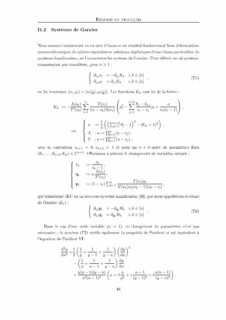
I1.2 Systèmes de Garnier
Nous sommes maintenant en mesure d'énon er un résultat fondamental liant déformations
isomonodromiques de sphères épointées et solutions algébriques d'une lasse parti ulière de
systèmes hamiltoniens, en l'o urren e les sytèmes de Garnier. Pour dénir un tel système,
ommençons par onsidérer, pour n ≥ 1 :
∂skνi = −∂ρiKk i, k ∈ [n]
∂skρi = ∂νiKk i, k ∈ [n], (E5)
en les in onnues (νi, ρi) = (νi(s), ρi(s)). Les fon tions Kk sont i i de la forme :
Kk := − Λ(sk)
T ′(sk)
n∑
i=1
T (νi)
(νi − sk)Λ(νi)
ρ2i −n+2∑
j=1
θj − δk,jνi − sj
ρi +κ
νi(νi − 1)
,
où
κ :=1
4
((∑n+2
j=1 θj − 1)2
− (θ∞ + 1)2)
,
Λ : u 7→ ∏nj=1(u− νj) ,
T : u 7→ ∏n+2j=1 (u− sj) ,
ave la onvention sn+1 = 0, sn+2 = 1 et pour un n + 3uplet de paramètres xés
(θ1, . . . , θn+2, θ∞) ∈ Cn+3. Ee tuons à présent le hangement de variables suivant :
tk :=sk
sk − 1,
qi := siΛ(si)
T ′(si),
pi := (1− si)∑n
k=1
T (si)ρkΛ′(νk)νk(νk − 1)(νk − si)
,
qui transforme (E5) en un nouveau système hamiltonien [46, que nous appellerons système
de Garnier (Gn) :
∂tkpi = −∂qiHk i, k ∈ [n]
∂tkqi = ∂piHk i, k ∈ [n]
. (E6)
Dans le as d'une seule variable (n = 1), e hangement de paramètres n'est pas
né essaire : le système (E5) vérie également la propriété de Painlevé et est équivalent à
l'équation de Painlevé VI :
d2y
du2=1
2
(1
y+
1
y − 1+
1
y − u
)(dy
du
)2
−(1
u+
1
u− 1+
1
y − u
)dy
du
+y(y − 1)(y − u)
u2(u− 1)2
(
α+ βu
y2+ γ
u− 1
(y − 1)2+ δ
u(u − 1)
(y − u)2
)
,
16

I1. DÉFORMATIONS ISOMONODROMIQUES, GROUPE MODULAIRE
pour les paramètres α =(θ∞ − 1)2
2, β = −θ
22
2, γ =
θ232
et δ =1− θ21
2.
Le lien entre es systèmes hamiltoniens et les déformations isomonodromiques est donné
par le résultat fondamental suivant, du aux travaux de Garnier et Malmquist.
Théorème I1.9 (Garnier, Malmquist). Pour i ∈ [n− 2], notons qi (resp. ti) les fon tions
algébriques ri (resp. les points ai ∈ P1) du paragraphe pré édent. Alors il existe n − 2
fon tions algébriques pi des variables (t1, . . . , tn−2) telles que (pi, qi)i soit solution d'un
système de Garnier (Gn−2) :
∂tkpi = −∂qiHk i, k ∈ [n]
∂tkqi = ∂piHk i, k ∈ [n]
,
pour des paramètres θi égaux aux valeurs propres des résidus Ai.
Les solutions algébriques de systèmes de Garnier font l'objet d'une attention parti -
ulière [7, 10, 11, 27, 34 et ont même été totalement lassiées dans le as n = 1 [42. Un
résultat du à Okamoto [38 (voir aussi le théorème I1.7) arme alors que e système véri-
e la propriété de Painlevé, qui pres rit la position des singularités " ompliquées" de ses
solutions. Plus pré isément, les seules singularités possibles pour une solution (pi, qi)i∈[n]du système (E6) en dehors des zones ritiques ti = tj (pour i, j ∈ [n + 2] tels que i 6= j)
doivent être des ples. Autrement dit, les seules singularités mobiles (i.e dépendant du
hoix de la solution) de l'équation sont des ples.
I1.3 Variété des ara tères d'une surfa e épointée
Soit Γ un groupe de type ni et soit A un anneau intègre; on peut alors onsidérer l'ensemble
des représentations de Γ dans SLd(A) (pour d ≥ 1):
Repd(Γ,A) := Hom(Γ, SLd(A)).
Considérons une présentation du groupe :
Γ = 〈a1, . . . , ak | (Rn(a1, . . . , ak))n≥0〉 ;
alors Repd(Γ,A) s'inje te dans SLd(A)k omme l'ensemble suivant :
(A1, . . . , Ak) ∈ SLkd | ∀n ≥ 0, Rn(A1, . . . , Ak) = Id.
Comme les équations Rn(A1, . . . , Ak) = Id sont polynomiales à oe ients entiers, l'ensemble
Repd(Γ,A) est une sousvariété de SLd(A)k. En parti ulier, il est naturellement muni de
deux topologies : elle induite par la topologie produit sur SLd(C)ket la topologie de
Zariski.
Une onséquen e de ette des ription en termes de variétés algébriques est que l'on
17

Résumé en français
peut onsidérer le quotient atégorique (au sens de la théorie géométrique des invariants) :
Repd(Γ,A)//SLd(A)
de Repd(Γ,A) sous l'a tion diagonale de SLd(A) par onjugaison simultanée. Il s'agit par
dénition de la variété algébrique :
Spec(
C[Repd(Γ,A)]SLd(A)
)
,
où C[Rep(Γ,A)]SL2(A)est l'anneau des fon tions polynomiales sur Rep(Γ,A) invariantes
sous l'a tion de SLd(A) ; on peut montrer qu'il s'agit dans le as omplexe du plus petit
quotient séparé (au sens de la topologie induite) du quotient topologique Repd(Γ,C)/
SLd(C).
Dénition I1.10. Soit Σ une surfa e fermée ompa te de genre g et soient p1, . . . , pb
b points distin ts de ette dernière. Alors le groupe fondamental Γ de la surfa e (non
ompa te) Σ := Σ \ p1, . . . , pb est de type ni et ne dépend que du ouple (g, b). La
variété algébrique suivante
Chard(g, b) := Repd(Γ,C)//SLd(C)
est alors appelée variété des ara tères de la surfa e Σ.
Remarque I1.11. Remarquons que l'on peut donner une présentation simple du groupe
fondamental de la surfa e Σ : si b 6= 0, il s'agit d'un groupe libre et dans le as ontraire
il est isomorphe à 〈a1, b1, . . . , ag, bg | [a1, b1] · · · [ag, bg]〉.
Deux variétés de ara tères vont être amenées à jouer un rle majeur dans les travaux
présentés i i : elles des sphères à quatre et inq trous dans SL2(C), que nous dé rivons
don brièvement i i. Dans le but d'alléger les notations dans la suite de e texte, on pose
Char(g, b) := Char2(g, b) .
I1.3.1 Variété des ara tères de la sphère à quatre trous
On s'intéresse à la sphère de Riemann S2 privée de quatre points, que nous noterons S24. Si
on xe un point de base z0 ∈ S24, le groupe fondamental π1(S24, z0) est isomorphe au groupe
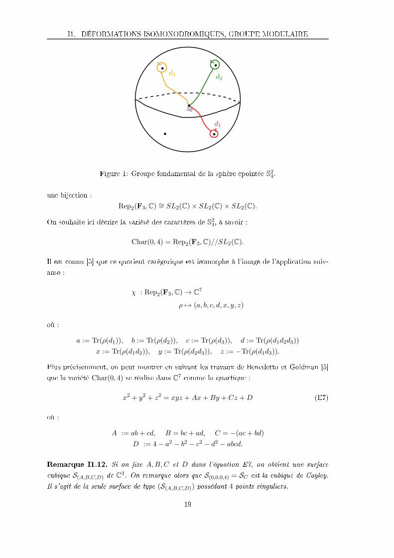
libre F3 engendré, par exemple, par les trois la ets élémentaires d1, d2 et d3 de la gure 1.
On souhaite étudier la variété des représentations du groupe fondamental de la sphère
S24 dans C, soit :
Rep2(F3,C) := Hom(F3, SL2(C)).
Comme le groupe π1(S24, z0) est un groupe libre à trois générateurs, un élément ρ ∈ Rep2(F3,C)
est totalement déterminé par les trois matri es ρ(d1), ρ(d2) et ρ(d3). De e fait on déduit
18
I1. DÉFORMATIONS ISOMONODROMIQUES, GROUPE MODULAIRE
bb
bb
d3 d2
d1
z0b
Figure 1: Groupe fondamental de la sphère épointée S24.
une bije tion :
Rep2(F3,C) ∼= SL2(C)× SL2(C)× SL2(C).
On souhaite i i dé rire la variété des ara tères de S24, à savoir :
Char(0, 4) = Rep2(F3,C)//SL2(C).
Il est onnu [5 que e quotient atégorique est isomorphe à l'image de l'appli ation suiv-
ante :
χ : Rep2(F3,C) → C7
ρ 7→ (a, b, c, d, x, y, z)
où :
a := Tr(ρ(d1)), b := Tr(ρ(d2)), c := Tr(ρ(d3)), d := Tr(ρ(d1d2d3))
x := Tr(ρ(d1d2)), y := Tr(ρ(d2d3)), z := −Tr(ρ(d1d3)).
Plus pré isemment, on peut montrer en suivant les travaux de Benedetto et Goldman [5
que la variété Char(0, 4) se réalise dans C7 omme la quartique :
x2 + y2 + z2 = xyz +Ax+By + Cz +D (E7)
où :
A := ab+ cd, B = bc+ ad, C = −(ac+ bd)
D := 4− a2 − b2 − c2 − d2 − abcd.
Remarque I1.12. Si on xe A,B,C et D dans l'équation E7, on obtient une surfa e
ubique S(A,B,C,D) de C3. On remarque alors que S(0,0,0,4) = SC est la ubique de Cayley.
Il s'agit de la seule surfa e de type (S(A,B,C,D)) possédant 4 points singuliers.
19

Résumé en français
Figure 2: Surfa es S(0,0,0,D) pour D = 12 , D = 3, D = 4 et D = 6 (parties réelles).
I1.3.2 Variété des ara tères de la sphère à inq trous
Dans le as de la sphère à inq trous, la lasse d'une représentation
ρ : F4 = 〈d1, . . . , d4 | ∅〉 → SL2(C)
dans la variété de ara tères Char(0, 5) est de la même façon déterminée par les quinze
fon tions oordonnées suivantes :
t1 := Tr(ρ(d1)), t2 := Tr(ρ(d2)), t3 := Tr(ρ(d3)),
t4 := Tr(ρ(d4)), t5 := Tr(ρ(d1d2d3d4)),
r1 := Tr(ρ(d1d2)), r2 := Tr(ρ(d1d3)), r3 := Tr(ρ(d1d4)),
r4 := Tr(ρ(d2d3)), r5 := Tr(ρ(d2d4)), r6 := Tr(ρ(d3d4)),
r7 := Tr(ρ(d1d2d3)), r8 := Tr(ρ(d1d2d4)), r9 := Tr(ρ(d1d3d4)), r10 := Tr(ρ(d2d3d4)).
Notons que, omme dans le as de la sphère à quatre trous, es dernières ne sont pas
algébriquement indépendantes ; des équations expli ites peuvent être obtenues de façon
20
I1. DÉFORMATIONS ISOMONODROMIQUES, GROUPE MODULAIRE
similaire au paragraphe pré édent (voir aussi les travaux de Komyo [40 sur le sujet).
I1.3.3 Correspondan e de RiemannHilbert
Un résultat fondamental de l'étude des onnexions logarithmiques plates est la orrespon-
dan e de Riemann Hilbert, qui arme que tout point de la variété de ara tères orrespond
à une déformation isomonodromique. Ce i justie notre démar he de her her à lassier
ertaines représentations de groupes avant de tenter de onstruire la déformation orre-
spondante.
Théorème I1.13 (RiemannHilbert). Soit (g, b) ∈ N2; alors pour tout point [ρ] ∈ Char(g, b)
il existe une onnexion logarithmique plate ∇ sur le bré trivial de rang 2 audessus d'une
surfa e fermée de genre g à b trous telle que [ρ∇] = [ρ] dans Char(g, b). Ré iproquement,
à toute telle onnexion logarithmique plate on peut asso ier un unique point de la variété
de ara tères Char(g, b).
Pour plus de détails, le le teur est invité à onsulter le hapitre 3 de [58, le para-
graphe III.18 de [35 ainsi que les travaux de Deligne [21 sur le sujet.
I1.4 A tion du groupe modulaire
Dans e paragraphe nous nous proposons de dé rire l'a tion du groupe modulaire d'une
surfa e fermée sur sa variété des ara tères. Le le teur pourra trouver plus de détails sur
les groupes modulaires dans la référen e [29.
Soit Σ une surfa e fermée ompa te de genre g et soient p1, . . . , pb des points deux à
deux distin ts de ette dernière ; on onsidère la surfa e épointée Σ := Σ \ p1, . . . , pb.On note alors Homeo+,∂(Σ) (resp. Homeo+,∂(Σ)) l'ensemble des homéomorphismes de Σ
préservant son orientation et xant son bord p1, . . . , pb dans son ensemble (resp. point
par point).
Dénition I1.14. Soit Σ une surfa e fermée de genre g à b trous. On a alors une relation
d'équivalen e ∼ sur Homeo+,∂(Σ) (resp. Homeo+,∂(Σ)) dénie de la façon suivante : on
note f ∼ g si et seulement si il existe une isotopie reliant f à g sur Σ dans Homeo+,∂(Σ)
(resp. Homeo+,∂(Σ)).On dénit alors les deux groupes suivants, ne dépendant à isomor-
phisme près que du ouple (g, b) :
1. le groupe modulaire de Σ :
Mod(g, b) := Homeo+,∂(Σ)/ ∼ ;
2. le groupe modulaire pur de Σ :
PMod(g, b) := Homeo+,∂(Σ)/ ∼ .
21

Résumé en français
Remarque I1.15. 1. Si b ≤ 1, on a naturellement PMod(g, b) ∼= Mod(g, b). En règle
générale toutefois, PMod est le noyau du morphisme surje tif naturel
Mod(g, b) ։ Sb
donné par l'a tion de Homeo+,∂(Σ) sur p1, . . . , pb. En parti ulier, PMod(g, b) est
un sousgroupe distingué d'indi e b! dans Mod(g, b).
2. Notons que l'a tion naturelle de Homeo+,∂(Σ) sur Σ n'est pas ompatible ave la
relation d'isotopie, et don ne passe pas au quotient.
Exemple I1.16. [29
1. le groupe modulaire de la sphère S2 est trivial ;
2. le groupe modulaire du tore R2/Z2est isomorphe à SL2(Z) ;
3. dans le as d'une sphère à b ≥ 1 trous, on a l'isomorphisme suivant [6, 29 :
PMod(0, b) ∼= PBb−1/Z(PBb−1)
où PBb−1 est le groupe des tresse pures à b − 1 brins et où pour tout groupe G la
notation Z(G) désigne le entre du dit groupe.
I1.4.1 Des ription générale
Fixons une surfa e fermée Σ de genre g ainsi que b points distin ts p1, . . . , pb de ette
dernière et onsidérons la surfa e épointée Σ := Σ \ p1, . . . , pb. Posons également
Γ := π1(Σ, p0) pour un hoix arbitraire de p0 ∈ Σ. Nous aurons également besoin de faire
usage de l'appli ation de quotient atégorique
χ : Repd(Γ,C) ։ Repd(Γ,C)//SLd(C) = Char(g, b) .
Le groupe Aut(Γ) des automorphismes du groupe fondamental de Σ agit naturellement
sur Repd(Γ,C) de la façon suivante :
Aut(Γ) → Aut(Repd(Γ,C))
Φ 7→ (ρ 7→ ρ Φ−1) .
On obtient de fait une a tion par automorphismes de Aut(Γ) sur le quotient Chard(g, b)
et on peut remarquer que le groupe Inn(Γ) des automorphismes intérieurs de Γ agit triv-
ialement sur la variété de ara tères Chard(g, b). On a don une a tion du groupe des
automorphismes extérieurs Out(Γ) := Aut(Γ)/Inn(Γ) sur Chard(g, b). L'inje tion na-
turelle Mod(g, b) → Out(Γ) [29 assure alors l'existen e d'un morphisme :
Mod(g, b) → Aut(Chard(g, b)) .
22

I1. DÉFORMATIONS ISOMONODROMIQUES, GROUPE MODULAIRE
I1.4.2 Le as des sphères épointées
L'a tion du groupe modulaire sur la variété des ara tères que nous venons de dé rire a été
reliée à l'étude des déformations isomonodromiques dans le as des sphères à quatre trous
dans les arti les séminaux de Philip Boal h [7, Boris Dubrovin et Marta Mazzo o [27 ;
des résultats similaires ont depuis été obtenus par Gaël Cousin dans le as de sphères
épointées générales [16.
Supposons que nous disposions d'une déformation isomonodromique de la sphère à
n trous S2n de monodromie asso iée ρ : Fn−1 → SL2(C) ; on peut alors s'intéresser
à l'orbite de la lasse [ρ] de ρ dans la variété de ara tères Char(0, n) sous l'a tion de
Mod(0, n). Cette dernière peut être visualisée de la façon suivante : à notre déformation
isomonodromique on peut asso ier une équation de S hlesinger (Théorème I1.8) de la forme
∀i ∈ [n], dAi = −∑
j 6=i
Ai, Ajai − aj
d(ai − aj)
portant sur les résidus de la onnexion logarithmique plate asso iée. L'a tion des auto-
morphismes extérieurs de Fn sur la variété des ara tères peut alors être vue omme le fait
de déformer les la ets élémentaires engendrant e dernier (vu omme groupe fondamental
de la sphère épointée) en "faisant tourner les points marqués les uns autour des autres" :
ela revient de fait à étudier la monodromie de ette équation. Lorsque la déformation
est algébrique, e pro édé ne peut qu'é hanger les bran hes de la solution algébrique du
système de Garnier (Gn) asso iée à ette déformation isomonodromique e qui implique
que l'orbite de [ρ] sous l'a tion de Mod(0, n) doit être nie.
Dans leur arti le [27, Dubrovin et Mazzo o ont prouvé la ré iproque dans le as
des solutions algébriques de ertaines équations de Painlevé VI, ellemême équivalente au
système de Garnier (G1). Ce résultat a été déterminant dans la lassi ation des solutions
algébriques de ette dernière équation, ouvrant la voix à une étude qui a été systématisée
par Cantat et Loray [11 puis a hevée par Lisovyy et Tykhyy [42 ; itons également les
travaux de Boal h [8, 9, Deift, Its, Kapaev et Zhou sur e sujet [20.
Un résultat analogue liant orbites nies sous l'a tion du groupe modulaire et solu-
tions algébriques de systèmes de Garnier a été ré emment obtenu par Cousin [16 dans le
as de déformations isomonodromiques logarithmiques de rang 2 sur une sphère épointée
quel onque. De fait, la re her he d'orbites nies sous ette a tion paraît une poursuite
pertinente et viable dans le adre de notre étude.
I1.5 Quelques avan ées ré entes
I1.5.1 Théorème de CorletteSimpson
Compte tenu de nos objets d'études, nous allons être amenés à nous intéresser aux représen-
tations de groupes fondamentaux de variétés quasiproje tives dans SL2(C). Ces dernières
ont fait l'objet d'une étude poussée par Corlette et Simpson [15 puis par Loray, Pereira
23

Résumé en français
et Touzet [43, qui a fait ressortir l'importan e d'une sous lasse de telles représentations,
par ailleurs déja très présente dans la littérature [1 : elles se fa torisant à travers une
ourbe.
Dénition I1.17. Soit X une variété quasiproje tive omplexe et soit Γ son groupe fon-
damental. On dit qu'une représentation ρ : Γ → SL2(C) se fa torise à travers une ourbe
si il existe une ourbe proje tive omplexe C, un diviseur ∆ (resp. δ) dans X (resp. C),
un morphisme algébrique f : X \∆ → C \δ et une représentation ρ du groupe fondamental
de C \ δ dans PSL2(C) tels que le diagramme
π1(C \ δ)
ρ&&
π1(X \∆)
f∗oo
Pρm
PSL2(C)
ommute, où P et m sont les morphismes de groupes naturels P : SL2(C) → PSL2(C) et
m : π1(X \∆) → Γ.
Cette lasse de représentations va jouer un rle majeur dans notre étude ; en eet
on peut par exemple iter le ranement suivant par Loray, Pereira et Touzet du résultat
séminal de Corlette et Simpson.
Théorème I1.18 (CorletteSimpson [15, LorayPereiraTouzet [43). Soit X une variété
quasiproje tive omplexe et soit Γ son groupe fondamental. Alors toute représentation
nonrigide ( i.e pouvant se déformer de façon analytique dans la variété des ara tères)
ρ : Γ → PSL2(C) d'image Zariskidense se fa torise à travers une ourbe.
I1.5.2 Solutions se fa torisant à travers une ourbe
À la lumière du théorème I1.18, la question suivante apparaît naturelle : quelles sont les so-
lutions algébriques d'un système de Garnier asso iées à des représentations de monodromie
se fa torisant à travers une ourbe ?
Les onnexions plates dont la monodromie se fa torise à travers une ourbe orrespon-
dent à des solutions de Garnier qui sont onstruites par la "méthode du tiréenarrière"
développée par Doran [26, Andreev et Kitaev [2. Karamoko Diarra a démontré dans sa
thèse [24 que seuls les systèmes de Garnier (Gn) pour n ≤ 3 admettent des solutions à mon-
odromie d'image Zariskidense obtenues par e pro édé ; es solutions s'obtiennent alors
en tirant en arrière des onnexions logarithmiques plates sur le bré trivial de rang 2 au
dessus de P1 \ 0, 1,∞ (aussi appelées équations hypergéométriques) par des revêtements
ramiés.
La monodromie ρ : F3 = 〈d1, d2, d3 | d1d2d3 = 1〉 → SL2(C) d'une onnexion hyper-
géométrique algébrique est ara térisée (en tant que point dans Char(0, 3)) par le triplet
(p0, p1, p∞) ∈ (N ∪ ∞)3 des ordres des matri es ρ(d1), ρ(d2) et ρ(d3). Dans [24, Diarra
24

I1. DÉFORMATIONS ISOMONODROMIQUES, GROUPE MODULAIRE
liste les tels triplets (p0, p1, p∞) ainsi que les types de rami ation des revêtements don-
nant lieu à des déformations isomonodromiques à monodromie Zariskidense d'une sphère
épointée, tout en pré isant le degré d du revêtement et l'indi e n du système de Garnier
(Gn) orrespondant ; nous reproduisons ette liste idessous.
(p0, p1, p∞) d Type de rami ation n
(2,∞,∞) 2 (2, 1 + 1, 1 + 1) 1
3 (2 + 1, 3, 1 + 1 + 1) 1
(2, 3,∞) 4 (2 + 2, 3 + 1, 1 + 1 + 1 + 1) 2
6 (2 + 2 + 2, 3 + 3, 1 + 1 + 1 + 1 + 1 + 1) 3
(2, 4,∞) 4 (2 + 2, 4, 1 + 1 + 1 + 1) 1
(2, 3, 7) 10 (2 + 2 + 2 + 2 + 2, 3 + 3 + 3 + 1, 7 + 1 + 1 + 1) 1
12 (2 + 2 + 2 + 2 + 2 + 2, 3 + 3 + 3 + 3, 7 + 1 + 1 + 1 + 1 + 1) 2
I1.6 Solutions algébriques de systèmes de Garnier obtenues à l'aide de
quintiques planes
Dans e paragraphe, nous exposons les résultats de la première partie de ette thèse, qui
ont trait à la lassi ation des solutions algébriques de systèmes de Garnier obtenues à
l'aide de quintiques planes.
I1.6.1 Un résultat de lassi ation
L'objet du premier hapitre de ette thèse est de lassier les représentations de groupes
ρ : Γ → PSL2(C), où Γ est le groupe fondamental du omplémentaire d'une ourbe de
degré inq dans P2(C), satisfaisant les onditions suivantes :
(C1) l'image de ρ est innie et irrédu tible ;
(C2) ρ ne se fa torise pas à travers une ourbe (voir dénition I1.17).
À la lumière de résultats obtenus par Diarra [24 et Mazzo o [46, es deux onditions
paraissent former un bon point de départ pour obtenir, à travers la orrespondan e de
RiemannHilbert (théorème I1.13), une nouvelle déformation isomonodromique algébrique.
En parti ulier, elles orrespondant à une monodromie d'image Zariskidense ne satis-
faisant pas (C2) ont été lassiées par le premier ; nous démontrons don le théorème
suivant.
Théorème A. Soit Γ le groupe fondamental du omplémentaire d'une ourbe Q de degré
inq dans P2(C) et soit ρ : Γ → PSL2(C) telle que :
• l'image de ρ est innie et irrédu tible ;
• ρ ne se fa torise pas à travers une ourbe.
25
Résumé en français
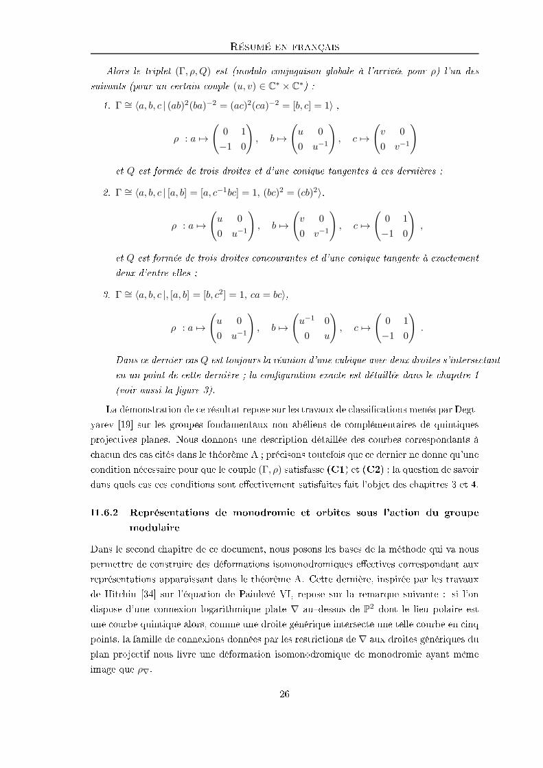
Alors le triplet (Γ, ρ,Q) est (modulo onjugaison globale à l'arrivée pour ρ) l'un des
suivants (pour un ertain ouple (u, v) ∈ C∗ × C∗) :
1. Γ ∼= 〈a, b, c | (ab)2(ba)−2 = (ac)2(ca)−2 = [b, c] = 1〉 ,
ρ : a 7→(
0 1
−1 0
)
, b 7→(
u 0
0 u−1
)
, c 7→(
v 0
0 v−1
)
et Q est formée de trois droites et d'une onique tangentes à es dernières ;
2. Γ ∼= 〈a, b, c | [a, b] = [a, c−1bc] = 1, (bc)2 = (cb)2〉,
ρ : a 7→(
u 0
0 u−1
)
, b 7→(
v 0
0 v−1
)
, c 7→(
0 1
−1 0
)
,
et Q est formée de trois droites on ourantes et d'une onique tangente à exa tement
deux d'entre elles ;
3. Γ ∼= 〈a, b, c |, [a, b] = [b, c2] = 1, ca = bc〉,
ρ : a 7→(
u 0
0 u−1
)
, b 7→(
u−1 0
0 u
)
, c 7→(
0 1
−1 0
)
.
Dans e dernier as Q est toujours la réunion d'une ubique ave deux droites s'interse tant
en un point de ette dernière ; la onguration exa te est détaillée dans le hapitre 1
(voir aussi la gure 3).
La démonstration de e résultat repose sur les travaux de lassi ations menés par Degt-
yarev [19 sur les groupes fondamentaux non abéliens de omplémentaires de quintiques
proje tives planes. Nous donnons une des ription détaillée des ourbes orrespondants à
ha un des as ités dans le théorème A ; pré isons toutefois que e dernier ne donne qu'une
ondition né essaire pour que le ouple (Γ, ρ) satisfasse (C1) et (C2) ; la question de savoir
dans quels as es onditions sont ee tivement satisfaites fait l'objet des hapitres 3 et 4.
I1.6.2 Représentations de monodromie et orbites sous l'a tion du groupe
modulaire
Dans le se ond hapitre de e do ument, nous posons les bases de la méthode qui va nous
permettre de onstruire des déformations isomonodromiques ee tives orrespondant aux
représentations apparaissant dans le théorème A. Cette dernière, inspirée par les travaux
de Hit hin [34 sur l'équation de Painlevé VI, repose sur la remarque suivante : si l'on
dispose d'une onnexion logarithmique plate ∇ audessus de P2dont le lieu polaire est
une ourbe quintique alors, omme une droite générique interse te une telle ourbe en inq
points, la famille de onnexions données par les restri tions de ∇ aux droites génériques du
plan proje tif nous livre une déformation isomonodromique de monodromie ayant même
image que ρ∇.
26
I1. DÉFORMATIONS ISOMONODROMIQUES, GROUPE MODULAIRE
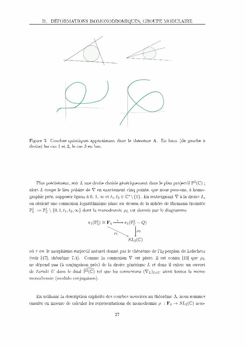
Figure 3: Courbes quintiques apparaissant dans le théorème A. En haut (de gau he à
droite) les as 1 et 2, le as 3 en bas.
Plus pré isément, soit L une droite hoisie génériquement dans le plan proje tif P2(C) ;
alors L oupe le lieu polaire de ∇ en exa tement inq points, que nous pouvons, à homo-
graphie près, supposer égaux à 0, 1,∞ et t1, t2 ∈ C∗ \1. En restreignant ∇ à la droite L,
on obtient une onnexion logarithmique plate audessus de la sphère de Riemann épointée
P15 := P1
C \ 0, 1, t1, t2,∞ dont la monodromie ρL est donnée par le diagramme
π1(P15)
∼= F4
ρL''P
PPPP
PPPP
PPP
τ // π1(P2C −Q)
ρ∇
SL2(C)
où τ est le morphisme surje tif naturel donné par le théorème de l'hyperplan de Lefs hetz
(voir [47, théorème 7.4). Comme la onnexion ∇ est plate, il est onnu [44 que ρL
ne dépend pas (à onjugaison près) de la droite générique L et don il existe un ouvert
de Zariski U dans le dual P2(C) tel que les onnexions (∇L)L∈U aient toutes la même
monodromie (modulo onjugaison).
En utilisant la des ription expli ite des ourbes asso iées au théorème A, nous sommes
ensuite en mesure de al uler les représentations de monodromie ρ : F4 → SL2(C) asso-
27

Résumé en français
iées aux ouples y apparaissant ; il s'agit (dans l'ordre et à onjugaison près) de :
ρ1 : d1 7→(
v 0
0 v−1
)
d2 7→(
u 0
0 u−1
)
d3 7→(
0 1
−1 0
)
d4 7→(
0 u2
−u−2 0
)
ρ2 : d1 7→(
0 1
−1 0
)
d2 7→(
v 0
0 v−1
)
d3 7→(
u 0
0 u−1
)
d4 7→(
v 0
0 v−1
)
ρ3 : d1 7→(
0 1
−1 0
)
d2 7→(
0 u−1
−u 0
)
d3 7→(
u 0
0 u−1
)
d4 7→(
u−1 0
0 u
)
ρ4 : d1 7→(
0 1
−1 0
)
d2 7→(
u 0
0 u−1
)
d3 7→(
u 0
0 u−1
)
d4 7→(
u−1 0
0 u
)
.
Nous nous intéressons ensuite aux orbites sous l'a tion du groupe modulaire de la sphère
à inq trous des points orrespondant à es représentations dans la variété de ara tères
Char(0, 5). Cette dernière est dénie omme le quotient atégorique de la variété des
représentations du groupe libre F4 dans SL2(C) sous l'a tion diagonale de SL2(C) par
onjugaison (voir paragraphe I1.3).
Nous al ulons alors de façon ee tive les orbites sous l'a tion du groupe modulaire
Mod(0, 5) sur la variété de ara tères Char(0, 5) orrespondantes et prouvons le résultat
suivant.
Théorème B. On s'intéresse aux quatre familles de représentations (paramétrées par
u, v ∈ C∗) du groupe libre à quatre générateurs F4 := 〈d1, . . . , d4 | ∅〉 dans SL2(C)
ρ1, . . . , ρ4 dé rites supra. Alors :
1. les points de Char(0, 5) asso iés à es dernières donnent lieu à quatre orbites deux à
deux distin tes de longueur quatre sous l'a tion du groupe modulaire pur PMod(0, 5) ;
2. les familles d'orbites sous l'a tion du groupe modulaire Mod(0, 5) asso iées à ρ1 et
ρ2 sont également distin tes ; toutefois elles asso iées à ρ3 et ρ4 sont des as parti-
uliers d'orbites de type ρ2. Plus pré isément, pour tous u ∈ C∗et i = 3, 4 il existe
deux paramètres (s, t) (dépendant de u et i) tels que l'orbite de la lasse de ρi ave
paramètre u soit égale à elle de ρ2 ave paramètres (s, t).
Le le teur intéressé par les orbites expli ites asso iées à es représentations est invité à
se référer à l'annexe A.
I1.6.3 Des ription expli ite des solutions
Les hapitres 3 et 4 sont dédiés (respe tivement) à la des ription expli ite des solutions du
système de Garnier (G2) asso iées aux familles de représentations ρ1 et ρ2. Dans haque
as nous donnons une onnexion expli ite sur le bré trivial de rang deux sur P2(C) puis
nous al ulons sa restri tion aux droites génériques et expli itons la solution algébrique de
(G2) asso iée.
28

I1. DÉFORMATIONS ISOMONODROMIQUES, GROUPE MODULAIRE
Solution asso iée à ρ1. Dans le hapitre 3, nous reprenons les résultats de l'arti le [32
on ernant la solution algébrique du système (G2) asso iée à la représentation ρ1. Ce i
signie que nous her hons tout d'abord à onstruire une onnexion logarithmique plate
sur le bré trivial de rang deux audessus de P2(C) dont le lieu polaire soit exa tement la
quintique Q apparaissant dans le as 1 du théorème A d'équation :
xyt(x2 + y2 + t2 − 2(xy + xt+ yt)) = 0
omposée d'une onique et de trois droites tangentes. Le groupe fondamental du omplé-
mentaire de ette ourbe est isomorphe au premier groupe dans la liste du théorème A,
soit :
Γ = 〈a, b, c | (ab)2(ba)−2 = (ac)2(ca)−2 = [b, c] = 1〉 .
On a un revêtement double ramié naturel π : P1×P1 2:1−−→ P2qui tire la quintique Q en
arrière sur l'ensemble D ⊂ P1 × P1 omposé des six droites u0, u1 = 0, 1,∞ (pour (u0, u1)
des oordonnées anes sur P1 × P1) et de la diagonale ∆ tout en ramiant uniquement
audessus de ette dernière. Comme la représentation ρ1 est diédrale don virtuellement
abélienne d'indi e deux, une idée naturelle pour onstruire notre onnexion est de dénir
une famille de onnexions logarithmiques de rang 1 à monodromie abélienne sur P1 × P1
et de la pousser en avant via π. On obtient alors le résultat suivant.
Théorème C. Il existe une famille expli ite à deux paramètres ∇λ0,λ1 de onnexions
logarithmiques plates sur le bré trivial de rang deux C2 × P2 → P2ayant les propriétés
suivantes :
(i) le lieu polaire de ∇λ0,λ1 est exa tement la ourbe quintique Q ⊂ P2d'équation :
xyt(x2 + y2 + t2 − 2(xy + xt+ yt)) = 0 ;
(ii) la monodromie de ∇λ0,λ1 est onjuguée à ρ1 ave paramètres u = −e−iπλ0 et v = e−iπλ1 .
La onnexion ∇λ0,λ1 est donnée dans la arte ane t = 1 ⊂ P2par :
∇λ0,λ1 = d− 1
2(x2 + y2 + 1− 2(xy + x+ y))(λ0A0 + λ1A1 +A2) ,
où
A0 :=
(
2(x− 1)ydx+ (x2 + x(y − 2)− y + 1)xdy
y2(2x− y + 2)ydx+ (2x2 + y(x− y + 3)− 2)xdy
y
−2y2dx+ (x + y − 1)x2 dy
y−2(x− 1)ydx− (x2 + x(y − 2)− y + 1)xdy
y
)
A1 :=
(
(x2 + (x− 1)(y − 1))y dx
x+ 2(x− 1)xdy (x2 + y(x− y + 3)− 2)y dx
x+ 2(2x− y + 2)xdy
−(x+ y − 1)y2 dx
x− 2x2dy −(x2 + (x− 1)(y − 1))y dx
x− 2(x− 1)xdy
)
A2 :=
(
−(x+ y + 1)ydx− (x2 − x(y + 2)− y + 1)xdy
y−2(x− y + 3)ydx− (x2 − 2y(x+ 1) + 1)xdy
y
0 (x+ y + 1)ydx+ (x2 − x(y + 2)− y + 1)xdy
y
)
.
29
Résumé en français
Partant de ela, nous sommes en mesure de donner un paramétrage rationnel ex-
pli ite des solutions algébriques de (G2) asso iées à la restri tion aux droites génériques de
ette famille de onnexion. Nous montrons ensuite que ette famille de onnexions vérie
génériquement la ondition (C2) ; plus pré isément, on prouve le résultat suivant.
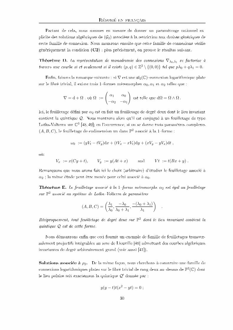
Théorème D. La représentation de monodromie des onnexions ∇λ0,λ1 se fa torise à
travers une ourbe si et seulement si il existe (p, q) ∈ Z2 \ (0, 0) tel que pλ0 + qλ1 = 0.
Enn, faisons la remarque suivante : si ∇ est une sl2(C) onnexion logarithmique plate
sur le bré trivial, il existe trois 1formes méromorphes α0, α1 et α2 telles que :
∇ = d+ Ω , où Ω :=
(
α1 α0
−α2 −α1
)
est telle que dΩ = Ω ∧ Ω .
I i, le feuilletage déni par α2 est en fait un feuilletage de degré deux dont le lieu invariant
ontient la quintique Q. Nous montrons alors qu'il est onjugué à un feuilletage de type
Lotka-Volterra sur C3[48, 49; en l'o urren e, si on se donne trois paramètres omplexes
(A,B,C), le feuilletage de odimension un dans P2asso ié à la 1forme :
ω0 := (yVt − tVy)dx+ (tVx − xVt)dy + (xVy − yVx)dt ,
où:
Vx := x(Cy + t), Vy := y(At+ x) and V t := t(Bx+ y) .
Remarquons que nous avons fait i i le hoix (arbitraire) d'étudier le feuilletage asso ié à
α2 ; la même étude peut être menée pour elui asso ié à α0.
Théorème E. Le feuilletage asso ié à la 1forme méromorphe α2 est égal au feuilletage
sur P2asso ié au système de LotkaVolterra de paramètres
(A,B,C) =
(λ1λ0,
−λ0λ0 + λ1
,−(λ0 + λ1)
λ1
)
.
Ré iproquement, tout feuilletage de degré deux sur P2dont le lieu invariant ontient la
quintique Q est de ette forme.
Nous démontrons enn que e i fournit un exemple de famille de feuilletages transver-
salement proje tifs intégrables au sens de Liouville [48 admettant des ourbes algébriques
invariantes de degré arbitrairement grand (voir aussi [41).
Solutions asso iée à ρ2. De la même façon, nous her hons à onstruire une famille de
onnexions logarithmiques plates sur le bré trivial de rang deux audessus de P2(C) dont
le lieu polaire soit exa tement la quintique Q′donnée par :
y(y − t)t(x2 − yt) = 0 ;
30

I2. CONVOLUTION INTERMÉDIAIRE DE KATZ
le groupe fondamental du omplémentaire de ette dernière est isomorphe au deuxième
groupe apparaissant dans le théorème A, soit :
〈a, b, c | [a, b] = [a, c−1bc] = 1, (bc)2 = (cb)2〉 .
Théorème F. Il existe une famille expli ite à deux paramètres ∇λ0,λ1 de onnexions
logarithmiques plates sur le bré trivial de rang deux C2 × P2 → P2ayant les propriétés
suivantes :
(i) le lieu polaire de ∇λ0,λ1 est exa tement la ourbe quintique Q ⊂ P2d'équation :
y(y − t)t(x2 − yt) = 0 ;
(ii) la monodromie de ∇λ0,λ1 est onjuguée à ρ2 ave paramètres u = eiπλ0 et v = eiπλ1 .
La onnexion ∇λ0,λ1 est donnée dans la arte ane t = 1 ⊂ P2par :
∇λ0,λ1 = d− 1
y(y − 1)(x2 − y)Ωλ0,λ1 ,
où
Ωλ0,λ1:=
− (y−1)(x2−y)4y
dy −2λ0y(y − 1)dx+ (λ0x(1− y) + λ1(x2 − y))dy
2y
−2λ0y(y − 1)dx + (λ0x(1− y) + λ1(x2 − y))dy
2
(y−1)(x2−y)4y
dy
.
De plus, la monodromie d'une telle onnexion ne fa torise pas par une ourbe pour λ0, λ1
génériques.
La onstru tion que nous proposons i i est sensiblement identique à elle entreprise
pré édemment ; il s'agit avant tout de pousser en avant une famille de onnexions "élé-
mentaires" via un revêtement ramié. Comme dans le hapitre pré édent, nous donnons
un paramétrage rationnel des solutions algébriques du système de Garnier asso ié.
I2 Convolution intermédiaire de Katz
Dans e paragraphe, nous dé rivons l'opération de onvolution intermédiaire (en anglais
dans la littérature middle onvolution) des représentations d'un groupe libre par l'a tion
du groupe de tresses introduite par Katz [37 ; nous renvoyons le le teur aux référen es [22,
23, 56, 57 pour plus de détails. Avant de dé rire e pro édé, nous pré isons e que nous
entendons dans e texte par opérateur de onvolution intermédiaire. Pour un ouple (g, b)
d'entiers naturels, posons :
Char∗(g, b) :=⋃
d∈N∗
Chard(g, b) ;
31
Résumé en français
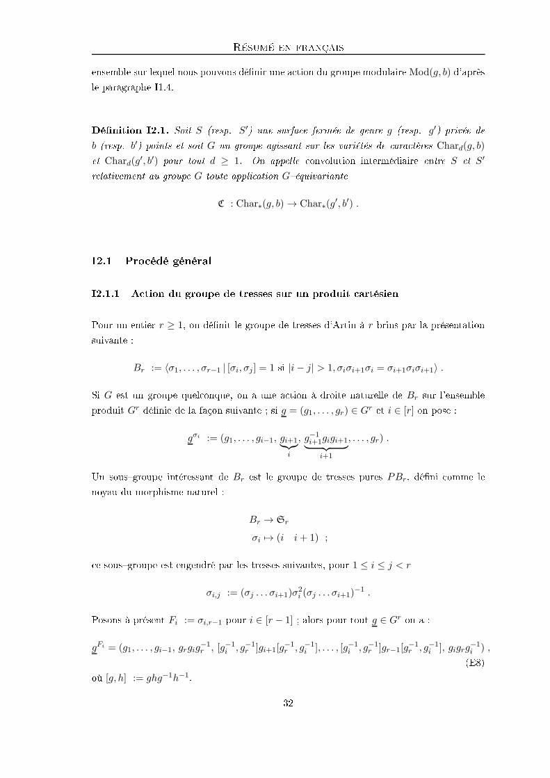
ensemble sur lequel nous pouvons dénir une a tion du groupe modulaire Mod(g, b) d'après
le paragraphe I1.4.
Dénition I2.1. Soit S (resp. S′) une surfa e fermée de genre g (resp. g′) privée de
b (resp. b′) points et soit G un groupe agissant sur les variétés de ara tères Chard(g, b)
et Chard(g′, b′) pour tout d ≥ 1. On appelle onvolution intermédiaire entre S et S′
relativement au groupe G toute appli ation Géquivariante
C : Char∗(g, b) → Char∗(g′, b′) .
I2.1 Pro édé général
I2.1.1 A tion du groupe de tresses sur un produit artésien
Pour un entier r ≥ 1, on dénit le groupe de tresses d'Artin à r brins par la présentation
suivante :
Br := 〈σ1, . . . , σr−1 | [σi, σj ] = 1 si |i− j| > 1, σiσi+1σi = σi+1σiσi+1〉 .
Si G est un groupe quel onque, on a une a tion à droite naturelle de Br sur l'ensemble
produit Gr dénie de la façon suivante ; si g = (g1, . . . , gr) ∈ Gr et i ∈ [r] on pose :
gσi := (g1, . . . , gi−1, gi+1︸︷︷︸
i
, g−1i+1gigi+1︸ ︷︷ ︸
i+1
, . . . , gr) .
Un sousgroupe intéressant de Br est le groupe de tresses pures PBr, déni omme le
noyau du morphisme naturel :
Br → Sr
σi 7→ (i i+ 1) ;
e sousgroupe est engendré par les tresses suivantes, pour 1 ≤ i ≤ j < r
σi,j := (σj . . . σi+1)σ2i (σj . . . σi+1)
−1 .
Posons à présent Fi := σi,r−1 pour i ∈ [r − 1] ; alors pour tout g ∈ Gr on a :
gFi = (g1, . . . , gi−1, grgig−1r , [g−1
i , g−1r ]gi+1[g
−1r , g−1
i ], . . . , [g−1i , g−1
r ]gr−1[g−1r , g−1
i ], gigrg−1i ) ,
(E8)
où [g, h] := ghg−1h−1.
32
I2. CONVOLUTION INTERMÉDIAIRE DE KATZ
I2.1.2 A tion par tresses sur les extensions anes de représentations d'un
groupe libre
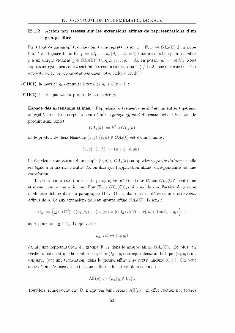
Dans tout e paragraphe, on se donne une représentation ρ : Fr−1 → GLd(C) du groupe
libre à r−1 générateurs Fr−1 := 〈d1, . . . , dr | d1 . . . dr = 1〉 ; notons que l'on peut assimiler
ρ à un unique élément g ∈ GLd(C)rtel que g1 . . . gr = Id, en posant gi := ρ(di). Nous
supposons également que ρ satisfait les onditions suivantes ( f. I2.2 pour une onstru tion
expli ite de telles représentations dans notre adre d'étude) :
(CIK1) la matri e gr ommute à tous les gi, i ∈ [r − 1] ;
(CIK2) 1 n'est pas valeur propre de la matri e gr.
Espa e des extensions anes. Rappelons brièvement que si d est un entier supérieur
ou égal à un et k un orps on peut dénir le groupe ane ddimensionnel sur k omme le
produit semidire t
GAd(k) := kd ⋊GLd(k)
où le produit de deux éléments (u, g), (v, h) ∈ GAd(k) est déni omme :
(u, g) · (v, h) := (u+ g · v, gh) .
La deuxième omposante d'un ouple (u, g) ∈ GAd(k) est appelée sa partie linéaire ; si elle
est égale à la matri e identité Id, on dira que l'appli ation ane orrespondante est une
translation.
L'a tion par tresses (au sens du paragraphe pré édent) de Br sur GLd(C)rpeut don
être vue omme une a tion sur Hom(Fr−1, GLd(C)), qui oïn ide ave l'a tion du groupe
modulaire dénie dans le paragraphe I1.4. On souhaite i i s'intéresser aux extensions
anes de ρ, i.e aux extensions de ρ au groupe ane GAd(C). Posons :
Uρ :=
u ∈ (Cd)r | (u1, g1) . . . (ur, gr) = (0, Id) et ∀i ∈ [r], ui ∈ Im(Id − gi)
;
alors pour tout u ∈ Uρ, l'appli ation
ρu : di 7→ (ui, gi)
dénit une représentation du groupe Fr−1 dans le groupe ane GAd(C). De plus, on
vérie rapidement que la ondition ui ∈ Im(Id− gi) est équivalente au fait que (ui, gi) soit
onjugué (par une translation) dans le groupe ane à sa partie linéaire (0, gi). On peut
don dénir l'espa e des extensions anes admissibles de ρ omme :
Aff(ρ) := ρu |u ∈ Uρ .
Toutefois, remarquons que Br n'agit pas sur l'espa e Aff(ρ) ; en eet l'a tion par tresses
33

Résumé en français
ne laisse pas invariante la partie linéaire.
Stru ture de Uρ et a tion par tresses. Soit u ∈ Im(Id − g1) × · · · × Im(Id − gr) ;
remarquons alors que :
u ∈ Uρ ⇔ (u1, g1) . . . (ur, gr) = (0, Id)
⇔ u1 + g1u2 + . . .+ g1 . . . gr−1ur = 0
⇔ u ∈ Ker(ϕ(ρ)) ,
où ϕ(ρ) est la matri e par blo s
(
Id g1 g1g2 . . . g1 . . . gr−1
)
.
Ainsi, Uρ est un sousespa e ve toriel de Im(Id−g1)×· · ·× Im(Id−gr) de odimension
d ; autrement dit on a l'égalité
dim(Uρ) =
r∑
i=1
rang(Id − gi)− d . (E9)
Comme rang(Id − gr) = d de par la ondition (CIK2), on peut simplier ette expression
en
dim(Uρ) =
r−1∑
i=1
rang(Id − gi) . (E10)
Considérons le sousgroupe suivant du groupe de tresses Br :
Gρ := σ ∈ Br | gσ = g .
Ce groupe est non trivial ; en eet la ondition (CIK1) ombinée à l'équation (E8) nous
livre que pour tout i ∈ [r − 1] la tresse pure
Fi = (σr−1 . . . σi+1)σ2i (σr−1 . . . σi+1)
−1
appartient à Gρ.
On peut alors vérier que Gρ agit (à droite) sur Aff(ρ). En eet, la partie linéaire
est préservée par onstru tion et un al ul rapide [57 montre que les deux onditions
dénissant Uρ sont bien préservées. En parti ulier, e i signie que si u ∈ Uρ, alors
∀σ ∈ Gρ, ∃v ∈ Uρ, ρσu = ρv ;
e qui signie que le groupe Gρ agit à droite sur l'espa e ve toriel Uρ.
34

I2. CONVOLUTION INTERMÉDIAIRE DE KATZ
Cal uls expli ites. Fixons u ∈ Uρ et i ∈ [r − 1] ; alors on peut al uler expli itement
l'image de la représentation ρu sous l'a tion de la tresse σi, en l'o urren e :
ρσiu = ((u1, g1), . . . , (ur, gr))σi
= ((u1, g1), . . . , (ui−1, gi−1, (ui+1, gi+1)︸ ︷︷ ︸
i
, (g−1i+1ui + g−1
i+1(gi − Id)ui+1, g−1i+1gigi+1)
︸ ︷︷ ︸
i+1
, . . . (ur, gr)) .
Ainsi, ρu est envoyée sur l'extension ane de gσi asso iée au ve teur Mσiu, où Mσi est la
matri e par blo s :
Mσi :=
Ii−1
0 g−1i+1
gi+1 g−1i+1(gi − Id)
Ir−i−1
où le blo spé ial est situé au niveau des olonnes/lignes i et i+1. Partant de ette remar-
que, on peut donner des formules expli ites pour l'a tion de Gρ sur Uρ ; en l'o urren e si
u ∈ Uρ alors uFi = Niu où Ni est la matri e obtenue omme suit : partant de la matri e
identité Ir, on rempla e ses ième et rième olonnes par (dans l'ordre) :
0.
.
.
0
gr
gi(Id − gr)(Id − g−1i+1)
.
.
.
gi(Id − gr)(Id − g−1r−1)
gi(Id − gr)
et
0.
.
.
0
gr(g−1i − Id)
gr(gi − Id)(Id − g−1i+1)
.
.
.
gr(gi − Id)(Id − g−1r−1)
Id − gr + gigr
où à haque fois le premier oe ient non nul se situe ligne i.
I2.1.3 Opérateur de onvolution intermédiaire
Extensions triviales. Nous avons vu dans le paragraphe pré édent que les extensions
anes de ρ onjuguées en haque générateur à leur partie linéaire sont stables sous l'a tion
d'un sousgroupe parti ulier du groupe de tresses Br. Supposons à présent que ρu ∈ Aff(ρ)
35
Résumé en français
est globalement onjuguée par une translation à sa partie linéaire, i.e que :
∃v ∈ Cd ∀i ∈ [r], (v, Id) · (ui, gi) · (−v, Id) = (0, gi) .
On remarque que omme le membre de gau he de ette égalité est égal à (ui+(Id−gi)v, gi)l'existen e d'un tel v est équivalente au fait que u ∈ Im(ψ(ρ)), où
ψ(ρ) :=
Id − g1.
.
.
Id − gr
.
Posons don :
Vρ := ψ(ρ)v | v ∈ Cd ;
et remarquons que l'on a l'in lusion Vρ ⊂ Uρ. On vérie ensuite en utilisant les formules
expli ites données plus haut que si i ∈ [r − 1] et v ∈ Cd alors les oordonnées (i, i + 1) de
ρσiψ(ρ)v = (((Id − g1)v, g1), . . . , ((Id − gr)v, gr))
σi
sont égales à (dans l'ordre) :
((Id − gi+1)v, gi+1) et (g−1i+1(Id − gi)v + g−1
i+1(gi − Id)(Id − gi+1)v, g−1i+1gigi+1) .
En développant ette dernière expression, on trouve que
ρσiψ(ρ)v = (((Id − h1)v, h1), . . . , ((Id − hr)v, hr) ,
où
h := gσi = (g1, . . . , gi−1, gi+1︸︷︷︸
i
, g−1i+1gigi+1︸ ︷︷ ︸
i+1
, . . . , gr) .
En parti ulier, e i implique que Gρ, en tant que stabilisateur de g dans Br, agit triviale-
ment sur Vρ.
Convolution intermédiaire de Katz. D'après le paragraphe pré édent, on a une a -
tion naturelle de Gρ sur l'espa e ve toriel quotient
Eρ := Uρ/Vρ .
De plus, omme la matri e Id − gr est inversible de part la ondition (CIK2), la matri e
ψ(ρ) est de rang d. L'équation (E10) nous permet alors d'é rire :
dρ := dim(Eρ) =r−1∑
i=1
rang(Id − gi)− d . (E11)
36

I2. CONVOLUTION INTERMÉDIAIRE DE KATZ
Il est de plus lair d'après les formules dé rivant leur a tion sur Uρ que les tresses pures Fi
agissent linéairement sur Eρ. Nous sommes maintenant en mesure de dénir la onvolution
intermédiaire de la représentation ρ sous l'a tion du groupe de tresses Br. Notons que le
lien entre e pro édé et la dénition I2.1 sera détaillé dans le paragraphe suivant.
Dénition I2.2. [37, 57 Soit ρ une représentation du groupe libre à r − 1 générateurs
Fr−1 := 〈d1, . . . , dr | d1 . . . dr = 1〉 dans GLd(C) vériant les onditions (CIK1) et
(CIK2). Pour i ∈ [r − 1], on onsidère l'appli ation linéaire gi ∈ GLdρ(C) orrespon-
dant à l'a tion de la tresse pure Fi sur Eρ et on pose gr := (g1 . . . gr−1)−1. On dénit la
onvolution intermédiaire de Katz de la représentation ρ omme la représentation
K(ρ) : Fr−1 → GLdρ(C)
di 7→ gi .
De plus, K(ρ) vérie les onditions (CIK1) et (CIK2).
I2.2 Appli ation à l'étude des orbites sous l'a tion de Mod(0, n)
I2.2.1 Équivarian e de la onvolution intermédiaire sous l'a tion du groupe
modulaire
La onvolution intermédiaire de Katz fournit un outil intéressant dans l'étude des orbites
nies sous l'a tion du groupe modulaireMod(0, n), que nous nous proposons de dé rire dans
e paragraphe. Supposons que nous disposions d'une représentation ρ : Fn−1 → SLd(C)
du groupe libre à n− 1 générateurs Fn−1 = 〈d1, . . . , dn | d1 . . . dn = 1〉 ; on lui asso ie alors
le nuplet des matri es hi := ρ(di) ∈ SLd(C). En xant n nombres omplexes non nuls
θi tels que θ1 . . . θn 6= 1 on peut alors poser :
∀i ∈ [n], gi :=1
θihi et gn+1 :=
(n∏
i=1
θi
)
Id .
Le n+1uplet g = (g1, . . . , gn+1) détermine alors une unique représentation ρ : Fn+1 → GLd(C)
vériant les onditions (CIK1) et (CIK2). En utilisant les formules expli ites données
pré édemment pour le al ul de g := K(ρ), on remarque que gn+1 doit être de la forme
λIdρ . Cette onstru tion permet de dénir pour haque hoix de θ une appli ation sur la
variété de ara tères Chard(0, n) en vériant que la quantité :
Kθ([ρ]) :=
[(1
τ1g1, . . . ,
1
τr−1gr−1 ,
τ1 . . . τr−1
τrλgr
)]
où τdρi = det(gi), ne dépend pas du hoix du représentant ρ dans ette dernière (elle dépend
par ontre du hoix de θ). On peut alors montrer que ette dernière onstitue bien une
onvolution intermédiaire au sens de la dénition I2.1 [22, 23.
37
Résumé en français
Théorème I2.3. L'appli ation Kθ dénie idessus est une onvolution intermédiaire entre
la sphère à n trous et ellemême relativement au groupe modulaire pur PMod(0, n).
Comme PMod(0, n) est isomorphe au quotient du groupe des tresses pures PBn−1
par son entre alors ette appli ation est PMod(0, n) équivariante par onstru tion, i.e si
τ ∈ PMod(0, n) et [ρ] ∈ Chard(0, n) alors :
Kθ(τ · [ρ]) = τ · Kθ([ρ])
où τ · [ρ] (resp. τ ·Kθ([ρ])) désigne l'image de [ρ] (resp. Kθ([ρ])) sous l'a tion de PMod(0, n)
sur Chard(0, n) (resp. Chardρ(0, n)). En eet, e pro essus mélange onvolution intermédi-
aire de Katz (au sens du paragraphe pré édent) et tensorisation par une représentation de
rang un, qui sont bien deux opérations PMod(0, n) équivariantes. Une onséquen e fonda-
mentale de ette équivarian e est la suivante : si l'orbite de [ρ] sous l'a tion de Mod(0, n)
est nie, alors elle de Kθ([ρ]) l'est également.
I2.2.2 Le as Mod(0, 4)
La onvolution intermédiaire de représentations a joué un rle majeur dans la lassi ation
des solutions algébriques des équations de Painlevé VI ; omme nous l'avons souligné
pré édemment, es dernières sont en orrespondan e ave les orbites nies sous l'a tion du
groupe modulaire Mod(0, 4) sur la variété de ara tères Char(0, 4). Dans son arti le [7,
Boal h met en pla e le pro édé suivant : partant de quatre matri es h1, . . . , h4 ∈ SL3(C)
engendrant un groupe ni (de réexions) et hoisies de telle sorte que h1, h2 et h3 aient
une valeur propre double θi on hoisit θ4 ∈ C∗de telle sorte que
• θ1 . . . θ4 6= 1 ;
• rang(I3 − θ−14 h4) = 2 .
Si ρ : F3 → SL3(C) est la représentation asso iée à (h1, h2, h3, h4), on peut alors onsid-
érer sa onvolution intermédiaire Kθ([ρ]). D'après l'équation (E11), ette dernière est une
représentation de rang 1+1+1+2−3 = 2. De plus, omme le groupe 〈h1, . . . , h4〉 ≤ SL3(C)
est ni, l'orbite de [ρ] sous l'a tion de Mod(0, 4) est nie ; 'est don également le as de
elle de Kθ([ρ]).
Ce pro édé a été utilisé par Boal h [7 pour générer des orbites nies sous ette dernière
a tion, e qui lui a permis de al uler les solutions algébriques de Painlevé VI. Cette étude
a été poursuivie par Filipuk [30, Dettweiler et Reiter [22, 23 qui ont étudié les symétries
de l'équation de Painlevé VI obtenues par onvolution intermédiaire. Plus pré isément,
si on part ette fois d'une solution algébrique d'une telle équation, de représentation de
monodromie asso iée ρ : F3 → SL2(C) ayant une orbite nie sous l'a tion du groupe
modulaire, alors sa onvolution intermédiaire via θ ∈ (C∗)4 hoisi de façon à e que θi
soit valeur propre simple de ρ(di) est également de rang deux (par l'équation E11) et don
orrespond également à une solution algébrique d'une équation de Painlevé VI (pour des
38

I2. CONVOLUTION INTERMÉDIAIRE DE KATZ
paramètres a priori diérents). Filipuk a montré que e type d'opération est relié aux
symétries mis en éviden e par Okamoto [51 dans les années 1980.
I2.3 Résultats originaux relatifs aux onvolutions intermédiaires
Dans e paragraphe, nous dé rivons les résultats démontrés dans la se onde partie de
ette thèse, en nous intéressant aux solutions qu'il est possible d'obtenir par onvolution
intermédiaire de Katz avant de dé rire les prémi es d'un pro édé analogue en genre 1.
I2.3.1 Quelques nouvelles orbites
Le hapitre 5 de ette thèse est dédié à l'adaptation partielle d'un travail mené par
Boal h [7 dans le as de l'équation de Painlevé VI au système de Garnier (G2). Plus pré-
isement, nous utilisons la onvolution intermédiaire de Katz ( f se tion I2) pour obtenir
des orbites nies dans la variété de ara tères Char(0, 5) sous l'a tion du groupe modulaire
Mod(0, 5) à partir de sousgroupes nis de SL3(C) (voir paragraphe I1.4).
Théorème G. On onsidère le groupe libre à quatre générateurs F4 := 〈d1, . . . , d4 | ∅〉.Alors, les lasses dans la variété des ara tères des représentations suivantes ont une orbite
nie sous l'a tion du groupe modulaire Mod(0, 5) :
ρ1 : d1 7→(
−1 0
−2 −1
)
d2 7→(
1 −12
0 1
)
d3 7→(
1 −12
0 1
)
d4 7→(
1 0
2 1
)
;
ρ2 : d1 7→(
−32
12
−12 −1
2
)
d2 7→(
1 0
2 1
)
d3 7→(
52 −1
292 −1
2
)
d4 7→(
1 0
4 1
)
;
ρ3 : d1 7→(
1 i
0 1
)
d2 7→(
1 i
0 1
)
d3 7→(
−15+i√3
6 −2√3+4i3
−i 9−i√3
6
)
d4 7→(
9−i√3
6
√3+i6
i 3+i√3
6
)
.
Ces orbites sont de plus deux à deux distin tes.
Ce théorème est plus à onsidérer omme une motivation pour poursuivre ette étude
que omme un résultat à part entière ; en eet l'étude que nous avons menée i i ne l'a
pas été faite de façon systématique, et nous n'avons pas en ore de des ription expli ite
(au sens des hapitres 3 et 4) des solutions algébriques d'un système de Garnier asso iées.
Nous donnons toutefois un algorithme ee tif, implémenté sous Maple pour le al ul de la
onvolution intermédiaire d'une représentation d'un groupe libre donnée, et explorons une
piste liée à la onuen e des ples du système de Garnier onsidéré.
I2.3.2 Convolution intermédiaire elliptique virtuelle
Dans le hapitre 6 nous nous intéressons au développement d'une possible extension de
la onvolution intermédiaire de Katz au as d'un tore à deux trous, prin ipalement en
39

Résumé en français
adaptant le formalisme donné par Völklein [57. Cependant, nous ne parvenons à obtenir
qu'une généralisation partielle de e pro édé.
Soient x0, p1, p2 et p3 quatre points deux à deux distin ts du tore omplexe T2 := C/Z2
et soit Γ2 (resp. Γ3) le groupe fondamental π1(T2\p1, p2, x0) (resp. π1(T2\p1, p2, p3, x0)).
Il est onnu que le groupe Γi (i = 2, 3) admet la présentation suivante (ave les notations
de la gure 4) :
Γ2 = 〈γ1, γ2, α, β | γ1γ2[α, β] = 1〉 et Γ3 = 〈γ1, γ2, γ3, α, β | γ1γ2γ3[α, β] = 1〉 .
γ2 γ1β
α
Figure 4: Générateurs de Γ2.
Alors pour tout la et δ ∈ π1(T2 \ p1, p2, p3), on peut déformer ontinûment les la ets
γ1, γ2, γ3, α et β en déplaçant p3 le long de δ. Ce i dénit un morphisme de groupes
Γ2 → Out(Γ3) .
Théorème H. Pour tout r ≥ 2, il existe une onvolution intermédiaire (au sens de la
dénition I2.1) expli ite entre le tore à deux trous et le tore à 2r trous relativement à
l'a tion du groupe fondamental du tore à deux trous dé rite idessus.
Ce résultat est plus faible que la onstru tion de Katz dans le sens où nous n'obtenons
qu'un représentation d'un sousgroupe d'indi e ni du groupe initial.
40

Part I
Algebrai Garniers solutions
obtained using plane quinti urves
41


Chapter 1
A lassi ation result
The obje t of this hapter is to lassify the group representations ρ : Γ → PSL2(C), where
Γ is the fundamental group of the omplement of some quinti urve in P2(C), that satisfy
the following onditions:
(C1) the image of ρ is irredu ible and innite;
(C2) ρ does not fa tor through a urve (see Denition 1.1.2).
Let C be an irredu ible omponent of some quinti urve Q.If U is a su iently small
analyti neighbourhood of some smooth point p ∈ C one gets:
π1(U \ C ∩ U) ∼= Z .
Let γ be any loop generating the above y li group; then ρ(γ) ∈ PSL2(C) must be non
trivial. Indeed, one would otherwise get a fa torisation of ρ through the fundamental group
of the omplement of some urve in P2with degree at most 4 in whi h ase earlier work
by Cousin (see Se tion 5.1 in [17) proves that ρ annot satisfy both (C1) and (C2). In
this hapter, we prove the following result.
Theorem A. Let Γ be the fundamental group of the omplement of some quinti urve Q
in P2(C) and let ρ : Γ → PSL2(C) satisfy the following onditions:
(C1) the image of ρ is irredu ible and innite;
(C2) ρ does not fa tor through a urve.
Then the triple (Γ, ρ,Q) is (up to global onjuga y for ρ and PGL3(C) a tion for Q)
one of the following:
1. Γ ∼= 〈a, b, c | (ab)2(ba)−2 = (ac)2(ca)−2 = [b, c] = 1〉 ,
ρ : a 7→(
0 1
−1 0
)
, b 7→(
u 0
0 u−1
)
, c 7→(
v 0
0 v−1
)
, for some u, v ∈ C∗ ,
and the urve Q is omposed of three lines tangent to a oni ;
43

CHAPTER 1. A CLASSIFICATION RESULT
2. Γ ∼= 〈a, b, c | [a, b] = [a, c−1bc] = 1, (bc)2 = (cb)2〉,
ρ : a 7→(
u 0
0 u−1
)
, b 7→(
v 0
0 v−1
)
, c 7→(
0 1
−1 0
)
, for some u, v ∈ C∗ ,
and Q is made of three on urrent lines and a oni tangent to two of the latter ;
3. Γ ∼= 〈a, b, c |, [a, b] = [b, c2] = 1, ca = bc〉,
ρ : a 7→(
t 0
0 t−1
)
, b 7→(
t−1 0
0 t
)
, c 7→(
0 1
−1 0
)
, for some t ∈ C∗ .
Here, the urve Q is one of two spe ial ongurations of two lines and a ubi ,
des ribed in Se tion 1.2.4.2.
Note that the above triples do o ur but do not ne essarily satisfy onditions (C1) and
(C2), depending on the parameters.
Figure 1.1: Quinti urves appearing in Theorem A. On the top row (from left to right)
are ase 1 and 2, ase 3 appears in the bottom row.
44
1.1. PRELIMINARY REMARKS
1.1 Preliminary remarks
1.1.1 The CorletteSimpson theorem
First, we re all a well known fa t about the rank two proje tive spe ial linear group
PSL2(C) ; to do so start by setting P : SL2(C) → PSL2(C) to be the anoni al pro-
je tion.
Proposition 1.1.1. [14 Let H be an innite non Zariskidense algebrai subgroup of
PSL2(C); then H is ontained (up to onjuga y) in the image of one of the following
groups in PSL2(C):
• the group of triangular 2× 2 matri es in SL2(C);
• the innite dihedral group:
D∞ :=
(
0 α
−α−1 0
)
,
(
β 0
0 β−1
)∣∣∣∣∣α, β ∈ C∗
≤ SL2(C) .
Representations of fundamental groups of quasi-proje tive varieties in SL2(C) have
been lassied mainly by Corlette and Simpson [15. One important lass of su h repre-
sentations is that of those fa toring through a urve.
Denition 1.1.2. [15, 43 Let Γ be the fundamental group of the omplement of some
urve in P2(C). We say that a representation ρ : Γ → PSL2(C) fa tors through a urve
if there exists a omplex proje tive urve C, a divisor ∆ (resp. δ) in P2(resp. C), an
algebrai mapping f : P2 −∆ → C − δ and a representation ρ of the fundamental group of
C − δ into PSL2(C) su h that
(i) ∆ ontains Q, therefore there exists a natural group homomorphismm : π1(P2−∆) → Γ2;
(ii) the diagram
π1(C − δ)
ρ''
π1(P
2 −∆)f∗
oo
ρm
PSL2(C)
ommutes.
Moreover, if some representation : Γ → SL2(C) is su h that P ρ : Γ → SL2(C), we will
say that fa tors through an orbi urve.
Indeed, representations admitting su h a fa torisation an be obtained through pullba k
from the monodromy of some logarithmi at onne tion on a urve [43. Moreover, we
have the following renement by Loray, Pereira and Touzet [43 of a theorem by Corlette
and Simpson [15.
45

CHAPTER 1. A CLASSIFICATION RESULT
Theorem 1.1.3 (CorletteSimpson, LorayPereiraTouzet). Let X be a quasiproje tive
surfa e. Then any nonrigid representation ρ : π1(X) → PSL2(C) with Zariskidense
image fa tors through a urve.
Remark 1.1.4. This implies that any representation satisfying ondition (C1) that is
neither rigid nor dihedral fa tors through a urve.
1.1.2 The ZariskiVan Kampen method
What follows is a brief a ount of the lassi al ZariskiVan Kampen theorem in the ase
of omplex proje tive plane urves. We refer the reader to a set of omprehensive le ture
notes by Shimada [55 for further details.
Let C ⊂ P2(C) be a proje tive plane urve ; onsider a pair (x0, L0), where x0 is a
point in the omplement of C in the proje tive plane P2(C) and L0 is a proje tive line
whi h does not ontain x0. Then there is a natural proje tion
πx0,L0 : P2(C) \ x0 → L0
∼= P1C .
There is a nite number of spe ial bres L1, . . . , Ln of the proje tion πx0,L0 , i.e bres su h
that Card(Li ∩ C) < d := deg(C). If one sets
X := P2(C) \(
C ∪n⋃
i=1
Li
)
then the restri tion πx0,L0 := πx0,L0 |X is a lo ally trivial bration over P1n := P1
C\πx0,L0(Li) | i ∈ [n],with bres equal to dpun tured Riemann spheres P1
d.
Theorem 1.1.5 (Van Kampen, Zariski). Let X and M be quasiproje tive manifolds su h
that M is aspheri al (i.e π2(M) = 0) and let π : X →M be a lo ally trivial bration. Let
s :M → X be a holomorphi se tion of π and x (p, x) ∈M ×X su h that s(p) = x. Then
there is a group isomorphism
π1(X,x) ∼= π1(π−1(p), x) ⋊ π1(M,p) ,
where the semidire t produ t is given by the monodromy of the bration π.
This theorem is mainly a onsequen e of the homotopy exa t sequen e asso iated with
the bration π; indeed sin e M is aspheri al the se tion s yields a splitting of this exa t
sequen e, namely:
0 = π2(M) → π1(π−1(x), x) → π1(X,x) → π1(M,p) → 0 .
Remark 1.1.6. Note that in the ase of the omplement of a proje tive urve in P2(C),
there always exists su h a se tion s, given by any generi line in the proje tive plane.
46
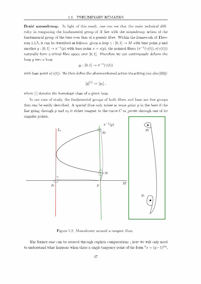
1.1. PRELIMINARY REMARKS
Braid monodromy. In light of this result, one an see that the main te hni al di-
ulty in omputing the fundamental group of X lies with the monodromy a tion of the
fundamental group of the base over that of a generi bre. Within the framework of Theo-
rem 1.1.5, it an be des ribed as follows: given a loop γ : [0, 1] →M with base point p and
another g : [0, 1] → π−1(p) with base point x = s(p), the pointed bres (π−1(γ(t)), s(γ(t)))
naturally form a trivial bre spa e over [0, 1]. Therefore we an ontinuously deform the
loop g into a loop
gt : [0, 1] → π−1(γ(t))
with base point s(γ(t)). We then dene the aforementioned a tion via setting (see also [55):
[g][γ] := [g1] ,
where [·] denotes the homotopy lass of a given loop.
In our ase of study, the fundamental groups of both bres and base are free groups
that an be easily des ribed. A spe ial bre only arises at some point p in the base if the
line going through p and x0 is either tangent to the urve C or passes through one of its
singular points.
M
g1
g2
γ
p
Li
pi
π−1(p)
g1
g2
Figure 1.2: Monodromy around a tangent bre.
The former ase an be treated through expli it omputations ; here we will only need
to understand what happens when there a single tangen y point of the form "x = (y−1)2",
47
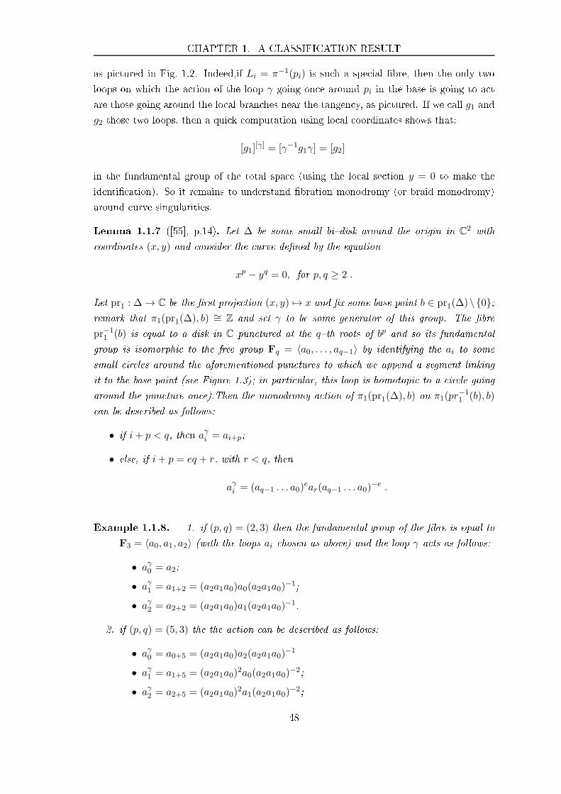
CHAPTER 1. A CLASSIFICATION RESULT
as pi tured in Fig. 1.2. Indeed,if Li = π−1(pi) is su h a spe ial bre, then the only two
loops on whi h the a tion of the loop γ going on e around pi in the base is going to a t
are those going around the lo al bran hes near the tangen y, as pi tured. If we all g1 and
g2 those two loops, then a qui k omputation using lo al oordinates shows that:
[g1][γ] = [γ−1g1γ] = [g2]
in the fundamental group of the total spa e (using the lo al se tion y = 0 to make the
identi ation). So it remains to understand bration monodromy (or braid monodromy)
around urve singularities.
Lemma 1.1.7 ([55, p.14). Let ∆ be some small bidisk around the origin in C2with
oordinates (x, y) and onsider the urve dened by the equation
xp − yq = 0, for p, q ≥ 2 .
Let pr1 : ∆ → C be the rst proje tion (x, y) 7→ x and x some base point b ∈ pr1(∆)\0;remark that π1(pr1(∆), b) ∼= Z and set γ to be some generator of this group. The bre
pr−11 (b) is equal to a disk in C pun tured at the qth roots of bp and so its fundamental
group is isomorphi to the free group Fq = 〈a0, . . . , aq−1〉 by identifying the ai to some
small ir les around the aforementioned pun tures to whi h we append a segment linking
it to the base point (see Figure 1.3); in parti ular, this loop is homotopi to a ir le going
around the pun ture on e).Then the monodromy a tion of π1(pr1(∆), b) on π1(pr−11 (b), b)
an be des ribed as follows:
• if i+ p < q, then aγi = ai+p;
• else, if i+ p = eq + r, with r < q, then
aγi = (aq−1 . . . a0)ear(aq−1 . . . a0)
−e .
Example 1.1.8. 1. if (p, q) = (2, 3) then the fundamental group of the bre is equal to
F3 = 〈a0, a1, a2〉 (with the loops ai hosen as above) and the loop γ a ts as follows:
• aγ0 = a2;
• aγ1 = a1+2 = (a2a1a0)a0(a2a1a0)−1;
• aγ2 = a2+2 = (a2a1a0)a1(a2a1a0)−1.
2. if (p, q) = (5, 3) the the a tion an be des ribed as follows:
• aγ0 = a0+5 = (a2a1a0)a2(a2a1a0)−1
• aγ1 = a1+5 = (a2a1a0)2a0(a2a1a0)
−2;
• aγ2 = a2+5 = (a2a1a0)2a1(a2a1a0)
−2;
48
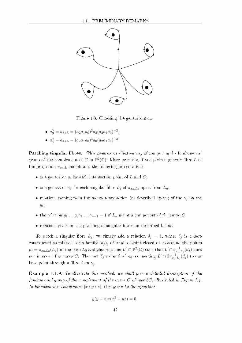
1.1. PRELIMINARY REMARKS
Figure 1.3: Choosing the generators ai.
• aγ3 = a3+5 = (a2a1a0)2a2(a2a1a0)
−2;
• aγ4 = a4+5 = (a2a1a0)3a0(a2a1a0)
−3.
Pat hing singular bres. This gives us an ee tive way of omputing the fundamental
group of the omplement of C in P2(C). More pre isely, if one pi ks a generi bre L of
the proje tion πx0,L one obtains the following presentation:
• one generator gi for ea h interse tion point of L and C;
• one generator γj for ea h singular bre Lj of πx0,L0 apart from Ln;
• relations oming from the monodromy a tion (as des ribed above) of the γj on the
gi;
• the relation g1 . . . gdγ1 . . . γn−1 = 1 if Ln is not a omponent of the urve C;
• relations given by the pat hing of singular bres, as des ribed below.
To pat h a singular bre Lj , we simply add a relation δj = 1, where δj is a loop
onstru ted as follows: set a family (dj)j of small disjoint losed disks around the points
pj = πx0,L0(Lj) in the base L0 and hoose a line L′ ⊂ P2(C) su h that L′ ∩π−1x0,L0
(dj) does
not interse t the urve C. Then set δj to be the loop onne ting L′ ∩ ∂π−1x0,L0
(dj) to our
base point through a bre then γj .
Example 1.1.9. To illustrate this method, we shall give a detailed des ription of the
fundamental group of the omplement of the urve C of type 3C2 illustrated in Figure 1.4.
In homogeneous oordinates [x : y : z], it is given by the equation:
y(y − z)z(x2 − yz) = 0 .
49
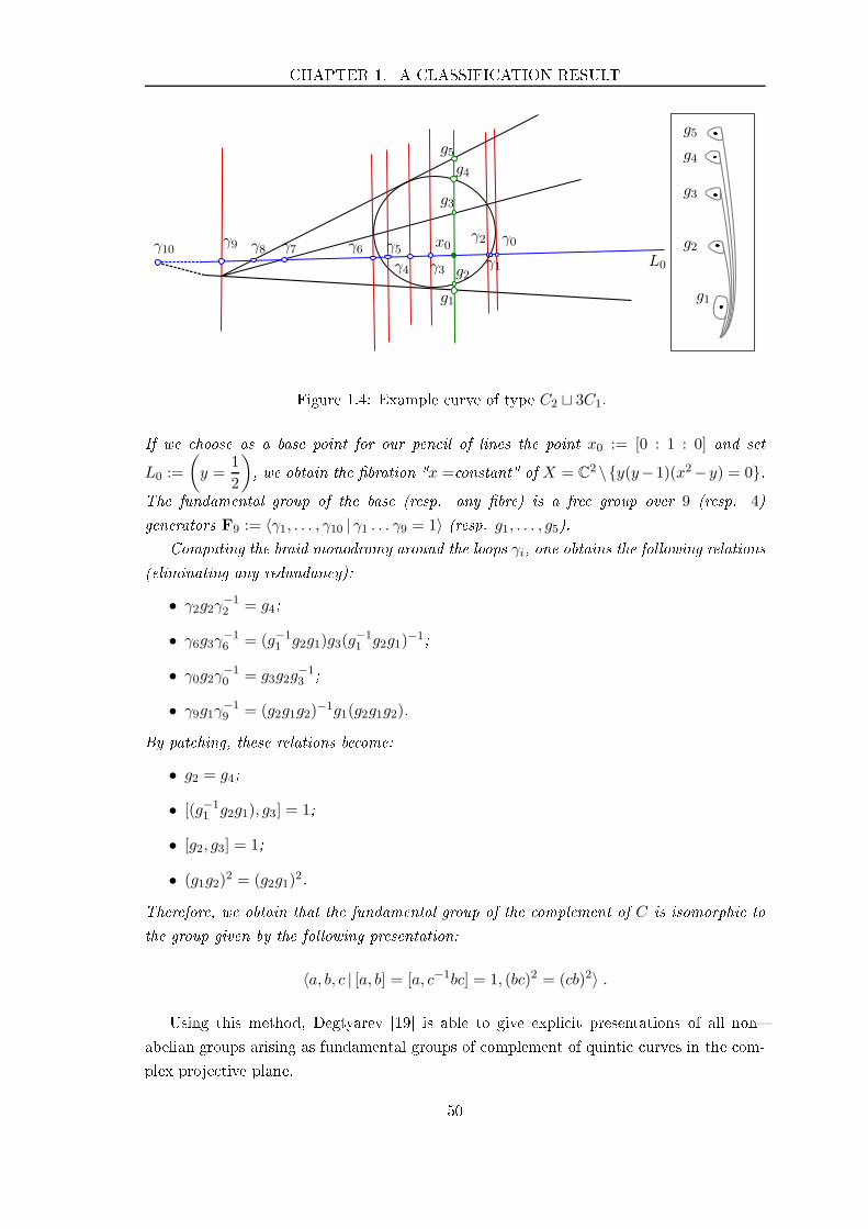
CHAPTER 1. A CLASSIFICATION RESULT
L0γ1
γ2
γ3
x0
γ4
γ5γ6γ7γ9 γ8
g1
g2
g3
g4
g5
γ0γ10
g1
g5
g4
g3
g2
Figure 1.4: Example urve of type C2 ⊔ 3C1.
If we hoose as a base point for our pen il of lines the point x0 := [0 : 1 : 0] and set
L0 :=
(
y =1
2
)
, we obtain the bration "x = onstant" of X = C2 \y(y−1)(x2−y) = 0.The fundamental group of the base (resp. any bre) is a free group over 9 (resp. 4)
generators F9 := 〈γ1, . . . , γ10 | γ1 . . . γ9 = 1〉 (resp. g1, . . . , g5).Computing the braid monodromy around the loops γi, one obtains the following relations
(eliminating any redundan y):
• γ2g2γ−12 = g4;
• γ6g3γ−16 = (g−1
1 g2g1)g3(g−11 g2g1)
−1;
• γ0g2γ−10 = g3g2g
−13 ;
• γ9g1γ−19 = (g2g1g2)
−1g1(g2g1g2).
By pat hing, these relations be ome:
• g2 = g4;
• [(g−11 g2g1), g3] = 1;
• [g2, g3] = 1;
• (g1g2)2 = (g2g1)
2.
Therefore, we obtain that the fundamental group of the omplement of C is isomorphi to
the group given by the following presentation:
〈a, b, c | [a, b] = [a, c−1bc] = 1, (bc)2 = (cb)2〉 .
Using this method, Degtyarev [19 is able to give expli it presentations of all non
abelian groups arising as fundamental groups of omplement of quinti urves in the om-
plex proje tive plane.
50
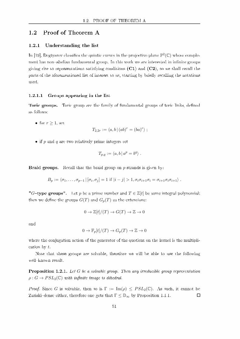
1.2. PROOF OF THEOREM A
1.2 Proof of Theorem A
1.2.1 Understanding the list
In [19, Degtyarev lassies the quinti urves in the proje tive plane P2(C) whose omple-
ment has nonabelian fundamental group. In this work we are interested in innite groups
giving rise to representations satisfying onditions (C1) and (C2), so we shall re all the
parts of the aforementioned list of interest to us, starting by briey re alling the notations
used.
1.2.1.1 Groups appearing in the list
Tori groups. Tori group are the family of fundamental groups of tori links, dened
as follows:
• for r ≥ 1, set
T2,2r := 〈a, b | (ab)r = (ba)r〉 ;
• if p and q are two relatively prime integers set
Tp,q := 〈a, b | ap = bq〉 .
Braid groups. Re all that the braid group on p strands is given by:
Bp := 〈σ1, . . . , σp−1 | [σi, σj ] = 1 if |i− j| > 1, σiσi+1σi = σi+1σiσi+1〉 .
"Gtype groups". Let p be a prime number and T ∈ Z[t] be some integral polynomial;
then we dene the groups G(T ) and Gp(T ) as the extensions:
0 → Z[t]/(T ) → G(T ) → Z → 0
and
0 → Fp[t]/(T ) → Gp(T ) → Z → 0
where the onjugation a tion of the generator of the quotient on the kernel is the multipli-
ation by t.
Note that these groups are solvable, therefore we will be able to use the following
wellknown result.
Proposition 1.2.1. Let G be a solvable group. Then any irredu ible group representation
ρ : G→ PSL2(C) with innite image is dihedral.
Proof. Sin e G is solvable, then so is Γ := Im(ρ) ≤ PSL2(C). As su h, it annot be
Zariskidense either, therefore one gets that Γ ≤ D∞ by Proposition 1.1.1.
51
CHAPTER 1. A CLASSIFICATION RESULT
Artin groups. We will also need a few Artin groups, namely:
• A1(p, q, r) := 〈a, b, c | ap = bq = cr = abc〉;
• A2(p, q, r) := 〈a, b, c | ap = bq = cr = abc = 1〉;
• A3(p, q, r) := 〈a, b | ap = bq = 1, (ab)r = (ba)r〉.
"Unusual" groups. Here we shall list some ex eptional groups arising in Degtyarev's
lassi ation by giving nite presentations obtained through the ZariskiVan Kampen
method.
• Γ5 := 〈u, v |u3 = v7 = (uv2)2〉;
• Γ4 := 〈a, b, c | aba = bab, cbc = bcb, abcb−1a = bcb−1abcb−1〉 ;
• Γ3 := 〈a, b | [a3, b] = 1 , ab2 = ba2〉;
• Γ′3 := 〈a, b, c | aca = cac, [b, c] = 1, (ab)2 = (ba)2〉;
• Γ2 := 〈a, b, c | [a, b] = [a, c−1bc] = 1, (bc)2 = (cb)2〉;
• Γ′2 := 〈a, b, c | (ab)2 = (ba)2, (ac)2 = (ca)2, [b, c] = 1〉.
1.2.1.2 Arnol'd's notation for urve singularities
In order to allow for an e ient listing of the urves involved in Degtyarev's lassi ation
we will make use of Arnol'd's notation for urves singularities [3. More spe i ally:
• we will denote by Ap a singular point of lo al type
x2 + yp+1 = 0 ;
• we will denote by E6 a singular point of lo al type
x3 + y4 = 0 ;
• we will say that a urve is of type Ck1⊔ . . .⊔Ckn if it (globally) has n irredu ible om-
ponents of respe tive degrees k1, . . . , kn. In the ase where several su h omponents
have the same degree, we will use the shorthand notation mCkℓ;
• if any degree d irredu ible omponent of our urve has singular points, we shall denote
it by writing Cd(Σ), where Σ is the list of the aforementioned urve's singularities,
of the form m1Ap1 ⊔ . . . ⊔mnApn (note that if the urve is smooth, we will simply
use the shorthand Cd instead of Cd(∅));
• nally, we will use the following notation regarding the mutual position of two irre-
du ible urves C and C ′:
52

1.2. PROOF OF THEOREM A
×d if C ′interse ts C with multipli ity d at a nonsingular point of C;
Ap if C′interse ts C transversally at a singular point of C of type Ap;
A∗p if C
′is tangent (with smallest possible multipli ity) to C transversally at a
singular point of C of type Ap.
Moreover, if the urve is of type C3 ⊔ 2C1 and the two lines interse t at one of the
spe ial points des ribed above, we shall underline it in the list.
Example 1.2.2. A urve of type C3(A1)⊔C1 with interse tion ×2, ×1 would be made up
of a nodal ubi and a line, the latter interse ting the former at two smooth points, on e
with a tangent and the other transversally. The same urve with interse tion A1, ×1 would
have the line interse t the ubi transversally at both some smooth point and the nodal
singular point.
1.2.1.3 The list
Table 1.1 sums up Degtyarev's list; for more details we refer the reader to the original
paper [19. Note that we have eliminated all nite groups from the list before reprodu ing
it.
We shall go through Degtyarev's list in three steps:
• rst, we investigate urves with large singularities, allowing us to remove some of
them from the list;
• se ondly, we eliminate any group in the list whi h annot yield a representation
satisfying onditions (C1) and (C2) for purely algebrai reasons;
• nally, we review the remaining fundamental groups in the list by urve type.
Doing so, we will make heavy use of the following elementary fa t about PSL2(C).
Lemma 1.2.3. Let M ∈ PSL2(C) entralising some nonabelian subgroup G ≤ PSL2(C);
then M is the identity element of PSL2(C).
Proof. Let A,B be two elements in G su h that AB 6= BA: A,B and M a t on P1(C) as
Möbius transformations and sin e M ommutes to A and B it stabilises (setwise) both
the sets FA and FB of xed points for A and B. Moreover, up to hanging A and/or B
to A2, B2, M must have at least one ommon xed point with both A and B, and sin e
Card(FA),Card(FB) ≤ 2 this means that M stabilises FA and FB pointwise. Now, as
A and B do not ommute, Card(FA ∪ FB) ≥ 3, and so M must be diagonalisable; let us
set P ∈ PGL2(C) su h that PMP−1is diagonal. Sin e G is nonabelian, there exists an
element C in G su h that PCP−1is not diagonal; however MC = CM thus M must be
the identity element of PSL2(C).
53

CHAPTER 1. A CLASSIFICATION RESULT
Curve type Interse tion type(s) Group(s)
C5(A6 ⊔ 3A2) Γ5
C4(3A2) ⊔ C1 ×2,×2 Γ4
×2,×1,×1 or A∗2,×1 B3
else G3(t+ 1)C4(2A2 ⊔A1) ⊔ C1 ×4 B4
×2,×2 B3
C4(2A2) ⊔ C1 ×4 or ×2,×2 B3
C4(A4 ⊔A2) ⊔ C1 ×3,×1 Z×A2(2, 3, 5)A∗
4 B3
A2,×2 G5(t+ 1)C4(A2 ⊔A2) ⊔ C1 A2,×2 B3
C4(A6) ⊔ C1 A6,×2 B3
C4(A5) ⊔ C1 ×4 or ×2,×2 B3
C4(E6) ⊔C1 ×4 T3,4×2,×2 B3
C3(A2) ⊔ C2 ×3,×3 Γ3
C3(A2) ⊔ 2C1 ×3 ;×2,×1 Γ′3
×3 ;A∗2 T2,6
×3 ;×1, A2 T2,4×3 ;×1,×1,×1 Z×B3
×3 ;A2 × 1 Z×B3
×3 ;×1,×1,×1 Z×B3
×2,×1 ;×1,×2 Z×B3
A2,×1 ;×1,×2 G(t2 − 1)C3(A1) ⊔ 2C1 ×3 ;×3 G(t3 − 1)
×3 ;×1,×2 G(t2 − 1)×1,×2 ;×1,×2 G(t2 − 1)
2C2 ⊔C1 the two C2 interse t with multipli ity 4 F2, T2,4the two C2 interse t at two points F2, T2,4
the two C2 interse t with multipli ity 3 Z×B3
C2 ⊔ 3C1 the three C1 have a ommon point Γ2, Z× F2
else Γ′2, Z× F2, Z× T2,4
5C1 the ve C1 have a ommon point F4
there is a quadruple point Z× F3
there are two triple points F2 × F2
there is only one triple point Z× Z× F2
Table 1.1: Degtyarev's list
1.2.2 Large singularities
The goal of this paragraph is to study the spe ial ases where the quinti urve has some
large order (i.e greater or equal to three) singular point. In fa t, we prove that represen-
tations of the fundamental group of the omplement of su h urves almost always fa tor
through some urve.
54
1.2. PROOF OF THEOREM A
1.2.2.1 Fivefold singularities
First, we an eliminate the ase of the urve 5C1 with a quintuple point through a rather
elementary reasoning, as eviden ed by the result below.
Proposition 1.2.4. Let Q be a quinti in the proje tive plane P2(C) of type 5C1 su h that
its ve irredu ible omponents share a ommon point. Then any representation ρ : π1(P2−Q) → PSL2(C)
with nonabelian image fa tors through a urve.
Proof. Sin e all irredu ible omponents of Q interse t at a ommon point then by blowing
it up we get a lo ally trivial bration
P2 − Qf
Coo
B
where B is isomorphi to P1minus ve points and Q is the total transform of the quinti
Q. The homotopy exa t sequen e asso iated with f then yields:
0 = π1(C) → π1(P2 − Q) → F4 = π1(B) → π0(C) .
Sin e π1(P2−Q) ∼= π1(P2−Q) (as we blew up a point inQ) then one gets that π1(P
2−Q) ∼= π1(B)
thus ρ fa tors through B by means of the morphism f .
1.2.2.2 Quadruple singularities
In the rare ase where a quinti urve in Degtyarev's list has a quadruple singularity, we
an dis ard it using the following result.
Proposition 1.2.5. Let Q be a quinti in the proje tive plane P2(C) of type 5C1 su h that
exa tly four of its irredu ible omponents share a ommon point. Then any representation
ρ : π1(P2 −Q) → PSL2(C)
with nonabelian image fa tors through a urve.
Proof. Up to an element in PGL3(C), one an assume that the line that does not interse t
the other four at their ommon point is the line at innity and that the aforementioned
quadruple point is the origin of the orresponding ane hart (identied with C2). One
gets a lo ally trivial bration ψ : P2−Q → P14 dened as follows: for any point x ∈ P2−Q,
ψ(x) the line going through the origin and x. This bration has bre equal to C∗and
a natural se tion given by any line not ontained in Q nor going through the origin, the
55

CHAPTER 1. A CLASSIFICATION RESULT
latter giving us an homeomorphism
f : P2 −Q∼−→ P1
4 × C∗
x 7→ (ψ(x), τ(x)) ,
where τ(x) is the slope of the line ψ(x) ⊂ C2. This means that π1(P
2 − Q) ∼= F3 × Z.
The fa t that the image of ρ must be nonabelian di tates that the image of one of these
fa tors must also be. As su h, any element in the image of the other one entralises a
nonabelian subgroup in PSL2(C) and os must be trivial by Lemma 1.2.3. Thus one gets
that ρ fa tors through P14 (as π1(C
∗) = Z is abelian).
1.2.2.3 Triple singularities
It remains to see what happens when the studied urve has a singular point of order exa tly
three.
Proposition 1.2.6. Let Q be a quinti in the proje tive plane P2(C). Assume that
there exists a triple point p0 ∈ Q, i.e that for any line L in P2 ontaining p0 one has
Card(L∩(Q−p0)) = 2 ( ounted with multipli ity); then any representation ρ : π1(P2−Q) → PSL2(C)
with nonabelian, nondihedral innite image fa tors through a urve up to pullba k by a
double overing.
Proof. Start by blowing up p0; in the following we will denote by C (resp. C) the total
(resp. stri t) transform of any urve C ⊂ P2by this blowup. This turns the pen il of
lines going through the point p0 into an a tual bration
P2
f
P1oo
B
endowed with a natural se tion τ given by the ex eptional divisor E(p0) (note that both
E(p0) and B are isomorphi to the proje tive line P1). Sin e a generi line ontaining p0
in P2 uts Q − p0 at two distin t points, we also get a "double se tion" of this bration,
namely a ramied double overing r : C 2:1−−→ P1and a mapping σ : C → P2
su h that the
diagram
P2
f
C r //
σ
??⑧⑧⑧⑧⑧⑧⑧⑧
B
ommutes. Note that by onstru tion σ(C) is a omponent of the stri t transform pf Q ;
in the ase where it is redu ible we have a mu h stronger result (see Remark 1.2.7).
56
1.2. PROOF OF THEOREM A
Consider the bre produ t S := P2 ×B C; by denition, this is exa tly the set
(p, q) ∈ P2 × C | f(p) = r(q),
giving us another ommutative diagram (and a natural mapping χ : S → P2):
S
π
χ// P2
f
Cr
2:1// B
The se ond proje tion π : S → C yields a bration
S
π
P1oo
C
endowed with three distin t se tions σ0, σ1 and σ∞. Indeed one an dene two se tions of π
using the double se tion σ as follows: for any x ∈ C there exists y ∈ C (generi ally distin t
from x) su h that r(x) = r(y), so we set σ0(x) := (σ(x), x) and σ0(x) := (σ(y), x) (this is
well dened sin e f σ = r). The third se tion σ∞ is then given by the ex eptional divisor:
x 7→ τ r(x). Note that there are nitely many points x ∈ C su h that σi(x) = σj(x) for
some i 6= j (i, j = 0, 1,∞); indeed these spe ial points ome from either singular points
of Q− p0, bres of f tangent to Q or possible interse tions between E(p0) and the stri t
transform of Q in P2.
One an now establish a birational mapping h between S and the dire t produ t P1×C.Let x ∈ C be some generi point (so that σ0(x), σ1(x) and σ∞(x) are pairwise distin t)
and dene h on L as the homography sending σ0(x) (resp. σ1(x), σ∞(x)) onto 0 (resp.
1,∞). This denes a rational mapping indu ing an isomorphism between a Zariskiopen
set in S and one in C × P1.
Let us now look at the above re ipe in topologi al terms: sin e we are blowing up a point
in Q then π1(P2 −Q) ∼= π1(P2 − Q). Then remark that we an extend our representation
ρ to the fundamental group of the omplement of Q ∪ L1 ∪ . . . ∪ Lk, where the Li are
the bres of f that are either bres above the rami ation lo us of r or ontain points of
the indetermina y lo us of h or h−1, by setting the image of any simple loop around any
spe ial bre Li that is not a omponent of Q to be the identity matrix I2.
This means that we have a new representation ρ : π1(P2−(Q∪L1∪. . .∪Lk) → PSL2(C)
su h that Im(ρ) = Im(ρ). The overing r being nonramied above B − f(L1 ∪ . . . ∪ Lk)one gets that the fundamental group G := π1(S − χ∗(Q ∪ L1 ∪ . . . ∪ Lk)) is isomorphi to
an index at most two subgroup of π1(P2 − (Q ∪ L1 ∪ . . . ∪ Lk)). Thus, by restri tion, one
gets a representation ρG : G→ PSL2(C).
57

CHAPTER 1. A CLASSIFICATION RESULT
Sin e the birational map h only blows up and/or ontra t divisors ontained in
χ∗(Q ∪ L1 ∪ . . . ∪ Lk),
there is an isomorphism between G and the fundamental group G′of C × P1 − δ, where δ
is the stri t transform under h of χ∗(Q∪L1∪ . . .∪Lk) (i.e the Zariski losure of its image
under h). This divisor δ is by onstru tion a nite union of "verti al" and/or "horizontal"
urves in C×P1thus C×P1−δ = (C−η)× (P1−η′), where η (resp. η′) is a nite divisorial
sum of points in C (resp. P1). This in turn implies that G′ ∼= π1(C − η)× π1(P
1 − η′).
Sin e Im(ρG) is an index at most 2 subgroup in the nondihedral group Im(ρ), it must
be nonabelian. This for es the image of one of the fa tors in G to be nonabelian therefore
any element in the image of the other one entralises a nonabelian subgroup in PSL2(C)
and so is trivial by Lemma 1.2.3. As su h, ρG fa tors through either C −η or P1−η′, usingeither the rst or the se ond proje tion.
Remark 1.2.7. If the "double se tion" σ in the proof above is a tually made up of two
welldened se tions (i.e if σ(C) is a redu ible omponent of Q), then one naturally does
not need the nondihedral hypothesis. Indeed, σ(C) must be made out of two lines and so
we get three welldened se tions of the initial bration, without needing to go through a
double overing. Thus, any representation ρ : π1(P2 − Q) → PSL2(C) with nonabelian,
innite image fa tors through a urve.
The following urves have a triple singularity that falls under Remark 1.2.7, therefore
we an remove them from the list:
• C4(E6) ⊔ C1;
• C3(A2) ⊔ 2C1 with interse tion types ×3 ;A∗2, ×3 ;×1, A2 and ×1,×2 ;×1, A2;
• 2C2 ⊔ C1 if either the two oni s interse t with multipli ity 4 and the line is their
ommon tangent at this point (F2 ase in the list) or if they have two interse tion
points through whi h the line passes (F2 ase);
• C2⊔3C1 if two of the line are tangent to the oni and the third passes through both
tangen y points;
• 5C1 with any number of triple points.
In the rst two ases, one needs to hose the singular point of the irredu ible omponent
with highest degree as the singularity in Proposition 1.2.6. For example, when one looks at
a urve of type C4(E6)⊔C1 then one sees that any line going through the E6 type singular
point interse ts the quinti in two distinguishable other points: one on the quarti C4 and
one on the line C1. Thus, after blowing up the aforementioned singular point, the pen il of
lines going through it be omes a bration endowed with two se tions. Thus Lemma 1.2.3
58

1.2. PROOF OF THEOREM A
for es the image of one of the fa tors in G to be nonabelian therefore any element in the
image of the other one entralises a nonabelian subgroup in PSL2(C) and so is trivial.
As su h, ρG fa tors through either C − η or P1 − η′, using either the rst or the se ond
proje tion.
To treat the ase of 2C2 ⊔ C1, take any interse tion between the line and quadri and
for C2 ⊔ 3C1 and 5C1 take any interse tion between exa tly three omponents. Note that
this means that we an ompletely eliminate the free group on two generators F2 from the
list.
1.2.3 Eliminating groups
In this paragraph, we eliminate several groups that, for stri tly algebrai reasons, annot
give rise to a representation satisfying onditions (C1) and (C2). More pre isely, we prove
the following result.
Proposition 1.2.8. Let G be one of the following groups:
• the braid groups B3 and B4;
• the group G(t3 − 1);
• the groups Gp(t+ 1) for some prime number p;
• the Artin group A2(2, 3, 5);
• the "unusual" groups Γ4, Γ3 and Γ′3;
• any dire t produ t of Z and one of the above.
Let ρ be a representation of G into PSL2(C). Then ρ annot satisfy both onditions (C1)
and (C2).
1.2.3.1 Braid groups
On three strands. Consider the group B3 = 〈σ1, σ2 |σ1σ2σ1 = σ2σ1σ2〉 ; we prove the
two following lemmas.
Lemma 1.2.9. There is no representation ρ : B3 → PSL2(C) with nonabelian dihedral
image.
Proof. Let A (resp. B) be the image of σ1 (resp. σ2) by ρ. Then one has ABA = BAB and
thus A = (AB)−1B(AB) is onjugate to B. Moreover, one an easily he k that (AB)3
ommutes with the whole (non abelian) image of ρ and so must be trivial (Lemma 1.2.3).
Sin e ρ is dihedral then sin e its image must be non abelian one must have (up to global
onjuga y and permuting A and B) either
A =
(
0 −1
1 0
)
and B =
(
λ 0
0 λ−1
)
59
CHAPTER 1. A CLASSIFICATION RESULT
or
A =
(
0 −1
1 0
)
and B =
(
0 −λλ−1 0
)
for some λ ∈ C\0,−1, 1 (if λ = ±1 then the image of ρ would be abelian). In the rst
ase, sin e A and B are onjugate, λ must be equal to ±i and so the groupe generated by A
and B is nite abelian. In the se ond ase, the ondition one an only have ABA = BAB
if λ = ±1 i.e if A = B, meaning that the image of ρ must be abelian.
Lemma 1.2.10. Let ρ : B3 → PSL2(C) be a representation with irredu ible nondihedral
image. Then ρ annot be rigid.
Proof. As above, let A (resp. B) be the image of σ1 (resp. σ2) by ρ. Sin e ρ is not dihedral,
then it is Zariskidense and so must be rigid by Theorem 1.1.3. Up to global onjuga y,
one an assume that either
A =
(
1 1
0 1
)
or A =
(
u 0
0 u−1
)
for some u ∈ C \ 0,−1, 1 .
In the rst ase, the fa ts that A and B are onjugate and Im(ρ) must be nonabelian
for es
B =
(
1 0
u 1
)
for some u ∈ C∗, but then for any su h u one has ABA = BAB in PSL2(C) if and
only if u = −1. However, one easily he ks that for any v ∈ C∗the following denes a
representation of B3:
σ1 7→(
v 1
0 v−1
)
, σ2 7→(
v−1 0
−1 v
)
and so ρ is not rigid. In the se ond ase, one an he k that the equation B = (AB)−1B(AB)
(in the variable B) admits a solution for any u 6= 0,±1 and that su h a pair (A,B) denes
a representation of B3 for any su h u. Therefore, the representation annot be rigid.
The ombination of Lemmas 1.2.9 and 1.2.10 with Theorem 1.1.3 yield that no repre-
sentation ρ : B3 → PSL2(C) may satisfy onditions (C1) and (C2).
On four strands. Consider the group
B4 = 〈σ1, σ2, σ3 | [σ1, σ3], σ1σ2σ1 = σ2σ1σ2, σ3σ2σ3 = σ2σ3σ2〉
and let A (resp. B, C) be the image of σ1 (resp. σ2, σ3) by ρ; the braid relations then
give us:
[A,C] = I2, ABA = BAB and BCB = CBC .
If either A or C is trivial then ρ fa tors through a representation of B3 and so annot
60

1.2. PROOF OF THEOREM A
satisfy onditions (C1) and (C2). Moreover, B annot be trivial sin e the image of ρ
must be nonabelian, nor an A ommute to B.
All three matri es must be onjugate as B = (AB)−1A(AB) and C = (BC)−1B(BC).
As su h, if ρ is dihedral then by applying Lemma 1.2.9 we get that both the groups 〈A,B〉and 〈B,C〉 must be nite; ombined with the fa t that A and C ommute, this for es
Im(ρ) to be nite.
Else, we pro eed again as above: up to global onjuga y, one an assume that either
A =
(
1 1
0 1
)
or A =
(
u 0
0 u−1
)
for some u ∈ C \ 0,−1, 1 .
In the rst ase, the fa ts that A, B and C are onjugate and Im(ρ) must be nonabelian
for es (up to global onjuga y)
B =
(
1 0
u 1
)
and C =
(
1 v
0 1
)
for some u, v ∈ C∗, but then the relation ABA = BAB (resp. BCB = CBC) in PSL2(C)
if and only if u = −1 (resp. v = 1). However, one easily he ks that for any w ∈ C∗the
following denes a representation of B4:
σ1 7→(
w 1
0 w−1
)
, σ2 7→(
w−1 0
−1 w
)
, σ3 7→(
w 1
0 w−1
)
,
and so ρ is not rigid. In the se ond ase, sin e A and C ommute one must have
C =
(
v 0
0 v−1
)
for some v ∈ C \ 0,−1, 1 .
One an then he k that both equations B = (AB)−1B(AB) and B = (CB)C(CB)−1(in
the variable B) admits a solution for any u, v 6= 0,±1 and that su h a triple (A,B,C)
denes a representation of B4 for any su h u, v. Therefore, the representation annot be
rigid.
1.2.3.2 Groups of type G(T ) and Gp(T )
Re all that sin e these groups are solvable, any of their irredu ible representation into
PSL2(C) must have dihedral image (see Proposition 1.2.1).
61
CHAPTER 1. A CLASSIFICATION RESULT
The group G(t3−1). Sin e t3−1 = (t−1)(t2+ t+1), the group G(t3+1) is isomorphi
to the semidire t produ t Z3ϕ⋊ Z, where:
ϕ(n) ·
u
v
w
=
0 −1 0
1 −1 0
0 0 1
n
u
v
w
.
Fix the following set of generators for G(t3 − 1):
a :=
1
0
0
, 0
, b :=
0
1
0
, 0
, c :=
0
0
1
, 0
, d :=
0
0
0
, 1
and let A,B,C,D be their images under ρ. Then C entralises the whole image of ρ, whi h
we assumed nonabelian therefore it must be equal to the identity in PSL2(C). Moreover,
sin e A and B ommute and Im(ρ) is dihedral and nonabelian one must have, up to global
onjuga y:
A =
(
u 0
0 u−1
)
, B =
(
v 0
0 v−1
)
and D =
(
0 −1
1 0
)
or
A = B =
(
0 −1
1 0
)
and D =
(
u 0
0 u−1
)
for some u, v ∈ C∗. Note that A must be equal to B in the se ond ase be ause those two
matri es need to ommute.
Using the above generators, one gets that in G(t3 − 1) one has the relation d · a = b · dand so one must have DA = BD, whi h is only possible in the rst ase and if uv = ±1.
But one also has d2 · a = b · d2 and so A = B = I2 in PSL2(C), whi h is impossible as the
image of ρ must be nonabelian.
Groups of type Gp(t + 1). Let p be some prime integer; then the group Gp(t + 1) is
isomorphi to the semidire t produ t Fp ϕ⋊ Z where φ(n) · k = (−1)nk. As su h, it has
two generators a := (1, 0) and b := (0, 1) su h that (using multipli ative notation) ap = 1
and ab2 = b2a.
If we onsider a representation ρ : Gp(t+1) → PSL2(C) and set (A,B) := (ρ(a), ρ(b))
then sin e B2 ommutes with every element of Im(ρ) we must have Ap = B2 = I2, therefore
the aforementioned image must be isomorphi to the semidire t produ t Fp ⋊ F2 and so
is nite.
1.2.3.3 Group A2(2, 3, 5)
If one sets A := ρ(a), B := ρ(b) and C := ρ(c) then one gets A2 = B3 = C5 = ABC = I2 in
PSL2(C). Lifting this to SL2(C), one an thereofore assume that A2 = ±I2, B3 = (AB)5 = −I2
62

1.2. PROOF OF THEOREM A
(up to hanging B to −B) and so Tr(A) ∈ −2, 0, 2, Tr(B) = 2 cos(π/3) = 1 and
Tr(C) = 2 cos(π/5) or 2 cos(3π/5) = −2 cos(2π/5).
The study of hypergeometri equations by S hwartz's yielded a list of all triples of matri-
es (M1,M2,M3) in SL2(C) satisfyingM1M2M3 = I2 su h that the group 〈M1,M2,M3〉 ≤ SL2(C)
is nite. An a ount of these works an be found in Chapter IX of [52, with the list itself
being reprodu ed on p. 310. If Tr(A) = 2 cos(π/2) = 0 then the aforementioned S hwartz's
list gives us that the image of ρ is nite, isomorphi to A5. Else, A must be equal to ±I2and so BC = ±I2: Im(ρ) must be abelian.
"Unusual" groups
Several of the ex eptional groups appearing in Degtyarev's list an be eliminated for alge-
brai reasons, as we show in this paragraph.
The group Γ4 Consider the following group:
Γ4 := 〈a, b, c | aba = bab, cbc = bcb, a(bcb−1)a = (bcb−1)a(bcb−1)〉 .
Let ρ be a representation of the above group into PSL2(C) and set A (resp. B, C) to be
the images ρ(a) (resp. ρ(b), ρ(c)). First remark that if [B,C] = I2 in PSL2(C) then the
se ond relation in the presentation above be omes:
C2B = CB2, i.e C = B
therefore ρ fa tors through a representation of the group:
〈a, b | aba = bab〉
whi h is isomorphi to the braid group B3 and so annot satisfy both onditions (C1) and
(C2).
Lets assume then that B does not ommute to C. This implies that the restri tion ρ
of ρ to 〈B,C〉 fa tors through the braid group B3, therefore it annot have dihedral image
by Lemma 1.2.9. So we get from Lemma 1.2.10 that there is an analyti family of matri es
u 7→ B(u), C(u) ontaining B and C su h that C(u)B(u)C(u) = B(u)C(u)B(u) for any
u in some Zariskiopen set in C. Therefore, [A,B] must not be the identity or else one
would have A = B and so ρ would not be rigid. But then, one he ks that, similarly to
what we did in Lemma 1.2.10, the braid relations
AB(u)A = bab and A(B(u)C(u)B(u)−1)A = (B(u)C(u)B(u)−1)A(B(u)C(u)B(u)−1)
are ompatible and so give us a way to analyti ally deform A as well, and so ρ is not rigid.
63

CHAPTER 1. A CLASSIFICATION RESULT
The group Γ3 We are looking at representations of the group
Γ3 := 〈a, b | [a3, b] = 1 , ab2 = ba2〉
into PSL2(C). Let ρ be su h a representation and set A (resp. B) to be the images ρ(a)
(resp. ρ(b)), then Lemma 1.2.3 for es A3to be the identity and so up to onjuga y it
must lift to the following matrix in SL2(C):
(
r 0
0 r−1
)
where r is some root of the polynomial Z2 + Z + 1. Then the relation AB2 = B2A and
ondition (C1) for e B to lift to
(r+23 1
−23
1−r3
)
.
However, the triple (A,B, (AB)−1) appears in S hwartz's list [52; as a onsequen e, su h
a representation has nite image (in this ase isomorphi to A4).
The group Γ′3 This group is given by the following presentation:
Γ′3 := 〈a, b, c | aca = cac, [b, c] = 1, (ab)2 = (ba)2〉 .
Let ρ be a representation of the above group into PSL2(C) and set A (resp. B, C) to be
the images ρ(a) (resp. ρ(b), ρ(c)). Condition (C1) and the fa t that B and C ommute
for e the pair (A,C) to be non ommutative. Sin e A and C are onjugate, it is possible
to assume, up to onjuga y that:
A =
(
u 1
0 u−1
)
, B =
(
v 0
w v−1
)
and C =
(
u 0
t u−1
)
for some u, v, w, t ∈ C∗. Solving the equations ACA = CAC and (AB)2 = (BA)2 in
PSL2(C) in the aforementioned variables, we get the following oneparameter families
(u ∈ C∗) of representations satisfying ondition (C1):
1.
A =
(
u−1 1
0 u
)
B =
(
u2 0
−(u+ u−1) u−2
)
C =
(
u 0
−1 u−1
)
;
2.
A =
(
u 1
0 u−1
)
B =
u2 0
−(u2 + 1)(u4 − u2 + 1)
u3u−2
C =
u 0
−u4 − u2 + 1
u2u−1
.
However, it is quite straightforward to he k that these are not onjugate to representations
64
1.2. PROOF OF THEOREM A
with dihedral image: indeed if that were the ase then in any pair of non ommutating
matri es there should be one with eigenvalues ±i. This an only happen here if u is
equal to ±i ; this annot happen in ase 1. as the asso iated representation has redu ible
image, nor in ase 2 sin e B would be equal to the identity. Consequently, it follows from
Theorem 1.1.3 that all of the above fa tor through a urve.
1.2.3.4 Produ t groups of Z and one of the above
Let ρ : Z× G → PSL2(C) be a group representation satisfying ondition (C1) and set a
to be a generator of the "Zpart of the above produ t. Then ρ(a) entralises the entire
image of ρ, is a nonabelian subgroup of PSL2(C): therefore ρ(a) is the identity element
in PSL2(C) and so ρ fa torises through a representation of G. It follows that there is no
representation of Z × G satisfying onditions (C1) and (C2), as this would imply there
exists one of G.
1.2.3.5 Filtered list
Curve type Interse tion type(s) Group(s)
C5(A6 ⊔ 3A2) Γ5
C3(A1) ⊔ 2C1 ×3 ;×1,×2 G(t2 − 1)×1,×2 ;×1,×2 G(t2 − 1)
2C2 ⊔C1 the two C2 interse t with multipli ity 4 T2,4the two C2 interse t at two points T2,4
C2 ⊔ 3C1 the three C1 have a ommon point Γ2, Z× F2
else Γ′2, Z× T2,4
Table 1.2: Degtyarev's list, after elimination of groups.
Proposition 1.2.8 allows us to substantially redu e Degtyarev's list, as eviden ed in
Table 1.2. It now only remains to look at this new list on a urve by urve basis to
on lude the proof of Theorem A.
1.2.4 Remaining quinti urves and their fundamental group
1.2.4.1 Irredu ible quinti s
The only su h urve with innite nonabelian fundamental group is that of type C5(A6⊔3A2);
the aforementioned group being isomorphi to
Γ5 := 〈u, v |u3 = v7 = (uv2)2〉 .
This ase has been previously studied by Cousin (see [17 Se tion 5.2, pages 110112):
any su h representation fa tors through 10 : 1 ramied over over P1, and so annot satisfy
ondition (C2).
65

CHAPTER 1. A CLASSIFICATION RESULT
1.2.4.2 Curves of type C3(A1) ⊔ 2C1
We already eliminated the ase where the interse tion type is ×3,×3 so we are left with
×3;×1× 2 and ×1× 2;×1 × 2. The fundamental group of the omplement of both these
urves is isomorphi to the solvable group G(t2 − 1) so ρ must be dihedral (see Proposi-
tion 1.2.1). This group is isomorphi to Z2ϕ⋊ Z, where:
ϕ(n) ·(
u
v
)
=
(
0 1
1 0
)n(
u
v
)
,
therefore it has three generators
a :=
((
1
0
)
, 0
)
, b :=
((
0
1
)
, 0
)
and c :=
((
0
0
)
, 1
)
su h that b · c2 = c2 · b, ca = bc and [a, b] = 1. Thus if one sets A,B,C to be the images
of these generators in PSL2(C), then one has ne essarily C2 = I2. Sin e the image of ρ
must be dihedral nonabelian, this implies that up to global onjuga y one gets diagonal
A and B and:
C =
(
0 1
−1 0
)
.
Therefore, the relation CA = BC implies that there exists u ∈ C∗su h that:
A =
(
u 0
0 u−1
)
, and B =
(
u−1 0
0 u
)
.
This is the third item in Theorem A.
1.2.4.3 Curves of type 2C2 ⊔C1
We already treated the "F2 ases" in Degtyarev's list using Remark 1.2.7, so we only need
to on ern ourselves with the remaining ases.
First, we onsider the ase where the two quadri urves have an interse tion point of
multipli ity 4 and the linear omponent is not the ommon tangent at the aforementioned
point; an example of su h a pair of urves is given (in homogeneous oordinates [x : y : z]
by the equation
(yz − x2)(yz − x2 − y2) = 0 .
It is a straightforward appli ation of the ZariskiVan Kampen method to show that the
lo al monodromy around the linear omponent entralises the whole fundamental group.
Indeed, if one looks at the loops given inFigure 1.5 then the braid monodromy relations
66

1.2. PROOF OF THEOREM A
γ1γ2γ3γ4γ6γ5γ7
g4
g3
g5
g2
g1
x0 L0
Figure 1.5: First ase.
x0L0
g1
g2
g3
g4
g5
γ1γ2γ3γ4γ5γ6γ7
Figure 1.6: Se ond ase.
yield that the fundamental group of the omplement of this urve is generated by the loops
g1 , g2 and g3 and that g3 entralises the other two. Therefore, no su h representation an
satisfy onditions (C1) and (C2).
The ase where the two oni s interse t at two points is treated in mu h the same way
67

CHAPTER 1. A CLASSIFICATION RESULT
(see Figure 1.6); here again the lo al monodromy around the line, materialised by the loop
g3 must entralise the entire group and so be trivial, whi h ontradi ts onditions (C1)
and (C2).
1.2.4.4 Curves of type C2 ⊔ 3C1
L0γ1
γ2
γ3
x0
γ4
γ5γ6γ7γ9 γ8
g1
g2
g3
g4
g5
γ0γ10
Figure 1.7: First ase.
We already eliminated one of those when looking at triple singularities; let us now deal
with the others.
Case 1: the three lines have a ommon point. If two of them are tangent to the
oni then the fundamental group of the omplement of this urve is given by:
Γ2 := 〈a, b, c | [a, b] = [a, c−1bc] = 1, (bc)2 = (cb)2〉.
More pre isely, if one applies the ZariskiVan Kampen method to this urve, one an iden-
tify a, b and c with (respe tively) the loops g3, g2 and g1 in Figure 1.7 (see Example 1.1.9).
If one sets A := ρ(a), B := ρ(b) and C := ρ(c) then it follows from the fa t that the
lo al monodromy must be nontrivial and Lemma 1.2.3 that B must ommute to C−1BC.
Thus, the ommutator [B,C2] must be trivial, hen e C2must be the identity element in
PSL2(C) and sin e C annot be trivial and [A,B] = 1 then up to global onjuga y ρ must
be of the following type:
ρ : a 7→(
u 0
0 u−1
)
, b 7→(
v 0
0 v−1
)
, c 7→(
0 1
−1 0
)
, for u, v ∈ C∗ .
This is the se ond ase in Theorem A.
On the other hand, if at most one of the lines is tangent to the oni , we derive from the
ZariskiVan Kampen method that the lo al monodromy around one of the nontangent
68
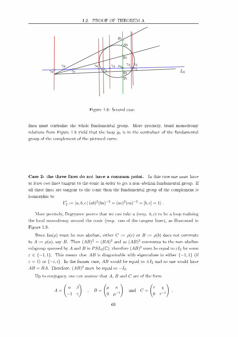
1.2. PROOF OF THEOREM A
L0γ1γ2γ3x0γ4
γ5γ6
γ7
γ8γ9
g1
g2
g3
g4
g5
Figure 1.8: Se ond ase.
lines must entralise the whole fundamental group. More pre isely, braid monodromy
relations from Figure 1.8 yield that the loop g3 is in the entraliser of the fundamental
group of the omplement of the pi tured urve.
Case 2: the three lines do not have a ommon point. In this ase one must have
at least two lines tangent to the oni in order to get a nonabelian fundamental group. If
all three lines are tangent to the oni then the fundamental group of the omplement is
isomorphi to
Γ′2 := 〈a, b, c | (ab)2(ba)−2 = (ac)2(ca)−2 = [b, c] = 1〉 .
More pre isely, Degtyarev proves that we an take a (resp. b, c) to be a loop realising
the lo al monodromy around the oni (resp. two of the tangent lines), as illustrated in
Figure 1.9.
Sin e Im(ρ) must be nonabelian, either C := ρ(c) or B := ρ(b) does not ommute
to A := ρ(a), say B. Then (AB)2 = (BA)2 and so (AB)2 ommutes to the nonabelian
subgroup spanned by A and B in PSL2(C), therefore (AB)2 must be equal to εI2 for some
ε ∈ −1, 1. This means that AB is diagonisable with eigenvalues in either −1, 1 (if
ε = 1) or −i, i. In the former ase, AB would be equal to ±I2 and so one would have
AB = BA. Therefore, (AB)2 must be equal to −I2.Up to onjuga y, one an assume that A, B and C are of the form
A =
(
α β
−1 γ
)
, B =
(
µ κ
0 µ−1
)
and C =
(
τ χ
0 τ−1
)
.
69
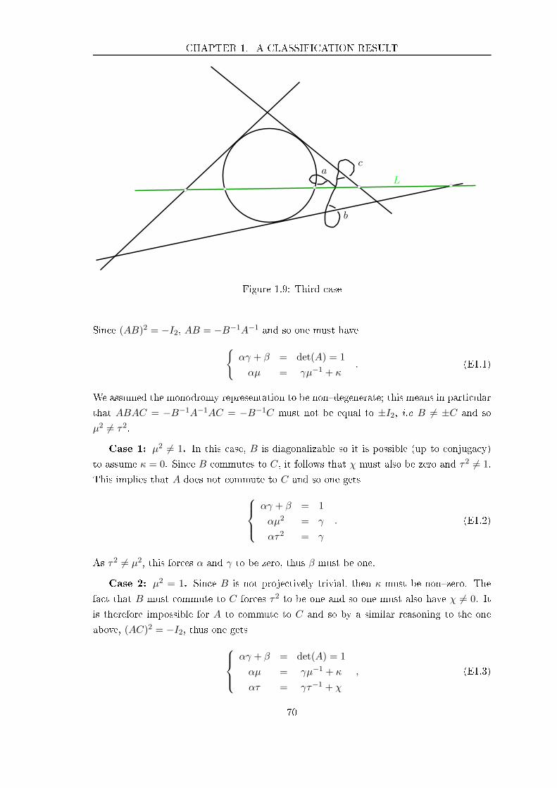
CHAPTER 1. A CLASSIFICATION RESULT
Lbcbcbcbc
a
b
c
bc
Figure 1.9: Third ase
Sin e (AB)2 = −I2, AB = −B−1A−1and so one must have
αγ + β = det(A) = 1
αµ = γµ−1 + κ. (E1.1)
We assumed the monodromy representation to be nondegenerate; this means in parti ular
that ABAC = −B−1A−1AC = −B−1C must not be equal to ±I2, i.e B 6= ±C and so
µ2 6= τ2.
Case 1: µ2 6= 1. In this ase, B is diagonalizable so it is possible (up to onjuga y)
to assume κ = 0. Sin e B ommutes to C, it follows that χ must also be zero and τ2 6= 1.
This implies that A does not ommute to C and so one gets
αγ + β = 1
αµ2 = γ
ατ2 = γ
. (E1.2)
As τ2 6= µ2, this for es α and γ to be zero, thus β must be one.
Case 2: µ2 = 1. Sin e B is not proje tively trivial, then κ must be nonzero. The
fa t that B must ommute to C for es τ2 to be one and so one must also have χ 6= 0. It
is therefore impossible for A to ommute to C and so by a similar reasoning to the one
above, (AC)2 = −I2, thus one gets
αγ + β = det(A) = 1
αµ = γµ−1 + κ
ατ = γτ−1 + χ
, (E1.3)
70

1.2. PROOF OF THEOREM A
γ1 L0
γ2γ3γ4
γ5x0γ6γ7γ8
γ9
g2
g3
g1
g4
g5
Figure 1.10: Fourth ase.
whi h is equivalent to (sin e µ2 = τ2 = 1)
αγ + β = det(A) = 1
α = γ + κµ
α = γ + χτ
, (E1.4)
therefore κµ = χτ . This means that B = ±C and so ABAC = ±I2, whi h ontradi ts
onditions (C1) and (C2).
In the end, the only (up to onjuga y) family of representations of Γ into PSL2(C)
satisfying onditions (C1) and (C2) is as follows:
ρu,v : a 7→(
0 1
−1 0
)
, b 7→(
u 0
0 u−1
)
, c 7→(
v 0
0 v−1
)
, for u, v ∈ C∗ .
This is the rst ase in Theorem A.
Otherwise, it is on e again a onsequen e of braid monodromy relations that the lo al
monodromy about any line not tangent to the oni must ommute to every loop in the
fundamental group (see Figure 1.10), thus we an dis ard this type of urve as well.
71

CHAPTER 1. A CLASSIFICATION RESULT
72
Chapter 2
Monodromy representations and
mapping lass group orbits
We saw in Chapter 1 that there are at most four families of "interesting" representations of
fundamental group of omplement of quinti s into PSL2(C). The aim of this hapter is to
explain how one an use this to obtain isomonodromi deformations of the ve pun tured
sphere and to des ribe the asso iated mapping lass group orbits.
2.1 Restri ting a plane onne tion to generi lines
2.1.1 General method
Let ∇ be a rank two logarithmi at sl2(C) onne tion over P2(C) whose polar lo us is
exa tly some quinti plane urve Q ⊂ P2(C) and let ρ : π1(P2(C) \ Q) → SL2(C) be its
monodromy representation. Assume that the representation ρ is nondegenerate in the
following sense.
Denition 2.1.1. We say that the monodromy representation asso iated with a rank two
logarithmi at sl2(C) onne tion over P2 −Q is nondegenerate if
• its image forms an irredu ible subgroup of SL2(C) ;
• its lo al monodromy around any irredu ible omponent of Q is proje tively nontrivial
(i.e is non-trivial in PSL2(C)).
If the representation ρ fa tors through an orbi urve, then it is a known fa t [15, 43
that ρ an be obtained as the monodromy of the pullba k of some logarithmi at on-
ne tion over a urve. Isomonodromi deformations of pun tured spheres arising from su h
onstru tions have been extensively studied by Diarra [24, 25, so let us assume that ρ
does not fa tor through an orbi urve. Therefore, it follows from Theorem A that the pair
(π1(P2(C) \ Q), P ρ) (where P : SL2(C) → PSL2(C) is the anoni al proje tion) must
be one of the following:
73
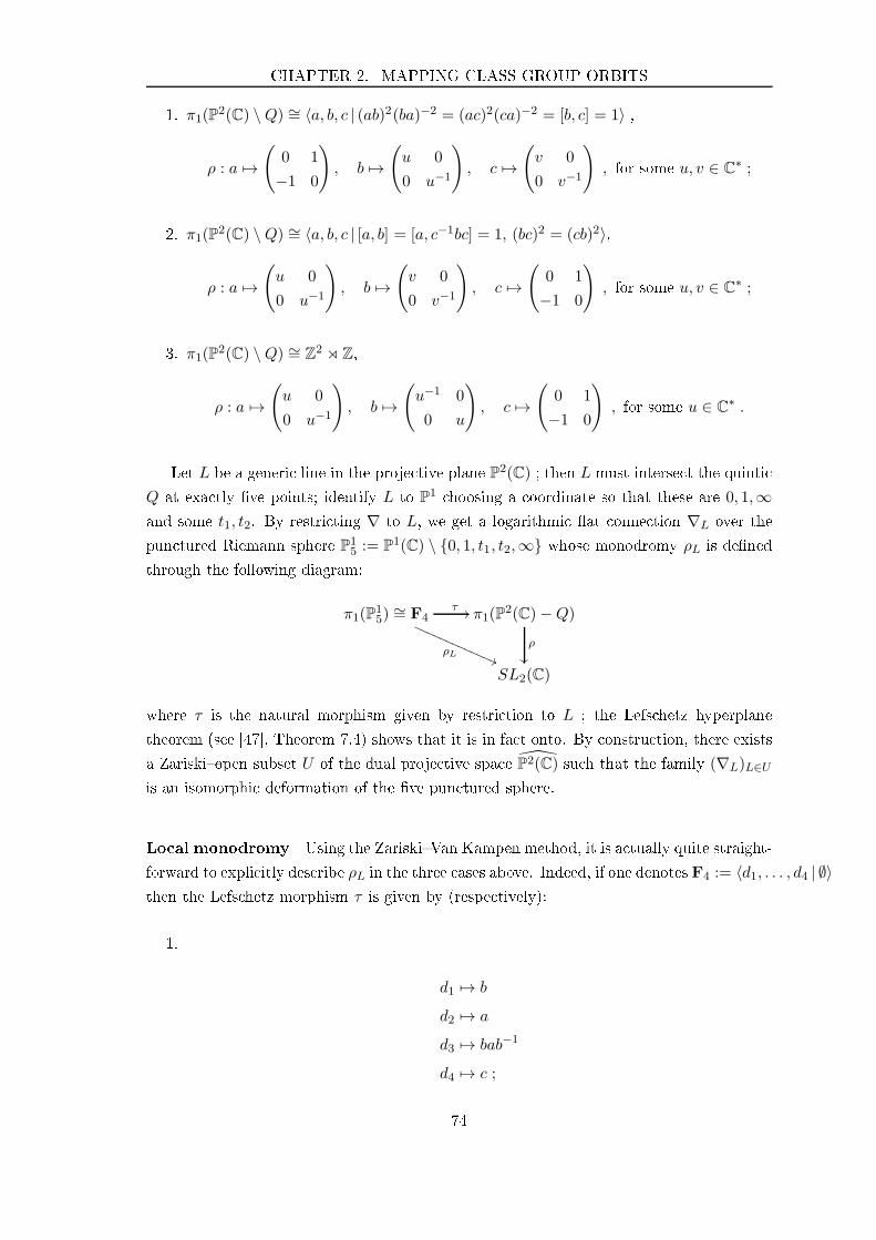
CHAPTER 2. MAPPING CLASS GROUP ORBITS
1. π1(P2(C) \Q) ∼= 〈a, b, c | (ab)2(ba)−2 = (ac)2(ca)−2 = [b, c] = 1〉 ,
ρ : a 7→(
0 1
−1 0
)
, b 7→(
u 0
0 u−1
)
, c 7→(
v 0
0 v−1
)
, for some u, v ∈ C∗ ;
2. π1(P2(C) \Q) ∼= 〈a, b, c | [a, b] = [a, c−1bc] = 1, (bc)2 = (cb)2〉,
ρ : a 7→(
u 0
0 u−1
)
, b 7→(
v 0
0 v−1
)
, c 7→(
0 1
−1 0
)
, for some u, v ∈ C∗ ;
3. π1(P2(C) \Q) ∼= Z2 ⋊Z,
ρ : a 7→(
u 0
0 u−1
)
, b 7→(
u−1 0
0 u
)
, c 7→(
0 1
−1 0
)
, for some u ∈ C∗ .
Let L be a generi line in the proje tive plane P2(C) ; then L must interse t the quinti
Q at exa tly ve points; identify L to P1 hoosing a oordinate so that these are 0, 1,∞
and some t1, t2. By restri ting ∇ to L, we get a logarithmi at onne tion ∇L over the
pun tured Riemann sphere P15 := P1(C) \ 0, 1, t1, t2,∞ whose monodromy ρL is dened
through the following diagram:
π1(P15)
∼= F4
ρL((
τ // π1(P2(C)−Q)
ρ
SL2(C)
where τ is the natural morphism given by restri tion to L ; the Lefs hetz hyperplane
theorem (see [47, Theorem 7.4) shows that it is in fa t onto. By onstru tion, there exists
a Zariskiopen subset U of the dual proje tive spa e P2(C) su h that the family (∇L)L∈Uis an isomorphi deformation of the ve pun tured sphere.
Lo al monodromy Using the ZariskiVan Kampen method, it is a tually quite straight-
forward to expli itly des ribe ρL in the three ases above. Indeed, if one denotes F4 := 〈d1, . . . , d4 | ∅〉then the Lefs hetz morphism τ is given by (respe tively):
1.
d1 7→ b
d2 7→ a
d3 7→ bab−1
d4 7→ c ;
74
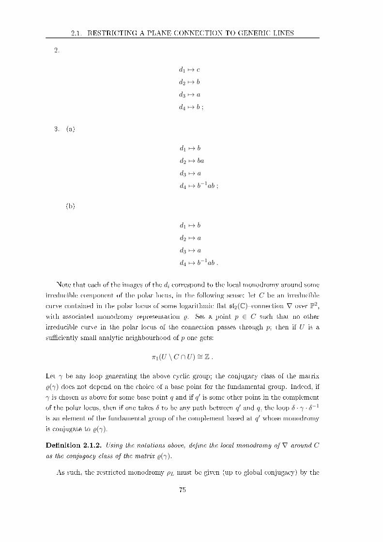
2.1. RESTRICTING A PLANE CONNECTION TO GENERIC LINES
2.
d1 7→ c
d2 7→ b
d3 7→ a
d4 7→ b ;
3. (a)
d1 7→ b
d2 7→ ba
d3 7→ a
d4 7→ b−1ab ;
(b)
d1 7→ b
d2 7→ a
d3 7→ a
d4 7→ b−1ab .
Note that ea h of the images of the di orrespond to the lo al monodromy around some
irredu ible omponent of the polar lo us, in the following sense: let C be an irredu ible
urve ontained in the polar lo us of some logarithmi at sl2(C) onne tion ∇ over P2,
with asso iated monodromy representation . Set a point p ∈ C su h that no other
irredu ible urve in the polar lo us of the onne tion passes through p; then if U is a
su iently small analyti neighbourhood of p one gets:
π1(U \ C ∩ U) ∼= Z .
Let γ be any loop generating the above y li group; the onjuga y lass of the matrix
(γ) does not depend on the hoi e of a base point for the fundamental group. Indeed, if
γ is hosen as above for some base point q and if q′ is some other point in the omplement
of the polar lo us, then if one takes δ to be any path between q′ and q, the loop δ · γ · δ−1
is an element of the fundamental group of the omplement based at q′ whose monodromy
is onjugate to (γ).
Denition 2.1.2. Using the notations above, dene the lo al monodromy of ∇ around C
as the onjuga y lass of the matrix (γ).
As su h, the restri ted monodromy ρL must be given (up to global onjuga y) by the
75
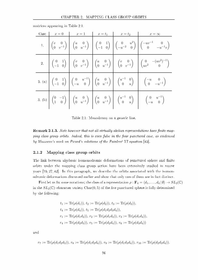
CHAPTER 2. MAPPING CLASS GROUP ORBITS
matri es appearing in Table 2.1.
Case x = 0 x = 1 x = t1 x = t2 x = ∞
1.
(v 00 v−1
) (u 00 u−1
) (0 1−1 0
) (0 u2
−u−2 0
) (−uv−1 0
0 −u−1v
)
2.
(0 1−1 0
) (v 00 v−1
) (u 00 u−1
) (v 00 v−1
) (0 −(uv2)−1
uv2 0
)
3. (a)
(0 1−1 0
) (0 u−1
−u 0
) (u 00 u−1
) (u−1 00 u
) (−u 00 −u−1
)
3. (b)
(0 −11 0
) (u 00 u−1
) (u 00 u−1
) (u−1 00 u
) (0 u−1
−u 0
)
Table 2.1: Monodromy on a generi line.
Remark 2.1.3. Note however that not all virtually abelian representations have nite map-
ping lass group orbits. Indeed, this is even false in the four pun tured ase, as eviden ed
by Mazzo o's work on Pi ard's solutions of the Painlevé VI equation [45.
2.1.2 Mapping lass group orbits
The link between algebrai isomonodromi deformations of pun tured sphere and nite
orbits under the mapping lass group a tion have been extensively studied in re ent
years [16, 27, 42. In this paragraph, we des ribe the orbits asso iated with the isomon-
odromi deformations dis ussed earlier and show that only two of them are in fa t distin t.
First let us x some notations; the lass of a representation ρ : F4 = 〈d1, . . . , d4 | ∅〉 → SL2(C)
in the SL2(C) hara ter variety Char(0, 5) of the ve pun tured sphere is fully determined
by the following:
t1 := Tr(ρ(d1)), t2 := Tr(ρ(d2)), t3 := Tr(ρ(d3)),
t4 := Tr(ρ(d4)), t5 := Tr(ρ(d1d2d3d4)),
r1 := Tr(ρ(d1d2)), r2 := Tr(ρ(d1d3)), r3 := Tr(ρ(d1d4)),
r4 := Tr(ρ(d2d3)), r5 := Tr(ρ(d2d4)), r6 := Tr(ρ(d3d4))
and
r7 := Tr(ρ(d1d2d3)), r8 := Tr(ρ(d1d2d4)), r9 := Tr(ρ(d1d3d4)), r10 := Tr(ρ(d2d3d4)).
76
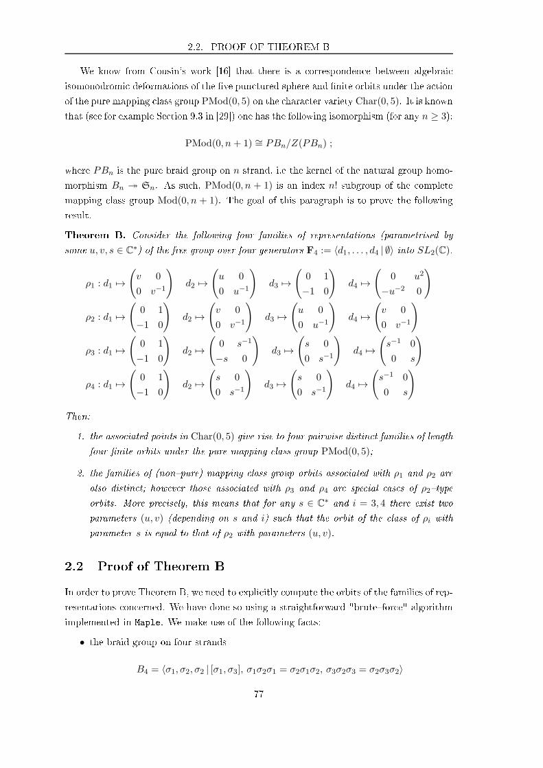
2.2. PROOF OF THEOREM B
We know from Cousin's work [16 that there is a orresponden e between algebrai
isomonodromi deformations of the ve pun tured sphere and nite orbits under the a tion
of the pure mapping lass group PMod(0, 5) on the hara ter variety Char(0, 5). It is known
that (see for example Se tion 9.3 in [29) one has the following isomorphism (for any n ≥ 3):
PMod(0, n + 1) ∼= PBn/Z(PBn) ;
where PBn is the pure braid group on n strand, i.e the kernel of the natural group homo-
morphism Bn ։ Sn. As su h, PMod(0, n + 1) is an index n! subgroup of the omplete
mapping lass group Mod(0, n + 1). The goal of this paragraph is to prove the following
result.
Theorem B. Consider the following four families of representations (parametrised by
some u, v, s ∈ C∗) of the free group over four generators F4 := 〈d1, . . . , d4 | ∅〉 into SL2(C).
ρ1 : d1 7→(
v 0
0 v−1
)
d2 7→(
u 0
0 u−1
)
d3 7→(
0 1
−1 0
)
d4 7→(
0 u2
−u−2 0
)
ρ2 : d1 7→(
0 1
−1 0
)
d2 7→(
v 0
0 v−1
)
d3 7→(
u 0
0 u−1
)
d4 7→(
v 0
0 v−1
)
ρ3 : d1 7→(
0 1
−1 0
)
d2 7→(
0 s−1
−s 0
)
d3 7→(
s 0
0 s−1
)
d4 7→(
s−1 0
0 s
)
ρ4 : d1 7→(
0 1
−1 0
)
d2 7→(
s 0
0 s−1
)
d3 7→(
s 0
0 s−1
)
d4 7→(
s−1 0
0 s
)
Then:
1. the asso iated points in Char(0, 5) give rise to four pairwise distin t families of length
four nite orbits under the pure mapping lass group PMod(0, 5);
2. the families of (nonpure) mapping lass group orbits asso iated with ρ1 and ρ2 are
also distin t; however those asso iated with ρ3 and ρ4 are spe ial ases of ρ2type
orbits. More pre isely, this means that for any s ∈ C∗and i = 3, 4 there exist two
parameters (u, v) (depending on s and i) su h that the orbit of the lass of ρi with
parameter s is equal to that of ρ2 with parameters (u, v).
2.2 Proof of Theorem B
In order to prove Theorem B, we need to expli itly ompute the orbits of the families of rep-
resentations on erned. We have done so using a straightforward "brutefor e" algorithm
implemented in Maple. We make use of the following fa ts:
• the braid group on four strands
B4 = 〈σ1, σ2, σ2 | [σ1, σ3], σ1σ2σ1 = σ2σ1σ2, σ3σ2σ3 = σ2σ3σ2〉
77

CHAPTER 2. MAPPING CLASS GROUP ORBITS
a ts on the hara ter variety Char(0, 5) as follows: the braid σi sends the lass of
some representation ρ : F4 → SL2(C) to that of the representation ρσi dened by:
ρσi : dj 7→
ρ(di)ρ(di+1)ρ(di)−1
if j = i
ρ(di) if j = i+ 1
ρ(dj) else
.
• The pure braid group PB4 is generated by the following braids, for 1 ≤ i < j ≤ 3:
σi,j := (σj . . . σi+1)σi(σj . . . σi+1)−1 ;
• the entre of the pure braid group on four strand is generated by the squared funda-
mental braid
∆2 := (σ3σ2σ1σ2σ1σ1)2 .
It is quite straightforward to see that ∆2a ts on a representation ρ as the onjuga y
by ρ(d1)ρ(d2)ρ(d3)ρ(d4) and thus a ts trivially on Char(0, 5). Therefore the orbit of
the lass of ρ under the a tion of PMod(0, 5) is the same as its orbit under that of
PB4.
We will now look in turn at the two on lusions of Theorem B by omputing the
asso iated orbits and using this data to rea h the desired on lusion.
2.2.1 Orbits under the pure mapping lass group
It follows from the remarks we made at the beginning of the proof that one only needs
to ompute the orbit of the lasses of the representations [ρi] under the pure braid group
on four strand; whi h we a hieve by using the "brutefor e" algorithms written down in
Appendix A.
In the oordinates (t | r) des ribed earlier, the orbits of the lasses of the representationsρ1, . . . , ρ4 under the a tion of PMod(0, 5) are as follows:
[ρ1
(a)
(1 + v2
v,1 + u2
u, 0, 0,−u
2 + v2
uv
∣∣∣∣
1 + u2v2
uv, 0, 0, 0, 0,−1 + u4
u2, 0, 0,−u
4 + v2
u2v,−1 + u2
u
)
(b)
(1 + v2
v,1 + u2
u, 0, 0,−u
2 + v2
uv
∣∣∣∣
u2 + v2
uv, 0, 0, 0, 0,−u
4 + v4
u2v2, 0, 0,−u
4 + v2
u2v,−u
2 + v4
uv2
)
( )
(1 + v2
v,1 + u2
u, 0, 0,−u
2 + v2
uv
∣∣∣∣
u2 + v2
uv, 0, 0, 0, 0,−2, 0, 0,−1 + v2
v,−1 + u2
u
)
(d)
(1 + v2
v,1 + u2
u, 0, 0,
u2 + v2
uv
∣∣∣∣
1 + u2v2
uv, 0, 0, 0, 0,−1 + v4
v2, 0, 0,−1 + v2
v,−u
2 + v4
uv2
)
[ρ2
78
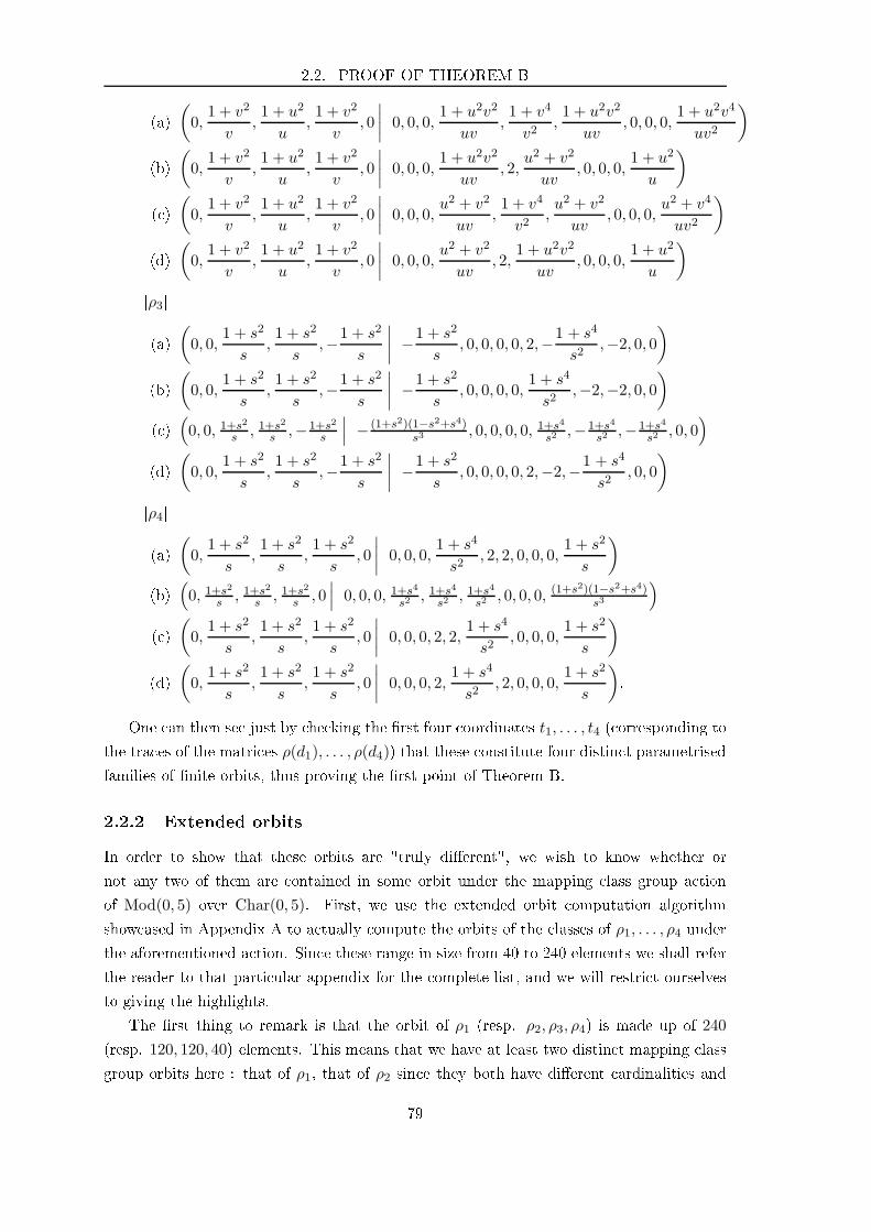
2.2. PROOF OF THEOREM B
(a)
(
0,1 + v2
v,1 + u2
u,1 + v2
v, 0
∣∣∣∣0, 0, 0,
1 + u2v2
uv,1 + v4
v2,1 + u2v2
uv, 0, 0, 0,
1 + u2v4
uv2
)
(b)
(
0,1 + v2
v,1 + u2
u,1 + v2
v, 0
∣∣∣∣0, 0, 0,
1 + u2v2
uv, 2,
u2 + v2
uv, 0, 0, 0,
1 + u2
u
)
( )
(
0,1 + v2
v,1 + u2
u,1 + v2
v, 0
∣∣∣∣0, 0, 0,
u2 + v2
uv,1 + v4
v2,u2 + v2
uv, 0, 0, 0,
u2 + v4
uv2
)
(d)
(
0,1 + v2
v,1 + u2
u,1 + v2
v, 0
∣∣∣∣0, 0, 0,
u2 + v2
uv, 2,
1 + u2v2
uv, 0, 0, 0,
1 + u2
u
)
[ρ3
(a)
(
0, 0,1 + s2
s,1 + s2
s,−1 + s2
s
∣∣∣∣−1 + s2
s, 0, 0, 0, 0, 2,−1 + s4
s2,−2, 0, 0
)
(b)
(
0, 0,1 + s2
s,1 + s2
s,−1 + s2
s
∣∣∣∣−1 + s2
s, 0, 0, 0, 0,
1 + s4
s2,−2,−2, 0, 0
)
( )
(
0, 0, 1+s2
s, 1+s
2
s,−1+s2
s
∣∣∣ − (1+s2)(1−s2+s4)
s3, 0, 0, 0, 0, 1+s
4
s2,−1+s4
s2,−1+s4
s2, 0, 0
)
(d)
(
0, 0,1 + s2
s,1 + s2
s,−1 + s2
s
∣∣∣∣−1 + s2
s, 0, 0, 0, 0, 2,−2,−1 + s4
s2, 0, 0
)
[ρ4
(a)
(
0,1 + s2
s,1 + s2
s,1 + s2
s, 0
∣∣∣∣0, 0, 0,
1 + s4
s2, 2, 2, 0, 0, 0,
1 + s2
s
)
(b)
(
0, 1+s2
s, 1+s
2
s, 1+s
2
s, 0∣∣∣ 0, 0, 0, 1+s
4
s2, 1+s
4
s2, 1+s
4
s2, 0, 0, 0, (1+s
2)(1−s2+s4)s3
)
( )
(
0,1 + s2
s,1 + s2
s,1 + s2
s, 0
∣∣∣∣0, 0, 0, 2, 2,
1 + s4
s2, 0, 0, 0,
1 + s2
s
)
(d)
(
0,1 + s2
s,1 + s2
s,1 + s2
s, 0
∣∣∣∣0, 0, 0, 2,
1 + s4
s2, 2, 0, 0, 0,
1 + s2
s
)
.
One an then see just by he king the rst four oordinates t1, . . . , t4 ( orresponding to
the tra es of the matri es ρ(d1), . . . , ρ(d4)) that these onstitute four distin t parametrised
families of nite orbits, thus proving the rst point of Theorem B.
2.2.2 Extended orbits
In order to show that these orbits are "truly dierent", we wish to know whether or
not any two of them are ontained in some orbit under the mapping lass group a tion
of Mod(0, 5) over Char(0, 5). First, we use the extended orbit omputation algorithm
show ased in Appendix A to a tually ompute the orbits of the lasses of ρ1, . . . , ρ4 under
the aforementioned a tion. Sin e these range in size from 40 to 240 elements we shall refer
the reader to that parti ular appendix for the omplete list, and we will restri t ourselves
to giving the highlights.
The rst thing to remark is that the orbit of ρ1 (resp. ρ2, ρ3, ρ4) is made up of 240
(resp. 120, 120, 40) elements. This means that we have at least two distin t mapping lass
group orbits here : that of ρ1, that of ρ2 sin e they both have dierent ardinalities and
79
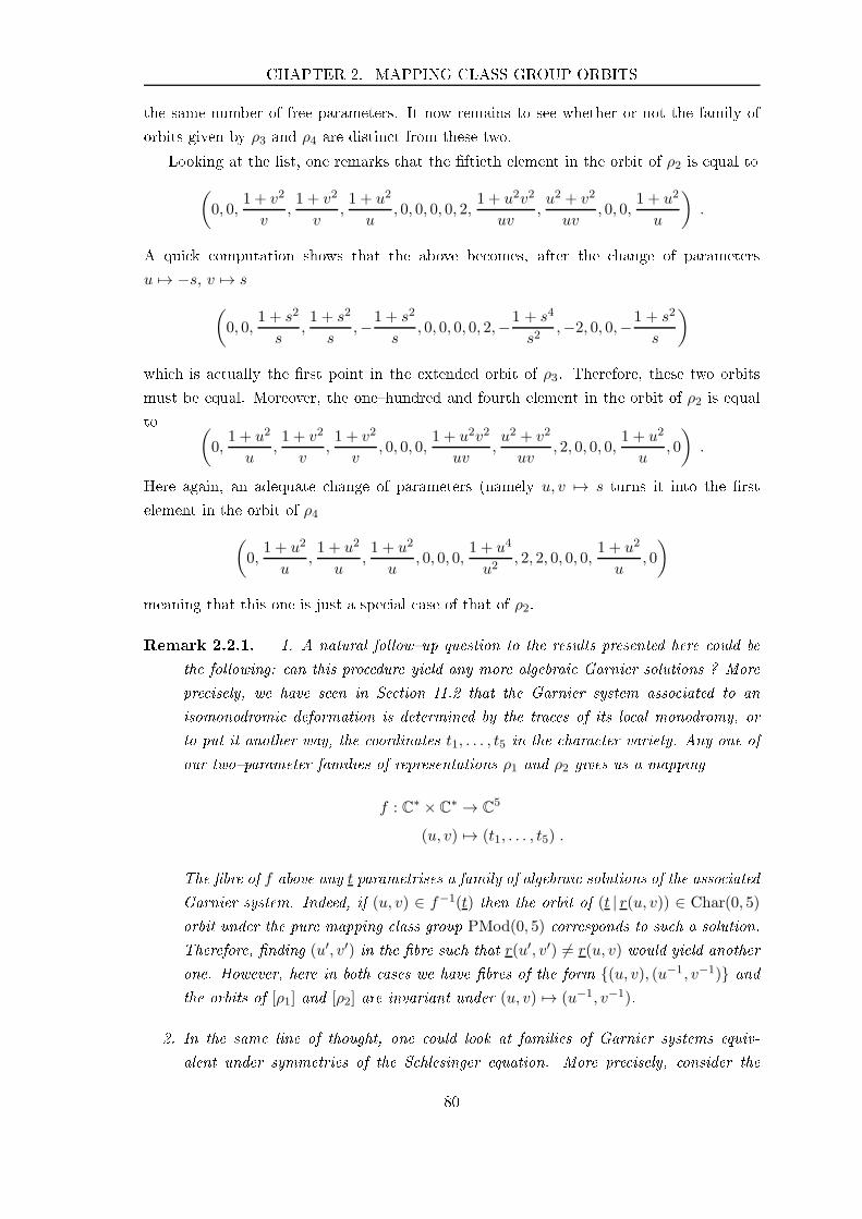
CHAPTER 2. MAPPING CLASS GROUP ORBITS
the same number of free parameters. It now remains to see whether or not the family of
orbits given by ρ3 and ρ4 are distin t from these two.
Looking at the list, one remarks that the ftieth element in the orbit of ρ2 is equal to
(
0, 0,1 + v2
v,1 + v2
v,1 + u2
u, 0, 0, 0, 0, 2,
1 + u2v2
uv,u2 + v2
uv, 0, 0,
1 + u2
u
)
.
A qui k omputation shows that the above be omes, after the hange of parameters
u 7→ −s, v 7→ s
(
0, 0,1 + s2
s,1 + s2
s,−1 + s2
s, 0, 0, 0, 0, 2,−1 + s4
s2,−2, 0, 0,−1 + s2
s
)
whi h is a tually the rst point in the extended orbit of ρ3. Therefore, these two orbits
must be equal. Moreover, the onehundred and fourth element in the orbit of ρ2 is equal
to (
0,1 + u2
u,1 + v2
v,1 + v2
v, 0, 0, 0,
1 + u2v2
uv,u2 + v2
uv, 2, 0, 0, 0,
1 + u2
u, 0
)
.
Here again, an adequate hange of parameters (namely u, v 7→ s turns it into the rst
element in the orbit of ρ4
(
0,1 + u2
u,1 + u2
u,1 + u2
u, 0, 0, 0,
1 + u4
u2, 2, 2, 0, 0, 0,
1 + u2
u, 0
)
meaning that this one is just a spe ial ase of that of ρ2.
Remark 2.2.1. 1. A natural followup question to the results presented here ould be
the following: an this pro edure yield any more algebrai Garnier solutions ? More
pre isely, we have seen in Se tion I1.2 that the Garnier system asso iated to an
isomonodromi deformation is determined by the tra es of its lo al monodromy, or
to put it another way, the oordinates t1, . . . , t5 in the hara ter variety. Any one of
our twoparameter families of representations ρ1 and ρ2 gives us a mapping
f : C∗ × C∗ → C5
(u, v) 7→ (t1, . . . , t5) .
The bre of f above any t parametrises a family of algebrai solutions of the asso iated
Garnier system. Indeed, if (u, v) ∈ f−1(t) then the orbit of (t | r(u, v)) ∈ Char(0, 5)
orbit under the pure mapping lass group PMod(0, 5) orresponds to su h a solution.
Therefore, nding (u′, v′) in the bre su h that r(u′, v′) 6= r(u, v) would yield another
one. However, here in both ases we have bres of the form (u, v), (u−1, v−1) and
the orbits of [ρ1] and [ρ2] are invariant under (u, v) 7→ (u−1, v−1).
2. In the same line of thought, one ould look at families of Garnier systems equiv-
alent under symmetries of the S hlesinger equation. More pre isely, onsider the
80
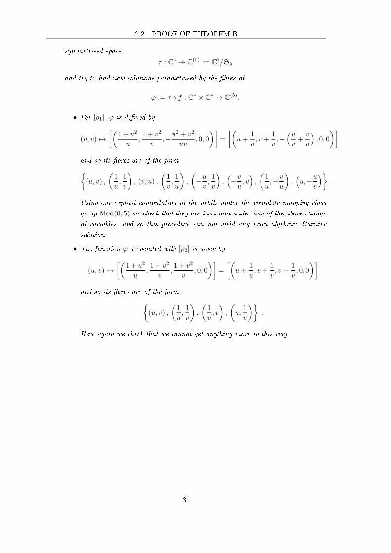
2.2. PROOF OF THEOREM B
symmetrised spa e
τ : C5։ C(5) := C5/S5
and try to nd new solutions parametrised by the bres of
ϕ := τ f : C∗ × C∗ → C(5).
• For [ρ1], ϕ is dened by
(u, v) 7→[(
1 + u2
u,1 + v2
v,−u
2 + v2
uv, 0, 0
)]
=
[(
u+1
u, v +
1
v,−(u
v+v
u
)
, 0, 0
)]
and so its bres are of the form
(u, v) ,
(1
u,1
v
)
, (v, u) ,
(1
v,1
u
)
,
(
−uv,1
v
)
,(
−vu, v)
,
(1
u,−v
u
)
,(
u,−uv
)
.
Using our expli it omputation of the orbits under the omplete mapping lass
group Mod(0, 5) we he k that they are invariant under any of the above hange
of variables, and so this pro edure an not yield any extra algebrai Garnier
solution.
• The fun tion ϕ asso iated with [ρ2] is given by
(u, v) 7→[(
1 + u2
u,1 + v2
v,1 + v2
v, 0, 0
)]
=
[(
u+1
u, v +
1
v, v +
1
v, 0, 0
)]
and so its bres are of the form
(u, v) ,
(1
u,1
v
)
,
(1
u, v
)
,
(
u,1
v
)
.
Here again we he k that we annot get anything more in this way.
81

CHAPTER 2. MAPPING CLASS GROUP ORBITS
82

Chapter 3
First family of solutions
In this hapter, we des ribe the main result of the paper [32, namely an expli it onstru -
tion of a twoparameter family of logarithmi at onne tions over the omplement of a
parti ular quinti urve in P2C. The restri tion of any element of this family to generi
lines in the proje tive plane gives a isomonodromi deformation over the ve pun tured
sphere, to whi h we an asso iate an algebrai solution of some Hamiltonian system of
partial dierential equations, namely the Garnier-2 system.
3.1 Setup and main results
3.1.1 Topology of the omplement of a parti ular plane quinti
We on ern ourselves with setting up a twoparameter family of logarithmi at sl2(C)
onne tions over P2with a spe i polar lo us, namely a quinti urve Q omposed of a
ir le and three tangent lines. More pre isely, in homogeneous oordinates [x : y : t], Q is
dened, up to PGL3(C) a tion, by the equation
xyt(x2 + y2 + t2 − 2(xy + xt+ yt)) = 0 .
Before stating our main result, let us spe ify what we are looking for: we want to nd
a family of rank two logarithmi at onne tions over P2with polar lo us equal to some
small degree urve and "interesting monodromy". We will show that it is possible to do
so with the quinti Q dened above.
Denition 3.1.1. We say that the monodromy representation asso iated with a rank two
logarithmi at sl2(C) onne tion over P2 −Q is nondegenerate if
• its image forms an irredu ible subgroup of SL2(C) ;
• its lo al monodromy around any irredu ible omponent of Q is proje tively nontrivial
(i.e is non-trivial in PSL2(C)).
83

CHAPTER 3. FIRST FAMILY OF SOLUTIONS
C
Lbcbcbcbc
a
b
c
bc
bc
bc
bc
bc
bc
L
d5
d3
d4
d1
d2
4 1
235
Figure 3.1: Fundamental group of the omplement of the quinti Q in P2and restri tion
to a generi line.
Note that if the proje tive monodromy of su h a onne tion satises the onditions
(C1) and (C2) introdu ed in Chapter 1 then it lifts to a nondegenerate representation.
However, the onverse does not hold, as we will show in Theorem D.
We know from Degtyarev's list that the fundamental group of the omplement of a
smooth oni and three tangent lines in P2is isomorphi to the following group
Γ2 := 〈a, b, c | (ab)2(ba)−2 = (ac)2(ca)−2 = [b, c] = 1〉 .
More pre isely, Degtyarev proves that we an take a (resp. b, c) to be a loop realising
the lo al monodromy around the oni C := (x2 + y2 + t2 − 2(xy+ xt+ yt) = 0) (resp. the
lines (y = 0), (x = 0)), as illustrated in the lefthand side of Figure 3.1. Also note that
the fundamental group of the interse tion of P2 −Q with any generi line is isomorphi to
the free group F4 := 〈d1, . . . , d5 | d1 . . . d5 = 1〉; the Lefs hetz hyperplane theorem (see [47,
Theorem 7.4) tells us that the natural morphism τ : F4 → Γ2 is onto. Moreover we know
from the expli it ZariskiVan Kampen method given in Subse tion 4.1 of [19 that the
group Γ2 an be omputed by taking the four free generators of the fundamental group
of the interse tion of P2 − Q with any generi line and adding some braid monodromy
relations. Thus, if we hose a line going through the base point used to dene a, b and c
then τ is given (up to a permutation of the di) by (see the righthand side of Figure 3.1):
d1 7→ b
d2 7→ a
d3 7→ bab−1
d4 7→ c
d5 7→ (abac)−1 .
84
3.1. SETUP AND MAIN RESULTS
In parti ular, any nondegenerate representation ρ of Γ2 must satisfy
ρ(a), ρ(b), ρ(c), ρ(abac) 6= ±I2 .
Proposition 3.1.2. The only (up to onjuga y) family of nondegenerate representations
of Γ2 into SL2(C) is as follows:
ρu,v : a 7→(
0 1
−1 0
)
, b 7→(
u 0
0 u−1
)
, c 7→(
v 0
0 v−1
)
, for u, v ∈ C∗ .
This result has already been proven in Chapter 1: indeed when we looked at represen-
tation of Γ satisfying onditions (C1) and (C2) we only used the fa t that any su h group
homomorphism must be nondegenerate in the sense of Denition 3.1.1.
Remark 3.1.3. This implies that any nondegenerate representation of Γ will have a "size-
able" kernel; indeed re all that we have a natural twofold ramied over π : P1×P1 2:1−−→ P2
ramifying over the diagonal ∆. This mapping yields a nonramied over π : X−D 2:1−−→ P2−Q,
where X := P1 × P1, and thus one gets that π1(X −D) embeds into π1(P
2 −Q) ∼= Γ as an
index two subgroup. If one denotes by P1n the n pun tured sphere, the proje tion on the line
(y = 0) gives a bration X −D → P13 with bre P1
4. As the universal over of P13 (namely
the hyperboli plane H2) is ontra tible, the homotopy exa t sequen e asso iated with this
bration yields:
0 = π2(P13) → π1(P
14) → π1(X −D) → π1(P
13) → 0 .
In parti ular, there is an inje tive morphism from π1(P14)
∼= F3, where Fr denotes the free
group over r generators, into π1(X −D); whi h in turn implies that the group Γ ontains
a non ommutative free group.
Moreover the orbifold fundamental group Γorbπ asso iated with the ramied over π also
ontains a free group; more pre isely if we dene
Γorbπ := 〈a, b, c | (ab)2(ba)−2 = (ac)2(ca)−2 = [b, c] = a2 = 1〉
then π indu es an embedding of the fundamental group of X minus six lines into Γorbπ , i.e
F2×F2 → Γorbπ . This is espe ially relevant sin e the proje tive representations Γ → PSL2(C)
asso iated with the monodromy of the onne tions we will des ribe in this paper fa tor
through this orbifold fundamental group.
3.1.2 Main results
The ore of this hapter will be devoted to proving the following theorem, in whi h we
expli itly onstru t the announ ed family of rank two logarithmi at onne tions.
85
CHAPTER 3. FIRST FAMILY OF SOLUTIONS
Theorem C. There exists an expli it twoparameter family ∇λ0,λ1 of logarithmi at on-
ne tions over the trivial rank two ve tor bundle C2×P2 → P2with the following properties:
(i) the polar lo us of ∇λ0,λ1 is equal to the quinti Q ∈ P2dened by the equation
xyt(x2 + y2 + t2 − 2(xy + xt+ yt)) = 0 ;
(ii) the monodromy of ∇λ0,λ1 is onjugated to ρu,v with u = −e−iπλ0 and v = e−iπλ1 . It is
a virtually abelian dihedral representation of the fundamental group Γ2 := π1(P2−Q)
into SL2(C) whose image is not Zariskidense.
The onne tion ∇λ0,λ1 is given in some (see Subse tion 3.2.1) ane hart C2x,y ⊂ P2
by:
∇λ0,λ1 = d− 1
2(x2 + y2 + 1− 2(xy + x+ y))(λ0A0 + λ1A1 +A2) ,
where
A0 :=
(
2(x − 1)ydx + (x2 + x(y − 2) − y + 1)x dy
y2(2x − y + 2)ydx + (2x2 + y(x − y + 3) − 2)x dy
y
−2y2dx + (x + y − 1)x2 dy
y−2(x − 1)ydx − (x2 + x(y − 2) − y + 1)x
dy
y
)
A1 :=
(
(x2 + (x − 1)(y − 1))y dx
x+ 2(x − 1)xdy (x2 + y(x − y + 3) − 2)y dx
x+ 2(2x − y + 2)xdy
−(x + y − 1)y2 dx
x− 2x2dy −(x2 + (x − 1)(y − 1))y dx
x− 2(x − 1)xdy
)
A2 :=
(
−(x + y + 1)ydx − (x2 − x(y + 2) − y + 1)x dy
y−2(x − y + 3)ydx − (x2 − 2y(x + 1) + 1)x dy
y
0 (x + y + 1)ydx + (x2 − x(y + 2) − y + 1)x dy
y
)
.
Remark 3.1.4. Note that the existen e, and uniqueness up to gauge transformation, of
su h a family of onne tions follows from Proposition 3.1.2 and the lassi al Riemann
Hilbert orresponden e. The original part of this work resides in the fa t that we give
a onstru tive proof of this result; in parti ular this allows us to des ribe the asso iated
algebrai Garnier solution.
Sin e P2is the symmetri produ t Sym2(P1) one has a natural twofold ramied over
π : P1 × P1 2:1−−→ P2whi h pulls the quinti Q ba k onto the subset D ⊂ X := P1 × P1
omposed of the six lines u0, u1 = 0, 1,∞ (for some pair (u0, u1) of proje tive oordinates
on X) and of the diagonal ∆ while ramifying over the latter (see Subse tion 3.2.1 for more
details). As we are aiming at dihedral monodromy, a natural idea to prove Theorem C is
to dene a family of rank one logarithmi at onne tions over X with innite monodromy
around D \ ∆ and to push it forward using π to get a family of su h onne tions over
P2−Q with monodromy of (generi ally) innite order around the three lines in the quinti
and of proje tive order two at the oni C. This is exa tly what we will do in Se tion 3.2.
We also prove that this family of representations generi ally satises ondition (C2);
more pre isely we have the following result.
Theorem D. The monodromy representation of the onne tions ∇λ0,λ1 introdu ed in The-
orem C fa tors through an orbi urve if and only if there exists (p, q) ∈ Z2 \ (0, 0) su h
that pλ0 + qλ1 = 0, i.e if and only if [λ0 : λ1] ∈ P1Q.
86

3.1. SETUP AND MAIN RESULTS
3.1.3 Isomonodromi deformations
By restri tion to generi lines in P2, we obtain a family (parametrised by (λ0, λ1)) of
isomonodromi deformations over the Riemann sphere with ve pairwise distin t pun tures
P1x \ 0, 1, t1, t2,∞, whose monodromy is given in Table 3.1, where x is a well hosen
proje tive oordinate on P1and t1, t2 are two independent variables (well dened up to
double over) orresponding to the interse tion of the line with the oni C. Sin e this
family of onne tions is algebrai we get a twoparameter family of algebrai solutions
of the isomonodromy equation asso iated with su h deformations, namely the following
Garnier system:
∂tkpi = −∂qiHk
∂tkqi = ∂piHk
i, j = 1, 2 , (E3.1)
where (pi, qi)i are algebrai fun tions of t1, t2 and H1,H2 are expli it Hamiltonians given
in Proposition 3.3.3 (see also [24,46). More pre isely if one sets Sq := q1 + q2, Pq := q1q2,
St := t1 + t2 and Pt := t1t2 one has the following relations:
(λ0 − 1)2λ21St = −F (Sq, Pq)(λ0 − 1)2Pt = −(λ0 + λ1 − 1)2P 2
q
; (E3.2)
where:
F (Sq, Pq) =(λ0 − λ1 − 1)(λ0 + λ1 − 1)3P 2q
+ (λ0 − 1)2(λ0 + λ1 − 1)2(2Pq − 2PqSq + S2q − 2Sq)
+ (λ0 − 1)3(λ0 + 2λ1 − 1) .
These solutions generalise the two parameter family known for the Painlevé VI equation
(see Subse tion 3.3.1) and the omplex surfa e asso iated with the graph of (t1, t2) 7→ (Sq, Pq)
is rational.
x = 0 x = 1 x = t1 x = t2 x = ∞(a1 0
0 a−11
) (−a0 0
0 −a−10
) (0 1−1 0
) (0 a20
−a−20 0
) (a0a
−11 0
0 a−10 a1
)
Table 3.1: Monodromy on a generi line; here aj = exp(−iπλj) for j ∈ 0, 1.
87

CHAPTER 3. FIRST FAMILY OF SOLUTIONS
3.1.4 LotkaVolterra foliations
One last fa t worth noting is that sin e ∇ is a at sl2(C) onne tion on a trivial bundle,
there exist three meromorphi oneforms α0, α1 and α2 (given in Theorem C) su h that
∇ = d + Ω , where Ω :=
(
α1 α0
−α2 −α1
)
satises dΩ = Ω ∧ Ω .
In parti ular, sin e dα2∧α2 = 0 one obtains a family of transversally proje tive degree two
foliations over P2(see [43 and Se tion 3.4; note that this family is therefore integrable in
the CasaleMalgrange sense [12) with invariant lo us ontaining the quinti Q. We show
that these are onjugate to a family of Lotka-Volterra foliations over C3[48, 49; namely
given three omplex parameters (A,B,C), the odimension one foliation asso iated with
the oneform over C3, with oordinates (x, y, t):
ω0 := (yVt − tVy)dx+ (tVx − xVt)dy + (xVy − yVx)dt ,
where:
Vx := x(Cy + t), Vy := y(At+ x) and V t := t(Bx+ y) .
Theorem E. The foliation dened by the meromorphi oneform α2 is equal to the folia-
tion over P2asso iated with a LotkaVolterra system with parameters
(A,B,C) =
(λ1λ0,
−λ0λ0 + λ1
,−(λ0 + λ1)
λ1
)
.
Conversely, any degree two foliation whose invariant lo us ontains the quinti Q is equal
to one of the above form.
One an see from Theorem E that this family of foliations is governed by the parameter
λ0/λ1; there exists a oneparameter family of onne tions orresponding to any given
foliation (see also Subse tion 4.4 in [43). We then prove that this gives an example of a
family of foliations with algebrai invariant urves of arbitrarily high degree (see also [41).
3.2 Proof of Theorem C
In this se tion we on ern ourselves with setting up a parti ular bre bundle over the
proje tive plane P2, and then endowing it with a family of logarithmi at onne tions
satisfying the onditions of Theorem C.
88
3.2. PROOF OF THEOREM C
3.2.1 A rank two bre bundle
Start by onsidering the omplex manifold X := P1×P1and dene the following involution:
η : X → X
(u0, u1) 7→ (u1, u0) .
The a tion of η gives us a twofold ramied over of P1 × P1over the proje tive plane
P2, i.e the bres of the morphism
P1 × P1 −→ P2
([u00 : u10], [u
01 : u11]) 7→ [s : p : t] := [(u00u
11 + u10u
01) : u
00u
01 : u
10u
11] .
are the orbits under η. However, for the purpose of this hapter, we will ompose this
mapping with the linear proje tive transformation of P2given by:
[s : p : t] 7→ [p+ t− s : p : t] .
This means that we will now work in the homogeneous oordinates x := p + t− s, y := p
and t. We get a twofold ramied over π : X → P2that ramies along the diagonal
∆ := (u0 = u1) ⊂ X and sends it onto the oni :
(C) x2 + y2 + t2 = 2(xy + xt+ yt) .
Now onsider the rank two bre bundle E over the proje tive plane asso iated with
the lo ally free sheaf
E := OP2 ⊕OP2(−1) .
Let e+ be some global nonvanishing holomorphi se tion of E ( orresponding to the OP2
part of the above de omposition) and e− be some global meromorphi se tion linearly
independent from e+ (and so orresponding to OP2(−1)) with asso iated (zeroes and poles)
divisor equal to −L∞, where L∞ is the line "at innity" (t = 0).
Let us ask ourselves the following question: what does the pullba k sheaf F := π∗E look
like ? For any open set U ⊂ X we have F(U) = E(π(U)), whi h implies that F is a rank
two lo ally free sheaf indu ing a rank two bre bundle F → X with two global se tion: one
nonvanishing holomorphi e1 := π∗e+ and one meromorphi e2 := π∗e−. Sin e π does not
ramify over L0∞ := (u0 = ∞) nor L1
∞ := (u1 = ∞), e2 has asso iated divisor −(L0∞+L1
∞);
thus:
F ∼= OX ⊕OX(−1,−1) .
To better understand the bundle F , start by onsidering the rank two trivial bundle
E0 := C2×X → X over X; it has two independent ( onstant) holomorphi global se tions
89
CHAPTER 3. FIRST FAMILY OF SOLUTIONS
f1 ≡ (1, 0) and f2 ≡ (0, 1). Dene the following involution:
E0 → E0
(u0, u1, (Z1, Z2)e1,e2) 7→ (u1, u0, (Z1,−Z2)e1,e2) .
First of all, note that its a tion on the base oin ides with that of the involution η.
One an then identify two global invariant se tions of the bundle E0:
• f1, whi h is holomorphi ;
• f2 := b · f2, where b is the global meromorphi fun tion (u0, u1) 7→ u0 − u1.
The lo al expression b · f2 denes a global meromorphi se tion with asso iated divisor
∆− (L0∞ + L1
∞). The OXmodule spanned by the se tions f1 and f2 is isomorphi to the
rank two lo ally free module F (by mapping f1 to e1 and f2 to e2) and as su h denes a
rank two ve tor bundle over X isomorphi to F . More pre isely, one goes (lo ally) from
E0 to F using the following transformation (whi h is trivial on the base):
(
Z1
Z2
)
e1,e2
7→(
Z1
Z2u0−u1
)
e1,e2
.
3.2.2 A rank one proje tive bundle
By quotient on the bres (P(C2) = P1C), one an asso iate to both ve tor bundles E0 and
E rank one proje tive bundles P1 ×X and P(E). We an des ribe the a tion of η on the
former as follows:
η : P1 × P1 × P1 → P1 × P1 × P1
(u0, u1, [Z1 : Z2]) 7→ (u1, u0, [Z2 : Z1]) ;
or, in the ane hart "z = Z1Z2", (u0, u1, z) 7→ (u1, u0, 1/z).
One goes from P1 ×X to P(E) through the following invariant rational fun tions:
s = u0 + u1
p = u0u1
w := (u0 − u1)z + 1
z − 1
;
here (s, p) gives us lo al oordinates over the base and w does the same in the bres.
We will use this proje tive point of view throughout this hapter as it allows for easier
omputations in the long run. It will also allow us to dene an interesting family of
LotkaVolterra foliations in Se tion 3.4.
90
3.2. PROOF OF THEOREM C
3.2.3 Logarithmi at onne tions
Start by endowing the trivial rank two ve tor bundle E0 → X with the following logarith-
mi at onne tion :
∇0 := d +1
2
(
ω0 0
0 −ω0
)
,
where u0, u1 are proje tive oordinates on the base X and
ω0 := λ0
(du0u0
− du1u1
)
+ λ1
(du0u0 − 1
− du1u1 − 1
)
,
with (λ0, λ1) ∈ C2 \ (0, 0). This onne tion has singular lo us equal to six lines in X (if
λ0λ1(λ0 + λ1) 6= 0) and naturally gives rise to a Ri ati foliation, dened by the following
oneform over P(E0) = X × P1:
R(∇0) := dz + ω0z where z is a proje tive oordinate on the bres.
Moreover one easily he ks that
u0−u1z
R(∇0) is an ηinvariant logarithmi oneform
over P(F ), asso iated with some onne tion ∇1 in the following sense: if one has, in some
lo al hart
(u0 − u1)R(∇0) = dz + α2z2 + 2α1z + α0 ,
with α0, α1, α2 meromorphi oneforms (remark that here α2 and α0 are zero), then one
an set (in the same lo al hart)
∇1 := d +
(
α1 α0
−α2 −α1
)
.
Sin e the asso iated Ri ati form R(∇1) := (u0 − u1)R(∇0) is ηinvariant one an use ∇1
to get a logarithmi onne tion ∇2 on E with poles along (y = 0), (x = 0), L∞ and C,the latter oming from the fa t that π ramies there. More pre isely, in the ane hart
des ribed in Subse tion 3.2.2 one has:
R(∇2) = dw +1
2(x2 + y2 + 1− 2(xy + x+ y))
(
g(λ0, λ1, w, x, y)dx
x+ g(λ1, λ0, w, y, x)
dy
y
)
,
where
g(λ0, λ1, w, x, y) =− ((2λ0 + λ1)x+ λ1(y − 1))w2 + 2(y − x+ 1)xw
+ (2λ0 + λ1)x3 − ((4λ0 + λ1)(y + 1) + 2λ1)x
2
− ((−2λ0 + λ1)y2 + 2(2λ0 + λ1)y − (2λ0 + 3λ1))x
+ λ1(y3 − 3y2 + 3y − 1) .
91
CHAPTER 3. FIRST FAMILY OF SOLUTIONS
3.2.4 Trivialisations
We wish to turn ∇2 into a onne tion on the trivial bundle C2 × P2; this an be done
simply by blowing up the pole of any global meromorphi se tion of P(E) then ontra ting
a suitable divisor, however we want to do so without disturbing the logarithmi nature of
the onne tion ∇2.
Lemma 3.2.1. There exists a birational mapping Φ : P(E) → P1 × P2 onjugating R(∇2)
to some Ri ati oneform, that is asso iated with a logarithmi at onne tion ∇ over the
trivial bundle C2 × P2 → P2.
Proof. First remark that we have the following lo al expression along (y = 0):
R(∇2)|(y=0)= dw + f(x)(w + x− 1)(w − x+ 1)
dy
y.
This tells us that the odimension one foliation asso iated with the oneform R(∇2) has
two singular points on ea h bre above (y = 0), namely at w = ±(x− 1). So in order to
get a birationnal map P(E) → P1 × P2one an pro eed as follows:
• move one of the aforementioned singular lo i (e.g (w = x − 1) ∩ (y = 0)) at
(w = y = 0);
• blow up (y = 0)∩ (w = ∞) then ontra t the stri t transform of the bre at (y = 0)
on (w = y = 0). This latest step is a hieved (in our usual ane hart) through the
birational map (x, y, w) 7→ (x, y, w/y).
Expli itly in our lo al hart, the mapping Φ is given by
Φ(w, x, y) = (y(w − x+ 1), x, y) .
This means that we are blowing up (inside the total spa e) a line in ea h bre over (y = 0)
then ontra ting the stri t transforms of said bres thus resolving the singularities of the
global meromorphi se tion e− des ribed in the proof of Theorem C; this shows that
our mapping does indeed end in a trivial bundle and sin e we took are of ontra ting
divisors only on points of the singular lo us of the foliation asso iated with R(∇2) we get
a logarithmi at onne tion over C2 × P2 → P2.
In the end, one gets a onne tion ∇ = ∇λ0,λ1 on the trivial bundle C2×P2that almost
satises ondition (i) in Theorem C, the only thing left to he k being whether or not it
is a sl2(C) onne tion. Expli itly, the Ri ati form asso iated with ∇ is given by (in the
ane hart (t = 1)):
R(∇) = dw − 1
2(x2 + y2 + 1− 2(xy + x+ y))
(
f1(w, x, y)ydx
x− f2(w, x, y)
xdy
y
)
92
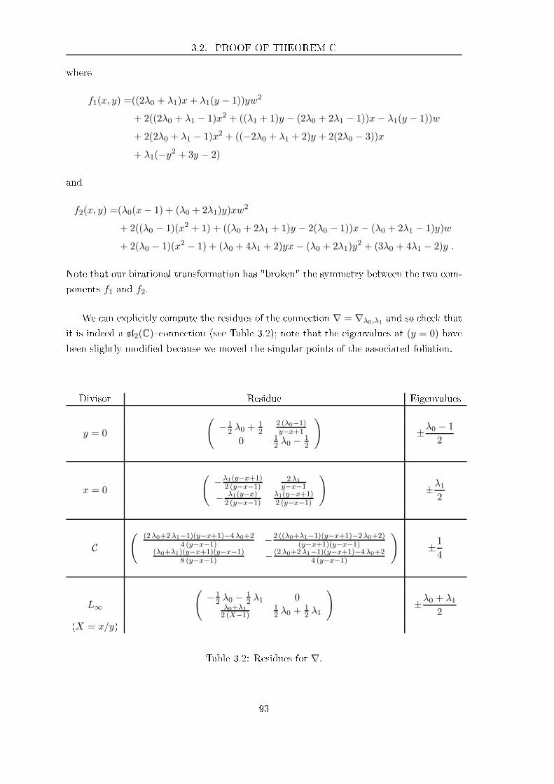
3.2. PROOF OF THEOREM C
where
f1(x, y) =((2λ0 + λ1)x+ λ1(y − 1))yw2
+ 2((2λ0 + λ1 − 1)x2 + ((λ1 + 1)y − (2λ0 + 2λ1 − 1))x− λ1(y − 1))w
+ 2(2λ0 + λ1 − 1)x2 + ((−2λ0 + λ1 + 2)y + 2(2λ0 − 3))x
+ λ1(−y2 + 3y − 2)
and
f2(x, y) =(λ0(x− 1) + (λ0 + 2λ1)y)xw2
+ 2((λ0 − 1)(x2 + 1) + ((λ0 + 2λ1 + 1)y − 2(λ0 − 1))x− (λ0 + 2λ1 − 1)y)w
+ 2(λ0 − 1)(x2 − 1) + (λ0 + 4λ1 + 2)yx− (λ0 + 2λ1)y2 + (3λ0 + 4λ1 − 2)y .
Note that our birational transformation has "broken" the symmetry between the two om-
ponents f1 and f2.
We an expli itly ompute the residues of the onne tion ∇ = ∇λ0,λ1 and so he k that
it is indeed a sl2(C) onne tion (see Table 3.2); note that the eigenvalues at (y = 0) have
been slightly modied be ause we moved the singular points of the asso iated foliation.
Divisor Residue Eigenvalues
y = 0
(
−12 λ0 +
12
2 (λ0−1)y−x+1
0 12 λ0 − 1
2
)
±λ0 − 1
2
x = 0
(
−λ1(y−x+1)2 (y−x−1)
2λ1y−x−1
− λ1(y−x)2 (y−x−1)
λ1(y−x+1)2 (y−x−1)
)
±λ12
C(
(2λ0+2λ1−1)(y−x+1)−4λ0+24 (y−x−1) −2 ((λ0+λ1−1)(y−x+1)−2λ0+2)
(y−x+1)(y−x−1)(λ0+λ1)(y−x+1)(y−x−1)
8 (y−x−1) − (2λ0+2λ1−1)(y−x+1)−4λ0+24 (y−x−1)
)
±1
4
L∞
(
−12 λ0 − 1
2 λ1 0λ0+λ12 (X−1)
12 λ0 +
12 λ1
)
±λ0 + λ12
(X = x/y)
Table 3.2: Residues for ∇.
93
CHAPTER 3. FIRST FAMILY OF SOLUTIONS
3.2.5 Monodromy representation
To on lude the proof of Theorem C one needs to ompute the monodromy representation
of the onne tion ∇ and see that it is, as announ ed, a dihedral representation of Γ2 into
SL2(C).
For j = 0, 1 set aj := e−iπλj ; the monodromy asso iated with the onne tion ∇0 is as
follows:
• around u0 = j (resp. u1 = j), j = 0, 1, it is the multipli ation by aj (resp. a−1j );
• around u0 = ∞ (resp. u1 = ∞), it is the multipli ation by a−10 a−1
1 (resp. a0a1).
This is a omplete des ription sin e the fundamental group of the proje tive line minus six
lines is isomorphi to F2 ×F2 and is generated by loops going around x, y = 0, 1 on e.
The monodromy of the onne tion ∇2 omes dire tly from that of ∇0 around the three
lines in its singular lo us; more pre isely we an expli itly ompute (up to onjuga y) its
lo al monodromy around:
• (y = 0):(
a0 0
0 a−10
)
;
• (x = 0):(
a1 0
0 a−11
)
;
• and L∞: (
(a0a1)−1 0
0 a0a1
)
.
However the monodromy of ∇2 around the oni C omes solely from the rami ation
of the over π. More pre isely sin e any path linking (u0, u1) ∈ X to (u1, u0) pushes
ba k as a loop on the quotient P2 = π(X) and sin e any lo al solution z of ∇0 satises
z(u1, u0) =1
z(u0, u1)the monodromy group of ∇2 must ontain the following matrix:
(
0 1
1 0
)
.
Proposition 3.2.2. The monodromy group of the onne tion ∇ is the subgroup of the
innite dihedral group
D∞ :=
(
0 α
−α−1 0
)
,
(
β 0
0 β−1
)∣∣∣∣∣α, β ∈ C∗
≤ SL2(C)
94
3.3. ALGEBRAIC GARNIER SOLUTIONS
generated by the following three matri es:
(
0 1
−1 0
)
,
(
−e−iπλ0 0
0 −eiπλ0
)
and
(
e−iπλ1 0
0 eiπλ1
)
.
Proof. We know from Degtyarev's list [19 that the fundamental group of the omplement
of the singular lo us of ∇ in P2has the following presentation:
Γ2 = 〈a, b, c | (ab)2(ba)−2 = (ac)2(ca)−2 = [b, c] = 1〉 ;
and that we an take a to be a loop whose lift is some path in X joining (x, y) and (y, x)
(for generi (x, y) ∈ X) and b (resp. c) to be a loop going around (y = 0) (resp. (x = 0))
on e (see Figure 3.1). If we hoose a set of lo al oordinates in whi h the monodromy
matri es of both b and c are diagonal (this is possible be ause the two loops ommute)
then the monodromy of a only omes from the over π and is equal to:
(
0 1
−1 0
)
.
In on lusion, the monodromy representation is given by the following matri es:
(
0 1
−1 0
)
,
(
−e−iπλ0 0
0 −eiπλ0
)
and
(
e−iπλ1 0
0 eiπλ1
)
,
whi h are elements of D∞.
3.3 Algebrai Garnier solutions
In this se tion we show that the onne tion ∇ indu es an isomonodromi deformation over
the four and ve pun tured spheres. Furthermore we give rational parametrisations of the
asso iated algebrai Painlevé VI and Garnier solutions and a des ription of the asso iated
monodromy representation.
3.3.1 Painlevé VI solutions
It is well known [34, 36 that isomonodromi deformations of rank two sl2(C) onne tions
over the four pun tured sphere orrespond to solutions of the sixth Painlevé equation,
95

CHAPTER 3. FIRST FAMILY OF SOLUTIONS
C
Figure 3.2: Spe ial lines.
namely the following order two nonlinear dierential equation:
d2q
du2=1
2
(1
q+
1
q − 1+
1
q − u
)(dq
du
)2
−(1
u+
1
u− 1+
1
q − u
)dq
du
+q(q − 1)(q − u)
u2(u− 1)2
(
α+ βu
q2+ γ
u− 1
(q − 1)2+ δ
u(u− 1)
(q − u)2
)
,
where α, β, γ and δ are omplexvalued parameters.
Let us look at the onne tion indu ed by ∇ on the family of lines going through
P0 := (x = 0) ∩L∞ (see Figure 3.2) that are neither (x = 0) nor the line at innity; these
are the lines of the form (y = c) in the ane hart (x, y) from Subse tion 3.2.1. A ording
to Subse tion 3.2.4, this orresponds to studying the isomonodromi deformation given by
the following Ri ati forms, for generi y:
R(∇y) := dw − y
2x(x2 + y2 + 1− 2(xy + x+ y))fy(x,w)dx ,
where
fy(x,w) =(λ0(x− 1) + (λ0 + 2λ1)y)yw2
+ 2((λ0 − 1)(x2 + 1) + ((λ0 + 2λ1 + 1)y − 2(λ0 − 1))x− (λ0 + 2λ1 − 1)y)w
+ 2(λ0 − 1)(x2 − 1) + (λ0 + 4λ1 + 2)yx− (λ0 + 2λ1)y2 + (3λ0 + 4λ1 − 2)y .
From this isomonodromi deformation we produ e algebrai solutions of the Painlevé VI
96

3.3. ALGEBRAIC GARNIER SOLUTIONS
Pole Residue Eigenvalues
x = 0 W0 :=
(
−λ1(z2+1)2 (z2−1)
2λ1z2−1
− λ1z2
2 (z2−1)λ1(z2+1)2 (z2−1)
)
±λ12
x = 1 W1 :=
((2λ0+2λ1−1)z+2λ0−1
4 (z+1)(λ0+λ1−1)z+λ0−1
z2+z
− (λ0+λ1)z2+λ0z4 (z+1) − (2 λ0+2λ1−1)z+2λ0−1
4 (z+1)
)
±1
4
x = t(z) W2 :=
((2λ0+2λ1−1)z−2λ0+1
4 (z−1) − (λ0+λ1−1)z−λ0+1z2−z
(λ0+λ1)z2−λ0z4 (z−1) − (2 λ0+2λ1−1)z−2λ0+1
4 (z−1)
)
±1
4
x = ∞ W :=
(−λ0 − 1
2 λ1 +12 0
0 λ0 +12 λ1 − 1
2
)
±2λ0 + λ1 − 1
2
Table 3.3: Residues for ∇y.
equation by adapting part of a paper by Hit hin [34.
Proposition 3.3.1. The family of algebrai solutions of the Painlevé VI equation asso i-
ated with the onne tions (∇λ0,λ1)λ0,λ1 is given by the fun tions
q(u) = − λ12λ0 + λ1
√u
and the parameters:
α =(2λ0 + λ1)
2
2, β = −λ
21
2, γ = 1/8 and δ = 3/8 .
Proof. Let z be a parameter su h that z2 = y; then ∇y has poles at x = (z ± 1)2, x = 0
and x = ∞. Up to Möbius transformation, one an assume that these are in fa t lo ated
at s ∈ 0, 1, u(z),∞, with:
u(z) =z2 − 2z + 1
z2 + 2z + 1=
(z − 1)2
(z + 1)2.
It is then possible to ompute the relevant data asso iated with this family of onne tions
(see Table 3.3).
Let us now set
H :=W0
x+
W1
x− 1+
W2
x− t,
where the Wi are the residues from Table 3.3; then sin e −W is diagonal and equal to the
97

CHAPTER 3. FIRST FAMILY OF SOLUTIONS
sum W0 +W1 +W2, its lower left oe ient is a degree one polynomial in x, whose root
an be expli itly omputed as a rational fun tion of z:
q(z) := − λ12λ0 + λ1
z − 1
z + 1,
or as an algebrai fun tion of u:
q(u) = − λ12λ0 + λ1
√u .
One an then he k that this fun tion u 7→ q(u) is indeed a solution of the sixth Painlevé
equation for the announ ed hoi e of parameters.
3.3.2 Restri tion to generi lines
Let us now onsider the onne tion indu ed by ∇ on generi lines in P2, su h a line being
given in our usual ane hart by an equation of the form y = αx + β. We thus obtain
an isomonodromi deformation (∇α,β)α,β over the ve pun tured sphere; more pre isely
if one hooses a parameter z su h that z2 = β(1 − α) + α then one gets (after Möbius
transformation) a family of logarithmi at onne tions over P1 \ 0, 1, t1, t2,∞, where:
t1 = − α(z + 1)2
(α− 1)(α − z2)and t2 = − α(z − 1)2
(α− 1)(α− z2).
The asso iated Ri ati forms are given by:
R(∇α,β) = dw +a2(x)w
2 + a1(x)w + a0(x)
2x(x− 1)(x− t1)(x− t2)dx
where:
a2(x)
α(x− 1)(z2 − α)=(λ0 + λ1)(α
2 − (z2 + 1)α + z2)x2
+ (−λ1α2 + (λ0(z2 + 1) + 2λ1)α− (2λ0 + λ1)z
2)x
+ λ1(z2 − 1)α
98

3.3. ALGEBRAIC GARNIER SOLUTIONS
a1(x)
2=(λ0 + λ1)(α
4 − 2(z2 + 1)α3 + (z4 + 4z2 + 1)α2 − 2(z4 + z2)α+ z4)x3
+ [−(2λ0 + 3λ1 − 1)α4
+ ((4λ0 + 4λ1 − 1)z2 + 4λ0 + 6λ1 − 1)α3
− ((2λ0 + λ1)z4 + 2(4λ0 + λ1 − 1)z2 + (2λ0 + 3λ1))α
2
+ ((4λ0 + 2λ1 − 1)z4 + (4λ0 + 4λ1 − 1)z2)α
− (2λ0 + λ1 + 1)z4]x2
+ [2λ1a4 − ((2λ0 − 1)z2 + (2λ0 + 6λ1 − 1))α3
+ ((λ0 − λ1)z4 + 2(3λ0 + 2λ1 − 1)z2 + λ0 + 3λ1)α
2
+ ((2λ0 − 1)z4 + (2λ0 + 2λ1 − 1)z2)α]x
+ λ1(2(1 − z2)α+ z4 − 1)α2
and
a0(x)
4α(α − 1)=(λ0 + λ1 − 1)(1 − α)(z2 − α)x2
+ (((λ0 − 1)(α − 2)− λ1)z2 − λ1α
2 + (λ0 + 2λ1 − 1)α)x
+ λ1α(z2 − 1) .
Using the expli it formulas given in Subse tion 3.2.4, we an expli itly ompute the spe -
tral data asso iated with these onne tions (see Table 3.4). To mirror what we did in
Subse tion 3.3.1, let us assume (up to a hange of basis) that the residue at innity M is
diagonal and set:
H :=M0
x+
M1
x− 1+
Mt1
x− t1+
Mt2
x− t2;
then sin e M does not depend on x, the lower left oe ient of H must be a degree two
polynomial in x, say:
H2,1 =c(t1, t2)(x
2 − Sq(t1, t2)x+ Pq(t1, t2))
x(x− 1)(x − t1)(x− t2), (E3.3)
where Sq := q1 + q2 and Pq := q1q2, with q1, q2 some algebrai fun tions of (t1, t2).
3.3.3 Rational parametrisations
First remark that one an rewrite (E3.3) as follows:
x(x− 1)(x2 − Stx+ Pt)H2,1 = c(t1, t2)(x2 − Sqx+ Pq) ,
where St = t1 + t2 and Pt = t1t2 are the elementary symmetri polynomials in (t1, t2).
Lemma 3.3.2. The parameters (α, z) introdu ed in Subse tion 3.3.2 give a rational map-
99
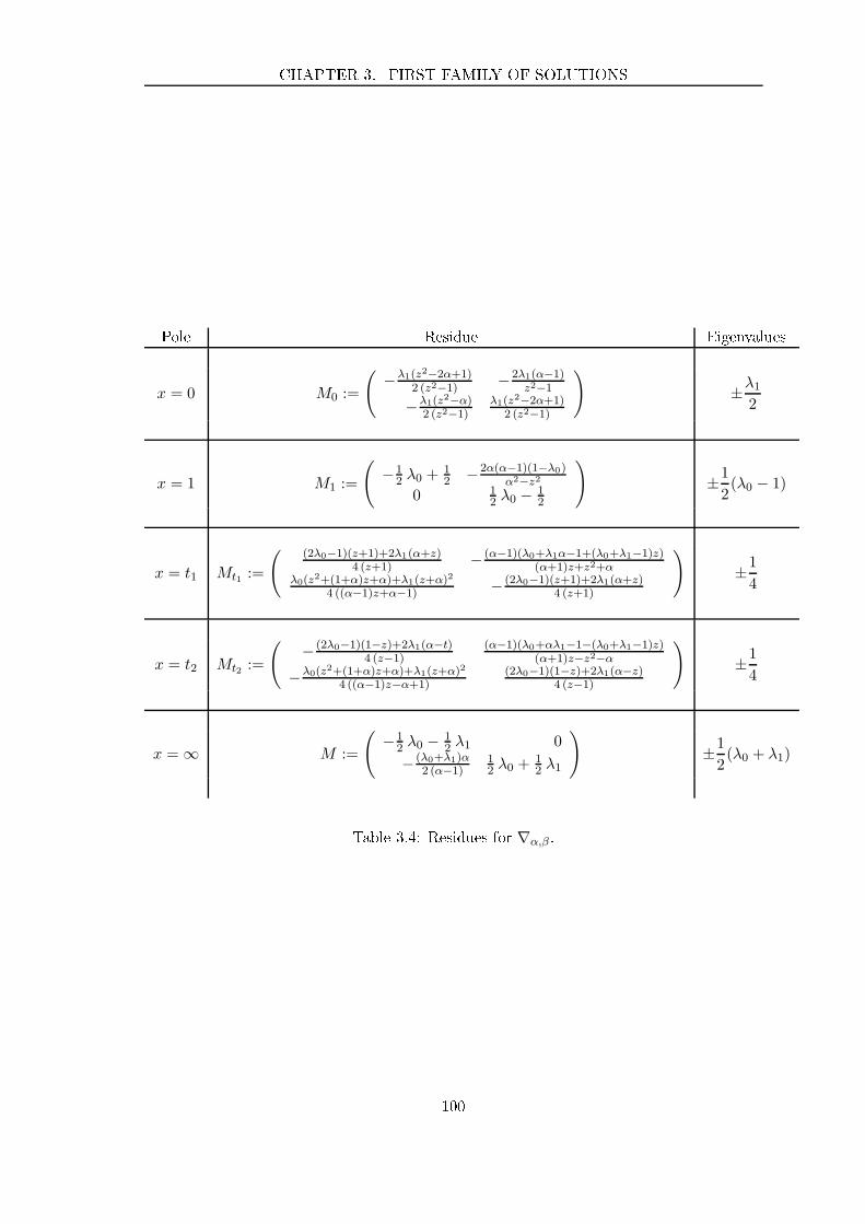
CHAPTER 3. FIRST FAMILY OF SOLUTIONS
Pole Residue Eigenvalues
x = 0 M0 :=
(
−λ1(z2−2α+1)2 (z2−1)
−2λ1(α−1)z2−1
−λ1(z2−α)2 (z2−1)
λ1(z2−2α+1)2 (z2−1)
)
±λ12
x = 1 M1 :=
(
−12 λ0 +
12 −2α(α−1)(1−λ0)
α2−z20 1
2 λ0 − 12
)
±1
2(λ0 − 1)
x = t1 Mt1 :=
((2λ0−1)(z+1)+2λ1(α+z)
4 (z+1) − (α−1)(λ0+λ1α−1+(λ0+λ1−1)z)(α+1)z+z2+α
λ0(z2+(1+α)z+α)+λ1(z+α)2
4 ((α−1)z+α−1) − (2λ0−1)(z+1)+2λ1(α+z)4 (z+1)
)
±1
4
x = t2 Mt2 :=
(
− (2λ0−1)(1−z)+2λ1(α−t)4 (z−1)
(α−1)(λ0+αλ1−1−(λ0+λ1−1)z)(α+1)z−z2−α
−λ0(z2+(1+α)z+α)+λ1(z+α)2
4 ((α−1)z−α+1)(2λ0−1)(1−z)+2λ1(α−z)
4 (z−1)
)
±1
4
x = ∞ M :=
(
−12 λ0 − 1
2 λ1 0
− (λ0+λ1)α2 (α−1)
12 λ0 +
12 λ1
)
±1
2(λ0 + λ1)
Table 3.4: Residues for ∇α,β.
100

3.3. ALGEBRAIC GARNIER SOLUTIONS
ping (P1)2 → (P1)4 giving expli it expressions of (t1, t2, Sq, Pq), namely:
t1 = − α(z + 1)2
(α− 1)(α − z2),
t2 = − α(z − 1)2
(α− 1)(α − z2),
Sq =λ0(α
2 − 2α+ z2)− λ1(1 + z2 + 2α)α + α(2 − α)− z2
(λ0 + λ1 − 1)(α − z2)(α − 1),
Pq =(λ0 − 1)(z − 1)(z + 1)α
(λ0 + λ1 − 1)(α − z2)(α − 1).
Proof. Using Gröbner bases to eliminate the variable x one obtains a system of equations
of the following form:
(λ0 − 1)2λ21St = −F (Sq, Pq)(λ0 − 1)2Pt = −(λ0 + λ1 − 1)2P 2
q
; (E3.4)
where:
F (Sq, Pq) =(λ0 − λ1 − 1)(λ0 + λ1 − 1)3P 2q
+ (λ0 − 1)2(λ0 + λ1 − 1)2(2Pq − 2PqSq + S2q − 2Sq)
+ (λ0 − 1)3(λ0 + 2λ1 − 1) .
The dis riminant ∆t of this system vanishes along 2 pairs of parallel lines in P1Sq
× P1Pq;
namely:
(∆t = 0) = (α = 0) ∪ (x′ = 0) ∪ (α = ∞) ∪ (x′ = ∞) ⊂ P1α × P1
x′
for some proje tive oordinate x′ su h that z2 = αx′. This expli it des ription of the
twofold ramied over given by z allows us to parametrize (Sq, Pq) as rational fun tions
of (α, z), hen e on luding the proof.
We an now prove that we have indeed onstru ted a family of algebrai solutions for
a Garnier system. More pre isely, onsider the following Hamiltonian system:
∂tkpi = −∂qiHk i, k = 1, 2
∂tkqi = ∂piHk i, k = 1, 2
, (E3.5)
where:
Hk := (−1)k2H(tk, t3−k,p1,p2,q1,q2) +H(tk, t3−k,p2,p1,q2,q1)
2(q1 − q2)(t1 − t2)(tk − 1)tk
101
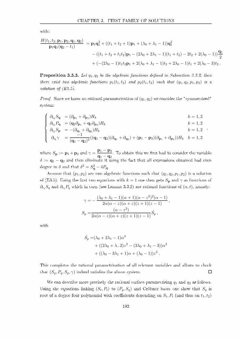
CHAPTER 3. FIRST FAMILY OF SOLUTIONS
with:
H(t1, t2,p1,p2,q1,q2)
p1q1(q2 − t1)= p1q
31 + ((t1 + t2 + 1)p1 + (λ0 + λ1 − 1))q2
1
− ((t1 + t2 + t1t2)p1 − (2λ0 + 2λ1 − 1)(t1 + t2)− 2t2 + 2(λ0 − 1))q1
2
+ (−(2λ0 − 1)t1t2p1 + 2(λ0 + λ1 − 1)t2 + 2λ0 − 1)t1 + 2(λ0 − 3)t2 .
Proposition 3.3.3. Let q1, q2 be the algebrai fun tions dened in Subse tion 3.3.2; then
there exist two algebrai fun tions p1(t1, t2) and p2(t1, t2) su h that (q1, q2, p1, p2) is a
solution of (E3.5).
Proof. Sin e we know no rational parametrisation of (q1, q2) we onsider the "symmetrised"
system:
∂tkSq = (∂p1 + ∂p2)Hk k = 1, 2
∂tkPq = (q2∂p1 + q1∂p2)Hk k = 1, 2
∂tkSp = −(∂q1 + ∂q2)Hk k = 1, 2
∂tkγ =−1
(q1 − q2)2((q1 − q2)(∂q1 + ∂q2) + (p1 − p2)(∂p1 + ∂p2))Hk k = 1, 2
,
where Sp := p1+p2 and γ =p1 − p2
q1 − q2. To obtain this we rst had to onsider the variable
δ := q1 − q2 and then eliminate it using the fa t that all expressions obtained had even
degree in δ and that δ2 = S2q− 4Pq.
Assume that (p1, p2) are two algebrai fun tions su h that (q1, q2, p1, p2) is a solution
of (E3.5). Using the rst two equations with k = 1 one then gets Sp and γ as fun tions of
∂t1Sq and ∂t1Pq whi h in turn (see Lemma 3.3.2) are rational fun tions of (α, t), namely:
γ =− (λ0 + λ1 − 1)(α + 1)(α− z2)2(α− 1)
2α(α − z)(α + z)(z + 1)(z − 1),
Sp =(α− z2)
2α(α − z)(α + z)(z + 1)(z − 1)Sp ,
with
Sp =(λ0 + 2λ1 − 1)α3
+ ((2λ0 + λ−2)z2 − (3λ0 + λ1 − 3))α2
+ ((λ0 − 3λ1 + 1)α + (λ0 − 1))z2 .
This ompletes the rational parametrisation of all relevant variables and allows us he k
that (Sq, Pq, Sp, γ) indeed satises the above system.
We an des ribe more pre isely the rational surfa e parametrising q1 and q2 as follows.
Using the equations linking (St, Pt) to (Pq, Sq) and Gröbner bases one show that Sq is
root of a degree four polynomial with oe ients depending on St, Pt (and thus on t1, t2)
102
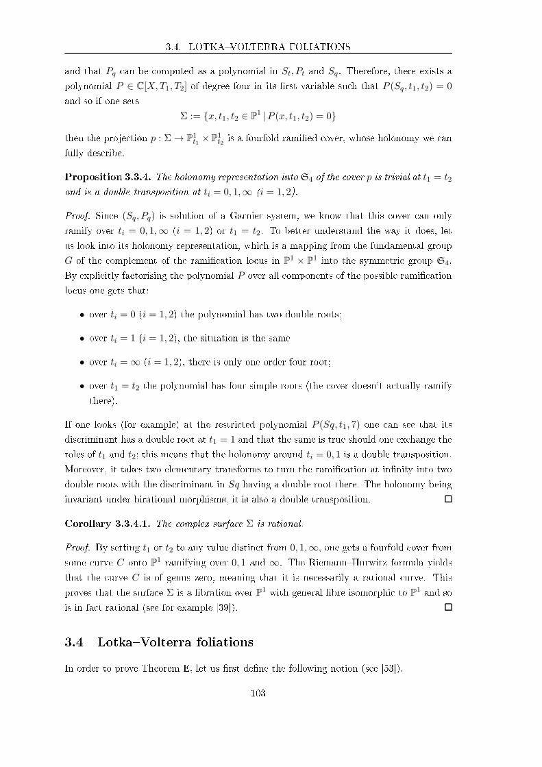
3.4. LOTKAVOLTERRA FOLIATIONS
and that Pq an be omputed as a polynomial in St, Pt and Sq. Therefore, there exists a
polynomial P ∈ C[X,T1, T2] of degree four in its rst variable su h that P (Sq, t1, t2) = 0
and so if one sets
Σ := x, t1, t2 ∈ P1 |P (x, t1, t2) = 0
then the proje tion p : Σ → P1t1× P1
t2is a fourfold ramied over, whose holonomy we an
fully des ribe.
Proposition 3.3.4. The holonomy representation into S4 of the over p is trivial at t1 = t2
and is a double transposition at ti = 0, 1,∞ (i = 1, 2).
Proof. Sin e (Sq, Pq) is solution of a Garnier system, we know that this over an only
ramify over ti = 0, 1,∞ (i = 1, 2) or t1 = t2. To better understand the way it does, let
us look into its holonomy representation, whi h is a mapping from the fundamental group
G of the omplement of the rami ation lo us in P1 × P1into the symmetri group S4.
By expli itly fa torising the polynomial P over all omponents of the possible rami ation
lo us one gets that:
• over ti = 0 (i = 1, 2) the polynomial has two double roots;
• over ti = 1 (i = 1, 2), the situation is the same
• over ti = ∞ (i = 1, 2), there is only one order four root;
• over t1 = t2 the polynomial has four simple roots (the over doesn't a tually ramify
there).
If one looks (for example) at the restri ted polynomial P (Sq, t1, 7) one an see that its
dis riminant has a double root at t1 = 1 and that the same is true should one ex hange the
roles of t1 and t2; this means that the holonomy around ti = 0, 1 is a double transposition.
Moreover, it takes two elementary transforms to turn the rami ation at innity into two
double roots with the dis riminant in Sq having a double root there. The holonomy being
invariant under birational morphisms, it is also a double transposition.
Corollary 3.3.4.1. The omplex surfa e Σ is rational.
Proof. By setting t1 or t2 to any value distin t from 0, 1,∞, one gets a fourfold over from
some urve C onto P1ramifying over 0, 1 and ∞. The RiemannHurwitz formula yields
that the urve C is of genus zero, meaning that it is ne essarily a rational urve. This
proves that the surfa e Σ is a bration over P1with general bre isomorphi to P1
and so
is in fa t rational (see for example [39).
3.4 LotkaVolterra foliations
In order to prove Theorem E, let us rst dene the following notion (see [53).
103

CHAPTER 3. FIRST FAMILY OF SOLUTIONS
Denition 3.4.1 (Transversally proje tive foliation). Let M be a smooth proje tive om-
plex manifold; a odimension one foliation F on M (dened by a Frobeniusintegrable
nonzero rational oneform ωF) is said to be transversally proje tive if there exist two
rational oneforms α, β over M su h that
d +
(
α β
ωF −α
)
denes a at sl2(C) onne tion over the rank two trivial bundle C2 ×M .
If one looks at the restri tion ω of the Ri ati oneform R(∇) to (w = ∞) one obtains
a odimension one transversally proje tive foliation F over the proje tive plane P2; indeed,
if
R(∇) = dw + ωw2 + 2αw + β
then
d +
(
α β
ω −α
)
is gaugeequivalent to∇ and as su h is a at sl2(C) onne tion over C2×P2. The oneform
ω an be written in the ane hart C2x,y ⊂ P2
des ribed in Subse tion 3.2.1 as:
ω = ((2λ0 + λ1)x+ λ1(y − 1))ydx− ((λ0 + 2λ1)y + λ0(x− 1))xdy
This foliation's invariant lo us ontains the singular lo us of ∇, namely the quinti Q and
has seven order one singularities, namely (in homogeneous oordinates [x : y : t] hosen so
that our usual ane hart orresponds to t = 1) [0 : 0 : 1], [0 : 1 : 1], [1 : 0 : 1], [λ21 : λ20 : (λ0+λ1)
2], [1 : 1 : 0]
and [1 : 0 : 0]. Also note that this foliation only depends on the quotient λ :=λ0λ1
; indeed
it is equivalent to:
((2λ+ 1)x+ y − 1)ydx− ((λ+ 2)y + λ(x− 1))xdy = 0 .
Also note that every singular point of the above foliation lies on the quinti Q.
Now dene, given three omplex parameters (A,B,C), the Lotka-Volterra ve tor eld
over C3(with oordinates x, y, t) as LV(A,B,C) := Vx∂x + Vy∂y + Vt∂t, where:
Vx := x(Cy + t), Vy := y(At+ x) and V t := t(Bx+ y) .
This system traditionally omes from the study of a "food hain" system with 3 spe ies
preying on ea h other in a y le. One an then [48, 49 onsider the foliation dened by
both LV(A,B,C) and the radial ve tor eld R := x∂x + y∂y + t∂t: it is the odimension
104
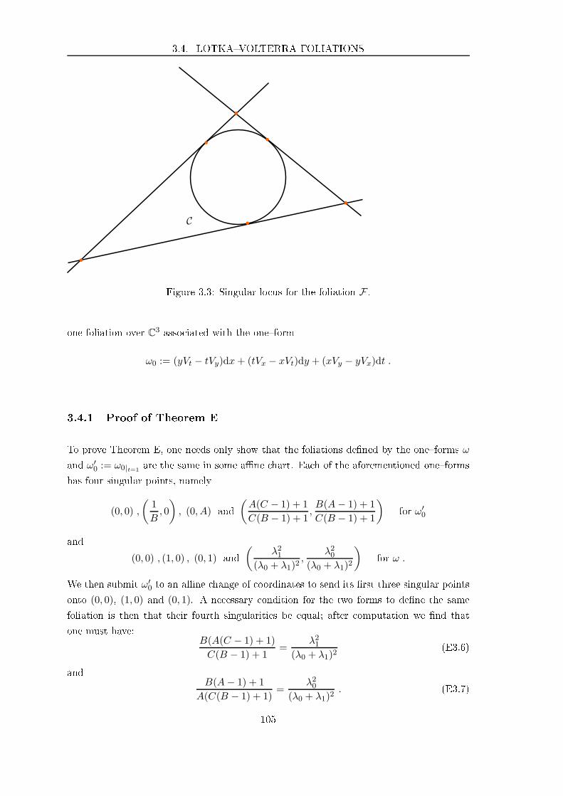
3.4. LOTKAVOLTERRA FOLIATIONS
C
b
bb
b
b
b
Figure 3.3: Singular lo us for the foliation F .
one foliation over C3asso iated with the oneform
ω0 := (yVt − tVy)dx+ (tVx − xVt)dy + (xVy − yVx)dt .
3.4.1 Proof of Theorem E
To prove Theorem E, one needs only show that the foliations dened by the oneforms ω
and ω′0 := ω0|t=1
are the same in some ane hart. Ea h of the aforementioned oneforms
has four singular points, namely
(0, 0) ,
(1
B, 0
)
, (0, A) and
(A(C − 1) + 1
C(B − 1) + 1,B(A− 1) + 1
C(B − 1) + 1
)
for ω′0
and
(0, 0) , (1, 0) , (0, 1) and
(λ21
(λ0 + λ1)2,
λ20(λ0 + λ1)2
)
for ω .
We then submit ω′0 to an ane hange of oordinates to send its rst three singular points
onto (0, 0), (1, 0) and (0, 1). A ne essary ondition for the two forms to dene the same
foliation is then that their fourth singularities be equal; after omputation we nd that
one must have:
B(A(C − 1) + 1)
C(B − 1) + 1=
λ21(λ0 + λ1)2
(E3.6)
and
B(A− 1) + 1
A(C(B − 1) + 1)=
λ20(λ0 + λ1)2
. (E3.7)
105

CHAPTER 3. FIRST FAMILY OF SOLUTIONS
Solving the two above equations, one obtains a rational parametrisation of A and C by B,
namely:
A =(B − 1)λ1
(2λ0 + λ1)Band C = −2B(λ0 + λ1)
2 + λ0λ1λ0λ1(B − 1)
.
A ne essary and su ient ondition for the two asso iated foliation to oin ide is that
ω ∧ ω′0 = 0; using this and the above parametrisation one gets that B must be equal to
− λ0λ0 + λ1
and thus obtains the rst par of Theorem E.
Conversely, dire t omputation shows that any degree two foliation over P2whose
invariant lo us ontains the quinti Q an be written in the ane hart (s, p) as
((γ1 + 2γ2)x+ γ1(y − 1))ydx− ((2γ1 + γ2)y + γ2(x− 1))xdy
with γ1, γ2 ∈ C. In parti ular, su h a foliation automati ally omes from the monodromy
representation of one of our onne tions ∇λ0,λ1 , with λ0 = γ2 and λ1 = γ1.
Remark 3.4.2.
1. The relation ABC = 1 obtained in Theorem E an be seen intuitively as oming from
the order 3 symmetry of the quinti Q: indeed if one denotes by J the homographi
order 3 transform dened on P1by
z 7→ − 1
1 + z
then one has
(A,B,C) =
(λ1λ0, J
(λ1λ0
)
, J2
(λ1λ0
))
.
2. The two variables LotkaVolterra system is usually dened as being following "prey
predator" dierential system:
x′ = x(α+ βy)
y′ = y(γ + δx),
to model an e osystem where x preys on y. However, the plane foliation asso iated
with this system annot be onjugate to the one asso iated with ω as it has two double
singular points whereas ω has seven simple singularities. Thus this gives some form
of justi ation to the fa t that we hose to onsider a three variables system in this
paragraph (as opposed to the more "natural" two variables one).
3.4.2 Invariant urves
The invariant lo us of the family of foliations presented here does not have normal rossings,
hen e the CerveauLins Neto bound on the degree (deg(F) + 2, see [13) does not apply
here. Furthermore one may note that (for generi parameters λ0, λ1) the foliation F has
106
3.5. PROOF OF THEOREM D
simple singularities at the tangen y lo us of the oni C and the three invariant lines.
Moreover, we have the following result.
Proposition 3.4.3. The foliation F admits, for λ0, λ1 ∈ Q, invariant algebrai urves of
arbitrarily high (depending on λ0/λ1) degree.
Proof. The se tion (w = ∞) ⊂ P1 × P2that we used to dene our foliations lifts through
π : P1×P1 2:1−−→ P2(see Subse tion 3.2.1) to the se tion (z = 1) of the trivial bundle X×P1
(see Subse tion 3.2.2) and so the foliation itself lifts (in our usual lo al hart) to:
(F ′) λ0
(du0u0
− du1u1
)
+ λ1
(du0u0 − 1
− du1u1 − 1
)
= 0 .
If one looks at rational values of λ0 and λ1, one gets a foliation F with nite holonomy
whi h as a onsequen e admits a rational rst integral. Moreover, in that parti ular ase
every leaf is an algebrai invarian e urve and it is possible to nd these with arbitrarily
high degree (for varying λ0, λ1). For example, if λ0 = n ≥ 1 is a positive integer and if we
set λ1 = 1 then a simple omputation shows that the urve
(Cn) un0 (u0 − 1)− un1 (u1 − 1) = 0
on X is invariant under F ′. An indu tion then shows that this urve is the pullba k by
π of a degree 2 + n urve on P2and so we get an invariant urve of su h degree for the
foliation F orresponding with the parameters (n, 1).
Remark 3.4.4. Note however that this is a slightly weaker example than the ones given
in [41 as the lo al type of our singularities depends on the parameter λ0/λ1.
3.5 Proof of Theorem D
In this paragraph, we prove that our family of monodromy representations annot be
generi ally obtained through a pullba k method [24,25 by showing that it does not fa tor
through an orbi urve [15.
3.5.1 First ase: λ0 and λ1 are not linearly dependant over Z
Suppose that we have some omplex proje tive urve C, a divisor δ = t1 + . . . + tk in C,
an algebrai mapping f : P2 − f−1(δ) → C − δ and a representation ρ of the fundamental
group of C − δ into PSL2(C) su h that the diagram
π1(C − δ, x0)ρ
((
π1(P
2 − f−1(δ))
Pρm
f∗oo
PSL2(C)
107

CHAPTER 3. FIRST FAMILY OF SOLUTIONS
ommutes. Sin e the ramied over π : X2:1−−→ P2
is unramied between X − D and
P2−Q, where D is the divisor in X made of the six lines u0, u1 = 0, 1,∞ and the diagonal
∆ = (u0 = u1), then the fundamental group π1(X − D) is realised as a subgroup of Γ2.
This means that if one sets φ := f π one has su h a diagram:
π1(C − δ, x0)ρ′
((
π1(X − φ−1(δ))
ρ′
φ∗oo
PSL2(C)
.
Now let L be a generi horizontal line in X (i.e of the form (u1 = c), with c 6= 0, 1,∞);
sin e f is algebrai the restri ted map φ|L extends as a ramied over φL : L → C with
topologi al degree equal to some d ≥ 1. The line L is isomorphi to P1, so the Riemann
Hurwitz formula for es the genus of the urve C to be equal to zero; as su h we an
assume without loss of generality that φL is a dfold over of the proje tive line over itself.
Moreover, one has that φ∗Lδ must ontain 0, 1, c,∞.The representation ρ′ must indu e innite order monodromy about at least one loop in
C − δ, say γ0, or else all elements in the image of ρ would be of nite order. This means
that M := ρ′(γ0) is a innite-order element in PSL2(C).
Let us assume that there are at least two distin t elements γ and γ′ in the bre of
(φL)∗ above γ0; then both ρ′(γ) and ρ′(γ′) must be powers of M . This gives us a relation
between words in the matri es
(
a0 0
0 a−10
)
,
(
a1 0
0 a−11
)
and
(
a0a1 0
0 (a0a1)−1
)
,
where aj = e−iπλj . Sin e generi ally λ0 and λ1 are not linearly dependant, this is impos-
sible; hen e we have that the bre (φL)−1∗ (γ0) may only ontain one element. This implies
that φL ramies totally over (at least) three points in C and so the RiemannHurwitz
formula yields that φL must be onetoone.
Let u ∈ P1and set hu ∈ PSL2(C) to be the Möbius transform sending the rami ation
lo us of φ(u1=u) onto 0, 1,∞; up to omposing it with (u0, u1) 7→ (hu1(u0), u1) we an
assume that φ is exa tly the rst proje tion pr1 : X → P1. However if one looks at the
restri tion of φ to some verti al line then one should again generi ally obtain innite lo al
monodromy at three points, whi h is impossible with pr1, thus on luding the proof.
3.5.2 Se ond ase: there exists (p, q) in Z2 \(0, 0) su h that pλ0+ qλ1 = 0
We an assume that at least one of
λ0λ1
or
λ1λ0
is a rational number, therefore the transversally
proje tive foliation F introdu ed in Se tion 3.4 has nite monodromy and so admits some
rational rst integral g : P2 → P1. Using Subse tion 4.4 in [43, one dedu es that the
transversally proje tive stru ture (β, α, ω) asso iated with F is equivalent to one of the
108

3.5. PROOF OF THEOREM D
form (β, 0,dg) with the following relations (see [43, Subse tion 4.1):
β ∧ dg = 0 and dβ = 0 .
The rst relation implies that β must be of the form β = fdg for some rational f : P2 → P1;
using the se ond relation one then gets that
df ∧ dg = 0 . (E3.8)
Using standard results from birational geometry (see for example Theorem II.7 in [4) one
obtains that there exists a omplex surfa e M and a nite sequen e b : M → P2of blow
ups su h that g := g b is a holomorphi fun tion on M . Moreover, if we set f := f bthen we must have
df ∧ dg = 0 . (E3.9)
It then follows from Stein's fa torisation theorem that there exists a omplex urve C, a
ramied over r : C → P1and a bration φ : M → C with onne ted bres su h that the
following diagram
M
g
φ// C
r~~⑥⑥⑥⑥⑥⑥⑥
P1
ommutes. This means that lo ally on any su iently small analyti open set U the over r
gives an orbifold oordinate x on the urve C and there exists a biholomorphism h between
U×F and φ−1(U), where F is a onne ted omplex urve, su h that for all (x, y) ∈ U×F ,g h(x, y) = x. Therefore relation (E3.9) yields:
d(f h) ∧ dx = 0 .
Thus f depends lo ally only on g and sin e the bres of φ are onne ted one an on lude
using analyti ontinuation that f is globally a fun tion of g. In the end, this implies that
the transversally proje tive stru ture asso iated with F is equivalent to (f(g)dg, 0,dg) and
so fa tors through through the algebrai map asso iated with f on P2 − I, where I is the
indetermina y lo us of f .
109

CHAPTER 3. FIRST FAMILY OF SOLUTIONS
110
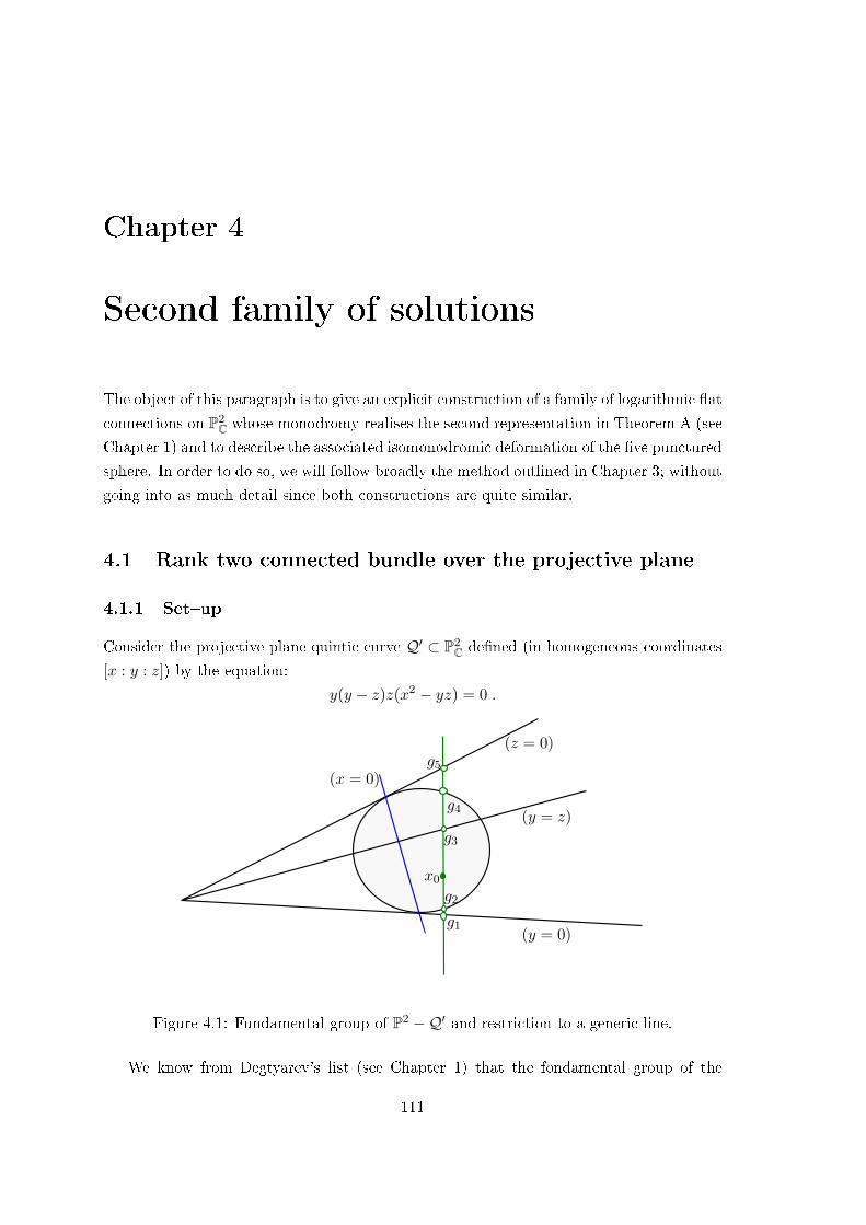
Chapter 4
Se ond family of solutions
The obje t of this paragraph is to give an expli it onstru tion of a family of logarithmi at
onne tions on P2C whose monodromy realises the se ond representation in Theorem A (see
Chapter 1) and to des ribe the asso iated isomonodromi deformation of the ve pun tured
sphere. In order to do so, we will follow broadly the method outlined in Chapter 3; without
going into as mu h detail sin e both onstru tions are quite similar.
4.1 Rank two onne ted bundle over the proje tive plane
4.1.1 Setup
Consider the proje tive plane quinti urve Q′ ⊂ P2C dened (in homogeneous oordinates
[x : y : z]) by the equation:
y(y − z)z(x2 − yz) = 0 .
x0
g1
g2
g3
g4
g5(x = 0)
(y = z)
(y = 0)
(z = 0)
Figure 4.1: Fundamental group of P2 −Q′and restri tion to a generi line.
We know from Degtyarev's list (see Chapter 1) that the fondamental group of the
111
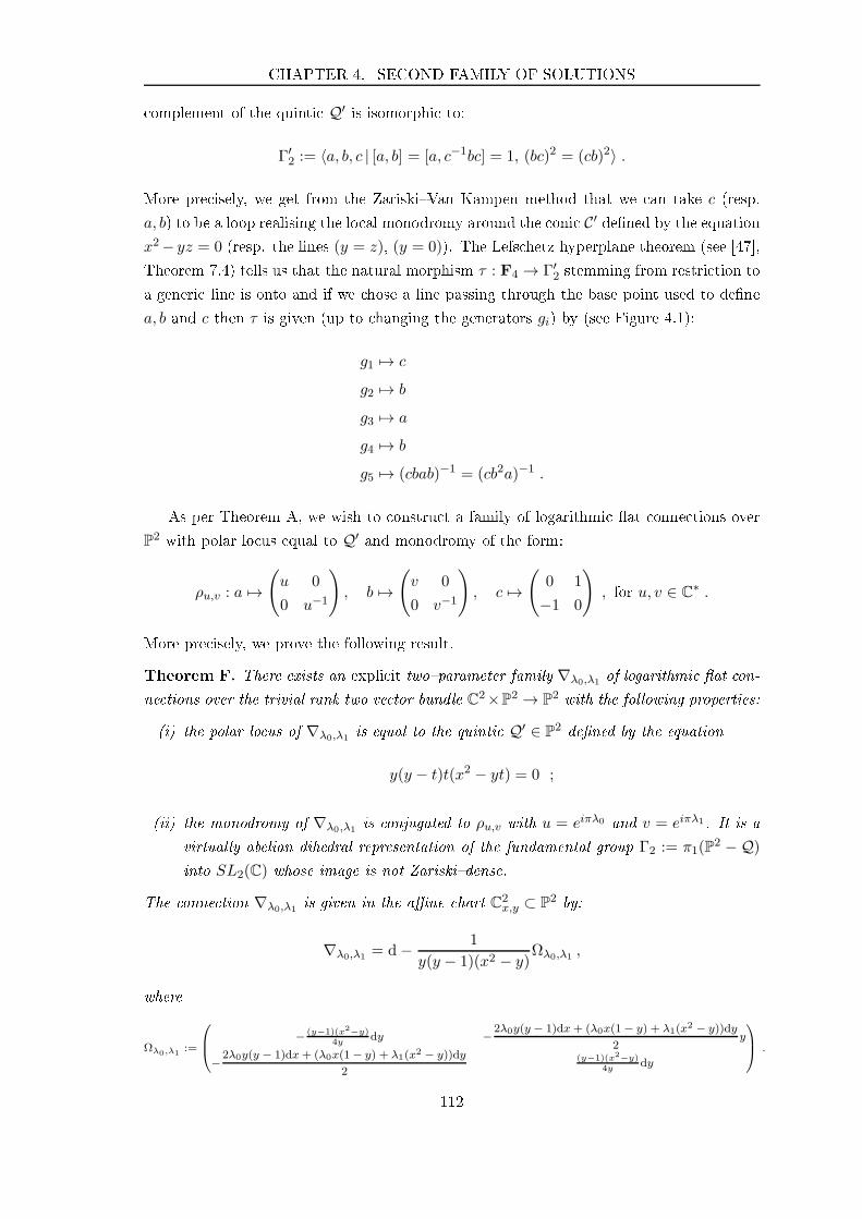
CHAPTER 4. SECOND FAMILY OF SOLUTIONS
omplement of the quinti Q′is isomorphi to:
Γ′2 := 〈a, b, c | [a, b] = [a, c−1bc] = 1, (bc)2 = (cb)2〉 .
More pre isely, we get from the ZariskiVan Kampen method that we an take c (resp.
a, b) to be a loop realising the lo al monodromy around the oni C′dened by the equation
x2− yz = 0 (resp. the lines (y = z), (y = 0)). The Lefs hetz hyperplane theorem (see [47,
Theorem 7.4) tells us that the natural morphism τ : F4 → Γ′2 stemming from restri tion to
a generi line is onto and if we hose a line passing through the base point used to dene
a, b and c then τ is given (up to hanging the generators gi) by (see Figure 4.1):
g1 7→ c
g2 7→ b
g3 7→ a
g4 7→ b
g5 7→ (cbab)−1 = (cb2a)−1 .
As per Theorem A, we wish to onstru t a family of logarithmi at onne tions over
P2with polar lo us equal to Q′
and monodromy of the form:
ρu,v : a 7→(
u 0
0 u−1
)
, b 7→(
v 0
0 v−1
)
, c 7→(
0 1
−1 0
)
, for u, v ∈ C∗ .
More pre isely, we prove the following result.
Theorem F. There exists an expli it twoparameter family ∇λ0,λ1 of logarithmi at on-
ne tions over the trivial rank two ve tor bundle C2×P2 → P2with the following properties:
(i) the polar lo us of ∇λ0,λ1 is equal to the quinti Q′ ∈ P2dened by the equation
y(y − t)t(x2 − yt) = 0 ;
(ii) the monodromy of ∇λ0,λ1 is onjugated to ρu,v with u = eiπλ0 and v = eiπλ1 . It is a
virtually abelian dihedral representation of the fundamental group Γ2 := π1(P2 −Q)
into SL2(C) whose image is not Zariskidense.
The onne tion ∇λ0,λ1 is given in the ane hart C2x,y ⊂ P2
by:
∇λ0,λ1 = d− 1
y(y − 1)(x2 − y)Ωλ0,λ1 ,
where
Ωλ0,λ1:=
− (y−1)(x2−y)4y
dy −2λ0y(y − 1)dx+ (λ0x(1− y) + λ1(x2 − y))dy
2y
−2λ0y(y − 1)dx+ (λ0x(1− y) + λ1(x2 − y))dy
2(y−1)(x2−y)
4ydy
.
112

4.1. RANK TWO CONNECTED BUNDLE
Moreover, the monodromy representation of su h a onne tion fa tors through an orbi urve
if and only if there exists (p, q) ∈ Z2 \ (0, 0) su h that pλ0 + qλ1 = 0.
Remark 4.1.1. Note that, similar to Chapter 3, the existen e, and uniqueness up to gauge
transformation, of su h a family of onne tions follows from the lassi al RiemannHilbert
orresponden e.
4.1.2 A suitable double over
As in Chapter 3, the key point of our onstru tion will be to nd a properly ramied double
over so that we are able to obtain a onne tion with dihedral monodromy. Here, sin e the
lo al monodromy with proje tive order two arises along the line y = 0, we will need to
have the aforementioned over ramify there. Consider the following 2 : 1 birational map:
π : P1 × P1 → P2
([u0 : u1], [v0, v1]) 7→ [u0v21 : u1v
20 : u1v
21 ] .
The map π has indetermina y lo us equal to the point ([1 : 0], [1 : 0]) and ramies over
y = 0 ⊂ P2C. Moreover, one also has (see Fig. 4.2):
π∗C′ = ([u0 : u1], [v0 : v1]) ∈ P1 × P1 | (u0v1 − u1v0)(u0v1 + u1v0) = 0= u = v ∪ u = −v ⊂ P1
u × P1v ,
π∗(y = z ∩ z 6= 0) = ([u0 : u1], [v0 : v1]) ∈ P1 × P1 | v20 = v21= v = 1 ∪ v = −1 ⊂ P1
u × P1v ,
π∗(y = 0 ∩ z 6= 0) = ([u0 : u1], [v0 : v1]) ∈ P1 × P1 | v0 = 0= v = 0 ⊂ P1
u × P1v
and
π∗z = 0 = ([u0 : u1], [v0 : v1]) ∈ P1 × P1 |u1v21 = 0= u = ∞ ∪ v = ∞ ⊂ P1
u × P1v .
This means that the quinti Q′is pulled ba k by π onto seven lines in P1 × P1
. The
over π orresponds to the quotient of P1×P1under the involution (u, v) 7→ (u,−v). Now
let us onsider the elementary transformation of P1 × P1dened by:
b : P1 × P1 → P1 × P1
([u0 : u1], [v0 : v1]) 7→ ([u0v0 : u1v1], [v0 : v1]) ;
113

CHAPTER 4. SECOND FAMILY OF SOLUTIONS
u = ∞
v = ∞
u = −vu = v
v = 0 π
C′z = 0
y = z
y = 0
Figure 4.2: Rami ation lo us of π.
then one an easily he k that:
b∗(u = ±v ∩ v 6= 0,∞) = ([u0 : u1], [v0 : v1]) ∈ P1 × P1 | (u0v0 −±v0)(u1v1 −±v1) = 0= u = ±1 ⊂ P1
u × P1v
and
b∗u = ∞ = ([u0 : u1], [v0, v1]) ∈ P1 × P1 |u1v1 = 0= u = ∞ ∪ v = ∞ ∪ v = ∞ ⊂ P1
u × P1v .
The heuristi behind this pro edure an be summed up as follows: imagine that we
have a logarithmi at onne tion ∇ over P2satisfying the hypotheses of Theorem F; then
π∗∇ will be a logarithmi at onne tion over P1 × P1whose monodromy around v = 0
must be (proje tively) trivial sin e π ramies over y = 0. As su h, its monodromy group
must be abelian and the pullba k onne tion (π b)∗∇ also has abelian monodromy and
fa tors through the fundamental group of the omplement of
u = ∞ ∪ v = ∞ ∪ u = 1 ∪ u = −1 ∪ v = 1 ∪ v = −1 in P1u × P1
v
whi h is a produ t of free groups. This will allow us to set up a onstru tion quite similar
to that of Chapter 3.
4.1.3 Constru ting the onne tion
Drawing inspiration from the above heuristi and Chapter 3, we onsider the trivial rank
two ve tor bundle E0 on X := P1 × P1endowed with the logarithmi at onne tion:
∇0 := d +1
2
(
ω0 0
0 −ω0
)
,
114
4.1. RANK TWO CONNECTED BUNDLE
where u, v are proje tive oordinates on the base X and
ω0 := λ0
(du
u− 1− du
u+ 1
)
+ λ1
(dv
v − 1− dv
v + 1
)
,
with (λ0, λ1) ∈ C2 \ (0, 0). This onne tion generi ally has singular lo us equal to four
lines in X and its lo al monodromy is given by the following matri es:
• around u = ±1:(
e−iπλ0 0
0 eiπλ0
)±1
;
• around v = ±1, j = 0, 1:(
eiπλj 0
0 eiπλj
)±1
.
One easily he ks that the oneform ω0 is the pullba k under the elementary transform
b of:
ω1 := λ0
(du
u− v− du
u+ v+u
v
(dv
u+ v− dv
u− v
))
+ λ1
(dv
v − 1− dv
v + 1
)
.
Note that this oneform gets nontrivial lo al monodromy around the lines v = 0 and
u = ∞; it naturally gives rise to a Ri ati foliation, dened by the following oneform
over P(E0) = X × P1:
R1 := dw − ω1w
where w is a proje tive oordinate on the bres.
Now dene the following involution on the proje tive bundle P(E0):
η : X × P1 → X × P1
(u, v, w) 7→ (−u,−v,−w)
that leaves invariant the oneform R1. This means that if we extend π into the map
π : X × P1 → P2 × P1
(u, v, [w0 : w1]) 7→ (π(u, v), [w0 + w1 : w0 −w1])
then R1 is the pullba k under π of the Ri ati oneform dened in some ane hart by:
R := dw+
(λ0
x2 − ydx+
(λ0x
x2 − y− λ1
2(y − 1)
)dy
y
)
w2
−dy
2yw − λ0y
x2 − ydx+
1
2
(λ0x
y(x2 − y)− λ1y − 1
)
dy .
The above is a logarithmi oneform over P2 × P1whose singular lo us is exa tly the
115
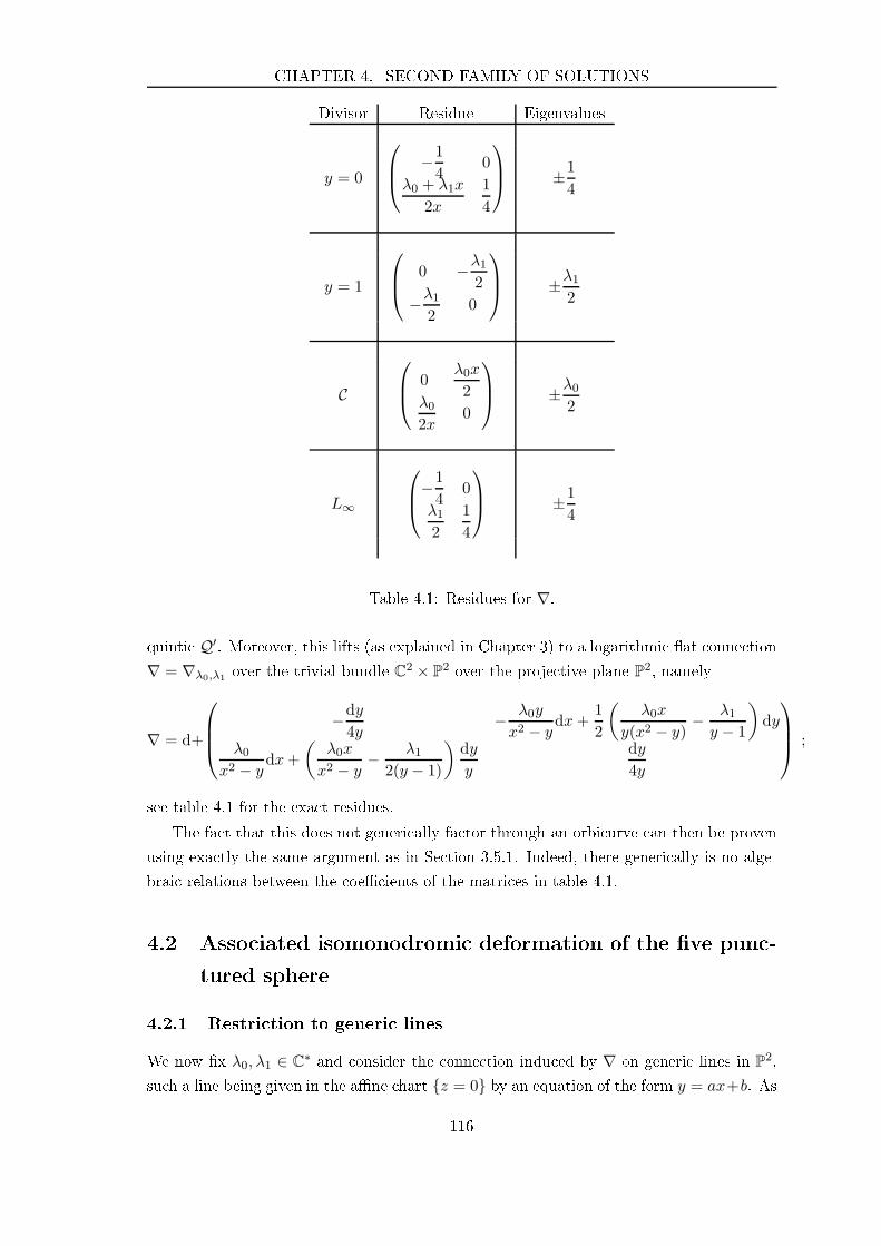
CHAPTER 4. SECOND FAMILY OF SOLUTIONS
Divisor Residue Eigenvalues
y = 0
−1
40
λ0 + λ1x
2x
1
4
±1
4
y = 1
0 −λ12
−λ12
0
±λ1
2
C
0λ0x
2λ02x
0
±λ0
2
L∞
−1
40
λ12
1
4
±1
4
Table 4.1: Residues for ∇.
quinti Q′. Moreover, this lifts (as explained in Chapter 3) to a logarithmi at onne tion
∇ = ∇λ0,λ1 over the trivial bundle C2 × P2over the proje tive plane P2
, namely
∇ = d+
−dy
4y− λ0y
x2 − ydx+
1
2
(λ0x
y(x2 − y)− λ1y − 1
)
dy
λ0x2 − y
dx+
(λ0x
x2 − y− λ1
2(y − 1)
)dy
y
dy
4y
;
see table 4.1 for the exa t residues.
The fa t that this does not generi ally fa tor through an orbi urve an then be proven
using exa tly the same argument as in Se tion 3.5.1. Indeed, there generi ally is no alge-
brai relations between the oe ients of the matri es in table 4.1.
4.2 Asso iated isomonodromi deformation of the ve pun -
tured sphere
4.2.1 Restri tion to generi lines
We now x λ0, λ1 ∈ C∗and onsider the onne tion indu ed by ∇ on generi lines in P2
,
su h a line being given in the ane hart z = 0 by an equation of the form y = ax+b. As
116

4.2. ASSOCIATED ISOMONODROMIC DEFORMATION
in Chapter 3, we obtain an isomonodromi deformation (∇a,b)a,b over the ve pun tured
sphere whose asso iated Ri ati oneform is given by the following lo al formula (in the
aforementioned ane hart):
R(∇a,b) =2a2y4 + (4ab− 2− 2a2)y3 + (2− 4ab+ 2b2)y2 − 2b2y
2y(y − 1)(a2y2 + (2ab− 1)y + b2)dw
+α2(y)w
2 + α1(y)w + α0
2y(y − 1)(a2y2 + (2ab− 1)y + b2)dy
where
α2(y) := (λ0a+ λ1a2)y2 + ((a− b)λ0 + (2ab− 1)λ1)y + λ0b+ λ1b
2
α1(y) := −a2y3 + (a2 − 2ab+ 1)y2 + (2ab− b2 − 1)y + b2
α0(y) := −(λ0a+ λ1a2)y3 + ((a+ b)λ0 + (1− 2ab)λ1)y
2 − (λ0b+ λ1b2)y .
As su h, if one hooses a parameter c su h that c2 = 1− 4ab then one gets a family of
logarithmi at onne tions (∇a,c)a,c over P1 \ 0, 1, t1, t2,∞, where:
t1 =
(c− 1
2a
)2
and t2 =
(c+ 1
2a
)2
.
An expli it lo al expression for this isomonodromi deformation an be obtained simply by
repla ing b by1− c2
4ain the above formula for R(∇a,b); this allows us to expli itly ompute
the spe tral data for ∇a,c, as detailed in Table 4.2.
4.2.2 Asso iated Garnier solution
Similar to what we did in Se tion 3.3.2, start by setting
H :=M0
y+
M1
y − 1+
M2
y − t1+
M3
y − t2;
then sin e the lower left oe ient of the residue at innity M∞ of ∇a,c is zero, the
numerator of H must be a degree two polynomial in y, say:
H2,1 =c(t1, t2)(y
2 − Sq(t1, t2)y + Pq(t1, t2))
y(y − 1)(y − t1)(y − t2), (E4.1)
where Sq := q1 + q2 and Pq := q1q2, with q1, q2 some algebrai fun tions of (t1, t2). In the
same manner that we did in Chapter 3, we obtain a rational parametrisation of Sq, Pq, t1, t2.
More pre isely, the parameters (a, c) give a rational mapping (P1)2 → (P1)4 giving
117
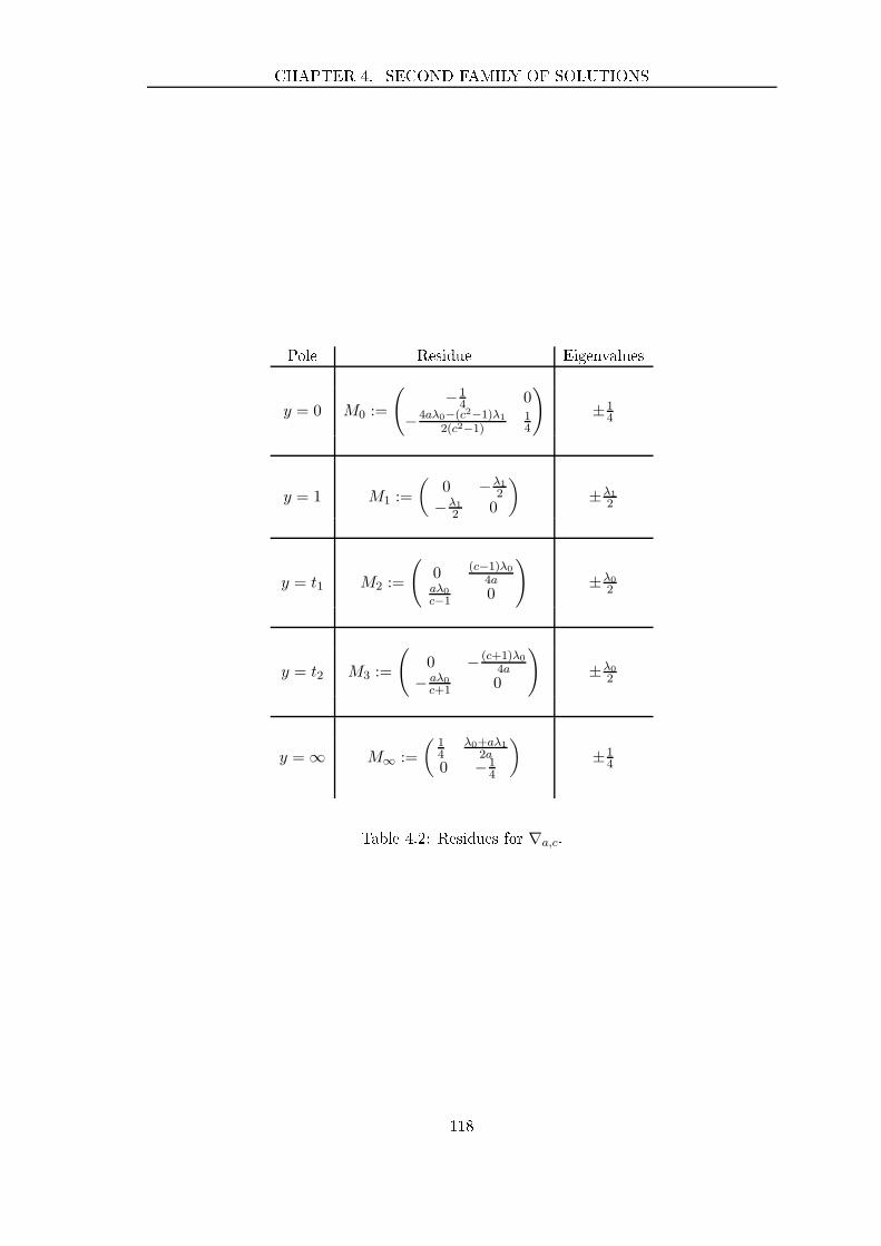
CHAPTER 4. SECOND FAMILY OF SOLUTIONS
Pole Residue Eigenvalues
y = 0 M0 :=
(
−14 0
−4aλ0−(c2−1)λ12(c2−1)
14
)
±14
y = 1 M1 :=
(0 −λ1
2
−λ12 0
)
±λ12
y = t1 M2 :=
(
0 (c−1)λ04a
aλ0c−1 0
)
±λ02
y = t2 M3 :=
(
0 − (c+1)λ04a
− aλ0c+1 0
)
±λ02
y = ∞ M∞ :=
(14
λ0+aλ12a
0 −14
)
±14
Table 4.2: Residues for ∇a,c.
118

4.2. ASSOCIATED ISOMONODROMIC DEFORMATION
expli it expressions of (t1, t2, Sq, Pq), namely:
t1 =(c− 1)2
4
t2 =(c+ 1)2
4,
Sq =(1− c2 + 4a2)λ0 + 2a(c2 + 1)λ1
4a2(λ0 + aλ1),
Pq = −(c− 1)(c + 1)(4aλ0 + (1− c2))
16a3(λ0 + aλ1).
We an now prove that we have indeed onstru ted a family of algebrai solutions for
a Garnier system. More pre isely, onsider the following Hamiltonian system:
∂tkpi = −∂qiHk i, k = 1, 2
∂tkqi = ∂piHk i, k = 1, 2
, (E4.2)
where the pair of Hamiltonians (H1,H2) is expli itly given in Appendix B. Note that it
diers slightly from the one presented in Chapter 3, as the lo al eigenvalues are not the
same.
Proposition 4.2.1. Let q1, q2 be the algebrai fun tions dened above; then there exist two
algebrai fun tions p1(t1, t2) and p2(t1, t2) su h that (q1, q2, p1, p2) is a solution of (E4.2).
Proof. We pro eed exa tly as we did for the rst family of solutions: we onsider the
"symmetrised" system:
∂tkSq = (∂p1 + ∂p2)Hk k = 1, 2
∂tkPq = (q2∂p1 + q1∂p2)Hk k = 1, 2
∂tkSp = −(∂q1 + ∂q2)Hk k = 1, 2
∂tkγ =−1
(q1 − q2)2((q1 − q2)(∂q1 + ∂q2) + (p1 − p2)(∂p1 + ∂p2))Hk k = 1, 2
,
where Sp := p1+p2 and γ =p1 − p2
q1 − q2. To obtain this we rst had to onsider the variable
δ := q1 − q2 and then eliminate it using the fa t that all expressions obtained had even
degree in δ and that δ2 = S2q− 4Pq.
Assume that (p1, p2) are two algebrai fun tions su h that (q1, q2, p1, p2) is a solution
of (E4.2). Using the rst two equations with k = 1 one then gets Sp and γ as fun tions of
∂t1Sq and ∂t1Pq whi h in turn are rational fun tions of (a, c), namely:
γ =8(1 + a)(λ0 + aλ1)a
3
(c2 − 1)(1 + c+ 2a)(1 − c+ 2a),
Sp =− 2a(1 + 3a− c2 + 4a2 − 3ac2 + 4a3)λ0 + (2a+ 4a2 + 2ac2)λ1(c2 − 1)(1 + c+ 2a)(1− c+ 2a)
.
This ompletes the rational parametrisation of all relevant variables and allows us to he k
119

CHAPTER 4. SECOND FAMILY OF SOLUTIONS
that (Sq, Pq, Sp, γ) indeed satises the above system, in the exa t same way we did in
Se tion 3.3.3.
120

Part II
Katz's middle onvolution and
derivatives
121

Chapter 5
Some new orbits
In this hapter we draw inspiration from earlier work by Boal h [7 on Painlevé VI equations
to obtain nite orbits under the mapping lass group a tion on some hara ter variety
through Katz's middle onvolution. The basi idea is the following : take a nite subgroup
G in SL3(C) and onsider a representation ρ : F4 → SL3(C) whose image is ontained in
G. Sin e the latter is nite, so must be the orbit of the lass [ρ] ∈ Char3(0, 5) under the
a tion of the mapping lass group Mod(0, 5). By applying Katz's middle onvolution as
des ribed in Se tion I2 of the introdu tion to this thesis, we get a new nite orbit under
the mapping lass group a tion on Chardρ for some expli it dρ ≥ 1. Sin e the upshot here
is to study rank two isomonodromi deformations of the ve pun tured sphere, we shall
endeavour to onstru t ρ so that dρ = 2.
5.1 Main result
5.1.1 Framework
Start by re alling that if ρ : F4 → SL3(C) is a group representation of the free group on
four generators F4 := 〈d1, . . . , d5 | d1 . . . d5 = 1〉 then its middle onvolution with respe t
to some θ ∈ (C∗)5 will be a representation ρ : F4 → SLdρ(C), with
dρ =
5∑
i=1
rg(Id − gi)− d ,
where gi =1θiρ(di) for i ∈ [5]. Our intention here is to use Katz's middle onvolution to
obtain rank two representation from nite subgroups of SL3(C), meaning that the matri es
hi and the omplex numbers θi will need to be hosen so that :
5∑
i=1
rank(Id − gi) = 5 .
In order to do so, we will pro eed as follows:
123
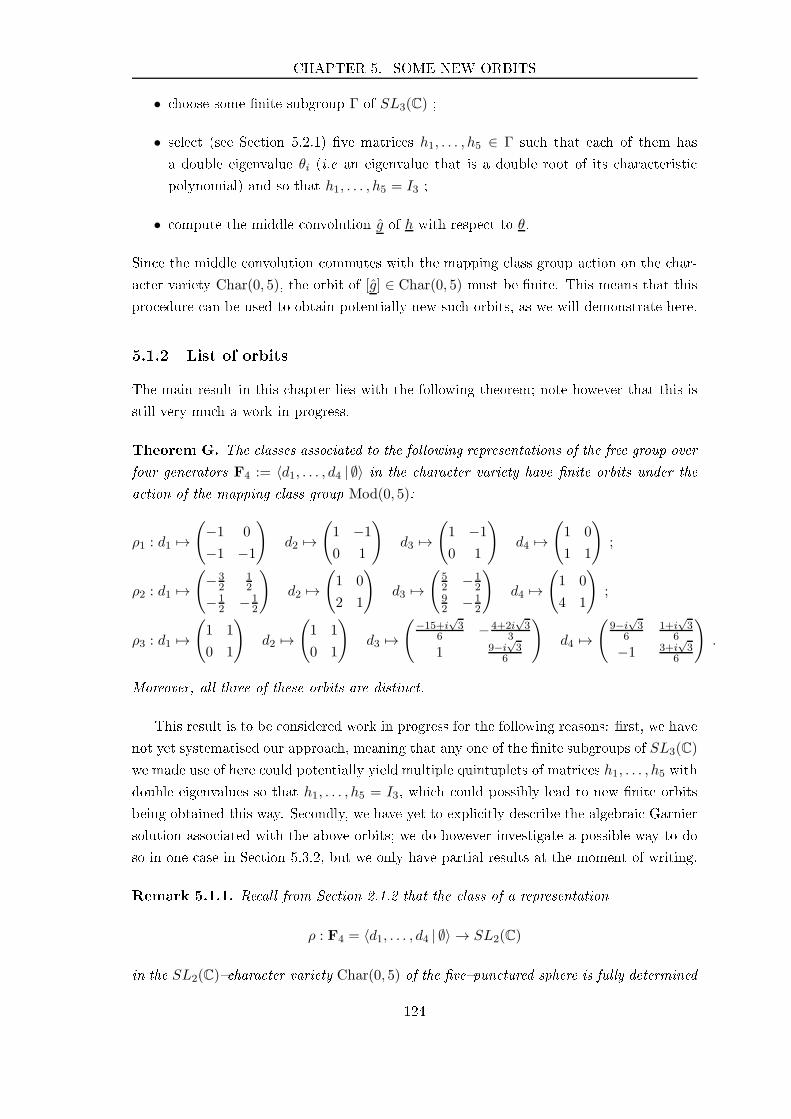
CHAPTER 5. SOME NEW ORBITS
• hoose some nite subgroup Γ of SL3(C) ;
• sele t (see Se tion 5.2.1) ve matri es h1, . . . , h5 ∈ Γ su h that ea h of them has
a double eigenvalue θi (i.e an eigenvalue that is a double root of its hara teristi
polynomial) and so that h1, . . . , h5 = I3 ;
• ompute the middle onvolution g of h with respe t to θ.
Sin e the middle onvolution ommutes with the mapping lass group a tion on the har-
a ter variety Char(0, 5), the orbit of [g] ∈ Char(0, 5) must be nite. This means that this
pro edure an be used to obtain potentially new su h orbits, as we will demonstrate here.
5.1.2 List of orbits
The main result in this hapter lies with the following theorem; note however that this is
still very mu h a work in progress.
Theorem G. The lasses asso iated to the following representations of the free group over
four generators F4 := 〈d1, . . . , d4 | ∅〉 in the hara ter variety have nite orbits under the
a tion of the mapping lass group Mod(0, 5):
ρ1 : d1 7→(
−1 0
−1 −1
)
d2 7→(
1 −1
0 1
)
d3 7→(
1 −1
0 1
)
d4 7→(
1 0
1 1
)
;
ρ2 : d1 7→(
−32
12
−12 −1
2
)
d2 7→(
1 0
2 1
)
d3 7→(
52 −1
292 −1
2
)
d4 7→(
1 0
4 1
)
;
ρ3 : d1 7→(
1 1
0 1
)
d2 7→(
1 1
0 1
)
d3 7→(
−15+i√3
6 −4+2i√3
3
1 9−i√3
6
)
d4 7→(
9−i√3
61+i
√3
6
−1 3+i√3
6
)
.
Moreover, all three of these orbits are distin t.
This result is to be onsidered work in progress for the following reasons: rst, we have
not yet systematised our approa h, meaning that any one of the nite subgroups of SL3(C)
we made use of here ould potentially yield multiple quintuplets of matri es h1, . . . , h5 with
double eigenvalues so that h1, . . . , h5 = I3, whi h ould possibly lead to new nite orbits
being obtained this way. Se ondly, we have yet to expli itly des ribe the algebrai Garnier
solution asso iated with the above orbits; we do however investigate a possible way to do
so in one ase in Se tion 5.3.2, but we only have partial results at the moment of writing.
Remark 5.1.1. Re all from Se tion 2.1.2 that the lass of a representation
ρ : F4 = 〈d1, . . . , d4 | ∅〉 → SL2(C)
in the SL2(C) hara ter variety Char(0, 5) of the vepun tured sphere is fully determined
124
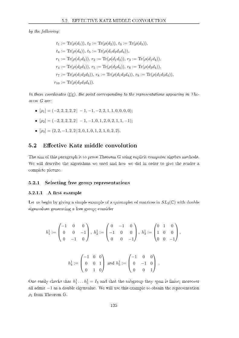
5.2. EFFECTIVE KATZ MIDDLE CONVOLUTION
by the following:
t1 := Tr(ρ(d1)), t2 := Tr(ρ(d2)), t3 := Tr(ρ(d3)),
t4 := Tr(ρ(d4)), t5 := Tr(ρ(d1d2d3d4)),
r1 := Tr(ρ(d1d2)), r2 := Tr(ρ(d1d3)), r3 := Tr(ρ(d1d4)),
r4 := Tr(ρ(d2d3)), r5 := Tr(ρ(d2d4)), r6 := Tr(ρ(d3d4)),
r7 := Tr(ρ(d1d2d3)), r8 := Tr(ρ(d1d2d4)), r9 := Tr(ρ(d1d3d4)),
r10 := Tr(ρ(d2d3d4)).
In these oordinates (t|r), the point orresponding to the representations appearing in The-
orem G are:
• [ρ1] = (−2, 2, 2, 2, 2 | − 1,−1,−2, 2, 1, 1, 0, 0, 0, 0);
• [ρ2] = (−2, 2, 2, 2, 2 | − 1,−1, 0, 1, 2, 0, 2, 1, 1,−1);
• [ρ3] = (2, 2,−1, 2, 2 | 2, 0, 1, 0, 1, 2, 1, 0, 2, 2).
5.2 Ee tive Katz middle onvolution
The aim of this paragraph is to prove Theorem G using expli it omputer algebra methods.
We will des ribe the algorithms we used and how we did in order to give the reader a
omplete pi ture.
5.2.1 Sele ting free group representations
5.2.1.1 A rst example
Let us begin by giving a simple example of a quintuplet of matri es in SL3(C) with double
eigenvalues generating a free group; onsider
h11 :=
−1 0 0
0 0 −1
0 −1 0
, h12 :=
0 −1 0
−1 0 0
0 0 −1
, h13 :=
0 1 0
1 0 0
0 0 −1
,
h14 :=
−1 0 0
0 0 1
0 1 0
and h15 :=
−1 0 0
0 −1 0
0 0 1
.
One easily he ks that h11 . . . h15 = I3 and that the subgroup they span is nite; moreover
all admit −1 as a double eigenvalue. We will use this example to obtain the representation
ρ1 from Theorem G.
125
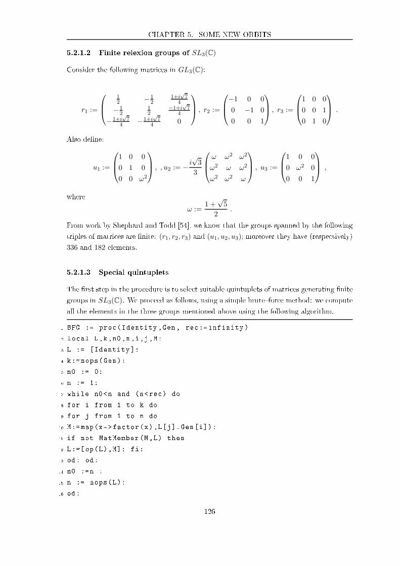
CHAPTER 5. SOME NEW ORBITS
5.2.1.2 Finite relexion groups of SL3(C)
Consider the following matri es in GL3(C):
r1 :=
12 −1
21+i
√7
4
−12
12
−1+i√7
4
−1+i√7
4 −1+i√7
4 0
, r2 :=
−1 0 0
0 −1 0
0 0 1
, r3 :=
1 0 0
0 0 1
0 1 0
.
Also dene:
u1 :=
1 0 0
0 1 0
0 0 ω2
, , u2 := − i
√3
3
ω ω2 ω2
ω2 ω ω2
ω2 ω2 ω
, u3 :=
1 0 0
0 ω2 0
0 0 1
,
where
ω :=1 +
√5
2.
From work by Shephard and Todd [54, we know that the groups spanned by the following
triples of matri es are nite: (r1, r2, r3) and (u1, u2, u3); moreover they have (respe tively)
336 and 182 elements.
5.2.1.3 Spe ial quintuplets
The rst step in the pro edure is to sele t suitable quintuplets of matri es generating nite
groups in SL3(C). We pro eed as follows, using a simple brutefor e method: we ompute
all the elements in the three groups mentioned above using the following algorithm.
1 BFG := pro (Identity ,Gen , re := infinity )
2 lo al L,k,n0,n,i,j,M:
3 L := [Identity :
4 k:=nops(Gen):
5 n0 := 0:
6 n := 1:
7 while n0<n and (n<re ) do
8 for i from 1 to k do
9 for j from 1 to n do
10 M:=map(x->fa tor(x),L[j.Gen[i):
11 if not MatMember (M,L) then
12 L:=[op(L),M: fi:
13 od: od:
14 n0 :=n :
15 n := nops(L):
16 od:
126

5.2. EFFECTIVE KATZ MIDDLE CONVOLUTION
17 RETURN(L):
18 end pro :
The above algorithm (BruteFor eGroup, or BFG) relies on the following entries: Identity is
the identity element (used to initialise the indu tion), Gen is a list ontaining the generators
of the group one wishes to ompute and the optional parameter re an be used to set a
re ursion limit (default is innity). To use BFG to ompute matrix groups one needs the
LinearAlgebra Maple pa kage and the following auxiliary fun tion determining whether
a matrix is a member of some list or not.
1 MatMember := pro (M,L)
2 lo al res , i:
3 res := false:
4 for i from 1 to nops(L) do
5 if Equal(M,L[i) then
6 res := true: fi: od:
7 RETURN(res):
8 end pro :
On e this is done, we look for all elements in the group that have double eigenvalue ;
this is done through the following pro edure.
1 Doubles := pro (S)
2 lo al i,n,L:
3 L := [:
4 n:=nops(S):
5 for i from 1 to n do
6 if hasDouble (S[i) then
7 L := [op(L),i: fi:od:
8 RETURN(L): end pro :
Here, the entry must be the indexed list of the eigenvalues of elements of the group; more
pre isely, if G is the list omputed using BFG, verb+S+ must be the list
1 S:=[seq(Eigenvalues(G[i), i=1..nops(G)):
we also make use of the following auxiliary fun tion to nd out if some list has repeated
elements.
1 hasDouble := pro (L)
2 lo al i,j,res , n:
3 n:= nops(L):
4 res := false:
5 for j from 1 to n do
6 for i from j+1 to n do
127

CHAPTER 5. SOME NEW ORBITS
7 if L[i = L[j then
8 res := true: fi:od:od:
9 RETURN(res):
10 end pro :
On e we are in possession of the list returned by Doubles, whi h ontains the indexes i
su h that G[i has double eigenvalue, we make use of one last Maple pro edure to nd
quintuplets of su h matri es whose produ t is a s alar matrix.
1 Quint := pro (ind ,G,i:=1)
2 lo al i1, i2, i3, i4, i5, n, L, P, ok:
3 L:=[:
4 ok :=0:
5 n:=nops(ind):
6 while evalb(ok<i) do
7 for i1 from 2 to n do
8 for i2 from i1+1 to n do
9 for i3 from i2+1 to n do
10 for i4 from i3+1 to n do
11 for i5 from i4+1 to n do
12 if evalb(ok<i) then
13 P := map(x->fa tor(x),G[ind[i1.G[ind[i2.G[ind[i3.G[ind[
i4.G[ind[i5):
14 if IsMatrixShape(P,s alar) then
15 L := [op(L), [ind[i1,ind[i2,ind[i3,ind[i4,ind[i5:ok:=ok
+1: print(ok ,[ind[i1,ind[i2,ind[i3,ind[i4,ind[i5):
fi:fi:
16 od:od:od:od:od:od:
17 RETURN(L):
18 end pro :
Here the entries are as follows: ind is the list of suitable indexes returned by Doubles, G
is the list of all elements in the group returned by BFG and i (by default equal to 1) is the
number of quintuplets one wishes the algorithm to return before stopping.
5.2.1.4 Expli it quintuplets
To obtain the representations ρ2 and ρ3 we run through the above pro edure on e with (in
that order) the groups generated by (r1, r2, r3) and (u1, u2, u3). This gives us the following
128

5.2. EFFECTIVE KATZ MIDDLE CONVOLUTION
quintuplets of matri es in GL3(C):
h21 :=
12 −1
2−1+i
√7
4
−12
12
−1+i√7
4
−1+i√7
4 −1+i√7
4 0
, h22 :=
1 0 0
0 0 1
0 1 0
, h23 :=
12
−1+i√7
4 −12
−1+i√7
4 0 −1+i√7
4
−12
−1+i√7
412
,
h24 :=
1 0 0
0 0 −1
0 −1 0
, h25 :=
1 0 0
0 −1 0
0 0 −1
,
and
h31 :=
1 0 0
0 −1+i√3
2 0
0 0 1
, h32 :=
1 0 0
0 1
0 0 −1+i√3
2 0
, h33 :=
3+i√3
6−3+i
√3
6−3+i
√3
6−3+i
√3
63+i
√3
6−3+i
√3
6−3+i
√3
6−3+i
√3
6 2 3+i√3
6
,
h34 :=
3−i√3
6 −3+i√3
6 −3+i√3
6
−3+i√3
63−i
√3
6 −3+i√3
6
−3+i√3
6 −3+i√3
63−i
√3
6
, h35 :=
1 0 0
0 −1+i√3
2 0
0 0 −1+i√3
2
.
Note that for i ∈ [3], we have hi1 . . . hi5 = I3.
5.2.2 Middle onvolution algorithm
5.2.2.1 Normalisation
Re all from Se tion I2 in the introdu tion that to use Katz's middle onvolution algorithm
we need a nuple of matri es g = (g1, . . . , gr) su h that g1 . . . gr is the identity matrix and
so that the following two onditions are met:
(CIK1) the matrix gr ommutes to all gi, for i ∈ [r − 1] ;
(CIK2) 1 is not an eigenvalue of the matrix gr.
In our ase, we follow the steps given in Se tion I2.2. Let us take r = 6 and, in order
to obtain rank two representations, we need to ensure that g1, . . . , g5 have 1 as a double
eigenvalue. This leads us to set:
• g1i = −h1i for i ∈ [5] and g16 := −I3;
• g2i = −h2i for i ∈ [5] and g26 := −I3;
• g3i = −h3i for i ∈ [4], g35 := − 21−i
√3h35 and g
26 := −1+i
√3
2 I3.
129

CHAPTER 5. SOME NEW ORBITS
One he ks that this gives us three sextuplets g1, g2, g3 of matri es in GL3(C) satisfying
onditions (CIK1) and (CIK2); moreover, one also gets that for all j ∈ [3], gj1 . . . gj6 = I3
and
5∑
i=1
rank(Id − gji ) = 5 .
5.2.2.2 The algorithm
Now we des ribe the algorithm we use to ompute the a tual Katz's middle onvolution
of the sextuplets g1, g2 and g3. This draws heavily on Völklein's formalism, as detailed in
Se tion I2; as su h we will use the same notations here than there. This pro edure requires
the following setup ommands.
1 with(LinearAlgebra):
2 o:= ZeroMatrix(3):
3 Id := IdentityMatrix(3):
Assume that we start with g1, g2, g3, g4, g5 and g6 six three by three matri es making
up one of the sextuplets gj . Start by setting up the invariant spa e Uρ pertaining to the
group representation ρ : F5 → GL3(C) asso iated with gj . To do so, we rst ompute the
ve tor spa e Im(I3 − gj1)× · · · × Im(I3 − gj6):
1 ROW:=op([RowSpa e (g1-Id), RowSpa e (g2-Id), RowSpa e (g3-Id),
RowSpa e (g4-Id), RowSpa e (g5-Id), RowSpa e (g6-Id) );
2 ve t := simplify (Ve tor([op( onvert(y1*ROW[1[1 , list)), op(
onvert(y2*ROW[2[1 , list)) ,op( onvert(y3*ROW[3[1 , list))
,op( onvert(y4*ROW [4[1 , list)),op( onvert(y5*ROW[5[1 ,
list)),x6,y6,z6));
and set up the matrix M orresponding to ϕ(ρ).
1 M := map(x->fa tor(x),Matrix ([[ Id ,[ MatrixInverse(g1), [
MatrixInverse(g1.g2),[MatrixInverse(g1.g2.g3),[
MatrixInverse(g1.g2.g3.g4),[MatrixInverse(g1.g2.g3.g4.g5)
));
The invariant set Uρ is then equal to the interse tion between Im(I3−gj1)×· · ·×Im(I3−gj6)and the kernel of M; it is a ve tor spa e of dimension ( f. equation (E10)
dim(Uρ) =
5∑
i=1
rank(Id − gi) = 5 (E5.1)
of whi h we an expli itly ompute a basis, say e1, . . . , e5, using Maple. We know use the
expli it formulas given in Se tion I2 to give the matri es F1, . . . , F5 orresponding to the
130

5.2. EFFECTIVE KATZ MIDDLE CONVOLUTION
a tion of the pure braids
Fi = (σr−1 . . . σi+1)σ2i (σr−1 . . . σi+1)
−1
on Uρ.
1 F1 := Transpose (Matrix ([[ g6 , g1.(Id-g6).(Id-MatrixInverse(g2
)) , g1.(Id-g6).(Id-MatrixInverse(g3)) , g1.(Id-g6).(Id-
MatrixInverse(g4)) , g1.(Id-g6).(Id-MatrixInverse(g5)) , g1
.(Id-g6) ,
2 [ o , Id , o , o , o , o ,
3 [ o , o , Id , o , o , o ,
4 [ o , o , o , Id , o , o ,
5 [ o , o , o , o , Id , o ,
6 [ g6.( MatrixInverse(g1)-Id) , g6.(g1-Id).(Id-
MatrixInverse(g2)) , g6.(g1-Id).(Id-MatrixInverse(
g3)) , g6.(g1-Id).(Id-MatrixInverse(g4)) , g6.(g1-
Id).(Id-MatrixInverse(g5)) , Id-g6+g1.g6 )):
7 F2 := Transpose (Matrix ([[ Id,o,o,o,o,o ,
8 [ o, g6 , g2.(Id-g6).(Id-MatrixInverse(g3)) , g2.(Id-
g6).(Id-MatrixInverse(g4)) , g2.(Id-g6).(Id-
MatrixInverse(g5)) , g2.(Id-g6),
9 [ o , o , Id , o , o , o ,
10 [ o , o , o , Id , o , o ,
11 [ o , o , o , o , Id , o ,
12 [ o, g6.( MatrixInverse(g2)-Id) , g6.(g2-Id).(Id-
MatrixInverse(g3)) , g6.(g2-Id).(Id-MatrixInverse(
g4)) , g6.(g2-Id).(Id-MatrixInverse(g5)) , Id-g6+g2
.g6 )):
13
14 F3 := Transpose (Matrix ([[ Id,o,o,o,o,o ,
15 [ o , Id , o , o , o , o ,
16 [ o,o, g6 , g3.(Id-g6).(Id-MatrixInverse(g4)) , g3.(Id
-g6).(Id-MatrixInverse(g5)) , g3.(Id-g6) ,
17 [ o , o , o , Id , o , o ,
18 [ o , o , o , o , Id , o ,
19 [ o, o, g6.( MatrixInverse(g3)-Id) , g6.(g3-Id).(Id-
MatrixInverse(g4)) , g6.(g3-Id).(Id-MatrixInverse(
g5)) , Id-g6+g3.g6 )):
20 F4 := Transpose (Matrix ([[ Id,o,o,o,o,o ,
21 [ o , Id , o , o , o , o ,
22 [ o , o , Id , o , o , o ,
131

CHAPTER 5. SOME NEW ORBITS
23 [ o,o, o,g6 , g4.(Id-g6).(Id-MatrixInverse(g5)) ,
g4.(Id-g6) ,
24 [ o , o , o , o , Id , o ,
25 [ o, o, o, g6.( MatrixInverse(g4)-Id) , g6.(g4-Id).(Id-
MatrixInverse(g5)) , Id-g6+g4.g6 )):
26 F5 := Transpose (Matrix ([[ Id,o,o,o,o,o ,
27 [ o , Id , o , o , o , o ,
28 [ o , o , Id , o , o , o ,
29 [ o , o , o , Id , o , o ,
30 [ o,o, o, o, g6 ,g5.(Id-g6) ,
31 [ o, o, o, o, g6.( MatrixInverse(g5)-Id) , Id-g6+g5.
g6 )):
We then turn our attention to the subspa e Vρ ⊂ Uρ made up of the trivial ane
extensions of ρ, namely the image of the mapping ψ(ρ) that we represent by the matrix N
below.
1 N:=map(x->fa tor(x),Matrix ([[ Id - MatrixInverse(g1), Id -
MatrixInverse(g2), Id - MatrixInverse(g3), Id -
MatrixInverse(g4), Id - MatrixInverse(g5),Id -
MatrixInverse(g6) ));
In order to expli itly ompute the a tion of the braids Fi on the quotient Eρ = Uρ/Vρ we
need to nd an adequate basis of Uρ.
1 f1 := simplify (Transpose (Row(N,1))):
2 f2 := simplify (Transpose (Row(N,2))):
3 f3 := simplify (Transpose (Row(N,3))):
Assume for the sake of simpli ity that the rank of the family (e1,e2,f1,f2,f3) is ve (up
to hanging one or more of the ei); now we only need to ompute the omponents of the
ve tors Fj(ei) along e1 and e2 to obtain the matri es gji ∈ GL2(C) orresponding to the
middle onvolution of gj .
1 sol11 := solve( onvert(map(x->fa tor(x),F1.e1 - (x1*e1+x2*e2+
x3*f1+x4*f2+x5*f3)),set),x1,x2,x3,x4,x5):
2 sol12 := solve( onvert(map(x->fa tor(x),F1.e2 - (x1*e1+x2*e2+
x3*f1+x4*f2+x5*f3)),set),x1,x2,x3,x4,x5):
3 h1 := simplify (Transpose (Matrix ([[ eval(x1,sol11) , eval(x1,
sol12) ,
4 [ eval(x2,sol11) , eval(x2,sol12) )));
5
6 sol21 := solve( onvert(map(x->fa tor(x),F2.e1 - (x1*e1+x2*e2+
x3*f1+x4*f2+x5*f3)),set),x1,x2,x3,x4,x5):
132

5.3. FURTHER STUDY OF THE MAPPING CLASS GROUP ORBITS
7 sol22 := solve( onvert(map(x->fa tor(x),F2.e2 - (x1*e1+x2*e2+
x3*f1+x4*f2+x5*f3)),set),x1,x2,x3,x4,x5):
8 h2 := simplify (Transpose (Matrix ([[ eval(x1,sol21) , eval(x1,
sol22) ,
9 [ eval(x2,sol21) , eval(x2,sol22) )));
10
11 sol31 := solve( onvert(map(x->fa tor(x),F3.e1 - (x1*e1+x2*e2+
x3*f1+x4*f2+x5*f3)),set),x1,x2,x3,x4,x5):
12 sol32 := solve( onvert(map(x->fa tor(x),F3.e2 - (x1*e1+x2*e2+
x3*f1+x4*f2+x5*f3)),set),x1,x2,x3,x4,x5):
13 h3 := simplify (Transpose (Matrix ([[ eval(x1,sol31) , eval(x1,
sol32) ,
14 [ eval(x2,sol31) , eval(x2,sol32) )));
15
16 sol41 := solve( onvert(map(x->fa tor(x),F4.e1 - (x1*e1+x2*e2+
x3*f1+x4*f2+x5*f3)),set),x1,x2,x3,x4,x5):
17 sol42 := solve( onvert(map(x->fa tor(x),F4.e2 - (x1*e1+x2*e2+
x3*f1+x4*f2+x5*f3)),set),x1,x2,x3,x4,x5):
18 h4 := simplify (Transpose (Matrix ([[ eval(x1,sol41) , eval(x1,
sol42) ,
19 [ eval(x2,sol41) , eval(x2,sol42) )));
20
21 sol51 := solve( onvert(map(x->fa tor(x),F5.e1 - (x1*e1+x2*e2+
x3*f1+x4*f2+x5*f3)),set),x1,x2,x3,x4,x5):
22 sol52 := solve( onvert(map(x->fa tor(x),F5.e2 - (x1*e1+x2*e2+
x3*f1+x4*f2+x5*f3)),set),x1,x2,x3,x4,x5):
23 h5 := simplify (Transpose (Matrix ([[ eval(x1,sol51) , eval(x1,
sol52) ,
24 [ eval(x2,sol51) , eval(x2,sol52) )));
By normalising these new two by two matri es as des ribed in Se tion I2.2, we obtain the
representations ρ1, ρ2 and ρ3 from (respe tively) g1, g2 and g3. Sin e these are the middle
onvolution of representations with nite image, the equivarian e of the latter under the
mapping lass group a tion implies that the points [ρ1], [ρ2] and [ρ3] in the hara ter
variety Char(0, 5) have nite orbit under the aforementioned group a tion.
5.3 Further study of the mapping lass group orbits
In this paragraph, we on ern ourselves with furthering our understanding of the mapping
lass group orbits of the points [ρ1], [ρ2] and [ρ3] in the hara ter variety Char(0, 5) or-
responding to the representations appearing in Theorem G. More pre isely, we expli itly
133
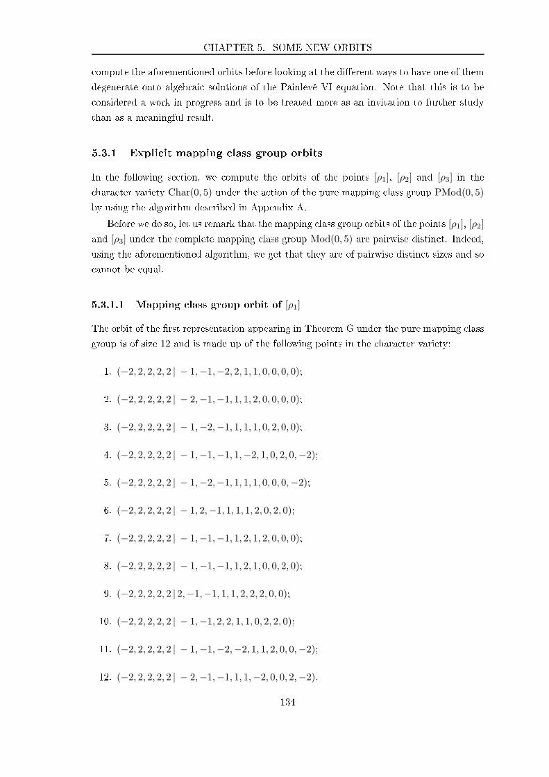
CHAPTER 5. SOME NEW ORBITS
ompute the aforementioned orbits before looking at the dierent ways to have one of them
degenerate onto algebrai solutions of the Painlevé VI equation. Note that this is to be
onsidered a work in progress and is to be treated more as an invitation to further study
than as a meaningful result.
5.3.1 Expli it mapping lass group orbits
In the following se tion, we ompute the orbits of the points [ρ1], [ρ2] and [ρ3] in the
hara ter variety Char(0, 5) under the a tion of the pure mapping lass group PMod(0, 5)
by using the algorithm des ribed in Appendix A.
Before we do so, let us remark that the mapping lass group orbits of the points [ρ1], [ρ2]
and [ρ3] under the omplete mapping lass group Mod(0, 5) are pairwise distin t. Indeed,
using the aforementioned algorithm, we get that they are of pairwise distin t sizes and so
annot be equal.
5.3.1.1 Mapping lass group orbit of [ρ1]
The orbit of the rst representation appearing in Theorem G under the pure mapping lass
group is of size 12 and is made up of the following points in the hara ter variety:
1. (−2, 2, 2, 2, 2 | − 1,−1,−2, 2, 1, 1, 0, 0, 0, 0);
2. (−2, 2, 2, 2, 2 | − 2,−1,−1, 1, 1, 2, 0, 0, 0, 0);
3. (−2, 2, 2, 2, 2 | − 1,−2,−1, 1, 1, 1, 0, 2, 0, 0);
4. (−2, 2, 2, 2, 2 | − 1,−1,−1, 1,−2, 1, 0, 2, 0,−2);
5. (−2, 2, 2, 2, 2 | − 1,−2,−1, 1, 1, 1, 0, 0, 0,−2);
6. (−2, 2, 2, 2, 2 | − 1, 2,−1, 1, 1, 1, 2, 0, 2, 0);
7. (−2, 2, 2, 2, 2 | − 1,−1,−1, 1, 2, 1, 2, 0, 0, 0);
8. (−2, 2, 2, 2, 2 | − 1,−1,−1, 1, 2, 1, 0, 0, 2, 0);
9. (−2, 2, 2, 2, 2 | 2,−1,−1, 1, 1, 2, 2, 2, 0, 0);
10. (−2, 2, 2, 2, 2 | − 1,−1, 2, 2, 1, 1, 0, 2, 2, 0);
11. (−2, 2, 2, 2, 2 | − 1,−1,−2,−2, 1, 1, 2, 0, 0,−2);
12. (−2, 2, 2, 2, 2 | − 2,−1,−1, 1, 1,−2, 0, 0, 2,−2).
134
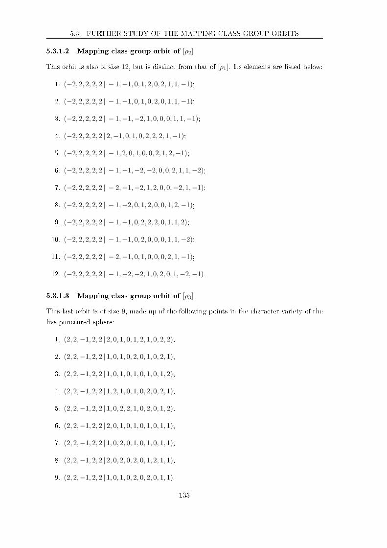
5.3. FURTHER STUDY OF THE MAPPING CLASS GROUP ORBITS
5.3.1.2 Mapping lass group orbit of [ρ2]
This orbit is also of size 12, but is distin t from that of [ρ1]. Its elements are listed below:
1. (−2, 2, 2, 2, 2 | − 1,−1, 0, 1, 2, 0, 2, 1, 1,−1);
2. (−2, 2, 2, 2, 2 | − 1,−1, 0, 1, 0, 2, 0, 1, 1,−1);
3. (−2, 2, 2, 2, 2 | − 1,−1,−2, 1, 0, 0, 0, 1, 1,−1);
4. (−2, 2, 2, 2, 2 | 2,−1, 0, 1, 0, 2, 2, 2, 1,−1);
5. (−2, 2, 2, 2, 2 | − 1, 2, 0, 1, 0, 0, 2, 1, 2,−1);
6. (−2, 2, 2, 2, 2 | − 1,−1,−2,−2, 0, 0, 2, 1, 1,−2);
7. (−2, 2, 2, 2, 2 | − 2,−1,−2, 1, 2, 0, 0,−2, 1,−1);
8. (−2, 2, 2, 2, 2 | − 1,−2, 0, 1, 2, 0, 0, 1, 2,−1);
9. (−2, 2, 2, 2, 2 | − 1,−1, 0, 2, 2, 2, 0, 1, 1, 2);
10. (−2, 2, 2, 2, 2 | − 1,−1, 0, 2, 0, 0, 0, 1, 1,−2);
11. (−2, 2, 2, 2, 2 | − 2,−1, 0, 1, 0, 0, 0, 2, 1,−1);
12. (−2, 2, 2, 2, 2 | − 1,−2,−2, 1, 0, 2, 0, 1,−2,−1).
5.3.1.3 Mapping lass group orbit of [ρ3]
This last orbit is of size 9, made up of the following points in the hara ter variety of the
ve pun tured sphere:
1. (2, 2,−1, 2, 2 | 2, 0, 1, 0, 1, 2, 1, 0, 2, 2);
2. (2, 2,−1, 2, 2 | 1, 0, 1, 0, 2, 0, 1, 0, 2, 1);
3. (2, 2,−1, 2, 2 | 1, 0, 1, 0, 1, 0, 1, 0, 1, 2);
4. (2, 2,−1, 2, 2 | 1, 2, 1, 0, 1, 0, 2, 0, 2, 1);
5. (2, 2,−1, 2, 2 | 1, 0, 2, 2, 1, 0, 2, 0, 1, 2);
6. (2, 2,−1, 2, 2 | 2, 0, 1, 0, 1, 0, 1, 0, 1, 1);
7. (2, 2,−1, 2, 2 | 1, 0, 2, 0, 1, 0, 1, 0, 1, 1);
8. (2, 2,−1, 2, 2 | 2, 0, 2, 0, 2, 0, 1, 2, 1, 1);
9. (2, 2,−1, 2, 2 | 1, 0, 1, 0, 2, 0, 2, 0, 1, 1).
135

CHAPTER 5. SOME NEW ORBITS
5.3.2 Regression to Painlevé VI
In this paragraph, we take a loser look at the orbit of the point
[ρ3] = (2, 2,−1, 2, 2 | 2, 0, 1, 0, 1, 2, 1, 0, 2, 2) ∈ Char(0, 5)
under the a tion of the pure mapping lass group PMod(0, 5). The idea here is the fol-
lowing: sin e the orbit of [ρ3] under the mapping lass group a tion is of size 9, the
orresponding algebrai Garnier solution must be a ninebran hed multivalued fun tion
over P1×P1(with oordinates t1 and t2) and the a tion of PMod(0, 5) permutes these nine
bran hes. This means that if one was to asso iate an a tual isomonodromi deformation
to [ρ3], one would have to do so on a 9 : 1 bran hed over over P1 × P1, so the upshot
would be to fully understand the latter.
One angle we explored during this thesis was to try and understand how su h an
isomonodromi deformation would behave should two of its singular points onate. More
pre isely, imagine that we have an isomonodromi deformation (∇t1,t2)t1,t2 of the ve
pun tured sphere with monodromy ρ3; this implies in parti ular that for any pair (t1, t2)
of distin t points in C∗ \ 0, 1, ∇t1,t2 is a logarithmi at onne tion over the pun tured
sphere P1 \ 0, 1, t1, t2,∞. If one looks at the (formal) limit of this family of onne tions
when (for example) t1 goes to 0, one gets an isomonodromi deformation over the four
pun tured sphere and thus obtains an algebrai solution of the Painlevé VI equation. Sin e
those have been lassied [42, we an give a omplete des ription of those "regressions".
5.3.2.1 Ex erpt from the lassi ation of algebrai Painlevé VI solutions
What follows is taken dire tly from [42; we give a brief des ription of the algebrai so-
lutions of the Painlevé VI that we will need later on. Re all that the following algebrai
oordinates hara terise the point in Char(0, 4) asso iated with some quadruplet of matri-
es (M1, . . . ,M4) ∈ SL2(C)4whose produ t is the identity (see Se tion I1.3):
a := Tr(M1), b := Tr(M2), c := Tr(M3), d := Tr(M4),
x := Tr(M1M2), y := Tr(M2M3), z := −Tr(M1M3).
However, for the sake of onvenien e, we will use the same oordinates than Tykhyy and
Lisovyy in their paper [42:
ωX := Tr(M3)Tr(M4) + Tr(M1)Tr(M2), ωY := Tr(M2)Tr(M4) + Tr(M1)Tr(M3),
ωZ := Tr(M1)Tr(M4) + Tr(M2)Tr(M3),
X := Tr(M1M2), Y := Tr(M1M3), Z := −Tr(M2M3).
Note that ωX , ωY and ωZ are invariant under the a tion of PMod(0, 4). The lassi ation
by Lisovyy and Tykhyy of the algebrai solutions of the sixth Painlevé equation tells us
that the only nonrigid families of solutions are the following (up to Okamoto symmetries):
136
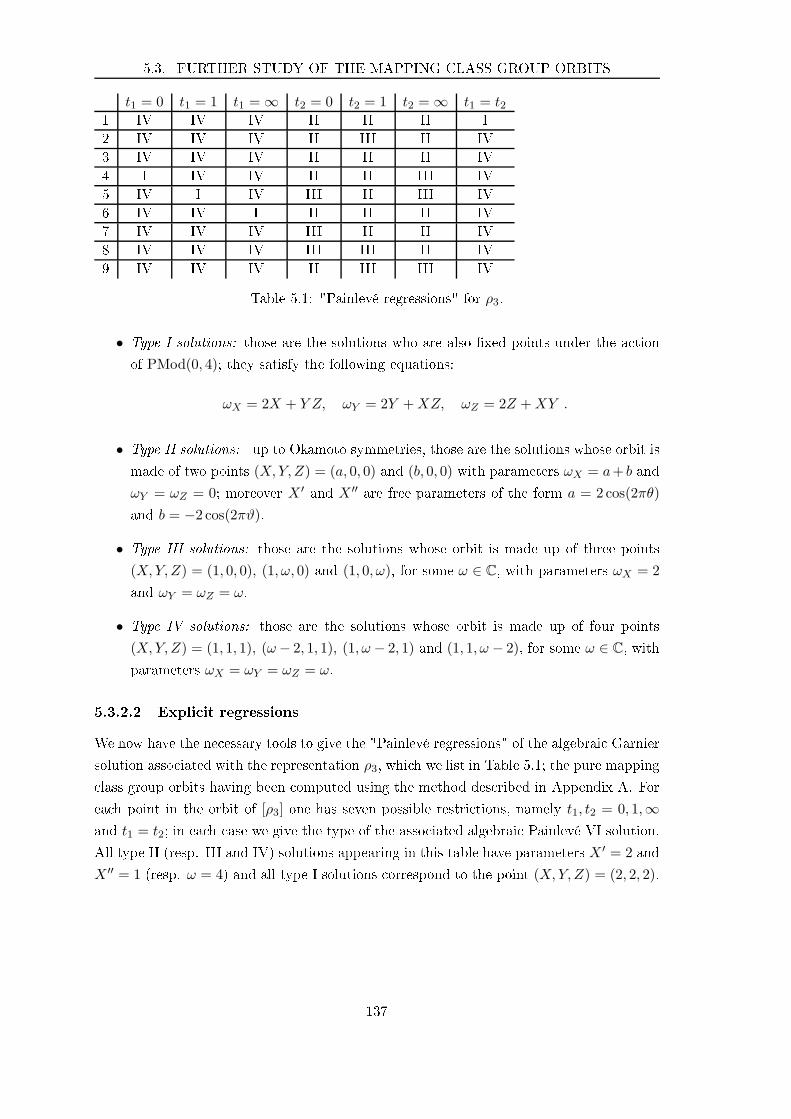
5.3. FURTHER STUDY OF THE MAPPING CLASS GROUP ORBITS
t1 = 0 t1 = 1 t1 = ∞ t2 = 0 t2 = 1 t2 = ∞ t1 = t21 IV IV IV II II II I
2 IV IV IV II III II IV
3 IV IV IV II II II IV
4 I IV IV II II III IV
5 IV I IV III II III IV
6 IV IV I II II II IV
7 IV IV IV III II II IV
8 IV IV IV III III II IV
9 IV IV IV II III III IV
Table 5.1: "Painlevé regressions" for ρ3.
• Type I solutions: those are the solutions who are also xed points under the a tion
of PMod(0, 4); they satisfy the following equations:
ωX = 2X + Y Z, ωY = 2Y +XZ, ωZ = 2Z +XY .
• Type II solutions: up to Okamoto symmetries, those are the solutions whose orbit is
made of two points (X,Y,Z) = (a, 0, 0) and (b, 0, 0) with parameters ωX = a+ b and
ωY = ωZ = 0; moreover X ′and X ′′
are free parameters of the form a = 2cos(2πθ)
and b = −2 cos(2πϑ).
• Type III solutions: those are the solutions whose orbit is made up of three points
(X,Y,Z) = (1, 0, 0), (1, ω, 0) and (1, 0, ω), for some ω ∈ C, with parameters ωX = 2
and ωY = ωZ = ω.
• Type IV solutions: those are the solutions whose orbit is made up of four points
(X,Y,Z) = (1, 1, 1), (ω− 2, 1, 1), (1, ω − 2, 1) and (1, 1, ω − 2), for some ω ∈ C, with
parameters ωX = ωY = ωZ = ω.
5.3.2.2 Expli it regressions
We now have the ne essary tools to give the "Painlevé regressions" of the algebrai Garnier
solution asso iated with the representation ρ3, whi h we list in Table 5.1; the pure mapping
lass group orbits having been omputed using the method des ribed in Appendix A. For
ea h point in the orbit of [ρ3] one has seven possible restri tions, namely t1, t2 = 0, 1,∞and t1 = t2; in ea h ase we give the type of the asso iated algebrai Painlevé VI solution.
All type II (resp. III and IV) solutions appearing in this table have parameters X ′ = 2 and
X ′′ = 1 (resp. ω = 4) and all type I solutions orrespond to the point (X,Y,Z) = (2, 2, 2).
137

CHAPTER 5. SOME NEW ORBITS
138
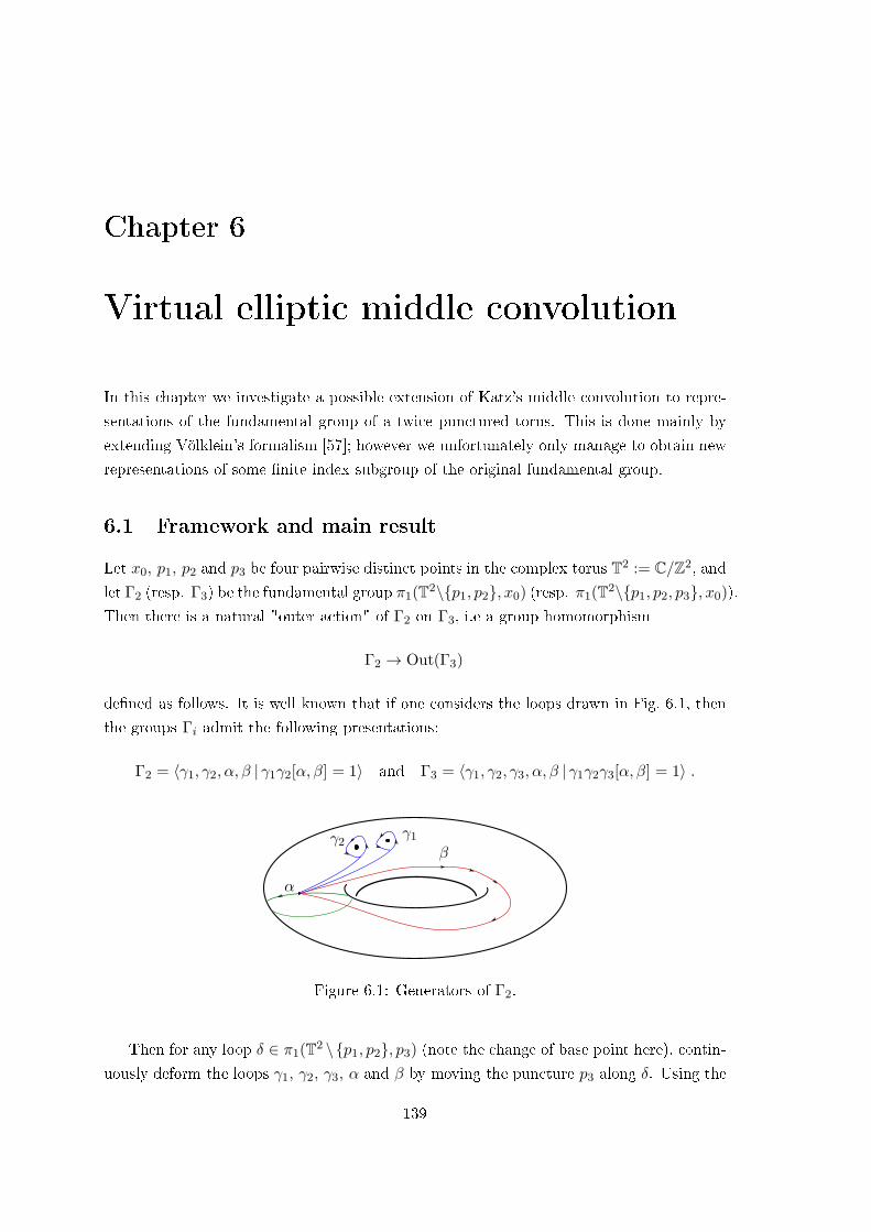
Chapter 6
Virtual ellipti middle onvolution
In this hapter we investigate a possible extension of Katz's middle onvolution to repre-
sentations of the fundamental group of a twi e pun tured torus. This is done mainly by
extending Völklein's formalism [57; however we unfortunately only manage to obtain new
representations of some nite index subgroup of the original fundamental group.
6.1 Framework and main result
Let x0, p1, p2 and p3 be four pairwise distin t points in the omplex torus T2 := C/Z2, and
let Γ2 (resp. Γ3) be the fundamental group π1(T2\p1, p2, x0) (resp. π1(T2\p1, p2, p3, x0)).
Then there is a natural "outer a tion" of Γ2 on Γ3, i.e a group homomorphism
Γ2 → Out(Γ3)
dened as follows. It is well known that if one onsiders the loops drawn in Fig. 6.1, then
the groups Γi admit the following presentations:
Γ2 = 〈γ1, γ2, α, β | γ1γ2[α, β] = 1〉 and Γ3 = 〈γ1, γ2, γ3, α, β | γ1γ2γ3[α, β] = 1〉 .
γ2 γ1β
α
Figure 6.1: Generators of Γ2.
Then for any loop δ ∈ π1(T2 \p1, p2, p3) (note the hange of base point here), ontin-
uously deform the loops γ1, γ2, γ3, α and β by moving the pun ture p3 along δ. Using the
139
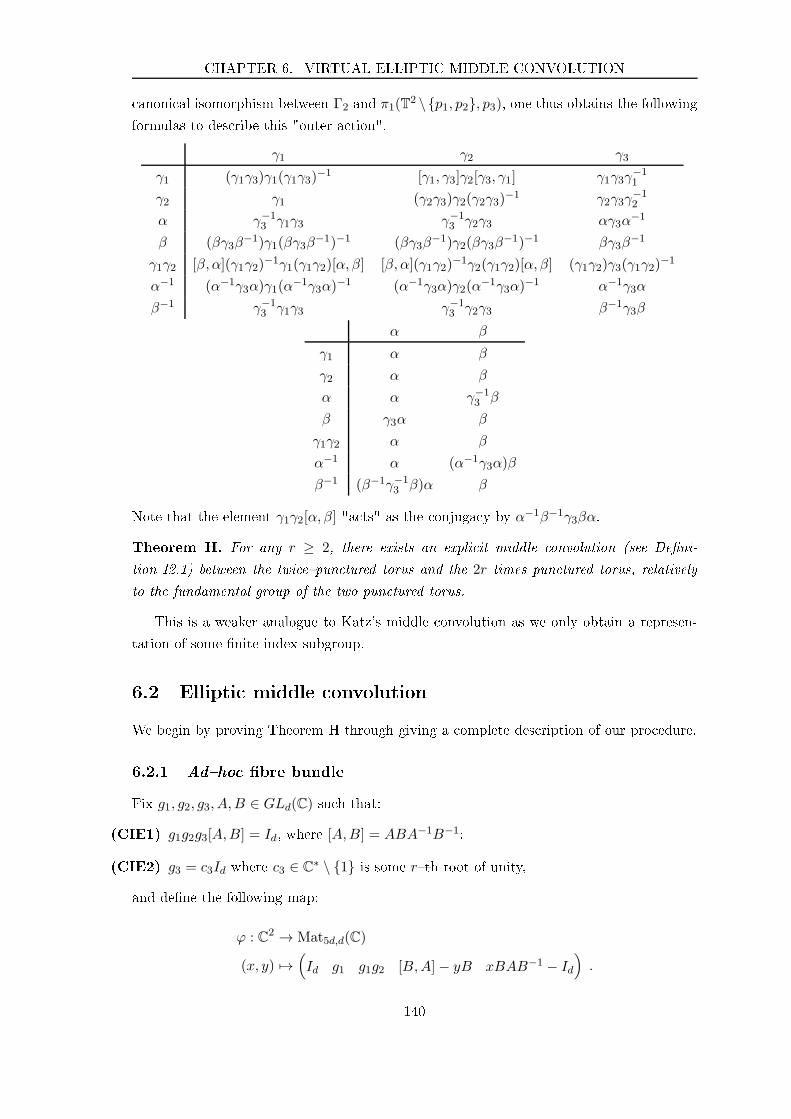
CHAPTER 6. VIRTUAL ELLIPTIC MIDDLE CONVOLUTION
anoni al isomorphism between Γ2 and π1(T2 \p1, p2, p3), one thus obtains the following
formulas to des ribe this "outer a tion".
γ1 γ2 γ3
γ1 (γ1γ3)γ1(γ1γ3)−1 [γ1, γ3]γ2[γ3, γ1] γ1γ3γ
−11
γ2 γ1 (γ2γ3)γ2(γ2γ3)−1 γ2γ3γ
−12
α γ−13 γ1γ3 γ−1
3 γ2γ3 αγ3α−1
β (βγ3β−1)γ1(βγ3β
−1)−1 (βγ3β−1)γ2(βγ3β
−1)−1 βγ3β−1
γ1γ2 [β, α](γ1γ2)−1γ1(γ1γ2)[α, β] [β, α](γ1γ2)
−1γ2(γ1γ2)[α, β] (γ1γ2)γ3(γ1γ2)−1
α−1 (α−1γ3α)γ1(α−1γ3α)
−1 (α−1γ3α)γ2(α−1γ3α)
−1 α−1γ3α
β−1 γ−13 γ1γ3 γ−1
3 γ2γ3 β−1γ3β
α β
γ1 α β
γ2 α β
α α γ−13 β
β γ3α β
γ1γ2 α β
α−1 α (α−1γ3α)β
β−1 (β−1γ−13 β)α β
Note that the element γ1γ2[α, β] "a ts" as the onjuga y by α−1β−1γ3βα.
Theorem H. For any r ≥ 2, there exists an expli it middle onvolution (see Deni-
tion I2.1) between the twi epun tured torus and the 2r times pun tured torus, relatively
to the fundamental group of the two pun tured torus.
This is a weaker analogue to Katz's middle onvolution as we only obtain a represen-
tation of some nite index subgroup.
6.2 Ellipti middle onvolution
We begin by proving Theorem H through giving a omplete des ription of our pro edure.
6.2.1 Adho bre bundle
Fix g1, g2, g3, A,B ∈ GLd(C) su h that:
(CIE1) g1g2g3[A,B] = Id, where [A,B] = ABA−1B−1;
(CIE2) g3 = c3Id where c3 ∈ C∗ \ 1 is some rth root of unity,
and dene the following map:
ϕ : C2 → Mat5d,d(C)
(x, y) 7→(
Id g1 g1g2 [B,A]− yB xBAB−1 − Id
)
.
140
6.2. ELLIPTIC MIDDLE CONVOLUTION
The above denes a morphism of ve tor bundles
C2 ×X
ϕ// C2 × Cd
xxrrrrrrrrrrr
C2
where X := Im(Id − g1)× Im(Id − g2)× C3d; note that for all x, y ∈ C2
one has
rank(ϕ(x, y)) = d .
This means that one an onsider the rank ℓ kernel bundle U := Ker(ϕ) → C2, with
ℓ := rank(Id − g1) + rank(Id − g2) + 2d .
6.2.2 Ane group and a tion on ane representations
Re all that the ddimensional ane group on a eld k is dened as the semidire t produ t
GAd(k) := kd ⋊ GLd(k), where if M ∈ GLd(k) and u ∈ kd we denote by (u,M) the
asso iated element in GAd(k) and set:
∀M,N ∈ GLd(k), ∀u, v ∈ kd, (u,M) · (v,N) := (u+Mv,MN) .
There is a natural group homomorphism between GAd(k) and GLd+1(k) given by:
(u,M) 7→(
M u
0 Id
)
.
Let ρ : Γ3 → GAd(k) be a group morphism. Then the above "outer a tion" of Γ2 on Γ3
gives rise to a group homomorphism Γ2 → Out(Im(ρ)) ≤ GAd(k).
Let (x, y) ∈ C2and u ∈ U(x,y); one has a natural group morphism ρ : Γ3 → GAd(C)
given by ∀i ∈ [3], ρ(γi) := (ui, gi), ρ(α) := (uA, xA) and ρ(β) := (uB , yB). Thus, the
"outer a tion" of Γ2 on Γ3 des ribed earlier gives us four mappings F1, F2, FA and FB ,
asso iated with the loops γ1, γ2, α and β in Γ2, that an be des ribed as follows.
• F1 and F2 a t trivially on the base, so they an be seen as linear automorphisms of
the bre U(x,y) a ting as the right multipli ation by the following matri es:
F1 :=
t
Id + g3g1 − g1 (g3 − Id)(g2 − Id) Id − g3 0 0
0 Id 0 0 0
g1(Id − g1) (g1 − Id)(Id − g2) g1 0 0
0 0 0 Id 0
0 0 0 0 Id
,
141

CHAPTER 6. VIRTUAL ELLIPTIC MIDDLE CONVOLUTION
F2 :=
t
Id 0 0 0 0
0 Id + g2g3 − g2 (Id − g3) 0 0
0 g2(Id − g2) g2 0 0
0 0 0 Id 0
0 0 0 0 Id
.
• FA a ts as (x, y) →(
x, yc3
)
on the base and as a linear isomorphism between bres
U(x,y) and U(x,c−13 y) given by the right multipli ation by the matrix:
FA :=
t
g−13 0 0 0 0
0 g−13 0 0 0
g−13 (g1 − Id) g−1
3 (g2 − Id) xA 0 −g−13
0 0 (Id − g3) Id 0
0 0 0 0 g−13
.
• Similarly, FB a ts as (x, y) → (x, c3y) on the base and as a linear isomorphism
between bres U(x,y) and U(x,c3y) given by the right multipli ation by the matrix:
FB :=
t
g3 0 0 0 0
0 g3 0 0 0
yB(Id − g1) yB(Id − g2) yB Id 0
0 0 0 g3 0
(g3 − Id)(g1 − Id) (g3 − Id)(g2 − Id) Id − g3 0 Id
.
6.2.3 A quotient ve tor spa e
The kernel ve tor bundle U has k linearly independent holomorphi se tions given by the
following formula, for u3 := (u1, u2, uA, uB) ∈ Im(Id − g1)× Im(Id − g2)× C2d:
σu3 : (x, y) 7→
u1
u2
−(g1g2)−1(u1 + g1u2 + ([B,A]− yB)uA + (xBAB−1 − Id)uB)
uA
uB
.
Let us denote by Σ the C(x, y)ve tor spa e spanned by these se tions ; right multipli ation
by the matri es F1, F2, FA and FB dened above gives us four linear automorphisms of this
142

6.2. ELLIPTIC MIDDLE CONVOLUTION
ve tor spa e through the following formulas, for σ ∈ Σ:
Fi · σ : (x, y) 7→ σ(x, y)Fi ∈ U(x,y) (i ∈ [2]) ;
FA · σ : (x, y) 7→ σ
(
x,y
c3
)
FA
(
x,y
c3
)
∈ U(x,c−13 y) ;
FB · σ : (x, y) 7→ σ (x, c3y)FB (x, c3y) ∈ U(x,c3y) .
Moreover, sin e γ1γ2[α, β] ∈ Γ2 a ts as the onjuga y by α−1β−1γ3βα on Γ3, F1F2[FA, FB ]
a ts on GAd(C) as the onjuga y by ((uB , yB) · (uA, xA))−1 · (u3, g3) · (uB , yB) · (uA, xA),whi h happens to have linear part equal to g3 sin e the latter ommutes to all of GLd(C).
Therefore, again be ause g3 is a s alar matrix, F1F2[FA, FB ] a ts on GAd(C) as the on-
juga y by a translation.
Therefore, a prerequisite to developing a working framework for our middle onvolution
will be to "kill" the diagonal a tion of Cd over U . More pre isely, remark that for all
(x, y) ∈ C2, u ∈ U(x,y) and for all v ∈ Cd, one gets:
(v, Id)·((u1, g1), (u2, g2), (u3, g3), (uA, A), (uB , B))·(−v, Id) = ((u1+(1−g1)v, g1), . . . , (uB+(1−B)v,B)) ,
therefore it makes sense to set
ψ(x, y) :=
Id − g1
Id − g2
Id − g3
Id − xA
Id − yB
and to onsider the quotient C(x, y)ve tor spa e
E := Σ/V ,
where V ⊂ Σ is the linear span 〈σv | v ∈ Cd〉 with
1σv : (x, y) 7→
(Id − g1)v
(Id − g2)v
(1− c3)v
(Id − xA)v
(Id − yB)v
.
The linear isomorphisms F1 and F2, a t trivially on V , therefore they a t on the quotient
E but this not the ase for FA and FB as they do not a t trivially on the base. So we need
to onsider the subgroup
〈F1, F2, FrA, F
rB〉 ≤ 〈F1, F2, FA, FB〉
143
CHAPTER 6. VIRTUAL ELLIPTIC MIDDLE CONVOLUTION
who does a t trivially on V sin e cr3 = 1. Therefore, one gets a group a tion of
Γr2 := 〈γ1, γ2, αr, βr〉 ≤ Γ2
on the quotient ve tor spa e E, whose dimension is:
dim(E) = dim(Σ)− d = rank(Id − g1) + rank(Id − g2) + d . (E6.1)
The subgroup Γr2 has nite index equal to 2r in Γ2; furthermore, it is isomorphi to the
fundamental group of a omplex torus with 4r pun tures. Indeed, sin e it is an index 2r
subgroup of Γ2, there exists a 2rfold ramied over X over the twi e pun tured torus
su h that Γr2∼= π1(X) and the orbifold RiemannHurwitz formula ensures that X must be
a 4r pun tured omplex torus.
6.2.4 Algorithm
Start with a group representation ρ : Γ2 → SLd(C) and let hi := ρ(γi) for i ∈ [2],
A0 := ρ(α) and B0 := ρ(β); hoose four nonzero omplex numbers θ1, θ2, θα and θβ su h
that c3 := θ1θ2θαθβ 6= 1 is a rth root of unity. Now set gi := θihi (i ∈ [2]), g3 := c3Id and
A := θαA0, B := θβB0. We now have ve matri es g1, g2, g3, A,B ∈ GLd(C) satisfying the
following onditions:
(CIE1) g1g2g3[A,B] = Id, where [A,B] = ABA−1B−1;
(CIE2) g3 = c3Id where c3 ∈ C∗ \ 1 is some rth root of unity.
Considering the index 2r subgroup
Γr2 := 〈γ1, γ2, αr, βr〉 ≤ Γ2
isomorphi to the fundamental group of a torus with 4r pun tures, we an dene a (weaker)
analog to Katz's middle onvolution in this parti ular ase.
Denition 6.2.1 (Virtual ellipti middle onvolution). Suppose that we have ρ and θ
satisfying the above onditions. Let g1, g2, A, B be the matri es of size
dρ := rank(Id − g1) + rank(Id − g2) + d
orresponding to the a tion of F1, F2, FrA, F
rB on the quotient ve tor spa e E dened in
Se tion 6.2.3. Then we dene the virtual ellipti middle onvolution of ρ with respe t to θ
as the group representation
Eθ(ρ) : Γr2 → SLdρ(C)
dened by
γ1 7→1
τ1g1, γ2 7→
τ1τAτBc3τ2
g2, α 7→ 1
τAA, β 7→ 1
τBB ,
144
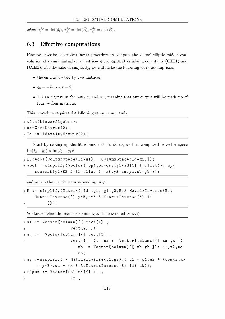
6.3. EFFECTIVE COMPUTATIONS
where τdρi = det(gi), τ
dρA = det(A), τ
dρB = det(B).
6.3 Ee tive omputations
Now we des ribe an expli it Maple pro edure to ompute the virtual ellipti middle on-
volution of some quintuplet of matri es g1, g2, g3, A,B satisfying onditions (CIE1) and
(CIE1). For the sake of simpli ity, we will make the following extra assumptions:
• the entries are two by two matri es;
• g3 = −I2, i.e r = 2;
• 1 is an eigenvalue for both g1 and g2 , meaning that our output will be made up of
four by four matri es.
This pro edure requires the following setup ommands.
1 with(LinearAlgebra):
2 o:= ZeroMatrix(2):
3 Id := IdentityMatrix(2):
Start by setting up the bre bundle U ; to do so, we rst ompute the ve tor spa e
Im(I2 − g1)× Im(I2 − g1):
1 ES:=op([ ColumnSpa e(Id-g1), ColumnSpa e(Id-g2));
2 ve t := simplify (Ve tor([op( onvert(y1*ES[1[1 , list)), op(
onvert(y2*ES[2[1 , list)) ,x3,y3,xa,ya,xb,yb));
and set up the matrix M orresponding to ϕ.
1 M := simplify (Matrix([Id ,g1, g1.g2,B.A.MatrixInverse(B).
MatrixInverse(A)-y*B,x*B.A.MatrixInverse(B)-Id
2 ));
We know dene the se tions spanning Σ (here denoted by sei)
1 u1 := Ve tor[ olumn ([ ve t[1 ,
2 ve t[2 ):
3 u2 := Ve tor[ olumn ([ ve t[3 ,
4 ve t[4 ): ua := Ve tor[ olumn ([ xa,ya ):
ub := Ve tor[ olumn ([ xb,yb ): u1,u2,ua,
ub;
5 u3 := simplify ( - MatrixInverse(g1.g2).( u1 + g1.u2 + (Com(B,A)
- y*B).ua + (x*B.A.MatrixInverse(B)-Id).ub));
6 sigma := Ve tor[ olumn ([ u1 ,
7 u2 ,
145
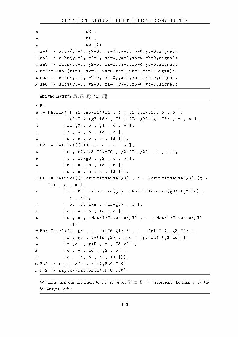
CHAPTER 6. VIRTUAL ELLIPTIC MIDDLE CONVOLUTION
8 u3 ,
9 ua ,
10 ub );
11 se1 := subs(y1=1, y2=0, xa=0,ya=0,xb=0,yb=0,sigma):
12 se2 := subs(y1=0, y2=1, xa=0,ya=0,xb=0,yb=0,sigma):
13 se3 := subs(y1=0, y2=0, xa=1,ya=0,xb=0,yb=0,sigma):
14 se4:= subs(y1=0, y2=0, xa=0,ya=1,xb=0,yb=0,sigma):
15 se5 := subs(y1=0, y2=0, xa=0,ya=0,xb=1,yb=0,sigma):
16 se6 := subs(y1=0, y2=0, xa=0,ya=0,xb=0,yb=1,sigma):
and the matri es F1, F2, F2A and F 2
B .
1 F1
2 := Matrix ([[ g1.(g3-Id)+Id , o , g1.(Id-g1), o , o ,
3 [ (g2-Id).(g3-Id) , Id , (Id-g2).(g1-Id) , o , o ,
4 [ Id-g3 , o , g1 , o , o ,
5 [ o , o , o , Id , o ,
6 [ o , o , o , o , Id );
7 F2 := Matrix ([[ Id ,o, o , o , o ,
8 [ o , g2.(g3-Id)+Id , g2.(Id-g2) , o , o ,
9 [ o , Id-g3 , g2 , o , o ,
10 [ o , o , o , Id , o ,
11 [ o , o , o , o , Id );
12 Fa := Matrix ([[ MatrixInverse(g3) , o , MatrixInverse(g3).(g1-
Id) , o , o ,
13 [ o , MatrixInverse(g3) , MatrixInverse(g3).(g2-Id) ,
o , o ,
14 [ o, o, x*A , (Id-g3) , o ,
15 [ o , o , o , Id , o ,
16 [ o , o , -MatrixInverse(g3) , o , MatrixInverse(g3)
);
17 Fb:=Matrix ([[ g3 , o ,y*(Id-g1).B , o , (g1-Id).(g3-Id) ,
18 [ o , g3 , y*(Id-g2).B , o , (g2-Id).(g3-Id) ,
19 [ o ,o , y*B , o , Id-g3 ,
20 [ o , o , Id , g3 , o ,
21 [ o , o, o , o , Id );
22 Fa2 := map(x->fa tor(x),Fa0.Fa0)
23 Fb2 := map(x->fa tor(x),Fb0.Fb0)
We then turn our attention to the subspa e V ⊂ Σ ; we represent the map ψ by the
following matrix:
146
6.3. EFFECTIVE COMPUTATIONS
1 N:= simplify (Matrix ([[ Id - g1, [Id - g2, [Id - g3, [Id -x*A
, [Id - y*B));
In order to expli itly ompute the a tion of the braids Fi on the quotient E = Σ/V we
need to nd an adequate basis of Σ.
1 e1 := Ve tor[ olumn ([ 1 ,
2 0 ): e2 := Ve tor[ olumn ([ 0 ,
3 1 ):
4
5
6 sf1 := onvert(simplify (Matrix ([[ (Id - g1).e1,[(Id - g2).e1
,[(Id - g3).e1,[(Id -x*A).e1,[(Id - y*B).e1)),Ve tor):
sf2 := onvert(simplify (Matrix ([[ (Id - g1).e2,[(Id - g2)
.e2,[(Id - g3).e2,[(Id -x*A).e2,[(Id - y*B).e2)),
Ve tor): sf1 ,sf2;
Assume for the sake of simpli ity that the rank of the family (se1,se2,se3,se4,sf1,sf1)
is six (up to hanging one or more of the sei); now we an ompute the virtual ellipti
middle onvolution of our initial quintuplet by applying the following pro edure
1 CME := pro (F)
2 lo al sol1 , sol2 ,sol3 ,sol4
3 simplify (F.se1 -(x1*se1+x2*se2+x3*se3+x4*se4+x5*sf1+x6*sf2)):
sol1:= solve( onvert (%,set),x1,x2,x3,x4,x5,x6):
4 simplify (F.se2 -(x1*se1+x2*se2+x3*se3+x4*se4+x5*sf1+x6*sf2)):
sol2:= solve( onvert (%,set),x1,x2,x3,x4,x5,x6):
5 simplify (F.se3 -(x1*se1+x2*se2+x3*se3+x4*se4+x5*sf1+x6*sf2)):
sol3:= solve( onvert (%,set),x1,x2,x3,x4,x5,x6):
6 simplify (F.se4 -(x1*se1+x2*se2+x3*se3+x4*se4+x5*sf1+x6*sf2)):
sol4:= solve( onvert (%,set),x1,x2,x3,x4,x5,x6):
7 RETURN(simplify (Transpose (Matrix ([[ eval(x1,sol1) , eval(x1,
sol2) , eval(x1,sol3),eval(x1,sol4) ,
8 [ eval(x2,sol1) , eval(x2,sol2) , eval(x2,sol3),eval(
x2,sol4),
9 [ eval(x3,sol1) , eval(x3,sol2) , eval(x3,sol3),eval(x3,sol4)
,
10 [ eval(x4,sol1) , eval(x4,sol2) , eval(x4,sol3),eval(x4,sol4)
)))):
11 end pro :
to the list below.
1 F := [F1,F2,Fa2 ,Fb2:
147

CHAPTER 6. VIRTUAL ELLIPTIC MIDDLE CONVOLUTION
148
Appendi es
149

Appendix A
Computing mapping lass group
orbits
The purpose of this appendix is to des ribe the algorithm we used in various part of our
work to ompute the orbit of sele ted point of hara ter varieties of pun tured spheres.
For the sake of simpli ity we will give a omplete overview of the ve pun tured ase, as
it is the most relevant to our study.
1.1 Pure mapping lass group orbits
All of the following Maple pro edures make use of the LinearAlgebra library. We start
by dening a simple but useful auxiliary fun tion giving the oordinates of the point in
Char(0, 5) asso iated with some list of ve matri es L.
1 Ch:= pro (L)
2 RETURN(map(x->fa tor(x) ,[Tra e(L[1), Tra e(L[2), Tra e(L[3)
, Tra e(L[4),Tra e(L[1.L[2),Tra e(L[1.L[3),Tra e(L[1.
L[4),Tra e(L[2.L[3),Tra e(L[2.L[4),Tra e(L[3.L[4),
Tra e(L[1.L[2.L[3),Tra e(L[1.L[2.L[4),Tra e(L[1.L
[3.L[4),Tra e(L[2.L[3.L[4),Tra e(L[1.L[2.L[3.L[4)
)): end pro :
Now re all that sin e we have the following isomorphism:
PMod(0, 5) ∼= PB4∼= Z(PB4)
we only need to ompute the a tion of the pure braid group PB4 on quintuplets of matri es,
so we start by dening pro edures realising the a tion of the elementary braids σi (and of
their inverses) su h that
B4 = 〈σ1, σ2, σ3 | [σ1, σ3], σ1σ2σ1 = σ2σ1σ2, σ3σ2σ3 = σ2σ3σ2〉 .
151

APPENDIX A. COMPUTING MAPPING CLASS GROUP ORBITS
1 s1 := pro (L)
2 RETURN([ simplify (L[1.L[2. MatrixInverse(L[1)),L[1,L[3,L
[4,L[5):
3 end pro :
4 s2 := pro (L)
5 RETURN([L[1, simplify (L[2.L[3.MatrixInverse(L[2)),L[2,L
[4,L[5):
6 end pro :
7 s3 := pro (L)
8 RETURN([L[1,L[2, simplify (L[3.L[4.MatrixInverse(L[3)),L
[3,L[5):
9 end pro :
10 s1i := pro (L)
11 RETURN([L[2, simplify (MatrixInverse(L[2).L[1.L[2),L[3,L
[4,L[5):
12 end pro :
13 s2i := pro (L)
14 RETURN([L[1,L[3, simplify (MatrixInverse(L[3).L[2.L[3),L
[4,L[5):
15 end pro :
16 s3i := pro (L)
17 RETURN([L[1,L[2,L[4, simplify (MatrixInverse(L[4).L[3.L[4)
,L[5):
18 end pro :
This allows us to dene pro edures emulating the a tion of the generators of the pure braid
group, namely, for i ≤ j < 3:
σi,j := (σj . . . σi+1)σ2i (σj . . . σi+1)
−1 .
1 F1 := pro (L)
2 RETURN(Ts3(Ts2(Ts1(Ts1(Ts2i(Ts3i(L))))))):
3 end pro :
4 F2 := pro (L)
5 RETURN(Ts3(Ts2(Ts2(Ts3i(L))))):
6 end pro :
7 F3 := pro (L)
8 RETURN(Ts3(Ts3(L))):
9 end pro :
10 F4 := pro (L)
152
1.1. PURE MAPPING CLASS GROUP ORBITS
11 RETURN(Ts2(Ts1(Ts1(Ts2i(L))))):
12 end pro :
13 F5 := pro (L)
14 RETURN(Ts2(Ts2(L))):
15 end pro :
16 F6 := pro (L)
17 RETURN(Ts1(Ts1(L))):
18 end pro :
19 F1i := pro (L)
20 RETURN(Ts3(Ts2(Ts1i(Ts1i(Ts2i(Ts3i(L))))))):
21 end pro :
22 F2i := pro (L)
23 RETURN(Ts3(Ts2i(Ts2i(Ts3i(L))))):
24 end pro :
25 F3i := pro (L)
26 RETURN(Ts3i(Ts3i(L))):
27 end pro :
28 F4i := pro (L)
29 RETURN(Ts2(Ts1i(Ts1i(Ts2i(L))))):
30 end pro :
31 F5i := pro (L)
32 RETURN(Ts2i(Ts2i(L))):
33 end pro :
34 F6i := pro (L)
35 RETURN(Ts1i(Ts1i(L))):
36 end pro :
Now, we set the following list to ontain all generators of PB4 and their inverses
1 F:=[F1,F2,F3,F4,F5,F6,F1i ,F2i ,F3i ,F4i ,F5i ,F6i;
and use the following brutefor e algorithm to ompute the desired orbits.
1 Orb := pro (L)
2 lo al R,n,n0,k,i,M:
3 R := simplify ([L):
4 n0 := 0:
5 n := 1:
6 while n0<n do
7 for k from n0+1 to n do
8 for i from 1 to nops(F) do
9 M := map(x->fa tor(x),F[i(R[k)):
10 if not member(M,R) then
153
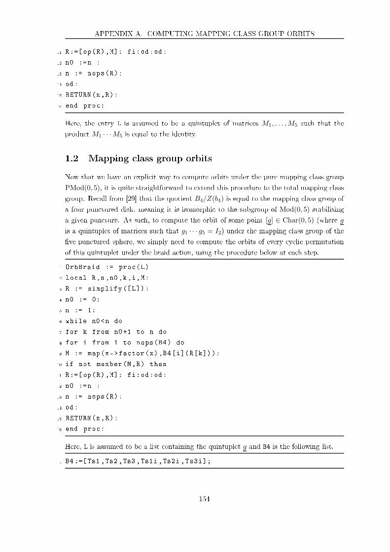
APPENDIX A. COMPUTING MAPPING CLASS GROUP ORBITS
11 R:=[op(R),M: fi:od:od:
12 n0 :=n :
13 n := nops(R):
14 od:
15 RETURN(n,R):
16 end pro :
Here, the entry L is assumed to be a quintuplet of matri es M1, . . . ,M5 su h that the
produ t M1 · · ·M5 is equal to the identity.
1.2 Mapping lass group orbits
Now that we have an expli it way to ompute orbits under the pure mapping lass group
PMod(0, 5), it is quite straightforward to extend this pro edure to the total mapping lass
group. Re all from [29 that the quotient B4/Z(b4) is equal to the mapping lass group of
a four pun tured disk, meaning it is isomorphi to the subgroup of Mod(0, 5) stabilising
a given pun ture. As su h, to ompute the orbit of some point [g] ∈ Char(0, 5) (where g
is a quintuplet of matri es su h that g1 · · · g5 = I2) under the mapping lass group of the
ve pun tured sphere, we simply need to ompute the orbits of every y li permutation
of this quintuplet under the braid a tion, using the pro edure below at ea h step.
1 OrbBraid := pro (L)
2 lo al R,n,n0,k,i,M:
3 R := simplify ([L):
4 n0 := 0:
5 n := 1:
6 while n0<n do
7 for k from n0+1 to n do
8 for i from 1 to nops(B4) do
9 M := map(x->fa tor(x),B4[i(R[k)):
10 if not member(M,R) then
11 R:=[op(R),M: fi:od:od:
12 n0 :=n :
13 n := nops(R):
14 od:
15 RETURN(n,R):
16 end pro :
Here, L is assumed to be a list ontaining the quintuplet g and B4 is the following list.
1 B4:=[Ts1 ,Ts2 ,Ts3 ,Ts1i ,Ts2i ,Ts3i;
154
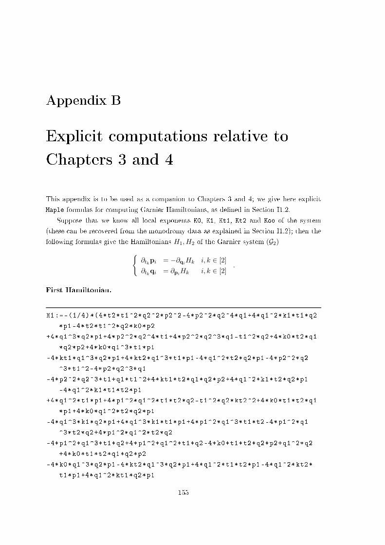
Appendix B
Expli it omputations relative to
Chapters 3 and 4
This appendix is to be used as a ompanion to Chapters 3 and 4; we give here expli it
Maple formulas for omputing Garnier Hamiltonians, as dened in Se tion I1.2.
Suppose that we know all lo al exponents K0, K1, Kt1, Kt2 and Koo of the system
(these an be re overed from the monodromy data as explained in Se tion I1.2); then the
following formulas give the Hamiltonians H1,H2 of the Garnier system (G2)
∂tkpi = −∂qiHk i, k ∈ [2]
∂tkqi = ∂piHk i, k ∈ [2]
.
First Hamiltonian.
H1:= -(1/4)*(4*t2*t1^2*q2^2*p2^2-4*p2^2*q2^4*q1+4*q1^2*k1*t1*q2
*p1 -4*t2*t1^2*q2*k0*p2
+4*q1^3*q2*p1+4*p2^2*q2^4*t1+4*p2^2*q2^3*q1-t1^2*q2+4*k0*t2*q1
*q2*p2+4*k0*q1^3*t1*p1
-4*kt1*q1^3*q2*p1+4*kt2*q1^3*t1*p1 -4*q1^2*t2*q2*p1 -4*p2^2*q2
^3*t1^2-4*p2*q2^3*q1
-4*p2^2*q2^3*t1+q1*t1^2+4*kt1*t2*q1*q2*p2+4*q1^2*k1*t2*q2*p1
-4*q1^2*k1*t1*t2*p1
+4*q1^2*t1*p1+4*p1^2*q1^2*t1*t2*q2-t1^2*q2*kt2 ^2+4*k0*t1*t2*q1
*p1+4*k0*q1^2*t2*q2*p1
-4*q1^3*k1*q2*p1+4*q1^3*k1*t1*p1+4*p1^2*q1^3*t1*t2 -4*p1^2*q1
^3*t2*q2+4*p1^2*q1^2*t2*q2
-4*p1^2*q1^3*t1*q2+4*p1^2*q1^2*t1*q2 -4*k0*t1*t2*q2*p2+q1^2*q2
+4*k0*t1*t2*q1*q2*p2
-4*k0*q1^3*q2*p1 -4*kt2*q1^3*q2*p1+4*q1^2*t1*t2*p1 -4*q1^2*kt2*
t1*p1+4*q1^2*kt1*q2*p1
155

APPENDIX B. EXPLICIT COMPUTATIONS
-4*q1^2*k0*t1*p1+4*k0*t1*q1*q2*p2+t1^2*q2*koo^2-t1^2*q2*k1^2-
t1^2*q2*kt1^2-
4*p1^2*q1^3*q2 -4*q1^2*q2*p1 -4*p1^2*q1^4*t1+4*p1^2*q1^3*t1+4*
kt2*t1*q1*q2*p2+4*q1*q2^2*p2
-4*k0*q1^2*t1*t2*p1+4*k0*q1^2*t1*q2*p1+4*kt1*q1^2*t2*q2*p1+4*
kt2*q1^2*t1*q2*p1 -4*t1^2*q2*k0*p2
+4*k0*t1*t2*q2*p1+4*t1^2*q2^2*p2^2-4*k1*t2*q1*q2^2*p2+4*k1*t1*
t2*q2^2*p2 -4*p2^2*q2^2*t1*t2*q1-
4*k1*t1*q1*q2^2*p2+4*kt2*q2^2*t1*p2 -4*k0*q2^2*q1*p2+4*k1*q2^3*
q1*p2 -4*kt2*q2^2*q1*p2 -2*q2^2*q1*kt2*k0
-2*q2^2*q1*kt2*kt1 +4*q2^3*p2*t1-q2^2*q1-q2^2*q1*kt2^2-q2^2*q1*
k0^2-q2^2*q1*kt1 ^2+4*k1*t1*t2*q1*q2*p2 -4*k0*t1*t2*q1*p2+4*
t1*q2^2*kt1*p2
+4*t1^2*q2^2*k1*p2+4*q2*p2*t1*t2 -4*k0*t1*q1*q2*p1 -4*k0*t2*q1*
q2*p1+4*t2*t1*q2^2*kt1*p2+4*t2*t1^2*q1*k0*p1 -4*t2*t1*q1^2*
kt1*p1
-4*t2*t1^2*q1^2*p1^2+4*t1^2*q1*k0*p1 -4*t1^2*q1^2*kt2*p1 -4*t1
^2*q1^2*k1*p1 -4*t1*q1^2*kt1*p1 -4*t1^2*kt2*q2*p2 -2*t1^2*q2*
kt2*k0 -2*t1^2*q2*kt2*kt1 -2*t1^2*q2*kt2*k1+4*t1^2*q2^2*kt2*
p2 -4*kt2*t1*q1*q2*p1
-4*kt1*t2*q1*q2*p1+4*p1^2*q1^4*q2+4*q1*t1^2*kt2*p1+2*q1*t1^2*
k0*k1+2*q1*t1^2*kt2*k0+2*q1*t1^2*kt2*kt1 -4*p1^2*q1^2*t1*t2
+2*t1^2*q2*kt2+2*t1^2*q2*k1+4*t2*q1*q2^2*p2 -4*t2*q1*q2*p2-
q1^2*t1*kt1^2+q1^2*t1*koo^2-q1^2*t1*k1 ^2+2*q1^2*t1*k0+2*q1
^2*t1*k1+2*q1^2*t1*kt1+2*q1^2*t1*kt2+q1^2*q2*kt2^2+q1^2*q2*
k0^2+q1^2*q2*kt1^2-2*q1^2*t1*kt2*k0-
2*q1^2*t1*kt2*kt1 -2*q1^2*t1*kt2*k1 -2*q1^2*t1*k0*kt1 -2*q1^2*t1*
k0*k1 -2*q1^2*t1*kt1*k1-q1^2*t1-q1^2*t1*kt2^2-q1^2*t1*k0
^2-4*k1*t1*t2*q1*q2*p1+q1*t1^2*kt2^2-2*q1*t1^2*k0 -2*q1*t1
^2*k1 -2*q1*t1^2*kt1+q1*t1^2*kt1^2+q1*t1^2*k1^2
-q1*t1^2*koo^2-2*t1^2*q2*k0*kt1 -2*t1^2*q2*k0*k1 -2*t1^2*q2*kt1*
k1+2*t1^2*q2*kt1 -q1^2*q2*koo^2+q1^2*q2*k1^2-2*q1^2*q2*k0 -2*
q1^2*q2*k1 -2*q1^2*q2*kt1 -2*q1^2*q2*kt2+2*q1^2*q2*kt2*k0+2*
q1^2*q2*kt2*kt1+2*q1^2*q2*kt2*k1+2*q1^2*q2*k0*kt1+2*q1^2*q2
*k0*k1+2*q1^2*q2*kt1*k1 -4*t1^2*q1^2*k0*p1+2*t1^2*q2*k0 -4*t1
*t2*q1*p1
+4*k0*t1^2*q2^2*p2+q1*t1^2*k0^2-2*q1*kt2*t1 ^2+2*q1*t1^2*k0*kt1
+2*q1*t1^2*kt2*k1+2*q1*t1^2*kt1*k1+4*t2*q1*q2*p1+4*q1^2*kt2
*q2*p1+4*q1^2*k0*q2*p1 -4*q2^2*p2*t1*t2-t1^2*q2*k0^2-4*q2^2*
p2*t1
156
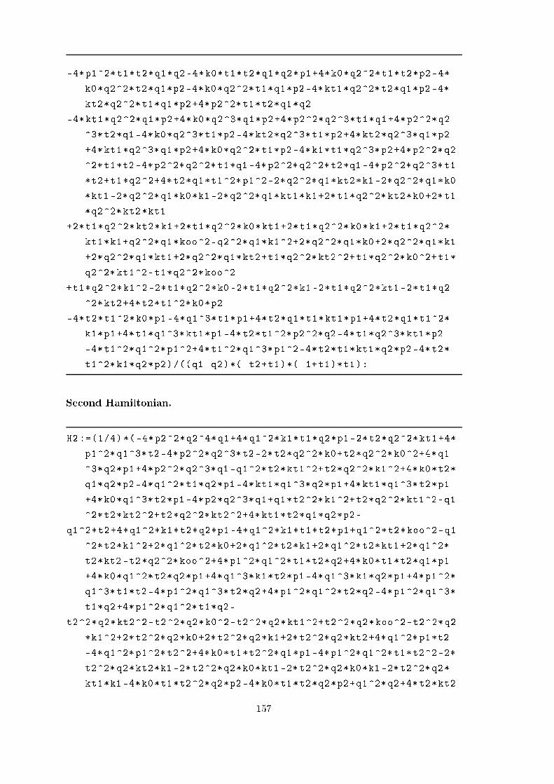
-4*p1^2*t1*t2*q1*q2 -4*k0*t1*t2*q1*q2*p1+4*k0*q2^2*t1*t2*p2 -4*
k0*q2^2*t2*q1*p2 -4*k0*q2^2*t1*q1*p2 -4*kt1*q2^2*t2*q1*p2 -4*
kt2*q2^2*t1*q1*p2+4*p2^2*t1*t2*q1*q2
-4*kt1*q2^2*q1*p2+4*k0*q2^3*q1*p2+4*p2^2*q2^3*t1*q1+4*p2^2*q2
^3*t2*q1 -4*k0*q2^3*t1*p2 -4*kt2*q2^3*t1*p2+4*kt2*q2^3*q1*p2
+4*kt1*q2^3*q1*p2+4*k0*q2^2*t1*p2 -4*k1*t1*q2^3*p2+4*p2^2*q2
^2*t1*t2 -4*p2^2*q2^2*t1*q1 -4*p2^2*q2^2*t2*q1 -4*p2^2*q2^3*t1
*t2+t1*q2 ^2+4*t2*q1*t1^2*p1^2-2*q2^2*q1*kt2*k1 -2*q2^2*q1*k0
*kt1 -2*q2^2*q1*k0*k1 -2*q2^2*q1*kt1*k1+2*t1*q2^2* kt2*k0+2*t1
*q2^2*kt2*kt1
+2*t1*q2^2*kt2*k1+2*t1*q2^2*k0*kt1+2*t1*q2^2*k0*k1+2*t1*q2^2*
kt1*k1+q2^2*q1*koo^2-q2^2*q1*k1^2+2*q2^2*q1*k0+2*q2^2*q1*k1
+2*q2^2*q1*kt1+2*q2^2*q1*kt2+t1*q2^2*kt2 ^2+t1*q2^2*k0^2+t1*
q2^2* kt1^2-t1*q2^2*koo^2
+t1*q2^2*k1^2-2*t1*q2^2*k0 -2*t1*q2^2*k1 -2*t1*q2^2*kt1 -2*t1*q2
^2*kt2+4*t2*t1^2*k0*p2
-4*t2*t1^2*k0*p1 -4*q1^3*t1*p1+4*t2*q1*t1*kt1*p1+4*t2*q1*t1^2*
k1*p1+4*t1*q1^3* kt1*p1 -4*t2*t1^2*p2^2*q2 -4*t1*q2^3*kt1*p2
-4*t1^2*q1^2*p1^2+4*t1^2*q1^3*p1^2-4*t2*t1*kt1*q2*p2 -4*t2*
t1^2*k1*q2*p2)/((q1-q2)*(-t2+t1)*(-1+t1)*t1):
Se ond Hamiltonian.
H2 :=(1/4) *(-4*p2^2*q2^4*q1+4*q1^2*k1*t1*q2*p1 -2*t2*q2^2*kt1 +4*
p1^2*q1^3*t2 -4*p2^2*q2^3*t2 -2*t2*q2^2*k0+t2*q2^2*k0^2+4*q1
^3*q2*p1+4*p2^2*q2^3*q1-q1^2*t2*kt1^2+t2*q2^2*k1^2+4*k0*t2*
q1*q2*p2 -4*q1^2*t1*q2*p1 -4*kt1*q1^3*q2*p1+4*kt1*q1^3*t2*p1
+4*k0*q1^3*t2*p1 -4*p2*q2^3*q1+q1*t2^2*k1^2+t2*q2^2*kt1^2-q1
^2*t2*kt2^2+t2*q2^2*kt2 ^2+4*kt1*t2*q1*q2*p2-
q1^2*t2+4*q1^2*k1*t2*q2*p1 -4*q1^2*k1*t1*t2*p1+q1^2*t2*koo^2-q1
^2*t2*k1^2+2*q1^2*t2*k0+2*q1^2*t2*k1+2*q1^2*t2*kt1+2*q1^2*
t2*kt2 -t2*q2^2*koo ^2+4*p1^2*q1^2*t1*t2*q2+4*k0*t1*t2*q1*p1
+4*k0*q1^2*t2*q2*p1+4*q1^3*k1*t2*p1 -4*q1^3*k1*q2*p1+4*p1^2*
q1^3*t1*t2 -4*p1^2*q1^3*t2*q2+4*p1^2*q1^2*t2*q2 -4*p1^2*q1^3*
t1*q2+4*p1^2*q1^2*t1*q2-
t2^2*q2*kt2^2-t2^2*q2*k0^2-t2^2*q2*kt1^2+t2^2*q2*koo^2-t2^2*q2
*k1 ^2+2*t2^2*q2*k0+2*t2^2*q2*k1+2*t2^2*q2*kt2+4*q1^2*p1*t2
-4*q1^2*p1^2*t2^2+4*k0*t1*t2^2*q1*p1 -4*p1^2*q1^2*t1*t2^2-2*
t2^2*q2*kt2*k1 -2*t2^2*q2*k0*kt1 -2*t2^2*q2*k0*k1 -2*t2^2*q2*
kt1*k1 -4*k0*t1*t2^2*q2*p2 -4*k0*t1*t2*q2*p2+q1^2*q2+4*t2*kt2
157
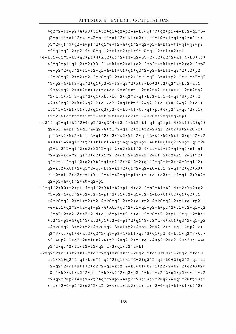
APPENDIX B. EXPLICIT COMPUTATIONS
*q2^2*t1*p2+4*k0*t1*t2*q1*q2*p2 -4*k0*q1^3*q2*p1 -4* kt2*q1^3*
q2*p1+4*q1^2*t1*t2*p1+4*q1^2*kt1*q2*p1+4*k0*t1*q1*q2*p2 -4*
p1^2*q1^3*q2 -4*p1^2*q1^4*t2 -4*q1^2*q2*p1+4*kt2*t1*q1*q2*p2
+4*q1*q2^2*p2 -4*k0*q1^2*t1*t2*p1+4*k0*q1^2*t1*q2*p1
+4*kt1*q1^2*t2*q2*p1+4*kt2*q1^2*t1*q2*p1 -2*t2*q2^2*k1+4*k0*t1*
t2*q2*p1-q1^2*t2*k0^2-4*k1*t2*q1*q2^2*p2+4*k1*t1*t2*q2^2*p2
-4*p2^2*q2^2*t1*t2*q1 -4*k1*t1*q1*q2^2*p2+4*kt1*q2^2*t2*p2
+4*k0*q2^2*t2*p2 -4*k0*q2^2*q1*p2+4*k1*q2^3*q1*p2 -4*k1*t2*q2
^3*p2 -4*kt2*q2^2*q1*p2+2*t2*q2^2*kt2*k0+2*t2*q2^2* kt2*kt1
+2*t2*q2^2*kt2*k1+2*t2*q2^2*k0*kt1 +2*t2*q2^2*k0*k1+2*t2*q2
^2*kt1*k1 -2*q2^2*q1*kt2*k0 -2*q2^2*q1*kt2*kt1+4*q2^3*p2*t2
-2*t2*q2^2*kt2 -q2^2*q1-q2^2*q1*kt2^2-q2^2*q1*k0^2-q2^2*q1*
kt1 ^2+4*k1*t1*t2*q1*q2*p2 -4*k0*t1*t2*q1*p2+4*p2^2*q2^2*t1*
t2^2+4*q2*p2*t1*t2 -4*k0*t1*q1*q2*p1 -4*k0*t2*q1*q2*p1
-t2^2*q2+q1*t2^2+4*p2^2*q2^4*t2 -4*kt2*t1*q1*q2*p1 -4*kt1*t2*q1*
q2*p1+4*p1^2*q1^4*q2 -4*p1^2*q1^2*t1*t2 -2*q1^2*t2*kt2*k0 -2*
q1^2*t2*kt2*kt1 -2*q1^2*t2*kt2*k1 -2*q1^2*t2*k0*kt1 -2*q1^2*t2
*k0*k1 -2*q1^2*t2*kt1*k1 -4*t1*q1*q2*p2+4*t1*q1*q2^2*p2+q1^2*
q2*kt2^2+q1^2*q2*k0^2+q1^2*q2*kt1^2-4*k1*t1*t2*q1*q2*p1-q1
^2*q2*koo^2+q1^2*q2*k1^2-2*q1^2*q2*k0 -2*q1^2*q2*k1 -2*q1^2*
q2*kt1 -2*q1^2*q2*kt2+q1*t2^2*k0^2+2*q1^2*q2*kt2*k0+2*q1^2*
q2*kt2*kt1 +2*q1^2*q2*kt2*k1+2*q1^2*q2*k0*kt1+2*q1^2*q2*k0*
k1+2*q1^2*q2*kt1*k1 -4*t1*t2*q1*p1+4*t1*q1*q2*p1+4*q1^2*kt2*
q2*p1+4*q1^2*k0*q2*p1
-4*q1^2*k0*t2*p1 -4*q1^2*kt1*t2*p1 -4*q2^2*p2*t1*t2 -4*t2*kt2*q2
^3*p2 -4*q2^2*p2*t2 -4*p1^2*t1*t2*q1*q2 -4*k0*t1*t2*q1*q2*p1
+4*k0*q2^2*t1*t2*p2 -4*k0*q2^2*t2*q1*p2 -4*k0*q2^2*t1*q1*p2
-4*kt1*q2^2*t2*q1*p2 -4*kt2*q2^2*t1*q1*p2+4*p2^2*t1*t2*q1*q2
-4*p2^2*q2^3*t2^2-4*q1^3*p1*t2 -4*q1^2*k0*t2^2*p1 -4*q1^2*kt1
*t2^2*p1+4*q1^3*kt2*p1*t2+4*p1^2*q1^3*t2^2-4*kt1*q2^2*q1*p2
-4*k0*q2^3*t2*p2+4*k0*q2^3*q1*p2+4*p2^2*q2^3*t1*q1+4*p2^2*
q2^3*t2*q1+4*kt2*q2^3*q1*p2+4*kt1*q2^3*q1*p2 -4*kt1*q2^3*t2*
p2+4*p2^2*q2^2*t1*t2 -4*p2^2*q2^2*t1*q1 -4*p2^2*q2^2*t2*q1 -4*
p2^2*q2^3*t1*t2+t2*q2^2-2*q1*t2^2*k1
-2*q2^2*q1*kt2*k1 -2*q2^2*q1*k0*kt1 -2*q2^2*q1*k0*k1 -2*q2^2*q1*
kt1*k1+q2^2*q1*koo^2-q2^2*q1*k1^2+2*q2^2*q1*k0+2*q2^2*q1*k1
+2*q2^2*q1*kt1+2*q2^2*q1*kt2+4*k0*t1*t2^2*p2 -2*t2^2*q2*kt2*
k0 -4*k0*t1*t2^2*p1 -4*k0*t2^2*q2*p2 -4*kt1*t2^2*q2*p2+4*k1*t2
^2*q2^2*p2+4*t2*kt2*q2^2*p2 -4*p2^2*t1*t2^2*q2 -4*q1^2*kt2*t1
*p1*t2+4*p2^2*q2^2*t2^2+4*q1*kt2*t1*p1*t2+4*q1*k1*t1*t2^2*
158

p1
-2*q1*t2^2*k0 -2*q1*t2^2*kt2 -q1*t2^2*koo^2-2*q1*t2^2*kt1+q1*t2
^2*kt2^2+q1*t2^2*kt1 ^2+2*q1*t2^2*kt1*k1+4*q1*p1^2*t1*t2
^2+2*q1*t2^2*kt2*k0+2*q1*t2^2*kt2*kt1+2*q1*t2^2* kt2*k1+2*q1
*t2^2*k0*kt1+2*q1*t2^2*k0*k1+4*q1*k0*t2^2*p1+4*q1*kt1*t2^2*
p1 -4*q1^2*kt2*p1*t2 -4*q1^2*k1*t2^2*p1 -4*k1*t1*t2^2*q2*p2+4*
kt1*q2^2*t2^2*p2+4*k0*q2^2*t2^2*p2 -4*t2*kt2*t1*q2*p2+2*kt1*
t2^2*q2 -2*t2^2*q2*kt2*kt1)/(t2*(q1-q2)*(-1+t2)*(-t2+t1)):
159

APPENDIX B. EXPLICIT COMPUTATIONS
160

Appendix
Bibliography
[1 J. Amorós, M. Burger, K. Corlette, D. Kots hi k, and D. Toledo, Fundamental groups of ompa t
Kähler manifolds, Mathemati al Surveys and Monographs, vol. 44, Ameri an Mathemati al So iety,
Providen e, RI, 1996.
[2 F. V. Andreev and A. V. Kitaev, Transformations RS24(3) of the ranks ≤ 4 and algebrai solutions of
the sixth Painlevé equation, Comm. Math. Phys. 228 (2002), no. 1, 151176.
[3 V. I. Arnol'd, S. M. Gusein-Zade, and A. N. Var henko, Singularities of dierentiable maps. Volume
1, Modern Birkhäuser Classi s, Birkhäuser/Springer, New York, 2012. Reprint of the 1985 edition.
[4 A. Beauville, Complex algebrai surfa es, Cambridge University Press, 1983.
[5 R. L. Benedetto and W. M. Goldman, The topology of the relative hara ter varieties of a quadruply-
pun tured sphere, Experiment. Math. 8 (1) (1999).
[6 J. S. Birman, Braids, links, and mapping lass groups, Prin eton Univ. Press, Ann. of Math. Studies
82, 1974.
[7 P. Boal h, From Klein to Painlevé via Fourier, Lapla e and Jimbo, Pro . London Math. So . (3) 90
(2005), no. 1, 167208.
[8 , The fty-two i osahedral solutions to Painlevé VI, J. Reine Angew. Math. 596 (2006), 183
214.
[9 , Some expli it solutions to the Riemann-Hilbert problem, Dierential equations and quantum
groups, 2007, pp. 85112.
[10 S. Cantat, Bers and Hénon, Painlevé and S hrödinger, Duke math. journal 149 (3) (2009).
[11 S. Cantat and F. Loray, Dynami s on hara ter varieties and Malgrange irredu ibility of Painlevé VI
equation, Ann. Inst. Fourier 59 (7) (2009).
[12 G. Casale, Feuilletages singuliers de odimension un, groupoïde de Galois et intégrales premières, Ann.
Inst. Fourier (Grenoble) 56 (2006), no. 3, 735779.
[13 D. Cerveau and A. Lins Neto, Holomorphi foliations in CP(2) having an invariant algebrai urve,
Ann. Inst. Fourier (Grenoble) 41 (1991), no. 4, 883903.
[14 R.C. Chur hill, Two generator subgroups of SL(2;C) and the hypergeometri , Riemann, and Lamé
equations, J. Symboli Comput. 28 (1999), no. 4-5, 521545.
[15 K. Corlette and C. Simpson, On the lassi ation of rank-two representations of quasiproje tive fun-
damental groups, Compos. Math. 144 (2008), no. 5, 12711331.
[16 G. Cousin, Algebrai isomonodromi deformations of logarithmi onne tions on the Riemann sphere
and nite braid group orbits on hara ter varieties, ArXiv e-prints (January 2015), available at 1501.
02753.
161

BIBLIOGRAPHY
[17 G. Cousin, Connexions plates logarithmiques de rang deux sur le plan proje tif omplexe, Ph.D. Thesis,
Université de Rennes 1.
[18 G. Cousin and J. V. Pereira, Transversely ane foliations on proje tive manifolds, Math. Res. Lett.
21 (2014), no. 5, 9851014.
[19 A. I. Degtyarev, Quinti s in CP2with nonabelian fundamental group, Algebra i Analiz 11 (1999),
no. 5, 130151.
[20 P. Deift, A. Its, A. Kapaev, and X. Zhou, On the algebro-geometri integration of the S hlesinger
equations, Comm. Math. Phys. 203 (1999), no. 3, 613633.
[21 P. Deligne, Équations diérentielles à points singuliers réguliers, Le ture Notes in Mathemati s, Vol.
163, Springer-Verlag, Berlin-New York, 1970.
[22 M. Dettweiler and S. Reiter, Middle onvolution of Fu hsian systems and the onstru tion of rigid
dierential systems, J. Algebra 318 (2007), no. 1, 124.
[23 , Painlevé equations and the middle onvolution, Adv. Geom. 7 (2007), no. 3, 317330.
[24 K. Diarra, Constru tion et lassi ation de ertaines solutions algébriques des systèmes de Garnier,
Bull. Braz. Math. So . (N.S.) 44 (2013), no. 1, 129154.
[25 , Solutions algébriques partielles des équations isomonodromiques sur les ourbes de genre 2,
ArXiv e-prints (De ember 2013), available at 1312.6233.
[26 C. F. Doran, Algebrai and geometri isomonodromi deformations, J. Dierential Geom. 59 (2001),
no. 1, 3385.
[27 B. Dubrovin and M. Mazzo o, Monodromy of ertain Painlevé-VI trans endents and ree tion groups,
Invent. Math. 141 (2000), no. 1, 55147.
[28 M. H. Èl'-Huti, Cubi surfa es of Markov type, Mat. Sb. (N.S.) 93 (135) (1974).
[29 B. Farb and D. Margalit, A primer on mapping lass groups, Prin eton Mathemati al Series, vol. 49,
Prin eton University Press, Prin eton, NJ, 2012.
[30 G. Filipuk, On the middle onvolution and birational symmetries of the sixth Painlevé equation, Ku-
mamoto J. Math. 19 (2006), 1523.
[31 A. Girand, Dynami al Green fun tions and dis rete S hrödinger operators with potentials generated
by primitive invertible substitution, Nonlinearity 27 (2014), no. 3, 527543.
[32 , A new twoparameter family of isomonodromi deformations over the ve pun tured sphere,
Bull. So . Math. Fran e 144 (2) (2016), 339368.
[33 V. Heu and F. Loray, Flat rank 2 ve tor bundles on genus 2 urves, ArXiv e-prints (January 2014),
available at 1401.2449.
[34 N. J. Hit hin, Pon elet polygons and the Painlevé equations, Geometry and analysis (Bombay, 1992),
1995, pp. 151185.
[35 Y. Ilyashenko and S. Yakovenko, Le tures on analyti dierential equations, Graduate Studies in
Mathemati s, vol. 86, Ameri an Mathemati al So iety, Providen e, RI, 2008.
[36 M. Jimbo and T. Miwa, Monodromy preserving deformation of linear ordinary dierential equations
with rational oe ients. II, Phys. D 2 (1981), no. 3, 407448.
[37 N. Katz, Rigid lo al systems, Prin eton University Press, Prin eton, N.J., 1996.
[38 H. Kimura and K. Okamoto, On the polynomial Hamiltonian stru ture of the Garnier systems, J.
Math. Pures Appl. (9) 63 (1984), no. 1, 129146.
[39 J. Kollàr, Rational urves on algebrai varieties, Ergebnisse der mathematik und ihrer grenzgebiete,
Springer, 1999.
162

BIBLIOGRAPHY
[40 A. Komyo, On ompa ti ations of hara ter varieties of n-pun tured proje tive line, ArXiv e-prints
(July 2013), available at 1307.7880.
[41 A. Lins Neto, Some examples for the Poin aré and Painlevé problems, Ann. S i. É ole Norm. Sup. (4)
35 (2002), no. 2, 231266.
[42 O. Lisovyy and Y. Tykhyy, Algebrai solutions of the sixth Painlevé equation, J. Geom. Phys. 85
(2014), 124163.
[43 F. Loray, F. Touzet, and J. Vitorio Pereira, Representations of quasiproje tive groups, Flat onne tions
and Transversely proje tive foliations, ArXiv e-prints (February 2014), available at 1402.1382.
[44 B. Malgrange, Sur les déformations isomonodromiques. I. Singularités régulières, Mathemati s and
physi s (Paris, 1979/1982), 1983, pp. 401426.
[45 M. Mazzo o, Pi ard and Chazy solutions to the Painlevé VI equation, Math. Ann. 321 (2001), no. 1,
157195.
[46 , The geometry of the lassi al solutions of the Garnier systems, Int. Math. Res. Not. 12 (2002),
613646.
[47 J. Milnor, Morse theory, Based on le ture notes by M. Spivak and R. Wells. Annals of Mathemati s
Studies, No. 51, Prin eton University Press, Prin eton, N.J., 1963.
[48 J. Moulin Ollagnier, Liouvillian integration of the Lotka-Volterra system, Qual. Theory Dyn. Syst. 2
(2001), no. 2, 307358.
[49 , Corre tions and omplements to: Liouvillian integration of the Lotka-Volterra system [Qual.
Theory Dyn. Syst. 2 (2001), no. 2, 307358; mr1913289, Qual. Theory Dyn. Syst. 5 (2004), no. 2,
275284.
[50 D. Novikov and S. Yakovenko, Le tures on meromorphi at onne tions, Normal forms, bifur ations
and niteness problems in dierential equations, 2004, pp. 387430.
[51 Kazuo Okamoto, Studies on the Painlevé equations. I. Sixth Painlevé equation PVI, Ann. Mat. Pura
Appl. (4) 146 (1987), 337381.
[52 H.-P. de Saint-Gervais, Uniformisation des surfa es de Riemann, ENS éditions, 2010.
[53 B. A. S árdua, Transversely ane and transversely proje tive holomorphi foliations, Ann. S i. É ole
Norm. Sup. (4) 30 (1997), no. 2, 169204.
[54 G. C. Shephard and J. A. Todd, Finite unitary ree tion groups, Canadian J. Math. 6 (1954), 274304.
[55 I. Shimada, Le tures notes on Zariski-Van Kampen theorem.
http://math.s i.hiroshima-u.a .jp/ shimada/Le tureNotes/LNZV.pdf.
[56 C. Simpson, Katz's middle onvolution algorithm, Pure Appl. Math. Q. 5 (2009), no. 2, Spe ial Issue:
In honor of Friedri h Hirzebru h. Part 1, 781852.
[57 H. Völklein, The braid group and linear rigidity, Geom. Dedi ata 84 (2001), no. 1-3, 135150.
[58 M. Yoshida, Fu hsian dierential equations, Aspe ts of Mathemati s, E11, Friedr. Vieweg & Sohn,
Brauns hweig, 1987. With spe ial emphasis on the Gauss-S hwarz theory.
163
Résumé
Une déformation isomonodromique d'une sphère épointée est une famille de
onnexions logarithmiques plates sur ette dernière ayant toutes, à onjugai-
son globale près, la même représentation de monodromie. Ces objets sont
paramétrés par les solutions d'une ertaine famille d'équations aux dérivées
partielles, les systèmes de Garnier, qui sont équivalents dans le as de la sphère
à quatre trous aux équations de Painlevé VI. L'objet des travaux présentés
i i est de onstruire de nouvelles solutions algébriques des es systèmes dans
le as de la sphère à inq trous. Dans une première partie, nous lassions
les déformations isomonodromiques algébriques obtenues par restri tion aux
droites d'une onnexion logarithmique plate sur P2(C) dont le lieu polaire est
une ourbe quintique. On obtient ainsi deux nouvelles familles de solutions
algébriques du système de Garnier asso ié. Dans une deuxième partie, nous
exploitons le fait qu'une déformation isomonodromique algébrique orrespond
à une orbite nie sous l'a tion du groupe modulaire sur la variété des ara -
tères de la sphère à inq trous pour obtenir de nouveaux exemples de telles
orbites. Nous employons pour e faire la onvolution intermédiaire sur les
représentations de groupes libres développée par Katz. Enn, nous dé rivons
une généralisation partielle de e pro édé au as d'un tore omplexe à deux
trous.
Abstra t
We all isomonodromi deformation any family of logarithmi at onne tions
over a pun tured sphere having the same monodromy representation up to
global onjuga y. These obje ts are parametrised by the solutions of a parti -
ular family of partial dierential equations alled Garnier systems, whi h are
equivalent to the Painlevé VI equations in the four pun tured ase. The pur-
pose of this thesis is to onstru t new algebrai solutions of these systems in the
ve pun tured ase. First, we give a lassi ation of algebrai isomonodromi
deformations obtained by restri ting to lines some logarithmi at onne tion
over P2(C) whose singular lo us is a quinti urve. We obtain two new families
of algebrai solutions of the asso iated Garnier system. In a se ond part, we
use the fa t that any algebrai isomonodromi deformation orresponds to a
nite orbit under the mapping lass group a tion on the hara ter variety of
the ve pun tured sphere to obtain new examples of su h orbits. We do this by
using Katz's middle onvolution on representations of free groups. Finally, we
give a partial generalisation of this pro edure in the ase of a twi e pun tured
omplex torus.