these` - polytechnique · du cea et de digiteo; ce travail leur doit tout. tout sp´ecialement...
TRANSCRIPT

ORSAYNo d’ordre: xxxx
UNIVERSITE DE PARIS-SUD
CENTRE D’ORSAY
THESEpresentee
pour obtenir
L’HABILITATION A DIRIGER DES RECHERCHESDE L’UNIVERSITE PARIS-SUD
PAR
Sylvie PUTOT−→←−
SUJET:
Static Analysis of Numerical Programs and Systems
soutenue le 13 decembre 2012 devant la commission d’examen
Eric WALTER PresidentJean-Claude BAJARD RapporteursNicolas HALBWACHSHelmut SEIDLJean GASSINO ExaminateursMichel RUEHERJean SOUYRISEric GOUBAULT InvitesClaude MARCHE

2

Remerciements
Aux membres de mon jury, qui m’ont fait l’honneur de bien vouloir examiner mon travail. En premier lieuaux rapporteurs, pour l’attention bienveillante portee a mon memoire. A Claude Marche, pour son soutienconstant et actif dans la preparation de cette habilitation. A Eric Goubault, chef du laboratoire MEASI, quia guide mes premiers pas sur le sujet, et toujours encouragee depuis. Comment en quelques mots evoquerplus de 10 ans a beneficier de son energie et de sa curiosite scientifique? Plus generalement a mes colleguesdu CEA et de Digiteo; ce travail leur doit tout. Tout specialement Karim Tekkal et Franck Vedrine, gracea qui l’aventure Fluctuat, avec ses hauts et ses bas, est restee un plaisir. A Khalil Ghorbal, mon premieretudiant en these, forcement unique.
A tous, merci!
3

4

Contents
1 Introduction 71.1 Analyzing the impact of rounding errors . . . . . . . . . . . . . . . . . . . . . . . . . . . . 101.2 From set-based methods to static analysis . . . . . . . . . . . . . . . . . . . . . . . . . . . 121.3 Analyzing real life programs . . . . . . . . . . . . . . . . . . . . . . . . . . . . . . . . . . 151.4 Organization of the document . . . . . . . . . . . . . . . . . . . . . . . . . . . . . . . . . . 16
2 Zonotopic Abstract Domains for Functional Abstraction 172.1 Affine arithmetic and zonotopes . . . . . . . . . . . . . . . . . . . . . . . . . . . . . . . . 19
2.1.1 Affine arithmetic . . . . . . . . . . . . . . . . . . . . . . . . . . . . . . . . . . . . 192.1.2 Affine sets and zonotopes . . . . . . . . . . . . . . . . . . . . . . . . . . . . . . . 20
2.2 An ordered structure for functional abstraction . . . . . . . . . . . . . . . . . . . . . . . . . 222.2.1 Perturbed affine sets and functional order . . . . . . . . . . . . . . . . . . . . . . . 232.2.2 Constrained affine sets: handling zonotopes intersection . . . . . . . . . . . . . . . 252.2.3 A join operator . . . . . . . . . . . . . . . . . . . . . . . . . . . . . . . . . . . . . 272.2.4 Modular analysis . . . . . . . . . . . . . . . . . . . . . . . . . . . . . . . . . . . . 33
2.3 First experiments . . . . . . . . . . . . . . . . . . . . . . . . . . . . . . . . . . . . . . . . 34
3 Extensions of the Zonotopic Approach 373.1 An under-approximating abstract domain . . . . . . . . . . . . . . . . . . . . . . . . . . . 37
3.1.1 Generalized affine sets for under-approximation . . . . . . . . . . . . . . . . . . . . 383.1.2 Applications and experiments . . . . . . . . . . . . . . . . . . . . . . . . . . . . . 41
3.2 Mixing P-boxes and Affine Arithmetic . . . . . . . . . . . . . . . . . . . . . . . . . . . . . 433.2.1 Basics: Dempster-Shafer structures and p-boxes . . . . . . . . . . . . . . . . . . . . 433.2.2 Affine arithmetic with probabilistic noise symbols . . . . . . . . . . . . . . . . . . 45
4 Loops and Fixpoint Computations 494.1 Kleene-like iteration schemes . . . . . . . . . . . . . . . . . . . . . . . . . . . . . . . . . . 49
4.1.1 Kleene’s iteration sequence, widening and narrowing . . . . . . . . . . . . . . . . . 494.1.2 Kleene-like iteration schemes for affine sets . . . . . . . . . . . . . . . . . . . . . . 504.1.3 Convergence properties for the analysis of linear filters . . . . . . . . . . . . . . . . 53
4.2 Policy iteration . . . . . . . . . . . . . . . . . . . . . . . . . . . . . . . . . . . . . . . . . 554.2.1 Lower selection . . . . . . . . . . . . . . . . . . . . . . . . . . . . . . . . . . . . . 554.2.2 Policy iteration . . . . . . . . . . . . . . . . . . . . . . . . . . . . . . . . . . . . . 56
5

6 CONTENTS
4.2.3 Implementation and experiments for the lattice of intervals . . . . . . . . . . . . . . 57
5 The Fluctuat Static Analyzer 595.1 Analyzing finite precision computations . . . . . . . . . . . . . . . . . . . . . . . . . . . . 59
5.1.1 Concrete model . . . . . . . . . . . . . . . . . . . . . . . . . . . . . . . . . . . . . 595.1.2 A non relational abstraction . . . . . . . . . . . . . . . . . . . . . . . . . . . . . . 615.1.3 A zonotopic abstraction . . . . . . . . . . . . . . . . . . . . . . . . . . . . . . . . 625.1.4 Order-theoretic operations and unstable tests . . . . . . . . . . . . . . . . . . . . . 64
5.2 Using Fluctuat . . . . . . . . . . . . . . . . . . . . . . . . . . . . . . . . . . . . . . . . . . 645.2.1 Building the analysis project - directives . . . . . . . . . . . . . . . . . . . . . . . . 655.2.2 Parameterizing the analysis . . . . . . . . . . . . . . . . . . . . . . . . . . . . . . . 665.2.3 Exploitation of results . . . . . . . . . . . . . . . . . . . . . . . . . . . . . . . . . 67
5.3 Examples and case studies . . . . . . . . . . . . . . . . . . . . . . . . . . . . . . . . . . . 685.3.1 A simple addition... . . . . . . . . . . . . . . . . . . . . . . . . . . . . . . . . . . . 695.3.2 A set of order 2 recursive filters . . . . . . . . . . . . . . . . . . . . . . . . . . . . 695.3.3 An interpolated sine approximation . . . . . . . . . . . . . . . . . . . . . . . . . . 725.3.4 Cosine approximation . . . . . . . . . . . . . . . . . . . . . . . . . . . . . . . . . 755.3.5 An iterative algorithm for square root approximation . . . . . . . . . . . . . . . . . 765.3.6 Analysis of hybrid systems . . . . . . . . . . . . . . . . . . . . . . . . . . . . . . . 775.3.7 Float to fixed-point conversion: bit-width optimisation . . . . . . . . . . . . . . . . 77
5.4 Looking back at the last ten years . . . . . . . . . . . . . . . . . . . . . . . . . . . . . . . . 78
6 Conclusion and Perspectives 816.1 Zonotopic abstract domains and extensions . . . . . . . . . . . . . . . . . . . . . . . . . . 816.2 Fixpoint computations . . . . . . . . . . . . . . . . . . . . . . . . . . . . . . . . . . . . . 836.3 Fluctuat and its applications . . . . . . . . . . . . . . . . . . . . . . . . . . . . . . . . . . 84
Chapter 1
Introduction
Software-driven systems are pervasive in today’s world, and grow more complex every day. While their -frequent - dysfunctions are mainly a hassle in most applications, the safety-critical systems can not allowbugs, their correct behavior has to be proved thoroughly. In that respect, the norms of the safety-criticalindustries, such as DO-178B [142] and its recent update DO-178C [143] for the aeronautic industry, areevolving towards replacing part of the tests by methods providing guarantees for all possible executions,such as static analysis.
Meanwhile, the complexity of computation in these safety-critical systems is quickly increasing. Forinstance, Airbus has been using fly-by-wire systems, that is flight control computers, to replace manualflight control, for all its commercial airplanes since the A320 program, officially launched in 1984. Ofcourse, if correct, these computer-driven systems increase the safety and performance of the flight control.But proving their correction, whatever the conditions driven by the airplane’s environment, is a challenge atthe state of the art of validation. These systems now involve millions of lines of programs, and, this will bethe point of this document, quite intricate numerical computations.
Indeed, the control and monitoring of physical systems needs computations in real numbers. Of course,these can only be approximated on a computer: most applications now use floating-point approximations, aflexible and efficient representation, well specified by the IEEE-754 standard [1]. By specifying in particularthe size of the mantissa and the exponent of floating-point numbers, this norm greatly improved the portabil-ity of programs: we know how the rounding error committed at each arithmetic operation is bounded. But,even though these approximations are well specified at the arithmetic operations level, their propagationthrough a chain of computation is, as we will see, difficult to predict. They can lead to subtle problems -with potentially catastrophic consequences - all the more so because some of the good algebraic propertiesof real arithmetic, such as, for instance, associativity, are no longer true in floating-point arithmetic. Theconsequences can be of two natures. First, a result computed in finite precision can be only a rough approx-imation of the real result. But also, the behavior of the program using finite precision can be unexpected:for instance, an algorithm that was proved to converge very well in real numbers, can no longer converge infinite precision, especially if some stopping criterion is not well suited to the precision.
The impact of rounding errors on numerical computations, and particularly in algebraic processes, hasbeen receiving attention since the very beginning of computers and numerical analysis, in a famous 1947article by Von Neumann and Goldstine [156]. The interest has not dropped since, let us for instance mentiontwo classic surveys, by Wilkinson [157] and Higham [99]. Also, trying to build automatic methods to
7

8 CHAPTER 1. INTRODUCTION
estimate the rounding errors was already of interest as early as 1958 [54], and has remained so ever since;let us highlight the work of Miller [127] which in 1975 aimed at searching numerical instabilities in a spiritclose to our present work.
Moreover, this problem of the propagation of rounding errors is only part of the larger problem ofvalidating numerical software. A difficulty, and not the least one actually when considering this largerproblem of validating numerically a possibly large program, is to decide and specify which properties haveto be proved, to increase the level of assurance that the software meets its goal. The absence of run-timeerrors, with a semantics handling floating-point computations, addressed for instance by the Polyspace1
or Astree [42] analyzers, is the first property that must be ensured in this context. But then, how can weknow for sure that the program computes what it is supposed to, and not just something that does notproduce an execution error? Of course, in general, the question is really hard to answer. But we haveinformation at our disposal, as the safety-critical software obey very strict rules of development, involvinga lot of documentation and requirement specifications. There can then be different and complementaryanswers, that correspond to different levels of view on the software. Locally, we may have specificationsof functional behavior on elementary symbols or portions of software. For instance, that such function, fora given range of inputs, should compute approximately some mathematical function, with not more than agiven approximation error. Then, globally on a large part of the software, we may for instance want to provethat the values of some variables representing physical quantities remain within their expected ranges. Ofcourse, this supposes to be able to model the environment precisely enough. And finally, locally or globally,we can prove that the use of finite precision in the computation does not significantly alter the result fromthe one that would be computed in real numbers. So that the end-user can decide whether his software meetsthe accuracy requirements, including modeling and computation errors.
My work takes inspiration from two worlds that take into account the use of finite precision numbers: thefirst is reliable computing, in which set-based methods are used to build computations that are guaranteedby construction to contain the real result; the second is static analysis by abstract interpretation, which aimsat proving properties on existing programs.
Reliable computing The first tool for guaranteed computations, introduced by Moore, is interval arith-metic [133], which he used to mechanize error analysis in computations as soon as 1959 [134]. Directlyrewriting the methods of numerical analysis with intervals gives very poor results, as dependencies be-tween numerical values are not taken into account. This motivated some methods that became classic, suchas the interval Newton method and methods to solve interval linear systems, for which Hansen was pio-neer [92, 96, 93, 95]. Many extensions of interval arithmetic have been developed since then, in order toovercome the dependency problem: let us mention Hansen’s generalized interval arithmetic [94] and affinearithmetic [33, 45], on which most of the work presented here is based. More accurate models include for in-stance Taylor model methods, introduced by Berz and Makino [12, 120], and used in particular for validatedintegration of ordinary differential equations. Ellipsoid arithmetic can also be an answer to the dependencyproblem, and could be especially interesting in the fixpoint computations induced by static analysis as it iswell suited to determine stability regions of non-linear discrete dynamical systems, as noted for instanceby Neumaier [136]. There is no simple way to compute with ellipsoids, which makes them scarcely usedfor verified computation although they received some attention quite early; but approximated computationswith ellipsoids have been used successfully [137, 108], and we hope to use them in the future, in conjunction
1http://www.mathworks.com/products/polyspace/

9
with affine forms. These set-based methods can be supplemented for bounded program verification by con-straint solving on real or floating-point numbers [126, 32]. Let us finally refer to Rump’s survey article [144]for a large overview on the field of reliable computing. The main direction of my work is to try to buildabstractions for static analysis on some of these methods.
Static analysis by abstract interpretation In contrast to dynamic analysis, which tests the programaround possible executions, static analysis aims at proving properties on programs without execution, forpotentially infinite sets of behaviors. But designing an analysis that can answer exactly and automatically,on all programs, whether a non-trivial property holds, is not possible. To make the problem tractable, onecan make different choices. A first choice is to lose automation: for instance, interactive theorem proverscan be used to assist the development of formal proofs: we will come back later to their use in the contextof floating-point computation analysis. A second choice is to lose soundness and possibly miss some errors.In this case, tools are rather used as bug-finders, or to give some level of confidence on the correctness ofprograms. This is for instance the choice made by Grammatech2 for its CodeSonar analysis tool. Finally,and this is the choice we made for the work presented here, we can lose completeness by abstracting (overor under approximating) the properties of interest. The analyzer may not be able to conclude about thesatisfaction of a property and produce false alarms, that is indicate possible erroneous behavior, that cannotoccur in reality. For a given property of interest, the art of abstraction is to find the optimal trade-off be-tween expressiveness and cost of the analysis. When my work started, this problem of false alarms indeedsullied the reputation of the first commercial sound static analyzer for run-time errors, Polyspace verifier3,which handles floating-point semantics. Demonstrating that a static analyzer could prove the absence ofrun-time errors for large scale aeronautic programs was actually the starting point of Cousot, Cousot, Feret,Mauborgne, Mine, Monniaux and Rival, in their design of Astree [42].
Our work also makes the choice of soundness by abstract interpretation, but aims at verifying refinednumerical properties, for safety-critical systems of a possibly large size. We introduced a new class ofzonotopic abstract domains well suited to the analysis of numerical properties, and built a static analyzernamed Fluctuat which is not specialized to programs from the aeronautic industry - the price to pay beingless scalability for the analyses on these particular programs. Still, Fluctuat is able to analyze several dozensof thousands of lines of typical control command software in a few hours (of course, this is only indicativeas the analysis time highly depends on the software analyzed).
Most of the work I present here is motivated by the practical verification needs of actors of the safety-critical industry, such as Airbus and IRSN (French Expert in nuclear and radiological risk). Both have beensupporting our work since its starting point in 2000-2001 and ever since, Airbus first by its participation tothe European project DAEDALUS4, then through direct projects. However, in the long term, we can hopethat these advances, developed in the context of safety-critical systems, will benefit to the numerically verycomplex programs from numerical simulation.
2http://en.wikipedia.org/wiki/GrammaTech3http://www.mathworks.com/products/polyspace/4Daedalus European IST project (2000-2002), http://www.di.ens.fr/ cousot/projects/DAEDALUS/

10 CHAPTER 1. INTRODUCTION
1.1 Analyzing the impact of rounding errors
Approximations and uncertainties lie everywhere in the numerical software that aim at modeling real phe-nomena. An additional source of approximation is due to the representation of real numbers on the computer,most of the time by floating-point numbers. The error due to the use of finite precision in computations isoften overlooked for at least two reasons. First, considered locally on a particular operation, the roundingerror as specified by the IEEE-754 norm [1], can seem insignificant compared to the other sources of uncer-tainties. Second, considered globally on a program, its accurate estimation is difficult. And most of the timeits impact is indeed negligible.
Still, experience tells us that an issue directly due to rounding error, with potentially catastrophic con-sequences, can occur even on numerically not very complex programs. Take for instance the example ofthe Patriot anti-missile during the Gulf war, that widely missed its target because of an inaccurately com-puted time counter, that caused a major localisation problem [58]. The accident actually occurred with animplementation in 24 bits fixed point arithmetic, but a similar problem - with different amplitude though -would have occurred with floating-point numbers. Indeed, this time counter was regularly incremented bythe constant 0.1, representing a time elapse. But constant 0.1, as harmless as it may seem to human eyes, isnot represented exactly in a binary finite format, whatever the precision. This causes a new rounding errorat each time increment, errors that accumulate. The computation of the time counter is thus affected, at eachtime increment, by the rounding of the result of the addition of the floating-point representation of 0.1 to thetime counter, result which in general is also not representable and must be rounded. This makes the erroractually not so obvious to predict manually, even for such a simple program5. And what makes things worseis that the problematic parts are most of the time buried among thousands of harmless lines of program,which calls for automatic tools able to extract and analyze the dubious parts.
Rounding error analysis As already mentioned, interest for the impact of the use of finite precision onthe behavior of programs started as early as 1947. The next step, that is designing methods to automaticallyestimate this impact, soon followed, in 1958. Still, we cannot say the problem has been fully solved since,let us quickly discuss contemporary approaches for rounding error analysis.
A well-established dynamic method for the analysis of numerical programs is the CESTAC (Controland Stochastic Estimation of Rounding Errors) method [155], implemented in the CADNA6 tool. In afew words, this method can be described as follows: the computation for each input is run several times,with random rounding: the deviation between these results gives the number of significant digits of theresult, with some probability. But this result is valid only under the hypothesis that the rounding errorsare independent centered random variables, hypothesis that is often wrong, as advocated with examples byKahan [105]. Also, this method gives no insurance that a very high error can not occur, which may havecatastrophic consequence even if this is with very small probability.
Another class of approaches to the estimation of the propagation of rounding errors relies on automaticdifferentiation, that computes values of function derivatives: a first order estimation of the sensitivity ofthe output of a computation to rounding error, or more generally to uncertainties, is given by derivatives orfirst order Taylor developments. This was used to estimate the propagation of rounding error [9, 118, 127,115]. But these estimations of the errors can also be used to try to correct the results of finite precision
5http://proval.lri.fr/gallery/clockdrift.en.html6http://www-pequan.lip6.fr/cadna/

1.1. ANALYZING THE IMPACT OF ROUNDING ERRORS 11
computation. This is the aim of the CENA (French acronym for correcting numerical rounding errors)method [113, 114, 112], which relies on automatic differentiation to compute and compensate the effects ofthe first-order rounding errors.
Finally, formal proof using interactive theorem provers is also applied to the verification of floating-point algorithms. Harrison has been working on floating-point verification using HOL since 1995 [97].Formalizations of floating-point arithmetics have been designed for several proof assistants [25, 18]. Whilewe are mainly concerned with software verification in our work, hardware verification is more widely spreadin formal proof, as hardware is most of the time designed in a more modular way, and such proofs as IEEE-754 compliance are both crucial and quite easily automated [145]. Indeed, the error in the floating-pointdivision in an Intel Pentium processor in 1994 [139] certainly had a non-negligible impact for Intel. Morerecently, Boldo, Filliatre, Melquiond, Ayad and Marche have started developing proofs for floating-pointarithmetic in Coq [15], with efforts towards automation [16, 7]. Pen and paper analyses of rounding errorsconstitute starting points for accurate computer-aided analyses of numerical algorithms, such as in Boldo’swork [14]. But, for the time being, these analyses are not generic, they have to be conducted again for eachnew problem. And the construction of the proof may require a lot of work and expertise by the user, andprevent the analysis of very large programs.
The birth of Fluctuat Eric Goubault conceived, mid 2000, the project to write a static analyzer of finiteprecision computations. An idea was, so that the analysis would be the more automatic possible, thatthe specification would be implicit: the static analyzer should be able not only to handle floating-pointcomputation, but also to compute its distance to the reference, the computation in a real number semantics.
He set in 2001 [73] the first ideas of an abstract domain that computes the floating-point value of avariable, by interval arithmetic, and its distance to the real value, decomposed along the program controlpoints, by a sum of interval contributions. When I began in Eric Goubault’s team at CEA (now the MEASIlaboratory, standing for Modelling and Analysis of Interacting Systems) in January 2001, with a backgroundmore turned towards scientific computing than theoretical computer science, I was first in charge, by wayof formation, to implement these first ideas. This was done in an emerging static analyzer for which a firststructure had been designed [75], and which soon became FLUCTUAT [77]. Meanwhile Matthieu Martel,who had joined the team shortly before I did, formalized this same abstract domain [121].
It soon became clear that the analysis we had designed was under-valuing the numerical interest of affinearithmetic [33, 45], from which it had drawn its inspiration. Indeed, from an arithmetic which had beenproposed in order to use affine relations between variables to improve interval arithmetic, we had reached anabstract domain that was purely non relational, based on intervals, even though it was adding a very valuableinformation: the provenance of rounding and approximation errors. Following that assessment, it took usseveral years, starting from 2002 and still on-going work, to design efficient abstract domains that also madeuse of the affine relations between variables. Coming back to the abstraction of real values of variables ofprograms, we proposed affine arithmetic based abstract domains, with zonotopic concretizations, which wecalled affine sets [81, 83, 84, 64, 65].
We then formalized the extension of these abstract domains to handle finite precision computations androunding errors along with their provenance [85] (they had been already implemented in Fluctuat for sometime [46]). Indeed, the relations that are true for real values are no longer true for floating-point values: butinstead of using interval linearisation as Mine did [130], we developed an abstract domain relying on affinesets for both values and errors.

12 CHAPTER 1. INTRODUCTION
Let us first quickly introduce the notion of abstract domain, which is central to static analysis by abstractinterpretation.
1.2 From set-based methods to static analysis
Abstract interpretation [38, 40] is a theory of approximation of program semantics. An analysis first relieson a concrete semantics, that is a description of the property of interest and the way it propagates throughprogram instructions. In our case, the properties of interest will be the values of variables of numerical pro-grams at each point of the program, considered both in real and floating-point numbers, and a decompositionof the discrepancy between these values.
The following step is to abstract this concrete semantics, that is to define a sound approximation of thisconcrete semantics, on which the property of interest (here over-approximations of values of variables androunding errors) can be automatically inferred on programs. The abstract domain defines this approximationof discrete values. Abstract operators, that allow to compute sound abstractions of transfer functions must bedefined. Finally, a partial order is needed, allowing to compare, join and intersect abstract elements: we willcompute safety properties of programs, that is invariants, obtained by fixpoint computations in this partiallyordered structures; a key point of abstract interpretation is that fixpoints of the concrete semantics can besoundly approximated in the abstract world, thus allowing the design of fully automatic abstract interpreters.Finally, abstract operators, that allow to compute sound abstractions of transfer functions, must be defined.
When using set-based methods, such as affine arithmetic, the abstract arithmetic operators will naturallyfollow from the guaranteed computation that was defined for use in numerical analysis. The difficulty isto define a partially ordered structure, on which abstract elements can be compared, and join and meetoperations defined.
The abstract interpretation framework Classic abstract interpretation relies on Galois connections be-tween partially ordered sets: a Galois connection between two partially ordered sets (D[,⊆[) and (D],⊆])is a function pair (α, γ) such that
1. α : D[ → D] is monotonic,
2. γ : D] → D[ is monotonic,
3. ∀(x[, x]) ∈ D[ ×D], α(x[) ⊆] x] ⇔ x[ ⊆[ γ(x])
In this definition, D[ is the concrete domain, D] the abstract domain, α the abstraction function, and γ theconcretization function. Here, α(x[) is the best abstraction for x[, and α(x[) ⊆] x] formalizes the fact thatx] is a sound abstraction for x[.
Let then f [ be an operator on the concrete domain. The best abstraction of f [ is α ◦ f [ ◦ γ, and a soundabstraction for f [ is any operator f ] such that for all x] ∈ D], (α ◦ f [ ◦ γ)(x]) ⊆] f ](x]).
This framework is well suited to some abstractions, such as intervals. However, it is sometimes toorestrictive, as, for instance, there is sometimes no best abstraction of a concrete element. This will be thecase for the affine arithmetic based abstract domains, and we will use a relaxed framework [40], whichallows to rely on a concretization function only. We will see that the concretization function by which ourabstraction by affine sets is defined, is the zonotope defining the inputs and variables of the program. Andindeed, the union of two zonotopes is not a zonotope, and neither is the intersection of zonotopes.

1.2. FROM SET-BASED METHODS TO STATIC ANALYSIS 13
Here, a concretization function from the abstract domain (D],⊆]) to the concrete domain (D[,⊆[),these domains being posets, is simply a monotonic function γ : D] → D[. The abstract value x] is a soundabstraction for x[ if x[ ⊆[ γ(x]). The abstract operator f ] is a sound abstraction for the concrete operator f [
if for all x] ∈ D], (f [ ◦ γ)(x]) ⊆[ (γ ◦ f ])(x]). There are no best values and operators abstraction. Whilein the Galois connection framework, if the best operator abstractions are used, the accuracy of an abstractdomain is directly related to the accuracy of its concretization function, this is no longer the case here.
Numerical abstract domains The more basic abstract domains are non relational: they abstract inde-pendently the value of each variable. Intervals are a typical example of a non relational abstract domains.Relational abstract domains additionally abstract some relations between variables. A number of relationalabstract domains have been defined, relying on concretization functions, that is ranges for values of tu-ples of variables, giving particular polyhedra. The first of these domains is the general convex polyhedra(∑
k akxk ≤ c) abstract domain [44], discovering invariant linear inequalities among numerical variablesof a program. In order to find trade-offs between cost and accuracy, were introduced particular polyhe-dra for which efficient abstract operators could be designed, among which zones (x − y ≤ c) [128],octagons (±x ± y ≤ c) [129], polyhedra with two variables per equality (ax + by ≤ c) [152], oc-tahedra (±xj ± . . . ± xk ≥ c) [31], pentagons (a ≤ x ≤ b ∧ x ≤ y) [119], or sub-polyhedra(a ≤ x ≤ b ∧
∑k akxk = c) [116]. Another way to yield a scalable analysis is to fix the coefficients ak in∑
k akxk ≤ c: this is the starting idea of the template polyhedra [147]. The implementation of polyhedralabstract domains in finite precision may need some precaution [28]: part of the interest of interval polyhedra(∑
k[ak, bk]xk ≤ c) [29] is to address this issue. The concrete semantics of a program often involves non-convex behaviors, in particular in the case of conditional branch statements. Designing possibly non-convexabstractions is thus of interest. Interval polyhedra have non convex concretization, and so have min and maxinvariants on max-plus polyhedra (max(λ0, x1 + λ1, . . . , xn + λn) ≤ max(µ0, x1 + µ1, . . . , xn + µn) andmin(λ′0, x1 + λ′1, . . . , xn + λ′n) ≤ min(µ′0, x1 + µ′1, . . . , xn + µ′n)) [4], that are well suited for handlingdisjunctions as in algorithms on strings or arrays. Some of these abstract domains aim at capturing specificpatterns or behaviors, such as for instance the relation to a loop counter [50], the output of order 2 linearfilters [49], or linear absolute value relations (
∑k akxk +
∑k bk|xk| ≤ c) [30]. Designing a static analyzer
relying on such abstract domains thus requires to combine these abstract domains [43], in order to be ableto handle sufficiently general programs.
We proposed a new class of abstract domains, all connected to affine forms, that are sufficiently non-specialized to handle a large class of programs, and which accuracy can be parameterized.
Zonotopic abstract domains The concretization function of affine sets - our affine arithmetic based ab-stract domains - is the zonotope including the inputs and variables of the program: the parameterization ofzonotopes by affine forms defines a functional abstraction, providing linearized input-output relations. Al-though yielding sub-polyhedric relations only, the comparison of its accuracy to the accuracy of polyhedrais not straightforward, as the non linear operations can be very conveniently abstracted by first-order Taylorexpansions. Indeed, the accuracy of abstract domains cannot be compared solely based on their geometricshapes, as would be tempting to do, but depends on the accuracy of operator abstractions.
The main difficulty, as we will see, was to propose efficient set-theoretic operations. This requiredseveral steps: a first ordered structure was proposed in 2006 [81], improved in preprints [83, 84], thenenhanced with a meet operation [65]. This meet operation was handled by a particular logical product [91]

14 CHAPTER 1. INTRODUCTION
between the affine sets and an abstract domain on the noise symbols that play a role in the affine sets: thiswas the subject of the PhD thesis of Khalil Ghorbal that I co-supervised. In this case, the concretization ofan abstract element is no longer a zonotope, but a more general polyhedron. Affine sets can then be extendedquite easily to handle floating-point computations. We will also demonstrate how these domains can be usedalso for the analysis of sensitivity to input uncertainties, or the proof of functional properties of numericalprograms.
Zonotopes are also successfully used in reachability analysis of hybrid systems [66]. Of course, thesame problem of computing unions of zonotopes, and intersections of zonotopes with guards arises [67, 5].
Refining the results An issue of abstract interpretation is the possibility of so-called false alarms: whenthe analysis is not able to conclude about some property, or gives possibly larger than expected values orrounding errors for a program variable, how does the user know if the program can indeed lead to someerroneous behavior, or if the accuracy of the analysis is at stake? Building abstract domains that are alwaysmore accurate can only be a partial answer. In that purpose, we recently started, in the frame of the ANRproject CPP7 (Confidence, Proof, Probability), some work allowing to combine some deterministic andprobabilistic information [20, 21], when for instance inputs or parameters of a program are only imperfectlyknown, but with more information than just a range: we combine this information, using a combinationof probability boxes [53] and more precisely Dempster-Shafer structures [151] with affine sets. In thefuture, this can be used to compute sound abstractions of some statistical characteristics of uncertainties ofthe outputs of some algorithm: for instance, in many cases, on top of giving a guaranteed range, we willbe able to say that the extreme values will be reached with extremely low probability. We hope to drawsome inspiration from the work on stochastic analysis of uncertainties in numerical programs, for instanceas treated in the MASCOT-NUM8 (Stochastic Analysis Methods for Numerical Programs and Treatments)research group.
A further solution to complement the information given by over-approximations, is to compute under-approximations, that is sets of values which we know are reached for some sets of inputs within the specifi-cation of the inputs. Kaucher arithmetic [106] was designed in order to compute such under-approximations,but its scope of application is limited. Building on affine sets and recent work revisiting modal intervals andKaucher arithmetic [69], we proposed in 2007 [82] an abstract domain to compute under-approximation ofreal values of variables. The distance between under and over approximations allows us to qualify the qualityof the analysis. Moreover, as we will see, this under-approximation gives a way to define test cases that aimat reaching values close to the maximum values of given variables. I co-supervise a PhD student funded by aDigiteo DIM LSC9 project, SANSCRIT, on these under-approximations, their extension for finite precisioncomputations, and their application to robust control. This cross-fertilization between guaranteed compu-tation and static analysis for numerical programs can hopefully benefit to each community. This is alsoamong the aims of other projects in which I took part, such as the ANR project ASOPT10 (Static analysisand Optimisation) and the Digiteo DIM LSC project PASO (Proof, Static Analysis and Optimisation).
7CPP (Confidence Proof Probability), ANR 2009-2012, http://www.lix.polytechnique.fr/ bouissou/cpp/8GdR MASCOT NUM (Methods of stochastic analysis of codes and numerical treatments), http://www.gdr-mascotnum.fr/9Digiteo research program: Software and Complex Systems, http://www.digiteo.fr/Digiteo dim lsc/
10ASOPT (Analyse Statique et OPTimisation), ANR Arpege 2008, http://asopt.inrialpes.fr/index.php/

1.3. ANALYZING REAL LIFE PROGRAMS 15
Fixpoint computation As already stated, invariants of the program are computed as fixpoints of the func-tional describing the behavior of the program. More specifically, we are interested in the least fixpointgreater than the initial state.
A fixpoint of an operator f is an element x such that f(x) = x. Let lfpxf denote the least fixpoint, ifit exists, of f larger than x. Let D] a complete lattice and f ] a sound abstraction of the concrete function.The least fixpoint over the concrete domain can be soundly abstracted in the abstract domain, and Kleene’stheorem gives a constructive way to compute these abstract least fixpoint: if f ] is monotonic, then theKleene iteration x]i+1 = f ](x]i) converges towards lfp
x]0f ]. However, if D] has infinite increasing chains,
this iteration can take infinite time. A way of getting an over-approximation of the fixpoint in finite time inthe general case is to use widening operators [38, 40], that is operators ∇] that compute an upper bound oftwo elements, such that the increasing chain y]0 = x]0, y
]i+1 = yi∇]f ](y]i ) reaches a post fixpoint y]n (such
that f ](y]n) ⊆] y]n) after a finite time.In our case, where we are not in complete lattices, we will however still use Kleene-like iterations
with potentially a final widening to intervals, which will allow us to compute post fixpoints. One of theissues in static analysis is to be able to compute these fixpoints efficiently. A first question, which wepartially answered, is on which classes of programs Kleene-like iterations with domains of affine sets givefinite fixpoints. Some particular chaotic iterations can also improve these computations. However, Kleeneiterations with numerical convergence accelerations and widening, can be quite slow. I participated to theintroduction for static analysis of policy iteration methods, for the domain of intervals [37]. They were sinceextended to other abstract domains, and we are currently working on their extension for affine sets domains.
1.3 Analyzing real life programs
I implemented these abstract domains, worked on improvements of fixpoint computations, and experimenteddifferent ideas in the FLUCTUAT analyzer, starting from an emerging analyzer [75]. We carried out numer-ous case studies, on programs from the aeronautic and nuclear industries, for Airbus and IRSN, but alsofor Hispano-Suiza, Dassault aviation, EADS Astrium, Delphi, Continental, MBDA, Thales Avionics andSagem. These case studies lead to joint papers [87, 46, 19], but also triggered new developments and ideas.They were conducted either through direct contracts or projects such as MODRIVAL11 or EDONA12 fromthe SYSTEMATIC pole, the ITI project of the European Space Agency SSVAI13, the ITEA 2 Europeanproject ES PASS, or the FP7 European project INTERESTED14.
The design of a pre-industrial static analyzer such as Fluctuat, dedicated to complex properties, does notonly require theoretical work and new abstract domains, but also a lot of everyday work to build a methodol-ogy that makes its use accessible to end-users. Interactions with these end-users lead us to gradually definea substantial assertion language, for instance allowing interactions with a continuous environment, but alsofor instance test case generation or proof of functional properties. The large quantity of information avail-able for an analysis also required some thinking for the user interface. A glimpse of these aspects will begiven in Chapter 5, but the reader can also refer to the Fluctuat user manual [88].
11MODRIVAL (2006-2008), Usine Logicielle, SYSTEMATIC pole, http://www.usine-logicielle.org/12EDONA (2007-2009), SYSTEMATIC pole, http://www.edona.fr/13SSVAI (Space Software Validation using Abstract Interpretation), ITI project from ESA (2007-2008)14INTERESTED (2008-2010), FP7 European project, http://www.interested-ip.eu/

16 CHAPTER 1. INTRODUCTION
1.4 Organization of the document
This document synthesizes my work since I started at CEA-LIST, after my PhD, and mainly relies onselected parts of my publications during these years. Chapter 2 presents different numerical abstract domainsrelying on affine sets for semantics in real numbers [81, 64, 65, 83, 84]. Chapter 3 quickly describes twoextensions of affine sets [82, 21]. Chapter 4 then discusses the crucial issue of fixpoint computations,and quickly describes a new method [37] based on policy iteration. Chapter 5 presents the Fluctuat staticanalyzer, with an emphasis on the extension of the affine sets abstract domains to handle finite precisionand the case studies conducted with it [77, 80, 85, 79, 87, 46, 19, 22]. I conclude in Chapter 6 with someperspectives on the future of static analysis of numerical programs.

Chapter 2
Zonotopic Abstract Domains for FunctionalAbstraction
In this chapter, we describe the zonotopic abstract domains we developed between 2003 and today for theanalysis of numerical properties of programs. These abstract domains are based on affine arithmetic [45],a more accurate version of interval arithmetic, that propagates affine correlations between variables. Ifcomputations rely on finite precision, these correlations do no longer hold exactly, but only approximatelyso. However, accurate abstractions are necessarily relational, that is have to capture relations betweenprogram variables. Even in order to abstract finite precision behavior, we thus have to start from a goodabstraction of the corresponding idealized computations in real values. This is all the more the case if, likeit is the case here, we want to compare the finite precision with the idealized computation. Chronologically,we first proposed to use affine arithmetic to improve the estimation of the propagation of rounding errors [80,78], before deciding to concentrate on variables value [81]. This lead us to go in depth into the definitionof a suitable ordered structure with efficient and accurate join and meet operators [83, 64, 84, 65], an aspectwhich is of primary importance for a use in static analysis.
We will first discuss in the present chapter these abstract domains for the analysis of programs operatingon real-values variables, as we presented them in [83, 64, 84, 65]. The extension of these abstract domainsto finite precision analysis will then be discussed in Chapter 5.
Classic relational abstract domains most often have abstract values which concretization are sub-polyhedra. The abstract domains we developed make no exception. We define abstract elements as tuples ofaffine forms, which we call affine sets; they describe particular polytopes, called zonotopes [160], which arebounded and center-symmetric. But these zonotopes are also explicitly parameterized, as affine combina-tions of symbolic variables, called noise symbols, that stand for uncertainties in inputs and parameters of theprogram, or approximations in the analysis. The affine sets then define a sound abstraction of relations thathold between the current values of the variables, for each control point, and the inputs of a program. Thisleads us to domains where abstract values are seen less as geometric envelopes than as enclosures of sets offunctional behaviors in the sense of Jeannet et al. [102], providing linearized input-output relations, at lowcost. The interests of such relations for static analysis are well-known [41], we mention but a few. We candesign precise compositional inter-procedural abstractions, making our domain very scalable as we recentlydescribed [89], and sketched in Section 2.2.4. This information can also be used for proofs of complexinvariants (involving relations between inputs and outputs), sensitivity analysis and test case generation, as
17

18 CHAPTER 2. ZONOTOPIC ABSTRACT DOMAINS FOR FUNCTIONAL ABSTRACTION
we will demonstrate in Section 3.1.2 and in Chapter 5 devoted to Fluctuat.We will present in this chapter the abstract domain we built on this arithmetic and highlight the difficult
points we are still working on, such as the join operator. Experimental results with its implementation in theFluctuat analyzer will be mostly left for Chapter 5. More exploratory variations on this abstract domain willbe discussed in Chapter 3.
Related work
Affine arithmetic and self validated methods Affine arithmetic, like interval arithmetic, has beenintroduced as a model for self-validated numerical analysis, also known as reliable or guaranteed computing.The aim in that context is to compute sets of values that are guaranteed to contain the real result, even whencomputing in finite precision, the reader can refer to Rump’s recent survey paper [144].
The first important developments of interval arithmetic began in the 60’s with Moore’s work [134, 133].The underlying idea is to compute the result of a function or a program no longer with numbers, but withintervals of numbers, often defined by their two bounds. Computations can thus be extended on intervals insuch a way that an enclosure which is guaranteed to contain the exact result is obtained. For static analysis,where the aim is to prove some behavior of a program, one of the first numerical abstract domains [38] indeedrelies on interval arithmetic. However, if applied by a direct extension of elementary operations to theirinterval counterpart, as is the natural way to apply it in static analysis for instance, the enclosure obtained isoften too large. One of the main problem is that two correlated variables (for instance having same value inan interval) are treated as completely uncorrelated in interval arithmetic. Several improvements of intervalarithmetic were proposed, among which affine arithmetic [33, 45], initially introduced for computer graphicsapplications. Among other such more accurate methods, we can also mention Hansen’s generalized intervalarithmetic [94], Taylor model methods [12, 120] (affine arithmetic is comparable, though better, to a firstorder Taylor method) or ellipsoidal arithmetic [137, 108, 136].
Zonotopes The concretization of an abstract element defined by affine forms is a zonotope. A largeamount of work has been carried out using zonotopes, mostly in control theory [107, 34, 3, 35] and forreachability analysis in hybrid systems [66]. But in general, in hybrid systems analysis, no union operatoris defined, whereas it is an essential feature of our work. Also, the methods used are purely geometrical: noinformation is kept concerning input/output relationships, e.g. as witnessed by the methods used for com-puting intersections [67]. Zonotopes have also been used in imaging, in collision detection for instance [90],where purely geometrical joins have been defined.
Contents
In Section 2.1, we quickly introduce the principles of affine arithmetic, and the link to zonotopes. Wethen describe in Section 2.2 the steps towards defining an abstract domain relying on this arithmetic: wewill first, in Subsection 2.2.1, differentiate noise symbols that correspond to uncertainty on inputs, fromnoise symbols that are introduced to handle uncertainty in the analysis - this underlies a functional input-output abstraction - and define and characterize a functional order; then, in Subsection 2.2.2, we will shortlyintroduce constrained affine sets, that allow us to interpret tests; the join operator is then discussed, beforehinting in Subsection 2.2.4 at the use of our abstract domain for modular analysis. We finally conclude withsome short experiments.

2.1. AFFINE ARITHMETIC AND ZONOTOPES 19
2.1 Affine arithmetic and zonotopes
2.1.1 Affine arithmetic
Affine arithmetic is an extension of interval arithmetic introduced in 1993 in the context of computer graph-ics by Comba and Stolfi [33]. It operates over affine forms, that is affine combinations of some primitivevariables called noise symbols, which stand for sources of uncertainty in the data or due to approximationsmade during the computation. It automatically derives first-order guaranteed approximations of arithmeticexpressions, thus being especially well suited in the approximation of the enclosure of smooth functions.
An affine form is defined as a formal sum over a set of noise symbols εi
xdef= αx0 +
n∑i=1
αxi εi,
with αxi ∈ R for all i. Each noise symbol εi stands for an independent component of the total uncertaintyon the quantity x, its value is unknown but bounded in [-1,1]; the corresponding coefficient αxi is a knownreal value, which gives the magnitude of that component. The same noise symbol can be shared by severalforms, indicating correlations among them. These noise symbols can not only model uncertainty in dataor parameters, but also uncertainty coming from computation. This last point is one more interest of affinearithmetic compared to interval arithmetic: it allows one to control the over-approximation due to the use offinite precision in the implementation of the analysis, while keeping a sound implementation.
In all the document, we will use the usual convention, that note affine forms by letters topped by a hatsymbol. The set of values that a variable x defined by an affine form x can take, lies in the interval
[αx0 −n∑i=1
|αxi |, αx0 +n∑i=1
|αxi |].
The assignment of a variable x whose value is given in a range [a, b], introduces a fresh noise symbolεi :
x =(a+ b)
2+
(b− a)
2εi.
Affine forms are closed by affine operations: for two affine forms x and y, and a real number r, we get
x+ ry = (αx0 + rαy0) +
n∑i=1
(αxi + rαyi )εi
For non affine operations, we select an approximate linear resulting form. Bounds for the error com-mitted using this approximate form are computed, and using these bounds a new noise term is added to thelinear form. For instance, the non-affine part of the multiplication of x and y, defined on the set of noisesymbols ε1, . . . , εn, can be over-approximated by
n∑i=1
|αxi αyi |[0, 1] +
∑1≤i<j≤n
|αxi αyj + αxjα
yi |[−1, 1].

20 CHAPTER 2. ZONOTOPIC ABSTRACT DOMAINS FOR FUNCTIONAL ABSTRACTION
Introducing a new noise symbol εn+1, we then write
x×y =
(αx0α
y0 +
1
2
n∑i=1
|αxi αyi |
)+
n∑i=1
(αxi αy0 + αyi α
x0) εi+
1
2
n∑i=1
|αxi αyi |+
∑1≤i<j≤n
|αxi αyj + αxjα
yi |
εn+1.
Example 1 Let us detail the interpretation of the program of example 1 with affine arithmetic.
1 r e a l a = [−2 ,0];2 r e a l b = [ 1 , 3 ] ;3 r e a l x = a + b ;4 r e a l y = −a ;5 r e a l z = x ∗ y ;
The assignments of a and b to a possible range of value create new noise symbols, say ε1 and ε2: a = −1+ε1
and b = 2 + ε2. Affine expressions are handled exactly, that is we get x = 1 + ε1 + ε2 and y = 1− ε1. Themultiplication produces a new noise symbol, say ε3, and we get z = 0.5 + ε2 + 1.5ε3. The range of z givenby this affine form is [−2, 3] while the exact range is [−2, 2.25], and with interval arithmetic, z can only beproved to be in [−2, 6].
We could compute a more accurate approximate form for z, using semi-definite programming, but ourexperiments [64] showed that this improvement is in general not worth the additional computational price.
Different semantics have been given and studied for the non-affine arithmetic operations, but this is notcentral here. We will mostly focus on the use of affine arithmetic in static analysis, and more precisely thedefinition of an ordered structure.
2.1.2 Affine sets and zonotopes
In what follows, we introduce matrix notations to handle tuples of affine forms, which we call affine sets.We then characterize the geometric concretization of sets of values taken by these affine sets.
We noteM(n, p) the space of matrices with n lines and p columns of real coefficients. An affine setexpressing the set of values taken by p variables over n noise symbols εi, 1 ≤ i ≤ n, can be represented bya matrix A ∈ M(n + 1, p). When these matrices represent affine spaces such as is the case in this section,we will number their rows starting from 0, while their columns start from 1. For A ∈M(n+ 1, p), we noteA+ ∈ M(n, p) the matrix obtained by keeping all lines but the first one. Finally, for a vector e ∈ Rn, wewill need its l∞ and l1 norms, defined by
‖e‖∞ = max1≤i≤n
|ei| and ‖e‖1 =n∑i=1
|ei|.
Example 2 Consider the affine set
x = 20− 4ε1 + 2ε3 + 3ε4 (2.1)
y = 10− 2ε1 + ε2 − ε4, (2.2)
we have n = 4, p = 2 and : tA =
(20 −4 0 2 310 −2 1 0 −1
).

2.1. AFFINE ARITHMETIC AND ZONOTOPES 21
We formally define the concretization of affine sets by :
Definition 1 (Geometric concretization) Let an affine set with p variables over n noise symbols, definedby a matrix A ∈M(n+ 1, p). Its geometric concretization is the zonotope
γ(A) =
{tA
(1e
)| e ∈ Rn, ‖e‖∞ ≤ 1
}⊆ Rp.
A zonotope [160] defining p variables over n noise symbols, is the affine image of a n-hypercube ina p-dimensional space: it is a center-symmetric bounded convex polyhedra, which faces are zonotopes oflower dimension.
Example 3 For instance, Figure 2.1 represents the concretization of the affine set defined by (2.1) and(2.2). It is a zonotope, with center (20, 10) given by the vector of constant coefficients of the affine forms.A zonotope inM(n+ 1, p) can also be seen as the Minkowski sum of n segments in Rp: for instance here,n = 4 and p = 2, we represent in Figure 2.2 the steps of the construction of the zonotope of Figure 2.1,taking n = 1, n = 2, n = 3. Direction ai is given by the i+ 1-th line of matrix A.
x
y
10 15 20 25 305
10
15
Figure 2.1: Geometric concretization γ(A) of affine set {(2.1)-(2.2)}
Definition 2 (Linear concretization) Let an affine set defined by matrix A ∈ M(n, p). We call its linearconcretization the zonotope centered on 0
γlin(A) ={tAe | e ∈ Rn, ‖e‖∞ ≤ 1
}⊆ Rp.
−a1
a1
15 20 255
10
15
a2
−a2
15 20 255
10
15
a3−a3
15 20 255
10
15
Figure 2.2: Construction of the geometric concretization of affine set {(2.1)-(2.2)}: from left to right, nfrom 1 to 3

22 CHAPTER 2. ZONOTOPIC ABSTRACT DOMAINS FOR FUNCTIONAL ABSTRACTION
The definition and study of these concretization and linear concretization will be both useful, as theconcretization of an element X of our abstract domain will be the Minkowski sum of a central zonotopeγ(CX) and a perturbation zonotope centered on 0, γlin(PX). There is an easy way to characterize the linearconcretization γlin(A):
Lemma 1 For matrices X ∈ M(nx, p) and Y ∈ M(ny, p), we have γlin(X) ⊆ γlin(Y ) if and only if‖Xu‖1 ≤ ‖Y u‖1 for all u ∈ Rp.
The following lemma now characterizes the geometric ordering on zonotopes, i.e. extends the result ofthe previous lemma to zonotopes that are no longer centered on zero:
Lemma 2 For matrices X ∈ M(nx + 1, p) and Y ∈ M(ny + 1, p), γ(X) ⊆ γ(Y ) if and only if, for allu ∈ Rp, ∣∣∣∣∣
p∑i=1
(y0,i − x0,i)ui
∣∣∣∣∣ ≤ ‖Y+u‖1 − ‖X+u‖1
As for polyhedra, there is no pseudo-inverse α to this “concretization” operation, γ, i.e. there is no bestover-approximation of a set of points in Rn by a zonotope. The abstract interpretation we can define withzonotopes is thus concretization-based, but not based on a Galois connection [40].
2.2 An ordered structure for functional abstraction
Static analysis by abstract interpretation requires the underlying abstract domain to be an ordered structure.For instance, intervals, where an interval [a, b] with a > b represents the empty interval, and with
[a, b] ⊆ [c, d] ⇔ a ≤ c and d ≤ b[a, b] ∪ [c, d] = [min(a, c),max(b, d)]
[a, b] ∩ [c, d] = [max(a, c),min(b, d)]
is a complete lattice. The situation with affine sets is more problematic, as the union of two zonotopes is ingeneral not a zonotope, and neither is the intersection of two zonotopes.
A first idea to build an ordered structure on affine sets, is to transpose the order and join operationsfrom intervals to the affine sets, by defining affine sets with interval coefficients, and defining the latticeoperations component-wise on these coefficients. This would be sound and presents the interest of handlingin a trivial way the implementation in finite precision of affine sets. However, we would lose much of theinterest of affine forms, and again come across the problem of loss of correlation inherent to intervals.
Another natural idea is to define the order on affine sets by the inclusion order on the correspondinggeometric concretization as zonotopes, that is X ≤ Y iff γ(X) ⊆ γ(Y ). We do not make this choice,as we want an abstraction that expresses input/output dependencies. We will thus define a stronger orderon affine sets, which preserves this functional abstraction: it will express the inclusion order on the geo-metric concretization of the affine set augmented by the inputs of the program. For that, we will introduceperturbed affine sets, on which we define this (pre-)order relation and a join operator. The intersection ofzonotopes, or of a zonotope and a hyper-plane cannot generally well represented as a zonotope, we will thusthen introduce constrained affine sets, that allow to interpret tests quite naturally. Affine arithmetic can be

2.2. AN ORDERED STRUCTURE FOR FUNCTIONAL ABSTRACTION 23
naturally extended to define abstract transformers for arithmetic operations for constrained affine sets, thisis not detailed here. Finally, as a natural application, we demonstrate that this abstract domain is well suitedto be used for an accurate modular analysis. For details and proofs on the results stated in this section, werefer the reader to [83, 84, 65, 89, 74].
2.2.1 Perturbed affine sets and functional order
As stated in Section 2.1, noise symbols in affine arithmetic model uncertainty both on the inputs and on theanalysis: in order to define a functional abstraction, we will for now on distinguish these two kinds of noisesymbols:
• the noise symbols that correspond to uncertain inputs will be called central noise symbols and notedεi. They model uncertainty in data or parameters, and are used to produce input-output relations.
• the noise symbols handling the uncertainty due to the analysis will be called perturbation noise sym-bols and noted ηj . We will have more flexibility on these symbols as they do not have any meaning interms of input-output relations.
Example 4 For instance, the multiplication in example 1 yields a symbol η1 instead of a ε3: we havez = 0.5 + ε2 + 1.5η1, where 0.5 + ε2 indicates the linearized correlation to the input, while 1.5η1 indicatesthe possible perturbation from this linearized form.
Definition 3 (Perturbed affine sets) We define a perturbed affine set X , expressing p variables over ncentral noise symbols and m perturbation noise symbols by the pair of matrices (CX , PX) ∈ M(n +1, p)×M(m, p). The kth variable of X is described by
xk = cX0k +n∑i=1
cXikεi +m∑j=1
pXjkηj .
In what follows, we will always handle perturbed affine sets, but, for more simplicity, simply call them affinesets.
The geometric concretization of perturbed affine sets X is thus defined as the Minkowski sum [11] of acentral zonotope γ(CX) and of a perturbation zonotope centered on 0, γlin(PX).
An affine set X = (CX , PX) ∈ M(n+ 1, p)×M(m+ 1, p) over n input noise symbols εi, abstractsa set of functions of the form x : Rn → Rp, with a relational function-abstraction in the sense of Jeannetet al. [102]. We write x1, . . . , xp its p components. X gives an over-approximation of the set of values that(ε1, . . . , εn, x1, . . . , xp) can take conjointly. In terms of sets of functions from Rn to Rp, its concretizationis
γf (X) =
{f : Rn → Rp | ∀ε ∈ [−1, 1]n, ∃η ∈ [−1, 1]m, f(ε) = tCX
(1ε
)+ tPXη
}.
The functional order is given naturally, as for any concretization-based abstract interpretation [40], byX ≤fY iff γf (X) ⊆ γf (Y ), which is equivalent to γ(X) ⊆ γ(Y ), where the augmented zonotope γ(X) is defined

24 CHAPTER 2. ZONOTOPIC ABSTRACT DOMAINS FOR FUNCTIONAL ABSTRACTION
by
X =
(t0nIn×n
)CX
0m×n PX
(2.3)
with In×n the identity matrix ofM(n, n), 0n the vector with n + 1 components equal to 0, and 0m×n thenull matrix ofM(m,n). γ(X) is the zonotope augmented by the input noise symbols.
Now, this order on the augmented zonotopes can be directly reformulated in terms of the current parame-terization (CX , PX) of abstract values for variables x1, . . . , xp, as formalized in Definition 4 and Lemma 3:
Definition 4 (Order relation) Let two affine sets over p variables, n input noise symbols and m perturba-tion noise symbols, X = (CX , PX) and Y = (CY , P Y ) inM(n+ 1, p)×M(m, p). We say that X ≤ Yiff
supu∈Rp
(‖(CY − CX)u‖1 + ‖PXu‖1 − ‖P Y u‖1
)≤ 0
Lemma 3 The binary relation ≤ of Definition 4 is a pre-order, and we have
• X ≤ Y is equivalent to X ≤f Y ,
• X ≤ Y always implies γ(X) ⊆ γ(Y ).
The equivalence relation X ∼ Y generated by this pre-order can be characterized by CX = CY andγlin(PX) = γlin(P Y ).
We still denote ≤ / ∼ by ≤ in the rest of the text.
Example 5 Consider the two affine sets: X defined by x1 = 1 + ε1 and x2 = 1 + η1, and Y defined byy1 = 1 + η2 and y2 = 1 + η1. We have
CX =
(1 11 0
), PX =
(0 10 0
), CY =
(1 10 0
), P Y =
(0 11 0
).
Their concretizations are the same: γ(X) = γ(Y ) = [0, 3] × [0, 3], and X ≤ Y , but Y 6≤ X . Indeed,they do not express the same input-output relations: in X , the first variable has direct dependency to theinput represented by ε1, while there is no known dependency in Y , or between Y and the input. Otherwisestated, the zonotope representing (ε1, x1, x2) is included in the zonotope for (ε1, y1, y2), but the contrarydoes not hold: (ε1, x1) is a line while (ε1, y1) is a box. This can also be seen using Definition 4: for allu = t(u1, u2),
∥∥(CX − CY )u∥∥
1+∥∥P Y u∥∥
1−∥∥PXu∥∥
1=
∥∥∥∥ 0u1
∥∥∥∥1
+
∥∥∥∥ u2
u1
∥∥∥∥1
−∥∥∥∥ 0u2
∥∥∥∥1
= 2 | u1 | .
So ‖(CX − CY )u‖1 + ‖P Y u‖1 − ‖PXu‖1 > 0 for all u = t(u1, u2) such that u1 6= 0.But we have X ≤ Y : indeed, ‖(CX − CY )u‖1 + ‖PXu‖1 − ‖P Y u‖1 = 0, for all u.
Note that this order is computable:

2.2. AN ORDERED STRUCTURE FOR FUNCTIONAL ABSTRACTION 25
Lemma 4 Let two affine sets X = (CX , PX) and Y = (CY , P Y ) inM(n + 1, p) ×M(m, p). The testX ≤ Y is decidable, with a complexity bounded by a polynomial in p and an exponential in n+m.
Hopefully, there is no need to use this general decision procedure in practice for static analysis. In somecases, the order on affine sets can be efficiently computed using the order independently on each affine form:
Lemma 5 Let (tk)k=1,...,p an orthonormal (in the sense of the standard scalar product in Rp) basis of Rp,and X = (CX , PX) and Y = (CY , P Y ) two affine sets, such that PX and P Y are Minkowski sums ofsegments λXk tk and λYk tk respectively, where λXk and λYk are any real numbers. Then X ≤ Y if and only iffor all k = 1, . . . , p,
‖(CY − CX)tk‖1 ≤ ‖P Y tk‖1 − ‖PXtk‖1
A particular case is given by t1 = (1, 0, . . . , 0), . . ., tk = (0, . . . , 1, . . . , 0), . . ., tp = (0, . . . , 0, 1), thecanonical basis of Rp: X ≤ Y is equivalent to component-wise inclusion, that is xk ≤ yk for all k =1, . . . , p, which can be decided in O((m+ n)p).
In the general case, component-wise inclusion can still be used as a necessary condition for inclusion. Sothat the full inclusion will be computed only if this weaker condition is satisfied. Moreover, we will definea join operator that introduces a box perturbation, so that we will often be able to use this more efficientcriterion.
Example 6 Consider, for all noise symbols in [−1, 1], affine sets X and Y defined by x1 = 1 + ε1, x2 =1 + ε2, and y1 = 1 + η1, y2 = 1 + η1. We have x1 ≤ y1 and x2 ≤ y2. However we do not have X ≤ Y .But Z, defined by z1 = 1 + η2 and z2 = 1 + η3, with a box perturbation, is an upper bound of X and Y .
2.2.2 Constrained affine sets: handling zonotopes intersection
There is no natural intersection on zonotopes. We proposed in 2010 [65] in the context of K.Ghorbal’s PhDthesis, an approach to handle these intersections, introducing an abstract domain on the noise symbols totake into account the constraints induced by tests. In order to give a short intuition on that approach, let usconsider the following program:
1 x = [ 0 , 1 ] ; / / ( 1 ) x = 0 . 5 + 0 . 5 eps12 y = 2∗x ; / / ( 2 ) y = 1 + eps1 i n [ 0 , 2 ]3 i f ( y >= 1) ( 3 )4 z = y −x ; ( 4 )
Interpreting this example simply using a reduced product of affine sets with boxes, we have at controlpoint (3) y = 1 + ε1∩ [1, 2] and x = 0.5 + 0.5ε1. We deduce at control point (4) z = 0.5 + 0.5ε1∩ ([1, 2]−[0, 1]) ∈ [0, 1]. Indeed, the constraint on y does not influence the value of x.
Now, instead of considering the noise symbols to be always in [−1, 1], we interpret the constraintsintroduced by the tests on the noise symbols in an abstract domain, for instance intervals. At point (3) wenow have y = 1 + ε1 and x = 0.5 + 0.5ε1, with ε1 ∈ [0, 1], at point (4) z = 0.5 + 0.5ε1 with ε1 ∈ [0, 1],and thus z ∈ [0.5, 1].
This can be formalized by introducing the logical product of the domain A1 of perturbed affine sets,with a lattice (A2,≤2,∪2,∩2) that abstracts the values of the noise symbols εi and ηj . Formally, supposingthat we have n noise symbols εi and m noise symbols ηj , we are given a concretization function γ2 : A2 →P({1} × Rn × Rm).

26 CHAPTER 2. ZONOTOPIC ABSTRACT DOMAINS FOR FUNCTIONAL ABSTRACTION
Definition 5 (Constrained affine sets) A constrained affine set U is a pair U = (X,ΦX) where X =(CX , PX) is an affine set, and ΦX is an element of A2. Equivalently, we write U = (CX , PX ,ΦX).
Abstractions of constraints on the noise symbols can be performed with any abstract domain that will notmake our abstraction too costly, for instance intervals, zones, octagons. Let us now define an order relationon the product domain A1 × A2. First, X = (CX , PX ,ΦX) ≤ Y = (CY , P Y ,ΦY ) should imply thatΦX ≤2 ΦY , i.e. the range of values that noise symbols can take in form X is smaller than for Y . Then,we have to adapt Definition 4 for noise symbols no longer defined in [−1, 1], but in the range of values ΦX
common to X and Y . Noting that:
‖CXu‖1 = supεi∈[−1,1]
|〈ε, CXu〉|,
where 〈., .〉 is the standard scalar product of vectors in Rn+1, we define:
Definition 6 (Pre-order on constrained affine sets) LetX and Y be two constrained affine sets expressingp variables. We say that X ≤ Y iff ΦX ≤2 ΦY and, for all t ∈ Rp,
sup(ε,−)∈γ2(ΦX)
|〈(CY − CX)t, ε〉| ≤ sup(−,η)∈γ2(ΦY )
|〈P Y t, η〉| − sup(−,η)∈γ2(ΦX)
|〈PXt, η〉| .
The binary relation defined in Definition 6 is a pre-order on constrained affine sets which coincides withDefinition 4 in the “unconstrained” case, that is when ΦX = ΦY = [−1, 1]n+m.
Definition 7 Let X be a constrained affine set, expressing p variables. Its concretization in P(Rp) is
γ(X) ={tCXε+ tPXη | ε, η ∈ γ2(ΦX)
}.
As for affine sets, the order relation of Definition 6 is stronger than the geometric order: if X ≤ Y thenγ(X) ⊆ γ(Y ).
In the case of an equality test, we can go further than on inequality tests, and also modify the affineforms: one of the noise symbols involved in the test can be substituted in the affine sets using the relationinduced by the test. The test will thus be exactly satisfied. Of course, we can also keep these constraints onnoise symbols, in order to use a constraint solver when needed.
Example 7 Consider, with an interval domain for the noise symbols, Z = [[x1 == x2]]X whereΦX = 1× [−1, 1]× [−1, 1]× [−1, 1]x1 = 4 + ε1 + ε2 + η1, γ(x1) = [1, 7]x2 = −ε1 + 3ε2, γ(x2) = [−4, 4]
We look for z = x1 = x2, with z = z0 + z1ε1 + z2ε2 + z3η1. Using x1 − x2 = 0, i.e.
4 + 2ε1 − 2ε2 + η1 = 0, (2.4)
and substituting η1 in z − x1 = 0, we deduce z0 = 4z3, z1 = 2z3 − 1, z2 = −2z3 + 3. The abstraction inintervals of constraint (2.4) yields tighter bounds on the noise symbols: ΦZ = 1 × [−1,−0.5] × [0.5, 1] ×

2.2. AN ORDERED STRUCTURE FOR FUNCTIONAL ABSTRACTION 27
[−1, 0]. We now look for z3 that minimizes the width of the concretization of z, that is 0.5|2z3−1|+ 0.5|3−2z3| + |z3|. A straightforward O((m + n)2) method to solve the problem evaluates this expression for z3
successively equal to 0, 0.5 and 1.5: the minimum is reached for z3 = 0.5. We then have{ΦZ = 1× [−1,−0.5]× [0.5, 1]× [−1, 0]z1 = z2 = 2 + 2ε2 + 0.5η1, γ(z1) = γ(z2) = [2.5, 4]
Note that the concretization γ(z1) = γ(z2) is not only better than the intersection of the concretizationsγ(x1) and γ(x2) which is [1, 4], but also better than the intersection of the concretization of affine forms(x1) and (x2) for noise symbols in ΦZ . Note also that there is not always a unique solution minimizing thewidth of the concretization.
Among the interests of this approach of constrained affine sets, we can state two points. It allows todefine abstract values that are no longer necessarily zonotopes. It is also computationally very efficient. Forinstance, when expressing a constraint on a possibly complicated expression, we do not have to inverse alloperations in order to propagate the constraints on all variables involved in the expression. This is naturallydone by sharing noise symbols between variables.
More details can be found in our 2010 paper [65] and in K. Ghorbal’s PhD thesis [63].
2.2.3 A join operator
In general, there exists no least upper bound operator on affine sets. We define here a join operator for affinesets which, in some cases, gives a minimal upper bound, and in any case gives an efficient upper boundoperator. For that, we proceed in two phases:
• We first study the one-dimensional case, that is when at most one component is different in the twovalues joined. We define in this case a join operator which gives a minimal upper bound in most cases,and an upper bound in other cases.
• We then derive a full p-dimensional join operator on affine sets, using either component-wise theone-dimensional join, or affine relations between program variables common to the abstract valuesjoined.
We restrict ourselves here to partial results, mostly in the unconstrained case. More details can be foundin preprints [83, 84], and for the constrained case to our 2010 paper [65] and to Khalil Ghorbal’s PhDthesis [63], which studies this problem in detail.
Note that we could also have defined upper bounds by using geometric join operations on the aug-mented zonotopes. But these are costly operations in general, the approach we propose is both efficient andconvenient to use in order to propagate input-output relations.
Let us first recall the definition of a minimal upper bound (mub):
Definition 8 (Minimal upper bound) Let v be a partial order on a set X . We say that z is a mub of twoelements x, y of X if and only if
• z is an upper bound of x and y, i.e. x v z and y v z,
• for all z′ upper bound of x and y, z′ v z implies z = z′.

28 CHAPTER 2. ZONOTOPIC ABSTRACT DOMAINS FOR FUNCTIONAL ABSTRACTION
The one-dimensional case
We will use the following definitions to (partially) characterize minimal upper bounds in the one-dimensional case:
Definition 9 (Generic positions) Let x and y be two intervals. We say that x and y are in generic positionsif, whenever x ⊆ y, inf x = inf y or supx = supy. By extension, we say that two affine forms x and y arein generic position when γ(x) and γ(y) are intervals in generic positions.
For two real numbers α and β, let α ∧ β denote their minimum and α ∨ β their maximum. We define
argmin|.|(α, β) = {γ ∈ [α ∧ β, α ∨ β], |γ| minimal}
The one-dimensional join computes in O(n + m) time, a mub in some cases, or a tight upper bound inall cases:
Definition 10 (One-dimensional join) Let two affine sets X and Y inM(n + 1, p) ×M(m, p) such thatat least p − 1 components (or variable values) are equal: for all l ∈ [1, p], l 6= k, xl = yl. We defineZ = X t1 Y by:- if X ⊆ Y then Z = Y else if Y ⊆ X then Z = X- else for all l ∈ [1, p], l 6= k, zl = xl = yl and zk = xk t1 yk is defined by:
• cZ0,k = mid (γ(xk) ∪ γ(yk))
• cZi,k = argmin|.|(cXi,k, c
Yi,k), ∀i = 1 ∈ [1, n]
• pZj,k = argmin|.|(pXj,k, p
Yj,k), ∀j ∈ [1,m]
• pZm+k,k = sup γ(xk) ∪ γ(yk)− cZ0,k −∑n
i=1 |cZi,k| −∑m
j=1 |pZj,k|
• pZm+k,l = 0, ∀l ∈ [1, p], l 6= k
Lemma 6 Under the hypotheses of Definition 10, Z = X t1 Y is an upper bound of X and Y such that,considering the interval concretizations, γ(zk) = γ(xk)∪γ(yk). And it is a minimal upper bound wheneverγ(xk) and γ(yk) are in generic positions.
In words, the center of the affine form zk is taken as the center of the concretizations of the two affine formsxk and yk. Then the coefficients of zk over the noise symbols present in xk and yk, are chosen to expressthe smallest dependency common to xk and yk. Finally we add a new noise term pZm+k,kηm+k to accountfor the uncertainty due to the join operation.
This operator has the advantages of presenting a simple and explicit formulation, a stable concretizationwith respect to the operands, and of being associative. And indeed, the solution with minimal intervalconcretization is particularly interesting for its stability when computing fixpoints in loops, as we will seein Theorem 20.
Example 8 Take X : (x1 = 1 + ε1, x2 = ε1) and Y : (y1 = 2ε1, y2 = ε1). We have γ(x1) = [0, 2] andγ(y1) = [−2, 2], so that x1 and y1 are in generic positions. Then Z = X t1 Y : (z1 = ε1 + η1, z2 = ε1) isa minimal upper bound of X and Y .

2.2. AN ORDERED STRUCTURE FOR FUNCTIONAL ABSTRACTION 29
Example 9 Now take X : (x1 = 1 + ε1) and Y : (y = 4ε1), this time γ(x) and γ(y) are not in genericpositions. The join of Definition 10 still gives an upper bound: Z : (z = ε1 + 3η1), but it is not a minimalupper bound. For instance W : (w = 2ε1 + 2η1) is also an upper bound, and we have W ⊆ Z.
Indeed, we can also characterize minimal upper bounds in the non generic case, but for simplicity’s sakewe omit them here. Moreover, these minimal upper bounds may be less interesting in many applicationsthan the upper bound defined here, because they keep more noise symbols in the affine sets, so that thecomputational cost will be higher.
This one-dimensional join operator generalizes to constrained affine sets where noise symbols are ab-stracted using intervals, except that some attention must be paid to the relative positions of the ranges ofnoise symbols. Let us consider two constrained affine sets (X,ΦX) and (Y,ΦY ) where at least p− 1 com-ponents of X and Y are equal. A minimal upper bound (Z,ΦZ) of (X,ΦX) and (Y,ΦY ) is obtained byjoining the interval ranges of the noise symbols, ΦZ = ΦX t ΦY , and using the property that a sufficientcondition for (Z,ΦZ) to be a minimal upper bound is to enforce a minimal concretization for the compo-nent k on which the join is performed, that is, on interval concretizations, γ(zk) = γ(xk) ∪ γ(yk), and thenminimize the perturbation term among upper bounds with this concretization. This underlies the algorithmthat is described in our 2010 paper [65] and K. Ghorbal’s PhD thesis, and which computes a minimal upperbound in some cases, and else an upper bound with minimal concretization.
Component-wise join operator for affine sets
We can extend this one-dimensional operator in order to obtain a p-dimensional join operator, when alldimensions of the affine sets are joined.
Definition 11 (Component-wise join) Let two affine sets X and Y inM(n+ 1, p)×M(m, p). We defineZ = X tC Y by: for all k ∈ [1, p], zk = xk t1 yk.
Lemma 7 Then Z = X tC Y is an upper bound of X and Y such that, for all k ∈ [1, p], if xk and yk arein generic positions, then γ(zk) = γ(xk) t γ(yk).
Intuitively, we independently compute an upper bound on each variable xk of the environment, using theone-dimensional join. The perturbation added to take into account the uncertainty due to the join is adiagonal block p× p: a new noise symbol ηm+k is added for each variable xk, and these new noise symbolsare not shared. This join operator thus loses some relation that may exist between variables. However, theconcretizations on each axis (i.e. the immediate concretization of all program variables) are optimal. and itscost of computation is O((n+m)p) only.
Example 10 Consider
X =
(1 + ε1 + ε3
1 + 2ε2 + ε3
)Y =
(−2 + ε1
−2 + 2ε2
)Z =
(ε1 + 2η1
2ε2 + 2η2
)Z = X tC Y , given by Definition 11, is an upper bound for X and Y . But it is not a minimal upper bound:
W =
(ε1 + 2η1
2ε2 + 2η1
)is also an upper bound, and it is such that W ⊆ Z.
30 CHAPTER 2. ZONOTOPIC ABSTRACT DOMAINS FOR FUNCTIONAL ABSTRACTION
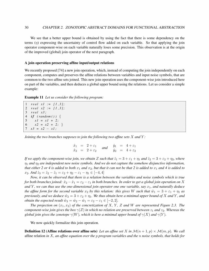
We see that a better upper bound is obtained by using the fact that there is some dependency on theterms (η) expressing the uncertainty of control flow added on each variable. So that applying the joinoperator component-wise on each variable naturally loses some precision. This observation is at the originof the improved (global) join operator of the next paragraph.
A join operation preserving affine input/output relations
We recently proposed [74] a new join operation, which, instead of computing the join independently on eachcomponent, computes and preserves the affine relations between variables and input noise symbols, that arecommon to the two affine sets joined. This new join operation uses the component-wise join introduced hereon part of the variables, and then deduces a global upper bound using the relations. Let us consider a simpleexample:
Example 11 Let us consider the following program:
1 r e a l x1 := [ 1 , 3 ] ;2 r e a l x2 := [ 1 , 3 ] ;3 r e a l x3 ;4 i f ( random ( ) ) {5 x1 = x1 + 2;6 x2 = x2 + 2; }7 x3 = x2 − x1 ;
Joining the two branches supposes to join the following two affine sets X and Y :
x1 = 2 + ε1
x2 = 2 + ε2and
y1 = 4 + ε1
y2 = 4 + ε2
If we apply the component-wise join, we obtain Z such that z1 = 3 + ε1 + η1 and z2 = 3 + ε2 + η2, whereη1 and η2 are independent new noise symbols. And we do not capture the somehow disjunctive information,that either 2 or 4 is added to both x1 and x2, but that it can not be that 2 is added to x1 and 4 is added tox2. And z3 = z2 − z1 = ε2 + η2 − ε1 − η1 ∈ [−4, 4]
Now, it can be observed that there is a relation between the variables and noise symbols which is truefor both branches joined: x2− x1 = ε2− ε1 in both branches. In order to get a global join operation on Xand Y , we can thus use the one-dimensional join operator one one variable, say x1, and naturally deducethe affine form for the second variable x2 by this relation: this gives W such that w1 = 3 + ε1 + η1 aspreviously, and we deduce w2 = 3 + ε2 + η1. We thus obtain here a minimal upper bound of X and Y , andobtain the expected result w3 = w2 − w1 = ε2 − ε1 ∈ [−2, 2].
The projection on (x1, x2) of the concretization of X , Y , Z and W are represented Figure 2.3. Thecomponent-wise join gives the box γ(Z) in which no relation are preserved between z1 and z2. Whereas theglobal join gives the zonotope γ(W ), which is here a minimal upper bound of γ(X) and γ(Y ).
We now quickly formalize this join operation.
Definition 12 (Affine relations over affine sets) Let an affine set X inM(n + 1, p) ×M(m, p). We callaffine relation in X , an affine equation over the p program variables and the n noise symbols, that holds for

2.2. AN ORDERED STRUCTURE FOR FUNCTIONAL ABSTRACTION 31
γ(X)
γ(Y )
γ(Z) γ(W )
x1
x2
1 3 50
1
3
5
Figure 2.3: X , Y and results Z and W of the component-wise and global join operators
any values of the noise symbols, i.e. is given by α1, . . . , αp, β0, . . . , βn ∈ R such that:
p∑r=1
αrxr = β0 +
n∑i=1
βiεi (2.5)
holds for any ε = t(ε1, . . . , εn) ∈ [−1, 1]n and η = t(η1, . . . , ηm) ∈ [−1, 1]m and (x1, . . . , xp) = tCXε +tPXη.
The set of affine relations defined in Equation 2.5, identified with vector (α1, . . . , αp, β0, . . . , βn), is a sub-vector space of Rp+n+1, hence generated by a finite number l of independent affine relations. This l isnecessarily smaller or equal to p, since the n noise symbols are linearly independent, and there is a constantterm.
Computing common affine relations An affine relation common to X and Y is an affine relation inX which is also an affine relation in Y . Consider we have k such affine relations, k being necessarily lessor equal to p as previously stated:
p∑r=1
αl,rxr = βl,0 +n∑i=1
βl,iεi, ∀l ∈ {1, . . . , k}. (2.6)
When the (xr)1≤r≤p are defined by an affine set X = (CX , PX), we can rewrite Equation 2.6:∑pr=1 αl,rxr =
∑ni=0 (
∑pr=1 αl,rci,r) εi +
∑mj=0 (
∑pr=1 αl,rpj,r) ηj , ∀l ∈ {1, . . . , k}
These relations being true for every value of the noise symbols εi and ηj implies that for all 1 ≤ l ≤ k,0 ≤ i ≤ n and 1 ≤ j ≤ m, we have:
p∑r=1
αl,rci,r = βl,i andp∑r=1
αl,rpj,r = 0

32 CHAPTER 2. ZONOTOPIC ABSTRACT DOMAINS FOR FUNCTIONAL ABSTRACTION
Example 12 Consider again the two affine sets joined in Example 11:
x1 = 2 + ε1
x2 = 2 + ε2and
y1 = 4 + ε1
y2 = 4 + ε2
We want the affine relations common to X and Y , of the form: α1x1 + α2x2 = β0 + β1ε1 + β2ε2 thathold for all (ε1, ε2) ∈ [−1, 1]. Substituting X and Y in this relation yields
β0 = 2α1 + 2α2 = 4α1 + 4α2
β1 = α1
β2 = α2
The solutions can be parameterized by a λ ∈ R, they are of the form β0 = 0, α1 = β1 = λ, α2 = β2 = −λ.For instance we can choose x2 − x1 = ε2 − ε1.
The following lemma states that the affine input/output relations of Equation 2.6 are compatible with thefunctional order, which shows the necessity to preserve them:
Lemma 8 Let X = (CX , PX) and Y = (CY , P Y ) be two affine sets such that
1. X ≤ Y ,
2. Y satisfies the k relations of Equation 2.6
Then X satisfies these k relations.
Preserving these affine relations Up to a renumbering of the variables, we can always suppose the kindependent common affine relations for X and Y are of the form:
xi = Ri(xi+1, . . . , xp, ε1, . . . , εn) (2.7)
We thus choose among the p variables, p − k variables on which we use the component-wise join. Fromthere, using the k Equations 2.7, we can construct an upper bound for the p variables. We note X>k theprojection of X ∈M(n+ 1, p)×M(m, p) on its last components xk+1, . . . , xp, and now define the globaljoin operator:
Definition 13 (Global join) Let two affine setsX and Y inM(n+1, p)×M(m, p), which have in commonk independent affine relations: for all i ∈ [1, k], xi = Ri(xi+1, . . . , xp, ε1, . . . , εn). We define Z = X tG Yby Z>k = X>k tC Y>k and for all i ∈ k, . . . , 1, zi = Ri(zi+1, . . . , zp, ε1, . . . , εn).
Note that in Definition 13, the operations are ordered: first computation of Z>k, then reconstruction of zk toz1. This operation indeed defines an upper bound, which is a minimal upper bound in some cases:
Lemma 9 Z = X tG Y is an upper bound of X and Y , and if Z>k is a minimal upper bound of X>k andY>k, then Z is a minimal upper bound of X and Y .

2.2. AN ORDERED STRUCTURE FOR FUNCTIONAL ABSTRACTION 33
2.2.4 Modular analysis
As already stated, affine sets provide linearized input-output relations, or functional abstraction, that are wellsuited for modular analyses. We recently proposed [89] a summary-based approach that is both natural andefficient, and still gives accurate results in realistic cases. The function summaries are pairs (I,O) of inputand output zonotopes, parameterized by the same central noise symbols ε1, . . . , εn representing the inputsof the program, so that both represent a function of these inputs. The pair also thus represents functionsfrom γ(I) to γ(O). For a given input zonotope I , the output zonotope O is computed by applying theanalysis with the zonotopic abstract domain, so that it is defined as a function of the input noise symbolsε1, . . . , εn, but also of the perturbation symbols I may contain. As I is usually obtained by joining severalcalling contexts, it contains some perturbation noise symbols corresponding to this join operation. TheoutputO can then be instantiated to any particular calling context included in the input I of the summary, bysubstituting some of these perturbation noise symbols by their expression for the particular calling context.
Example 13 Let us quickly sketch the summarizing process on a small example.
1 r e a l mu l t ( r e a l a , r e a l b ) {2 r e t u r n a ∗ ( b−2) ;3 }45 r e a l compute ( r e a l x ) {6 r e a l y1 = mul t ( x +1 , x ) ;7 r e a l y2 = mul t ( x , 2∗ x ) ;8 r e t u r n y2−y1 ;9 }
1011 compute ( [ −1 ,1] ) ;
Function compute is called with x = ε1 (input in [-1,1]). We build a summary for function mult after itsfirst call (y1 = mult(x+1, x);). Using the semantics on affine sets to abstract the body of the function,we get as summary the couple of affine sets (I,O) such that I = (ε1 + 1, ε1), O = (−1.5 − ε1 + 0.5η1),where I abstracts the calling context and O the output.
At the next call (y1 = mult(x, 2*x);), we try to see if the previous summary can be used, that isif the calling context is contained in the input I of the summary: it is not the case as (ε1, 2ε1) ≤ (ε1 + 1, ε1)does not hold.
We merge the two calling contexts with the join operator, and analyze again the body of the function:this gives a new (larger) summary for function mult: I = (0.5 + ε1 + 0.5η2, 1.5ε1 + 0.5η3), O = (−1
4 −54ε1 − η2 + 1
4η3 + 94η4).
Then, this new summary can be instantiated to the two calls (or any other call with calling contextcontained in affine set I = (0.5 + ε1 + 0.5η2, 1.5ε1 + 0.5η3)). Without instantiation, the output value ofthe summary ranges in [−5, 4.5]. But the summary is a function defined over input ε1 of the program, andover the symbols η2 and η3 that allow to express the inputs of function mult: we will thus get a tighterrange for the output, as well as a function of input ε1, by instantiating η2 and η3 and substituting them inthe output of the summary. For instance, for the second call of function mult, with (ε1, 2ε1), we identifyε1 with 0.5 + ε1 + 0.5η2 and 2ε1 with 1.5ε1 + 0.5η3, and deduce η2 = −1 and η3 = ε1, which yields forthe output 3
4 − ε1 + 94η4 ∈ [−5
2 , 4]. Direct computation gives 1− 2ε1 + η4 ∈ [−2, 4], which is just slightlytighter.

34 CHAPTER 2. ZONOTOPIC ABSTRACT DOMAINS FOR FUNCTIONAL ABSTRACTION
I1 t I2
I1
I2
−2 −1 0 1 2
−2
−1
0
1
2
a
b
Mult(I1 t I2)
Mult(I2)
ExM(I2)
−1 −0.5 0 0.5 1
−5−4−3−2−1
012345
ε1
Output
Figure 2.4: Summary and instantiation (left is input, right output)
We illustrate this in Figure 2.4: we represent on the left picture, the calling contexts (a, b) for the twocalls (I1 is first call, I2 is second call), and the zonotopic concretization of the calling context after merge,I1 t I2. On the right part of the figure, the parabola is the exact results of the second call, ExM(I2). Thedashed zonotope is the result of the abstraction with the semantics of affine sets of the second call,Mult(I2).The zonotope in plain lines is the output of the summary, Mult(I1 t I2). The zonotope in dotted lines is thesummary instantiated to the second call.
2.3 First experiments
The aim of this section is to study the behavior of the affine sets abstract domain, and compare it to otherclassic abstract domains. We restrict ourselves here to the analysis of programs in real number semantics,with small prototypes built for academic purposes. The extension to the study of finite precision computa-tions, and the use of the static analyzer Fluctuat on real examples will be the subject of Chapter 5. Also, thestudy of fixpoint computations being left for Chapter 4, examples requiring fixpoint computations will bedelayed until that chapter.
The presentation so far has assumed that the coefficients of affine sets are real numbers. In an imple-mentation, however, floating-point coefficients are used. Using them without care would produce possiblyunsound results: any rounding error would produce incorrect relationships between variables. A first ideato keep a sound over-approximation using finite precision numbers is to use affine sets with interval coeffi-cients. The problem is that the width of these interval coefficients would grow with computations, we wouldsuffer again from the defects of intervals. A better way to do this is to have floating-point coefficients. Inorder to keep a sound over-approximation, it is only needed to bound the error committed at each operationon these coefficients and account for this error by a new noise term. Practically, in order to reduce the num-ber of noise symbols used, we group these errors with other approximation terms. But we could imagineto keep different kind of symbols, accounting respectively for the uncertainty on the outputs due to inputuncertainty, abstract domain uncertainty, and uncertainty due to the finite precision implementation of theanalysis.
K. Ghorbal implemented the (constrained) affine sets in the APRON library [103], as an abstract domaincalled Taylor1+ [64]. We now compare the performance of this domain, on unrolled linear and non linear it-

2.3. FIRST EXPERIMENTS 35
erative computations, with classic abstract domains such as boxes, octagons and polyhedra. No summarizingis being applied here. The upper bound operator implemented for these experiments is the component-wiseone of Definition 11. More details can be found in [64, 65]. An implementation of the global join operatorwas also added to the Taylor1+ abstract domain, some results can be found in [74].
Linear schemes The first example we consider is the second order recursive filter:
xi = 0.7ei − 1.3ei−1 + 1.1ei−2 + 1.4xi−1 − 0.7xi−2,
where x0 = 0, x1 = 0, and the ei are independent inputs between 0 and 1.We here fully unroll the 2nd order filter scheme to compute the abstract value at each iteration. Figure 2.5
compares accuracy and performance of Taylor1+ with three classic abstract domains provided in APRON:boxes, octagons and polyhedra (both PK [101] and PPL [140] implementations were tested). The polyhedradomain with exact arithmetic (using GMP) gives the exact bounds for the filter output. One can see thatTaylor1+ wraps the exact range given by polyhedra (left figure) very closely, with great performance (rightfigure).
Figure 2.5: Unrolled scheme for the 2nd order filter
Non-linear computations; test interpretation We now consider a toy example demonstrating theperformance of the constrained version of the affine sets (constrained T1+ in its APRON implementation),where constraints on noise symbols are interpreted in intervals. We want to compute g(g(x)) on the rangex = [−2, 2], where
g(x) =
√x2 − x+ 0.5√x2 + 0.5
.
For that, we parameterize the program that computes g(g(x)) by a number of tests that subdivide the domainof the input variable (see Figure 2.6 left), in order to compare the cost and accuracy of the different domainswhen the size of the program grows. It can be noted (Figure 2.7 left) that the domain scales up wellwhile giving here more accurate results (Figure 2.7 right) than the other domains. As a matter of fact, with

36 CHAPTER 2. ZONOTOPIC ABSTRACT DOMAINS FOR FUNCTIONAL ABSTRACTION
Figure 2.6: Implementation of g(g(x)) for x in [-2,2] (left) and plot of g(g(x)) (right)
1 g ( x ) = s q r t ( x∗x−x + 0 . 5 ) / s q r t ( x∗x + 0 . 5 ) ;2 x = [−2 ,2 ] ;3 /∗ f o r n s u b d i v i s i o n s ∗ /4 h = 4 / n ;5 i f (−x<=h−2)6 y = g ( x ) ; z = g ( y ) ;7 . . .8 e l s e i f (−x<=i ∗h−2) /∗ i i n { 2 , . . . , n−1}∗ /9 y = g ( x ) ; z = g ( y ) ;
10 . . .11 e l s e12 y = g ( x ) ; z = g ( y ) ;
x
g(g(x))
20−2
0.54
0.58
0.62
Figure 2.7: Comparing analysis time and results of the different APRON domains.
polka
ppl
10 100 200 300# subdivisions (constraints)
400 50050
1
2
3
CP
Utim
e(s
)
4
• [Cons.T1+]
∗ [Octagons]
+ [Boxes]
◦ [Polyhedra]
2 4 8 20# subdivisions (constraints)
wid
thofg(g
(x))
1
2
3
4
• [Cons.T1+]
∗ [Octagons]
+ [Boxes]
◦ [Polyhedra]
an interval domain for the noise symbols, all abstract transfer functions are linear or at worst quadratic inthe number of noise symbols appearing in the affine forms. The fact that the results observed for 3 and 5subdivisions (Figure 2.7 right) are less accurate respectively than those observed for 2 and 4 subdivisions, isrelated to the behavior of g(g(x)) on [−2, 2] (see Figure 2.6 right): for example when a change of monotonyappears near the center of a subdivision, the approximations will be less accurate than when it appears at theborder.

Chapter 3
Extensions of the Zonotopic Approach
The zonotopic abstract domains of Chapter 2 lend themselves to several interesting extensions, still dealingwith the abstraction of real-valued computations. These extensions no longer present zonotopic concretiza-tions, but still use the ideas introduced in Chapter 2 in the zonotopic context. A first class of variations stillrelies on affine sets, but with coefficients that are no longer real numbers: we proposed in 2007 an under-approximating abstract domain based on affine sets with interval coefficients [82], which I will describe inSection 3.1. We are presently also considering extensions with zonotopic coefficients, that should definehigher-order approximations. A second class of variations relies on a parametrization of variables valuesby affine sets with real coefficients, but the noise symbols no longer simply lie in intervals: we recentlyproposed [20, 21] to thus mix probabilistic and deterministic information by using p-boxes [52, 53] insteadof interval noise symbols, this will be quickly described in Section 3.2. Finally, we are also considering touse vectors of noise symbols bounded in `2 norms for an ellipsoidal extension, or more generally in `p norm,as quickly discussed in the concluding chapter.
3.1 An under-approximating abstract domain
Most abstract interpretation numerical domains construct over-approximations of the range of pro-gram variables. Galois connections, which is the classic abstraction setting, naturally express over-approximations and we need dual Galois connections, or dual concretization-based frameworks, as devel-oped by Schmidt [149, 148], to express under-approximations. But the main problem is that it is verydifficult to compute good numerical under-approximations. Of course, testing or bounded model checkingprovide under-approximations, but what we want here is really some duals of classic over-approximatingabstract domains.
We present here a variation of affine sets, using ideas from generalized interval arithmetic [70, 69], thatallowed us to develop in 2007 [82] a first abstract interpretation domain for directly under-approximatingthe range of real values of program variables.
Such under-approximations, when combined with over-approximations, give an estimate of the qualityof the result of a static analysis. But they can also be applied to statically find run-time errors that are boundto occur, from some given set of possible initial states: we will show how they can be used to generate testcase scenarios that allow to minimize/maximize some variable.
37

38 CHAPTER 3. EXTENSIONS OF THE ZONOTOPIC APPROACH
x× y y ∈ P y ∈ Z y ∈ −P y ∈ dualZx ∈ P [xy, xy] [xy, xy] [xy, xy] [xy, xy]
x ∈ Z [xy, xy][min(xy, xy),
max(xy, xy)][xy, xy] 0
x ∈ −P [xy, xy] [xy, xy] [xy, xy] [xy, xy]
x ∈ dualZ [xy, xy] 0 [xy, xy][max(xy, xy),
min(xy, xy)]
Table 3.1: Kaucher multiplication ([106])
3.1.1 Generalized affine sets for under-approximation
We first introduce the principles of generalized and Kaucher interval arithmetic [106] and their interpretationas modal intervals using quantifiers, and thus in some conditions as under-approximations [70, 69]. We thendescribe our contribution, which is to extend these ideas to define generalized affine forms that will beinterpreted either as over or under-approximating forms for real values of variables.
Generalized intervals, modal intervals and Kaucher arithmetic Generalized intervals are intervalswhose bounds are not ordered. The set of classic intervals is denoted by IR = {[a, b], a ∈ R, b ∈ R, a ≤ b}.The set of generalized intervals is denoted by IK = {[a, b], a ∈ R, b ∈ R}. Intervals will be noted withbold letters.
For two real numbers a and b such that a ≤ b, one can consider two generalized intervals, [a, b], which iscalled proper, and [b, a], which is called improper. For any a, b, we define the operations dual [a, b] = [b, a]and pro [a, b] = [min(a, b),max(a, b)].
The generalized intervals are partially ordered by inclusion which extends inclusion of classic intervals.Given two generalized intervals x = [x, x] and y = [y, y], the inclusion is defined by
x v y ⇔ y ≤ x ∧ x ≤ y.
Kaucher addition extends addition on classic intervals :
x+ y = [x+ y, x+ y]
x− y = [x− y, x− y] = x+ (−y) where − y = [−y,−y].
We let P = {x = [x, x], x ≥ 0 ∧ x ≥ 0}, −P = {x = [x, x], x ≤ 0 ∧ x ≤ 0},Z = {x = [x, x], x ≤ 0 ≤ x}, and dual Z = {x = [x, x], x ≥ 0 ≥ x}. Kaucher multipli-cation x × y is described in table 3.1. Kaucher division is defined for all y such that 0 /∈ pro y byx/y = x × [1/y, 1/y]. When restricted to proper intervals, these operations coincide with the classicinterval operations.
Classic interval computations can be interpreted as quantified propositions. As an example, take f tobe the function defined by f(x) = x2 − x. Extended to interval arithmetic, its value on x = [2, 3] isf([2, 3]) = [2, 3]2 − [2, 3] = [1, 7], which can be interpreted as the proposition
(∀x ∈ [2, 3]) (∃z ∈ [1, 7]) (f(x) = z).

3.1. AN UNDER-APPROXIMATING ABSTRACT DOMAIN 39
Modal intervals extend classic intervals by coupling a quantifier to them. Extensions of modal intervals wererecently proposed by Goldsztejn [70] in the framework of generalized intervals, and called AE extensionsbecause universal quantifiers (All) always precede existential ones (Exist) in the interpretations. They giverise to a generalized interval arithmetic which coincides with Kaucher arithmetic. Let f : Rn → R afunction in which each variable appears only once. Let x ∈ IKn, which we can decompose in xA ∈ IRpand xE ∈ (dual IR)q with p+ q = n. We consider the problem of computing a quantifier Qz and an intervalz ∈ IK such that
(∀xA ∈ xA) (Qzz ∈ pro z) (∃xE ∈ pro xE)(f(x) = z). (3.1)
In these expressions, if z is proper then Qz = ∃, else Qz = ∀. When all intervals are proper, we retrievethe interpretation of classic interval computation, which gives an over-approximation of the range of f(x) :
(∀x ∈ x) (∃z ∈ z) (f(x) = z).
And when all intervals are improper, we get an under-approximation :
(∀z ∈ pro z) (∃x ∈ pro x) (f(x) = z).
Affine forms for over and under-approximation We will now use these notions to compute over whatwe call generalized affine forms, where the αx
i coefficients are no longer real numbers but intervals :
x = αx0 +αx
1ε1 + . . .+αxnεn, with αx
i ∈ IR. (3.2)
The classic concretization γ(x) of x is a proper interval obtained by the evaluation of expression (3.2)with proper intervals εi = [−1, 1] and classic interval arithmetic :
γ(x) = αx0 +αx
1ε1 + . . .+αxnεn.
We define the concretization δ(x) of x obtained by the evaluation of expression (3.2) with improperintervals ε∗i = [1,−1] and Kaucher interval arithmetic :
δ(x) = αx0 +αx
1ε∗1 + . . .+αx
nε∗n.
Generalized affine forms are closed under affine operations. For affine forms x and y, and real numbersλ1 and λ2, we have:
λ1x+ y + λ2 = (λ1αx0 +αy
0 + λ2) + (λ1αx1 +αy
1)ε1 + . . .+ (λ1αxn +αy
n)εn
We use for the under-approximation of the result of non affine arithmetic operations, an extension of themean-value theorem to generalized intervals [69], which we extend to our generalized affine forms. We thenderive an expression for the under-approximation of the multiplication. Note that we could also, in the sameway, derive semantics for other arithmetic operations.

40 CHAPTER 3. EXTENSIONS OF THE ZONOTOPIC APPROACH
Mean-value theorem for generalized affine forms Suppose variables x1, . . . , xk, are described asaffine combinations of noise symbols ε1, . . . , εn. For a differentiable function f : Rk → R, we writef ε : Rn → R the function induced by f on ε1 to εn. Suppose we have an over-approximation ∆i of thepartial derivatives {
∂fε
∂εi(ε), ε ∈ [−1, 1]n
}⊆∆i. (3.3)
Then
f ε(ε1, . . . , εn) = f ε(t1, . . . , tn) +
n∑i=1
∆i(εi − ti), (3.4)
where (t1, . . . , tn) is any point in [−1, 1]n, is interpretable in particular in the following sense :
• if f ε(ε∗1, . . . , ε∗n), computed with Kaucher arithmetic, is an improper interval, then pro f ε(ε∗1,
. . . , ε∗n) is an under-approximation of f ε(ε1, . . . , εn).
• if f ε(ε1, . . . , εn) is a proper interval, then it is an over-approximation of f ε(ε1, . . . , εn).
This theorem can be of course used when we take the εi in sub-ranges of [−1, 1], it will in fact be used inexamples to improve the accuracy of the results.
We derive from this theorem a simple under-approximating model for the multiplication. We can easilyprove by recurrence that, for all variables z whose real value is a linear function of noise symbols ε1, . . . , εn,the coefficient αz
i of the affine form obtained from our semantics is an over-approximation of ∂z∂εi
. Then,for f(x, y) = xy, we can over-approximate in Equation (3.4)
∂fε
∂εi(x, y) =
∂x
∂εiy +
∂y
∂εix
by∆i = αx
i y +αyi x, (3.5)
for any over-approximation x and y of the values taken by x and y.
Example 14 Let us consider f(x) = x2 − x when x ∈ [2, 3]. The interval of values taken by f(x) is [2, 6].Here, an under-approximation of f(x) can not be computed directly by Kaucher arithmetic, since variablex does not appear only once in expression f(x). An affine form for x is x = 2.5 + 0.5ε1, and we deduce
f ε(ε1) = (2.5 + 0.5ε1)2 − (2.5 + 0.5ε1).
We bound the derivative by ∆1 = 2 ∗ 0.5 ∗ (2.5 + 0.5ε1) − 0.5 ⊆ [1.5, 2.5], and, using the mean-valuetheorem with t1 = 0, we have
f ε(ε1) = 3.75 + [1.5, 2.5]ε1.
It can be interpreted as an under-approximation of the range of f(x) :
Γ(f ε(ε1)) = 3.75 + [1.5, 2.5][1,−1] = 3.75 + [1.5,−1.5] = [5.25, 4.25].
It can also be interpreted as an over-approximation :
Γ(f ε(ε1)) = 3.75 + [1.5, 2.5][−1, 1] = 3.75 + [−2.5, 2.5] = [1.25, 6.25].
However, the range thus obtained for over-approximation is not as good as the one obtained by classic affinearithmetic, where x2 − x = [3.75, 4] + 2ε1, which gives the range [1.75, 6].

3.1. AN UNDER-APPROXIMATING ABSTRACT DOMAIN 41
no subdivision 32 subdivisions
Figure 3.1: Estimation of the maximum value of result xi in the Newton algorithm.
Note that the generalized affine forms form a relational abstraction, as relations between variables areused to define the transfer functions. Still, we only characterized here under-approximations for the rangeof each variable taken independently, but not jointly. The join concretization is in particular no longerzonotopic, and characterizing it is one of our future objectives.
Order-theoretic considerations
We define the order on generalized affine sets by the following order applied component-wise on eachcomponent: x v y if and only if ∀i ≥ 0, αx
i v αyi . If x v y, then we have on the concretizations,
δ(x) v δ(y). In the case δ(x) and δ(y) are improper intervals, this is equivalent to pro δ(y) v pro δ(x).Inclusion x v y thus expresses that x is a better under-approximation that y, as it concretizes to an intervalwhose proper range is larger than the one of y. Also, x is a better over-approximation than y, as it concretizesto an interval whose proper range is included in the one of y: γ(x) v γ(y).
This means in particular that we can get safe over and under approximations when using finite precision,by outward rounding on the αx
i coefficients.
3.1.2 Applications and experiments
We consider, for some given A, the (non-linear) iteration of the Newton algorithm xi+1 = 2xi − Ax2i .
If we take x0 not too far away from the inverse of A, this iteration converges to the inverse of A. As anexample, we take A ∈ [1.99, 2.00], i.e. A = 1.995 + .005ε1, x0 = .4 and ask to iterate this scheme until|xi+1−xi| < 5×10⁻⁶. We get the concretizations of lower and upper forms shown in the left part of figure3.1. After 6 iterations, we get stable concretizations, for both lower and over-approximations of x6 :
[0.5012531328, 0.5012531328] v x6 v [0.499996841, 0.502512574],
[0, 0] v |x6 − x5| v [−3.17241289× 10⁻⁶, 3.17241289× 10⁻⁶].
And for the stopping criterion |xi+1 − xi| < 5 × 10⁻⁶, using simultaneously the over- and under-approximation, we obtain in addition that the Newton algorithm terminates after exactly 4 iterations, which

42 CHAPTER 3. EXTENSIONS OF THE ZONOTOPIC APPROACH
allows us to refine the invariant:
[0.5002532337, 0.5022530319] v x4 v [0.499996841, 0.502512574].
This is a general fact: the combination of under and over approximations gives in general a very powerfulmethod to determine the invariants of a program.
We can also refine the results using subdivisions of the input A, that give way to as many independentcomputations relying on different affine forms for A. For instance, when subdividing in 32 sub-intervals, weget after 6 iterations a relative difference between the bounds given by the over- and under-approximations,of less than 9× 10⁻⁶; the results obtained are shown in the right part of figure 3.1.
Filters, perturbations and worst case scenario
In the sequel, in order not to get into complicated details, we suppose that we have a real arithmetic at hand(or arbitrary precision arithmetic). We consider again the order 2 recursive filter considered in Chapter 2:
Si = 0.7Ei − 1.3Ei−1 + 1.1Ei−2 + 1.4Si−1 − 0.7Si−2,
where Ei are independent inputs between 0 and 1, so that Ei = Ei = 12 + 1
2εi+1, and S0 = S1 = 0.We first consider the output Si of this filter for a fixed number of unfoldings, e.g. i = 99. Using theover-approximating semantics of affine sets, we get
S99 = S99 = 0.83 + 7.8× 10⁻⁹ε1 − 2.1× 10⁻⁸ε2 − 1.6× 10⁻⁸ε3 . . .− 0.16ε99 + 0.35ε100,
whose concretization gives an exact enclosure of S99 :
[−1.0907188500, 2.7573854753] v S99 v [−1.0907188500, 2.7573854753].
Also, the affine form gives the sequence of inputs Ei that maximizes S99 : Ei = 1 if the correspondingcoefficient multiplying εi+1 is positive, Ei = −1 otherwise. Note that the exact enclosure actuallyconverges to S∞ = [−1.09071884989..., 2.75738551656...], and therefore the signal (sequence of inputsof size 99) leading to the maximal value of S99 is a very good estimate of the signal leading to the maximalvalue of Si, for any i ≥ 99. This can be used to find bad-case scenarios of a program, and generalizes tolinear recursive filters of any order.
We now perturb this linear scheme by adding a non-linear term 0.005EiEi−1:
Si = 0.7Ei − 1.3Ei−1 + 1.1Ei−2 + 1.4Si−1 − 0.7Si−2 + 0.005EiEi−1.
Again, we consider a fixed unfolding i = 99. Using over-approximation, we get
S99 = 0.837 + 7.81× 10⁻⁹ε1 − 2.09× 10⁻⁸ε2 . . .− 0.157ε99 + 0.351ε100
+1.77× 10⁻¹¹η1 − 2.66× 10⁻¹¹η2 + . . .+ 0.00175η97 + 0.00125η98,
in which terms from η1 to η98 account for the over-approximation of non-linear computations. A sequenceof inputs leading to a bad-case scenario is thus not given directly by the sign of the ε1, . . . , ε100 as in thelinear case: one can get a plausible worst-case scenario by choosing the E0, . . . , E99 that maximize the

3.2. MIXING P-BOXES AND AFFINE ARITHMETIC 43
sub affine form containing only these εk, but one has no assurance that this might be even close to the realsupremum of S99. But the under-approximating form allows us to choose at least part of the inputs. Usingthe under-approximating semantics, we get :
S99 = 0.837 + 7.81× 10⁻⁹ε1 − 2.09× 10⁻⁸ε2 + . . .+ [−0.0577, 0.0635]ε93
+[0.0705, 0.138]ε94 + [0.185, 0.223]ε95 + [0.25, 0.271]ε96 + [0.222, 0.234]ε97
+[0.081, 0.0876]ε98 + [−0.158,−0.155]ε99 + [0.35, 0.352]ε100.
This gives the following estimates for the real enclosure of S99:
[−0.47655194955570, 2.1515519079] v S99 v [−1.10177396494, 2.77677392330].
As the interval coefficient αk is an over-approximation of the partial derivative of S99 with respect to εk,we know how to choose input Ek−1 (Ek−1 corresponds to εk) to maximize or minimize the output. We thusknow that E93 = 1 E94 = 1, E95 = 1, E96 = 1, E97 = 1, E98 = 0 and E99 = 1 is the best depth 7 choiceof inputs that will maximize S99. For the other inputs, we use as a heuristic the ε0, . . . , ε92 that maximizethe over-approximating term, here this gives S99 = 2.766383. We thus found a scenario which is very closeto the worst-case bound 2.77677392330. A one hour simulation on a 2GHz PC for 109 random sequencesof 100 entries gives as estimate of the supremum 2.211418, far from our estimate in both time and precision.
3.2 Mixing P-boxes and Affine Arithmetic
In program analysis, a difficulty is to properly handle the inputs of the program. They are often not exactlyknown, but should rather be considered as being in a set of possible values. However, it is often the case thatwe have more information on the inputs than the mere fact that they belong to some set, such as a probabilitydistribution that states their likelihood to be at a specific point within the set.
P-boxes [52, 53] and Dempster-Shafer structures [151] are widely used to propagate both probabilisticand non-deterministic information. However, arithmetic rules on these structures are classically definedonly between structures representing either independent random variables, or variables with unknown de-pendency. This makes the usual p-box arithmetic not well adapted when many numerical computationsoccur between quantities (values of the program variables for instance) that cannot be considered indepen-dent, but whose dependency cannot be determined easily. The computations suffer from the drawbacks ofclassic interval arithmetic.
We thus proposed [20, 21] a new arithmetic that combines affine arithmetic to propagate the affinerelations between random variables and p-box arithmetic to over-approximate the probability distributionresulting from a given operation. This allows us to both increase the precision of the result and decrease thecomputation time compared to standard p-box arithmetic.
3.2.1 Basics: Dempster-Shafer structures and p-boxes
An interval based Dempster-Shafer structure [151] (we will call it DS in short) is a finite set of closedintervals (named focal elements) associated with a probability. DS structures thus represent real vari-ables whose value can be obtained by first probabilistically picking up an interval, and then non-deterministically picking up a value within this interval. In this article, we write a DS structure d as

44 CHAPTER 3. EXTENSIONS OF THE ZONOTOPIC APPROACH
−1 −0.5 0.250.5 1 2
1
Figure 3.2: A p-box (thick lines) and a CDF (thin line) included in this p-box.
d ={〈x1, w1〉 , 〈x2, w2〉 , . . . , 〈xn, wn〉
}, where xi ∈ IR is a closed non-empty interval and wi ∈]0, 1] is
the associated probability, with∑n
k=1wk = 1.A set of cumulative distribution functions can be represented by two non-decreasing functions P and
P such that P is left-continuous, P is right-continuous and ∀x, P (x) ≤ P (x). Such a pair[P , P
]is
called a p-box [52] and encloses all CDF P that satisfy ∀x, P (x) ≤ P (x) ≤ P (x). We will only considerhere discrete p-boxes, where P and P are step-functions. We refer the reader to Ferson et al. [52] for thecorrespondence between discrete p-boxes and DS structures; we note ζ the function that converts a DS to ap-box, and δ its inverse, that converts a discrete p-box to a DS.
Example 15 Let d1 ={〈[−1, 0.25], 0.1〉 ; 〈[−0.5, 0.5], 0.2〉 ; 〈[0.25, 1], 0.3〉 ; 〈[0.5, 1], 0.1〉 ; 〈[0.5, 2], 0.1〉 ;
〈[1, 2], 0.2〉}
. Then[P2, P2
]= ζ(d1) is as plotted in Figure 3.2.
Many arithmetics were proposed for p-boxes and DS structures [10, 51, 56, 158], most of them areequivalent in term of precision [141]. Here, we briefly explain the method of Berleant et al. [10] which weused. Let two random variables X and Y represented by DS structures dX = {〈xi, wi〉 , i ∈ [1, n]} anddY = {
⟨yj , w
′j
⟩, j ∈ [1,m]}, and Z be the random variable such that Z = X + Y . We want to compute
a DS that contains Z (the algorithms for other arithmetic operations are similar). We distinguish the casewhen X and Y are independent (in which case we denote the operation ⊕) and when they are not (in whichcase we denote the operation +).Independent variables. If X and Y are independent random variables, then the DS for Z = X ⊕ Y isdZ = {〈zi,j , ri,j〉 , i ∈ [1, n], j ∈ [1,m]} such that:
∀i ∈ [1, n], j ∈ [1,m], zi,j = xi + yj and ri,j = wi × w′j . (3.6)
The number of focal elements within the DS structures clearly grows exponentially with the number ofsuch operations. In order to keep the computation tractable, we bound the number of focal elements: ofcourse, this introduces some over-approximation.Variables with unknown dependency. If the random variables X and Y are not independent, the lowerbound FZ of the p-box
[FZ , FZ
]for Z is obtained by solving the linear programming problem defined by
Equation (3.7).
FZ(z) = maximize∑
xi+yj≤z ri,j
such that ∀i ∈ [1, n],∑m
j=1 ri,j = wi∀j ∈ [1,m],
∑ni=1 ri,j = w′j
(3.7)
The formula for FZ is similar. We then define dZ = δ([FZ , FZ
]), where δ is the conversion function from
p-boxes to DS.

3.2. MIXING P-BOXES AND AFFINE ARITHMETIC 45
3.2.2 Affine arithmetic with probabilistic noise symbols
We consider a set of uncertain quantities that will be propagated through a program. We will now express thelinearized (deterministic) dependencies between these quantities using affine arithmetic, while we expressthe uncertainty on each variable, by associating a DS to each noise symbol of the affine forms. In this way,we add structure to DS arithmetic. As in classic affine sets, we will define two kinds of noise symbols: theεi that are considered independent, and the ηk that cannot be considered as independent from other noisesymbols.
Definition 14 (Probabilistic affine form.) We define a probabilistic affine form for variable x, on n inde-pendent noise symbols (ε1, . . . , εn) and m noise symbols (η1, . . . , ηm) with unknown dependency to theothers, by a form
x = αx0 +
n∑i=1
αxi εi +
m∑j=1
βxj ηj
together with n DS (dε1 , . . . , dεn) and m DS (dη1 , . . . , dηm) describing the possible random variables (ofsupport [−1, 1]) for the noise symbols.
A probabilistic affine form x represents the set of all random variables X contained in the DS γ(x),called concretization of x:
Definition 15 (Concretization of affine forms as a DS) Let x be a probabilistic affine form, its concretiza-tion as a DS is:
γ(x) = αx0 +
n⊕j=1
αxj dεj +
m∑k=1
βxkdηk ,
where⊕
is the sum of independent DS,∑
is the sum of DS with unknown dependency, and we note αd(resp. α + d) where α ∈ R and d is a DS {〈xi, pi〉 | i = 1, . . . , q}, the result of the multiplication (resp.addition) of a constant by a DS: {〈αxi, pi〉 | i = 1, . . . , q} (resp. {〈α+ xi, pi〉 | i = 1, . . . , q}).
The interest of affine forms is to be able to represent affine relations that hold between uncertain quan-tities. We still have this representation, except only imprecise affine relations hold, as can be shown in theexample below.
Example 16 Let x1 = 1 + ε1 − η1, x2 = −12ε1 + 1
4η1, dε1 = {〈[−1, 0], 12〉, 〈[0, 1], 1
2〉},dη1 = {〈[− 1
10 , 0], 12〉, 〈[0,
110 ], 1
2〉}. Then x1+2x2 = 1− 12η1, with d = dx1+2x2 = {〈[19
20 , 1], 12〉, 〈[1,
2120 ], 1
2〉}.Thus the lower probability that x1 + 2x2 ≤ 21
20 is 1, and the upper probability that x1 + 2x2 <1920 is 0.
But for instance, x2 + 2x2 ≤ 1 has upper probability 12 and lower probability 0 and is thus an imprecise
relation.
Affine arithmetic operations are exactly the same as in the fully deterministic case. For non-linearoperations, we can rely on the affine form calculus, except that we use the available calculus on DS to forma correct DS representing this non-linear part. In this computation, some noise symbols are independentfrom the others, and we use both independent or unknown dependency versions of the operations on DS.
Noting that the square of a DS x = {〈xi, wi〉 | i = 1, . . . , p}, is the DS x2 = {〈x2i , wi〉 | i = 1, . . . , p},
we define the probabilistic affine form z = x× y as an affine form defined as for classic affine arithmetic, but

46 CHAPTER 3. EXTENSIONS OF THE ZONOTOPIC APPROACH
where the new symbol ηm+1 is considered with unknown dependency to the other symbols (characterizationof this dependency is left for future work), and has an associated DS dηm+1 defined by:
dηm+1 = 1T
(∑ni=1
∑mj=1(αxi β
yj + βxj α
yi )dεi × dηj +
∑ni=1
∑nj>i(α
xi α
yj + αxjα
yi )dεi ⊗ dεj
+∑m
i=1
∑mj>i(β
xi β
yj + βxj β
yi )dηi × dηj + 1
2
(⊕ni=1 α
xi α
yi dεi
2 +∑m
j=1 βxj β
yj dηj
2))
Let us remark that, although affine arithmetic usually increases the computation time compared to inter-val arithmetic, we here decrease the complexity of arithmetic operations by using affine forms. Actually, wedelay most of the DS arithmetic to the concretization function, and we can use the arithmetic of independentDS structures instead of arithmetic with unknown dependency, which is very costly.
Modeling rounding errors In the same way rounding errors can be computed using affine sets, as pre-sented in Chapter 5, they can also be modeled and computed by probabilistic affine forms. We give a quickhint here. We note f(rx) the nearest floating-point value to real value rx, and e(rx) the associated roundingerror e(rx) = f(rx) − rx. With normalized floating-point numbers and rounding mode to the nearest, wecan bound the error committed when rounding the real value rx to f(rx) by
|f(rx)− rx| ≤ δ.2i with i, |rx| ∈]2i, 2i+1], (3.8)
and δ is a constant that depends on the floating-point format.
The sum of the DS structures defining rx is a DS structure drx . To compute the error when rounding thisreal number, we thus compute the image by the error function of each focal element, and add the weightswhen theses images appear several times:
Definition 16 Suppose that the real value of x is given by the DS structure drx ={⟨xrk, w
rk
⟩, k =
1, . . . , n}, then for all k ∈ [1, n], we define ik such that max(|xrk|, |xr
k|) ∈]2ik , 2ik+1]. The roundingerror of x is defined by the DS
dex = R({⟨
[−δ2ik , δ2ik ], wek⟩, k = 1, . . . , n}),
where R is a reduction operator that bounds the number of focal elements.
Example Consider a given integer n and the sum yp of p independent variables xi, i = 1, . . . , p, eachof them defined in [−1, 1] by the DS with 2n non-overlapping elements of width 1
n and same weight. Thesevariables are first rounded as a floating-point value before being added. The envelop of the rounding erroron a variable xi is given in Figure 3.3. Consider for instance n = 5. The focal elements on the real valueare materialized on this figure by the grid. The image, by the rounding error function, of the focal elementsof rxi yields as DS for the error
dexi ={⟨[−δ
2,δ
2
], 3/5
⟩,
⟨[−δ
4,δ
4
], 1/5
⟩,
⟨[−δ
8,δ
8
], 1/5
⟩}.
We compute the partial results yk =∑
0≤i<k xi for k from 1 to p, and a new rounding error e(ryk) isassociated with each of these partial results. Finally, the rounding result on yp is thus eyp =
∑0≤i<p e(r
xi)+

3.2. MIXING P-BOXES AND AFFINE ARITHMETIC 47
−1 −0.8−0.6−0.4−0.2 0 0.2 0.4 0.6 0.8 1−4−2
024·10−8
rxie(rx
i)
Figure 3.3: Envelop on the rounding error of rxi ∈ [−1, 1] to a float (Example 3.2.2).
−10 −5 0 5 10
0.5
1
Figure 3.4: P-box for yp
−2.10−6 0 2.10−6
0.5
1
Figure 3.5: P-box for the error on yp
∑1≤i≤p e(r
yk), where the DS for e(rxi) are all independent between one another, and e(ryk) has unknowndependency to e(rxj ) and e(ryj ) for all j ≤ k. It is thus interesting to consider not only independence ordependency, but a generalized notion of dependency matrix between variables or noise symbols.
We present in Figures 3.4 and 3.5 the cumulative distribution functions of the DS obtained for n = 10and p = 10. We see in Figure 3.4 that we bound indeed a quasi-Gaussian distribution (sum of independentuniform laws). Figure 3.5 is compatible with the stochastic modeling of errors as popularized in the CESTACmethod [155]. The advantage here is that we have guaranteed lower and upper probabilities for roundingerrors. Here we can read from Figure 3.5 that the probability that the error is within [−1.2.10−6, 1.2.10−6]is 1
2 while the probability that the error is in absolute value greater than 2.10−6 (which is about the maximaldeterministic error one can get) is almost zero. An experiment with CADNA free allows us to estimate thatthe first 5 to 7 digits are correct in the calculation of the sum, and that the error is less, in absolute value,than 10−6 with a probability of a bit more than 1
3 , which is compatible with the results we get here.

48 CHAPTER 3. EXTENSIONS OF THE ZONOTOPIC APPROACH
Chapter 4
Loops and Fixpoint Computations
Fixpoint computation is a key point for static analysis by abstract interpretation: invariants of a programare obtained as fixpoints of the functional that describes the behavior of the program, and much time andaccuracy of an analysis can be lost in loop invariant computation. This chapter, dedicated to the computationof fixpoints occurring in the static analysis of numerical programs, comprises two parts, that discuss twoalternatives to solve the problem. The first section describes our use of Kleene-like iterations with zonotopicabstract domains [83, 64, 84]. The use of Kleene-like iterations in static analysis is classic, but we also tryhere to shortly discuss their convergence for given classes of programs, as one would do for any numericalalgorithm. The second section presents an algorithm based on Newton-like iterations called policy iterations,introduced by Howard in 1960 to solve stochastic control problems [100]. We proposed to use policyiterations in the context of static analysis in 2005 [37]. In this article, we demonstrated the interest of thisfixpoint iteration used with the abstract domain of intervals, and I will describe it here also in this context.However, it has since been applied for relational abstract domains [59, 2, 60, 61, 62], and we hope in thefuture to apply it for zonotopic abstract domains.
4.1 Kleene-like iteration schemes
We first briefly recall the classic computation of fixpoints in complete partial orders, based on Kleene’siteration, with widening and narrowing refinements [39], then specialize it to our context of affine sets.
4.1.1 Kleene’s iteration sequence, widening and narrowing
We say that a self-map F of a complete partial order1 (L,≤) is monotonic if x ≤ y ⇒ F (x) ≤ F (y). Andit is also continuous if and only if for all increasing chains l1 ≤ l2 ≤ . . . ≤ ln ≤ . . . of L, we have⋃
n∈N
F (ln) = F (⋃n∈N
ln).
The least fixpoint of such a monotonic and continuous F can be obtained by computing the sequence:x0 = ⊥, xn+1 = F (xn) for n ≥ 0. If the sequence becomes stationary, i.e., if xm = xm+1 for some m,
1a partial order for which every increasing chain has a least upper bound
49

50 CHAPTER 4. LOOPS AND FIXPOINT COMPUTATIONS
the limit xm is the least fixpoint of F . Of course, this procedure may be inefficient, and it may not eventerminate in the case of lattices of infinite height, such as the simple interval lattice. For this computationto become tractable, widening and narrowing operators have been introduced [39]. Widening operatorsare binary operators ∇ on L which ensure that any finite Kleene iteration x0 = ⊥, x1 = F (x0), . . . ,xk+1 = F (xk), followed by an iteration of the form xn+1 = xn∇F (xn), for n > k, yields an ultimatelystationary sequence, whose limit xm is a post fixpoint of F , i.e. a point x such that x ≥ F (x). Narrowingoperators are binary operators ∆ on L which ensure that any sequence xn+1 = xn∆F (xn), for n > m,initialized with the above post fixpoint xm, is eventually stationary, and converges to a fixpoint.
void main() {int x=0; // 1while (x<100) { // 2
x=x+1; // 3} // 4
}
x1 = [0, 0]x2 = ]−∞, 99] ∩ (x1 ∪ x3)x3 = x2 + [1, 1]x4 = [100,+∞[∩(x1 ∪ x3)
Figure 4.1: A simple integer loop and its semantic equations
Consider the program at the left of Figure 4.1. The corresponding semantic equations in the lattice ofintervals are given at the right of the figure. The intervals x1, . . . , x4 correspond to the control points 1, . . . , 4indicated as comments in the C code. The standard Kleene iteration sequence is eventually constant after100 iterations, reaching the least fixpoint. This fixpoint can be obtained in a faster way by using the classicwidening and narrowing operators [39]:
[a, b]∇[c, d] = [e, f ] with e =
{a if a ≤ c−∞ otherwise
and f =
{b if d ≤ b∞ otherwise,
[a, b]∆[c, d] = [e, f ] with e =
{c if a = −∞a otherwise
and f =
{d if b =∞b otherwise.
For instance, for k = 10, the iteration sequence using widening and narrowing takes 12 iterationsand reaches the least fixpoint of f : ∀k ∈ {1, . . . , 9}, (xk2, xk3, xk4) = ([0, k − 1], [1, k],⊥), then af-ter widening, (x10
2 , x103 , x
104 ) = ([0,∞[, [1,∞[, [100,∞[), and finally, after narrowing, (x11
2 , x113 , x
114 ) =
([0, 99], [1, 100], [100, 100]).
4.1.2 Kleene-like iteration schemes for affine sets
In the case of affine sets, which do not form a complete partial order, we still use Kleene-like iterations, butwith a final widening to intervals (Definition 17). We then propose some variations to improve the (post)fixpoint that is computed.
First variations on the Kleene iteration
We proved [84] that if S is a bounded and countable directed set of affine setsX inM(n+1, p)×M(mi, p)- we thus suppose we have a bounded number of noise symbols - then there exists a minimal upper bound

4.1. KLEENE-LIKE ITERATION SCHEMES 51
for S. As we have only this form of bounded completeness, and not unconditional completeness, ouriteration schemes will be parameterized by a large interval I: if the iterates remain bounded, the schemewill eventually converge, else when the current iterate leaves Ip, that is when the range of values taken byat least one of the p variables of the affine sets is not included in the interval I , we end iteration by >. Thisgives the following iteration scheme:
Definition 17 (Bounded Kleene iteration) Given an upper-bound operator t, the t-iteration scheme fora continuous and monotonic functional F on affine sets, is as follows:
• Start with X0 = F (⊥)
• Then iterate: Xu+1 = Xu t F (Xu) starting with u = 0
– if γlin(PXu+1
) ⊆ γlin(PXu) then stop with Xu+1
– if γlin(PXu+1
) 6⊆ Ip, then end with >
In this t-iteration scheme, γlin(PXu+1
) ⊆ γlin(PXu) can be checked by solving at worse O(m2) linear
programs, and guarantees thatXu+1 is a post fixpoint of F : combiningXu ≤ Xu+1 with stopping criterionγlin(PX
u+1) ⊆ γlin(PX
u) ensures that Xu+1 ∼ Xu. In practice, we can first use the simpler O(mp) time
test: Xu+1k ≤ Xu
k ∀k = 1, . . . , p. It is only when this test is true that we compute the more costly testγlin(PX
u+1) ⊆ γlin(PX
u).
But we can also even completely avoid computing this costly test when we use a slightly modifiedKleene iteration, with the particular join tC operator of Definition 11:
Definition 18 (Bounded component-wise Kleene iteration) Given the component-wise upper bound op-erator tC , we define the tC-iteration scheme for a continuous and monotonic functional F on affine setsas follows:
• Start with X0 = F (⊥)
• Then iterate: Xu+1 = X0 tC F (Xu) starting with u = 0
– if Xu+1k ≤ Xu
k for all k = 1, . . . , p, then stop with Xu+1
– if γlin(PXu+1
) 6⊆ Ip, then end with >,
This scheme converges to a post fixpoint of F: at each iteration, the current iterate is joined with the initialvalue X0, so that the noise symbols introduced in the loop are lost, using the join operator of Definition 11.Lemma 5 thus applies, and we can decide the convergence on the affine sets from the convergence on eachcomponent independently.
Initial and cyclic unfolding
A loop often takes a few iterations between entering its a permanent behavior: it is thus quite classic to applyan initial unfolding of a loop before actually beginning the Kleene iteration. Moreover, the Kleene iterationon an iterative loop can be seen as a perturbation of the scheme that is indeed executed. However, joiningstates coming from different iterations can be quite a heavy perturbation, all the more if the join operator

52 CHAPTER 4. LOOPS AND FIXPOINT COMPUTATIONS
is not perfect. In order to compute a tight post fixpoint of a loop abstracted by a functional F , it is ofteninteresting to perform cyclic unfoldings of the loop, so as to locally compute fixpoints of functionals F c,that is performing join operations only every c iterates. From there, we deduce the fixpoint of F :
Definition 19 (Kleene iteration with unfoldings) Let i and c be any positive integers, t any upper boundoperator. The (i, c,t)-iteration scheme for a continuous and monotonic functional F on affine sets, is:
• Start with X0 = F (⊥),
• first unroll i times the functional, i.e. compute X1 = F i(X0),
• then iterate: Xu+1 = Xu t F c(Xu) starting with u = 1,
• end when a fixpoint is reached or with > if γlin(PXu+1
) 6⊆ Ip.
This unrolling scheme can also be applied to the modified iteration defined in Lemma 18. Its use will beexemplified afterwards.
Convergence acceleration and narrowing
The convergence of the schemes of Section 4.1.2 can be accelerated using extrapolation before possiblywidening to>: we can use for convergence acceleration any convenient upper bound operator, let us mentiontwo accelerations that we widely use.
When considering numerical programs, the convergence of the fixpoint iteration is sometimes ratherlong, and even infinitely so, if operating with real numbers. The use of finite precision in the analysis israther an opportunity in this context, to accelerate convergence by gradually reducing the precision (the sizeof the mantissa) of the numbers used to compute. This can be thought of as an improvement of the stagedwidening with thresholds [13], in the sense that thresholds are dynamically chosen along the iterations,depending on the current values of the iterates. Of course, this has to be achieved soundly, with outwardrounding if on intervals, or accounting for this loss of precision by new noise terms if on coefficients ofaffine sets. We used this extrapolation with success in Fluctuat, this was facilitated by the use of the arbitraryprecision library MPFR [55].
We combine this with the acceleration obtained by using as upper bound on affine sets, the affine setthat keeps, for each variable, only the dependencies that are exactly the same (same coefficient for the samenoise symbols) for the two forms. A new perturbation term ensures that the concretization of the variableis the result of the join of the two concretizations. We thus keep dependencies that remain true with theiterations. Of course, this can also be used to define a global acceleration, on the model of the global joinoperator.
Finally, let us note that loop invariants are elliptic for some interesting classes of control programs, suchas order 2 linear recursive filters. It is still possible to abstract these invariants with zonotopes, but thenumber of faces and noise symbols will grow, and a widening as an enclosing ellipsoid would naturally beinteresting. This is linked to the idea of extending affine sets so as to obtain ellipsoidal abstract domains,that we would like to develop in the future, as quickly discussed in the concluding chapter.

4.1. KLEENE-LIKE ITERATION SCHEMES 53
4.1.3 Convergence properties for the analysis of linear filters
In this section, we demonstrate the behavior of the Kleene-like fixpoint iteration on iterative schemes thatare typical from control software, linear recursive filters. The iteration operates like replacing the numericalscheme by an abstract numerical scheme which has similar convergence properties, and fixpoints can thusbe computed in finite time and in a guaranteed manner, accurately. However, joining states perturbs thisscheme, so that it is not initially strongly contracting, the join must not be done too often, hence the use ofthe cyclic unfolding. We will also exemplify the use of extrapolation or widening techniques.
The results presented here are still very partial: they are for a restricted class of programs (linear inparticular), and are simple but pessimistic, using old versions of the join operator. Still, they give a first ideaof the potential of this abstract domain for fixpoint computation of some classic classes of programs, andthey open the way for stronger results in the future.
A class of programs of interest
Let us consider the class of programs obtained by implementing the infinite iteration of a filter of order nwith coefficients a1, . . . , an, b1, . . . , bn+1 and a new input e between m and M at each iteration :
xk+n+1 =n∑i=1
aixk+i +n+1∑j=1
bjek+j , (4.1)
starting with initial conditions x1, . . . , xn, xn+1. We can rewrite (4.1) as:
Xk+1 = AXk +BEk+1,∀k ≥ 1, (4.2)
with Xk = t(xk, xk+1, . . . , xk+n), Ek+1 = t(ek, ek+1, . . . , ek+n+1),
A =
0 1 . . . 00 0 . . . 0. . .0 0 . . . 1a1 a2 . . . an
B =
0 1 . . . 00 0 . . . 0. . .0 0 . . . 1b1 b2 . . . bn+1
Now, of course, (4.2) has solution
Xk = Ak−1X1 +k∑i=1
Ak−iBEi,
where X1 is the vector of initial conditions of this linear dynamical system. If A has eigenvalues (roots ofxn −
∑ni=1 aix
i−1) of modulus strictly less than 1, then the term Ak−1X1 will tend to zero when k tendstoward infinity, whereas the partial sums
∑ki=1A
k−iBEi will tend towards a finite value.
Example 17 Consider the following filter of order 2:
xi = 0.7ei − 1.3ei−1 + 1.1ei−2 + 1.4xi−1 − 0.7xi−2,
where x0 = 0, x1 = 0, and the ei are independent inputs between 0 and 1. A typical run of this algorithm,when ei = 0.5 for all i, always stays positive, reaches at most 1.1649, and eventually converges towards0.8333.

54 CHAPTER 4. LOOPS AND FIXPOINT COMPUTATIONS
Convergence properties
The only abstract domains known to give accurate results, either deal with filters of order 2 [49] (with anextension on linear recursive filters of any order, given a decomposition in terms of second-order filters), orare specialized for digital filters [131]. Also, convex polyhedra [44] can converge on linear recursive filters,but this is not actually studied in the literature.
We proved [83] that our approach allows us to find good estimates for the real bounds of these generalaffine recurrences:
Theorem 20 Suppose iteration (4.1) has bounded outputs, i.e. the (complex) roots of xn −∑n−1
i=0 ai+1xi
have modulus strictly less than 1. Then there exists q such that the (0, q,∇)-unrolling scheme of Defini-tion 19 (with modified iteration introduced in Definition 18) converges towards a finite over-approximationof the output.
This results relies on the fact that if A has eigenvalues strictly lower than 1, than we can find q such thatAq has coefficients such that the `1 norm on each row is strictly lower than 1. From there, even an intervaljoin allows to prove convergence. As affine sets allow to compute exactly Aq for a given q, we can easilyconclude.
We carry on with Example 17. Matrix A in this case is
A =
(0 1−0.7 1.4
)the `1 norm of the rows of A are bigger than 1. Iterating A, we see that:
A5 =
(−0.5488 0.2156−0.15092 −0.24696
)is the first iterate of A with `1 norm of rows less than 1. We know by Theorem 20 that all (0, k,∇)-iterationschemes, with k greater or equal to 5, will converge to a finite upper approximation of the invariant, whichwe can estimate to [-1.30,2.82]. Here, the (0, 5,∇)-iteration scheme gives range [-1.63,3.30], while the(0, 16,∇)-iteration scheme gives range [-1.30,2.8244]. We thus observe that a large enough unfoldingallows us to compute the fixpoint with all the accuracy we want.
The convergence to this invariant is asymptotic if computed in real numbers, meaning that we wouldneed an infinite Kleene iteration to reach the invariant. However, when affine sets are implemented usingfinite precision, the limit is reached in a finite number of steps. For instance, in the case of the (0, 16,∇)-iteration scheme implemented with floating-point numbers, the fixpoint is reached after 18 iterations. And ifwe use convergence acceleration by loss of dependencies after one classic normal iteration step, the fixpointis reached after 4 iterations. This time, convergence is reached in finite time, by construction, and no longerbecause of the use of finite precision.
We now consider the classic (non specialized) abstract domains that are implemented in the APRONlibrary [103]: boxes, octagons and polyhedra. The unrolled loop already diverges with boxes and octagons,so does the fixpoint computation, naturally. For this 2nd order filter, polyhedra give the least fixpoint for thesecond order filter, in a time comparable to the time taken by the affine sets abstract domain implemented

4.2. POLICY ITERATION 55
in this library, Taylor1+. But when we take a 8th order linear recursive digital filter, polyhedra take an enor-mous amount of time (we aborted computation after 24 hours). In comparison, the efficiency of Taylor1+is not really affected by the higher order (ratio to the analysis time of the 2nd order filter between 2 andless than 10, depending on the number of cyclic unfoldings). These results, among others, were presentedin [64].
4.2 Policy iteration
One difficulty when using Kleene-like iterations to compute fixpoint, is to design good acceleration andwidening/narrowing. Otherwise, the process will be inefficient or inaccurate, or both. When analyzingnumerical programs, and in particular if we want refined properties such as tight value and rounding errorsranges, the problem becomes crucial.
We present here a new algorithm, based on policy iteration and not value iteration, for solving ourfixpoint equations. Replacing the widening/narrowing process, it can improve both speed and precision ofresults over Kleene-like iterations. We describe it here in the case of abstraction by intervals, as we firstintroduced it [37]. But it is more general, and can be applied to a variety of abstract domains, provided thatwe can find a “selection principle”, that is that our loop functionals can be expressed as infimums of a finiteset of simpler functionals, on which fixpoint can be efficiently computed. Indeed it has been since appliedto relational domains [59, 2], and other ways to use policy iterations have also been proposed since [60,61, 62]. It is also integrated in the generic abstract domain library Apron (and actually demonstrated forintervals) [153], which can constitute a basis for future experiments with other abstract domains. First ideasto use policy iteration with our zonotopic domains will be mentioned, but are mainly future work.
Policy iteration was first introduced [100] to solve stochastic control problems with finite state andaction space. The policy iteration generalizes Newton’s algorithm to the equation x = f(x), where f ismonotonic, non-differentiable, and convex. It is experimentally efficient, although its complexity is still notwell understood theoretically - we suspect the worst case is exponential, as an exponential lower bound wasgiven for parity games by Friedman [57].
4.2.1 Lower selection
We assume that a map f is given as an infimum of a finite set G of “simpler” maps, and we wish to obtain afixpoint of f from the fixpoints of the maps of G:
Definition 21 (Lower selection) We say that a set G of maps from a set X to a lattice L admits a lowerselection if for all x ∈ X , there exists a map g ∈ G such that g(x) ≤ h(x), for all h ∈ G.
Setting f = inf G, we see that G has a lower selection if and only if for all x ∈ X , we have f(x) = g(x) forsome g ∈ G.
Let us consider the case of static analysis in the lattice of intervals. We define F the set of finitelygenerated functions on intervals, composed of expressions with arithmetic or order-theoretic (union, inter-section) operations, and F∪, the set of finitely generated functions of intervals, composed of expressionswith arithmetic operations and unions, but no intersections.
The intersection of two intervals I = [a, b] and J = [c, d], and hence, of two expressions on intervals, isgiven by:
I ∩ J = l(I, J) ∩ r(I, J) ∩m(I, J) ∩mop(I, J), (4.3)

56 CHAPTER 4. LOOPS AND FIXPOINT COMPUTATIONS
where l(I, J) = I (l for left), r(I, J) = J (r for right), m(I, J) = [a, d] and mop(I, J) = [c, b] (m formerge). These operators define the four possible policies on intervals.
To f ∈ F , we associate a family Π(f) of functions of F∪ obtained by replacing each occurrence of aterm I ∩ J by l(I, J), r(I, J), m(I, J) or mop(I, J). The set of policies Π(f) admits a lower selection. Inparticular, f = inf Π(f).
4.2.2 Policy iteration
We are interested here in the smallest fixpoint, noted f−, of f . The following result is a key ingredient ofpolicy iteration:
Theorem 22 Let G denote a family of monotonic self-maps of a complete lattice L with a lower selection,and let f = inf G. Then f− = infg∈G g
− .
We now state a general policy iteration algorithm. When it terminates, its output is a fixpoint of f =inf G.
Algorithm 1 (PI: Policy iteration in lattices) 1. Initialization. Set k = 1 and select any g1 ∈ G.
2. Value determination. Compute a fixpoint xk of gk.
3. Compute f(xk). If f(xk) = xk, return xk.
4. Policy improvement. Take gk+1 such that f(xk) = gk+1(xk). Increment k and go to Step 2.
The algorithm does terminate when at each step, the smallest fixpoint of gk, xk = g−k is selected:
Theorem 23 Assume that L is a complete lattice and that all the maps of G are monotonic. If at each stepk, the smallest fixpoint xk = g−k of gk is selected, then the number of iterations of Algorithm PI is boundedby the height of {g− | g ∈ G}.
Any xk ∈ L computed by Algorithm PI is a post fixpoint: f(xk) ≤ xk. In static analysis of programs,such a xk yields a valid, although suboptimal, information.
Although Algorithm PI may terminate with a non minimal fixpoint, it is often possible to check that theoutput of the algorithm is actually the smallest fixpoint and otherwise improve the results. We consider thespecial situation where f is such that ‖f(x) − f(y)‖∞ ≤ ‖x − y‖∞, for all x, y ∈ Rn. We say that suchmaps f have Property N.
Theorem 24 Assume that G is a finite set of monotone self-maps of Rn that all have Property N, that G hasa lower selection, and let f = inf G. If Algorithm PI terminates with a finite fixpoint xk = g−k such thatthere is only one g ∈ G such that f(xk) = g(xk), then, xk is the smallest finite fixpoint of f .
When the policy g such that f(xk) = g(xk) is not unique, we can still check whether xk is the smallestfinite fixpoint of f : we scan the set of maps g ∈ G such that g(xk) = f(xk), until we find a fixpointassociated to g smaller than xk, or all these maps g have been scanned.

4.2. POLICY ITERATION 57
4.2.3 Implementation and experiments for the lattice of intervals
A very simple static analyzer has been implemented. A policy is a table that associates to each intersectionnode in the semantic abstraction, a value modeling which policy is chosen among l, r,m ormop, in Equation(4.3). There are a number of heuristics that one might choose concerning the initial policy, which should bea guess of the value of G1 ∩G2 in Equation (4.3).
We now discuss two typical examples, comparing the policy iteration algorithm with Kleene’s iterationsequence with widening and narrowing, called Algorithm K here. We use a classic Kleene iterative solver(algorithm K′) for solving the reduced fixpoint equations (meaning, without intersections) for each policy.Using Algorithm K′ instead of a specific solver is an heuristics, since the convergence result requires thatat every value determination step, the smallest fixpoint is computed. We decided to widen intervals, both inAlgorithms K and K′, after ten standard Kleene iterations.
In the sequel, we put upper indices to indicate at which iteration the abstract value of a variable is shown.Lower indices are reserved to the control point number.
1 j =10; / / 22 whi le ( j >= i ) { / / 33 i = i +2 ; / / 44 j = −1+ j ; / / 55 } / / 6
Semantic equations at control points 3 and 6 are
(i3, j3) = (]−∞,max(j2, j5)] ∩ (i2 ∪ i5), [min(i2, i5),+∞[∩(j2 ∪ j5))
(i6, j6) = ([min(j2, j5) + 1,+∞[∩(i2 ∪ i5), ]−∞,max(i2, i5)− 1] ∩ (j2 ∪ j5))
The algorithm starts with policy mop for computation of i3, m for j3, m for i6 and mop for j6. The firstiteration using Algorithm K′ with this policy, finds the value (i16, j
16) = ([1, 12], [0, 11]). But the value for j6
applying again equation 6 using the previous result, is [0, 10] instead of [0, 11], meaning that the policy onequation 6 for j can be improved. The minimum (0) for j at equation 6 is reached as the minimum of the rightargument of ∩. The maximum (10) for j at equation 6 is reached as the maximum of the right argument of∩. Hence the new policy one has to choose for variable j in equation 6 is r. In one iteration of Algorithm K′,one finds the least fixpoint of the system of semantic equations, which is at line 6, (i26, j
26) = ([1, 12], [0, 10]).
This fixpoint is reached by several policies: we apply another policy iteration. This does not improve theresult, the current fixpoint is the smallest one. Algorithm PI uses 2 policy iterations and 5 values iterations.Algorithm K takes ten iterations to reach the same result.
Algorithm PI can also be both faster and more precise than Algorithm K, as in the case of the followingprogram:
6 k = 9 ; / / 27 j = −100; / / 38 whi le ( i <= 100) / / 4 {9 i = i + 1 ; / / 5
10 whi le ( j < 20) / / 611 j = i + j ; / / 7 / / 812 k = 4 ; / / 913 whi le ( k <=3) / / 1014 k = k +1; / / 11 / / 1 215 } / / 13

58 CHAPTER 4. LOOPS AND FIXPOINT COMPUTATIONS
Algorithm PI reaches the following fixpoint, at control point 13, in 13 value iterations, i = [101, 101],j = [−100, 120] and k = [4, 9] whereas Algorithm K only finds i = [101, 101], j = [−100,+∞] andk = [4, 9] in 62 iterations.
Indeed, after computing after some number of iterations (i4 = [0, 9], j4 = [−100, 28], k4 = [4, 9]),Algorithm K applies widening and gets (i4 = [0,+∞], j4 = [−100,+∞], k4 = [4, 9]).
From here on, there is no way, using further decreasing iterations, to find that j is finite (and less than20) inside the outer while loop, since this depends on a relation between i and j that cannot be simulatedusing this iteration strategy.
We will discuss the case of policy iteration for zonotopic abstract domains in the concluding chapter.
Chapter 5
The Fluctuat Static Analyzer
Fluctuat is a static analyzer by abstract interpretation, relying on the general-purpose zonotopic abstractdomains described in Chapter 2, and dedicated to the analysis of numerical properties of programs. Writtenin C++, it takes as input ANSI C or Ada programs, annotated with special assertions and directives.
Its primary objective is to prove that the computation performed by a program, using finite-precisionarithmetic, conforms to what is expected by the programmer, that is the same computation in the idealizedreal-number semantics. And in the case the analyzer reports that rounding errors produce potentially largeerrors, it points out the main sources of uncertainties in the analyzed program. But it was gradually used forassessing also more functional properties, thanks to its zonotopic abstract domains. Sensitivity of variablesto inputs and parameters deduced from the functional abstraction, can also be used to produce some testcases that aim at confirming a bad behavior, for the value or the error. We focus here on the analysisof programs implemented using integers and floating-point numbers, which is what we mainly studied;however the approach and the abstract domains developed are perfectly well suited to the handling of fixed-point numbers. And a simple abstract domain for the analysis of programs in fixed-point numbers is actuallyimplemented in Fluctuat.
We will quickly outline the main features of Fluctuat, with a special emphasis on the specialization of thezonotopic abstract domains for the analysis of finite precision computations (Section 5.1), before describingits use and results on test cases (Sections 5.2 and 5.3). We will finally conclude by an overview of the keysteps of the development of Fluctuat.
5.1 Analyzing finite precision computations
5.1.1 Concrete model
We first recall very briefly some basic properties of floating-point arithmetic, and refer the reader to sur-veys [68, 132] for more details. The IEEE 754 standard [1] specifies the way most processors handlefinite-precision approximation of real numbers known as floating-point numbers. It specifies four roundingmodes. When the rounding mode is fixed, it then uniquely specifies the result of rounding of a real numberto a floating-point number. Let ↑◦: R → F be the function that returns the rounded value of a real numberr. Whatever the rounding mode and the precision of the floating-point analyzed are, there exist two positiveconstants δr and δa (which value depend on the format of the floating-point numbers), such that the error
59
60 CHAPTER 5. THE FLUCTUAT STATIC ANALYZER
rx− ↑◦ rx when rounding a real number rx to its floating-point representation ↑◦ rx can be bounded by
|rx− ↑◦ rx| ≤ max(δr| ↑◦ rx|, δa). (5.1)
For any arithmetic operator on real numbers � ∈ {+,−,×, /}, we note �F the corresponding operator onfloating-point numbers, with rounding mode the one of the execution of the analyzed program. IEEE-754standardizes these four operations, as well as the square root: the result of the floating-point operation is thesame as if the operation were performed on the real numbers with the given inputs, then rounded. It alsomakes recommendation about some other operations, such as the trigonometric functions.
Fixed-point numbers are a finite approximation of real numbers with a fixed number of digits beforeand after the radix. The main differences with floating-point arithmetic are that the range of values is verylimited, and that the absolute rounding error is bounded and not the relative error. As the only propertieswe will use in our abstractions, are a function giving the rounded value ↑◦ rx of a real number rx, and arange for the rounding error rx− ↑◦ rx, all the work below naturally applies to the analysis of fixed-pointarithmetic.
The semantics of machine integers does not introduce rounding errors, but there may still be error termsassociated to integer variables. First, machine integers have finite range: we consider modular arithmetic,where adding one to the maximum value representable in a given data type gives the minimum value of thisdata type. The difference with natural integers will be an error term in our model (the “real” value beingthe natural integer). And of course, the propagation of an error term on a floating-point variable cast to aninteger can lead to an error term on this integer variable.
The concrete model on which Fluctuat is based was first sketched in 2001 by Goubault [73], and mademore explicit in 2002 by Martel [121]. Its underlying idea is to bound and describe the difference of behaviorbetween the execution of a program in real numbers and in floating-point numbers. For that, the concretevalue of a program variable x is a triplet (fx, rx, ex), where fx ∈ F is the value of the variable if the programis executed with a finite-precision semantics, rx is the value of the same variable if the program is executedwith a real numbers semantics, and ex is the rounding error, that is ex = rx − fx. Also, the error term ex
is decomposed along its provenance in the source code of the analyzed program, in order to point out themain sources of numerical discrepancy. The source of the main errors being most of the time localized ata few critical places, this should allow a user to either prove his program correct, or identify in a possiblylarge program the origin of a problem. Depending on the level of detail required, control points, blocks, orfunctions of a program can be annotated by a label `, which will be used to identify the errors introducedduring a computation. We note L the set of labels of the program, and L+ the set of words over these labels,then we express the error term as a sum
ex =⊕u∈L+
eu, (5.2)
where eu ∈ R is the contribution to the global error of operations involved in word u. A word of length nthus identifies an order n error, which originates from several points in the program.
Several abstractions of this concrete model were successively implemented in Fluctuat, among whichthree are still used. We are not particularly interested in run-time errors nor exceptions: when an overflowor undefined behavior is encountered, our analysis simply issues a warning and reports > as a result.
The non relational abstraction is the natural abstraction, with intervals, of the values and the decomposi-tion of error terms of the concrete model. It decomposes first order errors on their provenance, and abstractsall higher order errors by an interval. This was the first abstract domain implemented in Fluctuat, and it

5.1. ANALYZING FINITE PRECISION COMPUTATIONS 61
is still occasionally used, when one wants a strict decomposition of the error, and the program analyzed isnumerically not too complex. It is quickly described in Section 5.1.2.
The second domain that remains, abstracts by an affine form, the real value, each elementary first ordererror attached to one control point of the program, and the (agglomerated) higher order error terms. It thuspreserves a strict decomposition of the error, and is very accurate. But it is quite costly, and we observedthat the higher order term rather perturbs the convergence of fixpoint computations, so that it is better togroup it with first order terms.
Finally, the third abstract domain, which is also the latest implemented, is the one which presents thebest trade-off between cost and accuracy, and it is used more than 90 % of the time. It is quickly describedin Section 5.1.3.
5.1.2 A non relational abstraction
The first natural idea to get an efficient abstract domain of our concrete model, is to abstract the values anderrors with intervals, and to agglomerate all errors of order greater than one in a remaining interval term.This is what was first implemented in the Fluctuat static analyzer.
An abstract element x is a triplet
x =
(fx, rx,
⊕l∈L
exl ⊕ exho
)(5.3)
where interval fx has floating-point bounds and abstracts the floating-point value, interval rx has realbounds and abstracts the real value, exl bounds the first-order contribution of control point l on the errorbetween the real and the computed value of variable x, exho the sum of all higher-order contributions (mostof the time negligible), and the error intervals have real bounds.
Rounding error abstraction For an interval of real numbers rx = [rx, rx], we note ↑◦ rx = [↑◦rx, ↑◦ rx]. Using bound (5.1), we can over-approximate the rounding error of a real value given in intervalrx to its finite precision representation, by the interval
e(rx) = [−ux, ux] ∩ (rx− ↑◦ rx), (5.4)
where ux = max(δr max(| ↑◦ rx|, | ↑◦ rx|), δa). This expresses the fact that we can compute the error asthe intersection of the abstraction of bound given by (5.1), and the actual difference between the intervalsbounding the real and the finite precision values. The right-hand side or the left-hand side will be moreaccurate in different cases, depending for instance on the width of the range of values abstracted.
Arithmetic operations Then, using this abstraction of the rounding error with the fact that the arith-metic operations on floating-point operations are correctly rounded (Section 5.1.1), we define the transferfunction for expression z = x �n y at label n. When � is the plus or minus operator, we have:
z = (fx �F fy, rx � ry,⊕
l∈L∪ho(exl � e
yl )⊕ e(fx � fy)),

62 CHAPTER 5. THE FLUCTUAT STATIC ANALYZER
where the existing errors on the operands are propagated, and a new error term e(fx � fy) is associated tolabel (or control point) n. For the multiplication, we define:
z = (fx ×F fy, rx × ry,
⊕l∈L∪ho
(fx × eyl + fy × exl )⊕∑
(l,k)∈(L∪ho)2exl e
yk ⊕ e(fx × fy)).
The first order terms thus express the rounding errors and their propagation through computations.Higher-order errors appear in non affine arithmetic operations, and are non longer associated to a specificcontrol point.
Cast to Integer The cast of a floating-point (or fixed-point) number to an integer, as long as it doesnot result in an overflow of the integer result, is not seen as an additional error, so that the real value rx isalso cast to an integer. Let us note (int)(rx) the result of casting a real variable to an integer, and (int)(a)its extension to an interval a, then we define i = (int)x by:
i =
((int)(fx), (int)(rx),
( ∑l∈L∪ho
exl + [−1, 1]
)∩ ((int)(rx)− (int)(fx)
),
where the error is fully assigned to the label of the rounding operation: the sources of errors in previouscomputations are thus lost, we only keep track of the fact that rounding errors on floating-point computationcan have an impact on an integer variable.
5.1.3 A zonotopic abstraction
We describe in this section, an abstraction of the triplet (fx, rx, ex) relying on the zonotopic abstract domainof Chapter 2 for the real value rx and the error ex, from which the finite precision value of variables isbounded by the reduced product of rx − ex with the intersection of a direct interval computation of fx.More details can be found in [85].
An abstract value now consists of an interval and two affine forms, x = (fx, rx, ex), and relies ontwo sets of noise symbols, the εri that model the uncertainty on the real value, and the εei that model theuncertainty on the error. The uncertainty on the real value also introduces an uncertainty on the error, whichis partially modeled by the affine forms we consider:
rx = rx0 +∑i
rxi εri
ex = ex0 +∑i
exi εri +
∑l
exl εel
In the error expression ex, exl εel expresses the uncertainty on the rounding error committed at point l of
the program (its center being in ex0), and its propagation through further computations, while exi εri expresses
the propagation of the uncertainty on value at point i, on the error term and allows to model dependencybetween errors and values.
Note that simpler variations of this abstract domain can be used to compute the finite precision valueonly, basically using only one affine form. Each operation creates a new noise symbol that is used either toover-approximate a non-affine operation, either to add a rounding error, or both.

5.1. ANALYZING FINITE PRECISION COMPUTATIONS 63
We now define the transfer function for expression z = x �n y at label n. When � is the plus or minusoperator, we define:
rz = rx � ry,ez = ex � ey + newεe(e(γ(rz − ex � ey) ∩ (fx � fy))),f z = (fx �F fy) ∩ γ((rz − ez))
where γ is the interval concretization on affine forms, interval function e is the interval abstraction of therounding error defined in (5.4), and function newεe creates a centered form with a fresh error noise symbol.All operations on affine forms, for real value or error, are those defined in Chapter 2. The new error termis obtained from the estimation of bounds for the real result of the operation on the floating-point operands,γ(rz − ex � ey) ∩ (fx � fy).
For the multiplication, we define:
rz = rxry,
ez = ry ex + rxey − exey + newεe(e(γ(rz − (ry ex + rxey − exey)) ∩ (fxfy))),
f z = (fxfy) ∩ (γ(rz − ez)).
The propagation of the existing errors, obtained by expressing rxry − (rx − ex)(ry − ey), is computedwith affine arithmetic by ry ex+rxey−exey: this is how real noise symbols can appear in affine forms for theerror. Note that here, there is no first-order / higher order error distinctions, and that there is only one affineform for the error: thus the origin of the errors is not as strictly decomposed as in the non relational semanticsfor instance. Still, the noise symbols are associated to control points, which allows us to keep informationon the provenance of the uncertainties on the errors. The full decomposition was also implemented, but isvery barely used because costly for no gain of accuracy, and with slower convergence in fixpoint iterations.
Some specific properties of floating-point numbers can be used to refine the estimation of the new errorin some cases. For instance, the well-known Sterbenz Theorem [154] that says that is x and y are twofloating-point numbers such that y2 ≤ x ≤ 2y, then the result of x− y is a floating-point number, so that nonew rounding error is added in this case. This allows to refine the subtraction by writing ez = ex− ex whenthe floating-point values of x and y satisfy the hypotheses of Sterbenz Theorem.
Casts from floating-point value to integers As already stated, the truncation due to the cast is notseen as an error. So, the affine form for the real value is also cast to an integer, which results in a partialloss of relation, of amplitude bounded by 1, that expresses the quantization effect. We give here a simpleversion, that can be refined in some cases. If the error on x was not zero, a loss of relation also applies. Forthe floating-point value, the cast directly applied to the interval value will be more accurate than ri−ei. Thecast i = (int)x then writes
ri = rx + newεr([−1, 1])
ei =
0 if ex = 0newεe([−1, 1]) if γ(ex) ∈ [−1, 1]ex + newεe([−1, 1]) otherwise
f i = (int)fx

64 CHAPTER 5. THE FLUCTUAT STATIC ANALYZER
Affine operations and multiplication over integer variables can be directly extended from the floating-pointversion (same propagation of existing errors, no additional rounding error, but an additional error term if anoverflow occurs). The integer division can be interpreted by a division over real numbers (error propagationwith no additional error), followed by a cast to an integer.
Implementation in finite precision One advantage of the abstract domains relying on affine sets is tobe easily soundly implemented when using finite precision numbers. The coefficients of the affine sets canbe computed with finite precision: the computation is made sound by over-approximating the rounding errorcommitted on these coefficients and agglomerating the resulting error in new noise terms. Keeping track ofthese particular noise terms is interesting as they quantify the overestimation in the analysis specifically dueto the use of finite precision for the analysis.
5.1.4 Order-theoretic operations and unstable tests
The join and widening operators are defined component-wise on the real value, the floating-point value, andthe error. This does not raise any particular problem.
But the test interpretation, and thus the meet operation, rely, for the time being, on the assumptionthat the control flows in the program are the same when considering the finite precision and real values ofvariables; in this case we say the test is stable. The test conditions are thus interpreted both on real andfloating-point values. In the zonotopic abstract domains, the interpretation of tests yields constraints on thenoise symbols, so that for the meet operation, we will join the constraints over the noise symbols generatedby both rx ∩ ry and rx − ex ∩ ry − ey. We still consider all possible control flows and join the valuescomputed in each branch, so that even when an unstable test can occur, the bounds for the values will besound. But the error bounds may be unsound, because we do not consider as an error term the difference ofvalues obtained when the control flows diverge.
In practice, there are many potentially unstable tests, but most do not present a discontinuous behavior,in the sense that taking one branch or the other due to a rounding error does not dramatically change theresult, and the error bounds will remain sound. Still, this has to be checked. For the time being, in case ofan unstable test, a warning is issued by Fluctuat, indicating which test the user should check. We plan topropose in the near future a (dis)continuity analysis relying on the abstract domain of affine sets, that willadd a new error term bounding this discontinuity error as an affine set of the existing value and error noisesymbols, making the analysis sound even in presence of unstable tests.
5.2 Using Fluctuat
We chose in this document to describe Fluctuat through its use: first through a short description of thedifferent classes of assertions and of the options and parameters of the analysis, then through examples thatdemonstrate their use. We refer to the user manual [88] for a detailed list of assertions and parameters, andtheir exact names.
The analysis consists in three phases, that can be iterated: the user first selects the source files to beanalyzed, and, if useful, annotates them with the language of directives and assertions of Fluctuat. Then theparameters that are global to the analysis can be set via the user interface (the local parameters are ratherset using the directives). Finally the analysis is performed and the results consulted via the user interface

5.2. USING FLUCTUAT 65
(designed with QT). The user can then refine the analysis or ask for more specific task such as worst casegeneration.
Recently, an interactive version was developed, that works as an abstract debugger: it allows the user tobetter understand some results of the analysis, and refine them if needed, by changing some parameters orvalues during the analysis.
Let us now detail the three phases of the (non interactive) analysis:
5.2.1 Building the analysis project - directives
The directives added in the source code to be analyzed help tune the analysis locally, we will see their usein more details in the examples section. We do not want to be exhaustive here, but the main directives fallin one of the following classes:
Hypotheses on the environment of the program They can specify ranges on values (real or floating-point) of variables, ranges on errors on inputs and parameters, bounds on the variation of a variable betweentwo consecutive calls. A further step has been taken in the direction of taking into account a model of acontinuous environment in our analysis, using a guaranteed integration tool to bound the behavior of thecontinuous environment, see Section 5.3.6. Some special directives in the code then model the interactionwith the environment via sensors and actuators.
Local partitioning and collecting strategies They are used to improve the accuracy of the analysis,and are of two kinds. Either a particular partitioning is needed, and known by the user: the user thenbuilds this partitioning in the code with the assertions for the value on the variable to be partitioned, andspecifies the analyzer it must collect all results by a special assertion. Or there is no particular partitioningthat is expected to improve the accuracy, and we use local partitioning assertions, that specify, the scopeof the subdivision, and a number of subdivisions or an accuracy requirements. In the first case, a regularsubdivision will be used. In the second case, the analyzer will dynamically adapt the subdivision to therequirement.
Printing information If not specified otherwise, the analyzer prints bounds on values and errors onvariables at the end of the analysis. It would be too costly indeed to print all information computed duringthe analysis. Printing directives thus allow to print value and error information on variables of interest duringthe analysis: this evolution can then be visualized on graphs with the user interface. Some other directivesindicate to print relational information which is not given otherwise, such as sensitivity of an output to theinputs of the program: this in particular permits worst case generation, that will suggest scenarios to try tomaximize the value or error of the given output.
As already mentioned, we progressively moved from a use where we only characterized the propagationof errors, to the analysis of more functional behavior, such as sensitivity analysis, or even proof that theprogram actually computes something at least close to what is expected in term of the real mathematicalfunction. For the time being, the verification of a remarkable identity when available is done by addingvariables and computation of that identity in the source code. But it could be achieved in the future usingnew directives.

66 CHAPTER 5. THE FLUCTUAT STATIC ANALYZER
5.2.2 Parameterizing the analysis
The options set via the user interface (see Figure 5.1 for the main parameters window), define the globalparameterization of the analysis. We try to describe the main possibilities below:
Abstract semantics The different abstract domains presented in Section 5.1 can be chosen via theuser interface of Fluctuat. They all rely on the arbitrary precision library MPFR [55], which provides correctrounding for all elementary and library mathematical functions: the precision (length p of the mantissa) ofthe numbers used can be specified by the user.
Each abstract domain can be used for static analysis (with the iteration strategies mentioned below) orsymbolic execution: in the second case, the finite precision value of all variables given in an interval aretaken to the center of the interval, and loops are fully unfolded. However, the behavior of the programanalyzed around this floating-point scenario can still be studied by adding a perturbation as an error term.
Our alias and array analysis is based on a simple points-to analysis [111]. An abstract element is a graphof locations, where arcs represent the points-to relations, with a label (which we call a selector) indicatingwhich dereferencing operation can be used. Arrays and structs are interpreted in two different ways: eitherall entries are considered to be separate variables or the same one (for which the union of all possible valuesis taken). Although these abstractions have proved sufficient for the time being, we may have to refine themin the future.
Iteration strategies Fluctuat implements all the Kleene-like iteration variations and acceleration tech-niques described in Section 4.1 of Chapter 4. The choice of initial and cyclic unfolding of loops, number ofiterations before extrapolating the result can be parameterized in the user interface.
As already mentioned, computations in Fluctuat are performed with user-defined precision p, using theMPFR library. Before eventually using a widening to ensure termination of the analysis, we can use aconvergence acceleration operator for the computation of fixpoint, obtained by the progressive reductionof the precision p of the floating-point used for the analysis (in general, the more precision is used forcomputation, the more iterations are needed for fixpoint convergence): the number of mantissa bits lost ateach iteration can be specified by the user.
In the case of nested loops, a depth first strategy is chosen : at each iteration of the outer loop, thefixpoint of the inner loop is computed. In critical embedded systems, recursion is in general prohibited.Hence we chose to use a very simple inter-procedural domain, with static partitioning [104].
Finally, the user can choose in Fluctuat to reduce the level of correlation to be kept: different strategiesare proposed to group the noise symbols. For example, correlations can be kept only between the last niterations of a loop, where n is a parameter of the analyzer. Also, the user can choose to agglomerate, or not,the noise symbols introduced in a loop when getting out of it, the idea being that the correlations introducedinside the loop may be useful for fixpoint convergence inside the loop, but no longer outside the loop. Thesame thing holds when getting out of a function call.
Subdivisions and refinements The propagation of error bounds in operations in which most relationalinformation are lost, mainly bit-wise operations on integers, is most of the time very inaccurate if on a largeset of values: in this case, the user can specify to locally refine the computation of these error bounds, bysubdivision of the input values of these integer operations.

5.2. USING FLUCTUAT 67
Also, global subdivisions (for the whole program) of input variable ranges (in case we want very preciseresults on non-linear computations) can be specified via the user interface. On difficult cases, combined withsymbolic executions, this can be used to have sample values and corresponding analysis results, in order toget a first picture of the behavior of the program, before proceeding to a full static analysis.
Figure 5.1: Parameters window
5.2.3 Exploitation of results
The graphical interface (see Figure 5.2 for the main window) gives information during and at the end of theanalysis:
During the analysis During the analysis, the user has some knowledge about the status of the analysis:in case of loops, he knows in which loop the analysis is, and has an indication of the remaining time basedon worst case hypotheses for loops, and number of remaining subdivisions in case of global subdivisions.Also, in case of subdivisions, he has access to the result of the subdivisions already analyzed. And, in anycase, a pop-up window appears to warn the user that the analysis may be unsatisfying as soon as a variableis evaluated to top. Finally, the printing assertions can be used to watch the results during the analysis.
All this information allows the user to save some time: he has a first idea without waiting for the end ofthe analysis, of the time required for the analysis and the accuracy of results.
Warnings The tool warns about possible run-time errors or unspecified behaviors, and their source inthe analyzed program. When possible, the program should be fixed for the tool not to issue such warnings,before looking more closely at results. Unstable tests, that is when the floating-point and the real controlflows may be different, are also reported: the user must then make sure they have no dangerous impact,

68 CHAPTER 5. THE FLUCTUAT STATIC ANALYZER
Figure 5.2: Main window
namely that they do not create discontinuities (as already mentioned, we intend to propose a new analysis tocompute this information in the near future).
Identifying problems and refining results The interface presents graphically, at the end of the pro-gram and for each variable, bounds on the value and on elementary errors and their provenance in the sourcecode: the user can thus quickly identify the main sources of errors. Sensitivity of a given output to inputscan also be printed, and we implemented heuristics to compute scenarios leading to results close to the errorand value bounds. Finally, some help is provided for the analysis of portions of large programs: the codewhich is proved to be dead is indicated, as well as uninitialized variables.
The analyses may still yield abnormally large ranges or errors on output variables (the analyzer pointsto the main sources of errors). In this case, the user should switch to the symbolic execution mode of thetool, in order to make sure the analyzed program is not trivially unstable. More generally, the accuracy ofthe static analysis should be assessed through worst-case generation and symbolic execution with (possiblymany) subdivisions. The static analysis parameters should then be tuned until results can be compared tothat of symbolic execution.
5.3 Examples and case studies
Analysis of control software is the primary target of Fluctuat, at least for now. These software are usuallydeveloped in a model-based approach: most of the source code is generated automatically from high-levelsynchronous data-flow specifications and external basic clocks. And these basic blocks often implementapproximations of mathematical functions. When we have a specification for the function, we can in Fluctuatevaluate the accuracy of the approximation, in real and in finite precision. Bounds on the model errors,

5.3. EXAMPLES AND CASE STUDIES 69
which give a functional proof that the program in real numbers indeed computes something close to themathematical function, are obtained by bounding the real value of the result minus the mathematical functionconsidered. While bounds on the additional error due to finite precision computation are obtained with theerror bounds. This gives the user tools to adapt well the model error to the computational error: for instance,there is no need to use double precision numbers in an elementary function if the model error is very high;or conversely, there is no need to use a very fine approximation model if the finite precision computationintroduces errors that are larger than this model error. On the contrary, it can be counter-productive anddangerous in some cases, as it may prevent the floating-point program to terminate in all cases: see forinstance the square root approximation of section 5.3.5.
No real embedded code is shown here, but all the examples we will develop are strongly inspired bythe basic blocks we have encountered in our case studies: indeed, such elementary functions analyses wereor are conducted for different groups such as Airbus, Sagem, Continental, Thales and IRSN (the FrenchInstitute for Radioprotection and Nuclear Safety), and were a the the origin of several publications [79, 87,46, 19]. We have also studied longer and more complex pieces of programs, for instance in our studies forAstrium, IRSN, and for Airbus to a lesser extent.
5.3.1 A simple addition...
The simple program below fully demonstrates how tricky floating-point computations can be, already onrather harmless-looking programs:
Listing 5.1: Typical error accumulation1 f l o a t t , d e l t a = 0 . 1 ;2 f o r ( i n t i =0 ; i <500; i ++) {3 t = t + d e l t a ;4 FPRINT ( t ) ; / / a s s e r t i o n t o p r i n t e v o l u t i o n graphs t ( i )5 }
Fluctuat finds out that after 500 such iterations, the relative error between the real and the floating-pointcomputation of variable t is already equal to 3.81 × 10⁻⁶, that is more than an order of magnitude largerthan the elementary rounding error for simple precision. This is of course due to the fact that the nice lookingconstant 0.1 is not exactly representable as a floating-point number. One could then a little too quickly thinkthat the error is quite easy to assess as a linear function of the iterate, the error on delta accumulating at eachiteration. But this example on the contrary demonstrates that even on such an simple example the evolutionof the error is tricky to assess. Indeed, we should not forget that the addition at each iteration also introducesan error, which becomes more important than the initial error on delta as t grows. In Figure 5.3, we can seethat the main source of error is not the assignment delta = 0.1: the influence of this statement on thetotal error on t is negligible, as can be seen in the “error at current point” box when selecting this line in theerror graph (−7.45e−7 whereas the total error on t is 1.9e−4). The difficulty to predict the behavior of therounding error even on such a simple example can also be observed on the evolution graph for the error onvariable t as function of the iteration, shown in Figure 5.4.
5.3.2 A set of order 2 recursive filters
Consider the program of Listing 5.2: assertion x = DBETWEEN(a,b) is a Fluctuat directive specifyingthat double precision variable x can take any value between a and b, and that this initial value is without

70 CHAPTER 5. THE FLUCTUAT STATIC ANALYZER
Figure 5.3: Variable t at the end of Listing5.1
Figure 5.4: Evolution of the error on t in Listing 5.1 Figure 5.5: Evolution of the value of S in Listing 5.2

5.3. EXAMPLES AND CASE STUDIES 71
error (other assertions exist, that specify errors). This program implements a set of filters (as the filterscoefficients are uncertain), run N times, and here for any integer N , with at each iteration a new unknowninput E in [0, 1], with unknown dependency to the previous inputs. The poles of the Z-transform of this filterhave a module in [0.932, 0.975], thus close to instability.
Listing 5.2: Set of order 2 filters1 i n t main ( void N) {2 double A1 , A2 , A3 , B1 , B2 , E , E0 , E1 , S , S0 , S1 ;3 A1 = DBETWEEN( 0 . 5 , 0 . 8 ) ; A2 = DBETWEEN(−1.5 ,−1) ; A3 = DBETWEEN( 0 . 8 , 1 . 3 ) ;4 B1 = DBETWEEN( 1 . 3 9 , 1 . 4 1 ) ; B2 = DBETWEEN(−0.71 ,−0.69) ;5 E=DBETWEEN( 0 , 1 . 0 ) ; E0=DBETWEEN( 0 , 1 . 0 ) ;6 f o r ( i =1 ; i<=N; i ++) {7 E1=E0 ; E0=E ; E=DBETWEEN( 0 , 1 . 0 ) ;8 S1=S0 ; S0=S ;9 S=A1∗E+E0∗A2+E1∗A3+S0∗B1+S1∗B2 ;
10 }11 DSENSITIVITY ( S ) ;12 }
Analyzing a particular filter in the previous set We first consider one particular filter among these set offilters, by fixing the coefficients of the filter: A1 = 0.7, A2 = −1.3, A3 = 1.1, B1 = 1.4 and B2 = −0.7.We find the results summarized in Table 5.1. The first two columns of the table indicate the number of cyclicunfolding and the number of iterations after which we begin to widen instead of using the join operator.
c. unfold widen. time mem. S (float) S (error)10 150 92 s 45 Mb [−6.30; 7.96] [−5.55× 10⁻¹⁴; 5.58× 10⁻¹⁴]
30 40 24 s 45 Mb [−5.18; 6.84] [−3.36× 10⁻¹⁴; 3.38× 10⁻¹⁴]
Table 5.1: Filter for A1 = 0.7, A2 = −1.3, A3 = 1.1, B1 = 1.4 and B2 = −0.7.
The higher the cyclic unfolding is, the lower the widening threshold can be to obtain convergence of thefixpoint computation. Also, on this example we increased the precision in number of bits of the mantissa ofthe numbers used for the analysis to 200 bits. This gives more precision, but the computation is slower andconverges more slowly to a post fixpoint: for instance, using the default value of 60 mantissa bits in the casewhen the cyclic unfolding is 10, setting the widening threshold to 40 is enough to ensure convergence, andwe get in 8 seconds the same real and floating-point values as before, and an error in [−6.56×10⁻¹³, 6.56×10⁻¹³].
Completely unfolding the loop on 100 iterations confirms that the bounds found by the analysis are fairlyprecise: S is found to be in [-1.09, 2.76] with error in [−1.15 × 10⁻¹⁴, 1.17 × 10⁻¹⁴]. Still, there is roomfor improvement, with the global join operators on zonotopes presented in Chapter 2 (not yet implemented),or with finer iteration strategies.
Back to the set of filters
The results on the whole set of filters are summarized in Table 5.2. When considering the set of filters, withuncertain coefficients, the computations are no longer affine, and we thus subdivide some coefficients to
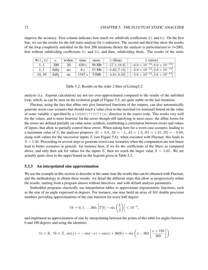
72 CHAPTER 5. THE FLUCTUAT STATIC ANALYZER
improve the accuracy. First column indicates how much we subdivide coefficients B1 and B2. On the firstline, we see the results for the full static analysis for N unknown. The second and third line show the resultsof the loop completely unfolded on the first 200 iterations (hence the analysis is particularized to N=200),first without subdividing coefficients B1 and B2, and then, subdividing them. The results of the static
#B1,B2 c. widen. time mem. S (float) S (error)1, 1 200 20 430 s 50 Mb [−17.1; 18.6] [−8.0× 10⁻¹⁴; 8.0× 10⁻¹⁴]
1, 1 fully no 6 s 53 Mb [−5.63; 7.13] [−2.9× 10⁻¹⁴; 2.9× 10⁻¹⁴]
10, 10 fully no 1347 s 53Mb [−4.81; 6.33] [−2.6× 10⁻¹⁴; 2.6× 10⁻¹⁴]
Table 5.2: Results on the order 2 filter of Listing5.2
analysis (i.e. fixpoint calculation) are not too over-approximated compared to the results of the unfoldedloop, which, as can be seen on the evolution graph of Figure 5.5, are quite stable on the last iterations.
Fluctuat, using the fact that affine sets give linearized functions of the outputs, can also automaticallygenerate worst-case scenario that should reach a value close to the maximal (or minimal) bound on the valueof some variable x specified by a DSENSITIVITY(x) directive in the source code. This works very wellfor the values, and is more heuristic for the errors though still satisfying in most cases: the affine forms forthe errors are defined partially on value noise symbols, establishing a correlation between errors and valuesof inputs, that allow to partially control these errors. When asking here for a worst case scenario, leading toa maximum value of S, the analyzer proposes A1 = 0.8, A2 = −1, A3 = 1.3, B1 = 1.41, B2 = −0.69,along with values for the successive inputs E (see Figure 5.6): when executed with Fluctuat, this leads toS = 5.36. Proceeding in several steps to generate worst-case scenarios when the computation are non linearlead to better scenarios in general: for instance here, if we fix the coefficients of the filters as computedabove, and only then ask for values for the inputs E, then we reach the larger value S = 5.65. We areactually quite close to the upper bound on the fixpoint given in Table 5.2.
5.3.3 An interpolated sine approximation
We use the example in this section to describe at the same time the results that can be obtained with Fluctuat,and the methodology to obtain these results: we detail the different steps that allow to progressively refinethe results, starting from a program almost without directives, and with default analysis parameters.
Embedded programs classically use interpolation tables to approximate trigonometric functions, suchas the sine of an angle expressed in degrees. For instance, one may build an array of 361 double precisionnumbers providing approximations of the sine function for every half degree:
∀k = 0, 1, . . . 360,
∣∣∣∣T [k]− sin
(k
2
)∣∣∣∣ < 10−4,
and implement an approximation of sine by interpolating between the points of this table for angles between0 and 180 degrees and using the identities
∀x ∈ R, ∀k ∈ Z, sin(x) = − sin(−x) = sin(x+ 360k) = sin
(x− 360
⌊x+ 180
360
⌋)

5.3. EXAMPLES AND CASE STUDIES 73
Figure 5.6: Worst case scenario on value of S in Listing 5.2
Let us try to run an analysis for the full range of double numbers, for the following naıve implementation ofthe sine operator:
Listing 5.3: Sine approximation1 e x t er n c o n s t double T [ 3 6 1 ] ;2 double SIN 0 180 ( double x ) {3 double dx , i d x , v i n f ;4 double v sup ; i n t i ;5 dx=2∗x ; i =dx ; i d x = i ;6 v i n f =T [ i ] ; v sup =T [ i + 1 ] ;7 re turn v i n f + ( dx − i d x )8 ∗ ( v sup − v i n f ) ; }9
10 double SIN 180 ( double x ) {11 i f ( x<0)12 re turn −SIN 0 180(−x ) ;13 e l s e14 re turn SIN 0 180 ( x ) ; }1516 double SIN POS ( double x ) {17 i f ( x>180) re turn SIN 180 ( x18 −360.∗( i n t ) ( ( x + 1 8 0 . ) / 3 6 0 . ) ) ;19 e l s e re turn SIN 180 ( x ) ; }2021 double SIN ( double x ) {22 i f ( x<0) re turn −SIN POS(−x ) ;23 e l s e re turn SIN POS ( x ) ; }
Fluctuat, in 1.5 seconds, issues infinite values and errors for the result of the sine function, and warnsthat the (int)((x+180.)/360.) cast may be undefined. Indeed this implementation uses a conversion

74 CHAPTER 5. THE FLUCTUAT STATIC ANALYZER
from double to int, so it is only valid for inputs x such that⌊|x|+180
360
⌋can be represented in the type int. In
our 32 bits case, this is the ] − 773094113100, 773094113100[ interval. This is not an issue, provided thatcall contexts for SIN in the whole control program are guaranteed to fall into this last interval.
The analysis costs for the reduced domain are unchanged, but its result is still disappointing: the com-puted over-approximation of the value (and error) interval for the result of the sine algorithm in floating-pointnumbers is [−3.09 × 10¹², 3.09 × 10¹²], whereas it is [−1.5, 1.5] in the real-number semantics. Besides,Fluctuat warns the user that the program test in function SIN 180 is unstable: it stresses here that when-ever the floating-point execution takes the (x<0) branch, the real execution is sure to execute the (x>=0)branch. This requires careful attention.
As a matter of fact, whenever x is very close to (but smaller than) a number of the form 180 + 360× k,for some k ∈ N, then a rounding error occurs when evaluating expression (x+180.)/360. in floating-point arithmetic. The result is rounded to the double representing k + 1. In all such cases, the x -360.*(int)((x+180.)/360.) expression has value close to (though below) 180 in real numbers, butclose to (though below)−180 in floats. In such a case, expression T [i+ 1] in function SIN 0 180 attemptsto access array T out of bounds, as signaled by Fluctuat. We thus fix the naıve implementation of the sineoperator: we add a 362nd array element, such that T [0] = T [360] = T [361] = sin(0) = sin(±180) = 0.
Custom non uniform subdivisions Now we have fixed the implementation, we would like to have anidea of the accuracy that can be ultimately expected from the analysis. For that, we switch to the symbolicexecution mode of Fluctuat with same range and subdivisions, thus choosing a sample of inputs in the inputrange. As a result, we get a useful (though unsound for the whole range of values) estimate of the errorrange for y: [−1.05× 10⁻¹⁶, 1.05× 10⁻¹⁶].
We thus look for a more precise way to perform the static analysis: we write a new main function im-plementing a custom irregular subdivision, with a singleton for every interpolation point of the interpolationtable:
[−180, 180.5[=360⋃
i=−360
{i
2
}∪]i
2,i+ 1
2
[This improves the accuracy of the analysis by a “manual” disjunctive analysis.
Listing 5.4: Custom non uniform subdivision1 double x =−180. , y = 0 . , x i , y i ; i n t i ;2 f o r ( i =−360; i <=360; i ++) {3 x i = i ∗ 0 . 5 ; y i = SIN ( x i ) ;4 x = DCOLLECT( x , x i ) ; y = DCOLLECT( y , y i ) ;5 x i = DBETWEEN(DSUCC( i ∗0 . 5 ) , DPREC ( ( i +1) ∗0 . 5 ) ) ;6 y i = SIN ( x i ) ;7 x = DCOLLECT( x , x i ) ; y = DCOLLECT( y , y i ) ; }
We then collect back the values that variables can take on the full domain using directive DCOLLECT, seeListing 5.4. We could also have used a variation of this assertion DCOLLECT WARN, that checks that thereis no hole in the values collected, and that we have thus subdivided the whole initial range.
The static analysis is run unrolling the main loop. It takes 97 seconds and 36 MB, and ensures that x ∈[−1.8×10², 1.805×10²] and y ∈ [−1.0, 1.0] with errors in [−4.97×10⁻¹⁶, 4.97×10⁻¹⁶]. The imprecisiongenerated by the floating-point implementation is thus proved negligible compared to the accuracy of theinterpolation table.
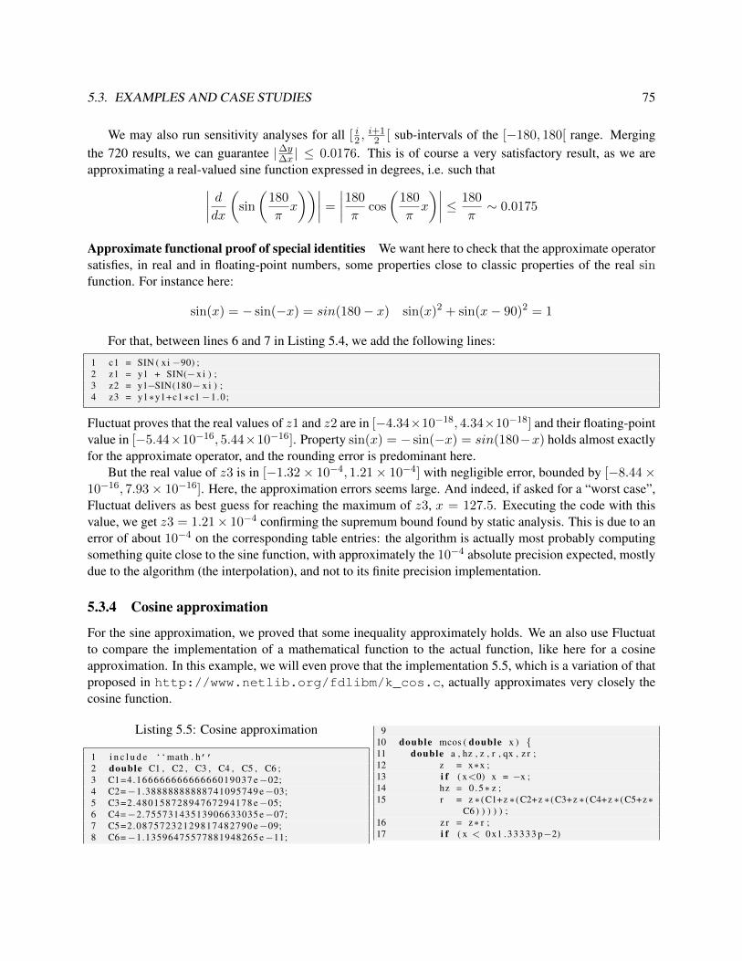
5.3. EXAMPLES AND CASE STUDIES 75
We may also run sensitivity analyses for all [ i2 ,i+1
2 [ sub-intervals of the [−180, 180[ range. Mergingthe 720 results, we can guarantee |∆y∆x | ≤ 0.0176. This is of course a very satisfactory result, as we areapproximating a real-valued sine function expressed in degrees, i.e. such that∣∣∣∣ ddx
(sin
(180
πx
))∣∣∣∣ =
∣∣∣∣180
πcos
(180
πx
)∣∣∣∣ ≤ 180
π∼ 0.0175
Approximate functional proof of special identities We want here to check that the approximate operatorsatisfies, in real and in floating-point numbers, some properties close to classic properties of the real sinfunction. For instance here:
sin(x) = − sin(−x) = sin(180− x) sin(x)2 + sin(x− 90)2 = 1
For that, between lines 6 and 7 in Listing 5.4, we add the following lines:
1 c1 = SIN ( xi −90) ;2 z1 = y1 + SIN(− x i ) ;3 z2 = y1−SIN(180− x i ) ;4 z3 = y1∗y1+c1∗c1−1.0 ;
Fluctuat proves that the real values of z1 and z2 are in [−4.34×10⁻¹⁸, 4.34×10⁻¹⁸] and their floating-pointvalue in [−5.44×10⁻¹⁶, 5.44×10⁻¹⁶]. Property sin(x) = − sin(−x) = sin(180−x) holds almost exactlyfor the approximate operator, and the rounding error is predominant here.
But the real value of z3 is in [−1.32× 10⁻⁴, 1.21× 10⁻⁴] with negligible error, bounded by [−8.44×10⁻¹⁶, 7.93× 10⁻¹⁶]. Here, the approximation errors seems large. And indeed, if asked for a “worst case”,Fluctuat delivers as best guess for reaching the maximum of z3, x = 127.5. Executing the code with thisvalue, we get z3 = 1.21× 10⁻⁴ confirming the supremum bound found by static analysis. This is due to anerror of about 10−4 on the corresponding table entries: the algorithm is actually most probably computingsomething quite close to the sine function, with approximately the 10−4 absolute precision expected, mostlydue to the algorithm (the interpolation), and not to its finite precision implementation.
5.3.4 Cosine approximation
For the sine approximation, we proved that some inequality approximately holds. We an also use Fluctuatto compare the implementation of a mathematical function to the actual function, like here for a cosineapproximation. In this example, we will even prove that the implementation 5.5, which is a variation of thatproposed in http://www.netlib.org/fdlibm/k_cos.c, actually approximates very closely thecosine function.
Listing 5.5: Cosine approximation
1 i n c l u d e ‘ ‘ math . h’’2 double C1 , C2 , C3 , C4 , C5 , C6 ;3 C1=4.16666666666666019037 e−02;4 C2=−1.38888888888741095749 e−03;5 C3=2.48015872894767294178 e−05;6 C4=−2.75573143513906633035 e−07;7 C5=2.08757232129817482790 e−09;8 C6=−1.13596475577881948265 e−11;
910 double mcos ( double x ) {11 double a , hz , z , r , qx , z r ;12 z = x∗x ;13 i f ( x<0) x = −x ;14 hz = 0 .5∗ z ;15 r = z ∗ (C1+z ∗ (C2+z ∗ (C3+z ∗ (C4+z ∗ (C5+z∗
C6 ) ) ) ) ) ;16 z r = z∗ r ;17 i f ( x < 0x1 .33333 p−2)

76 CHAPTER 5. THE FLUCTUAT STATIC ANALYZER
/∗ i f | x | < 0 . 3 ∗ /18 re turn 1 . − ( hz − z r ) ;19 e l s e {20 i f ( x > 0 . 7 8 1 2 5 ) { /∗ x
> 0 .78125 ∗ /21 qx = 0 . 2 8 1 2 5 ;22 } e l s e {23 f l o a t f = x ;24 qx = 0 . 2 5 f ∗ f ;25 }26 hz = hz−qx ;27 a = 1.−qx ;28 re turn a − ( hz − z r ) ;
29 }30 }3132 void main ( void )33 {34 double x , y , z ;35 double p i = 3 .141592653589793238462;36 x = DBETWEEN( 0 . 5 , 0 . 7 5 ) ;37 y = mcos ( x ) ;38 z = y − cos ( x ) ;39 }
We study function mcos on the range [0.5,0.75], this is added using the DBETWEEN assertion again.And we add line z = y - cos(x), where cos is the mathematical cosine function, in order to provethat function mcos actually computes something very close to the mathematical function. Bounds on thevalue of z will bound the approximation error, while bounds on its error will bound the error due to finiteprecision.
Fluctuat with default parameters gives in 0.01 sec, z in [−7.51× 10⁻³, 7.71× 10⁻³] with computationerror bounds [−2.7 × 10⁻¹⁶, 2.7 × 10⁻¹⁶]. Subdivisions on the input allow to refine this estimation: forinstance, in 10 sec, 16Mb and 1000 subdivisions, we have z in −7.5 × 10⁻⁹, 7.5 × 10⁻⁹], with an errorin [−2.62 × 10⁻¹⁶, 2.62 × 10⁻¹⁶]. And n 4 hours of computation, we obtain that the real value of z isin [−1.88 × 10⁻¹⁵, 1.88 × 10⁻¹⁵], with an error due to finite precision in [−3.45 × 10⁻¹⁶, 2.56 × 10⁻¹⁶].Subdividing even more allows to keep reducing the real value of z, that is the error due to the approximationscheme, while the error due to finite precision remains of the same order, so that the mcos function indeedapproaches the cosine very closely. But the computation times become unreasonable.
Proving such refined properties is not a central use of Fluctuat for the time being: the zonotopic abstractdomains are well suited to computations that do not involve too many non-linear computations, and for largeranges of values. But this example demonstrates that if time is not an issue, like on elementary symbols thatneed to be analyzed once, such use is conceivable, whereas it is not with a non relational domain such asintervals.
5.3.5 An iterative algorithm for square root approximation
We finally consider an example that illustrates the difficult case when the use of finite precision does notonly affect the accuracy of the result, but also the behaviour of the program. The function below computesby the Householder method the inverse of the square root of the input I . The loop stops when the differencebetween two successive iterates is below a criterion that depends on a value eps.
1 xn = 1 . 0 / I ; i = 0 ; r e s i d u = 2 .0∗ eps ;2 whi le ( f a b s ( r e s i d u ) > eps ) {3 xnp1 = xn ∗ ( 1 . 875+ I ∗xn∗xn ∗ (−1.25+0.375∗ I ∗xn∗xn ) ) ;4 r e s i d u = 2 . 0∗ ( xnp1−xn ) / ( xn+xnp1 ) ;5 xn = xnp1 ; i ++; }6 O = 1 . 0 / xnp1 ; sbz = O− s q r t ( I ) ;
This algorithm is known to quickly converge when in real numbers, whatever the value of eps is. However,in finite precision, the stopping criterion must be defined with caution: for instance, executed in simpleprecision, with eps=10−8, the program never terminates for some inputs, for instance I = 16.000005.
5.3. EXAMPLES AND CASE STUDIES 77
Analyzed with Fluctuat for an input in [16, 16.1], we obtain that the number of iterations i of the algorithmis potentially unbounded. We also obtain that residu has a real value bounded in [−3.66×10⁻⁹, 3.67×10⁻⁹]and a floating-point value is bounded in [−2.79×10⁻⁷, 2.79×10⁻⁷] (50 subdivisions), so that the real valuesatisfies the stopping criterion but not the floating-point value, which is also signaled by an unstable test onthe loop condition. Now, analyzing the same program but now for double precision variables, Fluctuat isable to prove in 3 seconds that the number of iterations is always 6 (both the real value and the floating-pointvalue satisfy the stopping criterion). Also, bounding the variable sbz, Fluctuat is also able to bound themethod error, so that we prove that the program indeed computes something that is close to the square root:the real and float value of sbz are found in [−1.03× 10⁻⁸,−1.03× 10⁻⁸], with an error due to the use offinite precision in [−1.05× 10⁻¹⁴, 1.05× 10⁻¹⁴].
5.3.6 Analysis of hybrid systems
An emerging trend in software verification is to extend the analysis of programs to take into account theirinteraction with the external world in a more refined manner than just specifying ranges of values for inputsand outputs of the programs. We extended Fluctuat in this direction and introduced new directives to describethe interaction of the program with a continuous environment, modeled as a set of switched ODEs, givenby the user as C++ functions. The directives model the action of sensors (with which the program readsthe value of a physical variable, solution of an ODE) and actuators (with which the program acts on thesystem’s behavior, that is modifies modes or parameters of the switched ODEs). Then Fluctuat calls aguaranteed ODE solver to bound the behavior of the continuous environment (we used the C++ libraryGRKLib [23]).
In our model, time is computed by the program: Fluctuat initializes the set of ODEs by sending boundson initial values, modes and parameters to the environment. Then any action by the program is also sent tothe environment (the ODE solver) when encountering the corresponding actuator directives in the program.When Fluctuat encounters a directive requesting a sensor value in the program, it calls the guaranteed ODEsolver, specifying the time at which it wants to read bounds on the continuous value of the given quantity,and the integration is performed on the fly. This extension is described in more details in [22].
We illustrated its use on a simplified version of the MSU main control loop, part of the AutomatedTransfer Vehicle (ATV) control software, represented Figure 5.7. The external environment (relating theposition of the ATV to accelerations due to thrusters) is modeled by an ODE of dimension 7. At eachcycle of the program, the vehicle’s configuration (the position, speed, acceleration etc.) is read from sensors(assertion HYBRID DVALUE in the program), then the program computes the command sent to actuatorsto achieve the desired thrust with the engines (assertion HYBRID PARAM in the program, that modifies theparameters of the ODE system modeling the environment).
We studied the behavior of the system on 25 seconds, starting from one point, and could prove that thevalues converge towards the the safe state that the ATV is supposed to reach in this escape mode. Moredetails and analysis results can be found in [19].
5.3.7 Float to fixed-point conversion: bit-width optimisation
There is a need in digital processing for automatic floating-point to fixed-point transformation of programs,guaranteeing output accuracy while minimizing the cost of implementation, cost for instance defined by thesum of word lengths of all variables. We developed and implemented in Fluctuat in 2005, during the M2

78 CHAPTER 5. THE FLUCTUAT STATIC ANALYZER
Figure 5.7: Hybrid system modeling: the ATV control software
internship of Jerome Mascunan [122], the counterpart of the non relational abstract domain for floating-pointnumbers, but for fixed-point numbers. Special Fluctuat assertions, give the size of word length and integerword length for each variable. Then, we started working on a small optimization tool, which, given a Cprogram written in floating-point numbers and an aim in terms of accuracy compared to the accuracy of thefloating-point program, should try to compute optimal (smallest) fixed point formats for each variable. Theaim is typically to achieve some percentage of the accuracy of the floating-point program; constraints canalso be added on the fixed point formats (such as fixed word length), so that the optimization can be eased.The tool relies on the dependencies between variables computed by the abstract domain on the floating-pointprogram, as heuristics to decide the format of which variable to modify in order to act on a given variable’sprecision.
This work is very preliminary, and relies on non relational abstractions of the values and errors. Weintend to improve our conversion algorithm, using the dependencies we are now able to compute, in theDEFIS ANR project. We shall compare our approach and results to other approaches [117, 159], whichalso use value and fixed point error models relying on affine arithmetic for bit-width optimization, oneby simulated annealing, the other by a greedy search algorithm. In digital processing, a commonly usedcriteria for the accuracy of a fixed-point implementation, is the signal-to-quantization-noise ratio, elementaryquantization errors being considered as uniformly distributed white noises. The CAIRN Inria team, whichleads the DEFIS project, uses a partially analytical approach to compute such ratios [123], and optimize thefloating-point to fixed-point conversion [124]; their noise propagation models based on perturbation theoryand Taylor developments resemble in some way to our own propagation model. We intend to exchangeinformation with this approach.
5.4 Looking back at the last ten years
Finally, let us quickly come back on the now more than 10 years of existence of Fluctuat, the develop-ment and transfer of which constantly accompanied and benefited from the research work presented in this

5.4. LOOKING BACK AT THE LAST TEN YEARS 79
document. It is a research prototype, but we have always had a high concern for usability by reasonablynon-expert users: the evolutions were equally driven by our progress on the zonotopic abstract domains, andrequirements and observations on the industrial source codes that were submitted to us.
Propagation of rounding errors, proof of concept (2001-2003) We started from an already existingsimple abstract interpreter developed at CEA [75], in which we first implemented the non-relational domainof Section 5.1.2. Our main industrial supports at that time were Airbus, through the Daedalus European ISTproject, and the IRSN (French Institute for Radioprotection and Nuclear Safety). In both cases, the objectivewas to be able to numerically study large programs, and identify loss of accuracy due to floating-pointnumbers. We designed the user interface that represents the decomposition of elementary rounding errors ashistograms, and links the error bars to their provenance in the source code. Soon, the need for informationabout intermediary steps in the analysis appeared. We added the first printing assertions and evolutiongraphs. Case studies concentrated on the propagation of perturbations around representative scenarios, thesymbolic execution mode was introduced and much used. The analyzer allowed us to point out some classicfloating-point issues such as oscillation problems due to sampling and catastrophic elimination.
First steps for a methodology, zonotopic domains (2004-2005) I would say the present Fluctuattakes much of its roots from this period. We were encouraged by our users to put some effort on theinterpretation of large pieces of software. This involves being able to interpret most most ANSI C constructs,at least those present in embedded code (no recursion): alias/arrays, casts from floats to integers by bit-wiseoperations, and more generally all integers and bit-wise operations, including modular arithmetic. Theytake time, as their design for our model of propagation of uncertainties is not obvious. Interpreting largeparts of full software also means giving the user some tools to interpret results, identify some parts that aremore difficult, and analyze them separately. We sorted the large amount of information at the end of theanalysis, by issuing warnings for the main points to be checked by the user, and displaying the error bars bydecreasing amplitude. We also started printing more information about the current state of the analysis, sothat the user needs not necessary wait for the end of a possibly long analysis. We also added a basic in/outanalysis, in order to point out variables that need to be initialized with assertions, or dead code information(code that is proved to be dead): this is especially useful when isolating a part of program. This methodologyfor the analysis of large programs was experimented on an extract of Airbus programs.
We also naturally felt the need for a more accurate analysis of the critical places. We began implement-ing a first version of our zonotopic abstract domain, relational on the values only at that time (not on theerrors) [81] (a hint on its extension to the errors was also presented around the same time [80]). With thisnew abstract domain came new assertions, specifying the real value, but also bounds on the gradient forrecurrent inputs, in order to avoid non realistic behaviours. Meanwhile, we introduced the possibility in theanalyzer to use regular subdivisions of some inputs - and for the whole program - to improve the accuracyfor non linear computations. With this new abstract domain, we started interesting ourselves to the elemen-tary symbols which are present in most control software, typically interpolation operators, linear recursivefilters, and approximations of elementary functions such as trigonometric functions. This work opened theway for some future joint publications with users, and future transfer to industrial users. We obtained atthat time first results of the analyzer proving termination of an algorithm in real but not in floating-pointnumbers, because of the loop exit condition.
We finally started to spend time on different iteration strategies for fixpoint computations, with initial

80 CHAPTER 5. THE FLUCTUAT STATIC ANALYZER
and cyclic unfolding, widening by reduction of the precision, strategies for nested loops and function calls,and for the level of dependency kept in loops or function calls.
Towards functional proof and maturity of the analyzer (2006-2009) Building on previous expe-rience, we developed during this time the zonotopic abstract domains for both values and errors that arestill presently used in Fluctuat, although these abstract domains were improved since. These new domainsallowed us to compute accurate bounds on the error and the floating-point value as well, when they werepreviously accurate on the real value only, with a drift of the error that prevented fixpoint computation. Wealso further exploited these domains, with sensitivity analysis and worst case generation. These were used inparticular for the case studies, that were mostly, but not exclusively, focused at elementary symbols analysis.We also started to prove functional properties on these symbols. As more refined properties were proved,we generalized the use of custom irregular subdivisions. The case studies lead at this time to several jointpublications with the users [87, 46, 19]. We also produced for Airbus a report on the analysis with Fluctuatof A380 elementary symbols, that prepared the way for use of the analyzer on field.
Towards industrial transfer and new uses (2008-present) We kept improving the abstract domains(join and meet over affine sets in particular), but the accent was also put on cleaning the older parts, like thefront-end, improving the usability and defining new usages, in particular in view of a potential valorisation.Karim Tekkal joined us (2008-2011) for a Digiteo maturation operation first, then more explicitly with theobjective of a start-up creation (project since abandoned). Franck Vedrine, who had previously worked onthe TWO analyzer, Fluctuat’s ancestor, also joined us in 2008, and committed in the valorisation project.These two arrivals brought a welcome impetus! A first extension to hybrid systems [22] was developed, withOlivier Bouissou, which we applied to the analysis of the ATV escape program [19]. On the application’sside, we considered again larger programs, but also with new difficulties, such as the quaternions of theATV study. Worst case generation was extended to error maximization, subdivisions were refined for local,possibly irregular, subdivisions. The proof of functional properties was more systematically explored andmore user-oriented assertions were added, for instance to compare or replace parts of programs, or ask fordifferent safety checks by the analyzer.
At the same time, we started thinking about possible interactions with other tools: to mention a fewof them, partial information was integrated in SCADE in the INTERESTED project; we are thinking ofpossible interfaces with the Frama-C platform via the interpretation of the ACSL language; in the DEFISANR project, we are discussing interactions around the float to fixed-point conversion of programs. Forthese purposes, a library was created in order to call and interact more smoothly with the heart of Fluctuat.It was used in particular to design an interactive version of Fluctuat [76].

Chapter 6
Conclusion and Perspectives
I synthesized in this document my research work at CEA LIST since 2001, first in the Software Safety Lab-oratory (LSL) led by Jacques Raguideau, then in the Laboratory for the Modelling and Analysis of Systemsin Interaction (LMeASI) led by Eric Goubault. I focused on the validation of numerical programs, drawinginspiration from such different fields as theoretical computer science, software engineering, control theory,numerical analysis, reliable computing and computer arithmetic. My main contributions on this subject arethe following. I first introduced, with Eric Goubault, a class of new abstract domains relying on a parame-terization by noise symbols: the abstract domain that was studied the more extensively was the zonotope (oraffine sets) domain, but many extensions can be derived, as partly described in Chapter 3. I also contributedto the introduction of a new general method for the solution of fixpoint equations occurring in static analysis;and meanwhile studied and implemented Kleene-like iterations in the context of zonotopic abstractions. Ifinally adapted the zonotopic abstract domains for the analysis of finite precision computations, and imple-mented these abstract domains in the Fluctuat analyzer. More generally, I have been the main developer ofthe Fluctuat analyzer during several years, and realized or participated in many case studies (Airbus, IRSN,Hispano-Suiza, EADS, Continental, etc), that drove us to the present possibilities of the tool.
Let me draw some perspectives on these different themes over the next few years:
6.1 Zonotopic abstract domains and extensions
We set up a formal framework for a fast and accurate abstract analysis based on affine sets, which is quitemature now. Improvements of affine sets, such as a better join operator in the case we do not exactly havecommon affine relations, would still be very valuable. But most future work concern the extensions of thisabstract domain presented in Chapter 3, or even other possible extensions, we give a few leads hereafter.
Under-approximations We have proposed in 2007 [82] a first practical, tractable abstract semantics,based on generalized affine sets, for under-approximating the values of program variables. One currentobjective is to extend this method to higher-order Taylor forms, for instance by using zonotopic coeffi-cients instead of interval coefficients in our generalized affine forms. This also remains to be comparedto other existing methods for under-approximations, mostly introduced in control theory (and called inner-approximations in that context), with the idea to improve our first results. Most other methods for under-approximation use bisections algorithms, that allow to build box pavings that are included in the image of
81

82 CHAPTER 6. CONCLUSION AND PERSPECTIVES
a vector-valued function. We have recently focused on the approach developed by Goldsztejn et al. [71],which was defined only for functions whose domain and co-domain have same dimensions. For applicationsto static analysis or robust control, this is usually not the case. Olivier Mullier, in his PhD thesis, which I co-supervise, proposed an extension to the general case, and first results were presented at SWIM’11 [135]. Ourinterest also goes to the nested inner-approximations for polynomial matrix inequalities [98], even thoughthese methods may prove intractable for our applications, or to inner-approximations by ellipsoids [109],two methods that manage to give somewhat dual over and under-approximations, as we are aiming at.Our generalized affine sets for under-approximation are somehow dual to over-approximation, as the sameforms can be interpreted both as under or over-approximation. But the under-approximations we obtain donot have a geometric concretization as zonotopes. Actually, we are currently trying to characterize theirconcretization, or at least find convex shapes that can be enclosed.
We then hope to use our under-approximation methods in both contexts of static analysis of programsand robust control of uncertain dynamical systems, this is again among the objectives of O.Mullier’s PhDthesis. For instance, we want to obtain an over- and under-approximation of the set of states that are reach-able by a physical system described by a discrete-time dynamical equation involving uncertain parameters,with constraints on the inputs of the system (bounds, energy...). This problem is similar to a viability prob-lem [6], with uncertainties in the system dynamics. This step will then allow us to consider the synthesisof commands (input sequences) of the system allowing to lead it from a state to another, with a guaranteedrobustness towards incoherent parameters. Still, we did not find yet a completely satisfying way to applyour under-approximations described in Section 3.1, which for the time being can solely be interpreted as AEformulas, to these robust control approach.
Finally, the under-approximating abstract semantics we introduced is for the time being applied to real-valued variables, and does not address yet floating-point variables, which are discrete by nature. As a partialsolution, one can think for instance of adding information about the minimal size of the gaps between twofloating-point values in the resulting interval.
P-boxes and affine arithmetic We have for now defined an arithmetic relying on p-boxes and affine arith-metic. There still remains to apply this to the static analysis of programs: we must in particular defineset-theoretic operations such as union and intersection, probably by generalizing those we introduced foraffine sets. Another direction is to maintain a better abstraction of the dependencies between variables,during computation. In the current work, we decomposed the dependency relationships between variableson a basis of independent noise symbols (εi) and noise symbols with unknown dependency (ηj). This is aparticular abstraction of some form of a correlation matrix between the noise symbols, which we hope torefine in the future. Finally, the probabilistic affine forms we have introduced should be linked with partic-ular Dempster-Shafer structures on Rp, whose focal elements are zonotopes (particular central symmetricpolytopes), parametrized by affine forms. These in turn might generalize to higher-order Taylor models asused by Makino and Berz [120] instead of order one models such as zonotopes.
A generalization of zonotopes and ellipsoids: super-ellipsoids The use of ellipsoids has been widelystudied in set estimation, control, and reachability analysis [137, 108], and also applied in the context ofstatic analysis by Feret [49]. Also, as already stated, among other interests, ellipsoids have been usedto provide both under and over-approximations, as we intend to. However, ellipsoidal calculus [110] israther intricate and costly. It could thus be interesting to investigate a variation of our abstract domain of
6.2. FIXPOINT COMPUTATIONS 83
affine sets based on ellipsoids, or combining zonotopes and ellipsoids. Indeed, as we noted in a NSV’11presentation [86], in the same way a zonotope is the image by an affine transformation of an hypercube, anellipsoid is the affine transformation of an n-dimensional disk, and can thus be parameterized by an affineform, just like zonotopes, except that the vector of noise symbols is bounded in l2 norm instead of in l∞norm. And this can generalize to other norms, yielding super-ellipsoids. Some arithmetic operations couldthus be achieved using the same arithmetic as on affine forms, avoiding a costly ellipsoidal calculus. Andwe would need much fewer terms to compute some loop invariants. This of course remains to be furtherdeveloped and experimented.
Other approximations We believe that we should be able to extend our zonotopic approach to deal withhigher-order Taylor models [120], where we use a polynomial approximation of functions with monomialson noise symbols εα with |α| ≤ n. Other ways to get higher-order approximations could also rely on affinesets with zonotopic coefficients, probably in the line of the affmat objects of Combastel [36]. From ourfirst observations, this second approach would in particular probably be more suited for building under-approximations.
But, while these forms are probably well suited to bound rounding errors, which are small compared tovalues, they may not be suitable to bound the values of variables: most of the time in static analysis, we wantto study the behavior of the program for large ranges of values. In this case, other rigorous approximationsmay be more interesting, such as for instance those relying on Chebyshev interpolation polynomials. Theidea of using better approximation polynomials, for example Chebyshev truncated series, in the context ofvalidated computations, was already introduced in 1982 [48] under the name ultra-arithmetic. As discussedby Makino and Berz [120], the arithmetic proposed there has some drawbacks that make it less accurate thanTaylor models. However, new Chebyshev interpolation models were proposed, for instance by Brisebarre etal. [24], that could be of interest to us.
Finally, a track that we intend to follow in the future, and believe very promising, builds on ideas ofSankaranarayanan [146]: he uses changes of bases to transform a non linear dynamical system into a linearone, that can be solved much more easily, by classic methods. We would like to extend these ideas to discretesystems, and automatically compute change of bases that would allow us to abstract systems that requirenon-linear invariants, by systems that could be solved efficiently with a linear abstract domain such as affinesets. These changes of bases could be polynomial, but we plan to possibly also include rational functions,logarithm or exponential.
6.2 Fixpoint computations
Kleene-like iterations One future direction is to use modified iteration schemes as a mean to computeglobal join operations, that preserve relations between variables and noise symbols, but in a more generalway than as proposed in Section 2.2.3. For instance, there are cases when there is no common affine relation-ship, so that the global join of Section 2.2.3 does not apply, but still, this component-wise computation losessome crucial correlations. Informally, the idea of this modified iteration is, when dependencies betweenvariables are discovered by our affine sets, to make the union only on part of these variables, and propagateit to the other dependent variables. This is close to the global join that we defined, but would apply morewidely than just the case of exact common relationships.

84 CHAPTER 6. CONCLUSION AND PERSPECTIVES
Another direction relies on the fact that typical critical real-time systems, as found in automotive, aero-nautic, and aerospace applications, usually consist in a huge iterated loop. But these systems do not runforever, and this loop will not be executed more than a (possibly very large) number of times. And whenimplemented with finite precision numbers, it may be for instance that there is a drift between the real andthe finite precision, that cannot be bounded for any number of iterations. We would still like to charac-terize and bound this drift, and more generally bound the abstract values of the program variables, usingthis bound on the number of iterations. As our global join operators explicit the implicit relation betweenprogram variables (and thus for instance a loop counter, but not exclusively so), we think we could then usesome abstract accelerations [72, 150] to accurately bound the behavior of such programs. This would alsobe close to the work of Feret [50] that defines an abstract domain relating variable values to a clock counterby affine expressions, and uses this relation to give bounds on the behavior that depend on the clock, butadapted to our abstract domain, and, we hope, of use on a larger class of programs.
Policy iteration for zonotopic abstract domains Policy iteration is a general algorithm that can be ap-plied to many abstract domains - and has indeed been applied to several - provided that our loop functionalscan be expressed as infimums of a finite set of simpler functionals. We started investigating two directions inorder to design a policy iteration algorithm for our affine sets abstract domains, but these are still preliminarywork. These two directions respectively define as policies, choices for the join or for the meet of two affinesets.
The meet operation in affine sets is expressed as constraints on the noise symbols, that can be interpretedin any abstract domain. If interpreted in intervals, we are then brought back to a variation of the policyiteration defined in Section 4.2. A policy is then, for each bound of each noise symbol occurring in the test,a choice between the old bound and the new bound generated by the constraint. Still, this idea remains tobe studied in depth, as its use is more problematic than the simple policy iteration on intervals.
During the internship of Mickael Buchet, we started some work on a simple idea in order to definepolicies on the join operator: we noted that the join operator of Definition 11 allows us to define policiesfor the coefficients of the noise symbols. Indeed, argmin|.|(x, y) is either x, or y, or 0, which can be chosenas policies. However, the problem is that this does not necessarily define a descending policy iteration: thechange of policy does not necessarily conduct to an improvement of the post fixpoint. Still, a first algorithmwas designed that allowed to avoid cycles, and the implementation gave promising results.
6.3 Fluctuat and its applications
We intend of course to gradually integrate the new abstract domains and fixpoint iteration techniques pre-viously described to the Fluctuat analyzer. A specific need linked to the analysis of the impact of finiteprecision, and that appeared in the use of Fluctuat, is the analysis of the behavior of program along the pathconditions:
Discontinuity analysis As mentioned in Section 5.1.4, we are currently exploring the use of affine sets tomake our analysis sound in presence of unstable tests. This is done by studying the conditions and the po-tential discontinuity of the program when the floating-point execution takes one path and the real executiontakes another path, and adding to the error on variables, a discontinuity term bounding this difference. This

6.3. FLUCTUAT AND ITS APPLICATIONS 85
will also give a (dis)continuity analysis in the sense of Chaudhuri et al. [26, 27], that is say if a programrepresents a continuous function of its inputs, and is thus robust to uncertainties on these inputs.
Modular analysis As mentioned in Chapter 2, we started to experiment, for the time being on a separateprototype, a modular abstraction based on zonotopic abstract domains [89]. It would be interesting tointegrate in the future this possibility to Fluctuat, in order to allow the analysis of larger pieces of programs,as a modular analysis can prove much cheaper than the full monolithic analysis. The functional abstractionby zonotopes is indeed well suited to a summary-based approach, where summaries can be instantiated toa given call at low cost and with very correct accuracy. Then, the use of policy iteration can accelerate theincremental analysis of a large piece of program: the policy giving the fixpoint of a given piece of programcan be used as a very good initial guess for the same piece of program but with a small modification. Still,the use of modularity strongly depends on the structure of the program to analyze, and this remains to befurther studied on actual applications.
Exchanging information We initiated some thinking on the possible interactions of Fluctuat with othertools. We took first steps already in this direction, for instance with the extension in HybridFluctuat to hybridsystems, where some directives in the source code are used to call a guaranteed differential equations solver.This can be further developed in several directions, first by studying the propagation of the imprecision inthe continuous environment, but also by bounding the method error due to an approximate ODE solver in aprogram, thanks to a call to a guaranteed ODE solver. This latter extension requires additional assertions tocompare a piece of code to a specification, that would in this case be a continuous model.
Some new directives could also be used in order to exchange information with other analysis tools,such as the provers integrated in the Frama-C platform1. This platform contains a chain of tools, that workon programs annotated by behavioral properties expressed in the ACSL language [8], that can be used tospecify computations both in real and floating-point numbers, and to speak about mathematical functions.This chain can be used for the formal verification of numerical programs, as described for instance in Boldoand Marche [17]. Exchanges between Fluctuat and such framework could benefit to both: for instance,automatically synthesized invariants of Fluctuat could be used as first annotation for the provers, partiallysaving the user a tedious manual phase; in the other hand, some refined properties that can be proved ona piece of program, can be used either as an annotation of the program analyzed by Fluctuat, or directlyas a property inside Fluctuat. For instance, the property that if x and y are two floating-point values suchthat y
2 ≤ x ≤ 2y, then their floating-point subtraction is exact, which was discovered by Sterbenz in the1970s [154], is a property used by the abstract domains of Fluctuat. But we could imagine to use moresuch properties, that would be specified in the program analyzed, and interpreted and used by Fluctuat.More generally, interpreting a specification language sufficiently general and expressive to define complexnumerical behavioral properties of C programs, is a goal that facilitates the constitution of benchmarks fornumerical program analysis, which is of course desirable.
We also hope to improve in the future the results of our analysis by automatically calling constraintsolvers, as already partially demonstrated by Ponsini et al. [138]. Interactions with other tools could alsofor instance include interactions with a compiler, or an analyzer of compiled code, in order for instance toconsider more refined information such as the actual order of execution of floating-point operations.
1http://frama-c.cea.fr/
86 CHAPTER 6. CONCLUSION AND PERSPECTIVES
Application fields The problematic of the validation of safety-critical systems is crucial, and justifies initself long-term researches for the validation of numerical properties of programs. We will naturally keepdeveloping our methods and tools in directions that come up from industrial test cases.
But in the long term, we can hope these advances will also benefit to less critical numerical systems. Forinstance, they can benefit to the conception of embedded programs, possibly in fixed point numbers, thatoptimize some aspects such as energy consumption under some given accuracy requirements. This is theproblem we will be addressing in the DEFIS ANR project.
Another challenge is to analyze numerically intricate programs coming from the area of simulation,where there is a high demand for such tools.
In scientific computing programs, different kinds of approximations occur: first the mathematical modelfor the physical phenomenon of interest is already an approximation; then an approximate algorithm is usedto solve that model: accuracy often depends on discretization steps for space and time, then linear systemsare often solved by approximate iterative methods, which accuracy depends on a stopping criterion; andfinally, this algorithm is implemented in finite precision. Ideally, all these approximations should be of thesame order of magnitude. The approximation in the mathematical model is an input of the analysis: we canadd uncertainties to the inputs and parameters of the program, that reflect this approximation, and analyzetheir propagation with Fluctuat. Additionally, when physical identities are known, that are true in the phys-ical world, functional proof can be used to see whether these identities hold in the implementation, or elsequantify the uncertainty or error on them: but in this case we may not distinguish the model error from thealgorithm error. When one has access both to the implementation and the mathematical model, a guaranteedsolution of the continuous model can be used to quantify the method error (and possibly propagate it withthe analyzer as a special error). This is indeed part of what we started to do in the extensions of Fluctuat forhybrid systems, using a guaranteed ODE solver to bound the solutions of differential equations. Then theuser can compare the orders of magnitude of the respective uncertainties on the model (propagation on theoutputs of uncertainties on inputs and parameters), on the algorithm (functional property / physical identity),and on the finite precision computation (rounding error on the outputs). In most cases we have little latitudeon the error due to finite precision: we can only decide to use either float or double precision numbers,depending on the adequacy between method and computation error. But in the general case, the accuracy ofthe algorithm can be adapted if necessary, for instance modifying a discretization step, the stopping criterionof an iterative algorithm, or even the level of approximation, so that for equivalent accuracy the computationtime will be optimal.
Scientific computing programs present the interest for numerical verification concerning finite precisionimplementations, that (pen and paper) studies on algorithms in finite precision have long been conducted,see Higham’s book [99] to mention only one reference, and can be used to validate the interest of our re-sults. Theoretical results about what can and cannot be computed accurately and efficiently such as recentlydeveloped by Demmel [47], are also very valuable to guide our work. However, automatically getting accu-rate error bounds on credible programs is a difficult task, at which we still aim. For instance, we obtainedsome first results on the solution of a small linear systems with small perturbations, by a conjugate gradientalgorithm, that confirmed (part) of the results of the mathematical studies on the behavior of such algo-rithms in finite precision as described in Meurant’s book [125]. But automatizing such studies for real-scalesimulation programs remains a long-term challenge for program verification.

Bibliography
[1] Standard for floating-point arithmetic (ieee 754-2008), http://dx.doi.org/10.1109/ieeestd.2008.4610935,2008.
[2] A. Adje, S. Gaubert, and E. Goubault. Coupling policy iteration with semi-definite relaxation tocompute accurate numerical invariants in static analysis. Logical Methods in Computer Science, 8(1),2011.
[3] T. Alamo, J.M. Bravo, and E.F. Camacho. Guaranteed state estimation by zonotopes. Automatica,41(6):1035 – 1043, 2005.
[4] X. Allamigeon, S. Gaubert, and E. Goubault. Inferring min and max invariants using max-pluspolyhedra. In Proceedings of SAS’08, Static Analysis Symposium, volume 5079 of Lecture Notes inComputer Science, pages 189–204. Springer, 2008.
[5] M. Althoff, O. Stursberg, and M. Buss. Computing reachable sets of hybrid systems using a combi-nation of zonotopes and polytopes. Nonlinear analysis: hybrid systems, 4(2):233–249, 2010.
[6] J.P. Aubin and H. Frankowska. Set-Valued Analysis. Birkhauser, Boston, 1990.
[7] A. Ayad and C. Marche. Multi-prover verification of floating-point programs. In Proceedings of IJ-CAR’10, 5th Joint Conference on Automated Reasoning, volume 6173 of Lecture Notes in ComputerScience, pages 127–141. Springer, 2010.
[8] P. Baudin, J.-C. Filliatre, C. Marche, B. Monate, Y. Moy, and V. Prevosto. ACSL: ANSI/ISO Cspecification language, 2008.
[9] F.L. Bauer. Computational graphs and rounding error. SIAM Journal of Numerical Analysis, 11:87–96, 1974.
[10] D. Berleant and C. Goodman-Strauss. Bounding the results of arithmetic operations on randomvariables of unknown dependency using intervals. Reliable Computing, 4(2):147–165, May 1998.
[11] D. P. Bertsekas, A. Nedic, and A. E. Ozdaglar. Convex Analysis and Optimization. Athena Scientific,2003.
[12] M. Berz. From taylor series to taylor models. In AIP Conference Proceedings 405, pages 1–23, 1997.
87

88 BIBLIOGRAPHY
[13] B. Blanchet, P. Cousot, R. Cousot, J. Feret, L. Mauborgne, A. Mine, D. Monniaux, and X. Rival.Design and implementation of a special-purpose static program analyzer for safety-critical real-timeembedded software. In The Essence of Computation: Complexity, Analysis, Transformation, number2566 in LNCS, pages 85–108. Springer, 2002.
[14] S. Boldo. Floats and ropes: a case study for formal numerical program verification. In Proceedings ofICALP’09, Colloquium on Automata, Languages and Programming, volume 5556 of Lecture Notesin Computer Science, pages 91–102. Springer, 2009.
[15] S. Boldo and J.-C. Filliatre. Formal verification of floating-point programs. In Proceedings ofARITH’07, 18th IEEE Symposium on Computer Arithmetic, pages 187–194. IEEE Computer Society,2007.
[16] S. Boldo, J.-C. Filliatre, and G. Melquiond. Combining coq and gappa for certifying floating-pointprograms. In Proceedings of Calculemus/MKM, volume 5625 of Lecture Notes in Computer Science,pages 59–74. Springer, 2009.
[17] S. Boldo and C. Marche. Formal verification of numerical programs: from c annotated programs tomechanical proofs. Mathematics in Computer Science, 5:377–393, 2011.
[18] S. Boldo and G. Melquiond. Flocq: a unified library for proving floating-point algorithms in Coq. InProceedings of the 20th IEEE Symposium on Computer Arithmetic, 2011.
[19] O. Bouissou, E. Conquet, P. Cousot, R. Cousot, J. Feret, K. Ghorbal, E. Goubault, D. Lesens,L. Mauborgne, A. Mine, S. Putot, and X. Rival. Space software validation using abstract inter-pretation. In Proceedings of DASIA’09, Conference on Data Systems in Aerospace, 2009.
[20] O. Bouissou, E. Goubault, J. Goubault-Larrecq, and S. Putot. A generalization of p-boxes to affinearithmetic, and applications to static analysis of programs. In Presented at SCAN 2010, 14th GAMM-IMACS International Symposium on Scientific Computing, Computer Arithmetic and Validated Nu-merics, 2010.
[21] O. Bouissou, E. Goubault, J. Goubault-Larrecq, and S. Putot. A generalization of p-boxes to affinearithmetic. Computing, 94(2-4):189–201, 2012.
[22] O. Bouissou, E. Goubault, S. Putot, K. Tekkal, and F. Vedrine. Hybridfluctuat: a static analyzer ofnumerical programs within a continuous environment. In Proceedings of CAV’09, 21st Conferenceon Computer Aided Verification, volume 5643 of Lecture Notes in Computer Science, pages 620–626.Springer, 2009.
[23] O. Bouissou and M. Martel. GRKLib: a guaranteed runge-kutta library. In Follow-up of Inter-national Symposium on Scientific Computing, Computer Arithmetic and Validated Numerics. IEEEPress, 2007.
[24] N. Brisebarre and M. Joldecs. Chebyshev interpolation polynomial-based tools for rigorous comput-ing. In Proceedings of ISSAC’10, International Symposium on Symbolic and Algebraic Computation,pages 147–154. ACM, 2010.

BIBLIOGRAPHY 89
[25] V. A. Carreno and P. S. Miner. Specification of the IEEE-854 floating-point standard in HOL andPVS. In HOL95: 8th Workshop on Higher-Order Logic Theorem Proving and Its Applications,Aspen Grove, UT, 1995.
[26] S. Chaudhuri, S. Gulwani, and R. Lublinerman. Continuity analysis of programs. In Proceedingsof POPL’10, 37th ACM SIGPLAN-SIGACT Symposium on Principles of Programming Languages,pages 57–70, 2010.
[27] S. Chaudhuri, S. Gulwani, R. Lublinerman, and S. NavidPour. Proving programs robust. In Proceed-ings of ISGSOLT/FSE’11, 9th ACM SIGSOFT Symposium on the Foundations of Software Engineer-ing, pages 102–112, 2011.
[28] L. Chen, A. Mine, and P. Cousot. A sound floating-point polyhedra abstract domain. In Proceedings ofAPLAS’08, 6th Asian Symposium on Programming Languages and Systems, volume 5356 of LectureNotes in Computer Science, pages 3–18. Springer, 2008.
[29] L. Chen, A. Mine, J. Wang, and P. Cousot. Interval polyhedra: an abstract domain to infer intervallinear relationships. In Proceedings of SAS’09, 16th Static Analysis Symposium, volume 5673 ofLecture Notes in Computer Science, pages 309–325. Springer, 2009.
[30] L. Chen, A. Mine, J. Wang, and P. Cousot. Linear absolute value relation analysis. In Proceedings ofESOP’11, 20th European Symposium on Programming, volume 6602 of Lecture Notes in ComputerScience, pages 156–175. Springer, 2011.
[31] R. Clariso and J. Cortadella. The octahedron abstract domain. In Proceedings of SAS’04, 11thSymposium on Static Analysis, volume 3148 of Lecture Notes in Computer Science, pages 312–327.Springer, 2004.
[32] H. Collavizza, M. Rueher, and P. Van Hentenryck. Cpbpv: a constraint-programming framework forbounded program verification. Constraints, 15(2):238–264, 2010.
[33] J. L. D. Comba and J. Stolfi. Affine arithmetic and its applications to computer graphics. In Proc. SIB-GRAPI’93 — VI Simposio Brasileiro de Computaccao Grafica e Processamento de Imagens (Recife,BR), pages 9–18, 1993.
[34] C. Combastel. A state bounding observer based on zonotopes. In Proceedings of European controlconference. Cambridge, UK, 2003.
[35] C. Combastel. A state bounding observer for uncertain non-linear continuous-time systems based onzonotopes. In Proceedings of 44th IEEE Conference on Decision and Control, 2005.
[36] C. Combastel. On computing envelopes for discrete-time linear systems with affine parametric un-certainties and bounded inputs, 2011.
[37] A. Costan, S. Gaubert, E. Goubault, M. Martel, and S. Putot. A policy iteration algorithm for com-puting fixed points in static analysis of programs. In Proceedings of CAV’05, 17th InternationalConference on Computer Aided Verification, volume 3576 of Lecture Notes in Computer Science,pages 462–475. Springer, 2005.

90 BIBLIOGRAPHY
[38] P. Cousot and R. Cousot. Abstract interpretation: a unified lattice model for static analysis of pro-grams by construction or approximation of fixpoints. In Proceedings of POPL’77, 4th ACM Sympo-sium on Principles of Programming Languages, pages 238–252. ACM Press, 1977.
[39] P. Cousot and R. Cousot. Comparison of the Galois connection and widening/narrowing approachesto abstract interpretation. JTASPEFL ’91, Bordeaux. JTASPEFT/WSA, 74:107–110, 1991.
[40] P. Cousot and R. Cousot. Abstract interpretation frameworks. Journal of Logic and Computation,2(4):511–547, 1992.
[41] P. Cousot and R. Cousot. Compositional separate modular static analysis of programs by abstractinterpretation. In Proceedings of SSGRR’01, Second International Conference on Advances in In-frastructure for E-Business, E-Science and E-Education on the Internet. Scuola Superiore G. ReissRomoli, 2001.
[42] P. Cousot, R. Cousot, J. Feret, L. Mauborgne, A. Mine, D. Monniaux, and X Rival. The astreeanalyzer. In Proceedings of ESOP’05, 14th European Symposium on Programming, volume 3444 ofLecture Notes in Computer Science, pages 21–30. Springer, 2005.
[43] P. Cousot, R. Cousot, J. Feret, L. Mauborgne, A. Mine, D. Monniaux, and X. Rival. Combination ofabstractions in the astree static analyzer. In Proceedings of ASIAN’06, 11th Asian Computing ScienceConference, volume 4435 of Lecture Notes in Computer Science, pages 272–300. Springer, 2006.
[44] P. Cousot and N. Halbwachs. Automatic discovery of linear restraints among variables of a program.In Proceedings of POPL’78, 5th ACM Symposium on Principles of Programming Languages, pages84–96. ACM Press, 1978.
[45] L. H. de Figueiredo and J. Stolfi. Affine arithmetic: concepts and applications. Numerical Algorithms,37:147–158, 2004.
[46] D. Delmas, E. Goubault, S. Putot, J. Souyris, K. Tekkal, and F. Vedrine. Towards an industrial use offluctuat on safety-critical avionics software. In Proceedings of FMICS’09, 14th Workshop on FormalMethods for Industrial Critical Systems, volume 5825 of Lecture Notes in Computer Science, pages53–69. Springer, 2009.
[47] J. Demmel. The complexity of accurate floating-point computation. In Proceedings of the 2002International Congress of Mathematicians, pages 697–706, 2002.
[48] C. Epstein, W.L. Miranker, and T.J. Rivlin. Ultra-arithmetic i: Function data types. Mathematics andComputers in Simulation, 24(1):1 – 18, 1982.
[49] J. Feret. Static analysis of digital filters. In David A. Schmidt, editor, Proceedings of ESOP’04, 13thEuropean Symposium on Programming, volume 2986 of Lecture Notes in Computer Science, pages33–48. Springer, 2004.
[50] J. Feret. The arithmetic-geometric progression abstract domain. In Proceedings of VMCAI’05, 6thConference on Verification, Model Checking, and Abstract Interpretation, volume 3385 of LectureNotes in Computer Science, pages 42–58. Springer, 2005.

BIBLIOGRAPHY 91
[51] S. Ferson. RAMAS Risk Calc 4.0 software: risk assessment with uncertain numbers. Lewis Publishers,Boca Raton, Florida, 2002.
[52] S. Ferson, V. Kreinovich, L. Ginzburg, D. Myers, and K. Sentz. Constructing probability boxes anddempster-shafer structures. Technical report, Sandia National Laboratories, 2003.
[53] S. Ferson, R.B. Nelsen, J. Hajagos, D.J. Berleant, J. Zhang, W.T. Tucker, L.R. Ginzburg, and W.L.Oberkampf. Dependence in probabilistic modelling, dempster–shafer theory and probability boundsanalysis. Technical report, Sandia National Laboratories, 2004.
[54] P. C. Fischer. Automatic propagated and round-off error analysis. In ACM, editor, Preprints of paperspresented at the 13th national meeting of the Association for Computing Machinery, 1958.
[55] L. Fousse, G. Hanrot, V. Lefvre, P. Plissier, and P. Zimmermann. Mpfr: A multiple-precision binaryfloating-point library with correct rounding. ACM Trans. Math. Softw, 33, 2007.
[56] M. J. Frank, R. B. Nelsen, and B. Schweizer. Best-possible bounds for the distribution of a sum aproblem of kolmogorov. Probability Theory and Related Fields, 74:199–211, 1987.
[57] O. Friedmann. An exponential lower bound for the parity game strategy improvement algorithm aswe know it. In Proceedings of LICS’09, 24th Annual IEEE Symposium on Logic in Computer Science,pages 145–156, 2009.
[58] IMTEC-92-26 GAO Report. Patriot missile defense, software problem led to system failure atdhahran, saudi arabia. Technical report, 1992.
[59] S. Gaubert, E. Goubault, A. Taly, and S. Zennou. Static analysis by policy iteration on relationaldomains. In Proceedings of ESOP’07, 16th European conference on Programming, volume 4421 ofLecture Notes in Computer Science, pages 237–252. Springer, 2007.
[60] T. Gawlitza and H. Seidl. Precise fixpoint computation through strategy iteration. In Proceedings ofESOP’07, 16th European conference on Programming, volume 4421 of Lecture Notes in ComputerScience, pages 300–315. Springer, 2007.
[61] T. Gawlitza and H. Seidl. Precise relational invariants through strategy iteration. In Proceedings ofCSL’07, 21st International Workshop on Computer Science Logic, volume 4646 of Lecture Notes inComputer Science, pages 23–40. Springer, 2007.
[62] T. Gawlitza and H. Seidl. Computing relaxed abstract semantics w.r.t. quadratic zones precisely. InProceedings of SAS’10, 17th Static Analysis Symposium, volume 6337 of Lecture Notes in ComputerScience, pages 271–286. Springer, 2010.
[63] K. Ghorbal. Static analysis of numerical programs: constrained affine sets, 2011.
[64] K. Ghorbal, E. Goubault, and S. Putot. The zonotope abstract domain taylor1+. In Proceedings ofCAV’09, 21st Conference on Computer Aided Verification, volume 5643 of Lecture Notes in ComputerScience, pages 627–633. Springer, 2009.

92 BIBLIOGRAPHY
[65] K. Ghorbal, E. Goubault, and S. Putot. A logical product approach to zonotope intersection. InProceedings of CAV’10, 22nd Conference on Computer Aided Verification, volume 6174 of LNCS,pages 212–226, 2010.
[66] A. Girard. Reachability of uncertain linear systems using zonotopes. In Proceedings of HSCC’05,8th International Workshop on Hybrid Systems: Computation and Control, volume 3414 of LectureNotes in Computer Science, pages 291–305. Springer, 2005.
[67] A. Girard and C. Le Guernic. Zonotope/hyperplane intersection for hybrid systems reachability anal-ysis. In Proceedings of HSCC’08, 11th Workshop on Hybrid Systems: Computation and Control,volume 4981 of Lecture Notes in Computer Science, pages 215–228. Springer, 2008.
[68] D. Goldberg. What every computer scientist should know about floating-point arithmetic. ACMComput. Surv., 23(1):5–48, 1991.
[69] A. Goldsztejn. Modal intervals revisited: a mean-value extension to generalized intervals. In Pro-ceedings of QCP-2005, Quantification in Constraint Programming, 2005.
[70] A. Goldsztejn. Modal intervals revisited part 1: a generalized interval natural extension. 2005.
[71] A. Goldsztejn and L. Jaulin. Inner approximation of the range of vector-valued functions. ReliableComputing, 1:23, 2010.
[72] L. Gonnord and N. Halbwachs. Combining widening and acceleration in linear relation analysis. InProceedings of SAS’06, 13th International Static Analysis Symposium, volume 4134 of Lecture Notesin Computer Science, pages 144–160. Springer, 2006.
[73] E. Goubault. Static analyses of the precision of floating-point operations. In Proceedings of SAS’01,8th Static Analysis Symposium, volume 2126 of Lecture Notes in Computer Science, pages 234–259.Springer, 2001.
[74] E. Goubault, T. Le Gall, and S. Putot. An accurate join for zonotopes, preserving affine input/out-put relations. Electronic Notes in Theoretical Computer Science, 287:65–76, 2012. Proceedings ofNSAD’12, 4th Workshop on Numerical and Symbolic Abstract Domains.
[75] E. Goubault, D. Guilbaud, A. Pacalet, B. Starynkevitch, and F. Vedrine. A simple abstract interpreterfor threat detection and test case generation. In Proceedings of WAPATV’01 (ICSE’01), 2001.
[76] E. Goubault, T. Le Gall, S. Putot, and F. Vedrine. Interactive analysis in fluctuat, 2012.
[77] E. Goubault, M. Martel, and S. Putot. Asserting the precision of floating-point computations: asimple abstract interpreter. In Proceedings of ESOP’02, 11st European Symposium on Programming,volume 2305 of Lecture Notes in Computer Science, pages 209–212. Springer, 2002.
[78] E. Goubault, M. Martel, and S. Putot. Static analysis-based validation of floating-point computations.In Dagstuhl Seminar Numerical Software with Result Verification, LNCS, volume 2991 of LectureNotes in Computer Science, pages 306–313. Springer, 2003.

BIBLIOGRAPHY 93
[79] E. Goubault, M. Martel, and S. Putot. Some future challenges in the validation of control systems. InProceedings of ERTS’06, Embedded Real-Time Systems, 2006.
[80] E. Goubault and S. Putot. Weakly relational domains for floating-point computation analysis. InProceedings of NSAD’05, Workshop on Numerical and Symbolic Abstract Domains, 2005.
[81] E. Goubault and S. Putot. Static analysis of numerical algorithms. In Proceedings of SAS’06,13th Static Analysis Symposium, volume 4134 of Lecture Notes in Computer Science, pages 18–34.Springer, 2006.
[82] E. Goubault and S. Putot. Under-approximations of computations in real numbers based on general-ized affine arithmetic. In Proceedings of SAS’07, 14th Static Analysis Symposium, volume 4634 ofLecture Notes in Computer Science, pages 137–152. Springer, 2007.
[83] E. Goubault and S. Putot. Perturbed affine arithmetic for invariant computation in numerical programanalysis. CoRR, abs/0807.2961, 2008.
[84] E. Goubault and S. Putot. A zonotopic framework for functional abstractions. CoRR, abs/0910.1763,2009.
[85] E. Goubault and S. Putot. Static analysis of finite precision computations. In Proceedings of VM-CAI’11, 12th Conference on Verification, Model Checking, and Abstract Interpretation, volume 6538of Lecture Notes in Computer Science, pages 232–247. Springer, 2011.
[86] E. Goubault and S. Putot. Superellipsoids: a generalization of the interval, zonotope and ellipsoiddomains, 2011.
[87] E. Goubault, S. Putot, P. Baufreton, and J. Gassino. Static analysis of the accuracy in control systems:principles and experiments. In Proceedings of FMICS’07, 12th Workshop on Formal Methods for In-dustrial Critical Systems, volume 4916 of Lecture Notes in Computer Science, pages 3–20. Springer,2007.
[88] E. Goubault, S. Putot, K. Tekkal, and F. Vedrine. Fluctuat user manual: static analysis of finiteprecision computations. Technical report, CEA, 2012.
[89] E. Goubault, S. Putot, and F. Vedrine. Modular static analysis with zonotopes. In Proceedings ofSAS’12, 19th Static Analysis Symposium, volume 7460 of Lecture Notes in Computer Science, pages24–40. Springer, 2012.
[90] L. J. Guibas, A. Nguyen, and L. Zhang. Zonotopes as bounding volumes. In Proceedings of SODA’03,14th ACM-SIAM Symposium on Discrete Algorithms, pages 803–812, 2003.
[91] S. Gulwani and A. Tiwari. Combining abstract interpreters. In Proceedings of PLDI’06, Conferenceon Programming Language Design and Implementation, pages 376–386. ACM Press, 2006.
[92] E. Hansen. Interval arithmetic in matrix computations, part i. Journal of the Society for Industrialand Applied Mathematics: Series B, Numerical Analysis, 2(2):308–320, 1965.

94 BIBLIOGRAPHY
[93] E. Hansen. On solving systems of equations using interval arithmetic. Math. Comp, 22:374–384,1968.
[94] E. Hansen. A generalized interval arithmetic. In Proceedings of the International Symposium onInterval Mathematics, pages 7–18. Springer, 1975.
[95] E. Hansen. Global optimization using interval analysis. M. Dekker, New York, 1992.
[96] E. Hansen and R. Smith. Interval arithmetic in matrix computations, part ii. SIAM Journal onNumerical Analysis, 4(1):1–9, 1967.
[97] J. Harrison. Floating-point verification in hol. In Proceedings of TPHOLs’95, 8th Workshop onHigher Order Logic Theorem Proving and Its Applications, volume 971 of Lecture Notes in ComputerScience, pages 186–199. Springer, 1995.
[98] D. Henrion and J. B. Lasserre. Inner approximations for polynomial matrix inequalities and robuststability regions. CoRR, abs/1104.4905, 2011.
[99] N. J. Higham. Accuracy and stability of numerical algorithms. Society for Industrial and AppliedMathematics, 1996.
[100] R. Howard. Dynamic programming and Markov processes. Wiley, 1960.
[101] B. Jeannet and al. Newpolka library. http://www.inrialpes.fr/pop-art/people/bjeannet/newpolka.
[102] B. Jeannet, D. Gopan, and T. Reps. A relational abstraction for functions. In Proceedings of NSAD’05,Int. Workshop on Numerical and Symbolic Abstract Domains, 2005.
[103] B. Jeannet and A. Mine. Apron: A library of numerical abstract domains for static analysis. InProceedings of CAV’09, 21st International Conference on Computer Aided Verification, volume 5643of Lecture Notes in Computer Science, pages 661–667. Springer, 2009.
[104] N. D. Jones and S. S. Muchnick. A flexible approach to interprocedural data flow analysis andprograms with recursive data structures. In Proceedings of POPL’82, 9th Symposium on Principlesof Programming Languages, pages 66–74. ACM, 1982.
[105] W. Kahan. The improbability of probabilistic error analyses for numerical computations, 1998.
[106] E. Kaucher. Interval analysis in the extended interval space ir. Computing, Suppl. 2:33–49, 1980.
[107] W. Kuhn. Zonotope dynamics in numerical quality control. In Visualization and Mathematics, pages125–134. Springer, 1998.
[108] A. B. Kurzhanski and I. Valyi. Ellipsoidal techniques for dynamic systems: the problem of controlsynthesis. Dynamics and Control, 1:357–378, 1991.
[109] Alexander B Kurzhanski and Pravin Varaiya. Ellipsoidal techniques for reachability analysis: internalapproximation. Systems Control Letters, 41(3):201–211, 2000.
BIBLIOGRAPHY 95
[110] A. B. Kurzhanskii and I. Vlyi. Ellipsoidal calculus for estimation and control. Systems and control :foundations and applications. Birkhuser, Boston, MA, 1997.
[111] W. Landi and B. G. Ryder. A safe approximate algorithm for interprocedural aliasing. In Proceed-ings of PLDI’92, ACM SIGPLAN Conference on Programming language design and implementation,pages 235–248. ACM, 1992.
[112] P. Langlois. Automatic linear correction of rounding errors. BIT, 41(3):515–539, 2001.
[113] P. Langlois and F. Nativel. Reduction and bounding of the rounding error in floating-point arithmetic.C.R. Acad. Sci. Paris, Serie 1, 327:781–786, 1998.
[114] P. Langlois and F. Nativel. When automatic linear correction of rounding errors is exact. C.R. Acad.Sci. Paris, Serie 1, 328:543–548, 1999.
[115] J. Larson and A. Sameh. Efficient calculation of the effects of roundoff errors. ACM Trans. Math.Softw., 4(3):228–236, 1978.
[116] V. Laviron and F. Logozzo. Subpolyhedra: a (more) scalable approach to infer linear inequalities. InProceedings of VMCAI’09, 10th Conference on Verification, Model Checking, and Abstract Interpre-tation, volume 5403 of Lecture Notes in Computer Science, pages 229–244. Springer, 2009.
[117] D.-U. Lee, A. Abdul Gaffar, W. Luk, and O. Mencer. MiniBit: Bit-width optimization via affinearithmetic. In Proceedings of DAC’05, Design Automation Conference, pages 837–840, 2005.
[118] S. Linnainmaa. Taylor expansion of the accumulated rounding error. BIT Numerical Mathematics,16:146–160, 1976.
[119] F. Logozzo and M. Fahndrich. Pentagons: a weakly relational abstract domain for the efficient vali-dation of array accesses. In Proceedings of SAC’08, ACM Symposium on Applied Computing, pages184–188. ACM Press, 2008.
[120] K. Makino and M. Berz. Taylor models and other validated functional inclusion methods. Interna-tional Journal of Pure and Applied Mathematics, 4(4):379–456, 2003.
[121] Matthieu Martel. Propagation of roundoff errors in finite precision computations: a semantics ap-proach. In Proceedings of ESOP’02, 11th European Symposium on Programming, volume 2305 ofLecture Notes in Computer Science, pages 194–208. Springer, 2002.
[122] J. Mascunan. Analyse statique de programmes en virgule fixe, 2005.
[123] D. Menard, R. Rocher, and O. Sentieys. Analytical fixed-point accuracy evaluation in linear time-invariant systems. IEEE Transactions on Circuits and Systems I: Regular Papers, 55(10):3197–3208,2008.
[124] D. Menard, R. Serizel, R. Rocher, and O. Sentieys. Accuracy constraint determination in fixed-pointsystem design. EURASIP J. Embedded Syst., pages 1:1–1:12, 2008.

96 BIBLIOGRAPHY
[125] G. Meurant. The lanczos and conjugate gradient algorithms; from theory to finite precision compu-tation. SIAM, 2006.
[126] C. Michel, M. Rueher, and Y. Lebbah. Solving constraints over floating-point numbers. In Proceed-ings of CP’01, 7th Conference on Principles and Practice of Constraint Programming, volume 2239of Lecture Notes in Computer Science, pages 524–538. Springer, 2001.
[127] W. Miller. Software for roundoff analysis. Transactions of the ACM on Mathematical Software,1:108–128, 1975.
[128] A. Mine. A new numerical abstract domain based on difference-bound matrices. In Proceedings ofPADO, 2nd Symposium on Programs as Data ObjectsO, volume 2053 of Lecture Notes in ComputerScience, pages 155–172. Springer, 2001.
[129] A. Mine. The octagon abstract domain. In Proceedings of WCRE’10, Eighth Working Conference onReverse Engineering, pages 310–, 2001.
[130] A. Mine. Relational abstract domains for the detection of floating-point run-time errors. In Pro-ceedings of ESOP’04, 13th European Symposium on Programming, volume 2986 of Lecture Notes inComputer Science, pages 3–17. Springer, 2004.
[131] D. Monniaux. Compositional analysis of floating-point linear numerical filters. In Proceedings ofCAV’05, 17th International Conference on Computer Aided Verification, volume 3576 of LectureNotes in Computer Science, pages 199–212. Springer, 2005.
[132] D. Monniaux. The pitfalls of verifying floating-point computations. ACM Trans. Program. Lang.Syst., 30(3):1–41, 2008.
[133] R. E. Moore. Interval analysis. Prentice-Hall, Englewood Cliffs N. J., 1966.
[134] R.E. Moore. Automatic error analysis in digital computation. Technical report space div. reportlmsd84821, Lockheed Missiles and Space Co., 1959.
[135] O. Mullier, E. Goubault, M. Kieffer, and S. Putot. Under-approximation of the range of vector-valuedfunctions extended. In SWIM’11 Small Workshop on Interval Methods, June 14-15, 2011, 2011.
[136] A. Neumaier. The wrapping eefect, ellipsoid arithmetic, stability and confidence regions, 1993.
[137] A. I. Ovseevich and F. L. Chernousko. On optimal ellipsoids approximating reachable sets. Problemsof Control and Information Theory, 16:125–134, 1987.
[138] O. Ponsini, C. Michel, and M. Rueher. Refining abstract interpretation based value analysis with con-straint programming techniques. In Proceedings of CP’2012, Conference on Principles and Practiceof Constraint Programming, volume 7514 of Lecture Notes in Computer Science, pages 593–607.Springer, 2012.
[139] V. Pratt. Anatomy of the pentium bug. In TAPSOFT ’95: Theory and Practice of Software Develop-ment, volume 915 of Lecture Notes in Computer Science, pages 97–107, 1995.

BIBLIOGRAPHY 97
[140] PPL project. The Parma Polyhedra Library. http://www.cs.unipr.it/ppl/.
[141] H. M. Regan, S. Ferson, and D. Berleant. Equivalence of methods for uncertainty propagation ofreal-valued random variables. Int. J. Approx. Reasoning, 36(1):1–30, 2004.
[142] RTCA. Do-178b, software considerations in airborne systems and equipment certification. Technicalreport, Radio Technical Commission for Aeronautics, 1992.
[143] RTCA. Do-178c, software considerations in airborne systems and equipment certification. Technicalreport, Radio Technical Commission for Aeronautics, 2011.
[144] S. M. Rump. Verification methods: rigorous results using floating-point arithmetic. Acta Numerica,19:287–449, 2010.
[145] D. M. Russinoff. A mechanically checked proof of IEEE compliance of the floating point multipli-cation, division and square root algorithms of the AMD-K7 processor. LMS Journal of Computationand Mathematics, 1:148–200, 1998.
[146] S. Sankaranarayanan. Automatic abstraction of non-linear systems using change of bases transforma-tions. In Proceedings of HSCC’11, 14th Conference on Hybrid Systems: Computation and Control,HSCC ’11, pages 143–152. ACM Press, 2011.
[147] S. Sankaranarayanan, H. B. Sipma, and Z. Manna. Scalable analysis of linear systems using mathe-matical programming. In Proceedings of VMCAI’05, 6th Conference on Verification, Model Check-ing, and Abstract Interpretation, volume 3385 of Lecture Notes in Computer Science, pages 25–41.Springer, 2005.
[148] D. A. Schmidt. A calculus of logical relations for over- and underapproximating static analyses. Sci.Comput. Program., 64(1):29–53, 2007.
[149] D.A. Schmidt. Underapproximating predicate transformers. In Proceedings of SAS’06, 13th In-ternational Static Analysis Symposium, volume 4134 of Lecture Notes in Computer Science, pages127–143. Springer, 2006.
[150] P. Schrammel and B. Jeannet. Extending abstract acceleration methods to data-flow programs withnumerical inputs. Electronic Notes in Theoretical Computer Science, 267(1):101 – 114, 2010. Pro-ceeding of NSAD’10, Second International Workshop on Numerical and Symbolic Abstract Do-mains.
[151] G. Shafer. A Mathematical theory of evidence. Princeton University Press, Princeton, 1976.
[152] A. Simon, A. King, and J. M. Howe. Two variables per linear inequality as an abstract domain. InProceedings of LOPSTR’02, 12th Workshop on Logic Based Program Synthesis and Tranformation,volume 2664 of Lecture Notes in Computer Science, pages 71–89. Springer, 2002.
[153] P. Sotin, B. Jeannet, F. Vedrine, and E. Goubault. Policy iteration within logico-numerical abstractdomains. In Proceedings of ATVA’11, 9th International Symposium on Automated Technology for Ver-ification and Analysis, volume 6996 of Lecture Notes in Computer Science, pages 290–305. Springer,2011.

98 BIBLIOGRAPHY
[154] P. H. Sterbenz. Floating point computation. Prentice Hall, 1974.
[155] J. Vignes. Review on stochastic approach to round-off error analysis and its applications. Mathematicsand Computers in Simulation, 30(6):481–491, 1988.
[156] J. von Neumann and H. H. Goldstine. Numerical inverting of matrices of high order. Bulletin of theAMS, 53(11):1021–1099, 1947.
[157] J. H. Wilkinson. Rounding errors in algebraic processes. Englewood Cliffs, New Jersey: PrenticeHall, 1963.
[158] R. C. Williamson and T. Downs. Probabilistic arithmetic I: numerical methods for calculating convo-lutions and dependency bounds. Journal of Approximate Reasoning, 1990.
[159] L. Zhang, Y. Zhang, and W. Zhou. A fast and flexible accuracy-guaranteed fractional bit-widthsoptimization approach. In Proceedings of ISCAS’09, IEEE International Symposium on Circuits andSystems, pages 1517 –1520, 2009.
[160] G. M. Ziegler. Lectures on Polytopes (updated seventh printing). Number 152 in Graduate Texts inMathematics. Springer-Verlag, 2007.