the journal of engineering research (tjer)
TRANSCRIPT


The Journal of Engineering Research (TJER)
ACADEMIC PUBLICATIONS BOARD (APB)
Dr. Mohammed Al-Suqri Prof. Ibrahim Metwally
Prof. Muhammad S. Khan Mr. Jamal Khalid Al-Ghailani
EDITORIAL BOARD
Electrical & Computer Engineering Prof. Abdullah H. Al-Badi ([email protected]) Prof. Afaq Ahmed ([email protected]) Dr. Mohammed Al-Badi ([email protected]) Dr. Lazhar Khriji ([email protected]) Dr. Hassan Yousef ([email protected])
Petroleum & Chemical Engineering Prof. Rashid S. Al-Maamari ([email protected]) Prof. Gholamreza Vakili-Nezhaad ([email protected]) Dr. Ala’a Hamed Al-Muhtaseb ([email protected])
Dr. Hasan Abdellatif Hasan ([email protected]) Dr. Majid A. Al-Wadhahi ([email protected])
Chair of Academic Publication BoardProf. Yahya M. Al-WehaibiProf. Lamk M. Al-Lamki Prof. Abdulla K. Ambusaidi Prof. Shafiur Rahman
Editor-in-Chief Prof. Ibrahim Metwally ([email protected]) Electrical & Computer Engineering Department Sultan Qaboos University, Oman
Editor Prof. Farouk Sabri Mjalli ([email protected]) Petroleum and Chemical Engineering Department Sultan Qaboos University, Oman
Associate Editors (Sultan Qaboos University, Oman)
Civil & Architectural Engineering Prof. Ali S. Al-Harthy ([email protected]) Prof. Khalifa S. Al-Jabri ([email protected]) Prof. Awni Shabaan ([email protected]) Prof. Ali S. Al-Nuaimi ([email protected]) Dr. Ahmed Sana ([email protected]) Dr. Sherif El-Gamal ([email protected]) Dr. Yahia Mohamedzein ([email protected])
Mechanical & Industrial Engineering Prof. Tasneem Pervez ([email protected]) Prof. Zahid Qamar ([email protected]) Dr. Amur S. Al-Yahmedi ([email protected]) Dr. Nabeel Z. Al-Rawahi ([email protected]) Dr. Khalid Zebdah ([email protected]) Dr. Nasser A. Al-Azri ([email protected]) Dr. Nasr H. Al-Hinai ([email protected])
INTERNATIONAL EDITORIAL ADVISORY BOARD
Civil & Architectural Engineering Electrical & Computer Engineering Prof. Imad Al-Qadi, USA ([email protected]) Prof. Chem Nayar, Australia ([email protected])
Prof. Louay Mohammed, USA ([email protected]) Prof. Mahmoud Dawoud, KSA ([email protected])
Prof. Vijaya Rangan, Australia ([email protected]) Prof. Nobuyuki Matsui, Japan ([email protected])
Mechanical & Industrial Engineering Petroleum & Chemical Engineering Prof. Afshin Ghajar, USA ([email protected]) Prof. Jai Gupta, India ([email protected]) Prof. Ahmed Al-Garni, KSA ([email protected]) Prof. Mehmet Hastaoglu, Turkey Prof. Bassam Jubran, Canada ([email protected]) Prof. Ramazan Kahraman,KSA [email protected]) Prof. Martin I. Pech-Canul, Mexico ([email protected]) Prof. Richard Korff, Germany ([email protected]) Prof. Mehmet Savsar, Kuwait ([email protected]) Prof. Samuel Kozaitis, USA ([email protected]) Prof. Mustapha Yagoub, Canada ([email protected]) Prof. Turgay Ertekin, USA ([email protected]) Prof. Yildiirim Omurtag, USA ([email protected])
Editorial Officer Mr. Abdulhameed Abdullah Al-Nudhairi ([email protected])

The Journal of Engineering Research (TJER)
AIM AND SCOPE
The Journal of Engineering Research ”TJER” (https://journals.squ.edu.om/index.php/tjer/index) is an open access refereed international publication of Sultan Qaboos University. TJER aims to provide a medium through which engineering researchers and scholars from around the world are able to publish their scholarly applied and/or fundamental research. Contributions of high technical merit are to span the breadth of engineering disciplines.
They may cover, the main areas of engineering: Electrical, Electronics, Control and Computer Engineering, Information Engineering and Technology, Mechanical, Industrial and Manufacturing Engineering, Aerospace Engineering, Automation and Mechatronics Engineering, Materials, Chemical and Process Engineering, Civil and Architecture Engineering, Biotechnology and Bio- Engineering, Environmental Engineering, Biological Engineering, Genetic Engineering, Petroleum and Natural Gas Engineering, Mining Engineering and Marine and Agriculture Engineering.
ACCEPTANCE AND REVIEWING PROCESS
All papers submitted to the Journal will be subjected to rigorous reviewing by a minimum of two reputable referees who are technically competent to evaluate the subject matter. Upon the acceptance of the contribution for publication it is possible that papers may be subject to minor editorial amendments. However, authors are solely responsible for the originality and accuracy of the findings in their papers. Statements, results and findings published in the Journal are understood to be those of the authors, not those of the Editorial Board or the publisher.
SUBMISSION OF MANUSCRIPTS
Submission of manuscripts in soft (electronic) format is preferred. Author(s) are requested to send an e-mail with an electronic version of the manuscript directly to:
Editor-in-Chief, The Journal of Engineering Research, College of Engineering, Sultan Qaboos University,
P. O. Box 33, P.C. 123 Al-Khoud, Muscat, Sultanate of Oman.
E-mail: [email protected] or [email protected]: 00968 24141392, Fax # 00968 24413686
TJER is currently indexed in SCOPUS, Google Scholar, DOAJ, Crossref, EBSCO, Jgate, LOCKSS, and Al Manhal
The Journal of Engineering Research (TJER) is not responsible for opinions printed in its publication. They represent the views of the individuals to whom they are credited and are not binding upon the journal.
Online Publications’ ISSN: 1726-6742; Printed publications’ ISSN: 1726-6009
Edited and designed by the Journal Editorial Office, College of Engineering, Sultan Qaboos University.
Printed by: Sultan Qaboos University Press, Al-Khoud, Muscat, Sultanate of Oman.

CONTENTS
Development of OEE Error-Proof (OEE-EP) Model for Production Process Improvement
B. Kareema, A.S. Alabia, T.I., Ogedengbea, B.O. Akinnulia, O.A. Aderobab and M.O. Idrisc
Spatial and Statistical Analysis of Environmental Noise Levels in the Main Campus of the University of Lagos Alfred S. Alademomi, Chukwuma J. Okolie, Babatunde M. Ojegbile, Olagoke E. Daramola, Johanson x,zC. Onyegbula, Rahmat O. Adepo, and Wemimo O. Ademeno
Modeling, Investigating, and Quantification of the Hot Weather Effects on Construction Projects in Oman Hajar Al Balushi, Mubarak AL-Alawi, and Mohammed Al Shahri
Analysis of Loss Reduction Techniques for Low Voltage Distribution NetworkA. Al-Badi, R. Ahshan, S. Al-Hinai, A. Moosa, R. Shah, M. Al Hasani, and S. Khan
Analysis of Factors Affecting Motivation on Projects: A Case Study in Oil And Gas Industry in The Sultanate of Oman Nasr Al-Hinai, Sujan Piya , and Khalid Al-Wardi
Pedestrian Midblock Crossing Safety Development Modeling in Dohuk City Road Network Ayman A. Abdulmawjoud, and Abdulkhalik A. Al-Taei
59
75
89
100
112
126
Development of Spinel Magnesium Aluminate by Solution Combustion Route Using Thiourea and Urea as Fuel
Srinath Ranjan Ghosh, Soumya Mukherjee, and Sathi Banerjee
135

The Journal of Engineering Research (TJER), Vol. 17, No. 2, (2020) 59-74
*Corresponding author’s e-mail: [email protected]
DOI:10.24200/tjer.vol17iss2pp59-74
DEVELOPMENT OF OEE ERROR-PROOF (OEE-EP) MODEL FOR PRODUCTION PROCESS IMPROVEMENT
B. Kareema, *
, A.S. Alabia, T.I. Ogedengbea, B.O. Akinnuli
a, O.A. Aderoba
b , and M.O. Idris
c
aMechanical Engineering, Federal University of Technology, Akure, Nigeria b Mechatronics Engineering, Federal University of Oye-Ekiti, Ikole Campus, Nigeria
c Mechanical Engineering, Osun State University, Osogbo Campus, Nigeria
ABSTRACT: The global demand for effective utilization of both humans and machinery is increasing due to wastage incurred during product manufacturing. Excessive waste generation has made entrepreneurs find it difficult to breakeven. The development of dynamic error-proof Overall Equipment Effectiveness (OEE) model for optimizing a complex production process is targeted at minimizing/eradicating operational wastes/losses. In this study, the error-proof sigma metric was integrated into the extended traditional OEE factors (availability, performance, quality) to include losses due to waste and man-machine relationships. Error-proof sigma statistics enabled continuous corrective measures on unsatisfactory or low-level OEE resulted from process output variations (quantity delivered or expected), which were mapped into sigma statistical standards (one- to six-sigma). Application of the model in a processing company showed that errors of the process were reduced by 78% and 42% respectively for traditional OEE and the new Error-Proof OEE (OEE-EP). The results revealed that the OEE-EP model is better than the other existing schemes in terms of losses elimination in the production process.
Keywords: OEE dynamism; Sigma metric; Process integration; Productivity.
تطویر نموذج تجنب الأخطاء الدینامیكیة المتعلقة بالفعالیة العامة للمعدات لتحسین عملیة الإنتاج
دیروبا و م. إدریسأو. ،كینوليأب. ،ت. أوجینجبي ،لابيأ. أ ،ب. كریم
یتزاید الطلب العالمي على الاستخدام الفعال للقوى العاملة والآلات تجنبا للھدر الذي یحدث أثناء عملیة التصنیع حیث :الملخصتجنب الأخطاء الدینامیكیة یستھدف تطویر نموذج .یصعب التولید المفرط للنفایات من عملیة تحقیق نتائج تصنیعیة مرضیة
المتعلقة بالفعالیة العامة للمعدات تحقیق الاستفادة المثلى من عملیة الإنتاج المعقدة عن طریق تقلیل النفایات و الخسائر التشغیلیة العامة للمعدات استخدم في ھذه الدراسة قیاس سیجما المقاوم للخطأ لاختبار العوامل المؤثرة في نظام الفعالیة .إلى أدنى حد ممكن
(التوفر والأداء والجودة) لتضمین الخسائر الناجمة عن النفایات والعلاقة بین الإنسان والآلة. أتاحت إحصائیات سیجما المتعلقة بتجنب الأخطاء اتخاذ إجراءات تصحیحیة مستمرة على مستوى غیر مرض أو منخفض من نظام الفعالیة العامة للمعدات نتیجة
سیجما). 6-1ي ناتج العملیة (الكمیة التي تم تسلیمھا أو المتوقعة)، والتي تم تعیینھا إلى معاییر إحصائیة للسیجما (للاختلافات ف% على التوالي بالنسبة 42% و78أن أخطاء العملیة انخفضت بنسبة المعالجة وقد أظھر تطبیق النموذج في إحدى الشركات
.و النموذج الجدید لنظام تجنب الأخطاء الدینامیكیة المتعلقة بالفعالیة العامة للمعداتلنظام الفعالیة العامة للمعدات التقلیدي أفضل من المخططات الأخرى من حیث وكشفت النتائج أن نموذج تجنب الأخطاء الدینامیكیة المتعلقة بالفعالیة العامة للمعدات
.التخلص من الخسائر في عملیة الإنتاج
.الإنتاجیة؛ تكامل العملیة الفعالیة العامة للمعدات؛ مقیاس سیجما؛امیكیة دین :المفتاحیة الكلمات

Development of OEE Error-proof (OEE-EP) Model for Production Process Improvement
60
NOMENCLATURE G Quality products delivered per unit time
(year) pG
Total quantity produced per unit time (year)
wG Actual waste generated (%) i Counter for overall equipment effectiveness
factor j Counter for sigma value n Traditional scheme ( n =3), new scheme ( n
=5) OEE Overall Equipment Effectiveness
cOEE Effectiveness improvement factor (%) wP Planned (expected) waste (%)
1t Actual production volume per unit time (year)
2t Planned production volume per unit time (year)
0t Actual system performance per unit time (year)
nt System performance expected per unit time (year)
aT Actual human productivity per unit time (year)
sT Expected human productivity per unit time (year)
x Time (year) iy Equipment effectiveness factor at a given
year, x 'yi Contribution of equip. effectiveness factors
(%) β Performance efficiency of equipment (%) σ Improvement (error-proof) factor α Availability efficiency of production equip.
(%) μ Quality rate (efficiency) of products (output)
(%) ω Waste generation rate (efficiency) of equip.
(%) γ Human/ergonomics-equipment efficiency
(%) EP Error-proof MSE Mean Square Error 1. INTRODUCTION Over the decades, manufacturing industries and organizations concentrated mostly on mass production of goods without paying attention to how best the Overall Equipment Effectiveness (OEE) measures can be integrated into the system to enhance productivity (Muchiri and Pintelon, 2008; Dilworth, 2013). In the recent past, there had been an attitudinal change of
corporate managers towards integrating OEE measures into manufacturing systems (Dilworth, 2013; Martand, 2014; Prinz, 2017). The High cost of operations maintenance was among the reasons responsible for the change (Gharbi and Kennen, 2000). Maintenance in this context is defined as a combination of all technical and associated administrative activities required to keep equipment, installations, and other physical assets in good working condition or restore them to their original condition (Mwanza, 2017). Industrial managers realized that there is a possibility of achieving significant savings in operation costs under proper OEE practice (Godfrey, 2002; Bruce, 2006). OEE measured under resource availability (Kareem and Jewo, 2015) can play a vital role in the performance improvement of industrial operations (Kadiri, 2000; Butlewski et al., 2018). The productivity improvements achieved so far at the industrial operations level from the past studies have been significant (Munoz-Villamizar et al., 2018), but insufficient because of emerging challenges of the working environment and waste generation that the organizations need to address. For the enhancement of sustainable productivity, factors of effectiveness measures (equipment availability, quality of products and plant performance, etc.) should be considered at the design stage of the production process. Overall equipment effectiveness can be sustainable under regular assessment of and improvement on those effectiveness factors (Joshi and Gupta, 1986). Industrial sectors, in compliance with the twenty-first-century development goal, are now moving from the traditional method of measuring productivity to the modern method where conducive working environments and waste elimination strategies are being considered important to maximize profit. Wastes are products of material, man, machine, methods, among other production process factors (Ghazali et al. 2013). On this basis, Value Stream Mapping (VSM) of processes is very important to find out production processes that required improvement or motivation (Meyer and Stewart, 2018). Therefore, the traditional OEE model needs to be improved upon by considering other emerging factors that influence productivity in modern industrial operations to survive the competition. Other challenges such as productivity monitoring, continuous improvement measures, customers’ satisfaction, and environmental dynamism faced by the production companies need to be addressed.
Overall equipment effectiveness measures can be extended to provide a basis for plant materials or overproduction wastes measurement and control. Overproduction is a condition where a company manufactures goods above the planned (expected) quantity. In a smart industrial environment, overproduction is a waste from the use of production resources such as material, manpower, and machines
B. Kareem, A.S. Alabi, T.I. Ogedengbe, B.O. Akinnuli, O.A. Aderoba, and M.O. Idris
61
(Muraa, 2016; Munoz-Villamizar et al., 2018). Poorly planned and worn-out equipment can lead to wastage in terms of worker’s time, material, and other components of the production line. Different techniques for eliminating wastes in production lines have been on the ground (Lennon, 2016). None of them have integrated the error-proof sigma metric tool into OEE, as done in this study, as a continuous improvement method of productivity monitoring, which targets customers’ satisfaction by minimizing process variation.
This study aims to develop an Error-Proof OEE (OEE-EP) model that integrates sigma matric into the modified traditional OEE measures. In the past, OEE was measured based on only three principal factors- availability, performance, and quality efficiencies (AFSC, 2010; Alexanda, 2012; Adams, 2014). This study expands the scope of measuring OEE by including human/ergonomics and waste generation into the effectiveness measure. Besides, the static nature of traditional OEE measure was replaced by a tractable, dynamic OEE which utilized an error-proof sigma metric as a continuous improvement tool. The application of error-proof or process variation (sigma metric) tool has not been popular in manufacturing industries as an improvement tool until recent times. The use of the sigma metric in OEE as an error-proof parameter can be hardly found. Therefore, the integration of the error-proof parameters into the OEE measure has widened its scope for sustainable application in modern and complex industrial systems. The rest of the paper is presented as follows: related works are in section 2; modelling and integration of OEE factors are in section 3; results and discussion are in section 4; and conclusions are given in section 5. 2. LITERATURE REVIEW Literature was reviewed in line with overall equipment effectiveness measure, sigma metric, and improvement tools, and areas of contribution to OEE research. 2.1. Overall Equipment Effectiveness Measure Traditional OEE factors (availability, performance, and quality) performances were optimized using response surface methodology (Kunsch et al., 2012). The model introduced no new input to the traditional OEE factors. A multidimensional view of technology (AMT) in the OEE measure provided by Swamidassa and Kothab (1998) had a direct impact on the performance of large scale firms only. A good OEE measure should be versatile and applicable to small-, medium- and large- scale industrial systems. The lean bundle OEE approach proposed by Shah and Ward (Shah and Ward, 2003), considered plant size only while plant integration and aging were neglected. Waste generation and workspace (ergonomic) condition were neglected in many other studies
related to traditional OEE measures (Wilson, 2010; Ljungberg, 1998; Madhavan et al., 2011; Nachiappan and Anantharaman, 2006; Muchiri and Pintelon, 2008; Wang and Pan, 2011; Andersson and Bellgran, 2015; Binti Aminuddin et al., 2016).
The Overall Equipment Effectiveness of Manufacturing Line (OEEML) scheme was established by Braglia et al., (2009) in an attempt to overcome a limitation of individual equipment over jointly operated machines. The model, however, failed to explain to which extent the effectiveness was supportive to the in-process inventory of spares and workplace management. The application of the traditional OEE metric in a steel company by Almeanazel (2010) led to the realization of 99% in quality factor, 76% in availability factor, and 72% in plant performance without practical implementation. He suggested the application of lean tools such as Single Minutes Exchange of Dies (SMED), Computer Maintenance Management System (CMMS), and Integrated Production Planning (IPP) to the production system to validate the outcome. The relationship between OEE and Process Capability (PC) measures was established which showed that a cutoff point of 1.33 Capability Indices (CI) instead of popular 1.0 was possible (Garza-Reyes et al., 2010). Therefore, the OEE cutoff point can be shifted beyond 1.0 when measured based on process capability. However, OEE greater than 1.0 can be defined as over capability utilisation in a lean manufacturing environment where wastages are not allowed. The efficacy of the OEE measure as a productivity tool was established by Hansen (2002). Productivity can only lead to profitability in an organization if workplace conditions and waste generation rates are considered during OEE evaluation. The challenge of variation of OEE across firms was addressed by creating a system of a dynamic process for OEE evaluation and control over time (Zuashkiani et al., 2011). Traditional actions taken at fixing OEE challenges (reactive maintenance, poor morale) were not sustainable in the long run, due to the emergence of lower OEE. Under good management, risks and challenges of productivity (reactive maintenance, poor worker morale, and hazard control) are transferrable to relevant experts in the production cycle to sustain OEE. 2.2. Sigma metric and improvement tools The improvements by reducing losses can be estimated (represented) in terms of sigma statistical control metric based on a normal distribution. On this metric, six sigma (0.0000034) process variation can perform more efficiently than one (0.69), two (0.31), three (0.067), four (0.0062), or five (0.00023) sigma process variations because it provides the highest and practicable improvement probability (99.99966%) which is close to 100% (Marselli, 2004). The six-sigma metric allows only 3.4 defects in one million products. Six-sigma tool was introduced into a lean

Development of OEE Error-proof (OEE-EP) Model for Production Process Improvement
62
manufacturing strategy recently, and it was classified as blackbelt and greenbelt, based on productivity enhancement (Domingo and Aguado, 2015).
Six-sigma focuses on reducing process variation and enhancing process control, while lean manufacturing seeks to eliminate or reduce wastes (non-value added activities) using teamwork, clean, organized, and well-marked workspaces (Michael, 2015). Lean and six-sigma have the same general purpose of providing the customer with the best possible quality, cost, delivery, and a newer attribute. Lean achieves its goal by using philosophical tools such as Kaizen, Just-in-Time (JIT), workplace organization (5S) and visual controls, Single Minute Exchange of Dies (SMED), 100% sampling (Jidoka), while six-sigma is based on statistical analysis, design of experiment and hypothesis test. There is a need to economize and simplify the OEE improvement process by replacing the conglomerate of lean technologies with a singular sigma metric tool for process variation measure. 2.3. Areas of contribution to OEE research Traditional or basic OEE model as an important metric in Total Productive Maintenance (TPM) has been successfully applied to packaging, chemical, automobile, production, foundry, and pulp product (rayon fiber) industries in the past (Michiri and Pintelon, 2008; Munteanu et al. 2010; Hossain and Sarker, 2016, Bhattacharjee et al. 2019; Sayuti et al., 2019). The traditional OEE has given birth to new OEE models which are either static/deterministic or stochastic in nature. The new static/deterministic OEE measures include: Overall Asset Effectiveness (OAE), Overall Plant Effectiveness (OPE), Total Equipment Effectiveness Performance (TEEP), Production Equipment Effectiveness (PEE) and Overall Factory Effectiveness (OFE) applied in packaging and chemical processing (Muchiri and Pintelon, 2008); Doubly Weighted Grouping Efficiency (DWGE) applied in cellular manufacturing systems (Sarker, 2001); Overall Line Effectiveness (OLE) for automobile industries (Nachiappan and Anantharaman, 2006); Overall Equipment Effectiveness of a Manufacturing Line (OEEML) for automobile firm (Braglia et al., 2009); Global Production Effectiveness (GPE) for global manufacturing system (Lanza et al., 2013); Overall Throughput Effectiveness (OTE) for wafer fab and glass firm (Muthiah et al., 2008); Overall Equipment Effectiveness Market-Based (OEEMB) for iron and steel industry (Anvari et al., 2010); Equipment Performance and Reliability (EPR) model for semiconductor production system (Samat et al., 2012); Rank-Order Centroid (ROC) method in Overall Weighting Equipment Effectiveness (OWEE) for fiber cement roof production system (Wudhikarn, 2010); Overall Equipment and Quality Cost Loss (OEQCL) for fiber cement manufacturing system (Wudhikarn, 2012); OEE and Productivity measure (OEEP) in automobile industry (Andersson and
Bellgran, 2015); and OEE- Total Productive Maintenance (TPM) and Lean Manufacturing (LM) measures in manufacturing systems (Binti Aminuddin et al., 2016). The stochastic OEE models evolved include: Probability density function (Normal and Beta distributions) of OEE applied to waterproofing coatings firm (Zammori et al., 2010); and the simulation-based Taguchi method in weighted OEE for crimping manufacturing line (Yuniawan et al., 2013). Automation of OEE measures has been carried out through: integration of a communication system and Manufacturing Execution System (MES) into the Automated Data Collection (ADC) system to enhance accurate data collection in the manufacturing line to enable accurate estimation of throughput, Unit Per Hour (UPH) machine rate for semiconductor assembly firm (Wang and Pan, 2011); and development of software package to identify losses associated with equipment effectiveness (Singh et al., 2013).
Apart from the established drawbacks from the stated studies which include equally weighted OEE parameters, subjective weights determination, unexplained lowest OEE–loss relationship, insufficient data to obtain the weights, weights probability approximation, inadequate general and quality cost accounting (Hossain and Sarker, 2016), and effectiveness limitation to machine/equipment rate only, it is inferable from the past studies that the traditional and the evolved OEE models have been applied separately to either machine(s)/equipment, plant, production/manufacturing line, or cellular manufacturing system without considering productivity of production line in terms of supply output (delivery) and demand (expectation). Besides, the emerging models only built their measures around the basic OEE three factors-availability, performance and quality. The stated models cannot work in a fast-moving product (beverage) production line where material needed in the production line is supplied as and when due in batches based on planned (expected) output delivery. Therefore, production waste can come from either surplus material supply or overproduction (higher product volume). They failed to also consider issues of: dynamic nature of process variation in a single fast-moving product production line over the years that will enable the manager to plan ahead accurately to meet customers’ delivery as and when required. This will call for a new OEE model with the following peculiarities: the ability to moderate/control yearly OEE variations to enable attainment of improved and balanced effectiveness of a single fast-moving product production line; inclusion of waste (surplus in materials/ overproduction) and human/ergonomic (production floor environment) factors which are critical to the production line; and integration of regression model and error-proof sigma metric parameters to serve as yearly predictive/dynamic OEE improvement tool for management to make the right choice of action. Once

B. Kareem, A.S. Alabi, T.I. Ogedengbe, B.O. Akinnuli, O.A. Aderoba, and M.O. Idris
63
the quality rate is measured based on percentage defective/rework items of output quantity, then it is sensible to consider waste rate as an independent OEE factor which is measurable using percentage leftover material (products) of the total input material (output product), excluding defective material (items).
It is inferable from the literature that the past OEE models are deficient, and hence require improvement to enhance a robust effectiveness measure. New or emerging OEE models should take care of a dynamic industrial environment. Replacement of cumbersome and costly to implement improvement tools (Kaizen, JIT, SMED, VSM, 5S, Automated system, weighting system, Lean bundle, Lean blackbelt & green belt, etc.) with singular error-proof sigma metric will simplify its application in industries. In this study, the OEE model will be made robust to cope with modern production line realities of enhancing competitiveness by integrating workplace conditions and waste generation factors into it. OEE measure will be made dynamic through the introduction of a continuous improvement tool, error-proof sigma metric, and integration of time-dependent predictable OEE parameters. A simplified, tractable OEE error-proof (OEE-EP) model will be provided to serve as a good replacement to the cumbersome and costly implementable past models.
3. INTEGRATION AND MODELLING
OF OEE PARAMETERS The methodology employed entails integration of Overall Equipment Effectiveness (OEE) factors, formulation of the OEE model, and analysis of OEE model parameters. 3.1. Integration of Overall Equipment
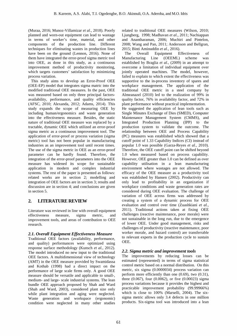
Effectiveness Parameters For a robust OEE evaluation in a balanced production line system for a fast-moving product, a dynamic OEE error-proof model was developed through the integration of the traditional OEE factors (availability, performance, and quality measures) with other emerging critical-factors/parameters (workplace condition, waste generation, and error-proof sigma metric). Figure 1 shows the proposed relationship of the Overall Equipment Effectiveness-OEE factors; quality, performance, availability, waste generation, and human ergonomic/workplace condition (temperature). Human/ergonomic elements as related to work environments such as temperature, illumination, and workers' wellbeing, have effects on productivity, and its magnitude depends on the degree of deviation from the established standards. Wastes can also hinder smooth workflow by creating unnecessary shortage/surplus in outputs of material, machine, manpower, etc. through excessive inventory operation and customers’ satisfaction. The duo, ergonomic and waste, was very important OEE
factors neglected many years past. The effective production process is attainable under the condition of excellent equipment availability, line performance, product quality, working environment, and waste reduction. This condition was hard to meet simultaneously in the manufacturing system.
A sustainable (acceptable) industrial plant operation should have OEE greater than 0.5 (50%) (Ljungberg, 1998). This shows that the OEE of 0.5 is the minimum effectiveness measure required of a manufacturing system to succeed. An OEE below 0.5 indicates danger or poor process performance, while an OEE≥1 signifies a highly productive process. However, a world-class OEE for a production line should be more than 0.85 (Sayuti et al., 2019). In a single product balanced production line, an OEE factor can be evaluated, in terms of productivity, based on a simple ratio of output delivered to the expected output. Variations that existed between the expected and delivered outputs are known as process errors. The multi-factor OEE measure led to the emergence of multiple errors due to its series relationship. Five-factor OEE can be represented as a series control system with errors measured as a difference between input (expected) OEE and output (delivered) OEE (Fig. 2).
The idea is to reduce the error (variation) to make the process effectively satisfactory. This needs to be done gradually on the production line. Every error reduction attained periodically is translatable to the OEE error-proof sigma metric and evaluable using a productivity improvement index, which can be monitored by the management for decision making (interface). The integration of the error-proof (EP) sigma metric as an improvement tool (𝜎𝜎) in line with the OEE control system in Fig. 2 has resulted in continuous improvements (Eqns. (1)-(3)).
Figure. 1. Overall Equipment Effectiveness factors integration.
B. Kareem, A.S. Alabi, T.I. Ogedengbe, B.O. Akinnuli, O.A. Aderoba, M.O. Idris
64
Figure. 2. System Control and Improvement Framework.
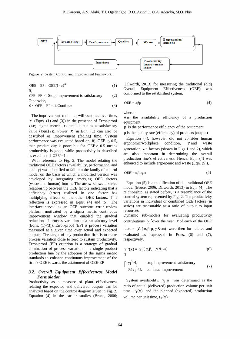
x)σ-1(OEE=EPOEE (1) If,
,1≥EPOEE Stop, improvement is satisfactory (2) Otherwise,
,1<EPOEE≤0 Continue (3) The improvement )EPOEE( will continue over time,
x (Eqns. (1) and (3)) in the presence of Error-proof )EP( sigma metric, σ until it attains a satisfactory
value (Eqn.(2)). Power x in Eqn. (1) can also be described as improvement (fading) time. System performance was evaluated based on, if; OEE ≤ 0.5, then productivity is poor; but for OEE > 0.5 means productivity is good, while productivity is described as excellent if OEE ≥ 1.
With reference to Fig. 2, The model relating the traditional OEE factors (availability, performance, and quality) was identified to fall into the family of control model on the basis at which a modified version was developed by integrating emerging OEE factors (waste and human) into it. The arrow shows a series relationship between the OEE factors indicating that a deficiency (error) realized in one factor has multiplying effects on the other OEE factors. This reflection is expressed in Eqns. (4) and (5). The interface served as an OEE outcome error review platform motivated by a sigma metric continuous improvement window that enabled the gradual reduction of process variation to a satisfactory level (Eqns. (1)-(3)). Error-proof (EP) is process variation measured at a given time over actual and expected outputs. The target of any production firm is to make process variation close to zero to sustain productivity. Error-proof (EP) criterion is a strategy of gradual elimination of process variation in a single product production line by the adoption of the sigma metric standards to enhance continuous improvement of the firm’s OEE towards the attainment of OEE-EP
3.2. Overall Equipment Effectiveness Model
Formulation Productivity as a measure of plant effectiveness relating the expected and delivered outputs can be analyzed based on the control diagram given in Fig. 2. Equation (4) in the earlier studies (Bruce, 2006;
Dilworth, 2013) for measuring the traditional (old) Overall Equipment Effectiveness (OEE) was conformed to the established system.
αβμ=OEE (4)
where: α is the availability efficiency of a production equipment β is the performance efficiency of the equipment μ is the quality rate (efficiency) of products (output)
Equation (4), however, did not consider human ergonomic/workplace condition, γ and waste generation, ω factors (shown in Figs 1 and 2), which are also important in determining the overall production line’s effectiveness. Hence, Eqn. (4) was enhanced to include ergonomic and waste (Eqn. (5)),
αβμγω='OEE (5)
Equation (5) is a modification of the traditional OEE model (Bruce, 2006; Dilworth, 2013) in Eqn. (4). The relationship, as stated before, is a resemblance of the control system represented by Fig. 2. The productivity variations in individual or combined OEE factors (in series) are measurable as a ratio of output to input resources. Dynamic sub-models for evaluating productivity contributions 'iy over the year x of each of the OEE
factors iy ( )ω.&γ,μ,β,α were then formulated and evaluated as expressed in Eqns. (6) and (7), respectively.
=)x('yi iy ( )ω.&γ,μ,β,α (6) If
[ ,1≥'iy
,1<'iy≤0 (7)
System availability, )α(yi was determined as the
ratio of actual (delivered) production volume per unit time, )x(t1 and the planned (expected) production volume per unit time, )x(t2 .
stop improvement satisfactory
continue improvement
B. Kareem, A.S. Alabi, T.I. Ogedengbe, B.O. Akinnuli, O.A. Aderoba, and M.O. Idris
65
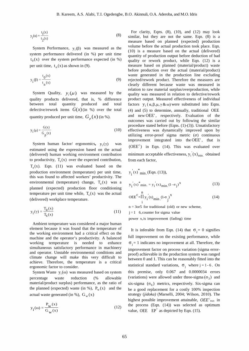
)x(2t)x(1t=)α(iy (8)
System Performance, )β(yi was measured as the
system performance delivered (in %) per unit time )x(t0 over the system performance expected (in %)
per unit time, )x(tn as shown in (9).
)x(nt
)x(0t=)β(iy (9)
System Quality, )(µiy was measured by the quality products delivered, that is, % difference between total quantity produced and total defective/rework items )(xG (in %) over the total
quantity produced per unit time, )(xGp (in %).
)x(pG)x(G
=)μ(iy (10)
System human factor/ ergonomics, )γ(yi was
estimated using the expression based on the actual (delivered) human working environment contribution to productivity, )x(Ts over the expected contribution,
).x(Ta Eqn. (11) was evaluated based on the production environment (temperature) per unit time, this was found to affected workers’ productivity. The environmental (temperature) change, )x(Ta was a planned (expected) production floor conditioning temperature per unit time while, )x(Ts was the actual (delivered) workplace temperature.
)x(sT)x(aT
=)γ(iy (11)
Ambient temperature was considered a major human
element because it was found that the temperature of the working environment had a critical effect on the machine and the operator’s productivity. A balanced working temperature is needed to enhance simultaneous satisfactory performance in machinery and operator. Unstable environmental conditions and climate change will make this very difficult to achieve. Therefore, the temperature is a critical ergonomic factor to consider.
System Waste )ω(yi was measured based on system percentage waste reduction (% allowable material/product surplus) performance, as the ratio of the planned (expected) waste (in %), )x(Pw and the actual waste generated (in %), )x(Gw
)x(wG
)x(wP=)ω(iy (12)
For clarity, Eqns. (8), (10), and (12) may look similar, but they are not the same. Eqn. (8) is a measure based on planned (expected) production volume before the actual production took place. Eqn. (10) is a measure based on the actual (delivered) quantity of production output before deduction of bad quality or rework product, while Eqn. (12) is a measure based on planned (material/product) waste before production over the actual (material/product) waste generated in the production line excluding rejected/rework product. Therefore the measures are clearly different because waste was measured in relation to raw material surplus/overproduction, while quality was measured in relation to defective/rework product output. Measured effectiveness of individual factors iy ( )ω&γ,μ,β,α were substituted into Eqns. (4) and (5) to determine, annually, traditional OEE and new 'OEE , respectively. Evaluation of the outcomes was carried out by following the similar procedure stated before (Eqns. (1)-(3)). Unsatisfactory effectiveness was dynamically improved upon by utilizing error-proof sigma metric (𝜎𝜎) continuous improvement integrated into the 'OEE , that is
)OEE( c in Eqn. (14). This was evaluated over
minimum acceptable effectiveness, .min'
i )x(y obtained from each factor,
.min*)x('iy (Eqn. (13)),
x)jσ-1(.min)x('iy=.min
*)x('iy (13)
x)j
-σ1(∏n
i.min(x)'
iy=cOEE (14)
time(fading)timprovemenisx,powervaluesigmaforcounter6,1=j
scheme,newor(old)ltraditionafor3or5=n
It is inferable from Eqn. (14) that jσ = 0 signifies
full improvement on the existing performance, while
jσ = 1 indicates no improvement at all. Therefore, the improvement factor on process variation (sigma error-proof) achievable in the production system was ranged between 0 and 1. This can be reasonably fitted into the statistical standard variations, jσ where 6-1=j . On this premise, only 0.067 and 0.0000034 errors (variations) were allowed under three-sigma )σ( 3 and six-sigma )σ( 6 metrics, respectively. Six-sigma can be a good replacement for a costly 100% inspection strategy (jidoka) (Marselli, 2004; Wilson, 2010). The highest possible improvement attainable, max
cOEE in the process (Eqn. (14)) was selected as optimum value, *EPOEE as depicted by Eqn. (15).

Development of OEE Error-proof (OEE-EP) Model for Production Process Improvement
66
maxc*c* OEE=OEE=EPOEE (15)
The model as stated is a constrained linear/
nonlinear programming model that can be solved via an analytical approach, and regression analysis using excel tool. 3.3. Analysis of Model Parameters The production firm where data was collected was established in a popular city in Nigeria more than two decades ago. The company was into mass production of a single but highly patronized beverage product. The company is a flow process, balanced production line firm, producing a fast-moving product to ever-increasing customers. The data collected were primary, and were gotten from a production line of the company based on the available records and presented in tabular format after analysis on the yearly bases to align with the data need of the model. The name of the company was concealed to protect her confidentiality and integrity. There have been reported cases that emanated from data analysis of unstable line availability, system performance, product quality, material waste, and floor condition during the production process which have affected customers patronage due to loss of goodwill, which in turn served as a hindrance to stable and sustainable productivity of the firm. This has defeated the objective of adopting a balanced line production system to enable a continuous flow of product for satisfactory performance at meeting customers’ delivery. Based on the foregoing, there is the need to minimize process variation such that the production line is utilized effectively with the target of meeting customers’ demand (delivery) as preplanned with little or no surplus or shortage. On this basis, there is the need to introduce error-proofing (EP) to the traditional and emerging OEE metrics as a solution to this challenge of productivity instability.
A small data set on expectations and deliveries of OEE factors spanning eight (8) years was made available from the company for the analysis (Tables 1-5).
The performance factors iy ( )ω.&γ,μ,β,α were estimated based on the expected and delivered production output parameters on a yearly basis ),x(t1
),x(t 2 ),x(t0 ),x(t n ),x(G ),x(Gp ),x(Ta ),x(Ts
),x(Pw ),x(G w using Eqns. (8)-(12). For example, system availability, )α(yi was estimated from the yearly, x , expected production volume (in million),
),x(2t (10,011.00), and delivered production volume
(in million), ),x(1t (11,211.17) using Eqn. (8) as
12.1=00.011,1017.211,11
=)α(iy
The other performance ratios were obtained using a
similar computation method, and the results are shown in the last columns of Tables 1-5.
To prevent static performance measures and to allow data updating of OEE factors, a dynamic approach was proposed via the regression model by utilizing yearly expected (delivered) output as the dependent variable and the time (in the year, x) as the independent variable. In the analysis, different regression options (exponential, linear, logarithmic, polynomial and power, etc.) were analyzed using Excel-tool to find equations that best-fit the data based on the highest coefficient of determination 2Rcriterion.
Actual and predicted output outcomes were validated using the Mean Square Error (MSE) statistic. The error between the actual and predicted results should not exceed 10% (Peng and Huang, 2012; Ryan et al., 2013, Hayes, 2018). The best polynomial regression equations )1≈R( 2
obtained are presented as Eqns. (16-25). The yearly predicted results on OEE factors by substituting year (x =1, 2,…, 8) into Eqns. (16-25) are presented in Table 6. Predicted OEE for individual factor (availability as a sample) )P(i )α(y was measured using similar approach as that of actual OEE measure,
)A(i )α(y (Table 7). The Mean Square Error MSE for availability as a sample is:
∑n
1=x=i n
2])P()α(iy)A()α(iy[= 00055.0=MSE
MSEs for other OEE factors were obtained using a
similar method. Then, OEEs based on 3-factor (old method) and 5-factor were estimated using Eqns. (4 and 5) and the results are shown in Table 7. The minimum (lowest) acceptable OEE outcomes,
.min'
i )x(y corresponding to year(s), min,*x for individual factors (Table 7) were selected for continuous improvement analysis on yearly basis (Eqn. (13)). For actual (A) availability,
97.0=)x(y .min'
i with error-proof, 3-sigma metric, 067.0=σ 3=j at year, 1=x , the improvement on the
minimum OEE, .min*'
i )x(y was computed by (Eqn. (13)), 90.0=)067.01(97.0=)x(y 1
.min*'
i
Other elements were computed by following the same process, and their corresponding improvements on 3-factor and 5-factor bases were estimated using

B. Kareem, A.S. Alabi, T.I. Ogedengbe, B.O. Akinnuli, O.A. Aderoba, and M.O. Idris
67
Eqn. (14). For 3-factor, then, 62.0≈)78.0)(89.0)(90.0(=OEEc
The obtained results are presented in Table 8. The same procedure was used for analysis based on the error-proof, six-sigma metric, 0000034.0=σ 6=j
(Table 9). The best improvement strategy (Eqn. (15)) to apply
was selected based on maximum improvement, *cOEE achieved so far (Tables 8 and 9).
4. RESULTS AND DISCUSSION Results are discussed based on; overview of the plant effectiveness trends establishment for OEE factors, OEE performance prediction and evaluation, equipment effectiveness evaluation, and equipment effectiveness improvement.
4.1. Overview of the Plant Effectiveness Computation results (Eqns. 8-11,13) for the plant’s effectiveness (productivity) factors in terms of expected and delivered system availability, system performance, system quality, ergonomic (temperature) and waste generation are presented in Tables 1-5. The analysis indicated that the plant was not working to expectation in terms of satisfying the expected deliveries. The plant was expected to satisfy the requirements of meeting customers’ demand (delivery) in terms of equipment availability, product quality, plant performance, working environment (temperature), and waste generation. The company was able to satisfy world-class productivity delivery requirements in a few years. Excellent (world-class) productivity (100%) was attained in equipment availability in the years 1, 2, 4, and 5; quality in the year 2; plant performance in the years 1 and 2; working condition (temperature) in the years 1, 2, 6, 7 and 8; and material waste generation in the years 7 and 8. There was evidence of productivity overshot (greater than 100%) due to higher delivery (in quantity) than expected (years 1, 2, 4, and 5). Effective deliveries of process factors were below expectations in many years under review (Tables 1-5). The worst, system waste productivity of 0.32 was found in the second year of the plant’s operation. This result was odd and inconsistent with other outcomes, and hence not reliable. The plant probably required alignment or corrective maintenance during this period. The results generally showed the management the need to improve on and moderate some effectiveness factors to attain the goal of meeting satisfactory productivity (100%) every year. In this case, the establishment of regression models had
Table 1. System Availability Data and Analysis.
Year (x)
Expected Production Volume (million) t2(x)
Production Volume Delivered (million) t1(x)
Ratio
yi(α)
1 10,011.00 11,211.17 1.12
2 13,541.26 13,541.26 1.0
3 15,096.49 14,593.49 0.97
4 14,281.36 16,290.13 1.14
5 16,035.19 18,058.25 1.13
6 18,996.82 18,499.26 0.97
7 19,736.88 19,298.22 0.98
8 20,808.32 20,341.56 0.98
Table 2. System Performance Data and Analysis.
Year (x)
Performance Expected (%)tn(x)
Performance Delivered (%) to(x)
Ratio yi(β)
1 90.00 90.00 1.00
2 91.00 91.00 1.00
3 91.50 80.00 0.87
4 91.50 79.00 0.86
5 92.00 82.00 0.89
6 92.00 77.00 0.84
7 92.50 80.00 0.86
8 92.50 82.00 0.89 Table 3: System Quality Data and Analysis.
Year (x)
Quality Product Delivered (%)G(x)
Quality Product Expected (%) Gp(x)
Ratio yi(μ)
1 75.00 77.00 0.97 2 76.00 70.00 1.09 3 77.00 79.00 0.98 4 77.00 79.50 0.97 5 78.00 81.00 0.96 6 78.50 81.00 0.97 7 79.00 81.20 0.97 8 80.00 81.21 0.99
Table 4. System Waste Data and Analysis.
Year (x)
Actual (delivered) manufacturing waste (%)Gw(x)
Planned (expected) manufacturing waste (%) Pw(x)
Ratio yi(ω)
1 3.50 3.18 0.91 2 3.10 1.00 0.32 3 3.10 2.16 0.70 4 2.50 1.86 0.74 5 2.00 1.87 0.94 6 2.00 1.86 0.93 7 1.85 1.85 1.00 8 1.85 1.85 1.00

Development of OEE Error-proof (OEE-EP) Model for Production Process Improvement
68
Table 5. Production Floor Ergonomics Temperature Data. Year (x)
Expected Production Floor Temperature(±2°C) Ta(x)
Delivered Production Floor Conditioning Temperature(±2°C) Ts(x)
Ratio yi(γ)
1 22.00 22.00 1.00 2 22.00 22.00 1.00 3 23.00 28.50 0.77 4 22.00 22.00 1.00 5 22.00 22.20 0.99 6 23.00 23.00 1.00 7 22.00 22.00 1.00 8 22.00 22.00 1.00
motivated dynamism in evaluating plant effectiveness, while the introduction of error-proofing parameters had played a prominent role in providing continuous improvement by eliminating process variation.
4.2. Trends Establishment for OEE Factors Regression analysis using Excel tool on the company’s production line data (Tables 1-5), yielded polynomial equations as the best models for the prediction of the expected, t2(x) and delivered, t1(x) production volume data at a given time (x) as given in Eqns. (16) and (17), respectively; t2(x) = 2.4673x6 - 63.552x5 + 587.96x4 - 2231.9x3 + 2195.6x2 + 5815.7x + 3668.3; R² = 0.99 (16) t1(x) = -2.7512x6 + 82.94x5 - 975.96x4 + 5655.7x3- 16801x2 + 25373x - 2119.2; R² = 0.9992 (17)
,1≈R 2 is an indication that the models had predicted the production volume data accurately. The regression models obtained for the prediction of the expected and delivered: system performance (tn(x), t0(x)); system quality (Gp(x), G(x)); system waste (Pw(x), Gw(x)); and system ergonomic (temperature) (Ta(x), Ts(x)) are respectively given as follows: tn(x) = -0.0007x6 + 0.0184x5 - 0.1976x4 + 1.109x3 - 3.4913x2 + 6.1828x + 86.375; R² = 0.9865 (18) t0(x) = -0.0521x6 + 1.4675x5 - 16.284x4 + 89.924x3 - 255.37x2 + 339.91x - 69.625; R² = 0.9845 (19) Gp(x) = 0.0031x6 - 0.0823x5 + 0.8438x4 - 4.2353x3 + 10.682x2 - 11.654x + 79.437; R² = 0.9941 (20) G(x) = 0.0276x6 - 0.7996x5 + 9.2103x4 - 53.372x3 + 161.19x2 - 231.88x + 192.6; R² = 0.9796 (21) Pw(x) = 0.0028x6 - 0.0779x5 + 0.8562x4 - 4.6474x3 + 12.86x2 - 17.056x + 11.563; R² = 0.9998 (22) Gw(x)) = 0.0058x6 - 0.1668x5 + 1.9113x4 - 11.011x3 + 33.156x2 - 48.399x + 27.68; R² = 0.9774 (23)
Ta(x) = 0.0125x6 - 0.3375x5 + 3.5625x4 - 18.563x3 + 49.425x2 - 62.1x + 50; R² = 1 (24) Ts(x) = 0.0302x6 - 0.7738x5 + 7.7099x4 - 37.775x3 + 94.537x2 - 112.67x + 72.938; R² = 0.9846 (25)
High coefficients of determination ,1≈R 2 in all cases had indicated that the models were accurate in predicting the expected and delivered outputs. 4.3. Performance Prediction and Evaluation The actual data and predicted results of the production process using regression models (16-25) for the expected and delivered outputs (production volume, product quality, plant performance, floor temperature, and manufacturing waste) are presented in Table 6. It can be clearly observed from the table that the predicted results and actual data were in close resemblance (Tables 1-5). This showed that the established regression models were adequate for expected and delivered performance prediction (Table 6). A sudden rise in waste output prediction was noticed in the fifth year, but as a whole, the actual system effectiveness measures were not largely affected as shown in Table 7. Irregular (unstable) productivity outcome of the factors for the years under review signaled the need for the management to improve on the plant’s effectiveness.
4.4. Evaluation of Equipment Effectiveness The results of the OEE prediction and evaluation of the production line are presented in Table 7. It was revealed from the results that the predicted OEEs values were very close to the actual values (Tables 1-5). The highest Mean Square Error (MSE) of 0.0089 was estimated between the outcomes of the actual and predicted parameters for all OEE factors (Table 7). This was eminently within the acceptable statistical error limit of 0 – 10%. Similarly, the 5-factor (new OEE) and the 3-factor (old OEE) prediction outcomes were very close to that of actual results. The maximum MSE of 0.0047 was computed between actual and predicted OEE results. The errors were far less than the 10% limit. Hence, the model can be effectively applied to the company’s production process to predict and evaluate her equipment effectiveness within an acceptable error margin. The least actual and predicted factor effectiveness (yi
’.min) were (0.97,0.95); (0.96,0.94); (0.84,0.78); (0.77,0.84); and (0.70,0.68), respectively for the years (3,6,7); (5,6); (6,7); (3,3); and (3,3). The waste effectiveness (0.32*, 0.33*) were neglected because of its wide gap to the next higher value (0.70, 0.68). The least actual and predicted OEE results for the old and the new models were (0.79, 0.68) and (0.45, 0.48). These results were obtained at years (3, 3) and (6,7), respectively (Table 7). The irregularity and low OEE outcomes had indicated the need for the company to improve the process to survive amid of present and

B. Kareem, A.S. Alabi, T.I. Ogedengbe, B.O. Akinnuli, O.A. Aderoba, and M.O. Idris
69
future competitors. It was generally revealed that OEE from the old model were in most cases higher than those obtained from the new model. The implication of utilizing the old model in the firm was for the management to have the impression that the plant’s effectiveness was good whereas in real sense it was not from the new model’s results. This indicated that the company manager should be vigilant at finding other underline factors which might have critically influenced the OEE of the plant. Production floor conditions (temperature) and material waste were good examples of such factors identified in and integrated into this system.
The OEEs from the old model seemed unrealistic because of its greediness in estimating the plant’s effectiveness as compared to the realistic new model which was more encompassing and robust in accommodating emerging critical factors that affect productivity. The new model OEE outcomes enabled the firm’s manager to know the true condition of the plant's effectiveness to take decisive action at improving the system to prepare it for present and future competitions. It was noticed that OEEs prediction or evaluation results from old and new methods were not stable through the years under review and were unlikely to be stable in the future. Therefore, the enhancement of improvement through the closing of process variation (gap) between expected and delivered effectiveness will go a long way to bring the plant’s performance stability and effectiveness in operations.
4.5. Equipment Effectiveness Improvement The improvement results on plant’s effectiveness by minimizing process variations via application of statistical sigma metrics under 3-sigma (j=3) and 6-sigma (j=6) using the OEE error-proofing (OEE-EP) model (Eqns. (13), (14) and (15)) are shown in Tables 8 and 9, respectively for 3-factor and 5-factor OEE measures. In both cases, the improvement was noticed in varying proportions over the minimum (lowest) OEE measured for the single (isolated) and combined factors. The improvement results under the 3-sigma metric were not constant (Table 8) over the minimum
benchmark (Table 7) for the years under review. Maximum improvements, actual (0.62, 0.29) and predicted (0.56, 0.28), were estimated (using Eqn. (15)) in the first year using 3-factor and 5-factor effectiveness measures, respectively, while the improvements were reducing (fading) steadily in the subsequent years (Table 8). The implication of these unstable improvements was to notify the firm’s manager of the need to put in place a sustainable plan towards meeting present and future delivery requests. The results (Table 8) further showed the greediness of 3-factor, 3-sigma error-proofing in providing higher improvement outcomes than the 5-factor, 3-sigma model. The improvements for the 9th year showed a similar trend. It was further noticed that the improvements became smaller in future years for both scenarios. This indicated that the improvements will continue to reduce in future years, and then converge to a point. On this basis, the application of this model in measuring the plant’s effectiveness improvement was sustainable due to the integration of regression and error-proof windows that enabled data updating to enhance improvement. However, improvements measured based on error-proof, 6-sigma metric were better and more stable than 3-sigma metric across singular and combined OEE factors (Table 9).
It was revealed from the table that 6-sigma error-proofing produced stable, satisfactory, and sustainable OEE improvements of actual and predicted values (0.78, 0.70) and (0.42, 0.40) over the lowest acceptable OEE for the 3-factor and 5-factor models, respectively. The improvement excesses of the 3-factor model were reflected in these results. Though the improvement attained using the 5-factor model was lesser than that of the 3-factor, but both were world-class compliant, sustainable, satisfactory, and significant to survive any emerging competitiveness. In comparison with past similar studies, attainment of 42% improvement based on the 5-factor, 6-sigma model was considered better than 20% and 23% obtained using lean & green (Pampanelli et al., 2014) and lean bundle (Shah and Ward, 2003) models, respectively.
Table 6. OEE Factors-Annual Outcome Predictions. OEE Factors Year(x) 1 2 3 4 5 6 7 8 Availability Expected, t2(x) 9,974.58 13,758.50 14,594.79 14,765.67 16,075.86 18,443.86 20,269.77 20,579.62 Availability Delivered, t1(x) 11,212.73 13,531.04 14,590.74 16,337.48 17,908.30 18,651.29 19,164.59 20,354.39 Quality expected, Gp(x) 76.98 70.17 78.48 80.41 80.39 82.37 83.32 86.53 Quality delivered, G(x) 74.99 76.04 76.87 77.11 77.43 77.47 76.03 73.42 Performance expected, tn(x) 89.995 91.030 91.400 91.61 91.477 91.66 91.466 90.263 Performance delivered, t0(x) 89.991 91.066 79.995 81.975 84.925 80.375 71.375 77.375 Ergonomics Expected, Ta(x) 21.997 21.996 22.987 21.968 21.938 22.892 21.829 21.744 Ergonomics Delivered, Ts(x) 23.996 24.076 24.320 22.312 23.576 24.823 18.949 21.767 Waste Expected, Pw(x) 3.18 1.03 2.10 2.12 2.15 3.14 4.75 8.26 Waste Delivered, Gw(x) 3.50 3.10 3.12 2.55 2.30 2.87 4.44 7.06

Development of OEE Error-proof (OEE-EP) Model for Production Process Improvement
70
Table 7. Prediction and Evaluation of OEE for the Production Process.
OEE measure, yi /year (x) 1 2 3 4 5 6 7 8 MSE.10-3 yi’.min. x*min
Availability yi(α) Actual (A) Predicted (P)
1.12 1.12
1.00 0.98
0.97 0.99
1.14 1.11
1.12 1.11
0.97 1.01
0.98 0.95
0.98 0.99
0.55
0.97 0.95
3,6 7
Quality yi(μ) Actual Predicted
0.97 0.97
1.09 1.08
0.98 0.98
0.97 0.96
0.96 0.96
0.97 0.94
0.97 0.91
0.99 0.95
3.00
0.96 0.94
5 6
Performance yi(β) Actual Predicted
1.00 1.00
1.00 1.00
0.87 0.87
0.86 0.89
0.89 0.92
0.84 0.87
0.86 0.78
0.89 0.86
1.25
0.84 0.78
6 7
Human/Ergonomics, yi(γ) Actual Predicted
1.00 0.91
1.00 0.91
0.77 0.84
1.00 0.99
0.99 0.93
1.00 0.92
1.00 1.15
1.00 1.00
6.71
0.77 0.84
3 3
Waste yi(ω ) Actual *unaccepted Predicted, Bold, mini. acceptable
0.91 0.91
0.32* 0.33*
0.70 0.68
0.74 0.83
0.94 0.94
0.93 1.09
1.00 1.09
1.00 1.17
8.90
0.70 0.68
3 3
5-factor OEE’-New-method (A) (P)
0.98 0.90
0.34 0.32
0.45 0.48
0.70 0.78
0.89 0.86
0.74 0.82
0.82 0.84
0.86 0.85
2.73
0.45 0.48
3 3
3-factor OEE- old method (A) (P)
1.08 1.08
1.06 1.06
0.83 0.84
0.95 0.95
0.96 0.98
0.79 0.82
0.82 0.68
0.86 0.73
4.70
0.79 0.68
6 7
Table 8. Improvement dynamism on the OEEs using three-sigma metrics.
Improvement dynamism OEE-EP (OEEc) at σj=3 = 0.067 measured at yi
’min./year (x) (Eqn. (14)), yi
’*(x)min
1 2 3 4 5 6 7 8 9
Availability (α) Actual (A) Predicted (P)
0.90 0.87
0.84 0.98
0.79 0.77
0.73 0.72
0.68 0.67
0.64 0.63
0.59 0.59
0.56 0.55
0.52 0.51
Quality (μ) Actual Predicted
0.89 0.88
0.84 0.82
0.78 0.76
0.73 0.71
0.68 0.67
0.63 0.62
0.59 0.58
0.55 0.54
0.51 0.50
Performance (β) Actual Predicted
0.78 0.73
0.73 0.68
0.68 0.63
0.64 0.59
0.59 0.55
0.55 0.52
0.52 0.48
0.48 0.45
0.45 0.42
Human/Ergonomics, (γ) Actual Predicted
0.72 0.78
0.67 0.73
0.63 0.68
0.58 0.64
0.54 0.59
0.51 0.55
0.47 0.52
0.44 0.48
0.41 0.45
Waste (ω ) Actual Predicted
0.65 0.63
0.61 0.59
0.57 0.55
0.53 0.52
0.49 0.48
0.46 0.45
0.43 0.42
0.40 0.39
0.38 0.36
Max. improvement over 3-factor, 3-sigma: OEEc* (OEE-EP*) (Eqn. (15))
(A) (P)
0.62 0.56
0.52 0.46
0.42 0.37
0.34 0.30
0.27 0.25
0.22 0.20
0.18 0.16
0.15 0.13
0.12 0.11
Max. improvement over 5-factor, 3-sigma: OEEc* (OEE-EP*) (Eqn. (15))
(A) (P)
0.29 0.28
0.21 0.20
0.15 0.14
0.10 0.10
0.07 0.07
0.06 0.06
0.04 0.04
0.03 0.03
0.02 0.02
Table 9. Improvement dynamism on the OEEs using six-sigma metrics. Improvement dynamism OEE-EP (OEEc) at σj=6 = 0.0000034 measured at (yi)min. /year (x) (Eqn. (14)), yi
’*(x)min.
1 2 3 4 5 6 7 8 9
Availability (α) Actual (A) Predicted (P)
0.97 0.95
0.97 0.95
0.97 0.95
0.97 0.95
0.97 0.95
0.97 0.95
0.97 0.95
0.97 0.95
0.97 0.95
Quality (μ) Actual Predicted
0.96 0.94
0.96 0.94
0.96 0.94
0.96 0.94
0.96 0.94
0.96 0.94
0.96 0.94
0.96 0.94
0.96 0.94
Performance (β) Actual Predicted
0.84 0.78
0.84 0.78
0.84 0.78
0.84 0.78
0.84 0.78
0.84 0.78
0.84 0.78
0.84 0.78
0.84 0.78
Human/Ergonomics, (γ) Actual Predicted
0.77 0.84
0.77 0.84
0.77 0.84
0.77 0.84
0.77 0.84
0.77 0.84
0.77 0.84
0.77 0.84
0.77 0.84
Waste (ω ) Actual Predicted
0.70 0.68
0.70 0.68
0.70 0.68
0.70 0.68
0.70 0.68
0.70 0.68
0.70 0.68
0.70 0.68
0.70 0.68
Max. improvement over 3-factor, 6-sigma: OEEc* (OEE-EP*) (Eqn. (15))
(A) (P)
0.78 0.70
0.78 0.70
0.78 0.70
0.78 0.70
0.78 0.70
0.78 0.70
0.78 0.70
0.78 0.70
0.78 0.70
Max. improvement over 5-factor, 6-sigma: OEEc* (OEE-EP*) (Eqn. (15))
(A) (P)
0.42 0.40
0.42 0.40
0.42 0.40
0.42 0.40
0.42 0.40
0.42 0.40
0.42 0.40
0.42 0.40
0.42 0.40
The 3-factor based performance (65%) attained by Hedman et al. (2016) using automatic measurement approach can only compete with the 62% improve-
ement of this new 3-factor, 3-sigma error-proof model (Table 8), but far below 78% attainable from the 3-factor, 6-sigma error-proof model (Table 9).

B. Kareem, A.S. Alabi, T.I. Ogedengbe, B.O. Akinnuli, O.A. Aderoba, and M.O. Idris
71
5. CONCLUSION The OEE model has been effectively formulated to plan production, labor utilization, maintenance, and working environment as reflected in the attainment of waste reduction, availability, quality, and performance improvements. The integration of human/ergonomic workplace environment (temperature) and system waste generation factors into the OEE measures has broken new ground in the field of overall equipment effectiveness research. Attainment of dynamism in the system effectiveness measures through the incorporation of best regression models and integration of encompassing error-proof, sigma metric parameter has made the system unique in terms of providing sustainable performance as compared to other popular techniques.
The six-sigma has performed well in system error-proofing and at the same time providing better productivity improvement platforms for the fast-moving goods production process. The models were applied successfully to measure critical equipment effectiveness factors which are availability, performance, quality, workplace condition (temperature), and material waste of a production plant. On this basis, challenges that hindered the effective operation of the plant were mitigated and improved system was sustained.
Results obtained using different scenarios of the model application to a production line showed a low performance which was improved upon using a better improvement program, the new OEE-EP model. The application of the OEE-EP model has made a landmark achievement by providing the highest level of improvements (0.42, 0.78), which are far better than those obtainable from past studies (0.20, 0.23). This landmark achievement can be attributed to excellent accuracy provided by error-proof, six-sigma metric in minimizing process variation. Specific conclusions drawn from this study are enumerated as follows: i. Unstable overall equipment effectiveness
measures were obtained for the company in the years under review. This revealed the need for the company to be evaluating her productivity/overall equipment effectiveness annually for early correction of any ailing process factor before it gets out of control to stabilize the changing firm’s productivity over time.
ii. The continuous improvement of the production process has been achieved for the company using overall equipment effectiveness error-proof strategy without an increase in input resources. This outcome has shown the management of the company the undesirability of increasing input resources before getting the productivity of the production process improved. Proper choice of resources management strategy can sustain and improve productivity. This has been shown by the outcome of this study.
iii. There is a wide gap between traditional 3-factor OEE and new scheme 5-factor OEE results. Therefore, in the presence of uncertainty, it is advisable that the company base its productivity measure on 5-factor which is more robust.
iv. The integration of error-proof sigma metric as a means of continuous improvement in the production process of the company has resulted in sustainable and stable productivity improvement. This lean metric has performed better than other improvement metrics such as lean bundle, lean green, and automation.
v. The data set available for productivity/OEE prediction was small. This can affect prediction accuracy. To improve prediction accuracy, it is advisable that the company has a good record of annual OEE data for timely data updates.
Further study is required in real-time implementation of the process through the application of computer programs to handle large data, to serve as a source of artificial intelligence at enhancing robust decision making in the future as regards the performance of the OEE-EP model. In such a study the null hypothesis shall be; the new OEE-EP model is robust enough to withstand emerging (future) wastes and environmental challenges, while the alternative hypothesis shall be the model cannot withstand future challenges.
Proper identification of processes that required improvement, choice of appropriate improvement methods (tools) required and adequate representation of the process outcomes for good decision making are other areas of further research. The implementation of this scheme will require good experience and deep knowledge of processes identification and analysis with criticality and necessity consideration.
CONFLICT OF INTEREST The authors declare that there are no conflicts of interest as regards this article. FUNDING
Managements of Federal University of Technology, Akure, and Fast Moving Products Industry, Ibadan, Nigeria are acknowledged for providing funds and facilities for the successful completion of this project. ACKNOWLEDGMENT B. Kareem thanks the management and staff of Fast Moving Products Industry for providing relevant information used in this study. The contribution of industrial and production engineering research group leader, Federal University of Technology Akure (FUTA), Nigeria is also acknowledged.

Development of OEE Error-proof (OEE-EP) Model for Production Process Improvement
72
REFERENCES
Adams JA (2014), Human factors engineering. New York: McMillan Publishing.
AFSC-Air Force Systems Command, (2010),Air Force Systems Command Design Handbook, Human Factors Engineering. United Kingdom: McMillan Publishing.
Alexander DC (2012), The practice and management of industrial ergonomics. New York: Englewood Cliffs, NJ: Prentice-Hall.
Almeanazel OTR (2010), Total productive maintenance review and overall equipment effectiveness measurement. Jordan Journal of Mechanical and Industrial Engineering (JJMIE) 4(4): 517 – 522.
Andersson C, Bellgran M (2015), On the complexity of using performance measures: Enhancing sustained production improvement capability by combining OEE and productivity. Journal of Manufacturing Systems, 35: 144-154.
Anvari F, Edwards R, Starr A (2010), Evaluation of overall equipment effectiveness based on market. Journal of Quality in Maintenance Engineering 16(3): 256-270.
Bhattachcharjee A, Roy S, Kundu S, Tiwary M, Chakraborty R (2019), An analytical approach to measure OEE for blast furnaces. Journal Ironmaking & Steelmaking; Processes, Products and Applications, published online: 31Jan 2019.
Binti Aminuddin NA, Garza-Reyes JA, Kumar V, Antony J, Rocha-Lona L (2016), An analysis of managerial factors affecting the implementation and use of overall equipment effectiveness. International Journal of Production Research 54(15): 4430-4447.
Braglia M, Frosolini M, Zammori F (2009), Overall equipment effectiveness of a manufacturing line (OEEML): An integrated approach to assess systems performance. Journal of Manufacturing Technology Management 20(1) 8-29.
Bruce CH (2006), Best Practices in Maintenance, http://www.tpmonline.com/articles_on_total_ productivemaintenance/management.htm, accessed 26:09:2011.
Butlewski M, Dahlke G, Drzewiecka-Dahlke M, G-orny A, Pacholski L (2018), Implementation of TPM methodology in worker fatigue management - a macroergonomic approach. Advanced Intelligence Systems and Computing 605:32-41. Dilworth JB (2013), Production and operations management. New York: McGraw-Hill.
Domingo R, Aguado S (2015), Overall environmental equipment effectiveness as a metric of a lean and green manufacturing system. Sustainability 7(7): 9031-9047.
Garza‐Reyes JA, Eldridge S, Barber KD, Soriano‐Meier H (2010), Overall equipment effectiveness (OEE) and process
capability (PC) measures: A relationship analysis. International Journal of Quality & Reliability Management 27(1): 48-62.
Gharbi A, Kennen JP (2000), Production and preventive maintenance rates control for a manufacturing system: An experimental design approach, International Journals of Production Economics 65: 275-287.
Ghazali A, Adegbola AA, Olaiya KA, Yusuff ON, Kareem B (2013): Evaluation of workers’ perception on safety in selected industries within Ibadan metropolis. SEEM Research and Development Journal 2(1): 82-88.
Godfrey P (2002), How the return on investment and cash flow can be improved by using the overall equipment effectiveness measure. Manufacturing Engineer 81(2): 109-112.
Hansen RC (2002), Overall equipment effectiveness: a powerful production/maintenance tool for increased profits. New York: Industrial Press Inc.
Hayes AF (2018), Introduction to mediation, moderation, and conditional process analysis: A regression-based approach. New York: The Guilford Press.
Hedman R, Subramaniyan M, Almström P (2016), Analysis of critical factors for automatic measurement of OEE. Procedia CIRP 57: 128-133
Hossain MSJ, Sarker BR (2016), Overall equipment effectiveness measures of engineering production systems, Conference paper: 2016 Annual Meeting of the Decision Science Institute, Austin, Texas, USA, accessed at www.researchgate.net/publication/315666207
Joshi S, Gupta R (1986), Scheduling of Routine Maintenance Using Production Schedule and Equipment Failure History. International Journal of Computers and Industrial Engineering 10(1) 11-20.
Kadiri M. A. (2000), “Scheduling of preventive maintenance in a manufacturing company: A computer model approach”, Unpublished M.S. Thesis, Dept. of Ind. and Prod. Eng., University of Ibadan, NG.
Kareem B, Jewo AO (2015), Development of a model for failure prediction on critical equipment in the petrochemical industry. Engineering Failure Analysis 56: 338–347.
Künsch HR, Stefanski LA, Carroll RJ (2012), Conditionally unbiased bounded-influence estimation in general regression models, with applications to generalized linear models. Journal of the American Statistical Association 84 (406): 23-37
Lanza G, Stoll J, Stricker N, Peters S, Lorenz C (2013), Measuring global production effectiveness. Forty Sixth CIRP Conference on Manufacturing Systems 2013, Procedia CIRP, 7 (2013), 31-36.
Lennon P (2016), Root-cause analysis underscores the

B. Kareem, A.S. Alabi, T.I. Ogedengbe, B.O. Akinnuli, O.A. Aderoba, and M.O. Idris
73
importance of understanding, addressing and communicating cold chain equipment failures to improve equipment performance. Technical report, Los Angeles, USA.
Ljungberg O (1998), Measurement of overall equipment effectiveness as a basis for TPM activities. International Journal of Operations & Production Management 18(5): 495-507.
Madhavan E, Paul R, Rajmohan M (2011), Study on the influence of human factors. European Journals, 23: 179-192.
Marselli M (2004), Lean manufacturing and six-sigma, Wire Journal International, http://www.aemconsulting.com/pdf/lean.pdf. accessed 12-10-2018
Martand T (2014), Industrial engineering and production management. New Delhi: S.Chand & Company Ltd.
Meyer FE, Stewart JR (2018), Motion and time study for lean manufacturing, 3rd edition, JS-89867 US, https://rzo0o4khw01.storage.googleapis.com/MDEzMDDMxNjcwOQ==01.pdf accessed 19-05-2018.
Michael JK (2015), Six sigma green belt training manual, Michael JK (UK Based), Lagos, NG.
Muchiri P, Pintelon L (2008), Performance measurement using overall equipment effectiveness (OEE): literature review and practical application discussion. International journal of production research 46(13): 3517-3535.
Muñoz-Villamizar A, Santos J, Montoya-Torres J, Jaca C (2018), Using OEE to evaluate the effectiveness of urban freight transportation systems: A case study. International Journal of Production Economics 197: 232-242.
Munteanu D, Gabor C, Munteanu I, Schreiner A (2010), Possibilities for increasing efficiency of industrial equipment. Bulletin of the Transilvania University of Brasov, Series I: Engineering Sciences 3(52):199-204.
Muraa MD (2016), Worker skills and equipment optimization in assembly line balancing by a Genetic Approach. Technical report, Dept. of Civil and Ind. Eng., Univ. of Pisa, Italy.
Muthiah KMN, Huang SH, Mahadevan S (2008), Automating factory performance diagnostics using overall throughput effectiveness (OTE) metric. International Journal of Advanced Manufacturing Technology 36(8): 11–824.
Mwanza BG (2017), An assessment of the effectiveness of equipment maintenance, practices in public hospitals. Technical report, Univ. of Johannesburg, South Africa.
Nachiappan RM, Anantharaman N (2006), Evaluation of overall line effectiveness (OLE) in a continuous product line manufacturing system. Journal of Manufacturing Technology Management 17(7): 987-1008
Pampanelli AB, Found P, Bernardes AM (2014), A lean & green model for a production cell. Journal of Cleaner Production 85: 19-30
Peng L, Huang Y (2012), Survival analysis with quartile regression models. Journal of the American Statistical Association 103 (482): 637-649
Prinz C (2017): Implementation of a learning environment for an Industrie 4.0 assistance system to improve the overall equipment effectiveness. Technical report, A Ruhr-Universität Bochum, Chair of Production Systems, Bochum, Germany.
Ryan AG, Montegomery DC, Peck EA, Vining GG, Ryan AG (2013), Solution manual to accompany introduction to linear regression analysis. New Jersey: John Wiley & Son Inc.
Samat HA, Kamaruddin S, Azid IA (2012), Integration of overall equipment effectiveness (OEE) and reliability method for measuring machine effectiveness. South African Journal of Industrial Engineering 23(1): 92-113.
Sarker BR (2001), Measures of grouping efficiency in cellular manufacturing systems. European Journal of Operational Research 130(3): 588-611.
Sayuti M, Juliananda, Syarifuddin F (2019), Analysis of the overall equipment effectiveness (OEE) to minimize six big losses of pulp machine: a case study in pulp and paper industries. International Conference on Science and Innovated Engineering (I-COSINE), IOP Conf. Series: Materials Science and Engineering 536 (2019): 012136 doi:10.1088/1757-899X/536/1/012136.
Shah R, Ward PT (2003), Lean manufacturing: context, practice bundles, and performance. Journal of Operations Management 21(2): 129-149
Singh R, Shah DB, Gohil AM, Shah MH (2013), Overall equipment effectiveness (OEE) calculation - automation through hardware & software development. Procedia Engineering 51: 579-584
Swamidassa PM, Kothab S (1998), Explaining manufacturing technology use, firm size and performance using a multidimensional view of technology. Journal of Operations Management 17(1): 23-37
Wang TY, Pan HC (2011), Improving the OEE and UPH data quality by Automated Data Collection for the semiconductor assembly industry. Expert Systems with Applications 38(5): 5764-5773.
Wilson L (2010), How to implement lean manufacturing. New York: McGraw-Hill Inc.
Wudhikarn R (2010), Overall weighting equipment effectiveness. Proceedings of the 2010 IEEE IEEM, 23-27.
Wudhikarn R (2012), Improving overall equipment cost loss adding cost of quality. International Journal of Production Research

Development of OEE Error-proof (OEE-EP) Model for Production Process Improvement
74
50(12): 3434-3449. Yuniawan D, Ito T, Bin ME (2013), Calculation of
overall equipment effectiveness weight by Taguchi method with simulation. Concurrent Engineering 21(4): 296-306. Zammori F, Braglia M, Frosolini M (2011), Stochastic overall equipment effectiveness.
International Journal of Production Research 49(21): 6469-6490.
Zuashkiani A, Rahmandad H, Jardine AKS (2011), Mapping the dynamics of overall equipment effectiveness to enhance asset management practices. Journal of Quality in Maintenance Engineering 17(1): 74-92.

The Journal of Engineering Research (TJER), Vol. 17, No. 2, (2020) 75-88
*Corresponding author’s e-mail: [email protected]
DOI:10.24200/tjer.vol17iss2pp75-88
SPATIAL AND STATISTICAL ANALYSIS OF ENVIRONMENTAL NOISE LEVELS IN THE MAIN CAMPUS OF THE UNIVERSITY OF LAGOS
Alfred S. Alademomi1, Chukwuma J. Okolie1*, Babatunde M. Ojegbile1, Olagoke E. Daramola1,
Johanson C. Onyegbula1, Rahmat O. Adepo1, and Wemimo O. Ademeno2 1Department of Surveying and Geoinformatics, Faculty of Engineering,
University of Lagos, Nigeria. 2Department of Surveying and Geoinformatics, D.S. Adegbenro ICT Polytechnic,
Ewekoro, Ogun State, Nigeria. ABSTRACT: The increasing student population, developmental, and commercial activities within the University of Lagos's main campus have led to an increase in daily noise levels. These have disrupted the serenity and tranquillity of the campus environment. In this study, the noise levels within the campus were assessed at 34 locations to determine compliance with international standards for tolerable noise levels in different environments. For three days, noise levels at the stations were measured using the Extech 407730 sound level meter. In the analysis, noise level maps were produced using the Inverse Distance Weighted (IDW) interpolation, and the correlation between observed noise levels and noise limits were determined. The noise levels measured in the study area ranged from 41.9 - 96.6dBA. It was observed that the minimum noise levels were associated mostly with residential and conservation areas; while the maximum noise levels were mostly associated with commercial areas, vehicle parks, and transportation corridors. Generally, the noise levels exceeded the tolerable limits for academic, commercial, and residential areas set by the World Health Organisation (WHO) and the National Environmental Standards and Regulations Enforcement Agency (NESREA). The Pearson’s correlation coefficients (r) between the average 𝐿𝐿𝐴𝐴 𝑒𝑒𝑒𝑒 noise levels and both standards (WHO and NESREA) were derived as 0.63 and 0.58 respectively, indicating a slightly high positive correlation. These findings serve as a valuable knowledge base to inform the University management on the need to implement abatement measures aimed at maintaining the noise levels within tolerable limits.
Keywords: Geographic information system; Inverse distance weighted interpolation; Noise pollution; Pearson’s correlation coefficient; Sound level.
تحلیل مكاني وإحصائي لمستویات الضوضاء في الحرم الجامعي
و ،رحمت ادیبو ،جوھانسون ك اونیجبولا ، اولاجوكي دارامولا, ،باباتوندي م اوجیجیبیلي ،شوكوما ج اوكولي ،ألفرید س الادیمومي ویمیمو ادمینو
: أدى تزاید عدد الطلاب والأنشطة الإنمائیة والتجاریة داخل الحرم الجامعي الرئیسي لجامعة لاجوس إلى زیادة في مستویات الملخص
الضوضاء الیومیة. وقد أدت ھذه الاضطرابات الضوضائیة المتزایدة إلى الإخلال بسكینة بیئة الحرم الجامعي وھدوئھ. في ھذه الدراسة التعرض للضوضاء لتحدید اختبارضاء في أربعة وثلاثین موقعا محددا داخل حرم جامعة لاجوس. وقد أجري یتم تقییم مستویات الضو
مدى موافقة بیئة الحرم الجامعي للمعاییر الدولیة فیما یتعلق بمستویات الضوضاء المقبولة في مختلف البیئات. تم قیاس الحد الأدنى . Extech 407730 المحطات لمدة ثلاثة أیام باستخدام مقیاس مستوى الصوتوالحد الأقصى ومتوسط مستویات الضوضاء في
وتراوحت مستویات الضوضاء التي تم قیاسھا .خرائط مستوى الضوضاء عن طریق الاستنباط من معكوس المسافة المرجحة رسمتودیسیبل. ولوحظ أن الحد الأدنى لمستویات الضوضاء یرتبط في الغالب بمناطق سكنیة ومناطق 96.6و 41.9في منطقة الدراسة بین
ت النقل. وبشكل محمیة؛ في حین أن الحد الأقصى لمستویات الضوضاء یرتبط في الغالب بالمناطق التجاریة ومواقف السیارات وممراعام، تجاوزت القراءات مستویات الضوضاء الحدود المقبولة للمناطق الأكادیمیة والتجاریة والسكنیة التي حددتھا منظمة الصحة
ومعیاییر بیرسون بین متوسط مستویات الضوضاء العالمیة والوكالة الوطنیة لتطبیق المعاییر واللوائح البیئیة. تشیر معاملات ارتباطدیسیبل على التوالي، إلى علاقة متبادلة إیجابیة مرتفعة 0.58و 0.63المقدرة بـ المشرعین المذكورین أعلاه ضاء الصادرة عن الضو
قاعدة معارف قیمة لإبلاغ إدارة لتكون نتائجھا ھذه الدراسة وتھدف .قلیلا بین مستویات الضوضاء المقاسة وتلك المسموح بھا دولیا .تدابیر خفض الضوضاء بھدف الحفاظ على مستویاتھا في حدود مقبولة الجامعة بضرورة تنفیذ
.الضوضاء؛ موجات صوتیة؛ تلوث سمعي؛ مستوى الصوت؛ معامل ارتباط بیرسون :الكلمات المفتاحیة

Spatial and Statistical Analysis of Environmental Noise Levels in the Main Campus of the University of Lagos
76
NOMENCLATURE I Intensity of the sound wave (in W/m2) N Number of measurements n Number of sampled points used for the
IDW estimation p Power parameter r Pearson’s correlation coefficient S’ Arithmetic mean of the 𝐿𝐿𝐴𝐴 𝑒𝑒𝑒𝑒 noise levels. 𝑆𝑆 𝐿𝐿𝐴𝐴 𝑒𝑒𝑒𝑒 values according to noise standards S1 Standard deviations of S’ S2 Standard deviations of S� t Calculated t value β Sound level 𝜆𝜆𝑖𝑖 Influence (weight) of sample points dB Decibels dBA A-weighted sound level in Decibels df Degree of freedom di Distance between the point of interest and
the sampled point Eqn Equation H0 Null hypothesis H1 Alternative hypothesis Io Standard reference intensity (= 10-12 W/m2) IDW Inverse Distance Weighted LGA Local Government Area 𝐿𝐿𝐴𝐴 𝑒𝑒𝑒𝑒 Average sound level 𝐿𝐿𝐴𝐴 𝑚𝑚𝑖𝑖𝑚𝑚 Minimum sound level 𝐿𝐿𝐴𝐴 𝑚𝑚𝑚𝑚𝑚𝑚 Maximum sound level Max. Maximum Min. Minimum S/N Serial number NESREA National Environmental Standards and
Regulations Enforcement Agency WHO World Health Organisation 1. INTRODUCTION
Sound waves are sensations perceived by the auditory nerves from the impact of acoustic pulses reaching the ear. These sound waves travel through the air, causing vibrations along the path of propagation which can be detected by the auditory nerves and causes a sensation of hearing to humans and other animals (Goshu et al., 2017). The intensity of sound waves, which can be described as the level of its impact on the auditory nerves and environment are generally known to decrease with increasing distance from the source (Hansen, 2001). The speed of sound in air is approximately 330m/s and depends on factors such as the temperature, pressure, and density of the medium (Paulet et al., 2016; Sharma, 2017). Noise is a sensation that irritates the auditory nerves (Zannin, 2013), and is characterised by irregular vibration of the propagating acoustic media or unpleasant acoustic sensations to the hearer. Hence, a sound that may be acceptable to one hearer might be noise to another. Prolonged exposure to sound, which initially may be pleasing or acceptable to one, may also be classified as noise since the user may become irritated over time
by it. Hence, the definition of noise is relative to individuals (Mehta et al., 2012; WHO, 2019). The sound level of an acoustic wave is a measure of the intensity of the sound wave, measured with respect to a threshold level on an accepted scale. Noise constitutes a nuisance to many people today as noise pollution has greatly increased in our environment and can make people consider leaving urban areas to regions with less noise (Obaidat, 2008). All over the world, urbanity and industrialisation have intensified the problem of environmental noise (Gholami et al., 2012).
The challenges posed by noise pollution cannot be overemphasised, as individuals, today are hardly aware of not just the negative consequences of long-term exposure to it, but what constitutes it (Luqman et al., 2013). Generally, the populace tends to overlook several factors as significant contributors to increased sound levels in the environment (Obiefuna et al., 2013). However, increased sound levels from sources we might deem justifiable could be sources of noise pollution, as the long-term effects are the same as that caused by repeated exposure to what many would personally term irritating sound. Noise emanates from different sources in the environment such as the neighbourhood (Niemann et al., 2006; Laze, 2017), industrial activities (Bublić et al., 2010), and transportation (Sotiropoulou et al., 2020). These noise sources are most times unnoticed by individuals due to their active contribution to it, investment of time and concentration in daily activities and personal goals. Hence, the negative effects of not acknowledging increased noise pollution as a contributory factor to their health conditions and reduced quality of life are heightened (Nwobi-Okoye et al., 2015). Noise is seen as a normal phenomenon by most urban dwellers and commuters, hence the reason for insufficient studies conducted on assessing its impacts, especially in Nigeria (Monazzam et al., 2014). Industrial workers in particular face this challenge as the nature of their work entails long and intense work hours, which requires high concentration levels despite the noise emanating from the factories they work in (Zare et al., 2018).
It is known that long term exposure to high sound levels and noise can lead to several medical conditions including increased blood pressure, irritation, hearing impairments to permanent deafness (Hatamzadi et al., 2018). Increased urbanisation today causes increased sound levels due to traffic congestion and industrialisation, among other sources. Several studies have identified a very high correlation between impaired hearing, mental health issues, and annoyance of people and the noise levels they are consistently exposed to (Ouis, 2002; Babisch, 2011; Benocci et al., 2016; Hammersen et al., 2016; Alimohammadi et al., 2019; Sonaviya et al., 2019). High noise levels have also been associated with the changes in genes responsible for vascular functions, infiltration, and remodelling of vascular cells leading

A. Alademomi, C. Okolie, B. Ojegbile, O. Daramola, J. Onyegbula, R. Adepo, and W. Ademeno
77
to acute cardiovascular diseases in people who are exposed to it (Munzel et al., 2018). Also, the auditory, reading and cognitive prowess of different learners in their learning environments are negatively impacted by high noise levels (Shield et al., 2003; Diaco, 2014). These and many other adverse effects of noise have led to the formulation of rules and several engineering solutions to manage and/or curtail its negative hazard on human (WHO, 2018; Taufner et al., 2020). Several engineering and non–engineering solutions have gained good recognition in the mitigation of noise (Science for Environment Policy, 2017). Non–engineering solutions are awareness and regulations aimed at reducing noise levels. Engineering solutions include the continuous advancements in vehicular engine technology, construction of roads with surface improvement, low–noise tyre technology, the introduction of hybrid electric vehicles, reduction of frictions along rail lines using acoustic grinding, adequate land-use planning/zoning based on compatible sound levels, and sound-proof technology in building and machinery (Oyedepo, 2013; Benocci et al., 2016; Science for Environment Policy, 2017; Pueh et al., 2019; Riboldi et al., 2020). All these engineering solutions are hinged on adequate noise mapping using a variety of approaches (Pueh et al., 2019; Verma et al., 2019; Sonaviya et al., 2019; Alam et al., 2020).
Noise pollution mapping is the determination of the noise level variations in an area to analyse the exposure of regions to unacceptable noise levels which exceed set standards. The literature is replete with research on noise pollution mapping, for example in Maisonneuve et al. (2010); Can et al. (2011); Ruge et al. (2013); Monazzam, et al., (2014); Halperin (2014); Leao et al. (2014); Lee et al. (2014); Zuo et al. (2014); Aguilera et al. (2015); Carrier et al. (2016); Ragettli et al. (2016), and Gloaguen et al. (2019). The mapping generally involves measuring noise levels with a suitable device at various observation stations. Although noise generally emanates from defined sources, it varies continuously from the location of the source and gradually thins out in intensity at infinity. Hence, measurements of noise levels at every single point in a geographic region is an impracticable task. Usually, discrete measurements of the noise levels are made at various observation points (Nassiri et al., 2016), well distributed throughout the study area to represent the variations in noise levels for the region. Then using a Geographic Information System (GIS), the noise level for all other points is interpolated from the values of the observation points measured in the course of the study. GIS can assimilate divergent sources of data making it a very versatile analytical tool for modelling continuous spatial data of environmental variables in natural resource management and biological conservation (Nwilo, 1998; Akeh and Mshelia, 2016). Although sound/noise levels data are often collected from point sources, GIS spatial interpolation
techniques such as Inverse Distance Weighted (IDW) interpolation can be used in the estimation of continuous spatial data of phenomena over a region of interest to enhance well-informed decisions (Li and Heap, 2008; Farcas and Sivertun, 2009; Eason, 2013; Taghizadeh-Mehrjardi et al., 2013).
Using GIS to map noise pollution in the environment can provide beneficial information on the sources and magnitude of the dangers people are exposed to from these negative acoustic sources. Furthermore, it provides sufficient information to aid the implementation of pragmatic measures for curtailing the negative effects of continuous exposure to noise (Zannin, 2013; Lavandier et al., 2016). The University of Lagos is an academic institution with a very high student population and high level of commuter traffic, commercial, and social activities which have led to increased noise levels and disturbance within the campus. As an academic environment, the university has to be conducive to learning and research. Therefore, it is required to monitor the contributions of the various noise sources to the overall noise concentration level within the campus. This study aims to map noise levels at various locations within the University of Lagos main campus and assess conformity with international standards. The assessment is conducted in line with the guidelines of the World Health Organisation (WHO) and National Environmental Standards and Regulations Enforcement Agency (NESREA) – National Environmental (Noise Standards and Control) Regulations on acceptable noise levels in the environment. The specific objectives of the study are to determine the minimum, maximum and average noise levels at different environments within the university campus; analyse the noise level variations using IDW interpolation; compare the measured noise levels with the WHO and NESREA noise limits using statistical metrics such as Pearson’s correlation coefficient and T-Test, and recommend measures for noise abatement and control.
2. MATERIALS AND METHODS 2.1 Study Area The study area is the University of Lagos's main campus, Akoka in Lagos Mainland Local Government Area (LGA) of Lagos State, Nigeria. The campus is located between longitudes 3o23’00”E – 3o24’30”E and latitudes 6o30’00”N – 6o31’30”N. It is a low-lying area located at the centre of Lagos metropolis; bounded to the east by the Lagos Lagoon and surrounded by densely populated built-up areas. As a citadel of learning, it has a growing student population, contains faculties and other academic and research infrastructure, including recreational facilities, religious buildings, restaurants, and residential buildings. Also, traffic congestion is a common occurrence immediately outside its gates. Consequently, the main campus is exposed to increased noise pollution levels.

Spatial and Statistical Analysis of Environmental Noise Levels in the Main Campus of the University of Lagos
78
2.2 Station Selection Before embarking on a noise mapping study, the choice of observation points and periods of observation must be decided upon. The choice of observation periods is usually influenced by general activity levels of the study area (Alam, 2011). The measurements were spread around the campus at thirty-four locations in different environment types. It was ensured that the stations covered areas with different characteristics such as noise activity level, land use type, and presence of external noise sources. Hence, the locations were spread across academic, residential, recreational, commercial, religious, and conservation areas, including traffic junctions and vehicle parks. Consequently, the measurement stations were categorised into eight environment types as shown in Table 1. Figure 1 presents a map showing the spatial distribution of the measurement stations in the study area.
2.3 Noise Level Measurement Sound/noise level is measured in decibels, denoted as dB. Sound level, 𝛽𝛽, is defined in Walker et al. (2014) using Eqn.1.
𝛽𝛽 = (10 𝑑𝑑𝑑𝑑𝐴𝐴) 𝑙𝑙𝑙𝑙𝑙𝑙(𝐼𝐼/𝐼𝐼0) (1)
where: I = intensity of the sound wave (in W/m2) Io = standard reference intensity (= 10-12 W/m2)
The intensity (I) of a sound wave at a surface is the average rate per unit area at which energy is transferred by the wave through or onto the surface. The sound level depends on the intensity of the emitted waves which varies with the square of the distance from the source. For the noise level measurement, this study relied on the Extech 407730 Digital Sound Level Meter. The meter measures and displays sound/noise pressure levels in decibels from 40 to 130dB and it permits choices of “A” and “C” weighting. This device has a basic accuracy of ±2dB and a digital display resolution of 0.1dB, measuring the minimum and maximum noise levels over time
Table 1. The distribution of measurement stations by location.
S/N Environment type *N 1 Academic 9 2 Commercial/ industrial/
shopping 6
3 Conservation area 4 4 Hospital outdoor 1 5 Public outdoor 1 6 Recreational 1 7 Residential 3 8 Traffic 9
Total 34 *N – Number of measurement stations
with its extended microphone windscreen (Extech, 2019). A-weighted continuous equivalent sound levels (𝐿𝐿𝐴𝐴 𝑒𝑒𝑒𝑒, 𝐿𝐿𝐴𝐴 𝑚𝑚𝑚𝑚𝑚𝑚, 𝐿𝐿𝐴𝐴 𝑚𝑚𝑚𝑚𝑚𝑚) were measured daily at the 34 stations for three days in the morning between 0800 – 1100 h and afternoon between 1300 – 1600 h. 𝐿𝐿𝐴𝐴 𝑒𝑒𝑒𝑒 represents the average sound level, 𝐿𝐿𝐴𝐴 𝑚𝑚𝑚𝑚𝑚𝑚 is the minimum sound level and 𝐿𝐿𝐴𝐴 𝑚𝑚𝑚𝑚𝑚𝑚 is the maximum sound level. The measurements were made by occupying each measurement station for 2 minutes – with the microphone windscreen of the sound level meter placed in the direction of noise sources – recording instantaneous minimum and maximum noise levels detected over the period as well as the instantaneous noise levels at the slow response time. These were manually recorded, the 𝐿𝐿𝐴𝐴 𝑒𝑒𝑒𝑒 values were computed from Eqn. 2 (Star–Orion South Diamond Project, 2010) and the arithmetic mean which is the average of 𝐿𝐿𝐴𝐴 𝑒𝑒𝑒𝑒 measurements per station over the days were also computed for both morning and afternoon.
𝐿𝐿𝐴𝐴 𝑒𝑒𝑒𝑒 = 10 𝑙𝑙𝑙𝑙𝑙𝑙 �∑ 𝑓𝑓𝑚𝑚 ∗ 10𝐿𝐿𝑚𝑚 10⁄ � (2)
where: 𝑓𝑓𝑚𝑚 = fraction of total time the constant level 𝐿𝐿𝑚𝑚 is present 𝐿𝐿𝑚𝑚 = sound level in dBA
2.4 Quantitative Analysis Following the measurement, the data in the field book was entered into a Microsoft Excel worksheet. The daily 𝐿𝐿𝐴𝐴 𝑚𝑚𝑚𝑚𝑚𝑚, 𝐿𝐿𝐴𝐴 𝑚𝑚𝑚𝑚𝑚𝑚 and 𝐿𝐿𝐴𝐴 𝑒𝑒𝑒𝑒 noise levels for both morning and afternoon periods were summarised to generate the averages of the 𝐿𝐿𝐴𝐴 𝑚𝑚𝑚𝑚𝑚𝑚, 𝐿𝐿𝐴𝐴 𝑚𝑚𝑚𝑚𝑚𝑚 and 𝐿𝐿𝐴𝐴 𝑒𝑒𝑒𝑒 noise levels for the entire period. The next stage of the analysis evaluated the compliance of the measured noise levels with the guidelines for noise levels specified by the World Health Organisation (WHO) in WHO (2019) and the National Environmental Standards and Regulations Enforcement Agency (NESREA) in the National Environmental (Noise Standards and Control) Regulations (2009). The WHO noise level guidelines for the environment types in this study as well as the National Environmental (Noise Standards and Control) Regulations (2009) are summarised in Table 2. The environment types include the academic areas (faculty complexes and schools), commercial/ industrial/shopping areas (supermarkets and shopping centres), conservation areas (gardens and parks), hospital outdoor (medical centre of the university), public outdoor (open-air/open space arena), recreational area (sports centre and parks) and the residential areas (staff quarters and students’ hostels).

A. Alademomi, C. Okolie, B. Ojegbile, O. Daramola, J. Onyegbula, R. Adepo, and W. Ademeno
79
Table 2. Noise Limits for the different locations. S/N Environment type WHO (dBA) NESREA
(dBA) 1 Academic 55 45 2 Commercial/
Industrial/ Shopping
70 70
3 Conservation area 45 45 4 Hospital outdoor 45 45 5 Public outdoor 70 75 6 Recreational 70 75 7 Residential 55 50
(Source: NESREA, 2009; WHO, 2019)
Pearson’s correlation coefficient (r) between the average of the noise levels within the campus and the average of the WHO and NESREA noise limits was calculated using Eqn. 3 (Dass, 2013). r = ∑𝑋𝑋𝑋𝑋
��∑𝑋𝑋2��∑𝑋𝑋2� (3)
Where X and Y are the deviations of the measured average noise level and WHO/NESREA noise limit from their mean values respectively. Next, a two-tailed t-test at 0.01 level of significance was carried out to compare the results with the WHO noise limits
Figure 1. Spatial distribution of measurement stations in the study area.
Spatial and Statistical Analysis of Environmental Noise Levels in the Main Campus of the University of Lagos
80
using Eqns. 4 and 5 for t-test (Devore, 2012).
t = 𝑆𝑆’ − 𝑆𝑆�
�𝑆𝑆12+𝑆𝑆2
2
𝑁𝑁
(4)
df (degree of freedom) = N – 1 (5)
where t is the calculated t value to be compared against the critical value obtained from the t-table. S� is the 𝐿𝐿𝐴𝐴 𝑒𝑒𝑒𝑒 value according to noise standard. S1 and S2 are the standard deviations of the 𝐿𝐿𝐴𝐴 𝑒𝑒𝑒𝑒 values, S’ and S� respectively. For this analysis the sample size (N) is 34 – the number of measurements, the null hypothesis used was H0: S’ = S�, implying no significant difference exists between the measured noise levels and the WHO and NESREA limits. The alternative hypothesis is H1: S’ ≠ S�. Pearson’s correlation analysis and t-test were executed using Microsoft Excel and the Statistical Package for the Social Sciences (SPSS) software.
2.5 Generation of Noise Level Maps The noise data was imported from the Microsoft Excel worksheet into the ArcGIS environment where it was represented as point shapefiles. Using the Inverse Distance Weighted (IDW) tool in the Spatial Analyst toolbox, noise level surfaces were interpolated for the average morning and afternoon noise levels. In the IDW dialog box, the input point shapefiles were selected, the Z-value field was set to the mean noise levels and a variable search radius was set for the interpolation. The resulting interpolated surfaces were saved as TIFF images. According to Li and Heap (2008), “the inverse distance weighting or inverse distance weighted (IDW) method estimates the values of an attribute at unsampled points using a linear combination of values at sampled points weighted by an inverse function of the distance from the point of interest to the sampled points.” The assumption is that sampled points closer to the unsampled point are more related to it than other sample points further away in their values. With IDW, the influence (weight) of sample points diminishes as distance increases, and the resultant spatial interpolation is local (Isaaks and Srivastava, 1989 in Li and Heap, 2008). The weights can be expressed as shown in Eqn. 6:
𝜆𝜆𝑚𝑚 =1𝑑𝑑𝑚𝑚𝑝𝑝�
∑ 1𝑑𝑑𝑚𝑚𝑝𝑝�𝑚𝑚
𝑚𝑚=1 (6)
Where di is the distance between the point of interest and the sampled point, p is a power parameter, and n represents the number of sampled points used for the estimation (Li and Heap, 2008). IDW is very applicable in this study due to the property of sound waves, whose intensity diminishes with increasing distance from the source of sound emission.
3. RESULTS AND DISCUSSION 3.1 Assessment of Noise Levels Tables 3 and 4 show the averages of the 𝐿𝐿𝐴𝐴 𝑚𝑚𝑚𝑚𝑚𝑚, 𝐿𝐿𝐴𝐴 𝑚𝑚𝑚𝑚𝑚𝑚 and 𝐿𝐿𝐴𝐴 𝑒𝑒𝑒𝑒 noise levels at all environment types for the morning and afternoon periods respectively. Generally, higher 𝐿𝐿𝐴𝐴 𝑒𝑒𝑒𝑒 noise levels are associated with the afternoon period than during the morning period in the following environments: commercial/ industrial/shopping, conservation, hospital outdoor, public outdoor, and recreational areas. However, the converse is the case in academic, residential, and traffic environments where the higher 𝐿𝐿𝐴𝐴 𝑒𝑒𝑒𝑒 values occur in the morning period and lower noise levels in the afternoon period. The higher morning noise levels and lower afternoon noise levels at traffic environments can be attributed to the early morning rush experienced by students, university staff, and visitors coming into the school to get to their various destinations. Hence, large numbers of people in queues for vehicles and increased vehicular traffic and human activity at those locations are the norm in the morning. Figure 2 presents the average of the 𝐿𝐿𝐴𝐴 𝑚𝑚𝑚𝑚𝑚𝑚 and 𝐿𝐿𝐴𝐴 𝑚𝑚𝑚𝑚𝑚𝑚 noise levels at all measurement locations or stations for the morning and afternoon periods respectively while Figure 3 presents the average of the 𝐿𝐿𝐴𝐴 𝑒𝑒𝑒𝑒 noise levels at all measurement locations for the morning and afternoon periods, respectively.
In the morning, the highest mean noise levels occur at Station 1 (University Main Gate, 77.67dBA) and Station 12 (Centre for Information Technology and Systems Bus Park, 76.33dBA).
The lowest mean noise levels occur at Station 37 (Academic Staff Quarters at Ozolua, 59.88dBA) and Station 24 (Lagoon front close to the University Guest House, 60.62dBA). In the afternoon, the highest mean noise levels occurred at Station 1 (University Main Gate, 74.55dBA) and Station 5 (Sports Centre, 74.23dBA). The lowest 𝐿𝐿𝐴𝐴 𝑒𝑒𝑒𝑒 value occurred at Station 15 (in the vicinity of the International School, 56.85dBA) and Station 6 (in the vicinity of Kofo Students residential hostel, 58.55dBA). In both morning and afternoon periods, some of the highest noise levels were observed at the main gate of the campus. This is because there is a continuous stream of vehicles moving in and out of the school through the main gate. Also, outside the main gate is the intersection of the University road and St. Finbarr’s road which are very busy roads in Lagos Mainland. Changes in the general activity levels in the school led to slight variations in noise levels at other stations between the morning and afternoon observations. These variations were most evident along non-traffic junctions/roundabouts on roads in the school.
Figures 4 and 5 show the average noise level maps for the morning and afternoon periods respectively. It is observed that there is a clustering of high noise levels at student residential and academic buildings in the afternoon period. This can be explained by the

A. Alademomi, C. Okolie, B. Ojegbile, O. Daramola, J. Onyegbula, R. Adepo, and W. Ademeno
81
Table 3. Average of the 𝐿𝐿𝐴𝐴 𝑚𝑚𝑖𝑖𝑚𝑚, 𝐿𝐿𝐴𝐴 𝑚𝑚𝑚𝑚𝑚𝑚 and 𝐿𝐿𝐴𝐴 𝑒𝑒𝑒𝑒 noise levels at all environment types for the morning period.
Environment type *N Average noise level (dBA) 𝐿𝐿𝐴𝐴 𝑚𝑚𝑖𝑖𝑚𝑚 𝐿𝐿𝐴𝐴 𝑚𝑚𝑚𝑚𝑚𝑚 𝐿𝐿𝐴𝐴 𝑒𝑒𝑒𝑒
Academic 9 61.25 74.52 67.41 Commercial/ Industrial/ Shopping
6 64.45 70.68 67.59
Conservation area 4 60.62 63.37 62.06 Hospital outdoor 1 61.73 61.73 61.73 Public outdoor 1 64.38 64.38 64.38 Recreational 1 64.17 64.17 64.17 Residential 3 59.88 70.42 64.53 Traffic 9 61.25 77.67 69.95 Total 34 59.88 77.67 66.88
timing of the afternoon observations (1300 – 1600 h), in which activity level including traffic and the early morning buzz is reduced. Visitors and students are expected to be at their destinations and lecture halls/classes respectively. This results in an accumulation of students and visitors in academic buildings and/or their respective destinations. In the afternoon, there is a decline in noise levels at the International School area due to a reduction in early morning commuting and commercial activities just outside it. Generally, students are expected to be in classes during the afternoon, hence the reduced and relatively stable noise levels for the region compared to its morning noise levels.
The Faculty of Science experiences reduced noise levels in the afternoon. This is attributed to the decline in the mass movement of students to and from lecture halls and laboratories in the afternoon. It can be seen that the lowest noise levels occur at relatively isolated regions including some residential buildings, the lagoon front of the school, and some locations at the outer fringes of the campus boundary. These low noise levels can be attributed to the minimal activity level occurring at such locations. The residential and conservation areas in the university environment are well vegetated and as such could have also contributed to the low noise level due to the dampening effect of green trees on noise dispersion (Mansouri et al., 2006). The residential areas with such low noise levels are located some distance away from the centre of the school, and in fact, away from any faculty or major activity hub. Conversely, regions with the highest noise levels were located at the major activity hubs of the school. These include hostels; traffic junctions where the noise is largely attributable to vehicles; shopping complexes with a lot of commercial activity; the university’s Sports Centre and major car parks. This is in line with the submission of Sulaiman et al. (2018) that an increase in noise level is significantly caused by an increase in traffic volume. In another study by Olayinka and Abdullahi (2010), traffic noise was identified as the major source of noise in their study area.
Table 4. Average of the 𝐿𝐿𝐴𝐴 𝑚𝑚𝑖𝑖𝑚𝑚, 𝐿𝐿𝐴𝐴 𝑚𝑚𝑚𝑚𝑚𝑚 and 𝐿𝐿𝐴𝐴 𝑒𝑒𝑒𝑒 noise levels at all environment types for the afternoon period.
Environment type *N Average noise level (dBA) 𝐿𝐿𝐴𝐴 𝑚𝑚𝑖𝑖𝑚𝑚 𝐿𝐿𝐴𝐴 𝑚𝑚𝑚𝑚𝑚𝑚 𝐿𝐿𝐴𝐴 𝑒𝑒𝑒𝑒
Academic 9 56.85 69.88 63.55 Commercial/ industrial/ shopping
6 65.77 73.65 71.22
Conservation area 4 59.8 64.95 62.1 Hospital outdoor 1 65.7 65.7 65.7 Public outdoor 1 65.15 65.15 65.15 Recreational 1 74.23 74.23 74.23 Residential 3 58.55 68.33 62.43 Traffic 9 63.05 74.55 68.38 Total 34 56.85 74.55 66.34
3.2 Comparison with WHO and NESREA Noise Limits
Figure 6 shows a graph of the average noise levels against the WHO and NESREA noise limits. It can be seen that average noise levels generally exceeded the environmental standards set by the WHO for most regions in the study area. The implication is that the WHO standard that is acceptable for the environmental health of the people living in the University of Lagos is generally exceeded and this threatens the sensibilities of the community. A few of the measurement stations had nearly equal noise levels as the WHO noise levels, and some slightly. A total of 11 stations had average noise levels lower than the WHO standard while 23 stations had noise levels higher than the WHO standards. The noise levels at 12 stations exceeded the limits with values as high as 10 – 19dBA. These stations were mostly found in the academic and conservation environments. In the same vein, a total of 14 stations had average noise levels lower than the NESREA standard while 20 stations had noise levels higher than the NESREA standard. The noise levels at 15 stations exceeded the limits with values as high as 10 – 22dBA. These stations were mostly found in the academic and conservation environments.
Pearson’s correlation coefficient (r), between the average 𝐿𝐿𝐴𝐴 𝑒𝑒𝑒𝑒 noise levels and the WHO noise standards was derived as r = 0.63. This value indicates a slightly high positive correlation between the measured noise levels and the WHO limits. Going further with the t-test analysis, the computed value of t was 3.10, whereas the critical value from the t-table was 2.73. Since this calculated value of t exceeds the acceptable bounds of the t-distribution at 33df (n=34), there is a significant difference between the measurements and the limits set by WHO. The computed Pearson’s correlation coefficient of 0.63 shows a positive correlation between the average noise levels and the WHO standards at the measurement stations.
The t-test revealed significant differences between the average noise levels and the WHO standards. Pearson’s correlation coefficient between the average

Spatial and Statistical Analysis of Environmental Noise Levels in the Main Campus of the University of Lagos
82
𝐿𝐿𝐴𝐴 𝑒𝑒𝑒𝑒 noise levels and the NESREA noise standards was derived as r = 0.58. This value indicates a slightly high positive correlation between the measured noise levels and the NESREA limits. The computed value of t was 2.81, whereas the critical value from the t-table was 2.73. Since this calculated value of t exceeds the acceptable bounds of the t-distribution at 33df (n=34), there is a significant difference between the measurements and the limits set by NESREA. The computed Pearson’s correlation coefficient of 0.58 shows a positive correlation between the average noise levels and NESREA standards at the measurement stations. The t-test revealed significant differences between the average noise levels and NESREA standards. Figure 7 presents a map showing a classification of measurement stations based on standards for noise limits.
Special emphasis is placed on the hostel residential areas and academic buildings (especially faculties of learning) since it is expected that many of the students spend a good part of their daily academic lives within these two environments. It was observed that the average noise levels for these regions of interest are unacceptable to a large extent, particularly in faculties. Hence, students are exposed to unacceptable noise levels, which could hamper concentration levels and academic performances. Furthermore, outside the Health Centre, the noise level is significantly greater than the acceptable noise standards. This might pose a problem to patients and health care officers/medical personnel as well. However, it should be noted that the noise level measurements in this study were taken outdoors; and not within the Health Centre or any other building.
Figure 2. Average of the 𝐿𝐿𝐴𝐴 𝑚𝑚𝑖𝑖𝑚𝑚 and 𝐿𝐿𝐴𝐴 𝑚𝑚𝑚𝑚𝑚𝑚 noise levels – morning and afternoon.
40
50
60
70
80
90
100
1 2 3 4 5 6 7 8 9 10 11 12 13 14 15 16 17 18 19 20 21 22 23 24 25 26 27 28 29 30 31 32 33 34
Noi
se L
evel
(dB
A)
Station ID
Min. Morning Min. Afternoon Max. Morning Max. Afternoon
Figure 3. Average of the 𝐿𝐿𝐴𝐴 𝑒𝑒𝑒𝑒 noise levels – morning and afternoon.
55
60
65
70
75
80
1 2 3 4 5 6 7 8 9 10 11 12 13 14 15 16 17 18 19 20 21 22 23 24 25 26 27 28 29 30 31 32 33 34
Noi
se L
evel
(dB
A)
Station ID
Mean. Morning Mean. Afternoon
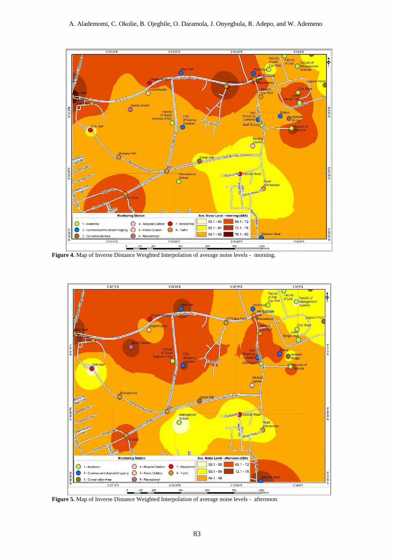
A. Alademomi, C. Okolie, B. Ojegbile, O. Daramola, J. Onyegbula, R. Adepo, and W. Ademeno
83
Figure 5. Map of Inverse Distance Weighted Interpolation of average noise levels - afternoon.
Figure 4. Map of Inverse Distance Weighted Interpolation of average noise levels - morning.

Spatial and Statistical Analysis of Environmental Noise Levels in the Main Campus of the University of Lagos
84
Figure 7. Classification of measurement stations based on standards for noise limits.
Figure 6. Average noise levels against WHO and NESREA noise standards.
40
45
50
55
60
65
70
75
80
0 1 2 3 4 5 6 7 8 9 10 11 12 13 14 15 16 17 18 19 20 21 22 23 24 25 26 27 28 29 30 31 32 33 34
Noi
se L
evel
(dB
A)
Station ID
Average LAeq WHO NESREA

A. Alademomi, C. Okolie, B. Ojegbile, O. Daramola, J. Onyegbula, R. Adepo, and W. Ademeno
85
4. CONCLUSION Environmental noise assessment and analysis from this study has revealed that noise levels obtained from the various environments, in general, failed to conform to acceptable environmental noise standards by WHO and NESREA. Inferring from the analysis of morning and afternoon observations, it was detected that noise level was averagely higher in the morning than the afternoon period and this is usually concentrated at the university gate, the university main road, the various classroom areas, and the student residential areas. This could be as a result of workers and students rushing to resume work and class early in the morning. Comparing the noise level for morning and afternoon at the two gates of the university, it was observed that average noise levels between 68.1 – 72 dBA were recorded at the second gate. However, the buffer area covered by this noise level range was higher in the morning compared to the afternoon observation. Conversely, the main gate, Sports Centre, New Hall, and Faculty of Social Science Shopping Complex recorded higher noise levels in the afternoon observation divergent to the trend of result from the general outcome of the research. This suggests that the areas need immediate attention to mitigate potential health problems that could affect the performance of the students and workers residing in the campus. Furthermore, Pearson’s correlation coefficient (r) of 0.63 was derived between the observed average noise levels and the WHO noise standard. Between the average noise levels and NESREA noise standards, the coefficient of correlation was 0.58. These values show a slightly high positive correlation between the measured noise levels and standards. Significant variation exists between the measured noise levels, and the WHO and NESREA noise standards. Hence, it could be inferred from this study that the health of the various groups of people living in the environment is in danger. However, a consistent noise modelling investigation should be continued in the region to frequently assess the noise pollution level. A continuous data gathering in this regard can help to establish a very good mathematical model to predict the noise level status of the study area. Specific regions of interest, the student inhabited areas (residential and academic buildings), showed much higher noise levels than acceptable noise standards. The University of Lagos environment is exposed to significantly higher levels of noise than it is deemed appropriate for healthy living. Hence, adequate measures must be taken to curb this menace of noise pollution currently being experienced. Immediate and definite measures are required. Knowing the implications of noise pollution to the health of a society, proper legislation to regulate human activities concerning noise generation is highly recommended to the local, state, and national legislators. Noise is damaging but can be controlled drastically to create a good environment.
This study aimed to assess the variations in environmental noise levels within the University of Lagos in line with international standards. The interpretation from the predicted noise level maps was limited by the number of observations and measurement stations. Another limitation was the length of observation which could have been longer but for logistical and budget constraints. Notwithstanding, the findings serve as a knowledge resource to inform a better understanding of noise level variations within a university campus. The awareness of the members of the university community to sources and effects of noise and their perceptions of its impacts is considered in another study. CONFLICT OF INTEREST The authors declare that there is no conflict of interest regarding the publication of this manuscript.
FUNDING This study did not receive any funding from the public, private or not-for-profit sectors.
ACKNOWLEDGEMENT The authors are thankful to Professor Alabi Soneye of the Department of Geography, the University of Lagos for the provision of the noise level meter used in this study. The authors are also grateful to the editors and reviewers of this paper for their critical feedback that helped in shaping and improving the quality of the output. REFERENCES Aguilera I, Foraster M, Basagaña X, Corradi E,
Deltell A, Morelli X, Phuleria HC, Ragettli MS, Rivera M, Thomasson A, Slama R, Künzli N (2015), Application of land use regression modelling to assess the spatial distribution of road traffic noise in three European cities. Journal of Exposure Science & Environmental Epidemiology, 25(1):97–105. Ncbi.nlm.nih.gov/pubmed/252277 31
Akeh GI, Mshelia AD (2016), The Role of Geographic Information System in Urban Land Administration in Nigeria. MOJ Eoc Environ Sci 1(1): 00004. DOI: 10.15406/mojes.2016.01. 00004.
Alam P, Ahmad K, Afsar S, Akhtar N, (2020), 3D noise mapping for preselected locations of urban area with and without noise barriers: A case study of Delhi, India. Noise Mapping, 7:74–83 https://doi.org/10.1515/noise-2020-0006
Alam W (2011), GIS based assessment of noise pollution in Guwahati city of Assam, India. Int. J. Environ. Sci., 2(2): 743 – 751. www. semanticscholar.org/paper/GIS-based-Assess-men t-of-Noise-Pollution-in-Guwahati-Alam/373fc-62 a055d2c210660b7d2e0c5f81bac7dd1c7

Spatial and Statistical Analysis of Environmental Noise Levels in the Main Campus of the University of Lagos
86
Alimohammadi I, Fakhradin AK, Jamileh A, Shahram V, Kazem R, Mohammad HC, Mohammad A (2019), Association between noise annoyance and hearing loss caused by chronic exposure to noise among the workers of an automotive industry. Journal of Trends in Medicine, 19:2–5; 2019. DOI: 10.15761/TiM.1000203
Babisch W (2011), Cardiovascular effects of noise. Noise & Health. 13(52): 201-204.
Benocci R, Smiraglia M, Zambon G, Roman H (2016), Predicting Hourly Traffic Noise from Traffic Flow Rate Model: Underlying Concepts for the DYNAMAP Project. Noise Mapping; 3:130–139. DOI 10.1515/noise-2016-0010
Bublić I, Tudor I, Skelin D (2010), Small scale noise mapping of industrial plants. 1st EAA-EuroRegio 2010. Congress on Sound and Vibration, 15-18 September 2010, Ljubljana, Slovenia.
Can A, Van Renterghem T, Rademaker M, Dauwe S, Thomas P, De Baets B, Bot-teldooren D (2011), Sampling approaches to predict urban street noise levels using fixed and temporary microphones. J. Environ. Monit., 13(10): 2710–2719. https://pubs. rsc.org/en/content/articlelanding/2011/em/c1em10292c
Carrier M. Apparicio P, Séguin A. (2016), Road traffic noise in Montreal and environmental equity: what is the situation for the most vulnerable population groups? J. Transp. Geogr., 51: 1-8, ISSN 0966-6923. https://www. sciencedirect.com/science/article/abs/pii/S0966692315002021
Dass HK (1988), Advanced engineering mathematics (First Edition ed.). https://books. Google .com.ng/books?id=IkZLAgAAQBAJ&printsec=copyright&redir_esc=y#v=onepage&q&f=false .
Devore JL (2012), Probability and statistics for engineering and the sciences (Eighth ed.): Richard Stratton. https://fac.ksu.edu.sa/sites/default/files/probability_and_statistics_for_engineering_and_the_sciences.pdf
Diaco SB (2014), Effects of Noise Pollution in the Learning Environment on Cognitive Perform-ances. Liceo Journal of Higher Education Research, 10(1), p. 83+. Gale Academic OneFile, Accessed 21 Aug. 2020.
Eason S (2013), Strategic noise mapping with GIS for the Universitat Jaume I Smart Campus: Best Methodology Practices. M.Sc. Thesis. Universitat Jaume I, Castellon, Spain. https://run.unl.pt /bitstream/10362/9194/1/TGEO0102.pdf
Extech (2019), 407730: Digital Sound Level Meter. http://www.extech.com/product/407730
Farcaş F, Sivertunb A (2009), Road Traffic Noise: GIS Tools for Noise Mapping and a Case Study for Skåne Region. The International Archives of the Photogrammetry, Remote Sensing and Spatial Information Sciences, Vol. 34, Part XXX. https://www.isprs.org/proceedings/xxxviii/2-
W11/Farcas_Sivertun.pdf Gholami A, Nasiri P, Monazzam M, Gharagozlou A,
Monavvari SM, Afrous A (2012), Evaluation of traffic noise pollution in a central area of Tehran through noise mapping in GIS. Adv. Environ. Biol., 6(8): 2365-2373. http://www. Aensiweb .com/old/ aeb/2012/2365-2371.pdf
Gloaguen JR, Can A, Lagrange M, Petiot JF (2019), Road traffic sound level estimation from realistic urban sound mixtures by Non-negative matrix factorization. Appl. Acoust., 143: 229-238. https://www.sciencedirect.com/science/article/abs/pii/S0003682X18303475
Goshu BS, Mamo H, Zerihun S (2017), Urban noise: a case study in Dire-Dawa city, Ethiopia. Eur. J. Biophys., 5: 17-26. https://www.semanticscholar. org/paper/Urban-Noise% 3A-A-Case-Study-in Dire- Dawa-City %2C-Goshu-Mamo/37d822e3 b5f53e28e-22d5f78fd82f8acac0a37de
Halperin D (2014), Environmental noise and sleep disturbances: a threat to health? Sleep. Sci., 7(4): 209–212. https://www.sciencedirect.com/science /article/pii/S1984006314000601
Hammersen F, Niemann H, Hoebel J (2016), Environmental Noise Annoyance and Mental Health in Adults: Findings from the Cross-Sectional German Health Update (GEDA) Study 2012. International Journal of Environmental Research and Public Health, 13, 954; DOI:10.3390/ijerph13100954
Hansen CH (2001), Fundamentals of acoustics. Occupational Exposure to Noise: Evaluation, Prevention and Control. World Health Organization, 23-52.
Hatamzadi J, Talaiekhozani A, Ziaei G (2018), Evaluation of noise pollution in Ilam City in 2018. J. Air Pollut. Health., 3: 73-80. https://www.researchgate.net/publication/326684123_Evaluation_of_Noise_Pollution_in_Ilam_City_in_2018
Isaaks EH, Srivastava RM (1989), Applied geostatistics. Oxford University Press, New York. https://www.questia.com/library/62419760/applied-geostatistics
Lavandier C, Aumond P, Gomez S, Dominguès C (2016), Urban soundscape maps modelled with geo-referenced data. Noise Mapping, 3:278–294. DOI: 10.1515/noise-2016-0020
Laze K (2017). Findings from measurements of noise levels in indoor and outdoor environments in an expanding urban area: a case of Tirana. Noise Mapping 4:45–56. DOI 10.1515/noise-2017-0003.
Leao S, Ong K, Krezel A (2014), 2loud?: Community mapping of exposure to traffic noise with mobile phones. Environ. Monit. Assess., 186(10): 6193-206. https://www.ncbi.nlm.nih.gov/pubmed/24920095
Lee EY, Jerrett M, Ross Z, Coogan PF, Seto EYW (2014), Assessment of traffic-related noise in three cities in the United States. Environ. Res., 132:182-

A. Alademomi, C. Okolie, B. Ojegbile, O. Daramola, J. Onyegbula, R. Adepo, and W. Ademeno
87
189. https://www.ncbi.nlm.nih.gov/pubmed/24792415
Li J, Heap AD (2008), A review of spatial interpolation methods for environmental scientists. Geoscience Australia, Record 2008/23. https://d28rz98at9flks.cloudfront.net/68229/Rec2008_023.pdf
Luqman YA, Rowland AG, Zhang Y, Zainab UO (2013), Work environment noise levels and risk locations in two selected commercial areas in Ibadan, Nigeria. Global J. Med. Res., 13(6). https://globaljournals.org/item/2579-work-environment-noise-levels-and-risk-locations-in-two-selected-commercial-areas-in-ibadan-nigeria
Maisonneuve N, Stevens M, Ochab B. (2010), Participatory noise pollution monitoring using mobile phones. Inf. Polity., 15(1,2):51–71. https://dl.acm.org/doi/10.5555/1858974.1858981
Mansouri N, Pourmahabadian M, Ghasemkhani M (2006), Road traffic noise in downtown area of Tehran, Iran. J. Environ. Health. Sci. Eng, 3(4): 267-272
Mehta R, Zhu R, Cheema A (2012), Is noise always bad? Exploring the effects of ambient noise on creative cognition. Journal of Consumer Research, 39(4): 784-799.
Taufner MD, Gama AP, Slama JG, Torres CB (2020), Noise Metrics Analysis in schools near airports: A Brazilian case study. Noise Mapping, 7: 21 – 34. http://doi.org/10.1515/noise - 2020 - 0003.
Monazzam MR, Abbaspour EKM, Nassiri P, Taghavi L (2014), Spatial traffic noise pollution assessment – a case study. Int. J. Occup. Med. Environ. Health., 28(3):625-634. https://www.ncbi .nlm.nih.gov/pubmed/26190737
Munzel T, Schmidt F, Sebastine S, Herzog J. Andrea D (2018), Environmental Noise and Cardiosvacular System. Journal of American College of Cardiology, 71: 688 – 697.
Nassiri P, Elham K, Mohammad RM, Majid A, Lobat T (2016), Analytical comparison of traffic noise indices — a case study in District 14 of Tehran City. J. Low Freq. Noise. Vibr. Act. Control., 35(3): 221–229. https://journals.sagepub .com/doi/full/10.1177/0263092316660917
NESREA (2009), National Environmental (Noise Standards and Control) Regulation, National Environmental Standards and Regulations Enforcement Agency (NESREA) 2009. http://www.nesrea.org/lawsandregulations
Niemann H, Bonnefoy X, Braubach M, Hecht K, Maschke C, Rodrigues C, Röbbel N. (2006). Noise-induced annoyance and morbidity results from the pan-European LARES study. Noise Health. 2006;8(31):63-79. DOI:10.4103/1463-1741.33537.
Nwilo PC (1998), Data Acquisition by Ground Survey Methods. In C.U. Ezeigbo (Ed.) Principles and Applications of Geographic Information Systems. Series in Surveying and Geoinformatics.
ISBN 978-027-764-1. Nwobi-Okoye CC, Uyaelumuo AE, Duru CA,
Okoronkwo GOO (2015), Analysis and modelling of road traffic noise in Onitsha metropolis, Nigeria. Int. J. Adv. Multidiscip. Res., 1(1): 1-20. http://rex.commpan.com/index.php/ijamrr/article/view/35
Obaidat MT (2008), Spatial mapping of traffic noise levels in urban areas. J. Transp. Res. Forum., 47(2): 89-102. https://pdfs.semanticscholar.org/69ca/2b0e8318a0097090948cfef833b66e3f19d6.pdf
Obiefuna JN, Bisong FE, Ettah EB (2013), A GIS analysis of noise islands in Calabar metropolis, Nigeria. J. Environ. Sci., (3), 12. https://pdfs.semanticscholar.org/3a11/7c932307724a169e9cd97b2679431420c1ff.pdf
Olayinka OS, Abdullahi SA (2010). Comparative analysis of noise descriptors in some selected areas in Ilorin Metropolis, Nigeria. Noise Control Engineering Journal, 58(6): 646-657.
Ouis D (2002), Annoyance caused by exposure to road traffic noise: An update. Noise Health [serial online] Available from: http://www. noiseandhealth.org/text.asp?2002/4/15/69/31785
Oyedepo SO (2013), Effective Noise Control Measures and Sustainable Development in Nigeria. World Journal of Environmental Engineering, 1(1): 5-15 Available online at http://pubs.sciepub.com/wjee/1/1/2 DOI:10.12691/wjee-1-1-2
Paulet MV, Salceanu A, Neacsu OM (2016), Ultrasonic radar. In 2016 International Conference and Exposition on Electrical and Power Engineering (EPE) (pp. 551-554). IEEE.
Pueh HL, Kian ML, Garg S (2019), A case study of recording soundwalk of Fushimi Inari shrine in Kyoto, Japan using smartphone. Noise Mapping, 6:94–102 https://doi.org/10.1515/noise-2019-0008
Ragettli MS, Goudreau S, Plante C, Fournier M, Hatzopoulou M, Perron S, Smargiassi A (2016), Statistical modeling of the spatial variability of environmental noise levels in Montreal, Canada, using noise measurements and land use characteristics. J. Expo. Sci. Environ. Epidemiol., 26(6):597-605. https://www.ncbi.nlm.nih.gov/pubmed/26732373
Riboldi CED, Lorenzo T, Mariani L, Rolando A, Salucci F. (2020), Predicting the effect of electric and hybrid-electric aviation on acoustic pollution. Noise Mapping, 7:35–56. DOI: 10.1515/noise-2020-0004
Ruge L Altakrouri B, Schrader A (2013), Sound of the city - continuous noise monitoring for a healthy city. In Proceedings of the 5th International Workshop on Smart Environments and Ambient Intelligen., 670–675. http://www.csee. usf.edu/~ mlabrador/Share/workshops/papers/p670-ruge.pdf
Science for Environment Policy (2017), Future Brief: Noise abatement approaches. April 2017 Issue 17.

Spatial and Statistical Analysis of Environmental Noise Levels in the Main Campus of the University of Lagos
88
https://ec.europa.eu/environment/integration/research/newsalert/pdf/noise_abatement_approaches_FB17_en.pdf
Sharma A (2017), The Generalized form of Principia’s Third Law of Motion. Indian J. Sci. Technol, 10(34): 1-18.
Shield BM, Dockrell JE (2003), The effects of Noise on Children at School: A review. Journal of Building Acoustics 10(2):97 – 106.
Sonaviya DR, Bhaven N T (2019), 2-D noise maps for tier-2 city urban Indian roads. Noise Mapping, 2019; 6:1-6. https://doi.org/10.1515/noise-2019-0001
Sotiropoulou A, Karagiannis I, Vougioukas E, Ballis A, Bouki A (2020), Measurements and prediction of road traffic noise along high-rise building façades in Athens. Noise Mapp. 2020; 7:1–13.
Star–Orion South Diamond Project (2010), Environmental Impact Statement, Appendix 5.2.5-A: Fundamentals of acoustics, SX03733 – Section 5.0, version 1.0, 7p. https://www.ceaa-acee.gc.ca/050/documents_staticpost/46277/89411/05-Appendix_5-2-5-A-Fundamentals_of_Acoustics.pdf
Sulaiman FS, Darus N, Mashros N, Haron Z, Yahya K (2018), Traffic Noise Assessment at Residential Areas in Skudai, Johor. E3S Web of Conferences, 34, 02024. doi:10.1051/e3sconf/20183402024
Taghizadeh-Mehrjardi R, Zare M, Zare S (2013), Mapping of noise pollution by different interpolation methods in recovery section of Ghandi telecommunication Cables Company. JOHE, Winter-spring 2013: 2 (1-2). DOI: 10.18869/acadpub.johe.2.1.2.1.
Verma D, Jana A, Ramamritham K (2019), Classification and mapping of sound sources in local urban streets through AudioSet data and Bayesian optimized Neural Networks. Noise Mapping.6:52 -71. https://doi.org/10.1515/noise-2019-0005
Walker J, Resnick R, Halliday D (2014), Fundamentals of Physics (10th ed.). http://www.primeuniversity.edu.bd/160517/vc/eBook/download/fundamentals-of-physics-textbook.pdf
WHO (2018), Environmantal Noise Guidelines for the Europian Region, World Health Organistaion, 2018. (Date accessed: 13th August, 2020). https://www.euro.who.int/__data/assets/pdf_file/0008/383921/noise-guidelines-eng.pdf?ua=1
WHO (2019), Guideline values (Date accessed: 18th December, 2019). https://www.who.int/docstore/ peh/noise/Comnoise-4.pdf
Zannin PHT (2013), Noise mapping of an educational environment. Can. Acoust., 41(1): 27-34.
Zare S, Hasheminejad N, Shirvan HE, Hasanvand D, Hemmatjo R, Ahmadi S (2018), Assessing individual and environmental sound pressure level and sound mapping in Iranian safety shoes factory. Romanian J. Acoust. Vib., 15(1). http://rjav.sra.ro/index.php/rjav/article/view/46/33
Zuo F, Li Y, Johnson S, Johnson J, Varughese S, Copes R, Liu F, Wu HJ, Hou R, Chen H (2014), Temporal and spatial variability of traffic-related noise in the city of Toronto, Canada. Sci. Total. Environ., 15;472:1100-1107. https://www.ncbi. nlm.nih.gov/pubmed/24361745
The Journal of Engineering Research (TJER), Vol. 17, No. 2, (2020) 89-99
*Corresponding author’s e-mail: [email protected]
DOI:10.24200/tjer.vol17iss2pp89-99
MODELING, INVESTIGATING, AND QUANTIFICATION OF THE HOT WEATHER EFFECTS ON CONSTRUCTION
PROJECTS IN OMAN
Hajar Al Balushi 1, Mubarak AL-Alawi 2, *, and Mohammed Al Shahri2 1 Civil Engineer, Petrofac E&C, Muscat, Oman
2 Dept. of Civil and Architectural Engineering, Sultan Qaboos University, Muscat, Oman
ABSTRACT: The construction industry is recognized as one of the industries most exposed to climatic conditions. Construction projects are mainly executed in an outdoor environment and the activities are considered weather-sensitive. Severe weather conditions can directly affect the productivity and efficient operation of construction projects. In addition, the weather is known to be one of the main factors that decrease labour productivity in construction projects causing project delays, cost overruns, and contractual claims between contractors and clients. Oman has a hot climate with very high temperatures in summer, warm winters, and low annual rainfall. During extremely hot weather, labour productivity significantly decreases, as construction work may stop partially or completely, therefore, this paper investigates and quantifies the hot and humid weather effects in construction projects in Oman. A construction productivity model was developed using the work/rest schedule proposed by the National Institute for Occupational Safety and Health (NIOSH), USA. The daily weather temperature and relative humidity of Muscat were inputs into the model and the expected productivity in terms of working hours were the output of the model. The model was applied to case studies, which involved three completed construction projects under different testing scenarios in Muscat. Results indicate that implementing the influence of hot and humid weather can lead to an extension of 3–38% longer project duration compared to the planned duration.
Keywords: Construction; Heat stress; Productivity; Project duration; Modeling.
نمذجة وبحث تأثیر الطقس الحار على مشاریع البناء في عمان
ومحمد الشحري ، *مبارك العلوي، ھاجر البلوشي
بیئة یتم تنفیذ مشاریع البناء بشكل أساسي في و تعتبر صناعة البناء من أكثر الصناعات المعرضة للظروف المناخیة: الملخصخارجیة وتعتبر أنشطتھا حساسة للطقس. یمكن أن تؤثر الظروف الجویة القاسیة بشكل مباشر على إنتاجیة وكفاءة عملیات
یة التي تقلل من بالإضافة إلى ذلك ، من المعروف أن تأثیرات الطقس على صناعة البناء ھي أحد العوامل الرئیس ،مشاریع البناء، مما یتسبب في تأخیر المشروع ، وتجاوز التكالیف ، والمطالبات التعاقدیة بین المقاولین وأصحاب المشروع. إنتاجیة العمالة
أثناء الظواھر الجویة شدیدة الحرارة، وشتاءدافئ درجات حرارة عالیة جدا في الصیف وب ویمتاز مناخ عمان جاف وحاریعتبر ھذه الورقة البحثیة إلى نمذجة ف . تھدتوقف أعمال البناء جزئیا أو كلیاؤدي إلى مما یقد تنخفض إنتاجیة عمال البناء بشكل كبیر
نسبة تأثیرات الطقس الحار والرطب في مشاریع البناء في عمان. تم تطویر نموذج إنتاجیة البناء باستخدام جدول قیاسبحث وودرجة حرارة الطقس الیومیة تم استخدام). NIOSHالمعھد الوطني للسلامة والصحة المھنیة ( لمقترح منالراحة اإلى العمل
مدخلات في النموذج وكانت الإنتاجیة المتوقعة من حیث ساعات العمل ھي ناتج النموذج. تم كمسقط لمحافظةوالرطوبة النسبیة ر الطقس الحار النتائج إلى أن تأثی أشارتسیناریوھات اختبار مختلفة. عدة في ظل و في ثلاث مشاریع انشائیةتطبیق النموذج
٪ مقارنة بالمدة المخطط لھا.38إلى 3والرطب یمكن أن یؤدي إلى إطالة مدة المشروع بنسبة
.النمذجة ؛مدة المشروع ؛الإنتاجیة ؛التشیید؛ الإجھاد الحراري :الكلمات المفتاحیة

Modeling, Investigating, and Quantification of the Hot Weather Effects on Construction Projects in Oman
90
1. INTRODUCTION
Construction projects are executed in an outdoor environment, most of its activities being conducted by workers outdoors (Al Shebani and Wedawattab, 2014) and therefore, are affected by various weather conditions (El-Rayes and Moselhi, 2001). Weather events such as extreme cold, heat, wind, snowfall or precipitation are recognized among the factors causing noticeable project delays, cost overruns, and contractual claims. It can significantly affect a project’s schedule and produce significant deviations from the baseline schedule (Shahin, AbouRizk, and Mohamed, 2011; Ballesteros-Péreza, et al., 2017).
The construction industry needs to take note of different weather conditions and improve their working environment to make it safer. Weather simulation can assist in optimizing the project’s schedule to make it more robust in terms of weather impacts. Weather simulation models can be seen as extremely complicated random number generators that outputs resemble weather circumstances at a certain place (Kerkhove and Vanhoucke, 2017). The simulation models follow a pattern to construct the necessary models and quantify the impact of adverse weather conditions on actual operation projects: 1) Study of construction processes, 2) Understanding the effect of weather on those processes, 3) Identify the weather variables that influence the construction processes, 4) Search for weather information sources, 5) Choosing a modelling method, 6) Develop an appropriate tool that will generate weather variables, 7) apply the model to real projects to validate the developed model (Moselhi, Gong, and El-Rayes, 1997). Although the processes of constructing a model to allow integrating weather effect in construction projects planning and operations seem to be well addressed, however, it is a challenging process in terms of finding the correct data, and generalize the model to all construction projects. For example, productivity data for different construction trades must be available to model the construction operation and not all construction companies keep track of such data. The National Institute for Occupational Safety and Health (NIOSH) issues regulations and work guidelines regarding occupational exposure to high temperatures and hot environment. Such regulations can be used to construct a model to help predict weather variables that affect the performance of the construction operation and will allow predicting its negative impact on the duration of the construction project. Thus, this research will use the threshold limits values published by NIOSH in hot weather region like experienced in Oman.
The climate of Oman can be described as dry and hot with low annual rainfall, very high temperatures in summer and warm winters. During extremely hot weather conditions, labour efficiency may
tremendously decrease, because construction work may stop partially or entirely. Moreover, workers have reduced working hours due to the Ministry of Manpower has issued a directive to all companies, especially construction firms in the country, to stop all outdoors activities between 12.30 pm and 3.30 pm, from June to August (Ministry of Manpower, 2008), when the weather is extremely hot and humid. The effect of such low productivity and shorter working hours during the hot summer months in Oman may cause construction delays and therefore, additional costs of the project. The consequence is a financial loss that must be borne by either the contractor, the client or both (Ballesteros-Péreza, et al., 2017). Therefore, this research aims to model, investigate, and quantify the effect of hot and humid weather on construction projects duration in Oman. 2. BACKGROUND Extreme weather conditions can cause productivity to fall and delays in the project, especially in the construction industry, because most of its activities being managed by labours outdoors (Al Shebani and Wedawattab, 2014). Hot weather affects construction worker physiologically as well as psychologically. Physiologically, individuals may suffer heat stress or stroke in the hot weather. All of this may affect a worker psychologically; to the point where he or she wishes not to be exposed to the unpleasant working conditions and become demoralized and less productive (Ibbs and Sun, 2017; Koehn and Brown, 1985). Based on the findings of Yildirim et al. (2009), Grimm and Wagner (2009), and Thomas and Yiakoumis (1987), there is an inverse relationship between the increase in temperature and labour productivity. Previous studies showed that at a temperature between 100° - 110° F the quality of the work declined, also working at this range of high temperatures resulted in serious health hazards and low productivity (Koehn and Brown, 1985). Palmer and Creagh (2013), Grimm and Wagner (1974), and Thomas and Yiakoumis (1987) noted that an increase in humidity could also be adversely affecting labour productivity. Ibbs and Sun (2017) concluded that humidity has a critical effect on productivity, but its impact is smaller compared to that of temperature. Studies also indicate that temperatures above 110° F and below -10° F with humidity above 50% are intolerable, and it is difficult to achieve construction operations (Kohen and Brown, 1985).
Though extreme weather condition in construction projects is recognized as one of the factors causing the productivity to fall, producing noticeable project delays, cost overruns, waste of resources and contractual claims (Apipattanavis, et al., 2010; Chan and Au, 2008; El-Rayes and Moselhi, 2001; Lee et al., 2017), it is also reported to be one of the main factors that influence financial performance and business

Hajar Al Balushi, Mubarak AL-Alawi, and Mohammed Al Shahri
91
continuity (Moselhi, Gong, and El-Rayes, 1997; Al Shebani and Wedawattab, 2014; Guo, Chen, and Chiu, 2017).
Weather can affect a construction process in various ways; it can slow down the works by lowering the performance of construction labours and materials and can cause a temporary work stoppage, which therefore affects the plan and schedule of the project (Al Shebani and Wedawattab, 2014). Thus, understanding inclement weather influence on any construction project can reduce claims and arguments caused by delays (Apipattanavis, et al., 2010; Chan and Au, 2008; Dytczak et al., 2013).
Previous studies investigated the impact of inclement weather on construction activities and productivity. Moselhi et al. (1997) quantified the influence of weather conditions on daily construction activity; they developed an automated decision support system called WEATHER to study the impact of adverse weather conditions on the labour productivity and work-stoppage of construction operations. The developed WEATHER model estimates construction productivity as well as the duration of construction activities and weather patterns in different modes to improve the accuracy of the planning and scheduling. A mathematical study of weather by Koehn and Brown (1985) employed some non-linear equations to examine the effect of weather changes on the productivity rate. Their investigation suggests a clear relationship between overall construction performance and weather-related factors such as temperature and humidity it shows that at a temperature between 100° and 110° F the quality of the work declined, also working at this range of high temperatures resulted in serious health hazards and low productivity. Koehn and Brown (1985) found that construction productivity decreases rapidly at elevated temperatures, and there is an adverse relationship between construction productivity and humidity. The quantification of weather impacts on productivity was reported by the National Electrical Contractors Association (NECA) (Hanna, 2004). The research engaged two travelling electricians installing electrical boxes and duplex outlets while operating in an environment chamber that monitored the temperature and humidity. The study found that productivity levels differ depending on humidity and temperature. Grimm and Wagner (1974) studied the productivity in masonry construction over a period of nine months during the construction of 283 test walls and published a diagram showing the impact of temperature and humidity on the productivity. The research found a decline in productivity as temperature and relative humidity deviated. They reported that relative humidity had a much greater effect on productivity rate. Ahuja and Nandakumar (1985) and Kavanagah (1985) measured the impact of weather as a percentage in their construction modelling and analyzed how frequently weather resulted in decreased
activity. AbouRizk and Wales (1997) research used a general regression neural network to study the relationship between weather variables and earthwork productivity. This study investigated three weather variables: precipitation, daily maximum temperature, and daily minimum temperature. It demonstrated the impact of these weather variables has on a project schedule by calculating the duration for the same project according to different start dates. The South Dakota Department of Transportation (Kenner, et al., 1998) adopted a pragmatic solution by combining their construction records with weather records to calculate contract time and determine time extensions for adverse weather. Yildirim, Koyuncu, and Koyuncu (2009) findings showed a negative association between temperature increase and labour productivity level. Palmer and Creagh (2013) state that the rise in humidity due to climate change reduces labour productivity. Studies also indicate that temperatures above 110° F with humidity above 50% are intolerable and all useful work stops, therefore, it is difficult to achieve efficient construction operations (Arditi, 1985). Thomas et al. (1990) described the factor model for evaluating the productivity of labour-intensive construction activities. The validity of the factor model is demonstrated by considering the effect of temperature and relative humidity on productivity. Thomas et al. (1990) also noted that the increase in humidity could be adversely affecting labour productivity. Ibbs and Sun (2017) concluded that humidity has a critical effect on productivity, but its impact is smaller compared to that of temperature. Shahin et al. (2011) proposed a simulation model that quantify the effects of extreme weather events on construction projects and to assist in project planning and decision support. Miroslaw et al. (2013) presented a numerical procedure to identify the efficient construction project structure and a corresponding schedule. It addressed the impact of inclement weather conditions on technological operations. Marzoughi et al. (2018) developed a model using multivariate statistical techniques and an analytical network (ANP) method to assess the duration of project operations, taking into consideration the effect of weather. 3. HEAT STRESS This section covers a brief introduction about heat stress in hot environments and present recommendations for workers exposed to heat and hot environments derived from the occupational exposure to heat and hot environments published by National Institute for Occupational Safety and Health (NIOSH) (NIOSH, 2018).
Total heat stress is controlled by the three factors, the heat generated in the body, the heat gained from the environment, and the heat lost to the environment from the body. Environmental and/ or metabolic heat

Modeling, Investigating, and Quantification of the Hot Weather Effects on Construction Projects in Oman
92
stress results in physiological reactions (heat stress) to promote heat transfer from the body back to the surroundings to maintain core body temperature. Many of the heat exposure responses in the body are desirable and useful. However, at some level of heat stress, the compensatory mechanisms are no longer capable of keeping body temperature at the rate needed for normal body tasks. Consequently, there is an increase in the risk of heat-related illnesses, disorders, and other hazards.
Workers who are subjected to extreme heat or work in indoor or outdoor hot environments or even those involved in exhausting physical activity may be at risk for heat stress. Those at risk of heat stress include outdoor workers and workers in hot environments, for example, firefighters, bakery workers, farmers, construction labours, miners, boiler room workers, and factory workers. Outdoor labours are subjected to a great deal of exertional and environmental heat stress. The recommendations are intended to provide limits of heat stress so that heat-related illnesses and disorders are reduced.
NIOSH proposes that employers implement measures to protect the health of labours exposed to heat and hot environments. Employers need to monitor environmental heat and determine the metabolic heat produced by workers (e.g., light, moderate, or heavy work). Based on the increase in risk, additional modifications (e.g., worker health interventions, clothing, and personal protective equipment) may be required to shield workers from heat stress. In hot conditions, physiological monitoring and medical screening are suggested. Employers, supervisors and workers need to be trained to recognize symptoms of heat-related illness, adequate hydration, care and use of heat-protective garments and equipment, the impact of multiple heat-tolerance risk variables (e.g., drugs, alcohol, obesity, etc.), the significance of acclimatization, the significance of reporting symptoms and suitable first aid. Employers should have a plan to acclimatize a new employee because it has been shown that the lack of acclimatization is a significant factor associated with worker heat-related illness and death. NIOSH recommends that employers provide the means for adequate hydration and that their employees be encouraged to hydrate themselves with drinking water below 15 ° C (59 ° F) close to the work zone. Workers in heat less than 2 hours and involved in moderate work activities should drink 1 cup (8 oz.) of water every 15–20 minutes. Furthermore, employers should establish a work/rest schedule and provide a cool environment for employees to rest and recover (e.g., air-conditioned or shaded). These essentials are intended to protect the health of workers from heat stress or injuries in hot environments.
4. WORK-REST HOURS PREDICTION MODEL
This section describes the research methods that have been used for assessing the relationship between the high temperature (T) and relative humidity (RH) and the productivity of the labours. Two primary data were collected for this research. First, historical weather data for daily temperature and relative humidity in Muscat city were collected from the Public Authority for Civil Aviation (PACA) for the years from 2015 to 2018. The data received from PACA were not clean, with missing records and limited years; only from 2015 until 2018 while the data needed should be at least from 2008. Therefore, actual weather data from the National Oceanic and Atmospheric Administration (NOAA) was used.
The data from NOAA covered daily temperature in Muscat from 2001 until 2018. To cover the daily relative humidity for the years from 2001 to 2018; daily relative humidity received from PACA was repeated every two years, with an assumption that the relative humidity will not differ much within two years and it was observed that almost same relative humidity was repeating every two years.
The database was established using the daily temperature (mean, maximum and minimum) from NOAA and daily relative humidity (mean, maximum and minimum) from PACA. The temperature ranged from a low of 12.4 °C to a high of 47.5 °C, and the relative humidity was in the range of 5%-100%. It was observed that the temperature and relative humidity were extreme in the months from April to September while it is normal during the remaining months of the year. Therefore, weather data from April to September was considered in this research.
To maintain a healthy and safe working environment, the National Institute for Occupational Safety and Health (NIOSH) developed a work/rest schedule for workers. Table 1 shows the work and rests time per hour for a certain temperature and humidity to minimize the effect of heat on the labours. The workload category is expressed as worker’s metabolic heat production: light work = <180 kcal/hr; moderate work = 180–300 kcal/hr; heavy work = 300–415 kcal/hr; and very heavy work = >520 kcal/hr (NIOSH, 2018). Table 1 is used for the quantification of weather effects on labourers' productivity in Table 2, which illustrates the percentage of rest per hour due to high temperature.

Hajar Al Balushi, Mubarak AL-Alawi, and Mohammed Al Shahri
93
More tables that are comprehensive were developed for the considered months – April to September. Data were summarized for each month, and Most-likely case and pessimistic cases were defined for each workload category for the data analysis. The most likely case reflected the percentage of rest per hour for the mean adjusted temperature based on mean relative humidity while the pessimistic case is the percentage of rest per hour for the maximum adjusted temperature based on maximum relative humidity. These two cases were defined because they reflect the worst-case scenarios compared to other cases (e.g. minimum adjusted temperature based on minimum relative humidity).
The data was analyzed using EasyFit software to find out the best-fit probability distribution function that represents the probability of percentage of rest per hour the work may experience for each month. For each month; six probability distributions were found as follows:
• Light work: most likely and pessimistic • Moderate work: most likely and pessimistic • Heavy work: most likely and pessimistic
Randomly generating percentages for rest per hour
in for a month will generate a full month affected by the weather condition, which is not logical and not valid. Therefore, the probability of occurrence of negative weather effect was calculated from the weather data set. Table 3 below illustrates the probability of occurrence of the affected days for each month; that was found using the following equation:
The probability of occurrence of an event is defined according to Eqn. (1):
𝑃𝑃(𝐸𝐸) = 𝑛𝑛𝑛𝑛𝑛𝑛𝑛𝑛𝑛𝑛𝑛𝑛 𝑜𝑜𝑜𝑜 𝑜𝑜𝑓𝑓𝑓𝑓𝑜𝑜𝑛𝑛𝑓𝑓𝑛𝑛𝑓𝑓𝑛𝑛 𝑜𝑜𝑛𝑛𝑜𝑜𝑜𝑜𝑜𝑜𝑛𝑛𝑛𝑛𝑜𝑜
𝑛𝑛𝑛𝑛𝑛𝑛𝑛𝑛𝑛𝑛𝑛𝑛 𝑜𝑜𝑜𝑜 𝑝𝑝𝑜𝑜𝑜𝑜𝑜𝑜𝑝𝑝𝑛𝑛𝑓𝑓𝑛𝑛 𝑜𝑜𝑛𝑛𝑜𝑜𝑜𝑜𝑜𝑜𝑛𝑛𝑛𝑛𝑜𝑜 (1)
Where the number of favourable outcomes is the
percentage of rest per hour which is more than 0%, and the number of possible outcomes is the total number of days considered in the data. The probability of occurrence along with the probability of the percentage of expected rest to work were jointly used to generate the expected rest percentage for construction labours.
5. MODEL VALIDATION
The data needs to be statistically validated. A
statistical comparison of the generated output for each month was carried out to ensure that the similarity between the historical data and the generated data is statistically adequate. The rest percentage prediction model was used to generate data for the expected percentages of rest construction labour may experience in months from April to September.
Table 1. Work/rest schedule for workers wearing normal clothing (NIOSH, 2018).
Adjusted Temperature
(C) †
Light work
(minutes work/rest)
Moderate work
(minutes work/rest)
Heavy work
(minutes work/rest)
32.22 Normal Normal Normal 32.78 Normal Normal Normal 33.33 Normal Normal Normal 33.89 Normal Normal Normal 34.44 Normal Normal Normal
35 Normal Normal 45/15 35.56 Normal Normal 45/15 36.11 Normal Normal 40/20 36.67 Normal Normal 35/25 37.22 Normal Normal 35/25 37.78 Normal 45/15 30/30 38.33 Normal 40/20 30/30 38.89 Normal 35/25 25/35 39.44 Normal 30/30 20/40
40 Normal 30/30 20/40 40.56 Normal 25/35 15/45 41.11 45/15 20/40 Caution 41.67 40/20 15/45 Caution 42.22 35/25 Caution Caution 42.78 30/30 Caution Caution 43.33 15/45 Caution Caution 43.89 Caution Caution Caution 44.44 Caution Caution Caution
† Note: Adjust the temperature reading as follows before going to the temperature column in the table: Full sun (no clouds): Add 13°F, Partly cloudy/overcast: Add 7° F No shadows visible/work is in the shade or at night: no adjustment Per relative humidity: 10%: Subtract 8° F, 20%: Subtract 4° F, 30%: No adjustment, 40%: Add 3° F, 50%: Add 6° F, 60%: Add 9° F ‡High levels of heat stress; consider rescheduling activities. Table 2. Percentage of rest per hour for workers wearing
normal work clothes. Adjusted
Temperature (C)
% Rest Per Hour Light work
Moderate work
Heavy work
32.22 0 0 0 32.78 0 0 0 33.33 0 0 0 33.89 0 0 0 34.44 0 0 0
35 0 0 25 35.56 0 0 25 36.11 0 0 33.33 36.67 0 0 41.67 37.22 0 0 41.67 37.78 0 25 50 38.33 0 33.33 50 38.89 0 41.67 58.33 39.44 0 50 66.67
40 0 50 66.67 40.56 0 58.33 75 41.11 25 66.67 100 41.67 33.33 75 100 42.22 41.67 100 100 42.78 50 100 100 43.33 75 100 100 43.89 100 100 100 44.44 100 100 100
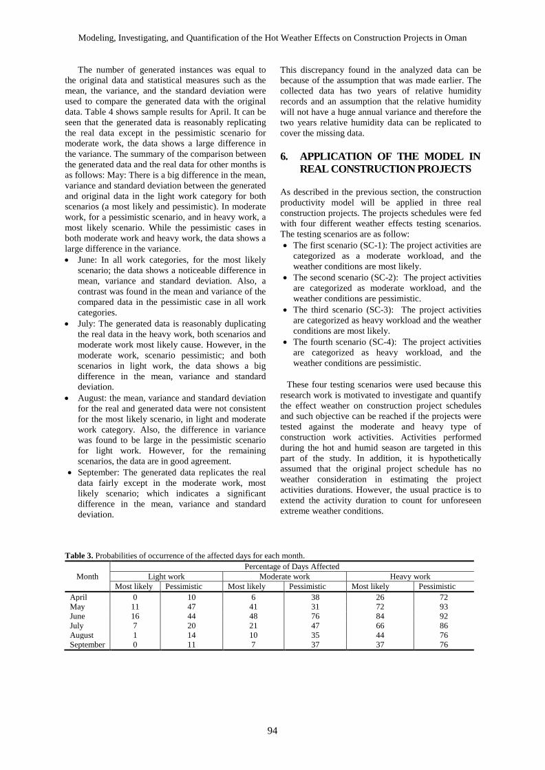
Modeling, Investigating, and Quantification of the Hot Weather Effects on Construction Projects in Oman
94
The number of generated instances was equal to the original data and statistical measures such as the mean, the variance, and the standard deviation were used to compare the generated data with the original data. Table 4 shows sample results for April. It can be seen that the generated data is reasonably replicating the real data except in the pessimistic scenario for moderate work, the data shows a large difference in the variance. The summary of the comparison between the generated data and the real data for other months is as follows: May: There is a big difference in the mean, variance and standard deviation between the generated and original data in the light work category for both scenarios (a most likely and pessimistic). In moderate work, for a pessimistic scenario, and in heavy work, a most likely scenario. While the pessimistic cases in both moderate work and heavy work, the data shows a large difference in the variance. • June: In all work categories, for the most likely
scenario; the data shows a noticeable difference in mean, variance and standard deviation. Also, a contrast was found in the mean and variance of the compared data in the pessimistic case in all work categories.
• July: The generated data is reasonably duplicating the real data in the heavy work, both scenarios and moderate work most likely cause. However, in the moderate work, scenario pessimistic; and both scenarios in light work, the data shows a big difference in the mean, variance and standard deviation.
• August: the mean, variance and standard deviation for the real and generated data were not consistent for the most likely scenario, in light and moderate work category. Also, the difference in variance was found to be large in the pessimistic scenario for light work. However, for the remaining scenarios, the data are in good agreement.
• September: The generated data replicates the real data fairly except in the moderate work, most likely scenario; which indicates a significant difference in the mean, variance and standard deviation.
This discrepancy found in the analyzed data can be because of the assumption that was made earlier. The collected data has two years of relative humidity records and an assumption that the relative humidity will not have a huge annual variance and therefore the two years relative humidity data can be replicated to cover the missing data. 6. APPLICATION OF THE MODEL IN
REAL CONSTRUCTION PROJECTS As described in the previous section, the construction productivity model will be applied in three real construction projects. The projects schedules were fed with four different weather effects testing scenarios. The testing scenarios are as follow: • The first scenario (SC-1): The project activities are
categorized as a moderate workload, and the weather conditions are most likely.
• The second scenario (SC-2): The project activities are categorized as moderate workload, and the weather conditions are pessimistic.
• The third scenario (SC-3): The project activities are categorized as heavy workload and the weather conditions are most likely.
• The fourth scenario (SC-4): The project activities are categorized as heavy workload, and the weather conditions are pessimistic.
These four testing scenarios were used because this research work is motivated to investigate and quantify the effect weather on construction project schedules and such objective can be reached if the projects were tested against the moderate and heavy type of construction work activities. Activities performed during the hot and humid season are targeted in this part of the study. In addition, it is hypothetically assumed that the original project schedule has no weather consideration in estimating the project activities durations. However, the usual practice is to extend the activity duration to count for unforeseen extreme weather conditions.
Table 3. Probabilities of occurrence of the affected days for each month.
Month Percentage of Days Affected
Light work Moderate work Heavy work Most likely Pessimistic Most likely Pessimistic Most likely Pessimistic
April 0 10 6 38 26 72 May 11 47 41 31 72 93 June 16 44 48 76 84 92 July 7 20 21 47 66 86 August 1 14 10 35 44 76 September 0 11 7 37 37 76

Hajar Al Balushi, Mubarak AL-Alawi, and Mohammed Al Shahri
95
Table 4. Comparing April generated data against the real data. Workload category Light work Moderate work Heavy work
Scenario Most-likely Pessimistic Most-likely Pessimistic Most-likely Pessimistic
Best Distribut
ion function
Constant=0 Gamma Frechet Beta Gamma General Extreme
Value
Type of data Real
data Generated
data Real data
Generated data
Real data
Generated data
Real data
Generated data
Real data
Generated data
Mean 4.42 4.42 1.92 1.53 19.96 12.18 8.96 8.26 37.00 24.68
Variance 213.33 225.34 67.60 52.95 859.53 363.09 265.70 267.42 997.6
2 936.88
Std. deviation 14.61 15.01 8.22 7.28 29.32 19.06 16.30 16.35 31.59 30.61
6.1 Project A
The construction of the project took 365 days. In this research, the construction part only was analyzed, which included; sub-structure works, super-structure works, and masonry works. The critical path of this part was identified, and its duration is 250 days.
Figure. 1 (a) shows the affected activities by the first testing scenario (SC1) applied to the construction schedule for project A. The increase in activity duration is shown in red font. For the remaining activities, the effect was negligible this is because of a lower percentage of rest per hour in a particular activity and because some of the activities are in October, November, December and January which are not considered in this research. The critical path duration for project A was increased by 41.5 days to reach a total of 291.5 days.
Figure. 1 (b) shows the construction activities affected by the second scenario. The affected activities are more than that of the first scenario. This increase in affected activities is due to the high percentage of rest per hour for the pessimistic scenario compared to the same moderate load work category.
It was observed that the critical path duration reaches a total of 307.5 days with an increase of 57.5 days.
The construction activities affected by the third testing scenario (SC3) for the project is shown in Fig. 1(c). It was observed that the critical path duration was increased by 60.5 days to reach a total of 310.5 days. The high duration of critical path compared to previous scenarios is because of the high percentage of rest per hour for heavy load category.
The construction activities affected by the fourth scenario is shown in Fig. 1(d). It was seen that the critical path duration is 344 days, with an increase of 94 days. This is the worst-case scenario in which the load category is heavy, and weather conditions are pessimistic. The percentage of rest per hours for this scenario is high. Thus the labour will take more rest in an hour during his work. As a result, the new duration for the affected activities is high compared to other scenarios.
In conclusion, for project A, it was found that the percentage increase in critical path duration for first, second, third and fourth scenarios are 17%, 23%, 24% and 38% respectively. The effect of hot weather was highest for the heavy load work and pessimistic weather conditions, and least for moderate workload category and most likely weather condition. 6.2 Project B
The project duration for project B is 423 days, started on 3rd April 2010 and completed on 31st May 2011, and the critical path duration of the construction part was 199 days.
The construction activities affected after applying the first scenario (SC1) is shown in Fig. 2(a). It was observed that the first four activities were affected by the hot weather, resulting in a shift in the start date of the remaining activities. Some of the activities were not affected by the weather conditions this is due to a lower percentage of rest per hour inactivity and because some of the activities are in October, November and December. The critical path duration was increased by eight days to reach a total of 207 days.
Figure 2(b) shows the construction activities affected by the second testing scenario (SC2); which is the moderate workload category and pessimistic weather condition. The affected activities more than that of the first scenario. This is a result of the high percentage of rest per hour for the pessimistic case compared to the same load work category, which is moderate. Consequently, the duration of the critical path was affected due to this increase in the duration of activities. It reached a total of 221 days with an escalation of 22 days.
For the third scenario (SC3), the output of the construction productivity model is shown in Fig. 2(c). It is shown that the hot weather affected the first seven activities, which increased in the duration of the critical path. The critical path duration for the construction part was increased by 18 days to reach a total of 217 days.

Modeling, Investigating, and Quantification of the Hot Weather Effects on Construction Projects in Oman
96
Figure. 1. Project A results after tested under four testing scenarios (SC1, SC2, SC3, and SC4); (a) Affected activities and their durations for SC1, (b) Affected activities and their durations for SC2, (c) Affected activities and their durations for SC3, (d) Affected activities and their durations for SC4.
Figure. 2. Project B results after tested under four testing scenarios (SC1, SC2, SC3, and SC4); (a) Affected activities and their durations for SC1, (b) Affected activities and their durations for SC2, (c) Affected activities and their durations for SC3, (d) Affected activities and their durations for SC4.

Hajar Al Balushi, Mubarak AL-Alawi, and Mohammed Al Shahri
97
affected by the fourth testing scenario (SC4). It is obvious from the graph that more activities are by the Figure. 2(d) shows the construction activities affected hot weather conditions. These observations are expected; since this scenario covering the heavy load work category and pessimistic weather conditions; in which the percentage of rest per hour is the highest. The labour will take more time resting per hour during his work, resulting in an extended duration to finish the work of the activity. It was seen that the critical path duration is 242 days, with an increase of 43 days from the duration of the original critical path.
In conclusion, the percentage increase in the critical path duration for the four scenarios was calculated. It was found that a 4% increase for the first scenario, 11% for the second scenario, 9% for the third scenario and 22% for the fourth scenario. The effect of hot weather was highest for the heavy load work and pessimistic weather conditions, and least for moderate workload category and most likely weather condition.
6.3 Project C
The construction duration of project C is 239 days; it was started on 24th June 2018 and accomplished on 28th February 2019. As followed in previous projects, the construction part was studied for this research
which includes; sub-structure works and superstructure work. The duration of the critical path for the construction part is 150 days.
The construction activities affected after applying the first scenario is shown in Fig. 3(a). The graph shows that the hot weather affected three activities.
For some of the activities the weather conditions had no impact, this is due to the low percentage of rest per hour for the moderate and most likely scenarios and because some of the activities are in October, November, December and January, which are not considered in this analysis. The critical path duration was calculated and found to be 154 days; it was increased by four days compared to the original critical path duration. Figure. 3 (b) shows the results for the second scenario; which is the moderate workload category and pessimistic weather condition. The hot weather conditions affected more activities compared to the first scenario. This is because of the high percentage of rest per hour for the pessimistic weather condition. Subsequently, the critical path duration was increased by five days. It reached a total of 155 days.
For the third scenario, the output of the construction productivity model is presented in Fig. 3(c). It shows that the critical path duration for the construction part was increased by eight days to reach a total of 158 days.
Figure. 3. Project C results after tested under four testing scenarios (SC1, SC2, SC3, and SC4); (a) Affected activities and
their durations for SC1, (b) Affected activities and their durations for SC2, (c) Affected activities and their durations for SC3, (d) Affected activities and their durations for SC4.

Modeling, Investigating, and Quantification of the Hot Weather Effects on Construction Projects in Oman
98
The output of the construction productivity model for the fourth scenario is shown in Fig.3(d). More activities were impacted by the hot weather conditions. The graph shows that the first eight activities increased in their working duration, resulting in an extension of the critical path duration. This is predicted because this scenario is the worst scenario; where the percentage of rest per hour is high. It was seen that the new critical path duration for the construction part is 167 days with a rise of 17 days from the duration of the original critical path.
In conclusion, the percentage increase in critical path duration was calculated for the four scenarios. For the first and second scenarios, the increase was found to be equal to 3%, 5% for the third scenario and an increase of 11% was calculated for the fourth scenario. It was observed that the effect of extreme weather conditions was highest for the heavy load work and pessimistic weather conditions, and least for moderate workload category and most likely weather condition
CONCLUSION
In this study, a construction productivity model was developed using the daily temperature and relative humidity of Muscat, Oman from the years 2001 to 2018. The daily temperature and relative humidity were used to calculate the percentage of rest per hour rule presented by NIOSH. The generated data were validated statistically against the original data. The rest per hour model was able to satisfactory replicate the real data with some discrepancies. This result may be driven from the fact that the collected data had a simplification due to lack of data and only two years relative humidity records were used in the study. This is a limitation to the model and a future extension of this model will incorporate a large range of relative humidity and temperature records.
The construction productivity model was used to investigate and quantify the weather effects on project duration. It was applied to three completed construction projects. For each project, four weather testing scenarios were applied to investigate the impact of hot weather under different workloads on the project duration. The critical path duration was calculated for each scenario in each project and compared with the original critical path durations. The results showed an increase in the critical path duration for all three projects in all scenarios. It was found that 17%, 23%, 24% and 38% increase in critical path duration for project A, for SC-1, SC-2, SC-3 and SC-4, respectively. For project B the percentages were 4%, 11%, 9% and 22% for each scenario respectively. In addition, 3%, 3%, 5% and 11% increase in critical path duration for project C were found for the four presented scenarios.
CONFLICT OF INTEREST Authors declare no conflicts of interest.
FUNDING This study did not receive any funding from the public, private or not-for-profit sectors. REFERENCES AbouRizk, S. M., & Wales, R. J. (1997). Combined
discrete-event/continuous simulation for project planning. Journal of Construction Engineering and Management, 123(1), 11-20.
Ahuja, H. N., & Nandakumar, V. (1985). Simulation Model to Forecast Project Completion Time. Journal of Construction Engineering and Management, 111(4), 325-342.
Al Shebani, M., & Wedawattab, G. (2014). Making the construction industry resilient to extreme weather: Lessons from construction in hot weather conditions. Procedia Economics and Finance, 635-642.
Apipattanavis, S., Sabol, K., Molenaar, K., Rajagopalan, B., Xi, Y., Blakard, B., & Patil, S. (2010). Integrated Framework for Quantifying and Predicting Weather-Related Highway Construction Delays. Journal of Construction Engineering and Management, 136(11), 1160-1168.
Arditi, D. (1985). Construction Productivity Improvement. Journal of Construction Engineering and Management, 111(1), 1-14.
Ballesteros-Péreza, P., Rojas-Céspedesb, Y. A., Hughesa, W., Kabiria, S., Pellicer, E., Mora-Melià, D., & Campo-Hitschfeld, M. L. (2017). Weather-wise: A weather-aware planning tool for improving construction productivity and dealing with claims. Automation in Construction, 81-95.
Chan, E. H., & Au, M. C. (2008). Relationship between organizational sizes and constractor's risk pricing behaviors for weather risk under different project values and durations. Journal of Construction Engineering and Management, 134(9), 673-680.
Dytczak, M., Ginda, G., Szklennik, N., & Wojtkiewicz, T. (2013). Weather influence-aware robust construction project structure. 11th International Conference on Modern Building Materials, Structures and Techniques. Vilnius.
El-Rayes, K., & Moselhi, O. (2001). Impact of rainfall on the production of highway construction. Journal of Construction Engineering and Management, 125-131.
Grimm, C., & Wagner, N. (1974). Weather effects on mason productivity. Journal of the Construction Division, 19-35.
Guo, S.-J., Chen, J.H., & Chiu, C.H. (2017). Fuzzy duration forecast model for wind turbine construction project subject to the impact of wind

Hajar Al Balushi, Mubarak AL-Alawi, and Mohammed Al Shahri
99
uncertainity. Automation in Construction, 81, 401-410.
Hanna, A. S. (2004). The effect of temperature on productivity. NECA, National Electrical Contractors Association.
Ibbs, W., & Sun, X. (2017). Weather's Effect on Construction Labor Productivity. Journal of legal affairs and dispute resolution in engineering and construction, 04517002-2 - 04517002-7.
Kavanagh, D. P. (1985). Siren: A Repetitive Construction Simulation Model. Journal of Construction Engineering and Management, 111(3), 308-323.
Kenner, S., Johnson, R. L., Miller, J. R., Salmen, J. A., & Matt, S. A. (1998). Development of working day weather charts for transportation construction in south Dakota. South Dakota Department of Transportation, Office of Research.
Kerkhove, L. P., & Vanhoucke, M. (2017). Optimised scheduling for weather sensitive offshore construction projects. Omega, 66(A), 58-78.
Koehn, E., M. , A., & Brown, G. (1985). Climatic effects on construction. Journal of Construction Engineering and Management, 129-137.
Lee, J., Park, Y.-J., Choi, C.-H., & Han, C.-H. (2017). BIM-assisted labor productivity measurement method for structural formwork. Automation in Construction, 84, 121-132.
Marzoughi, F., Arthanari, T., & Askarany, D. (2018). A decision support framework for estimating project duration under the impact of weather. Automation in Construction, 87, 287-296.
Ministry of Manpower. (2008). Regulation of
occupational safety and health measures in establishments subject to labor law. Muscat, Oman: Ministry of Manpower.
Moselhi, O., Gong, D., & El-Rayes, K. (1997). Estimating weather impact on the duration of construction activities. Canadian Journal of Civil Engineering, 24, 359-366.
NIOSH. (2018, 5 25). The National Institute for Occupational Safety and Health (NIOSH). (Centers for Disease Control and Prevention) Retrieved 8 1, 2019, from https://www.cdc.gov/niosh/index.htm
Palmer, C., & Creagh, S. (2013, February 25). Climate change linked to declines in labour productivity. Retrieved from The conversation: http://theconversation.com/climate-change-linked-to-declines-in-labour-productivity-12407
Shahin, A, S. M. AbouRizk, & Y. Mohamed. (2011). Modelling weather-sensitive construction activity using simulation. Journal of Construction Engineering and Management, 238-246.
Thomas, H., & Yiakoumis, I. (1987). Factor model of construction productivity. Journal of Construction Engineering and Management, 623-639.
Thomas, R. H., Maloney, W. F., Horner, R. W., Smith, G. R., Honda, V. K., & Sanders, S. R. (1990). Modeling construction labor productivity. Journal of Construction Engineering and Management, 116(4), 705-726.
Yildirim, K., Koyuncu, C., & Koyuncu, J. (2009). Does temperature affect labor productivity: Cross-country evidence. Applied Economics and International Development, 9(1), 29-38.

The Journal of Engineering Research (TJER), Vol. 17, No. 2, (2020) 100-111
*Corresponding author’s e-mail: [email protected]
DOI:10.24200/tjer.vol17iss2pp100-111
ANALYSIS OF LOSS REDUCTION TECHNIQUES FOR LOW VOLTAGE DISTRIBUTION NETWORK
A. Al-Badi1, R. Ahshan1, *, S. Al-Hinai1, A. Moosa2, R. Shah2, M. Al Hasani2, and S. Khan2 1 Department of Electrical & Computer Engineering, College of Engineering,
Sultan Qaboos University, Muscat, Oman 2 Muscat Electricity Distribution Company, Muscat, Oman
ABSTRACT: Energy losses in a typical distribution system can be in a range of 6 to 10%, and it depends on the system characteristics, installed equipment, and operating strategies of the distribution network. Losses reduction during peak periods needs special attention since the losses in the system and the cost of the losses are the highest during this peak. Distribution System Owner (DSO) always strives to reduce power losses in the distribution network that eventually leads to energy saving and cost reduction. This paper presents the model of a selected 33 kV, 11 kV and LV network of a representative primary substation, which is a part of the Muscat Electricity Distribution Company (MEDC) network. In order to quantify the losses in various components, the numerical simulation is carried out using the ETAP software package. The technical losses, power factors, and voltage profiles are quantified and analyzed. This paper also investigates on the optimal conductor and cable selection for 11kV lines, capitalization values for transformer losses to alleviate system losses and hence the system operational cost. The method of determining optimal conductor and cable size for an 11kV distribution network is presented, where the cost of losses for various conductors with their extra construction or material cost are compared. It also presents the detailed model of calculating capitalization values for distribution transformer losses and sample calculation of the capitalization values. Utilizing these capitalization values, the transformer buyer can calculate the total life cycle cost of the distribution transformers and select the most economical one.
Keywords: Distribution network; Loss reduction method; System modelling; Optimal conductor selection; Capitalization values.
المنخفض الجھد تحلیل تقنیات الحد من خسائر الطاقة لشبكة توزیع
خان أ. موسى، ر. شاه، م. الحسنى، س.، س. الھنائى، *ع. البادى ، ر. احسان
٪، وتعتمد على خصائص النظام والمعدات المركبة 10إلى 6یمكن أن تتراوح خسائر الطاقة في نظم التوزیع من : الملخص
الخسائر في النظم واستراتیجیات التشغیل لشبكة التوزیع. یحتاج تخفیض الخسائر خلال فترات الذروة إلى اھتمام خاص حیث أن وتكلفة الخسائر ھي الأعلى خلال ھذه الذروة. یسعى مالك نظام التوزیع دائما لتقلیل فقد الطاقة في شبكة التوزیع مما یؤدي في
من V 415كیلوفولت و 11كیلوفولت و 33النھایة إلى توفیر الطاقة وخفض التكلفة. تقدم ھذه الورقة نموذج شبكة مختارة بجھد رعیة وھي جزء من شبكة شركة مسقط لتوزیع الكھرباء. من أجل تحدید الخسائر في المكونات المختلفة ، یتم إجراء محطة ف
یتم تحدید وتحلیل الخسائر التقنیة وعوامل الطاقة وملامح الجھد. تبحث ھذه . ETAPالمحاكاة العددیة باستخدام حزمة برنامج خسائر المحولات للتخفیف من لقیم الرأسمالیة الكیلو فولت ، و 11كابلات لخطوط الورقة أیضا في الموصل الأمثل واختیار ال
كیلو فولت ، 11خسائر النظام وبالتالي التكلفة التشغیلیة للنظام. یتم تقدیم طریقة تحدید الموصل الأمثل وحجم الكابل لشبكة توزیع أو المواد الإضافیة. یتم عرض النموذج التفصیلي لاحتساب قیم حیث تتم مقارنة تكلفة الخسائر لمختلف الموصلات بتكلفة البناء
، ویتم توفیر حساب عینة منھا. باستخدام قیم الرأسمالیة ھذه، یمكن لمشتري المحولات حساب التوزیع الرأسمالیة لخسائر محولات .التكلفة الإجمالیة لدورة الحیاة لمحولات التوزیع واختیار الأكثر اقتصادا
.؛ قیم الرأسمالیةالأمثل ؛ اختیار الموصلنمذجة النظام كة توزیع؛ طریقة الحد من الخسارة؛شب :ةالمفتاحی الكلمات

Analysis of Loss Reduction Techniques for Low Voltage Distribution Network
101
NOMENCLATURE I Current flowing through the cable/conductor
in Ampere N Number of months in a year P Total peak losses in three-phase lines in kW H Number of hours in a year R Resistance of the cable in Ohm/km X No-load losses capitalization value in
OMR/W Y Load losses capitalization value in OMR/W.
Tη Transmission efficiency
kiθ Y-bus elements angle in radian ,k iδ δ Voltage angles in radian
iV Voltage magnitude at the ith bus in per unit
kV Voltage magnitude at the kth bus in per unit
kiY The Magnitude of Y-bus elements in per unit DSO Distribution system owner LF Load factor MEDC Muscat Electricity Distribution Company
ACCC Annual carrying charge on extra construction
ASC Cost of annual loss savings in OMR
DCC Annual demand cost in OMR/kW
eC Levelized cost of energy in OMR/kWh
ECC Annual energy cost of peak losses OMR/kW
kwhC Cost of unit energy in OMR/kWh
,Net ASC Net annual savings in OMR
scC System capacity cost in OMR
TACC Total annual cost for peak losses in OMR
/TAC kWC Total annual cost for per kW peak losses in OMR
,TAC PSC Total annual loss cost of a particular size of the conductor in OMR
,TAC SSC Total annual loss cost of the smallest size conductor in OMR
WECC Wholesale electricity purchase cost per month in OMR/kW
FI Increasing factor
fL Loss factor
plP Uniform annual peak load factor
kP Real power at the kth bus
,loss kiP Real power losses between the k-i branches
kQ Reactive power at the kth bus
,loss kiQ Reactive power losses between k-i branches
FR Peak responsibility factor
fcR Levelized annual fixed charge rate in OMR
,loss kiS Power losses between the k-i branches
1. INTRODUCTION With the continuous growth in size and complexity of the power distribution network, reduction in losses can return significant savings for the Distribution System Owner (DSO). Losses reduction strategy provides other advantages, such as relief in system capacity, and the possibility of extending capital expenses for improving and expanding the system for the DSO (Emmanuel M et al. 2017). To meet load demand, distribution companies need to alleviate the system losses and enhance the quality of power supply to achieve social and economic development.
Losses associated with the distribution network categorize as technical and non-technical losses. In distribution networks, the fixed losses are in a range of 1/4 to 1/3 of the technical losses (Inan H et al. 2014). Such fixed losses occur due to corona, leakage current, dielectric losses, no-load losses, and current flow through measurement and control elements and realize as heat and noise. The variable losses represent 2/3 and 3/4 of the distribution losses and depend on the magnitude of the current flow (MEDC 2018). Such variable losses include the copper losses in the distribution lines and transformers. An increase in load demand causes an increase in current flow through the lines and the distribution transformers windings, and hence an increase in losses. Such losses are significant in distribution networks because of the involvement of a large number of distribution transformers. In addition, system unbalances due to unbalanced load at the consumer side increases losses in the transformer. A small amount of copper losses also contributes to the system due to the harmonic currents. However, the high-frequency harmonic voltage has a greater contribution to the core losses of the transformer (Al-Badi AH et al. 2011, Daut I et al. 2013).
Depending upon only the initial cost of the transformers is not an economical choice in buying the efficient distribution transformers. The losses in distribution transformers, especially the load loss occurs based on the load pattern, which is variable during its operational lifetime (Al-Badi AH et al. 2011). Therefore, the transformer buyer needs to evaluate the no-load and load losses capitalization values for their requisition transformers over the transformer lifespan. The capitalization values of the transformer depend on system capacity cost, Levelized cost of the energy, load profile and the economic consideration (Wijayapala WDAS et al. 2016). The detailed model of calculating capitalization values for distribution transformer losses are presented, and the model is applied to capitalization values for MEDC distribution transformers. Further, the distribution system losses can be alleviated by increasing the conductor size (Zhu Z et al. 2016). However, increasing the conductor size without engineering sense may increase the cost and losses. Therefore, an economic

A. Al-Badi, R. Ahshan, S. Al-Hinai, A. Moosa, R. Shah, M. Al Hasani, and S. Khan
102
optimal conductor size needs to be selected. In this study, the differences in losses are not compared with the total material and labour costs for building/rebuilding the line; instead, the differences in the cost of losses for various conductors are compared with only construction costs above those required to build the line with the smallest suitable conductor.
The saving resulted from loss reduction does not only reflect on the financial aspect of the saved energy but also reflects on releasing the system capacity that can reduce the requirement of system development and lessen the deteriorating of system components. In the USA, the average losses in transmission and distribution systems are around 7.5%, whereas, the average losses in the distribution system only are about 6% (Inan H et al. 2014). The total losses in a distribution system for one of the distribution companies in Oman reached to 6.92% in 2018 (MEDC (2018)), which is very close to the reported percentage in the USA. The energy loss in the Main Interconnected System (MIS) in Oman reached 1.43% in 2018 (OETC 2019), which is well within international norms. In order to quantify the technical losses in MEDC distribution network, the model of a selected 33 kV, 11 kV and LV network of a representative primary substation is developed in this work. The distribution network components (transformer, cable, and load) model parameters are obtained from the concerned company using the system single-line diagrams (SLD). The transformer parameters include kVA rating, impedance ratio, and rated voltage. The cables are modelled using the cable type, length and cross-section area. The loads are modelled based on the collected data that is distributed in each feeder equally to all loads. ETAP software is used to implement and simulate the network model.
This introduction is followed by presenting the methods of minimizing losses in section 2. Section 3 presents the capitalization of losses for distribution transformers. Section 4 discusses the optimal conductor size selection for 11kV and LV networks. Modelling of a selected 3kV, 11kV and an LV network representative primary substation is presented in section 5. Section 6 summarizes the main conclusions of this study. 2. LOSSES REDUCTION METHODS Several ways are available to alleviate losses in the distribution network (Al-Sarmi, S et al. 2019). However, some mechanisms require additional equipment to be installed in the system that can increase the financial burden for companies.
Several devices such as fluorescent lamps, distribution transformers at no-loads, induction motors with light or no loads in the distribution networks can lead to poor power factor in the system. Power factor improvement using capacitors is an effective method, which helps in reducing distribution system losses and
maximizing the revenue. Power factor improvement can result in a reduction in the phase angle difference between the voltage and the current. The greater part of the loads in the distribution system is the inductive type, which needs reactive power to work. Installing a capacitor bank in parallel with the loads provides them with the necessary reactive power that lowers the phase angle difference between the voltage and current. Installing a capacitor bank can reduce the upstream current flow through the distribution lines, thus, reduces losses in the system. Another benefit of installing a capacitor bank is reducing voltage drop during heavy load periods. Such a capacitor bank installation requires determining the location of the capacitor bank placement, along with their types and proper sizes (Samineni S et al. 2010).
Switching optimization is also known as reconfiguration. It is a way of relocating the switching devices that already exist or introduce new devices in the appropriate location depending upon the size of loads, and the length and size of conductors. An effective method, switching optimization, helps in reducing technical losses in the distribution networks and improves its security. Compared to the method of reconductoring or new installation of feeders, switching optimization has been found as one of the most cost-effective methods to reduce the technical losses. Although the switching optimization method needs several new devices, the low-cost switching devices makes this method cost-effective compared to the reconductoring or new feeder installation method (Phetlamphanh V et al. 2012).
The selection of an appropriate conductor size can reduce the losses. The losses in the conductors depend on the connection quality at each end of the conductor, conductor size relative to the amount of current it carries, and the conductor operating voltage level. The line loss is inversely proportional to the conductor size and directly proportional to the square of the current that passes through the conductor. A smaller size of conductor can result in higher I2R losses and a higher voltage drop that causes a loss of credit for the DSO. The suggested practice is to ensure that the conductor is capable of delivering the peak demand of the consumers at the standard voltages. In other words, the voltage drop has to maintain within the standard range (Aburn G, and Hough M 2015). The shorter length distribution network can reduce distribution losses as studied in (Sadati SMB et al. 2012). Current density and heuristic index-based approximated optimal solution for conductor size selection for radial distribution system has been presented in (Wang Z. et al. 2000).
The main losses in distribution sub-stations are transformer losses. Two types of transformer losses: one is core (no-load) losses that are typically 25% to 30% of the total distribution losses and independent of the load (Al-Sarmi, S et al. 2019). This loss varies with the transformer size and the materials that are used to manufacture the transformer. The other one is

Analysis of Loss Reduction Techniques for Low Voltage Distribution Network
103
the copper losses that mainly depends on the magnitude of current passes through the windings of the transformer, and it dissipates as heat. With the increase in loads, the material behaves like more resistive and hence increases line losses. For better management of distribution transformers, it is recommended to de-energize the transformer one or more times at low-load periods, which can help to reduce excessive core losses. Similarly, the distribution transformers need to switch them on at high-demand periods to reduce excessive copper losses. Furthermore, the DSO needs to identify customers having premises connected to oversized (or undersized) line transformers so that the DSO can optimize the transformers’ sizes. An undersized transformer serving a particular load can operate with high losses.
The voltage upgrade is the changeover of lines and substations to the higher voltages. This method has developed practically to meet load growth or transmission requirements. It has several advantages in addition to the practical aspect; the economic advantages may be a benefit, especially if some of the used equipment can be used again with minimal modifications (Panek J, Elahi H 1989). This method plays a very important role in alleviating losses in case of the distribution network is overloaded. The best method in load balancing is to utilize the current duration curve, which can be developed for all three phases by the distribution system planner. Accordingly, if the loads in each phase of the distribution line are re-distributed, the losses can be minimized (Al-Sarmi, S et al. 2019). A tap-changing transformer allows adjusting the voltage level by altering turns the number of the transformer winding using a tap changer. In order to achieve a controllable voltage level, taps are normally adjusted on the high-tension side of the transformer. Off-load and On-load types of tap changing transformer are commonly utilized in the distribution network (Al-Sarmi, S et al. 2019).
With demand-side management, the DSO can reduce the overall system load, especially during peak periods, by turning off particular types of load or catering some stimulus for customers. Customer motivation to use smart and high efficient motors, refrigerators, and lighting systems can reduce the overall load (Al Badi AH et al. 2020). Advanced Metering Infrastructure (AMI) allows automated and bi-directional interaction between the smart utility meter with its IP address and the distribution company. The purpose of an AMI architecture is to update periodically about the real-time data related to power consumption to both the distribution companies and the consumers. It helps the customers to schedule their appliances to operate at the time of the best price and hence can reduce their cost of energy consumption (Al Badi AH et al. 2020).
3. RESEARCH METHODOLOGY Some of the loss reduction methods unfolded in section 2 have been used in the MEDC network. Such methods are capacitor banks for power factor improvement, transformer size and location, and tap-changing transformers. Recently, the AMI method is currently under installation in the network. However, there is an opportunity to reduce the distribution network losses by selecting economic optimal conductors and cables and account for the cost of losses for the transformer load and no-load losses during the time of buying a new transformer.
The following subsections present the detailed models to calculate losses in a representative distribution network, models for calculating optimal conductor and cable selection, and models for determining no-load and load losses capitalization values of distribution transformers. 3.1 System Modelling and Losses
Quantification A load flow study is conducted to quantify the losses in a representative distribution network. The load flow model uses actual data for load, lines, transformers, and short circuit capacity, which are given by the MEDC. The load flow model solves the following power balance equations to determine voltages at the different buses, real and reactive power flows through the lines (Saadat H 2011).
( )1
cosn
k k i ki k ki ii
P V V Y δ θ δ=
= − −∑ (1)
( )1
sinn
k k i ki k ki ii
Q V V Y δ θ δ=
= − −∑ (2)
The non-linear power balance Eqns. (1) and (2) can
be solved by different iterative methods such as the Newton-Raphson, the Gauss-Seidel, and the fast-decoupled methods. In this study, the Newton-Raphson method available in the ETAP software package is applied to solve the load flow equations. After solving the load flow problem, the system losses are computed by calculating the losses in any branch k-i using the following equations (Albadi M et al. 2017).
, , ,loss ki loss ki loss ki ki ikS P jQ S S= + = + (3)
* * and ki k ki ik i ikS V I S V I= = (4)
3.2 Optimal Cable and Conductor Selection Increasing the cross-sectional area of the conductors/cables can reduce the energy losses in the cable; however, the large size conductors cannot be a choice for the DSO. This subsection presents a simple method of selecting the most economical

A. Al-Badi, R. Ahshan, S. Al-Hinai, A. Moosa, R. Shah, M. Al Hasani, and S. Khan
104
conductor/cable sizes among the available sizes given by MEDC (Booth et al. 1988). The most economical conductor/cable size is determined by comparing the cost of losses for various conductors/cables with their extra construction/material cost considering peak load conditions.
The total peak power loss for three phases are calculated using the following equation,
23P I R= (5)
The annual demand cost per kW of peak losses is calculated as
DC WECC C N= × (6)
The annual energy cost per kW of peak losses is calculated as
EC kwh fC C L H= × × (7)
fL is the loss factor and can be determined as
( ) ( )fL a LF b LF= × + × (8)
where LF is the load factor, 0.2a = , and 1 .b a= − LF is defined as the ratio between the average load and the peak load for a given load pattern. The total annual loss cost for per kW peak losses is determined as
/ ( )TAC kW EC DCC C C= + (9)
The total annual loss cost for total peak losses is determined using the following equation
( )TAC EC DCC C C P= + × (10)
The cost of annual loss savings for a cable/conductor is calculated as
, ,( )AS TAC PS TAC SSC C C= − (11)
The net annual savings for a cable/conductor is determined as
, ( )Net AS AS ACCC C C= − (12)
The maximum net annual savings of a cable/conductor gives an indication about the most economical cable/conductor for a given annual peak load. 3.3 Capitalization of Losses for Distribution
Transformers The DSOs are always in the process of buying and installing distribution transformers because of the continuous expansion of the electrical distribution networks. Transformer economics is heavily connected to the pricing of the energy losses, e.g. load and no-load losses that occur during the transformer operation. The cost of such losses is important to calculate over the lifetime of the distribution transformers (Szwander W (1945)). The transformers with low initial cost may increase the cost of such losses over its lifetime, and vice versa. Therefore, the transformer-purchasing group needs to determine the cost of losses for the duration of the transformer lifespan in evaluating the most economical distribution transformer.
No-load losses capitalization value refers here as the value of one unit power loss in a distribution transformer under the no-load condition for the transformer lifetime. No-load losses capitalization value depends on the system capacity cost, and cost for generating, transmitting and distributing energy. No-load losses capitalization value is computed using the following equation (Al-Badi AH et al. 2011, Charalambous CA et al. 2013, and Wijayapala WDAS et al. 2016).
1000SC e
T fc F
C HCX
R Iη
+=
(13)
Load losses capitalization value refers here as the
value of one unit power losses in a distribution transformer under load condition for the transformer lifetime. The load pattern, growth of the load, and nature of the load profile are the main reasons for varying load losses capitalization value. Load losses capitalization value depends on the system capacity cost, the cost for generating, transmitting and distributing energy, yearly loss factor, peak responsibility factor, yearly peak load, and transformer fixed charge rate. Load losses capitalization value can be determined as (Al-Badi AH et al. 2011, Charalambous CA et al. 2013, and Wijayapala WDAS et al. 2016).
2
2
1000SC F e f
plT fc F
C R HC LY P
R Iη
+= ×
(14)
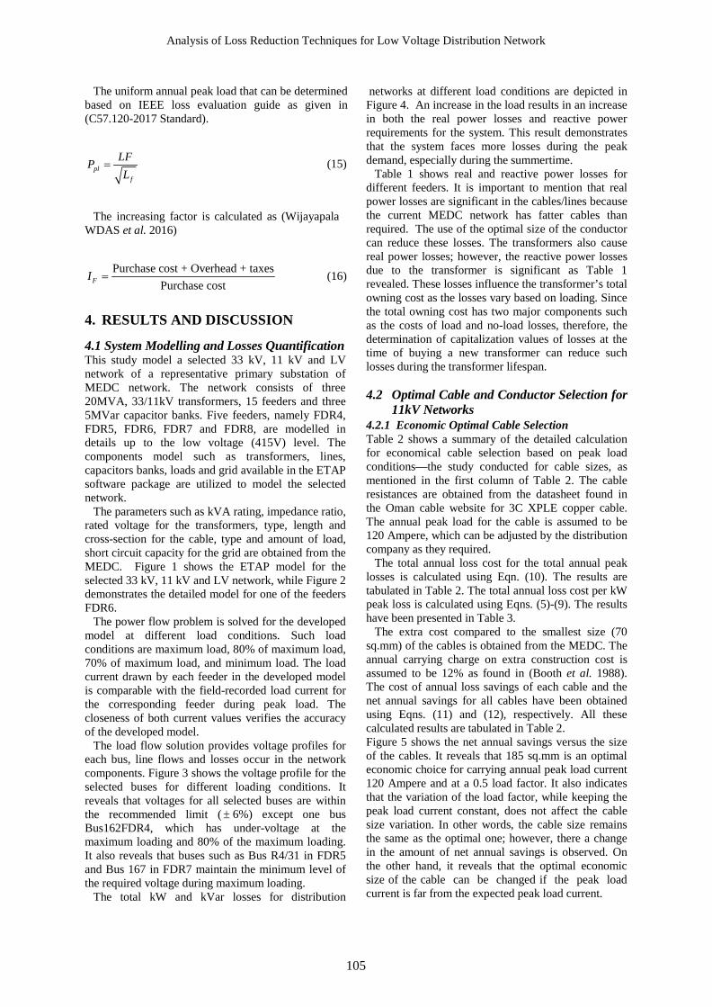
Analysis of Loss Reduction Techniques for Low Voltage Distribution Network
105
The uniform annual peak load that can be determined based on IEEE loss evaluation guide as given in (C57.120-2017 Standard).
plf
LFPL
= (15)
The increasing factor is calculated as (Wijayapala
WDAS et al. 2016)
Purchase cost + Overhead + taxesPurchase costFI = (16)
4. RESULTS AND DISCUSSION
4.1 System Modelling and Losses Quantification This study model a selected 33 kV, 11 kV and LV network of a representative primary substation of MEDC network. The network consists of three 20MVA, 33/11kV transformers, 15 feeders and three 5MVar capacitor banks. Five feeders, namely FDR4, FDR5, FDR6, FDR7 and FDR8, are modelled in details up to the low voltage (415V) level. The components model such as transformers, lines, capacitors banks, loads and grid available in the ETAP software package are utilized to model the selected network.
The parameters such as kVA rating, impedance ratio, rated voltage for the transformers, type, length and cross-section for the cable, type and amount of load, short circuit capacity for the grid are obtained from the MEDC. Figure 1 shows the ETAP model for the selected 33 kV, 11 kV and LV network, while Figure 2 demonstrates the detailed model for one of the feeders FDR6.
The power flow problem is solved for the developed model at different load conditions. Such load conditions are maximum load, 80% of maximum load, 70% of maximum load, and minimum load. The load current drawn by each feeder in the developed model is comparable with the field-recorded load current for the corresponding feeder during peak load. The closeness of both current values verifies the accuracy of the developed model.
The load flow solution provides voltage profiles for each bus, line flows and losses occur in the network components. Figure 3 shows the voltage profile for the selected buses for different loading conditions. It reveals that voltages for all selected buses are within the recommended limit ( ± 6%) except one bus Bus162FDR4, which has under-voltage at the maximum loading and 80% of the maximum loading. It also reveals that buses such as Bus R4/31 in FDR5 and Bus 167 in FDR7 maintain the minimum level of the required voltage during maximum loading.
The total kW and kVar losses for distribution
networks at different load conditions are depicted in Figure 4. An increase in the load results in an increase in both the real power losses and reactive power requirements for the system. This result demonstrates that the system faces more losses during the peak demand, especially during the summertime.
Table 1 shows real and reactive power losses for different feeders. It is important to mention that real power losses are significant in the cables/lines because the current MEDC network has fatter cables than required. The use of the optimal size of the conductor can reduce these losses. The transformers also cause real power losses; however, the reactive power losses due to the transformer is significant as Table 1 revealed. These losses influence the transformer’s total owning cost as the losses vary based on loading. Since the total owning cost has two major components such as the costs of load and no-load losses, therefore, the determination of capitalization values of losses at the time of buying a new transformer can reduce such losses during the transformer lifespan. 4.2 Optimal Cable and Conductor Selection for
11kV Networks 4.2.1 Economic Optimal Cable Selection Table 2 shows a summary of the detailed calculation for economical cable selection based on peak load conditions—the study conducted for cable sizes, as mentioned in the first column of Table 2. The cable resistances are obtained from the datasheet found in the Oman cable website for 3C XPLE copper cable. The annual peak load for the cable is assumed to be 120 Ampere, which can be adjusted by the distribution company as they required.
The total annual loss cost for the total annual peak losses is calculated using Eqn. (10). The results are tabulated in Table 2. The total annual loss cost per kW peak loss is calculated using Eqns. (5)-(9). The results have been presented in Table 3.
The extra cost compared to the smallest size (70 sq.mm) of the cables is obtained from the MEDC. The annual carrying charge on extra construction cost is assumed to be 12% as found in (Booth et al. 1988). The cost of annual loss savings of each cable and the net annual savings for all cables have been obtained using Eqns. (11) and (12), respectively. All these calculated results are tabulated in Table 2. Figure 5 shows the net annual savings versus the size of the cables. It reveals that 185 sq.mm is an optimal economic choice for carrying annual peak load current 120 Ampere and at a 0.5 load factor. It also indicates that the variation of the load factor, while keeping the peak load current constant, does not affect the cable size variation. In other words, the cable size remains the same as the optimal one; however, there a change in the amount of net annual savings is observed. On the other hand, it reveals that the optimal economic size of the cable can be changed if the peak load current is far from the expected peak load current.
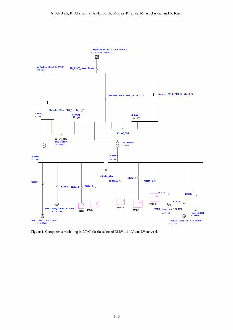
A. Al-Badi, R. Ahshan, S. Al-Hinai, A. Moosa, R. Shah, M. Al Hasani, and S. Khan
106
Figure 1. Components modelling in ETAP for the selected 33 kV, 11 kV and LV network.
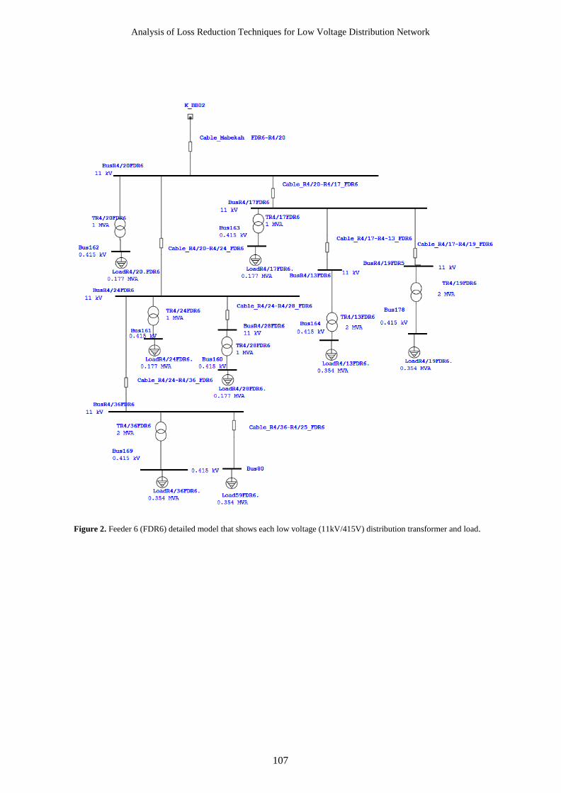
Analysis of Loss Reduction Techniques for Low Voltage Distribution Network
107
Figure 2. Feeder 6 (FDR6) detailed model that shows each low voltage (11kV/415V) distribution transformer and load.

A. Al-Badi, R. Ahshan, S. Al-Hinai, A. Moosa, R. Shah, M. Al Hasani, and S. Khan
108
Figure. 4. Total losses (kW and kVar) in the distribution
network for different loading conditions.
Table 3. Annual demand cost and energy cost detail.
Wholesale electricity purchase cost/kW-month (OMR)
17.7
Annual demand cost/kW (OMR) 212.4 Load factor 0.5
Loss factor 0.3
Cost/kWh (OMR) 0.015 Annual Energy cost/kW (OMR) 39.42
Total annual loss cost/kW(OMR) 251.8
Figure. 3. Voltage profiles for the selected buses at different loading conditions.
Table 1. Real and reactive power loses in distribution transformers and cables for different feeders.
kW losses (FDR
kVar losses (FDR4)
kW losses (FDR5)
kVar losses (FDR5)
kW losses (FDR6)
kVar losses (FDR6)
kW losses (FDR7)
kVar losses (FDR7)
kW losses (FDR8)
kVar losses (FDR8)
Cables/line 159.7 -28.3 81.8 -19.4 42.5 -60.8 81.8 -56.2 46.6 -39.6
Transformers 17.0 76.2 17.2 73.4 11.4 59.8 11.3 58.2 8.5 44.8 Total losses 176.8 47.9 99.2 53.9 53.9 1.0 93.1 2.1 55.5 5.2
Table 2. Cost of loss and net annual savings for various sizes of cables compared to the smallest size.
Cable sizes
(sq. mm)
Cable resistance
(Ohm/km)
Total peak loss for three phases (kW)
Total annual loss cost (OMR)
Extra construction costs in compared to the smallest size conductor (OMR)
Annual carrying charge on extra construction cost (OMR)
Annual loss savings compared to the smallest size conductor (OMR)
Net annual savings
(OMR)
70 0.3420 14.77 3720.49 0.00 0.00 0.00 0.00 120 0.1960 8.47 2132.21 4100.00 492.00 1588.28 1096.28 150 0.1590 6.87 1729.70 6757.00 810.84 1990.79 1179.95 185 0.1280 5.53 1392.46 8698.00 1043.76 2328.03 1284.27 240 0.0982 4.24 1068.28 15099.00 1811.88 2652.21 840.33 300 0.0794 3.43 863.76 18300.00 2196.00 2856.73 660.73 400 0.0636 2.75 691.88 23100.00 2772.00 3028.61 256.61

Analysis of Loss Reduction Techniques for Low Voltage Distribution Network
109
Figure. 5. Annual net savings variation for different sizes of
cables for annual peak load current 120 A, 0.5 load factor, where the optimal size is 185 sq. mm.
Figure. 6. Annual net savings variation for different sizes of overhead conductors for annual peak load current 120 A, 0.5 load factor, where the optimal conductor size is 200 sq. mm.
4.2.2 Economic Optimal Overhead Conductor Selection The detailed calculation is carried out using Eqns. (5) – (12) as described for the economic optimal cable selection, and the detailed results are presented in Table 4. Table 4 shows a summary of the detailed calculation for economic optimal conductor selection based on peak load conditions. The study conducted for conductor sizes is mentioned in the first column of Table 4. The conductor resistances are obtained from the datasheet found in the Oman cable website for ACSR conductors. The annual peak load for the conductors is assumed to be 120 Amperes, which can be adjusted by the distribution company as they required. Figure 6 shows the net annual savings versus the size of the conductors. It is found that 200 sq.mm is an optimal economic choice for carrying annual peak load current 120 Ampere with a 0.5 load factor. 4.3 Capitalization of Losses for Distribution
Transformers 4.3.1 Capitalization Value for No-load Loss The capitalization value for no-load loss (X) is determined using Eqn. (13). Considering the distribution transformers as fixed assets (Wijayapala WDAS et al. 2016), the fixed charge rate is taken by combining the opportunity cost or minimum acceptable return as 12.75% and the book depreciation as 4%. Since there is no income tax in the country, thus it is taken as zero; however, local property tax and insurance is considered as 0.1 %. Thus, the fixed charge rate is found at 16.85%. Since the overall system loss for MEDC is 6.92%, thus the system efficiency is considered as 93.08%.
Equation 16 is used to calculate the increasing factor considering there is no overhead fee and taxes, and the factor is found 1. The system capacity is taken approximately as 40 OMR/kW/year as per (CRT 2017). The average cost of energy for the year 2018 is considered to calculate the levelized cost over the
transformer lifetime (Capability Statement 2018). The discount rate and the inflation rate are considered as 7.5% and 6.425%, respectively. The cost recovery factor is utilized to calculate the annual levelized cost of energy. The levelized annual cost of energy is calculated as 0.0296 OMR/kWh. Thus, the no-load loss capitalization value was found 2.0467 OMR/W, as shown in Table 5. The calculated value in this study is higher than the value given in the Oman Electricity Standard (OES) as 0.8 OMR/W. Such a discrepancy may arise due to the differences in the load pattern, the system capacity cost, and the other parameters that were assumed in this study.
4.3.2 Load Loss Capitalization Value
The load loss capitalization value (Y) is determined using Eqn. (14). The loss factor is determined using the load factor of the transformer used in the distribution network. In order to determine the transformer load factor, it is essential to know the transformer load pattern even for a short period like one day during system peak load. With the use of the load profile of a distribution transformer, the load factor is determined by the ratio between the average load and the peak load. The load factor was calculated as 47.3% for a 2MVA transformer using the load profile provided by the MEDC. With this load factor, the loss factor was calculated as 0.2749. The peak responsibility factor was determined based on the IEEE loss guide (C57.120-2017) and was found as 0.9375.
The uniform annual peak load is calculated using Eqn. (15) as 0.9047. All calculated parameters are substituted to the Eqn. (14) to calculate the capitalization value of load loss, and it is found as 0.5959 OMR/W, as shown in Table 5. The calculated value in this study is higher than the value given in the OES (0.3 OMR/W). Such a discrepancy may arise due to the differences in the load pattern and transformer type (urban or rural), the system capacity cost, and the other parameters that are assumed in this study.
0
200
400
600
800
1000
1200
1400
50 100 150 200 250 300 350 400
Ann
ual
net
savi
ngs
(OM
R)
Cable sizes (sq. mm)
0
500
1000
1500
2000
2500
50 100 150 200 250 300 350 400
Ann
ual
net s
aving
s (O
MR)
Conductor sizes (sq. mm)

A. Al-Badi, R. Ahshan, S. Al-Hinai, A. Moosa, R. Shah, M. Al Hasani, and S. Khan
110
Table 5. No-load and load loss capitalization values of a 2 MVA distribution transformer.
Capitalization Values
OMR/W No-load loss 2.0467 Load loss 0.5959
5. CONCLUSION Distribution companies consider the power loss in the distribution lines as a serious problem because of the energy and money wasted. This paper has presented different methods to minimize such losses. Distribution system losses cannot be phased out; however, it can be decreased by appropriate planning of systems to assure that power loss remain within an acceptable range. This paper reveals the following conclusion and recommendation for reducing losses in the distribution system and hence increasing the system efficiency: • Losses in the distribution system can be quantified
by modelling and simulating the network. Such a kind of study reveals the components or subsystems that contribute to higher losses in the system. Through modelling and simulation of a representative distribution network, it was found that transformers and cables/lines contribute higher losses among all other components in the system.
• Determining an economic optimal conductor/ cable from the available sizes by comparing the cost of losses for various conductors with their extra construction/material cost can reduce the losses in the cables/lines. The study is carried out based on peak load conditions instead of average load conditions because the losses change with the square of the current. It is shown that 185-sq.mm cable is an optimal economic choice for carrying an annual peak load current 120 Ampere with a load factor 0.5. At the same time, 200-sq.mm, an overhead conductor is found as an optimal economic choice for carrying annual peak load
current 120 Ampere with a load factor 0.5. • Capitalization values of the losses have a
significant influence in evaluating the most economical distribution transformer. The utility can assess the capitalization value of the no-load and load losses using the measured load profile of various distribution transformers considering their lifetime. The utility can provide such values to the transformer manufacturing company and ask to design the requisition transformers accordingly. It was found in this paper that both the no-load and load loss capitalization values are higher than the values recommended by the Oman Electrical Standards (OES). Such differences may arise due to the differences in the variables such as the load pattern, load factor, transformer type (urban or rural), and the cost parameters, such as the system capacity cost, unit cost of energy, discount and inflation rates considered in the current study and the study done before. This study suggests recording the actual load profile of a particular distribution transformer for a period of time to determine its loss of capitalization values.
• Regular inspection and maintenance of distribution equipment such as isolators, connections, transformer and transformer bushings, LT switches and dropout fuses are required. Optimal location and appropriate size of the distribution transformers is an important factor. This study suggests placing the distribution transformers closer to the load centre and maintaining the minimum number of transformers, if possible.
• The feeders can directly supply heavy loads such as large buildings and industrial loads. Load balancing and appropriate load management can be considered for further reduction of the losses. The integration of digital, tamper-proof meters can help to reduce non-technical losses. In addition, the DSO can operate their system at a higher power factor. These suggestions can be further investigated for the network presented in this research.
Table 4. Cost of loss and net annual savings for various sizes of conductors compared to the smallest size.
Conductor sizes
(sq. mm)
Conductor resistance
(Ohm/km)
Total peak loss for three phases (kW)
Total annual loss cost (OMR)
Extra construction costs in compared to the smallest size conductor (OMR)
Annual carrying charge on extra construction cost (OMR)
Annual loss savings compared to the smallest size conductor (OMR)
Net annual savings
(OMR)
70 0.4156 17.95 4521.16 0.00 0.00 0.00 0.00 100 0.2885 12.46 3138.48 1681.70 201.80 1382.67 1180.87 150 0.193 8.34 2099.57 4737.10 568.45 2421.58 1853.13 200 0.1439 6.22 1565.43 6649.10 797.89 2955.72 2157.83 400 0.0712 3.08 774.56 20510.00 2461.20 3746.60 1285.40

Analysis of Loss Reduction Techniques for Low Voltage Distribution Network
111
CONFLICT OF INTEREST
The author declares no conflicts of interest. FUNDING
Muscat Electricity Distribution Company provided financial support to perform this research work.
ACKNOWLEDGMENT
The first three Authors would like to acknowledge SQU and Muscat Electricity Distribution Company for the financial support received to perform this research work.
REFERENCES Albadi M, Soliman H, Awlad Thani M, Al-Alawi A,
Al-Ismaili S, Al-Nabhani A, Baalawi H (2017), Optimal Allocation of PV Systems to Minimize Losses in Distribution Networks Using GA and PSO: Masirah Island Case Study. J. Electrical Systems, 13(4): 678-688.
Al-Sarmi S, Al-Ansari H, Al-Badi A, Ahshan R, Al-Hinai S, Al-Hadi Hilal (2019), “Designing a System to Minimize Power Losses in Distribution Network”, in Proc. 15th International Conference for GCC CIGRE, Muscat, Sultanate of Oman, pp. 432-440.
Aburn G, Hough M (2015), Implementing EPA’s Clean Power Plan: A Menu of Options. Technical report, National Association of Clean Air Agencies (NACAA).
Al-Badi AH, Elmoudi A, Metwally I, Al-Wahaibi A, Al-Ajmi H, Al Bulushi M (2011), “Losses Reduction In Distribution transformers”, in Proc. of the International MultiConference of Engineers and Computer Scientists, Hong Kong, pp. 1-5.
Al-Badi AH, Ahshan R, Hosseinzadeh N. Ghorbani R, Hossain E (2020), Survey of Smart Grid Concepts and Technological Demonstrations Worldwide Emphasizing on the Oman Perspective. Appl. Syst. Innov. 3, 5.
Booth and Associates, Inc. (1988), Distribution System Loss Evaluation Manual. Technical report, The University of Michigan, USA.
Charalambous CA, Milidonis A, Lazari A, Nikolaidis AI (2013), Loss Evaluation and Total Ownership Cost of Power Transformers—Part I: A Comprehensive Method. IEEE Transactions on Power Delivery, 28(3):1872-1880.
C57.120-2017 - IEEE Guide for Loss Evaluation of Distribution and Power Transformers and Reactors.
CRT (2017), Cost Reflective Tariff (CRT) Rates as per (2017), -Muscat Electricity Distribution Company, Oman.
Capability Statement (2018), Distribution System
Capability Statement, Muscat Electricity Distribution Company, 2019 – 2021.
Daut I, Hasan S, Taib S (2013), Magnetizing Current, Harmonic Content and Power Factor as the Indicators of Transformer Core Saturation. Journal of Clean Energy Technologies, 1(4): 304-307.
Emmanuel M, Rayudu R, Welch I (2017), Grid capacity released analysis and incremental addition computation for distribution system planning. Electric Power System Research, 152: 105-121.
Inan H, Batson J, Scheibe M (2014), Systems Loss Reduction. Leidos, TechAdvantage.
MEDC (2018), Muscat Electricity Distribution Company, Annual report, Muscat, Oman.
OETC 2019, Five-Year Annual Transmission Capability Statement (2019-2023). Technical Report, Oman Electricity Transmission Company.
Phetlamphanh V, Premrudeepreechacharn S, Ngamsanroaj K (2012), "Technical losses reduction of electrical distribution system in Vientiane capital," in Proc. International Conference on Renewable Energy Research and Applications (ICRERA), Nagasaki, pp. 1-6.
Panek J, Elahi H (1989), "Substation voltage upgrading," in IEEE Transactions on Power Delivery, vol. 4, no. 3, pp. 1715-1724.
Samineni S, Labuschagne C, Pope J (2010), "Principles of shunt capacitor bank application and protection," in Proc. of 63rd Annual Conference for Protective Relay Engineers, College Station, TX, USA, pp. 1-14.
Saadat H (2011), Power System Analysis. PSA Publishing LLC.
Szwander W (1945), The valuation and capitalization of transformer losses. Journal of the Institution of Electrical Engineers - Part II: Power Engineering, 92(26): 125-134.
Sadati S. M. B., Yazdani-Asrami M, Takami M. M. M. (2012), Decreasing Length of Distribution Network for Loss Reduction: Technical and Economical Analysis. Research Journal of Applied Sciences Engineering and Technology 4(7): 813-818.
Wijayapala WDAS, Gamage SRK, Bandara HMSLG (2016), Determination of Capitalization Values for No Load Loss and Load Loss in Distribution Transformers. Journal of the Institution of Engineers, Srilanka, 49(3): 11-20.
Wang, Z., H. Liu, D.C. Yu, X. Wang, H. Song (2000), A practical approach to the conductor size selection in planning radial distribution systems. IEEE Transaction on Power Delivery, 15(1): 350-353.
Zhu Z, Lu S, Gao B, Yi T, Chen B (2016), Life Cycle Cost Analysis of Three Types of Power Lines in 10 kV Distribution Network. Inventions, 1, 20.

The Journal of Engineering Research (TJER), Vol. 17, No. 2, (2020) 112-125
*Corresponding author’s e-mail: [email protected]
DOI:10.24200/tjer.vol17iss2pp112-125
ANALYSIS OF FACTORS AFFECTING MOTIVATION IN
PROJECTS: A CASE STUDY IN OIL AND GAS INDUSTRY IN THE SULTANATE OF OMAN
Nasr Al-Hinai 1, *, Sujan Piya 1, and Khalid Al-Wardi 2 1 Department of Mechanical and Industrial Engineering, Sultan Qaboos University, Muscat, Oman
2 Department of Petroleum and Chemical Engineering, Sultan Qaboos University, Muscat, Oman
ABSTRACT: Motivation is a key element for successful project execution. However, different people are motivated by various means in different sectors. Hence, this work aims to study, analyze and define the main motivational factors in project execution in the oil and gas industry. To achieve this, a dedicated survey is prepared and distributed among employees working in the oil and gas industry in Oman. To ensure diversifications and minimize biases, the survey is distributed randomly to people working in projects in different organizations in the oil and gas industry. Altogether, 86 respondents completed all the survey questions. The study revealed that, in general, external (extrinsic) factors have a significant motivational influence on employee performance in which money is considered as a powerful motivator. Moreover, task achievement is found to be the major intrinsic motivational factor influencing the employee’s performance. The study also reveals that irrespective of years of experience, organizational type and the level at which employee works, lack of management support will have a significant influence in lowering team motivation in the Oil and gas project. The study can serve as a guideline for the Oil and gas industry to target the specific factor which helps enhance the level of motivation of a specific segment of employees.
Keywords: Motivation; Project management; Oil and gas industry; Extrinsic factors; Intrinsic factors.
تحلیل العوامل المؤثرة على الدافع في تنفیذ المشاریع: دراسة حالة في صناعة النفط والغاز في سلطنة عمان
خالد الورديو، سوجان بیا، *نصر الھنائي
التحفیز ھو عنصر أساسي لنجاح تنفیذ المشروع. بید أن مختلف الناس تحركھم وسائل مختلفة في مختلف القطاعات. :الملخصیھدف ھذا العمل إلى دراسة وتحلیل وتحدید العوامل المحفزة الرئیسیة في تنفیذ المشاریع في صناعة النفط والغاز. وفي سبیل
ئیة وتوزیعھا على الموظفین العاملین في صناعة النفط والغاز في سلطنة عمان. ولضمان تحقیق ذلك تم إعداد دراسة استقصاتنویع عینة الاختبار وتقلیل التحیزات الشخصیة إلى أدنى حد، وزعت الدراسة الاستقصائیة عشوائیا على عاملین في مشاریع
86منظمات مختلفة في صناعة النفط والغاز. أكمل ل تابعة كشفت الدراسة أن العوامل الخارجیة وسئلة الاستبیان. جمیع أ موظفاتؤثر بشكل عام في أداء الموظفین بشكل تحفیزي كبیر حیث تعتبر الأموال حافزا قویا. وعلاوة على ذلك، تبین أن إنجاز المھمة
بصرف النظر عن سنوات یشكل العامل التحفیزي الأساسي الرئیسي الذي یؤثر على أداء الموظف. وتكشف الدراسة أیضا أنھ ، والمستوى الذي یعمل بھ الموظف، فإن نقص الدعم الإداري لھ تأثیر كبیر في خفض المنفذة للمشروع الخبرة، ونوع المنظمة
ي تالوامل ع النفط والغاز. ویمكن أن تكون الدراسة بمثابة دلیل لصناعة النفط والغاز لاستھداف العیراالحافز الجماعي في مش تعزیز الحافز لدى شریحة معینة من الموظفین.ساعد على ت
النفط والغاز؛ تحفیز الموظفین؛ إدارة المشاریع؛ عوامل داخلیة؛ عوامل خارجیة. :المفتاحیة الكلمات

Analysis of Factors Affecting Motivation in Projects: A Case Study in Oil and Gas Industry in Oman
113
1. INTRODUCTION
Every project manager would like to run a project that finishes with the desired quality standards, in the given time limit and within the predetermined budget such that it stands up to the end-users’ expectations. Despite the much attention given to projects, it is claimed that most of the projects do not reach their objective. The majority of projects do fail for several reasons. These reasons can be due, but are not limited, to poor planning, poor execution, poor coordination, unclear scope of work, unqualified project manager, conflicts between team members, lack of motivation, etc. Therefore, the success of a project depends to a large extent on how to overcome and minimize the causes of failure. The responsibilities put on the shoulders of project managers, as well as on the organization handling the project, is thus huge and require them to develop special managerial skills, frameworks, policies, and procedures (Al-Hinai et al., 2020).
In many projects, the failure rate is considered to be high. For example, at the end of the last century, The Standish Group found that 44% of information system projects are partially successful and about 40% were cancelled (Field, 1997). This leaves only 16% of the projects to be successful. One would expect that due to the increase in the use and the adaptation of project management tools and practices, the success rate will drastically improve. However, later figures released by The Standish Group is not much different. According to the 2014 CHAOS report, 31.1% of projects are cancelled before completion and 52.7% of projects face 189% cost overrun. The same scenario of higher failure rates in projects is not limited to the IT projects, but it is encountered by other types of projects (CHAOS report, 2015). Hence, many practitioners started to accept failure as unavoidable (McManus and Wood-Harper, 2003, Mahaney and Lederer, 2006). Nevertheless, such an attitude may have a further negative consequence on projects causing them to further exceed in-time, on-budget, or not finishing them according to the scope. The proper approach is, therefore, to strive and explore every possible way to increase the probability of project success rate.
Since running and conducting projects is at the end the result of individuals working together, personal motivation becomes one of the major pillars in the overall project success. Hence, acquiring the proper motivation process and rewards system for team members influences the project manager and his team to execute the project activities effectively and efficiently to meet project desires (Meredith, 2016). DeMarco and Lister (1999) conducted extensive surveys and game exercises to understand the reason for the project’s failure. They concluded that the absence of motivation is a frequent reason. Thus, while project managers may possess the required technical skills to manage projects, lack of motivation
may lead to poor performance (Germann, 2004). Further, Sansone and Harackiewicz (2000) defined motivation as the inner driver that stimulates and guides behaviour. While this definition may be debated as it limits it to inner drivers and ignores the outer drivers, yet one may conclude that the motivation process can be broken into three essentials (Nel et al., 2001). These essentials are the motive, the behaviour and the goal. The motivation process starts with the motive that a person has, which in turn initiates certain actions or a series of activities. These activities or actions are what defines the behaviour of the individual and his means of achieving a certain desired output or in other words, the goal. Hence, the goal can be thought of as the end result of something initiated by a motive. Therefore, to increase the probability of success when conducting projects the project manager, as well as the organization, needs to ensure that the team members work harmoniously and every member of the team is able to fulfil his personal needs, interest, desires, and aspirations along with the objective of the project. A number of researchers pointed that at the absence of motivation, gifted individuals perform far less than their actual capabilities and they may be outperformed by ordinary motivated individuals (Germann, 2004; Bateman and Snell, 1999).
An environment that inspires cooperation, mutual trust, honesty, and gives a sense of belonging will be positively reflected in the team members’ performance as they will tend to do their best when they are in an environment that makes them feel valued. To achieve this, it would require “motivation’’. Therefore, the definition of motivation can be generalized to be the essential means for stimulating the energy and the enthusiasm of the team in order to accomplish project goals by providing satisfactions to the team needs, interest and aspirations (Khoshnevis and Tahmasebi, 2016; Hall et al., 2009). It is worth emphasizing here that a highly motivated person would be encouraged to contribute his extreme efforts individually and as a team towards the effective performance of the project. Therefore, organizations must have the ability to identify and understand the motivational requirements for their employees as it is demonstrated that the higher the satisfaction of project team members’ needs is, the greater the chances for successful project execution will be.
Oil and gas development projects usually require a huge investment and the risk in the project is often quite high (Kim and Choi, 2019). Similar to other parts of the world, the oil and gas industry in Sultanate of Oman is divided into three major sectors: upstream, midstream and downstream. The upstream sector includes exploration and productions of hydrocarbon fields by bringing the crude oil and natural gas from underground to the surface. Companies like Petroleum Development Oman (PDO), Occidental Oman (OXY), Oman Oil

Nasr Al-Hinai, Sujan Piya, and Khalid Al-Wardi
114
Exploration and Production and Daleel Petroleum are an example of companies dealing with upstream industry. The midstream sector involves the transportation by either pipelines or other means of transportation of crude oil and gas from production sites (Upstream) to refineries (Downstream), an example of companies working in midstream companies is Oman Gas Company (OGC). Finally, the downstream sector deals with the refinement of petroleum crude oil and the processing and purification of raw natural gas, which is done by companies like ORPIC, Oman Oil Refineries and Petroleum Industries Company. The oil and gas industry is still considered to be the major contributor to the GDP in many countries, especially in the Middle East and the Sultanate of Oman depends heavily on it. This is reflected by the huge ongoing investments in this industry. These huge investments are usually associated with many ageing fields or newly discovered ones. This results in continuous project execution to ensure the sustainability of oil and gas production. This, on the other hand, increases the overall cost of production. Moreover, the falling oil price is putting further pressure on the shoulders of oil and gas companies as it lowers their margin of profit in contrast to the increase in cost.
While projects in the oil and gas industry have to continue, attention is now more serious than ever to ensure that these projects are successfully implemented and executed to meet the desired outcomes while meeting the on-budget and within-time constraint or at least minimize the deviations. Thus, the main objective of this study is to tackle a major pillar that affects project success. Specifically, the study is aiming to address two main research questions as shown below: 1. To determine the motivational factors that mainly
affect employee’s performance in projects related to the oil and gas industry in the Sultanate of Oman.
2. To examine the effect of motivational categories on team motivation during various project phases.
The focus of this study is to look at both, the intrinsic factors that can be monitored and analyzed by the organization and the extrinsic factors that can be influenced by it through the support and enforcements of the senior management. While one may argue that organizations have less degree of influence over the personal variables, however, understanding how these personal variables (intrinsic motivators) and how they emerge with time will enable senior management to better understand and organize the work-related motivational factors and accordingly their reward systems. 2. THE NEED FOR MOTIVATION Effective management of projects is crucial to the sustainability of organizations (Kanagarajoo et al.,
2019) and employee motivation plays a crucial role in managing project effectively (van der Kolk et al., 2019). Motivation is an essential element for stimulating the energy and enthusiasm of employee’s performance towards the achievement of the project’s goals. According to Lawal and Okhankhuele (2014), motivation is a method that starts with a physiological deficit or need that activates a behaviour or a drive aiming at a goal encouragement. Hence, they divide motivation into three interlinked elements, needs, drives and incentives. In practice, motivation helps to energize employees to work. Therefore, finding appropriate techniques to fulfil employees’ desires and needs is considered the key to a successful motivation process. The main challenge lays in the fact that each individual has different needs, wants and desires (Tabassi et al., 2011). In this sense, there may be many motivation sources that can affect the employee’s performance. Yet, these sources cannot be generalized as what motivate workers differs accordingly. Taylor (1903) who is voted the most influential in the field of management science, long stated that what motivates an individual employee today, may not motivate him tomorrow because human needs are limitless. Further to that, according to Maslow (1943) “A person tries to satisfy the most important need first. When the need is satisfied, it will stop being a motivator and the person will then try to satisfy the next most important need” (Kotler et al., 2018).
Motivation is, therefore, an essential key element to enhance productivity in the workplace (Asproni, 2004). A highly motivated employee puts more effort and energy towards the achievement of the project and the organizational goals by providing better performance. Well-motivated employees are usually results-oriented people in which they look forward to alternative methods to perform the assigned tasks while improving their performance. Therefore, employees should be motivated to bring high-quality service in an efficient way. Achieving this will have a better effect on project progress and success, which in turn can be reflected on the employee’s performance and achievement (Nchorbuno, 2011).
It is of utmost importance to understand that the motivation sources do not rely only on external sources but also can be internal sources. Based on psychological theories that concentrate mainly on human’s/employee’s needs, motivation source can be classified into two types. Intrinsic sources are in-built in the employee himself and as well between the employee and the job. These make the employee creative, enthusiastic, find work pleasurable, want to face challenges, and achieve something. Therefore, intrinsic motivation happens when an individual finds, or more precisely perceives, the activity itself interesting, enthusiastic, pleasant, and hence it derives spontaneous satisfaction (Herzberg, 1987). Different theories related to motivation discussed intrinsic motivation through content theories that may be found in Maslow (1943), Alderfer’s (1972), Herzberg et al.

Analysis of Factors Affecting Motivation in Projects: A Case Study in Oil and Gas Industry in Oman
115
(1959), etc. The second sources are extrinsic sources that come externally from outside the job itself. For example, the employer, the working environment, and other encouragements and incentives including salary, promotion, awards, and benefits, which in return increases employers’ level of commitment to work (Lawal and Okhankhuele, 2014) or even punishments that may lead to having a certain behaviour not to be repeated (Skinner, 1969). Theories discussing such extrinsic factors are categorized under process theories and such theories that can be found in Adams (1963), Locke (1968), Vroom (1964), etc. Nevertheless, the two factors, intrinsic and extrinsic, cannot be separated as a number of studies showed intrinsic factors have an influence on the extrinsic factors (Dolfi and Andrews, 2007; Lee-Kelly and Leong, 2003; Mueller and Turner, 2009, Kooij et al., 2010).
There are indeed numerous studies and literature over the past seven decades on how can team members be motivated at their jobs such as Dwivedula and Bredillet (2010), Sharp et al. (2009), Hall et al. (2009), Nicholson (2003), Pinder (1998), Heimovics and Brown (1976), and Labor Relations Institute (1946). The early survey study conducted by Labor Relations Institute (1946) revealed 10 motivators for employees working in the industry. These factors are appreciation over achieved work goals, sympathy over personal problems, good salaries, interesting work, loyalty to employees, job security, promotion, working conditions, feeling in control of things and tactful disciplining. Later studies indicated that salaries and appreciation over achieved work goals are ranked to be the top motivators (Keller, 1978; Kovach, 1987, 1995; Wiley, 1997; Fisher and Xue Ya Yuan, 1998; Baddoo et al., 2006). However, the study conducted by Ferratt and Short (1986) who studied the needs of an insurance company employees identified five central needs out of which none of these needs is related to good salaries. Similarly, Beecham et al. (2008) reviewed 92 papers that studied the motivational factors for software engineers. Accordingly, they were able to identify the seven most common motivators for these software engineers and none of these motivators is related to good salaries.
The high uncertainty and high demand nature of the projects’ environment resulted in a highly pressurized environment for project managers and project team members to work in. There exist at least three areas of pressure in the project environment, the uncertainty in projects, the extreme need for integration, and the frequent occurring urgencies (Turner and Mueller, 2003). This made it very clear that people working in projects must possess special characteristics that may not necessarily be required in people working in, for example, classical line departments. While some may argue that the project environment itself cause project team members to be self-motivated (Verma, 1996), others argue that this is an oversimplification as it underlines the focus to how project team members can be motivated rather than what motivates them (Seiler
et al., 2012). This may partly explain why there are fewer literature addressing the factors that motivate project team members (Tampoe and Thurloway, 1993; Sharp et al., 2009).
Tampoe and Thurloway (1993) conducted a study to identify the motives for project managers and team members working in IT and R&D organizations. Accordingly, they identified five motives, recognition for achievement, mutuality, authority and control, ability to use their own creativity, and belonging. Verma (1996) advocated eight motivational factors for project managers including the project culture, reward system, work itself, environment, previous success, feeling confident about the work, and competition. The list for possible motivators for project managers was later increased to contain other factors such as career development, receiving positive feedback, contribution to the organization, etc. (Linberg, 1999; Mak and Sockel, 2001). Mahaney and Lederer (2006) investigated the effect of intrinsic and extrinsic rewards on information system projects success. Their study revealed that intrinsic rewards leads to client satisfaction and maintain quality whereas extrinsic rewards affect the implementation success (on-time and within budget). Further, Seiler et al. (2012) developed an integrated model aimed at measuring the factors influencing project managers’ motivation. In their model, they defined motivational dimensions containing 47 items. An empirical study showed that project managers are motivated by a mixture of instinct and extrinsic factors along with specified needed support from the organization.
Khan and Jalbani (2009) studied the effect of the cash and non-cash reward compensation system for employees working at Pakistan Petroleum Limited Company. Their analyses were done based on a survey and a number of interviews with 60 employees. The employees are from different management level at the company. Their finding showed that lower-level employees are motivated more by cash rewards and less by non-cash rewards. However, the effect is vice-versa for the upper management level employees, who give much less attention to the cash rewards. As for the middle management level, the results indicated that cash and non-cash rewards are equally important. In this work, cash rewards are considered as an extrinsic motivator while non-cash rewards are considered as intrinsic motivators.
In short, while Herzberg (1987) advocated that workers could be motivated by using intrinsic and extrinsic rewards, careful study of the literature suggests that the effect of intrinsic and extrinsic rewards is not as conclusive. Many studies, as the above-discussed ones, showed that different workers will be motivated by different means in different organizations. They further revealed that the needs and motivators might differ according to the nature of the work and type of organization. Actually, the effect may not only depend on the organization, but it may change as the years of experience and/or the held
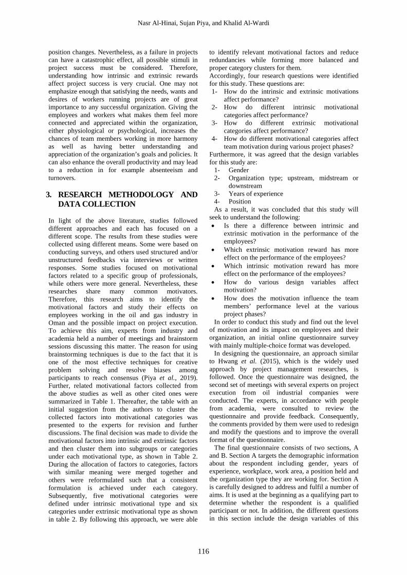
Nasr Al-Hinai, Sujan Piya, and Khalid Al-Wardi
116
position changes. Nevertheless, as a failure in projects can have a catastrophic effect, all possible stimuli in project success must be considered. Therefore, understanding how intrinsic and extrinsic rewards affect project success is very crucial. One may not emphasize enough that satisfying the needs, wants and desires of workers running projects are of great importance to any successful organization. Giving the employees and workers what makes them feel more connected and appreciated within the organization, either physiological or psychological, increases the chances of team members working in more harmony as well as having better understanding and appreciation of the organization’s goals and policies. It can also enhance the overall productivity and may lead to a reduction in for example absenteeism and turnovers.
3. RESEARCH METHODOLOGY AND DATA COLLECTION
In light of the above literature, studies followed different approaches and each has focused on a different scope. The results from these studies were collected using different means. Some were based on conducting surveys, and others used structured and/or unstructured feedbacks via interviews or written responses. Some studies focused on motivational factors related to a specific group of professionals, while others were more general. Nevertheless, these researches share many common motivators. Therefore, this research aims to identify the motivational factors and study their effects on employees working in the oil and gas industry in Oman and the possible impact on project execution. To achieve this aim, experts from industry and academia held a number of meetings and brainstorm sessions discussing this matter. The reason for using brainstorming techniques is due to the fact that it is one of the most effective techniques for creative problem solving and resolve biases among participants to reach consensus (Piya et al., 2019). Further, related motivational factors collected from the above studies as well as other cited ones were summarized in Table 1. Thereafter, the table with an initial suggestion from the authors to cluster the collected factors into motivational categories was presented to the experts for revision and further discussions. The final decision was made to divide the motivational factors into intrinsic and extrinsic factors and then cluster them into subgroups or categories under each motivational type, as shown in Table 2. During the allocation of factors to categories, factors with similar meaning were merged together and others were reformulated such that a consistent formulation is achieved under each category. Subsequently, five motivational categories were defined under intrinsic motivational type and six categories under extrinsic motivational type as shown in table 2. By following this approach, we were able
to identify relevant motivational factors and reduce redundancies while forming more balanced and proper category clusters for them. Accordingly, four research questions were identified for this study. These questions are: 1- How do the intrinsic and extrinsic motivations
affect performance? 2- How do different intrinsic motivational
categories affect performance? 3- How do different extrinsic motivational
categories affect performance? 4- How do different motivational categories affect
team motivation during various project phases? Furthermore, it was agreed that the design variables for this study are:
1- Gender 2- Organization type; upstream, midstream or
downstream 3- Years of experience 4- Position As a result, it was concluded that this study will
seek to understand the following: • Is there a difference between intrinsic and
extrinsic motivation in the performance of the employees?
• Which extrinsic motivation reward has more effect on the performance of the employees?
• Which intrinsic motivation reward has more effect on the performance of the employees?
• How do various design variables affect motivation?
• How does the motivation influence the team members’ performance level at the various project phases?
In order to conduct this study and find out the level of motivation and its impact on employees and their organization, an initial online questionnaire survey with mainly multiple-choice format was developed.
In designing the questionnaire, an approach similar to Hwang et al. (2015), which is the widely used approach by project management researches, is followed. Once the questionnaire was designed, the second set of meetings with several experts on project execution from oil industrial companies were conducted. The experts, in accordance with people from academia, were consulted to review the questionnaire and provide feedback. Consequently, the comments provided by them were used to redesign and modify the questions and to improve the overall format of the questionnaire.
The final questionnaire consists of two sections, A and B. Section A targets the demographic information about the respondent including gender, years of experience, workplace, work area, a position held and the organization type they are working for. Section A is carefully designed to address and fulfil a number of aims. It is used at the beginning as a qualifying part to determine whether the respondent is a qualified participant or not. In addition, the different questions in this section include the design variables of this

Analysis of Factors Affecting Motivation in Projects: A Case Study in Oil and Gas Industry in Oman
117
study and accordingly they help in categorizing the collected data from Section B and understand how, for example, gender, years of experience affects motivation. Further, this demographic information helps us to avoid making wrong or unrealistic interpretations from the collected data, and hence, avoid making inaccurate causal statements that may be associated with descriptive research. Section B consists of mainly multi-choice questions. These multi-choice questions aim to measure the effect of intrinsic and extrinsic motivation in project execution in the oil and gas industry in Oman and answer the research questions.
The questionnaire was made available and distributed via survey monkey website and app (an online survey-distribution service). Accordingly, e-mail invitations with the link for the questionnaire were sent to employees working in different oil and gas projects in Oman. Furthermore, to enhance and increase the respondent rate, the link was made available and sent through social communication media to random practitioners working in the oil and gas industry in Oman. The later medium was found to be the most convenient to reach the targeted participants and have them participate. From a total of 304 invitations that were sent via emails and social media, 71 were not valid emails and contact numbers.
4. DISCUSSION OF RESULTS AND FINDINGS
4.1. Analysis and Validations of Collected Data The total number of respondents who completed the survey and cross the qualifying check part is 86 respondents. Thus, the response rate is 36.9%. According to Shih and Fan (2007), in the meta-analysis, the average response rate in web-surveys is 19%. Hence, the achieved response rate in this study is above that average which reduces the probability for systematic biases due to non-response. Of the 86 respondents, 69 are male and 16 are female with various years of experience, a likely representation of gender working in projects in the oil and gas industry in Oman. The majority of respondents, forming about (48%) of the sample size, have 5-15 years of experience followed by (18%) of the sample size having 0-5 years of experience. The remaining 20 % of the respondents have more than 15 years’ experience. Out of 86 respondents, around 73% hold non-managerial position, and the rest hold a managerial position in various Oil and gas companies in Oman. This finding supports the actual environment of projects, as projects need more technical staff than managerial staff.
Table 1: Overview of motivational factors cited from literature. Reference Considered motivational factors Ferratt and Short (1986) Need for guidance; social needs; esteem needs; achievement needs; power needs Herzberg (1987) Company policy and administration; Supervision; Relation with supervisor/Relationship
with peers/Personal life (interpersonal relationships); Work condition; Salary; Relationship with subordinates; Status; Security; Achievement; Recognition for achievement; Work itself; Responsibility; Advancement; Growth
Keller (1978); Kovach (1987) Kovach (1995); Fisher and Xue Ya Yuan(1998)
A full appreciation of work done; tactful disciplining; personal loyalty to employees; good wages; project reward System; promotional; growth in the organization; sympathetic understanding on personal problems; job security; good working conditions; feeling of being on things; interesting work; competition
Verma (1996) Supervision; project culture/environment; reward system competition; work content; previous success; self-belief
Linberg (1999); Mak and Sockel (2001)
Receiving positive feedback; autonomy; belonging and making a contribution to the entire system; career development
Wiley (1997); Baddoo et al. (2006)
Wages and rewards
Mahaney and Lederer (2006) Favourable annual performance appraisals; Project completion celebration; Job security; Technical training; Flexible work schedule; Job promotion; Financial bonus; Newer technology (PC or laptop); Time off; Choice of future assignment; Opportunity to work at home; Private office space; Pride; Sense of contribution to organization; Public praise
Beecham et al. (2008) Need to identify with the task; clear goals; working on identifiable pieces of work; tasks variety; a clear career path; Personal interest and understanding the task; job satisfaction
Tampoe and Thurloway (1993); Sharp et al. (2009);
Recognition; bounded power mutuality/belongings; creative autonomy
Amin et al. (2010) Individual Rewards/ Group Rewards/ Tangible Extrinsic Rewards/ Intangible Extrinsic Rewards; Altruism; Courtesy; Conscientiousness; Civic virtue; Sportsmanship
Rony and Suki (2017) Employee Extrinsic Reward (promotions and benefits, work location, and working conditions); Internal communication; Training and Development; Leadership; Employee Intrinsic Reward (receiving positive values for doing meaningful works)

Nasr Al-Hinai, Sujan Piya, and Khalid Al-Wardi
118
Table 2: Summary of intrinsic and extrinsic motivational categories and sub-motivational factors. Motivational Type Motivational Category Motivational Factor
Intr
insi
c
Freedom to initiate Being able to initiate important decisions Being able to initiate control measure when needed Having the ability to use their own creativity Being able to take a time off when needed
Pleasure/Enjoyment/Fun
Having a good relationship with team members and superiors Being able to have fun when implementing given tasks and enjoy the moment Having a fair competitive atmosphere Having a personal interest in the assigned task Feeling satisfied when performing the task
Task challenges Assigned to challenging tasks/projects Being able to identify and understand given/assigned tasks Having clear task/project goals/scope Assigned to a variety of tasks
Task achievement Being recognized for achievements Being involved during project completion celebration Feeling proud when completing tasks Being recognized for previous achievement and success Being treated as a professional as a result of personal achievements
Others Receiving non-materialistic rewards Having good relationships with superiors, peers and subordinates Other non-mentioned intrinsic means of motivation
Ext
rins
ic
Engagement to company policy
Being able to engage in making policy for the company Being able to participate in making important decisions Being able to suggest the future assignment Being able to influence the roles of team members Being able to contribute to the organization administration
Rewards Receiving materialistic rewards Receiving rewards based on performance Having a clear promotional system based on performance Having a group incentive reward system Having an individual incentive reward system Receiving rewards as recognition for achievement
Training and development
Having a clear career and promotional paths Receiving technical and nontechnical training Having the opportunity for advancement and growth in the company Receiving proper guidance and supervision
Work environment Having an appreciation of work done Having job security Having necessary support and understanding of personal problems Working with coherent team members Being part of a team who works in an act of altruism Being treated with courtesy and good humour Having good working conditions Availability of needed space and new technologies (office, PC) Having flexible work schedules Having the opportunity to work from home Receiving necessary resources (financial, personnel, material, etc.) and support from management to complete the work
Salary/wages Receiving a good salary Receiving good monthly/quarterly/yearly bonuses
other Having a good internal communication system Receiving a favourable annual performance appraisals Receiving public praise Other non-mentioned extrinsic means of motivation
Oman, being an oil producer country, depends
heavily on oil production as the main contributor to its GDP. Especially, stakes are high in projects related to the exploration and extraction of oil and gas. When validating the sample size, we find that (85%) of respondents are from employees working in an upstream organization as compared to 6% and 9% of
responses from midstream and downstream organizations, respectively. Therefore, this higher response rate from upstream organizations’ employees is expected due to the bigger size of this sector compared with the other two sectors. Further, analysis of collected responses revealed that the majority of respondents, about (60%), are working in main offices
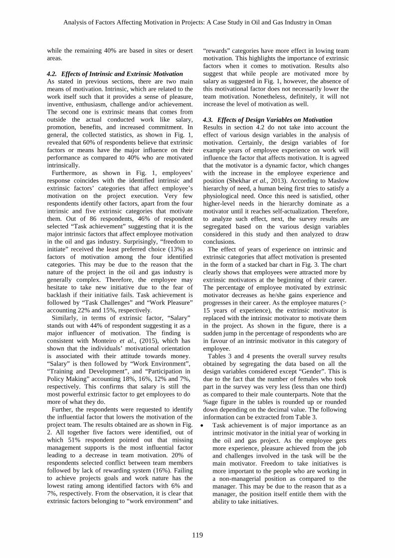
Analysis of Factors Affecting Motivation in Projects: A Case Study in Oil and Gas Industry in Oman
119
while the remaining 40% are based in sites or desert areas. 4.2. Effects of Intrinsic and Extrinsic Motivation As stated in previous sections, there are two main means of motivation. Intrinsic, which are related to the work itself such that it provides a sense of pleasure, inventive, enthusiasm, challenge and/or achievement. The second one is extrinsic means that comes from outside the actual conducted work like salary, promotion, benefits, and increased commitment. In general, the collected statistics, as shown in Fig. 1, revealed that 60% of respondents believe that extrinsic factors or means have the major influence on their performance as compared to 40% who are motivated intrinsically.
Furthermore, as shown in Fig. 1, employees’ response coincides with the identified intrinsic and extrinsic factors’ categories that affect employee’s motivation on the project execution. Very few respondents identify other factors, apart from the four intrinsic and five extrinsic categories that motivate them. Out of 86 respondents, 46% of respondent selected “Task achievement” suggesting that it is the major intrinsic factors that affect employee motivation in the oil and gas industry. Surprisingly, “freedom to initiate” received the least preferred choice (13%) as factors of motivation among the four identified categories. This may be due to the reason that the nature of the project in the oil and gas industry is generally complex. Therefore, the employee may hesitate to take new initiative due to the fear of backlash if their initiative fails. Task achievement is followed by “Task Challenges” and “Work Pleasure” accounting 22% and 15%, respectively.
Similarly, in terms of extrinsic factor, “Salary” stands out with 44% of respondent suggesting it as a major influencer of motivation. The finding is consistent with Monteiro et al., (2015), which has shown that the individuals’ motivational orientation is associated with their attitude towards money. “Salary” is then followed by “Work Environment”, “Training and Development”, and “Participation in Policy Making” accounting 18%, 16%, 12% and 7%, respectively. This confirms that salary is still the most powerful extrinsic factor to get employees to do more of what they do.
Further, the respondents were requested to identify the influential factor that lowers the motivation of the project team. The results obtained are as shown in Fig. 2. All together five factors were identified, out of which 51% respondent pointed out that missing management supports is the most influential factor leading to a decrease in team motivation. 20% of respondents selected conflict between team members followed by lack of rewarding system (16%). Failing to achieve projects goals and work nature has the lowest rating among identified factors with 6% and 7%, respectively. From the observation, it is clear that extrinsic factors belonging to “work environment” and
“rewards” categories have more effect in lowing team motivation. This highlights the importance of extrinsic factors when it comes to motivation. Results also suggest that while people are motivated more by salary as suggested in Fig. 1, however, the absence of this motivational factor does not necessarily lower the team motivation. Nonetheless, definitely, it will not increase the level of motivation as well. 4.3. Effects of Design Variables on Motivation Results in section 4.2 do not take into account the effect of various design variables in the analysis of motivation. Certainly, the design variables of for example years of employee experience on work will influence the factor that affects motivation. It is agreed that the motivator is a dynamic factor, which changes with the increase in the employee experience and position (Shekhar et al., 2013). According to Maslow hierarchy of need, a human being first tries to satisfy a physiological need. Once this need is satisfied, other higher-level needs in the hierarchy dominate as a motivator until it reaches self-actualization. Therefore, to analyze such effect, next, the survey results are segregated based on the various design variables considered in this study and then analyzed to draw conclusions.
The effect of years of experience on intrinsic and extrinsic categories that affect motivation is presented in the form of a stacked bar chart in Fig. 3. The chart clearly shows that employees were attracted more by extrinsic motivators at the beginning of their career. The percentage of employee motivated by extrinsic motivator decreases as he/she gains experience and progresses in their career. As the employee matures (> 15 years of experience), the extrinsic motivator is replaced with the intrinsic motivator to motivate them in the project. As shown in the figure, there is a sudden jump in the percentage of respondents who are in favour of an intrinsic motivator in this category of employee.
Tables 3 and 4 presents the overall survey results obtained by segregating the data based on all the design variables considered except “Gender”. This is due to the fact that the number of females who took part in the survey was very less (less than one third) as compared to their male counterparts. Note that the %age figure in the tables is rounded up or rounded down depending on the decimal value. The following information can be extracted from Table 3. • Task achievement is of major importance as an
intrinsic motivator in the initial year of working in the oil and gas project. As the employee gets more experience, pleasure achieved from the job and challenges involved in the task will be the main motivator. Freedom to take initiatives is more important to the people who are working in a non-managerial position as compared to the manager. This may be due to the reason that as a manager, the position itself entitle them with the ability to take initiatives.

Nasr Al-Hinai, Sujan Piya, and Khalid Al-Wardi
120
Figure 1. Main intrinsic and extrinsic motivational categories and their importance allotment as preferred by oil and gas industries employees.
Figure 2. The most influential factors that lower the team
motivation in projects.
Figure 3. Effect of experience on motivation.
• In the initial years, salary dominates the factor as
an extrinsic motivator. However, rather than salary, it is a reward system and Training, and self-development which is important as they mature. Further, a pleasant work environment dominates the extrinsic motivation landscape for those who are working in the midstream section of the Oil and Gas industry. In this case, the percentage of the participants who are motivated by “Work Environment” related factors is three times higher than those who are motivated by “Salary” related factors.
• The result shows that employee enjoys engaging themselves in the administrative position (for eg. developing company policy and procedure) when
they were somewhere in the middle of their years of experience. However, even in this case, very few employees prefer this role to motivate them. Rather than upstream and downstream, this role is lucrative for the employee who works in the midstream section of the oil and gas industry and is more preferred by the employee working in the managerial position.
The above results are in consistence with Maslow theory in which employees try to satisfy the most important needs first and these can be accomplished by having a satisfactory monetary value and rewards.
When the monetary need is satisfied, then the employee will try to satisfy the next need located in the Maslow hierarchy such as self-esteem and self-development. Both intrinsic and extrinsic motivators are important to help the managers to motivate their team to put all their effort toward the achievement of projects goal.
Similarly, Table 4 shows the effect of design variables on other factors related to motivation. The following information can be extracted from the table. • Interestingly, for all design variables, missing
management support is found to be the major factor that will significantly lower employee motivation except when the employee is highly matured (i.e., who has a work experience of more than 15 years). In this case, the employee will be less motivated towards work if it is not challenging and the work is of routine nature.
• The survey results show that employees themselves or their counterpart working at the same level is the person who can have the main influence on motivation, irrespective of the design variables. This is then followed by the manager. This is due to the reason that the employee will have interaction mainly with their counterpart or with the manager. Stakeholders have hardly any role to play to motivate employees towards work.

Analysis of Factors Affecting Motivation in Projects: A Case Study in Oil and Gas Industry in Oman
121
• The results show that motivation is important at the initial phase and the buildup phase of a project. However, it does not mean that motivation is not needed at the final closing phase. In general, out of three phases, most of the participants felt that it is mainly needed at the buildup phase of the project.
Moreover, it was found from the survey result that the level of motivation of most of the employees working in the oil and gas sector in Oman is medium.
Around 46% of the survey participant agreed to this view. The combined percentages of high and very high levels indicate that 32 % of employees are well motivated by their organizations while 21 % of employees are demotivated. A very low level of motivation has been found in employees that have 0-5 years of experience. On the other hand, a very high level of motivation is found with highly experienced employees.
Table 3: Effect of design variables on intrinsic and extrinsic motivation.
Des
ign
Var
iabl
e Intrinsic Motivation (%) Extrinsic Motivation (%)
Task Achievement
Freedom to Initiate
Task Challenge
Pleasure Salary Reward Training and Development
Engagement in Company
Policy
Work Environment
Years of Experience
0-5 50% 11% 28% 11% 55% 22% 6% 0% 17%
5-10 48% 17% 20% 15% 42% 10% 21% 8% 19%
10-15 49% 11% 26% 14% 51% 14% 9% 6% 20%
15+ 0% 0% 33% 67% 0% 34% 66% 0% 0%
Position
Man
ager
ial 43% 4% 30% 22% 39% 9% 22% 13% 17%
Non
-man
ager
ial 47% 18% 21% 14% 45% 15% 16% 5% 19%
Organization Type
Ups
trea
m 49% 15% 23% 12% 45% 15% 19% 7% 14%
Mid
stre
am 0% 20% 40% 40% 20% 0% 0% 20% 60%
Dow
nstr
eam
50% 0% 12.5% 12.5% 50% 0% 12.5% 0% 37.5%

Nasr Al-Hinai, Sujan Piya, and Khalid Al-Wardi
122
Table 4: Effect of design variables on other factors of motivation.
Des
ign
Var
iabl
e Factor that lowers motivation (%) People who have a major influence on motivation (%)
Phase at which motivation has a major
influence (%) M
issi
ng
man
agem
ent s
uppo
rt C
onfli
ct
betw
een
mem
bers
La
ck o
f re
war
ding
sy
stem
Fa
iling
to
achi
eve
proj
ect g
oal
Wor
k na
ture
Empl
oyee
Man
ager
Seni
or m
anag
er
Stak
ehol
ders
Initi
al p
hase
Bui
ldup
ph
ase
Clo
sing
pha
se
Years of Experience
0-5 50% 33% 11% 6% 0% 50% 44% 0% 6% 50% 33% 17% 5-10 51% 15% 21% 9% 4% 37% 40% 23% 0% 33% 54% 13% 10-15 49% 29% 11% 3% 9% 46% 34% 14% 6% 49% 37% 14%
15+ 33% 0% 0% 0% 67% 67% 33% 0% 0% 33% 33% 34%
Position
Man
ager
ial 65% 13% 17% 4% 0% 43% 35% 17% 4% 39% 52% 9%
Non
-m
anag
eria
l
46% 23% 15% 6% 10% 42% 37% 19% 2% 40% 44% 16%
Organization Type
Ups
trea
m 47% 19% 18% 7% 8% 44% 35% 18% 3% 41% 45% 14%
Mid
stre
am 60% 20% 20% 0% 0% 20% 60% 20% 0% 40% 40% 20%
Dow
nstr
eam
75% 25% 0% 0% 0% 37.5% 37.5% 25% 0% 25% 62.5% 12.5%
5. MANAGERIAL IMPLICATIONS
AND LIMITATIONS
The study identified the motivational factors and then clustered these factors into categories that belong to intrinsic and extrinsic motivational types. The study shows the there are various extrinsic and intrinsic factors that affect the employee’s level of motivation at different phases, working experiences and positions. Therefore, the result of this study can be used by the concerned authority and project managers to tailor the motivational factor that suits the need of the individual employee. This will have a significant positive impact
on employee’s satisfaction, as well as organizational goals. The rate at which employees being motivated in their organization can be improved by focusing more to mitigate the factors that lower team motivation like improving management support, managing the conflict and apply the rewarding system in the organization. Therefore, every organization should incorporate motivational packages and incentives in its corporate policies and plans in order to enable its implementation without interruptions to their business. It is recommended that a consistent study and assessment of individual organization needs to be carried out in order to know what motivates their employees and how motivation can affect their

Analysis of Factors Affecting Motivation in Projects: A Case Study in Oil and Gas Industry in Oman
123
performance. According to the results, the manager can develop the necessary action plan and then implemented it to ensure a comfortable environment that encourages employees to get their maximum efforts towards high performances and ensure efficient and effective project execution.
In this research work, the data were collected only from employees working in the oil and gas industries in Oman. Therefore, the analysis and the interpretation of the data may not be applicable to the oil and gas industries in other parts of the world. More research is needed and data needs to be collected from various countries with significant project activities in oil and gas industries is necessary to generalize the research outcome.
6. CONCLUSION AND FUTURE
RESEARCH DIRECTIONS The main objective of this study is to define and evaluate the effect of motivation on project execution for oil and gas employees in the Sultanate of Oman. For the purpose, the study was carried out mainly based on the literature review and questionnaire survey. Altogether 86 participants took part in the survey. These participants are working at various oil and gas companies and at different levels in the Sultanate of Oman. It can be figured out from the result that there is a significant relationship between motivation and employees’ performance. The survey results revealed that extrinsic factors are the most influential factor to motivate the employee in their work. Salary is found to be the powerful extrinsic motivator for most of the employees. On the other hand, task achievement and challenge in the work are found to be the major intrinsic motivation factors influencing the employee’s performance. The study also analyzed the effect of various design variables on motivation. The results show that irrespective of years of experience, position and organizational type, missing support from the management is found to have a major impact in lowering employees motivation. The result also revealed that motivation is mainly needed during the initial and buildup phase of project execution. As a future research direction, this finding can be considered as a hypothesis that can be expanded to verify up to what extent this is valid and answer why motivation is more important at these phases. Furthermore, the employee himself and their counterpart are found to be the main person who can increase the level of employee’s motivation at the workplace. Most of the workers working in the oil and gas project in Oman seems to have a medium level of motivation at work. This is especially true for those employees who have very few years of working experience. Further to this, it will be an interesting extension to anchor the motivational factors and examine how they are related to achieving the project scope and meeting the project schedule while maintaining the project budget.
Many research articles can be found in literature dedicated to measuring the maturity level of an organization to adopt and use project management tools. However, the scientific literature is still lacking the development of a solid framework capable of measuring the maturity level of the motivation system of the organization. Hence, a possible extension of studies concerned about the motivation of employees should consider this direction. Such frameworks can be more comprehensive by targeting the different needs of employees during the different phases of the project execution as well as their years of experience and containing a number of related key performance indicators (KPI). Moreover, recently Piya et al., (2020) have identified various factors and their inter-relationships that affect agility level in the oil and gas supply chain. Some of the identified factors of agility will have an impact on employee motivation. Therefore, the research can be extended to identify the factors of agility and their level of impact on motivating employees in the oil and gas project. CONFLICT OF INTEREST The authors declare that there are no conflicts of interest as regards this article. FUNDING
This study did not receive any funding from the public, private or not-for-profit sectors. ACKNOWLEDGMENT
The main author would like to acknowledge the financial support he received from Sultan Qaboos University during his sabbatical leave when this study was conducted. Moreover, the work of the main author has been partially carried out during his sabbatical research visit to the University of Nottingham (UK). The author would like to thank Dr. Ender Özcan and the University of Nottingham for such an opportunity. REFERENCES Adams, J.S. (1963). Toward an understanding of
equity. Journal of Abnormal and Social Psychology, 67, 422–436.
Alderfer, C.P. (1972). Existence, Relatedness, and Growth; Human Needs in Organizational Settings. Free Press, New York.
Al-Hinai, N., Abusharkh, E., Al-Shamli, A., & Summad, E. (2020). An Innovative Framework To Measure The Maturity Level of Core Soft Skills and Competencies (SSCM) Needed by Project Managers in Oil and Gas Industry, 10th Annual International Conference on Industrial Engineering and Operations Management, Dubai, UAE, pp. 2597-2604 .

Nasr Al-Hinai, Sujan Piya, and Khalid Al-Wardi
124
Amin, A., Hassan, M. F. B., Ariffin, M. B. M. (2010). Framework of intrinsic and extrinsic motivators of knowledge sharing: A case of training institutes of an oil and gas company in Malaysia, 2010 International Symposium on Information Technology, Kuala Lumpur, 1428-1432.
Asproni, G. (2004). Motivation, teamwork, and agile development. Agile Times, 4(1), 8-15.
Baddoo, N., Hall, T., Jagielska, D., (2006). Software developer motivation in a high maturity company: a case study. Journal of Software Process Improvement and Practice, 11(3), 219–228.
Bateman, T.S., Snell, S., (1999). Management—Building Competitive Advantage 4th ed. McGraw-Hill, Boston.
Beecham, S., Baddoo, N., Hall, T., Robinson, H., Sharp, H., (2008). Motivation in software engineering: a systematic literature review. Information and Software Technology, 50(9–10), 860–878.
CHAOS report (2014). The Standish Group Report. Project Smart, https://www.projectsmart.co.uk /whitepapers/chaos-report.pdf (last accessed on Nov. 13, 2019).
CHAOS report (2015), The Standish Group International, https://standishgroup.com/sample_ research_files/CHAOSReport2015-Final.pdf (last accessed on Nov. 13, 2019).
DeMarco, T., Lister, T., (1999). Peopleware: Productive Projects and Teams 2nd ed. Dorset House, New York.
Dolfi, J., Andrews, E.J., (2007). The subliminal characteristics of project managers: an exploratory study of optimism overcoming challenge in the project management work environment. International Journal of Project Management, 25, 674–682.
Dwivedula, R., Bredillet, C.N., (2010). Profiling work motivation of project workers. International Journal of Project Management, 28, 158–165.
Ferratt, T.W., Short, L.E., (1986). Are information systems people different: an investigation of motivational differences. Management Information Systems Quarterly, 10(4), 377–387.
Field, T. (1997). When bad things happen to good projects. CIO, 11(2), 54–62.
Fisher, C.D., Xue Ya Yuan, A., (1998). What motivates employees? A comparison of US and Chinese responses. The International Journal of Human Resource Management, 9(3), 516–528.
Germann, M., (2004). Influence of project managers on the motivational factors of a project team. Paper Presented at the 13th International Conference on Management of Technology IAMOT, Washington, DC. April.
Hall, T., Baddoo, N., Beecham, S., Robinson, H., Sharp, H., (2009). A systematic review of theory use in studies investigating the motivations of software engineers. ACM Transactions on Software Engineering and Methodology, 18(3),
48–77. Heimovics, R., Brown, F.G., (1976). Municipal
employee behavior as an exchange process. Midwest Review of Public Administration, 10(4), 201–215.
Herzberg, F. (1987). One more time: How do you motivate employees?. Harvard Business Review 65(5), 109–120.
Herzberg, F., Mausner, B., Snyderman, B.B., (1959). The Motivation to Work. John Wiley, New York.
Hwang, B. G., Zhao, X., & Ong, S. Y. (2015). Value management in Singaporean building projects: Implementation status, critical success factors, and risk factors. Journal of management in engineering, 31(6), 1-10.
Kanagarajoo, M. V., Fulford, R., & Standing, C. (2019). The contribution of social media to project management. International Journal of Productivity and Performance Management.
Keller, A.E., (1978). Personnel positioning. Infosystems, 25(6), 50.
Khan, B. A., Jalbani, A. A., (2009). Effect of Compensation System on Employee Motivation: A Case Study of Pakistan Petroleum Limited. Journal of Independent Studies and Research – MSSE, 7(2), 121 – 130.
Khoshnevis, H, Tahmasebi, A. (2016). The Motivation System in a Governmental Organization. Procedia - Social and Behavioral Sciences, 230, 212 – 218.
Kim, S. T., & Choi, B. (2019). Price risk management and capital structure of oil and gas project companies: Difference between upstream and downstream industries. Energy Economics, 83, 361-374.
Kooij, D., DeLange, A.H., Jansen, P.G.W., Kanfer, R., Dikkers, J.S., (2010). Age and work-related motives: results of a meta-analysis. Journal of Organizational Behavior, 31(8), 1111–1136.
Kotler, P., Armstrong, G., Opresnik, M. O. (2018). Principles of Marketing, 17th Edition. Pearson Education.
Kovach, K.A., (1987). What motivates employees? Workers and supervisors give different answers. Business Horizons, 30(5), 58–65.
Kovach, K.A., (1995). Employee motivation. Addressing a crucial factor in your organization's performance. Employment Relations Today, 22(2), 93–105.
Labor Relations Institute, (1946). Do you know your workers' wants?. Foremen Facts IX, 21, 1–3.
Lawal, A. L., Okhankhuele, O. T. (2014). The Effect of Motivation on Project Execution in Nigeria: A case study of Bayelsa Plastic Industry, Yenagoa, Baylesa State, Nigeria. British Journal of Applied Science & Technology, 4(21), 2985-3002.
Lee-Kelly, L., Leong, K.L., (2003). Turner's five functions of project-based management and situational leadership in IT services projects. International Journal of Project Management, 21,

Analysis of Factors Affecting Motivation in Projects: A Case Study in Oil and Gas Industry in Oman
125
583–591. Linberg, K.R., (1999). Software developer
perceptions about software project failure: a case study. The Journal of Systems and Software, 49(2), 177–192.
Locke, E.A., (1968). Towards a theory of task motivation and incentives. Organizational Behavior and Human Performance, 3, 157–189.
Mahaney, R. C., Lederer, A. L., (2006). The effect of intrinsic and extrinsic rewards for developers on information systems project success. Project Management Journal, 37(4), 42-54.
Mak, B.L., Sockel, H., (2001). A confirmatory factor analysis of IS employee motivation and retention. Information & Management, 38(5), 265–276.
Maslow, A.H., (1943). A theory of human motivation. Psychological Review, 50, 370–396.
McManus, J., Wood-Harper, T. (2003). Information systems project management: The price of failure. Management Services, 47(5), 16–19.
Meredith, M. (2016). Project Management -A Managerial Approach. Asia: Wiley Plus learning Space, John Wiley & Sons (Asia) Pte Ltd.
Monteiro, D. L. C., Peñaloza, V., Pinto, F. R., Coria, M. D. C. D., & Calderón, L. M. O. (2015). Attitudes towards money and motivational orientation to work in Brazilian young workers. Contaduría y administración, 60(1), 11-30.
Mueller, R., Turner, R., (2009). Leadership competency profiles of successful project managers. International Journal of Project Management, 28(5), 437–448.
Nchorbuno, D. A. (2011). The Role of Motivation on Employee Performance in the Public Sector: A Case Study of the University for Development Studies-Wa Campus, (Doctoral dissertation).
Nel, P.S., Gerber, P.D., Van Dyk, P.S., Haasbroek, G.D., Schultz, H.B., Sono, T., Werner, A., (2001). Human Resources Management 5th ed. Oxford University Press, Cape Town, South Africa.
Nicholson, N., (2003). How to motivate your problem people. Harvard Business Review, 81, 56–67.
Pinder, C.C., (1998). Work Motivation and Organizational Behavior. Prentice Hall, Upper Saddle River, NJ.
Piya, S., Shamsuzzoha, A., & Khadem, M. (2019). An approach for analysing supply chain complexity drivers through interpretive structural modelling. International Journal of Logistics Research and Applications, 1-26.
Piya, S., Shamsuzzoha, A., Khadem, M., & Al-Hinai, N. (2020). Identification of Critical Factors and Their Interrelationships to Design Agile Supply Chain: Special Focus to Oil and Gas Industries. Global Journal of Flexible Systems Management, 21(3), 263-281.
Rony, N. I., Suki, N. M., (2017). Modelling the
Relationships between Internal Marketing Factors and Employee Job Satisfaction in Oil and Gas Industry. Asian Social Science, 13(3), 135-144.
Sansone, C., Harackiewicz, J., (2000). Intrinsic and Extrinsic Motivation — the Search for optimal Motivation and Performance. Academic Press, San Diego, CA.
Seiler, S., Lent, B., Pinkowska, M., & Pinazza, M. (2012). An integrated model of factors influencing project managers' motivation—Findings from a Swiss Survey. International Journal of Project Management, 30(1), 60-72.
Sekhar, C., Patwardhan, M., & Singh, R. K. (2013). A literature review on motivation. Global Business Perspectives, 1(4), 471-487.
Sharp, H., Baddoo, N., Beecham, S., Hall, T., Robinson, H., (2009). Models of motivation in software engineering. Information and Software Technology, 51(1), 219–233.
Shih, T.-H., Fan, X., (2007). Response rates and mode preferences in web-mail mixed-mode surveys: a meta-analysis. International Journal of Internet Science, 2(1), 59–82.
Skinner, B.F., (1969). Contingencies of Reinforcement: A Theoretical Analysis. Prentice-Hall, Englewood Cliffs, NJ.
Tabassi, A. A., Ramli, M., Abu Bakar A. H. (2011). Training, motivation and teamwork improvement: The case of construction firms. African Journal of Business Management, 5(14), 5627-5636.
Tampoe, M., Thurloway, L., (1993). Project management: the use and abuse of techniques and teams (reflections from a motivation and environment study). International Journal of Project Management, 11(4), 245–250.
Taylor, F.W. (1903), Shop Management (New York, NY: American Society of Mechanical Engineers), OCLC 2365572. Project Gutenberg.
Turner, J.R., Mueller, R., (2003). On the nature of the project as a temporary organization. International Journal of Project Management, 21, 1–8.
van der Kolk, B., van Veen-Dirks, P. M., & ter Bogt, H. J. (2019). The impact of management control on employee motivation and performance in the public sector. European Accounting Review, 28(5), 901-928.
Verma, V.K., (1996). Human Resource Skills for the Project Manager: The Human Aspects of Project Management, Volume Two. Project Management Institute, Upper Darby, PA.
Vroom, V.H., (1964). Work and Motivation. John Wiley & Sons, New York.
Wiley, C., (1997). What motivates employees according to over 40 years of motivation surveys. International Journal of Manpower, 18(3), 263–288

The Journal of Engineering Research (TJER), Vol. 17, No. 2, (2020) 126-134
DOI:10.24200/tjer.vol17iss2pp126-134
PEDESTRIAN MIDBLOCK CROSSING SAFETY DEVELOPMENT MODELING IN DOHUK CITY ROAD
NETWORK
Ayman A. Abdulmawjoud *, and Abdulkhalik A. Al-Taei Civil Engineering Department, College of Engineering, University of Mosul, Mosul-Iraq
ABSTRACT: Pedestrians are vulnerable users walking on foot, having no or little protection-usually provided by police officers-when trying to cross from a midblock section in urban areas. A lot of conflicts and sometimes real pedestrian crashes probably took place in some locations in Dohuk City midblock crosswalks. For this purpose, and to have a comprehensive idea about the safety situation in this city, and what are the main safety countermeasures needed at some hazardous pedestrian crossing locations, this study was proposed. Data were collected from twenty crosswalk locations in central business district (CBD), and suburban areas related to pedestrian movement using two video camera photography to collect data. Data were compiled and presented to measure pedestrian speeds, space, unit flow, crossroad width, etc., meanwhile, vehicular traffic data related to crossing volume, speed…etc. were presented too. Safety and security data related to conflicts of pedestrians with cross vehicles and some actual crash data were obtained from the qualified offices controlling traffic in the city. The Exponential Model was found as best-fitting conflict rates and pedestrian spaces with high R2 in both urban and suburban areas. Meanwhile, the Quadratic Model was found to best fitting conflict rates and pedestrian speeds with R2 values of 0.764, and 0.818 in both urban and suburban areas respectively. Conflict rates are found as best correlating the real crash frequency with a high R2 value of 0.924 in suburban areas. Conflict rates in both CBD and suburban areas are going to be decreased as the pedestrian provided space, speed, crossed road width, and 85th percentile vehicular speed, but increased with the amount of waiting time experienced by pedestrians at crosswalk edge with R2 values of 0.84, and 0.90 for CBD and suburban crosswalks respectively.
Keywords: Conflicts; Crash; Midblock crossing; Pedestrian; Sidewalks.
في مدینة دھوكنمذجة تطویر السلامة لعبور السابلة على شبكة الطرق
عبدالخالق مال الله الطائيو ،ایمن عبدالھادي عبدالموجود
في الطریق على الأقدام ، ولا یتمتعون بأي سیرونمحصنین والذین یالغیر ي الطریق : السابلة او المشاة ھم مستخدمالملخصالتي یتم توفیرھا من الى الحمایةاغلبھا حمایة عند محاولة العبور على ضفتي الطریق في المناطق الحضریة للمدینة حیث تفتقر
ابلة في مدینة قبل مسؤلي المرور في بعض الاحیان. یحدث الكثیر من التعارض وأحیانا حوادث حقیقیة في بعض مواقع عبور السدھوك. ولأخذ مفھوم كامل حول وضع السلامة في ھذه المدینة وماھي التدابیر اللازمة في بعض مواقع عبور المشاة الخطرة, تم
صویر بكامیرتي تالباستخدام ھاضواحیوموقع لعبور السابلة من مناطق في مركز المدینة 20جمع أنواع مختلفة من البیانات من ، وفي الوقت نفسھ تم جمع بیانات تخص المركبات كالسرعة، والفضاء، وتدفق الجریان، ... إلخبیانات السابلة ع فیدیو. تم تجمی
... إلخ. تم الحصول على بیانات السلامة المروریة المتعلقة بالحوادث الفعلیة من المكاتب المؤھلة تھاوسرع ھامنھا حركة مرورتم تثبیت بعض البیانات الأخرى المتعلقة بعرض الشوارع واللازمة لفھم أسباب التي تتحكم في حركة المرور في المدینة.
جمیع ھذه البیانات من خلال إجراء تحلیل احصائي لربط المتغیرات المختلفة حللت في سلامة السابلة في مدینة دھوك ثم القصورم الحصول علیھا تعتبر التعارض فعال في وصف للحصول على نماذج تجریبیة تصف الموقف في المواقع المحددة. النتائج التي ت
الحوادث وكذلك معدلات التعارض تعتمد على سرعة السابلة وعرض موقع العبور.
.المماشي ؛سابلة ؛معبر الوسط ؛اصطدام ؛تعارضال الكلمات المفتاحیة:
*Corresponding author’s e-mail: [email protected]

Pedestrian Midblock Crossing Safety Development Modeling in Dohuk City Road Network
127
1. INTRODUCTION
Traffic safety is known as a critical social and a huge economic matter in Kurdistan Region-Iraq. The rapid economic growth has produced increased motorization, particularly in urban areas. In parallel, the improvements in the infrastructure have enhanced high traffic mobility and speed. As a result of a lack of comprehensive pedestrian traffic safety countermeasures by the government and people’s low sensibility of traffic safety, the proportion of traffic crashes and fatalities had constantly increased over the last five years. These impacts involve tragic loss in effort, time, money, and human lives. Moreover, they create growing feelings of a great lack of safety in all facilities of human lives.
NCHRP, 2008, defined traffic conflicts as an event involving two or more road users, in which one user performs some typical or unusual activity such as a direction or speed that places other users in jeopardy or crash unless an evasive manoeuvre is undertaken.
Hemasiri, and Edirisinghe, 2010 conducted a study in Sri-Lanka at pedestrian crossings as most of the drivers in the country don't follow the rule of ''Give way to pedestrians''. Three main types of field data were collected: video survey, observer measurements, and drivers' interview. Six different Zebra crossings located within the limits of the Kandy-Peradeniya-Gelioya road segment were selected for field surveys. The behaviour of drivers with pedestrians was summarized in this study to use as a guideline to improve pedestrian safety.
Hussein and Neham, 2008, investigated three "T", and, four "cross" legs signalized intersections in Iraqi Capital, Baghdad, to study the traffic conflicts as a surrogate to traffic crashes. They considered shapes of conflicts mostly took place at signalized intersections. Conflicts were correlated to approach spot speed, stopped vehicles near signals control, delay time, and some other traffic geometric parameters of the intersection approach such as lane width, median width, and length of the auxiliary lanes constructed near left-turn movement. The study concluded that conflicts are mostly correlated linearly to stopped delay time with R2=0.978, meanwhile, an exponential model described the relationship between conflict rate and traffic volume with R2 from 0.77 to 0.94 acceptable on 90% significance level. Multiple regression analysis showed that conflict rates increased with increasing approach spot speed, but reduced with increasing lane width, median width, and availability of auxiliary lanes.
Diogenes and Lindau, 2010, evaluated the pedestrian safety and analogy of midblock crossing with the highest number of pedestrian crashes in Porto Alegre city, Brazil. Twenty-one crosswalks were chosen for evaluation. Results show that pedestrian crash hazard was affected by a
combination of interacting hazard factors, such as the presence of bus stops, number of lanes, road width, and the volume of vehicles and pedestrians.
Zhang et al., 2019, investigated the behaviour and safety of pedestrian crossing at midblock crosswalks. For this goal, twelve midblock crosswalks located in Wuhan, China were chosen to gather data through field investigation. Descriptive statistics were applied to resolve pedestrian crossing attitudes and the allocation of pedestrian-vehicle conflicts. Three models for pedestrian-vehicle conflicts analysis were found to measure the influence of various factors on pedestrian safety. Also, it was pointed out that pedestrian behavioural properties such as rolling gap mode, crossing with others would obviously increase the potential of pedestrian-vehicle conflicts.
1.1 Pedestrian Safety Problem Pedestrian safety problem in Dohuk City is merely related to the sprawl in both population, and vehicles, especially in the last five years. Terrorist attacks to wide lands around the Kurdistan Region in Mosul, Anbar, and Kirkuk cities caused the migration of a lot of people to the region congesting both roads, and crosswalks due to the unusual movement of both people and vehicles in Dohuk City road network. Figure 1 is showing the trend of car ownership in Dohuk City between the period 2002 up to 2014. The average number of growths in car ownership was increased by 12 per cent between 2010 and 2014 periods (Accident Data Files, 2015). Vehicle-pedestrian conflicts increased as it seems clear from the crash statistics compiled by the Directorate of Traffic Police in Dohuk City Crash Files.
1.2 Study Purpose To reveal some of the tragedy related to the safety of the pedestrians, or the unprotected users walking on foot, the following goals are planned: • To prepare a database related to pedestrian safety
in Dohuk City for future research or development.
• To collect crash data related to pedestrians and where mostly the problem is probably going to accumulate.
• Nature of traffic conflicts produced between vehicles and crossing people, especially at peak service hours;
• To correlate pedestrian crashes with conflict rates on midblock pedestrian crossing zones;
• To correlate conflict rates with other pedestrian crossing parameters, and some road geometric parameters.
2. RESEARCH METHODOLOGY To execute the main goals of this study, a certain area was selected including all the urban, and suburban areas

Ayman A. Abdulmawjoud and Abdulkhalik A. Al-Taei
128
Figure 1. Number of vehicles owned by the people in Duhok City during the period (2002-2014), (Accident Data Files,
2015).
of Dohuk City. Figure 2 shows the selected areas, which is a type of GIS Map taken from the City (Golden Guide, 2010). Figure 3 shows the flow chart of the proposed methodology, which contains the main types of data collected. Traffic conflicts is an event that can be observed showing the interaction of vehicle against pedestrians while crossing the road. Conflicts used by Glauz and Migletz, 1980, as surrogates for the prediction of crashes at some hazardous locations are selected to study pedestrian crossing behaviour.
Using the conflict data collection form used by Glauz and Migletz, 1980, thousands of conflict data were observed between vehicles and pedestrians in both CBD and suburban crossing locations selected for analysis in this study. In this form, conflicts are classified into major conflicts (M.C.), and secondary conflicts (S.C.), Major conflicts are those related to turning or through movement contacts with pedestrians represented by some dangerous action or longhorn. Meanwhile, minor conflicts are represented by brake light during pedestrian crossing as a parameter to draw out some conclusions. Conflict rates per 1000 vehicles were computed for this correlation using the following equation given by Glauz and Migletz, 1980:
Conflict Rate/1000 Vehicle = (NCO/TVO) × 10 (1)
where: NCO: Number of conflicts observed during three hours of study; and TVO: Total number of vehicles counted during the same period of time in thousands.
Conflict rates during the period of observing
pedestrians were recorded in order to take an opinion
about the critical situations. Pedestrians were usually subjected to driver frustrations when passing the road in the existence of mechanized traffic. Crash data was compiled from crash data files from the Directorate of Traffic Control in Dohuk City, 2015, through the period (2009-2014) which is the up-to-date provided crash data to represent the safety behaviour of pedestrians crossing from different midblock locations. Crash data were provided only for suburban area pedestrian crossing locations meanwhile; CBD area crashes were not registered. Location selected on both areas within Dohuk City in this study is midblock segments not near to any congested signalized or unsignalised intersection, and those candidates as dangerous by police officers. Other data related to pedestrian flow parameters such as unit flows, speeds, spaces, etc., were collected from video filming and manually transferred into computer files. The huge volume of the compiled data was analyzed using SPSS Program version 24, 2017, and Microsoft Excel Package.
Figure 4 shows two locations one of them in CBD and the other in suburban Dohuk City area where data cameras had been fitted on illumination poles or at some vantage points for photography.
3. ANALYSIS OF RESULTS AND
DISCUSSIONS
In order to start the stage of results analysis and discussions, the twenty locations were investigated, ten of them are in the CBD area and the other ten is in suburban areas. To start the data analysis in this study, peak hour demands between (8:30-10:30 A.M.), and (5:30-7:30 P.M.) were selected as peak morning and evening periods for both vehicles and pedestrians and limited exactly in order to concentrate data collection and analysis.

Pedestrian Midblock Crossing Safety Development Modeling in Dohuk City Road Network
129
Figure 3. Research methodology workflow diagram.
(A)
(B)
Figure 4. Two photos showing two of the pedestrian
crosswalks in both CBD and suburban areas: (A) Panorama Centre Commercial. CBD pedestrian crosswalk. (B) Shelan Hospital (Qazi Mohammad St.). commercial suburban pedestrian crosswalk.
Data Collection from 20 Selected Midblock Pedestrian Crosswalk
Selected Crossing Locations in
Suburban Area
Pedestrian Flow Variables, Volumes, Speeds, Delay Time,
Space, Crossing Time, Geometrics
Vehicle-Pedestrian Conflict Rates from Observations Using Special Data Form
Statistical Analysis and Model
Crash Frequency from Police Data
Files
Conclusions and Recommendations
Selected Crossing Locations in CBD
Area
Location of pedestrian observations (E/37.3°N/43.9°, E/37.5°N/43.15°)
Figure 2. Dohuk City study area with 20 data collection locations, Golden Guide, 2010.

Ayman A. Abdulmawjoud and Abdulkhalik A. Al-Taei
130
Figure 5. Effect of pedestrian space on the conflict rate in
midblock crosswalks in Dohuk City CBD and suburban areas.
3.1 Pedestrian Conflict and Pedestrian Space
at CBD and Suburban Crossing Locations Pedestrian conflicts (i.e., both major and secondary conflicts) were computed in rates per 1000 vehicles from Eqn. (1) and correlated with pedestrian provided space in m2/pedestrian (m2/ped.) which is the number of pedestrians occupying an area of one square meter at the crosswalk during the crossing process stated by the HCM, 2010. The space variable was counted automatically from an area of one square meter using photoshop and Excel sheet limited with photo zoom picture by picture. Figure (5) shows the variation of conflict rates with space. A relationship is described by Exponential Models with a good correlation of determination coefficients R2 of 0.906 and 0.866 for both CBD and suburban locations, respectively. Equations (2) and (3) reflect the fact that as pedestrian move closer, conflicts with the adjacent vehicles will increase. The form of the models derived are as follows: Y1 = 683.35e−0.07x (2) Y2 = 745.55e−0.042x (3) where: Y1: Conflict rate/1000 vehicles in Dohuk City CBD crosswalks; Y2: Conflict rate/1000 vehicles in Dohuk City suburban crosswalks; and X: Pedestrian space in m2/ped.
Correlations between conflict rate and pedestrian space were implemented using the above statistical analysis by both simple and multiple regression to show the effect of the independent on the dependent variable and what shapes of empirical models are correlating them.
3.2 Pedestrian Conflict and Pedestrian Speed at
CBD and Suburban Crossing Locations Conflict rates and pedestrian speed variations on the crosswalks located in both CBD and suburban areas are
shown in Fig. 6. Coefficients of correlation R2 are 0.764 and 0.818 for CBD and suburban crosswalks respectively. The best models are 2nd Degree Polynomial Models with the following mathematical forms:
Y1 = 770.9X2 + 2332X − 1259 (4) Y2 = −4044.7X2 + 12492X− 9136.2 (5) where: Y1: Conflict rate/1000 vehicles for CBD crosswalks; Y2: Conflict rate/1000 vehicles for suburban crosswalks; and X: Pedestrian speed, m/s.
Figure 6 shows that at an optimum conflict rate of
about 500 conflicts/1000 vehicles, the pedestrian speed is around 1.55 m/sec. Both trends are going to increase with the increase of pedestrian speed up to the above-mentioned number of conflict rate and then goes down to reduce. The conflict rate decreases for suburban after a certain speed, since the number of pedestrians in the suburban is low with higher walking speed.
Figure 6. Effect of conflict rate on pedestrian speed on
midblock crossing sections in Dohuk City CBD and suburban areas.
Figure 7. Pedestrian crash frequency and conflict rates
correlation on midblock crossings located in Dohuk City suburban area.

Pedestrian Midblock Crossing Safety Development Modeling in Dohuk City Road Network
131
3.3 Pedestrian Traffic Crash Frequency and Conflict Rate Correlations
In order to detect how much traffic conflicts, represent the chance of traffic crashes to occur on pedestrian crosswalks, crash data and conflict rates are correlated in this study to know the empirical relationship combining them. The analysis was implemented for suburban locations only using a step-wise form of the SPSS program; as the CBD investigated locations did not have enough crash data to perform the analysis required.
Crash frequency and conflict rates data in a suburban area was plotted to find if there is any correlation with the conflict rates at suburban crosswalks. Figure 7 shows the predicted model obtained, which indicates that crashes increase as conflict rate increases on suburban crosswalks, up to a peak value of 43 crash at 365 conflicts rate/1000 vehicles, then decrease as conflict rates increase as drivers are going to be more sensitive and awake to drive obeying traffic rules and ordinances. This correlation is describing an empirical crash field data registered by police officers and conflicts from photography filming with manual data counting. In this crosswalk a special Zebra type is needed, in addition to an automatic push-button pedestrian crossing signal installation will be very useful to survive people's life, especially school students and elderly people. Some of the cross midblock locations investigated in this study are more than 10 meters wide, and some pedestrians are not so fast to cross, in this case, an overpass is required as a safe structure to provide more safety and security to some weak type pedestrians. The mathematical model is a 3rd Degree Polynomial with R2 of 0.924 as follows:
𝑌𝑌 = −1𝐸𝐸 − 06𝑋𝑋3 − 0.0003𝑋𝑋2 + 0.7346𝑋𝑋 − 117.6 (6) where: Y: Crash frequency of pedestrians on suburban crosswalks, and X: Conflict rate of pedestrians on suburban crosswalks in conflicts/1000 vehicles.
This result is supporting many other results found elsewhere, that crashes could be represented or replaced by conflict rates in other safety research or safety supporting projects such as those implemented by Khalik, 1997.
3.4 Analysis of conflict rates with pedestrians
and other traffic and geometric characteristics of the crossing locations
Pedestrians are usually coming to crosswalks to pass safely as soon as possible with minimum delay time and without interaction with the passing vehicles. This condition is highly affecting the behaviour of the pedestrian, which may lose his/her patience to cross without care. In this study, conflict rates are correlated with five main factors to know how they affect
pedestrian safety in both CBD and suburban areas. The main factors selected for step-wise correlation analysis with pedestrian conflict rates (as a dependent variable) are provided pedestrian spaces, the pedestrian speed at a crossing, road width which is the total approach width from curb to curb distance without considering median width as a geometric variable, 85th percentile vehicular traffic speed, and pedestrian waiting time. The analysis is performed for both CBD and suburban crosswalk locations included in this study. The analysis was performed using the SPSS program. The model variable introduced are described as below:
Y1 Conflict rate in conflicts/1000 vehicles on CBD
crosswalks; Y2 Conflict rate in conflicts/1000 vehicles on
suburban crosswalks; X1 Pedestrian space measured in m2/ped; X2 Pedestrian speed at crosswalks in m/sec; X3 Total width of a crossed road in (m); X4 85th percentile vehicular traffic speed on main
crossed road in km/h; and X5 Pedestrian waiting time on road curbstone in
sec/ped.
3.4.1 Pedestrian conflict rate modelling in
Dohuk City CBD area crosswalk
Step-wise regression analysis correlating conflict rates on CBD crosswalk, and other variables listed above is shown below:
Y 1 = 813.958 − 4.871X1 − 22.251X2 − 17.344X3 −
12.318X4 + 45.766X5 (7) From the above model, it is shown that some of the
variables are going to decrease conflict rates, meanwhile, only one is going to increase it. Pedestrian space, and speed, is going to decrease it, and the same effect seems for road width, and vehicle speed too, but pedestrian waiting time on curbstone on CBD is going to increase them. Collinearity table which shows the interaction among the five independent variables, X1, X2, X3, X4, and X5 is shown in Table 1.
Analysis of variance ANOVA is shown in Table 2 for the predicted model.
The derived model produced multiple correlation coefficient for the total model of R2= 0.84. VIF is best showing that collinearity is very weak as its value is less than 5.0, and the P-value of 0.838% is less than 5% required insignificance level (Anderson, 2008). In Table 2, the F-calculated value is more than the standardized value of F at 5% insignificance level of 3.84, this means that regression coefficients are the best-fitted values as the null hypothesis will be rejected. The partial correlation matrix shows no collinearity among the five independent variables, and proof model validity as it is shown in Table 3. Figure 8 shows the uniform

Ayman A. Abdulmawjoud and Abdulkhalik A. Al-Taei
132
Table 1: Collinearity matrix of independent variables X1, X2, X3, X4, and X5 for step-wise regression analysis of conflict
rates on Dohuk City CBD crosswalks.
Table 2: Analysis of variance of variables included in the regression analysis of Y1, X1, X2, X3, X4, and X5 of conflict rates
on Dohuk City CBD crosswalks.
Table 3: Partial correlation matrix of the step-wise regression of Y1, on the other variables X1, X2, X3, X4, and X5 of conflict
rates on Dohuk City CBD crosswalks.
Figure 8. Expected and observed regression validation of
conflict rates around normal probability diagonal line on Dohuk City CBD midblock crosswalks.
Figure 9. Expected and observed regression validation of
conflict rates around normal probability diagonal line on Dohuk City suburban midblock crosswalks.
Predictor Coefficients Standard Deviation
Student t-value
Probability of Insignificant
Variable Inflation Factor (VIF)
Constant 813.958 976.666 0.833 0.451 -
X1 -4.871 7.386 -0.659 0.546 2.667
X2 -22.251 405.281 -0.055 0.959 2.153 X3 -17.344 24.569 -0.706 0.519 1.193 X4 -12.318 10.757 -1.145 0.316 2.558 X5 45.766 41.532 1.102 0.332 3.349
Source of Variation D.F. SS MS F P
Regression 5 141363.85 28272.77 4.12 0.00838
Error 4 27449.28 6862.32
Total 9 168813.13
Variables Y1 X1 X2 X3 X4 X5
Y1 1.00 X1 -0.20 1.00
X2 -0.117 -0.416 1.00
X3 -0.110 -0.017 -0.007 1.00
X4 -0.233 -0.307 -0.395 -0.022 1.00
X5 0.241 0.474 -0.685 0.221 0.439 1.00

Pedestrian Midblock Crossing Safety Development Modeling in Dohuk City Road Network
133
Table 5: Analysis of variance of variables included in the regression analysis of Y1, X1, X2, X3, X4, and X5 for conflict rates on Dohuk City suburban crosswalks.
Table 6: Partial correlation matrix among Y2, and other variables X1, X2, X3, X4, and X5 for conflict rates on Dohuk City
suburban crosswalks.
distribution of SSE values around the diagonal of the normal probability plot around the zero value of the SSE, which represents the model validation as plotted using the SPSS programme. 3.4.2 Pedestrian conflict rate modelling in Dohuk
City suburban crosswalk Step-wise regression analysis correlating conflict rates on Dohuk suburban crosswalk and other same variables listed above is shown in the model represented in eqn. 8 as below:
𝑌𝑌2 = 698.479 − 3.815𝑋𝑋1 − 301.984𝑋𝑋2 − 12.829𝑋𝑋3 −0.966𝑋𝑋4 + 1.016𝑋𝑋5 (8)
From the model, it is shown that some of the variables are going to increase conflict rates, meanwhile, others are going to decrease it. Pedestrian space, pedestrian speed, total road width, and 85th percentile vehicle speed is decreasing conflict rates but, pedestrian waiting time on the curbstone of Dohuk City suburban area is increasing it. The collinearity table representing the interaction among the five independent variables X1, X2, X3, X4, and X5 is shown in Table 4.
Figure 9 shows the uniform distribution of SSE values around the diagonal of the normal probability plot around the zero value of the SSE, which represents the model validation criteria as plotted using the SPSS program. 4. CONCLUSION According to the size of data collected and the techniques used to analyze it and decide what is necessary to solve the pedestrian safety problem in Dohuk City in both CBD and suburban crosswalks. The following conclusions could be drawn out: • Vehicle conflicts and pedestrian space are related
in Exponential Models with R2=0.906 and R2=0.866 in CBD and suburban crosswalks respectively.
• Vehicle conflicts and pedestrian speed are related in Quadratic Polynomial Models with R2=0.764 and R2=0.818 in CBD and suburban crosswalks respectively. The optimum value was 500 conflicts /1000 vehicles at pedestrian speeds of 1.55 m/s.
• Crash and conflict rates correlations in the suburban area show a Cubic Polynomial Model with a high coefficient of multiple determination R2 of 0.924. The function is best fitted with a peak crash frequency at 365 conflict rates per 1000 vehicles at an optimum crash frequency of 43. The model concludes that in suburban area crosswalks conflict rates could be considered as a surrogate to crash frequency in describing the safety condition in Dohuk City suburban area.
• Conflict rate per 1000 vehicles happened in Dohuk City CBD and suburban crosswalks decrease with pedestrian provided space, speed, crossed road total approach width, and 85th percentile vehicular speed, but increases with the amount of waiting time experienced by a pedestrian at crosswalk edge with R2 values of 0.84 and 0.90 for CBD and suburban crosswalks respectively.
A lot of changes are found necessary to be recommended to develop pedestrian movement safety in Dohuk City in both CBD and suburban crosswalks, such as pedestrian crossing automatic signs, zebra, and pelican crossing markings where they are justified in order to reduce or eliminate conflicts, and/or crash occurrence near or at crosswalks and make crossing easier for pedestrians. Formal analysis obtained a lot of results that recommend some locations need overpass bridge structures to isolate pedestrians from the rapid hazardous traffic vehicles travelling with high speeds and, this selection is needing more study by decision-makers to put down the type of each solution needed.
Source of Variation
D.F. SS MS F P
Regression 5 150203.28 30040.656 7.3 0.0048 Error 4 16460.632 4115.158 Total 9 166663.912
Y2 X1 X2 X3 X4 X5
Y2 1.00 X1 -0.550 1.00 X2 -0.450 0.295 1.00 X3 -0.182 -0.151 0.589 1.00 X4 -0.233 -0.159 0.282 0.065 1.00 X5 0.013 0.252 0.262 0.522 0.217 1.00

Ayman A. Abdulmawjoud and Abdulkhalik A. Al-Taei
134
CONFLICT OF INTEREST The authors declare that there are no conflicts of interest as regards this article.
FUNDING
This study did not receive any funding from the public, private or not-for-profit sectors. ACKNOWLEDGMENT The authors wish to acknowledge the help provided by the staff of the Dohuk Governorate Traffic Police Department and, the staff of the Traffic Engineering Unit of Dohuk Municipality Directorate for their assistance in the collection of traffic data.
REFERENCES Anderson, DR., Sweeney, DJ., and Williams, TA.
2010. Statistics for Business and Economics, 11th edition, South-Western College Publication.
Diogenes, MC., and Lindau, LA. 2010. “Evaluation of pedestrian safety at midblock crossings, Porto Alegre, Brazil”. Transportation Research Record: Journal of the Transportation Research Board, No. 2193, Transportation Research Board of the National Academies, Washington, D.C., 37–43.
Dohuk City Traffic Police Directorate, 2015. Accident
Data Files (1995-2014); Dohuk Governorate, 2010. Guide and Information
Center GIC, Golden Guide. Glass, WD., and Migletz, DJ. 1980. “Application of
traffic conflict analysis at intersections”. NCHRP Report 219, Transportation Research Board.
Hemasiri, AG., and Edirisinghe, J. 2010. “Safety on pedestrian crossing”. University of Peradeniya, Peradeniya 20400, Sri Lanka.
Highway Capacity Manual, 2010. Transportation Research Board (TRB), National Research Council, Washington D.C.
Hussein, AE., and Neham, SS. 2008. “Traffic conflict technique: A tool for traffic safety study at three-leg signalized intersections”. Journal of Karbala University, Vol. 6, No.1 Scientific.
Khalik, AM. 1997. “Conflict analysis at unsignalized unchannelized T-intersections”. Scientific Journal of Tikrit University, Engineering Science Vol.4
National Center Highway Research Program, (NCHRP), 1980. “Application traffic conflict technique at urban intersection”. Transportation Research Record No.776.
SPSS Version 24, 2017. “Statistical Package for Social Sciences”.
Zhang, C., Chen, F., and Wei, Y. 2019. “Evaluation of pedestrian crossing behavior and safety at uncontrolled mid-block crosswalks with different numbers of lanes in China”. Accident Analysis Prevention, Vol.123, pp. 263-273.

The Journal of Engineering Research (TJER), Vol. 17, No. 2, (2020) 135-141
*Corresponding author’s e-mail: [email protected]
DOI:10.24200/tjer.vol17iss2pp135-141
DEVELOPMENT OF SPINEL MAGNESIUM ALUMINATE BY SOLUTION COMBUSTION ROUTE USING THIOUREA AND UREA AS FUEL
Srinath Ranjan Ghosh 1, Soumya Mukherjee
2, *, and Sathi Banerjee 1
1 Department of Metallurgical & Materials Engineering, Jadavpur University, India 2, * Department of Metallurgical Engineering, Kazi Nazrul University, India
Abstract: In the present article spinel phase magnesium aluminate was synthesized using Magnesium nitrate, Al-nitrate precursors in 1:2 molar ratio using urea and thiourea as fuel and reducing agent. Nitrate salts were mixed in a stoichiometric ratio in distilled water with three different molar ratios of two different fuels: urea and thiourea. The temperature of crystallization was obtained after thermal analysis followed by annealing at a fixed temperature, fixed soaking period for urea as fuel while variable temperature and soaking period were required for thiourea as fuel. FTIR analyses were carried out of the samples to verify the M-O co-ordinations for the phase formation. Prominent octahedral M-O stretching was noted at about 609 cm-1 while that of Al-Mg-O stretching was noted at about 1100 cm-1 for thiourea based samples. Using Urea as fuel Al-O stretching was noted at about 539cm-1 while that of Al-Mg-O vibration was noted at about 677cm-1. Morphological features of the synthesized samples were observed by SEM. Agglomeration was noted for both urea and thiourea as fuel having irregular polygon shape. Using thiourea as fuel, a bit of porous structure was noted while for urea as fuel negligible porosity was noted.
Keywords: Magnesium Aluminate; Thermal analysis; Phase analysis; M-O co-ordinations; Morphology
باستخدام عن طریق حرق المحلولالومینات المغنیسیوم تحضیر معدن السبینیل ذو یا كوقودیا والیوریوالثیور
، وساثي بنرجي*سریناث جوش، سومیا مخرجي
تصنیع ألومینات المغنیسیوم في طور الإسبنیل باستخدام نترات المغنیسیوم وسلائف النترات خلال ھذه الدراسة تم الملخص:بنسب متكافئة في الماء اختزال. تم خلط أملاح النترات ریا كوقود وعواملیوكلا من الیوریا والثیو باستخدام یةمولار 2: 1بنسبة
اسفرت الدراسة بعد التحلیل الحراري والتلدین للیوریا . لنوعي الوقود المذكورین اعلاهالمقطر مع ثلاث نسب مولاریة مختلفة ة ریا وجود درجة حرارة وفتریوالثیووقود بینما تطلب استخدام ثابتتین، ریا إلى أن فترة نقع الیوریا ودرجة حرارة تبلوره یووالثیو
ثماني السطوح M-Oلتشكیل الطور. لوحظ تمدد M-Oوتم إجراء التحلیل الطیفي للعینات للتأكد من تنسیقات ،نقع متغیرتینریا. وفي حالة یوللعینات القائمة على الثیو 1-سم 1100عند حوالي Al-Mg-Oبینما لوحظ امتداد 1-سم 609البارز عند حوالي
سم 677عند حوالي Al-Mg-Oبینما لوحظ استخدام اھتزاز 1-سم 539عند حوالي Al-O استخدام الیوریا كوقود لوحظ تمدد من نتائج التجارب أن لوحظ. تمت ملاحظة السمات المورفولوجیة للعینات المركبة بواسطة المجھر المسحي الألكتروني. كما 1-
كان للیوریا بینما تؤخذ بعین الإعتبار ریا بنیة مسامیةیولثیول أنكما ،ریا لھ شكل مضلع غیر منتظمیوتكتل كل من الیوریا والثیو .بنیة أقل مسامیة
.وقود، ریایوثیو، یوریا، تحلیل حراري، الومینات المغنیسیوم الكلمات المفتاحیة:

Development of Spinel Magnesium Aluminate by Solution Combustion Route Using Thiourea and Urea as Fuel
136
1. INTRODUCTION
Magnesium aluminate has lots of industrial applications due to its high melting point (2135°C), high-temperature mechanical strength, chemical inertness, thermal shock resistance, chemical resistance, and low thermal expansion coefficient. (C Păcurariu et al. 2007; S.R. Ghosh et al. 2018; Ali Saberi et al. 2008; P V Marakkar Kutty et al. 2013) The presence of such properties makes the compound suitable as high-temperature refractory material for both cement rotary kiln, and steel ladle. In the initial decades, chromite-based spinel is extensively used for steel making, glass tank regenerators, rotary kiln and even for copper industry. However, environmental concern regarding Cr+6 species from the chromite spinel is a hindrance to its applications. (Chandrima Ghosh et al. 2015) The above compound has spinel structure represented by the formula AB2O4 where A is the divalent ion, B is the trivalent ion and O represents the anion. Divalent Mg and trivalent Al ions occupy tetrahedral (1/8 of available) and octahedral sites (1/2 of available) respectively. (Shiva Salem 2015) The particular spinel ceramic also has excellent optical properties and can be used for transparent ceramics. The optical property enhances its eligibility as a prominent candidate material for transparent armour and visible-infrared windows. It is also utilized for ceramic paints and for making catalyst support, membranes, dye absorbent and as sensors. For the successful application of spinel aluminate as dye absorbent, catalyst, sensors, spinel fabricated needs to possess high purity, controlled particle size, high surface area and uniform pore size distribution. (Narges Habibi et al. 2017) Spinel magnesium aluminate also acts as a potential candidate for humidity sensors. In recent researches, it is noted that spinel magnesium aluminate as one potential candidate for photocatalyst to decompose reactive red methylene used as a dye for industrial operations. (Mostafa Y Nassar et al. 2014) Purity, particle size, chemical homogeneity, and reactivity of spinel magnesium aluminate are influenced by the synthesis route. (Ali Saberi et al. 2008) The material is found to be synthesized by various methods in addition to solid-state reaction like sol-gel (Debsikdar J.C 1985; Naskar M.K. et al. 2005) precipitation (Li J-G et al. 2000), aerosol method (Yang N et al. 1992), co-precipitation (Guo J et al. 2004), combustion synthesis, freeze-drying, decomposition of an organometallic complex in super critical fluids, hydrothermal route, plasma spray decomposition of powders, (Bickmore R Clint et al. 1996; Bratton R.J. 1969; Barj M. et al. 1992; Pommier C. et al. 1990; Yang Ning et al. 1992; Varnier Olivier et al. 1994) microwave-assisted combustion route (Torkian Leila et al. 2011), polymerized complex method (Lee P.Y et al. 2006; Du Xuelian et al. 2014), mechanochemical route (Domanski D. et al. 2004), self-propagating high-temperature synthesis (Gorshov V. A. et al. 2017) and others. In the present article, spinel magnesium aluminate is synthesized using urea and thiourea as fuel and reducing agent for three molar ratios along with nitrate precursors. The annealing temperature is confirmed after carrying thermal analysis of mixed solutions followed by phase analysis, bonding analysis and morphological studies.
2. EXPERIMENTAL METHODS AR grade of magnesium nitrate, aluminium nitrate, urea and thiourea were used as precursors for synthesizing spinel. The stoichiometric ratio of magnesium nitrate, aluminium nitrate were taken in 1:2 molar ratios in distilled water for stirring. The solution undergoes stirring by magnetic beads for sufficient time. After proper mixing of nitrates urea, thiourea was added in 1.25, 1.50 and 1.75 molar ratio with respect to nitrate salts and again undergoes stirring for about 1 hour to ensure homogeneity. The resultant solution undergoes drying in an oven (heater) at about 80°C for about 3-4 hours to obtain a dry gel-like mass. The gel was put into DTA-TGA analyzer (Diamond Pyris, Perkin Elmer) in presence of Nitrogen atmosphere at the heating rate of 10°C/min for determining the thermal characteristics of the sample. Crystallization temperature for spinelization was obtained and after that, the gel was put for annealing at 700°C for 5 hours in the case of urea as fuel. The annealing temperature was 700°C for 5 hours, 800°C for 4.5 hours and 900°C for 4.5 hours respectively for thiourea as fuel. Phase analysis was carried by XRD (Rigaku, Ultima III) having Cu Kα wavelength of 1.54Å, 40KV with a scan range of 10-80° having a scan rate of 5°/minute. Bonding analysis was carried by FTIR (IR Prestige-21, Shimadzu) to determine M-O coordination of the required phase after preparing pellet samples with KBr. Morphological structures were analyzed by SEM (Jeol, JAX 840A) using carbon conducting tape to stick the powder sample for better resolution and to avoid electrostatic charging.
3. RESULTS AND DISCUSSIONS DTA-TGA curve exhibits initial weight loss in the temperature range between 100-200°C. From the curve in Fig. 1 two prominent endothermic peaks at about 100°C and 200°C are noted. First one suggests the removal of physically absorbed water and 2nd one suggests removal of structural water. A large exothermic peak is observed due to burning or oxidation of organic compounds which is mainly mainly a combustion of carbonaceous and sulphur
0 100 200 300 400 500 600 700 800 900
-40
-20
0
20
40
60
temperature o C
heat
flow
(mW)
4
5
6
7
8
9
10
11
12
weight (mg)
Figure 1. DTA-TGA curve of Magnesium nitrate: Al-
nitrate precursors in 1:2 molar ratio with thiourea as fuel and reducing agent having a heating rate of 15°C/min.

Srinath Ranjan Ghosh , Soumya Mukherjee, and Sathi Banerjee
137
elements due to thiourea corresponding to 2nd prominent weight loss. A minor endothermic peak is observed around 350°C due to the initial formation of γ-alumina. (Macêdo Maria laponeide Fernandes et al. 2007) The second endothermic peak with minor weight change is noted due to possible dissociation of nitrate precursor salts at about 450°C (Macêdo Maria laponeide Fernandes et al. 2007). A broad weak exothermic peak ranging from 500°C to 700°C is noted which corresponds to the initiation of the crystallization process and records the third weight loss. Crystallization of gel from precursors always involves weight loss and undergoes exothermic reaction. Weight loss occurs possibly because of the presence of the multicomponent compound and their interactions. The stability of weight loss indicates full onset of the crystallization process.
Figures 2-7 represent XRD spectra of the synthesized sample using Urea and thiourea respectively as fuel. Three different molar ratios of 1.25, 1.50 and 1.75 are considered for each fuel respectively. It has been noted that for spinel magnesium aluminate synthesized by urea annealing temperature and soaking period are kept fixed. For such conditions, spinel has been noted for all molar ratios of urea as fuel, reducing agent. Peak intensity is optimum for all cases. Slight amorphous nature of spectra is noted for all cases. Lower urea fuel ratio of 1.25 exhibits much better crystalline nature of spectra than higher fuel ratio. It may be possible due to higher reduction tendency and calorific value of fuel with more molar ratio which could also possibly accelerate the reaction and shorten the transformation period to induce the required phase. In contrast with thiourea as fuel, the reducing agent annealing temperature is increased. Annealing temperature and soaking period carried are carried as follows 700°C for 5 hours, 800°C for 4.5 hours and 900°C for 4.5 hours, respectively. The crystallinity of peaks got increased with temperature for thiourea but in the present research the focus is on lower temperature spinelization hence for both fuels 700°C for 5 hours is taken as reference. For both cases, successful spinel phase formation is noted. For urea, spinel formation is verified by comparing the XRD spectra with JCPDS card file #01-077-1193, #01-075-1800, #01-082-2424 and #01-077-0437 respectively. For thiourea based fuel spinel is verified by comparing the XRD spectra with JCPDS card file #01-086-0085, #01-075-1800, #01-082-2424 and #01-077-0437 respectively. Using urea as fuel all peaks are indexed as spinel phase. No intermediates or other phases are noted. Major planes of growth for Spinel is noted along (311), (220), (111), (400), (511) and (440) planes. A similar trend is also noted for thiourea as fuel and reducing agent. For thiourea based fuel no intermediates or presence of other phases are noted except for only spinel phase. Crystallite size is calculated by Scherrers formula t=0.9λ/βCosθ where t is the crystallite size, λ is the wavelength, Cu Kα = 1.54Å, β is the full width of
half mean, θ is the angle corresponding to the spectra. For 1.25, 1.75 molar ratio of urea, crystallite size is found to be about 36.52nm, while for 1.50 molar ratio it is noted to be about 48.69nm. In the case of thiourea, crystallite size is calculated and noted to be about 42.96nm, 48.69nm and 73.02 nm respectively. Such variation in crystallite size is noted since annealing temperature varies. In the present context, the focus is on lower temperature synthesis henceforth, further analyses will be carried for samples synthesized at 700°C for 5 hours for both urea, thiourea as fuel where full phase development is noted from XRD analysis.
Figures 8-9 represent FTIR spectra of spinel synthesized using urea and thiourea as fuel. For both cases, scanning range is within 450-4500cm-1 while major M-O coordinations are noted within 1000cm-1. It has been noted for the urea-based synthesis of spinel, M-O coordinations are noted mostly within 1000cm-1. Al-O stretching is noted at about 539cm-1 while Mg-O-Al vibration is observed at 677cm-1
approximately. The FTIR analysis is noted to be in correspondence with research findings by (S.R. Ghosh et al. 2018; Mukherjee 2020). For thiourea, M-O coordinations are noted for Al-O stretching, Al-Mg-O stretching at about 609cm-1 and 1100cm-1 respectively. Spectral peaks at about 1655cm-1, 2356cm-1 and 3311cm-1 are noted for H-O-H stretching, CH3-CH2 vibration, and O-H bonding vibration. The presence of H-O-H stretching, O-H vibration is possibly due to some physically absorbed moisture on the surface of the sample since FTIR analysis is carried in a normal atmosphere without any purging of gas. Figures 10 and 11 represent morphology obtained by SEM analysis of spinel after annealing at 700°C for 5 hours using thiourea and urea of 1.25 molar ratios as fuel. For both fuels, agglomeration tendency is observed with the irregular polygonal shape of the agglomerated chunk. Figs. 10 A and B represent morphology for thiourea based spinel samples with minor porosity on the surface and negligible interconnected porosity. Figure 10 B exhibits agglomerated chunk for spinel by thiourea as fuel having irregular step around the periphery of agglomerate with some convex fracture at some portion of the chunk morphology. Figures 10 A-D execute individual particulates to be spherical or bean shape to irregular polygonal shape for thiourea based fuel for spinel formation. Figure 10 D represents a bit flaky structure for some portion. Figure 11 B represents an agglomerate chunk with a polygonal shape having sharp edges while the size of the agglomerated chunk is noted to be about 4 μm while individual particulates are about 0.2μm. Figures 11 A-C execute dense compact formation of spinel using urea as fuel in compare to a bit porous structure noted using thiourea as fuel. Individual particulates are spherical with agglomerate having dimensions close to 2.5μm to 5μm. Individual particulates are noted to be about 0.3μm to 0.4μm in range.

Development of Spinel Magnesium Aluminate by Solution Combustion Route Using Thiourea and Urea as Fuel
138
10 20 30 40 50 60 70 80
100
200
300
400
Inten
sity c
ps
Angle 2θ
(urea)1.25700oC 5hrs
[111] [220]
[311]
[400]
[511]
[440]
Figure 2. XRD spectra of Magnesium nitrate: Al-nitrate
precursors in 1:2 molar ratio with urea as fuel and reducing agent having 1.25 molar ratio after annealing at 700°C for 5 hours.
10 20 30 40 50 60 70 80
50
100
150
200
250
300
350
Inte
nsity
cps
Angle 2θ
(urea)1.5700oC 5hrs
[111] [220]
[311]
[400]
[511]
[440]
[533]
Figure 3. XRD spectra of Magnesium nitrate: Al-
nitrate precursors in 1:2 molar ratio with urea as fuel and reducing agent having 1.50 molar ratio after annealing at 700°C for 5 hours.
10 20 30 40 50 60 70 80
50
100
150
200
250
300
350
Inten
sity c
ps
Angle 2θ
(urea)1.75700oC 5hrs
[111] [220]
[311]
[400]
[511]
[440]
[533]
Figure 4. XRD spectra of Magnesium nitrate: Al-nitrate
precursors in 1:2 molar ratio with urea as fuel and reducing agent having 1.50 molar ratio after annealing at 700°C for 5 hours.
0 10 20 30 40 50 60 70 80 90
0
100
200
300
400
500
Inten
sity c
ps
Angle 2θ
(thio)1.25700oC 5hrs
[111][220]
[311]
[400]
[511]
[440]
[533]
Figure 5. XRD spectra of Magnesium nitrate: Al-nitrate
precursors in 1:2 molar ratio with thiourea as fuel and reducing agent having 1.25 molar ratio after annealing at 700°C for 5 hours.
10 20 30 40 50 60 70 80
100
200
300
400
Inten
sity c
ps
Angle 2θ
(thio)1.5800oC 4.5 hrs
[111] [220]
[311]
[400]
[511]
[440]
[622]
Figure 6. XRD spectra of Magnesium nitrate: Al-nitrate
precursors in 1:2 molar ratio with thiourea as fuel and reducing agent having 1.25 molar ratio after annealing at 800°C for 4.5 hours.
10 20 30 40 50 60 70 80
200
400
600
800
Inte
nsity
cps
Angle 2θ
(thio)1.75900oC 4.5 hrs
[111] [220]
[311]
[400]
[422]
[511]
[440]
[533]
Figure 7. XRD spectra of Magnesium nitrate: Al-nitrate
precursors in 1:2 molar ratio with thiourea as fuel and reducing agent having 1.25 molar ratio after annealing at 900°C for 4.5 hours.
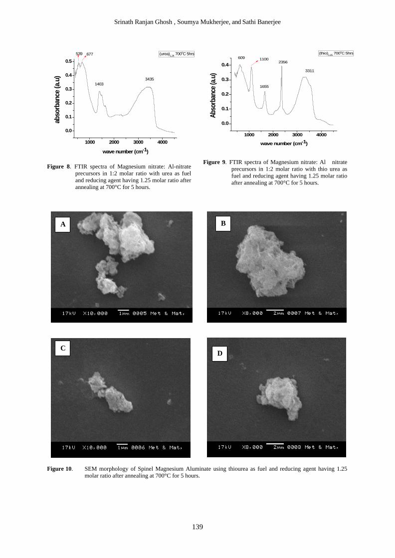
Srinath Ranjan Ghosh , Soumya Mukherjee, and Sathi Banerjee
139
1000 2000 3000 4000
0.0
0.1
0.2
0.3
0.4
0.5ab
sorb
ance
(a.u
)
wave number (cm-1)
(urea)1,25 700oC 5hrs539 677
14033435
Figure 8. FTIR spectra of Magnesium nitrate: Al-nitrate
precursors in 1:2 molar ratio with urea as fuel and reducing agent having 1.25 molar ratio after annealing at 700°C for 5 hours.
1000 2000 3000 4000
0.0
0.1
0.2
0.3
0.4
Abso
rban
ce (a
.u)
wave number (cm-1)
(thio)1.25 700oC 5hrs1100609
1655
2356
3311
Figure 9. FTIR spectra of Magnesium nitrate: Al nitrate
precursors in 1:2 molar ratio with thio urea as fuel and reducing agent having 1.25 molar ratio after annealing at 700°C for 5 hours.
Figure 10. SEM morphology of Spinel Magnesium Aluminate using thiourea as fuel and reducing agent having 1.25 molar ratio after annealing at 700°C for 5 hours.
A
D C
B
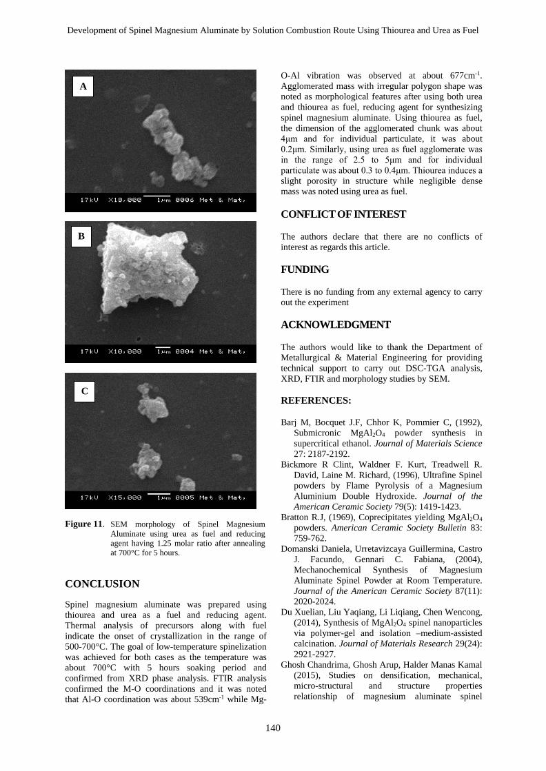
Development of Spinel Magnesium Aluminate by Solution Combustion Route Using Thiourea and Urea as Fuel
140
Figure 11. SEM morphology of Spinel Magnesium Aluminate using urea as fuel and reducing agent having 1.25 molar ratio after annealing at 700°C for 5 hours.
CONCLUSION
Spinel magnesium aluminate was prepared using thiourea and urea as a fuel and reducing agent. Thermal analysis of precursors along with fuel indicate the onset of crystallization in the range of 500-700°C. The goal of low-temperature spinelization was achieved for both cases as the temperature was about 700°C with 5 hours soaking period and confirmed from XRD phase analysis. FTIR analysis confirmed the M-O coordinations and it was noted that Al-O coordination was about 539cm-1 while Mg-
O-Al vibration was observed at about 677cm-1. Agglomerated mass with irregular polygon shape was noted as morphological features after using both urea and thiourea as fuel, reducing agent for synthesizing spinel magnesium aluminate. Using thiourea as fuel, the dimension of the agglomerated chunk was about 4μm and for individual particulate, it was about 0.2μm. Similarly, using urea as fuel agglomerate was in the range of 2.5 to 5μm and for individual particulate was about 0.3 to 0.4μm. Thiourea induces a slight porosity in structure while negligible dense mass was noted using urea as fuel.
CONFLICT OF INTEREST
The authors declare that there are no conflicts of interest as regards this article. FUNDING
There is no funding from any external agency to carry out the experiment ACKNOWLEDGMENT
The authors would like to thank the Department of Metallurgical & Material Engineering for providing technical support to carry out DSC-TGA analysis, XRD, FTIR and morphology studies by SEM. REFERENCES:
Barj M, Bocquet J.F, Chhor K, Pommier C, (1992), Submicronic MgAl2O4 powder synthesis in supercritical ethanol. Journal of Materials Science 27: 2187-2192.
Bickmore R Clint, Waldner F. Kurt, Treadwell R. David, Laine M. Richard, (1996), Ultrafine Spinel powders by Flame Pyrolysis of a Magnesium Aluminium Double Hydroxide. Journal of the American Ceramic Society 79(5): 1419-1423.
Bratton R.J, (1969), Coprecipitates yielding MgAl2O4 powders. American Ceramic Society Bulletin 83: 759-762.
Domanski Daniela, Urretavizcaya Guillermina, Castro J. Facundo, Gennari C. Fabiana, (2004), Mechanochemical Synthesis of Magnesium Aluminate Spinel Powder at Room Temperature. Journal of the American Ceramic Society 87(11): 2020-2024.
Du Xuelian, Liu Yaqiang, Li Liqiang, Chen Wencong, (2014), Synthesis of MgAl2O4 spinel nanoparticles via polymer-gel and isolation –medium-assisted calcination. Journal of Materials Research 29(24): 2921-2927.
Ghosh Chandrima, Ghosh Arup, Halder Manas Kamal (2015), Studies on densification, mechanical, micro-structural and structure properties relationship of magnesium aluminate spinel
A
B
C

Srinath Ranjan Ghosh , Soumya Mukherjee, and Sathi Banerjee
141
refractory aggregates prepared from Indian magnesite. Materials Characterization 99: 84-91.
Ghosh S.R, Mukherjee S, Banerjee S (2018), Solution combustion synthesis of Alumina spinel and its characterization. Interceram 67: 34-41.
Gorshkov V.A, Miloserdov P.A, Yukhvid V. I, Sachkova N.V, Kovalev I.D, (2017), Preparation of magnesium aluminate spinel by self propagating high temperature synthesis metallurgy methods. Inorganic Materials 53: 1046-1052.
Habibi Narges, Wang Yuan, Arandiyan Hamidreza, Rezaei Mehran (2017), Low temperature synthesis of mesoporous nanocrystalline magnesium aluminate (MgAl2O4) spinel with high surface area using a novel modified sol-gel method. Advanced Powder Technology 28: 1249-1257.
Lee P.Y, Suematsu H, Yano T, Yatsui K, (2006), Synthesis and Characterization of nanocrystalline MgAl2O4 spinel by polymerized complex method. Journal of Nanoparticle Research 8: 911-917.
Macêdo Maria laponeide Fernandes, Bertran Celso Aparecido, Osawa Carla Cristiane, (2007), Kinetics of the γ → α-alumina phase transformation by quantitative X-ray diffraction. Journal of Materials Science 42: 2830–2836. https://doi.org/10.1007/s10 853-006-1364-1
Marakkar Kutty P V, Dasgupta Subrata (2013), Low temperature synthesis of nanocrystalline magnesium aluminate spinel by a soft chemical method. Ceramics International 39(7): 7891-7894.
Mukherjee Soumya, (2020), Evolution of Spinel Magnesium Aluminate by Combustion route using Glycine as Fuel and its characterization. International Journal of Emerging Trends in Science and Technology 6(1): 24-27.
Nassar Y. Mostafa, Ahmed S. Ibrahim, Samir Ihab (2014), A novel synthetic route for magnesium aluminate (MgAl2O4) nanoparticles using sol-gel
auto combustion method and their photocatalytic properties. Spectrochimica Acta Part A: Molecular and Biomolecular Spectroscopy 131: 329-334.
Păcurariu C, Lazău I, Ecsedi Z, Lazău R, Barvinschi P, Mărginean G, (2007), New Synthesis methods of MgAl2O4 spinel. Journal of the European Ceramic Society 27: 707-710.
Pommier C, Chhor K, Bocquet J.F, Barj M, (1990), Reactions in supercritical fluids, a new route for oxide ceramic powder elaboration, synthesis of the spinel MgAl2O4. Materials Research Bulletin 25(2): 213-221.
Saberi Ali, Golestani-Fard Farhad, Sarpoolaky Hosein, Willert Porada Monika, Gerdes Thorsten, Simon Reinhard (2008), Chemical synthesis of nanocrystalline magnesium aluminate spinel via nitrate-citrate combustion route. Journal of Alloys and Compounds 462: 142-146.
Salem Shiva (2015) Application of autoignition technique for synthesis of magnesium aluminate in nano scale: Influence of starting solution pH on physico-chemical characteristics of particles. Materials Chemistry and Physics 155(1): 59-66.
Torkian Leila, Amini M Mostafa, Bahrami Zohreh, (2011), Synthesis of Nano Crystalline MgAl2O4 powder by Microwave assisted combustion. Journal of Inorganic Materials 26(5): 550-554.
Varnier Olivier, Hovnanian Nadine, Larbot André, Bergez Pierre, Cot Louis, Charpin Jean, (1994), Sol-gel synthesis of magnesium aluminum spinel from a heterometallic alkoxide. Materials Research Bulletin 29(5): 479-488.
Yang Ning, Chang Li, (1992), Structural inhomogenity and crystallization behavior of aerosol reacted MgAl2O4 powders. Materials Letters 15(1-2): 84-88.

Notes for Authors
MANUSCRIPT PREPARATION
Length of Manuscript Papers submitted for publication in TJER could be up to ten printed A4 pages single-spaced double column font size 12. The template for MS-WORD as per TJER format maybe downloaded from http://www.tjer.net. It is advisable that authors use this template in order to reduce the amount of time spent on typesetting the manuscript. The font sizes and the manuscript specifications are outlined as follows. Typing and Font SpecificationManuscripts should be typed double-spaced on one side of a sheet only, with margins of about 2.5 cm on each side of each page. The font should be Times New Roman for all the components of the manuscript with font size of 12 pt and regular attribute for the body of the text. Elements of the ManuscriptFull length papers generally consist of the title, author(s) affiliation(s), abstract, keywords, nomenclature if applicable, introduction, body, conclusion, references, list of figures and table captions, and original figures and tables for reproduction. A paper may also include appendices and acknowledgment. Titles Capitalize the first letter of each word, i.e. use title case. Author Names and Affiliation(s). Author names on technical papers should include the name of each author followed by his/her company affiliation. If two or more authors have the same company affiliation, it should not be repeated after each name. Do not use titles such as Mr., Mrs., Ms., Miss, Prof. or Dr. AbstractThe abstract should be limited to 250 words and must concisely state what was done, how it was done, principal results, and their significance. The abstract will appear later in various indices of abstracts and should contain the most critical information within the paper. KeywordsLeave two blank lines after the abstract and type 6-10 keywords and phrases (separated by semicolons";") that can be used to index the paper, listing the keywords in order of importance for indexing. Do not repeat words or strings of words from the title. Capitalize the first letter of each word. ConclusionPlease include a brief summary of the main points of the paper, do not replicate the abstract as the conclusion, and consider elaborating on the translational importance of the work or suggest applications and extensions. Confilct of interestThe authors declare no conflicts of interest.AcknowledgmentThe authors would like to acknowledge the University of Malaya Research Grant UMRG (RP034D-15AET) and University of Technology- Iraq for funding this research.Acknowledgment The same format as the body of the text should be followed. NomenclatureA separate nomenclature section should list in detail the symbols used in the manuscript, their definitions, and their units in SI system. The nomenclature list should be an alphabetical order with Greek symbols following the alphabetical listing. Subscripts and superscripts should follow Greek symbols and should be identified with a heading.
References The references should be included at the end of the manuscript in a separate section named References without a number. All references must be listed alphabetically by the last name of the first author. Ensure that the reference information is complete and accurate, including as necessary and in the following order: first names and initials of all authors; year of publication; title of paper, report, or book chapter (in quotes); title of book or periodical (in italics); volume and issue numbers; name and location of publisher (for books), name and location of publisher or sponsor (for proceedings), or city of publication and inclusive page numbers. Figures All figures must be cited in the body of the paper. Figures should be numbered in Arabic numerals in the order in which they are cited. Related figures or figure sections may be labeled with a shared numeral and consecutive lowercase letters (eg. Figs. 1a through 1d). Figures should be the smallest size possible without loss of clarity, preferably designed to occupy a single column (7.7 cm of width) of a printed journal page. Once the paper is accepted for publication, separate file for each figure in .tif or .tiff format is to be submitted to the technical editor for final printing. Tables All tables must be cited in the body of the paper. Tables should be numbered in Arabic numerals in the order they are cited in the paper. Tables should be the smallest size possible without loss of clarity. Table headings and column headings should be as concise as possible. Column alignment should be obtained using tabs NOT spaces. Tables should be designed to occupy a single column or the full width of the page. Care should be taken to avoid any arrangement that unduly increases the depth of a table. Use 10-point Times New Roman bold, centered, for table headings and 10- point Times New Roman for body in tables. Mathematical Notations and Equations To avoid errors in editing and typesetting, authors should clearly identify subscripts, superscripts, Greek letters, and other symbols. Equations should be numbered using Arabic numerals placed in parentheses. Break equations to fit within the page. Avoid ambiguities in equations and fractions in text through careful use of parentheses, brackets, solids (slants), etc. Note that in-text, fractions are usually “broken down” to fit in one line and confusion can result if terms are not properly labeled. The conventional order of brackets is {[0]}. Units and Abbreviations The International System of Units (SI units) is required. Unit symbols should be used with measured quantities, i.e. 1 mm, but not when unit names are used in text without quantities, i.e. “a few millimeters.” Acronyms and abbreviations should be defined the first time they are used in the text.
Publication ethics: Committee on Publication Ethics (COPE) will be followed. http://publicationethics.org
Creative Commons: CC BY-ND: This license allows for redistribution, commercial and non-commercial, as long as it is passed along unchanged and in whole, with credit to you. Content from this any work may be used under the terms of the Creative Commons Attribution 3.0 licence. Any further distributiuon of this work must maintain attribution to the author(s) and the title of the work, journal citation and DOI.

مجلة البحوث الهندسية
مجلس النشر الأكاديمي
محمد الصقري د.
إبراهيم متولي .د.أمحمد صلاح الدين خان .د.أ
رئیس مجلس النشر الأكادیمي أ.د. یحیى الوھیبي
أ.د. لمك بن محمد اللمكي أ.د. عبدالله امبوسعیدي
أ.د. شفور رحمان
الفاضل جمال الغيلاني
مجلس التحرير
رئیس ھیئة التحریر أ.د. إبراھیم متولي
قسم ھندسة الكھرباء والحاسب الآلي جامعة السلطان قابوس، سلطنة عمان
ھیئة التحریر (جامعة السلطان قابوس، سلطنة عمان)
محرر أ.د. فاروق صبري مجلي
قسم ھندسة النفط والكیمیاء جامعة السلطان قابوس، سلطنة عمان
قسم الھندسة المدنیة والمعماریة أ.د. علي بن سالم الحارثي
أ.د. خلیفة بن سیف الجابري أ.د. عونى شعبان
أ.د. علي بن سعید النعیمي د. أحمد سنا
د. شریف الجمل د. یحیى الحاج محمد زین
قسم ھندسة الكھرباء والحاسب الآلي أ.د. عبدالله بن حمد البادي
أ. د. أفاق أحمد د. محمد حمدان البادي
د. حسن عبدالحلیم یوسف د. الأزھر خریجي
قسم الھندسة المیكانیكیة والصناعیة ءأ.د. تسنیم برفیز أ.د. سید زاھد قمر
د. عامر بن سالم الیحمدي د. خالد زبده
د. نبیل بن زھران الرواحي د. ناصر بن أحمد العزري د. نصر بن حمود الھنائي
قسم هندسة النفط والكيمياء
المعمري سالم بن راشد د..أ
نجاد فكيلي رضا غلام. دأ. المحتسب حامد علاء. د
اللطيف حسن عبد حسن. د
الوضاحيبن أحمد ماجد. د
الدولي الاستشاري التحرير مجلس
والمعمارية المدنية الهندسة قسم
عماد القاضي، الولايات المتحدة الأمريكية. د.أ
الأمريكية المتحدة الولايات لؤي محمد،. د.أ
أستراليا فجايا رانكان،. د.أ
قسم هندسة الكهرباء والحاسب الآلي أستراليا شم ناير،. د.أ
المملكة العربية السعوديةمحمود داوود، .د.أ نوبيوكي ماتسو، اليابان .د.أ
قسم الهندسة الميكانيكية والصناعية
أفشن غجار، الولايات المتحدة الأمريكية. د.أ
المملكة العربية السعوديةاحمد القرني، . د.أ
كندا بسام جبران،. د.ا
كانول، المكسيك-مارتن بش. د.أ أ.د. محمت سفسار، الكويت
أ.د. مصطفى يعقوب، كندا
الأمريكية المتحدة الولايات يلديرم عمرتاك،. د.أ
النفط والكيمياءقسم هندسة الهند جي كوبتا،. د.أ
أ.د. محمت هاستكلو، تركيا
المملكة العربية السعوديةأ.د. رمضان كهرمان،
أ.د. ريتشارد كورف، ألمانيا
صامويل كوزيتز، الولايات المتحدة الأمريكية. د.أ
ترجيي إرتكن، الولايات المتحدة الأمريكية. د.أ
إدارة المجلة
الفاضل عبدالحمید عبدالله النظیري