the impacts of congestion on commercial vehicle tours

Figliozzi 1

The Impacts of Congestion on Commercial Vehicle Tours

Miguel Andres Figliozzi

Portland State University

Maseeh College of Engineering and Computer Science

[email protected]

5124 words + 7 Tables + 2 Figures = 7374

mailto:[email protected]

Figliozzi 2

THE IMPACTS OF CONGESTION ON COMMERCIAL VEHICLE TOURS

Miguel Andres Figliozzi

ABSTRACT

Congestion is a common phenomenon in all major cities of the world. Increased travel time and

uncertainty brought about by congestion impacts the efficiency of logistics operations. Recent studies

indicate that a significant proportion of commercial vehicle kilometers traveled (VKT) and vehicle hours

traveled (VHT) are generated by trip-chains or multi-stop tours. This paper presents research

demonstrating the impact of congestion on multi-stop tours in urban areas. An analytical model,

numerical experiments, and real-world tour data are used to understand the impact of congestion on tour

characteristics, carriers’ costs, VKT, and VHT. This research shows that travel time/distance between

customer and depot is a crucial factor that exacerbates the negative impacts of congestion. Travel time

variability is not as significant when the travel time between the depot and the customers is small in

relation to the maximum tour duration and when the routes are not highly constrained. As congestion

increases, the number of vehicles needed to complete the tour also increases. This is accompanied by an

increase in the percentage of total driving time and the average distance travelled per customer.

Congestion impacts on carriers’ costs are also considerable since congestion not only increases carriers’

operating costs but also affects carriers’ cost structure. As congestion worsens the relative weight of labor

costs – wages and overtime – escalates. This paper categorizes tours into three classes based on tour

efficiency and the relative weight of time and distance related costs. These are intuitive and valuable tools

to monitor congestion, represent real-world tour data, and classify tours in regards to their sensitivity to

congestion.

KEYWORDS: Congestion Modeling, Carrier Costs, Urban Freight, City Logistics

Figliozzi 3

1. Introduction

Increased travel times and the uncertainty brought about by congestion impacts the efficiency of logistics

operations. Direct and indirect costs associated with congestion have been widely studied and reported.

Most of the studies have focused on passengers’ value of travel time, shippers’ value of time and market

access costs, production costs, and labor productivity costs (Weisbrod et al., 2001). However, the

modeling and study of the specific impacts of urban congestion on commercial vehicle tours have

received scant attention. The lack of studies is largely explained by lack of disaggregated and

comprehensive commercial vehicle data, which due to privacy or competitive reasons, is expensive to

collect or unattainable at the desired level of detail.

This research studies the impact of congestion on commercial vehicle tours in urban areas. Recent studies

indicate that a high proportion of urban commercial vehicle kilometers traveled (VKT) originate at

distribution centers (DC), warehouses, or depots (Cambridge Systematics, 2003, Outwater et al., 2005)

and constitute trip-chains or multi-stop tours. Commercial vehicle tours are ubiquitous in urban areas; for

example, in Denver approximately 50% of single and combination truck tours include 5 to 23 stops per

tour (Holguin-Veras and Patil, 2005). The terms “route”, “tour”, and “trip-chain” are used

interchangeably in this research to designate the activity of a commercial vehicle that starts at a depot,

visits one or more customers, and then returns to the depot; for the sake of brevity the word tour is used

herein.

This research contributes to the understanding of the impacts of congestion on commercial vehicle tours.

The specific contributions of this research are threefold: a) it presents an analytical model to understand

the impact of congestion on tour characteristics and costs, b) it discusses congestion costs from a carrier’s

perspective, c) it uses a novel and intuitive classification of urban distribution tours according to their

efficiency and susceptibility to congestion. Real-life disaggregated tour data is also analyzed to validate

analytical insights of the model.

The research is organized as follows: section two provides a literature review of congestion impacts on

carrier operations and costs. Section three introduces a model to analyze the impacts of congestion on

commercial vehicle tours. Section four presents analytical insights for time constrained tours. Section five

contains a numerical analysis and discusses tour efficiency. Section six discusses the impact of

Figliozzi 4

congestion on carriers’ costs. Section seven examines real-life tour data; it also proposes a classification

of tours based on their efficiency and vulnerability to congestion. Section eight ends with conclusions.

2. Literature Review

It is widely recognized that congestion seriously affects logistics operations. McKinnon (1999) presents

the results of in-depth interviews with DC managers and discusses the negative effects of congestion on

logistics operations. Direct and indirect costs of congestion on passengers’ travel time, shippers’ travel

time and market access, production, and labor productivity have been widely studied and reported. For a

systematic review of this congestion literature the reader is referred to the work of Weisbrod et al. (2001).

Sizeable progress has been made in the development of econometric techniques to study the joint

behavior of carriers and shippers in regards to congestion (Hensher and Puckett, 2004, Hensher and

Puckett, 2005).

Survey results suggest that the type of freight operation has a significant influence on how congestion

affects carriers’ operations and costs. Data from a California survey indicate that congestion is perceived

as a serious problem for companies specializing in LTL (less-than-truckload), refrigerated, and

intermodal cargo (Golob and Regan, 2001). In addition, Golob and Regan (2003) found a positive

relationship between the level of local congestion and the purchase of routing software. Carriers that do

not follow regular routes, e.g. for-hire carriers, tend to place a higher value on the usage of real-time

information to mitigate the effects of congestion (Golob and Regan, 2005).

Another branch of the literature models the relationship between industrial/commercial procurement and

congestion. The negative impact of just-in-time (JIT) production on vehicle trip generation has been

analyzed and modeled (Rao et al., 1991, Moinzadeh et al., 1997). Using data from Auckland, New

Zealand, Sankaran et al (2005) study the impact of congestion and replenishment order sizes on carriers

with time-definite deliveries. Sankaran and Wood (2007) continues this work and presents a model using

Daganzo’s (1984, 1991) approximations to routing problems. For problems where routes have 10 or more

deliveries Sankaran and Wood (2007) indicate that congestion costs increase with the average number of

rounds per day and decrease with the workday length, the square root of the number of deliveries, and

that congestion is invariant with fixed or variable stop times.

Routing constraints limit the number and characteristics of the feasible set of tours that carriers can use to

meet customer demand. Figliozzi (2006) models tour constraints using Daganzo’s (1991) approximations

Figliozzi 5

to routing problems and analyzes how constraints and customer service time affect trip generation using

a tour classification based on supply chain characteristics and route constraints. Building on this work,

Figliozzi (2007) proposes an analytical framework to study the impact of policy or network changes on

urban freight VKT; the model shows that a decrease in travel speed severely affects tours with time

window constraints while capacity constrained tours are less affected. Figliozzi (Figliozzi, 2007) also

indicates that changes in both VKT and vehicle hours traveled (VHT) differ by type of tour and routing

constraint.

Confidentiality issues are usually an insurmountable barrier that precludes the collection of detailed and

complete freight data. To the best of the author’s knowledge, all freight congestion studies present

aggregated data with the exception of Figliozzi et al. (2007) where several months of detailed truck

activity have been analyzed And the disaggregated tour data was used to reveal tour characteristics, speed

variability, and data collection challenges.

Transportation agencies are increasingly using travel time reliability as a congestion measure (Chen et al.,

2003); reliability is often associated to a “buffer time index” (Lomax et al., 2003, Bremmer et al., 2004).

The buffer time index represents the extra time a traveler needs to allow in order to arrive on time 95

percent of the time. Carriers also use buffers to mitigate the effects of travel time or demand variability.

Reliability as a constraint or objective has also been incorporated in operations research models where

routes and service areas are designed using continuous approximations (Erera, 2000, Novaes et al., 2000)

or on stochastic programming (Laporte and Louveaux, 1993, Kenyon and Morton, 2003). In particular,

Erera (2000) proposes continuous approximations to estimate expected detour and distances in stochastic

version of the capacitated vehicle routing problem. To the best of the author’s knowledge, no model has

been developed to study the impacts of congestion on tour characteristics, costs, and VKT/VHT.

3. The Tour Model

This research considers a system with one DC or depot and customers. A tour is defined as the closed

path that a truck follows from its depot to visit one or more customers in a sequence before returning to

its depot during a single driver shift. A tour is comprised of several trips; a trip is defined by its origin and

destination and characterized by its distance and travel time attributes. The expression used to

approximate the length of a set of tours starting and ending at the depot is:

n

( ) 2 ln ml n rm k an

n−

= + (1)

Figliozzi 6

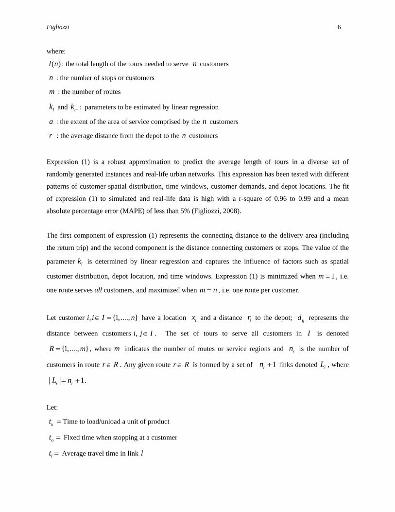
where:

( )l n : the total length of the tours needed to serve customers n

n : the number of stops or customers

m : the number of routes

lk and : parameters to be estimated by linear regression mk

a : the extent of the area of service comprised by the customers n

r : the average distance from the depot to the customers n

Expression (1) is a robust approximation to predict the average length of tours in a diverse set of

randomly generated instances and real-life urban networks. This expression has been tested with different

patterns of customer spatial distribution, time windows, customer demands, and depot locations. The fit

of expression (1) to simulated and real-life data is high with a r-square of 0.96 to 0.99 and a mean

absolute percentage error (MAPE) of less than 5% (Figliozzi, 2008).

The first component of expression (1) represents the connecting distance to the delivery area (including

the return trip) and the second component is the distance connecting customers or stops. The value of the

parameter is determined by linear regression and captures the influence of factors such as spatial

customer distribution, depot location, and time windows. Expression

lk

(1) is minimized when 1m = , i.e.

one route serves all customers, and maximized when m n= , i.e. one route per customer.

Let customer have a location , {1,...., }i i I n∈ = ix and a distance to the depot; represents the

distance between customers

ir ijd

,i j I∈ . The set of tours to serve all customers in I is denoted

{1,...., }R m m

r R∈

= , where indicates the number of routes or service regions and is the number of

customers in route . Any given route

rn

r R∈ is formed by a set of 1rn + links denoted , where

.

rL

| |r rL n= 1+

Let:

ut = Time to load/unload a unit of product

ot = Fixed time when stopping at a customer

lt = Average travel time in link l

Figliozzi 7

=

flt = Free-flow travel time in link l

/l l ls d t= Average travel speed in link l

s = Average travel speed in any given route r

lσ = Standard deviation of the travel time in link l

/l l ltυ σ= = Coefficient of variation in link l

klρ = Correlation between the distributions of travel time in links and k l

w = Tour duration constraint

b = Vehicle capacity

iq = Amount delivered at customer , {1,...., }i i I n∈ =

rq = Average amount delivered per customer in route , such that r r rn q b≤

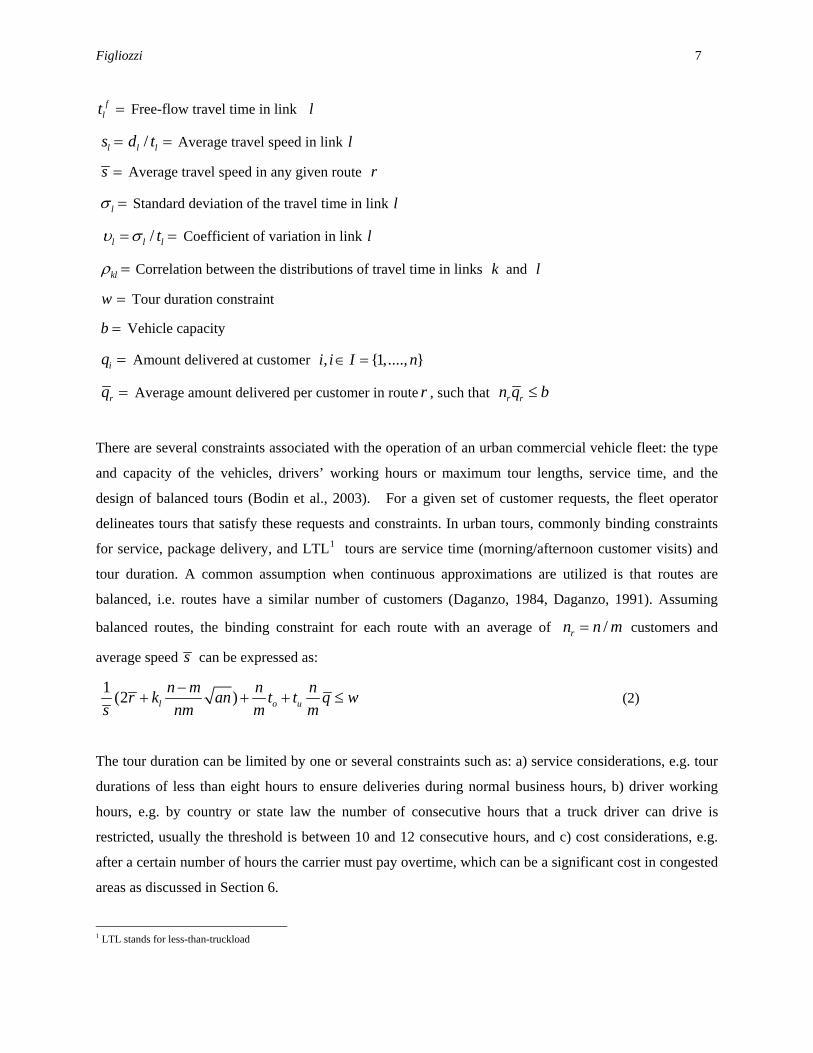
There are several constraints associated with the operation of an urban commercial vehicle fleet: the type

and capacity of the vehicles, drivers’ working hours or maximum tour lengths, service time, and the

design of balanced tours (Bodin et al., 2003). For a given set of customer requests, the fleet operator

delineates tours that satisfy these requests and constraints. In urban tours, commonly binding constraints

for service, package delivery, and LTL1 tours are service time (morning/afternoon customer visits) and

tour duration. A common assumption when continuous approximations are utilized is that routes are

balanced, i.e. routes have a similar number of customers (Daganzo, 1984, Daganzo, 1991). Assuming

balanced routes, the binding constraint for each route with an average of customers and

average speed

/rn n m=

s can be expressed as:

1 (2 )l o un m n nr k an t t q w

s nm m m−

+ + + ≤

(2)

The tour duration can be limited by one or several constraints such as: a) service considerations, e.g. tour

durations of less than eight hours to ensure deliveries during normal business hours, b) driver working

hours, e.g. by country or state law the number of consecutive hours that a truck driver can drive is

restricted, usually the threshold is between 10 and 12 consecutive hours, and c) cost considerations, e.g.

after a certain number of hours the carrier must pay overtime, which can be a significant cost in congested

areas as discussed in Section 6.

1 LTL stands for less-than-truckload

Figliozzi 8

4. Analysis of the Impact of Congestion on Duration Constrained Tours

The impact of congestion on distribution tours can be broken down into three cases: (a) the increase in

average travel time, (b) the increase in travel time variability, and (c) the interaction effect between a

simultaneous increase in average travel time and variability. A constraint coefficient is defined to control

for the relative impact of congestion on routing constraints for each customer.

(a) Increase in average travel time – no uncertainty

An increase in average travel time can be expressed by a coefficient 1lα ≥ that reflects the travel time

increase with respect to the free-flow travel time:

flt tlα= and

1 fls slα= (3)

By using this coefficient, expression (2) can be restated as:

(2 )l o uf

n m n nr k an t t q ws nm m mα −

+ + + ≤ (4)

If travel time increases and the tour duration constraint (4) is violated, the number of routes, , increases

to restore feasibility. An increase in average travel time increases not only driving time but may also

distance the number of tours and the total distance traveled. Therefore, the direct impact on VHT alone is

insufficient to describe the effects of congestion; the impact on VKT must also be considered. However,

for any given

m

α , the percentage-wise increase in VHT is always larger than the percentage-wise increase

in VKT. If percentage time driving is calculated as the ratio between time driving and tour duration, then

an increase in average travel time increases the percentage time driving whereas the customer time is

unaffected.

(b) Increase in travel time variability

If the travel times are not constant, the buffer r zσ must be added to (2) in order to guarantee a customer

service level:

1 (2 / )l o un m n nr k an m t t q w z

s n m m rσ−

+ + + ≤ − (5)

Assuming normally distributed travel times, the coefficient is related to the probability of completing

the tour within the allowed tour duration. The route travel time standard deviation can be expressed as:

z

Figliozzi 9

2

1

1 ,r

r

n

r k kl k lk L k

l k k l Lσ σ ρ σ σ∈ =

= + = +∑ ∑ r∈ (6)

Unlike previous studies and modeling approaches, the correlation between travel times is included

because empirical data suggests that a positive correlation may not be negligible (Figliozzi et al., 2007).

To minimize costs, a carrier will reduce the number of vehicles needed as well as the total route length-

duration without violating customer service constraints. For a given set of customers and depots, this is

equivalent to minimizing the number of routes subject to constraint (5).

The route travel time variance, expression (6), grows with the number of customers per route or with an

increase in variability (variances are non-negative numbers). An increase in travel time variability affects

the right-hand term of expression (5) which is decreased by the term r zσ . This may lead to a violation of

the constraint and therefore must increase in order to restore feasibility. Average route durations

decrease when the buffer increase makes expression

m

(5) binding and increases. Hence, on average,

route durations shorten but the sum of the route duration plus the buffer tends to remain constant. Despite

this, route duration variability increases. Unlike case (a), only if increases, distance traveled, time

driving, and percentage time driving are increased whereas average driving speed does not change but

effective speed may increase.

m

m

(c) Interaction effect between a simultaneous increase in travel time and variability

If there is an increase in congestion and average travel time increases while the coefficient of variation

remains constant the impact of congestion is amplified. A widespread approach to indicate the degree of

uncertainty in the distribution of a random variable is to calculate the coefficient of variation. Assuming

normal distributions and using coefficients of variations υ , expression (6) can be restated as:

2

1( ) 1 ,

r

r

n

r k k kl k k l lk L k

t t t l k kσ υ ρ υ υ∈ =

= + = +∑ ∑ rl L∈

r

Assuming a constant coefficient of variations, ,k l k l Lυ υ υ= = ∀ ∈ , then:

2

11 ,

r

r

n

r k kl k lk L k

t t t l k k lσ υ ρ∈ =

= + = +∑ ∑ rL∈ (7)

Figliozzi 10

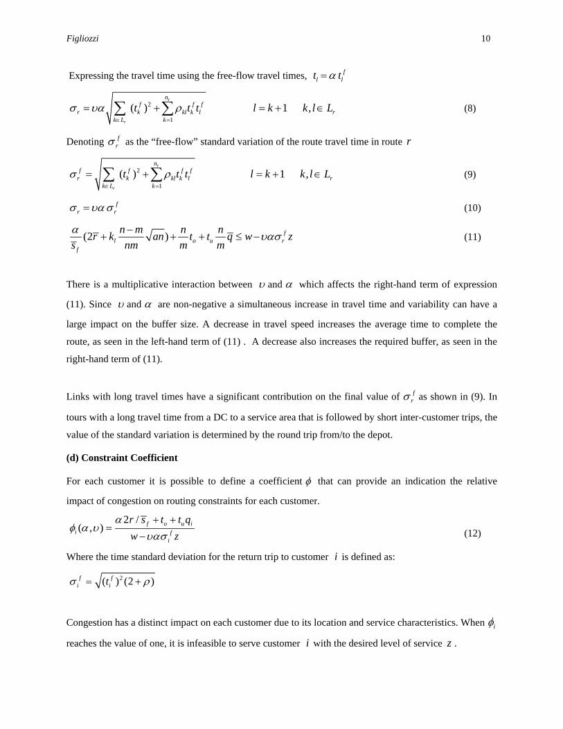
Expressing the travel time using the free-flow travel times, f

l lt tα=

2

1( ) 1 ,

r

r

nf f f

r k kl k lk L k

t t t l k k lσ υα ρ∈ =

= + = +∑ ∑ rL∈ (8)

Denoting frσ as the “free-flow” standard variation of the route travel time in route r

2

1( ) 1 ,

r

r

nf f f f

r k kl k lk L k

t t t l k k lσ ρ∈ =

= + = +∑ ∑ rL∈ (9)

fr rσ υασ= (10)

(2 ) fl o u

f

n m n nr k an t t q w zs nm m m rα υασ−

+ + + ≤ − (11)

There is a multiplicative interaction between υ and α which affects the right-hand term of expression

(11). Since υ and α are non-negative a simultaneous increase in travel time and variability can have a

large impact on the buffer size. A decrease in travel speed increases the average time to complete the

route, as seen in the left-hand term of (11) . A decrease also increases the required buffer, as seen in the

right-hand term of (11).

Links with long travel times have a significant contribution on the final value of frσ as shown in (9). In

tours with a long travel time from a DC to a service area that is followed by short inter-customer trips, the

value of the standard variation is determined by the round trip from/to the depot.

(d) Constraint Coefficient

For each customer it is possible to define a coefficient φ that can provide an indication the relative

impact of congestion on routing constraints for each customer.

2 /( , ) f o u i

i fi

r s t t qw z

αφ α υ

υασ+ +

=− (12)

Where the time standard deviation for the return trip to customer is defined as: i

2( ) (2 )f fi itσ ρ= +

Congestion has a distinct impact on each customer due to its location and service characteristics. When iφ

reaches the value of one, it is infeasible to serve customer with the desired level of service i z .

Figliozzi 11

5. Sensitivity Analysis

To illustrate how changes in travel time affect tour characteristics as well as VHT/VKT, a sensitivity

analysis based on a real-world situation2 and tour data reported in the literature is performed. Tour data

from different cities indicate that the average number of stops per tour in urban areas is equal or greater

than 5 stops per tour: approximately 6 in Calgary (Hunt and Stefan, 2005), 5.6 in Denver (Holguin-Veras

and Patil, 2005), and 6.2 in Amsterdam (Vleugel and Janic, 2004). Customer service is highly related to

the number of operations to be performed and the number of pallets/packages to be loaded/unloaded;

service time can be as short as a few minutes (package delivery). In Amsterdam, unloading/loading time

per stop is 21 minutes on average; LTL data from Sydney indicate a median stop time 30 minutes and an

average time of approximately 40 minutes (Figliozzi et al., 2007).

Routing scenarios were constructed assuming a service area of 39.5 square kilometers containing 30

customers, a maximum tour duration of eight hours ( w =8), three different round trip distances to the

depot ( 2r = 25, 50, and 75 kilometers), four different coefficient of variations (υ = 0.0, 0.2, 0.4, and

0.6), and four customer service times ranging from 15 to 60 minutes ( o ut t q+ =15, 30, and 45 minutes).

Tours were designed using a construction and improvement routing heuristics for three average speeds:

50, 25 and 12.5 km/hr.

Average Speed

Service Time ( ) ct15 min 30 min 45 min

Tours 50 km/h

1.00 1.00 1.00 Driving Time 1.00 1.00 1.00 Distance 1.00 1.00 1.00 Tours

25 km/h 1.00 1.11 1.25

Driving Time 2.00 2.16 2.39 Distance 1.00 1.08 1.20 Tours

12.5 km/h 1.50 1.56 1.58

Driving Time 5.28 5.62 5.82 Distance 1.32 1.40 1.46

Table 1 – Average Increase Factors for different customer service times ( ) ct

The sensitivity to congestion as a function of customer service time is presented in Table 1. Each of the

sections contains the average3 increase factors with respect to free-flow speed and assuming 2r = 25 km, 2 Tour characteristics and scenarios are based on data presented in Figliozzi et al. (2007). The service area represents the industrial district of Bankstown in the city of Sydney, Australia. 3 The average among the three variability factors: 0.2, 0.4, and 0.6

Figliozzi 12

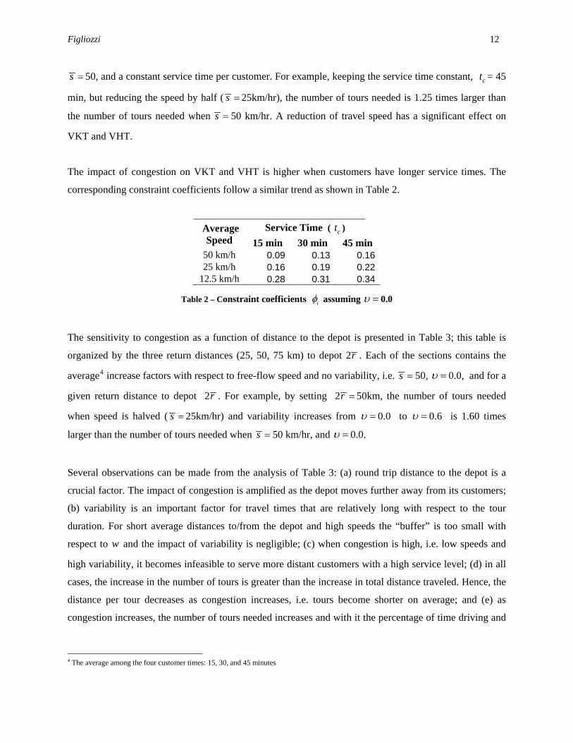
s = 50, and a constant service time per customer. For example, keeping the service time constant, = 45

min, but reducing the speed by half (

ct

s = 25km/hr), the number of tours needed is 1.25 times larger than

the number of tours needed when s = 50 km/hr. A reduction of travel speed has a significant effect on

VKT and VHT.

The impact of congestion on VKT and VHT is higher when customers have longer service times. The

corresponding constraint coefficients follow a similar trend as shown in Table 2.

Average Speed

Service Time ( ) ct15 min 30 min 45 min

50 km/h 0.09 0.13 0.1625 km/h 0.16 0.19 0.22

12.5 km/h 0.28 0.31 0.34

Table 2 – Constraint coefficients iφ assuming υ = 0.0

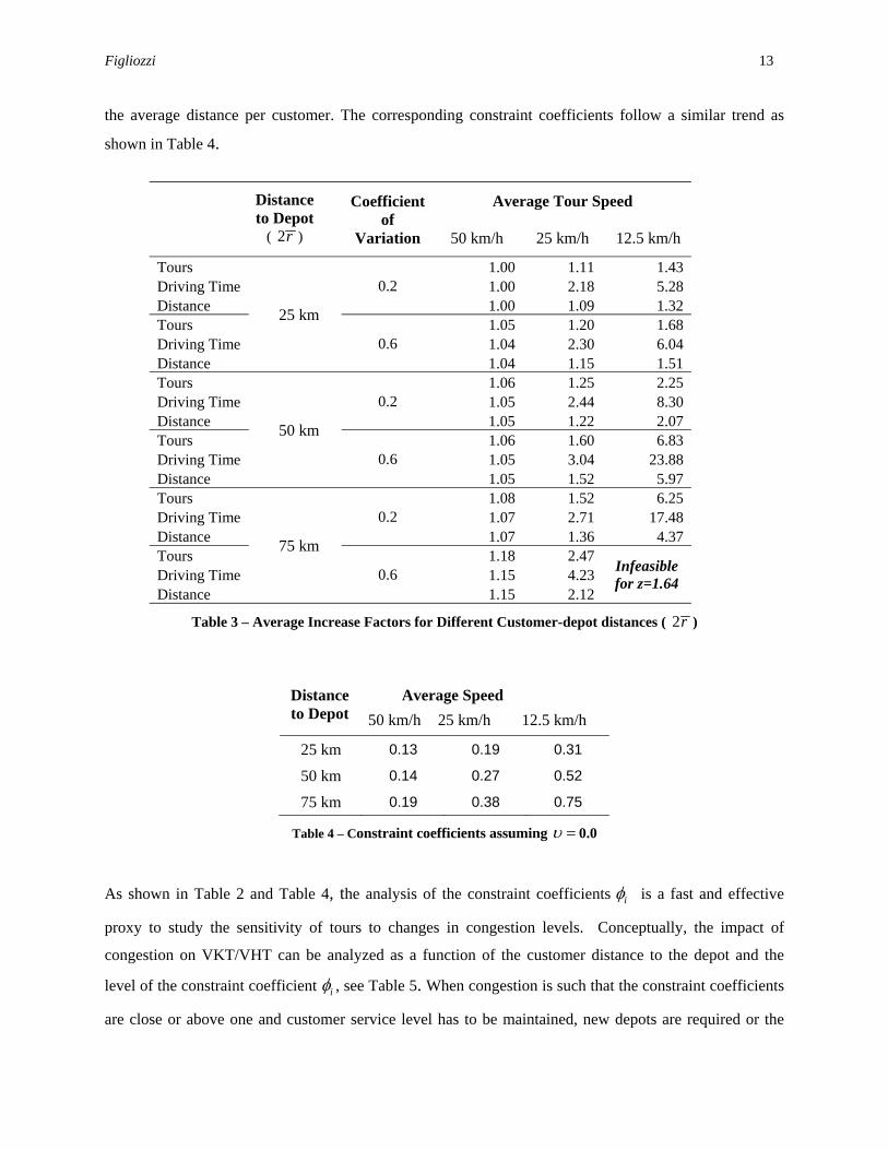
The sensitivity to congestion as a function of distance to the depot is presented in Table 3; this table is

organized by the three return distances (25, 50, 75 km) to depot 2r . Each of the sections contains the

average4 increase factors with respect to free-flow speed and no variability, i.e. s = 50, υ = 0.0, and for a

given return distance to depot 2r . For example, by setting 2r = 50km, the number of tours needed

when speed is halved ( s = 25km/hr) and variability increases from υ = 0.0 to υ = 0.6 is 1.60 times

larger than the number of tours needed when s = 50 km/hr, and υ = 0.0.

Several observations can be made from the analysis of Table 3: (a) round trip distance to the depot is a

crucial factor. The impact of congestion is amplified as the depot moves further away from its customers;

(b) variability is an important factor for travel times that are relatively long with respect to the tour

duration. For short average distances to/from the depot and high speeds the “buffer” is too small with

respect to and the impact of variability is negligible; (c) when congestion is high, i.e. low speeds and

high variability, it becomes infeasible to serve more distant customers with a high service level; (d) in all

cases, the increase in the number of tours is greater than the increase in total distance traveled. Hence, the

distance per tour decreases as congestion increases, i.e. tours become shorter on average; and (e) as

congestion increases, the number of tours needed increases and with it the percentage of time driving and

w

4 The average among the four customer times: 15, 30, and 45 minutes

Figliozzi 13

the average distance per customer. The corresponding constraint coefficients follow a similar trend as

shown in Table 4.

Distance to Depot

( 2r )

Coefficient of

Variation

Average Tour Speed

50 km/h 25 km/h 12.5 km/h

Tours

25 km

0.2 1.00 1.11 1.43


0.6 1.05 1.20 1.68


50 km

0.2 1.06 1.25 2.25


0.6 1.06 1.60 6.83


75 km

0.2 1.08 1.52 6.25


0.6 1.18 2.47

Infeasible for z=1.64 Driving Time 1.15 4.23

Distance 1.15 2.12

Table 3 – Average Increase Factors for Different Customer-depot distances ( 2r )

Distance to Depot

Average Speed 50 km/h 25 km/h 12.5 km/h

25 km 0.13 0.19 0.31

50 km 0.14 0.27 0.52

75 km 0.19 0.38 0.75

Table 4 – Constraint coefficients assuming υ = 0.0

As shown in Table 2 and Table 4, the analysis of the constraint coefficients iφ is a fast and effective

proxy to study the sensitivity of tours to changes in congestion levels. Conceptually, the impact of

congestion on VKT/VHT can be analyzed as a function of the customer distance to the depot and the

level of the constraint coefficient iφ , see Table 5. When congestion is such that the constraint coefficients

are close or above one and customer service level has to be maintained, new depots are required or the

Figliozzi 14

service of customers located far away from the depot must be transferred to another transport provider,

for example a third party logistics company (3PL).

Distance to Depot

Short Medium Long C

onst

rain

t

Coe

ffic

ient

Low

Low High

Very High

Approaching

Infeasibility H

igh

Medium

Very High

Approaching

Infeasibility

Use 3PL or

New Depot

Table 5 – Conceptual Impact of Congestion on VKT/VHT

6. Impact on Costs

Congestion not only increases carriers’ costs but also changes the relative weight of daily operational

costs such as fuel and labor needed per customer. Table 6 presents congestion related fuel and wage

increases as a function of travel speed and its coefficient of variation. The column named “total increase

factor” shows the total cost increase using as a base scenario a travel time of 50 km/h and no travel speed

variation. The columns named “service time”, “driving time”, and “fuel” respectively indicate their share

as a percentage of the total fuel plus labor costs5.

Average Tour

Speed

Coefficient of

Variation

Total increase Factor

Service Time

Driving Time Fuel

50 km/h 0.2 1.01 60% 13% 27% 0.6 1.02 58% 14% 28%

25 km/h 0.2 1.33 43% 24% 32% 0.6 1.50 38% 27% 36%

12.5 km/h 0.2 2.69 21% 40% 40% 0.6 6.49 8% 47% 45%

Table 6 –Impact of Congestion on Tour Costs

5 The fuel and labor costs were calculated using fuel consumption of a medium-size delivery truck of approximately three kilometers per liter of diesel at a cost of $1.25 per liter of diesel. Fuel consumption was increased to account for lower fuel efficiency at low speeds and congested driving conditions. Labor cost was assumed as $20 per driver hour. Return distance to distance was assumed to be 50 kilometers and the service time per customer 30 minutes.

Figliozzi 15

For a given number of customers served, total customer service time is not affected by congestion – i.e.

time spent at the customers’ locations does not change – whereas fuel and wages are directly affected by

the amount of VHT and VKT. As congestion increases, labor and fuel costs related to time and distance

driven become dominant. From a carrier’s perspective, the ultimate monetary impact of congestion

depends on how much a carrier can charge customers or pass on congestion costs along the supply chain.

If direct distance between distribution center and customer location is the main basis to price transport

services, carriers cannot readily and transparently transfer the costs brought about by congestion.

Table 6 does not include costs associated with the increases in fleet size needed for the increase in the

number of tours. In addition, for a carrier operating in an urban area, the costs of congestion may be

compounded by: (a) customer service employee time to handle customer complaints and rescheduling

issues; (b) stiff penalties due to JIT (just-in-time) late deliveries or the cost of large time-buffers; (c)

capital and operational costs of real time information systems, sophisticated vehicle routing and tracking

software needed to mitigate the impact of congestion (Regan and Golob, 1999); (d) tolls road usage to

avoid highly congested streets – trucks that come on/off main tolled highways several times a day to

access different delivery areas can accrue a significant toll cost (Figliozzi et al., 2007); and (e) parking

fees and/or the payment of traffic/parking fines in dense urban areas lacking loading zones (Morris et al.,

1998).

In transport or highway planning studies, commuter/passenger congestion costs are traditionally estimated

as the sum of three different components: 1) the product of the travel time delays and the value of time

per vehicle-driver, 2) a cost due to travel time unreliability, and 3) higher operating and environmental

costs. Carriers’ costs are harder to quantify; the impact of congestion is heavily dependent on network

(e.g. depot location), route type (e.g. number of stops and its density) and customer service characteristics

(e.g. time windows) that may greatly vary among carriers.

7. Real-world Tour Data Classification and Representation

This section relates the insights of previous sections to empirical tour data obtained from a company

based in Sydney, Australia. The company’s customers are located in several industrial suburbs of Sydney

and round trips between the depot and these industrial suburbs range between 14 to 40 kilometers. For

this particular distribution operation time windows are not an overriding concern; however, deliveries

must take place within the promised day. In addition, deliveries have to be carried out within normal

business hours (most customers prefer morning deliveries); therefore, the starting time of the tour and its

Figliozzi 16

length are constrained to meet this condition. This is clearly revealed in the tour data: 13% of the

deliveries took place before 8 am, 45% of the deliveries took place before 11 am, 76% of the deliveries

took place before 2 pm, and 99% of the deliveries took place before 5 pm. A detailed description and

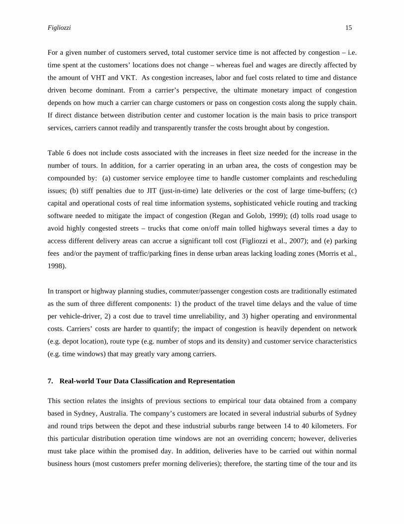
analysis of the tour data is presented in Figliozzi et al. (2007).

y = 1.3844x + 11.275R² = 0.8725

0

20

40

60

80

100

120

140

160

0 20 40 60 80

Tim

e D

riven

per

Sto

p (m

in)

Distance Travelled per Stop (km)

100

Figure 1 – Time and Distance per Customer Served

In many real-world distribution routes, to reduce distribution costs customers are served and clustered

according to their requirements and geographical location. At the disaggregate tour level, time driven and

distance driven per customer (or tour) are highly correlated as shown in Figure 1.

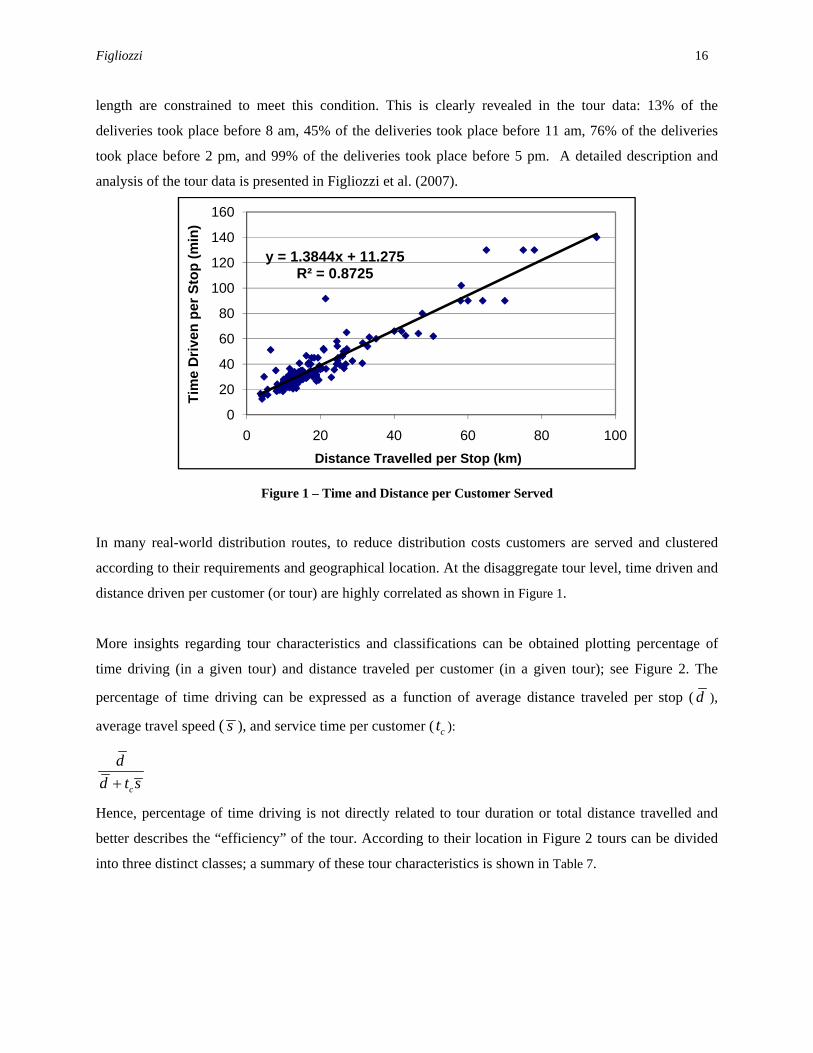
More insights regarding tour characteristics and classifications can be obtained plotting percentage of

time driving (in a given tour) and distance traveled per customer (in a given tour); see Figure 2. The

percentage of time driving can be expressed as a function of average distance traveled per stop ( d ),

average travel speed ( s ), and service time per customer ( ): ct

c

dd t s+

Hence, percentage of time driving is not directly related to tour duration or total distance travelled and

better describes the “efficiency” of the tour. According to their location in Figure 2 tours can be divided

into three distinct classes; a summary of these tour characteristics is shown in Table 7.

Figliozzi 17

0%

10%

20%

30%

40%

50%

60%

70%

80%

90%

0 10 20 30 40 50 60 70 80 90 100

% T

our T

ime

Driv

ing

Avg Distance Per Stop (Km)

IV. INFEASIBLE REGION

III. FEWEST STOPSFARTHER AWAY FROM

DEPOT

II. FEWER STOPSLARGER DELIVERY

AREA

I. MANYSTOPS

Figure 2 - Tour Classification by Percentage Time Driving and Distance Traveled per Stop

Class I tours, Figure 2 lower left, have many stops and a low percentage of the tour duration is spent

driving. The average driving speed is low because the percentage of local and access roads/streets used

increases with the number of customers visited. Despite the low average travel speed, tours are highly

efficient from the distributor perspective because many customers are served driving a short distance and

a low percentage of time is spent driving.

On the upper right section of the graph (Class III), tours have few stops and a high percentage of the tour

duration is spent driving. The tour distance is long because customers are located further away from each

other and/or the depot is far from the distribution area. Tour duration is high and very few customers can

be served. The average driving speed is high because the percentage of local and access roads/streets used

is small and main highways are used to connect the depot with the distribution area. Comparing delivery

costs, class III tours have a delivery cost per customer that is approximately 3 times higher than class I

tours. In addition, class III tours are more constrained; the average constraint coefficient for class I

customers is 0.20 whereas for class III customers is 0.49.

Class II tours are not as efficient as class I tours as the average distance per stop is significantly higher

because the density of stops is lower than in class I tours. Given that the daily design of tours is based on

what freight is available on a particular day, carriers cannot always utilize routes that are “tight” both in

terms of customer locations and total tour duration. In class II tours, more customers could have been

added to the tour if more demand had materialized. Finally, on the lower right section of the graph (Class

Figliozzi 18

IV or infeasible tours), below the feasibility boundary, there is an area where feasible tours cannot be

found at practical travel speeds.

Tour Class

% Time

Driving

Dist. per stop

(km) Stops

per Tour Tour

Duration (hr)

Tour Distance

(km)

Tour Speed (km/hr)

Effective Tour

Speed (km/hr)

Class I 43% 13.3 7.5 8.2 88.0 24.9 11.1

Class II 58% 21.1 6.4 7.2 117.4 26.7 17.2

Class III 65% 59.6 3.9 8.3 206.3 36.4 28.0

Table 7 – Summary of Tour Characteristics by Class (Averages)

For a given customer time, tour efficiency and the relative weight of time and distance related costs can

be classified based on percentage of time driving and the average distance per customer. As congestion

worsens the relative weight of labor costs – wages and overtime – escalates and the proportion of class II

and III tours will grows since reduced travel time and larger buffers preclude the design of tight or

efficient routes.

As indicated in sections 4 and 5, the impact of congestion are more severe in tours that have a relatively

long distance between depot and customers and there is a significant reduction in travel speed. Given the

tour classification presented in this section, class III tours are more exposed to negative congestion

impacts: (a) congestion on freeways drastically reduces free-flow travel speed; (b) the longer distance

between depot and customers exacerbates the increase in driving travel time; and (c) using local streets

may not be feasible due to their lower travel speed.

Despite the simplifying assumptions made in the analytical modeling of congestion impacts to ensure

analytical tractability, the intuition and insights obtained can be applied to the characterization and

analysis of real-world tour data and networks.

Figliozzi 19

8. Conclusions

This research analyzes the impact of congestion on commercial vehicle tours. An analytical model,

numerical experiments, and real-life tour data are used to understand changes in tour characteristics,

carriers’ costs, and VKT-VHT. An increase in average travel time increases not only driving time but also

distance traveled. Therefore, the direct impact on VHT alone is insufficient to describe the effects of

congestion; the impact on VKT must also be considered. This research shows that long travel

time/distance between customer and depot is a crucial factor that exacerbates the negative impacts of

congestion. Travel time variability is not as significant when the travel time between the depot and

customers is small in relation to the maximum tour duration and when the routes are not highly

constrained.

Congestion impacts on carriers’ costs are also considerable since congestion not only increases carriers’

operating costs but also affects carriers’ cost structure. It is shown that as congestion worsens labor costs,

wages and overtime, may outweigh other operating costs. The productivity of the carrier can be measured

in terms of tour time and distance required to serve a customer. Percentage of time driving and the

average distance traveled per customer are tour characteristics suitable to indicate the efficiency of an

individual tour because they are directly related to driving time and inversely related to customer time.

This paper categorizes tours into three classes based on tour efficiency and the relative weight of time and

distance related costs. The proposed classification is based on percentage of time driving and the average

distance per customer. In addition for a given customer time, a feasibility boundary that is a function of

percentage of time driving and average distance per stop can be established. The tour classification and

feasibility boundaries are valuable and intuitive parameters represent real-world tour data and classify

tours in regards to their sensitivity to congestion.

Figliozzi 20

References

BODIN, L., MANIEZZO, V. & MINGOZZI, A. (2003) Street Routing and Scheduling Problems. IN HALL, R. W. (Ed.) Handbook of Transportation Science, 2nd Edition. Norwell, Ma., Kluwer Academic Publishers.

BREMMER, D., COTTON, K. C., COTEY, D., PRESTRUD, C. E. & WESTBY, G. (2004) Measuring congestion - Learning from operational data. TRANSPORTATION RESEARCH RECORD (1895), 188-196.

CAMBRIDGE SYSTEMATICS (2003) Accounting for Commercial Vehicles in Urban Transportation Models - Task 3 - Magnitude and Distribution. prepared for Federal Highway Administration- prepared by Cambridge Systematics, Inc.Cambridge, MA.

CHEN, C., SKABARDONIS, A. & VARAIYA, P. (2003) Travel-time reliability as a measure of service. Transportation Research Record 1855, 74-79.

DAGANZO, C. F. (1984) The Distance Traveled To Visit N-Points With A Maximum Of C-Stops Per Vehicle - An Analytic Model And An Application. Transportation Science, 18, 331-350.

DAGANZO, C. F. (1991) Logistics Systems-Analysis. Lecture Notes In Economics And Mathematical Systems, 361, 1-321.

ERERA, A. (2000) Design of Large-Scale Logistics Systems for Uncertain Environments. Ph D dissertation, University of California-Berkeley.

FIGLIOZZI, M. A. (2006) Modeling the Impact of Technological Changes on Urban Commercial Trips by Commercial Activity Routing Type. Transportation Research Record 1964, 118-126.

FIGLIOZZI, M. A. (2007) Analysis of the efficiency of urban commercial vehicle tours: Data collection, methodology, and policy implications. Transportation Research Part B, 41, 1014-1032.

FIGLIOZZI, M. A. (2008) Planning Approximations to the Average Length of Vehicle Routing Problems with Varying Customer Demands and Routing Constraints. Proceeding of the 87th Transportation Research Board Annual Meeting CD rom - Washington DC. USA.

FIGLIOZZI, M. A., KINGDON, L. & WILKITZKI, A. (2007) Analysis of Freight Tours in a Congested Urban Area Using Disaggregated Data: Characteristics and Data Collection Challenges. Proceedings 2nd Annual National Urban Freight Conference, Long Beach, CA. December.

GOLOB, T. F. & REGAN, A. C. (2001) Impacts of highway congestion on freight operations: perceptions of trucking industry managers. Transportation Research Part A-Policy And Practice, 35, 577-599.

GOLOB, T. F. & REGAN, A. C. (2003) Traffic congestion and trucking managers' use of automated routing and scheduling. Transportation Research Part E-Logistics And Transportation Review, 39, 61-78.

GOLOB, T. F. & REGAN, A. C. (2005) Trucking industry preferences for traveler information for drivers using wireless Internet-enabled devices. Transportation Research Part C-Emerging Technologies, 13, 235-250.

HENSHER, D. & PUCKETT, S. (2004) Freight Distribution in Urban Areas: The role of supply chain alliances in addressing the challenge of traffic congestion for city logistics. Working Paper ITS-WP-04-15.

HENSHER, D. A. & PUCKETT, S. M. (2005) Refocusing the modelling of freight distribution: Development of an economic-based framework to evaluate supply chain behaviour in response to congestion charging. Transportation, 32, 573-602.

HOLGUIN-VERAS, J. & PATIL, G. (2005) Observed Trip Chain Behavior of Commercial Vehicles. Transportation Research Record 1906, 74-80.

HUNT, J. & STEFAN, K. (2005) Tour-based microsimulation of urban commercial movements. presented at the 16th International Symposium on Transportation and Traffic Theory (ISTTT16), Maryland, July 2005.

KENYON, A. S. & MORTON, D. P. (2003) Stochastic vehicle routing with random travel times. Transportation Science, 37, 69-82.

LAPORTE, G. & LOUVEAUX, F. V. (1993) The Integer L-Shaped Method For Stochastic Integer Programs With Complete Recourse. Operations Research Letters, 13, 133-142.

LOMAX, T., SCHRANK, D., TURNER, S. & MARGIOTTA, R. (2003) Selecting Travel Reliability Measures. Texas Transportation Institute monograph (May 2003).

MCKINNON, A. (1999) The Effect of Traffic Congestion on the Efficiency of Logistical Operations. International Journal of Logistics: Research & Applications, 2, 111-129.

MOINZADEH, K., KLASTORIN, T. & BERK, E. (1997) The impact of small lot ordering on traffic congestion in a physical distribution system. Iie Transactions, 29, 671-679.

MORRIS, A. G., KORNHAUSER, A. L. & KAY, M. J. (1998) Urban freight mobility - Collection of data on time, costs, and barriers related to moving product into the central business district. Freight Transportation. Washington, Natl Acad Sci.

Figliozzi 21

NOVAES, A. G. N., DE CURSI, J. E. S. & GRACIOLLI, O. D. (2000) A continuous approach to the design of

physical distribution systems. Computers & Operations Research, 27, 877-893. OUTWATER, M., ISLAM, N. & SPEAR, B. (2005) The Magnitude and Distribution of Commercial Vehicles in

Urban Transportation. 84th Transportation Research Board Annual Meeting - Compendium of Papers CD-ROM.

RAO, K., GRENOBLE, W. & YOUNG, R. (1991) Traffic Congestion and JIT. Journal of Business Logistics, 12, 105–121.

REGAN, A. C. & GOLOB, T. F. (1999) Freight operators' perceptions of congestion problems and the application of advanced technologies: Results from a 1998 survey of 1200 companies operating in California. Transportation Journal, 38, 57-67.

SANKARAN, J., GORE, K. & COLDWELL, B. (2005) The impact of road traffic congestion on supply chains: insights from Auckland, New Zealand. International Journal of Logistics: Research & Applications, 8, 159–180.

SANKARAN, J. & WOOD, L. (2007) The Relative Impact of Consignee Behaviour and Road Traffic Congestion on Distribution Costs. Transportation Research part B, 41, 1033-1049.

VLEUGEL, J. & JANIC, M. (2004) Route Choice and the Impact of 'Logistic Routes'. IN TANIGUCHI, E. & THOMPSON, R. (Eds.) LOGISTICS SYSTEMS FOR SUSTAINABLE CITIES. Elsevier.

WEISBROD, G., DONALD, V. & TREYZ, G. (2001) Economic Implications of Congestion. NCHRP Report #463. Washington, DC, National Cooperative Highway Research Program, Transportation Research Board.

Figliozzi 22

Table 1 – Average Increase Factors for different customer service times ( ) ........................................................... 11 ct

Table 2 – Constraint coefficients iφ assuming υ = 0.0 ............................................................................................. 12 Table 3 – Average Increase Factors for Different Customer-depot distances ( 2r ) .................................................. 13 Table 4 – Constraint coefficients assuming υ = 0.0 ................................................................................................... 13 Table 5 – Conceptual Impact of Congestion on VKT/VHT ........................................................................................ 14 Table 6 –Impact of Congestion on Tour Costs ............................................................................................................ 14 Table 7 – Summary of Tour Characteristics by Class (Averages) ............................................................................... 18

the impacts of congestion on commercial vehicle tours

Documents