static and dynamic modeling of a ups system in an ip topology€¦ · the second objective is to...

http://lib.ulg.ac.be http://matheo.ulg.ac.be

Static and dynamic modeling of a UPS system in an IP topology

Auteur : Hedia, Kevin

Promoteur(s) : Van Cutsem, Thierry

Faculté : Faculté des Sciences appliquées

Diplôme : Master en ingénieur civil électricien, à finalité approfondie

Année académique : 2015-2016

URI/URL : http://hdl.handle.net/2268.2/1441

Avertissement à l'attention des usagers :

Tous les documents placés en accès ouvert sur le site le site MatheO sont protégés par le droit d'auteur. Conformément

aux principes énoncés par la "Budapest Open Access Initiative"(BOAI, 2002), l'utilisateur du site peut lire, télécharger,

copier, transmettre, imprimer, chercher ou faire un lien vers le texte intégral de ces documents, les disséquer pour les

indexer, s'en servir de données pour un logiciel, ou s'en servir à toute autre fin légale (ou prévue par la réglementation

relative au droit d'auteur). Toute utilisation du document à des fins commerciales est strictement interdite.

Par ailleurs, l'utilisateur s'engage à respecter les droits moraux de l'auteur, principalement le droit à l'intégrité de l'oeuvre

et le droit de paternité et ce dans toute utilisation que l'utilisateur entreprend. Ainsi, à titre d'exemple, lorsqu'il reproduira

un document par extrait ou dans son intégralité, l'utilisateur citera de manière complète les sources telles que

mentionnées ci-dessus. Toute utilisation non explicitement autorisée ci-avant (telle que par exemple, la modification du

document ou son résumé) nécessite l'autorisation préalable et expresse des auteurs ou de leurs ayants droit.

UNIVERSITY OF LIEGE - FACULTY OF APPLIED SCIENCES

MASTER THESIS

Static and Dynamic Modeling of a UPS System in anIP Topology

Author:Kevin Hedia

Master thesis advisors:Pr Thierry Van Cutsem

Dr Patrick Scarpa

Graduation Studies conducted for obtaining the Master’s degree in Electrical Engineering

Academic year 2015-2016

Abstract

Title : Static and Dynamic Modeling of a UPS System in an IP Topology

Author: Kevin Hedia

Master thesis advisors: Pr Thierry Van Cutsem and Dr Patrick Scarpa

Master in Electrical Engineering

Academic year 2015-2016

This master thesis analyzes the behavior of Diesel Rotary Uninterruptible Power Supply (DRUPS) baptizedNO-BREAK KS® built and configured by EURO-DIESEL. Once the technical specifications is acquired bythe electrical engineering department, studies must be carried with respect to the number and power ratingsof DRUPS and the network topology, within which the DRUPS will be installed, chosen by the customer.

The guidelines of this master thesis include two main objectives.

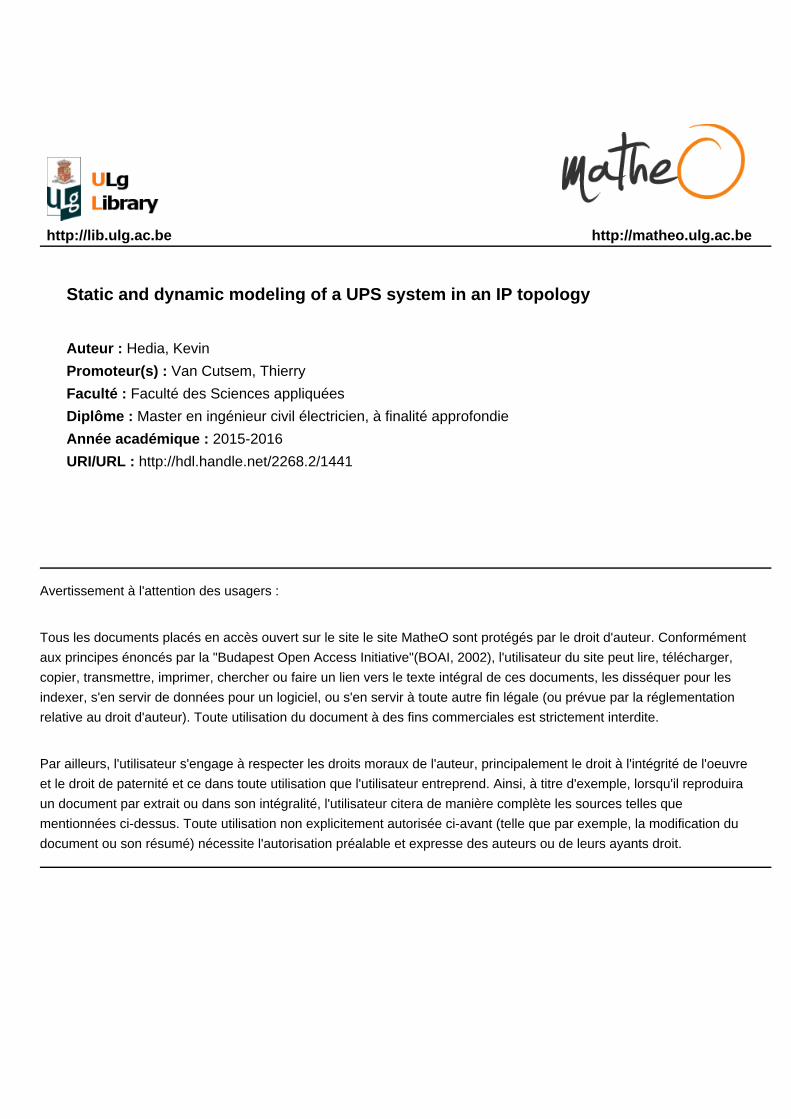
The first objective of the master thesis is to create a program in SCILAB to perform a power flow analysisin which the DRUPS are placed within an Isolated Parallel (IP) topology where the value of the IP chokeis important for the isolation of the units. The program must also be able to compute several scenariosto evaluate the redundancy level of the system and the fault study. Through the program, we can see thatincreasing the value of the IP choke, the voltage drop grows exponentially at a load terminal (Figure 1).Therefore, we can notice that the value of the IP choke limits the transmitted power to this load.

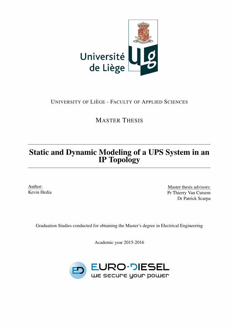
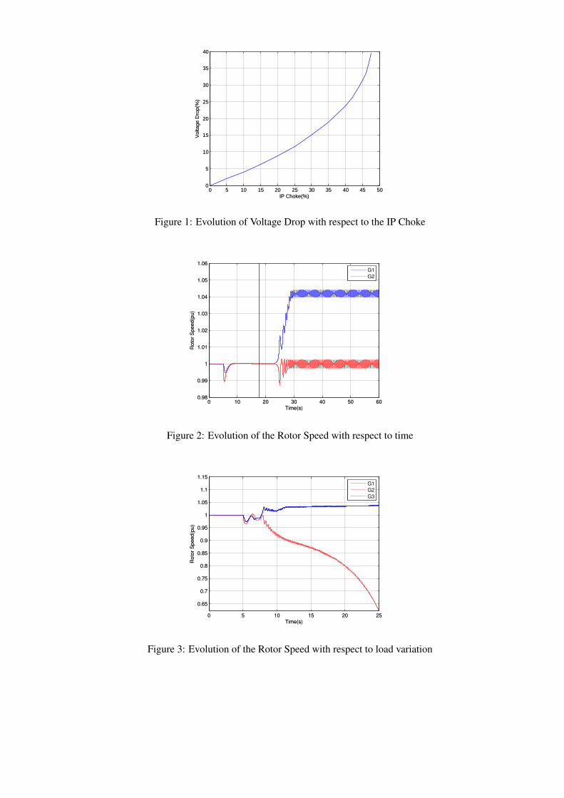
The second objective is to examine the dynamic modeling, by using RAMSES software, of the NO-BREAKKS® to accurately analyze the transitional period. The numerical simulation of the dynamic response ofthe NO-BREAK KS® allows the analysis of the rotor speed which is fundamental to detect instability. Thesimulation of this instability will be done through sudden load variation. To illustrate these results, twocases will be considered: a load variation of 1 MW with a very high value of IP choke (Figure 2) and a loadvariation of 6 MW with a low value of IP choke (Figure 3).

In conclusion, the program allows electrical engineers to perform studies of electrical quantities, pre-faultand post-fault, in the IP topology. Moreover, the developed dynamic models in this master thesis representrather well the behavior of the NO-BREAK KS® at the time of occurrence of one or more disturbances andto check whether the electrical system is still stable or not.

0 5 10 15 20 25 30 35 40 45 500

5

10

15

20

25

30

35

40

IP Choke(%)V

olta

ge D

rop(

%)

0 5 10 15 20 25 30 35 40 45 500

5

10

15

20

25

30

35

40

IP Choke(%)V

olta

ge D

rop(

%)

Figure 1: Evolution of Voltage Drop with respect to the IP Choke

0 10 20 30 40 50 600.98

0.99

1

1.01

1.02

1.03

1.04

1.05

1.06

Roto

r S

pee

d(p

u)

Time(s)

G1

G2

0 10 20 30 40 50 600.98

0.99

1

1.01

1.02

1.03

1.04

1.05

1.06

Roto

r S

pee

d(p

u)

Time(s)

Figure 2: Evolution of the Rotor Speed with respect to time

0 5 10 15 20 25

0.65

0.7

0.75

0.8

0.85

0.9

0.95

1

1.05

1.1

1.15

Roto

r S

pe

ed(p

u)

Time(s)

G1

G2

G3

0 5 10 15 20 25

0.65

0.7

0.75

0.8

0.85

0.9

0.95

1

1.05

1.1

1.15

Roto

r S

pe

ed(p

u)

Time(s)

Figure 3: Evolution of the Rotor Speed with respect to load variation

Acknowledgement

I would like to take this opportunity to thank everyone who supported me throughout this master thesis, Iam thankful for the time they have given me, for their advice, constructive criticism and technical support.

First of all I express my gratitude to my master thesis advisors Professor Thierry Van Cutsem and DoctorPatrick Scarpa, for their patience, guidance, and immense knowledge. They accompanied me in my effortsand supervised my progress throughout this work. I thank them for the confidence they always testified me.

I thank the team of EURO-DIESEL who have helped and supported me to carry this master thesis. And Iwould especially like to express my gratitude to Vincent Defosse, Quentin Dejace, Georges Romischer andLuc Thiteux.

Then I would like to thank the PhD students of Prof. Thierry Van Cutsem : Lampros Papangelis and TilmanWeckesser who were always available during the development of this work.

Before concluding, I would like to thank all the Professors of Faculty of Applied Sciences. And especiallythe Professors Patricia Rousseaux and Christophe Geuzaine who agreed to be part of my jury.

And last but not least, I thank my friends and family.

I

Contents

Introduction 1

Statement of the Problem and Objective of the Master Thesis . . . . . . . . . . . . . . . . . . . . 1

Structure of the Work . . . . . . . . . . . . . . . . . . . . . . . . . . . . . . . . . . . . . . . . . 1

I Euro-Diesel’s UPS and IP Topology 3

1 Introduction To The NO-BREAK KS® System [3] 4

2 IP System Philosophy [4-5] 7

1 Parallel Topology . . . . . . . . . . . . . . . . . . . . . . . . . . . . . . . . . . . . . . . . 7

2 IP Topology . . . . . . . . . . . . . . . . . . . . . . . . . . . . . . . . . . . . . . . . . . . 8

2.1 IP Star . . . . . . . . . . . . . . . . . . . . . . . . . . . . . . . . . . . . . . . . . 8

2.2 IP Ring . . . . . . . . . . . . . . . . . . . . . . . . . . . . . . . . . . . . . . . . . 12

II Static Modeling 13

3 Recall of the Power Systems Analysis Methods 15

1 Power flow [6] . . . . . . . . . . . . . . . . . . . . . . . . . . . . . . . . . . . . . . . . . . 15

1.1 The Newton-Raphson Procedure . . . . . . . . . . . . . . . . . . . . . . . . . . . . 15

1.2 Admittance Matrix . . . . . . . . . . . . . . . . . . . . . . . . . . . . . . . . . . . 18

II

1.3 The Power Flow Equations . . . . . . . . . . . . . . . . . . . . . . . . . . . . . . . 20

1.4 Application of NR to Power Flow Problem . . . . . . . . . . . . . . . . . . . . . . 22

2 Sensitivity Analysis [7] . . . . . . . . . . . . . . . . . . . . . . . . . . . . . . . . . . . . . 24

2.1 Derivation of the Control Model . . . . . . . . . . . . . . . . . . . . . . . . . . . . 24

2.2 Sensitivity of Generation Variable to Load Voltage Variable . . . . . . . . . . . . . 25

3 Fault Study [8] . . . . . . . . . . . . . . . . . . . . . . . . . . . . . . . . . . . . . . . . . 26

3.1 Analysis of Balanced Faults . . . . . . . . . . . . . . . . . . . . . . . . . . . . . . 26

3.2 Analysis of Unbalanced Faults . . . . . . . . . . . . . . . . . . . . . . . . . . . . . 31

4 Numerical Simulations 43

1 Program Implementation . . . . . . . . . . . . . . . . . . . . . . . . . . . . . . . . . . . . 43

2 Validation . . . . . . . . . . . . . . . . . . . . . . . . . . . . . . . . . . . . . . . . . . . . 45

2.1 First validation test . . . . . . . . . . . . . . . . . . . . . . . . . . . . . . . . . . . 45

2.2 Second validation test . . . . . . . . . . . . . . . . . . . . . . . . . . . . . . . . . 47

3 Case Study . . . . . . . . . . . . . . . . . . . . . . . . . . . . . . . . . . . . . . . . . . . 49

III Dynamic Modeling 58

5 Interaction with RAMSES [9] 60

6 Derivation of the Models 63

1 Exciter Model . . . . . . . . . . . . . . . . . . . . . . . . . . . . . . . . . . . . . . . . . . 63

2 Diesel Governor Model . . . . . . . . . . . . . . . . . . . . . . . . . . . . . . . . . . . . . 64

7 Results using the Models 66

1 Validation Test of The Models . . . . . . . . . . . . . . . . . . . . . . . . . . . . . . . . . 66

III

2 Stability Test . . . . . . . . . . . . . . . . . . . . . . . . . . . . . . . . . . . . . . . . . . 69

2.1 Load Variation Using Big IP Choke Reactance . . . . . . . . . . . . . . . . . . . . 69

2.2 Load Variation Using Conventional IP Choke Reactance . . . . . . . . . . . . . . . 72

IV Euro-Diesel’s Strategies 77

8 Conclusion 81

A Euro-Diesel’s Particular Data 82

1 Negative Reactance Value . . . . . . . . . . . . . . . . . . . . . . . . . . . . . . . . . . . . 82

2 Dual Cord Load . . . . . . . . . . . . . . . . . . . . . . . . . . . . . . . . . . . . . . . . . 83

IV

List of Figures

1 Evolution of Voltage Drop with respect to the IP Choke . . . . . . . . . . . . . . . . . . . . 2

2 Evolution of the Rotor Speed with respect to time . . . . . . . . . . . . . . . . . . . . . . . 2

3 Evolution of the Rotor Speed with respect to load variation . . . . . . . . . . . . . . . . . . 2

1.1 Package Sold by EURO-DIESEL . . . . . . . . . . . . . . . . . . . . . . . . . . . . . . . . 4

1.2 The Stato-Alternator . . . . . . . . . . . . . . . . . . . . . . . . . . . . . . . . . . . . . . 5

2.1 Parallel Topology - Low Voltage . . . . . . . . . . . . . . . . . . . . . . . . . . . . . . . . 7

2.2 Parallel Topology - Medium Voltage . . . . . . . . . . . . . . . . . . . . . . . . . . . . . . 8

2.3 IP Star Topology . . . . . . . . . . . . . . . . . . . . . . . . . . . . . . . . . . . . . . . . 9

2.4 IP Star Topology - Conditioning Mode . . . . . . . . . . . . . . . . . . . . . . . . . . . . . 10

2.5 IP Star Topology - Independent Mode . . . . . . . . . . . . . . . . . . . . . . . . . . . . . 11

2.6 IP Star Topology - Conditioning Mode when a KS tripped . . . . . . . . . . . . . . . . . . 11

2.7 IP Ring Topology . . . . . . . . . . . . . . . . . . . . . . . . . . . . . . . . . . . . . . . . 12

3.1 A Unit of the IP Star Topology . . . . . . . . . . . . . . . . . . . . . . . . . . . . . . . . . 18

3.2 Equivalent Circuit of a DRUPS . . . . . . . . . . . . . . . . . . . . . . . . . . . . . . . . . 27

3.3 Short-Circuit on bus f . . . . . . . . . . . . . . . . . . . . . . . . . . . . . . . . . . . . . . 28

3.4 Star-Connected Load . . . . . . . . . . . . . . . . . . . . . . . . . . . . . . . . . . . . . . 32

3.5 Delta-Connected Load . . . . . . . . . . . . . . . . . . . . . . . . . . . . . . . . . . . . . 33

V

3.6 Voltages and Impedances . . . . . . . . . . . . . . . . . . . . . . . . . . . . . . . . . . . . 34

3.7 Currents and Admittances . . . . . . . . . . . . . . . . . . . . . . . . . . . . . . . . . . . . 34

3.8 Generator model . . . . . . . . . . . . . . . . . . . . . . . . . . . . . . . . . . . . . . . . 35

3.9 Symmetrical Components Circuits of a Synchronous Generator . . . . . . . . . . . . . . . . 35

3.10 Line Model . . . . . . . . . . . . . . . . . . . . . . . . . . . . . . . . . . . . . . . . . . . 37

3.11 Transformer Model . . . . . . . . . . . . . . . . . . . . . . . . . . . . . . . . . . . . . . . 38

3.12 Positive-Sequence equivalent Circuit . . . . . . . . . . . . . . . . . . . . . . . . . . . . . . 38

3.13 Zero-sequence Equivalent Two-port . . . . . . . . . . . . . . . . . . . . . . . . . . . . . . 39



4.1 Flowchart of the Program . . . . . . . . . . . . . . . . . . . . . . . . . . . . . . . . . . . . 44

4.2 IP Star Topology with 2 DRUPS . . . . . . . . . . . . . . . . . . . . . . . . . . . . . . . . 45

4.3 IP Start Topology with 7 DRUPS . . . . . . . . . . . . . . . . . . . . . . . . . . . . . . . . 47

4.4 IP Star Topology with 5 DRUPS . . . . . . . . . . . . . . . . . . . . . . . . . . . . . . . . 50

4.5 Evolution of Voltage Drop with respect to the IP Choke . . . . . . . . . . . . . . . . . . . . 56

5.1 RAMSES Components . . . . . . . . . . . . . . . . . . . . . . . . . . . . . . . . . . . . . 60

5.2 User Interaction . . . . . . . . . . . . . . . . . . . . . . . . . . . . . . . . . . . . . . . . . 61

5.3 Model Description . . . . . . . . . . . . . . . . . . . . . . . . . . . . . . . . . . . . . . . 61

5.4 Model Structure . . . . . . . . . . . . . . . . . . . . . . . . . . . . . . . . . . . . . . . . . 62

5.5 File Structure . . . . . . . . . . . . . . . . . . . . . . . . . . . . . . . . . . . . . . . . . . 62

6.1 Bloc diagram of the exciter model . . . . . . . . . . . . . . . . . . . . . . . . . . . . . . . 63

6.2 Bloc diagram of Torque controller . . . . . . . . . . . . . . . . . . . . . . . . . . . . . . . 65

VI

7.1 Saturation curve . . . . . . . . . . . . . . . . . . . . . . . . . . . . . . . . . . . . . . . . . 67

7.2 Load variation in conditioning mode . . . . . . . . . . . . . . . . . . . . . . . . . . . . . . 68

7.3 Voltage Magnitude of the Load Computed with RAMSES versus the Real Voltage Magnitude 68

7.4 Comparison of the Rotor Speed between the Simulation and the Real Response . . . . . . . 69

7.5 IP Star Topology with 2 Loads . . . . . . . . . . . . . . . . . . . . . . . . . . . . . . . . . 70

7.6 Evolution of the Rotor Speed with respect to time . . . . . . . . . . . . . . . . . . . . . . . 70

7.7 Evolution of the Active Power produced by The DRUPS . . . . . . . . . . . . . . . . . . . 71

7.8 Evolution of the Voltage Phase Angle . . . . . . . . . . . . . . . . . . . . . . . . . . . . . 72

7.9 IP Star Topology with 3 Loads . . . . . . . . . . . . . . . . . . . . . . . . . . . . . . . . . 73

7.10 Evolution of the Rotor Speed with respect to time . . . . . . . . . . . . . . . . . . . . . . . 73

7.11 Evolution of the Rotor Angle of the three DRUPS . . . . . . . . . . . . . . . . . . . . . . . 74

7.12 Evolution of the Rotor speed of the three DRUPS . . . . . . . . . . . . . . . . . . . . . . . 74

7.13 Evolution of the Rotor speed of the three DRUPS . . . . . . . . . . . . . . . . . . . . . . . 75

7.14 Evolution of the Stabilized Rotor Angle with respect to load variation . . . . . . . . . . . . 75

7.15 The Worldwide Presence of Euro-Diesel . . . . . . . . . . . . . . . . . . . . . . . . . . . . 78

7.16 Communication with World-Wide Customers . . . . . . . . . . . . . . . . . . . . . . . . . 79

A.1 Tapped Inductor . . . . . . . . . . . . . . . . . . . . . . . . . . . . . . . . . . . . . . . . . 82

A.2 Magnetically Coupled Circuits . . . . . . . . . . . . . . . . . . . . . . . . . . . . . . . . . 83

A.3 Equivalent Circuit of the Tapped Inductor . . . . . . . . . . . . . . . . . . . . . . . . . . . 83

A.4 Supply of the Dual Cord Load . . . . . . . . . . . . . . . . . . . . . . . . . . . . . . . . . 83

A.5 Supply of the Dual Cord Load in Case of the Loss of the Left Distribution Switchboard . . . 84

VII

List of Tables

4.1 Impedances of The Lines . . . . . . . . . . . . . . . . . . . . . . . . . . . . . . . . . . . . 45

4.2 Voltage Profile . . . . . . . . . . . . . . . . . . . . . . . . . . . . . . . . . . . . . . . . . 46

4.3 Active and reactive power consumed by the 7 loads . . . . . . . . . . . . . . . . . . . . . . 47

4.4 Results of the power flow . . . . . . . . . . . . . . . . . . . . . . . . . . . . . . . . . . . . 48

4.5 Active power consumed by the loads in kW . . . . . . . . . . . . . . . . . . . . . . . . . . 49

4.6 Reactive power consumed by the loads in kVar . . . . . . . . . . . . . . . . . . . . . . . . 49

4.7 Line Impedance . . . . . . . . . . . . . . . . . . . . . . . . . . . . . . . . . . . . . . . . . 50

4.8 Important Results for the Normal Stage . . . . . . . . . . . . . . . . . . . . . . . . . . . . 50

4.9 Important Results of the Loss of DRUPS 1 . . . . . . . . . . . . . . . . . . . . . . . . . . . 51

4.10 Important Results of the Loss of DRUPS 4 . . . . . . . . . . . . . . . . . . . . . . . . . . . 52

4.11 Important Results of the Loss of Distribution Switchboard 1 . . . . . . . . . . . . . . . . . 52


4.13 Important Results of the Loss of DRUPS 1 and 2 . . . . . . . . . . . . . . . . . . . . . . . 53

4.14 Voltage profile before and after the fault . . . . . . . . . . . . . . . . . . . . . . . . . . . . 54

4.15 Magnitude of the current produced by the DRUPS . . . . . . . . . . . . . . . . . . . . . . . 55

4.16 Voltage profile before and after fault . . . . . . . . . . . . . . . . . . . . . . . . . . . . . . 55


VIII

7.1 Data of the NO-BREAK KS7® . . . . . . . . . . . . . . . . . . . . . . . . . . . . . . . . . 66

7.2 Line Data of the Topology . . . . . . . . . . . . . . . . . . . . . . . . . . . . . . . . . . . 70

7.3 Line Data of the Topology . . . . . . . . . . . . . . . . . . . . . . . . . . . . . . . . . . . 72

A.1 Dual Cord Power Specification . . . . . . . . . . . . . . . . . . . . . . . . . . . . . . . . . 84

IX

Introduction

Statement of the Problem and Objective of the Master Thesis

EURO-DIESEL is a private company established in 1989 from the province of Liege, Belgium, by a teamof innovators who specialized in critical power systems [1]. EURO-DIESEL ensures power supply securityfor major businesses and industries worldwide by building and configuring a Diesel Rotary UninterruptiblePower Supply (DRUPS) system baptized the NO-BREAK KS®. But EURO-DIESEL also sells to theircustomers, along with their DRUPS, control panels and power panels.

Once the technical specifications is acquired by the electrical engineering department, studies must be car-ried with respect to the number and power ratings of DRUPS and the network topology, within which theDRUPS will be installed, chosen by the customer. More precisely, a part of these studies evaluates the re-dundancy level of the system by means of several scenarios and another part consists in studying the impactof a fault on the electrical quantities. On completion of these studies, the engineer can conclude whether thecase is feasible or not.

In this context, the guidelines of my master thesis include two main objectives.

The first objective of the master thesis is to create a program in SCILAB (an open source, cross-platformnumerical computational package and a high-level, numerically oriented programming language [2]) toperform a power flow analysis in which the DRUPS are placed within an Isolated Parallel (IP) topology.The program must also be able to compute several scenarios to evaluate the redundancy level of the systemand the fault study. The main features of the program should be fast, efficient and ergonomic.

The second objective is to examine the dynamic modeling of the NO-BREAK KS® to accurately analyzethe transitional period. The numerical simulation of the dynamic response of the NO-BREAK KS® has, sofar, never been investigated by EURO-DIESEL.

Structure of the Work

In the first chapter, we introduce the basics of how the NO-BREAK KS® works whose purpose is to supplyimmediately the critical loads in case of an outage.

1

The second chapter explains the different topologies used by EURO-DIESEL and more precisely, the IPtopology whose main objective is to secure critical loads for high power ratings at low voltage and to reducethe short-circuit current.

In chapter three, we introduce the theoretical background of the power systems analysis methods. These lat-ter will be recall in three steps. The first step recalls the theoretical basis of the Newton-Raphson procedurefor the power flow study. The second step recalls the theoretical background of sensitivity analysis whichnumerically allows to directly know how the output voltage of the UPS system influences the load voltage.The last step recalls the theoretical background of the fault study which is divided into two main parts : theanalysis of balanced faults and the analysis of unbalanced faults.

In chapter four, we will show the results of different numerical models that I developed using SCILABbased on the power systems analysis methods. This chapter will be divided into three parts. The first partwill show the program implementation and the flowchart of the program. While the second part deals withthe validation of my numerical models. Finally, we will apply my program for the full study of a practicalproblem provided by EURO-DIESEL.

The fifth chapter will introduce the RAMSES software as well as how to use CODEGEN utility via astructured file needed for the creation and addition of a new model in RAMSES.

The sixth chapter will describe the models developed for the excitation and torque controls to simulate thebehavior of the NO-BREAK KS®.

In chapter seven, the models will be used in RAMSES to simulate the response of the NO-BREAK KS®.The first section of this chapter will compare the response of the numerical models to the real response ofthe NO-BREAK KS® while the second section will explore the stability limits of the system.

The main conclusions about the contribution of this work is summarized in chapter eight. Following annexeswhich include the specific data to which the reader may refer. And finally, the main references in order ofappearance in this thesis.

2

Part I

Euro-Diesel’s UPS and IP Topology

3

Chapter 1

Introduction To The NO-BREAK KS®System [3]

EURO-DIESEL manufacture a Diesel Rotary Uninterruptible Power Supply (DRUPS) system called theNO-BREAK KS® whose purpose is to secure immediately the supply of critical loads in case of an outage.

The package sold by EURO-DIESEL is shown in Figure 1.1, as can be seen there are two main parts : thecontrol and power panels and the DRUPS. In this section, only the DRUPS operation will be explaineddespite the fact that the control and power panels are crucial components but it is not necessary for theunderstanding of the continuation of this master thesis.

Figure 1.1: Package Sold by EURO-DIESEL

4

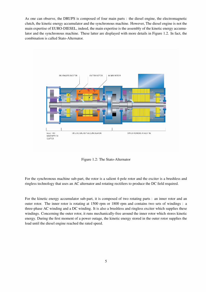
As one can observe, the DRUPS is composed of four main parts : the diesel engine, the electromagneticclutch, the kinetic energy accumulator and the synchronous machine. However, The diesel engine is not themain expertise of EURO-DIESEL, indeed, the main expertise is the assembly of the kinetic energy accumu-lator and the synchronous machine. These latter are displayed with more details in Figure 1.2. In fact, thecombination is called Stato-Alternator.

Figure 1.2: The Stato-Alternator

For the synchronous machine sub-part, the rotor is a salient 4-pole rotor and the exciter is a brushless andringless technology that uses an AC alternator and rotating rectifiers to produce the DC field required.

For the kinetic energy accumulator sub-part, it is composed of two rotating parts : an inner rotor and anouter rotor. The inner rotor is rotating at 1500 rpm or 1800 rpm and contains two sets of windings : athree-phase AC winding and a DC winding. It is also a brushless and ringless exciter which supplies thesewindings. Concerning the outer rotor, it runs mechanically-free around the inner rotor which stores kineticenergy. During the first moment of a power outage, the kinetic energy stored in the outer rotor supplies theload until the diesel engine reached the rated speed.

5

The DRUPS can be operate in three different states : conditioning mode, transient period and independentmode.

In conditioning mode, the synchronous machine is supplied by the mains and acts as a motor which drivesthe main shaft and thus the inner rotor. The AC winding of the inner rotor is supplied in order to generatea rotating magnetic field that induced eddy currents at the windings of the outer rotor and thus, the lattercan reach the maximum speed of 3000 rpm. However, since the inner rotor is already rotating at 1500 rpm,the AC winding needs to feed with a current of a frequency of 50Hz. So the outer rotor stores kinetic energy.

In the transient period, directly after a power outage, the DC winding of the inner rotor is supplied which,in consequence, will create a magnetic coupling between the inner and outer rotor. Since the outer rotor hasstored some kinetic energy, it will be transferred through this coupling in a controlled manner to keep theinner rotor at nominal speed. This transient period secure the critical loads until the diesel engine is readyto take over.

In independent mode, the diesel engine is at the rated speed and is ready to take over. There is then a cou-pling between the stato-alternator and the diesel engine via an electromagnetic clutch. The diesel engineprovides the power to the load for an indeterminate time. During this mode, The outer rotor is acceleratedto 3000 rpm again and stores the kinetic energy to its full capacity.

6

Chapter 2

IP System Philosophy [4-5]

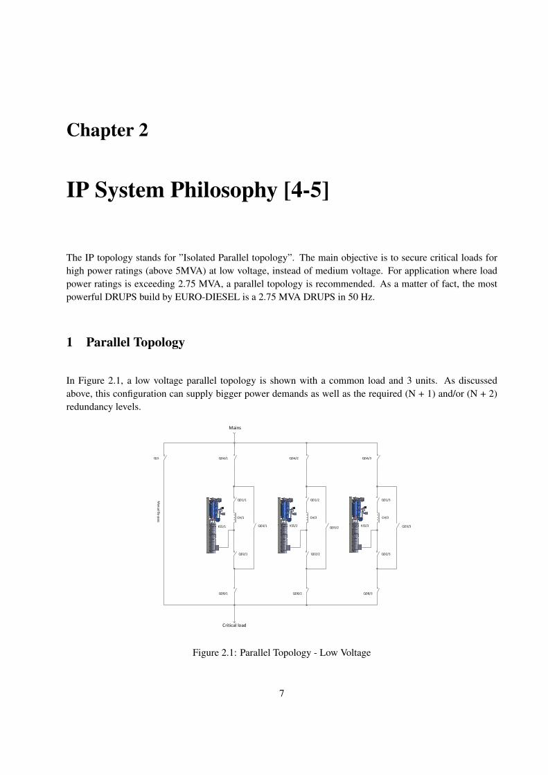
The IP topology stands for ”Isolated Parallel topology”. The main objective is to secure critical loads forhigh power ratings (above 5MVA) at low voltage, instead of medium voltage. For application where loadpower ratings is exceeding 2.75 MVA, a parallel topology is recommended. As a matter of fact, the mostpowerful DRUPS build by EURO-DIESEL is a 2.75 MVA DRUPS in 50 Hz.

1 Parallel Topology

In Figure 2.1, a low voltage parallel topology is shown with a common load and 3 units. As discussedabove, this configuration can supply bigger power demands as well as the required (N + 1) and/or (N + 2)redundancy levels.

QDA/1 QDA/2

Man

ual B

y-pass

QI3

QDB/1

Critical load

Mains

QDB/2

QDA/3

QDB/3

CH/1

QD2/1

QD1/1

QD3/1KS5/1

CH/2

QD2/2

QD1/2

QD3/2KS5/2

CH/3

QD2/3

QD1/3

QD3/3KS5/3

Figure 2.1: Parallel Topology - Low Voltage

7

Due to its simple and reliable design, this configuration is used for many applications such as supplyinglarge datacenters facilities. However, when the power consumed by the load increases, exceeding 5 MVA,more DRUPS systems need to be paralleled, which can lead to high short-circuit currents. Therefore, oneneeds to adapt the switchgears due to the high value of short-circuit current, hence these latter become veryspecific and expensive. A mean to overcome this effect is to pass from low voltage to medium voltage.

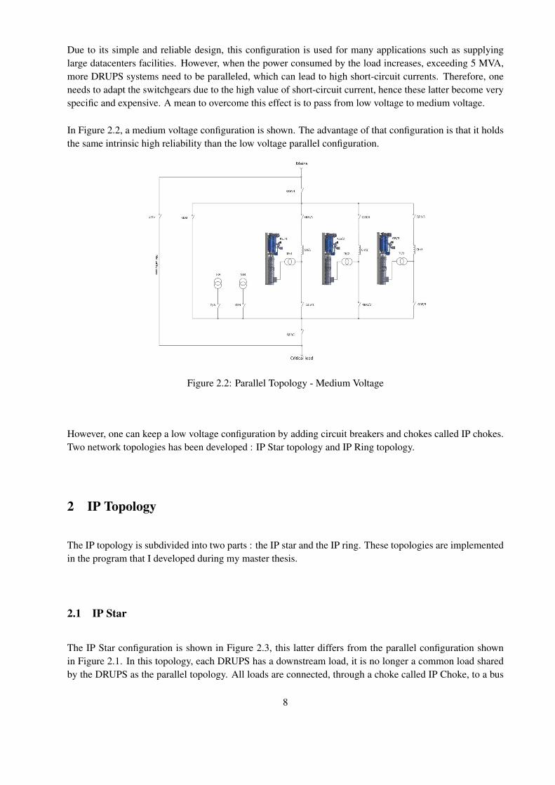
In Figure 2.2, a medium voltage configuration is shown. The advantage of that configuration is that it holdsthe same intrinsic high reliability than the low voltage parallel configuration.

This document is the property of EURO-DIESEL SA and may neither be disclosed nor reproduced without written authorization. Information provided is believed to be correct and reliable. EURO-DIESEL SA reserves the right to amend this document without notice.

ISOLATED PARALLEL STAR BUS TI0020 • Rev04

Page 4/13

Obviously (and even if the failure probability is low), the output bus remains a single point of failure, but this can easily be overcome by adding a redundant output bus. Redundant parallel configurations, in combination with the double output busbar system meet the Uptime Institute design criteria of Tier III. It is even possible to meet the Tier IV design criteria by designing an A and a B side, each one being a parallel system. When the load further increases, more DRUPS systems need to be paralleled, which leads to high short-circuit currents. Switchgear up to 100kA is quite usual, but it becomes very specific and expensive above this rating. This can easily be overcome by up-grading the low voltage 400 or 480 V system to a medium voltage system up to 22 kV. The maximum load for a low voltage parallel configuration is approximately 5MVA. Above 5 MVA, the usual practice is to increase the voltage and use medium voltage systems. An example of such a system is shown on Figure 2. The beauty of such medium voltage parallel configuration is that it holds the same intrinsic high reliability than the low voltage parallel configuration. The medium voltage parallel configuration is a modular design as units can be added at later stage in accordance to the load demand. The medium voltage parallel configuration is limited to paralleling maximum 31 units. As for low voltage, redundancy, double output buses, or A and B sides concepts can be introduced to meet the Tier III or Tier IV design criteria.

Figure 2: Parallel medium voltage with 3 units

This is also a simple and reliable system but of course with the need of implementing medium voltage equipments. In case a customer for whatever reason doesn’t want to go to a medium voltage design the alternative can be the IP Star system, which was introduced to maintain a low voltage configuration while allowing loads well above 5MVA. Obviously this can only be realised by increasing the number of circuit breakers and adding so called IP-Chokes.

Figure 2.2: Parallel Topology - Medium Voltage

However, one can keep a low voltage configuration by adding circuit breakers and chokes called IP chokes.Two network topologies has been developed : IP Star topology and IP Ring topology.

2 IP Topology

The IP topology is subdivided into two parts : the IP star and the IP ring. These topologies are implementedin the program that I developed during my master thesis.

2.1 IP Star

The IP Star configuration is shown in Figure 2.3, this latter differs from the parallel configuration shownin Figure 2.1. In this topology, each DRUPS has a downstream load, it is no longer a common load sharedby the DRUPS as the parallel topology. All loads are connected, through a choke called IP Choke, to a bus

8

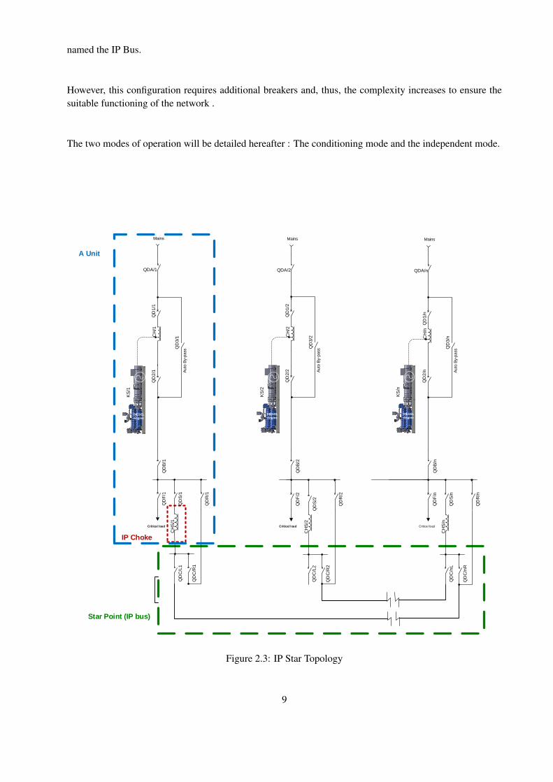
named the IP Bus.

However, this configuration requires additional breakers and, thus, the complexity increases to ensure thesuitable functioning of the network .

The two modes of operation will be detailed hereafter : The conditioning mode and the independent mode.

QD

S/n

QD

R/n

QD

F/n

QD

C/n

L

QD

C/n

R

QD

S/2

QD

R/2

QD

F/2

CH

S/2

QD

C/L

2

QD

C/R

2

QD

2/1

QD

1/1

QDA/1

QD

3/1

Auto

By-p

ass

QD

2/n

QD

1/n

QD

3/n

Auto

By-p

ass

DIESEL

Engine

KS

/1

DIESEL

Engine

KS

/n

CH

/2Q

D2/2

QD

1/2

QD

3/2

Auto

By-p

ass

DIESEL

Engine

KS

/2

DIESEL

Engine

QD

S/1

QD

R/1

QD

F/1

QD

C/L

1

QD

C/R

1

QDA/2 QDA/n

Mains

QD

B/1

QD

B/2

QD

B/n

MainsMains

Critical loadCritical loadCritical load

IP Choke

Star Point (IP bus)

CH

/n

CH

S/n

CH

S/1

CH

/1

A Unit

Figure 2.3: IP Star Topology

9

Conditioning Mode

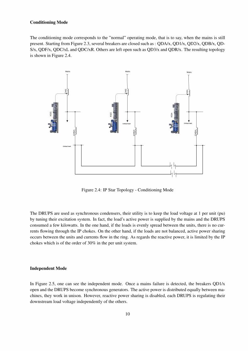
The conditioning mode corresponds to the ”normal” operating mode, that is to say, when the mains is stillpresent. Starting from Figure 2.3, several breakers are closed such as : QDA/x, QD1/x, QD2/x, QDB/x, QD-S/x, QDF/x, QDC/xL and QDC/xR. Others are left open such as QD3/x and QDR/x. The resulting topologyis shown in Figure 2.4.

CH

S/2

DIESEL

Engine

KS

/1

DIESEL

Engine

KS

/n

CH

/2

Mains

Critical load

Critical load

CH

/n

CH

S/n

CH

S/1

CH

/1

DIESEL

Engine KS

/2

Mains

Critical load

Mains

Figure 2.4: IP Star Topology - Conditioning Mode

The DRUPS are used as synchronous condensers, their utility is to keep the load voltage at 1 per unit (pu)by tuning their excitation system. In fact, the load’s active power is supplied by the mains and the DRUPSconsumed a few kilowatts. In the one hand, if the loads is evenly spread between the units, there is no cur-rents flowing through the IP chokes. On the other hand, if the loads are not balanced, active power sharingoccurs between the units and currents flow in the ring. As regards the reactive power, it is limited by the IPchokes which is of the order of 30% in the per unit system.

Independent Mode

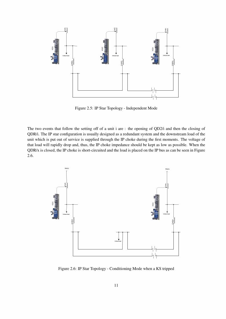
In Figure 2.5, one can see the independent mode. Once a mains failure is detected, the breakers QD1/xopen and the DRUPS become synchronous generators. The active power is distributed equally between ma-chines, they work in unison. However, reactive power sharing is disabled, each DRUPS is regulating theirdownstream load voltage independently of the others.

10

CH

S/2

DIESEL

Engine

KS

/1

DIESEL

Engine

KS

/n

CH

/2

Critical loadCritical load

CH

/n

CH

S/n

CH

S/1

CH

/1

DIESEL

Engine KS

/2

Critical load

Figure 2.5: IP Star Topology - Independent Mode

The two events that follow the setting off of a unit i are : the opening of QD2/i and then the closing ofQDR/i. The IP star configuration is usually designed as a redundant system and the downstream load of theunit which is put out of service is supplied through the IP choke during the first moments. The voltage ofthat load will rapidly drop and, thus, the IP choke impedance should be kept as low as possible. When theQDR/x is closed, the IP choke is short-circuited and the load is placed on the IP bus as can be seen in Figure2.6.

DIESEL

Engine

KS

/1

DIESEL

Engine

KS

/n

Mains

Critical load

Critical load

CH

/n

CH

S/n

CH

S/1

CH

/1

DIESEL

Engine

Critical load

Mains

Figure 2.6: IP Star Topology - Conditioning Mode when a KS tripped

11

2.2 IP Ring

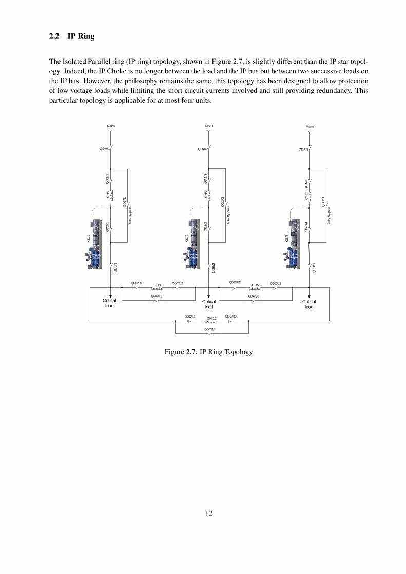
The Isolated Parallel ring (IP ring) topology, shown in Figure 2.7, is slightly different than the IP star topol-ogy. Indeed, the IP Choke is no longer between the load and the IP bus but between two successive loads onthe IP bus. However, the philosophy remains the same, this topology has been designed to allow protectionof low voltage loads while limiting the short-circuit currents involved and still providing redundancy. Thisparticular topology is applicable for at most four units.

QD

2/1

QD

1/1

QDA/1

QD

3/1

Auto

By-p

ass

QD

2/3

QD

1/3

QD

3/3

Auto

By-p

ass

DIESEL

Engine

KS

/1

DIESEL

Engine

KS

/3

CH

/2Q

D2/2

QD

1/2

QD

3/2

Auto

By-p

ass

DIESEL

Engine

KS

/2

DIESEL

Engine

QDA/2 QDA/3

Mains

QD

B/1

MainsMains

CH

/3

CH

/1

QD

B/2

QD

B/3

CH/12QDC/L2QDC/R1

QDC/12

CH/23QDC/L3QDC/R2

QDC/23

CH/13QDC/R3QDC/L1

QDC/13

Critical

loadCritical

load

Critical

load

Figure 2.7: IP Ring Topology

12

Part II

Static Modeling

13

Purpose of This Part

The main objective of the part that we will study is to compute the steady state electrical quantities in twodifferent topologies.

To succeed, this part will include two chapters. The first will focus to implement the theoretical backgroundof the power systems analysis. Then the second chapter will show the results of different numerical modelsthat I developed using SCILAB. We will check that the results provided by my program correspond withgood accuracy to the results provided a power flow software and then apply my program to a practical casestudy.

14

Chapter 3

Recall of the Power Systems AnalysisMethods

1 Power flow [6]

The main goal of EURO-DIESEL is to secure the supply of electrical energy for their customer load. Pre-analysis must be perform in order to know the voltage magnitudes and phase angles for a set of buses in theIP topology.

A way to solve the problem is to apply a specific procedure to the power flow problem. Since the powerflow equations are non-linear, one needs an iterative procedure to solve the problem. In this context, theNewton-Raphson method is chosen due its computational robustness.

Thereafter, the theoretical basis of the Newton-Raphson procedure will be detailed and then applied to thepower flow formulation to solve the EURO-DIESEL’s problem.

1.1 The Newton-Raphson Procedure

In fact, the Newton-Raphson method finds the roots of non-linear algebraic system of equations. It requiressuccessive approximations to reach the real solution. It is called iterative root finding procedure.

The procedure starts by an initial guess. In this particular problem, due to the small number of buses in thenetwork, a flat start can be chosen. The latter is when the voltage magnitudes of buses are set to 1 pu and thephase angles are set to 0. This first guess is usually incorrect, an updated of the guesses is needed in orderto converge towards the solution.

15

Several methods exist to solve the power flow problem such as Gauss-Seidel method but Newton-Raphsonmethod has become, most of the time, the de-facto industry standard [6]. The main reason is that the con-vergence properties of this method are pretty good even if it begins with a flat start. Moreover, it convergesquadratically.

Let reminds the mathematically basis of the Newton-Raphson method.

Newton Raphson for the Multidimensional Case

Assume we have n nonlinear algebraic equations and n unknowns. A first initial guess x(0) is made butsince it is a guess, f(x(0)) 6= 0. An update of the solution is required. Let denotes ∆x(0) the variation of thesolution which will make f(x(0) + ∆x(0)) = 0.

The NR procedure is based on the Taylor series expansion of the functions f(x) :

f(x(0) + ∆x(0)) = f(x(0)) + f′(x(0))∆x(0) +1

2f′′(x(0))(∆x(0))2 + ... = 0 (3.1)

Higher order terms are small and can be neglected assuming that guess is a good enough such that ∆x(0) issmall. So,

f(x(0) + ∆x(0)) = f(x(0)) + f′(x(0))∆x(0) = 0 (3.2)

At this point, the Jacobian matrix can be introduced. The latter stores all the derivatives for each individualfunction with respect to each individual unknown. So for the kth function and the jth unknown, the term ofthe Jacobian is ∂fk(x(0))

∂xj.

16

Since we have n functions and n unknowns, the Jacobian matrix should be of size nxn :

J =

∂f1(x(0))∂x1

∂f1(x(0))∂x2

. . . ∂f1(x(0))∂xn

∂f2(x(0))∂x1

∂f2(x(0))∂x2

. . . ∂f2(x(0))∂xn

......

...∂fn(x(0))

∂x1

∂fn(x(0))∂x2

. . . ∂fn(x(0))∂xn

From eq. (3.2) we have

f′(x(0))∆x(0) = −f(x(0)) (3.3)

From the equation above the term f′(x(0)) is in fact the Jacobian, it becomes

J∆x(0) = −f(x(0)) (3.4)

We can easily find ∆x(0)

∆x(0) = −J−1f(x(0)) (3.5)

Considering the small number of buses of the system, we can easily obtain the inverse of the Jacobian.However, in programming, a LDU decomposition is used to solve the problem for large system.

Since we know the variation of the state vector, we can update it

x(1) = x(0) + ∆x(0) (3.6)

And finally, for any iteration

x(i+1) = x(i) + ∆x(i) (3.7)

The basis of the Newton-Raphson procedure have been developed. Let now introduce the form of theadmittance matrix for this application.

17

1.2 Admittance Matrix

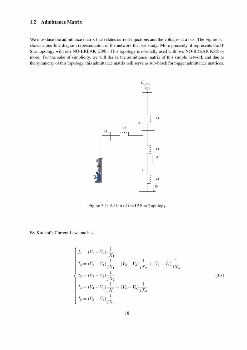
We introduce the admittance matrix that relates current injections and the voltages at a bus. The Figure 3.1shows a one-line diagram representation of the network that we study. More precisely, it represents the IPStar topology with one NO-BREAK KS® . This topology is normally used with two NO-BREAK KS® ormore. For the sake of simplicity, we will derive the admittance matrix of this simple network and due tothe symmetry of this topology, this admittance matrix will serve as sub-block for bigger admittance matrices.

Main

X2

X1

X3

X4

I1

I2

I3

I4

I5

Figure 3.1: A Unit of the IP Star Topology

By Kirchoffs Current Law, one has

I1 = (V1 − V2)1

jX1

I2 = (V2 − V1)1

jX1+ (V2 − V3)

1

jX2+ (V2 − V4)

1

jX3

I3 = (V3 − V2)1

jX2

I4 = (V4 − V2)1

jX3+ (V4 − V5)

1

jX4

I5 = (V5 − V4)1

jX4

(3.8)

18

In order to simplify the writing, let use the admittance since 1X = y. The equations system becomes :

I1 = y12V1 − y12V2

I2 = (y21 + y23 + y24)V2 − y21V1 − y23V3 − y24V4

I3 = y32V3 − y32V2

I4 = (y42 + y45)V4 − y42V2 − y45V5

I5 = y54V5 − y54V4

(3.9)

We may write the system of equations in matrix form :

I1

I2

I3

I4

I5

=

y12 −y21 0 0 0

−y12 y21 + y23 + y24 −y23 −y24 0

0 −y32 y32 0 0

0 −y42 0 y42 + y45 −y45

0 0 0 −y54 y54

V1

V2

V3

V4

V5

So we have the admittance matrix

Y =

y12 −y21 0 0 0

−y12 y21 + y23 + y24 −y23 −y24 0

0 −y32 y32 0 0

0 −y42 0 y42 + y45 −y45

0 0 0 −y54 y54

Denoting the element in row i, column j, as Yij , the latter becomes element of the admittance matrix ratherthan an admittance.

Y =

Y11 Y21 0 0 0

Y12 Y22 Y23 Y24 0

0 Y32 Y33 0 0

0 Y42 0 Y44 Y45

0 0 0 Y54 Y55

We can observe that the admittance matrix is symmetric which is, in fact, the sub-bloc that will be repeatedfor bigger admittance matrices. And we finally have

19

I1

I2

I3

I4

I5

=

Y11 Y21 0 0 0

Y12 Y22 Y23 Y24 0

0 Y32 Y33 0 0

0 Y42 0 Y44 Y45

0 0 0 Y54 Y55

V1

V2

V3

V4

V5

(3.10)

1.3 The Power Flow Equations

Mathematical Statement

Let define the net complex power injection into a bus, we assume that all quantities are in per unit :

Sk = VkI∗k (3.11)

From the eq. (3.10), we can easily derive the current injection into any bus k :

Ik =

N∑

j=1

Ykj Vj (3.12)

Substitution of eq. (3.12) into eq. (3.11) yields

Sk = Vk(

N∑

j=1

Ykj Vj)∗ (3.13)

One can develop the eq. (3.13) since V is a phasor and the admittance Ykj is a complex number

Sk = Vk

N∑

j=1

Y ∗kj V∗j = |Vk|∠θk

N∑

j=1

(Gkj + jBkj)∗(|Vj |∠θj)∗

=

N∑

j=1

|Vk||Vj |∠(θk − θj)(Gkj − jBkj) (3.14)

20

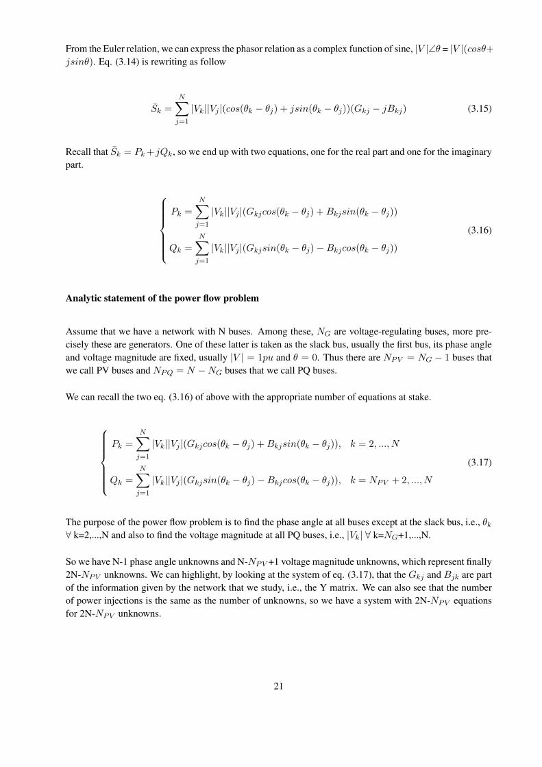
From the Euler relation, we can express the phasor relation as a complex function of sine, |V |∠θ = |V |(cosθ+jsinθ). Eq. (3.14) is rewriting as follow

Sk =N∑

j=1

|Vk||Vj |(cos(θk − θj) + jsin(θk − θj))(Gkj − jBkj) (3.15)

Recall that Sk = Pk+jQk, so we end up with two equations, one for the real part and one for the imaginarypart.

Pk =

N∑

j=1

|Vk||Vj |(Gkjcos(θk − θj) +Bkjsin(θk − θj))

Qk =N∑

j=1

|Vk||Vj |(Gkjsin(θk − θj)−Bkjcos(θk − θj))(3.16)

Analytic statement of the power flow problem

Assume that we have a network with N buses. Among these, NG are voltage-regulating buses, more pre-cisely these are generators. One of these latter is taken as the slack bus, usually the first bus, its phase angleand voltage magnitude are fixed, usually |V | = 1pu and θ = 0. Thus there are NPV = NG − 1 buses thatwe call PV buses and NPQ = N −NG buses that we call PQ buses.

We can recall the two eq. (3.16) of above with the appropriate number of equations at stake.

Pk =

N∑

j=1

|Vk||Vj |(Gkjcos(θk − θj) +Bkjsin(θk − θj)), k = 2, ..., N

Qk =N∑

j=1

|Vk||Vj |(Gkjsin(θk − θj)−Bkjcos(θk − θj)), k = NPV + 2, ..., N

(3.17)

The purpose of the power flow problem is to find the phase angle at all buses except at the slack bus, i.e., θk∀ k=2,...,N and also to find the voltage magnitude at all PQ buses, i.e., |Vk| ∀ k=NG+1,...,N.

So we have N-1 phase angle unknowns and N-NPV +1 voltage magnitude unknowns, which represent finally2N-NPV unknowns. We can highlight, by looking at the system of eq. (3.17), that the Gkj and Bjk are partof the information given by the network that we study, i.e., the Y matrix. We can also see that the numberof power injections is the same as the number of unknowns, so we have a system with 2N-NPV equationsfor 2N-NPV unknowns.

21

We can define the state vector which is the unknowns vector.

x =

[θ

|V |

]=

θ2

θ2...θN

|VNPV +2||VNPV +3|

...|VN |

=

x1

x2...

xN−1

xNxN+1

...x2N−NPV

(3.18)

We can also define the mismatch vector.

f(x) =

f1(x)...

fN−1(x)

fN (x)...

f2N−NPV (x)

=

P2(x)− P2...

PN (x)− PN

QNPV (x)−QNPV...

QN (x)−QN

=

∆P2...

∆PN

∆QNPV...

∆QN

= 0 (3.19)

This vector is used during the Newton-Raphson procedure to compute ∆x, seen in the ”The Newton-Raphson Procedure” section. In fact, we never reach a pure zero but once we reach the defined error suchthat | f(x) | ≤ ε, we can stop the procedure and the convergence is achieved.

1.4 Application of NR to Power Flow Problem

As developed in the ”The Newton-Raphson Procedure” section, we can update the solution as follow :

x(i+1) = x(i) − J−1f(x(i)) (3.20)

The key step of the procedure is to determine the Jacobian matrix J−1. Therefore, we can see from eq.(3.18) that we only have two sets of unknowns, the voltage magnitude and the phase angle.

Thus, the Jacobian will be composed of 4 sub-matrices since there are only four basic types of derivatives: JPθ, JPV , JQθ, JQV . For the simplicity of the writing, the first superscript express the type of equationwe differentiate while the second express the unknowns with respect to which we differentiate. So we canwrite,

22

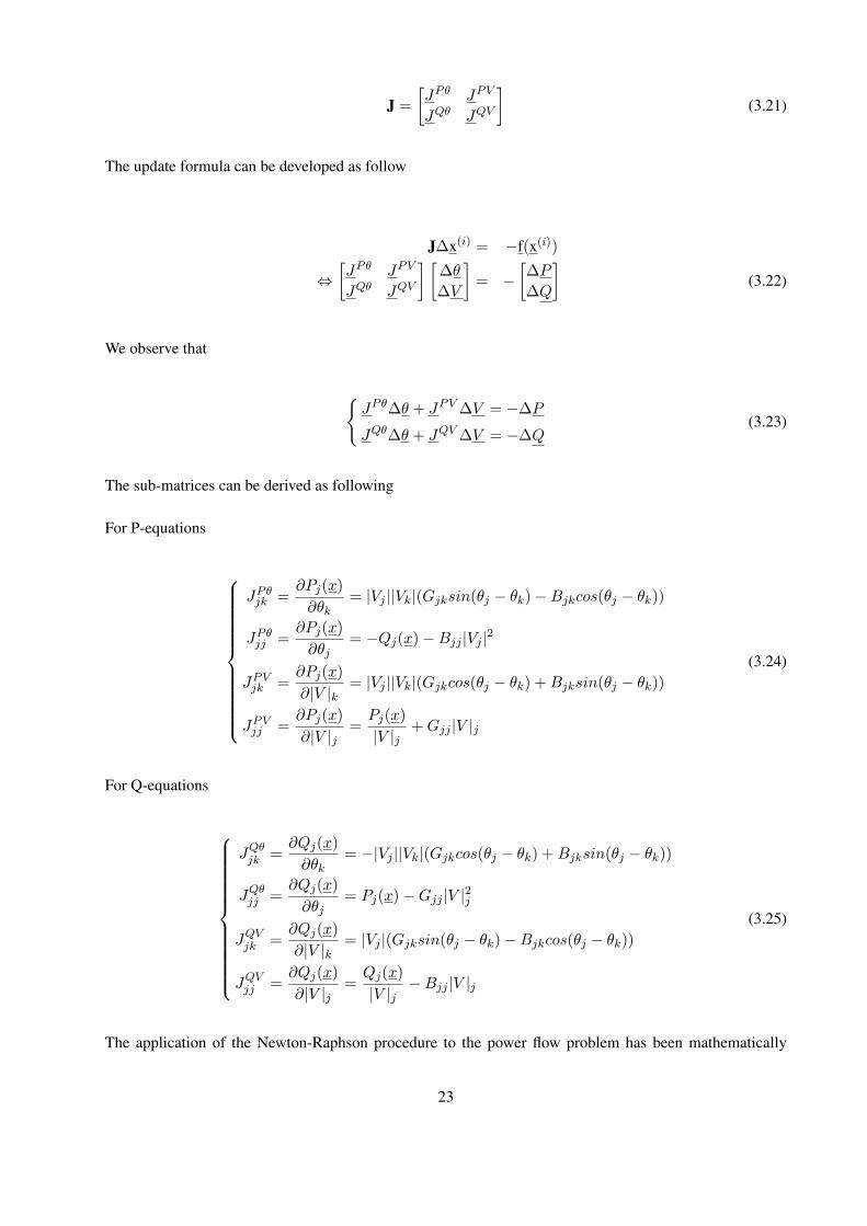
J =

[JPθ JPV

JQθ JQV

](3.21)

The update formula can be developed as follow

J∆x(i) = −f(x(i))

⇔[JPθ JPV

JQθ JQV

] [∆θ

∆V

]= −

[∆P

∆Q

](3.22)

We observe that

{JPθ∆θ + JPV ∆V = −∆P

JQθ∆θ + JQV ∆V = −∆Q(3.23)

The sub-matrices can be derived as following

For P-equations

JPθjk =∂Pj(x)

∂θk= |Vj ||Vk|(Gjksin(θj − θk)−Bjkcos(θj − θk))

JPθjj =∂Pj(x)

∂θj= −Qj(x)−Bjj |Vj |2

JPVjk =∂Pj(x)

∂|V |k= |Vj ||Vk|(Gjkcos(θj − θk) +Bjksin(θj − θk))

JPVjj =∂Pj(x)

∂|V |j=Pj(x)

|V |j+Gjj |V |j

(3.24)

For Q-equations

JQθjk =∂Qj(x)

∂θk= −|Vj ||Vk|(Gjkcos(θj − θk) +Bjksin(θj − θk))

JQθjj =∂Qj(x)

∂θj= Pj(x)−Gjj |V |2j

JQVjk =∂Qj(x)

∂|V |k= |Vj |(Gjksin(θj − θk)−Bjkcos(θj − θk))

JQVjj =∂Qj(x)

∂|V |j=Qj(x)

|V |j−Bjj |V |j

(3.25)

The application of the Newton-Raphson procedure to the power flow problem has been mathematically

23

developed. Let now derive the numerical procedure to perform a sensitivity analysis.

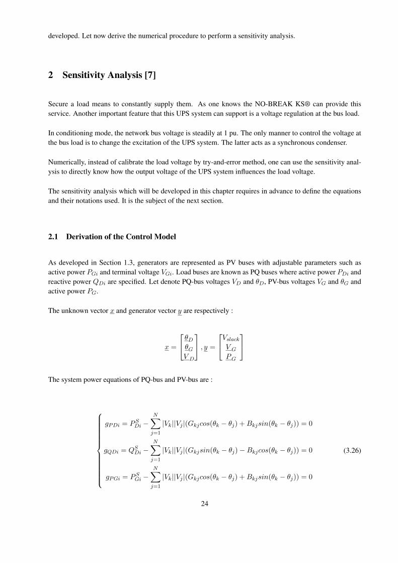
2 Sensitivity Analysis [7]

Secure a load means to constantly supply them. As one knows the NO-BREAK KS® can provide thisservice. Another important feature that this UPS system can support is a voltage regulation at the bus load.

In conditioning mode, the network bus voltage is steadily at 1 pu. The only manner to control the voltage atthe bus load is to change the excitation of the UPS system. The latter acts as a synchronous condenser.

Numerically, instead of calibrate the load voltage by try-and-error method, one can use the sensitivity anal-ysis to directly know how the output voltage of the UPS system influences the load voltage.

The sensitivity analysis which will be developed in this chapter requires in advance to define the equationsand their notations used. It is the subject of the next section.

2.1 Derivation of the Control Model

As developed in Section 1.3, generators are represented as PV buses with adjustable parameters such asactive power PGi and terminal voltage VGi. Load buses are known as PQ buses where active power PDi andreactive power QDi are specified. Let denote PQ-bus voltages VD and θD, PV-bus voltages VG and θG andactive power PG.

The unknown vector x and generator vector y are respectively :

x =

θDθGV D

, y =

VslackV G

PG

The system power equations of PQ-bus and PV-bus are :

gPDi = PSDi −N∑

j=1

|Vk||Vj |(Gkjcos(θk − θj) +Bkjsin(θk − θj)) = 0

gQDi = QSDi −N∑

j=1

|Vk||Vj |(Gkjsin(θk − θj)−Bkjcos(θk − θj)) = 0

gPGi = PSGi −N∑

j=1

|Vk||Vj |(Gkjcos(θk − θj) +Bkjsin(θk − θj)) = 0

(3.26)

24

Consequently, we can clearly introduce the theoretical basis of the sensitivity analysis.

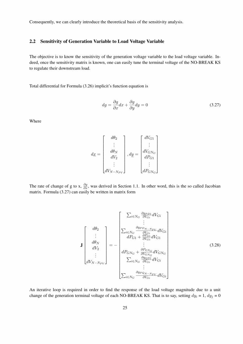
2.2 Sensitivity of Generation Variable to Load Voltage Variable

The objective is to know the sensitivity of the generation voltage variable to the load voltage variable. In-deed, once the sensitivity matrix is known, one can easily tune the terminal voltage of the NO-BREAK KSto regulate their downstream load.

Total differential for Formula (3.26) implicit’s function equation is

dg =∂g

∂xdx+

∂g

∂ydy = 0 (3.27)

Where

dx =

dθ2...

dθNdV2

...dVN−NPV

, dy =

dVG1...

dVGNGdPG1

...dPGNG

The rate of change of g to x, ∂g∂x , was derived in Section 1.1. In other word, this is the so called Jacobianmatrix. Formula (3.27) can easily be written in matrix form

J

dθ2...

dθNdV2

...dVN−NPV

= −

∑i∈NG

∂gPD1∂VGi

dVGi...

∑i∈NG

∂gPDN−NPV∂VGi

dVGi

dPG1 + ∂PG1∂VG1

dVG1

...

dPGNG +∂PGNG∂VGNG

dVGNG∑i∈NG

∂gQD1

∂VGidVGi

...∑

i∈NG∂gPQN−NPV

∂VGidVGi

(3.28)

An iterative loop is required in order to find the response of the load voltage magnitude due to a unitchange of the generation terminal voltage of each NO-BREAK KS. That is to say, setting dyi = 1, dyj = 0

25

(i=1,2,...,2NPV + 1, j6=i) and then solving successively dxi. In matrix form

Jdxi = −∂g

∂y

0...1...0

(3.29)

One can denote D, the rate of change of x to y or D = J−1 ∂g

∂y . Once this matrix is obtained, one caneasily find the rate of change of a particular load voltage to the terminal voltage of one NO-BREAK KS® .Therefore, the differential equation is

dx = Ddy (3.30)

Finally, for this application, the system of equations to be solved is

dVG1

...dVGNG

=

∂VG1∂VPD1

. . . ∂VG1∂VPDN−NPV

... . . ....

∂VGNG∂VPD1

. . .∂VGNG

∂VPDN−NPV

dVPD1...

dVPDN−NPV

(3.31)

3 Fault Study [8]

In this chapter, the techniques used to compute the voltages of different buses, during the fault, will bederived. In order to determine the magnitude of the short-circuit current which will be a crucial informationfor the dimensioning of the circuit breakers and the adjustment of the protections settings.

The fault study is divided into two main parts : the analysis of balanced faults and the analysis of unbalancedfaults.

3.1 Analysis of Balanced Faults

The balanced faults are encountered when there is a symmetrical three-phase short-circuit in the network.In other words, the per phase analysis is still applicable.

26

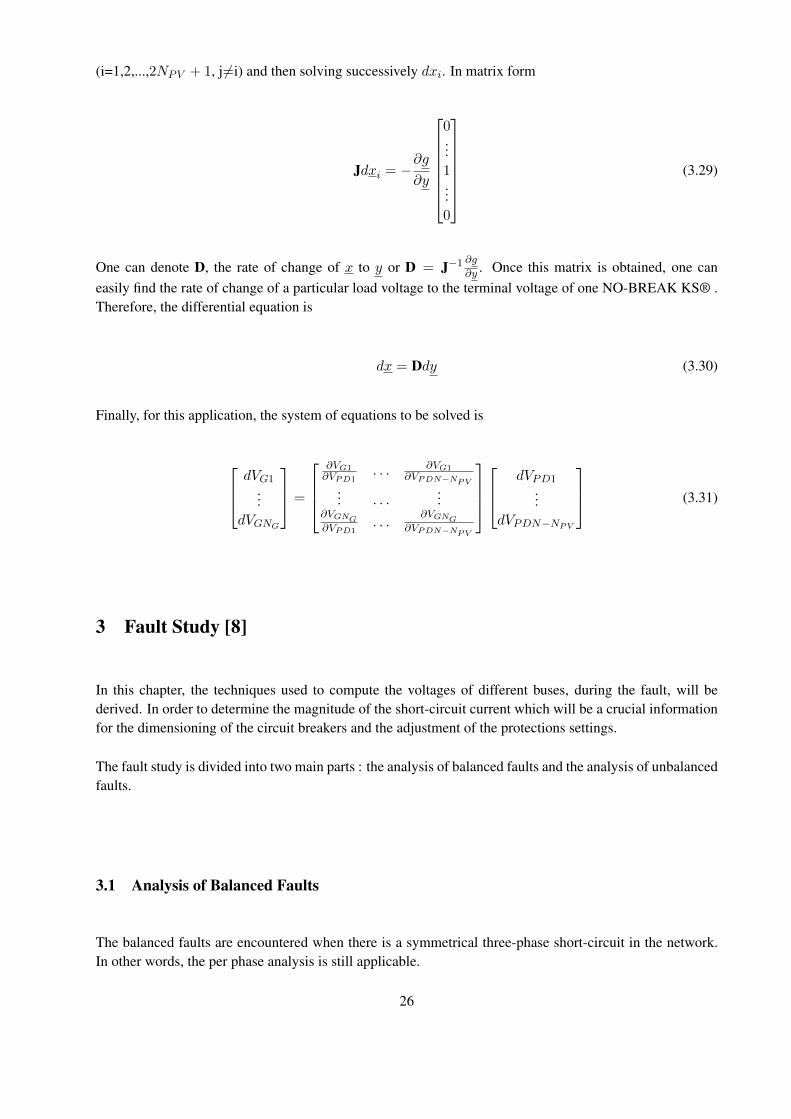
Three-phase Short-circuits

Let consider an IP topology with N buses. Each DRUPS is represented by a Thevenin equivalent as can beseen in Figure 3.2.

proportionnelle aux flux dans les enroulements rotoriques de la machine, lesquels ne changentdans les premiers instants qui suivent le court-circuit. En pratique, on appelle E ′′ la f.e.m. derrierereactance subtransitoire. La resistance statorique a ete negligee.

−+

V

IX′′

d

E′′

FIGURE 7 – schema equivalent d’une machine synchrone

Supposant le court-circuit applique en t = 0, la continuite de cette f.e.m. se traduit par :

E′′(0+) = E

′′(0−) = V (0−) + jX

′′d I(0

−) (12)

On peut donc determiner cette f.e.m. au depart d’un calcul de load flow pre-incident fournis-sant V (0−) et I(0−). On retrouve evidemment le cas du generateur initialement a vide en posantI(0−) = 0 d’ou E

′′(0−) = V (0−) = Eo

q .

3 Calcul des courants de court-circuit triphase

Il importe d’evaluer l’amplitude des courants de defaut pour :• dimensionner les disjoncteurs, qui doivent avoir un pouvoir de coupure suffisant pour inter-

rompre les courants en question ;• regler les protections commandant les disjoncteurs. Celles-ci doivent imperativement agir lors-

qu’il leur incombe d’eliminer le defaut mais ne doivent pas agir intempestivement lorsque cen’est pas necessaire.

3.1 Hypotheses de calcul

Considerons un reseau a N noeuds, comportant des lignes, des cables et des transformateurs. Soitn le nombre de machines synchrones. Sans perte de generalite, nous supposerons que les noeuds dureseau sont numerotes en reservant les n premiers numeros aux noeuds de connexion des machinessynchrones.

Chaque machine synchrone est representee par le schema equivalent de Thevenin de la figure 7.

Chaque charge est supposee se comporter a admittance constante. Cette hypothese est raisonnablepour de nombreux equipements, dans les premiers instants qui suivent un court-circuit. L’admit-tance equivalente Yc d’une charge peut se calculer a partir des puissances active P (0−) et reactive

13

Figure 3.2: Equivalent Circuit of a DRUPS

The electromotive force E′′ is constant during the first moments of the short-circuit, indeed, the latter isproportional to the flux of the field windings which is unchanged during the first moments.

Each load is supposed to behave as a constant admittance which is also a correct hypothesis during the firstmoments of the short-circuit. The equivalent admittance Yc of each load can be computed using the pre-faultactive and reactive power consumed by it and the voltage at its terminal. One have

YC =P (0−)− jQ(0−)

[V (0−)]2(3.32)

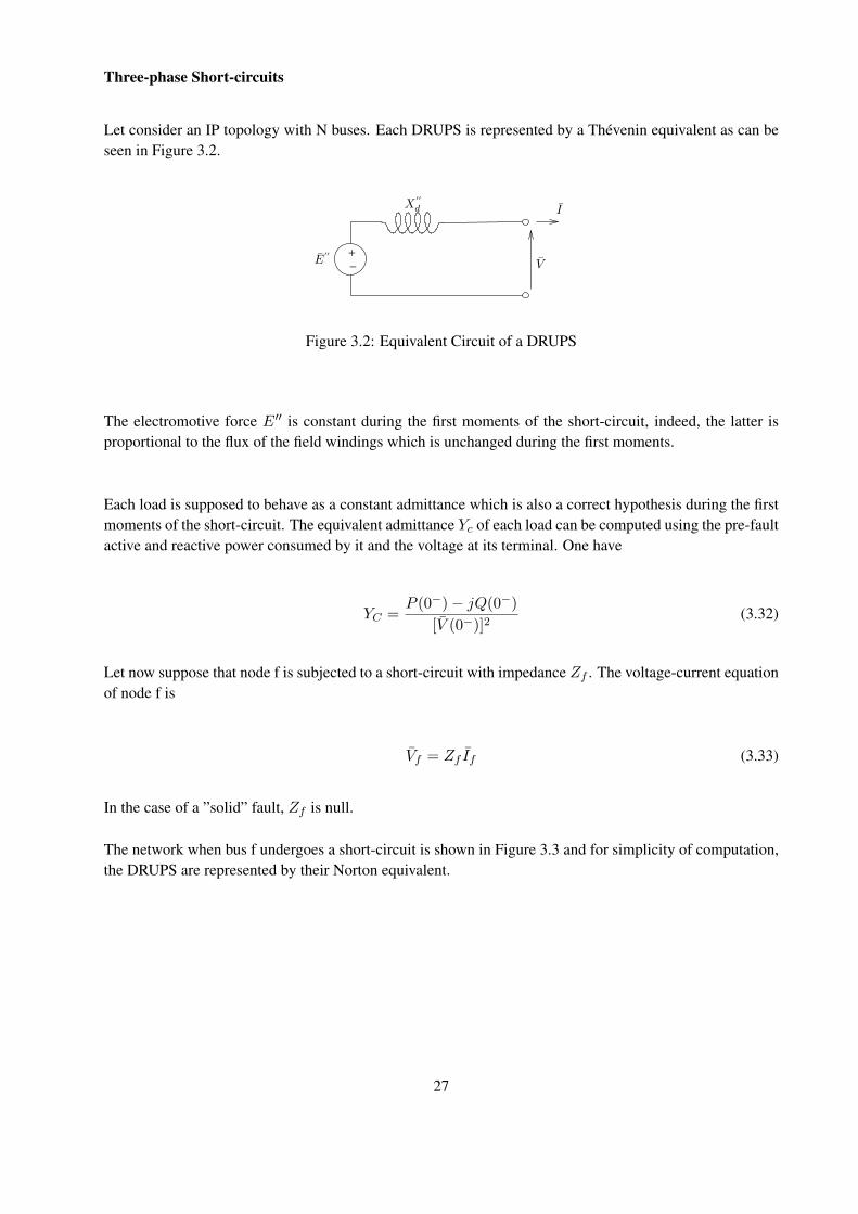
Let now suppose that node f is subjected to a short-circuit with impedance Zf . The voltage-current equationof node f is

Vf = Zf If (3.33)

In the case of a ”solid” fault, Zf is null.

The network when bus f undergoes a short-circuit is shown in Figure 3.3 and for simplicity of computation,the DRUPS are represented by their Norton equivalent.

27

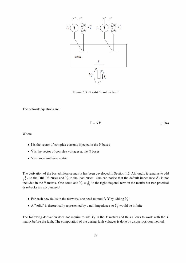
Figure 3.3: Short-Circuit on bus f

The network equations are :

I = YV (3.34)

Where

• I is the vector of complex currents injected in the N buses

• V is the vector of complex voltages at the N buses

• Y is bus admittance matrix

The derivation of the bus admittance matrix has been developed in Section 1.2. Although, it remains to add1

jX′′ to the DRUPS buses and Yc to the load buses. One can notice that the default impedance Zf is notincluded in the Y matrix. One could add Yf = 1

Zfto the right diagonal term in the matrix but two practical

drawbacks are encountered:

• For each new faults in the network, one need to modify Y by adding Yf

• A ”solid” is theoretically represented by a null impedance so Yf would be infinite

The following derivation does not require to add Yf in the Y matrix and thus allows to work with the Ymatrix before the fault. The computation of the during-fault voltages is done by a superposition method.

28

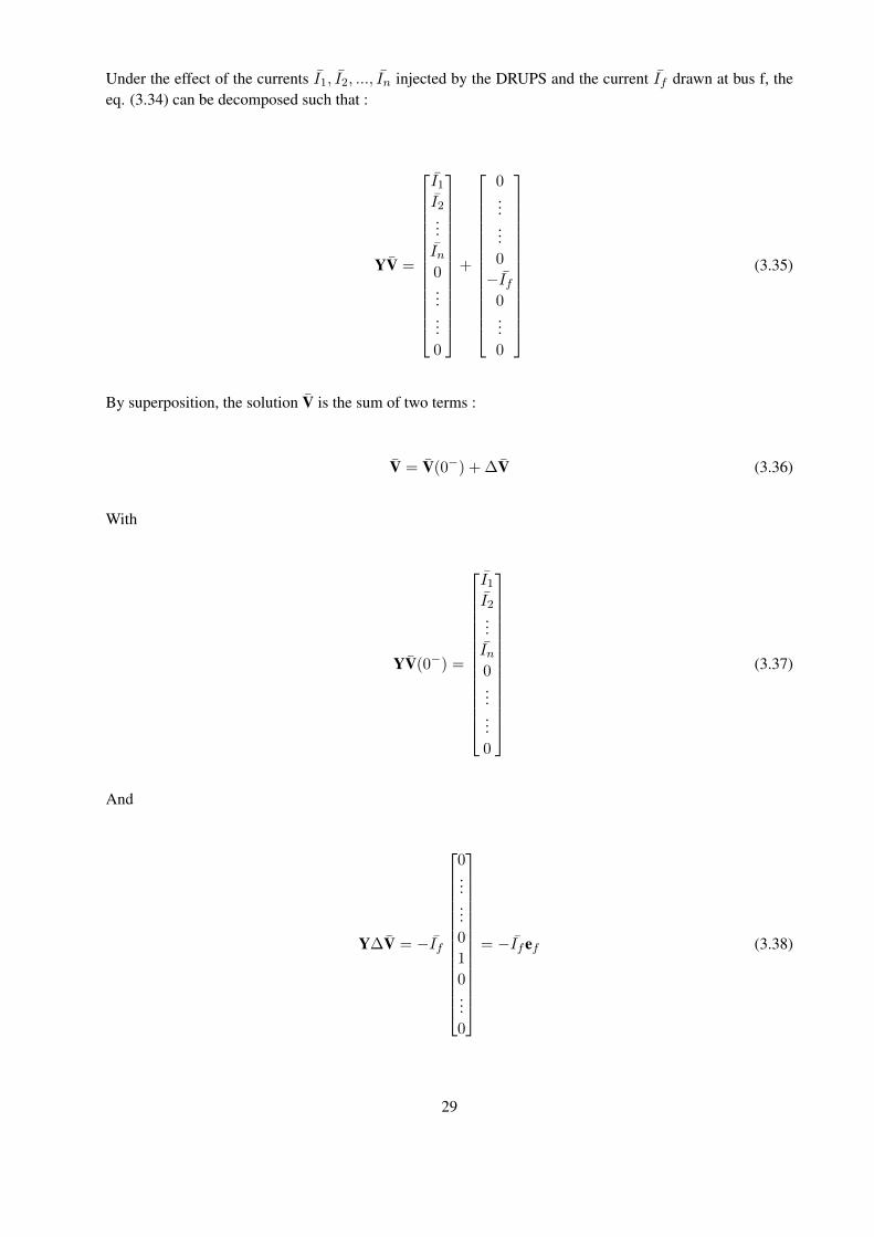
Under the effect of the currents I1, I2, ..., In injected by the DRUPS and the current If drawn at bus f, theeq. (3.34) can be decomposed such that :

YV =

I1

I2...In0......0

+

0......0

−If0...0

(3.35)

By superposition, the solution V is the sum of two terms :

V = V(0−) + ∆V (3.36)

With

YV(0−) =

I1

I2...In0......0

(3.37)

And

Y∆V = −If

0......0

1

0...0

= −Ifef (3.38)

29

V(0−) is the vector of bus voltages before the fault occurs in the system. ∆V can be consider as a correctionwhich simulate the effect of the short-circuit. And ef is a vector of zeros except for the f-th one which isequal to 1.

At this point, the value of If is still unknown. So, let one solves the linear system :

Y ∆V(1)= ef (3.39)

The right hand side of eq. (3.38) and (3.39) differs by the factor -If , one has :

∆V = −If∆V(1) (3.40)

Introducing this result in eq. (3.36), one obtains :

V = V(0−)− If∆V(1) (3.41)

The f-th component of this equation is

Vf = Vf (0−)− If∆V(1)f (3.42)

By combining the above equation and eq.(3.33), one obtains the value of If :

If =Vf (0−)

∆V(1)f + Zf

(3.43)

And finally, by injecting this solution in eq.(3.41), one finds the post-fault bus voltages

V = V(0−)− Vf (0−)

∆V(1)f + Zf

∆V(1) (3.44)

To complete the analysis of the fault study, it remains to develop the second part concerning the analysis ofunbalanced faults.

30

3.2 Analysis of Unbalanced Faults

For the analysis of unbalanced faults, two approaches can be used.

The first approach is a ”traditional” approach whose purpose is to solve three balanced systems : the positive-sequence system, the negative-sequence system and the zero-sequence system. According to the networktopology, one assembles the positive-sequence models, the negative-sequence models and the zero-sequencemodels taking into account the components of this network such that lines, transformers, loads and genera-tors. At the location of the fault, one connects the positive-, negative- and zero-sequence models in a waythat the nature of the fault is taking into account. Once the voltages and currents are found, one can easilyuse the Fortescue transformation and obtains the solution in (a,b,c).

The second approach, used in this master thesis, is based on the resolution of the equation system in (a,b,c):

I = YV (3.45)

Let consider a N-bus network. The bus admittance matrix Y is thus a 3Nx3N matrix and the vector of three-phase injected currents I is a 3Nx1 size vector. These latter can be constructed by assembling individualmodels that represent the loads, mains, DRUPS, lines and transformers according to the network topology.One must highlight that some of the models needs values from an initial power flow computation of thebalanced system.

Let us clarify successively the different models.

Load Model

Firstly, the model of a star-connected load will be developed. And secondly, the model of a delta-connectedload will be developed.

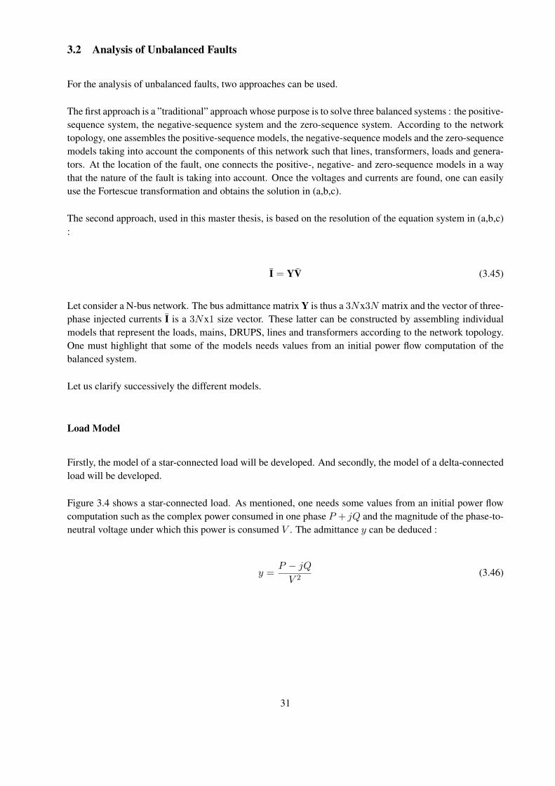
Figure 3.4 shows a star-connected load. As mentioned, one needs some values from an initial power flowcomputation such as the complex power consumed in one phase P + jQ and the magnitude of the phase-to-neutral voltage under which this power is consumed V . The admittance y can be deduced :

y =P − jQV 2

(3.46)

31

Three-phase analysis of unbalanced systems Load

Load

Star-connected load

Input data:

complex power consumed in one phase: P + jQ (in pu)

magnitude of the phase-to-neutral voltage under which this power isconsumed: V (in pu)

impedance between neutral and ground: zn (in pu)

y =P − jQ

V 2yn =

1

zn

5 / 27

Figure 3.4: Star-Connected Load

By Ohm’s law,

Ia = y(Va − Vn)

Ib = y(Vb − Vn)

Ic = y(Vc − Vn)

Ia + Ib + Ic = ynVn

(3.47a)

(3.47b)

(3.47c)

(3.47d)

By adding eq. (3.47a, 3.47b and 3.47c) and introducing the result in eq.(3.47d) yields :

Vn =yVa + yVb + yVc

ytot(3.48)

With ytot = 3y + yn.

Injecting eq. (3.48) into eq. (3.47a, 3.47b and 3.47c) and arranging the results in matrix form gives :

IaIbIc

=

y − y2

ytot− y2

ytot− y2

ytot

− y2

ytoty − y2

ytot− y2

ytot

− y2

ytot− y2

ytoty − y2

ytot

︸︷︷︸Contribution to matrix Y

VaVbVc

(3.49)

Let derive the delta-connected load model. Figure 3.5 shows a delta-connected load. The complex powerP + jQ consumed by the load needs also to be know and the magnitude of the phase-to-phase voltage Uunder which this power is consumed is also obtained by an initial power flow computation.

32

Three-phase analysis of unbalanced systems Load

Delta-connected load

Input data:

complex power consumed in each branch: P + jQ (in pu)

magnitude of the phase-to-phase voltage under which those powers areconsumed: U (in pu)

y =P − jQ

U2

7 / 27

Figure 3.5: Delta-Connected Load

The branch admittance is given by :

y =P − jQU2

(3.50)

By Ohm’s law,

Ia = y(Va − Vb) + y(Va − Vc)Ib = y(Vb − Va) + y(Vb − Vc)Ic = y(Vc − Va) + y(Vc − Vb)

(3.51a)

(3.51b)

(3.51c)

The system of eq. (3.51) can be written in matrix form :

IaIbIc

=

2y −y −y−y 2y −y−y −y 2y


VaVbVc

(3.52)

Model of Balanced Norton Equivalent Of The Mains

As can be seen in Figure 3.2, the mains is modeled as a three-phase Norton equivalent which is suitable forthe present application. Despite the fact that the mains could also be represented by a three-phase Theveninequivalent as seen in Figure 3.6.

For this model, one needs to know the complex power produced by one phase P + jQ, the Thevenin

33

Three-phase analysis of unbalanced systems Balanced Norton equivalent

Balanced Norton equivalent

Input data:

complex power produced by one of the three phases: P + jQ (in pu)Thevenin impedance: zth (in pu)complex (phase-to-neutral) voltage of phase a: Va (in pu)

Ea = Va + zthP − jQ

V ?a

Eb = a2Ea Ec = aEa

10 / 27

Figure 3.6: Voltages and Impedances

Three-phase analysis of unbalanced systems Balanced Norton equivalent

Balanced Norton equivalent

Input data:

complex power produced by one of the three phases: P + jQ (in pu)Thevenin impedance: zth (in pu)complex (phase-to-neutral) voltage of phase a: Va (in pu)

Ea = Va + zthP − jQ

V ?a

Eb = a2Ea Ec = aEa

10 / 27

Figure 3.7: Currents and Admittances

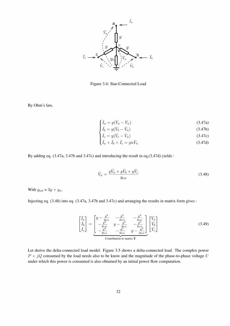
impedance zth = 1Ssc

where Ssc is the short-circuit power and the complex (phase-to-neutral) voltage ofphase a Va. The electromotive force of each phase depends of these physical quantities :

Ea = Va + zthP − jQV ∗a

Eb = a2Ea

Ec = aEa

(3.53a)

(3.53b)

(3.53c)

Where a = ej2π3 .

By Ohm’s law,

Ia =(Va − Ea)

zth

Ib =(Vb − Eb)

zth

Ic =(Vc − Ec)

zth

(3.54a)

(3.54b)

(3.54c)

The matrix form of this system of equations yields :

IaIbIc

=

1zth

0 0

0 1zth

0

0 0 1zth


VaVbVc

−

Ea/zthEb/zthEc/zth

︸︷︷︸Contribution to matrix I

(3.55)

34

DRUPS Model

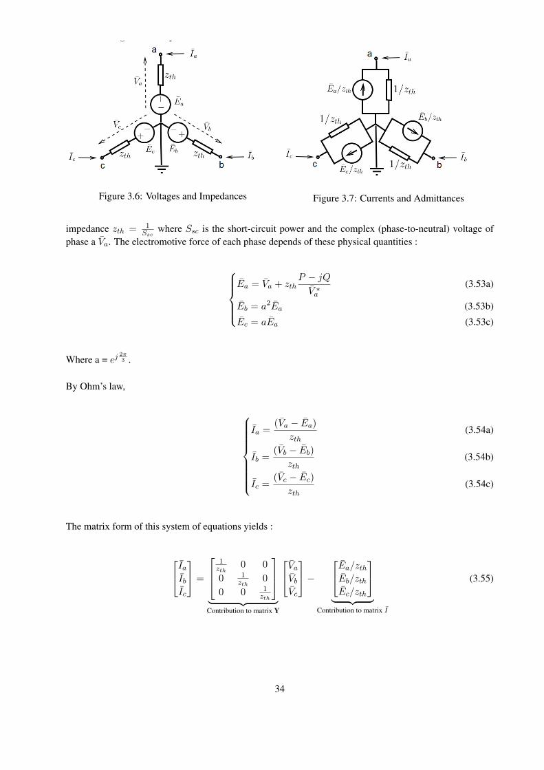
For the generator model shown in Figure 3.8, the contribution to admittance matrix Y can be derived fromthe positive, negative and zero-sequence equivalent circuits of a synchronous generator.

Figure 3.8: Generator model

Let assume a star configuration, with an impedance zn in the neutral. The positive-, negative- and zero-sequence equivalent circuits of a synchronous generator are shown in Figure 3.9.

Analysis of unbalanced systems: the symmetrical components Positive, negative and zero-sequence equiv. circuits of a synchronous generator

Positive, negative and zero-sequence equivalent circuits ofa synchronous generator

We assume a star configuration, with an impedance zn in the neutral.

By construction, generators present a three-phase symmetry ⇒ the positive,negative and zero-sequence equivalent circuits are decoupled(see case of load in slide # 12)

the neutral impedance appears in the zero-sequence circuit only, andmultiplied by 3 (see Exercise 1)

if the stator windings are connected in triangle, zn is infinite (see Exercise 2).

16 / 42

Figure 3.9: Symmetrical Components Circuits of a Synchronous Generator

The equivalent admittance matrix YG of the synchronous generator can easily be derived from positive-,negative- and zero-sequence impedances of the latter. Indeed, using the inverse Fortescue Transformationyields :

YG = TYFT−1 (3.56)

35

With:

YF =

1z+

0 0

0 1z+

0

0 0 1z0+3zn

and T =

1 1 1

a2 a 1

a a2 1

The contribution to admittance matrix Y has been derived, it only remains to derive the contribution to thecurrents vector I. For that, one need to identify Inor,a, Inor,b and Inor,c by assuming an initial balancedoperating conditions. For the voltages:

V+ = Va

V− = 0

V0 = 0

(3.57a)

(3.57b)

(3.57c)

For the currents:

I+ = Ia = −P − jQV ∗a

I− = 0

I0 = 0

(3.58a)

(3.58b)

(3.58c)

Hence,

E+ = V+ − z+I+ = Va + z+P − jQV ∗a

(3.59)

Thus, the contribution to vector I is

Inor,aInor,bInor,b

=

E+/z+

a2E+/z+

aE+/z+

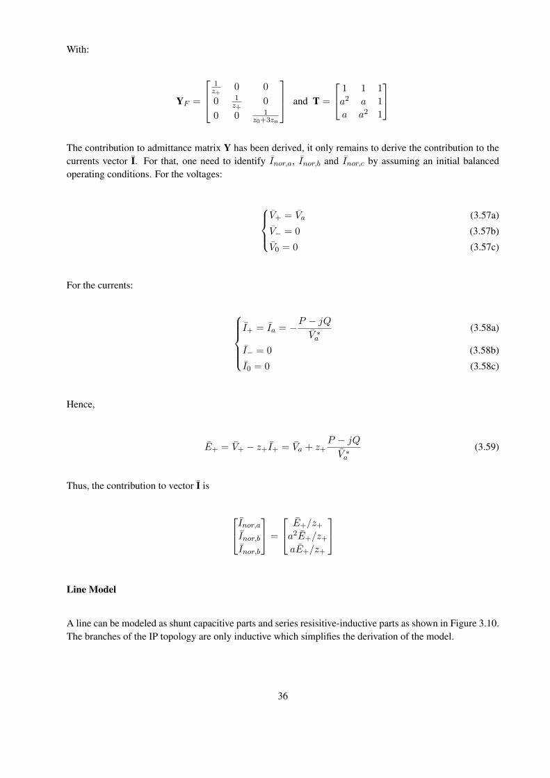
Line Model

A line can be modeled as shunt capacitive parts and series resisitive-inductive parts as shown in Figure 3.10.The branches of the IP topology are only inductive which simplifies the derivation of the model.

36

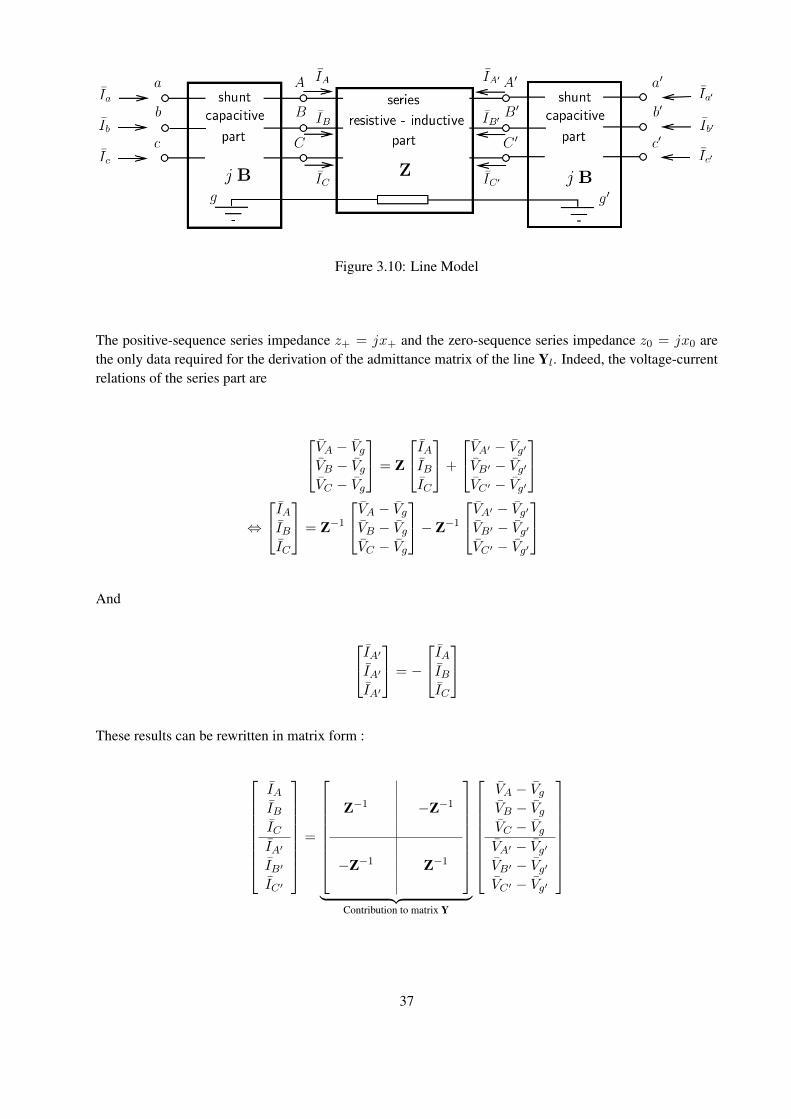
Three-phase analysis of unbalanced systems Line or cable

Line or cable

Full three-phase symmetry is assumed.

Input data:

positive-sequence series impedance: z+ = r+ + jx+ (in pu)

zero-sequence series impedance: zo = ro + jxo (in pu)

positive-sequence half shunt susceptance: b+ (in pu)

zero-sequence half shunt susceptance: bo (in pu)

16 / 27Figure 3.10: Line Model

The positive-sequence series impedance z+ = jx+ and the zero-sequence series impedance z0 = jx0 arethe only data required for the derivation of the admittance matrix of the line Yl. Indeed, the voltage-currentrelations of the series part are

VA − VgVB − VgVC − Vg

= Z

IAIBIC

+

VA′ − Vg′VB′ − Vg′VC′ − Vg′

⇔

IAIBIC

= Z−1

VA − VgVB − VgVC − Vg

− Z−1

VA′ − Vg′VB′ − Vg′VC′ − Vg′

And

IA′

IA′

IA′

= −

IAIBIC

These results can be rewritten in matrix form :

IAIBICIA′

IB′

IC′

=

Z−1 −Z−1

−Z−1 Z−1


VA − VgVB − VgVC − VgVA′ − Vg′VB′ − Vg′VC′ − Vg′

37

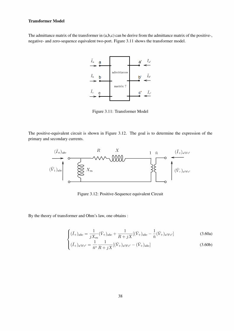
Transformer Model

The admittance matrix of the transformer in (a,b,c) can be derive from the admittance matrix of the positive-,negative- and zero-sequence equivalent two-port. Figure 3.11 shows the transformer model.

Three-phase analysis of unbalanced systems Transformer

Transformer

Input data:

positive-sequence series impedance: R + jX (in pu)

positive-sequence magnetizing reactance: Xm (in pu)

zero-sequence series impedance: Ro + jXo (in pu)

zero-sequence magnetizing reactance: Xmo (in pu)

impedance neutral - ground on primary and secondary sides: zn1, zn2 (in pu) 3

complex transformer ratio n

3not used in some transformers21 / 27

Figure 3.11: Transformer Model

The positive-equivalent circuit is shown in Figure 3.12. The goal is to determine the expression of theprimary and secondary currents.


Admittance matrix of the direct-sequence equivalent two-port

(I+)abc =1

jXm(V+)abc +

1

R + jX

[(V+)abc −

1

n(V+)a′b′c′

]

(I+)a′b′c′ =1

n?1

R + jX

[1

n(V+)a′b′c′ − (V+)abc

]

or in matrix form:

[(I+)abc

(I+)a′b′c′

]=

[1

jXm+ 1

R+jX − 1n

1R+jX

− 1n?

1R+jX

1|n|2

1R+jX

]

︸︷︷︸posit.-sequ. admittance matrix

[(V+)abc

(V+)a′b′c′

]

22 / 27

Figure 3.12: Positive-Sequence equivalent Circuit

By the theory of transformer and Ohm’s law, one obtains :

(I+)abc =1

jXm(V+)abc +

1

R+ jX[(V+)abc −

1

n(V+)a′b′c′ ]

(I+)a′b′c′ =1

n∗1

R+ jX[(V+)a′b′c′ − (V+)abc]

(3.60a)

(3.60b)

38

Or in matrix form :

[(I+)abc

(I+)a′b′c′

]=

[1

jXm+ 1

R+jX − 1n

1R+jX

− 1n∗

1R+jX − 1

|n|21

R+jX

]

︸︷︷︸pos.−seq.admittancematrix

[(V+)abc

(V+)a′b′c′

]

Concerning the derivation of the negative-sequence admittance matrix, it is similar to the positive-sequence.However, one must replace n by n∗ in the positive-sequence admittance matrix. So one has :

[(I−)abc

(I−)a′b′c′

]=

[1

jXm+ 1

R+jX − 1n∗

1R+jX

− 1n

1R+jX − 1

|n|21

R+jX

]

︸︷︷︸neg.−seq.admittancematrix

[(V−)abc

(V−)a′b′c′

]

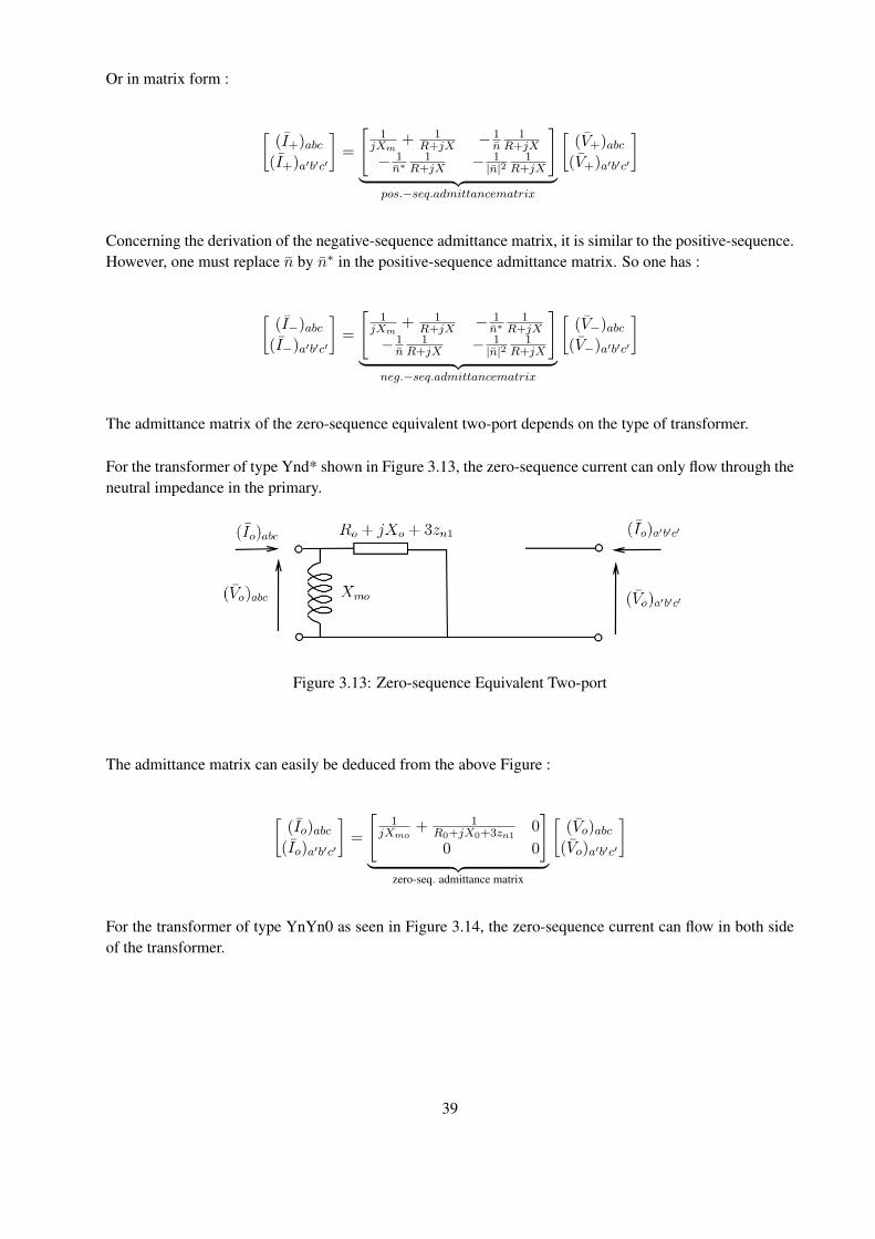
The admittance matrix of the zero-sequence equivalent two-port depends on the type of transformer.

For the transformer of type Ynd* shown in Figure 3.13, the zero-sequence current can only flow through theneutral impedance in the primary.


Admittance matrix of the negative-sequence equivalent two-port

Replacing n by n? in the direct-sequence admittance matrix:[

(I−)abc(I−)a′b′c′

]=

[ 1jXm

+ 1R+jX − 1

n?1

R+jX

− 1n

1R+jX

1|n|2

1R+jX

]

︸︷︷︸negative-sequ. admittance matrix

[(V−)abc

(V−)a′b′c′

]

Admittance matrix of the zero-sequence equivalent two-port

1. Transformer of type Ynd*

[(Io)abc

(Io)a′b′c′

]=

[1

jXmo+ 1

Ro+jXo+3zn10

0 0

]

︸︷︷︸zero-sequ. admit. matrix

[(Vo)abc

(Vo)a′b′c′

]

23 / 27

Figure 3.13: Zero-sequence Equivalent Two-port

The admittance matrix can easily be deduced from the above Figure :

[(Io)abc

(Io)a′b′c′

]=

[1

jXmo+ 1

R0+jX0+3zn10

0 0

]

︸︷︷︸zero-seq. admittance matrix

[(Vo)abc

(Vo)a′b′c′

]

For the transformer of type YnYn0 as seen in Figure 3.14, the zero-sequence current can flow in both sideof the transformer.

39


2. Transformer of type Ynyn0

[(Io)abc

(Io)a′b′c′

]=

[ 1jXmo

+ 1Ro+jXo+3zn1+3zn2/n2 − 1

n1

Ro+jXo+3zn1+3zn2/n2

− 1n

1Ro+jXo+3zn1+3zn2/n2

1n2


]

︸︷︷︸zero-sequ. admittance matrix

[(Vo)abc

(Vo)a′b′c′

]

3. Transformer of any other type

[(Io)abc

(Io)a′b′c′

]=

[1

jXmo0

0 0

]


[(Vo)abc

(Vo)a′b′c′

]

24 / 27


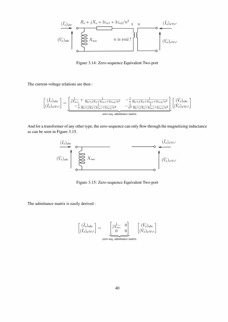
The current-voltage relations are then :

[(Io)abc

(Io)a′b′c′

]=

[1

jXmo+ 1

R0+jX0+3zn1+3zn2/n2 − 1n

1R0+jX0+3zn1+3zn2/n2

− 1n

1R0+jX0+3zn1+3zn2/n2 − 1

n21

R0+jX0+3zn1+3zn2/n2

]


[(Vo)abc

(Vo)a′b′c′

]

And for a transformer of any other type, the zero-sequence can only flow through the magnetizing inductanceas can be seen in Figure 3.15.


2. Transformer of type Ynyn0

[(Io)abc

(Io)a′b′c′

]=

[ 1jXmo

+ 1Ro+jXo+3zn1+3zn2/n2 − 1

n1

Ro+jXo+3zn1+3zn2/n2

− 1n


1n2


]

︸︷︷︸zero-sequ. admittance matrix

[(Vo)abc

(Vo)a′b′c′

]

3. Transformer of any other type

[(Io)abc

(Io)a′b′c′

]=

[1

jXmo0

0 0

]


[(Vo)abc

(Vo)a′b′c′

]

24 / 27


The admittance matrix is easily derived :

[(Io)abc

(Io)a′b′c′

]=

[1

jXmo0

0 0

]


[(Vo)abc

(Vo)a′b′c′

]

40

One can now assemble the admittance matrices of all three sequences :

(I+)abc(I−)abc(Io)abc

(I+)a′b′c′

(I−)a′b′c′

(Io)a′b′c′

= YF

(V+)abc(V−)abc(Vo)abc

(V+)a′b′c′

(V−)a′b′c′

(Vo)a′b′c′

With :

YF =

1jXm

+ 1R+jX 0 0 − 1

n1

R+jX 0 0

0 1jXm

+ 1R+jX 0 0 − 1

n∗1

R+jX 0

0 0 y11 0 0 y12

− 1n∗

1R+jX 0 0 − 1

|n|21

R+jX 0 0

0 − 1n

1R+jX 0 0 − 1

|n|21

R+jX 0

0 0 y21 0 0 y22

Where[y11 y12

y21 y22

]depends on the type of transformer. One can use the inverse Fortescue transformation to

obtain the contribution to admittance matrix Y :

IaIbIcIa′

Ib′

Ic′

=

T 0

0 T

YF

T−1 0

0 T−1


VaVbVcV ′aV ′bV ′c

Let introduces the numerical techniques to take into account the three types of fault.

Phase-to-ground Short-circuit

For the simulation of a phase-to-ground short-circuit, one modifies the Y matrix such as phase i is connectedto the ground by a small impedance :

41

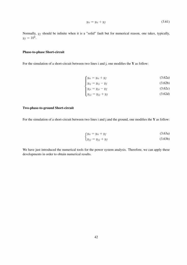
yii = yii + yf (3.61)

Normally, yf should be infinite when it is a ”solid” fault but for numerical reason, one takes, typically,yf = 106.

Phase-to-phase Short-circuit

For the simulation of a short-circuit between two lines i and j, one modifies the Y as follow:

yii = yii + yf

yij = yij − yfyji = yji − yfyjj = yjj + yf

(3.62a)

(3.62b)

(3.62c)

(3.62d)

Two-phase-to-ground Short-circuit

For the simulation of a short-circuit between two lines i and j and the ground, one modifies the Y as follow:

{yii = yii + yf

yjj = yjj + yf

(3.63a)

(3.63b)

We have just introduced the numerical tools for the power system analysis. Therefore, we can apply thesedevelopments in order to obtain numerical results.

42

Chapter 4

Numerical Simulations

This section will show the results of different numerical models that I developed using SCILAB.

Firstly, we will show the flowchart diagram of my program and explained the steps offer to the user in orderto perform a case study.

Secondly, we will validate my developed numerical models in two steps. The first step, we use a topologyfor which circuits theory can easily find an analytical solution. Then we will compare the results of myprogram for this topology and we will find that the results are identical. The second step, concerning acomplex problem, is to compare my results with these of a reference program used by the service of Prof.Thierry Van Cutsem, ARTERE.

At last, we will apply my program for the full study of a problem provided by EURO-DIESEL. And we willfind that the results obtained by the technical service of EURO-DIESEL correspond with these found by myprogram.

1 Program Implementation

The flowchart of the program developed within the framework of this thesis is shown in Figure 4.1.

When the program is launched, one can choose between the conditioning mode or independent mode. Oncethe choice is made, the program automatically reads an Excel file where the topology data are stored andinitializes the variables needed for the power flow problem. The user can solve the power flow problem forthe normal stage which corresponds to the stage describes in the Excel file or skip it and directly goes tothe fault study. If the user wants to solve the normal stage, the Newton-Raphson procedure is used until itconverges and the sensitivity analysis is used in order to change the terminal voltage of the DRUPS to bringthe load voltage to 1 per unit. Then another choice is proposed to the user to proceed a fault study or not,if the decides to skip this study then he is directly send to the choice of scenario. If the user wants a faultstudy, then the nature of short-circuit is proposed and depending on the nature, different script files are usedto compute the post-fault voltages. And finally, the user can choose the scenario (loss of one DRUPS, loss

43

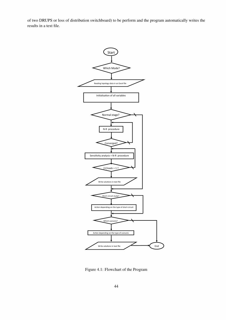
of two DRUPS or loss of distribution switchboard) to be perform and the program automatically writes theresults in a text file.

Start

Which Mode?

Normal stage?

N-R procedure

Converged?

|V|loads = 1 ?

Write solutions in text file

Short-circuit study?

Action depending on the type of short-circuit

Which scenario?

Action depending on the type of scenario

End

Reading topology data in an Excel file

Initialisation of all variables

Write solutions in text file

Sensitivity analysis + N-R procedure

Figure 4.1: Flowchart of the Program

44

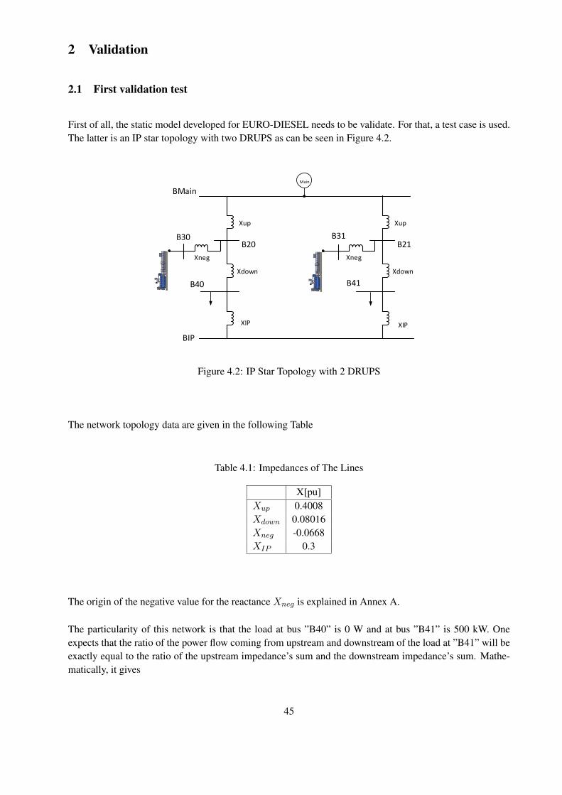
2 Validation

2.1 First validation test

First of all, the static model developed for EURO-DIESEL needs to be validate. For that, a test case is used.The latter is an IP star topology with two DRUPS as can be seen in Figure 4.2.

BMain

B20B30

B40

BIP

B21

B41

Xup

Xneg

Xdown

XIP

Xup

Xdown

Xneg

XIP

Main

B31

Figure 4.2: IP Star Topology with 2 DRUPS

The network topology data are given in the following Table

Table 4.1: Impedances of The Lines

X[pu]Xup 0.4008Xdown 0.08016Xneg -0.0668XIP 0.3

The origin of the negative value for the reactance Xneg is explained in Annex A.

The particularity of this network is that the load at bus ”B40” is 0 W and at bus ”B41” is 500 kW. Oneexpects that the ratio of the power flow coming from upstream and downstream of the load at ”B41” will beexactly equal to the ratio of the upstream impedance’s sum and the downstream impedance’s sum. Mathe-matically, it gives

45

Xupstream = Xup +Xdown = 0.4810 (4.1)

Xdownstream = Xup +Xdown + 2XIP = 1.081 (4.2)

And the ratio between the eq. (4.1) and (4.2)

Xupstream

Xdownstream=

0.4810

1.081= 0.445 (4.3)

The numerical power flow results are shown in the Table 4.2

Table 4.2: Voltage Profile

|V | θ

BMain 1.0000 0B20 1.0001 -0.0235B30 0.9999 -0.0235B40 1.0000 -0.0282B21 1.0001 -0.0528B31 0.9997 -0.0528B41 1.0000 -0.0634BIP 0.9998 -0.0458

One can compute the active power flowing through lines ”BIP -B41” and ”B21-B41”.

Pupstream =|VBIP ||VB41 |sin(θBIP − θB41)

XIP= 153.9798 kW (4.4)

Pdownstream =|VB21 ||VB41 |sin(θB21 − θB41)

Xdown= 346.0202 kW (4.5)

Finally the ratio between eq. (4.4) and (4.5) is

PupstreamPdownstream

=153.9798

346.0202= 0.445 (4.6)

46

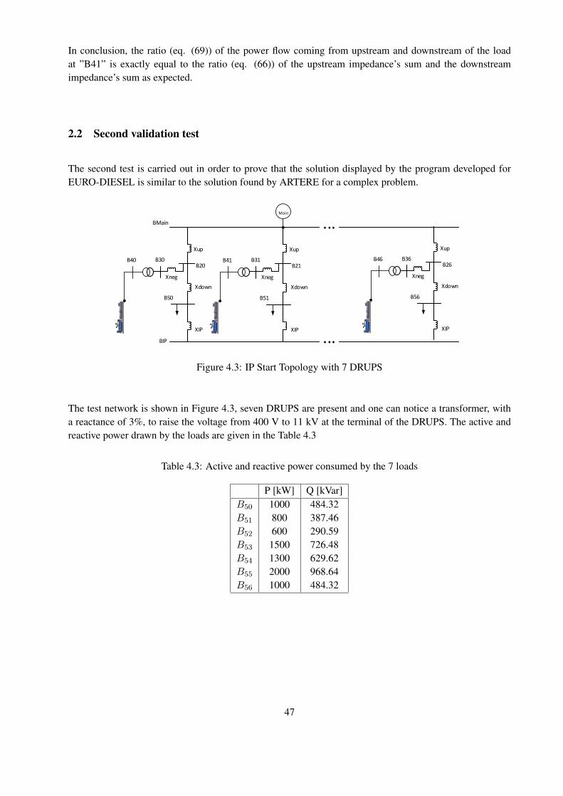
In conclusion, the ratio (eq. (69)) of the power flow coming from upstream and downstream of the loadat ”B41” is exactly equal to the ratio (eq. (66)) of the upstream impedance’s sum and the downstreamimpedance’s sum as expected.

2.2 Second validation test

The second test is carried out in order to prove that the solution displayed by the program developed forEURO-DIESEL is similar to the solution found by ARTERE for a complex problem.

BMain

B20B30B40

B50

BIP

Xup

Xneg

Xdown

XIP

B21B31B41

B51

Xup

Xneg

Xdown

XIP

B26B36B46

B56

Xup

Xneg

Xdown

XIP

...

...

Main

Figure 4.3: IP Start Topology with 7 DRUPS

The test network is shown in Figure 4.3, seven DRUPS are present and one can notice a transformer, witha reactance of 3%, to raise the voltage from 400 V to 11 kV at the terminal of the DRUPS. The active andreactive power drawn by the loads are given in the Table 4.3

Table 4.3: Active and reactive power consumed by the 7 loads

P [kW] Q [kVar]B50 1000 484.32B51 800 387.46B52 600 290.59B53 1500 726.48B54 1300 629.62B55 2000 968.64B56 1000 484.32

47

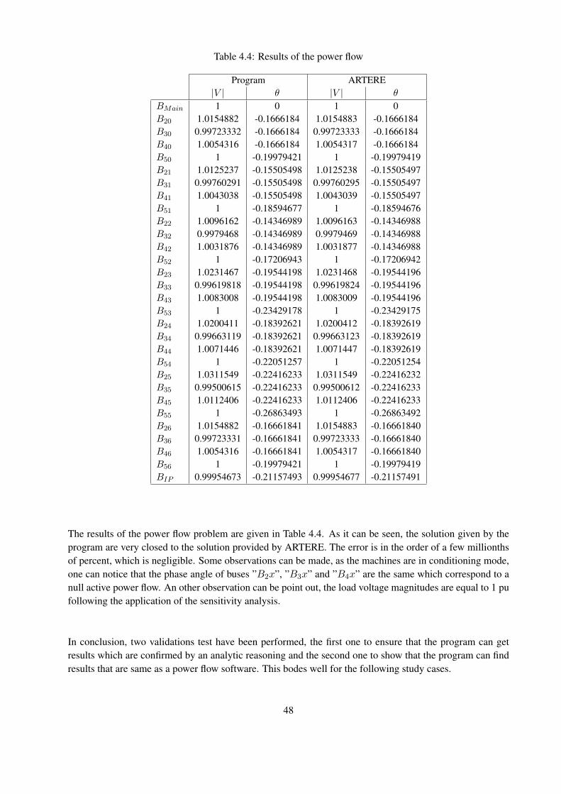
Table 4.4: Results of the power flow

Program ARTERE|V | θ |V | θ

BMain 1 0 1 0B20 1.0154882 -0.1666184 1.0154883 -0.1666184B30 0.99723332 -0.1666184 0.99723333 -0.1666184B40 1.0054316 -0.1666184 1.0054317 -0.1666184B50 1 -0.19979421 1 -0.19979419B21 1.0125237 -0.15505498 1.0125238 -0.15505497B31 0.99760291 -0.15505498 0.99760295 -0.15505497B41 1.0043038 -0.15505498 1.0043039 -0.15505497B51 1 -0.18594677 1 -0.18594676B22 1.0096162 -0.14346989 1.0096163 -0.14346988B32 0.9979468 -0.14346989 0.9979469 -0.14346988B42 1.0031876 -0.14346989 1.0031877 -0.14346988B52 1 -0.17206943 1 -0.17206942B23 1.0231467 -0.19544198 1.0231468 -0.19544196B33 0.99619818 -0.19544198 0.99619824 -0.19544196B43 1.0083008 -0.19544198 1.0083009 -0.19544196B53 1 -0.23429178 1 -0.23429175B24 1.0200411 -0.18392621 1.0200412 -0.18392619B34 0.99663119 -0.18392621 0.99663123 -0.18392619B44 1.0071446 -0.18392621 1.0071447 -0.18392619B54 1 -0.22051257 1 -0.22051254B25 1.0311549 -0.22416233 1.0311549 -0.22416232B35 0.99500615 -0.22416233 0.99500612 -0.22416233B45 1.0112406 -0.22416233 1.0112406 -0.22416233B55 1 -0.26863493 1 -0.26863492B26 1.0154882 -0.16661841 1.0154883 -0.16661840B36 0.99723331 -0.16661841 0.99723333 -0.16661840B46 1.0054316 -0.16661841 1.0054317 -0.16661840B56 1 -0.19979421 1 -0.19979419BIP 0.99954673 -0.21157493 0.99954677 -0.21157491

The results of the power flow problem are given in Table 4.4. As it can be seen, the solution given by theprogram are very closed to the solution provided by ARTERE. The error is in the order of a few millionthsof percent, which is negligible. Some observations can be made, as the machines are in conditioning mode,one can notice that the phase angle of buses ”B2x”, ”B3x” and ”B4x” are the same which correspond to anull active power flow. An other observation can be point out, the load voltage magnitudes are equal to 1 pufollowing the application of the sensitivity analysis.

In conclusion, two validations test have been performed, the first one to ensure that the program can getresults which are confirmed by an analytic reasoning and the second one to show that the program can findresults that are same as a power flow software. This bodes well for the following study cases.

48

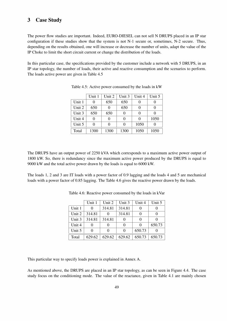
3 Case Study

The power flow studies are important. Indeed, EURO-DIESEL can not sell N DRUPS placed in an IP starconfiguration if these studies show that the system is not N-1 secure or, sometimes, N-2 secure. Thus,depending on the results obtained, one will increase or decrease the number of units, adapt the value of theIP Choke to limit the short circuit current or change the distribution of the loads.

In this particular case, the specifications provided by the customer include a network with 5 DRUPS, in anIP star topology, the number of loads, their active and reactive consumption and the scenarios to perform.The loads active power are given in Table 4.5

Table 4.5: Active power consumed by the loads in kW

Unit 1 Unit 2 Unit 3 Unit 4 Unit 5Unit 1 0 650 650 0 0Unit 2 650 0 650 0 0Unit 3 650 650 0 0 0Unit 4 0 0 0 0 1050Unit 5 0 0 0 1050 0

Total 1300 1300 1300 1050 1050

The DRUPS have an output power of 2250 kVA which corresponds to a maximum active power output of1800 kW. So, there is redundancy since the maximum active power produced by the DRUPS is equal to9000 kW and the total active power drawn by the loads is equal to 6000 kW.

The loads 1, 2 and 3 are IT loads with a power factor of 0.9 lagging and the loads 4 and 5 are mechanicalloads with a power factor of 0.85 lagging. The Table 4.6 gives the reactive power drawn by the loads.

Table 4.6: Reactive power consumed by the loads in kVar

Unit 1 Unit 2 Unit 3 Unit 4 Unit 5Unit 1 0 314.81 314.81 0 0Unit 2 314.81 0 314.81 0 0Unit 3 314.81 314.81 0 0 0Unit 4 0 0 0 0 650.73Unit 5 0 0 0 650.73 0

Total 629.62 629.62 629.62 650.73 650.73

This particular way to specify loads power is explained in Annex A.

As mentioned above, the DRUPS are placed in an IP star topology, as can be seen in Figure 4.4. The casestudy focus on the conditioning mode. The value of the reactance, given in Table 4.1 are mainly chosen

49

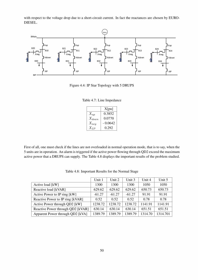
with respect to the voltage drop due to a short-circuit current. In fact the reactances are chosen by EURO-DIESEL.

BMain

B10B20

B30

BIP

Xup

Xneg

Xdown

XIP

Main

B11

B31

Xup

Xneg

Xdown

XIP

B12

B32

Xup

Xneg

Xdown

XIP

B13

B33

Xup

Xneg

Xdown

XIP

B14

B34

Xup

Xneg

Xdown

XIP

B21 B22 B23 B24

Figure 4.4: IP Star Topology with 5 DRUPS

Table 4.7: Line Impedance

X[pu]Xup 0.3852Xdown 0.0770Xneg - 0.0642XIP 0.292

First of all, one must check if the lines are not overloaded in normal operation mode, that is to say, when the5 units are in operation. An alarm is triggered if the active power flowing through QD2 exceed the maximumactive power that a DRUPS can supply. The Table 4.8 displays the important results of the problem studied.

Table 4.8: Important Results for the Normal Stage

Unit 1 Unit 2 Unit 3 Unit 4 Unit 5Active load [kW] 1300 1300 1300 1050 1050Reactive load [kVAR] 629.62 629.62 629.62 650.73 650.73Active Power to IP ring [kW] -61.27 -61.27 -61.27 91.91 91.91Reactive Power to IP ring [kVAR] 0.52 0.52 0.52 0.78 0.78Active Power through QD2 [kW] 1238.72 1238.72 1238.72 1141.91 1141.91Reactive Power through QD2 [kVAR] 630.14 630.14 630.14 651.51 651.51Apparent Power through QD2 [kVA] 1389.79 1389.79 1389.79 1314.70 1314.701

50

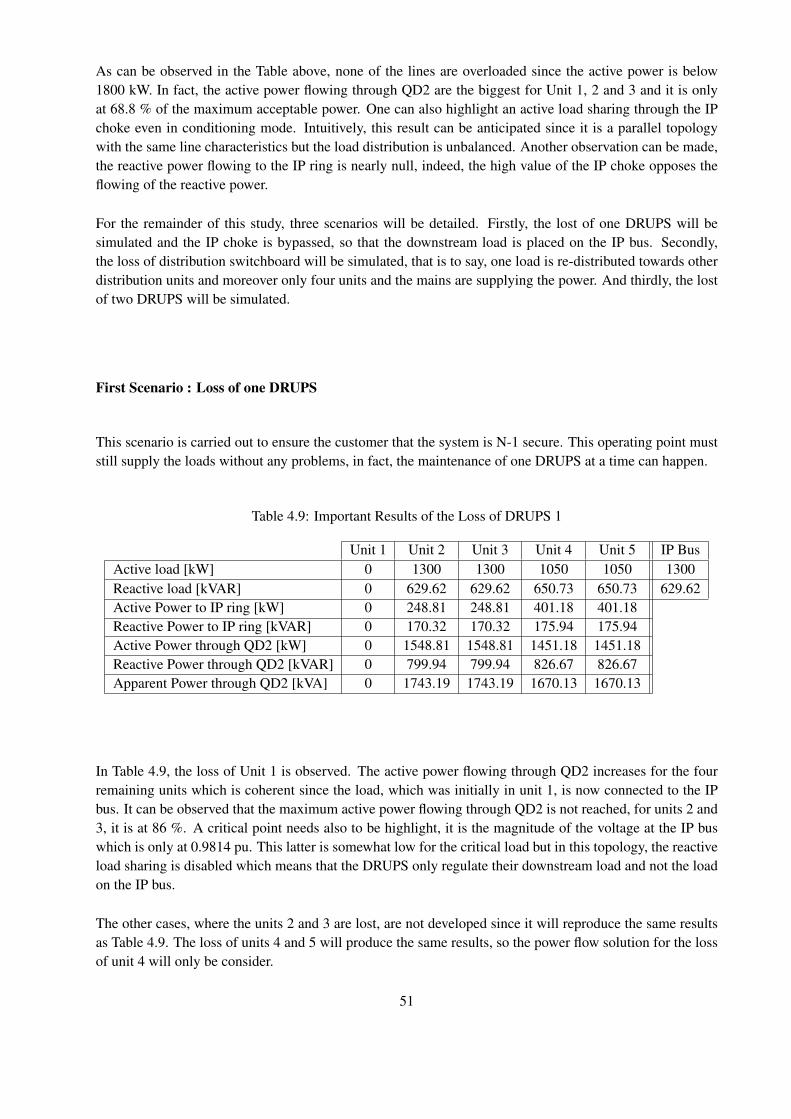
As can be observed in the Table above, none of the lines are overloaded since the active power is below1800 kW. In fact, the active power flowing through QD2 are the biggest for Unit 1, 2 and 3 and it is onlyat 68.8 % of the maximum acceptable power. One can also highlight an active load sharing through the IPchoke even in conditioning mode. Intuitively, this result can be anticipated since it is a parallel topologywith the same line characteristics but the load distribution is unbalanced. Another observation can be made,the reactive power flowing to the IP ring is nearly null, indeed, the high value of the IP choke opposes theflowing of the reactive power.

For the remainder of this study, three scenarios will be detailed. Firstly, the lost of one DRUPS will besimulated and the IP choke is bypassed, so that the downstream load is placed on the IP bus. Secondly,the loss of distribution switchboard will be simulated, that is to say, one load is re-distributed towards otherdistribution units and moreover only four units and the mains are supplying the power. And thirdly, the lostof two DRUPS will be simulated.

First Scenario : Loss of one DRUPS

This scenario is carried out to ensure the customer that the system is N-1 secure. This operating point muststill supply the loads without any problems, in fact, the maintenance of one DRUPS at a time can happen.

Table 4.9: Important Results of the Loss of DRUPS 1

Unit 1 Unit 2 Unit 3 Unit 4 Unit 5 IP BusActive load [kW] 0 1300 1300 1050 1050 1300Reactive load [kVAR] 0 629.62 629.62 650.73 650.73 629.62Active Power to IP ring [kW] 0 248.81 248.81 401.18 401.18Reactive Power to IP ring [kVAR] 0 170.32 170.32 175.94 175.94Active Power through QD2 [kW] 0 1548.81 1548.81 1451.18 1451.18Reactive Power through QD2 [kVAR] 0 799.94 799.94 826.67 826.67Apparent Power through QD2 [kVA] 0 1743.19 1743.19 1670.13 1670.13

In Table 4.9, the loss of Unit 1 is observed. The active power flowing through QD2 increases for the fourremaining units which is coherent since the load, which was initially in unit 1, is now connected to the IPbus. It can be observed that the maximum active power flowing through QD2 is not reached, for units 2 and3, it is at 86 %. A critical point needs also to be highlight, it is the magnitude of the voltage at the IP buswhich is only at 0.9814 pu. This latter is somewhat low for the critical load but in this topology, the reactiveload sharing is disabled which means that the DRUPS only regulate their downstream load and not the loadon the IP bus.

The other cases, where the units 2 and 3 are lost, are not developed since it will reproduce the same resultsas Table 4.9. The loss of units 4 and 5 will produce the same results, so the power flow solution for the lossof unit 4 will only be consider.

51

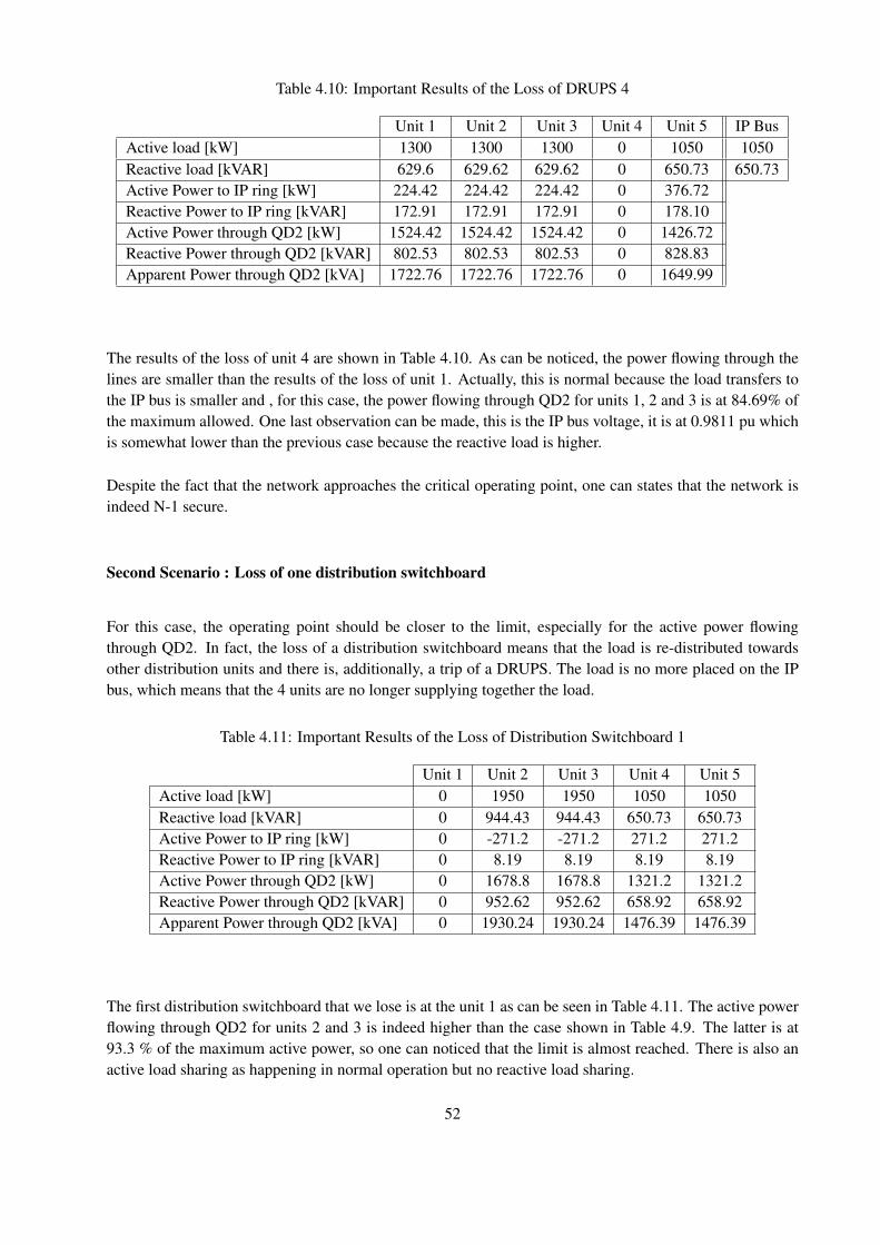
Table 4.10: Important Results of the Loss of DRUPS 4

Unit 1 Unit 2 Unit 3 Unit 4 Unit 5 IP BusActive load [kW] 1300 1300 1300 0 1050 1050Reactive load [kVAR] 629.6 629.62 629.62 0 650.73 650.73Active Power to IP ring [kW] 224.42 224.42 224.42 0 376.72Reactive Power to IP ring [kVAR] 172.91 172.91 172.91 0 178.10Active Power through QD2 [kW] 1524.42 1524.42 1524.42 0 1426.72Reactive Power through QD2 [kVAR] 802.53 802.53 802.53 0 828.83Apparent Power through QD2 [kVA] 1722.76 1722.76 1722.76 0 1649.99

The results of the loss of unit 4 are shown in Table 4.10. As can be noticed, the power flowing through thelines are smaller than the results of the loss of unit 1. Actually, this is normal because the load transfers tothe IP bus is smaller and , for this case, the power flowing through QD2 for units 1, 2 and 3 is at 84.69% ofthe maximum allowed. One last observation can be made, this is the IP bus voltage, it is at 0.9811 pu whichis somewhat lower than the previous case because the reactive load is higher.

Despite the fact that the network approaches the critical operating point, one can states that the network isindeed N-1 secure.

Second Scenario : Loss of one distribution switchboard

For this case, the operating point should be closer to the limit, especially for the active power flowingthrough QD2. In fact, the loss of a distribution switchboard means that the load is re-distributed towardsother distribution units and there is, additionally, a trip of a DRUPS. The load is no more placed on the IPbus, which means that the 4 units are no longer supplying together the load.

Table 4.11: Important Results of the Loss of Distribution Switchboard 1

Unit 1 Unit 2 Unit 3 Unit 4 Unit 5Active load [kW] 0 1950 1950 1050 1050Reactive load [kVAR] 0 944.43 944.43 650.73 650.73Active Power to IP ring [kW] 0 -271.2 -271.2 271.2 271.2Reactive Power to IP ring [kVAR] 0 8.19 8.19 8.19 8.19Active Power through QD2 [kW] 0 1678.8 1678.8 1321.2 1321.2Reactive Power through QD2 [kVAR] 0 952.62 952.62 658.92 658.92Apparent Power through QD2 [kVA] 0 1930.24 1930.24 1476.39 1476.39

The first distribution switchboard that we lose is at the unit 1 as can be seen in Table 4.11. The active powerflowing through QD2 for units 2 and 3 is indeed higher than the case shown in Table 4.9. The latter is at93.3 % of the maximum active power, so one can noticed that the limit is almost reached. There is also anactive load sharing as happening in normal operation but no reactive load sharing.

52

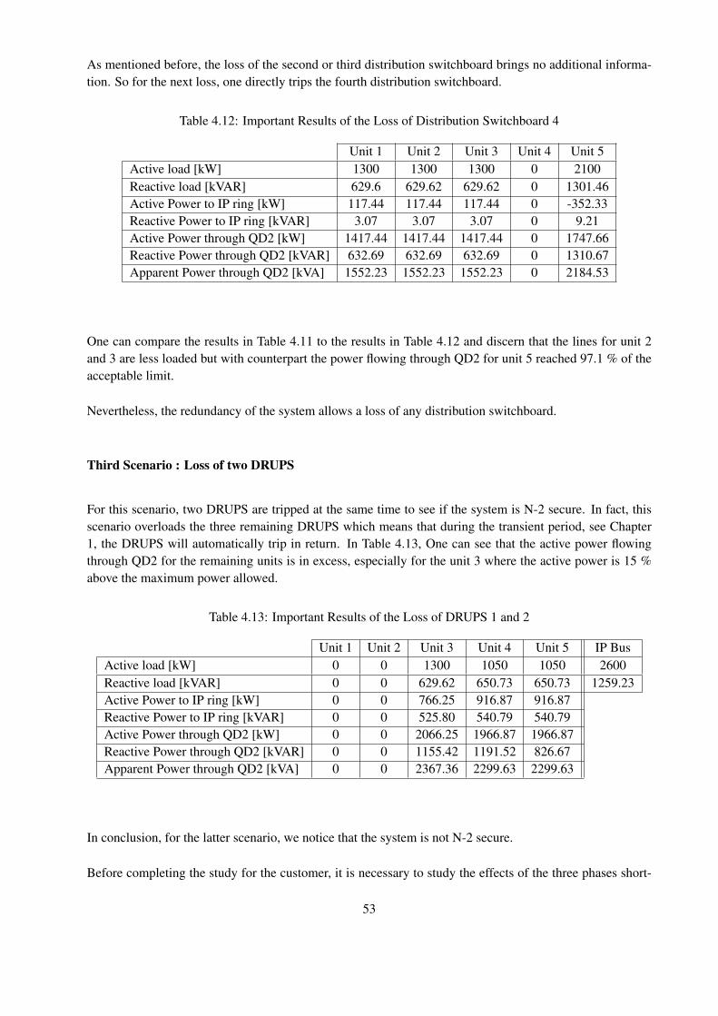
As mentioned before, the loss of the second or third distribution switchboard brings no additional informa-tion. So for the next loss, one directly trips the fourth distribution switchboard.


Unit 1 Unit 2 Unit 3 Unit 4 Unit 5Active load [kW] 1300 1300 1300 0 2100Reactive load [kVAR] 629.6 629.62 629.62 0 1301.46Active Power to IP ring [kW] 117.44 117.44 117.44 0 -352.33Reactive Power to IP ring [kVAR] 3.07 3.07 3.07 0 9.21Active Power through QD2 [kW] 1417.44 1417.44 1417.44 0 1747.66Reactive Power through QD2 [kVAR] 632.69 632.69 632.69 0 1310.67Apparent Power through QD2 [kVA] 1552.23 1552.23 1552.23 0 2184.53

One can compare the results in Table 4.11 to the results in Table 4.12 and discern that the lines for unit 2and 3 are less loaded but with counterpart the power flowing through QD2 for unit 5 reached 97.1 % of theacceptable limit.

Nevertheless, the redundancy of the system allows a loss of any distribution switchboard.

Third Scenario : Loss of two DRUPS

For this scenario, two DRUPS are tripped at the same time to see if the system is N-2 secure. In fact, thisscenario overloads the three remaining DRUPS which means that during the transient period, see Chapter1, the DRUPS will automatically trip in return. In Table 4.13, One can see that the active power flowingthrough QD2 for the remaining units is in excess, especially for the unit 3 where the active power is 15 %above the maximum power allowed.

Table 4.13: Important Results of the Loss of DRUPS 1 and 2

Unit 1 Unit 2 Unit 3 Unit 4 Unit 5 IP BusActive load [kW] 0 0 1300 1050 1050 2600Reactive load [kVAR] 0 0 629.62 650.73 650.73 1259.23Active Power to IP ring [kW] 0 0 766.25 916.87 916.87Reactive Power to IP ring [kVAR] 0 0 525.80 540.79 540.79Active Power through QD2 [kW] 0 0 2066.25 1966.87 1966.87Reactive Power through QD2 [kVAR] 0 0 1155.42 1191.52 826.67Apparent Power through QD2 [kVA] 0 0 2367.36 2299.63 2299.63

In conclusion, for the latter scenario, we notice that the system is not N-2 secure.

Before completing the study for the customer, it is necessary to study the effects of the three phases short-

53

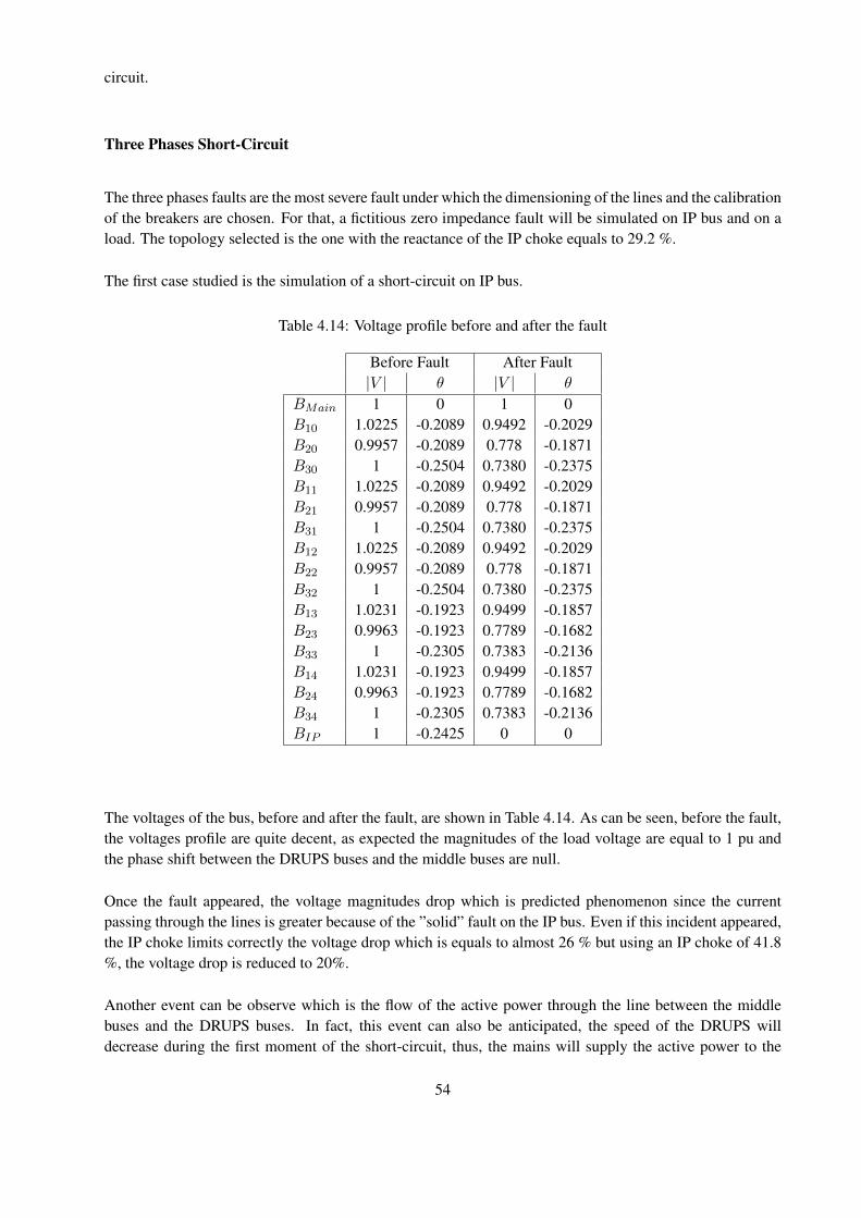
circuit.

Three Phases Short-Circuit

The three phases faults are the most severe fault under which the dimensioning of the lines and the calibrationof the breakers are chosen. For that, a fictitious zero impedance fault will be simulated on IP bus and on aload. The topology selected is the one with the reactance of the IP choke equals to 29.2 %.

The first case studied is the simulation of a short-circuit on IP bus.

Table 4.14: Voltage profile before and after the fault

Before Fault After Fault|V | θ |V | θ

BMain 1 0 1 0B10 1.0225 -0.2089 0.9492 -0.2029B20 0.9957 -0.2089 0.778 -0.1871B30 1 -0.2504 0.7380 -0.2375B11 1.0225 -0.2089 0.9492 -0.2029B21 0.9957 -0.2089 0.778 -0.1871B31 1 -0.2504 0.7380 -0.2375B12 1.0225 -0.2089 0.9492 -0.2029B22 0.9957 -0.2089 0.778 -0.1871B32 1 -0.2504 0.7380 -0.2375B13 1.0231 -0.1923 0.9499 -0.1857B23 0.9963 -0.1923 0.7789 -0.1682B33 1 -0.2305 0.7383 -0.2136B14 1.0231 -0.1923 0.9499 -0.1857B24 0.9963 -0.1923 0.7789 -0.1682B34 1 -0.2305 0.7383 -0.2136BIP 1 -0.2425 0 0

The voltages of the bus, before and after the fault, are shown in Table 4.14. As can be seen, before the fault,the voltages profile are quite decent, as expected the magnitudes of the load voltage are equal to 1 pu andthe phase shift between the DRUPS buses and the middle buses are null.

Once the fault appeared, the voltage magnitudes drop which is predicted phenomenon since the currentpassing through the lines is greater because of the ”solid” fault on the IP bus. Even if this incident appeared,the IP choke limits correctly the voltage drop which is equals to almost 26 % but using an IP choke of 41.8%, the voltage drop is reduced to 20%.

Another event can be observe which is the flow of the active power through the line between the middlebuses and the DRUPS buses. In fact, this event can also be anticipated, the speed of the DRUPS willdecrease during the first moment of the short-circuit, thus, the mains will supply the active power to the

54

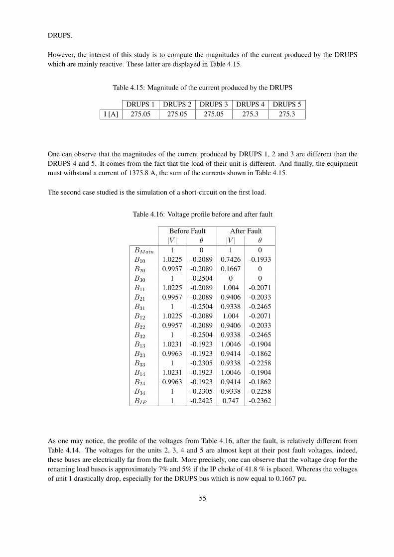
DRUPS.

However, the interest of this study is to compute the magnitudes of the current produced by the DRUPSwhich are mainly reactive. These latter are displayed in Table 4.15.

Table 4.15: Magnitude of the current produced by the DRUPS

DRUPS 1 DRUPS 2 DRUPS 3 DRUPS 4 DRUPS 5I [A] 275.05 275.05 275.05 275.3 275.3

One can observe that the magnitudes of the current produced by DRUPS 1, 2 and 3 are different than theDRUPS 4 and 5. It comes from the fact that the load of their unit is different. And finally, the equipmentmust withstand a current of 1375.8 A, the sum of the currents shown in Table 4.15.

The second case studied is the simulation of a short-circuit on the first load.

Table 4.16: Voltage profile before and after fault

Before Fault After Fault|V | θ |V | θ

BMain 1 0 1 0B10 1.0225 -0.2089 0.7426 -0.1933B20 0.9957 -0.2089 0.1667 0B30 1 -0.2504 0 0B11 1.0225 -0.2089 1.004 -0.2071B21 0.9957 -0.2089 0.9406 -0.2033B31 1 -0.2504 0.9338 -0.2465B12 1.0225 -0.2089 1.004 -0.2071B22 0.9957 -0.2089 0.9406 -0.2033B32 1 -0.2504 0.9338 -0.2465B13 1.0231 -0.1923 1.0046 -0.1904B23 0.9963 -0.1923 0.9414 -0.1862B33 1 -0.2305 0.9338 -0.2258B14 1.0231 -0.1923 1.0046 -0.1904B24 0.9963 -0.1923 0.9414 -0.1862B34 1 -0.2305 0.9338 -0.2258BIP 1 -0.2425 0.747 -0.2362

As one may notice, the profile of the voltages from Table 4.16, after the fault, is relatively different fromTable 4.14. The voltages for the units 2, 3, 4 and 5 are almost kept at their post fault voltages, indeed,these buses are electrically far from the fault. More precisely, one can observe that the voltage drop for therenaming load buses is approximately 7% and 5% if the IP choke of 41.8 % is placed. Whereas the voltagesof unit 1 drastically drop, especially for the DRUPS bus which is now equal to 0.1667 pu.

55

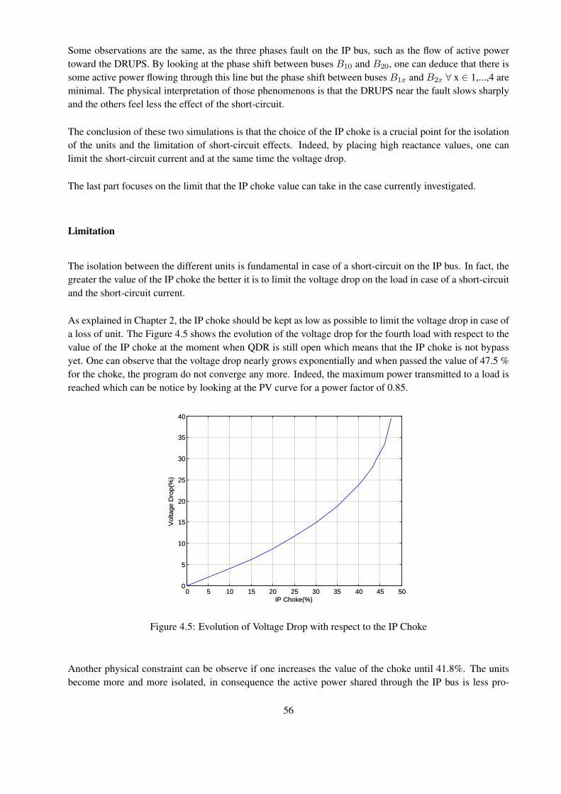
Some observations are the same, as the three phases fault on the IP bus, such as the flow of active powertoward the DRUPS. By looking at the phase shift between buses B10 and B20, one can deduce that there issome active power flowing through this line but the phase shift between buses B1x and B2x ∀ x ∈ 1,...,4 areminimal. The physical interpretation of those phenomenons is that the DRUPS near the fault slows sharplyand the others feel less the effect of the short-circuit.

The conclusion of these two simulations is that the choice of the IP choke is a crucial point for the isolationof the units and the limitation of short-circuit effects. Indeed, by placing high reactance values, one canlimit the short-circuit current and at the same time the voltage drop.

The last part focuses on the limit that the IP choke value can take in the case currently investigated.

Limitation

The isolation between the different units is fundamental in case of a short-circuit on the IP bus. In fact, thegreater the value of the IP choke the better it is to limit the voltage drop on the load in case of a short-circuitand the short-circuit current.

As explained in Chapter 2, the IP choke should be kept as low as possible to limit the voltage drop in case ofa loss of unit. The Figure 4.5 shows the evolution of the voltage drop for the fourth load with respect to thevalue of the IP choke at the moment when QDR is still open which means that the IP choke is not bypassyet. One can observe that the voltage drop nearly grows exponentially and when passed the value of 47.5 %for the choke, the program do not converge any more. Indeed, the maximum power transmitted to a load isreached which can be notice by looking at the PV curve for a power factor of 0.85.

0 5 10 15 20 25 30 35 40 45 500

5

10

15

20

25

30

35

40

IP Choke(%)

Vol

tage

Dro

p(%

)

0 5 10 15 20 25 30 35 40 45 500

5

10

15

20

25

30

35

40

IP Choke(%)

Vol

tage

Dro

p(%

)

Figure 4.5: Evolution of Voltage Drop with respect to the IP Choke

Another physical constraint can be observe if one increases the value of the choke until 41.8%. The unitsbecome more and more isolated, in consequence the active power shared through the IP bus is less pro-

56

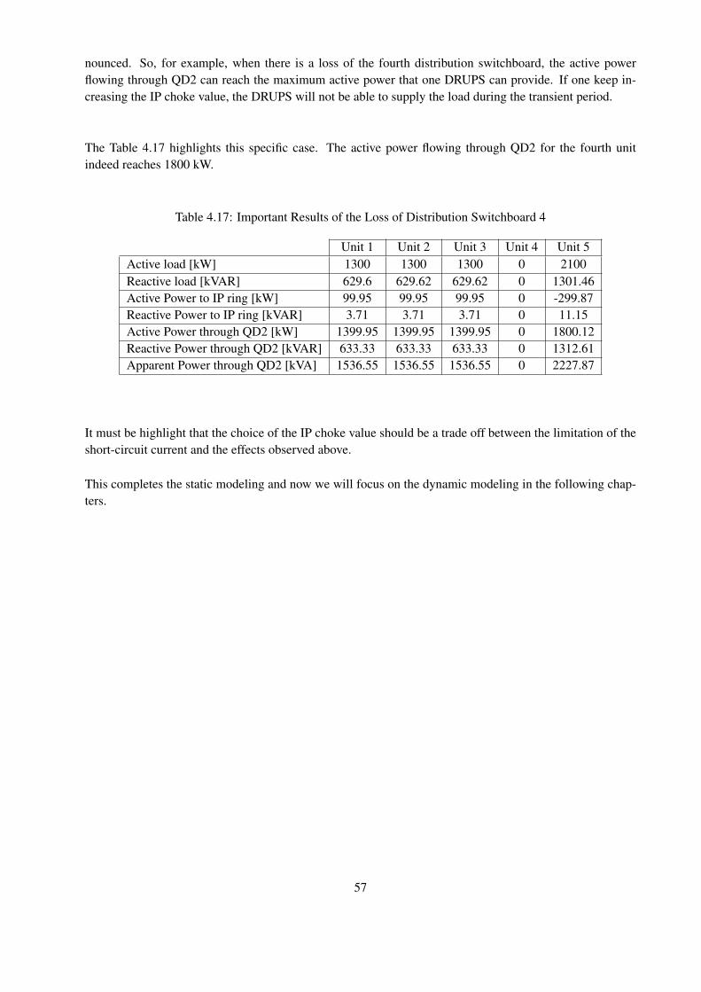
nounced. So, for example, when there is a loss of the fourth distribution switchboard, the active powerflowing through QD2 can reach the maximum active power that one DRUPS can provide. If one keep in-creasing the IP choke value, the DRUPS will not be able to supply the load during the transient period.

The Table 4.17 highlights this specific case. The active power flowing through QD2 for the fourth unitindeed reaches 1800 kW.


Unit 1 Unit 2 Unit 3 Unit 4 Unit 5Active load [kW] 1300 1300 1300 0 2100Reactive load [kVAR] 629.6 629.62 629.62 0 1301.46Active Power to IP ring [kW] 99.95 99.95 99.95 0 -299.87Reactive Power to IP ring [kVAR] 3.71 3.71 3.71 0 11.15Active Power through QD2 [kW] 1399.95 1399.95 1399.95 0 1800.12Reactive Power through QD2 [kVAR] 633.33 633.33 633.33 0 1312.61Apparent Power through QD2 [kVA] 1536.55 1536.55 1536.55 0 2227.87

It must be highlight that the choice of the IP choke value should be a trade off between the limitation of theshort-circuit current and the effects observed above.

This completes the static modeling and now we will focus on the dynamic modeling in the following chap-ters.

57

Part III

Dynamic Modeling

58

Purpose of This Part

The numerical simulation of the dynamic response of a NO-BREAK KS® has, so far, never been investi-gated by EURO-DIESEL. So this part of the thesis will be devoted to this important study.

To reach this goal, this dynamic modeling part will be divided into three Chapter. The first chapter willintroduce the software RAMSES as well as the user interaction to create and add a new model in RAMSES.Then the second chapter will describe the models developed for the excitation and torque controls of theNO-BREAK KS®. And finally, for the third section, the models will be used in RAMSES to simulate theresponse of the NO-BREAK KS®.

59

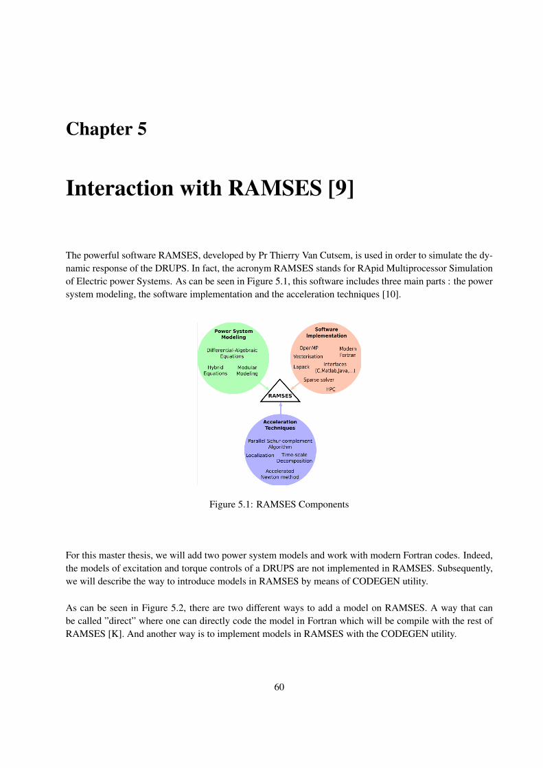
Chapter 5

Interaction with RAMSES [9]

The powerful software RAMSES, developed by Pr Thierry Van Cutsem, is used in order to simulate the dy-namic response of the DRUPS. In fact, the acronym RAMSES stands for RApid Multiprocessor Simulationof Electric power Systems. As can be seen in Figure 5.1, this software includes three main parts : the powersystem modeling, the software implementation and the acceleration techniques [10].

RAMSES ingredients

4

Figure 5.1: RAMSES Components

For this master thesis, we will add two power system models and work with modern Fortran codes. Indeed,the models of excitation and torque controls of a DRUPS are not implemented in RAMSES. Subsequently,we will describe the way to introduce models in RAMSES by means of CODEGEN utility.

As can be seen in Figure 5.2, there are two different ways to add a model on RAMSES. A way that canbe called ”direct” where one can directly code the model in Fortran which will be compile with the rest ofRAMSES [K]. And another way is to implement models in RAMSES with the CODEGEN utility.

60

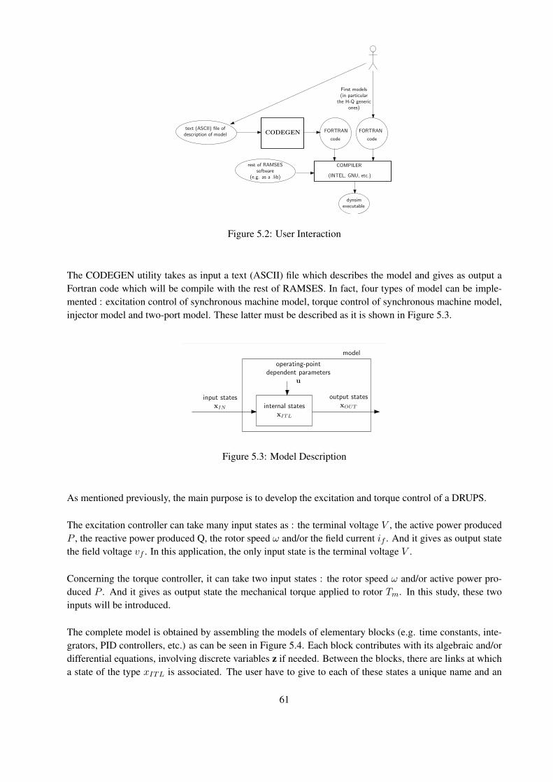
Implementing models in RAMSES with the CODEGEN utility

Context

FORTRAN

COMPILER

(INTEL, GNU, etc.)

dynsim

First models(in particular

the H-Q genericones)

CODEGENtext (ASCII) file of

description of modelcode

FORTRAN

code

rest of RAMSESsoftware

(e.g. as a .lib)

executable

2 / 13

Figure 5.2: User Interaction

The CODEGEN utility takes as input a text (ASCII) file which describes the model and gives as output aFortran code which will be compile with the rest of RAMSES. In fact, four types of model can be imple-mented : excitation control of synchronous machine model, torque control of synchronous machine model,injector model and two-port model. These latter must be described as it is shown in Figure 5.3.Implementing models in RAMSES with the CODEGEN utility

The four types of models

internal statesxITL

input statesxIN

output statesxOUT

operating-pointdependent parameters

u

model

type of model input states output states internal states

excitation control of V ,P,Q, ω, if vf defined by usersynchronous machine of machine of machine

torque control of P, ω Tm defined by usersynchronous machine of machine of machine

injector vx , vy at bus ix , iy into bus defined by userωcoi

two-port vx1, vy1, vx2, vy2 ix1, iy1, ix2, iy2 defined by userat buses into buses

ωcoi

3 / 13

Figure 5.3: Model Description

As mentioned previously, the main purpose is to develop the excitation and torque control of a DRUPS.

The excitation controller can take many input states as : the terminal voltage V , the active power producedP , the reactive power produced Q, the rotor speed ω and/or the field current if . And it gives as output statethe field voltage vf . In this application, the only input state is the terminal voltage V .

Concerning the torque controller, it can take two input states : the rotor speed ω and/or active power pro-duced P . And it gives as output state the mechanical torque applied to rotor Tm. In this study, these twoinputs will be introduced.

The complete model is obtained by assembling the models of elementary blocks (e.g. time constants, inte-grators, PID controllers, etc.) as can be seen in Figure 5.4. Each block contributes with its algebraic and/ordifferential equations, involving discrete variables z if needed. Between the blocks, there are links at whicha state of the type xITL is associated. The user have to give to each of these states a unique name and an

61

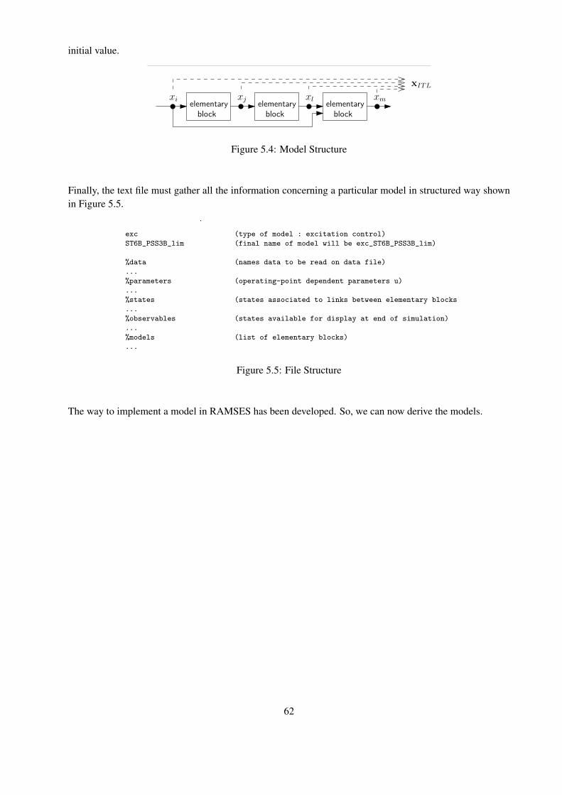
initial value.Implementing models in RAMSES with the CODEGEN utility

Model assembly

elementaryblock

elementaryblock

elementaryblock

xi xj xl xm

xITL

The model (2) is obtained by assembling the models of elementary blocks(e.g. time constants, integrators, PID controllers, non-linearities, etc.)

each block contributes with its algebraic and/or differential equations,involving discrete variables z if needed

the blocks are interconnected through links

a state of the type xITL is associated to each link. It can be differential oralgebraic6

each of these states is given a unique name, and an initial value by the user7

some elementary blocks involve additional states. The user does not need todefine nor initialize them (this can be done automatically).

6a block has a single output state; it can have one or several multiple input states7there are reserved names for the input and output states, which cannot be re-used

9 / 13

Figure 5.4: Model Structure

Finally, the text file must gather all the information concerning a particular model in structured way shownin Figure 5.5.

Implementing models in RAMSES with the CODEGEN utility

CODEGEN

A utility program

to generate the whole FORTRAN code of a model, corresponding to the sixcalls detailed in previous slide

starting from a text (ASCII file) description of the model

separate from the main simulator dynsim itself.

Overall structure of input text file:

exc (type of model : excitation control)

ST6B_PSS3B_lim (final name of model will be exc_ST6B_PSS3B_lim)

%data (names data to be read on data file)

...

%parameters (operating-point dependent parameters u)

...

%states (states associated to links between elementary blocks)

...

%observables (states available for display at end of simulation)

...

%models (list of elementary blocks)

...

12 / 13

Figure 5.5: File Structure

The way to implement a model in RAMSES has been developed. So, we can now derive the models.

62

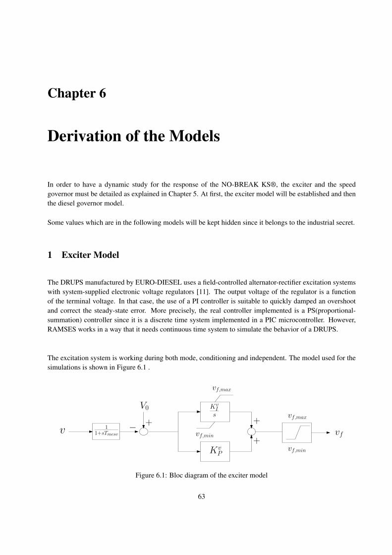
Chapter 6

Derivation of the Models

In order to have a dynamic study for the response of the NO-BREAK KS®, the exciter and the speedgovernor must be detailed as explained in Chapter 5. At first, the exciter model will be established and thenthe diesel governor model.

Some values which are in the following models will be kept hidden since it belongs to the industrial secret.

1 Exciter Model

The DRUPS manufactured by EURO-DIESEL uses a field-controlled alternator-rectifier excitation systemswith system-supplied electronic voltage regulators [11]. The output voltage of the regulator is a functionof the terminal voltage. In that case, the use of a PI controller is suitable to quickly damped an overshootand correct the steady-state error. More precisely, the real controller implemented is a PS(proportional-summation) controller since it is a discrete time system implemented in a PIC microcontroller. However,RAMSES works in a way that it needs continuous time system to simulate the behavior of a DRUPS.

The excitation system is working during both mode, conditioning and independent. The model used for thesimulations is shown in Figure 6.1 .

v 11+sTmesv

V0

KvP

KvIs

+−vf

vf,max

vf,min

+

+

vf,max

vf,min

Figure 6.1: Bloc diagram of the exciter model

63

One can notice that the terminal voltage of the DRUPS, v, is first delayed by a time constant Tmesv, in-deed, in reality, the measurements are not instantaneous. The measure voltage is then compare to a voltagesetpoint V0, if the error is different from 0, then the PI part of the model act and tries to bring the voltageback to its setpoint value by tuning the field voltage vf . One can also observe a non windup integrator toprevent the integral terms to accumulate a significant error during the rise and thus decrease the overshoot.The last part of the exciter model is a limiter which bounds the value of vf so it never exceeds the physical,maximum and minimum, values of vf .

2 Diesel Governor Model

The diesel governor is either a speed control or a torque control for the DRUPS produced by EURO-DIESELbut in the following simulations, only the torque controller is developed. In fact, it depends on the dieselengine manufacturer and for this master thesis, one will work with a particular manufacturer which requiresa torque controller. The Diesel Governor Model, developed in this master thesis, is only used for the inde-pendent mode.

The bloc diagram of the torque controller can be seen in Figure 6.2. One can observe two main parts in thebloc diagram, the upper part is the PI controller to bring back the speed of the DRUPS to 1 pu and the lowerpart is the PI controller which takes care of the active load sharing. As for the terminal voltage in Figure6.1, the speed w and the active power produced by the DRUPS P are delayed by time constant, respectively,Tmesw and Tmesp. The interesting part is that all the DRUPS of a network share the same setpoint for thespeed and the active power. More precisely, for the latter, it is the mean of active power produced by allDRUPS. There is, then, the PI parts of the controller with the non windup integrator and the limiter of thetorque values. At last, one can see an additional transfer function with a time constant Tdelay which is animage of the delay between the moment when the new torque value is computed and the moment when themechanical torque of the diesel engine is really set to this value.

64

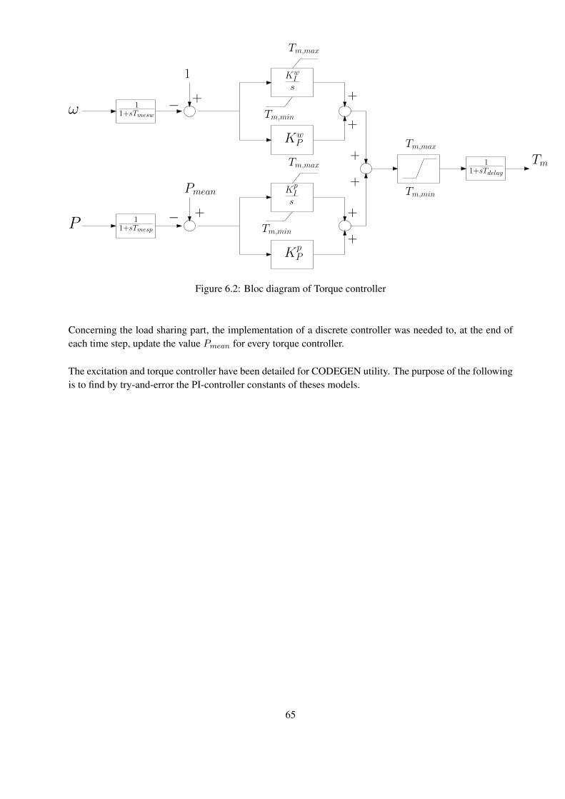
ω 11+sTmesw

1

KwP

KwIs

P 11+sTmesp

Pmean

KpP

KpIs

+−

+−

11+sTdelay

Tm+

+

Tm,max

Tm,min

+

+

+

+

Tm,max

Tm,min

Tm,max

Tm,min

Figure 6.2: Bloc diagram of Torque controller

Concerning the load sharing part, the implementation of a discrete controller was needed to, at the end ofeach time step, update the value Pmean for every torque controller.

The excitation and torque controller have been detailed for CODEGEN utility. The purpose of the followingis to find by try-and-error the PI-controller constants of theses models.

65

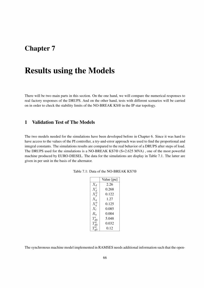
Chapter 7

Results using the Models

There will be two main parts in this section. On the one hand, we will compare the numerical responses toreal factory responses of the DRUPS. And on the other hand, tests with different scenarios will be carriedon in order to check the stability limits of the NO-BREAK KS® in the IP star topology.

1 Validation Test of The Models

The two models needed for the simulations have been developed before in Chapter 6. Since it was hard tohave access to the values of the PI controller, a try-and-error approach was used to find the proportional andintegral constants. The simulations results are compared to the real behavior of a DRUPS after steps of load.The DRUPS used for the simulations is a NO-BREAK KS7® (S=2.625 MVA) , one of the most powerfulmachine produced by EURO-DIESEL. The data for the simulations are display in Table 7.1. The latter aregiven in per unit in the basis of the alternator.

Table 7.1: Data of the NO-BREAK KS7®

Value [pu]Xd 2.26X ′d 0.268X ′′d 0.122Xq 1.27X ′′q 0.125Xl 0.085Ra 0.004T ′d0 5.048T ′′d0 0.032T ′′q0 0.12

The synchronous machine model implemented in RAMSES needs additional information such that the open-

66

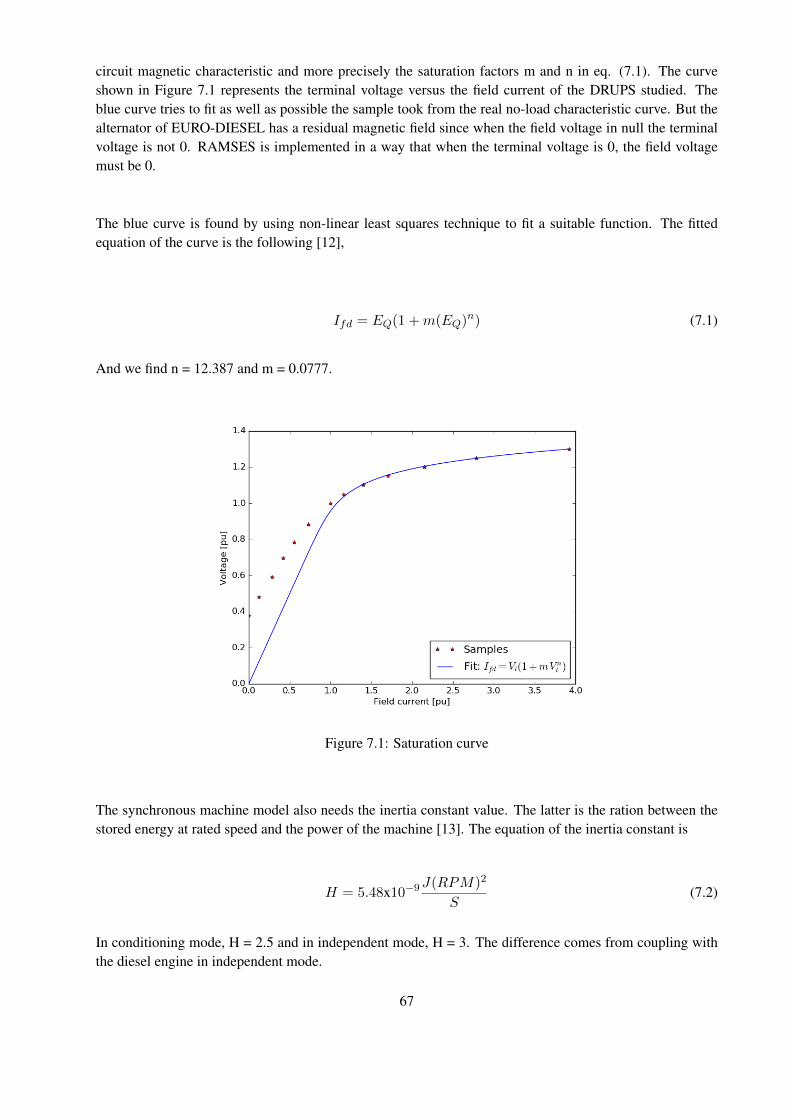
circuit magnetic characteristic and more precisely the saturation factors m and n in eq. (7.1). The curveshown in Figure 7.1 represents the terminal voltage versus the field current of the DRUPS studied. Theblue curve tries to fit as well as possible the sample took from the real no-load characteristic curve. But thealternator of EURO-DIESEL has a residual magnetic field since when the field voltage in null the terminalvoltage is not 0. RAMSES is implemented in a way that when the terminal voltage is 0, the field voltagemust be 0.

The blue curve is found by using non-linear least squares technique to fit a suitable function. The fittedequation of the curve is the following [12],

Ifd = EQ(1 +m(EQ)n) (7.1)

And we find n = 12.387 and m = 0.0777.

Figure 7.1: Saturation curve

The synchronous machine model also needs the inertia constant value. The latter is the ration between thestored energy at rated speed and the power of the machine [13]. The equation of the inertia constant is

H = 5.48x10−9J(RPM)2

S(7.2)

In conditioning mode, H = 2.5 and in independent mode, H = 3. The difference comes from coupling withthe diesel engine in independent mode.

67

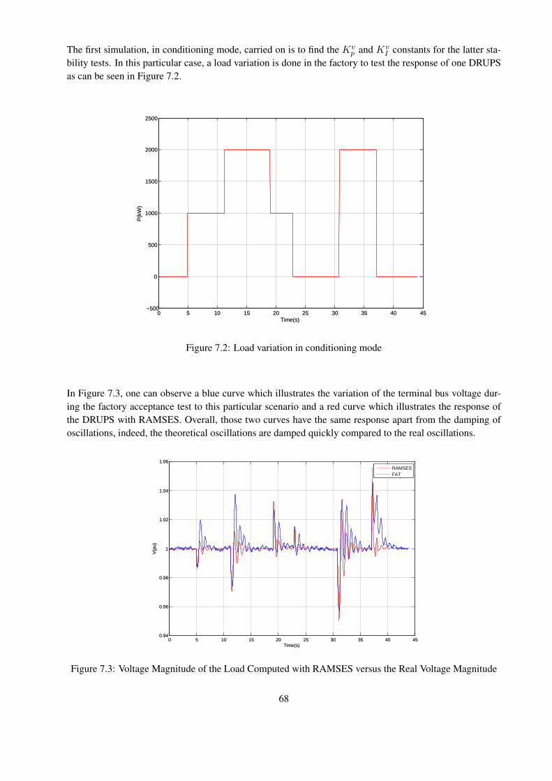
The first simulation, in conditioning mode, carried on is to find the Kvp and Kv

I constants for the latter sta-bility tests. In this particular case, a load variation is done in the factory to test the response of one DRUPSas can be seen in Figure 7.2.

0 5 10 15 20 25 30 35 40 45−500

0

500

1000

1500

2000

2500

P(k

W)

Time(s)0 5 10 15 20 25 30 35 40 45

−500

0

500

1000

1500

2000

2500

P(k

W)

Time(s)

Figure 7.2: Load variation in conditioning mode

In Figure 7.3, one can observe a blue curve which illustrates the variation of the terminal bus voltage dur-ing the factory acceptance test to this particular scenario and a red curve which illustrates the response ofthe DRUPS with RAMSES. Overall, those two curves have the same response apart from the damping ofoscillations, indeed, the theoretical oscillations are damped quickly compared to the real oscillations.

0 5 10 15 20 25 30 35 40 450.94

0.96

0.98

1

1.02

1.04

1.06

V(p

u)

Time(s)

RAMSESFAT

0 5 10 15 20 25 30 35 40 450.94

0.96

0.98

1

1.02

1.04

1.06

V(p

u)

Time(s)

Figure 7.3: Voltage Magnitude of the Load Computed with RAMSES versus the Real Voltage Magnitude

68

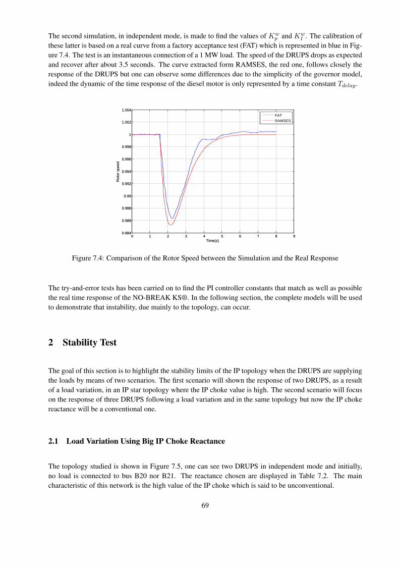
The second simulation, in independent mode, is made to find the values of Kwp and Kw

I . The calibration ofthese latter is based on a real curve from a factory acceptance test (FAT) which is represented in blue in Fig-ure 7.4. The test is an instantaneous connection of a 1 MW load. The speed of the DRUPS drops as expectedand recover after about 3.5 seconds. The curve extracted form RAMSES, the red one, follows closely theresponse of the DRUPS but one can observe some differences due to the simplicity of the governor model,indeed the dynamic of the time response of the diesel motor is only represented by a time constant Tdelay.

0 1 2 3 4 5 6 7 8 90.984

0.986

0.988

0.99

0.992

0.994

0.996

0.998

1

1.002

1.004

Rot

or s

peed

Time(s)

FATRAMSES

0 1 2 3 4 5 6 7 8 90.984

0.986

0.988

0.99

0.992

0.994

0.996

0.998

1

1.002

1.004

Rot

or s

peed

Time(s)

Figure 7.4: Comparison of the Rotor Speed between the Simulation and the Real Response

The try-and-error tests has been carried on to find the PI controller constants that match as well as possiblethe real time response of the NO-BREAK KS®. In the following section, the complete models will be usedto demonstrate that instability, due mainly to the topology, can occur.

2 Stability Test

The goal of this section is to highlight the stability limits of the IP topology when the DRUPS are supplyingthe loads by means of two scenarios. The first scenario will shown the response of two DRUPS, as a resultof a load variation, in an IP star topology where the IP choke value is high. The second scenario will focuson the response of three DRUPS following a load variation and in the same topology but now the IP chokereactance will be a conventional one.

2.1 Load Variation Using Big IP Choke Reactance

The topology studied is shown in Figure 7.5, one can see two DRUPS in independent mode and initially,no load is connected to bus B20 nor B21. The reactance chosen are displayed in Table 7.2. The maincharacteristic of this network is the high value of the IP choke which is said to be unconventional.

69

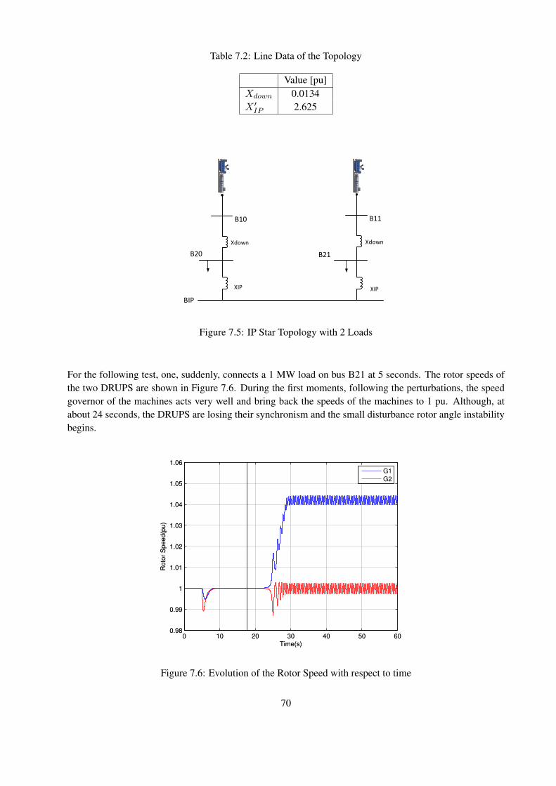
Table 7.2: Line Data of the Topology

Value [pu]Xdown 0.0134X ′IP 2.625

B10

B20

BIP

Xdown

XIP XIP

B11

Xdown

B21

Figure 7.5: IP Star Topology with 2 Loads

For the following test, one, suddenly, connects a 1 MW load on bus B21 at 5 seconds. The rotor speeds ofthe two DRUPS are shown in Figure 7.6. During the first moments, following the perturbations, the speedgovernor of the machines acts very well and bring back the speeds of the machines to 1 pu. Although, atabout 24 seconds, the DRUPS are losing their synchronism and the small disturbance rotor angle instabilitybegins.

0 10 20 30 40 50 600.98

0.99

1

1.01

1.02

1.03

1.04

1.05

1.06

Roto

r S

pe

ed

(pu

)

Time(s)

G1

G2

0 10 20 30 40 50 600.98

0.99

1

1.01

1.02

1.03

1.04

1.05

1.06

Roto

r S

pe

ed

(pu

)

Time(s)

Figure 7.6: Evolution of the Rotor Speed with respect to time

70

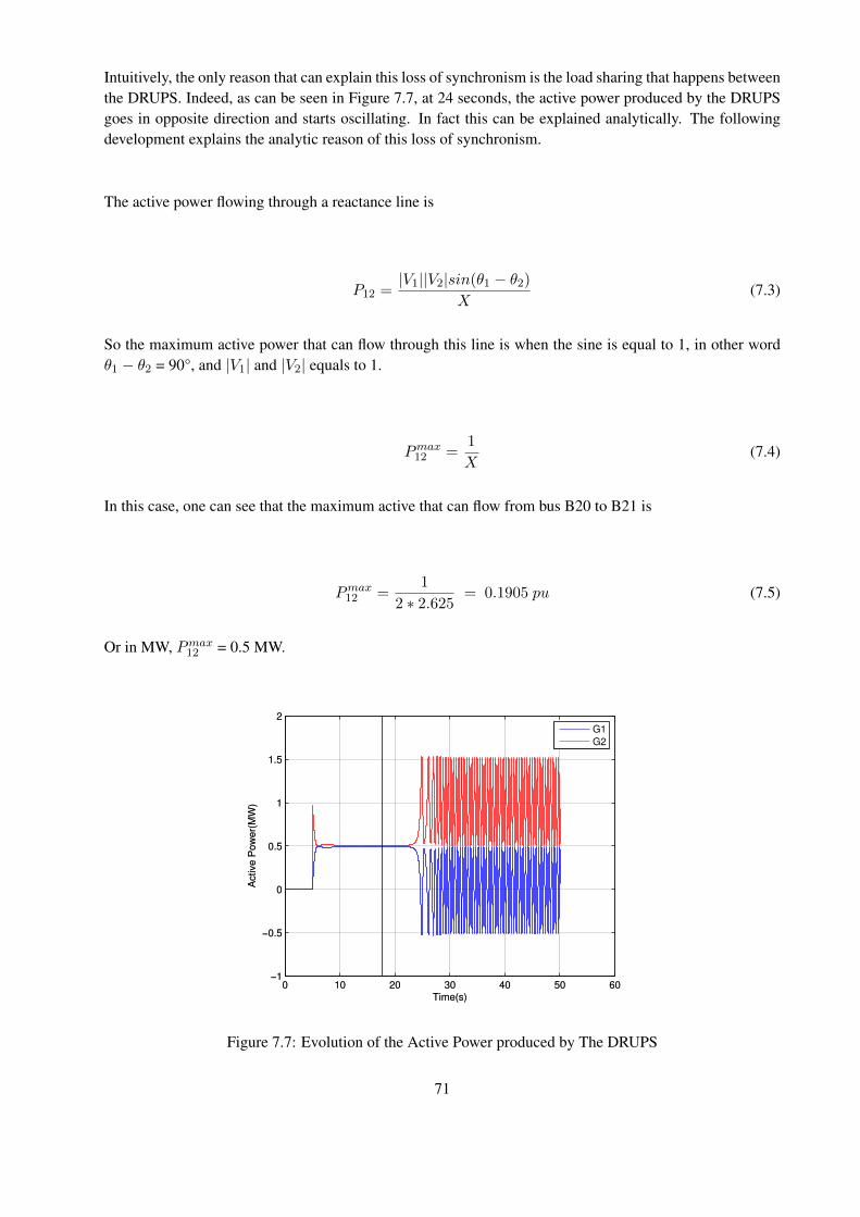
Intuitively, the only reason that can explain this loss of synchronism is the load sharing that happens betweenthe DRUPS. Indeed, as can be seen in Figure 7.7, at 24 seconds, the active power produced by the DRUPSgoes in opposite direction and starts oscillating. In fact this can be explained analytically. The followingdevelopment explains the analytic reason of this loss of synchronism.

The active power flowing through a reactance line is

P12 =|V1||V2|sin(θ1 − θ2)

X(7.3)

So the maximum active power that can flow through this line is when the sine is equal to 1, in other wordθ1 − θ2 = 90°, and |V1| and |V2| equals to 1.

Pmax12 =1

X(7.4)

In this case, one can see that the maximum active that can flow from bus B20 to B21 is

Pmax12 =1

2 ∗ 2.625= 0.1905 pu (7.5)

Or in MW, Pmax12 = 0.5 MW.

0 10 20 30 40 50 60−1

−0.5

0

0.5

1

1.5

2

Active P

ow

er(

MW

)

Time(s)

G1

G2

0 10 20 30 40 50 60−1

−0.5

0

0.5

1

1.5

2

Active P

ow

er(

MW

)

Time(s)

Figure 7.7: Evolution of the Active Power produced by The DRUPS

71

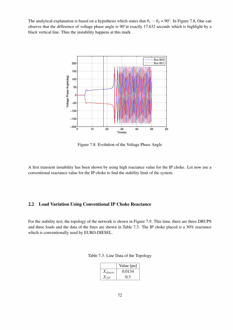
The analytical explanation is based on a hypothesis which states that θ1 − θ2 = 90°. In Figure 7.8, One canobserve that the difference of voltage phase angle is 90°at exactly 17.632 seconds which is highlight by ablack vertical line. Thus the instability happens at this mark.

0 10 20 30 40 50 60−200

−150

−100

−50

0

50

100

150

200

Volta

ge P

hase

Ang

le(d

eg)

Time(s)

Bus B20

Bus B21

0 10 20 30 40 50 60−200

−150

−100

−50

0

50

100

150

200

Volta

ge P

hase

Ang

le(d

eg)

Time(s)

Figure 7.8: Evolution of the Voltage Phase Angle

A first transient instability has been shown by using high reactance value for the IP choke. Let now use aconventional reactance value for the IP choke to find the stability limit of the system.

2.2 Load Variation Using Conventional IP Choke Reactance

For the stability test, the topology of the network is shown in Figure 7.9. This time, there are three DRUPSand three loads and the data of the lines are shown in Table 7.3. The IP choke placed is a 30% reactancewhich is conventionally used by EURO-DIESEL.

Table 7.3: Line Data of the Topology

Value [pu]Xdown 0.0134XIP 0.3

72

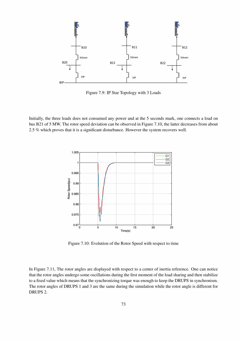
B10

B20

BIP

Xdown

XIP XIP

B11

Xdown

B21

XIP

B12

Xdown

B22

Figure 7.9: IP Star Topology with 3 Loads

Initially, the three loads does not consumed any power and at the 5 seconds mark, one connects a load onbus B21 of 5 MW. The rotor speed deviation can be observed in Figure 7.10, the latter decreases from about2.5 % which proves that it is a significant disturbance. However the system recovers well.

0 5 10 15 20 250.97

0.975

0.98

0.985

0.99

0.995

1

1.005

Roto

r S

peed(p

u)

Time(s)

G1

G2

G3

0 5 10 15 20 250.97

0.975

0.98

0.985

0.99

0.995

1

1.005

Roto

r S

peed(p

u)

Time(s)

Figure 7.10: Evolution of the Rotor Speed with respect to time

In Figure 7.11, The rotor angles are displayed with respect to a center of inertia reference. One can noticethat the rotor angles undergo some oscillations during the first moment of the load sharing and then stabilizeto a fixed value which means that the synchronizing torque was enough to keep the DRUPS in synchronism.The rotor angles of DRUPS 1 and 3 are the same during the simulation while the rotor angle is different forDRUPS 2.

73

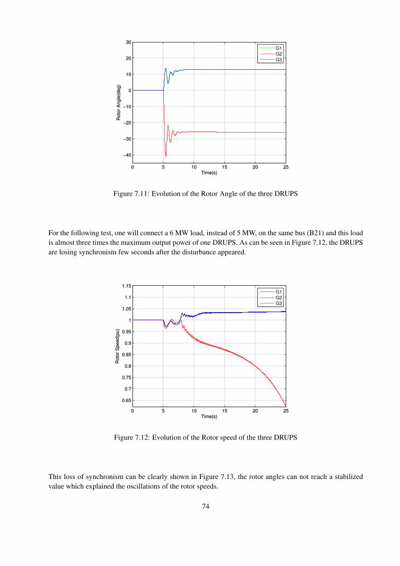
0 5 10 15 20 25

−40

−30

−20

−10

0

10

20

30

Ro

tor

Ang

le(d

eg

)

Time(s)

G1

G2

G3

0 5 10 15 20 25

−40

−30

−20

−10

0

10

20

30

Ro

tor

Ang

le(d

eg

)

Time(s)

Figure 7.11: Evolution of the Rotor Angle of the three DRUPS

For the following test, one will connect a 6 MW load, instead of 5 MW, on the same bus (B21) and this loadis almost three times the maximum output power of one DRUPS. As can be seen in Figure 7.12, the DRUPSare losing synchronism few seconds after the disturbance appeared.

0 5 10 15 20 25

0.65

0.7

0.75

0.8

0.85

0.9

0.95

1

1.05

1.1

1.15

Roto

r S

peed(p

u)

Time(s)

G1

G2

G3

0 5 10 15 20 25

0.65

0.7

0.75

0.8

0.85

0.9

0.95

1

1.05

1.1

1.15

Roto

r S

peed(p

u)

Time(s)

Figure 7.12: Evolution of the Rotor speed of the three DRUPS

This loss of synchronism can be clearly shown in Figure 7.13, the rotor angles can not reach a stabilizedvalue which explained the oscillations of the rotor speeds.

74

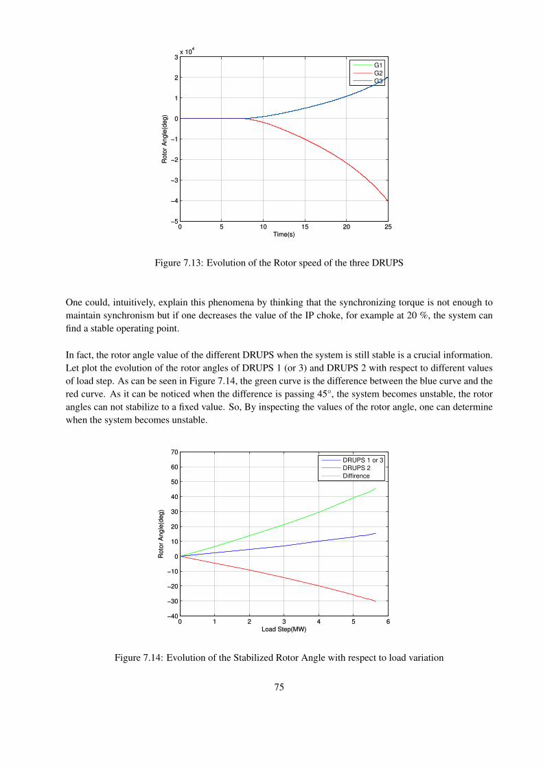
0 5 10 15 20 25−5

−4

−3

−2

−1

0

1

2

3x 10

4

Ro

tor

Ang

le(d

eg)

Time(s)

G1

G2

G3

0 5 10 15 20 25−5

−4

−3

−2

−1

0

1

2

3x 10

4

Ro

tor

Ang

le(d

eg)

Time(s)

Figure 7.13: Evolution of the Rotor speed of the three DRUPS

One could, intuitively, explain this phenomena by thinking that the synchronizing torque is not enough tomaintain synchronism but if one decreases the value of the IP choke, for example at 20 %, the system canfind a stable operating point.

In fact, the rotor angle value of the different DRUPS when the system is still stable is a crucial information.Let plot the evolution of the rotor angles of DRUPS 1 (or 3) and DRUPS 2 with respect to different valuesof load step. As can be seen in Figure 7.14, the green curve is the difference between the blue curve and thered curve. As it can be noticed when the difference is passing 45°, the system becomes unstable, the rotorangles can not stabilize to a fixed value. So, By inspecting the values of the rotor angle, one can determinewhen the system becomes unstable.

0 1 2 3 4 5 6−40

−30

−20

−10

0

10

20

30

40

50

60

70

Roto

r A

ngle

(deg)

Load Step(MW)

DRUPS 1 or 3

DRUPS 2

Diffirence

0 1 2 3 4 5 6−40

−30

−20

−10

0

10

20

30

40

50

60

70

Roto

r A

ngle

(deg)

Load Step(MW)

Figure 7.14: Evolution of the Stabilized Rotor Angle with respect to load variation

75

In conclusion, for those two tests of stability, the value of IP choke chosen has a drastic effect on the step ofload that can occur on the load buses. Recall that during the factory test acceptance, it is usual to performload steps.

76

Part IV

Euro-Diesel’s Strategies

77

Marketing Strategy

EURO-DIESEL’s product is the NO-BREAK KS® (range power : 100 to 3000 kVA) as discussed in Sec-tion 1. The market environment in which EURO-DIESEL is present is called a niche market. So, by beingactive in such a market, EURO-DISEL aimed at being a big fish in a small pond instead of being a smallfish in a big pond. Two main product families have a hand in this niche market : The static UPS and thedynamic UPS. The static UPS are mainly batteries and have a large part of the market, the principal actorsand, thus, competitors for EURO-DIESEL are : Schneider Electric, Eaton and Emerson. Concerning thedynamic UPS family where EURO-DIESEL is present, their principal competitors are : Piller, Hitec andHitzinger.

As discussed, EURO-DIESEL targets a particular market and in Europe, the demand is limited. Therefore,the need to grow worldwide was important for the company. As can be seen in Figure 7.15 [13], EURO-DIESEL is present internationally, the blue dots represent the distributors and the yellow dots represent thesubsidiaries.

This document is the property of EURO-DIESEL S.A. and may neither be disclosed nor reproduced without written authorization. Information provided is believed to be correct and reliable. EURO-DIESEL S.A. reserves the right to amend this document without notice.

CERVIN DE CRISTAL 2014 Dossier de participation• 10 Juin 2014

Page 5/19

Allemagne création d’Euro-Diesel GmbH en Allemagne (2002) Angleterre prise de contrôle d’Euro-Diesel (UK) Ltd (2007) USA création d’E1 Dynamics aux USA (2007) France création d’Euro-Diesel SAS en France (2007) Singapour création d’Euro-Diesel Pte Ltd à Singapour (2009) Arabie Saoudite création d’Euro-Diesel LLC en Arabie Saoudite (2011) Brésil création d’Euro-Diesel Ltda au Brésil (2011) Turquie création d’un bureau de représentation (2012) Russie création d’un bureau de représentation (2013) Mexique création d’un bureau de représentation (2013)

EURO-DIESEL : une présence mondiale

Bureaux EURO-DIESEL Distributeurs

Figure 7.15: The Worldwide Presence of Euro-Diesel

The early strategy of EURO-DIESEL was only to work with distributors but the drawback of this strategy isthat the NO-BREAK KS® was a product among others within the distributors. So, they chose, in additionto the distributors, to create subsidiaries across the world in order to thrive. In fact, some problems camewith their expansion such that technical constraints, indeed, for some parts of the world, the UPS must resisthigh temperature and for other parts, the UPS must resist low temperature. EURO-DIESEL also faced otherproblems such that the adaptation to the culture of different countries and the legislative aspects (importduty...).

To be successful, EURO-DIESEL has been able to adapt their philosophy depending on the country theywere settled. The reliability, longevity and efficiency of the product are the strength of EURO-DIESEL.

78

The commerce in which EURO-DIESEL is involved is a business-to-business commerce. In fact, there arethree principal ways to get clients. For the first way, the clients can directly contact EURO-DIESEL bysearching them on the web, if one type ”Dynamic UPS” on Google, the first link is the EURO-DIESEL’swebsite. For the second way, EURO-DIESEL’s salesmen contact potential clients. And for the third way,EURO-DIESEL attend events such as the DCD (DataCenter Dynamics) event.

After Sales Strategy [14]

After sales service contributes to the success and the well-being of EURO-DIESEL. Indeed, this departmentgenerates continuous cash-flow and growth along with the installed base in order to generate continuousshare-holder value and cover substantial parts of the company-cost, more specifically in bad times. Theservice allows to achieve customer satisfaction and to enable new business by excellent relations. For this towork, the department manager must monitor and manage employee motivation pro-actively in order to makesure talent stays within the company and our service level remains constantly excellent without exception.

The employees in this department are mainly engineers. In addition to their technical skills, they should atleast speak a foreign language to ease the discussion with the different customers. Indeed, each engineer isassigned to a part of the world and have to manage customers in this part. For Belgium and Luxembourg, theBelgian team is the first level and second level support meaning that they take care of the organizing main-tenance visits, machine-breakdown and managing the renewal of maintenance contracts. For the subsidariesand distributors (world-wide), the are a back office support or second level support as can be seen in Figure7.16, they take care of diagnostics, training, spare parts, contracts on service-levels, updating archives andthe ten year overhaul.

Figure 7.16: Communication with World-Wide Customers

79

The particularity of this service is that it is a 24 hours on 24 and 7 days on 7 worldwide technical support viaphone or via automated alarm transfer. The new technology of the KS-Vision allow to automatically sendmails to the back office when a problem arrived to the NO-BREAK KS®. Although, there are seven machinemaintenances during a year and every 10 years, an overhaul program is performed, a previously overhauledstato-alternator and the clutch owned by EURO-DIESEL are sent to customers site and are swapped withthe original one from the customers site.

New Strategies

Due to all of these factors discussed previously, EURO-DIESEL is growing every year and thus the humanresource employees are looking for qualified people. The parent company of EURO-DIESEL is located inGrace-Hollogne (Belgium) and employs 125 people (225 across the world). Early 2016, the company wasbought out by an investor group called 3I and new strategies are implemented.

The creation of an IT (Information Technology) department was necessary since the communication andthe information exchanged between employees are bigger. Before, the information transits were delocalizedand time were lost to retrieve certain information. So the IT team want to develop a plan that will makeinformation exchanges optimal and efficient. To gather the information (especially with the subsidiaries),several tools and techniques will be implemented such that the Customer Relationship Management (CRM)or Computerized Maintenance Management System (CMMS). This new strategy will be benefit for the em-ployees working speed.

EURO-DIESEL is setting up a strategy aimed at optimize the workflow (reducing waiting times, reduction ofintermediate stock ...) by using a method called the lean manufacturing. In other word, the goal is to reducethe cycle time. The strategy is to make the mechanical workshop the reference model for the other part ofthe workshop. For that, the supply chain manager will do the mapping process with precise instructions andmonitor the mechanical part in the workshop with a tracking sheet.

After more than 80 days in the company I come out with a positive experience. Indeed, the team thatsupervised my work during my internship was always opened to questions and discussions. This experienceallowed me to discover the rhythm of life of a company: discussions between colleagues for cases, meetings... Moreover it also allowed me to meet people from around the world. I think that, overall, EURO-DIESELis well-balanced company which is constantly evolving.

80

Chapter 8

Conclusion

Reached the end of this work, we will outline the path that has allowed us to develop a static and dynamicmodeling of the NO-BREAK KS® in an IP topology.

The first stage was devoted to describing the operation of the NO-BREAK KS® as well as the descriptionof the different topologies with which we worked.

The second stage, for its part, was dedicated to the static modeling of NO-BREAK KS® in the IP topology.Indeed, a program was developed for the EURO-DIESEL electrical engineering department which solvesthe power flow equations using the Newton-Raphson procedure. This program would also allow the userto work with a simple input interface and the program is able to automatically perform various scenariosusing SCILAB software. This helps to quickly and efficiently obtain essential electrical results to optimizethe studied electrical network. Thus, we can easily check if the power of machines is optimal, otherwise,we can readjust the number and power of the DRUPS. In addition, fundamental information about loaddistribution is given accurately. Simulation of faults has also been implemented which allows the technicaldepartment to simulate the effect of a short-circuit on the electrical quantities.

The third stage was to develop the dynamic model of NO-BREAK KS®. To do this, we added to theRAMSES library via CODEGEN utility, the exciter and torque controller models. The response of thesemodels was compared to the response of the real machine during a factory acceptance test to find the PIcontroller constants. Finally, the models were used to study the stability limits of KS® in the IP topology.

The last stage highlighted the strategies implemented by EURO-DIESEL which allows it to have a goodstability on the UPS market especially through the marketing and after sales departments. Emphasize that theimplementation of the new IT department will optimize, in the future, the access and transfer of informationfirstly between the different department and also between subsidiaries distributed throughout the world.

In conclusion, my program allows electrical engineers to EURO-DIESEL to perform faster studies of elec-trical quantities, pre-fault and post-fault, in the IP topology. Moreover, the developed dynamic models inthis master thesis represent rather well the behavior of the engine at the time of occurrence of one or moredisturbances and to check whether the electrical system is still stable or not. However, in the future, based onthe developments of this thesis, we could consider introducing new features to the current dynamic model.

81

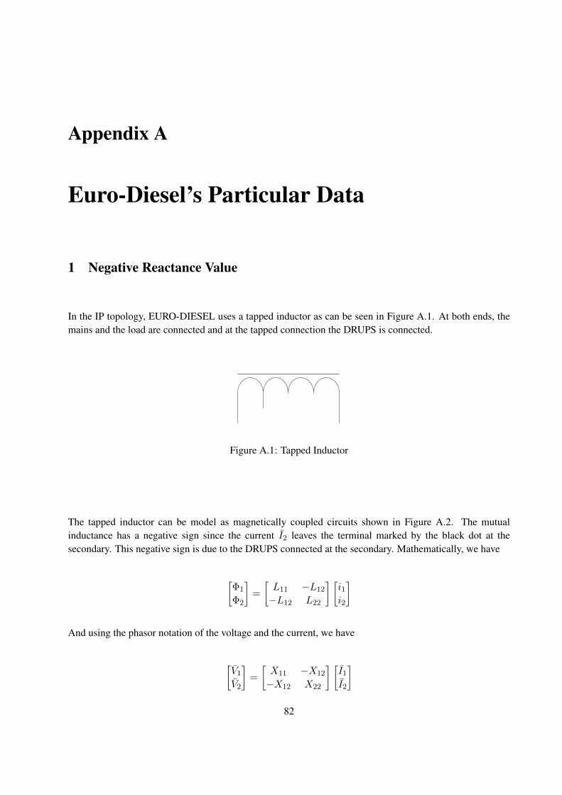
Appendix A

Euro-Diesel’s Particular Data

1 Negative Reactance Value

In the IP topology, EURO-DIESEL uses a tapped inductor as can be seen in Figure A.1. At both ends, themains and the load are connected and at the tapped connection the DRUPS is connected.

L11 + L12 L22 + L12

- L12

Figure A.1: Tapped Inductor

The tapped inductor can be model as magnetically coupled circuits shown in Figure A.2. The mutualinductance has a negative sign since the current I2 leaves the terminal marked by the black dot at thesecondary. This negative sign is due to the DRUPS connected at the secondary. Mathematically, we have

[Φ1

Φ2

]=

[L11 −L12

−L12 L22

] [i1i2

]

And using the phasor notation of the voltage and the current, we have

[V1

V2

]=

[X11 −X12

−X12 X22

] [I1

I2

]

82

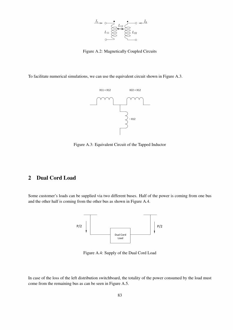
I2I1

L11 L22

L12

FIGURE 3 – circuits magnetiquement couples

Rappelons aussi que l’inductance mutuelle a un signe. Si les courants sont comptes positivementen entrant par les bornes marquees du point noir •, l’inductance mutuelle est positive. C’est le casdans la figure 3.

Enfin, on montre aisement que le marquage • indique des tensions qui sont en phase lorsque letransformateur est suppose ideal. La difference entre le potentiel de la borne marquee et celui dela borne non marquee au primaire est en phase avec la difference de potentiel correspondante ausecondaire.

Les tensions aux bornes des enroulements s’obtiennent alors comme suit :

v1 = R1i1 +dψ1

dt= R1i1 + Lℓ1

di1dt

+ Lm1di1dt

+n2

n1

Lm1di2dt

v2 = R2i2 +dψ2

dt= R2i2 + Lℓ2

di2dt

+(n2

n1

)2

Lm1di2dt

+n2

n1

Lm1di1dt

Le lecteur est invite a verifier que le schema equivalent de la figure 4 correspond parfaitement aces deux dernieres relations.

Lm1

R1 Lℓ1 n1 n2Lℓ2 R2

v1 v2

i1 i2

FIGURE 4 – schema equivalent du transformateur monophase (1ere version)

Ce dernier schema peut etre modifie en faisant passer la resistanceR2 et l’inductance Lℓ2 de l’autrecote du transformateur ideal, moyennant multiplication par (n1/n2)

2. Ceci conduit au schemaequivalent de la figure 5.

Le modele pourrait etre raffine en considerant (voir trait pointille dans la figure 5) :

1. les pertes Joule causees par les courants de Foucault induits dans le materiau magnetique.On designe couramment ces pertes sous le nom de “pertes fer”, par opposition aux “pertescuivre” R1i

21 +R2i

22 subies dans les enroulements. Celles-ci peuvent etre prise en compte en

placant une resistance en parallele sur l’inductance magnetisante Lm1

6

Figure A.2: Magnetically Coupled Circuits

To facilitate numerical simulations, we can use the equivalent circuit shown in Figure A.3.

X11 + X12 X22 + X12

- X12

Figure A.3: Equivalent Circuit of the Tapped Inductor

2 Dual Cord Load

Some customer’s loads can be supplied via two different buses. Half of the power is coming from one busand the other half is coming from the other bus as shown in Figure A.4.

Dual Cord Load

P/2 P/2

Dual Cord Load

P

Figure A.4: Supply of the Dual Cord Load

In case of the loss of the left distribution switchboard, the totality of the power consumed by the load mustcome from the remaining bus as can be seen in Figure A.5.

83

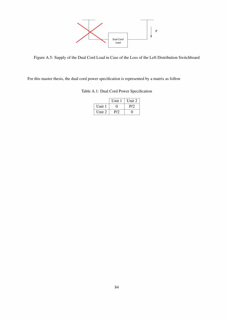
Dual Cord Load

P/2 P/2

Dual Cord Load

P

Figure A.5: Supply of the Dual Cord Load in Case of the Loss of the Left Distribution Switchboard

For this master thesis, the dual cord power specification is represented by a matrix as follow

Table A.1: Dual Cord Power Specification

Unit 1 Unit 2Unit 1 0 P/2Unit 2 P/2 0

84

References

[1] Euro-Diesel Website. Available on-line : http://www.euro-diesel.com/english/about-us/3/2

[2] Wikipedia Website. Available on-line : https://en.wikipedia.org/wiki/Scilab

[3] Euro-Diesel, ”The Leading-EDGE Diesel Rotary Uninterruptible Power Supply System”, 2015.

[4] Euro-Diesel, ”ISOLATED PARALLEL STAR BUS PRINCIPLE OF OPERATION - TI0020”, rev 04.

[5] Euro-Diesel, ”ISOLATED PARALLEL RING BUS PRINCIPLE OF OPERATION - TI0021”, rev 01.

[6] James D. McCalley, ”The Power Flow Problem”, Iowa State University. Available on-line :home.eng.iastate.edu/ jdm/ee553/PowerFlow.doc

[7] Yang Liu-Lin, Hang Nai-Shan, Liu Bai-Jiang, ”A Modular Approach to Power Flow Regulation So-lution”, The Open Electrical & Electronic Engineering Journal , 2015, 9:91-98. Available on-line :http://benthamopen.com/ABSTRACT/TOEEJ-9-91

[8] T. Van Cutsem, Electric Power System Analysis, Univ. of Liege, Lecture notes of course ELEC0029,2016. Available on-line : http://montefiore.ulg.ac.be/ vct/courses.html

[9] Thierry Van Cutsem, Implementing models in RAMSES with the CODEGEN utility, Version 3, May2016.

[10] Thierry Van Cutsem, Petros Aristidou, ”An overview of RAMSES (RApid MultiprocessorSimulation of Electric power Systems)”, Univ. of Liege, September 2014. Available on-line :http://www.montefiore.ulg.ac.be/ vct/software.html

[11] IEEE Std 421. 5-2005, ”IEEE recommended practice for excitation system models for power systemstability studies”, IEEE Power Eng. Soc., pp. 14, 2006.

[12] T. Van Cutsem, Power systems dynamics, control and stability, Univ. of Liege, Lecture notes of courseELEC0047, 2016. Available on-line : http://montefiore.ulg.ac.be/ vct/courses.html

[13] Prabha Kundur, ”Power System Stability and Control”, McGraw-Hill, 1994.

[14] Euro-Diesel, ”CERVIN DE CRISTAL 2014 DOSSIER DE PARTICIPATION”, 2014.

[15] Strijn Briers, ”After Sales Department”, Euro-Diesel, 06-01-2016.

85

static and dynamic modeling of a ups system in an ip topology€¦ · the second objective is to...

Documents