RESUME

Nous etudions le choix de portefeuille financier optimal d’un individusoumis a un risque individuel assurable. Les decisions risquees portent doncsur le partage de la richesse investie entre un actif risque et non risque et surle choix d’assurer ou non un risque individuel independant.

On sait depuis Kimball (1993) que si la fonction d’utilite de l’individu est“standard” (c’est-a-dire que l’aversion pour le risque et la prudence decroissentavec la richesse initiale) tout addition d’un risque independant non assurablea pour effet d’augmenter l’aversion pour le risque de l’agent. Ceci contrasteavec les conclusions de la theorie du portefeuille dans laquelle les effets croisesne peuvent provenir que de la presence de correlation. Si les effets decrits parKimball sont absents de la theorie usuelle du portefeuille c’est parce qu’ilsfont jouer un role important aux derivees d’ordres superieurs ou egaux a troisde la fonction d’utilite de l’agent, alors que la theorie du portefeuille reposeprincipalement sur l’hypothese d’un comportement guide par l’esperance etla variance uniquement.

Pour autant, les travaux de Kimball (1993) et de ceux qui l’ont suivi nepermettent pas reellement de montrer que la theorie du portefeuille devrait sesoucier de la presence de risques independants des risques financiers usuels,dans la mesure ou l’individu ne peut pas assurer ces risques. Que devientdonc le resultat de Kimball quand un contrat d’assurance complet ou partielest disponible ? Deux effets jouent en sens contraire. Le fait de s’assurer estonereux, et la baisse de la richesse devrait engendrer une hausse de l’aversionpour le risque. Actif risque et contrat d’assurance seraient alors des bienssusbtituts. Mais l’assurance fait egalement diminuer (voire disparaitre en casde couverture complete) le risque individuel ce qui diminue l’aversion pourle risque a cause de l’effet de prudence. Si ce second effet l’emporte, actifrisque et contrat d’assurance seraient alors des biens complementaires. Nousmontrons que l’effet qui domine est toujours le second. Ce resultat est obtenude faon globale (“in the large”) comme chez Pratt (1964). Il ne repose doncpas sur l’approximation usuelle d’un risque de “petite” ampleur.

1

Joint demand for insurance contracts and financialassets with standard utility functions

Frederic Jouneau-Sion and Maxime Druon 1

Gremars, Universite Lille 3

Abstract : The effect of an insurable background risk on risky invest-ment decision is studied. It is showed that standardness of the utility func-tion implies that the investor is more willing to bear financial risk when hechooses to insure against the background risk. This result is used to arguefor complementarity of insurance and risky financial contracts.

1Adresses mail des auteurs pour la correspondance : frederic.jouneau@univ-lille3.fr etmaxime.druon@tiscali.fr.

2

1 Introduction

The individual decision saving under uncertainty have been extensivelystudied since the seminal works by Arrow (1971) and Pratt (1964). Threemain aspects of the question have received particular attention. First, theinvestment decisions when several risky assets are available has been the mainsubject of the portfolio theory (see, among others, Allais (1953), Markowitz(1959), Tobin (1958), Sharpe (1964) and Mossin (1966)). This branch of theliterature emphasizes the role of correlations between the risky returns toexplain the (joined) demand for risky assets. Second, insurance theory dealswith situations where individual risks may be totally or partially sold byrisk-averse agents to risk-neutral companies. This literature tries to explainthe nature of this contract in particular whether the contract offers completeor partial coverage and its price (premium). Finally and more recently, manypapers emphasize the fact that bearing one risk modifies the willingness toface other ones even when both risk are independent. Typically, adding a newrisk increase risk aversion. Dreze and Modigliani (1972) seem to have been thefirst to recognize the importance of this effect. This prudential aspect of thesaving behavior under uncertainty has been used to study the substitutionbetween independent risks and its impact on saving behavior. Measures ofthis phenomenon has been proposed. In particular Kimball (1990) and (1993)proposes to introduce a new premium (called precautionary premium) andshows how it is related to the modification of the attitude toward risk whenthe situation is “more risky”. This “prudential” literature grows very quicklyand tackles challenging theoretical problems.

It could be claimed however that empirical issues are rarely raised byprudential theory (undoubtedly much less compared to the portfolio andinsurance theories). Indeed a major problem is that it deals with totally exo-genous risks (the so-called “background risks”). In particular, it cannot beseen as a generalization of the portfolio theory in which the risks may bepartially exchanged. To consider a very concrete and rather counterfactualexample, prudential behavior suggests that if an individual wins a extra carhe will reduce his risky investment because his risk of car accident has in-creased. Now this happens only if this new risk cannot be exchanged, whichis clearly not the case. The literature on prudential or precautionary savingbehavior cannot be used to study the joined decision of insuring a car andchoosing a financial portfolio. In a word prudential literature does not sub-sume the two other ones. As a consequence, the effect discovered by Drezeand Modigliani (1972) does not shed much light on the links between thefinancial and insurance markets.

This question is of theoretical and empirical importance for many rea-

3

sons. First, has the “prudential” literature makes clear, substitution effectsbetween independent marketable risk may exists. The portfolio theory cannothandle this phenomenon because it uses constrained utility functions whereprudential behaviors cannot arise. Second, bank-insurance intermediaries doexist and a joined demand theory is the adequate model for them. Third,from the demand side, such a theory could explain why empirical studiesshow increasing propensity to buy insurance contracts and financial assetsby wealthy people, eventhough they should vary in opposite ways, influencedby the variation of risk aversion.

To tackle these questions we consider a model where an individual withstandard preferences can build a portfolio constituted with a risky asset anda risk-free asset. Standardness of preferences was first introduced by Kim-ball (1993), and states “that any undesirable risk should increase an agent’ssensitivity to independent risks whenever a nonrandom reduction in wealthwould”, in the sense that “one risk should make an agent less willing tobear another risk, even when the two risks are independent”. Standardnessis equivalent to Decreasing Absolute Risk Aversion together with DecreasingAbsolute Prudence. Two situations are compared. In the first one, the in-dividual bears an independent risk, and in the second one he purchases aninsurance contract against this risk (the contract may be partial or complete).DARA and DAP imply respectively that the payment of the insurance pre-mium reduces the optimal amount of risky assets, and the reduction of therisk increases it. Risky investment and insurance contract for independentrisk may be complement or substitute depending on the dominant effect.The aim of this paper is precisely to study the total effect.

The strategy to handle this problem follows Kimball (1990) and Pratt(1964). Consider an individual constrained to be insured. Clearly, its expec-ted utility level is a decreasing function of the premium. Under mild hypo-theses there exists a level of premium such that he would be better off not toinsure. In the terminology of Pratt (1964), the level of premium that makesthe agent indifferent between both situations is a risk premium. 2 Now consi-der the optimal amount of risky asset. Because of the DARA hypothesis,the constrained individual will decrease the amount of risky investment asthe premium increases. Indeed, increasing the premium decreases its wealthand increases its risk aversion under DARA. Assume there exists a level ofpremium such that the optimal risky investments of the constrained insuredand the uninsured individual coincide. Following Kimball terminology, thisis a precautionary premium3 Consider now that the insurance contract is

2Notice however that the situation we consider differs from Pratt since our individualfaces two risky decisions, namely insurance and financial investment.

3Again notice that the situation we consider differs from Kimball since our individual

4

sold by a unique insurance company under total information. The level ofthe premium would be the risk premium (indeed the monopoly extracts allthe surplus). If the risk premium is smaller (resp. lower) than the precautio-nary premium, then the indifferent individual chooses a higher (resp. smaller)amount of risky investment when he is insured. We show that standardnessimplies that the “background risk effect” dominate the “DARA effect” andthat insurance and financial investment are always complementary.

Notice that combining Pratt and Kimball’s contributions allows us toescape from the usual local (or “in the small”) approach. Indeed, as Pratt(1964) and Kimball (1990) make clear, premia may be globally compared.As a consequence, the result we derive are valid for a broad class of randomvariables. Furthermore “in the small” approaches would be completely in-adequate in our setting since the decision to insure entails a discrete upwardjump in the investment function. Typically, the investment function is dis-continuous with respect to the premium exactly at the marketed price (undermonopoly).

Section 2 introduces hypotheses, notations, and useful lemmas. Section 3defines precisely the risk and precautionary premia. Existence and uniquenessare derived. In this section we show that the precautionary premium alwaysexceed the risk premium. Section 4 is devoted to some easy extensions ofthe result. Section 5 concludes. Some proofs are gathered in the appendixsection.

2 Hypotheses and lemmas

2.1 Hypotheses

The individual maximizes a utility function u characterized by the follo-wing hypotheses.

Hypothesis 1 u(·) is C4.

Hypothesis 2 u′(·) > 0 and u′′(·) < 0.

Hypothesis 3 The absolute risk aversion function −u′′(·)/u′(·) is decrea-sing.

Hypothesis 4 The absolute prudence function −u′′′(·)/u′′(·) is decreasing.

may choose to bear the extra risk or not.

5

Remark that H1 and H2 imply that H3 is equivalent to u′′′(·)u′(·) > u′′(·)2

and

−u′′′(·)u′′(·) > −u′′(·)

u′(·)Notice also that H1 to H3 imply u′′′(·) > 0. Similarly remark that H1 to H3imply that H4 is equivalent to u(4)(·)u′′(·) > u′′′(·)2 and

−u(4)(·)u′′′(·) > −u′′′(·)

u′′(·)and that H1 to H4 imply u4(·) < 0.

Hypotheses H1 to H3 are classical. Hypothesis H4 is more demanding. Itis necessary to make the individual less willing to take risks when holdingan independent zero mean risk. For more justifications on H4 the reader isreferred to Kimball [7]. Finally notice that the CRRA utility functions alwaysfulfills H1 to H4.

The individual faces a portfolio problem. The financial investments maybe shared between a risky and a riskless asset. The riskless return is norma-lized to zero and the risky return is a random variable x.

Hypothesis 5 The random variable x has a cumulative distribution functiondenoted Fx, with a finite support [xmin, xmax]. Moreover we have xmin < 0 <

xmax and Ex

[x]

> 0.

Notice that xmin < 0 < xmax is necessary to avoid arbitrage between risk-free

and risky asset while Ex

[x]

> 0 implies that the optimal investment of a risk

averse agent is positive. The quantity invested in the risky asset is denotedq.

The agent also faces a insurance problem. More precisely when he choosesnot to be insured, he bears a risk ε. We assume the following.

Hypothesis 6 The random variable ε is independent of x and has a cumu-lative distribution function denoted Fε with a finite support [εmin, εmax] andεmin < εmax.

The independence assumption is consistent with the interpretation of ε hasan (insurable) background risk. This assumption may be slightly relaxed (seesection 5 for details).

As emphasized in the introduction, the background risk may be insu-red. More precisely, there exists a contract such that if the individual paysthe premium P he bears the risk R0(ε). We assume the contract fulfills thefollowing properties.

6

Hypothesis 7 The function R0 is differentiable. Moreover ∀ε ∈ [εmin, εmax],R0(ε) ≥ ε, and R′

0(·) ∈ [0, 1].

The previous hypothesis entails that the contract (−P, R0(.)) is an insurancecontract in the sense that the insured individual faces a lower risk. Theassumption that R′

0 is less than 1 means that the amount of damage handledby the insurance company (which is ε−R0(ε)) cannot grow when the damagedecreases. The franchise is clearly not covered since R0 is not a differentiablefunction. Albeit this case, notice that the hypothesis H7 is consistent withmany actual contracts (including complete insurance for which R0(.) = 0).

2.2 The individual’s program

If the individual is not insured his expected level of utility denoted u is

u(w, Fε, Fx) ≡ Eε,x

[u(w + ε + q(w, Fε, Fx)x

)] ∀ w, ε, x, (1)

where the optimal amount of risky asset, q, fulfills the following first-ordercondition4

Eε,x

[xu′

(w + ε + q(w, Fε, Fx)x

)]= 0. (2)

Now if he is insured his expected level of utility is

u(w,P, Fε, Fx) ≡ Eε,x

[u(w−P + R0(ε) + q(w, P, Fε, Fx)x

)] ∀w, P, ε, x. (3)

where q fulfills the following first-order condition

Eε,x

[xu′

(w − P + R0(ε) + q(w,P, Fε, Fx)x

)]= 0. (4)

Finally we denote the expected level of utility of the individual which isconstrained to insure and to hold q as

uc(w, P, Fε, Fx) ≡ Eε,x

[u(w − P + R0(ε) + q(w, Fε, Fx)x

)].

Notice that we clearly have uc < u whenever q 6= q, and uc = u wheneverq = q.

4When no risk of confusion exists we shall simplify the notations as much as possible.

7

2.3 Lemmas

The result relies on some lemma some of which may have interest in theirown rights. These lemmas are presented below.

Lemma 1 Let η be a real random variable such that the function v(w) =

Eη

[u(w + η

)]is well defined. v(·) fulfills hypotheses H1 to H4. 2

In the terminology of Gollier (2001), we shall say that the “induced” utilityfunction v(.) inherits the properties fulfilled by u(.). In particular v(.) displaysDARA and DAP whenever u(.) does. 5

Lemma 2 For any given(Fε, Fx

)fulfilling H5 and H6, q(w,Fε, Fx) is a

strictly increasing function of w. 2

This lemma is direct consequence of Lemma 1 and of the result by Arrowthat DARA implies that risky investment is a normal good. An immediatecorollary is given by the following result

Corollary 1 For any given(Fε, Fx

)fulfilling H5 and H6, q(w, P, Fε, Fx) is

a strictly increasing function of w and is a strictly decreasing function of P .2

Lemma 3 For any given(Fε, Fx

)fulfilling H5 and H6, u(w, Fε, Fx) is a

strictly increasing function of w. 2

Again, this result is not surprising in view of Lemma 1. The following corol-lary is easily derived.

Corollary 2 For any given(Fε, Fx

)fulfilling H5 and H6, u(w,P, Fε, Fx) and

uc(w,P, Fε, Fx) are strictly increasing functions of w and strictly decreasingfunctions of P . 2

The following lemma describes the behavior of a function which plays akey role in the definition of the precautionary premium in our setting.

Lemma 4 For any given triplet(Fε, Fx, q

)consider the function which for

any w associates

R+ 7→ Rw → v(w) = Eε,x

[xu′

(w + ε + qx

)].

(5)

5Notice that Kimball used the terminology “indirect” instead of “induced”. We feelthat confusion with what is usually called “indirect utility function” may be misleadingand propose the term “induced”.

8

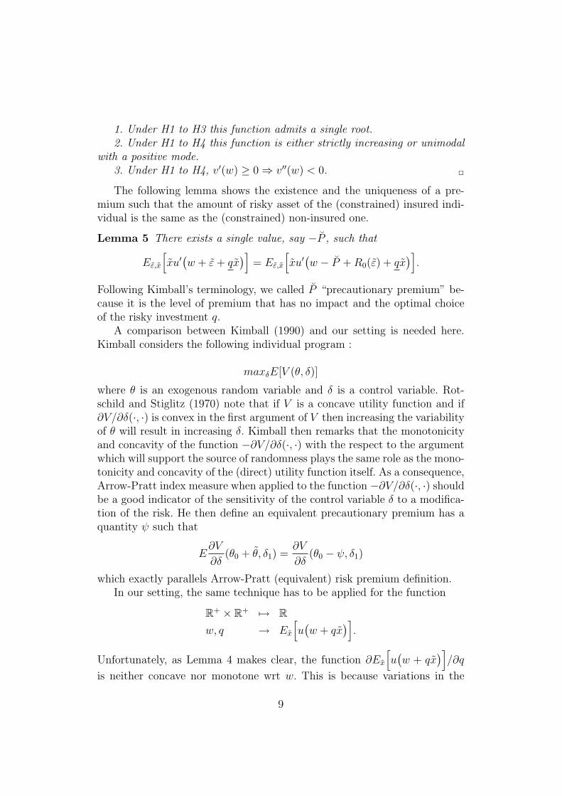
1. Under H1 to H3 this function admits a single root.2. Under H1 to H4 this function is either strictly increasing or unimodal

with a positive mode.3. Under H1 to H4, v′(w) ≥ 0 ⇒ v′′(w) < 0. 2

The following lemma shows the existence and the uniqueness of a pre-mium such that the amount of risky asset of the (constrained) insured indi-vidual is the same as the (constrained) non-insured one.

Lemma 5 There exists a single value, say −P , such that

Eε,x

[xu′

(w + ε + qx

)]= Eε,x

[xu′

(w − P + R0(ε) + qx

)].

Following Kimball’s terminology, we called P “precautionary premium” be-cause it is the level of premium that has no impact and the optimal choiceof the risky investment q.

A comparison between Kimball (1990) and our setting is needed here.Kimball considers the following individual program :

maxδE[V (θ, δ)]

where θ is an exogenous random variable and δ is a control variable. Rot-schild and Stiglitz (1970) note that if V is a concave utility function and if∂V/∂δ(·, ·) is convex in the first argument of V then increasing the variabilityof θ will result in increasing δ. Kimball then remarks that the monotonicityand concavity of the function −∂V/∂δ(·, ·) with the respect to the argumentwhich will support the source of randomness plays the same role as the mono-tonicity and concavity of the (direct) utility function itself. As a consequence,Arrow-Pratt index measure when applied to the function −∂V/∂δ(·, ·) shouldbe a good indicator of the sensitivity of the control variable δ to a modifica-tion of the risk. He then define an equivalent precautionary premium has aquantity ψ such that

E∂V

∂δ(θ0 + θ, δ1) =

∂V

∂δ(θ0 − ψ, δ1)

which exactly parallels Arrow-Pratt (equivalent) risk premium definition.In our setting, the same technique has to be applied for the function

R+ × R+ 7→ Rw, q → Ex

[u(w + qx

)].

Unfortunately, as Lemma 4 makes clear, the function ∂Ex

[u(w + qx

)]/∂q

is neither concave nor monotone wrt w. This is because variations in the

9

control variable q entail modifications of the exposition to risk. Kimball doesnot face this problem because (from section 4 on) δ is interpreted as the firstperiod level of consumption the modification of which entails no extra sourceof risk. Thus our setting does not fit exactly to Kimball’s paper. However, asfar as terminology is concerned, we feel free to use the term “precautionarypremium” to P .

The next lemma has a clear interest in its own right. It extends Pratt’sresult to partial insurance contracts.

Lemma 6 Consider any functions u1(·) and u2(·) fulfilling H1 to H3 suchthat

−u′′1(w)/u′1(w) > −u′′2(w)/u′2(w) ∀w,

a risk ε, and a function R0(ε) fulfilling (H7). Define Pi such that

Eε

[ui

(w + ε)

)]= Eε

[ui

(w − Pi + R0(ε)

)]i = 1, 2. (6)

Then P1 > P2. 2

We shall also use a version of this result where inequalities are broad.

Corollary 3 Take two functions fulfilling H1 to H3 such that

−u′′1(w)/u′1(w) ≥ −u′′2(w)/u′2(w) ∀w,

a risk ε, and a function R0(ε) fulfilling (H7). Define Pi such that

Eε

[ui

(w + ε)

)]= Eε

[ui

(w − Pi + R0(ε)

)]. (7)

Then P1 ≥ P2. 2

3 Premia : definitions, existence and unique-

ness

3.1 Risk premium

The risk premium, P , is defined as the level of P which equals u withu(P ), more precisely we have

Eε,x

[u(w + ε + qx

)]= Eε,x

[u(w − P + R0(ε) + q(P )x

)]. (8)

Notice that P clearly depends on w, Fε, Fx and R0(.).

10

We now show that P exists and is unique. Consider P1 such that −P1 +R0(ε) > ε ∀ε. Using definitions of u(·), q(·) and u′(·) > 0 we get

u(P1) ≡ Eε,x

[u(w − P1 + R0(ε) + qx

)] ≥

Eε,x

[u(w − P1 + R0(ε) + qx

)]> Eε,x

[u(w + ε + qx

)] ≡ u.

Now consider P2 such that −P2 + R0(ε) < ε ∀ε. Using definitions of u(·),q(·) and u′(·) > 0 we get

u(P2) ≡ Eε,x

[u(w − P2 + R0(ε) + qx

)]<

Eε,x

[u(w + ε + qx

)] ≤ Eε,x

[u(w + ε + qx

)] ≡ u.

Now since u(P ) is a strictly decreasing function of P (in view of Lemma 2),P exists and is unique.

Notice that P1, P2 may be used to derived boundaries for P . Indeed, wehave

{ −P1 + R0(ε) > ε ∀ε ∈ [εmin, εmax]−P2 + R0(ε) < ε ∀ε ∈ [εmin, εmax]

⇔{

P1 < R0(εmax)− εmax

P2 > R0(εmin)− εmin

These inequalities together with 0 ≤ R′0(.) ≤ 1 gives

P ∈ [R0(εmax)− εmax; R0(εmin)− εmin

].

3.2 Precautionary premium

According to Lemma 5, there exists a unique P such that

Eε,x

[xu′

(w + ε + qx

)]= Eε,x

[xu′

(w − P + R0(ε) + qx

)]. (9)

3.3 Constrained risk premium

Finally, we shall use a constrained version of the risk premium. Moreprecisely define P as

Eε,x

[u(w + ε + qx

)]= Eε,x

[u(w − P + R0(ε) + qx

)]. (10)

The existence of P , follows along the same lines as that of P . Consideragain P1 and P2 as before. Lemma 2, and 0 ≤ R′

0(ε) ≤ 1 and u′(·) > 0 imply{

uc(P1) > uuc(P2) < u

⇒ ∃ ! P ∈ [R0(εmax)− εmax; R0(εmin)− εmin

].

11

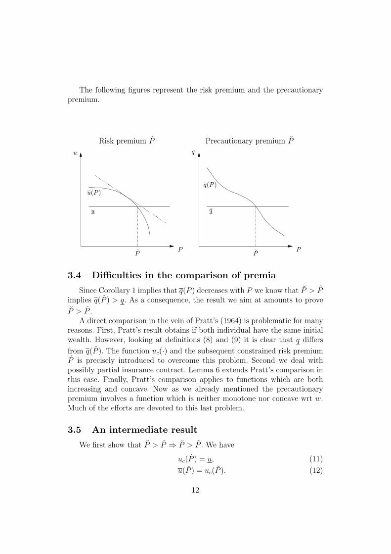
The following figures represent the risk premium and the precautionarypremium.

PP

u

u

u(P )

PP

q

q

q(P )

Risk premium P Precautionary premium P

3.4 Difficulties in the comparison of premia

Since Corollary 1 implies that q(P ) decreases with P we know that P > Pimplies q(P ) > q. As a consequence, the result we aim at amounts to prove

P > P .A direct comparison in the vein of Pratt’s (1964) is problematic for many

reasons. First, Pratt’s result obtains if both individual have the same initialwealth. However, looking at definitions (8) and (9) it is clear that q differs

from q(P ). The function uc(·) and the subsequent constrained risk premiumP is precisely introduced to overcome this problem. Second we deal withpossibly partial insurance contract. Lemma 6 extends Pratt’s comparison inthis case. Finally, Pratt’s comparison applies to functions which are bothincreasing and concave. Now as we already mentioned the precautionarypremium involves a function which is neither monotone nor concave wrt w.Much of the efforts are devoted to this last problem.

3.5 An intermediate result

We first show that P > P ⇒ P > P . We have

uc(P ) = u, (11)

u(P ) = uc(P ). (12)

12

If P > P using Lemma 2 we get

uc(P ) < uc(P ). (13)

Combining equations (11), (12), and (13) we get

u(P ) < u. (14)

Now, by definition of P we derive

u(P ) = u. (15)

Finally using equations (14) and (15), and Lemma 2 gives

u(P ) < u(P ) ⇔ P > P

This intermediate result show that all what is needed is a comparisonbetween P and P .

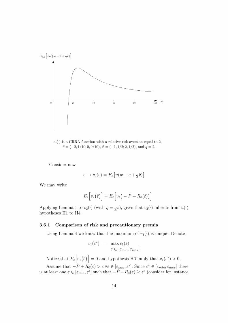
3.6 Rewriting precautionary and constrained risk pre-mia

Consider the following function

ε → v1(ε) = Ex

[xu′

(w + ε + qx

)]

This function may be used to rewrite P as

Eε

[v1

(ε)]

= Eε

[v1

(− P + R0(ε))]

= 0. (16)

Lemma 4 shows that this function may not be monotone. Figure 1 belowprovides a typical shape for this function.

13

0 20 40 60 80 100

Eε,x

[xu′

(w + ε + qx

)]

w

u(·) is a CRRA function with a relative risk aversion equal to 2,ε = (−2, 1/10; 0, 9/10), x = (−1, 1/2; 2, 1/2), and q = 2.

Consider now

ε → v2(ε) = Ex

[u(w + ε + qx)

]

We may write

Eε

[v2

(ε)]

= Eε

[v2

(− P + R0(ε))]

Applying Lemma 1 to v2(·) (with η = qx), gives that v2(·) inherits from u(·)hypotheses H1 to H4.

3.6.1 Comparison of risk and precautionary premia

Using Lemma 4 we know that the maximum of v1(·) is unique. Denote

v1(ε∗) = max v1(ε)

ε ∈ [εmin, εmax]

Notice that Eε

[v1

(ε)]

= 0 and hypothesis H6 imply that v1(ε∗) > 0.

Assume that −P + R0(ε) > ε ∀ε ∈ [εmin, ε∗]. Since ε∗ ∈ [εmin, εmax] there

is at least one ε ∈ [εmin, ε∗] such that −P +R0(ε) ≥ ε∗ (consider for instance

14

the case ε = ε∗). Now equation (16) hypothesis H6 and lemma 4 imply thatthere exists at least one ε ∈ [εmin, ε

∗] such that v1

( − P + R0(ε))

< 0.Consider such a value of ε (εl say). Recall from lemma 4 that whenever v1

is negative it is increasing. Using v1(ε∗) > 0 > v1

(− P + R0(εl))

we deduce

ε∗ > −P+R0(εl) Now the continuity of R0 entails the existence of ε∗ such that−P + R0(ε∗) = ε∗. Denote δ = ε∗ − ε∗. Since −P + R0(ε) > ε ∀ε ∈ [εmin, ε

∗]we have δ > 0.

Using 0 ≤ R′0(ε) ≤ 1 we deduce

ε < ε∗ ⇒ ε∗ ≥ −P + R0(ε) ≥ ε + δ

ε > ε∗ ⇒ ε∗ ≤ −P + R0(ε) ≤ ε + δ

Now, recall from lemma 4 that v1 is an increasing (resp. decreasing) functionin the interval [εmin, ε

∗] (resp. [ε∗, εmax]).

ε < ε∗ ⇒ v1(−P + R0(ε)) ≥ v1(ε + δ)

ε > ε∗ ⇒ v1(−P + R0(ε)) ≤ v1(ε + δ)

Thus we have

Eε

[v1

(− P + R0(ε))] ≥ Eε

[v1

(ε + δ

)].

Using δ > 0, Eε

[v1

(ε)]

= 0 and lemma 2 we have Eε

[v1

(ε + δ

)]> 0 hence

Eε

[v1

(− P + R0(ε))]

> 0 which contradicts equation (16).

The above argument shows that either −P + R0(ε) < ε ∀ε ∈ [εmin, εmax]or there exists ε ∈]εmin, ε

∗[ such that −P + R0(ε) = ε.Consider the first case. Since P ∈ [

R0(εmax)−εmax; R0(εmin)−εmin

], this

implies that P > P and we are done.Finally consider the second case. Consider ε such that −P + R0(ε) = ε.Let us introduce the function v12(·) such that

∀ε ≥ ε v12(ε) = v2(ε),

∀ε < ε v12(ε) = k+

∫ ε

εmin

k′ exp

(u− ε

ε− εmin

ln(v′1(u)

)+

εmin − u

ε− εmin

ln(v′2(u)

))du.

(17)With

k = v2(ε)−∫ ε

εmin

k′ exp

(u− ε

ε− εmin

ln(v′1(u)

)+

εmin − u

ε− εmin

ln(v′2(u)

))du

and k′ =(v′2(ε)

)2.

15

Notice that k and k′ are chosen so that v12 is continuously differentiable.Since k′ > 0 we have

v′12(ε) = k′ exp

(ε− ε

ε− εmin

ln(v′1(ε)

)+

εmin − ε

ε− εmin

ln(v′2(ε)

))> 0 ∀ε < ε.

Now since v′12(·) continuous we have v′12(·) > 0.Finally, remark that

−v′′12(ε)

v′12(ε)= −v′′1(ε)

v′1(ε)ε− ε

ε− εmin

− v′′2(ε)v′2(ε)

(1− ε− ε

ε− εmin

)∀ε < ε. (18)

This expression clearly shows that v′′12 is a continuous function in the in-terval [εmin, ε[. Moreover, it also shows that v′′12 admits a continuous extensionat ε. Hence v′′12 may be continuously defined for all ε.

We shall say that the function f is strictly more “curved” than g at ε ifand only if

−f ′′(ε)f ′(ε)

> −g′′(ε)g′(ε)

. (19)

Let compare the curvature of v1 and v2 for all ε ∈ [εmin, ε∗].

Consider the function

ε → v3(ε) = Ex

[u′

(w + ε + qx

)]

Using Lemma 1 and H3 we get

−Ex

[u′′

(w + ε + qx

)]

Ex

[u′

(w + ε + qx

)] < −Ex

[u′′′

(w + ε + qx

)]

Ex

[u′′

(w + ε + qx

)] .

Hence the inequality (19) is fulfilled for f = v1 and g = v3 if

−v′′1(ε)v′1(ε)

≥ −v′′3(ε)v′3(ε)

⇔ v′′1(ε)v′3(ε) ≥ v′1(ε)v

′′3(ε). (20)

Now recall v1 is increasing on [εmin, ε∗]. Lemma 4 implies that v1 is concave

on this interval. Now remak that by hypotheses H1 to H3 v′3(·) < 0 andv′′3(·) > 0.

For any fixed ε define λ < 0 such that v′′1(ε) = λv′′3(ε) < 0. Multiplyingeach side of (20) by λ gives

v′′1(ε)λv′3(ε) ≤ v′1(ε)λv′′3(ε)

16

which is true by definition of λ if

λv′3(ε) ≥ v′1(ε).

Finally, the equation (20) is fulfilled if

v′′1(ε)− λv′′3(ε) = 0 ⇒ λv′3(ε)− v′1(ε) ≥ 0.

Replacing v1 and v3 by their expressions gives

Ex

[xu′′′

(w + ε + qx

)− λu′′′(w + ε + qx

)]= 0

⇒Ex

[λu′′

(w + ε + qx

)− xu′′(w + ε + qx

)] ≥ 0.

The above implication is true whenever there exists a ν such that

λu′′(w + ε + qx

)− xu′′(w + ε + qx

) ≥ν[xu′′′

(w + ε + qx

)− λu′′′(w + ε + qx

)] ∀x

⇔ (λ− x)(u′′

(w + ε + qx

)+ νu′′′

(w + ε + qx

)) ≥ 0 ∀x.

For x = λ the previous inequality is obviously fulfilled. For other valuesof x, it requires that

∀x < λ, − u′′(w + ε + qx

)

u′′′(w + ε + qx

) ≤ ν,

∀x > λ, − u′′(w + ε + qx

)

u′′′(w + ε + qx

) ≥ ν.

Since from H4 −u′′(w + ε + qx

)/u′′′

(w + ε + qx

)increases with x for any

x ∈ [xmin, xmax] such a ν exists, and v1 is strictly more curved than v2 forany ε < ε∗.

Notice that if v1 is increasing over the entire interval [εmin, εmax] applyingLemma 3 gives P > hatP and we are done. Thus assume that Fε(ε

∗) < 1.Since

0 < (ε− ε)/(ε− εmin) < 1 ∀ε ∈]εmin, ε[,

17

using equation (18), ε < ε∗ and the fact that v1 is strictly more curvedthan v2 all ε < ε∗ we derive

−v′′1(ε)v′1(ε)

> −v′′12(ε)

v′12(ε)> −v′′2(ε)

v′′2(ε)∀ε ∈]εmin, ε[. (21)

Moreover

−v′′1(εmin)

v′1(εmin)= −v′′12(εmin)

v′12(εmin)> −v′′2(εmin)

v′′2(εmin), (22)

and

−v′′1(ε)v′1(ε)

> −v′′12(ε)

v′12(ε)= −v′′2(ε)

v′′2(ε). (23)

Since v′12 > 0, there exists a unique P1 such that

Eε

[v12

(ε)]

= Eε

[v12

(− P1 + R0(ε))]

. (24)

Now using Lemma 3 and

−v′′12(ε)/v′12(ε) ≥ −v′′2(ε)/v

′2(ε) ∀ε ∈ [εmin, εmax],

gives P1 ≥ P .Let now show that P > P1. Using equations (16), (24), and v′12(·) > 0,

P ≥ P1 if

Eε

[v1

(ε)− v1

(− P + R0(ε))]

= 0 ⇒ Eε

[v12

(ε)− v12

(− P + R0(ε))] ≥ 0.

This proposition is true if there exists a µ such that

v12

(ε)−v12

(− P +R0(ε)) ≥ µ

(v1

(ε)−v1

(− P +R0(ε))) ∀ε ∈ [εmin, εmax].

(25)Define the function

φ(ε) = v12(ε)− µv1(ε).

The condition (25) may be rewritten as

φ(ε) ≥ φ(− P + R0(ε)

) ∀ε ∈ [εmin, εmax]. (26)

Now by definition of ε, and using the fact that 0 ≤ R′0(ε) ≤ 1 we get

∀ε ≤ ε ε ≤ −P + R0(ε),

∀ε ≥ ε ε ≥ −P + R0(ε).

18

Hence, the inequality (26) is true if

∀ε ∈ [εmin, ε] φ′(ε) ≤ 0,∀ε ∈ [ε, εmax] φ′(ε) ≥ 0.

Now choose µ such that v′12(ε) = µv′1(ε). Equations (21) and (22) imply that

v′12(ε) < µv′1(ε) ∀ε ∈ [εmin, ε[,

which is equivalent to

φ′(ε) < 0 ∀ε ∈ [εmin, ε[.

Moreover, since for all ε ∈ [ε, ε∗[, v1(ε) is strictly more curved than v12(ε)and since for all ε ∈ [ε∗, εmax], we have v′1(ε) ≤ 0 and v′12(ε) > 0, then

φ′(ε) > 0 ∀ε ∈ [ε, εmax].

since we assumed that Fε(ε∗) < 1, this proves also that

IPε

(v12

(ε)− v12

(− P + R0(ε)) ≥ µ

(v1

(ε)− v1

(− P + R0(ε))))

> 0

from which we deduce P > P1. QED

4 Some simple extensions

This section is devoted to two almost trivial generalizations of the model.However these generalizations have a substantial economic content.

4.1 Price competition

The model assumes that the agent faces a monopoly. In this case, weobtained that the insurance company chooses a level of premium P smallerthan P which induces that the individual increases the optimal amount ofrisky investment when he decides to purchase the insurance contract.

If competition arises between insurance companies, it is clear that thesubstitutability result remains, insofar competition lowers the premium. As-sume for instance that the competition ends with a pure premium then it issmaller than P hence again smaller P . In any case, competition cannot alterthe complementarity between insurance contract and financial asset.

Of course, competition may also have impact on the quality of the contractR(.). The above easy generalization cannot cope with this case.

19

4.2 Correlated risks

We also assumed that x and ε are independent. We now discuss how toextend the model to some form of dependence between the risks.

Assume for this paragraph that the contract is complete (that is R(.) = 0).Also assume that

ε = ρx + η a.s.

where x and η are independent. The independent case corresponds to ρ = 0.We now have

u = Eε,x[u(w + ρx + η + qx)]

u = Ex[u(w − P + qx)]

We notice that u may be rewritten as

U = Eε,x[U(w + η + (q + ρ)x)].

Now since x and η are independent, changing the variable q + ρ to q bringsus back to the case previously studied.

This shows that the complementarity result may be reversed if ρ is largerthan the difference between q and q in the independent case. Notice thatsubstitutability requires a substantial level of correlation. More precisely, thestudy of the independent case shows that ρ must be positive and large enoughfor the insurance contract and financial asset to be substitute. An extremeinstance of this is the case ˜eta = 0 where that the insurance contract andthe financial asset are clearly identical items.

Notice also that the above message is very similar to that of the portfoliotheory. If risks are correlated, complementarity or substitutability dependson the level of correlation. If the correlation is very high, substitutability isthe rule.

If the insurance contract is incomplete, others effects appears. Indeed, tokeep things as simple as possible assume that R(ε) = αε where α ∈ ]0, 1[.Then we have

u = Eε,x[u(w + η + (q + ρ)x)]

u = Ex[u(w − P + (q + ρα)x)]

and we must have ρ(1 − α) large enough to reach substitutability. Whenthe insurance contract is incomplete, substitutability then requires a largeramount of correlation between the risks.

The kind of correlation assumed here is undoubtedly very specific. Sois the type of incompleteness. The conclusion we derived here goes withqualifications in more general settings.

20

5 Conclusion

Kimball (1990) studies a model where a risk averse individual facing anindividual risk chooses an optimal amount of risky and risk-free asset. In thispaper we enlarge the situation to the case where the individual risk may beinsured. We assume that the insurance contract is provided by an insurancecompany. The insurance contract may be incomplete. The question is whe-ther the risky investment is larger or smaller when the individual chooses toinsure the risk. In a sense, are insurance contracts and risky financial assetscomplementary or substitute ? Under monopoly the contract proposed makesthe individual indifferent between insured and non-insured situation. We findthat standardness of the utility function implies that the risky investment isalways larger when the individual is insured.

This result is not trivial since standardness is equivalent to the coexistenceof Decreasing Absolute Risk Aversion and Decreasing Absolute Prudence.Thus, on the one hand, choosing insurance -implying smaller wealth- wouldreduce the optimal amount of risky investment (DARA assumption). But, onthe other hand, the insured individual faces less risk and this implies largerdemand for risky assets (DAP assumption). This is true for any type of risk(that is the result is not restricted to a “small” individual risk). This is alsotrue if the insurance industry do not operate under monopoly.

Moreover, as a by-product we obtain several interesting results in thevein of Pratt (1964) and Kimball (1964). For instance, we extend Pratt’sresults to incomplete insurance contracts. We also show that the concept ofprecautionary premium may be useful in broader frameworks than that ofKimball(1990).

Several extensions of the techniques and the results presented here may beenvisaged. First, the model may be enlarged to cope with consumption effectsin the vein of Dreze and Modigliani (1972). Second, the techniques developedin this paper may prove to be useful to study complementarity effects of thedemand for risky assets without the usual mean/variance approximation.

References

[1] Allais, Maurice (1953), “L’extension des theories de l’equilibre generalet du rendement social au cas du risque” Econometrica, 21, 269-290.

[2] Arrow, Kenneth J. (1971), Essays of the Theory of Risk Bearing, Chi-cago : Markham Publishing Co.

21

[3] Dreze, Jacques H. and Franco Modigliani, (1972), “Consumption Deci-sions under Uncertainty,” Journal of Economic Theory, 5, 308-335.

[4] Eeckhoudt, Louis and Harold Schlesinger, (2003), “Putting Risk in itsProper Place,” mimeo.

[5] Gollier, Christian, (2001), The Economics of Risk and Time, Cam-bridge : MIT Press.

[6] Kimball, Miles S., (1990), “Precautionary Savings in the Small and inthe Large,” Econometrica, 58, 53-73.

[7] Kimball, Miles S., (1993), “Standard Risk Aversion,” Econometrica, 61,589-611.

[8] Markowitz, Harry (1959) Portfolio Selection New York John Wiley andSons.

[9] Mossin, Jan (1966) “Equilibrium in a Capital Asset Market” Econome-trica, 34, 768-783

[10] Pratt, John W., (1964), “Risk Aversion in the Small and in the Large,”Econometrica, 32, 122-136.

[11] Pratt, John W. and Richard J. Zeckhauser, (1987), “Proper Risk Aver-sion,” Econometrica, 55 , 143-154.

[12] Rothschild, Michael and Joseph E. Stigltiz (1970) “Increasing Risk I : aDefinition” Journal of Economic Theory, 2, 225-243.

[13] Sharpe, William F. (1964) “Capital Asset Prices : A Theory of MarketEquilibrium under Conditions of Risk” The Journal of Finance, 19,425-442.

[14] Tobin, James (1958) “Liquidity Preference as Behaviour Toward Risk”Review of Economic Studies, 67 65-86.

22

6 APPENDIX

6.1 Lemma 1 (Gollier (2001)

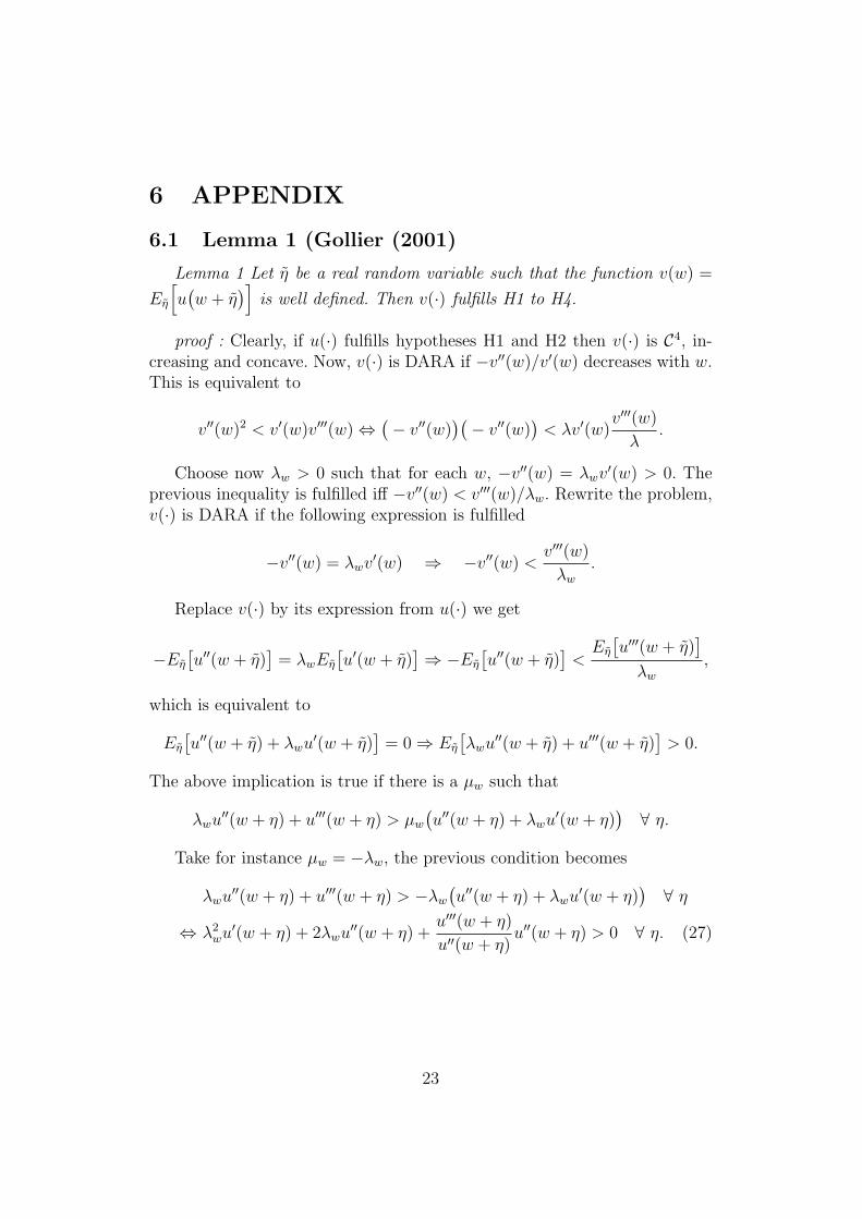
Lemma 1 Let η be a real random variable such that the function v(w) =

Eη

[u(w + η

)]is well defined. Then v(·) fulfills H1 to H4.

proof : Clearly, if u(·) fulfills hypotheses H1 and H2 then v(·) is C4, in-creasing and concave. Now, v(·) is DARA if −v′′(w)/v′(w) decreases with w.This is equivalent to

v′′(w)2 < v′(w)v′′′(w) ⇔ (− v′′(w))(− v′′(w)

)< λv′(w)

v′′′(w)

λ.

Choose now λw > 0 such that for each w, −v′′(w) = λwv′(w) > 0. Theprevious inequality is fulfilled iff −v′′(w) < v′′′(w)/λw. Rewrite the problem,v(·) is DARA if the following expression is fulfilled

−v′′(w) = λwv′(w) ⇒ −v′′(w) <v′′′(w)

λw

.

Replace v(·) by its expression from u(·) we get

−Eη

[u′′(w + η)

]= λwEη

[u′(w + η)

] ⇒ −Eη

[u′′(w + η)

]<

Eη

[u′′′(w + η)

]

λw

,

which is equivalent to

Eη

[u′′(w + η) + λwu′(w + η)

]= 0 ⇒ Eη

[λwu′′(w + η) + u′′′(w + η)

]> 0.

The above implication is true if there is a µw such that

λwu′′(w + η) + u′′′(w + η) > µw

(u′′(w + η) + λwu′(w + η)

) ∀ η.

Take for instance µw = −λw, the previous condition becomes

λwu′′(w + η) + u′′′(w + η) > −λw

(u′′(w + η) + λwu′(w + η)

) ∀ η

⇔ λ2wu′(w + η) + 2λwu′′(w + η) +

u′′′(w + η)

u′′(w + η)u′′(w + η) > 0 ∀ η. (27)

23

Now we have ηu′′′(w + η)

u′′(w + η)<

u′′(w + η)

u′(w + η). Moreover u′′(w + η) < 0. Hence

condition (27) is true if

λ2wu′(w + η) + 2λwu′′(w + η) +

u′′(w + η)

u′(w + η)u′′(w + η) > 0 ∀ η

⇔ λ2wu′(w + η) + 2λw

u′′(w + η)

u′(w + η)u′(w + η)

+u′′(w + η)

u′(w + η)

u′′(w + η)

u′(w + η)u′(w + η) > 0 ∀ η

⇔ u′(w + η)

(λ2

w + 2λwu′′(w + η)

u′(w + η)+

(u′′(w + η)

u′(w + η)

)2)

> 0 ∀ η

⇔ u′(w + η)

(λw +

u′′(w + η)

u′(w + η)

)2

> 0 ∀ η.

Finally (H2) implies the desired result. Similarly, v(·) inherits H4 from u(·)if u(w) expresses decreasing absolute prudence for any w. Q.E.D

6.2 Lemma 2

Lemma 2 For any given(Fε, Fx

)fulfilling H5 and H6, q(w, Fε, Fx) is a

strictly increasing function of w.

proof Using H6 we have

u(w) = Eε,x

[u(w + ε + q(w)x

)]= Ex

[Eε

[u(w + ε + q(w)x

)]] ∀ w.

Consider now a new utility function v(·) such that v(w) = Eε

[u(w +

ε)]

∀ w. Notice that

u(w) = Ex

[v(w+q(w)x

)]and u(w+dw) = Ex

[v(w+dw+q(w+dw)x

)].

If v1(·) and q1(·) are functions induced respectively by v(·) and q(·) such

thatv1(w) = v(w + dw) and q

1(w) = q(w + dw) ∀ w,

thenEx

[v(w + dw + q(w + dw)x

)]= Ex

[v1

(w + q

1(w)x

)].

24

If for any dw > 0, q1(w) > q(w) then it is clear that q grows with w.

Applying Pratt’s results (more precisely Theorem 1 page 128), we know thatq1(w) > q(w) if the absolute risk aversion related to v(w) is larger than it is

for v1(w). But this is true, since

−v′′1(w)

v′1(w)= −v′′(w + dw)

v′(w + dw)< −v′′(w)

v′(w)∀ dw > 0,

(the last inequality follows from H3 and Lemma 1.) Q.E.D

6.3 Corollary 1

Corollary 1 For any given(Fε, Fx

)fulfilling H5 and H6, q(w−P,C, Fε, Fx)

is a strictly increasing function of w and is a strictly decreasing function ofP .

proof : This result follows trivially by taking w − P instead of w, andR0(ε) instead of ε in the proof of Lemma 2.Q.E.D

6.4 Lemma 3

Lemma 3 For any given(Fε, Fx

)fulfilling H5 and H6, u(w, Fε, Fx) is a

strictly increasing function of w.

proof : For any given Fx and Fε, Eε,x

[u(w + ε + q(w)x

)]is the optimal

level of utility of one individual with a level of wealth w (provided that heholds the asset ε).

Fix any dw > 0. The condition u′(·) > 0 implies

u(w + dw + ε + q(w)x) > u(w + ε + q(w)x) ∀ ε, x

⇒ Eε,x

[u(w + dw + ε + q(w)x

)]> Eε,x

[u(w + ε + q(w)x

)].

Since for a level of wealth w + dw, q(w) is not optimal (C.f. Lemma 2),then

Eε,x

[u(w + dw + ε + q(w + dw)x

)] ≥ Eε,x

[u(w + dw + ε + q(w)x

)].

Using the two previous inequalities we finally get

u(w+dw) = Eε,x

[u(w+dw+ε+q(w+dw)x

)]> Eε,x

[u(w+ε+q(w)x

)]= u(w).

Q.E.D

25

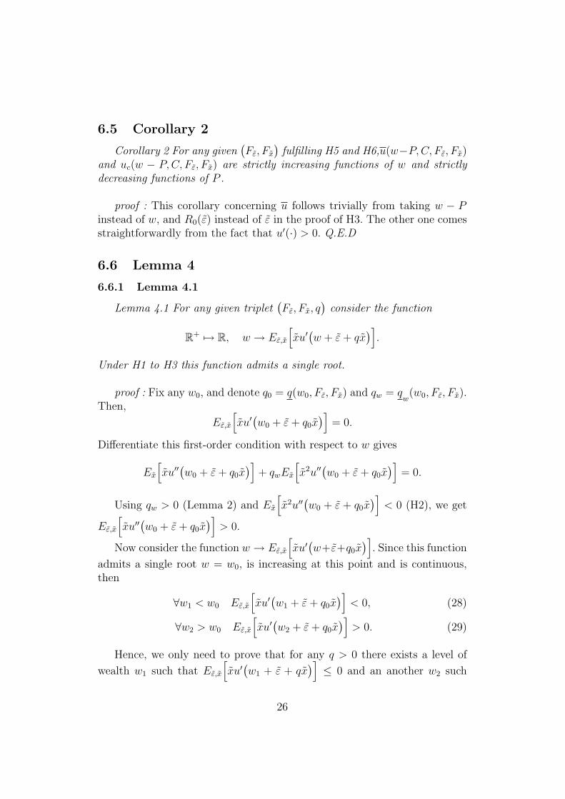
6.5 Corollary 2

Corollary 2 For any given(Fε, Fx

)fulfilling H5 and H6,u(w−P,C, Fε, Fx)

and uc(w − P,C, Fε, Fx) are strictly increasing functions of w and strictlydecreasing functions of P .

proof : This corollary concerning u follows trivially from taking w − Pinstead of w, and R0(ε) instead of ε in the proof of H3. The other one comesstraightforwardly from the fact that u′(·) > 0. Q.E.D

6.6 Lemma 4

6.6.1 Lemma 4.1

Lemma 4.1 For any given triplet(Fε, Fx, q

)consider the function

R+ 7→ R, w → Eε,x

[xu′

(w + ε + qx

)].

Under H1 to H3 this function admits a single root.

proof : Fix any w0, and denote q0 = q(w0, Fε, Fx) and qw = qw(w0, Fε, Fx).

Then,

Eε,x

[xu′

(w0 + ε + q0x

)]= 0.

Differentiate this first-order condition with respect to w gives

Ex

[xu′′

(w0 + ε + q0x

)]+ qwEx

[x2u′′

(w0 + ε + q0x

)]= 0.

Using qw > 0 (Lemma 2) and Ex

[x2u′′

(w0 + ε + q0x

)]< 0 (H2), we get

Eε,x

[xu′′

(w0 + ε + q0x

)]> 0.

Now consider the function w → Eε,x

[xu′

(w+ε+q0x

)]. Since this function

admits a single root w = w0, is increasing at this point and is continuous,then

∀w1 < w0 Eε,x

[xu′

(w1 + ε + q0x

)]< 0, (28)

∀w2 > w0 Eε,x

[xu′

(w2 + ε + q0x

)]> 0. (29)

Hence, we only need to prove that for any q > 0 there exists a level of

wealth w1 such that Eε,x

[xu′

(w1 + ε + qx

)] ≤ 0 and an another w2 such

26

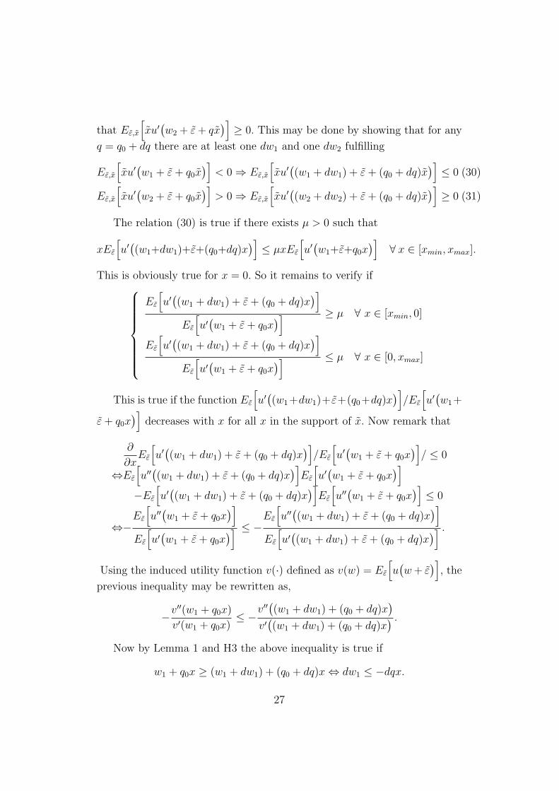
that Eε,x

[xu′

(w2 + ε + qx

)] ≥ 0. This may be done by showing that for any

q = q0 + dq there are at least one dw1 and one dw2 fulfilling

Eε,x

[xu′

(w1 + ε + q0x

)]< 0 ⇒ Eε,x

[xu′

((w1 + dw1) + ε + (q0 + dq)x

)] ≤ 0 (30)

Eε,x

[xu′

(w2 + ε + q0x

)]> 0 ⇒ Eε,x

[xu′

((w2 + dw2) + ε + (q0 + dq)x

)] ≥ 0 (31)

The relation (30) is true if there exists µ > 0 such that

xEε

[u′

((w1+dw1)+ε+(q0+dq)x

)] ≤ µxEε

[u′

(w1+ε+q0x

)] ∀ x ∈ [xmin, xmax].

This is obviously true for x = 0. So it remains to verify if

Eε

[u′

((w1 + dw1) + ε + (q0 + dq)x

)]

Eε

[u′

(w1 + ε + q0x

)] ≥ µ ∀ x ∈ [xmin, 0]

Eε

[u′

((w1 + dw1) + ε + (q0 + dq)x

)]

Eε

[u′

(w1 + ε + q0x

)] ≤ µ ∀ x ∈ [0, xmax]

This is true if the function Eε

[u′

((w1+dw1)+ ε+(q0+dq)x

)]/Eε

[u′

(w1+

ε + q0x)]

decreases with x for all x in the support of x. Now remark that

∂

∂xEε

[u′

((w1 + dw1) + ε + (q0 + dq)x

)]/Eε

[u′

(w1 + ε + q0x

)]/ ≤ 0

⇔Eε

[u′′

((w1 + dw1) + ε + (q0 + dq)x

)]Eε

[u′

(w1 + ε + q0x

)]

−Eε

[u′

((w1 + dw1) + ε + (q0 + dq)x

)]Eε

[u′′

(w1 + ε + q0x

)] ≤ 0

⇔−Eε

[u′′

(w1 + ε + q0x

)]

Eε

[u′

(w1 + ε + q0x

)] ≤ −Eε

[u′′

((w1 + dw1) + ε + (q0 + dq)x

)]

Eε

[u′

((w1 + dw1) + ε + (q0 + dq)x

)] .

Using the induced utility function v(·) defined as v(w) = Eε

[u(w + ε

)], the

previous inequality may be rewritten as,

−v′′(w1 + q0x)

v′(w1 + q0x)≤ −v′′

((w1 + dw1) + (q0 + dq)x

)

v′((w1 + dw1) + (q0 + dq)x

) .

Now by Lemma 1 and H3 the above inequality is true if

w1 + q0x ≥ (w1 + dw1) + (q0 + dq)x ⇔ dw1 ≤ −dqx.

27

Hence, as long as dw1 ≤ −dqx for all x in the domain of x, the condition(30) is fulfilled. Then, if dq < 0 (respectively dq > 0 ) we need to find adw1 ≤ −dqxmin (respectively dw1 ≤ −dqxmax).

On the other hand, the condition (31) is fulfilled as long as the function

Eε

[u′

((w1 + dw1) + ε + (q0 + dq)x

)]/Eε

[u′

(w1 + ε + q0x

)]increases with x

for all x in the support of x. Along the same lines as above, we deduce thatthis is true as long as dw2 ≥ −dqx for all x in [xmin, xmax]. Thus for anydq < 0 (respectively dq > 0 ) we need to find a dw2 ≥ −dqxmax (respectivelydw2 ≥ −dqxmin).

Finally, using the continuity of Eε,x

[xu′

(w+ε+qx

)]with respect to w, we

obtain the existence of at least one w3 such that Eε,x

[xu′

(w3 + ε+ qx

)]= 0.

Hence, the uniqueness of w3 comes from the same arguments as those usedfor w0. Q.E.D

6.6.2 Lemma 4.2

Lemma 4.2 For any given triplet(Fε, Fx, q

)consider the function

R+ 7→ R, w → Eε,x

[xu′

(w + ε + qx

)].

Under H1 to H4 this function is either strictly increasing or unimodal witha positive mode.

proof Fix any η > 0. Let show first that

Eε,x

[xu′′

(w + ε + q0x

)] ≤ 0 ⇒ Eε,x

[xu′′

(w + ε + q0x + η

)] ≤ 0.

This condition is fulfilled if there is one µ > 0 such that

Eε

[xu′′

(w + ε + q0x + η

)] ≤ µEε

[xu′′

(w + ε + q0x

)] ∀x.

Since for x = 0 we have Eε

[xu′′

(w+ε+q0x+η

)]= µEε

[xu′′

(w+ε+q0x

)],

the above condition is fulfilled if∀ x < 0, Eε

[u′′

(w + ε + q0x + η

)]> µEε

[u′′

(w + ε + q0x

)],

∀ x > 0, Eε

[u′′

(w + ε + q0x + η

)]< µEε

[u′′

(w + ε + q0x

)].

⇔∀ x < 0, Eε

[u′′

(w + ε + q0x + η

)]/Eε

[u′′

(w + ε + q0x

)]< µ,

∀ x > 0, Eε

[u′′

(w + ε + q0x + η

)]/Eε

[u′′

(w + ε + q0x

)]> µ.

28

One may find such a µ if

∂

∂x

Eε

[u′′

(w + ε + q0x + η

)]

Eε

[u′′

(w + ε + q0x

)] > 0

⇔ Eε

[u′′′

(w + ε + q0x + η

)]Eε

[u′′

(w + ε + q0x

)]

−Eε

[u′′

(w + ε + q0x + η

)]Eε

[u′′′

(w + ε + q0x

)]> 0

⇔ −Eε

[u′′′

(w + ε + q0x + η

)]

Eε

[u′′

(w + ε + q0x + η

)] < −Eε

[u′′′

(w + ε + q0x

)]

Eε

[u′′

(w + ε + q0x

)] . (32)

Define v(·) as follows v(w) = Eε

[u(w + ε + q0x

)]. Using Lemma 1 and

H4 gives that v(·) has a decreasing absolute prudence and then that theinequality (32) is always fulfilled.

Now remark that since x is not degenerated there exists at least one xi

the event such that

Eε

[xiu

′′(w + ε + q0xi + η)]

< µEε

[xiu

′′(w + ε + q0xi

)]

obtains with a strict positive probability.It implies that

Eε,x

[xu′′

(w + ε + q0x

)] ≤ 0 ⇒ Eε,x

[xu′′

(w + ε + q0x + η

)]< 0.

Using Lemma 4.1 we deduce the existence of a w such that Eε,x

[xu′

(w +

ε + qx)]

> 0.

Q.E.D

6.6.3 Lemma 4.3

Lemma 4.3 For any given triplet(Fε, Fx, q

)consider the function

R+ 7→ R, w → Eε,x

[xu′

(w + ε + qx

)].

Under H1 to H4, v′(w) ≥ 0 ⇒ v′′(w) < 0.

29

proof : First let show that

Eε,x

[xu′′

(w + ε + q0x

)]> 0 ⇒ Eε,x

[xu′′′

(w + ε + q0x

)] ≤ 0

⇔ Eε,x

[xu′′

(w + ε + q0x

)]> 0 ⇒ −Eε,x

[xu′′′

(w + ε + q0x

)] ≥ 0.

The previous relation is fulfilled if it exists one µ > 0 such that

−xEε

[u′′′

(w + ε + q0x

)] ≥ µxEε

[u′′

(w + ε + q0x

)] ∀x.

For x = 0, −xEε

[u′′′

(w + ε + q0x

)]= µxEε

[u′′

(w + ε + q0x

)]and the

previous condition is true if∀ x < 0, −Eε

[u′′′

(w + ε + q0x

)]< µEε

[u′′

(w + ε + q0x

)]

∀ x > 0, −Eε

[u′′′

(w + ε + q0x

)]> µEε

[u′′

(w + ε + q0x

)]

⇔∀ x < 0, −Eε

[u′′′

(w + ε + q0x

)]/Eε

[u′′

(w + ε + q0x

)]> µ

∀ x > 0, −Eε

[u′′′

(w + ε + q0x

)]/Eε

[u′′

(w + ε + q0x

)]< µ

Such a µ exists if the function −Eε

[u′′′

(w+ ε+q0x

)]/Eε

[u′′

(w+ ε+q0x

)]

decreases with respect to w. Now this follows from Lemma 1 and H4.

Remark that since x is not degenerated there exists at least one xi suchthat the following event

−xiEε

[u′′′

(w + ε + q0xi

)]> µxiEε

[u′′

(w + ε + q0xi

)]

obtains with a strictly positive probability.Hence we have

Eε,x

[xu′′

(w + ε + q0x

)]> 0 ⇒ Eε,x

[xu′′′

(w + ε + q0x

)]< 0.

Q.E.D

6.7 Lemma 5

Lemma 5 There exists a single value, say −P , such that

0 = Eε,x

[xu′

(w + ε + qx

)]= Eε,x

[xu′

(w − P + R0(ε) + qx

)].

30

proof : Apply Lemma 4.1 to the case where ε is replaced by−P+R0(ε). We

deduce that there is a unique w0 such that Eε,x

[xu′

(w0−P +R0(ε)+qx

)]= 0

Now for any given w this is equivalent to the existence if a unique P denoted

P such that Eε,x

[xu′

(w − P + R0(ε) + qx

)]= 0. Q.E.D

6.8 Lemma 6

Lemma 6 Consider two functions fulfilling H1 to H3 such that

−u′′1(w)/u′1(w) > −u′′2(w)/u′2(w) ∀w,

a risk ε, and a function R0(ε) fulfilling (H7).Now define Pi such that

Eε

[ui

(w + ε)

)]= Eε

[ui

(w − Pi + R0(ε)

)]. (33)

Then P1 > P2.

proof : Consider a new function induced by R0(ε) and denoted R(β, ε)such that

R(β, ε) = βR0(ε) + (1− β)εR(0, ε) = εR(1, ε) = R0(ε)β ∈ [0, 1]

By the linearity of R(., .) as a function of β, we know that ∂R(β, ε)/∂βdoes not depend on β. Generalize definition (6) to any β gives

Eε

[ui

(w + ε)

)]= Eε

[ui

(w − Pi(β) + R(β, ε)

)]. (34)

Thus, since R(β, ε) and ui(·) are C1, ∂Pi/∂β exists and is C1 also. Now diffe-rentiate equation (34) with respect to β gives

0 = Eε

[(− ∂Pi(β)

∂β+

∂R(β, ε)

∂β

)u′i

(w − Pi(β) + R(β, ε)

)]. (35)

Remark that P1(0) = P2(0). Now assume there exists β1,2, a value of β suchthat P1(β1,2) = P2(β1,2) = P (β1,2).

31

The inequality ∂P1(β1,2)/∂β ≥ ∂P2(β1,2)/∂β and equation (35) are equi-valent to

Eε

[(− ∂P1

∂β(β1,2) +

∂R(β, ε)

∂β

)u′1

(w − P1(β1,2) + R(β1,2, ε)

)]= 0

Eε

[(− ∂P1

∂β(β1,2) +

∂R(β, ε)

∂β

)u′2

(w − P2(β1,2) + R(β1,2, ε)

)] ≤ 0

Now the above statement is true if there exists a µ such that(− ∂P1

∂β(β1,2) +

∂R(β, ε)

∂β

)u′2

(w − P (β1,2) + R(β1,2, ε)

)

≤ µ

(− ∂P1

∂β(β1,2) +

∂R(β, ε)

∂β

)u′1

(w − P (β1,2) + R(β1,2, ε)

) ∀ε(36)

⇔

u′2(w − P (β1,2) + R(β1,2, ε)

)

u′1(w − P (β1,2) + R(β1,2, ε)

) ≤ µ ∀ε such that∂R(β, ε)

∂β>

∂P1

∂β(β1,2)

u′2(w − P (β1,2) + R(β1,2, ε)

)

u′1(w − P (β1,2) + R(β1,2, ε)

) ≥ µ ∀ε such that∂R(β, ε)

∂β<

∂P1

∂β(β1,2)

Using R′0(ε) ≤ 1 we get ∂2R(β, ε)/(∂β∂ε) ≤ 0. Now since ∂R(β, ε)/∂β

continuous, there exists at least one ε denoted ε0 such that ∂R(β, ε0)/∂β =∂P1(β1,2)/∂β. Hence the above condition may be rewritten

u′2(w − P (β1,2) + R(β1,2, ε)

)

u′1(w − P (β1,2) + R(β1,2, ε)

) ≤ µ ∀ε < ε0

u′2(w − P (β1,2) + R(β1,2, ε)

)

u′1(w − P (β1,2) + R(β1,2, ε)

) ≥ µ ∀ε > ε0

Finally, R′0(ε) ≥ 0 and −u′′1(w)/u′1(w) > −u′′2(w)/u′2(w) ∀w imply respec-

tively ∂R(β1,2, ε)/∂ε ≥ 0 and ∂(u′2(w)/u′1(w))/∂w > 0 ∀w which prove thatµ fulfilling the above conditions may always be found.

Then

P1(β1,2) = P2(β1,2) ⇒ ∂P1(β1,2)/∂β ≥ ∂P2(β1,2)/∂β ∀β1,2 ∈ [0, 1]. (37)

Now remark that

∂R(β, ε)

∂ε= β

∂R0(ε)

∂ε+ 1− β > 0 ∀β ∈ [0, 1[

This inequality implies that for any β1,2 ∈ [0, 1[, R(β1,2, ε) is not a dege-nerated, random variable. Hence there exists ε such that the strict version ofthe inequality (36) obtains with a strict probability.

32

Thus we deduce

P1(β1,2) = P2(β1,2) ⇒ ∂P1(β1,2)/∂β > ∂P2(β1,2)/∂β ∀0 ≤ β1,2 < 1. (38)

Now notice that P1(0) = P2(0). Apply the previous result to β = 0, we getthe existence of a neighborhood of β = 0 in [0, 1] such that P1(β) > P2(β).Now assume that there exists β ∈]0, 1[, such that P1(β) = P2(β). Considerthe smallest of these and denote it β1,2. Since P ′

1(β) and P ′2(β) are continuous

for all β ∈ [0, 1], it requires that P ′1(β1,2) ≤ P ′

2(β1,2) which contradicts theprevious result.

Finally, condition (37) says that if P1(1) = P2(1), there exists a neighbo-rhood of β = 1 in [0, 1] such that P1(β) ≤ P2(β). Since this fact is impossible,for all β ∈]0, 1], P1(β) > P2(β). Q.E.D

6.9 Lemma 3

Lemma 3 Consider two functions fulfilling H1 to H3 such that

−u′′1(w)/u′1(w) ≥ −u′′2(w)/u′2(w) ∀w,

a risk ε, and a function R0(ε) fulfilling (H7). Now define Pi such that

Eε

[ui

(w + ε)

)]= Eε

[ui

(w − Pi + R0(ε)

)]. (39)

Then P1 ≥ P2.

proof : Notice that (37) does not require that u1(·) be strictly more curvedthan u2(·). Since P1(0) = P2(0), for P1(β) < P2(β) to be true one would needβ1,2 such that P1(β1,2) = P2(β1,2) and P ′

1(β1,2) < P ′2(β1,2) which contradicts

the previous implication. Q.E.D

33