resolution search and dynamic branch-and- bound sa¯d hanafi fred
TRANSCRIPT
DynamicB&B 1 18/04/01
RESOLUTION SEARCH AND DYNAMIC BRANCH-AND-
BOUND
Saïd Hanafi LAMIH - UMR CNRS n° 8530
Unité de Recherche Opérationnelle et d’Aide à la Décision Université de Valenciennes et du Hainaut-Cambrésis
Le Mont Houy - B.P. 311 - 59304 Valenciennes Cedex – France
Fred Glover Hearin Center for Enterprise Science School of Business Administration
University of Mississippi University, MS 38677 USA
January, 2001
Abstract
A novel approach to pure 0-1 integer programming problems called Resolution Search
has been proposed by Chvatal (l997) as an alternative to implicit enumeration, with a
demonstration that the method can yield more effective branching strategies. We show that
an earlier method called Dynamic Branch-and-Bound (DB&B), due to Glover and Tangedahl
(1976), yields the same branching strategies as Resolution Search, and other strategic
alternatives in addition. Moreover, Dynamic B&B is not restricted to pure 0-1 problems, but
applies to general mixed integer programs containing both general integer and continuous
variables.
We provide examples comparing Resolution Search to enhanced variants. We also
show the relation of these approaches to Dynamic B&B, suggesting the value of further study
of this neglected approach.
Keywords: Branch-and-Bound; Dynamic Branch-and-Bound; Resolution Search; Mixed
Integer Programming.
DynamicB&B 2 18/04/01
1. Introduction
A novel approach to pure 0-1 integer programming problems called Resolution Search
(RS) has been proposed by Chvatal (l997) as an alternative to implicit enumeration, with a
demonstration that the method can yield more effective branching strategies. We show that
an earlier method called Dynamic Branch-and-Bound (DB&B), proposed by Glover and
Tangedahl (1976), yields the same branching strategies as Resolution Search, and other
strategic alternatives in addition. Moreover, DB&B is not restricted to pure 0-1 problems, but
applies to general mixed integer programs containing both general integer and continuous
variables. We provide examples comparing Resolution Search to enhanced variants. We also
show the relation of these approaches to DB&B, suggesting the value of further study of this
approach.
The RS and DB&B algorithms progressively restrict the set of feasible solutions that
offer a possibility to improve on the best known solution. The methods can be viewed as
generating an enumeration tree where the root corresponds to the original problem instance.
The execution of the DB&B algorithm, in common with B&B methods generally,
corresponds to a tree search starting from the root and exploring the descendant nodes until all
terminal nodes are reached. Conversely, RS explores the B&B tree starting from terminal
nodes until the root is reached. Nevertheless, we show how the methods can be reconciled
within a common perspective.
2. LP-Based Branch and Bound
The mixed integer programming (MIP) problem consists of optimizing (Minimizing or
Maximizing) a linear function subject to linear inequality and / or equality constraints, where
some or all of the variables are required to be integral. The MIP problem can be expressed as
follows
Minimize z = cx
Subject to Aix ≥ bi for i ∈ M = {1, 2, …, m}
(MIP) xj ≥ 0 for j ∈ N = {1, 2, …, n}
xj integer for j ∈ P = {1, 2, …, p}
where the input data are : the dimension m corresponding to the number of constraints, the
number n corresponding to the number of decision variables xj (with the first p integral and
DynamicB&B 3 18/04/01
the remainder continuous). The matrices c(1 x n), A(m x n), b(m x 1) are assumed without
special structure. The general MIP problem is reduced to the mixed binary integer program
(01-MIP) when all integer variables must equal 0 or 1, and becomes a pure integer program
when p is equal to n. Numerous combinatorial optimization problems can be modeled as an
MIP problem. Complexity results have not yet definitively identified the level of difficulty of
these problems, but empirical findings suggest that the computational resources required to
solve certain MIP problem instances can grow exponentially with the size of problem.
In order to establish terminology and conventions, we briefly sketch the well known
branch-and-bound (B&B) algorithm in the form that is often applied for solving pure integer
and mixed-integer linear programming problems. The branch-and-bound structure can be
viewed as an enumeration tree where the root node corresponds to the original problem MIP.
During the execution of a B&B algorithm, the tree grows by a branching process and shrinks
by eliminating earlier branches that have been rendered conditionally superfluous by
subsequent decisions.
The process of branching from a given node, denoted the parent node, creates two or
more child nodes. Each of the problems at the child nodes is formed by adding constraints to
the problem at the parent node, so that each feasible solution of the parent node problem is
feasible for at least one of the child node problems. A terminal node of the B&B tree
corresponds to a subproblem that can be solved directly, or that can be eliminated by pruning
rules based on information about the likelihood that branching from this particular node will
not lead to a feasible solution that improves the best known feasible solution. This
information is generally deduced from a lower bound function on the nodes of B&B tree,
structured so that the lower bound on a given node is no larger than the lower bound on its
descendant. Clearly there is no need to create a subtree rooted at a terminal node. That is, in
order to improve the best known feasible solution there is no reason to examine descendant
nodes of a terminal node.
The goal of the B&B procedure is to find a terminal node of minimum cost. The
process, starting with the root, successively expands some non-terminal node on the frontier
of the tree until a terminal node is identified as an optimal solution. Expanding a node u
means producing its children, thus identifying arcs in the tree from the node u to these
children and generating the associated lower bounds. A node can be expanded only if it is the
root of the tree or if it is a child of some node previously expanded. A frontier node is a node
DynamicB&B 4 18/04/01
that has been generated but not yet expanded. In other terms, the frontier of the current B&B
tree is the set of nodes with no successors in this tree.
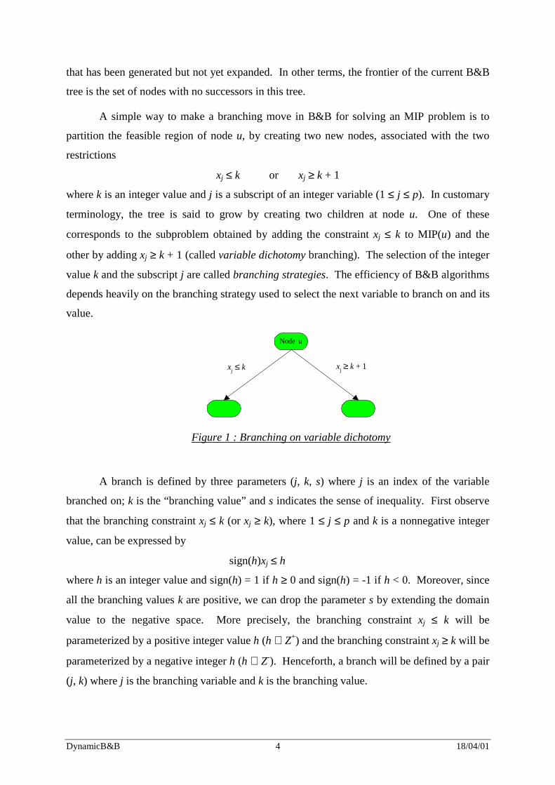
A simple way to make a branching move in B&B for solving an MIP problem is to
partition the feasible region of node u, by creating two new nodes, associated with the two
restrictions
xj ≤ k or xj ≥ k + 1
where k is an integer value and j is a subscript of an integer variable (1 ≤ j ≤ p). In customary
terminology, the tree is said to grow by creating two children at node u. One of these
corresponds to the subproblem obtained by adding the constraint xj ≤ k to MIP(u) and the
other by adding xj ≥ k + 1 (called variable dichotomy branching). The selection of the integer
value k and the subscript j are called branching strategies. The efficiency of B&B algorithms
depends heavily on the branching strategy used to select the next variable to branch on and its
value.
Node u
xj ≤ k xj ≥ k + 1
Figure 1 : Branching on variable dichotomy
A branch is defined by three parameters (j, k, s) where j is an index of the variable
branched on; k is the “branching value” and s indicates the sense of inequality. First observe
that the branching constraint xj ≤ k (or xj ≥ k), where 1 ≤ j ≤ p and k is a nonnegative integer
value, can be expressed by
sign(h)xj ≤ h
where h is an integer value and sign(h) = 1 if h ≥ 0 and sign(h) = -1 if h < 0. Moreover, since
all the branching values k are positive, we can drop the parameter s by extending the domain
value to the negative space. More precisely, the branching constraint xj ≤ k will be
parameterized by a positive integer value h (h ∈ Z+) and the branching constraint xj ≥ k will be
parameterized by a negative integer h (h ∈ Z-). Henceforth, a branch will be defined by a pair
(j, k) where j is the branching variable and k is the branching value.
DynamicB&B 5 18/04/01
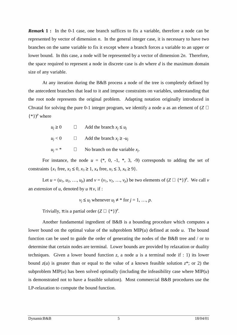
Remark 1 : In the 0-1 case, one branch suffices to fix a variable, therefore a node can be
represented by vector of dimension n. In the general integer case, it is necessary to have two
branches on the same variable to fix it except where a branch forces a variable to an upper or
lower bound. In this case, a node will be represented by a vector of dimension 2n. Therefore,
the space required to represent a node in discrete case is dn where d is the maximum domain
size of any variable.
At any iteration during the B&B process a node of the tree is completely defined by
the antecedent branches that lead to it and impose constraints on variables, understanding that
the root node represents the original problem. Adapting notation originally introduced in
Chvatal for solving the pure 0-1 integer program, we identify a node u as an element of (Z ∪
{*})p where
uj ≥ 0 ⇔ Add the branch xj ≤ uj
uj < 0 ⇔ Add the branch xj ≥ -uj
uj = * ⇔ No branch on the variable xj.
For instance, the node u = (*, 0, -1, *, 3, -9) corresponds to adding the set of
constraints {x1 free, x2 ≤ 0, x3 ≥ 1, x4 free, x5 ≤ 3, x6 ≥ 9}.
Let u = (u1, u2, …, up) and v = (v1, v2, …, vp) be two elements of (Z ∪ {*})p. We call v
an extension of u, denoted by u π v, if :
vj ≤ uj whenever uj ≠ * for j = 1, …, p.
Trivially, π is a partial order (Z ∪ {*})p.
Another fundamental ingredient of B&B is a bounding procedure which computes a
lower bound on the optimal value of the subproblem MIP(u) defined at node u. The bound
function can be used to guide the order of generating the nodes of the B&B tree and / or to
determine that certain nodes are terminal. Lower bounds are provided by relaxation or duality
techniques. Given a lower bound function z, a node u is a terminal node if : 1) its lower
bound z(u) is greater than or equal to the value of a known feasible solution z*; or 2) the
subproblem MIP(u) has been solved optimally (including the infeasibility case where MIP(u)
is demonstrated not to have a feasible solution). Most commercial B&B procedures use the
LP-relaxation to compute the bound function.
DynamicB&B 6 18/04/01
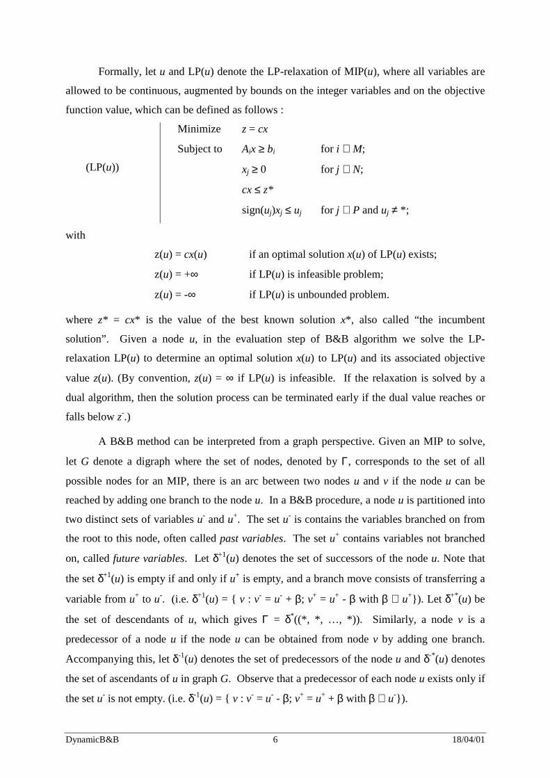
Formally, let u and LP(u) denote the LP-relaxation of MIP(u), where all variables are
allowed to be continuous, augmented by bounds on the integer variables and on the objective
function value, which can be defined as follows :
(LP(u))
Minimize z = cx
Subject to Aix ≥ bi for i ∈ M;
xj ≥ 0 for j ∈ N;
cx ≤ z*
sign(uj)xj ≤ uj for j ∈ P and uj ≠ *;
with
z(u) = cx(u) if an optimal solution x(u) of LP(u) exists;
z(u) = +∞ if LP(u) is infeasible problem;
z(u) = -∞ if LP(u) is unbounded problem.
where z* = cx* is the value of the best known solution x*, also called “the incumbent
solution”. Given a node u, in the evaluation step of B&B algorithm we solve the LP-
relaxation LP(u) to determine an optimal solution x(u) to LP(u) and its associated objective
value z(u). (By convention, z(u) = ∞ if LP(u) is infeasible. If the relaxation is solved by a
dual algorithm, then the solution process can be terminated early if the dual value reaches or
falls below z-.)
A B&B method can be interpreted from a graph perspective. Given an MIP to solve,
let G denote a digraph where the set of nodes, denoted by Γ, corresponds to the set of all
possible nodes for an MIP, there is an arc between two nodes u and v if the node u can be
reached by adding one branch to the node u. In a B&B procedure, a node u is partitioned into
two distinct sets of variables u- and u+. The set u- is contains the variables branched on from
the root to this node, often called past variables. The set u+ contains variables not branched
on, called future variables. Let δ+1(u) denotes the set of successors of the node u. Note that
the set δ+1(u) is empty if and only if u+ is empty, and a branch move consists of transferring a
variable from u+ to u-. (i.e. δ+1(u) = { v : v- = u- + β; v+ = u+ - β with β ∈ u+}). Let δ+*(u) be
the set of descendants of u, which gives Γ = δ*((*, *, …, *)). Similarly, a node v is a
predecessor of a node u if the node u can be obtained from node v by adding one branch.
Accompanying this, let δ-1(u) denotes the set of predecessors of the node u and δ-*(u) denotes
the set of ascendants of u in graph G. Observe that a predecessor of each node u exists only if
the set u- is not empty. (i.e. δ-1(u) = { v : v- = u- - β; v+ = u+ + β with β ∈ u-}).
DynamicB&B 7 18/04/01
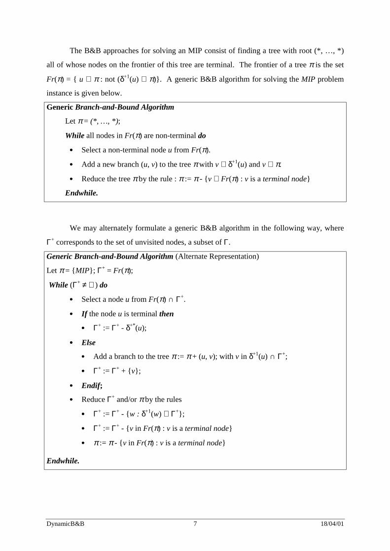
The B&B approaches for solving an MIP consist of finding a tree with root (*, …, *)
all of whose nodes on the frontier of this tree are terminal. The frontier of a tree π is the set
Fr(π) = { u ∈ π : not (δ+1(u) ⊆ π)}. A generic B&B algorithm for solving the MIP problem
instance is given below.
Generic Branch-and-Bound Algorithm
Let π = (*, …, *);
While all nodes in Fr(π) are non-terminal do
•••• Select a non-terminal node u from Fr(π).
•••• Add a new branch (u, v) to the tree π with v ∈ δ+1(u) and v ∉ π.
•••• Reduce the tree π by the rule : π := π - {v ∈ Fr(π) : v is a terminal node}
Endwhile.
We may alternately formulate a generic B&B algorithm in the following way, where
Γ+ corresponds to the set of unvisited nodes, a subset of Γ.
Generic Branch-and-Bound Algorithm (Alternate Representation)
Let π = {MIP}; Γ+ = Fr(π);
While (Γ+ ≠ ∅ ) do
•••• Select a node u from Fr(π) ∩ Γ+.
•••• If the node u is terminal then
•••• Γ+ := Γ+ - δ+*(u);
•••• Else
•••• Add a branch to the tree π := π + (u, v); with v in δ+1(u) ∩ Γ+;
•••• Γ+ := Γ+ + {v};
•••• Endif;
•••• Reduce Γ+ and/or π by the rules
•••• Γ+ := Γ+ - {w : δ+1(w) ⊆ Γ+};
•••• Γ+ := Γ+ - {v in Fr(π) : v is a terminal node}
•••• π := π - {v in Fr(π) : v is a terminal node}
Endwhile.
DynamicB&B 8 18/04/01
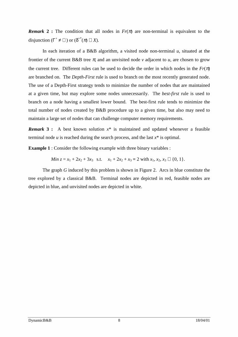
Remark 2 : The condition that all nodes in Fr(π) are non-terminal is equivalent to the
disjunction (Γ+ ≠ ∅ ) or (δ+*(π) ⊇ X).
In each iteration of a B&B algorithm, a visited node non-terminal u, situated at the
frontier of the current B&B tree π, and an unvisited node v adjacent to u, are chosen to grow
the current tree. Different rules can be used to decide the order in which nodes in the Fr(π)
are branched on. The Depth-First rule is used to branch on the most recently generated node.
The use of a Depth-First strategy tends to minimize the number of nodes that are maintained
at a given time, but may explore some nodes unnecessarily. The best-first rule is used to
branch on a node having a smallest lower bound. The best-first rule tends to minimize the
total number of nodes created by B&B procedure up to a given time, but also may need to
maintain a large set of nodes that can challenge computer memory requirements.
Remark 3 : A best known solution x* is maintained and updated whenever a feasible
terminal node u is reached during the search process, and the last x* is optimal.
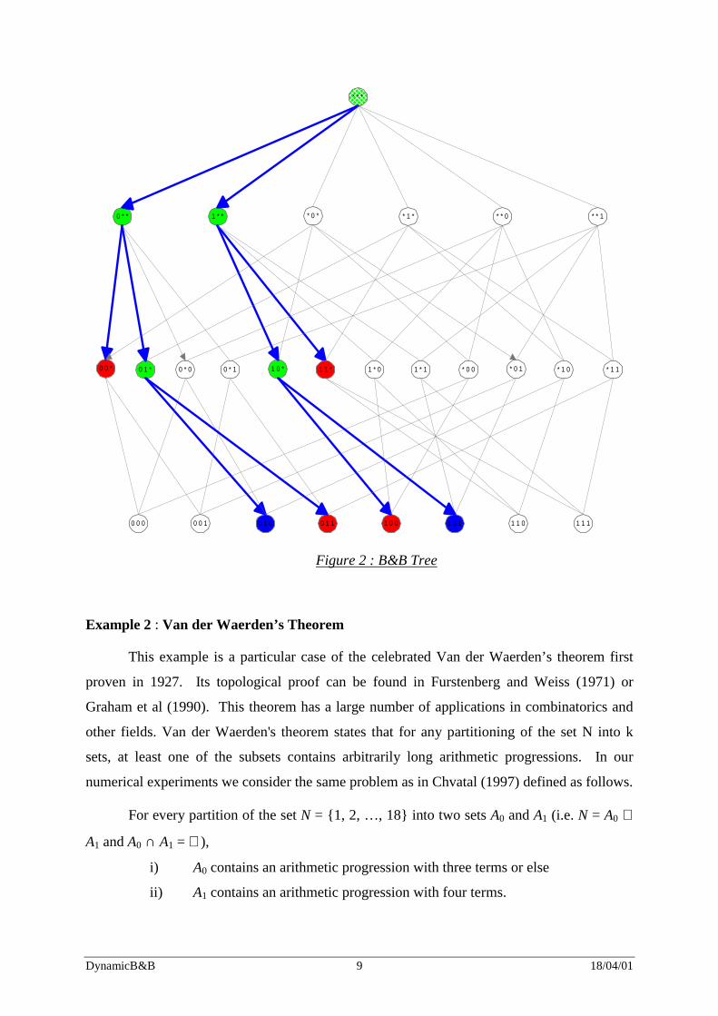
Example 1 : Consider the following example with three binary variables :
Min z = x1 + 2x2 + 3x3 s.t. x1 + 2x2 + x3 = 2 with x1, x2, x3 ∈ {0, 1}.
The graph G induced by this problem is shown in Figure 2. Arcs in blue constitute the
tree explored by a classical B&B. Terminal nodes are depicted in red, feasible nodes are
depicted in blue, and unvisited nodes are depicted in white.
DynamicB&B 9 18/04/01
0 0 0 0 0 1 0 1 0 0 1 1 1 0 0 1 0 1 1 1 0 1 1 1
0 0 * 0 1 * 1 0 * * 0 0
0 * * 1 * *
��
* * *
* * 1* * 0* 1 ** 0 *
* 1 1* 1 0* 0 11 * 11 * 01 1 *0 * 10 * 0
Figure 2 : B&B Tree
Example 2 : Van der Waerden’s Theorem
This example is a particular case of the celebrated Van der Waerden’s theorem first
proven in 1927. Its topological proof can be found in Furstenberg and Weiss (1971) or
Graham et al (1990). This theorem has a large number of applications in combinatorics and
other fields. Van der Waerden's theorem states that for any partitioning of the set N into k
sets, at least one of the subsets contains arbitrarily long arithmetic progressions. In our
numerical experiments we consider the same problem as in Chvatal (1997) defined as follows.
For every partition of the set N = {1, 2, …, 18} into two sets A0 and A1 (i.e. N = A0 ∪
A1 and A0 ∩ A1 = ∅ ),
i) A0 contains an arithmetic progression with three terms or else
ii) A1 contains an arithmetic progression with four terms.
DynamicB&B 10 18/04/01
Observe that a partition Ai, for i = 0,1 of N can be defined by a given a vector x in {0,
1}18 such that xj = i if and only if j ∈ Ai. Letting cx be an arbitrary objective function, a (0-1
IP) formulation of the Van der Waerden's theorem is as follows:
(0-1 IP)
Minimize z = cx
Subject to
xa + xa+d + xa+2d ≥ 1 ∀ a, d such that a + 2d ≤ 18,
xa + xa+d + xa+2d + xa+3d ≤ 3 ∀ a, d such that a + 3d ≤ 18,
x ∈ {0, 1}18
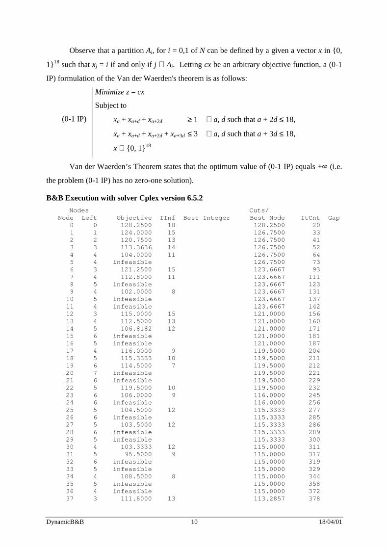
Van der Waerden’s Theorem states that the optimum value of (0-1 IP) equals +∞ (i.e.
the problem (0-1 IP) has no zero-one solution).
B&B Execution with solver Cplex version 6.5.2 Nodes Cuts/
Node Left Objective IInf Best Integer Best Node ItCnt Gap 0 0 128.2500 18 128.2500 20 1 1 124.0000 15 126.7500 33 2 2 120.7500 13 126.7500 41 3 3 113.3636 14 126.7500 52 4 4 104.0000 11 126.7500 64 5 4 infeasible 126.7500 73 6 3 121.2500 15 123.6667 93 7 4 112.8000 11 123.6667 111 8 5 infeasible 123.6667 123 9 4 102.0000 8 123.6667 131 10 5 infeasible 123.6667 137 11 4 infeasible 123.6667 142 12 3 115.0000 15 121.0000 156 13 4 112.5000 13 121.0000 160 14 5 106.8182 12 121.0000 171 15 6 infeasible 121.0000 181 16 5 infeasible 121.0000 187 17 4 116.0000 9 119.5000 204 18 5 115.3333 10 119.5000 211 19 6 114.5000 7 119.5000 212 20 7 infeasible 119.5000 221 21 6 infeasible 119.5000 229 22 5 119.5000 10 119.5000 232 23 6 106.0000 9 116.0000 245 24 6 infeasible 116.0000 256 25 5 104.5000 12 115.3333 277 26 6 infeasible 115.3333 285 27 5 103.5000 12 115.3333 286 28 6 infeasible 115.3333 289 29 5 infeasible 115.3333 300 30 4 103.3333 12 115.0000 311 31 5 95.5000 9 115.0000 317 32 6 infeasible 115.0000 319 33 5 infeasible 115.0000 329 34 4 108.5000 8 115.0000 344 35 5 infeasible 115.0000 358 36 4 infeasible 115.0000 372 37 3 111.8000 13 113.2857 378
DynamicB&B 11 18/04/01
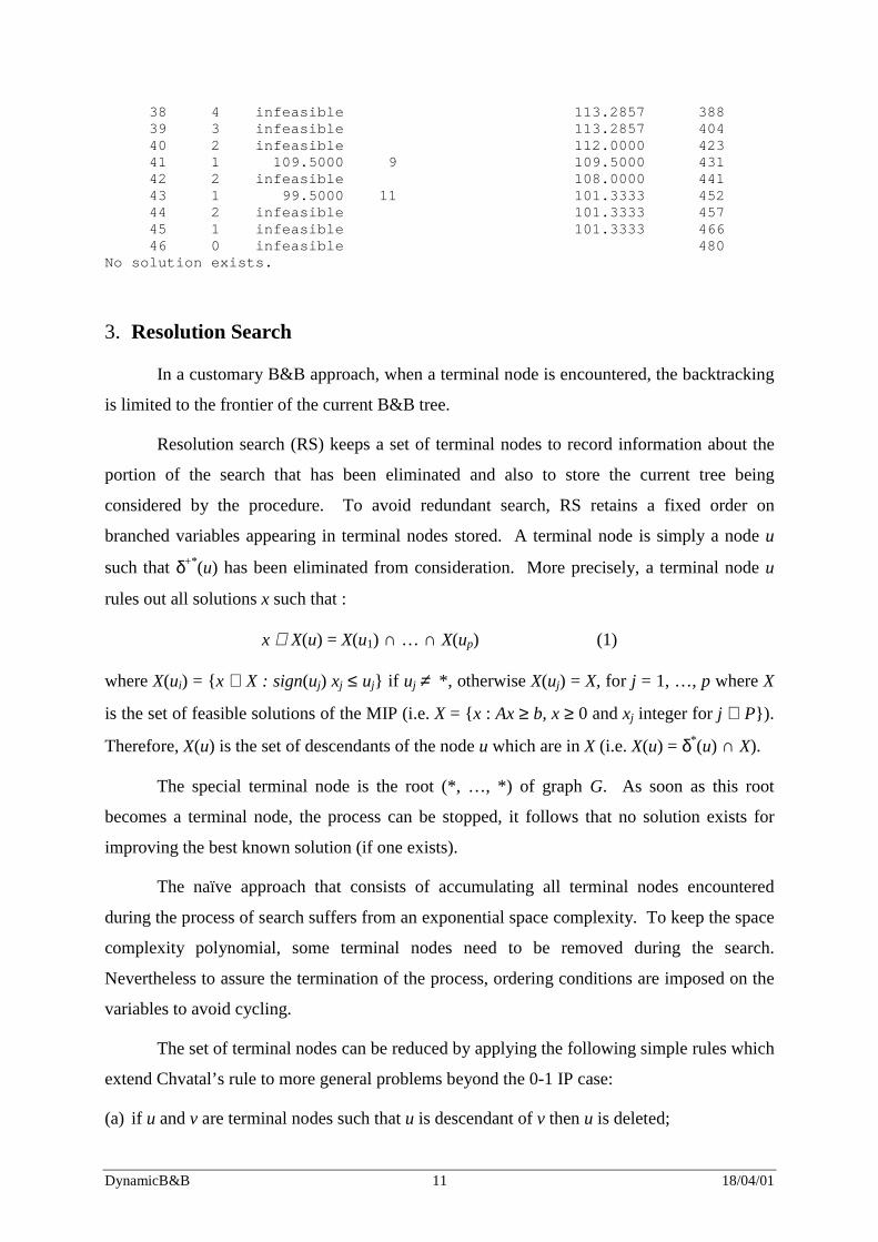
38 4 infeasible 113.2857 388 39 3 infeasible 113.2857 404 40 2 infeasible 112.0000 423 41 1 109.5000 9 109.5000 431 42 2 infeasible 108.0000 441 43 1 99.5000 11 101.3333 452 44 2 infeasible 101.3333 457 45 1 infeasible 101.3333 466 46 0 infeasible 480 No solution exists.
3. Resolution Search
In a customary B&B approach, when a terminal node is encountered, the backtracking
is limited to the frontier of the current B&B tree.
Resolution search (RS) keeps a set of terminal nodes to record information about the
portion of the search that has been eliminated and also to store the current tree being
considered by the procedure. To avoid redundant search, RS retains a fixed order on
branched variables appearing in terminal nodes stored. A terminal node is simply a node u
such that δ+*(u) has been eliminated from consideration. More precisely, a terminal node u
rules out all solutions x such that :
x ∉ X(u) = X(u1) ∩ … ∩ X(up) (1)
where X(ui) = {x ∈ X : sign(uj) xj ≤ uj} if uj ≠ *, otherwise X(uj) = X, for j = 1, …, p where X
is the set of feasible solutions of the MIP (i.e. X = {x : Ax ≥ b, x ≥ 0 and xj integer for j ∈ P}).
Therefore, X(u) is the set of descendants of the node u which are in X (i.e. X(u) = δ*(u) ∩ X).
The special terminal node is the root (*, …, *) of graph G. As soon as this root
becomes a terminal node, the process can be stopped, it follows that no solution exists for
improving the best known solution (if one exists).
The naïve approach that consists of accumulating all terminal nodes encountered
during the process of search suffers from an exponential space complexity. To keep the space
complexity polynomial, some terminal nodes need to be removed during the search.
Nevertheless to assure the termination of the process, ordering conditions are imposed on the
variables to avoid cycling.
The set of terminal nodes can be reduced by applying the following simple rules which
extend Chvatal’s rule to more general problems beyond the 0-1 IP case:
(a) if u and v are terminal nodes such that u is descendant of v then u is deleted;
DynamicB&B 12 18/04/01
(b) if u, v are terminal nodes such that u and v can be reached by a move that adds one branch
move from a node w then the node w replaces the nodes u and v.
In the following, we give an extension of Chvatal’s rule b) above.
3.1 Resolvent Operator
First observe that for any branching variable j associated with a given terminal node u
(i.e. uj ≠ *), the expression (1) is logically equivalent to
x ∈ X(u – {uj}) ⇒ x ∈ X( ju ) (2)
where ju is the complement of a uj defined by ju = - uj – 1 (by convention, we set ju = uj if
uj = *). Clearly There are many different ways of representing a given terminal node. This
provides freedom in the choice of the variable appearing in the conclusion of the implication
(2).
Different ways may be used to derive new terminal nodes. A simple approach consists
of generating a new terminal node from the current set of terminal nodes already visited. In
Chvatal, nodes u and v are called clashing if there is exactly one node w such that u and v are
children of w. The node w is called the resolvent of the clashing nodes u and v. Formally,
nodes u and v are clashing if there is exactly one subscript j such that
i) uj’ = vj’ for all j’ ≠ j;
ii) uj ≠ * and vj ≠ *;
iii) {xj : sign(uj)xj ≤ uj } ∪ {xj : sign(vj)xj ≤ vj } = Z.
It is easy to see that the last condition iii) can be expressed as
iii’) uj + vj + 1 = 0.
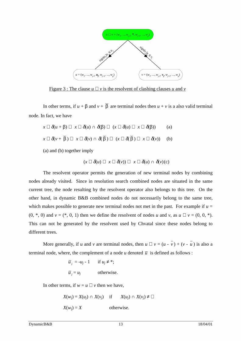
The resolvent of clashing clauses u and v, denoted by u ∇ v = w, is defined by wj’ = uj’
for all j’ ≠ j; and uj = *, where uj + vj + 1 ≥ 0 and uj ≠ * ≠ vj.
DynamicB&B 13 18/04/01
sign(u j)x
j ≤ u j
u = (w1, ..., wj-1, uj, wj+1, ..., wp) v = (w1, ..., wj-1, vj, wj+1, ..., wp)
u ∇ v = (w1, ..., wj-1, *, wj+1, ..., wp)
sign(vj )x
j ≤ vj
Figure 3 : The clause u ∇ v is the resolvent of clashing clauses u and v
In other terms, if u + β and v + β are terminal nodes then u + v is a also valid terminal
node. In fact, we have
x ∉ δ(u + β) ⇔ x ∉ δ(u) ∩ δ(β) ⇔ (x ∉ δ(u) ⇒ x ∈ δ(β)) (a)
x ∉ δ(v + β ) ⇔ x ∉ δ(v) ∩ δ( β ) ⇔ (x ∉ δ( β ) ⇒ x ∈ δ(v)) (b)
(a) and (b) together imply
(x ∉ δ(u) ⇒ x ∈ δ(v)) ⇔ x ∉ δ(u) ∩ δ(v) (c)
The resolvent operator permits the generation of new terminal nodes by combining
nodes already visited. Since in resolution search combined nodes are situated in the same
current tree, the node resulting by the resolvent operator also belongs to this tree. On the
other hand, in dynamic B&B combined nodes do not necessarily belong to the same tree,
which makes possible to generate new terminal nodes not met in the past. For example if u =
(0, *, 0) and v = (*, 0, 1) then we define the resolvent of nodes u and v, as u ∇ v = (0, 0, *).
This can not be generated by the resolvent used by Chvatal since these nodes belong to
different trees.
More generally, if u and v are terminal nodes, then u ∇ v = (u - v ) + (v - u ) is also a
terminal node, where, the complement of a node u denoted u is defined as follows :
ju = -uj - 1 if uj ≠ *;
ju = uj otherwise.
In other terms, if w = u ∇ v then we have,
X(wj) = X(uj) ∩ X(vj) if X(uj) ∩ X(vj) ≠ ∅
X(wj) = X otherwise.
DynamicB&B 14 18/04/01
Remark 4 : The resolvent operator is also used in classical B&B approaches by combining
nodes situated in the same current tree. In fact, in these approaches the operator is
particularly used to reduce the space needed to represent the current B&B tree.
3.2 The Obstacle Function and Its Extension
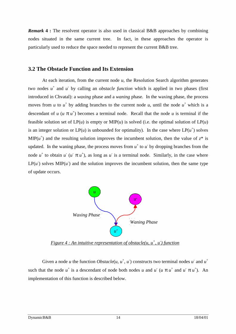
At each iteration, from the current node u, the Resolution Search algorithm generates
two nodes u+ and u- by calling an obstacle function which is applied in two phases (first
introduced in Chvatal): a waxing phase and a waning phase. In the waxing phase, the process
moves from u to u+ by adding branches to the current node u, until the node u+ which is a
descendant of u (u π u+) becomes a terminal node. Recall that the node u is terminal if the
feasible solution set of LP(u) is empty or MIP(u) is solved (i.e. the optimal solution of LP(u)
is an integer solution or LP(u) is unbounded for optimality). In the case where LP(u+) solves
MIP(u+) and the resulting solution improves the incumbent solution, then the value of z* is
updated. In the waning phase, the process moves from u+ to u- by dropping branches from the
node u+ to obtain u- (u- π u+), as long as u- is a terminal node. Similarly, in the case where
LP(u-) solves MIP(u-) and the solution improves the incumbent solution, then the same type
of update occurs.
u-
u+
u
Waxing PhaseWaning Phase
Figure 4 : An intuitive representation of obstacle(u, u+, u-) function
Given a node u the function Obstacle(u, u+, u-) constructs two terminal nodes u- and u+
such that the node u+ is a descendant of node both nodes u and u- (u π u+ and u- π u+). An
implementation of this function is described below.
DynamicB&B 15 18/04/01
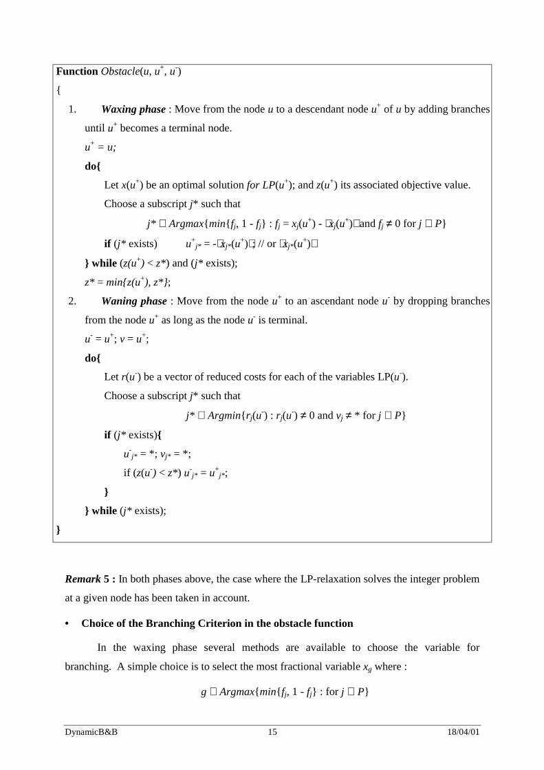
Function Obstacle(u, u+, u-)
{
1. Waxing phase : Move from the node u to a descendant node u+ of u by adding branches
until u+ becomes a terminal node.
u+ = u;
do{
Let x(u+) be an optimal solution for LP(u+); and z(u+) its associated objective value.
Choose a subscript j* such that
j* ∈ Argmax{min{fj, 1 - fj} : fj = xj(u+) - xj(u+) and fj ≠ 0 for j ∈ P}
if (j* exists) u+j* = -xj*(u+) ; // or xj*(u+)
} while (z(u+) < z*) and (j* exists);
z* = min{z(u+), z*};
2. Waning phase : Move from the node u+ to an ascendant node u- by dropping branches
from the node u+ as long as the node u- is terminal.
u- = u+; v = u+;
do{
Let r(u-) be a vector of reduced costs for each of the variables LP(u-).
Choose a subscript j* such that
j* ∈ Argmin{rj(u-) : rj(u-) ≠ 0 and vj ≠ * for j ∈ P}
if (j* exists){
u-j* = *; vj* = *;
if (z(u-) < z*) u-j* = u+
j*;
}
} while (j* exists);
}
Remark 5 : In both phases above, the case where the LP-relaxation solves the integer problem
at a given node has been taken in account.
• Choice of the Branching Criterion in the obstacle function
In the waxing phase several methods are available to choose the variable for
branching. A simple choice is to select the most fractional variable xg where :
g ∈ Argmax{min{fj, 1 - fj} : for j ∈ P}
DynamicB&B 16 18/04/01
and where fj = xj - xj is the associated fractional value. Other rules are based on the idea of
estimating the cost of forcing the variable xj to become integer.
In the waning phase branches are dropped (which frees some of the variables)
according to rules based on identifying influential choices in retrospect, at the point where
backtracking would occur (see Section 4).
Remark 6 : The waning phase and the waxing phase can be accelerated by saving some calls
of the Oracle function. This can be accomplished by adding (or dropping) more than one
branch at each iteration in the waning phase (or waxing phase).
3.3 Family Updating to Assure Convergence
Trivially, since each terminal node eliminates a portion of the search space from
consideration, the naive approach that maintains all terminal nodes visited during the process
of search will terminate if the search space is bounded. However, the approach that removes
terminal nodes during the search may not assure the convergence of the process. Therefore,
to assure the termination when terminal nodes are removed, Chvatal’s resolution search
imposes a total order on the variables branched on. More precisely, for pure 0-1 IP problems
with n-dimensional vectors, Chvatal maintains a set of terminal nodes of at most n nodes,
called a path-like family. At each iteration, a new terminal node is generated so that the
portion of the search space eliminated by this node includes the portions that were eliminated
by the terminal nodes that are removed from the path-like family. Consequently the size of
the eliminated search space increases monotonically which assures the convergence of
resolution search.
The path-like Family of Chvatal (1997) can be easily extended to the MIP setting. The
members of the path-like family F are enumerated as (ui, βi) for i=1, …,|F|, where ui is a
terminal node and βi is a branch appearing in the node ui such that
• the branch βj appears in ui if and only if i = j,
• if the branch jβ the complement of βj appears in ui then i > j,
• if a branch β appears in ui and its complement β appears in uj then β = βi or β = βj.
With each path-like family F we associate the node u(F) defined as follows
DynamicB&B 17 18/04/01
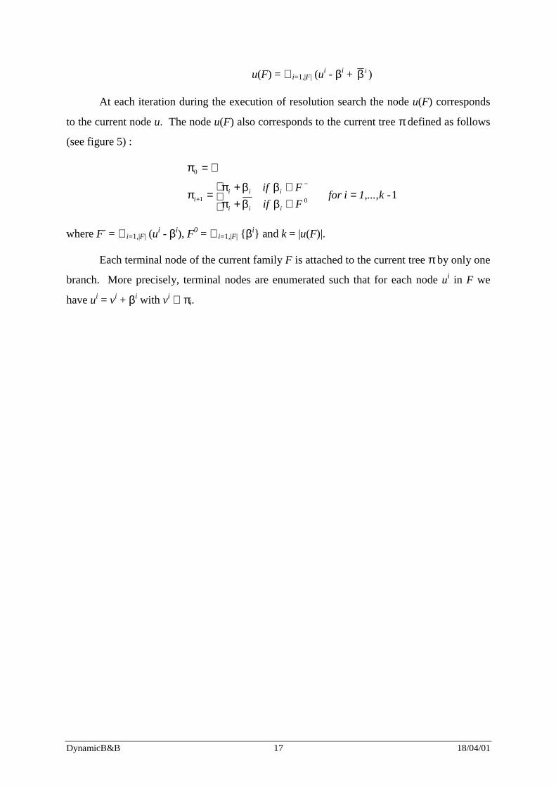
u(F) = ∪ i=1,|F| (ui - βi + iβ )
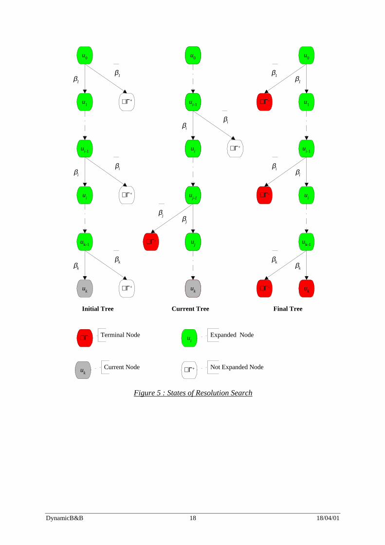
At each iteration during the execution of resolution search the node u(F) corresponds
to the current node u. The node u(F) also corresponds to the current tree π defined as follows
(see figure 5) :
101
0
-k1,...,i forF ifF if
iii
iiii =
∈ββ+π∈ββ+π
=π
∅=π−
+
where F- = ∪ i=1,|F| (ui - βi), F0 = ∪ i=1,|F| {βi} and k = |u(F)|.
Each terminal node of the current family F is attached to the current tree π by only one
branch. More precisely, terminal nodes are enumerated such that for each node ui in F we
have ui = vi + βi with vi ⊆ πi.
DynamicB&B 18 18/04/01
∈Γ -
∈Γ +
ui
uk
Terminal Node Expanded Node
Current Node Not Expanded Node
u0
β1
u1
β1
∈Γ +
uk-1
βk
uk
βk
∈Γ +
ui
ui-1
βiβi
∈Γ +
Initial Tree Current Tree
u0
u1
uk-1
uk
ui
ui-1
βj
∈Γ -
u0
βi
ui-1
∈Γ +
uj
uk
uj-1
ui
βi
βj
u0
u1
β1
uk-1
uk
βk
ui
ui-1
βi
β1
∈Γ -
βi
∈Γ -
βk
∈Γ -
Final Tree
Figure 5 : States of Resolution Search
DynamicB&B 19 18/04/01
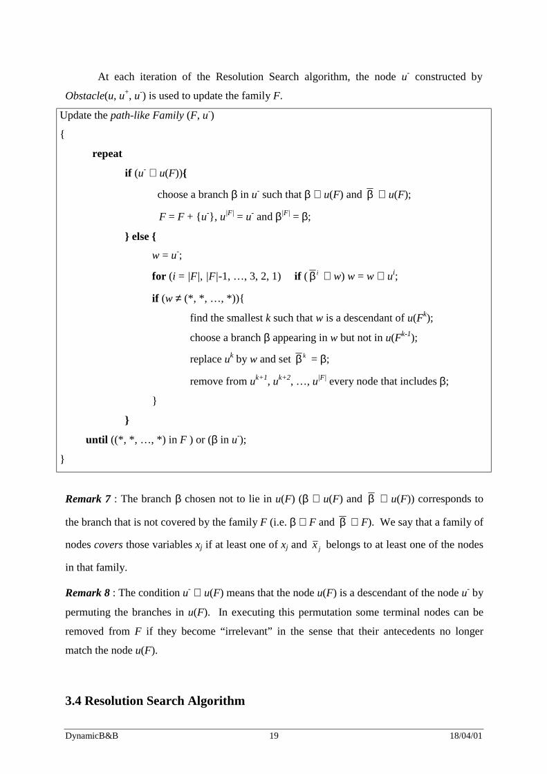
At each iteration of the Resolution Search algorithm, the node u- constructed by
Obstacle(u, u+, u-) is used to update the family F.
Update the path-like Family (F, u-)
{
repeat
if (u- ⊄ u(F)){
choose a branch β in u- such that β ∉ u(F) and β ∉ u(F);
F = F + {u-}, u|F| = u- and β|F| = β;
} else {
w = u-;
for (i = |F|, |F|-1, …, 3, 2, 1) if ( iβ ∈ w) w = w ∇ ui;
if (w ≠ (*, *, …, *)){
find the smallest k such that w is a descendant of u(Fk);
choose a branch β appearing in w but not in u(Fk-1);
replace uk by w and set kβ = β;
remove from uk+1, uk+2, …, u|F| every node that includes β;
}
}
until ((*, *, …, *) in F ) or (β in u-);
}
Remark 7 : The branch β chosen not to lie in u(F) (β ∉ u(F) and β ∉ u(F)) corresponds to
the branch that is not covered by the family F (i.e. β ∉ F and β ∉ F). We say that a family of
nodes covers those variables xj if at least one of xj and jx belongs to at least one of the nodes
in that family.
Remark 8 : The condition u- ⊆ u(F) means that the node u(F) is a descendant of the node u- by
permuting the branches in u(F). In executing this permutation some terminal nodes can be
removed from F if they become “irrelevant” in the sense that their antecedents no longer
match the node u(F).
3.4 Resolution Search Algorithm
DynamicB&B 20 18/04/01
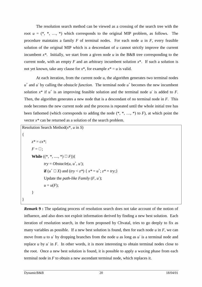
The resolution search method can be viewed as a crossing of the search tree with the
root u = (*, *, …, *) which corresponds to the original MIP problem, as follows. The
procedure maintains a family F of terminal nodes. For each node u in F, every feasible
solution of the original MIP which is a descendant of u cannot strictly improve the current
incumbent x*. Initially, we start from a given node u in the B&B tree corresponding to the
current node, with an empty F and an arbitrary incumbent solution x*. If such a solution is
not yet known, take any clause for x*, for example x* = u is valid.
At each iteration, from the current node u, the algorithm generates two terminal nodes
u+ and u- by calling the obstacle function. The terminal node u+ becomes the new incumbent
solution x* if u+ is an improving feasible solution and the terminal node u- is added to F.
Then, the algorithm generates a new node that is a descendant of no terminal node in F. This
node becomes the new current node and the process is repeated until the whole initial tree has
been fathomed (which corresponds to adding the node (*, *, …, *) to F), at which point the
vector x* can be returned as a solution of the search problem.
Resolution Search Method(x*, u in S)
{
z* = cx*;
F = ∅ ;
While ((*, *, ...., *) ∉ F)){
try = Obstacle(u, u+, u-);
if (u+ ∈ X) and (try < z*) { x* = u+; z* = try;}
Update the path-like Family (F, u-);
u = u(F);
}
}
Remark 9 : The updating process of resolution search does not take account of the notion of
influence, and also does not exploit information derived by finding a new best solution. Each
iteration of resolution search, in the form proposed by Chvatal, tries to go deeply to fix as
many variables as possible. If a new best solution is found, then for each node u in F, we can
move from u to u- by dropping branches from the node u as long as u- is a terminal node and
replace u by u- in F. In other words, it is more interesting to obtain terminal nodes close to
the root. Once a new best solution is found, it is possible to apply a waxing phase from each
terminal node in F to obtain a new ascendant terminal node, which replaces it.
DynamicB&B 21 18/04/01
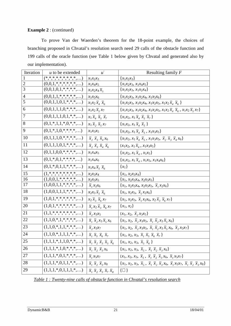
Example 2 : (continued)
To prove Van der Waerden’s theorem for the 18-point example, the choices of
branching proposed in Chvatal’s resolution search need 29 calls of the obstacle function and
199 calls of the oracle function (see Table 1 below given by Chvatal and generated also by
our implementation).
Iteration u to be extended u- Resulting family F 1 (*,*,*,*,*,*,*,*,*,…) x1x2x3 {x1x2x3} 2 (0,0,1,*,*,*,*,*,*,…) x1x4x5 {x1x2x3, x1x4x5} 3 (0,0,1,0,1,*,*,*,*,…) x1x2x4 5x {x1x2x3, x1x2x4} 4 (0,0,1,1,*,*,*,*,*,…) x1x5x6 {x1x2x3, x1x2x4, x1x5x6} 5 (0,0,1,1,0,1,*,*,*,…) x1x2 4x 6x {x1x2x3, x1x2x4, x1x2x5, x1x2 4x 6x } 6 (0,0,1,1,1,0,*,*,*,…) x1x2 5x x7 {x1x2x3, x1x2x4, x1x2x5, x1x2 4x 6x , x1x2 5x x7} 7 (0,0,1,1,1,0,1,*,*,…) x1 4x 5x 7x {x1x2, x1 4x 5x 7x } 8 (0,1,*,1,1,*,0,*,*,…) x1 2x 5x x7 {x1x2, x1 4x 5x } 9 (0,1,*,1,0,*,*,*,*,…) x1x3x5 {x1x2, x1 4x 5x , x1x3x5} 10 (0,1,1,1,0,*,*,*,*,…) 2x 3x 4x x6 {x1x2, x1 4x 5x , x1x3x5, 2x 3x 4x x6} 11 (0,1,1,1,0,1,*,*,*,…) 2x 3x 4x 6x {x1x2, x1 4x , x1x3x5} 12 (0,1,1,0,0,*,*,*,*,…) x1x4x5 {x1x2, x1 4x , x1x5} 13 (0,1,*,0,1,*,*,*,*,…) x1x4x6 {x1x2, x1 4x , x1x5, x1x4x6} 14 (0,1,*,0,1,1,*,*,*,…) x1x4 5x 6x {x1} 15 (1,*,*,*,*,*,*,*,*,…) x2x3x4 {x1, x2x3x4} 16 (1,0,0,1,*,*,*,*,*,…) x2x3x5 {x1, x2x3x4, x2x3x5} 17 (1,0,0,1,1,*,*,*,*,…) 1x x2x6 {x1, x2x3x4, x2x3x5, 1x x2x6} 18 (1,0,0,1,1,1,*,*,*,…) x2x3 5x 6x {x1, x2x3, 1x x2x6} 19 (1,0,1,*,*,*,*,*,*,…) x2 3x 6x x7 {x1, x2x3, 1x x2x6, x2 3x 6x x7} 20 (1,0,1,*,*,*,*,*,*,…) 1x x2 3x 6x x7 {x1, x2} 21 (1,1,*,*,*,*,*,*,*,…) 2x x3x5 {x1, x2, 2x x3x5} 22 (1,1,0,*,1,*,*,*,*,…) 1x 2x x3 5x x6 {x1, x2, 2x x3x5, 1x 2x x3 5x x6} 23 (1,1,0,*,1,1,*,*,*,…) 2x x3x7 {x1, x2, 2x x3x5, 1x 2x x3 5x x6, 2x x3x7} 24 (1,1,0,*,1,1,1,*,*,…) 1x 5x 6x 7x {x1, x2, x3, 1x 5x 6x 7x } 25 (1,1,1,*,1,1,0,*,*,…) 1x 2x 3x 5x 6x {x1, x2, x3, 5x 6x } 26 (1,1,1,*,1,0,*,*,*,…) 1x 2x 3x x6 {x1, x2, x3, 5x , 1x 2x 3x x6} 27 (1,1,1,*,0,1,*,*,*,…) 1x x5x7 {x1, x2, x3, 5x , 1x 2x 3x x6, 1x x5x7} 28 (1,1,1,*,0,1,1,*,*,…) 1x 2x 3x x8 {x1, x2, x3, 5x , 1x 2x 3x x6, 1x x5x7, 1x 2x 3x x8} 29 (1,1,1,*,0,1,1,1,*,…) 1x 2x 3x 7x 8x {∅ }
Table 1 : Twenty-nine calls of obstacle function in Chvatal’s resolution search
DynamicB&B 22 18/04/01
4. Dynamic Branch-and-Bound
In the customary B&B approach branching decisions are generally based on very
limited information about the likelihood that a particular branch will lead to an optimal
solution. This information is especially pronounced at early stages of the branch and bound
tree. Moreover, even 'reasonable' choices can be extremely poor if they are not sufficiently
influential to reduce the alternatives for other variables. Unless a current branch has the
power to inhibit the range of remaining alternatives, the branch and bound process can
degenerate into the disastrous approximation to total enumeration sometimes observed. So, it
seems worthwhile to consider a branching technique that has the ability to rid itself of certain
types of uninfluential branches on the basis of more reliable information available at later
stages. A chief component of this technique is to shrink the branch and bound tree by
eliminating earlier branches that have been rendered conditionally superfluous by subsequent
decisions.
The theme of Dynamic B&B (Glover and Tangedahl, 1976) introduces a strategy that
modifies the sequence of decisions in B&B by:
(1) Discarding certain earlier branches as the process continues, thereby shrinking the
B&B tree.
(2) Allowing for branches to be reversed based on the solution state created by the other
currently imposed branches.
(3) Resequencing certain branches, according to rules based on identifying "influential
choices" in retrospect, at the point where backtracking would occur (since the
influence of branches can be identified more clearly when they are accompanied by
other branch choices - as generally occurs at backtracking points - than when they may
first be selected as branches). The goal is to maintain the most influential branches
earlier in the tree by moving less influential branches to the end.
Component (3) is the one that includes the basic idea of Chvatal's Resolution Search,
although introduced in a proposal that appears somewhat earlier. The notion of an influential
branch, identified in retrospect, is critical. It is a conditional concept, that depends on other
branches currently imposed, and embodies the idea of limiting the possibilities that exist for
remaining choices. (It is related to the idea of a "strong cut", for example.)
DynamicB&B 23 18/04/01
Remark 10 : Solving an MIP by this design consists of finding a tree with root (*, …, *) in
its associated graph G such that all the nodes in the frontier of this tree are terminal nodes.
Dynamic Branch-and-Bound and resolution search take advantage of the search space being a
graph rather than a tree, in contrast to the approach of classical B&B.
Generic Dynamic Branch-and-Bound Algorithm
Let the current tree π = (*, …, *);
While all node in Fr(π) are not terminal do
•••• Select an unvisited terminal node u from Γ.
•••• If the node u is a descendant of π, add branches to π such that u will be in Fr(π).
•••• Else change the tree π into a new tree one covering the node u.
Endwhile.
We may express the algorithm in greater detail as follows, where Γ- corresponds to the
set of visited nodes, a subset of Γ.
Generic Dynamic Branch-and-Bound Algorithm (Detailed Form)
• π = Any tree, Γ- = Interior(π); Γ+ = Γ - Γ-;
• let Γ- = ∅ , Γ+ = Γ;
• while (Γ- ≠ Γ) and (Γ+ ≠ ∅ ) and (x ∉ X*) do
•••• Select a node u from Fr(π) ∩ Γ+.
•••• If u is not terminal then
•••• Add a branch to the tree π:= π + (u, v); with v in δ+1(u) ∩ Γ+;
•••• Γ+ := Γ+ + {v};
•••• Reduce Γ+ and/or π by the rules
•••• Γ+ := Γ+ - {w} if δ+1(w) ⊆ Γ+;
•••• Γ+ := Γ+ - {v ∈ Fr(π) : v is a terminal node}
•••• π := π - {v ∈ Fr(π) : v is a terminal node}
•••• Else
•••• Γ- := Γ- + δ+*(u);
•••• Update Γ- and/or Tree by the rules
•••• Γ- := Γ- - δ+1(w) + {w} if δ+1(w) ⊆ Γ-;
DynamicB&B 24 18/04/01
•••• Change a new tree from the current state such that Γ- increases or Γ+ decreases.
•••• Reduce Γ+ and/or π by the rules
•••• Drop a branch of the tree π := π - (u, v); with v in δ-1(u) ∩ Γ+;
•••• π:= π - {v ∈ Fr(π) : v is a terminal node}
Endwhile.
Influence can be measured also in terms of the effect on the objective function, as by
the values of updated objective function coefficients for slack variables associated with
branches.
i) currently uninfluential : The branching constraint xj ≤ vj (or xj ≥ vj), where j ∈ P and
vj is an integer value, will be called currently uninfluential if the constraint does not
affect the optimality of the current LP solution. For example, if xj receives the value
vj in the current LP solution, then clearly the branching constraint does not affect LP
optimality.
ii) highly influential : A branch qualifies as be highly influential when it creates an
immediate infeasibility or a bound violation when it is reversed. (By keeping a
constraint that compels the objective function to improve at each step, the
infeasibility criterion includes the bound violation criterion.)
iii) more (or less) influential : The branch xj ≥ vj is more (or less) influential than the
branch xk ≥ vk if upon introducing their branching slacks sj = xj - vj ≥ 0 and sk = xk -
vk ≥ 0 (using substitution to replace xj by sj + vj and to replace xk by sk + vk), and
optimizing the LP problem, the objective function coefficient of sj in the optimal LP
tableau is larger (smaller) than the one of sk.
iv) A branch whose alternative has been eliminated by fathoming or by examination
(i.e. by a tree search that exhausts all relevant solution possibilities on the branch)
will be called a compulsory branch. (Note : a highly influential branch is a special
case of a compulsory branch.)
Remark 11 : Emulating strategies applied in tabu search (Glover and Laguna, 1997), it can
be judicious to keep historical records of influence and evaluations of branching alternatives
to supplement the decision process.
When the concept of influence is applied in retrospect as a basis for resequencing the
choices, as in (3), with the goal of maintaining the most influential branches earlier in the tree,
DynamicB&B 25 18/04/01
then the most extreme case is where one of the current branches will violate feasibility if it is
moved to the end of the sequence and reversed. That means that the collection of preceding
branches is so influential that the branch moved to the end cannot be changed - hence, by the
rules of B&B, such a branch at the end of the tree can be dropped. Also, more generally, this
retrospective analysis gives strategies for moving branches to the end even when the extreme
case just described does not occur. That is, even if infeasibility will not occur by a reversal, it
is still possible to identify which branches will come closest to violating feasibility when
moved to the end, and therefore one of these will indeed be the one chosen for this relocation.
The shrinking operation in a sense is a special case of the resequencing - if the
operation is postponed until a backtracking step occurs - but it can be done more efficiently
because it isn't necessary to reverse the branch to discover that it can be dropped by an
additional backtrack step.
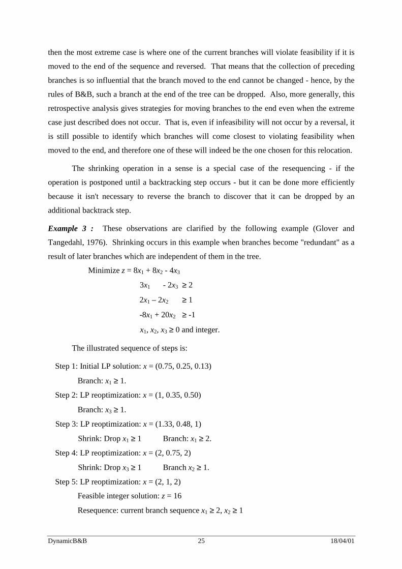
Example 3 : These observations are clarified by the following example (Glover and
Tangedahl, 1976). Shrinking occurs in this example when branches become "redundant" as a
result of later branches which are independent of them in the tree.
Minimize z = 8x1 + 8x2 - 4x3
3x1 - 2x3 ≥ 2
2x1 – 2x2 ≥ 1
-8x1 + 20x2 ≥ -1
x1, x2, x3 ≥ 0 and integer.
The illustrated sequence of steps is:
Step 1: Initial LP solution: x = (0.75, 0.25, 0.13)
Branch: x1 ≥ 1.
Step 2: LP reoptimization: x = (1, 0.35, 0.50)
Branch: x3 ≥ 1.
Step 3: LP reoptimization: x = (1.33, 0.48, 1)
Shrink: Drop x1 ≥ 1 Branch: x1 ≥ 2.
Step 4: LP reoptimization: x = (2, 0.75, 2)
Shrink: Drop x3 ≥ 1 Branch x2 ≥ 1.
Step 5: LP reoptimization: x = (2, 1, 2)
Feasible integer solution: z = 16
Resequence: current branch sequence x1 ≥ 2, x2 ≥ 1
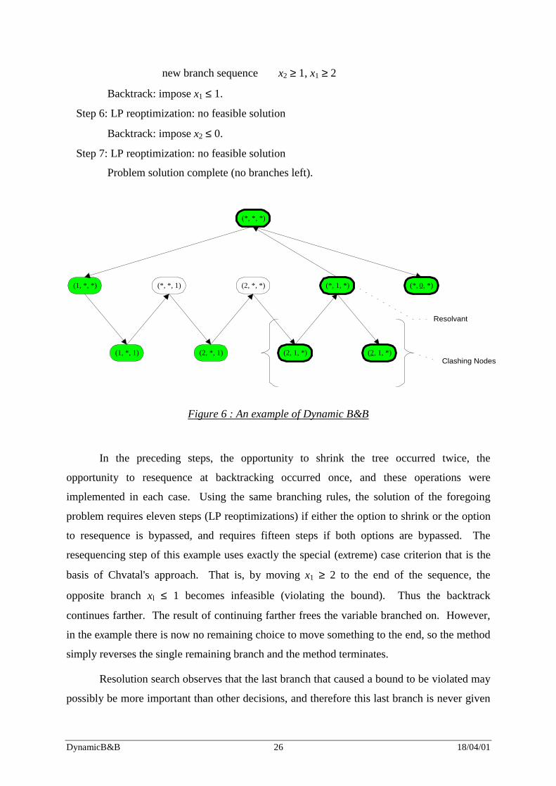
DynamicB&B 26 18/04/01
new branch sequence x2 ≥ 1, x1 ≥ 2
Backtrack: impose x1 ≤ 1.
Step 6: LP reoptimization: no feasible solution
Backtrack: impose x2 ≤ 0.
Step 7: LP reoptimization: no feasible solution
Problem solution complete (no branches left).
(*, *, 1)
(2, 1, *)(2, *, 1)(1, *, 1)
(*, *, *)
(*, 0, *)(*, 1, *)(2, *, *)(1, *, *)
(2, 1, *)Clashing Nodes
Resolvant
Figure 6 : An example of Dynamic B&B
In the preceding steps, the opportunity to shrink the tree occurred twice, the
opportunity to resequence at backtracking occurred once, and these operations were
implemented in each case. Using the same branching rules, the solution of the foregoing
problem requires eleven steps (LP reoptimizations) if either the option to shrink or the option
to resequence is bypassed, and requires fifteen steps if both options are bypassed. The
resequencing step of this example uses exactly the special (extreme) case criterion that is the
basis of Chvatal's approach. That is, by moving x1 ≥ 2 to the end of the sequence, the
opposite branch xl ≤ 1 becomes infeasible (violating the bound). Thus the backtrack
continues farther. The result of continuing farther frees the variable branched on. However,
in the example there is now no remaining choice to move something to the end, so the method
simply reverses the single remaining branch and the method terminates.
Resolution search observes that the last branch that caused a bound to be violated may
possibly be more important than other decisions, and therefore this last branch is never given
DynamicB&B 27 18/04/01
a lower priority than other branches. That is, the approach incorporates a partial
approximation of the idea of influence (without using that term).
In the numerical example the backtracking occurs not because an objective function
bound was violated by the last branch, but rather because the last branch led to a new best
solution (with z = 16). When the objective function constraint associated with this solution is
imposed (z ≤ 15), the current LP becomes infeasible, and hence backtracking results, but there
is no reason to assume the last branch is the one that is most important. For example, in the
illustration given, the choice sequence that led to this solution could easily have been x2 ≥ 1
followed by x1 ≥ 2. Then, if the last branch was maintained as "primary", Chvatal's rule
would free the x2 branch and then impose x1 ≤ 1. But this choice would be inferior to the one
identified in the example. That is, the branch x2 ≥ 1 is decidedly more influential than the
branch x1 ≥ 2, keeping in mind that we will be dropping one of the branches and reversing the
other. (The example does not identify the source of information that discloses which branch
is more influential, but this knowledge, however obtained, is the reason for the resequencing
step that moves the less influential branch x1 ≥ 2 to the end of the sequence. In other words,
according to Chvatal’s terminology, an "Oracle" is used to identify when the property is
present.)
The preceding illustration shows that the concept of influence can be more effective
for resequencing branches than the approach used in Resolution Search, for two reasons:
(1) Resolution Search gives no rule for the case when backtracking may occur as a
result of finding a new best solution (where potential impact on the decision
process can be significant).
(2) Resolution Search can also miss opportunities to make advantageous decisions in
other cases, as demonstrated by the example just given where the bound z ≤ 15
might have been pre-established. Then the sequence x2 ≥ l, x1 ≥ 2 could have been
the one that was discovered to violate this bound.
In short, the resequencing mechanism of Dynamic B&B gives the options proposed in
Resolution Search, and also gives additional strategic possibilities. These observations
motivate a more thorough examination of the practical potential of the Dynamic B&B
approach, which has remained largely unexplored to date.

DynamicB&B 28 18/04/01
Remark 12 : To prove Van der Waerden’s theorem, the extension of resolution search that
results by using influential information, as in Dynamic B&B, needs only 2 calls of the
obstacle function and 11 calls of the oracle function.
Acknowledgements:
We would like to thank the anonymous referees for their detailed comments and
suggestions which improved this paper.
References: [1] V. Chvatal. "Resolution Search", Discrete Applied Mathematics, 73, 81-99, 1997.
[2] F. Glover and L. Tangedahl. "Dynamic Strategies for Branch and Bound", Omega, 4, 571-
576, 1976.
[3] F. Glover and M.Laguna, "Tabu Search", Kluwer Academic Publishers, 1997.
[4] R. L. Graham, B. L. Rothschild and J. H. Spencer, “Ramsey Theory”, 2nd ed., Wiley, 1990.
[5] B.L. van der Waerden, “How the proof of Baudet’s conjecture was found”, In: Studies in
Pure Mathematics (Presented to Richard Rado), pp. 251-260. Academic Press, London,
1971.