pls regression methods & extended...
TRANSCRIPT

1
PLS regression methods & extended tools
Philippe BastienL’Oreal Research, Clichy, France ([email protected])
2
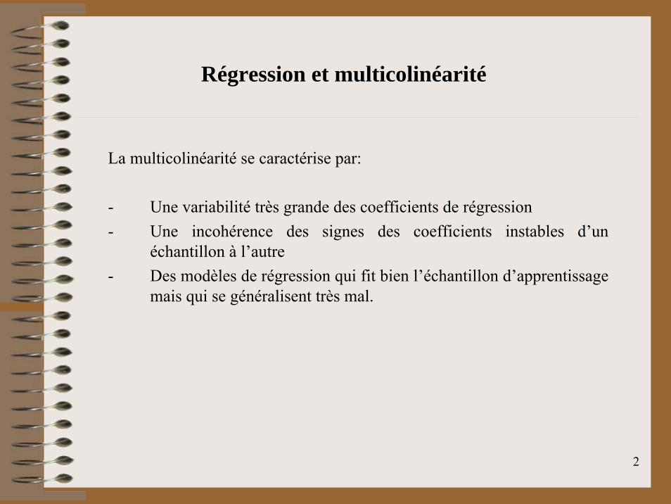
Régression et multicolinéarité
La multicolinéarité se caractérise par:
- Une variabilité très grande des coefficients de régression- Une incohérence des signes des coefficients instables d’un
échantillon à l’autre- Des modèles de régression qui fit bien l’échantillon d’apprentissage
mais qui se généralisent très mal.
3
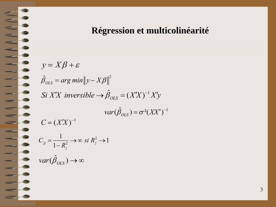
Régression et multicolinéarité
y X β ε= +2ˆ
OLS arg min y Xβ β= −
1ˆ ( )OLSSi X X inversible X X X yβ −′ ′ ′→ =
1( )C X X −′=
22
1 11jj j
j
C si RR
= →∞ →−
1ˆ( ) ²( )OLSvar XXβ σ −′=
ˆ( )OLSvar β →∞

4
1) Diagonaliser X X′
2( )X X V V− −′ ′= Σ2 1ˆ ( )X X X y V V V U y V U yβ − − −′ ′ ′ ′ ′= = Σ Σ = Σ
Inverse généralisé de Moore-Penrose, solution de norme minimum
PCR
Si X X est singulière comment l'inverser ?′
1'
r
i i ii
X U V u vλ=
′= Σ =∑
1λ= rλ++ ...
1uX 1'v ru rv'

5
b X y et A X X′ ′= =
2) Tridiagonaliser X’X
Méthode de Lanczos (1950) pour l’approximation des plus grandes valeurs propres de matrices symétriques.
Soit b un vecteur et A une matrice symétrique, Lanczos construit une séquence de matrices tridiagonales T
j jW AW.
Les vecteurs qui composent Wj sont construits par orthogonalisation de Gram-Schmidt de la série de Krylov: K(b,A,j)= (b, Ab, A²b,…, Ajb)
Lanczos C.. (1950). An iterative method for the solution of the eigenvalue problem of linear differential and integral operators. J. Res. Nat. Bur. Standards, Sect B.
En particulier la régression PLS correspond à:
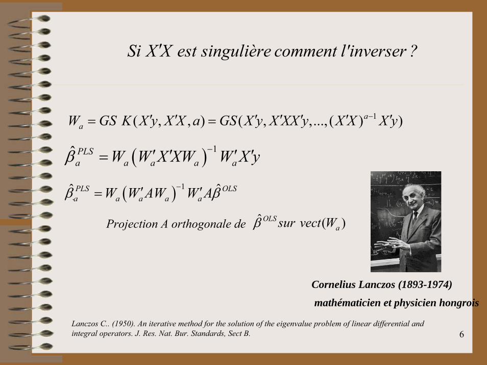
Si X X est singulière comment l'inverser ?′
6
1 ( , , ) ( , ,..., ( ) )aaW GS K X y X X a GS X y X XX y X X X y−′ ′ ′ ′ ′ ′ ′= =
( ) 1ˆ PLSa a a a aW W X XW W X yβ −′ ′ ′ ′=
( ) 1ˆ ˆPLS OLSa a a a aW W AW W Aβ β−′ ′=.
Projection A orthogonale de ˆ ( )OLSasur vect Wβ
Lanczos C.. (1950). An iterative method for the solution of the eigenvalue problem of linear differential and integral operators. J. Res. Nat. Bur. Standards, Sect B.
Cornelius Lanczos (1893-1974)
mathématicien et physicien hongrois
Si X X est singulière comment l'inverser ?′

7
.
3) Une factorisation particulière de X
X URW avec U U W W I et R inversible′ ′ ′= = =
1ˆ X y WR U yβ − − ′= =
Golub G. and Kahan W. (1965). Calculating the singular values and pseudo-inverse of a matrix, SIAM Journal on Numerical Analysis, 2: 205-224.
L’algorithme Bidiag2 de Golub et Kahan (1965) construit une matrice R bidiagonale àdroite et donc facilement inversible.
0
1
0/
uw X y X y=
′ ′=
1 1
1
[ ( )], 1[ ( )], 1
i i i i i i
i i i i i i
u k Xw u u Xw iw k X u w w X u i
− −
+
′= − ≥′ ′ ′ ′= − ≥
Si X X est singulière comment l'inverser ?′

8
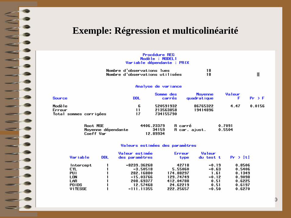
Exemple: Régression et multicolinéarité

9
Exemple: Régression et multicolinéarité
Toutes les variables apparaissent significatives et corrélées positivement avec le prix.
10
Exemple: Régression et multicolinéarité

11
Exemple: Régression et multicolinéarité : PLSR

12
Exemple: Régression et multicolinéarité

13
Exemple: Régression et multicolinéarité: PLSR

14
Exemple: Régression et données manquantes
15
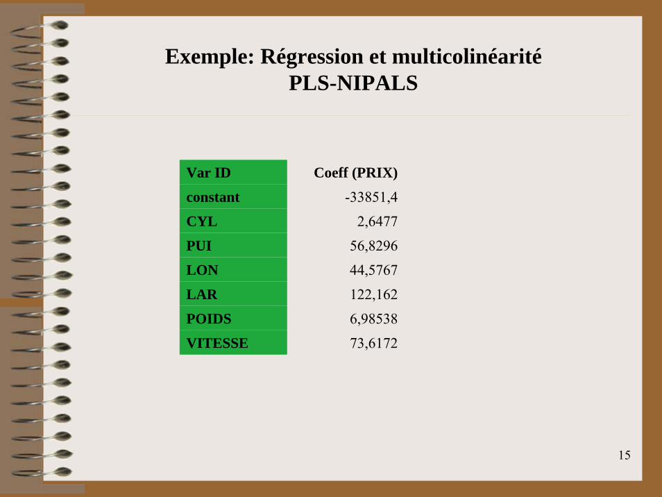
Exemple: Régression et multicolinéaritéPLS-NIPALS
Var ID Coeff (PRIX)
constant -33851,4
CYL 2,6477
PUI 56,8296
LON 44,5767
LAR 122,162
POIDS 6,98538
VITESSE 73,6172

16
Régularisation
- Régularisation par réduction de la dimensionnalité: PCR/PLS
- Régularisation par pénalisation L1(Lasso), L2 (Ridge), L1&L2 (Elastic net)
Remarques:- Ridge = OLS stabilisé- Elastic net = Lasso stabilisé
Nécessité de régularisation afin d’obtenir un modèle prédictif stable

17
Régularisation et biais
- Théorème de Gauss-Markov:
Gauss : 1777-1855 Markov : 1856-1922
ˆOLSβ est de tous les estimateurs sans biais celui de variance minimale
(BLUE)
On ne peut diminuer la variance qu’en biaisant l’estimateur
Compromis biais-variance

18
Compromis biais-variance
( ) ( )
( ) ( ) ( ) ( )
ˆ ˆ ˆ( )
ˆ ˆ ˆ ˆ ˆ ˆ( ) ( ) ( ) ( )
MSE E
E E E E E
β β β β β
β β β β β β β β
⎡ ⎤′= − −⎢ ⎥⎣ ⎦
⎡ ⎤′ ′= − − + − −⎢ ⎥⎣ ⎦
ˆ² ( )biais variance β= +
Quel est le biais de PLS ?
PLS shrinks (1995) de Jong, Jounal of Chemometrics
19
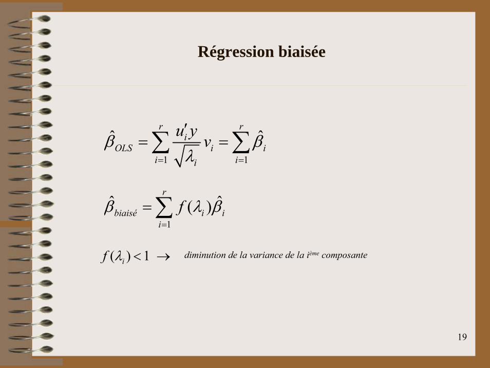
Régression biaisée
1
ˆ ˆ( )r
biaisé i ii
fβ λ β=
=∑
1 1
ˆ ˆr r
iOLS i i
i ii
u y vβ βλ= =
′= =∑ ∑
( ) 1 if λ < → diminution de la variance de la ième composante

20
Régression ridge et biais
.
( )2 1ˆ ˆarg min ² RR RRy X X X I X yβ
β β λ β β λ −′ ′= − + → = +
11312
2321
31 32
11 1
1ˆ 11 1 1
11 1
RR X y
ρρλ λ
ρρβλ λ λ
ρ ρλ λ
−⎛ ⎞⎜ ⎟+ +⎜ ⎟⎜ ⎟ ′= ⎜ ⎟+ + +⎜ ⎟⎜ ⎟⎜ ⎟+ +⎝ ⎠
1
ˆ ˆr
iRR i
i i
λβ βλ λ=
=+∑ ( ) 1if λ <
Hoerl A.E.. and Kennard R.W. (1970). Ridge regression: biased estimation for non orthogonal problems. Technometrics
Remarque: Un effet subtile de la ridge est de contraindre à tendre vers des valeurs voisines les coefficients associés à des variables corrélées.On retrouve cet effet avec PLS.

21
Régression PLS et biais
( ) 1 !if peut aussi êtreλ >
.
1 1
ˆ ˆ1 1pr
iPLS i
i j j
λβ βμ= =
⎡ ⎤⎛ ⎞= − −⎢ ⎥⎜ ⎟⎜ ⎟⎢ ⎥⎝ ⎠⎣ ⎦∑ ∏
{ }
-
, ,..., ( )
j
j
p
vecteur de Ritz
approximation de au sous espace de Krylov
span X y X XX y X X X y
μ
λ
=
=
′ ′ ′ ′ ′
Relation non claire en terme de « shrinkage » car

22
NIPALS (Wold H., 1966)
• L’algorithme de régression PLS classique, comme cas particulier de l’approche PLS, est basé sur des développements de l’algorithme NIPALS, acronyme de Nonlinear estimation by Iterative Partial Least Squares.
• L’algorithme NIPALS est une méthode robuste pour déterminer de façon itérative les valeurs et vecteurs propres d’une matrice.
• Elle permet en particulier de faire de l’analyse en composantes principales en présence de valeurs manquantes.
• Cet algorithme est directement inspiré de la méthode de la puissance itérée (Hotelling 1936)
Wold H. Estimation of principal components and related models by iterative least squares. In Krishainaah, P.R. (ed), Multivariate Analysis. New Academic Press, New York 1966, pp. 391-420.
23
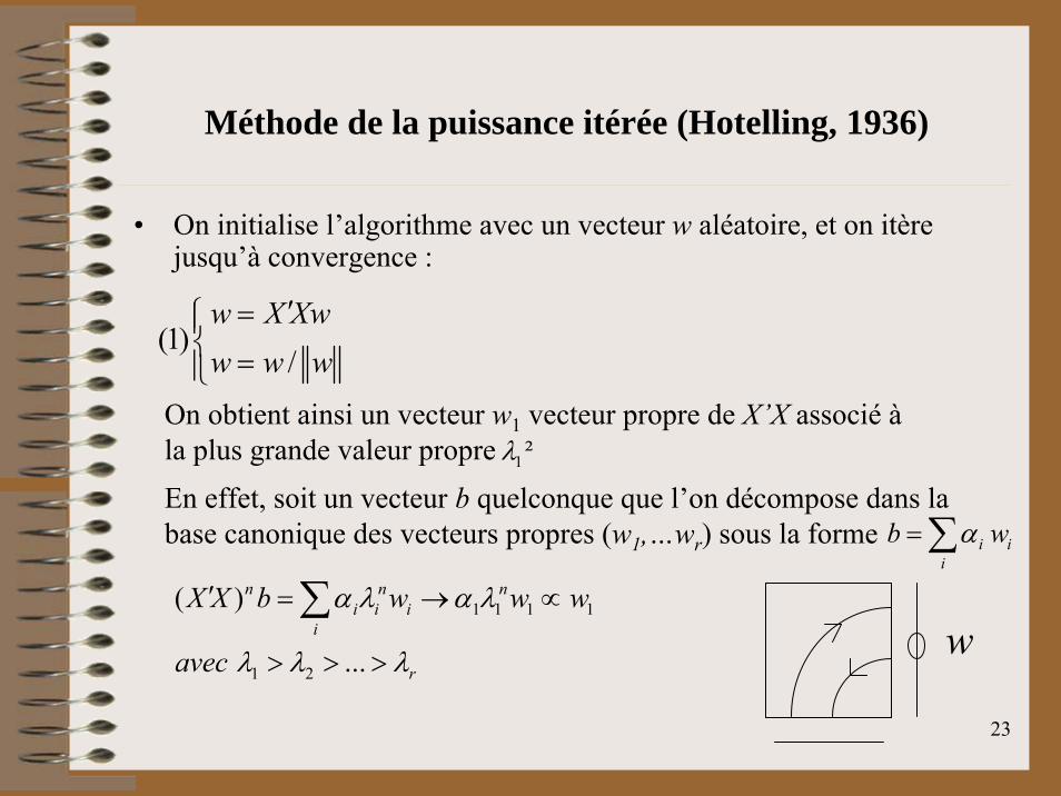
Méthode de la puissance itérée (Hotelling, 1936)
• On initialise l’algorithme avec un vecteur w aléatoire, et on itère jusqu’à convergence :
(1)/
w X Xww w w
′=⎧⎪⎨ =⎪⎩
On obtient ainsi un vecteur w1 vecteur propre de X’X associé àla plus grande valeur propre 1²λ
En effet, soit un vecteur b quelconque que l’on décompose dans la base canonique des vecteurs propres (w1,…wr) sous la forme i i
ib wα=∑
1 1 1 1
1 2
( )
...
n n ni i i
i
r
X X b w w w
avec
α λ α λ
λ λ λ
′ = → ∝
> > >
∑w

24
• Lorsque l’algorithme convergence, on a la relation :
21 1 1X Xw wλ′ =
A partir de laquelle on dérive l’expression de :( 1)12
1 ( )1
iterration n
iterration n
w
wλ
+
=
1 2 '1 1 1( )X X X X w wλ′ ′= −
2 '
1( )
ii
i i ij
X X X X w wλ=
′ ′= −∑
On déflate ensuite la matrice X’X :
Cette méthode extrait ainsi les vecteurs propres l’un après l’autre dans l’ordre décroissant des valeurs propres.
Méthode de la puissance itérée (Hotelling, 1936)
25
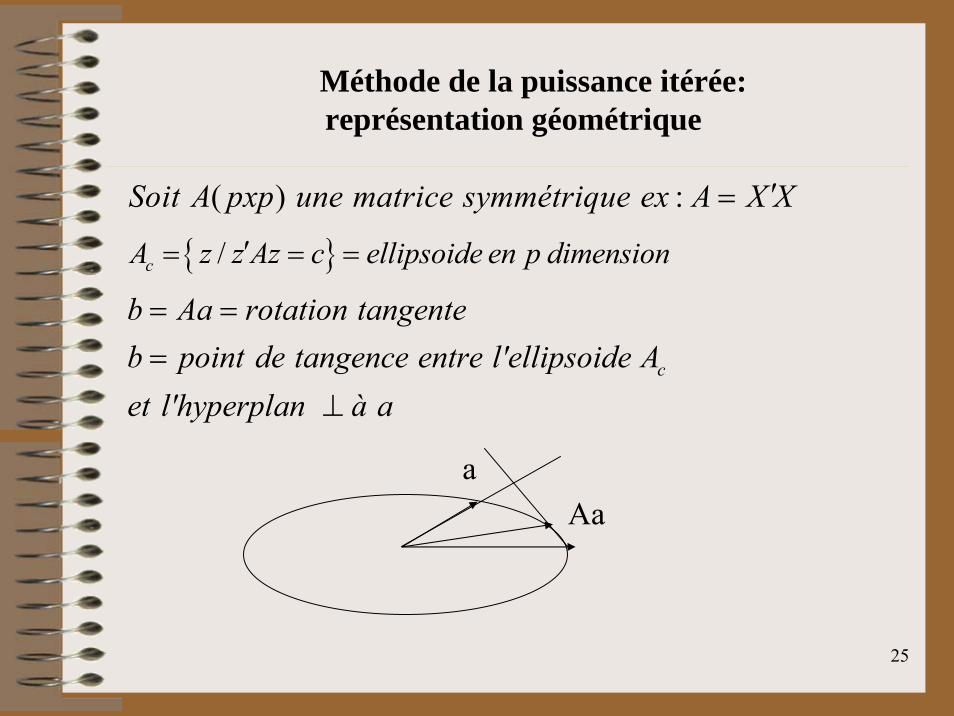
Méthode de la puissance itérée:représentation géométrique
( ) :Soit A pxp une matrice symmétrique ex A X X′=
{ }/cA z z Az c ellipsoide en p dimension′= = =
c
b Aa rotation tangenteb point de tangence entre l'ellipsoide Aet l'hyperplan à a
= ==
⊥
aAa

26
Algorithme NIPALS
• C’est un algorithme inspiré de la méthode de la puissance itérée appliqué à la matrice X, où l’on a remplacé le produit matrice vecteur par des régressions simples.
0
1
1
1
1
1) 2) pour 1,2.1) 2.2) répéter jusqu'à convergence de 2.2.1) / 2.2.2) / 2.2.3) /2.3)
h h
h
h h h h h
h h h
h h h h h
h h h h
X Xh a
t colonne de Xp
p X t t tp p pt X p p p
X X t p
−
−
−
−
==
=
′ ′=
=
′=′= −
Wold H. (1966). Estimation of principal components and related models by iterative least squares, in Multivariate Analysis, Krishnaiah P.R.(Ed.), Academic Press, New York,
p’
Xt

27
NIPALS et données manquantes
*
*
*
*
*
*
*
**
* *
*
*
*
*
*
thixh-1,i
ph
(phj,xh-1,ij)
L’algorithme peut fonctionner en présence de données manquantes.
1,h i hhi
h h
x pt
p p−=′
Wold H. (1966). Estimation of principal components and related models by iterative least squares, in Multivariate Analysis, Krishnaiah P.R.(Ed.), Academic Press, New York,

28
( )g (x)= x ( )
sig xλ λ+
−
Soft thresholding function
Sparse PCA

29
Sparse PCA : Algorithme
( )
0
1
1 1
1
X=U , 1,
1) , 2) ' )
) / ) 3) /4)
old h h old h
new new
new h old
new h new h new
old new
new new new
h h h new new
Décompose V X XPour h H
v v u uJusqu à convergence de u et v
a v g X u
b u X v X vc u u
v v vX X u v
λ
δ
δ
−
− −
−
′Σ =
== =
′=
=
=
=
′= −v’
u
X
H. Shen, J.Huang(2008). Sparse principal component analysis via regularized low rank matrix application. Journal of multivariate Analysis

30
Algorithme PLS1-NIPALS
1
1
1
1
11
1) , 2) 2.1) / 2.2) 1 2.3) / 2.4) /
2.5) ˆ3) [ ,.., ], ( )
h h
h
h h h h h
h h h h h
h h h h
a PLS
X y centréspour h 1,a
w X y y yw
t X w w wp X t t t
X X t p
T t t y T T T T y
−
−
−
−
−
=′ ′=
=
′=′ ′=
′= −
′ ′= =
( )
*1
1 1 1
* 1
ˆ
( )
a a aPLS i i i i i i
i i i ii i ii i i i i i
h-1*h i i h
i=1
y t y t y ty t X w Xwt t t t t t
W W P W w = I - w p w
−= = =
−
′ ′ ′= = =
′ ′ ′
⎛ ⎞′ ′= ⎜ ⎟⎝ ⎠
∑ ∑ ∑
∏1
1
[ ,..., ][ ,..., ]
a
a
W w wP p p==

31
Sparse PLS: Algorithme
2
0 0
1 1
1
1/ ,2 / 1: ) , ) ' ) (
h h
old h old h
new new
new h
X Y U VX X Y Ypour i Ha décompose X Y et extraire la première paire de vecteurs singuliers
u u v vb jusqu à convergence de u et v
i u g Xλ
− −
−
′ ′= Δ= =
=′
= =
′=
1
1
1 1
1
1
1
1
), 1
) ( ), 1
) , ) / / ) / / )
h old new
new h h old new
old new old new
h h new new new
h h new new new
h h h h h
h h h h h
Y v u
ii v g Y X u v
iii u u v vc X u u u
w Y v v vd c X
d Ye X
λ
ξ
ξ ξ ξξ ξ ξ
−
− −
−
−
−
−
=
′= =
= =′=′=
′ ′=′ ′=
1
1 ) h h h h
h h h h
X cf Y Y d
ξξ
−
−
′= −′= − v
u
X’h-1Yh-1
Kim-Anh lë Cao et al. (2008).A sparse PLS for variable selection when integrating Omics data.Statisticalapplications in genetics and molecular biology

32
Régression PLS et très grande dimensionKernel PLS
1 ( ) ( )t XX y ZZ y PLS X PLS Z′ ′= → =p
1 ( )n p w premier vecteur propre de X YY X pxp′ ′>> →
Quand n >> p ou p >> n des algorithmes rapides ont été proposés dans les années 90 consistant à effectuer l’essentiel des calculs sur des matrices de taille réduite appelées « kernel ».
De Jong et ter Braak ont proposés lorsque p >> n d’effectuer la régression PLS sur la matrice des composantes principales Z, la régression PLS étant invariante par transformation orthogonale.
De Jong, and ter Braak C. (1994). Comments on the PLS kernel algorithm. Journal of Chemometrics.
1 ( )p n t premier vecteur singulier à gauche de XX YY nxn′ ′>> →
Lindgren F., Geladi P., and Wold S., (1993). The kernel algorithm for PLS. Journal of chemometrics.Rännar S., Geladi P., Lindgren F., Wold S., (1994). A PLS kernel algorithm for data sets with many variables and fewer objects. Journal of Chemometrics.

33
Régression PLS et très grande dimension Canonical PLS
Avec l’algorithme « Canonical Partial Least Squares » en 2001, De Jong et al. proposent d’effectuer l’essentiel des calculs dans la base formée par les composantes principales (base canonique).
21 2( , ,..., ) ( , ( ) ,..., ( ) )a
aT t t t GS XX y XX y XX y′ ′ ′= =2( , ,..., )aGS ULU y UL U y UL U y′ ′ ′=
De Jong, (1993). SIMPLS: an alternative approach to partial least squares resgression. Chemometrics and Intelligent Laboratory Systems.
De Jong S., Wise B., and Ricker N., (2001). Canonical partial least squares and continuum powerregression. Journal of. Chemometrics,
1/ 2ˆPLS VL U TT yβ − ′ ′=
34
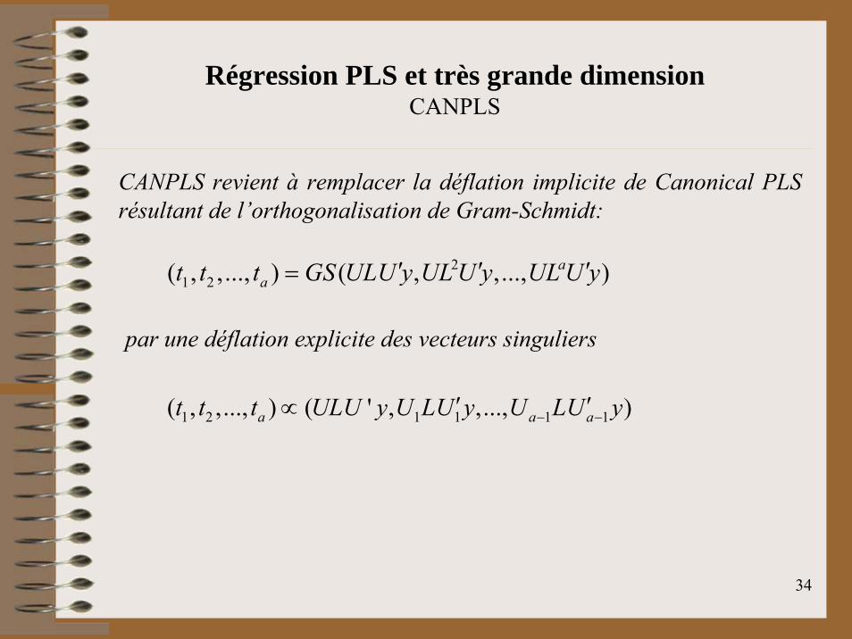
Régression PLS et très grande dimensionCANPLS
CANPLS revient à remplacer la déflation implicite de Canonical PLS résultant de l’orthogonalisation de Gram-Schmidt:
21 2( , ,..., ) ( , ,..., )a
at t t GS ULU y UL U y UL U y′ ′ ′=
1 2 1 1 1 1( , ,..., ) ( ' , ,..., )a a at t t ULU y U LU y U LU y− −′ ′∝
par une déflation explicite des vecteurs singuliers

35
CANPLS algorithm
21 ( )i i i
i
t ULU y u y uλ′ ′= =∑
1 1 1 2( )h h h hU I t t U− − − −′= −
1 1t =
21 1 , 1 , 1( )h h h i i h i h
it U LU y u y uλ− − − −′ ′= =∑
1/ 2 ' ( )let X UL V the SVD of X or X ′=
1/ 2ˆ ' 'PLS VL U TT yβ −=
1ht =

36
Modified Continuum power regression
Le compromis réalisé par PLS entre fit et stabilité qui donne le même poids aux deux termes peut être modifié et CanPLS peut être généralisé dans la même logique que la Continuum Power Regression de de Jong et al.
'1
1' ( )
r
i i ii
t UL U y u y uγ γλ=
∝ =∑%
'1 1 1, ,
1' ( )
r
k k k i k i k ii
t U L U y u y uγ γλ− − −=
∝ =∑%
γ

37
Modified Continuum power regression
'1 1 1, ,
1' ( )
r
k k k i k i k ii
t U L U y u y uγ γλ− − −=
∝ =∑%
γ
Définit une trajectoire entre OLS et PCR
0, 1,
OLS forPLS forPCR for
γγγ
==→∞
( ) ( )PLS X PLS Z=( )PCR X PLS sur un sous ensemble de CP standardisés=

38
Régression PLS et très grande dimensionSample-based PLS
Bush et Nachbar (1993) ont montré que la régression PLS dépendde la distance entre les observations à travers le produit XX’ plus que des valeurs individuelles des descripteurs.
Bush R. and Nachbar B., (1993). J. Comput.-Aided Mol. DesignLewi, P.J. (1995). Pattern recognition, reflection from a chemometric point of view. Chemometricsand Intelligent laboratory System
Approche très intéressante lorsque les individus sont difficiles voiremême impossibles à caractériser vectoriellement.

39
Sample-based PLS
cos( )θ =+ −d d d
d dij ik jk
ij ik
2 2 2
2b d d
d d dijk ij ik
ij ik jk= =+ −
cos( )θ2 2 2
2
' ( )'B UVU U V U V XX′= = =
Torgerson (1952) détermine de manière analytique les coordonnées des points à partir de la distance entre ces points
Young & Householder 1938 θj
k
Loi du cosinus
i

40
Sample-based PLS
( ) ( )22 2 2 2 2. . .. 1/ 2
ij ik jk ij ij i jk
ij
D X X C D D D D
C XX si X centré
SAMPLS algorithm
= − ⇒ = − − − +
′=
→
∑
Bush R. and Nachbar B., 1993. J. Comput.-Aided Mol. Design 1993, 7, 587)
La généralisation à des distances non euclidiennes ouvre la voievers le non-linéaire

41Schölkopf et Smola, Learning with Kernels, MIT Press, 2001
Kernel methods

42
Kernel methods
2 21 2 1 1 2 2 ( , ) ( ) ( , 2 , )Soit x x x et x x x x x= Φ =
( ): ( , ) ,d
Noyau polynomial K x y x y C= +
2 2 2 21 2 1 2 1 2 1 2
2 21 1 2 2
( ), ( ) 2
(x ) ,
x y x x x x y y y y
y x y x y
< Φ Φ > = + +
= + =< >
2
: ( , ) exp2 ²
x yNoyau Gaussien K x y
σ
⎛ ⎞−= ⎜− ⎟
⎜ ⎟⎝ ⎠

43
Régression PLS et optimisation
La régression PLS peut aussi être vue comme un problème d’optimisation avec un critère à optimiser, le critère de Tucker.
Tucker L.R. (1958). An inter-battery method of factor analysis. Psychometrika.
1 1 1 1 ( ( , ))1 1w w =1
T Xw avec w solution de max cov² Xw y′
=
1 1( ) ²( , )1cov²(Xw , y) var Xw cor Xw yp
X yy X′ ′La solution w1 est le vecteur propre normalisé de
1jj
jj
cov(x , y)w
cov²(x , y)=∑
112
1
1 cov( , )cov( , )
p
j jpj
jj
t y x xy x =
=
= ∑∑
X yy XX y X y′ ′ ′ ′∝

44
Régression PLS généraliséeune réinterprétation de le régression PLS
1 ( )j
jj
xy a
var xε= +
1 1 2 2 1 1 1...j j j h j h h jx p t p t p t x− − −= + + + +
En 99, Michel Tenenhaus a proposé une interprétation des composantes PLS en fonction de simples régressions linéaires dans une approche similaire à celle proposée par Gartwhaite (1994), mais qui permet la prise en compte des valeurs manquantes dans l’esprit de NIPALS
1 , )
j
jj j
j
j
xcov(y, )
var(x )a = cov(y xx
var( )var(x )
=
Tenenhaus M. (1999). La regression logistique PLS in Proceedings of the 32èmes journées de Statistique de la Société française de Statistique, FesGarthwaite P.H. (1994). An interpretation of Partial Least Squares. Journal of the American Statistical Association, 425:122-127
11 1 2 2 1 1
1
...( )h j
h h hjh j
xy c t c t c t a
var xε−
− −−
= + + + + +1, )hj h ja cov(y x −=
PLS GLR

45
PLS-GLR algorithm
.
The PLS-GLR algorithm consists of four steps :
(1) Computation of the m PLS components th(2) GL regression on the m retained PLS components(3) Expression of PLS-GLR in terms of the original explanatory variables(4) Bootstrap validation of coefficients in the final model

46
PLS-GLR algorithm
1,1
11
1
11
1 1
( ) , j pj ja GLRfit x
awa
Xwtw w
==
=
=′
1,2, 1
22
2
1,1, 1
1 22
2 2
( , ) ,
( / ) ,
j pj j
j pj j
a GLRfit x t
awa
x linfit x t
X wtw w
=
=
=
=
=
=′
.1,, 1 2 1
1,1, 1 2 1
1
( , , ,..., ) ,
( / , ,..., ) ,
j ph j j h
hh
h
j ph j j h
h hh
h h
a GLRfit x t t t
awa
x linfit x t t t
X wtw w
=−
=− −
−
=
=
=
=′
47
PLS-GLR and sparsity
.
By taking advantage from the statistical tests associated withgeneralized linear regression, it is feasible to select the significant explanatory variables to include in the model.
Computation of the PLS components th can thus be simplified by setting to 0 those regression coefficients ah-1,j that show to be not significant at a predefined threshold.
Only significant variables will then contribute to the computation of the PLS components.
Moreover, the number m of PLS components to be retained maybe chosen by observing that the component tm+1 is not significantbecause none of the coefficients am,j is significantly different from0.

48
Soft/HardThresholding
Soft thresholding exhibits continuous shrinkage but suffersfrom substancial biais for large coefficients.
Hard thresholding exhibits non continuous shrinkage but doesnot suffer from such a biais.

49
Régression logistique PLS

50
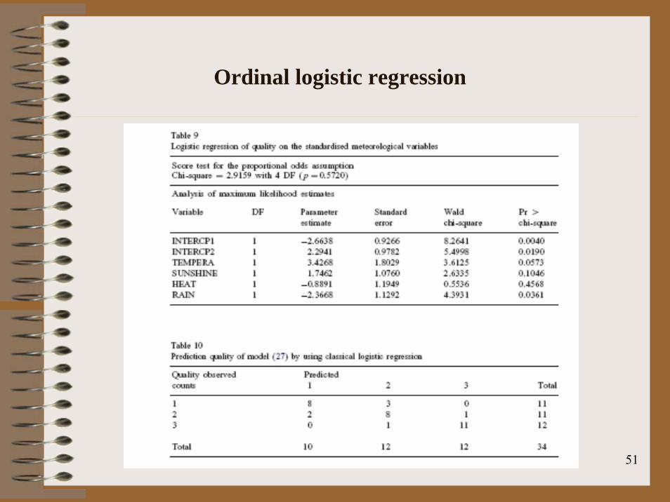
Ordinal logistic regression
• Ordinal logistic regression of quality on the four standardised predictorscorresponds to the following model
k 1 2 3 4
k 1 2 3 4
a +b Temperature+b Sunshine+b heat+b Rain
a +b Temperature+b Sunshine+b heat+b Rain
eProb(y k)=1+e
≤
Wine quality (k): 1 = good; 2 = average; 3 = poor
51
Ordinal logistic regression

52
Régression logistique PLS
( ) ( ) ( ) ( )1 2 2 2
3.0117* 3.3401* 2.1445* 1.7906*
3.0117 3.3401 2.1445 1.7906
0.5688* 0.6309* 0.4050* 0.3282*
Temperature Sunshine Heat Raint
Temperature Sunshine Heat Rain
+ + −=
+ + + −
= + + −
Régressions logistiques de la qualité du vin sur chaque prédicteur standardisé:
1,1
11
1
11
1 1
( ) , j pj ja GLRfit x
awa
Xwtw w
==
=
=′
Temperature: 3.0117 (p = 0.0002)Sunshine: 3.3401 (p = 0.0002)Heat: 2.1445 (p = 0.0004)Rain: -1.7906 (p = 0.0016)

53
Régression logistique PLS

54
Régression logistique PLS
*1 1 2
*1 1 2
2
( )1
k j j
k j j
t x
t x
eProb y ke
t NS
α β β
α β β
+ +
+ +≤ =
+→
2.265 1.53x 1.70x 1.09x 0.91x
2.265 1.53x 1.70x 1.09x 0.91x( 1)1
0.5688x 0.6309 x 0.4050 x 0.3282 x
Temperature Sunshine Heat Rain
Temperature Sunshine Heat Rain
eProb ye
Temperature Sunshine Heat Rain
− + + + −
− + + + −= =+
= + + −
Détermination de t2
Expression du modèle final en fonction des descripteurs standardisés

55
Régression logistique PLS Balanced Bootstrap CI

56
The Cox proportional hazard model
The model assumes the following hazard function for the occurrence of an event at time t in the presence of censoring:
The Cox’s partial likelihood can be written as :
When p > n, there is no unique β to maximize this partial likelihood.
Even when p ≤ n , covariates could be highly correlated and regularization may still be required in order to reduce the variance of the estimates and to improve the prediction performance.
0( ) ( ) exp( )t t Xλ λ β=
exp( ' )( )exp( ' )
k
k
k D jj R
xPLx
βββ∈ ∈
=∏∑
Cox D.R. 1972. Journal of the Royal Statistical Society B.; 74: 187-220

57
PLS-Cox regression(Bastien & Tenenhaus, 2001)
• Computation of the first PLS component t1
1,1
11
1
11
1 1
( ) , i pi ia Coxfit xawa
Xwtw w
==
=
=′
.
1,2, 1
22
2
1,1, 1
1 22
2 2
( , ) ,
( / ) ,
i pi i
i pi i
a Coxfit t xawa
x linfit x tX wtw w
=
=
=
=
=
=′
• Computation of the second PLS component t2
Bastien P., and Tenenhaus M., 2001. Proceedings of the PLS’01 International Symposium
58
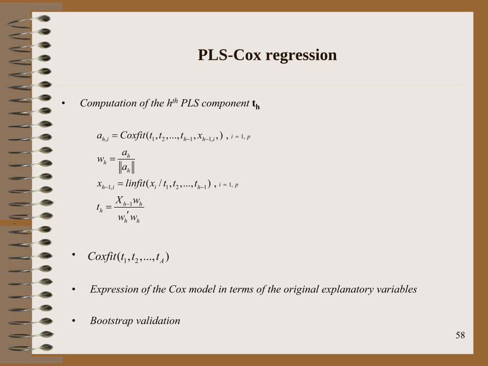
PLS-Cox regression
• Computation of the hth PLS component th
1,, 1 2 1 1,
1,1, 1 2 1
1
( , ,..., , , ) ,
( / , ,..., ) ,
i ph i h h i
hh
h
i ph i i h
h hh
h h
a Coxfit t t t xawa
x linfit x t t tX wtw w
=− −
=− −
−
=
=
=
=′
.
•1 2( , ,..., ) ACoxfit t t t
• Expression of the Cox model in terms of the original explanatory variables
• Bootstrap validation

59
L1 penalized Cox regression
In the context of censored data, Tibshirani (1997) extended the LASSO procedure to variable selection with the Cox model.
p
jj=1
ˆ , argmin - l( ) subject to sβ β β= ≤∑
Tibshirani proposed an iterative procedure which require the minimization of a one-term Taylor series expansion of le log partial likelihood.
p
j=1( ) ( ) T
jargmin z X A z X subject to sβ β β− − ≤∑2
1 , =X , , =-l lwith z A Aη μ η β μη ηη
− ∂ ∂= + =
′∂ ∂
Tibshirani R. (1997). Statistics in Medicine, 16:385-395
60
LARS procedure
Efron B., Johnston I., Hastie T., and Tibshirani R., 2004. Annals of Statistics, 32:407-499
Efron et al. (2004), proposed a highly efficient procedure, called Least Angle Regression for variable Selection which can be used to perform variable selection with very large matrices.
Using the connection between LARS and Lasso, Gui and Li (2005)proposed LARS-Cox for gene selection in high-dimension and low sample size settings.
Using a Choleski factorization they transform the minimization in a constrained version of OLS which can be solved by the LARS-Lasso procedure.

61
LARS-Cox
p
j=1
ˆ ˆ ( ) ( ) Tjarg min y X y X subject to sβ β β− − ≤∑
Gui J. and Li H., (2005). Bioinformatics Penalized Cox regression analysis in the high-dimensional and low-sample size settings, with application to microarray gene expression data. Bioinformatics
p
j=1 ( ) ( ) T
jarg min z X A z X subject to sβ β β− − ≤∑
ˆ , , ( )with y Tz X TX et A TT Choleski′= = =
However, the IRWLS iterations performed in the LARS-Cox procedure counter balanced the efficiency of the LARS-Lasso algorithm and render the Gui and Li algorithm computationally costly.
62
Cox-Lasso procedure on deviance residuals
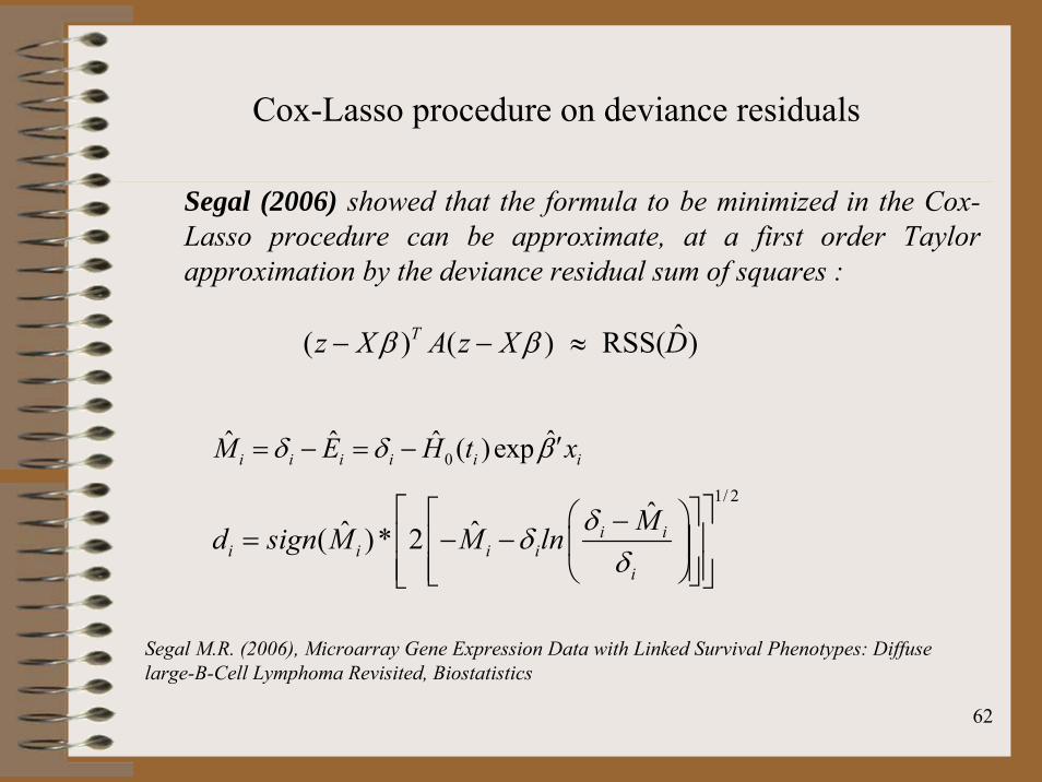
Segal (2006) showed that the formula to be minimized in the Cox-Lasso procedure can be approximate, at a first order Taylor approximation by the deviance residual sum of squares :
ˆ( ) ( ) RSS( )Tz X A z X Dβ β− − ≈
0ˆˆ ˆ ˆ ( )expi i i i i iM E H t xδ δ β ′= − = −
1/ 2ˆˆ ˆ( )* 2 i i
i i i ii
Md sign M M ln δδδ
⎡ ⎤⎡ ⎤⎛ ⎞−= − −⎢ ⎥⎢ ⎥⎜ ⎟
⎢ ⎥⎢ ⎥⎝ ⎠⎣ ⎦⎣ ⎦
Segal M.R. (2006), Microarray Gene Expression Data with Linked Survival Phenotypes: Diffuse large-B-Cell Lymphoma Revisited, Biostatistics

63
Cox-Lasso procedure on deviance residuals
The deviance residual is a measure of excess of death and can therefore be interpreted as a measure of hazard.
Segal thus proposed to speed-up the calculations by replacing the survival times by the deviance residuals, a normalized version of Martingal residuals that result from fitting a null (intercept only) Cox regression model.
Therneau T.M., Grambasch P.M., and Fleming T.R. (1990). Martingale-based residuals for survival models. Biometrika

64
PLS on deviance residual
We have proposed to use the same idea in the setting of Partial Least Squares. A very simple and fast alternative formulation of the PLS-Cox model could be derived by fitting the deviance residuals of a null Cox model with a simple PLS regression.

65
• 240 patients atteints de DLBCL.• 138 décès / médiane de survie 2.8 ans / 30% de censure• 7399 zones qui représentent 4128 gènes• 160 échantillon d’apprentissage / 80 échantillon de test
Application en transcriptomique
Rosenwald A. et al., 2002. The new England Journal of medicine, 346:1937-1947Heagerty P.J., Lumley T., and Pepe M. 2000. Biometrics 56,337-344
(http://www-stat.standford.edu/∼tibs/superpc/standt.html )

66
Wald test, p=0.001
DLBCL Rosenwald (2002)
0 T High Riskβ > ⇒ 0 T Low Riskβ < ⇒

67
plsRcox• Récemment dans Bioinformatics (2009) Sohn et al. ont proposé un
algorithme de type « gardient lasso » qui comme PLS ne requiert pas d’inversion de matrices.
• Bertrand et al ont montré sur les données de Rosenwald sur des données d’allélotypage que la PLSDR semble surperformer l’approche de Sohn et al.
Bertrand F., Maumey-Bertrand M., beau-Faller M., Meyer N. PLSRcox: modèles de Cox en présence d’un grand nombre de variables explicatives. Poster Chimiométrie 2010, ENSPCI PARIS.

68
Packages sous R
• Package ‘integrOmics’ : Regularized CCA and Sparse PLSAuthor Sebastien Dejean, Ignacio Gonzalez and Kim-Anh Le Cao
• Package ‘plsRglm’ : Partial least squares Regression for generalized linearmodelsAuthor Frederic Bertrand <[email protected]>, Nicolas Meyer
• Package ‘plsRcox’ : Partial least squares Regression for Cox regressionAuthor Frederic Bertrand <[email protected]>, Maumy-Bertrand, Beau-Faller, Nicolas Meyer
• Package PLSDOF : Degrees of Freedom and Confidence Intervals for Partial Least Squares RegressionAuthor Nicole Kraemer, Mikio L. Braun
R Development Core Team : R : A language and environment for statistical computing, R Foundation for Statistical Computing, Vienna, Austria, 2008. http ://www.R-project.org.