physique mesoscopique des electrons et des photons ... de c… · physique mesoscopique des...
TRANSCRIPT

Physique mesoscopique des electrons et des photons -
Structures fractales et quasi-periodiques
Eric AkkermansPhysics-Technion
IS
RA
EL
SC
I E N C E F OU
N
DA
TIO
N
Show selected photi http://www.admin.technion.ac.il/pard/mediaarc/showphoto.asp?photol...
1 of 1 12/12/08 12:46 PM
Back
Technion logo English
Aux frontieres de la physique mesoscopique, Mont Orford Quebec, Canada, Septembre 2013
Thursday, September 19, 13

Towards a quantitative description : the tools of quantum mesoscopic physics
Part 2
1. More details on diffusion and quantum crossings
2. The global scattering approach (Landauer-Schwinger)
3. How to relate local quantum crossings to the global scattering approach ?
Thursday, September 19, 13
Towards a quantitative description : the tools of quantum mesoscopic physics
Part 2
1. More details on diffusion and quantum crossings
2. The global scattering approach (Landauer-Schwinger)
3. How to relate local quantum crossings to the global scattering approach ?
Thursday, September 19, 13

Towards a quantitative description : the tools of quantum mesoscopic physics
Part 2
1. More details on diffusion and quantum crossings
2. The global scattering approach (Landauer-Schwinger)
3. How to relate local quantum crossings to the global scattering approach ?
Thursday, September 19, 13

Towards a quantitative description : the tools of quantum mesoscopic physics
Part 2
1. More details on diffusion and quantum crossings
2. The global scattering approach (Landauer-Schwinger)
3. How to relate local quantum crossings to the global scattering approach ?
Thursday, September 19, 13

Towards a quantitative description : the tools of quantum mesoscopic physics
Part 2
1. More details on diffusion and quantum crossings
2. The global scattering approach (Landauer-Schwinger)
3. How to relate local quantum crossings to the global scattering approach ?
4. A brief overview on Anderson localization phase transition
Thursday, September 19, 13

Multiple scattering of electrons
k
k'
k
L L
2 characteristic lengths:
Wavelength:
Elastic mean free path: (Disorder - Origin ?)
Weak disorder : independent scattering events
l
A reminder
Thursday, September 19, 13

Multiple scattering of electrons
k
k'
k
L L
2 characteristic lengths:
Wavelength:
Elastic mean free path: (Disorder - Origin ?)
Weak disorder : independent scattering events
l
We shall be
interested
only by this
limit
Thursday, September 19, 13

Probability of quantum diffusion
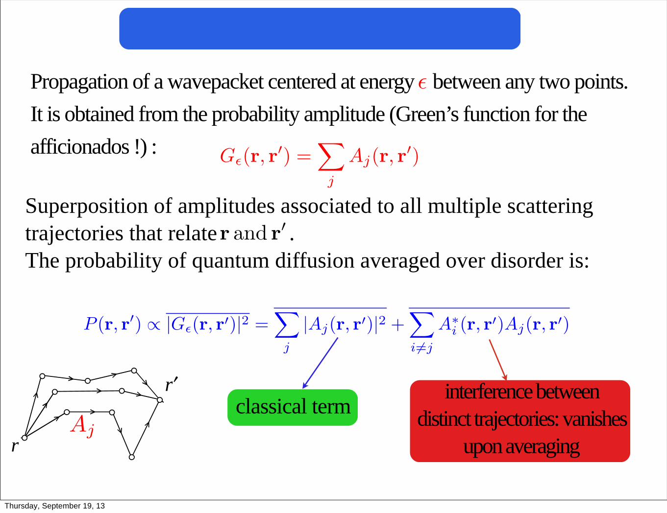
Propagation of a wavepacket centered at energy between any two points.
It is obtained from the probability amplitude (Green’s function for the
afficionados !) :
!
G!(r, r!) =
!
j
Aj(r, r!)
Superposition of amplitudes associated to all multiple scattering
trajectories that relate .
The probability of quantum diffusion averaged over disorder is:
r and r!
P (r, r!) ! |G!(r, r!)|2 =!
j
|Aj(r, r!)|2 +!
i"=j
A#i (r, r
!)Aj(r, r!)
k
r1
r2
k'
Aj
classical terminterference between
distinct trajectories: vanishes
upon averaging�
′ r
�
r
Thursday, September 19, 13
Probability of quantum diffusion
Propagation of a wavepacket centered at energy between any two points.
It is obtained from the probability amplitude (Green’s function for the
afficionados !) :
!
G!(r, r!) =
!
j
Aj(r, r!)
Superposition of amplitudes associated to all multiple scattering
trajectories that relate .
The probability of quantum diffusion averaged over disorder is:
r and r!
P (r, r!) ! |G!(r, r!)|2 =!
j
|Aj(r, r!)|2 +!
i"=j
A#i (r, r
!)Aj(r, r!)
k
r1
r2
k'
Aj
classical terminterference between
distinct trajectories: vanishes
upon averaging�
′ r
�
r
Thursday, September 19, 13

aj
ai*
r r'
r'r
(a)
(b)
Before averaging : speckle pattern (full coherence)
Configuration average: most of the contributions vanish because
of large phase differences.
Diffuson Pcl(r, r!) =
!
j
|Aj(r, r!)|2
Ai
A!j
Vanishes upon averaging
Ai
A!j
A new design !
Thursday, September 19, 13

aj
ai*
r r'
r'r
(a)
(b)
Before averaging : speckle pattern (full coherence)
Configuration average: most of the contributions vanish because
of large phase differences.
Diffuson Pcl(r, r!) =
!
j
|Aj(r, r!)|2
Ai
A!j
Vanishes upon averaging
Ai
A!j
A new design !
Thursday, September 19, 13
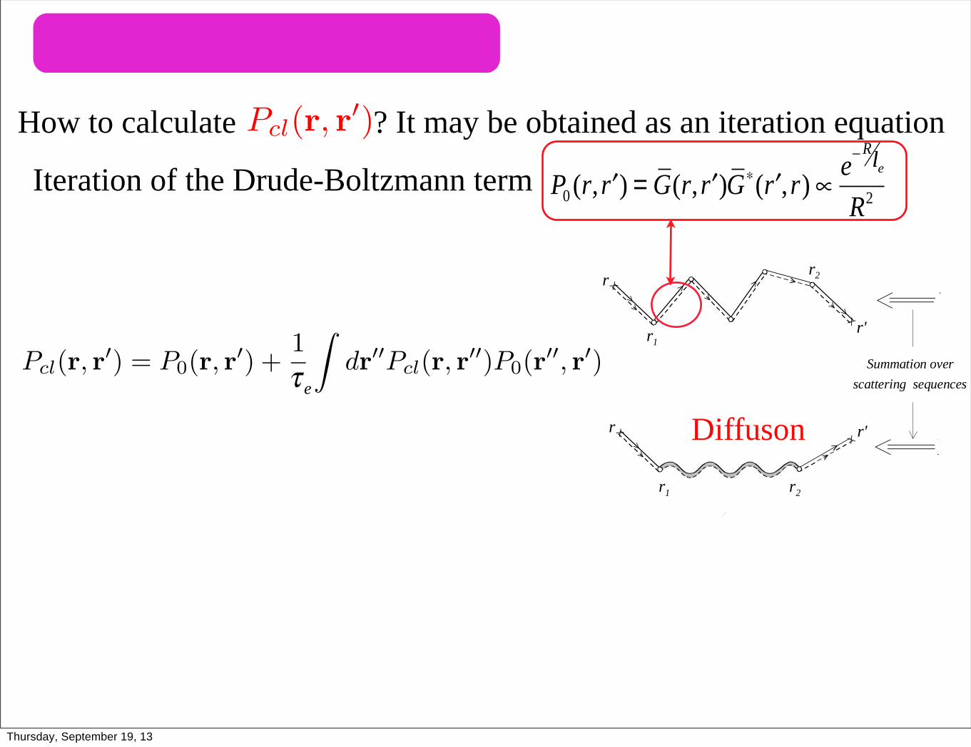
The diffusion approximation:
How to calculate ? It may be obtained as an iteration equation Pcl(r, r!)
(c)
r'
r
r1
r2
(a)r2
r2
r1
r1 (b)
(d)
Summation overscattering sequences
r
r1 r2
r'
r1 r2
r1 r2
r'r r'
GR
GA
r
Iteration of the Drude-Boltzmann term P0 (r, ′r ) = G(r, ′r )G∗( ′r ,r) ∝e−R
l
R2
Pcl(r, r!) = P0(r, r
!) +1
!
!dr!!Pcl(r, r
!!)P0(r!!, r!)
!!
!t! D!
"Pcl(r, r
!, t) = "(r ! r!)"(t)
with D =vgl3
In the limit of slow spatial and temporal
variations, and |r ! r!| " l t ! !
Diffuson
(diffusion equation)�
le
�
le
�
le
�
τ e�
τ e
Thursday, September 19, 13

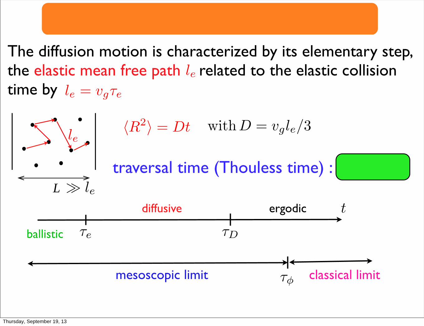
Mesoscopic limit: characteristic length scales
The diffusion motion is characterized by its elementary step, the elastic mean free path related to the elastic collision time by
lele = vg!e
L
saa sb
sa' sb'
le!R2" = Dt
traversal time (Thouless time) : L2 = D!D
t
!e !D
!!
ballistic
diffusive ergodic
mesoscopic limit classical limit
! le
withD = vgle/3
Thursday, September 19, 13

Did we miss something ?
Thursday, September 19, 13

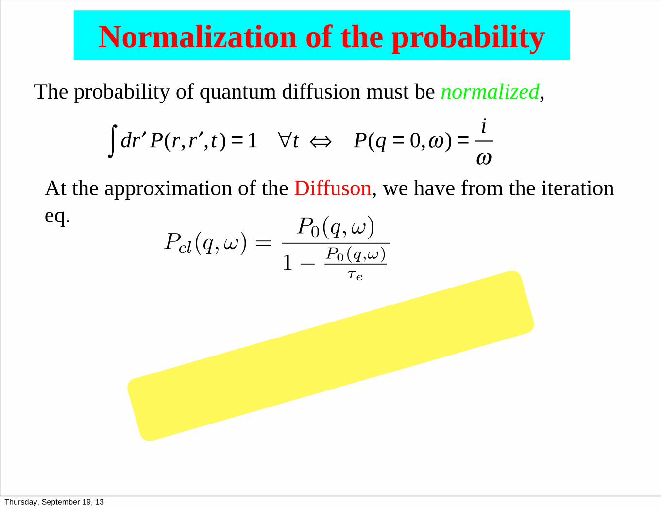
Normalization of the probabilityThe probability of quantum diffusion must be normalized,
d ′r P(r, ′r ,t) = 1 ∀t ⇔ P(q = 0,ω ) =iω∫
At the approximation of the Diffuson, we have from the iteration
eq.
since
The Diffuson provides a normalized approx. to the probability of
Quantum diffusion ! Missing terms ?
Pcl(q, !) =P0(q, !)
1 !
P0(q,!)
"e
P0(q, !) ="e
1 ! i!"e
" Pcl(q = 0, !) =i
!
Thursday, September 19, 13

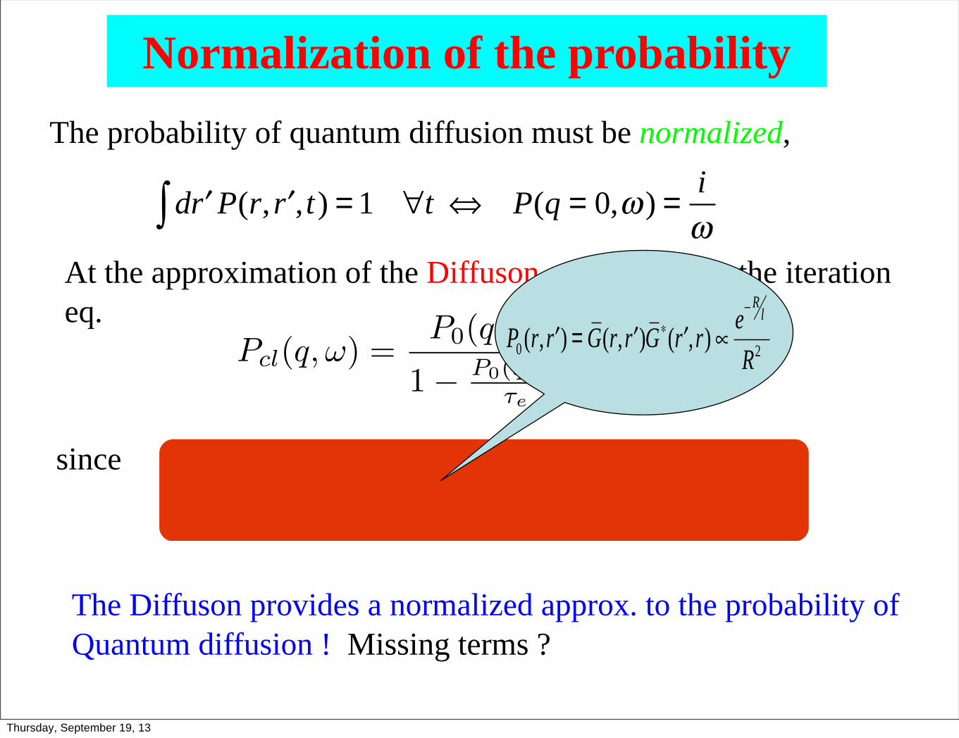
Normalization of the probabilityThe probability of quantum diffusion must be normalized,
d ′r P(r, ′r ,t) = 1 ∀t ⇔ P(q = 0,ω ) =iω∫
At the approximation of the Diffuson, we have from the iteration
eq.
since
The Diffuson provides a normalized approx. to the probability of
Quantum diffusion ! Missing terms ?
Pcl(q, !) =P0(q, !)
1 !
P0(q,!)
"e
P0(q, !) ="e
1 ! i!"e
" Pcl(q = 0, !) =i
!
Thursday, September 19, 13
Normalization of the probabilityThe probability of quantum diffusion must be normalized,
d ′r P(r, ′r ,t) = 1 ∀t ⇔ P(q = 0,ω ) =iω∫
At the approximation of the Diffuson, we have from the iteration
eq.
since
The Diffuson provides a normalized approx. to the probability of
Quantum diffusion ! Missing terms ?
Pcl(q, !) =P0(q, !)
1 !
P0(q,!)
"e
P0(q, !) ="e
1 ! i!"e
" Pcl(q = 0, !) =i
!
Pcl(r, r
! ) = P0(r, r
! ) +1!
!dr
!!Pcl(r, r
!! )P0(r
!! , r! )
Thursday, September 19, 13
Normalization of the probabilityThe probability of quantum diffusion must be normalized,
d ′r P(r, ′r ,t) = 1 ∀t ⇔ P(q = 0,ω ) =iω∫
At the approximation of the Diffuson, we have from the iteration
eq.
since
The Diffuson provides a normalized approx. to the probability of
Quantum diffusion ! Missing terms ?
Pcl(q, !) =P0(q, !)
1 !
P0(q,!)
"e
P0(q, !) ="e
1 ! i!"e
" Pcl(q = 0, !) =i
!
P0 (r, ′r ) = G(r, ′r )G∗( ′r ,r) ∝e−R
l
R2
Thursday, September 19, 13

Normalization of the probabilityThe probability of quantum diffusion must be normalized,
d ′r P(r, ′r ,t) = 1 ∀t ⇔ P(q = 0,ω ) =iω∫
At the approximation of the Diffuson, we have from the iteration
eq.
since
The Diffuson provides a normalized approx. to the probability of
Quantum diffusion ! Missing terms ?
Pcl(q, !) =P0(q, !)
1 !
P0(q,!)
"e
P0(q, !) ="e
1 ! i!"e
" Pcl(q = 0, !) =i
!
Thursday, September 19, 13
Reciprocity theorem
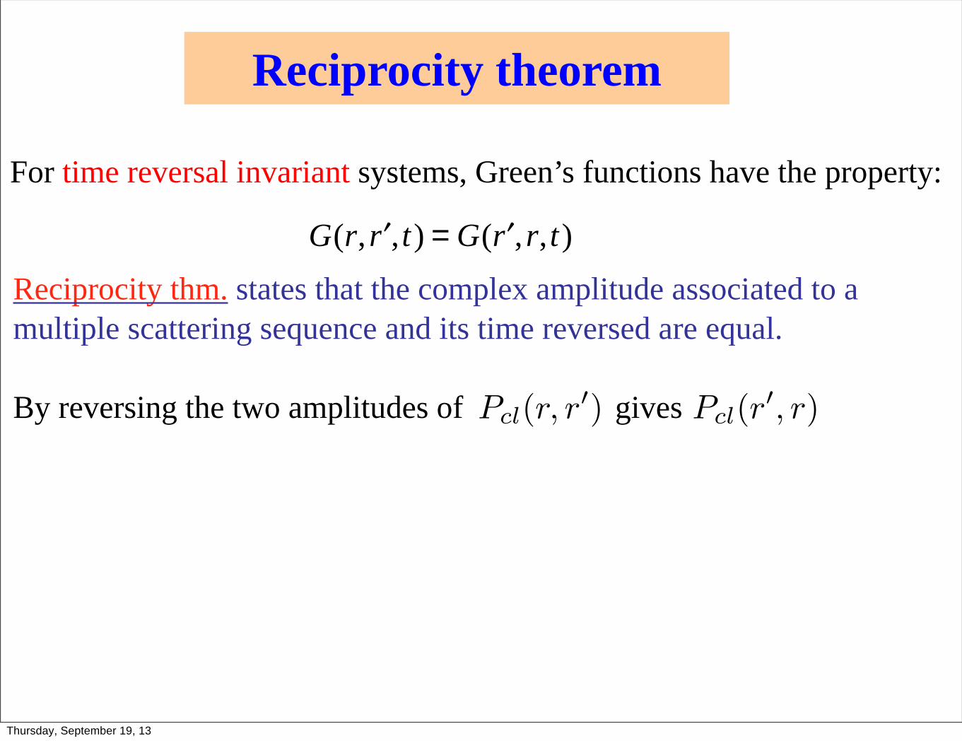
For time reversal invariant systems, Green’s functions have the property:
G(r, ′r ,t) = G( ′r ,r,t)Reciprocity thm. states that the complex amplitude associated to a
multiple scattering sequence and its time reversed are equal.
By reversing the two amplitudes of gives
Reversing only ONE of the two amplitudes should also give a
contribution to the probability, but it is not anymore a Diffuson!
The Diffuson approx. does not take into account all contributions to
the probability.
Pcl(r, r!) Pcl(r
!, r)
Thursday, September 19, 13
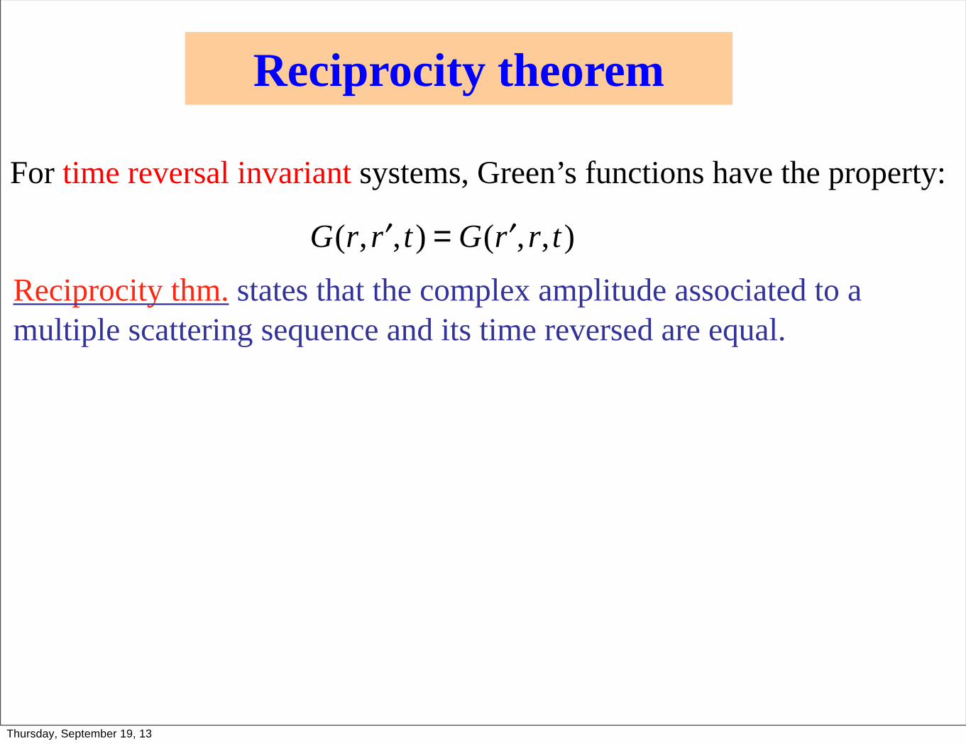
Reciprocity theorem
For time reversal invariant systems, Green’s functions have the property:
G(r, ′r ,t) = G( ′r ,r,t)Reciprocity thm. states that the complex amplitude associated to a
multiple scattering sequence and its time reversed are equal.
By reversing the two amplitudes of gives
Reversing only ONE of the two amplitudes should also give a
contribution to the probability, but it is not anymore a Diffuson!
The Diffuson approx. does not take into account all contributions to
the probability.
Pcl(r, r!) Pcl(r
!, r)
Thursday, September 19, 13

Reciprocity theorem
For time reversal invariant systems, Green’s functions have the property:
G(r, ′r ,t) = G( ′r ,r,t)Reciprocity thm. states that the complex amplitude associated to a
multiple scattering sequence and its time reversed are equal.
By reversing the two amplitudes of gives
Reversing only ONE of the two amplitudes should also give a
contribution to the probability, but it is not anymore a Diffuson!
The Diffuson approx. does not take into account all contributions to
the probability.
Pcl(r, r!) Pcl(r
!, r)
P (r, r!) ! |G!(r, r!)|2 =!
j
|Aj(r, r!)|2 +!
i"=j
A#i (r, r
!)Aj(r, r!)
Thursday, September 19, 13

Reciprocity theorem
For time reversal invariant systems, Green’s functions have the property:
G(r, ′r ,t) = G( ′r ,r,t)Reciprocity thm. states that the complex amplitude associated to a
multiple scattering sequence and its time reversed are equal.
By reversing the two amplitudes of gives
Reversing only ONE of the two amplitudes should also give a
contribution to the probability, but it is not anymore a Diffuson!
The Diffuson approx. does not take into account all contributions to
the probability.
Pcl(r, r!) Pcl(r
!, r)
Thursday, September 19, 13

k
k'
r1
rb
ry
r2
ra
rz
k
k'
r1
rb
ry
r2
ra
rz
(b)
(a)
r1 ! ra ! rb · · · ! ry ! rz ! r2
r2 ! rz ! ry · · · ! rb ! ra ! r1
The total average intensity is:
|A(k,k!)|2 =!
r1,r2
|f(r1, r2)|2"1 + ei(k+k!).(r1"r2)
#
incoherent
classical term
interference term
Diffuson
Cooperon
Thursday, September 19, 13

k
k'
r1
rb
ry
r2
ra
rz
k
k'
r1
rb
ry
r2
ra
rz
(b)
(a)
r1 ! ra ! rb · · · ! ry ! rz ! r2
r2 ! rz ! ry · · · ! rb ! ra ! r1
The total average intensity is:
|A(k,k!)|2 =!
r1,r2
|f(r1, r2)|2"1 + ei(k+k!).(r1"r2)
#
incoherent
classical term
interference term
Diffuson
Thursday, September 19, 13

k
k'
r1
rb
ry
r2
ra
rz
k
k'
r1
rb
ry
r2
ra
rz
(b)
(a)
r1 ! ra ! rb · · · ! ry ! rz ! r2
r2 ! rz ! ry · · · ! rb ! ra ! r1
The total average intensity is:
|A(k,k!)|2 =!
r1,r2
|f(r1, r2)|2"1 + ei(k+k!).(r1"r2)
#
incoherent
classical term
interference term
Diffuson
Cooperon
Thursday, September 19, 13

k
k'
r1
rb
ry
r2
ra
rz
k
k'
r1
rb
ry
r2
ra
rz
(b)
(a)
r1 ! ra ! rb · · · ! ry ! rz ! r2
r2 ! rz ! ry · · · ! rb ! ra ! r1
The total average intensity is:
|A(k,k!)|2 =!
r1,r2
|f(r1, r2)|2"1 + ei(k+k!).(r1"r2)
#
incoherent
classical term
interference term
Diffuson
Cooperon
Thursday, September 19, 13

|A(k,k!)|2 =!
r1,r2
|f(r1, r2)|2"1 + ei(k+k!).(r1"r2)
#
Generally, the interference term vanishes due to the
sum over , except for two notable cases:r1 and r2
k + k! ! 0 : Coherent backscattering
r1 ! r2 " 0 : closed loops, weak localization and periodicity
of the Sharvin effect.
!0/2
-100 0 100 200 300
0.8
1.2
1.6
2.0
Sca
led
In
ten
sity
Angle (mrad)
-5 0 51.8
1.9
2.0
Coherent backscattering
L
Lz
a
Thursday, September 19, 13

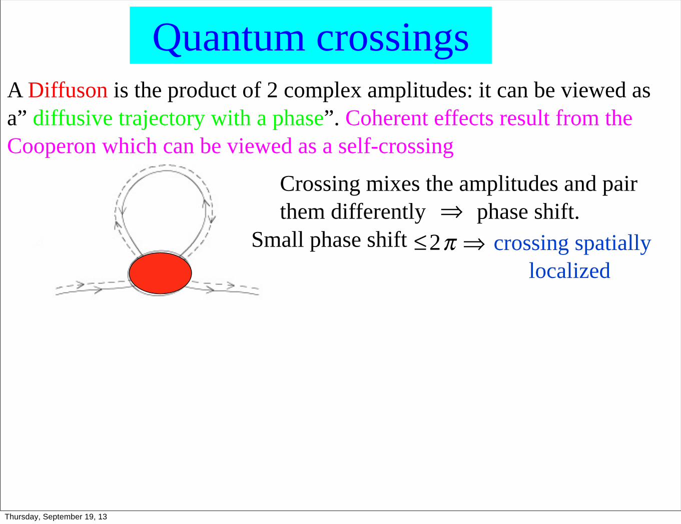
Quantum crossings
A Diffuson is the product of 2 complex amplitudes: it can be viewed as
a” diffusive trajectory with a phase”. Coherent effects result from the
Cooperon which can be viewed as a self-crossing
Crossing probability of 2 diffusons:
Crossing mixes the amplitudes and pair
them differently phase shift.⇒
τD = L2 / D
Small phase shift ≤2π ⇒ crossing spatially
localized
!d!1le
volume of a crossing
g =le
3!d!1
Ld!2 ! 1
�
p× =λd −1vg dt
Ld0
τ D
∫ =1
g
Thursday, September 19, 13

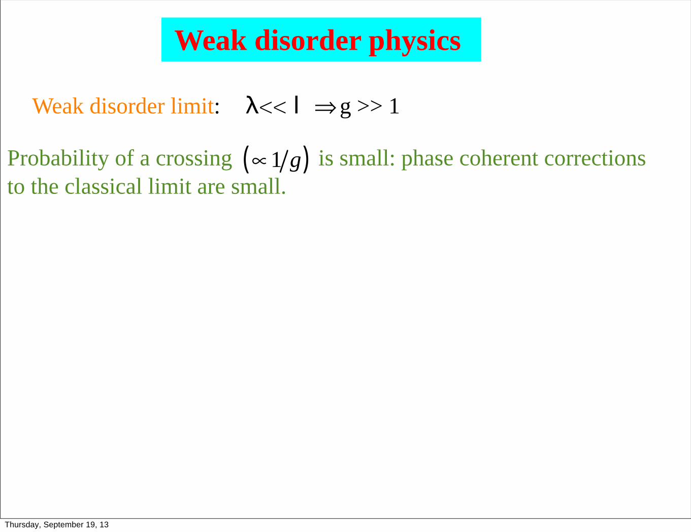
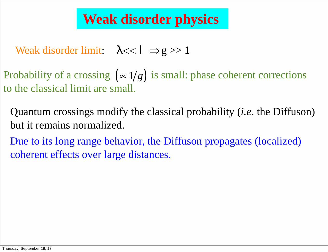
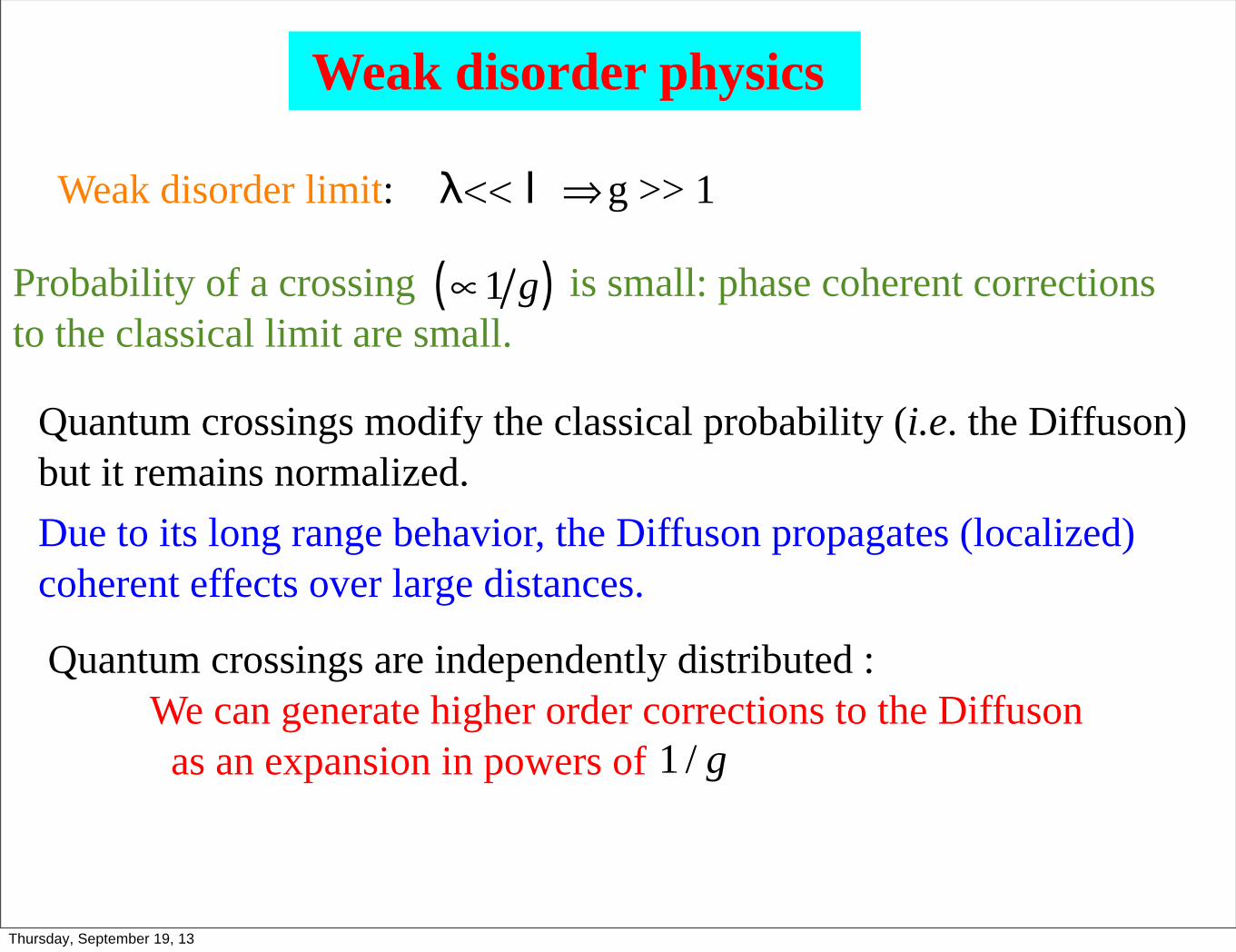
Weak disorder limit:
Probability of a crossing is small: phase coherent corrections
to the classical limit are small.
Quantum crossings modify the classical probability (i.e. the Diffuson)
but it remains normalized.
Due to its long range behavior, the Diffuson propagates (localized)
coherent effects over large distances.
Weak disorder physics
Quantum crossings are independently distributed :
We can generate higher order corrections to the Diffuson
as an expansion in powers of 1 / g
∝1 g( )
λ<< l ⇒ g >> 1
Thursday, September 19, 13
In the presence of a dephasing mechanism that breaks time coherence,
only trajectories with contribute.
In the presence of an Aharonov-Bohm flux, paired amplitudes in the
Cooperon acquire opposite phases:
!
2!"/"0 !2!"/"0the phase difference becomes: 4!"/"0
t < !!
Cooperon
!0/2 periodicity of the Sharvin effect
is obtained from the covariant diffusion equationPint(r, r!, t)
!1
!!
+"
"t! D
""r! + i
2e
h̄A(r!)
#2$
Pint(r, r!, t) = #(r ! r!)#(t)
effective charge 2e
Thursday, September 19, 13

To the classical probability corresponds
the Drude conductance Gcl
First correction involves one quantum
crossing and the probability to have a
closed loop:
(∝1 / g)
Return probability
quantum correction decreases
the conductance: weak localization
L
Weak localization- Electronic transport
τD = L2 D
Z(t) =
!drPint(r, r, t) =
"!D
4"t
#d/2
�
po (τD )
�
ΔGGcl
=− po (τD )
�
po (τD ) =1
gZ(t)
dtτD0
τ D
∫
Thursday, September 19, 13

Quantum mesoscopic physics :
the global scattering approach
(Landauer-Schwinger)
Thursday, September 19, 13

An Intermezzo !
global vs. local
Thursday, September 19, 13
Aim of the intermezzo:
to present in general terms, a global (i.e. non local) approach to account for both the thermodynamic and the non equilibrium behavior of quantum complex systems
In complex systems (metals, dielectrics, ...), it is difficult to obtain local quantities and sometimes it is even impossible. But in many cases, it is also not necessary.
Use a global description : Landauer-Schwinger approach
Thursday, September 19, 13

Elastic disorder does not break phase coherence and it does not introduce irreversibility
Disorder introduces randomness and complexity:
All symmetries are lost, there are no good quantum numbers.
A reminder
Thursday, September 19, 13
Elastic disorder does not break phase coherence and it does not introduce irreversibility
Disorder introduces randomness and complexity:
All symmetries are lost, there are no good quantum numbers.
Thursday, September 19, 13

Exemple: speckle patterns in optics
Diffraction through a circular aperture: order in
interference
Transmission of light through a
disordered suspension:
complex systemThursday, September 19, 13

Aim of the intermezzo:
to present in general terms, a global (i.e. non local) approach to account for both the thermodynamic and the non equilibrium behavior of quantum complex systems
In complex systems (metals, dielectrics, ...), it is difficult to obtain local quantities and sometimes it is even impossible. But in many cases, it is also not necessary.
Use a global description : Landauer-Schwinger approach
Thursday, September 19, 13
Basics: Usually we start from local differential equations and try to solve them with appropriate boundary conditions.
Express local physical quantities, e.g. electrical conductivity, dielectric function in terms of local Green’s functions for the quantum coherent matter field (electrons)
Thursday, September 19, 13
This approach is often doomed to failure due to either :1. local divergences of the Green’s functions close to a boundary
2. average over existing intrinsic disorder : no analytic known solution of the
Anderson problem either for weak or strong disorder.
Thursday, September 19, 13

This approach is often doomed to failure due to either :1. local divergences of the Green’s functions close to a boundary
2. average over existing intrinsic disorder : no analytic known solution of the
Anderson problem either for weak or strong disorder.
Thursday, September 19, 13

This approach is often doomed to failure due to either :1. local divergences of the Green’s functions close to a boundary
2. average over existing intrinsic disorder : no analytic known solution of the
Anderson problem either for weak or strong disorder.
Thursday, September 19, 13

3. It can be also because we simply do not have local differential eqs., e.g. on fractals
4. or because the physical quantity we wish to calculate does not have a local description : for instance there exists a local wave eqs. but we do not have a (local) Kubo formula for the diffusion coefficient.
Thursday, September 19, 13

3. It can be also because we simply do not have local differential eqs., e.g. on fractals
4. Or because the physical quantity we wish to calculate does not have a local description : for instance there exists a local wave eq. but we do not have a (local) Kubo formula for the diffusion coefficient.
Thursday, September 19, 13

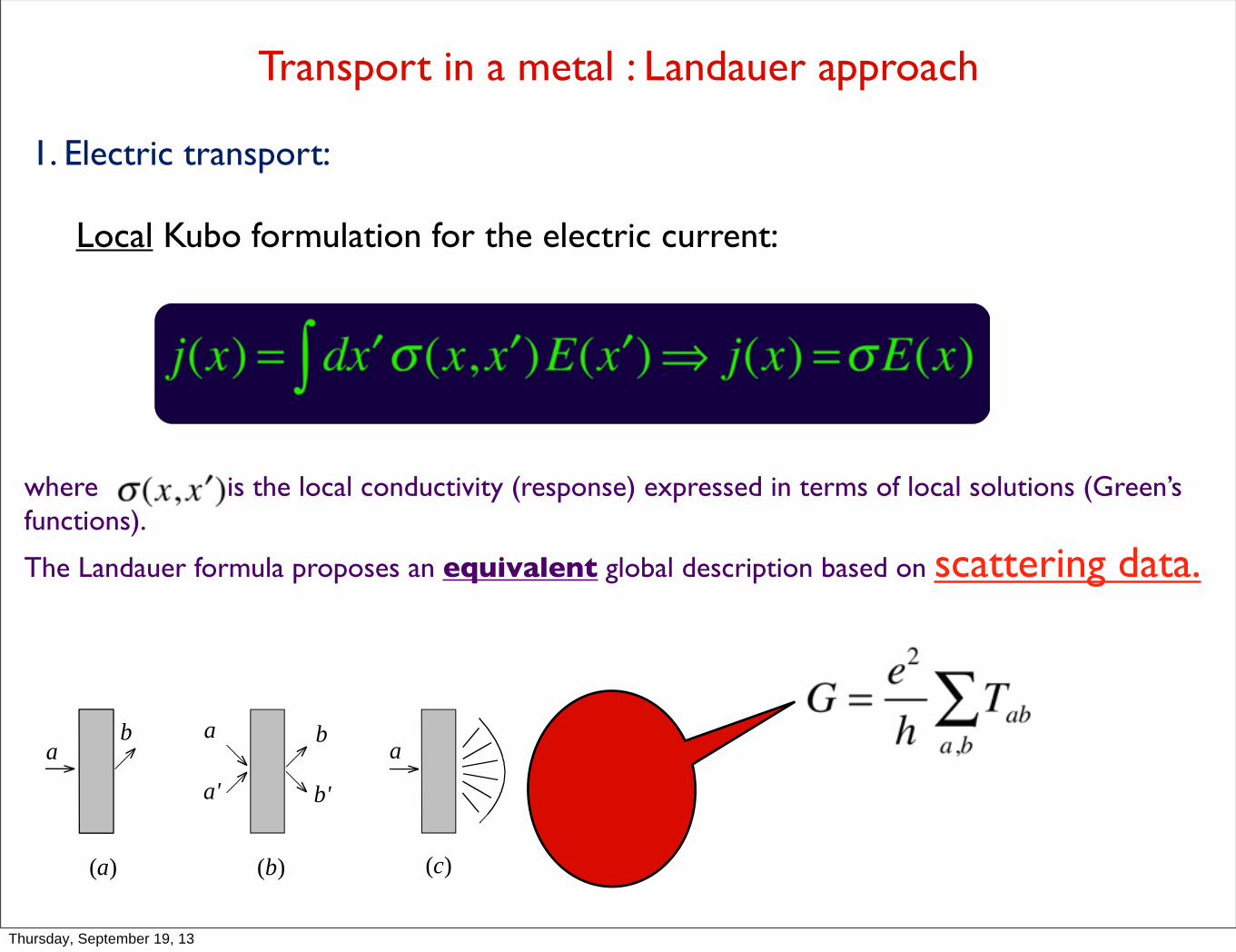
Transport in a metal : Landauer approach
1. Electric transport:
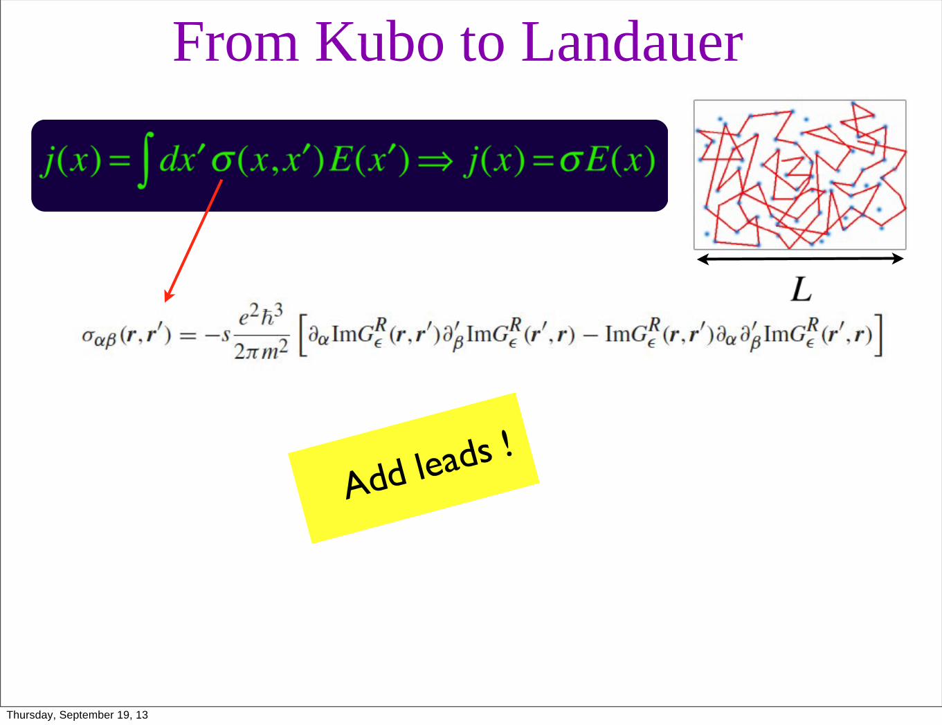
Local Kubo formulation for the electric current:
where is the local conductivity (response) expressed in terms of local solutions (Green’s functions). The Landauer formula proposes an equivalent global description based on scattering data.
(a)
ab a
ab
(b)
a' b'
(c) (d)
Thursday, September 19, 13

Transport in a metal : Landauer approach
1. Electric transport:
Local Kubo formulation for the electric current:
where is the local conductivity (response) expressed in terms of local solutions (Green’s functions).
The Landauer formula proposes an equivalent global description based on scattering data.
(a)
ab a
ab
(b)
a' b'
(c) (d)
Thursday, September 19, 13
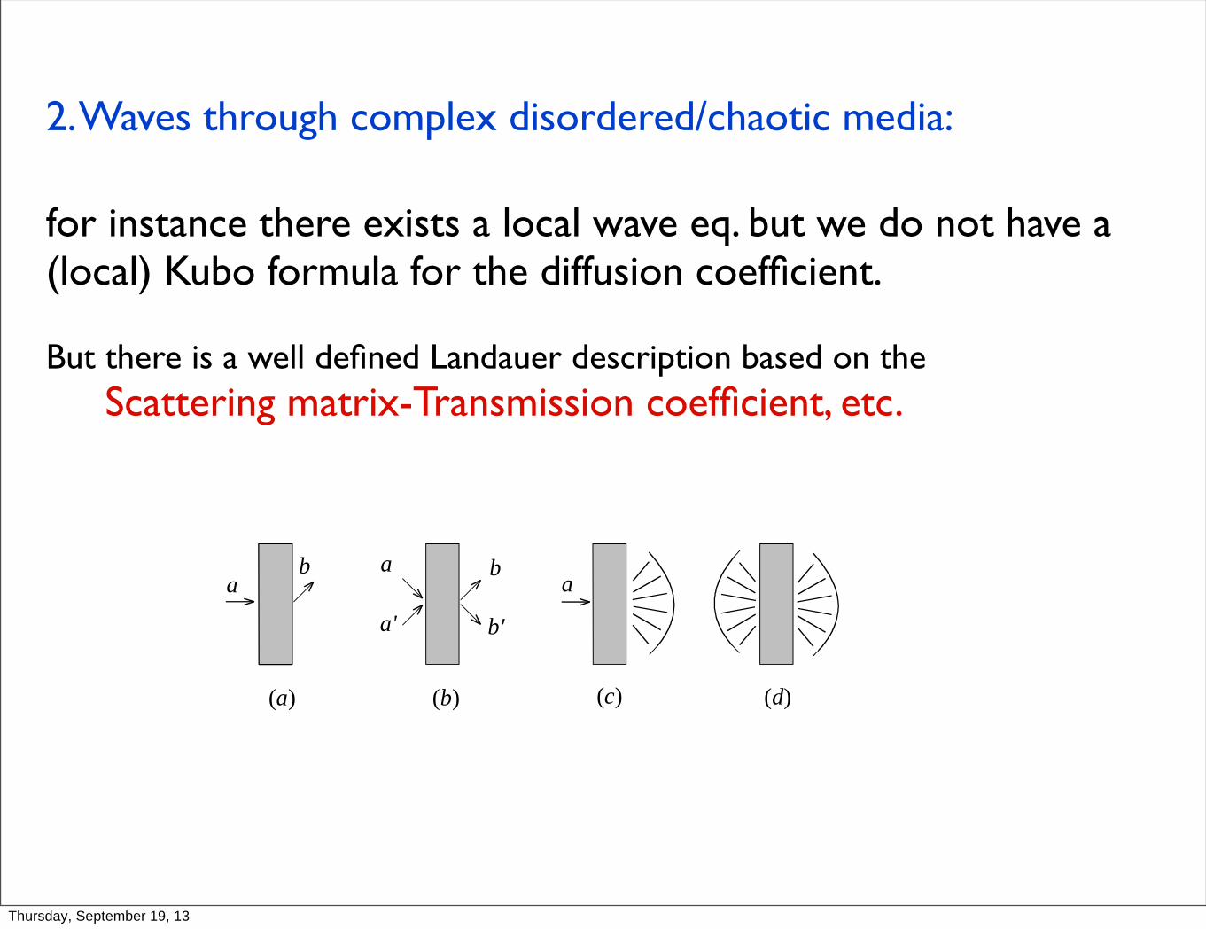
2. Waves through complex disordered/chaotic media:
for instance there exists a local wave eq. but we do not have a (local) Kubo formula for the diffusion coefficient.
But there is a well defined Landauer description based on the Scattering matrix-Transmission coefficient, etc.
(a)
ab a
ab
(b)
a' b'
(c) (d)
Thursday, September 19, 13

Spectral properties-Thermodynamics : Krein-Schwinger formula
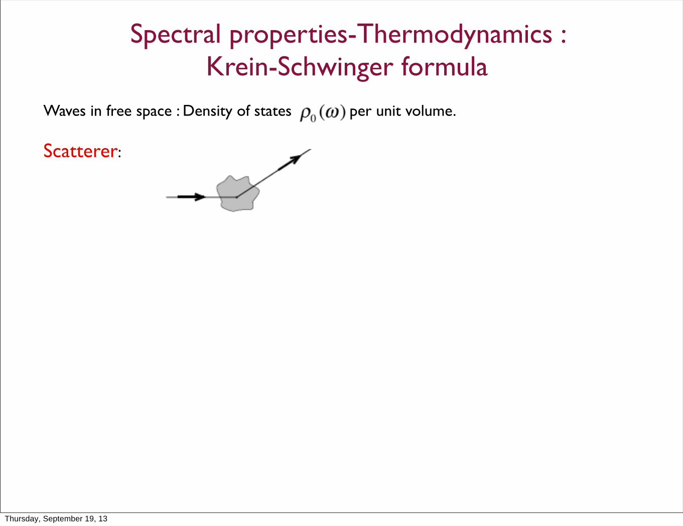
Waves in free space : Density of states per unit volume.
Scatterer:
The S-matrix accounts for all relevant changes : e.g. DOS of the waves in the presence of the scatterer is:
Thermodynamic changes can be deduced from this formula:
Variation of the partition function (Dashen,Ma,Bernstein):
Krein formula
Thursday, September 19, 13
Spectral properties-Thermodynamics : Krein-Schwinger formula
Waves in free space : Density of states per unit volume.
Scatterer:
The S-matrix accounts for all relevant changes : e.g. DOS of the waves in the presence of the scatterer is:
Thermodynamic changes can be deduced from this formula:
Variation of the partition function (Dashen,Ma,Bernstein):
Krein formula
Thursday, September 19, 13

Thermodynamics : persistent current in a mesoscopic ring submitted to a Aharonov-Bohm flux
Electrical conductance G (out of equilibrium)
Equivalent to the Landauer formula.
Energy spectrum of an electron in a Aharonov-Bohm magnetic flux
Easy !
Thursday, September 19, 13

Thermodynamics : persistent current in a mesoscopic ring submitted to a Aharonov-Bohm flux
Electrical conductance G (out of equilibrium)
Equivalent to the Landauer formula.
Energy spectrum of an electron in a Aharonov-Bohm magnetic flux
Easy !
Thursday, September 19, 13

Thermodynamics : persistent current in a mesoscopic ring submitted to a Aharonov-Bohm flux
Electrical conductance G (out of equilibrium)
Equivalent to the Landauer formula.
Energy spectrum of an electron in a Aharonov-Bohm magnetic flux
Easy !
Disordered metal
Less easy !
Thursday, September 19, 13

Thermodynamics : persistent current in a mesoscopic ring submitted to a Aharonov-Bohm flux
Electrical conductance G (out of equilibrium)
Equivalent to the Landauer formula.
Add leads !
Thursday, September 19, 13

Thermodynamics : persistent current in a mesoscopic ring submitted to a Aharonov-Bohm flux
Electrical conductance G (out of equilibrium)
Equivalent to the Landauer formula.
Thursday, September 19, 13

Thermodynamics : persistent current in a mesoscopic ring submitted to a Aharonov-Bohm flux
Electrical conductance G (out of equilibrium)
Equivalent to the Landauer formula.
Thursday, September 19, 13

From Kubo to Landauer
Landauer formula
Thursday, September 19, 13

From Kubo to Landauer
Landauer formula
Thursday, September 19, 13
From Kubo to Landauer
Landauer formula
Add leads !
Thursday, September 19, 13

From Kubo to Landauer
Thursday, September 19, 13

From Kubo to Landauer
Landauer formula
(a)
ab a
ab
(b)
a' b'
(c) (d)
Tab = tab2
Thursday, September 19, 13

Quantum conductance and shot noise
Slab geometry - two-terminal conductors
Landauer formula
(a)
ab a
ab
(b)
a' b'
(c) (d)
Tab = tab2
Thursday, September 19, 13

Noise power is defined as the symmetric current-current correlation function
where are electronic current operators
(Nyquist fluctuation-dissipation)
Equilibrium noise (V=0)
Thursday, September 19, 13

Non-equilibrium noise at
Excess noise measures the second cumulant of charge fluctuations :
Thursday, September 19, 13
The Fano factor
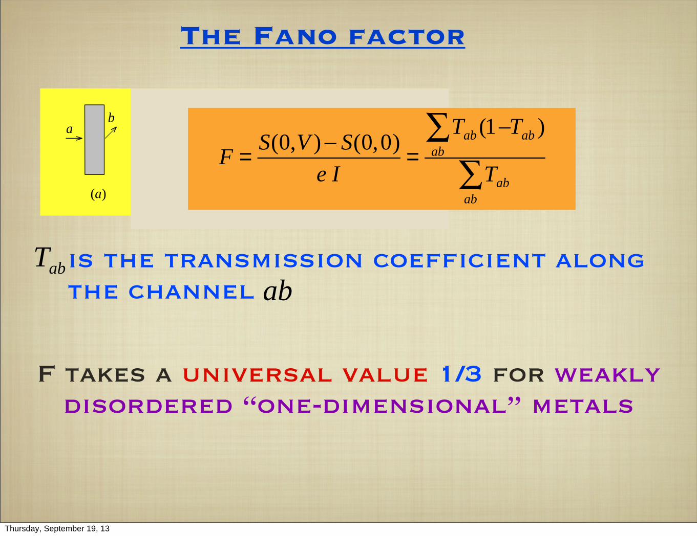
F takes a universal value 1/3 for weakly disordered “one-dimensional” metals
is the transmission coefficient along the channel
Tabab
(a)
ab a
ab
(b)
a' b'
(c) (d)
F = S(0,V )− S(0,0)
e I=
Tab (1−ab∑ Tab )
Tabab∑
Thursday, September 19, 13

Well known examples (Landauer-Schwinger approach). For didactic purposes, we shall review some of them and then present new limits and results.
Basic idea of Landauer-Schwinger is to provide a non local approach by means of tools like the S-matrix.
Physically relevant quantities of a system are expressed in terms of in-out signals, including correlations.
This idea has been successfully used in Quantum mesoscopic physics, quantum optics, quantum field theory,...
It is relatively new and promising in other fields:
1.Shannon information theory- MIMO (Multiple input-Multiple output)2.Full counting statistics and shot noise (quantum mesoscopic physics)3.Out of equilibrium quantum systems- Wigner time delay4.Casimir effects5.Non-perturbative effects (Unruh effects, Hawking radiation, Schwinger pair production,...)6.Waves and quantum mechanics on fractal structures.
To end this intermezzo :
Thursday, September 19, 13

Energy spectrum - Thermodynamics - Transport ?
Thursday, September 19, 13

Energy spectrum - Thermodynamics - Transport ?
Add leads !
Thursday, September 19, 13

Energy spectrum - Thermodynamics - Transport ?
and calculate the S-matrix : possible
Thursday, September 19, 13

How to connect the 2 previous approaches:
* Local quantum crossings
* Global Landauer scattering formalism
Thursday, September 19, 13

Beyond the conductance
Thursday, September 19, 13
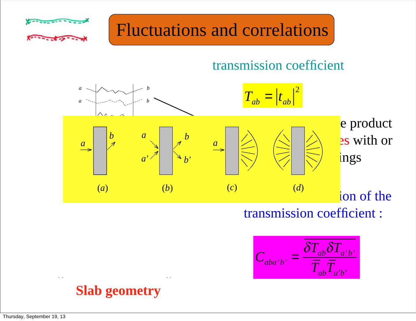
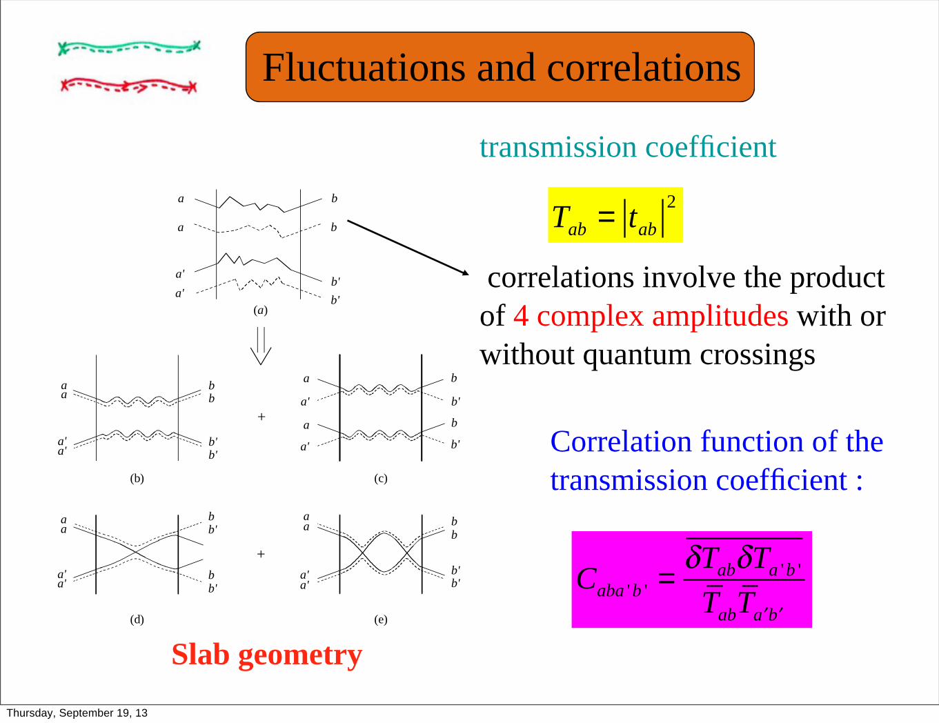
Tab = tab2
Caba 'b ' =δTabδTa 'b '
TabT ′a ′b
Slab geometry
transmission coefficient
Correlation function of the
transmission coefficient :
correlations involve the product
of 4 complex amplitudes with or
without quantum crossingsaa
a'a'
bb
b'
(b)
b'
b'
a
a
a'
(c)
a'
b
b
b'
(a)
(d) (e)
aa
a'a'
b'
b
b'
b
a
a
a'a'
b
b
b'b'
+
+
aa
a'a'
b
b
b'
b'
Fluctuations and correlations
(a)
ab a
ab
(b)
a' b'
(c) (d)
Thursday, September 19, 13

Tab = tab2
Caba 'b ' =δTabδTa 'b '
TabT ′a ′b
Slab geometry
transmission coefficient
Correlation function of the
transmission coefficient :
correlations involve the product
of 4 complex amplitudes with or
without quantum crossingsaa
a'a'
bb
b'
(b)
b'
b'
a
a
a'
(c)
a'
b
b
b'
(a)
(d) (e)
aa
a'a'
b'
b
b'
b
a
a
a'a'
b
b
b'b'
+
+
aa
a'a'
b
b
b'
b'
Fluctuations and correlations
Thursday, September 19, 13

Classical transport : Gcl = g !e2
hwith g " 1
Quantum corrections: !G = Gcl !1
g
A direct consequence: quantum corrections to electrical transport
so that is universal#
Not that simple ! We wish to obtain precise
numbers... Need to sum up Feynman diagrams.
Thursday, September 19, 13

The Fano factor
F takes a universal value 1/3 for weakly disordered “one-dimensional” metals
is the transmission coefficient along the channel
Tabab
(a)
ab a
ab
(b)
a' b'
(c) (d)
F = S(0,V )− S(0,0)
e I=
Tab (1−ab∑ Tab )
Tabab∑
Since we know how to get numbers, what about that one ?
Thursday, September 19, 13

Weak localization corrections to the
electrical conductance
Z(t)= dr Pcl (r,r,t)=∫τD
4πt⎛⎝⎜
⎞⎠⎟
d /2
Conductance fluctuations
Summary ... and closed loops :
�
δG2
Gcl2∝
1
g2Z(t)
t dtτD
2
0
τ D
∫
�
ΔGGcl
∝−1
gZ(t) dt
τD0
τ D
∫
Thursday, September 19, 13

Weak localization corrections to the
electrical conductance
Z(t)= dr Pcl (r,r,t)=∫τD
4πt⎛⎝⎜
⎞⎠⎟
d /2
Conductance fluctuations
Summary ... and closed loops :
�
δG2
Gcl2∝
1
g2Z(t)
t dtτD
2
0
τ D
∫
�
ΔGGcl
∝−1
gZ(t) dt
τD0
τ D
∫
Thursday, September 19, 13

An exercise
Thursday, September 19, 13

Universal conductance fluctuations
Dephasing and decoherence
aa
bb
a'a' b'
b'
(K )1
aa
bb
b'b'a'
a'
(K )2
aa
a'a'
bb
b'b'
(K )d3
aa
a'a'
bb
b'b'
(K )c3
cd
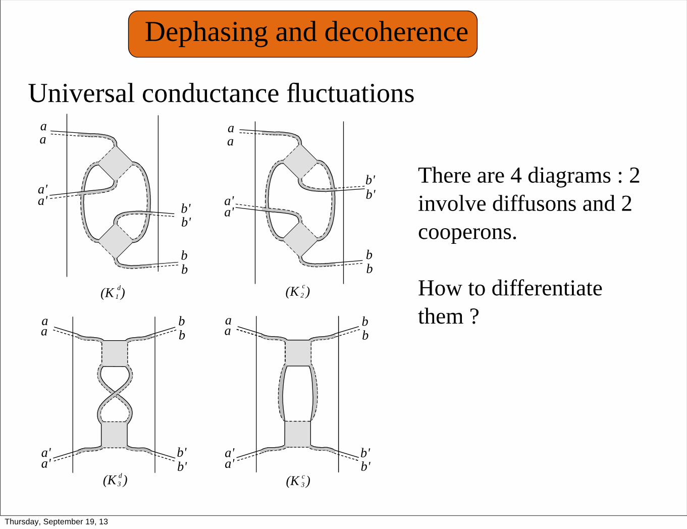
There are 4 diagrams : 2
involve diffusons and 2
cooperons.
How to differentiate
them ?
aa
a'a'
bb
b'
(b)
b'
b'
a
a
a'
(c)
a'
b
b
b'
(a)
(d) (e)
aa
a'a'
b'
b
b'
b
a
a
a'a'
b
b
b'b'
+
+
aa
a'a'
b
b
b'
b'
Thursday, September 19, 13
Universal conductance fluctuations
Dephasing and decoherence
aa
bb
a'a' b'
b'
(K )1
aa
bb
b'b'a'
a'
(K )2
aa
a'a'
bb
b'b'
(K )d3
aa
a'a'
bb
b'b'
(K )c3
cd
There are 4 diagrams : 2
involve diffusons and 2
cooperons.
How to differentiate
them ?
Thursday, September 19, 13

Universal conductance fluctuations
Dephasing and decoherence
aa
bb
a'a' b'
b'
(K )1
aa
bb
b'b'a'
a'
(K )2
aa
a'a'
bb
b'b'
(K )d3
aa
a'a'
bb
b'b'
(K )c3
cd
sensitive to an applied
Aharonov-Bohm magnetic flux
!
!!
!
!
There are 4 diagrams : 2
involve diffusons and 2
cooperons.
How to differentiate
them ?
Thursday, September 19, 13

Universal conductance fluctuations
Dephasing and decoherence
aa
bb
a'a' b'
b'
(K )1
aa
bb
b'b'a'
a'
(K )2
aa
a'a'
bb
b'b'
(K )d3
aa
a'a'
bb
b'b'
(K )c3
cd
2 Diffusons
2 Cooperons
sensitive to an applied
Aharonov-Bohm magnetic flux
!
!!
!
!
Thursday, September 19, 13

We expect the conductance
fluctuations to be reduced by a factor 2
!G2 !G2
2
!
1.5
vanishing of the weak localization
correction for the same magnetic field
In the presence of incoherent
processes : L > L!
!G2 ! 0
46 Si-doped GaAs samples at 45 mK
!G2
�
G
(Mailly-Sanquer)
Thursday, September 19, 13
Beyond weak disorder - a glimpse of Anderson
localization phase transition
Thursday, September 19, 13
Weak disorder limit:
Probability of a crossing is small: phase coherent corrections
to the classical limit are small.
Quantum crossings modify the classical probability (i.e. the Diffuson)
but it remains normalized.
Due to its long range behavior, the Diffuson propagates (localized)
coherent effects over large distances.
Weak disorder physics
Quantum crossings are independently distributed :
We can generate higher order corrections to the Diffuson
as an expansion in powers of 1 / g
∝1 g( )
λ<< l ⇒ g >> 1
Thursday, September 19, 13
114
Expansion in powers of quantum crossings allows to calculate quantum corrections to physical quantities.
This singular perturbation expansion is not a simple coincidence but an expression of scaling
A renormalization of D(L) changes also g(L):
1 g
The diffusion coefficient D is reduced (weak localization) and becomes size dependent :
g(L) =D(L)
cλd−1Ld−2 ≈
N⊥2 (L)
N
A quantum phase transition: Anderson localization
D(L) = D 1−1
πgln L
l( ) +1
πgln L
l( )⎛⎝⎜
⎞⎠⎟
2
+ ....⎛
⎝⎜
⎞
⎠⎟ (d = 2)
Thursday, September 19, 13

115
Expansion in powers of quantum crossings allows to calculate quantum corrections to physical quantities.
This singular perturbation expansion is not a simple coincidence but an expression of scaling
A renormalization of D(L) changes also g(L):
1 g
The diffusion coefficient D is reduced (weak localization) and becomes size dependent :
g(L) =D(L)
cλd−1Ld−2 ≈
N⊥2 (L)
N
A quantum phase transition: Anderson localization
D(L) = D 1−1
πgln L
l( ) +1
πgln L
l( )⎛⎝⎜
⎞⎠⎟
2
+ ....⎛
⎝⎜
⎞
⎠⎟ (d = 2)
Thursday, September 19, 13
116
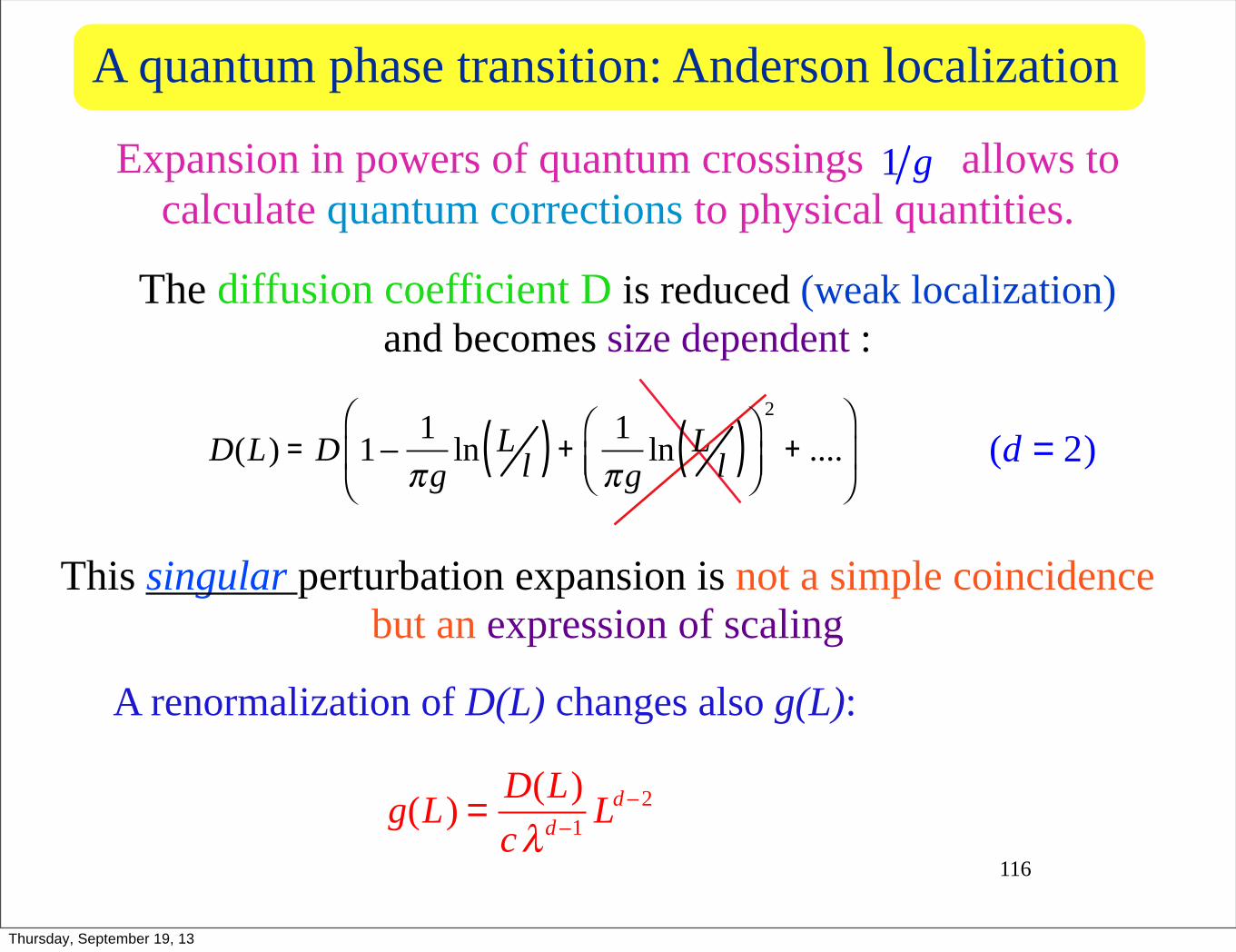
Expansion in powers of quantum crossings allows to calculate quantum corrections to physical quantities.
This singular perturbation expansion is not a simple coincidence but an expression of scaling
A renormalization of D(L) changes also g(L):
1 g
The diffusion coefficient D is reduced (weak localization) and becomes size dependent :
g(L) =D(L)
cλd−1Ld−2 ≈
N⊥2 (L)
N
A quantum phase transition: Anderson localization
D(L) = D 1−1
πgln L
l( ) +1
πgln L
l( )⎛⎝⎜
⎞⎠⎟
2
+ ....⎛
⎝⎜
⎞
⎠⎟ (d = 2)
Thursday, September 19, 13
117
Scaling and its meaning :
If we know , we know it at any scale :
g (L(1 + !)) = g(L)!1 + !"(g) + O(g!5)
"
!(g) =d ln g
d lnL
Expanding, we have
with (Gell-Mann - Low function)
Scaling behavior :
(P.W. Anderson et al.,1979)
g(L)
g L(1+ ε)( )= f g(L),ε( )
ξ(W ) is the localization length
g(L,W ) = f Lξ(W )( )
Thursday, September 19, 13

118
Scaling and its meaning :
If we know , we know it at any scale :
g (L(1 + !)) = g(L)!1 + !"(g) + O(g!5)
"
!(g) =d ln g
d lnL
Expanding, we have
with (Gell-Mann - Low function)
Scaling behavior :
(P.W. Anderson et al.,1979)
g(L)
g L(1+ ε)( )= f g(L),ε( )
ξ(W ) is the localization length
g(L,W ) = f Lξ(W )( )
Thursday, September 19, 13

119
Scaling and its meaning :
If we know , we know it at any scale :
g (L(1 + !)) = g(L)!1 + !"(g) + O(g!5)
"
!(g) =d ln g
d lnL
Expanding, we have
with (Gell-Mann - Low function)
Scaling behavior :
(P.W. Anderson et al.,1979)
g(L)
g L(1+ ε)( )= f g(L),ε( )
ξ(W ) is the localization length
g(L,W ) = f Lξ(W )( )
Thursday, September 19, 13

120
Scaling and its meaning :
If we know , we know it at any scale :
g (L(1 + !)) = g(L)!1 + !"(g) + O(g!5)
"
!(g) =d ln g
d lnL
Expanding, we have
with (Gell-Mann - Low function)
Scaling behavior :
(P.W. Anderson et al.,1979)
g(L)
g L(1+ ε)( )= f g(L),ε( )
ξ(W ) is the localization length
g(L,W ) = f Lξ(W )( )
Thursday, September 19, 13

g(L,W )
Lξ(W )
d = 3
Anderson phase transition
d = 2
B.Kramer, A. McKinnon, 1981
Anderson localization phase transition occurs in d > 2
It has been observed experimentally with electromagnetic waves (Aegarter, Maret et al., 2006)
Numerical calculations on the (universal) Anderson Hamiltonian
Thursday, September 19, 13