phy-6795 magnetohydrodynamique astrophysiquepaulchar/phy6795/ch1+2.pdf · 2 avertissement les notes...
TRANSCRIPT
1
PHY-6795
MAGNETOHYDRODYNAMIQUE
ASTROPHYSIQUE
Notes de cours
Paul Charbonneau
Departement de Physique
Universite de Montreal
Septembre 2008
2
AVERTISSEMENT
Les notes qui suivent ont ete originellement preparees dans le cadre d’un cours gradueen Physique Solaire enseigne a trois reprises par Tom Bogdan et moi-meme a l’Universite duColorado a Boulder, sous les sigles APAS7500 et ASTR7500, ainsi qu’en automne 2004 a l’UdeMdans la cadre de la premiere moitie de PHY6795A. Vous remarquerez rapidement que ces notesde cours sont ecrites en anglais. La raison principale en est que ce que vous avez en mainrepresente une partie d’un ouvrage gradue sur la magnetohydrodynamique solaire, que Tom etmoi esperons bien finir par publier un de ces jours... Comme vous le constaterez rapidement,tous les chapitres n’en sont pas au meme stade de “perfectionnement”; Tom et moi apprecierionsgrandement tout commentaires et suggestions que vous pourriez nous faire quant au contenuet a la presentation des sujets couverts ici.
La magnetohydrodynamique astrophysique est un sujet particulierement vaste; fidele al’approche adoptee des la premiere version de ce cours, J’ai choisi ici de couvrir deux sujets endetails, plutot que de faire un survol inevitablement superficiel de tout le domaine.
En electromagnetisme, le choix d’unites a des consequences non-triviales, entre autre auniveau de la forme que prennent les equations de Maxwell. Bien que les unites CGS demeurentla norme en astrophysique, j’ai finalement choisi d’utiliser dans ces notes le systeme SI (aliasMKS). J’ai cependant inclut un petit Appendice qui, je l’espere, devrait aider les accros dusysteme CGS a s’y retrouver dans le passage des gauss aux tesla, des weber aux maxwell, etc.
Au fil des annees et a travers les diverses incarnations de ces notes de cours, plusieurscollegues ont apporte des contributions importantes et/ou gracieusement fourni des diagrammesou resultats de calculs numeriques servant a illustrer certains aspects de la matiere couverte. Jetiens particulierement a remercier Fausto Cattaneo, David Galloway, Keith MacGregor, SteveTobias, Mathieu Ossendrijver, Nic Brummell, Rony Keppens et Gregg Wade. Merci egalementa Jacques Richer pour sa precieuse aide avec les subtilites du LaTeX avance
La version 2008 de ces notes a grandement beneficie d’une lecture critique en aout 2008par Michel-Andre Vallieres-Nollet; en plus de lui offrir ici mes plus chaleureux remerciements,je profite de cette pseudo-preface pour lui promettre une lecture tout aussi attentive de sonmemoire de maitrise!
Paul CharbonneauMontreal, septembre 2008
Contents
I Introduction 7
1 Magnetohydrodynamics 9
1.1 The fluid approximation . . . . . . . . . . . . . . . . . . . . . . . . . . . . . . . 9
1.1.1 Matter as a continuum . . . . . . . . . . . . . . . . . . . . . . . . . . . . 9
1.1.2 Solid versus fluid . . . . . . . . . . . . . . . . . . . . . . . . . . . . . . . 11
1.2 Essentials of hydrodynamics . . . . . . . . . . . . . . . . . . . . . . . . . . . . . 11
1.2.1 Mass: the continuity equation . . . . . . . . . . . . . . . . . . . . . . . . 12
1.2.2 The D/Dt operator . . . . . . . . . . . . . . . . . . . . . . . . . . . . . 13
1.2.3 Linear momentum: the Navier-Stokes equations . . . . . . . . . . . . . . 14
1.2.4 Angular momentum: the vorticity equation . . . . . . . . . . . . . . . . 16
1.2.5 Energy: the entropy equation . . . . . . . . . . . . . . . . . . . . . . . . 17
1.3 The magnetohydrodynamical induction equation . . . . . . . . . . . . . . . . . 18
1.4 Scaling analysis . . . . . . . . . . . . . . . . . . . . . . . . . . . . . . . . . . . . 19
1.5 The Lorentz force . . . . . . . . . . . . . . . . . . . . . . . . . . . . . . . . . . . 21
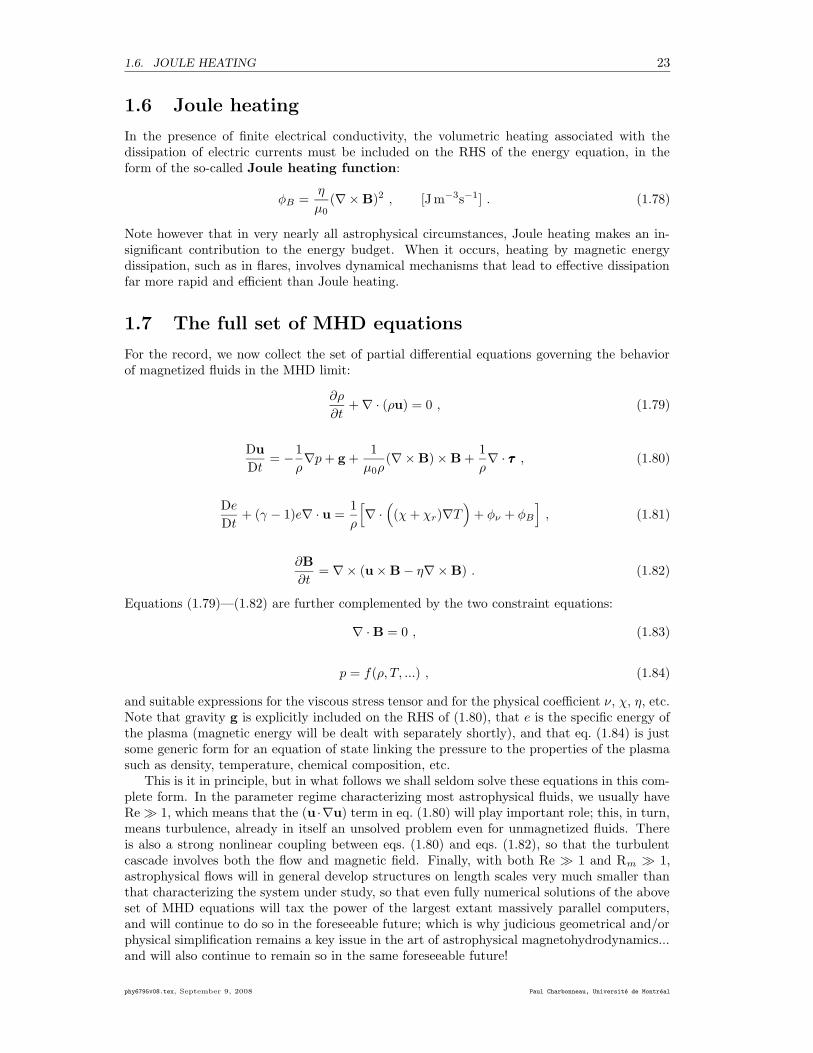
1.6 Joule heating . . . . . . . . . . . . . . . . . . . . . . . . . . . . . . . . . . . . . 23
1.7 The full set of MHD equations . . . . . . . . . . . . . . . . . . . . . . . . . . . 23
1.8 MHD waves . . . . . . . . . . . . . . . . . . . . . . . . . . . . . . . . . . . . . . 24
1.9 Magnetic energy . . . . . . . . . . . . . . . . . . . . . . . . . . . . . . . . . . . 25
1.10 Magnetic flux freezing and Alfven’s theorem . . . . . . . . . . . . . . . . . . . . 25
1.11 Magnetic helicity . . . . . . . . . . . . . . . . . . . . . . . . . . . . . . . . . . . 26
1.12 Mathematical representations of magnetic fields . . . . . . . . . . . . . . . . . . 27
1.12.1 Pseudo-vectors and solenoidal vectors . . . . . . . . . . . . . . . . . . . 27
1.12.2 The vector potential . . . . . . . . . . . . . . . . . . . . . . . . . . . . . 28
1.12.3 Axisymmetric magnetic fields . . . . . . . . . . . . . . . . . . . . . . . . 28
1.12.4 Force-free magnetic fields . . . . . . . . . . . . . . . . . . . . . . . . . . 29
2 Magnetic fields in astrophysics 33
2.1 Earth’s magnetic field . . . . . . . . . . . . . . . . . . . . . . . . . . . . . . . . 33
2.2 Other solar system planets . . . . . . . . . . . . . . . . . . . . . . . . . . . . . . 34
2.3 The Sun . . . . . . . . . . . . . . . . . . . . . . . . . . . . . . . . . . . . . . . . 35
2.4 Sun-like stars . . . . . . . . . . . . . . . . . . . . . . . . . . . . . . . . . . . . . 37
2.5 Early-type stars . . . . . . . . . . . . . . . . . . . . . . . . . . . . . . . . . . . . 40
2.6 Pre- and post-main-sequence stars . . . . . . . . . . . . . . . . . . . . . . . . . 42
2.7 Compact objects . . . . . . . . . . . . . . . . . . . . . . . . . . . . . . . . . . . 44
2.8 Galaxies and beyond . . . . . . . . . . . . . . . . . . . . . . . . . . . . . . . . . 44
2.9 Why B and not E? . . . . . . . . . . . . . . . . . . . . . . . . . . . . . . . . . . 45
2.10 The ultimate origin of astrophysical magnetic fields . . . . . . . . . . . . . . . . 45
2.10.1 Magnetic monopoles . . . . . . . . . . . . . . . . . . . . . . . . . . . . . 47
2.10.2 Batteries . . . . . . . . . . . . . . . . . . . . . . . . . . . . . . . . . . . 47
3
4 CONTENTS
II Magnetized stellar winds 51
3 The solar wind 53
3.1 Solar and stellar coronae and winds . . . . . . . . . . . . . . . . . . . . . . . . . 533.1.1 The solar corona . . . . . . . . . . . . . . . . . . . . . . . . . . . . . . . 533.1.2 The solar wind . . . . . . . . . . . . . . . . . . . . . . . . . . . . . . . . 54
3.2 Hydrostatic Corona Model . . . . . . . . . . . . . . . . . . . . . . . . . . . . . . 573.3 Polytropic winds . . . . . . . . . . . . . . . . . . . . . . . . . . . . . . . . . . . 59
3.3.1 The Parker Solution . . . . . . . . . . . . . . . . . . . . . . . . . . . . . 593.3.2 Computing a solution . . . . . . . . . . . . . . . . . . . . . . . . . . . . 613.3.3 Mass loss . . . . . . . . . . . . . . . . . . . . . . . . . . . . . . . . . . . 623.3.4 Asymptotic behavior and existence of wind solutions . . . . . . . . . . 633.3.5 Energetics . . . . . . . . . . . . . . . . . . . . . . . . . . . . . . . . . . . 643.3.6 Comparison with the Solar Wind . . . . . . . . . . . . . . . . . . . . . . 65
4 Magnetic confinement of winds 69
4.1 Magnetic fields in the solar corona . . . . . . . . . . . . . . . . . . . . . . . . . 694.2 The plasma-β . . . . . . . . . . . . . . . . . . . . . . . . . . . . . . . . . . . . . 704.3 The β = 0 case: magnetostatic solutions . . . . . . . . . . . . . . . . . . . . . . 704.4 The β ¿ 1 limit: magnetic flow tubes . . . . . . . . . . . . . . . . . . . . . . . 724.5 Generalized polytropic wind solutions . . . . . . . . . . . . . . . . . . . . . . . 744.6 The β À 1 limit: The Parker spiral . . . . . . . . . . . . . . . . . . . . . . . . . 76
5 Magnetic driving of winds 81
5.1 The Weber-Davis MHD wind solution . . . . . . . . . . . . . . . . . . . . . . . 815.2 Numerical models of rotating MHD winds . . . . . . . . . . . . . . . . . . . . . 875.3 Stellar spin-down . . . . . . . . . . . . . . . . . . . . . . . . . . . . . . . . . . . 91
5.3.1 Stellar rotation: the observational picture . . . . . . . . . . . . . . . . . 915.3.2 The Skumanich square root law . . . . . . . . . . . . . . . . . . . . . . . 925.3.3 The spindown of late-type stars . . . . . . . . . . . . . . . . . . . . . . . 95
5.4 Wind driving by Alfven waves . . . . . . . . . . . . . . . . . . . . . . . . . . . . 965.4.1 The magnetic force exerted by Alfven waves . . . . . . . . . . . . . . . . 965.4.2 The Wave force in the WKB approximation . . . . . . . . . . . . . . . . 975.4.3 Obtaining wind solutions . . . . . . . . . . . . . . . . . . . . . . . . . . 985.4.4 Some representative solar solutions . . . . . . . . . . . . . . . . . . . . . 985.4.5 Wave-driven winds . . . . . . . . . . . . . . . . . . . . . . . . . . . . . . 100
III Astrophysical Dynamos 105
6 The solar cycle as a dynamo 107
6.1 The solar cycle . . . . . . . . . . . . . . . . . . . . . . . . . . . . . . . . . . . . 1076.1.1 Sunspots . . . . . . . . . . . . . . . . . . . . . . . . . . . . . . . . . . . 1076.1.2 The sunspot cycle . . . . . . . . . . . . . . . . . . . . . . . . . . . . . . 1106.1.3 The Waldmaier and Gnevyshev-Ohl Rules . . . . . . . . . . . . . . . . . 1116.1.4 The butterfly diagram . . . . . . . . . . . . . . . . . . . . . . . . . . . . 1146.1.5 Hale’s polarity laws . . . . . . . . . . . . . . . . . . . . . . . . . . . . . 1156.1.6 Joy’s law . . . . . . . . . . . . . . . . . . . . . . . . . . . . . . . . . . . 1166.1.7 Modeling the buoyant rise of magnetic flux ropes . . . . . . . . . . . . . 1176.1.8 Poloidal field reversals . . . . . . . . . . . . . . . . . . . . . . . . . . . . 1186.1.9 Current helicity in active regions . . . . . . . . . . . . . . . . . . . . . . 1196.1.10 The Maunder Minimum . . . . . . . . . . . . . . . . . . . . . . . . . . . 1196.1.11 Cyclic modulation of solar activity . . . . . . . . . . . . . . . . . . . . . 1206.1.12 Summary of solar cycle characteristics . . . . . . . . . . . . . . . . . . . 121
6.2 A simple dynamo . . . . . . . . . . . . . . . . . . . . . . . . . . . . . . . . . . . 121
CONTENTS 5
6.3 The astrophysical dynamo problem(s) . . . . . . . . . . . . . . . . . . . . . . . 124
7 Decay and Amplification of Magnetic Fields 129
7.1 Resistive decays of magnetic fields . . . . . . . . . . . . . . . . . . . . . . . . . 1297.1.1 Reformulation as an eigenvalue problem . . . . . . . . . . . . . . . . . . 1307.1.2 Poloidal field decay . . . . . . . . . . . . . . . . . . . . . . . . . . . . . . 1317.1.3 Toroidal field decay . . . . . . . . . . . . . . . . . . . . . . . . . . . . . 1327.1.4 Results for a magnetic diffusivity varying with depth . . . . . . . . . . . 134
7.2 Magnetic field amplification by stretching and shearing . . . . . . . . . . . . . 1357.2.1 Hydrodynamical stretching and field amplification . . . . . . . . . . . . 1367.2.2 The Vainshtein & Zeldovich flux rope dynamo . . . . . . . . . . . . . . 1377.2.3 Toroidal field production by differential rotation . . . . . . . . . . . . . 139
7.3 Magnetic field evolution in a cellular flow . . . . . . . . . . . . . . . . . . . . . 1417.3.1 A cellular flow solution . . . . . . . . . . . . . . . . . . . . . . . . . . . 1417.3.2 Flux expulsion . . . . . . . . . . . . . . . . . . . . . . . . . . . . . . . . 1447.3.3 Digression: the electromagnetic skin depth . . . . . . . . . . . . . . . . 1487.3.4 Timescales for field amplification and decay . . . . . . . . . . . . . . . . 1487.3.5 Global flux expulsion in spherical geometry: axisymmetrization . . . . . 150
7.4 Two anti-dynamo theorems . . . . . . . . . . . . . . . . . . . . . . . . . . . . . 152
8 Fast and slow dynamos 157
8.1 The Roberts cell dynamo . . . . . . . . . . . . . . . . . . . . . . . . . . . . . . 1578.1.1 The Roberts cell . . . . . . . . . . . . . . . . . . . . . . . . . . . . . . . 1578.1.2 Dynamo action at last . . . . . . . . . . . . . . . . . . . . . . . . . . . . 1588.1.3 Exponential stretching and stagnation points . . . . . . . . . . . . . . . 1598.1.4 Mechanism of field amplification in the Roberts cell . . . . . . . . . . . 162
8.2 Fast versus slow dynamos . . . . . . . . . . . . . . . . . . . . . . . . . . . . . . 1628.2.1 The singular limit Rm → ∞ . . . . . . . . . . . . . . . . . . . . . . . . . 164
8.3 Fast dynamo action: the CP flow . . . . . . . . . . . . . . . . . . . . . . . . . . 1648.3.1 The CP flow . . . . . . . . . . . . . . . . . . . . . . . . . . . . . . . . . 1658.3.2 Measures of chaos . . . . . . . . . . . . . . . . . . . . . . . . . . . . . . 1658.3.3 Necessary conditions for fast dynamo action . . . . . . . . . . . . . . . . 1688.3.4 Fast dynamo action . . . . . . . . . . . . . . . . . . . . . . . . . . . . . 1688.3.5 Magnetic flux versus magnetic energy . . . . . . . . . . . . . . . . . . . 1728.3.6 Fast dynamo action in the nonlinear regime . . . . . . . . . . . . . . . . 173
8.4 The solar small-scale magnetic field . . . . . . . . . . . . . . . . . . . . . . . . . 174
9 Mean-field theory 181
9.1 Scale separation and statistical averages . . . . . . . . . . . . . . . . . . . . . . 1819.2 The α–effect and turbulent diffusivities . . . . . . . . . . . . . . . . . . . . . . . 182
9.2.1 First order smoothing . . . . . . . . . . . . . . . . . . . . . . . . . . . . 1859.2.2 The Lagrangian approximation . . . . . . . . . . . . . . . . . . . . . . . 187
9.3 Dynamo waves . . . . . . . . . . . . . . . . . . . . . . . . . . . . . . . . . . . . 1919.3.1 Numerical simulations . . . . . . . . . . . . . . . . . . . . . . . . . . . . 193
9.4 The mean-field dynamo equations . . . . . . . . . . . . . . . . . . . . . . . . . . 1939.4.1 Axisymmetric formulation . . . . . . . . . . . . . . . . . . . . . . . . . . 1939.4.2 Scalings and dynamo numbers . . . . . . . . . . . . . . . . . . . . . . . 1949.4.3 The little zoo of mean-field dynamo models . . . . . . . . . . . . . . . . 195
10 Dynamo models of the solar cycle 197
10.1 Basic model design . . . . . . . . . . . . . . . . . . . . . . . . . . . . . . . . . . 19910.1.1 The differential rotation . . . . . . . . . . . . . . . . . . . . . . . . . . . 19910.1.2 The total magnetic diffusivity . . . . . . . . . . . . . . . . . . . . . . . . 19910.1.3 The meridional circulation . . . . . . . . . . . . . . . . . . . . . . . . . . 199
10.2 Mean-field models . . . . . . . . . . . . . . . . . . . . . . . . . . . . . . . . . . 201
6 CONTENTS
10.2.1 The αΩ dynamo equations . . . . . . . . . . . . . . . . . . . . . . . . . 20310.2.2 Linear dynamo solutions . . . . . . . . . . . . . . . . . . . . . . . . . . . 20310.2.3 Nonlinearities and α-quenching . . . . . . . . . . . . . . . . . . . . . . . 20710.2.4 Kinematic αΩ models with α-quenching . . . . . . . . . . . . . . . . . . 20810.2.5 αΩ models with meridional circulation . . . . . . . . . . . . . . . . . . . 20910.2.6 Other classes of mean-field solar cycle models . . . . . . . . . . . . . . . 213
10.3 Babcock-Leighton models . . . . . . . . . . . . . . . . . . . . . . . . . . . . . . 21310.3.1 Sunspot decay and the Babcock-Leighton mechanism . . . . . . . . . . . 21310.3.2 Axisymmetrization revisited . . . . . . . . . . . . . . . . . . . . . . . . . 21610.3.3 Dynamo models based on the Babcock-Leighton mechanism . . . . . . . 21710.3.4 The Babcock-Leighton poloidal source term . . . . . . . . . . . . . . . . 21710.3.5 A sample solution . . . . . . . . . . . . . . . . . . . . . . . . . . . . . . 218
10.4 Models based on MHD instabilities . . . . . . . . . . . . . . . . . . . . . . . . . 21910.5 Nonlinearities, fluctuations and intermittency . . . . . . . . . . . . . . . . . . . 21910.6 Predicting future cycles . . . . . . . . . . . . . . . . . . . . . . . . . . . . . . . 219
11 Stellar dynamos 225
11.1 Late-type stars other than the Sun . . . . . . . . . . . . . . . . . . . . . . . . . 22711.2 Early-type stars . . . . . . . . . . . . . . . . . . . . . . . . . . . . . . . . . . . . 227
11.2.1 α2 dynamos . . . . . . . . . . . . . . . . . . . . . . . . . . . . . . . . . . 22811.2.2 α2Ω and αΩ dynamos . . . . . . . . . . . . . . . . . . . . . . . . . . . . 231
11.3 Getting the magnetic field to the surface . . . . . . . . . . . . . . . . . . . . . . 233
A A compilation of useful vector identities 235
A.1 Identites vectorielles . . . . . . . . . . . . . . . . . . . . . . . . . . . . . . . . . 235A.2 The divergence theorem . . . . . . . . . . . . . . . . . . . . . . . . . . . . . . . 235A.3 Stokes’ theorem . . . . . . . . . . . . . . . . . . . . . . . . . . . . . . . . . . . . 235
B Coordinate systems and the equations of MHD 237
B.1 Cylindrical coordinates (s, φ, z) . . . . . . . . . . . . . . . . . . . . . . . . . . . 237B.1.1 Vector operators . . . . . . . . . . . . . . . . . . . . . . . . . . . . . . . 237B.1.2 Components of the viscous stress tensor . . . . . . . . . . . . . . . . . . 238B.1.3 Equations of motion . . . . . . . . . . . . . . . . . . . . . . . . . . . . . 239B.1.4 The MHD induction equation . . . . . . . . . . . . . . . . . . . . . . . . 239B.1.5 Conservation de l’energie . . . . . . . . . . . . . . . . . . . . . . . . . . 239
B.2 Spherical coordinates (r, θ, φ) . . . . . . . . . . . . . . . . . . . . . . . . . . . . 239B.2.1 Operators . . . . . . . . . . . . . . . . . . . . . . . . . . . . . . . . . . . 239B.2.2 Components of the viscous stress tensor . . . . . . . . . . . . . . . . . . 240B.2.3 Equations of motion . . . . . . . . . . . . . . . . . . . . . . . . . . . . . 241B.2.4 The MHD induction equation . . . . . . . . . . . . . . . . . . . . . . . . 241B.2.5 Conservation de l’energie . . . . . . . . . . . . . . . . . . . . . . . . . . 241
C Maxwell’s equations and physical units 243
D The polytropic approximation 245
E Essential numerics 247
Paul Charbonneau, Universite de Montreal phy6795v08.tex, September 9, 2008
Part I
Introduction
phy6795v08.tex, September 9, 2008 7 Paul Charbonneau, Universite de Montreal


Chapter 1
Magnetohydrodynamics
From a long view of history —seen from, say, ten thousand years from now—
there can be little doubt that the most significant event of the 19th century
will be judged as Maxwell’s discovery of the laws of electrodynamics.
Richard FeynmanThe Feynmann Lectures on Physics (1964)
To sum it all up in a single sentence, magnetohydrodynamics (hereafter MHD) is con-cerned with the behavior of electrically conducting but globally neutral fluids flowing at non-relativistic speeds and obeying Ohm’s Law. Before we dive into MHD proper, it would be wiseto clarify what we mean by “fluid” (§1.1), and review the fundamental physical laws governingthe flow of unmagnetized fluid, i.e., classical hydrodynamics (§1.2). We then introduce magneticfields into the fluid picture (§§1.3—1.11), and close with useful mathematico-physical tidbits.
1.1 The fluid approximation
1.1.1 Matter as a continuum
It did take some two thousand years to figure it out, but we now know that Democritus wasright after all: matter is composed of small, microscopic “atomic” constituents. Yet on ourdaily macroscopic scale, things sure look smooth and continuous. Under what circumstancescan an assemblage of microscopic elements be treated as a continuum? The key constraint isthat there be a good separation for scales between the “microscopic” and “macroscopic”.
Consider the situation depicted on Figure 1.1, corresponding to an amorphous substance(spatially random distribution of microscopic constituents). Denote by λ the mean interparticledistance, and by L the macroscopic scale of the system; we now seek to construct macroscopicvariables defining fluid characteristics at the macroscopic scale. For example, if we are dealingwith an assemblage of particles of mass m, then the density (ρ) associated with a cartesianvolume element of linear dimensions l centered at position x would be given by something like:
ρ(x) =1
l3
∑
k
mk , [kg m−3] , (1.1)
where the sum runs over all particles contained within the volume element. One often hearsor reads that for a continuum representation to hold, it is only necessary that the density be“large”. But large with respect to what? For the above expression to yield a well-definedquantity, in the sense that the numerical value of ρ so computed does not depend sensitivelyon the size and location of the volume element, or on time if the particles are moving, it isessential that a great many particles be contained within the element. Moreover, if we want
phy6795v08.tex, September 9, 2008 9 Paul Charbonneau, Universite de Montreal
10 CHAPTER 1. MAGNETOHYDRODYNAMICS
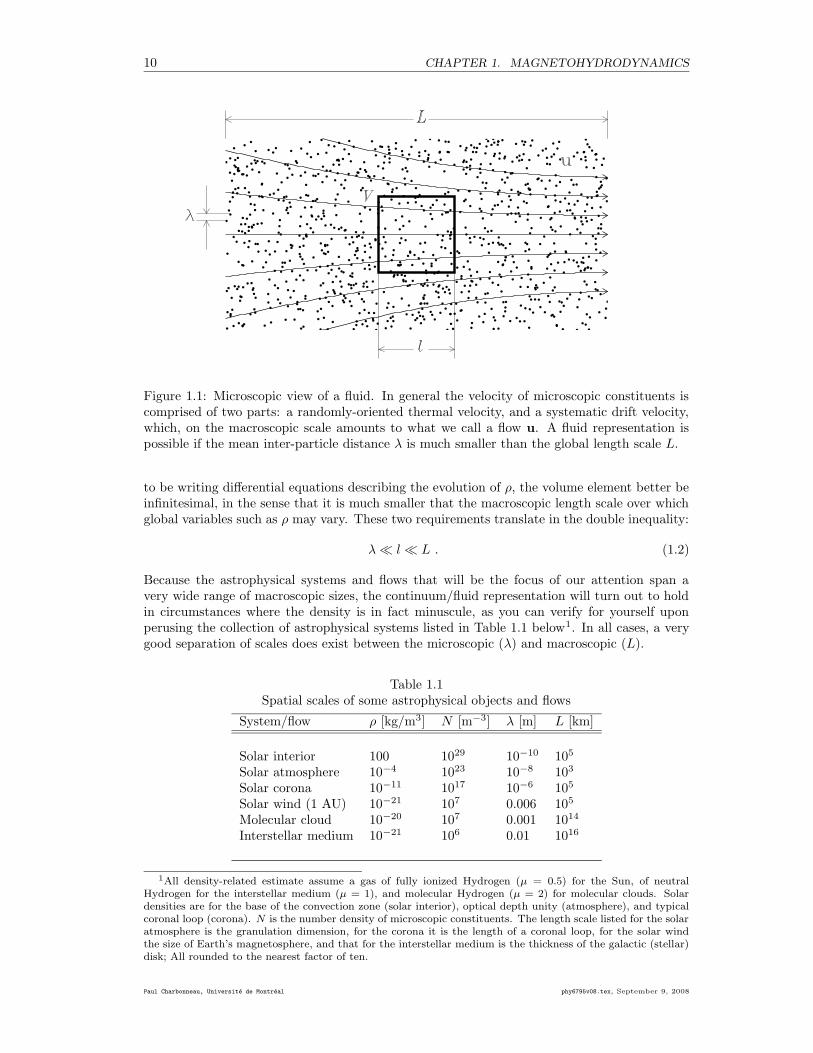
Figure 1.1: Microscopic view of a fluid. In general the velocity of microscopic constituents iscomprised of two parts: a randomly-oriented thermal velocity, and a systematic drift velocity,which, on the macroscopic scale amounts to what we call a flow u. A fluid representation ispossible if the mean inter-particle distance λ is much smaller than the global length scale L.
to be writing differential equations describing the evolution of ρ, the volume element better beinfinitesimal, in the sense that it is much smaller that the macroscopic length scale over whichglobal variables such as ρ may vary. These two requirements translate in the double inequality:
λ ¿ l ¿ L . (1.2)
Because the astrophysical systems and flows that will be the focus of our attention span avery wide range of macroscopic sizes, the continuum/fluid representation will turn out to holdin circumstances where the density is in fact minuscule, as you can verify for yourself uponperusing the collection of astrophysical systems listed in Table 1.1 below1. In all cases, a verygood separation of scales does exist between the microscopic (λ) and macroscopic (L).
Table 1.1Spatial scales of some astrophysical objects and flows
System/flow ρ [kg/m3] N [m−3] λ [m] L [km]
Solar interior 100 1029 10−10 105
Solar atmosphere 10−4 1023 10−8 103
Solar corona 10−11 1017 10−6 105
Solar wind (1 AU) 10−21 107 0.006 105
Molecular cloud 10−20 107 0.001 1014
Interstellar medium 10−21 106 0.01 1016
1All density-related estimate assume a gas of fully ionized Hydrogen (µ = 0.5) for the Sun, of neutralHydrogen for the interstellar medium (µ = 1), and molecular Hydrogen (µ = 2) for molecular clouds. Solardensities are for the base of the convection zone (solar interior), optical depth unity (atmosphere), and typicalcoronal loop (corona). N is the number density of microscopic constituents. The length scale listed for the solaratmosphere is the granulation dimension, for the corona it is the length of a coronal loop, for the solar windthe size of Earth’s magnetosphere, and that for the interstellar medium is the thickness of the galactic (stellar)disk; All rounded to the nearest factor of ten.
Paul Charbonneau, Universite de Montreal phy6795v08.tex, September 9, 2008
1.2. ESSENTIALS OF HYDRODYNAMICS 11
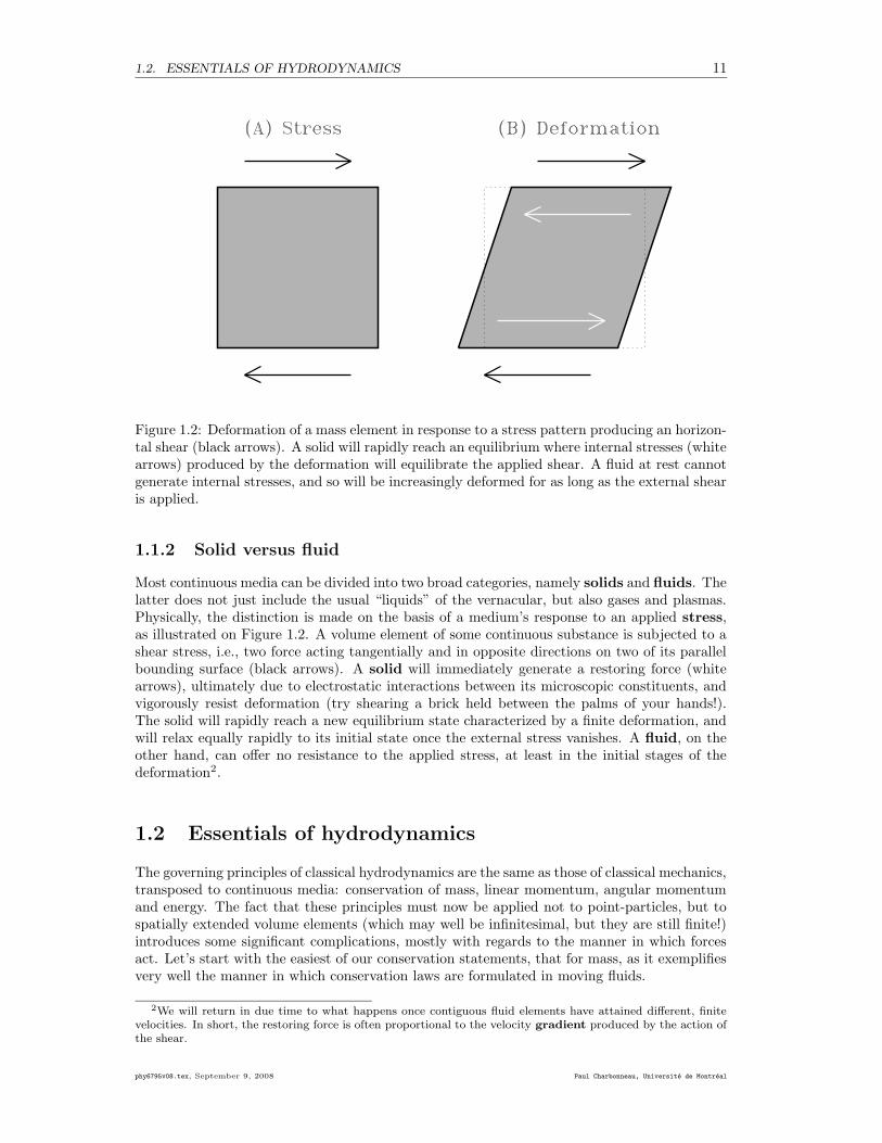
Figure 1.2: Deformation of a mass element in response to a stress pattern producing an horizon-tal shear (black arrows). A solid will rapidly reach an equilibrium where internal stresses (whitearrows) produced by the deformation will equilibrate the applied shear. A fluid at rest cannotgenerate internal stresses, and so will be increasingly deformed for as long as the external shearis applied.
1.1.2 Solid versus fluid
Most continuous media can be divided into two broad categories, namely solids and fluids. Thelatter does not just include the usual “liquids” of the vernacular, but also gases and plasmas.Physically, the distinction is made on the basis of a medium’s response to an applied stress,as illustrated on Figure 1.2. A volume element of some continuous substance is subjected to ashear stress, i.e., two force acting tangentially and in opposite directions on two of its parallelbounding surface (black arrows). A solid will immediately generate a restoring force (whitearrows), ultimately due to electrostatic interactions between its microscopic constituents, andvigorously resist deformation (try shearing a brick held between the palms of your hands!).The solid will rapidly reach a new equilibrium state characterized by a finite deformation, andwill relax equally rapidly to its initial state once the external stress vanishes. A fluid, on theother hand, can offer no resistance to the applied stress, at least in the initial stages of thedeformation2.
1.2 Essentials of hydrodynamics
The governing principles of classical hydrodynamics are the same as those of classical mechanics,transposed to continuous media: conservation of mass, linear momentum, angular momentumand energy. The fact that these principles must now be applied not to point-particles, but tospatially extended volume elements (which may well be infinitesimal, but they are still finite!)introduces some significant complications, mostly with regards to the manner in which forcesact. Let’s start with the easiest of our conservation statements, that for mass, as it exemplifiesvery well the manner in which conservation laws are formulated in moving fluids.
2We will return in due time to what happens once contiguous fluid elements have attained different, finitevelocities. In short, the restoring force is often proportional to the velocity gradient produced by the action ofthe shear.
phy6795v08.tex, September 9, 2008 Paul Charbonneau, Universite de Montreal
12 CHAPTER 1. MAGNETOHYDRODYNAMICS
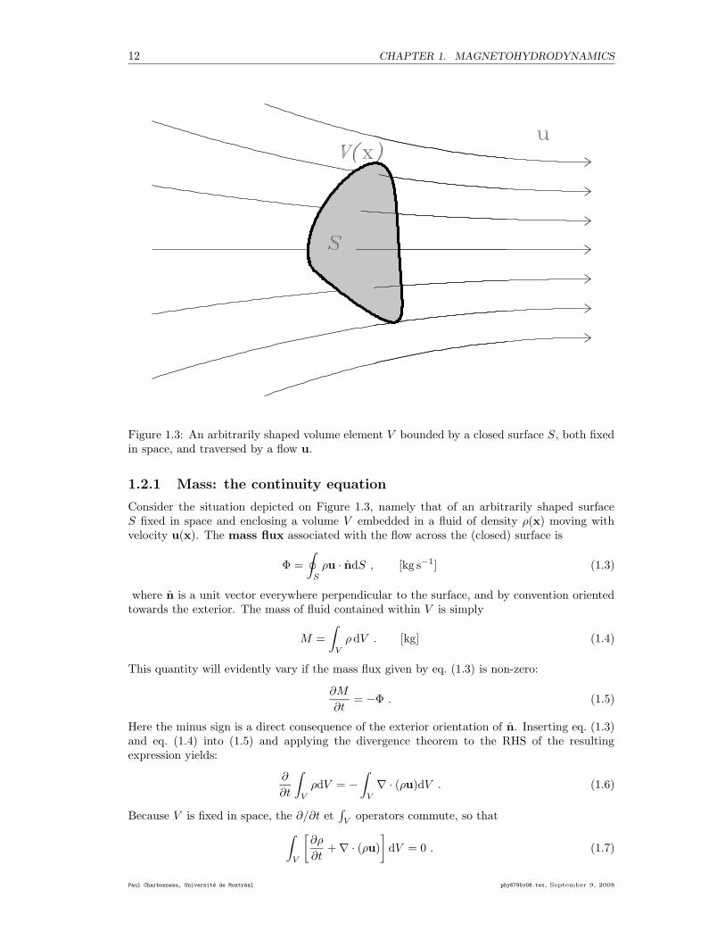
Figure 1.3: An arbitrarily shaped volume element V bounded by a closed surface S, both fixedin space, and traversed by a flow u.
1.2.1 Mass: the continuity equation
Consider the situation depicted on Figure 1.3, namely that of an arbitrarily shaped surfaceS fixed in space and enclosing a volume V embedded in a fluid of density ρ(x) moving withvelocity u(x). The mass flux associated with the flow across the (closed) surface is
Φ =
∮
S
ρu · ndS , [kg s−1] (1.3)
where n is a unit vector everywhere perpendicular to the surface, and by convention orientedtowards the exterior. The mass of fluid contained within V is simply
M =
∫
V
ρdV . [kg] (1.4)
This quantity will evidently vary if the mass flux given by eq. (1.3) is non-zero:
∂M
∂t= −Φ . (1.5)
Here the minus sign is a direct consequence of the exterior orientation of n. Inserting eq. (1.3)and eq. (1.4) into (1.5) and applying the divergence theorem to the RHS of the resultingexpression yields:
∂
∂t
∫
V
ρdV = −∫
V
∇ · (ρu)dV . (1.6)
Because V is fixed in space, the ∂/∂t et∫
Voperators commute, so that
∫
V
[∂ρ
∂t+ ∇ · (ρu)
]
dV = 0 . (1.7)
Paul Charbonneau, Universite de Montreal phy6795v08.tex, September 9, 2008
1.2. ESSENTIALS OF HYDRODYNAMICS 13
Because V is completely arbitrary, in general this can only be satisfied provided that
∂ρ
∂t+ ∇ · (ρu) = 0 . (1.8)
This expresses mass conservation in differential form, and is known in hydrodynamics as thecontinuity equation.
Incompressible fluids have constant densities, so that in this limiting case the continuityequation reduces to
∇ · u = 0 , [incompressible]. (1.9)
Water is perhaps the most common example of an effectively incompressible fluid (under the vastmajority of naturally occuring conditions anyway). The gaseous nature of most astrophysicalfluids may lead you to think that incompressibility is likely to be a pretty lousy approximationin cases of interest in this course. It turns out that the incompressible approximation can leadto a pretty good approximation of the behavior of compressible fluids provided that the flow’sMach number (ratio of flow speed to sound speed) is much smaller than unity.
1.2.2 The D/Dt operator
Suppose we want to compute the time variation of some physical quantity (Z, say) at somefixed location x0 in a flow u(x). In doing so we must take into account the fact that Z is ingeneral both an explicit and implicit function of time, because the volume element “containing”Z is moving with the fluid, i.e., Z → Z(t,x(t)). We therefore need to use the chain rule andwrite:
dZ
dt=
∂Z
∂t+
∂Z
∂x
∂x
∂t+
∂Z
∂y
∂y
∂t+
∂Z
∂z
∂z
∂t. (1.10)
Noting that u = dx/dt, this becomes
dZ
dt=
∂Z
∂t=
∂Z
∂t+
∂Z
∂xux +
∂Z
∂yuy +
∂Z
∂zuz =
∂Z
∂t+ (u · ∇)Z . (1.11)
This corresponds to the time variation of Z following the fluid element as it is carried by the
flow. It is a very special kind of derivative in hydrodynamics, known as the Lagrangian
derivative, which will be represented by the operator:
D
Dt≡ ∂
∂t+ (u · ∇) . (1.12)
Note in particular that the Lagrangian derivative of u yields the acceleration of a fluid element:
a =Du
Dt, (1.13)
a notion that will soon come very handy when we’ll write F = ma for a fluid.
A material surface is defined as an ensemble of points that define a surface, all movingalong with the flow. Therefore, in a local frame of reference S ′ co-moving with any infinitesimalelement of a material surface, u′ = 0. The distinction between material surfaces, as opposedto surfaces fixed in space such as in eq. (1.3), has crucial consequences with respect to thecommuting properties of temporal and spatial differential operators. In the latter case
∫
Vcom-
mutes with ∂/∂t, whereas for material surfaces and volume elements it is D/Dt that commuteswith
∫
V(and
∮
S, etc.).
phy6795v08.tex, September 9, 2008 Paul Charbonneau, Universite de Montreal
14 CHAPTER 1. MAGNETOHYDRODYNAMICS
1.2.3 Linear momentum: the Navier-Stokes equations
A force F acting on a point-object of mass m is easy to deal with; it simply procuces anacceleration a = F/m in the same direction as the force (sounds simple but it still took thegenius of Newton to figure it out...). In the presence of a force acting on the surface of a spatiallyextended fluid element, the resulting fluid acceleration will depend on both the orientation ofthe force and the surface. We therefore define the net force t in terms of a stress tensor:
tx = exsxx + eysxy + ezsxz , (1.14)
ty = exsyx + eysyy + ezsyz , (1.15)
tz = exszx + eyszy + ezszz , (1.16)
where “sxy” denotes the force per unit area acting in the y-direction on a surface perpendicularto the x-direction, tx is the net force acting on the surfaces perpendicular to the x-direction,and similarly for the other components. Consider now a unit vector perpendicular to a surfacearbitrarily oriented in space:
n = exnx + eyny + eznz , n2x + n2
y + n2z = 1 . (1.17)
The net force along this direction is simply
tn = (n · ex)tx + (n · ey)ty + (n · ez)tz = n · s . (1.18)
We can now use the Lagrangian acceleration to write the equivalent of “F = ma” or moreaccurately “∂p/∂t = F”, for the fluid element:
D
Dt
∫
V
ρudV =
∮
S
s · ndS . (1.19)
We now pull the same tricks as in §1.2.1: use the divergence theorem to turn the surfaceintegral into a volume integral, commute the temporal derivative and volume integral on theRHS, expand carefully the vector operator u · ∇ acting on ρu, invoke the arbitrariness of theactual integration volume V , and finally make good use of the continuity equation (1.8), toobtain the differential equation for u:
ρDu
Dt= ∇ · s . (1.20)
We now define the pressure (units: pascal; 1 Pa≡ 1N m−2) as the isotropic part of theforce acting perpendicularly on the volume’s surfaces, and separate it explicitly from the stresstensor:
s = −pI + ττττ , (1.21)
where I is the identity tensor, and the minus sign arises from the convention that pressuresacts on the bounding surface towards the interior of the volume element, and ττττ will presentlybecome the viscous stress tensor. Since ∇ · (pI) = ∇p, eq. (1.20) becomes
Du
Dt= −1
ρ∇p +
1
ρ∇ · ττττ . (1.22)
The next step is to obtained expressions for the components of the tensor ττττ . The viscous force,which is what ττττ stands for, can be viewed as a form of friction acting between contiguous
Paul Charbonneau, Universite de Montreal phy6795v08.tex, September 9, 2008
1.2. ESSENTIALS OF HYDRODYNAMICS 15
laminae of fluid moving with different velocities, so that we expect it to be proportional tovelocity derivatives. Consider now the following decomposition of a velocity gradient:
∂uk
∂xl
=1
2
(∂uk
∂xl
+∂ul
∂xk
)
︸ ︷︷ ︸
Dkl
+1
2
(∂uk
∂xl
− ∂ul
∂xk
)
︸ ︷︷ ︸
Ωkl
. (1.23)
The first term on the RHS is a pure shear, and is described by the (symmetric) deformation
tensor Dkl; the second is a pure rotation , and is described by the antisymmetric vorticity
tensor Ωkl. It can be shown that the latter causes no deformation of the fluid element, therefore
the viscous force can only involve Dkl. A Newtonian fluid is one for which the (tensorial)relation between ττττ and Dkl is linear:
τij = fij(Dkl) , i, j, k, l = (1, 2, 3) ≡ (x, y, z) (1.24)
The next step is to invoke the invariance of the physical laws embodied in eq. (1.24) underrotation of the coordinate axes. The mathematics is rather tedious, but at the end of the dayyou end up with:
τxx = 2µDxx + (µϑ − 23µ)(Dxx + Dyy + Dzz) (1.25)
τyy = 2µDyy + (µϑ − 23µ)(Dxx + Dyy + Dzz) (1.26)
τzz = 2µDzz + (µϑ − 23µ)(Dxx + Dyy + Dzz) (1.27)
τxy = 2µDxy (1.28)
τyz = 2µDyz (1.29)
τzx = 2µDzx (1.30)
where µ and µϑ are the coefficients dynamical viscosity and bulk viscosity, respectively.Is is often convenient to define a coefficent of kinematic viscosity as
ν =µ
ρ, [m2 s−1] . (1.31)
In an incompressible flow, the terms multiplying µϑ vanish and it is possible to rewrite theNavier-Stokes equation in the simpler form:
Du
Dt= −1
ρ∇p + ν∇2u . [incompressible] (1.32)
Note here the presence of a Laplacian operator acting on a vector quantity (here u); this isonly equivalent to the Laplacian acting on the scalar components of u in the special case ofcartesian coordinates.
Incompressible or not, the behavior of viscous flows will often hinge on the relative impor-tance of the advective and dissipative terms in the Navier-Stokes equation:
ρ(u · ∇)u ↔ ∇ · ττττ . (1.33)
Introducing characteristic length scales u0, L, ρ0 and ν0, dimensional analysis yields:
ρ0
u20
L↔ 1
Lρ0ν0
u0
L, (1.34)
where we made use of the fact that the viscous stress tensor has dimensions µ × Dik, withµ = ρν and the deformation tensor Dik has dimension of velocity per unit length (cf. eq. 1.23).The ratio of these two terms is a dimensionless quantity called the Reynolds Number:
Re =u0L
ν0
. (1.35)
phy6795v08.tex, September 9, 2008 Paul Charbonneau, Universite de Montreal
16 CHAPTER 1. MAGNETOHYDRODYNAMICS
This measures the importance of viscous forces versus fluid inertia. It is a key dimension-less parameter in hydrodynamics, as it effectively controls fundamental processes such as thetransition to turbulence, as well as more mundane matters such as boundary layer thicknesses.
A few words on boundary conditions; in the presence of viscosity, the flow speed must vanishwherever the fluid is in contact with a rigid surface S:
u(x) = 0 , x ∈ S . (1.36)
This remains true even in the limit where the viscosity is vanishingly small. For a free surface
(e.g., the surface of a fluid sphere floating in a vacuum), the normal components of both theflow speed and viscous stress must vanish instead:
u · n(x) = 0 , ττττ · n = 0 , x ∈ S . (1.37)
1.2.4 Angular momentum: the vorticity equation
The “rotation” and “angular momentum” of a fluid system cannot simply be reduced to simplescalars such as angular velocity and moment of inertia, because the application of a torque toa fluid element can alter not just its rotation rate, but also its shape and mass distribution. Amore useful measure of “rotation” is the circulation Γ about some closed contour γ embeddedin and moving with the fluid:
Γ(t) =
∮
γ
u(x, t) · d` =
∫
S
(∇× u) · ndS =
∫
S
ωωωω · n dS , (1.38)
where the second equality follows from Stokes’ theorem, and the third from the definition ofvorticity:
ωωωω = ∇× u . (1.39)
Thinking about flows in terms of vorticity ωωωω rather than speed u can be useful because ofKelvin’s theorem, which states that the circulation Γ along any closed loop γ advected bythe moving fluid is a conserved quantity:
DΓ
Dt= 0 . (1.40)
Applying again Stokes’ theorem yields the equivalent expression
D
Dt
∫
S
ωωωω · n dS = 0 , (1.41)
stating that the flux of vorticity across any material surface S bounded by γ is also a conservedquantity, both in fact being integral expressions of angular momentum conservation.
An evolution equation for ωωωω can be obtained via the Navier-Stokes equation, in a particularlyilluminating manner in the case of an incompressible fluid (∇ · u = 0) with constant kinematicviscosity ν, in which case eq. (1.32) can be rewritten as
Du
Dt== −∇
(p
ρ+ Φ
)
− ν∇× (∇× u) , [incompressible] (1.42)
where it was assumed that gravity can be expressed as the gradient of a (gravitational) potential.Taking the curl on each side of this expression then yields:
∇×(
∂u
∂t
)
+ ∇× (u · ∇u) = ∇×[
∇(
p
ρ+ Φ
)]
︸ ︷︷ ︸
=0
−ν∇×∇× (∇× u) , (1.43)
Paul Charbonneau, Universite de Montreal phy6795v08.tex, September 9, 2008
1.2. ESSENTIALS OF HYDRODYNAMICS 17
then, commuting the time derivative with ∇× and making judicious of some vector identitiesto develop the second term on the LHS, remembering also that ∇ · ωωωω = 0, eventually leads to:
Dωωωω
Dt− ωωωω · ∇u = ν∇2ωωωω , [incompressible] . (1.44)
This is the vorticity equation, expressing in differential form the conservation of the fluid’sangular momentum.
A useful vorticity-related quantity is the kinetic helicity, defined as
h = u · ωωωω , (1.45)
which measures the amount of twisting in a flow. This will prove an important concept wheninvestigating magnetic field amplification by fluid flows.
1.2.5 Energy: the entropy equation
Omitting to begin with the energy dissipated in heat by viscous friction, the usual accounting ofenergy flow into and out of a volume element V fixed in space leads to the following differentialequation expressing the conservation of the plasma’s internal energy per unit mass (e, inunits J/kg):
De
Dt+ (γ − 1)e∇ · u =
1
ρ∇ ·
[
(χ + χr)∇T]
, (1.46)
where for a perfect gas we have
e =1
γ − 1
p
ρ=
1
γ − 1
kT
µm, (1.47)
with γ = cp/cv the ratio of specific heats, and (χ + χr)∇T the heat flux in or out of thefluid element, with χ and χr the coefficients of thermal and radiative conductivity, respectively(units: J K−1m−1s−1). Equation (1.46) expresses that any variation of the specific energy in aplasma volume moving with the flow (LHS) is due to heat flowing in or out of the volume byconduction or radiation (here in the diffusion approximation). The “extra” term ∝ ∇ · u onthe LHS of eq (1.46) embodies the work done against (or by) the pressure force in compressing(or letting expand) the volume element.
It is often convenient to rewrite the energy conservation equation in terms of the plasma’sentropy S = ρ−γp, which allows to rewrite eq. (1.46) in the more compact form:
ρTDS
Dt= ∇ ·
[
(χ + χr)∇T]
, (1.48)
which states, now unambiguously, that any change in the entropy S as one follows a fluidelement (LHS) can only be due to heat flowing out of or into the domain by conduction (RHS).For incompressible fluids eq. (1.48) can be written
ρcp
DT
Dt= ∇ ·
[
(χ + χr)∇T]
, [incompressible] (1.49)
where
cp = T
(∂S
∂T
)
p
, (1.50)
is the heat capacity at constant pressure.
phy6795v08.tex, September 9, 2008 Paul Charbonneau, Universite de Montreal
18 CHAPTER 1. MAGNETOHYDRODYNAMICS
While this is seldom an important factor in astrophysical flows, in general we must add tothe RHS of eq. (1.48) the heat produced by viscous dissipation (and, as we shall see later, byOhmic dissipation). This is given by the so-called (volumetric) viscous dissipation function:
φν =µ
2
(∂ui
∂xk
+∂uk
∂xi
− 2
3δik
∂us
∂xs
)2
+ µϑ
(∂us
∂xs
)2
, [J m−3s−1] , (1.51)
where summation over repeated indices is implied here. Note that since φν is positive definite,its presence on the RHS of eq. (1.48) can only increase the fluid element’s entropy, which makesperfect sense since friction, which is what viscosity is for fluids, is an irreversible process.
For more on classical hydrodynamics, see the references listed in the bibliography at theend of this chapter.
1.3 The magnetohydrodynamical induction equation
Our task is now to generalize the governing equations of hydrodynamics to include the effectsof the electric and magnetic fields, and to obtain evolution equations for these two physicalquantities. Keep in mind that electrical charge neutrality, as required by MHD, does not implythat the fluid’s microscopic constituents are themselves neutral, but rather that positive andnegative electrical charges are present in equal numbers in any fluid element.
The starting point, you guess it I hope, is Maxwell’s celebrated equations:
∇ · E =ρe
ε0
, [Gauss′ Law] (1.52)
∇ · B = 0 , [Anonymous] (1.53)
∇× E = −∂B
∂t, [Faraday′s Law] (1.54)
∇× B = µ0J + µ0ε0
∂E
∂t, [Ampere/Maxwell′s Law] (1.55)
where, in the SI system of units, the electric field is measured in N C−1 (≡ V m−1), the magneticfield3 B in tesla (T). The quantity ρe is the electrical charge density (C m−3), and J is theelectrical current density (A m−2). The permittivity ε0 (= 8.85×10⁻¹²C2 N−1m−2 in vacuum)and magnetic permeability µ0 (= 4π × 10−7 N A−2 in vacuum) can be considered as constantsin what follows, since we will not be dealing with polarisable or ferromagnetic substances.
The first step is (with all due respect to the man) to do away altogether with Maxwell’sdisplacement current in eq. (1.55). This can be justified if the fluid flow is non-relativistic andthere are no batteries around being turned on or off, two rather sweeping statement that willbe substantiated in §1.5. For the time being we just revert to the original form of Ampere’sLaw:
∇× B = µ0J . (1.56)
In general, the application of an electrical field E across an electrically conducting substance willgenerate an electrical current density J. Ohm’s Law postulates that the relationship betweenJ and E is linear:
J′ = σE′ , (1.57)
3strictly speaking, B should be called and the magnetic flux density or somesuch, but on this one we’ll stickto common astrophysical usage.
Paul Charbonneau, Universite de Montreal phy6795v08.tex, September 9, 2008
1.4. SCALING ANALYSIS 19
where σ is the electrical conductivity (units: C2s−1m−3kg−1 ≡ Ω−1m−1, Ω ≡Ohm). Herethe primes (“′”) are added to emphasize that Ohm’s Law is expected to hold in a conductingsubstance at rest. In the context of a fluid moving with velocity u (relativistic or not), eq. (1.57)can only be expected to hold in a reference frame comoving with the fluid. So we need totransform eq. (1.57) to the laboratory (rest) frame. In the non-relativitic limit (u/c ¿ 1,implying γ → 1), the usual Lorentz transformation for the electrical current density simplifiesto J′ = J, and that for the electric field to E′ = E + u × B, so that Ohm’s Law takes on theform
J = σ(E + u × B) , (1.58)
or, making use of the pre-Maxwellian form of Ampere’s Law and reorganizing the terms:
E = −u × B +1
µ0σ(∇× B) . (1.59)
We now insert this expression for the electric field into Faraday’s Law (1.54) to obtain the veryfamous magnetohydrodynamical induction equation:
∂B
∂t= ∇× (u × B − η∇× B) . (1.60)
where
η =1
µ0σ[m2s−1] (1.61)
is the magnetic diffusivity4. The first term on the RHS of eq. (1.60) represents the inductiveaction of fluid flowing across a magnetic field, while the second term represents dissipation ofthe electrical currents sustaining the field.
Keep in mind that any solution of eq. (1.60) must also satisfy eq. (1.53) at all times. It canbe easily shown (try it!) that if ∇·B = 0 at some initial time, the form of eq. (1.60) guaranteesthat zero divergence will be maintained at all subsequent times5
1.4 Scaling analysis
The evolution of a magnetic field under the action of a prescribed flow u will depend greatly onwhether or not the inductive term on the RHS of eq. (1.60) dominates the diffusive term. Underwhat conditions will this be the case? We seek a first (tentative) answer to this question byperforming a dimensional analysis of eq. (1.60); this involves replacing the temporal derivativeby 1/τ and the spatial derivatives by 1/`, where τ and ` are time and length scales that suitablycharacterizes the variations of both u and B:
B
τ=
u0B
`+
ηB
`2, (1.62)
where B and u0 are a “typical” values for the flow velocity and magnetic field strength overthe domain of interest. The ratio of the first to second term on the RHS of eq. (1.62) is adimensionless quantity known as the magnetic Reynolds number6:
Rm =u0`
η, (1.63)
4A note of warning: some MHD textbooks, included the Goedbloed & Poedts tome cited in the bibliography,use the symbol “η” for the inverse conductivity (units Ωm), so that the dissipative term on the RHS of theinduction equation retains a µ−1
0prefactor. The Davidson book uses the same definition as here... but the
symbol λ! Be careful.5This is true under exact arithmetic; if numerical solutions to eq. (1.60) are sought, care must be taken to
ensure ∇ · B = 0 as the solution is advanced in time.6Not the structural similarity with the usual viscous Reynolds number defined in §1.2.3, with the magnetic
diffusivity η replacing the kinematic viscosity ν in the denominator. Had we not absorbed µ0 in our definitionof η, the magnetic permeability µ0 would appear in the numerator of the magnetic Reynolds number, which Ipersonally find objectionable.
phy6795v08.tex, September 9, 2008 Paul Charbonneau, Universite de Montreal
20 CHAPTER 1. MAGNETOHYDRODYNAMICS
which measures the relative importance of induction versus dissipation over length scales of
order `. Note that Rm does not depend on the magnetic field strength, a direct consequence ofthe linearity (in B) of the MHD induction equation. Our scaling analysis simply says that inthe limit Rm À 1, induction by the flow dominates the evolution of B, while in the oppositelimit of Rm ¿ 1, induction makes a negligible contribution and B simply decays away underthe influence of Ohmic dissipation.
One may anticipate great simplifications of magnetohydrodynamics if we operate in eitherof these limits. If Rm ¿ 1, only the second term is retained on the RHS of eq. (1.62), whichleads immediately to
τ =`2
η, (1.64)
a quantity known as the magnetic diffusion time. It measures the time taken for a magneticfield contained in a volume of typical linear dimension ` to dissipate and/or diffusively leakout of the volume. Now, for most astrophysical objects, this timescale turns out to be quitelarge, indeed often larger than the age of the universe! (see Table 1.2). This is not so muchbecause astrophysical plasmas are such incredibly good electrical conductors, but rather becauseastrophysical objects tend to be very, very large.
The opposite limit Rm À 1, defines the ideal MHD limit. Then it is the first term that isretained on the RHS of eq. (1.62), so that
τ = `/u0 , (1.65)
corresponding to the turnover time associated with the flow u. Note already that under idealMHD, the only non-trivial (i.e., u 6= 0 and B 6= 0) steady-state (∂/∂t = 0) solutions of theMHD equation are only possible for field-aligned flows.
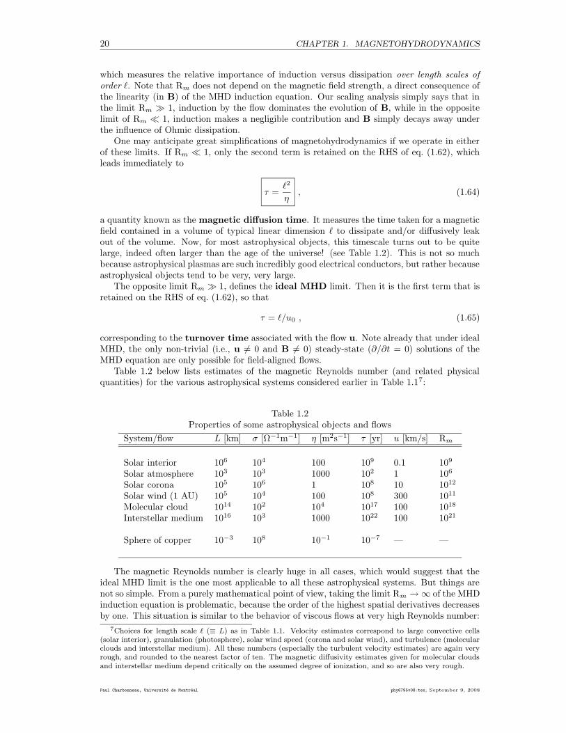
Table 1.2 below lists estimates of the magnetic Reynolds number (and related physicalquantities) for the various astrophysical systems considered earlier in Table 1.17:
Table 1.2Properties of some astrophysical objects and flows
System/flow L [km] σ [Ω−1m−1] η [m2s−1] τ [yr] u [km/s] Rm
Solar interior 106 104 100 109 0.1 109
Solar atmosphere 103 103 1000 102 1 106
Solar corona 105 106 1 108 10 1012
Solar wind (1 AU) 105 104 100 108 300 1011
Molecular cloud 1014 102 104 1017 100 1018
Interstellar medium 1016 103 1000 1022 100 1021
Sphere of copper 10−3 108 10−1 10−7 — —
The magnetic Reynolds number is clearly huge in all cases, which would suggest that theideal MHD limit is the one most applicable to all these astrophysical systems. But things arenot so simple. From a purely mathematical point of view, taking the limit Rm → ∞ of the MHDinduction equation is problematic, because the order of the highest spatial derivatives decreasesby one. This situation is similar to the behavior of viscous flows at very high Reynolds number:
7Choices for length scale ` (≡ L) as in Table 1.1. Velocity estimates correspond to large convective cells(solar interior), granulation (photosphere), solar wind speed (corona and solar wind), and turbulence (molecularclouds and interstellar medium). All these numbers (especially the turbulent velocity estimates) are again veryrough, and rounded to the nearest factor of ten. The magnetic diffusivity estimates given for molecular cloudsand interstellar medium depend critically on the assumed degree of ionization, and so are also very rough.
Paul Charbonneau, Universite de Montreal phy6795v08.tex, September 9, 2008
1.5. THE LORENTZ FORCE 21
solutions to eq. (1.60) with η → 0 in general do not smoothly tend towards solutions obtainedfor η = 0. Moreover, the distinction between the two physical regimes Rm ¿ 1 and Rm À 1is meaningful as long as one can define a suitable Rm for the flow as a whole, which, in turn,requires one to estimate, a priori, a length scale ` that adequately characterizes the evolvingmagnetic field at all time and throughout the spatial domain of interest. As we proceed itwill become clear that this is not always straightforward, or even possible. Finally, the scalinganalysis does away entirely with the geometrical aspects of the problem, by substituting u0Bfor u × B; yet there are situations (e.g. a field-aligned flow) where even a very large u has noinductive effect whatsoever, in which case the induction equation assumes the mathematicalform
∂B
∂t= −∇× (η∇× B) , (1.66)
even though Rm may be very large, and B evolves on the (long) magnetic diffusion timescale(1.64) rather than on the (short) turnover time.
1.5 The Lorentz force
Getting to eq. (1.60) was pretty easy (because we summarily swept the displacement currentunder the rug), but it represents only half (in fact the easy half) of our task; we must nowinvestigate the effect of the magnetic field on the flow u; and this, it turns out, is the trickypart of the MHD approximation.
You will certainly recall that the Lorentz force acting on an electrically charge particlemoving at velocity u in a region of space permeated by electric and magnetic fields is given by
f = q(E + u × B) , [N] . (1.67)
where q is the electrical charge. Consider now a volume element ∆V containing many suchparticles; in the continuum limit, the total force per unit volume (F) acting on the volumeelement will be the sum of the forces acting on each individual charged constituents divided bythe volume element:
F =1
∆V
∑
k
fk =1
∆V
∑
k
qk(E + uk × B)
=
(
1
∆V
∑
k
qk
)
E +
(
1
∆V
∑
k
qkuk
)
× B
= ρeE + J × B , [Nm−3] . (1.68)
where the last equality follows from the usual definition of charge density and electrical currentdensity. At this point you might be tempted to eliminate the term proportional to E, on thegrounds that in MHD we are dealing with a globally neutral plasma, meaning ρe = 0, thereforeρeE ≡ 0 and that’s the end of it. That would be way too easy...
Let’s begin by taking the divergence on both side of the generalized form of Ohm’s Law(eq. (1.58)). We then make use of Gauss’s Law (eq. (1.53)) to get rid of the ∇ ·E term, and ofthe charge conservation Law
∂ρe
∂t+ ∇ · J = 0 (1.69)
to get rid of the ∇·J term. The end result of all this physico-algebraical juggling is the followingexpression:
∂ρe
∂t+
ρe
(ε0/σ)+ σ∇ · (u × B) = 0 . (1.70)
phy6795v08.tex, September 9, 2008 Paul Charbonneau, Universite de Montreal
22 CHAPTER 1. MAGNETOHYDRODYNAMICS
The combination ε0/σ has units of time, and is called the charge relaxation time, henceforthdenoted τe. It is the timescale on which charge separation takes place in a conductor if an electricfield is suddenly turned on. For most conductors, this a very small number, of order 10−18 s !!This is because the electrical field reacts to the motion of electric charges at the speed of light(in the substance under consideration, which is slower than in a vacuum but still mighty fast).Indeed, in a conducting fluid at rest (u = 0) the above expression integrates readily to
ρe(t) = ρe(0) exp(−t/τe) , (1.71)
thus the name “relaxation time” for τe.Now let us consider the case of a slowly moving fluid, in the sense that it is moving on a
timescale much larger than τe; this means that the induced electrical field will vary on a similartimescale (at best), and therefore the time derivative of ρe can be neglected in comparison tothe ρe/τe term in eq. (1.70), leading to
ρe = ε0∇ · (u × B) . (1.72)
This indicates that a finite charge density can be sustained inside a moving conducting fluid.The associated electrostatic force per unit volume, ρeE, is definitely non-zero but turns outto much smaller than the magnetic force. Indeed, a dimensional analysis of eq. (1.68), usingeq. (1.72) to estimate ρe, gives:
ρeE ∼(
ε0uB
`
)(J
σ
)
∼(uτe
`
)
JB , (1.73)
J × B ∼ JB , (1.74)
where Ohm’s Law was used to express E in terms of J, and once again ` is a typical lengthscale characterizing the variations of the flow and magnetic field. The ratio of electrostatic tomagnetic force is thus of order uτe/`. Now τe ¿ 1 to start with, and for non-relativistic fluidmotion we can expect that the flow’s turnover time `/u is much larger than the crossing timefor an electromagnetic disturbance ∼ `/c ∼ τe; both effects conspire to render the electrostaticforce absolutely minuscule compared to the magnetic force, so that eq. (1.68) becomes
F = J × B , [MHD approximation] . (1.75)
and this must be added to the RHS of the Navier-Stokes equation (1.22)... with a 1/ρ prefactorso we get a force per unit mass, rather than per unit volume.
Now, getting back to this business of having dropped the displacement current in the fullMaxwellian form of Ampere’s Law (eq. (1.55)); it can now be all justified on the grounds thatthe time derivative of the charge density can be neglected in the non-relativistic limit. Indeed,to be consistent the charge conservation equation (1.69) now reduces to
∇ · J = 0 ; (1.76)
taking the divergence on both sides of eq. (1.55) then leads to
∇ · J = −ε0∇ ·(
∂E
∂t
)
= ε0
∂
∂t(∇ · E) =
∂ρe
∂t; (1.77)
this demonstrates that dropping the time derivative of the charge density is equivalent toneglecting Maxwell’s displacement current in eq. (1.55). To sum up, provided we exclude veryrapid transient events (such as turning a battery on or off, or any such process which wouldgenerate a large ∂ρe/∂t), under the MHD approximation the following statements all hold true:
• The fluid motions are non-relativistic;
• The electrostatic force can be neglected as compared to the magnetic force;
• Maxwell’s displacement current can be neglected.
Paul Charbonneau, Universite de Montreal phy6795v08.tex, September 9, 2008
1.6. JOULE HEATING 23
1.6 Joule heating
In the presence of finite electrical conductivity, the volumetric heating associated with thedissipation of electric currents must be included on the RHS of the energy equation, in theform of the so-called Joule heating function:
φB =η
µ0
(∇× B)2 , [J m−3s−1] . (1.78)
Note however that in very nearly all astrophysical circumstances, Joule heating makes an in-significant contribution to the energy budget. When it occurs, heating by magnetic energydissipation, such as in flares, involves dynamical mechanisms that lead to effective dissipationfar more rapid and efficient than Joule heating.
1.7 The full set of MHD equations
For the record, we now collect the set of partial differential equations governing the behaviorof magnetized fluids in the MHD limit:
∂ρ
∂t+ ∇ · (ρu) = 0 , (1.79)
Du
Dt= −1
ρ∇p + g +
1
µ0ρ(∇× B) × B +
1
ρ∇ · ττττ , (1.80)
De
Dt+ (γ − 1)e∇ · u =
1
ρ
[
∇ ·(
(χ + χr)∇T)
+ φν + φB
]
, (1.81)
∂B
∂t= ∇× (u × B − η∇× B) . (1.82)
Equations (1.79)—(1.82) are further complemented by the two constraint equations:
∇ · B = 0 , (1.83)
p = f(ρ, T, ...) , (1.84)
and suitable expressions for the viscous stress tensor and for the physical coefficient ν, χ, η, etc.Note that gravity g is explicitly included on the RHS of (1.80), that e is the specific energy ofthe plasma (magnetic energy will be dealt with separately shortly), and that eq. (1.84) is justsome generic form for an equation of state linking the pressure to the properties of the plasmasuch as density, temperature, chemical composition, etc.
This is it in principle, but in what follows we shall seldom solve these equations in this com-plete form. In the parameter regime characterizing most astrophysical fluids, we usually haveRe À 1, which means that the (u ·∇u) term in eq. (1.80) will play important role; this, in turn,means turbulence, already in itself an unsolved problem even for unmagnetized fluids. Thereis also a strong nonlinear coupling between eqs. (1.80) and eqs. (1.82), so that the turbulentcascade involves both the flow and magnetic field. Finally, with both Re À 1 and Rm À 1,astrophysical flows will in general develop structures on length scales very much smaller thanthat characterizing the system under study, so that even fully numerical solutions of the aboveset of MHD equations will tax the power of the largest extant massively parallel computers,and will continue to do so in the foreseeable future; which is why judicious geometrical and/orphysical simplification remains a key issue in the art of astrophysical magnetohydrodynamics...and will also continue to remain so in the same foreseeable future!
phy6795v08.tex, September 9, 2008 Paul Charbonneau, Universite de Montreal
24 CHAPTER 1. MAGNETOHYDRODYNAMICS
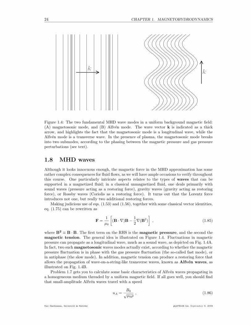
Figure 1.4: The two fundamental MHD wave modes in a uniform background magnetic field:(A) magnetosonic mode, and (B) Alfven mode. The wave vector k is indicated as a thickarrow, and highlights the fact that the magnetosonic mode is a longitudinal wave, while theAlfven mode is a transverse wave. In the presence of plasma, the magnetosonic mode breaksinto two submodes, according to the phasing between the magnetic pressure and gas pressureperturbations (see text).
1.8 MHD waves
Although it looks innocuous enough, the magnetic force in the MHD approximation has somerather complex consequences for fluid flows, as we will have ample occasions to verify throughoutthis course. One particularly intricate aspects relates to the types of waves that can besupported in a magnetized fluid; in a classical unmagnetized fluid, one deals primarily withsound waves (pressure acting as a restoring force), gravity waves (gravity acting as restoringforce), or Rossby waves (Coriolis as a restoring force). It turns out that the Lorentz forceintroduces not one, but really two additional restoring forces.
Making judicious use of eqs. (1.53) and (1.56), together with some classical vector identities,eq. (1.75) can be rewritten as
F =1
µ0
[
(B · ∇)B − 1
2∇(B2)
]
, (1.85)
where B2 ≡ B · B. The first term on the RHS is the magnetic pressure, and the second themagnetic tension. The general idea is illustrated on Figure 1.4. Fluctuations in magneticpressure can propagate as a longitudinal wave, much as a sound wave, as depicted on Fig. 1.4A.In fact, two such magnetosonic waves modes actually exist, according to whether the magneticpressure fluctuation is in phase with the gas pressure fluctuation (the so-called fast mode), orin antiphase (the slow mode). In addition, magnetic tension can produce a restoring force thatallows the propagation of wave-on-a-string-like transverse waves, known as Alfven waves, asillustrated on Fig. 1.4B.
Problem 1.7 gets you to calculate some basic characteristics of Alfven waves propagating ina homogeneous medium threaded by a uniform magnetic field. If all goes well, you should findthat small-amplitude Alfven waves travel with a speed
uA =B0√µ0ρ
, (1.86)
Paul Charbonneau, Universite de Montreal phy6795v08.tex, September 9, 2008
1.9. MAGNETIC ENERGY 25
where B0 is the magnitude of the (uniform) magnetic field along which the wave is propagating,and ρ is the (constant) fluid density. We will not be dealing much with magnetosonic waves inthis course, but we will return to Alfven waves in part II, when we examine their dynamicalimpact on the acceleration of wind-like outflows from the sun and stars.
1.9 Magnetic energy
Consider the expression resulting from dotting B into the induction equation (1.60), integratingover the spatial domain (V ) under consideration, and making judicious use of various well-known vector identities and of Gauss’ theorem:
d
dt
∫
V
B2
2µ0
dV = −∫
S
(S · n) dS −∫
V
(u · F) dV −∫
V
σ−1J2 dV , (1.87)
where E is the electric field, and n is a outward-directed unit vector normal to the boundarysurface S. The vector quantities S, L and J are the Poynting flux, Lorentz force and currentdensity, respectively. Recall that in the MHD limit these take the form:
S =1
µ0
E × B , (1.88)
F =1
µ0
(∇× B) × B , (1.89)
µ0J = ∇× B . (1.90)
We also made use of the fact that in the MHD approximation, the net current J is expressedvia the generalized form of Ohm’s law as the sum of the conduction and induction currents:
J = σ(E + u × B) . (1.91)
Examine now the three terms on the RHS of eq. (1.87); the first is the Poynting flux componentinto the domain, integrated over the domain boundaries, i.e., the flux of electromagnetic energyin (integrand < 0) or out (integrand > 0) of the domain. This term evidently vanishes in theabsence of applied magnetic or electric fields on the boundaries. The second is the work doneby the Lorentz force (F) on the flow. In general this term can be either positive or negative; inthe context of magnetic driving of stellar winds (part II of the course) we are concerned withthe u ·F > 0 situation8, while in the dynamo context (part III of the course) we are interestedin the u ·F < 0 situation, where the flow transfers energy to the magnetic field. The third termis evidently always negative, and represents the rate of energy loss due to Ohmic dissipation.Equations (1.87) then naturally leads to interpret the quantity B2/2µ0 as the magnetic energydensity, since the LHS of eq. (1.87) is clearly the rate of change of the total magnetic energy
(EB) within the domain:
EB =1
2µ0
∫
V
B2dV . (1.92)
1.10 Magnetic flux freezing and Alfven’s theorem
Let us return to the differential form of Faraday’s Law:
∇× E = −∂B
∂t. (1.93)
8which is also quite relevant to the design of magnetic pumps for electrically conducting fluids. This hasreceived quite a bit of attention in light of the use of liquid sodium to cool the core of nuclear reactors.
phy6795v08.tex, September 9, 2008 Paul Charbonneau, Universite de Montreal
26 CHAPTER 1. MAGNETOHYDRODYNAMICS
Project now each side of this expression onto a unit vector normal to some surface S fixed inspace and bounded by a closed countour γ, integrate over S, and apply Stokes’ theorem to theLHS:
∫
S
(∇× E) · ndS =
∮
γ
E · d` = −∫
S
(∂B
∂t
)
· ndS . (1.94)
So far the surface S remains completely arbitrary. If it is fixed in space, then we get the usualintegral form of Faraday’s Law:
∮
γ
E · d` = − ∂
∂t
∫
S
B · ndS , (1.95)
with the LHS corresponding to the electromotive force, and the RHS to the time variationof the magnetic flux (ΦB). If we now assume instead that the surface S is a material surfacemoving with the fluid, then (1) we must substitute the Lagrangian operator D/Dt for the partialderivative on the RHS of eq. (1.95); and (2) we are allowed to invoke Ohm’s Law to substituteJ for E on the RHS since any point of the (material) contour is by definition co-moving withthe fluid:
1
σ
∮
γ
J · d` = − D
Dt
∫
S
B · ndS . (1.96)
Now, obviously, in the limit of infinite conductivity we have
D
Dt
∫
S
B · ndS = 0 . (1.97)
This states that in the ideal MHD limit σ → ∞, the magnetic flux threading any (open) surfaceis a conserved quantity as the surface is advected (and possibly deformed) by the flow. Thisresults is known as Alfven’s theorem. Note in particular that in the limit of an infinitisemalsurface pierced by “only one” fieldline, Alfven’s theorem is equivalent to saying that magneticfieldline must move in the same way as fluid elements; it is customary to stay that the magneticfield is “frozen” into the fluid. In this manner it behaves just like vorticity in the inviscid limitν → 0. And like in the case of vorticity, sheared flows can amplify magnetic fields by stretching,a subject we will investigate in all great details in Part III of these class notes.
1.11 Magnetic helicity
In anology with fluid helicity, one can define the magnetic helicity as
hB = A · B . (1.98)
Note that the magnetic vector potential A is playing here the role of the flow field u in eq. (1.45).A substantial amount of vector algebra can show that the total magnetic helicity in any volumeV of magnetized fluid
HB =
∫
V
A · BdV , (1.99)
is a conserved quantity under ideal MHD (σ → ∞). In direct analogy to fluid helicity, this isa measure of twist of magnetic fieldlines, and/or of topological linkage between distinct fluxsystems. A closely related quantity is the current helicity:
HJ =
∫
V
J · BdV , (1.100)
which, in the astrophysical context, is often an easier quantity to determine observationally.Note that since J ∝ ∇×B and B ∝ ∇×A, a proportionality between HB and HJ is expected,and the two quantities should certainly have the same sign for a given physical system.
Paul Charbonneau, Universite de Montreal phy6795v08.tex, September 9, 2008
1.12. MATHEMATICAL REPRESENTATIONS OF MAGNETIC FIELDS 27
1.12 Mathematical representations of magnetic fields
We close this heavy-duty chapter with a somewhat disorganized collection of mathematical andphysical properties of the vector magnetic field, which will be of great use in chapters to follow.
1.12.1 Pseudo-vectors and solenoidal vectors
It is worth distinguishing between real vectors (also called axial vectors) and pseudo-vectors,the latter class including the magnetic field vector. Real vectors remain invariant upon inver-sion of the (3D) coordinates about the origin, i.e., x → −x, hereafter thinking in cartesiancoordinates to ease the discussion. This will leave the “physical” direction in space of a truevector (like a velocity u) unchanged, since both the coordinate unit vectors and the componentsof the velocity will change sign:
u′ = (−ux)(−ex) + (−uy)(−ey) + (−uz)(−ez) = u . (1.101)
However, in terms of vector products, curl operators, orientation of surfaces and so on, thecoordinate inversion will take us from a right-handed coordinate system to a left-handed system.This implies that a vector like the magnetic field must remain invariant under coordinateinversion. This can be appreciated by considering the expression for the magnetic force actingon a charge q moving at velocity u in a magnetic field B:
f = q u × B ; (1.102)
we just argued that the components of f and u will change sign under coordinate inversion;therefore the magnetic field components must not change sign under coordinate inversion, foreq. (1.102) to remain valid (physical laws do not care about our coordinate conventions!).One must conclude that upon coordinate inversion, the direction of a vector field such as B
immediately flips! So the Earth’s north magnetic pole instantly becomes the south magneticpole9. Weird behavior for a vector, which is why such vectors inherit the prefix “pseudo”.
Pseudo or not, there are numerous vectors fields of physical interest out there that have theproperty that their divergence vanishes; the magnetic field is evidently such a vector field, asper our second Maxwell equation (1.53). The fluid vorticity (§1.2.4) is clearly another. Anyvector field (G, say) satisfying ∇ · G = 0 is called a solenoidal vector.
Soleinodal vectors have a very interesting property related to the conservation of their fluxacross material surfaces transported and deformed by a flow field u. They can be shown tosatisfy the following kinematic theorem:
D
Dt
∫
Sm
G · ndS =
∫
Sm
[∂G
∂t−∇× (u × G)
]
· ndS . (1.103)
This is simply saying that the net variation of the flux (LHS) can be due either to intrinsic time-variation of the vector field (first term in the square brackets on the RHS) or to deformationof the material surface Sm by the flow u (second term).
Note that we could have arrived at Alfven’s theorem (§1.10) starting from this kinematictheorem for solenoidal vector fields, as applied to B:
D
Dt
∫
Sm
B · ndS =
∫
Sm
[∂B
∂t−∇× (u × B)
]
· ndS (1.104)
Obviously, the quantity within square brackets on the RHS will vanish as per our MHD induc-tion equation (1.60) written in the ideal limit η → 0, which gets us directly to eq. (1.97). Youwill recall, of course, that Ohm’s Law is indeed already embodied in the MHD induction equa-tion, so this is really getting to the same result by two mathematically distinct but physicallyequivalent paths.
9Does this mean that your compass needle will instantly rotate by 180 degrees? Think about that one a bit...
phy6795v08.tex, September 9, 2008 Paul Charbonneau, Universite de Montreal
28 CHAPTER 1. MAGNETOHYDRODYNAMICS
1.12.2 The vector potential
It will often prove useful to work with the MHD induction equation written in terms of a vectorpotential A (units T m) such that B = ∇× A. Equation (1.60) is then readily integrated to
∂A
∂t= u × (∇× A) − η∇× (∇× A) + ∇Φ , (1.105)
where, in “uncurling” the induction equation we may elect to append the gradient of a scalarfunction to the RHS, with no effect on B. This additional term may contribute to the electricfield E, however, and so Φ is conveniently regarded as the electrostatic potential10. Clearly,any solution of eq. (1.105) identically satisfies the solenoidal constraint ∇ · B = 0.
1.12.3 Axisymmetric magnetic fields
In many astrophysical situations to be encountered in subsequent chapters we will facing astro-physical magnetofluid systems that show symmetry about an axis, in fact usually a rotationalaxis. For example, the sun’s differential rotation and meridional circulation, as inferred fromsurface measurements and helioseismology, are very closely axisymmetric on the largest spa-tial scales. In spherical polar coordinates (r, θ, φ), the most general axisymmetric (∂/∂φ = 0)magnetic field and flow can be written as
u(r, θ, t) =1
ρ∇× (Ψ(r, θ, t)eφ) + $Ω(r, θ, t)eφ (1.106)
B(r, θ, t) = ∇× (A(r, θ, t)eφ) + B(r, θ, t)eφ (1.107)
where $ = r sin θ. Here the vector potential component A and stream function Ψ define thepoloidal components of the field and flow, i.e., the component contained in meridional (r, θ)planes. The azimuthal component B is often called the toroidal field, and Ω is the angularvelocity (units rad s−1). Evidently eqs. (1.106)—(1.107) satisfies the constraints ∇ · (ρu) = 0(mass conservation in a steady flow) and ∇ · B = 0 by construction.
A practical advantage of this so-called mixed representation is that it allows the separationof the (vector) MHD induction equation into two components for the 2D scalar fields A and B:
∂
∂t($A) + up · ∇($A) = $η
(
∇2 − 1
$2
)
A , (1.108)
∂
∂t
(B
$
)
+ up · ∇(
B
$
)
=η
$
(
∇2 − 1
$2
)
B +1
$(∇η) × (Beφ)
−(
B
$
)
∇ · up + Bp · ∇Ω , (1.109)
where Bp and up are notational shortcuts for the poloidal field and meridional flow. Noticethat the vector potential A evolves in a manner entirely independent of the toroidal field B,the latter being conspicuously absent on the RHS of eq. (1.108). This is not true of the toroidalfield B, which is well aware of the poloidal field’s presence via the ∇Ω shearing term.
On numerous occasions in this and subsequent chapters we will seek solutions to eqs. (1.108)—(1.109) inside a sphere (radius R) of magnetized fluid; in the “exterior” r > R there is onlyvacuum, which implies vanishing electric currents. In practice we will need to match whateversolution we compute in r < R to a current-free solution in r > R; such a solution must satisfy
µ0J = ∇× B = 0 . (1.110)10In most (but not all!) situations dealt with in the following pages, Φ can (and will) be set to zero without
objectionable consequences.
Paul Charbonneau, Universite de Montreal phy6795v08.tex, September 9, 2008
1.12. MATHEMATICAL REPRESENTATIONS OF MAGNETIC FIELDS 29
For an axisymmetric system eq. (1.110) then translates into
(
∇2 − 1
$2
)
A(r, θ, t) = 0 , (1.111)
B(r, θ, t) = 0 . (1.112)
Solutions to eq. (1.111) have the general form
A(r, θ, t) =
∞∑
l=1
al
(R
r
)l+1
P 1l (cos θ) r > R , (1.113)
where the P 1l are the associated Legendre functions of order 1 and l is a positive integer.
Solutions to eqs. (1.108)–(1.109) computed within the sphere must then be smoothly matchedto eqs. (1.112)—(1.113) in the exterior. In particular, the vector potential A must be continuousup to its first derivative normal to the surface, so that the magnetic field component tangentialto the surface remains continuous across r = R. Regularity of the magnetic field on thesymmetry axis (θ = 0) requires that we set B = 0 there. Without any loss of generality, wecan also set A = 0 on the axis.
1.12.4 Force-free magnetic fields
In many astrophysical systems, the magnetic field dominates the dynamics and energetics ofthe system. Left to itself, such a system would tend to evolve to a force-free state described by
F = J × B = 0 . (1.114)
Broadly speaking, this can be achieved in two physically distinct ways (excluding the trivialsolution B = 0). The first is J = 0 throughout the system. Then Ampere’s Law becomes∇×B = 0, which means that, as with the electric field in electrostatic, B can be expressed asthe gradient of a potential. Such a magnetic field is called a potential field. Substitution intoGauss’ Law then yields a Laplace-type problem:
B = ∇Φ , ∇2Φ = 0 , [Potential field] , (1.115)
with Ampere’s Law being trivially satisfied (0 = 0!). Alternately, a system including a non-zerocurrent density can still be force free, provided the currents flow everywhere parallel to themagnetic field, i.e.,
∇× B = αB , (1.116)
where α need not necessarily be a constant, i.e., it can vary from one fieldline to another, varyin space, and even depend on the (local) value of B. Imagine now a situation where, in somedomain (for example, the exterior of a star), we are provided with a boundary condition on B
and the task is to construct a force-free field. Adopting the potential field anzatz can lead tovery different reconstructions that if we adopt instead eq. (1.116), given that in the latter caseone is free to specify any electric current distribution within the domain, as long as J remainsparallel to B.
A very important result in this context is known as Aly’s Theorem; it states that in asemi-infinite domain with B⊥ imposed at the boundary and B → 0 as x → ∞, the (unique)potential field solution satisfying the boundary conditions has a magnetic energy that is lower
than any of the (multiple) solutions of eq. (1.116) that satisfy the same boundary conditions,even with complete freedom to specify α(x) within the domain. This poses a strict limit tothe amount of magnetic energy stored into a system that can actually be tapped into to powerastrophysically interesting phenomena.
phy6795v08.tex, September 9, 2008 Paul Charbonneau, Universite de Montreal
30 CHAPTER 1. MAGNETOHYDRODYNAMICS
Problems:
1. Obtain the charge conservation equation (1.69) by following the general logic used in§1.2.1 to obtain the continuity equation (1.8).
2. Fill in the missing mathematical steps leading to eq. (1.70)
3. Fill in the missing mathematical steps leading to eq. (1.85)
4. Obtain equations (1.108) and (1.109) by substitution of eqs. (1.106) and (1.107) into theMHD induction equation (1.60). Hint: the induction equation is a vector equation; terms“oriented” in the φ-direction must cancel one another independently of terms orientedperpendicular to the φ-direction.
5. This one is a challenge to your vector algebraic skills. The idea is to mathematically provethe statement made in §1.11, namely that the magnetic helicity in a volume of plasmais a conserved quantity in the idea MHD limit (σ → ∞). Remembering that the volumeitself is carried (and possibly deformed) by the flow, you must show that
D
Dt
∫
V
A · BdV = 0 . (1.117)
If you get stuck, take a look at the Goedbloed & Poedts textbook cited below for helpfulhints...
6. This problem lets you dig a bit deeper in the concept of magnetic energy (§1.9).
(a) Starting from the induction equation, fill in the missing mathematical steps leadingto eq. (1.87).
(b) Show that in the absence of induction (meaning u = 0), a force-free magnetic con-tained in a domain V will always decay.
(c) Making use of eq. (1.91), obtain an expression involving B and u but not E, forthe Poynting flux component normal to the boundary S enclosing an electricallyconducting fluid. Give a physical interpretation for each term in the resulting math-ematical expression.
7. In this one you get to calculate the propagation speed of a pure Alfven wave in an ho-mogeneous, incompressible medium (constant density ρ). Sounds imposing, but a carefulchoice of geometry will make it easier than you may think. Working in cartesian geometry,consider a uniform x-directed magnetic field subjected to a velocity perturbation uy(x, t)oriented in the y direction (the problem is invariant with respect to z).
(a) As warmup, begin by showing that eqs. (1.79) and eq. (1.83) are automaticallysatisfied;
(b) then show that the ideal form of the (incompressible) MHD equations reduces to twonon-trivial coupled equations, for the y-components of the flow and magnetic field;
(c) now manipulate these two equations into a single partial second-order partial differ-ential equation;
(d) Show that this equation admits wave-type solutions, with phase speed given byeq. (1.86).
Paul Charbonneau, Universite de Montreal phy6795v08.tex, September 9, 2008
1.12. MATHEMATICAL REPRESENTATIONS OF MAGNETIC FIELDS 31
Bibliography:
There are a great many textbooks available on classical hydrodynamics. The following are myown top-three personal favorites:
Tritton, D.J., Physical Fluid Dynamics, 2nd ed., Oxford University Press (1988),Acheson, D.J., Elementary Fluid Dynamics, Clarendon Press (1990)Landau, L., et Lifschitz, E. 1959, Fluid Mechanics, Oxford: Pergamon Press.
If you are looking for an introduction to the topic targeted at physics-trained readers, you maywant to work through the first six chapters of my class notes for PHY-3140, the 2007 versionof which being still available on the Web:
http://www.astro.umontreal.ca/∼paulchar/phy3140/notes07.pdf(I’m working on a revised version for the winter of 2009). If you need a refresher on undergrad-uate electromagnetism, you should go back to
Griffith, D.J., Introduction to Electrodynamics, 3rd ed., Prentice Hall (1999).
At the graduate level, the standard reference remains
Jackson, J.D., Classical Electrodynamics, 2nd ed., John Wiley & Sons (1975),
who does devote a chapter to magnetohydrodynamics, including a discussion of magnetic wavemodes. My personal favorite on magnetohydrodynamics is:
Davidson, P.A., An Introduction to Magnetohydrodynamics, Cambridge University Press(2001).
Sections 1.5 and 1.10 are strongly inspired by Davidson’s own presentation of the subject. Healso presents an illuminating proof of the kinematic theorem embodied in eq. (1.103). Thefollowing textbook is also well worth consulting:
Goedbloed, H., & Poedts, S., Principles of Magnetohydrodynamics, Cambridge UniversityPress (2004).
These authors put greater emphasis on MHD waves, shocks, and on the intersection of MHDand plasma physics. For those seeking even more focus on plasma physics aspects, I wouldrecommend:
Kulsrud, R.M., Plasma Physics for Astrophysics, Princeton University Press (2005).
Also noteworthy in the general astrophysical context:
Choudhuri, A.R., The Physics of Fluids and Plasmas, Cambridge University Press (1998).
On Aly’s theorem, see
Aly, J.-J. 1984, Astrophys. J., 283, 349,Aly, J.-J. 1991, Astrophys. J., 375, L61,Smith, D.F., & Low, B.C. 1993, Astrophys. J., 410, 412,
but brace yourself for some serious math.
phy6795v08.tex, September 9, 2008 Paul Charbonneau, Universite de Montreal

32 CHAPTER 1. MAGNETOHYDRODYNAMICS
Paul Charbonneau, Universite de Montreal phy6795v08.tex, September 9, 2008
Chapter 2
Magnetic fields in astrophysics
By now you may think you have landed in some sort of deranged combined crash course on fluidmechanics, electromagnetism... and vector algebra! To dispel this idea we now return closerto our subject matter, by briefly documenting the omnipresence of magnetic fields throughoutthe universe (§§2.1—2.8), pondering as to the conspicuous absence of electric fields (§2.9), andto the ultimate origin of magnetic fields (§2.10).
2.1 Earth’s magnetic field
Natural magnetism (in technical parlance, ferromagnetism) is known at least since Antiquity,but it took the monumental treatise De Magnete, published in 1600 by William Gilbert (1544-1603), to really drive home the point that the Earth is one huge spherically-shaped bar magnet.Gilbert arrived at this conclusion from comparing the known behavior of compass needless towhat he observed around a bar magnet carved into a sphere (see Figure 2.1). A medical doctorby training, in his book Gilbert also debunked many semi-occult beliefs about the behavior ofmagnetic objects and their influence on the human body and psyche.
To a good first approximation, the Earth’s magnetic field has the form of a dipole approxi-mately aligned with the Earth’s rotation axis, with an average surface field strength of ∼ 50µT.Geologic evidence has shown that the Earth’s magnetic field is not steady, but flips polaritiesbetween the N and S hemisphere, these reversals being rapid (on geological timescales; theylast some 10,000yr), are irregularly spaced, and punctuating much longer epochs of more orless stable field configuration, lasting a few 105 yr on average. At the present Earth’s dipolemoment is M⊕ = 8.1× 10²² A m2. Paleomagnetic studies indicate that M⊕ has been decliningrather rapidly over the past few 1000 yr, suggesting that we may be heading for a polarityreversal sometimes in the next few 1000 yr if the current trend persists.
Because the Earth’s crust and troposphere are such lousy electrical conductors, the presenceof the geomagnetic field is seldom felt in our daily life (and is ever more fading from popularconsciousness with the replacement of magnetic compasses by GPS). In the Earth’s ionosphere,however, the geomagnetic field is quite significant, and it interaction with the solar wind (to beencountered in part II of these notes) is what defines the magnetosphere, which happens toshield us from a lot of high energy particles often accelerated as a side effect of solar eruptiveevents (more on those shortly!). The impact of solar ejecta on the magnetosphere triggersgeomagnetic storms. Their most spectacular manifestation being auroral emission, but theinduced electric fields can pose threats to technological infrastructures such as power lines andpipelines.
phy6795v08.tex, September 9, 2008 33 Paul Charbonneau, Universite de Montreal
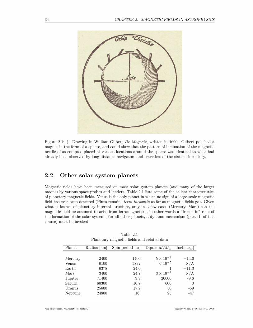
34 CHAPTER 2. MAGNETIC FIELDS IN ASTROPHYSICS
Figure 2.1: ). Drawing in William Gilbert De Magnete, written in 1600. Gilbert polished amagnet in the form of a sphere, and could show that the pattern of inclination of the magneticneedle of as compass placed at various locations around the sphere was identical to what hadalready been observed by long-distance navigators and travellers of the sixteenth century.
2.2 Other solar system planets
Magnetic fields have been measured on most solar system planets (and many of the largermoons) by various space probes and landers. Table 2.1 lists some of the salient characteristicsof planetary magnetic fields. Venus is the only planet in which no sign of a large-scale magneticfield has ever been detected (Pluto remains terra incognita as far as magnetic fields go). Givenwhat is known of planetary internal structure, only in a few cases (Mercury, Mars) can themagnetic field be assumed to arise from ferromagnetism, in other words a “frozen-in” relic ofthe formation of the solar system. For all other planets, a dynamo mechanism (part III of thiscourse) must be invoked.
Table 2.1Planetary magnetic fields and related data
Planet Radius [km] Spin period [hr] Dipole M/M⊕ Incl.[deg.]
Mercury 2400 1406 5 × 10⁻⁴ +14.0Venus 6100 5832 < 10−5 N/AEarth 6378 24.0 1 +11.3Mars 3400 24.7 3 × 10⁻⁴ N/AJupiter 71400 9.9 20000 -9.6Saturn 60300 10.7 600 0Uranus 25600 17.2 50 -59Neptune 24800 16. 25 -47
Paul Charbonneau, Universite de Montreal phy6795v08.tex, September 9, 2008
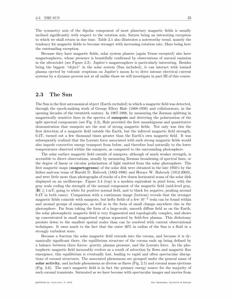
2.3. THE SUN 35
The symmetry axis of the dipolar component of most planetary magnetic fields is usuallyinclined significantly with respect to the rotation axis, Saturn being an interesting exceptionto which we shall return in due time. Table 2.1 also illustrates a noteworthy trend, namely thetendency for magnetic fields to become stronger with increasing rotation rate, Mars being herethe outstanding exception.
Because they have magnetic fields, solar system planets (again Venus excepted) also havemagnetospheres, whose presence is beautifully confirmed by observations of auroral emissionin the ultraviolet (see Figure 2.2). Jupiter’s magnetosphere is particularly interesting. Besidesbeing the biggest “object” in the solar system (Sun included), it can interact with ionizedplasma ejected by volcanic eruptions on Jupiter’s moon Io to drive intense electrical currentsystems by a dynamo process not at all unlike those we will investigate in part III of this course.
2.3 The Sun
The Sun is the first astronomical object (Earth excluded) in which a magnetic field was detected,through the epoch-making work of George Ellery Hale (1868-1938) and collaborators, in theopening decades of the twentieth century. In 1907-1908, by measuring the Zeeman splitting inmagnetically sensitive lines in the spectra of sunspots and detecting the polarization of thesplit spectral components (see Fig. 2.3), Hale provided the first unambiguous and quantitativedemonstration that sunspots are the seat of strong magnetic fields. Not only was this thefirst detection of a magnetic field outside the Earth, but the inferred magnetic field strength,0.3T, turned out a few thousand times greater than the Earth’s own magnetic field. It wassubsequently realized that the Lorentz force associated with such strong magnetic fields wouldalso impede convective energy transport from below, and therefore lead naturally to the lowertemperatures observed within the sunspots, as compared to the surrounding photosphere.
The solar surface magnetic field outside of sunspots, although of much weaker strength, isaccessible to direct observations, usually by measuring Zeeman broadening of spectral lines, orthe degree of linear or circular polarisation of light emitted from the solar photosphere. Thefirst magnetic maps (magnetograms) of the solar disk were obtained in the late 1950’s by thefather-and-son team of Harold D. Babcock (1882-1986) and Horace W. Babcock (1912-2003),and were little more than photographs of stacks of a few dozen horizontal scans of the solar diskdisplayed on an oscilloscope. Figure 2.4 (top) is a modern equivalent in pixel form, with thegray scale coding the strength of the normal component of the magnetic field (mid-level gray,|B| ∼< 1mT; going to white for positive normal field, and to black for negative, peaking around0.4T in both cases). Comparison with a continuum image (bottom) reveals that the strongermagnetic fields coincide with sunspots, but hefty fields of a few 10−2 tesla can be found withinand around groups of sunspots, as well as in the form of small clumps anywhere else in thephotosphere. Far from taking the form of a large-scale, smooth diffuse field as on the Earth,the solar photospheric magnetic field is very fragmented and topologically complex, and showsup concentrated in small magnetized regions separated by field-free plasma. This dichotomypersists down to the smallest spatial scales than can be resolved with current observationaltechniques. It owes much to the fact that the outer 30% in radius of the Sun is a fluid in astrongly turbulent state.
Because a fraction the solar magnetic field extends into the corona, and because it is dy-namically significant there, the equilibrium structure of the corona ends up being defined bya balance between three forces: gravity, plasma pressure, and the Lorentz force. As the pho-tospheric magnetic field inexorably evolves as a result of advection by flows and magnetic fluxemergence, this equilibrium is eventually lost, leading to rapid and often spectacular disrup-tions of coronal structures. The associated phenomena are grouped under the general name ofsolar activity, and include phenomena as diverse as flares (Fig. 2.5) and coronal mass ejections(Fig. 2.6). The sun’s magnetic field is in fact the primary energy source for the majority ofsuch coronal transients. Saturated as we have become with spectacular images and movies from
phy6795v08.tex, September 9, 2008 Paul Charbonneau, Universite de Montreal
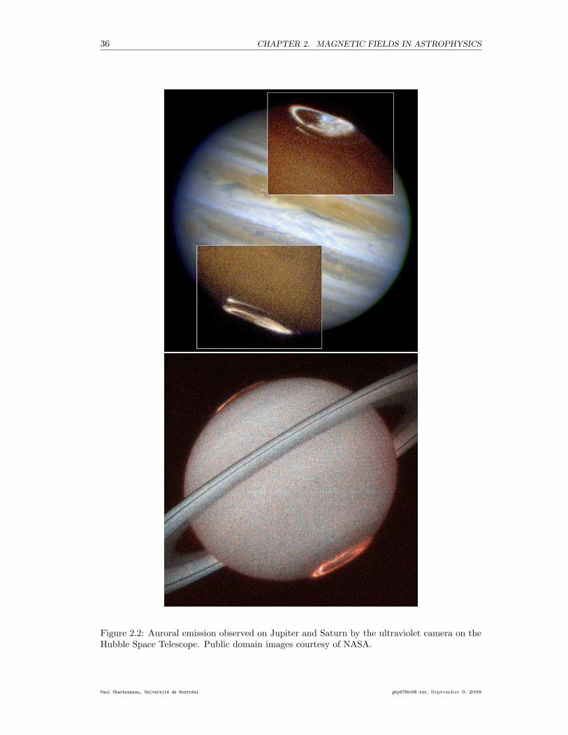
36 CHAPTER 2. MAGNETIC FIELDS IN ASTROPHYSICS
Figure 2.2: Auroral emission observed on Jupiter and Saturn by the ultraviolet camera on theHubble Space Telescope. Public domain images courtesy of NASA.
Paul Charbonneau, Universite de Montreal phy6795v08.tex, September 9, 2008
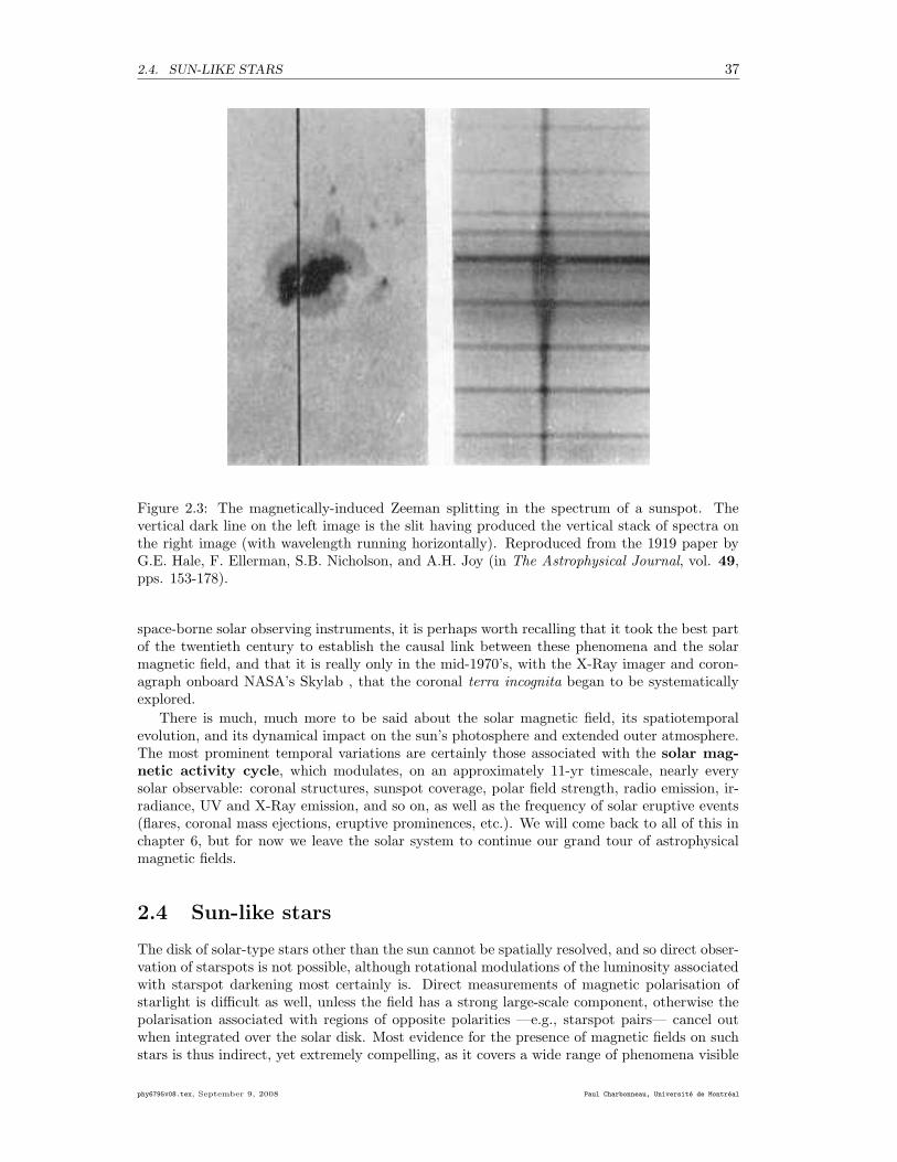
2.4. SUN-LIKE STARS 37
Figure 2.3: The magnetically-induced Zeeman splitting in the spectrum of a sunspot. Thevertical dark line on the left image is the slit having produced the vertical stack of spectra onthe right image (with wavelength running horizontally). Reproduced from the 1919 paper byG.E. Hale, F. Ellerman, S.B. Nicholson, and A.H. Joy (in The Astrophysical Journal, vol. 49,pps. 153-178).
space-borne solar observing instruments, it is perhaps worth recalling that it took the best partof the twentieth century to establish the causal link between these phenomena and the solarmagnetic field, and that it is really only in the mid-1970’s, with the X-Ray imager and coron-agraph onboard NASA’s Skylab , that the coronal terra incognita began to be systematicallyexplored.
There is much, much more to be said about the solar magnetic field, its spatiotemporalevolution, and its dynamical impact on the sun’s photosphere and extended outer atmosphere.The most prominent temporal variations are certainly those associated with the solar mag-
netic activity cycle, which modulates, on an approximately 11-yr timescale, nearly everysolar observable: coronal structures, sunspot coverage, polar field strength, radio emission, ir-radiance, UV and X-Ray emission, and so on, as well as the frequency of solar eruptive events(flares, coronal mass ejections, eruptive prominences, etc.). We will come back to all of this inchapter 6, but for now we leave the solar system to continue our grand tour of astrophysicalmagnetic fields.
2.4 Sun-like stars
The disk of solar-type stars other than the sun cannot be spatially resolved, and so direct obser-vation of starspots is not possible, although rotational modulations of the luminosity associatedwith starspot darkening most certainly is. Direct measurements of magnetic polarisation ofstarlight is difficult as well, unless the field has a strong large-scale component, otherwise thepolarisation associated with regions of opposite polarities —e.g., starspot pairs— cancel outwhen integrated over the solar disk. Most evidence for the presence of magnetic fields on suchstars is thus indirect, yet extremely compelling, as it covers a wide range of phenomena visible
phy6795v08.tex, September 9, 2008 Paul Charbonneau, Universite de Montreal
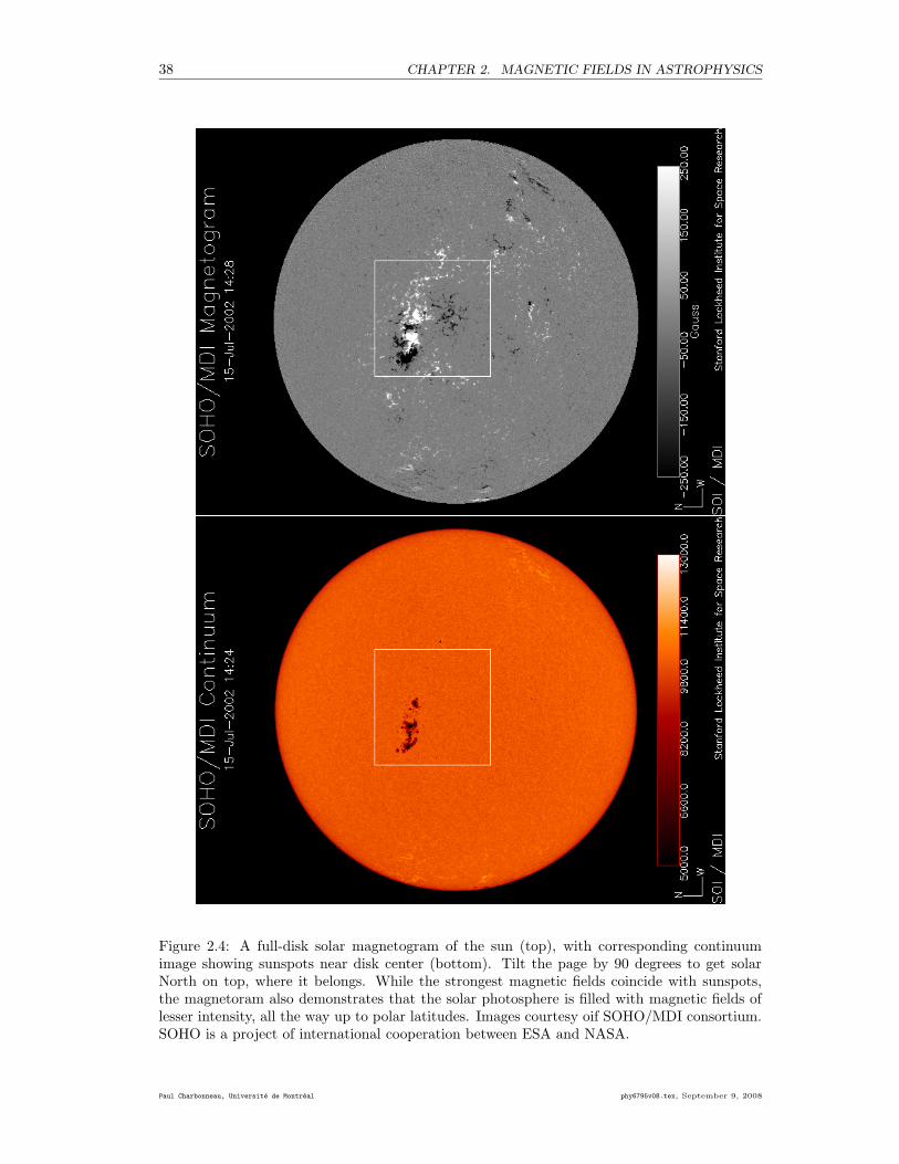
38 CHAPTER 2. MAGNETIC FIELDS IN ASTROPHYSICS
Figure 2.4: A full-disk solar magnetogram of the sun (top), with corresponding continuumimage showing sunspots near disk center (bottom). Tilt the page by 90 degrees to get solarNorth on top, where it belongs. While the strongest magnetic fields coincide with sunspots,the magnetoram also demonstrates that the solar photosphere is filled with magnetic fields oflesser intensity, all the way up to polar latitudes. Images courtesy oif SOHO/MDI consortium.SOHO is a project of international cooperation between ESA and NASA.
Paul Charbonneau, Universite de Montreal phy6795v08.tex, September 9, 2008
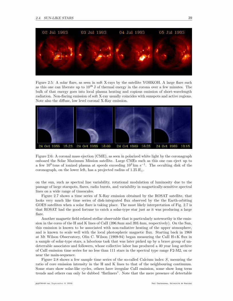
2.4. SUN-LIKE STARS 39
Figure 2.5: A solar flare, as seen in soft X-rays by the satellite YOHKOH. A large flare suchas this one can liberate up to 1026 J of thermal energy in the corona over a few minutes. Thebulk of that energy goes into local plasma heating and copious emission of short-wavelengthradiation. Non-flaring emission of soft X-ray usually coincides with sunspots and active regions.Note also the diffuse, low level coronal X-Ray emission.
Figure 2.6: A coronal mass ejection (CME), as seen in polarized white light by the coronagraphonboard the Solar Maximum Mission satellite. Large CMEs such as this one can eject up toa few 109 tons of ionized plasma at speeds exceeding 103 km s−1. The occulting disk of thecoronograph, on the lower left, has a projected radius of 1.25 R¯.
on the sun, such as spectral line variability, rotational modulation of luminosity due to thepassage of large starspots, flares, radio bursts, and variability in magnetically-sensitive spectrallines on a wide range of timescales.
Figure 2.7 shows a time series of X-Ray emission obtained by the ROSAT satellite, thatlooks very much like time series of disk-integrated flux observed by the the Earth-orbitingGOES satellites when a solar flare is taking place. The most likely interpretation of Fig. 2.7 isthat ROSAT had the good fortune to catch a solar-type star just as it was producing a largeflare.
Another magnetic field-related stellar observable that is particularly noteworthy is the emis-sion in the cores of the H and K lines of CaII (396.8nm and 393.4nm, respectively). On the Sun,this emission is known to be associated with non-radiative heating of the upper atmosphere,and is known to scale well with the local photospheric magnetic flux. Starting back in 1968at Mt Wilson Observatory, Olin C. Wilson (1909-94) began measuring the CaII H+K flux ina sample of solar-type stars, a laborious task that was later picked up by a brave group of un-deterrable associates and followers, whose collective labor has produced a 40 year long archiveof CaII emission time series for no less than 111 stars in the spectral type range F2-M2, on ornear the main-sequence.
Figure 2.8 shows a few sample time series of the so-called Calcium index S, mesuring theratio of core emission intensity in the H and K lines to that of the neighbouring continuum.Some stars show solar-like cycles, others have irregular CaII emission, some show long termtrends and others can only be dubbed “flatliners”. Note that the mere presence of detectable
phy6795v08.tex, September 9, 2008 Paul Charbonneau, Universite de Montreal
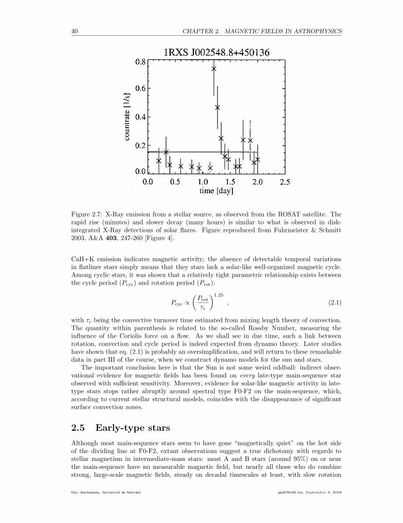
40 CHAPTER 2. MAGNETIC FIELDS IN ASTROPHYSICS
Figure 2.7: X-Ray emission from a stellar source, as observed from the ROSAT satellite. Therapid rise (minutes) and slower decay (many hours) is similar to what is observed in disk-integrated X-Ray detections of solar flares. Figure reproduced from Fuhrmeister & Schmitt2003, A&A 403, 247-260 [Figure 4].
CaH+K emission indicates magnetic activity; the absence of detectable temporal variationsin flatliner stars simply means that they stars lack a solar-like well-organized magnetic cycle.Among cyclic stars, it was shown that a relatively tight parametric relationship exists betweenthe cycle period (Pcyc) and rotation period (Prot):
Pcyc ∝(
Prot
τc
)1.25
, (2.1)
with τc being the convective turnover time estimated from mixing length theory of convection.The quantity within parenthesis is related to the so-called Rossby Number, measuring theinfluence of the Coriolis force on a flow. As we shall see in due time, such a link betweenrotation, convection and cycle period is indeed expected from dynamo theory. Later studieshave shown that eq. (2.1) is probably an oversimplification, and will return to these remarkabledata in part III of the course, when we construct dynamo models for the sun and stars.
The important conclusion here is that the Sun is not some weird oddball: indirect obser-vational evidence for magnetic fields has been found on every late-type main-sequence starobserved with sufficient sensitivity. Moreover, evidence for solar-like magnetic activity in late-type stars stops rather abruptly around spectral type F0-F2 on the main-sequence, which,according to current stellar structural models, coincides with the disappearance of significantsurface convection zones.
2.5 Early-type stars
Although most main-sequence stars seem to have gone “magnetically quiet” on the hot sideof the dividing line at F0-F2, extant observations suggest a true dichotomy with regards tostellar magnetism in intermediate-mass stars: most A and B stars (around 95%) on or nearthe main-sequence have no measurable magnetic field, but nearly all those who do combinestrong, large-scale magnetic fields, steady on decadal timescales at least, with slow rotation
Paul Charbonneau, Universite de Montreal phy6795v08.tex, September 9, 2008
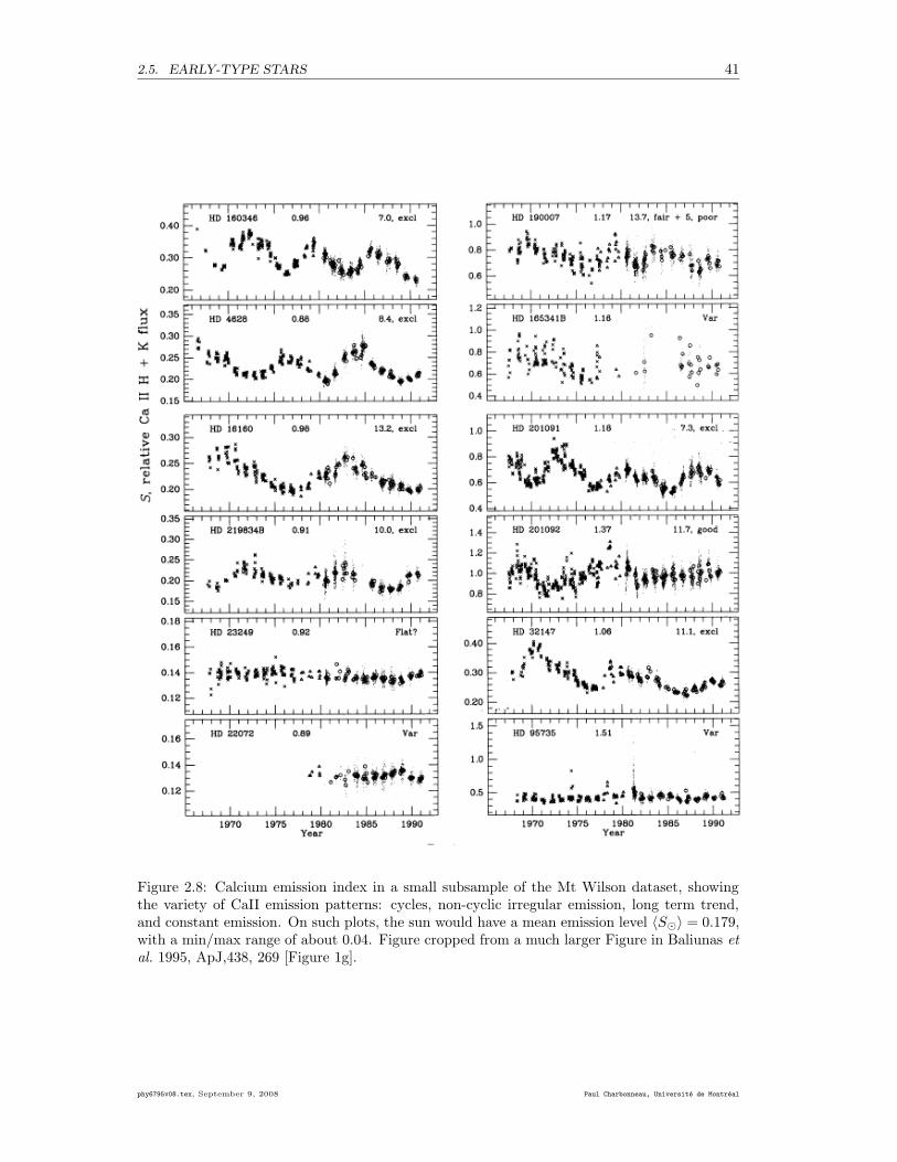
2.5. EARLY-TYPE STARS 41
Figure 2.8: Calcium emission index in a small subsample of the Mt Wilson dataset, showingthe variety of CaII emission patterns: cycles, non-cyclic irregular emission, long term trend,and constant emission. On such plots, the sun would have a mean emission level 〈S¯〉 = 0.179,with a min/max range of about 0.04. Figure cropped from a much larger Figure in Baliunas et
al. 1995, ApJ,438, 269 [Figure 1g].
phy6795v08.tex, September 9, 2008 Paul Charbonneau, Universite de Montreal
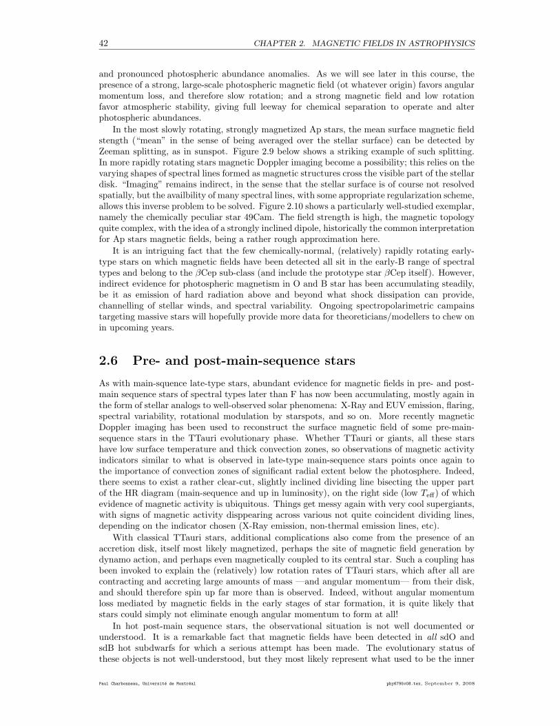
42 CHAPTER 2. MAGNETIC FIELDS IN ASTROPHYSICS
and pronounced photospheric abundance anomalies. As we will see later in this course, thepresence of a strong, large-scale photospheric magnetic field (ot whatever origin) favors angularmomentum loss, and therefore slow rotation; and a strong magnetic field and low rotationfavor atmospheric stability, giving full leeway for chemical separation to operate and alterphotospheric abundances.
In the most slowly rotating, strongly magnetized Ap stars, the mean surface magnetic fieldstength (“mean” in the sense of being averaged over the stellar surface) can be detected byZeeman splitting, as in sunspot. Figure 2.9 below shows a striking example of such splitting.In more rapidly rotating stars magnetic Doppler imaging become a possibility; this relies on thevarying shapes of spectral lines formed as magnetic structures cross the visible part of the stellardisk. “Imaging” remains indirect, in the sense that the stellar surface is of course not resolvedspatially, but the availbility of many spectral lines, with some appropriate regularization scheme,allows this inverse problem to be solved. Figure 2.10 shows a particularly well-studied exemplar,namely the chemically peculiar star 49Cam. The field strength is high, the magnetic topologyquite complex, with the idea of a strongly inclined dipole, historically the common interpretationfor Ap stars magnetic fields, being a rather rough approximation here.
It is an intriguing fact that the few chemically-normal, (relatively) rapidly rotating early-type stars on which magnetic fields have been detected all sit in the early-B range of spectraltypes and belong to the βCep sub-class (and include the prototype star βCep itself). However,indirect evidence for photospheric magnetism in O and B star has been accumulating steadily,be it as emission of hard radiation above and beyond what shock dissipation can provide,channelling of stellar winds, and spectral variability. Ongoing spectropolarimetric campainstargeting massive stars will hopefully provide more data for theoreticians/modellers to chew onin upcoming years.
2.6 Pre- and post-main-sequence stars
As with main-squence late-type stars, abundant evidence for magnetic fields in pre- and post-main sequence stars of spectral types later than F has now been accumulating, mostly again inthe form of stellar analogs to well-observed solar phenomena: X-Ray and EUV emission, flaring,spectral variability, rotational modulation by starspots, and so on. More recently magneticDoppler imaging has been used to reconstruct the surface magnetic field of some pre-main-sequence stars in the TTauri evolutionary phase. Whether TTauri or giants, all these starshave low surface temperature and thick convection zones, so observations of magnetic activityindicators similar to what is observed in late-type main-sequence stars points once again tothe importance of convection zones of significant radial extent below the photosphere. Indeed,there seems to exist a rather clear-cut, slightly inclined dividing line bisecting the upper partof the HR diagram (main-sequence and up in luminosity), on the right side (low Teff) of whichevidence of magnetic activity is ubiquitous. Things get messy again with very cool supergiants,with signs of magnetic activity disppearing across various not quite coincident dividing lines,depending on the indicator chosen (X-Ray emission, non-thermal emission lines, etc).
With classical TTauri stars, additional complications also come from the presence of anaccretion disk, itself most likely magnetized, perhaps the site of magnetic field generation bydynamo action, and perhaps even magnetically coupled to its central star. Such a coupling hasbeen invoked to explain the (relatively) low rotation rates of TTauri stars, which after all arecontracting and accreting large amounts of mass —and angular momentum— from their disk,and should therefore spin up far more than is observed. Indeed, without angular momentumloss mediated by magnetic fields in the early stages of star formation, it is quite likely thatstars could simply not eliminate enough angular momentum to form at all!
In hot post-main sequence stars, the observational situation is not well documented orunderstood. It is a remarkable fact that magnetic fields have been detected in all sdO andsdB hot subdwarfs for which a serious attempt has been made. The evolutionary status ofthese objects is not well-understood, but they most likely represent what used to be the inner
Paul Charbonneau, Universite de Montreal phy6795v08.tex, September 9, 2008
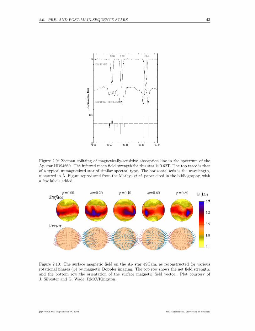
2.6. PRE- AND POST-MAIN-SEQUENCE STARS 43
Figure 2.9: Zeeman splitting of magnetically-sensitive absorption line in the spectrum of theAp star HD94660. The inferred mean field strength for this star is 0.62T. The top trace is thatof a typical unmagnetized star of similar spectral type. The horizontal axis is the wavelength,measured in A. Figure reproduced from the Mathys et al. paper cited in the bibliography, witha few labels added.
Figure 2.10: The surface magnetic field on the Ap star 49Cam, as reconstructed for variousrotational phases (ϕ) by magnetic Doppler imaging. The top row shows the net field strength,and the bottom row the orientation of the surface magnetic field vector. Plot courtesy ofJ. Silvester and G. Wade, RMC/Kingston.
phy6795v08.tex, September 9, 2008 Paul Charbonneau, Universite de Montreal
44 CHAPTER 2. MAGNETIC FIELDS IN ASTROPHYSICS
core of giants prior to the episode of strong mass loss that accompanies the transition to thehorizontal branch. Detection of kG-strength magnetic fields in such stars is strong evidence forthe existence of magnetic fields in the deep interior of their main-sequence progenitors.
2.7 Compact objects
Magnetic fields in isolated white dwarfs have been detected through circular polarisation mea-surements in the wings of strong spectral lines, usually Balmer lines in the so-called “DA” whitedwarfs showing Hydrogen lines in their photospheres. Actual Zeeman splitting is only detectedin the most strongly magnetized objects (∼> a few 102 T). Inferred field strengths range froma few T up to a whopping 105 T, with the overall incidence of magnetism standing at a fewpercent. However, these techniques are only sensitive to large-scale magnetic fields, still pro-ducing a net polarisation signal when integrated over the stellar disk, and so the true incidenceof magnetism in white dwarfs may actually be significantly higher.
Inferred magnetic field strengths in neutron stars range from 104 to 1011 T. Neutron starsmagnetic fields are of course most readily detected via the pulsar phenomenon, most likelyarising from slight misalignement of the magnetic axis with respect to the rotation axis of the(very rapidly rotating) neutron star. It is quite striking that the highest strengths of large-scalemagnetic fields in main-sequence stars (a few T in Ap stars), in white dwarfs (∼ 105 T) and inthe most strongly magnetized neutron stars (∼ 1011 T) all amount to similar surface magneticfluxes, lending support to the idea that these high field strengths can be understood from simpleflux-freezing arguments (§1.10... and Problem 2.1!). There is also observational evidence thatactual magnetic field evolution is taking place as pulsars age, but this remains very slipperyterritory, both from the modelling and observational points of view.
Observationally, very little is known about black holes except that there is quite possiblyone at the center of our galaxy, so you won’t be surprised to hear that even less is knownabout black hole magnetic fields. One should perhaps just point out that solutions to thefield equations of general relativity for rotating, electrically charged black holes do exist, whichis a good start towards magnetic fields production. Evidence to date is limited to energeticphenomena interpreted in terms of magnetic channelling of material onto the black hole. Butbeyond that, at the present time there is only religious fervor.
2.8 Galaxies and beyond
Magnetic fields in the diffuse, low-density interstellar gas is most readily detected through syn-chrotron radiation emitted by relativistic charged particles spiralling along magnetic fieldlines.This technique is succesfull not only within the Milky Way, but also for other galaxies. Othermeans of detection, for the time being limited to the Milky Way, include the polarisation ofoptical starlight by elongated (i.e., non-spherical) dust grains aligning themselves perpendicu-larly to magnetic fieldlines; these aligned dust grains also sometimes emit detectable polarizedinfrared radiation. Finally, for relatively strong fields Zeeman splitting of spectral lines in theradio domain has also been measured. As with stars, magnetic fields seem to be ubiquitousfeatures in pretty much all galaxies.
The galactic magnetic field in the solar neighbourhood has a strength of about 0.6nT, up to afew nT near galactic center. This is indeed typical of spiral galaxies, which show field strengthsin the range 0.5–1.5nT, up to some 3nT in high density regions of spiral arms. The strongestlarge-scale galactic magnetic fields so far measured have strength reaching 1nT, and have beenfound in starburst galaxies. While this may seem quite low values, such field strengths haveimportant consequences for star formation, the distribution of cosmic rays, and equilibratingthe interstellar medium against gravity.
Given that most stars appear to be magnetized to some degrees, and that many stars tendlose mass (some by blowing up!), it is perhaps not surprising to detect magnetic field in thegalactic interstellar medium. What is surprising is that this magnetic field tends to be organized
Paul Charbonneau, Universite de Montreal phy6795v08.tex, September 9, 2008
2.9. WHY B AND NOT E? 45
on large spatial scales, commensurate in fact with galactic dimensions. An example is shown onFigure 2.11, showing radio intensity isocontours and polarisation vectors superimposed on anoptical image of the spiral galaxy M51. Such large-scale, spatially well-organized magnetic fieldsare most likely produced by a dynamo mechanism, not at all dissimilar to that responsible forthe presence of magnetic fields in many stars, including the Sun. Additional, indirect evidencefor well-organized large-scale magnetic fields in galaxies include the collimation of jets, andenergetic phenomena often encountered in quasars and AGN; at the present time, the mostconvincing physical models for such phenomena all involve magnetic fields at some level.
Indirect evidence for the existence of extragalactic magnetic fields exists, with an upperlimit of ∼ 10−3 nT on the mean field strength over length scales of order 100MPc and larger.These fields could be primordial in origin, or could have been ejected in intergalactic space bygalactic winds.
2.9 Why B and not E?
Even the very brief survey of astrophysical magnetic fields of the preceding section should havemade it clear that there are magnetic fields of all strengths and shapes pretty much everywherewe look in the known universe. Yet electric fields are conspicuously absents. Why is that?You might think, looking at Maxwell’s equations (1.52)–(1.55) that E and B appear therein onapparently equal footing, leaving nothing to allow us to anticipate the observed astrophysicalpreponderance of magnetic fields over electrical fields. Moreover, one observer’s magnetic fieldcan be turned into another’s electric field by judicious change of reference frame. So what’s thedeal here?
Well, for one thing if you use any sort of sensible “rest frame” for astronomical observation(Earth at rest; solar system at rest; Milky Way at rest; local group at rest; etc ad infinitum)there is a lot of B around and precious little E. The crucial difference between E and B
in Maxwell’s equations is not the fields themselves, or the reference frame in which they aremeasured, but in their sources. The Universe may be largely empty, but the fact is that iscontains a whopping number of electrically charged particles of various sorts (free electrons,ionized atoms or molecules, photoelectrically charged dust grains, etc). If a large-scale electricfield were suddenly to be turned on, all these charges will do the honorable thing, which is toseparate along the electric field direction until the secondary electric field so produced cancelsthe externally applied electric field, at which point charge separation ceases. Moreover, thelow densities of most astrophysical plasmas lead to very large mean-free paths for microscopicconstituents, leading in turn to fairly good electrical conductivities and very short electrostaticrelaxation times τe (see eq. (1.71)), even when the ionisation fraction is quite low (such as inmolecular clouds). In other words, astrophysical electric fields, if and whenever they appear,get shortcircuited mighty fast.
Not so with magnetic fields. For starters, as far as anyone can tell there are no magneticmonopoles out there (well, maybe just one, of primordial origin... more on this shortly), soshortcircuiting the magnetic field by monopole separation is out of the question. Magnetic fields,left to themselves, will simply decay as the electrical currents that support them (rememberAmpere’s Law) suffer good ol’Ohmic dissipation. We already obtained a timescale for thisprocess given by eq. (1.64), and we already noted, on the basis of the compilation presented inTable 1.2, that this timescale is extremely large, often exceeding the age of the universe. Oncemagnetic fields are produced, by whatever means, they stick around for a long, long time.
2.10 The ultimate origin of astrophysical magnetic fields
So, there are magnetic fields all over the place in the Universe. How did they originate? If westick to MHD, then we immediately hit a Big Problem, arising from the linearity of the MHDinduction equation (1.60): if B = 0 at some time t0 then B = 0 at all subsequent times t > t0,a problem that persists unabated as t0 is pushed all the way back to the Big Bang.
phy6795v08.tex, September 9, 2008 Paul Charbonneau, Universite de Montreal
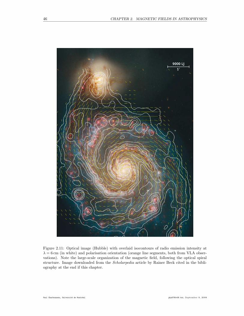
46 CHAPTER 2. MAGNETIC FIELDS IN ASTROPHYSICS
Figure 2.11: Optical image (Hubble) with overlaid isocontours of radio emission intensity atλ = 6 cm (in white) and polarisation orientation (orange line segments, both from VLA obser-vations). Note the large-scale organization of the magnetic field, following the optical spiralstructure. Image downloaded from the Scholarpedia article by Rainer Beck cited in the bibli-ography at the end if this chapter.
Paul Charbonneau, Universite de Montreal phy6795v08.tex, September 9, 2008
2.10. THE ULTIMATE ORIGIN OF ASTROPHYSICAL MAGNETIC FIELDS 47
In part III of this course we will see that astrophysical flows are actually quite apt atamplifying magnetic fields, so what we are after here is a very small “seed field” to start up theprocess. Cheap and easy explanations along the line of an original seed magnetic field being aprimordial relic of the Big Bang need not concern us here. Nor is early-universe ferromagnetisma viable option, since permanent magnets require an externally-applied magnetic field to becomemagnetized in the first place. Interestingly, the two options that are currently deemed viablestand at the opposite ends of the physical exotism scale: magnetic monopoles... and batteries.Let’s briefly discuss these in turn1.
2.10.1 Magnetic monopoles
On the theoretical front, already back in 1931 Paul Dirac (1902-1984) pointed out that thereis nothing to prevent there being magnetic monopoles so long as the magnetic charge on aparticle is some integer multiple of g ≡ hc/(4πe) ≈ 69e, where h is Planck’s constant, and e isthe fundamental electric charge. With just one magnetic monopole in the universe we have ourbasic seed field. In the early 1970’s, G. t’Hooft and A.M. Polyakov argued that the spontaneoussymmetry-breaking of the Grand Unified (field) Theory Lagrangian, which occurs very early inthe formation of the universe at kBT ≈ 1015 GeV, would produce a lot of mg ≈ 1016 GeV/c2
magnetic monopoles.2 So many in fact that inflationary cosmology was invented in part to dealwith this embarrassment of riches and to leave about one monopole within each subdomain ofthe inflated universe(s). But again, we only need one monopole to produce our seed field, sothe realist stops there.
2.10.2 Batteries
Leaving magnetic monopoles aside, we should inquire about more pedestrian means to createseed magnetic fields. Since it could be that t’Hooft and Polyakov got the wrong Lagrangian,GUT’s will be superseded by something else, etc. So it would be nice to have a fall backmechanism to generate a seed magnetic field that relies on basic physics that we know functionssensibly at least in our part of the universe. To this end, we return to our derivation of theinduction equation (§1.3). Recall that one essential next step toward MHD from Maxwellrequired stipulating Ohm’s law, in the form of eq. (1.58) for the laboratory frame of reference.Consider now the possibility of a “mechanically-driven” process of charge separation (i.e., notrelated to the presence of an electric field in any reference frame); Ohm’s law then picks up anextra term:
J = σ[
E + U × B]
+ Jmech . (2.2)
If we keep only the very first term on the RHS of equation (2.2), and drop the displacementcurrent in equation (1.55), then we get back to the induction equation (1.60). If we availourselves of neither of these opportunities then we obtain instead:
1 +η
c2
∂
∂t
∂B
∂t= ∇×
(
U × B − η∇× B + µ0Jmech
)
. (2.3)
Notice that our only hope for creating B out of nothing (so to speak) is the Jmech term; retainingthe displacement current gives us no advantage.
The Jmech term represents our ability to mechanically grab a hold of electric charges andforce currents to flow; in other words, an electromotive force. In the dense interior of a con-ducting star, plasma kinetic theory permits one to write down a prescription for this “battery”contribution to the total electric current density as:
Jmech =σ
ene
[
∇pe −1
cJ × B
]
, (2.4)
1Most of the remainder of this section was written by T.J. Bogdan as part of an earlier version of these classnotes, with only some slight rewording, notational homogeneization, and minor additions on my part.
2You might find it amusing to figure out how many kilograms that works out to be!
phy6795v08.tex, September 9, 2008 Paul Charbonneau, Universite de Montreal
48 CHAPTER 2. MAGNETIC FIELDS IN ASTROPHYSICS
where pe is the contribution of the electrons alone to the thermal pressure (see references inbibliography). For a completely ionized pure hydrogen plasma, pe is just half of the total gaspressure, and ne = ρ/mp, and so,
Jmech =σmp
2eρ
[
∇p − 2
cJ × B
]
. (2.5)
Now, the second term on the RHS of equation (2.5) does not do us any good since it carries afactor of B, so the whole plan rests upon the first term generating a seed magnetic field. For aspherically symmetric star, we know from hydrostatic equilibrium that ∇Φ = (∇p)/ρ, and sothe product ηJmech ∝ ∇Φ. Which does not do us any good because of the presence of the curloperator on the RHS of equation (2.3), which yields zero upon acting on Jmech since (∇p) is agradient of a scalar function. How can we get around this constraint? A viable possibility isrotation. If a star is rotating, then there is a centrifugal force per unit density of $Ω2e$ whichadds to ∇Φ and which leads to the generation of a seed magnetic field. This process of thecentrifugal force driving a flow of electrons relative to the ions was first pointed out by LudwigBiermann (1950) and is now called the Biermann battery.
In fact any process that can produce a relative motion between the ions and electrons is apotential battery mechanism, and a possible candidate for creating seed magnetic fields. Forexample, consider a rotating proto-galaxy, where the outer portions of the proto-galaxy moveat a speed U = RΩ relative to the frame in which the microwave background is isotropic. TheThomson scattering of the microwave photons by the electrons results in the so-called Compton
drag effect, which causes the electrons to counter-rotate with respect to the ions The net resultis an azimuthal current which generates a poloidal magnetic field.
Of course, if you bother to put typical numbers in these various examples you will find thatyou don’t really generate very much magnetic field. But generating a lot of field is not thepoint, that can be one via magnetic flux conservation in a collapsing protostellar cloud, or, aswe shall see in part III of this course, via the u × B term in our MHD induction equation. Thebasic idea to take away from this section is that invoking weird, unproven physics to get awayfrom B = 0 is not necessary.
Time to move on to part II of this course; for the time being, we just consider that moststars are magnetized to some degree, and investigate in the following 3 chapters the impactsuch magnetic fields may have on mass loss via wind-like outflows.
Problems:
1. This problem lets you explore some astrophysical implications of the flux freezing con-straints encountered in the previous chapter.
(a) Assume that the Sun has formed from the spherically symmetric collapse of aninitially spherical gas cloud of radius 10 light-years and threaded by a large-scalegalactic magnetic field of strength 10−10 T. Under the assumption of flux freezing,what should then be the strength of the internal solar magnetic field? Is this areasonable number?
(b) The large-scale surface poloidal field of the Sun is actually of order 10−3 T. Underthe same assumptions as in (a), compute the strength of the magnetic field expectedin a White Dwarf (RWD/R¯ = 0.01). Is this a reasonable number?
(c) What would you think are the primary problem with these two estimates?
2. Let’s consider a constant-density “sun” made of purely ionized Hydrogen. Suppose nowthat its exterior magnetic field can be approximated by a dipole, with a surface fieldstrength of 10−3 T. Assume now that this magnetic field is produced by an azimuthal(i.e., φ-directed) current density within the interior (r/R¯ < 1); then,
Paul Charbonneau, Universite de Montreal phy6795v08.tex, September 9, 2008
2.10. THE ULTIMATE ORIGIN OF ASTROPHYSICAL MAGNETIC FIELDS 49
(a) Estimate the magnitude of the current density required to produce such a dipolarfield;
(b) Estimate the drift velocity between protons and electrons required to produce sucha current density. How does it compare to the average thermal velocity?
(c) How can such a small velocity difference not be erased by collisions between micro-scopic constituents? To answer this one will have to think back to some fundamentalaspects of the induction process, as covered in your first course on electromagnetism.
3. Suppose that a large flare, liberating some 1026 J , is power by the complete dissipationof a uniform magnetic field of strength 0.1 tesla contained within a volume V . How largedoes V has to be to add up to 1026 J? Does this make sense, given typical dimensions fora large active region (which you can eyeball, e.g., from Fig. 2.4).
4. With this one you get to play with some of the timescales introduced in the precedingpages. We’ll consider a solar-like star, with uniform electrical conductivity throughout(feel free to use the value in Table 1.2.
(a) Estimate the diffusion time for a magnetic field contained in the solar interior.How large would the magnetic diffusivity have to be to produce a typical diffu-sive timescale of the order of the observed solar cycle period of ∼ 10 yr? Do youthink this is a reasonable number?
(b) Estimate now a flow speed that would lead to a turnover time of order 10 yr. Is thisa reasonable number in the solar/stellar context?
5. At long last, a problem that asks you to surf the Web!! Use your surfing skills to locatewhat is (in your opinion) a very cool image of some astrophysical magnetic field(s).But careful now, you must be able to explain what is actually on the image! And pleaseprovide a full working URL.
Bibliography:
Many ambitious monographs have been written on the general topic of astrophysical magneticfields. My personal “top-three” selection is:
Parker, E.N. 1979, Cosmic magnetic fields, Oxford: Clarendon,Mestel, L. 1999, Stellar magnetism, Oxford: Clarendon,Rudiger, G., & Hollerbach, R. 2004, The magnetic universe, New York: John Wiley.
Parker’s book is unfortunately out of print, and Rudiger & Hollerbach’s outrageously priced($230!). The Mestel book was issued in paperback in 2003, but still at a whopping $125! Forgood introduction on planetary magnetic fields, see
Bagenal, F. 1992, Ann. Rev. Earth & Planet. Sci., 20, 289-328
Table 2.1 was in fact adapted from this paper, augmented by data extracted from the Goedbloed& Poedts textbook cited in the preceding chapter. The following (relatively) recent conferenceproceedings is devoted to documenting the ubiquitous presence of magnetic fields throughoutthe Hertzsprung-Russell diagram:
Mathys, G., Solanki, S.K., & Wickramasinghe, D.T. (eds.), Magnetic fields in the Hertzsprunbg-
Russell diagram, ASP Conf. Series 248 (2001).
See in particular the review papers by Mathys, Bagnulo (Ap stars), Campbell (binary stars),Valenti & Johns-Krull (cool stars), Schmidt (white dwarfs) Reisenegger (neutron stars), as wellas the introductory overview paper by Mestel.
The following are two good, recent textbooks on Solar Physics at the higher undergraduatelevel, including extensive discussions of solar magnetism:
phy6795v08.tex, September 9, 2008 Paul Charbonneau, Universite de Montreal
50 CHAPTER 2. MAGNETIC FIELDS IN ASTROPHYSICS
Stix, M., 2001, The Sun: an introduction, 2nd ed., Springer,Foukal, P., 2006, Solar Astrophysics, 2nded., John Wiley & Sons.
If the historical aspects of sunspots and solar magnetic studies are of interest to you, you mayalso want to consult the ever-being-enlarged Web site “Great Moments in the History of SolarPhysics”:
http : //www.astro.umontreal.ca/ ∼ paulchar/grps/histoire physique.html.
Hale’s original papers on sunspots are still well worth reading. The two key papers are:
Hale, G.E. 1908, “On the probable existence of a magnetic field in sunspots”, The Astro-
physical Journal, 28, 315-343,Hale, G.E., Ellerman, F., Nicholson, S.B., and Joy, A.H. 1919, The Astrophysical Journal,
49, 153-178.
Figure 2.8 was taken from the following paper, still today one of the more cogent exposition ofthe Mt Wilson CaII project and data:
Baliunas, S.L., Donahue, R.A., Soon, W.H., and 24 co-authors, ApJ, 438, 269,
For a recent review of magnetic field detections in early-type stars, see
Wade, G.A. 2005, in Element stratification in stars: 40 years of atomic diffusion, eds. G. Ale-cian, O. Richard & S. Vauclair, EAS Publication Series, 17, 227-237.
and more specifically on Ap stars:
Mathys, G., Hubrig, S., Landstreet, J.D., Lanz, T., & Manfroid, J. 1997, Astron. Astro-
phys. Suppl.. 123, 353.
On magnetic field detection in hot subdwarfs, see
O’Toole, S.J., Jordan, S., Friedrich, S., & Heber, U. 2005, Astron. Ap., 437, 227.
I found the following online article a good starting point to learn about galactic magnetic fields:
Beck, R. 2007, Scholarpedia, 2(8), 2411http://www.scholarpedia.org/articles/Galactic magnetic fields.
For some “light” reading on magnetic monopoles in field theory and astrophysics, try,
Dirac, P.A.M. 1931, Proc. R. Soc. Lond. A, 133, 60Parker, E.N. 1970, ApJ, 160, 383t’Hooft, G. 1974, Nucl. Phys. B, 79, 276Polyakov, A.M. 1975, Sov. Phys. JETP, 41, 988Cabrera, B. 1982, Phys. Rev. Lett., 48, 1378Kolb, E.W., & Turner, M.S. 1990, The Early Universe, (New York: Addison-Wesley), §7.6.
and references therein. For more on Biermann’s battery, see
Biermann, L. 1950, Zeits. f. Naturforsch. A, 5, 65,Roxburgh, I.W. 1966, MNRAS, 132, 201,Chakrabarti, S.K., Rosner, R., & Vainshtein, S.I. 1994, Nature 368, 434,
as well as chap. 13 in the Kulsrud book cited in the bibliography of the preceding chapter.
Paul Charbonneau, Universite de Montreal phy6795v08.tex, September 9, 2008