Oil price dynamics, macro-�nanceinteractions and the role of �nancial

speculation

Claudio Morana�

Università di Milano Bicocca (Milano, Italy),

CeRP-Collegio Carlo Alberto (Moncalieri, Italy),

Fondazione Eni Enrico Mattei (Milano, Italy),

International Centre for Economic Research (ICER, Torino)

First draft December 2011; this draft August, 28, 2012

Abstract

What is the role of �nancial speculation in determining the real oilprice? We �nd that while macroeconomic shocks have been the mainreal oil price upward driver since mid-1980s, �nancial shocks have siz-ably contributed since early 2000s as well, and at a much larger extentsince mid-2000s. Even though �nancial shocks contribute 44% out ofthe 65% real oil price increase over the period 2004-2010, the thirdoil price shock is a macro-�nance episode: macroeconomic shocks ac-tually largely account for the 2007-2008 oil price swing. While wethen �nd support to the demand side view of real oil price determina-tion, we however also �nd a much larger role for �nancial shocks thanpreviously noted in the literature.

Keywords: Oil price, �nancial speculation, macro-�nance interface,international business cycle, factor vector autoregressive model.JEL classi�cation: C22; E32; G12

�Electronic address: claudio.morana@unimib.it.

1

1 Introduction

After about two decades of stability, both nominal and real oil prices havebeen increasing since 2003 (US$ 30 per barrel), with unprecedented volatilityin 2008, as nominal oil prices peaked up at US$ 140 in July, to bottom downat US$ 40 in December; oil prices have mostly been increasing thereafter,achieving a new peak in April 2011 (US$ 110).Recent trends, hikes and volatility have indeed revived the debate on the

factors contributing to oil price determination, and two main explanationsfor the third oil price shock have so far been proposed in the literature:�rstly, increasing oil demand, due to rapid growth in emerging countries andstable OECD oil consumption (Kilian, 2008, 2009a,b) or to expansionarymonetary policies (Frankel, 2007; Calvo, 2008; Kilian, 2010), in the face ofstagnant oil production; secondly, increased speculation in the oil futuresmarket since mid-2000s (Davidson, 2008; Krugman, 2008, 2009; Masters2008, 2009; Masters and White, 2008).While strong empirical support for the economic growth hypothesis is

found in the literature (Kilian and Murphy, 2010; Kilian and Hicks, 2011;Hamilton 2009a,b, Baumeister and Perssman, 2008; Dvir and Rogo¤, 2010),the empirical evidence in favor of the excess liquidity explanation is weak.For instance, Barsky and Killian (2002, 2004) and Kilian (2010) point to apositive linkage between liquidity conditions and the real oil price over the1970s; yet, beyond any e¤ect exercised through real activity and in�ation,there is little evidence of liquidity and interest rate direct e¤ects (see alsoAnzuini et al.; 2012, Thomas et al., 2010; Frankel and Rose, 2010). Moreover,the impact of liquidity on the real oil price is only transitory, and thereforeunlikely to account for the 2008 episode (Erceg et al., 2011).On the other hand, the narrative evidence on the contribution of excess

speculation to recent oil price dynamics is based on the steady increase inthe market share of non hedging open interest positions in the US commod-ity futures and option markets1, following the �nancial liberalization provi-sions contained in the U.S. Commodity Futures Modernization Act (CFMA)passed in 20002.

1Since 2002 the Working (1960)�s T index for the oil futures market has been increasingat an average 2% annual rate. Moreover, the global value of outstanding OTC commodityderivatives has grown from 0.4 US$ trillion in 1998:1 to 2.9 US$ trillions in 2005:1 and13.2 US$ trillions in 2008:1, plunging to 4.4 US$ trillions in 2008:2, closely tracking oiland other commodities price dynamics over the same period.

2See H.R. 5660: Commodity Futures Modernization Act, included in H.R. 4577: Con-solidated Appropriations Act for FY 2001, signed by US President Clinton in December,21, 2000.

2

Since 2005 contango, rather than backwardation as over the 1980s and1990s, has prevailed in the oil futures market: the increased presence ofnon-commercial investors, seeking portfolio diversi�cation, might have indeedlead to a reversal in the receipt of the premium, i.e., from arbitrageurs tooil producers, rather than the other way around (Hamilton and Wu, 2011).This might also be indicative of a structural shift in inventories manage-ment, as contango (backwardation) is in general associated with a high (low)level of inventories, which may be induced by speculative behavior (Gor-ton et al., 2008). Alquist and Kilian (2010), actually document that thetwelve-month oil futures spread (future12t � spott) is strictly related to pre-cautionary/speculative oil demand shocks; yet, the latter linkage, as well asthe entire oil futures price term structure (Fattouh and Scaramozzino, 2011),has undergone structural change since 2004.Albeit heterogeneous behavior in the oil futures market - crucial condi-

tion for �nancial speculation to be destabilizing - is actually documented invarious papers (Vansteenkiste, 2011; Reitz and Slopek, 2008; ter-Ellen andZwinkles, 2010; Ci¤arelli and Paladino, 2010), the empirical evidence on itse¤ects is controversial.For instance, some studies, based on U.S. Commodity Futures Trading

Commission (CFTC) data, �nd that speculation has dampened price volatil-ity since mid-2000s, by increasing oil futures market liquidity (Brunetti et al.,2010; Buyuksahin et al., 2010). Moreover, there is no evidence of Grangercausality from trading positions to futures oil prices, but some support tothe view that oil prices lead trading positions (Buyuksahin and Harris, 2011;Alquist and Gervais, 2011; Irwin and Sanders, 2012). Also, both hedging andnon-hedging traders in the oil futures market would herd (Buyuksahin andHarris, 2011); yet, herding behavior by hedge funds, by being countercycli-cal, is not destabilizing (Boyd et al., 2009). Di¤erently, other papers �ndherding behavior by speculators contributing to the 2008 price hike (Frankeland Rose, 2010), the thirteen-week change in the imputed positions of indexinvestors and in the managed-money spread positions predicting weekly oilfutures price returns (Singleton, 2011), (negative) Granger causality from theWorking�s-T index to oil futures prices (Manera et al., 2012), endogeneity ofcrude oil - and other individual commodities - futures prices relative to Com-modity Linked Note (CLN) trades (Henderson et al., 2012), and support forhedging pressure mechanisms (Melolinna, 2011; Acharya et al., 2012; Mou,2011; Etula, 2010; Hong and Yogo, 2011).Within the framework of structural vector autoregressive models, Kilian

and Murphy (2010) also �nd evidence against any role of �nancial specula-tion in the recent oil price episode, while according to Juvenal and Petrella(2011) and Lombardi and Van Robays (2011), speculative (non fundamental)

3

�nancial shocks account for 15% of the real oil price increase between 2004and 2008 and a 10% real oil price overshooting between August 2007 andJune 2008, respectively. Finally, Phillips and Yu (2011) and Gilbert (2010)point to a speculative bubble in the real oil price, originating in March 2008,and therefore posterior to the collapse of the housing bubble dated June 2007,consistent with the theory of migrating bubbles of Caballero et al. (2008a,b);Shi and Arora (2012) yield supporting evidence for the latter �nding.In the light of the contrasting empirical evidence, the current paper then

aims at assessing the role of �nancial speculation in the recent oil priceepisode, providing original contributions under di¤erent perspectives.Firstly, large-scale modeling of the oil market-macro-�nance interface is

implemented, considering macro-�nancial data for �fty countries, includingOECD and emerging economies, and a detailed description of oil physicaland futures market conditions. Single country macro-�nancial data are usedto estimate the unobserved factors driving the global business and �nancialcycle; additional observed US �nancial factors, proxying for expectationsabout future fundamentals and economic/�nancial fragility conditions arealso considered: the size and value Fama and French (1993) factors, theCarhart (1997) momentum factor, the Pastor and Stambaugh (1997) liquidityfactor, the Adrian, Etula and Muir (2011) leverage factor and the Baglianoand Morana (2012) economic/�nancial fragility index, in particular.The careful and large-scale modelling of the oil market macro-�nance in-

terface surely is an important novelty of our study; while Kilian and Murphy(2010), by including inventories in their model, do allow for a �nancial oildemand component and, indirectly, for the e¤ect of future fundamentals onoil demand, our contribution, by conditioning on risk factors, is the �rstattempt to directly measure their e¤ects; by including measures of excessspeculation, our study also aims at disentangling the fundamental and nonfundamental components of �nancial oil demand, similar to Juvenal and Pe-trella (2011) and Lombardi and Van Robays (2011), which are left indistinctin Kilian and Murphy (2010); yet, relatively to Juvenal and Petrella (2011)and Lombardi and Van Robays (2011), disentangling is more accurate as, byconditioning on risk factors, liquidity, interest rates and portfolio�s diversi�-cation opportunities, non-fundamental speculative shocks can be identi�ed.We do �nd that without a careful description of the �nancial side, shocksand transmission mechanisms which are important to the understanding ofthe working of the oil market would go neglected.Secondly, the proposed modelling approach sheds new insights on the

determination of the real oil price: while we con�rm that, at least since mid-1980s, macroeconomic shocks have been the major upward driver of the realoil price, we also �nd a sizable contribution of oil market supply side and

4

�nancial shocks since early 2000s. In general, di¤erently from oil marketsupply side shocks, macroeconomic and �nancial shocks had a stabilizinge¤ect on nominal oil price volatility.The impact of �nancial shocks has surely been remarkable since mid-

2000s, contributing 44% out of the 65% real oil price increase over the period2004 through 2010. Yet, the third oil price shock is a macro-�nance episode:macroeconomic shocks account for 58% out of the 68% real oil price runup over the 2007(2)-2008(2) period, and �nancial shocks for 6% in 2007(4);moreover, the -67% and -31% contractions in 2008(4) and 2009(1) are alsolargely accounted for by macroeconomic shocks (-40% and -26%), with �nan-cial shocks (-14% and -7%) also sizably contributing; the 54% real oil priceincrease over the 2009(2) through 2009(4) period is �nally equally accountedfor by macroeconomic (21%) and �nancial (20%) shocks.In 2010, following the subprime crisis and the large oil (and other com-

modities) price swings, regulatory reforms aimed at promoting �nancial sta-bility were then launched in the US3 and EU4. With reference to the commod-ity derivatives market, among other provisions, the latter reforms reintroduceposition limits for �nancial investors, to safeguard price discovery in the fu-tures market. More recently, a proposal for the introduction of a EU global�nancial transaction tax5 has been put forward; such a provision, if endorsedat a global level, would also contribute to indirectly controlling OTC tradingand speculative positions in commodities futures markets.While the results of this study would then provide empirical support to

the regulatory changes proposed and implemented since 2010, they wouldnot however be consistent with an explanation of the third oil price episodeneglecting the contribution of macroeconomic developments.The paper is organized as follows. In Section 2 the econometric method-

ology is introduced, while in Section 3 the data are presented. Then, inSection 4 speci�cation and estimation issues are discussed, while in Section5, 6 and 7 the empirical results are presented. Finally, conclusions are drawnin Section 8.

3See H.R. 4173: Dodd-Frank Wall Street Reform and Consumer Protection Act, signedby US President Obama in July, 21, 2010.

4See the Proposal for a Regulation of the European Parliament and of the Councilon OTC derivatives, central counterparties and trade repositories (COM(2010) 484 �nal2010/0250 (COD)), approved by the European Parliament on March, 29, 2012.

5See the European Commission proposal (COM/2011/594) endorsed by the UnitedNations independent rights experts on extreme poverty, food, business, foreign debt andinternational soidarity on May, 14, 2012 and by the European Parliament on May, 23,2012.

5

2 The econometric model

The econometric model is described by two blocks of equations. The �rstblock refers to the observed (F2;t) and unobserved (F1;t) global macro-�nancialfactors and oil market demand and supply side variables (Ot), collected in ar � 1 vector Ft =

�F01;t F

02;t O

0t

�0, while the second block refers to q macro-

�nancial variables for m countries, collected in a n�1 vector Zt (n = m�q).The joint dynamics of the �global�macro-�nance-oil market interface (theglobal economy thereafter) and the �local�macro-�nance interface are thenmodelled by means of the following reduced form dynamic factor model

(I�P(L))(Ft � �t) = �t (1)

�t � i:i:d:(0;��) (2)

(I�C(L)) ((Zt � �t)�� (Ft � �t)) = vt (3)

vt � i:i:d:(0;�v): (4)

The model is cast in a weakly stationary representation, as (Ft��t); (Zt��t) � I(0), where �t and �t are n � 1 and r � 1 vectors of deterministiccomponents, respectively, with r � n, including an intercept term, and,possibly, linear or non linear trends components.6

Global dynamics are described by the stationary �nite order polynomialmatrix in the lag operator P(L), P(L) � P1L+P2L2+ :::+PpLp, where Pj,j = 1; ::; p, is a square matrix of coe¢ cients of order r, and �t is a r�1 vectorof i.i.d. reduced form shocks driving the Ft factors. The contemporaneouse¤ects of the global factors on each country�s variables in Zt are measuredby the loading coe¢ cients collected in the n� r matrix � =

��0F1 �

0F2�0O�0.

Finally, vt � i:i:d:(0;�v) is the n�1 vector of reduced-form idiosyncratic(i.e., country-speci�c) disturbances, with E

��jtvis

�= 0 for all i; j; t; s, and

C(L) is a �nite order stationary block (own country) diagonal polynomialmatrix in the lag operator, C(L) � C1L + C2L

2 + ::: + CcLc, where Cj,

j = 0; ::; c, is a square matrix of coe¢ cients of order n, partitioned as

Cjn�n

=

26666664

Cj;11q�q

0 ::: 0

0 Cj;22q�q

::: 0

... :::. . .

...0 0 ::: Cj;mm

q�q

37777775 : (5)

The speci�cation of the model in (1)-(3) embeds a set of important as-sumptions on the structure of global and local linkages: (i) global shocks

6�t = � and �t = � in the current application.

6

(�t) a¤ect both the global and local economy through the polynomial ma-trix P(L) and the factor loading matrix �; (ii) country-speci�c disturbances(vt) do not a¤ect global factor dynamics, limiting their impact only to thecountry of origin (C(L) is assumed to be block (own-country) diagonal).By substituting (1) into (3), the reduced form vector autoregressive (VAR)

representation of the dynamic factor model can be written as

(I�A(L)) (Yt � t) = "t ; (6)

where Yt = [F0t Z

0t]0, t = [�

0t �

0t]0,

A(L) =

�P(L) 0

[�P(L)�C(L)�] C(L)

�;

"t ��"1;t"2;t

�=

�I�

�[�t] +

�0vt

�;

with variance-covariance matrix

E ["t"0t] = �" =

��� ���

0

��� ����0 +�v

�:

The structural vector moving average representation for the global modelin (1) can then be written as

(Ft � �t) = HF (L)K�1�t; (7)

where �t is the vector of the r structural shocks driving the common factorsin Ft, i.e., �t = K�t, K is a r � r invertible matrix, and

H(L) ��HF (L) 0HFZ(L) HZ(L)

�� (I�A(L))�1 :

By assumption the structural factor shocks are orthogonal and have unitvariance, so that E [�t�

0t] = K��K

0 = Ir. To achieve exact identi�cationof the structural disturbances, additional r(r � 1)=2 restrictions need to beimposed. Since �t = K�1�t, imposing exclusion restrictions on the con-temporaneous impact matrix amounts to imposing zero restrictions on theelements of K�1, for which a lower-triangular structure is assumed. Op-erationally, K�1 (with the r(r � 1)=2 zero restrictions necessary for exactidenti�cation imposed) is estimated by the Choleski decomposition of thefactor innovation variance-covariance matrix ��, i.e., K�1 = chol(��). Fore-cast error variance and historical decompositions can then be obtained bymeans of standard formulas.

7

Consistent and asymptotically normal estimation of the two-block spec-i�cation in (1) and (3) is obtained by means of the procedures proposedin Morana (2011a, 2012a), shown to yield accurate estimation also in smallsamples (see the Monte Carlo results reported in Morana, 2011a, 2012a).Following the thick modelling strategy of Granger and Jeon (2004), medianestimates of the parameters of interest, impulse responses, forecast error vari-ance and historical decompositions, as well as their con�dence intervals, areobtained by means of simulation. See the Appendix for a detailed accountof the estimation procedure and the econometric methodology.

3 The data

We use seasonally adjusted quarterly macroeconomic time series data for 31advanced economies (Australia, Austria, Belgium, Canada, Czech Republic,Denmark, Finland, France, Germany, Greece, Hong Kong, Iceland, Ireland,Israel, Italy, Japan, Luxembourg, Netherlands, New Zealand, Norway, Portu-gal, Singapore, Slovakia, Slovenia, South Korea, Spain, Sweden, Switzerland,Taiwan, United Kingdom), 5 advanced emerging economies (Brazil, Hun-gary, Mexico, Poland, South Africa), and 14 secondary emerging economies(Argentina, Chile, China, Colombia, India, Indonesia, Malaysia, Morocco,Pakistan, Peru, Philippines, Russia, Thailand, Turkey), for a total of 50countries. The (main) data source is IMF International Financial Statis-tics7.Concerning the block of equations in (3), for each of the 50 countries,

apart from some exceptions, 17 macroeconomic variables are employed, namelyreal GDP, private consumption and investment growth, public expenditure toGDP ratio growth, nominal bilateral US$ exchange rate (value of 1 US$ inunits of country currency) returns, CPI in�ation rate, M2 or M3 to GDP ra-tio growth, nominal M2/M3 growth, civilian employment growth, unemploy-ment rate changes, real wages growth, real stock prices returns, real housingprices returns, real short and long term interest rates, real e¤ective exchangerate returns, bank loans to the private sector to GDP ratio growth. A totalof over 800 equations is then considered in block (3). For OECD countriesthe macro-�nancial sample extends from 1980:1 through 2010:3, while fornon OECD countries only from 1995:1 through 2010:3. Di¤erent samples aretherefore employed in estimation.

7Other data sources employed are FRED2 (Federal Reserve Bank of St. Louis); OECDand BIS (uno¢ cial) house price data sets, and International Energy Agency (IEA-OECD)data sets.

8

Concerning the block of equations in (1), 33 variables are considered inthe vector Ft.Firstly, 11 variables are included in the vector of (global) observed factors

F2;t, i.e., the Bagliano and Morana (2011) US economic/�nancial fragilityindex (FRA) in di¤erences, the Fama and French (1993) size and valuefactors (SMB, HML), the Carhart (1997) momentum factor (MOM), thePastor and Stambaugh (1997) stocks� liquidity factor (PSL), the S&P 500stock return volatility in di¤erences (FV ), computed from an asymmetricGARCH model, the real gold price (GD) return, real IMF non-energy com-modities price index returns (M), the US �scal (Fd) and trade de�cit (Td)to GDP ratios in di¤erences, the Adrian, Etula and Muir (2011) leveragefactor (LEV ). The sample for the observed macro-�nancial factors extendsfrom 1980:1 through 2010:3.Secondly, 10 additional variables, concerning global oil demand and sup-

ply conditions, are included in the vector Ot, i.e., world oil reserves growth(R), net world oil production changes (increase: Pp, decrease: Pm)8, OECDoil re�neries margins growth (RM), world oil consumption (C) growth,OECD oil inventories rate of growth (INV ), real WTI oil price (OP ) re-turn, nominal WTI oil price volatility in di¤erences (OV ), computed froma GARCH model, the twelve-month futures basis, i.e., the ratio of the nomi-nal twelve-month futures-spot spread over the nominal spot oil price (FB),computed using Crude Oil (Light-Sweet, Cushing, Oklahoma) 12th Contractsettle futures prices, and the growth rate of the oil futures market Work-ing (1960)-T index (WT ), computed using US Commodity Futures TradingCommission (CFTC) Commitment of Trades (COT) data.9 The sample forthe latter variables extends from 1986:1 through 2010:3.Thirdly, 12 variables are collected in the vector of (global) unobserved fac-

tors F1;t; the latter are estimated using (3), with �t = �, using a �rst orderown country diagonal dynamic structure, as suggested by the BIC informa-tion criterion.10 In particular, the unobserved global macro-�nancial factorsare estimated using subsets of homogeneous variable, i.e., a real activity fac-tor (Y ) is extracted from real GDP, private consumption and investment

8See Hamilton (1996), albeit for an application to the oil price.9The Working�s T index is calculated as the ratio of speculative open interest to to-

tal open interest resulting from hedging activity, i.e., as 1+SS/(HS+HL) if HS HL and1+SL/(HS+HL) if HS<HL, where open interest held by speculators (noncommercials)and hedgers (commercials) is denoted as follows: SS = Speculation, Short; HL = Hedging,Long; SL = Speculation, Long; HS = Hedging, Short.10F1;t has been obtained by conditioning with respect to F2;t and only a subset of the

variables considered in Ot, i.e. the real oil price and the real non-energy commoditiesprice index, which are avavilable since 1980:1. The other oil market variables are availbleonly since 1986:1.

9

growth series; a �scal stance factor from the public expenditure to GDP ra-tio growth series (G); a global bilateral US$ exchange rate index from thevarious bilateral exchange rates against the US$ returns (X); a nominal (corein�ation) factor (N) from the in�ation rate and the nominal money growth,short and long term interest rate series; an excess liquidity index (L) fromthe M3(M2) to GDP ratio and the private loans to GDP ratio growth series;an employment factor (E) from the civilian employment growth series; anunemployment rate factor (U) from the unemployment rate in changes series;a real wage factor (W ) from the real wage growth series; a real stock marketreturn factor (F ) from the real stock market price index return series; a realhousing return factor (H) from the real housing price index return series; areal short term rate factor (SR) from the real short term interest rate series;a term spread factor (TS) from the term spread series.11

4 The global oil market-macro-�nance inter-face model: speci�cation and estimation

The global model for the oil market macro-�nance interface in (1) counts 33endogenous variables, collected in the vector Ft =

�F01;t F

02;t O

0t

�0, with �t =

�. For PC-VAR estimation, 12 principal components of Ft, jointly accountingfor 80% of total variance, and three lags are selected, according to MonteCarlo results (Morana, 2012a) and speci�cation tests. Hence, 36 parametersare estimated for each of the 33 equations in the model. Note that, given thesample size available, the estimation of an unrestricted VAR(3) model wouldhave been unfeasible, counting 99 parameters for each equations.The identi�cation of the structural shocks is performed by means of the

Choleski decomposition approach. The latter implies a recursive structuralmodel, whose ordering is assumed as follows: reserves, net oil productionchanges (negative and positive), re�neries margins, employment and the un-employment rate, real activity, the �scal stance, the US �scal and trade de�citto GDP ratios, the nominal factor, real wages, oil consumption, excess liq-uidity, the real short term rate and term spread, real housing prices, the US$exchange rate index, stock market volatility, the size and value Fama-Frenchfactors, the Carhart momentum factor, the Pastor-Stambaugh liquidity fac-tor, the Adrian-Etula-Muir leverage factor, the Working-T speculative index,the futures market basis, oil inventories, the real oil price, nominal oil price

11Detailed results on PCA and unit root testing are not included for reasons of space,but are available from the author upon request. Further details on data construction canalso be found in the working paper version of this article. See Morana (2011b).

10

volatility, the real non-energy commodities price index, real stock marketprices, real gold prices and the Bagliano-Morana economic/�nancial fragilityindex.As a caveat it should be recalled that the identi�ed shocks may be sensi-

tive to the ordering of the variables, requiring therefore economic motivations.The selected ordering is then based on the following rationale concerning theworking of the oil market:� the oil market supply side is constrained by geophysical conditions,

reacting therefore with (at least one quarter) delay to macro-�nancial condi-tions;� oil consumption is contemporaneously determined by the state of the

world business cycle;� inventories are contemporaneously a¤ected by oil market demand and

supply side conditions, as well as fundamental and non fundamental �nancialfactors;� real oil price and nominal oil price volatility are contemporaneously

determined by oil market supply side, �ow and �nancial oil demand condi-tions, and inventories; they also react with delay to additional fundamental�nancial factors.Moreover, concerning macro-�nancial interactions, it is assumed that:� real activity, over the business cycle, is determined by labor market

conditions, through a short-run production function;� the �scal/trade stance contemporaneously adjust to business cycle con-

ditions;� aggregate demand then feedbacks with delay to aggregate supply, and

prices adjust according to their interaction;� real wages contemporaneously react to aggregate demand and supply

developments, and prices as well;� the liquidity stance, set (by central banks) according to the state of the

business cycle, contemporaneously determines the real short-term interestrate, also impacting on asset prices and �nancial risk;� liquidity, consistent with a leaning-against-the-wind strategy followed

by central banks, may then respond to asset prices and �nancial risk devel-opments only with (at least one-quarter) delay.Three main sets of structural shocks are then identi�ed by means of the

assumed recursive structure, i.e., oil market supply side, macroeconomic and�nancial shocks, in addition to two other shocks, related to the real oil priceand nominal oil price volatility, and two preference shocks, related to oil con-sumption and inventories. The recursive structure implies that oil marketsupply side variables are relatively exogenous to macroeconomic and �nan-cial shocks, and that macroeconomic (and oil consumption) variables are

11

relatively exogenous to �nancial factors. Di¤erently, inventories, the real oilprice and nominal oil price volatility are endogenous relatively to oil marketsupply side, macroeconomic and (most of the) �nancial variables. Struc-tural macroeconomic shocks are therefore contemporaneously orthogonal tostructural oil market supply side shocks; similarly, structural �nancial shocksare contemporaneously orthogonal to structural oil market supply side andmacroeconomic shocks. Within each set of shocks, the same reasoning ap-plies, i.e., for any two variables in the ordering, the leading one is relativelyexogenous to the one which follows.As the implied recursive structural model is exactly identi�ed, the as-

sumed (weak exogeneity) restrictions cannot be tested. Yet, pair wise LMweak exogeneity testing can always be carried out to gauge further evidenceon data properties. A joint test, based on the Bonferroni bounds principle,carried out using the 528 possible bivariate tests implied by the recursivestructure involving the 33 variables, does not reject, even at the 20% signi�-cance level, the weak exogeneity null hypothesis.12 While this result cannotbe taken as a validation for the set of restrictions at the system level, it how-ever suggests that the implied pair wise recursive structure is coherent withthe data.Concerning the block of physical oil market variables, eight structural

shocks can then be identi�ed, i.e., oil reserves, net positive and negativeproduction, re�neries margins, oil consumption and inventories preferences,and other real oil price and nominal oil price volatility shocks.The interpretation of the own equation shocks in terms of reserves, net

production and re�neries margins shocks is clear-cut, each of the latter ac-counting for about 100% of the own variable �uctuations at the impact (seebelow for details). The interpretation of the oil consumption and invento-ries own shocks in terms of preferences shocks depends on the former beingnet of the contemporaneous e¤ect of the macroeconomic variables driving�ow oil demand, and the latter also of the e¤ect of the (�nancial) variablesdriving �nancial oil demand; hence, preferences shocks captures changes inoil consumption and inventories which are unrelated to macroeconomic and�nancial fundamentals. Similarly for the other real oil price and nominal oilprice volatility own shocks, to which we do not attach an economic interpre-tation. Supporting evidence for the proposed interpretation is also providedby the impulse response analysis (see below for details).Moreover, concerning the block of macroeconomic variables, eight struc-

tural shocks can be identi�ed, i.e., labor supply, (negative) labor demand,

12The value of the test is 0.005 to be compared with a 20% critical value equal to 0.0004.Details are available upon request from the author.

12

aggregate demand, �scal stance, US �scal and trade de�cit, core in�ationand productivity shocks.The interpretation of the shocks is grounded on economic reasoning and

correspondence with FEVD and impulse response properties.13 For instance,consistent with economic theory, a positive labor supply shock (upward shiftin the labor supply schedule) induces a negative long-term correlation be-tween employment (1.3%) and the real wage (-1.3%), while a positive cor-relation is induced by a (negative) labor demand shock (downward shift inthe labor demand schedule; -0.10%, employment, short-term; -0.33%, realwage, long-term); the labor supply and demand shocks also account for 90%of employment and unemployment rate �uctuations in the very short-term,respectively.A positive aggregate demand shock (upward shift in the aggregate de-

mand schedule) induces a permanent positive correlation in aggregate activ-ity (0.29%) and the price level (0.02%), while a negative correlation is inducedby the productivity shock (rightward shift in the aggregate supply schedule)(0.7%, real activity, long-term; -0.01%, price level, short-term); while theaggregate demand shock accounts for 80% of real activity �uctuations in thevery short-term, impacting on real activity more strongly in the very short-(0.67%) than in the long-term, the productivity shock is the largest contribu-tor to real activity long-term �uctuations (20%), a¤ecting real activity morein the long- (0.3%) than in the short-term.The core/expected in�ation shock (upward shift in the short-term Phillips

curve) accounts for 60% of nominal factor �uctuations in the very short-term,inducing a positive short-term correlation between the nominal factor (0.05%,long-term) and the unemployment rate (0.19%, short-term).Due to the ordering, �scal stance and US �scal and trade de�cit shocks

are orthogonal to global business cycle shocks (aggregate demand, labor de-mand and supply shocks). Therefore, they re�ect growing global imbalances,unrelated to fundamental business cycle developments; a negative impact onreal activity can be noted in all cases (-0.5%, �scal stance; -0.23%, US �scalde�cit; -0.4%, US trade de�cit); also, they account for 58%, 85%, and 80%of �uctuations in the own variable in the very short-term.Finally, concerning the block of �nancial variables, seventeen structural

shocks can be identi�ed. The shocks can be collected into two groups, i.e.,fundamental and non fundamental shocks; fundamental shocks can then befurther decomposed into three groups, i.e., liquidity and interest rates, risk

13Results concerning the structural interpretation of macroeconomic and fundamental�nancial shocks are not reported for reasons of space. A full set of results is howeveravailable upon request from the author.

13

factors and portfolio shocks. Among fundamental �nancial shocks, excessliquidity, risk-free rate and term spread shocks belong to the former group;risk aversion, size, value, leverage, stocks�liquidity, momentum, and fragilityindex shocks to the middle group; real stock market, housing, gold, and nonenergy commodity index prices shocks to the latter group; an US$ exchangerate index shock could also be included in the latter category. Among non-fundamental shocks, two oil futures market speculative shocks are considered,i.e., Working�s-T and futures basis shocks.The excess liquidity shock accounts for 35% of excess liquidity �uctuations

in the very short-term and leads to a permanent contraction in the realshort-term interest rate (-0.07%), as well as in the real long-term interestrate (-0.03%, implied by the 0.04% increase in the term spread following theshock). Being net of the contemporaneous e¤ect of (oil market supply sideand) macroeconomic and liquidity shocks, the risk-free rate shock may beinterpreted in terms of a short-term bond risk premium shock. The latteraccounts for 30% of short-term real interest rate �uctuations in the veryshort-term. Being also net of the contemporaneous e¤ect of the risk-freerate shock, the term spread shock is related to unexpected changes to thelong-term rate, i.e., to revision in expectations about future business cycleconditions; it accounts for 64% of term spread �uctuations in the very short-term.The risk aversion, size, value, leverage, stocks�liquidity, and momentum

factor shocks account for 60%, 54%, 56%, 35%, 51% and 54% of stock mar-ket volatility, size, value, momentum, stocks�liquidity and leverage factors�uctuations, respectively, in the very short-term. Being contemporaneouslyorthogonal to (oil market supply side and) macroeconomic, liquidity andinterest rates shocks, the risk factor shocks measure revisions in market ex-pectations about future fundamentals. Moreover, the economic and �nancialfragility index shock accounts for 15% of the economic and �nancial fragilityindex �uctuations in the very short-term, and, being orthogonal to all theother shocks considered in the model, it then bears the interpretation ofresidual fragility shock.Being net of the contemporaneous e¤ect of (oil market and) macroeco-

nomic, liquidity and interest rates, and risk factor shocks - apart from housingprices and the exchange rate index -, the real stock market, housing, gold,and non energy commodity index prices shocks bear the interpretation ofpreference/portfolio shocks; the latter account for 21%, 68%, 24% and 38%of very short-term �uctuations in the corresponding variables, respectively.Similarly for the US$ exchange rate shock, accounting for 50% of US$ ex-change rate index �uctuations in the very short-term.Finally, the oil futures market speculative shocks, i.e., the Working�s-T

14

and futures basis shocks account for 55% (each) of Working�s-T and futuresbasis �uctuations in the very short-term, respectively. Their interpretationin terms of oil futures market speculative shocks follows from their positiveimpact on both the oil futures and spot price, also a¤ecting inventories atvarious horizons, in addition to being orthogonal to the set of macroeconomicand �nancial shocks driving �ow and fundamental �nancial oil demand.

5 Forecast error variance decomposition

Median forecast error variance decompositions are computed up to a horizonof ten years (40 quarters). Results for the oil market variables are reportedin Table 1, for selected horizons; for expository purposes, we denote as veryshort-term the horizon within 2 quarters, short-term the horizon between 1and 2 years, medium-term the horizon between three and �ve years, and long-term the 10-year horizon. Rather than focusing on the contribution of eachstructural shock, results are discussed with reference to various categories ofshocks, distinguishing among oil market supply side shocks (SUP: reserves,net negative and positive production, re�neries margins), oil consumptionpreferences shocks (C), inventories preferences shocks (INV), macroeconomicshocks (MAC: labor supply and demand, aggregate demand, �scal stance, US�scal and trade de�cit, core in�ation and productivity), fundamental �nan-cial shocks (FIN: excess liquidity, risk-free rate, term spread, real housingprices, risk aversion, size, value, momentum, stocks� liquidity and lever-age factors, real non-energy commodity price index, real stock prices, realgold prices, economic and �nancial fragility index, (other) nominal oil pricevolatility), US$ exchange rate index shocks (X), speculative/non fundamen-tal �nancial shocks (SPC: Working�s-T index, futures basis), (other) real oilprice shocks (OP). In both cases the contribution of the own shock (OWN)is isolated from the overall contribution: for instance, with reference to oilreserves, the SUP category would not include the reserves shock, whose con-tribution is reported under the OWN category.14

5.1 Oil consumption and production

According to the results of the forecast error variance decomposition, oilconsumption and production are similarly exogenous in the very short-term,yet similarly endogenous already in the short-term. In fact, the own shock

14A full set of results is available upon request from the author.

15

accounts for about 80% of oil consumption �uctuations in the very short-term and 60% at longer horizons; similarly for net oil production changes,i.e., 70% and 90% for negative and positive changes, respectively, in the veryshort-term, and about 50% in both cases since the two-year horizon. Macro-economic shocks sizably contribute to oil consumption �uctuations alreadyin the very short-term (20% within 1-quarter), as well as in the medium- tolong-term (16%); similarly for �nancial shocks (12%). Moreover, net oil sup-ply contractions are more a¤ected by macroeconomic (20% since the 1-yearhorizon) than �nancial shocks (up to 18%), and the other way around fornet oil supply increases (10% and up to 30%, respectively).Overall, the sizable proportion of oil production and consumption �uctu-

ations accounted for by the own shocks, also in the medium- to long-term,is consistent with the presence of geophysical constraints in the former case,and rigidities in oil consumption patterns, small, and declining over time,income and price elasticities, and low substitutability among energy sources,in the latter case.Even stronger endogeneity is shown by both reserves and re�neries mar-

gins in the short-term. For instance, the own shock accounts for 40% and20% of �uctuations at the two- and �ve-year horizon, respectively, for bothvariables; macroeconomic and �nancial shocks jointly explain 50% of reserves�uctuations since the two-year horizon, while (other) oil market supply sideshocks up to 20% in the medium- to long-term; similarly for re�neries mar-gins �uctuations, i.e., 20% and 40% (each) at the two-year horizon and inthe medium- to long-term, respectively. The evidence is then consistent withthe view that macro-�nancial developments may create incentives for oil pro-ducers in engaging in reserves discovery activities and investment, as well asthat re�neries margins are tuned according to the state of the business and�nancial cycle.

5.2 Oil inventories and futures market variables

Also inventories are strongly endogenous, the own shock accounting for only40% of �uctuations in the very short-term and 20% in the long-term. Both oilmarket supply side (12% in the medium- to long-term) and oil consumption(10% in the short-term) shocks, as well as macroeconomic (20% to 30%) andfundamental (20% to 25%) and non fundamental (4% to 7%) �nancial shocks,sizably contribute to inventories �uctuations. In particular, the relevance of�nancial shocks for inventories �uctuations is consistent with the existenceof a �nancial demand for oil, as the latter would in�uence the real oil pricethrough inventories management.

16

Both the Working�s-T (WT) and futures basis (FB) are fairly endogenousas well, the own shock accounting for about 50% of �uctuations in the veryshort-term in both cases; 40% and 20% in the short- and long-term, respec-tively, for WT; 20% and 15% for FB. Fundamental �nancial shocks yield asizable contribution to �uctuations in both variables in the very short-term(20%), while macroeconomic shocks in the short- to long-term (20% to 40%for WT; 30% for FB): among �nancial factors, liquidity/interest rate shocksmatter more for the futures basis (10%; not reported) than excess specula-tion (6%; not reported) in the short-term, and the other way around for riskfactors shocks (6% and 17%, respectively; not reported); a sizable contribu-tion is also yield by oil market supply side shocks (up to 16%; long-term).Once accounted for the common fundamental information, residual �uctua-tions in FB and WT appear to be strongly unrelated; the proportion of FBvariance explained by the WT shock is not larger than 0.3%, and the otherway around. The two variables convey therefore complementary informationconcerning the role of excess speculation in the oil futures market, justifyingtheir joint inclusion in the model.

5.3 Real oil price and nominal oil price volatility

Strong endogeneity is also shown by the real oil price at any horizon, theown shock accounting for 20% of �uctuations in the very short-term, andfor no more than 10% at any other horizon; similarly for nominal oil pricevolatility (30% in the very short-term; 15% in the long-term). Macroeco-nomic and fundamental �nancial shocks jointly account for the bulk of realoil price �uctuations at any horizon (70% in the very short-term; 60% in thelong-term), with macroeconomic shocks yielding a larger contribution than�nancial shocks (up to 50% and 25%, respectively, short-term; 40% and 20%,respectively, medium- to long-term). The contribution of macroeconomic andfundamental �nancial shocks to nominal oil price volatility �uctuations is alsosizable, and larger for �nancial than macroeconomic shocks in the long-term(15% in the short-term; 30% and 5%, respectively, in the long-term); macro-�nancial shocks then jointly account for 25% of nominal oil price volatility�uctuations in the very short-term; 45% and 35% in the short- and long-term,respectively.Among fundamental �nancial shocks, risk factors shocks (up to 30%; not

reported) are the main determinant of nominal oil price volatility �uctua-tions, while liquidity and interest rates shocks (up to 15%; not reported)matter most for the real oil price; risk factors (10%; not reported) and port-folio (up to 10%) shocks also yield a sizable contribution to real oil price

17

�uctuations. Moreover, among macroeconomic shocks, aggregate demand(up to 20%; not reported), US trade de�cit and productivity shocks (up to14% each; not reported) matter most for the real oil price, while labor supplyshocks for nominal oil price volatility (up to 7%; not reported).Also, non fundamental �nancial shocks yield a larger contribution to real

oil price �uctuations in the medium- to long-term (5%) than in the short-term, and the other way around for nominal oil price volatility (5% in thevery short-term); a larger role for oil market supply side shocks is also foundfor nominal oil price volatility than the real oil price (15% to 30% and 5%to 10%, respectively); similarly for US$ exchange rate (up to 10% and 5%,respectively) and inventory shocks (up to 5%, respectively); conversely, oilconsumption preferences shocks more sizably contribute to real oil price thannominal oil price volatility �uctuations (up to 10% and 5%, respectively).Finally, real oil price and nominal oil price volatility own shocks negligibly

account for each other �uctuations (1%; not reported).

6 Impulse response analysis

Concerning the transmission mechanisms of the structural shocks, the im-pulse response analysis is reported in Figures 1-2 for the real oil price and inTables 2-4 for all the oil market variables, over selected horizons, as for theforecast error variance decomposition analysis. In all cases median cumu-lated responses have been computed with 90% signi�cance bands; signi�cant�gures at the 10% level, are shown in bold.15

6.1 Oil market shocks

6.1.1 Oil market supply side shocks

Firstly, a (unitary and permanent) positive reserves shock leads to a siz-able short-term contraction in the real oil price (-1%; Table 3, Panel C). Atemporary negative e¤ect can also be noted on the futures basis, stronglydeclining within two quarters (-1.9%, Table 4, Panel B), consistent with themarket expecting lower real oil prices in the future. Both nominal oil pricevolatility (-0.75%, Table 4, Panel C) and excess speculation (Working�s-T,-0.34%, Table 5, Panel A) are permanently dampened.Secondly, a negative net production shock (downward shift in the �ow oil

supply) leads to a short-term increase in the real oil price (3.3%) and nominal

15Non cumulated responses are only reported for the futures basis and the stocks�liq-uidity and leverage factors.

18

oil price volatility (0.7%). Consistent with expected higher oil prices andweaker fundamentals in the future, the futures basis increases (0.63%, veryshort-term), while excess speculation (Working�s-T index) is permanentlydampened (-0.6%); a permanent increase in inventories (0.3%) and re�neriesmargins (0.82%) for precautionary reasons can �nally be noted.Di¤erently, a positive net production shock (upward shift in the �ow oil

supply) leads to a contraction in the real oil price in the short-term (-1.9%),but to a permanent increase in nominal oil price volatility (1.3%). The futuresbasis increases in the short-term (1.1%), consistent with expected strongerfuture �ow oil demand. Inventories and oil consumption are also increased inthe short-term (0.18% and 0.09%, respectively), stimulated by the reductionin the real oil price. A transitory negative impact on excess speculation can�nally be noted (-0.15%).Thirdly, a positive re�neries margins shock triggers a permanent con-

traction in the real oil price, which is already sizable in the short-term (-2%within 2 quarters; -1.4% at the 10-year horizon), consistent with a shift in theproduction mix favoring (relatively less expensive) medium and heavy sourcrudes. The futures basis then contracts at the outset (-1.1%), while excessspeculation increases in the short-term (0.17%). The impact on nominal oilprice volatility is also permanent and sizable (0.5%).

6.1.2 Oil market demand side shocks

Fourthly, concerning the e¤ects of oil consumption and inventories prefer-ences shocks, a positive oil consumption shock leads to a permanent increasein the real oil price (3.3%), yet dampening nominal oil price volatility (-0.39%). The futures basis increases in the very short-term (1.2%), consistentwith the expectation of stronger demand also in the future, while excessspeculation (Working�s-T) in the short-term (0.13%). The shock also perma-nently increases oil production and re�neries margins (0.14% and 0.28%),while inventories are drawn down in the short-term (-0.3%) in order tosmooth consumption. Di¤erently, a positive inventories shock triggers apermanent contraction in the real oil price (-2.3% in the short-term; -0.93%in the long-term), dampening nominal oil price volatility (-0.56%) and stimu-lating oil consumption in the short-term (0.07%). The futures price contractsless than the spot price in the short-term, fully adjusting in the medium- tolong-term, and therefore leading to a temporary increase in the futures basis(1.3%); re�neries margins also permanently contract (-0.1%).

19

6.1.3 Other real oil price and nominal oil price volatility shocks

Consistent with oil being traded as a �nancial asset, a positive risk-returnrelationship can be noted, as a positive other nominal oil price volatilityshock leads to a permanent increase in the real oil price (1.1%). The levelof the oil price also matters for oil price uncertainty, as a positive other realoil price shock leads to a permanent increase in nominal oil price volatility(0.21%). Hence, a bidirectional linkage can be found for the real oil pricelevel and nominal oil price volatility.Moreover, consistent with price discovery in the spot market spilling over

to the futures market, both positive real oil price and nominal oil price volatil-ity shocks lead to an increase in the futures price. As the futures price in-creases less (more) than the spot price following the former (latter) shock inthe short-term, a temporary contraction (-0.44%) (increase, 0.3%) in the fu-tures basis is observed. Excess speculation is also permanently increased bythe real oil price shock (Working�s-T, 0.06%), consistent with expectationsof tighter future conditions in the physical oil market, yet dampened in theshort-term (-0.14%) by the nominal oil price volatility shock (uncertaintye¤ect). Finally, the real oil price shock triggers a short- to medium-termcontraction in oil consumption (-0.03%), a short-term drawing down in in-ventories (-0.05%) to smooth oil consumption, and a permanent decrease inre�neries margins (-0.05%), consistent with the contraction in oil demand.Di¤erently, a building up of inventories (0.07%) and a contraction in re�ner-ies margins (-0.23%) are triggered by the nominal oil price volatility shock(uncertainty e¤ect).

6.2 Macroeconomic shocks

6.2.1 Business cycle and productivity shocks

Firstly, the evidence is consistent with the view that macroeconomic funda-mentals determine the real oil price by shifting �ow oil demand accordingto the state of the business cycle; in fact, positive labor supply, aggregatedemand, and labor demand16 shocks all exercise a sizable, positive impact onthe real oil price at various horizons.The strongest e¤ect is shown by the aggregate demand shock at all hori-

zons, leading to real oil price overshooting (6.6% very short-term; 3.6% long-term); di¤erently, the impact of the labor supply (employment) shock builds

16In the impulse response tables, �gures correspond to the e¤ects of a negative labordemand shock; signs should then be reversed in order to gauge the e¤ects of a positiveshock.

20

gradually over time (0.86% very short-term; 2.3% long-term), while the ef-fects of the labor demand shock fade away in the medium-term (2.13% veryshort-term; 0.63% medium-term). Coherently, oil consumption increases,particularly in the short-term (0.13%, 0.21% and 0.11%, respectively); more-over, inventories are drawn down (-0.30%) and re�neries margins increased(0.14%), in order to smooth consumption.An improvement in economic conditions also leads to the expectation of

a higher real oil price in the future, as revealed by the futures basis per-manently increasing following the labor supply (0.3%) and demand (0.16%)shocks, as well as the aggregate demand (0.32%; medium-term) shock; excessspeculation in the oil futures market would be dampened by the two formershocks (-0.23% and -0.26%), yet increased by the latter one (0.13%).Secondly, a positive productivity shock also increases oil consumption

(0.2% very short-term; 0.15% long-term) and re�neries margins (0.44% long-term). The negative impact on the real oil price (-3.8% very short-term;-2.1% long-term) may be explained through a mechanism involving �nancialoil demand, as the productivity shock leads to a long-term liquidity contrac-tion (-0.5%; not reported) and a long-term increase in the real short-terminterest rate (0.11%; not reported), both determining a reduction in the realoil price (see below for details); the increase in re�neries margins triggeredby the shock also contributes to the real oil price contraction.Thirdly, in general, business cycle shocks exercise a dampening e¤ect on

nominal oil price volatility, which is permanent for labor demand (-0.46%)and productivity (-0.29%) shocks and transitory for the aggregate demandshock (-0.35%); di¤erently, a destabilizing e¤ect can be noted for the laborsupply shock (0.48%).Fourthly, the evidence is also consistent with the view that the oil supply

is managed according to the state of the business cycle. In fact, positive laborsupply (0.11%) and aggregate demand (0.17%) shocks lead to an increase inoil production, i.e., to an upward shift in the �ow oil supply function; yet, onlyaggregate demand shocks leave permanent e¤ects on oil production (0.12%).

6.2.2 Other macroeconomic shocks

Fifthly, a worsening in global economic conditions, as signaled by positivecore in�ation (N), �scal stance (G) and US �scal de�cit (Fd) shocks, leadsto a contraction in oil consumption and production, most sizable in the short-term (-0.13% and -0.02%, N; -0.05% and -0.18%, G; -0.14% and -0.09%, Fd),and to a permanent contraction in the real oil price (-1.7%, -1.8% and -1.2%, respectively); as a positive US trade de�cit shock leads to a long-termcontraction in the real interest rate (-0.04%; not reported), its positive impact

21

on the real oil price may then be explained through a �nancial oil demande¤ect (see below for details), as well as through the short-term contraction inre�neries margins triggered by the shock (-0.08%). Finally, mixed transitorye¤ects can be found for nominal oil price volatility, increasing following theUS �scal de�cit (0.59%) and core in�ation (0.12%) shocks, and contractingfollowing the �scal stance (-0.12%) and US trade de�cit (-0.18%) shocks.

6.3 Financial shocks

6.3.1 Excess liquidity and interest rate shocks

Firstly, a positive excess liquidity shock leads to a permanent contraction inthe real short-term interest rate (-0.07%; not reported) and increase in thereal oil price (2.3%); a short-term increase in the oil futures basis (1.5%)and contraction in nominal oil price volatility (-0.21%) can also be noted;coherently, inventories hoarding (0.22% in the short-term; 0.09% in the long-term) and a re�neries margins contraction (-0.1%) can be noted. A long-term dampening e¤ect on excess speculation (Working�s-T, -0.86%) and oilconsumption (-0.07%) is also found.The above linkage between excess liquidity, the real interest rate, inven-

tories, and the real oil price is then fully consistent with various mechanismsimplying the existence of a fundamental �nancial demand for oil; for in-stance, a contraction in the real interest rate leads to a higher real oil priceby lowering the cost of holding inventories for traders and slowing down therate of extraction for producers (Hotelling, 1931), as well as through lowerdiscounting of the expected future stream of convenience yields (Pindyck,1993); also, some evidence of overshooting in the real oil price, reminiscentof the Dornbusch-type monetarist mechanism (Frankel, 2007), can be noted:in fact, following the excess liquidity shock, the real oil price overshoots itslong-term value after one quarter (3%; not reported), then undershoots itwithin one-year (1.5%), to �nally overshoot it again within two years (2.6%)and stabilize after �ve years (2.3%)17; moreover, a positive excess liquidityshock leads to an increase in the demand for oil as a �nancial asset through aportfolio rebalancing/diversi�cation mechanism (Frankel, 2007; Calvo, 2008;Caballero et al., 2008a,b): following the excess liquidity shock real commod-ity prices increase (2.3% oil; 2.2% gold and 1.1% non energy commodities; notreported), while real stock and housing prices contract (-0.09% and -0.56%,respectively; not reported).

17Note that the above dynamics are not strictly comparable with what predicted by themonetarist mechanism, as the latter refers to the e¤ect of a temporary increase in liquidity,while the identi�ed liquidity shock is a permanent one.

22

An inverse relationship between the real interest rate and the real oil pricecan also be noted, as a positive risk-free rate shock leads to a permanentcontraction in the real oil price (-0.67%). Consistent with the Theory ofStorage (Kaldor, 1939), the risk-free rate shock also leads to an increasein the futures basis (1%, short-term) and in inventories (0.11%, long-term).Moreover, coherent with Hotelling (1931), an increase in oil production inthe short- to medium-term can be noted (0.03%), as well as a permanentincrease in reserves (0.38%).

6.3.2 Asset prices (portfolio) shocks

Secondly, a similar pattern can be detected concerning the e¤ects of portfolioshocks; in fact, positive real stock market, housing, non energy commoditiesand gold price shocks lead to a permanent increase in the real oil price (1.1%,2.3%, 0.32% and 1.3%, respectively), the futures basis being also increasedin the short-term (0.14%, 1.1%, 0.36% and 0.57%, respectively); an increasein excess speculation (Working�s-T), following the real housing and stockmarket price shocks (0.06%, 0.11%), as well as a permanent building up ofinventories, apart from the stock market shock (0.16%, 0.04% and 0.08%),can also be noted. The above interactions are then consistent with an assetprice channel and the existence of a fundamental �nancial demand for oil.Interestingly, only the real gold price shock leads to a permanent increase innominal oil price volatility (0.21%).Thirdly, a positive US$ exchange rate index shock (depreciation shock)

leads to a permanent increase in the real oil price (2.5%), nominal oil pricevolatility (1.1%), excess speculation (Working�s-T, 0.27%), and the futuresbasis (0.45%; short- to medium-term only); re�neries margins also perma-nently contract (-0.2%), while inventories, albeit drawn down in the short-term (-0.18%) to smooth consumption, do increase in the long-term (0.14%).A US$ depreciation might then lead to a higher real oil price by contractingre�neries margins and stimulating excess speculation in the futures market.

6.3.3 Risk factors shocks

Fourthly, a worsening in economic and �nancial stability conditions, as mea-sured by positive risk aversion, value and leverage factor shocks, and negativesize, stocks�liquidity, momentum and term spread18 shocks19, leads to a con-18In the impulse response tables, �gures correspond to the e¤ects of a positive term

spread shock; signs should then be reversed in order to gauge the e¤ects of a negativeshock.19During economic downturn, small �rms are more strongly a¤ected than large �rms

(negative size shock), investors shift from growth to value stocks (�ight to quality; positive

23

traction in the real oil price: in the short-term following the risk aversionand value factor shocks (-0.97% and -1.18%, respectively), as well as in thelong-term following the size, momentum, stocks�liquidity, leverage and termspread shocks (-0.93%, -0.55%, -0.65%, -2.2%, -0.48%, respectively).A reduction in the futures basis (-0.27% to -1.2%) and in excess �nan-

cial speculation (Working�s-T; -0.12% to -0.59%, apart from the leverage andterm spread shocks) can also be noted at various horizons, consistent with re-cent hedging-pressure-based theoretical models (Acharya et al., 2012; Etula,2010).The e¤ects on oil price volatility and inventories are mixed. In fact,

volatility is dampened by the value, momentum, and stocks�liquidity shocks(-1.2%, -0.91%, -0.27%), yet stimulated by the risk aversion, size, leverageand term spread shocks (0.32%, 0.25%, 0.34%, 0.31%); also, inventories aredrawn down following risk aversion, momentum, leverage and term spreadshocks (-0.1% to -0.37%), yet accumulated following size, value and stocks�liquidity shocks (0.08% to 0.3%).Di¤erently, a positive fragility shock leads to a short-term increase in

the real oil price (0.22%) and the futures basis (0.24%) and to a permanentincrease in oil price volatility (0.09%).Overall, the e¤ects of risk factors shocks on the real oil price can be ex-

plained through a liquidity e¤ect: in fact, excess liquidity increases followingthe positive fragility shock (0.11%; not reported), therefore contributing toincrease the real oil price; also, following positive value and leverage shocks,as well as negative momentum and size shocks, excess liquidity decreases(-0.49%, -0.31%, -0.14%, -0.72%; not reported), therefore leading to a con-traction in the real oil price; di¤erently, positive risk aversion and negativestocks� liquidity shocks lead to an increase in liquidity (0.30%, 0.09%; notreported) and therefore in the real oil price. Moreover, the negative e¤ectof the term spread shock on the real oil price can be related to decreasedoil consumption (-0.11% short-term; -0.05% long-term), production (-0.07%short-term; -0.02% long-term) and inventories (-0.1%), as triggered by theshock, and therefore to �ow oil demand and supply interactions, in the ex-pectation of a worsening in economic conditions.

value shock), stock returns are in general negative (negative momentum shock), uncer-tainty and risk aversion increase (positive risk aversion shock), portfolios are rebalancedfavoring (safer) bonds over stocks (negative stocks�liquidity shock), credit and liquidityconditions worsen (positive fragility shock), monetary policy is accommodative (negativeterm spread shock); moreover, the higher is the leverage and the lower the resilience ofthe �nancial system (positive leverage shock).

24

6.3.4 Oil futures market speculative shocks

Following positive Working�s-T and futures basis shocks, the real oil priceincreases 0.3% in the very short-term, and 0.6% and 2.4%, respectively, in thelong-term. The latter �nding is consistent with the discovery of the oil price(and of the price of commodities in general) occurring in the futures market(Fattouh, 2011; Garbade and Silber, 1983).20 The impact of Working�s-Tand futures basis shocks on nominal oil price volatility is also permanent, yetnegative (-0.2% and -0.1%, respectively), pointing to a signi�cant liquiditye¤ect associated with non fundamental �nancial shocks in the oil futuresmarket.Moreover, consistent with Market Pressure Theory (Cootner, 1960), a

positive Working�s-T shock leads to an increase in the futures basis (0.08%),pointing therefore to a linkage between traders positions in the oil futuresmarket and risk premia21. A permanent accumulation of inventories canalso be noted following a positive Working�s-T shock, coherent with �nan-cial speculation a¤ecting the spot oil price through inventories management.Di¤erently, a drawing down of oil inventories is triggered by a positive fu-tures basis shock (-0.15%): the latter �nding may be related to consumptionsmoothing as, following the sizable real oil price increase triggered by the fu-tures basis shock, oil consumption contracts also in the long-term (-0.03%).Interestingly, the futures basis shock permanently and negatively a¤ects

also oil production (-0.03%) and re�neries margins (-0.07%). Hence, nonfundamental �nancial shocks may lead to a higher real oil price also withouta¤ecting (above ground and o¤shore) inventories: this would entail a down-ward shift in the �ow oil supply schedule and a shift in the production mix infavor of (relatively more expensive and scarce) light crudes, possibly in theexpectation of a contraction in �ow oil demand triggered by the higher realoil price and less binding margins. The downward shift in the �ow oil supplyschedule is also consistent with an oil in the ground type of policy, i.e., the

20The oil spot price is not an observed price but an identi�ed price, i.e., determinedthrough the assessment of the oil price reporting agencies, i.e., Platts and Argus Media,which is based on long-term contracts, spot and futures market transactions and derivativesinstruments. Since the move to market based pricing at the end of the 1980s, the isolationof the physical oil market pricing signal from that of the paper oil market has becomeincreasingly di¢ cult and it is now probably infeasible. See Fattouh (2011) for details. Seealso the 2011 IEA, IEF, OPEC and IOSCO Report on Oil Price Reporting Agencies tothe G-20 Finance Ministers.21Note that predictability of risk premia, conditional on traders positions, is what can

be expected also under imperfect information. In fact, if the large long position of indexfunds (noise traders) in the futures market were (mistakenly) believed to reveal valuableinformation on future price dynamics, due to the successive upward revision in the demandof informed (commercial) traders, the futures price would increase (Irwin et al., 2011).

25

underground accumulation of inventories by oil producers, through slowingdown the extraction rate.

7 Historical decomposition: the oil price-macro-�nance interface

In order to gauge the e¤ects of various categories of shocks on the level ofthe real oil price and nominal oil price volatility, as for the forecast errorvariance decomposition analysis, in Figures 3-4 the cumulative historical de-composition (net of base prediction) for the real oil price growth rate andnominal oil price volatility changes, over the period 1986:4 through 2010:3,is reported. To facilitate visual inspection, the initial value is set equal tozero in all cases and a spline smoother is also plotted in the graphs.As shown in Figure 3, macroeconomic shocks are the major upward driver

of the real oil price over the whole period investigated; �nancial shocks sizablycontribute to increase the real oil price since early 2000s as well, and evenmore since mid-2000s, fundamental dominating non fundamental �nancialshocks; inventories and other real oil price shocks contribute as well, albeitat a smaller extent; similarly US$ exchange rate and oil market supply sideshocks since early 2000s. Di¤erently, the oil consumption preferences shockis a downward driver of the real oil price over the whole period investigated,consistent with a substitution pattern favoring other energy sources.Moreover, as shown in Figure 4, oil market supply side shocks are the

major upward driver of nominal oil price volatility; oil consumption and in-ventories shocks also yield a minor contribution to increasing nominal oil pricevolatility over the whole period considered, and similarly US$ exchange rateshocks since mid-2000s. Macroeconomic and fundamental �nancial shocks, aswell as nominal oil price volatility shocks, contribute to stabilize the nominaloil price over the whole period investigated, as well as non fundamental �nan-cial shocks since mid-2000s. While the stabilizing contribution of �nancialshocks can be understood in terms of a liquidity e¤ect, the Great Modera-tion phenomenon and the progressive disin�ation achieved by improved USmonetary policy management over the period considered may explain thedampening e¤ect of macroeconomic shocks on nominal oil price volatility.Finally, the smaller contribution of oil market supply side shocks to real oilprice �uctuations since early 2000s (Figure 3), yet their impact on nominaloil price volatility (Figure 4), may be understood as a US CPI price indexe¤ect.22

22If o is the log real oil price and p log US CPI, the variance of the log nominal oil price

26

Moreover, in Figure 5 and 6 the decomposition of the �nancial componentfor both variables, relatively to the sub categories of liquidity and interestrate shocks (MP: excess liquidity, risk-free rate, term spread), portfolio al-location shocks (PA: real housing, stocks, gold, and non energy commodityindex prices) and risk factors shocks (RF: risk aversion, size, value, momen-tum, stocks�liquidity, leverage and fragility factors) is plotted. In the latterplots, the non fundamental and fundamental �nancial components are alsocontrasted for both series.As shown in Figure 5, among the fundamental �nancial shocks, portfolio

allocation shocks are the main upward driver of the real oil price, particularlysince mid-2000s; also liquidity and interest rate shocks contribute to increasethe real oil price, particularly over the 1990s and since mid-2000s; while riskfactor shocks, in general, contribute to decrease the real oil price over thesample investigated, a sizable positive impact can however be noted in 2006and 2007.Also, as shown in Figure 6, liquidity and interest rate shocks contribute to

decrease nominal oil price volatility over the sample investigated; di¤erently,the evidence for portfolio allocation and risk factors shocks is not clear-cut.Risk factors shocks also are the main determinant of the fundamental

�nancial component for both the real oil price and nominal oil price volatil-ity; also liquidity/interest rate shocks and portfolio allocation shocks sizablycontribute to determine the fundamental �nancial component, and the for-mer more than the latter for the real oil price. Finally, the dominance of thefundamental over the non fundamental �nancial component is a clear-cut�nding for both series.

7.1 The third oil price shock episode

The 2007-2009 oil price episode surely stands out for both the very high nom-inal oil price level (US$ 140, July 2008), comparable in real terms with thesecond oil price shock, and volatility (100 US$ drop within 5 months; downto US$ 40, December 2008). As reported in Table 5, over the period 2004:1through 2010:3, the real oil price increases 65%; of the latter, 44% is jointlyaccounted for by fundamental (33%) and non fundamental (11%) �nancialshocks; macroeconomic and oil market supply side shocks contribute witha 5% and 3% increase, respectively; �nally, 13% is jointly accounted for byinventories (3%), other real oil price and oil consumption (5.5% each), andUS$ exchange rate (-1%) shocks. Over the same period, nominal oil price

(p + o) is Vp+o = Vp + Vo + 2Cov(p; o). Hence, when Vo contracts, Vp+o may increase,decrease or remain unchanged, depending on changes occurring in Vp and Cov(p; o).

27

volatility cumulatively increases 1%, as the result of fundamental (-4%) andnon fundamental (-3%) �nancial shocks, macroeconomic (-4%), oil consump-tion (-2%) and other nominal oil price volatility (-4%) shocks dampening thedestabilizing e¤ects of oil market supply side (14%), inventories (1%), andUS$ exchange rate (2%) shocks.Despite the large contribution of �nancial shocks to the real oil price

increase since 2004, describing the third oil price shock as a purely �nancialepisode is inaccurate. As shown in Table 5, the 2007-2008 episode is amacro-�nance episode, with macroeconomic factors actually playing a larger rolethan �nancial factors.In fact, the 2007(2) through 2008 (2) real oil price run up (68%) is largely

accounted for by macroeconomic shocks. Indeed, macroeconomic shocks ac-count for 6% out of the 9% increase in 2007(2), 7% out of the 15% increase in2007(3), 14% out of the 17% increase in 2007(4), 14% out of the 6% increasein 2008(1) and 17% out of the 21% increase in 2008(2), i.e., 58% out of the68% overall real oil price increase. The contribution of fundamental and nonfundamental �nancial shocks to the real oil price increase is positive (6%) in2007(4), yet negative in 2007(2) and 2008(1) (-4% and -3%, respectively).Moreover, while the -7% real oil price drop in 2008(3) is accounted for

by oil market supply side (-4%) and other real oil price shocks (-7%), the-67% contraction in 2008(4) is jointly accounted for by macroeconomic (-40%) and �nancial (-14%) shocks, with the former largely dominating thelatter; similarly for the -31% real oil price contraction in 2009(1) (-26% and-7%, respectively). Over the 2009(2) through 2009(4) period, macroeconomic(21%) and �nancial (20%) shocks however equally contribute to the 54% realoil price increase.23

7.2 Other episodes

The sample investigated covers some additional relevant real oil price episodes,namely the �rst Persian Gulf War (1990-1991), the East Asia crisis and re-covery (1997-2000), the Venezuelan strike and the second Persian Gulf War(2002-2003).Interestingly, a sizable role for macro-�nancial shocks can be found for all

the above mentioned episodes.

23See the working paper version of this article (Morana, 2011b) and Morana (2012b) fora macro-�nance interface perspective on the �rst and second Persian Gulf War and theEast-Asia crisis oil price episodes.

28

7.2.1 The �rst Persian Gulf War

As shown in Table 6, following the Iraqi invasion of Kuwait in August 1990,an abrupt and large increase in the real oil price occurs in 1990:3 (38%),followed by an additional sizable increase in 1990:4 (17%); the oil price crisisis however already resolved in 1991:1 (-40%), as Saudi Arabia used its sparecapacity to restore global oil production. Oil market supply side shockslargely contribute to real oil price dynamics over the selected period, i.e.,10% in 1990:3, 16% in 1990:4, -12% in 1991:1 and -9% in 1991:2, as wellas to oil price volatility (10% in 1990:3); yet, macro-�nancial shocks alsoplay a relevant role for the quarters over which the largest swing can benoted, i.e., 1990:3 and 1991:1. In particular, macro-�nancial shocks accountfor a 22% increase in 1990:3 and a -24% contraction in 1991:1, hence dom-inating the contribution of oil market supply side shocks in both quarters;also, while �nancial shocks (17%) dominate macroeconomic shocks (5%) in1990(3), macroeconomic (-11%) and �nancial (-12%) shocks yield a similarcontribution in 1991(1). Moreover, while the contribution of macroeconomicshocks is negligible, �nancial shocks contribute a 4% increase in 1991(2);hence, only in 1990(4) and 1991(2) the contribution of oil market supply sideshocks is dominant. Finally, among �nancial shocks, fundamental shocksalways dominate non fundamental shocks over the period investigated.Overall, over the period 1990:3-1991:2, the real oil price shows a 10% in-

crease; of the latter, 5% can be associated with oil market supply side shocksand 12% with fundamental �nancial shocks; also, -9% is accounted for bymacroeconomic shocks, while non fundamental �nancial shocks contribute a-4% contraction. Moreover, over the same period, nominal oil price volatilityshows an 11% increase; of the latter, 4% can be related to oil market supplyside shocks, 5% to fundamental �nancial shocks, and 1% (each) to macro-economic and non fundamental �nancial shocks. Hence, while the 1990-1991episode can be understood as an oil market supply side episode, the sizablecontribution given by macro-�nancial shocks should not be neglected; in par-ticular, �nancial shocks contribute to increase both the level and volatilityof the oil price during the �rst Persian Gulf War episode.

7.2.2 East Asia crisis and recovery

As shown in Table 6, the -23% real oil price contraction in 1998:1 is largelyexplained by fundamental �nancial shocks (-13%); non fundamental �nan-cial (-1.4%), US$ exchange rate and oil market supply side (-3% each) shocksalso contribute, consistent with the East Asia �nancial crisis, started in sum-mer 1997, exercising its e¤ects on the global economy; sizable real oil price

29

contractions can be noted throughout 1998 (-23%, 1998:2 through 1998:4),largely related to macroeconomic (-4%), oil supply side (-15%) and non fun-damental �nancial (6%) shocks. A sizable role for fundamental �nancialshocks can be noted in 1998(3) (16%) and 1998(4) (-16%), also contributinga 2% increase in 1998(2). Finally, the 3% nominal oil price volatility increasein 1998 can be largely related to oil market supply side and macroeconomicshocks.As recovery from the �nancial crisis gained pace, steady real oil price

appreciation can be noted in 1999, i.e., a cumulative 53% increase, largelyaccounted for by oil market supply side (30%), macroeconomic (42%) andfundamental �nancial (-15%) shocks; also, the moderate increase in oil pricevolatility in 1999 (2.5%) is mostly related to fundamental �nancial shocks(4.9%), dampened by macroeconomic shocks (-3.1%).Overall, over the period 1998:1 through 1999:4, the real oil price shows

a 15% increase; of the latter, 12% can be associated with oil market supplyside shocks, 38% with macroeconomic shocks and 3% with non fundamental�nancial shocks; fundamental �nancial and exchange rate shocks contributedto dampen the real oil price increase (-26% and -7%, respectively). Moreover,of the 6% cumulative increase in nominal oil price volatility over the sameperiod, 7% can be related to oil market supply side shocks, 6% to fundamental�nancial shocks, and 1% to non fundamental �nancial shocks; di¤erently,macroeconomic and exchange rate shocks contribute to dampen nominal oilprice volatility (-1% and -2%, respectively). Hence, while the 1998-1999episode is largely a macro-�nancial episode, the sizable contribution of oilmarket supply side shocks should not be neglected. Also, �nancial shockscontribute to decrease the real oil price level, yet to increase nominal oil pricevolatility during the East Asia crisis episode.

7.2.3 Venezuelan strike and second Persian Gulf War

Between December 2002 and January 2003 a strike lead to a sizable contrac-tion in Venezuelan oil supply. Then, following the US intervention in Irack,in April 2003 a sizable contraction in Iraqi oil supply is also scored. However,global oil supply did not drop signi�cantly following the events (Hamilton,2011a).As shown in Table 6, oil market supply side shocks do not contribute

sizably to oil price determination in 2002:4; of the -1% contraction, oil marketsupply side shocks contribute -2%, with additional -5% and -4% yield bymacroeconomic and fundamental �nancial shocks, respectively; di¤erently,inventories, non fundamental �nancial and exchange rate shocks contributea 2% increase each. Also oil price volatility (-2%) is not sizably a¤ected

30

by the Venezuelan strike, the only destabilizing e¤ect being exercised bymacroeconomic shocks (3%).Oil market supply side conditions do not contribute also to the 18% oil

price increase in 2003:1 (-2%), mostly driven by oil consumption (4%) andfundamental �nancial shocks (16%); the 3.3% volatility increase occurring in2003:1 can only be partially related to oil market supply side shocks (1%) aswell.The oil price episode was already resolved in 2003:2, as the real oil price

dropped -17%, with a small increase in volatility (2%). Oil market supply sideand US$ exchange rate shocks contribute with a 5% and 3% increase in thereal oil price and a 1% increase in nominal oil price volatility (each), respec-tively; the real oil price contraction can be associated with macroeconomic(-14%) and �nancial shocks, both fundamental (-6%) and non fundamental(-3%).Overall, over the period 2002:4 through 2003:3, the real oil price shows a

3% increase; of the latter, 7% can be associated with oil market supply sideshocks, 8% with US$ exchange rate shocks and 4% with non fundamental �-nancial shocks; di¤erently, fundamental �nancial and macroeconomic shockscontribute to dampen the real oil price increase (-6% and -17%, respectively).Also, of the 2% volatility increase, 2% can be related to oil market supplyside shocks, 3% to macroeconomic shocks, and 2% to exchange rate shocks;di¤erently, �nancial shocks, fundamental (-2%) and non fundamental (-1%),contribute to dampen nominal oil price volatility. Hence, while sizable con-tributions are provided by oil market supply side shocks during the 2002-2003oil price episode, also the latter is however largely macro-�nance driven. Fi-nally, �nancial shocks contribute to decrease both the oil price level andvolatility over the second Persian Gulf War episode.

8 Conclusions

In 2010, following the subprime crisis and the large oil (and other commodi-ties) price swings, regulatory reforms aimed at promoting �nancial stabilitywere launched in the US and EU. With reference to the commodity deriva-tives market, among other provisions, the latter reforms reintroduce positionlimits for �nancial investors, to safeguard price discovery in the futures mar-ket from potential distortions yield by excess speculation. More recently, aproposal for the introduction of a EU global �nancial transaction tax hasbeen put forward; the latter, if endorsed at a global level, might also con-tribute to indirectly controlling OTC trading and speculation in commoditiesfutures markets.

31

A skeptical view on the new regulatory provisions has been stated by someauthors, i.e., Pirrong (2010), Irwin and Sanders (2012), Irwin et al. (2009),Fattouh et al. (2012). The overall argument is that, laking clear-cut evidence,the new regulatory provisions could impair the functioning of commoditiesfutures markets, by depriving them of liquidity and risk-absorption capacity.In the light of the above issues, by means of detailed and large-scale

modelling of the oil market macro-�nance interface, this paper then shedsnew insights on the role of �nancial speculation in the determination of thereal oil price, and on shocks and transmission mechanisms, which have gonemostly neglected in the literature so far. The main �ndings of the study canbe summarized as follows.In terms of forecast error variance decomposition, we �nd strong en-

dogeneity of the real oil price, nominal oil price volatility, inventories andoil production relatively to macroeconomic and �nancial shocks: macroeco-nomic shocks yield a larger contribution than �nancial shocks to real oil priceand inventories �uctuations, and the other way around for nominal oil pricevolatility and oil production. Hence, while the results are consistent withthe demand side view of oil price determination, the contribution of �nan-cial shocks to oil price �uctuations (about 30%) is however much larger thanpreviously noted in the literature.Oil futures market risk premium (basis) and excess speculation (Working�s-

T) are also strongly endogenous; in particular, fundamental �nancial shocksyield a sizable contribution to �uctuations in both variables in the very short-term: among �nancial factors, liquidity/interest rate shocks would mattermore for futures basis than excess speculation �uctuations in the short-term,and the other way around for risk factors shocks. Once accounted for thecommon fundamental information, residual �uctuations in the two oil fu-tures market variables appear to be strongly unrelated, the latter thereforeconveying complementary information.The impulse response analysis also provides clear-cut support to the ex-

istence of a �nancial demand for oil. Firstly, consistent with oil being tradedas a �nancial asset, a positive bidirectional linkage, i.e., a risk-return rela-tionship, relating the real oil price level and nominal oil price volatility, isfound.Secondly, a positive (negative) linkage between liquidity (real interest

rate), inventories and the real oil price can be noted; in the light of theendogenous response of oil inventories and production to �nancial shocks, thelatter �nding is then consistent with various mechanisms positing a linkagebetween �nancialization and real oil price determination, working throughinventories management, as well as portfolio reallocation e¤ects.Thirdly, a two-sided linkage between �nancialization and oil price dynam-

32

ics can be noted.On the one hand, other positive real oil price and nominal oil price volatil-

ity shocks lead to an increase in the futures oil price; di¤erently, excessspeculation is triggered by a positive real oil price shock, yet dampened byincreased volatility. The above evidence is then consistent with oil pricediscovery occurring in the spot market spilling over to the futures market,and expectations about tighter future conditions in the physical market trig-gering excess speculation; moreover, increased nominal uncertainty dampensspeculation in the futures market and stimulates precautionary inventorieshoarding (uncertainty e¤ect).On the other hand, consistent with the Theory of Storage (Kaldor, 1939),

positive risk-free rate and inventories (preferences) shocks lead to an increasein the futures basis. Moreover, consistent with Market Pressure Theory(Cootner, 1960), a positive Working�s-T shock leads to an increase in thefutures basis; a linkage between traders positions in the oil futures marketand risk premia can then be established, coherent with the reversal in thereceipt of the market premium since mid-2000s (Hamilton and Wu, 2011) aswell. A permanent accumulation of inventories can also be noted followinga positive Working�s-T shock, consistent with �nancial speculation a¤ectingthe spot oil price through inventories management. Moreover, an increase inrisk aversion leads to a contraction in the futures basis and a dampening inexcess speculation, as predicted by recent hedging-pressure-based theoreticalmodels (Acharya et al., 2012; Etula, 2010).Finally, positive Working�s-T and futures basis shocks also led to an

increase in the spot real oil price, yet dampening nominal oil price volatility(liquidity e¤ect). The latter �nding is consistent with the discovery of theoil price occurring in the futures market and the spot price being an assessedrather then an observed price (Fattouh, 2011; Garbade and Silber, 1983). Asa consequence, any distortion in the futures price is likely to be transmitted tothe spot price, even without requiring (above ground and o¤shore) inventoriesadjustments or a null price elasticity of oil (gasoline) consumption (Hamilton,2009b).Interestingly, the futures basis shock also leads to a contraction in oil

production and re�neries margins, pointing to an additional channel throughwhich �nancial speculation may a¤ect the spot oil price: in the expectationof a reduction in �ow oil demand, triggered by a higher real oil price, anoil in the ground type of policy might be implemented by oil producers,while re�neries might shift the production mix in favor of (relatively moreexpensive and scarce) light crudes.The potential e¤ects of the �nancialization of the oil futures market, as

described by the above �ndings, are then clear-cut, pointing to several mech-

33

anisms through which a vicious spot-futures price spiral could have set insince early 2000s, leading to the formation of a bubble in the real price of oil.The actual e¤ects of the �nancialization of the oil futures market, can

then be gauged from the results of the historical decomposition. While wethen con�rm that, at least since mid-1980s, macroeconomic shocks have beenthe major upward driver of the real oil price, we also �nd a sizable contri-bution of oil market supply side and �nancial shocks since early 2000s. Thecontribution of �nancial shocks to real oil price �uctuations has been partic-ularly remarkable since mid-2000s: out of the 65% real oil price increase overthe period 2004 through 2010, 44% is related to �nancial shocks. The latterevidence is then consistent with the potential e¤ects that the large-scale entryinto markets for derivatives based on oil and other commodities of institu-tional investors, following the 2000 U.S. Commodity Futures ModernizationAct (CFMA), might have exercised.Yet, according to our results, the third oil price shock is a macro-�nance

episode: macroeconomic shocks account for 58% out of the 68% real oil pricerun up over the 2007(2)-2008(2) period, while �nancial shocks contribute 6%in 2007(4); moreover, the -67% and -31% contractions in 2008(4) and 2009(1)are also largely accounted for by macroeconomic shocks (-40% and -26%;�nancial shocks: -14% and -7%, respectively); the 54% real oil price increaseover the 2009(2) through 2009(4) period is however equally accounted for bymacroeconomic (21%) and �nancial (20%) shocks.Hence, while the results of this study provide empirical support to the

regulatory changes proposed and implemented since 2010, they are howevernot consistent with an explanation of the third oil price episode neglectingthe contribution of macroeconomic developments.In a broader perspective, recent dramatic economic episodes have re-

minded of the somewhat forgotten macro-�nance interface in macroeconomicanalysis; the paper also contributes to this issue, pointing to the importanceof better integrating �nancial shocks and transmission mechanisms withinthe modelling of oil price and macroeconomic dynamics. Our contributionthen provides new empirical facts on the oil market-macro-�nance interface,as well as methodological insights suitable for more general applications.

9 Ackowledgements

The paper bene�ted from comments by participants at the Fondazione EniEnrico Mattei (FEEM) workshops on �Oil Prices and Financial Specula-tion�, Milan, July and November 2011; January 2012; the University ofLimerick workshop on �New Directions in Modeling International Finance�,

34

Limerick, November 2011; the 20th Symposium of the Society for NonlinearDynamics and Econometrics, Instanbul, April 2012; the Bank of England,MMF and CAMA workshop on �Understanding Commodity Prices�, Lon-don, May 2012; the 15th Annual Conference on Global Economic Analy-sis, World Trade Organization, Geneva, June 2012; the III World FinanceConference, Rio de Janeiro, July 2012; the 66th European Meeting of theEconometric Society, Málaga, August 2012; at seminars at Banca San Paolo-Intesa (Research Unit) and the Department of Economics of the University ofMilan-Bicocca. Many thanks also to A. Beltratti, F.C. Bagliano, N. Cassola,R.T. Baillie, I. McAvinchey, L. Kilian, M. Rockinger, I. Petrella, M. Robe,R. Gencay, G. Koop, for constructive comments. The author gratefully ac-knowledges �nancial support from Fondazione ENI Enrico Mattei (FinancialSpeculation in the Oil Market project) and MIUR (PRIN project).

10 Appendix: Econometric methodology

The econometric model is described by two blocks of equations. The formerrefers to the observed (F2;t) and unobserved (F1;t) global macro-�nancialfactors and oil market demand and supply side variables (Ot), collected in ther�1 vector Ft =

�F01;t F

02;t O

0t

�0, while the latter to q macro-�nancial variables

for m countries (n = m � q equations in total). The joint dynamics of the�global�macro-�nance-oil market interface (the global economy thereafter)and the �local�macro-�nance interface are then modelled by means of thefollowing reduced form dynamic factor model

(I�P(L))Ft � �t = �t (8)

�t � i:i:d:(0;��) (9)

(I�C(L)) ((Zt � �t)�� (Ft � �t)) = vt (10)

vt � i:i:d:(0;�v): (11)

The model is cast in a weakly stationary representation, as (Ft��t); (Zt��t) � I(0), where �t and �t are n � 1 and r � 1 vectors of deterministiccomponents, respectively, with r � n, including an intercept term, and,possibly, linear or non linear trends components.Global dynamics are described by the stationary �nite order polynomial

matrix in the lag operator P(L), P(L) � P1L+P2L2+ :::+PpLp, where Pj,j = 1; ::; p, is a square matrix of coe¢ cients of order r, and �t is a r�1 vectorof i.i.d. reduced form shocks driving the Ft factors. The contemporaneouse¤ects of the global factors on each country variables in Zt are measured bythe loading coe¢ cients collected in the n � r matrix � =

��0F1 �

0F2�0O�0.

35

Finally, C(L) is a �nite order stationary block (own country) diagonal poly-nomial matrix in the lag operator, C(L) � C1L+C2L

2 + :::+CcLc, where

Cj, j = 1; ::; c, is a square matrix of coe¢ cients of order n, partitioned as

Cjn�n

=

26666664

Cj;11q�q

0 ::: 0

0 Cj;22q�q

::: 0

... :::. . .

...0 0 ::: Cj;mm

q�q

37777775 ; (12)

and vt is the n � 1 vector of i.i.d. reduced-form idiosyncratic (i.e. country-speci�c) disturbances. It is assumed that E

��jtvis

�= 0 for all i; j; t; s.

The speci�cation of the model in (8)-(10) embeds a set of importantassumptions on the structure of global and local linkages: (i) global shocks(�t) a¤ect both the global and local economy through the polynomial matrixP(L) and the factor loading matrix �; (ii) idiosyncratic disturbances (vt)do not a¤ect the global economy, while impact on the local economy onlythrough own-country linkages (C(L) is block (own country) diagonal).By substituting (8) into (10), the reduced form vector autoregressive

(VAR) representation of the dynamic factor model can be written as

(I�A(L)) (Yt � t) = "t (13)

where Yt = [F0t Z

0t]0, t = [�

0t �

0t]0,

A(L) =

�P(L) 0

[�P(L)�C(L)�] C(L)

�;

"t ��"1;t"2;t

�=

�I�

�[�t] +

�0vt

�;

with variance-covariance matrix

E ["t"0t] = �" =

��� ���

0

��� ����0 +�v

�;

where E [�t�0t] = �� and E [vtv0t] = �v.

10.1 Estimation

Consistent and asymptotically Normal estimation of the model can be achievedfollowing the multi-step iterative procedure described in Morana (2011a),which, for the current application, consists of the following steps.

36

� Step 1: initialization.An initial estimate of the r1 unobserved common factors in F1;t can be

obtained through the application of Principal Components Analysis (PCA)to the whole cross-country macro-�nancial data set Z = fZ1; :::;ZTg or, toenhance economic interpretability, on subsets of homogeneous cross-countrydata Zi = fZi;1; :::;Zi;Tg, i = 1; :::; r1, r1 � q; for instance, a GDP growthglobal factor can be estimated by means of the application of PCA to thevector of cross-country GDP growth data, a stock return global factor can beestimated through PCA applied to the vector of cross-country stock returndata, and so on.Then, conditional on the estimate of the unobserved stochastic factors, a

preliminary estimate of the polynomial matrix C(L) and the factor loadingmatrix � is obtained by means of OLS estimation of the equation system in(10). This can be performed by �rst regressing Ft on �t to obtain �t; thenthe actual series Zt are regressed on �t and Ft� �t to obtain � and �t; C(L)is then obtained by means of OLS estimation of the VAR model for the gapvariables Zt � �t � �

�Ft � �t

�in (10).

� Step 2: the iterative procedure.Next, a new estimate of the unobserved common factors in F1;t can be

obtained by means of PCA applied to the �ltered variables Z�t = Zt �hI� C(L)

i��

�F�;t � ��;t

�, with F�;t =

�F02;t O

0t

�0, �� =

h�0F2 �

0O

i0and

��;t =��0F2;t �

0O;t

�0. Then, conditional on the new unobserved common fac-

tors, a new estimate of the polynomial matrix C(L) and the factor loadingmatrix � is attained as above described. The procedure is then iterateduntil convergence. Note that the proposed iterative procedure bears the in-terpretation of QML estimation performed by means of the EM algorithm.In the E-step the unobserved factors are estimated, given the observed dataand the current estimate of model parameters, by means of PCA; in theM -step the likelihood function is maximized (OLS estimation of the C(L)matrix is performed) under the assumption that the unobserved factors areknown, conditioning on their E-step estimate. Convergence to the one-stepQML estimate is ensured, as the value of the likelihood function is increasedat each step. See Morana (2011a) for additional details on the asymptoticproperties of the iterative estimation procedure.� Step 3: restricted estimation of the reduced form VAR model.

Once the �nal estimates of the unobserved factors F1;t are available the poly-nomial matrix P(L) in (13) can be consistently estimated by various ap-proaches, i.e. OLS estimation of an asymmetric or asymmetric VAR model,or of a symmetric restricted VAR (PC-VAR), as proposed and implemented

37

in the current paper; then, by employing P(L) and the �nal estimate ofthe C(L) and � matrices, the ��(L) polynomial matrix is estimated as

��(L) =h�P(L)� C(L)�

i.

10.1.1 PC-VAR estimation

PC-VAR estimation of P(L) relies on a second round implementation of PCAon the global variables Ft. The rationale for the second-round application ofPCA is di¤erent from the one justifying the �rst-round one. While the aimof the �rst-round application of PCA is estimating the unobserved globalfactors, the second round application aims at a parsimonious description ofthe information contained in the estimated (F1;t) and observed (F2;t, Ot)global factors, in order to lessen the curse of dimensionality a¤ecting theestimation of symmetric VAR models in samples.Then, following Morana (2011b) given the r � 1 vector xt � Ft � �t,

consider the vector autoregressive (VAR) model in (8).PC-VAR estimation relies on the following identity

xt � �f t; (14)

where ft = �0xt is the r � 1 vector of estimated principal components ofxt, � is the r � r matrix of orthogonal eigenvectors associated with the r(ordered) eigenvalues of � (� =E [xtx0t]). This follows from the eigenvalue-eigenvector decomposition of �, i.e. ��1�� =�, where � =diag( 1; :::; r)is the r � r diagonal matrix containing the (ordered) eigenvalues of �.PC-VAR estimation of P(L) would then be implemented as follows:� apply PCA to xt and compute ft = �0xt;� obtain D(L) by means of OLS estimation of the stationary dynamic

vector regression model

xt = D(L)ft + "t (15)

"t � i:i:d: (0;�") ;

where D(L) � D1L +D2L2 + ::: +DpL

p features all the roots outside theunit circle;� recover the (implied OLS) estimate of the actual parameters yield by

the symmetric VAR model in (8) by solving the linear constraints

P(L)PCV AR = D(L)�0:

Note that, by construction, the PC-VAR estimator and the OLS estimatorof the symmetric VAR model in (8) are the same estimator, i.e.

38

P(L)OLS = P(L)PCV AR:

In fact, substituting (14) in (8) yields

xt = P(L)�f t + �t (16)

i.e. the dynamic vector regression in (15), with D(L) = P(L)� and �t = "t.The implied P(L) matrix is then estimated by computing

D(L)�0 = P(L)��0

= P(L);

as ��0= Ir due to the orthonormality of the eigenvectors. The PC-VAR

estimator would therefore show the same asymptotic properties of the OLSestimator.The case considered is however of no interest for empirical implementa-

tions, as it does not allow for any dimensionality reduction, relatively to theestimation of the symmetric VAR model.

The unfeasible case Consider the case in which only the �rst s, s < r,principal components associated with the s largest ordered eigenvalues of �are considered, with j = 0; j = s + 1; :::; r. The same results as obtainedabove (s = r, implicitly) would hold.Rewrite the identity in (14) as

xt = �sfs;t + �r�sfr�s;t (17)

= x�;t +� t

= x�;t (18)

where ft(r�1)

=

"f 0s;t(1�s)

f 0r�s;t(1�(r�s))

#0, �(r�r)

=

"�s(r�s)

�r�s(r�r�s)

#; x�;t � �sfs;t, � t �

�r�sfr�s;t= 0 as fr�s;t = 0.Then, substituting (17) in (8) yields

xt = P(L) (x�;t + � t) + �t (19)

= P(L)x�;t + �t:

39

PC-VAR would then entail OLS estimation of

xt = D(L)fs;t + "t (20)

"t � i:i:d: (0;�") :

Then, by writing D�(L) � D�1L + D�2L2 + ::: + D�pL

p, with D�j(L) ="Dj(L)(r�s)

0(r�r�s)

#, j = 1; :::; p, and P�(L) � P1�L+P2�L2 + :::+Pp�Lp, with

P�j =

"Pj�s(r�s)

0(r�r�s)

#=

"Pj(r�r)

0(r�r�s)

#� �, j = 1; :::; p, and where � is the

Hadamart product, it follows that

D�(L)�0 = P�(L)�

0

= P(L)� � �0

= P(L);

That is,

P(L)PCV AR = D�(L)�0 = D(L)�0s: (21)

The feasible case Consider the case in which only the �rst s, s < r,principal components associated with the s largest ordered eigenvalues of �are considered and j ' 0, j = s+ 1; :::; r.Consistency of the PC-VAR estimator in (21)

P(L)PCV AR = D(L)�0s;

obtained from OLS estimation of (20), can then be established.In fact, by rewriting (19) as

xt = P(L)x�;t +P(L)� t + �t (22)

= P(L)�sfs;t +P(L)�r�sfr�s;t + �t

= P(L)�sfs;t + #t; (23)

where #t = �t +P(L)� t ' �t, as, for j ! 0, fr�s;t ! 0:

Consistency of the PC-VAR estimator D(L)�0s depends on the limiting

contemporaneous uncorrelation condition plim

f 0s#

T

!= 0 being satis�ed,

40

where fs =�fs;�1 ::: fs;�p

�is the T � (s� p) design matrix containing the

temporal information on the lagged principal components and # is the T � 1vector containing the temporal information on the error process. The lattercondition would necessarily hold for the p = 1 case, as plim

�x�;t�1� t�1T

�= 0

by construction, due to the orthogonality of fs;t and fr�s;t, and therefore of

x�;t and � t. For the p > 1 case, the condition plim�x�;t�i� t�j

T

�= 0; i; j =

1; :::; p; i 6= j; would appear to be required. As under the weak stationarityassumption, for any generic element in the x�;t and � t vectors, the Wolddecomposition would yield

x�m;t�i = (L)"x�;m;t�i m = 1; :::; s

"x�;m;t � i:i:d:�0; �2"x�;m

�

� �n;t�j = �(L)"�n;t�j n = 1; :::; r � s"�n;t � i:i:d:

�0; �2�n

�;

with (L) and �(L) stationary in�nite order polynomials in the lag operator,provided E

�"x�;m;t"�n;t

�= 0, the necessary conditions for consistency would

then be satis�ed; the latter requirement it appears to be not restrictive.Asymptotic Normality also follows under the same conditions of validity forthe OLS estimator.Monte Carlo results (see the Appendix) strongly support the PC-VAR

estimation strategy, showing that the suggested procedure may yield gains,in terms of both lower bias and higher e¢ ciency, over unrestricted OLS VARestimation. Selecting the number of principal components (s) such that theproportion of total variance accounted for is in the range 80% to 90% wouldbe advisable for empirical applications in general.

10.1.2 Reduced form vector moving average representation of theF-VAR model

By inverting the VAR model in (13), the reduced form VMA representationis obtained; this yields

Yt � t = H(L)"t ; (24)

where H(L) � (I�A(L))�1.

41

By partitioning H(L) according to the block diagonal structure of (13),

i.e. H(L) ��HF (L) 0HFZ(L) HZ(L)

�, the VMA representation in (24) can then

be written �Ft � �tZt � �t

�=

�HF (L) 0HFZ(L) HZ(L)

��"1;t"2;t

�: (25)

10.1.3 Structural vector moving average representation of the F-VAR model

The identi�cation of the structural shocks can be achieved through the fol-lowing double-Choleski strategy.Denoting by �t the vector of the r structural shocks driving the com-

mon factors in Ft, the relation between the reduced form and the structuralfactor disturbances can be written as �t = K�t, where K is a r � r in-vertible matrix. By assumption the structural factor shocks are orthogonaland have unit variance, so that E [�t�

0t] = K��K

0 = Ir. To achieve exactidenti�cation of the structural disturbances, additional r(r�1)=2 restrictionsneed to be imposed. Since �t = K�1�t, imposing exclusion restrictions onthe contemporaneous impact matrix amounts to imposing zero restrictionson the elements of K�1, for which a lower-triangular structure is assumed.This latter assumption implies a precise �ordering�of the common factorsin Ft. In particular, the �rst factor is allowed to have a contemporaneousimpact on all other factors, but reacts only with a one-period lag to theother structural disturbances; instead, the last factor is contemporaneouslya¤ected by all structural shocks, having only lagged e¤ects on all other fac-tors. Operationally, K�1 (with the r(r � 1)=2 zero restrictions necessary forexact identi�cation imposed) is estimated by the Choleski decomposition ofthe factor innovation variance-covariance matrix ��, i.e. K�1 = chol(��).A similar procedure is applied to obtain the identi�cation of the idio-

syncratic structural shocks driving the innovations in vt, which can be es-timated by regressing "2;t on �t by OLS, yielding vt as the residuals. De-noting by �t the vector of n structural idiosyncratic shocks (uncorrelatedwith the �t shocks), the relation between the reduced form and the struc-tural idiosyncratic disturbances can be written as �t = Gvt, where Gis a n � n invertible matrix. In addition to the orthogonality conditionsE [�t�

0t] = G�0

vG0 = In, n(n � 1)=2 zero restrictions are needed for exact

identi�cation. Since vt = G�1�t, the required restrictions can be imposedby assuming a lower-triangular structure for the contemporaneous impactmatrix G�1. Operationally, also G�1 is then estimated by the Choleski de-

42

composition of the idiosyncratic innovation variance-covariance matrix �v,i.e. G�1 = chol(�v).The structural VMA representation can then be written as�

Ft � �tZt � �t

�=

�HF (L)K

�1 0HFZ(L)K

�1 HZ(L)G�1

���t�t

�: (26)

Forecast error variance and historical decompositions can then be ob-tained by means of standard formulas.Following the thick modelling strategy of Granger and Jeon (2004), me-

dian estimates of the parameters of interest, impulse responses, forecast errorvariance and historical decompositions, as well as of their con�dence inter-vals, robust to model misspeci�cation, can be obtained by means of simulatedimplementation of the proposed estimation strategy.

11 References

References

[1] Adrian, T., Etula, E., Muir, T., 2012. Financial intermediaries and thecross-section of asset returns. Federal Reserve Bank of New York Sta¤Report, no. 464, July 2010, revised.

[2] Acharya, V.V., Lochstoer, L.A., Ramadorai, T., 2012. Limits to ar-bitrage and hedging: Evidence from commodity markets. New YorkUniversity-Stern, mimeo.

[3] Alquist, R., Gervais, O., 2011. The role of �nancial speculation in drivingthe price of crude oil. Bank of Canada Discussion Papers, no. 2011-6.

[4] Alquist, R., Kilian, L., Vigfusson, R.J., 2011. Forecasting the price ofoil, University of Michigan, mimeo.

[5] Anzuini, A., Lombardi, M.J., Pagano, P., 2012. The impact of monetarypolicy shocks on commodity prices, Bank of Italy Working Papers, no.851.

[6] Bagliano, F.C., Morana, C., 2012. The Great Recession: US dynamicsand spillovers to the world economy. Journal of Banking and Finance36, 1-13.

[7] Baumeister, C., Peersman, G., 2008. Time-varying e¤ects of oil supplyshocks on the US economy. University of Ghent, mimeo.

43

[8] Barsky, R.B., Kilian, L., 2002, Do we really know that oil caused thegreat stag�ation? A monetary alternative. In: Bernanke, B., Rogo¤, K.(Eds.), NBER Macroeconomics Annual 2001, 137-183.

[9] Barsky, R.B., Kilian, L., 2004. Oil and the macroeconomy since the1970s. Journal of Economic Perspectives 18, 115-134.

[10] Boyd, N., Buyuksahin, B., Haigh, M.S., Harris, J.H., 2009. The impactof herding in futures markets. CFTC Working Paper.

[11] Brunetti, C., Buyuksahin, B., Harris, J.H., 2010. Is speculation desta-bilizing? CFTC Working Paper.

[12] Buyuksahin, B., Haigh, S.M., Robe, M.A., 2010. Commodities and eq-uities: Ever a�market of one? Journal of Alternative Investments 12,76-95.

[13] Buyuksahin, B., Haigh, S.M., Harris, J.H., Overdahl, J. A., Robe, M.A.,2009. Fundamentals, trader acivity and derivative pricing. EFA 2009Bergen Meeting Paper, updated, August 2011.

[14] Buyuksahin, B., Harris, J.H., 2011. Do Speculators Drive Crude OilFutures Prices? Energy Journal 32, 167-202.

[15] Caballero, R., Farhi, E., Gourinchas, P.O., 2008a. An equilibrium modelof �global imbalances�and low interest rates. American Economic Re-view 98, 358-393.

[16] Caballero, R., Farhi, E., Gourinchas, P.O., 2008b. Financial crash, com-modity prices and global imbalances. Brookings Papers on EconomicActivity 98, 1-55.

[17] Calvo, G., 2008. Exploding commodity prices, lax monetary policy andsovereign wealth funds. VoxEU, 20 June.

[18] Carhart, M., 1997. On persistence of mutual fund performance. Journalof Finance 52, 57-82.

[19] Ci¤arelli, G., Paladino, G., 2010. Oil price dynamics and speculation:A multivariate �nancial approach. Energy Economics 32, 363-372.

[20] Davidson, P., 2008. Crude oil prices: Market fundamentals or specula-tion? Challenge 51, 1110-1118.

44

[21] Cootner, P.H., 1960. Returns to speculators: Telser vs. Keynes, Journalof Political Economy 68, 396-404.

[22] Dees, S., Karadeloglou, P., Kaufmann, R.K., Sanchez, M., 2007. Mod-elling the world oil market: Assessment of a quarterly econometricmodel. Energy Policy 35, 178-191.

[23] Dees, S., Gasteuil, A., Kaufmann, R.K., Mann, M., 2008. Assessing thefactors behind oil price changes. ECB Working Paper Series, no. 855.

[24] Dvir, E., Rogo¤, K.S., 2010. Three epochs of oil. Harvard University,mimeo.

[25] Erceg, C. J., Guerrieri, L., Kamin, S. B., 2011. Did easy money in theDollar bloc fuel the the oil price run-up? International Journal of CentralBanking 7, no. 1, 131-160.

[26] Etula, E., 2010. Broker-dealers risk appetite and commodity returns.Federal Reserve Bank of New York Sta¤ Reports, no. 1, 131-160.

[27] Fama, E.F., French, K.R., 1993. Common risk factors in the returns onstocks and bonds. Journal of Financial Econonomics 33, 3-56.

[28] Fattouh, B., Scaramozzino, P., 2011. Uncertainty, expectations, and fun-damentals: Whatever happened to long-term oil prices? Oxford Reviewof Economic Policy 27, 186-206.

[29] Fattouh, B., 2011. An anatomy of the crude oil pricing system. TheOxford Institute for Energy Studies Working Papers, no. 40/2011.

[30] Fattouh, B., Kilian, L., Mahadeva, L., 2012. The role of speculation inoil markets: What have we learned so far? CEPR Working Papers, no.8916.

[31] Frankel, J.A., 2007. The e¤ects of monetary policy on real commod-ity prices. In: Campbell, J. (Ed.), Asset Prices and Monetary Policy,University of Chicago Press, Chicago, US.

[32] Frankel, J.A., Rose, A.K., 2010. Determinants of agricultural and min-eral commodity prices. In: Fry, R., Jones, C., Kent, C. (Eds.), In�ationin an Era of Relative Price Shocks, Reserve Bank of Australia, Sydney,Australia.

45

[33] Garbade, K.D., Silber, W.L., 1983. Price movements and price discoveryin futures and cash markets. The Review of Economics and Statistics65, 89-287.

[34] Gorton, G.B., Hayashi, F., Rouwenhorst, K.G., 2008. The fundamentalsof commodity futures returns. ICF Working Paper, no. 07/08.

[35] Gilbert, C.L., 2010. Speculative in�uences on commodity futures prices2006-2008. UNCTAD Discussion Papers, no. 197/10.

[36] Grossman, S.J., 1986. An analysis of the role of �insider trading� onfutures markets. The Journal of Business, 59, S129-S146.

[37] Hamilton, J., 1996. This is what happened to the oil price-macroeconomy relationship, Journal of Monetary Economics 38, 215-20.

[38] Hamilton, J., 2003. What is an oil shock? Journal of Econometrics 113,363-398.

[39] Hamilton, J.D., 2009a. Understanding crude oil prices. Energy Journal30, 179-206.

[40] Hamilton, J.D., 2009b. Causes and consequences of the oil shock of2007-08. Brookings Papers on Economic Activity 99, 215-283.

[41] Hamilton, J.D., 2011a. Historical oil shocks. In Parker, R., Whaples, R.(Eds.), The Routledge Handbook Of Major Events In Economic History,Routledge, London, UK, forthcoming.

[42] Hamilton, J.D., 2011b. Oil Prices, exhaustible resources, and economicgrowth. Handbook of Energy and Climate Change, Edward Elgar Pub-lications, Cheltenam, UK, forthcoming.

[43] Hamilton, J.D., Wu, C., 2011. Risk premia in crude oil futures prices.University of California San Diego, mimeo.

[44] Henderson, B.J., Pearson, N.D., Wang, L., 2012. New evidence on the�nancialization of commodity markets. George Washington University,mimeo.

[45] Hong, H., Yogo, N., 2011. What does futures market interest tell usabout the macroeconomy and asset prices? NBER Working Paper Se-ries, no. 16712.

46

[46] Hotelling, H., 1931. The economics of exhaustible resources, Journal ofPolitical Economy 39, 137-175.

[47] IEA, IEF, OPEC, IOSCO, 2011. Report on Oil Price Reporting Agenciesto the G-20 Finance Ministers. Available at www.g20.org.

[48] Irwin, S.H., Sanders, D.R., 2012. Testing the Masters hypothesis in com-modity futures markets. Energy Economics 34, 256-69.

[49] Irwin, S.H., Sanders, D.R., Merrin, R., 2009. Devil or angel: The role ofspeculation in the recent commodity price boom (and bust). Journal ofAgricultural Applied Economics 41, 377-91.

[50] Kaldor, N., 1939. Speculation and economic stability. Review of Eco-nomic Studies 7, 1-27.

[51] Juvenal, L., Petrella, I., 2011. Speculation in the oil market. FederalReserve Bank of St. Louis, Working Paper, no. 2011-027A.

[52] Kilian, L., 2008. Exogenous oil supply shocks: How big are they andhow much do they matter for the U.S. Economy? Review of Economicsand Statistics 90, 216-240.

[53] Kilian, L., 2009a. Not all price shocks are alike: Disentangling demandand supply shocks in the crude oil market. American Economic Review99, 1053-1069.

[54] Kilian, L., 2009b. Comment on "Causes and consequences of the oilshock of 2007-08" by James D. Hamilton, Brookings Papers on EconomicActivity, 267-278.

[55] Kilian, L., 2010. Oil price shocks, monetary policy and stag�ation, in:Fry, R., Jones, C., Kent, C. (Eds.), In�ation in an Era of Relative PriceShocks, Reserve Bank of Australia, Sydney.

[56] Kilian, L., Vega, C., 2011. Do energy prices respond to US macroeco-nomic news? A test of the hypothesis of predetermined energy prices.Review of Economics and Statistics 93, 660-671.

[57] Kilian, L., Murphy, D.P., 2010. The role of inventories and speculativetrading in the global market of oil. CEPR Discussion Paper, no. DP7753.

[58] Kilian, L., Hicks, J., 2011. Did unexpectedly strong economic growthcause the oil price shock of 2003-2008? Journal of Forecasting, forth-coming.

47

[59] Krugman, P., 2008. More on oil and speculation. The New York Times,May 13.

[60] Krugman, P., 2009. Oil and speculation. The New York Times, July 8.

[61] Lombardi, M.J., Van Robays, I., 2011. Do �nancial investors destabilizethe oil price? ECB Working Paper Series, no. 1346.

[62] Manera, M., Nicolini, M., Vignati, L., 2012. Returns in commodity fu-tures markets and �nancial speculation: A multivariate GARCH ap-proach. FEEM Nota di Lavoro, no. 23/2012.

[63] Masters, M.W., 2008. Testimony before the Committee on HomelandSecurity and Governemental A¤airs, United States. May 20.

[64] Masters, M.W., 2009. Testimony before the Commodity Futures TradingCommission, United States. August 5.

[65] Masters, M.W., White, A.K., 2008. The accidental Hunt brothers: Howinstitutional investors are driving up food and energy prices. SpecialReport, available at www.accidentalhuntbrothers.com2008.

[66] Melolinna, M., 2011. What explains risk premia in crude oil futures.Bank of Finland Research Discussion Papers, no. 2/2011.

[67] Morana, C., 2011a. Factor vector autoregressive estimation of het-eroskedastic persistent and non persistent processes subject to struc-tural breaks. University of Milano-Bicocca, mimeo, available at SSRN:http://ssrn.com/abstract=1756376.

[68] Morana, C., 2011b. Oil price dynamics, macro-�nance interactions andthe role of �nancial speculation. FEEM Working Paper Series, Series,No. 7/2011, available at SSRN: http://ssrn.com/abstract=2025787.

[69] Morana, C., 2012a. PC-VAR estimation of vector autoregressive models.Open Journal of Statistics 2, 251-259.

[70] Morana, C., 2012b. Real oil prices since the 1990s. Reviewof Environment, Energy and Economics, January, available athttp://www.feem.it/getpage.aspx?id=4558.

[71] Mou, Y., 2011. Limits to arbitrage and commodity index investment:Front-running the Goldman roll. Columbia University, mimeo.

48

[72] Pastor, L., Stambaugh, R.F., 2003. Liquidity risk and expected stockreturns. Journal of Political Economy, 11, 642-685.

[73] Phillips, P.C.B., Yu, J., 2011. Dating the timeline of �nancial bubblesduring the subprime crisis. Quantitative Economics 2, 455-491.

[74] Pindyck, R.S., 1993. The present value model of rational commoditypricing. The Economic Journal 103, 511-530.

[75] Reitz, S., Slopek, U., 2008. Nonlinear oil price dynamics - A tale ofheterogeneous speculators? German Economic Review 10, 270-283.

[76] Singleton, K.J., 2011. Investor �ows and the 2008 boom/bust in oilprices. Stanford University, mimeo.

[77] Shi, S., Arora, V., 2012. An application of models of speculative behav-iour to oil prices. Economics Letter 115, 469-472.

[78] ter Ellen, S., Zwinkles, R.C.J, 2010. Oil price dynamics: A behavioral �-nance approach with heterogeneous agents. Energy Economics 12, 1427-1434.

[79] Vansteenkiste, I., 2011. What is driving oil futures prices? Fundamentalsversus speculation. ECB Working Paper Series, no. 1371.

[80] Working, H., 1960. Speculation on hedging markets. Stanford UniversityFood Research Institute Studies 1, 185-220.

49

Table 1: forecast error variance decomposition, contributions of subsets of structural shocks 

  World oil reserves  Oil net production decreases  Oil net production increases  SUP  C  INV MAC X FIN  SPC  OP OWN SUP C INV MAC X FIN  SPC OP OWN SUP C INV MAC X FIN SPC OP  OWN 0  0.0  0.0  0.0 0.0 0.0  0.0  0.0  0.0 100.0 3.0 0.0 0.0 0.0 0.0 0.0  0.0 0.0 97.0 0.1 0.0 0.0 0.0 0.0 0.0 0.0 0.0  99.9 2  6.8  0.7  0.3 13.2 0.0  6.1  0.6  0.2 72.1 3.4 0.6 0.5 15.3 0.8 7.7  1.0 0.0 70.7 0.9 0.4 0.0 3.8 1.0 3.2 0.1 0.0  90.6 4  9.3  0.4  0.1 23.9 0.7  9.9  0.3  0.1 55.4 2.7 0.6 0.4 21.9 0.5 14.3  0.9 0.1 58.6 1.0 0.9 0.6 8.6 1.1 11.8 0.6 0.1  75.3 6  9.8  0.9  0.1 30.0 1.1  12.7  0.2  0.1 45.1 2.1 0.8 0.4 22.8 0.5 17.7  1.2 0.1 54.5 2.5 2.2 1.3 11.1 1.2 19.1 0.8 0.2  61.6 8  10.8  1.7  0.1 32.8 1.4  14.5  0.2  0.2 38.3 1.8 0.8 0.4 22.6 0.4 17.6  1.7 0.2 54.4 3.3 3.7 1.5 11.7 1.1 24.5 0.7 0.2  53.3 12  13.1  3.0  0.2 34.1 1.2  17.0  0.1  0.4 30.9 1.6 1.2 0.5 22.8 0.4 17.9  1.9 0.2 53.5 3.3 5.6 1.3 12.4 1.0 28.8 0.6 0.1  46.8 20  16.7  3.7  0.3 34.2 0.8  17.5  0.1  0.6 26.2 1.3 1.1 0.6 23.4 0.4 17.9  2.2 0.3 52.7 2.9 6.5 1.4 12.1 0.9 30.2 0.5 0.1  45.4 40  21.2  3.7  0.2 33.8 0.5  15.4  0.1  0.6 24.5 1.2 0.8 0.8 23.6 0.3 17.5  2.7 0.4 52.7 2.5 6.7 1.8 11.3 1.0 30.1 0.6 0.1  45.9   Refineries margins  Oil consumption Inventories  SUP  C  INV MAC X FIN  SPC  OP OWN SUP C INV MAC X FIN  SPC OP OWN SUP C INV MAC X FIN SPC OP  OWN 0  0.9  0.0  0.0 0.0 0.0  0.0  0.0  0.0 99.1 3.7 82.6 0.0 13.7 0.0 0.0  0.0 0.0 82.6 2.1 5.7 37.0 21.2 4.7 25.0 4.2 0.0  37.0 2  2.2  3.9  0.0 7.1 0.1  6.5  0.2  0.3 79.6 6.3 66.0 0.7 19.3 0.1 7.3  0.2 0.1 66.0 1.8 10.2 31.2 28.9 3.1 21.2 3.4 0.1  31.2 4  7.6  12.8  0.1 8.8 0.3  13.3  0.2  0.2 56.6 5.8 58.8 0.5 22.0 0.3 12.3  0.3 0.1 58.8 3.0 9.7 31.9 26.7 2.1 22.6 3.9 0.1  31.9 6  13.8  12.5  0.2 10.2 0.9  16.9  0.1  0.2 45.0 6.0 56.3 0.5 22.0 0.6 14.3  0.3 0.1 56.3 4.5 8.5 30.8 27.4 1.6 23.0 4.1 0.1  30.8 8  19.0  10.6  0.3 13.4 1.3  17.0  0.2  0.2 38.0 6.0 55.9 0.5 21.1 0.7 15.4  0.3 0.1 55.9 4.9 8.3 29.0 28.8 1.6 22.4 4.9 0.1  29.0 12  26.0  8.4  0.3 17.3 1.4  17.0  0.1  0.2 29.2 5.8 57.0 0.4 19.4 1.0 16.0  0.3 0.1 57.0 7.9 6.1 25.5 30.4 2.1 21.9 5.9 0.1  25.5 20  31.1  5.2  0.4 20.5 1.3  17.9  0.2  0.1 23.3 6.0 60.1 0.3 17.3 1.3 14.5  0.3 0.1 60.1 10.2 3.7 23.3 31.9 2.3 22.2 6.2 0.1  23.3 40  36.1  3.8  0.4 22.1 1.2  17.2  0.2  0.1 19.0 6.5 63.1 0.2 15.7 1.6 12.4  0.4 0.1 63.1 12.4 2.0 22.2 32.8 2.2 21.7 6.6 0.1  22.2   Oil price  Oil price volatility  SUP  C  INV MAC X FIN  SPC  OP OWN SUP C INV MAC X FIN  SPC OP OWN0  7.9  0.0  2.3 44.2 1.9  25.7  0.3  17.7 17.7 20.8 4.6 5.9 10.7 7.3 13.6  6.4 1.5 29.22  10.9  3.8  2.5 49.4 3.2  17.2  3.2  9.9 9.9 15.9 2.8 5.3 16.0 3.8 27.5  3.3 0.9 24.64  9.1  4.7  3.1 46.9 4.3  17.7  3.3  10.8 10.8 20.0 2.1 4.3 11.9 5.4 34.0  2.2 0.5 19.66  7.7  5.8  3.2 43.8 4.6  19.9  3.7  11.3 11.3 22.3 1.9 3.9 9.7 7.3 34.7  1.9 0.5 17.88  6.8  7.2  2.8 41.8 5.0  21.0  4.4  10.9 10.9 24.0 1.9 3.7 8.9 8.3 33.7  1.7 0.4 17.512  6.0  8.4  2.1 41.0 5.1  22.2  5.0  10.1 10.1 26.7 1.8 3.5 7.8 8.4 32.2  1.4 0.4 17.620  5.1  9.9  1.7 39.4 5.4  22.8  5.7  10.0 10.0 29.3 1.7 3.4 6.4 9.8 31.2  1.1 0.4 16.740  4.3  10.8  1.4 38.6 5.9  22.9  6.2  9.9 9.9 31.6 1.6 3.3 5.7 10.8 30.1  0.8 0.4 15.6  Working’s T index  Futures basis  SUP  C  INV MAC X FIN  SPC  OP OWN SUP C INV MAC X FIN  SPC OP OWN0  5.5  0.2  0.0 14.8 7.0  19.6  0.0  0.0 52.9 5.7 3.7 0.0 17.2 0.0 19.0  0.2 0.0 54.22  5.4  2.4  0.3 21.5 2.9  21.2  0.3  0.3 45.8 13.3 7.5 4.9 32.2 0.8 18.8  0.3 1.2 21.14  5.4  2.1  0.2 24.2 3.0  22.5  0.2  0.2 42.1 17.1 7.2 4.9 32.8 0.7 19.1  0.3 1.1 16.86  5.5  1.5  0.1 27.8 3.1  23.2  0.1  0.2 38.5 16.9 6.7 4.5 32.5 0.8 22.4  0.3 1.0 14.98  5.6  1.3  0.1 30.2 3.0  22.5  0.1  0.1 36.9 17.0 6.7 4.3 33.0 1.0 22.4  0.3 1.0 14.312  6.5  1.0  0.1 34.0 2.8  21.6  0.1  0.1 33.8 17.5 6.6 4.3 32.2 1.7 22.9  0.3 1.0 13.520  8.6  0.5  0.2 39.5 2.6  20.3  0.0  0.1 28.2 16.9 6.7 4.1 32.1 1.9 24.1  0.3 1.0 13.040  12.0  0.3  0.3 42.7 2.6  19.0  0.0  0.1 22.9 16.9 6.7 4.1 32.0 1.9 24.2  0.3 1.0 12.9The table reports the forecast error variance decomposition for world oil reserves, net oil production changes, refineries margins, oil consumption, inventories, the real oil price, the nominal oil price volatility, the Working’s T index, and the futures basis, at selected horizons (impact (0) and 2 to 40 quarters), relatively to subsets of structural shocks (net of the contribution of the own shock) : oil supply shocks (SUP, reserves, net production changes, refineries margins, oil consumption shocks (C), inventories shocks (INV), macroeconomic shocks (MAC: labor supply and demand, aggregate demand, fiscal stance, US fiscal and trade deficit, core inflation, productivity), US$ exchange rate index shocks (X), fundamental financial shocks (FIN: excess liquidity, risk‐free rate, term spread, real housing prices, risk aversion, size, value, momentum, liquidity and leverage factors, real commodity prices, real stock prices, economic and financial fragility index, nominal oil price volatility), financial speculation (SPC: Working‐T index, futures basis), the real oil price (OP), and the own shock (OWN). For instance, for world oil reserves, the SUP subset is net of the contribution of the reserves own shock, which is reported under the OWN category. 

Table 2: impulse response analysis, world oil reserves, production and refineries margins; responses to each structural shock 

Panel A: world oil reserves   R  Pm  Pp  RM  E  U  Y G Fd Td N W C  L  SR  TS H0  0.39  0.00  0.00  0.00  0.00  0.00  0.00 0.00 0.00 0.00 0.00 0.00 0.00  0.00  0.00 0.00 0.002  0.79  0.20  0.21  0.10  0.07  ‐0.08  0.03 ‐0.02 0.09 ‐0.21 0.05 0.32 ‐0.09  0.04  ‐0.02 0.00 0.164  1.00  0.38  0.25  0.17  0.08  ‐0.24  0.00 ‐0.08 0.28 ‐0.44 0.03 0.59 0.08  0.05  0.09 0.06 0.366  1.20  0.55  0.22  0.24  0.07  ‐0.38  0.03 ‐0.15 0.42 ‐0.64 0.00 0.80 0.26  0.01  0.18 0.13 0.538  1.29  0.79  0.14  0.26  0.13  ‐0.52  0.09 ‐0.26 0.51 ‐0.75 ‐0.03 0.92 0.42  ‐0.01  0.28 0.18 0.6612  1.43  1.10  0.00  0.26  0.13  ‐0.61  0.05 ‐0.38 0.66 ‐0.88 ‐0.06 1.12 0.59  ‐0.07  0.43 0.26 0.7720  1.53  1.44  ‐0.19  0.27  ‐0.09  ‐0.66  0.02 ‐0.33 0.77 ‐0.87 0.02 1.21 0.64  ‐0.11  0.41 0.23 0.6740  1.66  1.65  ‐0.29  0.35  ‐0.19  ‐0.70  0.03 ‐0.31 0.83 ‐0.92 0.08 1.34 0.66  ‐0.14  0.38 0.21 0.66

   X  FV  SMB  HML  MOM  PSL  LEV WT FB INV OP OV M  F  GD  FRA0  0.00  0.00  0.00  0.00  0.00  0.00  0.00 0.00 0.00 0.00 0.00 0.00 0.00  0.00  0.00 0.002  0.02  0.04  ‐0.15  0.01  0.06  0.00  ‐0.03 ‐0.02 ‐0.07 ‐0.05 0.04 0.13 ‐0.03  ‐0.04  ‐0.06 0.014  0.16  0.21  ‐0.17  ‐0.01  0.08  ‐0.14  ‐0.10 0.01 ‐0.07 ‐0.02 ‐0.03 0.16 ‐0.02  ‐0.06  0.02 0.036  0.24  0.35  ‐0.11  0.01  0.05  ‐0.26  ‐0.18 0.02 ‐0.06 0.01 ‐0.09 0.15 0.01  ‐0.08  0.06 0.038  0.31  0.43  ‐0.03  0.07  0.01  ‐0.36  ‐0.24 0.03 ‐0.06 0.07 ‐0.15 0.12 0.04  ‐0.07  0.12 0.0312  0.26  0.56  0.08  0.21  ‐0.09  ‐0.50  ‐0.34 0.02 ‐0.04 0.15 ‐0.23 0.05 0.06  ‐0.08  0.15 0.0320  0.17  0.56  ‐0.05  0.37  ‐0.11  ‐0.56  ‐0.30 0.01 ‐0.04 0.16 ‐0.26 ‐0.05 0.07  ‐0.15  0.12 0.0140  0.13  0.53  ‐0.15  0.44  ‐0.11  ‐0.57  ‐0.27 0.01 ‐0.07 0.15 ‐0.27 ‐0.08 0.07  ‐0.19  0.08 ‐0.01

 Panel B: oil production   R  Pm  Pp  RM  E  U  Y G Fd Td N W C  L  SR  TS H0  ‐0.02  ‐0.21  0.40  0.00  0.00  0.00  0.00 0.00 0.00 0.00 0.00 0.00 0.00  0.00  0.00 0.00 0.002  ‐0.03  ‐0.17  0.41  0.00  0.07  ‐0.01  0.03 ‐0.03 ‐0.09 0.00 0.01 ‐0.04 0.03  0.00  0.01 ‐0.05 0.014  0.03  ‐0.15  0.42  0.02  0.07  ‐0.01  0.17 ‐0.03 ‐0.05 0.00 0.00 ‐0.08 0.07  ‐0.04  0.00 0.02 0.076  0.12  ‐0.15  0.41  0.05  0.11  0.00  0.17 ‐0.04 0.04 0.00 ‐0.02 ‐0.03 0.14  ‐0.06  0.02 0.06 0.128  0.17  ‐0.15  0.42  0.03  0.08  ‐0.01  0.14 ‐0.05 0.06 0.00 ‐0.02 0.04 0.19  ‐0.05  0.03 0.07 0.1212  0.08  ‐0.13  0.36  0.01  0.05  ‐0.01  0.12 ‐0.03 0.03 0.01 ‐0.01 ‐0.02 0.19  ‐0.05  0.03 0.06 0.0920  0.05  ‐0.14  0.35  0.02  0.01  0.00  0.11 ‐0.02 0.01 0.05 0.00 ‐0.07 0.13  ‐0.05  ‐0.03 0.01 0.0240  0.06  ‐0.13  0.36  0.02  0.03  0.00  0.12 ‐0.02 0.01 0.04 ‐0.01 ‐0.04 0.14  ‐0.05  ‐0.02 0.02 0.04

   X  FV  SMB  HML  MOM  PSL  LEV WT FB INV OP OV M  F  GD  FRA0  0.00  0.00  0.00  0.00  0.00  0.00  0.00 0.00 0.00 0.00 0.00 0.00 0.00  0.00  0.00 0.002  0.02  ‐0.02  0.04  0.00  0.00  ‐0.01  0.01 0.00 ‐0.02 0.00 0.01 ‐0.02 0.00  0.02  0.00 0.014  0.07  0.09  0.15  0.00  ‐0.04  0.00  ‐0.01 0.00 ‐0.02 0.00 0.03 0.04 0.00  0.01  ‐0.02 0.016  0.06  0.20  0.14  0.00  ‐0.03  0.00  ‐0.02 0.00 ‐0.04 ‐0.01 0.03 0.10 0.00  0.02  ‐0.03 0.038  0.07  0.31  0.12  0.00  ‐0.02  ‐0.02  ‐0.02 0.01 ‐0.04 ‐0.02 0.01 0.09 0.00  0.01  ‐0.02 0.0312  0.05  0.26  0.13  0.00  ‐0.02  ‐0.01  ‐0.01 0.01 ‐0.03 ‐0.01 0.00 0.02 0.00  0.01  ‐0.02 0.0220  0.04  0.18  0.07  0.00  ‐0.02  0.00  0.00 0.01 ‐0.03 ‐0.02 0.01 0.02 0.00  0.00  ‐0.03 0.0140  0.05  0.20  0.09  0.00  ‐0.02  ‐0.01  0.00 0.01 ‐0.03 ‐0.02 0.01 0.03 0.00  0.00  ‐0.03 0.02

 Panel B: refineries margins   R  Pm  Pp  RM  E  U  Y G Fd Td N W C  L  SR  TS H0  ‐0.01  0.02  0.02  0.32  0.00  0.00  0.00 0.00 0.00 0.00 0.00 0.00 0.00  0.00  0.00 0.00 0.002  0.09  0.03  0.01  0.43  ‐0.05  0.01  0.09 ‐0.04 ‐0.12 ‐0.06 ‐0.03 0.02 0.15  ‐0.09  0.01 ‐0.02 0.054  0.18  0.18  ‐0.04  0.40  ‐0.08  0.01  0.14 ‐0.08 ‐0.06 ‐0.04 0.01 0.08 0.29  ‐0.16  0.04 0.01 0.046  0.25  0.26  ‐0.09  0.46  ‐0.17  ‐0.01  0.09 ‐0.10 0.08 ‐0.08 0.00 0.18 0.26  ‐0.24  0.04 0.06 0.038  0.33  0.36  ‐0.14  0.50  ‐0.29  0.01  0.04 ‐0.07 0.12 ‐0.05 0.00 0.28 0.28  ‐0.24  0.02 0.04 ‐0.0112  0.32  0.54  ‐0.27  0.54  ‐0.45  ‐0.03  0.06 0.03 0.14 ‐0.02 0.10 0.24 0.27  ‐0.24  ‐0.05 ‐0.02 ‐0.1120  0.42  0.65  ‐0.35  0.64  ‐0.56  ‐0.04  0.07 0.10 0.17 ‐0.04 0.17 0.32 0.24  ‐0.26  ‐0.12 ‐0.07 ‐0.1540  0.53  0.82  ‐0.43  0.68  ‐0.61  ‐0.08  0.07 0.08 0.24 ‐0.09 0.19 0.44 0.28  ‐0.29  ‐0.10 ‐0.07 ‐0.13

   X  FV  SMB  HML  MOM  PSL  LEV WT FB INV OP OV M  F  GD  FRA0  0.00  0.00  0.00  0.00  0.00  0.00  0.00 0.00 0.00 0.00 0.00 0.00 0.00  0.00  0.00 0.002  0.02  ‐0.02  0.06  0.03  ‐0.05  ‐0.04  ‐0.03 0.03 ‐0.01 0.00 ‐0.03 ‐0.07 0.04  0.00  0.00 ‐0.034  ‐0.05  0.03  0.11  0.11  ‐0.12  ‐0.03  ‐0.09 0.01 0.01 ‐0.04 ‐0.02 ‐0.09 0.03  0.00  ‐0.06 ‐0.046  ‐0.12  0.09  0.08  0.14  ‐0.11  ‐0.05  ‐0.08 0.00 ‐0.03 ‐0.05 ‐0.03 ‐0.07 ‐0.01  ‐0.04  ‐0.09 ‐0.038  ‐0.14  0.14  ‐0.07  0.17  ‐0.08  ‐0.11  ‐0.07 0.01 ‐0.04 ‐0.06 ‐0.04 ‐0.10 ‐0.02  ‐0.09  ‐0.10 ‐0.0412  ‐0.15  0.04  ‐0.18  0.24  ‐0.08  ‐0.10  0.01 0.01 ‐0.03 ‐0.07 ‐0.05 ‐0.19 0.01  ‐0.13  ‐0.11 ‐0.0620  ‐0.16  ‐0.04  ‐0.32  0.27  ‐0.04  ‐0.09  0.08 0.03 ‐0.06 ‐0.11 ‐0.03 ‐0.20 0.01  ‐0.18  ‐0.15 ‐0.0840  ‐0.20  ‐0.02  ‐0.36  0.34  ‐0.06  ‐0.12  0.07 0.03 ‐0.07 ‐0.10 ‐0.05 ‐0.23 0.01  ‐0.20  ‐0.16 ‐0.09

The table reports impulse responses for oil reserves (Panel A), oil production (Panel B) and refineries margins (Panel C), at selected horizons (impact (0) and 2 to 40 quarters), relatively to the various structural shocks: reserves (R), net negative production (Pm), net positive production (Pp), refineries margins (RM), labor supply  (E),  labor  demand  (U),  aggregate  demand  (Y),  fiscal  stance  (G), US  fiscal  deficit  (Fd), US  trade  deficit  (Td),  core  inflation  (N),  productivity  (W),  oil consumption  (C), excess  liquidity  (L),  risk‐free  rate  (S),  term  spread  (TS),  real housing prices,  (H), US$ exchange  rate  index  (X),  risk aversion  (FV),  size  factor (SMB), value factor (HML), momentum factor (MOM), stocks’ liquidity factor (PSL), leverage factor (LEV), Working‐T index (WT), futures basis (FB), inventories (INV),  real oil price  (OP), nominal oil price volatility  (OV), non‐energy  commodity price  index  (M),  real  stock prices  (F),  real   gold price  (GD), economic and financial fragility index (FRA). Figures in bold denote statistical significance at the 10% level. 

Table 3: impulse response analysis, oil consumption, inventories and oil price; responses to each structural shock 

Panel A: oil consumption   R  Pm  Pp  RM  E  U  Y G Fd Td N W C  L  SR  TS H0  0.04  ‐0.09  0.06  ‐0.01  0.07  ‐0.11  0.13 0.00 ‐0.01 0.11 ‐0.02 0.05 0.54  0.00  0.00 0.00 0.002  0.09  ‐0.04  0.07  ‐0.04  0.21  ‐0.09  0.13 ‐0.06 ‐0.14 0.00 ‐0.06 0.05 0.45  0.04  0.04 0.03 0.074  0.15  ‐0.06  0.08  ‐0.03  0.20  ‐0.09  0.12 ‐0.16 ‐0.05 ‐0.02 ‐0.12 0.14 0.53  ‐0.06  0.09 0.11 0.116  0.17  ‐0.05  0.09  ‐0.06  0.21  ‐0.10  0.10 ‐0.18 0.00 0.00 ‐0.12 0.20 0.58  ‐0.04  0.12 0.09 0.128  0.17  0.00  0.06  ‐0.05  0.14  ‐0.09  0.10 ‐0.16 ‐0.03 0.04 ‐0.13 0.17 0.59  ‐0.06  0.09 0.10 0.0912  0.15  0.06  0.00  ‐0.03  0.08  ‐0.08  0.10 ‐0.13 ‐0.01 0.08 ‐0.11 0.14 0.57  ‐0.07  0.06 0.09 0.0420  0.14  0.04  ‐0.02  ‐0.01  0.04  ‐0.06  0.10 ‐0.07 ‐0.03 0.10 ‐0.07 0.12 0.53  ‐0.06  0.01 0.04 ‐0.0140  0.17  0.07  ‐0.02  0.00  0.05  ‐0.07  0.10 ‐0.09 ‐0.02 0.08 ‐0.08 0.15 0.55  ‐0.07  0.02 0.05 0.01

   X  FV  SMB  HML  MOM  PSL  LEV WT FB INV OP OV M  F  GD  FRA0  0.00  0.00  0.00  0.00  0.00  0.00  0.00 0.00 0.00 0.00 0.00 0.00 0.00  0.00  0.00 0.002  ‐0.02  ‐0.05  0.13  0.06  ‐0.05  ‐0.01  ‐0.06 ‐0.03 ‐0.02 0.07 0.00 0.02 0.03  0.04  0.01 ‐0.014  ‐0.07  0.10  0.20  0.08  ‐0.08  ‐0.05  ‐0.13 ‐0.04 ‐0.04 0.06 ‐0.02 0.04 ‐0.01  0.03  ‐0.01 0.006  ‐0.08  0.13  0.16  0.10  ‐0.08  ‐0.07  ‐0.14 ‐0.04 ‐0.02 0.06 ‐0.03 0.03 ‐0.01  0.03  ‐0.01 0.018  ‐0.08  0.17  0.15  0.09  ‐0.08  ‐0.09  ‐0.15 ‐0.04 ‐0.02 0.05 ‐0.03 0.01 ‐0.01  0.01  0.00 0.0012  ‐0.10  0.14  0.11  0.12  ‐0.08  ‐0.08  ‐0.11 ‐0.04 ‐0.02 0.04 ‐0.03 ‐0.01 ‐0.01  ‐0.01  ‐0.02 0.0020  ‐0.09  0.07  0.04  0.11  ‐0.05  ‐0.05  ‐0.07 ‐0.03 ‐0.03 0.02 ‐0.01 ‐0.01 ‐0.01  ‐0.02  ‐0.03 ‐0.0140  ‐0.10  0.09  0.04  0.12  ‐0.06  ‐0.06  ‐0.08 ‐0.03 ‐0.03 0.02 ‐0.01 ‐0.01 ‐0.01  ‐0.02  ‐0.03 ‐0.01

 Panel B: inventories   R  Pm  Pp  RM  E  U  Y G Fd Td N W C  L  SR  TS H0  0.05  ‐0.01  0.06  ‐0.10  0.00  ‐0.23  ‐0.24 ‐0.05 0.17 ‐0.02 ‐0.04 0.06 ‐0.20  0.09  0.15 0.15 0.012  0.03  ‐0.03  0.08  ‐0.03  0.04  ‐0.35  ‐0.30 ‐0.06 0.27 ‐0.11 ‐0.04 0.21 ‐0.30  0.17  0.17 0.13 0.084  0.03  0.05  0.18  ‐0.08  ‐0.04  ‐0.30  ‐0.23 0.11 0.14 ‐0.07 0.07 0.01 ‐0.27  0.22  0.08 0.04 ‐0.016  0.02  0.16  0.18  ‐0.03  ‐0.04  ‐0.39  ‐0.12 0.10 0.22 ‐0.07 0.06 ‐0.08 ‐0.22  0.13  0.05 0.09 0.028  0.15  0.13  0.14  0.05  ‐0.03  ‐0.39  ‐0.09 0.09 0.29 ‐0.11 0.02 ‐0.01 ‐0.21  0.10  0.03 0.09 0.0912  0.21  0.27  0.15  0.05  ‐0.01  ‐0.44  ‐0.09 0.04 0.31 ‐0.13 ‐0.02 0.08 ‐0.06  0.11  0.09 0.08 0.1620  0.20  0.30  0.10  0.02  0.02  ‐0.45  ‐0.10 ‐0.01 0.32 ‐0.14 ‐0.04 0.08 ‐0.04  0.09  0.14 0.11 0.1840  0.20  0.31  0.09  0.03  0.00  ‐0.44  ‐0.09 0.01 0.31 ‐0.13 ‐0.03 0.06 ‐0.06  0.09  0.11 0.10 0.16

   X  FV  SMB  HML  MOM  PSL  LEV WT FB INV OP OV M  F  GD  FRA0  ‐0.18  ‐0.21  0.07  0.10  0.00  ‐0.18  ‐0.18 0.13 ‐0.11 0.50 0.00 0.00 0.00  0.00  0.00 0.002  ‐0.10  ‐0.22  ‐0.08  0.03  0.10  ‐0.23  ‐0.10 0.15 ‐0.13 0.58 ‐0.05 0.02 0.01  ‐0.03  0.08 0.034  ‐0.05  ‐0.37  ‐0.07  0.08  0.06  ‐0.18  ‐0.07 0.16 ‐0.10 0.51 0.01 ‐0.04 0.05  ‐0.01  0.05 ‐0.026  0.04  ‐0.29  0.02  0.02  0.06  ‐0.18  ‐0.09 0.16 ‐0.13 0.45 0.02 0.00 0.05  ‐0.01  0.06 ‐0.018  0.12  ‐0.23  ‐0.02  ‐0.01  0.10  ‐0.20  ‐0.11 0.19 ‐0.18 0.39 0.05 0.07 0.03  ‐0.03  0.04 0.0012  0.17  ‐0.13  ‐0.04  ‐0.03  0.10  ‐0.28  ‐0.15 0.22 ‐0.15 0.42 0.00 0.04 0.04  ‐0.03  0.08 0.0020  0.14  ‐0.10  0.03  0.02  0.06  ‐0.30  ‐0.18 0.20 ‐0.14 0.45 ‐0.01 0.03 0.04  ‐0.02  0.08 0.0040  0.14  ‐0.13  0.01  0.02  0.07  ‐0.29  ‐0.17 0.20 ‐0.15 0.44 ‐0.01 0.03 0.04  ‐0.02  0.08 0.00

 Panel C: real oil price   R  Pm  Pp  RM  E  U  Y G Fd Td N W C  L  SR  TS H0  ‐0.92  1.59  ‐0.96  ‐1.44  ‐0.41  ‐1.00  3.13 0.90 ‐0.72 3.33 0.86 ‐3.29 0.16  1.43  ‐2.59 ‐1.93 ‐0.872  ‐1.03  3.26  0.34  ‐2.07  0.86  ‐2.13  6.57 ‐0.86 ‐1.44 4.04 0.17 ‐3.84 2.79  2.42  ‐3.09 0.51 0.734  ‐0.05  0.73  ‐1.85  ‐0.25  1.46  ‐0.08  4.26 ‐1.22 ‐0.63 2.79 ‐1.33 ‐1.94 3.12  1.48  ‐1.75 0.36 1.896  0.73  ‐0.04  0.00  ‐0.55  1.86  ‐0.04  3.12 ‐1.47 ‐0.89 2.02 ‐1.51 ‐0.36 2.91  2.16  ‐1.05 0.14 2.408  ‐0.61  0.80  0.26  ‐1.25  2.05  ‐0.40  3.16 ‐1.94 ‐1.38 2.38 ‐1.82 ‐1.06 3.54  2.58  ‐0.51 0.27 2.3212  ‐0.74  0.38  ‐0.16  ‐1.39  2.61  ‐0.61  3.70 ‐2.23 ‐1.30 1.76 ‐1.74 ‐1.76 3.24  2.03  ‐0.37 0.83 2.6120  ‐0.91  0.38  ‐0.23  ‐1.36  2.03  ‐0.63  3.63 ‐1.73 ‐1.12 2.21 ‐1.55 ‐2.00 3.33  2.21  ‐0.72 0.50 2.2440  ‐0.98  ‐0.01  0.03  ‐1.42  2.27  ‐0.54  3.58 ‐1.80 ‐1.23 2.24 ‐1.67 ‐2.05 3.27  2.26  ‐0.67 0.48 2.32

   X  FV  SMB  HML  MOM  PSL  LEV WT FB INV OP OV M  F  GD  FRA0  1.23  ‐0.97  ‐1.98  1.03  1.04  0.32  0.13 0.36 0.30 ‐1.35 3.73 0.00 0.00  0.00  0.00 0.002  2.62  ‐0.25  ‐0.09  0.65  0.16  1.48  ‐1.84 ‐0.22 2.60 ‐1.98 3.69 0.21 0.79  0.61  0.97 ‐0.114  2.58  ‐0.10  ‐0.15  ‐1.18  1.17  1.60  ‐1.71 0.78 2.00 ‐2.32 3.63 1.79 ‐0.13  0.82  0.51 0.136  2.31  0.40  ‐0.81  ‐1.10  1.36  0.87  ‐1.92 0.75 2.05 ‐1.56 3.24 1.75 ‐0.13  0.75  0.78 0.228  2.30  0.17  ‐0.05  ‐0.59  0.89  0.47  ‐2.00 0.73 2.67 ‐0.66 2.64 0.83 0.34  0.98  1.52 0.1712  2.15  0.03  1.66  ‐0.13  0.23  0.72  ‐2.40 0.48 2.34 ‐0.71 2.86 1.06 0.36  1.27  1.28 0.1420  2.48  0.08  0.90  ‐0.29  0.48  0.63  ‐2.12 0.59 2.42 ‐0.93 2.92 0.92 0.37  1.07  1.33 0.1140  2.54  0.15  0.93  ‐0.46  0.55  0.65  ‐2.16 0.59 2.39 ‐0.93 2.95 1.05 0.32  1.14  1.34 0.15

The table reports impulse responses for oil consumption (Panel A), inventories (Panel B) and the real oil price (Panel C) at selected horizons (impact (0) and 2 to 40 quarters), relatively to the various structural shocks: reserves (R), net negative production (Pm), net positive production (Pp), refineries margins (RM), labor supply  (E),  labor  demand  (U),  aggregate  demand  (Y),  fiscal  stance  (G), US  fiscal  deficit  (Fd), US  trade  deficit  (Td),  core  inflation  (N),  productivity  (W),  oil consumption  (C), excess  liquidity  (L),  risk‐free  rate  (S),  term  spread  (TS),  real housing prices,  (H), US$ exchange  rate  index  (X),  risk aversion  (FV),  size  factor (SMB), value factor (HML), momentum factor (MOM), stocks’ liquidity factor (PSL), leverage factor (LEV), Working‐T index (WT), futures basis (FB), inventories (INV),  real oil price  (OP), nominal oil price volatility  (OV), non‐energy  commodity price  index  (M),  real  stock prices  (F),  real   gold price  (GD), economic and financial fragility index (FRA). Figures in bold denote statistical significance at the 10% level. 

 

Table 4: impulse response analysis, Working’s‐T, futures basis, and volatility responses to each structural shock 

Panel A: Working’s‐T   R  Pm  Pp  RM  E  U  Y G Fd Td N W C  L  SR  TS H0  0.11  ‐0.04  ‐0.11  0.17  ‐0.01  0.05  ‐0.02 0.03 ‐0.20 0.12 ‐0.08 ‐0.29 ‐0.04  ‐0.12  ‐0.03 ‐0.07 0.062  0.07  ‐0.11  ‐0.01  0.04  ‐0.23  0.16  ‐0.09 0.09 ‐0.40 0.16 ‐0.05 ‐0.34 0.15  ‐0.20  0.02 0.00 ‐0.074  ‐0.09  ‐0.21  ‐0.13  0.16  ‐0.01  ‐0.01  0.13 ‐0.07 ‐0.20 0.13 ‐0.05 ‐0.47 0.08  ‐0.35  0.04 0.07 0.026  ‐0.05  ‐0.19  ‐0.15  0.15  0.05  0.13  0.12 ‐0.07 ‐0.44 0.16 ‐0.15 ‐0.54 0.13  ‐0.33  0.04 0.02 0.048  ‐0.08  ‐0.21  ‐0.14  0.12  0.01  0.16  0.10 ‐0.03 ‐0.40 0.28 ‐0.15 ‐0.59 0.13  ‐0.32  0.00 ‐0.02 ‐0.0212  ‐0.18  ‐0.34  ‐0.13  0.11  ‐0.03  0.19  0.10 0.00 ‐0.45 0.33 ‐0.15 ‐0.68 0.06  ‐0.32  ‐0.05 ‐0.02 ‐0.0820  ‐0.27  ‐0.49  ‐0.08  0.10  0.00  0.25  0.11 0.06 ‐0.52 0.40 ‐0.15 ‐0.81 0.00  ‐0.29  ‐0.10 ‐0.07 ‐0.1340  ‐0.34  ‐0.61  ‐0.02  0.07  0.08  0.26  0.11 0.04 ‐0.57 0.42 ‐0.19 ‐0.86 ‐0.01  ‐0.28  ‐0.08 ‐0.05 ‐0.11

   X  FV  SMB  HML  MOM  PSL  LEV WT FB INV OP OV M  F  GD  FRA0  0.26  ‐0.14  ‐0.15  ‐0.33  0.12  0.02  0.05 0.72 0.00 0.00 0.00 0.00 0.00  0.00  0.00 0.002  0.14  0.04  ‐0.05  ‐0.35  0.02  ‐0.01  ‐0.03 0.68 0.08 0.01 ‐0.05 ‐0.14 0.00  0.00  ‐0.01 ‐0.014  0.17  ‐0.08  0.20  ‐0.36  ‐0.01  0.10  0.01 0.68 ‐0.01 0.01 ‐0.03 ‐0.06 ‐0.02  0.05  ‐0.03 0.026  0.22  ‐0.06  0.21  ‐0.44  0.01  0.08  ‐0.03 0.71 0.00 ‐0.01 ‐0.02 ‐0.05 ‐0.01  0.08  ‐0.02 0.018  0.21  ‐0.04  0.15  ‐0.43  0.03  0.08  ‐0.02 0.72 0.00 ‐0.05 0.01 ‐0.05 ‐0.02  0.07  ‐0.04 0.0112  0.22  ‐0.06  0.14  ‐0.46  0.04  0.09  0.01 0.72 ‐0.01 ‐0.05 0.02 ‐0.06 ‐0.02  0.06  ‐0.03 0.0020  0.25  ‐0.12  0.13  ‐0.54  0.08  0.15  0.05 0.73 ‐0.01 ‐0.09 0.06 ‐0.03 ‐0.02  0.08  ‐0.04 0.0140  0.27  ‐0.11  0.19  ‐0.59  0.07  0.16  0.03 0.73 0.00 ‐0.09 0.06 0.00 ‐0.03  0.11  ‐0.03 0.01

 Panel B: futures basis   R  Pm  Pp  RM  E  U  Y G Fd Td N W C  L  SR  TS H0  0.65  0.63  ‐0.17  ‐1.09  ‐0.70  1.01  ‐0.62 ‐0.44 ‐1.47 ‐0.17 1.30 ‐0.24 1.15  1.51  0.86 0.38 1.142  ‐1.90  ‐1.96  ‐0.14  ‐0.31  0.20  0.72  ‐3.05 0.40 0.93 ‐0.63 ‐0.46 0.24 ‐2.09  0.89  1.04 ‐0.08 ‐0.274  ‐0.59  ‐0.64  1.14  ‐0.22  ‐0.57  0.38  ‐1.32 0.33 ‐0.29 ‐0.71 ‐0.23 ‐0.06 ‐0.83  0.52  0.39 0.18 ‐0.206  ‐1.03  ‐0.09  0.35  ‐0.39  0.00  ‐0.36  0.06 0.61 ‐0.05 0.02 0.53 ‐0.93 ‐0.37  0.71  ‐0.18 ‐0.25 ‐0.298  ‐0.15  ‐0.77  0.34  0.08  0.22  ‐0.20  0.32 0.38 ‐0.12 ‐0.52 0.23 ‐0.68 ‐0.62  0.02  ‐0.25 ‐0.02 0.0912  0.31  ‐0.19  0.25  0.08  0.24  ‐0.16  0.17 0.02 0.12 ‐0.20 ‐0.05 0.15 0.30  0.09  0.02 ‐0.05 0.3620  ‐0.05  ‐0.02  0.08  ‐0.13  0.12  0.01  ‐0.07 ‐0.16 0.02 0.01 ‐0.11 0.03 0.10  ‐0.02  0.15 0.08 0.0740  ‐0.01  ‐0.04  0.03  ‐0.01  0.03  0.00  0.00 ‐0.01 ‐0.01 0.00 ‐0.02 ‐0.01 0.01  0.00  0.01 0.01 0.02

   X  FV  SMB  HML  MOM  PSL  LEV WT FB INV OP OV M  F  GD  FRA0  ‐0.02  0.07  0.89  ‐0.14  ‐0.07  0.71  ‐0.94 0.24 4.36 0.00 0.00 0.00 0.00  0.00  0.00 0.002  ‐0.46  ‐0.83  ‐0.23  ‐0.27  0.57  ‐0.24  0.86 0.24 ‐0.06 1.26 ‐0.44 0.30 ‐0.25  0.12  0.57 0.244  ‐0.23  ‐0.52  0.30  0.74  ‐0.30  ‐0.52  0.06 ‐0.04 0.19 0.90 ‐0.41 ‐0.49 0.31  ‐0.02  0.50 ‐0.166  0.37  ‐1.16  0.10  0.34  ‐0.13  0.25  0.46 0.01 0.35 0.24 0.01 ‐0.35 0.36  0.14  0.33 ‐0.128  0.42  ‐0.45  0.52  0.01  ‐0.09  0.18  0.07 ‐0.05 ‐0.26 ‐0.12 0.23 0.20 0.11  0.11  ‐0.01 ‐0.0512  0.45  0.21  ‐0.03  ‐0.26  0.11  ‐0.07  ‐0.11 0.10 0.00 ‐0.17 0.05 0.21 0.00  0.04  0.05 0.0220  ‐0.06  0.18  0.18  0.01  ‐0.06  ‐0.08  ‐0.11 ‐0.02 0.03 0.08 ‐0.06 0.00 ‐0.02  0.04  0.04 0.0340  0.01  0.01  0.03  ‐0.02  0.00  0.00  ‐0.01 0.00 0.00 0.00 0.00 0.01 0.00  0.01  0.01 0.00

 Panel C: nominal oil price volatility   R  Pm  Pp  RM  E  U  Y G Fd Td N W C  L  SR  TS H0  ‐0.13  0.74  0.32  0.16  0.37  0.30  0.02 ‐0.12 0.27 ‐0.12 0.12 0.09 ‐0.39  0.05  0.03 ‐0.26 0.012  ‐0.03  0.14  0.82  0.65  0.00  0.52  ‐0.35 ‐0.07 0.59 ‐0.18 0.00 0.60 ‐0.42  ‐0.21  0.06 ‐0.10 0.024  ‐0.39  ‐0.40  1.18  0.48  0.15  0.33  ‐0.12 0.02 0.23 0.05 0.06 0.32 ‐0.29  0.08  ‐0.02 ‐0.42 ‐0.026  ‐0.65  ‐0.52  1.05  0.51  0.42  0.27  0.26 0.00 ‐0.18 ‐0.07 0.07 ‐0.16 ‐0.29  0.08  ‐0.06 ‐0.38 0.098  ‐0.55  ‐0.65  1.00  0.58  0.46  0.37  0.12 ‐0.06 0.04 ‐0.23 ‐0.01 ‐0.08 ‐0.37  ‐0.04  0.02 ‐0.24 0.1612  ‐0.52  ‐0.79  1.24  0.55  0.38  0.44  ‐0.06 ‐0.04 0.13 ‐0.09 ‐0.12 0.07 ‐0.35  0.04  0.04 ‐0.28 0.1420  ‐0.64  ‐0.85  1.18  0.59  0.38  0.46  0.03 0.05 0.03 ‐0.03 ‐0.11 ‐0.18 ‐0.38  0.02  ‐0.05 ‐0.31 0.1040  ‐0.75  ‐1.02  1.26  0.52  0.48  0.46  0.07 0.03 ‐0.03 0.00 ‐0.15 ‐0.29 ‐0.39  0.04  ‐0.04 ‐0.31 0.13

   X  FV  SMB  HML  MOM  PSL  LEV WT FB INV OP OV M  F  GD  FRA0  0.49  ‐0.02  ‐0.10  ‐0.28  0.51  0.09  0.16 ‐0.43 ‐0.15 ‐0.44 0.22 0.98 0.00  0.00  0.00 0.002  0.46  0.32  ‐0.54  ‐1.05  0.94  0.25  0.31 ‐0.31 ‐0.21 ‐0.61 0.18 1.28 ‐0.27  ‐0.12  ‐0.07 0.144  0.74  0.11  ‐0.74  ‐1.00  0.96  0.11  0.44 ‐0.25 ‐0.10 ‐0.46 0.10 1.00 ‐0.08  ‐0.09  0.14 0.096  0.96  ‐0.22  ‐0.25  ‐1.06  0.83  0.26  0.41 ‐0.26 ‐0.05 ‐0.42 0.12 0.95 0.06  0.06  0.23 0.058  0.86  ‐0.18  ‐0.04  ‐1.05  0.79  0.34  0.33 ‐0.27 ‐0.13 ‐0.50 0.18 1.14 ‐0.03  0.09  0.13 0.0712  0.89  0.04  ‐0.31  ‐1.11  0.91  0.20  0.33 ‐0.23 ‐0.10 ‐0.50 0.15 1.17 ‐0.07  0.03  0.17 0.0920  1.01  ‐0.04  ‐0.25  ‐1.18  0.92  0.24  0.36 ‐0.20 ‐0.12 ‐0.56 0.19 1.17 ‐0.05  0.05  0.19 0.0840  1.06  ‐0.03  ‐0.14  ‐1.24  0.91  0.27  0.34 ‐0.20 ‐0.11 ‐0.56 0.21 1.19 ‐0.04  0.09  0.21 0.09

The table reports impulse responses for Working‐T index (Panel A), futures basis (Panel B) and nominal oil price volatility (Panel C) at selected horizons (impact (0) and 2 to 40 quarters), relatively to the various structural shocks: reserves (R), net negative production (Pm), net positive production (Pp), refineries margins (RM), labor supply (E), labor demand (U), aggregate demand (Y), fiscal stance (G), US fiscal deficit (Fd), US trade deficit (Td), core inflation (N), productivity (W), oil consumption (C), excess liquidity (L), risk‐free rate (S), term spread (TS), real housing prices, (H), US$ exchange rate index (X), risk aversion (FV), size factor (SMB), value factor (HML), momentum factor (MOM), stocks’ liquidity factor (PSL), leverage factor (LEV), Working‐T index (WT), futures basis (FB), inventories (INV),  real oil price  (OP), nominal oil price volatility  (OV), non‐energy  commodity price  index  (M),  real  stock prices  (F),  real   gold price  (GD), economic and financial fragility index (FRA). Figures in bold denote statistical significance at the 10% level. 

 

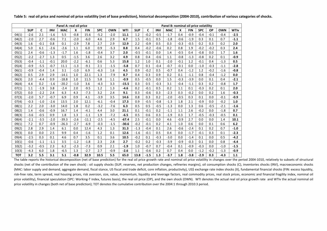
Table 5:  real oil price and nominal oil price volatility (net of base prediction), historical decomposition (2004‐2010), contribution of various categories of shocks. 

Panel A: real oil price  Panel B: nominal oil price volatility   SUP  C  INV  MAC  X  FIN  SPC  OWN  WTI  SUP  C  INV  MAC  X  FIN  SPC  OP  OWN  WTIv 

04(1)  ‐2.6  2.1  ‐1.6  5.5  ‐0.8  15.6  ‐5.2  ‐2.0  11.1  1.2  ‐0.2  ‐0.5  ‐1.7  0.4  ‐0.9  ‐0.4  ‐0.1  ‐0.4  ‐2.5 04(2)  ‐2.0  2.7  ‐0.6  7.1  ‐2.0  ‐6.0  4.6  2.9  6.7  1.5  ‐0.1  0.5  ‐1.8  ‐0.6  ‐1.9  0.3  0.1  0.7  ‐1.1 04(3)  1.6  ‐0.1  0.8  0.1  ‐2.9  7.8  2.7  2.9  12.9  2.2  ‐0.9  0.5  0.3  ‐0.3  ‐0.5  0.2  0.3  0.2  2.0 04(4)  5.0  6.1  ‐2.6  ‐2.6  1.1  6.0  0.9  ‐5.3  8.8  0.4  ‐0.2  ‐0.6  0.2  0.8  1.9  ‐0.2  ‐0.2  0.3  2.4 05(1)  2.4  ‐0.6  ‐1.3  ‐1.7  1.6  ‐1.8  ‐0.4  3.7  2.0  ‐0.5  ‐0.1  0.0  1.4  ‐0.5  0.4  ‐0.8  0.0  1.7  1.6 05(2)  ‐2.2  ‐2.7  1.3  0.5  ‐1.5  3.6  2.6  3.2  4.9  0.8  0.4  ‐0.6  1.1  ‐0.8  ‐1.3  ‐0.8  0.2  0.1  ‐0.9 05(3)  ‐0.4  ‐1.1  ‐0.1  20.0  ‐2.2  ‐6.1  0.6  5.3  15.8  1.2  1.0  0.1  ‐2.0  ‐0.1  1.2  ‐0.1  0.4  ‐1.3  0.5 05(4)  ‐0.9  ‐5.5  ‐0.7  11.1  ‐1.3  ‐9.1  2.1  ‐1.5  ‐5.8  0.7  0.1  ‐0.4  ‐0.7  ‐0.1  0.0  ‐1.0  ‐0.3  ‐1.1  ‐2.8 06(1)  ‐0.9  ‐0.4  1.4  3.1  ‐1.0  6.9  ‐6.3  1.6  4.5  0.9  ‐0.2  0.5  ‐0.7  0.4  ‐1.2  1.2  ‐0.2  ‐1.6  ‐0.8 06(2)  0.5  2.9  2.9  ‐14.1  1.0  22.1  1.3  ‐7.9  8.7  0.4  0.3  0.9  0.2  0.1  ‐1.1  0.8  ‐0.4  ‐1.2  0.0 06(3)  2.0  ‐4.4  0.9  ‐18.8  1.0  11.5  5.8  1.1  ‐0.9  0.5  ‐0.5  0.0  1.5  ‐0.3  ‐3.9  0.0  0.1  0.4  ‐2.1 06(4)  4.4  0.2  ‐1.6  ‐20.2  ‐1.0  3.6  ‐4.3  3.3  ‐15.5  0.3  0.5  ‐0.3  3.1  ‐0.4  ‐1.1  0.3  0.2  ‐0.8  1.7 07(1)  1.1  ‐1.9  3.8  ‐2.4  2.0  ‐9.5  1.2  1.3  ‐4.6  0.2  ‐0.1  0.5  0.2  1.1  0.1  ‐0.3  0.2  0.1  2.0 07(2)  0.0  ‐2.2  2.4  6.3  4.3  ‐7.3  3.2  2.4  9.1  0.3  ‐0.6  0.3  ‐2.3  0.3  ‐0.2  0.0  0.2  1.6  ‐0.3 07(3)  ‐2.0  5.7  ‐0.7  6.9  0.9  4.1  ‐3.9  3.5  14.6  0.8  0.3  0.2  ‐2.0  ‐0.5  0.3  0.1  0.0  ‐0.1  ‐0.9 07(4)  ‐0.3  ‐1.0  ‐2.6  13.5  2.0  12.1  ‐6.1  ‐0.4  17.3  0.9  ‐0.5  ‐0.8  ‐1.3  1.8  2.1  ‐0.9  0.0  ‐0.2  1.0 08(1)  2.2  2.0  ‐3.0  14.0  1.8  0.2  ‐3.2  ‐7.6  6.3  0.5  0.5  ‐0.5  ‐1.3  0.0  1.3  0.6  ‐0.5  ‐2.1  ‐1.6 08(2)  1.4  ‐0.6  ‐0.9  16.7  1.4  ‐4.1  4.4  3.0  21.1  0.1  ‐0.1  0.2  ‐1.1  1.1  2.6  ‐0.2  0.0  ‐1.8  0.7 08(3)  ‐3.6  ‐0.5  0.9  1.8  1.3  ‐1.1  1.9  ‐7.2  ‐6.5  0.5  0.6  0.3  ‐1.9  0.3  1.7  ‐0.5  ‐0.3  ‐0.5  0.1 08(4)  ‐2.1  ‐3.5  ‐2.0  ‐39.3  ‐2.6  ‐11.1  ‐2.5  ‐4.5  ‐67.4  2.5  ‐0.1  0.0  4.6  ‐0.9  2.7  0.0  0.0  1.4  10.1 09(1)  7.2  0.7  ‐0.9  ‐26.3  ‐2.7  ‐6.9  ‐0.3  ‐1.5  ‐30.6  ‐0.2  ‐0.1  0.2  4.1  1.0  0.6  0.0  0.1  0.6  6.2 09(2)  2.8  2.9  1.4  6.1  0.0  12.4  4.3  1.3  31.3  ‐1.3  ‐0.4  0.1  2.6  ‐0.6  ‐2.4  0.1  0.2  0.7  ‐1.0 09(3)  0.0  0.0  2.5  9.9  0.4  ‐1.6  1.2  0.1  12.6  ‐1.6  ‐0.1  0.5  0.4  0.0  ‐1.7  ‐0.1  0.3  0.1  ‐2.3 09(4)  ‐2.5  0.3  0.1  4.6  0.7  3.5  0.1  3.6  10.5  ‐0.2  0.1  ‐0.3  ‐3.0  0.0  ‐1.4  0.1  0.0  0.5  ‐4.2 10(1)  ‐0.6  ‐1.1  ‐1.1  3.5  ‐1.2  ‐1.8  2.3  2.8  2.7  ‐0.2  0.2  ‐0.3  ‐3.9  ‐0.9  ‐0.3  0.1  0.0  0.8  ‐4.4 10(2)  ‐3.2  ‐0.5  2.3  6.2  ‐2.3  ‐7.3  0.9  2.1  ‐1.9  1.0  ‐0.7  0.7  ‐0.4  0.1  ‐0.9  ‐0.3  0.0  ‐1.0  ‐1.5 10(3)  ‐4.3  6.0  1.8  ‐6.5  1.3  ‐2.7  2.7  ‐0.9  ‐2.6  1.1  ‐0.6  0.2  0.7  0.4  0.0  ‐1.2  ‐0.2  ‐1.3  ‐0.9 TOT  3.2  5.5  3.1  5.1  ‐0.8  32.9  10.5  5.5  65.0  13.8  ‐1.5  1.3  ‐3.7  1.8  ‐3.8  ‐2.9  0.3  ‐4.3  1.1 The table reports the historical decomposition (net of base prediction) for the real oil price growth rate and nominal oil price volatility in changes over the period 2004‐1010, relatively to subsets of structural shocks (net of the contribution of the own shock)  : oil supply shocks (SUP, reserves, net production changes, refineries margins), oil consumption shocks (C),  inventories shocks (INV), macroeconomic shocks (MAC: labor supply and demand, aggregate demand, fiscal stance, US fiscal and trade deficit, core inflation, productivity), US$ exchange rate index shocks (X), fundamental financial shocks (FIN: excess liquidity, risk‐free rate, term spread, real housing prices, risk aversion, size, value, momentum, liquidity and leverage factors, real commodity prices, real stock prices, economic and financial fragility index, nominal oil price volatility), financial speculation (SPC: Working‐T index, futures basis), the real oil price (OP), and the own shock (OWN).  WTI denotes the actual real oil price growth rate  and WTIv the actual nominal oil price volatility in changes (both net of base prediction); TOT denotes the cumulative contribution over the 2004:1 through 2010:3 period.  

 

 

 

Table 6:  real oil price and nominal oil price volatility (net of base prediction), historical decomposition  (various sub periods), contribution of various categories of shocks. 

Panel A: real oil price  Panel B: nominal oil price volatility   SUP  C  INV  MAC  X  FIN  SPC  OWN  WTI  SUP  C  INV  MAC  X  FIN  SPC  OP  OWN  WTIv 

90(3)  9.9  2.5  ‐0.2  4.7  0.4  12.3  4.8  3.2  37.6  5.5  0.2  ‐0.2  1.7  0.2  2.5  ‐0.3  0.0  0.8  10.4 90(4)  15.8  ‐0.4  2.9  ‐1.7  0.6  ‐1.6  0.1  1.4  17.1  0.4  0.5  0.9  1.7  0.3  1.8  1.0  0.0  0.1  6.7 91(1)  ‐11.7  ‐6.0  ‐0.2  ‐11.7  0.7  ‐6.6  ‐5.2  1.2  ‐39.5  ‐0.5  ‐0.3  0.5  ‐2.0  ‐0.5  0.6  0.1  0.2  ‐0.9  ‐2.8 91(2)  ‐9.2  5.1  ‐1.6  ‐0.3  ‐0.3  7.7  ‐3.5  ‐3.3  ‐5.3  ‐1.6  ‐0.3  ‐0.4  ‐0.5  0.1  0.1  0.2  ‐0.2  ‐1.3  ‐3.9 TOT  4.9  1.1  0.9  ‐9.0  1.4  11.8  ‐3.8  2.5  9.8  3.7  0.1  0.9  0.9  0.0  5.0  1.0  0.1  ‐1.3  10.5                                        

98(1)  ‐2.8  ‐0.7  ‐0.8  0.6  ‐3.1  ‐13.3  ‐1.4  ‐1.3  ‐22.7  1.1  0.7  0.0  1.3  ‐0.7  0.1  0.2  0.2  ‐2.3  0.7 98(2)  ‐3.7  ‐4.2  0.1  ‐6.0  ‐2.5  1.8  1.7  3.4  ‐9.3  2.0  ‐0.1  ‐1.2  ‐0.8  0.2  ‐1.9  0.0  0.1  ‐0.1  ‐1.7 98(3)  ‐9.8  0.2  ‐2.3  ‐4.1  0.5  15.8  1.5  ‐5.8  ‐4.0  2.7  ‐0.3  ‐0.7  1.3  ‐0.4  ‐1.0  ‐0.2  ‐0.5  ‐0.7  0.3 98(4)  ‐1.2  2.9  ‐0.6  6.4  2.2  ‐15.6  2.9  ‐7.0  ‐10.0  1.1  ‐0.1  ‐0.8  0.2  0.0  3.5  0.2  ‐0.3  ‐0.1  3.7 99(1)  9.6  ‐1.2  1.3  5.1  ‐0.2  ‐22.9  ‐0.2  9.0  0.6  ‐0.8  ‐0.5  0.3  1.0  ‐0.8  2.9  0.5  0.4  ‐0.7  2.3 99(2)  13.5  4.7  1.8  14.0  ‐3.0  ‐3.5  2.8  ‐1.3  29.0  2.2  0.4  1.2  ‐0.2  ‐0.8  2.7  ‐0.9  ‐0.1  0.3  4.8 99(3)  9.9  ‐2.1  ‐0.4  18.7  ‐2.4  3.5  ‐1.5  ‐5.8  19.9  ‐1.0  ‐0.3  0.3  ‐1.6  0.0  0.8  0.0  ‐0.2  ‐0.8  ‐3.0 99(4)  ‐3.5  1.4  ‐0.1  3.6  1.2  8.6  ‐2.9  3.0  11.3  ‐0.8  0.4  0.3  ‐2.3  0.5  ‐1.5  1.0  0.0  1.1  ‐1.3 TOT  12.0  1.1  ‐1.0  38.3  ‐7.4  ‐25.6  2.9  ‐5.7  14.6  6.5  0.3  ‐0.6  ‐1.1  ‐2.1  5.5  0.8  ‐0.3  ‐3.2  5.8                                        

02(4)  ‐2.0  0.7  2.5  ‐4.5  1.7  ‐3.7  2.2  2.1  ‐1.0  0.0  ‐0.9  0.5  3.4  ‐0.3  ‐2.4  ‐0.6  ‐0.1  ‐1.2  ‐1.6 03(1)  ‐1.9  4.4  ‐0.9  0.4  0.3  16.4  0.5  ‐1.7  17.6  0.9  0.2  0.2  1.1  1.0  ‐0.7  ‐0.2  ‐0.3  1.0  3.3 03(2)  4.7  ‐2.4  ‐0.1  ‐14.1  3.3  ‐5.5  ‐3.1  0.5  ‐16.6  0.9  0.1  ‐0.3  ‐0.8  1.2  0.5  0.4  0.0  ‐0.5  1.6 03(3)  5.9  ‐3.1  ‐0.4  1.3  2.7  ‐13.2  4.7  5.0  3.2  0.1  0.6  ‐0.5  ‐0.6  0.2  1.0  ‐0.6  0.2  ‐1.6  ‐1.1 TOT  6.8  ‐0.4  1.1  ‐16.8  8.1  ‐5.9  4.3  5.9  3.1  1.8  0.0  0.0  3.0  2.1  ‐1.5  ‐0.9  ‐0.1  ‐2.3  2.2 The table reports the historical decomposition (net of base prediction) for the real oil price growth rate and nominal oil price volatility in changes for the first Persian Gulf War (1990‐1991), the East Asia crisis and recovery (1998‐1999), the Venezuelan strike and second Persian Gulf War (2002‐2003) periods, relatively to subsets of structural shocks (net of the contribution of the own shock) : oil supply shocks (SUP, reserves, net production changes, refineries margins), oil consumption shocks (C),  inventories shocks (INV), macroeconomic shocks (MAC: labor supply and demand, aggregate demand, fiscal stance, US fiscal and trade deficit, core inflation, productivity), US$ exchange rate index shocks (X), fundamental financial shocks (FIN: excess liquidity, risk‐free rate, term spread, real housing prices, risk aversion, size, value, momentum, liquidity and leverage factors, real commodity prices, real stock prices, economic and financial fragility index, nominal oil price volatility), financial speculation (SPC: Working‐T index, futures basis), the real oil price (OP), and the own shock (OWN). WTI denotes the actual real oil price growth rate   and WTIv the actual nominal oil price volatility  in changes (both net of base prediction); TOT denotes the cumulative contribution over the selected periods. 

 

Figure 1: Impulse responses for the real oil price to various structural shocks (median and 90% confidence interval): reserves (R), net negative production (Pm), net positive production (Pp), refineries margins  (RM),  labor  supply  (E),  labor demand  (U), aggregate demand  (Y),  fiscal  stance  (G), US  fiscal deficit  (Fd), US  trade deficit  (Td),  core  inflation  (N), productivity  (W), oil consumption (C), Working‐T index (WT), futures basis (FB), inventories (INV), real oil price (OP), nominal oil price volatility (OV). 

R

0 10 20 30 40

-1

1 R Pm

0 10 20 30 40

0

5 Pm Pp

0 10 20 30 40-2

2 Pp RM

0 10 20 30 40-4

0 RM

E

0 10 20 30 400

4 E U

0 10 20 30 40-2

2 U Y

0 10 20 30 40

4

8 Y G

0 10 20 30 40-2

2 G

Fd

0 10 20 30 40

-2

0Fd Td

0 10 20 30 402

6 Td N

0 10 20 30 40

-1

1 N W

0 10 20 30 40-5

0 W

C

0 10 20 30 400

4 C WT

0 10 20 30 40

0

1 WT FB

0 10 20 30 40

1

3 FB INV

0 10 20 30 40

-2

0 INV

OP

0 10 20 30 40

3

4 OP OV

0 10 20 30 400

2 OV

 

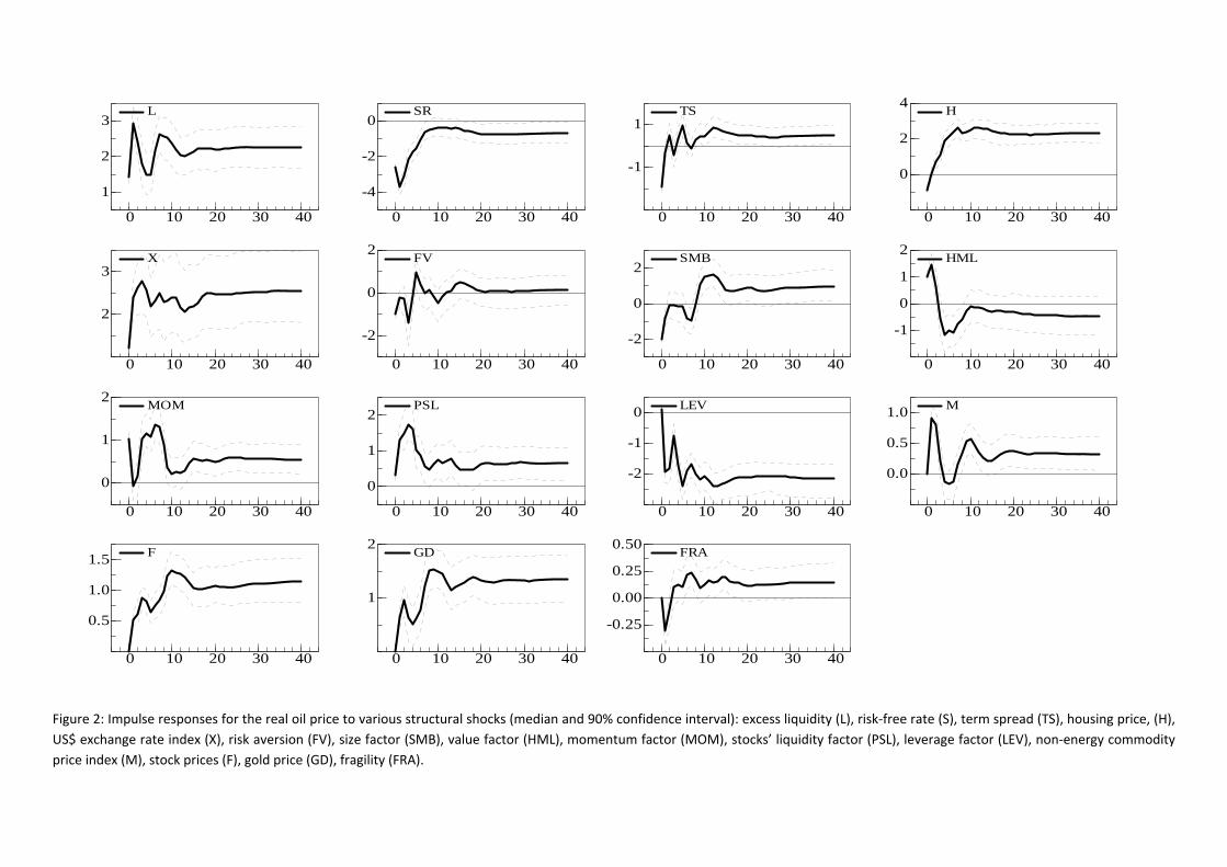
Figure 2: Impulse responses for the real oil price to various structural shocks (median and 90% confidence interval): excess liquidity (L), risk‐free rate (S), term spread (TS), housing price, (H), US$ exchange rate index (X), risk aversion (FV), size factor (SMB), value factor (HML), momentum factor (MOM), stocks’ liquidity factor (PSL), leverage factor (LEV), non‐energy commodity price index (M), stock prices (F), gold price (GD), fragility (FRA). 

 

L

0 10 20 30 40

1

2

3L SR

0 10 20 30 40

-4

-2

0SR TS

0 10 20 30 40

-1

1TS H

0 10 20 30 40

0

2

4 H

X

0 10 20 30 40

2

3X FV

0 10 20 30 40

-2

0

2 FV SMB

0 10 20 30 40

-2

0

2SMB HML

0 10 20 30 40

-1

0

1

2 HML

MOM

0 10 20 30 40

0

1

2 MOM PSL

0 10 20 30 40

0

1

2PSL LEV

0 10 20 30 40

-2

-1

0 LEV M

0 10 20 30 40

0.0

0.5

1.0 M

F

0 10 20 30 40

0.5

1.0

1.5 F GD

0 10 20 30 40

1

2 GD FRA

0 10 20 30 40

-0.25

0.00

0.25

0.50 FRA

 

Figure 3: Cumulative contribution of various categories of shocks to the real oil price (dashed line) and spline smoother (solid line); 1986(4)‐20010(3); supply side shocks (SUP: reserves, net negative and positive production, refineries margins), oil consumption own shock (C),  inventories (I), macroeconomic shocks (MAC:  labor supply,  labor demand, aggregate demand, fiscal stance, US fiscal deficit, US trade deficit, core inflation, productivity), fundamental financial shocks (FIN: excess liquidity, risk‐free rate, term spread, housing prices, risk aversion, size, value, momentum, stocks’ liquidity and leverage factors, non‐energy commodity prices, stock prices, gold prices, fragility factor) , US$ exchange rate shocks (X), non‐fundamental financial shocks (SPC: Working‐T index, futures basis), real oil price own shock (OWN). 

MAC Spline

1990 1995 2000 2005 2010

0

50MAC Spline FIN Spline

1990 1995 2000 2005 2010

0

25

50FIN Spline

SUP Spline

1990 1995 2000 2005 2010

0

20SUP Spline

SPC Spline 1990 1995 2000 2005 2010

0

10

20

SPC Spline

1990 1995 2000 2005 2010

-20

-10

0

X Spline C Spline

1990 1995 2000 2005 2010-20

-10

0

10

C Spline

INV Spline

1990 1995 2000 2005 2010

0

10INV Spline OWN Spline

1990 1995 2000 2005 20100

10

20

30OWN Spline

 

Figure 4: Cumulative contribution of various categories of shocks to the nominal oil price volatility (dashed line) and spline smoother (solid line); 1986(4)‐20010(3); supply side shocks (SUP: reserves, net negative and positive production,  refineries margins), oil consumption own shock  (C),  inventories  (I), macroeconomic shocks  (MAC:  labor supply,  labor demand, aggregate demand,  fiscal  stance, US  fiscal deficit, US  trade deficit, core  inflation, productivity),  fundamental  financial  shocks  (FIN: excess  liquidity,  risk‐free  rate,  term  spread, housing prices,  risk aversion,  size,  value, momentum,  stocks’  liquidity  and  leverage  factors,  non‐energy  commodity  prices,  stock  prices,  gold  prices,  fragility  factor)  , US$  exchange  rate  shocks  (X),  non‐fundamental financial shocks (SPC: Working‐T index, futures basis), nominal oil price volatility own shock (OWN) . 

MAC Spline 1990 1995 2000 2005 2010

-10

-5

0

MAC Spline FIN Spline 1990 1995 2000 2005 2010

-10

-5

0

FIN Spline

SPC Spline 1990 1995 2000 2005 2010

-1

1

SPC Spline

SUP Spline

1990 1995 2000 2005 2010

0

20

40SUP Spline

X Spline 1990 1995 2000 2005 2010

-10

-5

0

X Spline

C Spline

1990 1995 2000 2005 2010-1

0

1

2C Spline

INV Spline

1990 1995 2000 2005 2010

-2

0

2 INV Spline

OWN Spline 1990 1995 2000 2005 2010

-20

-10

0

OWN Spline

 

Figure 5: Cumulative contribution of various categories of fundamental financial shocks to the real oil price (dashed line) and spline smoother (solid line) (top plots), contribution of various categories of  fundamental  financial shocks  to  the  fundamental  financial component of  real oil price growth  (center plots) and  relative dimension of non‐fundamental and  fundamental financial shocks  (bottom plot); 1986(4)‐20010(3). Contributions  from  liquidity and  interest  rate shocks  (MP: excess  liquidity,  risk‐free  rate,  term spread), portfolio allocation shocks  (PA: housing prices, non‐energy commodity prices, stock prices, gold price) and risk factors shocks (RF: risk aversion, size factor, value factor, momentum factor, stocks’ liquidity factor, leverage factor, fragility factor). SPC is the non‐fundamental financial component of the real oil price growth rate (SPC: Working‐T index + futures basis); FIN is the fundamental financial component of the real oil price growth rate (FIN: MP + PA + RF). 

MP Spline

1990 2000 2010

0

20MP Spline PA Spline

1990 2000 2010

0

25

50PA Spline RF Spline

1990 2000 2010

-10

0

10

20RF Spline

MP FIN

1990 2000 2010-20

0

20 MP FIN PA FIN

1990 2000 2010-20

0

20 PA FIN RF FIN

1990 2000 2010-20

0

20 RF FIN

SPC FIN

1990 2000 2010-20

0

20 SPC FIN

 

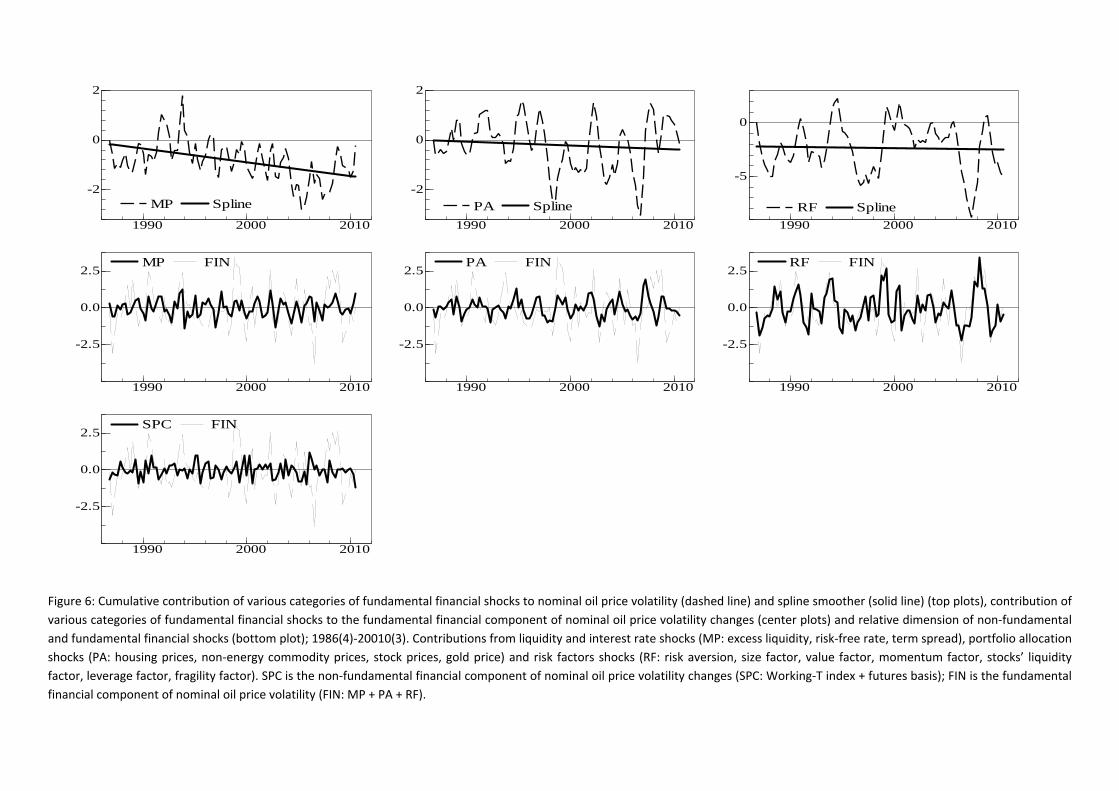
Figure 6: Cumulative contribution of various categories of fundamental financial shocks to nominal oil price volatility (dashed line) and spline smoother (solid line) (top plots), contribution of various categories of fundamental financial shocks to the fundamental financial component of nominal oil price volatility changes (center plots) and relative dimension of non‐fundamental and fundamental financial shocks (bottom plot); 1986(4)‐20010(3). Contributions from liquidity and interest rate shocks (MP: excess liquidity, risk‐free rate, term spread), portfolio allocation shocks  (PA: housing prices, non‐energy commodity prices, stock prices, gold price) and risk  factors shocks  (RF: risk aversion, size  factor, value  factor, momentum  factor, stocks’  liquidity factor, leverage factor, fragility factor). SPC is the non‐fundamental financial component of nominal oil price volatility changes (SPC: Working‐T index + futures basis); FIN is the fundamental financial component of nominal oil price volatility (FIN: MP + PA + RF). 

MP Spline

1990 2000 2010

-2

0

2

MP Spline PA Spline 1990 2000 2010

-2

0

2

PA Spline RF Spline 1990 2000 2010

-5

0

RF Spline

MP FIN

1990 2000 2010

-2.5

0.0

2.5MP FIN PA FIN

1990 2000 2010

-2.5

0.0

2.5PA FIN RF FIN

1990 2000 2010

-2.5

0.0

2.5RF FIN

SPC FIN

1990 2000 2010

-2.5

0.0

2.5SPC FIN