L R I

CNRS – Université de Paris Sud Centre d’Orsay

LABORATOIRE DE RECHERCHE EN INFORMATIQUE Bâtiment 650

91405 ORSAY Cedex (France)

RAPPORT DE RECHERCHE

A HIGH LEVEL QUERY LANGUAGE

FOR BIG DATA ANALYTICS

SPYRATOS N / SUGIBUCHI T

Unité Mixte de Recherche 8623 CNRS-Université Paris Sud – LRI

11/2014

Rapport de Recherche N° 1575

AHighLevelQueryLanguageforBigDataAnalytics

NicolasSpyratosLaboratoiredeRechercheenInformatique,UMR8623ofCNRS,UniversitéParis‐Sud11,FranceTsuyoshiSugibuchiInternetMemoryResearch,France

Abstract

Inthispaper,weproposeahighlevelquerylanguageforexpressinganalyticqueriesoverbigdatasets.Amaincontributionofourapproachistheclearseparationbetweentheconceptualandthephysicallevel.Ananalyticqueryanditsansweraredefinedattheconceptuallevelindependentlyofthenatureandlocationofdata.Theabstractdefinitionsarethenmappedtolowerlevelevaluationmechanisms,takingintoaccountthenatureandlocationofdata,aswellasotherrelatedaspects.Ouroverallobjectiveistohavequeryformulationdoneonanabstractlevel,whileactualqueryevaluationcanadapttotheevaluationmechanismsofferedineachcase.Toachievethisobjectiveitisnecessarytoraisethelevelofabstraction,byprovidingasoundmathematicalbasisforthemappingofqueriestolowerlevelevaluationmechanisms.However,raisingthelevelofabstractionoffersthreeadvantages:(a)usefulinsightsintotheprocessofdataanalyticsingeneral,andMapReduceinparticular(b)aformalapproachtotherewritingofanalyticqueriesandthegenerationofqueryexecutionplansand(c)thepossibilityofleveragingstructureandsemanticsindatainordertoimproveperformance.Weemphasizethat,althoughtheoreticalinnature,thisworkusesonlybasicandwellknownmathematicalconcepts(namelyfunctionsandsetpartitions).\end{abstract}

Category:H.2.4{DatabaseManagement}{Systems}Terms:MapReduce,QueryLanguage,DataAnalytics

Résumé

Danscetarticlenousproposonsunlangagederequêtesdehautniveaupourl’analysededonnéesmassives.Unedescontributionsprincipalesdenotreapprocheestlaséparationclaireentreleniveauconceptueletleniveauphysique.Unerequêteanalytiqueetsaréponsesontdéfiniesauniveauconceptuel,indépendammentdelanatureetdel’emplacementdesdonnéessous‐jacentes.Lesdéfinitionsabstraitessontensuitetraduitesversdesmécanismesd’évaluationàunniveauinférieur,entenantcomptedelanatureetdel’emplacementdesdonnées,ainsiqued’autresaspectspertinentsàl’évaluationderequêtes.Notreobjectifprincipalestdepouvoirformulerdesrequêtesàunniveauabstrait,etadapterleurévaluationauxmécanismesdisponiblesdanschaqueenvironnementphysique.Pouratteindrecetobjectifilestnécessairederaisonneràunniveauabstraitenseservantd’unebasemathématiquesolidepourpouvoirensuitetraduirelesrequêtesversdesmécanismesd’évaluationconcrets.Cetteapprocheoffrelesavantagessuivants:(a)unemeilleurecompréhensionduprocessusd’analysededonnéesdemanièregénérale,etdel’analysededonnéessuivantMapReduceenparticulier(b)uneapprocheformelledelaréécrituredesrequêtesanalytiquesetdelagénérationdeplansd’évaluationdetellesrequêteset(c)lapossibilitédes’appuyersurlastructureetsurlasémantiquededonnéespouraméliorerlesperformances.Anoterque,bienquenotreapprochesoitdenaturethéorique,ellenefaitappelqu’àdesnotionsmathématiquesélémentaires(notammentdesfonctionsetdespartitionsd’unensemble).

Catégorie:H.2.4{DatabaseManagement}{Systems}Termes:MapReduce,QueryLanguage,DataAnalytics

1

A High Level Query Language for Big DataAnalytics

Nicolas Spyratos1, Tsuyoshi Sugibuchi2

1 Laboratoire de Recherche en Informatique, UMR8623 of CNRS,Universite Paris-Sud 11, France Nicolas.Spyratos@lri.fr

2 Internet Memory Research, France tsuyoshi.sugibuchi@internetmemory.net

Abstract. In this paper, we propose a high level query language for ex-pressing analytic queries over big data sets. A main contribution of ourapproach is the clear separation between the conceptual and the physi-cal level. An analytic query and its answer are defined at the conceptuallevel independently of the nature and location of data. The abstract def-initions are then mapped to lower level evaluation mechanisms, takinginto account the nature and location of data, as well as other relatedaspects. Our overall objective is to have query formulation done on anabstract level, while actual query evaluation can adapt to the evaluationmechanisms offered in each case. To achieve this objective it is necessaryto raise the level of abstraction, by providing a sound mathematical basisfor the mapping of queries to lower level evaluation mechanisms. How-ever, raising the level of abstraction offers three advantages: (a) usefulinsights into the process of data analytics in general, and MapReduce inparticular (b) a formal approach to the rewriting of analytic queries andthe generation of query execution plans and (c) the possibility of lever-aging structure and semantics in data in order to improve performance.We emphasize that, although theoretical in nature, this work uses onlybasic and well known mathematical concepts (namely functions and setpartitions).

1 Introduction

Data analysis is a well established research field with multiple applications inseveral domains. However, the methods and tools of data analysis evolve rapidly,and in significant ways, as the size of data accumulated by modern applicationsincreases in unprecedented rates. The work reported in this paper contributes inthis evolution by proposing a high level query language for big data analytics.In this section we first introduce the context of our work (i.e big data and bigdata analytics) and then we present briefly our motivations and contributions.

1.1 Big Data

Today, scientists regularly encounter limitations due to the very large sizes ofdata sets, in many areas, including meteorology, genomics, complex physics sim-ulations, and biological and environmental research. The limitations also affectInternet search, finance and business informatics.

2

Examples of such large data sets include web logs, social network data, In-ternet text and documents, Internet search indexing, call detail records, medicalrecords, photography archives, video archives, and large-scale e-commerce data.Striking examples from the business world include Facebook, which handles 40billion photos from its user base; and Walmart, which handles more than 1 mil-lion customer transactions every hour, imported into databases estimated tocontain more than 2.5 petabytes of data.

The term “big data” refers to data sets with sizes beyond the ability ofcommonly used software tools to capture, curate, manage, and process the datawithin a reasonable lapse of time [30]. As a consequence, what is considered bigdata varies depending on the capabilities of the organization managing the dataset. However, though big data is a moving target, what is considered big datatoday is in the order of petabytes to exabytes[26].

It is worth noting here that size is not the only characteristic of big data. Asstated in [7], big data are high-volume, high-velocity, and/or high-variety infor-mation assets that require new forms of processing to enable enhanced decisionmaking, insight discovery and process optimization.

The potential uses of big data, but also the difficulties connected with theircapture, curation, management and processing have been recognized at the high-est administration levels [27][28].

However, the use of big data has drawn considerable criticism as well. Broadercritiques have been leveled at the assertion that big data will spell the end oftheory, focusing in particular on the notion that big data will always need to becontextualized in their social, economic and political contexts [3][22]. Anothercriticism comes from the fact that, even as companies invest huge amounts toderive insight from information streaming in from suppliers and customers, lessthan half of the employees have sufficiently mature processes and skills to do so.

Moreover, consumer privacy advocates are concerned about the threat to pri-vacy represented by increasing storage and integration of personally identifiableinformation; and expert panels have released various policy recommendations toconform practice to expectations of privacy [38] (see also the articles in ”TheGuardian” and ”Washington Post”, June 6, 2013, on the controversial PRISMproject). All this criticism simply points to the fact that there is another side tobig data regarding societal benefits and risks [34][31].

However, inspite the criticism that the use of big data has drawn recently,their collection and processing holds big promises for a variety of human activ-ities. In fact, a new field centered on big data is emerging, usually referred toas “data science”, and several universities and educational institutions alreadyoffer degrees in this field [47]. [18].

1.2 Data Analytics

Big data is difficult to analyze and to work with using relational databases anddesktop statistics and visualization packages, requiring instead massively parallelsoftware running on tens, hundreds, or even thousands of servers [29][36][37].

3

The analysis of data, or data analytics, is the process of highlighting usefulinformation drawn from big data sets, usually with the goal to support decisionmaking. Data analysis has multiple facets and approaches, encompassing diversetechniques under a variety of names, in different business, science, and socialscience domains. It differs from data mining which is a particular data analysistechnique that focuses on modeling and knowledge discovery for predictive ratherthan purely descriptive purposes.

Big data analytics demands real or near-real time information delivery, andlatency is therefore avoided whenever and wherever possible. With this difficulty,a new platform of big data tools has arisen, such as in the Apache Hadoop BigData Platform [13] derived from papers on Google’s MapReduce and Google FileSystem.

Actually, MapReduce [15] is emerging as a leading framework for performingscalable parallel analytics and data mining; and there is already an impressivebody of literature on MapReduce, but also some controversy coming mainly fromthe database community [44][4][45].

The success of MapReduce is due to several reasons: it is offered as a free andopen source implementation; it is easy to use [40]; it is widely used by Google,Yahoo! and Facebook; and it has been shown to deliver excellent performance onextreme scale benchmarks [14][51]. All these factors have resulted in the rapidadoption of MapReduce for many different kinds of data analysis and processing[10][33][49][39][11].

Originally, MapReduce was mainly used for Web indexing, text analytics,and graph data mining. Today, as MapReduce is becoming the de facto dataanalysis standard, it is also used for the analysis of structured data, an areatraditionally dominated by relational databases in data warehouse deployments.Even though many argue that MapReduce is not optimal for analyzing struc-tured data [44][40], it is nonetheless used increasingly frequently for that purposebecause of a growing tendency to unify the data management platform.

In fact, there is already a significant body of literature on integrating MapRe-duce and relational database technology [48][2][12][53] [17][9], following one oftwo approaches: either adding MapReduce features to a parallel database sys-tem [20][12][52] or adding database technology to MapReduce[48][53] [2][17][9].The second approach seems to be more promising as MapReduce is offered as afree and open source implementation while there exists no widely available opensource parallel database system. The most notable representative of the secondapproach is HadoopDB [2], which is commercialized by Hadapt [24][5].

1.3 Motivation and Contributions

There are many systems developed today for the parallel processing of big datasets [21][48][35] [19][6][2]. All these systems co-exist, each carefully optimizedin accordance with the final application goals and constraints. However, theirevolution has resulted in an array of solutions catering to a wide range of diverseapplication environments. Unfortunately, this has also fragmented the big datasolutions that are now adapted to particular types of applications.

4

At the same time, applications have moved towards leveraging multiple paradigmsin conjunction, for instance combining real time data and historical data. Thishas led to a pressing need for solutions that seamlessly and transparently allowpractitioners to mix different approaches that can function and provide answersas an all-in-one solution.

Based on this observation, the overall objective of our work is to separateclearly the conceptual and the physical level so that one can express analysistasks as queries at the conceptual level independently of how their evaluation isdone at the physical level. To achieve this objective we propose (a) a high levellanguage in which we can formulate queries and study their properties at theconceptual level and (b) mappings to existing evaluation mechanisms (e.g. SQLengines, MapReduce) which perform the actual evaluation of queries. In otherwords, we propose a language which is agnostic of the application environmentas well as of the nature and location of data.

In defining our language, the basic notion that we use is that of attribute ofthe data set. However, we view an attribute as a function from the data set tosome domain of values. For example, if the data set D is a set of tweets, then theattribute “character count” (cc) is seen as a function cc : D → Integers suchthat, for each tweet i, cc(i) is the number of characters in i.

A query in our language is defined to be a triple Q = (g,m, op) such thatg and m are attributes of the data set D, and op is an aggregate operationapplicable on m-values. The evaluation of Q is done in three steps as follows: (a)group the items of the data set D using the values of g (i.e. items with the sameg-value gi are grouped together), (b) in each group of items thus created, extractfrom D the m-value of each item in the group, and (c) aggregate the m-valuesin each group to obtain a single value vi. The aggregate value vi is defined to bethe answer of Q on gi, that is ansQ(gi) = vi. This means that a query is a tripleof functions and its answer is also a function.

Conceptually, all one needs in order to perform the three-step query eval-uation described above is the ability to extract attribute values from the dataset. Now, the method of extraction depends on the nature and location of data.For example, if the data resides in relational tables then one can use SQL inorder to extract attribute values, whereas if the data resides in a distributed filesystem then one needs specialized algorithms to do the extraction. We note inthis respect that, while raw, in-situ data processing is traditionally perceivedas a significant performance bottleneck, novel indexing and caching structuresgradually speed up raw data access.

Anyhow, at the conceptual level, we are not interested in how attribute valuesare extracted from the data set. Rather, we are interested in using the definitionof a query and its answer in order to define formal methods for query rewritingthat will help improve performance of query evaluation at a lower level. Ad-ditionally, we are interested in the use of rewriting to leverage structure andsemantics in data in order to improve performance.

As for user interaction, in our approach, the analyst interacts with the dataset using a set of attributes of interest that we call an “analysis context”. The

5

analyst uses the attributes of his context to write analytic queries in the formof triples, in the way described above. He can add or remove attributes to thecontext at will, so an analysis context can be seen as a “light-weight” schemawhich is agnostic of the nature and location of data. This is in sharp contrastto “heavy-weight” schemas such as relational schemas, which are aware of thestructure of data into tables.

In previous work [8] a functional data model was presented as an alternativeto the relational model. Although the scope of that work is different than ours,some of the functional operations used are similar to those that we use in thedefinition of our language.

In [42], a functional model was presented for data analysis in data ware-houses over star schemas, using a definition of query similar to ours. We buildon that work by enlarging the scope to big data environments, by introducingthe concept of analysis context and by presenting a formal method for queryrewriting and generating query execution plans. Moreover, we provide mappingsfrom our model to existing evaluation mechanisms (SQL engines, MapReduce)where actual query evaluation takes place.

In other recent work [43], a language for data analysis was presented basedentirely on partitions of the data set. Moreover, a notion of query rewriting wasproposed based on the concept of quotient partition. However, no algorithms forquery rewriting were presented and no definition of query execution plan wasgiven.

The remaining of the paper is organized as follows. In section 2 we presentthe conceptual model. In section 2.1 we present the abstract definition of a queryand its answer; in section 2.2 we introduce the concept of analysis context andits query language; in section 2.3 we present a formal approach to the rewritingof analytic queries; and in section 2.4 we use query rewriting to provide a formalmethod for generating query execution plans. Section 3 is devoted to mappingsbetween the conceptual and the physical level. In section 3.1 we present a gen-eral, conceptual scheme for query evaluation based on our abstract definitionof query. Then we present the mapping of our conceptual evaluation scheme tothree important, practical application environments: MapReduce (section 3.2),Column Databases (section 3.3) and Row Databases (section 3.4). Section 4contains some concluding remarks and outlines research perspectives.

We emphasize that, although theoretical in nature, our approach uses onlybasic and well known mathematical concepts, namely functions and set parti-tions.

2 The Formal Model

In the formal model that we present in this section, we consider a data set D,whose elements we call data items, and we make two assumptions:

– Item identification: We assume that D consists of data items that can beuniquely identified. For example, if D is a set of tweets then each tweet can

6

be identified by a time stamp or by a URI; and if D is the set of tuples ina relational table then each tuple can be identified by a tuple identifier orsome key of the table.

– Attributes as functions: We assume that each attribute of D is a functionassociating each data item of D with a value, in some set of values. Forexample, if D is a set of tweets then the attribute Date is seen as a functionassociating each tweet in D with the date in which the tweet was sent. Inthe remaining of the paper we shall use the terms “function on D” and“attribute of D” interchangeably.

We note that the attributes-as-functions assumption is compatible with thenotion of attribute in both column databases and row databases (i.e. relationaldatabases). Indeed, a column database stores columns instead of rows of data(e.g. MonetDB). At the conceptual level, a column database can be seen asstoring a set of functions of the form fA : IDA → A, where A is an attribute andIDA is a subset of the set ID of identifiers used by the column store. Similarly,in a table T of a row database, we can associate each attribute A of T with afunction fA : TIDT → A, where TIDT is the set of tuple identifiers in T ; thisfunction is defined as follows: fA(t) = t(A), for each tuple identifier t in TIDT ,where t(A) denotes the value of t on attribute A. Note that if we assume TIDT

to be an extra attribute of T , then the function fA can be extracted from T byprojection over TIDT and A; in other words, fA = projTIDT ,A(T ).

We emphasize that, apart from the two assumptions above, we make no otherassumption whatsoever throughout the paper. In other words, the data set canbe structured or unstructured, homogeneous or heterogeneous, centrally storedor distributed. Our results apply in all these cases. Moreover, as we shall see inSection 3, if the data is structured, then our approach can leverage structureand semantics to improve performance.

2.1 The definition of analytic query and its answer

As we have already mentioned in the introduction, a query in our language isdefined to be a triple Q = (g,m, op) such that g and m are attributes of the dataset D, and op is an aggregate operation applicable on m-values. The attributesg and m are called the “grouping attribute” and the “measuring attribute”,respectively. The evaluation of Q is done in three steps as follows:

– Grouping: Group the items of the data set D using the values of g (i.e.items with the same g-value gi are grouped together)

– Measuring: In each group of items thus created, extract from D the m-valueof each item in the group

– Reduction: Aggregate the m-values in each group to obtain a single valuevi

The aggregate value vi is defined to be the answer of Q on gi, that isansQ(gi) = vi.

7

Quantity

Product Branch

b p

q d Date D

Fig. 1. Running example

Let us see an example in detail in order to motivate the definition of “query”in our approach. We shall use this example as our running example throughoutthe paper. Suppose D is the set of all delivery invoices over a year, in a distribu-tion center (e.g. Walmart), which delivers products of various types in a numberof branches. A delivery invoice has an identifier (e.g. an integer) and shows thedate of delivery, the branch in which the delivery took place, the type of productdelivered (e.g. CocaLight) and the quantity (i.e. the number of units deliveredof that type of product). There is a separate invoice for each type of productdelivered.

The data of all invoices during the year is stored in a database for analysispurposes. The stored data is shown schematically in Figure 1, where D representsthe set of all delivery invoices and the arrows represent attributes of D. Foreach stored invoice, the function d returns the date in which the delivery tookplace; the function b returns the branch in which the delivery occurred; and thefunctions p and q return the type of product delivered and the quantity (i.e. thenumber of units) of that type of product.

D Qty Branch b q

1 2 3 4 5 6 7

Branch-1 Branch-2 Branch-3

200 100 200 400 100 400 100

300

600

600

TotQty sum

Fig. 2. Computing the total quantity delivered by branch

Suppose now that we want to know the total quantity delivered to eachbranch (during the year). This computation needs the extensions of the functionsb and q. Figure 2 shows a toy example of the data returned by b and q, wherethe data set D consists of seven invoices, numbered 1 to 7. In order to find thetotal quantity by branch we proceed in three steps as follows:

8

Grouping: During this step we group together all invoices referring to thesame branch (using the function b). We obtain the following groups of invoices(as shown in the figure):

– Branch-1: 1, 2– Branch-2: 3, 4– Branch-3: 5, 6, 7

Measuring: In each group of the previous step, we find the quantity corre-sponding to each invoice (using the function q):

– Branch-1: 200, 100– Branch-2: 200, 400– Branch-3: 100, 400, 100

Reduction: In each group of the previous step, we sum up the quantitiesfound:

– Branch-1: 200+100= 300– Branch-2: 200+400= 600– Branch-3: 100+400+100= 600

Then the association of each branch to the corresponding total quantity isthe desired result (called TotQty in the figure):

– Branch-1 → 300– Branch-2 → 600– Branch-3 → 600

Branch-1 Branch-2 Branch-3

300 600 600

Branch TotQty answer intension

answer extension

Q= (b, q, sum)

evaluation of Q

ansQ

(a)

(b)

D Qty Branch b q

1 2 3 4 5 6 7

Branch-1 Branch-2 Branch-3

200 100 200 400 100 400 100

300

600

600

TotQty sum

Fig. 3. An analytic query and its answer

9

We view the ordered triple Q = (b, q, sum) as a query over D (see Figure 3(a)), the function ansQ : Branch → TotQty as the answer to Q (see Figure 3(b)), and the computations in Figure 3 (a) as the query evaluation process. Notethat what makes the association of branches to total quantities possible is thefact that b and q have a common source (which is D in this example).

The function b that appears first in the triple (b, q, sum) and is used in thegrouping step is called the grouping function; the function q that appears secondin the triple is called the measuring function, or the measure; and the functionsum that appears third in the triple is called the reduction operation or theaggregate operation. Actually, a triple such as (b, q, sum) should be regarded asthe specification of an analysis task to be carried out over the data set D.

Note that, as our example shows, the requirements for a triple such as(b, q, sum) to qualify as a query over D are the following:

– the grouping and measuring function must both be attributes of D (i.e.functions with D as their common source)

– the reduction operation must be an operation among those applicable overthe target of the measuring function

Also note that, as the only requirement for b and q is that they must beattributes of D, each of them can play the role of either a grouping function ora measuring function. In other words, the triple (q, b, count) is a valid query andasks for the number of branches by quantity delivered. To answer this query weuse q to group together all invoices having the same quantity delivered (this isthe grouping step); then we use b to find the branches that were delivered thatquantity (this is the measuring step); and finally we count the branches in eachgroup (this is the reduction step). For example, in Figure 2, if we consider thequantity 200, then we find that there are 2 branches that were delivered thatquantity (namely Branch-1 and Branch-2).

To see another example of query, suppose that D is a set of tweets accumu-lated over a year; dd is the function associating each tweet t with the date dd(t)in which the tweet was sent; and cc is the function associating each tweet t withits character count, cc(t). If we want to know the average number of charactersin a tweet by date, then we can follow the same steps as in the delivery invoicesexample: first we group the tweets by date (using dd); then we find the numberof characters per tweet (using cc); and finally we take the average of the char-acter counts in each group (using “average” as the reduction operation). Theappropriate query formulation in this case is (dd, cc, avg).

We note that the grouping and reduction steps can be applied independentlyof the nature of data. Indeed, in the delivery invoices example, the data willmost likely be a set of records in a relational table (therefore structured data),whereas in the tweets example the data is text of variable length (thereforeunstructured data). Yet in both cases the definition of a query and its answeris done in the same way. However, in order to actually evaluate the answer, weneed the extensions of the grouping and measuring attribute (as was the casefor attributes b and q in Figure 2). These extensions will have to be extracted

10

from the underlying data set. This means that for each attribute (grouping ormeasuring attribute) we need an algorithm for extracting that attribute’s valuefrom each data item.

In view of the preceding discussion, we can now give the formal definition ofa query and its answer in our model.

Definition 1 (Query). Let D = {d1, . . . , dn} be a finite set. An analytic query(or simply query) over D is a triple Q = (g,m, op) such that g : D → A andm : D → V are attributes of D, and op is an operation over V taking its valuesin a set W .

The reduction operation op is actually a function that associates every finitetuple of elements from V with an element in a set W . In our running example,where the reduction operation is “sum”, the set V is the set of integers (numberof units delivered) and so is W (sums of quantities delivered); therefore in thisexample we have V = W . However, in general, V can be different than W .Indeed, in our tweets example, where V is the set of integers (character counts)and op is the operation “average”, the set W is the set of real numbers (averagesof character counts) and therefore V 6= W .

It is important to note that the reduction operation must be among thoseoperations that are applicable on V . For example, if V is the set of integers (asin the tweets example), then the reduction operation can be any among “sum”,“average”, “median”, “count”, “max”, “min”, and so on.

In order to define formally the answer to a query over D, we need to defineformally the steps of grouping and reduction.

Definition 2 (Grouping).Let D = {d1, . . . , dn} be a finite set, let g : D → A be an attribute of D and

let {a1, . . . , ak} be the values of g over D (clearly, k ≤ n). We call grouping ofD by g the partition induced by g on D.

We denote this partition by πg, therefore we have:

πg = {g−1(a1), . . . , g−1(ak)}

Note: We recall that a partition of D is any collection of nonempty subsetsof D (also called the “blocks” of the partition), with the following properties: (a)the subsets are pairwise disjoint and (b) their union is D.

For example, in Figure 3 (a), the grouping of D by b consists of three groups,one for each of the values of b:

– b−1(Branch-1) = {1, 2}– b−1(Branch-2) = {3, 4}– b−1(Branch-3) = {5, 6, 7}

We now define formally the reduction operation.

11

Definition 3 (Reduction).Let D = {d1, . . . , dn} be a finite set, let m : D → V be an attribute of D,

and let op be an operation over V with values in a set W . The reduction of mwith respect to op, denoted red(m, op), is a value of W defined as follows:

red(m, op) = op(〈m(d1), . . . ,m(dn)〉)

Note that in the above definition of reduction we use the notation op(〈m(d1),. . . ,m(dn)〉) to emphasize that all values of m must be taken into account, evenif there are repeated values (i.e. even if m(di) = m(dj), for some di 6= dj). Forexample, in Figure 3(a), although we have q(5) = q(7) = 100, the value 100 istaken twice into account when computing the sum of all values.

Here is an example of reduction of the function q : D → Quantity in Figure3 (a): red(q, sum) = 200 + 100 + 200 + 400 + 100 + 400 + 100 = 1500. Otherexamples of reductions in that same figure are the following:

– red(q/b−1(Branch-1), sum) = 200 + 100 = 300– red(q/b−1(Branch-2), sum) = 200 + 400 = 600– red(q/b−1(Branch-3), sum) = 100 + 400 + 100 = 600

Here q/b−1(Branch-i) denotes the restriction of function q to the subsetb−1(Branch-i) of D, i= 1, 2, 3.

We can now define formally the notion of query answer.

Definition 4 (Query Answer). Let Q = (g,m, op) be a query over D, whereD = {d1, . . . , dn} is a finite set, g : D → A and m : D → V are attributes of D,and op is an operation over V with values in a set W . Let {a1, . . . , ak} be thevalues of g over D. The answer to Q, denoted ansQ, is a function from the setof values of g to W defined by:

ansQ(ai) = red(m/g−1(ai), op), i = 1, 2, ..., k,

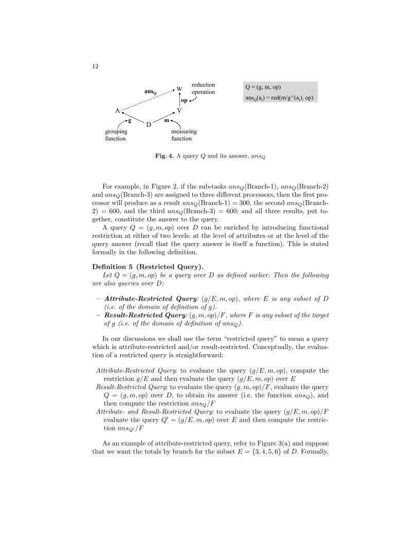
Figure 3(b) shows schematically the answer, ansQ (which is a function); andFigure 4 shows the relationship between ansQ and the functions appearing in thequery Q. It is worth noting that a query is a triple of functions and the answer isalso a function. Moreover, as we shall see later, the fact that ansQ(ai) is given bya closed formula facilitates the proof of theorems when studying query rewriting.

It should be clear from the above definition of query answer that the taskof evaluating Q can be easily parallelized. Indeed, if for each i we consider theevaluation of ansQ(ai) as a sub-task then we can assign the sub-tasks to a numberof processors, each processor receiving one or more sub-tasks. Each processorthen executes its own sub-task(s) independently of all other processors, and theresults from all processors, put together, constitute the answer to the query.

Note: While evaluating a sub-task, a processor may decide to further partitionthe sub-task block into smaller blocks, before performing reduction (and this canbe done recursively). This is possible under the assumption that the reductionoperation is “distributive”, a concept to be defined later on.

12

D

V mg

ansQ

A

Q = (g, m, op)

ansQ(ai) = red(m/g-1(ai), op)

grouping function

measuring function

op

W reduction operation

Fig. 4. A query Q and its answer, ansQ

For example, in Figure 2, if the sub-tasks ansQ(Branch-1), ansQ(Branch-2)and ansQ(Branch-3) are assigned to three different processors, then the first pro-cessor will produce as a result ansQ(Branch-1) = 300, the second ansQ(Branch-2) = 600, and the third ansQ(Branch-3) = 600; and all three results, put to-gether, constitute the answer to the query.

A query Q = (g,m, op) over D can be enriched by introducing functionalrestriction at either of two levels: at the level of attributes or at the level of thequery answer (recall that the query answer is itself a function). This is statedformally in the following definition.

Definition 5 (Restricted Query).Let Q = (g,m, op) be a query over D as defined earlier. Then the following

are also queries over D:

– Attribute-Restricted Query: (g/E,m, op), where E is any subset of D(i.e. of the domain of definition of g).

– Result-Restricted Query: (g,m, op)/F , where F is any subset of the targetof g (i.e. of the domain of definition of ansQ).

In our discussions we shall use the term “restricted query” to mean a querywhich is attribute-restricted and/or result-restricted. Conceptually, the evalua-tion of a restricted query is straightforward:

Attribute-Restricted Query: to evaluate the query (g/E,m, op), compute therestriction g/E and then evaluate the query (g/E,m, op) over E

Result-Restricted Query: to evaluate the query (g,m, op)/F , evaluate the queryQ = (g,m, op) over D, to obtain its answer (i.e. the function ansQ), andthen compute the restriction ansQ/F

Attribute- and Result-Restricted Query: to evaluate the query (g/E,m, op)/Fevaluate the query Q′ = (g/E,m, op) over E and then compute the restric-tion ansQ′/F

As an example of attribute-restricted query, refer to Figure 3(a) and supposethat we want the totals by branch for the subset E = {3, 4, 5, 6} of D. Formally,

13

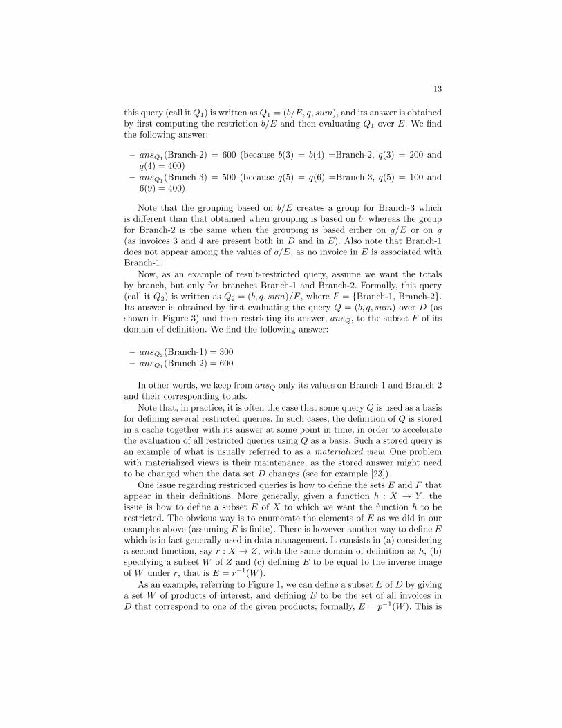
this query (call itQ1) is written asQ1 = (b/E, q, sum), and its answer is obtainedby first computing the restriction b/E and then evaluating Q1 over E. We findthe following answer:

– ansQ1(Branch-2) = 600 (because b(3) = b(4) =Branch-2, q(3) = 200 and

q(4) = 400)

– ansQ1(Branch-3) = 500 (because q(5) = q(6) =Branch-3, q(5) = 100 and

6(9) = 400)

Note that the grouping based on b/E creates a group for Branch-3 whichis different than that obtained when grouping is based on b; whereas the groupfor Branch-2 is the same when the grouping is based either on g/E or on g(as invoices 3 and 4 are present both in D and in E). Also note that Branch-1does not appear among the values of q/E, as no invoice in E is associated withBranch-1.

Now, as an example of result-restricted query, assume we want the totalsby branch, but only for branches Branch-1 and Branch-2. Formally, this query(call it Q2) is written as Q2 = (b, q, sum)/F , where F = {Branch-1, Branch-2}.Its answer is obtained by first evaluating the query Q = (b, q, sum) over D (asshown in Figure 3) and then restricting its answer, ansQ, to the subset F of itsdomain of definition. We find the following answer:

– ansQ2(Branch-1) = 300

– ansQ1(Branch-2) = 600

In other words, we keep from ansQ only its values on Branch-1 and Branch-2and their corresponding totals.

Note that, in practice, it is often the case that some query Q is used as a basisfor defining several restricted queries. In such cases, the definition of Q is storedin a cache together with its answer at some point in time, in order to acceleratethe evaluation of all restricted queries using Q as a basis. Such a stored query isan example of what is usually referred to as a materialized view. One problemwith materialized views is their maintenance, as the stored answer might needto be changed when the data set D changes (see for example [23]).

One issue regarding restricted queries is how to define the sets E and F thatappear in their definitions. More generally, given a function h : X → Y , theissue is how to define a subset E of X to which we want the function h to berestricted. The obvious way is to enumerate the elements of E as we did in ourexamples above (assuming E is finite). There is however another way to define Ewhich is in fact generally used in data management. It consists in (a) consideringa second function, say r : X → Z, with the same domain of definition as h, (b)specifying a subset W of Z and (c) defining E to be equal to the inverse imageof W under r, that is E = r−1(W ).

As an example, referring to Figure 1, we can define a subset E of D by givinga set W of products of interest, and defining E to be the set of all invoices inD that correspond to one of the given products; formally, E = p−1(W ). This is

14

precisely what is done when querying a relational table T by issuing a statementsuch as:

Select * From T Where Product=P1 or Product=P2 .

Indeed, this statement returns all tuples whose value on attribute Product iseither P1 or P2.

Note that we can even use the function h itself for defining a subset E of itsdomain of definition. For example, consider the function b of Figure 2 and letW = {Branch-1,Branch-2}. Then we can define E = b−1(W ) = {1, 2, 3, 4}.

We end this section with two important remarks regarding the definitionof a query and its answer. First, the mathematical concepts used are actuallyelementary: (a) the concept of function, (b) the inverse of a function and thepartition that this inverse induces on its domain of definition, and (c) the re-striction of a function to a subset of its domain of definition. As we have seenin this section these concepts are sufficient in order to define an analytic queryand its answer at the conceptual level; and as we shall see shortly, these sameconcepts are sufficient in order to define formally query rewriting.

Our second remark concerns the fact that, in a query Q = (g,m, op), thefunctions g and m might not be defined on every item of D. Therefore groupingand reduction as described earlier can be performed only on the set of items onwhich g and m are both defined. However, in order to simplify the presentation,and without loss of generality, we shall assume that g and m are defined onall items of D. In other words, D actually represents the common domain ofdefinition of g and m, defined as D = def(g)∩def(m), where def(g) and def(m)denote the domains of definition of g and m, respectively.

2.2 Analysis Context

Analysts are usually interested in analyzing a data set in many ways, using anumber of different attributes in their analytic queries. For example, in Figure1, one can define analytic queries using any of the attributes b, p and q. Theseare “factual”, or direct attributes of D as their values appear on the deliveryinvoices.

However, apart from these factual or direct attributes, analysts might beinterested in attributes that are not direct but can be “derived” from the di-rect attributes. Figure 5(a) shows several derived attributes. For instance, theattributes m and y are derived attributes as their values can be computed fromthose of attribute d (e.g. from the date 05/06/1986 one can derive the month06/1986 and the year 1986). Similarly, the attribute r can be derived from geo-graphical information on the locations of the branches; and the attributes s andc might be possible to derive from data carried by RFID tags embedded in theproducts themselves.

Roughly speaking, the set of attributes of interest to a group of analysts iswhat we call an analysis context (or simply a context); and these attributes canbe direct or derived attributes of the data set. Hence the following definition.

15

Region

Quantity

Category Supplier

b

r

p

s c

q d Date y Year mMonth

(a)

(b)

D

Product Branch

Quantity

b p

q D

Product Branch

Quantity

p

q D

Product Category Supplier

s c

Product

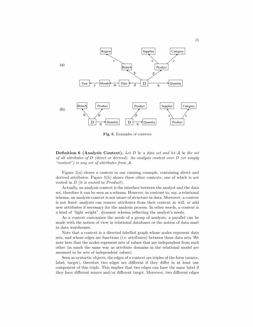
Fig. 5. Examples of contexts

Definition 6 (Analysis Context). Let D be a data set and let A be the setof all attributes of D (direct or derived). An analysis context over D (or simply“context”) is any set of attributes from A.

Figure 5(a) shows a context in our running example, containing direct andderived attributes. Figure 5(b) shows three other contexts, one of which is notrooted in D (it is rooted in Product).

Actually, an analysis context is the interface between the analyst and the dataset, therefore it can be seen as a schema. However, in contrast to, say, a relationalschema, an analysis context is not aware of structure in data. Moreover, a contextis not fixed: analysts can remove attributes from their context at will, or addnew attributes if necessary for the analysis process. In other words, a context isa kind of “light weight”, dynamic schema reflecting the analyst’s needs.

As a context customizes the needs of a group of analysts, a parallel can bemade with the notion of view in relational databases or the notion of data martin data warehouses.

Note that a context is a directed labelled graph whose nodes represent datasets, and whose edges are functions (i.e. attributes) between these data sets. Wenote here that the nodes represent sets of values that are independent from eachother (in much the same way as attribute domains in the relational model areassumed to be sets of independent values).

Seen as syntactic objects, the edges of a context are triples of the form (source,label, target), therefore two edges are different if they differ in at least onecomponent of this triple. This implies that two edges can have the same label ifthey have different source and/or different target. Moreover, two different edges

16

can have the same source and the same target as long as they have differentlabels (we call such edges “parallel edges”).

Most importantly, a context is always an acyclic graph, in the sense describedby the following proposition.

Proposition 1 (Context Acyclicity).Let C be a context over D. Then for every node A of C the only possible cycleon A is ιA, that is the identity function on A.

Proof. Let A and B be two nodes of C, and suppose there is a cycle on Aconsisting of two functions: f : A → B and g : B → A. Suppose that there issome element a in A such that g ◦ f(a) = a′ and a 6= a′. This implies that a′

depends on a, a contradiction to our assumption that the nodes of C representsets of independent values. Therefore the only possibility to have a cycle on Ais when g ◦ f(a) = a for all a in A; in other words the only possible cycle on Ais ιA, where ιA is the identity function on A.

A typical example where identity cycles occur is when prices of productsare given in two or more different currencies, such as the price in dollars andthe price in euros of the same product: Price-in-Dollars → Price-in-Euros andPrice-in-Euros → Price-in-Dollars. In such cases the two nodes are equivalent,in the sense that there is one-to-one correspondence between their values.

We note that, although acyclic, a context is not necessarily a tree. It canhave one or more roots and it can also have parallel edges and parallel paths(“parallel” in the sense “same source and same target”).

In general, the users of a context have two main ways for expressing queries.First, they can express queries on any node of the context - not just on D.For example, in the context of Figure 5(a), suppose we add an attribute u :Product → UnitPrice, giving the unit price for each product. Then one canformulate the following query on Product: (c, u,max), asking for the maximumunit price by product category.

Second, users of a context can combine its attributes to form complex group-ing functions. For example, in the context of Figure 5(a) one can ask for thetotal quantities by region, using as grouping function the composition of theattributes b and r: (r ◦ b, q, sum).

In our model, we can form complex grouping functions using the followingfour operations on functions: composition, pairing, restriction and Cartesianproduct projection. These operations form the so called functional algebra (seefor example [42]). We note that the operations of the functional algebra are wellknown, elementary operations except probably for pairing, which is defined asfollows.

Definition 7 (Pairing). Let f : X → Y and g : X → Z be two functions withcommon domain X. The pairing of f and g, denoted by f × g is a function fromX to Y × Z defined as follows: f × g(x) = (f(x), g(x)), for all x in X

The above definition of pairing can be extended to more than two functionsin the obvious way. Roughly speaking, pairing works as a tuple constructor.

17

Indeed, if we view the elements of X as identifiers, then for each x in X thepairing constructs a tuple of the images of x under its input functions; and thistuple is identified by x.

To see an example of using pairing, refer to Figure 5(a) and consider thefollowing query: (b×p, q, sum). This query asks for the total quantities deliveredby branch and product (i.e. its answer associates every pair (branch, product)with a total quantity).

Note that the order of the images in the result of pairing is immaterial, aslong as each image is prefixed by the function that produced it. In other words,pairing can be actually defined as follows: f × g(x) = {f : f(x), g : g(x)}, for allx ∈ X. This definition implies that pairing is a commutative operation. On theother hand, when pairing two or more other pairings we obtain nested sets. If weagree to “flatten” the results, then pairing becomes an associative operation aswell, and we can parenthesize at will, or even omit inner parentheses altogether,without ambiguity.

Using the operations of the functional algebra we can form not only complexgrouping functions but also complex conditions when defining restrictions. Forexample, in Figure 5(a), we can ask for the total quantities by region and sup-plier, only for the month of January, using the following query: (((r ◦ b) × (s ◦p))/E, q, sum), where E = {x|x ∈ D ∧m ◦ d(x) = January}

Region

Quantity

Category Supplier

b

r

p

s c

q d Date D

Product Branch

h

Fig. 6. A context with parallel paths

As another example, refer to Figure 6, showing a context with two parallelpaths from D to Region. In this context, for each supplier, the attribute h givesthe region where the suppliers’ headquarters is located. Suppose now that wewant the total quantities by Category, only for those invoices in D for whichthe branch is located in the same region as the headquarters of the productsupplier. This is expressed by the following query: ((h ◦ c)/E, q, sum), whereE = {x|x ∈ D ∧ (h ◦ s ◦ p)(x) = (r ◦ b)(x)}.

Note that in the above restricted query we use equality of two functionalexpressions in order to define attribute restriction. As we shall see in the sectionon rewriting (Section 2.3), equality of two functional expressions can be also

18

used as an integrity constraint on the context itself, and as such it can be usedin query rewriting.

In general, a query over a context is a usual query (as defined in the previoussection) in which we can use functional expressions instead of just functions.More formally, a functional expression over a context is defined as follows.

Definition 8 (Functional Expression). A functional expression over a con-text C is either an edge of C or a well formed expression whose operands areedges and whose operations are those of the functional algebra.

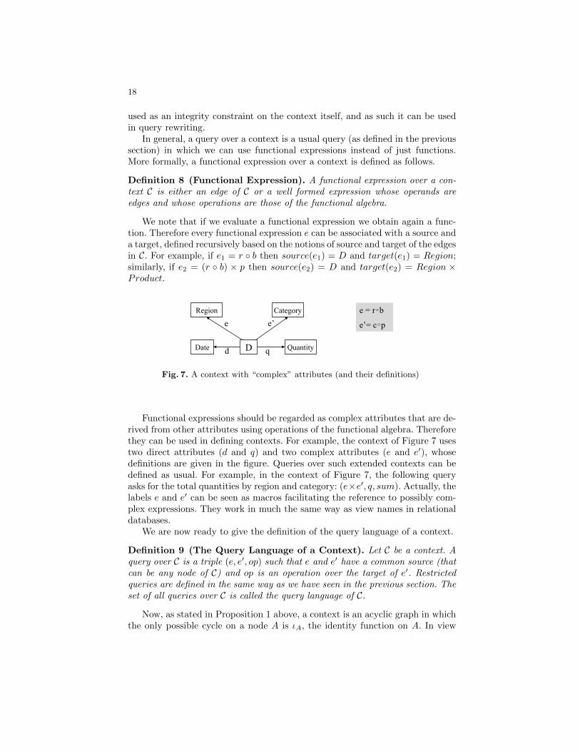
We note that if we evaluate a functional expression we obtain again a func-tion. Therefore every functional expression e can be associated with a source anda target, defined recursively based on the notions of source and target of the edgesin C. For example, if e1 = r ◦ b then source(e1) = D and target(e1) = Region;similarly, if e2 = (r ◦ b) × p then source(e2) = D and target(e2) = Region ×Product.

e = r�b

e’= c�p

Quantity

e e’

q d Date D

Category Region

Fig. 7. A context with “complex” attributes (and their definitions)

Functional expressions should be regarded as complex attributes that are de-rived from other attributes using operations of the functional algebra. Thereforethey can be used in defining contexts. For example, the context of Figure 7 usestwo direct attributes (d and q) and two complex attributes (e and e′), whosedefinitions are given in the figure. Queries over such extended contexts can bedefined as usual. For example, in the context of Figure 7, the following queryasks for the total quantities by region and category: (e×e′, q, sum). Actually, thelabels e and e′ can be seen as macros facilitating the reference to possibly com-plex expressions. They work in much the same way as view names in relationaldatabases.

We are now ready to give the definition of the query language of a context.

Definition 9 (The Query Language of a Context). Let C be a context. Aquery over C is a triple (e, e′, op) such that e and e′ have a common source (thatcan be any node of C) and op is an operation over the target of e′. Restrictedqueries are defined in the same way as we have seen in the previous section. Theset of all queries over C is called the query language of C.

Now, as stated in Proposition 1 above, a context is an acyclic graph in whichthe only possible cycle on a node A is ιA, the identity function on A. In view

19

of this proposition, we shall assume that every node A of a context is endowedwith the identity function ιA. Moreover, we shall assume that every context C isendowed with an extra node denoted by K such that: (a) K denotes a singletonset {All} and (b) for every node A of C there is an edge from A to K denotedby κA; that is κA : A→ K.

From a strictly technical point of view, the introduction of the functions ιAand κA is justified as follows. The inverses of all functions on A induce the setof all partitions of A. This set is partially ordered by: π ≤ π′ if each block of πis a subset of a block of π′. Under this ordering the set of partitions becomes acomplete lattice with least, or bottom element the fine partition (i.e. the partition{{a}/a ∈ A}); and with largest, or top element the coarse partition (i.e. thepartition {{A}}). Now, the fine partition of A is induced by any injective functionon A, and in particular by ιA, the identity function on A; and the coarse partitionof A is induced by any constant function on A, and in particular by κA

3.

Clearly, given a context C, we can use ιA and κA in the same way as any otheredge of C. In particular, we can use them in queries or in functional expressions.For example, referring to Figure 5(a), consider the following queries using ιA:

Q1 = (ιD, q, sum) and Q2 = (q, ιD, count)

During the evaluation of Q1, in the grouping step, the function ιD puts eachelement of D in a single block. Therefore summing up the values of q in eachblock we simply find the value of q on the single element of D in that block; thenthe measuring step simply returns this value of q. It follows that ansQ1

= q.

As for the query Q2, the grouping function q groups together all invoiceshaving the same delivered quantity; and as ιD doesn’t change the values in eachblock, the answer to Q2 is the number of invoices by quantity delivered.

The function ιA is typically used for finding the cardinality of A, using thefollowing query: (κA, ιA, count). The constant function κA, on the other hand, istypically used for finding the reduction of the whole of A under some measuringfunction.

Consider for example the following query: Q3 = (κD, q, sum). During theevaluation of Q3, in the grouping step, the function κD puts all elements of Din a single block. Therefore by summing up the values of q in that block we findthe total of all quantities delivered (i.e. for all dates, branches and products).

Regarding the use of ιA and κA in functional expressions, we note the fol-lowing facts: for any nodes A and B, and any functional expression e : A→ B,we have:

e ◦ ιB = ιA ◦ e = e

e ◦ κB = κA

3 The reason why we denote the unique value of κ by All is in order to hint to thefact that the function κA puts all the elements of A in a single block of the partitionit induces on A

20

One important aspect regarding the evaluation of analytic queries in a con-text is visualization of the results. In our model, as the answer to a query is afunction, its visualization can be done in any of the known ways for representinga (finite) function.

For example, consider the query Q = (b× (s◦p), q, sum) asking for the totalsby branch and supplier. The answer to this query is the following function:

ansQ : Branch× Supplier → TotQty

One way to represent its extension is by a binary table < y, TotQty(y) >, inwhich each pair y = (bi, sj) of a branch bi and a supplier sj , corresponds to atotal quantity TotQty(y) (this table can also be seen as a ternary table withBranch, Supplier and TotQty as its columns). This is the standard way forrepresenting a function by its graph.

However, a different (but equivalent) representation is possible, based on thefollowing observation: any triple of values (x, y, z) is equivalent to the triple(x, (y, z)), in the sense that they both carry the same information but encodedin different ways. Following this observation, the above answer can be also rep-resented as follows: if we fix a value bi of b then for each value sj of s therecorresponds a value of TotQty. In other words, each branch bi is associated witha function fi : Supplier → TotQty. Therefore, for each branch bi, one can “vi-sualize” the corresponding function fi using some visualization template (e.g. ahistogram, a pie or any other template). Similarly, if we fix a value si of s thenfor each value bj of b there corresponds a value of TotQty. In other words, eachsupplier si is associated with a function hi : Branch → TotQty, providing adifferent visualization of the answer.

The existence of two or more representations of the answer, combined withvarious visualization templates, is highly valuable in data analysis. Indeed, onemight envisage a user friendly interface allowing the user to formulate an ana-lytic query, and then explore its answer by switching from one representationto another, while selecting appropriate templates for visualizing each represen-tation. In doing so, the user can explore the answer from different angles, thusgetting better insight into the answer, and “discovering” patterns of informationthat might miss in a single representation.

In general, when the target of the grouping function is a Cartesian product,there is a formal method for generating all possible representations of the an-swer using Currification [46]. However, a detailed treatment of visualization andexploration of query results lies outside the scope of the present paper.

As a final remark, the fact that a context is an acyclic graph implies that itmight have one or more roots. The existence of a single root means that dataanalysis concerns a single data set, such as the set D of our running example.The existence of two or more roots means that data analysis concerns two ormore data sets possibly sharing attributes (and possibly being of different natureand structure). In such cases, one might want to combine information comingfrom queries over the two or more data sets to obtain further insights into thedata.

21

2.3 Query Rewriting

In the previous section, we presented the definition of our query language overan analysis context. In section 3, we shall see how queries in our model can beevaluated by providing mappings to existing evaluation mechanisms. However,no matter how a query is evaluated, an orthogonal issue is the following: howcan we rewrite a given query, at the conceptual level, in terms of one or moreother queries. In this section we present the basic rewriting rules of our model.First, we note that query rewriting has two major applications:

– Optimizing the evaluation of a query: This is done by rewriting an incomingquery in terms of the results of queries which have already been evaluatedand their results stored (for example in a cache). The stored queries andtheir results are usually referred to as “materialized views”. In query op-timization, finding a rewriting of a query using a set of materialized viewscan yield a more efficient query execution plan.This problem also arises indata integration and data warehousing systems, where data sources can bedescribed as precomputed views over a mediated schema.

– Optimizing the evaluation of a set Q of queries: In this approach, the queriesof Q are arranged in a graph, in which there is an edge from query Q toquery Q′ if Q′ can be rewritten in terms of Q. The problem is then to findan optimal execution plan for the whole set Q, (using eventually materializedviews if such views are available).

Query rewriting has been studied extensively in the 1990s (see [25] for asurvey), and it is still an active topic of research in areas such as the semanticweb [50]. Basically, as far as we are concerned in this paper, there are threedistinct cases of rewriting a set Q of queries:Q = {(g,m, op1), ..., (g,m, opn)}: Here, the set Q contains n queries, all hav-

ing the same grouping function and the same measuring function but possi-bly different reduction operations. In this case we can rewrite Q as follows:Q = ((g,m), {op1, ..., opn}), meaning that grouping and measuring is done onlyonce and the n reduction operations are applied to the result of measuring. Inother words, grouping and measuring are “factored out”.

Q = {(g,m1, op1), ..., (g,mn, opn)}: Here, the set Q contains n queries,all having the same grouping function but possibly different measuring func-tions and reduction operations. In this case we can rewrite Q as follows: Q =(g, {(m1, op1), ..., (mn, opn)}), meaning that grouping is done only once whereasthe n measuring and reduction steps are applied to the result of grouping. Inother words, grouping is “factored out”.Q = {(g1,m, op), ..., (gn,m, op)}: Here, the set Q contains n queries, having

the same measuring function and the same reduction operation but possiblydifferent grouping functions. There is no obvious rewriting of the set Q thistime, and this is precisely the problem that we tackle in this section.

Our approach to query rewriting is based on the form that a functionalexpression can have when used as a grouping function. To see intuitively howour approach works, consider the following queries on the context of Figure 5(a):

22

Q = (p, q, sum), asking for the totals by productQ′ = (c ◦ p, q, sum), asking for the totals by product category

Clearly, the query Q′ can be answered directly, following the abstract defi-nition of answer (i.e. by grouping, measuring and reduction). However, Q′ canalso be answered indirectly, if we know (a) the totals by product and (b) whichproducts are in which category. Then all we have to do is to sum up the totals byproduct in each category to find the totals by category. Now, the totals by prod-uct are given by the answer to Q, and the association of products with categoriesis given by the function c. Therefore the query Q′ can be answered by the follow-ing query Q′′, which uses the answer to Q as its measure: Q′′ = (c, ansQ, sum),asking for the sum of answers to Q by product category. Note that the queryQ′′ is well formed as c and ansQ have Product as their (common) source.

This observation leads to our basic rewriting rule, stated formally in Propo-sition 2 below. However, in order to state this proposition, we need the followingdefinition of “distributive operation”.

Definition 10 (Distributive Operation).Let X be a finite set, let m : X → V be an attribute of X, and let op be an

operation over V with values in a set W . Then op is called distributive if forevery partition π = {X1, . . . , Xr} of X the following holds:

– red(m, op) = op(red(m/X1, op) . . . , red(m/Xr, op))

Many common operations (such as sum, max, min etc.) are distributive butsome common operations, such as “average” are not, as the following exampleshows: avg(1, 2, 3, 4, 5) 6= avg(avg(1, 2), avg(3, 4, 5)). Although there are “correc-tive” algorithms allowing the use of many non-distributive operations (average,median, etc.), we shall not pursue this subject any further. Rather, in order tosimplify the discussion, we shall tacitly assume that all reduction operations aredistributive.

Proposition 2 (Rewriting Compositions). Let C be a context; let f : A→ Band g : B → C be two (composable) edges of C. Let m : A→ V be an edge of Cand let op be a distributive operation on V (with values in V ). Let Q = (f,m, op),Q′ = (g ◦ f,m, op), Q′′ = (g, ansQ, op) be three queries on C. Then we have:ansQ′ = ansQ′′

Proof. Observe first that, as ansQ is a function with source B, the query Q′′ iswell formed, that is, its grouping function g and its measuring function ansQhave the same source (namely B), and op is an operation on the target of ansQ.

Let c ∈ C. It follows from well known properties of functions that:

if g−1(c) = {b1, . . . , bk} then (g ◦ f)−1(c) = f−1(b1)⋃. . .

⋃f−1(bk)

From our definition of answer, we have:

ansQ′(c) = red(m/(g ◦ f)−1(c), op)

23

As op is a distributive operation and the family {f−1(b1), . . . , f−1(bk)} is apartition of (g ◦ f)−1(c), we have:

ansQ′(c) = red(m/(g ◦ f)−1(c), op)

= op(red(m/f−1(b1), op), . . . , red(m/f−1(bk), op))

= op(ansQ(b1), . . . , ansQ(bk))

= red(m/g−1(c), op)

= ansQ′′(c)

Therefore ansQ′(c) = ansQ′′(c) for all c in C and this concludes the proof.

In the above proposition, it is important to note that Q is a query on A,whereasQ′′ (which is used for the rewriting ofQ) is a query on B. This fact pointsto an important side effect, namely the possibility of avoiding join computationsthrough rewriting.

Indeed, suppose that the extensions of f and g reside in different files, say Fand G respectively. If the query Q′ is evaluated directly (i.e. without rewriting)then a join of F and G followed by a projection is necessary in order to computethe composition g ◦ f (which serves as the grouping function for Q′). On theother hand, if Q′ is evaluated indirectly (i.e. using rewriting), then this can bedone without joining F and G as follows: first evaluate the query Q on A (in thefile F ), and then the query Q′′ on B (in the file G) to obtain the answer to Q′

(since ansQ′ = ansQ′′).Therefore, when using rewriting, the extension of f (the grouping function of

Q) is extracted from F , and the extension of g (the grouping function of Q′′) isextracted from G, and no join is needed. In other words, the grouping functionsf and g are each extracted from the file in which its extension resides and nojoin is needed.

In view of the previous proposition, we shall adopt the following notation forrewritings:

The Basic Rewriting Rule : (g ◦ f,m, op) = (g, (f,m, op), op)

We shall refer to the above notation as a rewriting of (g ◦ f,m, op) basedon g. The meaning of this rewriting is as follows: to obtain the answer of thequery on the left, first replace the “nested query” Q = (f,m, op) on the rightby its answer, ansQ, and then evaluate the resulting query (g, ansQ, op). Thebasic rewriting rule will be used in the next section for generating efficient queryexecution plans.

Now, using the basic rewriting rule we can derive a rewriting rule for pairings.To this end, we need the following proposition which ties together composition,pairing and projection of Cartesian product of sets. Its proof is an immediateconsequence of the definitions (and it is actually a rephrasing of the mathematicaldefinition of Cartesian product of sets [41]).

24

Proposition 3 (Decomposing a pairing). Let f : X → Y and g : X → Z betwo functions with common domain X. Then the following hold:

– f = projY ◦ (f × g) and g = projZ ◦ (f × g)

In other words, each of the factors of f × g can be reconstructed from f × gby composition with the corresponding projection function. This leads naturallyto the following rewriting rule for pairings (which is a direct consequence of ourbasic rewriting rule and the above proposition).

Proposition 4 (Rewriting with Pairings).Let C be a context; let f : A→ B, g : A→ C be two edges of C with common

source. Then we have:

– (f,m, op) = (projB , (f × g,m, op), op)– (g,m, op) = (projC , (f × g,m, op), op)

To see how this rewriting rule for pairings works, refer to Figure 5(a) andsuppose that the query Q = (b × p, q, sum) has been evaluated and its resultstored (e.g. in a cache). Then we can compute the totals by branch and thetotals by product from the result of Q, using the following rewritings:

(b, q, sum) = (projBranch, (b× p, q, sum), sum)(p, q, sum) = (projProduct, (b× p, q, sum), sum)

Clearly, the more the rewritings the better the chances for improving perfor-mance during the evaluation of a set of queries. One way to increase the numberof possible rewritings among queries is to use properties of functional opera-tions. A prime example in case is distributivity of composition over pairing asstated in the following proposition. Its proof is an immediate consequence of thedefinitions.

Proposition 5 (Composition Distributes over Pairing).

Let C be a context; let f : A→ B, g : B → C and h : B → D be three edgesof C. Then we have: (g × h) ◦ f = (g ◦ f)× (h ◦ f)

This proposition can be used to derive additional rewriting rules. For exam-ple, refer to Figure 5(a) and consider the following rewritings:

((s× c) ◦ p, q, sum) = ((s× c), (p, q, sum), sum)(s ◦ p, q, sum) = (projSupplier, ((s× c) ◦ p, q, sum), sum)(c ◦ p, q, sum) = (projCategory, ((s× c) ◦ p, q, sum), sum)

The first rewriting allows to compute the totals by supplier and categoryfrom the totals by product; the second rewriting allows to compute the totals bysupplier from the totals by supplier and category; and the third rewriting allowsto compute the totals by category from the totals by supplier and category.

25

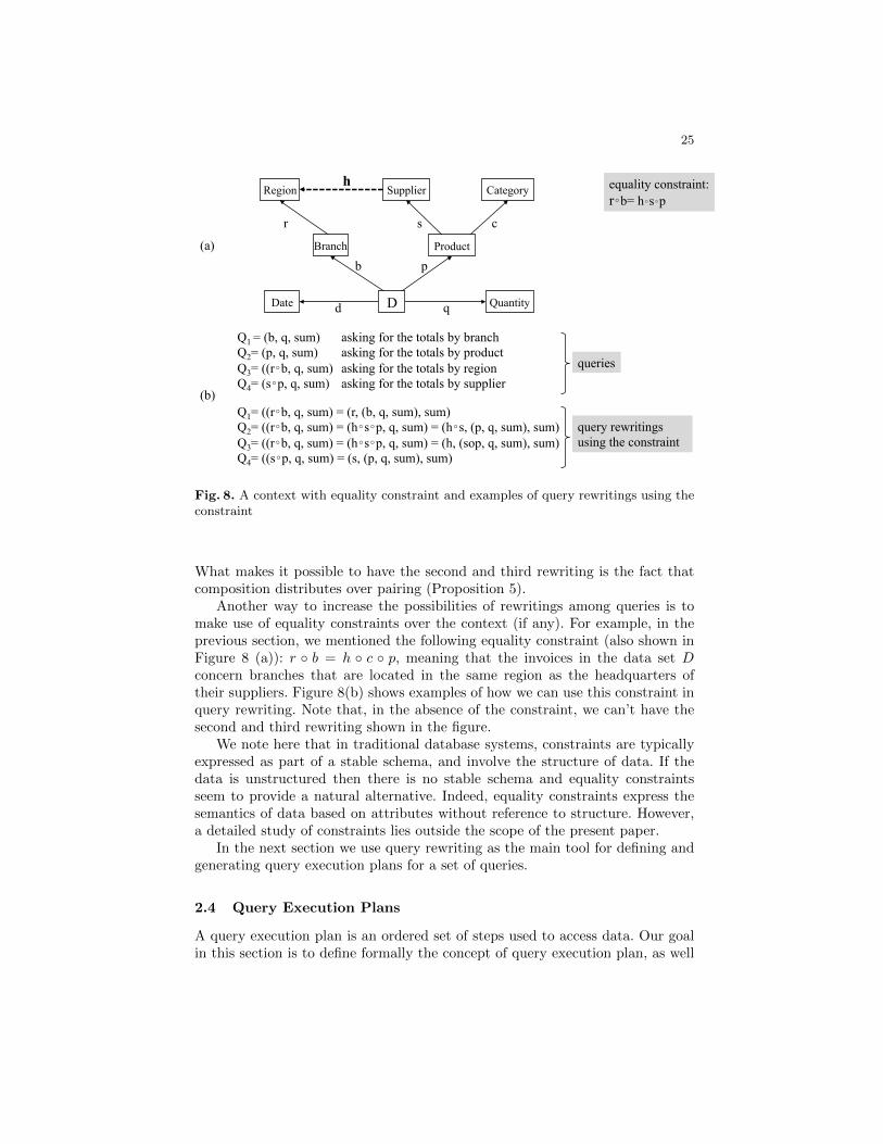
equality constraint: r�b= h�s�p

(a)

Q1 = (b, q, sum) asking for the totals by branch Q2= (p, q, sum) asking for the totals by product Q3= ((r�b, q, sum) asking for the totals by region Q4= (s�p, q, sum) asking for the totals by supplier

query rewritings using the constraint

(b)

queries

Q1= ((r�b, q, sum) = (r, (b, q, sum), sum) Q2= ((r�b, q, sum) = (h�s�p, q, sum) = (h�s, (p, q, sum), sum) Q3= ((r�b, q, sum) = (h�s�p, q, sum) = (h, (sop, q, sum), sum) Q4= ((s�p, q, sum) = (s, (p, q, sum), sum)

Region

Quantity

Category Supplier

b

r

p

s c

q d Date D

Product Branch

h

Fig. 8. A context with equality constraint and examples of query rewritings using theconstraint

What makes it possible to have the second and third rewriting is the fact thatcomposition distributes over pairing (Proposition 5).

Another way to increase the possibilities of rewritings among queries is tomake use of equality constraints over the context (if any). For example, in theprevious section, we mentioned the following equality constraint (also shown inFigure 8 (a)): r ◦ b = h ◦ c ◦ p, meaning that the invoices in the data set Dconcern branches that are located in the same region as the headquarters oftheir suppliers. Figure 8(b) shows examples of how we can use this constraint inquery rewriting. Note that, in the absence of the constraint, we can’t have thesecond and third rewriting shown in the figure.

We note here that in traditional database systems, constraints are typicallyexpressed as part of a stable schema, and involve the structure of data. If thedata is unstructured then there is no stable schema and equality constraintsseem to provide a natural alternative. Indeed, equality constraints express thesemantics of data based on attributes without reference to structure. However,a detailed study of constraints lies outside the scope of the present paper.

In the next section we use query rewriting as the main tool for defining andgenerating query execution plans for a set of queries.

2.4 Query Execution Plans

A query execution plan is an ordered set of steps used to access data. Our goalin this section is to define formally the concept of query execution plan, as well

26

as its graphical representation using the concepts introduced so far. We describehow one can generate execution plans but do not address the issue of generatingoptimal query execution plans.

The formal definition of a query execution plan in our model relies essentiallyon two concepts, namely that of rewriting graph and that of query executiongraph that we define next.

As we have seen earlier, at the conceptual level, a query in our model can beevaluated either directly, based on the definition of its answer, or after rewriting.The goal of rewriting an incoming query Q′ in terms of an already evaluatedquery Q is to reuse the result of Q in evaluating Q′ (assuming that the result ofQ has been stored either in temporary memory or in a cache).

In this section we consider a more general problem that can be stated roughlyas follows: given a set of queries that have to be evaluated in a given analysiscontext, define an ordered set of steps such that (a) each query is evaluated once(and only once) and (b) the evaluation order implied by rewriting is maintained.Our approach is based on the following two observations:

Sharing Two or more queries might have rewritings in terms of the same query,and therefore they can share its (stored) result.

Choice A given query might have two or more different rewritings in terms ofother queries in the set, therefore a choice is necessary (according to somecriterion).

Let us see an example illustrating the above observations. Consider again thecontext of Figure 8(a) with its equality constraint: r ◦ b = h ◦ s ◦ p, where thefunction h gives the region in which the headquarters of each supplier is located.

We recall that an equality between two functional expressions can be usedin two different ways: (a) as a means to formulate a restricted query or (b) as aconstraint over the data set being analyzed (as in Figure 8(a)).

In Figure 8(b) we see four queries, Q1, Q2, Q3 and Q4 and four rewrit-ings among these queries. Note that what makes possible the second and thirdrewriting is precisely the presence of the equality constraint. These rewritings areshown in Figure 9(a) encoded in the form of a graph, where each edge Q→ Q′

with label l means that Q′ can be rewritten in terms of Q using the attributel of the context. For example, the edge from Q1 to Q3 has label r because thefollowing rewriting holds: (r ◦ b, q, sum) = (r, (b, q, sum), sum). We shall callthis graph the “query rewriting graph”. However, in order to define this conceptformally we need the following definition.

Definition 11 (Comparing Grouping Functions).Let f and g be two functions having the same source, say A.

– (a) We shall say that f is less than or equal to g, denoted by f ≤ g, if forall a, a′ in A, f(a) = f(a′) implies g(a) = g(a′); or equivalently, if πf ≤ πg(i.e. if the partition of A induced by f is less than or equal to the partitionof A induced by g).

27

– (b) We shall say that f and g are equivalent, denoted by f ≡ g, if f ≤ g andg ≤ f (i.e. if πf = πg).

This definition can be extended to functional expressions in the obvious way.We note that two queries having equivalent grouping functions, the same mea-suring function and the same reduction operation are equivalent queries in thesense that they always return the same answer. This follows from the fact thatequivalent grouping functions induce the same partition on their common source.

Definition 12 (Query Rewriting Graph). Let Q be a set of queries to beevaluated in a given analysis context, such that:

– No two queries have equivalent grouping functions– All queries have the same measuring function and the same reduction oper-

ation.

We define the query rewriting graph of Q to be a directed graph with labellededges such that:

– The nodes of the graph are the queries of Q– There is an edge from node Q to node Q′ if Q′ can be rewritten in terms

of Q. The label of the edge Q → Q′ is the function on which is based therewriting of Q′ in terms of Q

Now, rewriting is a binary relation, which is actually a partial order overqueries. Indeed, we can show that rewriting is a reflexive, transitive and anti-symmetric relation (up to equivalence of grouping functions):

Reflexivity Every query Q can be rewritten in terms of itself (trivially, basedon the identity function).

Transitivity Consider three queries Q = (g,m, op), Q′ = (g′,m, op) and Q′′ =(g′′,m, op) such that: Q rewrites Q′ and Q′ rewrites Q′′. It follows that: thereexist functions h′, h′′ such that g = h′ ◦ g′ and g′ = h′′ ◦ g′′. Therefore wehave: g = h′ ◦ g′ = h′ ◦ h′′ ◦ g′′ = (h′ ◦ h′′) ◦ g′′ It follows that Q rewrites Q′′

based on (h′ ◦ h′′).Anti-symmetry Suppose Q rewrites Q′ and Q′ rewrites Q. It follows that there

exist functions h′, h′′ such that g′ = h′◦g and g = h′′◦g′. Therefore we have:g = h′ ◦ h′′ ◦ g. It follows that h′ ◦ h′′ is the identity function and thereforeQ = Q′.

We shall denote by ≤w the above partial order defined by query rewriting.Recall now that, given a set of queries, its query rewriting graph gives all

possible rewritings among the queries in the set; and that each edge Q → Q′

implies that query Q should be evaluated before query Q′ if we want Q′ touse the result of Q. Moreover, as we observed earlier, each query in the queryrewriting graph might have more than one rewriting in terms of other queries;therefore a choice of one among the possible rewritings of each query is necessarybefore evaluating the given set of queries. So the problem is to find a subgraph

28

of the query rewriting graph such that (a) the evaluation order implied by therewritings is maintained and (b) each query is evaluated exactly once. Theseobservations lead to the following definition of query execution graph.

Definition 13 (Query Execution Graph). A query execution graph for a setQ of queries is defined to be a subgraph EG of the query rewriting graph of Qsuch that:

– The nodes of EG are the queries of Q (i.e. EG has the same nodes as thequery rewriting graph of Q)

– Each node of EG has at most one predecessor

Note that every query execution graph is an acyclic graph. This follows fromthe fact that query rewriting is a partial order and therefore the rewriting graphis an acyclic graph.

two different execution graphs EG-1 and EG-2

two different execution plans EP-1.1 and EP-1.2 derived from EG-1

EG-1 EG-2

EP-1.1 EP-1.2

(b)

(c)

Q1= (b, q, sum) Q2= (p, q, sum) Q3= (r�b, q, sum)= (h�s�p, q, sum) Q4= (s�p, q, sum)

a set of queries to be executed and their rewriting graph RG

r s

h

h�s

Q1 Q2

Q4 Q3

(a) RG

r s

Q1 Q2

Q4 Q3

s

Q1 Q2

Q4 Q3

s h�s

Q1 Q2

Q4 Q3

s

h

Q1 Q2

Q4 Q3

Fig. 9. A query rewriting graph RG, two of its query execution graphs, EG-1 andEG-2, and two query execution plans EP-1.1 and EP-1.2 from EG-1

Figure 9(a) shows a set of queries and their rewriting graph RG; and Figure9(b) shows two query execution graphs, EG-1 and EG-2 of RG. The fact thatan edge of the rewriting graph is not present in a query execution graph simplymeans that the corresponding rewriting is not considered as an option (for somereason). In other words the query execution graph allows the freedom of not

29

using some rewritings present in the rewriting graph. On the other hand, both,rewriting graphs and query execution graphs might have isolated nodes (as inEG-1). An isolated node simply means that it will be evaluated in isolation,neither reusing the result of another query nor being reused in the evaluation ofanother query).

Now, while the rewriting graph of a set Q of queries gives all possible rewrit-ings among the queries in Q, each query execution graph of Q gives those rewrit-ings that are to be used during the evaluation of the queries in Q. The rewritingsof a query execution graph indicate the order in which the queries in Q shouldbe executed in order to reuse the results of previously executed queries.

Privileging query rewriting is certainly reasonable, as query rewriting takesinto account the semantics of data. However, apart from rewriting there mightbe other factors that influence the overall performance of query evaluation. Ingeneral, these other factors include the following:

– The physical storage of data, namely their format and their possible distri-bution

– The model of distributed computation– The availability of cached query results– The availability of processors and their configuration– Load balancing– etc.

In this work we privilege query rewriting and do not discuss the above factorsany further. Instead, we assume that their influence is expressed as an orderingof the queries to be evaluated. We shall call this ordering the external order andwe shall denote it by ≤e. Actually, what we call a query execution plan, is aquery execution graph together with an external order.

Definition 14 (Query Execution Plan). A query execution plan for a setQ of queries is defined to be a query execution graph together with an externalorder ≤e compatible with the rewriting order ≤w.

Compatibility in the above definition means that the resulting graph isacyclic. Technically speaking, this means that the relation ≤w ∪ ≤e is an acyclicrelation; we shall denote this relation by ≤. In case ≤w ∪ ≤e is not an acyclicrelation, we shall remove a minimal number of external edges so that it becomesacyclic (and this is a non-deterministic process). In other words, we shall privi-lege the rewriting order while leaving in the result as big a part of the externalorder as possible.

We note that a query execution graph is itself a query execution plan (withthe trivial order as external order). We also note that the rewriting order ≤w

depends on the semantics of queries whereas the external order ≤e is applicationdependent.

Figure 9(c) shows two query execution plans, EP-1.1 and EP-1.2, derivedfrom the query execution graph EG-1. The rewriting order ≤w is indicated bythe edges in solid line, whereas the external order ≤e is indicated by the edges in

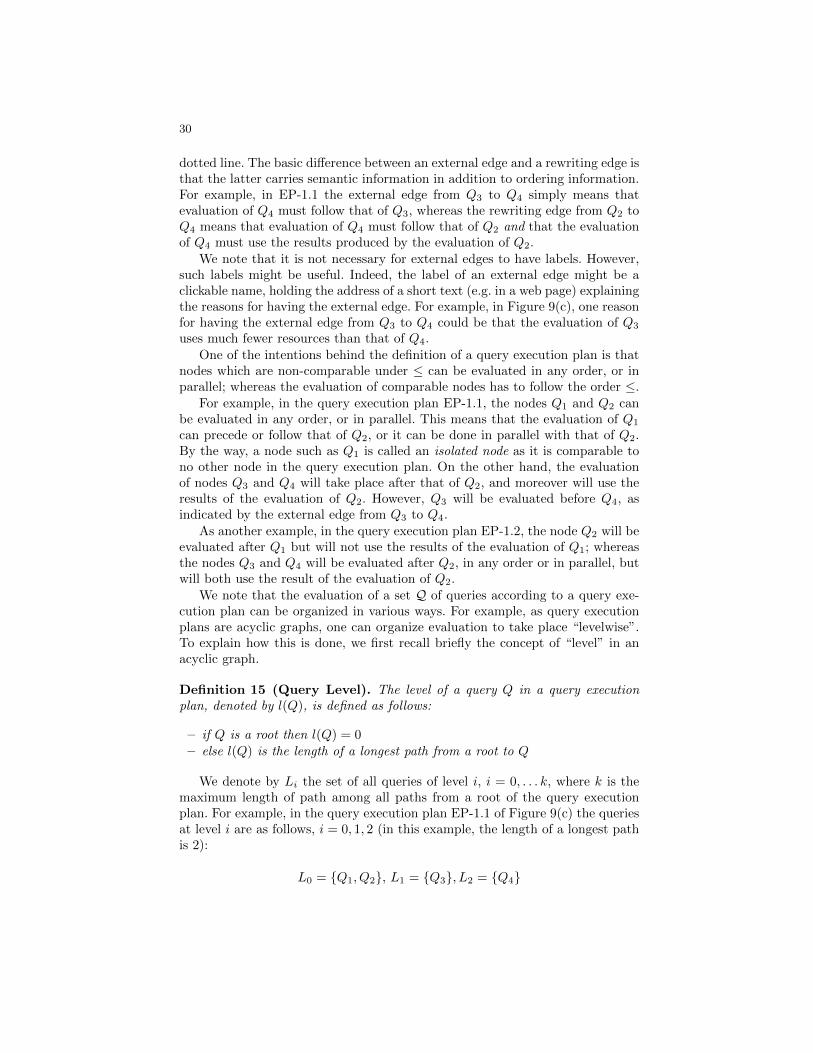
30

dotted line. The basic difference between an external edge and a rewriting edge isthat the latter carries semantic information in addition to ordering information.For example, in EP-1.1 the external edge from Q3 to Q4 simply means thatevaluation of Q4 must follow that of Q3, whereas the rewriting edge from Q2 toQ4 means that evaluation of Q4 must follow that of Q2 and that the evaluationof Q4 must use the results produced by the evaluation of Q2.

We note that it is not necessary for external edges to have labels. However,such labels might be useful. Indeed, the label of an external edge might be aclickable name, holding the address of a short text (e.g. in a web page) explainingthe reasons for having the external edge. For example, in Figure 9(c), one reasonfor having the external edge from Q3 to Q4 could be that the evaluation of Q3

uses much fewer resources than that of Q4.One of the intentions behind the definition of a query execution plan is that

nodes which are non-comparable under ≤ can be evaluated in any order, or inparallel; whereas the evaluation of comparable nodes has to follow the order ≤.

For example, in the query execution plan EP-1.1, the nodes Q1 and Q2 canbe evaluated in any order, or in parallel. This means that the evaluation of Q1

can precede or follow that of Q2, or it can be done in parallel with that of Q2.By the way, a node such as Q1 is called an isolated node as it is comparable tono other node in the query execution plan. On the other hand, the evaluationof nodes Q3 and Q4 will take place after that of Q2, and moreover will use theresults of the evaluation of Q2. However, Q3 will be evaluated before Q4, asindicated by the external edge from Q3 to Q4.

As another example, in the query execution plan EP-1.2, the node Q2 will beevaluated after Q1 but will not use the results of the evaluation of Q1; whereasthe nodes Q3 and Q4 will be evaluated after Q2, in any order or in parallel, butwill both use the result of the evaluation of Q2.

We note that the evaluation of a set Q of queries according to a query exe-cution plan can be organized in various ways. For example, as query executionplans are acyclic graphs, one can organize evaluation to take place “levelwise”.To explain how this is done, we first recall briefly the concept of “level” in anacyclic graph.

Definition 15 (Query Level). The level of a query Q in a query executionplan, denoted by l(Q), is defined as follows:

– if Q is a root then l(Q) = 0– else l(Q) is the length of a longest path from a root to Q

We denote by Li the set of all queries of level i, i = 0, . . . k, where k is themaximum length of path among all paths from a root of the query executionplan. For example, in the query execution plan EP-1.1 of Figure 9(c) the queriesat level i are as follows, i = 0, 1, 2 (in this example, the length of a longest pathis 2):

L0 = {Q1, Q2}, L1 = {Q3}, L2 = {Q4}

31

The following facts are immediate consequences of the above definition oflevel:

Fact 1 No two queries of Li are comparable, i = 0, . . . k (therefore the queriesof Li can be executed in any order or in parallel)

Fact 2 Each query Q′ at level i has at most one predecessor at level i− 1 (i.e.there is at most one rewriting of Q′ in terms of a query Q at level i− 1)

The sets Li can be computed by topological sorting of the query executionplan, in time linear with respect to n + e, where n is the number of nodes ande is the number of edges of the query execution plan. Once the levels have beencomputed, evaluation can be done in a number of different ways. For example,one way is to follow the order of the levels (i.e. first executing the queries of L0,then the queries of L1, and so on).

It is important to note that, as all nodes of any given level are pairwise noncomparable, their evaluation can be done in any order or in parallel. This means,in particular, that once the evaluation of a node Q at level i has terminated, wecan proceed with the evaluation of the successors of Q (if any) at level i+1 (andthis independently of all other nodes at level i).

We end this section with a few remarks regarding query execution plans.First, in our definition of query execution plan, we have privileged the rewritingorder over the external order. Clearly one could privilege the external order overthe rewriting order (or mix the two, provided that the result is a partial order).The method described above would remain the same, as the only thing thatmatters is acyclicity.

Second, our definition of query execution plan is “static”, in the sense thatthe execution plan is defined before query evaluation starts, and it is followeduntil the last query is evaluated. However, our formal framework applies alsoin dynamic environments in which the actual order (i.e. the next query to beevaluated) is decided “on the fly” depending on the current values of a set ofparameters (e.g. currently available processors). In this case, we start not witha query execution plan but with the query rewriting graph to which we add theexternal order; the resulting graph shows all possibilities of rewritings but willpossibly have conflicts with the external order. Choosing one among all possiblerewritings of a query and resolving conflicts between the rewriting order and theexternal order is done on the fly when deciding the next query to be evaluated.However, we shall not elaborate any further on dynamic query execution plansin this paper.

3 From Theory to Practice

As we mentioned in the introduction, data analysis is the process of highlightinguseful information “hidden” in big data sets, usually with the goal to supportdecision making. Data analysis usually requires the execution of several analysistasks, and a query Q = (g,m, op), as defined in section 2.1, can be seen as ameans to specify one such task.

32

In the formal model presented in the previous section, there is a clear sepa-ration between the conceptual and the physical level. An analytic query and itsanswer are defined at the conceptual level independently of the nature and loca-tion of data. However, the abstract definitions have to be mapped to lower levelevaluation mechanisms, at the physical level, where the actual query evaluationis done.

In this section we first propose a conceptual query evaluation scheme andthen we explain how this scheme can be mapped in three important cases,namely in MapReduce, in column databases and in row databases (i.e. relationaldatabases). Moreover, we explain how our model can leverage structure and se-mantics in data in order to improve the performance of the query evaluationprocess.

3.1 Our Conceptual Query Evaluation Scheme

At the conceptual level, the answer to a query Q = (g,m, op) is defined in astraightforward manner that we briefly recall here. Let g1, . . . , gn be the valuesof g and let πg = {G1, . . . , Gn} be the partition of D into blocks, induced by g(i.e. Gj = g−1(gj), j = 1, . . . , n). Then the answer of Q on value gj is defined asfollows: ansQ(gj) = red(m/Gj , op). In other words the answer of Q on value gjis the reduction (under op) of the values of m on the block Gj = g−1(gj).

However, this abstract definition of the answer assumes that the (extensionsof the) functions g and m are stored in some repository and that they are ac-cessible for processing. In practice, this assumption is rarely true. Actually, thefunctions g and m usually have to be extracted from the (possibly) much largerdata set D in which they are embedded; and their extraction may require oneor more joins, which are expensive operations.

Moreover, the data set from which the functions g and m are extracted isusually distributed, and this further complicates their extraction. Indeed, thedata assets of an institution usually reside in several different repositories thatcan even be geographically distributed.

For example, in a big company with several branches, it is very likely thatthe sales transactions in each branch will be stored in a local database. As aresult, data analysis queries concerning the company data assets, as a whole,will have to take into account data distribution. Moreover, even if we assumethat all transactions are stored in a central repository, the size of the data setmight require their deployment over several computational nodes for reasons ofparallel processing. Indeed, in some application environments, the size of the dataset is such that massive parallel processing is the only way to achieve acceptableperformance.

The conceptual evaluation scheme that we propose in this section consists ofthree steps:

– Query input preparation– πg construction– πg reduction

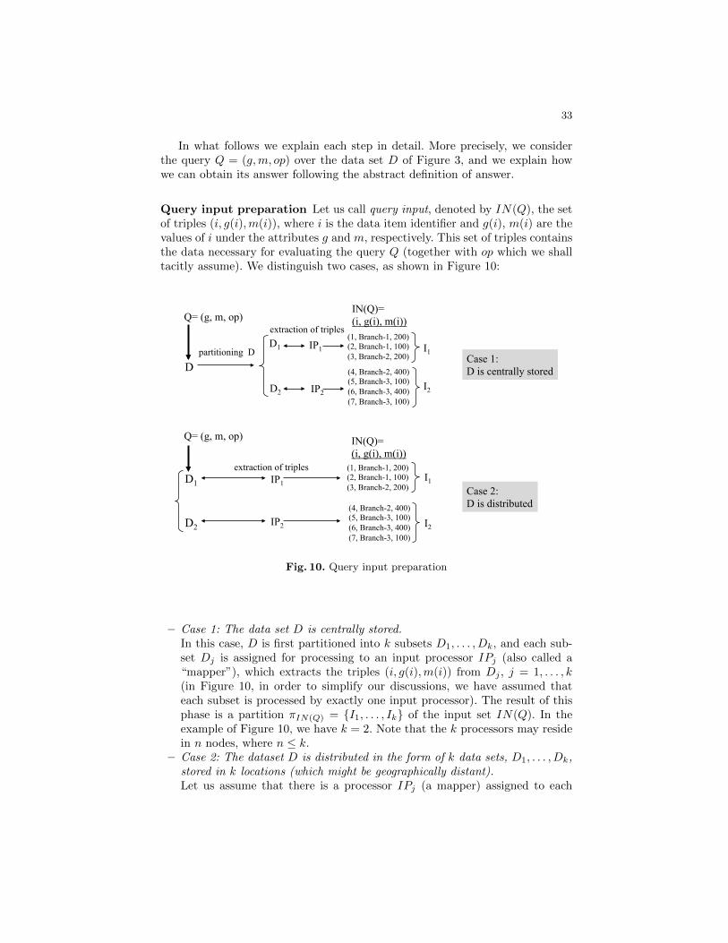
33

In what follows we explain each step in detail. More precisely, we considerthe query Q = (g,m, op) over the data set D of Figure 3, and we explain howwe can obtain its answer following the abstract definition of answer.

Query input preparation Let us call query input, denoted by IN(Q), the setof triples (i, g(i),m(i)), where i is the data item identifier and g(i), m(i) are thevalues of i under the attributes g and m, respectively. This set of triples containsthe data necessary for evaluating the query Q (together with op which we shalltacitly assume). We distinguish two cases, as shown in Figure 10:

(1, Branch-1, 200) (2, Branch-1, 100) (3, Branch-2, 200)

(4, Branch-2, 400) (5, Branch-3, 100) (6, Branch-3, 400) (7, Branch-3, 100)

(1, Branch-1, 200) (2, Branch-1, 100) (3, Branch-2, 200)

IN(Q)= (i, g(i), m(i))

I1

I2

D

Q= (g, m, op) extraction of triples

partitioning D D1 IP1

D2 IP2

IN(Q)= (i, g(i), m(i))

I1

I2

D1

Q= (g, m, op)

extraction of triples IP1

IP2 D2

Case 1: D is centrally stored

Case 2: D is distributed

(4, Branch-2, 400) (5, Branch-3, 100) (6, Branch-3, 400) (7, Branch-3, 100)

Fig. 10. Query input preparation

– Case 1: The data set D is centrally stored.In this case, D is first partitioned into k subsets D1, . . . , Dk, and each sub-set Dj is assigned for processing to an input processor IPj (also called a“mapper”), which extracts the triples (i, g(i),m(i)) from Dj , j = 1, . . . , k(in Figure 10, in order to simplify our discussions, we have assumed thateach subset is processed by exactly one input processor). The result of thisphase is a partition πIN(Q) = {I1, . . . , Ik} of the input set IN(Q). In theexample of Figure 10, we have k = 2. Note that the k processors may residein n nodes, where n ≤ k.

– Case 2: The dataset D is distributed in the form of k data sets, D1, . . . , Dk,stored in k locations (which might be geographically distant).Let us assume that there is a processor IPj (a mapper) assigned to each

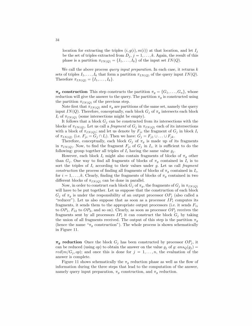
34

location for extracting the triples (i, g(i),m(i)) at that location, and let Ijbe the set of triples extracted from Dj , j = 1, . . . , k. Again, the result of thisphase is a partition πIN(Q) = {I1, . . . , Ik} of the input set IN(Q).

We call the above process query input preparation. In each case, it returns ksets of triples I1, . . . , Ik that form a partition πIN(Q) of the query input IN(Q).Therefore πIN(Q) = {I1, . . . , Ik}.

πg construction This step constructs the partition πg = {G1, . . . , Gn}, whosereduction will give the answer to the query. The partition πg is constructed usingthe partition πIN(Q) of the previous step.

Note first that πIN(Q) and πg are partitions of the same set, namely the queryinput IN(Q). Therefore, conceptually, each block Gj of πg intersects each blockIi of πIN(Q) (some intersections might be empty).

It follows that a block Gj can be constructed from its intersections with theblocks of πIN(Q). Let us call a fragment of Gj in πIN(Q) each of its intersectionswith a block of πIN(Q); and let us denote by Fji the fragment of Gj in block Iiof πIN(Q) (i.e. Fji = Gj ∩ Ii). Then we have: Gj = Fj1 ∪ . . . ∪ Fjk.

Therefore, conceptually, each block Gj of πg is made up of its fragmentsin πIN(Q). Now, to find the fragment Fji of Gj in Ii, it is sufficient to do thefollowing: group together all triples of Ii having the same value gj .

However, each block Ii might also contain fragments of blocks of πg otherthan Gj . One way to find all fragments of blocks of πg contained in Ii is tosort the triples of Ii according to their values under g. Let us call fragmentconstruction the process of finding all fragments of blocks of πg contained in Ii,for i = 1, . . . , k. Clearly, finding the fragments of blocks of πg contained in twodifferent blocks of πIN(Q) can be done in parallel.

Now, in order to construct each block Gj of πg, the fragments of Gj in πIN(Q)

will have to be put together. Let us suppose that the construction of each blockGj of πg is under the responsibility of an output processor OPj (also called a“reducer”). Let us also suppose that as soon as a processor IPi computes itsfragments, it sends them to the appropriate output processors (i.e. it sends F1i

to OP1, F12 to OP2, and so on). Clearly, as soon as processor OPj receives thefragments sent by all processors IPi it can construct the block Gj by takingthe union of all fragments received. The output of this step is the partition πg(hence the name “πg construction”). The whole process is shown schematicallyin Figure 11.

πg reduction Once the block Gj has been constructed by processor OPj , itcan be reduced (using op) to obtain the answer on the value gj of g: ansQ(gj) =red(m/Gj , op); and once this is done for j = 1, . . . , n, the evaluation of theanswer is complete.

Figure 11 shows schematically the πg reduction phase as well as the flow ofinformation during the three steps that lead to the computation of the answer,namely query input preparation, πg construction, and πg reduction.

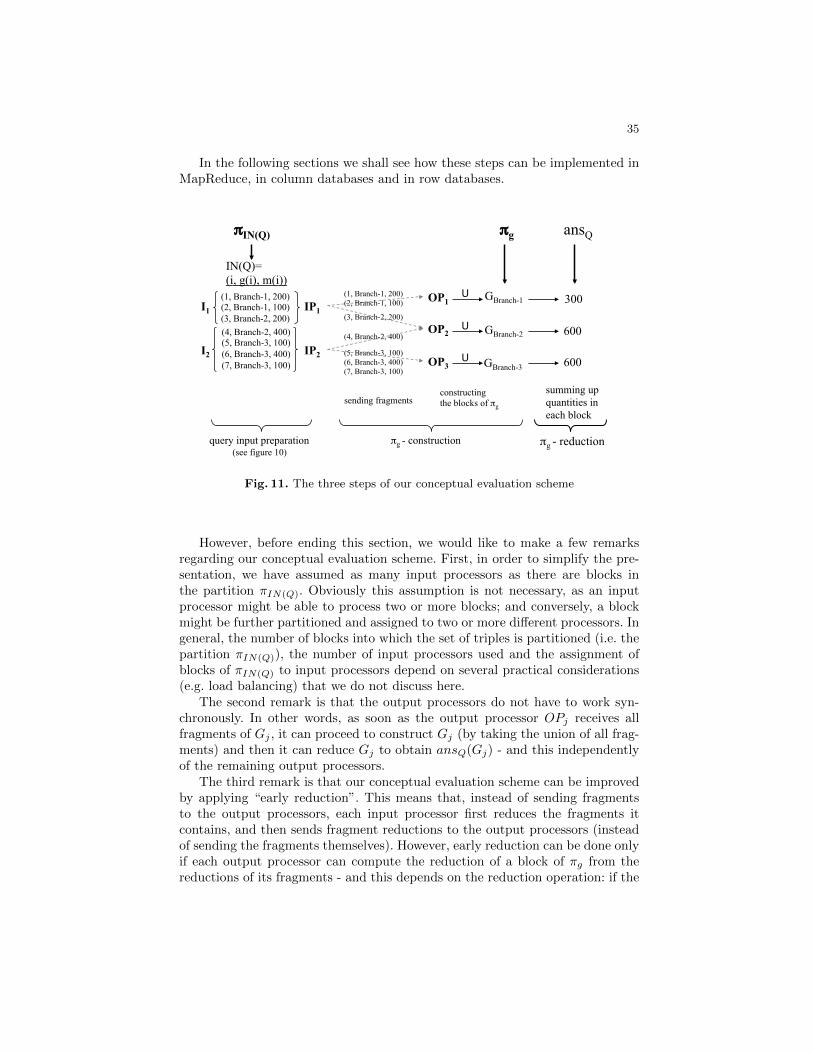
35

In the following sections we shall see how these steps can be implemented inMapReduce, in column databases and in row databases.

πg ansQ πIN(Q)

πg - construction query input preparation πg - reduction

summing up quantities in each block

IP1

IP2

OP1

OP2

OP3

(1, Branch-1, 200) (2, Branch-1, 100)

(3, Branch-2, 200)

(4, Branch-2, 400)

(5, Branch-3, 100) (6, Branch-3, 400) (7, Branch-3, 100)

GBranch-1

GBranch-2

GBranch-3

(1, Branch-1, 200) (2, Branch-1, 100) (3, Branch-2, 200)

IN(Q)= (i, g(i), m(i))

I1

I2

(4, Branch-2, 400) (5, Branch-3, 100) (6, Branch-3, 400) (7, Branch-3, 100)

300

600

600

U�

U�

U�

(see figure 10)

sending fragments constructing the blocks of πg

Fig. 11. The three steps of our conceptual evaluation scheme

However, before ending this section, we would like to make a few remarksregarding our conceptual evaluation scheme. First, in order to simplify the pre-sentation, we have assumed as many input processors as there are blocks inthe partition πIN(Q). Obviously this assumption is not necessary, as an inputprocessor might be able to process two or more blocks; and conversely, a blockmight be further partitioned and assigned to two or more different processors. Ingeneral, the number of blocks into which the set of triples is partitioned (i.e. thepartition πIN(Q)), the number of input processors used and the assignment ofblocks of πIN(Q) to input processors depend on several practical considerations(e.g. load balancing) that we do not discuss here.

The second remark is that the output processors do not have to work syn-chronously. In other words, as soon as the output processor OPj receives allfragments of Gj , it can proceed to construct Gj (by taking the union of all frag-ments) and then it can reduce Gj to obtain ansQ(Gj) - and this independentlyof the remaining output processors.

The third remark is that our conceptual evaluation scheme can be improvedby applying “early reduction”. This means that, instead of sending fragmentsto the output processors, each input processor first reduces the fragments itcontains, and then sends fragment reductions to the output processors (insteadof sending the fragments themselves). However, early reduction can be done onlyif each output processor can compute the reduction of a block of πg from thereductions of its fragments - and this depends on the reduction operation: if the

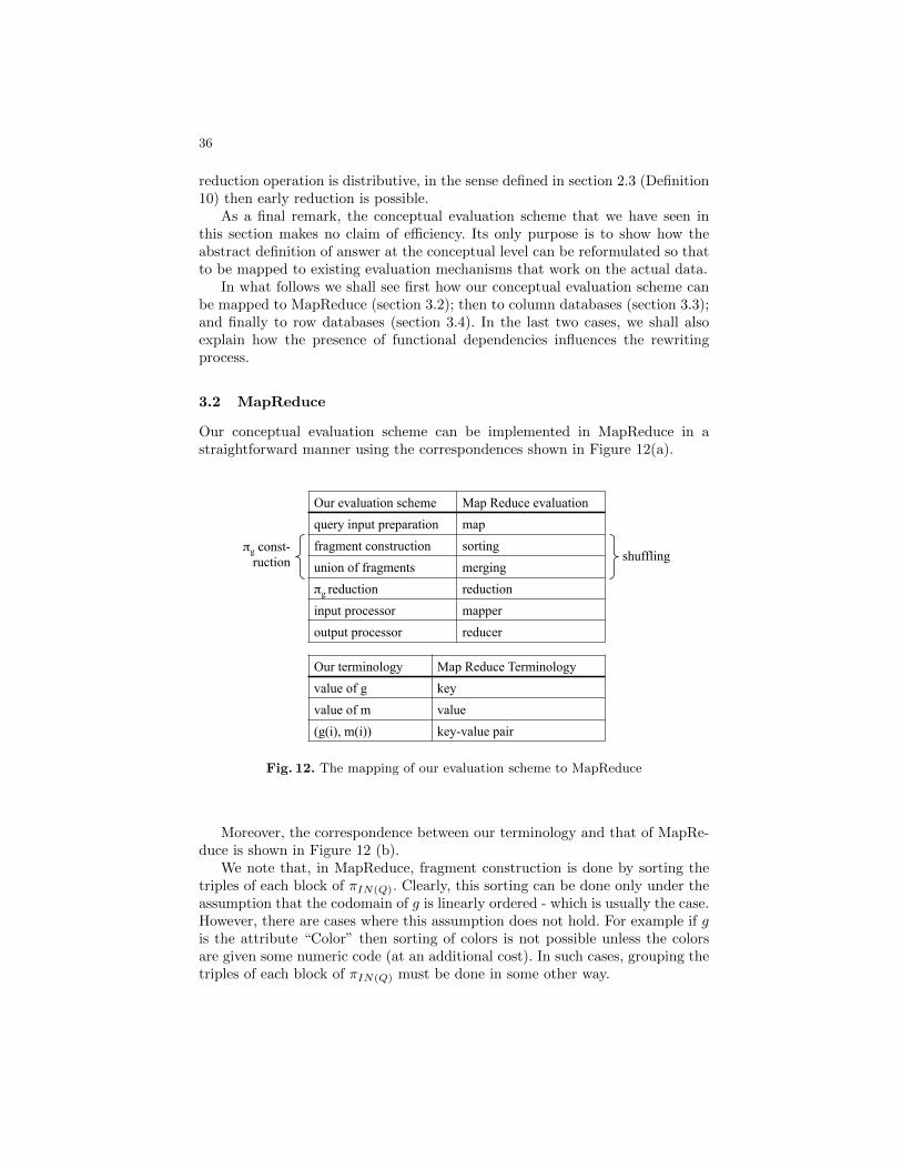
36

reduction operation is distributive, in the sense defined in section 2.3 (Definition10) then early reduction is possible.

As a final remark, the conceptual evaluation scheme that we have seen inthis section makes no claim of efficiency. Its only purpose is to show how theabstract definition of answer at the conceptual level can be reformulated so thatto be mapped to existing evaluation mechanisms that work on the actual data.

In what follows we shall see first how our conceptual evaluation scheme canbe mapped to MapReduce (section 3.2); then to column databases (section 3.3);and finally to row databases (section 3.4). In the last two cases, we shall alsoexplain how the presence of functional dependencies influences the rewritingprocess.

3.2 MapReduce

Our conceptual evaluation scheme can be implemented in MapReduce in astraightforward manner using the correspondences shown in Figure 12(a).

Our evaluation scheme Map Reduce evaluation query input preparation map fragment construction sorting union of fragments merging πg reduction reduction input processor mapper output processor reducer

πg const- ruction shuffling

Our terminology Map Reduce Terminology value of g key value of m value (g(i), m(i)) key-value pair

Fig. 12. The mapping of our evaluation scheme to MapReduce

Moreover, the correspondence between our terminology and that of MapRe-duce is shown in Figure 12 (b).

We note that, in MapReduce, fragment construction is done by sorting thetriples of each block of πIN(Q). Clearly, this sorting can be done only under theassumption that the codomain of g is linearly ordered - which is usually the case.However, there are cases where this assumption does not hold. For example if gis the attribute “Color” then sorting of colors is not possible unless the colorsare given some numeric code (at an additional cost). In such cases, grouping thetriples of each block of πIN(Q) must be done in some other way.

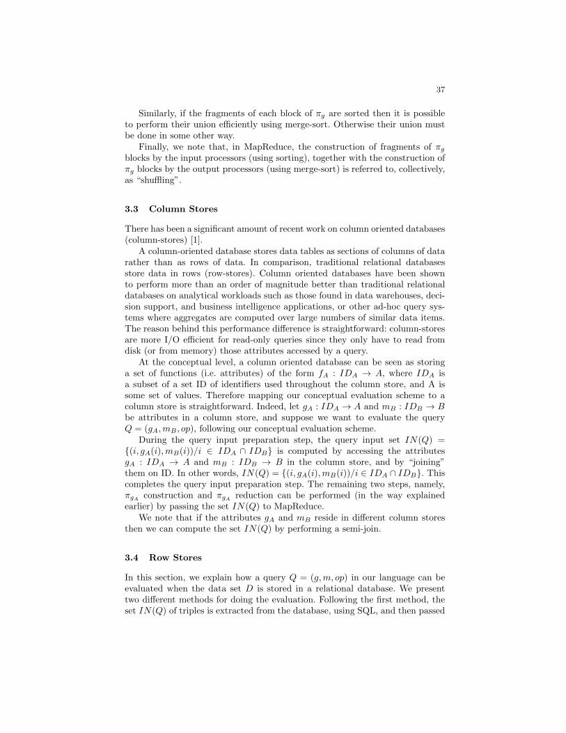
37

Similarly, if the fragments of each block of πg are sorted then it is possibleto perform their union efficiently using merge-sort. Otherwise their union mustbe done in some other way.

Finally, we note that, in MapReduce, the construction of fragments of πgblocks by the input processors (using sorting), together with the construction ofπg blocks by the output processors (using merge-sort) is referred to, collectively,as “shuffling”.

3.3 Column Stores

There has been a significant amount of recent work on column oriented databases(column-stores) [1].

A column-oriented database stores data tables as sections of columns of datarather than as rows of data. In comparison, traditional relational databasesstore data in rows (row-stores). Column oriented databases have been shownto perform more than an order of magnitude better than traditional relationaldatabases on analytical workloads such as those found in data warehouses, deci-sion support, and business intelligence applications, or other ad-hoc query sys-tems where aggregates are computed over large numbers of similar data items.The reason behind this performance difference is straightforward: column-storesare more I/O efficient for read-only queries since they only have to read fromdisk (or from memory) those attributes accessed by a query.

At the conceptual level, a column oriented database can be seen as storinga set of functions (i.e. attributes) of the form fA : IDA → A, where IDA isa subset of a set ID of identifiers used throughout the column store, and A issome set of values. Therefore mapping our conceptual evaluation scheme to acolumn store is straightforward. Indeed, let gA : IDA → A and mB : IDB → Bbe attributes in a column store, and suppose we want to evaluate the queryQ = (gA,mB , op), following our conceptual evaluation scheme.

During the query input preparation step, the query input set IN(Q) ={(i, gA(i),mB(i))/i ∈ IDA ∩ IDB} is computed by accessing the attributesgA : IDA → A and mB : IDB → B in the column store, and by “joining”them on ID. In other words, IN(Q) = {(i, gA(i),mB(i))/i ∈ IDA ∩ IDB}. Thiscompletes the query input preparation step. The remaining two steps, namely,πgA construction and πgA reduction can be performed (in the way explainedearlier) by passing the set IN(Q) to MapReduce.

We note that if the attributes gA and mB reside in different column storesthen we can compute the set IN(Q) by performing a semi-join.

3.4 Row Stores

In this section, we explain how a query Q = (g,m, op) in our language can beevaluated when the data set D is stored in a relational database. We presenttwo different methods for doing the evaluation. Following the first method, theset IN(Q) of triples is extracted from the database, using SQL, and then passed

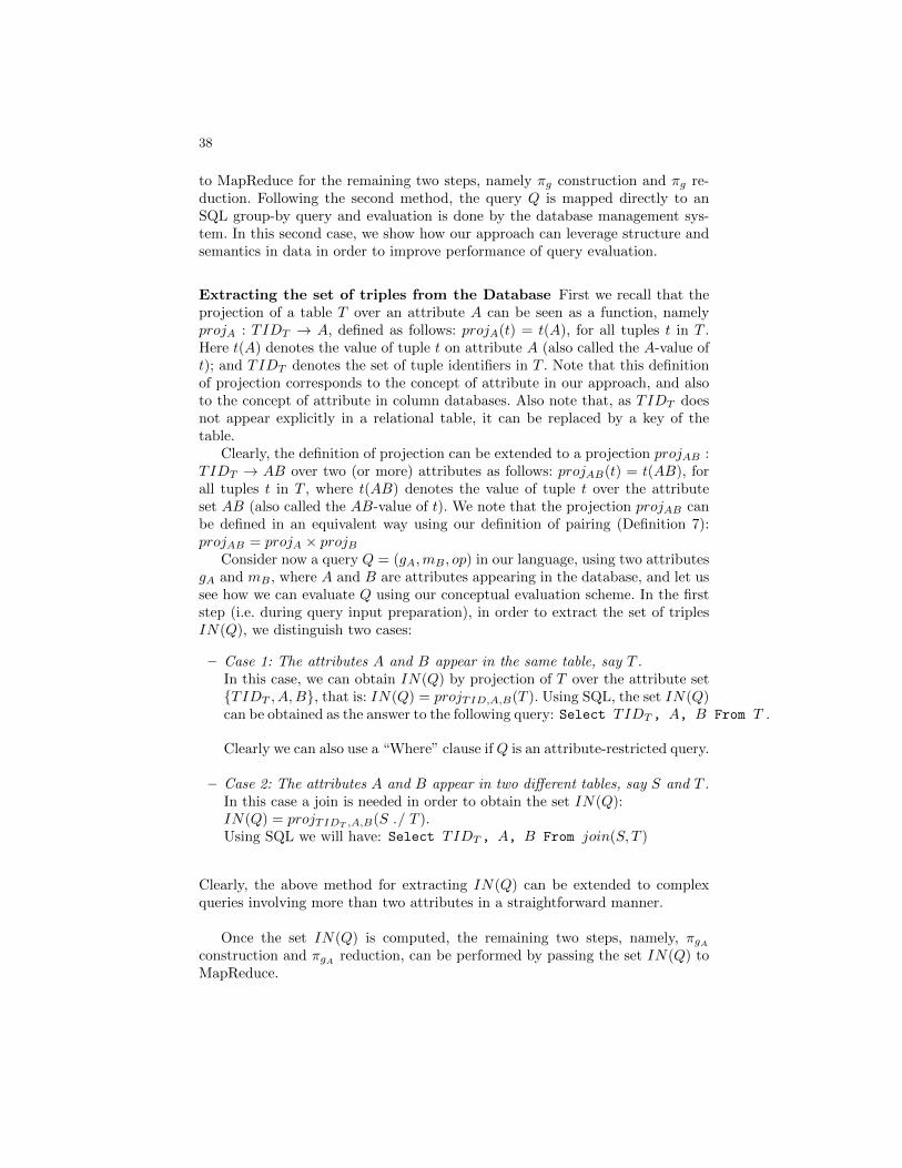
38

to MapReduce for the remaining two steps, namely πg construction and πg re-duction. Following the second method, the query Q is mapped directly to anSQL group-by query and evaluation is done by the database management sys-tem. In this second case, we show how our approach can leverage structure andsemantics in data in order to improve performance of query evaluation.

Extracting the set of triples from the Database First we recall that theprojection of a table T over an attribute A can be seen as a function, namelyprojA : TIDT → A, defined as follows: projA(t) = t(A), for all tuples t in T .Here t(A) denotes the value of tuple t on attribute A (also called the A-value oft); and TIDT denotes the set of tuple identifiers in T . Note that this definitionof projection corresponds to the concept of attribute in our approach, and alsoto the concept of attribute in column databases. Also note that, as TIDT doesnot appear explicitly in a relational table, it can be replaced by a key of thetable.

Clearly, the definition of projection can be extended to a projection projAB :TIDT → AB over two (or more) attributes as follows: projAB(t) = t(AB), forall tuples t in T , where t(AB) denotes the value of tuple t over the attributeset AB (also called the AB-value of t). We note that the projection projAB canbe defined in an equivalent way using our definition of pairing (Definition 7):projAB = projA × projB

Consider now a query Q = (gA,mB , op) in our language, using two attributesgA and mB , where A and B are attributes appearing in the database, and let ussee how we can evaluate Q using our conceptual evaluation scheme. In the firststep (i.e. during query input preparation), in order to extract the set of triplesIN(Q), we distinguish two cases:

– Case 1: The attributes A and B appear in the same table, say T .In this case, we can obtain IN(Q) by projection of T over the attribute set{TIDT , A,B}, that is: IN(Q) = projTID,A,B(T ). Using SQL, the set IN(Q)can be obtained as the answer to the following query: Select TIDT , A, B From T .

Clearly we can also use a “Where” clause if Q is an attribute-restricted query.

– Case 2: The attributes A and B appear in two different tables, say S and T .In this case a join is needed in order to obtain the set IN(Q):IN(Q) = projTIDT ,A,B(S ./ T ).Using SQL we will have: Select TIDT , A, B From join(S, T )

Clearly, the above method for extracting IN(Q) can be extended to complexqueries involving more than two attributes in a straightforward manner.

Once the set IN(Q) is computed, the remaining two steps, namely, πgAconstruction and πgA reduction, can be performed by passing the set IN(Q) toMapReduce.

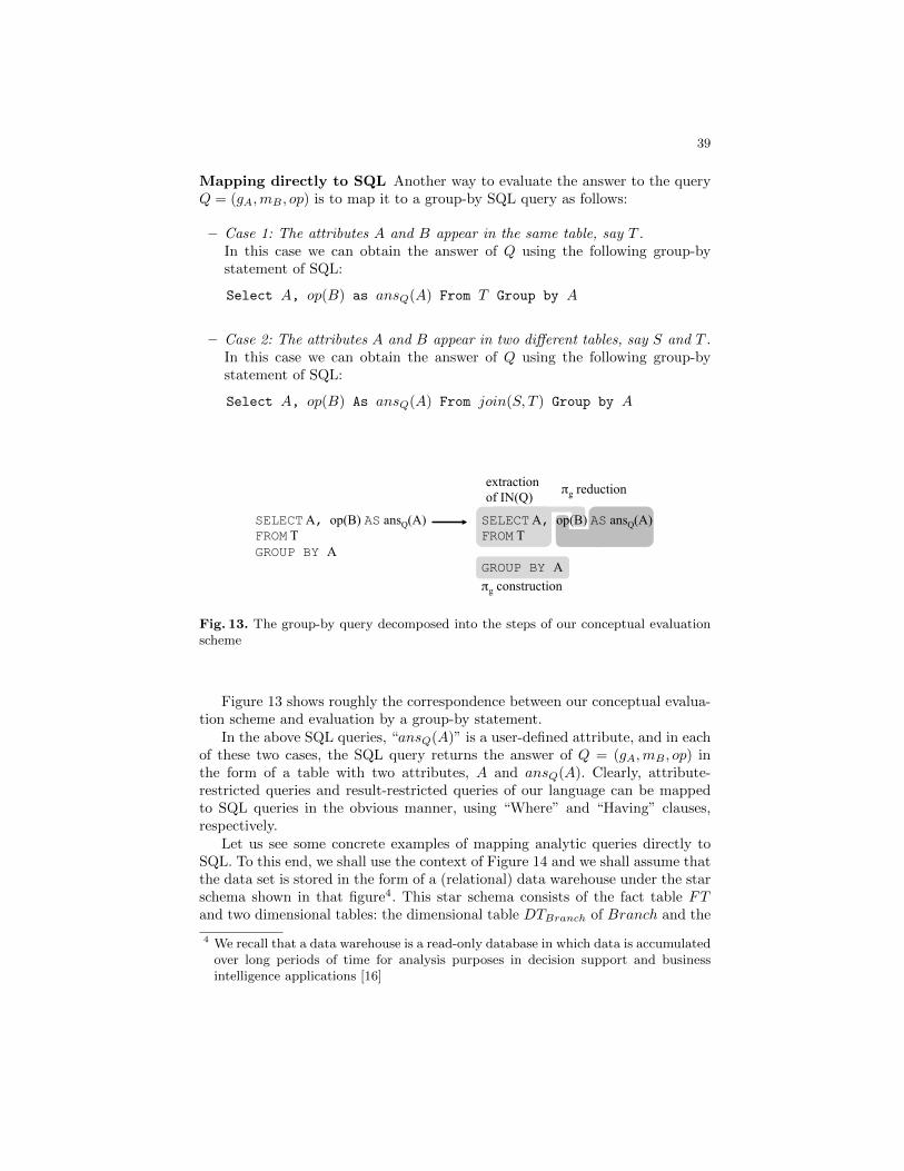
39

Mapping directly to SQL Another way to evaluate the answer to the queryQ = (gA,mB , op) is to map it to a group-by SQL query as follows:

– Case 1: The attributes A and B appear in the same table, say T .In this case we can obtain the answer of Q using the following group-bystatement of SQL:

Select A, op(B) as ansQ(A) From T Group by A

– Case 2: The attributes A and B appear in two different tables, say S and T .In this case we can obtain the answer of Q using the following group-bystatement of SQL:

Select A, op(B) As ansQ(A) From join(S, T ) Group by A

extraction of IN(Q) πg reduction

πg construction

SELECT A, op(B) AS ansQ(A) FROM T GROUP BY A

SELECT A, op(B) AS ansQ(A) FROM T GROUP BY A

Fig. 13. The group-by query decomposed into the steps of our conceptual evaluationscheme

Figure 13 shows roughly the correspondence between our conceptual evalua-tion scheme and evaluation by a group-by statement.

In the above SQL queries, “ansQ(A)” is a user-defined attribute, and in eachof these two cases, the SQL query returns the answer of Q = (gA,mB , op) inthe form of a table with two attributes, A and ansQ(A). Clearly, attribute-restricted queries and result-restricted queries of our language can be mappedto SQL queries in the obvious manner, using “Where” and “Having” clauses,respectively.

Let us see some concrete examples of mapping analytic queries directly toSQL. To this end, we shall use the context of Figure 14 and we shall assume thatthe data set is stored in the form of a (relational) data warehouse under the starschema shown in that figure4. This star schema consists of the fact table FTand two dimensional tables: the dimensional table DTBranch of Branch and the

4 We recall that a data warehouse is a read-only database in which data is accumulatedover long periods of time for analysis purposes in decision support and businessintelligence applications [16]

40

dimensional table DTProduct of Product. The edges of the context are embeddedin these three tables as functional dependencies that the tables must satisfy, andthe underlined attribute in each of these three tables is the key of the table.

FT(D, Date, Branch, Product, Quantity) DTBranch(Branch, Region) DTProduct(Product, Supplier, Category)

Region

Quantity

Category Supplier

b

r

p

s c

q d Date D

Product Branch

Fig. 14. A context and its underlying data stored in the form of a star schema

In this setting, consider the query Q = (p, q, sum) over the context, askingfor the totals by product. This query will be mapped to the following SQL query:

Select Product, sum(Quantity) As ansQ(Product)From FTGroup by Product

As another example, consider the attribute-restricted queryQ = (b/E, q, sum),where E = {x|x ∈ D ∧ d(x) = 20/01/2014}, asking for the totals by branch inJanuary 20, 2014. This query will be mapped to the following SQL query:

Select Branch, sum(Quantity) As ansQ(Branch)From FTWhere Date = 20/01/2014

Group by Branch

Continuing with the previous example, consider the queryQ = (b/E, q, sum)/F ,where E is as above and F = {y|y ∈ Branch ∧ ansQ(y) ≤ 1000}. This queryasks for the totals by branch in January 20, 2014, only for branches for which thetotal is less than or equal to 1000. This query will be mapped to the followingSQL query:

Select Branch, sum(Quantity) As ansQ(Branch)From FTWhere Date= 20/01/2014

Group by BranchHaving ansQ(Branch) ≤ 1000

As a final and rather extreme example, consider the query Q = (κD, q, sum),asking for the total quantity delivered (independently of date, branch and prod-uct type). We recall that κD is the constant function on D (see section 2.3),

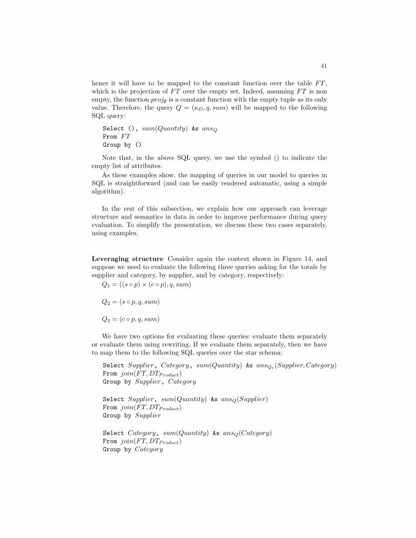
41

hence it will have to be mapped to the constant function over the table FT ,which is the projection of FT over the empty set. Indeed, assuming FT is nonempty, the function proj∅ is a constant function with the empty tuple as its onlyvalue. Therefore, the query Q = (κD, q, sum) will be mapped to the followingSQL query:

Select (), sum(Quantity) As ansQFrom FTGroup by ()

Note that, in the above SQL query, we use the symbol () to indicate theempty list of attributes.

As these examples show, the mapping of queries in our model to queries inSQL is straightforward (and can be easily rendered automatic, using a simplealgorithm).

In the rest of this subsection, we explain how our approach can leveragestructure and semantics in data in order to improve performance during queryevaluation. To simplify the presentation, we discuss these two cases separately,using examples.

Leveraging structure Consider again the context shown in Figure 14, andsuppose we need to evaluate the following three queries asking for the totals bysupplier and category, by supplier, and by category, respectively:

Q1 = ((s ◦ p)× (c ◦ p), q, sum)

Q2 = (s ◦ p, q, sum)

Q3 = (c ◦ p, q, sum)

We have two options for evaluating these queries: evaluate them separatelyor evaluate them using rewriting. If we evaluate them separately, then we haveto map them to the following SQL queries over the star schema:

Select Supplier, Category, sum(Quantity) As ansQ1(Supplier, Category)From join(FT,DTProduct)Group by Supplier, Category

Select Supplier, sum(Quantity) As ansQ(Supplier)From join(FT,DTProduct)Group by Supplier

Select Category, sum(Quantity) As ansQ(Category)From join(FT,DTProduct)Group by Category

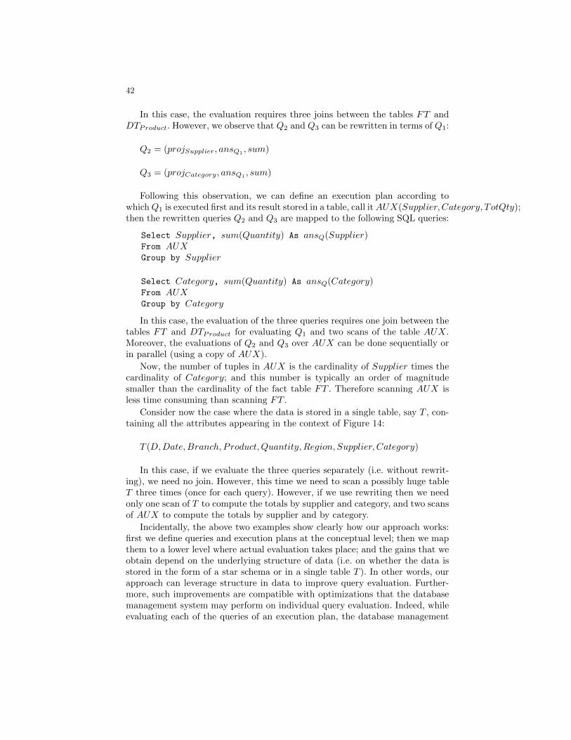
42

In this case, the evaluation requires three joins between the tables FT andDTProduct. However, we observe that Q2 and Q3 can be rewritten in terms of Q1:

Q2 = (projSupplier, ansQ1 , sum)

Q3 = (projCategory, ansQ1, sum)

Following this observation, we can define an execution plan according towhichQ1 is executed first and its result stored in a table, call itAUX(Supplier, Category, TotQty);then the rewritten queries Q2 and Q3 are mapped to the following SQL queries:

Select Supplier, sum(Quantity) As ansQ(Supplier)From AUXGroup by Supplier

Select Category, sum(Quantity) As ansQ(Category)From AUXGroup by Category

In this case, the evaluation of the three queries requires one join between thetables FT and DTProduct for evaluating Q1 and two scans of the table AUX.Moreover, the evaluations of Q2 and Q3 over AUX can be done sequentially orin parallel (using a copy of AUX).

Now, the number of tuples in AUX is the cardinality of Supplier times thecardinality of Category; and this number is typically an order of magnitudesmaller than the cardinality of the fact table FT . Therefore scanning AUX isless time consuming than scanning FT .

Consider now the case where the data is stored in a single table, say T , con-taining all the attributes appearing in the context of Figure 14:

T (D,Date,Branch, Product,Quantity,Region, Supplier, Category)

In this case, if we evaluate the three queries separately (i.e. without rewrit-ing), we need no join. However, this time we need to scan a possibly huge tableT three times (once for each query). However, if we use rewriting then we needonly one scan of T to compute the totals by supplier and category, and two scansof AUX to compute the totals by supplier and by category.

Incidentally, the above two examples show clearly how our approach works:first we define queries and execution plans at the conceptual level; then we mapthem to a lower level where actual evaluation takes place; and the gains that weobtain depend on the underlying structure of data (i.e. on whether the data isstored in the form of a star schema or in a single table T ). In other words, ourapproach can leverage structure in data to improve query evaluation. Further-more, such improvements are compatible with optimizations that the databasemanagement system may perform on individual query evaluation. Indeed, whileevaluating each of the queries of an execution plan, the database management

43

system may use its own query optimizer (if any) to further improve the queryevaluation process.

Leveraging semantics Let us now see how our approach can leverage seman-tics in data to improve query evaluation. To this end we shall consider the caseof the well known functional dependencies of the relational model, and we shallshow how they can be incorporated into query rewriting. The basic observationhere is that a functional dependency X → Y between attribute sets X and Y ofa table T , is actually a function from X to Y , whose extension can be derivedby projecting T over the union of X and Y .

The following proposition will help explain how functional dependecies canbe incorporated in query rewriting, and therefore contribute in improving thequery evaluation process.

Proposition 6. Let f : A → B and g : A → C be two functions having thesame source. Then f ≤ g iff there is a function h : B → C such that g = h ◦ f .Moreover h is unique up to the range of f (i.e. if there is a function h′ such thatg = h′ ◦ f then h′/range(f) = h/range(f)).

Proof. Suppose first that there is a function h : A → B such that g = h ◦ f .Then for all a, a′ in A such that f(a) = f(a′) we have: g(a) = h(f(a)) =h(f(a′)) = g(a′). Therefore f ≤ g. Suppose next that f ≤ g. It follows thatπf ≤ πg. Consider now any b in the range of f and define: h(b) = g(f−1(b)).As f ≤ g, the block f−1(b) of πf is included in some block of πg, say g−1(c),where c is in the range of g. It follows that: g(f−1(b)) = c, therefore h is a welldefined function over the range of f . Moreover, from the definition of h we have:h(f(a)) = g(f−1(b)) = g(b). Therefore h ◦ f = g. Finally, suppose there is afunction h′ : A→ B such that h′ 6= h and h′ ◦ f = g = h ◦ f . Now, for any b inthe range of f there is a in A such that f(a) = b. Therefore h′(b) = h′(f(a)) =(h′ ◦ f)(a) = g = (h ◦ f)(a). It follows that: h′/range(f) = h/range(f) and thiscompletes the proof.

As an immediate corollary we obtain the following proposition.

Proposition 7. Let X → Y be a functional dependency over D. Then we have:X → Y holds in T if and only if there is a unique function h : X → Y such thath ◦ projX = projY .

Note that the projections projX and projY are seen as functions, in the wayexplained earlier.

We note that, if the functional dependency X → Y holds in T , then the(extension of) function h can be obtained by projecting the table T over XY(i.e. over the union of attribute sets X and Y ).

As an immediate corollary of the above proposition, and our basic rewritingrule for compositions, we have the following rewriting rule:

Corollary 1. (projY , projZ , op) = (h, (projX , projZ , op), op)

44

Following this rule, the evaluation of any queryQ of the formQ = (projY , projZ , op)can be done by first evaluating the query Q′ = (projX , projZ , op) and then thequery Q′′ = (h, ansQ′ , op).

Summarizing our discussion so far, it is clear that functional dependenciescan be seamlessly integrated in our model, and moreover, they can be used forimproving query evaluation performance through rewriting.

In fact, Proposition 7 above is a powerful tool for query rewriting when thedata set is a relational table. Moreover, this proposition, combined with a wellknown result from relational database theory, provides the basis for studying notonly query rewriting but also the generation of query execution plans. Indeed, abasic question is: given a query Q = (projX , projZ , op) over a table T , what is theset of all queries of the form Q′ = (projY , projZ , op) that can be rewritten usingQ. It follows from Proposition 7 that a query of the form Q′ = (projY , projZ , op)can be rewritten using Q only if the functional dependency X → Y holds in T .

Now, from relational database theory we know that: X → Y holds in T ifand only if Y ⊆ X+, where X+ is the closure of the attribute set X with respectto the functional dependencies that T must satisfy [32]. Therefore to answer theabove question we need an algorithm for computing X+. Fortunately, there areefficient (linear) algorithms for the computation of X+ from X ([32]).

Actually, the attributes of a relational table T together with the set offunctional dependencies that hold in T can be seen as an analysis context.More precisely, let A = {A1, A2, . . . , Am} be the set of attributes of T , F ={f1, f2, . . . , fn} be the set of functional dependencies of T and TID the set of tu-ple identifiers of T . As explained earlier, each attribute Ai, can be seen as a func-tion: projAi

: TID → Ai. Then the set AF = {projA1, . . . , projAm

, f1, . . . , fn}can be seen as a context, with TID as its single root, and we can call this context“the analysis context of T”. Using this context we can express analytic queriesover T , and this independently of whether T is normalized or not, or whether Tis a database table or a table derived from the tables in the database.

Moreover, as attributes may be shared by two or more tables, we can en-visage combining the results of analytic queries over the contexts of differenttables. For example, referring to Figure 14, suppose that the dimensional tableDTProduct contains an additional attribute u : Product → UnitPrice, givingthe unit price for each type of product delivered. In other words, the table hasnow the following form:

DTProduct(Product, Supplier, Category, UnitPrice)

Consider now the following two queries, asking for (a) the total quantity de-livered by category and (b) the average unit price by category:

Q1 = (c ◦ p, q, sum)

Q2 = (c, u, avg)

45

The first query is expressed in the context of the join between the tablesFT and DTProduct, whereas the second is expressed in the context of tableDTProduct. Their results are the following two binary tables:

(Category, ansQ1(Category))

(Category, ansQ2(Category))

By combining these two analysis results we may discover, for example, thatin some product category, although the average unit price is quite high, the totaldelivered quantity is quite high as well; and this might lead to useful insights asto the sales of products in that category.

4 Concluding Remarks

In this paper, we have presented a high level query language for expressinganalytic queries over a big data set, based on its attributes. The main featuresof our approach are:

– A clear separation between the conceptual and the physical level: queriesare defined at the conceptual level independently of the nature and locationof data and then they are mapped to lower level evaluation mechanisms(MapReduce, SQL engines) where actual evaluation takes place.

– A lightweight interface, called an analysis context, consisting of a set ofattributes arranged in a graph. Analysts can express analytic queries withintheir context by defining triples of the form (g,m, op), where g and m areattributes of the context having common source, and op is an operation overthe target of m.

– A sound, yet simple mathematical basis (using functions and partitions)that allows a formal approach to query rewriting, and to the definition andgeneration of query execution plans.

– The ability to leverage structure and semantics in data in order to improveperformance through rewriting.

Future work includes several research items. The first concerns the computa-tion of the query rewriting graph of a set of queries. We have sketched how thiscan be done, based on the closure of the set of functional dependencies, in thecase where the data set D is a relational table. We would like to use graph theo-retic techniques in order to give a general algorithm for computing the rewritinggraph.

The second research item concerns the extension of the concept of queryexecution plan for a set Q of queries, in two different directions: (a) Consideringexecution plans that, apart from the queries in Q, contain queries outside Qwhich are able to rewrite one or more queries in Q. The objective is to accept theextra cost of evaluating such “external” queries if their rewritings can contributeto improving the overall performance significantly. (b) Studying the definition

46

and use of dynamic query execution plans in the sense explained only briefly inthe section on query execution plans.

The third research item concerns query result visualization and exploration,based on Currification, in the sense explained in the section on analysis contexts.

The last research item concerns change in the data set D. Indeed, throughoutthe paper we have tacitly assumed that the data set is “static”. While this mightbe a reasonable assumption in several application environments, it is by no meanstrue for big data sets in general. Indeed, there are application environmentswhere the data set changes frequently and where the results to some important,continuous queries have to be updated frequently as well. The objective here isto study incremental algorithms that take as input the increment in data andproduce the increment in the query result.

References

1. Abadi, D.J., Madden, S.R., Hachem, N.: Column-stores vs. row-stores: How dif-ferent are they really? In: Proceedings of the 2008 ACM SIGMOD InternationalConference on Management of Data. pp. 967–980. SIGMOD ’08, ACM, New York,NY, USA (2008), http://doi.acm.org/10.1145/1376616.1376712

2. Abouzeid, A., Bajda-Pawlikowski, K., Abadi, D., Silberschatz, A., Rasin, A.:Hadoopdb: An architectural hybrid of mapreduce and dbms technologies for ana-lytical workloads. Proc. VLDB Endow. 2(1), 922–933 (Aug 2009), http://dx.doi.org/10.14778/1687627.1687731

3. Anderson, C.: The end of theory: The data deluge makes the scientific method ob-solete. http://archive.wired.com/science/discoveries/magazine/16-07/pb_

theory (Jun 2008)

4. Bain, T.: Was stonebraker right?http://blog.tonybain.com/tony_bain/2010/09/was-stonebraker-right.html

(2010)

5. Bajda-Pawlikowski, K., Abadi, D.J., Silberschatz, A., Paulson, E.: Efficient pro-cessing of data warehousing queries in a split execution environment. In: Pro-ceedings of the 2011 ACM SIGMOD International Conference on Management ofData. pp. 1165–1176. SIGMOD ’11, ACM, New York, NY, USA (2011), http:

//doi.acm.org/10.1145/1989323.1989447

6. Beyer, K.S., Ercegovac, V., Gemulla, R., Balmin, A., Eltabakh, M.Y., Kanne, C.,Ozcan, F., Shekita, E.J.: Jaql: A scripting language for large scale semistructureddata analysis. PVLDB 4(12), 1272–1283 (2011), http://www.vldb.org/pvldb/

vol4/p1272-beyer.pdf

7. Beyer, M.A., Laney, D.: The importance of ’big data’: A definition. https://www.gartner.com/doc/2057415/importance-big-data-definition (Jun 2012)

8. Buneman, P., Frankel, R.E.: Fql: A functional query language. In: Proceedings ofthe 1979 ACM SIGMOD International Conference on Management of Data. pp.52–58. SIGMOD ’79, ACM, New York, NY, USA (1979), http://doi.acm.org/10.1145/582095.582104

9. Chen, S.: Cheetah: A high performance, custom data warehouse on top of mapre-duce. Proc. VLDB Endow. 3(1-2), 1459–1468 (Sep 2010), http://dx.doi.org/10.14778/1920841.1921020

47

10. Chu, C., Kim, S.K., Lin, Y.A., Yu, Y., Bradski, G., Ng, A.Y., Olukotun, K.: Map-reduce for machine learning on multicore. In: Proceedings of Advances in neuralinformation processing systems NIPS 2006. pp. 281–288. MIT; 1998 (2006)

11. Cloudera: Why europes largest ad targeting platform usesapache hadoop. http://blog.cloudera.com/blog/2010/03/

why-europes-largest-ad-targeting-platform-uses-hadoop/ (2010)

12. Cohen, J., Dolan, B., Dunlap, M., Hellerstein, J.M., Welton, C.: Mad skills: Newanalysis practices for big data. Proc. VLDB Endow. 2(2), 1481–1492 (Aug 2009),http://dx.doi.org/10.14778/1687553.1687576

13. Cutting, D., Cafarella, M.: Hadoop. http://hadoop.apache.org/ (2005)

14. Czajkowski, G.: Sorting 1pb with mapreduce. http://googleblog.blogspot.fr/2008/11/sorting-1pb-with-mapreduce.html (Nov 2008)

15. Dean, J., Ghemawat, S.: Mapreduce: Simplified data processing on large clus-ters. Commun. ACM 51(1), 107–113 (Jan 2008), http://doi.acm.org/10.1145/1327452.1327492

16. Devlin, B.: Data Warehouse: From Architecture to Implementation. Addison-Wesley Longman Publishing Co., Inc., Boston, MA, USA (1996)

17. Dittrich, J., Quiane-Ruiz, J.A., Jindal, A., Kargin, Y., Setty, V., Schad, J.:Hadoop++: Making a yellow elephant run like a cheetah (without it even noticing).Proc. VLDB Endow. 3(1-2), 515–529 (Sep 2010), http://dx.doi.org/10.14778/1920841.1920908

18. Erez Aiden, J.B.M.: Cthe predictive power of big data. http://www.newsweek.

com/predictive-power-big-data-225125 (Dec 2013)

19. Ewen, S., Schelter, S., Tzoumas, K., Warneke, D., Markl, V.: Iterative paralleldata processing with stratosphere: An inside look. In: Proceedings of the 2013ACM SIGMOD International Conference on Management of Data. pp. 1053–1056.SIGMOD ’13, ACM, New York, NY, USA (2013), http://doi.acm.org/10.1145/2463676.2463693

20. Friedman, E., Pawlowski, P., Cieslewicz, J.: Sql/mapreduce: A practical ap-proach to self-describing, polymorphic, and parallelizable user-defined functions.Proc. VLDB Endow. 2(2), 1402–1413 (Aug 2009), http://dx.doi.org/10.14778/1687553.1687567

21. Gates, A.F., Natkovich, O., Chopra, S., Kamath, P., Narayanamurthy, S.M., Ol-ston, C., Reed, B., Srinivasan, S., Srivastava, U.: Building a high-level dataflowsystem on top of map-reduce: The pig experience. Proc. VLDB Endow. 2(2), 1414–1425 (Aug 2009), http://dx.doi.org/10.14778/1687553.1687568

22. Graham, M.: Big data and the end of theory? http://www.theguardian.com/

news/datablog/2012/mar/09/big-data-theory (Mar 2012)

23. Gupta, A., Mumick, I.S., Subrahmanian, V.S.: Maintaining views incrementally.SIGMOD Rec. 22(2), 157–166 (Jun 1993), http://doi.acm.org/10.1145/170036.170066

24. Hadapt: http://www.hadapt.com (2013)

25. Halevy, A.Y.: Answering queries using views: A survey. The VLDB Journal 10(4),270–294 (Dec 2001), http://dx.doi.org/10.1007/s007780100054

26. Horowitz, M.: Visualizing big data: Bar charts for words. http://archive.wired.com/science/discoveries/magazine/16-07/pb_visualizing (Jun 2008)

27. House, W.: Big data across the federal government. http://www.whitehouse.gov/sites/default/files/microsites/ostp/big_data_fact_sheet_final.pdf (Mar2012)

48

28. House, W.: Big data: Seizing opportunities, preserving values. http:

//www.whitehouse.gov/sites/default/files/docs/big_data_privacy_

report_may_1_2014.pdf (May 2014)29. Jacobs, A.: The pathologies of big data. Commun. ACM 52(8), 36–44 (Aug 2009),

http://doi.acm.org/10.1145/1536616.153663230. James Manyika, Michael Chui, B.B.J.B.R.D.C.R., Byers, A.H.: Big

data: The next frontier for innovation, competition, and productivity.http://www.mckinsey.com/insights/business_technology/big_data_the_

next_frontier_for_innovation (May 2011)31. Leinweber, D.: Stupid data miner tricks: How quants fool

themselves and the economic indicator in your pants.http://www.forbes.com/sites/davidleinweber/2012/07/24/

stupid-data-miner-tricks-quants-fooling-themselves-the-economic-indicator-in-your-pants/

(Jul 2012)32. Maier, D.: Theory of Relational Databases. Computer Science Pr (1983)33. Malewicz, G., Austern, M.H., Bik, A.J., Dehnert, J.C., Horn, I., Leiser, N.,

Czajkowski, G.: Pregel: A system for large-scale graph processing. In: Proceed-ings of the 2010 ACM SIGMOD International Conference on Management ofData. pp. 135–146. SIGMOD ’10, ACM, New York, NY, USA (2010), http:

//doi.acm.org/10.1145/1807167.180718434. Marcus, G., Davis, E.: Eight (no, nine!) problems with big data. www.nytimes.

com/2014/04/07/opinion/eight-no-nine-problems-with-big-data.html (Apr2014)

35. Melnik, S., Gubarev, A., Long, J.J., Romer, G., Shivakumar, S., Tolton, M., Vassi-lakis, T.: Dremel: Interactive analysis of web-scale datasets. Proc. VLDB Endow.3(1-2), 330–339 (Sep 2010), http://dx.doi.org/10.14778/1920841.1920886

36. Monash, C.: ebays two enormous data warehouses. http://www.dbms2.com/2009/04/30/ (Apr 2009)

37. Monash, C.: ebay followup — greenplum out, teradata > 10 petabytes, hadoophas some value, and more. http://www.dbms2.com/2010/10/06/ (Oct 2010)

38. Ohm, P.: Dont build a database of ruin.http://blogs.hbr.org/2012/08/dont-build-a-database-of-ruin/ (Aug 2012)

39. Panda, B., Herbach, J.S., Basu, S., Bayardo, R.J.: Planet: Massively parallel learn-ing of tree ensembles with mapreduce. Proc. VLDB Endow. 2(2), 1426–1437 (Aug2009), http://dx.doi.org/10.14778/1687553.1687569

40. Pavlo, A., Paulson, E., Rasin, A., Abadi, D.J., DeWitt, D.J., Madden, S., Stone-braker, M.: A comparison of approaches to large-scale data analysis. In: Pro-ceedings of the 2009 ACM SIGMOD International Conference on Managementof Data. pp. 165–178. SIGMOD ’09, ACM, New York, NY, USA (2009), http:

//doi.acm.org/10.1145/1559845.155986541. Pierce, B.C.: Basic Category Theory for Computer Scientists. MIT Press, Cam-

bridge, MA, USA (1991)42. Spyratos, N.: A functional model for data analysis. In: Proceedings of the

7th International Conference on Flexible Query Answering Systems. pp. 51–64. FQAS’06, Springer-Verlag, Berlin, Heidelberg (2006), http://dx.doi.org/10.1007/11766254_5

43. Spyratos, N., Sugibuchi, T.: Restrict-reduce: Parallelism and rewriting for bigdata processing. In: Tanaka, Y., Spyratos, N., Yoshida, T., Meghini, C. (eds.)Information Search, Integration and Personalization, Communications in Com-puter and Information Science, vol. 146. Springer Berlin Heidelberg (2013), http://dx.doi.org/10.1007/978-3-642-40140-4_8

49

44. Stonebraker, M.: Mapreduce: A major step backwards. http://databasecolumn.vertica.com/2008/01/mapreduce_a_major_step_back.html (2008)

45. Stonebraker, M., Abadi, D., DeWitt, D.J., Madden, S., Paulson, E., Pavlo, A.,Rasin, A.: Mapreduce and parallel dbmss: Friends or foes? Commun. ACM 53(1),64–71 (Jan 2010), http://doi.acm.org/10.1145/1629175.1629197

46. Strachey, C.: Fundamental concepts in programming languages. Higher OrderSymbol. Comput. 13(1-2), 11–49 (Apr 2000), http://dx.doi.org/10.1023/A:

1010000313106

47. Swanstrom, R.: Colleges with data science degrees. http://101.datascience.

community/2012/04/09/colleges-with-data-science-degrees/ (Apr 2012)48. Thusoo, A., Sarma, J.S., Jain, N., Shao, Z., Chakka, P., Zhang, N., Anthony,

S., Liu, H., Murthy, R.: Hive - a petabyte scale data warehouse using hadoop.In: Proceedings of the 26th International Conference on Data Engineering, ICDE2010, March 1-6, 2010, Long Beach, California, USA. pp. 996–1005 (2010), http://dx.doi.org/10.1109/ICDE.2010.5447738

49. Vernica, R., Carey, M.J., Li, C.: Efficient parallel set-similarity joins using mapre-duce. In: Proceedings of the 2010 ACM SIGMOD International Conference onManagement of Data. pp. 495–506. SIGMOD ’10, ACM, New York, NY, USA(2010), http://doi.acm.org/10.1145/1807167.1807222

50. Vidal, M., Raschid, L., Marquez, N., Cardenas, M., Wu, Y.: Query rewriting inthe semantic web. In: Data Engineering Workshops, 2006. Proceedings. 22nd In-ternational Conference on. pp. 7–7 (2006)

51. Yahoo: Hadoop terasort. http://developer.yahoo.com/blogs/hadoop/

Yahoo2009.pdf (2009)52. Yang, C., Yen, C., Tan, C., Madden, S.: Osprey: Implementing mapreduce-style

fault tolerance in a shared-nothing distributed database. In: Proceedings of the26th International Conference on Data Engineering, ICDE 2010, March 1-6, 2010,Long Beach, California, USA. pp. 657–668. ICDE’10, IEEE, Washington, DC, USA(2010)

53. Yang, H.c., Dasdan, A., Hsiao, R.L., Parker, D.S.: Map-reduce-merge: Simplifiedrelational data processing on large clusters. In: Proceedings of the 2007 ACM SIG-MOD International Conference on Management of Data. pp. 1029–1040. SIGMOD’07, ACM, New York, NY, USA (2007), http://doi.acm.org/10.1145/1247480.1247602