high-temperature radical polymerization of methyl ... · consecutive tube reactor, ... sion en...
TRANSCRIPT
THÈSE NO 3460 (2006)
ÉCOLE POLYTECHNIQUE FÉDÉRALE DE LAUSANNE
PRÉSENTÉE LE 10 mARS 2006
À LA FACULTÉ SCIENCES DE BASE GROUPE DES PROCÉDÉS mACROmOLÉCULAIRES
SECTION DE CHImIE ET GÉNIE CHImIQUE
POUR L'OBTENTION DU GRADE DE DOCTEUR ÈS SCIENCES
PAR
Dipl.-Ing. Univ., Friedrich-Alexander-Universität, Erlangen-Nürnberg, Allemagneet de nationalité allemande
acceptée sur proposition du jury:
Lausanne, EPFL2006
Prof. P. Vogel, président du juryDr Th. meyer, directeur de thèse
Dr R. Carloff, rapporteurProf. H.-A. Klok, rapporteur
Prof. F. Pla, rapporteur
high-temperature radical polymerization of methyl methacrylate in a continuous pilot scale process
Philip NISING

i
Abstract
The present PhD thesis deals with the high temperature polymerization of methyl meth-
acrylate in a continuous pilot scale process. The major aim is to investigate the feasibility of a
polymerization process for the production of PMMA molding compound at temperatures in the
range from 140 °C to 170 °C. Increasing the process temperature has the advantage of decreas-
ing molecular weight and viscosity of the reaction mixture, thus allowing to reduce the addi-
tion of chain transfer agent and to increase the polymer content in the reactor. At the same
time, the reaction rates are higher and the devolatilization is facilitated compared to low con-
version polymerizations. Altogether, it leads to an improved space time yield of the process.
However, increasing the process temperature also has an important impact on both, polymer-
ization kinetics and polymer properties.
The first two parts of this work are, therefore, dedicated to the self-initiation respectively
the high temperature gel effect observed for the polymerization of MMA at the given tempera-
ture range. The self-initiation of MMA is mostly caused by polymeric peroxides that form
from physically dissolved oxygen and the monomer, itself. The formation, decomposition and
constitution of these peroxides are intensively studied and a formal kinetic is proposed for the
formation and decomposition reaction.
The polymerization of MMA is subject to a rather strong auto-acceleration, called gel
effect, the intensity of which depends on process conditions and solvent content. There are sev-
eral models proposed in the specialized literature to describe this phenomenon by modifying
the termination rate constant as a function of conversion and temperature. The second part of
this study contains the evaluation of these models with regards to their applicability to high
Abstract
ii
temperature MMA polymerization as well as the development of a new variant of an existing
model, which correctly describes the gel effect in the temperature range of interest as a function of
polymer content, temperature and molecular weight. The advantage of this new variant is that it
includes all other factors influencing the gel effect, i.e. chain transfer agent, initiator load,
comonomer and solvent content, and that it is suitable for the description of batch and continuous
processes. A complete kinetic model for the description of the high temperature copolymerization
of MMA and MA, containing the results from the first two parts of this work, is established within
the software package PREDICI® and validated by means of several series of batch polymeriza-
tions.
In the third part of this work, a complete pilot plant installation for the continuous polymer-
ization of MMA is designed and constructed in order to study the impact of increasing the reac-
tion temperature on process properties and product quality under conditions similar to those of an
industrial-scale polymerization. The pilot plant is based on a combination of recycle loop and
consecutive tube reactor, equipped with SULZER SMXL® / SMX® static mixing technology.
Furthermore, it is equipped with a static one-step flash devolatilization and a pelletizer for poly-
mer granulation. At the same time, a refined method for inline conversion monitoring by speed of
sound measurement is developed and tested in the pilot plant. By means of this technique it is
possible to follow the dynamic behavior of the reactor and to measure directly the monomer con-
version without taking a sample. The results of several pilot plant polymerizations carried out
under different conditions are presented and the impact of temperature, comonomer and chain
transfer agent on the thermal stability of the product is analyzed. From these results, the r-param-
eters for the copolymerization of MMA and MA at 160 °C as well as the chain transfer constant
for n-dodecanethiol at 140 °C are determined. Finally, the pilot plant experiments are used to val-
idate the kinetic model established beforehand in PREDICI® for the continuous copolymeriza-
tion.
Keywords: High Temperature Polymerization, Methyl methacrylate, Copolymerization, Reactiv-
ity ratio, Chain Transfer, Ultrasound conversion monitoring, Gel effect, Thermal sta-
bility, Kinetic Modeling, Pilot Plant Technology, Static mixing
iii
Version abrégée
Cette thèse traite de la polymérisation à haute température du méthacrylate de méthyle
dans un procédé à l'échelle d'un système pilote. Le but principal est l'étude de faisabilité d'un
procédé de polymérisation pour la production de PMMA fondu à des températures entre
140 °C et 170 °C. Dans ce procédé l'augmentation de la température a pour avantage la dimi-
nution de la masse moléculaire et de la viscosité du mélange réactionnel, ce qui permet de
réduire l'ajout d'agent de transfert de chaîne et d'augmenter la quantité de polymère dans le
réacteur. En même temps, les vitesses de réaction sont plus élevées et la dévolatilisation est
facilitée par rapport à des polymérisations à basse conversion. Pris ensemble, ces éléments per-
mettent d'améliorer le rendement en espace et en temps du procédé. Toutefois, augmenter la
température du procédé a aussi un effet important sur la cinétique de polymérisation, ainsi que
sur les propriétés des polymères.
Les deux premières parties de ce travail sont, par conséquent, dédiées à l'auto-initiation
et à l'effet de gel à haute température, observés dans l'intervalle de température considéré.
L'auto-initiation du MMA est principalement causée par des peroxydes polymères formés par
réactions des monomères avec de l'oxygène dissous dans les derniers. La formation, la décom-
position et la constitution de ces peroxydes sont étudiées de manière intensive et une cinétique
formelle est proposée pour les réactions de formation et de décomposition.
La polymérisation du MMA est sujette à une auto-accélération conséquente appelée
"effet de gel", dont l'intensité dépend des conditions du procédé et de la quantité de solvant.
Plusieurs modèles proposés dans la littérature spécialisée décrivent ce phénomène en modifi-
ant la constante de vitesse de terminaison en fonction de la conversion et de la température. La
seconde partie de cette étude comprend l'évaluation de ces modèles au regard de leur applica-
Version abrégée
iv
bilité à la polymérisation à haute température du MMA, ainsi que le développement d'une nou-
velle variante d'un modèle existant, décrivant correctement l'effet gel dans l'intervalle de
température considéré en fonction de la quantité de polymère, de la température et de la masse
moléculaire. Les avantages de cette nouvelle variante sont le fait qu'elle inclut tous les autres fac-
teurs influençant l'effet gel, à savoir l'agent de transfert de chaîne, la charge d'initiateur, les quan-
tités de comonomère et de solvant, et sa capacité à décrire les procédés en batch et en continu. Un
modèle cinétique complet pour la description de la copolymérisation à haute température du
MMA et du MA, contenant les résultats des deux premières parties de ce travail, est établi à l'aide
du logiciel PREDICI® et validé par plusieurs séries de polymérisations en batch.
Dans la troisième partie de ce travail, une installation pilote complète pour la polymérisa-
tion du MMA est conçue et construite, de façon à pouvoir étudier l'effet de l'augmentation de la
température de réaction sur les propriétés du processus et la qualité du produit dans des conditions
similaires à celles d'une polymérisation à l'échelle industrielle. L'installation pilote est formée à la
base de la succession d'un réacteur avec recyclage en boucle et d'un réacteur tubulaire, équipés de
mélangeurs statiques Sulzer SMXL® / SMX®. Elle est en outre équipée d'un dévaporisateur flash
à une étape et d'une granuleuse. De plus, une méthode affinée pour la surveillance de la conver-
sion en ligne par mesure de la vitesse du son est développée et testée sur l'installation pilote. Il est
possible au moyen de cette technique de suivre le comportement dynamique du réacteur et de
mesurer directement la conversion de monomère sans prendre d'échantillon. Les résultats de plu-
sieurs polymérisations en installation pilote effectuées dans différentes conditions sont présentés,
et les influences de la température, du comonomère et de l'agent de transfert de chaîne sur la sta-
bilité thermique du produit sont analysées. Ces résultats permettent en outre la détermination des
paramètres r pour la copolymérisation du MMA et du MA à 160 °C, et de la constante de transfert
de chaîne pour le n-dodécanethiol à 140 °C. Finalement, les expériences en installation pilote sont
utilisées pour valider le modèle cinétique établi auparavant avec PREDICI® pour la copolyméri-
sation en continu.
Mots-clés: Polymérisation radicalaire, Haute température, Méthacrylate de méthyle,
Copolymérisation, Surveillance en ligne par ultrason, Effect de gel, Stabilité ther-
mique, Modélisation cinetique, Pilot Plant Technologie, Mélangeurs statiques.
v
Table of contents
Abstract . . . . . . . . . . . . . . . . . . . . . . . . . . . . . . . . . . . . . . . . . . . . . . . . . . . . . . . . . . . . . . . . i
Version abrégée . . . . . . . . . . . . . . . . . . . . . . . . . . . . . . . . . . . . . . . . . . . . . . . . . . . . . . . . . iii
Preface . . . . . . . . . . . . . . . . . . . . . . . . . . . . . . . . . . . . . . . . . . . . . . . . . . . . . . . . . . . . . . . . . 1
1 Introduction . . . . . . . . . . . . . . . . . . . . . . . . . . . . . . . . . . . . . . . . . . . . . . . . . . . . . . . . . . 3
1.1 General . . . . . . . . . . . . . . . . . . . . . . . . . . . . . . . . . . . . . . . . . . . . . . . . . . . . . . . . . 3
1.2 Historical background . . . . . . . . . . . . . . . . . . . . . . . . . . . . . . . . . . . . . . . . . . . . . 4
1.3 Aim of this work . . . . . . . . . . . . . . . . . . . . . . . . . . . . . . . . . . . . . . . . . . . . . . . . . 6
2 Self-Initiation at high temperatures . . . . . . . . . . . . . . . . . . . . . . . . . . . . . . . . . . . . . . . 9
2.1 MMA peroxides . . . . . . . . . . . . . . . . . . . . . . . . . . . . . . . . . . . . . . . . . . . . . . . . . 102.1.1 Introduction. . . . . . . . . . . . . . . . . . . . . . . . . . . . . . . . . . . . . . . . . . . . . . . 102.1.2 Formation of poly (methyl methacrylate) peroxide (PMMAP) . . . . . . . 13
MMA-peroxide formation experiments . . . . . . . . . . . . . . . . . . . . . . . 142.1.3 Isolation and Characterization of PMMAP. . . . . . . . . . . . . . . . . . . . . . . 20
Size Exclusion Chromatography (SEC/GPC) . . . . . . . . . . . . . . . . . . 22NMR. . . . . . . . . . . . . . . . . . . . . . . . . . . . . . . . . . . . . . . . . . . . . . . . . . 23
2.1.4 Decomposition of PMMAP . . . . . . . . . . . . . . . . . . . . . . . . . . . . . . . . . . 26Differential Scanning Calorimetry (DSC) . . . . . . . . . . . . . . . . . . . . . 26Mass-spectrometer coupled Thermogravimetry (TGA-MS) . . . . . . . 33Odian method . . . . . . . . . . . . . . . . . . . . . . . . . . . . . . . . . . . . . . . . . . . 37
2.2 Thermal initiation. . . . . . . . . . . . . . . . . . . . . . . . . . . . . . . . . . . . . . . . . . . . . . . . 40
2.3 Initiation by the Chain Transfer Agent . . . . . . . . . . . . . . . . . . . . . . . . . . . . . . . 42
2.4 Formation of the Dimer . . . . . . . . . . . . . . . . . . . . . . . . . . . . . . . . . . . . . . . . . . . 43
2.5 Verification of the Kinetics in Batch Experiments . . . . . . . . . . . . . . . . . . . . . . 44
Table of contents
vi
2.6 Discussion . . . . . . . . . . . . . . . . . . . . . . . . . . . . . . . . . . . . . . . . . . . . . . . . . . . . . .53
3 High Temperature Gel Effect. . . . . . . . . . . . . . . . . . . . . . . . . . . . . . . . . . . . . . . . . . . .573.1 Theory . . . . . . . . . . . . . . . . . . . . . . . . . . . . . . . . . . . . . . . . . . . . . . . . . . . . . . . . .59
3.1.1 Model basics . . . . . . . . . . . . . . . . . . . . . . . . . . . . . . . . . . . . . . . . . . . . . .61
3.2 Existing Model Evaluation . . . . . . . . . . . . . . . . . . . . . . . . . . . . . . . . . . . . . . . . .623.2.1 Chiu, Carratt and Soong (CCS) . . . . . . . . . . . . . . . . . . . . . . . . . . . . . . . . 633.2.2 Achilias and Kiparissides . . . . . . . . . . . . . . . . . . . . . . . . . . . . . . . . . . . . 653.2.3 Hoppe and Renken. . . . . . . . . . . . . . . . . . . . . . . . . . . . . . . . . . . . . . . . . .663.2.4 Fleury. . . . . . . . . . . . . . . . . . . . . . . . . . . . . . . . . . . . . . . . . . . . . . . . . . . .663.2.5 Fenouillot, Terrisse and Rimlinger . . . . . . . . . . . . . . . . . . . . . . . . . . . . .723.2.6 Tefera, Weickert and Westerterp. . . . . . . . . . . . . . . . . . . . . . . . . . . . . . .74
3.3 A new approach for a gel effect model . . . . . . . . . . . . . . . . . . . . . . . . . . . . . . . . 78
3.4 Influence of various parameters on the gel effect . . . . . . . . . . . . . . . . . . . . . . . .863.4.1 Influence of the chain transfer agent on the gel effect . . . . . . . . . . . . . .863.4.2 Influence of temperature on the gel effect. . . . . . . . . . . . . . . . . . . . . . . .883.4.3 Influence of solvent on the gel effect . . . . . . . . . . . . . . . . . . . . . . . . . . .893.4.4 Influence of the comonomer . . . . . . . . . . . . . . . . . . . . . . . . . . . . . . . . . . 90
3.5 Discussion . . . . . . . . . . . . . . . . . . . . . . . . . . . . . . . . . . . . . . . . . . . . . . . . . . . . . .92
4 Continuous High-Temperature Polymerization. . . . . . . . . . . . . . . . . . . . . . . . . . . . .95
4.1 The Sulzer Pilot Plant . . . . . . . . . . . . . . . . . . . . . . . . . . . . . . . . . . . . . . . . . . . . .974.1.1 Viscous tubular flows . . . . . . . . . . . . . . . . . . . . . . . . . . . . . . . . . . . . . . .974.1.2 The concept of static mixing . . . . . . . . . . . . . . . . . . . . . . . . . . . . . . . . . . 984.1.3 Choice of mixing elements . . . . . . . . . . . . . . . . . . . . . . . . . . . . . . . . . . 1004.1.4 Considerations concerning the viscosity . . . . . . . . . . . . . . . . . . . . . . . .1034.1.5 The Pilot Plant in Detail . . . . . . . . . . . . . . . . . . . . . . . . . . . . . . . . . . . . 106
Feed preparation . . . . . . . . . . . . . . . . . . . . . . . . . . . . . . . . . . . . . . . .107The reaction zone . . . . . . . . . . . . . . . . . . . . . . . . . . . . . . . . . . . . . . .107The Devolatilization Zone . . . . . . . . . . . . . . . . . . . . . . . . . . . . . . . . 110Product Granulation 112The final product 114
4.2 Ultrasound Polymerization Monitoring . . . . . . . . . . . . . . . . . . . . . . . . . . . . . .1154.2.1 The Measurement Principle. . . . . . . . . . . . . . . . . . . . . . . . . . . . . . . . . . 1174.2.2 The Measuring Equipment . . . . . . . . . . . . . . . . . . . . . . . . . . . . . . . . . . 1184.2.3 Calibration of the measuring system . . . . . . . . . . . . . . . . . . . . . . . . . . .1234.2.4 Results for the ultrasound reaction monitoring . . . . . . . . . . . . . . . . . . .130

Table of contents
vii
4.3 Verification of the High-Temperature Kinetics . . . . . . . . . . . . . . . . . . . . . . . . 1364.3.1 Results from the Pilot Plant . . . . . . . . . . . . . . . . . . . . . . . . . . . . . . . . . 1364.3.2 R-parameters . . . . . . . . . . . . . . . . . . . . . . . . . . . . . . . . . . . . . . . . . . . . 1384.3.3 Chain Transfer Constants . . . . . . . . . . . . . . . . . . . . . . . . . . . . . . . . . . . 149
4.4 Modeling the pilot plant . . . . . . . . . . . . . . . . . . . . . . . . . . . . . . . . . . . . . . . . . 1544.4.1 Model validation for the continuous polymerization . . . . . . . . . . . . . . 1554.4.2 Variation of process parameters - Model predictions . . . . . . . . . . . . . . 158
Varying the residence time . . . . . . . . . . . . . . . . . . . . . . . . . . . . . . . 158Varying the temperature . . . . . . . . . . . . . . . . . . . . . . . . . . . . . . . . . 160Varying the initiator concentration . . . . . . . . . . . . . . . . . . . . . . . . . 161Varying the chain transfer agent concentration . . . . . . . . . . . . . . . . 162Influence of the solvent content . . . . . . . . . . . . . . . . . . . . . . . . . . . . 164
4.5 Discussion . . . . . . . . . . . . . . . . . . . . . . . . . . . . . . . . . . . . . . . . . . . . . . . . . . . . 165
5 Thermal stability and Depolymerization . . . . . . . . . . . . . . . . . . . . . . . . . . . . . . . . . 169
5.1 Depropagation of poly (methyl methacrylate) chains . . . . . . . . . . . . . . . . . . . 170
5.2 Thermal stability of the polymer . . . . . . . . . . . . . . . . . . . . . . . . . . . . . . . . . . . 1755.2.1 Effect of the polymerization temperature . . . . . . . . . . . . . . . . . . . . . . . 1795.2.2 Effect of the comonomer . . . . . . . . . . . . . . . . . . . . . . . . . . . . . . . . . . . 1805.2.3 Influence of the chain transfer agent . . . . . . . . . . . . . . . . . . . . . . . . . . 1835.2.4 Results from the pilot plant polymerization . . . . . . . . . . . . . . . . . . . . . 184
5.3 Discussion . . . . . . . . . . . . . . . . . . . . . . . . . . . . . . . . . . . . . . . . . . . . . . . . . . . . 188
6 Conclusions and Perspectives . . . . . . . . . . . . . . . . . . . . . . . . . . . . . . . . . . . . . . . . . . 191
Annex
1 Analytical Techniquesand Method Development . . . . . . . . . . . . . . . . . . . . . . . . . . . . I
1.1 Headspace Gas Chromatography . . . . . . . . . . . . . . . . . . . . . . . . . . . . . . . . . . . . . ISampling system . . . . . . . . . . . . . . . . . . . . . . . . . . . . . . . . . . . . . . . . IIISample preparation . . . . . . . . . . . . . . . . . . . . . . . . . . . . . . . . . . . . . . IVHS-GC Calibration . . . . . . . . . . . . . . . . . . . . . . . . . . . . . . . . . . . . . . .VCalculation . . . . . . . . . . . . . . . . . . . . . . . . . . . . . . . . . . . . . . . . . . . . .V
1.2 Size Exclusion Chromatography . . . . . . . . . . . . . . . . . . . . . . . . . . . . . . . . . . . VIISample preparation . . . . . . . . . . . . . . . . . . . . . . . . . . . . . . . . . . . . . . IXTriple Detection (SEC3) . . . . . . . . . . . . . . . . . . . . . . . . . . . . . . . . . . IXConventional Calibration . . . . . . . . . . . . . . . . . . . . . . . . . . . . . . . . . XI
1.3 Differential Scanning Calorimetry . . . . . . . . . . . . . . . . . . . . . . . . . . . . . . . . .XIII
1.4 Thermogravimetry-Mass spectroscopy . . . . . . . . . . . . . . . . . . . . . . . . . . . . . . XV

Table of contents
viii
1.5 Organic Peroxide Determination by UV . . . . . . . . . . . . . . . . . . . . . . . . . . . .XVIIMethod description . . . . . . . . . . . . . . . . . . . . . . . . . . . . . . . . . . . XVIII
1.6 Oxygen determination in organic solvents . . . . . . . . . . . . . . . . . . . . . . . . . . XXI
2 Experimental procedures . . . . . . . . . . . . . . . . . . . . . . . . . . . . . . . . . . . . . . . . . . . . XXV
3 Modeling with Predici® . . . . . . . . . . . . . . . . . . . . . . . . . . . . . . . . . . . . . . . . . . . . .XXXI
4 Determination of the Initiator Decomposition by DSC . . . . . . . . . . . . . . . . . . . . . XLI
5. Physico-chemical data . . . . . . . . . . . . . . . . . . . . . . . . . . . . . . . . . . . . . . . . . . . . . . . LIII
6 Raw Materials and Qualities . . . . . . . . . . . . . . . . . . . . . . . . . . . . . . . . . . . . . . . . . . LXI
7 List of pilot plant experiments . . . . . . . . . . . . . . . . . . . . . . . . . . . . . . . . . . . . . . LXVII
8 Tablecurve fitting parameters . . . . . . . . . . . . . . . . . . . . . . . . . . . . . . . . . . . . . . . .LXIX
Symbols and Abbreviations . . . . . . . . . . . . . . . . . . . . . . . . . . . . . . . . . . . . . . . . . . . . . . . xi
Bibliography . . . . . . . . . . . . . . . . . . . . . . . . . . . . . . . . . . . . . . . . . . . . . . . . . . . . . . . . . . .xv
Acknowledgements . . . . . . . . . . . . . . . . . . . . . . . . . . . . . . . . . . . . . . . . . . . . . . . . . . . . .xxv
Curriculum vitae . . . . . . . . . . . . . . . . . . . . . . . . . . . . . . . . . . . . . . . . . . . . . . . . . . . . . xxviii
1
Preface
There is nothing new under the sun, but there are lots of old things we don’t know.
- Ambrose Gwinnett Bierce (1842-1914)
The research on pilot scale polymerization reactions in the polymer reaction engineering
group at EPFL began more than 20 years ago. The first PhD thesis of 1982 [1] dealt with a
newly developed tubular reactor concept that was based on tubes equipped with Sulzer mixing
elements. Up to that moment, industrial polymerization reactors consisted mainly of stirred
tank reactors, whereas tubular reactors played only an unimportant role due to their bad heat
exchange properties and small capacities. The aim of that first thesis was to describe the fluid-
and thermodynamical behavior of this new type of reactor, which generally consists of a recy-
cle loop and a consecutive tube, as well as to prove its superiority to classical stirred tank reac-
tors. In the following years, this concept was continuously further-developed in various
different projects [2-4] and although first researches concentrated on the polymerization of sty-
rene as a model reaction, the same kind of reactor setup has lately been employed with great
success for methyl methacrylate (MMA) polymerizations:
The work of P.-A. Fleury [5] in the 90’s dealt for the first time with the high-temperature
polymerization of MMA in the Sulzer pilot plant.
Between 1998 and 2001, the plant was used in the frame of a European research project
that aimed for the reduction of residual volatiles’ concentration (LOWRESCO) in industrial
polymerization and degassing. From the side of EPFL it was the thesis of Thomas Zeilmann
[6] that contributed to this project. The pilot plant setup designed for that project was the basis
Preface
2
for the one used in the present work: recycle loop, consecutive plug flow tube and devolatilization
chamber with continuous polymer discharge. Also the ultrasound conversion measurement,
which had been developped by Renken and Cavin shortly beforehand [7, 8], was applied for the
first time in an installation of this size.
When I came to EPFL in January 2001 for my diploma work [9], which was a part of the
before-mentioned project, Thomas Zeilmann was in the last year of his thesis. During the follow-
ing time, various interesting features concerning PMMA, itself, and the continuous polymeriza-
tion of MMA were investigated. These were in particular the thermal stability and thermal
stabilization of PMMA during devolatilization, the two-phase devolatilization strategy and the
addition of a stripping agent to the reaction mixture for improved devolatilization.
At the end of 2001, a first contact with the Degussa Röhm GmbH&Co KG in Darmstadt,
one of the most important producers of acrylics in the world, was established with the aim of a
joint research project between Röhm and EPFL. This was also the moment when I took the deci-
sion to stay in Lausanne for my PhD thesis. Luckily, we received a very positive feedback from
Degussa Röhm concerning the cooperation and in the beginning of 2003, after one year of prepa-
rations and defining the general frame for this quest, the project officially started.
This cooperation with Degussa brought a new, rather industrially orientated drive into the
research on pilot scale polymerization at EPFL, with a major focus on the high temperature poly-
merization process and the kinetic particularities connected to it. Also, for the first time, the pro-
duced polymer had actually to compete with the commercial grade product and, although the
“real” production conditions remained a well-kept secret, the process conditions for the pilot plant
experiments came much closer to reality than they had been in earlier projects.
During the three years of this PhD project, I had the opportunity not only to present my
results at various international conferences but also in various meetings with the industrial part-
ner, from where I received constant feedback concerning the progress of my work, which, looking
back, I would not have liked to miss.
In the following chapters and appendixes, the results of this joint research project, which
unfortunately has to end with the present report, are presented and I already want to express my
deep gratitude to all persons that have been involved in it, no matter to what extent.
3
CHAPTER 1
Introduction
1.1 General
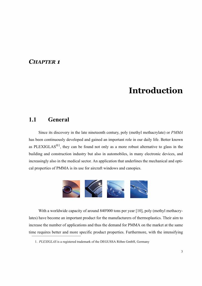
Since its discovery in the late nineteenth century, poly (methyl methacrylate) or PMMA
has been continuously developed and gained an important role in our daily life. Better known
as PLEXIGLAS®1, they can be found not only as a more robust alternative to glass in the
building and construction industry but also in automobiles, in many electronic devices, and
increasingly also in the medical sector. An application that underlines the mechanical and opti-
cal properties of PMMA is its use for aircraft windows and canopies.
With a worldwide capacity of around 840'000 tons per year [10], poly (methyl methacry-
lates) have become an important product for the manufacturers of thermoplastics. Their aim to
increase the number of applications and thus the demand for PMMA on the market at the same
time requires better and more specific product properties. Furthermore, with the intensifying
1. PLEXIGLAS is a registered trademark of the DEGUSSA Röhm GmbH, Germany
Chapter 1: Introduction
4
competition on the world market, the need to optimize processes and process yields has become
even more evident.
For a long time, PMMA was only manufactured by casting. A few applications, i.e. aircraft
windows and thick polymer sheets, where very high molecular weights are mandatory in order to
guarantee a maximum mechanical strength, still require this discontinuous process. However,
with the increasing demand for lower molecular weight types, especially for extrusion and injec-
tion moulding, continuous polymerization processes are needed to meet production capacity and
product quality requirements.
The continuous technical and product development has produced a huge amount of different
polymer and copolymer types, the composition of which strongly depends on their application.
There are highly specialized mixtures for applications in the optical and coating industry on the
one hand, and on the other hand large-scale copolymer commodities for the automobile and con-
struction industry. Most of them have in common to be polymerized in solution or bulk polymer-
ization processes. The by far mostly spread process variant is the CSTR - tube reactor
combination with process temperatures up to 140 °C. In order to improve the thermal and
mechanical strength of the polymer, comonomers and other additives (e.g. transfer agents) are
added in small amounts. At the end of the polymerization process, the polymer melt is degassed in
several steps and the devolatilized polymer is pelletized for transport and storage.
For the production of work pieces with the desired shape (e.g. car lights), the polymer pel-
lets are molten up in an extruder and injected into part-specific molds. During this last production
step, the thermal stress on the polymer is the highest and thermal stability of the polymer becomes
a very important issue.
1.2 Historical background
When Polymethylmethacrylate was synthesized for the first time in the year 1877 [11], the
general understanding of polymerization and its products was still in its infancy. Polymers were
regarded as useless side products and discarded. The person who started the research and further
development of PMMA was Otto Röhm by his thesis in 1901. Yet, it took him another 30 years to
build up the first production of cast PMMA sheets. This was the basis for his company, the Ger-
man Röhm GmbH, today subsidiary of the Degussa AG, which introduced in 1934 Polymethyl-
1.2: Historical background
5
methacrylate under the registered trademark Plexiglas®, still the most common name for this
polymer. At the same time, the British Imperial Chemical Industries (ICI), started the production
of PMMA.
During the Second World War, the polymer gained importance in the production of military
aircraft canopies because of its, compared to glass, smaller specific weight and its strong mechan-
ical properties. It was considered as war-important and thus, the production capacity was
increased considerably in the United States, Britain and Germany. After the war, the demand for
PMMA drastically decreased until other, civil applications were found, among which the use for
streetlamps, neon tubes, safety glass and optical lenses. Also, first copolymers with acrylonitrile
were applied for their better impact strength. With the ability to injection mould poly (methacry-
lates), the continuous production of molding compound pellets catched up quickly with the cast-
ing and, nowadays, more than two thirds of monomer are converted to moulding compound.
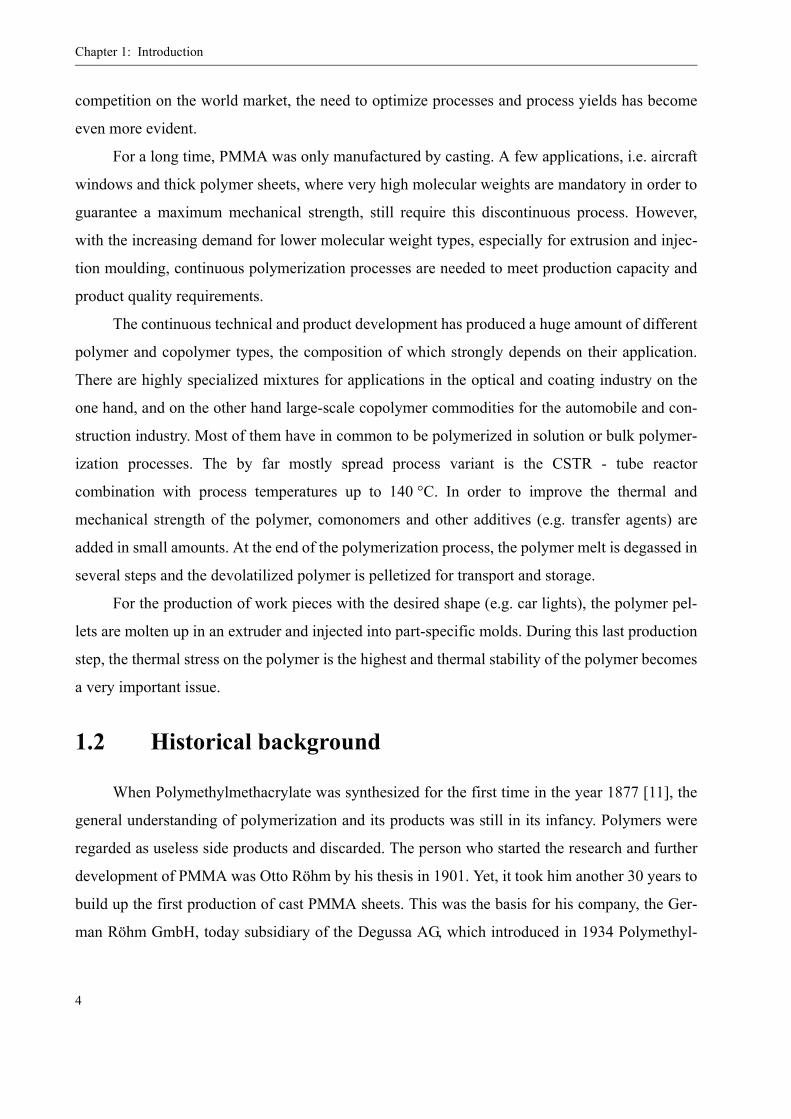
Four European manufacturers - Atoglas (Atofina), Degussa-Röhm, Barlo PLC and Ineos -
and four Asian manufacturers dominate the present PMMA market. Together, they have a produc-
tion capacity of about 840'000 tons / year. Yet, compared to other thermoplastics, PMMA holds
only a small share of all thermoplastics on the world market, as figure 1.1 shows. In order to
increase this share, manufacturers of acrylics make every effort to develop new product qualities
for highly sophisticated applications. These include the use of acrylic polymers for optical discs,
for example new generations of the DVD, where the concurrence with polycarbonates is the driv-
ing force for new product developments.
Figure 1.1: Thermoplastic consumption in Western Europe 2001-2003 [12]
Chapter 1: Introduction
6
1.3 Aim of this work
The aim of this work, which has been carried out in close cooperation with industry, is to
kinetically describe the high temperature polymerization of methyl (methacrylate), to investigate
the feasibility of a polymerization process at 140 °C < T < 170 °C and to study the impact of tem-
perature on the product quality in a continuous pilot-scale process.
The polymerization of methyl methacrylate is probably the best described polymerization
reaction in polymer science. However, most research that has been published in the specialized
literature deals with the polymerization at a rather low temperature range (< 100 °C). Unfortu-
nately, increasing the reaction temperature above this value changes significantly the underlying
polymerization kinetics. In particular, the following three phenomena have to be reevaluated:
• the self-initiation reactions
• the gel effect
• and the depolymerization
It was, therefore, necessary to start with the determination of kinetic parameters and the
development of a gel effect model for the given temperature range and to validate both with the
help of experimental data. These features could then be included in a general kinetic model for the
description of the whole polymerization process. Several series of experiments were carried out at
bench-scale and various analytical methods had to be established in order to accomplish this
important part of this work.
The second step was the design and setup of a continuous pilot plant in order to investigate
the polymerization under conditions similar to the industrial process. For the present work, a
setup based on the combination of a recycle loop and tube reactor was chosen, as it had been
already successfully employed in earlier research studies of this workgroup. The frame of the
continuous polymerization process also allowed a development study of a relatively new process
monitoring technique based on the speed of sound measurement and the determination of copoly-
merization and chain transfer related parameters from steady-state polymerizations.
The various goals of this PhD project are itemized once again in the following list contain-
ing each individual part of this work together with a brief description of the work carried out to
achieve them.

1.3: Aim of this work
7
Self-Initiation at high temperatures
• Determination of the formation kinetics of MMA peroxides in batch experiments:
Development of an analytical method for the determination of organic peroxides
• Determination of the decomposition kinetics of MMA peroxides by DSC:
Synthesis and Isolation of MMA peroxides
Method for the determination of reaction kinetics by DSC
• Characterization of MMA peroxides by GPC, TGA and NMR
• Investigation and characterization of other mechanisms influencing the self-initiation
of MMA (thermal initiation, initiation by CTA, dimerization)
• Verification of the entire self-initiation kinetics in batch polymerization experiments
Gel effect at high temperatures
• Evaluation of existing gel effect models toward their application at high temperatures
• Derivation of an adapted model for the correct description of the high temperature gel
effect
• Determination of the parameters influencing the gel effect
• Model verification by means of batch polymerization experiments
Continuous High Temperature Polymerization
• Design and construction of a pilot plant with a capacity of 1-5 kg PMMA per hour
• Development of a method for the direct and inline monomer conversion monitoring
by speed of sound measurement
• Determination of r-parameters for the copolymerization MMA / MA
• Determination of the chain transfer constant for n-dodecanethiol
• Evaluation of the obtained product at high temperatures concerning molecular
weight, residual monomer and thermal stability
• Production of several batches of polymer pellets for the evaluation of the product qual-
ity in injection molding experiments (carried out by the industrial partner)
• Establishing a kinetic model in PREDICI® for the description of the continuous copo-
lymerization process and validation with experimental data

Chapter 1: Introduction
8
9
CHAPTER 2
Self-Initiation at high temperatures
Monomers used in radical polymerization are unsaturated compounds that can undergo
various reactions and therefore exhibit only a limited stability. Many of them polymerize
already at room temperature when not sufficiently stabilized by radical scavengers. Styrene,
for example, has a very distinctive self-initiation potential, which is caused by intermolecular
interactions due to its molecular structure, i.e. the formation of an unstable dimer [13]. There-
fore, it usually needs to be stored under cooling or with rather large amounts of stabilizer.
Since this self-initiation gets more important with increasing temperature, it is usually referred
to also as “spontaneous thermal initiation”.
For MMA, the thermal initiation also exists but, due to the different molecular structure
compared to styrene, the mechanism is much slower. Depending on the temperature, it usually
takes days if not months for a sample of purified MMA to polymerize to noticeable extents.
However, if technical MMA as supplied by the producers is heated to above 100°C, quickly a
considerable polymerization with monomer conversions of more than 20% can be observed.
This motivates the question of which nature the initiation that is the cause for this polymeriza-
tion might be and, if there are radicals involved in the mechanism, what their origin is.
In literature, several reasons for thermal polymerization of MMA can be found. Stickler,
Lingnau and Meyerhoff, for example, have carried out extensive research on this topic. In their
series of publications “The Spontaneous Thermal Polymerization of Methyl Methacrylate 1-6”
[14-19], they determine the rate constants for the reproducible spontaneous thermal initiation,
which is not overlaid by initiation reactions of impurities, and discuss furthermore the forma-
Chapter 2: Self-Initiation at high temperatures
10
tion of di- and trimers as well as the initiation potential of chain transfer agents. Even the initia-
tion by cosmic and environmental radiation is taken into account and evaluated by them. As
concerns initiation reactions caused by impurities, the attention is quickly drawn to peroxides in
the relevant literature. The possibility that MMA and other unsaturated compounds react with
oxygen traces to form peroxides has already been described in the 50‘s by Mayo and Miller [20]
and Barnes et al. [21]. These peroxides have been proven to decompose at higher temperatures
and to form radicals that can initiate polymerization. This mechanism is even supposed to be the
dominant reason for “thermal initiation” of MMA at temperatures above 100°C [22].
In this chapter, the different initiation mechanisms1 are discussed, first of all the MMA per-
oxide initiation, and experimental results that were obtained in this work are presented. The char-
acterization of MMA peroxides, their formation and decomposition has been one of the key
interests of this project. Especially in industrial processes, where impurities and atmospheric
gases are always present, it is of great importance to carefully characterize these reactions since
they may have a significant influence on process safety and are able to falsify results in pilot plant
experiments, which can then lead to misinterpretation of data.
2.1 MMA peroxides
2.1.1 Introduction
Methyl methacrylate is in most cases stabilized for transportation and storage with stabiliz-
ers of the hydroquinone type, e.g. hydroquinone and 4-methoxyphenol. The active principle of
this class of stabilizers is based on an interaction with oxygen, since they are not capable of cap-
turing radicals themselves [23, 24]. However, they readily react with peroxy radicals. In the fol-
lowing, the stabilization mechanism is presented and the role of oxygen in the stabilization
becomes evident.
The primary radical R. is generated by not further defined, arbitrary processes as for exam-
ple radiation, molecular interactions or decomposition of other impurities in the system. The oxy-
1. The dimerization does not represent an initiation mechanism for the radical polymerization of MMA but is discussed nevertheless in this chapter as it can have significant effects on the monomer conversion at high temperatures.
2.1: MMA peroxides
11
gen molecule O2 is a biradical with a very high affinity to other radicals. Therefore, the radical R.
rather reacts with oxygen than with another radical [23]. As long as there is enough stabilizer and
oxygen present in the system, radical initiation of the polymerization is inhibited:
(EQ 2.1)
(EQ 2.2)
(EQ 2.3)
(EQ 2.4)
Hence, it is important to store the monomer under oxygen containing atmosphere so that the
inhibition is guaranteed.
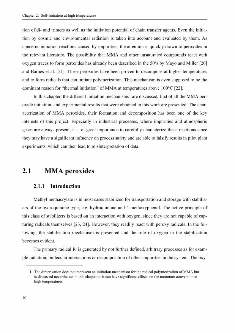
In the absence of stabilizer, either in purified monomer or due to its consumption by reac-
tions as in equation 2.3 and equation 2.4, the radical ROO. from equation 2.2 is no longer trapped
by the methoxyphenol, but can react freely with other molecules. Thus, if there’s enough oxygen
present, it creates an alternating, copolymeric chain of oxygen and monomer, as it was proven by
NMR, FTIR and pyrolysis studies [25, 26]:
(qualitative mechanism) (EQ 2.5)
The peroxide obtained is also referred to as PMMA peroxide, MMA polyperoxide, MMA-OO
or simply PMMAP. Since these chains are stable at medium temperatures (i.e. in general below
100 °C), also oxygen indirectly has a stabilizing effect on the monomer (by scavenging radicals
and forming peroxides), which means that storage under oxygen containing atmosphere is already
enough in order to prevent polymerization. The principle of this stabilization with oxygen was
first investigated in 1955 by Schulz and Henrici [27]. However, with time the peroxide chains
accumulate in the monomer, a fact that becomes an issue at higher temperatures. As reported by
several authors, the thermal decomposition of PMMAP starts between 130 °C [28] and 150 °C
[25]. In the latter article also a decomposition mechanism via radical chain scission is proposed:
OH OCH3 + R.
R. + O2 ROO.
ROO. + OH OCH3 ROOH O OCH3+
+ O OCH3ROO OOCH3
OOR
ROO + M ROOM ROO(MOO)nO2
Chapter 2: Self-Initiation at high temperatures
12
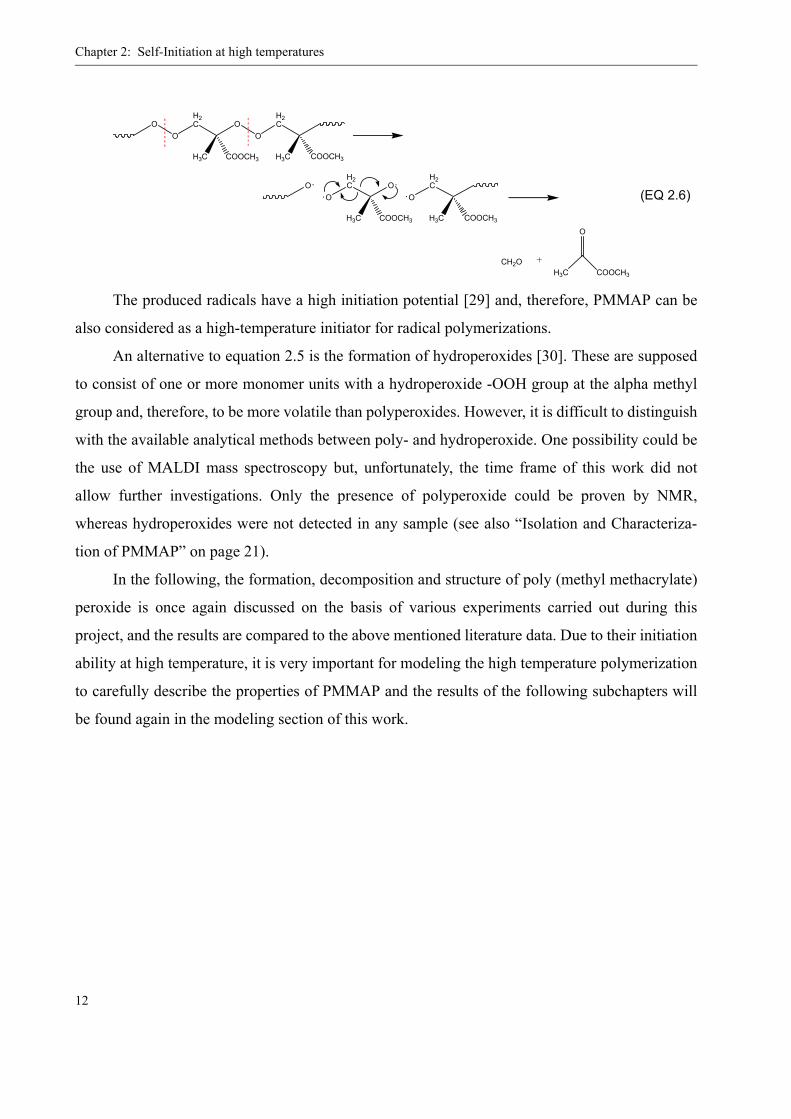
(EQ 2.6)
The produced radicals have a high initiation potential [29] and, therefore, PMMAP can be
also considered as a high-temperature initiator for radical polymerizations.
An alternative to equation 2.5 is the formation of hydroperoxides [30]. These are supposed
to consist of one or more monomer units with a hydroperoxide -OOH group at the alpha methyl
group and, therefore, to be more volatile than polyperoxides. However, it is difficult to distinguish
with the available analytical methods between poly- and hydroperoxide. One possibility could be
the use of MALDI mass spectroscopy but, unfortunately, the time frame of this work did not
allow further investigations. Only the presence of polyperoxide could be proven by NMR,
whereas hydroperoxides were not detected in any sample (see also “Isolation and Characteriza-
tion of PMMAP” on page 21).
In the following, the formation, decomposition and structure of poly (methyl methacrylate)
peroxide is once again discussed on the basis of various experiments carried out during this
project, and the results are compared to the above mentioned literature data. Due to their initiation
ability at high temperature, it is very important for modeling the high temperature polymerization
to carefully describe the properties of PMMAP and the results of the following subchapters will
be found again in the modeling section of this work.
OO
H2C O
O
H2C
COOCH3H3C H3C COOCH3
OO
H2C O
O
H2C
COOCH3H3C H3C COOCH3
O
H3C COOCH3
CH2O +
2.1: MMA peroxides
13
2.1.2 Formation of poly (methyl methacrylate) peroxide (PMMAP)
For the determination of the PMMAP formation kinetics, several approaches are possible.
One is to measure the oxygen absorption or consumption rate in MMA at different temperatures
[23, 31, 32]. With the above mentioned formation mechanism, the kinetics can then be estimated.
Another way, which was chosen in this work, is to determine directly the peroxide concentration
in the monomer. However, this proved to be a non-trivial problem, since most methods for perox-
ide determination work in aqueous media only. Few titration methods for organic peroxides were
found, working with sodium iodide (NaI) and thiosulfate (NaS2O3) and glacial acetic acid as
reagents in solvents like isopropanol [33] or chloroform / methanol mixtures or even two-phase
systems with water. The problem is already to dissolve the inorganic salts in the organic solvents.
A second weak point of these methods is that iodide is readily oxidized by atmospheric oxygen in
these solvents, so the measurement error is relatively high. Additionally, within the expected
rather low concentration range (< 100 ppm O2), the precision of titration methods was considered
to be not sufficient for kinetic investigations.
Finally, a method found in [34] from 1946, which is described by the authors to be not influ-
enced by air in the same extent than other methods, was modified to work in combination with
UV-Vis spectrophotometry. The only difference between this procedure and the previously men-
tioned one is that it uses acetic anhydride as a solvent, which acts as solvent and proton donor for
the oxidation of I- at the same time and exhibits excellent solubility for NaI.
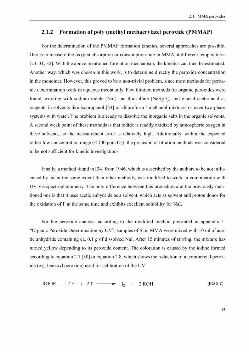
For the peroxide analysis according to the modified method presented in appendix 1,
“Organic Peroxide Determination by UV”, samples of 5 ml MMA were mixed with 10 ml of ace-
tic anhydride containing ca. 0.1 g of dissolved NaI. After 15 minutes of stirring, the mixture has
turned yellow depending to its peroxide content. The coloration is caused by the iodine formed
according to equation 2.7 [30] or equation 2.8, which shows the reduction of a commercial perox-
ide (e.g. benzoyl peroxide) used for calibration of the UV.
(EQ 2.7)ROOR 2 H+ 2 I- I2 2 ROH+ + +
Chapter 2: Self-Initiation at high temperatures
14
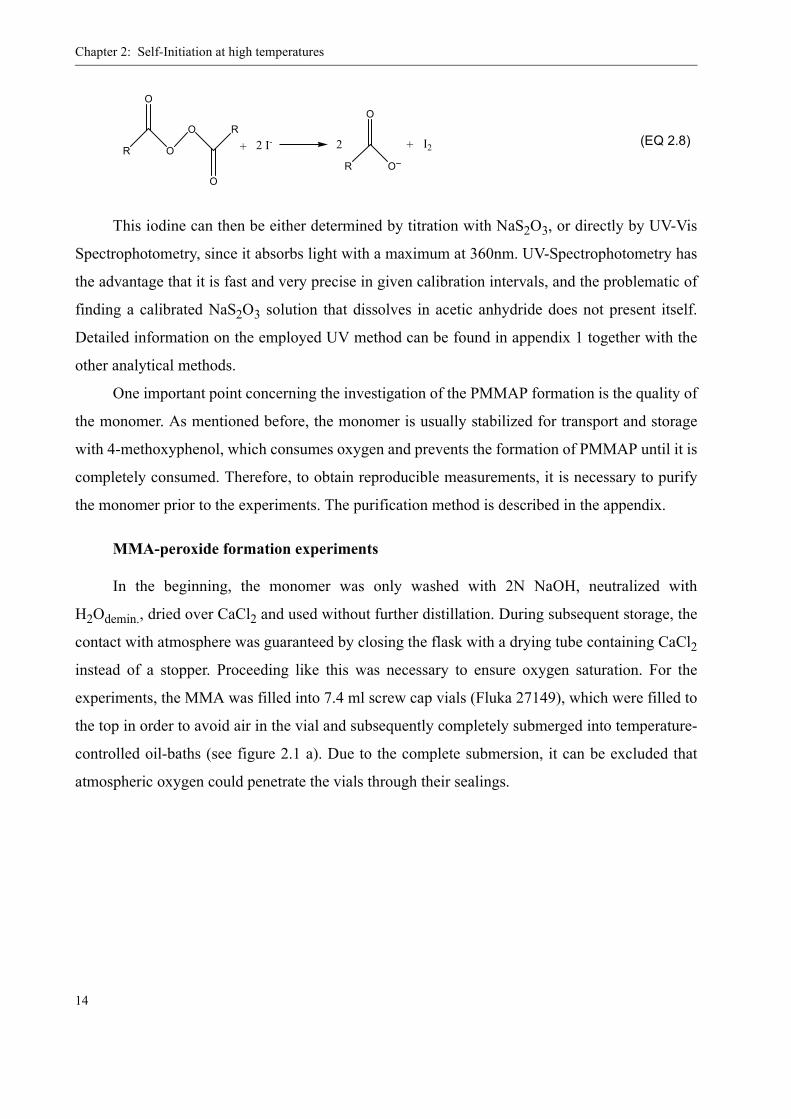
(EQ 2.8)
This iodine can then be either determined by titration with NaS2O3, or directly by UV-Vis
Spectrophotometry, since it absorbs light with a maximum at 360nm. UV-Spectrophotometry has
the advantage that it is fast and very precise in given calibration intervals, and the problematic of
finding a calibrated NaS2O3 solution that dissolves in acetic anhydride does not present itself.
Detailed information on the employed UV method can be found in appendix 1 together with the
other analytical methods.
One important point concerning the investigation of the PMMAP formation is the quality of
the monomer. As mentioned before, the monomer is usually stabilized for transport and storage
with 4-methoxyphenol, which consumes oxygen and prevents the formation of PMMAP until it is
completely consumed. Therefore, to obtain reproducible measurements, it is necessary to purify
the monomer prior to the experiments. The purification method is described in the appendix.
MMA-peroxide formation experiments
In the beginning, the monomer was only washed with 2N NaOH, neutralized with
H2Odemin., dried over CaCl2 and used without further distillation. During subsequent storage, the
contact with atmosphere was guaranteed by closing the flask with a drying tube containing CaCl2instead of a stopper. Proceeding like this was necessary to ensure oxygen saturation. For the
experiments, the MMA was filled into 7.4 ml screw cap vials (Fluka 27149), which were filled to
the top in order to avoid air in the vial and subsequently completely submerged into temperature-
controlled oil-baths (see figure 2.1 a). Due to the complete submersion, it can be excluded that
atmospheric oxygen could penetrate the vials through their sealings.
R
O
O
O
O
R2 I-+ I2+2
R
O
O
2.1: MMA peroxides
15
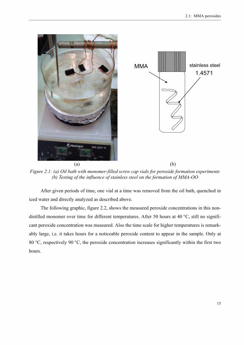
After given periods of time, one vial at a time was removed from the oil bath, quenched in
iced water and directly analyzed as described above.
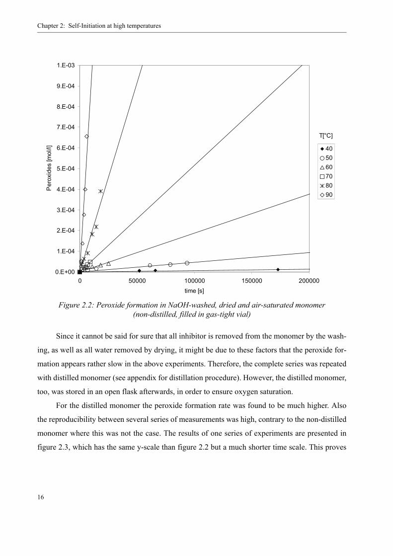
The following graphic, figure 2.2, shows the measured peroxide concentrations in this non-
distilled monomer over time for different temperatures. After 50 hours at 40 °C, still no signifi-
cant peroxide concentration was measured. Also the time scale for higher temperatures is remark-
ably large, i.e. it takes hours for a noticeable peroxide content to appear in the sample. Only at
80 °C, respectively 90 °C, the peroxide concentration increases significantly within the first two
hours.
(a) (b)Figure 2.1: (a) Oil bath with monomer-filled screw cap vials for peroxide formation experiments
(b) Testing of the influence of stainless steel on the formation of MMA-OO
MMA1.4571
stainless steel
Chapter 2: Self-Initiation at high temperatures
16
Since it cannot be said for sure that all inhibitor is removed from the monomer by the wash-
ing, as well as all water removed by drying, it might be due to these factors that the peroxide for-
mation appears rather slow in the above experiments. Therefore, the complete series was repeated
with distilled monomer (see appendix for distillation procedure). However, the distilled monomer,
too, was stored in an open flask afterwards, in order to ensure oxygen saturation.
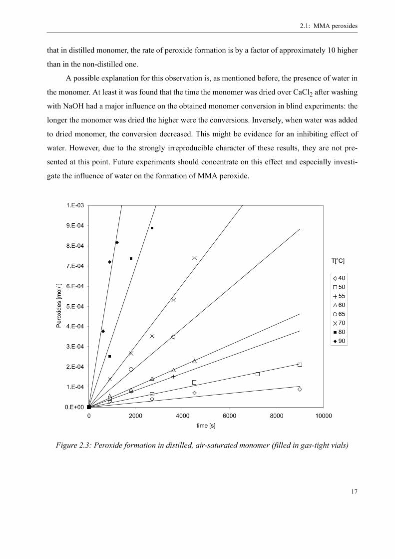
For the distilled monomer the peroxide formation rate was found to be much higher. Also
the reproducibility between several series of measurements was high, contrary to the non-distilled
monomer where this was not the case. The results of one series of experiments are presented in
figure 2.3, which has the same y-scale than figure 2.2 but a much shorter time scale. This proves
Figure 2.2: Peroxide formation in NaOH-washed, dried and air-saturated monomer(non-distilled, filled in gas-tight vial)
0.E+00
1.E-04
2.E-04
3.E-04
4.E-04
5.E-04
6.E-04
7.E-04
8.E-04
9.E-04
1.E-03
0 50000 100000 150000 200000time [s]
Per
oxid
es [m
ol/l] 40
5060708090
T[°C]
2.1: MMA peroxides
17
that in distilled monomer, the rate of peroxide formation is by a factor of approximately 10 higher
than in the non-distilled one.
A possible explanation for this observation is, as mentioned before, the presence of water in
the monomer. At least it was found that the time the monomer was dried over CaCl2 after washing
with NaOH had a major influence on the obtained monomer conversion in blind experiments: the
longer the monomer was dried the higher were the conversions. Inversely, when water was added
to dried monomer, the conversion decreased. This might be evidence for an inhibiting effect of
water. However, due to the strongly irreproducible character of these results, they are not pre-
sented at this point. Future experiments should concentrate on this effect and especially investi-
gate the influence of water on the formation of MMA peroxide.
Figure 2.3: Peroxide formation in distilled, air-saturated monomer (filled in gas-tight vials)
0.E+00
1.E-04
2.E-04
3.E-04
4.E-04
5.E-04
6.E-04
7.E-04
8.E-04
9.E-04
1.E-03
0 2000 4000 6000 8000 10000time [s]
Per
oxid
es [m
ol/l]
4050556065708090
T[°C]
Chapter 2: Self-Initiation at high temperatures
18
In order to use this data in a way to obtain formation kinetics for PMMAP, some mechanis-
tic considerations and simplifications had to be made. Since PMMAP is a polymeric peroxide
with only ideally an alternating copolymeric structure, the correct mathematical description of its
formation would be quite complicated. Therefore, an idealized unimolecular approach was cho-
sen to determine the kinetic constants according to Arrhenius, which will be explained in the fol-
lowing. One unknown in this approach is the oxygen concentration in the monomer at the
beginning of the experiment, i.e. the temperature-dependant saturation concentration of O2 in
MMA. This oxygen concentration has been determined experimentally for acrylic acid / meth-
acrylic acid [23] and for tripropylene glycol diacrylate (TPGDA) [35]. In both cases, the results
were in the order of 60 ppm or 10-3 mol/l, so it seems justified to assume this value also for MMA
in this work.
The simplified mechanism for the peroxide formation is:
(EQ 2.9)
The rate of peroxide formation is therefore:
(EQ 2.10)
Due to its great excess with regards to oxygen, the MMA concentration can be considered
constant:
(EQ 2.11)
Since not the oxygen concentration but the peroxide concentration at time t is measured, it
is necessary to express [O2] by [ROOR’] and the initial oxygen concentration [O2]0:
(EQ 2.12)
Hence, the rate of peroxide formation becomes:
(EQ 2.13)
2MMA + O ROOR'→
[ ] [ ] [ ]m n2
d ROOR' = k MMA O
dt
[ ] [ ]mobsMMA constant k MMA = k⇒
[ ] [ ] [ ]2 2 0O = O - ROOR'
[ ] [ ] [ ]( )n
obs 2 0
d ROOR' = k O - ROOR'
dt⇒
2.1: MMA peroxides
19
(EQ 2.14)
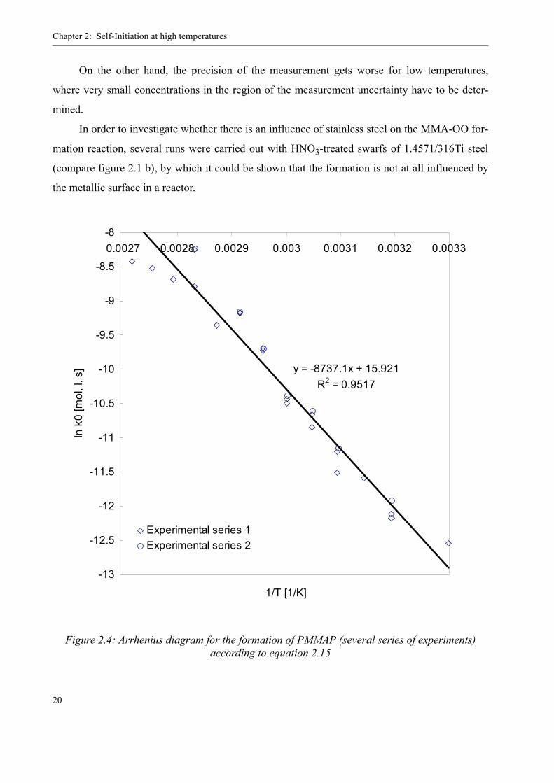
Integration of equation 2.14 yields equation 2.15 and equation 2.16 for n = 1, respectively,
n ≠ 1. However, with equation 2.15, a straight line is obtained in the Arrhenius diagram, which
legitimates the assumption of first order kinetics with regards to oxygen and of zero-th order
kinetics with regards to monomer.
(EQ 2.15)
(EQ 2.16)
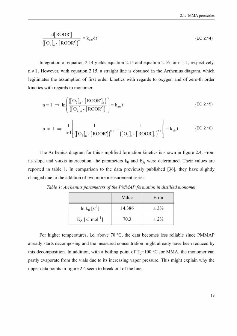
The Arrhenius diagram for this simplified formation kinetics is shown in figure 2.4. From
its slope and y-axis interception, the parameters k0 and EA were determined. Their values are
reported in table 1. In comparison to the data previously published [36], they have slightly
changed due to the addition of two more measurement series.
For higher temperatures, i.e. above 70 °C, the data becomes less reliable since PMMAP
already starts decomposing and the measured concentration might already have been reduced by
this decomposition. In addition, with a boiling point of Tb=100 °C for MMA, the monomer can
partly evaporate from the vials due to its increasing vapor pressure. This might explain why the
upper data points in figure 2.4 seem to break out of the line.
Table 1: Arrhenius parameters of the PMMAP formation in distilled monomer
Value Error
ln k0 [s-1] 14.386 ± 3%
EA [kJ mol-1] 70.3 ± 2%
[ ][ ] [ ]( ) obsn
2 0
d ROOR' = k dt
O - ROOR'
[ ] [ ]( )[ ] [ ]( )
2 0 0obs
2 0
O - ROOR'n = 1 ln = k t
O - ROOR'
⎛ ⎞⎜ ⎟⇒⎜ ⎟⎝ ⎠
[ ] [ ]( ) [ ] [ ]( ) obsn-1 n-1
2 20 0 0
1 1 1n 1 - = k tn-1 O - ROOR' O - ROOR'
⎡ ⎤⎢ ⎥≠ ⇒⎢ ⎥⎣ ⎦
Chapter 2: Self-Initiation at high temperatures
20
On the other hand, the precision of the measurement gets worse for low temperatures,
where very small concentrations in the region of the measurement uncertainty have to be deter-
mined.
In order to investigate whether there is an influence of stainless steel on the MMA-OO for-
mation reaction, several runs were carried out with HNO3-treated swarfs of 1.4571/316Ti steel
(compare figure 2.1 b), by which it could be shown that the formation is not at all influenced by
the metallic surface in a reactor.
Figure 2.4: Arrhenius diagram for the formation of PMMAP (several series of experiments) according to equation 2.15
y = -8737.1x + 15.921R2 = 0.9517
-13
-12.5
-12
-11.5
-11
-10.5
-10
-9.5
-9
-8.5
-80.0027 0.0028 0.0029 0.003 0.0031 0.0032 0.0033
1/T [1/K]
ln k
0 [m
ol, l
, s]
Experimental series 1Experimental series 2
2.1: MMA peroxides
21
2.1.3 Isolation and Characterization of PMMAP
The amounts of PMMAP produced in the formation experiments of chapter 2.1.2 are cer-
tainly not sufficient for further analysis and characterization of the peroxide. In order to carry out
GPC and NMR experiments for conformational analysis, sample weights in the order of some
milligrams are needed. Thus, the aim was to synthesize and isolate the polymeric peroxide.
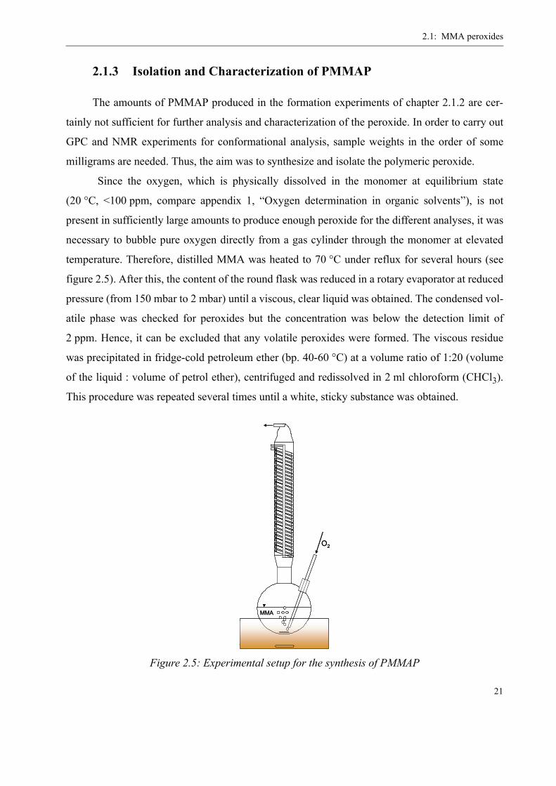
Since the oxygen, which is physically dissolved in the monomer at equilibrium state
(20 °C, <100 ppm, compare appendix 1, “Oxygen determination in organic solvents”), is not
present in sufficiently large amounts to produce enough peroxide for the different analyses, it was
necessary to bubble pure oxygen directly from a gas cylinder through the monomer at elevated
temperature. Therefore, distilled MMA was heated to 70 °C under reflux for several hours (see
figure 2.5). After this, the content of the round flask was reduced in a rotary evaporator at reduced
pressure (from 150 mbar to 2 mbar) until a viscous, clear liquid was obtained. The condensed vol-
atile phase was checked for peroxides but the concentration was below the detection limit of
2 ppm. Hence, it can be excluded that any volatile peroxides were formed. The viscous residue
was precipitated in fridge-cold petroleum ether (bp. 40-60 °C) at a volume ratio of 1:20 (volume
of the liquid : volume of petrol ether), centrifuged and redissolved in 2 ml chloroform (CHCl3).
This procedure was repeated several times until a white, sticky substance was obtained.
Figure 2.5: Experimental setup for the synthesis of PMMAP
O2
MMA
O2
MMA
Chapter 2: Self-Initiation at high temperatures
22
The obtained sticky polymer was supposed to be or at least to contain the PMMAP. How-
ever, it could not be excluded that also ordinary PMMA had been formed during the oxygen bub-
bling due to radicals produced by the various reactions described above. Thus, in order to clarify
the composition of the substance, at a first instance GPC analysis was done (details about the used
GPC method in appendix 1).
Size Exclusion Chromatography (SEC/GPC)
Figure 2.6 shows the result of a GPC injection of three different solutions of the same poly-
mer in THF (c = 1.8, 2.4 and 3.7 mg/ml). It can be seen that there are two peaks that change with
concentration, corresponding to molecular weights of Mw ~ 2.5 106 g/mol and of Mw ~ 8’200 g/
mol, respectively. These average molecular weights were obtained by conventional calibration
with PMMA standards (PSS, Mainz, Germany, Mw values can be found in appendix 1).
The smaller one is attributed to the PMMAP, which is in good agreement with literature
data: Sivalingam et. al. [37] found a molecular weight of Mn ~ 2’750 g/mol for their PMMAP,
which was polymerized at 50 °C with 0.01mol/l azoisobutyronitril (AIBN). Subramanian [28]
reports a molecular weight of 1’800 g/mol for PMMAP that was polymerized at 40 °C with AIBN
as radical source. However, in the latter case it is not clear if the reported molecular weight is Mn
or Mw. The rather low molecular weight of PMMAP is explained by a high transfer activity and
mutual termination of peroxy radicals [38].
The higher molecular weight peak is assumed to correspond to a high molecular PMMA
that is formed in parallel to the peroxide by radical initiation at 70 °C. The high molecular weight
is caused by the small amount of radicals following thermal breakdown of peroxides in the system
and the rather low polymerization temperature.
This hypothesis of two separate polymers formed during the experiment also corresponds to
the conclusion that Bamford and Morris come to in their work [38]. Looking at the surface under
each peaks, which corresponds to the concentration of each component, reveals a ratio PMMA :
PMMAP of 75% : 25%. However, the concentration is only comparable for identical dn/dc1 val-
1. dn/dc stands for the change in refractive index n of a solution with increasing solute concentration c. This value is characteristic for various polymers and other substances.

2.1: MMA peroxides
23
ues of each polymer. In this case, it can, therefore, only be an approximation, as the dn/dc value
for PMMAP is not known but likely to differ from the one for PMMA. Anyway, the peroxide con-
tent of the sample will be discussed later together with the results from the TGA measurements.
Figure 2.6: GPC analysis of the substance obtained in the PMMAP synthesis experiment
Table 2: Molecular weights of different PMMAP syntheses (GPC analysis)
Mn [g/mol] Mw [g/mol] PD
1 1’961 7’451 3.8
2 2’893 6’921 2.4
3 3’654 8’172 2.2
PMMAMw ~ 2.5 106 g/mol
PMMAPMw ~ 8200 g/mol
Det
ecto
r res
pons
e [m
V]

Chapter 2: Self-Initiation at high temperatures
24
NMR
For conformational analysis as well as for identification of PMMAP in the polymeric resi-
due, 1H- and 13C-NMR spectra were taken. Due to the strong deshielding effect of the oxygen
[30], peroxide groups in the polymer can be identified by several chemical shifts as explained in
the following.
The 1H-NMR spectrum, taken on a Bruker NMR at 400MHz, is depicted in figure 2.7. Cor-
responding to literature data [25] and information provided by an NMR specialist from the indus-
trial partner [39], the spectrum shows the expected signals for PMMAP:
• 1.44 ppm -CCH3-
• 3.76 ppm -OCH3
• 4.34 ppm -OCH2-
The same applies for the 13C-NMR spectrum, shown in figure 2.8, despite a small shift
towards lower values with respect to the following literature data:
• 18.47 ppm CH3-C-
• 52.33 ppm CH3-C=O
• 75.79 ppm, 75.41 ppm -CH2-O-
• 84.78 ppm -C-O-
• 171.03 ppm -C=O
The decomposition product of PMMAP, methyl pyruvate or propanoic acid-2-oxo-methyl-
ester, could be identified (1H: 2.46, and 3.86 ppm). On the other hand, no evidence of hydroper-
oxides was found (1H: 6.4, 5.9 and 4.7ppm, 13C: 165.8, 128.7, 135.1 and 72.8 ppm).

2.1: MMA peroxides
25
Figure 2.7: 1H-NMR spectrum of the polymeric residue
Figure 2.8: 13C-NMR spectrum of the polymeric residue

Chapter 2: Self-Initiation at high temperatures
26
2.1.4 Decomposition of PMMAP
The decomposition mechanism for PMMAP has already been mentioned before (see equa-
tion 2.6) and was proven by the identification of the pyrolysis products formaldehyde and methyl
pyruvate. However, when it comes to the determination of the decomposition rate, respectively
the decomposition kinetics, the data found in literature are quite inconsistent. Mukundan and
Kishore [25] report a starting point of 100 °C with a maximum rate at 150 °C for the decomposi-
tion measured by DSC and TGA. Subramanian [28] mentions a thermal degradation temperature
determined by TGA of 132 °C - 134 °C, respectively of 145 °C in case of DSC measurement. It
seems that both, the method of measurement, and possible differences in the molecular structure
of the peroxide itself influence the results. At least it seems plausible that polymerization temper-
ature and the fact that initiator was added or not can have an effect on the thermal stability of the
produced peroxide.
In this work, different approaches have been undertaken to determine the decomposition
kinetics for PMMAP. First of all, DSC scanning experiments were carried out in combination
with a software-integrated calculation method for the kinetics (see below). Secondly, TGA-MS
experiments were used to verify the degradation mechanism by its products. Finally, the decom-
position kinetics were determined in batch polymerizations by means of the Odian method [40]
(dead-end polymerization).
Differential Scanning Calorimetry (DSC)
A very comfortable way to determine kinetics in general is by DSC scanning experiments
(compare “Differential Scanning Calorimetry”in appendix 1). Since due to the linear heating
ramp the reaction virtually runs through an infinite number of infinitesimal isothermal tempera-
ture steps, the Arrhenius parameters k0 and EA can be determined from only one experiment. For
the mathematical treatment of the measured data, there are several methods available (e.g. Fried-
man method, Chang method, Kissinger method [37]). The software of the DSC device uses a mul-
tilinear regression for the determination of k0, EA and reaction order n as explained in the
following [41].
The time-dependent degree of conversion X for a reaction of n-th order can be expressed by
equation 2.17.

2.1: MMA peroxides
27
(EQ 2.17)
In order to solve this equation, either one variable needs to be held constant (this is the case
in isothermal experiments: ) or related with another one. The latter can be achieved for
constant heating rates by relating the temperature with time, since it is
(EQ 2.18)
the definition of the heating rate. Now, combining equation 2.17 with equation 2.18 leads to
the following expression, which is used in its linearized form (equation 2.20) to determine the
kinetic parameters.
(EQ 2.19)
(EQ 2.20)
From the DSC curve, values for ΔH and ΔHpartial(t) are derived, which, in the case that the
reaction terminates with full conversion, can be related with the conversion by the following
expression:
(EQ 2.21)
In this equation, ΔH corresponds to the total energy dissipated by the reaction and
ΔHpartial(t) to the dissipated energy from t=0 to t (area under the DSC curve). With this informa-
tion, the software can now determine k0, EA and n by multilinear regression.
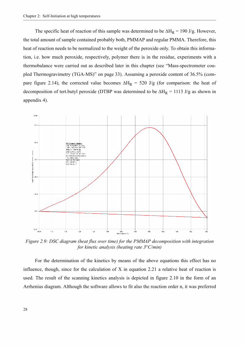
Figure 2.9 shows the heat flux diagram for the decomposition of the bulk PMMAP contain-
ing residue (i.e. not in solution). The strong exothermal character of the reaction is clearly visible.
At a heating rate of 3 °C/min, the decomposition starts at approximately 100 °C with a maximum
rate at 145 °C. This corresponds very well to the above mentioned literature data.
tddX k0 e
EA
RT-------–
1 X–( )n⋅ ⋅=
d Xdt-----
T const=
β tddT=
β TddX⋅ k0 e
EA
RT-------–
1 X–( )n⋅ ⋅=
β TddX⋅⎝ ⎠
⎛ ⎞ln k0( )lnEART-------– n 1 X–( )ln⋅+=
XΔHpartial
ΔH----------------------=
Chapter 2: Self-Initiation at high temperatures
28
The specific heat of reaction of this sample was determined to be ΔHR = 190 J/g. However,
the total amount of sample contained probably both, PMMAP and regular PMMA. Therefore, this
heat of reaction needs to be normalized to the weight of the peroxide only. To obtain this informa-
tion, i.e. how much peroxide, respectively, polymer there is in the residue, experiments with a
thermobalance were carried out as described later in this chapter (see “Mass-spectrometer cou-
pled Thermogravimetry (TGA-MS)” on page 33). Assuming a peroxide content of 36.5% (com-
pare figure 2.14), the corrected value becomes ΔHR = 520 J/g (for comparison: the heat of
decomposition of tert.butyl peroxide (DTBP was determined to be ΔHR = 1113 J/g as shown in
appendix 4).
For the determination of the kinetics by means of the above equations this effect has no
influence, though, since for the calculation of X in equation 2.21 a relative heat of reaction is
used. The result of the scanning kinetics analysis is depicted in figure 2.10 in the form of an
Arrhenius diagram. Although the software allows to fit also the reaction order n, it was preferred
Figure 2.9: DSC diagram (heat flux over time) for the PMMAP decomposition with integration for kinetic analysis (heating rate 3°C/min)
2.1: MMA peroxides
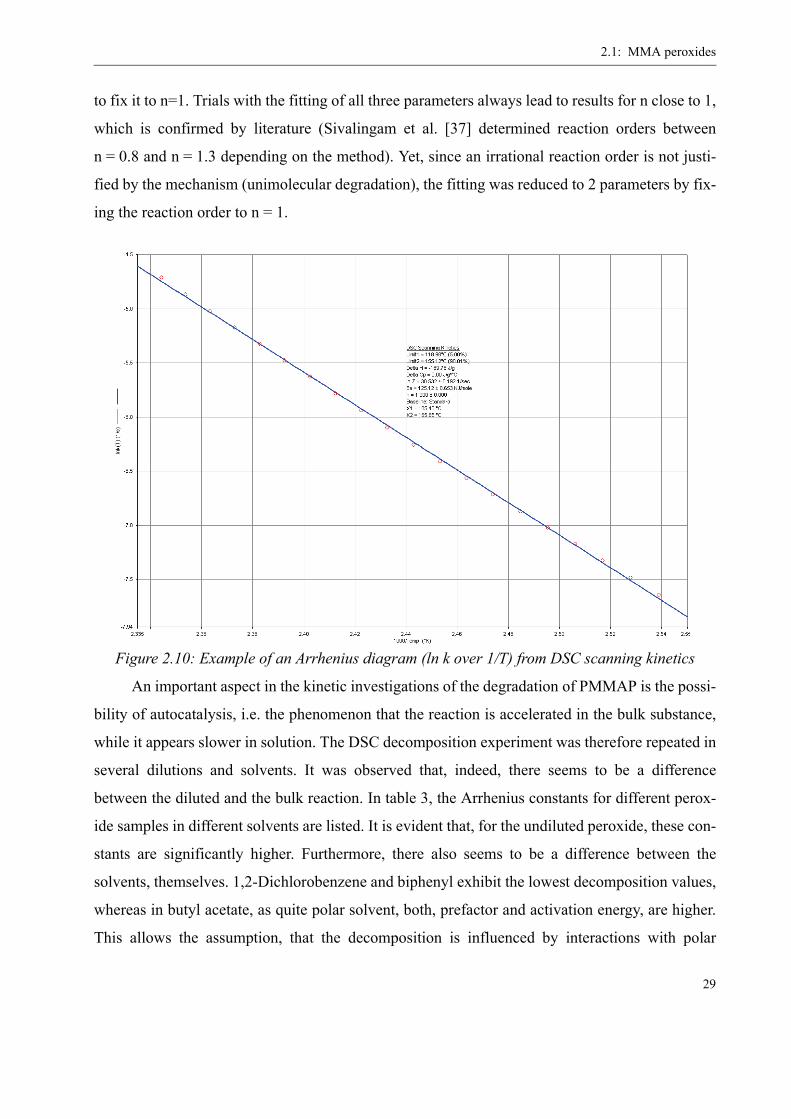
29
to fix it to n=1. Trials with the fitting of all three parameters always lead to results for n close to 1,
which is confirmed by literature (Sivalingam et al. [37] determined reaction orders between
n = 0.8 and n = 1.3 depending on the method). Yet, since an irrational reaction order is not justi-
fied by the mechanism (unimolecular degradation), the fitting was reduced to 2 parameters by fix-
ing the reaction order to n = 1.
An important aspect in the kinetic investigations of the degradation of PMMAP is the possi-
bility of autocatalysis, i.e. the phenomenon that the reaction is accelerated in the bulk substance,
while it appears slower in solution. The DSC decomposition experiment was therefore repeated in
several dilutions and solvents. It was observed that, indeed, there seems to be a difference
between the diluted and the bulk reaction. In table 3, the Arrhenius constants for different perox-
ide samples in different solvents are listed. It is evident that, for the undiluted peroxide, these con-
stants are significantly higher. Furthermore, there also seems to be a difference between the
solvents, themselves. 1,2-Dichlorobenzene and biphenyl exhibit the lowest decomposition values,
whereas in butyl acetate, as quite polar solvent, both, prefactor and activation energy, are higher.
This allows the assumption, that the decomposition is influenced by interactions with polar
Figure 2.10: Example of an Arrhenius diagram (ln k over 1/T) from DSC scanning kinetics
Chapter 2: Self-Initiation at high temperatures
30
groups, therefore also with other peroxidic groups, which might be a reason for the, what it seems,
faster decomposition of the undiluted samples. The consequences of these differences are demon-
strated by the halflife-time values for each sample, which are traced in figure 2.11.
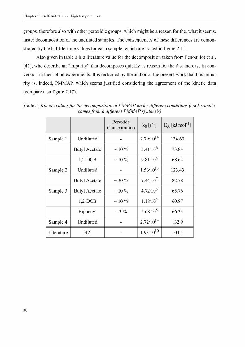
Also given in table 3 is a literature value for the decomposition taken from Fenouillot et al.
[42], who describe an “impurity” that decomposes quickly as reason for the fast increase in con-
version in their blind experiments. It is reckoned by the author of the present work that this impu-
rity is, indeed, PMMAP, which seems justified considering the agreement of the kinetic data
(compare also figure 2.17).
Table 3: Kinetic values for the decomposition of PMMAP under different conditions (each sample comes from a different PMMAP synthesis)
Peroxide Concentration k0 [s-1] EA [kJ mol-1]
Sample 1 Undiluted - 2.79.1014 134.60
Butyl Acetate ~ 10 % 3.41.106 73.84
1,2-DCB ~ 10 % 9.81.105 68.64
Sample 2 Undiluted - 1.56.1013 123.43
Butyl Acetate ~ 30 % 9.44.107 82.78
Sample 3 Butyl Acetate ~ 10 % 4.72.105 65.76
1,2-DCB ~ 10 % 1.18.105 60.87
Biphenyl ~ 3 % 5.68.105 66.33
Sample 4 Undiluted - 2.72.1014 132.9
Literature [42] - 1.93.1010 104.4

2.1: MMA peroxides
31
In order to obtain kinetic values for kpo,d to use in PREDICI® for the modeling of the initi-
ation by MMA peroxides, the averages of the above described values for the undiluted and the
diluted case were calculated by linear regression of the ln k over 1/T curves for the different sam-
ples kinetics. The result is depicted in figure 2.12. From the average ln k over 1/T curves, the fol-
lowing kinetics constants were calculated:
Figure 2.11: Half-life time - temperature plot for different peroxide samples and dilutions
0.01
0.1
1
10
100
1000100 120 140 160 180 200
T [°C]t 0.
5 [m
in]
Sample 1 undiluted Sample 1 BuAc Sample 1 1,2-DCBSample 2 undiluted Sample 2 BuAc Sample 3 BuAcSample 3 1,2-DCB Sample 3 Biphenyl Sample 4 undiluted
diluted
undiluted
Chapter 2: Self-Initiation at high temperatures
32
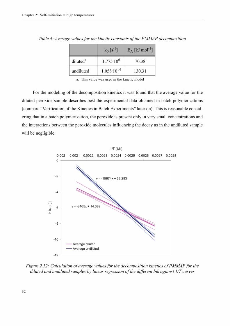
For the modeling of the decomposition kinetics it was found that the average value for the
diluted peroxide sample describes best the experimental data obtained in batch polymerizations
(compare “Verification of the Kinetics in Batch Experiments” later on). This is reasonable consid-
ering that in a batch polymerization, the peroxide is present only in very small concentrations and
the interactions between the peroxide molecules influencing the decay as in the undiluted sample
will be negligible.
Table 4: Average values for the kinetic constants of the PMMAP decomposition
k0 [s-1] EA [kJ mol-1]
diluteda
a. This value was used in the kinetic model
1.775.106 70.38
undiluted 1.058.1014 130.31
Figure 2.12: Calculation of average values for the decomposition kinetics of PMMAP for the diluted and undiluted samples by linear regression of the different lnk against 1/T curves
y = -15674x + 32.293
y = -8465x + 14.389
-12
-10
-8
-6
-4
-2
00.002 0.0021 0.0022 0.0023 0.0024 0.0025 0.0026 0.0027 0.0028
1/T [1/K]
ln k
po,d
[-]
Average dilutedAverage undiluted
2.1: MMA peroxides
33
Mass-spectrometer coupled Thermogravimetry (TGA-MS)
In order to determine the composition of the polymeric residue, i.e. how much peroxide,
respectively normal polymer was formed during the oxygenation reaction, TGA-MS runs were
carried out with different samples. Thermogravimetry allows the determination of weight losses
as a function of temperature. Furthermore, often a calorimetric signal is produced, which can help
to describe the nature of the weight loss (i.e. exothermic, endothermic).
In this part of the project, TGA was employed to investigate and understand the composi-
tion of the peroxide samples obtained from the above oxygenation experiments. It has been
already conjectured that the samples do not consist of polymeric peroxide only but that there is
also “ordinary” PMMA present. If this is the case, then in the thermogravimetry there should be
different weight loss steps, according to the amount of peroxide and polymer present. In fact, the
samples decompose in two steps, as can be seen from figure 2.13, which shows the weight loss
curve with increasing temperature (heating rate 5°C/min) under inert conditions. Here, the sample
weight over temperature is depicted together with the SDTA® (single differential thermal analy-
sis, trademark of Mettler Toledo, Switzerland) signal. The SDTA signal represents the tempera-
ture difference between the temperature near the sample and a reference program temperature.
Analogous to the differential scanning calorimeter (DSC), the SDTA signal indicates whether a
weight loss measured by the thermobalance is an exothermic or endothermic process. The SDTA
signal can also measure heat flow of transitions that do not involve a weight change, i.e. melting
of the sample.
The first weight loss corresponds to the decomposition of PMMAP. Firstly, it starts at
approximately 100 °C and has its maximum rate between 140-150 °C, which is in perfect agree-
ment with data from DSC experiments. Secondly, it is an exothermic weight loss, as can be seen
from the SDTA curve, a fact, which underlines that this weight loss is due to the peroxide. The
second weight loss, on the other hand, is endothermic. This is typical for a scission mechanism of
a polymeric chain like PMMA. Also the temperature range of this step between 300 °C and
400 °C is typical for PMMA main chain scission [43].
In figure 2.14, the integration of the weight loss curve from figure 2.13 is shown. By step
integration, it is calculated that of the total sample mass, 36% decompose during the first step and
50% during the second. The remaining 14% of the sample weight decompose in the transition
Chapter 2: Self-Initiation at high temperatures
34
period between the two steps, probably due to weak linkages in the PMMA chains. The amount of
residue in the crucible due to unreacted tar is negligible. Therefore, the amount of PMMA decom-
posed during the experiment can be estimated to be of 64% in total.
Still, this ratio is a little more in favor of the peroxide, compared to the results obtained by
GPC before (see figure 2.6), where only 25% of the sample were assigned to PMMAP and 75% to
PMMA. The reason for this difference might be that PMMA starts decomposing at temperatures
as low as 150°C due to head-to-head bonds in the polymeric chains. Having a closer look at the
TGA curve in figure 2.14 reveals that the weight loss between 150 °C and 200 °C is of approxi-
mately 10%. It might, therefore, be that within the 36% weight loss of the first decomposition
step, there is already a significant part of “normal” decomposing PMMA included. Another
important reason for the lower value found by GPC might be, as mentioned above, a difference in
the dn/dc ratio for homogeneous PMMA and PMMAP. Each species has a different increment of
the refractive index with concentration. The peak areas are - being strict on it - only comparable if
this value is identical for both polymers. Otherwise the direct comparison of the peak areas in the
GPC spectrum does not make sense. For PMMA and PMMAP a difference in dn/dc is possible
since due to the peroxide groups the conformation of the polymer chains is no longer the same as
for linear PMMA. The TGA result is, therefore, the more reliable as concerns the peroxide con-
tent of the sample.
Last but not least, the amount of peroxide in the sample also depends to a large extent on the
synthesis conditions (temperature, duration). It is, thus, not necessarily a reproducible parameter.

2.1: MMA peroxides
35
Figure 2.13: TGA curve (5°C/min) with SDTA signal for the decomposition of PMMAP in inert atmosphere
Figure 2.14: TGA curve with step integration for quantification of weight loss
0
10
20
30
40
50
60
70
80
90
100
0 100 200 300 400
T [°C]
rel.
wei
ght l
oss
[%]
-1
-0.8
-0.6
-0.4
-0.2
0
0.2
0.4
0.6
0.8
1
SD
TA s
igna
l [°C
]
TGA SDTA
exothermalendothermal
0
10
20
30
40
50
60
70
80
90
100
0 100 200 300 400
T [°C]
rel.
wei
ght l
oss
[%]
36.5%
50.6%
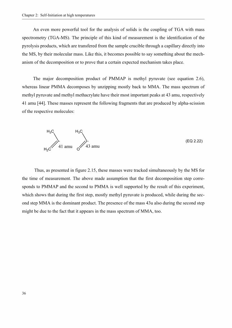
Chapter 2: Self-Initiation at high temperatures
36
An even more powerful tool for the analysis of solids is the coupling of TGA with mass
spectrometry (TGA-MS). The principle of this kind of measurement is the identification of the
pyrolysis products, which are transfered from the sample crucible through a capillary directly into
the MS, by their molecular mass. Like this, it becomes possible to say something about the mech-
anism of the decomposition or to prove that a certain expected mechanism takes place.
The major decomposition product of PMMAP is methyl pyruvate (see equation 2.6),
whereas linear PMMA decomposes by unzipping mostly back to MMA. The mass spectrum of
methyl pyruvate and methyl methacrylate have their most important peaks at 43 amu, respectively
41 amu [44]. These masses represent the following fragments that are produced by alpha-scission
of the respective molecules:
(EQ 2.22)
Thus, as presented in figure 2.15, these masses were tracked simultaneously by the MS for
the time of measurement. The above made assumption that the first decomposition step corre-
sponds to PMMAP and the second to PMMA is well supported by the result of this experiment,
which shows that during the first step, mostly methyl pyruvate is produced, while during the sec-
ond step MMA is the dominant product. The presence of the mass 43u also during the second step
might be due to the fact that it appears in the mass spectrum of MMA, too.
H3C
H2C
H3C
O41 amu 43 amu

2.1: MMA peroxides
37
Odian method
It is generally preferable to determine decomposition kinetics of a species under the same
conditions under which the decomposition takes place in the real process, rather than in isolated
experiments where concentrations and interactions with other molecules are different. This means
that rather than determining the decomposition in a DSC with the undiluted peroxide, it should be
determined from a polymerization experiment in a stirred reactor. The Odian method [40] allows
the estimation of both, initiator decomposition rate and efficiency, from dead-end batch polymer-
izations. A dead-end polymerization is a polymerization that stops short of its final conversion
due to insufficient initiator (so-called “initiator burn-out”).
Based on the expression
(EQ 2.23)
Figure 2.15: TGA-MS curves for the decomposition of PMMAP / PMMA
0
10
20
30
40
50
60
70
80
90
100
0 100 200 300 400
T [°C]
rel.
wei
ght l
oss
[%]
0
0.1
0.2
0.3
0.4
0.5
0.6
0.7
MS
resp
onse
[nA
]
TGA m = 43 u (methyl pyruvate) m = 41 u (MMA)
PMMAP PMMA
1 1 X–( )ln1 X∞–( )ln
--------------------------–ln–kd t⋅–2
--------------=

Chapter 2: Self-Initiation at high temperatures
38
where is the dead-end conversion (obtained by extrapolation of the measured conver-
sion to ), the parameter kd can be determined from the slope of the graph -ln[...] against t.
The initiator effiency at zero conversion f0 is then calculated in a second step by the following
equation:
(EQ 2.24)
However, for the calculation to be precise, it is necessary to have isothermal reaction condi-
tions. This is not the case for the decomposition of PMMAP in a batch reaction, since it starts
decomposing already during the heating phase. The resulting kinetics will, therefore, be much
slower than the ones determined by DSC, since the effective temperature is significantly below
the set temperature for each experiment. Only the efficiency value can be considered as reliable,
when it is estimated according to equation 2.24 with the temperature dependent values for kd, kt
and kp, determined previously by other methods.
Yet, for initiators added later to the reaction, i.e. under isothermal conditions, the method is
suitable. Results for the thermal initiators TBPEH and DTBP are presented in the section “Verifi-
cation of the Kinetics in Batch Experiments” of this chapter.
For PMMAP, three curves were measured in a bench-scale batch reactor (VR = 1 L) at dif-
ferent temperatures (130 °C, 150 °C, 170 °C). The graphs are presented in figure 2.16. For each
curve, a kd value can be determined with help of equation 2.23 and the following Arrhenius
decomposition kinetics were calculated:
Table 5: Kinetic parameters for the PMMAP decomposition as calculated by the Odian method
k0 [l mol-1s-1] EA [kJ mol-1] f [-]
PMMAP 4.72.107 a
a. These values are too small due to non-isothermal conditions (compare text). For modeling purposes use values provided in table 4.
85.6a 0.21b
b. Value estimated according to equation 2.24 consid-ering the heating ramp and using literature kt, kp as well as the kd determined by DSC.
X∞
t ∞→
f01 X∞–( )ln2 kp⋅
--------------------------⎝ ⎠⎛ ⎞
2 kd kt⋅I[ ]0
-------------⋅=
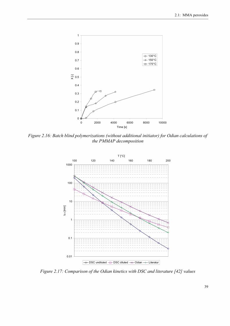
2.1: MMA peroxides
39
Figure 2.16: Batch blind polymerizations (without additional initiator) for Odian calculations of the PMMAP decomposition
Figure 2.17: Comparison of the Odian kinetics with DSC and literature [42] values
0
0.1
0.2
0.3
0.4
0.5
0.6
0.7
0.8
0.9
1
0 2000 4000 6000 8000 10000Time [s]
X [-
]
130°C150°C170°C
0.01
0.1
1
10
100
1000100 120 140 160 180 200
T [°C]
t 0.5 [
min
]
DSC undiluted DSC diluted Odian Literatur
Chapter 2: Self-Initiation at high temperatures
40
From figure 2.17 it becomes evident that there is a rather large discrepancy between the dif-
ferent kinetics for the decompositon of PMMAP. The kinetic constants determined by the Odian
method deliver, as expected, the slowest decomposition rate while the undiluted DSC sample
yields the fastest one. The true values can be found somewhere inbetween and comparison to
experimental data from batch polymerizations (conversion over time curves, see chapter 2.5) have
shown that the kinetics determined by DSC for the diluted sample lead to the best matching
results. Therefore, in all further modeling, the constants from table 4 were used for the PMMAP
decomposition rate.
2.2 Thermal initiation
By the term “thermal initiation”, polymer chemists understand the spontaneous initiation of
polymerization without interaction of any other compound than the monomer itself. For MMA,
this mechanism is, as explained in the following, bimolecular (unlike, for example, for styrene,
where it is unimolecular):
(EQ 2.25)
This definition needs to be underlined here, since the simple fact of observing an important
monomer conversion without addition of initiator does not necessarily reflect a thermal initiation.
As seen before, many different reactions can take place in the reaction system, which cause inita-
tion. Thus, for the correct determination of “true” thermal initiation rate coefficients, the mono-
mer must be carefully purified in order to exclude as much as possible impurities and foreign
substances.
Stickler and Meyerhoff [14] undertook a whole series of experiments in the late 70’s, where
they purified the monomer in a specially developped high-vacuum distillation device, from which
the monomer was immediately isolated in hermetic, silane treated glass ampoules. These
ampoules were closed by melting under high vacuum (10-4 Pa). Accordingly, the authors obtained
data for the thermal initiation that was significantly lower than what had been published before. In
fact, the rate of polymerization was so low that even the radical production by natural ionising
radiation (cosmic radiation) had to be taken into account. At 100 °C, the obtained polymer weight
M M+ 2P1∗→
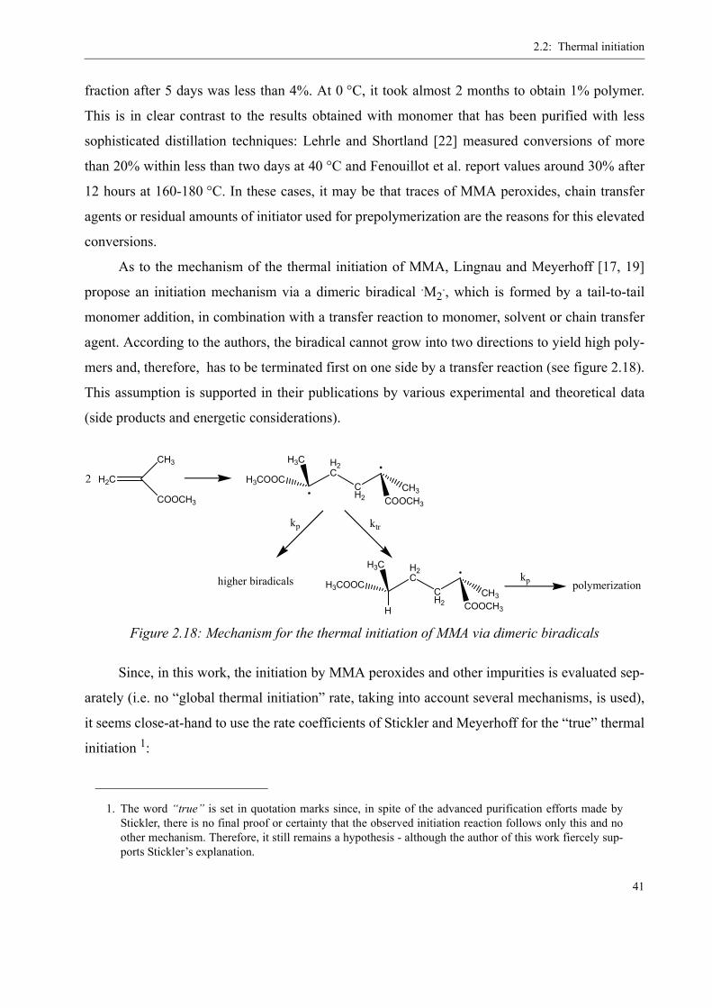
2.2: Thermal initiation
41
fraction after 5 days was less than 4%. At 0 °C, it took almost 2 months to obtain 1% polymer.
This is in clear contrast to the results obtained with monomer that has been purified with less
sophisticated distillation techniques: Lehrle and Shortland [22] measured conversions of more
than 20% within less than two days at 40 °C and Fenouillot et al. report values around 30% after
12 hours at 160-180 °C. In these cases, it may be that traces of MMA peroxides, chain transfer
agents or residual amounts of initiator used for prepolymerization are the reasons for this elevated
conversions.
As to the mechanism of the thermal initiation of MMA, Lingnau and Meyerhoff [17, 19]
propose an initiation mechanism via a dimeric biradical .M2., which is formed by a tail-to-tail
monomer addition, in combination with a transfer reaction to monomer, solvent or chain transfer
agent. According to the authors, the biradical cannot grow into two directions to yield high poly-
mers and, therefore, has to be terminated first on one side by a transfer reaction (see figure 2.18).
This assumption is supported in their publications by various experimental and theoretical data
(side products and energetic considerations).
Since, in this work, the initiation by MMA peroxides and other impurities is evaluated sep-
arately (i.e. no “global thermal initiation” rate, taking into account several mechanisms, is used),
it seems close-at-hand to use the rate coefficients of Stickler and Meyerhoff for the “true” thermal
initiation 1:
Figure 2.18: Mechanism for the thermal initiation of MMA via dimeric biradicals
1. The word “true” is set in quotation marks since, in spite of the advanced purification efforts made byStickler, there is no final proof or certainty that the observed initiation reaction follows only this and noother mechanism. Therefore, it still remains a hypothesis - although the author of this work fiercely sup-ports Stickler’s explanation.
H2C
CH3
COOCH3
2H2C
H3C
COOCH3
H3COOCCH3C
H2
kp ktr
higher biradicalsH2C
H3C
COOCH3
H3COOCCH3C
H2H
polymerizationkp
Chapter 2: Self-Initiation at high temperatures
42
(EQ 2.26)
As mentioned above (equation 2.25), it is a second order reaction in monomer concentra-
tion, thus it is
(EQ 2.27)
2.3 Initiation by the Chain Transfer Agent
Apart from the thermal initiation reactions by peroxide and the monomer itself, also chain
transfer agents can have a strong initiating potential. Common chain transfer agents in radical
polymerization are thiols, substances with a more or less long carbon backbone and an -SH reac-
tive end group. Most widely used are n-butanethiol, n-dodecanethiol and the aromatic species
phenylthiol.
Concerning the initiation of radical polymerization, Xia et al. [45] have investigated this
phenomenon for the MMA polymerization with different thiols at low temperatures and propose a
hydrogen transfer from thiol to MMA as mechanism of initiation:
(EQ 2.28)
For the high temperature polymerization, the initiating behavior is even more pronounced
than for low temperatures, as found by Fenouillot et al. [42], who determined the kinetic parame-
ters for n-butanethiol and MMA in the temperature range 130 °C - 168 °C. Although in this work
n-dodecanethiol (DDT) is used, these parameters were used for the modeling, assuming that they
Table 6: “True” thermal initiation rate coefficients from [14]
k0 [l mol-1s-1] EA [kJ mol-1]
kth 5.3703 108.5
Rthlog 0.73 5670T
------------–=
d M[ ]dt
------------- kth M[ ]2⋅–=
RSH + MMA MMA+RS
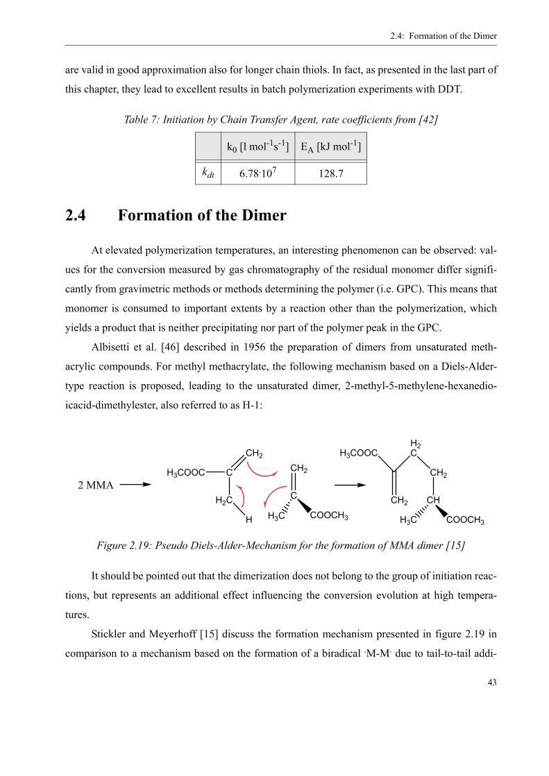
2.4: Formation of the Dimer
43
are valid in good approximation also for longer chain thiols. In fact, as presented in the last part of
this chapter, they lead to excellent results in batch polymerization experiments with DDT.
2.4 Formation of the Dimer
At elevated polymerization temperatures, an interesting phenomenon can be observed: val-
ues for the conversion measured by gas chromatography of the residual monomer differ signifi-
cantly from gravimetric methods or methods determining the polymer (i.e. GPC). This means that
monomer is consumed to important extents by a reaction other than the polymerization, which
yields a product that is neither precipitating nor part of the polymer peak in the GPC.
Albisetti et al. [46] described in 1956 the preparation of dimers from unsaturated meth-
acrylic compounds. For methyl methacrylate, the following mechanism based on a Diels-Alder-
type reaction is proposed, leading to the unsaturated dimer, 2-methyl-5-methylene-hexanedio-
icacid-dimethylester, also referred to as H-1:
It should be pointed out that the dimerization does not belong to the group of initiation reac-
tions, but represents an additional effect influencing the conversion evolution at high tempera-
tures.
Stickler and Meyerhoff [15] discuss the formation mechanism presented in figure 2.19 in
comparison to a mechanism based on the formation of a biradical .M-M. due to tail-to-tail addi-
Table 7: Initiation by Chain Transfer Agent, rate coefficients from [42]
k0 [l mol-1s-1] EA [kJ mol-1]
kdt 6.78.107 128.7
Figure 2.19: Pseudo Diels-Alder-Mechanism for the formation of MMA dimer [15]
2 MMAC
CH2
H2C
H3COOC
H
CH2
C
COOCH3H3C
CH2
H2C
CH2
CH
H3COOC
COOCH3H3C
Chapter 2: Self-Initiation at high temperatures
44
tion of two monomer molecules analog to the one of the thermal MMA polymerization (see
page 41), but in the end it appears that they favour the above presented enophilic mechanism.
In their publication, they also determine the formation rate for the MMA dimer over a wide
temperature range (100 °C - 275 °C). In agreement with the mechanism in figure 2.19, they find
second order reaction kinetics:
(EQ 2.29)
The formed dimer can be incorporated in the growing PMMA chains by copolymerization
as pointed out by Brand, Stickler and Meyerhoff [16], but this reaction as well as the homopoly-
merization of the dimer, itself, can be neglected in initiator-started polymerizations. The copoly-
merization might influence the thermal reaction of MMA, though.
2.5 Verification of the Kinetics in Batch Experiments
A series of batch experiments were carried out to verify the kinetics of the different thermal
initiation mechanisms as discussed above. The reactor setup is presented in figure 2.20. It consists
of a 1-l stainless steel reactor that is fixed into a double jacket and closed with a cover containing
a mechanical stirrer. It is heated by a flow of heat transfer fluid (synthetic oil, Shell Aseol Trans
SH) through the double jacket and an internal heating coil. For pressurization and sampling there
is an immersion tube with a three-way valve. One end of the three-way valve is connected to a
nitrogen gas cylinder, the other ends in a sampling vial. Samples are taken through the three-way
valve directly into pre-cooled glass vials with screw caps (Schott Duran) and immediately frozen
to -20°C. They are consecutively analyzed for conversion and molecular weight.
Table 8: Formation rate coefficients for the dimerisation of MMA [15]
k0 [l mol-1 s-1] EA [kJ mol-1]
kH-1 4.9386 105 107.2
d H 1–[ ]dt
------------------- kH 1– M[ ]2⋅=

2.5: Verification of the Kinetics in Batch Experiments
45
The addition of initiator or other additives under pressure is realized by a pressurized steel
cylinder on top of the cover. The reactor content is mixed by a propeller and an anchor stirrer at
the bottom, both fixed on the same axis.
The monomer / solvent mixture is filled into the open reactor, which is then closed tightly
and pressurized with N2 at 10 bar. With the help of an oil thermostat, the whole device is brought
as quickly as possible to reaction temperature (ΔT/Δt ~ 3 °C/min). Depending on the experiment,
an initiator solution can be added at an arbitrary time t through the cylinder fixed on top of the
reactor without opening or depressurizing the reactor.
In the beginning, blind experiments without any radical initiator were carried out to exam-
ine the auto-initiation of non-purified MMA (i.e. from the barrel) and to verify the model parame-
ters determined in the preceding paragraphs. Figure 2.21 contains the results of these experiments
Figure 2.20: Schematic drawing and photograph of the 1-L batch reactor used in this work
Oil circuit Oil circuit
Sampling
Cylinder for the addition of initiator
N2-pressurization
Oil circuit Oil circuit
Sampling
Cylinder for the addition of initiator
N2-pressurization
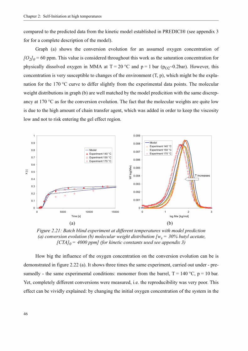
Chapter 2: Self-Initiation at high temperatures
46
compared to the predicted data from the kinetic model established in PREDICI® (see appendix 3
for for a complete description of the model).
Graph (a) shows the conversion evolution for an assumed oxygen concentration of
[O2]0 = 60 ppm. This value is considered throughout this work as the saturation concentration for
physically dissolved oxygen in MMA at T = 20 °C and p = 1 bar (pO2~0.2bar). However, this
concentration is very susceptible to changes of the environment (T, p), which might be the expla-
nation for the 170 °C curve to differ slightly from the experimental data points. The molecular
weight distributions in graph (b) are well matched by the model predicition with the same discrep-
ancy at 170 °C as for the conversion evolution. The fact that the molecular weights are quite low
is due to the high amount of chain transfer agent, which was added in order to keep the viscosity
low and not to risk entering the gel effect region.
How big the influence of the oxygen concentration on the conversion evolution can be is
demonstrated in figure 2.22 (a). It shows three times the same experiment, carried out under - pre-
sumedly - the same experimental conditions: monomer from the barrel, T = 140 °C, p = 10 bar.
Yet, completely different conversions were measured, i.e. the reproducibility was very poor. This
effect can be vividly explained: by changing the initial oxygen concentration of the system in the
(a) (b)Figure 2.21: Batch blind experiment at different temperatures with model prediction (a) conversion evolution (b) molecular weight distribution [ws = 30% butyl acetate,
[CTA]0 = 4000 ppm] (for kinetic constants used see appendix 3)
0
0.1
0.2
0.3
0.4
0.5
0.6
0.7
0.8
0.9
1
0 5000 10000 15000
Time [s]
X [-
]
ModelExperiment 140 °CExperiment 150 °CExperiment 170 °C
0
0.001
0.002
0.003
0.004
0.005
0.006
0.007
0.008
0.009
0 1 2 3log Mw [kg/mol]
Wf l
og(M
w)
ModelExperiment 140 °CExperiment 150 °CExperiment 170 °C
T increases
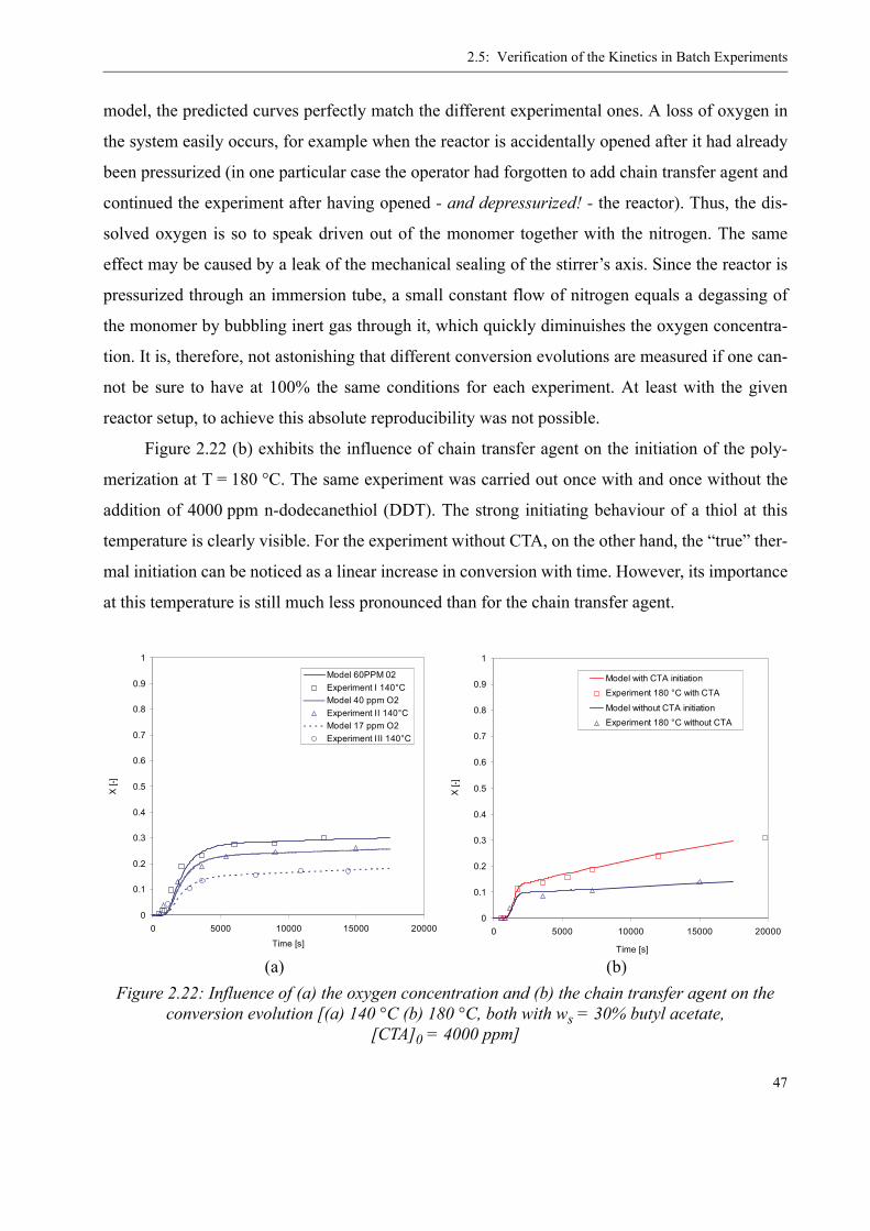
2.5: Verification of the Kinetics in Batch Experiments
47
model, the predicted curves perfectly match the different experimental ones. A loss of oxygen in
the system easily occurs, for example when the reactor is accidentally opened after it had already
been pressurized (in one particular case the operator had forgotten to add chain transfer agent and
continued the experiment after having opened - and depressurized! - the reactor). Thus, the dis-
solved oxygen is so to speak driven out of the monomer together with the nitrogen. The same
effect may be caused by a leak of the mechanical sealing of the stirrer’s axis. Since the reactor is
pressurized through an immersion tube, a small constant flow of nitrogen equals a degassing of
the monomer by bubbling inert gas through it, which quickly diminuishes the oxygen concentra-
tion. It is, therefore, not astonishing that different conversion evolutions are measured if one can-
not be sure to have at 100% the same conditions for each experiment. At least with the given
reactor setup, to achieve this absolute reproducibility was not possible.
Figure 2.22 (b) exhibits the influence of chain transfer agent on the initiation of the poly-
merization at T = 180 °C. The same experiment was carried out once with and once without the
addition of 4000 ppm n-dodecanethiol (DDT). The strong initiating behaviour of a thiol at this
temperature is clearly visible. For the experiment without CTA, on the other hand, the “true” ther-
mal initiation can be noticed as a linear increase in conversion with time. However, its importance
at this temperature is still much less pronounced than for the chain transfer agent.
(a) (b)Figure 2.22: Influence of (a) the oxygen concentration and (b) the chain transfer agent on the
conversion evolution [(a) 140 °C (b) 180 °C, both with ws = 30% butyl acetate, [CTA]0 = 4000 ppm]
0
0.1
0.2
0.3
0.4
0.5
0.6
0.7
0.8
0.9
1
0 5000 10000 15000 20000
Time [s]
X [-
]
Model 60PPM 02Experiment I 140°CModel 40 ppm O2Experiment II 140°CModel 17 ppm O2Experiment III 140°C
0
0.1
0.2
0.3
0.4
0.5
0.6
0.7
0.8
0.9
1
0 5000 10000 15000 20000
Time [s]
X [-
]
Model with CTA initiationExperiment 180 °C with CTA
Model without CTA initiationExperiment 180 °C without CTA
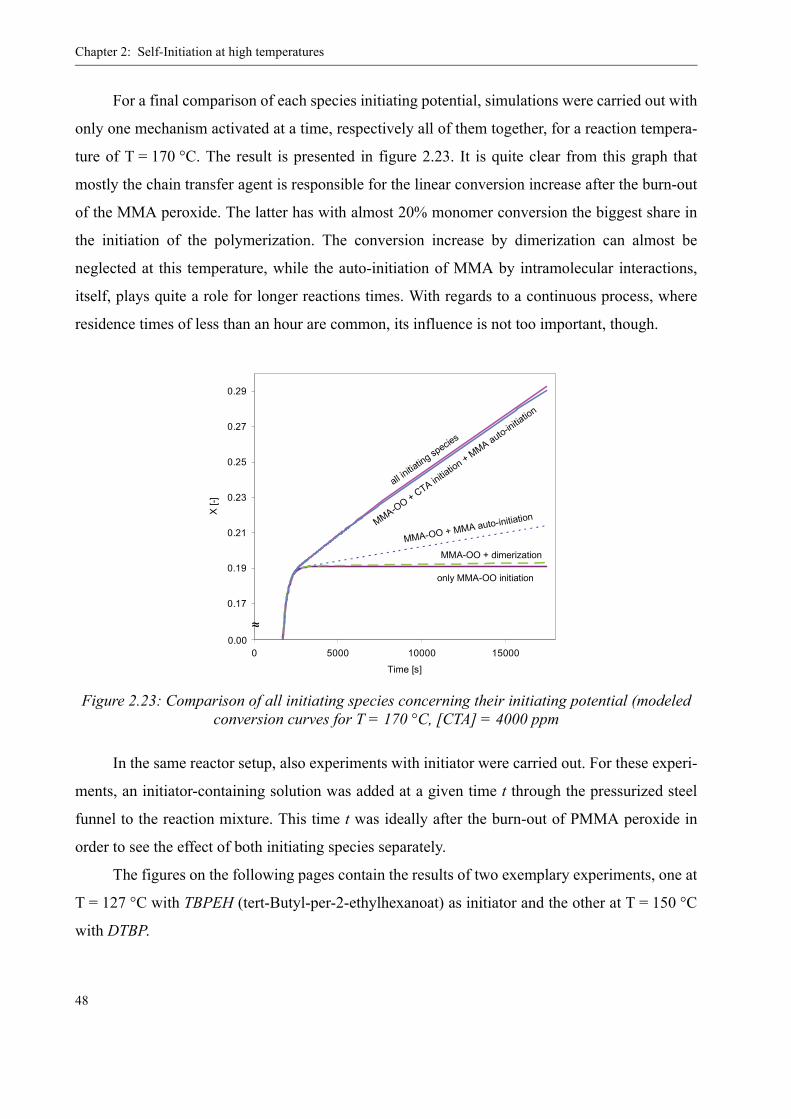
Chapter 2: Self-Initiation at high temperatures
48
For a final comparison of each species initiating potential, simulations were carried out with
only one mechanism activated at a time, respectively all of them together, for a reaction tempera-
ture of T = 170 °C. The result is presented in figure 2.23. It is quite clear from this graph that
mostly the chain transfer agent is responsible for the linear conversion increase after the burn-out
of the MMA peroxide. The latter has with almost 20% monomer conversion the biggest share in
the initiation of the polymerization. The conversion increase by dimerization can almost be
neglected at this temperature, while the auto-initiation of MMA by intramolecular interactions,
itself, plays quite a role for longer reactions times. With regards to a continuous process, where
residence times of less than an hour are common, its influence is not too important, though.
In the same reactor setup, also experiments with initiator were carried out. For these experi-
ments, an initiator-containing solution was added at a given time t through the pressurized steel
funnel to the reaction mixture. This time t was ideally after the burn-out of PMMA peroxide in
order to see the effect of both initiating species separately.
The figures on the following pages contain the results of two exemplary experiments, one at
T = 127 °C with TBPEH (tert-Butyl-per-2-ethylhexanoat) as initiator and the other at T = 150 °C
with DTBP.
Figure 2.23: Comparison of all initiating species concerning their initiating potential (modeled conversion curves for T = 170 °C, [CTA] = 4000 ppm
0.15
0.17
0.19
0.21
0.23
0.25
0.27
0.29
0 5000 10000 15000
Time [s]
X [-
]
0.00~~
only MMA-OO initiation
MMA-OO + dimerization
MMA-OO + MMA auto-initiationMMA-OO + CTA initiation + MMA auto-initia
tion
all initia
ting species
0.15
0.17
0.19
0.21
0.23
0.25
0.27
0.29
0 5000 10000 15000
Time [s]
X [-
]
0.00~~
only MMA-OO initiation
MMA-OO + dimerization
MMA-OO + MMA auto-initiationMMA-OO + CTA initiation + MMA auto-initia
tion
all initia
ting species
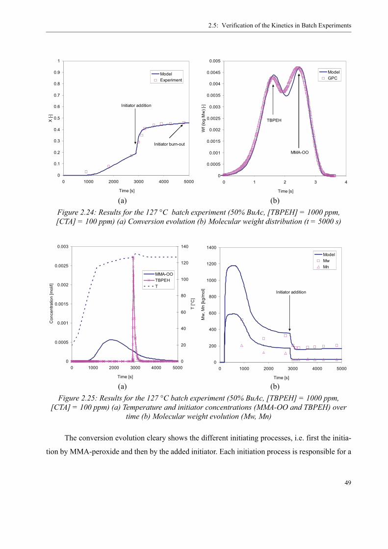
2.5: Verification of the Kinetics in Batch Experiments
49
The conversion evolution cleary shows the different initiating processes, i.e. first the initia-
tion by MMA-peroxide and then by the added initiator. Each initiation process is responsible for a
(a) (b)Figure 2.24: Results for the 127 °C batch experiment (50% BuAc, [TBPEH] = 1000 ppm, [CTA] = 100 ppm) (a) Conversion evolution (b) Molecular weight distribution (t = 5000 s)
(a) (b)Figure 2.25: Results for the 127 °C batch experiment (50% BuAc, [TBPEH] = 1000 ppm,
[CTA] = 100 ppm) (a) Temperature and initiator concentrations (MMA-OO and TBPEH) over time (b) Molecular weight evolution (Mw, Mn)
0
0.1
0.2
0.3
0.4
0.5
0.6
0.7
0.8
0.9
1
0 1000 2000 3000 4000 5000
Time [s]
X [-
]
ModelExperiment
Initiator addition
Initiator burn-out
0
0.0005
0.001
0.0015
0.002
0.0025
0.003
0.0035
0.004
0.0045
0.005
0 1 2 3 4
Time [s]
Wf (
log
Mw
) [-]
ModelGPC
TBPEH
MMA-OO
0
0.0005
0.001
0.0015
0.002
0.0025
0.003
0 1000 2000 3000 4000 5000
Time [s]
Con
cent
ratio
n [m
ol/l]
0
20
40
60
80
100
120
140
T [°
C]
MMA-OOTBPEHT
0
200
400
600
800
1000
1200
1400
0 1000 2000 3000 4000 5000
Time [s]
Mw
, Mn
[kg/
mol
]
ModelMwMn
Initiator addition
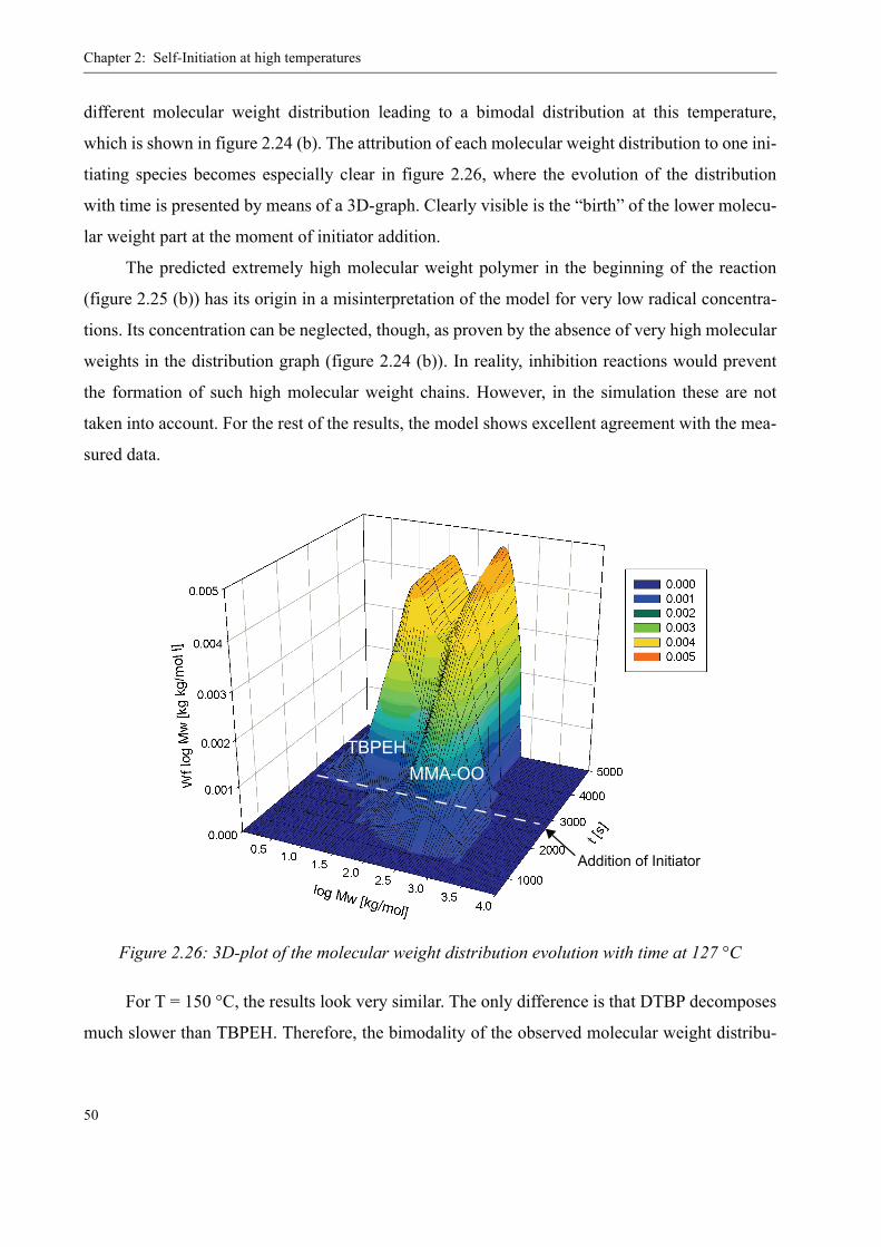
Chapter 2: Self-Initiation at high temperatures
50
different molecular weight distribution leading to a bimodal distribution at this temperature,
which is shown in figure 2.24 (b). The attribution of each molecular weight distribution to one ini-
tiating species becomes especially clear in figure 2.26, where the evolution of the distribution
with time is presented by means of a 3D-graph. Clearly visible is the “birth” of the lower molecu-
lar weight part at the moment of initiator addition.
The predicted extremely high molecular weight polymer in the beginning of the reaction
(figure 2.25 (b)) has its origin in a misinterpretation of the model for very low radical concentra-
tions. Its concentration can be neglected, though, as proven by the absence of very high molecular
weights in the distribution graph (figure 2.24 (b)). In reality, inhibition reactions would prevent
the formation of such high molecular weight chains. However, in the simulation these are not
taken into account. For the rest of the results, the model shows excellent agreement with the mea-
sured data.
For T = 150 °C, the results look very similar. The only difference is that DTBP decomposes
much slower than TBPEH. Therefore, the bimodality of the observed molecular weight distribu-
Figure 2.26: 3D-plot of the molecular weight distribution evolution with time at 127 °C
MMA-OOTBPEH
Addition of Initiator
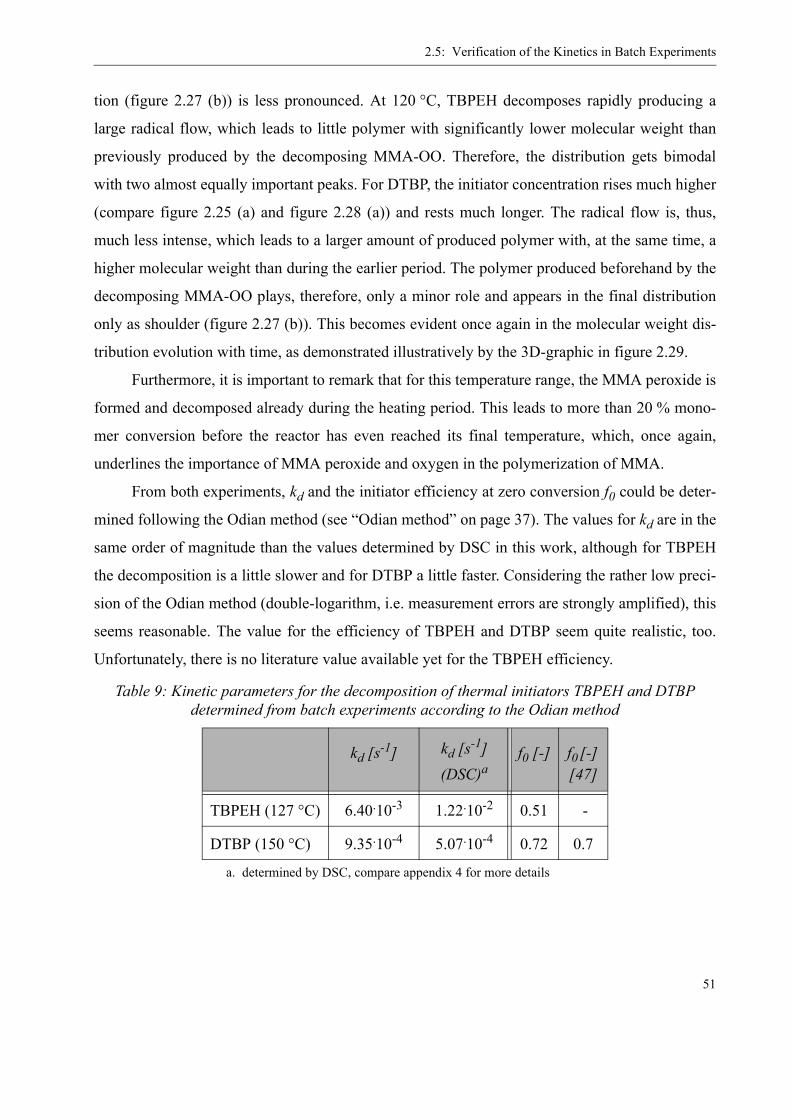
2.5: Verification of the Kinetics in Batch Experiments
51
tion (figure 2.27 (b)) is less pronounced. At 120 °C, TBPEH decomposes rapidly producing a
large radical flow, which leads to little polymer with significantly lower molecular weight than
previously produced by the decomposing MMA-OO. Therefore, the distribution gets bimodal
with two almost equally important peaks. For DTBP, the initiator concentration rises much higher
(compare figure 2.25 (a) and figure 2.28 (a)) and rests much longer. The radical flow is, thus,
much less intense, which leads to a larger amount of produced polymer with, at the same time, a
higher molecular weight than during the earlier period. The polymer produced beforehand by the
decomposing MMA-OO plays, therefore, only a minor role and appears in the final distribution
only as shoulder (figure 2.27 (b)). This becomes evident once again in the molecular weight dis-
tribution evolution with time, as demonstrated illustratively by the 3D-graphic in figure 2.29.
Furthermore, it is important to remark that for this temperature range, the MMA peroxide is
formed and decomposed already during the heating period. This leads to more than 20 % mono-
mer conversion before the reactor has even reached its final temperature, which, once again,
underlines the importance of MMA peroxide and oxygen in the polymerization of MMA.
From both experiments, kd and the initiator efficiency at zero conversion f0 could be deter-
mined following the Odian method (see “Odian method” on page 37). The values for kd are in the
same order of magnitude than the values determined by DSC in this work, although for TBPEH
the decomposition is a little slower and for DTBP a little faster. Considering the rather low preci-
sion of the Odian method (double-logarithm, i.e. measurement errors are strongly amplified), this
seems reasonable. The value for the efficiency of TBPEH and DTBP seem quite realistic, too.
Unfortunately, there is no literature value available yet for the TBPEH efficiency.
Table 9: Kinetic parameters for the decomposition of thermal initiators TBPEH and DTBP determined from batch experiments according to the Odian method
kd [s-1] kd [s-1](DSC)a
a. determined by DSC, compare appendix 4 for more details
f0 [-] f0 [-] [47]
TBPEH (127 °C) 6.40.10-3 1.22.10-2 0.51 -
DTBP (150 °C) 9.35.10-4 5.07.10-4 0.72 0.7
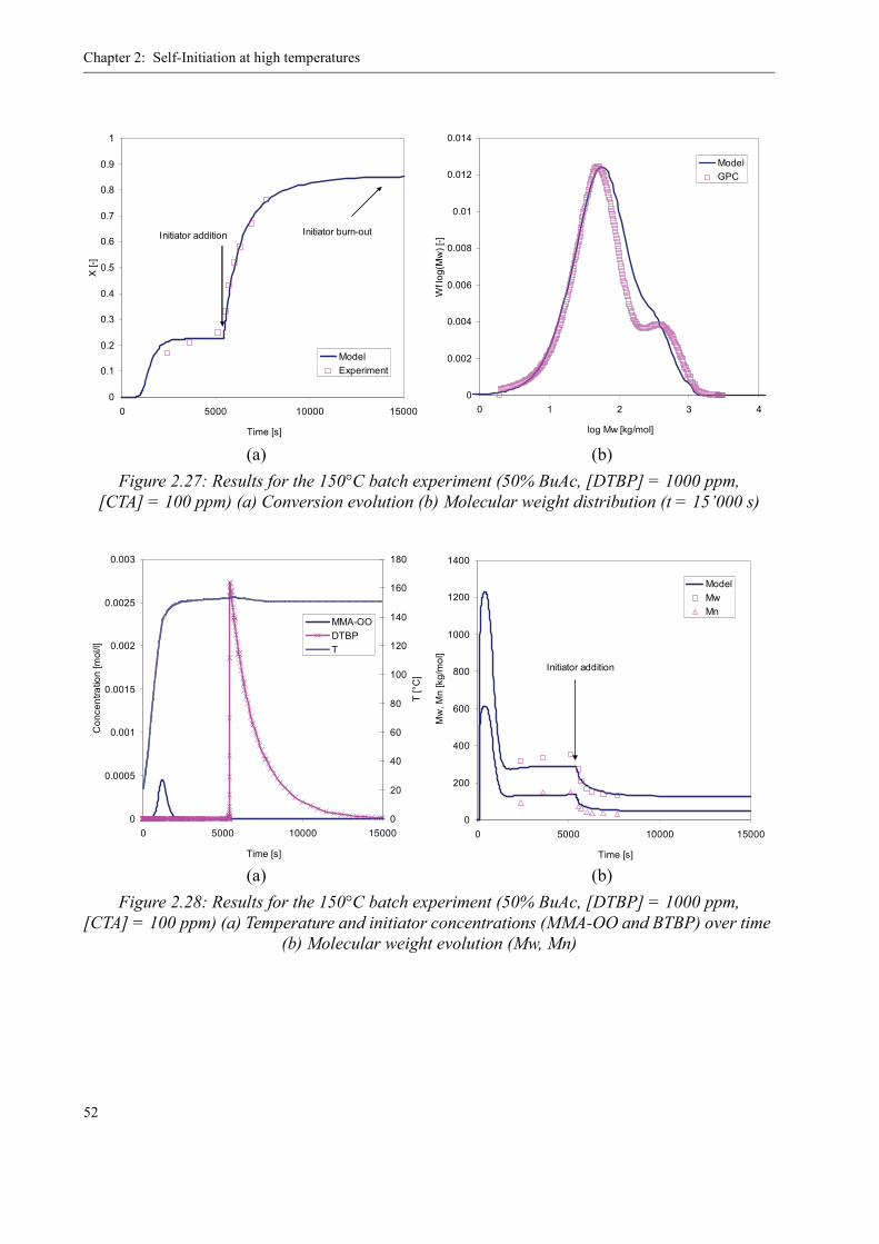
Chapter 2: Self-Initiation at high temperatures
52
(a) (b)Figure 2.27: Results for the 150°C batch experiment (50% BuAc, [DTBP] = 1000 ppm,
[CTA] = 100 ppm) (a) Conversion evolution (b) Molecular weight distribution (t = 15’000 s)
(a) (b)Figure 2.28: Results for the 150°C batch experiment (50% BuAc, [DTBP] = 1000 ppm,
[CTA] = 100 ppm) (a) Temperature and initiator concentrations (MMA-OO and BTBP) over time (b) Molecular weight evolution (Mw, Mn)
0
0.1
0.2
0.3
0.4
0.5
0.6
0.7
0.8
0.9
1
0 5000 10000 15000
Time [s]
X [-
]
ModelExperiment
Initiator addition Initiator burn-out
0
0.002
0.004
0.006
0.008
0.01
0.012
0.014
0 1 2 3 4
log Mw [kg/mol]W
f log
(Mw
) [-]
ModelGPC
0
0.0005
0.001
0.0015
0.002
0.0025
0.003
0 5000 10000 15000
Time [s]
Con
cent
ratio
n [m
ol/l]
0
20
40
60
80
100
120
140
160
180
T [°
C]
MMA-OODTBPT
0
200
400
600
800
1000
1200
1400
0 5000 10000 15000
Time [s]
Mw
, Mn
[kg/
mol
]
ModelMwMn
Initiator addition
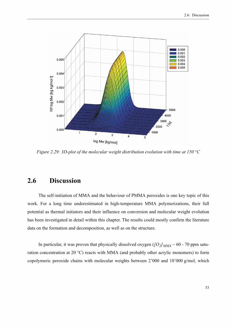
2.6: Discussion
53
2.6 Discussion
The self-initiation of MMA and the behaviour of PMMA peroxides is one key topic of this
work. For a long time underestimated in high-temperature MMA polymerizations, their full
potential as thermal initiators and their influence on conversion and molecular weight evolution
has been investigated in detail within this chapter. The results could mostly confirm the literature
data on the formation and decomposition, as well as on the structure.
In particular, it was proven that physically dissolved oxygen ([O2]MMA ~ 60 - 70 ppm satu-
ration concentration at 20 °C) reacts with MMA (and probably other acrylic monomers) to form
copolymeric peroxide chains with molecular weights between 2’000 and 10’000 g/mol, which
Figure 2.29: 3D-plot of the molecular weight distribution evolution with time at 150 °C

Chapter 2: Self-Initiation at high temperatures
54
accumulate in the system until the monomer is heated. The presence of these peroxides was
proven by several analytical techniques, among which NMR, GPC and TGA-MS.
At high temperatures (> 100 °C), these peroxides decompose exothermally and initiate the
radical polymerization. It is, therefore, legitimate to speak of a high-temperature decomposing
initiator. Depending on the reaction conditions, monomer conversions as high as 30 % can be
observed.
The formation and decomposition kinetics were determined experimentally and the results
included as reaction (formation-, decomposition- and initiation-) steps in a kinetic model (the
complete model is presented in appendix 3). With this model, it is now possible to describe batch
polymerizations with and without the addition of thermal initiator in a very precise way. A miss-
ing point is the possibility to determine reliably the oxygen content of MMA samples. The satura-
tion concentration had to be estimated to 60-80 ppm, a value which corresponds to literature data
for other acrylics and organic solvents [35, 48]. Especially in the batch reactor the reproducibility
of experiments was sometimes rather poor, which is assumed to be due to changing oxygen con-
centrations. These are produced by the pressurization and depressurization of the reactor with
nitrogen during the preparation phase. A determination of the O2 amount in the organic phase
could help improve the understanding of these effects.
Aside from the initiation by MMA peroxides, the initiation by chain transfer agent, the ther-
mal initiation of MMA due to intramolecular interactions in the pure monomer, as well as the for-
mation of dimers were also investigated. While the chain transfer agent has a significant influence
on the initiation at 170 °C and above, the “true” thermal initiation of MMA plays no major role
below 180 °C and is, therefore, negligible for most experiments carried out in this work. The
same applies for the formation of dimers and higher oligomers, which only start having a measur-
able effect on the conversion even above 180 °C.
The observed phenomena will be included in the model for the description of the continu-
ous pilot plant process and evaluated once again in this context.
2.6: Discussion
55
Short Summary:
• The spontaneous polymerization of MMA is an important aspect in high tempera-
ture processes and cannot be neglected in the kinetic modeling
• Different mechanisms for the initiation and dimerization of MMA have been
evaluated concerning their importance in terms of monomer conversion
• It was found that the major role in the thermal initiation of MMA play polymeric
peroxides that form from physically dissolved oxygen
• The formation and decomposition kinetics of these peroxides were successfully
determined in this work and the peroxides, themselves, were characterized by
various analytical methods
• Finally, the determined kinetics for the various reaction mechanisms discussed in
this chapter were discussed with respect to experimental data obtained from high
temperature polymerization reactions carried out in this work.

Chapter 2: Self-Initiation at high temperatures
56
57
CHAPTER 3
High Temperature Gel Effect
The term “gel effect” or “Trommsdorff effect” generally describes the phenomenon that,
in homogeneous bulk polymerizations at higher polymer contents and in particular at low tem-
peratures, the reaction rate and degree of polymerization increase significantly. This effect is
especially intense in the methyl methacrylate polymerization, but occurs also for monomers
like styrene, vinyl acetate and others. Trommsdorff [49] was among the first to explain his
observations by the fact that, with increasing viscosity of the reaction medium, the diffusion of
the macro radicals and, thus, the termination of the reactive chains is impeded whereas the dif-
fusion of the smaller monomer molecules to the reactive centers at the chain ends continues
undisturbed [50]. The reason of this apparent increase in reaction rate and degree of polymer-
ization is, therefore, a strong drop of the termination rate with growing polymer fraction in the
reaction medium.
In the modeling of MMA polymerizations, the gel effect is one of the most important
factors to consider. It has a strong influence on both, the rate of monomer conversion and its
final value (and, therefore, on the heat production that is to expect), as well as on the molecular
weight distribution. Thus, it becomes inevitable for any kinetic model to correctly describe the
changing of the termination rate kt with increasing viscosity. The term conversion is avoided
on purpose in this context, since the intensity of the gel effect does not only depend on the
monomer conversion, but also on factors like solvent content, molecular weight and tempera-
ture. For example, as will be shown further on in this chapter, in a polymerization above 120°C
with 30% solvent, the gel effect becomes almost negligible. The same applies to bulk polymer-

Chapter 3: High Temperature Gel Effect
58
izations at temperatures above 170°C, where in the conversion-time curve no clear acceleration is
visible anymore.
Since the beginnings of polymerization modeling, the gel effect has been extensively inves-
tigated and kinetically described by innumerable authors. In particular during the 80’s, several
important advances in its description were made. According to Tefera, Weickert and Westerterp
[51], there exist 5 different model concepts, each of them describing the termination rate constant
by another phenomenon:
• Viscosity based models
• Conversion or polymer weight fraction based models
• Reptation theory based models
• Entanglement concept based models
• Free volume theory based models,
Apart from the theory that lies behind each model, one major difference is the use of a break
point in some of them, i.e. an artificial switch at a certain conversion, for example, from where on
the calculation of kt changes suddenly. This is, however, in contradiction to reality, since the gel
effect does not start at a sudden time t, but is slowly increasing with the polymer fraction. There-
fore, there is no sense in considering these models for this work. In the following, only models
that offer a continuous correlation of kt with other reaction parameters will be discussed, namely
models based on the free volume theory.
Although these models are based on the same theory, i.e. the free volume theory of Vrentas
and Duda [52-55], they differ fundamentally in their general concept. However, one thing they all
have in common is the fact that they were derived for temperature ranges far below the glass tran-
sition temperature Tg, except for two models developed at EPFL in the 90’s, one by Fleury and
the other by Hoppe [5, 56]. The glass transition is the temperature, where the polymer changes
from an amorphous glass state to a viscous melt, which comes along with drastic consequences on
its physical properties, in particular the diffusion characteristics. The Tg for homogeneous PMMA
is approximately 115°C [57], but varies depending on the method of determination and on the
polymer characteristics (mostly the tacticity, which changes with polymerization temperature).
In this chapter, it will be tried to comprehensively explain the gel effect, the different gel
effect models and their applicability to different types of processes. Finally, a refined model for
the high temperature gel effect in batch and continuous processes is developed and presented.

3.1: Theory
59
3.1 Theory
Following a simplified model, the rate of polymerization for homogeneous radical polymer-
izations is defined as:
(EQ 3.1)
and the kinetic chain length as:
(EQ 3.2)
This “classical” kinetic description of the polymerization is only valid in first approxima-
tion and for small monomer conversions, since it does not take into account any diffusion limita-
tions. It assumes ideal homogeneous conditions, in which the rate determining steps are the
reactions themselves. However, with increasing monomer conversion, the viscosity of the system
can - depending on the reaction conditions - increase drastically, thus severely limiting the free-
dom to move first only for the larger chain molecules, then also for the small monomer molecules.
The first consequence of this limited mobility is that the active polymer chains are hindered from
terminating each other by disproportionation or combination. According to the theory established
by Chiu, Carratt and Soong [58] in 1983, the termination takes place in three steps:
1. The polymer radicals, initially separated by more than one molecular diameter, approach by translational diffusion
2. Once in direct proximity, the radical chain ends move toward each other (segmental diffusion)
3. After proper orientation of the chains to each other is reached, the termination reaction can take place
In figure 3.1 is illustrated schematically the surrounding of an active chain radical on the
molecular level. Within the termination radius rt around the active radical center, the termination
rate is the intrinsic one kt,0. This “true” termination rate reflects the speed of termination of two
polymer radicals under ideal, i.e. not diffusion controlled, conditions. However, as soon as the dif-
fusion of large chain molecules from r >> rt to r < rt is limited, the apparent termination rate con-
Rpd M[ ]
dt-------------–
kp
kt
-------- 2 f kd I[ ]⋅ ⋅ ⋅ M[ ]⋅ ⋅= =
Pkp
2
kt----- M[ ]2
Rp------------⋅
kp
kt
-------- 12 f kd I[ ]⋅ ⋅ ⋅
---------------------------------- M[ ]⋅ ⋅= =
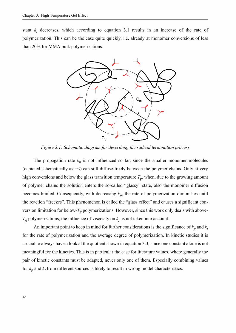
Chapter 3: High Temperature Gel Effect
60
stant kt decreases, which according to equation 3.1 results in an increase of the rate of
polymerization. This can be the case quite quickly, i.e. already at monomer conversions of less
than 20% for MMA bulk polymerizations.
The propagation rate kp is not influenced so far, since the smaller monomer molecules
(depicted schematically as =<) can still diffuse freely between the polymer chains. Only at very
high conversions and below the glass transition temperature Tg, when, due to the growing amount
of polymer chains the solution enters the so-called “glassy” state, also the monomer diffusion
becomes limited. Consequently, with decreasing kp, the rate of polymerization diminishes until
the reaction “freezes”. This phenomenon is called the “glass effect” and causes a significant con-
version limitation for below-Tg polymerizations. However, since this work only deals with above-
Tg polymerizations, the influence of viscosity on kp is not taken into account.
An important point to keep in mind for further considerations is the significance of kp and kt
for the rate of polymerization and the average degree of polymerization. In kinetic studies it is
crucial to always have a look at the quotient shown in equation 3.3, since one constant alone is not
meaningful for the kinetics. This is in particular the case for literature values, where generally the
pair of kinetic constants must be adapted, never only one of them. Especially combining values
for kp and kt from different sources is likely to result in wrong model characteristics.
Figure 3.1: Schematic diagram for describing the radical termination process
rt
Cb
Cm
rb
rt
Cb
Cm
rb
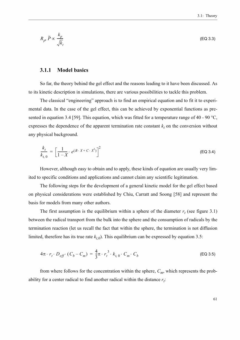
3.1: Theory
61
(EQ 3.3)
3.1.1 Model basics
So far, the theory behind the gel effect and the reasons leading to it have been discussed. As
to its kinetic description in simulations, there are various possibilities to tackle this problem.
The classical “engineering” approach is to find an empirical equation and to fit it to experi-
mental data. In the case of the gel effect, this can be achieved by exponential functions as pre-
sented in equation 3.4 [59]. This equation, which was fitted for a temperature range of 40 - 90 °C,
expresses the dependence of the apparent termination rate constant kt on the conversion without
any physical background.
(EQ 3.4)
However, although easy to obtain and to apply, these kinds of equation are usually very lim-
ited to specific conditions and applications and cannot claim any scientific legitimation.
The following steps for the development of a general kinetic model for the gel effect based
on physical considerations were established by Chiu, Carratt and Soong [58] and represent the
basis for models from many other authors.
The first assumption is the equilibrium within a sphere of the diameter rt (see figure 3.1)
between the radical transport from the bulk into the sphere and the consumption of radicals by the
termination reaction (let us recall the fact that within the sphere, the termination is not diffusion
limited, therefore has its true rate kt,0). This equilibrium can be expressed by equation 3.5:
(EQ 3.5)
from where follows for the concentration within the sphere, Cm, which represents the prob-
ability for a center radical to find another radical within the distance rt:
Rp P,kp
kt
--------∝
ktkt 0,-------- 1
1 X–------------ e B X C X2⋅+⋅( )⋅
2=
4π rt Deff Cb Cm–( )⋅ ⋅ ⋅ 43---π rt
3 kt 0, Cm Cb⋅ ⋅ ⋅ ⋅=

Chapter 3: High Temperature Gel Effect
62
(EQ 3.6)
The apparent reaction rate, which can be written as ktCb2, is equal to kt,0 Cb Cm (the intrinsic
termination rate constant times the probability for two radicals to encounter each other), which
gives:
(EQ 3.7)
Therefore, from equation 3.6 and equation 3.7 follows the basic equation for the apparent
termination rate, including reaction and mass-transfer limitation:
(EQ 3.8)
kt,0 is independent of conversion and molecular weight, yet strongly temperature dependent.
The diffusion coefficient Deff, on the other hand, is a function of temperature, conversion and
molecular weight. The termination radius rm can, for reasons of simplification, be considered con-
stant.
Since rm, Cb and Deff are unknowns, the transformation of equation 3.8 into something more
tangible is the basic work of the different authors that have developed their models on this basis.
In the following, the most important ones will be presented.
3.2 Existing Model Evaluation
The following evaluation of existing models only represents a small part of all the different
models that can be found in literature. Due to the limited time frame and the variety of different
subjects dealt with in this work, only the most representative modeling approaches could be cho-
sen for comparison. This should not imply that models not mentioned here are less suitable for the
description of the gel effect under the conditions they were derived for. Namely the viscosity
related model of Buback [60] and the free-volume gel effect model of Hamielec [61], which are
well known in the polymer reaction engineering field, were not considered in the following evalu-
CmD Cb⋅
Drt
2
3------ kt 0, Cb⋅ ⋅+
-----------------------------------------=
kt Cb2 kt 0, Cb Cm⋅ ⋅≡⋅
1kt---- 1
kt 0,--------
rt2 Cb⋅3Deff---------------+=
3.2: Existing Model Evaluation
63
ation due to known issues at high temperatures [62]. A more exhaustive description of a large
number of existing models can be found in [51].
3.2.1 Chiu, Carratt and Soong (CCS) [58]
Chiu, Carrat and Soong continued the development of their model by separating the diffu-
sion coefficient Deff into a temperature- and molecular-weight-dependent part D(T, Mw) and a
conversion dependent part D(X):
(EQ 3.9)
The term is expressed by a function ; Cb is replaced by the zeroth
moment of the polymer distribution. The temperature- and molecular-weight-dependence of θt
can, according to the authors, not take any simple mathematical form and is, therefore, fitted to
experimental data. Since the molecular weight, at least for non-chain-transfer-regulated batch
polymerizations, is mainly governed by the initial initiator concentration [I]0, it can also be writ-
ten θt(T, [I]0). The conversion dependence of D can be described by the free volume theory. The
authors make use of the so-called Fujita-Doolittle equation:
with (monomer volume fraction) (EQ 3.10)
A and B are functions of temperature that have to be fitted to experimental data, too. D0 is
the diffusion coefficient at zero conversion. As result of the combination of above equations, the
authors present the following:
(EQ 3.11)
D0 was taken into the function θt(T, [I]0) and transformation of the log into the natural log-
arithm ln leaves a factor ln(10) = 2.3. The necessary information about the fitting of the parame-
ters θt(T, [I]0), A(T) and B(T) to experimental data can, unfortunately, only be found in a
consecutive article of the authors [63]: θt(T, [I]0) is expressed by an Arrhenius law,
1kt---- 1
kt 0,--------
rt2
3D T Mw,( )---------------------------
CbD X( )------------- 1
kt 0,-------- θt
λ0D X( )-------------⋅+≡⋅+=
rt2
3D T Mw,( )--------------------------- θt T Mw,( )
DD0------log
φmA T( ) B T( ) φm⋅+-----------------------------------------= φm
1 X–1 εX+----------------=
1kt---- 1
kt 0, T( )----------------- θt T I[ ]0,( )
λ02.3φm
A T( ) B T( )φm+-------------------------------------exp
-----------------------------------------------------⋅+=
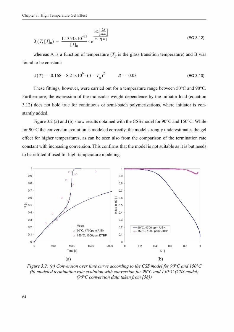
Chapter 3: High Temperature Gel Effect
64
(EQ 3.12)
whereas A is a function of temperature (Tg is the glass transition temperature) and B was
found to be constant:
(EQ 3.13)
These fittings, however, were carried out for a temperature range between 50°C and 90°C.
Furthermore, the expression of the molecular weight dependence by the initiator load (equation
3.12) does not hold true for continuous or semi-batch polymerizations, where initiator is con-
stantly added.
Figure 3.2 (a) and (b) show results obtained with the CSS model for 90°C and 150°C. While
for 90°C the conversion evolution is modeled correctly, the model strongly underestimates the gel
effect for higher temperatures, as can be seen also from the comparison of the termination rate
constant with increasing conversion. This confirms that the model is not suitable as it is but needs
to be refitted if used for high-temperature modeling.
(a) (b)Figure 3.2: (a) Conversion over time curve according to the CSS model for 90°C and 150°C
(b) modeled termination rate evolution with conversion for 90°C and 150°C (CSS model)(90°C conversion data taken from [58])
θt T I[ ]0,( ) 1.1353 22–×10I[ ]0
--------------------------------- e
142 kJmol---------
R T K[ ]⋅------------------------
⋅=
A T( ) 0.168 8.21 6×10 T Tg–( )2⋅–= B 0.03=
0
0.1
0.2
0.3
0.4
0.5
0.6
0.7
0.8
0.9
1
0 500 1000 1500 2000
Time [s]
X [-
]
Model
90°C, 4700ppm AIBN
150°C, 1000ppm DTBP
0
0.1
0.2
0.3
0.4
0.5
0.6
0.7
0.8
0.9
1
0 0.2 0.4 0.6 0.8 1
X [-]
ln k
t / ln
kt0
[-]
90°C, 4700 ppm AIBN150°C, 1000 ppm DTBP

3.2: Existing Model Evaluation
65
3.2.2 Achilias and Kiparissides [64]
The model of Achilias and Kiparissides uses the same basic considerations. Yet, the authors
were motivated to derive a model that does not contain any adjustable parameters but only param-
eters that have a clear physical meaning and can be evaluated in terms of physical and transport
properties of the reactive species. Thus, in spite of using the Fujita-Doolittle equation (see equa-
tion 3.10), they propose to calculate the diffusion coefficients of each species by physical means:
for the polymer (EQ 3.14)
for the monomer (EQ 3.15)
with the following equations for the calculation of the specific volume of the solution:
(EQ 3.16)
(EQ 3.17)
So, in order to calculate the effective diffusion coefficient Deff in equation 3.8, already 15
nonadjustable physical parameters need to be calculated that will not be specified here any fur-
ther: , , , , K11, K12, K21, K22, γ, ξ, N*, Dp0, Ep, Dm0, Em. And for these calcula-
tions, various further values are necessary, so that in the end more than 20 parameters are found
only in the model for the gel effect. This becomes especially problematic when the reaction sys-
tem becomes more complicated than the polymer-monomer binary system used in the work of
Achilias and Kiparissides. In addition, most of the literature values for the needed parameters are
only available for the classical temperature range 50-90°C. Considering the complexity of this
model together with the fact that the achieved precision as regards the modeling of conversion
and molecular weight is not significantly improved in comparison to semi-empirical approaches
Deff N Dp0 eEp
RT-------–
e
γ wmVm'ˆ wpVp'ˆ ξ+( )
V̂fξ----------------------------------------------–
⋅ ⋅ ⋅=
D'eff Dm0 eEm
RT-------–
e
γ wmVm'ˆ wpVp'ˆ ξ+( )
V̂f----------------------------------------------–
⋅ ⋅=
V̂f wm K11 K21 T Tgm–+( )[ ] wp K12 K22 T Tgp–+( )[ ]+=
wmφm
φm φpVmˆ 0
Vpˆ 0
---------⋅+⎝ ⎠⎜ ⎟⎜ ⎟⎛ ⎞--------------------------------------= wm
φpVmˆ 0
Vpˆ 0
---------⋅
φm φpVmˆ 0
Vpˆ 0
---------⋅+⎝ ⎠⎜ ⎟⎜ ⎟⎛ ⎞--------------------------------------=
Vmˆ 0
Vpˆ 0
Vm'ˆ Vp'ˆ
Chapter 3: High Temperature Gel Effect
66
[51], its adaptation for a continuous, high-temperature polymerization as in this work seems to be
neither very promising nor justified.
3.2.3 Hoppe and Renken [56]
Nevertheless, this way was chosen by Hoppe and Renken in the 90’s, who extended the
Kiparissides model to a ternary mixture of monomer, polymer and solvent and added high-tem-
perature characteristics from the work of Fleury [5], thus increasing its complexity once again. In
the end, they manage to satisfactorily model the batch conversion evolution for different solvents
over a large temperature range (45 - 165°C). The molecular weight modelling, however, is com-
pletely missed.
The problem with these non-empirical models is that they do not offer enough flexibility for
industrial applications. The necessity to exactly know the physical and transport properties of
each species in the system makes it impossible to apply them to large-scale polymerizations, let
alone copolymerizations, where now and then quite exotic initiators and solvents are used. It is,
therefore, of advantage to have a model that allows to be adapted to changing reaction conditions
by fitting and that exhibits minimal calculation requirements. The approach of Chiu, Carrat and
Soong was taken up again in the PhD work of Fleury on the high temperature polymerization of
MMA.
3.2.4 Fleury [5]
In his model development, Fleury interprets the basic equation of the Chiu, Carrat and
Soong model (equation 3.8) in a different way. His aim is to linearize the equation for the appar-
ent termination rate constant:
(EQ 3.18)
In order to simplify this expression, he reasons that while for small conversions the diffu-
sion part of the equation is negligible
kt 0,
kt-------- 1 θt
kt 0, λ0⋅2.3 1 φp–( )
A B 1 φp–( )+---------------------------------⎝ ⎠
⎛ ⎞exp------------------------------------------------⋅+=
3.2: Existing Model Evaluation
67
so it is kt = kt,0 (EQ 3.19)
for higher conversions, this is the case for the intrinsic termination rate:
(EQ 3.20)
With the Fujita-Doolittle theory, equation 3.20 can - for the diffusion regime - also be writ-
ten as (compare equation 3.11):
(EQ 3.21)
Now, for increasing polymer fractions , this means that the term θt(T, [I]0) λ0 gets domi-
nant:
and as well (EQ 3.22)
(EQ 3.23)
Neglecting the two smaller terms in equation 3.22 and using equation 3.23 for the polymer
fraction allows to write equation 3.18 in a logarithmic form:
with (EQ 3.24)
For a constant temperature, this equation represents a straight line, which can be parame-
trized as follows. First of all, the term is added to both sides of the equation:
(EQ 3.25)
1kt---- 1
kt 0,--------
rt2 Cb⋅3Deff---------------+=
0
1kt---- 1
kt 0,--------
rt2 Cb⋅3Deff---------------+=
0
kt
2.3 1 φp–( )⋅A B 1 φp–( )⋅+-------------------------------------⎝ ⎠
⎛ ⎞exp
θt λ0⋅-----------------------------------------------------≅
φp
θt λ02.3 1 φp–( )⋅
A B 1 φp–( )⋅+-------------------------------------⎝ ⎠
⎛ ⎞exp»⋅ A B 1 φP–( )⋅»
φp wpρρp-----⋅ 1 ws–( ) X ρ
ρp----- 1 ws–( ) X⋅≅⋅ ⋅= =
ktkt 0,--------⎝ ⎠
⎛ ⎞ln 2.3A
------- θt λ0 kt 0,⋅ ⋅( )ln– 2.3A
------- 1 ws–( ) X⋅–= λ0 2 f k⋅ d I[ ]0⋅ ⋅=
kt 0, γ⋅( )ln
ktkt 0,--------⎝ ⎠
⎛ ⎞ kt 0, γ⋅( )ln+ln 2.3A
------- θt λ0 kt 0,⋅ ⋅( ) kt 0, γ⋅( )ln+ln– 2.3A
------- 1 ws–( ) X⋅–=
Chapter 3: High Temperature Gel Effect
68
where γ has the value 1 and the inverse unit of the termination rate constant, so that in the
end an adimensional expression is obtained within the logarithm. Further development of equa-
tion 3.25 leads to the following linear equation for the diffusional termination rate constant:
(EQ 3.26)
(EQ 3.27)
Combined with equation 3.18 this means that for the apparent termination rate constant can
be written:
(EQ 3.28)
The parameters α and β are fittable to experimental data and determine the starting point of
the gel effect (α and β) and its intensity (only β). Fleury fitted these parameters to his high-tem-
perature (135°-165°C) batch experiments and found the following dependencies on temperature,
solvent fraction and initiator concentration:
(EQ 3.29)
(EQ 3.30)
with
Tg = 114°C
Tref = 123.3°C
[I]0,min = 2 mol/m3
α0 = 14.14
β0 = 14.34
It is important not to forget that this fitting is only valid in the boundaries for which it was
done (135°C < T < 165°C, 2 mol/m3 < [I]0 < 200 mol/m3, 0 < ws < 0.2).
kt( )ln 2.3A
------- γθt λ0⋅--------------⎝ ⎠
⎛ ⎞ln+ 2.3A
------- 1 ws–( ) X⋅–=⎧ ⎪ ⎪ ⎨ ⎪ ⎪ ⎩ ⎧ ⎪ ⎨ ⎪ ⎩
α β
kt( )ln α β X⋅–=
1kt---- 1
kt 0,-------- 1
α β X⋅–( )exp-----------------------------------+=
α α0 10.9 wsI[ ]0
I[ ]0 min,------------------⎝ ⎠
⎛ ⎞0.56
ln+⋅–=
β β0T Tg–
Tref Tg–--------------------– 38.3 ws 2.32 1
I[ ]0 I[ ]0 min,⁄3.34
--------------------------------–⎝ ⎠⎛ ⎞exp–⋅+⋅–=
3.2: Existing Model Evaluation
69
The Fleury model is a good example for a semi-empirical model, where a basic theory was
simplified and the adaptation to different experimental conditions enabled by introduction of
adjustable parameters. However, its weak point is the use of the initiator concentration for molec-
ular weight dependence modeling, which becomes obsolete for continuous process simulation,
and the fact that the expressions for α and β lack any physico-chemical connection with regards to
the theory of the gel effect.
In this work, the Fleury model was successfully applied to batch and DSC experiments. Yet,
the parameters α0 and β0 needed to be refitted to experimental data. Taking a closer look at them
revealed that they are not constant but temperature-dependant, which means that Fleury appar-
ently did not correctly consider the changing of the gel effect with temperature in his model.
Equations 3.31 and 3.32 contain the results of this fitting, which are valid for the temperature
range 130 °C < T < 180 °C. The values are slightly different from those published earlier [65],
which is due to the fact that several rate constants of the basic kinetic model were changed in the
meanwhile in adaptation with the constants used by the industrial partner.
(EQ 3.31)
(EQ 3.32)
Figure 3.3 (a)-(f) shows the results from the modeling with the Fleury model obtained with
the fitted values for α0 and β0. For conversion evolution (a) and heat flow signal (b) measured by
the DSC, the model yields an excellent agreement with measured data as regards starting point
and intensity of the gel effect. For the heat flow signal, the shape of the modeled curve is different
in the beginning and in the end. This can be explained by how the modeled curve is calculated in
the Predici® model, i.e. by determining the consumption rate of MMA (only) and multiplying it
with the heat of polymerization (ΔrH = 56 kJ/mol) and the sample weight. It does not consider
influences on the heat flow by other reactions (e.g. MMA peroxide, initiator decomposition etc.).
An explanation for the slow drop of the modeled curve is the depolymerization step in the model,
which continuously (i.e. also at almost full conversion) produces MMA from unterminated radi-
cal chains due to the absence of natural termination reactions (i.e. with the wall, intramolecular
reactions etc.) in the model.
α0 0.0574 0.000758±( ) T °C[ ] 12.926 0.120267±( )+⋅=
β0 0.0528 0.00128±( ) T °C[ ] 8.0716 0.203035±( )+⋅=
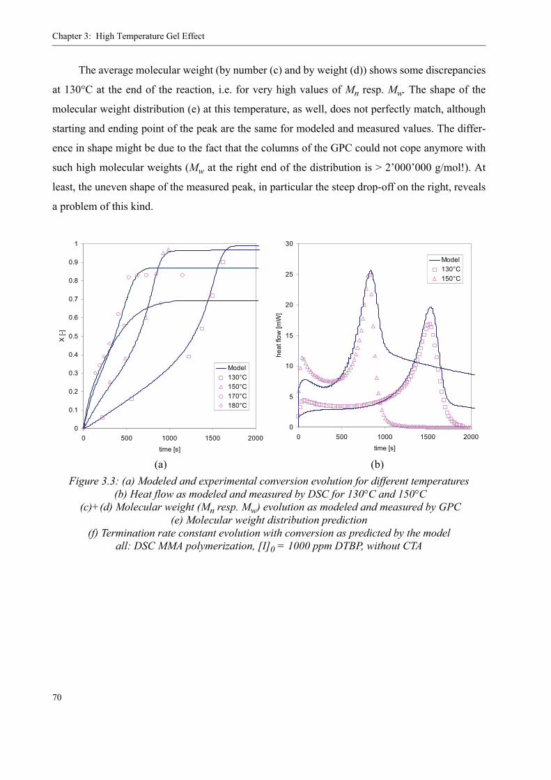
Chapter 3: High Temperature Gel Effect
70
The average molecular weight (by number (c) and by weight (d)) shows some discrepancies
at 130°C at the end of the reaction, i.e. for very high values of Mn resp. Mw. The shape of the
molecular weight distribution (e) at this temperature, as well, does not perfectly match, although
starting and ending point of the peak are the same for modeled and measured values. The differ-
ence in shape might be due to the fact that the columns of the GPC could not cope anymore with
such high molecular weights (Mw at the right end of the distribution is > 2’000’000 g/mol!). At
least, the uneven shape of the measured peak, in particular the steep drop-off on the right, reveals
a problem of this kind.
(a) (b)Figure 3.3: (a) Modeled and experimental conversion evolution for different temperatures
(b) Heat flow as modeled and measured by DSC for 130°C and 150°C (c)+(d) Molecular weight (Mn resp. Mw) evolution as modeled and measured by GPC
(e) Molecular weight distribution prediction(f) Termination rate constant evolution with conversion as predicted by the model
all: DSC MMA polymerization, [I]0 = 1000 ppm DTBP, without CTA
0
0.1
0.2
0.3
0.4
0.5
0.6
0.7
0.8
0.9
1
0 500 1000 1500 2000
time [s]
X [-
]
Model130°C150°C170°C180°C
0
5
10
15
20
25
30
0 500 1000 1500 2000
time [s]
heat
flow
[mW
]
Model130°C150°C
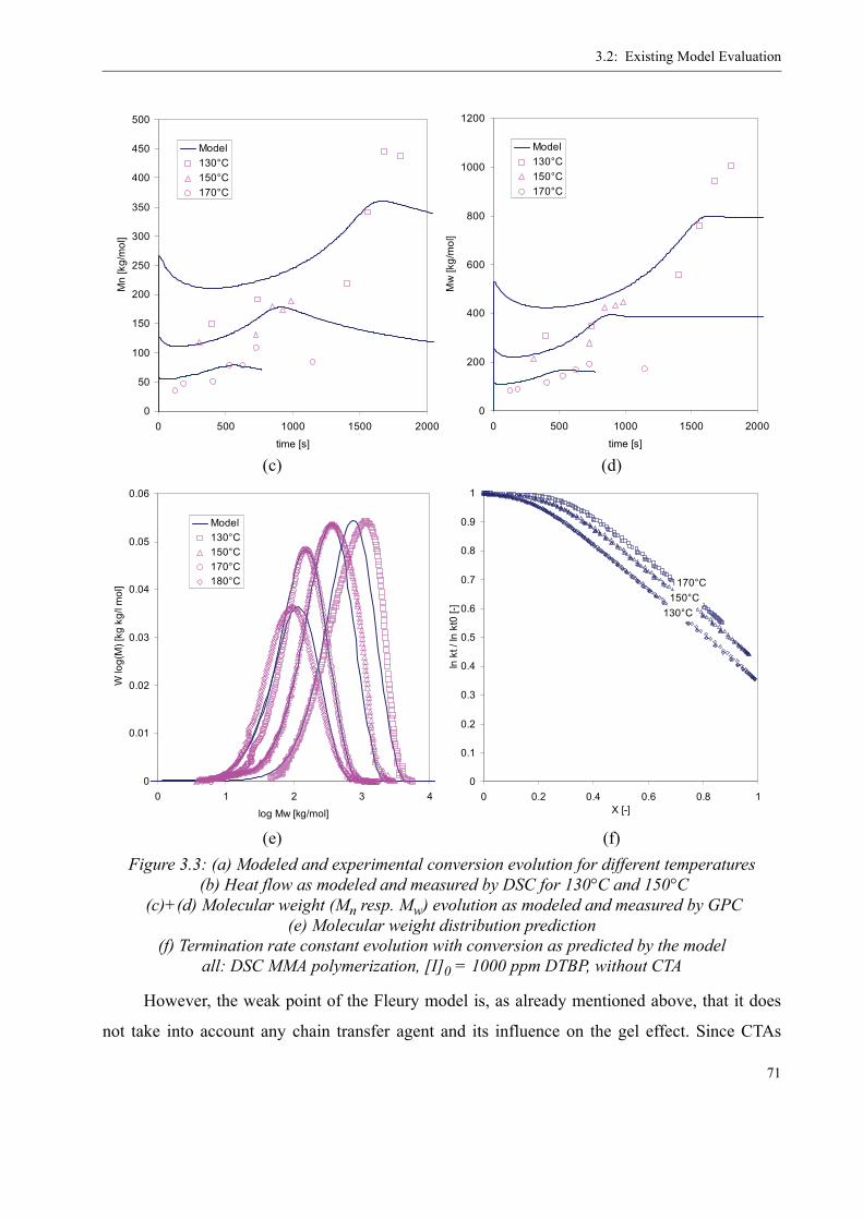
3.2: Existing Model Evaluation
71
However, the weak point of the Fleury model is, as already mentioned above, that it does
not take into account any chain transfer agent and its influence on the gel effect. Since CTAs
(c) (d)
(e) (f)Figure 3.3: (a) Modeled and experimental conversion evolution for different temperatures
(b) Heat flow as modeled and measured by DSC for 130°C and 150°C (c)+(d) Molecular weight (Mn resp. Mw) evolution as modeled and measured by GPC
(e) Molecular weight distribution prediction(f) Termination rate constant evolution with conversion as predicted by the model
all: DSC MMA polymerization, [I]0 = 1000 ppm DTBP, without CTA
0
50
100
150
200
250
300
350
400
450
500
0 500 1000 1500 2000
time [s]
Mn
[kg/
mol
]
Model130°C150°C170°C
0
200
400
600
800
1000
1200
0 500 1000 1500 2000
time [s]M
w [k
g/m
ol]
Model130°C150°C170°C
0
0.01
0.02
0.03
0.04
0.05
0.06
0 1 2 3 4
log Mw [kg/mol]
W lo
g(M
) [kg
kg/
l mol
]
Model130°C150°C170°C180°C
0
0.1
0.2
0.3
0.4
0.5
0.6
0.7
0.8
0.9
1
0 0.2 0.4 0.6 0.8 1X [-]
ln k
t / ln
kt0
[-]
130°C150°C
170°C

Chapter 3: High Temperature Gel Effect
72
decrease the molecular weight without influencing the conversion, also the gel effect becomes
less pronounced. This deficit is depicted in figure 3.4 (a), where it can be clearly seen that, for a
CTA-containing polymerization, the model largely overestimates the gel effect. The influence of
solvent, on the other hand, is considered in the model (compare eqs. 3.29 and 3.30). Therefore,
the attenuation of the gel effect with increasing solvent content is more or less correctly mirrored
(see figure 3.4 (b)).
3.2.5 Fenouillot, Terrisse and Rimlinger [66]
The weakness of the Fleury model, i.e. the missing CTA influence, was improved by
Fenouillot et al., who modified the Fleury equation in order to include the CTA concentration in
the description of the gel effect. Unfortunately, they eliminated the solvent influence, which dis-
qualifies the model again for industrial application. Additionally, this model as well needs an ini-
tial concentration (of CTA instead of initiator) as fixed parameter, which makes its use for
continuous processes doubtful. The decisive equation for the gel effect is equation 3.33, which
(a) (b)Figure 3.4: (a) Modeled and experimental conversion evolution for polymerization with CTA
(data points taken from [66])(b) Modeled and experimental heat flow curve for solvent containing polymerization
(140°C, [I]0 = 1000 ppm DTBP)
0
0.1
0.2
0.3
0.4
0.5
0.6
0.7
0.8
0.9
1
0 2000 4000 6000 8000 10000
Time [s]
X [-
]
Model
150°C, 20.5x10⁻³ mol/l CTA
130°C, 20.5x10⁻³ mol/l CTA
-25
-20
-15
-10
-5
00 20 40 60 80 100
Time [min]
Hea
t flo
w [m
W]
0% BuAc
20% BuAc
30% BuAc
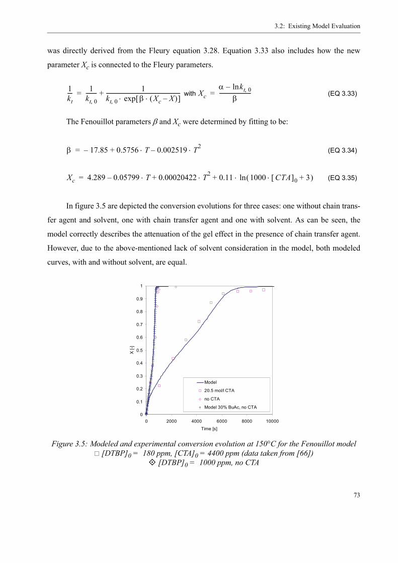
3.2: Existing Model Evaluation
73
was directly derived from the Fleury equation 3.28. Equation 3.33 also includes how the new
parameter Xc is connected to the Fleury parameters.
with (EQ 3.33)
The Fenouillot parameters β and Xc were determined by fitting to be:
(EQ 3.34)
(EQ 3.35)
In figure 3.5 are depicted the conversion evolutions for three cases: one without chain trans-
fer agent and solvent, one with chain transfer agent and one with solvent. As can be seen, the
model correctly describes the attenuation of the gel effect in the presence of chain transfer agent.
However, due to the above-mentioned lack of solvent consideration in the model, both modeled
curves, with and without solvent, are equal.
Figure 3.5: Modeled and experimental conversion evolution at 150°C for the Fenouillot model [DTBP]0 = 180 ppm, [CTA]0 = 4400 ppm (data taken from [66])
[DTBP]0 = 1000 ppm, no CTA
1kt---- 1
kt 0,-------- 1
kt 0, β Xc X–( )⋅[ ]exp⋅-------------------------------------------------------+= Xc
α kt 0,ln–β
------------------------=
β 17.85– 0.5756 T 0.002519 T2⋅–⋅+=
Xc 4.289 0.05799 T 0.00020422 T2 0.11 1000 CTA[ ]0 3+⋅( )ln⋅+⋅+⋅–=
0
0.1
0.2
0.3
0.4
0.5
0.6
0.7
0.8
0.9
1
0 2000 4000 6000 8000 10000
Time [s]
X [-
]
Model
20.5 mol/l CTA
no CTA
Model 30% BuAc, no CTA

Chapter 3: High Temperature Gel Effect
74
3.2.6 Tefera, Weickert and Westerterp [51, 67]
Tefera, Weickert and Westerterp follow the same approach of a three-stage diffusion model
for their description of the gel effect. Yet, they tackle the problem in a different way. For them, the
apparent termination rate constant is governed by three mechanisms: the segmental diffusion at
early polymerization stages, the translational diffusion at intermediate conversions and the reac-
tion diffusion taking place throughout the whole reaction. In mathematical terms they express this
by equation 3.36:
(EQ 3.36)
where ktR is the intrinsic termination rate constant, k*TD the molecular weight dependent
translational-diffusion termination rate coefficient and kRD the reaction diffusion termination rate
coefficient.
At very low conversions, the apparent termination rate constant kt equals kt,0, therefore it
can be written for equation 3.36:
(EQ 3.37)
So it follows for ktR
(EQ 3.38)
The molecular weight dependence of k*TD is expressed by the term
(EQ 3.39)
where
(EQ 3.40)
D is the diffusion coefficient, Vf the free volume and g1 an adjustable parameter. Merging
these equations into equation 3.36 gives for the apparent termination rate coefficient:
kt1
1ktR------- 1
k∗TD-----------+
------------------------- kRD+=
kt01
1ktR------- 1
k∗TD 0,----------------+
------------------------------ kRD 0,+=
1ktR------- 1
kt 0, kRD 0,–( )--------------------------------- k∗TD 0,–=
k∗TDkTD
Mwn
--------=
kTD Dg1Vf-----–⎝ ⎠
⎛ ⎞exp⋅=

3.2: Existing Model Evaluation
75
(EQ 3.41)
The free volume Vf is obtained assuming additivity of the free volume of the reaction com-
ponents:
with (EQ 3.42)
with Vf,i,0 = 0.025 and αm = 0.001 K-1, respectively, αp = 0.00048 K-1. kRD is determined by
the frequency of monomer addition to the radical end and, therefore, it is
(EQ 3.43)
kTD,0 is unknown and needs to be fitted together with the parameter g1 to experimental data.
By introducing a third adjustable parameter, g2, also the initiator efficiency becomes conversion
dependent as a function of the free volume in this model:
(EQ 3.44)
The authors determined the four adjustable parameters for their experimental data in the
temperature range of 50°C - 90°C to be
g1 = 1.8254
g2 = 3.792 x exp(-746/T[K])
kTD,0 = 5.101 x 10⁹ exp(3211/T[K])
n = 1
The advantage of this model is its inclusion of the molecular weight dependence. In their
article, the authors also claim that the model works for polymerizations with chain transfer agents.
Unfortunately, it does not use a ternary monomer-polymer-solvent system. In any case, the three
parameters need to be refitted to experimental data from high-temperature polymerizations in
order to be valid for this temperature range.
kt1
1kt 0, kRD 0,–---------------------------- 1
kTD 0,------------- Mw
n g11Vf----- 1
Vf 0,---------–⎝ ⎠
⎛ ⎞⎝ ⎠⎛ ⎞ Mw 0,
n–exp⋅+----------------------------------------------------------------------------------------------------------------------------------- kRD+=
Vf Vf i, φi⋅i
∑= Vf i, Vf i 0, , α T Tg i,–( )⋅+=
kRD kp M[ ]⋅=
f2 f0⋅
1 g21Vf----- 1
Vf 0,---------–⎝ ⎠
⎛ ⎞⎝ ⎠⎛ ⎞exp+
---------------------------------------------------------=
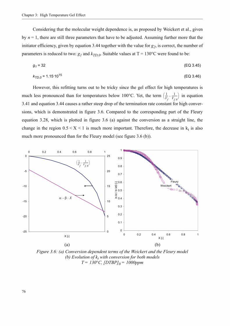
Chapter 3: High Temperature Gel Effect
76
Considering that the molecular weight dependence is, as proposed by Weickert et al., given
by n = 1, there are still three parameters that have to be adjusted. Assuming further more that the
initiator efficiency, given by equation 3.44 together with the value for g2, is correct, the number of
parameters is reduced to two: g1 and kTD,0. Suitable values at T = 130°C were found to be:
g1 = 32 (EQ 3.45)
kTD,0 = 1.15.1015 (EQ 3.46)
However, this refitting turns out to be tricky since the gel effect for high temperatures is
much less pronounced than for temperatures below 100°C. Yet, the term in equation
3.41 and equation 3.44 causes a rather steep drop of the termination rate constant for high conver-
sions, which is demonstrated in figure 3.6. Compared to the corresponding part of the Fleury
equation 3.28, which is plotted in figure 3.6 (a) against the conversion as a straight line, the
change in the region 0.5 < X < 1 is much more important. Therefore, the decrease in kt is also
much more pronounced than for the Fleury model (see figure 3.6 (b)).
(a) (b)Figure 3.6: (a) Conversion dependent terms of the Weickert and the Fleury model
(b) Evolution of kt with conversion for both modelsT = 130°C, [DTBP]0 = 1000ppm
1Vf----- 1
Vf 0,---------–⎝ ⎠
⎛ ⎞
-25
-20
-15
-10
-5
00 0.2 0.4 0.6 0.8 1
X [-]
0
5
10
15
20
25
1Vf----- 1
Vf 0,-----------–⎝ ⎠
⎛ ⎞
α β X⋅–
0
0.1
0.2
0.3
0.4
0.5
0.6
0.7
0.8
0.9
1
0 0.2 0.4 0.6 0.8 1X [-]
ln k
t / ln
kt0
[-] Fleury
Weickert
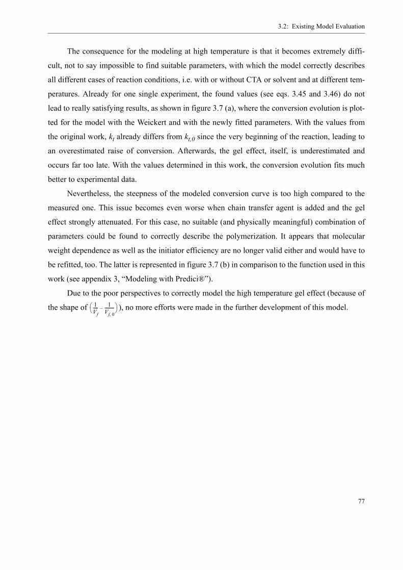
3.2: Existing Model Evaluation
77
The consequence for the modeling at high temperature is that it becomes extremely diffi-
cult, not to say impossible to find suitable parameters, with which the model correctly describes
all different cases of reaction conditions, i.e. with or without CTA or solvent and at different tem-
peratures. Already for one single experiment, the found values (see eqs. 3.45 and 3.46) do not
lead to really satisfying results, as shown in figure 3.7 (a), where the conversion evolution is plot-
ted for the model with the Weickert and with the newly fitted parameters. With the values from
the original work, kt already differs from kt,0 since the very beginning of the reaction, leading to
an overestimated raise of conversion. Afterwards, the gel effect, itself, is underestimated and
occurs far too late. With the values determined in this work, the conversion evolution fits much
better to experimental data.
Nevertheless, the steepness of the modeled conversion curve is too high compared to the
measured one. This issue becomes even worse when chain transfer agent is added and the gel
effect strongly attenuated. For this case, no suitable (and physically meaningful) combination of
parameters could be found to correctly describe the polymerization. It appears that molecular
weight dependence as well as the initiator efficiency are no longer valid either and would have to
be refitted, too. The latter is represented in figure 3.7 (b) in comparison to the function used in this
work (see appendix 3, “Modeling with Predici®”).
Due to the poor perspectives to correctly model the high temperature gel effect (because of
the shape of ), no more efforts were made in the further development of this model.1Vf----- 1
Vf 0,---------–⎝ ⎠
⎛ ⎞
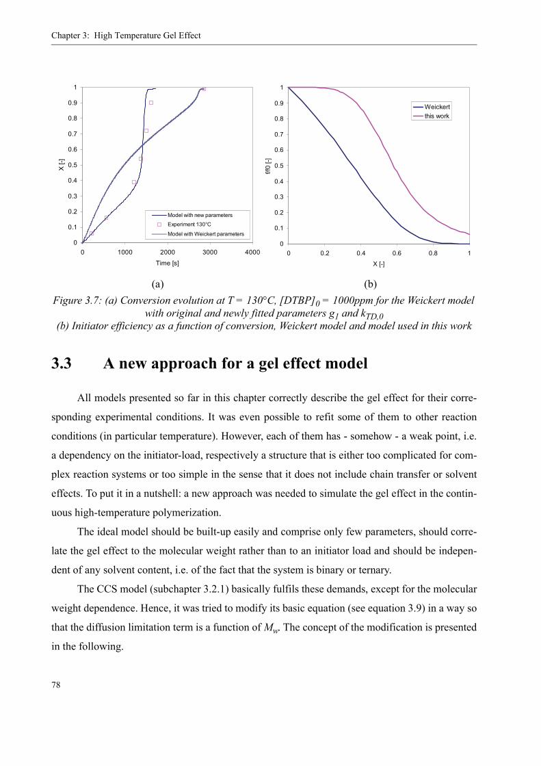
Chapter 3: High Temperature Gel Effect
78
3.3 A new approach for a gel effect model
All models presented so far in this chapter correctly describe the gel effect for their corre-
sponding experimental conditions. It was even possible to refit some of them to other reaction
conditions (in particular temperature). However, each of them has - somehow - a weak point, i.e.
a dependency on the initiator-load, respectively a structure that is either too complicated for com-
plex reaction systems or too simple in the sense that it does not include chain transfer or solvent
effects. To put it in a nutshell: a new approach was needed to simulate the gel effect in the contin-
uous high-temperature polymerization.
The ideal model should be built-up easily and comprise only few parameters, should corre-
late the gel effect to the molecular weight rather than to an initiator load and should be indepen-
dent of any solvent content, i.e. of the fact that the system is binary or ternary.
The CCS model (subchapter 3.2.1) basically fulfils these demands, except for the molecular
weight dependence. Hence, it was tried to modify its basic equation (see equation 3.9) in a way so
that the diffusion limitation term is a function of Mw. The concept of the modification is presented
in the following.
(a) (b)Figure 3.7: (a) Conversion evolution at T = 130°C, [DTBP]0 = 1000ppm for the Weickert model
with original and newly fitted parameters g1 and kTD,0(b) Initiator efficiency as a function of conversion, Weickert model and model used in this work
0
0.1
0.2
0.3
0.4
0.5
0.6
0.7
0.8
0.9
1
0 1000 2000 3000 4000
Time [s]
X [-
]
Model with new parameters
Experiment 130°C
Model with Weickert parameters
0
0.1
0.2
0.3
0.4
0.5
0.6
0.7
0.8
0.9
1
0 0.2 0.4 0.6 0.8 1
X [-]f/f
0 [-]
Weickertthis work

3.3: A new approach for a gel effect model
79
(EQ 3.47)
Combining in the function and separating D again into a molecular-weight and a
conversion-dependent part with the help of the Fujita-Doolittle equation leads to
(EQ 3.48)
The diffusion is inversely proportional to the molecular weight . Hence, it will be
introduced into equation 3.48 with a proportionality constant .
(EQ 3.49)
Another consideration concerns the radical concentration λ0, which substituted the bulk
radical concentration Cb in equation 3.9 and which is mainly a function of the initiator load (see
the simplified equation 3.50 for the example of a batch reaction) but, with increasing conversion,
subject to an important increase due to the volume shrink:
(EQ 3.50)
λ0 has a strong influence on the obtained molecular weight (increasing the initiator load
and, thus, the radical concentration, drastically decreases the molecular weight in an unregulated
polymerization) and has, therefore, also an influence on the shape of the gel effect. Yet, since the
molecular weight dependence is already accounted for in equation 3.49, the presence of λ0 would
constitute a repetition, i.e. an overestimation of the molecular weight influence and lead to a gel
effect that is too steep with respect to reality. It shall be assumed in the course of this model devel-
opment that λ0 is included in the introduced term . Thus, equation 3.49 becomes:
(EQ 3.51)
1kt---- 1
kt 0,--------
rt2λ03D
----------+=
rt2
3---- τ T( )
1kt---- 1
kt 0,-------- τ T( )
λ0
D02.3 1 φp–( )
A B 1 φp–( )+---------------------------------⎝ ⎠
⎛ ⎞exp--------------------------------------------------------+=
D 1Mw
a--------∼
D̃
1kt---- 1
kt 0,-------- τ T( )
λ0 Mwα⋅
D̃2.3 1 φp–( )
A B 1 φp–( )+---------------------------------⎝ ⎠
⎛ ⎞exp⋅---------------------------------------------------------+=
tddλ0 2 f kd I[ ] kt λ0
2 λ0V-----
tddV⋅–⋅–⋅ ⋅ ⋅=
Mwα
D̃--------
1kt---- 1
kt 0,-------- τ T( )
Mwα
D̃2.3 1 φp–( )
A B 1 φp–( )+---------------------------------⎝ ⎠
⎛ ⎞exp⋅---------------------------------------------------------+=
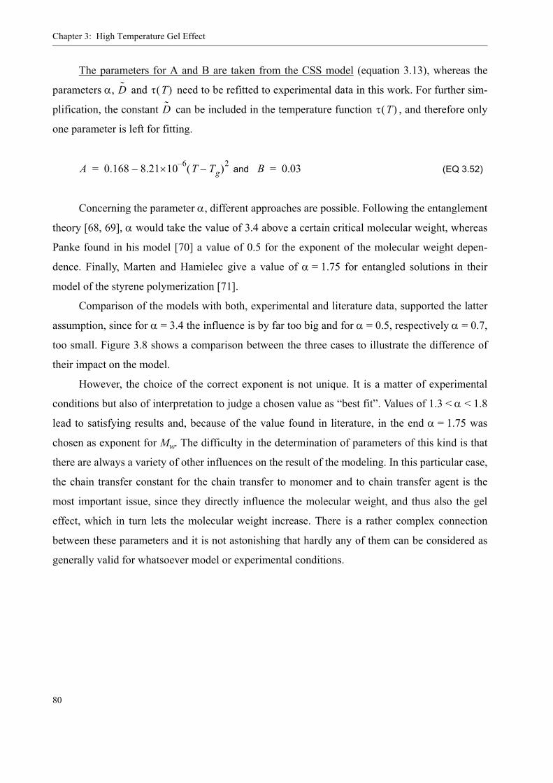
Chapter 3: High Temperature Gel Effect
80
The parameters for A and B are taken from the CSS model (equation 3.13), whereas the
parameters α, and need to be refitted to experimental data in this work. For further sim-
plification, the constant can be included in the temperature function , and therefore only
one parameter is left for fitting.
and (EQ 3.52)
Concerning the parameter α, different approaches are possible. Following the entanglement
theory [68, 69], α would take the value of 3.4 above a certain critical molecular weight, whereas
Panke found in his model [70] a value of 0.5 for the exponent of the molecular weight depen-
dence. Finally, Marten and Hamielec give a value of α = 1.75 for entangled solutions in their
model of the styrene polymerization [71].
Comparison of the models with both, experimental and literature data, supported the latter
assumption, since for α = 3.4 the influence is by far too big and for α = 0.5, respectively α = 0.7,
too small. Figure 3.8 shows a comparison between the three cases to illustrate the difference of
their impact on the model.
However, the choice of the correct exponent is not unique. It is a matter of experimental
conditions but also of interpretation to judge a chosen value as “best fit”. Values of 1.3 < α < 1.8
lead to satisfying results and, because of the value found in literature, in the end α = 1.75 was
chosen as exponent for Mw. The difficulty in the determination of parameters of this kind is that
there are always a variety of other influences on the result of the modeling. In this particular case,
the chain transfer constant for the chain transfer to monomer and to chain transfer agent is the
most important issue, since they directly influence the molecular weight, and thus also the gel
effect, which in turn lets the molecular weight increase. There is a rather complex connection
between these parameters and it is not astonishing that hardly any of them can be considered as
generally valid for whatsoever model or experimental conditions.
D̃ τ T( )
D̃ τ T( )
A 0.168 8.21 6–×10 T Tg–( )2–= B 0.03=

3.3: A new approach for a gel effect model
81
The fitting of α and was done with data from literature [66] and DSC data obtained in
this work. As mentioned above, the value for α was found to be α = 1.75 in accordance with the
Marten-Hamielec literature value [71]. For the temperature-dependent parameter , an expo-
nential dependence was found, which corresponds to θt(T) in the CSS model (see page 63). The
Arrhenius diagram for the determination of is depicted in figure 3.9, leading to the follow-
ing equation:
[-] (EQ 3.53)
It should be kept in mind that this equation is only valid for the model parameters used in
this work and for the given set of kinetic constants (see appendix 3). Changing a rate constant, e.g.
for the depolymerization or the chain transfer, can lead to significant changes in the values for
.
Figure 3.8: Comparison of different values for α
1.E+00
1.E+01
1.E+02
1.E+03
1.E+04
1.E+05
1.E+06
1.E+07
1.E+08
1.E+09
1.E+10
1.E+11
0 200 400 600 800 1'000 1'200
Mw [kg/mol]
α = 3.4
α = 1.75
α = 0.5
α = 0.7
Mw
α [k
gα/m
olα]
τ T( )
τ T( )
τ T( )
τ T( ) 7.69265 10 9– e4.0365 104 J mol⁄[ ]⋅–
RT K[ ]------------------------------------------------------
⋅ ⋅=
τ T( )

Chapter 3: High Temperature Gel Effect
82
The results of the modeling with this equation for the gel effect are presented in the follow-
ing. Figure 3.10 (a) and (b) shows the modeled and experimental conversion evolution for two
cases: (a) for polymerizations at different temperatures without chain transfer agent, carried out as
batch polymerizations in the DSC, and (b) for polymerizations with different chain transfer agent
loads at constant temperature, carried out by Fenouillot et al. [66] as batch polymerizations in a
dilatometric reactor setup. Note that for the second series of reactions, the initiator load is one
order of magnitude smaller than for the DSC runs, leading to much longer reaction times.
For the DSC experiment without chain transfer agent, the model is in very good agreement
with experimental data as regards conversion evolution (figure 3.10 (a)) and heat flow (figure
3.11 (a)), except that for T = 130 °C, the onset of the gel effect is a little too early. The source of
this difference is the overestimation of the molecular weight in the beginning of the reaction, vis-
ible in figure 3.12 (a) + (b). The model predicts here a much higher molecular weight than mea-
sured, leading at the same time to an earlier onset of the gel effect. The reason for the
overestimation of the molecular weight by the model might be that under experimental conditions
inhibition reactions caused by impurities keep the molecular weight in the beginning of the reac-
tion rather low, which the model does not account for. The difference in the beginning and the end
of the heat flow curve has already been discussed earlier (see page 69).
Figure 3.9: Arrhenius diagram for the calculation of the parameter in the gel effect model
y = -4855x - 18.683R2 = 0.9998
-30.8
-30.6
-30.4
-30.2
-30
-29.8
-29.6
-29.4
-29.20.00215 0.0022 0.00225 0.0023 0.00235 0.0024 0.00245 0.0025
1/T [1/K]
ln τ
(T) [
-]
τ T( )
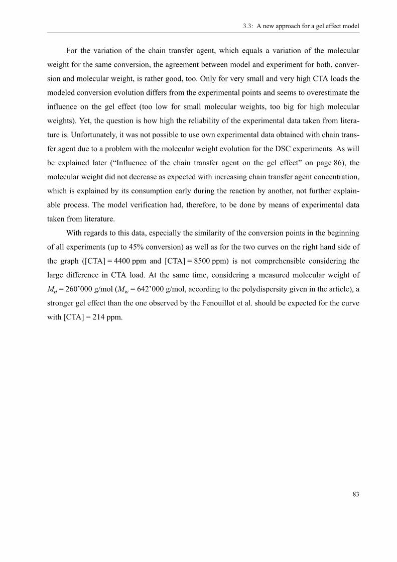
3.3: A new approach for a gel effect model
83
For the variation of the chain transfer agent, which equals a variation of the molecular
weight for the same conversion, the agreement between model and experiment for both, conver-
sion and molecular weight, is rather good, too. Only for very small and very high CTA loads the
modeled conversion evolution differs from the experimental points and seems to overestimate the
influence on the gel effect (too low for small molecular weights, too big for high molecular
weights). Yet, the question is how high the reliability of the experimental data taken from litera-
ture is. Unfortunately, it was not possible to use own experimental data obtained with chain trans-
fer agent due to a problem with the molecular weight evolution for the DSC experiments. As will
be explained later (“Influence of the chain transfer agent on the gel effect” on page 86), the
molecular weight did not decrease as expected with increasing chain transfer agent concentration,
which is explained by its consumption early during the reaction by another, not further explain-
able process. The model verification had, therefore, to be done by means of experimental data
taken from literature.
With regards to this data, especially the similarity of the conversion points in the beginning
of all experiments (up to 45% conversion) as well as for the two curves on the right hand side of
the graph ([CTA] = 4400 ppm and [CTA] = 8500 ppm) is not comprehensible considering the
large difference in CTA load. At the same time, considering a measured molecular weight of
Mn = 260’000 g/mol (Mw = 642’000 g/mol, according to the polydispersity given in the article), a
stronger gel effect than the one observed by the Fenouillot et al. should be expected for the curve
with [CTA] = 214 ppm.
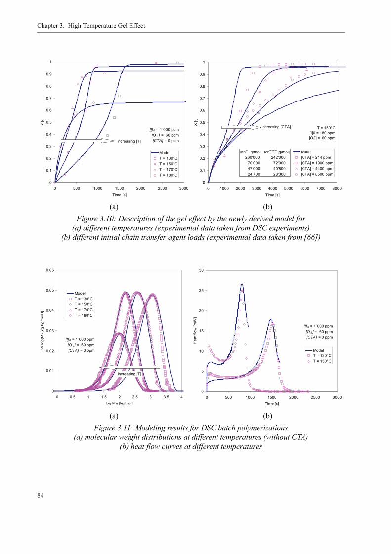
Chapter 3: High Temperature Gel Effect
84
(a) (b)Figure 3.10: Description of the gel effect by the newly derived model for
(a) different temperatures (experimental data taken from DSC experiments)(b) different initial chain transfer agent loads (experimental data taken from [66])
(a) (b)Figure 3.11: Modeling results for DSC batch polymerizations
(a) molecular weight distributions at different temperatures (without CTA)(b) heat flow curves at different temperatures
0
0.1
0.2
0.3
0.4
0.5
0.6
0.7
0.8
0.9
1
0 500 1000 1500 2000 2500 3000Time [s]
X [-
]
ModelT = 130°CT = 150°CT = 170°CT = 180°C
[I] 0 = 1´000 ppm [O 2 ] = 60 ppm
[CTA] = 0 ppmincreasing [T]
0
0.1
0.2
0.3
0.4
0.5
0.6
0.7
0.8
0.9
1
0 1000 2000 3000 4000 5000 6000 7000 8000Time [s]
X [-
]
Model[CTA] = 214 ppm[CTA] = 1900 ppm[CTA] = 4400 ppm[CTA] = 8500 ppm
T = 150°C [I]0 = 180 ppm [O2] = 60 ppm
increasing [CTA]
Mnlit. [g/mol] Mnmodel [g/mol] 260'000 242'000 70'000 72'000 47'000 40'800 24'700 28'300
0
0.01
0.02
0.03
0.04
0.05
0.06
0 0.5 1 1.5 2 2.5 3 3.5 4log Mw [kg/mol]
W lo
g(M
) [kg
kg/
mol
l]
ModelT = 130°CT = 150°CT = 170°CT = 180°C
[I] 0 = 1´000 ppm [O 2] = 60 ppm
[CTA] = 0 ppm
increasing [T]
0
5
10
15
20
25
30
0 500 1000 1500 2000 2500 3000Time [s]
Hea
t flo
w [m
W]
ModelT = 130°CT = 150°C
[I] 0 = 1´000 ppm [O 2] = 60 ppm
[CTA] = 0 ppm
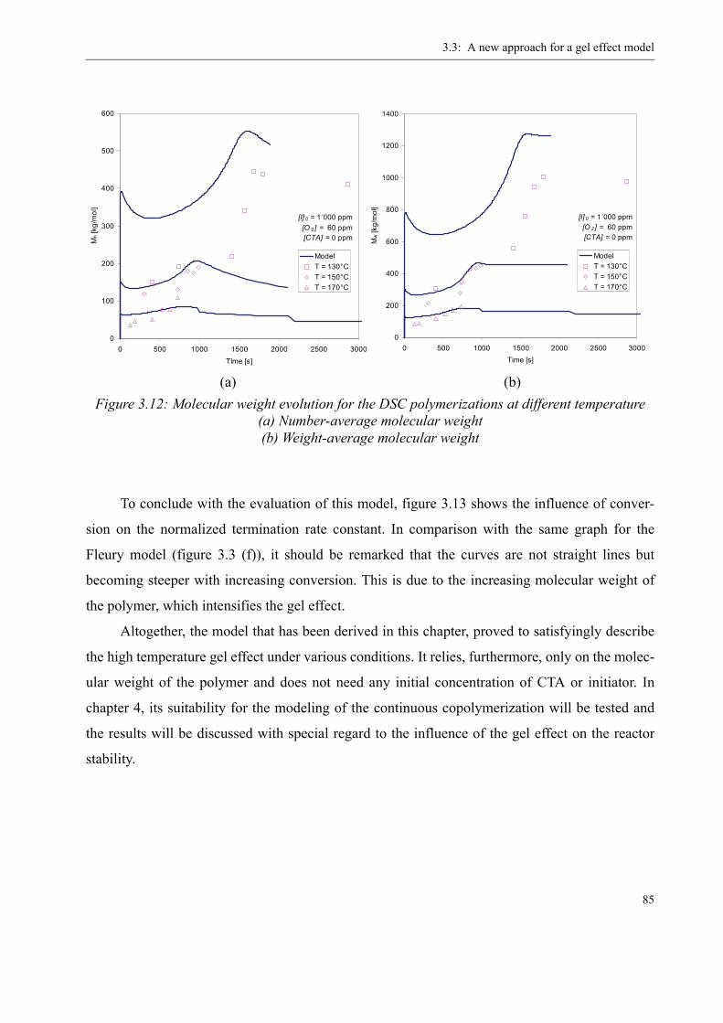
3.3: A new approach for a gel effect model
85
To conclude with the evaluation of this model, figure 3.13 shows the influence of conver-
sion on the normalized termination rate constant. In comparison with the same graph for the
Fleury model (figure 3.3 (f)), it should be remarked that the curves are not straight lines but
becoming steeper with increasing conversion. This is due to the increasing molecular weight of
the polymer, which intensifies the gel effect.
Altogether, the model that has been derived in this chapter, proved to satisfyingly describe
the high temperature gel effect under various conditions. It relies, furthermore, only on the molec-
ular weight of the polymer and does not need any initial concentration of CTA or initiator. In
chapter 4, its suitability for the modeling of the continuous copolymerization will be tested and
the results will be discussed with special regard to the influence of the gel effect on the reactor
stability.
(a) (b)Figure 3.12: Molecular weight evolution for the DSC polymerizations at different temperature
(a) Number-average molecular weight(b) Weight-average molecular weight
0
100
200
300
400
500
600
0 500 1000 1500 2000 2500 3000Time [s]
Mn [
kg/m
ol]
ModelT = 130°CT = 150°CT = 170°C
[I] 0 = 1´000 ppm [O 2] = 60 ppm
[CTA] = 0 ppm
0
200
400
600
800
1000
1200
1400
0 500 1000 1500 2000 2500 3000Time [s]
Mw [k
g/m
ol]
ModelT = 130°CT = 150°CT = 170°C
[I] 0 = 1´000 ppm [O 2] = 60 ppm
[CTA] = 0 ppm
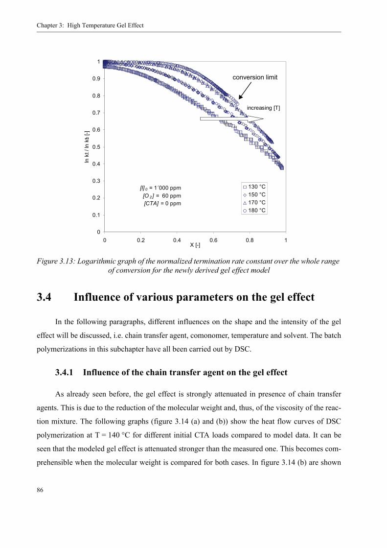
Chapter 3: High Temperature Gel Effect
86
3.4 Influence of various parameters on the gel effect
In the following paragraphs, different influences on the shape and the intensity of the gel
effect will be discussed, i.e. chain transfer agent, comonomer, temperature and solvent. The batch
polymerizations in this subchapter have all been carried out by DSC.
3.4.1 Influence of the chain transfer agent on the gel effect
As already seen before, the gel effect is strongly attenuated in presence of chain transfer
agents. This is due to the reduction of the molecular weight and, thus, of the viscosity of the reac-
tion mixture. The following graphs (figure 3.14 (a) and (b)) show the heat flow curves of DSC
polymerization at T = 140 °C for different initial CTA loads compared to model data. It can be
seen that the modeled gel effect is attenuated stronger than the measured one. This becomes com-
prehensible when the molecular weight is compared for both cases. In figure 3.14 (b) are shown
Figure 3.13: Logarithmic graph of the normalized termination rate constant over the whole range of conversion for the newly derived gel effect model
0
0.1
0.2
0.3
0.4
0.5
0.6
0.7
0.8
0.9
1
0 0.2 0.4 0.6 0.8 1X [-]
ln k
t / ln
kt 0
[-]
130 °C150 °C170 °C180 °C
[I] 0 = 1´000 ppm [O 2] = 60 ppm
[CTA] = 0 ppm
increasing [T]
conversion limit
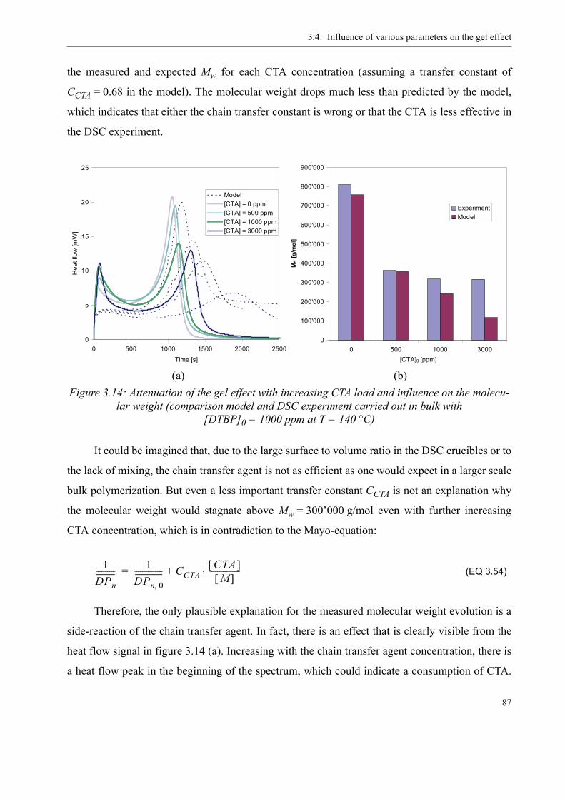
3.4: Influence of various parameters on the gel effect
87
the measured and expected Mw for each CTA concentration (assuming a transfer constant of
CCTA = 0.68 in the model). The molecular weight drops much less than predicted by the model,
which indicates that either the chain transfer constant is wrong or that the CTA is less effective in
the DSC experiment.
It could be imagined that, due to the large surface to volume ratio in the DSC crucibles or to
the lack of mixing, the chain transfer agent is not as efficient as one would expect in a larger scale
bulk polymerization. But even a less important transfer constant CCTA is not an explanation why
the molecular weight would stagnate above Mw = 300’000 g/mol even with further increasing
CTA concentration, which is in contradiction to the Mayo-equation:
(EQ 3.54)
Therefore, the only plausible explanation for the measured molecular weight evolution is a
side-reaction of the chain transfer agent. In fact, there is an effect that is clearly visible from the
heat flow signal in figure 3.14 (a). Increasing with the chain transfer agent concentration, there is
a heat flow peak in the beginning of the spectrum, which could indicate a consumption of CTA.
(a) (b)Figure 3.14: Attenuation of the gel effect with increasing CTA load and influence on the molecu-
lar weight (comparison model and DSC experiment carried out in bulk with [DTBP]0 = 1000 ppm at T = 140 °C)
0
5
10
15
20
25
0 500 1000 1500 2000 2500
Time [s]
Hea
t flo
w [m
W]
Model[CTA] = 0 ppm[CTA] = 500 ppm[CTA] = 1000 ppm[CTA] = 3000 ppm
0
100'000
200'000
300'000
400'000
500'000
600'000
700'000
800'000
900'000
0 500 1000 3000[CTA]0 [ppm]
Mw
[g/m
ol]
ExperimentModel
1DPn
---------- 1DPn 0,
--------------- CCTACTA[ ]
M[ ]----------------⋅+=

Chapter 3: High Temperature Gel Effect
88
This could explain the high molecular weight, since the effective CTA concentration would be
much lower than initially adjusted. The nature of this side-reaction is unknown but, in general,
thioles can be easily oxidized, which - in this case - would be possible by the initiator or by oxy-
gen from air.
3.4.2 Influence of temperature on the gel effect
Also the temperature has a rather strong effect on the gel effect, as seen already in the prece-
dent subchapter. Up to approximately 150 °C, the gel effect intensifies as the reaction rate
increases. Above 150 °C, the amplitude of the gel effect diminishes and both, depolymerization
and low viscosity, reduce the acceleration of the reaction until it is hardly present, which is the
case above 180 °C. In figure 3.15 (a) + (b) is presented this influence of the reaction temperature
on gel effect and molecular weight for DSC batch polymerizations with [DTBP]0 = 1000 ppm,
compared to the model predictions for each case. For T = 170 °C, the model underestimates the
heat flow curve a little and the precision is not as high as for the other cases. However, for the
same experimental conditions, the conversion evolution, presented in figure 3.10 (a), is in perfect
agreement with the model. It might, therefore, be that the measured heat flow curve for
T = 170 °C presented in figure 3.15 (a) varies to a small extent from the other experiments carried
out at this temperature.

3.4: Influence of various parameters on the gel effect
89
3.4.3 Influence of solvent on the gel effect
Since the gel effect is a viscosity related phenomenon, naturally also the presence of solvent
has an important influence on its shape. Adding for example 30% solvent means reducing the
polymer content wp by 30%, too. As shown in figure 4.8 in chapter 4, a reduction of the polymer
content of 30% reduces the viscosity of the solution by several orders of magnitude (for
T = 120°C and Mw = 100’000 g/mol the viscosity decreases by approximately a factor 104!).
This is reflected also by the results from DSC experiments and the modeling. Figure 3.16 (a) + (b)
contains the measured and simulated curves for three different solvent contents (0%, 20% and
30% of n-butyl acetate) as well as the molecular weights for each experiment. It is apparent that
for 30% solvent, the gel effect is hardly remarkable anymore. The modeled molecular weight
matches the GPC values very well, too. This is a confirmation that the transfer constant for the
solvent, which had been assumed to be CS = 0.0001, is more or less correct.
Figure 3.15: Changing of the gel effect with increasing reaction temperature and influence on the molecular weight (comparison model and DSC experiment carried out in bulk with
[DTBP]0 = 1000 ppm at T = 140 °C)
0
5
10
15
20
25
30
35
0 500 1000 1500 2000 2500
Time [s]
Hea
t flo
w [m
W]
ModelT = 130 °CT = 150 °CT = 170°CT = 180 °C
0
200'000
400'000
600'000
800'000
1'000'000
1'200'000
1'400'000
130 150 170 180
T [°C]
Mw
[g/m
ol]
ExperimentModel
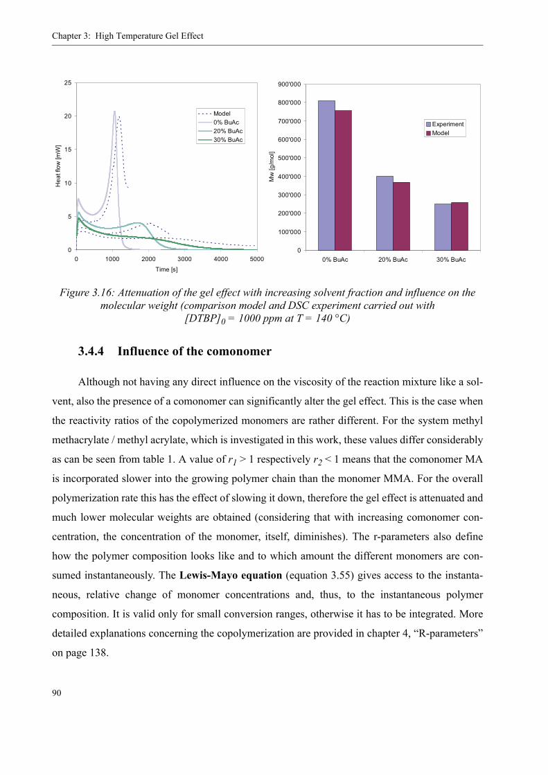
Chapter 3: High Temperature Gel Effect
90
3.4.4 Influence of the comonomer
Although not having any direct influence on the viscosity of the reaction mixture like a sol-
vent, also the presence of a comonomer can significantly alter the gel effect. This is the case when
the reactivity ratios of the copolymerized monomers are rather different. For the system methyl
methacrylate / methyl acrylate, which is investigated in this work, these values differ considerably
as can be seen from table 1. A value of r1 > 1 respectively r2 < 1 means that the comonomer MA
is incorporated slower into the growing polymer chain than the monomer MMA. For the overall
polymerization rate this has the effect of slowing it down, therefore the gel effect is attenuated and
much lower molecular weights are obtained (considering that with increasing comonomer con-
centration, the concentration of the monomer, itself, diminishes). The r-parameters also define
how the polymer composition looks like and to which amount the different monomers are con-
sumed instantaneously. The Lewis-Mayo equation (equation 3.55) gives access to the instanta-
neous, relative change of monomer concentrations and, thus, to the instantaneous polymer
composition. It is valid only for small conversion ranges, otherwise it has to be integrated. More
detailed explanations concerning the copolymerization are provided in chapter 4, “R-parameters”
on page 138.
Figure 3.16: Attenuation of the gel effect with increasing solvent fraction and influence on the molecular weight (comparison model and DSC experiment carried out with
[DTBP]0 = 1000 ppm at T = 140 °C)
0
5
10
15
20
25
0 1000 2000 3000 4000 5000
Time [s]
Hea
t flo
w [m
W]
Model0% BuAc20% BuAc30% BuAc
0
100'000
200'000
300'000
400'000
500'000
600'000
700'000
800'000
900'000
0% BuAc 20% BuAc 30% BuAc
Mw
[g/m
ol]
ExperimentModel
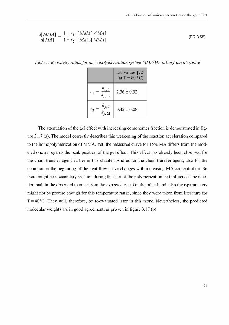
3.4: Influence of various parameters on the gel effect
91
(EQ 3.55)
The attenuation of the gel effect with increasing comonomer fraction is demonstrated in fig-
ure 3.17 (a). The model correctly describes this weakening of the reaction acceleration compared
to the homopolymerization of MMA. Yet, the measured curve for 15% MA differs from the mod-
eled one as regards the peak position of the gel effect. This effect has already been observed for
the chain transfer agent earlier in this chapter. And as for the chain transfer agent, also for the
comonomer the beginning of the heat flow curve changes with increasing MA concentration. So
there might be a secondary reaction during the start of the polymerization that influences the reac-
tion path in the observed manner from the expected one. On the other hand, also the r-parameters
might not be precise enough for this temperature range, since they were taken from literature for
T = 80°C. They will, therefore, be re-evaluated later in this work. Nevertheless, the predicted
molecular weights are in good agreement, as proven in figure 3.17 (b).
Table 1: Reactivity ratios for the copolymerization system MMA/MA taken from literature
Lit. values [72](at T = 80 °C)
d MMA[ ]d MA[ ]
----------------------1 r1 MMA[ ] MA[ ]⁄⋅+1 r2 MA[ ] MMA[ ]⁄⋅+-------------------------------------------------------=
r1kp 1,
kp 12,-----------= 2.36 0.32±
r2kp 2,
kp 21,-----------= 0.42 0.08±
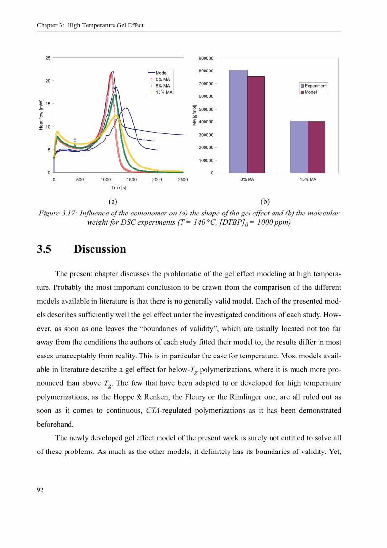
Chapter 3: High Temperature Gel Effect
92
3.5 Discussion
The present chapter discusses the problematic of the gel effect modeling at high tempera-
ture. Probably the most important conclusion to be drawn from the comparison of the different
models available in literature is that there is no generally valid model. Each of the presented mod-
els describes sufficiently well the gel effect under the investigated conditions of each study. How-
ever, as soon as one leaves the “boundaries of validity”, which are usually located not too far
away from the conditions the authors of each study fitted their model to, the results differ in most
cases unacceptably from reality. This is in particular the case for temperature. Most models avail-
able in literature describe a gel effect for below-Tg polymerizations, where it is much more pro-
nounced than above Tg. The few that have been adapted to or developed for high temperature
polymerizations, as the Hoppe & Renken, the Fleury or the Rimlinger one, are all ruled out as
soon as it comes to continuous, CTA-regulated polymerizations as it has been demonstrated
beforehand.
The newly developed gel effect model of the present work is surely not entitled to solve all
of these problems. As much as the other models, it definitely has its boundaries of validity. Yet,
(a) (b)Figure 3.17: Influence of the comonomer on (a) the shape of the gel effect and (b) the molecular
weight for DSC experiments (T = 140 °C, [DTBP]0 = 1000 ppm)
0
5
10
15
20
25
0 500 1000 1500 2000 2500
Time [s]
Hea
t flo
w [m
W]
Model0% MA5% MA15% MA
0
100000
200000
300000
400000
500000
600000
700000
800000
900000
0% MA 15% MA
Mw
[g/m
ol]
ExperimentModel
3.5: Discussion
93
the innovation of this high-temperature model is that, based on the classic diffusion approach, it
directly correlates the gel effect with molecular weight and polymer volume fraction, both decid-
ing factors for solution viscosity. Thus, it takes into account the influence of chain transfer agent
and changing initiator concentration without needing their concentrations. It does not matter,
either, if the polymerization takes place in batch or in a continuous process.
At the same time, the rather simple model structure with few fitting parameters and practi-
cally no required material-related data, allows the comfortable adaptation of the model to differ-
ent reaction conditions, if necessary. The two parameters fitted in this work, α and , might
also leave room for some further optimization. They were determined with the help of DSC batch
polymerizations, which surely exhibit some process-related limitations (no mixing, high surface-
to-volume ratio, difficult sampling for GC and GPC etc.). The comparison to literature data, in
this case the data of Rimlinger et al., illustrated the fact that the results of this fit should be care-
fully evaluated.
This will be done in the context of the pilot plant experiments, where the gel effect model
derived in this chapter will be validated with the help of data from the continuous process. The
results obtained for the batch polymerization and copolymerization of MMA are, however, very
satisfactory. Apart from some minor inaccuracies, the model correctly predicts the influence of
temperature, solvent, chain transfer agent and comonomer on monomer conversion and molecular
weight. This flexibility is, to the knowledge of the author, not featured by any other gel effect
model so far published in literature.
Short Summary:
• Different existing gel effect models for MMA have been examined towards their
applicability to high temperature polymerizations
• By modifying a suitable existing gel effect model, a new one could be derived,
which allows the correct description of the high temperature gel effect in batch
and continuous polymerizations of MMA
• This new model was tested concerning the correct prediction of the gel effect
under various conditions and validated by experimental data from this work and
from literature.
τ T( )

Chapter 3: High Temperature Gel Effect
94

95
CHAPTER 4
Continuous High-TemperaturePolymerization
Chapter 2 and chapter 3 dealt with some characteristic kinetic aspects of the high-tem-
perature polymerization of MMA. More precisely, the thermal initiation reactions, caused
among other by MMA peroxides, as well as the high-temperature gel effect were investigated
by means of batch experiments. These points are extremely important, since they influence sig-
nificantly the thermal behavior of the reaction.
The following chapter will now combine the results of the preceding ones with the con-
cept of continuous polymerization at pilot-scale. For industrial considerations these pilot trials
are inevitable for the evaluation of a high-temperature process as to its feasibility and final
product qualities. It is important to conduct these experiments under conditions as similar as
possible to those of a “real” production process to allow a direct comparison. The problem
with most scientific research is that it is done under conditions that are far from the “produc-
tion reality” and routines, for example the use of highly purified material, while in industrial-
scale reactions rather technical grades are present, or of miniaturized reactors without mixing
and heat transfer issues as they are present in large-scale industrial reactors. This part of the
present work was, therefore, carried out using commercial grade raw materials as provided by
the producers (see appendix 6), and a reactor setup similar to that of an industrial reactor.
In industry, a widely used setup for bulk polymerization processes is the combination of
CSTR and plug flow tubular reactor (see figure 4.1). In the CSTR, the polymerization is usu-
ally conducted to medium polymer fractions below 50% (for high temperatures sometimes up
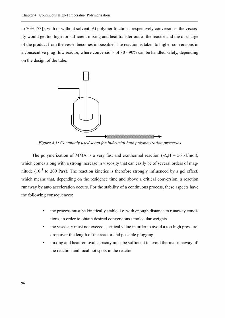
Chapter 4: Continuous High-Temperature Polymerization
96
to 70% [73]), with or without solvent. At polymer fractions, respectively conversions, the viscos-
ity would get too high for sufficient mixing and heat transfer out of the reactor and the discharge
of the product from the vessel becomes impossible. The reaction is taken to higher conversions in
a consecutive plug flow reactor, where conversions of 80 - 90% can be handled safely, depending
on the design of the tube.
The polymerization of MMA is a very fast and exothermal reaction (-ΔrH = 56 kJ/mol),
which comes along with a strong increase in viscosity that can easily be of several orders of mag-
nitude (10-3 to 200 Pa.s). The reaction kinetics is therefore strongly influenced by a gel effect,
which means that, depending on the residence time and above a critical conversion, a reaction
runaway by auto acceleration occurs. For the stability of a continuous process, these aspects have
the following consequences:
• the process must be kinetically stable, i.e. with enough distance to runaway condi-
tions, in order to obtain desired conversions / molecular weights
• the viscosity must not exceed a critical value in order to avoid a too high pressure
drop over the length of the reactor and possible plugging
• mixing and heat removal capacity must be sufficient to avoid thermal runaway of
the reaction and local hot spots in the reactor
Figure 4.1: Commonly used setup for industrial bulk polymerization processes
4.1: The Sulzer Pilot Plant
97
As to the danger of a thermal runaway, an advantage of the MMA polymerization is that it
exhibits a rather strong depolymerization at high temperatures. With a ceiling temperature of
Tc = 220°C [11], above which no propagation takes place anymore, a possible runaway of the
reaction, at least in terms of the polymerization heat, would come automatically to halt. Neverthe-
less, a sufficient heat removal capacity is indispensible for safe control of the reaction conditions.
Finally, the presence of local hot spots can lead to thermal degradation of the polymer and to a
widening of the molecular weight distribution, both leading to a reduced product quality.
The runaway of the medium viscosity is a rather delicate matter concerning the reactor sta-
bility, as already small changes in reaction conditions (T, τ) may have drastic effects. These
changes might be due to technical problems, i.e. failure of the feed pump or feed flow variations,
temperature drop of the heating circuit, or may be caused by long-term phenomena as, for exam-
ple, the obstruction of heat removal due to the formation of polymer residues on the reactor walls.
An unforeseen increase in viscosity usually has severe consequences for the process: the reactor
pressure increases until either sealings break or the reactor plugs completely, and the heat removal
becomes more difficult leading to an increase in temperature and a consecutive reaction accelera-
tion. It must, therefore, be taken care of the right choice of residence time with eventual security
margins in case of feed flow variations.
One of the goals of the present work is to design a pilot plant for the continuous production
of PMMA molding compound that takes into account the above-mentioned issues. The reactor
concept chosen to achieve this goal is a combination of a tubular, high-recycle-ratio loop, replac-
ing the common CSTR, followed by a plug flow tube reactor. These concepts have already been
successfully applied in other research projects at EPFL (Recycle loop: [1, 5, 74], combination
loop / tube: [6, 75]). The operating conditions are predetermined by constraints from the industrial
partner of this project.
4.1 The Sulzer Pilot Plant
4.1.1 Viscous tubular flows
Since the environment of polymerization reactions is usually rather viscous, the flow profile
in a tubular reactor exhibits laminar behavior. This means that the flow rate in the middle of the
tube is high, whereas in close proximity to the reactor wall the flow stagnates. The consequence is

Chapter 4: Continuous High-Temperature Polymerization
98
that the residence time at outer diametric zones are much higher than in the inner tube, for bulk
polymerizations first leading to highly viscous films and finally to solid, high molecular weight
polymer deposits on the tube wall. This effect is even enhanced when the heat transfer is limited
by the viscosity of the medium and the temperature drops at the outer tube zones (let’s recall that
the reaction is highly exothermal and heat needs to be removed from the reactor). A heated tube
wall can, therefore, increase significantly the heat transfer and lead to a more uniform flow pro-
file. In figure 4.2 are shown schematically the flow profiles for laminar flows in an empty tube. It
is easily understandable that an empty tube, even with wall heating, is not the ideal configuration
for a polymerization reactor.
4.1.2 The concept of static mixing
The concept of static mixing elements - in contrast to active mixing in an extruder - is the
use of the mechanical energy of the flow to ensure intense radial mixing and to achieve a homog-
enous flowrate and temperature profile over the entire tubes’ section. Additionally, metallic static
Newtonian fluid in an empty adiabatic tube
Non-newtonian fluid in an empty adiabatic tube
Newtonian fluid in an empty, heated tube
Newtonian fluid in an empty, cooled tube
Figure 4.2: Different laminar flow profiles in an empty tube depending on fluid-type and conditions at the tube walls [5]
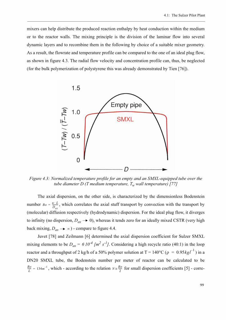
4.1: The Sulzer Pilot Plant
99
mixers can help distribute the produced reaction enthalpy by heat conduction within the medium
or to the reactor walls. The mixing principle is the division of the laminar flow into several
dynamic layers and to recombine them in the following by choice of a suitable mixer geometry.
As a result, the flowrate and temperature profile can be compared to the one of an ideal plug flow,
as shown in figure 4.3. The radial flow velocity and concentration profile can, thus, be neglected
(for the bulk polymerization of polystyrene this was already demonstrated by Tien [76]).
The axial dispersion, on the other side, is characterized by the dimensionless Bodenstein
number , which correlates the axial stuff transport by convection with the transport by
(molecular) diffusion respectively (hydrodynamic) dispersion. For the ideal plug flow, it diverges
to infinity (no dispersion, Dax 0), whereas it tends zero for an ideally mixed CSTR (very high
back mixing, Dax ) - compare to figure 4.4.
Juvet [78] and Zeilmann [6] determined the axial dispersion coefficient for Sulzer SMXL
mixing elements to be Dax = 6.10-4 [m2 s-1]. Considering a high recycle ratio (40:1) in the loop
reactor and a throughput of 2 kg/h of a 50% polymer solution at T = 140°C ( ) in a
DN20 SMXL tube, the Bodenstein number per meter of reactor can be calculated to be
, which - according to the relation for small dispersion coefficients [5] - corre-
Figure 4.3: Normalized temperature profile for an empty and an SMXL-equipped tube over the tube diameter D (T medium temperature, Tw wall temperature) [77]
Bo u L⋅Dax----------=
∞
ρ 0.95kgl 1–=
BoL
------- 134m 1–= N Bo2
-------≅

Chapter 4: Continuous High-Temperature Polymerization
100
sponds to a cascade of 67 CSTR’s per meter SMXL tube. This illustrates that the axial dispersion
can be neglected as well for the recycle loop.
4.1.3 Choice of mixing elements
Sulzer offers three different types of static mixers, depending on the geometry of the reac-
tor:
The SMX and SMXL type are employed for tube diameters up to 10 cm. The L in SMXL
stands for “large”, which means that the geometry is more open than the one of the SMX (see fig-
ure 4.5). It is characterized by a higher porosity (less volume taken by the mixing elements) and
lower shear of the product. On the other hand, the SMX mixer exhibits better mixing (higher
Bodenstein number).
For larger tubes, the specific surface for the heat exchange, which decreases by the factor
with the contact diameter of the heat exchanger, becomes too small to cope with the strong heat
dissipation of exothermal reactions and local hot spots can occur [79]. Therefore, the SMR mixer
type was designed with “active” mixing elements, i.e. contrary to the other two types where the
mixing elements are metal shapes welded to the tube wall and therefore only heat conductors, the
mixing elements of the SMR type are hollow and actively heated / cooled by flowing heat transfer
medium. Thus, they exhibit a quasi constant volume specific heat exchange surface. Table 1 con-
tains the main design parameters for the three different mixer types. The data was taken from a
Sulzer sales brochure for given tube diameters [80].
Figure 4.4: Normalized residence time distribution at different Bodenstein numbers [77]
4dt----
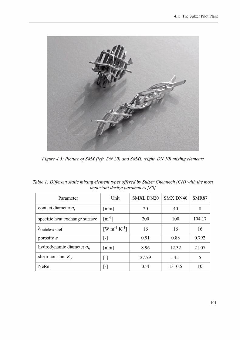
4.1: The Sulzer Pilot Plant
101
Figure 4.5: Picture of SMX (left, DN 20) and SMXL (right, DN 10) mixing elements
Table 1: Different static mixing element types offered by Sulzer Chemtech (CH) with the most important design parameters [80]
Parameter Unit SMXL DN20 SMX DN40 SMR87
contact diameter dt [mm] 20 40 8
specific heat exchange surface [m-1] 200 100 104.17
λstainless steel [W m-1 K-1] 16 16 16
porosity ε [-] 0.91 0.88 0.792
hydrodynamic diameter dh [mm] 8.96 12.32 21.07
shear constant Kγ [-] 27.79 54.5 5
NeRe [-] 354 1310.5 10

Chapter 4: Continuous High-Temperature Polymerization
102
The advantage of the different mixing elements is that their heat transfer coefficient com-
pare to each other, which is an important factor in the scale-up of polymerization processes. A
pilot-scale reactor can, therefore, directly be scaled-up to production-scale since the heat transfer
is more or less the same. This is illustrated in figure 4.6, where the pilot-scale SMXL tube is com-
pared to an industrial-scale SMR reactor.
The relatively constant heat exchange coefficient of the SMR type is once again illustrated
in figure 4.7, where it is compared to other types of reactors used for the production of polymers.
For high reactor volumes, the heat transfer coefficient drastically drops for the empty tube and the
CSTR. As discussed above, also the conventional static mixers reach quite soon a certain limit
due to the fact that they only conduct the heat to the reactor wall.
Pilot: SMXL DN 20U = 220 W m-2 K-1
A = 130 m2 m-3
Industrial: SMR DN 100-1500U = 310 W m-2 K-1
A = 85 m2 m-3
Volume specific heat transfer coefficient:K = 28 kW m-3 K-1 K = 26 kW m-3 K-1
Comparison CSTR: A = 1-4 m2 m-3
Figure 4.6: Comparison of SMXL and SMR mixer type as regards the scale-up of the process
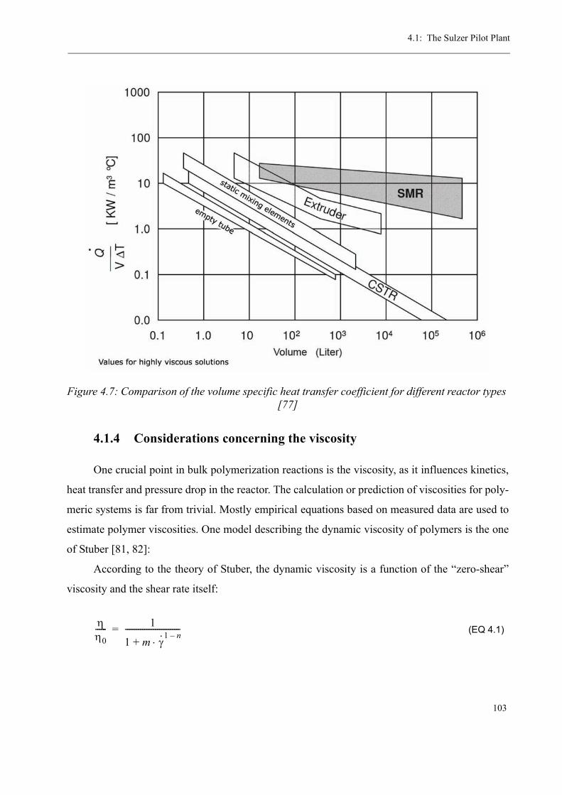
4.1: The Sulzer Pilot Plant
103
4.1.4 Considerations concerning the viscosity
One crucial point in bulk polymerization reactions is the viscosity, as it influences kinetics,
heat transfer and pressure drop in the reactor. The calculation or prediction of viscosities for poly-
meric systems is far from trivial. Mostly empirical equations based on measured data are used to
estimate polymer viscosities. One model describing the dynamic viscosity of polymers is the one
of Stuber [81, 82]:
According to the theory of Stuber, the dynamic viscosity is a function of the “zero-shear”
viscosity and the shear rate itself:
(EQ 4.1)
Figure 4.7: Comparison of the volume specific heat transfer coefficient for different reactor types [77]
ηη0------ 1
1 m γ·1 n–
⋅+-----------------------------=
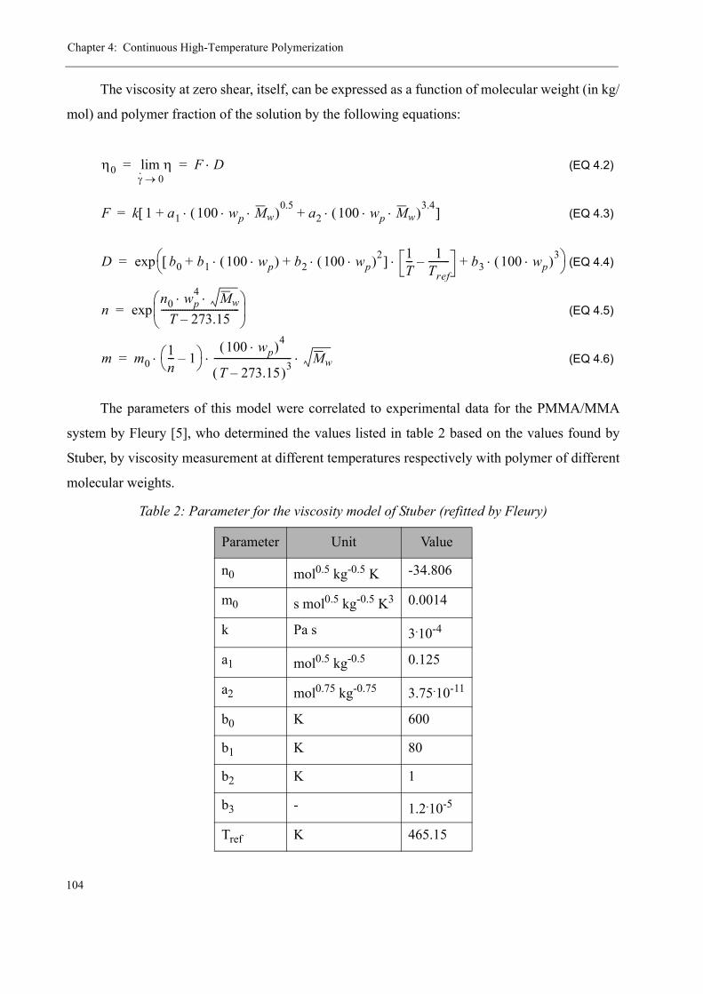
Chapter 4: Continuous High-Temperature Polymerization
104
The viscosity at zero shear, itself, can be expressed as a function of molecular weight (in kg/
mol) and polymer fraction of the solution by the following equations:
(EQ 4.2)
(EQ 4.3)
(EQ 4.4)
(EQ 4.5)
(EQ 4.6)
The parameters of this model were correlated to experimental data for the PMMA/MMA
system by Fleury [5], who determined the values listed in table 2 based on the values found by
Stuber, by viscosity measurement at different temperatures respectively with polymer of different
molecular weights.
Table 2: Parameter for the viscosity model of Stuber (refitted by Fleury)
Parameter Unit Value
n0 mol0.5 kg-0.5 K -34.806
m0 s mol0.5 kg-0.5 K3 0.0014
k Pa s 3.10-4
a1 mol0.5 kg-0.5 0.125
a2 mol0.75 kg-0.75 3.75.10-11
b0 K 600
b1 K 80
b2 K 1
b3 - 1.2.10-5
Tref K 465.15
η0 ηγ· 0→lim F D⋅= =
F k 1 a1 100 wp Mw⋅ ⋅( )0.5 a2 100 wp Mw⋅ ⋅( )
3.4⋅+⋅+[ ]=
D b0 b1 100 wp⋅( ) b2 100 wp⋅( )2⋅+⋅+[ ] 1T--- 1
Tref---------– b3 100 wp⋅( )3⋅+⋅⎝ ⎠
⎛ ⎞exp=
nn0 wp
4 Mw⋅ ⋅T 273.15–
---------------------------------⎝ ⎠⎜ ⎟⎛ ⎞
exp=
m m01n--- 1–⎝ ⎠
⎛ ⎞ 100 wp⋅( )4
T 273.15–( )3--------------------------------- Mw⋅ ⋅ ⋅=
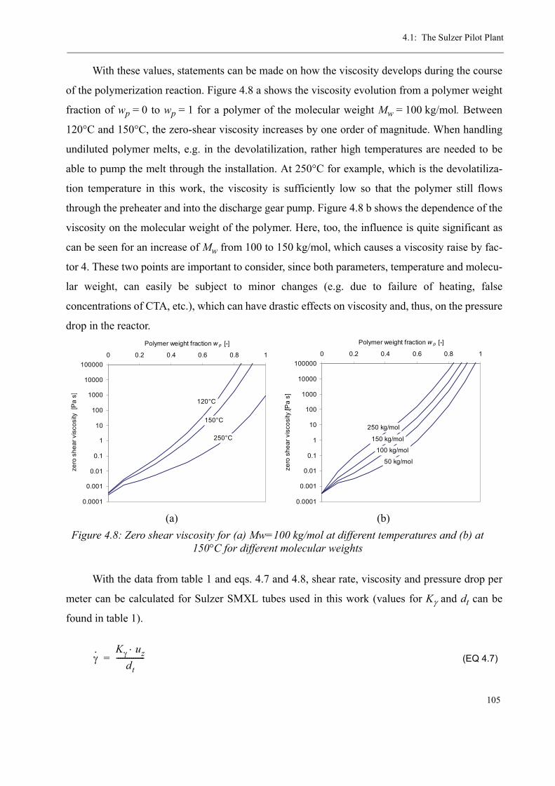
4.1: The Sulzer Pilot Plant
105
With these values, statements can be made on how the viscosity develops during the course
of the polymerization reaction. Figure 4.8 a shows the viscosity evolution from a polymer weight
fraction of wp = 0 to wp = 1 for a polymer of the molecular weight Mw = 100 kg/mol. Between
120°C and 150°C, the zero-shear viscosity increases by one order of magnitude. When handling
undiluted polymer melts, e.g. in the devolatilization, rather high temperatures are needed to be
able to pump the melt through the installation. At 250°C for example, which is the devolatiliza-
tion temperature in this work, the viscosity is sufficiently low so that the polymer still flows
through the preheater and into the discharge gear pump. Figure 4.8 b shows the dependence of the
viscosity on the molecular weight of the polymer. Here, too, the influence is quite significant as
can be seen for an increase of Mw from 100 to 150 kg/mol, which causes a viscosity raise by fac-
tor 4. These two points are important to consider, since both parameters, temperature and molecu-
lar weight, can easily be subject to minor changes (e.g. due to failure of heating, false
concentrations of CTA, etc.), which can have drastic effects on viscosity and, thus, on the pressure
drop in the reactor.
With the data from table 1 and eqs. 4.7 and 4.8, shear rate, viscosity and pressure drop per
meter can be calculated for Sulzer SMXL tubes used in this work (values for Kγ and dt can be
found in table 1).
(EQ 4.7)
(a) (b)Figure 4.8: Zero shear viscosity for (a) Mw=100 kg/mol at different temperatures and (b) at
150°C for different molecular weights
0.0001
0.001
0.01
0.1
1
10
100
1000
10000
1000000 0.2 0.4 0.6 0.8 1
Polymer weight fraction w p [-]
zero
she
ar v
isco
sity
[P
a s]
120°C
150°C
250°C
0.0001
0.001
0.01
0.1
1
10
100
1000
10000
1000000 0.2 0.4 0.6 0.8 1
Polymer weight fraction w p [-]
zero
she
ar v
isco
sity
⎠[Pa
s]
50 kg/mol
100 kg/mol
250 kg/mol
150 kg/mol
γ·Kγ uz⋅
dt---------------=

Chapter 4: Continuous High-Temperature Polymerization
106
(EQ 4.8)
Assuming a monomer conversion of X = 50% in the loop reactor (uz = 0.07 m/s at a recycle
ratio of 45:1) with a molecular weight of Mw = 100 kg/mol at 150°C results, according to this cal-
culation, in a pressure drop of Δp = 0.58 bar/m, which is easy to handle. However, in the case of a
feed pump failure, the reaction mixture would go straight into gel effect conditions and lead to
conversions around 80 to 90%, which would result in a pressure drop of uncontrollable
Δp = 190 bar/m, i.e. the sure plugging of the reactor.
A detailed discussion of the pressure drop in different zones of the pilot plant will follow
together with the results from pilot plant experiments at a later point in this chapter.
4.1.5 The Pilot Plant in Detail
After discussing the possibilities concerning the choice of pilot plant setup and mixing ele-
ments, the pilot plant setup used in this work will now be presented in detail. As mentioned
before, the reactor consists of two zones:
• A tubular recycle loop reactor with high recycle ratio (recycle : feed = 45:1)
• A conventional tube reactor
At the end of the reaction zone, there is a nitrogen-pressurized membrane flash valve from
where the polymer solution is flashed into a two-phase heat exchanger, which leads into devolatil-
ization chamber. From the devolatilization chamber, the devolatilized polymer melt is discharged
by a rotary gear pump and sent in two strands to the granulator.
There are four independent heating zones in the pilot plant, which can be identified in figure
4.9. The loop reactor, the first and the second part including the flash valve are each heated by a
4kW Karl Juchheim laboratory oil thermostat. The preheater and the devolatilization chamber
including the gear pump are heated by a 10kW HTT industrial oil thermostat. The heat transfer
medium in all thermostats is a synthetic oil on dibenzyltoluene basis (Shell Aseol Trans-SH) with
a temperature resistance up to 350°C.
The whole reactor is constructed with double-jacketed, stainless steel (316 / 1.4401) tubes
with diameter DN 20 and equipped with Sulzer SMXL respectively SMX static mixing elements.
ΔpL
-------NeRe η uz⋅ ⋅
dt2
-------------------------------= Pam-------
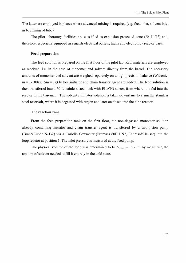
4.1: The Sulzer Pilot Plant
107
The latter are employed in places where advanced mixing is required (e.g. feed inlet, solvent inlet
in beginning of tube).
The pilot laboratory facilities are classified as explosion protected zone (Ex II T2) and,
therefore, especially equipped as regards electrical outlets, lights and electronic / reactor parts.
Feed preparation
The feed solution is prepared on the first floor of the pilot lab. Raw materials are employed
as received, i.e. in the case of monomer and solvent directly from the barrel. The necessary
amounts of monomer and solvent are weighed separately on a high-precision balance (Witronic,
m = 1-100kg, Δm = 1g) before initiator and chain transfer agent are added. The feed solution is
then transferred into a 60-L stainless steel tank with EKATO stirrer, from where it is fed into the
reactor in the basement. The solvent / initiator solution is taken downstairs to a smaller stainless
steel reservoir, where it is degassed with Argon and later on dosed into the tube reactor.
The reaction zone
From the feed preparation tank on the first floor, the non-degassed monomer solution
already containing initiator and chain transfer agent is transferred by a two-piston pump
(Bran&Lübbe N-J32) via a Coriolis flowmeter (Promass 60E DN2, Endress&Hauser) into the
loop reactor at position 1. The inlet pressure is measured at the feed pump.
The physical volume of the loop was determined to be Vloop = 907 ml by measuring the
amount of solvent needed to fill it entirely in the cold state.
Chapter 4: Continuous High-Temperature Polymerization
108
Within the recycle loop, the solution is pumped counterclockwise around by a high-speed
gear pump (Witte VAH-25,6 ED, position 2) at a recycle flow to feed flow ratio of approximately
Figure 4.9: Detailed scheme of the pilot plant setup used in this work
4b
4a
1
2
3
5
6
7
8
4.1: The Sulzer Pilot Plant
109
45:1. The displaced volume per turn of the pump head corresponds to 25.6 ml, therefore an aver-
age rotation frequency of n > 50 min-1 is needed. The high recycle ratio is necessary in order to
have (near-)CSTR conditions in the loop. In fact, it was shown by Zacca and Ray [83] that, as a
rule of thumb, above recycle ratios of 30:1, loop reactors behave as a CSTR (with regards to con-
version and molecular weight distribution). The limiting point in this consideration is the life-time
of the initiator, which must be higher than the time the solution needs to go around the loop. At a
recycle pump rotation speed of ω = 50 min-1 the cycle time in the loop is approximately 0.7 min.
Ideally, the half-life time of the initiator at given reaction temperatures is higher than this value.
The temperature inside the reactor is measured by means of several thermocouples (type K)
and there are two pressure transducers (Dynisco PT 435A / TPT 432A) that measure the pressure
drop in the loop at the gear pumps entry and exit. A small sapphire window allows optical inspec-
tion of the flowing reaction mixture inside the reactor. Samples can be taken through a sampling
valve at the loops exit. In the same place (position 3), there is also the ultrasound probe for inline
conversion measurement, which will be referred to later (see “Ultrasound Polymerization Moni-
toring” on page 115). The results from the ultrasound measurement can, thus, be directly com-
pared to offline sampling.
Connected to the exit of the recycle loop is a partially vertical, partially horizontal tube
reactor of the same diameter and a total length of approximately l = 3.5 m. The volume of the tube
reactor was determined to be Vtube = 1147 ml. Within this tube, the conversion reaches its maxi-
mum. As seen in the preceding subchapter, the “zero-shear” viscosity increases by a factor 103 for
an increase in polymer fraction from wp = 0.5 to 0.8 (T = 150 °C, Mw = 100 kg/mol). It is, there-
fore, regarded as necessary to add a solvent to this part of the reactor, by which the viscosity can
be kept at acceptable values. This is done by continuously injecting the desired amount of solvent
punctually in the center of the reactor stream. For an exact and constant dosing of the necessary
amount of solvent, a membrane microdosing pump is used (LEWA MLM/M210/3mm). In order
to achieve sufficient mixing of the low-viscous solvent with the highly-viscous polymer solution
from the loop, only the first half a meter of tube is equipped with SMX mixing elements, the rest
of the tube reactor contains SMXL mixing elements. Together with the solvent a second initiator
can be added in order to obtain higher conversions in the tube if needed. A second sapphire win-
dow is installed after one meter of tube and after approximately 2/3 of the total tube length, a sec-
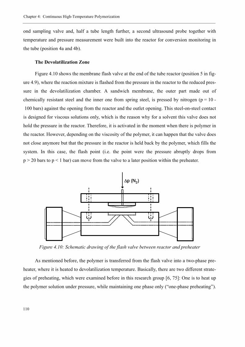
Chapter 4: Continuous High-Temperature Polymerization
110
ond sampling valve and, half a tube length further, a second ultrasound probe together with
temperature and pressure measurement were built into the reactor for conversion monitoring in
the tube (position 4a and 4b).
The Devolatilization Zone
Figure 4.10 shows the membrane flash valve at the end of the tube reactor (position 5 in fig-
ure 4.9), where the reaction mixture is flashed from the pressure in the reactor to the reduced pres-
sure in the devolatilization chamber. A sandwich membrane, the outer part made out of
chemically resistant steel and the inner one from spring steel, is pressed by nitrogen (p = 10 -
100 bars) against the opening from the reactor and the outlet opening. This steel-on-steel contact
is designed for viscous solutions only, which is the reason why for a solvent this valve does not
hold the pressure in the reactor. Therefore, it is activated in the moment when there is polymer in
the reactor. However, depending on the viscosity of the polymer, it can happen that the valve does
not close anymore but that the pressure in the reactor is held back by the polymer, which fills the
system. In this case, the flash point (i.e. the point were the pressure abruptly drops from
p > 20 bars to p < 1 bar) can move from the valve to a later position within the preheater.
As mentioned before, the polymer is transferred from the flash valve into a two-phase pre-
heater, where it is heated to devolatilization temperature. Basically, there are two different strate-
gies of preheating, which were examined before in this research group [6, 75]: One is to heat up
the polymer solution under pressure, while maintaining one phase only (“one-phase preheating”).
Figure 4.10: Schematic drawing of the flash valve between reactor and preheater
Δp (N2)Δp (N2)
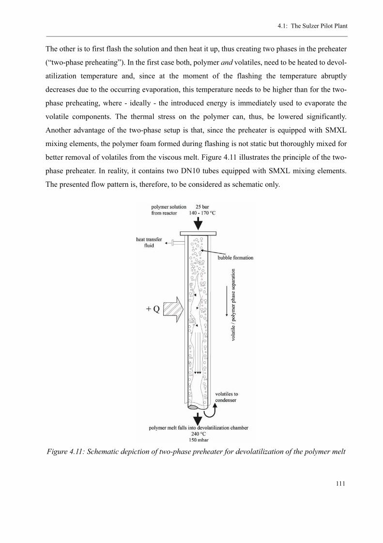
4.1: The Sulzer Pilot Plant
111
The other is to first flash the solution and then heat it up, thus creating two phases in the preheater
(“two-phase preheating”). In the first case both, polymer and volatiles, need to be heated to devol-
atilization temperature and, since at the moment of the flashing the temperature abruptly
decreases due to the occurring evaporation, this temperature needs to be higher than for the two-
phase preheating, where - ideally - the introduced energy is immediately used to evaporate the
volatile components. The thermal stress on the polymer can, thus, be lowered significantly.
Another advantage of the two-phase setup is that, since the preheater is equipped with SMXL
mixing elements, the polymer foam formed during flashing is not static but thoroughly mixed for
better removal of volatiles from the viscous melt. Figure 4.11 illustrates the principle of the two-
phase preheater. In reality, it contains two DN10 tubes equipped with SMXL mixing elements.
The presented flow pattern is, therefore, to be considered as schematic only.
Figure 4.11: Schematic depiction of two-phase preheater for devolatilization of the polymer melt
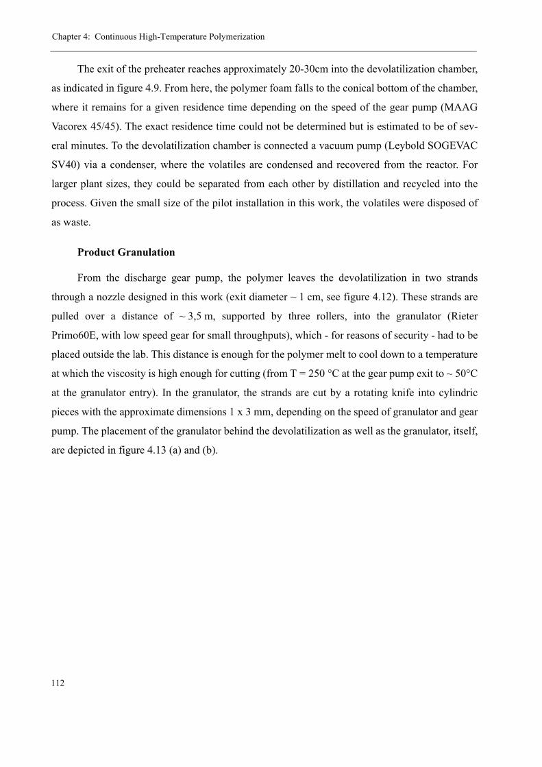
Chapter 4: Continuous High-Temperature Polymerization
112
The exit of the preheater reaches approximately 20-30cm into the devolatilization chamber,
as indicated in figure 4.9. From here, the polymer foam falls to the conical bottom of the chamber,
where it remains for a given residence time depending on the speed of the gear pump (MAAG
Vacorex 45/45). The exact residence time could not be determined but is estimated to be of sev-
eral minutes. To the devolatilization chamber is connected a vacuum pump (Leybold SOGEVAC
SV40) via a condenser, where the volatiles are condensed and recovered from the reactor. For
larger plant sizes, they could be separated from each other by distillation and recycled into the
process. Given the small size of the pilot installation in this work, the volatiles were disposed of
as waste.
Product Granulation
From the discharge gear pump, the polymer leaves the devolatilization in two strands
through a nozzle designed in this work (exit diameter ~ 1 cm, see figure 4.12). These strands are
pulled over a distance of ~ 3,5 m, supported by three rollers, into the granulator (Rieter
Primo60E, with low speed gear for small throughputs), which - for reasons of security - had to be
placed outside the lab. This distance is enough for the polymer melt to cool down to a temperature
at which the viscosity is high enough for cutting (from T = 250 °C at the gear pump exit to ~ 50°C
at the granulator entry). In the granulator, the strands are cut by a rotating knife into cylindric
pieces with the approximate dimensions 1 x 3 mm, depending on the speed of granulator and gear
pump. The placement of the granulator behind the devolatilization as well as the granulator, itself,
are depicted in figure 4.13 (a) and (b).
4.1: The Sulzer Pilot Plant
113
Figure 4.12: Gear pump exit nozzle designed to create two polymer strands for granulation
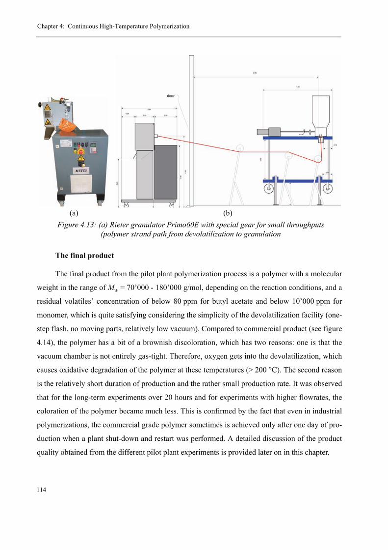
Chapter 4: Continuous High-Temperature Polymerization
114
The final product
The final product from the pilot plant polymerization process is a polymer with a molecular
weight in the range of Mw = 70’000 - 180’000 g/mol, depending on the reaction conditions, and a
residual volatiles’ concentration of below 80 ppm for butyl acetate and below 10’000 ppm for
monomer, which is quite satisfying considering the simplicity of the devolatilization facility (one-
step flash, no moving parts, relatively low vacuum). Compared to commercial product (see figure
4.14), the polymer has a bit of a brownish discoloration, which has two reasons: one is that the
vacuum chamber is not entirely gas-tight. Therefore, oxygen gets into the devolatilization, which
causes oxidative degradation of the polymer at these temperatures (> 200 °C). The second reason
is the relatively short duration of production and the rather small production rate. It was observed
that for the long-term experiments over 20 hours and for experiments with higher flowrates, the
coloration of the polymer became much less. This is confirmed by the fact that even in industrial
polymerizations, the commercial grade polymer sometimes is achieved only after one day of pro-
duction when a plant shut-down and restart was performed. A detailed discussion of the product
quality obtained from the different pilot plant experiments is provided later on in this chapter.
(a) (b)Figure 4.13: (a) Rieter granulator Primo60E with special gear for small throughputs
(polymer strand path from devolatilization to granulation
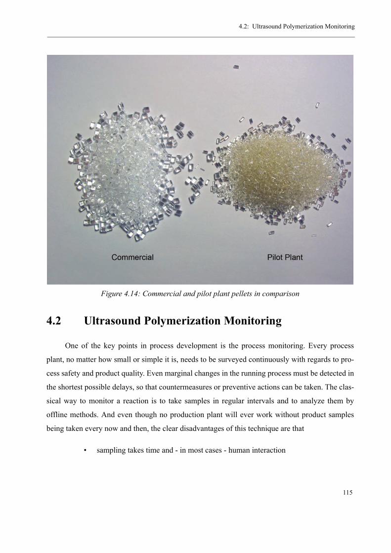
4.2: Ultrasound Polymerization Monitoring
115
4.2 Ultrasound Polymerization Monitoring
One of the key points in process development is the process monitoring. Every process
plant, no matter how small or simple it is, needs to be surveyed continuously with regards to pro-
cess safety and product quality. Even marginal changes in the running process must be detected in
the shortest possible delays, so that countermeasures or preventive actions can be taken. The clas-
sical way to monitor a reaction is to take samples in regular intervals and to analyze them by
offline methods. And even though no production plant will ever work without product samples
being taken every now and then, the clear disadvantages of this technique are that
• sampling takes time and - in most cases - human interaction
Figure 4.14: Commercial and pilot plant pellets in comparison
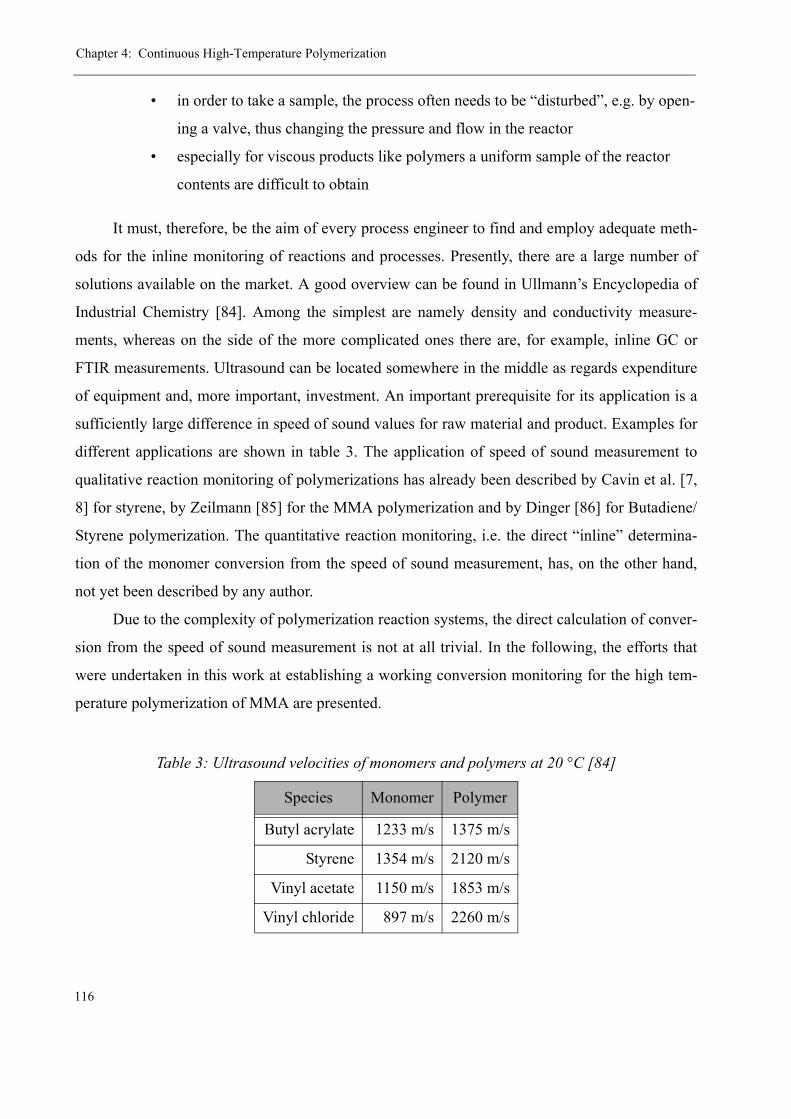
Chapter 4: Continuous High-Temperature Polymerization
116
• in order to take a sample, the process often needs to be “disturbed”, e.g. by open-
ing a valve, thus changing the pressure and flow in the reactor
• especially for viscous products like polymers a uniform sample of the reactor
contents are difficult to obtain
It must, therefore, be the aim of every process engineer to find and employ adequate meth-
ods for the inline monitoring of reactions and processes. Presently, there are a large number of
solutions available on the market. A good overview can be found in Ullmann’s Encyclopedia of
Industrial Chemistry [84]. Among the simplest are namely density and conductivity measure-
ments, whereas on the side of the more complicated ones there are, for example, inline GC or
FTIR measurements. Ultrasound can be located somewhere in the middle as regards expenditure
of equipment and, more important, investment. An important prerequisite for its application is a
sufficiently large difference in speed of sound values for raw material and product. Examples for
different applications are shown in table 3. The application of speed of sound measurement to
qualitative reaction monitoring of polymerizations has already been described by Cavin et al. [7,
8] for styrene, by Zeilmann [85] for the MMA polymerization and by Dinger [86] for Butadiene/
Styrene polymerization. The quantitative reaction monitoring, i.e. the direct “inline” determina-
tion of the monomer conversion from the speed of sound measurement, has, on the other hand,
not yet been described by any author.
Due to the complexity of polymerization reaction systems, the direct calculation of conver-
sion from the speed of sound measurement is not at all trivial. In the following, the efforts that
were undertaken in this work at establishing a working conversion monitoring for the high tem-
perature polymerization of MMA are presented.
Table 3: Ultrasound velocities of monomers and polymers at 20 °C [84]
Species Monomer Polymer
Butyl acrylate 1233 m/s 1375 m/s
Styrene 1354 m/s 2120 m/s
Vinyl acetate 1150 m/s 1853 m/s
Vinyl chloride 897 m/s 2260 m/s
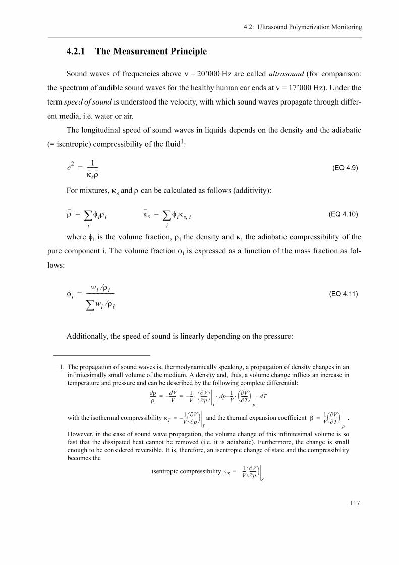
4.2: Ultrasound Polymerization Monitoring
117
4.2.1 The Measurement Principle
Sound waves of frequencies above ν = 20’000 Hz are called ultrasound (for comparison:
the spectrum of audible sound waves for the healthy human ear ends at ν = 17’000 Hz). Under the
term speed of sound is understood the velocity, with which sound waves propagate through differ-
ent media, i.e. water or air.
The longitudinal speed of sound waves in liquids depends on the density and the adiabatic
(= isentropic) compressibility of the fluid1:
(EQ 4.9)
For mixtures, κs and ρ can be calculated as follows (additivity):
(EQ 4.10)
where φi is the volume fraction, ρi the density and κi the adiabatic compressibility of the
pure component i. The volume fraction φi is expressed as a function of the mass fraction as fol-
lows:
(EQ 4.11)
Additionally, the speed of sound is linearly depending on the pressure:
1. The propagation of sound waves is, thermodynamically speaking, a propagation of density changes in aninfinitesimally small volume of the medium. A density and, thus, a volume change inflicts an increase intemperature and pressure and can be described by the following complete differential:
with the isothermal compressibility and the thermal expansion coefficient .
However, in the case of sound wave propagation, the volume change of this infinitesimal volume is sofast that the dissipated heat cannot be removed (i.e. it is adiabatic). Furthermore, the change is smallenough to be considered reversible. It is, therefore, an isentropic change of state and the compressibilitybecomes the
isentropic compressibility
dρρ
------ dVV
-------– 1V---– ∂V
∂p------⎝ ⎠
⎛ ⎞⋅T
dp 1V---– ∂V
∂T------⎝ ⎠
⎛ ⎞⋅p
dT⋅⋅= =
κT1V---– ∂V
∂p------⎝ ⎠
⎛ ⎞
T= β 1
V--- ∂V
∂T------⎝ ⎠
⎛ ⎞
p=
κS1V---– ∂V
∂p------⎝ ⎠
⎛ ⎞
S
=
c2 1κsρ--------=
ρ φiρii
∑= κs φiκs i,i
∑=
φiwi ρi⁄
wi ρi⁄i
∑---------------------=
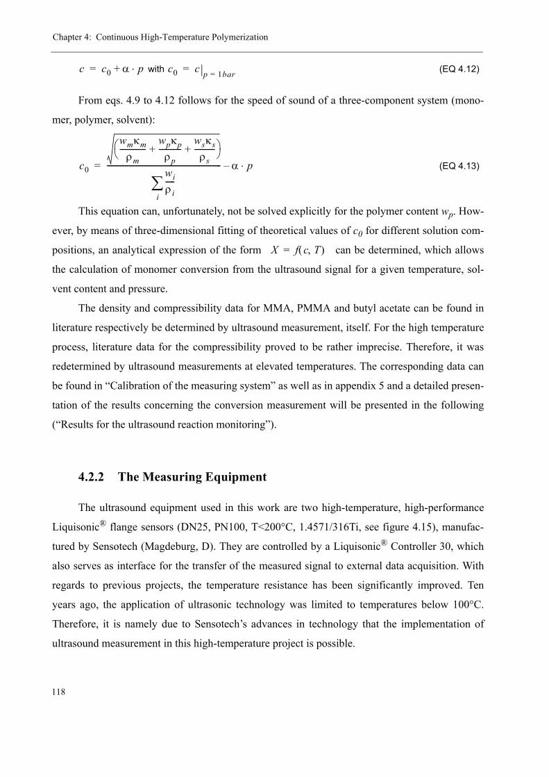
Chapter 4: Continuous High-Temperature Polymerization
118
with (EQ 4.12)
From eqs. 4.9 to 4.12 follows for the speed of sound of a three-component system (mono-
mer, polymer, solvent):
(EQ 4.13)
This equation can, unfortunately, not be solved explicitly for the polymer content wp. How-
ever, by means of three-dimensional fitting of theoretical values of c0 for different solution com-
positions, an analytical expression of the form can be determined, which allows
the calculation of monomer conversion from the ultrasound signal for a given temperature, sol-
vent content and pressure.
The density and compressibility data for MMA, PMMA and butyl acetate can be found in
literature respectively be determined by ultrasound measurement, itself. For the high temperature
process, literature data for the compressibility proved to be rather imprecise. Therefore, it was
redetermined by ultrasound measurements at elevated temperatures. The corresponding data can
be found in “Calibration of the measuring system” as well as in appendix 5 and a detailed presen-
tation of the results concerning the conversion measurement will be presented in the following
(“Results for the ultrasound reaction monitoring”).
4.2.2 The Measuring Equipment
The ultrasound equipment used in this work are two high-temperature, high-performance
Liquisonic® flange sensors (DN25, PN100, T<200°C, 1.4571/316Ti, see figure 4.15), manufac-
tured by Sensotech (Magdeburg, D). They are controlled by a Liquisonic® Controller 30, which
also serves as interface for the transfer of the measured signal to external data acquisition. With
regards to previous projects, the temperature resistance has been significantly improved. Ten
years ago, the application of ultrasonic technology was limited to temperatures below 100°C.
Therefore, it is namely due to Sensotech’s advances in technology that the implementation of
ultrasound measurement in this high-temperature project is possible.
c c0 α p⋅+= c0 c p 1bar==
c0
wmκmρm
--------------wpκp
ρp------------
wsκsρs
-----------+ +⎝ ⎠⎛ ⎞
wiρi-----
i∑
-------------------------------------------------------------- α p⋅–=
X f c T,( )=

4.2: Ultrasound Polymerization Monitoring
119
In order to reduce the dead volume inside the probe, plastic parts were introduced from both
sides occupying most of the volume around emitter and receptor (several issues arouse from this
feature, which will be discussed further down in this chapter).
The functioning of the flange sensor is depicted in figure 4.16. On one side of the probe, a
transducer emits pulsated sound waves of a given pressure amplitude (proportional to the applied
voltage U0) and frequency, orthogonal to the flow direction. The signal reaches the receptor,
where it creates a voltage again proportional to its amplitude. The speed of sound can be deter-
mined by the time necessary to travel from the emitter to the receiver, whereas the attenuation of
the signal δ is calculated from the change of amplitude (eqs. 4.14 and 4.15). However, for conver-
sion monitoring in polymerization systems, only the speed of sound measurement is of impor-
tance.
(EQ 4.14)
(EQ 4.15)
Figure 4.15: Liquisonic® flange sensor DN25
uzxΔt-----=
δ 1x---
A0Ax------ln⋅ 1
x---
U0Ux------ln⋅= =
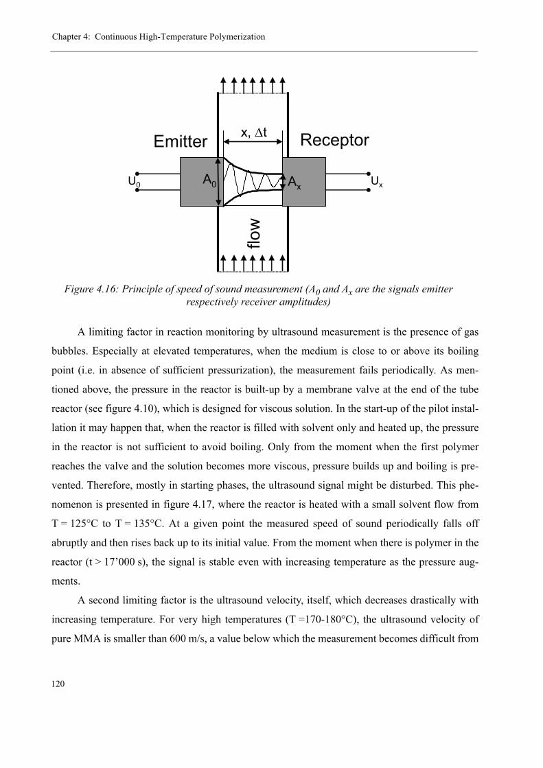
Chapter 4: Continuous High-Temperature Polymerization
120
A limiting factor in reaction monitoring by ultrasound measurement is the presence of gas
bubbles. Especially at elevated temperatures, when the medium is close to or above its boiling
point (i.e. in absence of sufficient pressurization), the measurement fails periodically. As men-
tioned above, the pressure in the reactor is built-up by a membrane valve at the end of the tube
reactor (see figure 4.10), which is designed for viscous solution. In the start-up of the pilot instal-
lation it may happen that, when the reactor is filled with solvent only and heated up, the pressure
in the reactor is not sufficient to avoid boiling. Only from the moment when the first polymer
reaches the valve and the solution becomes more viscous, pressure builds up and boiling is pre-
vented. Therefore, mostly in starting phases, the ultrasound signal might be disturbed. This phe-
nomenon is presented in figure 4.17, where the reactor is heated with a small solvent flow from
T = 125°C to T = 135°C. At a given point the measured speed of sound periodically falls off
abruptly and then rises back up to its initial value. From the moment when there is polymer in the
reactor (t > 17’000 s), the signal is stable even with increasing temperature as the pressure aug-
ments.
A second limiting factor is the ultrasound velocity, itself, which decreases drastically with
increasing temperature. For very high temperatures (T =170-180°C), the ultrasound velocity of
pure MMA is smaller than 600 m/s, a value below which the measurement becomes difficult from
Figure 4.16: Principle of speed of sound measurement (A0 and Ax are the signals emitter respectively receiver amplitudes)
flow
Emitter Receptorx, Δt
A0 AxU0 Ux

4.2: Ultrasound Polymerization Monitoring
121
a physical point of view due to structure-born sound disturbances (elastic vibration of solid mate-
rial, i.e. probe material) and which was enforced electronically as lower measurement limit to
avoid inaccuracies. Therefore, at these temperatures, measuring is only possible in the presence of
polymer in the system, which causes an increase in ultrasound velocity big enough to be again
above the limit.
Another probe specific problem is fouling and dead volumes. Since the cylinder-like trans-
ducers penetrate the medium and the flow is slowed down due to the widening of the diameter in
the sensor, the formation of polymer layers is favoured. For this reason, special filling pieces have
been developed with the aim to fill this empty volume and to incorporate the transducer cylinders
except for their emitting / receiving surface.
Several problems were encountered as to the use of these pieces. First to mention is the
choice of a suitable material, which resists the process conditions. In contrast to recommendations
from industry, poly (vinylidene fluoride), PVDF, was found to be not a good candidate since it
dissolved already after a few heating cycles to large extents in the reaction medium (compare
parts before and after use shown in figure 4.18), leading to severe problems with reactor leaking.
The dissolved PVDF was later found in the produced PMMA as encapsulated droplets.
Figure 4.17: Loss of ultrasound signal due to bubble formation
600
620
640
660
680
700
720
740
760
780
800
13'000 14'000 15'000 16'000 17'000 18'000
Time [s]
spee
d of
sou
nd [m
/s]
100
105
110
115
120
125
130
135
140
145
150
T [°
C]
US TubeUS LoopLoop Temperature
Bubble formation due to boiling
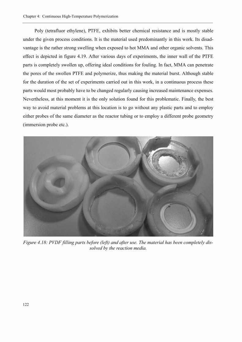
Chapter 4: Continuous High-Temperature Polymerization
122
Poly (tetrafluor ethylene), PTFE, exhibits better chemical resistance and is mostly stable
under the given process conditions. It is the material used predominantly in this work. Its disad-
vantage is the rather strong swelling when exposed to hot MMA and other organic solvents. This
effect is depicted in figure 4.19. After various days of experiments, the inner wall of the PTFE
parts is completely swollen up, offering ideal conditions for fouling. In fact, MMA can penetrate
the pores of the swollen PTFE and polymerize, thus making the material burst. Although stable
for the duration of the set of experiments carried out in this work, in a continuous process these
parts would most probably have to be changed regularly causing increased maintenance expenses.
Nevertheless, at this moment it is the only solution found for this problematic. Finally, the best
way to avoid material problems at this location is to go without any plastic parts and to employ
either probes of the same diameter as the reactor tubing or to employ a different probe geometry
(immersion probe etc.).
Figure 4.18: PVDF filling parts before (left) and after use. The material has been completely dis-solved by the reaction media.
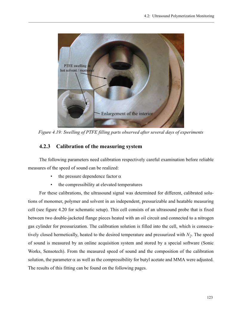
4.2: Ultrasound Polymerization Monitoring
123
4.2.3 Calibration of the measuring system
The following parameters need calibration respectively careful examination before reliable
measures of the speed of sound can be realized:
• the pressure dependence factor α
• the compressibility at elevated temperatures
For these calibrations, the ultrasound signal was determined for different, calibrated solu-
tions of monomer, polymer and solvent in an independent, pressurizable and heatable measuring
cell (see figure 4.20 for schematic setup). This cell consists of an ultrasound probe that is fixed
between two double-jacketed flange pieces heated with an oil circuit and connected to a nitrogen
gas cylinder for pressurization. The calibration solution is filled into the cell, which is consecu-
tively closed hermetically, heated to the desired temperature and pressurized with N2. The speed
of sound is measured by an online acquisition system and stored by a special software (Sonic
Works, Sensotech). From the measured speed of sound and the composition of the calibration
solution, the parameter α as well as the compressibility for butyl acetate and MMA were adjusted.
The results of this fitting can be found on the following pages.
Figure 4.19: Swelling of PTFE filling parts observed after several days of experiments
Enlargement of the interior
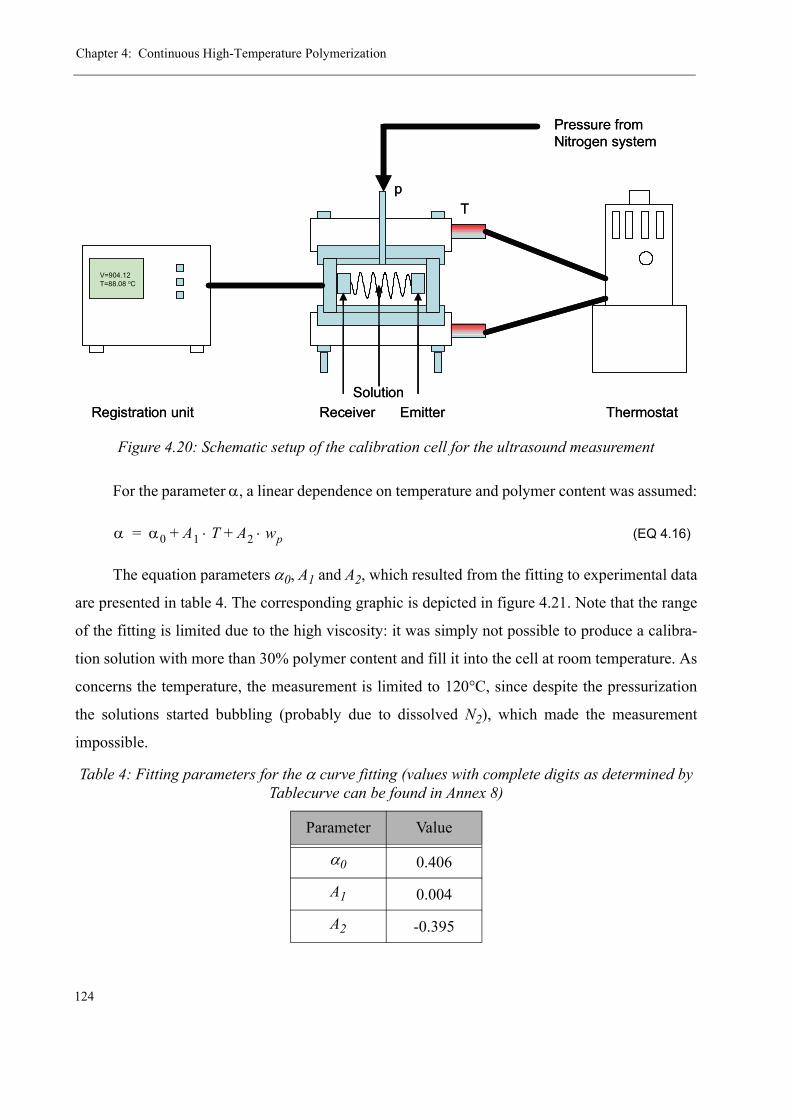
Chapter 4: Continuous High-Temperature Polymerization
124
For the parameter α, a linear dependence on temperature and polymer content was assumed:
(EQ 4.16)
The equation parameters α0, A1 and A2, which resulted from the fitting to experimental data
are presented in table 4. The corresponding graphic is depicted in figure 4.21. Note that the range
of the fitting is limited due to the high viscosity: it was simply not possible to produce a calibra-
tion solution with more than 30% polymer content and fill it into the cell at room temperature. As
concerns the temperature, the measurement is limited to 120°C, since despite the pressurization
the solutions started bubbling (probably due to dissolved N2), which made the measurement
impossible.
Figure 4.20: Schematic setup of the calibration cell for the ultrasound measurement
Table 4: Fitting parameters for the α curve fitting (values with complete digits as determined by Tablecurve can be found in Annex 8)
Parameter Value
α0 0.406
A1 0.004
A2 -0.395
V=904.12 T=88.08 oC
Pressure fromNitrogen system
p
Receiver Emitter Thermostat
T
Registration unitSolution
V=904.12 T=88.08 oC
Pressure fromNitrogen system
p
Receiver Emitter Thermostat
T
Registration unitSolution
α α0 A1 T A2 wp⋅+⋅+=
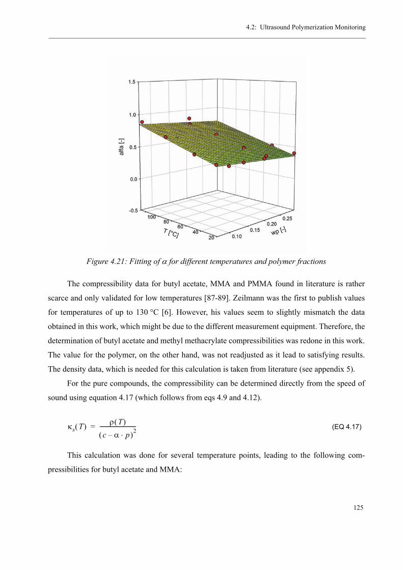
4.2: Ultrasound Polymerization Monitoring
125
The compressibility data for butyl acetate, MMA and PMMA found in literature is rather
scarce and only validated for low temperatures [87-89]. Zeilmann was the first to publish values
for temperatures of up to 130 °C [6]. However, his values seem to slightly mismatch the data
obtained in this work, which might be due to the different measurement equipment. Therefore, the
determination of butyl acetate and methyl methacrylate compressibilities was redone in this work.
The value for the polymer, on the other hand, was not readjusted as it lead to satisfying results.
The density data, which is needed for this calculation is taken from literature (see appendix 5).
For the pure compounds, the compressibility can be determined directly from the speed of
sound using equation 4.17 (which follows from eqs 4.9 and 4.12).
(EQ 4.17)
This calculation was done for several temperature points, leading to the following com-
pressibilities for butyl acetate and MMA:
Figure 4.21: Fitting of α for different temperatures and polymer fractions
κs T( ) ρ T( )
c α p⋅–( )2---------------------------=
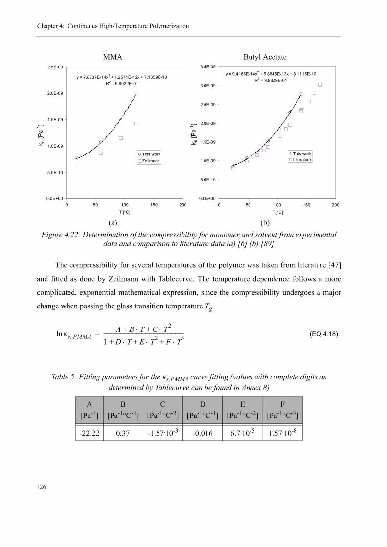
Chapter 4: Continuous High-Temperature Polymerization
126
The compressibility for several temperatures of the polymer was taken from literature [47]
and fitted as done by Zeilmann with Tablecurve. The temperature dependence follows a more
complicated, exponential mathematical expression, since the compressibility undergoes a major
change when passing the glass transition temperature Tg.
(EQ 4.18)
MMA Butyl Acetate
(a) (b)Figure 4.22: Determination of the compressibility for monomer and solvent from experimental
data and comparison to literature data (a) [6] (b) [89]
Table 5: Fitting parameters for the κs,PMMA curve fitting (values with complete digits as determined by Tablecurve can be found in Annex 8)
A[Pa-1]
B[Pa-1°C-1]
C[Pa-1°C-2]
D[Pa-1°C-1]
E[Pa-1°C-2]
F[Pa-1°C-3]
-22.22 0.37 -1.57.10-3 -0.016 6.7.10-5 1.57.10-8
y = 7.8237E-14x2 + 1.2571E-12x + 7.1359E-10R2 = 9.9922E-01
0.0E+00
5.0E-10
1.0E-09
1.5E-09
2.0E-09
2.5E-09
0 50 100 150 200
T [°C]
This workZeilmann
k s [P
a-1]
y = 9.4166E-14x2 + 5.8845E-13x + 8.1115E-10R2 = 9.9829E-01
0.0E+00
5.0E-10
1.0E-09
1.5E-09
2.0E-09
2.5E-09
3.0E-09
3.5E-09
0 50 100 150 200
T [°C]
This workLiterature
k s [P
a-1]
κs PMMA,ln A B T C T2⋅+⋅+1 D T E T2 F T3⋅+⋅+⋅+--------------------------------------------------------------=
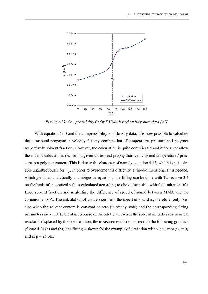
4.2: Ultrasound Polymerization Monitoring
127
With equation 4.13 and the compressibility and density data, it is now possible to calculate
the ultrasound propagation velocity for any combination of temperature, pressure and polymer
respectively solvent fraction. However, the calculation is quite complicated and it does not allow
the inverse calculation, i.e. from a given ultrasound propagation velocity and temperature / pres-
sure to a polymer content. This is due to the character of namely equation 4.13, which is not solv-
able unambiguously for wp. In order to overcome this difficulty, a three-dimensional fit is needed,
which yields an analytically unambiguous equation. The fitting can be done with Tablecurve 3D
on the basis of theoretical values calculated according to above formulas, with the limitation of a
fixed solvent fraction and neglecting the difference of speed of sound between MMA and the
comonomer MA. The calculation of conversion from the speed of sound is, therefore, only pre-
cise when the solvent content is constant or zero (in steady state) and the corresponding fitting
parameters are used. In the startup phase of the pilot plant, when the solvent initially present in the
reactor is displaced by the feed solution, the measurement is not correct. In the following graphics
(figure 4.24 (a) and (b)), the fitting is shown for the example of a reaction without solvent (ws = 0)
and at p = 25 bar.
Figure 4.23: Compressibility fit for PMMA based on literature data [47]
0.0E+00
1.0E-10
2.0E-10
3.0E-10
4.0E-10
5.0E-10
6.0E-10
7.0E-10
20 40 60 80 100 120 140 160 180 200
T[°C]
LiteratureFit Tablecurve
Tg
k s [P
a-1]
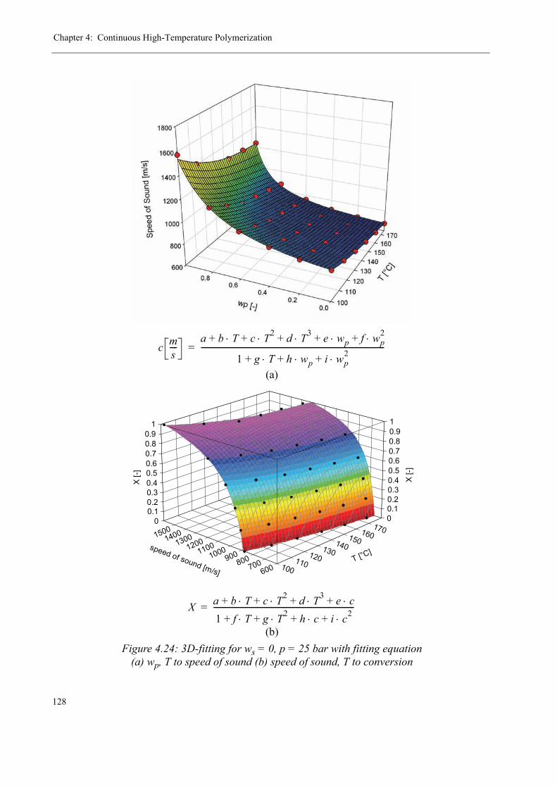
Chapter 4: Continuous High-Temperature Polymerization
128
(a)
(b)Figure 4.24: 3D-fitting for ws = 0, p = 25 bar with fitting equation
(a) wp, T to speed of sound (b) speed of sound, T to conversion
c ms----
a b T c T2 d T3 e wp f wp2⋅+⋅+⋅+⋅+⋅+
1 g+ T h wp i wp2⋅+⋅+⋅
--------------------------------------------------------------------------------------------------=
100110
120130
140150
160170
T [°C]
600700800900100011001200130014001500
speed of sound [m/s]
0 00.1 0.10.2 0.20.3 0.30.4 0.40.5 0.50.6 0.60.7 0.70.8 0.80.9 0.9
1 1
X [-] X [-]
X a b T c T2 d T3 e c⋅+⋅+⋅+⋅+1 f T g T2 h c i c2⋅+⋅+⋅+⋅+---------------------------------------------------------------------------=
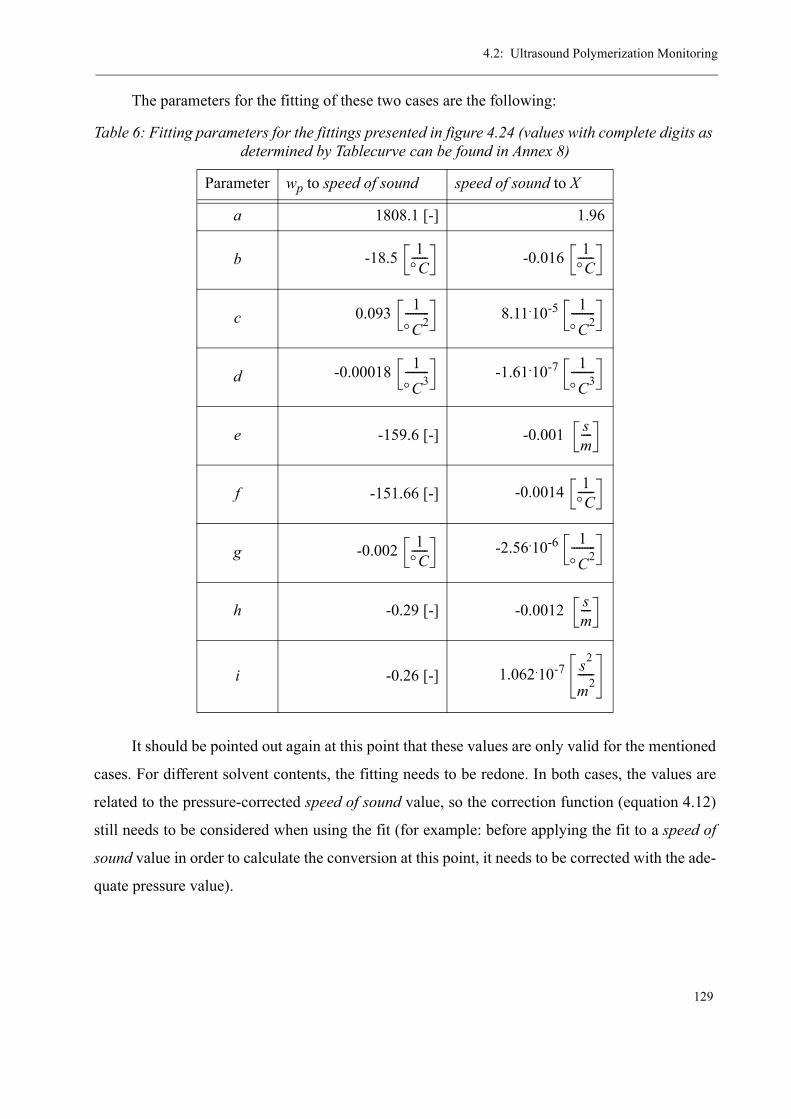
4.2: Ultrasound Polymerization Monitoring
129
The parameters for the fitting of these two cases are the following:
It should be pointed out again at this point that these values are only valid for the mentioned
cases. For different solvent contents, the fitting needs to be redone. In both cases, the values are
related to the pressure-corrected speed of sound value, so the correction function (equation 4.12)
still needs to be considered when using the fit (for example: before applying the fit to a speed of
sound value in order to calculate the conversion at this point, it needs to be corrected with the ade-
quate pressure value).
Table 6: Fitting parameters for the fittings presented in figure 4.24 (values with complete digits as determined by Tablecurve can be found in Annex 8)
Parameter wp to speed of sound speed of sound to X
a 1808.1 [-] 1.96
b -18.5 -0.016
c 0.093 8.11.10-5
d -0.00018 -1.61.10-7
e -159.6 [-] -0.001
f -151.66 [-] -0.0014
g -0.002 -2.56.10-6
h -0.29 [-] -0.0012
i -0.26 [-] 1.062.10-7
1°C------ 1
°C------
1°C2--------- 1
°C2---------
1°C3--------- 1
°C3---------
sm----
1°C------
1°C------
1°C2---------
sm----
s2
m2------

Chapter 4: Continuous High-Temperature Polymerization
130
4.2.4 Results for the ultrasound reaction monitoring
Apart from a quantitative determination of the conversion in the reactor (inline conversion
measurement), which will be presented later on, the ultrasound technique gives access to other
important (qualitative) information. It is, for example, possible to observe the stability of a contin-
uous process or its dynamic behavior during condition changes (i.e. start-up, shut-down, tempera-
ture change etc.).
The process monitoring by ultrasound is illustrated in figure 4.25 for the example of a poly-
merization at T = 140 °C (curve shown for the loop probe). During the initial heating phase with a
very low solvent flowrate, the speed of sound decreases continuously until the final reaction tem-
perature is reached. This decrease is only due to the change in density and compressibility of
butyl acetate with increasing temperature. As soon as the feed stream is switched from solvent to
monomer solution, the polymerizations starts and the polymer volume fraction increases. The
consequence is an increasing speed of sound signal. Once the solvent is displaced and the reactor
is in hydrodynamic and kinetic steady-state, the signal becomes constant. In the presented case,
the time necessary to reach steady state is t = 150 min, i.e. 5 residence times at the flowrate of
F = 1.8 kg/h.
Figure 4.25: Ultrasound process monitoring example for the loop probe in experiment no. 2 (see appendix 7)
700
750
800
850
900
950
1000
1050
1100
1150
1200
0 5000 10000 15000 20000 25000 30000
Time [s]
Spe
ed o
f sou
nd [m
/s]
Heating to 100 °C
Heating to 135 °C
Switch tomonomer feed
Steady state
Switch tosolvent feed & cooling down
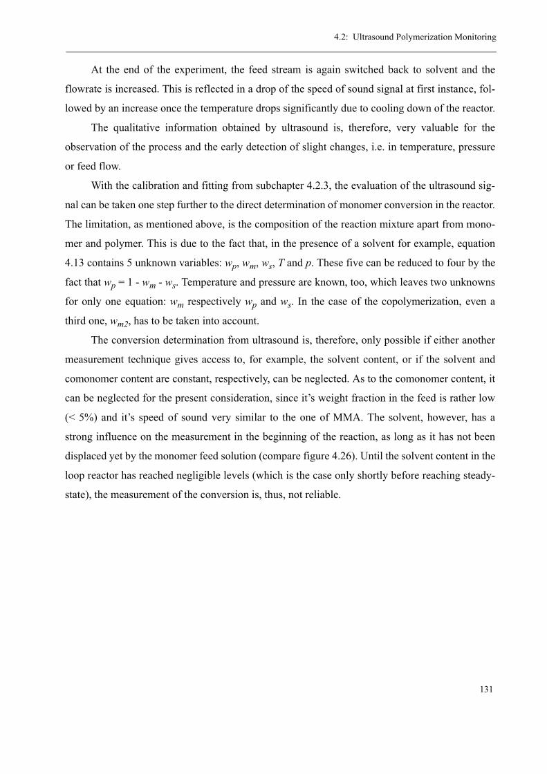
4.2: Ultrasound Polymerization Monitoring
131
At the end of the experiment, the feed stream is again switched back to solvent and the
flowrate is increased. This is reflected in a drop of the speed of sound signal at first instance, fol-
lowed by an increase once the temperature drops significantly due to cooling down of the reactor.
The qualitative information obtained by ultrasound is, therefore, very valuable for the
observation of the process and the early detection of slight changes, i.e. in temperature, pressure
or feed flow.
With the calibration and fitting from subchapter 4.2.3, the evaluation of the ultrasound sig-
nal can be taken one step further to the direct determination of monomer conversion in the reactor.
The limitation, as mentioned above, is the composition of the reaction mixture apart from mono-
mer and polymer. This is due to the fact that, in the presence of a solvent for example, equation
4.13 contains 5 unknown variables: wp, wm, ws, T and p. These five can be reduced to four by the
fact that wp = 1 - wm - ws. Temperature and pressure are known, too, which leaves two unknowns
for only one equation: wm respectively wp and ws. In the case of the copolymerization, even a
third one, wm2, has to be taken into account.
The conversion determination from ultrasound is, therefore, only possible if either another
measurement technique gives access to, for example, the solvent content, or if the solvent and
comonomer content are constant, respectively, can be neglected. As to the comonomer content, it
can be neglected for the present consideration, since it’s weight fraction in the feed is rather low
(< 5%) and it’s speed of sound very similar to the one of MMA. The solvent, however, has a
strong influence on the measurement in the beginning of the reaction, as long as it has not been
displaced yet by the monomer feed solution (compare figure 4.26). Until the solvent content in the
loop reactor has reached negligible levels (which is the case only shortly before reaching steady-
state), the measurement of the conversion is, thus, not reliable.
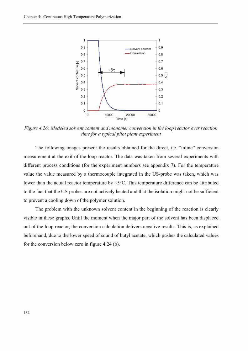
Chapter 4: Continuous High-Temperature Polymerization
132
The following images present the results obtained for the direct, i.e. “inline” conversion
measurement at the exit of the loop reactor. The data was taken from several experiments with
different process conditions (for the experiment numbers see appendix 7). For the temperature
value the value measured by a thermocouple integrated in the US-probe was taken, which was
lower than the actual reactor temperature by ~5°C. This temperature difference can be attributed
to the fact that the US-probes are not actively heated and that the isolation might not be sufficient
to prevent a cooling down of the polymer solution.
The problem with the unknown solvent content in the beginning of the reaction is clearly
visible in these graphs. Until the moment when the major part of the solvent has been displaced
out of the loop reactor, the conversion calculation delivers negative results. This is, as explained
beforehand, due to the lower speed of sound of butyl acetate, which pushes the calculated values
for the conversion below zero in figure 4.24 (b).
Figure 4.26: Modeled solvent content and monomer conversion in the loop reactor over reaction time for a typical pilot plant experiment
0
0.1
0.2
0.3
0.4
0.5
0.6
0.7
0.8
0.9
1
0 10000 20000 30000Time [s]
Solv
ent c
onte
nt w
s [-]
0
0.1
0.2
0.3
0.4
0.5
0.6
0.7
0.8
0.9
1
X [-]
Solvent contentConversion
~5τ
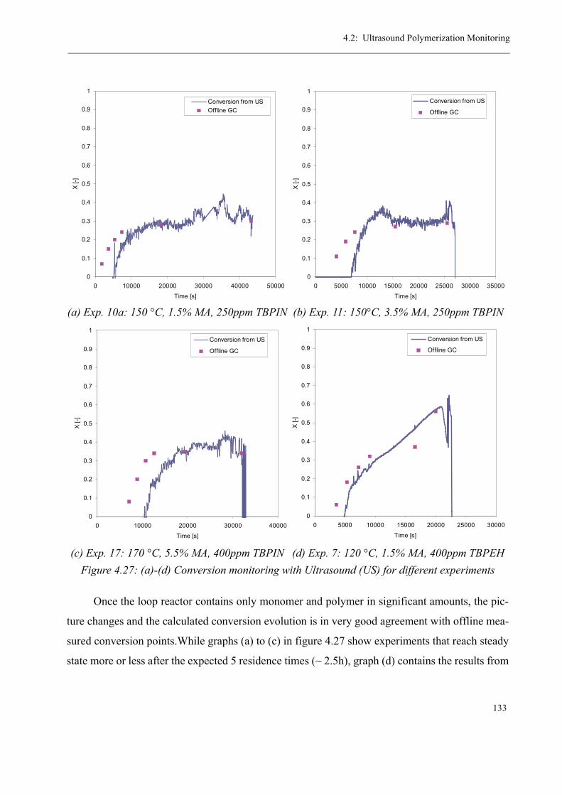
4.2: Ultrasound Polymerization Monitoring
133
Once the loop reactor contains only monomer and polymer in significant amounts, the pic-
ture changes and the calculated conversion evolution is in very good agreement with offline mea-
sured conversion points.While graphs (a) to (c) in figure 4.27 show experiments that reach steady
state more or less after the expected 5 residence times (~ 2.5h), graph (d) contains the results from
(a) Exp. 10a: 150 °C, 1.5% MA, 250ppm TBPIN (b) Exp. 11: 150°C, 3.5% MA, 250ppm TBPIN
(c) Exp. 17: 170 °C, 5.5% MA, 400ppm TBPIN (d) Exp. 7: 120 °C, 1.5% MA, 400ppm TBPEHFigure 4.27: (a)-(d) Conversion monitoring with Ultrasound (US) for different experiments
0
0.1
0.2
0.3
0.4
0.5
0.6
0.7
0.8
0.9
1
0 10000 20000 30000 40000 50000
Time [s]
X [-
]
Conversion from USOffline GC
0
0.1
0.2
0.3
0.4
0.5
0.6
0.7
0.8
0.9
1
0 5000 10000 15000 20000 25000 30000 35000
Time [s]X
[-]
Conversion from US
Offline GC
0
0.1
0.2
0.3
0.4
0.5
0.6
0.7
0.8
0.9
1
0 10000 20000 30000 40000
Time [s]
X [-
]
Conversion from US
Offline GC
0
0.1
0.2
0.3
0.4
0.5
0.6
0.7
0.8
0.9
1
0 5000 10000 15000 20000 25000 30000
Time [s]
X [-
]
Conversion from US
Offline GC

Chapter 4: Continuous High-Temperature Polymerization
134
a somewhat particular experiment. It was carried out at 120 °C, i.e. at the lower end of the temper-
ature scale used in this work, and with an elevated initiator concentration (400 ppm). The combi-
nation of higher viscosity at this temperature and the slightly higher conversion lead during the
course of experiment to the triggering of the gel effect. Both, ultrasound conversion measurement
and offline GC clearly show the runaway of the reaction, which - after 5 hours - had to be aborted
due to an excessive increase in pressure drop.
Since the conversion measurement by offline GC is not available right away during the
experiment but needs at least several hours for the analysis to be done, the reason for this pressure
increase inside the reactor could not be figured out immediately. Only the ultrasound measure-
ment enabled the controller to realize the reactor instability with the tendency of a reaction run-
away and to react by aborting before the situation got out of control (e.g. plugging of the reactor,
bursting of sealings etc.).
It can, therefore, without doubt be stated that the inline conversion measurement by ultra-
sound is an important and useful tool for the monitoring of polymerization reactions.
Some improvements will need to be done concerning the reliability of the measurement, as
for some experiments, the signal was seriously disturbed by inexplicable fluctuations of the speed
of sound (figure 4.28), leading to a misinterpretation of the conversion by almost 20%.
Figure 4.28: Fluctuations of the speed of sound signal during an experiment (140 °C, 3.5% MA, 250ppm TBPEH)
0
0.1
0.2
0.3
0.4
0.5
0.6
0.7
0.8
0.9
1
0 10000 20000 30000 40000 50000
Time [s]
X [-
]
600
630
660
690
720
750
780
810
840
870
900
Spe
ed o
f sou
nd [m
/s]
Conversion from USOffline GCSpeed of Sound
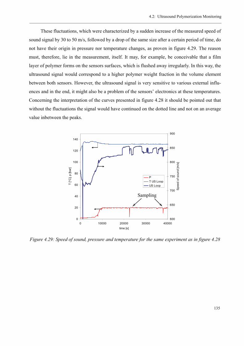
4.2: Ultrasound Polymerization Monitoring
135
These fluctuations, which were characterized by a sudden increase of the measured speed of
sound signal by 30 to 50 m/s, followed by a drop of the same size after a certain period of time, do
not have their origin in pressure nor temperature changes, as proven in figure 4.29. The reason
must, therefore, lie in the measurement, itself. It may, for example, be conceivable that a film
layer of polymer forms on the sensors surfaces, which is flushed away irregularly. In this way, the
ultrasound signal would correspond to a higher polymer weight fraction in the volume element
between both sensors. However, the ultrasound signal is very sensitive to various external influ-
ences and in the end, it might also be a problem of the sensors’ electronics at these temperatures.
Concerning the interpretation of the curves presented in figure 4.28 it should be pointed out that
without the fluctuations the signal would have continued on the dotted line and not on an average
value inbetween the peaks.
Figure 4.29: Speed of sound, pressure and temperature for the same experiment as in figure 4.28
0
20
40
60
80
100
120
140
0 10000 20000 30000 40000
time [s]
T [°
C],
p [b
ar]
600
650
700
750
800
850
900
Spe
ed o
f sou
nd [m
/s]
PT US LoopUS Loop
Sampling
Chapter 4: Continuous High-Temperature Polymerization
136
4.3 Verification of the High-Temperature Kinetics
4.3.1 Results from the Pilot Plant
A complete list of all pilot plant experiments carried out in this work, together with the cor-
responding process conditions and a result overview can be found in appendix 7. Altogether, 23
experiments were accomplished under different conditions (i.e. 5 different temperatures, 3 differ-
ent comonomer and chain transfer agent contents) and evaluated concerning monomer conver-
sion, molecular weight and final product quality. The latter was characterized in collaboration
with the analytical department of the industrial partner by determining:
• the molecular weight
• the residual volatiles (monomer and solvent)
• the comonomer weight fraction in the polymer
• the tacticity
• and the thermostability of each sample.
The aim for all experiments was to obtain monomer conversions of XLoop = 50% in the loop
and an additional Xtube = 30% in the tube reactor while maintaining the molecular weight of the
final polymer in the region of Mw = 100’000 g/mol, which is an average value for commercial
molding compound PMMA.
This goal was practically achieved for most experiments. The effective conversion range in
the loop reactor lies around XLoop = 40 - 50%, except for some experiments where the conversion
stayed particularly low (around 30%). For the tube, the conversion was determined at two points:
the first at the sampling valve after two-thirds of the tube length, the second from the condensate
samples, which corresponds to the total conversion over the whole process. The aim of achieving
30% conversion in the tube was only partly achieved, namely for the experiments with DTBP as
initiator in the tube. For those with TBPIN (No. 1-5), the conversion was rather 20 than 30%,
which is connected to its faster decomposition kinetics. At the injection point, the initiator is
dosed into the tube as dilute solution in butyl acetate. This low-viscous liquid needs to be mixed
thoroughly with the polymer melt from the loop reactor, which - at 40 - 50% conversion - is sig-
nificantly more viscous (approximately by a factor 1000). If the decomposition of the initiator is -
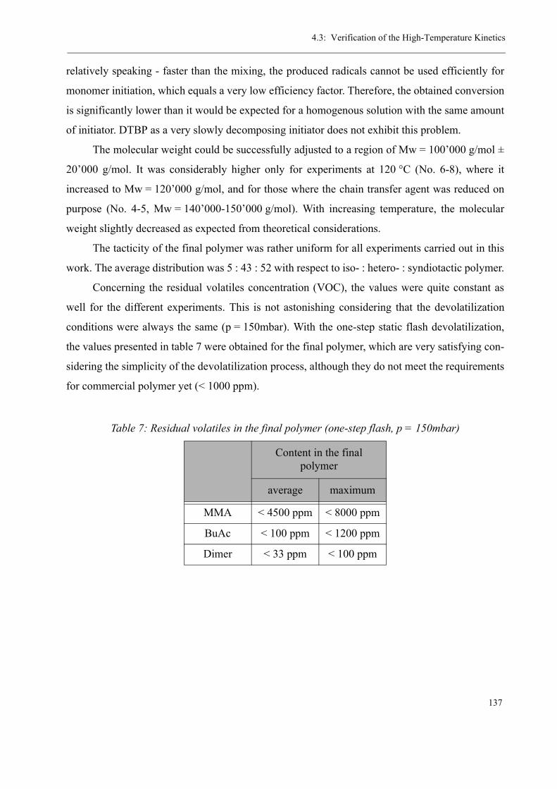
4.3: Verification of the High-Temperature Kinetics
137
relatively speaking - faster than the mixing, the produced radicals cannot be used efficiently for
monomer initiation, which equals a very low efficiency factor. Therefore, the obtained conversion
is significantly lower than it would be expected for a homogenous solution with the same amount
of initiator. DTBP as a very slowly decomposing initiator does not exhibit this problem.
The molecular weight could be successfully adjusted to a region of Mw = 100’000 g/mol ±
20’000 g/mol. It was considerably higher only for experiments at 120 °C (No. 6-8), where it
increased to Mw = 120’000 g/mol, and for those where the chain transfer agent was reduced on
purpose (No. 4-5, Mw = 140’000-150’000 g/mol). With increasing temperature, the molecular
weight slightly decreased as expected from theoretical considerations.
The tacticity of the final polymer was rather uniform for all experiments carried out in this
work. The average distribution was 5 : 43 : 52 with respect to iso- : hetero- : syndiotactic polymer.
Concerning the residual volatiles concentration (VOC), the values were quite constant as
well for the different experiments. This is not astonishing considering that the devolatilization
conditions were always the same (p = 150mbar). With the one-step static flash devolatilization,
the values presented in table 7 were obtained for the final polymer, which are very satisfying con-
sidering the simplicity of the devolatilization process, although they do not meet the requirements
for commercial polymer yet (< 1000 ppm).
Table 7: Residual volatiles in the final polymer (one-step flash, p = 150mbar)
Content in the final polymer
average maximum
MMA < 4500 ppm < 8000 ppm
BuAc < 100 ppm < 1200 ppm
Dimer < 33 ppm < 100 ppm
Chapter 4: Continuous High-Temperature Polymerization
138
4.3.2 R-parameters
For the kinetic description of copolymerizations according to the ultimate model (i.e. only
the final monomer unit of an active chain is considered as influencing the propagation mecha-
nism), there are four propagation reactions to take into account:
Propagation P1,n
. + MMA P1,n+1. kp11
P1,n. + MA P2,n+1
. kp12
P2,n. + MA P2,n+1
. kp22
P2,n. + MMA P1,n+1
. kp21
where P1,n. and P2,n
. represent the MMA, respectively MA terminated chain radicals.
As to the rate coefficients, it is either necessary to know all four of them separately, or to
express the cross-propagation (e.g. propagation of an MMA-terminated chain with an MA mono-
mer) by so-called reactivity ratios or “r-parameters”:
and (EQ 4.19)
These r-parameters express the probability for an active polymer chain to react with either
the one or the other monomer for a binary copolymerization. They are determined experimentally
by the Tüdös-Kelen-approach [90], which is a further-development of the equations derived by
Lewis-Mayo and Fineman-Ross [91].
For the relative change of monomer consumption as a function of the instantaneous mono-
mer ratio [MMA]/[MA], it can be written
(EQ 4.20)
This equation also describes the instantaneous polymer composition for small conversion
changes.
For the determination of the r-parameters from experimental data, equation 4.20 needs to be
linearized by setting y = d[MMA]/d[MA] and x = [MMA]/[MA]:
r12k11k12-------= r21
k22k21-------=
d MMA[ ]d MA[ ]
----------------------1 r12 MMA[ ] MA[ ]⁄⋅+1 r21 MA[ ] MMA[ ]⁄⋅+---------------------------------------------------------- MMA[ ]
MA[ ]-------------------
r12 MMA[ ] MA[ ]+⋅r21 MA[ ] MMA[ ]+⋅---------------------------------------------------⋅= =
4.3: Verification of the High-Temperature Kinetics
139
and further to (EQ 4.21)
This equation can be further simplified by introducing and :
respectively (EQ 4.22)
Equation 4.22 is also called the Fineman-Ross equation. Tracing G against F or G/F against
1/F gives r12 as the slope and r21 as the intercept or vice-versa, respectively.
However, this method is not very well balanced since the slope of a straight line fitted
through experimental data is overly influenced by points at the far end of the scale. The result
might, therefore, change for experiments with different concentration values [MMA] or [MA], or
when, for example, the monomer indices are inverted and the calculation is repeated. Kelen and
Tüdös propose an equilibration algorithm in order to equally weigh the experimental points from
the whole range of concentration values in form of equation 4.23:
(EQ 4.23)
where α denotes a constant (α > 0), which is arbitrarily defined by the authors to be
. By introducing
and (EQ 4.24)
equation 4.23 can be written
(EQ 4.25)
The variable ξ can only take values in the interval (0, 1), therefore tracing the variable η
against ξ delivers the parameters r12 and r21 as intercepts.
y x1 r12x+r21 x+
-------------------⋅= y 1–( )x
---------------- r12 r21yx2-----⋅–=
G x y 1–( )y
-------------------= F x2
y-----=
G r12F r21–= GF---- r12
r21F
-------–=
Gα F+------------- r12
r21α
-------+⎝ ⎠⎛ ⎞ F
α F+-------------
r21α
-------–⋅=
α min F( ) max F( )⋅=
η Gα F+-------------= ξ F
α F+-------------=
η r12r21α
-------+⎝ ⎠⎛ ⎞ ξ
r21α
-------–⋅=
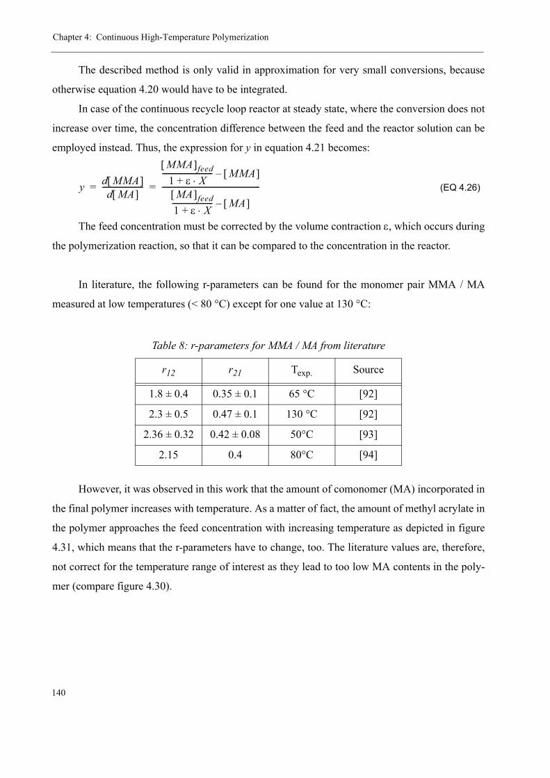
Chapter 4: Continuous High-Temperature Polymerization
140
The described method is only valid in approximation for very small conversions, because
otherwise equation 4.20 would have to be integrated.
In case of the continuous recycle loop reactor at steady state, where the conversion does not
increase over time, the concentration difference between the feed and the reactor solution can be
employed instead. Thus, the expression for y in equation 4.21 becomes:
(EQ 4.26)
The feed concentration must be corrected by the volume contraction ε, which occurs during
the polymerization reaction, so that it can be compared to the concentration in the reactor.
In literature, the following r-parameters can be found for the monomer pair MMA / MA
measured at low temperatures (< 80 °C) except for one value at 130 °C:
However, it was observed in this work that the amount of comonomer (MA) incorporated in
the final polymer increases with temperature. As a matter of fact, the amount of methyl acrylate in
the polymer approaches the feed concentration with increasing temperature as depicted in figure
4.31, which means that the r-parameters have to change, too. The literature values are, therefore,
not correct for the temperature range of interest as they lead to too low MA contents in the poly-
mer (compare figure 4.30).
Table 8: r-parameters for MMA / MA from literature
r12 r21 Texp. Source
1.8 ± 0.4 0.35 ± 0.1 65 °C [92]
2.3 ± 0.5 0.47 ± 0.1 130 °C [92]
2.36 ± 0.32 0.42 ± 0.08 50°C [93]
2.15 0.4 80°C [94]
y d MMA[ ]d MA[ ]
----------------------
MMA[ ]feed1 ε X⋅+
--------------------------- MMA[ ]–
MA[ ]feed1 ε X⋅+---------------------- MA[ ]–
-----------------------------------------------------= =
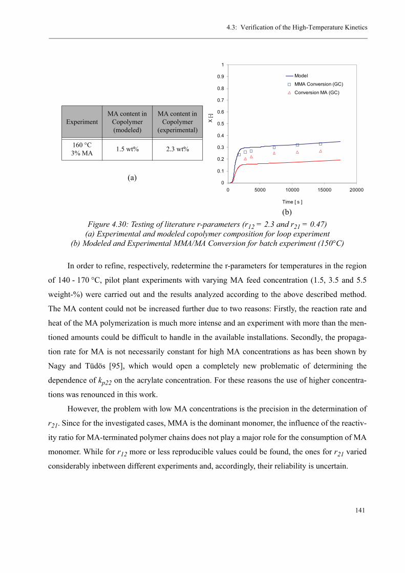
4.3: Verification of the High-Temperature Kinetics
141
In order to refine, respectively, redetermine the r-parameters for temperatures in the region
of 140 - 170 °C, pilot plant experiments with varying MA feed concentration (1.5, 3.5 and 5.5
weight-%) were carried out and the results analyzed according to the above described method.
The MA content could not be increased further due to two reasons: Firstly, the reaction rate and
heat of the MA polymerization is much more intense and an experiment with more than the men-
tioned amounts could be difficult to handle in the available installations. Secondly, the propaga-
tion rate for MA is not necessarily constant for high MA concentrations as has been shown by
Nagy and Tüdös [95], which would open a completely new problematic of determining the
dependence of kp22 on the acrylate concentration. For these reasons the use of higher concentra-
tions was renounced in this work.
However, the problem with low MA concentrations is the precision in the determination of
r21. Since for the investigated cases, MMA is the dominant monomer, the influence of the reactiv-
ity ratio for MA-terminated polymer chains does not play a major role for the consumption of MA
monomer. While for r12 more or less reproducible values could be found, the ones for r21 varied
considerably inbetween different experiments and, accordingly, their reliability is uncertain.
(b)Figure 4.30: Testing of literature r-parameters (r12 = 2.3 and r21 = 0.47)
(a) Experimental and modeled copolymer composition for loop experiment(b) Modeled and Experimental MMA/MA Conversion for batch experiment (150°C)
(a)
ExperimentMA content in
Copolymer (modeled)
MA content in Copolymer
(experimental)
160 °C3% MA 1.5 wt% 2.3 wt%
0
0.1
0.2
0.3
0.4
0.5
0.6
0.7
0.8
0.9
1
0 5000 10000 15000 20000
Time [ s ]
X [-
]
Model
MMA Conversion (GC)
Conversion MA (GC)
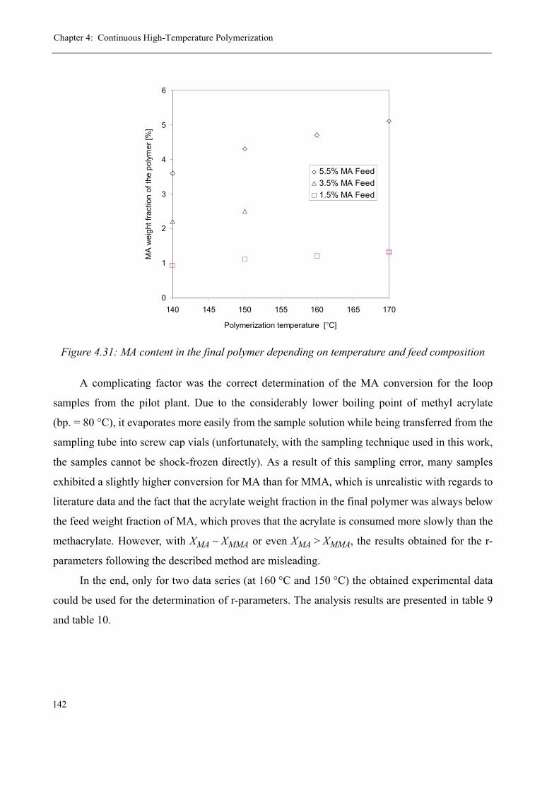
Chapter 4: Continuous High-Temperature Polymerization
142
A complicating factor was the correct determination of the MA conversion for the loop
samples from the pilot plant. Due to the considerably lower boiling point of methyl acrylate
(bp. = 80 °C), it evaporates more easily from the sample solution while being transferred from the
sampling tube into screw cap vials (unfortunately, with the sampling technique used in this work,
the samples cannot be shock-frozen directly). As a result of this sampling error, many samples
exhibited a slightly higher conversion for MA than for MMA, which is unrealistic with regards to
literature data and the fact that the acrylate weight fraction in the final polymer was always below
the feed weight fraction of MA, which proves that the acrylate is consumed more slowly than the
methacrylate. However, with XMA ~ XMMA or even XMA > XMMA, the results obtained for the r-
parameters following the described method are misleading.
In the end, only for two data series (at 160 °C and 150 °C) the obtained experimental data
could be used for the determination of r-parameters. The analysis results are presented in table 9
and table 10.
Figure 4.31: MA content in the final polymer depending on temperature and feed composition
0
1
2
3
4
5
6
140 145 150 155 160 165 170
Polymerization temperature [°C]
MA
wei
ght f
ract
ion
of th
e po
lym
er [%
]
5.5% MA Feed3.5% MA Feed1.5% MA Feed

4.3: Verification of the High-Temperature Kinetics
143
With the results from this tables, the r-parameters could be estimated graphically according
to the Kelen-Tüdös method by calculating and tracing η and ξ. For comparison, the y in equation
4.21 was calculated from both, the final polymer composition and the loop sample composition,
even if the use of the polymer composition is not fully correct as the polymer sample was taken at
the end of the pilot reactor and the polymer composition still changes during the course of poly-
merization in the tube reactor.
The graph containing the tracing of η over ξ is depicted in figure 4.32 for the example of the
experiment at 160 °C. The resulting r-parameters for T = 160 °C are r12 = 1.55 and r21 = 3.59 for
the calculation based on the loop sample data and r12 = 1.89 and r21 = 3.07 for the polymer com-
position data. For 150 °C, on the other hand, the values were determined from the loop sample
concentration to be r12 = 1.47 and r21 = 0.79.
Table 9: Results from three copolymerization experiments at T = 160 °C
1.5% MA Feed 3.0% MA Feed 5.5% MA Feed
Final polymer composition 1.2 wt% MA 2.3 wt% MA 4.7 wt% MA
MMA loop conversion 44.8 % 30.3 % 35.2 %
MA loop conversion 38.2 % 25.7 % 31.9 %
Table 10: Results from two copolymerization experiments at T = 150 °C
1.5% MA Feed 5.5% MA Feed
Final polymer composition 1.1 wt% MA 4.3 wt% MA
MMA loop conversion 45.3 % 36.7 %
MA loop conversion 48.1 % 39.5 %

Chapter 4: Continuous High-Temperature Polymerization
144
It is obvious that the value for r21 at 160 °C is far off the expected scale in comparison to lit-
erature data (table 8) and it is also in contradiction to the fact that MMA is preferably incorpo-
rated in the growing chains (i.e. r21 < 1 !). This is due to the problem that with the experimental
conditions in this work, i.e. the extremely low MA content, it is not possible to unambiguously
solve the copolymerization balance equation with the employed graphical method, as it will be
demonstrated in the following:
From the r-parameters determined by the above method and those from literature, it is pos-
sible to draw a phase diagram of the monomer and polymer composition in terms of MMA con-
tent (see figure 4.33). It can be seen that for the pair of parameters determined beforehand by the
Kelen-Tüdös method (r12 = 1.55 and r21 = 3.59), an azeotropic course of the curve is obtained,
whereas for the literature values from Grassie [92] determined at 130 °C, the curve does not cross
the 45° line corresponding to equal feed and polymer composition. Regarding the measured data
points in the upper right corner, it becomes evident that there exist several combinations of r12
and r21 that lead to a satisfying description of the found polymer compositions. For the experi-
ments carried out at 150 °C, the found pair of r-parameters happens to fulfill the requirement r21 <
1. However, the solution r12 = 1.55 and r21 = 3.59 for 160 °C would lead to completely unrealistic
Figure 4.32: Kelen-Tüdös plot for the determination of r-parameters (160 °C and 150 °C data from table 9)
y = 1.5525x - 0.1657
y = 1.8976x - 0.176y = 1.4736x - 0.0452
0
0.2
0.4
0.6
0.8
1
1.2
0 0.2 0.4 0.6 0.8 1
Loop sample composition 170°CPolymer composition 170°CLoop sample composition 150°C
η
ξ
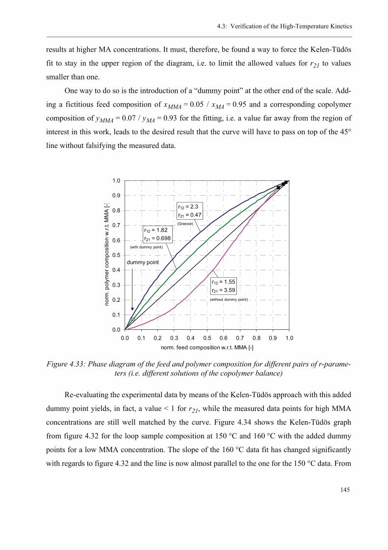
4.3: Verification of the High-Temperature Kinetics
145
results at higher MA concentrations. It must, therefore, be found a way to force the Kelen-Tüdös
fit to stay in the upper region of the diagram, i.e. to limit the allowed values for r21 to values
smaller than one.
One way to do so is the introduction of a “dummy point” at the other end of the scale. Add-
ing a fictitious feed composition of xMMA = 0.05 / xMA = 0.95 and a corresponding copolymer
composition of yMMA = 0.07 / yMA = 0.93 for the fitting, i.e. a value far away from the region of
interest in this work, leads to the desired result that the curve will have to pass on top of the 45°
line without falsifying the measured data.
Re-evaluating the experimental data by means of the Kelen-Tüdös approach with this added
dummy point yields, in fact, a value < 1 for r21, while the measured data points for high MMA
concentrations are still well matched by the curve. Figure 4.34 shows the Kelen-Tüdös graph
from figure 4.32 for the loop sample composition at 150 °C and 160 °C with the added dummy
points for a low MMA concentration. The slope of the 160 °C data fit has changed significantly
with regards to figure 4.32 and the line is now almost parallel to the one for the 150 °C data. From
Figure 4.33: Phase diagram of the feed and polymer composition for different pairs of r-parame-ters (i.e. different solutions of the copolymer balance)
0.0
0.1
0.2
0.3
0.4
0.5
0.6
0.7
0.8
0.9
1.0
0.0 0.1 0.2 0.3 0.4 0.5 0.6 0.7 0.8 0.9 1.0
norm. feed composition w.r.t. MMA [-]
norm
. pol
ymer
com
posi
tion
w.r.
t. M
MA
[-]
dummy point
r12 = 1.55r21 = 3.59
r12 = 2.3r21 = 0.47
r12 = 1.82r21 = 0.698
(Grassie)
(with dummy point)
(without dummy point)
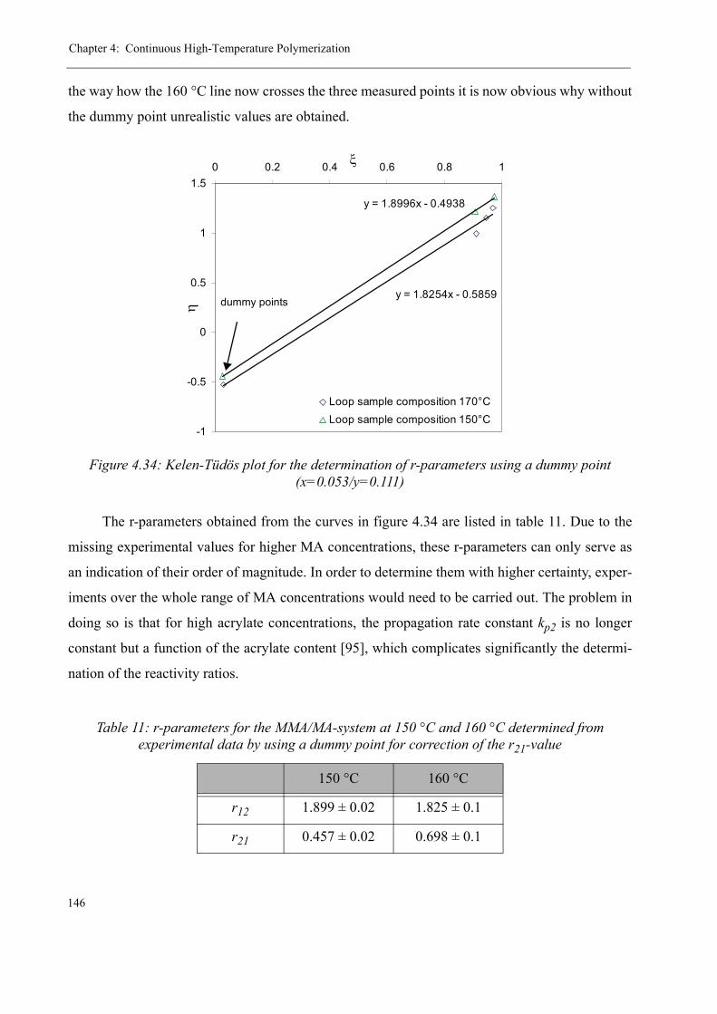
Chapter 4: Continuous High-Temperature Polymerization
146
the way how the 160 °C line now crosses the three measured points it is now obvious why without
the dummy point unrealistic values are obtained.
The r-parameters obtained from the curves in figure 4.34 are listed in table 11. Due to the
missing experimental values for higher MA concentrations, these r-parameters can only serve as
an indication of their order of magnitude. In order to determine them with higher certainty, exper-
iments over the whole range of MA concentrations would need to be carried out. The problem in
doing so is that for high acrylate concentrations, the propagation rate constant kp2 is no longer
constant but a function of the acrylate content [95], which complicates significantly the determi-
nation of the reactivity ratios.
Figure 4.34: Kelen-Tüdös plot for the determination of r-parameters using a dummy point (x=0.053/y=0.111)
Table 11: r-parameters for the MMA/MA-system at 150 °C and 160 °C determined from experimental data by using a dummy point for correction of the r21-value
150 °C 160 °C
r12 1.899 ± 0.02 1.825 ± 0.1
r21 0.457 ± 0.02 0.698 ± 0.1
y = 1.8254x - 0.5859
y = 1.8996x - 0.4938
-1
-0.5
0
0.5
1
1.50 0.2 0.4 0.6 0.8 1
Loop sample composition 170°CLoop sample composition 150°C
η
ξ
dummy points
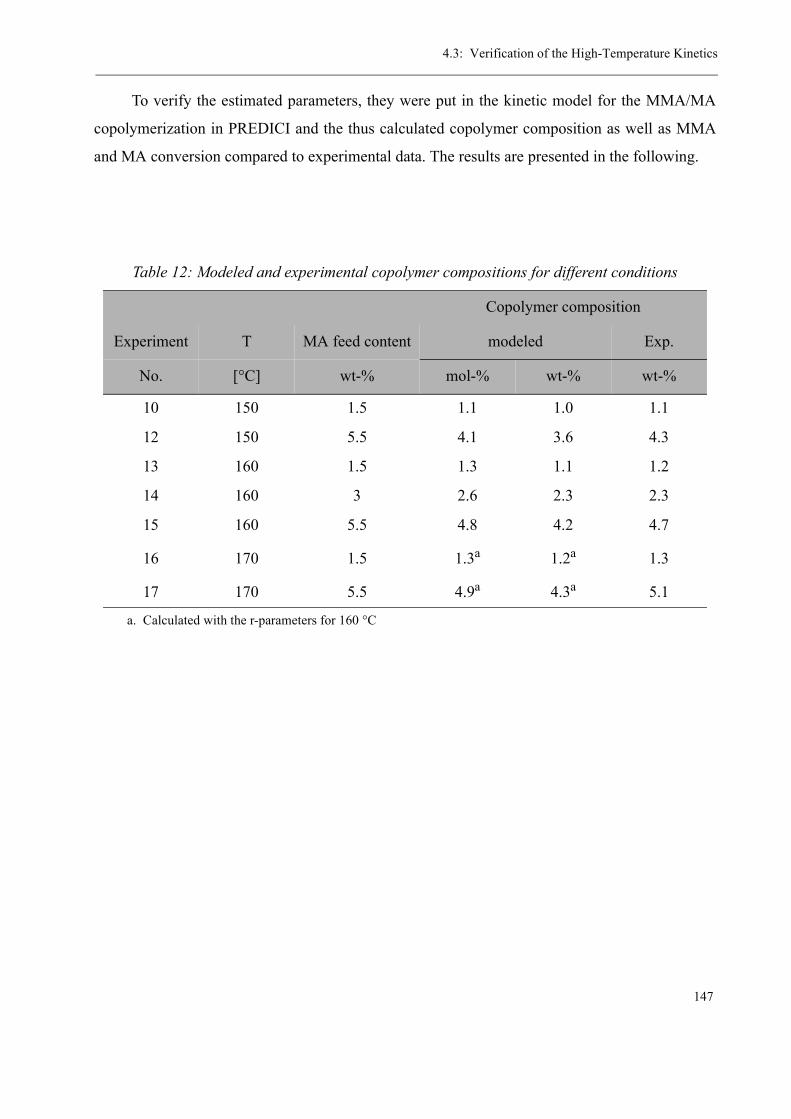
4.3: Verification of the High-Temperature Kinetics
147
To verify the estimated parameters, they were put in the kinetic model for the MMA/MA
copolymerization in PREDICI and the thus calculated copolymer composition as well as MMA
and MA conversion compared to experimental data. The results are presented in the following.
Table 12: Modeled and experimental copolymer compositions for different conditions
Copolymer composition
Experiment T MA feed content modeled Exp.
No. [°C] wt-% mol-% wt-% wt-%
10 150 1.5 1.1 1.0 1.1
12 150 5.5 4.1 3.6 4.3
13 160 1.5 1.3 1.1 1.2
14 160 3 2.6 2.3 2.3
15 160 5.5 4.8 4.2 4.7
16 170 1.5 1.3a
a. Calculated with the r-parameters for 160 °C
1.2a 1.3
17 170 5.5 4.9a 4.3a 5.1
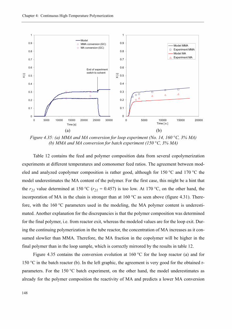
Chapter 4: Continuous High-Temperature Polymerization
148
Table 12 contains the feed and polymer composition data from several copolymerization
experiments at different temperatures and comonomer feed ratios. The agreement between mod-
eled and analyzed copolymer composition is rather good, although for 150 °C and 170 °C the
model underestimates the MA content of the polymer. For the first case, this might be a hint that
the r21 value determined at 150 °C (r21 = 0.457) is too low. At 170 °C, on the other hand, the
incorporation of MA in the chain is stronger than at 160 °C as seen above (figure 4.31). There-
fore, with the 160 °C parameters used in the modeling, the MA polymer content is underesti-
mated. Another explanation for the discrepancies is that the polymer composition was determined
for the final polymer, i.e. from reactor exit, whereas the modeled values are for the loop exit. Dur-
ing the continuing polymerization in the tube reactor, the concentration of MA increases as it con-
sumed slowlier than MMA. Therefore, the MA fraction in the copolymer will be higher in the
final polymer than in the loop sample, which is correctly mirrored by the results in table 12.
Figure 4.35 contains the conversion evolution at 160 °C for the loop reactor (a) and for
150 °C in the batch reactor (b). In the left graphic, the agreement is very good for the obtained r-
parameters. For the 150 °C batch experiment, on the other hand, the model underestimates as
already for the polymer composition the reactivity of MA and predicts a lower MA conversion
(a) (b)Figure 4.35: (a) MMA and MA conversion for loop experiment (No. 14, 160 °C, 3% MA)
(b) MMA and MA conversion for batch experiment (150 °C, 3% MA)
0
0.1
0.2
0.3
0.4
0.5
0.6
0.7
0.8
0.9
1
0 5000 10000 15000 20000 25000 30000
Time [s]
X [-
]
ModelMMA conversion (GC)MA conversion (GC)
End of experimentswitch to solvent
0
0.1
0.2
0.3
0.4
0.5
0.6
0.7
0.8
0.9
1
0 5000 10000 15000 20000Time [ s ]
X [-
]
Model MMAExperiment MMAModel MAExperiment MA

4.3: Verification of the High-Temperature Kinetics
149
than actually measured. This is a second indication that the r-parameters at 150 °C need to be
readjusted.
It should be kept in mind, though, that for the investigated cases, the copolymer composi-
tion is mainly governed by the r12-value, since MMA is the dominating monomer and that this
r12-value could be determined quite reliably in this work. For polymerizations with higher MA
concentration, the results might be less precise due to the uncertainty connected with the determi-
nation of r21. It is, therefore, necessary to consider further experiments with higher MA fractions
in order to improve the precision of r21.
Another important issue to take into account when further increasing the temperature
(>170 °C), is the depolymerization. Due to the depolymerization mechanism (unzipping, see
chapter 5 “Thermal stability”), which only works for methacrylates and is stopped by the occur-
rence of acrylates in the chain, the incorporation of acrylate becomes more pronounced at high
temperatures: while the effective propagation rate for MMA needs to be corrected by the depoly-
merization
(EQ 4.27)
the propagation of the acrylate is, in first approximation1, not influenced by this mecha-
nism. This is the reason why the acrylate fraction increases disproportionally much for very high
temperatures, an issue that is not taken into account by the r-parameters.
4.3.3 Chain Transfer Constants
In order to correctly predict the molecular weight distributions in the modeling, the chain
transfer constants for all transfer reactions are needed at the given temperature range. For the
transfer to monomer and solvent, these are taken from literature or assumed to be constant (see
appendix 3). However, in the presence of a strong chain transfer agent, like the n-dodecanethiol
used in this work, their influence on the molecular weight can be neglected without any remark-
1. This is valid for the “ultimate” model only. For the “penultimate” model, i.e. when the second-last ele-ment of the active radical chain is taken into account, too, the depolymerization needs to be considered. However, this would lead too far concerning the frame of this work.
kp1 effective, kp 1,kdp
MMA[ ]-------------------–=
Chapter 4: Continuous High-Temperature Polymerization
150
able deterioration of the model precision. The transfer constants for thiols are, indeed, by almost a
factor 104 higher than the ones for monomer and solvent transfer [47].
The value of the transfer constant for n-dodecanethiol (DDT) can be found in literature
[96]:
(EQ 4.28)
However, as for so many rate constants found in literature for the MMA polymerization, the
temperature range of its determination is 20 °C < T < 80 °C and it cannot be said for sure if the
same value applies to higher temperatures. The aim was, therefore, to redetermine the chain trans-
fer constant for the system MMA/DDT from the results of high-temperature experiments.
Several experiments at various concentration ratios [CTA]/[MMA] were carried out and the
results treated by two different methods. A detailed description of these methods can be found in
an article by De la Fuente and Madruga [97].
The first one is the Mayo-method. It is generally known that, according to the Mayo equa-
tion, the degree of polymerization DPn in the presence of a transfer agent is related to the one of a
polymerization without transfer agent DPn,0 as follows:
(EQ 4.29)
where CCTA is the transfer constant, [CTA] the concentration of the transfer agent and [M]
the concentration of the monomer. The transfer constant is determined graphically rather than
from two points only, by tracing against .
Usually, the number-average degree of polymerization is to be taken. However, the exact
determination of the number-average molecular weight Mn is usually flawed with a rather large
error due to a very pronounced baseline sensitivity as regards the peak integration in SEC mea-
surements. The determination of the weight average molecular weight Mw is much more robust
and less sensitive to the choice of the baseline. De la Fuente and Madruga propose, therefore, to
take the weight-average molecular weight divided by a factor 2 for the Mayo-plot, which holds
true for most CTA regulated polymerizations1. In this work, calculations with both values were
CDDTkCTA
kp----------- 0.678= =
1DPn
---------- 1DPn 0,
--------------- CCTACTA[ ]
M[ ]----------------⋅+=
1DPn
---------- CTA[ ]MMA[ ]
-------------------
4.3: Verification of the High-Temperature Kinetics
151
compared to each other and no significant difference could be found, as will be shown later in this
subchapter.
An alternative method for the determination of CCTA is developed in the paper of De la
Fuente and Madruga, which is based on the shape of the number average molecular weight distri-
bution of the produced polymer. For a system where the chain transfer to initiator, monomer and
solvent can be neglected compared to that of the CTA, the molecular weight distribution at any
instant will follow an exponential decay as presented in equation 4.30 [97].
(EQ 4.30)
where P(M) is the number distribution of molecular weight M, M0 the monomer molecular
weight and B a proportionality constant. The number distribution P(M) can be obtained by SEC
measurement of the polymer from the calibrated SEC molecular weight distribution Wf (log M):
(EQ 4.31)
By plotting the number-average molecular weight distribution obtained in equation 4.31 as
ln P(M) against the molecular weight M, a straight line is obtained for the region of the distribu-
tion that is controlled by the CTA, whose slope Λ corresponds to
(EQ 4.32)
Analogous to the Mayo plot, the CCTA value is obtained graphically from the slope of the
plot Λ against for experiments with different CTA content, in order to obtain a higher
precision than for only one experiment. Figure 4.36 contains the plotting of ln P(M) against M,
from which the slopes Λ presented in table 13 were determined.
1. The polydispersity is usually in the region of 2 for radical polymerizations with chain transfer
agent.
PDMw
Mn--------=
P M( )M ∞→I[ ] 0→
lim BkCTA CTA[ ] M⋅ ⋅kp MMA[ ] M0⋅ ⋅------------------------------------------–⎝ ⎠
⎛ ⎞exp⋅=
P M( ) Wf Mlog( ) elogM2
----------⋅=
Λ CCTACTA[ ]
MMA[ ] M0⋅-------------------------------⋅–=
CTA[ ]MMA[ ]
-------------------

Chapter 4: Continuous High-Temperature Polymerization
152
With the values from table 13, the following two graphs can be drawn, leading directly to
the chain transfer constant for n-dodecanethiol (slopes):
Table 13: Results from pilot plant experiments for the determination of the DDT chain transfer constant at T = 140 °C (Initiator [TBPEH] = 250ppm)
Exp. No.(appendix 7)
103 Mn [g/mol] Mw [g/mol] Λ . 105
4 1.13066 84’187 162’070 1.93 -1.04
1 1.69599 51’264 106’303 2.07 -1.55
5 2.82665 35’328 73’022 2.07 -2.54
Figure 4.36: Plot ln P(M) against M according to equation 4.30
CTA[ ]MMA[ ]
------------------- PDMw
Mn--------=
-16
-14
-12
-10
-8
-6
-4
-2
00 100000 200000 300000 400000 500000 600000
Mw [g/mol]
ln P
(M)
0.5% DDM0.2% DDM0.3% DDM
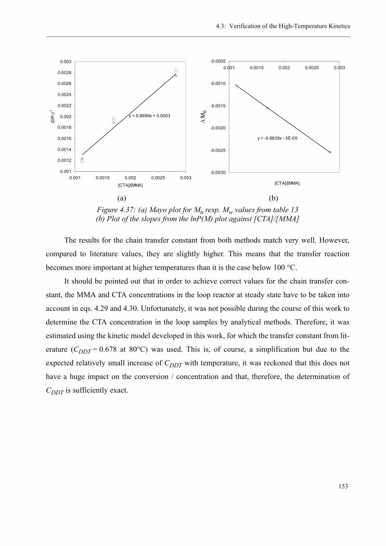
4.3: Verification of the High-Temperature Kinetics
153
The results for the chain transfer constant from both methods match very well. However,
compared to literature values, they are slightly higher. This means that the transfer reaction
becomes more important at higher temperatures than it is the case below 100 °C.
It should be pointed out that in order to achieve correct values for the chain transfer con-
stant, the MMA and CTA concentrations in the loop reactor at steady state have to be taken into
account in eqs. 4.29 and 4.30. Unfortunately, it was not possible during the course of this work to
determine the CTA concentration in the loop samples by analytical methods. Therefore, it was
estimated using the kinetic model developed in this work, for which the transfer constant from lit-
erature (CDDT = 0.678 at 80°C) was used. This is, of course, a simplification but due to the
expected relatively small increase of CDDT with temperature, it was reckoned that this does not
have a huge impact on the conversion / concentration and that, therefore, the determination of
CDDT is sufficiently exact.
(a) (b)Figure 4.37: (a) Mayo plot for Mn resp. Mw values from table 13(b) Plot of the slopes from the lnP(M) plot against [CTA]/[MMA]
y = 0.8699x + 0.0003
0.001
0.0012
0.0014
0.0016
0.0018
0.002
0.0022
0.0024
0.0026
0.0028
0.003
0.001 0.0015 0.002 0.0025 0.003
[CTA]/[MMA]
(DP
n)-1
y = -0.8839x - 5E-05
-0.0030
-0.0025
-0.0020
-0.0015
-0.0010
-0.00050.001 0.0015 0.002 0.0025 0.003
[CTA]/[MMA]
Λ. M
0
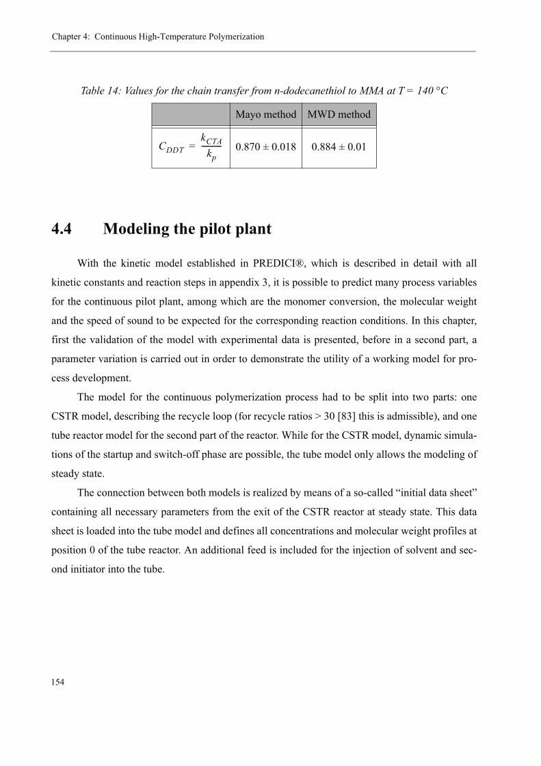
Chapter 4: Continuous High-Temperature Polymerization
154
4.4 Modeling the pilot plant
With the kinetic model established in PREDICI®, which is described in detail with all
kinetic constants and reaction steps in appendix 3, it is possible to predict many process variables
for the continuous pilot plant, among which are the monomer conversion, the molecular weight
and the speed of sound to be expected for the corresponding reaction conditions. In this chapter,
first the validation of the model with experimental data is presented, before in a second part, a
parameter variation is carried out in order to demonstrate the utility of a working model for pro-
cess development.
The model for the continuous polymerization process had to be split into two parts: one
CSTR model, describing the recycle loop (for recycle ratios > 30 [83] this is admissible), and one
tube reactor model for the second part of the reactor. While for the CSTR model, dynamic simula-
tions of the startup and switch-off phase are possible, the tube model only allows the modeling of
steady state.
The connection between both models is realized by means of a so-called “initial data sheet”
containing all necessary parameters from the exit of the CSTR reactor at steady state. This data
sheet is loaded into the tube model and defines all concentrations and molecular weight profiles at
position 0 of the tube reactor. An additional feed is included for the injection of solvent and sec-
ond initiator into the tube.
Table 14: Values for the chain transfer from n-dodecanethiol to MMA at T = 140 °C
Mayo method MWD method
0.870 ± 0.018 0.884 ± 0.01CDDTkCTA
kp-----------=
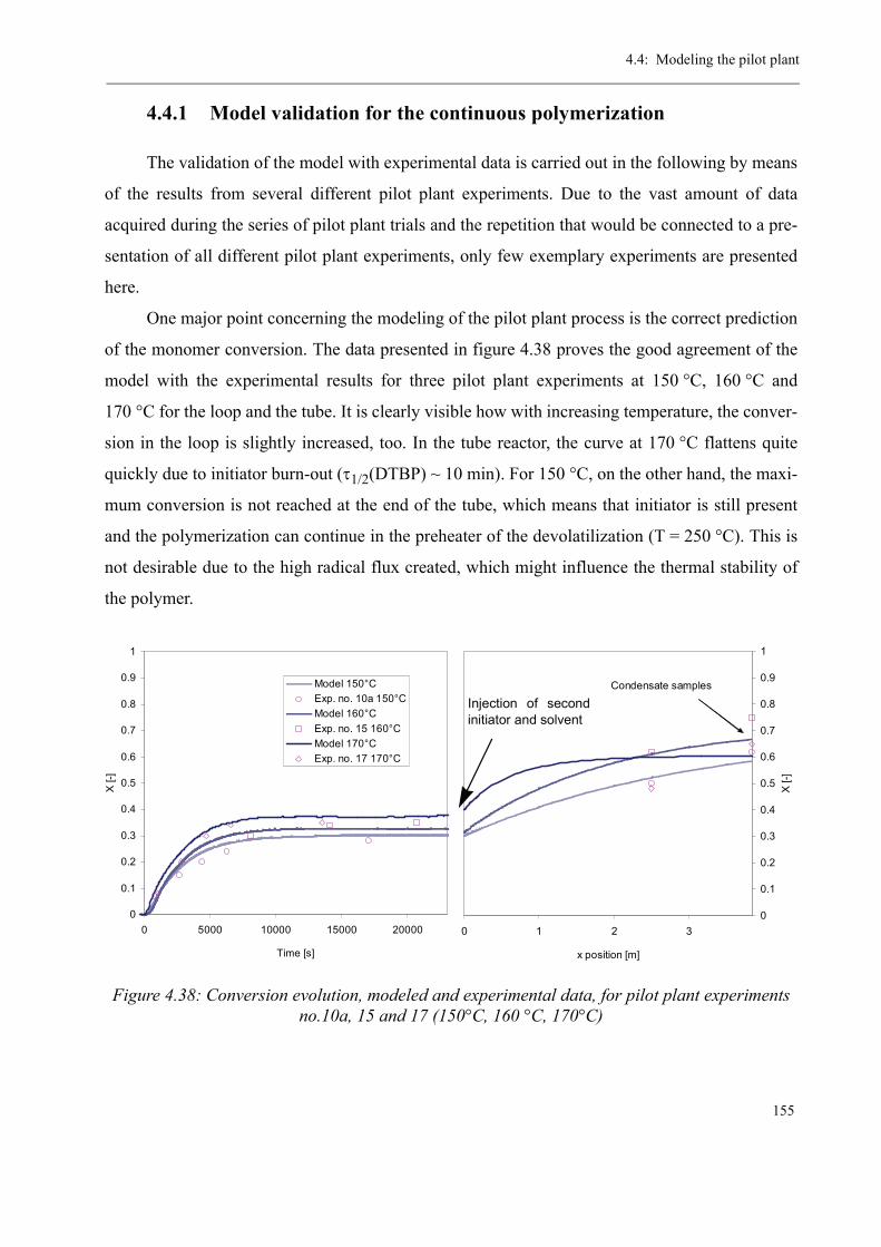
4.4: Modeling the pilot plant
155
4.4.1 Model validation for the continuous polymerization
The validation of the model with experimental data is carried out in the following by means
of the results from several different pilot plant experiments. Due to the vast amount of data
acquired during the series of pilot plant trials and the repetition that would be connected to a pre-
sentation of all different pilot plant experiments, only few exemplary experiments are presented
here.
One major point concerning the modeling of the pilot plant process is the correct prediction
of the monomer conversion. The data presented in figure 4.38 proves the good agreement of the
model with the experimental results for three pilot plant experiments at 150 °C, 160 °C and
170 °C for the loop and the tube. It is clearly visible how with increasing temperature, the conver-
sion in the loop is slightly increased, too. In the tube reactor, the curve at 170 °C flattens quite
quickly due to initiator burn-out (τ1/2(DTBP) ~ 10 min). For 150 °C, on the other hand, the maxi-
mum conversion is not reached at the end of the tube, which means that initiator is still present
and the polymerization can continue in the preheater of the devolatilization (T = 250 °C). This is
not desirable due to the high radical flux created, which might influence the thermal stability of
the polymer.
Figure 4.38: Conversion evolution, modeled and experimental data, for pilot plant experiments no.10a, 15 and 17 (150°C, 160 °C, 170°C)
0
0.1
0.2
0.3
0.4
0.5
0.6
0.7
0.8
0.9
1
0 5000 10000 15000 20000
Time [s]
X [-
]
Model 150°CExp. no. 10a 150°CModel 160°CExp. no. 15 160°CModel 170°CExp. no. 17 170°C
0
0.1
0.2
0.3
0.4
0.5
0.6
0.7
0.8
0.9
1
0 1 2 3
x position [m]
X [-
]
Condensate samples
Injection of secondinitiator and solvent
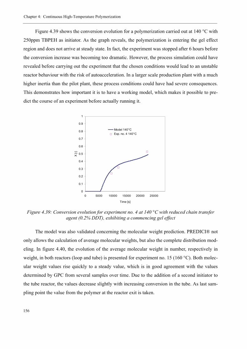
Chapter 4: Continuous High-Temperature Polymerization
156
Figure 4.39 shows the conversion evolution for a polymerization carried out at 140 °C with
250ppm TBPEH as initiator. As the graph reveals, the polymerization is entering the gel effect
region and does not arrive at steady state. In fact, the experiment was stopped after 6 hours before
the conversion increase was becoming too dramatic. However, the process simulation could have
revealed before carrying out the experiment that the chosen conditions would lead to an unstable
reactor behaviour with the risk of autoacceleration. In a larger scale production plant with a much
higher inertia than the pilot plant, these process conditions could have had severe consequences.
This demonstrates how important it is to have a working model, which makes it possible to pre-
dict the course of an experiment before actually running it.
The model was also validated concerning the molecular weight prediction. PREDICI® not
only allows the calculation of average molecular weights, but also the complete distribution mod-
eling. In figure 4.40, the evolution of the average molecular weight in number, respectively in
weight, in both reactors (loop and tube) is presented for experiment no. 15 (160 °C). Both molec-
ular weight values rise quickly to a steady value, which is in good agreement with the values
determined by GPC from several samples over time. Due to the addition of a second initiator to
the tube reactor, the values decrease slightly with increasing conversion in the tube. As last sam-
pling point the value from the polymer at the reactor exit is taken.
Figure 4.39: Conversion evolution for experiment no. 4 at 140 °C with reduced chain transfer agent (0.2% DDT), exhibiting a commencing gel effect
0
0.1
0.2
0.3
0.4
0.5
0.6
0.7
0.8
0.9
1
0 5000 10000 15000 20000 25000
Time [s]
X [-
]
Model 140°CExp. no. 4 140°C
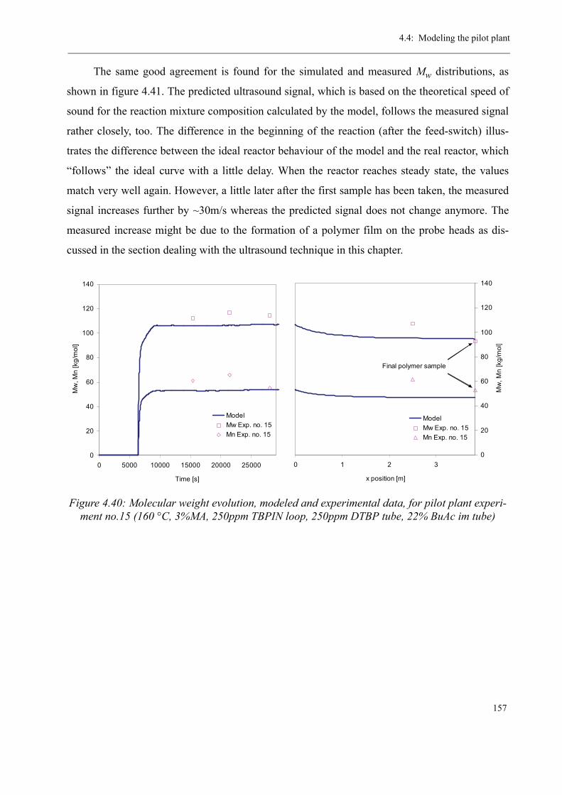
4.4: Modeling the pilot plant
157
The same good agreement is found for the simulated and measured Mw distributions, as
shown in figure 4.41. The predicted ultrasound signal, which is based on the theoretical speed of
sound for the reaction mixture composition calculated by the model, follows the measured signal
rather closely, too. The difference in the beginning of the reaction (after the feed-switch) illus-
trates the difference between the ideal reactor behaviour of the model and the real reactor, which
“follows” the ideal curve with a little delay. When the reactor reaches steady state, the values
match very well again. However, a little later after the first sample has been taken, the measured
signal increases further by ~30m/s whereas the predicted signal does not change anymore. The
measured increase might be due to the formation of a polymer film on the probe heads as dis-
cussed in the section dealing with the ultrasound technique in this chapter.
Figure 4.40: Molecular weight evolution, modeled and experimental data, for pilot plant experi-ment no.15 (160 °C, 3%MA, 250ppm TBPIN loop, 250ppm DTBP tube, 22% BuAc im tube)
0
20
40
60
80
100
120
140
0 5000 10000 15000 20000 25000
Time [s]
Mw
, Mn
[kg/
mol
]
ModelMw Exp. no. 15Mn Exp. no. 15
0
20
40
60
80
100
120
140
0 1 2 3
x position [m]
Mw
, Mn
[kg/
mol
]
ModelMw Exp. no. 15Mn Exp. no. 15
Final polymer sample
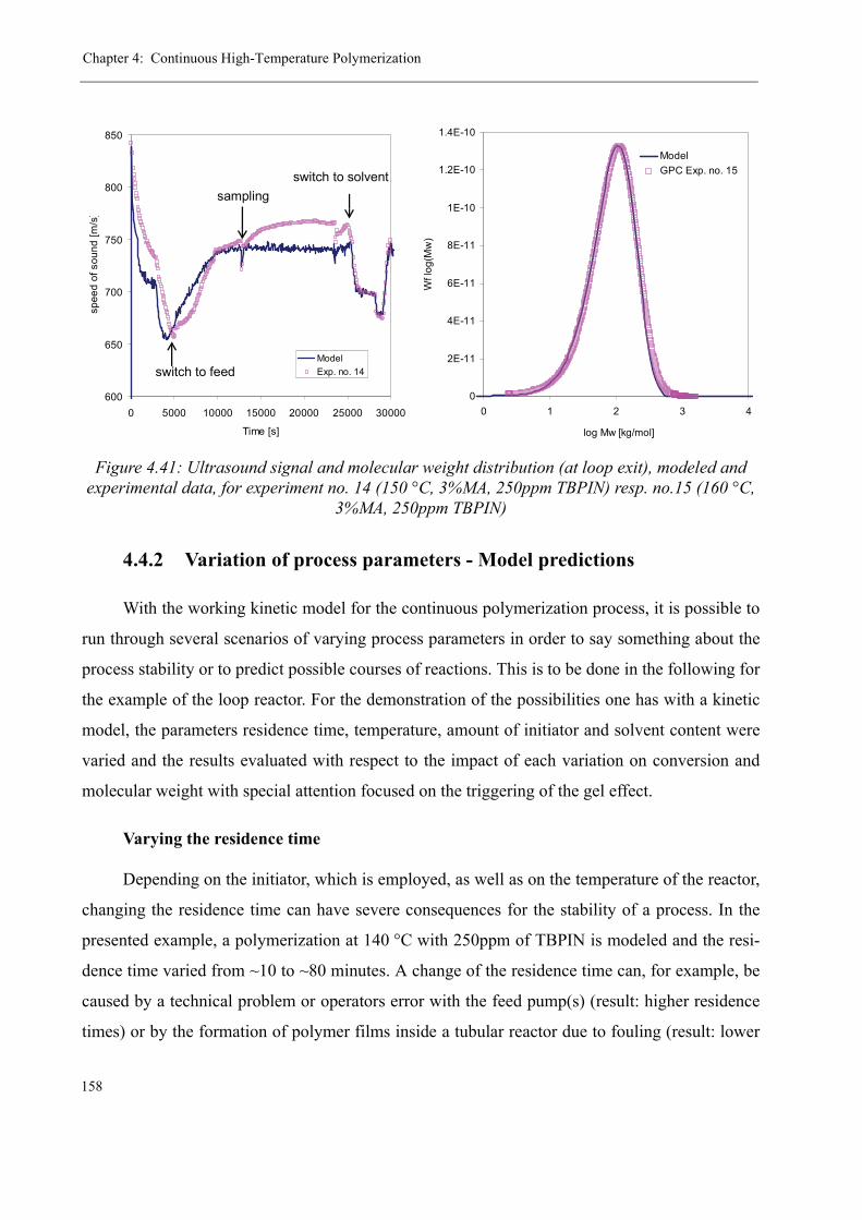
Chapter 4: Continuous High-Temperature Polymerization
158
4.4.2 Variation of process parameters - Model predictions
With the working kinetic model for the continuous polymerization process, it is possible to
run through several scenarios of varying process parameters in order to say something about the
process stability or to predict possible courses of reactions. This is to be done in the following for
the example of the loop reactor. For the demonstration of the possibilities one has with a kinetic
model, the parameters residence time, temperature, amount of initiator and solvent content were
varied and the results evaluated with respect to the impact of each variation on conversion and
molecular weight with special attention focused on the triggering of the gel effect.
Varying the residence time
Depending on the initiator, which is employed, as well as on the temperature of the reactor,
changing the residence time can have severe consequences for the stability of a process. In the
presented example, a polymerization at 140 °C with 250ppm of TBPIN is modeled and the resi-
dence time varied from ~10 to ~80 minutes. A change of the residence time can, for example, be
caused by a technical problem or operators error with the feed pump(s) (result: higher residence
times) or by the formation of polymer films inside a tubular reactor due to fouling (result: lower
Figure 4.41: Ultrasound signal and molecular weight distribution (at loop exit), modeled and experimental data, for experiment no. 14 (150 °C, 3%MA, 250ppm TBPIN) resp. no.15 (160 °C,
3%MA, 250ppm TBPIN)
0
2E-11
4E-11
6E-11
8E-11
1E-10
1.2E-10
1.4E-10
0 1 2 3 4
log Mw [kg/mol]W
f log
(Mw
)
ModelGPC Exp. no. 15
600
650
700
750
800
850
0 5000 10000 15000 20000 25000 30000
Time [s]
spee
d of
sou
nd [m
/s]
ModelExp. no. 14
sampling
switch to feed
switch to solvent

4.4: Modeling the pilot plant
159
residence times). For this example, a relatively slowly decomposing initiator (TBPIN) is com-
pared to a faster decomposing one (TBPEH) in order to demonstrate the effect on conversion.
It can be seen from figure 4.42 that the polymerization is stable for residence times up to
~33 minutes. However, above this value, the reaction enters the autoacceleration zone and the
conversion is continuously driven to higher values. Further reducing the residence time leads to a
strong reaction acceleration followed by almost full conversion, which, in reality, would be
impossible to handle due to viscosity issues. For the faster decomposing initiator TBPEH, this
effect is slightly less pronounced, in particular for very high residence times.
The scenario of a decreasing feed stream, causing higher residence times can be taken one
step further to the case of a complete failure of the feed pump. In this case, the recycle loop will
behave like a batch reactor and follow a different reaction path. Again, depending on initiator and
temperature, a feed pump failure can have drastic consequences on the heat production and con-
version respectively viscosity evolution in the reactor.
The simulation results for this failure scenario are shown in figure 4.43, where a complete
cut of the feed flow occurs at t = 10’000 s. The same calculations have been carried out for three
initiators with different decomposition characteristics: TBPEH, TBPIN and DTBP. The latter
decomposes extremely slowly at T = 140 °C, which is the reason for the high monomer conver-
Figure 4.42: Conversion evolution in the loop reactor as a function of the residence time (140 °C, 0.3% DDT, left: 250ppm TBPIN, right: 250ppm TBPEH)
0
0.1
0.2
0.3
0.4
0.5
0.6
0.7
0.8
0.9
1
0 5000 10000 15000 20000 25000 30000
Time [s]
X [-
]
27 min30 min
69 min
40 min
residence time τ
0
0.1
0.2
0.3
0.4
0.5
0.6
0.7
0.8
0.9
1
0 5000 10000 15000 20000 25000 30000
Time [s]
X [-
]
9 min
14 min
23 min27 min
33 min
55 min
82 min
40 min
residence time τ

Chapter 4: Continuous High-Temperature Polymerization
160
sion obtained after the failure of the feed pump. While for TBPEH and TBPIN the risk concerning
a reaction runaway is practically zero due to the quick consumption of initiator after cutting the
feed flow, this risk is extremely high for DTBP. Additionally, the time to react after a possible
pump failure and to take countermeasures is rather low (~10% conversion increase per 10 min-
utes).
It is, therefore, indispensable to carefully choose the right initiator for a given temperature
in order to reduce the risk that the polymerization is taken to high conversions in case of a major
residence time variation by, for example, a feed pump failure.
Varying the temperature
Varying the process temperature has a less important effect on the process. On the one hand,
this is due to the fact that lowering the temperature automatically reduces the decomposition rate
of the thermal initiator, which leads to a reduction of monomer conversion. On the other hand,
increasing the temperature leads, depending on the chosen initiator, either to a quick initiator
burn-out, or to a conversion limitation due to the depolymerization.
Figure 4.43: Conversion evolution in the loop reactor after an assumed feed pump failure for dif-ferent initiators (140 °C, 0.3% DDT)
0
0.1
0.2
0.3
0.4
0.5
0.6
0.7
0.8
0.9
1
0 5000 10000 15000 20000 25000 30000
Time [s]
X [-
]
TBPEH
DTBP
TBPIN
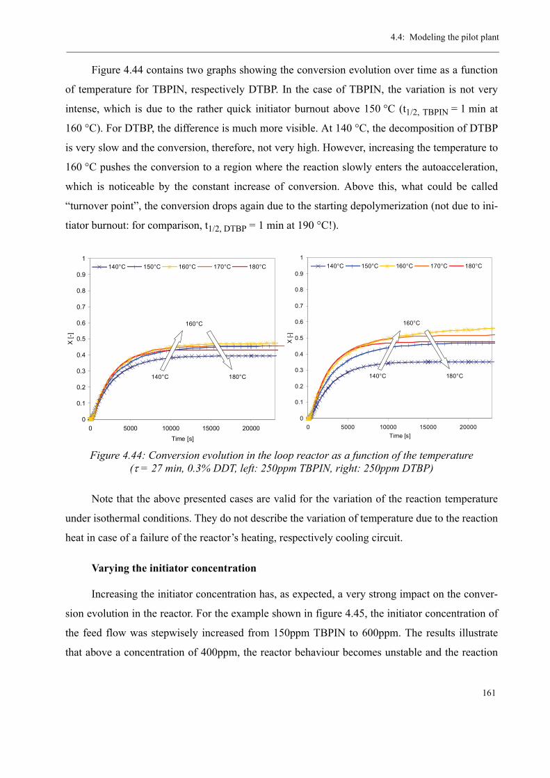
4.4: Modeling the pilot plant
161
Figure 4.44 contains two graphs showing the conversion evolution over time as a function
of temperature for TBPIN, respectively DTBP. In the case of TBPIN, the variation is not very
intense, which is due to the rather quick initiator burnout above 150 °C (t1/2, TBPIN = 1 min at
160 °C). For DTBP, the difference is much more visible. At 140 °C, the decomposition of DTBP
is very slow and the conversion, therefore, not very high. However, increasing the temperature to
160 °C pushes the conversion to a region where the reaction slowly enters the autoacceleration,
which is noticeable by the constant increase of conversion. Above this, what could be called
“turnover point”, the conversion drops again due to the starting depolymerization (not due to ini-
tiator burnout: for comparison, t1/2, DTBP = 1 min at 190 °C!).
Note that the above presented cases are valid for the variation of the reaction temperature
under isothermal conditions. They do not describe the variation of temperature due to the reaction
heat in case of a failure of the reactor’s heating, respectively cooling circuit.
Varying the initiator concentration
Increasing the initiator concentration has, as expected, a very strong impact on the conver-
sion evolution in the reactor. For the example shown in figure 4.45, the initiator concentration of
the feed flow was stepwisely increased from 150ppm TBPIN to 600ppm. The results illustrate
that above a concentration of 400ppm, the reactor behaviour becomes unstable and the reaction
Figure 4.44: Conversion evolution in the loop reactor as a function of the temperature (τ = 27 min, 0.3% DDT, left: 250ppm TBPIN, right: 250ppm DTBP)
0
0.1
0.2
0.3
0.4
0.5
0.6
0.7
0.8
0.9
1
0 5000 10000 15000 20000Time [s]
X [-
]
140°C 150°C 160°C 170°C 180°C
140°C
160°C
180°C
0
0.1
0.2
0.3
0.4
0.5
0.6
0.7
0.8
0.9
1
0 5000 10000 15000 20000Time [s]
X [-]
140°C 150°C 160°C 170°C 180°C
140°C
160°C
180°C

Chapter 4: Continuous High-Temperature Polymerization
162
goes into the gel effect. The influence on the molecular weight distribution is that the amount of
polymer increases (in analogy to the conversion). The average molecular weight remains rather
unchanged due to the presence of chain transfer agent. Only a small drift to lower molecular
masses can be observed with increasing initiator concentration.
This example proves once again the importance of process modeling, making it possible to
estimate a tolerance interval for the initiator concentration to guarantee a safe and stable reactor
behavior, which is particulary important before changing the process conditions, e.g. the type of
initiator or temperature.
Varying the chain transfer agent concentration
The chain transfer agent influences the reaction mostly by changing the molecular weight of
the produced polymer and, thus, the viscosity of the reactor contents. Reducing the CTA feed con-
centration too much can lead to a strong increase in molecular weight, which can trigger the gel
effect. In this work, the CTA concentration was at all times adjusted in a way to obtain a polymer
of approximately 100 kg/mol in Mw.
How strong the impact of reducing the CTA feed concentration can be is illustrated in figure
4.46. A reduction from 0.3% to 0.1% causes an increase in molecular weight by 80% from
~100 kg/mol to ~180 kg/mol, by which the viscosity of the reaction mixture rises in a way that the
Figure 4.45: Conversion evolution and molecular weight distribution in the loop reactor as a function of the initiator concentration (T = 140 °C, τ = 27 min, 0.3% DDT)
0
0.01
0.02
0.03
0.04
0.05
0.06
0 1 2 3 4
log Mw [kg/mol]
Wf l
og M
w
150ppm
250ppm
400ppm
500ppm
600ppm
0
0.1
0.2
0.3
0.4
0.5
0.6
0.7
0.8
0.9
1
0 5000 10000 15000 20000 25000 30000Time [s]
X [-
]
150ppm250ppm
400ppm
500ppm
600ppm
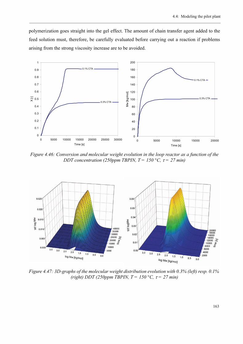
4.4: Modeling the pilot plant
163
polymerization goes straight into the gel effect. The amount of chain transfer agent added to the
feed solution must, therefore, be carefully evaluated before carrying out a reaction if problems
arising from the strong viscosity increase are to be avoided.
Figure 4.46: Conversion and molecular weight evolution in the loop reactor as a function of the DDT concentration (250ppm TBPIN, T = 150 °C, τ = 27 min)
Figure 4.47: 3D-graphs of the molecular weight distribution evolution with 0.3% (left) resp. 0.1% (right) DDT (250ppm TBPIN, T = 150 °C, τ = 27 min)
0
20
40
60
80
100
120
140
160
180
200
0 5000 10000 15000 20000
Time [s]
Mw
[kg/
mol
]
0.3% CTA
0.1% CTA
0
0.1
0.2
0.3
0.4
0.5
0.6
0.7
0.8
0.9
1
0 5000 10000 15000 20000 25000 30000
Time [s]
X [-
]
0.3% CTA
0.1% CTA
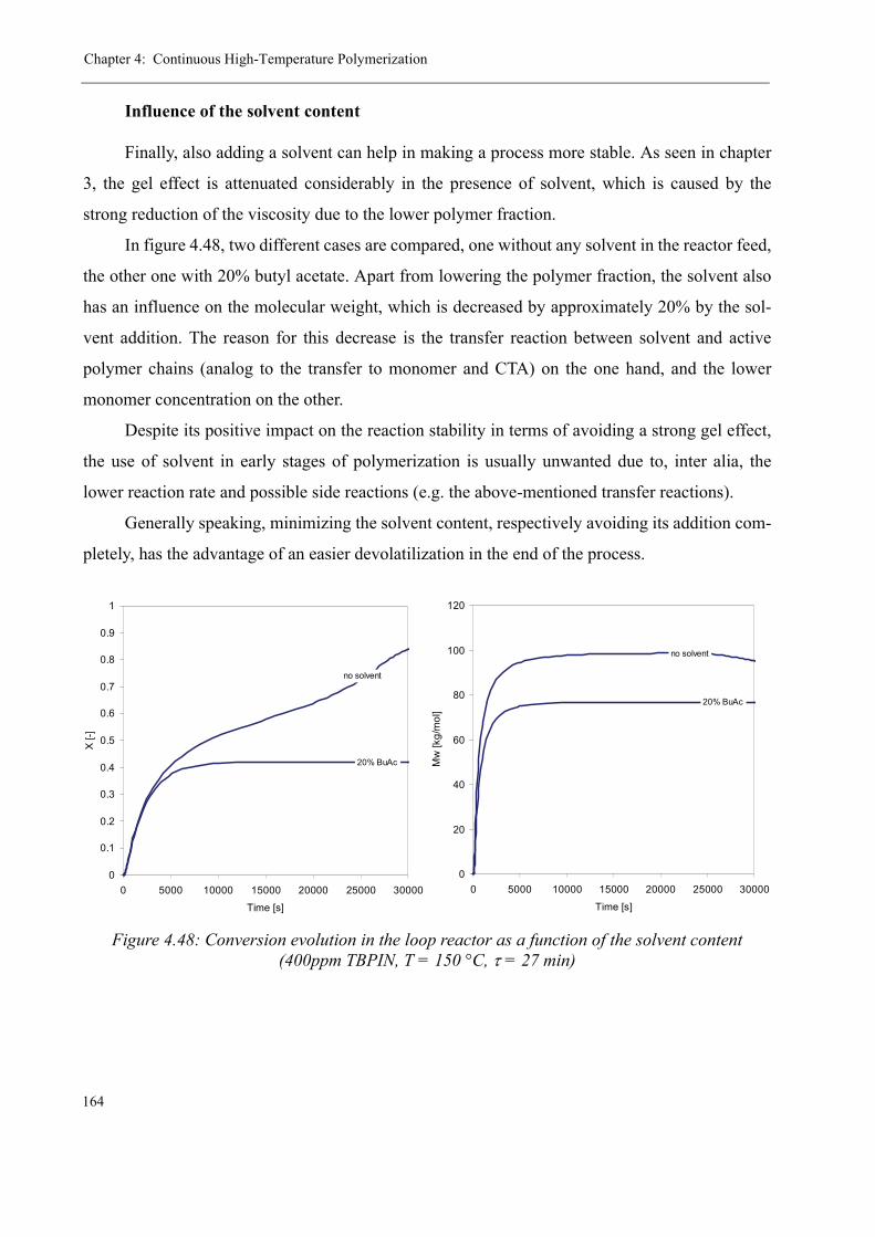
Chapter 4: Continuous High-Temperature Polymerization
164
Influence of the solvent content
Finally, also adding a solvent can help in making a process more stable. As seen in chapter
3, the gel effect is attenuated considerably in the presence of solvent, which is caused by the
strong reduction of the viscosity due to the lower polymer fraction.
In figure 4.48, two different cases are compared, one without any solvent in the reactor feed,
the other one with 20% butyl acetate. Apart from lowering the polymer fraction, the solvent also
has an influence on the molecular weight, which is decreased by approximately 20% by the sol-
vent addition. The reason for this decrease is the transfer reaction between solvent and active
polymer chains (analog to the transfer to monomer and CTA) on the one hand, and the lower
monomer concentration on the other.
Despite its positive impact on the reaction stability in terms of avoiding a strong gel effect,
the use of solvent in early stages of polymerization is usually unwanted due to, inter alia, the
lower reaction rate and possible side reactions (e.g. the above-mentioned transfer reactions).
Generally speaking, minimizing the solvent content, respectively avoiding its addition com-
pletely, has the advantage of an easier devolatilization in the end of the process.
Figure 4.48: Conversion evolution in the loop reactor as a function of the solvent content (400ppm TBPIN, T = 150 °C, τ = 27 min)
0
20
40
60
80
100
120
0 5000 10000 15000 20000 25000 30000
Time [s]
Mw
[kg/
mol
]
20% BuAc
no solvent
0
0.1
0.2
0.3
0.4
0.5
0.6
0.7
0.8
0.9
1
0 5000 10000 15000 20000 25000 30000
Time [s]
X [-
]
20% BuAc
no solvent

4.5: Discussion
165
4.5 Discussion
The present chapter is the most extensive one in this report. This is due to the fact that it
contains a variety of topics and information related to the pilot plant process.
On the first pages, the pilot plant setup has been described in detail and the advantages of a
combination of recycle loop and tube reactor was pointed out with regards to a classic setup of
CSTR and tube reactor. At the same time, the static mixing elements and their characteristics were
presented. The concept of chosing mixing elements with the same specific heat transfer coeffi-
cient as found in industrial scale reactors simplifies the scale-up from pilot plant to industrial pro-
duction size.
Connected to every polymerization reaction is a more or less pronounced viscosity increase
with rising polymer fraction. In the case of PMMA, this increase can be of several orders of mag-
nitude. A model from literature was presented for the prediction of the viscosity and the pressure
drop in the tubular reactor. By means of this model, it is possible to estimate the viscosity evolu-
tion with increasing conversion and molecular weight.
One major aim of this work was the implementation of a method for the inline conversion
measurement based on ultrasound technology. The pilot plant had been equipped with two probes
for the speed of sound measurement of the polymer solution at high temperatures. A problem aris-
ing from the determination of the monomer conversion from the speed of sound has been a rather
large discrepancy between the measured values and speeds of sound calculated from theory. It
was found that by readjusting the compressibility data for solvent and monomer, which had been
found in literature only for low temperatures, this offset could be avoided. The equation for the
calculation of the speed of sound for a mixture of known composition can, unfortunately, not be
solved explicitly to yield the polymer weight fraction as a function of speed of sound and temper-
ature. This limitation could be overcome by fitting calculated speed of sound values as a function
of solution composition and temperature, leading to an analytical expression for the direct conver-
sion calculation from measured speed of sound and temperature. The correct functioning of this
measurement technique was demonstrated by comparison of conversion data from ultrasound to
offline measured values from GC measurements. A limitation that could not be resolved is the
restricted ability to measure in the presence of solvent. Since the above mentioned fitting is lim-
ited to three dimensions (speed of sound, temperature and polymer fraction / conversion), it is
Chapter 4: Continuous High-Temperature Polymerization
166
impossible to include the influence of the solvent on the measured speed of sound in the calcula-
tion. Therefore, the conversion measurement can only be precise if the solvent fraction is constant
or zero. If solvent is to be used in the process, the fitting presented in this work needs to be redone
considering the influence of a constant amount of solvent on the speed of sound. However, it was
shown in this chapter, that the ultrasound technology is a powerful tool for the monitoring of the
process stability in polymerization reactions.
In several pilot plant experiments, the feasibility of the high temperature polymerization of
MMA was demonstrated as well as the influence of various process parameters on the product
quality investigated. Generally, a polymer of approximately 100 kg/mol and a residual volatiles’
concentration of ~4000ppm was obtained with the process conditions applied in this work. The
total monomer conversion was X = 40-50% in the recycle loop and X = 20-30% in the tube reac-
tor (corresponds to 60-80% overall conversion).
From experiments with different comonomer, respectively chain transfer agent concentra-
tion, the reactivity ratios for the system MMA/MA and the transfer constant for n-dodecanethiol
could be determined at high temperature. For the calculation of these parameters certain simplifi-
cations and assumptions had to be made in order to overcome limitations related to the narrow
measuring range (r-parameters) or to missing CTA concentration values (transfer constant). After
all, for the reactivity ratios of the system methyl methacrylate / methyl acrylate, the values
r12 = 1.825 ± 0.1 and r21 = 0.698 ± 0.1 were found for T = 160 °C and MA fractions below 10%
by the Kelen-Tüdös method. For higher acrylate fractions, more experiments need to be carried
out to refine the r21-parameter, which, in this work, could only be determined by the addition of
an auxiliary “dummy” point positioned at an MA fraction close to one. The chain transfer con-
stant for n-dodecanethiol at T = 140 °C was determined by means of the Mayo-plot and by a
method found in literature (de la Fuente and Madruga) to be CCTA = 0.88 ± 0.01.
Finally, the validity of the kinetic model established in this work for the continuous poly-
merization process was proven by comparison to experimental data. The agreement between
modeled and measured data in terms of conversion evolution and molecular weight distribution
modeling is very satisfying. Last but not least, the importance of process modeling in polymer
reaction engineering was pointed out by a parameter variation study. With the help of the pilot
plant model, several scenarios of changing process parameters were simulated and the influence
of each parameter on process stability and comportment was evaluated.
4.5: Discussion
167
Short Summary:
• The continuous polymerization of MMA at high reaction temperatures is dis-
cussed and results from several pilot plant experiments are presented
• With the reaction conditions applied in this work, a PMMA with a molecular
weight of Mw = 100 kg/mol is obtained at high monomer conversion
• For inline conversion monitoring, a technique based on speed of sound measure-
ment was successfully implemented and tested
• From the experimental data it was possible to determine two important kinetic
parameters: the reactivity ratios for the comonomer system MMA/MA and the
chain transfer constant for n-dodecanethiol at high temperature
• The validity of the kinetic model established during this work in PREDICI® was
proven by comparison to experimental data. With the help of this model, a param-
eter variation was carried out to predict the response of the process to several sce-
narios of changing process conditions.

Chapter 4: Continuous High-Temperature Polymerization
168
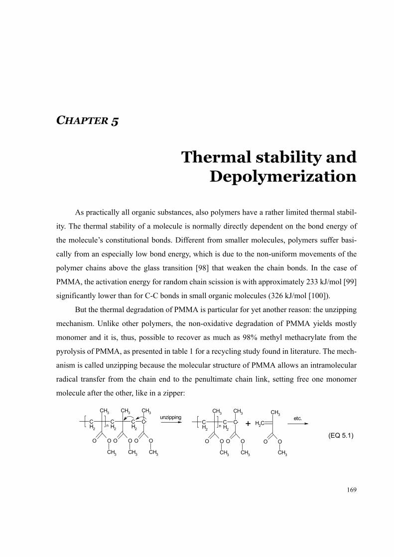
169
CHAPTER 5
Thermal stability andDepolymerization
As practically all organic substances, also polymers have a rather limited thermal stabil-
ity. The thermal stability of a molecule is normally directly dependent on the bond energy of
the molecule’s constitutional bonds. Different from smaller molecules, polymers suffer basi-
cally from an especially low bond energy, which is due to the non-uniform movements of the
polymer chains above the glass transition [98] that weaken the chain bonds. In the case of
PMMA, the activation energy for random chain scission is with approximately 233 kJ/mol [99]
significantly lower than for C-C bonds in small organic molecules (326 kJ/mol [100]).
But the thermal degradation of PMMA is particular for yet another reason: the unzipping
mechanism. Unlike other polymers, the non-oxidative degradation of PMMA yields mostly
monomer and it is, thus, possible to recover as much as 98% methyl methacrylate from the
pyrolysis of PMMA, as presented in table 1 for a recycling study found in literature. The mech-
anism is called unzipping because the molecular structure of PMMA allows an intramolecular
radical transfer from the chain end to the penultimate chain link, setting free one monomer
molecule after the other, like in a zipper:
(EQ 5.1)
CH2
CH2
CH2
C CH3 CH3 CH3
O O O OOO
CH3 CH3 CH3
n
CH2
CH2
C CH3 CH3
O OOO
CH3 CH3
n
CH3
CH2
OO
CH3
etc.+
unzipping
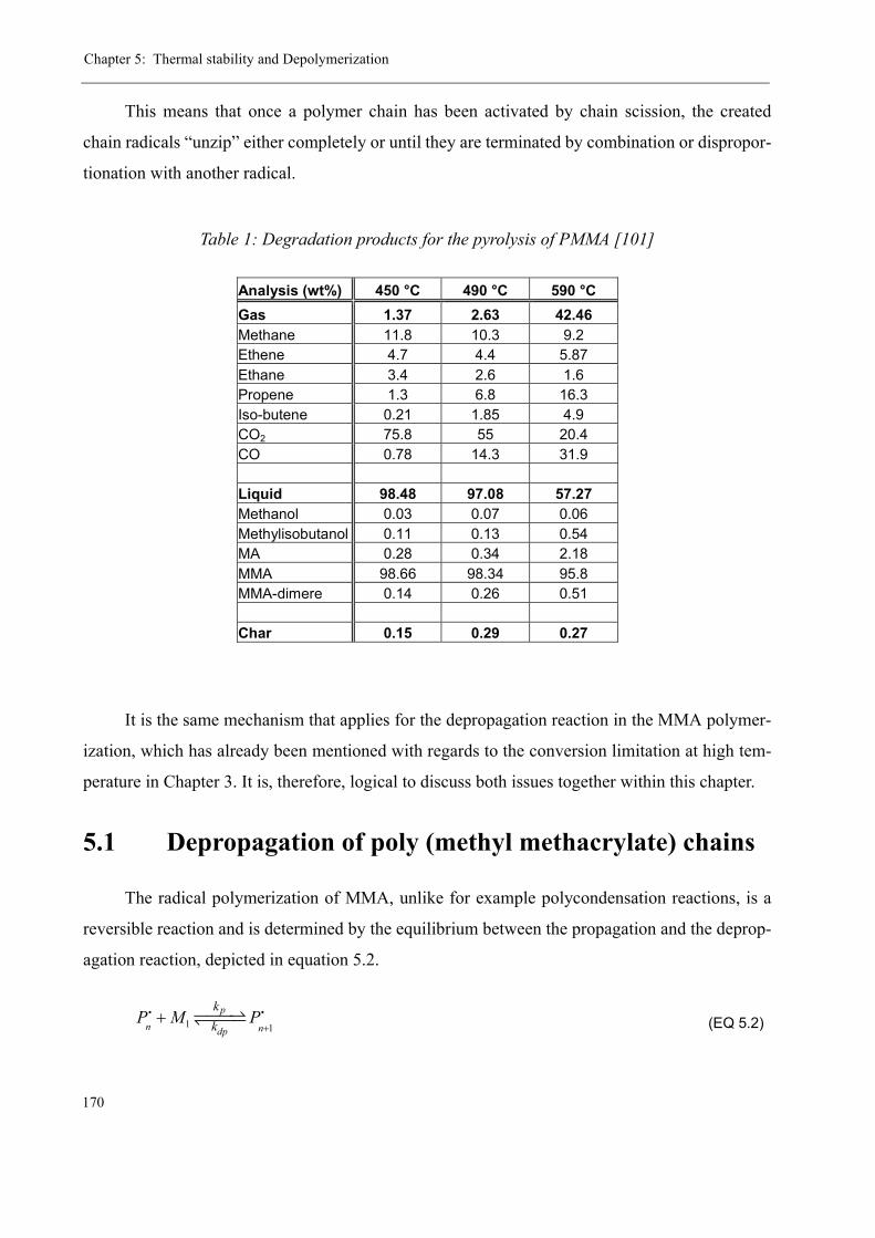
Chapter 5: Thermal stability and Depolymerization
170
This means that once a polymer chain has been activated by chain scission, the created
chain radicals “unzip” either completely or until they are terminated by combination or dispropor-
tionation with another radical.
It is the same mechanism that applies for the depropagation reaction in the MMA polymer-
ization, which has already been mentioned with regards to the conversion limitation at high tem-
perature in Chapter 3. It is, therefore, logical to discuss both issues together within this chapter.
5.1 Depropagation of poly (methyl methacrylate) chains
The radical polymerization of MMA, unlike for example polycondensation reactions, is a
reversible reaction and is determined by the equilibrium between the propagation and the deprop-
agation reaction, depicted in equation 5.2.
(EQ 5.2)
Table 1: Degradation products for the pyrolysis of PMMA [101]
Analysis (wt%) 450 °C 490 °C 590 °C Gas 1.37 2.63 42.46 Methane 11.8 10.3 9.2 Ethene 4.7 4.4 5.87 Ethane 3.4 2.6 1.6 Propene 1.3 6.8 16.3 Iso-butene 0.21 1.85 4.9 CO2 75.8 55 20.4 CO 0.78 14.3 31.9 Liquid 98.48 97.08 57.27 Methanol 0.03 0.07 0.06 Methylisobutanol 0.11 0.13 0.54 MA 0.28 0.34 2.18 MMA 98.66 98.34 95.8 MMA-dimere 0.14 0.26 0.51 Char 0.15 0.29 0.27
1 1
pn ndp
kkP M P
++i i
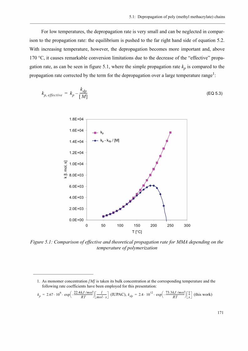
5.1: Depropagation of poly (methyl methacrylate) chains
171
For low temperatures, the depropagation rate is very small and can be neglected in compar-
ison to the propagation rate: the equilibrium is pushed to the far right hand side of equation 5.2.
With increasing temperature, however, the depropagation becomes more important and, above
170 °C, it causes remarkable conversion limitations due to the decrease of the “effective” propa-
gation rate, as can be seen in figure 5.1, where the simple propagation rate kp is compared to the
propagation rate corrected by the term for the depropagation over a large temperature range1:
(EQ 5.3)
1. As monomer concentration [M] is taken its bulk concentration at the corresponding temperature and the following rate coefficients have been employed for this presentation:
(IUPAC), (this work)
Figure 5.1: Comparison of effective and theoretical propagation rate for MMA depending on the temperature of polymerization
kp 2.67 106 22.4kJ mol⁄RT
------------------------------–⎝ ⎠⎛ ⎞ l
mol s⋅----------------exp⋅ ⋅= kdp 2.4 1012 73.3kJ mol⁄
RT------------------------------–⎝ ⎠
⎛ ⎞ 1s---exp⋅ ⋅=
kp effective, kpkdpM[ ]
---------–=
0.0E+00
2.0E+03
4.0E+03
6.0E+03
8.0E+03
1.0E+04
1.2E+04
1.4E+04
1.6E+04
1.8E+04
0 50 100 150 200 250 300
T [°C]
k [l,
mol
, s]
kp - kdp / [M]
kp

Chapter 5: Thermal stability and Depolymerization
172
Once the system reaches the ceiling temperature, i.e. the temperature where propagation
and depropagation rate are the same, the apparent rate of polymerization is zero. This means that
the propagation still takes place but for each element that is added to the chain, one is taken away
at the same time. Thus, the net chain growth is zero.
Kinetically, an equilibrium between two reactions like propagation and depropagation is
expressed by equation 5.4:
(EQ 5.4)
from which the equilibrium constant can be isolated:
(EQ 5.5)
From a thermodynamic point of view, propagation and depropagation are in the equilibrium
state at ceiling temperature, which in terms of the standard Gibbs enthalpy of polymerization
ΔGp0 can be written as
(at constant pressure) (EQ 5.6)
where ΔHp0 is the standard enthalpy and ΔSp
0 the standard entropy of polymerization (for
PMMA these values are -57.8 kJ/mol respectively -117 J/mol K [47]). From equations 5.5 and 5.6
follows for the calculation of the ceiling temperature:
(EQ 5.7)
Note that the concentration [M] is the equilibrium concentration of MMA at Tc. Usually,
[M] is taken as unit concentration ([M] = 1 mol/l) [102] and Tc is then the temperature above
which it is not possible to form polymer from unit or lower concentration. This means that if the
polymerization started at Tc, it would proceed until the monomer concentration reaches the equi-
librium concentration. Conversely, polymer chains that are made at a lower temperature and con-
kp Tc( ) Pn'[ ] M[ ]⋅ ⋅ kdp Tc( ) Pn 1+ '[ ]⋅=
K Tc( )kp Tc( )kdp Tc( )------------------
Pn 1+ '[ ]Pn'[ ] M[ ]⋅
-------------------------- 1M[ ]
---------≈= =
ΔGp0 Tc( ) ΔHp
0 TΔSp0– R– Tc K Tc( )ln⋅= =
TcΔHp
0
ΔSp0 R M[ ]ln⋅+
--------------------------------------- 494K 221°C∼= =
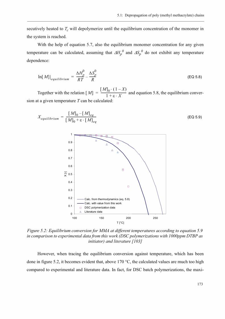
5.1: Depropagation of poly (methyl methacrylate) chains
173
secutively heated to Tc will depolymerize until the equilibrium concentration of the monomer in
the system is reached.
With the help of equation 5.7, also the equilibrium monomer concentration for any given
temperature can be calculated, assuming that ΔHp0 and ΔSp
0 do not exhibit any temperature
dependence:
(EQ 5.8)
Together with the relation and equation 5.8, the equilibrium conver-
sion at a given temperature T can be calculated:
(EQ 5.9)
However, when tracing the equilibrium conversion against temperature, which has been
done in figure 5.2, it becomes evident that, above 170 °C, the calculated values are much too high
compared to experimental and literature data. In fact, for DSC batch polymerizations, the maxi-
Figure 5.2: Equilibrium conversion for MMA at different temperatures according to equation 5.9 in comparison to experimental data from this work (DSC polymerizations with 1000ppm DTBP as
initiator) and literature [103]
M[ ]ln equilibrium
ΔHp0
RT----------
ΔSp0
R---------–=
M[ ]M[ ]0 1 X–( )⋅
1 ε X⋅+----------------------------------=
XequilibriumM[ ]0 M[ ]eq–
M[ ]0 ε M[ ]⋅ eq+----------------------------------------=
0
0.1
0.2
0.3
0.4
0.5
0.6
0.7
0.8
0.9
1
100 150 200 250
T [°C]
X [-
]
Calc. from thermodynamics (eq. 5.8)Calc. with value from this workDSC polymerization dataLiterature data

Chapter 5: Thermal stability and Depolymerization
174
mum attainable conversion drops quickly to zero between 170 °C and 210 °C while the calculated
values remain quite high until approximately 230 °C and reach zero conversion at ~260 °C. This
might be due to the simplifications made in the above considerations, e.g. that the chain radicals
[Pn+1.] and [Pn
.] have the same reactivity (equation 5.6). If, for example, the reactivity of [Pn+1.]
is lower than for [Pn.], the equilibrium conversion will be lower, too. Also the fact that other, irre-
versible reactions (like chain termination) take place at the same time influences the thermody-
namic equilibrium and prevents the use of the purely theoretical development made up to here for
the estimation of the depropagation rate constant, which is the real aim of this.
In order to determine a depropagation rate constant for MMA radical chains, it is therefore
more appropriate to do this with respect to experimental data rather than based on the theoretical
curve in figure 5.2. Also literature provides values for kdp as shown in table 2, but unfortunately,
values from both sources did not deliver satisfying results in the modeling of this work. The value
of Chiu et al. underestimated the conversion limitation by depropagation, whereas the Fleury rela-
tions for the calculation of Xequ and kdp resulted in a too strict reduction of the final monomer
conversion.
With the technical possibilities to fit rate constants to experimental data in PREDICI® and
the data from several high temperature polymerizations at 170 °C and 180 °C, a new value for kdp
was determined, which leads to a correct description of the conversion limitation in the frame of
the modeling used in this work.
Table 2: Literature values for the depropagation rate of MMA radical chains
Source kdp
Chiu et al. [58]
Fleury [5] (fitted by Fleury)
kdp 6.48 1011 76.4 kJ mol⁄[ ]–RT
--------------------------------------⎝ ⎠⎛ ⎞ 1
s---exp⋅ ⋅=
kdp kp MMA[ ]0 1 Xequ–( )ρequρ0
----------⋅ ⋅ ⋅=
Xequ 1 23.66 11282.7T K[ ]
-------------------–exp–=
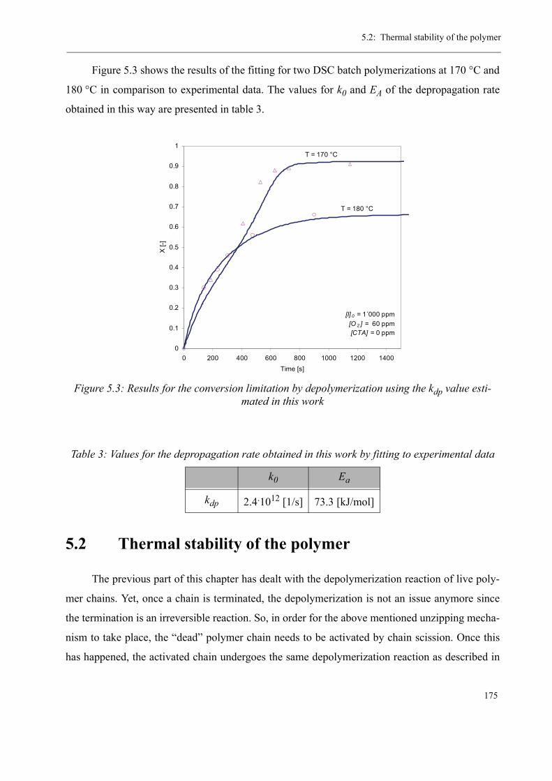
5.2: Thermal stability of the polymer
175
Figure 5.3 shows the results of the fitting for two DSC batch polymerizations at 170 °C and
180 °C in comparison to experimental data. The values for k0 and EA of the depropagation rate
obtained in this way are presented in table 3.
5.2 Thermal stability of the polymer
The previous part of this chapter has dealt with the depolymerization reaction of live poly-
mer chains. Yet, once a chain is terminated, the depolymerization is not an issue anymore since
the termination is an irreversible reaction. So, in order for the above mentioned unzipping mecha-
nism to take place, the “dead” polymer chain needs to be activated by chain scission. Once this
has happened, the activated chain undergoes the same depolymerization reaction as described in
Figure 5.3: Results for the conversion limitation by depolymerization using the kdp value esti-mated in this work
Table 3: Values for the depropagation rate obtained in this work by fitting to experimental data
k0 Ea
kdp 2.4.1012 [1/s] 73.3 [kJ/mol]
0
0.1
0.2
0.3
0.4
0.5
0.6
0.7
0.8
0.9
1
0 200 400 600 800 1000 1200 1400Time [s]
X [-
]
[I] 0 = 1´000 ppm [O 2 ] = 60 ppm
[CTA] = 0 ppm
T = 180 °C
T = 170 °C
Chapter 5: Thermal stability and Depolymerization
176
section 5.1., as postulated by Grassie and Melville [104]. The thermal degradation of PMMA is,
therefore, nothing else than a depolymerization initiated by chain scission, with the chain scission
being the rate determining step.
For radically polymerized PMMA, chain scission can occur at different places of the mole-
cule. Basically there are three main bond types, each exhibiting a different thermal stability.
Therefore, PMMA degrades in three steps with increasing temperature, as it was demonstrated by
previous research studies carried out in this laboratory [43] as well as by many other authors [99,
105-117].
The three most important bond types in order of increasing thermal stability are:
• head-to-head bonds that form by combination termination of two active
polymer chains
• unsaturated end groups that form by disproportionation termination of two
active polymer chains
• random C-C bonds of the main chain
Apart from these three types of bonds, other weak linkages can be introduced into the poly-
mer chains depending on, for example, the process conditions and impurities. However, their
occurrence is too random and non-reproducible in order to relate them to any thermal degradation
step as the above mentioned ones. In general, it can be said that the more regular a polymer chain
is, the more thermally stable it will be.
The following figure 5.4 shows a typical result from the thermogravimetry of PMMA,
which has been polymerized at 140 °C and not been stabilized or heat-treated after polymeriza-
tion. The three degradation steps are easily recognizable. Remarkable is the low starting point for
the head-to-head degradation at little above 150 °C. This temperature is far from the ceiling tem-
perature of MMA, which means that the monomer set free by the degradation can repolymerize
with the active chains [109], while for the two other steps, both taking place beyond 220°C, the
chain scission leads inevitably to a complete unzipping of the whole chain.
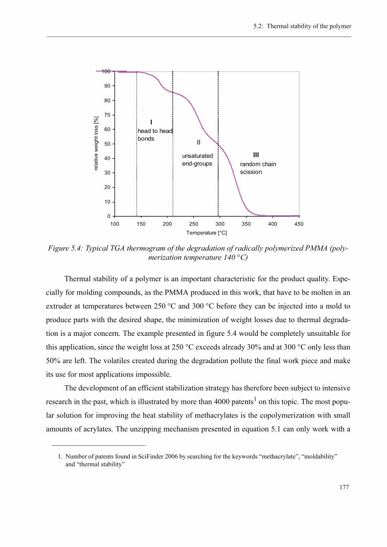
5.2: Thermal stability of the polymer
177
Thermal stability of a polymer is an important characteristic for the product quality. Espe-
cially for molding compounds, as the PMMA produced in this work, that have to be molten in an
extruder at temperatures between 250 °C and 300 °C before they can be injected into a mold to
produce parts with the desired shape, the minimization of weight losses due to thermal degrada-
tion is a major concern. The example presented in figure 5.4 would be completely unsuitable for
this application, since the weight loss at 250 °C exceeds already 30% and at 300 °C only less than
50% are left. The volatiles created during the degradation pollute the final work piece and make
its use for most applications impossible.
The development of an efficient stabilization strategy has therefore been subject to intensive
research in the past, which is illustrated by more than 4000 patents1 on this topic. The most popu-
lar solution for improving the heat stability of methacrylates is the copolymerization with small
amounts of acrylates. The unzipping mechanism presented in equation 5.1 can only work with a
Figure 5.4: Typical TGA thermogram of the degradation of radically polymerized PMMA (poly-merization temperature 140 °C)
1. Number of patents found in SciFinder 2006 by searching for the keywords “methacrylate”, “moldability” and “thermal stability”
0
10
20
30
40
50
60
70
80
90
100
100 150 200 250 300 350 400 450
Temperature [°C]
rela
tive
wei
ght l
oss
[%]
head to head bonds
unsaturatedend-groups random chain
scission
I
II
III

Chapter 5: Thermal stability and Depolymerization
178
methyl group in the alpha position of the acrylate. As soon as this methyl group is replaced by a
hydrogen atom, the unzipping stops [118]. This is, for example, the case for methyl acrylate but
also works for any other acrylate comonomer:
(EQ 5.10)
The stabilization with a comonomer is simple and cheap and it does not significantly
change other product properties of the polymer, since already small amounts of comonomer are
sufficient for stabilization reasons. This is the reason why nowadays practically no homopolymer-
ized PMMA is sold but only copolymers with various comonomer contents.
Another possibility to make PMMA thermally more stable is the use of chain transfer
agents. This group of substances, which are mostly of the thiol type, has already been mentioned
at other occasions in this work, namely with regards to the thermal initiation and the gel effect.
Apart from their primary application in polymerization reactions, i.e. to control the molecular
weight, they also have an important stabilizing effect on the polymer. In fact, the principle of
chain transfer is the termination of active polymer chains by transferring the radical from the
chain to the transfer agent in exchange for a hydrogen atom, which terminates the active chain.
Thus, the probability that polymer chains contain weak bonds is considerably lower. Since the
chain transfer is in concurrence with the other termination reactions it is: the higher the amount of
chain transfer agent, the less termination by combination or disproportionation occurs and the
more stable the polymer. An additional side-effect is the presence of residual thiols in the final
polymer. As the degradation of PMMA is a process involving radicals, thiols being radical scav-
engers can capture active radicals and, thus, slow down the degradation by unzipping.
Finally, also the polymerization conditions can have a major impact on the thermal stability
of the polymer. As said before, the uniformity of the polymer chains is a key to good resistance
against thermal stress. Increasing the radical flow during a polymerization reaction, e.g. by over-
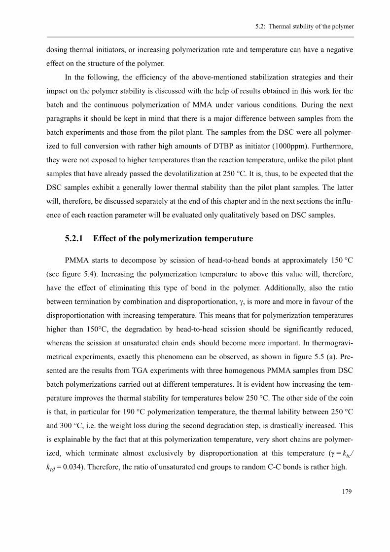
5.2: Thermal stability of the polymer
179
dosing thermal initiators, or increasing polymerization rate and temperature can have a negative
effect on the structure of the polymer.
In the following, the efficiency of the above-mentioned stabilization strategies and their
impact on the polymer stability is discussed with the help of results obtained in this work for the
batch and the continuous polymerization of MMA under various conditions. During the next
paragraphs it should be kept in mind that there is a major difference between samples from the
batch experiments and those from the pilot plant. The samples from the DSC were all polymer-
ized to full conversion with rather high amounts of DTBP as initiator (1000ppm). Furthermore,
they were not exposed to higher temperatures than the reaction temperature, unlike the pilot plant
samples that have already passed the devolatilization at 250 °C. It is, thus, to be expected that the
DSC samples exhibit a generally lower thermal stability than the pilot plant samples. The latter
will, therefore, be discussed separately at the end of this chapter and in the next sections the influ-
ence of each reaction parameter will be evaluated only qualitatively based on DSC samples.
5.2.1 Effect of the polymerization temperature
PMMA starts to decompose by scission of head-to-head bonds at approximately 150 °C
(see figure 5.4). Increasing the polymerization temperature to above this value will, therefore,
have the effect of eliminating this type of bond in the polymer. Additionally, also the ratio
between termination by combination and disproportionation, γ, is more and more in favour of the
disproportionation with increasing temperature. This means that for polymerization temperatures
higher than 150°C, the degradation by head-to-head scission should be significantly reduced,
whereas the scission at unsaturated chain ends should become more important. In thermogravi-
metrical experiments, exactly this phenomena can be observed, as shown in figure 5.5 (a). Pre-
sented are the results from TGA experiments with three homogenous PMMA samples from DSC
batch polymerizations carried out at different temperatures. It is evident how increasing the tem-
perature improves the thermal stability for temperatures below 250 °C. The other side of the coin
is that, in particular for 190 °C polymerization temperature, the thermal lability between 250 °C
and 300 °C, i.e. the weight loss during the second degradation step, is drastically increased. This
is explainable by the fact that at this polymerization temperature, very short chains are polymer-
ized, which terminate almost exclusively by disproportionation at this temperature (γ = ktc/
ktd = 0.034). Therefore, the ratio of unsaturated end groups to random C-C bonds is rather high.
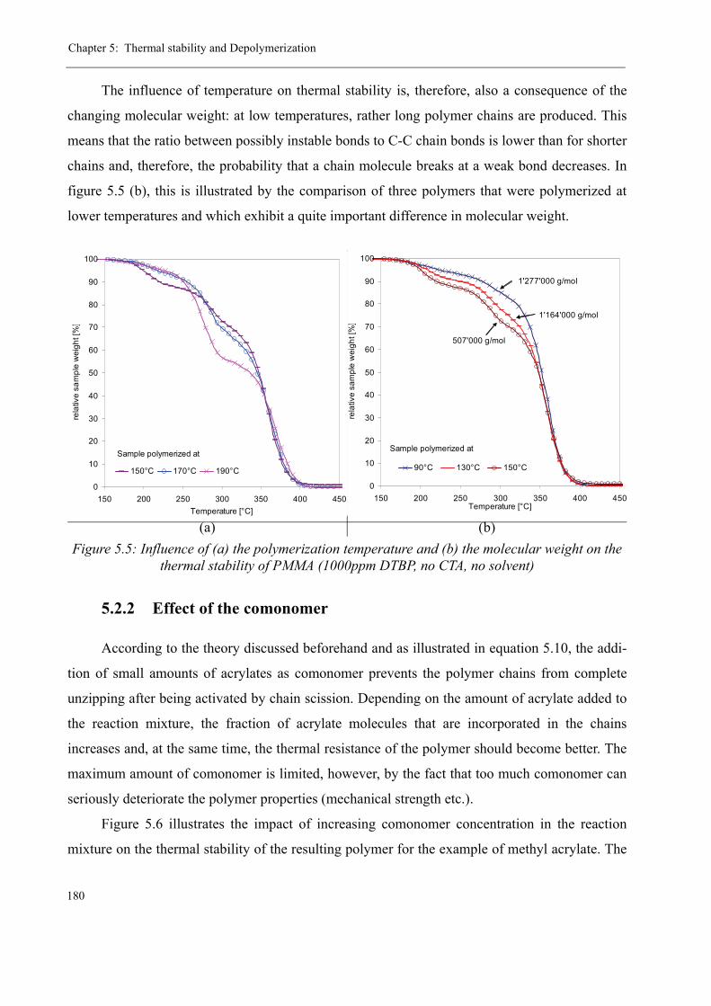
Chapter 5: Thermal stability and Depolymerization
180
The influence of temperature on thermal stability is, therefore, also a consequence of the
changing molecular weight: at low temperatures, rather long polymer chains are produced. This
means that the ratio between possibly instable bonds to C-C chain bonds is lower than for shorter
chains and, therefore, the probability that a chain molecule breaks at a weak bond decreases. In
figure 5.5 (b), this is illustrated by the comparison of three polymers that were polymerized at
lower temperatures and which exhibit a quite important difference in molecular weight.
5.2.2 Effect of the comonomer
According to the theory discussed beforehand and as illustrated in equation 5.10, the addi-
tion of small amounts of acrylates as comonomer prevents the polymer chains from complete
unzipping after being activated by chain scission. Depending on the amount of acrylate added to
the reaction mixture, the fraction of acrylate molecules that are incorporated in the chains
increases and, at the same time, the thermal resistance of the polymer should become better. The
maximum amount of comonomer is limited, however, by the fact that too much comonomer can
seriously deteriorate the polymer properties (mechanical strength etc.).
Figure 5.6 illustrates the impact of increasing comonomer concentration in the reaction
mixture on the thermal stability of the resulting polymer for the example of methyl acrylate. The
(a) (b)Figure 5.5: Influence of (a) the polymerization temperature and (b) the molecular weight on the
thermal stability of PMMA (1000ppm DTBP, no CTA, no solvent)
0
10
20
30
40
50
60
70
80
90
100
150 200 250 300 350 400 450Temperature [°C]
rela
tive
sam
ple
wei
ght [
%]
150°C 170°C 190°C
Sample polymerized at
0
10
20
30
40
50
60
70
80
90
100
150 200 250 300 350 400 450Temperature [°C]
rela
tive
sam
ple
wei
ght [
%]
90°C 130°C 150°C
Sample polymerized at
507'000 g/mol
1'277'000 g/mol
1'164'000 g/mol
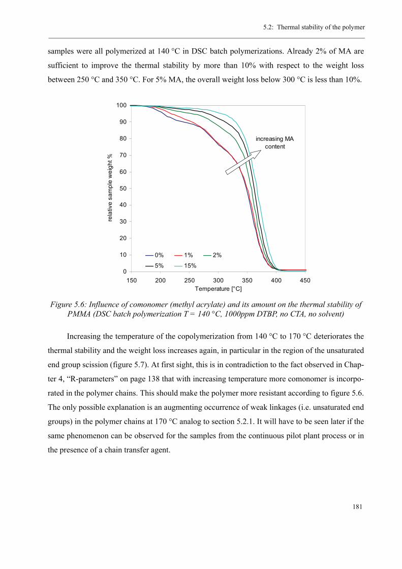
5.2: Thermal stability of the polymer
181
samples were all polymerized at 140 °C in DSC batch polymerizations. Already 2% of MA are
sufficient to improve the thermal stability by more than 10% with respect to the weight loss
between 250 °C and 350 °C. For 5% MA, the overall weight loss below 300 °C is less than 10%.
Increasing the temperature of the copolymerization from 140 °C to 170 °C deteriorates the
thermal stability and the weight loss increases again, in particular in the region of the unsaturated
end group scission (figure 5.7). At first sight, this is in contradiction to the fact observed in Chap-
ter 4, “R-parameters” on page 138 that with increasing temperature more comonomer is incorpo-
rated in the polymer chains. This should make the polymer more resistant according to figure 5.6.
The only possible explanation is an augmenting occurrence of weak linkages (i.e. unsaturated end
groups) in the polymer chains at 170 °C analog to section 5.2.1. It will have to be seen later if the
same phenomenon can be observed for the samples from the continuous pilot plant process or in
the presence of a chain transfer agent.
Figure 5.6: Influence of comonomer (methyl acrylate) and its amount on the thermal stability of PMMA (DSC batch polymerization T = 140 °C, 1000ppm DTBP, no CTA, no solvent)
0
10
20
30
40
50
60
70
80
90
100
150 200 250 300 350 400 450Temperature [°C]
rela
tive
sam
ple
wei
ght %
0% 1% 2%
5% 15%
increasing MA content
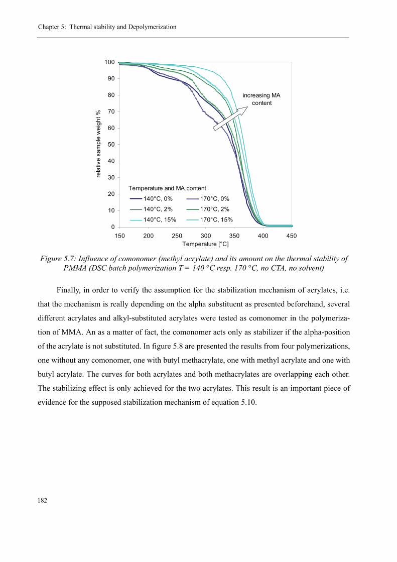
Chapter 5: Thermal stability and Depolymerization
182
Finally, in order to verify the assumption for the stabilization mechanism of acrylates, i.e.
that the mechanism is really depending on the alpha substituent as presented beforehand, several
different acrylates and alkyl-substituted acrylates were tested as comonomer in the polymeriza-
tion of MMA. An as a matter of fact, the comonomer acts only as stabilizer if the alpha-position
of the acrylate is not substituted. In figure 5.8 are presented the results from four polymerizations,
one without any comonomer, one with butyl methacrylate, one with methyl acrylate and one with
butyl acrylate. The curves for both acrylates and both methacrylates are overlapping each other.
The stabilizing effect is only achieved for the two acrylates. This result is an important piece of
evidence for the supposed stabilization mechanism of equation 5.10.
Figure 5.7: Influence of comonomer (methyl acrylate) and its amount on the thermal stability of PMMA (DSC batch polymerization T = 140 °C resp. 170 °C, no CTA, no solvent)
0
10
20
30
40
50
60
70
80
90
100
150 200 250 300 350 400 450Temperature [°C]
rela
tive
sam
ple
wei
ght %
140°C, 0% 170°C, 0%
140°C, 2% 170°C, 2%
140°C, 15% 170°C, 15%
increasing MA content
Temperature and MA content
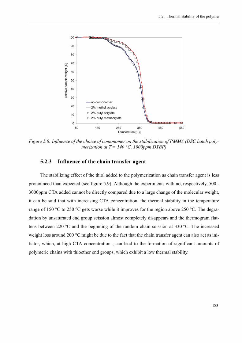
5.2: Thermal stability of the polymer
183
5.2.3 Influence of the chain transfer agent
The stabilizing effect of the thiol added to the polymerization as chain transfer agent is less
pronounced than expected (see figure 5.9). Although the experiments with no, respectively, 500 -
3000ppm CTA added cannot be directly compared due to a large change of the molecular weight,
it can be said that with increasing CTA concentration, the thermal stability in the temperature
range of 150 °C to 250 °C gets worse while it improves for the region above 250 °C. The degra-
dation by unsaturated end group scission almost completely disappears and the thermogram flat-
tens between 220 °C and the beginning of the random chain scission at 330 °C. The increased
weight loss around 200 °C might be due to the fact that the chain transfer agent can also act as ini-
tiator, which, at high CTA concentrations, can lead to the formation of significant amounts of
polymeric chains with thioether end groups, which exhibit a low thermal stability.
Figure 5.8: Influence of the choice of comonomer on the stabilization of PMMA (DSC batch poly-merization at T = 140 °C, 1000ppm DTBP)
0
10
20
30
40
50
60
70
80
90
100
50 150 250 350 450 550Température [°C]
rela
tive
sam
ple
wei
ght [
%]
no comonomer
2% methyl acrylate
2% butyl acrylate2% butyl methacrylate

Chapter 5: Thermal stability and Depolymerization
184
5.2.4 Results from the pilot plant polymerization
The polymer samples coming from the pilot plant were analyzed in the analytical facilities
of the industrial partner according to a method validated for commercial polymers. This allowed
the direct comparison between the product from the pilot scale reactor to industrial scale produced
PMMA. The specifications concerning the thermal stability of a product are given by characteris-
tic values, which quantify the weight loss at certain criteria and can be easily compared for differ-
ent samples. These criteria are:
• Td: the temperature where the total weight loss is of 2% of the sample
• Tv0.05, Tv0.1, Tv0.2: the temperature where the rate of weight loss is of
0.05%/min, 0.1%/min, respectively 0.2%/min
• Tmax: the temperature of maximum rate of weight loss
Apart from the relative weight loss suffered at a given temperature, also the rate of weight
loss is important, since the exposure of the polymer to elevated temperatures is usually kept rather
short in extrusion.
Figure 5.9: Influence of the chain transfer agent (n-dodecanethiol) on the stability of the polymer (DSC batch polymerization at 140 °C, 1000ppm DTBP)
0
10
20
30
40
50
60
70
80
90
100
150 200 250 300 350 400 450temperature [°C]
rela
tive
sam
ple
wei
ght [
%]
no CTA
1000ppm DDT
2000ppm DDT
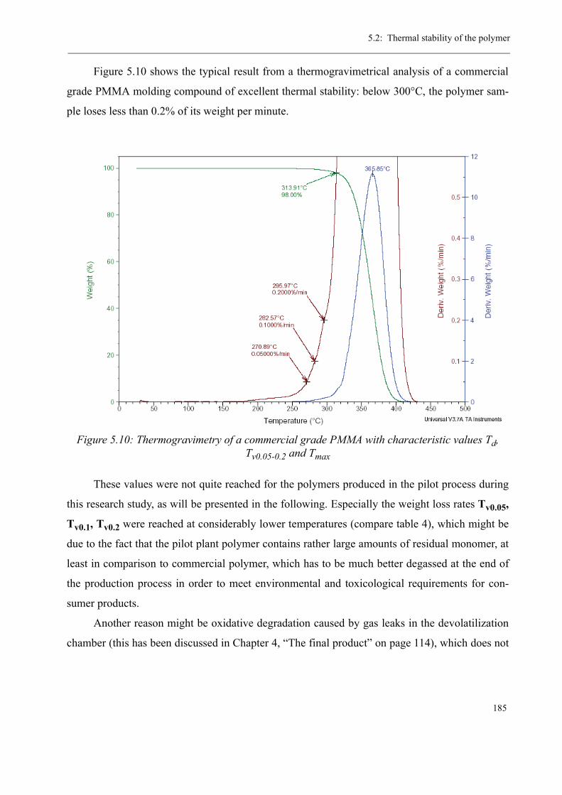
5.2: Thermal stability of the polymer
185
Figure 5.10 shows the typical result from a thermogravimetrical analysis of a commercial
grade PMMA molding compound of excellent thermal stability: below 300°C, the polymer sam-
ple loses less than 0.2% of its weight per minute.
These values were not quite reached for the polymers produced in the pilot process during
this research study, as will be presented in the following. Especially the weight loss rates Tv0.05,
Tv0.1, Tv0.2 were reached at considerably lower temperatures (compare table 4), which might be
due to the fact that the pilot plant polymer contains rather large amounts of residual monomer, at
least in comparison to commercial polymer, which has to be much better degassed at the end of
the production process in order to meet environmental and toxicological requirements for con-
sumer products.
Another reason might be oxidative degradation caused by gas leaks in the devolatilization
chamber (this has been discussed in Chapter 4, “The final product” on page 114), which does not
Figure 5.10: Thermogravimetry of a commercial grade PMMA with characteristic values Td, Tv0.05-0.2 and Tmax

Chapter 5: Thermal stability and Depolymerization
186
only cause a brownish coloration of the polymer but can also lead to instable bonds in the polymer
chains (e.g. by formation of (hydro)-peroxides).
For a clearer structure, only three values are compared for the following evaluation of the
thermal stability: Td2%, Tv0.1 and Tmax.
One important trend already observed for the DSC batch polymerizations could be con-
firmed: the thermal stability is considerably improved by the addition of acrylate comonomer.
Polymer samples containing no or little comonomer exhibit a lower Tmax and Tv0.1 values than
the samples with 5.5% MA. The Td2% value is difficult to compare for the different samples since
it is an integral value and depends, for example, on the amount of volatiles evaporated already at
lower temperatures.
A second important observation is that also increasing the polymerization temperature
improves the thermostability, even if the improvement is much less important than for the addi-
tion of comonomer. This is, at first sight, in contradiction to the results from batch polymerized
Figure 5.11: Thermogravimetry of a pilot plant sample (Exp. no 15) with characteristic values Td, Tv0.05-0.2 and Tmax
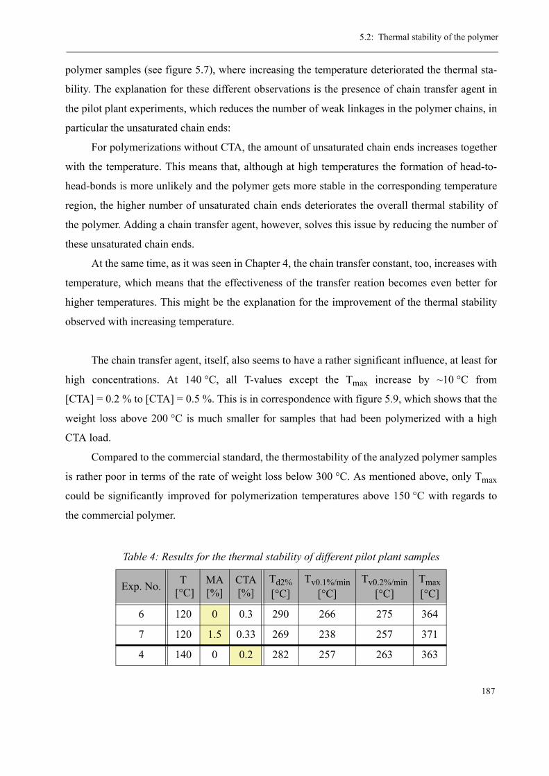
5.2: Thermal stability of the polymer
187
polymer samples (see figure 5.7), where increasing the temperature deteriorated the thermal sta-
bility. The explanation for these different observations is the presence of chain transfer agent in
the pilot plant experiments, which reduces the number of weak linkages in the polymer chains, in
particular the unsaturated chain ends:
For polymerizations without CTA, the amount of unsaturated chain ends increases together
with the temperature. This means that, although at high temperatures the formation of head-to-
head-bonds is more unlikely and the polymer gets more stable in the corresponding temperature
region, the higher number of unsaturated chain ends deteriorates the overall thermal stability of
the polymer. Adding a chain transfer agent, however, solves this issue by reducing the number of
these unsaturated chain ends.
At the same time, as it was seen in Chapter 4, the chain transfer constant, too, increases with
temperature, which means that the effectiveness of the transfer reation becomes even better for
higher temperatures. This might be the explanation for the improvement of the thermal stability
observed with increasing temperature.
The chain transfer agent, itself, also seems to have a rather significant influence, at least for
high concentrations. At 140 °C, all T-values except the Tmax increase by ~10 °C from
[CTA] = 0.2 % to [CTA] = 0.5 %. This is in correspondence with figure 5.9, which shows that the
weight loss above 200 °C is much smaller for samples that had been polymerized with a high
CTA load.
Compared to the commercial standard, the thermostability of the analyzed polymer samples
is rather poor in terms of the rate of weight loss below 300 °C. As mentioned above, only Tmax
could be significantly improved for polymerization temperatures above 150 °C with regards to
the commercial polymer.
Table 4: Results for the thermal stability of different pilot plant samples
Exp. No. T [°C]
MA[%]
CTA[%]
Td2%[°C]
Tv0.1%/min[°C]
Tv0.2%/min[°C]
Tmax[°C]
6 120 0 0.3 290 266 275 364
7 120 1.5 0.33 269 238 257 371
4 140 0 0.2 282 257 263 363
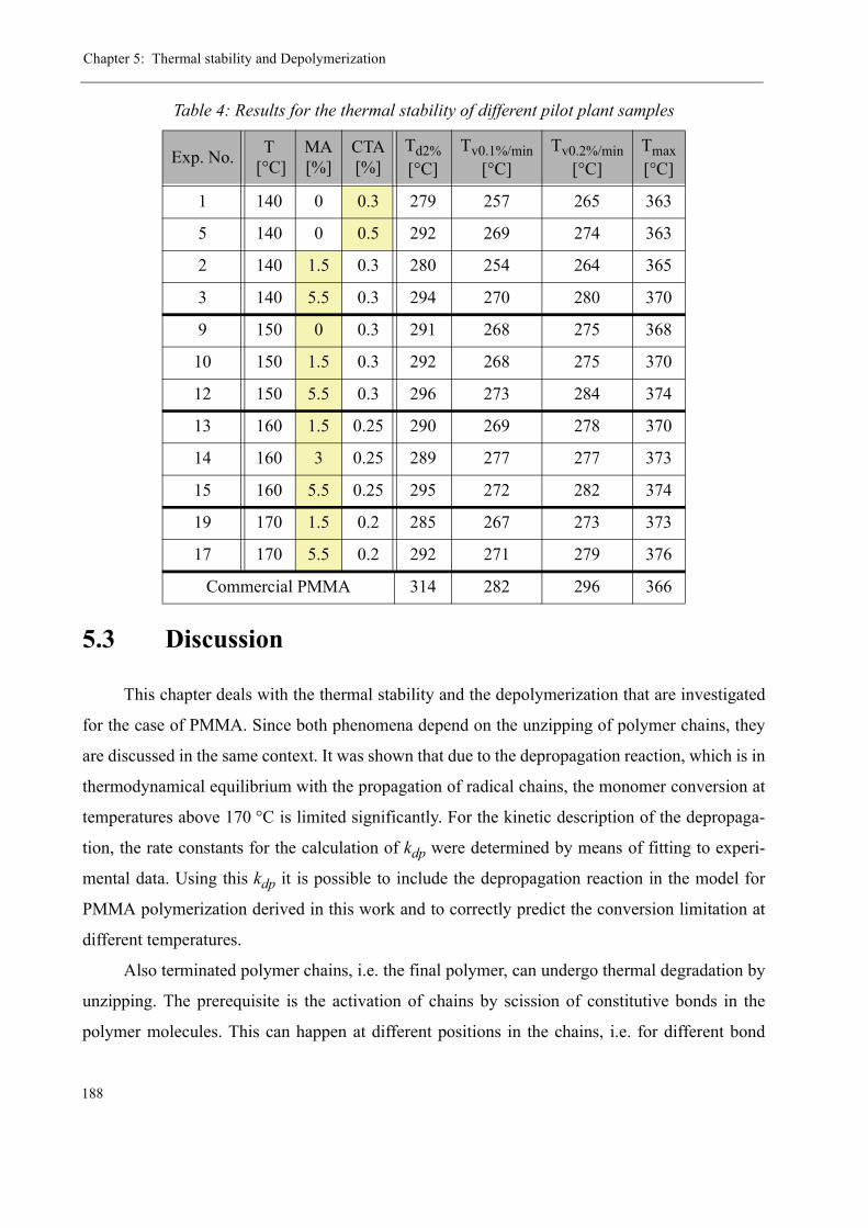
Chapter 5: Thermal stability and Depolymerization
188
5.3 Discussion
This chapter deals with the thermal stability and the depolymerization that are investigated
for the case of PMMA. Since both phenomena depend on the unzipping of polymer chains, they
are discussed in the same context. It was shown that due to the depropagation reaction, which is in
thermodynamical equilibrium with the propagation of radical chains, the monomer conversion at
temperatures above 170 °C is limited significantly. For the kinetic description of the depropaga-
tion, the rate constants for the calculation of kdp were determined by means of fitting to experi-
mental data. Using this kdp it is possible to include the depropagation reaction in the model for
PMMA polymerization derived in this work and to correctly predict the conversion limitation at
different temperatures.
Also terminated polymer chains, i.e. the final polymer, can undergo thermal degradation by
unzipping. The prerequisite is the activation of chains by scission of constitutive bonds in the
polymer molecules. This can happen at different positions in the chains, i.e. for different bond
1 140 0 0.3 279 257 265 363
5 140 0 0.5 292 269 274 363
2 140 1.5 0.3 280 254 264 365
3 140 5.5 0.3 294 270 280 370
9 150 0 0.3 291 268 275 368
10 150 1.5 0.3 292 268 275 370
12 150 5.5 0.3 296 273 284 374
13 160 1.5 0.25 290 269 278 370
14 160 3 0.25 289 277 277 373
15 160 5.5 0.25 295 272 282 374
19 170 1.5 0.2 285 267 273 373
17 170 5.5 0.2 292 271 279 376
Commercial PMMA 314 282 296 366
Table 4: Results for the thermal stability of different pilot plant samples
Exp. No. T [°C]
MA[%]
CTA[%]
Td2%[°C]
Tv0.1%/min[°C]
Tv0.2%/min[°C]
Tmax[°C]
5.3: Discussion
189
types exhibiting different thermal stabilities, and each type breaks in a characteristic temperature
range. For homogeneous PMMA, the thermal degradation usually takes place in three steps, cor-
responding to three bond types that are particular for this kind of polymer: head-to-head bonds,
unsaturated chain ends and the random C-C bonds of the polymer backbone.
One aim of the present work is to improve the thermal stability of the final polymer and to
investigate different strategies of stabilization: the addition of an acrylic comonomer to prevent
the polymer chains from complete unzipping, the addition of chain transfer agent to reduce the
occurrence of weak bonds in the chains caused by non-uniform termination processes, and finally
to increase the polymerization temperature in order to avoid completely the formation of ther-
mally weak linkages in the molecules. The different influences on the thermostability were dis-
cussed at first instance by comparing TGA-curves for different polymer samples from batch
polymerizations. Secondly, the thermostability results for different pilot plant polymer samples
were evaluated.
The results showed that each of the three factors positively influences the thermal stability
of the polymer, most of all the addition of a comonomer. Furthermore, by adding different acrylic
and methacrylic comonomers to the reaction mixture, it could be proven that the alpha methyl
group of the methacrylate is responsible for the unzipping mechanism and that by introducing
small amounts of acrylic groups into the polymer chains, the thermal degradation can be signifi-
cantly reduced.
The quality of the pilot plant polymer in terms of thermostability does not reach the high
standards of commercial polymer. However, the slightly worse thermal resistance below 300 °C
can be explained by the rather high residual monomer content and by oxidative processes taking
place in the devolatilization, which, despite the efforts made during this research study, could not
be made entirely gas tight. Additionally, the duration of each pilot plant experiment was by far too
short to obtain a polymer that compares in terms of molecular uniformity to a commercial prod-
uct, where the production process runs for long periods in steady state. However, it is remarkable
that the value of Tmax, i.e. the temperature of maximum rate of weight loss, is shifted upward by
~5-10 °C compared to the commercial polymer when the polymerization temperature is higher
than 150 °C.
Short Summary:
Chapter 5: Thermal stability and Depolymerization
190
• The depolymerization reaction has to be taken into account for the correct predic-
tion of the monomer conversion at high temperature
• The value of the depolymerization rate constant was determined by fitting to
experimental data
• PMMA thermally decomposes in three steps, which are due to the scission of (in
the order of their thermal stability): the polymer chain at head-to-head bonds,
unsaturated chain ends and random C-C bonds.
• The thermal stability of PMMA is influenced by the following parameters: pres-
ence of acrylic comonomers, presence of chain transfer agent, polymerization
temperature
• Each effect is discussed by means of experimental results from batch and continu-
ous polymerizations.
191
CHAPTER 6
Conclusions and Perspectives
Anyone who has never made a mistakehas never tried anything new.
- Albert Einstein (1879-1955)
The present Ph.D. thesis focused on the continuous high temperature polymerization of
methyl (methacrylate) at pilot scale, its kinetic description and a study of the impacts of vari-
ous process parameters on the obtained polymer. Its major aims are listed in the introduction of
this report on page 7 and the summarized conclusions will be presented in the same order
together with the perspectives, i.e. issues that, according to the authors opinion, might need to
be refined or be interesting subject of further investigations in future.
Generally, it can be stated that the high temperature polymerization aiming for the pro-
duction of PMMA molding compounds is technically feasible and yields certain advantages in
comparison to a lower temperature process. The most important features are
• a better and safer handling of the process due to reduced viscosity
• less risk to enter the gel effect and, therefore, higher kinetic reactor stability
• higher reaction rates and, therefore, higher space time yields
• reduced need for chain transfer agent and initiators
• increased thermal stability of the polymer
Chapter 6: Conclusions and Perspectives
192
A major disadvantage of a high temperature process might be an increased energy demand
for heating and more expensive equipment to resist the more severe process conditions. Unfortu-
nately, the time frame of this work did not allow a study of the economical consequences of
increasing the temperature. It might be an important aspect of future investigations to weigh the
additional costs against the benefits concerning process and product quality.
In the following, the results from all different parts of this work will be summarized with
respect to the different chapters they were discussed in.
Self-Initiation at high temperature
Acrylic monomers are subject to a rather pronounced spontaneous initiation. In the case of
MMA it was demonstrated that, depending on the process conditions, monomer conversions as
high as 30% can be observed in absence of any intentionally added initiator. The source of this
self-initiation is mainly the formation and decomposition of a polymeric peroxide (the so-called
MMA-peroxide or PMMAP), which forms from physically dissolved oxygen in the monomer and
the monomer, itself. However, there are other mechanisms contributing to the initiation at high
temperature. These are the initiation by chain transfer agent as well as the “true” thermal initi-
ation of the monomer (i.e. no other species involved). At very high temperatures (> 170 °C), also
the dimerization and formation of higher MMA oligomers influences the monomer conversion,
but these reactions follow a different mechanism and do not directly take part in the initiation of
the radical polymerization. The importance of all different initiating mechanisms was compared
for the temperature range 140 °C - 180 °C and related to each other.
The formation and decomposition of MMA-peroxides have been extensively investigated
in this work, which resulted in the determination of reaction rate constants for both of them. As a
part of the peroxide formation investigations, a method for the determination of organic peroxides
by UV spectrophotometry was developed. The MMA-peroxide could be successfully synthesized
in sufficiently large quantities to allow its characterization by advanced analytical methods (GPC,
TGA, NMR). It was found that it consists of copolymeric chains of the alternating structure
~MMA-OO-MMA-OO~ with molecular weights of approximately Mw = 5’000-8’000 g/mol
(determined by GPC). They form quickly and in significant amounts at temperatures between
50 °C and 100 °C and start decomposing above ~110 °C. It is, therefore, legitimate to compare
193
them to high-temperature decomposing thermal initiators. Although their efficiency as initiator is
rather low (f ~ 0.2), their presence even in small quantities is enough to cause considerable mono-
mer conversions.
The information obtained from studying the spontaneous initiation of MMA were imple-
mented in a kinetic model for the description of the high temperature kinetics and validated by
comparison to experimental data from batch polymerizations with and without initiator.
A point, which needs to be improved for future studies is the determination of oxygen in
monomer and solvent. In this work, it was tried to determine the concentration of oxygen in
MMA under different conditions. However, the analytical method is quite complicated due to the
strong disturbing effect of atmospheric oxygen, so that in the end only a concentration estimate
for the saturation concentration at one temperature could be realized. This estimate (~60-80 ppm
O2 at 18 °C) is, nevertheless, in agreement with literature values for other acrylic monomers.
Gel effect at high temperatures
Since the characteristic of the gel effect changes drastically at high temperatures with
respect to the gel effect observed at temperatures below 100 °C, it was necessary to find suitable
model equations to describe it in the kinetic model for the batch and the continuous process.
Unfortunately, most existing models that can be found in the specialized literature are rather lim-
ited concerning their interval of validity and their applicability to continuous polymerization. The
challenge was, therefore, to find a suitable basic gel effect model and to refine it in a way so that
it meets the requirements of this work. This could be realized by modifying the widely-known
Chiu, Carrat and Soong (CCS-) model. The modification consisted mainly in eliminating the
dependency on the initiator concentration and to relate the change of the termination rate con-
stant directly to the molecular weight, instead. The new model equation could then be fitted to
experimental data obtained in this work as well as to literature data.
The correct prediction of the high temperature gel effect with this adapted modeling
approach could be proven for batch and continuous polymerization experiments within the exper-
imental conditions used in this work and, at the same time, the results allowed investigating the
influence of changing different process conditions (CTA, T, solvent etc.) on the shape and
intensity of the gel effect and the correct consideration of this influence by the model.

Chapter 6: Conclusions and Perspectives
194
Continuous High Temperature Polymerization
The major challenge in this work was the design and construction of a complete pilot plant
installation for the continuous polymerization of MMA. The final setup used for the polymeriza-
tion experiments presented in this report consisted of a recycle loop combined with a single tube
reactor equipped with Sulzer SMXL/SMX static mixing elements. The pilot plant was operated
for 5 - 10 hours experiments, depending on the quantity of polymer needed. The mean residence
time in each reactor part was of ~ 30 min. The obtained polymer had a molecular weight of
approximately 100 kg/mol and was analyzed for its thermal stability and residual volatiles’ con-
centration.
Moreover, the pilot plant was equipped with two ultrasound probes for speed of sound
measurements of the polymer solution. This technique allowed the inline conversion measure-
ment based on a mathematical treatment of the obtained speed of sound values as a function of
temperature and pressure. The realization of a correct conversion measurement required the
reevaluation of compressibility data for MMA and butyl acetate taken from literature. Unfortu-
nately, there was no possibility to determine at the same time the solvent fraction in the reactor.
The equation for the calculation of the speed of sound had, therefore, to be reduced assuming an
either constant or zero solvent fraction. Since in the beginning of the reaction the solvent that is
present in the reactor during heating needs to be displaced, which takes approximately 5 residence
times, this assumption does not hold true and the conversion measurement is only correct at,
respectively, close to steady state. An improvement for the future would be the combination of
ultrasound measurement with other analytical methods in order to have access to the solvent con-
centration. Thus, the number of unknowns in the ultrasound equation could be reduced and mono-
mer conversion measurement would be possible independently of the solvent fraction present in
the reactor.
For the modeling of the continuous polymerization in loop and tube reactor, a kinetic model
was established in PREDICI®. This model allowed the correct prediction of conversion and
molecular weight distribution as well as a parameter study for various process parameters.
The data obtained from experiments in the loop reactor with varying amounts of CTA and
comonomer allowed the determination of the chain transfer constant for n-dodecanethiol as
well as the reactivity ratios for the system MMA / MA at the investigated temperature range. In
195
order to obtain these values, some simplifications respectively assumptions had to be made. For
the chain transfer constant, the concentration of thiol in the reactor could not be determined ana-
lytically and had, therefore, to be estimated. The determination of the r-parameters for MMA and
MA by the Kelen-Tüdös method turned out to be difficult due to a too limited variation of the
comonomer fraction (1 - 5 wt-%), leading to unrealistic results for the reactivity of the comono-
mer. Only by the addition of a fictive point on the other end of the concentration scale it was pos-
sible to come to realistic values for the reactivity ratio of MA-terminated chains. The results
showed that future experiments should be carried out with higher MA weight fractions of at least
20% in order to obtain more precise values for the r-parameters.
Finally, the thermal stability and the depolymerization of PMMA were discussed. They
both base on the same degradation mechanism of active polymer chains, the so-called unzipping,
which can be stopped by the incorporation of acrylate monomers in the polymer chain. This is the
reason why the thermal stability of PMMA can be significantly improved by the addition of
methyl acrylate. The change of thermal stability with changing process parameters (temperature,
chain transfer agent, comonomer concentration) was discussed for samples from batch and con-
tinuous polymerizations. It was found that increasing the process temperature has only a slightly
improving impact on the thermal stability. On the other hand, it is strongly improved by the addi-
tion of methyl acrylate as comonomer or a n-dodecanethiol as chain transfer agent. This is due to
the stopping of the unzipping mechanism at comonomer units in the chain, respectively due to
more uniform chains with less instable bonds in the case of a chain transfer regulated polymeriza-
tion.
After all, the results of the present Ph.D. thesis are motivating for further studies concerning
the high temperature polymerization of MMA. It could be shown that in many regards, increasing
the reaction temperature yields interesting improvements of process and product properties. And
although the pilot plant setup used in this work as well as the process conditions will have to be
further optimized in order to obtain a final product with the degree of sophistication of a modern
commercial PMMA concerning its optical and thermal qualities, the results concerning the kinet-
ics and parameter studies will, hopefully, be valuable for future research and process optimization
in industry.

Chapter 6: Conclusions and Perspectives
196

A-I
ANNEXE 1
Analytical Techniquesand Method Development
In this work, various techniques have been employed for all the different analytical tasks.
Since most of them are relevant for several chapters of this thesis, it was chosen to bundle their
description in one Annex and to refer hereto within each chapter. In the following are explained in
detail each analytical technique used in this work as well as the corresponding methods, many of
which had to be developed in the frame of this study.
1.1 Headspace Gas Chromatography
Gas chromatography (GC) is the method of choice for the analysis of volatile compounds.
The general concept is widely known and not presented again at this point. When it comes to
polymers or polymer containing mixtures, the use of standard gas chromatography is, however,
not possible. The simple reason for this is that polymers are not volatile and must, therefore, not
be injected into the evaporator of a GC, where they would simply get stuck and block the injector
port with time.
A technical solution for this problem is the so-called headspace gas chromatography (HS-
GC), the principle of which is rather simple: Before the injection into the GC, itself, the polymer
is separated from the volatiles to be analyzed. In the case of the dynamic headspace technique,
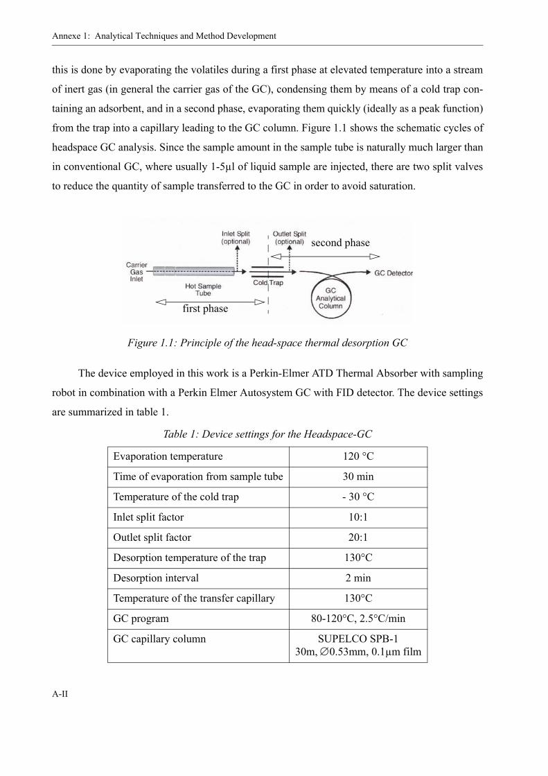
Annexe 1: Analytical Techniques and Method Development
A-II
this is done by evaporating the volatiles during a first phase at elevated temperature into a stream
of inert gas (in general the carrier gas of the GC), condensing them by means of a cold trap con-
taining an adsorbent, and in a second phase, evaporating them quickly (ideally as a peak function)
from the trap into a capillary leading to the GC column. Figure 1.1 shows the schematic cycles of
headspace GC analysis. Since the sample amount in the sample tube is naturally much larger than
in conventional GC, where usually 1-5µl of liquid sample are injected, there are two split valves
to reduce the quantity of sample transferred to the GC in order to avoid saturation.
The device employed in this work is a Perkin-Elmer ATD Thermal Absorber with sampling
robot in combination with a Perkin Elmer Autosystem GC with FID detector. The device settings
are summarized in table 1.
Figure 1.1: Principle of the head-space thermal desorption GC
Table 1: Device settings for the Headspace-GC
Evaporation temperature 120 °C
Time of evaporation from sample tube 30 min
Temperature of the cold trap - 30 °C
Inlet split factor 10:1
Outlet split factor 20:1
Desorption temperature of the trap 130°C
Desorption interval 2 min
Temperature of the transfer capillary 130°C
GC program 80-120°C, 2.5°C/min
GC capillary column SUPELCO SPB-130m, ∅0.53mm, 0.1µm film
first phase
second phase
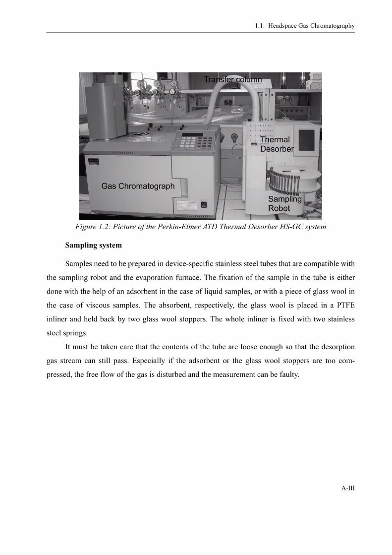
1.1: Headspace Gas Chromatography
A-III
Sampling system
Samples need to be prepared in device-specific stainless steel tubes that are compatible with
the sampling robot and the evaporation furnace. The fixation of the sample in the tube is either
done with the help of an adsorbent in the case of liquid samples, or with a piece of glass wool in
the case of viscous samples. The absorbent, respectively, the glass wool is placed in a PTFE
inliner and held back by two glass wool stoppers. The whole inliner is fixed with two stainless
steel springs.
It must be taken care that the contents of the tube are loose enough so that the desorption
gas stream can still pass. Especially if the adsorbent or the glass wool stoppers are too com-
pressed, the free flow of the gas is disturbed and the measurement can be faulty.
Figure 1.2: Picture of the Perkin-Elmer ATD Thermal Desorber HS-GC system
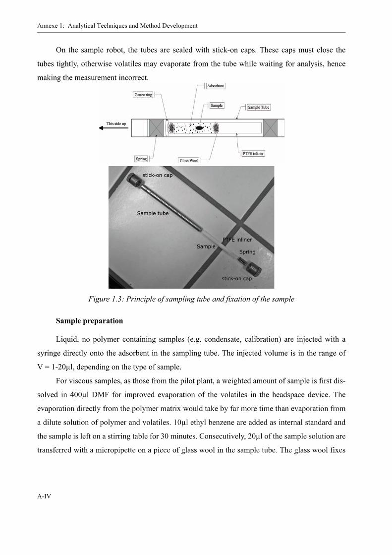
Annexe 1: Analytical Techniques and Method Development
A-IV
On the sample robot, the tubes are sealed with stick-on caps. These caps must close the
tubes tightly, otherwise volatiles may evaporate from the tube while waiting for analysis, hence
making the measurement incorrect.
Sample preparation
Liquid, no polymer containing samples (e.g. condensate, calibration) are injected with a
syringe directly onto the adsorbent in the sampling tube. The injected volume is in the range of
V = 1-20µl, depending on the type of sample.
For viscous samples, as those from the pilot plant, a weighted amount of sample is first dis-
solved in 400µl DMF for improved evaporation of the volatiles in the headspace device. The
evaporation directly from the polymer matrix would take by far more time than evaporation from
a dilute solution of polymer and volatiles. 10µl ethyl benzene are added as internal standard and
the sample is left on a stirring table for 30 minutes. Consecutively, 20µl of the sample solution are
transferred with a micropipette on a piece of glass wool in the sample tube. The glass wool fixes
Figure 1.3: Principle of sampling tube and fixation of the sample
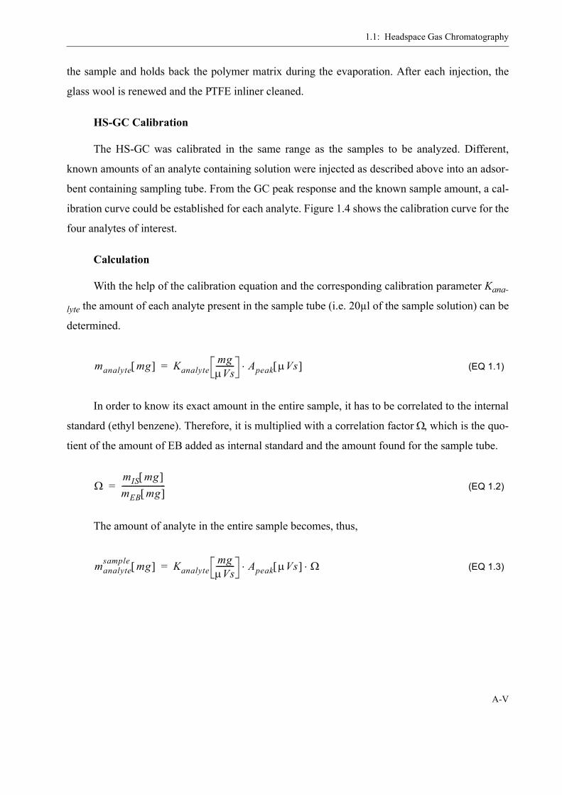
1.1: Headspace Gas Chromatography
A-V
the sample and holds back the polymer matrix during the evaporation. After each injection, the
glass wool is renewed and the PTFE inliner cleaned.
HS-GC Calibration
The HS-GC was calibrated in the same range as the samples to be analyzed. Different,
known amounts of an analyte containing solution were injected as described above into an adsor-
bent containing sampling tube. From the GC peak response and the known sample amount, a cal-
ibration curve could be established for each analyte. Figure 1.4 shows the calibration curve for the
four analytes of interest.
Calculation
With the help of the calibration equation and the corresponding calibration parameter Kana-
lyte the amount of each analyte present in the sample tube (i.e. 20µl of the sample solution) can be
determined.
(EQ 1.1)
In order to know its exact amount in the entire sample, it has to be correlated to the internal
standard (ethyl benzene). Therefore, it is multiplied with a correlation factor Ω, which is the quo-
tient of the amount of EB added as internal standard and the amount found for the sample tube.
(EQ 1.2)
The amount of analyte in the entire sample becomes, thus,
(EQ 1.3)
manalyte mg[ ] KanalytemgμVs---------- Apeak μVs[ ]⋅=
ΩmIS mg[ ]mEB mg[ ]-----------------------=
manalytesample mg[ ] Kanalyte
mgμVs---------- Apeak μVs[ ] Ω⋅⋅=
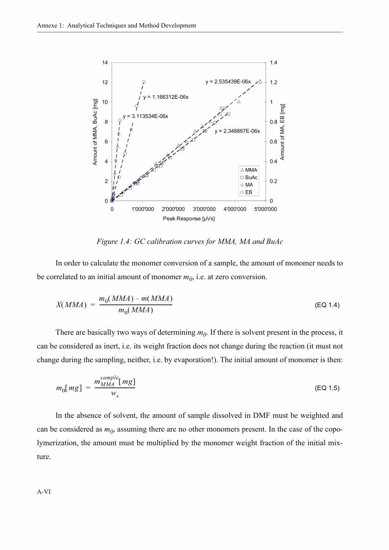
Annexe 1: Analytical Techniques and Method Development
A-VI
In order to calculate the monomer conversion of a sample, the amount of monomer needs to
be correlated to an initial amount of monomer m0, i.e. at zero conversion.
(EQ 1.4)
There are basically two ways of determining m0. If there is solvent present in the process, it
can be considered as inert, i.e. its weight fraction does not change during the reaction (it must not
change during the sampling, neither, i.e. by evaporation!). The initial amount of monomer is then:
(EQ 1.5)
In the absence of solvent, the amount of sample dissolved in DMF must be weighted and
can be considered as m0, assuming there are no other monomers present. In the case of the copo-
lymerization, the amount must be multiplied by the monomer weight fraction of the initial mix-
ture.
Figure 1.4: GC calibration curves for MMA, MA and BuAc
y = 3.113534E-06x
y = 1.166312E-06x
y = 2.535439E-06x
y = 2.348887E-06x
0
2
4
6
8
10
12
14
0 1'000'000 2'000'000 3'000'000 4'000'000 5'000'000
Peak Response [µVs]
Am
ount
of M
MA
, BuA
c [m
g]
0
0.2
0.4
0.6
0.8
1
1.2
1.4
Am
ount
of M
A, E
B [m
g]
MMABuAcMAEB
X MMA( )m0 MMA( ) m MMA( )–
m0 MMA( )--------------------------------------------------------=
m0 mg[ ]mMMA
sample mg[ ]ws
-------------------------------=
1.2: Size Exclusion Chromatography
A-VII
The residual volatiles’ concentration is determined in the same way: a known amount of
polymer is dissolved in 400µl DMF and analyzed as described in the HS-GC. The found amount
of volatiles is divided by the sample weight and the residual volatiles’ concentration is obtained.
1.2 Size Exclusion Chromatography
Another very important kind of analysis in polymer reaction engineering is the determina-
tion of the molecular weight. The technique of choice is the Gel Permeation Chromatography. In
the Wikipedia online encyclopedia [119], it is defined as follows:
“Gel permeation chromatography (GPC), also known as size exclusion chromatography
(SEC), is a chromatographic method in which molecules are separated based on their size. This
method is most widely used in the analysis of polymer molecular weights (or molar mass). The
term GPC was used in the beginning of polymer analysis when people used glass columns filled
with gels to perform GPC. Nowadays more and more automated and high pressure liquid chro-
matographic columns are used. Therefore GPC is an old terminology and size exclusion chroma-
tography (SEC) is the correct expression for the determination of molecular weights.
In SEC, a column (steel cylinder typically 10 mm in diameter and 500 to 1000 mm in
length) is packed with a porous material (typically silica or crosslinked polystyrene) and solvent
is forced through the column (at rates typically 1 ml/min and pressures of 50 to 200 bar). A sam-
ple is dissolved in the same solvent that is running through the column and is then introduced into
the solvent stream going through the column. A detector monitors the concentration of sample
exiting the end of the column. Inside the column, molecules are separated based on their hydrody-
namic volume (the volume the molecule occupies in a dilute solution). For polymers this can vary
greatly with the particular solvent and the temperature. By studying the properties of polymers in
particular solvents and by calibrating each column setup with samples of known molecular
weight, it is possible to get a relative distribution of molecular weights for a given polymer sam-
ple. Using this data, it is possible to calculate number average molecular weight, weight average
molecular weight, polydispersity, as well as higher order molecular weights within a useful level
of accuracy.
Inside the column, molecules are separated by whether or not they can fit within the pore
size of the packing material. When columns are created they are packed with porous beads with a

Annexe 1: Analytical Techniques and Method Development
A-VIII
specific pore size so that they are most accurate at separating molecules with sizes similar to the
pore size. As a molecule flows through the column it passes by a number of these porous beads. If
the molecule can fit inside the pore then it is drawn in by the force of diffusion. There it stays a
short while and then moves on. If a molecule can not fit into a pore then it continues following the
solvent flow. For this reason, in a GPC column, molecules with larger size will reach the end of
the column before molecules with smaller size. The effective range of the column is determined
by the pore size of the packing. Any molecules larger than all the pores in a column will be eluted
together regardless of their size. Likewise, any molecules that can fit into all the pores in the pack-
ing material will elute at the same time.
It is important to remember that the only absolute measure in SEC is volume of the mole-
cule (hydrodynamic volume), and even that measurement has certain error built into it. Interac-
tions between the solvent, packing, and or the sample will affect the measurement as will
concentration due to sample-sample interactions. Calculating the molecular weight from this
molecular size introduces even more error into the system. SEC is a useful tool for determining
molecular weight in polymers, but it is essential that the column and instrumentation be carefully
equilibrated and properly calibrated for the results to be trusted.”
The device used in this work is a Viscotek Triple Detection SEC TDA300 with refractive
index, viscosity and light scattering detector. Measurement parameters are provided in table 2.
Table 2: Measurement parameters for the SEC molecular weight analysis
Solvent / Eluent: THF (GPC grade, Fisher Scientific T/0709/PB17)
Flowrate: 1 ml/min
Sample concentration approx. 1 - 20 mg/ml
Sampling volume: 100 µl
Column set: 2 x PSS (Germany) linear M SDV 8x300 5µm1 guard column
Column temperature: 35°C
Polymer standards: For conventional calibration:PSS ReadyCal PMMA standards (series) (800 - 1’180’000 g/mol)
For triple detection:PSS Polystyrene standards (one at a time) (60’000 - 470’000 g/mol)

1.2: Size Exclusion Chromatography
A-IX
Sample preparation
The polymer sample (viscous or solid) is weighted and, depending on the sample size, 1 - 5
ml THF (GPC grade) are added so that a final concentration in the range of 1 - 20 mg/ml is
obtained. In the following, the solution is left on a stirring table overnight until complete dissolu-
tion of the polymer (optical inspection). For very high molecular weight or branched polymers it
might be necessary to leave them on a heated stirring table (T ~ 40 °C) in order to shorten the
time necessary for dissolution.
The knowledge of the exact sample concentration is necessary for the determination of the
polymer content by RI. Since the RI determines a concentration corresponding to the polymer
peak (it does not “see” the low-molecular volatiles), the polymer content respectively the conver-
sion can be determined by the equation:
and (EQ 1.6)
Triple Detection (SEC3)
The fractionated polymer molecules undergo three different analyses:
First of all the refractive index detector (RI). By means of the refractive index, the concen-
tration of each polymer fraction can be determined, as the refractive index increases linearly with
concentration:
(for linear PMMA) (EQ 1.7)
Figure 1.5: Viscotek SEC-System with (1) HPLC pump, (2) Degasser, (3) Autosampler, (4) Eluent storage, (5) Detector unit, (6) Computer for data acquisition
1 2
4
3 5611 22
44
33 5566
wpcpolymer mg ml⁄[ ]
ctotalsample mg ml⁄[ ]-------------------------------------------------= X
wp1 ws–--------------=
dndc------ 0.083=
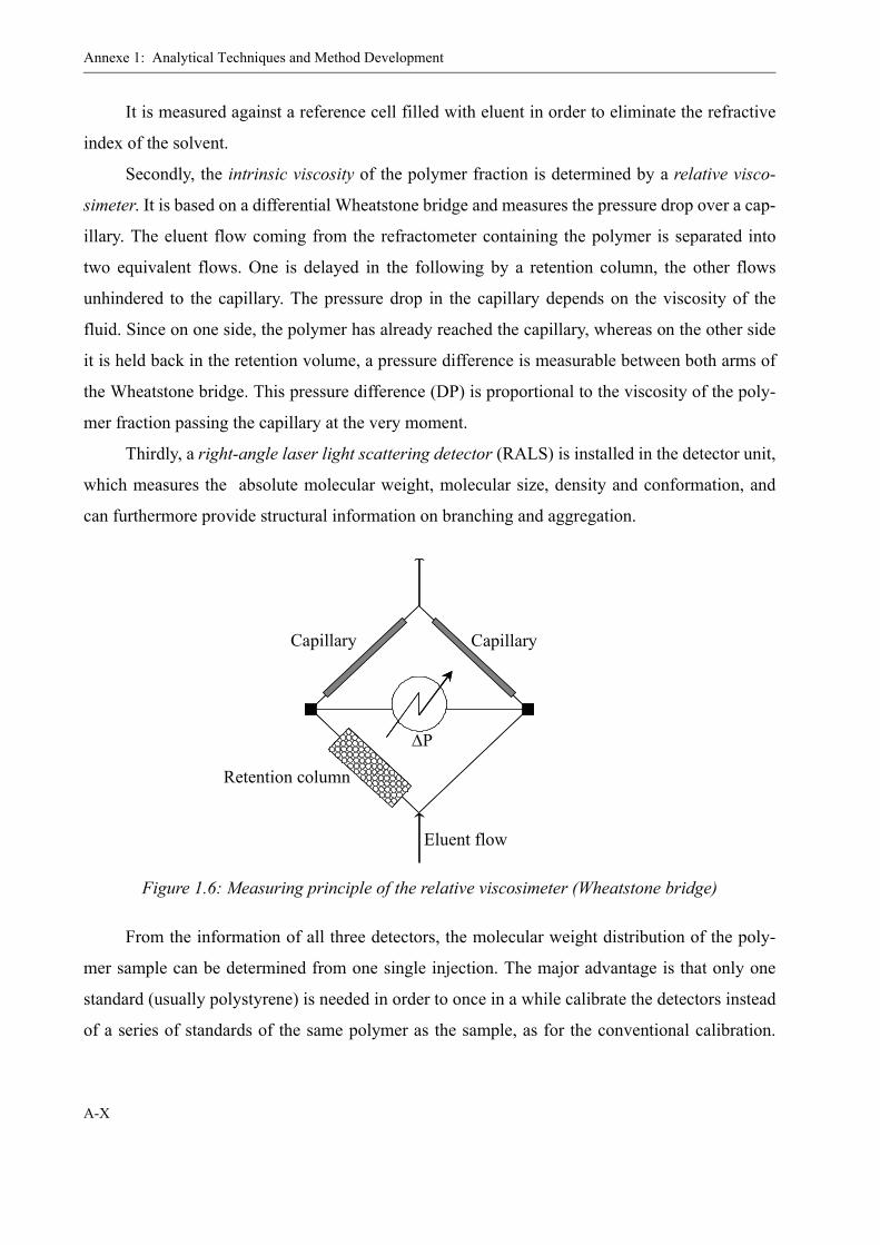
Annexe 1: Analytical Techniques and Method Development
A-X
It is measured against a reference cell filled with eluent in order to eliminate the refractive
index of the solvent.
Secondly, the intrinsic viscosity of the polymer fraction is determined by a relative visco-
simeter. It is based on a differential Wheatstone bridge and measures the pressure drop over a cap-
illary. The eluent flow coming from the refractometer containing the polymer is separated into
two equivalent flows. One is delayed in the following by a retention column, the other flows
unhindered to the capillary. The pressure drop in the capillary depends on the viscosity of the
fluid. Since on one side, the polymer has already reached the capillary, whereas on the other side
it is held back in the retention volume, a pressure difference is measurable between both arms of
the Wheatstone bridge. This pressure difference (DP) is proportional to the viscosity of the poly-
mer fraction passing the capillary at the very moment.
Thirdly, a right-angle laser light scattering detector (RALS) is installed in the detector unit,
which measures the absolute molecular weight, molecular size, density and conformation, and
can furthermore provide structural information on branching and aggregation.
From the information of all three detectors, the molecular weight distribution of the poly-
mer sample can be determined from one single injection. The major advantage is that only one
standard (usually polystyrene) is needed in order to once in a while calibrate the detectors instead
of a series of standards of the same polymer as the sample, as for the conventional calibration.
Figure 1.6: Measuring principle of the relative viscosimeter (Wheatstone bridge)
Retention column
CapillaryCapillary
Eluent flow
ΔP
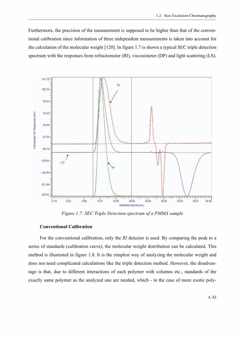
1.2: Size Exclusion Chromatography
A-XI
Furthermore, the precision of the measurement is supposed to be higher than that of the conven-
tional calibration since information of three independent measurements is taken into account for
the calculation of the molecular weight [120]. In figure 1.7 is shown a typical SEC triple detection
spectrum with the responses from refractometer (RI), viscosimeter (DP) and light scattering (LS).
Conventional Calibration
For the conventional calibration, only the RI detector is used. By comparing the peak to a
series of standards (calibration curve), the molecular weight distribution can be calculated. This
method is illustrated in figure 1.8. It is the simplest way of analyzing the molecular weight and
does not need complicated calculations like the triple detection method. However, the disadvan-
tage is that, due to different interactions of each polymer with columns etc., standards of the
exactly same polymer as the analyzed one are needed, which - in the case of more exotic poly-
Figure 1.7: SEC Triple Detection spectrum of a PMMA sample

Annexe 1: Analytical Techniques and Method Development
A-XII
mers than PMMA - can be difficult to find. Furthermore, the molecular weight changes with dif-
ferent standard origins. It can occur that by changing the producer of the standards, the measured
molecular weight increases by as much as 10%. On this account, the triple detection provides a
more independant measure of the molecular weight.
Figure 1.8: Conventional GPC analysis
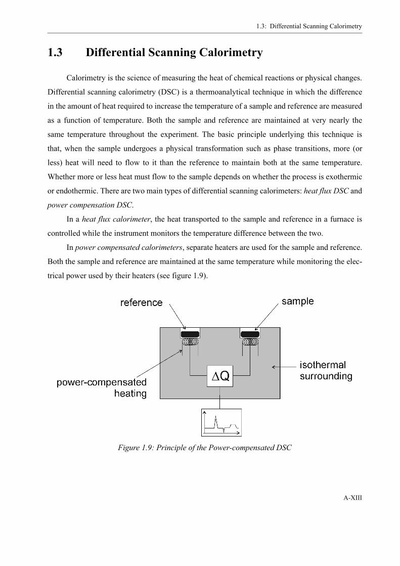
1.3: Differential Scanning Calorimetry
A-XIII
1.3 Differential Scanning Calorimetry
Calorimetry is the science of measuring the heat of chemical reactions or physical changes.
Differential scanning calorimetry (DSC) is a thermoanalytical technique in which the difference
in the amount of heat required to increase the temperature of a sample and reference are measured
as a function of temperature. Both the sample and reference are maintained at very nearly the
same temperature throughout the experiment. The basic principle underlying this technique is
that, when the sample undergoes a physical transformation such as phase transitions, more (or
less) heat will need to flow to it than the reference to maintain both at the same temperature.
Whether more or less heat must flow to the sample depends on whether the process is exothermic
or endothermic. There are two main types of differential scanning calorimeters: heat flux DSC and
power compensation DSC.
In a heat flux calorimeter, the heat transported to the sample and reference in a furnace is
controlled while the instrument monitors the temperature difference between the two.
In power compensated calorimeters, separate heaters are used for the sample and reference.
Both the sample and reference are maintained at the same temperature while monitoring the elec-
trical power used by their heaters (see figure 1.9).
Figure 1.9: Principle of the Power-compensated DSC

Annexe 1: Analytical Techniques and Method Development
A-XIV
The calorimeter employed in this work is a power-compensated Perkin Elmer Pyris1 DSC
(figure 1.10 b) with cryostat (IP Intracooler unit) for sub-ambient measurements. Sample solu-
tions of usually 20µl are filled into 60µl stainless steel medium pressure crucibles (figure 1.10 a),
which resist pressures of up to 40 bars.
The DSC was mainly used to polymerize samples at different temperatures, but also to
determine peroxide decomposition kinetics and glass transition temperatures Tg. For the polymer-
izations, an isothermal temperature programm was used with an initial heating rate of 40 °C/min
until reaction temperature. The conversion at time t can be determined by two methods: one is to
stop the reaction by throwing the crucible into liquid nitrogen and measuring the conversion by
GC analysis. In order to obtain also the molecular weight at time t, the experiment needs to be
repeated under the exact same conditions and this time GPC analysis is done with the sample.
Another way to obtain the conversion is integration of the heat flow curve. Assuming that
the reaction reaches full (= 100 %) conversion at the end, the conversion at time t can be calcu-
lated from the heat flow curve by equation 2.21 on page 28. This method has the advantage that
the experiment only needs to be done once and that the reaction does not need to be stopped each
time, which causes a certain error of the measurement. On the other hand, by assuming full con-
version, this method is not fully correct, neither, which is in particular the case for high tempera-
tures, where the calculation needs to be corrected by the “real” final conversion that is reached for
the given temperature.
(a) (b)Figure 1.10: (a) Medium-pressure stainless steel crucibles consisting of bottom, cover and O-
Ring, (b) Perkin-Elmer Pyris1 DSC with Intracooler
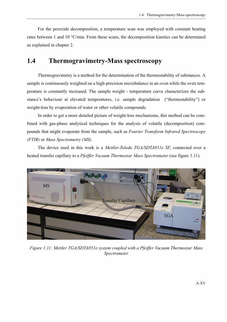
1.4: Thermogravimetry-Mass spectroscopy
A-XV
For the peroxide decomposition, a temperature scan was employed with constant heating
rates between 1 and 10 °C/min. From these scans, the decomposition kinetics can be determined
as explained in chapter 2.
1.4 Thermogravimetry-Mass spectroscopy
Thermogravimetry is a method for the determination of the thermostability of substances. A
sample is continuously weighted on a high-precision microbalance in an oven while the oven tem-
perature is constantly increased. The sample weight - temperature curve characterizes the sub-
stance’s behaviour at elevated temperatures, i.e. sample degradation (“thermostability”) or
weight-loss by evaporation of water or other volatile compounds.
In order to get a more detailed picture of weight-loss mechanisms, this method can be com-
bined with gas-phase analytical techniques for the analysis of volatile (decomposition) com-
pounds that might evaporate from the sample, such as Fourier Transform Infrared Spectroscopy
(FTIR) or Mass Spectrometry (MS).
The device used in this work is a Mettler-Toledo TGA/SDTA851e SF, connected over a
heated transfer capillary to a Pfeiffer Vacuum Thermostar Mass Spectrometer (see figure 1.11).
Figure 1.11: Mettler TGA/SDTA851e system coupled with a Pfeiffer Vacuum Thermostar Mass Spectrometer
MS
Transfer Capillary
TGA
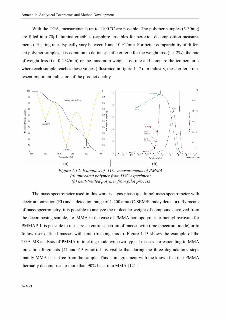
Annexe 1: Analytical Techniques and Method Development
A-XVI
With the TGA, measurements up to 1100 °C are possible. The polymer samples (5-30mg)
are filled into 70µl alumina crucibles (sapphire crucibles for peroxide decomposition measure-
ments). Heating rates typically vary between 1 and 10 °C/min. For better comparability of differ-
ent polymer samples, it is common to define specific criteria for the weight loss (i.e. 2%), the rate
of weight loss (i.e. 0.2 %/min) or the maximum weight loss rate and compare the temperatures
where each sample reaches these values (illustrated in figure 1.12). In industry, these criteria rep-
resent important indicators of the product quality.
The mass spectrometer used in this work is a gas phase quadrupol mass spectrometer with
electron ionization (EI) and a detection range of 1-200 amu (C-SEM/Faraday detector). By means
of mass spectrometry, it is possible to analyze the molecular weight of compounds evolved from
the decomposing sample, i.e. MMA in the case of PMMA homopolymer or methyl pyruvate for
PMMAP. It is possible to measure an entire spectrum of masses with time (spectrum mode) or to
follow user-defined masses with time (tracking mode). Figure 1.13 shows the example of the
TGA-MS analysis of PMMA in tracking mode with two typical masses corresponding to MMA
ionization fragments (41 and 69 g/mol). It is visible that during the three degradations steps
mainly MMA is set free from the sample. This is in agreement with the known fact that PMMA
thermally decomposes to more than 90% back into MMA [121].
(a) (b)Figure 1.12: Examples of TGA-measurements of PMMA
(a) untreated polymer from DSC experiment (b) heat-treated polymer from pilot process
0
10
20
30
40
50
60
70
80
90
100
150 200 250 300 350 400
Temperature [°C]
Nor
mal
ized
Wei
ght L
oss
[%]
-1
-0.9
-0.8
-0.7
-0.6
-0.5
-0.4
-0.3
-0.2
-0.1
0
Derivative of w
eight loss
200.70°C
Heating rate 3°C/min
276.36°C353.34°C
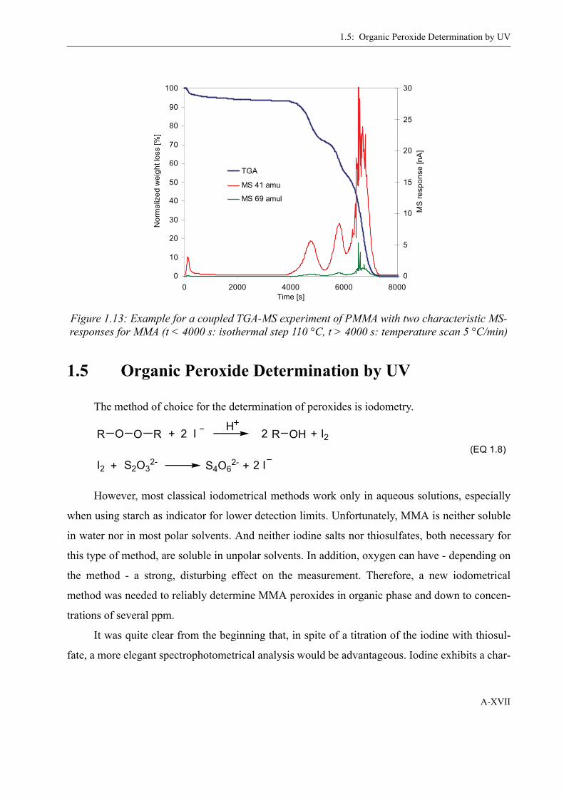
1.5: Organic Peroxide Determination by UV
A-XVII
1.5 Organic Peroxide Determination by UV
The method of choice for the determination of peroxides is iodometry.
(EQ 1.8)
However, most classical iodometrical methods work only in aqueous solutions, especially
when using starch as indicator for lower detection limits. Unfortunately, MMA is neither soluble
in water nor in most polar solvents. And neither iodine salts nor thiosulfates, both necessary for
this type of method, are soluble in unpolar solvents. In addition, oxygen can have - depending on
the method - a strong, disturbing effect on the measurement. Therefore, a new iodometrical
method was needed to reliably determine MMA peroxides in organic phase and down to concen-
trations of several ppm.
It was quite clear from the beginning that, in spite of a titration of the iodine with thiosul-
fate, a more elegant spectrophotometrical analysis would be advantageous. Iodine exhibits a char-
Figure 1.13: Example for a coupled TGA-MS experiment of PMMA with two characteristic MS-responses for MMA (t < 4000 s: isothermal step 110 °C, t > 4000 s: temperature scan 5 °C/min)
0
10
20
30
40
50
60
70
80
90
100
0 2000 4000 6000 8000Time [s]
Nor
mal
ized
wei
ght l
oss
[%]
0
5
10
15
20
25
30
MS
resp
onse
[nA
]
TGA
MS 41 amu
MS 69 amul
R O O R + I2 H 2 R OH + I2
I2 + S2O32- 2 IS4O6
2- +
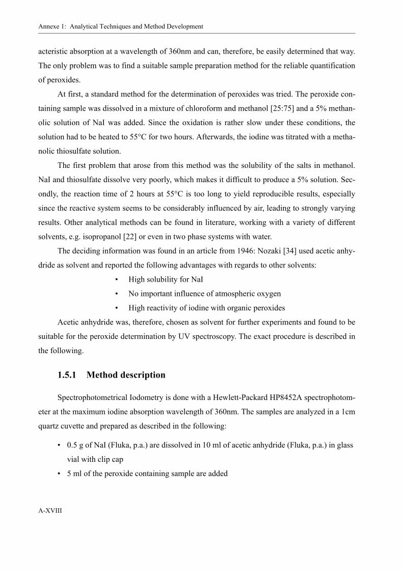
Annexe 1: Analytical Techniques and Method Development
A-XVIII
acteristic absorption at a wavelength of 360nm and can, therefore, be easily determined that way.
The only problem was to find a suitable sample preparation method for the reliable quantification
of peroxides.
At first, a standard method for the determination of peroxides was tried. The peroxide con-
taining sample was dissolved in a mixture of chloroform and methanol [25:75] and a 5% methan-
olic solution of NaI was added. Since the oxidation is rather slow under these conditions, the
solution had to be heated to 55°C for two hours. Afterwards, the iodine was titrated with a metha-
nolic thiosulfate solution.
The first problem that arose from this method was the solubility of the salts in methanol.
NaI and thiosulfate dissolve very poorly, which makes it difficult to produce a 5% solution. Sec-
ondly, the reaction time of 2 hours at 55°C is too long to yield reproducible results, especially
since the reactive system seems to be considerably influenced by air, leading to strongly varying
results. Other analytical methods can be found in literature, working with a variety of different
solvents, e.g. isopropanol [22] or even in two phase systems with water.
The deciding information was found in an article from 1946: Nozaki [34] used acetic anhy-
dride as solvent and reported the following advantages with regards to other solvents:
• High solubility for NaI
• No important influence of atmospheric oxygen
• High reactivity of iodine with organic peroxides
Acetic anhydride was, therefore, chosen as solvent for further experiments and found to be
suitable for the peroxide determination by UV spectroscopy. The exact procedure is described in
the following.
1.5.1 Method description
Spectrophotometrical Iodometry is done with a Hewlett-Packard HP8452A spectrophotom-
eter at the maximum iodine absorption wavelength of 360nm. The samples are analyzed in a 1cm
quartz cuvette and prepared as described in the following:
• 0.5 g of NaI (Fluka, p.a.) are dissolved in 10 ml of acetic anhydride (Fluka, p.a.) in glass
vial with clip cap
• 5 ml of the peroxide containing sample are added
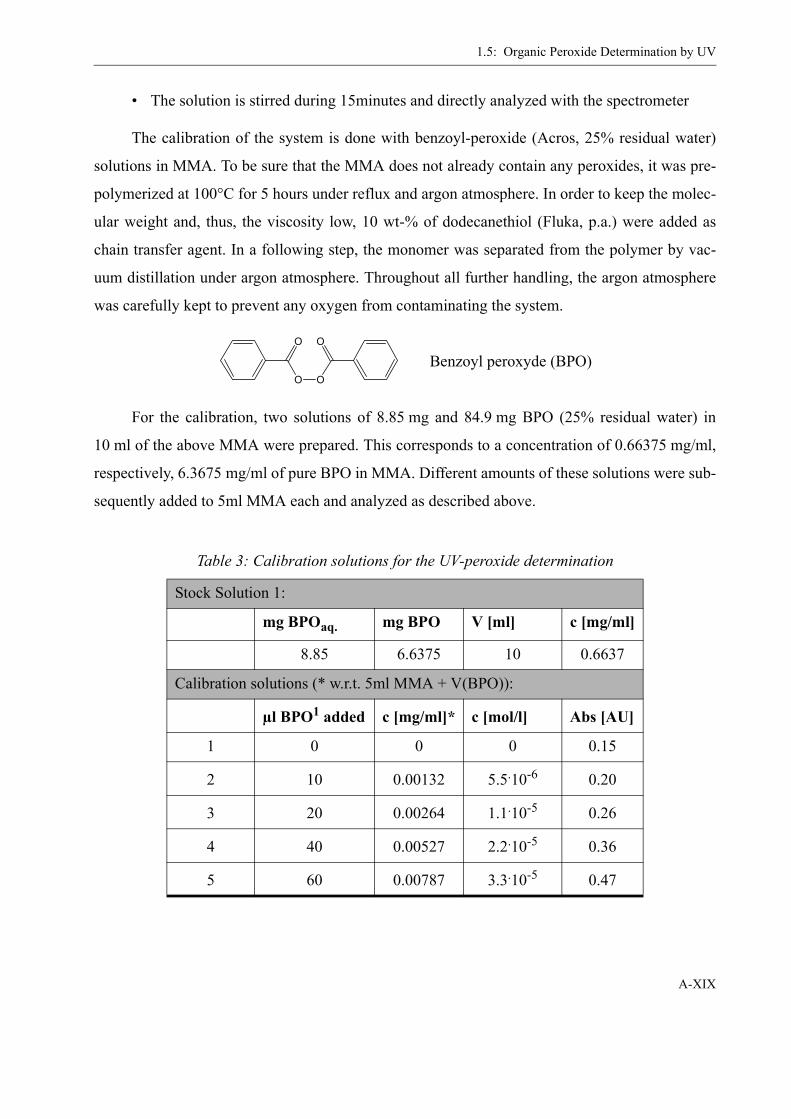
1.5: Organic Peroxide Determination by UV
A-XIX
• The solution is stirred during 15minutes and directly analyzed with the spectrometer
The calibration of the system is done with benzoyl-peroxide (Acros, 25% residual water)
solutions in MMA. To be sure that the MMA does not already contain any peroxides, it was pre-
polymerized at 100°C for 5 hours under reflux and argon atmosphere. In order to keep the molec-
ular weight and, thus, the viscosity low, 10 wt-% of dodecanethiol (Fluka, p.a.) were added as
chain transfer agent. In a following step, the monomer was separated from the polymer by vac-
uum distillation under argon atmosphere. Throughout all further handling, the argon atmosphere
was carefully kept to prevent any oxygen from contaminating the system.
Benzoyl peroxyde (BPO)
For the calibration, two solutions of 8.85 mg and 84.9 mg BPO (25% residual water) in
10 ml of the above MMA were prepared. This corresponds to a concentration of 0.66375 mg/ml,
respectively, 6.3675 mg/ml of pure BPO in MMA. Different amounts of these solutions were sub-
sequently added to 5ml MMA each and analyzed as described above.
Table 3: Calibration solutions for the UV-peroxide determination
Stock Solution 1:
mg BPOaq. mg BPO V [ml] c [mg/ml]
8.85 6.6375 10 0.6637
Calibration solutions (* w.r.t. 5ml MMA + V(BPO)):
µl BPO1 added c [mg/ml]* c [mol/l] Abs [AU]
1 0 0 0 0.15
2 10 0.00132 5.5.10-6 0.20
3 20 0.00264 1.1.10-5 0.26
4 40 0.00527 2.2.10-5 0.36
5 60 0.00787 3.3.10-5 0.47
O
O O
O

Annexe 1: Analytical Techniques and Method Development
A-XX
These calibration points lead to the following calibration curve and relation between UV
absorption and peroxide concentration:
Stock solution 2:
mg BPOaq. mg BPO V [ml] c [mg/ml]
84.9 63.675 10 6.3675
Calibration solutions (* w.r.t. 5ml MMA + V(BPO)):
µl BPO2 added c [mg/ml]* c [mol/l] Abs [AU]
6 10 0.01271 5.25.10-5 0.61
7 20 0.02537 1.05.10-4 1.00
8 50 0.06304 2.60.10-4 2.30
9 70 0.08791 3.63.10-4 3.08
Figure 1.14: Calibration curve for the UV peroxide quantification
Table 3: Calibration solutions for the UV-peroxide determination
y = 8.0628E+03x + 1.7378E-01R2 = 9.9949E-01
0
0.5
1
1.5
2
2.5
3
3.5
0.E+00 5.E-05 1.E-04 2.E-04 2.E-04 3.E-04 3.E-04 4.E-04 4.E-04Concentration [mol/l]
Abs
orba
nce
360n
m [A
U]
15min
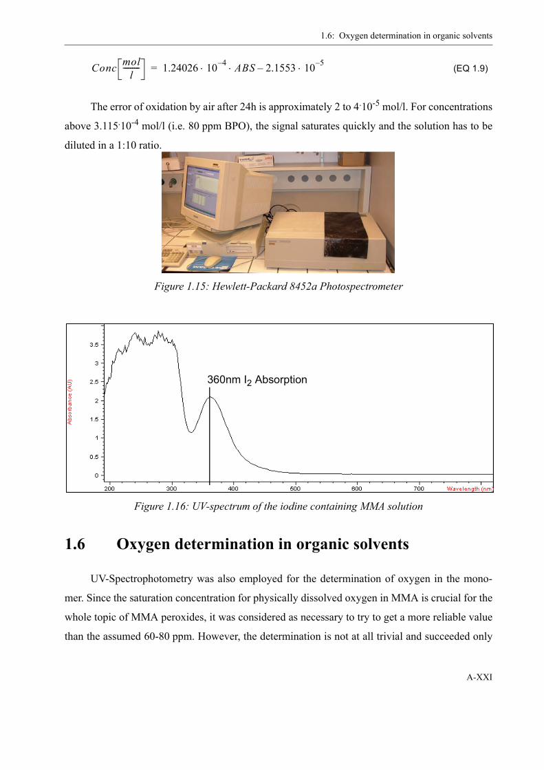
1.6: Oxygen determination in organic solvents
A-XXI
(EQ 1.9)
The error of oxidation by air after 24h is approximately 2 to 4.10-5 mol/l. For concentrations
above 3.115.10-4 mol/l (i.e. 80 ppm BPO), the signal saturates quickly and the solution has to be
diluted in a 1:10 ratio.
1.6 Oxygen determination in organic solvents
UV-Spectrophotometry was also employed for the determination of oxygen in the mono-
mer. Since the saturation concentration for physically dissolved oxygen in MMA is crucial for the
whole topic of MMA peroxides, it was considered as necessary to try to get a more reliable value
than the assumed 60-80 ppm. However, the determination is not at all trivial and succeeded only
Figure 1.15: Hewlett-Packard 8452a Photospectrometer
Figure 1.16: UV-spectrum of the iodine containing MMA solution
Conc moll
--------- 1.24026 10 4– ABS 2.1553 10 5–⋅–⋅ ⋅=
360nm I2 Absorption

Annexe 1: Analytical Techniques and Method Development
A-XXII
partially. The basic method was found in literature: Scherzer and Langguth [35] determined the
temperature dependent oxygen concentration for tripropylene glycol diacrylate (TPGDA) and
found a strong decrease in oxygen with increasing temperature (see figure 1.17). Another, similar
method is provided by Gou et al. [122], but was not considered in this work.
Their method proceeds as follows:
• The monomer is saturated with air at the desired temperature
• It is then shock-frosted with a dry-ice / acetone mixture (-90 °C)
• The gas phase over the frozen monomer is purged with inert gas (He)
• The monomer is defrosted and purged continuously with inert gas
• The inert gas is conducted through a washing bottle with an ammoniacal
containing solution of Cu-(I)-Cl (0.01 mol/l)
• The Cu-(I) ion is oxidized by the O2 driven out of the monomer and the cre-ated Cu-(II) ion forms a complex with ammonia (Cu(NH3)4
2+)
• This complex can be detected by UV-spectrophotometry at λ = 600nm and,
thus, the oxygen content of the monomer be quantified.
As simple as it sounds, several problems were encountered while trying to reproduce this
method: firstly, it was not possible to completely freeze the monomer with a dry-ice / acetone
mixture. Only with liquid nitrogen was this possible. Secondly, atmospheric oxygen had a
strongly disturbing effect, especially during the sampling from the washing bottle and during the
Figure 1.17: Temperature-dependent oxygen concentration in TPGDA [35]
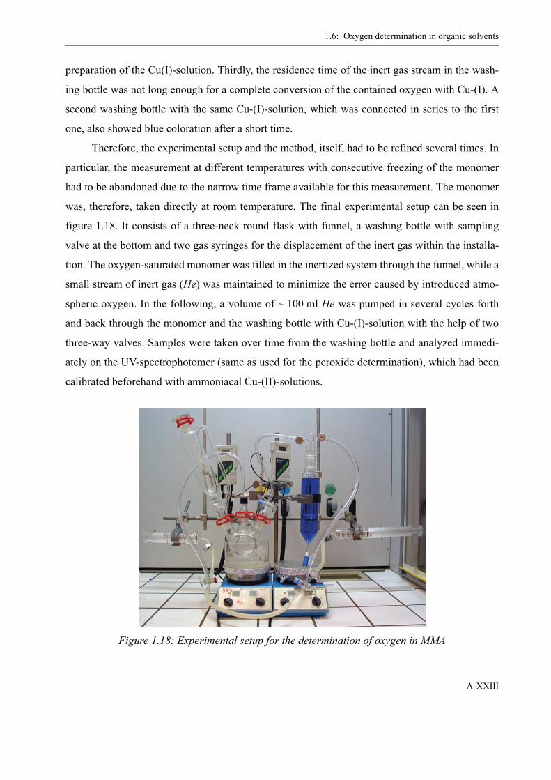
1.6: Oxygen determination in organic solvents
A-XXIII
preparation of the Cu(I)-solution. Thirdly, the residence time of the inert gas stream in the wash-
ing bottle was not long enough for a complete conversion of the contained oxygen with Cu-(I). A
second washing bottle with the same Cu-(I)-solution, which was connected in series to the first
one, also showed blue coloration after a short time.
Therefore, the experimental setup and the method, itself, had to be refined several times. In
particular, the measurement at different temperatures with consecutive freezing of the monomer
had to be abandoned due to the narrow time frame available for this measurement. The monomer
was, therefore, taken directly at room temperature. The final experimental setup can be seen in
figure 1.18. It consists of a three-neck round flask with funnel, a washing bottle with sampling
valve at the bottom and two gas syringes for the displacement of the inert gas within the installa-
tion. The oxygen-saturated monomer was filled in the inertized system through the funnel, while a
small stream of inert gas (He) was maintained to minimize the error caused by introduced atmo-
spheric oxygen. In the following, a volume of ~ 100 ml He was pumped in several cycles forth
and back through the monomer and the washing bottle with Cu-(I)-solution with the help of two
three-way valves. Samples were taken over time from the washing bottle and analyzed immedi-
ately on the UV-spectrophotomer (same as used for the peroxide determination), which had been
calibrated beforehand with ammoniacal Cu-(II)-solutions.
Figure 1.18: Experimental setup for the determination of oxygen in MMA
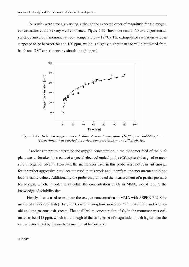
Annexe 1: Analytical Techniques and Method Development
A-XXIV
The results were strongly varying, although the expected order of magnitude for the oxygen
concentration could be very well confirmed. Figure 1.19 shows the results for two experimental
series obtained with monomer at room temperature (~ 18 °C). The extrapolated saturation value is
supposed to be between 80 and 100 ppm, which is slightly higher than the value estimated from
batch and DSC experiments by simulation (60 ppm).
Another attempt to determine the oxygen concentration in the monomer feed of the pilot
plant was undertaken by means of a special electrochemical probe (Orbisphere) designed to mea-
sure in organic solvents. However, the membranes used in this probe were not resistant enough
for the rather aggressive butyl acetate used in this work and, therefore, the measurement did not
lead to stable values. Additionally, the probe only allowed the measurement of a partial pressure
for oxygen, which, in order to calculate the concentration of O2 in MMA, would require the
knowledge of solubility data.
Finally, it was tried to estimate the oxygen concentration in MMA with ASPEN PLUS by
means of a one-step flash (1 bar, 25 °C) with a two-phase monomer / air feed stream and one liq-
uid and one gaseous exit stream. The equilibrium concentration of O2 in the monomer was esti-
mated to be ~115 ppm, which is - although of the same order of magnitude - much higher than the
values determined by the methods mentioned beforehand.
Figure 1.19: Detected oxygen concentration at room temperature (18 °C) over bubbling time (experiment was carried out twice, compare hollow and filled circles)

A-XXV
ANNEXE 2
Experimental procedures
2.1 Monomer purification
For certain experiments, the monomer could not be taken directly from the barrel but had to
be purified prior to its use. This was done in several manners, depending on the necessary purity.
Removing the stabilizer
In order to remove the stabilizer (20 ppm MEHQ), the monomer was washed with 2N-
NaOH and rinsed with deionized water until the aqueous phase was neutral (pH = 6-7).
Prepolymerization
In the case of the UV calibration, it was necessary to be sure that the monomer used for the
calibration solutions did not contain any peroxide. Therefore, a prepolymerization was carried out
at 100°C during 5 hours under argon atmosphere. A large amount of chain transfer agent (~ 10 wt-
%) was added to the monomer in order to keep the viscosity low. Following the prepolymeriza-
tion, the monomer was distilled as described in the next paragraph.
Annexe 2: Experimental procedures
A-XXVI
Vacuum distillation
The distillation of MMA was carried out under argon atmosphere at reduced pressure
(~ 150 mbar) and at T = 45 °C. A The monomer was distilled over a column for better separation
and fractionated in three distillate fractions, of which only the middle one was kept. Depending on
the use of the monomer in the following experiments, it was either kept under argon atmosphere
or in a flask closed only with a drying tube in order to garantuee contact with air (e.g. for MMA-
peroxide formation experiments).
2.2 PMMAP synthesis
For the synthesis of PMMAP, 250 ml of distilled monomer are heated to 70 °C under reflux
and molecular oxygen from a gas cylinder bubbled through it for several hours (4 - 7 h). A picture
of the setup can be found in chapter 2, figure 2.5. In a following step, the monomer was removed
from the flask at a rotary evaporator until a viscous residue was obtained. This residue was
reduced as far as possible in vaccuum (~ 1 mbar), dissolved in chloroform (CHCl3) and precipi-
tated twice in 20 times the volume of cold petrol ether (bp. 40-60 °C) for purification. From the
petrol ether, the precipates were separated by centrifugation. The final product was a white, sticky
powder. Its quantity depends largely on the duration and the temperature of the formation experi-
ment. It varied from 8 to 125 mg for 3h at 60 °C and 7h at 70 °C, respectively. In the latter exper-
iment, also the molecular weight of the peroxide and its amount compared to the parallely formed
PMMA was higher. It can, therefore, be said that with increasing temperature and duration of
oxygen bubbling, the amount and molecular weight of the formed peroxides increases. However,
it has to be considered that with increasing temperature, also the decomposition of the peroxide
gets more important.
2.3 Batch experiments
The batch experiments for verification of the kinetic model were carried out in a stainless
steel bench-scale reactor. The general procedure for each experiment is presented in the follow-
ing:
2.4: Pilot Plant experiments
A-XXVII
Preparation:
• Chemicals (monomer, solvent, CTA) are weighed and filled in the reactor
• Screw cap vials are stored in the deep freezer to cool them to -18 oC
Reaction:
• t = 0 min: The reactor is pressurized to p = 10 bar and the reaction subsequently started
by heating (heating ramp = 3.5 oC / min.) to the desired reaction temperature
• t = 15 min: First sample; The immersion tube is purged with 10 ml reaction mixture
before another 10 ml of the reaction mixture are taken for sampling into a frozen
screw cap vial and immediately stored at -18 oC
• t = 30 - 240 min: Samples are taken in regular intervals as described before. For certain
experiments, the initiator solution is filled into the funnel and added under pressure to
the reaction mixture at a preset time.
• t = 240 min: Reaction is stopped by cooling down; the rest of the reaction mixture is
disposed and the reactor is cleaned
Analysis:
• Samples are analyzed by GPC and GC for conversion respectively molecular weight
analysis
2.4 Pilot Plant experiments
For the pilot plant experiments, always the same procedure was followed during startup,
running and shut-down. This procedure is described in the following as detailed as possible.
Heating Phase
• Firstly, the pilot plant was heated up by setting the temperature on the thermostats to
120 °C for the reaction zone and to 260 °C for the devolatilization.
• During the heating up of the pilot plant, the feed solution was prepared. Therefore, the
necessary amounts of monomer, initiator and CTA, which had been calculated before-
hand for the planned duration of the experiment, were weighed and mixed in a stain-
Annexe 2: Experimental procedures
A-XXVIII
less steel recipient. From this recipient, they were transferred into a 60-litres stainless
steel tank through a hose by reducing the pressure inside the tank. From this tank, the
feed solution is transferred directly into the pilot plant.
• When the reactor has reached the set temperature, a small solvent flow (0.5 kg/h) is
established and the recycle pump activated. The membrane valve is set to 10 bars to
evoke a slight pressurization of the reactor. At the same time, the pressure in the
devolatilization chamber is reduced (150 mbar) so that the solvent is correctly
removed and condensed.
• The computer with Dasylab is switched on for data acquisition
Startup phase
• With the solvent flow established, the temperature is set to reaction temperature and the
feed flow switched from solvent to monomer feed. The flowrate is set to the desired
value (e.g. 1.84 kg/h for a residence time of 30 minutes in the loop)
• During this phase, the beginning reaction can be followed by ultrasound and by an
increase in pressure.
• As soon as polymer falls into the devolatilization chamber (approximately after 1 hour
at the given feed flowrate), the discharge gear pump is activated.
• Samples are taken regularly from positions at the loop exit, at 2/3 length of the tube and
from the condensate and the final polymer. During the sampling, the second feed
pump, which pumps solvent and initiator into the tube reactor, is deactivated to avoid
a backflow into the loop sample. The reactor samples are taken through heated valves,
on which hermetic, 10cm stainless steel tubes with 12mm diameter are screwed.
Before mounting the tubes, the valves are purged (tube valve before, then loop valve).
For the sampling, the valves are left open until the sampling tubes are hot over their
whole length. The sample is consecutively transferred from the tubes into 25ml screw
cap vials (Schott) and immediately frozen at -18°C.
• At steady state, the polymer is transfered as two strands to the granulator and processed
to granules.
• In regular intervals, the condensate recipient is emptied.

2.4: Pilot Plant experiments
A-XXIX
Shut-down phase
• At the end of the experiment, the feed flow is again switched from monomer solution to
solvent and the flowrate increased to 10 kg/h. Thus, the polymer / monomer solution
is pushed out of the reactor. The flowrate is varied several times from 10 to 5 kg/h in
order to improve the rinsing of the plant.
• Once the polymer stops falling into the devolatilization chamber, which is generally the
case after 1 hour, the solvent flow and the reactor temperature are decreased to 0.5 kg/
h and 120 °C, respectively.
• Both gear pumps, the one in the recycle loop and at the exit, are stopped.
• For the final shut-down, the temperature of all thermostats is lowered to <20°C, the
cooling water circuits are openend, the membrane valve depressurized, the vacuum of
the devolatilization cut and the solvent flow stopped.
• At last, the condensate recipient is emptied, the data acquisition is halted and all equip-
ment switched off.

Annexe 2: Experimental procedures
A-XXX
A-XXXI
ANNEXE 3
Modeling with Predici®
PREDICI® stands for Polyreaction Distributions by Countable System Integration and is the
name of an industrially recognized and widely spread simulation package for the treatment of
kinetic equations in models of polymerization reactions. The input consists of a complete reaction
model with reaction equations and kinetic parameters, together with concentrations and stuff-data
of all reactive components and reaction conditions. The software performs a numerical integration
of the resulting system of differential equations, based on recent mathematical-numerical methods
[123]. For each time step, the complete concentration profile as well as molecular weight distribu-
tions of polymeric species are estimated.
The user can - within the limits of available kinds of reaction steps - freely add elementary
reactions of all types to the model and define various output-functions (e.g. ultrasound velocity,
conversion, etc.), the calculation of which can be based on the estimated process parameters for
each time step (e.g. temperature, concentration of a species, etc.).
PREDICI® offers four different reactor models: ideal batch, semi-batch and continuous tank
reactor and the ideal plug flow tube reactor. Several CSTR can be combined to a cascade. The
combination of CSTR and tube, however, is not possible in the present version. This combination
can, yet, be realized by a transfer data sheet, which uses the data of a CSTR exit stream as input
for a tubular reactor located in another file.
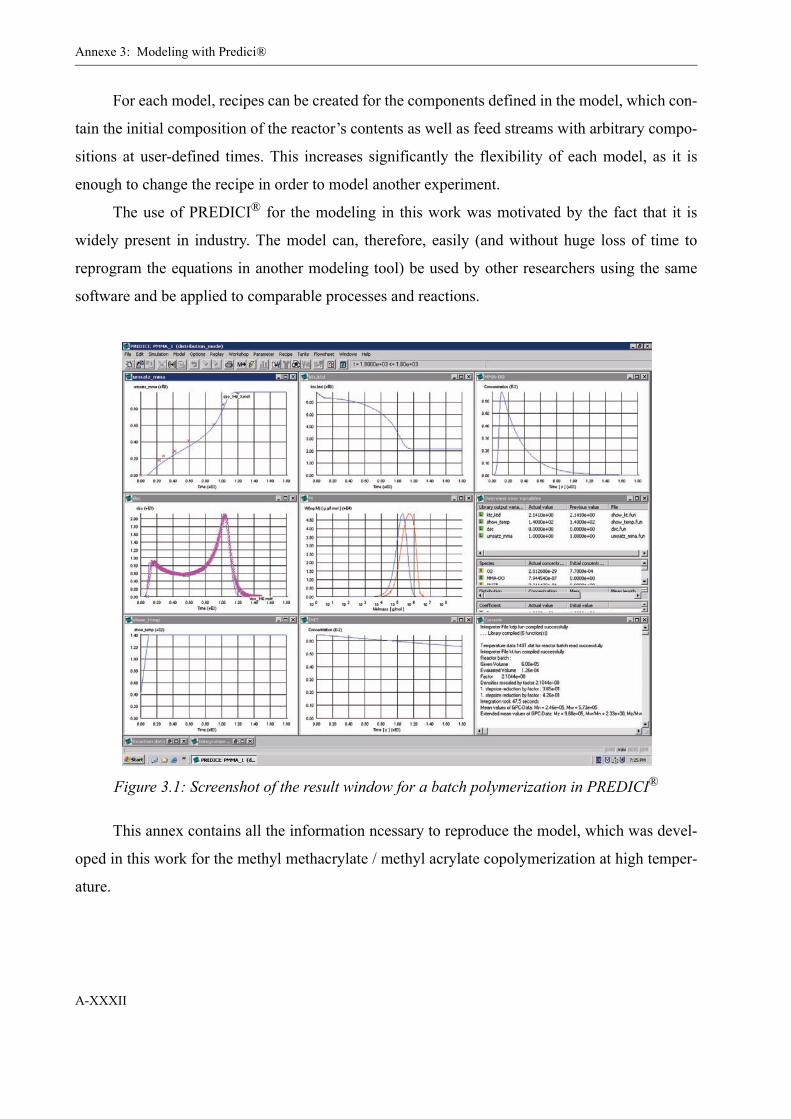
Annexe 3: Modeling with Predici®
A-XXXII
For each model, recipes can be created for the components defined in the model, which con-
tain the initial composition of the reactor’s contents as well as feed streams with arbitrary compo-
sitions at user-defined times. This increases significantly the flexibility of each model, as it is
enough to change the recipe in order to model another experiment.
The use of PREDICI® for the modeling in this work was motivated by the fact that it is
widely present in industry. The model can, therefore, easily (and without huge loss of time to
reprogram the equations in another modeling tool) be used by other researchers using the same
software and be applied to comparable processes and reactions.
This annex contains all the information ncessary to reproduce the model, which was devel-
oped in this work for the methyl methacrylate / methyl acrylate copolymerization at high temper-
ature.
Figure 3.1: Screenshot of the result window for a batch polymerization in PREDICI®

3.1: Reactor
A-XXXIII
3.1 Reactor
R1 continuous
Vr = 0.907 l
T = temperature program following pilot plant data
p = pressure program following pilot plant data
flowrate defined by recipe
Tube Tube reactor
Length L = 3.84 m
Diameter d = 0.02 m
T = constant (as in experiment)
p = constant (as in experiment)
Input flow as defined in “initial data sheet”
Additional solvent / initiator feed defined by recipe
3.2 Reaction equations
Reaction step Reaction equation Rate constant
MMA-OO formation MMA + O2 MMA-OO kpo,f
MMA-OO decomposition MMA-OO 2 fpo MMA-OO. kpo,d , fpo
MMA-OO initiation MMA-OO. + MMA P1,1. kp1
MMA-OO. + MA P2,1. kp2
Thermal initiation 2 MMA 2 MMA. kth
MMA.+ MMA P1,1. kp1
MMA. + MA P2,1. kp2
Initiation by CTA CTA CTA. kdt
CTA.+ MMA P1,1. kp1
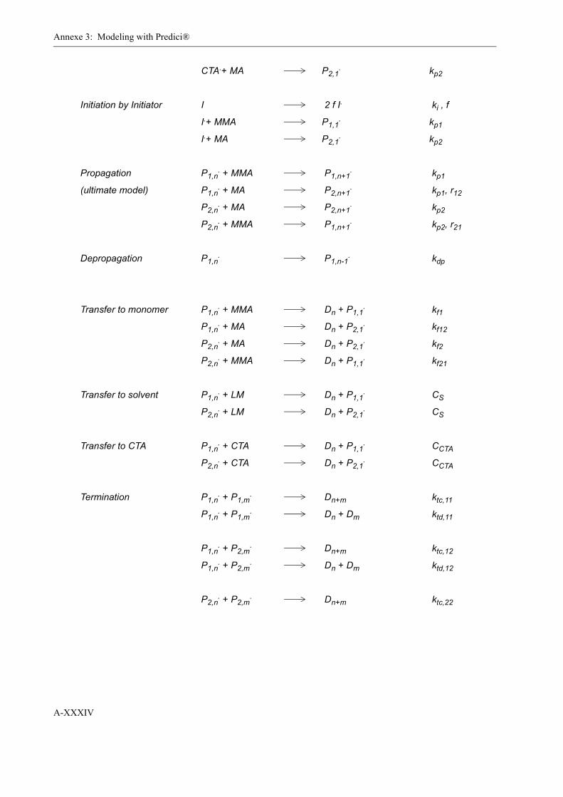
Annexe 3: Modeling with Predici®
A-XXXIV
CTA.+ MA P2,1. kp2
Initiation by Initiator I 2 f I. ki , f
I.+ MMA P1,1. kp1
I.+ MA P2,1. kp2
Propagation P1,n. + MMA P1,n+1
. kp1
(ultimate model) P1,n. + MA P2,n+1
. kp1, r12
P2,n. + MA P2,n+1
. kp2
P2,n. + MMA P1,n+1
. kp2, r21
Depropagation P1,n. P1,n-1
. kdp
Transfer to monomer P1,n. + MMA Dn + P1,1
. kf1
P1,n. + MA Dn + P2,1
. kf12
P2,n. + MA Dn + P2,1
. kf2
P2,n. + MMA Dn + P1,1
. kf21
Transfer to solvent P1,n. + LM Dn + P1,1
. CS
P2,n. + LM Dn + P2,1
. CS
Transfer to CTA P1,n. + CTA Dn + P1,1
. CCTA
P2,n. + CTA Dn + P2,1
. CCTA
Termination P1,n. + P1,m
. Dn+m ktc,11
P1,n. + P1,m
. Dn + Dm ktd,11
P1,n. + P2,m
. Dn+m ktc,12
P1,n. + P2,m
. Dn + Dm ktd,12
P2,n. + P2,m
. Dn+m ktc,22
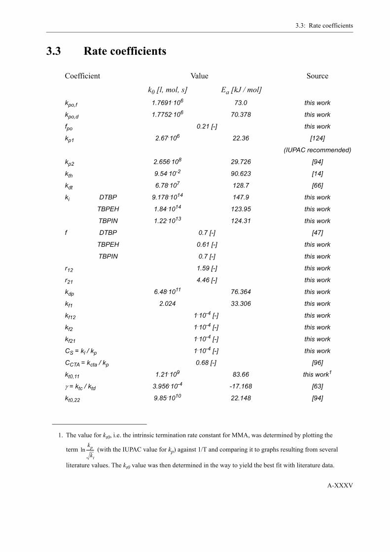
3.3: Rate coefficients
A-XXXV
3.3 Rate coefficients
Coefficient Value Source
k0 [l, mol, s] Ea [kJ / mol]kpo,f 1.7691.106 73.0 this work
kpo,d 1.7752.106 70.378 this work
fpo 0.21 [-] this work
kp1 2.67.106 22.36 [124]
(IUPAC recommended)
kp2 2.656.108 29.726 [94]
kth 9.54.10-2 90.623 [14]
kdt 6.78.107 128.7 [66]
ki DTBP 9.178.1014 147.9 this work
TBPEH 1.84.1014 123.95 this work
TBPIN 1.22.1013 124.31 this work
f DTBP 0.7 [-] [47]
TBPEH 0.61 [-] this work
TBPIN 0.7 [-] this work
r12 1.59 [-] this work
r21 4.46 [-] this work
kdp 6.48.1011 76.364 this work
kf1 2.024 33.306 this work
kf12 1.10-4 [-] this work
kf2 1.10-4 [-] this work
kf21 1.10-4 [-] this work
CS = kl / kp 1.10-4 [-] this work
CCTA = kcta / kp 0.68 [-] [96]
kt0,11 1.21.109 83.66 this work1
γ = ktc / ktd 3.956.10-4 -17.168 [63]
kt0,22 9.85.1010 22.148 [94]
1. The value for kt0, i.e. the intrinsic termination rate constant for MMA, was determined by plotting the
term (with the IUPAC value for kp) against 1/T and comparing it to graphs resulting from several
literature values. The kt0 value was then determined in the way to yield the best fit with literature data.
kp
kt
--------ln
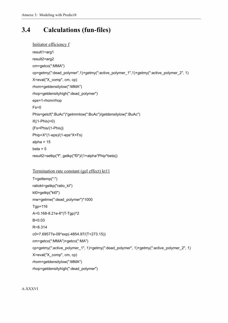
Annexe 3: Modeling with Predici®
A-XXXVI
3.4 Calculations (fun-files)
Initiator efficiency fresult1=arg1
result2=arg2
cm=getco(":MMA")
cp=getmy(":dead_polymer",1)+getmy(":active_polymer_1",1)+getmy(":active_polymer_2", 1)
X=eval("X_comp", cm, cp)
rhom=getdensitylow(":MMA")
rhop=getdensityhigh(":dead_polymer")
eps=1-rhom/rhop
Fs=0
Phis=getcf(":BuAc")*getmmlow(":BuAc")/getdensitylow(":BuAc")
if((1-Phis)>0)
{Fs=Phis/(1-Phis)}
Phip=X*(1-eps)/(1-eps*X+Fs)
alpha = 15
beta = 5
result2=setkp("f", getkp("f0")/(1+alpha*Phip^beta))
Termination rate constant (gel effect) kt11T=gettemp(":")
ratiokt=getkp("ratio_kt")
kt0=getkp("kt0")
mw=getmw(":dead_polymer")*1000
Tgp=116
A=0.168-8.21e-6*(T-Tgp)^2
B=0.03
R=8.314
c0=7.69577e-09*exp(-4854.97/(T+273.15))
cm=getco(":MMA")+getco(":MA")
cp=getmy(":active_polymer_1", 1)+getmy(":dead_polymer", 1)+getmy(":active_polymer_2", 1)
X=eval("X_comp", cm, cp)
rhom=getdensitylow(":MMA")
rhop=getdensityhigh(":dead_polymer")

3.4: Calculations (fun-files)
A-XXXVII
eps=1-rhom/rhop
Phis=getcf(":BuAc")*getmmlow(":BuAc")/getdensitylow(":BuAc")
Fs=0
if((1-Phis)>0)
{Fs=Phis/(1-Phis)}
Phip=X*(1-eps)/(1-eps*X+Fs)
delta=mw^1.75*c0/exp(2.3*(1-Phip)/(A+B*(1-Phip)))
kt=setkp("kt", 1/(1/kt0+delta))
result1=kt*ratiokt/(1+ratiokt)
result2=kt/(1+ratiokt)
Termination rate constant (gel effect) kt12t=gettemp(":")
F1=getmolpart("M1")
F2=getmolpart("M2")
kt11=getkp("kt0")
kt22=getkp("kt22_0")
kt0=F1*kt11+F2*kt22
ratiokt=getkp("ratio_kt")
mw=getmw(":dead_polymer")*1000
Tgp=116
A=0.168-8.21e-6*(t-Tgp)^2
B=0.03
c0=7.69577e-09*exp(-4854.97/(t+273.15))
cm=getco(":MMA")+getco(":MA")
cp=getmy(":dead_polymer", 1)+getmy(":active_polymer_1", 1)+getmy(":active_polymer_2", 1)
X=eval("X_comp", cm, cp)
rhom=getdensitylow(":MMA")
rhop=getdensityhigh(":dead_polymer")
eps=1-rhom/rhop
Phis=getcf(":BuAc")*getmmlow(":BuAc")/getdensitylow(":BuAc")
Fs=0
if((1-Phis)>0)
{Fs=Phis/(1-Phis)}
Phip=X*(1-eps)/(1-eps*X+Fs)
if(kt0>0)
Annexe 3: Modeling with Predici®
A-XXXVIII
{delta=mw^1.75*c0/exp(2.3*(1-Phip)/(A+B*(1-Phip)))
kt=1/(1/kt0+delta)}
else
{kt=kt0}
result1=kt*ratiokt/(1+ratiokt)
result2=kt/(1+ratiokt)
Termination rate constant (gel effect) kt22t=gettemp(":")
kt0=getkp("kt22_0")
ratiokt=getkp("ratio_kt")
mw=getmw(":dead_polymer")*1000
Tgp=116
A=0.168-8.21e-6*(t-Tgp)^2
B=0.03
c0=7.69577e-09*exp(-4854.97/(t+273.15))
cm=getco(":MMA")+getco(":MA")
cp=getmy(":dead_polymer", 1)+getmy(":active_polymer_1", 1)+getmy(":active_polymer_2", 1)
X=eval("X_comp", cm, cp)
rhom=getdensitylow(":MMA")
rhop=getdensityhigh(":dead_polymer")
eps=1-rhom/rhop
Phis=getcf(":BuAc")*getmmlow(":BuAc")/getdensity(":BuAc")
Fs=0
if((1-Phis)>0)
{Fs=Phis/(1-Phis)}
Phip= X*(1-eps)/(1-eps*X+Fs)
if(kt0>0)
{delta=mw^1.75*c0/exp(2.3*(1-Phip)/(A+B*(1-Phip)))
kt=1/(1/kt0+delta)}
else
{kt=kt0}
result1=kt*ratiokt/(1+ratiokt)
result2=kt/(1+ratiokt)

3.4: Calculations (fun-files)
A-XXXIX
Ultrasound calculation (theoretical speed of sound from solution composition)T=gettemp("dummy")
kappa_m1 = 7.823735E-14*T^2 + 1.257146E-12*T + 7.135903E-10
kappa_m2 = 0.00000000000004*T^2 + 0.000000000002*T + 0.0000000006
kappa_s = 9.416596E-14*T^2 + 5.884506E-13*T + 8.111514E-10
kappa_p=exp((-22.220389+0.36888905*T-0.0015726875*T^2)/(1-
0.016394164*T+0.000067228059*T^2+0.000000015752519*T^3))
rho_m1 = getdensitylow("M1")
rho_m2 = getdensitylow("M2")
rho_s = getdensitylow("LM")
rho_p = getdensityhigh(":dead_polymer")
p=getpressure("R1")
wp = getmy(":dead_polymer", 1)*getvol("R1")*getmmlow(":MMA") / getmass("R1")
wm1 = getco(":MMA")*getmmlow(":MMA")*getvol("R1") / getmass("R1")
wm2 = getco(":MA")*getmmlow(":MA")*getvol("R1") / getmass("R1")
ws = getco("LM")*getmmlow("LM")*getvol("R1") / getmass("R1")
alpha=0.40604-0.37541*wp+0.00364*T
result1=1/sqrt(1000)*(wp/rho_p + wm1/rho_m1 + ws/rho_s + wm2/rho_m2)/sqrt(wp*kappa_p/rho_p
+ ws*kappa_s/rho_s + wm1*kappa_m1/rho_m1 + wm2*kappa_m2/rho_m2)+alpha*p
Density monomerT=arg1
rho=(-9.4146E-06*T^3 + 1.3028E-03*T^2 - 1.1552*T + 9.6339E+02)/1000
result1=1/rho-arg3
Density solventT=arg1
rho=-2.48E-06*T^2 - 5.28E-04*T + 8.70E-01
result1=1/rho-arg3
Density polymerT=arg1
rho=-1E-06*T^2 - 0.0002*T + 1.195
result1=1/rho-arg3

Annexe 3: Modeling with Predici®
A-XL
A-XLI
ANNEXE 4
Determination of the InitiatorDecomposition by DSC
In analogy to the determination of the MMA peroxide decay kinetics by DSC (compare
chapter 2, “Differential Scanning Calorimetry (DSC)” on page 26), also the decomposition of
commercial initiators has been investigated as a part of this work. For standard initiators like di-
tert.butyl-peroxide (DTBP) or azo-bis-isobutyro-nitril (AIBN), which are widely used in polymer
research, the kinetics of their decomposition are well-known and published in unnumerous scien-
tific articles. When it comes to less common peroxides, as they are used mostly in industrial pro-
cesses, where it is important to have very specific decomposition characteristics, the situation
changes drastically and it gets very difficult to obtain reliable kinetic parameters. Often, the data
provided for a component vary between different manufacturers and the conditions under which
they had been determined are rarely revealed.
It is, therefore, inevitable for precise modeling of polymerization processes, to determine
the exact decomposition kinetics of the employed thermal initiators under controlled experimental
conditions. In the following, the results from DSC experiments are presented for the two indus-
trial initiators tert.butyl-peroxy-2-ethylhexanoat (TBPEH) and tert.butyl-peroxy-3,5,5-trimethyl-
hexanoate (TBPIN), as well as for di-tert.butyl-peroxide (DTBP) in order to validate the determi-
nation method with values from literature.

Annexe 4: Determination of the Initiator Decomposition by DSC
A-XLII
The experiments were carried out in 60 µl medium-pressure, stainless steel crucibles (see
annex 1, “Differential Scanning Calorimetry” on page XIII) with either the pure peroxide or per-
oxide diluted in butyl acetate. For the mathematical algorithm, which is used by the PerkinElmer
software to determine the kinetic parameters, see chapter 2, “Differential Scanning Calorimetry
(DSC)” on page 26.
4.1 Tert.butyl-peroxy-2-ethylhexanoat (TBPEH)
The decomposition of TBPEH was measured by DSC in solution (~50% butyl acetate) and
for the undiluted peroxide. The DSC results, i.e. heat flow peak and Arrhenius diagram from the
peak integration, are shown in figure 4.1 (a)+(b) for the undiluted and in figure 4.2 (a)+(b) for the
diluted peroxide.
The kinetic parameters for both cases, as well as values provided by two different producers
of TBPEH are presented in table 1.
Finally, the different kinetic parameters are compared by tracing the half life time against
temperature in figure 4.3.
Table 1: Kinetic rate constants for the thermal decomposition of TBPEH
k0 [s-1] EA [kJ mol-1]
DSC pure 1.312.1014 124.13
DSC (50% BuAc) 1.847.1014 123.95
Degussa Initiators 1.840.1015 132.68
Akzo 9.990.1013 122.96
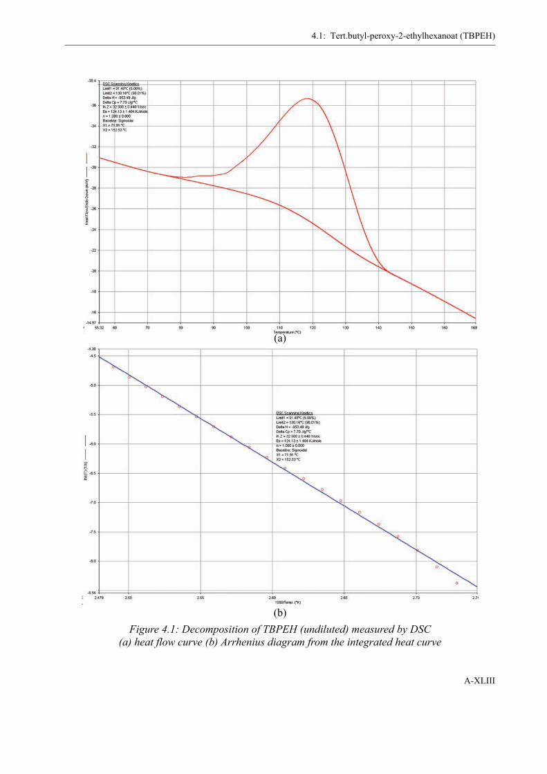
4.1: Tert.butyl-peroxy-2-ethylhexanoat (TBPEH)
A-XLIII
(a)
(b)Figure 4.1: Decomposition of TBPEH (undiluted) measured by DSC
(a) heat flow curve (b) Arrhenius diagram from the integrated heat curve

Annexe 4: Determination of the Initiator Decomposition by DSC
A-XLIV
(a)
Figure 4.2: Decomposition of TBPEH (50% BuAc solution) measured by DSC(a) heat flow curve (b) Arrhenius diagram from the integrated heat curve
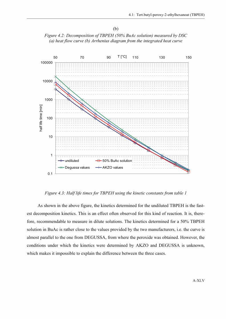
4.1: Tert.butyl-peroxy-2-ethylhexanoat (TBPEH)
A-XLV
As shown in the above figure, the kinetics determined for the undiluted TBPEH is the fast-
est decomposition kinetics. This is an effect often observed for this kind of reaction. It is, there-
fore, recommendable to measure in dilute solutions. The kinetics determined for a 50% TBPEH
solution in BuAc is rather close to the values provided by the two manufacturers, i.e. the curve is
almost parallel to the one from DEGUSSA, from where the peroxide was obtained. However, the
conditions under which the kinetics were determined by AKZO and DEGUSSA is unknown,
which makes it impossible to explain the difference between the three cases.
(b)
Figure 4.3: Half life times for TBPEH using the kinetic constants from table 1
Figure 4.2: Decomposition of TBPEH (50% BuAc solution) measured by DSC(a) heat flow curve (b) Arrhenius diagram from the integrated heat curve
0.1
1
10
100
1000
10000
10000050 70 90 110 130 150T [°C]
half
life
time
[min
]
undiluted 50% BuAc solution
Degussa values AKZO values
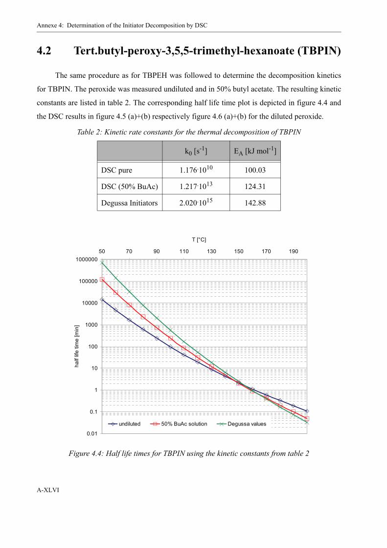
Annexe 4: Determination of the Initiator Decomposition by DSC
A-XLVI
4.2 Tert.butyl-peroxy-3,5,5-trimethyl-hexanoate (TBPIN)
The same procedure as for TBPEH was followed to determine the decomposition kinetics
for TBPIN. The peroxide was measured undiluted and in 50% butyl acetate. The resulting kinetic
constants are listed in table 2. The corresponding half life time plot is depicted in figure 4.4 and
the DSC results in figure 4.5 (a)+(b) respectively figure 4.6 (a)+(b) for the diluted peroxide.
Table 2: Kinetic rate constants for the thermal decomposition of TBPIN
k0 [s-1] EA [kJ mol-1]
DSC pure 1.176.1010 100.03
DSC (50% BuAc) 1.217.1013 124.31
Degussa Initiators 2.020.1015 142.88
Figure 4.4: Half life times for TBPIN using the kinetic constants from table 2
0.01
0.1
1
10
100
1000
10000
100000
100000050 70 90 110 130 150 170 190
T [°C]
half
life
time
[min
]
undiluted 50% BuAc solution Degussa values
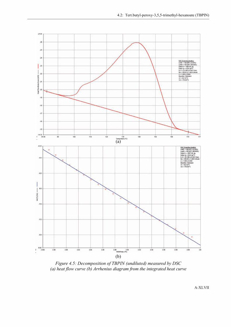
4.2: Tert.butyl-peroxy-3,5,5-trimethyl-hexanoate (TBPIN)
A-XLVII
(a)
(b)Figure 4.5: Decomposition of TBPIN (undiluted) measured by DSC
(a) heat flow curve (b) Arrhenius diagram from the integrated heat curve

Annexe 4: Determination of the Initiator Decomposition by DSC
A-XLVIII
(a)
(b)Figure 4.6: Decomposition of TBPIN (50% BuAc solution) measured by DSC
(a) heat flow curve (b) Arrhenius diagram from the integrated heat curve
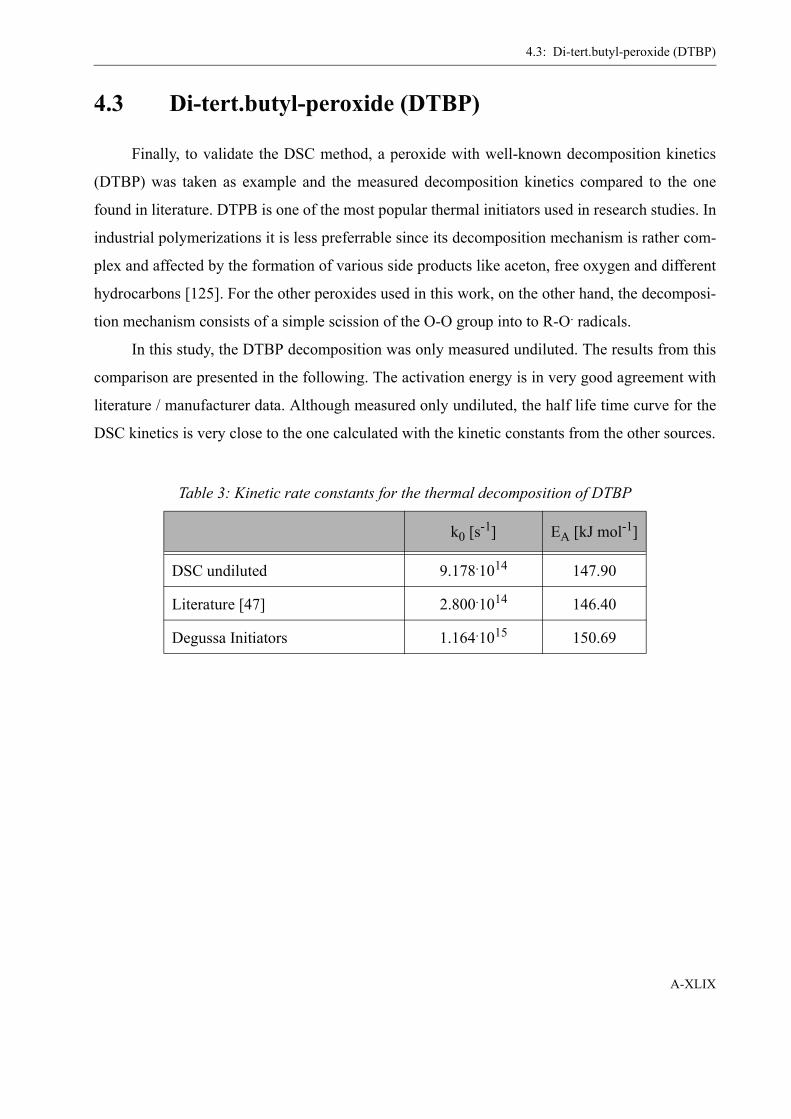
4.3: Di-tert.butyl-peroxide (DTBP)
A-XLIX
4.3 Di-tert.butyl-peroxide (DTBP)
Finally, to validate the DSC method, a peroxide with well-known decomposition kinetics
(DTBP) was taken as example and the measured decomposition kinetics compared to the one
found in literature. DTPB is one of the most popular thermal initiators used in research studies. In
industrial polymerizations it is less preferrable since its decomposition mechanism is rather com-
plex and affected by the formation of various side products like aceton, free oxygen and different
hydrocarbons [125]. For the other peroxides used in this work, on the other hand, the decomposi-
tion mechanism consists of a simple scission of the O-O group into to R-O. radicals.
In this study, the DTBP decomposition was only measured undiluted. The results from this
comparison are presented in the following. The activation energy is in very good agreement with
literature / manufacturer data. Although measured only undiluted, the half life time curve for the
DSC kinetics is very close to the one calculated with the kinetic constants from the other sources.
Table 3: Kinetic rate constants for the thermal decomposition of DTBP
k0 [s-1] EA [kJ mol-1]
DSC undiluted 9.178.1014 147.90
Literature [47] 2.800.1014 146.40
Degussa Initiators 1.164.1015 150.69

Annexe 4: Determination of the Initiator Decomposition by DSC
A-L
Figure 4.7: Half life times for DTBP using the kinetic constants from table 3
0.1
1
10
100
1000
10000
100000
1000000
10000000
10000000050 70 90 110 130 150 170 190
T [°C]
half
life
time
[min
]
DSC undiluted Polymer Handbook Degussa values
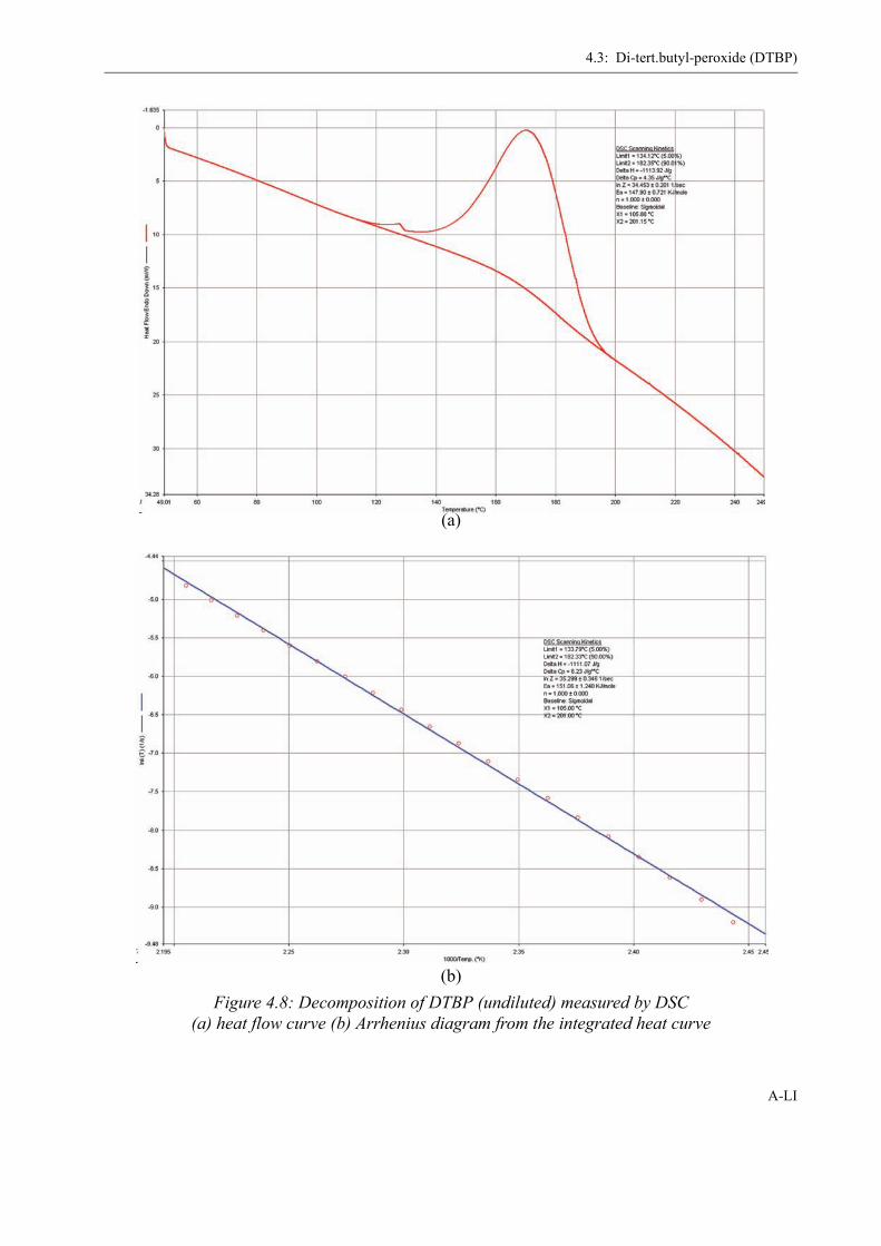
4.3: Di-tert.butyl-peroxide (DTBP)
A-LI
(a)
(b)Figure 4.8: Decomposition of DTBP (undiluted) measured by DSC
(a) heat flow curve (b) Arrhenius diagram from the integrated heat curve

Annexe 4: Determination of the Initiator Decomposition by DSC
A-LII

A-LIII
ANNEXE 5
Physico-chemical data
5.1 Density of methyl methacrylateρΜΜΑ(Τ) = -9.4146.10-6.T3 + 1.3028.10-3.T2 - 1.1552 T + 9.6339 102
Figure 5.1: Density of methyl methacrylate as a function of temperature [°C], source: measured data from industrial partner
y = -9.4146E-06x3 + 1.3028E-03x2 - 1.1552E+00x + 9.6339E+02R2 = 9.9995E-01
500.0
550.0
600.0
650.0
700.0
750.0
800.0
850.0
900.0
950.0
1000.0
0 50 100 150 200 250 300
T [°C]
rho
[g/l]

Annexe 5: Physico-chemical data
A-LIV
5.2 Density of butyl acetate
ρBuAc(Τ) = -3.1905.10-4.T2 - 1.0635.T + 9.0305 102
Figure 5.2: Density of butyl acetate as a function of temperature [°C], source: [88] (straight line), [126](squares)
700
720
740
760
780
800
820
840
860
880
900
0 20 40 60 80 100 120 140 160 180T [°C]
roh
[g/l]
Literature: Beilstein
Literature: Oswal (2004)
y = -3.1905E-04x2 - 1.0635E+00x + 9.0305E+02R2 = 0.99998
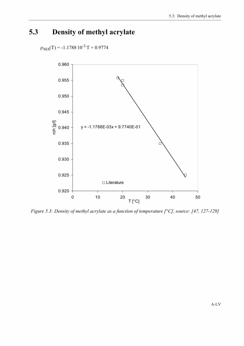
5.3: Density of methyl acrylate
A-LV
5.3 Density of methyl acrylate
ρMA(Τ) = -1.1788.10-3.T + 0.9774
Figure 5.3: Density of methyl acrylate as a function of temperature [°C], source: [47, 127-129]
y = -1.1788E-03x + 9.7740E-01
0.920
0.925
0.930
0.935
0.940
0.945
0.950
0.955
0.960
0 10 20 30 40 50T [°C]
roh
[g/l]
Literature

Annexe 5: Physico-chemical data
A-LVI
5.4 Density of poly (methyl methacrylate)
ρPMMA(Τ) = -0.0014.T2 - 0.2309.T + 1195
Figure 5.4: Density of poly (methyl methacrylate) as a function of temperature [°C]
y = -0.0014x2 - 0.2309x + 1195R2 = 0.99998
1000
1020
1040
1060
1080
1100
1120
1140
1160
1180
1200
0 20 40 60 80 100 120 140 160 180T [°C]
roh
[g/l]
Literature: Polymer Handbook
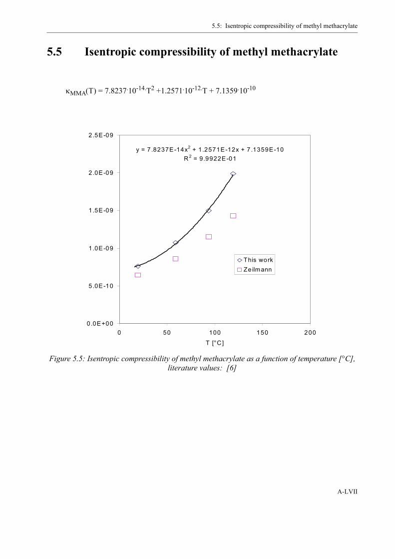
5.5: Isentropic compressibility of methyl methacrylate
A-LVII
5.5 Isentropic compressibility of methyl methacrylate
κMMA(Τ) = 7.8237.10-14.T2 +1.2571.10-12.T + 7.1359.10-10
Figure 5.5: Isentropic compressibility of methyl methacrylate as a function of temperature [°C], literature values: [6]
y = 7.8237E-14x2 + 1.2571E-12x + 7 .1359E-10R 2 = 9.9922E-01
0.0E+00
5.0E-10
1.0E-09
1.5E-09
2.0E-09
2.5E-09
0 50 100 150 200
T [°C ]
This workZe ilmann
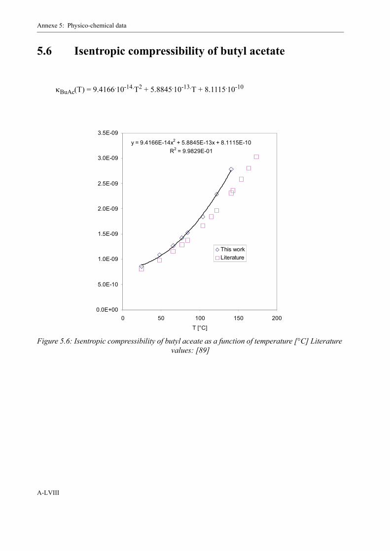
Annexe 5: Physico-chemical data
A-LVIII
5.6 Isentropic compressibility of butyl acetate
κBuAc(Τ) = 9.4166.10-14.T2 + 5.8845.10-13.T + 8.1115.10-10
Figure 5.6: Isentropic compressibility of butyl aceate as a function of temperature [°C] Literature values: [89]
y = 9.4166E-14x2 + 5.8845E-13x + 8.1115E-10R2 = 9.9829E-01
0.0E+00
5.0E-10
1.0E-09
1.5E-09
2.0E-09
2.5E-09
3.0E-09
3.5E-09
0 50 100 150 200
T [°C]
This workLiterature
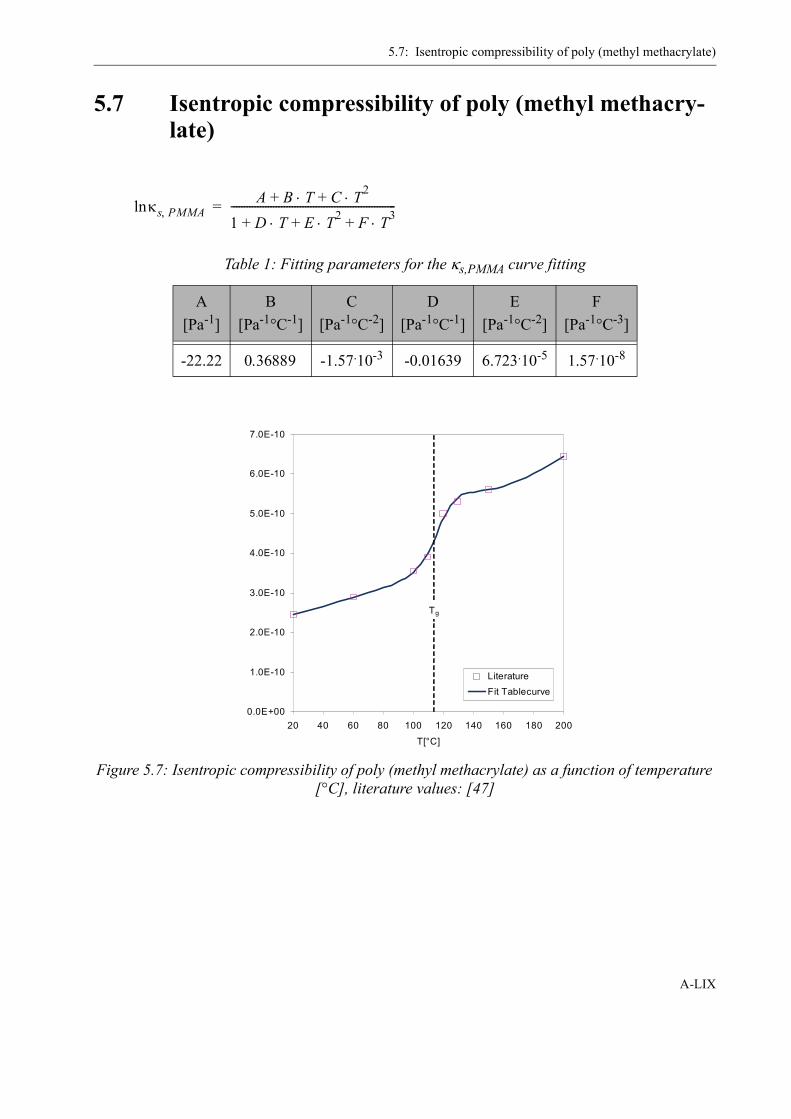
5.7: Isentropic compressibility of poly (methyl methacrylate)
A-LIX
5.7 Isentropic compressibility of poly (methyl methacry-late)
Table 1: Fitting parameters for the κs,PMMA curve fitting
A[Pa-1]
B[Pa-1°C-1]
C[Pa-1°C-2]
D[Pa-1°C-1]
E[Pa-1°C-2]
F[Pa-1°C-3]
-22.22 0.36889 -1.57.10-3 -0.01639 6.723.10-5 1.57.10-8
Figure 5.7: Isentropic compressibility of poly (methyl methacrylate) as a function of temperature [°C], literature values: [47]
κs PMMA,ln A B T C T2⋅+⋅+1 D T E T2 F T3⋅+⋅+⋅+--------------------------------------------------------------=
0.0E+00
1.0E-10
2.0E-10
3.0E-10
4.0E-10
5.0E-10
6.0E-10
7.0E-10
20 40 60 80 100 120 140 160 180 200
T[°C]
LiteratureFit Tablecurve
Tg

Annexe 5: Physico-chemical data
A-LX
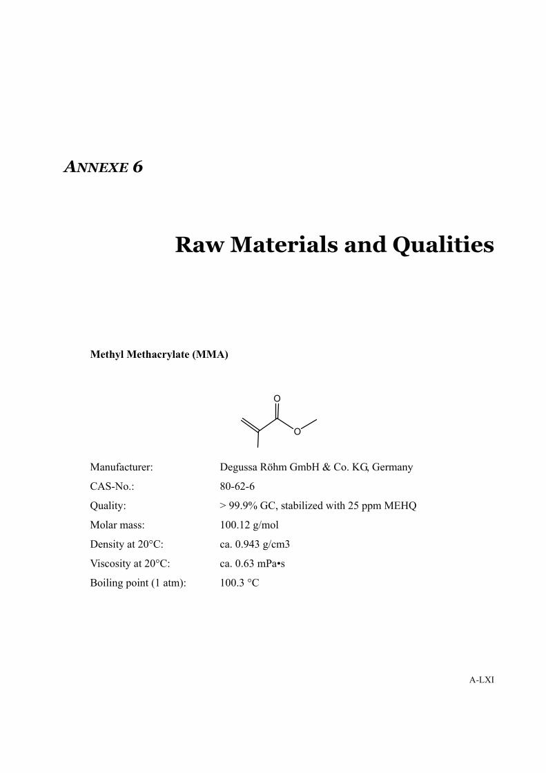
A-LXI
ANNEXE 6
Raw Materials and Qualities
Methyl Methacrylate (MMA)
Manufacturer: Degussa Röhm GmbH & Co. KG, Germany
CAS-No.: 80-62-6
Quality: > 99.9% GC, stabilized with 25 ppm MEHQ
Molar mass: 100.12 g/mol
Density at 20°C: ca. 0.943 g/cm3
Viscosity at 20°C: ca. 0.63 mPa•s
Boiling point (1 atm): 100.3 °C
O
O
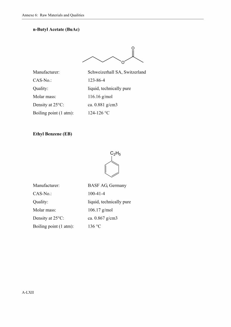
Annexe 6: Raw Materials and Qualities
A-LXII
n-Butyl Acetate (BuAc)
Manufacturer: Schweizerhall SA, Switzerland
CAS-No.: 123-86-4
Quality: liquid, technically pure
Molar mass: 116.16 g/mol
Density at 25°C: ca. 0.881 g/cm3
Boiling point (1 atm): 124-126 °C
Ethyl Benzene (EB)
Manufacturer: BASF AG, Germany
CAS-No.: 100-41-4
Quality: liquid, technically pure
Molar mass: 106.17 g/mol
Density at 25°C: ca. 0.867 g/cm3
Boiling point (1 atm): 136 °C
O
O
C2H5
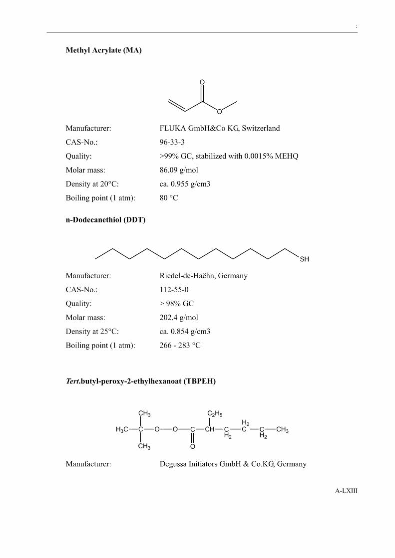
:
A-LXIII
Methyl Acrylate (MA)
Manufacturer: FLUKA GmbH&Co KG, Switzerland
CAS-No.: 96-33-3
Quality: >99% GC, stabilized with 0.0015% MEHQ
Molar mass: 86.09 g/mol
Density at 20°C: ca. 0.955 g/cm3
Boiling point (1 atm): 80 °C
n-Dodecanethiol (DDT)
Manufacturer: Riedel-de-Haëhn, Germany
CAS-No.: 112-55-0
Quality: > 98% GC
Molar mass: 202.4 g/mol
Density at 25°C: ca. 0.854 g/cm3
Boiling point (1 atm): 266 - 283 °C
Tert.butyl-peroxy-2-ethylhexanoat (TBPEH)
Manufacturer: Degussa Initiators GmbH & Co.KG, Germany
O
O
SH
H3C C O O C CH CH2
H2C C
H2CH3
CH3
CH3 O
C2H5
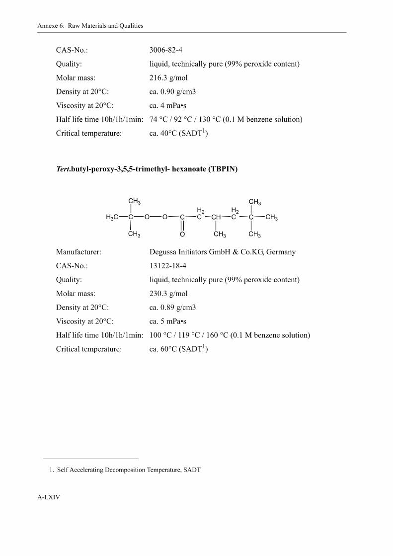
Annexe 6: Raw Materials and Qualities
A-LXIV
CAS-No.: 3006-82-4
Quality: liquid, technically pure (99% peroxide content)
Molar mass: 216.3 g/mol
Density at 20°C: ca. 0.90 g/cm3
Viscosity at 20°C: ca. 4 mPa•s
Half life time 10h/1h/1min: 74 °C / 92 °C / 130 °C (0.1 M benzene solution)
Critical temperature: ca. 40°C (SADT1)
Tert.butyl-peroxy-3,5,5-trimethyl- hexanoate (TBPIN)
Manufacturer: Degussa Initiators GmbH & Co.KG, Germany
CAS-No.: 13122-18-4
Quality: liquid, technically pure (99% peroxide content)
Molar mass: 230.3 g/mol
Density at 20°C: ca. 0.89 g/cm3
Viscosity at 20°C: ca. 5 mPa•s
Half life time 10h/1h/1min: 100 °C / 119 °C / 160 °C (0.1 M benzene solution)
Critical temperature: ca. 60°C (SADT1)
1. Self Accelerating Decomposition Temperature, SADT
H3C C O O CH2C CH
H2C C CH3
CH3
CH3 O CH3
CH3
CH3
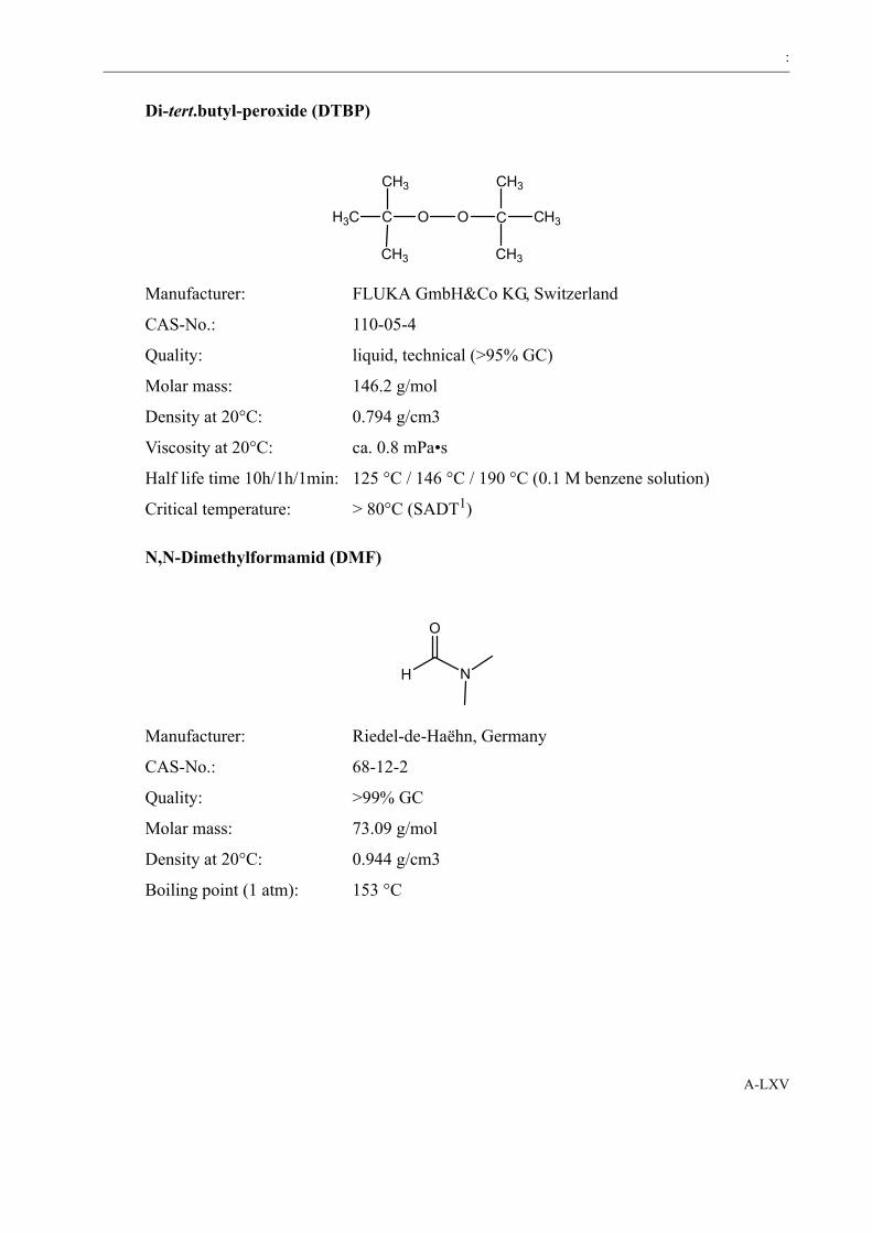
:
A-LXV
Di-tert.butyl-peroxide (DTBP)
Manufacturer: FLUKA GmbH&Co KG, Switzerland
CAS-No.: 110-05-4
Quality: liquid, technical (>95% GC)
Molar mass: 146.2 g/mol
Density at 20°C: 0.794 g/cm3
Viscosity at 20°C: ca. 0.8 mPa•s
Half life time 10h/1h/1min: 125 °C / 146 °C / 190 °C (0.1 M benzene solution)
Critical temperature: > 80°C (SADT1)
N,N-Dimethylformamid (DMF)
Manufacturer: Riedel-de-Haëhn, Germany
CAS-No.: 68-12-2
Quality: >99% GC
Molar mass: 73.09 g/mol
Density at 20°C: 0.944 g/cm3
Boiling point (1 atm): 153 °C
H3C C O O C CH3
CH3
CH3 CH3
CH3
H N
O
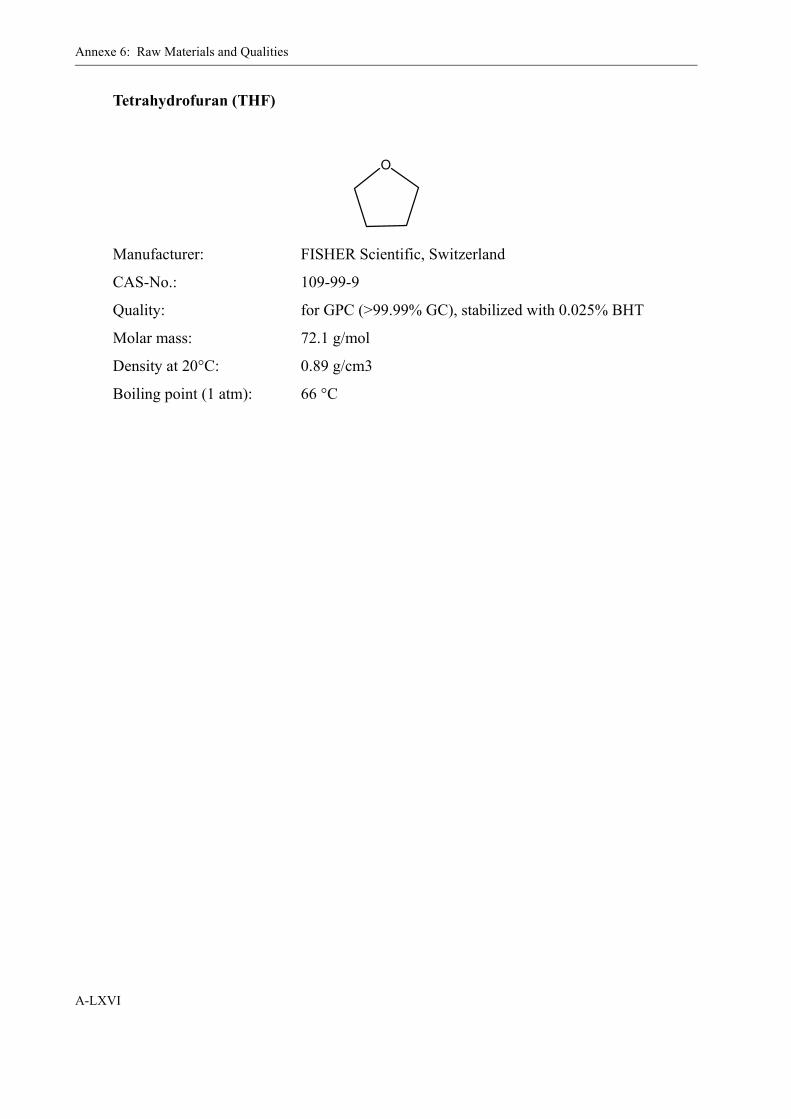
Annexe 6: Raw Materials and Qualities
A-LXVI
Tetrahydrofuran (THF)
Manufacturer: FISHER Scientific, Switzerland
CAS-No.: 109-99-9
Quality: for GPC (>99.99% GC), stabilized with 0.025% BHT
Molar mass: 72.1 g/mol
Density at 20°C: 0.89 g/cm3
Boiling point (1 atm): 66 °C
O
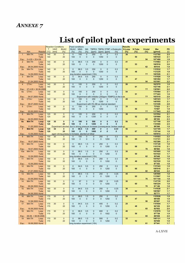
A-LXVII
ANNEXE 7
List of pilot plant experimentsReaction Conditions Feed conditions Results
T VWZ BUAC BUAC MMA MA TBPEH TBPIN DTBP n-Dodecylm. X-Loop X-Tube X-total Mw PDNr. Aim Reactor [°C] [min] [%] [%] [%] [%] [ppm] [ppm] [ppm] [%] [%] [%] [%] [g/mol] [-]
1 MA-TH Loop 140 30 0 0 100 0 250 0 0 0.3 38 112'782 2.5Tube 140 20 100 0 0 0 1250 0 0 50 106'534 2.1
Exp.: 5.4.05 + 20.4.05 54 107'499 1.92 MA-TH Loop 140 30 0 0 98.5 1.5 250 0 0 0.3 41 114'863 2.1
Tube 140 20 100 0 0 0 1250 0 0 53 106'916 2.0Exp.: 26.04.2005 Kond 62 95'618 1.9
2a MA-TH Loop 140 30 0 0 96.5 3.5 250 0 0 0.3 35 119'832 1.7Tube 140 20 100 0 0 0 1250 0 0 48 112'235 1.8
Exp.: 14.09.2005 Kond long duration experiment (10h) ?? 100'026 2.13 MA-TH Loop 140 30 0 0 94.5 5.5 250 0 0 0.3 35 110'928 1.9
Tube 140 20 100 0 0 0 1250 0 0 47 106'494 1.7Exp.: 21.04.2005 Kond 54 103'007 2.2
4 CTA-I Loop 140 30 0 0 100 0 250 0 0 0.2 50 162'070 1.9Tube 140 20 100 0 0 0 1250 0 0 61 152'746 2.1
Exp.: 27.4.05 + 30.06.2005 ?? 138'901 2.24a CTA-I Loop 140 30 0 0 100 0 250 0 0 0.2 54 176'064 2.1
Tube 140 20 100 0 0 0 0 0 0 51 177'443 1.9Exp.: 04.07.2005 Kond Experiment with Inhibitor (250ppm TEMPO) in the tube ?? 165'510 2.0
4b CTA-I Loop 140 30 0 0 100 0 250 0 0 0.2 45 149'323 1.7Tube 140 20 100 0 0 0 1250 0 0 56 140'055 2.1
Exp.: 08.07.2005 Kond Experiment with 5% EB as internal standard ?? 133'446 2.85 CTA-I Loop 140 30 0 0 100 0 250 0 0 0.5 35 73'022 2.1
Tube 140 20 100 0 0 0 1250 0 50 73'807 1.9Exp.: 03.05.2005 Kond ?? 117'043 2.2
6 MA-TH Loop 120 30 0 0 100 0 250 0 0 0.3 38 123'954 2.1Tube 120 20 100 0 0 1250 0 0 0 52 120'669 2.2
Exp.: 04.05.2005 Kond 62 68'352 2.36a MA-TH Loop 120 30 0 0 100 0 500 0 0 0.3 56 127'708 2.0
Tube 120 20 100 0 0 1250 0 0 0 72 116'000 2.5Exp.: 11.05.2005 Kond Experiment aborted due to strong pressure increase (consequence: broken sealing) ?? 99'268 1.9
7 MA-TH Loop 120 30 0 0 98.5 1.5 400 0 0 0.33 56 123'195 1.7Tube 120 20 100 0 0 1000 0 0 0 67 119'144 1.8
Exp.: 13.09.2005 Kond again strong pressure increase, aborted at 42bar ?? 105'672 1.79 MA-TH Loop 150 30 0 0 100 0 0 250 0 0.3 53 119'553 2.2
Tube 150 20 100 0 0 0 0 1250 0 65 113'721 2.2Exp.: 18.07.2005 Kond 78 102'280 2.1
10 MA-TH Loop 150 30 0 0 98.5 1.5 0 250 0 0.3 52 115'120 1.8Tube 150 20 100 0 0 0 0 1250 0 68 110'316 2.1
Exp.: 19.07.2005 Kond 78 96'982 1.810a MA-TH Loop 150 30 0 0 98.5 1.5 0 250 0 0.3 30 105'695 1.6
Tube 150 20 100 0 0 0 0 1250 0 50 103'522 1.7Exp.: 12.09.2005 Kond long duration experiment (10h) 62 92'048 1.8
11 MA-TH Loop 150 30 0 0 96.5 3.5 0 250 0 0.3 29 104'927 1.9Tube 150 20 100 0 0 0 0 1250 0 49 102'535 1.8
Exp.: 15.09.2005 Kond 63 87'352 1.812 MA-TH Loop 150 30 0 0 94.5 5.5 0 250 0 0.3 50 115'343 1.9
Tube 150 20 100 0 0 0 0 1250 0 66 108'016 2.1Exp.: 21.07.2005 Kond 82 86'532 2.2
13 MA-TH Loop 160 30 0 0 98.5 1.5 0 250 0 0.25 45 126'900 1.8Tube 160 20 100 0 0 0 0 1250 0 65 113'607 1.8
Exp.: 03.08.2005 Kond 76 101'144 1.814 MA-TH Loop 160 30 0 0 97 3 0 250 0 0.25 30 114'735 2.0
Tube 160 20 100 0 0 0 0 1250 0 60 108'224 1.8Exp.: 05.08.2005 Kond 70 91'146 1.8
15 MA-TH Loop 160 30 0 0 94.5 5.5 0 250 0 0.25 36 114'638 2.1Tube 160 20 100 0 0 0 0 1250 0 62 106'967 1.7
Exp.: 04.08.2005 Kond 75 92'771 1.716 MA-TH Loop 170 30 0 0 98.5 1.5 0 250 0 0.2 26 119'838 1.9
Tube 170 20 100 0 0 0 0 1250 0 47 98'056 1.9Exp.: 12.08.2005 Kond 58 85'007 1.9
17 MA-TH Loop 170 30 0 0 94.5 5.5 0 400 0 0.2 25 110'654 1.7Tube 170 20 100 0 0 0 0 1250 0 48 94'330 2.0
Exp.: 16.08.2005 Kond 65 82'852 2.018 MA-TH Loop 170 30 0 0 96.5 3.5 0 600 0 0.2 48 110'876 1.8
Tube 170 20 100 0 0 0 0 1502 0 56 97'738 1.9Exp.: 06.09. + 08.09.2005 65 88'058 2.0
19 MA-TH Loop 170 30 0 0 98.5 1.5 0 500 0 0.2 32 108'121 1.9Tube 170 20 100 0 0 0 0 1250 0 52 92'658 1.9
Exp.: 18.08.2005 Kond long duration experiment (10h) 61 87'541 1.7

Chapter 7: List of pilot plant experiments
A-LXVIII
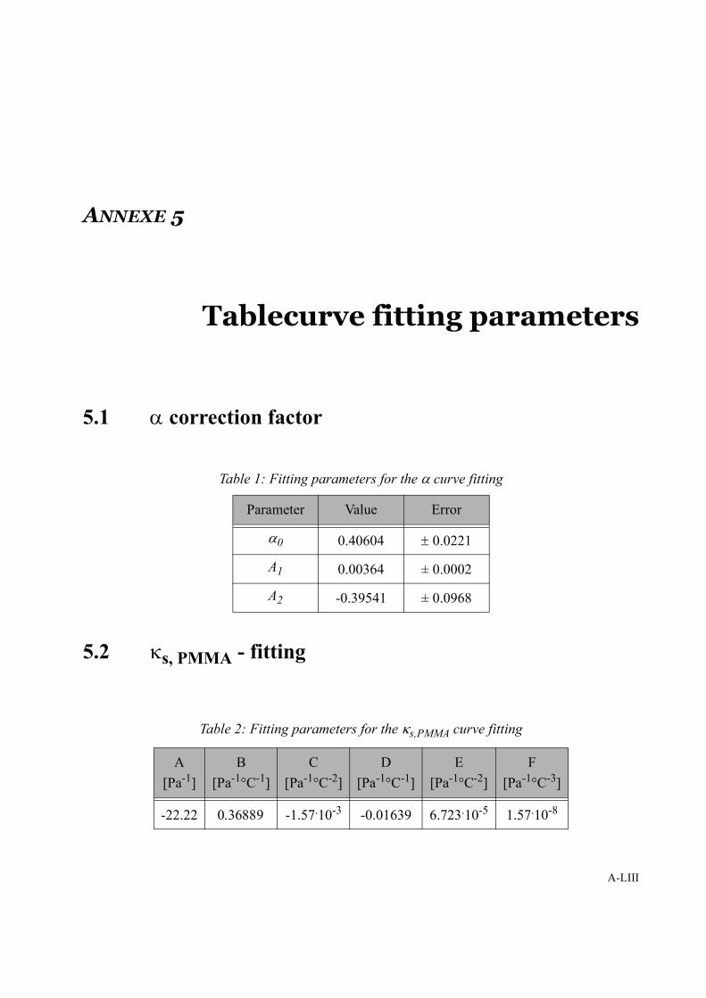
A-LIII
ANNEXE 5
Tablecurve fitting parameters
5.1 α correction factor
5.2 κs, PMMA - fitting
Table 1: Fitting parameters for the α curve fitting
Parameter Value Error
α0 0.40604 ± 0.0221
A1 0.00364 ± 0.0002
A2 -0.39541 ± 0.0968
Table 2: Fitting parameters for the κs,PMMA curve fitting
A[Pa-1]
B[Pa-1°C-1]
C[Pa-1°C-2]
D[Pa-1°C-1]
E[Pa-1°C-2]
F[Pa-1°C-3]
-22.22 0.36889 -1.57.10-3 -0.01639 6.723.10-5 1.57.10-8
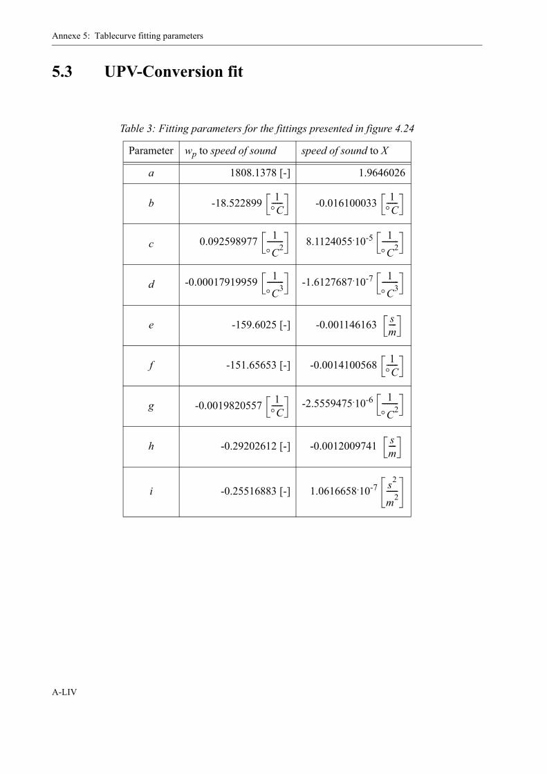
Annexe 5: Tablecurve fitting parameters
A-LIV
5.3 UPV-Conversion fit
Table 3: Fitting parameters for the fittings presented in figure 4.24
Parameter wp to speed of sound speed of sound to X
a 1808.1378 [-] 1.9646026
b -18.522899 -0.016100033
c 0.092598977 8.1124055.10-5
d -0.00017919959 -1.6127687.10-7
e -159.6025 [-] -0.001146163
f -151.65653 [-] -0.0014100568
g -0.0019820557 -2.5559475.10-6
h -0.29202612 [-] -0.0012009741
i -0.25516883 [-] 1.0616658.10-7
1°C------ 1
°C------
1°C2--------- 1
°C2---------
1°C3--------- 1
°C3---------
sm----
1°C------
1°C------
1°C2---------
sm----
s2
m2------
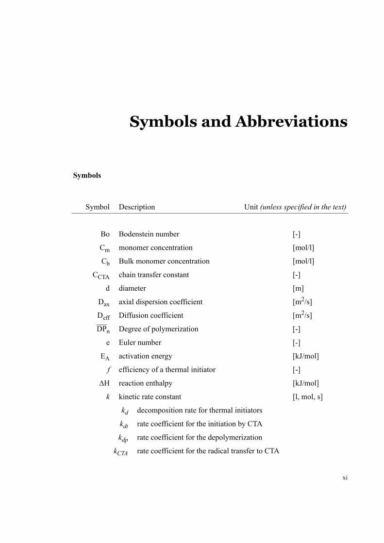
xi
Symbols and Abbreviations
Symbols
Symbol Description Unit (unless specified in the text)
Bo Bodenstein number [-]
Cm monomer concentration [mol/l]
Cb Bulk monomer concentration [mol/l]
CCTA chain transfer constant [-]
d diameter [m]
Dax axial dispersion coefficient [m2/s]
Deff Diffusion coefficient [m2/s]
DPn Degree of polymerization [-]
e Euler number [-]
EA activation energy [kJ/mol]
f efficiency of a thermal initiator [-]
ΔH reaction enthalpy [kJ/mol]
k kinetic rate constant [l, mol, s]
kd decomposition rate for thermal initiators
kdt rate coefficient for the initiation by CTA
kdp rate coefficient for the depolymerization
kCTA rate coefficient for the radical transfer to CTA
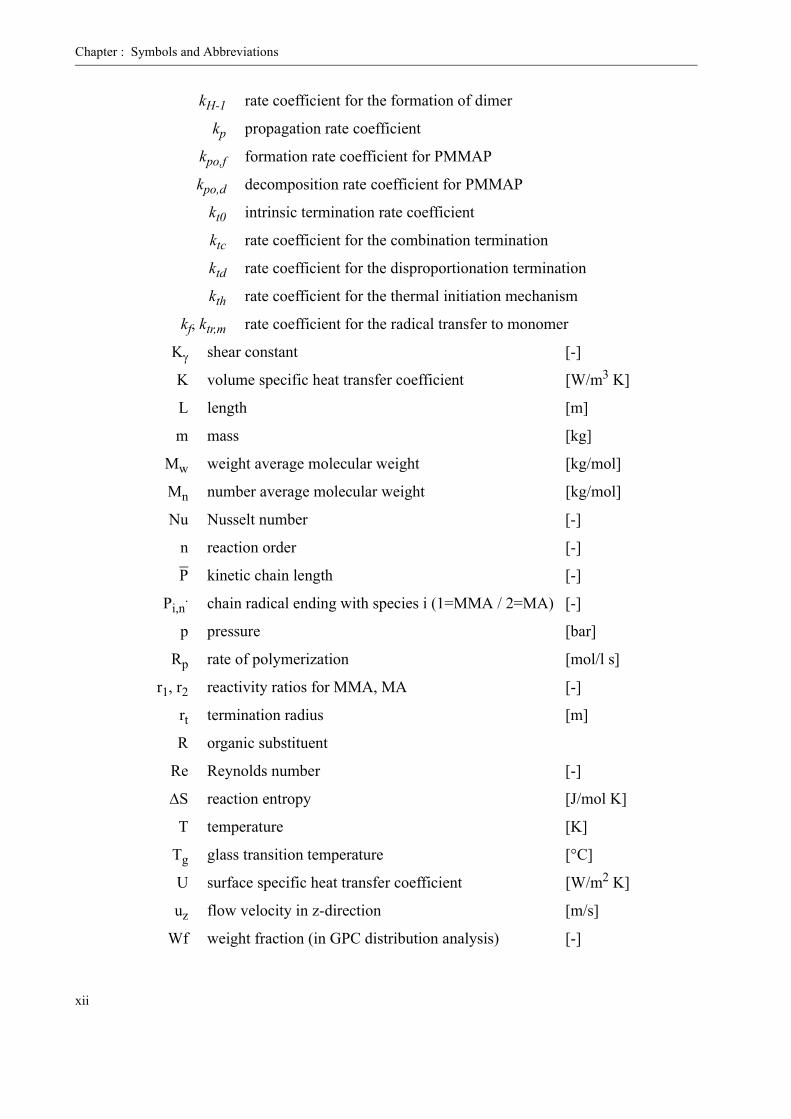
Chapter : Symbols and Abbreviations
xii
kH-1 rate coefficient for the formation of dimer
kp propagation rate coefficient
kpo,f formation rate coefficient for PMMAP
kpo,d decomposition rate coefficient for PMMAP
kt0 intrinsic termination rate coefficient
ktc rate coefficient for the combination termination
ktd rate coefficient for the disproportionation termination
kth rate coefficient for the thermal initiation mechanism
kf, ktr,m rate coefficient for the radical transfer to monomer
Kγ shear constant [-]
K volume specific heat transfer coefficient [W/m3 K]
L length [m]
m mass [kg]
Mw weight average molecular weight [kg/mol]
Mn number average molecular weight [kg/mol]
Nu Nusselt number [-]
n reaction order [-]
P kinetic chain length [-]
Pi,n. chain radical ending with species i (1=MMA / 2=MA) [-]
p pressure [bar]
Rp rate of polymerization [mol/l s]
r1, r2 reactivity ratios for MMA, MA [-]
rt termination radius [m]
R organic substituent
Re Reynolds number [-]
ΔS reaction entropy [J/mol K]
T temperature [K]
Tg glass transition temperature [°C]
U surface specific heat transfer coefficient [W/m2 K]
uz flow velocity in z-direction [m/s]
Wf weight fraction (in GPC distribution analysis) [-]
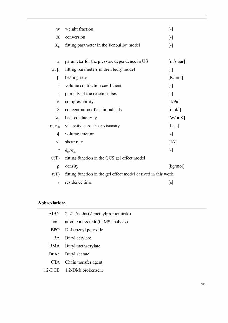
:
xiii
w weight fraction [-]
X conversion [-]
Xc fitting parameter in the Fenouillot model [-]
α parameter for the pressure dependence in US [m/s bar]
α, β fitting parameters in the Fleury model [-]
β heating rate [K/min]
ε volume contraction coefficient [-]
ε porosity of the reactor tubes [-]
κ compressibility [1/Pa]
λ concentration of chain radicals [mol/l]
λl heat conductivity [W/m K]
η, η0 viscosity, zero shear viscosity [Pa s]
φ volume fraction [-]
γ’ shear rate [1/s]
γ ktc/ktd [-]
θ(T) fitting function in the CCS gel effect model
ρ density [kg/mol]
τ(T) fitting function in the gel effect model derived in this work
τ residence time [s]
Abbreviations
AIBN 2, 2’-Azobis(2-methylpropionitrile)
amu atomic mass unit (in MS analysis)
BPO Di-benzoyl peroxide
BA Butyl acrylate
BMA Butyl methacrylate
BuAc Butyl acetate
CTA Chain transfer agent
1,2-DCB 1,2-Dichlorobenzene
Chapter : Symbols and Abbreviations
xiv
DSC Differential scanning calorimetry
DTBP Di-tert.butyl peroxide
EB Ethyl benzene
GPC Gel permeation chromatography
HS-GC Head space gas chromatography
MA Methyl acrylate
MMA Methyl methacrylate
MMA-OO MMA polyperoxide
MS Mass spectroscopy
NMR Nuclear Magnetic Resonance spectroscopy
PMMA Poly (methyl methacrylate)
PS Poly (styrene)
PMMAP MMA polyperoxide
SEC3 Size Exclusion Chromatography with triple detection
TBPEH Tert.butyl-peroxy-2-ethylhexanoat
TBPIN Tert.butyl-peroxy-3,5,5-trimethylhexanoat
TGA Thermogravimetry
THF Tetrahydrofuran
US Ultrasound
UV UV-Vis Photospectrometry
Indices
m monomer
s solvent
p polymer
obs apparant value (for rate constants)

xv
Bibliography
[1] K.T. Nguyen, "Mélangeur statique comme réacteur tubulaire de polymérisation",Ph.D. thesis: Département de Chimie, no., EPFL (Lausanne), 1982.
[2] T. Meyer, "Etude à l'aide d'une méthode chimique de la ségragation lors d'unepolymérisation dans un réacteur tubulaire à recyclage", Ph.D. thesis: Département dechimie, no. 810, EPFL (Lausanne), 1989.
[3] S. Belkhiria, "Copolymérisations en masse de styrène et d'anhydride maléique dansun réacteur tubulaire à recyclage: Etude cinétique, stabilité de réacteur et qualité desproduits", Ph.D. thesis: Département de chimie, no. 1258, EPFL (Lausanne), 1994.
[4] L. Cavin, "Polymérisation radicalaire du styrène initiée par un initiateur bifonction-nel dans un réacteur tubulaire à recyclage", Ph.D. thesis: Département de chimie, no.2083, EPFL (Lausanne), 2000.
[5] P.-A. Fleury, "Polymérisation du méthacrylate de méthyle à haute température",Ph.D. thesis: Département de Chimie Thesis no.1986, no., École PolytechniqueFédérale de Lausanne (Lausanne), 1993.
[6] T. Zeilmann, "Continuous Methylmethacrylate Polymerization Process - Reactionand Devolatilization", Ph.D. thesis: Institute of Chemical and Biological Process Sci-ence, no. 2554, EPFL (Lausanne), 2002.
[7] L. Cavin, T. Meyer, and A. Renken, "On-line conversion monitoring through ultra-sound velocity measurements in bulk styrene polymerization in a recycle reactor -Part I: Experimental validation", Polymer Reaction Engineering, 8(3): p. 201-223,2000.
[8] L. Cavin, A. Renken, and T. Meyer, "On-line conversion monitoring through ultra-sound velocity measurements in bulk styrene polymerization in a recycle reactor -Part II: Mathematical Model", Polymer Reaction Engineering, 8(3): p. 225-240,2000.
[9] P. Nising, "Optimization of the Polymerization of PMMA in a Sulzer Pilot Plant",Ph.D. thesis: Lehrstuhl für Technische Chemie I, no., Friedrich-Alexander-Univer-sität (Erlangen), 2001.
Bibliography
xvi
[10] K. Albrecht, Polymethacrylat - Ein vielseitiger Kunststoff als Granulat und Halbzeug, inRoehm GmbH. 2001: Darmstadt.
[11] R. Vieweg and F. Esser, Polymethylmethacrylate. 1975. Carl Hauser Verlag. München.
[12] C.J. Simon, Plastics Business Data and Charts, www.vke.de.
[13] W.A. Pryor and L.D. Lasswell, Advances in Free Radical Chemistry. 1975. AcademicPress. N.Y.
[14] M. Stickler and G. Meyerhoff, "Die thermische Polymerisation von Methylmethacrylat, 1Polymerisation in Substanz", Makromolekulare Chemie, 179: p. 2739-2745, 1978.
[15] M. Stickler and G. Meyerhoff, "Die thermische Polymerisation von Methylmethacrylat, 2Bildung des ungesättigten Dimeren", Makromolekulare Chemie, 181(1): p. 131-147,1980.
[16] E. Brand, M. Stickler, and G. Meyerhoff, "Die thermische Polymerisation von Methyl-methacrylat, 3 Verhalten des ungesättigten Dimeren bei der Polymerisation", Makro-molekulare Chemie, 181: p. 913-921, 1980.
[17] J. Lingnau, M. Stickler, and G. Meyerhoff, "The spontanteous Polymerization of Methyl-Methacrylate: IV Formation of cyclic dimers and linear trimers", European PolymerJournal, 16: p. 789-791, 1980.
[18] M. Stickler and G. Meyerhoff, "The Spontaneous Thermal Polymerization of Methyl-Methacrylate: 5. Experimental-Study and Computer Simulation of the High ConversionReaction at 130°C", Polymer, 22(7): p. 928-933, 1981.
[19] J. Lingnau and G. Meyerhoff, "The Spontaneous Polymerization of Methyl-Methacry-late: VI. Polymerization in Solution - Participation of Transfer Agents in the InitiationReaction", Polymer, 24(11): p. 1473-1478, 1983.
[20] F.R. Mayo and A.A. Miller, "The Oxidation of Unsaturated Compounds. VIII. The Oxi-dation of Methacrylic Esters", 1957.
[21] C.E. Barnes, R.M. Elofson, and G.D. Jones, "Role of Oxygen in Vinyl Polymerization. II.Isolation and Structure of the Peroxides of Vinyl Compounds", Journal of the AmericanChemical Society, 72: p. 210-215, 1950.
[22] R.S. Lehrle and A. Shortland, "A Study of the Purification of Methyl Methacrylate sug-gests that the "Thermal" Polymerisation of this Monomer is initiated by AdventitiousPeroxides", European Polymer Journal, 24(5): p. 425-429, 1987.
[23] S. Schulze and H. Vogel, "Aspects of the safe storage of acrylic monomers: Kinetics ofthe oxygen consumption", Chemical Engineering & Technology, 21(10): p. 829-837,1998.
[24] G.L. Batch and C.W. Macosko, "Oxygen Inhibition in Differential Scanning Calorimetryof Free- Radical Polymerization", Thermochimica Acta, 166: p. 185-198, 1990.
[25] T. Mukundan and K. Kishore, "Structure and Pyrolysis of Poly(methyl methacrylate per-oxide): A Thermochemical Approach", Macromolecules, 20: p. 2382-2385, 1986.

Bibliography
xvii
[26] K. Ganesh, S. Paramasivam, and K. Kishore, "Determination of end groups inpoly(methylmethacrylate peroxide) by fast atom bombardment mass spectrometry and IRspectroscopy", Polymer Bulletin, 37(6): p. 785-790, 1996.
[27] G.V. Schulz and G. Henrici, "Kinetik Der Polymerisationsreaktionen .22. Reaktionskine-tik Der Polymerisationshemmung Durch Molekularen Sauerstoff (Versuche Mit Methyl-methacrylat)", Makromolekulare Chemie, 18-9(MAR): p. 437-454, 1956.
[28] K. Subramanian, "Formation, degradation, and applications of polyperoxides", Journalof Macromolecular Science-Polymer Reviews, C43(3): p. 323-383, 2003.
[29] K.S. Murthy, K. Kishore, and V.K. Mohan, "Vinyl Monomer Based Polyperoxides asPotential Initiators for Radical Polymerization - an Exploratory Investigation withPoly(Alpha-Methylstyrene Peroxide)", Macromolecules, 27(24): p. 7109-7114, 1994.
[30] K. Kishore, V. Gayathri, and K. Ravindran, "Formation and Degradation of PolymericPeroxides", Journal of Macromolecular Science and Chemistry, A16(8): p. 1359-1383, 1981.
[31] R. Kerber, "Kinetische Untersuchungen zur Bildung polymerer Peroxyde des Methyl-methacrylates. I." Die makromolekulare Chemie, 40(25): p. 25-38, 1960.
[32] C. Vila, R. Moreno, M. Perez, E. Abuin, and E. Lissi, "Methyl Methacrylate Polymeriza-tion in the Presence of Oxygen", Anales Asoc. Quím. Argentina, 61: p. 197-203, 1973.
[33] C.D. Wagner, R.H. Smith, and E.D. Peters, "Determination of Organic Peroxides - Eval-uation of a Modified Iodometric Method", Analytical Chemistry, 19(12): p. 976, 1947.
[34] K. Nozaki, "Iodometric Method of Analysis for Organic Peroxides", Industrial andEngineering Chemistry-Analytical Edition, 18(9): p. 583-583, 1946.
[35] T. Scherzer and H. Langguth, "Temperature Dependence of the oxygen solubility in Acry-lates and its Effect on the induction period in UV photopolymerization", Macromolecu-lar Chemistry and Physics, 206: p. 240-245, 2005.
[36] P. Nising, T. Meyer, R. Carloff, and M. Wicker, "Thermal Initiation of MMA in HighTemperature Radical Polymerizations", Macromolecular Materials and Engineering,290: p. 311-318, 2005.
[37] G. Sivalingam, P. De, R. Karthik, and G. Madras, "Thermal degradation kinetics of vinylpolyperoxide copolymers", Polymer Degradation and Stability, 84(1): p. 173-179,2004.
[38] C.H. Bamford and P.R. Morris, "The Oxidative Polymerization of Methyl Methacrylate",Die makromolekulare Chemie, 87: p. 73-89, 1965.
[39] Personal communication, N. Deusch, 2003.
[40] G. Odian, Principles of Polymerization. 1991. New York [etc.].
[41] PerkinElmer, Pyris Software online help - Scanning Kinetics theory,
[42] F. Fenouillot, J. Terrisse, and T. Rimlinger, "Thermal polymerization of methyl methacry-late at high temperature", International Polymer Processing, 13(2): p. 154-161, 1998.
Bibliography
xviii
[43] P. Nising, T. Zeilmann, and T. Meyer, "On the Degradation and Stabilization ofPoly(Methyl Methacrylate) in a Continuous Process", Chem. Eng. Technol., 26(5): p.599-604, 2003.
[44] NIST, NIST Chemistry WebBook, http://webbook.nist.gov.
[45] P. Xia, H. Cheng, and D. Yan, "Free-radical polymerization of methyl methacrylate initi-ated by thiol alone", Journal of Applied Polymer Science, 45(4): p. 579-582, 1992.
[46] C.J. Albisetti, D.C. England, M.J. Hogsed, and R.M. Joyce, "Dimers of MethacrylicComounds", Journal of the American Chemical Society, 78: p. 472-475, 1956.
[47] I.E.H. Brandrup J., Polymer Handbook. 1989. J. Wiley & Sons.
[48] R. Battino, Oxygen and Ozone - Solubility Data Series. 1981. Pergamon Press. Oxford.
[49] E. Trommsdorff, H. Kohle, and P. Lagally, "Zur Polymerisation Des Methacrylsaureme-thylesters", Makromolekulare Chemie-Macromolecular Chemistry and Physics,1(3): p. 169-198, 1948.
[50] A. Echte, Handbuch der Technischen Polymerchemie. 1993. VCH Verlagsgesellschaft.Weinheim.
[51] N. Tefera, G. Weickert, and K.R. Westerterp, "Modeling of free radical polymerizationup to high conversion .1. A method for the selection of models by simultaneous parame-ter estimation", Journal of Applied Polymer Science, 63(12): p. 1649-1661, 1997.
[52] J.S. Vrentas, "Review of the applications of free volume theory for diffusion in polymers",Polym Rev., 15(136-138), 1981.
[53] J.S. Vrentas and J.L. Duda, "Diffusion in polymer solvent systems. 1. Reexamination ofthe free volume theory", Journal of Polymer Science: Polymer Physics Edition, 15: p.403-416, 1977.
[54] J.S. Vrentas and J.L. Duda, "Diffusion in polymer solvent systems. 2. Predictive theoryfor the dependence of diffision coefficients on temp. , conc. and molecular weight",Journal of Polymer Science: Polymer Physics Edition, 15: p. 417-439, 1977.
[55] J.S. Vrentas and J.L. Duda, "Molecular diffusion in polymer solutions", AIChE Journal,25(1): p. 1-21, 1979.
[56] S. Hoppe and A. Renken, "Modelling of the free radical polymerisation of methyl-methacrylate up to high temperature", Polymer Reaction Engineering, 6(1): p. 1-+,1998.
[57] S.K. Soh and D.C. Sundberg, "Diffusion-Controlled Vinyl Polymerization .2. Limitationson the Gel Effect", Journal of Polymer Science Part a-Polymer Chemistry, 20(5): p.1315-1329, 1982.
[58] W.Y. Chiu, G.M. Carratt, and D.S. Soong, "A Computer Model for the Gel Effect in Free-Radical Polymerization", Macromolecules, 16((3)): p. 348-357, 1983.
[59] N. Friis and A.E. Hamielec, "Gel-Effect in Emulsion Polymerization of Vinyl Mono-mers", Acs Symposium Series, (24): p. 82-91, 1976.
Bibliography
xix
[60] M. Buback, "Free-Radical Polymerization up to High Conversion - a General KineticTreatment", Makromolekulare Chemie-Macromolecular Chemistry and Physics,191(7): p. 1575-1587, 1990.
[61] F.L. Marten and A.E. Hamielec, American Chemical Society Symposium Series, 104:p. 43, 1979.
[62] Personal communication, R. Carloff,
[63] B.M. Louie, G.M. Carratt, and D.S. Soong, "Modeling the Free-Radical Solution andBulk-Polymerization of Methyl-Methacrylate", Journal of Applied Polymer Science,30(10): p. 3985-4012, 1985.
[64] D. Achilias and C. Kiparissides, "Modeling of Diffusion-Controlled Free-Radical Poly-merization Reactions", Journal of Applied Polymer Science, 35: p. 1303-1323, 1988.
[65] P. Nising and T. Meyer, "Modeling of the High-Temperature Polymerization of MethylMethacrylate. 1. Review of Existing Models for the Description of the Gel Effect", Ind.Eng. Chem. Res., 43(23): p. 7220-7226, 2004.
[66] F. Fenouillot, J. Terrisse, and T. Rimlinger, "Polymerization of methyl methacrylate athigh temperature with 1-butanethiol as chain transfer agent", Journal of Applied Poly-mer Science, 72(12): p. 1589-1599, 1999.
[67] N. Tefera, G. Weickert, and K.R. Westerterp, "Modeling of free radical polymerizationup to high conversion .2. Development of a mathematical model", Journal of AppliedPolymer Science, 63(12): p. 1663-1680, 1997.
[68] G.C. Berry, "The Viscosity of Polymer-Diluent Mixtures", Journal of Physical Chemis-try, 70: p. 1194-1198, 1965.
[69] F. Bueche, "Viscosity, Self-Diffusion, and Allied Effects in Solid Polymers", Journal ofChemical Physics, 20(12): p. 1959-1964, 1952.
[70] D. Panke, "Polymerization of Methyl-Methacrylate up to High Degrees of Conversion -Model-Calculations Considering the Presence of a Prepolymer", MakromolekulareChemie-Rapid Communications, 7(4): p. 171-174, 1986.
[71] F.L. Marten and A.E. Hamielec, "High-Conversion Diffusion-Controlled Polymerizationof Styrene .1", Journal of Applied Polymer Science, 27(2): p. 489-505, 1982.
[72] M. Fernandez-Garcia, M.M.C. Lopez-Gonzales, L.M. Barrales-Rienda, E.L. Madruga,and C. Arias, "Effect of Copolymer Composition and Conversion on the Glass Transitionof Methyl Acrylate - Methyl Methacrylate Copolymers", Journal of Polymer SciencePart B-Polymer Physics, 32: p. 1191-1203, 1994.
[73] K. TAKASHI and M. MASAHIKO, Process for production of methacrylate polymers.1998, SUMITOMO CHEMICAL CO.
[74] T. Meyer, "Etude à l'aide d'une methode chimique de la ségrégation lors d'une polyméri-sation dans un réacteur tubulaire à recyclage", Ph.D. thesis: Département de Chimie,Thesis No. 810, no., EPFL (Lausanne), 1989.
[75] P. Nising, T. Zeilmann, T. Meyer, "On the degradation and stabilization of PMMA in acontinuous process", Proceedings ISCRE 17, HongKong, 2002.
Bibliography
xx
[76] N.K. Tien, E. Flaschel, and A. Renken, "Bulk-Polymerization of Styrene in a StaticMixer", Chemical Engineering Communications, 36(1-6): p. 251-267, 1985.
[77] A. Heierle, "Statische Mischer - Wärmetauscher", Chemie-Anlagen + verfahren, 7,1994.
[78] J.-E. Juvet, "Etude de la ségrégation thermique dans un échangeur de chaleur tubu-laire", Ph.D. thesis: Département de chimie, Thesis No. 791, no., EPFL (Lausanne),1989.
[79] K.T. Nguyen, F. Streiff, E. Flaschel, and A. Renken, "Motionless mixers for the design oftubular polymerization reactors", Chemical Engineering & Technology, 13(1): p. 214-220, 1990.
[80] Sulzer, "Mixing and Reaction Processes", Sulzer Chemtech Sales Brochure,MRT0655, 1992.
[81] N.P. Stuber, "Studies of continuous methylmethacrylate polymerization in a twin-screwextruder", Ph.D. thesis: Thesis (Ph.D.), no. 000125258, University of Minnesota 1986.
[82] N.P. Stuber and M. Tirrell, "Continuous polymerization studies in a twin-screwextruder", Polymer Process Engineering, 3(1-2): p. 71-83, 1985.
[83] J.J. Zacca and W.H. Ray, "Modeling of the Liquid-Phase Polymerization of Olefins inLoop Reactors", Chemical Engineering Science, 48(22): p. 3743-3765, 1993.
[84] W.-D. Hergeth, On-Line Monitoring of Chemical Reactions,
[85] T. Zeilmann and T. Meyer, "Inline Conversion Monitoring in MMA High Solid ContentPolymerization Process", Chimia, 55(3): p. 249-250, 2001.
[86] F. Dinger, "Polymerisationsüberwachung mit Ultraschall", Chemie Technik, 28(3): p.30-34, 1999.
[87] S.L. Oswal, "Speed of Sound, Isentropic Compressibility, Viscosity, and Excess Volumeof Binary Mixtures. 1. Alkanenitriles with Alkyl Acetates", Journal of Chemical Engi-neering Data, 40: p. 840-844, 1995.
[88] S.L. Oswal, O. Oswal, P.S. Modi, J.P. Dave, and R.L. Gardas, "Acoustic, volumetric,compressibility and refractivity properties and Flory's reduction parameters of somehomologous series of alkyl alkanoates from 298.15 to 333.15K", Thermochimica Acta,410: p. 1-14, 2004.
[89] M. Pancholy and S.S. Mathur, "Adiabatic Compressibility and Ultrasonic Velocity inEsters", Journal of the Physical Society of Japan, 18(3): p. 449-451, 1963.
[90] T. Kelen and F. Tüdös, "Analysis of the Linear Methods for Determining Copolymeriza-tion Reactivity Ratios. I. A New Improved Linear Graphic Method", Journal of Macro-molecular Science and Chemistry, A9(1): p. 1-27, 1975.
[91] H.-G. Elias, An Introduction to Polymer Science. 1997. VCH Verlagsgesellschaft. Wein-heim.
Bibliography
xxi
[92] N. Grassie, B.J.D. Torrance, J.D. Fortune, and J.D. Gemmel, "Reactivity Ratios for theCopolymerization of Acrylates and Methacrylates by Nuclear Magnetic ResonanceSpectroscopy", Polymer, 6(12): p. 653-658, 1965.
[93] C. Arias, M.M.C. López-González, M. Fernández-García, J.M. Barrales-Rienda, andE.L. Madruga, "Free-radical copolymerization of methyl acrylate with methyl methacry-late in benzene solution", Polymer, 34(8): p. 1786-1789, 1993.
[94] M.-J. Park, S.-M. Ahn, and H.-K. Rhee, "Kinetic Parameter Estimation for the MMA/MA Copolymerization System", Journal of Applied Polymer Science, 78: p. 2554-2564, 2000.
[95] A. Nagy, T. Földes-Berezsnich, and F. Tüdös, "Kinetics of Radical Polymerization -Investigation of the polymerization of Methyl Acrylate in Solution by the Rotating SectorMethod", European Polymer Journal, 20(1): p. 25-29, 1984.
[96] R.A. Hutchinson, D.A. Paquet, and J.H. McMinn, "Determination of Free-RadicalChain-Transfer Rate Coefficients by Pulsed-Laser Polymerization", Macromolecules,28(16): p. 5655-5663, 1995.
[97] J.L. De la Fuente and E.L. Madruga, "Homopolymerization of methyl methacrylate andstyrene: Determination of the chain-transfer constant from the mayo equation and thenumber distribution for n-dodecanethiol", Journal of Polymer Science Part a-PolymerChemistry, 38(1): p. 170-178, 2000.
[98] M. Fontanille and Y. Gnanou, Chimie et Physico-chimie des polymères. 2002. Dunod.Paris.
[99] T. Kashiwagi, T. Hirata, and J.E. Brown, "Thermal and Oxidative-Degradation ofPoly(Methyl Methacrylate) - Molecular-Weight", Macromolecules, 18(2): p. 131-138,1985.
[100] E. Weast, Handbook of Chemistry and Physics. 1983. CRC Press.
[101] K. Smolders and J. Baeyens, "Thermal degradation of PMMA in fluidised beds", WasteManagement, 24(8): p. 849-857, 2004.
[102] A. Rudin, The Elements of Polymer Science and Engineering. 1998. Academic Press.San Diego.
[103] S. Beuermann, M. Buback, and M. Gadermann, "Depropagation in methacrylate poly-merizations", Dechema monogr., 138: p. 461-465, 2004.
[104] N. Grassie and H.W. Melville, "Degradation of poly (methyl methacrylate) C: The mech-anism of the thermal degradation of poly (methyl methacryalte)", Discussions of theFaraday Society, 2: p. 378-383, 1947.
[105] T. Hirata, T. Kashiwagi, and J.E. Brown, "Thermal and Oxidative-Degradation ofPoly(Methyl Methacrylate) - Weight-Loss", Macromolecules, 18(7): p. 1410-1418,1985.
[106] B.J. Holland and J.N. Hay, "The kinetics and mechanisms of the thermal degradation ofpoly(methyl methacrylate) studied by thermal analysis-Fourier transform infrared spec-troscopy", Polymer, 42(11): p. 4825-4835, 2001.
Bibliography
xxii
[107] K.A. Holland and I.D. Rae, "Thermal Degradation of a compound which models thehead-to-head linkage in Poly(methyl methacrylate)", Australian Journal of Chemistry,40(4): p. 687-692, 1987.
[108] Y.H. Hu and C.Y. Chen, "The effect of end groups on the thermal degradation ofpoly(methyl methacrylate)", Polymer Degradation and Stability, 82(1): p. 81-88, 2003.
[109] T. Kashiwagi, A. Inaba, J.E. Brown, K. Hatada, T. Kitayama, and E. Masuda, "Effects ofWeak Linkages on the Thermal and Oxidative- Degradation of Poly(Methyl Methacry-lates)", Macromolecules, 19(8): p. 2160-2168, 1986.
[110] G. Madras, J.M. Smith, and B.J. McCoy, "Degradation of poly(methyl methacrylate) insolution", Industrial & Engineering Chemistry Research, 35(6): p. 1795-1800, 1996.
[111] L.E. Manring, "Thermal-Degradation of Saturated Poly(Methyl Methacrylate)", Macro-molecules, 21(2): p. 528-530, 1988.
[112] L.E. Manring, "Thermal-Degradation of Poly(Methyl Methacrylate) .2. Vinyl- Termi-nated Polymer", Macromolecules, 22(6): p. 2673-2677, 1989.
[113] L.E. Manring, "Thermal-Degradation of Poly(Methyl Methacrylate) .4. Random Side-Group Scission", Macromolecules, 24(11): p. 3304-3309, 1991.
[114] L.E. Manring and W.R. Hertler, "The Thermal-Degradation of Pmma Polymer with Ter-minal Head-to- Head Linkages", Abstracts of Papers of the American Chemical Soci-ety, 206: p. 19-POLY, 1993.
[115] L.E. Manring, D.Y. Sogah, and G.M. Cohen, "Thermal-Degradation of Poly(MethylMethacrylate) .3. Polymer with Head-to-Head Linkages", Macromolecules, 22(12): p.4652-4654, 1989.
[116] G.R. Morrow and I.D. Rae, "Thermal-Degradation of Polymers and Polymer Models .4.Thermolysis of a Polymethacrylate Model with an Unsaturated End Group", AustralianJournal of Chemistry, 40(8): p. 1477-1481, 1987.
[117] J.D. Peterson, S. Vyazovkin, and C.A. Wight, "Kinetic Study of Stabilizing Effect of Oxy-gen on Thermal Degredation of Poly(methyl methacrylate)", Journal of PhysicalChemistry B, 103: p. 8087-8092, 1999.
[118] H.H.G. Jellinek, Aspects of Degradation and Stabilization of Polymers. 1978. Elsevier.Amsterdam.
[119] Wikipedia Online Encyclopedia,http://en.wikipedia.org/wiki/Gel_permeation_chromatography.
[120] Viscotek, Instruction Manual TDA300 SEC3 System. 2000.
[121] F. Sasse, "Chemisches Recycling von Acrylgläsern", Ph.D. thesis: Lehrstuhl für Tech-nische Chemie I, no., Friedrich-Alexander-Universität (Erlangen-Nürnberg), 1998.
[122] L. Gou, C.N. Coretsopoulos, and A.B. Scranton, "Measurement of the Dissolved OxygenConcentration in Acrlyate Monomers with a Novel Photochemical Method", Journal ofPolymer Science Part A - Polymer Chemistry, 42: p. 1285-1292, 2004.
Bibliography
xxiii
[123] M. Wulkow, "The simulation of molecular weight distributions in polyreaction kineticsby discrete Galerkin methods", Macromolecular Theory and Simulations, 5(3): p.393-416, 1996.
[124] S. Beuermann, M. Buback, T.P. Davis, R.G. Gilbert, R.A. Hutchinson, O.F. Olaj, G.T.Russell, J. Schweer, and A.M.v. Herk, "Critically evaluated rate coefficients for free-radical polymerizations - Propagation rate coefficients for methyl methacrylate", Mac-romolecular Chemistry and Physics, 198: p. 1545-1560, 1997.
[125] P.J. Skrdla, "Thermal decomposition of tert-butyl peroxide in a gas chromatographicreactor: A comparison of kinetic approaches", International Journal of ChemicalKinetics, 36(7): p. 386-393, 2004.
[126] Crossfire Beilstein Database,
[127] N.V. Sastry and M.K. Valand, "Volumetric behaviour of acrylic esters (methyl-, ethyl-,and butyl acrylate) + 1-Alcohol at 298.15K and 308.15K", Phys. Chem. Liq., 38: p. 61-72, 2000.
[128] J. George, N.V. Sastry, S.R. Patel, and M.K. Valand, "Densities, Viscosities, Speeds ofSound, and Relative Permittivities for Methyl Acrylate + 1-Alcohols (C1-C6) atT=(302.15 and 318.15)K", Journal of Chemical Engineering Data, 47: p. 262-269,2002.
[129] P. Bahadur and N.V. Sastry, "Densities, Sound Speeds, Excess Volumes, and Excess Isen-tropic Compressibilities for Methyl Acrylate + 1-Propanol + Hydrocarbons", Interna-tional Journal of Thermophysics, 24(2): p. 447-462, 2003.

Bibliography
xxiv

xxv
Acknowledgements
Firstly, and most importantly, I want to express my deep gratitude and love to my darling
wife, Anna, who not only opened my eyes for so many new things, but also supported and
comforted me throughout the past four years in Lausanne, which surely was not always easy.
Without the strength and confidence that I received from our partnership, I would not be who
and where I am now.
I also owe a debt of gratitude to my parents, Annette and Wolfgang Nising, who since I
can remember always provided me with far more than the necessary amount of love, education
and moral support and thanks to who I never lacked for anything in my life. At the same time,
I want to thank my brother, Carl, for all the fun and the good relationship we’ve shared so far,
as well as my parents-in-law, Angela and Nicola Bozzi, for their sincere and hearty compas-
sion and for having included me so in their family.
My first year in Lausanne was quite a challenge in terms of making friends and bonding
with people. Without the warm welcome of my two dear friends Nicolas, who has been trying
for five years now to motivate me for all different kinds of sport, and Thomas, my compatriot
from the Rhineland who immediately made me feel at home, I would probably not have stayed
all that long. Having good friends makes life so much easier and also helps enormously to cope
with the difficult moments that occur during almost every thesis. Therefore, I want to thank my
Acknowledgements
xxvi
closest friends, who I met here in Lausanne, for all the happy moments and the pleasure we had
together during the last years: Elisabeth and Mathias, for the innumerable excursions and eve-
nings spent together; Nadia and Marc, for teaching me the beauty of boating on the lake; Benoît,
for his linguistic and moral support; and Massimo, for his patience in teaching me and listening to
my Italian. I also thank my dear friend Thorsten, with whom together I went through the major
part of my school and university time, for keeping in touch through all these years I’ve been away
from Sankt Augustin.
On the side of EPFL, there are a lot of people that have been directly or indirectly involved
in this thesis. Most importantly, I express my sincere gratitude to the mechanicians of the ISIC
workshop, in particular Gérard Bovard and Jean-Claude Rapit, for their constant help in con-
structing, maintaining and dismantling the pilot plant. Without them, their knowledge and perma-
nent availability, I would not have been able to carry out this thesis. Another big thank you goes to
my numerous diploma students, who not only did a lot of measurements for me but also contrib-
uted to the social life in our group: Khaled, Séverine, Nathanael, and especially Valéry and Felix,
with who I shared not only working hours but also lots of happy moments as friends. I also want
to mention our secretary, Madame Anken, and her various apprentices at this point, who took care
of a lot of organizational matters throughout this thesis, for which I want to thank all of them very
dearly. During most of my time at EPFL, I shared the office with Ivan Pantchev, who always had
some good advice or joke for me and who I could always rely on, which I am very thankful for.
This thesis was made possible with the full financial and scientific support of Röhm in Ger-
many. On their side, I want to express my deep gratitude to Dr. Rüdiger Carloff, Dr. Michael
Wicker and Dr. Klaus Albrecht for the trust they put in me and the time they spent for the many
discussions and meetings we had during the last four years. In particular, I thank Rüdiger Carloff
for the scientific guidance he provided me with throughout this project.
The person who enabled me to do my diploma work and PhD here at EPFL is my supervi-
sor, MER Dr. Thierry Meyer. I want to thank Thierry for the leeway he gave to me and for the
confidence he had in me during the last 5 years. Moreover, I am very thankful for the opportunity

Acknowledgements
xxvii
to participate in the many international conferences we went together, which is far from being
common for PhD students.
Lots of thanks go to the members of the examining board, Prof. Pla, Prof. Klok and Dr. Car-
loff for their appreciation of my work and the positive feedback I got from their side.
Finally, I want to thank the following people for their help, company and sometimes also
moral support: my colleagues Charalampos Mantelis, Patrick Farquet, Petra Prechtl, Pascal Tribo-
let, Frédéric Lavanchy, Marina Ruta, Alain Fankhauser, Edy Casali and Martin Grasemann; our
dutch exchange professor, Maartje Kemmere, for her advice and moral support; the people from
the electronic workshop, Gabriel Roch and Olivier Noverraz, for their help with the electric
installations in the pilot plant; Peter Péchy for the NMR support; the people from Sulzer
Chemtech, in particular Albert Breiter and Claude Passaplan, for their technical support and for
organizing spare parts; Sandrine Olivier and Philippe Lievens from Viscotek for their GPC sup-
port; and finally Mr. Cottier and the Lausanne firebrigade for coming to EPFL on a sunny sunday
afternoon for a false alarm that I triggered with one of my experiments.
xxviii
Curriculum vitae
Axel Philip NISING
Chemin du Noirmont 15 Age: 30CH – 1004 Lausanne Citizenship: German
MarriedE-mail: [email protected]
Summary• PhD in Chemical Engineering with specialization in Polymer Reaction Engineering• Summa cum Laude Diploma in Chemical Engineering at the University of Erlangen-Nürnberg, Germany.• Strong background in polymer science and analytics: pilot plant technology, free-radical polymerizations,
GPC, Headspace-GC, TGA-MS, Reaction Calorimetry and Reaction Simulation: Predici®• German mother tongue, fluent in English, French and Italian.
Current Position
Education
2002 - 2005 PhD student at ETH Lausanne, Polymer Reaction Engineering Group (GPM)“High-Temperature Polymerization of MMA in a continuous pilot plant process”- Conception and Construction of a Pilot Plant for the MMA polymerization at high temperature
- Realization of an inline conversion measurement by ultrasound- Process simulation with PREDICI® and ASPEN PLUS® software packages- Excellent knowledge in analytical techniques (GPC, GC, DSC, TGA-MS, UV)- Project organization in cooperation with industry- Oral and written presentations within international conferences- Several scientific publications in international journals, one book chapter- Responsible of five diploma works and two interns- Teaching and tutoring of students (lectures, exercises and practical work)- Network Administrator
2001 Diploma thesis at ETH Lausanne, Polymer Reaction Engineering“Optimization of the Polymerization of MMA in a Sulzer Pilot Plant”
1996-2000 Diploma (summa cum laude) in Chemical Engineering (Dipl.-Ing. Univ.) at the University of Erlangen-Nürnberg
1986 - 1995 Abitur (A-levels)Albert-Einstein-Gymnasium, Sankt Augustin (D)
Curriculum vitae
xxix
Military service
Internships
Languages
Computer Skills
Social activities
References
1995 - 1996 Military service (compulsory) in the German Army (Bundeswehr) (10 months)First-aid man in the medical corps
1999 & 2000 Endress & Hauser Flowtec AG, Reinach (CH)Internship (2 months) – Marketing and Documentation
1997 Bayer AG, Leverkusen (D)Internship (1 month) – Process and Plant Design
1995 Bayer AG, Leverkusen (D)Internship (2 months) – Aromatics Production Plant
German: mother tongueEnglish: fluent (oral / written)French: fluent (oral / written)Italian: fluent oral / good written
Simulation software Aspen Plus® and Predici®
Network and group administrator (GPM) at ETH LausanneExcellent knowledge in all important desktop and office applications
Student member of the Studying Committee Chemical Engineering at the University of Erlangen (2 years)Foundation and chair of the Students Association Chemical Engineering at the University of Erlangen
MER Dr. Thierry MeyerISIC-GPM, Station 6EPFL1015 Lausanne, SwitzerlandTel.: +41 21 693 3614Email: [email protected]
Dr. Thomas ZeilmannCiba Specialty Chemicals AGProcess DevelopmentCE6.23, WMO-3691870 Monthey, SwitzerlandTel.: +41 24 474 4975Email: [email protected]
Curriculum vitae
xxx
Publications
8. Nising P. and Meyer Th., Kunststoffe (Book Chapter), Wiley VCH, Weinheim, Germany, 2006
7. Nising P. and Meyer Th., Apparate zur Herstellung, Aufbereitung und Konfektionierung vonKunststoffen (Book Chapter), Winnacker-Küchler Encyclopedia, Wiley VCH, Weinheim, Germany, 2005
6. P. Nising, Th. Meyer, R. Carloff, M. Wicker, Thermal Initiation of MMA in High Temperature RadicalPolymerizations, Macromol. Mater. Eng., 290, 311, 2005
5. Nising, Ph. and Meyer Th., High Temperature MMA polymerization, Dechema Monograph, 138, 511,2004.
4. Philip Nising and Thierry Meyer, Modelling of the High Temperature Polymerization of MethylMethacrylate, Ind. Eng. Chem. Res., 43(23), 7220-7226, 2004.
3. S. Fortini, F. Lavanchy, P. Nising, Th. Meyer, A new tool for the study of polymerization undersupercritical conditions - preliminary results, Macromolecular Symposia (2004), 206(Polymer ReactionEngineering V), 79-92.
2. P. Nising, T. Zeilmann, Th. Meyer, On the degradation and stabilization of Poly (methyl methacrylate)in a continuous process, Chemical Engineering & Technology (2003), 26(5), 599-604.
1. Zeilmann, T., P. Nising, Th. Meyer, Thermal stabilization and devolatilization of PMMA in a continuouspolymerization pilot loop reactor, Dechema Monograph., Vol. 137, 481-486, 2001.
Contribution to Conferences
6. P. Nising, Th. Meyer, Continuous high-temperature polymerization of MMA at pilot scale (OralPresentation), AIChE Annual Meeting 2005, Cincinnati, 30 October - 4 November 2005.
5. P. Nising, Th. Meyer, Continuous high-temperature polymerization of methyl methacrylate (PosterPresentation), 7th World Congress of Chemical Engineering, Glasgow, 10-14 July 2005.
4. P. Nising, Th. Meyer, High Temperature Polymerization of MMA (Poster Presentation), 8th InternationalWorkshop on Polymer Reaction Engineering, Hamburg, 3-6 October 2004.
3. P. Nising, Th. Meyer, Modeling of the high temperature polymerization of poly (methyl Methacrylate):I. Review of existing models for the description of the Gel Effect (Poster Presentation), Polymer ReactionEngineering: Modeling, Optimization and Control, Lyon, France, 30 November -3 December 2003.
2. P. Nising, T. Zeilmann and Th. Meyer, On the degradation and stabilization of poly(methylmethacrylate) in a continuous process (Oral Presentation), 17th Int. Symposium on Chemical ReactionEngineering, Hong-Kong, 25-28 August 2002.
1. T. Zeilmann, A.P. Nising, Th. Meyer, Thermal stabilization and devolatilization of PMMA in acontinuous polymerization pilot loop reactor (Poster Presentation), 7th International congress onpolymer reaction engineering, Hamburg, 8-10 October 2001.