frequency combs applications and optical frequency standards€¦ · frequency combs applications...
TRANSCRIPT

DOI 10.1393/ncr/i2007-10027-5
RIVISTA DEL NUOVO CIMENTO Vol. 30, N. 12 2007
Frequency combs applications and optical frequencystandards(∗)
Th. Udem(1) and F. Riehle(2)
(1) Max-Planck Institute fur Quantenoptik - Hans-Kopfermann Straße 1, 85748 Garching,Germany
(2) Physikalisch-Technische-Bundesanstalt - Bundesallee 100, 38116 Braunschweig, Germany
564 1. Introduction
565 2. Frequency combs from mode locked lasers
566 2.1. Derivation from cavity boundary conditions
568 2.2. Derivation from the pulse train
571 2.3. Linewidth of a single mode
573 2.4. Generating an octave spanning comb
577 3. Self-referencing
582 4. Scientific applications
583 4.1. Hydrogen and drifting constants
586 4.2. Fine structure constant
587 4.3. Optical frequencies in astronomy
588 4.4. Reconstructing pulse transients and generating attosecond pulses
590 4.5. Frequency comb spectroscopy
593 5. All optical clocks
595 6. Optical frequency standards
597 6.1. Optical frequency standards based on single ions
597 6.1.1. Clock interrogation by use of quantum jumps
598 6.1.2. Yb+ and Hg+ single-ion standards
599 6.1.3. 88Sr+ single-ion standard
599 6.2. Neutral atom optical frequency standards
599 6.2.1. Atomic beam standards
599 6.2.2. Neutral atom standards based on ballistic atoms
601 6.2.3. Optical lattice clocks
602 7. Conclusions
(∗) Reproduced from Proceedings of the International School of Physics “Enrico Fermi” CourseCLXVI “Metrology and Fundamental Constants” edited by T. W. Hansch, S. Leschiutta, A. J.Wallard and M. L. Rastello (IOS Press, Amsterdam and SIF, Bologna) 2007, pp. 317-365
c© Societa Italiana di Fisica 563
564 TH. UDEM and F. RIEHLE
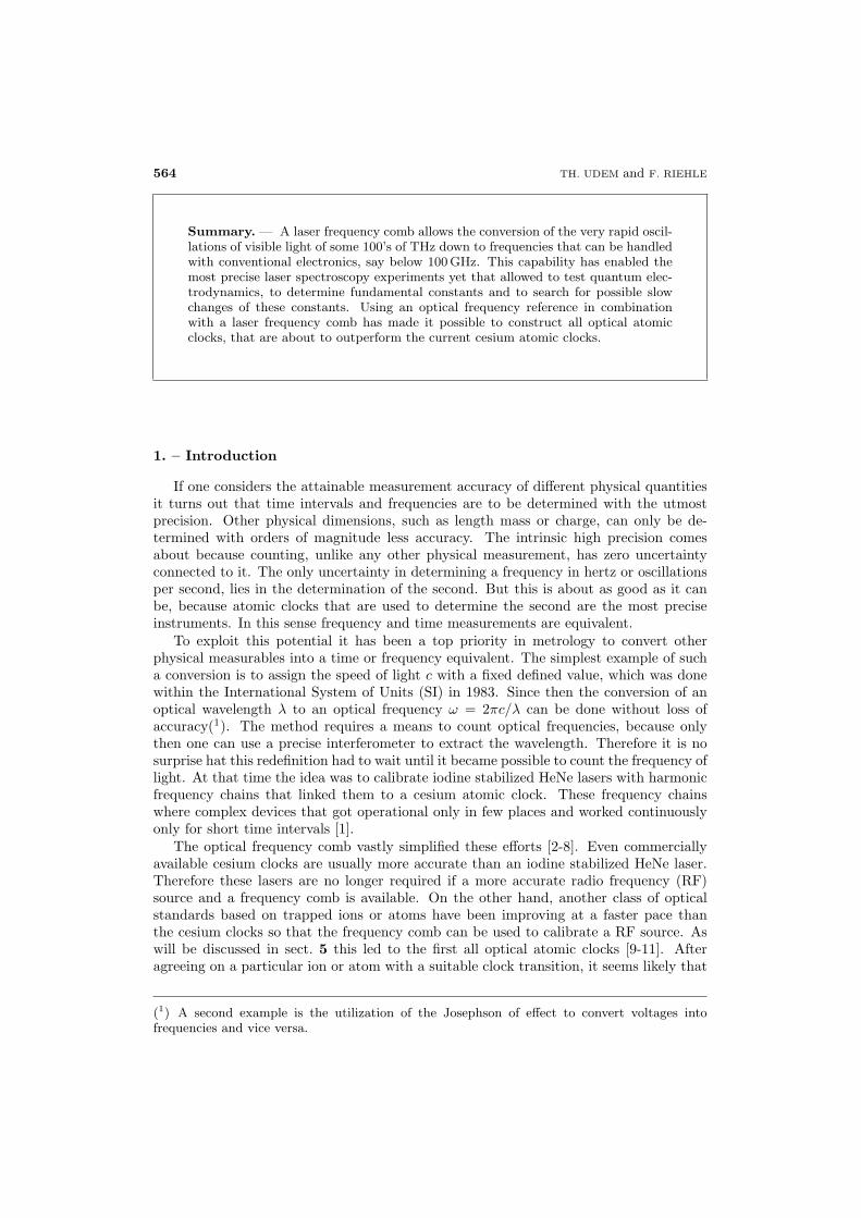
Summary. — A laser frequency comb allows the conversion of the very rapid oscil-lations of visible light of some 100’s of THz down to frequencies that can be handledwith conventional electronics, say below 100 GHz. This capability has enabled themost precise laser spectroscopy experiments yet that allowed to test quantum elec-trodynamics, to determine fundamental constants and to search for possible slowchanges of these constants. Using an optical frequency reference in combinationwith a laser frequency comb has made it possible to construct all optical atomicclocks, that are about to outperform the current cesium atomic clocks.
1. – Introduction
If one considers the attainable measurement accuracy of different physical quantitiesit turns out that time intervals and frequencies are to be determined with the utmostprecision. Other physical dimensions, such as length mass or charge, can only be de-termined with orders of magnitude less accuracy. The intrinsic high precision comesabout because counting, unlike any other physical measurement, has zero uncertaintyconnected to it. The only uncertainty in determining a frequency in hertz or oscillationsper second, lies in the determination of the second. But this is about as good as it canbe, because atomic clocks that are used to determine the second are the most preciseinstruments. In this sense frequency and time measurements are equivalent.
To exploit this potential it has been a top priority in metrology to convert otherphysical measurables into a time or frequency equivalent. The simplest example of sucha conversion is to assign the speed of light c with a fixed defined value, which was donewithin the International System of Units (SI) in 1983. Since then the conversion of anoptical wavelength λ to an optical frequency ω = 2πc/λ can be done without loss ofaccuracy(1). The method requires a means to count optical frequencies, because onlythen one can use a precise interferometer to extract the wavelength. Therefore it is nosurprise hat this redefinition had to wait until it became possible to count the frequency oflight. At that time the idea was to calibrate iodine stabilized HeNe lasers with harmonicfrequency chains that linked them to a cesium atomic clock. These frequency chainswhere complex devices that got operational only in few places and worked continuouslyonly for short time intervals [1].
The optical frequency comb vastly simplified these efforts [2-8]. Even commerciallyavailable cesium clocks are usually more accurate than an iodine stabilized HeNe laser.Therefore these lasers are no longer required if a more accurate radio frequency (RF)source and a frequency comb is available. On the other hand, another class of opticalstandards based on trapped ions or atoms have been improving at a faster pace thanthe cesium clocks so that the frequency comb can be used to calibrate a RF source. Aswill be discussed in sect. 5 this led to the first all optical atomic clocks [9-11]. Afteragreeing on a particular ion or atom with a suitable clock transition, it seems likely that
(1) A second example is the utilization of the Josephson of effect to convert voltages intofrequencies and vice versa.

FREQUENCY COMBS APPLICATIONS AND OPTICAL FREQUENCY STANDARDS 565
the definition of the SI second will be adjusted accordingly.By definition an optical frequency comb consists of many continuous wave laser modes,
equidistant in frequency space, that can be used like ruler to determine large frequencydifferences between lasers. By measuring the frequency separation between a laser at afrequency f and its second harmonic 2f , the lasers absolute frequency f = 2f − f isdetermined [12]. A frequency comb used for that purpose must span a complete opticaloctave. Then, not only f and 2f are known relative to the comb mode spacing, but allthe modes in between, providing an octave full of calibrated laser lines at once.
Since light from lasers has been used to gather nearly all high-precision data aboutatoms, the analysis of this light is key to a better understanding of the microscopic world.To test quantum electrodynamics and to determine the Rydberg constant, transitionfrequencies in atomic hydrogen have been measured [13, 14]. In fact the spectroscopy ofthe narrowest line in hydrogen, the 1S-2S transition, was the motivation for setting up thefirst frequency comb [2-4]. From these measurements the Rydberg constant became themost accurately measured fundamental constant [14]. The frequency comb also helpedto determined the fine-structure constant from atomic recoil shifts [15, 16] using precisevalues of the Rydberg constant and was the key for laboratory searches for possible slowvariations of these constants [17-19]. Even if there is not yet a physical theory that wouldpredict such a slow change there are some arguments, rather philosophically in nature,that they should be there. The frequency combs are now providing a sharp tool for atleast setting up stringent upper limits.
2. – Frequency combs from mode locked lasers
Frequency combs can be produced with fast and efficient electro-optik modulators thatimpose a large number of side bands on a single-frequency continuous laser [20]. Thefactor that limited the achievable width of the generated frequency comb was dispersionof the modulator crystal. After dispersion compensation was introduced [21], boostingthe intensity with external optical amplifier allowed spectral broadening up to 30 THzbandwidth with the process of self-phase modulation [22].
Even more bandwidth can be generated with a device that already included dispersioncompensation, gain and self-phase modulation: the Kerr lens mode-locked laser. Such alaser stabilizes the relative phase of many longitudinal cavity modes such that a solitaryshort pulse is formed. In the time domain this pulse propagates with its group velocity vg
back and forth between the end mirrors of the resonator. After each round trip a copy ofthe pulse is obtained at one of these mirrors that is partially transparent like in any otherconventional laser. Because of its periodicity, the pulse train generated this way producesa spectrum that consists of discrete modes that can be identified with the longitudinalcavity modes. The process of Kerr lense mode locking (KLM) introduced in the early90s [23], allows to generate pulses of 10 femtoseconds (fs) duration and below in a rathersimple way. For Fourier-limited pulses the bandwidth is given by the inverse of the pulseduration, with a correction factor of order unity that depends on the pulse shape andthe way spectral and temporal widths are measured [24]. A 10 fs for example will havea bandwidth of about 100 THz, which is close to the optical carrier frequency, typicallyat 375 THz (800 nm) for a laser operated near the gain maximum of titanium-sapphire,the most commonly used gain medium in these lasers. By virtue of the repeating pulses,this broad spectrum forms the envelope of a frequency comb. Depending on the lengthof the laser cavity, that determines the pulse round trip time, the pulse repetition rateωr is typically on the order of 100 MHz but 4 MHz through 2 GHz repetition rates have
566 TH. UDEM and F. RIEHLE
been used. In any case ωr is a radio frequency readily measured and stabilized. Theusefulness of this comb critically depends on how constant the mode spacing is acrossthe spectrum and to what precision it agrees with the readily measurable repetition rate.These questions will be addressed in the next two section.
2.1. Derivation from cavity boundary conditions. – As in any laser the modes withwave number k(ωn) and frequencies ωn must obey the following boundary conditions ofthe resonator of length L:
(1) 2Lk(ωn) = n2π.
Here n is a large integer number that measures the number of half wavelengths within theresonator. Besides this propagation phase shift there might be additional phase shifts,caused for example by diffraction (Guoy phase) or by the mirror coatings that are thoughtof being included in the above dispersion relation. This phase shift may depend on thewavelength of the mode, i.e. on the mode number n, and is not simple to determineaccurately in practice. So we are seeking a description that lumps all the low-accuracyquantities into readily measurable radio frequencies. For this purpose dispersion is bestbe included by the following expansion of the wave vector about some mean frequencyωm, not necessarily a cavity mode according to eq. (1):
(2) 2L
[k(ωm) + k′(ωm)(ωn − ωm) +
k′′(ωm)2
(ωn − ωm)2 + . . .
]= 2πn.
The mode separation Δω ≡ ωn+1−ωn is obtained by subtracting this formula from itselfwith n being replaced by n + 1:
(3) 2L
[k′(ωm)Δω +
k′′(ωm)2
((ωn+1 − ωm)2 − (ωn − ωm)2
)+ . . .
]= 2π.
To obtain a constant mode spacing, as the most important requirement for optical fre-quency combs, Δω must be independent of n. This is the case if and only if all con-tributions of the expansion of k(ω) beyond the group velocity term k′(ωm) = 1/vg(ωm)exactly vanish. The unwanted perturbing terms, or “higher-order dispersion” terms, thatcontradict a constant mode spacing are those that deform the pulse as it travels inside thelaser resonator. Therefore the mere observation of a stable undeformed pulse envelopestored in the laser cavity leads to a frequency comb with constant mode spacing givenby
(4) Δω = 2πvg
2Lwith vg =
1k′(ωm)
with the round trip averaged group velocity(2) given by vg. Having all derivatives beyondk′(ωm) vanishing, means that k′(ωm) and vg must independent of frequency. Thereforethis derivation is independent of the particular choice of ωm, provided it resides within
(2) The usual textbook approach ignores dispersion either as a whole (Δω = 2πc/2L) or justincludes a constant refractive index: Δω = 2πvph/2L with vph and c being the phase velocitieswith and without dispersive material, respectively.
FREQUENCY COMBS APPLICATIONS AND OPTICAL FREQUENCY STANDARDS 567
the laser spectrum. The group velocity determines the cavity round trip time T of thepulse and therefore the pulse repetition rate ωr = Δω:
(5) T−1 =vg
2L=
ωr
2π.
The frequencies of the modes ωn of any frequency comb with a constant mode spacingωr can be expressed by [3,8, 25,26]
(6) ωn = nωr + ωCE
with a yet unknown frequency offset ωCE common to all modes. As a convention wewill now number the modes such that 0 ≤ ωCE ≤ ωr. This means that ωCE, like ωr
resides in the radio frequency domain. Using (6) to measure the optical frequencies ωn
requires the measurement of ωr, ωCE and n. The pulse repetition rate can be measuredanywhere in the beam of the mode-locked laser. To determine the comb offset requiressome more effort as will be detailed in sect. 3. In practice the beam of a continuous wavelaser whose frequency is should be determined is superimposed with the beam containingthe frequency comb on a photo detector to record a beat note with the nearest combmode. Knowing ωr and ωCE the only thing missing is the mode number n. This may bedetermined by a coarse and simple wavelength measurement or by repeating the samemeasurement with slightly different repetition rates [27].
Some insight on the nature of the frequency offset ωCE is obtained by resolving (6) forωCE and using the cavity averaged phase velocity of the n-th mode vp(ωn) = ωn/k(ωn).With the expansion of the wave vector in (2) and the fact that that it ends with thegroup velocity term, one derives
(7) ωCE = ωn − nωr = ωm
(1 − vg
vp(ωm)
)
For this the frequency offset is independent of n, i.e. common to all modes, and vanishesif the cavity averaged group and phase velocities are identical. In such a case the pulsetrain possesses a strictly periodic field that produces a frequency comb containing onlyinteger multiples of ωr. In general though this condition is not fulfilled and the comboffset frequency is related to the difference of the group and phase round trip time. Foran unchirped pulse, that has a well-defined carrier frequency ωc, it makes sense to expandthe wave vector about ωm = ωc so that eq. (7) becomes
(8) ωCET = Δϕ with Δϕ = ωc
(2L
vg− 2L
vp
).
As discussed in more detail in the next section, it follows that the pulse envelope contin-uously shifts relative to the carrier wave in one direction. The shift per pulse round tripΔϕ is given by the advance of the carrier phase during a phase round trip time 2L/vp ina frame that travels with the pulse. The shift Δϕ per pulse round trip time T = 2L/vg
fixes the frequency comb offset. Hence it has been dubbed carrier-envelope (CE) offsetfrequency.
How precise the condition of vanishing higher-order dispersion is fulfilled in practicecould be estimated by knowing that an irregular phase variations between the modes on

568 TH. UDEM and F. RIEHLE
the order of 2π are sufficient to completely destroy the stored pulse in the time domain.The phase between adjacent modes of a proper frequency comb advances as ωrt, i.e.typically by some 108 times 2π a second. An extra random cycle per second wouldoffset the modes by only 1 Hz from the perfectly regular grid, but destroy the pulse inthe same time. Compared to the optical carrier frequency this corresponds to a relativeuncertainty of 3 parts in 1015 at most, which is already close to the best cesium atomicclocks. Experimentally one observes the same pulse for a much longer time, in somelasers even for months. In fact no deviations have been detected yet at a sensitivity of afew parts in 1016 [28, 7, 29,30].
It should be noted that a more appropriate derivation of the frequency comb mustinclude non-linear shifts of the group and phase velocities because this is used to lockthe modes in the first place. In fact it has been shown that initiating the mode-lockingmechanism significantly shifts the cavity modes of a laser [31]. Of course the questionremains how this mode-locking process forces the cancellation of all pulse deformingdispersive contributions with this precision. Even though this is beyond the scope of thisarticle and details may be found elsewhere [32, 24], the simplest explanation is given inthe time domain: Mode locking, i.e. synchronizing the longitudinal cavity modes to sumup for a short pulse, is most commonly achieved with the help of the Kerr effect whichis expressed in the time domain through
(9) n(t) = n0 + n2I(t).
Here n2 denotes a small intensity I(t) dependence of the refractive index n(t). Generallya Kerr coefficient with a fs response time is very small, so that it becomes noticeable onlyfor the high peak intensity of short pulses. Kerr lens mode locking uses this effect in twoways. The radially intensity variation of a Gaussian mode produces a lens that becomespart of the laser resonator for a short pulse. This resonator is designed such that it haslarger losses without such a lens, i.e. for a superposition of randomly phased modes. Inaddition self phase modulation can compensate the some de-phasing of the modes. Awave packet that does not deform as it travels because higher-order dispersive terms arecompensated by self phase modulation, is called a soliton [33,34]. The nice feature aboutthis cancellation is that it is self-adjusting: Slightly larger peak intensity extends thepulse duration and reduces the peak intensity leaving the pulse energy constant and viceversa. So that neither the pulse intensity nor the dispersion has to be matched exactly(which would not be possible) to generate a soliton. Of course it helps to pre-compensatehigher-order dispersion as good as possible before initiating mode locking. It appearsthat for the shortest pulses the emission bandwidth is basically given by the bandwidththis pre-compensation is achieved [35, 36]. Once mode locking is initiated, mostly bya mechanical disturbance of the laser cavity, the modes are pulled on the regular griddescribed by eq. (6). Another way of thinking about this process is that self phasemodulation that occurs with the repetition frequency, produces side bands on each modethat will injection lock the neighboring modes by mode pulling. This pulling producesthe regular grid of modes and is limited by the injection locking range [37], i.e. how wellthe pre-compensation of higher-order dispersion was done.
2.2. Derivation from the pulse train. – Rather than considering intracavity dispersion,the cavity length and so on, one may simply analyze the emitted pulse train with littleconsideration how it is generated. For this one assumes that the electric field E(t),measured for example at the output coupling mirror, can be written as the product of a

FREQUENCY COMBS APPLICATIONS AND OPTICAL FREQUENCY STANDARDS 569
periodic envelope function A(t) and a carrier wave C(t):
(10) E(t) = A(t)C(t) + c.c.
The envelope function defines the pulse repetition time T = 2π/ωr by demanding A(t) =A(t − T ). The only thing about dispersion that should be added for this description, isthat there might be a difference between the group velocity and the phase velocity insidethe laser cavity. This will shift the carrier with respect to the envelope by a certainamount after each round trip. The electric field is therefore in general not periodic withT . To obtain the spectrum of E(t) the Fourier integral has to be calculated:
(11) E(ω) =∫ +∞
−∞E(t)eiωtdt.
Separate Fourier transforms of A(t) and C(t) are given by
(12) A(ω) =+∞∑
n=−∞δ (ω − nωr) An and C(ω) =
∫ +∞
−∞C(t)eiωtdt.
A periodic frequency chirp imposed on the pulses is accounted for by allowing a complexenvelope function A(t). Thus the “carrier” C(t) is defined to be whatever part of theelectric field that is non-periodic with T . The convolution theorem allows us to calculatethe Fourier transform of E(t) from A(ω) and C(ω):
(13) E(ω) =12π
∫ +∞
−∞A(ω′)C(ω − ω′)dω′ + c.c. =
12π
+∞∑n=−∞
AnC (ω − nωr) + c.c.
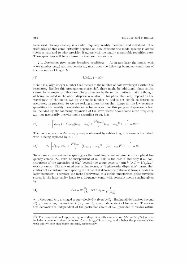
The sum represents a periodic spectrum in frequency space. If the spectral width of thecarrier wave Δωc is much smaller than the mode separation ωr, it represents a regularlyspaced comb of laser modes just like eq. (6), with identical spectral line shapes, namelythe line shape of C(ω) (see fig. 1). If C(ω) is centered at say ωc, than the comb is shiftedfrom containing only exact harmonics of ωr by ωc. The center frequencies of the modemembers are calculated from the mode number n [3, 8, 25,26]:
(14) ωn = nωr + ωc .
The measurement of the frequency offset ωc [2-8]. as described below usually yields avalue modulo ωr, so that renumbering the modes will restrict the offset frequency tosmaller values than the repetition frequency and again yields eq. (6).
The individual modes can be separated with a suitable spectrometer if the spectralwidth of the carrier function is narrower than the mode separation: Δωc � ωr. Thiscondition is easy to satisfy, even with a free-running titanium-sapphire laser. If a singlemode is selected from the frequency comb, one obtains a continuous wave. However itis easy to show that a grating with sufficient resolution would be at least as large asthe laser cavity, which appears unrealistic for a typical laser with a 2 m cavity length.Fortunately for experiments performed so far it has never been necessary to resolve asingle mode in the optical domain as explained in sect. 3.
570 TH. UDEM and F. RIEHLE
��
�� ��� �
�������������������
�� �� �����
� �� �������
����
Fig. 1. – The spectral shape of the carrier function (left), assumed to be narrower than thepulse repetition frequency (Δωc � ωr), and the resulting spectrum according to eq. (13) aftermodulation by the envelope function (right).
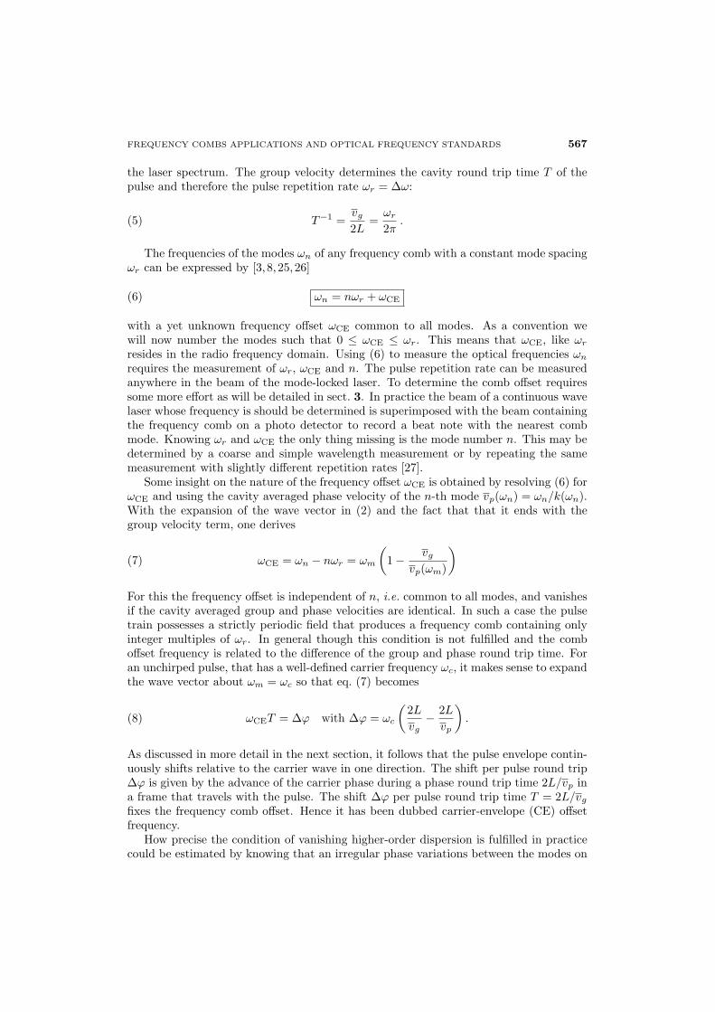
Now let us consider two instructive examples of possible carrier functions. Ifthe carrier wave is monochromatic C(t) = e−iωct−iϕ, its spectrum will be δ-shapedand centered at the carrier frequency ωc. The individual modes are also δ-functionsC(ω) = δ(ω −ωc)e−iϕ. The frequency offset (14) is identified with the carrier frequency.According to eq. (10) each round trip will shift the carrier wave with respect to theenvelope by Δϕ = arg(C(t− T ))− arg(C(t)) = ωcT so that the frequency offset is given
���� Δ
����� ������� ���
��
�����
�
���
��
Δ
Fig. 2. – Consecutive un-chirped pulses (A(t) real) with carrier frequency ωc and the correspond-ing spectrum (not to scale). Because the carrier propagates with a different velocity within thelaser cavity than the envelope (phase- and group velocity), the electric field does not repeatitself after one round trip. A pulse-to-pulse phase shift Δϕ results in an offset frequency ofωCE = Δϕ/T . The mode spacing is given by the repetition rate ωr. The width of the spectralenvelope is given by the inverse pulse duration up to a factor order unity that depends on thepulse shape (the time bandwidth product of a Gaussian pulse for example is 0.441 [24]).

FREQUENCY COMBS APPLICATIONS AND OPTICAL FREQUENCY STANDARDS 571
by ωCE = Δϕ/T [3,8,25,26]. In a typical laser cavity this pulse-to-pulse carrier-envelopephase shift is much larger than 2π, but measurements usually yield a value modulo 2π.The restriction 0 ≤ Δϕ ≤ 2π is synonymous with the restriction 0 ≤ ωCE ≤ ωr introducedearlier. Figure 2 sketches this situation in the time domain for a chirp free-pulse train.
As a second example consider a train of half-cycle pulses like
(15) E(t) = E0
∑k
e−( t−kTτ )2
.
In this case the electric field would be repetitive with the round trip time. ThereforeC(t) is a constant and its Fourier transform is a delta-function centered as ωc = 0. If itbecomes possible to build a laser able to produce a stable pulse train of that kind, all thecomb frequencies would become exact harmonics of the pulse repetition rate. Obviously,this would be an ideal situation for optical frequency metrology(3).
As these examples are instructive it is important to note that one neither relies onassuming a strictly periodic electric field nor that the pulses are unchirped. The strictperiodicity of the spectrum as stated in eq. (13), and the possibility to generate beatnotes between continuous lasers and single modes [38], are the only requirement thatenables precise optical to radio frequency conversions.
In a real laser the carrier wave will not be a clean sine wave as in the above example.The mere periodicity of the field, allowing a pulse-to-pulse carrier envelope phase shift,already guarantees the comb-like spectrum. Very few effects can disturb that property.In particular, for an operational frequency comb, both ωr and ωCE will be servo controlledso that slow drifts are compensated. The property that the comb method really relieson, is the mode spacing being constant across the spectrum. As explained above, evena small deviation from this condition will have very quick and devastating effects on thepulse envelope. Not even an indefinitely increasing chirp could disturb the mode spacingconstancy, as this can be seen as a constantly drifting carrier frequency that does notperturb the spectral periodicity but shifts the comb as a whole. However, the phaseof individual modes can fluctuate about an average value required for staying in lockwith the rest of the comb. This will cause noise that can broaden individual modes asdiscussed in the next section.
2.3. Linewidth of a single mode. – The modes of a frequency comb have to be under-stood as continuous laser modes. As such they possess a linewidth which is of interesthere. Of course as usual in such a case, several limiting factors are effective at the sametime. It is instructive to derive the Fourier limited linewidth that is due to observing thepulse train for a limited number of pulses only. Following a derivation by Siegman [37](4)the linewidth of a train of N pulses can be derived. In accordance with the previous sec-tion we assume that the pulse train consists of identical pulses E(t) separated in time byT and subjected to a pulse-to-pulse phase shift of eiΔϕ:
(16) E(t) =E0√N
N−1∑m=0
eimΔϕE(t − mT ).
(3) It should be noted though that this is a rather academic example because such a pulse wouldbe deformed quickly upon propagation since it contains vastly distinct frequency componentswith different diffraction. For example, the DC component that this carrier certainly has, wouldnot propagate at all.(4) The carrier envelope phase shift was ignored in [37] but can easily be accounted for here.

572 TH. UDEM and F. RIEHLE
For decent pulse shapes, that fall off at least as ∝ 1/t from the maximum, this seriesconverges even as N goes to infinity. Using the shift theorem
(17) FT {E(t − τ)} = e−iωτFT {E(t)}
one can relate the Fourier transform of the pulse train E(t) to the Fourier transform ofa single pulse E(ω). With the sum formula for the geometric series this becomes
(18) E(ω) =E0E(ω)√
N
N−1∑m=0
e−im(ωT−Δϕ) =E0E(ω)√
N
1 − e−iN(ωT−Δϕ)
1 − e−i(ωT−Δϕ).
Now the intensity spectrum for N pulses IN (ω) may be calculated from the spectrum ofa single pulse I(ω) ∝ |E(ω)|2:
(19) IN (ω) =1 − cos(N(ωT − Δϕ))N(1 − cos(ωT − Δϕ))
I(ω).
Figure 3 sketches this result for several N . As the spectrum of single pulse is trulya continuum, the modes are emerging and becoming sharper as more pulses are added.This is similar to the diffraction from a grating that becomes sharper as more grating linesare illuminated. The spectral width of a single mode can now be calculated from (19) andmay be approximated by Δω ≈
√24/TN for the pulse train observation time NT . From
this the Fourier limited line width is reduced after one second of observation time NTto
√24/2π Hz ≈ 0.78Hz and further decreases as the inverse observation time. In the
limit of an infinite number of pulses pulse the spectral shape of the modes approximatedelta-functions with x = ωT − Δϕ ≈ 2πn
(20)12π
limN→∞
1 − cos(Nx)N(1 − cos(x))
≈ 1π
limN→∞
1 − cos(Nx)Nx2
= δ(x).
The whole frequency comb becomes an equidistant array of delta-functions:
(21) IN (ω) → I(ω)∑
n
δ(ωT − Δϕ − 2πn).
The Fourier limit to the linewidth derived here is important when only a numberof pulses can be used for example for direct comb spectroscopy as will be discussed insubsect. 4.5. On the other hand, when a large number of pulses contribute to the signal,for example when measuring the carrier envelope beat note, other limits enter. In mostof these cases acoustic vibrations seem to set the limit as can be seen by observingthat the noise of the repetition rate of an unstabilized laser dies off very steeply forfrequencies above typical ambient acoustic vibrations around 1 kHz [39]. Even if thesefluctuations are controlled as they can be with the best continuous wave lasers, a limitset by quantum mechanics in terms of the power-dependent Schawlow-Townes formulaapplies. Remarkably the total power of all modes enters this formula to determine theline width of a single mode [40]. In fact subhertz linewidths have been measured acrossthe entire frequency comb when it is stabilized appropriately [41,42].
FREQUENCY COMBS APPLICATIONS AND OPTICAL FREQUENCY STANDARDS 573
�
� π
��� � π
����� π
����� π
���
����
�
��������
�����
������
���
��
����
���
����
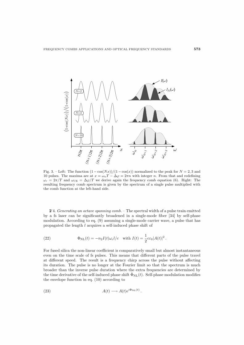
Fig. 3. – Left: The function (1− cos(Nx))/(1− cos(x)) normalized to the peak for N = 2, 3 and10 pulses. The maxima are at x = ωnT − Δϕ = 2πn with integer n. From that and redefiningωr = 2π/T and ωCE = Δϕ/T we derive again the frequency comb equation (6). Right: Theresulting frequency comb spectrum is given by the spectrum of a single pulse multiplied withthe comb function at the left-hand side.
2.4. Generating an octave spanning comb. – The spectral width of a pulse train emittedby a fs laser can be significantly broadened in a single-mode fiber [34] by self-phasemodulation. According to eq. (9) assuming a single-mode carrier wave, a pulse that haspropagated the length l acquires a self-induced phase shift of
(22) ΦNL(t) = −n2I(t)ωcl/c with I(t) =12cε0|A(t)|2 .
For fused silica the non-linear coefficient is comparatively small but almost instantaneouseven on the time scale of fs pulses. This means that different parts of the pulse travelat different speed. The result is a frequency chirp across the pulse without affectingits duration. The pulse is no longer at the Fourier limit so that the spectrum is muchbroader than the inverse pulse duration where the extra frequencies are determined bythe time derivative of the self-induced phase shift ΦNL(t). Self-phase modulation modifiesthe envelope function in eq. (10) according to
(23) A(t) −→ A(t)eiΦNL(t) .

574 TH. UDEM and F. RIEHLE
Because ΦNL(t) has the same periodicity as A(t) the comb structure of the spectrum ismaintained and the derivations of subsect. 2.2 remain valid because periodicity of A(t)was the only assumption made. An optical fiber is most appropriate for this processbecause it can maintain the necessary small focus area over a virtually unlimited length.In practice, however, other pulse reshaping mechanisms, both linear and non-linear, arepresent so that the above explanation is too simple.
Higher-order dispersion is usually limiting the effectiveness of self-phase modulation asit increases the pulse duration and therefore lowers the peak intensity after a propagationlength of a few mm or cm for fs pulses. On can get a better picture if pulse broadeningdue to group velocity dispersion k′′(ωc) is included. To measure the relative importanceof the two processes, the dispersion length LD (the length that broadens the pulse by afactor
√2) and the non-linear length LNL (the length that corresponds to the peak phase
shift ΦNL(t = 0) = 1) are used [34]:
(24) LD =4 ln(2)τ2
|k′′(ωc)|LNL =
cAf
n2ωcP0,
where τ0, Af and P0 = (1/2)Af cε0|A(t = 0)|2 are the initial pulse duration, the effectivefiber core area and the pulse peak power. In the dispersion dominant regime LD � LNL
the pulses will disperse before any significant non-linear interaction can take place. ForLD > LNL spectral broadening could be thought as effectively taking place for a length LD
even though the details are more involved. The total non-linear phase shift can thereforebe approximated by the number of non-linear lengths within one dispersion length. Asthis phase shift occurs roughly within one pulse duration τ , the spectral broadening isestimated to be ΔωNL = LNL/LDτ . As an example consider a silica single mode fiber(Newport F-SF) with Af = 26 μm2, k′′(ωc) = 281 fs/cm2 and n2 = 3.2 × 10⁻¹⁶ cm2/Wthat is seeded with τ = 73 fs Gaussian pulses (FWHM intensity) at 905 nm with 225 mWaverage power and a repetition rate of 76 MHz [3, 4]. In this case the dispersion lengthbecomes 6.1 cm and the non-linear length 35 mm. The expected spectral broadening ofLNL/LDτ = 2π × 44 THz is indeed very close to the observed value [3].
It turns out that within this model the spectral broadening is independent of thepulse duration τ because P0 ∝ τ . Therefore using shorter pulses may not be effectivefor extending the spectral bandwidth beyond an optical octave as required for simpleself-referencing (see sect. 3). However, very efficient spectral broadening can be obtainedin microstructure fiber(5) that can be manufactured with k′′(ωc) ≈ 0 around a designwavelength [43-45]. In this case the pulses are broadened by other processes (linear andnon-linear) than group velocity dispersion as they propagate along the fiber. Eventuallythis will also terminate self-phase modulation and the dispersive length has to be replacedappropriately in the above analysis. At this point a whole set of effects enter such asRaman and Brillouin scattering, optical wave breaking and modulation instability [34].Some of these processes even spoil the usefulness of the broadened frequency combs asthe amplify noise.
A microstructure fiber uses an array of submicron-sized air holes that surround the
(5) Some authors refer to these fibers as photonic crystal fibers that need to be distinguishedform photonic bandgap fibers. The latter use Bragg diffraction to guide the light, while thefibers discussed here use the traditional index step, with the refractive index determined by theair filling factor.

FREQUENCY COMBS APPLICATIONS AND OPTICAL FREQUENCY STANDARDS 575
��������������
��� ��� ��� �� !�� "�� ���� ���� � �� ��������
����
�"�
�!�
� �
���
���
���
���
� �
���
#���$#�$�
�%��%&��
Fig. 4. – Left: SEM image of a the core of a microstructure fiber made at the University ofBath, UK [43]. The light is guided in the central part but the evanescent part of the wavepenetrates into the air holes that run parallel to the fiber core and lower the effective refractiveindex without any doping. The guiding mechanism is the same as in a conventional singlemode fiber. Right: Power per mode on a logarithmic scale (0 dBm = 1 mW). The lighter30 nm (14THz–3 dB) wide spectrum displays the laser intensity and the darker octave spanningspectrum (532 nm through 1064 nm) is observed after the microstructure fiber that was 30 cmlong. The laser was operated at ωr = 2π × 750 MHz (modes not resolved) with 25 fs pulseduration. An average power of 180 mW was coupled through the microstructure fiber [47].
fiber core and run the length of a silica fiber to obtain a desired effective dispersion. Thiscan be used to maintain the high peak power over an extended propagation length andto significantly increase the spectral broadening. With these fibers it became possibleto broaden low peak power, high repetition rate lasers to beyond one optical octave asfig. 4 shows.
A variant of the microstructure fibers are regular single-mode fibers that have beenpulled in a flame to form a tapered section of a few cm lengths [46]. When the diameterof the taper becomes comparable to the core diameter of the microstructure fibers, prettymuch the same properties are observed. In the tapered section the action of the fibercore is taken over by the whole fiber. The original fiber core then is much too smallto have any influence on the light propagation. The fraction of evanescent field aroundthe taper and along with it the dispersion characteristics can be adjusted by choosing asuitable taper diameter.
The peak intensity that can be reached with a given mode-locked laser does not onlydepend on the pulse duration but critically on the repetition rate. Because most laserhave pretty much the same average output power, a lower repetition rate concentratesthis available power into fewer pulses per second. Comparing different laser systems therepetition rates in use cover more than 12 orders of magnitude from the most powerfullasers (one laser shot per 1000 s) to highly repetitive lasers at ωr = 2π × 2 GHz [48]. Ithas been long known that with enough peak intensity one can produce very wide spectrathat where initially called “white light continuum”. Unfortunately for a long time thiswas only possible at a repetition rate of around 1 kHz that indeed justifies the name:The generated spectrum could be called a “continuum” as there was not much hope toresolve the modes in any way for self-referencing or by a beat note with another cw laser.Because of its high efficiency the microstructure fiber allowed to generate an octave widespectra with repetition rates up to 1 GHz that conveniently allowed the beat notes to be

576 TH. UDEM and F. RIEHLE
separated as described in sect. 3. In addition a large mode spacing puts more power ineach mode improving the signal to noise of the beat notes.
The laser that quickly became the working horse in the field for this reason was arather compact titanium-sapphire ring laser with typical repetition rates of 500 MHz to1 GHz [48]. The ring design solved another problem that is frequently encountered whencoupling a laser into an optical fiber. Optical feedback from the fiber may disturb thelaser operation and even prevent mode locking in some cases. The standard solution tothis problem would be to place an optical isolator between the fiber and and the laser.In this case however such a device would have almost certainly enough group velocitydispersion to prevent any subsequent spectral broadening if this is not compensated for.In a ring laser the pulses reflected back from the fiber travel in the opposite directionand do not talk to the laser pulses unless they meet inside the laser crystal. The lattercan be prevented by observing the distance of the fiber from the laser. A disadvantageof these lasers is that they are not easy to align and have so far not become turn keysystems that can be operated unattended for a long time say in an all optical atomicclock (see below).
Even though microstructure fibers have allowed the simple f − 2f self-referencingfor the first time, they also have some drawbacks. To achieve the desired properties,the microstructure fibers need to have a rather tiny core. The coupling to this corecauses problems due to mechanical instabilities and temperature drifts even with lowlevel and stable mounts. Another problem is the observed but not fully understoodstrong polarization dependence of the fibers broadening action. The possibility of long-term continuous operation is not so much of an issue for spectroscopy, because datataking in these experiments usually do not last very long and they need some attentionon there own. However, this possibility seem to be a key requirement operating anall optical atomic clock. So far the only way to operate such a system unattended forhours was to use a set of additional servo systems that continuously measure and correctdeviations from the fiber coupling and polarization [49].
Another problem with spectral broadening by self phase modulation in general isa excess noise level of the beat notes well above the shot noise limit [50, 51]. In factusing the 73 fs laser mentioned above with a microstructure fiber, a two-octave–spanningspectrum is generated within a few centimeters of fiber. However this spectrum does notseparate into modes that could be detected by a beat note measurement with a cw laserbut consist of noise [52]. One possible explanation is the Raman effect that producesstrong gain about 13 THz to the red from the pump wavelength. If this gain is not seeded,it may trigger an avalanche of photons from the vacuum, that bear no phase relationshipto the carrier wave and coherence is lost(6). For sufficiently broad input spectra theRaman gain is seeded coherently with modes from the frequency comb amplifying thelow-frequency modes at the cost of the high-frequency modes. For longer pulses, saybelow 0.441/(13THz) = 34 fs for Gaussian pulse shape, less seeding occurs. In fact amore detailed calculation predicts that enough coherence is maintained by self-phasemodulation if the seeding the pulses are shorter than 50 fs [53].
By going to shorter pulses for the the seed laser this problem can be handled butthe alignment issue remains. On the other hand, lasers that reach an octave-spanning
(6) This process is called “stimulated Raman scattering” because all but the first photon isproduced by stimulated emission. It should be noted though that the first spontaneous photondestroys the coherence of the whole process.

FREQUENCY COMBS APPLICATIONS AND OPTICAL FREQUENCY STANDARDS 577
spectrum without using any external self-phase modulation can solve this problem [54-57].So far however, these lasers seem to be rather delicate to handle so that one alignmentproblem is replaced with another. An interesting alternative are lasers that avoid the useof microstructure fibers in another way. For wide-band but not quite octave-spanninglasers, a 2f − 3f self-referencing becomes possible by doubling the blue wing of thespectrum and beat it with the tripled red wing [58,59]. Such a system can remain phaselocked unattended for several hours without the burden of having extra servo systems.Related but somewhat simpler seems to be a laser that produces pulses short enough sothat a little bit of self-phase modulation generated in single pass through a differencefrequency generating crystal provides sufficient spectral broadening [60].
Yet another class of frequency combs that can stay in lock for even longer times arefs fiber lasers [61]. The most common type is the erbium-doped fiber laser that emitswithin the telecom band around 1500 nm. For this reason advanced and cheap opticalcomponents are available to build such a laser. The mode-locking mechanism is similarto the Kerr lens method, except that non-linear polarization rotation is used to favorthe pulsed high peak intensity operation. Up to a short free-space section that canbe build very stable, these lasers have no adjustable parts. Bulk fused silica has itszero group velocity dispersion at around 1.2μm but this can be shifted to 1.5μm in anoptical fiber. If, in addition, the radial dependence of the refractive index is designed toobtain a small core area Af , the fiber becomes what is called a highly non-linear fiber(HNLF) without any microstructure. These HNLF’s are commercially available and canbe spliced directly to a fs fiber laser. This virtually eliminates the remaining alignmentsensitive parts as the free space frequency doubling stage and bat note detection can bebuild rather robust. Continuous stabilized operation for many hours [62, 63] have beenreported. The Max-Planck Institute fur Quantenoptik in Garching/Germany operatesa fiber based self-referenced frequency comb that stays locked without interruption formonths. A significantly large jitter of the observed CE-beat note has been observed inthese lasers and can either be suppressed by using low noise pump lasers [64] or eliminatedwith a fast servo system.
3. – Self-referencing
The measurement of ωCE fixes the position of the whole frequency comb and is calledself-referencing. The method relies on measuring the frequency gap between differentharmonics derived from the same laser or frequency comb. The first crude demonstra-tion [2] employed the 4th and the 3.5th harmonic of a f = 88.4 THz (3.39 μm) laser todetermine ωCE according to 4ωn − 3.5ωn′ = (4n − 3.5n′)ωr + 0.5ωCE = 0.5ωCE with4n− 3.5n′ = 0. To achieve the condition of the latter equation, both n and n′ have to beactive modes of the frequency comb. The required bandwidth is 0.5f = 44.2 THz whichis what the 73 fs laser together with a single-mode fiber as discussed in the previoussection can generate.
A much simpler approach is to fix the absolute position of the frequency comb bymeasuring the gap between ωn and ω2n of modes taken directly from the frequencycomb [4-8]. In this case the carrier-envelope offset frequency ωCE is directly producedby beating the frequency doubled(7) red wing of the comb 2ωn with the blue side of the
(7) It should be noted that this does not simply mean the doubling of each individual mode, butthe general sum frequencies generation of all modes. Otherwise the mode spacing, and therefore

578 TH. UDEM and F. RIEHLE
%��$��'����#����$
����+����
'������������
(
�)* �
%������$��� %������$��
+$�,����-%��'���
�� �� �
�
��������$���$����$�+'�$
λ�
�$����
%���-
λ� λ�
“'���”
���������##�$���%����.�%����$
“'���” “$�%”
�
λ�
#���$/��'����#����$�
���+���
Fig. 5. – Top: f − 2f self-referencing by detecting a beat note at ωCE between the frequencydoubled “red” wing 2(nωr + ωCE) of the frequency comb and the “blue” modes at 2nωr + ωCE.Bottom: Layout of the self-referencing scheme. See text for details.
comb at ω2n: 2ωn − ωn′ = (2n − n′)ωr + ωCE = ωCE where again the mode numbers nand n′ are chosen such that (2n − n′) = 0. This approach requires an octave spanningcomb, i.e. a bandwidth of 375 THz if centered at the titanium-sapphire gain maximumat 800 nm.
Figure 5 sketches the f − 2f self-referencing method. The spectrum of a titanium-sapphire mode-locked laser is first broadened to more than one optical octave with amicrostructure fiber. A broad-band λ/2 wave plate allows to choose the polarizationwith the most efficient spectral broadening. After the fiber a dichroic mirror separatesthe infrared (“red”) part from the green (“blue”). The former is frequency doubled in anon-linear crystal and reunited with the green part to create a wealth of beat notes, allat ωCE. These beat notes emerge as frequency difference between 2ωn−ω2n according to
the repetition rate, would be doubled as well.

FREQUENCY COMBS APPLICATIONS AND OPTICAL FREQUENCY STANDARDS 579
eq. (6) for various values of n. The number of contributing modes is given by the phasematching bandwidth Δνpm of the doubling crystal and can easily exceed 1 THz. To bringall these beat notes at ωCE in phase, so that they all add constructively an adjustabledelay in form of a pair of glass wedges or corner cubes is used. It is straightforward toshow that the condition for a common phase of all these beat notes is that the green andthe doubled infrared pulse reach the photo detector at the same time. The adjustabledelay allows to compensate for different group delays, including the fiber. In practicethe delay needs to be correct within cΔνpm which is 300 μm for Δνpm = 1 THz. Outsidethis range a beat note at ωCE is usually not detectable.
Whereas the half wave plates in the two interferometer arms are used to adjust forwhatever polarization exits the microstructure fiber, the half wave plate between the twopolarizing beam splitters helps to find the optimum relative intensity of the two beatingpulses. It can be shown that the maximum signal to noise ratio is obtained for equalintensities reaching the detector within the optical bandwidth that contributes to thebeat note [3]. In practice this condition is most conveniently adjusted by observing thesignal-to-noise ratio of the ωCE beat note with a radio frequency spectrum analyzer. Forthis purpose a low-cost analog device that operates up to ωr is usually sufficient.
A grating is used to prevent the extra optical power, that does not contribute to thesignal but adds to the noise level, from reaching the detector. Typically only a largerelative bandwidth of say 1 THz/375 THz needs to be selected so that a very moderateresolution illuminating 375 lines is sufficient. For this reason it is usually not necessary touse a slit between the grating and the photo detector. Sufficient resolution can be reachedwith a small low-cost 1200 lines per mm grating illuminated with a beam collimated with×10 microscope objective out of the microstructured fiber.
When detecting the beat note as described above, more than one frequency componentis obtained for two reasons. First of all any beat note, even between two cw lasers,generates two components because the radio frequency domain cannot decide which ofthe two optical frequencies is larger than the other. Secondly, observing the beat notesbetween frequency combs, not only the desired component k = 2n− n′ = 0 is registered,but all integer values of k, positive and negative contribute, up to the bandwidth of thephoto detector. This leads to a set of radio frequency beat notes at kωr ± ωCE for k =. . .− 1, 0,+1 . . .. In addition the repetition rate, including its harmonics will most likelygive the strongest components. After carefully adjusting the nonlinear interferometer,spatially and spectrally, and scanning the delay line for the proper pulse arrival times,the radio frequency spectrum may look like the one shown in fig. 6. A low-pass filter witha cut-off frequency of 0.5ωr selects exactly one beat note at ±ωCE. The design of such afilter may be tricky, mostly depending on how much stronger the repetition rate signalexceeds the beat note at ωCE. The sketch in fig. 6 gives a feeling on how steep this filterneeds to be at the cut-off in order to suppress the unwanted components below the noiselevel. Such a suppression is required for taking the full advantage of the signal-to-noiseratio. For this reason it is desirable to work at higher repetition rates. At ωr around2π × 800 MHz, as used mostly for the ring titanium-sapphire lasers described above, thefilter requirements are much more relaxed than say at 80 MHz. In addition, a largerrepetition rate concentrates more power in each mode further improving the beat noteswith the frequency comb. It should be noted though, that currently higher repetitionrates cannot be used because the associated lower peak power will make it difficult toachieve spectral broadening beyond one optical octave as detailed in subsect. 2.4.
As described, both degrees of freedom ωr and ωCE of the frequency comb can bemeasured up to a sign in ωCE that will be discussed below. For stabilization of these
580 TH. UDEM and F. RIEHLE
����
�"�
�!�
� �
���
���
���
���
� �
���
�
$�%�+$�,����-#���$�%&�
0��$�$+$�,����-
��−
��
�
��
�
��
��+
��
�
��−
��
�
�����#���+���$
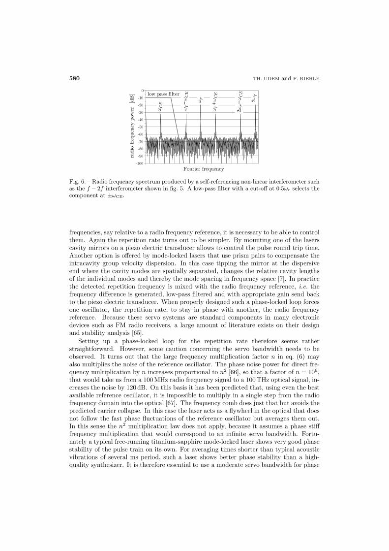
Fig. 6. – Radio frequency spectrum produced by a self-referencing non-linear interferometer suchas the f − 2f interferometer shown in fig. 5. A low-pass filter with a cut-off at 0.5ωr selects thecomponent at ±ωCE.
frequencies, say relative to a radio frequency reference, it is necessary to be able to controlthem. Again the repetition rate turns out to be simpler. By mounting one of the laserscavity mirrors on a piezo electric transducer allows to control the pulse round trip time.Another option is offered by mode-locked lasers that use prism pairs to compensate theintracavity group velocity dispersion. In this case tipping the mirror at the dispersiveend where the cavity modes are spatially separated, changes the relative cavity lengthsof the individual modes and thereby the mode spacing in frequency space [7]. In practicethe detected repetition frequency is mixed with the radio frequency reference, i.e. thefrequency difference is generated, low-pass filtered and with appropriate gain send backto the piezo electric transducer. When properly designed such a phase-locked loop forcesone oscillator, the repetition rate, to stay in phase with another, the radio frequencyreference. Because these servo systems are standard components in many electronicdevices such as FM radio receivers, a large amount of literature exists on their designand stability analysis [65].
Setting up a phase-locked loop for the repetition rate therefore seems ratherstraightforward. However, some caution concerning the servo bandwidth needs to beobserved. It turns out that the large frequency multiplication factor n in eq. (6) mayalso multiplies the noise of the reference oscillator. The phase noise power for direct fre-quency multiplication by n increases proportional to n2 [66], so that a factor of n = 106,that would take us from a 100 MHz radio frequency signal to a 100 THz optical signal, in-creases the noise by 120 dB. On this basis it has been predicted that, using even the bestavailable reference oscillator, it is impossible to multiply in a single step from the radiofrequency domain into the optical [67]. The frequency comb does just that but avoids thepredicted carrier collapse. In this case the laser acts as a flywheel in the optical that doesnot follow the fast phase fluctuations of the reference oscillator but averages them out.In this sense the n2 multiplication law does not apply, because it assumes a phase stifffrequency multiplication that would correspond to an infinite servo bandwidth. Fortu-nately a typical free-running titanium-sapphire mode-locked laser shows very good phasestability of the pulse train on its own. For averaging times shorter than typical acousticvibrations of several ms period, such a laser shows better phase stability than a high-quality synthesizer. It is therefore essential to use a moderate servo bandwidth for phase

FREQUENCY COMBS APPLICATIONS AND OPTICAL FREQUENCY STANDARDS 581
locking the repetition rate of a few 100 Hz at most. A small servo bandwidth may be im-plemented electronically by appropriate filtering or mechanically by using larger massesthan the usual tiny mirrors mounted on piezo transducers for high servo speed. In somecase a complete one inch mirror mount has been moved for controlling the repetitionrate [15].
Controlling the carrier envelope frequency requires some effort. Experimentally itturned out that the energy of the pulse stored inside the mode locked laser has a stronginfluence on ωCE. After initial explanations of this effects turned out to be too crude,more appropriate mechanisms have been found [68,69]. Conventional soliton theory [33]predicts a dependence of the phase velocity but no dependence of the group velocity onthe pulse peak intensity. Any difference in the cavity round trip phase delay and thecavity round trip group delay results in a pulse to pulse carrier envelope phase shift andtherefore a non-vanishing ωCE. However, the intensity dependence of that effect mayturn out to have the wrong sign [70]. The reason is that higher-order effects, usuallyneglected in the conventional soliton theory, play an important role. The Raman effectin the titanium-sapphire crystal produces an intensity-dependent redshift that in turnaffects the group round trip time. In general this leads to an extra term in eq. (8) forthe pulse to pulse carrier envelope phase shift per round trip [69]:
(25) Δϕ = ωc
(2L
vg− 2L
vp+ BIp
).
Because this phase shift is directly proportional to ωCE this equation also describes itsdependence on the pulse peak power Ip. The magnitude of the parameter B may bestbe determined experimentally, as it turns out to depend on the operating parameters ofthe mode-locked laser. In some cases it even changes in sign as the pump laser intensityis changed [51].
To phase lock the carrier envelope offset frequency ωCE, one uses an actuator, inmost cases an acousto-optic modulator, that drains an adjustable part of the pump laserpower. Electro-optic modulators have also been used, but they have the disadvantagethat they need to a bias voltage that wastes some of the pump energy to work in thelinear regime. To servo control the phase of the ωCE component usually requires muchmore servo bandwidth than locking the repetition rate. How much is needed in practicedepends on the type of laser, the intensity and beam pointing stability of the pumplaser and the phase detector in use. Mode-locked lasers that use pairs of prisms tocompensate for group velocity dispersion generally show a much larger carrier envelopefrequency noise. This is because intensity fluctuations slightly change the pulse round trippath because of the intensity-dependent refraction of the titanium-sapphire crystal [71].Even small variations of the beam pointing result in a varying prism intersection. Itshould be noted that already 50μm of extra BK7 glass in the path, shifts the carrierenvelope phase by 2π and the carrier envelope frequency by ωr. In most cases the carrierenvelope frequency fluctuations seem to be dominated by the pump laser noise, so thatstabilizing ωCE with a modulator as described above even reduces this noise. Todaytitanium-sapphire lasers are mostly pumped by frequency doubled solid-state lasers thatseem to show some differences between the models currently on the market [72]. Fiber-based mode-locked lasers used to have significantly larger noise in the carrier envelopebeat note than titanium-sapphire lasers before the semiconductor pump lasers have beenstabilized carefully [64].

582 TH. UDEM and F. RIEHLE
In most cases a simple mixer is not sufficient to detect the phase of ωCE relative to areference oscillator as the expected in-loop phase fluctuations are usually much larger asfor the ωr servo. Prescalers or forward-backward counting digital phase detectors may beused to allow for larger phase fluctuations, that in turn allow the use of moderate speed(several 10 kHz) electronics. A complete circuit that has been used for that purpose verysuccessfully is published in [73]. Stabilizing the carrier envelope frequency, even thoughit generally requires faster electronics, does not have the stability and accuracy issuesthat enter via the repetition rate due to the large factor n in eq. (6). Any fluctuation orinaccuracy in ωCE just adds to the optical frequencies rather than in the radio frequencydomain where it is subsequently multiplied by n.
None of the controls discussed here acts solely on either frequency ωCE and ωr. Ingeneral a linear combination of the two is affected. In practice this turns out to be notimportant because the different speeds of the two servo systems ensure that they do notinfluence each other.
Measuring the frequency of an unknown cw laser at ωL with a stabilized frequencycomb, involves the creation of yet another beat note ωb with the comb. For this purposethe beam of the cw laser is matched with the beam that contains the frequency comb,say with similar optics components as used for creating the carrier envelope beat note.A dichroic beam splitter, just before the grating in fig. 5, could be used to reflect outthe spectral region of the frequency comb around ωL without effecting the beat noteat ωCE. This beam would then be fed into another set-up consisting of two polarizingbeam splitters, one half wave plate, a grating and a photo detector for an optimumsignal-to-noise ratio. The frequency of the cw laser is then given by
(26) ωL = nωr ± ωCE ± ωb ,
where the same considerations as above apply for the sign of the beat note ωb. Thesesigns may be determined by introducing small changes to one of the frequencies with aknown sign while observing the sign of changes in another frequency. For example therepetition rate cold be increased by picking a slightly different frequency of the referenceoscillator. If ωL stays constant we expect ωb to decrease (increase) if the “+” sign (“−”sign) is correct.
The last quantity that needs to be determined is the mode number n. If the opticalfrequency ωL is already known to a precision better than the mode spacing, the modenumber can simply be determined by solving the corresponding equation (26) for n andallowing for an integer solution only. A coarse measurement could be provided by a wavemeter for example if its resolution and accuracy is trusted to be better than the modespacing of the frequency comb. If this is not possible, at least two measurements of ωL
with two different and properly chosen repetition rates may leave only one physicallymeaningful value for ωL [27].
4. – Scientific applications
In this section a few experiments in fundamental research where optical frequencymeasurements have been applied are discussed. Before the introduction of optical fre-quency combs only a few measurements of visible light could be carried out. Since thennot only the available data has multiplied but also its accuracy has improved significantly.Maybe even more important, the frequency combs have enabled the construction of alloptical atomic clocks that are treated in sect. 5.

FREQUENCY COMBS APPLICATIONS AND OPTICAL FREQUENCY STANDARDS 583
&&1
+$�,����-���'
%-�����$
��$��
$�+�$��������-
213
�!���
������������ ����
�����������$�������$ ����
4α�%������$
���%��//��
5
Fig. 7. – Exciting the hydrogen 1S-2S transition with two counterpropagating photons in astanding-wave field at 243 nm. This radiation is obtained from a dye laser frequency doubled ina BBO crystal and stabilized to a reference cavity. While scanning the hydrogen resonance thefrequency of this laser is measured with a frequency comb to be 2 466 061 413 187 074 (34) Hzfor the hyperfine centroid [74].
4.1. Hydrogen and drifting constants. – The possibility to readily count optical fre-quencies has opened up new experimental possibilities. High-precision measurements onhydrogen have allowed for improved tests of the predictions of quantum electrodynamicsand the determination of the Rydberg constant [14]. As the simplest of all stable atomicsystems, the hydrogen atom, provides the unique possibility to confront theoretical pre-dictions with experimental results. To explore the full capacity of such a fundamentaltest, one should aim for the highest possible accuracy so that measuring a frequency isimperative as explained in the introduction. At the same time one should use a narrowtransition line that can be well controlled in terms of systematic frequency shifts. Thenarrowest line starting from the 1S ground state in hydrogen is the 1S-2S two-photontransition with a natural line width of 1.3 Hz and a line Q of 2 × 10¹⁵.
At the Max-Planck-Institute fur Quantenoptik (MPQ) in Garching measurements ofthis transitions frequency around 2466 THz has been improved over many years [13, 19,74]. The hydrogen spectrometer used for that purpose is sketched in fig. 7. It consists of ahighly stable frequency-doubled dye laser whose 243 nm radiation is enhanced in a linearcavity located in a vacuum vessel. The emission linewidth of the dye laser is narrowedto about 60 Hz by stabilizing it to an external reference cavity. This stabilization alsoreduces the drift rate below 1 Hz per second. The linear enhancement cavity ensures thatthe exciting light field is made of two counterpropagating laser fields, so that the Dopplereffect is cancelled to first order. Hydrogen atoms are produced in a gas discharge andejected from a copper nozzle kept at a temperature of 6 K. After propagating the lengthof 13 cm, the excited atoms are detected by quenching them to the ground state in anelectric field. The Lyman-α photon at 121 nm released in this process is then detectedwith a photomultiplier.
The optical transition frequency was determined in 1999 [13] and in 2003 [74] with a

584 TH. UDEM and F. RIEHLE
5����6�789:;
5��6�73<=
>'���6�7<;&
�"�� �"�� �"�� �" � �""� ���������������������� �������������"���!��� ��������
-��$
�� �� � � � �
��
�
�
�
α/α������-$���
μ/μ������ -$�� �
$����������$����-
Fig. 8. – Left: a century of hydrogen data. Since the early 1950’s when quantum electrodynamicswas developed, measurements have been improved by almost 7 orders of magnitude and still noserious discrepancy has been discovered. Right: from the observation of transitions in singletrapped ytterbium and mercury ions and the 1S-2S transition over several years, upper limitson small possible variations of the electromagnetic and the strong interaction can be found. Thelatter appears here as a variation of the cesium nuclear magnetic moment μ measured in unitsof Bohrs magneton.
frequency comb that was referenced to a transportable cesium fountain clock from LNE-SYRTE, Paris [75]. At this time the repeated measurement did not yield an improvedvalue for the 1S-2S transition frequency. Lacking a suitable laser cooling method is aparticular problem for the light hydrogen atom. Even after thermalizing with the coldnozzle to 6 K, the average atomic velocity is v = 360 m/s causing a second-order Dopplereffect of 0.5(v/c)2 = 7 × 10⁻¹³ that needs to be accounted for. In addition the briefinteraction of the atoms with the laser cause a variety of problems and can distort andshift the lineshape in an unpredictable way on the 10−14 level. In addition, because ofthe limited interaction time, larger laser power has to be used for a sufficient excitationrate. This increases to ac Stark shift and cause problems when extrapolating to zero laserpower to find the unperturbed transition frequency. Nevertheless the inaccuracy is onlyabout an order of magnitude larger than the best atomic clocks. A historic summaryof hydrogen spectroscopy is given at the left side of fig. 8. As a remarkable aspect itshould be noted that before the introduction of quantum electrodynamics basically everyorder of magnitude that measurement improved, required a new theory or at least somerefinement. Quantum electrodynamics by now has resisted a gain of almost 7 orders ofmagnitude without such a refinement. This is probably unprecedented for any physicaltheory. The development is summarized at the left panel of fig. 8.
The two comparisons of the hydrogen 1S-2S frequency with the LNE-SYRTE fountainclock may also be used to derive upper limits of possible slow variations of the fundamen-tal interactions. The question of a possible time variation of fundamental constants(8)was first raised in 1937 by P. A. M. Dirac, where he speculated that fundamental con-stants could change their values during the lifetime of the universe [77]. The traditionalway to search for such a phenomenon is to determine the value of say the fine-structureconstant as it was effective billions of years ago. For this purpose atomic absorption lines
(8) For a review on this subject see ref. [76].

FREQUENCY COMBS APPLICATIONS AND OPTICAL FREQUENCY STANDARDS 585
of interstellar clouds back-illuminated by distant quasars have been analyzed [78-81]. Ina related method, the only known natural nuclear fission reactor that became criticalsome 2 billion years ago at Oklo, Gabon has been investigated [82-84]. Analyzing thefission products the responsible cross-sections and from that the fine-structure constantat the time this reactor was active can be deduced.
Now using frequency combs, high-precision optical standards can be compared withthe best cesium clocks on a regular basis. Besides the hydrogen transition, the best mon-itoring data of this type so far derives from comparisons of narrow lines in single trappedmercury [17] and ytterbium [18] ions with the best cesium atomic clocks. Remarkably,the precision of these laboratory measurement makes it possible to reach the same sen-sitivity within a few years of monitoring that astronomical and geological observationsrequire billions of years of look back time. The laboratory comparisons address some ad-ditional issues: Geological and astronomical observations may be affected by systematiceffects that lead to partially contradicting results (see refs. [78,81,85,86] for contradictingresults on quasar absorption and [83,84] for Oklo phenomenon data).
In the laboratory systematics can be investigated or challenged, and if in doubt,experiments may be repeated given the relative short time intervals. So far atomic tran-sition frequencies have been compared with the cesium ground-state hyperfine splitting,which is proportional to its nuclear magnetic moment. The latter is determined by thestrong interaction, but unlike the electronic structure, this interaction cannot easily beexpressed in terms of the coupling constant. Lacking an accepted model describing thedrift of the fundamental constants, it is a good advice trying to analyze the drift datawith as few assumptions as possible. In previous analysis of the Oklo phenomenon, forexample, it was assumed that all coupling constants but the fine-structure constant arereal constant in time. However, if grand unification is a valid theory, at least at someenergy scale, all coupling constants should merge and drift in a coordinated way [87].Therefore the possibility that the cesium ground-state hyperfine splitting, i.e. the paceof the fountain clocks may have changed, should not be ruled out by the analysis. Inthis sense any of the optical frequencies monitored relative to the cesium clock can onlyput limits on the relative drift of the electromagnetic and the strong coupling constant.Fortunately the three mentioned comparisons show different functional dependences onthe fine-structure constant leading to different slopes in a two-dimensional plot that dis-plays the relative drift rates of the coupling constants (see right panel of fig. 8). Theregion compatible with this data is consistent with no drift at all, at a sensitivity levelonly a factor 2 away from the best astronomical observations that have been detecting astatistically significant variation [19]. It should be noted though that without a model forthe drift, linearity in time cannot be assumed, so that the laboratory measurements donot even compare with the astronomical observations as they probe on different epochs.In the near future direct comparisons between different optical transitions will providemuch better data because the cesium clock drops out and some optical transitions aregetting more accurate than even the best cesium fountain clocks [9, 88]. The frequencycomb also allows this type of frequency comparison by locking one of the optical modesωn to the first optical reference and measuring the second with another mode ωn′ . Ide-ally the carrier envelope offset frequency is stabilized to an integer fraction 1/m of therepetition rate, so that the ratio of the two optical frequencies derives as [89].
(27)ωn′
ωn=
n + 1/m
n′ + 1/m.

586 TH. UDEM and F. RIEHLE
No radio frequency enters in this comparison and possible beat notes can also be refer-enced to the repetition rate. Probably the most advanced experiment of this type wouldbe the comparison of narrow transitions in aluminum and mercury ions operated in thegroup of J. Bergquist at NIST, Boulder. These standards are now reaching a reproduciblewithin a few parts in 1017 [9]. To put this in perspective, it should be noted that thegravitational red shift at the Earth’s surface is g/c2 = 1.1 × 10⁻¹⁶ m−1.
4.2. Fine structure constant . – Besides helping to detect a possible variation of thefine-structure constant α, the frequency combs are also useful to determine its actualvalue. All experiments to determine α have in common that a quantity that dependson it, is measured. The fine-structure constant is then determined by inverting thetheoretical expression which usually comes as a power series in α.
As mentioned above, precision spectroscopy of hydrogen has led to an accurate ex-perimental value for the Rydberg constant. Using all the available hydrogen data, i.e.the 1S-2S transition frequency and other less precise measurements [14], a value with anuncertainty of only 7 parts in 1012 is obtained [14, 90]. The Rydberg constant R∞ canbe traced back to other constants according to
(28) R∞ =α2mec
2h,
so that the fine-structure constant α is derived as precise as me/h, the electron massdivided by Planck’s constant, is known. This is because the speed of light c has a definedvalue within the SI units and enters with no uncertainty.
Currently the most precise measurement of the fine-structure constant has an uncer-tainty of 7 parts in 1010 [91]. This measurement is based on an experimental value ofthe electrons gyromagnetic ratio or more precisely its deviation from 2. This quantitycan be calculated with quantum electrodynamics with comparable accuracy in terms ofa power series in α. By comparison with the measured value, the fine-structure constantis determined.
Because α scales the strength of all electromagnetic interactions, it can in principlebe determined with a large number of different experiments. Currently the second bestmethod is based on the recoil an atom, such as cesium [92] or rubidium [93], experienceswhen absorbing an optical photon. Momentum conservation requires that the transitionfrequency is shifted by the kinetic energy associated with the photon momentum hk andthe atomic mass M :
(29) Δω =ΔE
h=
hk2
2M=
h
M
ω2
2c2.
Measuring this recoil shift Δω and the optical transition frequency ω yields a value forM/h. The recoil shift is typically only a few kHz on top of the transition frequency of sev-eral 100 THz. Therefore high-resolution optical frequency measurements are mandatory.To obtain α from (28) one additionally needs to know the mass ration me/M . Atomicmass rations can be measured very precise by comparing their cyclotron frequencies inPenning traps [94]. In fact such an effort was the motivation for the first frequencycomb measurement performed with a femtosecond laser [15]. Note that all ingredientsfor deriving α via eq. (29) are obtained from precision frequency measurements, two ofwhich optical frequencies.

FREQUENCY COMBS APPLICATIONS AND OPTICAL FREQUENCY STANDARDS 587
����� ?���(���
�"!�
�""�
�""�
����
����
����
�-��
��
50:
26�@���#����
,���
���5
���
����$��
���
$�'%�����
��������
�����$��
��
Fig. 9. – The agreement of various values, derived from different experiments is a crucial test forquantum electrodynamics. Currently the values nicely agree within their assigned uncertainty,except the one derived from the Josephson effect. For further details see [91,90].
Even though less precise than the gyromagnetic ratio, the recoil measurements areimportant when it comes to testing of quantum electrodynamics. In general any theorythat uses N parameters can only be said to have a predictive character if at least N + 1different experimental outcomes can be verified. The first N measurements are onlyfixing the parameters. In this context here the available data may be interpreted in away where the gyromagnetic ratio fixes α without any verification of the theory. Therecoil measurements are then interpreted as a test quantum electrodynamics, or the otherway around. Currently the gyromagnetic ratio fits very well with recoil measurementsin cesium and rubidium and other measurements. As fig. 9 shows, the only exemptionmay be a value derived from the Josephson effect, which does not seem to fit within itsassigned error bar.
Finally it should be mentioned that of course quantum electrodynamics could be cor-rect while calculations and/or measurements have some undetected errors. Calculatingthe electron gyromagnetic ratio as a function of α has so far used 891 Feynman diagrams.One might think that the recoil measurements does not show this problem, but derivingthe Rydberg constant from hydrogen data involves a similar complex evaluation [95].
4.3. Optical frequencies in astronomy . – In connection with cosmological search for avariation of what we believe are fundamental constants, optical frequency measurementsare required on samples in the sky and on Earth as reference. Yet another type of obser-vation relies on precise optical frequency measurements. To detect extrasolar planets themost powerful method has been to measure the changing recoil velocity of its star duringthe orbital period. These recoils velocities are rather small unless a massive planet in closeorbit is considered. This is the reason why mostly “hot Jupiters” are among the roughly200 extrasolar planets detected so far. The lightest of those planets possesses about 10Earth masses. The wobble that our planet imposes on the motion of our Sun has a veloc-ity amplitude of only vE = 9 cm/s with a period of one year of course. Because Earth andSun maintain their distance as they go around their common center of mass, this motionis invisible from Earth. On the other hand, it can be detected at other stars, where it issuperimposed with the center-of-mass motion of that system of typically 100’s of km/sand the motion of the Earth around the Sun. To detect Earth-like planets that orbitsun-like suns with the recoil velocity method, a relative Doppler shift of vE/c = 3×10⁻¹⁰
needs to be measurable. Converted to visible radiation of say 500 THz this requires a
588 TH. UDEM and F. RIEHLE
resolution of 150 kHz and the same reproducibility after half the orbital time.Spectral lines from atoms and ions from interstellar clouds and the surface of stars
are subject to strong line broadening due to collisions and the Doppler broadening oftypically several GHz due to their thermal motion. They are measured with telescopeslike the Very Large Telescope operated by the European Southern Observatory whichcan be connected to an Echelle-type spectrometer for high resolution. Given these ratherbroad lines, the required spectral or velocity resolution can be obtained only by usingthe statistics of many lines observed simultaneously. It requires a spectrometer with verysmall irregularities in the calibration curve. So far the rather irregular line spectrum Tr-Ar lamps have been used for that purpose, with large spectral gaps. Using a frequencycomb for this purpose appears to be the optimum tool, both in terms of providing anequidistant dense calibration and for allowing long-term reproducibility that goes wellbeyond the typical life time of an individual spectrometer [96]. The latter propertyderives from the possibility to reference to a precise clock. In this case even a simpleGPS disciplined rubidium clock suffices for the required 3 × 10⁻¹⁰ reproducibility todetect Earth-like extrasolar planets.
In the long run one may even think about direct heterodyne detection with a fre-quency comb. In this scheme the star light is mixed with the frequency comb on a fastphoto detector producing a radio frequency spectrum identical to the optical spectrumbut shifted by the optical frequency. Signal processing can then be done with a radiofrequency spectrum analyzer rather than a with an optical spectrometer. This type ofdetection is known for producing shot noise limited signals and is used to demonstratenoise levels below the shot noise limit with squeezed light. The frequency comb canprovide a large number of optical local oscillators to shift any optical component withinits span to the radio frequency domain.
4.4. Reconstructing pulse transients and generating attosecond pulses. – The appli-cation of the frequency combs has also enabled advances in another field as it allowsthe possibility for stabilizing the carrier envelope phase [3, 6]. According to fig. 2 andeq. (8), a pulse train with a vanishing carrier envelop frequency ωCE has a fixed phase ofthe carrier with respect to the envelope. This means that all the pulses have the sameelectric field. With the technique of self-referencing this can be readily accomplished.However, even though the electric-field transients of the pulses are identical in this case,it is unknown what value the carrier envelope phase actually assumes upon stopping itspulse-to-pulse slippage. In order to figure out at what position the carrier envelope phasehas actually stopped, all delays in the system including the optical path delays have tobe known. Taking into account that the latter progresses by 2π for each wavelengthpropagation distance such an attempt seems unrealistic.
To detect the value of the carrier envelope phase very short pulses that drive processeswhich depend on the electric field in high order are used. The left-hand side of fig. 10shows two extreme values of the carrier envelope phase that correspond to a “cos” and a“sine” pulse. Close observation of the field transients reveals that the peak electric fieldslightly depends on the carrier envelope phase. In addition the duration of the opticalcarrier cycle changes slightly due to the steep pulse envelope when measured say betweentwo field maxima. These effects are largely enhanced if the pulses are short and can bedetected using highly non-linear process such as “high harmonic generation” [100-102]or “above threshold ionization” [103]. High harmonics are generated if pulses of highintensity are focused into a noble-gas jet and are emitted in nicely collimated laser-like beam. Very short wavelengths up to the soft–X-ray regime have been produced this

FREQUENCY COMBS APPLICATIONS AND OPTICAL FREQUENCY STANDARDS 589
��+� ��+��+�
"� ��� ��� � � ��� ��� ���!�
#��������$�-��A�
�#���$��
���$�������?�?�
����#����
��+� ��+��+�
����#����
����#����
����#����
�����'�/�%
Fig. 10. – Left: infrared driving pulses of high intensity and the calculated intensity of highharmonic radiation around the short wavelength cut-off spectral region for two different valuesof the carrier envelope phase [97]. Whereas a “sine” pulse creates two high harmonic pulses,a “cos” produces a single isolated attosecond pulse [98]. Right: measured spectra (differentintensity) for the two values of the carrier envelope phase. It is seen that the cut-off regionlooses its periodicity with the carrier wave as expected for single isolated attosecond pulses.Figures adapted from ref. [97,99].
way [104]. Added to the left-hand side of fig. 10 is the calculated high harmonic radiationat a narrow bandwidth around the high-frequency cut-off. Two important aspects arerealized from this: For “cos” driving pulse the high harmonic pulse is much shorterthan one cycle of the generating field. So by stabilizing the carrier envelope phase tothe proper value (“cos” drive pulses) single isolated attosecond could be produced forthe first time [97, 99]. Secondly the high-harmonic spectrum reveals whether the carrierenvelope phase has been fixed at the proper value or not. A “sine” drive pulse creates twohigh-harmonic pulses, that have almost but not quite the time separation given by thecarrier frequency. For this reason the spectrum shows well-separated peaks even in thecut-off spectral region. However the positions of these peaks are not exactly harmonicsof the infrared driving field. In contrast to that, a “cos” produces a shifted harmonicspectrum that looses its periodicity in the cut-off region. This is because it belongs to asingle isolated attosecond pulse [98], as show in the upper left part of fig. 10. It should benoted that all of this applies only when the high-harmonic radiation is properly filtered.This should be obvious for two reasons: Only the highest harmonics posses enough non-linearity to distinguish the carrier envelope phase settings. Secondly when attosecondpulses are generated, their carrier frequency must be significantly larger than the inversepulse duration.
Not only that the detection and stabilization of the carrier envelope phase allowedthe production of attosecond pulses for the first time, it also allowed to completelyrecover the electric-field transients of ultrashort pulses. The work in that direction reliedon measuring the pulses autocorrelation which, together with the determination of thecarrier envelope phase via spectral analysis of high harmonic allows the calculation of thefield transient [99]. A more direct measurement uses cross correlation between attosecondpulses generated the way described above with the driving pulses. In this way the fieldtransient of the latter can be sampled with a temporal resolution significantly shorter

590 TH. UDEM and F. RIEHLE
�����$��
.�������$�-
����
"�
!�
�
��
��
�! �� � � � !
���%���-�+��
�����$����������?�?�
Fig. 11. – Cross-correlating attosecond pulses with the driving fundamental infrared laser pulses.The attosecond pulses are used to ionize atoms and the liberated electrons are accelerated bythe instantaneous field of the infrared pulses. By changing the delay between the pulses, theelectric-field transient can be sampled with sufficient temporal resolution. Figure courtesy of E.Goulielmakis et al. [105].
than one optical cycle [105]. Figure 11 shows the result of such a measurement.
4.5. Frequency comb spectroscopy . – While for high-resolution spectroscopy of tran-sitions such as the hydrogen 1S-2S single-mode lasers are currently employed, manytransitions of fundamental interest occur at wavelengths too short for state-of-the-artcontinuous wave lasers. The boundary is set by the transparency range of the existingnon-linear crystals. The crystal material that is useful for the shortest wavelength isBBO (β-barium-borate), with a transparency cut-off at about 190 nm. Only with pulsedlasers it is possible to efficiently convert into new regimes in the vacuum UV (200–10 nm),extreme UV (30–1 nm) and possible even the soft X-ray (< 10 nm)(9). The process thatallows this is high-harmonic generation [100-102], that was already discussed in the lastsection. For a long-time–pulsed lasers and high-resolution spectroscopy seemed to ex-clude each other because of the large bandwidth associated with short pulses. However,coherent train of pulses as compared to isolated or non-coherent pulses (say from a Q-switched laser) have quite distinct spectra. The coherent pulse train generated from amode locked laser consists of narrow modes. It was shown in subsect. 2.3 that the Fourierand the Schawlow-Townes limit of the linewidth of an isolated mode is identical to thelinewidth of a single-mode laser of the same type with the same average power. Thisopens the possibility to combine the high peak powers of mode-locked lasers, suitable forfrequency conversion, with the properties of a sharp laser line produced by a single-modelaser.
One obvious problem with this approach is the limited power per mode in a broadfrequency comb. Given an octave-spanning comb, as required for simple self-referencing,this can easily drop below 100 nW in practice. In addition the unused modes may causeexcess ac Stark shift that poses a problem in high-accuracy measurements. Still theseproblems can be handled as demonstrated in ref. [106]. Another solution, at least for the
(9) These spectral ranges are not used in a unified way and partially overlap.
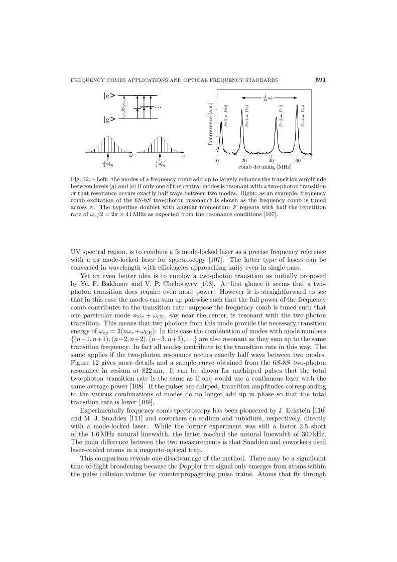
FREQUENCY COMBS APPLICATIONS AND OPTICAL FREQUENCY STANDARDS 591
���π
���
���
� � �� �����'%�������35/�
+���
$�����
����?�?�
� �
��
�
���� ����
���
�*� �
�*� �
�*� �
�*� �
�*� �
�*� �
�*� �
�*� �
�
Fig. 12. – Left: the modes of a frequency comb add up to largely enhance the transition amplitudebetween levels |g〉 and |e〉 if only one of the central modes is resonant with a two-photon transitionor that resonance occurs exactly half ways between two modes. Right: as an example, frequencycomb excitation of the 6S-8S two-photon resonance is shown as the frequency comb is tunedacross it. The hyperfine doublet with angular momentum F repeats with half the repetitionrate of ωr/2 = 2π × 41MHz as expected from the resonance conditions [107].
UV spectral region, is to combine a fs mode-locked laser as a precise frequency referencewith a ps mode-locked laser for spectroscopy [107]. The latter type of lasers can beconverted in wavelength with efficiencies approaching unity even in single pass.
Yet an even better idea is to employ a two-photon transition as initially proposedby Ye. F. Baklanov and V. P. Chebotayev [108]. At first glance it seems that a two-photon transition does require even more power. However it is straightforward to seethat in this case the modes can sum up pairwise such that the full power of the frequencycomb contributes to the transition rate: suppose the frequency comb is tuned such thatone particular mode nωr + ωCE, say near the center, is resonant with the two-photontransition. This means that two photons from this mode provide the necessary transitionenergy of ωeg = 2(nωr +ωCE). In this case the combination of modes with mode numbers{(n−1, n+1), (n−2, n+2), (n−3, n+3), . . .} are also resonant as they sum up to the sametransition frequency. In fact all modes contribute to the transition rate in this way. Thesame applies if the two-photon resonance occurs exactly half ways between two modes.Figure 12 gives more details and a sample curve obtained from the 6S-8S two-photonresonance in cesium at 822 nm. It can be shown for unchirped pulses that the totaltwo-photon transition rate is the same as if one would use a continuous laser with thesame average power [108]. If the pulses are chirped, transition amplitudes correspondingto the various combinations of modes do no longer add up in phase so that the totaltransition rate is lower [109].
Experimentally frequency comb spectroscopy has been pioneered by J. Eckstein [110]and M. J. Snadden [111] and coworkers on sodium and rubidium, respectively, directlywith a mode-locked laser. While the former experiment was still a factor 2.5 shortof the 1.6 MHz natural linewidth, the latter reached the natural linewidth of 300 kHz.The main difference between the two measurements is that Snadden and coworkers usedlaser-cooled atoms in a magneto-optical trap.
This comparison reveals one disadvantage of the method. There may be a significanttime-of-flight broadening because the Doppler free signal only emerges from atoms withinthe pulse collision volume for counterpropagating pulse trains. Atoms that fly through

592 TH. UDEM and F. RIEHLE
this volume can only absorb a limited number of pulses that cause the line broadeningeffects described in subsect. 2.3. To obtain a narrow resonance, it is therefore importantto apply many pulses, ideally for a time that exceeds the inverse natural linewidth. Whenusing fs pulses the collision volume may be smaller than 1 mm so that the atoms mustbe laser cooled and/or trapped as in ref. [111] to reach the natural linewidth. Note thatthe time-of-flight broadening may also be understood as a residual first-order Dopplereffect. This comes about because, unlike the single-mode case, the Doppler shift k1v and−k2v for counterpropagating beams with wave numbers k1 and −k2 does not exactlycompensate for the motion of the atom with velocity v. However for any residual first-order Doppler shift there exists a component obtained by exchanging the wave numbersk1 ⇀↽ k2 that possess the opposite shift. Hence a pure broadening and no shift resultsjust as in the time domain description. This is certainly an advantage.
In the meantime several other groups have used laser-cooled atoms for frequency combspectroscopy [112, 113]. S. Witte and coworkers used UV pulses at 212 nm generated inconventional non-linear crystals to excite a two-photon transition in krypton [114]. Inthis work only 3 pulses could be applied to the atoms so that the expected linewidthwas about one third of the repetition rate or 23 MHz. Indeed that is about the observedlinewidth which compares to the natural linewidth of 6.9 MHz. This experiment demon-strates the principle, knowing that improvements by many orders of magnitude shouldbe possible. However, realizing these disadvantages of frequency comb spectroscopy, itappears advisable to use a continuous wave laser whenever possible. On the other hand,if there is no laser of this kind, frequency comb spectroscopy can become a very power-ful method. One of the first demonstration in the short, so far inaccessible wavelengthrange, uses the ninth harmonic of a titanium-sapphire laser generated in a xenon gas jetto perform Ramsey-type spectroscopy on krypton at 88 nm [115]. The Ramsey methodis identical to frequency comb spectroscopy with two pulses and produces narrow linesonly when the two pulses come at a long delay (low repetition rate). In the meantime thesame Ramsey-type spectroscopy has also been demonstrated at a one-photon transitionin xenon at 125 nm [116]. The required radiation was obtained as the third harmonicproduced in a gas cell. In this experiment the “repetition rate”, i.e. the time separationbetween the Ramsey pulses was varied to increase the resolution.
Using high harmonics from titanium-sapphire lasers several 100 octaves of laser radi-ation may be addressed without gaps. Given the large tunability of these lasers allowsto shift between the harmonics seamlessly. Therefore it might become possible to usea single laser system to cover everything from the near infrared to soft X-rays withatomic clock resolution. A possibility that seems out of reach for single-mode lasers. Forsuch a general laser system there is yet another obstacle that needs to be solved. Sofar long pulse trains of many pulses at very short wavelengths with a high repetitionrate necessary to resolve the modes have been contradicting requirements. This is be-cause all methods up to very recently, that allowed to reach the necessary intensity forhigh-harmonic generation of typically 5 × 10¹³ W/cm2, effectively concentrate the avail-able average power in fewer pulses per second. For this the repetition rate is typicallyreduced to the kHz regime. The modes of the resulting dense frequency comb wouldbe very difficult to resolve. Even if the time-of-flight broadening could be reduced, sayby using trapped ions and transitions with narrow natural linewidths, the requirementson the laser system would be difficult to achieve. For this reason a method allowingthe production of high-harmonic radiation with MHz repetition rates was sought. Thesolution to this problem was to use an enhancement resonator for the driving pulses withan intracavity gas jet for high-harmonic generation [117, 118]. This method is similar

FREQUENCY COMBS APPLICATIONS AND OPTICAL FREQUENCY STANDARDS 593
to resonantly enhanced second-harmonic generation that has been used for many years.However, there are several extra requirements that need to be fulfilled in order to res-onantly enhance fs pulses. First of all the pulse round trip time in that cavity has tobe matched to repetition rate of the laser. In fact this is not difficult to accomplish andstandard continuous wave locking schemes can be applied to stabilize the frequency combto the modes of the enhancement resonator. Somewhat more difficult is it to preventthe pulse stored in the enhancement resonator from reshaping, or more precisely to re-shape it such that after one round trip it will match the next pulse from the laser. Asdiscussed in subsect. 2.1 this means that the carrier envelope phase shift of the cavityhas to be the same as for the laser and higher-order dispersion has to be suppressed. Inthe frequency domain this simply means that the modes of the enhancement resonatormust be equidistant in frequency just as the frequency comb is. In this case all modescan resonate at the same time. So far this problem has not been solved completely, sothat the high-harmonic intensity generated this way still seems too low for a reasonabletransition rate in stored ions. Fortunately this process scales very favorably with thedriving intensity I. The so-called plateau harmonics scale with number of fundamentalphotons required for ionization, which is ∝ I9 for Xe driven with a titanium-sapphirelaser around 800 nm.
5. – All optical clocks
Most likely the first time piece of mankind was the periodic movement of a shadowcast by a fixed object. The daily period would measure the Earth rotation and thesuperimposed annual period could be used to find the solstice and measure the lengthof the year in units of days. Later other periodic phenomena have been used. For anoperational clock the periodic phenomena or oscillator has to be completed by a counterthat keeps track of the number of periods. The early sundials had a human operator forcounting the days. Later pendulum clocks used mechanical counters and todays preciseclocks such as quartz or atomic clocks have electronic counters. If we look at the historyof time keeping, it becomes obvious that clocks got more accurate as the oscillationfrequency increased. One simple reason for that is that higher oscillation frequencies canslice time into finer intervals. Similar to a ruler that improves with the density of lengthmarks.
The two most important properties of clocks are accuracy and stability. The formerdescribes at what level two identically constructed clocks agree. The clocks stability,on the other hand, measures how well a particular clock maintains its pace. Both,accuracy and stability are determined by comparing at least two clocks and are limitedby many factors such as the oscillators sensitivity to external perturbations. An increasedoscillator frequency helps to improve stability. As an example consider the Earth rotationrepresented by a sundial and a good quartz oscillator. Whereas the two oscillators maybe comparable in terms of accuracy, it would be much more difficult to measure a periodof one second with a sundial than with a quartz oscillator that typically vibrates 32 768times a second. Even faster than the vibration of a quartz standard is the precession ofthe Cs nuclear magnetic moment in the magnetic field of its electrons. This frequencyhas been defined within the International Systems of Units (SI) to be exactly 9 192 631770 Hz.
To quantify the mutual stability of two oscillators a statistical analysis of a set ofsubsequent phase comparisons, obtained by averaging over time intervals τ , is used. Forthis purpose one may not use the standard deviation because it does not converge if the

594 TH. UDEM and F. RIEHLE
two clocks have slightly different frequencies, which is almost always the case. Instead thestatistical analysis is done in terms of the Allan variance σ(τ) [119]. Having eliminatedall other sources of instability an atomic oscillator, that obeys the laws of quantummechanics, possesses the following expression for the Allan variance:
(30) σ(τ) =Δω0
πω0
√Tc
2Nτ.
Here the frequency and the linewidth of the transition are given by ω0 and Δω0, respec-tively and the number of oscillators (atoms or ions) and the interrogation time is given byN and Tc. Modern Cs atomic clock can be operated close to that limit [75]. Of course theAllan variance will not reduce indefinitely for longer averaging times as suggested by thequantum limit. At some point varying systematic effects will set in and prevent furtherreduction. Current state-of-the-art Cs clocks need to be averaged for hours to reach thatlimit at around one part in 1015. If one sets out to reach an accuracy of one part in 1018,which is the predicted systematic uncertainty for some optical transitions, the necessaryaveraging times would extend by 6 orders of magnitude according to eq. (30). This ofcourse is no longer useful for any practical purpose.
Fortunately the same equation suggests that one can make up for this by increas-ing the transition frequency ω0 as illustrated above. At first glance it may seem thatreducing the linewidth Δω0 by choosing a narrow transition would serve the same pur-pose. In principle one could pick an almost arbitrary narrow transition, such as betweenground-state hyperfine levels that basically live forever or highly forbidden transition suchas the Yb+ 2S1/2 → 2F7/2 transition, whose upper level lives for about ten years [120].However this means that there will be one photon of information per lifetime available atmost, assuming 100% detection efficiency. For this reason a much better strategy is to usea larger transition frequency such as an optical transition leaving the linewidth, i.e. theinverse transition rate fixed. Ideally one would choose an optical transition that repre-sents an oscillator at frequency of several hundreds of terahertz. Operating at these highfrequencies would have been possible after tremendous advances in laser spectroscopyin the 1970s that ultimately resulted in trapped atom and ion standards [121] in the1980s. What was missing though was an efficient counter that keeps track of these fastoscillations. When it became possible to count these oscillations with the so-called har-monic frequency chains in the early 1970s [122], physicists started to seriously thinkingof running an optical clock. However, working with these counters was so tedious thatmost of the harmonic frequency chains never reached the stage where they could operatecontinuously even for minutes. So it was decided to use them only to calibrate somechosen frequencies, like iodine or methane stabilized HeNe lasers, that could then bereproduced in other labs that could not provide the tremendous resources required forsetting up a harmonic frequency chain. The calibrated lasers where then mostly usedas wavelength references in interferometers for the realization of the meter and in somescientific experiments as frequency references.
With the introduction of femtosecond frequency combs a reliable running opticalclock became reality. In particular the fiber-based frequency combs can now run formonths with out touching them [63]. In addition excess noise observed in these lasershas recently been suppressed to the level of titanium-sapphire laser [64]. One of the firstset-ups that deserved the term “optical clock” used a transition at 1064 THz in a trappedsingle mercury ion operated at NIST [89]. For a device deserving this name one wouldask for some requirements on its accuracy and its ability to be operated long enough to

FREQUENCY COMBS APPLICATIONS AND OPTICAL FREQUENCY STANDARDS 595
�" � �"!� ���
���B���
�B���
��
�?�
�?���
�����
���"
���� ����.����$����-���#�$%�-
�
�����
�"�� �""� ���
���������������������������
�� ������ ������
-��$
$����������$����-
Fig. 13. – The historic comparison of radio frequency standards reveals that just about now theoptical standards seem to take over the lead. The current lowest uncertainty is reached withthe Hg+ clock at NIST [9] with an estimated standard uncertainty of 7 parts in 1017.
calibrate a hydrogen maser for example. The NIST Hg+ clock can be operated repeatedlywith an uncertainty low enough such that comparison with an ensemble of very stablehydrogen masers resulted in an Allan variance of the latter [9]. By now many nationalstandard institutes are working on optical atomic clocks. The Physikalisch-TechnischeBundesanstalt, Germany (PTB) on Yb+ [123], the National Physics Laboratory, UK(NPL) on Sr+ and Yb+ [11] and the Laboratoire national de metrologie et d’essais—Systeme de References Temps-Espace, France (LNE-SYRTE) on neutral Sr [124] to namea few. The tremendous progress of the optical standards made since frequency combswhere introduced is summarized in fig. 13.
To operate a frequency comb as a clockwork mechanism one might stabilize its nearestmode ωk to the clock transition. Similar to the frequency ratio scheme of eq. (27), thecarrier envelope offset frequency and possibly any local oscillator used in the stabilization,can be locked to an integer fraction m of the repetition rate [89].
(31) ωk = kωr + ωCE = ωr(k + 1/m).
The countable clock output is then obtained in form of the pulse repetition rate thatis given by the optical reference ωk divided by k + 1/m. No other reference frequencybesides the optical reference is required at this point as it should be for a real clock.In particular there is no radio frequency source required other than the repetition rate.To use the repetition rate in this way as a radio frequency generator is advantageous asit can be shown that, on a short time scale, this frequency is more stable than a goodsynthesizer even for a free-running laser [39].
6. – Optical frequency standards
Since the redefinition of the unit of length, the meter, in the International Sys-tems of Units (SI) in 1983 by the 17th General Conference on Weights and Measures(CGPM) [125] the speed of light is fixed by definition to c = 299 792 458 m/s. With the
596 TH. UDEM and F. RIEHLE
general relation c = λ× ν any radiation emitting device whose frequency ν and hence itswavelength λ is stable and can be traced back to the frequency of the Cs clock can be usedas a frequency standard or a wavelength standard. Such frequency standards have beenused for decades for interferometric length metrology. The International Committee ofWeights and Measures (CIPM) has therefore recommended a list of evaluated frequencystandards, i.e. the so-called Mise en Pratique for the definition of the Metre [126] whichhas been updated on several occasions [125,127,128].
The first frequency standards in this list where mainly gas lasers whose frequencieswere stabilized to the saturated absorption of suitable transitions in molecules. Theselected molecules by natural coincidence have transitions whose frequencies are locatedin the tuning range of the laser. The most prominent examples are the CH4 stabilizedHe-Ne laser at 3.39 μm, the OsO4 stabilized CO2 laser at 10.3 μm and the I2 stabilizedNe-He or Nd:YAG lasers at 632 nm and 532 nm, respectively. While the first two of theselasers probably have the best reproducibility of all lasers stabilized this way, the muchmore compact and transportable iodine stabilized laser has been the working horse inlength metrology for quite some time. The best of these lasers are reproducible within afew parts in 1013 and therefore cannot compete with the current Cs atomic clocks.
The possibility to cool atoms and ions by laser radiation has led to optical frequencystandards that could rival the best microwave clocks. In these laser-cooled quantumabsorbers suitable narrow transitions can be interrogated that are no longer excessivelybroadened and shifted by effects associated with the velocity of the absorbers, e.g., theshort interaction time and the influence of the second-order Doppler effect.
Optical frequency standards employing ions or neutral atoms as the frequency refer-ences show distinctive differences. Ions can be stored in a so-called radio frequency trapwhere an alternating electric voltage is applied to a suitable arrangement of electrodesthat results in a net force onto the ions directed towards the field-free center of the iontrap. Since alike charged ions repel each other only a single ion can be kept in the centerwhereas the non-vanishing field outside the center in general shifts the transition fre-quency. Most accurate ion frequency standards therefore store only a single ion which,however, leads to a very weak signal.
To produce a much stronger signal and an associated much higher stability as com-pared to single ions (N = 1 in eq. (30)) the second type of laser-cooled optical frequencystandards uses clouds of millions of neutral atoms. In this case though collisions betweenthe atoms may result in uncontrollable shifts in frequency. In other words, so far (butnot necessarily in the long run) single-ion standards have high statistical but low sys-tematic uncertainties whereas neutral-atom standards have excellent short-term stabilitybut poorer systematic properties.
The recent progress with optical frequency standards in the mean time motivatedthe CIPM to recommend in autumn 2006 four optical frequency standards (see table I)that can be used as “secondary representations of the second” and be included intothe new list of “Recommended frequency standard values for applications including thepractical realisation of the metre and secondary representations of the second”. Thephrase “secondary representations” takes into account that the frequency of such anoptical frequency standard can never surpass the accuracy of the primary standard of timeand frequency, the Cs clock, but that it might be very important also for time keepingto use optical clocks because of their better stability. We will discuss the frequencystandards of table I in more detail in the following subsections.
The uncertainties given in table I are in general larger than the uncertainties presented

FREQUENCY COMBS APPLICATIONS AND OPTICAL FREQUENCY STANDARDS 597
Table I. – Optical clock transitions recommended by the CIPM.
Ion/Atom Transition Frequency/ Fractionalwavelength uncertainty
88Sr+ 5s 2S1/2-4d 2D5/2 444 779 044 095 484 Hz 7 × 10⁻¹⁵
674 nm171Yb+ 6s 2S1/2-5d 2D3/2 688 358 979 309 308 Hz 9 × 10⁻¹⁵
435 nm199Hg+ 5d10 6s 2S1/2-5d9 6s2 2D5/2 1 064 721 609 899 145Hz 3 × 10⁻¹⁵
282 nm87Sr 5s 2S1/2-4d 2D5/2 429 228 004 229 877 Hz 1.5 × 10⁻¹⁴
698 nm
in the relevant publications since additional contributions have been taken into accountcaused for example by the uncertainty in linking to different Cs clocks.
6.1. Optical frequency standards based on single ions. – The trapping and preparationof ions and their use for frequency standards has been described in detail in a number ofreviews and textbooks (see, e.g., [129-132]). An important feature however is the specialkind of interrogation of single ions that will be discussed briefly in the following.
6.1.1. Clock interrogation by use of quantum jumps. A properly chosen ion can get closeto the ideal situation where a single unperturbed particle at rest is probed. The drawbackthough is that a single ion does not produce a strong signal by scattering many photonsper second on the clock transition. However, the method of quantum jumps or elec-tron shelving proposed by Dehmelt [133,134] and demonstrated later in Wineland’s [135]and Dehmelt’s group [136] is capable to detect a transition with unity probability. Thetechnique is often applied to so-called V-systems where, as in fig. 14, a strong (cooling)
Fig. 14. – Excerpt from the energy level diagram of Yb+. The transition at 369 nm is used forcooling the ion and for detecting quantum jumps (see text). Dashed lines (411 nm, 435 nm and467 nm) represent transitions that were proposed for optical clocks.
598 TH. UDEM and F. RIEHLE
transition and a weak (clock) transition are connected at the ground state. When the ionis irradiated by radiation whose frequency is in resonance with the strong transition up toabout 108 absorption-emission cycles lead to the same number of emitted photons. Evenwith a limited detection probability of the order of 10−3 about 105 photons per secondcan be detected. If, however, the ion is excited on the weak clock transition by resonantradiation, the excited electron is “shelved” in the excited state. Consequently the fluores-cence on the strong transition cannot be excited before the ion makes a transition to theground state again. Thus the fluorescence light from the strong transition monitors the“quantum jumps” of the ion into the excited state and back as sudden intensity changes.
6.1.2. Yb+ and Hg+ single-ion standards. The clock transitions of the 171Yb+ and199Hg+ ions given in table I are quadrupole transitions with natural linewidths of 3.1 Hzand 1.1 Hz, respectively. The level scheme of both ions is basically very similar andhence both systems will be treated here at the same time. In Yb+ the transition at369 nm is used for cooling the ion and for detecting quantum jumps. The 2S1/2-2D3/2
transition at 435 nm is preferred, rather than the 2S1/2-2D5/2 transition at 411 nm sincethe 2D5/2 level decay may occur into the long-lived 2F7/2 that has a natural lifetime ofabout ten years. This level is connected to the ground state by an 467 nm octupole clocktransition with a natural linewidth of the transition in the nanohertz range [120] and isalso investigated as an optical frequency standard.
Two independent 171Yb+ single-ion optical frequency standards operating at the435 nm line were compared at PTB to look for systematic frequency shifts. A signif-icant contribution to the systematic uncertainty could result from the interaction of theatomic electric quadrupole moment with the gradient of an electric stray field in the trap.Two methods can be used to eliminate the quadrupole shift. One uses the fact that thequadrupole shift averages to zero in three mutually orthogonal directions of the magneticquantization field [137]. A second method uses the fact that the average over all Zeemanand quadrupole shifts of all magnetic sublevels is zero [138].
Another possible systematic shift can result from the quadratic Stark shift. In the caseof the 171Yb+ clock transition the scalar polarizability of the ground state, αS(2S1/2), andfrom the scalar and tensorial polarizabilities of the 2D3/2 state, αS(2D3/2) and αT (2D3/2)contribute to this effect. The contribution has been measured and is corrected for.
For the unperturbed clock transition a mean relative frequency difference of the fre-quencies between both standards of (3.8±6.1)×10−16 was observed [88]. This agreementis similar to that of the most accurate comparisons between cesium fountain clocks. Thefrequency of the 171Yb+ standard was measured with a relative systematic uncertaintyof 3 × 10⁻¹⁵ and a statistical uncertainty of 0.6 × 10⁻¹⁵ using a femtosecond frequencycomb generator based on an Er3+-doped fiber laser [139].
A similar level scheme of the cooling and clock transitions is present in the opticalfrequency standard based on the 1.06×10¹⁵ Hz (282 nm) electric quadrupole transition ina single trapped 199Hg+ ion that was developed at NIST. This frequency standard uses acryogenic spherical electromagnetic (Paul trap) to trap a single Hg ion for up to 100 days.The frequency measurements over a period of more than five years between the 199Hg+
standard and the Cs primary clock transition agreed to better than 1× 10⁻¹⁵ over threeyears [9]. A fractional frequency instability of about 7 × 10⁻¹⁵ at 1 s was demonstratedthat follows the τ−1/2 dependence down to the 10−17 regime. The uncertainty budgetpresented from the NIST groups leads to a total fractional uncertainty of 7.2 × 10⁻¹⁷
and represents the smallest uncertainty to find the unperturbed line center reported foran optical clock. This uncertainty is an order of magnitude smaller as the uncertainty

FREQUENCY COMBS APPLICATIONS AND OPTICAL FREQUENCY STANDARDS 599
Fig. 15. – 40Sr+ energy level scheme.
of the best cesium atomic clocks. As a result the frequency (in SI Hz) of such an opticalclock can never surpass the uncertainty of the latter one.
6.1.3. 88Sr+ single-ion standard. In contrast to the Yb+ and Hg+ single-ion standardsdiscussed so far the 88Sr+ 5s 2S1/2-4d 2D5/2 at 674 nm 444 779 044 095 484 Hz (fig. 15) ofthe even isotope is lacking hyperfine structure. Thus there is no magnetic-field insensitivemF=0 → mF=0 transition and a small external field splits the clock transition with anatural linewidth of 0.4 Hz into five pairs of Zeeman components.
This standard is investigated at the British National Physical Laboratory (NPL) [140]and at the National Research Council (NRC) [138] of Canada. In order to eliminate thefirst-order Zeeman shift, these groups probe alternately a symmetric pair of Zeemancomponents.
6.2. Neutral atom optical frequency standards. – Neutral-atom–based frequency stan-dards can be divided in three groups: the first one is based on free atoms in an atomicbeam effusing from a nozzle and collimated by diaphragms.
6.2.1. Atomic beam standards. The most advanced beam standard in the optical regimeare the hydrogen standard based on the 1S-2S transition in atomic hydrogen [13,19,74]described above and the Ca standard based on the 1S0-3P1 transition (see fig. 16) inatomic Ca [141-143]. The large velocity of the atoms leads to a large second-orderDoppler effect which leads to a considerable broadening and shift of the interrogatedline. Even though techniques that suppress the first-order Doppler effect were applied,residuals resulting from non-ideal alignment or curvature of the interrogating opticalbeams (residual first-order Doppler effect) occur that seem to prevent the use of atomicbeam for use in optical frequency standards with the highest accuracy.
6.2.2. Neutral atom standards based on ballistic atoms. The large influence of the first-and second-order Doppler effects can be reduced very efficiently by laser cooling theatoms, e.g., in a magneto-optical trap. After shutting off the magneto-optical trap thereleased atoms have an initial velocity between a few cm/s and a m/s and follow ballisticpaths in the gravitational field. Due to the free fall the interrogation of these atoms is
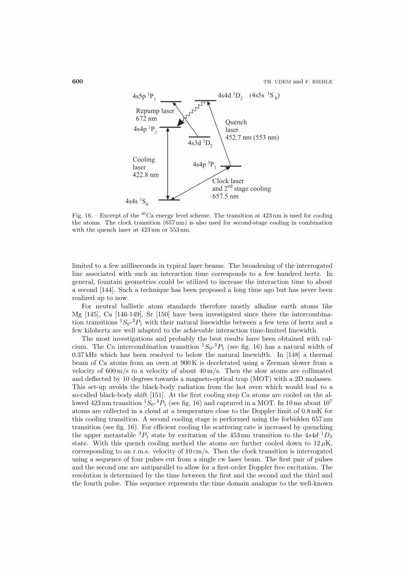
600 TH. UDEM and F. RIEHLE
Fig. 16. – Excerpt of the 40Ca energy level scheme. The transition at 423 nm is used for coolingthe atoms. The clock transition (657 nm) is also used for second-stage cooling in combinationwith the quench laser at 423 nm or 553 nm.
limited to a few milliseconds in typical laser beams. The broadening of the interrogatedline associated with such an interaction time corresponds to a few hundred hertz. Ingeneral, fountain geometries could be utilized to increase the interaction time to abouta second [144]. Such a technique has been proposed a long time ago but has never beenrealized up to now.
For neutral ballistic atom standards therefore mostly alkaline earth atoms likeMg [145], Ca [146-149], Sr [150] have been investigated since there the intercombina-tion transitions 1S0-3P1 with their natural linewidths between a few tens of hertz and afew kilohertz are well adapted to the achievable interaction time-limited linewidth.
The most investigations and probably the best results have been obtained with cal-cium. The Ca intercombination transition 1S0-3P1 (see fig. 16) has a natural width of0.37 kHz which has been resolved to below the natural linewidth. In [148] a thermalbeam of Ca atoms from an oven at 900 K is decelerated using a Zeeman slower from avelocity of 600 m/s to a velocity of about 40 m/s. Then the slow atoms are collimatedand deflected by 10 degrees towards a magneto-optical trap (MOT) with a 2D molasses.This set-up avoids the black-body radiation from the hot oven which would lead to aso-called black-body shift [151]. At the first cooling step Ca atoms are cooled on the al-lowed 423 nm transition 1S0-3P1 (see fig. 16) and captured in a MOT. In 10 ms about 107
atoms are collected in a cloud at a temperature close to the Doppler limit of 0.8 mK forthis cooling transition. A second cooling stage is performed using the forbidden 657 nmtransition (see fig. 16). For efficient cooling the scattering rate is increased by quenchingthe upper metastable 3P1 state by excitation of the 453 nm transition to the 4s4d 1D2
state. With this quench cooling method the atoms are further cooled down to 12μK,corresponding to an r.m.s. velocity of 10 cm/s. Then the clock transition is interrogatedusing a sequence of four pulses cut from a single cw laser beam. The first pair of pulsesand the second one are antiparallel to allow for a first-order Doppler free excitation. Theresolution is determined by the time between the first and the second and the third andthe fourth pulse. This sequence represents the time domain analogue to the well-known
FREQUENCY COMBS APPLICATIONS AND OPTICAL FREQUENCY STANDARDS 601
optical separated field excitation [152] or a Ramsey-Borde atom interferometer [153].The necessary radiation to interrogate the clock transition with a spectral linewidth ofapproximately 1 Hz was provided by a master-slave diode laser system [154].
The frequency of the clock transition at 657 nm was referenced to the caesium fountainclock utilizing a femtosecond comb generator to be 455 986 240 494 144 (5.3) Hz in PTBwith a fractional uncertainty of 1.2×10⁻¹⁴ and later at NIST with 6.6×10⁻¹⁵ [149], oneof the lowest uncertainties reported to date for a neutral atom optical standard. Theseauthors also concluded that this type of standard could be capable to achieve a fractionaluncertainty in the 10−16 regime.
A fractional frequency instability of 4 × 10⁻¹⁵ at 1 s averaging time was achieved.As has been pointed out [39, 146] the quantum projection-noise limit [151] for the Castandard corresponds to a fractional instability or Allan deviation of σy(τ) < 10−16 forτ = 1 s. To approach this limit, a frequency instability of the spectroscopy laser of betterthan 3 × 10⁻¹⁶ for the duration of the atom interferometry 2T ≈ 1.3 ms is necessarysince the so-called Dick effect [155] degrades the stability through the aliasing of thelaser frequency noise in a discontinuous interrogation. The Dick effect for an opticalfrequency standard with Ramsey-Borde interrogation was first addressed by Quessada etal. [156]. Hence, the relatively short interaction time achievable with neutral atoms infree flight limits the accuracy and the stability.
6.2.3. Optical lattice clocks. A possible way to combine the advantages of trappedsingle ions and the large number of neutral atoms, i.e. the long storage times and thegood signal-to-noise ratio, respectively, was pointed out by Katori [157, 158]. A largearray of micro traps for atoms (see fig. 17) can be generated in a standing wave laserfield capable of holding maybe a million of atoms. Even though these optical latticeshave been investigated for a long time they did not seem to be appropriate to be usedin an optical frequency standard because of the large ac Stark shifts associated with thelaser field. The remedy for this effect is to tune the lattice laser to a so-called “magicwavelength” where the upper and lower clock levels are shifted by the same amount,leaving the clock transition frequency unaltered (see fig. 18). The big advantage hereis that the ac Stark shift can be controlled by controlling the lattice laser frequencyrather than by measuring the lattice laser intensity. The former can be determined veryaccurately, in particular if one has an optical clock at hand.
Several atomic species are investigated for use as lattice clocks, e.g., 87Sr [10,159-161],Yb [162], and in the future also Hg. The best results have been obtained with 87Sr whichwill be discussed in the following. The strongly forbidden J = 0 → J = 0 transition 1S0-3P0 in Sr (see fig. 19) at 689 nm becomes weakly allowed through hyperfine mixing leadingto a natural linewidth of about 1 mHz. The atoms are cooled on the 461 nm transition toseveral hundred microkelvin. To further reduce the temperature cooling on the 1S0-3P1
transition is performed before the atoms are transferred into a dipole trap operated atthe magic wavelength near 813.4 nm. In a one-dimensional lattice Boyd et al. [160] storedtypically 2× 10⁴ atoms distributed across about 80 lattice sites. Interrogating the atomsseveral effects contribute to the uncertainty to find the unperturbed line center. Theseauthors gave an uncertainty budget where the perturbations due to the residual ac Starkshift of the lattice laser, the effect of the magnetic field necessary to separate the Zeemanlevels, and possible collisions contribute the largest effects ending up with a fractionaluncertainty below 1 × 10⁻¹⁵. The frequency of this transition has been determined nowby three independent groups [159-161]. The measurement of Boyd et al. [160] gave 429228 004 229 874.0 (1.1) Hz. The associated uncertainty is already much smaller as the
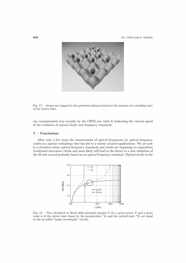
602 TH. UDEM and F. RIEHLE
Fig. 17. – Atoms are trapped in the potential minima located at the maxima of a standing waveof the lattice laser.
one recommended very recently by the CIPM (see table I) indicating the current speedof the evolution of optical clocks and frequency standards.
7. – Conclusions
After only a few years the measurement of optical frequencies by optical frequencycombs is a mature technology that has led to a variety of novel applications. We are nowin a situation where optical frequency standards and clocks are beginning to outperformtraditional microwave clocks and most likely will lead in the future to a new definition ofthe SI unit second probably based on an optical frequency standard. Optical clocks in the
Fig. 18. – The calculated ac Stark shift potential energies U for a given power P and a givenwaist w of the lattice laser beam for the ground-state 1S0 and the excited state 3P0 are equalat the so-called “magic wavelength” (circle).

FREQUENCY COMBS APPLICATIONS AND OPTICAL FREQUENCY STANDARDS 603
Fig. 19. – Excerpt from the energy level scheme of 40Sr. The transitions at 461 nm and 689 nmare used for cooling the atoms. The dashed line (698 nm) is the clock transition.
visible part of the spectrum by no means need be the end of the evolution. Transitionsin the UV or even in the XUV might give superior stability, as this important propertyscales as the transition frequency in use. It can be expected that the evolution in thisfield also in the future will keep its current pace since novel ideas like reading out ofclock transitions by quantum information techniques [163, 164] or the use of nucleartransitions [165] will continuously shift the frontiers in optical frequency metrology.
REFERENCES
[1] Hall J. L., IEEE Sel. Top. Quantum Electron., 6 (2000) 1136.[2] Udem Th. et al., in Proceedings of the 1999 Joint Meeting of the European Frequency
and Time Forum and the IEEE International Frequency Control Symposium, BesanconFrance, IEEE catalog no. 99CH36313 (1999), pp. 602-625.
[3] Reichert J. et al., Opt. Commun., 172 (1999) 59.[4] Reichert J. et al., Phys. Rev. Lett., 84 (2000) 3232.[5] Diddams S. A. et al., Phys. Rev. Lett., 84 (2000) 5102.[6] Jones D. J. et al., Science, 288 (2000) 635.[7] Holzwarth R. et al., Phys. Rev. Lett., 85 (2000) 2264.[8] Udem Th., Holzwarth R. and Hansch T. W., Nature, 416 (2002) 233.[9] Oskay W. H. et al., Phys. Rev. Lett., 97 (2006) 020801.
[10] Takamoto M. et al., Nature, 435 (2005) 321.[11] Gill P. and Margolis H., Physics World, 18 May issue (2005) 35.[12] High Resolution Spectroscopy of Hydrogen, in The Hydrogen Atom, edited by Bassani
G. F., Inguscio M. and Hansch T. W. (Springer Verlag, Berlin, Heidelberg, NewYork) 1989, pp. 93-102.
[13] Niering M. et al., Phys. Rev. Lett., 84 (2000) 5496.[14] de Beauvoir B. et al., Eur. Phys. Lett. D, 12 (2000) 61.[15] Udem Th. et al., Phys. Rev. Lett., 82 (1999) 3568.[16] Gerginov V. et al., Phys. Rev. A, 73 (2006) 032504.[17] Bize S. et al., Phys. Rev. Lett., 90 (2003) 150802.[18] Peik E. et al., Phys. Rev. Lett., 93 (2004) 170801.

604 TH. UDEM and F. RIEHLE
[19] Zimmermann M. et al., Laser Phys., 15 (2005) 997.[20] Kourogi M. et al., IEEE J. Quantum Electron., 31 (1995) 2120.[21] Brothers L. R. and Wong N. C., Opt. Lett., 22 (1997) 1015.[22] Imai K. et al., IEEE J. Quantum Electron., 34 (1998) 1998.[23] Spence D. E., Kean P. N. and Sibbett W., Opt. Lett., 16 (1991) 42.[24] Diels J. C. and Rudolph W., Ultrashort Laser Pulse Phenomena (Elsevier, Amsterdam,
Heidelberg, Tokyo) 2006.[25] Eckstein J. N., High Resolution Spectroscopy using Multiple Coherent Pulses (Thesis,
Stanford University, USA) 1978.[26] Bassani G. F., Inguscio M. and Hansch T. W. (Editors) Frequency Standards in
the Optical Spectrum, in The Hydrogen Atom, (Springer Verlag, Berlin, Heidelberg, NewYork) 1989, pp. 123-133.
[27] Holzwarth R. et al., Appl. Phys. B, 73 (2001) 269.[28] Udem Th. et al., Opt. Lett., 24 (1999) 881.[29] Diddams S. A. et al., Opt. Lett., 27 (2002) 58.[30] Ma L. S. et al., Science, 303 (2004) 1843.[31] Stenger J. and Telle H. R., Opt. Lett., 25 (2000) 1553.[32] Krausz F. et al., IEEE J. Quantum Electron, 28 (1992) 2097.[33] Hasegawa A. and Tappert F., Appl. Phys. Lett., 23 (1973) 142.[34] Agrawal G. P., Nonlinear Fiber Optics (Academic Press, New York) 2001.[35] Sutter D. H. et al., Opt. Lett., 24 (1999) 631.[36] Morgner U. et al., Opt. Lett., 24 (1999) 411.[37] Siegman A. E., Lasers (University Science Books, Mill Valley Ca USA) 1986.[38] Bramwell S. R., Kane D. M. and Ferguson A. I., Opt. Commun., 56 (1985) 112.[39] Hollberg L. et al., see fig. 9 in IEEE J. Quantum Electron., 37 (2001) 1502.[40] Rush D. W., Ho P. T. and Burdge G. L., Opt. Commun., 52 (1984) 41.[41] Bartels A. et al., Opt. Lett., 29 (2004) 1081.[42] Swann W. C. et al., Opt. Lett., 31 (2006) 3046.[43] Knight J. C. et al., Opt. Lett., 21 (1996) 1547.[44] Ranka J. K. et al., Opt. Lett., 25 (2000) 25.[45] Russell P. St. J., Science, 299 (2003) 358.[46] Birks T. A., Wadsworth W. J. and Russell P. St. J., Opt. Lett., 25 (2000) 1415.[47] Holzwarth R. et al., Laser Phys., 11 (2001) 1100.[48] Bartels A., Dekorsy T. and Kurz H., Opt. Lett., 24 (1999) 996.[49] Hoi M. et al., Phys. Rev. Lett., 96 (2006) 243401.[50] Corwn K. L. et al., Phys. Rev. Lett., 90 (2003) 113904.[51] Holman K. W. et al., Opt. Lett., 28 (2003) 851.[52] Holzwarth R., PhD thesis Ludwig-Maximilians-Universitat Munich (2001).[53] Dudley J. M. et al., J. Opt. Soc. Am. B, 19 (2002) 765.[54] Ell R. et al., Opt. Lett., 26 (2001) 373.[55] Fortier T. M. et al., Opt. Lett., 28 (2003) 2198.[56] Matos L. et al., Opt. Lett., 29 (2004) 1683.[57] Fortier T. M. et al., Opt. Lett., 31 (2006) 1011.[58] Morgner U. et al., Phys. Rev. Lett., 86 (2001) 5462.[59] Diddams S. A. et al., IEEE J. Quantum Electron, 9 (2003) 1072.[60] Fuji T. et al., Opt. Lett., 30 (2005) 332.[61] Nelson L. E. et al., Appl. Phys. B, 65 (1997) 277.[62] Kubina P. et al., Opt. Express, 13 (2005) 909.[63] Adler F. et al., Opt. Express, 12 (2004) 5872.[64] McFerran J. J. et al., Opt. Lett., 31 (2006) 1997.[65] See, for example, Gardener F. M., Phaselock Techniques (John Wiley & Sons, New
York) 1979.[66] Walls F. L. and DeMarchi A., IEEE Trans. Instrum. Meas., 24 (1975) 210.[67] Telle H. R., in Frequency Control of Semiconductor Lasers, edited by Ohtsu M. (Wiley,
New York) 1996, pp. 137-167.

FREQUENCY COMBS APPLICATIONS AND OPTICAL FREQUENCY STANDARDS 605
[68] Brabec T., private communication.[69] Haus H. A. and Ippen E. P., Opt. Lett., 26 (2001) 1654.[70] Xu L. et al., Opt. Lett., 21 (1996) 2008.[71] Helbing F. W. et al., Appl. Phys. B, 74 (2002) S35.[72] Witte S. et al., Appl. Phys. B, 78 (2004) 5.[73] Prevedelli M., Freegarde T. and Hansch T. W., Appl. Phys. B, 60 (1995) S241.[74] Fischer M. et al., Phys. Rev. Lett., 92 (2004) 230802.[75] Santarelli G. et al., Phys. Rev. Lett., 82 (1999) 4619.[76] Uzan J. P., Rev. Mod. Phys., 75 (2003) 403.[77] Dirac P. A. M., Nature (London), 139 (1937) 323.[78] Webb J. K. et al., Phys. Rev. Lett., 87 (2001) 091301.[79] Murphy M. T., Webb J. K. and Flambaum V. V., Mon. Not. R. Astron. Soc., 345
(2003) 609.[80] Quast R. et al., Astron. Astrophys., 417 (2004) 853.[81] Srianand R. et al., Phys. Rev. Lett., 92 (2004) 121302.[82] Shlyakhter A. I., Nature, 264 (1976) 340.[83] Fujii Y. et al., Nucl. Phys. B, 573 (2000) 377.[84] Lamoreaux S. K. and Torgerson J. R., Phys. Rev. D, 69 (2004) 121701(R).[85] Murphy M. T. et al., arXiv:astro-ph/0612407v1.[86] Murphy M. T., Webb J. K. and Flambaum V. V., arXiv:astro-ph/0611080 v3.[87] Calmet X. and Fritzsch H., Phys. Lett. B, 540 (2002) 173.[88] Schneider T., Peik E. and Tamm Chr., Phys. Rev. Lett., 94 (2005) 230801.[89] Diddams S. A. et al., Science, 293 (2001) 825.[90] Mohr P. J. and Taylor B. N., Rev. Mod. Phys., 77 (2005) 1.[91] Gabrielse G. et al., Phys. Rev. Lett., 97 (2006) 030802.[92] Wicht A. et al., Phys. Scr., T02 (2002) 82.[93] Clade P. et al., Phys. Rev. Lett., 96 (2006) 03301.[94] Bradley et al., Phys. Rev. Lett., 83 (1999) 4510.[95] Pachucki K. and Jentschura U. D., Phys. Rev. Lett., 91 (2003) 113005.[96] Murphy M. T. et al., sumitted to Mon. Not. R. Astron. Soc.[97] Apolonski A. et al., Phys. Rev. Lett., 85 (2000) 740.[98] Kienberger R. et al., Nature, 427 (2004) 817.[99] Baltuska A. et al., Nature, 421 (2003) 611.
[100] Wahlstrom C. G. et al., Phys. Rev. A, 48 (1993) 4709.[101] Brabec T. and Krausz F., Rev. Mod. Phys., 72 (2000) 545.[102] Eden J. G., Prog. Quantum Electron., 28 (2004) 197.[103] Paulus G. G. et al., Phys. Rev. Lett., 85 (2000) 253004.[104] Seres J. et al., Nature, 433 (2005) 596.[105] Goulielmakis E. et al., Science, 305 (2004) 1267.[106] Gerginov V. et al., Opt. Lett., 30 (2005) 1734.[107] Fendel P. et al., Opt. Lett., 32 (2007) 701.[108] Baklanov Ye. F. and Chebotayev V. P., Appl. Phys. Lett., 12 (1977) 97.[109] Meshulach D. and Silberberg Y., Nature, 396 (1998) 239.[110] Eckstein J., Ferguson A. I. and Hansch T. W., Phys. Rev. Lett., 40 (1978) 847.[111] Snadden M. J. et al., Opt. Commun., 125 (1996) 70.[112] Marian A. et al., Science, 306 (2004) 2063.[113] Fortier T. M. et al., Phys. Rev. Lett., 97 (2006) 163905.[114] Witte S. et al., Science, 307 (2005) 400.[115] Cavalieri S. et al., Phys. Rev. Lett., 89 (2002) 133002.[116] Zinkstok R. Th. et al., Phys. Rev. A, 73 (2006) 061801(R).[117] Gohle Ch. et al., Nature, 436 (2005) 234.[118] Jones R. J., Moll K. Thorpe M. and Ye J., Phys. Rev. Lett., 94 (2005) 193201.[119] Barnes J. A. et al., IEEE Trans. Instrum. Meas., 20 (1971) 105.[120] Webster S. A. et al., Phys. Rev. A., 65 (2002) 052501.

606 TH. UDEM and F. RIEHLE
[121] See, for example, contributions of Madej A. A., Bernard J. E., Riehle F. andHelmcke J., in Frequency Measurement and Control, edited by Luiten A. N. (SpringerVerlag, Berlin, Heidelberg, New York) 2001.
[122] Evenson K. M. et al., Appl. Phys. Lett., 22 (1973) 192.[123] Peik E., Schneider T. and Tamm Chr., J. Phys. B, 39 (2006) 145.[124] Brusch A. et al., Phys. Rev. Lett., 96 (2006) 103003.[125] Quinn T. J., Metrologia, 40 (2003) 103.[126] Editor’s note: Documents concerning the new definition of the metre, Metrologia, 19
(1984) 163.[127] Quinn T. J., Metrologia, 30 (1993/1994) 523.[128] Quinn T. J., Metrologia, 36 (1999) 211.[129] Wineland D. J. et al., Phys. Rev. A, 36 (1987) 2220.[130] Blatt R., Gill P. and Thompson R. C., J. Mod. Opt., 39 (1992) 193.[131] Madej A. A. and Bernard J. E., Frequency Measurement and Control: Topics in
Applied Physics, edited by A. N. Luiten, 79 (2001) 153.[132] Riehle F., Frequency Standards: Basics and Applications (Wiley-VCH, Weinheim) 2004.[133] Dehmelt H., Bull. Am. Phys. Soc., 20 (1975) 60.[134] Wineland D. J. and Dehmelt H., Bull. Am. Phys. Soc., 20 (1975) 637.[135] Wineland D. J. et al., Opt. Lett., 5 (1980) 245.[136] Nagourney W., Sandberg J. and Dehmelt H., Phys. Rev. Lett., 56 (1986) 2797.[137] Itano W. M., J. Res. Natl. Inst. Stand. Technol., 105 (2000) 829.[138] Dube P. et al., Phys. Rev. Lett., 95 (2005) 033001.[139] Tamm Chr. et al., to be published in IEEE Trans. Instrum. Meas.[140] Margolis H. S. et al., Science, 306 (2004) 1355.[141] Ito N. et al., Opt. Commun., 109 (1994) 414.[142] Zibrov A. S. et al., Appl. Phys. B, 59 (1994) 327.[143] Kersten P. et al., Appl. Phys. B, 68 (1999) 27.[144] Beausoleil R. G. and Hansch T. W., Phys. Rev. A, 33 (1986) 1661.[145] Sterr U. et al., Appl. Phys. B, 54 (1992) 341.[146] Wilpers G. et al., Phys. Rev. Lett., 89 (2002) 230801.[147] Sterr U. et al., C. R. Physique, 5 (2005) 845.[148] Sterr U. et al., Phys. Rev. A, 72 (2005) 062111.[149] Wilpers G., Oaetes C. W. and Hollberg L. W., Appl. Phys. B, 85 (2006) 31.[150] Sorrentino F. et al., arXiv:physics/0609133 v1 (2006).[151] Itano W. M. et al., Phys. Rev. A, 47 (1993) 3554.[152] Borde Ch. J. et al., Phys. Rev. A, 30 (1984) 1836.[153] Borde Ch. J., Phys. Lett. A, 30 (1989) 10.[154] Stoehr H. et al., Opt. Lett., 31 (2006) 736.[155] Dick G. J., Proceedings of 19th Annual Precise Time and Time Interval (PTTI)
Applications and Planning Meeting, Redondo Beach, CA, 1987 (U. S. Naval Observatory)1987, pp. 133-147.
[156] Quessada A. et al., J. Opt. B: Quantum Semiclassical Opt., 5 (2003) S150.[157] Katori H., Ido T. and Kuwata-Gonokami M., J. Phys. Soc. Jpn., 68 (1999) 2479.[158] Katori H., in Proceedings of the 6th Symposium on Frequency Standards and Metrology,
edited by P. Gill (World Scientific, Singapore) 2002, p. 323.[159] Takamoto M. et al., J. Phys. Soc. Jpn., 75 (2006) 104302.[160] Boyd M. M. et al., Phys. Rev. Lett., 98 (2007) 083002.[161] Le Targat R. et al., Phys. Rev. Lett., 97 (2006) 130801.[162] Barber Z. W. et al., Phys. Rev. Lett., 96 (2006) 083002.[163] Wineland D. J. et al., in Proceedings of the 6th Symposium on Frequency Standards and
Metrology, edited by P. Gill (World Scientific, Singapore) 2002, p. 361.[164] Schmidt P. O. et al., Science, 309 (2005) 749.[165] Peik E. and Tamm Ch., Europhys. Lett., 61 (2003) 161.