INVESTIGATIONHIGHLIGHTED ARTICLE

Fast and Efficient Estimation of IndividualAncestry Coefficients

Eric Frichot,* François Mathieu,* Théo Trouillon,*,† Guillaume Bouchard,† and Olivier François*,1

*Université Joseph Fourier Grenoble 1, Centre National de la Recherche Scientifique, Techniques de l’Ingénierie Médicale et de laComplexité - Informatique, Mathématiques et Applications, Grenoble Unité Mixte de Recherche 5525, 38042 Grenoble, France,

and †Xerox Research Center Europe, F38240 Meylan, France

ABSTRACT Inference of individual ancestry coefficients, which is important for population genetic and association studies, iscommonly performed using computer-intensive likelihood algorithms. With the availability of large population genomic data sets, fastversions of likelihood algorithms have attracted considerable attention. Reducing the computational burden of estimation algorithmsremains, however, a major challenge. Here, we present a fast and efficient method for estimating individual ancestry coefficients basedon sparse nonnegative matrix factorization algorithms. We implemented our method in the computer program sNMF and applied it tohuman and plant data sets. The performances of sNMF were then compared to the likelihood algorithm implemented in the computerprogram ADMIXTURE. Without loss of accuracy, sNMF computed estimates of ancestry coefficients with runtimes �10–30 timesshorter than those of ADMIXTURE.

INFERENCE of population structure from multilocus geno-type data is commonly performed using likelihood meth-

ods implemented in the computer programs STRUCTURE,FRAPPE, and ADMIXTURE (Pritchard et al. 2000a; Tanget al. 2005; Alexander et al. 2009). These programs computeprobabilistic quantities called ancestry coefficients that repre-sent the proportions of an individual genome that originatefrom multiple ancestral gene pools. Estimation of ancestryproportions is important in many respects, for example indelineating genetic clusters, drawing inference about thehistory of a species, screening genomes for signatures ofnatural selection, and performing statistical corrections ingenome-wide association studies (Pritchard et al. 2000b;Marchini et al. 2004; Price et al. 2006; Frichot et al. 2013).

Individual ancestry coefficients can be estimated usingeither supervised or unsupervised statistical methods. Su-pervised estimation methods use predefined source popula-tions as ancestral populations. Classical supervised estimationapproaches were based on least-squares regression of allelefrequencies in hybrid and source populations (Roberts and

Hiorns 1965; Cavalli-Sforza and Bodmer 1971). Unsupervisedapproaches attempt to infer ancestral gene pools from thedata, using likelihood methods. An undesired feature of likeli-hood methods is that they can be computer intensive, withtypical runs lasting several hours or more. With the use ofdense genomic data and increased sample sizes, reducingthe time lag necessary to perform estimation is a major chal-lenge of population genetic data analysis.

A fast approach to the estimation of ancestry coefficientsis by using principal component analysis (PCA) (Pattersonet al. 2006). PCA is an exploratory method that describeshigh-dimensional data, using a small number of dimensions,and makes no assumptions about sampled and ancestral pop-ulations. Using PCA can lead to results surprisingly close tolikelihood methods, and connections between methods havebeen intensively investigated during recent years (Pattersonet al. 2006; Engelhardt and Stephens 2010; Frichot et al.2012; Lawson et al. 2012; Lawson and Falush 2012). Buta drawback of PCA is that interpretation in terms of ancestryis often difficult, as it can be confounded by demographicfactors or irregular sampling designs (Novembre and Stephens2008; McVean 2009; François et al. 2010).

In this study, we introduce computationally fast algorithmsthat lead to estimates of ancestry coefficients comparableto those obtained with STRUCTURE or ADMIXTURE. Thealgorithms were implemented in the computer program sNMFbased on sparse nonnegative matrix factorization (NMF) and

Copyright © 2014 by the Genetics Society of Americadoi: 10.1534/genetics.113.160572Manuscript received December 11, 2013; accepted for publication January 23, 2014;published Early Online February 4, 2014.Supporting information is available online at http://www.genetics.org/lookup/suppl/doi:10.1534/genetics.113.160572/-/DC1.1Corresponding author: Faculty of Medicine, TIMC-IMAG UMR 5525, Grenoble,F38706 La Tronche, France. E-mail: olivier.francois@imag.fr

Genetics, Vol. 196, 973–983 April 2014 973

least-squares optimization (Lee and Seung 1999; Kim andPark 2007; Kim and Park 2011). Like PCA, NMF algorithmsare flexible approaches that are robust to departures fromtraditional population genetic model assumptions. In addition,NMF algorithms produce estimates of ancestry proportionswith runtimes that are much shorter than those of STRUCTUREor ADMIXTURE. This study assesses the utility of NMF algo-rithms when analyzing population genetic data sets and com-pares the performances of the algorithms implemented insNMF with those implemented in ADMIXTURE on the basisof human and plant data.

Materials and Methods

To provide statistical estimates of ancestry proportions usingmultilocus genotype data sets, we implemented sparse NMFleast-squares optimization algorithms in the computer pro-gram sNMF.

Modeling ancestry coefficients

We considered allelic data for a sample of n multilocus geno-types at L loci representing single-nucleotide polymorphisms(SNPs). The data were stored into a genotypic matrix (X),where each entry records the number of derived alleles atlocus ℓ for individual i. For autosomes in a diploid organism,the number of derived alleles at locus ℓ is then 0, 1, or 2. In ouralgorithm, we used 3 bits of information to encode each 0, 1,or 2 value as an indicator of a heterozygote or a homozygotelocus. In other words, the value 0 was encoded as 100, 1 wasencoded as 010, and 2 as 001. The use of a binary codingwarrants that the entries sum up to L for each row of thetransformed data matrix.

Admixture models generally suppose that the geneticdata originate from the admixture of K ancestral popula-tions, where K is unknown a priori. Given K populations,the probability that individual i carries j derived alleles atlocus ℓ can be written as

piℓð jÞ ¼XKk¼1

qikgkℓðjÞ; j ¼ 0; 1; 2; (1)

where qik is the fraction of individual i’s genome that origi-nates from the ancestral population k, and gkℓ(j) represents thehomozygote (j = 0, 2) or the heterozygote (j = 1) frequencyat locus ℓ in population k. Since it makes no assumption about

Hardy–Weinberg equilibrium, the above framework is appro-priate to deal with inbreeding and outbreeding in ancestralpopulations. Using our binary coding, Equation 1 writes as

P ¼ QG; (2)

where P = (piℓ) is an n 3 3L matrix, Q = (qik) is an n 3 Kmatrix, and G = (gkℓ( j)) is a K 3 3L matrix. The Q matrixrecords ancestry proportions for each individual in the sam-ple. Although the focus of the above framework is on esti-mating ancestry estimates for each sampled individual, itcan be easily modified to provide ancestry estimates basedon allele frequencies in population samples.

Least-squares estimates of ancestry proportions

We approached the inference of ancestry coefficients byusing least-squares (LS) optimization algorithms (Engelhardtand Stephens 2010). Estimates of the Q and G matrices wereobtained after minimizing the least-squares criterion

LSðQ;GÞ ¼ ��jX2QGj��2F   ; (3)

where ||M||F denotes the Frobenius norm of a matrix M(Berry et al. 2007). Without constraints on Q and G, thesolutions of the LS problem are given by the singular valuedecomposition of the matrix X, and the resulting matrices Qand G contain the scores and loadings of a PCA. To obtainancestry coefficients, the matrices Q and G must have non-negative entries such that

XKk¼1

qik ¼ 1  ;X2j¼0

gkℓð jÞ ¼ 1: (4)

With the constraints of Equation 4, estimating ancestrycoefficients and genotypic frequencies is equivalent toperforming NMF of the data matrix, X. NMF was previouslyapplied to gene expression data (Kim and Park 2007), andalgorithms for NMF were surveyed and compared in Kimand Park (2011). In sNMF, estimates of Q and G were com-puted using the alternating nonnegativity-constrained least-squares (ANLS) algorithm with the active set (AS) method(Berry et al. 2007; Kim and Park 2011). We modified theANLS-AS algorithm as follows.

Our algorithm begins with the initialization of the Qentries with nonnegative values. Then it iterates the follow-ing cycles until convergence. The first step of an algorithm

Table 1 Data sets used in this study

Data set Sample size No. SNPs Reference

HGDP00778 934 78,000 Patterson et al. (2012)HGDP00542 934 48,500 —

HGDP00927 934 124,000 —

HGDP00998 934 2,600 —

HGDP01224 934 10,600 —

HGDP-CEPH 1,043 660,000 Li et al. (2008)1000 Genomes 1,092 2,200,000 1000 Genomes Project Consortium (2012)A. thaliana 168 216,000 Atwell et al. 2010)

974 E. Frichot et al.

cycle consists of computing a nonnegative matrix G that-minimizes the quantity

LS1ðGÞ ¼��jX2QG j��2F   ; G$ 0: (5)

The G matrix was obtained by setting all negative entries tozero, after solving classical linear regression equations. Theobtained solution was then normalized so that its entriessatisfy Equation 4.

Given G, the second step of the cycle consists of comput-ing a nonnegative matrix Q that minimizes the quantity

LS2ðQÞ ¼����������

GTffiffiffia

p  e13K

�Q2�

XT

013n

� ���������2

F

; (6)

where e13K is a row vector having all entries equal to 1, 013n isa vector of length n with all entries equal to 0, and a is a non-negative regularization parameter. This minimization problemwas solved using the block principal pivoting method proposedby Kim and Park (2011). The obtained solution, Q, was thennormalized so that the row entries sum up to 1. Iterations werestopped based on a stationarity criterion derived from theKarush–Kuhn–Tucker conditions (Kim and Park 2011) andwhen the relative difference between two successive values ofthe criterion was less than a tolerance threshold of e = 1024.

For a . 0, the algorithm amounts to performing sparseNMF for the data matrix X. We tested values a . 0 becausethey can reduce the variance of Q and G estimates for thesmaller data sets, force irrelevant estimates to zero, andimprove the numerical behavior the ANLS minimization al-gorithm. In addition, the programming structures used insNMF optimized the time spent in memory access. Severalalgorithmic methods were also used to accelerate computa-tion of matrix products. While we evaluated sNMF runtimesusing a single computer processor unit (2.4 GHz, 64 bits,Intel Xeon), a multithreaded version of the sNMF programwas also developed for multiprocessor systems.

Data sets

Ancestry inference and runtime analyses were performed onsix worldwide samples of genomic DNA from 52 populationsof the Human Genome Diversity Project–Centre d’Etude duPolymorphisme Humain (HGDP-CEPH). Five panels wereextracted from the Harvard HGDP-CEPH database. These pan-els were given identification nos. HGDP00778, HGDP00542,HGDP00927, HGDP00998, and HGDP01224 and containedprecisely ascertained genotypes of n = 934 individuals. Thegenotypes were specifically designed for population geneticanalyses (Patterson et al. 2012). Each marker was ascertainedin individuals of Han, Papuan, Yoruba, Karitiana, and Mongo-lian ancestry, and the data matrices included 78,253, 48,531,124,115, 2635, and 10,664 SNPs, respectively (Patterson et al.2012, Table 1). A sample of 1043 individuals from the HGDP-CEPH Human Genome Diversity Cell Line Panel was also an-alyzed. The genotypes were generated on Illumina 650Karrays (Li et al. 2008), and the SNP data were filtered to

remove low-quality SNPs included in the original files. In ad-dition, we used data from the 1000 Genomes Project. The1000 Genomes Project data contain the genomes of 1092individuals from 14 populations, constructed using a combina-tion of low-coverage whole-genome and exome sequencing[phase 1 data (1000 Genomes Project Consortium 2012)].The data matrix included 2.2 million polymorphic sites acrossthe human genome (Table 1).

To examine the robustness of sNMF to departures fromclassical population genetic hypotheses, additional analyseswere performed on a sample of n = 168 European acces-sions of the plant species Arabidopsis thaliana. A. thaliana isa widely distributed self-fertilizing plant known to harborconsiderable genetic variation and complex patterns ofpopulation structure and relatedness (Atwell et al. 2010).We analyzed 216,130 SNPs spread across the genome ofA. thaliana (Atwell et al. 2010, Table 1).

Comparisons with ADMIXTURE

The computer program ADMIXTURE (version 1.22) esti-mates ancestry coefficients based on the likelihood modelimplemented in STRUCTURE. In ADMIXTURE, the assump-tion of Hardy–Weinberg equilibrium in ancestral popula-tions translates into a binomial model for allele counts ateach locus. Considering unrelated individuals, the logarithmof the likelihood can thus be computed as

LðQ; FÞ¼P

i

Pℓ

xiℓlog

Pkqikfkℓ

!þ ð12 xiℓÞlog

Pkqikð12 fkℓÞ

!!

up to an additive constant that does not influence estimationalgorithms. In this formula, Q = (qik) represents the matrix

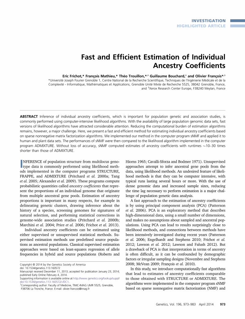
Figure 1 Correlation between sNMF and ADMIXTURE estimates. Shownis squared correlation (coefficient of determination, R2) between the an-cestry coefficients estimated by each program. For each number of clus-ters (K), the result corresponds to the maximum correlation over five runs,averaged over values of the regularization parameter ,1000 and over sixHGDP data sets. The shaded area corresponds to a 95% confidence in-terval displayed for each value of the regularization parameter, a.

Superfast Inference of Population Structure 975

of ancestry coefficients for all individuals, and F = ( fkℓ) rep-resents a matrix of allele frequencies for all loci. The F ma-trix can be converted to a G matrix comparable to the onecomputed by sNMF, using the binomial model, gkℓ(0) =(1 2 fkℓ)2, gkℓ(1) = 2fkℓ(12 fkℓ), and gkℓð2Þ ¼ f2kℓ: ADMIXTUREprovides numerical estimates of Q and F that maximize thequantity L(Q, F). The local optimization algorithm relies ona block relaxation scheme, using sequential quadratic pro-gramming for block updates, coupled with a quasi-Newtonacceleration of convergence.

A difficulty with optimization algorithms used byADMIXTURE and sNMF is that the solutions producedcan be dependent on the initial values used for Q, F, orG. To enable comparisons with estimates obtained withADMIXTURE, the clusters output by runs of each programwas permuted using CLUMPP (Jakobsson and Rosenberg2007). Differences in ancestry estimates obtained withADMIXTURE (QADM) and with sNMF (QsNMF) were assessedby two measures. The first measure was defined as the rootmean-squared error (RMSE) between the matrices QADM andQsNMF obtained from each program,

RMSE ¼

1nK

Xni¼1

XKk¼1

�qADMik 2qsNMF

ik�2!1=2

  :

Although Gmatrices could be mainly considered as nuisanceparameters for our estimation problem, a similar RMSE cri-terion was defined for comparing them. The second measurewas defined as the squared Pearson correlation coefficient(R2) between the matrices QADM and QsNMF. When simula-tions with known Q matrices were analyzed, one of the twomatrices was replaced by the true Q matrix used to generatethe simulated data.

Runs of ADMIXTURE and sNMF were performed forvalues of the number of clusters set to K= 2210, 15, and 20for human data sets and set to K = 227 for A. thaliana. For

sNMF, the values of the regularization parameter (a) rangedbetween 0 and 10,000, using a log10 scale (5 values). Eachrun was replicated five times for a total of 1410 experi-ments. Missing data imputation was initially performed afterresampling missing genotypes from empirical frequencies ateach locus. The missing values were updated using predic-tive probabilities after 20 sweeps of the algorithm (seebelow).

Cross-entropy criterion

We employed a cross-validation technique based on impu-tation of masked genotypes to evaluate the prediction errorof ancestry estimation algorithms (Wold 1978; Eastmentand Krzanowski 1982). The procedure partitioned the geno-typic matrix entries into a training set and a test set. To buildthe test set, 5% of all genotypes were randomly selected andtagged as missing values. The occurrence probabilities forthe masked entries were computed using the program out-puts obtained from training sets according to the formula

pprediℓ ð jÞ ¼XKk¼1

qikgkℓðjÞ; j ¼ 0; 1; 2  : (7)

ADMIXTURE predicts each masked value byE½xiℓjQADM; FADM� ¼ 2

Pkq

ADMik fADMkℓ and the prediction error

is estimated by averaging the squares of the deviance resid-uals for the binomial model (Alexander and Lange 2011).Extending the approach employed by ADMIXTURE to ournonparametric approach, the predicted values were com-pared to the masked values, xiℓ, by averaging the quantitydefined as 2 logpprediℓ ðxiℓÞ over all SNPs in the test set. Instatistical terms, our criterion provides an estimate of thequantity

H�psample; ppred

¼ 2

X2j¼0

psampleð jÞlog pprediℓ ð jÞ  ; j5 0; 1; 2: (8)

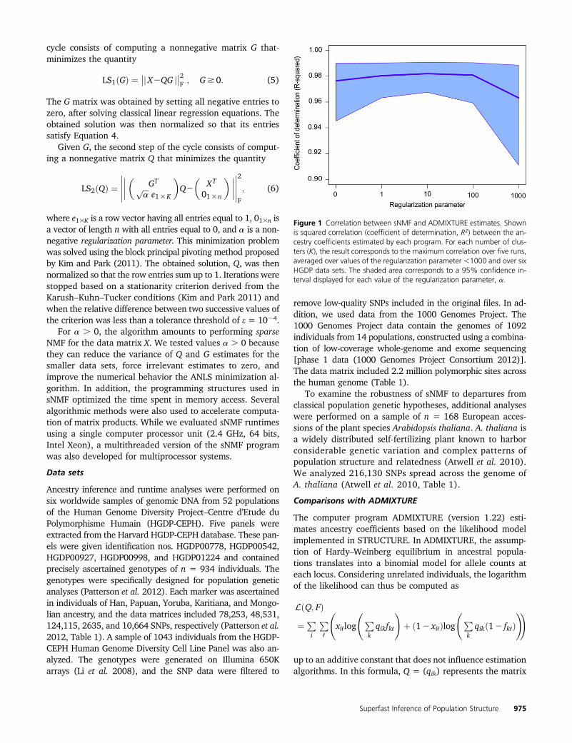
Figure 2 Runtimes for sNMF andADMIXTURE runs. Averaged timeelapsed before the stopping criterionof the sNMF (blue) and ADMIXTURE(orange) programs is met. Time isexpressed in unit of hours. (A) Run-time analysis for Harvard HGDPpanel 01224 (10,600 SNPs). (B) Run-time analysis for Harvard HGDPpanel 00778 (78,000 SNPs). (C) Run-time analysis for the HGDP-CEPHdata (660,000 SNPs).

976 E. Frichot et al.

This quantity corresponds to the sum of the Kullback–Leiberdivergence between the sampled (psample) and predicted(ppred) allelic distributions and the Shannon entropy of thesample distribution. It also corresponds to the cross-entropybetween psample and ppred. The number of ancestral genepools (K) and the regularization parameter (a) were chosento minimize the cross-entropy criterion. In general, smallervalues of the criterion indicate better algorithm outputs andestimates. The standard error of the cross-entropy criterionis of order 1=

ffiffiffiffiffinL

p; where nL is the number of masked gen-

otypes. For data sets including 1000 individuals genotypedat .20,000 SNPs, the third digit of the cross-entropy crite-rion can be significant.

Simulated data analysis

We adopted a simulation approach to compare RMSEsbetween the Q matrix computed by ADMIXTURE or by sNMFand a known matrix used to generate the simulated data. Inaddition, we assessed whether the correct value of K could beidentified by sNMF, using the cross-entropy criterion.

In a first series of simulations, we used the 1000 GenomesProject data set to generate artificial data showing variouslevels of admixture. As ancestral populations, we chose theHan Chinese (CHB), British (GBR), and Yoruba (YRI) samples(1000 Genomes Project 2012). We considered 50,000 SNPs inlinkage equilibrium, exhibiting no missing genotypes. Theallele frequencies observed in our three ancestral populationswere used as the true values for the F matrix. The genotypicmatrix was constructed according to the binomial model usedby ADMIXTURE. For 1000 individuals in each simulated dataset, a Q matrix was simulated from a Dirichlet probabilitydistribution, and several parameters were explored. Ourexperiments reproduced the parameters used for evaluatingthe accuracy of ADMIXTURE in a previous study (Alexanderet al. 2009). Runs of sNMF were performed for values of thenumber of clusters set to K = 225 (a = 0), and the choiceof K was made on the basis of the cross-entropy criterion.For K = 3, the values of the regularization parameter (a)were varied between 0 and 100.

Additional data sets were created to mimic the populationstructure of European populations of A. thaliana, using10,000 SNPs (168 individuals). To define ancestral frequen-cies, we used the western European populations, grouping

samples from the United Kingdom, Belgium and France (23individuals); central European populations, grouping samplesfrom the Czech Republic (24 individuals); and northern Eu-ropean populations, grouping samples from Finland andNorthern Sweden (13 individuals). ADMIXTURE and sNMFgrouped these samples within three well-separated clustersexhibiting low levels of admixture with other plant populations.The empirical frequencies computed from the three populationswere considered as the true frequencies for a generative modelwith K = 3 ancestral populations. From empirical frequencies,we computed genotypic frequencies, fkℓ, using four distinct val-ues of population inbreeding coefficient, FIS = 25–100%, thatcorresponded to moderate and strong levels of inbreeding. For168 individuals, 10,000 genotypes were simulated using thesampling equation pðxiℓ ¼ jÞ ¼PkqikgkℓðjÞ; where qik corre-sponds to the Q matrix computed from the full empirical dataset (216,000 SNPs). In addition, simulated data sets were gen-erated with or without missing data (0 or 20%). Fifty replicateswere created for each value of the inbreeding coefficient and foreach value of the ratio of missing data.

Results

We used the program sNMF to implement nonnegative matrixfactorization algorithms and to compute least-squares esti-mates of ancestry coefficients for worldwide human popula-tion samples and for European populations of the plant speciesA. thaliana. As in the likelihood model implemented in thecomputer programs STRUCTURE and ADMIXTURE, sNMFsupposes that the genetic data originate from the admixtureof K parental populations, where K is unknown, and it returnsestimates of ancestry proportions for each multilocus genotypein the sample (Pritchard et al. 2000a; Alexander et al. 2009).To estimate ancestry coefficients, sNMF solves a constrainedleast-squares minimization problem, using an alternating al-gorithm based on a block principal pivoting method (Kim andPark 2011) (see Materials and Methods).

Comparison of ancestry estimates for HGPD data sets

First we evaluated the ability of ADMIXTURE estimates to beaccurately reproduced by sNMF for five Harvard HGDPpanels and for the HGDP-CEPH data set (Li et al. 2008;Patterson et al. 2012). For each run of ADMIXTURE, we

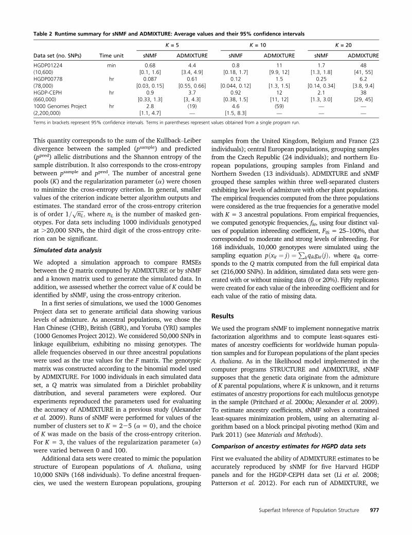
Table 2 Runtime summary for sNMF and ADMIXTURE: Average values and their 95% confidence intervals

K = 5 K = 10 K = 20

Data set (no. SNPs) Time unit sNMF ADMIXTURE sNMF ADMIXTURE sNMF ADMIXTURE

HGDP01224 min 0.68 4.4 0.8 11 1.7 48(10,600) [0.1, 1.6] [3.4, 4.9] [0.18, 1.7] [9.9, 12] [1.3, 1.8] [41, 55]HGDP00778 hr 0.087 0.61 0.12 1.5 0.25 6.2(78,000) [0.03, 0.15] [0.55, 0.66] [0.044, 0.12] [1.3, 1.5] [0.14, 0.34] [3.8, 9.4]HGDP-CEPH hr 0.9 3.7 0.92 12 2.1 38(660,000) [0.33, 1.3] [3, 4.3] [0.38, 1.5] [11, 12] [1.3, 3.0] [29, 45]1000 Genomes Project hr 2.8 (19) 4.6 (59) — —

(2,200,000) [1.1, 4.7] — [1.5, 8.3] — — —

Terms in brackets represent 95% confidence intervals. Terms in parentheses represent values obtained from a single program run.

Superfast Inference of Population Structure 977

computed a maximum squared correlation coefficient (R2)and a minimum RMSE over runs of sNMF performed withthe same number of clusters (K). For K ranging from 5 to 10,squared correlation coefficients remained .0.96 across allruns (480 runs, Figure 1). Average values of the RMSEremained ,5.5% across all runs (Supporting Information,Table S1). These results provided evidence that sNMF esti-mates closely reproduce those obtained with ADMIXTUREacross the six HGDP data sets.

Runtime analysis

Next we performed runtime analyses for ADMIXTURE andfor sNMF, using the 1000 Genomes Project phase 1 data inaddition to the previous HGDP data sets. The runtimes wereaveraged over distinct random seed values for each value ofK. Runtimes increased with the number of SNPs in the dataset and with the number of clusters in each algorithm (Fig-ure 2, Table 2, Figure S1). For data set HGDP01224 (10,600SNPs), it took on average 0.8 min (1.7 min) for sNMF tocompute ancestry estimates for K = 10 (K = 20) clusters.For ADMIXTURE, the runtime was on average 11 min(48 min) for K = 10 (K = 20) clusters. For panel HGDP00778(78,000 SNPs), it took on average 7.2 min (15 min) for sNMFto compute ancestry estimates for K = 10 (K = 20) clusters.For ADMIXTURE, the average runtime was 1.5 hr (6.2 hr) forK = 10 (K = 20) clusters. For the CEPH-HGDP data sets(660,000 SNPs), it took on average 55 min (2.1 hr) for sNMFto compute ancestry estimates for K = 10 (K = 20) clusters.For ADMIXTURE, the average runtime was 12 hr (38 hr)for K = 10 (K = 20) clusters. Runtimes increased in a qua-dratic fashion with K for ADMIXTURE whereas they in-creased linearly for sNMF (Figure 2). For the values of Kused in our analyses, sNMF ran 5–30 times faster thanADMIXTURE when these programs were applied to HGPDdata sets. Regarding the 1000 Genomes Project phase 1 dataset, the average runtimes of sNMF were �2.8 hr (4.6 hr)for K = 5 (K = 10) clusters. The ADMIXTURE runs led to

similar estimates of Q, but a single run on the phase 1 dataset took .19 hr for K = 5 (59 hr for K = 10).

Prediction of masked genotypes

To decide which program options could provide the bestestimates, we employed a cross-validation technique based onthe imputation of masked genotypes (Wold 1978; Alexanderand Lange 2011). The cross-validation method partitionsthe genotypic matrix entries into a training set and a testset that are used for estimation and validation sequentially.To build test sets, 5% of the genotypic matrix entries weretagged as missing values. The masked entries were thenpredicted using estimates obtained from training sets. Pre-dictions were assessed using a cross-entropy criterion thatmeasured the capability of an algorithm to correctly imputemasked genotypes (see Materials and Methods). Lower val-ues of the cross-entropy criterion generally indicate betterpredictive capabilities of an algorithm.

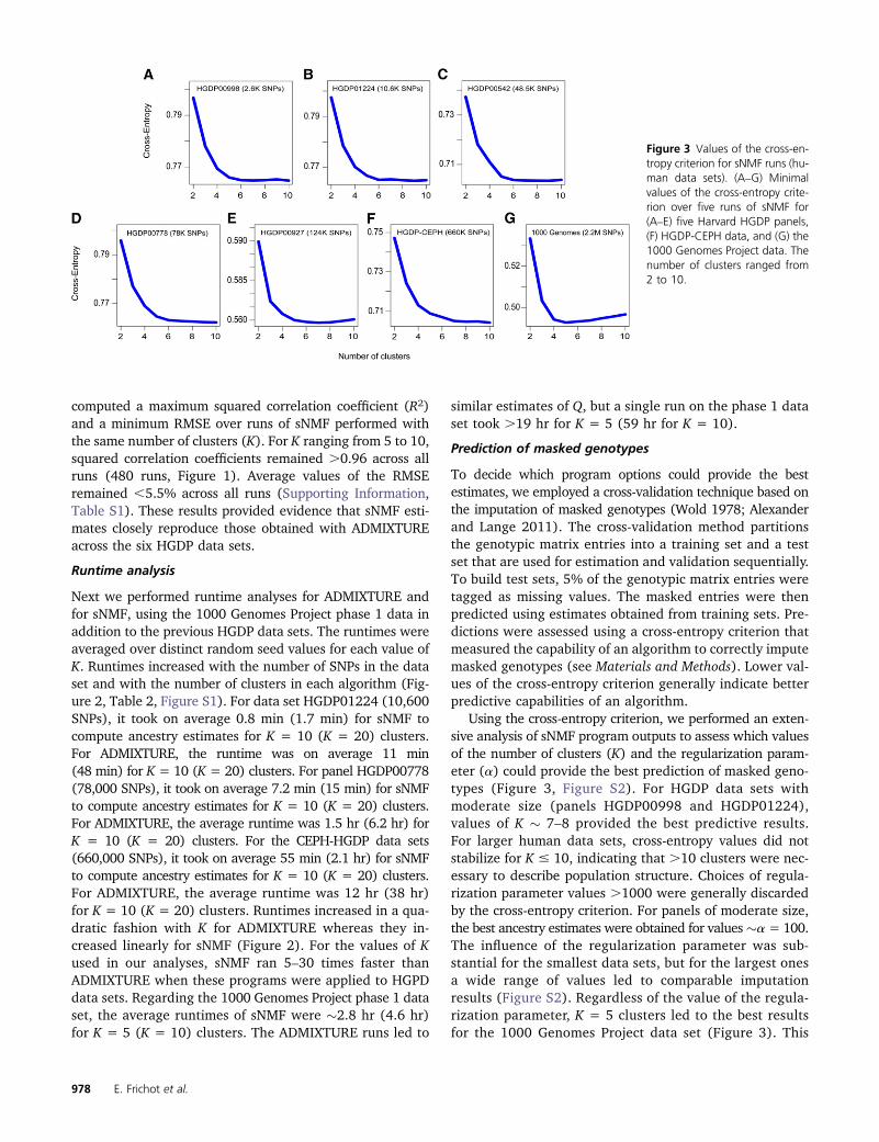
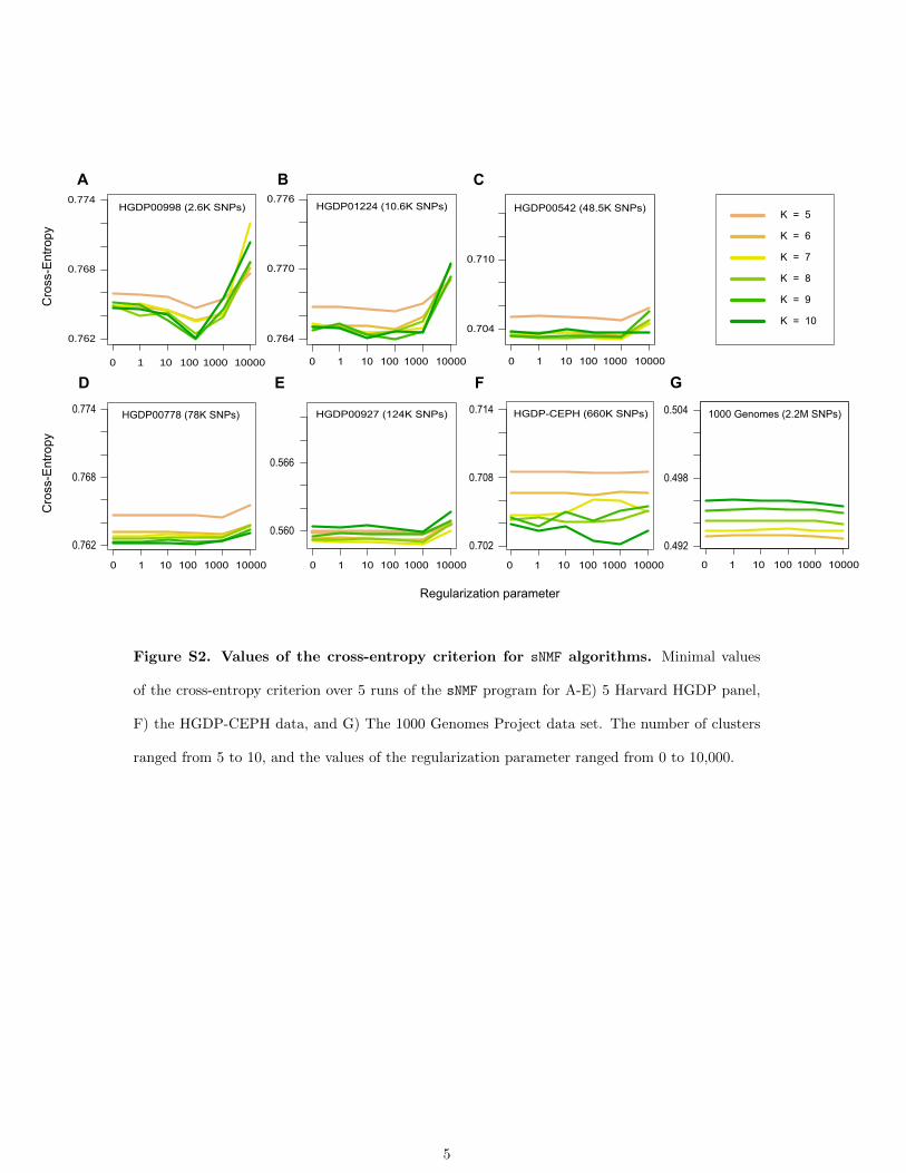
Using the cross-entropy criterion, we performed an exten-sive analysis of sNMF program outputs to assess which valuesof the number of clusters (K) and the regularization param-eter (a) could provide the best prediction of masked geno-types (Figure 3, Figure S2). For HGDP data sets withmoderate size (panels HGDP00998 and HGDP01224),values of K � 7–8 provided the best predictive results.For larger human data sets, cross-entropy values did notstabilize for K # 10, indicating that .10 clusters were nec-essary to describe population structure. Choices of regula-rization parameter values .1000 were generally discardedby the cross-entropy criterion. For panels of moderate size,the best ancestry estimates were obtained for values�a = 100.The influence of the regularization parameter was sub-stantial for the smallest data sets, but for the largest onesa wide range of values led to comparable imputationresults (Figure S2). Regardless of the value of the regula-rization parameter, K = 5 clusters led to the best resultsfor the 1000 Genomes Project data set (Figure 3). This

Figure 3 Values of the cross-en-tropy criterion for sNMF runs (hu-man data sets). (A–G) Minimalvalues of the cross-entropy crite-rion over five runs of sNMF for(A–E) five Harvard HGDP panels,(F) HGDP-CEPH data, and (G) the1000 Genomes Project data. Thenumber of clusters ranged from2 to 10.

978 E. Frichot et al.

last result is in accordance with the criteria used forchoosing populations included in the 1000 GenomesProject.

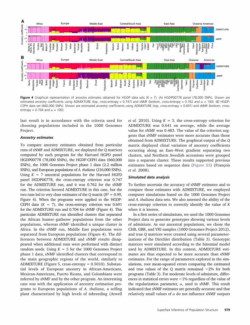
Ancestry estimates

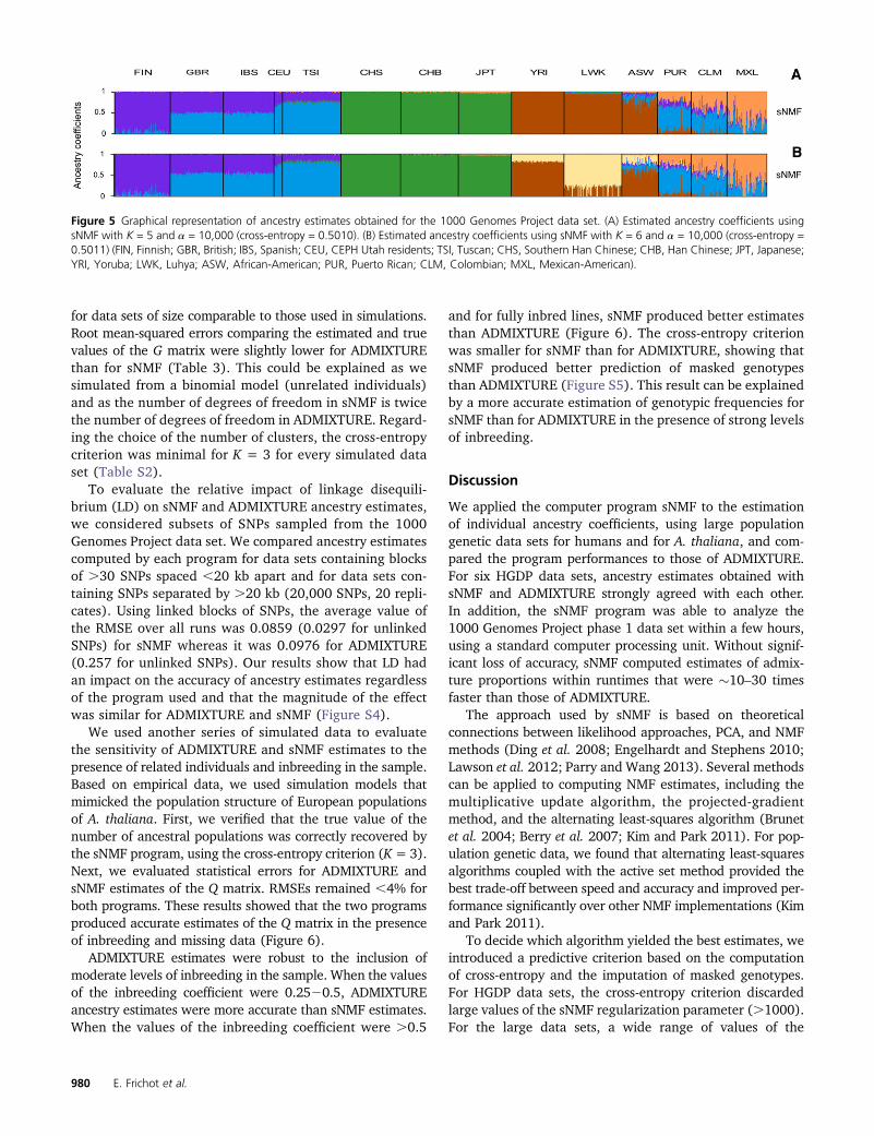
To compare ancestry estimates obtained from particularruns of sNMF and ADMIXTURE, we displayed the Qmatricescomputed by each program for the Harvard HGPD panelHGDP00778 (78,000 SNPs), the HGDP-CEPH data (660,000SNPs), the 1000 Genomes Project phase 1 data (2.2 millionSNPs), and European populations of A. thaliana (216,000 SNPs).Using K = 7 ancestral populations for the Harvard HGPDpanel HGDP00778, the cross-entropy criterion was 0.747for the ADMIXTURE run, and it was 0.762 for the sNMFrun. The criterion favored ADMIXTURE in this case, but thetwo runs led to very close estimates of the Qmatrix (R2 = 0.99,Figure 4). When the programs were applied to the HGDP-CEPH data (K = 7), the cross-entropy criterion was 0.691for the ADMIXTURE run and 0.704 for sNMF (Figure 4). Thisparticular ADMIXTURE run identified clusters that separatedthe African hunter–gatherer populations from the otherpopulations, whereas sNMF identified a unique cluster inAfrica. In the sNMF run, Middle East populations wereseparated from European populations (Figure 4). The dif-ferences between ADMIXTURE and sNMF results disap-peared when additional runs were performed with distinctrandom seeds. Using K = 5 for the 1000 Genomes Projectphase 1 data, sNMF identified clusters that correspond tothe main geographic regions of the world, similarly toADMIXTURE (Figure 5, cross-entropy = 0.5010). Substan-tial levels of European ancestry in African-Americans,Mexican-Americans, Puerto Ricans, and Colombians wereinferred by sNMF and by the other program. An interestingcase was with the application of ancestry estimation pro-grams to European populations of A. thaliana, a selfingplant characterized by high levels of inbreeding (Atwell

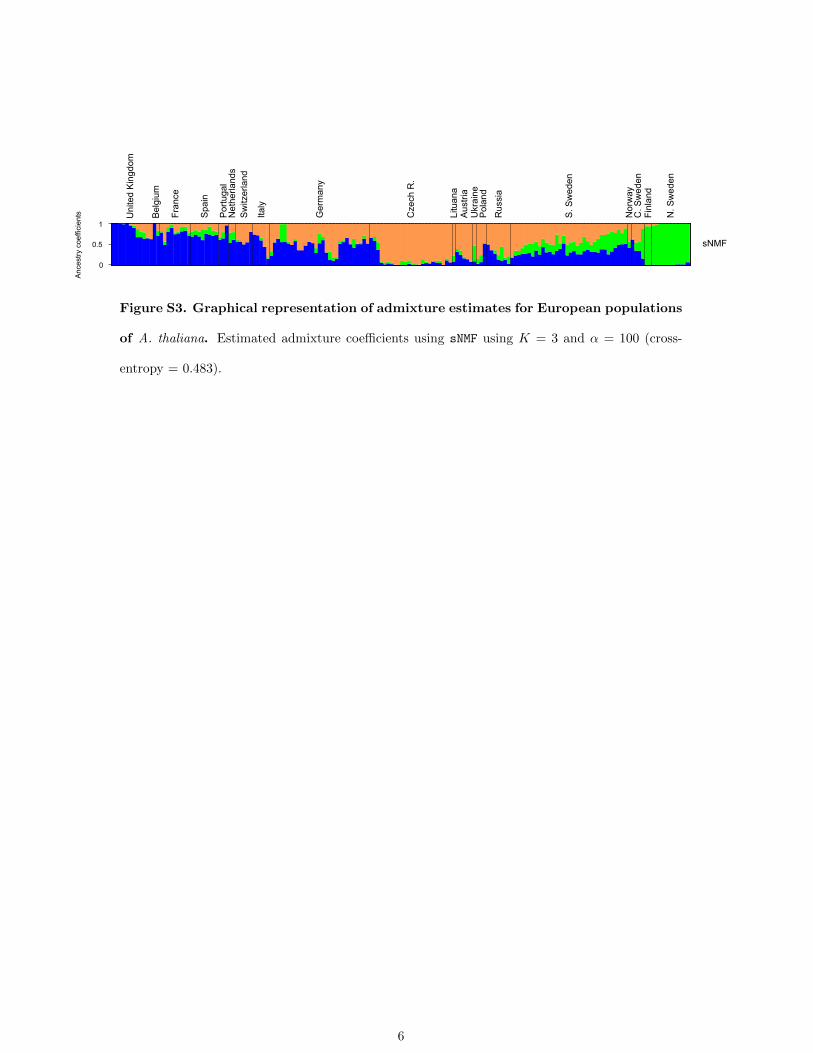
et al. 2010). Using K = 3, the cross-entropy criterion forADMIXTURE was 0.641 on average, while the averagevalue for sNMF was 0.483. The value of the criterion sug-gests that sNMF estimates were more accurate than thoseobtained from ADMIXTURE. The graphical output of the Qmatrix displayed clinal variation of ancestry coefficientsoccurring along an East–West gradient separating twoclusters, and Northern Swedish accessions were groupedinto a separate cluster. These results supported previousestimates based on sequence data (Figure S3) (Françoiset al. 2008).

Simulated data analysis

To further ascertain the accuracy of sNMF estimates and tocompare those estimates with ADMIXTURE, we employedcomputer simulations based on the 1000 Genomes Projectand A. thaliana data sets. We also assessed the ability of thecross-entropy criterion to correctly identify the value of Kwhen it is known.

In a first series of simulations, we used the 1000 GenomesProject data to generate genotypes showing various levelsof admixture. As our ancestral populations, we chose theCHB, GBR, and YRI samples (1000 Genomes Project 2012),and true Q matrices were created using several parameter-izations of the Dirichlet distribution (Table 3). Genotypicmatrices were simulated according to the binomial modelused by ADMIXTURE. In this context, ADMIXTURE esti-mates are thus expected to be more accurate than sNMFestimates. For the range of parameters explored in the sim-ulations, root mean-squared errors comparing the estimatedand true values of the Q matrix remained ,2% for bothprograms (Table 3). For moderate levels of admixture, differ-ences in statistical errors were,1% regardless of the value ofthe regularization parameter, a, used in sNMF. This resultindicated that sNMF estimates are generally accurate and thatrelatively small values of a do not influence sNMF outputs

Figure 4 Graphical representation of ancestry estimates obtained for HGDP data sets (K = 7). (A) HGDP00778 panel (78,000 SNPs). Shown areestimated ancestry coefficients using ADMIXTURE (top, cross-entropy = 0.747) and sNMF (bottom, cross-entropy = 0.762 and a = 100). (B) HGDP-CEPH data set (660,000 SNPs). Shown are estimated ancestry coefficients using ADMIXTURE (top, cross-entropy = 0.691) and sNMF (bottom, cross-entropy = 0.704 and a = 100).

Superfast Inference of Population Structure 979

for data sets of size comparable to those used in simulations.Root mean-squared errors comparing the estimated and truevalues of the G matrix were slightly lower for ADMIXTUREthan for sNMF (Table 3). This could be explained as wesimulated from a binomial model (unrelated individuals)and as the number of degrees of freedom in sNMF is twicethe number of degrees of freedom in ADMIXTURE. Regard-ing the choice of the number of clusters, the cross-entropycriterion was minimal for K = 3 for every simulated dataset (Table S2).

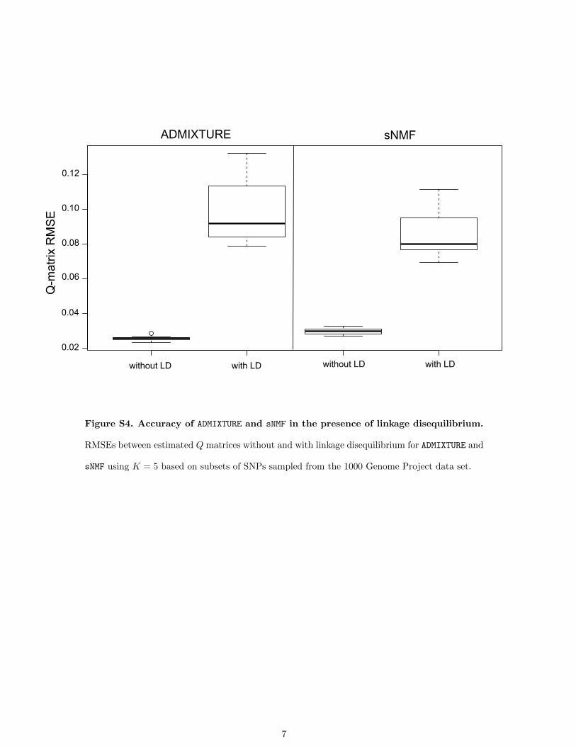
To evaluate the relative impact of linkage disequili-brium (LD) on sNMF and ADMIXTURE ancestry estimates,we considered subsets of SNPs sampled from the 1000Genomes Project data set. We compared ancestry estimatescomputed by each program for data sets containing blocksof .30 SNPs spaced ,20 kb apart and for data sets con-taining SNPs separated by .20 kb (20,000 SNPs, 20 repli-cates). Using linked blocks of SNPs, the average value ofthe RMSE over all runs was 0.0859 (0.0297 for unlinkedSNPs) for sNMF whereas it was 0.0976 for ADMIXTURE(0.257 for unlinked SNPs). Our results show that LD hadan impact on the accuracy of ancestry estimates regardlessof the program used and that the magnitude of the effectwas similar for ADMIXTURE and sNMF (Figure S4).

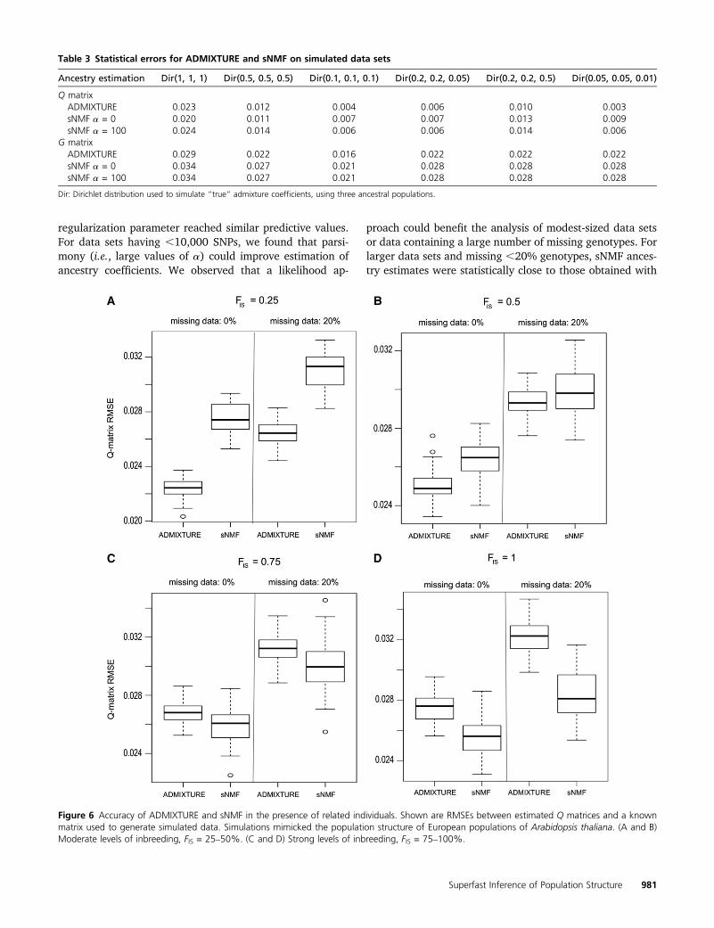
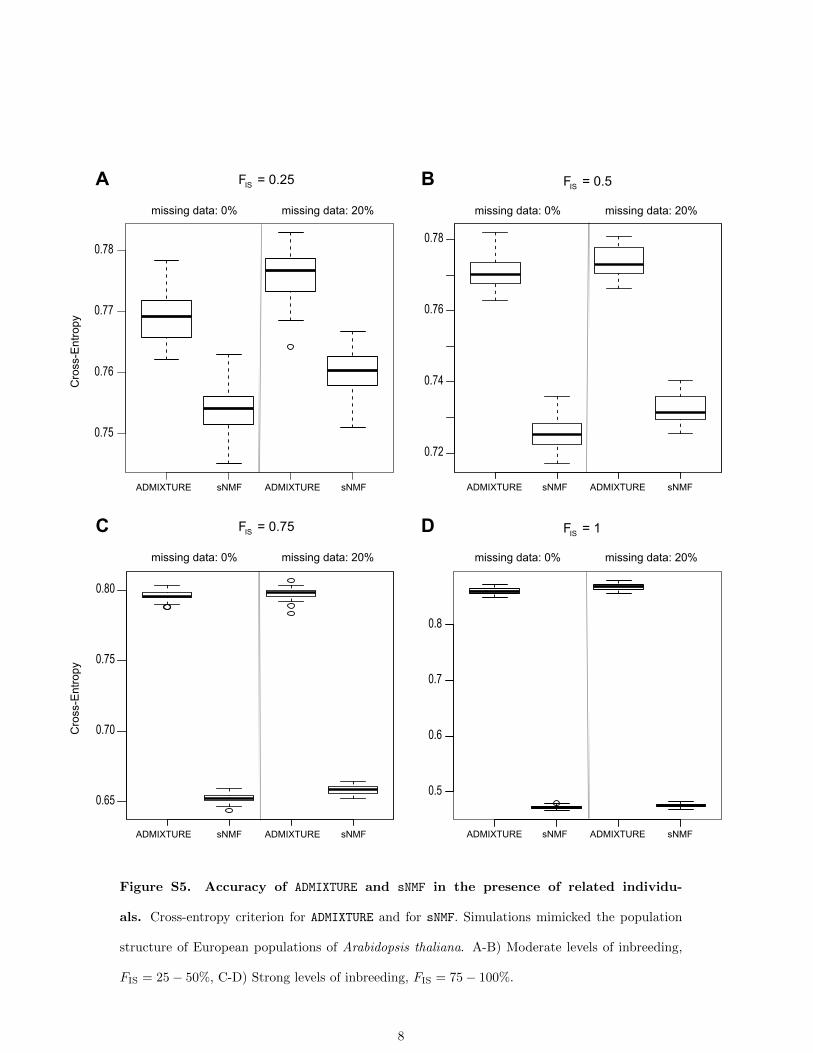
We used another series of simulated data to evaluatethe sensitivity of ADMIXTURE and sNMF estimates to thepresence of related individuals and inbreeding in the sample.Based on empirical data, we used simulation models thatmimicked the population structure of European populationsof A. thaliana. First, we verified that the true value of thenumber of ancestral populations was correctly recovered bythe sNMF program, using the cross-entropy criterion (K= 3).Next, we evaluated statistical errors for ADMIXTURE andsNMF estimates of the Q matrix. RMSEs remained ,4% forboth programs. These results showed that the two programsproduced accurate estimates of the Q matrix in the presenceof inbreeding and missing data (Figure 6).

ADMIXTURE estimates were robust to the inclusion ofmoderate levels of inbreeding in the sample. When the valuesof the inbreeding coefficient were 0.2520.5, ADMIXTUREancestry estimates were more accurate than sNMF estimates.When the values of the inbreeding coefficient were .0.5

and for fully inbred lines, sNMF produced better estimatesthan ADMIXTURE (Figure 6). The cross-entropy criterionwas smaller for sNMF than for ADMIXTURE, showing thatsNMF produced better prediction of masked genotypesthan ADMIXTURE (Figure S5). This result can be explainedby a more accurate estimation of genotypic frequencies forsNMF than for ADMIXTURE in the presence of strong levelsof inbreeding.

Discussion

We applied the computer program sNMF to the estimationof individual ancestry coefficients, using large populationgenetic data sets for humans and for A. thaliana, and com-pared the program performances to those of ADMIXTURE.For six HGDP data sets, ancestry estimates obtained withsNMF and ADMIXTURE strongly agreed with each other.In addition, the sNMF program was able to analyze the1000 Genomes Project phase 1 data set within a few hours,using a standard computer processing unit. Without signif-icant loss of accuracy, sNMF computed estimates of admix-ture proportions within runtimes that were �10–30 timesfaster than those of ADMIXTURE.

The approach used by sNMF is based on theoreticalconnections between likelihood approaches, PCA, and NMFmethods (Ding et al. 2008; Engelhardt and Stephens 2010;Lawson et al. 2012; Parry and Wang 2013). Several methodscan be applied to computing NMF estimates, including themultiplicative update algorithm, the projected-gradientmethod, and the alternating least-squares algorithm (Brunetet al. 2004; Berry et al. 2007; Kim and Park 2011). For pop-ulation genetic data, we found that alternating least-squaresalgorithms coupled with the active set method provided thebest trade-off between speed and accuracy and improved per-formance significantly over other NMF implementations (Kimand Park 2011).

To decide which algorithm yielded the best estimates, weintroduced a predictive criterion based on the computationof cross-entropy and the imputation of masked genotypes.For HGDP data sets, the cross-entropy criterion discardedlarge values of the sNMF regularization parameter (.1000).For the large data sets, a wide range of values of the

Figure 5 Graphical representation of ancestry estimates obtained for the 1000 Genomes Project data set. (A) Estimated ancestry coefficients usingsNMF with K = 5 and a = 10,000 (cross-entropy = 0.5010). (B) Estimated ancestry coefficients using sNMF with K = 6 and a = 10,000 (cross-entropy =0.5011) (FIN, Finnish; GBR, British; IBS, Spanish; CEU, CEPH Utah residents; TSI, Tuscan; CHS, Southern Han Chinese; CHB, Han Chinese; JPT, Japanese;YRI, Yoruba; LWK, Luhya; ASW, African-American; PUR, Puerto Rican; CLM, Colombian; MXL, Mexican-American).

980 E. Frichot et al.

regularization parameter reached similar predictive values.For data sets having ,10,000 SNPs, we found that parsi-mony (i.e., large values of a) could improve estimation ofancestry coefficients. We observed that a likelihood ap-

proach could benefit the analysis of modest-sized data setsor data containing a large number of missing genotypes. Forlarger data sets and missing ,20% genotypes, sNMF ances-try estimates were statistically close to those obtained with

Table 3 Statistical errors for ADMIXTURE and sNMF on simulated data sets

Ancestry estimation Dir(1, 1, 1) Dir(0.5, 0.5, 0.5) Dir(0.1, 0.1, 0.1) Dir(0.2, 0.2, 0.05) Dir(0.2, 0.2, 0.5) Dir(0.05, 0.05, 0.01)

Q matrixADMIXTURE 0.023 0.012 0.004 0.006 0.010 0.003sNMF a = 0 0.020 0.011 0.007 0.007 0.013 0.009sNMF a = 100 0.024 0.014 0.006 0.006 0.014 0.006

G matrixADMIXTURE 0.029 0.022 0.016 0.022 0.022 0.022sNMF a = 0 0.034 0.027 0.021 0.028 0.028 0.028sNMF a = 100 0.034 0.027 0.021 0.028 0.028 0.028

Dir: Dirichlet distribution used to simulate “true” admixture coefficients, using three ancestral populations.

Figure 6 Accuracy of ADMIXTURE and sNMF in the presence of related individuals. Shown are RMSEs between estimated Q matrices and a knownmatrix used to generate simulated data. Simulations mimicked the population structure of European populations of Arabidopsis thaliana. (A and B)Moderate levels of inbreeding, FIS = 25–50%. (C and D) Strong levels of inbreeding, FIS = 75–100%.

Superfast Inference of Population Structure 981

ADMIXTURE, and both programs were equally efficient atpredicting masked genotypes. Statistical theory actually pre-dicts that errors in evaluating the cross-entropy criterion areof order Oð1= ffiffiffiffiffi

nLp Þ; where nL is the number of masked gen-

otypes. For Harvard HGDP panels, differences between theADMIXTURE and sNMF results could be considered hardlysignificant and estimates were statistically similar. The ex-ample of the Harvard HGDP panels showed that the cross-entropy criterion could also be used to discriminate amongprogram runs regardless of the program used.

The assumptions underlying STRUCTURE and ADMIXTURErely on simplified population genetic hypotheses. Morespecifically, the assumptions include absence of geneticdrift and Hardy–Weinberg and linkage equilibrium in an-cestral populations. The coding used by sNMF enabled theestimation of homozygote and heterozygote frequenciesand avoided Hardy–Weinberg equilibrium assumptions. Al-though ADMIXTURE analyses were robust to small depar-tures from Hardy–Weinberg equilibrium in human data,sNMF was more appropriate to deal with inbred lineages.For European populations of A. thaliana, the values of thecross-entropy criterion indicated better predictive resultsfor sNMF than for ADMIXTURE. The difference betweensNMF and ADMIXTURE predictions could be explained asthe binomial model of ADMIXTURE is not suited to thehigh levels of inbreeding observed in A. thaliana popula-tions (Atwell et al. 2010). As seen from Equation 1, animplicit assumption underlying NMF predictions is that ge-notypic frequencies can be formed according to instanta-neous mixtures of ancestral frequencies without geneticdrift. Interpretations of admixture using estimates obtainedusing likelihood and least-squares methods can be confoundedby the existence of phylogenetic relationships among pop-ulation samples (see Patterson et al. 2012 for an alternativeapproach) or by complex demographic scenarios such asspatial range expansion (François et al. 2010).

Comparing the relative computational performancesof ADMIXTURE and sNMF was a difficult task becauseruntimes are dependent on several factors. These factorsinclude the size and other characteristics of each data set,the tolerance threshold used when stopping programiterations, the use of multiprocessor algorithms, and theinitial values of the Q and G matrices. For example, run-times could be shortened by using initial values obtainedafter running the program on reduced data sets.

We explain the relative speed of the NMF algorithm bylooking at algorithmic complexity for each program. TheANLS algorithm iterates cycles that solve linear regressionequations for Q and G. The complexity of a single cycle ofsNMF is of order O(KLn), where K is the number of clusters,n the number of individuals, and L the number of loci. Thecomplexity of a single cycle of ADMIXTURE is of order O(K2Ln) (Alexander et al. 2009). Since the default tolerancethreshold in this program implies that the program generallyruns a small number of cycles (e.g.,,40 cycles for the 78,000-SNPs Harvard HGDP panel), we observed that least-squares

algorithms ran significantly faster than likelihood algorithmswhen analyzing large population genomic data sets with largevalues of K. The sNMF program can be downloaded fromhttp://membres-timc.imag.fr/Olivier.Francois/snmf.html.

Acknowledgments

We thank Nick Patterson, Eric Stone, Badr Benjelloun, and ananonymous reviewer for their useful comments on a previousversion of this manuscript. We thank the 1000 GenomesProject for authorizing us to use the phase 1 data. This workwas supported by a grant from la Région Rhône-Alpes to EricFrichot and Olivier François. Olivier François acknowledgessupport from Grenoble Institute of Technology.

Literature Cited

Alexander, D. H., and K. Lange, 2011 Enhancements to the ad-mixture algorithm for individual ancestry estimation. BMC Bio-informatics 12: 246.

Alexander, D. H., J. Novembre, and K. Lange, 2009 Fast model-based estimation of ancestry in unrelated individuals. GenomeRes. 19: 1655–1664.

Atwell, S., Y. S. Huang, B. J. Vilhjálmsson, G. Willems, M. Hortonet al., 2010 Genome-wide association study of 107 phenotypesin Arabidopsis thaliana inbred lines. Nature 465: 627–631.

Berry, M. W., M. Browne, A. N. Langville, V. P. Pauca, and R. J.Plemmons, 2007 Algorithms and applications for approximatenonnegative matrix factorization. Comput. Stat. Data Anal. 52:155–173.

Brunet, J. P., P. Tamayo, T. R. Golub, and J. P. Mesirov,2004 Metagenes and molecular pattern discovery using matrixfactorization. Proc. Natl. Acad. Sci. USA 101: 4164–4169.

Cavalli-Sforza, L. L., and W. F. Bodmer, 1971 The Genetics of Hu-man Populations. Dover, New York.

Ding, C., T. Li, and W. Peng, 2008 On the equivalence betweennon-negative matrix factorization and probabilistic latent se-mantic indexing. Comput. Stat. Data Anal. 52: 3913–3927.

Eastment, H. T., and W. J. Krzanowski, 1982 Cross-validatorychoice of the number of components from a principal compo-nent analysis. Technometrics 24: 73–77.

Engelhardt, B. E., and M. Stephens, 2010 Analysis of populationstructure: a unifying framework and novel methods based onsparse factor analysis. PLoS Genet. 6: 12.

François, O., M. G. B. Blum, M. Jakobsson, and N. A. Rosenberg,2008 Demographic history of European populations of Arabidopsisthaliana. PLoS Genet. 4: e1000075.

François, O., M. Currat, N. Ray, E. Han, L. Excoffier et al.,2010 Principal component analysis under population geneticmodels of range expansion and admixture. Mol. Biol. Evol. 27:1257–1268.

Frichot, E., S. D. Schoville, G. Bouchard, and O. François,2012 Correcting principal component maps for effects of spa-tial autocorrelation in population genetic data. Front. Genet. 3:254.

Frichot, E., S. D. Schoville, G. Bouchard, and O. François,2013 Testing for associations between loci and environmentalgradients using latent factor mixed models. Mol. Biol. Evol. 30:1687–1699.

Kim, H., and H. Park, 2007 Sparse non-negative matrix factoriza-tions via alternating non-negativity-constrained least squares formicroarray data analysis. Bioinformatics 23: 1495–1502.

982 E. Frichot et al.

Kim, J., and H. Park, 2011 Fast nonnegative matrix factorization:an active-set-like method and comparisons. SIAM J. Sci. Com-put. 33: 3261–3281.

Jakobsson, M., and N. A. Rosenberg, 2007 CLUMPP: a clustermatching and permutation program for dealing with labelswitching and multimodality in analysis of population structure.Bioinformatics 23: 1801–1806.

Lawson, D. J., and D. Falush, 2012 Population identification usinggenetic data. Annu. Rev. Genomics Hum. Genet. 13: 337–361.

Lawson, D. J., G. Hellenthal, S. Myers, and D. Falush,2012 Inference of population structure using dense haplotypedata. PLoS Genet. 8: e1002453.

Lee, D. D., and H. S. Seung, 1999 Learning the parts of objectsby non-negative matrix factorization. Nature 401(6755):788–791.

Li, J. Z., D. M. Absher, H. Tang, A. M. Southwick, A. M. Casto et al.,2008 Worldwide human relationships inferred from genome-wide patterns of variation. Science 319: 1100–1104.

Marchini, J., L. R. Cardon, M. S. Phillips, and P. Donnelly,2004 The effects of human population structure on large ge-netic association studies. Nat. Genet. 36: 512–517.

McVean, G., 2009 A genealogical interpretation of principal com-ponents analysis. PLoS Genet. 5: 10.

Novembre, J., and M. Stephens, 2008 Interpreting principal com-ponent analyses of spatial population genetic variation. Nat.Genet. 40: 646–649.

1000 Genomes Project Consortium, 2012 An integrated map ofgenetic variation from 1,092 human genomes. Nature 491:56–65.

Parry, R. M., and M. D. Wang, 2013 A fast least-squares algorithmfor population inference. BMC Bioinformatics 14: 28.

Patterson, N., A. Price, and D. Reich, 2006 Population structureand eigenanalysis. PLoS Genet. 2: e190.

Patterson, N. J., P. Moorjani, Y. Luo, S. Mallick, N. Rohland et al.,2012 Ancient admixture in human history. Genetics 192:1065–1093.

Price, A. L., N. J. Patterson, R. M. Plenge, M. E. Weinblatt, N. A.Shadick et al., 2006 Principal components analysis corrects forstratification in genome-wide association studies. Nat. Genet.38: 904–909.

Pritchard, J. K., M. Stephens, and P. Donnelly, 2000a Inference ofpopulation structure using multilocus genotype data. Genetics155: 945–959.

Pritchard, J. K., M. Stephens, N. A. Rosenberg, and P. Donnelly,2000b Association mapping in structured populations. Am. J.Hum. Genet. 67: 170.

Roberts, D. F., and R. W. Hiorns, 1965 Methods of analysis of thegenetic composition of a hybrid population. Hum. Biol. 37:38–43.

Tang, H., J. Peng, P. Wang, and N. Risch, 2005 Estimation ofindividual admixture: analytical and study design considera-tions. Genet. Epidemiol. 28: 289–301.

Wold, S., 1978 Cross-validatory estimation of the number of com-ponents in factor and principal components models. Technomet-rics 20: 397–405.

Communicating editor: E. Stone

Superfast Inference of Population Structure 983

GENETICSSupporting Information

http://www.genetics.org/lookup/suppl/doi:10.1534/genetics.113.160572/-/DC1

Fast and Efficient Estimation of IndividualAncestry Coefficients

Eric Frichot, François Mathieu, Théo Trouillon, Guillaume Bouchard, and Olivier François

Copyright © 2014 by the Genetics Society of AmericaDOI: 10.1534/genetics.113.160572

Table S1: Root mean square error (RMSE) for 6 HGDP data sets as a function ofthe regularization parameter.

α 0 1 10 100 1000

RMSE0.046 0.044 0.041 0.041 0.055

[0.035,0.064] [0.035,0.057] [0.035,0.052] [0.031,0.061] [0.033, 0.095]

2

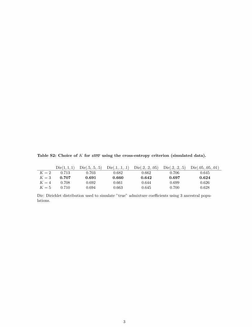
Table S2: Choice of K for sNMF using the cross-entropy criterion (simulated data).

Dir(1, 1, 1) Dir(.5, .5, .5) Dir(.1, .1, .1) Dir(.2, .2, .05) Dir(.2, .2, .5) Dir(.05, .05, .01)K = 2 0.713 0.703 0.682 0.662 0.706 0.645K = 3 0.707 0.691 0.660 0.642 0.697 0.624K = 4 0.708 0.692 0.661 0.644 0.699 0.626K = 5 0.710 0.694 0.663 0.645 0.700 0.628

Dir: Dirichlet distribution used to simulate ”true” admixture coefficients using 3 ancestral popu-lations.

3

5 10 15 20 5 10 15 20 5 10 15 20

Rur-time(m

in)

0.5

1

1.5

5

10

15

20

50

100

150

HGDP01224 (10.6K SNPs) HGDP00778 (78K SNPs) HGDP-CEPH (660K SNPs)

Number of clusters

A B C

Figure S1. Run-times for sNMF. Time is expressed in unit of minutes. A) Run-time analysis

for Harvard HGDP panel 01224 (10.6K SNPs). B) Run-time analysis for Harvard HGDP panel

00778 (78K SNPs). C) Run-time analysis for the HGDP-CEPH data (660K SNPs).

4

K = 5

K = 6

K = 7

K = 8

K = 9

K = 10

0 1 10 100 1000 10000

0.762

0.768

0.774HGDP00998 (2.6K SNPs)

0 1 10 100 1000 10000

0.764

0.776

0.770

HGDP01224 (10.6K SNPs)

0 1 10 100 1000 10000

0.704

0.710

HGDP00542 (48.5K SNPs)

0 1 10 100 1000 10000

0.762

0.768

0.774

0 1 10 100 1000 10000

0.560

0.566

HGDP00927 (124K SNPs)

0 1 10 100 1000 10000

0.702

0.708

0.714 HGDP-CEPH (660K SNPs)

0 1 10 100 1000 10000

0.492

0.498

0.504 1000 Genomes (2.2M SNPs)HGDP00778 (78K SNPs)

A

F G

Cro

ss-E

ntro

pyC

ross

-Ent

ropy

Regularization parameter

B C

D E

Figure S2. Values of the cross-entropy criterion for sNMF algorithms. Minimal values

of the cross-entropy criterion over 5 runs of the sNMF program for A-E) 5 Harvard HGDP panel,

F) the HGDP-CEPH data, and G) The 1000 Genomes Project data set. The number of clusters

ranged from 5 to 10, and the values of the regularization parameter ranged from 0 to 10,000.

5

Fra

nce

Spa

in

Por

tuga

lN

ethe

rland

sS

witz

erla

nd

Italy

Ger

man

y

Cze

chR

.

Litu

ana

Aus

tria

Ukr

aine

Pol

and

Rus

sia

S.S

wed

en

Nor

way

C.S

wed

enF

inla

nd

N.S

wed

en

Uni

ted

Kin

gdom

Bel

gium

0

0.5

1

Anc

estr

y co

effic

ient

s

sNMF

Figure S3. Graphical representation of admixture estimates for European populations

of A. thaliana. Estimated admixture coefficients using sNMF using K = 3 and α = 100 (cross-

entropy = 0.483).

6

0.02

0.04

without LD with LD without LD with LD

ADMIXTURE sNMF

Q-m

atrix

RM

SE

0.06

0.08

0.10

0.12

Figure S4. Accuracy of ADMIXTURE and sNMF in the presence of linkage disequilibrium.

RMSEs between estimated Q matrices without and with linkage disequilibrium for ADMIXTURE and

sNMF using K = 5 based on subsets of SNPs sampled from the 1000 Genome Project data set.

7

0.5

0.6

0.7

0.8

missing data: 0% missing data: 20%

F = 0.75IS F = 1ISC D

Cro

ss-E

ntro

py

ADMIXTURE sNMF ADMIXTURE sNMF ADMIXTURE sNMF ADMIXTURE sNMF

missing data: 0% missing data: 20%

0.75

0.76

0.77

0.78

missing data: 0% missing data: 20%

F = 0.25IS F = 0.5ISA B

Cro

ss-E

ntro

py

ADMIXTURE sNMF ADMIXTURE sNMF ADMIXTURE sNMF ADMIXTURE sNMF

missing data: 0% missing data: 20%

0.72

0.74

0.76

0.78

0.65

0.70

0.75

0.80

Figure S5. Accuracy of ADMIXTURE and sNMF in the presence of related individu-

als. Cross-entropy criterion for ADMIXTURE and for sNMF. Simulations mimicked the population

structure of European populations of Arabidopsis thaliana. A-B) Moderate levels of inbreeding,

FIS = 25 − 50%, C-D) Strong levels of inbreeding, FIS = 75 − 100%.

8