evaluation of instruction prefetch methods for coresonic

Master of Science Thesis in Electrical Engineering Department of Electrical Engineering, Linköping University, 2016

Department of Electrical Engineering Linköpings tekniska högskola

Linköping University Institutionen för systemteknik

S-581 83 Linköping, Sweden 581 83 Linköping

Evaluation of instruction prefetch methods for Coresonic DSP processor

Tobias Lind

Master of Science Thesis in Electrical Engineering Department of Electrical Engineering, Linköping University, 2016

Department of Electrical Engineering Linköpings tekniska högskola

Linköping University Institutionen för systemteknik

S-581 83 Linköping, Sweden 581 83 Linköping

Evaluation of instruction prefetch methods for

Coresonic DSP processor

Examensarbete i Datorteknik

av Tobias Lind

LiTH-ISY-EX--16/4959--SE

Linköping 2016

Handledare: Andreas Tyrberg

MediaTek Sweden AB

Handledare: Anders Nilsson

ISY, Linköpings Universitet

Examinator: Kent Palmqvist

ISY, Linköpings Universitet

iii

Presentationsdatum

2016-06-07

Publiceringsdatum (elektronisk version)

2016-06-13

Institution och avdelning

Institutionen för systemteknik, Datorteknik

Department of Electrical Engineering, Computer Engineering

URL för elektronisk version

http://www.ep.liu.se

Publikationens titel

Evaluation of instruction prefetch methods for Coresonic DSP processor

Författare

Tobias Lind

Sammanfattning

With increasing demands on mobile communication transfer rates the circuits in mobile phones

must be designed for higher performance while maintaining low power consumption for

increased battery life. One possible way to improve an existing architecture is to implement

instruction prefetching. By predicting which instructions will be executed ahead of time the

instructions can be prefetched from memory to increase performance and some instructions

which will be executed again shortly can be stored temporarily to avoid fetching them from the

memory multiple times.

By creating a trace driven simulator the existing hardware can be simulated while running a

realistic scenario. Different methods of instruction prefetch can be implemented into this

simulator to measure how they perform. It is shown that the execution time can be reduced by

up to five percent and the amount of memory accesses can be reduced by up to 25 percent with

a simple loop buffer and return stack. The execution time can be reduced even further with the

more complex methods such as branch target prediction and branch condition prediction.

Nyckelord

Instruction prefetch, branch prediction, DSP, computer architecture

v

ABSTRACT

With increasing demands on mobile communication transfer rates the circuits in mobile

phones must be designed for higher performance while maintaining low power consumption

for increased battery life. One possible way to improve an existing architecture is to

implement instruction prefetching. By predicting which instructions will be executed ahead of

time the instructions can be prefetched from memory to increase performance and some

instructions which will be executed again shortly can be stored temporarily to avoid fetching

them from the memory multiple times.

By creating a trace driven simulator the existing hardware can be simulated while running a

realistic scenario. Different methods of instruction prefetch can be implemented into this

simulator to measure how they perform. It is shown that the execution time can be reduced by

up to five percent and the amount of memory accesses can be reduced by up to 25 percent

with a simple loop buffer and return stack. The execution time can be reduced even further

with the more complex methods such as branch target prediction and branch condition

prediction.

SAMMANFATTNING

Med ökande krav på överföringshastighet för mobil kommunikation så måste kretsarna i

mobiltelefoner designas för högre prestanda samtidigt som strömförbrukningen hålls nere för

att batteritiden ska öka. Ett sätt att förbättra existerande kretsar är att implementera

instruktions prefetch. Genom att förutse vilka instruktioner som ska utföras i förväg så kan

dessa hämtas från minnet för att öka prestandan samt instruktioner som snart ska utföras igen

kan lagras temporärt för att undvika att de ska hämtas från minnet flera gånger.

Genom att skapa en tracedriven simulator så kan existerande hårdvara simuleras i ett

realistiskt scenario. Olika typer av tidig instruktions prefetch kan sedan implementeras i denna

simulator för att mäta hur de presterar. Det visas att körtiden kan reduceras med fem procent

och antalet hämtningar från minnet kan minskas med 25 procent med en enkel loop buffer och

return stack. Körtiden kan reduceras ytterligare genom mer komplexa metoder som branch

target prediction och branch condition prediction.

vi

ACKNOWLEDGMENTS

I want to thank the staff at MediaTek for good company and a great work environment. And I

especially want to thank my supervisor Andreas Tyrberg for his help and support throughout

this project.

Linköping, Sweden, April 2016

vii

TABLE OF CONTENTS

Chapter 1 Introduction .......................................................................................................... 1

1.1 Motivation ................................................................................................................... 1

1.2 Background .................................................................................................................. 1

1.3 Purpose ........................................................................................................................ 1

1.4 Problem statements ...................................................................................................... 2

1.5 Limitations ................................................................................................................... 2

1.6 Thesis outline ............................................................................................................... 3

Chapter 2 Theory .................................................................................................................. 5

2.1 Introduction ................................................................................................................. 5

2.2 The concept of instruction prefetch ............................................................................. 5

2.2.1 Sequential prefetch or next-line prefetch ............................................................. 5

2.2.2 Loop buffer ........................................................................................................... 6

2.3 Branches ...................................................................................................................... 6

2.3.1 Delay slots ............................................................................................................ 6

2.3.2 Branch target prediction ....................................................................................... 7

2.3.3 Branch Target Buffer ........................................................................................... 7

2.3.4 Return address stack ............................................................................................. 8

2.4 Conditional branches and branch prediction ............................................................... 8

2.4.1 Static prediction .................................................................................................... 8

2.4.2 Dynamic prediction .............................................................................................. 9

2.4.3 Two-level adaptive branch predictors ................................................................ 12

2.4.4 PHT interference ................................................................................................ 19

2.4.5 Hybrid branch predictors .................................................................................... 20

2.4.6 Neural networks ................................................................................................. 21

2.4.7 Alternative solutions .......................................................................................... 23

Chapter 3 Method ............................................................................................................... 25

3.1 Introduction ............................................................................................................... 25

3.2 Prestudy ..................................................................................................................... 25

3.3 Implementation .......................................................................................................... 25

3.4 Evaluation .................................................................................................................. 26

Chapter 4 Results ................................................................................................................ 27

4.1 Introduction ............................................................................................................... 27

viii

4.2 Prestudy ..................................................................................................................... 27

4.3 Simulation results ...................................................................................................... 27

4.3.1 Loop buffer ......................................................................................................... 27

4.3.2 Return stack ........................................................................................................ 30

4.3.3 Unconditional branches ...................................................................................... 33

4.3.4 Conditional branches .......................................................................................... 39

Chapter 5 Discussion .......................................................................................................... 57

5.1 Results ....................................................................................................................... 57

5.1.1 General ............................................................................................................... 57

5.1.2 Loop buffer ......................................................................................................... 58

5.1.3 Return stack ........................................................................................................ 59

5.1.4 Unconditional branches ...................................................................................... 60

5.1.5 Conditional branches .......................................................................................... 62

5.1.6 Strategies worth implementing ........................................................................... 64

5.2 Method ....................................................................................................................... 65

Chapter 6 Conclusions ........................................................................................................ 67

6.1 Result in relation to objectives .................................................................................. 67

6.2 Future work ................................................................................................................ 68

References ................................................................................................................................ 69

Appendix A .............................................................................................................................. 70

A.1 Loop buffer result data .............................................................................................. 70

A.2 Return stack result data .............................................................................................. 71

A.3 Unconditional branches result data ............................................................................ 73

A.4 Conditional branches result data ................................................................................ 75

ix

LIST OF FIGURES

Figure 2-1: Branch target buffer. ................................................................................................ 7

Figure 2-2: Two bit counter state diagram. .............................................................................. 10

Figure 2-3: Intel Pentium two bit counter state diagram. ......................................................... 10

Figure 2-4: Branch history table predictor with PHT indexed by instruction address. ............ 11

Figure 2-5: Combined BTB and BHT in a cache-like memory. .............................................. 11

Figure 2-6: GAg predictor with three bit GHR. ....................................................................... 13

Figure 2-7: GAp predictor with three bit GHR. ....................................................................... 14

Figure 2-8: GAs predictor with three bit GHR. ....................................................................... 15

Figure 2-9: PAg predictor with three bit BHRs. ...................................................................... 15

Figure 2-10: PAp predictor with three bit BHRs. .................................................................... 16

Figure 2-11: PAs predictor with three bit BHRs. ..................................................................... 17

Figure 2-12: SAg predictor with three bit BHRs. .................................................................... 18

Figure 2-13: SAp predictor with three bit BHRs. .................................................................... 18

Figure 2-14: SAs predictor with three bit BHRs. ..................................................................... 19

Figure 2-15: Gshare predictor with three bit GHR. ................................................................. 20

Figure 2-16: Majority predictor with three predictors.............................................................. 20

Figure 2-17: Selector predictor with one local predictor and one global predictor. ................ 21

Figure 2-18: Perceptron predictor with three inputs and one bias input. ................................. 22

Figure 2-19: Perceptron network with multiple levels and multiple input sets........................ 22

Figure 4-1: Loop distribution by number of iterations. ............................................................ 28

Figure 4-2: Loop distribution by number of instructions in loop. ............................................ 28

Figure 4-3: Completely prefetchable loops by loop buffer size in instructions. ...................... 29

Figure 4-4: Relative memory accesses for loop buffer in all traces. ........................................ 30

Figure 4-5: Relative execution time for return stack in all traces. ........................................... 31

Figure 4-6: Relative memory accesses for return stack in all traces. ....................................... 32

Figure 4-7: Relative memory accesses for improved return stack in all traces. ....................... 32

Figure 4-8: Relative execution time for BTB in Trace A. ....................................................... 34

Figure 4-9: Relative execution time for BTB in Trace B. ........................................................ 34

Figure 4-10: Relative execution time for BTB in Trace C. ...................................................... 35

Figure 4-11: Relative execution time for BTB in Trace D. ..................................................... 35

Figure 4-12: Relative memory accesses for BTB in Trace A. ................................................. 36

Figure 4-13: Relative memory accesses for BTB in Trace B. ................................................. 36

Figure 4-14: Relative memory accesses for BTB in Trace C. ................................................. 37

Figure 4-15: Relative memory accesses for BTB in Trace D. ................................................. 37

Figure 4-16: BTB performance with and without return instructions in Trace A. ................... 38

Figure 4-17: BTB relative memory accesses with and without return instructions in Trace A.

.................................................................................................................................................. 38

Figure 4-18: Distribution of conditional branch instructions by times executed. .................... 39

Figure 4-19: Weighted distribution of conditional branches by times executed. ..................... 40

Figure 4-20: Distribution of conditional branch instructions by taken probability. ................. 41

Figure 4-21: Weighted distribution of conditional branch instructions by taken probability. . 42

Figure 4-22: Branch prediction accuracy for different methods in Trace A. ........................... 43

Figure 4-23: Branch prediction accuracy for different methods in Trace B. ........................... 43

Figure 4-24: Branch prediction accuracy for different methods in Trace C. ........................... 44

Figure 4-25: Branch prediction accuracy for different methods in Trace D. ........................... 44

x

Figure 4-26: GAg predictor accuracy in all traces. .................................................................. 45

Figure 4-27: Gshare predictor accuracy in all traces. ............................................................... 45

Figure 4-28: Hybrid predictor accuracy in all traces. ............................................................... 46

Figure 4-29: Relative execution time for basic branch predictors in Trace A. ........................ 47

Figure 4-30: Relative execution time for basic branch predictors in Trace B. ........................ 47

Figure 4-31: Relative execution time for basic branch predictors in Trace C. ........................ 48

Figure 4-32: Relative execution time for basic branch predictors in Trace D. ........................ 48

Figure 4-33: Relative memory accesses for basic branch predictors in Trace A. .................... 49

Figure 4-34: Relative memory accesses for basic branch predictors in Trace B. .................... 49

Figure 4-35: Relative memory accesses for basic branch predictors in Trace C. .................... 50

Figure 4-36: Relative memory accesses for basic branch predictors in Trace D. .................... 50

Figure 4-37: Relative execution time for advanced branch predictors in Trace A. ................. 51

Figure 4-38: Relative execution time for advanced branch predictors in Trace B................... 51

Figure 4-39: Relative execution time for advanced branch predictors in Trace C................... 52

Figure 4-40: Relative execution time for advanced branch predictors in Trace D. ................. 52

Figure 4-41: Relative memory accesses for branch advanced predictors in Trace A. ............. 53

Figure 4-42: Relative memory accesses for advanced branch predictors in Trace B. ............. 53

Figure 4-43: Relative memory accesses for advanced branch predictors in Trace C. ............. 54

Figure 4-44: Relative memory accesses for advanced branch predictors in Trace D. ............. 54

Figure 4-45: Relative execution time of Gshare predictor with varying BTB size in Trace A.

.................................................................................................................................................. 55

Figure 4-46: Relative memory accesses for Gshare predictor with varying BTB size in Trace

A. .............................................................................................................................................. 55

Figure 4-47: Relative performance of combined BTB and BHT in Trace A. .......................... 56

Figure 4-48: Relative memory accesses of combined BTB and BHT in Trace A. .................. 56

xi

LIST OF TABLES

Table 2-1: Two-level adaptive branch predictor naming scheme. ........................................... 12

Table 4-1: Relative amount of instructions which are prefetchable from a loop buffer for each

trace. ......................................................................................................................................... 29

Table 4-2: Unconditional branch statistics. .............................................................................. 33

Table 4-3: Relative amounts of executed conditional branch instructions in traces. ............... 39

Table 4-4: Conditional branch statistics. .................................................................................. 41

Table 5-1: Total performance of best prefetch methods. ......................................................... 57

Table A-1: Loop distribution by number of iterations. ............................................................ 70

Table A-2: Loop distribution by number of instructions in loop. ............................................ 70

Table A-3: Completely prefetchable loops by loop buffer size in instructions. ...................... 70

Table A-4: Relative memory accesses for loop buffer. ............................................................ 70

Table A-5: Relative execution time for return stack. ............................................................... 71

Table A-6: Relative memory accesses for return stack. ........................................................... 71

Table A-7: Relative memory accesses for improved return stack............................................ 71

Table A-8: Relative execution time for indexed BTB. ............................................................ 73

Table A-9: Relative memory accesses for indexed BTB. ........................................................ 73

Table A-10: Relative execution time for cache BTB. .............................................................. 73

Table A-11: Relative memory accesses for cache BTB. .......................................................... 74

Table A-12: Relative execution time and memory accesses for indexed BTB with return

instructions in Trace A. ............................................................................................................ 74

Table A-13: Relative execution time and memory accesses for cache BTB with return

instructions in Trace A. ............................................................................................................ 74

Table A-14: Distribution of conditional branch instructions by times executed. .................... 75

Table A-15: Weighted distribution of conditional branch instructions by times executed. ..... 75

Table A-16: Distribution of conditional branches by taken frequency. ................................... 75

Table A-17: Weighted distribution of conditional branches by taken frequency. ................... 76

Table A-18: Branch predictor accuracy for simple predictors. ................................................ 76

Table A-19: Indexed BHT prediction accuracy. ...................................................................... 76

Table A-20: GAg prediction accuracy. .................................................................................... 76

Table A-21: Gshare prediction accuracy. ................................................................................. 77

Table A-22: Hybrid prediction accuracy. ................................................................................. 77

Table A-23: Relative execution time for simple branch predictors. ........................................ 77

Table A-24: Relative memory accesses for simple branch predictors. .................................... 77

Table A-25: Relative execution time for indexed BHT predictor. ........................................... 79

Table A-26: Relative memory accesses for indexed BHT predictor........................................ 79

Table A-27: Relative execution time for cache BHT predictor. .............................................. 79

Table A-28: Relative memory accesses for cache BHT predictor. .......................................... 80

Table A-29: Relative execution time for GAg predictor. ......................................................... 80

Table A-30: Relative memory accesses for GAg predictor. .................................................... 80

Table A-31: Relative execution time for Gshare predictor. ..................................................... 81

Table A-32: Relative memory accesses for Gshare predictor. ................................................. 81

Table A-33: Relative execution time for hybrid predictor. ...................................................... 81

Table A-34: Relative memory accesses for hybrid predictor. .................................................. 82

Table A-35: Relative execution time for Gshare predictor with varying BTB size in Trace A.

.................................................................................................................................................. 82

xii

Table A-36: Relative memory accesses for Gshare predictor with varying BTB size in Trace

A. .............................................................................................................................................. 82

xiii

LIST OF ABBREVIATIONS AND ACRONYMS

Abbreviation/

Acronym

Meaning Explanation Context

BHR Branch history register A register which keeps

history about the

outcomes of previous

conditional branches.

A part in dynamic

branch predictors.

BTB Branch target buffer A memory used to store

target addresses of

encountered branches.

Used to predict

target addresses for

branches.

DSP Digital signal

processing

Manipulation of digital

signals.

The target

architecture is

designed for DSP.

GBHR Global branch history

register

When a single BHR is

used it is called GBHR.

A part used in some

dynamic branch

predictors.

GHR Global history register Same as GBHR. Same as GBHR.

NT Not taken Possible outcome of a

conditional branch.

Used in state

diagram figures.

PC Program counter A part in processors

which keeps track of the

current instruction

address.

Used in figures.

PHT Pattern history table A table of two bit

counters.

A part in dynamic

branch predictors.

T Taken Possible outcome of a

conditional branch.

Used in state

diagram figures.

1

Chapter 1

Introduction

1.1 Motivation

With increasing demand for high speed connectivity and with 5G communication in

development the performance requirements for the integrated processors in the mobile phone

market are huge. The speed of integrated circuits has increased tremendously during the last

decades but the speed of memory circuits have not increased at the same rate. Therefore the

memory has a large latency compared to the speed of the processor. Due to this memory

latency it is very important for the performance that the correct instructions are fetched at the

correct time. Unfortunately the correct time is in most cases before the processor knows what

instruction to fetch. To achieve instruction fetching in such a way that the memory latency is

hidden the instruction flow must be predicted with high accuracy. This thesis work will

evaluate and simulate several ways to predict the instruction flow for a specific processor and

conclude which method is the most suitable.

1.2 Background

This thesis project aims to develop instruction prefetch methods for a commercial digital

signal processing (DSP) processor called Coresonic. This processor is used in LTE modems

for mobile phone communications and it is owned by MediaTek. Since this work is done for

Mediatek, some parts of the work are confidential and will therefore not be included in this

report.

1.3 Purpose

The main part of this work is to evaluate the Coresonic processor architecture and the code it

is running to determine the properties of the instruction flow. With these properties a set of

suitable instruction prefetch mechanisms will be implemented into a simulator to see how

they affect the execution of the programs. The metrics that will be affected the most are the

execution time and the amount of instruction fetches from memory. A good prefetch method

can reduce the execution time as well as reduce the amount of fetches from memory.

However by implementing an instruction prefetch unit one will always get some negative

effects as well. Firstly you get an extra unit which consumes both power and requires area on

the chip to implement and secondly you get added complexity in the architecture which can

add difficulty when maintaining and upgrading the architecture.

2

So the purpose of this work is to see if there is a method for instruction prefetching that can

reduce the execution time and the amount of instruction fetches while the complexity and

power consumption is kept low enough for the method to be worth implementing.

1.4 Problem statements

The goals of this master thesis work can be narrowed down into several questions that need an

answer. The first question is: How does one compare different prefetch strategies? To answer

this question the Coresonic architecture must be studied to determine which instruction

prefetch properties are the most desirable and which limitations there are in the architecture.

After that question has been answered the focus can be moved to more specific questions

about which method to use. So the second question can be formulated as: Which method of

instruction prefetch is most suitable for the Coresonic DSP? This will be the main question for

this work however it can be quite extensive. To reduce the size of that question a third

question may be added: Which method of branch prediction is most suitable for the Coresonic

DSP? While branch prediction is a part of the instruction prefetch mechanism it can be

handled separately. Branch prediction will be described in Chapter 2.

1.5 Limitations

This work will only focus on the average values of speedup and such. The implementation of

prefetching might have a positive or negative effect on the worst case execution time. If the

worst case execution time is too long the deadline for some task may be missed and the result

will be some kind of failure. However since this specific product is for mobile

communication, a missed deadline will in the worst case result in losing the connection for a

device. While this is not a wanted behaviour, it is not as bad as for example space travel,

where a missed deadline might result in a navigation error and the vessel might crash.

This work will also not include any parts about data prefetching. Data prefetching is the same

concept as for instruction prefetching, but the system has to predict which data will be

accessed by the instructions. Although it does seem to be very similar, the properties of

dataflow can be completely different from the instruction flow. Because of this the methods

for data prefetching will be different from the methods for instruction prefetch and if it was

included in this work, the amount of time would be almost doubled.

3

1.6 Thesis outline

This report is divided into six chapters. The introduction chapter will introduce the reader to

the problem and motivate why it is worth solving. The second chapter will cover the theory

required to fully understand the problem and its solution. After that the method that was used

to solve the problem will be described. The fourth chapter will go through the results,

followed by the discussion chapter where the results are reviewed. Finally there will be a

conclusions chapter to summarize the results of this work.

5

Chapter 2

Theory

2.1 Introduction

This chapter will describe and summarize some of the research that was studied for this thesis

work.

2.2 The concept of instruction prefetch

All embedded processors perform their tasks by executing instructions which are stored in a

memory. When an instruction is to be executed, it must first be fetched from the memory. The

design of the memory system will have a huge effect on the overall performance of a circuit

since over time the speed of the execution unit has increased much more than the speed of

memories. If the execution unit does not know what instruction to execute it must wait until it

arrives from the memory. One way to hide the latency of the memory is to try and predict

what instructions will be executed and fetch them from memory before they are requested by

the execution unit. This is the basic principle of instruction prefetch.

While the concept is simple, actually predicting what instructions are to be performed ahead

of time is far from easy. It is also very dependent on the architecture of the processor as well

as the code it is executing. Because of this there is no good way to tell which method is the

overall best for a specific processor without analyzing the architecture and the code that it is

running.

Most of the time instructions are executed sequentially. However all code will include some

kind of jumps. These jumps, mostly referred to as branches, are what make the instruction

flow difficult to predict. Branches can be unconditional and conditional. Unconditional

branches will always jump to another place in the code while conditional branches will only

jump if a certain condition is fulfilled. The effect of branches and how to predict the outcome

of branches will be covered below.

2.2.1 Sequential prefetch or next-line prefetch

The sequential prefetch or next-line prefetch is the simplest prefetch method. It relies on the

code to be sequential and will prefetch instructions that are a few rows ahead of the

instruction that is currently being executed [1, p. 9]. As long as the code is sequential and the

6

prefetch distance is sufficient this method will hide the latency of the memory completely.

But this will not handle non sequential cases.

2.2.2 Loop buffer

The loop buffer is a small buffer used to store a number of recently executed instructions. If

there is a loop in the code these recent instructions will be executed again [2, p. 7]. If all the

instructions of the loop fit inside the loop buffer, all required instructions will be in the loop

buffer after the first iteration. So for the second and higher iterations all instructions will be

fetched from the loop buffer and not from the memory.

2.3 Branches

Branches are the instructions in the code which make the code execute in a non sequential

order. They will cause a jump to another place in the code and continue the execution of the

program from there. While branches are a very natural part when writing code, for example an

if-statement or a function call, the effects in hardware are mostly negative in terms of

execution speed. All larger processors are pipelined, meaning the evaluation of an instruction

is separated into many stages and each stage takes one clock cycle. The largest circuits have

more than 15 pipeline stages [3, p. 25]. In pipelined processors many instructions are

processed at once but all are in different stages of the pipeline. So when a branch is inserted

into the pipeline the processor won’t know which instruction to insert into the pipeline after

the branch. Only when the branch has reached the final pipeline stage will this be known.

That means that for a large processor a branch can stop the execution of new instructions until

the branch is completely executed, up to 15 clock cycles. Therefore the execution of branches

is much slower than the execution of non branch instructions [4, p. 447].

There are also different types of branches, mainly unconditional and conditional branches.

Unconditional branches will always jump to their branch target but conditional branches will

only jump to their target if a given condition is fulfilled. To reduce the negative effect of

branches one would like to know the target of the branch and for the conditional branch if the

condition is fulfilled or not. These are the goals of branch target prediction and branch

prediction.

2.3.1 Delay slots

One simple way to reduce the negative effects of branches is to use the period directly after a

branch. The cycles after the branch, inserted into the pipeline to when the branch is evaluated,

are called delay slots [15, p. 501]. These slots can be used for other instructions and they will

always be evaluated independent on whether the branch is taken or not. With instructions in

the delay slots these cycles will not be wasted. However it is not always possible to find

instructions that could be placed in these delay slots. In these cases the delay slots need to be

filled with no operation instructions, instructions that tell the processor to do nothing. These

no operation instructions can either be written in the program code or special hardware can be

implemented to insert them into the pipeline automatically. This will waste cycles and it also

7

requires additional program memory to store these instructions or additional hardware to

insert them.

2.3.2 Branch target prediction

For both unconditional branches and conditional branches the target of the branch needs to be

predicted. When a branch target is predicted this target instruction will be fetched and the

processor will continue execution from this instruction. When the branch instruction reaches

the end of the pipeline the predicted target is compared to the actual target. If the predicted

target was the correct target the execution will continue but if the predicted target was

incorrect all instructions which have entered the pipeline after the branch will be incorrect.

These instructions have to be flushed from the pipeline and any results from these instructions

need to be reverted [4, 448].

There are not many methods for predicting target addresses but the available methods are

quite simple yet effective.

2.3.3 Branch Target Buffer

A branch target buffer (BTB) is used to store the target addresses of branches. The memory

used to store the target addresses can be designed in several ways. It can be a simple table

indexed by parts of the instruction address or it can have a cache-like structure. For each

branch instruction the address of the target is stored. By storing the target for the branch

address the target can be prefetched without the branch instruction needing to be fully

decoded [2, 8]. Branch target buffers are used in many high performance architectures [3], [5,

p. 116].

Figure 2-1: Branch target buffer.

8

The branch target buffer shown in Figure 2-1 is implemented with a cache-like structure. A

part of the instruction address is used to check if the desired branch target is stored in the

buffer.

2.3.4 Return address stack

When a function is called inside a program the hardware will jump to the start of that function

and save the address from where the function was called. When the function has completed

the program will return to where the function was called [4, p. 373]. There are many ways to

store the address to which the program should return. A return address stack is a small stack

in the prefetch unit which is used to store these return addresses. When a function is called the

address is stored at the top of the return stack and when the program returns from a function

the return address is taken from the top of the return address stack. Return address stack is

also a very common part in many processors [3] [5, p. 116].

2.4 Conditional branches and branch prediction

To predict the outcome of conditional branches the target needs to be predicted as well as the

branch condition. The target prediction can be done with a BTB, described in chapter 2.3.3,

and the different methods of predicting the branch condition used in this project are described

in this section.

2.4.1 Static prediction

Static prediction is a general term for prediction methods that does not change its behaviour

during runtime. These predictors will be very simple in hardware but they will not suffice for

any advanced system with many different branch behaviours.

2.4.1.1 Always taken and always not taken

The simplest method for predicting the outcome of a conditional branch is the always taken or

always not taken method. Depending on the construction of the hardware, the predictor will

always predict that the branch is either taken or not taken [4, p. 456]. The misprediction rate

will then be directly dependent on the statistical properties of the code. If the code has

branches which are taken 95% of the time then static prediction will predict the correct

outcome 95% of the time. However, most programs do not have these properties. The

properties of the code used in this project can be seen in Table 4-4.

2.4.1.2 Backwards taken forward not taken prediction

Backwards taken forward not taken (BTFN) prediction is a slightly more advanced prediction

method than static prediction. It predicts that a conditional branch is taken if the target address

is backwards in the code and not taken if it jumps forward in the code [6, p. 1614]. This works

well for programs with loops where a counter is decreased in each iteration and the closing

branch jumps to the beginning if the counter has not reached zero. The method requires at

least part of the target address to be decoded so the direction of the jump can be decided. To

9

be able to do this decoding additional hardware needs to be implemented. But if the code is

written to suit this predictor the resulting prediction rate will be better than for the always

taken and always not taken prediction.

2.4.1.3 Instruction word hint or simple profile

With instruction word hint or simple profile the instruction contains a bit which tells if the

branch is likely to be taken or not [4, p. 456]. This can be done manually by the programmer

or by the compiler. This method requires the conditional branch instructions to be one bit

longer or the instruction encoding scheme has to be changed. Depending on the target

architecture for this predictor the implementation of this prediction method may vary from

very easy to almost impossible.

The instruction word hint branch predictor is the overall best predictor among the static

predictors. With all hints set correctly this prediction method can reach about 87% prediction

accuracy [7, p. 215].

2.4.2 Dynamic prediction

Dynamic prediction is the general term for predictors that base their predictions on the

runtime behaviour. To be able to adapt to the branch behaviour of a program all dynamic

predictors require a memory. The size of this memory varies between methods and can be

between a single bit to almost infinitely large. There are a huge number of different types of

dynamic predictors. Many of the basic structures will be described in detail in the following

part and the concept of some of the more advanced methods will be introduced briefly.

2.4.2.1 One-level adaptive branch predictors

The dynamic predictors can be divided into several smaller groups depending on how they

work and what kind of history they save from previous branch results. One-level adaptive

branch predictors use one level of history to predict the outcome of a branch.

2.4.2.2 Last time

The simplest kind of dynamic predictor is the last time predictor. With last time prediction the

predictor keeps one bit which tells if the last branch was taken or not. The prediction will be

the same as for the last branch [4, p. 456]. After a branch is evaluated the predictor will be

updated with the result.

For more accurate prediction the predictor can have separate bits for each instruction or some

kind of mapping function which uses the branch instruction address to compute where its

corresponding bit is located. This kind of predictor will look like the one in Figure 2-4 but

there will be only one bit instead of two in each slot.

10

2.4.2.3 Two bit saturating counter

This prediction method works similarly to the last time method. But instead of only having

one bit to keep track of the last result it is using a two bit saturating counter [4, p. 456]. The

four different states are called strongly not taken, weakly not taken, weakly taken and strongly

taken. In hardware two bits are used to store the current state. Often the strongly not taken

state is represented by 00, weakly not taken is 01, weakly taken is 10 and strongly taken is 11.

If the counter is in any of the not taken states it will predict a branch to be not taken and if it is

any of the taken states it will predict a branch to be taken. The state will be updated when the

branch has been evaluated. There are several ways for the counter to switch between states.

The most common can be seen in Figure 2-2. When the counter is in the strongly taken or

strongly not taken, it requires two mispredictions to start predicting the other way. This

prevents the predictor from going from a strongly taken state to a not taken state with a single

misprediction.

Figure 2-2: Two bit counter state diagram.

Other types of state diagrams can also be used. Changing where the transitions go and what

prediction that will be taken in each state will change the behaviour of the predictor. Another

type of state diagram that was used in the Intel Pentium processor can be seen in Figure 2-3.

However the utilization of this particular state diagram might have been a design error [3, p.

18].

Figure 2-3: Intel Pentium two bit counter state diagram.

As with the last time predictor the two bit counter can have many different two bit counters

which are indexed by some kind of mapping function on the instruction address. The table of

two bit counters is called a pattern history table (PHT) and this predictor is called a branch

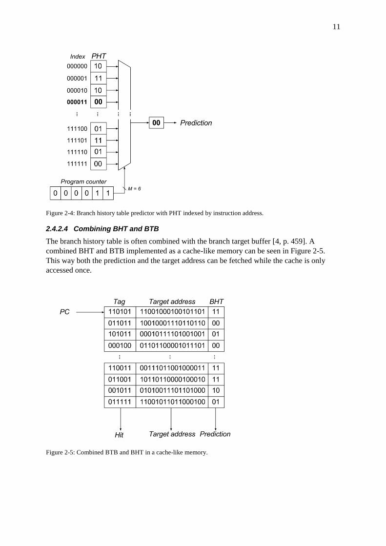
history table (BHT). Figure 2-4 shows a branch history table predictor where the mapping

function is simply taking the bits of the instruction address to index the table of separate two

bit counters. The two bit counter in the figure is set to 00 which corresponds to the strongly

not taken state which means that not taken is predicted.

11

Figure 2-4: Branch history table predictor with PHT indexed by instruction address.

2.4.2.4 Combining BHT and BTB

The branch history table is often combined with the branch target buffer [4, p. 459]. A

combined BHT and BTB implemented as a cache-like memory can be seen in Figure 2-5.

This way both the prediction and the target address can be fetched while the cache is only

accessed once.

Figure 2-5: Combined BTB and BHT in a cache-like memory.

12

2.4.3 Two-level adaptive branch predictors

The next group of dynamic predictors are called two-level adaptive branch predictors. Unlike

the one-level adaptive branch predictors this group uses two types of history to make a

prediction. Which two types of history is dependent on the predictor. These predictors will be

explained in detail in this report but first a few common parts will be explained.

The first common part is the branch history register (BHR) [7, p. 217]. A branch history

register is a set of k shift registers used to keep track of the outcomes of the last k branches.

Each time a new branch is evaluated the result is shifted in and the least recent result is shifted

out. If the branch is taken a one is shifted in otherwise a zero is shifted in. These values can be

shifted in from either direction as long as it is always the same direction. The content of the

BHR is called the current pattern. If the predictor uses a single BHR that records the outcome

of all evaluated branches it is called a global branch history register (GBHR) or global history

register (GHR). If more than one BHR is used these are stored in a table indexed by some

kind of mapping function on the instruction address.

The second part is the pattern history table (PHT) [7, p. 217]. Each slot in the PHT contains

history data for the outcomes of branches when the current pattern has been active. The most

commonly used type of history data is the previously explained two bit counter. The PHT is

indexed by the current pattern from the GHR or BHR. Many of the two-level adaptive

predictors also use many different PHTs. The current instruction address is used to choose

which PHT to use. When the condition of a branch is evaluated the state of the corresponding

two bit counter is updated.

2.4.3.1 Classification of two-level adaptive branch predictors

There are nine basic variations of two-level adaptive branch predictors. To keep these apart a

simple naming scheme with abbreviations is used [7, p. 217-218]. The different names can be

seen in Table 2-1.

Table 2-1: Two-level adaptive branch predictor naming scheme.

Global PHT Per-address PHTs Per-set PHTs

Global BHR GAg GAp GAs

Per-address BHRs PAg PAp PAs

Per-set BHRs SAg SAp SAs

The first letter in the name indicates how many BHRs the predictor uses. G stands for global

which only uses a GHR. P stands for per-address BHRs which uses one separate BHR for

each branch instruction. S is when the predictor uses a BHR table indexed by a mapping

function on the branch instruction address. The A simply stands for adaptive. The last letter

tells how many PHTs are used. If one PHT is used the final letter is g, if there are one PHT for

each branch instruction the letter is p and if there are many PHTs indexed by a mapping

function on the instruction address the final letter is s.

2.4.3.2 GAg

The GAg uses a GHR to index a PHT and each slot contains a two bit counter. An example

GAg predictor with a three bit long GHR can be seen in Figure 2-6. This predictor keeps track

13

of the outcome of the last three conditional branches and for each of the eight possible

patterns a two bit counter is stored in the PHT. This predictor relies on all branch instructions

to be correlated to the global branch history in the same way. The GAg method only looks at

the global history and does not have any separation between different branches making it a

completely global predictor.

Figure 2-6: GAg predictor with three bit GHR.

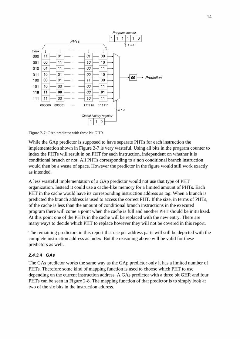
2.4.3.3 GAp

GAp is similar to the GAg predictor in the way that it uses a GHR to index a PHT. However

GAp has one PHT per branch instruction. A GAp predictor with three bit GHR and 64 PHTs

containing two bit counters can be seen in Figure 2-7. This makes the predictor rely on each

branch instruction to be correlated to the global branch history.

14

Figure 2-7: GAp predictor with three bit GHR.

While the GAp predictor is supposed to have separate PHTs for each instruction the

implementation shown in Figure 2-7 is very wasteful. Using all bits in the program counter to

index the PHTs will result in on PHT for each instruction, independent on whether it is

conditional branch or not. All PHTs corresponding to a non conditional branch instruction

would then be a waste of space. However the predictor in the figure would still work exactly

as intended.

A less wasteful implementation of a GAp predictor would not use that type of PHT

organization. Instead it could use a cache-like memory for a limited amount of PHTs. Each

PHT in the cache would have its corresponding instruction address as tag. When a branch is

predicted the branch address is used to access the correct PHT. If the size, in terms of PHTs,

of the cache is less than the amount of conditional branch instructions in the executed

program there will come a point when the cache is full and another PHT should be initialized.

At this point one of the PHTs in the cache will be replaced with the new entry. There are

many ways to decide which PHT to replace however they will not be covered in this report.

The remaining predictors in this report that use per address parts will still be depicted with the

complete instruction address as index. But the reasoning above will be valid for these

predictors as well.

2.4.3.4 GAs

The GAs predictor works the same way as the GAp predictor only it has a limited number of

PHTs. Therefore some kind of mapping function is used to choose which PHT to use

depending on the current instruction address. A GAs predictor with a three bit GHR and four

PHTs can be seen in Figure 2-8. The mapping function of that predictor is to simply look at

two of the six bits in the instruction address.

15

Figure 2-8: GAs predictor with three bit GHR.

The two-level adaptive branch predictors with a global history register are a common part in

many modern high-end processors [3], [5, p. 116].

2.4.3.5 PAg

The PAg predictor uses a table with BHRs for each instruction address and one PHT. Figure

2-9 shows a PAg predictor with three bit long BHRs and a single PHT with two bit counters.

This predictor relies on all branch instructions to have similar evaluation history.

Figure 2-9: PAg predictor with three bit BHRs.

16

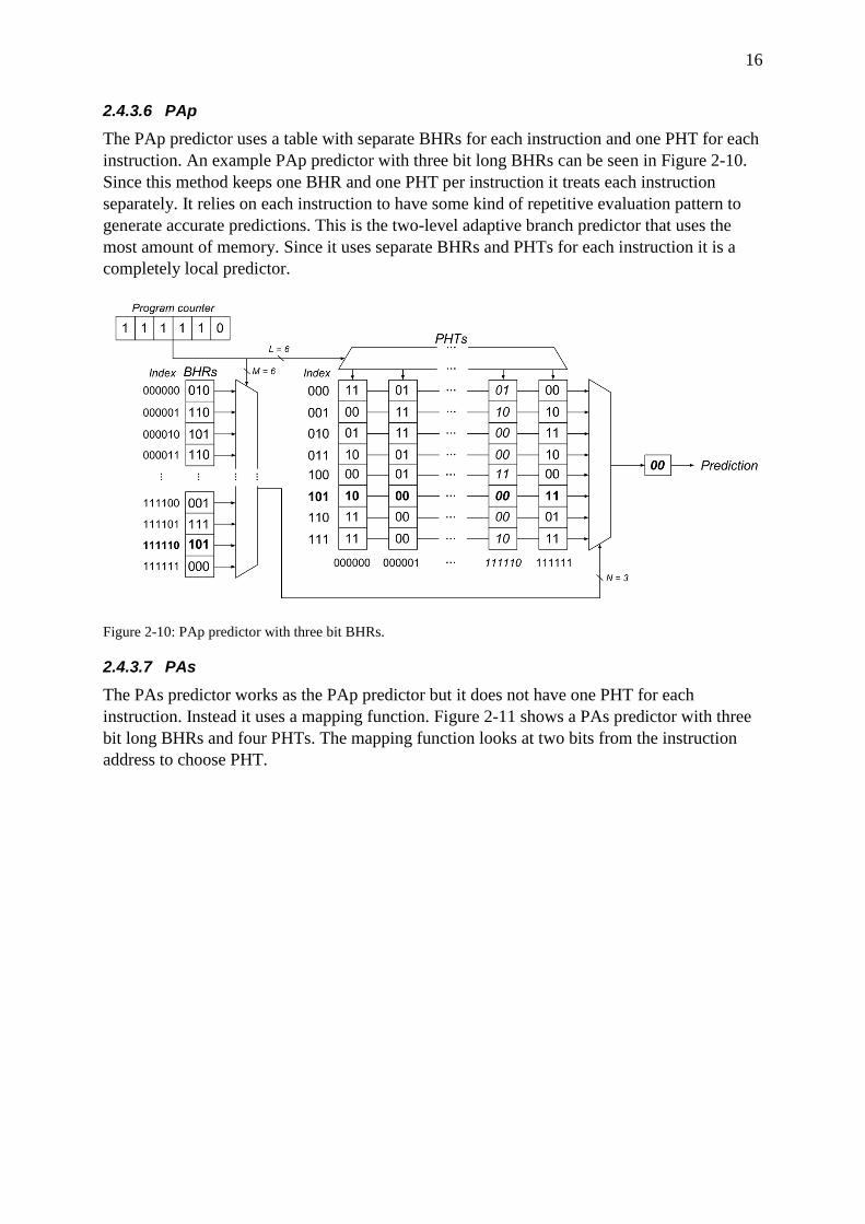
2.4.3.6 PAp

The PAp predictor uses a table with separate BHRs for each instruction and one PHT for each

instruction. An example PAp predictor with three bit long BHRs can be seen in Figure 2-10.

Since this method keeps one BHR and one PHT per instruction it treats each instruction

separately. It relies on each instruction to have some kind of repetitive evaluation pattern to

generate accurate predictions. This is the two-level adaptive branch predictor that uses the

most amount of memory. Since it uses separate BHRs and PHTs for each instruction it is a

completely local predictor.

Figure 2-10: PAp predictor with three bit BHRs.

2.4.3.7 PAs

The PAs predictor works as the PAp predictor but it does not have one PHT for each

instruction. Instead it uses a mapping function. Figure 2-11 shows a PAs predictor with three

bit long BHRs and four PHTs. The mapping function looks at two bits from the instruction

address to choose PHT.

17

Figure 2-11: PAs predictor with three bit BHRs.

18

2.4.3.8 SAg

The SAg predictor has one BHT with BHR which is indexed through a mapping function and

one PHT. Figure 2-12 shows a SAg predictor with a BHT with three bit long BHRs indexed

by looking at three bits from the instruction address. Similarly to the PAg predictor this

predictor relies on all branch instructions to have similar evaluation history.

Figure 2-12: SAg predictor with three bit BHRs.

2.4.3.9 SAp

A SAp predictor is very similar to the PAp predictor. The only difference is that the BHT

does not contain separate BHRs for each individual instruction. A mapping function on the

instruction address is used instead. An example SAp predictor were the mapping function is to

look at the last three bits of the instruction address can be seen in Figure 2-13.

Figure 2-13: SAp predictor with three bit BHRs.

19

2.4.3.10 SAs

The last type of two-level adaptive predictor is the SAs predictor. It indexes both the BHT and

the PHTs with mapping functions. A SAs predictor with three bit long BHRs and four PHTs

can be seen in Figure 2-14. The mapping functions used in the figure is to look at the three

most significant bits for the BHT and the two least significant bits for the PHTs.

Figure 2-14: SAs predictor with three bit BHRs.

2.4.4 PHT interference

A drawback with the two-level adaptive predictors that does not use per address PHTs or

BHRs is that the same PHT or BHR may be used by different branches or the same branch

history might occur at different parts in the code [6, p. 1616]. In this case the same two bit

counter will be used to predict two different situations. If these situations should be predicted

differently they will interfere with each other. This is called PHT interference and it will

cause lower prediction accuracy. To reduce the amount of PHT interference different mapping

functions for the PHTs can be used. A simple way to do this for the GAg predictor gives the

Gshare predictor.

2.4.4.1 Gshare

This method is very similar to GAg since it also uses a single branch history register and a

single pattern history table. But the pattern history table is indexed using the exclusive or

function on the branch history and the branch instruction address [7, p. 218]. A Gshare

predictor with a three bit GHR can be seen in Figure 2-15. This type of mapping function

gives a better utilization of the pattern history table with less PHT interference.

20

Figure 2-15: Gshare predictor with three bit GHR.

2.4.5 Hybrid branch predictors

Hybrid branch predictors are the next step after two level adaptive predictors. Instead of only

using one technique to predict the outcome of a branch multiple techniques are used and then

some kind of selector is used to decide which of the predictions to use [7, p. 219]. Two

common ways of doing this is the majority predictor and selector predictor.

2.4.5.1 Majority predictor

The majority predictor uses an odd number of predictors and the final prediction is the

prediction which has the most amounts of predictions. A simple majority predictor can be

seen in Figure 2-16.

Figure 2-16: Majority predictor with three predictors.

21

2.4.5.2 Selector predictor

The selector predictor uses any number of predictors and then chose which prediction to use

by having an extra predictor [6, p. 1617]. This extra predictor chooses which prediction to use

based on which predictor has been correct in previous cases. Figure 2-17 shows the most

basic selector predictor with one local predictor and one global predictor which predict the

outcome of branches and one selector predictor which predict which prediction to use.

Figure 2-17: Selector predictor with one local predictor and one global predictor.

2.4.6 Neural networks

The last type of predictor covered in this project is the neural network predictor. This is a very

advanced method for branch prediction and it will not be fully covered in this report, only

briefly introduced. Since real neural networks are very expensive to implement in hardware,

an artificial neuron called perceptron is used. This kind of predictor is only considered for

very recent high performance circuits such as high end desktop and server CPUs. The AMD

Bulldozer architecture uses a predictor based on perceptrons [12, p. 33].

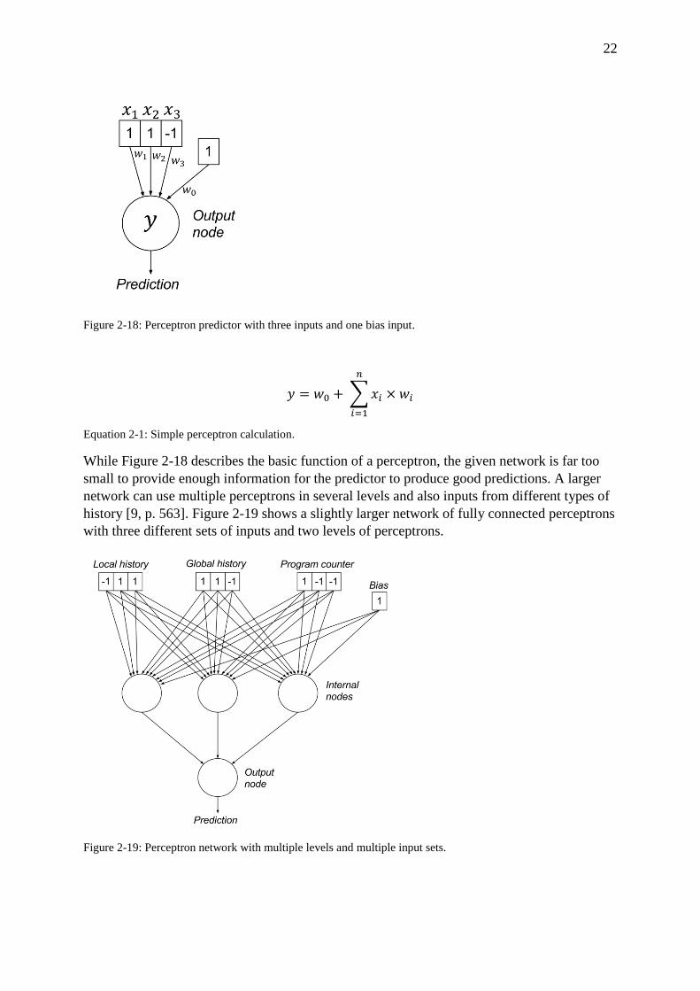
A perceptron is a small computation network which takes a set of inputs and multiplies them

with different weights and the results are then summed up to produce an output [8, p. 370]. A

small perceptron predictor can be seen in Figure 2-18 and the equation which is used to

produce the output can be seen in Equation 2-1. If the output value is positive the predictor

predicts the branch to be taken. After the branch condition is evaluated the weights used by

the perceptron is updated according to some algorithm to allow the perceptron to learn the

behaviour of the system.

22

Figure 2-18: Perceptron predictor with three inputs and one bias input.

𝑦 = 𝑤0 + ∑ 𝑥𝑖 × 𝑤𝑖

𝑛

𝑖=1

Equation 2-1: Simple perceptron calculation.

While Figure 2-18 describes the basic function of a perceptron, the given network is far too

small to provide enough information for the predictor to produce good predictions. A larger

network can use multiple perceptrons in several levels and also inputs from different types of

history [9, p. 563]. Figure 2-19 shows a slightly larger network of fully connected perceptrons

with three different sets of inputs and two levels of perceptrons.

Figure 2-19: Perceptron network with multiple levels and multiple input sets.

23

2.4.7 Alternative solutions

There are many other ways of dealing with branches and avoid the penalties for having a

pipeline other than those described earlier in this chapter. These methods mostly rely on other

concepts than instruction prefetching therefore they are not considered for implementation in

this project.

2.4.7.1 Loop unrolling

One way to avoid the branch penalties are to try and avoid branches, for example by loop

unrolling. In loop unrolling the code is rewritten so that instead of having a branch which

jumps to the beginning of the loop, the code inside the loops is duplicated the amount of times

which the loop is supposed to iterate [4, p. 503]. While loop unrolling can reduce the number

of branches and also increase the performance it will require more memory to store the

program.

2.4.7.2 Hardware loops

Loops can also be handled by using hardware loops. With hardware loops there is no branch

at the end of the loop. Instead there is an instruction that tell how many iterations the loop

should run and which instruction is the last instruction. The hardware will then detect if the

last instruction of the loop is reached and jump to the first instruction unless it is not the last

iteration. The number of iterations is handled by the hardware and all loop overhead caused

by the closing branch and the decrease of the loop counter can be removed. But this does

require special loop hardware to be implemented.

2.4.7.3 Multiple streams

Another way to handle branches is to have multiple hardware units. When a branch is

encountered both the taken and the not taken path of the branch is executed [4, p. 454]. When

the branch condition is evaluated the correct path is chosen and the other is discarded. While

this solution avoids branch penalties it requires double hardware in the execution unit and it

also requires two different parts of the program to be fetched from the memory. A slight

modification to this can be to only duplicate the first stages of the pipeline to execute the

beginning of both paths reducing the hardware cost slightly but still requires two separate

parts of the program to be fetched from memory.

A final solution is to add extra hardware in the beginning of the pipeline specifically for

evaluation branch conditions. This would allow branches to be handled quicker thus giving a

lower penalty despite having a long pipeline.

25

Chapter 3

Method

3.1 Introduction

The method chapter will go through the steps taken to complete this master thesis work.

3.2 Prestudy

During the prestudy phase of this thesis work all relevant theory was studied. The main goal

of the prestudy was to learn the available methods for instruction prefetching and to learn the

properties of these methods. The most important properties at this stage were when they work

and when they do not. As a first step to get familiar with the concepts of instruction

prefetching and branch prediction method books on computer architecture basics were used.

To further increase the knowledge about these areas many different scientific articles were

studied. At first older articles were used since they studied many of the methods used in the

currently existing hardware. Recent scientific articles were then studied to learn what methods

are currently researched and which might possibly be implemented into hardware in the

future. As a last step the documentation on many different circuits were studied to see what

kinds of instruction prefetch and branch prediction are actually used in hardware today.

The most important parts of the studied theory is summarized and shown in the theory

chapter, Chapter 2.

After the theory was studied the focus was turned to the Coresonic architecture and the

programs it is running. To know which methods of instruction prefetch and branch prediction

to implement the properties of the current fetch unit was studied as well as the instruction set

and some of the available programs for it. The details about the architecture are not included

in this report.

3.3 Implementation

A good way to determine the performance of different prefetch methods is to simulate the

behaviour of the methods when running a designated program. However implementing a

complete simulator for the Coresonic architecture to simulate how the hardware behaves

would be a far too big task with the limited amount of time available for this thesis work.

Instead a trace driven simulator was to be implemented.

26

A trace driven simulator uses collected data from the execution of an actual program running

on the hardware. The available traces in this project consist of one file with the full program

memory contents and one file which specified the discontinuities in the instruction flow. With

this information one can follow the complete execution path of the program, instruction by

instruction. For this thesis work four different traces were used. The traces will in this report

be noted as Trace A, Trace B, Trace C and Trace D.

The first implemented trace driven simulator for this work was a simple kind which only

modelled the basic structure of the actual hardware. Its main purpose was to run through the

available traces to collect statistics about the instructions in the program. These statistics

would help determining the properties of the programs. These statistics can be seen

throughout Chapter 4. By using these statistics and the properties of different prefetch

methods the methods which would be implemented into the simulator was chosen. Another

feature in this simulator was that the accuracy of branch predictors and branch target buffers

could be tested.

The second simulator was designed to simulate the behaviour of the Coresonic architecture in

terms of pipeline depth and fetch mechanism more accurately. The most important part of this

simulator was to keep the timing for fetching instructions and executing branches true to how

the timing in the Coresonic hardware in terms of clock cycles.

The chosen prefetch methods were then implemented into the simulators to evaluate their

performance by measuring the execution time for the trace as well as the amount of memory

accesses.

3.4 Evaluation

The evaluation of the results is split up into two steps. The first step is to evaluate if the model

is correct and if the results from the simulations correspond to how the different methods

would perform if they were implemented into the architecture. It is also possible to determine

if the different methods perform as expected by comparing the statistical properties with the

results from simulations.

The final step of the project is to evaluate the results of all simulations and determine which

methods should be considered for implementation into the architecture. To simplify this

process all data is visualized in many plots and figures which allows for a much simpler

comparison.

27

Chapter 4

Results

4.1 Introduction

In this chapter all of the result from the project will be given. The meanings of the results are

discussed in the next chapter, Chapter 5.

4.2 Prestudy

Based on the prestudy the first problem statement in this project, given in chapter 1.4, can be

answered. The most important properties of different methods are the difference in execution

time, the difference in the amount of memory accesses and the implementation cost. Both the

execution time and the amount of memory accesses can be reduced with good prefetching but

it will always require additional hardware to be implemented into the architecture. If a method

is worth implementing the reduction in execution time and memory accesses need to be worth

more than the increased implementation cost.

4.3 Simulation results

In this section the results for all simulated instruction prefetch methods will be presented.

4.3.1 Loop buffer

To determine if a loop buffer should be implemented into the final model, statistics about the

loops in the traces were collected. The distribution of these loops depending on the number of

iterations in each loop is shown in Figure 4-1.

The data used to create this figure and all upcoming loop buffer results can be found in A.1.

28

Figure 4-1: Loop distribution by number of iterations.

As described in section 2.2.2 the loop buffer is supposed to store the instructions during the

first iteration so that for all iterations after that the instructions can be fetched from the buffer

instead of the memory. However as seen in Figure 4-1 most loops run for five or less iteration

and for two traces over half of the loops have two or less iteration. This will limit the

effectiveness of the loop buffer.

To gain more knowledge about the loops the amount of instructions in each loop were

measured and the distribution can be seen in Figure 4-2.

Figure 4-2: Loop distribution by number of instructions in loop.

0%

10%

20%

30%

40%

50%

60%

70%

80%

90%

100%

Trace A Trace B Trace C Trace D

50+

21-50

11-20

6-10

3-5

1-2

0%

10%

20%

30%

40%

50%

60%

70%

80%

90%

100%


50+

21-50

11-20

6-10

3-5

1-2

29

According to these numbers about half of the loops in all traces are ten instructions or shorter.

However there are several loops in each trace which contains more than 50 instructions.

With these statistics and the knowledge of how many times each loop is encountered (these

numbers are not included in this report) one can make a crude prediction on how well a loop

buffer will perform. Table 4-1 shows the part of the relative amount of instructions that can be

prefetched from a loop buffer for each trace.

Table 4-1: Relative amount of instructions which are prefetchable from a loop buffer for each trace.

Trace Trace A Trace B Trace C Trace D

Prefetchable instructions 0,1070 0,1808 0,0432 0,0257

The values in Table 4-1 are the relative amount of prefetchable instructions calculated

according to Equation 4-1 and divided by the total amount of instructions in the traces.

𝑃𝑟𝑒𝑓𝑒𝑡𝑐ℎ𝑎𝑏𝑙𝑒 𝑖𝑛𝑠𝑡𝑟𝑢𝑐𝑡𝑖𝑜𝑛𝑠 = ∑ 𝐼𝑛𝑠𝑡𝑟𝑢𝑐𝑡𝑖𝑜𝑛𝑠𝑖 × (𝐼𝑡𝑒𝑟𝑎𝑡𝑖𝑜𝑛𝑠𝑖 − 1)

𝑙𝑜𝑜𝑝𝑠

𝑖=1

× 𝐸𝑛𝑐𝑜𝑢𝑛𝑡𝑒𝑟𝑠𝑖

Equation 4-1: Formula for calculating the amount of instructions prefetchable with a loop buffer.

Instructionsi is the amount of instructions in loop i, Iterationsi is the number of iterations for

loop i and Encountersi is the amount of times that loop i is encountered in the trace. The

number of iterations is subtracted by one since the first iteration of the loop is used to store

the instructions into the loop buffer, therefore they cannot be fetched from the loop buffer

until the second iteration.

Figure 4-3 shows how much of the loops can be completely prefetched from a loop buffer

depending on the loop buffer size in instructions. These values are also calculated from

Equation 4-1 but separated depending on how many instructions there are in the loop.

Figure 4-3: Completely prefetchable loops by loop buffer size in instructions.

0%

10%

20%

30%

40%

50%

60%

70%

80%

90%

100%


Unlimited

50

20

10

5

2

30

Figure 4-3 gives an indication of how large loop buffer to have. However one does need to

realize that it only shows the loops that can be completely stored in the given loop buffer.

However a loop buffer that is too small will still be able to prefetch the maximum amount of

instructions that it can store and the remaining instructions will have to be fetched from the

memory.

While statistics can give a reasonably good idea of how a loop buffer will perform the most

accurate results are given by implementing it into the model and run simulations. One

difference between these simulations compared to the previous statistics is that the amount of

instructions is no longer measured. Instead the amount of fetches from memory is used. While

these two metrics are strongly related, the fetch mechanism in the Coresonic architecture

results in no direct translation between them.

The result from the simulations of the loop buffer can be seen in Figure 4-4. These

simulations measure the relative amount of memory accesses that are made throughout the

traces with a loop buffer varying size given in bytes.

Figure 4-4: Relative memory accesses for loop buffer in all traces.

These results show that by implementing a loop buffer the amount of fetches from memory

can be reduced by over 15% in Trace B but in Trace D the amount of fetches is not even

reduced by one percent. The performance of a loop buffer is strongly dependent on the

program which the processor is running.

4.3.2 Return stack

The next prefetch method that was considered for implementation was the return stack. A

return stack will reduce the number of clock cycles by fetching the return address from the

return stack instead of waiting until the return instruction has reached the last stage of the

pipeline. If the address from the return stack was correct the performance will increase and no

extra memory accesses will be required. If the return address from the return stack is wrong

0,8

0,82

0,84

0,86

0,88

0,9

0,92

0,94

0,96

0,98

1

16B 32B 48B 64B 80B 96B 112B 128B

Re

lati

ve m

em

ory

acc

ess

es

Loop buffer size

Trace A

Trace B

Trace C

Trace D

31

there will be no increase in performance and the memory accesses will increase since the

wrong instructions will be fetched. When the return instruction reaches the final pipeline stage

the mispredicted return will be detected and the correct instructions will be fetched.

While a return should be preceded by a call instruction, this is not always true in the given

traces. With the available instructions the return addresses can be manipulated. Doing this

causes the return address from the return stack to be incorrect. In the traces used in this

project these occurrences are only happening within some interrupt sections. By not using the

return stack for instructions within interrupts these can be avoided.

Thanks to the simple concept yet promising performance the return stack was chosen for

implementation into the model. The performance results from the simulated return stack can

be seen in Figure 4-5 with increasing return stack depth. The largest stacks include an extra

stack for the return instructions within interrupts described in the section above.

Figure 4-5: Relative execution time for return stack in all traces.

The data used for this and all upcoming result figures for the return stack are found in A.2.

0,965

0,97

0,975

0,98

0,985

0,99

0,995

1

1 2 4 6 8 10 10+1 10+2 10+3

Re

lati

ve e

xecu

tio

n t

ime

Return stack entries [normal entries + interrupt entries]

Trace A

Trace B

Trace C

Trace D

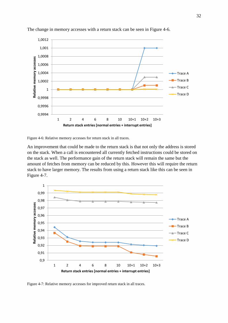
32

The change in memory accesses with a return stack can be seen in Figure 4-6.

Figure 4-6: Relative memory accesses for return stack in all traces.

An improvement that could be made to the return stack is that not only the address is stored

on the stack. When a call is encountered all currently fetched instructions could be stored on

the stack as well. The performance gain of the return stack will remain the same but the

amount of fetches from memory can be reduced by this. However this will require the return

stack to have larger memory. The results from using a return stack like this can be seen in

Figure 4-7.

Figure 4-7: Relative memory accesses for improved return stack in all traces.

0,9994

0,9996

0,9998

1

1,0002

1,0004

1,0006

1,0008

1,001

1,0012

1 2 4 6 8 10 10+1 10+2 10+3

Re

lati

ve m

em

ory

acc

ess

es


Trace A

Trace B

Trace C

Trace D

0,9

0,91

0,92

0,93

0,94

0,95

0,96

0,97

0,98

0,99

1

1 2 4 6 8 10 10+1 10+2 10+3

Re

lati

ve m

em

ory

acc

ess

es


Trace A

Trace B

Trace C

Trace D

33

4.3.3 Unconditional branches

Next up is the unconditional branches. Since unconditional branches are always taken it is the

branch target that should be predicted. This can be done with a branch target buffer described

in section 2.3.3. As before the first step was to gather statistics to determine the properties of

unconditional branches in the traces. Table 4-2 shows the unconditional branch statistics for

the traces.

Table 4-2: Unconditional branch statistics.


Relative amount of

executed unconditional

branches

0,0463 0,0566 0,2073 0,2724

Relative amount of

executed returns

0,0168 0,0198 0,0067 0,0043

Given in Table 4-2 are the relative amounts of unconditional branches in the traces. The

relative amounts of returns are also included. Return instructions are unconditional branches

however they can be predicted more accurately with the previously shown return stack. By

implementing both a branch target buffer and a return stack the return instructions can be kept

out of the BTB which will increase the accuracy of the BTB.

While the hardware for a BTB is much larger than for the two previous methods, it is a very

common and potent method. Therefore it has been chosen for implementation into the model.

Two types of branch target buffers have been implemented and simulated. The first one is a

fully associative cache, as shown in Figure 2-1. The cache uses the least recently used

replacement method when the cache is full and a new entry is inserted. The second BTB is a

table where the slots are indexed by some of the bits in the branch instruction address, much

like the branch history table in Figure 2-4. A correctly predicted target address will increase

the performance while a mispredicted target address will give an increased amount of fetches

from memory. The results from these branch target buffers can be seen in Figure 4-8 to Figure

4-15 where the size of the BTB is varied. In these simulations the return instructions did not

use the BTB.

The data used to create all figures for the unconditional branch results can be found in A.3.

34

Figure 4-8: Relative execution time for BTB in Trace A.

Figure 4-9: Relative execution time for BTB in Trace B.

0,94

0,945

0,95

0,955

0,96

0,965

0,97

0,975

0,98

0,985

0,99

32 64 128 256 512 1024 2048 4096 8192

Re

lati

ve e

xecu

tio

n t

ime

BTB entries

Indexed BTB

Cache BTB

0,92

0,93

0,94

0,95

0,96

0,97

0,98

32 64 128 256 512 1024 2048 4096 8192

Re

lati

ve e

xecu

tio

n t

ime

BTB entries

Indexed BTB

Cache BTB

35

Figure 4-10: Relative execution time for BTB in Trace C.

Figure 4-11: Relative execution time for BTB in Trace D.

0,61

0,612

0,614

0,616

0,618

0,62

0,622

0,624

0,626

0,628

0,63

0,632

32 64 128 256 512 1024 2048 4096 8192

Re

lati

ve e

xecu

tio

n t

ime

BTB entries

Indexed BTB

Cache BTB

0,472

0,474

0,476

0,478

0,48

0,482

0,484

32 64 128 256 512 1024 2048 4096 8192

Re

lati

ve e

xecu

tio

n t

ime

BTB entries

Indexed BTB

Cache BTB

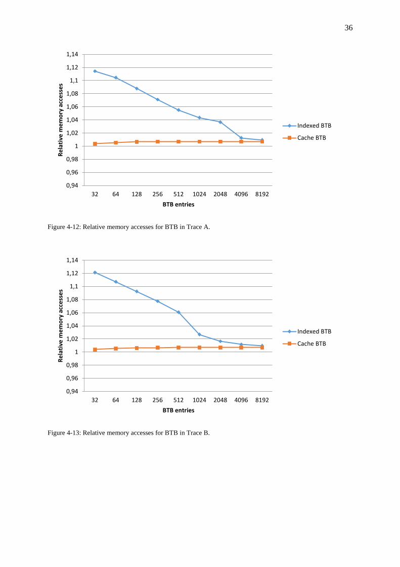
36

Figure 4-12: Relative memory accesses for BTB in Trace A.

Figure 4-13: Relative memory accesses for BTB in Trace B.

0,94

0,96

0,98

1

1,02

1,04

1,06

1,08

1,1

1,12

1,14

32 64 128 256 512 1024 2048 4096 8192

Re

lati

ve m

em

ory

acc

ess

es

BTB entries

Indexed BTB

Cache BTB

0,94

0,96

0,98

1

1,02

1,04

1,06

1,08

1,1

1,12

1,14

32 64 128 256 512 1024 2048 4096 8192

Re

lati

ve m

em

ory

acc

ess

es

BTB entries

Indexed BTB

Cache BTB

37

Figure 4-14: Relative memory accesses for BTB in Trace C.

Figure 4-15: Relative memory accesses for BTB in Trace D.

0,99

0,995

1

1,005

1,01

1,015

1,02

1,025

1,03

1,035

32 64 128 256 512 1024 2048 4096 8192

Re

lati

ve m

em

ory

acc

ess

es

BTB entries

Indexed BTB

Cache BTB

0,995

1

1,005

1,01

1,015

1,02

32 64 128 256 512 1024 2048 4096 8192

Re

lati

ve m

em

ory

acc

ess

es

BTB entries

Indexed BTB

Cache BTB

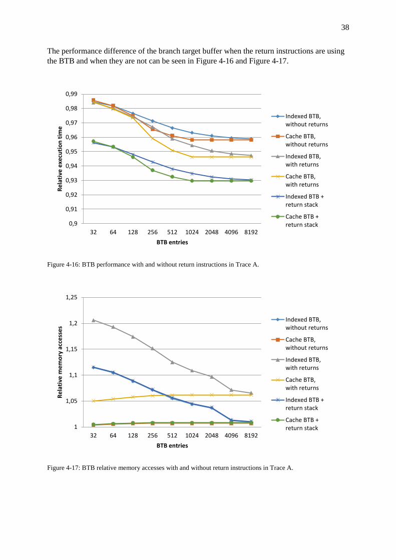
38

The performance difference of the branch target buffer when the return instructions are using

the BTB and when they are not can be seen in Figure 4-16 and Figure 4-17.

Figure 4-16: BTB performance with and without return instructions in Trace A.

Figure 4-17: BTB relative memory accesses with and without return instructions in Trace A.

0,9

0,91

0,92

0,93

0,94

0,95

0,96

0,97

0,98

0,99

32 64 128 256 512 1024 2048 4096 8192

Re

lati

ve e

xecu

tio

n t

ime

BTB entries

Indexed BTB,without returns

Cache BTB,without returns

Indexed BTB,with returns

Cache BTB,with returns

Indexed BTB +return stack

Cache BTB +return stack

1

1,05

1,1

1,15

1,2

1,25

32 64 128 256 512 1024 2048 4096 8192

Re

lati

ve m

em

ory

acc

ess

es

BTB entries

Indexed BTB,without returns

Cache BTB,without returns

Indexed BTB,with returns

Cache BTB,with returns

Indexed BTB +return stack

Cache BTB +return stack

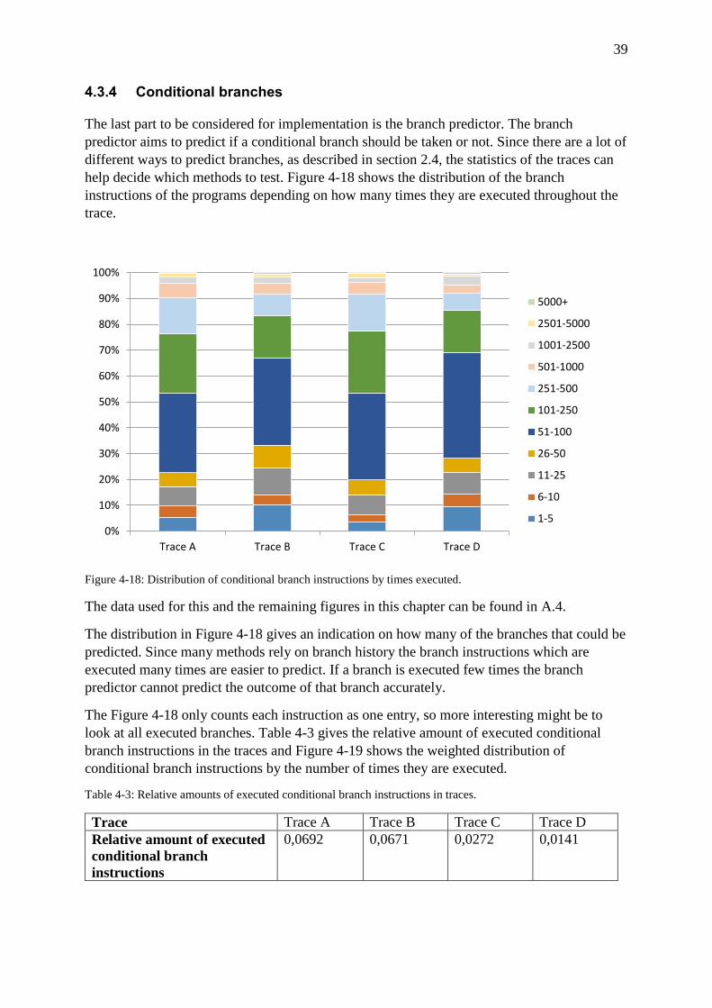
39

4.3.4 Conditional branches

The last part to be considered for implementation is the branch predictor. The branch

predictor aims to predict if a conditional branch should be taken or not. Since there are a lot of

different ways to predict branches, as described in section 2.4, the statistics of the traces can

help decide which methods to test. Figure 4-18 shows the distribution of the branch

instructions of the programs depending on how many times they are executed throughout the

trace.

Figure 4-18: Distribution of conditional branch instructions by times executed.

The data used for this and the remaining figures in this chapter can be found in A.4.

The distribution in Figure 4-18 gives an indication on how many of the branches that could be

predicted. Since many methods rely on branch history the branch instructions which are

executed many times are easier to predict. If a branch is executed few times the branch

predictor cannot predict the outcome of that branch accurately.

The Figure 4-18 only counts each instruction as one entry, so more interesting might be to

look at all executed branches. Table 4-3 gives the relative amount of executed conditional

branch instructions in the traces and Figure 4-19 shows the weighted distribution of

conditional branch instructions by the number of times they are executed.

Table 4-3: Relative amounts of executed conditional branch instructions in traces.


Relative amount of executed

conditional branch

instructions

0,0692 0,0671 0,0272 0,0141

0%

10%

20%

30%

40%

50%

60%

70%

80%

90%

100%


5000+

2501-5000

1001-2500

501-1000

251-500

101-250

51-100

26-50

11-25

6-10

1-5

40

Figure 4-19: Weighted distribution of conditional branches by times executed.

Figure 4-19 shows that the conditional branch instructions that are executed few times are a

very small part of the total amount of executed conditional branches. And the instructions that

are executed over 5000 times are a quite significant part of the total amount of executed

branches while in Figure 4-18 these branches can hardly be seen. These branches will execute

a large amount of times giving the branch predictor the possibility to gather lots of history

about these branches which in turn will allow the predictor to produce more accurate

predictions for these branches.

The amount of executions of a conditional branch instruction is not the only relevant

statistical property when considering branch prediction. It is also relevant to look at how the

branches behave in terms of taken and not taken probabilities. Figure 4-20 shows the

distribution of the conditional branch instructions depending on their taken probabilities.

0%

10%

20%

30%

40%

50%

60%

70%

80%

90%

100%


5000+

2501-5000

1001-2500

501-1000

251-500

101-250

51-100

26-50

11-25

6-10

1-5

41

Figure 4-20: Distribution of conditional branch instructions by taken probability.

Figure 4-20 shows that there are a lot of branches that are either always taken or always not

taken. These conditional branches should be easily predicted with a prediction method that

uses local history.

As with the distribution by times executed it is also interesting to look at the weighted

distribution of conditional branch instructions by taken probability. Table 4-4 shows the

probability that a branch is taken for each trace. Figure 4-21 shows the weighted distribution

of conditional branch instructions by their taken probability.

Table 4-4: Conditional branch statistics.


Branch taken

probability

41.3% 42.4% 38.8% 43.8%

0%

10%

20%

30%

40%

50%

60%

70%

80%

90%

100%


100%

80-100%

60-80%

40-60%

20-40%

0-20%

0%

42

Figure 4-21: Weighted distribution of conditional branch instructions by taken probability.

Figure 4-21 shows that even when the weighted distribution is considered there is a large part

of the executed conditional branches that are from branch instructions that are either always

taken or always not taken.

The branch prediction method is the most complex of the prefetch methods in this project. But

since the conditional branches are a large part of the evaluated instructions the method is

implemented into the simulator. Many different prediction methods are chosen so that the

importance of a good branch predictor could be determined.

The chosen static methods are the always taken, always not taken and instruction hint

methods, described in section 2.4.1. These do not require any type of memory in the predictor

hardware but the instruction hint method requires each conditional branch instruction to

contain an extra bit for the prediction. The one-level adaptive methods that are simulated are

the one bit counter, the two bit counter and the branch history table, all described in section

2.4.2. The one bit counter requires one bit of memory while the two bit counter requires two

bits. The amount of memory in the BHT can be varied and is given in all simulations. The

two-level adaptive prediction methods included in the simulations are GAg, Gshare. These are

explained in section 2.4.3. The final predictor is the hybrid predictor. The hybrid predictor is a

selector predictor, described in section 2.4.5.2 and it consists of one Gshare predictor and one

cache BHT predictor, each taking half of the given memory. The selector in the hybrid

predictor is also a cache BHT which is the same size as the BHT for the prediction.

0%

10%

20%

30%

40%

50%

60%

70%

80%

90%

100%


100%

80-100%

60-80%

40-60%

20-40%

0-20%

0%

43

The accuracy of the different methods for branch prediction with varying predictor size, given

in bytes (Ki is the binary prefix kibi which means 210 which is equal to 1024), can be seen in

Figure 4-22, Figure 4-23, Figure 4-24 and Figure 4-25.

Figure 4-22: Branch prediction accuracy for different methods in Trace A.

Figure 4-23: Branch prediction accuracy for different methods in Trace B.

40

50

60

70

80

90

16B 32B 64B 128B 256B 512B 1KiB 2KiB 4KiB 8KiB 16KiB

Pre

dic

tio

n a

ccu

racy

[%

]

Predictor size

Always taken

Never taken

Instruction hint

One bit counter

Two bit counter

Gag

Gshare

BHT

Hybrid

40

50

60

70

80

90


Pre

dic

tio

n a

ccu

racy

[%

]

Predictor size

Always taken

Never taken

Instruction hint

One bit counter

Two bit counter

Gag

Gshare

BHT

Hybrid

44

Figure 4-24: Branch prediction accuracy for different methods in Trace C.

Figure 4-25: Branch prediction accuracy for different methods in Trace D.

35

45

55

65

75

85

95


Pre

dic

tio

n a

ccu

racy

[%

]

Predictor size

Always taken

Never taken

Instruction hint

One bit counter

Two bit counter

Gag

Gshare

BHT

Hybrid

40

50

60

70

80

90


Pre

dic

tio

n a

ccu

racy

[%

]

Predictor size

Always taken

Never taken

Instruction hint

One bit counter

Two bit counter

Gag

Gshare

BHT

Hybrid

45

To show the performance difference of the adaptive prediction methods depending on the

trace their results are shown in Figure 4-26 to Figure 4-28.

Figure 4-26: GAg predictor accuracy in all traces.

Figure 4-27: Gshare predictor accuracy in all traces.

60

65

70

75

80

85

90

95


Pre

dic

tio

n a

ccu

racy

[%

]

Predictor size

Trace A

Trace B

Trace C

Trace D

60

65

70

75

80

85

90

95


Pre

dic

tio

n a

ccu

racy

[%

]

Predictor size

Trace A

Trace B

Trace C

Trace D

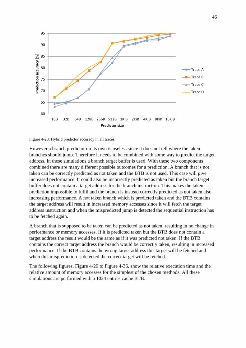
46

Figure 4-28: Hybrid predictor accuracy in all traces.

However a branch predictor on its own is useless since it does not tell where the taken

branches should jump. Therefore it needs to be combined with some way to predict the target

address. In these simulations a branch target buffer is used. With these two components

combined there are many different possible outcomes for a prediction. A branch that is not

taken can be correctly predicted as not taken and the BTB is not used. This case will give

increased performance. It could also be incorrectly predicted as taken but the branch target

buffer does not contain a target address for the branch instruction. This makes the taken

prediction impossible to fulfil and the branch is instead correctly predicted as not taken also

increasing performance. A not taken branch which is predicted taken and the BTB contains

the target address will result in increased memory accesses since it will fetch the target

address instruction and when the mispredicted jump is detected the sequential instruction has

to be fetched again.

A branch that is supposed to be taken can be predicted as not taken, resulting in no change in

performance or memory accesses. If it is predicted taken but the BTB does not contain a

target address the result would be the same as if it was predicted not taken. If the BTB

contains the correct target address the branch would be correctly taken, resulting in increased

performance. If the BTB contains the wrong target address this target will be fetched and

when this misprediction is detected the correct target will be fetched.

The following figures, Figure 4-29 to Figure 4-36, show the relative execution time and the

relative amount of memory accesses for the simplest of the chosen methods. All these

simulations are performed with a 1024 entries cache BTB.

60

65

70

75

80

85

90

95


Pre

dic

tio

n a

ccu

racy

[%

]

Predictor size

Trace A

Trace B

Trace C

Trace D

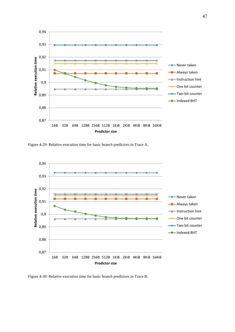
47

Figure 4-29: Relative execution time for basic branch predictors in Trace A.

Figure 4-30: Relative execution time for basic branch predictors in Trace B.

0,87

0,88

0,89

0,9

0,91

0,92

0,93

0,94


Re

lati

ve e

xecu

tio

n t

ime

Predictor size

Never taken

Always taken

Instruction hint

One bit counter

Two bit counter

Indexed BHT

0,87

0,88

0,89

0,9

0,91

0,92

0,93

0,94


Re

lati

ve e

xecu

tio

n t

ime

Predictor size

Never taken

Always taken

Instruction hint

One bit counter

Two bit counter

Indexed BHT

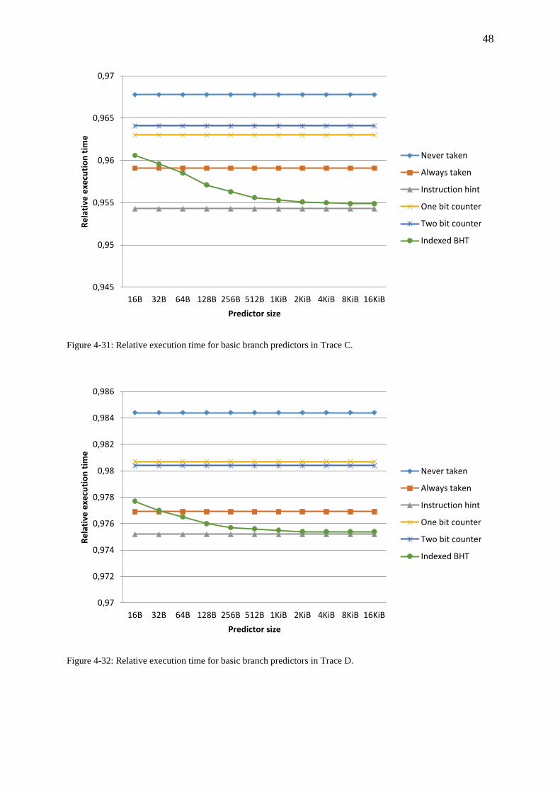
48

Figure 4-31: Relative execution time for basic branch predictors in Trace C.

Figure 4-32: Relative execution time for basic branch predictors in Trace D.

0,945

0,95

0,955

0,96

0,965

0,97


Re

lati

ve e

xecu

tio

n t

ime

Predictor size

Never taken

Always taken

Instruction hint

One bit counter

Two bit counter

Indexed BHT

0,97

0,972

0,974

0,976

0,978

0,98

0,982

0,984

0,986


Re

lati

ve e

xecu

tio

n t

ime

Predictor size

Never taken

Always taken

Instruction hint

One bit counter

Two bit counter

Indexed BHT

49

Figure 4-33: Relative memory accesses for basic branch predictors in Trace A.

Figure 4-34: Relative memory accesses for basic branch predictors in Trace B.

0,9

0,95

1

1,05

1,1

1,15

1,2


Re

lati

ve m

em

ory

acc

ess

es

Predictor size

Never taken

Always taken

Instruction hint

One bit counter

Two bit counter

Indexed BHT

0,9

0,95

1

1,05

1,1

1,15

1,2


Re

lati

ve m

em

ory

acc

ess

es

Predictor size

Never taken

Always taken

Instruction hint

One bit counter

Two bit counter

Indexed BHT

50

Figure 4-35: Relative memory accesses for basic branch predictors in Trace C.

Figure 4-36: Relative memory accesses for basic branch predictors in Trace D.

0,97

0,98

0,99

1

1,01

1,02

1,03

1,04

1,05


Re

lati

ve m

em

ory

acc

ess

es

Predictor size

Never taken

Always taken

Instruction hint

One bit counter

Two bit counter

Indexed BHT

0,99

0,995

1

1,005

1,01

1,015

1,02


Re

lati

ve m

em

ory

acc

ess

es

Predictor size

Never taken

Always taken

Instruction hint

One bit counter

Two bit counter

Indexed BHT

51

Up next is the same type of simulations but with the more advanced methods of branch

prediction. Figure 4-37 to Figure 4-44 shows the results from these simulations. A 1024

entries cache BTB is still used.

Figure 4-37: Relative execution time for advanced branch predictors in Trace A.

Figure 4-38: Relative execution time for advanced branch predictors in Trace B.

0,87

0,875

0,88

0,885

0,89

0,895

0,9

0,905

0,91

0,915

0,92


Re

lati

ve e

xecu

tio

n t

ime

Predictor size

Indexed BHT

Cache BHT

GAg

Gshare

Hybrid

0,875

0,88

0,885

0,89

0,895

0,9

0,905

0,91

0,915


Re

lati

ve e

xecu

tio

n t

ime

Predictor size

Indexed BHT

Cache BHT

GAg

Gshare

Hybrid

52

Figure 4-39: Relative execution time for advanced branch predictors in Trace C.

Figure 4-40: Relative execution time for advanced branch predictors in Trace D.

0,944

0,946

0,948

0,95

0,952

0,954

0,956

0,958

0,96

0,962

0,964


Re

lati

ve e

xecu

tio

n t

ime

Predictor size

Indexed BHT

Cache BHT

GAg

Gshare

Hybrid

0,97

0,971

0,972

0,973

0,974

0,975

0,976

0,977

0,978

0,979

0,98


Re

lati

ve e

xecu

tio

n t

ime

Predictor size

Indexed BHT

Cache BHT

GAg

Gshare

Hybrid

53

Figure 4-41: Relative memory accesses for branch advanced predictors in Trace A.

Figure 4-42: Relative memory accesses for advanced branch predictors in Trace B.

0,99

1

1,01

1,02

1,03

1,04

1,05

1,06

1,07

1,08


Re

lati

ve m

em

ory

acc

ess

es

Predictor size

Indexed BHT

Cache BHT

GAg

Gshare

Hybrid

0,99

1

1,01

1,02

1,03

1,04

1,05

1,06

1,07


Re

lati

ve m

em

ory

acc

ess

es

Predictor size

Indexed BHT

Cache BHT

GAg

Gshare

Hybrid

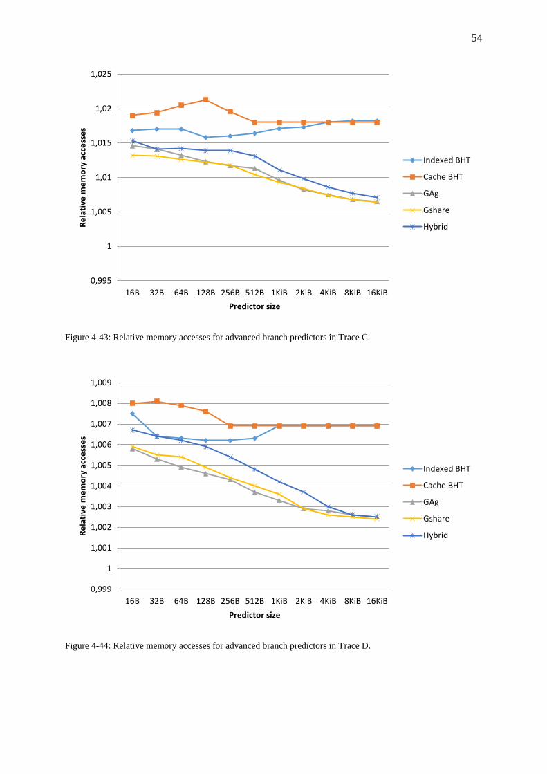
54

Figure 4-43: Relative memory accesses for advanced branch predictors in Trace C.

Figure 4-44: Relative memory accesses for advanced branch predictors in Trace D.

0,995

1

1,005

1,01

1,015

1,02

1,025


Re

lati

ve m

em

ory

acc

ess

es

Predictor size

Indexed BHT

Cache BHT

GAg

Gshare

Hybrid

0,999

1

1,001

1,002

1,003

1,004

1,005

1,006

1,007

1,008

1,009


Re

lati

ve m

em

ory

acc

ess

es

Predictor size

Indexed BHT

Cache BHT

GAg

Gshare

Hybrid

55

To show the effects of varying branch target buffer Trace A were simulated with the Gshare

predictor with different cache BTB sizes. The results can be seen in Figure 4-45 and Figure

4-46.

Figure 4-45: Relative execution time of Gshare predictor with varying BTB size in Trace A.

Figure 4-46: Relative memory accesses for Gshare predictor with varying BTB size in Trace A.

0,87

0,875

0,88

0,885

0,89

0,895

0,9

0,905

0,91

0,915

0,92


Re

lati

ve e

xecu

tio

n t

ime

Predictor size

32 entries

64 entries

128 entries

256 entries

512 entries

1024 entries

0,98

0,99

1

1,01

1,02

1,03

1,04

1,05

1,06


Re

lati

ve m

em

ory

acc

ess

es

Predictor size

32 entries

64 entries

128 entries

256 entries

512 entries

1024 entries

56

The last configuration that was chosen was the combined branch history table and branch

target buffer that was described in section 2.4.2.4. Both the indexed and the cache version

were simulated and the results are shown in Figure 4-47 and Figure 4-48.

Figure 4-47: Relative performance of combined BTB and BHT in Trace A.

Figure 4-48: Relative memory accesses of combined BTB and BHT in Trace A.

0,87

0,88

0,89

0,9

0,91

0,92

0,93

0,94

Re

lati

ve e

xecu

tio

n t

ime

Entries

Indexed BTB+BHT

Cached BTB+BHT

0,98

1

1,02

1,04

1,06

1,08

1,1

1,12

1,14

Re

lati

ve m

em

ory

acc

ess

es

Entries

Indexed BTB+BHT

Cache BTB+BHT

57

Chapter 5

Discussion

5.1 Results

The purpose of this chapter is to discuss and evaluate the results presented in Chapter 4.

5.1.1 General

The general discussion will cover the parts which affect all simulations, not just a specific part

or method.

5.1.1.1 Performance

Since the different prefetch methods cover different cases in the execution their results can be

added up to get the results from implementing several methods. To show what instruction

prefetching can accomplish the results from all the best performing methods have been added

and the total results are given in Table 5-1.

Table 5-1: Total performance of best prefetch methods.


Relative execution time 0,8179 0,8019 0,5557 0,4419

Relative memory

accesses 0,8541 0,7766 0,965 0,9865

The table clearly shows that with good instruction prefetching it is possible to both reduce the

execution time as well as the amount of memory accesses.

5.1.1.2 Verification

All the results in this thesis are based on the data from simulating the Coresonic architecture.

For this data to be correct the implemented model of Coresonic needs to be correct. The main

features and characteristics of the architecture are implemented according to the architecture.

However the implemented model is not fully correct. There are many special cases in the

traces which the real hardware handles in a clever way while the implemented model does

not. Fortunately these special cases are quite rare in the traces so the effects could be

neglected. They are also occurring in both the simulations without prefetch and those with

prefetch so they will affect all simulations in the same way. So the absolute numbers in terms

of clock cycles and memory accesses will not be correct but the difference between

simulations is the most important aspect here. So the model is not fully correct but the results

are still useful.

58

The model that is used for the simulations is correct enough which should mean that the given

result should be the same as if any of the simulated prefetch methods were implemented into

the hardware. But this will only be true if everything else in the hardware and software is the

same as in the simulation. This will most likely not be the case. If a prefetch method is chosen

both the hardware and the software could be optimized to utilize this new prefetch method

more effectively. For example if a small loop buffer is implemented some of the loops that are

too large to completely fit inside the loop buffer might be split into several separate loops

which could fit in the loop buffer. It is also possible for both the programmers and the

compilers to optimize the code with the branch prediction method in mind which can make

the branch predictor more accurate.

One thing to note throughout all the results is that the result varies a lot between the different

traces. Except for the simulation for unconditional branch target prediction the results in

Trace A and Trace B is much better compared to the results from Trace C and Trace D. But

all of these differences are because of the different traces. Trace C and Trace D contain a lot

of waiting sections which are described in section 5.1.4.1. This results in a large part of these

traces to be useless code in terms of instruction prefetching. The absolute numbers in terms of

saved clock cycles and reduced memory accesses are often very similar between traces but

due to these waiting sections the differences in relation to total execution time are smaller for

Trace C and Trace D. Therefore Trace A and Trace B give a better picture of how the

instruction prefetch methods perform.

5.1.1.3 Other aspects

One implementation detail that is not taken into account in the simulations is how to detect a

branch instruction. To be able to predict and fetch the targets of branches the branch

instruction needs to be detected early enough so that the target address can be predicted and

fetched from memory in time to be executed directly after the branch instructions. This will

be needed for all the simulated methods except for the loop buffer. If the branch instruction is

not detected early enough the branch will be predicted later and the performance gain of the

prefetch can be lost.

5.1.1.4 Conclusion

While the hardware model used in the simulations in not fully correct it models the general

features of the hardware and the error in the results will be small. The results in this report are

therefore useful when evaluating different prefetch methods.

5.1.2 Loop buffer

This section will discuss the results from the loop buffer simulations.

5.1.2.1 Performance

The loop buffer result plot seen in Figure 4-4 shows that the amount of fetches from memory

can be reduced significantly. Reducing the amount of memory accesses with up to 15 percent

is good for such a simple method with such a small memory.

59


The first thing to note about the plots is that they are approaching a limit when increasing the

loop buffer size. This is an expected result since there is a limited amount of loops in the

traces so only a limited amount of instructions can be fetched from the loop buffer. The

difference in performance between the traces is because of the different amount of

instructions that are inside loops. The limit for each trace correlates very well with the

amounts of instructions in loops, given in Table 4-1.

One thing that does not match the expected result is how the loop buffer performs in Trace D.

Figure 4-3 shows that there should be a lot of large loops that require a large loop buffer but

Figure 4-4 show that the decrease in memory accesses stops at low sizes. However this is due

to the actual execution of loops with many instructions. In most cases they are not simply

sequential instructions, they contain branches as well. This can cause the number of evaluated

instructions in each iteration of the loop to be less than the total amount of instructions within

the loop. The results will also suffer due to the way the loop buffer is implemented in these

simulations. If many instructions are skipped during the first iteration of the loop these will

not be stored in the loop buffer for the following iterations. A cleverer implementation of the

loop buffer which would fetch missing instructions during the later iterations could be used to

decrease the amount of fetches further.

Another thing that can seem inconsistent is the decrease in memory accesses from no loop

buffer to the 16 byte loop buffer. This decrease is not given in the result figure, Figure 4-4,

but it can easily be determined through this figure. The amount of fetches that could be saved

by a loop buffer should increase the most when going from no loop buffer to the smallest size

loop buffer since this will be able to store the beginning of all loops. When increasing from a

16 byte to a 32 byte loop buffer the decrease in memory fetches will not be as big since not all

loops require more than 16 bytes. But the loop buffer used in these simulations uses memory

alignment. The address of the instructions in memory will then determine where in each 16

byte slot in the loop buffer the instruction will be stored. The first instruction of the loop will

therefore not be stored at the start of the loop buffer for most loops. Due to this alignment the

first 16 byte slot will not be fully utilized and the decrease in memory accesses will be lower

than expected.

5.1.2.3 Conclusion

The loop buffer is a simple method which requires a small amount of memory. Yet it gives a

significant reduction of memory accesses. The loop buffer should therefore be considered for

implementation.

5.1.3 Return stack

This section will discuss the results from the return stack simulations.

5.1.3.1 Performance

The results of the return stack shown in Figure 4-5 show that the execution time can be

reduced by over three percent and the required hardware for a return stack can be considered

very simple. The extra return stack for the more unsecure returns does reduce the execution

60

time further but the amount of fetches from memory increases slightly due to mispredicted

returns. However the increase in fetches is not large at all which can be seen in Figure 4-6.

The results from the improved type of return stack where also some instructions are stored can

be seen in Figure 4-7. The difference in execution time is the same as for the first type of

return stack but the amount of fetches from memory is greatly reduced with this type of return

stack. The drawback of this return stack is that the amount of memory needed is larger.


As with the loop buffer, the performance of the return stack is approaching a limit when

increasing the return stack size. This is also expected since there is a limited amount of return

instructions in the traces. The limits for the different traces correspond well to the amount of

return instructions in each trace which can be seen in Table 4-2.


One good thing is that the improvements of implementing a return stack do not interfere with

the improvements from the loop buffer. Returns are mostly not a part of loops. The results of

implementing both a loop buffer and a return stack should be additive.

5.1.3.4 Conclusion

With a simple concept and low memory requirements the return stack is a very promising

feature that should be considered for implementation. The improved return stack used to

reduce memory accesses should also be considered since it does not add much complexity, it

only adds a small amount of memory.

5.1.4 Unconditional branches

This section will discuss the results from the simulations where the target of unconditional

branches were predicted with a branch target buffer.

5.1.4.1 Performance

Predicting the targets of branches is done with a branch target buffer. The results of

implementing a BTB can be seen in section 4.3.3. As the figures show, implementing a BTB

gives reduced execution time but increases the amount of fetches from memory. This

behaviour is expected since every correctly predicted target will allow the execution to

continue immediately after the branch instruction while an incorrect prediction will cause the

wrong instructions to be fetched before the correct target address is detected.

The performance of the BTB in Trace C and Trace D shown in Figure 4-10 and Figure 4-11 is

at first glance incredible with an execution time of around 50 percent of the original. However

there is a reason for this seemingly incredible performance. There are waiting segments in the

code which include unconditional branches. Predicting the target address of these is very

simple since it jumps to the same address many consecutive times. But these are waiting for

some external signals or for a specific amount of time to pass. Predicting these branches will

cause each wait segment to be shorter and instead it needs to run more times to wait for the

same amount of time. This large performance increase will not occur if the BTB is

implemented in the hardware.

61

Luckily, these wait branches are all predicted by even the smallest BTB. Because of this none

of the points in the plots will give the correct relative execution time but the difference in

relative execution time between different BTB sizes is still relevant.

The required hardware for a BTB can be quite large. The smallest BTB used in the

simulations contains 32 entries which might not be that large but the size can be doubled

many times while the performance keeps increasing. The largest simulated BTB would be

completely unrealistic to implement into the architecture due to its size.

Out of the versions of BTB, indexed and cache, the results clearly show that the cache version

performs better, both in terms of relative execution time and relative memory fetches.

However it is also more expensive both to implement and to use.


It is also expected that the performance approaches a limit when increasing the size of the

BTB. Since there are a limited amount of unconditional branches in each trace the

performance will not increase when adding more slots than there are branches. As with the

previous method these limits correspond to the amount of unconditional branches in the traces

seen in Table 4-2.


The simulations with a cache branch target buffer have only been done with a fully

associative cache with the least recently used replacement algorithm. Different cache

organizations such as a set associative cache and other replacement algorithm might give

different results compared to the ones given here. Other cache types have not been tested due

to lack of time.

If a branch target buffer is considered for implementation, the return stack should be

considered as well. Figure 4-16 shows the performance of a BTB which is used for returns as

well as the performance of a BTB which is not used for return instructions along with a return

stack. As the figure shows the performance of the combined branch target buffer without

return instructions and return stack is much better than the BTB alone. The return stack is also

much smaller. The largest simulated return stack is used in the figure and it contains 13

entries compared to the BTB which varies from 32 to 8192 entries.

The amount of fetches from memory is also much larger when the return instructions are

using the BTB which can be seen in Figure 4-17. Since the target of a return instruction is

dependent on where the function was called from it is very likely that the next time a return is

executed it was called from another place in the code and therefore it has another target.

Using a BTB for return instructions will therefore result in many mispredicted targets. If the

returns do not use the BTB there will also be less interference between instructions since there

will be less instructions using the available slots in the BTB.

5.1.4.4 Conclusion

A branch target buffer can be used to predict the targets of unconditional branches which

reduce the execution time. However this reduction is similar to the one from the return stack

while the hardware is many times larger. A BTB is therefore not as promising for

implementation.

62

5.1.5 Conditional branches

The branch prediction unit can require the largest and most complicated hardware of the

simulated prefetch methods. It requires some kind of predictor to predict if a branch is taken

or not as well as a way to predict the target address. As with the prediction of unconditional

branches the implementation of a conditional branch predictor can result in reduced execution

time at the cost of more fetches from memory.

5.1.5.1 Chosen methods

There are many aspects of a conditional branch predictor to consider. First of all the

prediction method predict whether a branch is taken or not. The chosen methods for this

project are mostly the simple ones since these are more suited for the considered architecture.

The hybrid predictor is included in the simulations to show the possible increase of using a

more advanced branch prediction method.

The backwards taken forward not taken branch prediction method described in section 2.4.1.2

is not included in any of the simulations. This is because of indirect branch targets, target

addresses which are not given in the instruction but is instead stored in a register in the

processor. The content of these registers is not known when running this kind of trace driven

simulation. The BTFN prediction method has therefore not been possible to simulate.

5.1.5.2 Performance

As seen in Figure 4-22 to Figure 4-25 some of the simulated predictors can reach a prediction

accuracy of over 90 percent. Combined with a good branch target buffer these methods can

reduce the execution time to around 90 percent of the original execution time according to

Figure 4-37 and Figure 4-38. But when other methods than the most expensive ones are

considered, for example a branch history table of limited size, the execution time is not

lowered as much and the amount of memory accesses increases which is shown in Figure

4-37 to Figure 4-44.

In section 2.4.4.1 the Gshare branch prediction method was described as an improvement to

the GAg method. The difference should allow the Gshare to use the available memory more

effectively than GAg due to the reduction of pattern history table interference. As seen in

Figure 4-37 to Figure 4-40 this is also the case for all traces. When increasing the predictor

size the performance of Gshare increases more than GAg.

Unsurprisingly the most advanced branch prediction method simulated in this project is the

most accurate when given enough memory to store enough history about the branch

execution. The hybrid is closely followed by the Gshare and GAg predictors when the

predictor is allowed to use a large memory. For smaller predictor sizes it is the instruction hint

and the branch history table that has the highest accuracy. The remaining methods have much

lower accuracy.

Since the target of conditional branches also needs to be predicted a branch target buffer is

used. While the results from simulating a BTB for unconditional branches can be used to get

an idea of how the different types and sizes of the BTB will affect the performance the hit rate

of the BTB does not tell how it will work combined with the predictor. As described in

section 4.3.4 it is also important to know which prediction was made and if the right target

address was stored in the BTB. A mispredicted branch can be corrected if the BTB does not

63

contain a target address or a correctly predicted branch can result in extra fetches if the BTB

contains the wrong target addresses.

Figure 4-45 and Figure 4-46 show how the execution time and the amount of memory

accesses vary for the Gshare predictor with different BTB sizes. It is clear that a larger BTB

gives a lower execution time but it does not always give a lower amount of memory accesses.


As for the other methods there are a limited amount of conditional branches in the traces. It is

therefore reasonable that the performance of the branch predictors approach some limit.

However in the case of the conditional branches there are several different limits for different

methods. The BHTs approaches one level while the GAg, Gshare and Hybrid approach

another level. This is because the different methods make their predictions based on different

history and the limit is based on how well the prediction methods work for the specific trace.

The difference between the best relative execution time in the traces corresponds well with

the difference in the amounts of conditional branches given in Table 4-3. Given in Table 4-4

are the total taken probabilities for each trace. As expected the accuracy of the never taken

and always taken predictors are exactly as the values in the table.


The instruction hint prediction method described in section 2.4.1.3 performs well as seen in

Figure 4-29 to Figure 4-36. But which branches it should predict as taken are based on the

statistics from running the trace. This would be impossible for a real profiler to achieve

therefore the given result could be considered an upper limit to the performance increase.

While instruction hint prediction is used in some processors the hints are ignored in many

recent high-end processors since the built in predictor performs better [3, p. 36-37].

One advantage of the GAg predictor compared to the Gshare predictor is that the prediction

can be made before the next branch is detected. The branch history is the only needed

information and that will not change until the next branch is predicted or evaluated. The

Gshare also requires the branch address to make a prediction. While these two methods

theoretically use the same type of PHT the one for the GAg predictor can use much slower

hardware than the one in the Gshare predictor.

While the results from this project match the ones from several scientific papers [7, p. 219],

[6, p. 1614-1617] when comparing different branch prediction methods, it is not completely

relevant to compare the results. The hardware models are very different from each other and

their purpose is mostly different. The Coresonic architecture is designed to run one program

while the architectures used in papers are general purpose processors, designed for all kinds of

programs. Because of these differences the results from the papers may vary a lot compared to

the results from this project.

Many of the scientific papers covering branch prediction use what is called a learning period

for their simulations. This learning period is a period at the start of the simulation where no

results on prediction accuracy are gathered. It is used to allow the predictor to gather history

about branches and learn the execution patterns before the result is being measured. A

64

learning period is not used in any simulations in this project. This results in slightly lowered

performance compared to if a learning period is used.

5.1.5.5 Conclusion

A good branch predictor can reduce the execution time without a big increase in memory

accesses. However a branch predictor which can manage this requires a lot of memory, both

for the predictor and for the BTB. A smaller predictor with a smaller BTB can still reduce the

execution speed at the cost of more memory accesses.

5.1.6 Strategies worth implementing

To say which method or methods to implement is not an easy task even after all the results are

evaluated. A very important feature is that all the different prefetch methods, the loop buffer,

the return stack, the unconditional BTB and the branch predictor, can be combined and the

results from each method will be added together. This is due to the fact that these methods

improve four different cases in the execution. Because of this all methods can be evaluated

separately to determine if they are worth implementing.

The result of implementing any given method in terms of performance is shown in Chapter 4

but the implementation cost in terms of area, power and complexity is very difficult to predict

without experience from similar projects and detailed knowledge on the hardware of the target

processor. To say which methods are worth implementing will therefore not be possible in

this thesis project. However a recommendation on which methods to consider can be done.

The first recommendation is the loop buffer. With simple hardware and with very limited

requirements for memory the loop buffer gives a significant reduction in memory accesses. A

48 byte loop buffer can reduce the amount of memory accesses with almost 15 percent

according to Figure 4-4.

The second recommendation is the improved return stack. The required hardware is still

simple but the return stack can decrease the execution time with close to four percent and

reduce the amount of memory accesses with almost ten percent as shown in Figure 4-5 and

Figure 4-7.

The last two types, the unconditional branch target predictor and the conditional branch

predictor, are more difficult to recommend. They are capable of increasing the performance in

terms of reduced execution time compared to the return stack but they both require much

larger memories and more complex hardware. Therefore they are not a given choice for

implementation but if improvements from the loop buffer and the return stack are not enough

these predictors will also be needed.

65

5.2 Method

The first phase of the project, the prestudy, is heavily reliant on the available literature.

Thankfully, there is a lot of available literature which covers the methods and principles of

instruction prefetch. The sources used in this thesis report are only a small part of the studied

literature. The only differences in these sources are sometimes the names of specific methods

but the description of how they work is the same.

The information on the Coresonic architecture was taken from the available internal

documentation as well as from the engineers at MediaTek, especially from my supervisor.

This information is not included in this report.

The implementation method chosen for this project was trace driven simulations. Trace driven

simulation is a great tool for these kinds of evaluations. It allows the simulator to be limited

and only focus on the parts that are relevant for the project. And as long as the model of the

relevant hardware is correct it does not matter how it is implemented, the results will be the

same. It also allows different traces to be used in the same simulator without any changes.

And with multiple traces more results can be produced and comparisons between the different

results can be made. Trace driven simulations are also the chosen simulation methods in many

scientific papers [10, p. 497], [6, p. 1611], [2, p. 10].

67

Chapter 6

Conclusions

Through trace driven simulation and the implementation of a Coresonic model with different

instruction prefetch mechanisms this work has shown that there are many prefetch methods

which can improve the performance and reduce the amount of memory accesses. Out of all

tested methods the loop buffer and the return stack were the recommended methods due to

their promising result and simple concept. The remaining prefetch methods that were studied

were the unconditional branch target prediction and the conditional branch prediction. The

results from implementing these methods are very good but the required amount of memory is

very large compared to the recommended methods.

6.1 Result in relation to objectives

The first problem statement required a way to compare different instruction prefetch methods

to determine which one is the best. This was determined to be possible by comparing the

change in execution time and the amount of memory accesses with the cost of implementation

for a given method to acquire a rating on how good the method suits the target architecture.

These ratings could then be compared to determine the most suitable method.

The second problem statement wanted the most suitable prefetch method or methods to be

determined. However this was not completely answered by this work. The implementation

cost for the simulated methods could not be determined due to lack of experience with

hardware implementation. Instead two methods were recommended for further investigation

thanks to their good performance, simple concept and low amount of memory. These methods

were the loop buffer and the return stack.

The third and final problem statement covered the branch prediction methods and the method

which performs the best was to be determined. The method that gave the largest performance

increase with a limited amount of memory was the branch history table. But with a memory of

1 KiB or larger the Gshare predictor performed the best. The hybrid predictor was not

considered due to its more complex functionality.

68

6.2 Future work

The future work that would be required to take this project to the next step is to evaluate the

recommended methods and determine their implementation cost. The negative aspects of this

implementation cost must then be compared with the positive aspects in terms of improved

performance and decreased amount of memory fetches which are shown in this report.

Through this comparison the most suitable methods can be chosen for implementation into the

Coresonic architecture.

69

References

[1] S. Verma, D. M. Koppelman, ”The Interaction and Relative Effectiveness of Hardware

and Software Data Prefetch”, Journal of Curcuits, Systems, and Computers, Vol. 21, No. 2,

2012.

[2] J. K. F. Lee, A. J. Smith, “Branch Prediction Strategies and Branch Target Buffer Design”,

Computer, Vol. 17, No. 1, p. 6-22, Jan. 1984.

[3] A. Fog, ”The microarchitecture of Intel, AMD and VIA CPUs”, Agner, 2016-01-16,

[Online]. Available: http://www.agner.org/optimize/microarchitecture.pdf, Accessed on: Mar.

22, 2016.

[4] W. Stallings, Computer Organization and Architecture Designing for Performance, 8th

ed., Upper Saddle River, NJ: Prentice Hall.

[5] Coretex-A9 Technical Reference Manual Revision: r4p1, ARM, Jun. 2012, [Online].

Available:

http://infocenter.arm.com/help/topic/com.arm.doc.100511_0401_10_en/arm_cortexa9_trm_1

00511_0401_10_en.pdf. Accessed on: Nov. 13, 2015

[6] M. Evers, T.-Y. Yeh, “Understanding Branches and Designing Branch Predictors for

High-Performance Microprocessors”, Proceedings of the IEEE, Vol. 89, No. 11, p. 1610-

1620, Nov. 2001.

[7] N. A. Ismail, “Evaluation of dynamic branch predictors for modern ILP processors”,

Microprocessors and Microsystems, Vol. 26, No. 5, p. 215-231, Jun. 2002.

[8] D. A. Jiménez, C. Lin, “Neural Methods for Dynamic Branch Prediction”, ACM

Transactions on Computer Systems, Vol. 20, No. 4, p. 369-397, Nov. 2002.

[9] C. Egan et al., “Two-level branch prediction using neural networks”, Journal of Systems

Architecture, Vol. 49, No. 12-15, p. 557-570, Dec. 2003.

[10] W.-C. Hsu, J. E. Smith, ”A Performance Study of Instruction Cache Prefetching

Methods”, IEEE Transactions on Computers, Vol. 47, No. 5, p. 497-508, May 1998.

http://www.agner.org/optimize/microarchitecture.pdf

http://infocenter.arm.com/help/topic/com.arm.doc.100511_0401_10_en/arm_cortexa9_trm_100511_0401_10_en.pdf

http://infocenter.arm.com/help/topic/com.arm.doc.100511_0401_10_en/arm_cortexa9_trm_100511_0401_10_en.pdf

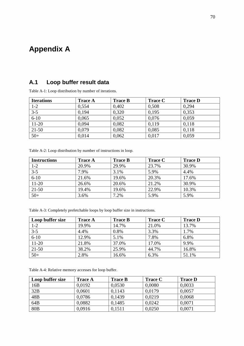
70

Appendix A

A.1 Loop buffer result data

Table A-1: Loop distribution by number of iterations.

Iterations Trace A Trace B Trace C Trace D

1-2 0,554 0,402 0,508 0,294

3-5 0,194 0,320 0,195 0,353

6-10 0,065 0,052 0,076 0,059

11-20 0,094 0,082 0,119 0,118

21-50 0,079 0,082 0,085 0,118

50+ 0,014 0,062 0,017 0,059

Table A-2: Loop distribution by number of instructions in loop.

Instructions Trace A Trace B Trace C Trace D

1-2 20.9% 29.9% 23.7% 30.9%

3-5 7.9% 3.1% 5.9% 4.4%

6-10 21.6% 19.6% 20.3% 17.6%

11-20 26.6% 20.6% 21.2% 30.9%

21-50 19.4% 19.6% 22.9% 10.3%

50+ 3.6% 7.2% 5.9% 5.9%

Table A-3: Completely prefetchable loops by loop buffer size in instructions.

Loop buffer size Trace A Trace B Trace C Trace D

1-2 19.9% 14.7% 21.0% 13.7%

3-5 4.4% 0.8% 3.3% 1.7%

6-10 12.9% 5.1% 7.8% 6.8%

11-20 21.8% 37.0% 17.0% 9.9%

21-50 38.2% 25.9% 44.7% 16.8%

50+ 2.8% 16.6% 6.3% 51.1%

Table A-4: Relative memory accesses for loop buffer.

Loop buffer size Trace A Trace B Trace C Trace D

16B 0,0192 0,0530 0,0080 0,0033

32B 0,0601 0,1143 0,0179 0,0057

48B 0,0786 0,1439 0,0219 0,0068

64B 0,0882 0,1485 0,0242 0,0071

80B 0,0916 0,1511 0,0250 0,0071

71

96B 0,0939 0,1530 0,0256 0,0071

112B 0,0946 0,1538 0,0257 0,0072

128B 0,0952 0,1542 0,0258 0,0072

A.2 Return stack result data

Table A-5: Relative execution time for return stack.

Return stack

size


1 entry 0,9801 0,9772 0,9912 0,9955

2 entries 0,9756 0,9730 0,9892 0,9947

4 entries 0,9735 0,9710 0,9883 0,9941

6 entries 0,9731 0,9708 0,9882 0,9941

8 entries 0,9730 0,9708 0,9882 0,9941

10 entries 0,9730 0,9708 0,9882 0,9941

10+1 entries 0,9722 0,9678 0,9878 0,9927

10+2 entries 0,9718 0,9668 0,9876 0,9921

10+3 entries 0,9715 0,9660 0,9875 0,9918

Table A-6: Relative memory accesses for return stack.

Return stack

size


1 entry 1 1 1 1

2 entries 1 1 1 1

4 entries 1 1 1 1

6 entries 1 1 1 1

8 entries 1 1 1 1

10 entries 1 1 1 1

10+1 entries 1 1 1 1

10+2 entries 1,0010 1,0001 1,0003 1,00001

10+3 entries 1,0010 1,0001 1,0003 1,00001

Table A-7: Relative memory accesses for improved return stack.

Return stack

size


1 entry 0,9443 0,9367 0,9844 0,9937

2 entries 0,9312 0,9252 0,9808 0,9923

4 entries 0,9255 0,9194 0,9791 0,9913

6 entries 0,9241 0,9189 0,9789 0,9913

8 entries 0,9240 0,9189 0,9789 0,9913

10 entries 0,9239 0,9189 0,9789 0,9913

10+1 entries 0,9214 0,9106 0,9781 0,9891

10+2 entries 0,9202 0,9078 0,9777 0,9882

10+3 entries 0,9194 0,9055 0,9774 0,9879

73

A.3 Unconditional branches result data

Table A-8: Relative execution time for indexed BTB.

BTB size Trace A Trace B Trace C Trace D

32 entries 0,9847 0,9747 0,6292 0,4834

64 entries 0,9817 0,9702 0,6275 0,4813

128 entries 0,9765 0,9656 0,6253 0,4796

256 entries 0,9713 0,9609 0,6224 0,4784

512 entries 0,9664 0,9557 0,6209 0,4775

1024 entries 0,9632 0,9507 0,6194 0,4769

2048 entries 0,9610 0,9483 0,6181 0,4765

4096 entries 0,9594 0,9469 0,6176 0,4762

8192 entries 0,9589 0,9463 0,6173 0,4761

Table A-9: Relative memory accesses for indexed BTB.


32 entries 1,1145 1,1213 1,0322 1,0166

64 entries 1,1046 1,1071 1,0287 1,0131

128 entries 1,0880 1,0925 1,0243 1,0101

256 entries 1,0712 1,0776 1,0185 1,0081

512 entries 1,0551 1,0607 1,0155 1,0065

1024 entries 1,0436 1,0267 1,0124 1,0049

2048 entries 1,0367 1,0164 1,0092 1,0042

4096 entries 1,0126 1,0116 1,0082 1,0038

8192 entries 1,0095 1,0096 1,0073 1,0036

Table A-10: Relative execution time for cache BTB.


32 entries 0,9857 0,9773 0,6289 0,4833

64 entries 0,9819 0,9691 0,6272 0,4802

128 entries 0,9747 0,9641 0,6240 0,4780

256 entries 0,9656 0,9553 0,6207 0,4774

512 entries 0,9611 0,9509 0,6186 0,4761

1024 entries 0,9582 0,9454 0,6172 0,4760

2048 entries 0,9582 0,9454 0,6172 0,4760

4096 entries 0,9582 0,9454 0,6172 0,4760

8192 entries 0,9582 0,9454 0,6172 0,4760

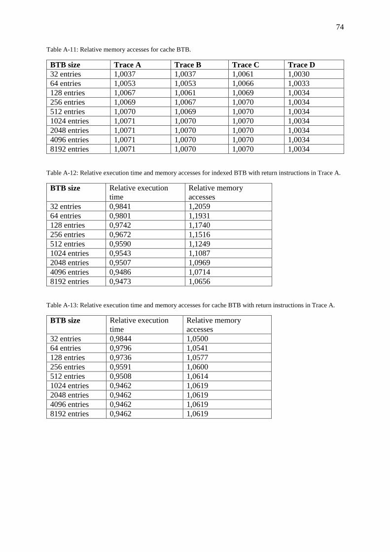
74

Table A-11: Relative memory accesses for cache BTB.


32 entries 1,0037 1,0037 1,0061 1,0030

64 entries 1,0053 1,0053 1,0066 1,0033

128 entries 1,0067 1,0061 1,0069 1,0034

256 entries 1,0069 1,0067 1,0070 1,0034

512 entries 1,0070 1,0069 1,0070 1,0034

1024 entries 1,0071 1,0070 1,0070 1,0034

2048 entries 1,0071 1,0070 1,0070 1,0034

4096 entries 1,0071 1,0070 1,0070 1,0034

8192 entries 1,0071 1,0070 1,0070 1,0034

Table A-12: Relative execution time and memory accesses for indexed BTB with return instructions in Trace A.

BTB size Relative execution

time

Relative memory

accesses

32 entries 0,9841 1,2059

64 entries 0,9801 1,1931

128 entries 0,9742 1,1740

256 entries 0,9672 1,1516

512 entries 0,9590 1,1249

1024 entries 0,9543 1,1087

2048 entries 0,9507 1,0969

4096 entries 0,9486 1,0714

8192 entries 0,9473 1,0656

Table A-13: Relative execution time and memory accesses for cache BTB with return instructions in Trace A.

BTB size Relative execution

time

Relative memory

accesses

32 entries 0,9844 1,0500

64 entries 0,9796 1,0541

128 entries 0,9736 1,0577

256 entries 0,9591 1,0600

512 entries 0,9508 1,0614

1024 entries 0,9462 1,0619

2048 entries 0,9462 1,0619

4096 entries 0,9462 1,0619

8192 entries 0,9462 1,0619

75

A.4 Conditional branches result data

Table A-14: Distribution of conditional branch instructions by times executed.

Times executed Trace A Trace B Trace C Trace D

1-5 0,0548 0,1031 0,0352 0,0958

6-10 0,0423 0,0366 0,0277 0,0467

11-25 0,0756 0,1050 0,0787 0,0848

26-50 0,0534 0,0877 0,0562 0,0553

51-100 0,3072 0,3372 0,3373 0,4091

101-250 0,2302 0,1647 0,2376 0,1622

251-500 0,1387 0,0819 0,1439 0,0663

501-1000 0,0555 0,0424 0,0450 0,0319

1001-2500 0,0250 0,0241 0,0180 0,0332

2501-5000 0,0146 0,0116 0,0172 0,0098

5000+ 0,0028 0,0058 0,0030 0,0049

Table A-15: Weighted distribution of conditional branch instructions by times executed.

Times executed Trace A Trace B Trace C Trace D

1-5 0,0006 0,0010 0,0004 0,0012

6-10 0,0012 0,0011 0,0009 0,0016

11-25 0,0047 0,0084 0,0051 0,0077

26-50 0,0082 0,0140 0,0080 0,0098

51-100 0,0808 0,0911 0,0876 0,1176

101-250 0,1322 0,1045 0,1376 0,1401

251-500 0,1824 0,1053 0,1858 0,0917

501-1000 0,1423 0,1316 0,1129 0,1123

1001-2500 0,1308 0,1296 0,0978 0,1971

2501-5000 0,1463 0,1148 0,1876 0,1107

5000+ 0,1701 0,2987 0,1762 0,2101

Table A-16: Distribution of conditional branches by taken frequency.

Taken frequency Trace A Trace B Trace C Trace D

0% 0,3551 0,3391 0,3778 0,3563

0-20% 0,0929 0,0684 0,0907 0,0872

20-40% 0,0680 0,0385 0,0727 0,0258

40-60% 0,0867 0,0944 0,0982 0,0725

60-80% 0,0902 0,0963 0,0915 0,0848

80-100% 0,0922 0,0703 0,0690 0,0823

100% 0,2150 0,2929 0,2002 0,2912

76

Table A-17: Weighted distribution of conditional branches by taken frequency.

Taken frequency Trace A Trace B Trace C Trace D

0% 0,3606 0,3189 0,3774 0,3734

0-20% 0,0855 0,1416 0,0948 0,0843

20-40% 0,0779 0,0348 0,0676 0,0198

40-60% 0,0909 0,0920 0,1164 0,0926

60-80% 0,1120 0,1183 0,0960 0,0942

80-100% 0,1485 0,1634 0,1342 0,1856

100% 0,1247 0,1309 0,1136 0,1501

Table A-18: Branch predictor accuracy for simple predictors.

Predictor Trace A Trace B Trace C Trace D

Always taken 0,4129 0,4243 0,3878 0,4383

Always not taken 0,5871 0,5757 0,6122 0,5617

Instruction word

hint

0,8774 0,8898 0,8711 0,8961

One bit counter 0,6004 0,6331 0,5932 0,5700

Two bit counter 0,6096 0,6442 0,5964 0,6099

Table A-19: Indexed BHT prediction accuracy.

Predictor size Trace A Trace B Trace C Trace D

16B 0,6929 0,7593 0,6922 0,7603

32B 0,7196 0,7928 0,7171 0,7986

64B 0,7519 0,8116 0,7576 0,8236

128B 0,7859 0,8344 0,7886 0,8452

256B 0,8146 0,8525 0,8160 0,8645

512B 0,8425 0,8683 0,8381 0,8770

1KiB 0,8562 0,8751 0,8487 0,8822

2KiB 0,8644 0,8803 0,8553 0,8862

4KiB 0,8689 0,8823 0,8587 0,8892

8KiB 0,8704 0,8832 0,8610 0,8893

16KiB 0,8710 0,8836 0,8620 0,8895

Table A-20: GAg prediction accuracy.


16B 0,6452 0,6780 0,6346 0,6745

32B 0,6694 0,6971 0,6494 0,7014

64B 0,6915 0,7241 0,6759 0,7260

128B 0,7135 0,7494 0,7022 0,7485

256B 0,7454 0,7750 0,7339 0,7797

512B 0,7801 0,8054 0,7686 0,8158

1KiB 0,8098 0,8376 0,8091 0,8521

2KiB 0,8393 0,8603 0,8446 0,8778

4KiB 0,8634 0,8846 0,8712 0,8961

8KiB 0,8787 0,8969 0,8909 0,9098

77

16KiB 0,8948 0,9050 0,9002 0,9172

Table A-21: Gshare prediction accuracy.


16B 0,6366 0,6928 0,6395 0,6792

32B 0,6567 0,7110 0,6524 0,7098

64B 0,6799 0,7332 0,6757 0,7250

128B 0,7038 0,7473 0,7085 0,7520

256B 0,7488 0,7761 0,7448 0,7857

512B 0,7894 0,8155 0,7863 0,8317

1KiB 0,8386 0,8535 0,8376 0,8754

2KiB 0,8644 0,8940 0,8716 0,9033

4KiB 0,8960 0,9101 0,8960 0,9202

8KiB 0,9153 0,9171 0,9179 0,9269

16KiB 0,9227 0,9242 0,9243 0,9327

Table A-22: Hybrid prediction accuracy.


16B 0.6430 0.6717 0.6305 0.6702

32B 0.6511 0.7094 0.6466 0.7149

64B 0.6684 0.7442 0.6704 0.7660

128B 0.7087 0.7878 0.7070 0.8022

256B 0.7738 0.8257 0.7780 0.8274

512B 0.8221 0.9065 0.8454 0.9080

1KiB 0.8965 0.9155 0.8935 0.9179

2KiB 0.9077 0.9242 0.9034 0.9274

4KiB 0.9209 0.9315 0.9184 0.9384

8KiB 0.9311 0.9416 0.9292 0.9468

16KiB 0.9369 0.9467 0.9377 0.9508

Table A-23: Relative execution time for simple branch predictors.


Never taken 0,9295 0,9327 0,9678 0,9844

Always taken 0,9072 0,9122 0,9591 0,9769

Instruction hint 0,8948 0,8963 0,9543 0,9752

One bit counter 0,9148 0,9147 0,9630 0,9807

Two bit counter 0,9173 0,9159 0,9641 0,9804

Table A-24: Relative memory accesses for simple branch predictors.


Never taken 1 1 1 1

Always taken 1,1610 1,1788 1,0450 1,0154

Instruction hint 1,0436 1,0445 1,0131 1,0057

One bit counter 1,0684 1,0546 1,0188 1,0082

78

Two bit counter 1,0634 1,0583 1,0158 1,0059

79

Table A-25: Relative execution time for indexed BHT predictor.


16B 0,9098 0,9065 0,9606 0,9777

32B 0,9072 0,9036 0,9596 0,9770

64B 0,9043 0,9021 0,9585 0,9765

128B 0,9017 0,9003 0,9571 0,9760

256B 0,8996 0,8989 0,9563 0,9757

512B 0,8977 0,8977 0,9556 0,9756

1KiB 0,8965 0,8972 0,9553 0,9755

2KiB 0,8959 0,8969 0,9551 0,9754

4KiB 0,8955 0,8967 0,9550 0,9754

8KiB 0,8954 0,8967 0,9549 0,9754

16KiB 0,8953 0,8967 0,9549 0,9754

Table A-26: Relative memory accesses for indexed BHT predictor.


16B 1,0651 1,0600 1,0168 1,0075

32B 1,0633 1,0529 1,0170 1,0064

64B 1,0589 1,0515 1,0170 1,0063

128B 1,0598 1,0522 1,0158 1,0062

256B 1,0597 1,0541 1,0160 1,0062

512B 1,0605 1,0530 1,0164 1,0063

1KiB 1,0618 1,0574 1,0171 1,0069

2KiB 1,0611 1,0575 1,0173 1,0069

4KiB 1,0617 1,0573 1,0180 1,0069

8KiB 1,0626 1,0573 1,0182 1,0069

16KiB 1,0627 1,0576 1,0182 1,0069

Table A-27: Relative execution time for cache BHT predictor.


16B 0,9144 0,9124 0,9626 0,9784

32B 0,9134 0,9082 0,9621 0,9773

64B 0,9087 0,9033 0,9604 0,9765

128B 0,9008 0,9004 0,9570 0,9763

256B 0,8982 0,8966 0,9555 0,9754

512B 0,8954 0,8966 0,9549 0,9754

1KiB 0,8954 0,8966 0,9549 0,9754

2KiB 0,8954 0,8966 0,9549 0,9754

4KiB 0,8954 0,8966 0,9549 0,9754

8KiB 0,8954 0,8966 0,9549 0,9754

16KiB 0,8954 0,8966 0,9549 0,9754

80

Table A-28: Relative memory accesses for cache BHT predictor.


16B 1,0629 1,0618 1,0190 1,0080

32B 1,0650 1,0627 1,0194 1,0081

64B 1,0700 1,0643 1,0205 1,0079

128B 1,0722 1,0637 1,0213 1,0076

256B 1,0687 1,0576 1,0196 1,0069

512B 1,0628 1,0576 1,018 1,0069

1KiB 1,0628 1,0576 1,018 1,0069

2KiB 1,0628 1,0576 1,018 1,0069

4KiB 1,0628 1,0576 1,018 1,0069

8KiB 1,0628 1,0576 1,018 1,0069

16KiB 1,0628 1,0576 1,018 1,0069

Table A-29: Relative execution time for GAg predictor.


16B 0,9134 0,9121 0,9623 0,9789

32B 0,9113 0,9103 0,9617 0,9783

64B 0,9089 0,9085 0,9607 0,9778

128B 0,9071 0,9063 0,9598 0,9773

256B 0,9040 0,9041 0,9586 0,9768

512B 0,9006 0,9012 0,9571 0,9761

1KiB 0,8981 0,8984 0,9556 0,9753

2KiB 0,8954 0,8963 0,9541 0,9748

4KiB 0,8933 0,8943 0,9531 0,9745

8KiB 0,8919 0,8932 0,9523 0,9744

16KiB 0,8903 0,8925 0,9519 0,9741

Table A-30: Relative memory accesses for GAg predictor.


16B 1,0580 1,0465 1,0146 1,0058

32B 1,0543 1,0444 1,0141 1,0053

64B 1,0507 1,0430 1,0132 1,0049

128B 1,0479 1,0397 1,0123 1,0046

256B 1,0428 1,0363 1,0117 1,0043

512B 1,0370 1,0326 1,0113 1,0037

1KiB 1,0335 1,0280 1,0096 1,0033

2KiB 1,0294 1,0261 1,0082 1,0029

4KiB 1,0263 1,0223 1,0075 1,0028

8KiB 1,0239 1,0211 1,0068 1,0026

16KiB 1,0214 1,0199 1,0065 1,0025

81

Table A-31: Relative execution time for Gshare predictor.


16B 0,9136 0,9108 0,9624 0,9789

32B 0,9128 0,9095 0,9618 0,9785

64B 0,9104 0,9078 0,9607 0,9781

128B 0,9077 0,9063 0,9593 0,9776

256B 0,9040 0,9031 0,9580 0,9769

512B 0,9004 0,8993 0,9563 0,9758

1KiB 0,8963 0,8962 0,9546 0,9751

2KiB 0,8928 0,8939 0,9530 0,9745

4KiB 0,8902 0,8919 0,9520 0,9741

8KiB 0,8890 0,8909 0,9514 0,9739

16KiB 0,8882 0,8905 0,9510 0,9738

Table A-32: Relative memory accesses for Gshare predictor.


16B 1,0541 1,0461 1,0132 1,0059

32B 1,0526 1,0449 1,0131 1,0055

64B 1,0509 1,0435 1,0126 1,0054

128B 1,0483 1,0420 1,0122 1,0049

256B 1,0429 1,0377 1,0118 1,0044

512B 1,0398 1,0310 1,0104 1,0040

1KiB 1,0344 1,0278 1,0093 1,0036

2KiB 1,0293 1,0243 1,0084 1,0029

4KiB 1,0262 1,0203 1,0074 1,0026

8KiB 1,0245 1,0190 1,0068 1,0025

16KiB 1,0228 1,0183 1,0064 1,0024

Table A-33: Relative execution time for hybrid predictor.


16B 0,9129 0,9130 0,9627 0,9792

32B 0,9120 0,9096 0,9618 0,9784

64B 0,9108 0,9071 0,9610 0,9774

128B 0,9075 0,9035 0,9596 0,9768

256B 0,9020 0,9002 0,9571 0,9763

512B 0,8980 0,8942 0,9548 0,9748

1KiB 0,8923 0,8932 0,9531 0,9746

2KiB 0,8910 0,8922 0,9526 0,9743

4KiB 0,8895 0,8913 0,9519 0,9740

8KiB 0,8883 0,8902 0,9513 0,9738

16KiB 0,8876 0,8896 0,9509 0,9737

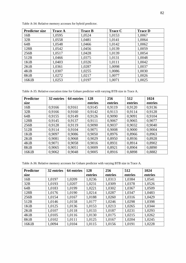
82

Table A-34: Relative memory accesses for hybrid predictor.


16B 1,0595 1,0524 1,0153 1,0067

32B 1,0558 1,0481 1,0141 1,0064

64B 1,0548 1,0466 1,0142 1,0062

128B 1,0542 1,0456 1,0139 1,0059

256B 1,0517 1,0428 1,0139 1,0054

512B 1,0466 1,0375 1,0131 1,0048

1KiB 1,0403 1,0326 1,0111 1,0042

2KiB 1,0361 1,0287 1,0098 1,0037

4KiB 1,0307 1,0255 1,0086 1,0030

8KiB 1,0272 1,0217 1,0077 1,0026

16KiB 1,0253 1,0197 1,0071 1,0025

Table A-35: Relative execution time for Gshare predictor with varying BTB size in Trace A.

Predictor

size

32 entries 64 entries 128

entries

256

entries

512

entries

1024

entries

16B 0,9166 0,9161 0,9145 0,9119 0,9120 0,9136

32B 0,9166 0,9160 0,9142 0,9113 0,9114 0,9128

64B 0,9155 0,9149 0,9126 0,9090 0,9091 0,9104

128B 0,9145 0,9137 0,9111 0,9067 0,9065 0,9077

256B 0,9128 0,9119 0,9090 0,9037 0,9032 0,9040

512B 0,9114 0,9104 0,9071 0,9008 0,9000 0,9004

1KiB 0,9097 0,9086 0,9050 0,8976 0,8966 0,8963

2KiB 0,9081 0,9068 0,9029 0,8950 0,8936 0,8928

4KiB 0,9071 0,9058 0,9016 0,8931 0,8914 0,8902

8KiB 0,9065 0,9051 0,9009 0,8921 0,8904 0,8890

16KiB 0,9062 0,9048 0,9005 0,8916 0,8898 0,8882

Table A-36: Relative memory accesses for Gshare predictor with varying BTB size in Trace A.

Predictor

size

32 entries 64 entries 128

entries

256

entries

512

entries

1024

entries

16B 1,0197 1,0209 1,0236 1,0313 1,0384 1,0541

32B 1,0193 1,0207 1,0231 1,0309 1,0378 1,0526

64B 1,0183 1,0199 1,0221 1,0302 1,0367 1,0509

128B 1,0176 1,0190 1,0214 1,0287 1,0347 1,0483

256B 1,0154 1,0167 1,0188 1,0260 1,0316 1,0429

512B 1,0146 1,0158 1,0177 1,0246 1,0298 1,0398

1KiB 1,0125 1,0136 1,0153 1,0213 1,0265 1,0344

2KiB 1,0107 1,0118 1,0133 1,0187 1,0231 1,0293

4KiB 1,0105 1,0116 1,0130 1,0175 1,0215 1,0262

8KiB 1,0102 1,0111 1,0125 1,0167 1,0204 1,0245

16KiB 1,0094 1,0104 1,0115 1,0156 1,0191 1,0228

evaluation of instruction prefetch methods for coresonic

Documents