electrochimie en solution - epfl.ch · electrochimie • une réaction est ... which are...
TRANSCRIPT

Electrochimie en solution
Printemps 2014
���1

Electrochimie
• Une réaction est électrochimique si l’énergie de Gibbs de la réaction dépend non seulement de la température et de la pression, mais aussi d’une différence de potentiel, par exemple entre une électrode et une solution électrolytique.
• Un paramètre additionnel : Champ électrique à l’interface
���2
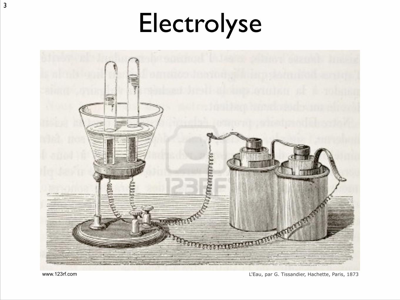
Electrolyse
L'Eau, par G. Tissandier, Hachette, Paris, 1873
���3
www.123rf.com

Electrochimie
Réactions de transferts de charge aux interfaces
Transfert d’ion
Transfert d’électron - Réaction rédox
Réactions acide-base interfaciale
Conductivité ionique en solution
De la bioénergétique aux applications industrielles, Du fondamental à l’appliqué
���4

Photosynthèse
Photosynthetic electron transport chain of the thylakoid membrane (Wikipedia)
���5
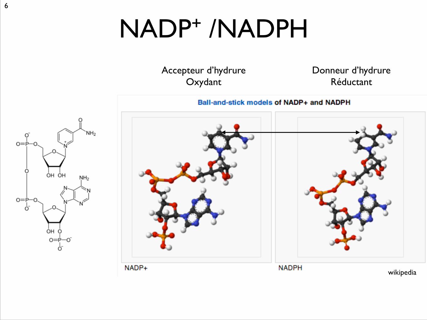
NADP+ /NADPH���6
wikipedia
Accepteur d’hydrure Oxydant
Donneur d’hydrure Réductant

ApplicationsIndustrie
Production du chlore, de l’aluminium Galvanoplastie et microtechnique Electrodialyse
Analyse pH, électrodes sélectives d’ions Capteurs - Electrode à glucose
Energie Piles et accumulateurs Piles à combustible Hydrogène - Power to fuel Photopiles solaires
���7

Production d’aluminium
Sept Iles, Quebec, Canada
���8

Fabrication combinée chlore-soude
Membrane échangeurde cations
H+
Na+
Cl–
Cl2
Ano
de
Cat
hode
H+
H2
Saumure
ChloreHydrogène + Soude
Soude diluée
Réduction du proton
Oxydation du chlorure
Courant protonique
���9

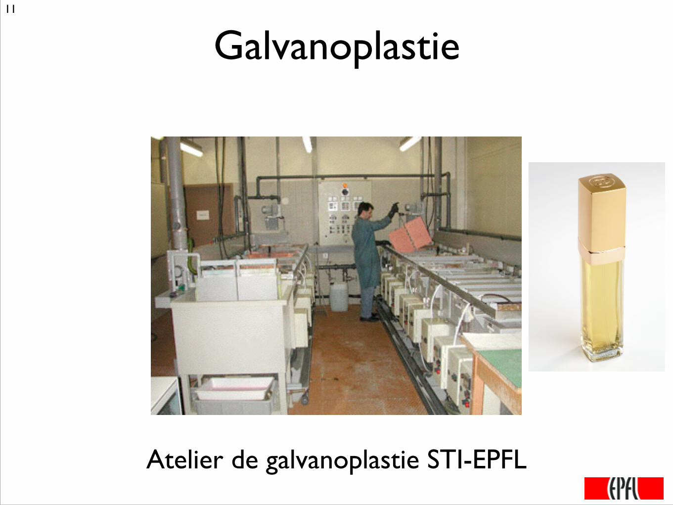
Galvanoplastie
Atelier de galvanoplastie STI-EPFL
���11
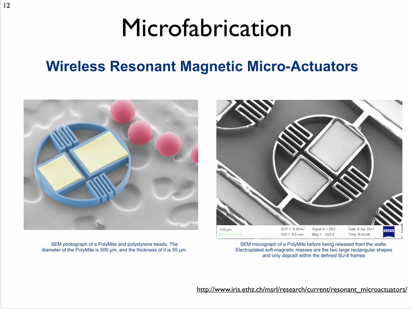
Microfabrication
http://www.iris.ethz.ch/msrl/research/current/resonant_microactuators/
SEM photograph of a PolyMite and polystyrene beads. The diameter of the PolyMite is 500 µm, and the thickness of it is 55 µm.
SEM micrograph of a PolyMite before being released from the wafer. Electroplated soft-magnetic masses are the two large rectangular shapes
and only deposit within the defined SU-8 frames
Wireless Resonant Magnetic Micro-Actuators
���12

Electrodialyse
Acid recovery in Steel industries with electro dialysis
���13

Chimique Mecanique Electrique
Conversion de l’énergie
Vent
Marée
Solaire
Hydro
Grille
Charbon Gaz
Pétrole
CO2
Pétrole
Photovoltaique
Usine solaire
Piles à combustible
Stockage
Batteries
Electrolyse
Photosynthesis
H2, CH4
Water splitting
CO2 reduction
���14

Suisse���15
240 TJ·an = 66,7 TWh 1Wh=3600 J 8766 heures par année Puissance moyenne: 7.6 GW

���16
Suisse

Current Issues Natural resources
An ambitious shift in energy policy, such as that of the German government and which other countries are aiming to emulate, poses great challenges. One Herculean task is integrating those renewable sources of electricity generation which are experiencing dynamic growth but are also subject to relatively strong fluctuations.
The volatility of the increasing volumes of solar and wind energy needs to be evened out and matched to consumption in order for Germany to enjoy a stable power supply and avoid blackouts. Storing electrical energy is a proven means of absorbing any immediate surplus power and then making it available when required.
By 2025, the requirement for short-term power storage could well double at the very least and increase still further thereafter. The end of production from ageing fossil-fuel power stations and the abandonment of nuclear energy require new capacity available on demand (in addition to the options of more imports, renewables and greater capacity utilisation) in order to avoid bottlenecks. Pumped and compressed air storage systems and storage power stations can offer short-term storage.
By 2040 at the latest, it will be regularly necessary to store 40 TWh in order to absorb the surpluses which will arise. The electricity will then need to be stored for several weeks and months. In the next two decades alone, the capital investment required for new energy storage systems in Germany will total around EUR 30 bn.
Hydrogen and methane storage systems will need to be developed further so that the energy revolution can remain affordable and be implemented with assurance. Alternative or additional adjustment strategies, such as accelerating and expanding the integration of the European electricity grids, must also be driven forward.
Authors Josef Auer +49 69 910-31878 [email protected] Jan Keil Editor Antje Stobbe
Deutsche Bank AG DB Research Frankfurt am Main Germany E-mail: [email protected] Fax: +49 69 910-31877
www.dbresearch.com
Managing Director Thomas Mayer
March 8, 2012
State-of-the-art electricity storage systems Indispensable elements of the energy revolution
0 2 4 6 8
10 12 14
Wind PV
Fluctuations in wind and solar-generated electricity DX
Hourly feed-in values (GW), Germany, September 2011
Source: ENTSO-E
State-of-the-art electricity storage systems
4 | March 8, 2012 Current Issues
The federal government’s planned rise in regenerative energy’s contribution to electricity generation requires adjustments to be made to the existing power station structure. Table 9 shows how wind energy and PV capacity could be expanded by 2025 and 2040. This scenario, which we are taking as our starting point, also illustrates the drop in conventional (including adjustable) potential if, apart from the power stations currently under construction, there are no further new builds and old power stations are decommissioned in accordance with their assumed service life.6
The risk of supply bottlenecks in 2025
In line with the reduction targeted by the federal government, we calculate that net electricity consumption will fall from 538 TWh in 2010 to 484 TWh in 2025 (reduction of 12.5 per cent) and to 430 TWh in 2040 (reduction of 20 per cent). The slowdown in consumption will certainly tend to diminish the risk of a temporary undersupply. Another buffer is the present surplus electricity which Germany has been exporting since 2003 (2010: 17.7 TWh). If the 2010 capacity utilisation rates are to continue to apply in future, the reduction in conventional capacity will produce a 10 TWh demand for electricity in 2025 which cannot be met, whereas an overproduction of 16 TWh can be expected in 2040. The supply bottleneck in 2025 could be relieved by importing electricity, by a temporary (moderate) increase in the capacity utilisation of conventional power stations or by new builds of gas, coal or biomass power stations.7
Flexible power stations as an option
When using flexible conventional power stations to balance power demand and supply, a minimum capacity utilisation is essential. Frequent downtimes and running at low utilisation rates mean less profit while still incurring fixed costs. Operating in load following mode also leads to additional wear, less efficient use of fuel and higher costs. Despite this, even if there were to be noticeably lower capacity utilisation in 2025 (a reduction from 37 per cent to 25 per cent for gas and steam power stations), the rise of 1.5 cents/kWh in the production costs of gas-fired power stations would still be moderate. This implies that the capacity utilisation problem can be kept within bounds and that building additional flexible gas-fired power stations could be thoroughly worthwhile. The option of relieving bottlenecks by using flexible power stations is one conceivable (partial) solution to the renewables problem for the transitional period.
achieved. On average, the degree to which wind and PV capacities are utilised is well below that of conventional power stations. This is due to a far more dramatic increase in capacity than in annual power generation.
6 If no new power stations are built, the assumption on which this scenario is based will lead to an even greater rise in the proportion of annual production accounted for by renewables. The wind energy proportion rises from 15 per cent to 26 per cent (2025) and 35 per cent (2040), mainly due to the increase produced by offshore systems and to much bigger, more sophisticated new build and repowered systems. The PV contribution would grow from today’s 1.9 per cent to 9 per cent (2025) and 19 per cent (2040). Both PV modules and system components such as inverters are becoming significantly more efficient and are already achieving efficiency levels of 16-18 per cent (inverters: 98-99 per cent).
7 An increase from gas, biomass, coal and lignite-fired power stations by ten percentage points (lignite: increase of 5 per cent) to 47 per cent, 58 per cent, 56 per cent and 87 per cent respectively would be sufficient.
Important system services 8
System services such as voltage and frequency preservation and the provision of reactive power and minute reserves are essential for disruption-free power supply. These services are regularly traded in the market as feed-in and draw-off capacities available on demand.
Power station capacities 9
Without building any new conventional power stations after 2014 (GW)
2010 2025 2040
Wind 27,3 57,1 68
PV 17,0 39,5 67
Biomass 4,8 10,0 20
Hydropower 4,7 5,2 6
Gas 25,7 16,2 12
Coal 28,0 23,5 9
Lignite 20,3 14,0 10
Nuclear power 20,5 0,0 0
Oil, miscellaneous 6,5 1,2 0
Sources: BDEW, Federal Network Agency, DB Research
Important assumptions 11
Assumptions for conventional energy are based on EEX spot prices for November 2011. We have assumed emission allowances in the range of EUR 10 (2011) and EUR 20 (2025), USD 110/t of coal in 2011 and USD 125/t for 2025, 2.3 cts/kWh for gas in 2011 and 2.6 cts/kWh in 2025. Compared with others, these assumptions are relatively conservative. The assumptions for wind from North German coast onshore sites (on average 1,040 kWh/p.a./qm, cost degression: 1 per cent p.a.) and from offshore sites in 20 m of water and 20 km out to sea (cost degression: 5 per cent p.a., from 2015). As for PV, we have assumed 92 cts/Wp (average Chinese supplier in October 2011), system costs of 50 cts/Wp, a performance ratio of 85 per cent and average sunshine for Frankfurt from 1981 to 2008. We calculate an annual cost degression of 20 per cent for 2012, falling to 10 per cent p.a. (from 2015) and amounting to 5 per cent from 2020.
0 5 10 15
PV Offhore
Onshore Gas/steam
Coal Lignite
Nuclear
2011 2025
Electricity generation costs 10
Germany (cents/kWh)
Sources: BDEW, DIW
State-of-the-art electricity storage systems
6 | March 8, 2012 Current Issues
according to Dena (Grid Study II), the forecasting error will reduce by 40-50 per cent by 2020, thanks to better forecasting methods. Nonetheless, doubling the volume of wind energy fed in to the grid will require the error to be reduced by more than 50 per cent, if additional adjustable output is not to be kept in readiness.12 We expect that the forecasts will show a 65 per cent improvement by 2025 and be 85 per cent better by 2040. As a result of the growth in wind-generated electricity and also taking the (more accurately forecastable) PV into account, the adjustable output requirement compared with 2010 will rise by 50 per cent by 2025 and by 70 per cent by 2040. Greater decentralised generation and the major feed-in volatility of the renewables will also increase the require-ment for additional system services. Considerably more adjustable output will be needed in future overall.13
Preventing surpluses and undersupply
Storage systems can be used if the volume of non-adjustable electricity generation temporarily exceeds consumption (either within a grid or within a geographically defined area), or if consumption cannot be satisfied by the generation capacity which can be called upon. Even the operators themselves often have difficulty in estimating the extent to which storage capacity is currently used for balancing renewables (smoothing and system services) on the one hand and classical operation on the other.14 The proportion used for balancing renewables has recently seen strong growth and, with some storage systems, can account for most of the profit.
From a simulation study, based on hourly consumption, wind and PV feed-in data for 2010 and 2011 and on the basic scenario described above, we estimate that surpluses would only accrue at federal level today in the order of magnitude of 15 GWh (0.1 per cent of the annual production of wind and PV generated electricity), assuming the grid had been expanded so that it could in theory transmit 100 per cent of the energy produced by renewables within Germany. Positive (not reducible at national level by expanding the grid) surpluses will rise to 3.5 TWh, or 2 per cent of annual production, by 2025. This still rather moderate volume, a result of declining ‘must run’ output, will amount to almost 40 TWh (or 14 per cent of PV and wind-generated electricity) by 2040.
The volume which cannot be directly covered by wind and sun amounts today to 260 TWh and will, in our scenario, be 220 TWh in 2025 and 115 TWh in 2040. Those residual load power stations, which are currently either operational or under construction, will not be sufficient to cover this supply gap in future. In 2025 and 2040, a shortfall of at least 4.5 and 12.5 GW respectively will remain, which will need to be covered by new power stations, more closely integrated European grids or positive storage capacity.
Storage over different timeframes is essential
Because fluctuation patterns for PV, wind and power consumption vary, it may also be necessary to provide storage capacity for timeframes of differing lengths: 1. for a few minutes (feed-in fluctuations); 2. up to one day (daily PV pattern); 3. up to three days (random PV fluctuations); 4. for one to two weeks (periods of sustained strong or light winds); 5. seasonal timeframes. Our 12 Klobasa, Marian (2007). Dynamic simulation of a load management system and the integration of
wind energy into an electricity grid at national level from control engineering and cost aspects. ETH Zurich.
13 Estimating the order of magnitude of these system services is not easy, making it impossible to quantify them precisely here.
14 The rate at which electricity is drawn off from and fed into the grid is determined by market prices, which themselves follow from the relationship between overall electricity production and con-sumption.
8
14
16.5
0 2 4 6 8
10 12 14 16 18
2010 2025 2040
Adjustable output required* 13
Germany (TWh)
* Positive adjustable output to compensate for forecasting errors
Source: DB Research
1.8
20
0
5
10
15
20
25
2025 2040
Electricity surpluses to be stored* 14
Germany (TWh)
Source: DB Research
* Assumption: 50% of all electricity surpluses will be stored

Allemagne 2013���18
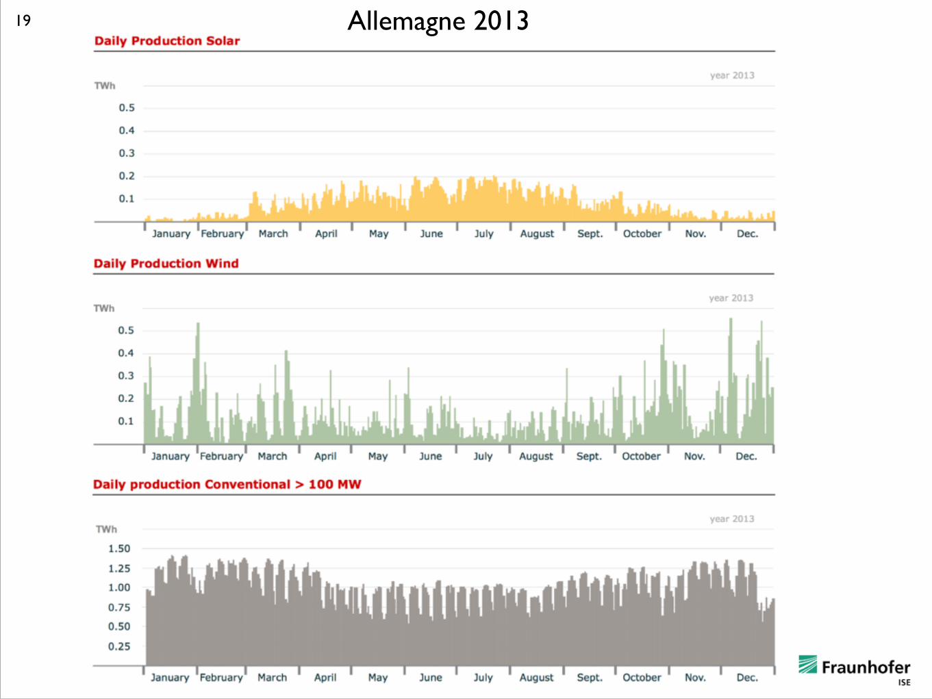
���19 Allemagne 2013

Objectifs d’Apprentissage Bases thermodynamiques
Comprendre la notion de potentiels chimique et électrochimique
Activités et concentrations
Savoir utiliser les différents potentiels électriques entre phases et aux interfaces
���20
Objectifs d’Apprentissage Applications analytiques
Potentiométrie - Titrage rédox
pH - Electrode à pH - ISE
Introduction à la spéciation Diagramme de Pourbaix
���21

Objectifs d’Apprentissage Solutions Ioniques
Maîtriser les aspects thermodynamiques de la solvatation
Connaître les modèles simples
Born
Debye-Hückel
Bjerrum et Fuoss
���22

Objectifs d’Apprentissage Transport en solution
Diffusion - Migration -Convection
Conductivité ionique
Introduction à la thermodynamique des systèmes irréversibles - Tension de diffusion
���23
Objectifs d’Apprentissage Interfaces électrifiées
Interface métal | électrolyte
Capacités et supercapacités
���24

Objectifs d’Apprentissage Ampérométrie
Cinétique électrochimique
Courant sous contrôle diffusionel
���25
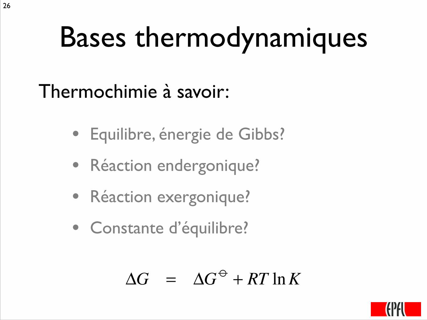
Bases thermodynamiques
• Equilibre, énergie de Gibbs?
• Réaction endergonique?
• Réaction exergonique?
• Constante d’équilibre?
ΔG = ΔG o + RT lnK
Thermochimie à savoir:
���26

Potentiel Chimique
U = Etrans + Erot + Evib + Eel + Eint + Emasse
Energie interne
dU = − pdV + TdS + µii∑ dni
Potentiel chimique
Variables extensives
µi = ∂U∂ni
⎛
⎝⎜
⎞
⎠⎟V ,S,nj≠i
���27

Transformée de Legendre
U =U V ,S ,ni( )Energie interne
Enthalpie H =U + pV = H p,S,ni( )p = −
∂U∂V
⎛⎝⎜
⎞⎠⎟ S, ni
Energie de Gibbs G = H − TS = G p,T ,ni( )T =
∂U∂S
⎛⎝⎜
⎞⎠⎟V ,ni
dG = Vdp − SdT + µii∑ dni
���28

Potentiel Chimique
Travail pour transférer une espèce vers une phase à pression et température constantes
Pour un corps pur : Potentiel chimique = énergie de Gibbs molaire
µ = Gm
Potentiel chimique
Variables physiques intensives
µi = ∂G∂ni
⎛
⎝⎜
⎞
⎠⎟T , p,nj≠i
= Gi
���29
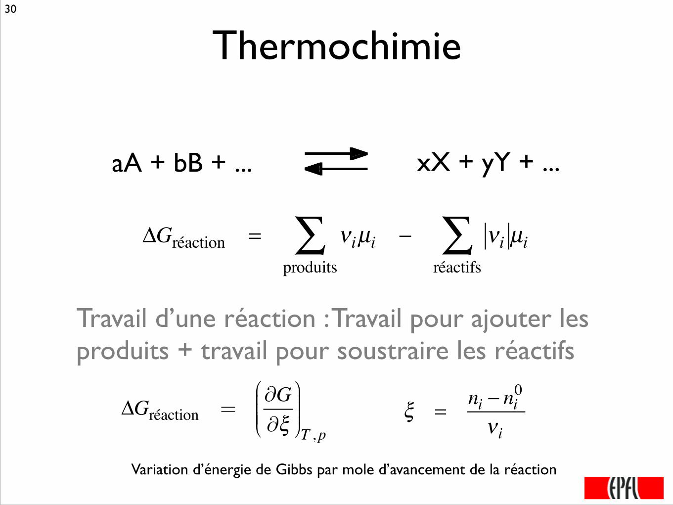
Thermochimie
aA + bB + ... xX + yY + ...
Travail d’une réaction : Travail pour ajouter les produits + travail pour soustraire les réactifs
ξ = ni − ni0
νi
Variation d’énergie de Gibbs par mole d’avancement de la réaction
ΔGréaction =∂G∂ξ⎛
⎝⎜⎜⎜⎜⎞
⎠⎟⎟⎟⎟T , p
ΔGréaction = νiproduits∑ µi − νi
réactifs∑ µi
���30

ExerciceCalculons la variation d'énergie de Gibbs associée à la compression isotherme de 1 à 2 bars ( T=298 K ) d’une mole d'eau (1) liquide supposée incompressible et (2) vapeur traitée comme un gaz parfait.
���31

Potentiel chimique en phase gazeuse
Pour un gaz pur dµ = dGm
���32
µ(T , p) − µ o (T ) = Vmdp
p o
p
∫ =RTpdp
p o
p
∫
Potentiel chimique d’un gaz parfait
µ(T , p) = µ o (T )+ RT ln p
p o
⎛
⎝⎜⎜⎜⎜
⎞
⎠⎟⎟⎟⎟
Pression standard = 1 bar = 100’000 Pa
Etat standard = Gaz parfait à la pression standard
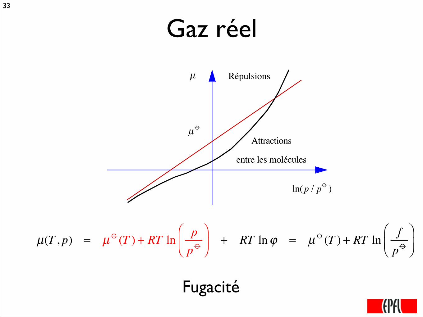
Gaz réel
Fugacité
ln(p / po )
µo
µ Répulsions
Attractions
entre les molécules
µ(T , p) = µ o (T ) + RT ln p
p o⎛⎝⎜
⎞⎠⎟
+ RT lnϕ = µ o (T ) + RT ln fp o
⎛⎝⎜
⎞⎠⎟
���33

Solution idéale
pression totale
AB
pApB
Fraction molaire
Interactions A–A, A–B, B–B
similaires
Benzène - Toluène
pi = xi pi*Loi de Raoult
p* = Pression de vapeur saturante quasi-indépendante de la pression totale !
Exemple: La pression de vapeur saturante de l’eau est indépendante de la présence d’autres molécules insolubles dans la phase aqueuse, e.g. azote.
pA*
pB*
���34
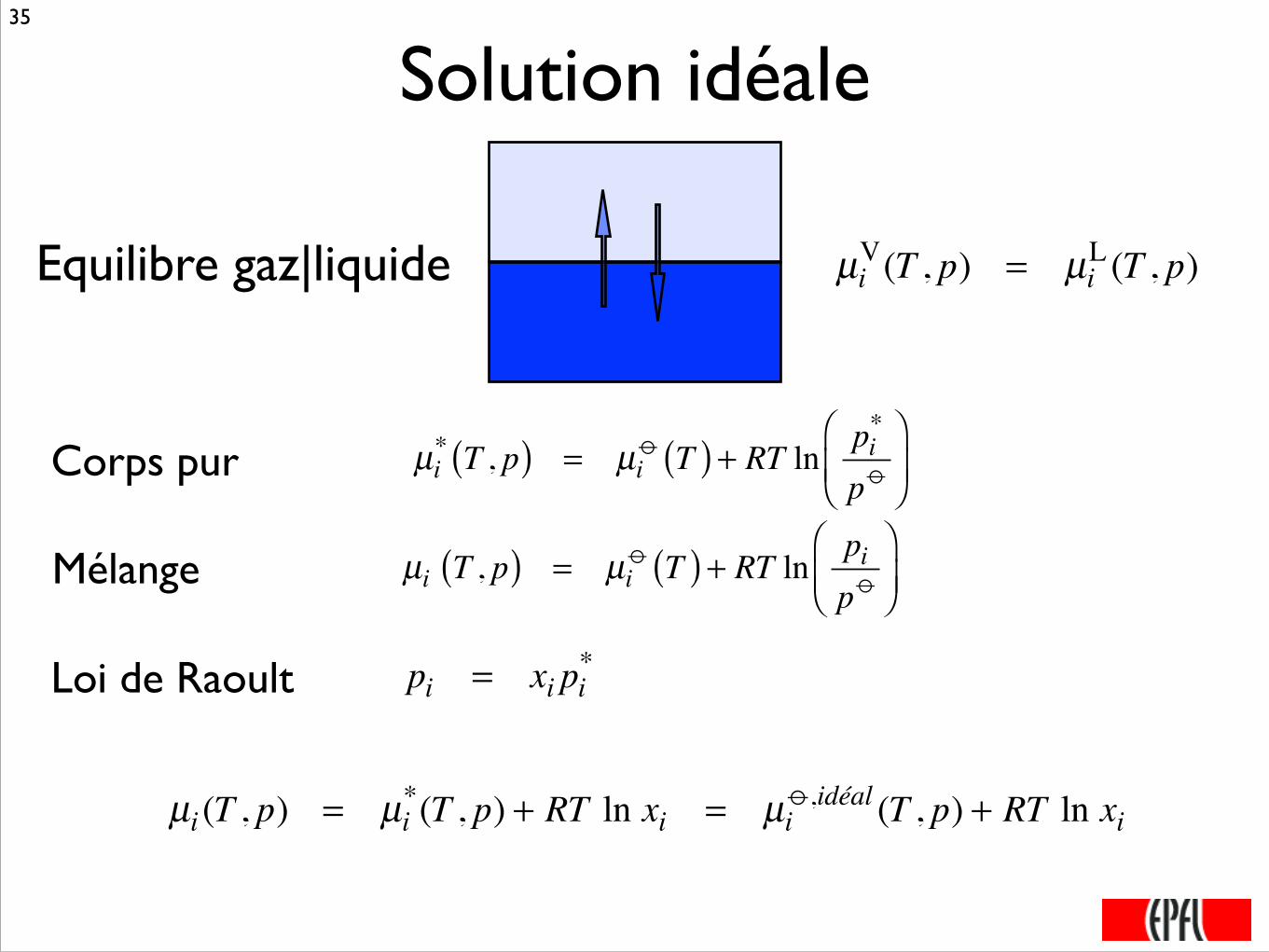
Solution idéale
pi = xi pi*Loi de Raoult
Equilibre gaz|liquide µiV(T , p) = µi
L(T , p)
µi (T , p) = µi*(T , p) + RT ln xi = µi
o ,idéal (T , p) + RT ln xi
Corps pur µi* T , p( ) = µi
o T( ) + RT ln pi*
p o
⎛
⎝⎜⎞
⎠⎟
Mélange µi T , p( ) = µi
o T( ) + RT ln pip o
⎛
⎝⎜⎞
⎠⎟
���35
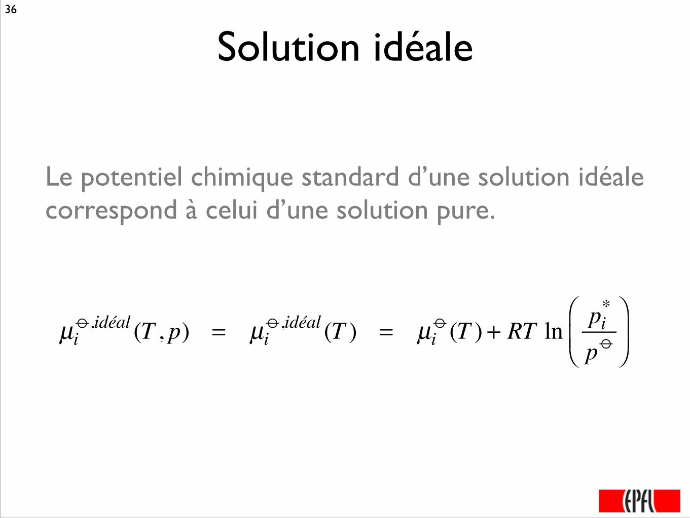
Solution idéale
Le potentiel chimique standard d’une solution idéale correspond à celui d’une solution pure.
µi
o ,idéal (T , p) = µio ,idéal (T ) = µi
o (T ) + RT ln pi*
p o
⎛
⎝⎜⎞
⎠⎟
���36

Echelle des fractions molaires
Fraction molaire
p*
Solution idéalement
diluée
Solution idéale
A = Solvant
Loi de Raoult
Solution idéale
µA(T , p) = µAo ,idéal (T ) + RT ln xA
xA → 1
γ A → 1
Solution réelle
µA(T , p) = µAo ,idéal (T ) + RT ln xA + RT ln γ A
µA(T , p) = µAo ,idéal (T ) + RT ln aA
���37

ExerciceLa pression de vapeur saturante d’une solution de 0.5M KNO3 à 100°C est 749.7 Torr.
Quelle est l’activité de l’eau à cette température?
���38

Echelle des fractions molaires
Fraction molaire
p*
Solution idéalement
diluée
Solution idéale
B = Soluté
Loi de HenrypB = xBKB
La constante de Henry a la dimension d’une pression et ne varie quasiment pas avec la pression totale
µBo ,idéal dil (T, p) = µB
o ,idéal dil (T ) = µBo (T ) + RT ln KB
p o
⎛
⎝⎜⎞
⎠⎟
Solution idéalement diluée
µB(T , p) = µB
o ,idéal dil (T , p) + RT ln xB = µBo (T ) + RT ln pB
p o⎛⎝⎜
⎞⎠⎟
���39

Echelle des fractions molaires
Fraction molaire
p*
Solution idéalement
diluée
Solution idéale
B = Soluté
Loi de HenrypB = xBKB
xB→ 0
γ B→ 1
Solution réelle diluée
µB(T , p) = µBo ,idéal dil (T ) + RT ln xB + RT ln γ B
µB(T , p) = µBo ,idéal dil (T ) + RT ln aB
���40

Echelle des fractions molaires
-12
-10
-8
-6
-4
-2
0
2
4µ
/ k
J·mol
-1
10-22 3 4 5 6 7 8 9
10-12 3 4 5 6 7 8 9
100
Fraction molaire de B (x B)
Solution idéale
Solution idéalement diluée
µB
o , idéal dil
Proportionnalité à RT lnx pour les solutions idéalement diluées et les solutions idéales
���41

Activité
RT lnγ
xBaBFraction molaire
réel
idéal
Activité = Fraction molaire effective
RT ln γ B = Travail d’interactions des solutés
���42

Exercice
On fait buller de l’hydrogène dans un récipient. Calculer la concentration en hydrogène dissous sachant que la constante de Henry est 5.37 107 Torr.
H2
���43
On fait buller de l’oxygène dans un récipient. Calculer la concentration en oxygène dissous sachant que la constante de Henry est 769.23 L· atm· mol–1.

Echelle des molalités
mB =nB
nA MAMolalité
xB =nB
nA + nB=
nAMAmBnA + nB
= xAMAmB
µB(T , p) = µB
o ,idéal dil (T ) + RT ln m o MA( )⎡⎣
⎤⎦ + RT ln
γ B xA mBm o
⎛⎝⎜
⎞⎠⎟
µB(T , p) = µB
o ,m (T ) + RT ln γ Bm mBm o
⎛⎝⎜
⎞⎠⎟
���44

Echelle des molarités
Molarité cB =nBV
mB =nB
nAMA=
nB(nAMA + nBMB) − nBMB
=cB
d − cBMB
µB(T , p) = µB
o ,c(T ) + RT ln γ Bc cBc o
⎛⎝⎜
⎞⎠⎟
���45

Echelle des molarités���46
µ = µ o ,id dil + RT ln γ BxB( ) = µ o ,id dil + RT ln MAγ BxAmB( )
On part de l’échelle des fractions molaires
µB(T , p) = µB
o ,c(T ) + RT ln γ Bc cBc o
⎛⎝⎜
⎞⎠⎟
d0 =MAVmA
mB =nB
nAMA=
nB(nAMA + nBMB) − nBMB
=cB
d − cBMB
On définit les densités du solvant et de la solution
µ = µ o ,id dil + RT ln VmAco( )+ RT ln d0
c o γ BxAcB
d − cBMB
⎛⎝⎜
⎞⎠⎟
On remplace

Potentiel chimique en solution
-10
-5
0
5µ−
µo / kJ
·mol
–1
0.012 3 4 5 6
0.12 3 4 5 6
12 3 4 5 6
10
c / M
���47

Solution idéalement diluée
Le potentiel chimique standard d’une solution idéalement diluée correspond à celui d’une solution virtuelle idéalement diluée mais à: !
- une fraction molaire unitaire (corps pur) - une concentration de 1 molal - une concentration de 1 molaire
���48
Trois conventions d’états standard
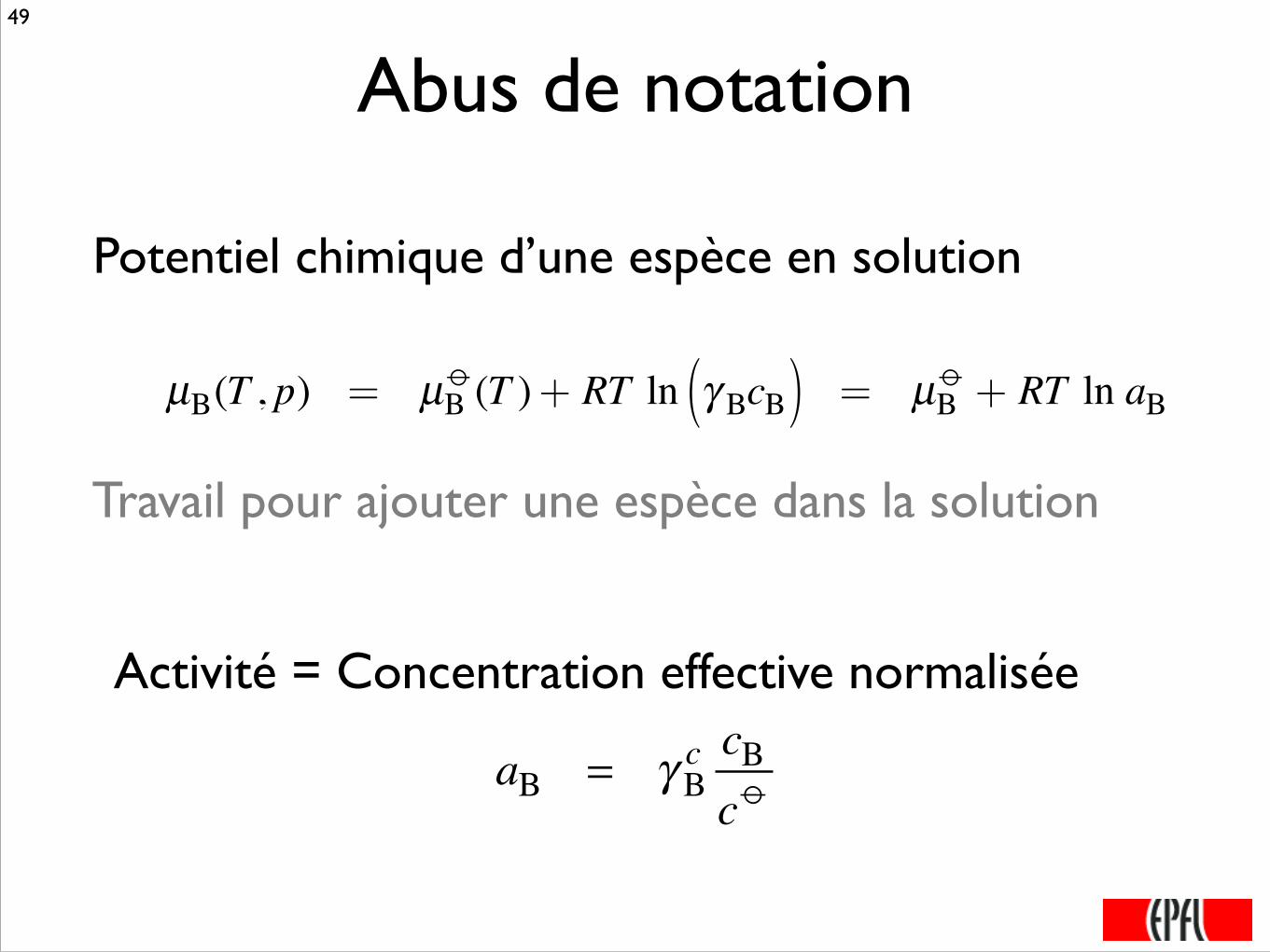
Abus de notation
Potentiel chimique d’une espèce en solution
Travail pour ajouter une espèce dans la solution
µB(T , p) = µB
o (T )+ RT ln γ BcB( ) = µBo + RT ln aB
aB = γ B
c cBc o
Activité = Concentration effective normalisée
���49

ExempleRéaction en solution
A + B C + D
ΔGréaction = µC + µD − µA − µB
Energie de Gibbs de la réaction
A l’équilibre K =
aCaDaAaB
= e−ΔGro /RT
ΔGréaction = µC
o + µDo − µA
o − µBo( ) + RT ln aCaD
aAaB
⎛⎝⎜
⎞⎠⎟
ΔGro = µC
o + µDo − µA
o − µBo
Energie de Gibbs standard
���50

ExempleRéaction biphasique gaz(g) - solution (aq)
A(g) + B (aq) C (aq) + D (aq)
ΔGréaction = µC + µD − µA − µB
Energie de Gibbs de la réaction
A l’équilibre K =
aCaDpo
pAaB= e−ΔGr
o /RT
ΔGro = µC
o ,id + µDo ,id − µA
o − µBo ,id
ΔGr = µC
o ,id + µDo ,id − µA
o − µBo ,id⎡⎣ ⎤⎦ + RT ln
aCaDpo
pAaB
⎛
⎝⎜⎞
⎠⎟
���51
Exercice
Donner la constante d’équilibre pour la dissolution du zinc dans une solution d’acide chlorydrique
���52