dynamic modeling of pv units in response to voltage ... modeling of pv units in response to voltage...
TRANSCRIPT

http://lib.ulg.ac.be http://matheo.ulg.ac.be
Dynamic Modeling of PV Units in response to Voltage Disturbance
Auteur : Chaspierre, Gilles
Promoteur(s) : Van Cutsem, Thierry
Faculté : Faculté des Sciences appliquées
Diplôme : Master en ingénieur civil électricien, à finalité approfondie
Année académique : 2015-2016
URI/URL : http://hdl.handle.net/2268.2/1429
Avertissement à l'attention des usagers :
Tous les documents placés en accès ouvert sur le site le site MatheO sont protégés par le droit d'auteur. Conformément
aux principes énoncés par la "Budapest Open Access Initiative"(BOAI, 2002), l'utilisateur du site peut lire, télécharger,
copier, transmettre, imprimer, chercher ou faire un lien vers le texte intégral de ces documents, les disséquer pour les
indexer, s'en servir de données pour un logiciel, ou s'en servir à toute autre fin légale (ou prévue par la réglementation
relative au droit d'auteur). Toute utilisation du document à des fins commerciales est strictement interdite.
Par ailleurs, l'utilisateur s'engage à respecter les droits moraux de l'auteur, principalement le droit à l'intégrité de l'oeuvre
et le droit de paternité et ce dans toute utilisation que l'utilisateur entreprend. Ainsi, à titre d'exemple, lorsqu'il reproduira
un document par extrait ou dans son intégralité, l'utilisateur citera de manière complète les sources telles que
mentionnées ci-dessus. Toute utilisation non explicitement autorisée ci-avant (telle que par exemple, la modification du
document ou son résumé) nécessite l'autorisation préalable et expresse des auteurs ou de leurs ayants droit.

UNIVERSITY OF LIEGE
FACULTY OF APPLIED SCIENCES
ATFE0014-1
MASTER THESIS
Dynamic Modeling of PV Units in response toVoltage Disturbance
Author:Gilles Chaspierre
Master Thesis adviser:Pr. Thierry Van Cutsem
A dissertation submitted in partial fulfillment of the requirements for the Master’s degree inelectrical engineering
Academic year 2015-2016

Summary of the work
Gilles ChaspierreUniversity of Liege
Academic Year 2015-2016
1 General information about the work
Work Title: Dynamic Modeling of PV Units in response to Voltage Disturbances.
Section: Electrical engineering, orientation ”electric power and energy system”.
Master thesis adviser: Pr. Thierry Van Cutsem.
2 Work overview
The aim of this work was to build a mathematical model of small-scale PV units connected to the Low Voltage(LV) network and aggregated at a higher voltage level, such as the Medium Voltage (MV) network. This model iscompatible with nowadays grid requirements and is able to catch the main dynamics of PV systems in response tovoltage disturbances. The proceedings of this work can be divided in three parts. First, one third of the time hasconsisted in literature review and research in present grid codes to make out a list of PV model specifications. Themost important specifications are the Low Voltage Ride-Through (LVRT) capability, the reactive power support andthe switch between the active and reactive priority following a fault. During the second third of the time, the dynamicmodel of PV units has been built based on existing elaborated models and representing the PV model specifications.Finally, the remaining time has been devoted to dynamic simulations using a MV test network where the implementedPV model is agglomerated to each node. The external transmission system has been represented by its Theveninequivalent. Different scenarios interesting from a System Operator point of view have been investigated in order to seehow the units react in fault/low voltage situations. It particularly shows that units remain connected following a faultin the High Voltage level whereas units close to a fault occurring at the Medium Voltage level disconnect. Hopefully,these PV systems responses are in agreement with System Operators expectations. A part of these results shows thedynamic response of the Phase Locked Loop (PLL) controller for different fault locations. The latter seems to beless efficient for fault occurring at the MV level. Some issues caused by a too efficient voltage support provided byPV installations are also highlighted and solutions to avoid such problems are proposed. Finally, based on these casestudies results, the work ends by proposing an equivalent MV network model and more specifically an equivalent PVmodel well suited for transmission system representation. The main contribution of this work is a detailed dynamicmodel providing a reliable insight on the small-scale PV units reactions in response to voltage disturbances.
1

3 Meaningful work illustrations
OverVoltageControl
LVRT
1
1 + sTm
N
D
Vt Vm
ReacticeSupport
Fvh
Fvl
Ipmax
0
Ipcmd 1
1 + sTg
1
1 + sTg
IP
IQ
Iqmax
Iqmin
Vm < 0:9
PQstrategy
0.01
Fvh Fvl
MAX
Ip Iq
ix
iy
T 1
sT
vxlv
vylv
vd
vq ∆!PLL θPLL
Iqext +
+
Iqref
Pext
Switch0
(Vm−0:9)
Pflag
Pflag = 1
Iqcmd
Pflag = 0
1
1
1 + sTm
1
1 + sTm
vxlvm
vylvm−kPLL
0Switch
Figure 1: Small-scale PV units mathematical model
0.6 0.8 1 1.2 1.4 1.6
time(s)
0
0.01
0.02
0.03
0.04
0.05
0.06
(pu)
-0.1 p.u
-0.3 p.u
-0.6 p.u
(a) Active current
0.6 0.8 1 1.2 1.4 1.6
time(s)
0
0.02
0.04
0.06
0.08
0.1
0.12
(pu)
-0.1 p.u
-0.3 p.u
-0.6 p.u
(b) Reactive current
Figure 2: Injected current by PV units during three different voltage drops (-0.1, -0.3, -0.6 p.u) at the transmissionside. It highlights the increase in the reactive current (when V < 0.9 p.u) due to the reactive support function and thedecrease of the active power for larger voltage deviation to require more reactive current injection.
2
Contents
Abstract 1
1 Introduction 2
1.1 Presentation of the subject . . . . . . . . . . . . . . . . . . . . . . . . . . . . . . . . . . . 2
1.2 Presentation of the problematic . . . . . . . . . . . . . . . . . . . . . . . . . . . . . . . . . 2
1.3 Report Structure . . . . . . . . . . . . . . . . . . . . . . . . . . . . . . . . . . . . . . . . . 4
References . . . . . . . . . . . . . . . . . . . . . . . . . . . . . . . . . . . . . . . . . . . . . . . 6
2 Basic principles of grid-connected PV systems 7
2.1 Background . . . . . . . . . . . . . . . . . . . . . . . . . . . . . . . . . . . . . . . . . . . 7
2.2 Components of PV systems . . . . . . . . . . . . . . . . . . . . . . . . . . . . . . . . . . . 7
References . . . . . . . . . . . . . . . . . . . . . . . . . . . . . . . . . . . . . . . . . . . . . . . 11
3 Specifications of the PV Model 12
3.1 Literature review . . . . . . . . . . . . . . . . . . . . . . . . . . . . . . . . . . . . . . . . 12
3.2 Specification of the PV model in faulty conditions . . . . . . . . . . . . . . . . . . . . . . . 13
3.3 Specifications of the PV model in normal operating conditions . . . . . . . . . . . . . . . . 18
3.4 Summary . . . . . . . . . . . . . . . . . . . . . . . . . . . . . . . . . . . . . . . . . . . . 20
References . . . . . . . . . . . . . . . . . . . . . . . . . . . . . . . . . . . . . . . . . . . . . . . 21
2

4 Implementation of the PV model 22
4.1 Equivalent distribution system . . . . . . . . . . . . . . . . . . . . . . . . . . . . . . . . . 22
4.2 Block Diagram of the model . . . . . . . . . . . . . . . . . . . . . . . . . . . . . . . . . . 23
4.3 The Phase Locked Loop (PLL) controller . . . . . . . . . . . . . . . . . . . . . . . . . . . 29
References . . . . . . . . . . . . . . . . . . . . . . . . . . . . . . . . . . . . . . . . . . . . . . . 32
5 Dynamic simulations results and model validation 33
5.1 Software and simulation tools . . . . . . . . . . . . . . . . . . . . . . . . . . . . . . . . . 33
5.2 Network modeling . . . . . . . . . . . . . . . . . . . . . . . . . . . . . . . . . . . . . . . 37
5.3 PV model validation . . . . . . . . . . . . . . . . . . . . . . . . . . . . . . . . . . . . . . 39
5.4 Summary . . . . . . . . . . . . . . . . . . . . . . . . . . . . . . . . . . . . . . . . . . . . 48
References . . . . . . . . . . . . . . . . . . . . . . . . . . . . . . . . . . . . . . . . . . . . . . . 49
6 Case studies on different networks and faults scenarios 50
6.1 Impact of PV units on the MV network’s voltage profile . . . . . . . . . . . . . . . . . . . . 50
6.2 Simulations for different faults locations . . . . . . . . . . . . . . . . . . . . . . . . . . . . 53
6.3 PLL analysis . . . . . . . . . . . . . . . . . . . . . . . . . . . . . . . . . . . . . . . . . . 59
6.4 Issues caused by the PV units voltage support . . . . . . . . . . . . . . . . . . . . . . . . . 67
6.5 Summary . . . . . . . . . . . . . . . . . . . . . . . . . . . . . . . . . . . . . . . . . . . . 72
References . . . . . . . . . . . . . . . . . . . . . . . . . . . . . . . . . . . . . . . . . . . . . . . 73
7 Equivalent model for the transmission network representation 74
7.1 Modeling the equivalent MV network . . . . . . . . . . . . . . . . . . . . . . . . . . . . . 74
7.2 Assumptions of the equivalent PV model . . . . . . . . . . . . . . . . . . . . . . . . . . . . 75
7.3 Equivalent model validation based on the voltage response . . . . . . . . . . . . . . . . . . 75
3

7.4 Reactive support and LVRT capabilities trade-off . . . . . . . . . . . . . . . . . . . . . . . 77
7.5 Limitations of the model . . . . . . . . . . . . . . . . . . . . . . . . . . . . . . . . . . . . 77
7.6 Summary . . . . . . . . . . . . . . . . . . . . . . . . . . . . . . . . . . . . . . . . . . . . 78
References . . . . . . . . . . . . . . . . . . . . . . . . . . . . . . . . . . . . . . . . . . . . . . . 79
8 Discussion and conclusion 80
8.1 Summary of the work and key results . . . . . . . . . . . . . . . . . . . . . . . . . . . . . 80
8.2 Suggestions for future work . . . . . . . . . . . . . . . . . . . . . . . . . . . . . . . . . . . 81
Acknowledgements 83
A AC test Network 84
4

Abstract
This master thesis considers one of the most elaborated dynamic model of distributed photovoltaic (PV)units connected to the distribution network. Starting from this, the model has been improved focusing onthe capabilities and the control actions that should be performed by PV units in agreement with currentand future grid codes. The most important network services implemented in this work are the Low VoltageRide-Through capability combined with the reactive power support. Then, this work proposes a mathematicalmodel of small-scale PV units compatible with these technical requirements. Moreover, a detailed PhaseLocked Loop (PLL) controller is implemented and included in the model for grid synchronization purpose.The simulations are performed using a 75-bus Medium Voltage (MV) test network where distributed modelsof PV units are agglomerated at each node. The external transmission system is represented by its Theveninequivalent. Different scenarios interesting from a System Operator point of view are further investigatedin order to see how the units react in fault/low voltage situations. It particularly shows that units remainconnected following a fault in the High Voltage level whereas units close to a fault occurring at the MediumVoltage level disconnect. Hopefully, these PV systems responses are in agreement with System Operatorsexpectations. Moreover, it illustrates that the reactive support of PV units has much more impacts on thenetwork voltage profile in case of a weak external grid. A part of these results shows the dynamic response ofthe PLL controller for different fault locations. The latter appears to be less efficient for fault occurring atthe MV level. Some issues caused by a too efficient voltage support provided by PV installations are alsohighlighted and solutions to avoid such problems are proposed. Finally, based on these case studies results,the work ends by proposing an equivalent MV network model and more specifically an equivalent PV modelwell suited for transmission system representation. The main contribution of this work is a detailed dynamicmodel providing a reliable insight on the small-scale PV units reactions in response to voltage disturbances.

Chapter 1
Introduction
1.1 Presentation of the subject
The steadily diminishing fossil fuels and long-range planning to decrease green house gas emissions,especially in Europe, have more and more promoted the use of renewable energy sources.
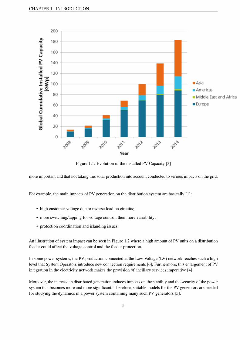
Due to the permanent decrease of PV technology prices and its simple integration at any point of the thedistribution grid, the amount of PV installed capacity around the world is constantly increasing. PV powerproduction is becoming a non-negligible part of the total electricity production. The global cumulative PVinstallations until 2014 can be seen in Figure 1.1. This fast enlargement in installed capacity is not expectedto stop and the total PV production will thus become more and more important.
The increasing PV and wind generation capacity is forcing significant changes across the electricity industryin terms of planning and operation procedures, grid reliability and performance standards, energy and capacitymarkets structures as well as policy and regulatory framework [1]. The demand for simulations of PV plantsproperties for the purpose of planning and design of the distribution and transmission systems increases [2].
These previous points make it urgent to have a complete reliable PV model and to use it in a simulation toolin order to get results that should give insight about PV units behavior and help System Operators in terms ofplanning and security studies. This work mainly focuses on the model of distributed small-scale PV unitsconnected to the distribution level. Moreover, the presence of larger installations directly connected to theMedium Voltage (MV) level also becomes more and more common, e.g. on the top of some companies’roofs. A model representing such larger PV installations is not considered in this work and is proposed as afuture improvement.
1.2 Presentation of the problematic
A few decades ago, the progressive introduction of the PV production in the power system was not a bigdeal. Indeed, the level of penetration was too low to be taken into account and an accurate model of PV unitwas useless. Several years ago, it was noticed that the installed PV power capacity was becoming more and
2
CHAPTER 1. INTRODUCTION
Figure 1.1: Evolution of the installed PV Capacity [3]
more important and that not taking this solar production into account conducted to serious impacts on the grid.
For example, the main impacts of PV generation on the distribution system are basically [1]:
• high customer voltage due to reverse load on circuits;
• more switching/tapping for voltage control, then more variability;
• protection coordination and islanding issues.
An illustration of system impact can be seen in Figure 1.2 where a high amount of PV units on a distributionfeeder could affect the voltage control and the feeder protection.
In some power systems, the PV production connected at the Low Voltage (LV) network reaches such a highlevel that System Operators introduce new connection requirements [6]. Furthermore, this enlargement of PVintegration in the electricity network makes the provision of ancillary services imperative [4].
Moreover, the increase in distributed generation induces impacts on the stability and the security of the powersystem that becomes more and more significant. Therefore, suitable models for the PV generators are neededfor studying the dynamics in a power system containing many such PV generators [5].
3

CHAPTER 1. INTRODUCTION
Figure 1.2: Example of system impact caused by large PV penetration in the distribution network [1]
Based on all these elements, the goal of this work is to build a mathematical model able to catch the maincharacteristics of photovoltaic units mainly connected to the distribution network. The model should respectthe present connection requirements and the ancillary services model that distributed PV generators connectedat the distribution level should nowadays respect and perform.
Particularly, this model should allow to strictly represent the dynamic behavior of distributed PV units whenthe electrical network is subject to a fault leading to large voltage sags. In this work, one will investigate,among others, how the units contribute to the voltage support and how this will impact the network’s voltageprofile.
1.3 Report Structure
The report is divided in four main parts:
1. the first part includes theoretical backgrounds of PV systems and their basic principles. Moreover itlooks over the existing PV models in the literature review, presents the PV model specifications basedon nowadays grid codes and the mathematical PV model in agreement with these specifications;
2. secondly, simulation tools are presented and dynamic simulations are performed to show the PV modelvalidation;
3. then, different fault situations interesting from a System Operator point of view are considered toobserve the different dynamic responses that PV units can present during voltage sags;
4. finally, an equivalent network model is proposed and especially an equivalent PV model that rep-resents all the small-scale units connected in the network. This model condenses the MV network
4

CHAPTER 1. INTRODUCTION
representation to ease transmission side planning and security studies.
5

CHAPTER 1. INTRODUCTION
References
[1] A. Ellis. ”PV plant electrical modeling for interconnection and transmission planning studies”September 12, 2012. Expanding Grid Integration of Renewable Energy in South Africa, Available:http://www.sapvia.co.za/wp-content/uploads/2013/09/Ellis-ESKOM-Webinar-Update.pdf, [AccessedFebruary 2016].
[2] D. PREMM , O. GLITZA , T. FAWZY , B. ENGEL and G. BETTENWORT. ”Grid integration ofphotovoltaic plants a generic description of pv plants for grid studies”. CIRED, 21st InternationalConference on Electricity Distribution, Paper 1190, Frankfurt, 6-9 June 2011.
[3] ISE Fraunhofer Institute for Solar Energy Systems. ”Photovoltaics report, ” freiburg, 17 november2015. Available: https://www.ise.fraunhofer.de/de/downloads/pdf-files/aktuelles/photovoltaics-report-in-englischer-sprache.pdf, [Accessed March 2016].
[4] P. Kotsampopoulos , Nikos Hatziargyriou , Benoit Bletterie , Georg Lauss. ”Review, analysis andrecommendations on recent guidelines for the provision of ancillary services by distributed generation”.Intelligent Energy Systems, IEEE International Workshop, pp 185-190.
[5] X. Mao and R. Ayyanar. ”Average and phasor models of single phase pv generators for analysis andsimulation of large power distribution systems”. Applied Power Electronics Conference and Exposition,IEEE, pp 1964-1970, 2009.
[6] P. Eguia , A. Etxegarai , E. Torres , J.I San Martin and I. Albizu. ”Use of generic dynamic models forphotovoltaic plants”. International Conference on Renewable Energies and Power Quality, No.13, April,2015.
6

Chapter 2
Basic principles of grid-connected PVsystems
2.1 Background
The fundamental element of the PV system is the solar cell made of semiconducor materials able to convertsunlight into electricity. First practical uses of PV systems were restricted to space applications since the PVtechnology was extremely expensive [3]. The progressive need for alternative energy sources has led the lastdecade to long-range supporting scheme for the connection of PV systems to the grid. This has induced moreresearches and investments leading to an increase in solar cell efficiency as well as a decrease in the price.This phenomenon keeps spreading. Nowadays, the cost of electricity produced by PV systems becomescompetitive compared to the retail price in certain regions.
This chapter presents the fundamental components of PV units, the basic principles of each component andthe way PV systems are linked to the grid in order to give some general insights on how PV systems are builtand works.
2.2 Components of PV systems
The different components of a PV system are illustrated in Figure 2.1. It can be seen that the system has twomain components, the PV array and the Power Conditioning Unit (PCU). The sunlight is first converted intoDC power that is then converted in AC power thanks to the inverter in the PCU. A load consumes a part ofthis AC power and the excess of power is injected into the distribution grid.
7

CHAPTER 2. BASIC PRINCIPLES OF GRID-CONNECTED PV SYSTEMS
Figure 2.1: Schematic of the building blocks of typical grid-connected PV system [3]
2.2.1 The solar cell
Solar cells are the building blocks of photovoltaic modules, otherwise known as solar panels. They are ableto convert directly the sunlight into electricity through the photoelectric effect. Basically, the operation of aPV cell includes three basic aspects:
1. the generation of either electron-hole pairs by the absorption of light;
2. the separation of opposite charge carriers;
3. the extraction of those carriers to an external circuit to produce electricity.
These attributes are illustrated in Figure 2.2 where the energy brought by the photons in the sunlight istransmitted to the charge carriers that are collected in order to generate a useful current.
The output of the solar cell is characterized by a voltage and a current. The I-V characteristic for a certainirradiance can be seen in Figure 2.3. VOC is the Open-Circuit voltage and ISC is the Short-Circuit current,two parameters that vary according to the solar irradiance. The two main parameters are IMPP and VMPP
intercepting the power (in green) at the maximum power point.
An ideal equivalent electrical circuit is represented by a current source in parallel with a diode. The resistanceRs and Rp take into account the losses and make the model more realistic. The resulting equivalent circuit isshown in Figure 2.3. According to the values obtained for the output current and voltage, cells are put inparallel or in series in order to get the desired voltage and current values for a given application.
8

CHAPTER 2. BASIC PRINCIPLES OF GRID-CONNECTED PV SYSTEMS
Figure 2.2: The photocell principles [2], ~E is the internal electrical field and the �i (i = 1, 2, 3) representdifferent wavelengths of the sunlight, which can be reflected, pass through or be absorbed by the cell
Figure 2.3: I-V characteristic and equivalent circuit of a solar cell [3]
2.2.2 The PCU
A simplified scheme of the PCU is illustrated in Figure 2.4. The PCU is composed of two main electronicstages. The first one is a DC-DC converter able to control the DC output of the solar array and keep theDC power at the maximum power point. This task is called Maximum Power Point Tracking (MPPT). Thesecond stage is the DC/AC converter also called inverter that will provide AC power compatible with theelectrical network. The inverter interfacing the PV system to the power grid is the key to power quality.Indeed, it transforms the Direct-Current (DC) power produced by the PV array into the Alternating-Current(AC) power so as to match utility power requirements [4].
In this work, only the electronic interface with the network has been modeled since the latter makes invisiblethe upstream part of the PV system. Inverters are designed in order to be able to perform different functions.These ones are described in the next chapter based on technical requirements and ancillary services thatnowadays PV units should perform.
9

CHAPTER 2. BASIC PRINCIPLES OF GRID-CONNECTED PV SYSTEMS
Figure 2.4: PCU structure [1]
10

CHAPTER 2. BASIC PRINCIPLES OF GRID-CONNECTED PV SYSTEMS
References
[1] Available:http://soltis.be/fr/photovoltaique/aspects-techniques/onduleurs/. [Accessed Mars 2016].
[2] Roger A. Massenger , Jerry Ventre. ”Photovoltaic systems engineering ”. CRC Press, 2005.
[3] A. Samadi. ”Large scale solar power integration in distribution grids”, 2014. Doctoral Thesis, Stockholm,Sweden, Available: http://repository.tudelft.nl/view/ir/uuid[Accessed February 2016].
[4] Nguyen Hoang Viet and Akihiko Yokoyama. ”Impact of fault ride-through characteristics of high-penetration photovoltaic generation on transient stability”. Power System Technology (POWERCON),2010 International Conference, pp. 1 - 7, October 2010.
11

Chapter 3
Specifications of the PV Model
In case of wide-scale penetration of single-phase PV systems in the low voltage grid, the rapid and almostinstantaneous disconnection of the units following a fault can lead to large power outages and significantimpacts on the system. To address these issues, the PV units, and in particular the inverters, should bedesigned to be able to provide ancillary services to the grid.
In this chapter a small review of the literature about existing PV models is presented. Then the specificationsof the PV model implemented in this work is proposed based on existing simplified models and nowadaystechnical requirements for small distributed PV units connected to the LV network. The model implementedin the framework of the work is presented in Chapter 4 and is based on the following model specifications.
3.1 Literature review
A decade ago, detailed models of PV system were implemented in order to focus on power system dynamicsstudying the effect of the irradiance or temperature variability such as presented in [5]. In the latter paper,the model comprised an explicit modeling of solar panels and the Maximum Power Point Tracking (MPPT)block with a DC/AC converter block. The associated control system was designed based on space vectortechniques for decoupled control of active and reactive power. This model was associated to a simple networkrepresentation for dynamic studies.
The model presented in [7] is an empirical model based on experimental results rather than on analyticalcharacterization to study the dynamic behavior the PV units following changes in irradiance. This model ofPV units generation was suitable for studying its interaction with the power system. A lot of other PV modelsrepresenting explicitly the PV panels and the MPPT block have been build for the study of the impacts onpower system stability following unpredictable changes in irradiance.
Since the electrical properties of PV plants are mainly determined by the inverters, more recent worksfocus on a detailed model of the inverter of the PV unit rather than on the solar panel and the MPPT logicrepresentation which are considered to be known and not seen from the rest of the system. In [3] is presentedan approach to model a three-phase PV inverter for grid integration studies under balanced and unbalanced
12

CHAPTER 3. SPECIFICATIONS OF THE PV MODEL
conditions. A grid integration study is an analytical framework used to evaluate a power system with highpenetration levels of variable renewable energy [6]. Indeed, it has become important to study how theinverter will behave under faulty conditions and accurate models are required to represent the grid supportingfunctions of the equipment.
With the constant evolution of grid codes, the manufacturers have to adapt the design of their PV invertersto be able to provide proper services to the grid. Changes in inverter model for dynamic studies are thusconstantly needed. At now, the most elaborated model of PV inverter is the one presented by the WesternElectricity Coordinating Council (WECC). In [9] is presented a generic dynamic model of PV plants whichis well suited for the representation of large-scale PV power plants.
However, this work is based on the simplified WECC generic model for Distributed and Small PV Plantspresented in [10]. Typically, this model is recommended to represent distribution-connected small PV plantsor multiple PV plants aggregated at a higher voltage level as it is done in the framework of this work.
Starting from this simplified model, some modifications have been made and functionalities have been addedto take into account technical requirements presented in current grid codes. These functionalities make upthe specifications of the PV model implemented in this work and are presented in the next sections of thischapter.
3.2 Specification of the PV model in faulty conditions
In this section, services that PV inverters should provide during large voltage deviations are described. Themain specification of PV inverters are the Low Voltage Ride-Through (LVRT) Capability and the reactivesupport. Other specifications such as the over voltage control and the active-reactive (PQ) strategy duringfaults are also detailed.
3.2.1 Low Voltage Ride-Through Capability
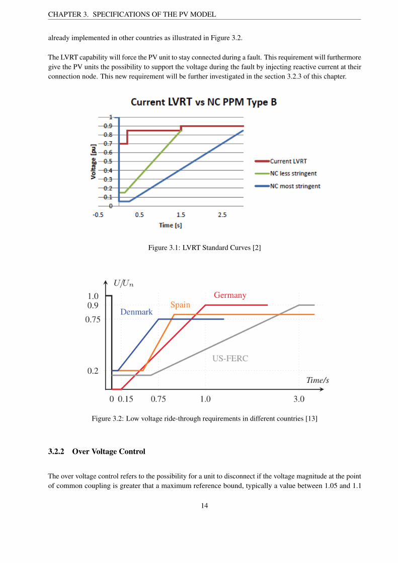
The Low Voltage Ride-Through (LVRT) Capability of a unit refers to its ability to stay connected to thenetwork during a low voltage situation. LVRT avoids simultaneous tripping of different sets of generationthat would lead to a lack of power in the system causing frequency issues. The requirement of LVRT variesfrom system to system depending on the grid code [12]. The LVRT requirement that will be implemented isbased on the standard curves provided to us by Elia (Belgium) and presented in Figure 3.1. As long as thevoltage measured at the Point of Common Coupling (PCC) remains above the selected LVRT standard curve,the unit should remain connected while it is allowed to disconnect otherwise.
In Figure 3.1, it is shown that different standard curves according to the technological requirements dependon the grid code. The present LVRT curve in red is not acceptable any longer since it shows that the unitsremain connected for a very short time. Indeed, it can be seen that the minimum voltage level is at 0.7 p.u,which is quite high. With the fast growing share of PV production at the LV network, the role of these unitsshould be no longer passive. In a shortcoming future, new curves will be implemented to require the units tostay connected during a fault: : see for instance the green and the blue curves. Such LVRT requirements are
13
CHAPTER 3. SPECIFICATIONS OF THE PV MODEL
already implemented in other countries as illustrated in Figure 3.2.
The LVRT capability will force the PV unit to stay connected during a fault. This requirement will furthermoregive the PV units the possibility to support the voltage during the fault by injecting reactive current at theirconnection node. This new requirement will be further investigated in the section 3.2.3 of this chapter.
Figure 3.1: LVRT Standard Curves [2]
Figure 3.2: Low voltage ride-through requirements in different countries [13]
3.2.2 Over Voltage Control
The over voltage control refers to the possibility for a unit to disconnect if the voltage magnitude at the pointof common coupling is greater that a maximum reference bound, typically a value between 1.05 and 1.1
14

CHAPTER 3. SPECIFICATIONS OF THE PV MODEL
p.u. Inverters are equipped with an over voltage protection device that will trigger and disconnect the unit ifvoltage conditions are no longer satisfied. This preventive action avoids damaging the insulation componentsof the electronic devices of the units.
However, some grid codes specify a more elaborated over voltage control, the High Voltage Ride-Throughcapability. The latest requires the unit to stay connect in high voltage conditions. This permits the unit toconsume reactive power during high voltage situations and to reduce the voltage rise. This last point is notinvestigated in this work and the HVRT capability has not been implemented in our model.
3.2.3 Reactive current support in case of large voltage deviation
The reactive support capability during large voltage deviation is based on the reactive current injectionrequirement showed in Figure 3.3. This figure shows basically the amplitude of reactive current that has to beinjected in the network in low voltage situation (V < 0.9 p.u) in order to support the voltage. Between 0.9and 0.5 p.u, the injected reactive current is given by
IQ = k(1� Vg)IN (3.1)
where IN is the rated current magnitude and a typical value for k is 2 p.u. When the voltage falls below 0.5p.u, the unit gives priority to the reactive power and it should inject 100 % of reactive current in the network.
Figure 3.3: Reactive current injection requirement [1]
Although the voltage sag issue has been much more considered in this work, in some grid codes the unitshould also be able to absorb reactive power in case of an over voltage situation. Figure 3.4 shows a droop-based voltage control where both low and high voltage situations are considered. However, in this work, ithas been assumed that the PV units should disconnect when V > 1.1 p.u in order to be more consistent withnowadays requirements. Therefore, the over voltage support is not investigated in the framework of the work.
The main difference between Figures 3.3 and 3.4 is the level of reactive production outside the dead-band.
15

CHAPTER 3. SPECIFICATIONS OF THE PV MODEL
Figure 3.4: Graphical schematic of droop-based voltage control [4]
Indeed, in Figure 3.3, it is shown that the unit should already inject 20% of its nominal current when V = 0.9p.u while in Figure 3.4, it can be seen that reactive power production of the unit is zero at that point. The firstreactive support implementation has been preferred in this work.
16
CHAPTER 3. SPECIFICATIONS OF THE PV MODEL
3.2.4 PQ Strategy during a fault
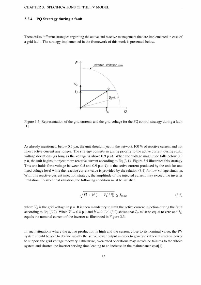
There exists different strategies regarding the active and reactive management that are implemented in case ofa grid fault. The strategy implemented in the framework of this work is presented below.
IP
IQ
Figure 3.5: Representation of the grid currents and the grid voltage for the PQ control strategy during a fault[1]
As already mentioned, below 0.5 p.u, the unit should inject in the network 100 % of reactive current and notinject active current any longer. The strategy consists in giving priority to the active current during smallvoltage deviations (as long as the voltage is above 0.9 p.u). When the voltage magnitude falls below 0.9p.u, the unit begins to inject more reactive current according to Eq.(3.1). Figure 3.5 illustrates this strategy.This one holds for a voltage between 0.5 and 0.9 p.u. IP is the active current produced by the unit for onefixed voltage level while the reactive current value is provided by the relation (3.1) for low voltage situation.With this reactive current injection strategy, the amplitude of the injected current may exceed the inverterlimitation. To avoid that situation, the following condition must be satisfied:
qI2P + k2(1� Vg)2I2N Imax (3.2)
where Vg is the grid voltage in p.u. It is then mandatory to limit the active current injection during the faultaccording to Eq. (3.2). When V = 0.5 p.u and k = 2, Eq. (3.2) shows that IP must be equal to zero and IQequals the nominal current of the inverter as illustrated in Figure 3.3.
In such situations where the active production is high and the current close to its nominal value, the PVsystem should be able to de-rate rapidly the active power output in order to generate sufficient reactive powerto support the grid voltage recovery. Otherwise, over-rated operations may introduce failures to the wholesystem and shorten the inverter serving time leading to an increase in the maintenance cost[1].
17

CHAPTER 3. SPECIFICATIONS OF THE PV MODEL
3.3 Specifications of the PV model in normal operating conditions
Hereafter we present the characteristics of the model that will prevail at a normal operating point, i.e. whenV is greater than 0.9 and smaller than 1.1 p.u. The first two characteristics aim at alleviating possible voltagerise when steady state active power production is high. This is done through either the dynamic power factorcharacteristic or the active power dependent reactive power characteristic. Only one of these characteristics(presented in Sections 3.3.1 and 3.3.2, respectively) has been implemented in the PV model since bothgive the same effect. Basically, this will influence the starting operating point provided by the load flowcomputation. Finally, the last specification considered concerns the PQ capability diagram in order to verifythat the inverter limit is never exceeded in normal operating conditions.
3.3.1 Dynamic Power Factor Characteristic
The dynamic power factor characteristic is a control of the power factor according to the level of activepower that is injected into the grid. The characteristic is shown in Figure 3.6. The terms ”under-excited” and”over-excited” generally refer to synchronous machine operations. The first one corresponds to a absorptionof reactive power while the second refers to a production of reactive power.
As over voltage conditions normally occur because of high active power production by the distributedgenerations, the cos�(P) characteristic curve is usually designed so that reactive power is absorbed by thegenerator only when its active power is above a threshold (e.g. 50% Pnom) and reaches the minimum cos�at nominal active power. The ”standard cos�(P) curve” is defined in VDE application rule VDE-AR-N4105:2011-08 [4]. A shortcoming of this approach is that unnecessary reactive power flow occurs resulting inhigher losses. Furthermore, it is worth mentioning that in LV grids the X/R ratio is quite low (and muchlower than at higher voltage levels). That can rise the need for active power curtailment if the reactive powerabsorption is not sufficient. Nowadays, the active power curtailment operation in over voltage situation is notaddressed in current standards [8] and is thus not considered as a grid requirement of PV systems.
Figure 3.6: Dynamic Power Factor Characteristic [4]
18

CHAPTER 3. SPECIFICATIONS OF THE PV MODEL
3.3.2 Active power dependent reactive power characteristic
The idea behind this control is the same that the previous one since the goal is to alleviate future over voltageby absorbing reactive power if the active power production becomes important. The corresponding curve canbe seen in Figure 3.7.
Figure 3.7: Q(P) characteristic curve [11]
The German Grid Code (GGC) standard Q(P ) characteristic requires the PV system to operate in an under-excited mode when the feed-in active power goes beyond a threshold of 50 % of Pmax in order to alleviatethe possible voltage rise [4]. On the other hand, reactive power is injected when the active power productionis low.
3.3.3 PQ capability diagram
There exists three types of PQ capability diagram in the normal operating conditions [8]:
1. ”Triangular” PQ capability diagram;
2. ”Rectangular” PQ capability diagram;
3. ”Semi-circular” PQ capability diagram.
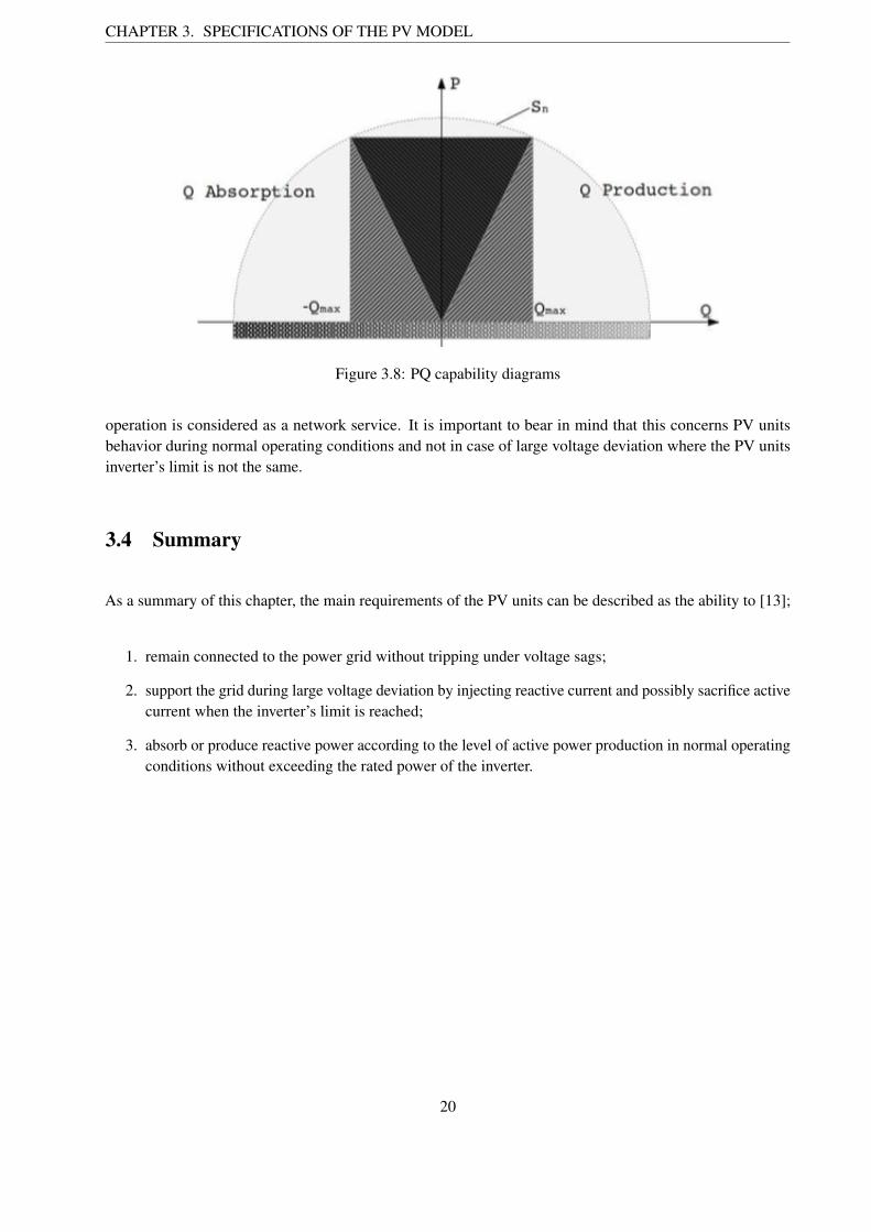
These ones can be seen in Figure 3.8. These diagrams have been built to control P and Q power flows injectedby the PV unit without exceeded the power limit of the inverter in normal operating conditions. Yet, ifthe dynamic power factor characteristic or the active power dependent reactive power characteristic is welldesigned, the power limit of the inverter is supposed to be never reached.
In this work, the capability diagram that has been selected is the ”rectangular” one. In this configuration,the maximum amount of reactive power is required even in conditions of reduced active power infeed. This
19
CHAPTER 3. SPECIFICATIONS OF THE PV MODEL
Figure 3.8: PQ capability diagrams
operation is considered as a network service. It is important to bear in mind that this concerns PV unitsbehavior during normal operating conditions and not in case of large voltage deviation where the PV unitsinverter’s limit is not the same.
3.4 Summary
As a summary of this chapter, the main requirements of the PV units can be described as the ability to [13];
1. remain connected to the power grid without tripping under voltage sags;
2. support the grid during large voltage deviation by injecting reactive current and possibly sacrifice activecurrent when the inverter’s limit is reached;
3. absorb or produce reactive power according to the level of active power production in normal operatingconditions without exceeding the rated power of the inverter.
20

CHAPTER 3. SPECIFICATIONS OF THE PV MODEL
References
[1] Y. Yang , W. Chen and F. Blaabjerg. Chapter 2, ”Advanced Control of Photovoltaic and Wind TurbinesPower Systems”. Advanced and Intelligent Control in Power Electronics and Drives, Studies, SpringerInternational Publishing Switzerland, 2014.
[2] Elia. ”current requirements in BE and NC rfg”. 2016.
[3] D. PREMM , O. GLITZA , T. FAWZY , B. ENGEL and G. BETTENWORT. ”Grid integration ofphotovoltaic plants a generic description of pv plants for grid studies”. CIRED, 21st InternationalConference on Electricity Distribution, Paper 1190, Frankfurt, 6-9 June 2011.
[4] A. Samadi , R. Eriksson and L. Soder. ”Coordinated droop based reactive power con-trol for distribution grid voltage regulation with PV systems,” Available: http://www.smooth-pv.info/doc/app14 kth coordinated droop based reactive power control.pdf, [Accessed february 2016].
[5] F. Fernandez-Bernal , L. Rouco , P. Centeno , Miguel Gonzalez and Manuel Alonso. ”Modelling ofphotovoltaic plants for power system dynamic studies”. Fifth International Conference Power SystemManagement and Control, pp. 341-346, 2002.
[6] J. Katz. ” Grid integration studies: Data requirements”. Greening the grid, National Renewable EnergyLaboratory, 2015.
[7] Yun Tiam Tan , Daniel S. Kirschen and Nicholas Jenkins. ”A model of pv generation suitable forstability analysis ”. IEEE Transactions on Energy Conversion, Vol 19. pp. 748 - 755, 2004.
[8] P. Kotsampopoulos , Nikos Hatziargyriou , Benoit Bletterie , Georg Lauss. ”Review, analysis andrecommendations on recent guidelines for the provision of ancillary services by distributed generation”.Intelligent Energy Systems, IEEE International Workshop, pp 185-190.
[9] P. Eguia , A. Etxegarai , E. Torres , J.I San Martin and I. Albizu. ”Use of generic dynamic modelsfor photovoltaic plants”. International Conference on Renewable Energies and Power Quality, No.13,April, 2015.
[10] Western Electricity Coordinating Council Modeling and Validation Work Group. ”Generic so-lar photovoltaic system dynamic simulation model specification,” September 2012. Available:http://www.wecc.biz/ [Accessed January 2014].
[11] A. Samadi. ”Large scale solar power integration in distribution grids”, 2014. Doctoral Thesis, Stockholm,Sweden, Available: http://repository.tudelft.nl/view/ir/uuid[Accessed February 2016].
[12] Nguyen Hoang Viet and Akihiko Yokoyama. ”Impact of fault ride-through characteristics of high-penetration photovoltaic generation on transient stability”. Power System Technology (POWERCON),2010 International Conference, pp. 1 - 7, October 2010.
[13] Y. Yang and F. Blaabjerg. ”Synchronization in single-phase grid-connected photovoltaic systems undergrid faults”. 3rd IEEE International Symposium on Power Electronics for Distributed GenerationSystems, pp. 476-482, June 2012.
21

Chapter 4
Implementation of the PV model
In this chapter, a mathematical model of small PV units connected to the LV network is presented. Thismodel implements the technical requirements given in the previous chapter and is represented by a blockdiagram. Especially, it will be explained how features such as reactive support and LVRT curve have beenimplemented and how the variables are linked together. A simplified Phase Locked Loop (PLL) controllerimplementation is eventually proposed for grid synchronization purpose.
4.1 Equivalent distribution system
The distributed PV model represents multiple PV units connected at the LV level and aggregated at a highervoltage level. Since then, the equivalent impedance of the distribution system taking into account amongothers the impedance of the transformer MV-LV has to be included in the model. A representation can beseen in Figure 4.1 where the impedance Z represents the equivalent impedance of the distribution system andthe transformer. Based on this figure, it can be written
V = VLV � ZI. (4.1)
The voltage and current phasors can be expressed in the rectangular form and the impedance can bedecomposed into its real and imaginary parts,
vx + jvy = vxlv + jvylv � (R+ jX)(ix + jiy). (4.2)
Decomposing Eq. (4.2) into its real and imaginary parts gives two equations that are included in the PVmodel.
22

CHAPTER 4. IMPLEMENTATION OF THE PV MODEL
PV Z
MVLV
VIVLV
Figure 4.1: Modeling the impedance of the LV network
4.2 Block Diagram of the model
The block diagram implementing the ancillary services and specifications described in Chapter 3 is shown inFigure 4.2. The latter is based on the PVD1 model presented in the WECC report [2] and on the PV dynamicmodel presented in [1].
LVRT holds for Low Voltage Ride-Through capability block. The block MAX with Vm and the constant 0.01as inputs avoids a division by zero in case of a severe fault. The specifications of the PV model for normaloperating conditions are not represented since it will not influence the dynamics of the units during faultsstudied in this work. These last requirements will be taken into account at the starting operating point duringthe static load flow computation. The parameters and variables of the PV model are described in Table 4.1.
The present section details the implementation of each specification presented in the previous chapter whichare, the reactive support, the over voltage control, the LVRT capability and the PQ strategy during faults.Moreover, it presents an original implementation for the permanent disconnection of the PV units.
4.2.1 Reactive current support implementation
Based on the reactive current injection requirement explained in Chapter 3, the reactive current control unitthat has been implemented is shown in Figure 4.3. This block defines a piece-wise linear function of theinput, defined by 6 points. The input of the block is the measured voltage magnitude Vm and the output isthe reactive current variable Iqext. It can be seen that the reference reactive current value (based on the loadflow calculation) Iqref switches to zero when the measured voltage magnitude falls below 0.9 p.u. Indeed, aninitial important reactive consumption by the PV unit may lead to an inefficient voltage support since a largenegative value would be added to Iqext in that case.
Figure 4.3 shows that Iqext = IN as Vm reaches 0.5 p.u. If the voltage falls below 0.5 p.u, the unit is able toprovide a reactive current that is greater than the nominal current of the unit until it eventually reaches themaximum rated current of the inverter Imax at the limit where the voltage falls to zero. In practice, this limitis never reached since the unit should be disconnected before the voltage reaches zero. This last point hasbeen implemented assuming that the nominal current is lower than the maximum rated current of the inverter.
23

CHAPTER 4. IMPLEMENTATION OF THE PV MODEL
OverVoltageControl
LVRT
1
1 + sTm
N
D
Vt Vm
ReacticeSupport
Fvh
Fvl
Ipmax
0
Ipcmd 1
1 + sTg
1
1 + sTg
IP
IQ
Iqmax
Iqmin
Vm < 0:9
PQstrategy
0.01
Fvh Fvl
MAX
Ip Iq
ix
iy
T 1
sT
vxlv
vylv
vd
vq ∆!PLL θPLL
Iqext +
+
Iqref
Pext
Switch0
(Vm−0:9)
Pflag
Pflag = 1
Iqcmd
Pflag = 0
1
1
1 + sTm
1
1 + sTm
vxlvm
vylvm−kPLL
0Switch
Figure 4.2: Block diagram of the distributed PV model
4.2.2 Over Voltage control implementation
In Figure 4.4 the implementation of the Over Voltage control block of Figure 4.2 is illustrated. In this figure,it is shown that the output of the block becomes one if the input is positive, i.e. when Vm > Vmax. On theother hand, as long as the input is negative, i.e. when Vm < Vmax, the output stays at zero. The multiplier oncurrent command Fvh is thus
Fvh = 1� y,
24

CHAPTER 4. IMPLEMENTATION OF THE PV MODEL
Imax
IN
0:2 · IN
0.90.5 Vm
Iqext(Vm)
1.1 1.2
Dead Band
−0:2 ·IN
Figure 4.3: Reactive current control unit (Reactive Support)
which means that the unit is disconnected when Vm > Vmax as the current multiplier becomes 0 and the unitsdo not inject current in the network any longer.
y(Vm−Vmax)
1
0
Figure 4.4: Over voltage control implementation
4.2.3 Low Voltage Ride-Through implementation
In Figure 4.5 the implementation of the LVRT block of Figure 4.2 is illustrated1. This block is implementedusing a timer model with varying delay. The input of the timer is the opposite of the measured voltagemagnitude (�Vm) and the output of the timer is a discrete variable z ✏{0, 1}.
If the input of the timer is smaller than the threshold �a, i.e. Vm > a, then the output of the timer is equal tozero. Otherwise, the output changes from zero to one at the time t+ ⌧(�Vm) where t is the time at which theinput (-Vm) becomes larger than �a and the delay ⌧(�Vm) varies with the input according to a piece-wiselinear characteristic involving three points. For example, tLV RT1 is the tolerated delay when Vm = Vmin andtLV RT2 is the tolerated delay when Vm = a.
1The parameters values have been provided to us by Doctor Jonathan Sprooten from Elia during a meeting.
25

CHAPTER 4. IMPLEMENTATION OF THE PV MODEL
Table 4.1: PV Model Parameters and Variables
Name DescriptionPext Initial active power signal, result of the load flow computationVt Terminal voltage magnitudeTm Time constant due to voltage measurement delayVm Measured voltage magnitudeIqref Initial reactive currentIqext External reactive signal for voltage supportIpmax Dynamic active current limitIqmax Dynamic reactive current limitIpcmd Active current commandIqcmd Reactive current commandIP , IQ Active and reactive current injectionTg Inverter current lag time constant
Fvl, Fvh Multiplier on current command in low voltage or high voltage situation (0 or 1)Pflag If 1, priority to the active power, else priority to the reactive power
vxlvm, vylvm Measured voltage components in the (x,y) reference frame at the LV level for the PLL controller✓PLL Voltage phase angle PLL signal
−Vm
τ
−Vmin−a
tLV RT2
tLV RT1
Figure 4.5: Low Voltage Ride-Through (LVRT) implementation: typical values for nowadays LVRT require-ments: a = 0.9 p.u, Vmin = 0.3 p.u, tLV RT1 = 0.2 s and tLV RT2 = 1.5 s
The output of the timer z is linked to the current command multiplier through Fvl = 1� z. Then, accordingto the value of Vm, the units disconnect if the tolerated delay ⌧(�Vm) is exceeded.
4.2.4 Permanent disconnection of the PV unit
In this work, it has been assumed that the units, once there are disconnected from the network, are not ableto automatically reconnect once the network conditions are fulfilled. Then, it was necessary to find a trick
26

CHAPTER 4. IMPLEMENTATION OF THE PV MODEL
in order to keep the current multipliers Fvl and Fvh at zero once these ones are set to zero due to externalvoltage conditions. Therefore, a Hysteresis block has been implemented in order to achieve that goal. Thegeneral representation of the hysteresis curve is shown in Figure 4.6.
The corresponding equations are given by
(xj = yIA + y
IA
�yDB
xi
�xI
if z = 1,
xj = yDA + yIB
�yDA
xi
�xD
if z = �1.(4.3)
Figure 4.6: General representation of the hysteresis curve
The hysteresis curve that has been implemented in the model is illustrated in Figure 4.7 and is the same forboth current multipliers. Fvli and Fvhi are intermediate variables such that
Fvli = 1� z
andFvhi = 1� y.
Initially, Fvli (resp Fvhi) and Fvl (resp Fvh) are both equal to one. Then, once the LVRT limit (resp. themaximum voltage) is reached, the output of the timer z (resp. the variable y) changes from zero to oneand the corresponding intermediate variable is momentarily equal to 0. According to the hysteresis curve,the variable Fvl (resp Fvh) switches from one to zero, the point (0,0) is then reached. Once the acceptablenetwork conditions are recovered, Fvli (resp Fvhi) gets back to one and the variable Fvl (resp Fvh) stays atzero since the increasing point of the hysteresis is at 1.1, a value that is never reached by the intermediatevariables. The system remains stuck at the point (1,0) and the PV units are permanently disconnected evenwhen the voltage has recovered.
27

CHAPTER 4. IMPLEMENTATION OF THE PV MODEL
1
1 1.1 Fvli, Fvhi
Fvl, Fvh
StartingPoint(1,1)
0
Figure 4.7: Hysteresis implementation for the permanent disconnection of PV units
4.2.5 PQ strategy implementation
The PQ strategy is implemented through these algebraic equations
8<
:Ipmax = PflagIN + (1� Pflag)
qI2N � I2qcmd
Iqmax = Pflag
qI2N � I2pcmd + (1� Pflag)Imax.
(4.4)
If the priority is given to the active current, i.e. Pflag = 1, Equation (4.4) indicates that the maximum valuethat can be reached by the active current is fixed and equal to the nominal current of the inverter IN . Then,the maximum value that can be reached by the reactive current varies according to
Iqmax =qI2N � I2pcmd (4.5)
in order to not exceed the nominal current magnitude of the inverter in normal operating conditions.
On the contrary, if the priority is given to the reactive current, i.e. Pflag = 0, Equation (4.4) indicates that themaximum value that can be reached by the active current is no longer fixed and is given by
Ipmax =q
I2N � I2qcmd. (4.6)
In this case, the maximum value that can be reached by the reactive current is fixed and equal to the maximumrated current of the inverter Imax.
Since the reactive current value reaches the nominal current value of the inverter when Vm < 0.5, accordingto Eq.(4.6) the active current falls to zero. The units work in active priority when the voltage magnitude isbigger than 0.9 p.u. At one point, when Iqcmd > IN , the argument of the square root in Eq. (4.6) becomesnegative. The problem is addressed in Chapter 5.
28

CHAPTER 4. IMPLEMENTATION OF THE PV MODEL
Control of Pflag
According to the technical requirements explained in the previous chapter, if Vm < 0.9, the priority shouldalways be given to the reactive current in order to efficiently support the voltage. Therefore, a switch wasimplemented in order to force the value of Pflag to zero when the measured voltage falls below 0.9 p.u. Thelatter can be seen in Figure 4.2. In that situation, the upper limit of the reactive current is equal to to themaximum rated current of the inverter which allows the system to inject a large amount of reactive current inthe network while the active current is sacrificed.
4.3 The Phase Locked Loop (PLL) controller
The Phase Locked Loop controller is required for grid synchronization purpose. Grid synchronizationtechniques are crucial for single-phase PV systems to ride-through utility fault or operate under abnormalgrid conditions in compliance with the existing grid requirements[4]. Indeed, the injected active and reactivecurrents into the grid have to be synchronized with the grid voltage anytime. If a fault occurs in the networkleading to a voltage drop at the point of common coupling, the detection and the synchronization systemshould be able to respond to this abnormal operating condition immediately [4]. The PLL controller mustgenerate correct reference signals using fast and accurate synchronization mechanism to ride through thevoltage drop efficiently.
Different PLL-based methods exist in order to achieve that goal. The one that is implemented in this work isa simplified Second Order Generalized Integrator based PLL. Indeed, as presented in [4], this method is thebest candidate for single-phase applications connected to the low voltage grid.
The block diagram used for this PLL implementation is shown in Figure 4.8. The difference between theexact Second Order Generalized Integrator based PLL and this simplified model is the presence of only oneintegrator. Indeed, the PI controller of the Second Order Generalized Integrator based PLL has been replacedby a P controller defined with the parameter kPLL influencing the time response of the PLL controller duringlarge voltage deviations.
The phase ✓PLL is adjusted until the voltage vq in the Park reference frame reaches 0 where �!PLL is thespeed deviation of the terminal voltage V illustrated in Figure 4.9. Indeed, the angle velocity is chosen tobe the same as the terminal voltage of the inverter V ; as a result, vq of the PV terminal voltage becomes 0and vd equals to the terminal voltage magnitude, theoretically [3]. In practice, when vq is null, vd is equal tothe measured voltage magnitude. vxlvm and vylvm are the real part and the imaginary part of the measuredterminal voltage at the LV bus in the (x,y) reference frame while vd and vq are the projections of the measuredvoltage phasor on the d� q Park reference frame as shown in Figure 4.9. The phase angle ✓PLL is initiallyequal to atan(
vylvm
vxlvm
), i.e. in steady state condition, the current injected by the PV units in the network isassumed to be perfectly synchronized with the grid voltage.
29

CHAPTER 4. IMPLEMENTATION OF THE PV MODEL
T
vxlvm
vylvm
vd
vq−kPLL
1
s
∆!PLL θPLL
Figure 4.8: PLL block diagram
Figure 4.9: Voltages Phasors diagram
The voltage components vd and vq are obtained using these relations:
⇢vd = vxlvmcos✓PLL + vylvmsin✓PLL
vq = vxlvmsin✓PLL � vylvmcos✓PLL(4.7)
The PLL controller will thus determine at any time vd that is supposed to be equal to V as vq = 0 when itworks correctly. From vd, the active and reactive power generated by the PV units can be determined. Thecurrents id and iq corresponds to the active and reactive currents that are injected in the network, respectively.
8><
>:
id = Pvd
= IP
iq = Qvd
= IQ
(4.8)
From these values, current components in the (x, y) reference frame (ix and iy) can be retrieved throughthese relations:
⇢IP = ixcos✓PLL + iysin✓PLL
IQ = ixsin✓PLL � iycos✓PLL.(4.9)
30

CHAPTER 4. IMPLEMENTATION OF THE PV MODEL
and thus
⇢ix = IP cos✓PLL + IQsin✓PLL
iy = IP sin✓PLL � IQcos✓PLL.(4.10)
The value atan( iyix
) determines the phase angle of the injected current.
31

CHAPTER 4. IMPLEMENTATION OF THE PV MODEL
References
[1] Frederic Olivier , Petros Aristidou , Damien Ernst and Thierry Van Cutsem. ”Active management oflow-voltage networks for mitigating overvoltages due to photovoltaic units”. IEEE Transactions onSmart Grid, vol. 2, pp. 926-936, 2014.
[2] Western Electricity Coordinating Council Modeling and Validation Work Group. ”Generic so-lar photovoltaic system dynamic simulation model specification,” September 2012. Available:http://www.wecc.biz/ [Accessed January 2014].
[3] Nguyen Hoang Viet and Akihiko Yokoyama. ”Impact of fault ride-through characteristics of high-penetration photovoltaic generation on transient stability”. Power System Technology (POWERCON),2010 International Conference, pp. 1 - 7, October 2010.
[4] Y. Yang and F. Blaabjerg. ”Synchronization in single-phase grid-connected photovoltaic systems undergrid faults”. 3rd IEEE International Symposium on Power Electronics for Distributed Generation Systems,pp. 476-482, June 2012.
32

Chapter 5
Dynamic simulations results and modelvalidation
This chapter first describes the software and the simulation tools that have been used for the practicalimplementation of the mathematical model presented in Chapter 4 and for dynamic simulations. Then themodeling of the network is explained presenting the network topology and the components that have beenused. Finally, some simulation results are showed for the PV model validation. All the faults simulated inthis work are balanced three-phase faults.
5.1 Software and simulation tools
In this section, the architecture and the philosophy more specifically behind the software used to perform thedynamic simulations are explained. Especially, it describes how the software represents and solves the modelequations and electric power systems equations in general.
5.1.1 Small overview of RAMSES
RAMSES holds for RApid Multiprocessors Simulation of Electric power Systems and is a dynamic simulationsoftware able to cope with large models taking advantage of computer technology. Indeed, RAMSES exploitsparallel computing tools and is based on system decomposition. The algorithm provides numerical andcomputational acceleration of the procedure as detailed in [6]. In Figure 5.1 can be seen a schematic of PowerSystem as it is modeled in RAMSES.
The PV model that is implemented in this work is represented in RAMSES by an injector that will be connectedto one bus of an AC network. Injectors are interfaced to the AC network through the rectangular componentsof bus voltage (vx,vy) and injected current (ix, iy). They are modeled with their own Differential-AlgebraicEquations (DAEs):
33

CHAPTER 5. DYNAMIC SIMULATIONS RESULTS AND MODEL VALIDATION
Figure 5.1: Power system modeling in RAMSES [3]
Figure 5.2: Injector modeling in RAMSES [3]
• algebraic equations yield higher modeling flexibility;
• the solver handles equations changing between differential and algebraic.
In Figure 5.2 is represented an injector as it is modeled in RAMSES.
5.1.2 CODEGEN
All the blocks presented in the previous chapter have been implemented using a library of models available inCODEGEN.
CODEGEN is a code generation utility that allows the user to provide an easy-to-understand description of the
34

CHAPTER 5. DYNAMIC SIMULATIONS RESULTS AND MODEL VALIDATION
!coi
Figure 5.3: Injector model in CODEGEN
Figure 5.4: From the construction of the model described by a text file to its incorporation into RAMSES [3]
model in a text format. Indeed, once the model is entirely described in a text file, CODEGEN will convert thistext file into fortran 2003 code. This is compiled and linked to the rest of the RAMSES software (availableas a library) to eventually obtain a executable comprising the new model representation that will be used toperform the dynamic simulations in RAMSES.
In CODEGEN, as in RAMSES, the PV model is modeled as an injector as sketched in Figure 5.3 where !coi isthe angular speed of the center of inertia of all synchronous machines and can be used as an approximation ofthe angular frequency of voltage and current at the bus of connection.
vx, vy and !coi are the input states of the injector model. The latter are processed outside the model. On thecontrary, ix and iy are internal variables of the injector model and must be computed together with the othervariables of the model [4].
In CODEGEN, a model is represented by a set of blocks that are interconnected through links. Each block isdefined by a set of differential, algebraic or differential-algebraic equations. These equations are gathered toform the model. To each link is affected a state variable that must be explicitly declared and initialized by theuser. It can be differential or algebraic. A particularity of CODEGEN is that the algebraic constraints can bewritten by the user himself. Furthermore, some elementary blocks involve additional states. The user doesnot need to define nor initialize them (this can be done automatically). Some blocks also involve discreteinternal variables not seen by the rest of the model and causing changes of equations, e.g. due to limits,discontinuities, etc. These discrete transitions are further detailed in the next section.
Finally, in Figure 5.4 can be seen the user-defined scheme that illustrates how CODEGEN and RAMSES arelinked together.
35

CHAPTER 5. DYNAMIC SIMULATIONS RESULTS AND MODEL VALIDATION
5.1.3 Handling of discrete transitions
The power system models typically used in dynamic simulations involve discrete events in addition to thestandards differential-algebraic equations [2]. This causes some equations to change. The solver handle suchjumps.
The proposed simulation scheme detailed in [2] is implemented in RAMSES and uses non synchronized timestep with the system jumps, i.e. that the moment where the transition occurred is not precisely identified. Thisleads to a posteriori corrective step after such a jump has occurred. In other words, all blocks are first solvedbefore treating the discrete transitions. If needed, a corrective step is applied to the variables afterwards. Thehandling of discrete transitions of an internal variable z is illustrated in Figure 5.5. It can be seen that passingfrom t to t+ h [5]:
1. for the current value of z, the DAEs are integrated (with full accuracy);
2. at the resulting point, the discrete transitions are checked. If needed, z is changed (hence, the DAEsare modified);
3. the previous time step from t to t+ h is canceled and the new DAEs are integrated from t to t+ h;
4. if needed, the procedure cycles until no z changes.
If the number of cycles reaches a maximum, the time step size h is reduced. Eventually, if h has beendecreased to hmin, and the problem persists, simulation stops [5].
Figure 5.5: Handling of discrete transitions passing from t to t+ h [5]
This method makes the solver very robust and able to handle system of big size in a limited amount oftime. However, in some situations, this may lead to several solving problems. Indeed, in the PQ strategyimplementation shown in the previous chapter, the active and reactive current limiters have variable boundsvarying according to
8<
:Ipmax = PflagIN + (1� Pflag)
qI2N � I2qcmd
Iqmax = Pflag
qI2N � I2pcmd + (1� Pflag)Imax
(5.1)
36

CHAPTER 5. DYNAMIC SIMULATIONS RESULTS AND MODEL VALIDATION
Since the corrective step is performed after the jump has occurred, a situation where Ipcmd is greater thanIN during one time step may happens leading to a negative argument for the square root which forces thesimulation to stop.
Therefore, in the text file describing the model, the equations of the variable bounds of the limiters have to berewritten as
8<
:Ipmax = PflagIN + (1� Pflag)
qmax(0.d0, (I2N � I2qcmd)
Iqmax = Pflag
qmax(0.d0, (I2N � I2pcmd) + (1� Pflag)Imax
(5.2)
Equation. (5.2) avoids a negative argument of the square root by limiting it to zero, if Ipcmd is greater than INor when Iqcmd is greater than IN for large voltage deviations. In that case, the simulation does not encounterany problem.
5.2 Network modeling
Simulations have been carried out using a 75-bus MV test network. The external transmission grid isrepresented by its Thevenin equivalent and is connected to the MV network through a power transformer of25 MVA. This test network is represented in the Appendix A of the report.
At each bus of the network, the load is divided into an equivalent load with constant admittance holding forthe static part and an equivalent induction machine holding for the dynamic part. In Figure 5.6, the modelingof the load at each bus of the test network is illustrated as well as the equivalent circuit of the induction motor.The active and reactive power consumed by the constant admittance load are given by
8><
>:
P = P0(VV0)2
Q = Q0(VV0)2
(5.3)
where P0, Q0 and V0 are the powers and voltage initial set points.
37
CHAPTER 5. DYNAMIC SIMULATIONS RESULTS AND MODEL VALIDATION
M
constant
admittancedouble-cage induction
motor
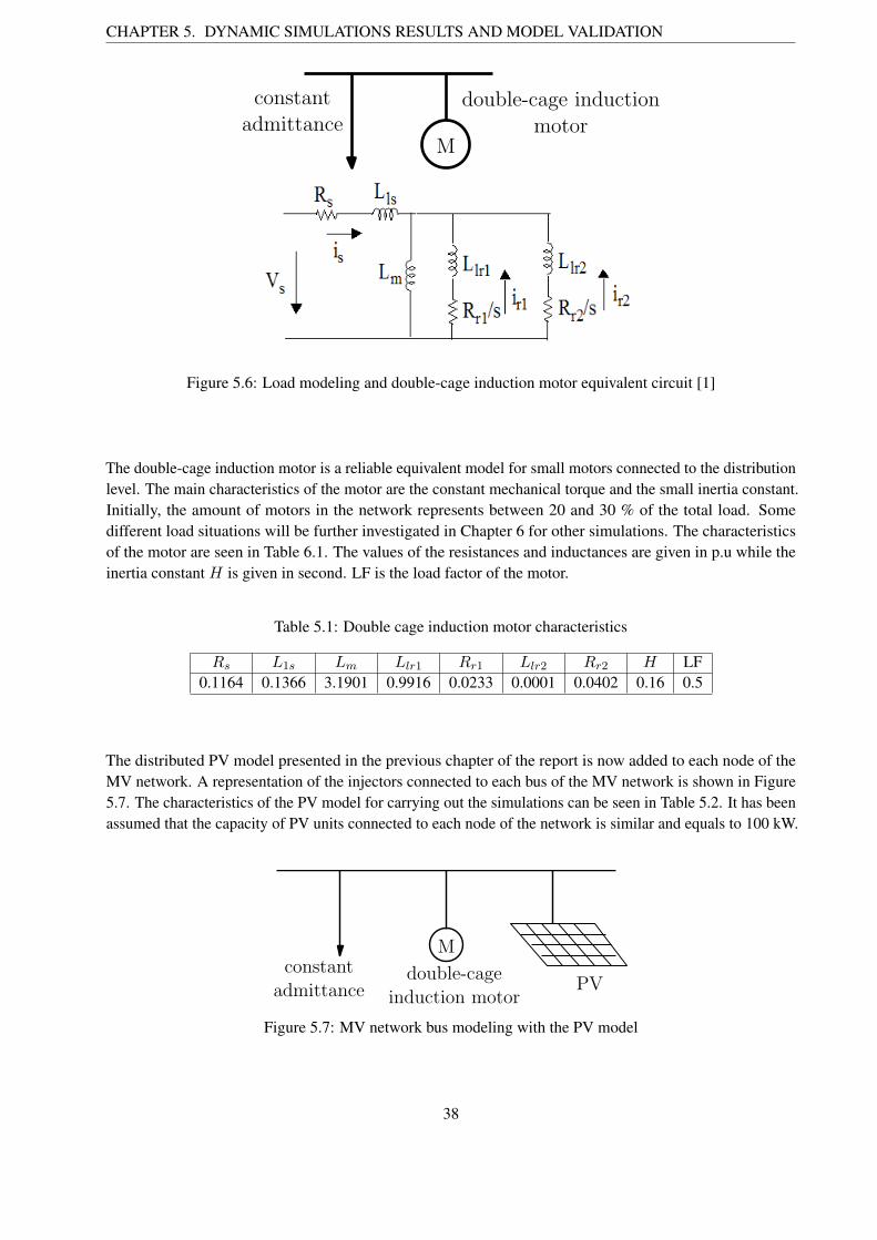
Figure 5.6: Load modeling and double-cage induction motor equivalent circuit [1]
The double-cage induction motor is a reliable equivalent model for small motors connected to the distributionlevel. The main characteristics of the motor are the constant mechanical torque and the small inertia constant.Initially, the amount of motors in the network represents between 20 and 30 % of the total load. Somedifferent load situations will be further investigated in Chapter 6 for other simulations. The characteristicsof the motor are seen in Table 6.1. The values of the resistances and inductances are given in p.u while theinertia constant H is given in second. LF is the load factor of the motor.
Table 5.1: Double cage induction motor characteristics
Rs L1s Lm Llr1 Rr1 Llr2 Rr2 H LF0.1164 0.1366 3.1901 0.9916 0.0233 0.0001 0.0402 0.16 0.5
The distributed PV model presented in the previous chapter of the report is now added to each node of theMV network. A representation of the injectors connected to each bus of the MV network is shown in Figure5.7. The characteristics of the PV model for carrying out the simulations can be seen in Table 5.2. It has beenassumed that the capacity of PV units connected to each node of the network is similar and equals to 100 kW.
constant
admittancedouble-cage
induction motor
M
PV
Figure 5.7: MV network bus modeling with the PV model
38
CHAPTER 5. DYNAMIC SIMULATIONS RESULTS AND MODEL VALIDATION
Table 5.2: PV model characteristics
Imax IN Tg Tm tLV RT1 tLV RT2 Vmax kpll a Vmin
0.12 p.u 0.1 p.u 0.02 s 0.05 s 0.2 s 1.5 s 1.1 p.u 30 0.9 p.u 0.3 p.u
5.3 PV model validation
In this section, some simulations are performed for the model validation. Different faults are simulated onthe transmission side to verify that the PV units responses are in agreement with the PV model specifica-tions. Particularly, the transition in the PV units priority and the LVRT control are investigated in order todemonstrate that these implementations are efficient.
5.3.1 Behavior of the units during voltage sags in the transmission system
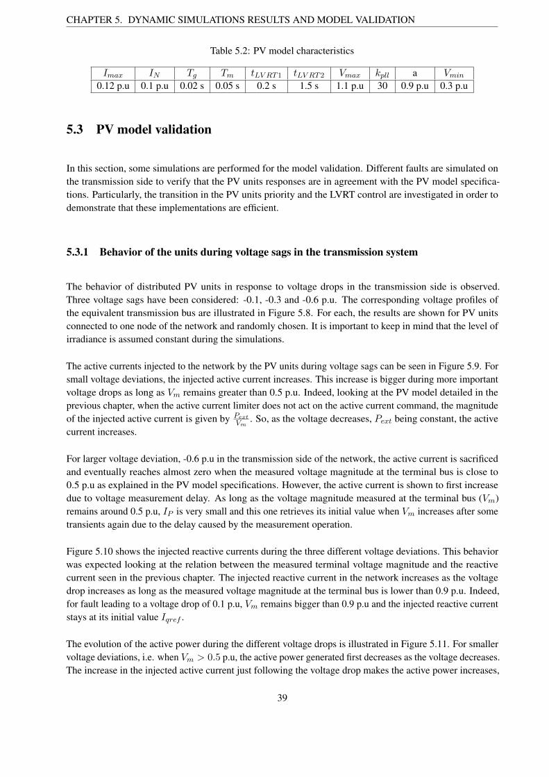
The behavior of distributed PV units in response to voltage drops in the transmission side is observed.Three voltage sags have been considered: -0.1, -0.3 and -0.6 p.u. The corresponding voltage profiles ofthe equivalent transmission bus are illustrated in Figure 5.8. For each, the results are shown for PV unitsconnected to one node of the network and randomly chosen. It is important to keep in mind that the level ofirradiance is assumed constant during the simulations.
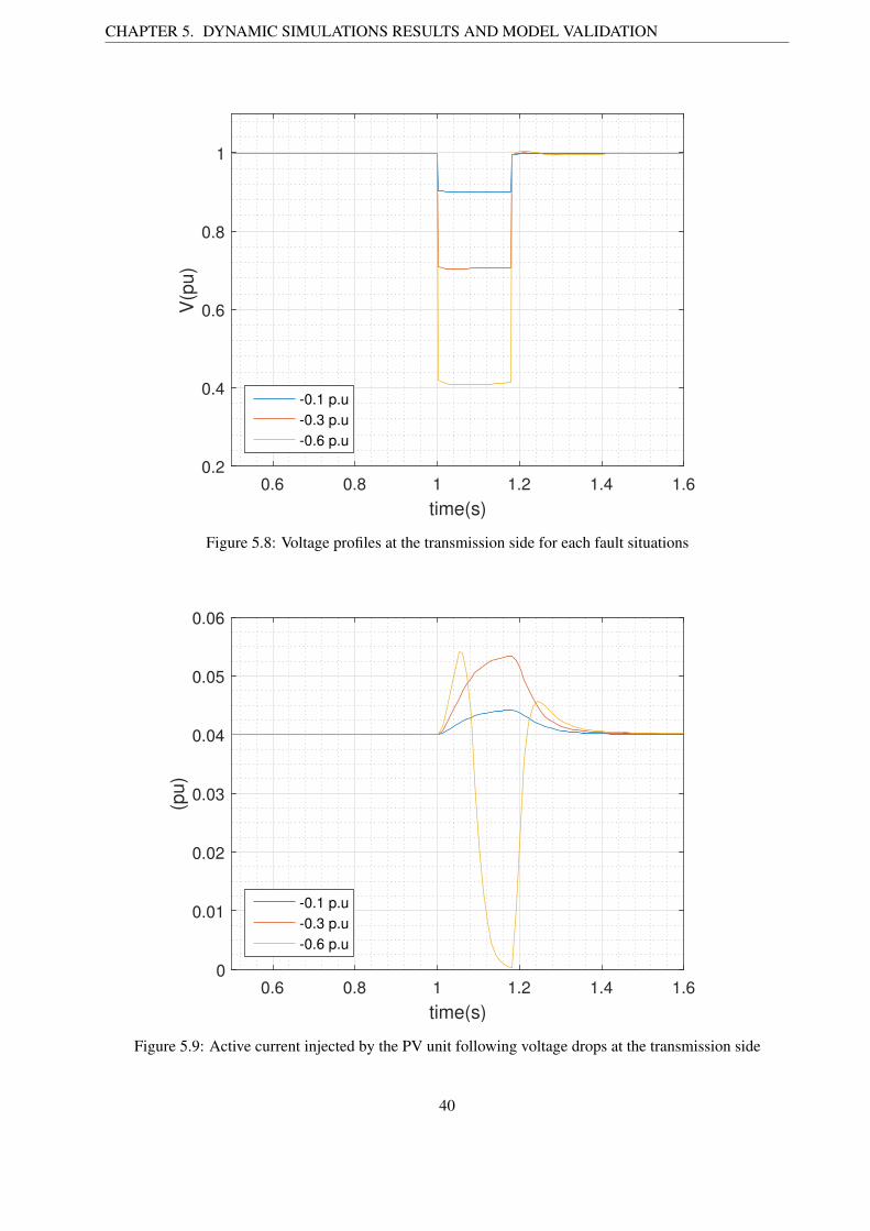
The active currents injected to the network by the PV units during voltage sags can be seen in Figure 5.9. Forsmall voltage deviations, the injected active current increases. This increase is bigger during more importantvoltage drops as long as Vm remains greater than 0.5 p.u. Indeed, looking at the PV model detailed in theprevious chapter, when the active current limiter does not act on the active current command, the magnitudeof the injected active current is given by P
ext
Vm
. So, as the voltage decreases, Pext being constant, the activecurrent increases.
For larger voltage deviation, -0.6 p.u in the transmission side of the network, the active current is sacrificedand eventually reaches almost zero when the measured voltage magnitude at the terminal bus is close to0.5 p.u as explained in the PV model specifications. However, the active current is shown to first increasedue to voltage measurement delay. As long as the voltage magnitude measured at the terminal bus (Vm)remains around 0.5 p.u, IP is very small and this one retrieves its initial value when Vm increases after sometransients again due to the delay caused by the measurement operation.
Figure 5.10 shows the injected reactive currents during the three different voltage deviations. This behaviorwas expected looking at the relation between the measured terminal voltage magnitude and the reactivecurrent seen in the previous chapter. The injected reactive current in the network increases as the voltagedrop increases as long as the measured voltage magnitude at the terminal bus is lower than 0.9 p.u. Indeed,for fault leading to a voltage drop of 0.1 p.u, Vm remains bigger than 0.9 p.u and the injected reactive currentstays at its initial value Iqref .
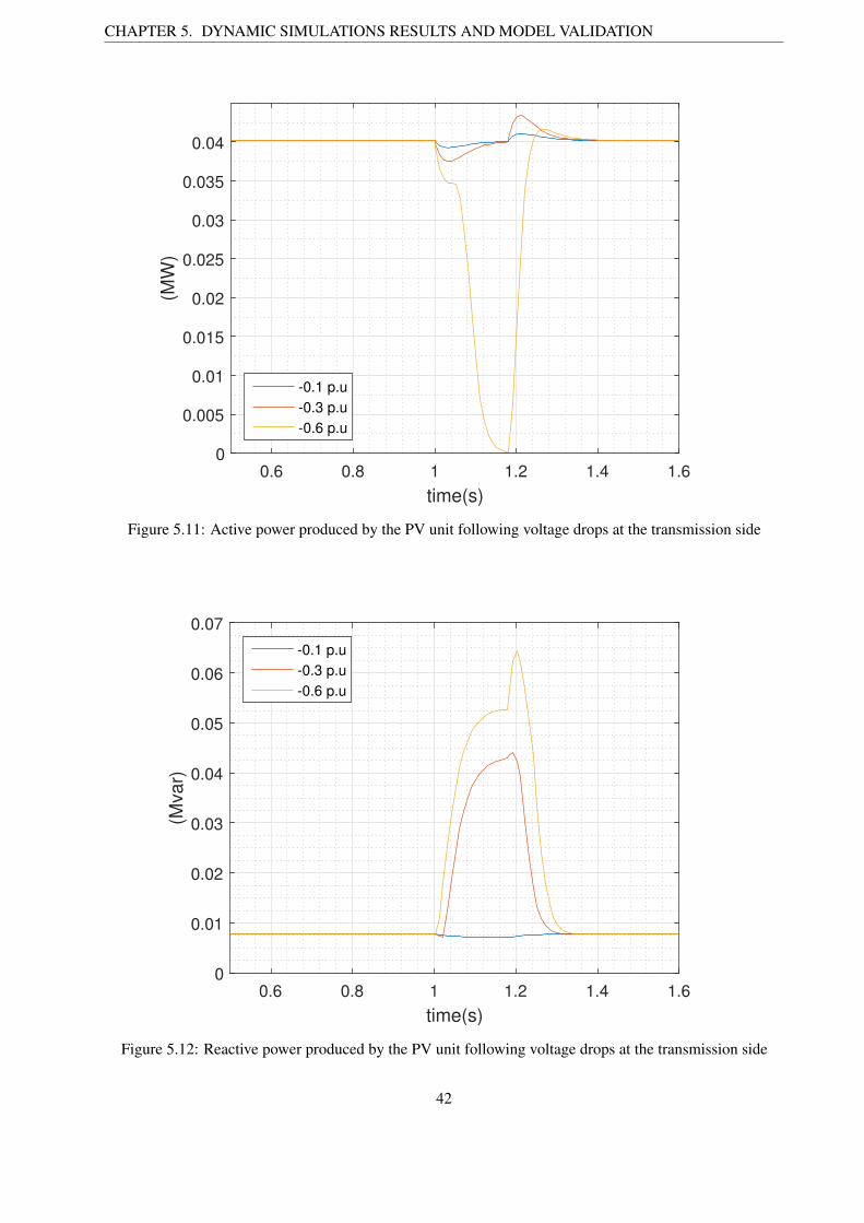
The evolution of the active power during the different voltage drops is illustrated in Figure 5.11. For smallervoltage deviations, i.e. when Vm > 0.5 p.u, the active power generated first decreases as the voltage decreases.The increase in the injected active current just following the voltage drop makes the active power increases,
39
CHAPTER 5. DYNAMIC SIMULATIONS RESULTS AND MODEL VALIDATION
0.6 0.8 1 1.2 1.4 1.6
time(s)
0.2
0.4
0.6
0.8
1
V(p
u)
-0.1 p.u
-0.3 p.u
-0.6 p.u
Figure 5.8: Voltage profiles at the transmission side for each fault situations
0.6 0.8 1 1.2 1.4 1.6
time(s)
0
0.01
0.02
0.03
0.04
0.05
0.06
(pu)
-0.1 p.u
-0.3 p.u
-0.6 p.u
Figure 5.9: Active current injected by the PV unit following voltage drops at the transmission side
40

CHAPTER 5. DYNAMIC SIMULATIONS RESULTS AND MODEL VALIDATION
the observed delay is due to the voltage measurement delay. As the voltage recovers and the injected activecurrent is still high (again due to measurement delay), the active power increases for a short moment beforethe injected active current retrieves its initial steady state value, as the active power does. For a larger voltagedeviation, it is shown that the active power strongly decreases to eventually falls to zero, since the activecurrent is sacrificed.
It can be seen in Figure 5.12 that the reactive power generated by the unit during the voltage deviation of-0.1 p.u slightly decreases as the injected reactive current remains constant and the voltage decreases. It isalso observed that the reactive power generated increases during larger voltage deviations. More the voltagesag is important and more the amount of generated reactive power is important. This is due to the injectedreactive current that increases as the voltage sag is more important but also to the value of the voltage at theterminal of the PV units that is much more supported for bigger fault. Due to the voltage measurement delay,the injected reactive current is still high when the voltage has recovered leading to a short peak of reactivepower production that increases for more important voltage drops. In all cases, as explained in the modelspecifications, it is shown that the units are initially producing reactive power due to the steady state activepower production which is initially small for PV units connected to this bus.
0.6 0.8 1 1.2 1.4 1.6
time(s)
0
0.02
0.04
0.06
0.08
0.1
0.12
(pu)
-0.1 p.u
-0.3 p.u
-0.6 p.u
Figure 5.10: Reactive current injected by the PV unit following voltage drops at the transmission side
41
CHAPTER 5. DYNAMIC SIMULATIONS RESULTS AND MODEL VALIDATION
0.6 0.8 1 1.2 1.4 1.6
time(s)
0
0.005
0.01
0.015
0.02
0.025
0.03
0.035
0.04
(MW
)
-0.1 p.u
-0.3 p.u
-0.6 p.u
Figure 5.11: Active power produced by the PV unit following voltage drops at the transmission side
0.6 0.8 1 1.2 1.4 1.6
time(s)
0
0.01
0.02
0.03
0.04
0.05
0.06
0.07
(Mva
r)
-0.1 p.u
-0.3 p.u
-0.6 p.u
Figure 5.12: Reactive power produced by the PV unit following voltage drops at the transmission side
42
CHAPTER 5. DYNAMIC SIMULATIONS RESULTS AND MODEL VALIDATION
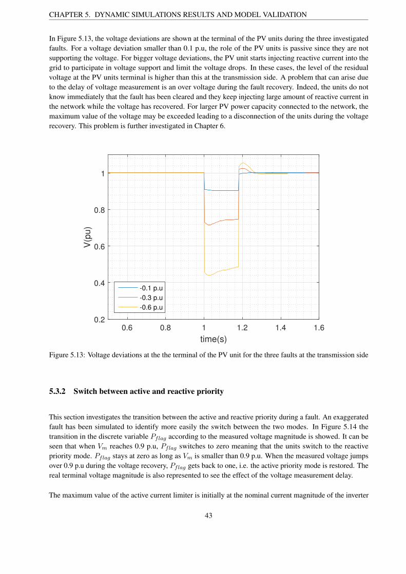
In Figure 5.13, the voltage deviations are shown at the terminal of the PV units during the three investigatedfaults. For a voltage deviation smaller than 0.1 p.u, the role of the PV units is passive since they are notsupporting the voltage. For bigger voltage deviations, the PV unit starts injecting reactive current into thegrid to participate in voltage support and limit the voltage drops. In these cases, the level of the residualvoltage at the PV units terminal is higher than this at the transmission side. A problem that can arise dueto the delay of voltage measurement is an over voltage during the fault recovery. Indeed, the units do notknow immediately that the fault has been cleared and they keep injecting large amount of reactive current inthe network while the voltage has recovered. For larger PV power capacity connected to the network, themaximum value of the voltage may be exceeded leading to a disconnection of the units during the voltagerecovery. This problem is further investigated in Chapter 6.
0.6 0.8 1 1.2 1.4 1.6
time(s)
0.2
0.4
0.6
0.8
1
V(p
u)
-0.1 p.u
-0.3 p.u
-0.6 p.u
Figure 5.13: Voltage deviations at the the terminal of the PV unit for the three faults at the transmission side
5.3.2 Switch between active and reactive priority
This section investigates the transition between the active and reactive priority during a fault. An exaggeratedfault has been simulated to identify more easily the switch between the two modes. In Figure 5.14 thetransition in the discrete variable Pflag according to the measured voltage magnitude is showed. It can beseen that when Vm reaches 0.9 p.u, Pflag switches to zero meaning that the units switch to the reactivepriority mode. Pflag stays at zero as long as Vm is smaller than 0.9 p.u. When the measured voltage jumpsover 0.9 p.u during the voltage recovery, Pflag gets back to one, i.e. the active priority mode is restored. Thereal terminal voltage magnitude is also represented to see the effect of the voltage measurement delay.
The maximum value of the active current limiter is initially at the nominal current magnitude of the inverter
43

CHAPTER 5. DYNAMIC SIMULATIONS RESULTS AND MODEL VALIDATION
0 0.2 0.4 0.6 0.8 1 1.2 1.4 1.6 1.8 2
time(s)
-0.2
0
0.2
0.4
0.6
0.8
1
1.2
Terminal Voltage (pu)
Measured Voltage (pu)
Pflag
Figure 5.14: Terminal voltage, terminal voltage measurement and Pflag for the study of the change betweenactive and reactive priority
while this one strongly decreases when the units have switched to the reactive priority mode to eventuallyreach zero when the measured voltage magnitude falls below 0.5 p.u. The injected active power is directlyimpacted since its value cannot exceed the maximum value of the limiter. This effect is illustrated in Figure5.15. Due to the solving philosophy of RAMSES, i.e. the corrective step is applied after the discrete transitionhas occurred, it can be seen that the value of the injected active current can be slightly greater than Ipmax.The upper active current limiter value and then the injected active current finally retrieve their initial valueswhen the units have restored the active priority mode.
The initial value of the upper limit of the reactive current limiter is dependent on the active current command.Once the units switch to the reactive priority, the maximum value of the reactive current limiter switches tothe maximum rated current of the inverter in order to free the injection of reactive current for the voltagesupport as illustrated in Figure 5.16.
44

CHAPTER 5. DYNAMIC SIMULATIONS RESULTS AND MODEL VALIDATION
0 0.2 0.4 0.6 0.8 1 1.2 1.4 1.6 1.8 2
time(s)
-0.02
0
0.02
0.04
0.06
0.08
0.1
0.12
(pu
)
Injected active current
Maximum active current limit
Figure 5.15: Evolution of the active current and the maximum value of the active current limiter for the studyof the change between active and reactive priority
0 0.2 0.4 0.6 0.8 1 1.2 1.4 1.6 1.8 2
time(s)
-0.02
0
0.02
0.04
0.06
0.08
0.1
0.12
(pu
)
Injected reactive current
Maximum reactive current limit
Figure 5.16: Evolution of the reactive current and the maximum value of the reactive current limiter for thestudy of the change between active and reactive priority
45

CHAPTER 5. DYNAMIC SIMULATIONS RESULTS AND MODEL VALIDATION
0 0.5 1 1.5 2 2.5 30
0.5
1
V(p
u)
LVRT curve
0 0.5 1 1.5 2 2.5 3
time(s)
0
0.5
1
Fvl
Voltage drop 1
Voltage drop 2
Voltage drop 3
Figure 5.17: LVRT analysis for three different fault situations and associated changes in the current commandmultiplier Fvl
5.3.3 LVRT analysis
In Figure 5.17 some voltage profiles of a PV units terminal during faults are compared to the LVRT controlcurve. They are associated with their corresponding multiplier on the current command (Ipcmd and Iqcmd)Fvl. It is shown that the LVRT control unit makes its job very well.
The first voltage drop in blue remains above the LVRT curve and then Fvl stays at one, the PV units remainconnected to the network. The second voltage drop is more important (-1 p.u) and makes the units to almostimmediately trip. Fvl falls to zero with a small delay due to voltage measurement operation. The third voltagedrop is less important but its duration has been exaggerated to observe the effect on the LVRT control. At1.34 s, the voltage falls below the LVRT curve and the PV units disconnect after a delay of 50 ms becauseof the measurement operation. It is also noticed that the voltage is further reduced when the PV units aredisconnected since these ones were participating in voltage support providing reactive power. When the unitshave been disconnected, the voltage peak at the voltage recovery is no longer present.
Finally, it is shown how currents and powers behave for the third voltage drop. In Figures 5.18 and 5.19the injected active and reactive currents and the generated active and reactive powers by the PV units areillustrated, respectively.
It can be seen that the active current falls almost immediately to zero. Indeed, since the voltage drop is moreimportant than 0.5 p.u, the maximum value of the current limiter is zero during the fault. Once again, the
46

CHAPTER 5. DYNAMIC SIMULATIONS RESULTS AND MODEL VALIDATION
active current starts increasing in the very first moment of the fault before the voltage falls below 0.9 p.u dueto the small measurement delay. When the fault is cleared, because the voltage has fallen below the LVRTcurve, the units are disconnected and then the injected active current in the network is null.
0 0.2 0.4 0.6 0.8 1 1.2 1.4 1.6 1.8 2
time(s)
-0.02
0
0.02
0.04
0.06
0.08
0.1
0.12
(pu
)
Active current
Reactive current
Figure 5.18: Active and reactive current injected by the PV unit in the network for the third voltage drop ofthe LVRT analysis
As long as the units remain connected, the amount of injected reactive current is important since the voltagesag is big. Around 1.4 s, the LVRT curve limit is detected and the injected reactive current falls to zero.
The same explanations hold for the power. Indeed, Figure 5.19 shows that the active power falls directly tozero since the active current is sacrificed to require the units to inject more reactive power and stays at zeroonce the fault has been cleared as the units have been disconnected. It can be seen that the generated reactivepower is important as long as the units stay connected to the network and then falls to zero after the unitshave tripped.
47

CHAPTER 5. DYNAMIC SIMULATIONS RESULTS AND MODEL VALIDATION
0 0.2 0.4 0.6 0.8 1 1.2 1.4 1.6 1.8 2
time(s)
-0.01
0
0.01
0.02
0.03
0.04
0.05
Active power (MW)
Reactive power (Mvar)
Figure 5.19: Active and reactive power generated by the PV units for the third voltage drop of the LVRTanalysis
5.4 Summary
The present chapter has first described the software and simulation tools. It has been specifically shown howthe solver handles discrete transitions and the problems that can arise with that solving philosophy. The solverfirst entirely solves all the equations before treating the discrete transitions. Therefore, in the PQ strategyimplementation, during a fault, the current command values may be greater than the nominal current valueleading to a negative argument of the square root that forced the simulation to stop. To solve that issue, aspecial command in the text file has been used to set the argument of the square root to zero in that situation.
In a second phase, it has been presented the test network used to perform the simulations. The latter can beseen in the Appendix A of the report. More specifically, it has been shown the static load and the dynamicload modeling which are represented by a constant admittance load and a double-cage induction motor,respectively.
Finally, different faults have been applied on the transmission system in order to verify that the PV unitsresponses are in agreement with the PV model specifications. It has been shown that PV units do injectreactive power in case of voltage drops greater than 0.1 p.u at the PV units terminal and do sacrifice activecurrent if the inverter’s limit is reached. Moreover, the switch between the active and the reactive priority andthe LVRT control unit appear to be efficient.
48

CHAPTER 5. DYNAMIC SIMULATIONS RESULTS AND MODEL VALIDATION
References
[1] Available:http://nl.mathworks.com/help/physmod/sps/powersys/ref/power asynchronousmachineparams.html, [Ac-cessed June 2016].
[2] David Fabozzi , Angela S. Chiech and Patrick Panciatici. ”On simplified handling of state events intime-domain simulation”. 17th Power System Computation Conference, Augustus 2011.
[3] T. Van Cutsem and P. Aristidou. ”An overview of RAMSES (RApid Multiprocessor Simulation of Electricpower Systems)”. University of Liege, Belgium, September 2014.
[4] Thierry Van Cutsem. ”Presentation de l’utilitaire codegen pour le codage de modeles dans RAMSES ”.University of Liege, Version 1, Juillet 2014.
[5] Thierry Van Cutsem. ”Implementing models in RAMSES with the CODEGEN utility ”. University ofLiege, Version 3, May 2016.
[6] Petros Aristidou , David Fabozzi and Thierry Van Cutsem. ”Dynamic simulation of large-scale powersystems using a parallel schur- complement-based decomposition method”. IEEE Transactions onParallel and Distributed Systems, vol. 25, pp. 2561 - 2570, September 2014.
49
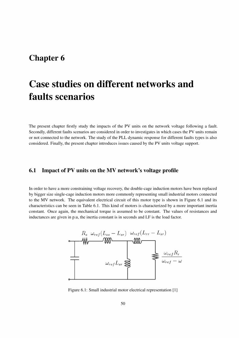
Chapter 6
Case studies on different networks andfaults scenarios
The present chapter firstly study the impacts of the PV units on the network voltage following a fault.Secondly, different faults scenarios are considered in order to investigates in which cases the PV units remainor not connected to the network. The study of the PLL dynamic response for different faults types is alsoconsidered. Finally, the present chapter introduces issues caused by the PV units voltage support.
6.1 Impact of PV units on the MV network’s voltage profile
In order to have a more constraining voltage recovery, the double-cage induction motors have been replacedby bigger size single-cage induction motors more commonly representing small industrial motors connectedto the MV network. The equivalent electrical circuit of this motor type is shown in Figure 6.1 and itscharacteristics can be seen in Table 6.1. This kind of motors is characterized by a more important inertiaconstant. Once again, the mechanical torque is assumed to be constant. The values of resistances andinductances are given in p.u, the inertia constant is in seconds and LF is the load factor.
Figure 6.1: Small industrial motor electrical representation [1]
50

CHAPTER 6. CASE STUDIES ON DIFFERENT NETWORKS AND FAULTS SCENARIOS
Table 6.1: Induction motor characteristics
Rs Lss Lsr Lrr Rr H LF0.031 0.1 3.2 0.180 0.018 0.7 0.6
In this section the impact of the PV units on the voltage profile of the MV network is studied for differentvalues of the short circuit power (Scc) of the 36 kV network. Recall that the short circuit power reflects thestrength of the network. A high short circuit power corresponds to a strong system while a small one isassociated to a weak system.
It is assumed that a fault occurs at the very high voltage level (e.g. 380 kV) and leads to a voltage drop of0.75 p.u on the external 36 kV grid. Results are successively compared for Scc= 1000, 500 and 100 MVA 1.For each situation, the voltage profiles are compared with and without PV units connected to the network.These results are illustrated in Figures 6.2a, 6.2b and 6.2c. The voltage profiles are observed at the bus 1100of the MV network (see Appendix A).
Whereas the difference of voltages can be clearly seen for each case, the effect of PV systems during thevoltage sag is much more important in case of a weak transmission system as it can be seen in Figure 6.2c forScc = 100 MVA. For the latter, the effect of this voltage support by the PV units is observed on the speedprofile of the motors connected to the MV network. This is illustrated in Figure 6.3. It is shown that themotors speed is less reduced due to the higher residual voltage thanks to the reactive support provided by thePV units. Therefore, once the voltage has recovered, the acceleration phase is less important and lasts shortermeaning that the current drawn by the motors during the acceleration is reduced. This, combined with theextend reactive support, eases the voltage recovery as it can be seen in Figure 6.2c.
1These values seem quite reasonable based on the values of the 36 kV network in Belgium, provided to us by Doctor JonathanSprooten from Elia.
51

CHAPTER 6. CASE STUDIES ON DIFFERENT NETWORKS AND FAULTS SCENARIOS
0 0.2 0.4 0.6 0.8 1 1.2 1.4 1.6 1.8 2
time(s)
0.2
0.3
0.4
0.5
0.6
0.7
0.8
0.9
1
V(p
u)
No PV
With PV
(a) Scc = 1000 MVA
0 0.2 0.4 0.6 0.8 1 1.2 1.4 1.6 1.8 2
time(s)
0.2
0.3
0.4
0.5
0.6
0.7
0.8
0.9
1
V(p
u)
No PV
With PV
(b) Scc = 500 MVA
0 0.2 0.4 0.6 0.8 1 1.2 1.4 1.6 1.8 2
time(s)
0.2
0.3
0.4
0.5
0.6
0.7
0.8
0.9
1
V(p
u)
No PV
With PV
(c) Scc = 100 MVA
Figure 6.2: Difference of voltage profiles at the MV network with and without PV units for different valuesof the transmission system short circuit power
52
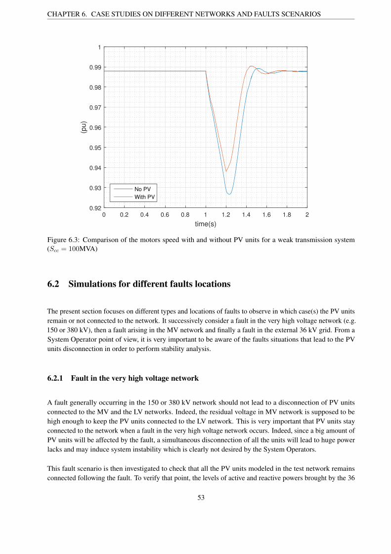
CHAPTER 6. CASE STUDIES ON DIFFERENT NETWORKS AND FAULTS SCENARIOS
0 0.2 0.4 0.6 0.8 1 1.2 1.4 1.6 1.8 2
time(s)
0.92
0.93
0.94
0.95
0.96
0.97
0.98
0.99
1
(pu
)
No PV
With PV
Figure 6.3: Comparison of the motors speed with and without PV units for a weak transmission system(Scc = 100MVA)
6.2 Simulations for different faults locations
The present section focuses on different types and locations of faults to observe in which case(s) the PV unitsremain or not connected to the network. It successively consider a fault in the very high voltage network (e.g.150 or 380 kV), then a fault arising in the MV network and finally a fault in the external 36 kV grid. From aSystem Operator point of view, it is very important to be aware of the faults situations that lead to the PVunits disconnection in order to perform stability analysis.
6.2.1 Fault in the very high voltage network
A fault generally occurring in the 150 or 380 kV network should not lead to a disconnection of PV unitsconnected to the MV and the LV networks. Indeed, the residual voltage in MV network is supposed to behigh enough to keep the PV units connected to the LV network. This is very important that PV units stayconnected to the network when a fault in the very high voltage network occurs. Indeed, since a big amount ofPV units will be affected by the fault, a simultaneous disconnection of all the units will lead to huge powerlacks and may induce system instability which is clearly not desired by the System Operators.
This fault scenario is then investigated to check that all the PV units modeled in the test network remainsconnected following the fault. To verify that point, the levels of active and reactive powers brought by the 36
53

CHAPTER 6. CASE STUDIES ON DIFFERENT NETWORKS AND FAULTS SCENARIOS
0 0.2 0.4 0.6 0.8 1 1.2 1.4 1.6 1.8 2
time(s)
0
0.2
0.4
0.6
0.8
1
V(p
u)
Figure 6.4: Voltage at the transmission side during the fault in the 150 kV network
kV external grid before and after the fault are analyzed. Simulations are made with Scc = 500 MVA.
It is assumed that the fault leads to a voltage drop of 0.75 p.u at the 36 kV external grid. The correspondingvoltage sag can be seen in Figure 6.4. The active and reactive powers flowing out of the transformer to theMV network are illustrated in Figure 6.5. Both active and reactive powers brought by the external grid arereduced during the fault due to voltage reduction. It can be even seen that the external grid actually consumesreactive power during the voltage reduction. Once the fault has been cleared, the power consumption of themotors in the MV network is big during the acceleration phase and the power brought by the external grid ishigh. It is shown that the levels of active and reactive powers before and after the fault are respectively thesame, meaning that no PV units have been disconnected, as desired.
6.2.2 Fault in the MV network
A fault of 1 second duration is simulated at the bus 1160 of the network and is cleared by the opening of thebreakers of the branch ’1100 1151’ (see Appendix A) assuming protection devices of radial MV network arelocated at the top of each feeder.
For a fault occurring in the MV network, PV units near the fault must imperatively be disconnected becausethese ones are participating to the short circuit current, which is not desirable. This explains why the minimumtolerated voltage of the LVRT curve cannot be too low. With a too low tolerated voltage value, the units closeto a MV or a LV fault feeding the short circuit current will not be disconnected and this may cause moredamages to the network equipment.
54

CHAPTER 6. CASE STUDIES ON DIFFERENT NETWORKS AND FAULTS SCENARIOS
0 0.5 1 1.5 2 2.5
time(s)
-6
-4
-2
0
2
4
6
8
10
12
Active power (MW)
Reactive power (Mvar)
Figure 6.5: Active and reactive powers flowing out the transformer for a fault in the 150 kV grid
Moreover, the fault duration of MV faults is generally much longer, between 0.5 and 1.5 s 2. It is thusexpected to see the units located further, but still at the same feeder where the fault occurs, to disconnect.However, the disconnections occur after a longer time since the residual voltage of these remote units isbigger. The disconnection of the units attached to this feeder is wanted. Indeed, since the network protectionsare located at the top of the feeder, the opening of the breakers after the fault occurred will not preventdownstream units to feed the fault. It is thus preferable to observe the disconnection of all the PV unitsattached to the feeder where the fault is located.
The units located in a remote area and connected to other feeders of the MV network will be prevented offeeding the fault by the opening of the network protections and will generally remain connected because theirresidual voltages remain high.
However, if the fault occurs close to the main bus of the MV network to which are connected all the feeders,the voltage of all the MV network will be strongly impacted and it may happen that a majority of the unitstrips. A fault in the MV network will thus generally cause a partial disconnection of the PV units in thenetwork.
The change in current multipliers of some PV units during the MV fault connected to the same feeder wherethe fault occurs can be seen in Figure 6.6. It is shown that all the current multipliers fall to zero before thefault has been cleared at t = 2 s. This means that the units of the feeder have tripped as desired.
Figure 6.7 illustrates the voltage profile at the main bus of the MV network (bus 1100) where all the feeders
2Numbers provided to us by Doctor J. Sprooten during a meeting at Elia.
55

CHAPTER 6. CASE STUDIES ON DIFFERENT NETWORKS AND FAULTS SCENARIOS
0 0.5 1 1.5 2 2.5 3
time(s)
0
0.2
0.4
0.6
0.8
1
Fvl
PV 1151
PV 1155
PV 1159
PV 1163
PV 1167
PV 1175
Figure 6.6: Change in current multiplier during the fault of the PV units connected to some nodes of thefeeder where the fault occurs, the PV units number indicates the bus number to which their are connected
are connected. It can be seen that the voltage drop is quite limited. This makes that the PV units of the otherfeeders will remain connected to the network as it is shown in Figure 6.8 illustrating some correspondingvoltage profiles of PV terminals. It is shown that all the voltage profiles are almost equivalent and the residualvoltage values during the fault are strongly influenced by the residual voltage of the bus 1100. That is whya fault occurring too close of the main MV bus may lead to a large part of the PV units to trip because theresidual voltages of all PV terminals will be strongly reduced.
56

CHAPTER 6. CASE STUDIES ON DIFFERENT NETWORKS AND FAULTS SCENARIOS
0 0.5 1 1.5 2 2.5 3
time(s)
0.6
0.65
0.7
0.75
0.8
0.85
0.9
0.95
1
(pu
)
Figure 6.7: Voltage at the main bus (1100) of the MV network during a fault in the MV network
0 0.5 1 1.5 2 2.5 3
time(s)
0.65
0.7
0.75
0.8
0.85
0.9
0.95
1
1.05
(pu
)
PV 1111
PV 1107
PV 1138
PV 1126
PV 1116
PV 1101
PV 1104
Figure 6.8: Voltages of PV units terminals of other feeders, the PV units number indicates the bus number towhich their are connected
57
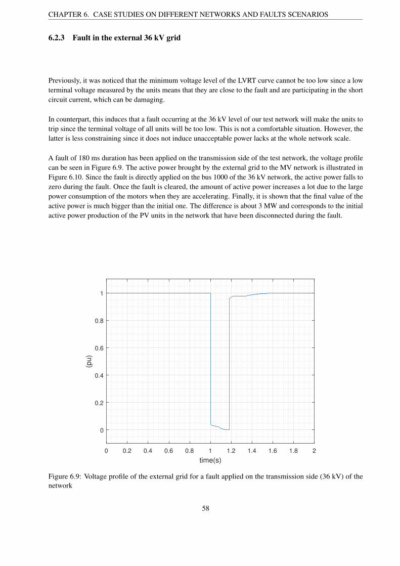
CHAPTER 6. CASE STUDIES ON DIFFERENT NETWORKS AND FAULTS SCENARIOS
6.2.3 Fault in the external 36 kV grid
Previously, it was noticed that the minimum voltage level of the LVRT curve cannot be too low since a lowterminal voltage measured by the units means that they are close to the fault and are participating in the shortcircuit current, which can be damaging.
In counterpart, this induces that a fault occurring at the 36 kV level of our test network will make the units totrip since the terminal voltage of all units will be too low. This is not a comfortable situation. However, thelatter is less constraining since it does not induce unacceptable power lacks at the whole network scale.
A fault of 180 ms duration has been applied on the transmission side of the test network, the voltage profilecan be seen in Figure 6.9. The active power brought by the external grid to the MV network is illustrated inFigure 6.10. Since the fault is directly applied on the bus 1000 of the 36 kV network, the active power falls tozero during the fault. Once the fault is cleared, the amount of active power increases a lot due to the largepower consumption of the motors when they are accelerating. Finally, it is shown that the final value of theactive power is much bigger than the initial one. The difference is about 3 MW and corresponds to the initialactive power production of the PV units in the network that have been disconnected during the fault.
0 0.2 0.4 0.6 0.8 1 1.2 1.4 1.6 1.8 2
time(s)
0
0.2
0.4
0.6
0.8
1
(pu
)
Figure 6.9: Voltage profile of the external grid for a fault applied on the transmission side (36 kV) of thenetwork
58

CHAPTER 6. CASE STUDIES ON DIFFERENT NETWORKS AND FAULTS SCENARIOS
0 0.2 0.4 0.6 0.8 1 1.2 1.4 1.6 1.8 2
time(s)
-2
0
2
4
6
8
10
12
14
16
(MW
)
Figure 6.10: Active power from the external grid to the MV network for the fault at the 36 kV level
6.3 PLL analysis
In this section, the dynamic response of the PLL controller is investigated for different types of faults in thenetwork.
As presented in Chapter 4, the role of the PLL is to synchronize the injected current (ix, iy) with the networkvoltage (vx, vy). Its role is to always keep the voltage component vq to zero which is considered as theerror term. Therefore, the PV units inverters assume that the voltage component vd is the correct measuredvoltage magnitude at the terminal and consequently generate reactive power. During each fault type, thedynamic response of the PLL will be assessed based on these voltage components and the consequences ofthe PLL efficiency will be reflected through the generated reactive power and the terminal voltage profile.Furthermore, the reactive power computed from the PV units’ side in the (d, q) reference frame will becompared with the network reactive power in the (x, y) reference frame, which are ideally supposed to beequal anytime.
Moreover, for each fault considered, different performances of the PLL will be tested by changing theparameter kpll. In relevant literature is usually proposed that PLL filter response settling time have to be setaround 20 ms for grid frequency of 50 Hz [3], which corresponds to a kpll between 10 and 30. Of course, thetime response depends on the phase jump of the voltage that varies from faults to faults as it will be showedin this section.
59

CHAPTER 6. CASE STUDIES ON DIFFERENT NETWORKS AND FAULTS SCENARIOS
0 0.5 1 1.5 2 2.5 3
time(s)
-60
-50
-40
-30
-20
-10
0
10
de
g(°
)
External grid fault
MV fault
Purely resistive fault
(a) ✓PLL
0.5 1 1.5 2 2.5
time(s)
-0.4
-0.3
-0.2
-0.1
0
0.1
0.2
(pu
)
External grid fault
MV fault
Purely resistive fault
(b) vq
Figure 6.11: Comparison of the change in the variables ✓PLL and vq for three types of faults (kpll = 30)
Three types of faults have been assumed. The three faults lead to the same voltage drop at the bus 1100 ofthe network. Results are observed for PV units connected to the bus 1101 for which the residual voltagemagnitude is similar for each fault type. Therefore, based on the reactive support unit of the model, theinjected reactive current IQ by PV units is the same in each case.
6.3.1 Fault at the transmission side
First a fault occurring in the external grid is assumed. This one lasts for 180 ms and the voltage drop isabout 0.65 p.u at the bus 1101. Figures 6.11a and 6.11b show that the phase jump at the PV units terminalduring the fault is almost nonexistent and so is the variation in vq. In that case, the time response of the PLLcontroller is very fast and the dynamic response is almost instantaneous. Then, the voltage component vd isexactly the same as Vm as illustrated in Figure 6.12a.
The same fault has been applied with a less efficient PLL controller, fixing kpll to 10 while this one waspreviously at 30. The difference in the vq voltage component can be seen in Figure 6.14a. Although the PLLperformance is reduced, the deviation of vq remains small and Figure 6.15a shows that it does not impact thevoltage component vd remaining extremely close to Vm. The difference in the generated reactive power isthen not existent as shown in Figure 6.16a.
For a fault in the transmission grid, phase jumps are so low that the performance of the PLL does almost notinfluence its dynamic response and thus its efficiency.
6.3.2 Fault on a MV bus
The second fault occurs on the MV bus 1154. The latter lasts 500 ms and leads to a voltage drop of about0.65 p.u at the bus 1101. In Figure 6.11a, it can be seen that this fault leads to a much bigger change in the
60
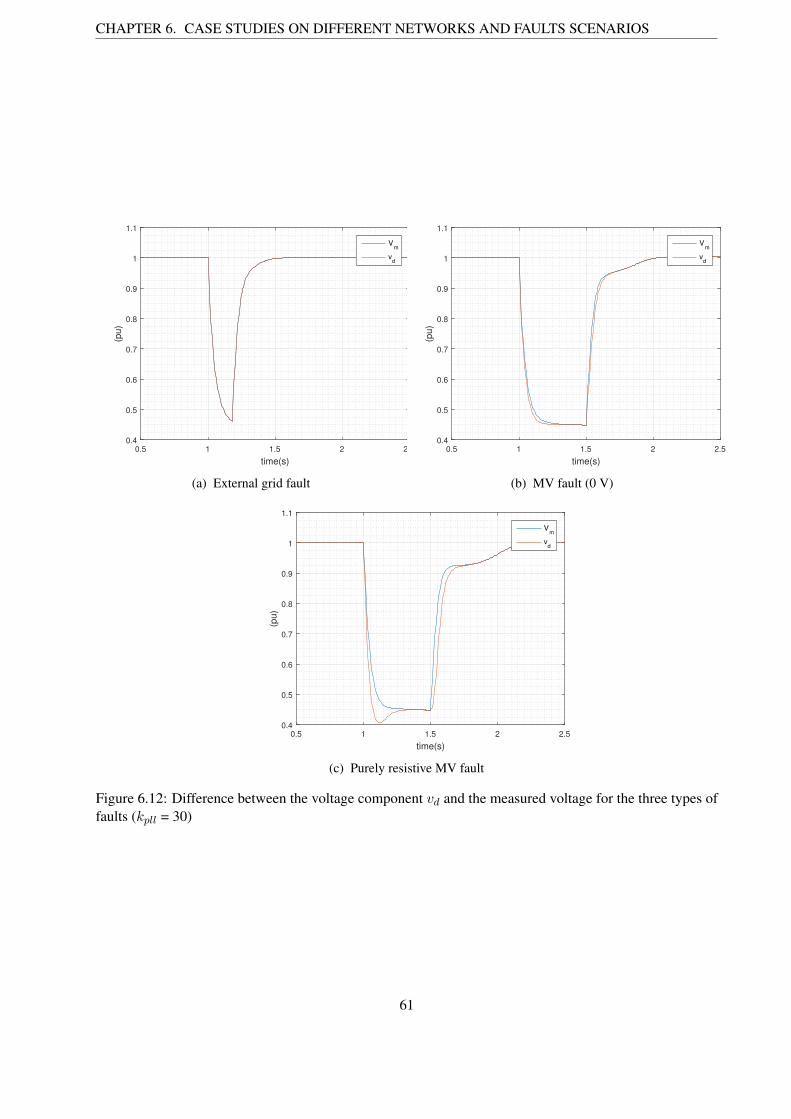
CHAPTER 6. CASE STUDIES ON DIFFERENT NETWORKS AND FAULTS SCENARIOS
0.5 1 1.5 2 2.5
time(s)
0.4
0.5
0.6
0.7
0.8
0.9
1
1.1
(pu
)
Vm
vd
(a) External grid fault
0.5 1 1.5 2 2.5
time(s)
0.4
0.5
0.6
0.7
0.8
0.9
1
1.1
(pu
)
Vm
vd
(b) MV fault (0 V)
0.5 1 1.5 2 2.5
time(s)
0.4
0.5
0.6
0.7
0.8
0.9
1
1.1
(pu
)
Vm
vd
(c) Purely resistive MV fault
Figure 6.12: Difference between the voltage component vd and the measured voltage for the three types offaults (kpll = 30)
61

CHAPTER 6. CASE STUDIES ON DIFFERENT NETWORKS AND FAULTS SCENARIOS
0.5 1 1.5 2 2.5
time(s)
0
0.01
0.02
0.03
0.04
0.05
0.06
(Mva
r)
MV fault
Purely resistive fault
(a) Reactive power
0.5 1 1.5 2 2.5
time(s)
0.4
0.5
0.6
0.7
0.8
0.9
1
1.1
(pu
)
MV fault
Purely resistive fault
(b) Terminal voltage profile
Figure 6.13: Comparison between the (d, q) generated reactive powers and the terminal voltage profiles forthe two types of MV faults (kpll = 30)
PLL phase angle which inevitably leads to a bigger time response. The corresponding change in the voltagecomponent vq is then also bigger compared to a fault at the transmission side as illustrated in Figure 6.11b.
However, the deviation in vq remains acceptable such as vd remains quite close to the measured voltagemagnitude as illustrated in Figure 6.12b. It can be seen that vd is slightly different from Vm in the very firstmoment of the fault due to the longer time response of the PLL controller.
Again, the same fault has been applied for a less efficient PLL controller setting now kpll to 10 although thisone was previously 30. A big difference is observed in Figure 6.14b in term of the voltage component vqwhich becomes not negligible. This makes that the difference between the voltage component vd and Vm
is bigger and is visible for a longer time as it can be seen in Figure 6.15b. This will impact the generatedreactive power which is a bit lower than required during the fault as illustrated in Figure 6.16b.
In case of a MV fault, the performance of the PLL controller does influence its dynamic response, even if theconsequences on the (d,q) generated reactive power remains small.
6.3.3 Purely resistive fault on a MV bus
In this section, the behavior of the PLL controller is investigated when a purely resistive fault of 0.265 ⌦ isapplied on the main bus (1100) of the MV network. This fault leads to a voltage drop of 0.65 p.u as for theprevious faults.
When a purely resistive fault is applied on a MV bus, the downstream PV units almost see a purely resistiveimpedance as illustrated in Figure 6.17. It is thus expected to see the PLL controller meeting more difficultiesto correctly synchronize the injected current with the network voltage. A simple question to illustrate theproblem is the following: how to generate a large amount of reactive power if there is nothing to absorb it ?
62
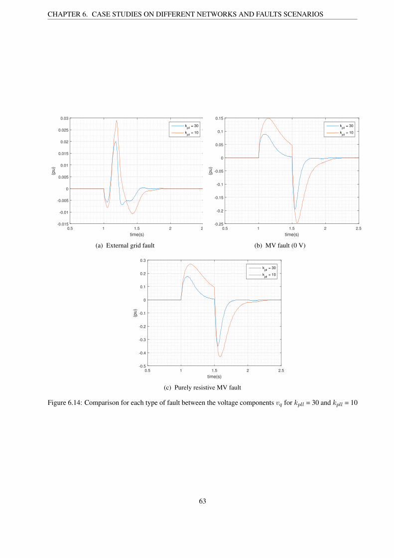
CHAPTER 6. CASE STUDIES ON DIFFERENT NETWORKS AND FAULTS SCENARIOS
0.5 1 1.5 2 2.5
time(s)
-0.015
-0.01
-0.005
0
0.005
0.01
0.015
0.02
0.025
0.03
(pu
)
kpll
= 30
kpll
= 10
(a) External grid fault
0.5 1 1.5 2 2.5
time(s)
-0.25
-0.2
-0.15
-0.1
-0.05
0
0.05
0.1
0.15
(pu
)
kpll
= 30
kpll
= 10
(b) MV fault (0 V)
0.5 1 1.5 2 2.5
time(s)
-0.5
-0.4
-0.3
-0.2
-0.1
0
0.1
0.2
0.3
(pu
)
kpll
= 30
kpll
= 10
(c) Purely resistive MV fault
Figure 6.14: Comparison for each type of fault between the voltage components vq for kpll = 30 and kpll = 10
63

CHAPTER 6. CASE STUDIES ON DIFFERENT NETWORKS AND FAULTS SCENARIOS
0.5 1 1.5 2 2.5
time(s)
0.4
0.5
0.6
0.7
0.8
0.9
1
1.1
(pu
)
Vm
vd
(a) External grid fault
0.5 1 1.5 2 2.5
time(s)
0.4
0.5
0.6
0.7
0.8
0.9
1
1.1
(pu
)
Vm
vd
(b) MV fault (0 V)
0.5 1 1.5 2 2.5
time(s)
0.3
0.4
0.5
0.6
0.7
0.8
0.9
1
1.1
(pu
)
Vm
vd
(c) Purely resistive MV fault
Figure 6.15: Difference between the voltage component vd and the measured voltage for the three types offaults (kpll = 10)
64
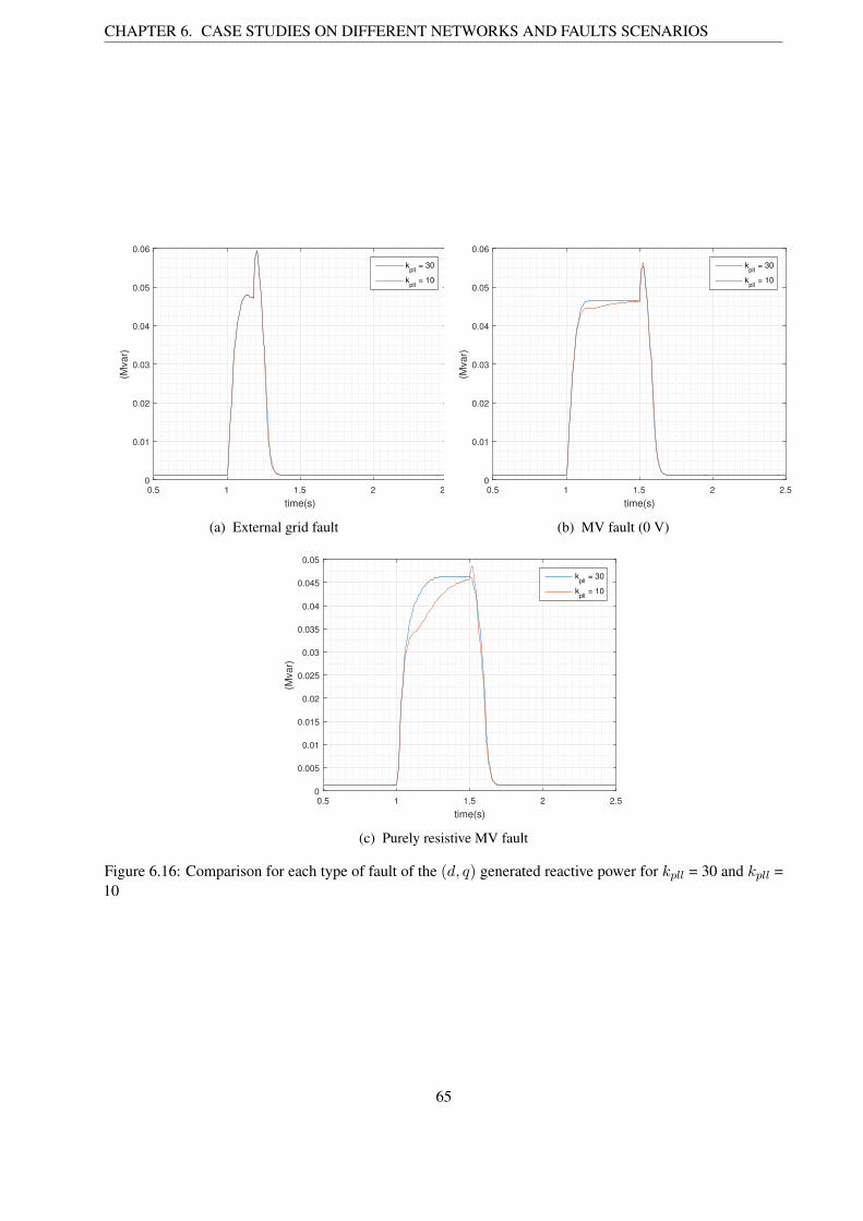
CHAPTER 6. CASE STUDIES ON DIFFERENT NETWORKS AND FAULTS SCENARIOS
0.5 1 1.5 2 2.5
time(s)
0
0.01
0.02
0.03
0.04
0.05
0.06
(Mva
r)
kpll
= 30
kpll
= 10
(a) External grid fault
0.5 1 1.5 2 2.5
time(s)
0
0.01
0.02
0.03
0.04
0.05
0.06
(Mva
r)
kpll
= 30
kpll
= 10
(b) MV fault (0 V)
0.5 1 1.5 2 2.5
time(s)
0
0.005
0.01
0.015
0.02
0.025
0.03
0.035
0.04
0.045
0.05
(Mva
r)
kpll
= 30
kpll
= 10
(c) Purely resistive MV fault
Figure 6.16: Comparison for each type of fault of the (d, q) generated reactive power for kpll = 30 and kpll =10
65
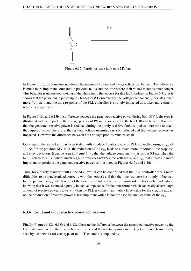
CHAPTER 6. CASE STUDIES ON DIFFERENT NETWORKS AND FAULTS SCENARIOS
PV
R
Figure 6.17: Purely resistive fault on a MV bus
In Figure 6.12c, the comparison between the measured voltage and the vd voltage can be seen. The differenceis much more important compared to previous faults and the time before their values match is much longer.This behavior is understood looking at the phase jump that occurs for this fault. Indeed, in Figure 6.11a, it isshown that the phase angle jumps up to - 60 degrees! Consequently, the voltage component vq deviates muchmore from zero and the time response of the PLL controller is strongly impacted as it takes more time toremove a bigger error.
In Figure 6.13a and 6.13b the difference between the generated reactive power during both MV faults type isillustrated and the impact on the voltage profiles of PV units connected to the bus 1101 can be seen. It is seenthat the generated reactive power is reduced during the purely resistive fault as it takes more time to reachthe required value. Therefore, the residual voltage magnitude is a bit reduced and the voltage recovery isimpacted. However, the difference between both voltage profiles remains small.
Once again, the same fault has been tested with a reduced performance of PLL controller using a kpll of10. As for the previous MV fault, the reduction of the kpll leads to a much more important time responseand error deviation. It can be seen in Figure 6.14c that the voltage component vq is still at 0.1 p.u when thefault is cleared. This induces much bigger differences between the voltages vd and Vm that impacts in moreimportant proportions the generated reactive power as illustrated in Figures 6.15c and 6.16c.
Thus, for a purely resistive fault at the MV level, it can be confirmed that the PLL controller meets moredifficulties to be synchronized correctly with the network and that the time response is strongly influencedby the parameter kpll which was not the case for a fault at the transmission side. This can be understoodknowing that it was assumed a purely inductive impedance for the transformer which can easily absorb largeamount of reactive power. However, when the PLL is efficient, i.e. with a large value for the kpll, the impacton the production of reactive power is less important which is not the case for smaller value of the kpll.
6.3.4 (d, q) and (x, y) reactive power comparison
Finally, Figures 6.18a, 6.18b and 6.18c illustrate the difference between the generated reactive power by thePV units computed in the (d,q) reference frame and the reactive power in the (x,y) reference frame reallyseen by the network for each type of fault. The latter is computed by
66

CHAPTER 6. CASE STUDIES ON DIFFERENT NETWORKS AND FAULTS SCENARIOS
Qnetwork = vxlviy � vylvix. (6.1)
If the synchronization is perfect, both reactive powers should be equal anytime.
For a fault in the external grid, it is shown that both reactive powers are almost similar. The difference is onlycaused by the voltage measurement delay, not by a synchronization issue.
For the MV faults, the slower time response of the PLL induces that the rectangular currents components inthe (x,y) reference frame are not directly correctly synchronized with the network voltage. Consequently,the reactive power really seen by the network differs initially strongly from the reactive power computed inthe (d,q) frame. Indeed, it can even be seen that in the very first moments of the fault, PV units are actuallyconsuming reactive power which initially impacts the voltage badly. This effect is much more present for apurely resistive fault. In this case, the units start re-injecting reactive power in the network 90 ms after thefault has started and match the (d,q) reactive power value after 200 ms of delay.
In conclusion, it has been seen that the performance of the PLL (reflected through the magnitude of theparameter kpll) is very important to face a resistive fault at the MV level. Although this type of fault is prettyrare, the resulting efficiency of the PLL is strongly reduced compared to a fault at the transmission side.This induces that the reactive power seen by the network may initially strongly differ form the (d, q) basedreactive power and units are noticed to consume reactive power at the first moment of the fault. The reactivesupport initially fails.
6.4 Issues caused by the PV units voltage support
While the voltage support by the injection of reactive current in the network is considered as a networkservice provided by PV units during a fault, this service may lead in some cases to uncomfortable situations.Two issues, over voltage following the voltage recovery and islanding, respectively, caused by the voltagesupport service will be highlighted in this section and solutions will be proposed in order to solve them.
6.4.1 Over voltage issue following the voltage recovery
The over voltage protection is very important in order to protect the expensive electronic devices of the PVunits inverters. This is why it has to act pretty fast in order to prevent any damages. For that reason, it hasbeen assumed in this case that the input of the over voltage control block is directly the terminal voltage ofthe units, by-passing the measurement delay.
As previously said, the PV units do not know directly when the fault is cleared due to voltage measurementdelay. These ones keep injecting for a short moment large amount of reactive current in the network as thevoltage has already recovered. If the installed capacity of PV units is important, it may cause over voltagethat will trig the over voltage protections (Vmax = 1.1 p.u) followed by the disconnection of the units.
As the capacity of the installed PV units is big, it is even more important to keep them connected to the
67

CHAPTER 6. CASE STUDIES ON DIFFERENT NETWORKS AND FAULTS SCENARIOS
0 0.5 1 1.5 2 2.5
time(s)
0
0.02
0.04
0.06
0.08
0.1
0.12
(Mva
r)
(d,q)
(x,y)
(a) External grid fault
0 0.5 1 1.5 2 2.5
time(s)
-0.02
0
0.02
0.04
0.06
0.08
0.1
(Mva
r)
(d,q)
(x,y)
(b) MV fault (0 V)
0 0.5 1 1.5 2 2.5
time(s)
-0.02
0
0.02
0.04
0.06
0.08
0.1
(Mva
r)
(d,q)
(x,y)
(c) Purely resistive MV fault
Figure 6.18: Comparison for each type of fault between the reactive power computed from the PV side in the(d,q) reference frame and the reactive power in the (x,y) reference frame with kpll = 10
68

CHAPTER 6. CASE STUDIES ON DIFFERENT NETWORKS AND FAULTS SCENARIOS
network during a fault in very high voltage network. This over voltage problem may lead to significantimpacts in the network if a fault occurring in the 380 kV level network is followed by the disconnection ofmany units leading to large power cuts.
To visualize this effect, the nominal capacity of PV units attached to each node of the MV network has beentripled assuming the presence of many PV installations. The initial power production remains the same inorder to not modify the power flow computation. A fault lasting for 200 ms in the external grid has beenapplied simulating a fault in the 380 kV network. This fault lead to a residual voltage of 0.3 p.u on the 36 kVgrid. Each voltage profile at the terminal of the PV units is identical and one of them is shown in Figure 6.19.The latter is associated with the change in the over voltage current multiplier. It can be seen that it switchesto zero during the voltage recovery which means that the units have tripped because of the over voltage.
Moreover, in Figure 6.20 the evolution of the active power that comes from the external grid is illustrated.It can be seen that the the final value is bigger than the initial one and the difference represents the poweroutage of PV units caused by the over voltage. At the scale of the MV network, the impact is not importantsince the initial power production of the unit is low. While at the scale of the whole network, this may resultin serious impacts on the power system.
However, it is important to precise the strong assumption that has been made, i.e. the capacity tripled at eachnode and the same PV capacity at each node. Since then, this reflects a particular situation where there is alarge capacity of PV units at the LV level divided equally among nodes. A more realistic situation would be anetwork that includes some large PV plants directly connected to the MV level. In that case, only a part ofPV units located around these PV plants is expected to trip because of the over voltage protection and thepower outage is then less constraining.
Because the input of the over voltage control unit is directly the terminal voltage, the disconnection isinstantaneous when the over voltage limit is reached. Nevertheless, if the over voltage detection takes thesame time or more time than the voltage measurement operation, the voltage peak which lasts a short timewill not be detected and the PV units will remain connected. This prevents the network from important poweroutages but may damage the PV systems equipment.
To eradicate such problem, in the future, PV systems should be designed in order to be able to ride throughhigh voltage situations for a short time, i.e. a High Voltage Ride-Through (HVRT) capability.
6.4.2 Islanding issue
The islanding phenomenon of distributed generations refers to its independent powering to a portion of theutility system even though the portion has been disconnected from the main grid. Islanding can producesafety problems to utility service personnel or related equipment [2]. Indeed, reclosing the circuit onto anactive island may induce problems with the utility’s equipment, or cause automatic reclosing systems to failto notice the problem.
This is why the islanding detection is important for PV systems in order to prevent the units to keep poweringthe network when the MV network is disconnected from the transmission network.
69

CHAPTER 6. CASE STUDIES ON DIFFERENT NETWORKS AND FAULTS SCENARIOS
0 0.2 0.4 0.6 0.8 1 1.2 1.4 1.6 1.8 20.2
0.4
0.6
0.8
1
V(p
u)
0 0.2 0.4 0.6 0.8 1 1.2 1.4 1.6 1.8 2
time(s)
0
0.5
1
Fvh
Figure 6.19: Illustration of the PV units disconnection due to over voltage after the voltage recovery
0 0.2 0.4 0.6 0.8 1 1.2 1.4 1.6 1.8 2
time(s)
0
2
4
6
8
10
12
14
(MW
)
Figure 6.20: Active power from the external grid to the MV network before, during and after the fault
70

CHAPTER 6. CASE STUDIES ON DIFFERENT NETWORKS AND FAULTS SCENARIOS
There exist many islanding detection methods. The one that is considered here is the under voltage methodthat is implemented through the LVRT curve construction. Indeed, when the MV network is disconnectedfrom the external grid, the PV units are not able to supply correctly the load and the voltage drops. If theLVRT curve is correctly designed, the units should have tripped before the re-connection with the externalgrid.
Because the LVRT capability, the PV units are expected to still powering the network in the first moment ofthe disconnection with the main network. Therefore, automatic re-connection of protection devices shouldnot be too fast and a dead time should let the voltage falls below the LVRT curve before reconnecting the MVnetwork to the external grid. This dead time is about 400 ms 3.
In this section, a fault that leads to the opening of the transformer linking the MV and HV network is assumed.In practice, a back-up transformer is found in parallel with the main transformer and the latter connects 400ms after the first one has been disconnected.
A fault with residual impedance is then simulated during 100 ms on the transmission side and inducesa voltage drop of 0.7 p.u in the network. The opening of the transformer clears the fault. The back-uptransformer is assumed to connect 400 ms after the main one has been disconnected. The evolution of thevoltage at the bus 1100 of the MV network is analyzed.
In Figure 6.21 the evolution of the different voltages in the MV network can be seen when PV units areproviding reactive support and when the reactive support is deactivated. The reactive support makes that thevoltage magnitude when the MV network is disconnected from the external grid remains high enough suchthat the PV units remain connected to the network, which is a big issue as explained previously. Otherwise,when the units do not help supporting the voltage, the voltage drop is important when the transformer branchis opened and the PV units are all disconnected when the MV network re-connects, which is much moresecure and reliable in that situation.
Once again, it has been illustrated a situation where the voltage support provided by the PV units maybe damaging. This may be solved by changing the LVRT curve design, finding an other anti-islandingprotection/detection method or by reducing the reactive provision of PV units during voltage sags.
3Provided to us by Doctor Jonathan Sprooten during a meeting at Elia
71

CHAPTER 6. CASE STUDIES ON DIFFERENT NETWORKS AND FAULTS SCENARIOS
0 0.5 1 1.5 2 2.5
time(s)
0.1
0.2
0.3
0.4
0.5
0.6
0.7
0.8
0.9
1
V(p
u)
No reactive support
Reactive support
Figure 6.21: Difference in the voltage profiles with and without reactive support of PV units
6.5 Summary
The present chapter is certainly the most important of this work. Indeed, the latter has used the implementedPV model in order to investigate practical situations of interest for System Operators. It has first demonstratedthat the PV units voltage support is much more important in case of a weak 36 kV network. Then it hasillustrated the types of faults leading to a partial or a total disconnection of the PV units agglomerated in theMV network. Hopefully, conclusions seem in agreement with System Operators expectations.
The PLL controller dynamic response has also been analyzed for different types of faults. The latter seemsto meet more difficulties to be correctly synchronized with the voltage network in case of MV faults. Theperformance of the PLL controller, reflected through the parameter kPLL, strongly influences the timeresponse in that case whereas it appears to be efficiently synchronized for a fault in the transmission grideven with a reduced performance.
Finally, the chapter has highlighted two problems induced by the reactive support. Firstly, an over voltageissue may happen after a fault clearance with a too large PV units capacity in the network. This problemcan be solved implementing the HVRT capability. Secondly, the reactive support prevents the PV units fromdisconnecting in case of islanding situation. This may induce problems with the utility’s equipment whenreconnecting to the main network. The islanding issue may be solved using a different detection method orby reducing the reactive support provided by the PV units.
72

CHAPTER 6. CASE STUDIES ON DIFFERENT NETWORKS AND FAULTS SCENARIOS
References
[1] Thierry Van Cutsem. ”Dynamics of the induction machine”. Power system dynamics, control andstability, University of Liege, November 2015.
[2] F. Ruz , A. Rey , J.M. Torrelo , A. Nieto , F.J. Cnovas. ” Real time test benchmark design for photovoltaicgrid-connected control systems”. Electr. Power Syst. Res., doi:10.1016/j.epsr.2010.11.023, 2010.
[3] Evgenije Adzic , Vlado Porobic , Boris Dumnic , Nikola Celanovic , Vladimir Katic. ”PLL synchroniza-tion in grid-connected converters”. The 6th PSU-UNS International Conference on Engineering andTechnology, Paper No. T.12-1.1, pp. 1-5, May 2013.
73

Chapter 7
Equivalent model for the transmissionnetwork representation
Based on previous results, this chapter proposes an equivalent MV network model and more specifically aequivalent PV model well suited for the transmission network representation. The latter is interesting from aSystem Operator point of view since it eases the network representation for planning and security studies.
The present chapter first explains how the equivalent network components have been built. Then, it presentsthe assumptions that has been made for the construction of the model. The equivalent model is validatedbased on the voltage response following a fault at the transmission side and the latter is used to illustratethe existing trade-off between the reactive support and the LVRT capability services. Finally, the modellimitations are considered in order to present the particular cases where the equivalent model is reliable.
7.1 Modeling the equivalent MV network
The equivalent model of the network has been built based on the ”grey-box” approach presented in the cigrereport [1]. This approach assumes a known structure of each components and estimates the parameters of themodel from measurements. Based on that, the three components of the equivalent network are
• firstly, the equivalent constant admittance load, which is assumed to represent all the constant admit-tance loads that were present in the MV network. The power consumed by the equivalent load is thesum of the power consumed by each load initially;
• secondly, the equivalent induction motor accounting for the dynamic load, representing all the smallmotors of the MV network. The power consumed by the equivalent motor is the sum of the powerconsumed by each motor initially;
• thirdly, the equivalent PV model for which it has been assumed that the initial power generated is thesum of the power generated by all the small PV units of the MV network. The nominal capacity of theequivalent PV model is the sum of all the nominal capacities of the 75 distributed PV models of the
74
CHAPTER 7. EQUIVALENT MODEL FOR THE TRANSMISSION NETWORK REPRESENTATION
MV network. Initially, each distributed model had 100 kW of nominal power, the equivalent model hasthus 7.5 MW of nominal power.
The network’s modeling and its equivalent components are represented in Figure 7.1. The PV modelimplementation is similar to the non equivalent PV model.
7.2 Assumptions of the equivalent PV model
The representation of the equivalent PV model is based on the following assumptions:
1. a voltage drop at the transmission side will lead to the same residual voltage at the terminal of all PVunits;
2. thus, following a fault in the transmission network, if the voltage falls below the LVRT control curve,the units are expected to disconnect at the same time.
These assumptions have been made based on the results presented in Chapter 6.
Actually, when a fault occurs at the transmission level, the contribution of each PV unit to the short circuitpower is negligible compared to the contribution of the external grid. Consequently, the voltage dropexperienced by each PV unit is almost similar during the fault.
Therefore, since the residual voltage magnitude during a fault at the transmission side is the same for eachunit, they are expected to simultaneously disconnect if voltage conditions are no longer satisfied.
7.3 Equivalent model validation based on the voltage response
A fault lasting for 180 ms has been applied at the transmission side and the voltage profile at the MV bus1100 (see Appendix A) is observed. This profile is compared with the voltage profile of the non-equivalentnetwork at the same bus for a fault of same location, duration and magnitude. Both voltage profiles areidentical as represented in Figure 7.2 which indicates that the equivalent network is a reliable representationof the MV network.
75

CHAPTER 7. EQUIVALENT MODEL FOR THE TRANSMISSION NETWORK REPRESENTATION
EQU.
Equivalent Constant
Admittance Load Equivalent
Induction Motor
M
Equivalent
Distributed PV
Model
Figure 7.1: Modeling of the equivalent network
0 0.2 0.4 0.6 0.8 1 1.2 1.4 1.6 1.8 2
time(s)
0.3
0.4
0.5
0.6
0.7
0.8
0.9
1
V(p
u)
Equivalent
Non equivalent
Figure 7.2: Voltage profile comparison for a fault at the transmission side between the non equivalent and theequivalent MV network.
76
CHAPTER 7. EQUIVALENT MODEL FOR THE TRANSMISSION NETWORK REPRESENTATION
7.4 Reactive support and LVRT capabilities trade-off
Based on the previous results, the equivalent network can be considered as a correct representation of theMV network. Therefore, the latter is used to show an important trade-off concerning the two main ancillaryservices provided by PV units, the reactive support and the LVRT capability. Both are two distinct networkservices. However, the reactive support cannot exist if units are not able to stay connected during a voltagesag.
From a PV manufacturer point of view, a unit that must stay connected for low residual voltage magnitudeinduces more equipment expenses which are not desirable.
The question is thus the following: if the unit provides reactive support in order to rise the level of the residualvoltage magnitude during a fault, should this unit be allowed to trip quicker ?
A new variable has been added to the model in order to choose the level of reactive support provided by thePV units. It acts as a reactive current multiplier in the reactive support block. The equivalent network is usedto show the difference of voltage magnitude reached during a fault for different levels of reactive support.
It is assumed that the System Operator want that units stay connected for faults on the very high voltagelevels such as 150 kV and 380 kV leading to a voltage drop of 0.7 p.u on the 36 kV external grid. In Figure7.3 different voltage profiles at the terminal of the PV model can be seen for different levels of reactivesupport. As expected, the residual voltage magnitude is higher for a higher level of reactive support. Thus, iffor the same fault, units providing reactive support maintain a higher voltage level, they should be allowed todisconnect for higher residual voltage magnitude. For example and according to Figure 7.3, units that do notprovide reactive support should not disconnect before the voltage reaches 0.3 p.u, while the units providingfull reactive support should be allowed to disconnect when the voltage falls below 0.4 p.u.
7.5 Limitations of the model
Although the equivalent network model appeared to be efficient, it presents some limitations. Indeed, theassumptions are valid because the distributed generations of the network are only composed of PV units. Yet,this is not so common. In the majority of MV networks, some synchronous generators of combined heat andpower plants are generally found.
If synchronous generators figure among the distributed generations of the network, the voltage level during afault will not be the same at each bus since the synchronous generators will also support the voltage at thebus where there are connected. Since then, the reactive support of each units will not be identical and the unitwill not simultaneously disconnect if voltage conditions are no longer respected.
Another limitation of this model is the inability to simulate a fault occurring on a random bus of the MVnetwork. Indeed, to simulate such fault, the equivalent PV model should include partial tripping capabilityand the representation of the opening of a feeder that will also lead to a partial reduction of the load. However,this scenario remains less constraining at the whole network scale and presents less interest.
77

CHAPTER 7. EQUIVALENT MODEL FOR THE TRANSMISSION NETWORK REPRESENTATION
0 0.2 0.4 0.6 0.8 1 1.2 1.4 1.6 1.8 2
time(s)
0.3
0.4
0.5
0.6
0.7
0.8
0.9
1
1.1
V(p
u)
No support
50% support
Full support
Figure 7.3: Voltage profile at the PV model terminal for different levels of reactive support during a fault inthe external grid (-0.7 p.u)
Finally, even if this model is well suited for simulations of large voltage deviations occurring at higher voltagelevel, the over voltage issue is not reliable since it cannot represent the effect of PV plants connected to MVlevel that would also lead to partial tripping, if any. Nevertheless, with only PV units connected to the LVnetwork, the model is expected to give correct results.
7.6 Summary
Based on results presented in Chapter 6, some assumptions have been made for the construction of anequivalent model of MV network and more specifically for the construction of an equivalent PV model. Thecurrent chapter has demonstrated that the equivalent model is reliable when the distributed generation is onlycomposed of PV units connected to the LV network and for the representation of faults at the transmission side.For other types of faults and for other networks scenarios, e.g. MV network with synchronous generators, themodel presents some limitations.
The equivalent model has been used to illustrate the existing trade-off between the reactive support and theLVRT capability services. It has been concluded that units providing more reactive support should be able todisconnect quicker, raising the minimum voltage level of the LVRT curve.
78

CHAPTER 7. EQUIVALENT MODEL FOR THE TRANSMISSION NETWORK REPRESENTATION
References
[1] Cigre Report. ”Modelling and aggregation of loads in flexible power networks”. WG C4.605, 2013.
79

Chapter 8
Discussion and conclusion
8.1 Summary of the work and key results
This master thesis has presented a reliable dynamic model of small-scale distributed PV units connected todistribution systems. This model has been build based on nowadays most elaborated model of small-scale PVunits and on current grid codes presenting technical requirements and ancillary services that PV units shouldprovide. Based on these elements, the PV model specifications have been defined in Chapter 3.
The mathematical representation of the model and more specifically of the PLL controller has been presentedin Chapter 4. For the latter, a simplified implementation with one integration stage has been proposed.Chapter 5 has first introduced software and simulation tools that have been used. Moreover it has showed thatthe units react as expected in response to voltage sags in the network. Particularly, it has been demonstratedthat both the switch between the active and reactive priority during a fault and the LVRT control workperfectly.
Some case studies have been investigated in Chapter 6 considering different network scenarios and differenttypes of faults. The results of this chapter are certainly the most important of this work since they are veryinteresting in a System Operator point of view for system planning and stability studies.
It has first been shown the effect of the PV units voltage support on the voltage profile of the MV network. Ithas been concluded that the effect of voltage support is much more marked as the strength of the externalgrid is reduced. More importantly, this chapter has showed in which fault situations the PV units remain ornot connected to the network based on the LVRT curve design. The main conclusions are:
• for a fault at very High Voltage level, units remain connected to the network;
• for a fault located in the MV network, units connected to the feeder where the fault occurs aredisconnected while others units remain connected as far as the fault is not too close from the main MVbus where all the feeders are connected;
• for a fault at the 36 kV network, all the units trip although this situation is less constraining at thewhole network scale.
80

CHAPTER 8. DISCUSSION AND CONCLUSION
All these PV units responses seem to match the System Operators expectations.
Moreover, a part of Chapter 6 has focused on the PLL dynamic response in case of different fault locations.It has been concluded that the PLL time response is much more important for faults occurring at the MVlevel and this may impact voltage support efficiency for less performing PLL controllers.
Finally this chapter has highlighted two issues caused by reactive support services provided by the PV unitsand has proposed solutions in order to solve them:
1. first, because of voltage measurement delay, when a fault is cleared, over voltage can occur for largecapacity of PV units in the LV network. Indeed, PV units keep injecting large amount of reactive powerwhen the voltage has already recovered. A potential solution is to implement the HVRT capability;
2. the second, very important and subtle, concerns the islanding detection issue. For security reasons andequipment protection, PV units should imperatively be disconnected in islanding situation. Yet, it hasbeen highlighted that when the units support the voltage too efficiently, the islanding situation is notdetected and the PV installations remain connected. To solve this important problem, another islandingdetection method can be used or the voltage support provided by PV units can be reduced.
Based on previous case studies, this work is closed by suggesting an equivalent MV network model andespecially an equivalent PV model well suited for transmission network representation and for evaluatingvoltage disturbances issues caused by faults at the transmission side. However, this model presents somelimitations for MV network accommodating some synchronous machines.
This model is finally used to illustrate the existing trade-off between the LVRT capability and the reactivesupport provided by PV units. It has been shown that PV units providing efficiently reactive support shouldbe allowed to disconnect quicker since they rise the level of the residual voltage.
8.2 Suggestions for future work
Different suggestions for model improvements and future works are to be considered:
• first, for the current small-scale PV model presented in this work, it would be interesting to add afrequency dependence on the active power generated by the units. Indeed, PV units should also be ableto regulate the network frequency and this model improvement would be consistent with that networkservice. This would allow to investigate the islanding issue using the frequency detection method;
• secondly, the main improvement that could be brought to this master thesis concerns the equivalentmodel. Indeed, it would be very interesting to implement a model considering the presence ofsynchronous machines agglomerated in the MV network. This would permit to take into accountthe effect of the difference in the voltage levels between buses during fault that may lead to partialdisconnection of PV units;
81

CHAPTER 8. DISCUSSION AND CONCLUSION
• finally, the ancillary services provided by small-scale PV units mainly connected to the LV networkare limited and changes are not expected to be consistent in the future. However, the number oflarge-scale PV installations such as PV power plants connected to the MV network is expected toincrease. Therefore, based on the WECC model for large PV power plants, it would be interesting toimplement a detailed model representing large PV installations for which the presence and the rolewill become more and more important in nowadays and future power systems.
82

Acknowledgements
I would first like to thank my master thesis adviser Pr. Thierry Van Cutsem whose office was always openwhenever I encountered a difficulty or had a question about my work. He consistently allowed this paper tobe my own work, but steered me in the right direction whenever he thought necessary.
I would also like to thank the expert Dr Jonathan Sprooten from Elia for his availability and his preciousadvice. His passionate participation helped me to successfully conduct this master thesis.
Finally, I would like to express my sincere gratitude to Pr. Van Cutsem PhD’s student team who neverhesitated to bring their help and provide me with precious information for the implementation of my model.
83

84

APPENDIX A. AC TEST NETWORK
Appendix A
AC test Network
Figure A.1: 75 BUS AC Network
85