Documents de Travail duCentre d’Economie de la Sorbonne

Maison des Sciences Économiques, 106-112 boulevard de L'Hôpital, 75647 Paris Cedex 13http://ces.univ-paris1.fr/cesdp/CES-docs.htm

ISSN : 1955-611X

Efficient Frontier for Robust Higher-order Moment

Portfolio Selection

Emmanuel F. JURCZENKO, Bertrand B. MAILLET, Paul M. MERLIN

2008.62

hals

hs-0

0336

475,

ver

sion

1 -

4 N

ov 2

008

Efficient Frontier for RobustHigher-order Moment Portfolio Selection∗

Emmanuel F. Jurczenko† Bertrand B. Maillet‡ Paul M. Merlin§

October 2008

Abstract

This article proposes a non-parametric portfolio selection criterion for the static

asset allocation problem in a robust higher-moment framework. Adopting the Short-

age Function approach, we generalize the multi-objective optimization technique in

a four-dimensional space using L-moments, and focus on various illustrations of a

four-dimensional set of the first four L-moment primal efficient portfolios. Our em-

pirical findings, using a large European stock database, mainly rediscover the earlier

works by Jean (1973) and Ingersoll (1975), regarding the shape of the extended

higher-order moment efficient frontier, and confirm the seminal prediction by Levy

and Markowitz (1979) about the accuracy of the mean-variance criterion.

∗We are gratefu l to Christophe Boucher, Th ierry Chauveau, Jean-Ph ilipp e M édecin , Thierry M ichel and Patrick Roger for help and

encouragem ent in preparing th is work. We acknow ledge Patrick Kouontchou and Ghisla in Yanou for excellent prelim inary research assistance

and an active partic ipation in earlier versions. We also thank Nathalie P icard, P ierre-Charles P rad ier and D id ier Rullière for prov id ing us w ith

interesting complem entary references. The second author thanks the Europ lace Institute of F inance for financia l support. The usual d iscla im ers

apply.

†ESCP-EAP.

‡A.A .Advisors-QCG (ABN AMRO), Variances and University of Paris-1 (CES/CNRS and EIF), CES, 106 bv de l’hôpita l, F -75647 Paris

cedex 13, France.

§A.A .Advisors (ABN AMRO), Variances and University of Paris-1 (CES/CNRS).

1

hals

hs-0

0336

475,

ver

sion

1 -

4 N

ov 2

008

Efficient Frontier for RobustHigher-order Moment Portfolio Selection

Abstract

This article proposes a non-parametric portfolio selection criterion for the static

asset allocation problem in a robust higher-moment framework. Adopting the Short-

age Function approach, we generalize the multi-objective optimization technique in

a four-dimensional space using L-moments, and focus on various illustrations of a

four-dimensional set of the first four L-moment primal efficient portfolios. Our em-

pirical findings, using a large European stock database, mainly rediscover the earlier

works by Jean (1973) and Ingersoll (1975), regarding the shape of the extended

higher-order moment efficient frontier, and confirm the seminal prediction by Levy

and Markowitz (1979) about the accuracy of the mean-variance criterion.

Since the first mention of higher-order moments than the variance of returns byMarschak

(1938) and Hicks (1939), it is now generally accepted by the financial community that in-

vestors generally exhibit preferences for positively skewed and light-tailed asset return

distributions (see, for instance, Beedles and Simkowitz (1978), Dittmar (2002), Jurczenko

and Maillet (2006a), and Mitton and Vorkink (2007)). Developments with higher moments

followed since the origin three main (complementary) directions in finance: a tentative in-

tegration in the von Neumann-Morgenstern utility function of a rational investor (Cf.

Arrow (1964) and Pratt (1964)) of higher-order moments of returns by Arditti (1967),

Samuelson (1970) and Tsiang (1972); an attempt to generalize the Markowitz (1952) ef-

ficient frontier to incorporate the effect of higher moments on optimal asset allocations

by Jean (1971 and 1973), Arditti and Levy (1972), Ingersoll (1975) and Schweser (1978);

and a first partial explicit modelling of returns by Rubinstein (1973), and Kraus and

Litzenberger (1976), through extensions of the CAPM by Sharpe (1964). True departures

1

hals

hs-0

0336

475,

ver

sion

1 -

4 N

ov 2

008

from Gaussianity may indeed affect the optimal allocation of assets (see Jondeau and

Rockinger (2003b and 2006a)) and the mean-variance portfolio selection criterion pro-

posed by Markowitz (1952) is a priori somehow inadequate for some risky assets whose

characteristics are very special (see Jondeau and Rockinger (2006a)). In such a context,

different multi-moment approaches have been proposed in the financial literature to in-

corporate higher-order moment preferences into asset allocation problems1, in order to

characterize generalized geometric efficient frontiers (see Athayde and Flôres (2002 and

2003)); but all suffer more or less from the traditional drawbacks of algebraic moments.

First, higher-order moments do not always exist (see Embrechts, Kluepelberg and Mikosh

(1997), and Jondeau and Rockinger (2003a and 2003b)), and even when they do, such

moments do not always uniquely define a probability distribution, so that two distinct

distributions can have the same sequence of moments (see Heyde (1963) for the example

of the Log-normal density). Secondly, conventional moments tend to be very sensitive to

a few extreme observations (see Hampel, Ronchetti, Rousseeuw and Stahel (2005)). The

asymptotic efficiency of the empirical moments is also rather poor, especially for distrib-

utions with fat tails. This last property is an immediate consequence of the fact that the

asymptotic variances of these estimators are mainly determined by higher-order moments,

which tend to be rather large, or even unbounded, for heavy-tailed distributions.

The objective of this paper is to overcome the limits of traditional multi-moment as-

set allocation models by using an alternative set of statistics in traditional optimization

programs, namely L-moments. Recent attempts for modelling distributions in a multi-

variate framework are indeed built on the concept of order-statistics, for calibrating a

Bernstein Copula in Baker (2008) or for defining extreme co-movements using L-moments

in Serfling and Xiao (2007). The latter, which are linear functions of the expectations of

order statistics, were introduced under this name by Sillitto (1951) and comprehensively

reviewed by Hosking (1989). As so-called U-statistics (see Hoeffding (1948)), L-moments

offer one main advantage over Conventional moments (denoted herein C-moments as in

Ulrych, Velis, Woodbury and Sacchi (2000), and Chu and Salmon (2008)). Their empirical

counterparts are less sensitive to the effects of sampling variability, since they are linear

functions of the ordered data, and are therefore shown to provide more robust estimators

1See Athayde and Flôres (2002 and 2006), Briec, Kerstens and Jokung (2007), Jurczenko and Mail-let (2006b), and Jurczenko, Maillet and Merlin (2006) for the primal approaches of the mean-variance-skewness-kurtosis portfolio decision problems; and Simaan (1993), Gamba and Rossi (1998a and 1998b),Jurczenko and Maillet (2001 and 2006a), and Jondeau and Rockinger (2006a) for the dual approaches of

the higher-order moment asset allocation problems.

2

hals

hs-0

0336

475,

ver

sion

1 -

4 N

ov 2

008

of higher moments than the corresponding sample C-moments (Sankarasubramanian and

Srinivasan (1999)). More precisely, L-moments are defined as certain linear functions of

the Probability Weighted Moments (Greenwood, Landwehr, Matalas and Wallis (1979))

and can characterize a wider range of distributions compared to C-moments. Indeed, they

exist whenever the mean of the distribution does, even though some C-moments do not

(which is very likely to be the case in finance). As we will see later on, they are also

particularly well adapted for addressing some specific concerns in the field of finance. And

the beauty is that they are easy and fast(er) to compute, besides being reliable estimators

of characteristic shape parameters of general distributions.

Because of their proven advantages, L-moments have already found wide applications

in various fields such as meteorology, hydrology, geophysics and regional analysis (see

Hosking and Wallis (1997)) - where large deviations really matter, namely for instance

when studying extreme floods or low flows (see among the main references: Hosking and

Wallis (1987), Ben-Zvi and Azmon (1997), Wang (1997), Bayazit and Önöz (2002), Moi-

sello (2007), and Shao, Chen and Zhang (2008)), rainfall extremes (see Guttman, Hosking

and Wallis (1993), Lee and Maeng (2003), and Parida and Moalafhi (2008)), raindrop

sizes (see Kliche, Smith and Johnson (2008)), velocity of gale force winds (see Pandey,

Gelder and Vrijling (2001), Whalen, Savage and Jeong (2004), and Modarres (2008)) or

the measurement of earthquake intensities (Thompson, Baise and Vogel (2007)). Lately,

they have also found an interest in finance, first, as Monsieur Jourdain by Molière with-

out noticing it, when using a special case of an L-moment which is the Gini coefficient

(see Gini (1912) and below) as a substitute to the volatility in asset pricing models (see

Shalit and Yitzhaki (1989), Okunev (1990), and Benson, Faff and Pope (2003)); then,

secondly, for more general purposes: for fitting return distributions (Hosking, Bonti and

Siegel (2000), Carrillo, Hernández and Seco (2006a), and Karvanen (2006)) and the rate of

profit densities (Wells (2007)), the design of a GMM-type Goodness-of-Fit test (see Chu

and Salmon (2008)), risk modelling purposes (see Martins-Filho and Yao (2006), Tolikas

and Brown (2006), Tolikas, Koulakiotis and Brown (2007), Gouriéroux and Jasiak (2008),

and Tolikas (2008)), calibrating extreme return distributions (Gettinby, Sinclair, Power

and Brown (2006), French (2008), and Tolikas and Gettinby (2008)) or rogue-volatility

densities (Maillet and Médecin (2008), and Maillet Médecin and Michel (2008)), and very

recently for defining a new set of measures of performance for hedge funds (see Darolles,

Gouriéroux and Jasiak (2008)).

Thanks to the so-called shortage function technique and relying on robust L-statistics,

we thus generalize in this article the traditional mean-variance-skewness-kurtosis efficient

3

hals

hs-0

0336

475,

ver

sion

1 -

4 N

ov 2

008

frontier in the four L-moment space, proposing a new and fast formulation of higher-order

(L-)comoments of efficient portfolios. The shortage function of Luenberger (1995) was in-

deed first applied to the portfolio performance evaluation in the traditional mean-variance

framework by Morey and Morey (1999), then developed by Briec, Kerstens and Lesourd

(2004), and recently extended to multi-horizon performance appraisals (Briec and Ker-

stens (2009)). In brief, the shortage function rates the performance of any portfolio by

measuring a distance between the coordinates of this specific portfolio and those of its ra-

dial projection onto the multi-moment efficient frontier. Based on this distance definition,

the so-called Goal Attainment Method enables us to solve the multiple conflicting and

competing allocation objectives, without assuming a detailed knowledge of the preference

parameters of the indirect investor’s utility function.

After a theoretical presentation of L-moments and of the shortage function approach

in a portfolio selection context, we propose to rewrite the multi-moment optimization

program of the investor within a new compact notation, using both C-moments and L-

moments, then derive the four L-moment efficient set and provide various illustrations

using a universe of 162 European stocks. Our empirical results regarding links between

moments of efficient portfolios and the various shapes of the higher-order moment efficient

frontier - from (pseudo-)parabolae to (deformed) cones, confirm the earlier findings by

Jean (1973) and Ingersoll (1975) presenting the first three-dimensional representation of

the efficient set. They are also consistent with more recent evidences provided in other

frameworks (see for instance, Athayde and Flôres (2004), Jurczenko, Maillet and Merlin

(2006), Maringer and Parpas (2008)). However, it is worth noting that our attempt to

evaluate the cost of not using higher-order moments is still not conclusive in a traditional

“mixed” utility setting, since differences between optimal asset allocation implied utilities

are found to be marginal. In other words, the mean-variance criterion - corner stone of

the Modern Portfolio Theory of de Finetti2 (1940) and Markowitz (1952) - is shown to

be rather accurate as predicted, among others, by Levy and Markowitz (1979) and Kroll,

Levy and Markowitz (1984). As mentioned by Jondeau and Rockinger (2006a), the use of

higher-order moments, in a the traditional expected utility framework and in a restrictive

“mixed” utility setting (in which sensitivities only depends upon the first moment), may

thus only prove their efficiency either if the underlying assets are largely non-Gaussian (in

some specific sense) or if the representative investor exhibits some very peculiar features

regarding her prudence and temperance characteristics. Nevertheless, we also suggest that

2See Markowitz (2006), Pressacco and Serafini (2007) and Barone (2008).

4

hals

hs-0

0336

475,

ver

sion

1 -

4 N

ov 2

008

complementary controls of higher-order moments of some traditional low-dispersion return

efficient portfolios (such as the Global Minimum-Variance Portfolio) may be of interest for

the investors.

The remainder of the article is organized as follows. In section 2, we formally present

the L-moments, briefly recall some of their main properties, and illustrate their compu-

tations on a long record of stock index quotes. In section 3, we precisely define in a

new notation higher-order moments of returns on portfolios and describe how the optimal

portfolio selection L-moment program can be solved in a shortage function framework.

In section 4, we present the data and discuss the results of the various optimal asset al-

locations. Section 5 concludes. The Appendices are dedicated to proofs, some technical

details, Tables and Figures.

I. Robust Higher-order Moments for Portfolio Selec-

tion

Introduced by Sillitto (1951) and popularized by Hosking (1989), L-moments can be inter-

preted, like C-moments, as simple descriptors of the shape of a general distribution, albeit

offering a number of advantages.

First, all population (higher) L-moments exist and uniquely determine a probability

distribution, provided that the mean exists (see Chan (1967), and Arnold and Meelden

(1975)). In this case, a distribution can always be specified by its L-moments, even if

some of its higher-order C-moments do not exist. Furthermore, this specification is always

unique. For the standard errors of L-moments to be finite, it is also only required that

the distribution has a finite variance; no condition on higher-order moments is necessary

(Hosking (1990)). Moreover, although moment ratios can be arbitrarily large, sample mo-

ment ratios have algebraic bounds (see Dalén (1987)) and sample L-moment ratios can

take any values that the corresponding population quantities can (Hosking (1990)). Moti-

vated by the sampling properties of L-statistics, Hosking and Wallis (1987) thus advocate

that L-moments provide a better approximation of the unknown parent distribution than

C-moments. They also provide reliable estimators for Extreme Value densities and have

been widely used in fields where exceptions are at stake (see Hosking (1990)).

Secondly, L-moments exhibit some specifically interesting features for financial applica-

tions. Since a (complete) set of L-moments determine a unique density, the so-called Ham-

burger problem (see Jondeau and Rockinger (2003a) and Jurczenko and Maillet (2006a))

5

hals

hs-0

0336

475,

ver

sion

1 -

4 N

ov 2

008

- when C-moments lead to several laws - is limited. Since they always exist, the problem

of working with non-defined quantities such as higher C-moments is avoided. L-moments

are also coherent shape measures of risk (see Artzner, Delbaen, Eber and Heath (1999)),

since they are translation and scale invariants (Serfling and Xiao (2007), and Gouriéroux

and Jasiak (2008)). They, furthermore, allow us a clearer focus on a specific part of the

distribution, thus avoiding confusion between the center and the extreme parts of the

distribution as in the traditional case (see Haas (2007)). Finally, the sample estimates of

L-moments are more robust to data outliers (Vogel and Fennessey (1993)) - since they are

only linearly influenced by large deviations (see Hosking (1990)) - and more efficient than

C-moments (see Sankarasubramanian and Srinivasan (1999), and Carrillo, Hernández and

Seco (2006b)), especially within a Generalized Method of (L-)Moment context (see Get-

tinby, Sinclair, Power and Brown (2006), Chu and Salmon (2008), and also Gouriéroux

and Jasiak (2008)).

After having briefly recalled the different analytical representations of the univariate

population L-moments3 - we mainly refer here to the work by Hosking and Wallis (1997),

we will present in the following sub-section their sample unbiased estimator counterparts

and shall illustrate the four first L-moment estimates on a long sample of one century of

daily quotes of the Dow Jones Index.

A. Population L-comoments

Population L-moments are defined as certain linear functions of the expectations of the

order statistics from the population distribution of the underlying random variable. Let

us start with some basic notations and definitions.

Let Xt, with t = [1, ..., T ], be a conceptual random sample of size T drawn from

a continuous probability distribution F (.) of a real-valued random variable X, with T ∈IN∗; Q (u) = F−1 (u) , for u =]0, 1[, a quantile function, and X[1:T ] ≤ X[2:T ] ≤ ... ≤X[T :T ] denoting the corresponding order statistics. Then the k-th population univariate

L-moment (using the L-functional representation) is defined, ∀k ∈ IN∗ and k < T , as

3Other variants of L-moments, called TL-moments (encompassing the PL-moments, the LH-momentsand the LL-moments), LQ-moments (see Maillet and Médecin (2008), for a comprehensive review and anapplication to extreme volatilities), as well as the LSD-moments (SD-PWM - see Haktanir (1997), andWhalen, Savage and Jeong (2004)), have already been used in extreme studies, since they are proven tobe even less sensitive to outliers. However, to be as close as possible to the portfolio value as perceived bythe investors, we will stick, in this article, with the traditional simple L-moments in our portfolio context.

6

hals

hs-0

0336

475,

ver

sion

1 -

4 N

ov 2

008

(see, for instance, Hosking (1990)):

λk (X) =k−1Pj=0

(−1)j ©[k (k − j − 1)!j!]−1 [(k − 1)!]ª×E¡X[k−j:k]

¢=

R 10Q (u) P ∗k−1 (u) du,

(1)

with: ⎧⎪⎪⎪⎨⎪⎪⎪⎩E¡X[r:k]

¢=

©[(r − 1)! (k − r)!]−1 (k!)

ª× R 10Q (u)ur−1 (1− u)k−r du

P ∗k (u) =kP

r=0

p∗k, r ur

p∗k, r = (−1)k−rn£(r!)2 (k − r)!

¤−1(k + r)!

o,

where λk (.) is the L-moment of order k, r = [1, ..., k], 0 < u < 1, E (.) is the expectation

operator and p∗k, r corresponds to the r-th coefficient of the shifted orthogonal Legendrepolynomial of degree k denoted P ∗k (.) and defined as P

∗k (u) = Pk (2u− 1) where Pk (.) is

the traditional Legendre polynomial of degree k.

Thus, the shifted orthogonal Legendre polynomial satisfies, ∀ (k, s) ∈ IN∗2:( R 10P ∗r (u) P

∗s (u) du = (2r − 1)−1

= 0

if r = s

if r 6= s,(2)

with P ∗0 (u) = 1.In particular, the first four population L-moments are:⎧⎪⎪⎪⎨⎪⎪⎪⎩

λ1 (X) = E¡X[1:1]

¢λ2 (X) = (2)

−1E¡X[2:2] −X[1:2]

¢λ3 (X) = (3)

−1E£¡X[3:3] −X[2:3]

¢− ¡X[2:3] −X[1:3]

¢¤λ4 (X) = (4)

−1E£¡X[4:4] −X[1:4]

¢− 3 ¡X[3:4] −X[2:4]

¢¤.

(3)

Knowing relation (1), they also satisfy the following equalities:⎧⎪⎪⎪⎨⎪⎪⎪⎩λ1 (X) =

R 10Q (u) du

λ2 (X) =R 10Q (u) (2u− 1) du

λ3 (X) =R 10Q (u) (6u2 − 6u+ 1) du

λ4 (X) =R 10Q (u) (20u3 − 30u2 + 12u− 1) du.

(4)

Note that λ1 (.) , λ2 (.) , λ3 (.) and λ4 (.) are population measures of location, scale and

shape, strictly analogous to the corresponding traditional central moments. The first L-

moment is the mean of the population distribution and the second L-moment, defined

7

hals

hs-0

0336

475,

ver

sion

1 -

4 N

ov 2

008

in terms of a conceptual random sample of size 2, is a measure of the typical spread of

the random variable X, being half the expected value of Gini’s Mean Difference (see Gini

(1912)), which has some desirable properties in finance when replacing the traditional vari-

ability measure (see Yitzhaki (2003)). In short, the third L-moment simply represents the

difference between the upper tail and the lower tail, and hence measures the asymmetric

shape of the population distribution from which the conceptual random sample has been

drawn. Similarly, the fourth L-moment measures the kurtosis of the probability distribu-

tion function, and can be expressed as a (rescaled) difference between the typical spread

in the tails and the typical spread in the center.

While Equation (1) is the classical L-functional’s representation for the population

L-moments, there exist several other representations for λk (.) that prove to be useful

for financial applications (see below). For example, using the definition of the Probability

Weighted Moments, we can also express Equation (1) as a linear function of the Probability

Weighted Moments, that is (see Hosking (1989)):

λk (X) =kX

r=1

p∗k−1, r−1 βr−1 (X) , (5)

with:

βr−1 (X) = r−1E¡X[r:r]

¢=

Z 1

0

Q (u) ur−1 du,

where k ∈ IN∗, βr (.) are the Probability Weighted Moments of order r, with r =

[2, ..., k], and p∗k−1, r−1 is the (r − 1)-th coefficient of the shifted Legendre polynomial ofdegree (k − 1) defined in Equation (1).Using the definition and orthogonal property of the shifted Legendre polynomials, the

k-th population L-moment can also be represented as the covariance between the random

variable X and its distribution function denoted F (.), that is (see Serfling and Xiao

(2007)):

λk (X) =

(E (X)

Cov©X,P ∗k−1 [F (X)]

ª if k = 1

if k 6= 1, (6)

with:

E P ∗k [F (X)] =Z 1

0

P ∗k (u) du = 0,

where P ∗0 (u) = 1, with k ∈ IN∗, P ∗k (.) the shifted orthogonal Legendre polynomial ofdegree k defined as previously, and Cov (., .) the covariance operator.

8

hals

hs-0

0336

475,

ver

sion

1 -

4 N

ov 2

008

Since E [F (X)] = 1/2, relation (6) allows us to obtain alternative expressions for the

first four population L-moments such as:⎧⎪⎪⎪⎨⎪⎪⎪⎩λ1 (X) = E (X)

λ2 (X) = 2E [X − E (X)]× [F (X)− E [F (X)]]λ3 (X) = 6E

©[X −E (X)]× [F (X)−E [F (X)]]2

ªλ4 (X) = 20E

©[X − E (X)]× [F (X)− E [F (X)]]3

ª− 3 (2)−1 λ2 (X) ,(7)

where λ1 (.) and λ2 (.) represent respectively the (L-)mean and the L-variance, and λ3 (.)

and λ4 (.) correspond to the unscaled L-skewness and L-kurtosis of the population distri-

bution F (.).

The population L-moments presented in Equation (7) are defined for a given probability

distribution, but, in practice, they are directly estimated with some uncertainty from a

finite sample draw, corresponding to an unknown distribution. The following sub-section

is devoted to a brief presentation of the (original) sample counterparts of the population

L-moments.

B. Sample Portfolio Return L-moments

Following Hosking (1989), sample L-moments can be estimated in a straightforward man-

ner by estimating the empirical Probability Weighted Moments, denoted βr (.), in con-

junction with their L-statistic representations in (5).

Indeed, let X[1:T ] ≤ X[2:T ] ≤ ... ≤ X[T :T ] be again the order statistics of a random

sample Xt of size T , drawn from a continuous non-degenerated probability distributionF (.) of a real-valued random variable X, with t = [1, ..., T ] and T ∈ IN∗. The r-th

Probability Weighted Moment estimator is given, ∀r ∈ IN∗ and 1 < r < T , by:

bβr (X) = (T )−1 × TXt=1

(rY

j=1

∙(t− j)

(T − j)

¸X[t:T ]

), (8)

where bβr (.) is the unbiased estimator of βr (.) .Thus, for a sample of size T , the k-th sample L-moment is defined as:

bλk (X) = kXr=1

p∗k−1, r−1 bβr−1 (X) , (9)

where bλk (X) is the k-th sample L-moment corresponding to the population L-momentλk (.) of a real-valued random variable X, (r × k × T ) ∈ (IN∗)3 with r < k < T , p∗r−1, k−1

9

hals

hs-0

0336

475,

ver

sion

1 -

4 N

ov 2

008

is the (r − 1)-th coefficient of the shifted Legendre polynomial of degree (k − 1) definedas in Equation (1).

The L-moment estimator (9) is an unbiased L-statistic estimator of the population

L-moment. In particular, in a time-series context, the first four sample L-moments from

(9) are given by (with previous notations):⎧⎪⎪⎪⎪⎪⎪⎪⎪⎪⎪⎪⎪⎪⎪⎪⎪⎪⎨⎪⎪⎪⎪⎪⎪⎪⎪⎪⎪⎪⎪⎪⎪⎪⎪⎪⎩

bλ1 (X) = (T )−1TPt=1

X[t:T ]

bλ2 (X) = [T (T − 1)]−1TPt=1

(2t− 1− T ) X[t:T ]

bλ3 (X) = [T (T − 1) (T − 2)]−1TPt=1

[6 (t− 1) t− 6 (t− 1) T

+(T − 1) (T − 2)]X[t:T ]bλ4 (X) = [T (T − 1) (T − 2) (T − 3)]−1

×TPt=1

[20 (t− 1) (t− 2) (t− 3)− 30 (t− 1) (t− 2) (T − 3)+12 (t− 1) (T − 2) (T − 3)− (T − 1) (T − 2) (T − 3)]X[t:T ].

(10)

Under the second central moment existence condition, the standard theory for U-

statistics and L-statistics states that the (first) k-th sample L-moments are asymptotically

jointly normally distributed, with a similar result for the vector of the sample L-moment

ratios (see, for instance, Hoeffding (1948)).

Figure 1 illustrates the first (rescaled) L-moment estimations against the traditional

sample moments, calculated on a long sample of one century of daily quotes of the Dow

Jones Index. The set of figures on the left part (Figure 1) corresponds to time-evolutions

of the second, third and fourth moments, recursively computed since the 1st of January

1900, whilst the set of right figures represents the one-year rolling window first moment

non-parametric empirical densities. As expected, it is clear from these figures that sam-

ple L-moments are far more stable than C-moment estimates. Moreover, densities of

L-moments are more concentrated around a unique mode of L-moment values and exhibit

fewer extreme values, indicating faster decreasing tails. This visually confirms that higher-

order L-moments are less prone to the influence of outliers, and thus may be seen as more

accurate.

- Please, Insert Figure 1 somewhere here -

The main properties of population L-moments and their corresponding sample quanti-

ties now stated and their empirical robustness illustrated, we generalize in the next section,

10

hals

hs-0

0336

475,

ver

sion

1 -

4 N

ov 2

008

by using the shortage function approach of Luenberger (1995), the mean-variance efficient

frontier in the first four L-moment space.

II. Portfolio Selection with Higher-order Moments

In the context of portfolio selection, the aim of the investors is to determine their asset

allocation in order to maximize their utility function. We refer here to a general class of

utility functions exhibiting a “mixed” risk aversion respecting the fourth-order stochastic

dominance criterion (see Caballé and Pomansky (1996)), which alternate the signs of par-

tial derivatives. In such a setting, we thus consider an exact (or accurate approximative)

fourth-order Taylor expansion of a general utility function (see for details Jurzcenko and

Maillet (2006a), and Garlappi and Skoulakis (2008)) with a strictly (monotone) increas-

ing first derivative representative of the preference of non-satiable individuals, a strictly

decreasing second derivative for risk-averse agents, a strictly increasing third derivative

for prudent investors, and a strictly decreasing fourth derivative for temperate behaviors.

More precisely (see Appendix 1 for a few illustrations with some usual utility functions),

the expected utility of the random return on a portfolio p (denoted Rp) held by a rational

investor, can be represented by an indirect utility function, denoted V (.), successively,

concave and increasing with the expected return - denoted E (Rp), concave and decreasing

with the variance - reading σ2 (Rp), concave and increasing with the skewness - written

m3 (Rp), and, concave and decreasing with the kurtosis4 - defined by κ4 (Rp). Such an

expected utility function can be written in a general form as:

E [U (Rp)] = V£E (Rp) , σ

2 (Rp) ,m3 (Rp) , κ

4 (Rp)¤, (11)

with:

V1 =∂ V (.)∂ E(Rp)

> 0, V2 =∂ V (.)

∂ σ2(Rp)< 0, V3 =

∂ V (.)∂ m3(Rp)

> 0 and V4 =∂ V (.)

∂ κ4(Rp)< 0,

where Rp =W/W0− 1 is the (random) return on the portfolio p held by the investors,withW0 their initial wealth (being equal to unity for the sake of simplicity), W their ran-

dom final wealth, and V (.) a general (non-)linear indirect utility function whose arguments

are the first four conventional moments of returns on portfolio p.

4Whilst, in general, skewness and kurtosis correspond to the standardised third and fourth centered

moment, they are used here as the third and fourth centered moment.

11

hals

hs-0

0336

475,

ver

sion

1 -

4 N

ov 2

008

The various first derivatives of such a general indirect utility function characterize at the

same time both economic agent behavioural assumptions - his rational reaction to increases

in downside risk, fear of ruin, will of self-protection and self-insurance (see Chiu (2005 and

2008), Crainich and Eeckhoudt (2008)), and a (simple) transformation of a density function

of his return on wealth (see, for instance, Eeckhoudt, Gollier and Schneider (1995)). More

precisely, the first derivative with respect to the expected return governs the so-called

“greediness” of the investor, the second sensitivity represents his “risk aversion”, whilst

the third5 and fourth terms characterize respectively the “prudence” (Kimball (1990) and

Lajeri-Chaherli (2004)) and “temperance” (Kimball (1992 and 1993), Eeckhoudt, Gollier

and Schneider (1995), Menezes and Wang (2005))6.

From a theoretical point of view, the link between moments and preferences (Scott and

Horwath (1980)) is still under question for at least four main reasons. First, moments are

only single statistics that can only be imperfect summaries of the plain return distribution

characteristics (see Romano and Siegel (1986))7. Depending on the exact transfer (pre-

serving function) of probability weights, we can imagine all sorts of density distortions that

basically break the rationale of the investor choice when comparing asset allocations (see

Brockett and Kahane (1992) for some explicit examples). Secondly, first moments merely

share the same information contained in the return series: the higher the order (and the

power of the conventional moment), the more important the focus on the tail and extreme

events ceteris paribus. Hence, some of them exhibit certain correlations per construction.

In other words, redundant information8 is present in the various comoments (see Galaged-

5Some interesting recent works, however, also show that the ratio [U000(.) /U

0(.)] is also link to a risk

aversion characteristic of a rational agent, who makes an arbitrage between the first and the third moments(Cf. Crainich and Eeckhoudt (2008)).

6Lajeri-Chaherli (2004) extends the expansion to the order five, mentioning in reference the fifth-orderrisk apportionment “edginess”, whilst Caballé and Pomansky (1996) refine even further the expansion

to the n-th order, referring to the “risk aversion of order n”, as an analogue to the traditional classicalabsolute risk aversion (see also Eeckhoudt and Schlesinger, (2006)). However, to our knowledge, no moreprecise label of utility characteristic yet exists for extensions to higher-order moments than the fifth.In the following, we nevertheless restrict our analysis to the four first moments, mainly for the sake oftractability, but also due to some questions regarding the existence of empirical counterparts of higher-order C-moments.

7The counterexample they mentioned being that the apparently left-skewed distribution of x =

−2, 1, 3 with associated probabilities of f(x) = .4, .5, .1, has a null skewness.8It is straightforward to show, for instance, that some terms in the conventional cokurtosis matrix also

appear in both covariance and coskewness matrices (see among others Jurczenko and Maillet (2006a), onnotations of higher-order co-moments).

12

hals

hs-0

0336

475,

ver

sion

1 -

4 N

ov 2

008

era and Maharaj (2008)). Thirdly, the explicit expressions of links between moments and

preferences strongly depend upon the precise preference definition (see Haas (2007)) and

on the performance of measures of higher-order moments (see Kim and White (2004), for

various measures). Fourthly, in a more general prospect theory framework (Kahneman and

Tversky (1979)), the rational investor may also further relax the linearity-in-probability

property inherent in expected utility theory, by allowing the physical probabilities to be

nonlinearly subjectively transformed into “decision weights” (see Kliger and Levy (2008)).

Nevertheless, from a more practical point of view, a wealth of literature (see Jondeau

and Rockinger (2006a), Jurczenko and Maillet (2006a), and Briec and Kerstens (2007),

for a precise reference list on the subject) points out a realistic positive preference of

investors for the highest right asymmetries and the lowest tail-fatnesses; we will take this

common sense hypothesis as granted in the following, where we simply try to extend the

two-moment Markowitz’ analysis in an expected utility framework, only considering higher

moments with better properties.

Since we will also only consider “mixed” utility functions, the signs of the sensitivities

Vn (partial derivatives), for n = [1, ..., 4], will alternate. Furthermore, in a portfolio con-

text, one could intuitively expect that the investor cares more about a (positive) expected

return than about other characteristics9, and, as a result, that the sensitivities decrease

with the order of related moments.

In such a framework, the agent’s portfolio general problem can be stated as (with

previous notations):

Maxw0p

E [U (Rp)] = Maxw0p

V [E (Rp) , σ2 (Rp) ,m

3 (Rp) , κ4 (Rp)]

s.t. : w0p1N =1,

(12)

where 1N is the (N × 1) unit vector and V (.) a general non-explicited (non-)linear functiondepending on the four first C-moments of returns on portfolio p that we explicit hereafter.

9It is difficult to believe that most rational investors care more about higher-order moments thanabout the expected return in their asset allocation decisions (which can be the case in a lottery forinstance, where the potential big prize may entail a large skewness, allowing them to forget in some sensethe likely negative profit of the game). This is the reason why in the following, we further restrict thesearch for optimal portfolios in regions where the expected returns are positive, and only select, in somerepresentations, portfolios where impacts on the utility functions of moments are ranked according to

their order (see Section 4).

13

hals

hs-0

0336

475,

ver

sion

1 -

4 N

ov 2

008

A. Higher-order C-comoments of Portfolio Returns

Actually, the mean, variance, skewness and kurtosis of portfolio p returns used in Equation

(11) are given by, with (i, j, k, l) = [1, ..., N ]4 (and with previous notations):⎧⎪⎪⎪⎪⎪⎪⎪⎪⎪⎪⎪⎨⎪⎪⎪⎪⎪⎪⎪⎪⎪⎪⎪⎩

E (Rp) =NPi=1

wpiE (Ri)

σ2 (Rp) = E©[Rp −E (Rp)]

2ª = NPi=1

NPj=1

wpiwpj σij

m3 (Rp) = E©[Rp − E (Rp)]

3ª = NPi=1

NPj=1

NPk=1

wpiwpjwpkmijk

κ4 (Rp) = E©[Rp −E (Rp)]

4ª = NPi=1

NPj=1

NPk=1

NPl=1

wpiwpjwpkwplκijkl,

(13)

with: ⎧⎪⎨⎪⎩σij = E [Ri − E (Ri)] [Rj −E (Rj)]mijk = E [Ri −E (Ri)] [Rj −E (Rj)] [Rk −E (Rk)]κijkl = E [Ri − E (Ri)] [Rj −E (Rj)] [Rk − E (Rk)] [Rl −E (Rl)] ,

where wpi, Ri, σij, mijk and κijkl represent, respectively, the weight of the asset i in

portfolio p, the return on the asset i, the covariance between the returns on assets i and j,

the coskewness between the returns on assets i, j and k, and the cokurtosis between the

returns on assets i, j, k and l.

These various C-moments of portfolio returns were previously written in a matrix

format (see Diacogiannis (1994), Athayde and Florès (2002, 2003, 2004 and 2006), Har-

vey, Liechty, Liechty, Mueller (2002), Prakash, Chang and Pactwa (2003), Jondeau and

Rockinger (2003a, 2003b and 2006a) and Jurczenko, Maillet and Merlin, (2006)) defined

as such (with previous notations):⎧⎪⎪⎪⎨⎪⎪⎪⎩E (Rp) = w

0pE

σ2 (Rp) = w0pΩwp

m3 (Rp) = w0p ×Σ× (wp ⊗wp)

κ4 (Rp) = w0p × Γ × (wp ⊗wp ⊗wp) ,

(14)

where wp is the weight vector of assets in p, E is the (N × 1) vector of expected returns,Ω is the (N ×N) matrix of covariance, Σ is the (N ×N2) global matrix of coskewness,

and Γ is the (N ×N3) global matrix of cokurtosis between all risky security returns, and

14

hals

hs-0

0336

475,

ver

sion

1 -

4 N

ov 2

008

the sign ⊗ standing for the symbol of the Kronecker product10.In this representation, matrices Σ and Γ are built using the following scheme:⎧⎨⎩ Σ

(N×N2)= (Σ1 Σ2 · · · ΣN)

Γ(N×N3)

= (Γ11 Γ12 · · · Γ1N | Γ21 Γ22 · · · Γ2N | ... | ΓN1 ΓN2 · · · ΓNN)(15)

whereΣk andΓkl are the (N ×N) associated sub-matrices ofΣ andΓ, with single elements

(sijk)(i,j)=[1,..,N ]2 and (κijkl)(i,j)=[1,..,N ]2 , for any given coupled (k × l) = (IN∗)2.We now propose herein a strictly equivalent notation for defining C-moments. Let us

first start by defining the n-th recursive convolution matrix operator of a function H(.),

denoted per convention H(°n) (wp), for n ∈ IN∗, such as:

H(°n) (.) ≡ H H [...H (.)]| z n operations

, (16)

and with for n = 0, per definition, H(°0) (.) = Id (.) the identity function.

Secondly, we can define the following recurrent relation, applied to weight wp, with

n ∈ IN (and with previous notations):

H(°n) (wp) = VechH [°(n−1)] (wp)×w0

p

i= H [°(n−1)] (wp)⊗wp, (17)

10If A is a (M × P ) matrix and B a (N ×Q) matrix, the (MN × PQ) matrix (A⊗B) is called theKronecker product of A and B, and is defined as such:

A⊗B(MN×PQ)

=

⎛⎜⎜⎜⎜⎝a11B a12B · · · a1PB

a21B a22B · · · a2PB...

.... . .

...aM1B aM2B · · · aMPB

⎞⎟⎟⎟⎟⎠ ,

where:

anpB(N×Q)

=

⎛⎜⎜⎜⎜⎝anpb11 anpb12 · · · anpb1Q

anpb21 anpb22 · · · anpb2Q...

.... . .

...

anpbN1 anpbN2 · · · anpbNQ

⎞⎟⎟⎟⎟⎠ ,

with amp and bnq are the elements of matrices A and B, and (m,n, p, q) = [1, ...,M ] × [1, ..., N ] ×[1, ..., P ]× [1, ..., Q] ⊂ IN∗4.

15

hals

hs-0

0336

475,

ver

sion

1 -

4 N

ov 2

008

where the function H (.) is defined such as H (Wp) = Vec¡Wp ×w0

p

¢, with Wp being

a vector of transformed weights wp and Vec (.) the operator that reshapes a (N ×M)

matrix in a (NM × 1) vector, with (N,M) = IN∗2.Thirdly, define the (repeated) Hadamard product of returns on any set of n assets of

the portfolio p under studies, such that (per convention) we have, with n ∈ [2, ..., 4]:nK

q=1

R¡a[q]¢

(T×1)

≡ R¡a[1]¢¯ ...¯ R ¡a[n]¢| z

n terms

, (18)

where the sign ¯ stands for the symbol of the (simple) Hadamard product11, and with

R (q) the q-th column of R, R = R − (E× 10T )0 being the (T ×N) matrix of centered

returns, R the (T ×N) matrix of returns on the N assets, 1T the (T × 1) unit vector andthe a[q] (with q ∈ [1, ..., n] ⊂ [1, ..., N ]) being the ranks (column number) of the assets inthe matrix of excess returns R (taken in any order), that we want to compute the related

higher-order comoment, and which identify the location of a specific element in global

matrices of higher-order comoments of individual stock returns.

With the two previous definitions and the recurrent relation, we are now able to define

any (scalar) C-moment12 of order n, denotedmn (Rp), as well as any related global (higher-

11The (N ×M) Hadamard product matrix (A¯B) of two similar (N ×M) matrices A and B, isdefined as such:

(A¯B)(n,m)(1×1)

= A(n,m) ×B(n,m)⇐⇒

A¯B(N×M)

=

⎛⎜⎜⎜⎜⎝a11b11 a12b12 · · · a1Mb1M

a21b21 a22b22 · · · a2Mb2M...

.... . .

...aN1bN1 aN2bN2 · · · aNMbNM

⎞⎟⎟⎟⎟⎠ ,

where anm and bnm are elements of A and B, with (n,m) = [1, ..., N ]× [1, ...,M ] ⊂ IN∗2.12This notation can furthermore be extended to higher higher-order L-comoments with no difficulty.

For instance, the fifth-order Linear moment and comoment read (with the same notations):(m5 (Rp) = w

0p ×M5 ×H(°5) (wp)

mijklm =M5[i,(j−1)N3+(k−1)N2+(l−1)N+m] = T−1 × 10T ×

£R (i)¯ R (j)¯ R (k)¯ R (l)¯ R (m)¤ .

Since L-moments always exist, this expression may interestingly lead to further future refinements.

16

hals

hs-0

0336

475,

ver

sion

1 -

4 N

ov 2

008

order) comoment (N × N n−1) matrix Mn, with elements13 Mn(i,j)=(N×Nn−1), with j =

n−1Pq=1

¡a[q]N

n−1−q¢, being such that, with n ∈ [2, ..., 4] (and with previous notations):

⎧⎪⎪⎪⎨⎪⎪⎪⎩mn (Rp)(1×1)

= w0p ×Mn ×H [°(n−2)] (wp)

ma[1]...a[n](1×1)

= Mn

a[1],n−1

q=1(a[q+1]−1)×Nn−1−q

= T−1 × 10T ×"

nKq=1

R¡a[q]¢#

.(19)

Using this generic writing, the system of C-moments in equation (14) then can simply

be expressed as such (with previous notations):⎧⎪⎪⎪⎨⎪⎪⎪⎩E (Rp) = w

0pE×1

σ2 (Rp) = w0p ×Ωwp = w

0p × (Ω ×wp) ≡ w0

p ×£Ω×H(°0) (wp)

¤m3 (Rp) = w

0p ×Σwp = w

0p × [Σ× [H (wp)]] ≡ w0

p ×£Σ×H(°1) (wp)

¤κ4 (Rp) = w

0p × Γwp = w

0p × Γ×H [H (wp)] ≡ w0

p ×£Γ×H(°2) (wp)

¤,

(20)

where Σ and Γ are (still) the global (N ×N2) coskewness and (N ×N3) cokurtosis ma-

trices (strictly equivalent to their previous tensor forms), but with each element being

expressed in the new notation such as, ∀(i, j, k, l) = [1, ..., N ]4 (with previous notations):⎧⎪⎪⎪⎪⎪⎨⎪⎪⎪⎪⎪⎩

σij(1×1)

= Ω[i,j] = T−1 × 10T ×£R (i)¯ R (j)¤

mijk(1×1)

= Σ[i,(j−1)N+k] = T−1 × 10T ×£R (i)¯ R (j)¯ R (k)¤

κijkl(1×1)

= Γ[i,(j−1)N2+(k−1)N+l] = T−1 × 10T ×£R (i)¯ R (j)¯ R (k)¯ R (l)¤ .

The previous new compact notation exhibits some advantages compared to the tradi-

tional one (Athayde and Flôres (2002)), which essentially relied on a tensor notation of

13As pointed out by Jondeau, Poon and Rockinger (2007), many elements are the same in the matricesΣ and Γ: only N(N +1)(N +2)/6 out of N3 for Σ and N(N +1)(N +2)(N +3)/24 out of N4 for Γ aredifferent. Imposing the a[q], q ∈ [1, ..., n] ⊂ [1, ..., N ] , the ranks of the assets (that we want to compute aspecific higher-order comoment) to be ordered as in the matrix R (and not free as in the above notation),allows us to only provide the distinct elements of the matrix Mn. For illustration purpose, we note thatfor the 162 stocks used in the following empirical application (see below), the coskewness and cokurtosismatrices contain more than 3 millions and 650 millions redundant terms. Not computing these terms and

weighting the distinct ones according to the number of their repetitions, leads us to divide by ten or sothe computation time of matrix Σ and Γ. Moreover, the parsimonious new approach permits us to handlelarge-scale portfolio problems more easily.

17

hals

hs-0

0336

475,

ver

sion

1 -

4 N

ov 2

008

coskewness and cokurtosis of asset returns on a portfolio, its global skewness and kurtosis.

This new notation, more “computational-oriented”, is strictly equivalent to the previous

one (since the Hadamard product terms are all included in the Kronecker matrices of

weights), but first can be generalized in a more compact form in a recursive manner from

the first moment to the n-th higher than the fourth, and, furthermore, gives a direct ex-

pression of all elements of the skewness and kurtosis matrices; secondly, it still allows us

to disentangle the weight and the asset return impacts on higher-order moments; thirdly,

it explicits the links between higher-order comoments and fourthly, it uses only tradi-

tional simple (low-level) pre-programmed operators (for building matrices of coskewness

and cokurtosis) and thus appears to lead to a substantial overall gain in terms of execution

time14.

The traditional multi-moment asset allocation setting now revisited, we shall adapt it

hereafter to the analogues of the above C-moments of returns on any portfolio p, in the

robust framework of Linear moments.

B. Higher-order L-comoments of Portfolio Returns

Let us also recall that R, E and R denote respectively the (T ×N), (N × 1) and (T ×N)

vectors of effective returns, expected returns and centered realized returns on the N risky

assets. In the context of robust L-comoment computations, the expectation (denoted

E¡Rwp

¢, with Rwp being a random variable) of the (N × 1) vector of observed returns,

Rwp, on the portfolio defined by its weightwp, the matricesΩ(L)wp , Σ

(L)wp and Γ

(L)wp , represent-

ing respectively the (N × 1) vectors of the L-covariance, L-coskewness and L-cokurtosis1514When we empirically double-checked the strict equivalence of the two alternative notations of higher-

order comoments (i.e. the traditional Kronecker versus the new recursive Hadamard forms), it appearsthat the new one leads to a (limited) reduction of the execution time (by 7% or so), representing, how-ever, several hours of spared computation time in large-scale portfolio selection applications. Moreover,both previous notations using C-comoments include a lot of redundant information in global matrices of

coskewness and cokurtosis (see previous Footnote). Only computing the distinct elements may representa 90% economy of execution time in a large-scale problem (see below).15Note that the dimension of the second C-comoment matrix Ω and those of the second L-comoment

matrix Ω(L)wp , are different; the same is true for higher-order comoments (i.e. Σwp and Σ(L)wp , Γwp and

Γ(L)wp ).

18

hals

hs-0

0336

475,

ver

sion

1 -

4 N

ov 2

008

of the security returns with the returns on the portfolio p, can be defined16 as (with

previous notations):⎧⎪⎪⎪⎪⎪⎪⎪⎪⎪⎨⎪⎪⎪⎪⎪⎪⎪⎪⎪⎩

E¡Rwp

¢(1×1)

= w0pE

Ω(L)wp

(N×1)= 2E

©R× F ¡Rwp

¢− E£F¡Rwp

¢¤ªΣ(L)wp

(N×1)= 6E

©R× F ¡Rwp

¢− E£F¡Rwp

¢¤2ªΓ(L)wp

(N×1)= 20E

©R× F ¡Rwp

¢−E£F¡Rwp

¢¤3ª ,(21)

where F (.) is the distribution of the random variable Rwp.

Using the covariance representation of L-moments defined in Equation (6) and the

bilinear property of the covariance operator (see, for instance, Yitzhaki (2003)), the various

population L-(co)moments of the returns on any attainable portfolio are respectively given

by (with previous notations):⎧⎪⎪⎪⎪⎪⎪⎪⎪⎪⎪⎪⎪⎪⎨⎪⎪⎪⎪⎪⎪⎪⎪⎪⎪⎪⎪⎪⎩

λ1¡Rwp

¢= E

¡Rwp

¢=

NPi=1

wiE (Ri)

λ2¡Rwp

¢= 2Cov[Rwp, F

¡Rwp

¢] =

NPi=1

wi λ-Cov¡Ri, Rwp

¢λ3¡Rwp

¢= 6CovRwp , F

¡Rwp

¢−E£F¡Rwp

¢¤2 = NPi=1

wi λ-Cos¡Ri, Rwp

¢λ4¡Rwp

¢= Cov

nRwp, 20

©F¡Rwp

¢−E£F¡Rwp

¢¤ª3 − 3©F ¡Rwp

¢−E£F¡Rwp

¢¤ªo=

NPi=1

wi

£λ-Cokurt

¡Ri, Rwp

¢− 3 (2)−1 λ-Cov ¡Ri, Rwp

¢¤,

(22)

16The first L-moment strictly corresponds to the arithmetic mean return. Since we propose robuststatistics to assess portfolio return peculiarities, it was natural to wonder if the use of the alternative

measures of expected performance could have been more appropriate in a portfolio choice context. Someauthors have shown that a bias could arise when using an arithmetic mean; a geometric mean is certainlymore accurate when estimating a long term expected return. But with the one-week horizon used in ourapplication, this bias is not relevant (see Hughson, Stutzer and Yung (2006)). Other authors prefer touse a robust statistic for a location parameter (such as the median) instead of the classical mean whenestimating expected returns (see McCulloch (2003)). Two reasons motivate us to stay here in the classicalparadigm. First, the median (or the first Trimmed L-moment) neglects the impact of (some of) theextreme returns on the performance; considering the median could thus in some cases blur the investorperception. Secondly, we also computed Four-moment optimal portfolios using the median, but we did

not find any clear difference between the two approaches (same overall conclusions in Section 4 apply; seealso Footnote 21).

19

hals

hs-0

0336

475,

ver

sion

1 -

4 N

ov 2

008

and, for any asset i, with i ∈ [1, ..., N ]:⎧⎪⎪⎪⎨⎪⎪⎪⎩λ-Cov

¡Ri, Rwp

¢= 2E

©[Ri −E (Ri)]× F

¡Rwp

¢−E£F¡Rwp

¢¤ªλ-Cos

¡Ri, Rwp

¢= 6E

©[Ri −E (Ri)]× F

¡Rwp

¢− E£F¡Rwp

¢¤2ªλ-Cokurt

¡Ri, Rwp

¢= 20E

©[Ri −E (Ri)]× F

¡Rwp

¢−E£F¡Rwp

¢¤3ªE£F¡Rwp

¢¤= 1/2,

where λ-Cov(.), λ-Cos(.) and λ-Cokurt(.) correspond respectively to the L-covariance, L-

coskewness and L-cokurtosis between any asset i return and the portfolio p return defined

by its holdings wp.

The L-covariance, L-coskewness and L-cokurtosis of portfolio returns used in Equation

(21) can be written in a compact matrix format17 as such, for n ≥ 2 (with previous

notations):

M(L) nwp

(N×1)= p∗n−1, n−1 T

−1(R¯

(n−1Kq=1

nq0 ×

hF¡Rwp

¢× 10N − 1/2io))0

× 1T , (23)

with M(L) 2wp = Ω

(L)wp , M

(L) 3wp = Σ

(L)wp , M

(L) 4wp = Γ

(L)wp and p∗n−1, n−1 = [2 (n− 1)]! [(n− 1)!]−2

a factor being equal to the (n-1)-th (highest) coefficient of the shifted orthogonal Legendre

polynomial P ∗n−1 (.) of degree n− 1, as previously defined in equation (1).The L-moments, written in a generic manner such as (with previous notations):⎧⎪⎪⎪⎨⎪⎪⎪⎩

λ1¡Rwp

¢= w

0pE

λ2¡Rwp

¢= w

0pΩ

(L)wp

λ3¡Rwp

¢= w

0pΣ

(L)wp

λ4¡Rwp

¢= w

0pΓ

(L)wp − 3 (2)−1w0

pΩ(L)wp ,

(24)

These L-moments can be reformulated in a (even) more compact manner18 reading, for

n ≥ 2:

λn¡Rwp

¢= w

0pMc

(L) nwp

, (25)

17Compared to higher-order C-comoment writings, we note here that L-comoment analogues do notcontain any redundant element.18The use of higher-order L-comoments, computed with this compact writing instead of the previous

related C-moment one, leads empirically to a drastic reduction in the execution time (divided by aboutfour or so) in our general Goal Attainement problem (see below), whilst computing the first L-momentsinstead of the first C-moments of portfolio returns is approximately 40% faster.

20

hals

hs-0

0336

475,

ver

sion

1 -

4 N

ov 2

008

with:

Mc(L) nwp= T−1

nR¯

n©P ∗n−1

£F¡Rwp

¢¤−E©P ∗n−1

£F¡Rwp

¢¤ªª× 10Noo0

× 1T ,

whereMc(L) 2wp= Ω

(L)wp ,Mc

(L) 3wp

= Σ(L)wp , andMc

(L) 4wp

= Γ(L)wp − 3 (2)−1Ω(L)

wp .

Since we now have the complete characterization of all L-moments of portfolio returns,

we can then define hereafter more precisely the set of efficient portfolios.

C. Higher-order L-moments and the Efficient Frontier Definition

We now consider the problem of an investor selecting a portfolio from N risky assets (with

N ≥ 4) in the four L-moment framework. We assume that the investor does not have

access to a riskless asset, and that the portfolio weights sum to one. In addition, we

impose19 a no short-sale portfolio constraint.

Any portfolio p is here entirely defined by wp ∈ IRN , the vector of weights of assets,

and the set of the attainable portfolios A can then be expressed as follows:

A =nw ∈ IRN : w

01 = 1 and w ≥ 0

o, (26)

where w0is the (1×N) transposed vector of the investor’s holdings in the various risky

assets, 1 is the (N × 1) unitary vector and 0 is the (N × 1) null vectorAs in Markowitz (1952), the definition of moments of portfolio’s returns indeed leads to

the disposal representation of the set of the feasible portfolios, denoted F, in the extended

four L-moment space20 (see Briec, Kerstens and Lesourd (2004), and Briec, Kerstens and

Jokung (2007)), reading:

F = λw : w ∈ A+ [(−IR+)× IR+ × (−IR+)× IR+] , (27)

19This assumption can however be relaxed to some extent with no loss of generality (see Footnote 28).20For the sake of simplicity, for each point of the efficient frontier, we choose to consider “portfolios” even

if we should only speak about “classes of equivalence induced by these portfolios” (see end of Appendix2).

21

hals

hs-0

0336

475,

ver

sion

1 -

4 N

ov 2

008

where λw is the (4× 1) vector of the first four L-moments21 of the portfolio return Rw,

i.e.:

λw = [λ1 (Rw) ; λ2 (Rw) ; λ3 (Rw) ; λ4 (Rw)]0.

This disposal representation is necessary here to ensure the convexity of the feasible port-

folio set in the four L-moment space (see Briec and Kerstens, (2007), and Zhang (2008) for

an illustration on consequences of the non-convexity of the set of portfolios on the choice

of optimal ones).

We define a strict (generic) order relation, denoted by Â, on IR4, that is for any

(λ, eλ) ∈ (IR4)2:λ º eλ ⇐⇒ [λ1 ≥ eλ1, λ2 ≤ eλ2, λ3 ≥ eλ3, λ4 ≤ eλ4], (28)

altogether with a strict relation, denoted by Â, as such:

λ Â eλ ⇐⇒ [λ1 > eλ1, λ2 < eλ2, λ3 > eλ3, λ4 < eλ4]. (29)

The four L-moment weakly efficient frontier L is then defined as follows:

L =nλw ∈ F : ∀ λ ∈ IR4, λ Â λw ⇒ λ /∈ F

o. (30)

whilst the four L-moment strong efficient frontierM is defined as follows:

21As mentioned earlier, we make use here of the traditional L-moments instead of other variants (suchas the Trimmed L-moments for instance). Despite the fair argument by Darolles, Gouriéroux and Jasiak(2008), highlighting that for large samples the “...Trimmed L-moments of order 1 bridge the mean andthe median”, we choose not to use them in a portfolio choice context for three main reasons. As a firstreason, it is clear that Trimmed or Quantile L-moments provide more accurate estimates of the underlyingdistribution characteristics when focusing on extremes in a risk estimation exercise for instance; it is farfrom obvious, however, that the influence of large deviations should be too much reduced in a portfolio

choice framework, since extremes should have - in a sense - some influence on the first and the secondmoments of returns. Deleting some really “bad” returns of a hedge fund record for instance and computingthe related first Trimmed L-moment will probably result in an upward bias of the future anticipatedperformance of the fund. Secondly, if there exist more robust alternatives to the sensitive mean operatorfor the location parameter of a distribution (such as the median or the first Trimmed L-moment of ordern), a more realistic and safer approach in a portfolio choice framework would probably be to stick with thefirst conventional moment, since it is more in line with the value of the portfolio, as directly perceived bythe investor and recommended by market authorities. The third and last reason is that replacing mean bymedian in our preliminary tests, did not lead to huge differences in our application; that is to say that themain general conclusions of the following empirical study (see Section 4) stay the same in our long-only

plain vanilla stock application (see also Footnote 16).

22

hals

hs-0

0336

475,

ver

sion

1 -

4 N

ov 2

008

M =nλw ∈ D : ∀ λ ∈ IR4, [(λ º λw) and (λ 6= λw)] ⇒ λ /∈ D

o. (31)

The strong efficient portfolio frontier is then the set of portfolios, defined by their weights

w, such that the associated L-moment quadruplet is not strictly dominated in the four-

dimensional space. It is then given in the simplex by:

E = w ∈ A : λw ∈M . (32)

By analogy with tools developed in the field of the production theory (see Luenberger

(1995)), the next section introduces the so-called shortage function as an indicator of a

portfolio L-moment (in)efficiency, and presents the non-convex higher-order L-moment

version of the portfolio optimization program. The solution of the resulting program will

be called the four L-moment Efficient Set.

D. The Shortage Function and the Robust Efficient Frontier

In order to obtain the set of portfolios of the weakly efficient frontier, we need to resolve

a multi-objective optimization problem. That is maximize simultaneously the first and

the third order L-moments and minimize the second and the fourth L-moments. Several

methods allowing the solution of multi-objective problems have been proposed in the

literature. Goal Programming, a branch of multi-objective optimization theory introduced

by Charnes, Cooper and Ferguson (1955), operates with a set of linear objective functions.

Since higher L-moments are clearly non-linear, such an approach should be banned in

our case. Another intuitive approach is to aggregate all objectives in a global weighted

target function. Optimal portfolios could then be obtained using a traditional non-linear

optimizer, but one still needs to specify the importance of the different objectives, which

is finally equivalent to introducing a utility function into the problem.

In the following, we choose to use a sequential quadratic programming method to solve

our problem. The introduction of a shortage function enables us to optimize simultaneously

all the objectives, since this latter function measures the distance between some points

of the possibility set and the efficient frontier (see Luenberger (1995)). The properties of

the set of the portfolio return moments on which the shortage function is defined have

already been discussed in the mean-variance plane by Briec, Kerstens and Lesourd (2004)

and in the higher moment space by Jurczenko, Maillet and Merlin (2006), Ryoo (2007),

Briec and Kerstens (2007), Briec, Kerstens and Jokung (2007), and Yu, Wang and Lai

(2008). Their definitions can be extended to obtain a portfolio efficiency indicator in

23

hals

hs-0

0336

475,

ver

sion

1 -

4 N

ov 2

008

the four L-moment framework. The shortage function associated to any portfolio w in

the feasible set A, with reference to the direction vector g = ( g1 ; g2 ; g3; g4) , with g ∈(IR+ × IR− × IR+ × IR−) \ 0, in the mean-L-variance-L-skewness-L-kurtosis space, isthe real-valued function Sg (.) defined such as:

Sg (w) = Supδ∈IR+

δ : (λw + δg) ∈ F . (33)

We have the following existence result regarding the shortage function.

Proposition 1. For every g ∈ (IR+ × IR− × IR+ × IR−) \ 0 and every w ∈ A, thereexists a unique element δ∗, δ∗ ∈ IR+, such that:

Sg(w) = λw + δ∗g. (34)

See Appendix 2 for proof.

The use of the shortage function in the mean-L-variance-L-skewness-L-kurtosis can

unfortunately only guarantee the weak efficiency for a portfolio since it does not exclude

projections on the vertical and horizontal parts of the frontier allowing portfolios for ad-

ditional improvements, but hopefully constraints can be easily imposed in the practical

implementation for searching only strong efficient portfolios22 (see below).

The disposal representation of the feasible portfolio set can now be used for deriving

the lower bound of the true but unknown four L-moment efficient frontier, through the

computation of the associated portfolio shortage function. Let us consider a specific port-

folio p, defined by its vector of weights denoted wp, compound from a set of N assets

and whose performance needs to be evaluated in the four L-moment dimensions. We then

define the function Φwp,g (.) from A to IR+ by:

Φwp, g(w) = Supδ∈IR+

©δ : λw º ¡

λwp + δg¢ª

. (35)

We also remark that:

Φwp,g(w) = Mini∈[1,...,4]

©£λi (Rw)− λi

¡Rwp

¢¤(gi)

−1ª , (36)

where gi is the i-th component, with i = [1, . . . , 4], of the direction vector g.

22Wierzbicki (1986) proposes a theorem of characterization of strong efficient solutions (based on theevaluation of marginal substitution rates between objectives) that allows us to remove a part of weakefficient portfolios from the set of optimal solutions. However, we did not want at this stage to imposeany explicit preference specification in a particular utility function setting.

24

hals

hs-0

0336

475,

ver

sion

1 -

4 N

ov 2

008

The function Sg is related to the function Φwp,g (.) by the following relation:

Sg(wp) = Supw∈A

©Φwp,g(w)

ª. (37)

Using the Goal Attainment method (see Gembicki and Haimes (1975) for a general compre-

hensive presentation), the shortage function for this portfolio is then computed by solving

the following non-linear optimization program Pwp,g:

w∗ = ArgMax(w, δ)∈(A× IR+)

©Φwp,g(w)

ª, (38)

where w∗ is a (N × 1) weakly efficient portfolio weight vector that (weakly) maximizesthe expected performance, L-variance, L-skewness, and L-kurtosis relative improvements

over the evaluated portfolio p in the direction vector g.

Using the vectorial notations of the portfolio return higher L-moments in (24) and

using the first four L-moments of the specific evaluated portfolio wp in the expression of

the direction vector g, the non-parametric portfolio optimization program (38) can then

be written in a restated version23 such as (with previous notations):

w∗ = ArgMax(w, δ)∈(A× IR+)

δ

s.t.

⎧⎪⎪⎪⎨⎪⎪⎪⎩λ1¡Rwp

¢+ δ λ1

¡Rwp

¢ ≤ w0E

λ2¡Rwp

¢− δ λ2¡Rwp

¢ ≥ w0Ω(L)w

λ3¡Rwp

¢+ δ λ3

¡Rwp

¢ ≤ w0Σ(L)w

λ4¡Rwp

¢− δ λ4¡Rwp

¢ ≥ w0Γ(L)w − 3 (2)−1w0

Ω(L)w ,

(39)

with:

g =£λ1¡Rwp

¢;−λ2

¡Rwp

¢;λ3

¡Rwp

¢;−λ4

¡Rwp

¢¤0.

Due to the non-convex nature of the optimization program, we still need to establish

the necessary and sufficient conditions showing that a local optimal solution of (38) is also

a global optimum. We actually use the following result.

23However, restricting (for instance) the search in the direction of an increase in the expected return

may lead us to miss some peculiar portfolios that exhibit low (negative) expected returns but have otheradvantageous characteristics (namely low volatility, outstanding high skewness and rather small kurtosis).Nevertheless, in the specific context of portfolio selection, it is doubtful that such portfolios (lotteries)might be considered by any rational investor as optimal. We thus restrict our study to positive expectedreturns in the algorithm implementation that follows. The same problem arises when looking for asystematic increase in the skewness. In this case, we have to authorize the third coordinate of vector g tobe zero.

25

hals

hs-0

0336

475,

ver

sion

1 -

4 N

ov 2

008

Proposition 2. If (w∗, δ∗) ∈ (A×IR+) is a local solution of the following non-linearoptimization program Pwp, g:

Max(w, δ)∈(A× IR+)

Φwp,g(w), (40)

it is then a global solution.

See Appendix 2 for proof.

Indeed, despite the non-convex nature of the first four L-moment portfolio selection

program, the shortage function maximization achieves a global optimum for the non-linear

portfolio optimization program. This makes the shortage function technique superior to

the other primal and dual approaches of the four moment efficient set, since the latter only

guarantees to end with a local optimum. In the next section, we illustrate the shortage

function technique in the case of a robust strong efficient portfolio selection.

For obtaining the set M, which corresponds to the set of portfolios whose first four

L-moments are not simultaneously dominated, we then consider the evolutionary opti-

mization problem Pwp,gj at step j, j ∈ IN∗, such as (with previous notations):

w∗ = ArgMax(w, δ)∈(A× IR+)

δ

s.t.

⎧⎪⎪⎪⎨⎪⎪⎪⎩∆1,wp(w, δ,g

j) ≤ 0∆2,wp(w, δ,g

j) ≥ 0∆3,wp(w, δ,g

j) ≤ 0∆4,wp(w, δ,g

j) ≥ 0,

(41)

where ∆i,wp(.), with i = [1, ..., 4] , being the following admissible portfolio directional

differences: ⎧⎪⎪⎪⎨⎪⎪⎪⎩∆1,wp(w, δ, g

j) = λ1¡Rwp

¢+ δgj1 −w0

E

∆2,wp(w, δ, gj) = λ2

¡Rwp

¢+ δgj2 −w0

Ω(L)w

∆3,wp(w, δ, gj) = λ3

¡Rwp

¢+ δgj3 −w0

Σ(L)w

∆4,wp(w, δ, gj) = λ4

¡Rwp

¢+ δgj4 −w0

Γ(L)w + 3 (2)−1w

0Ω(L)w ,

with gji is the i-th component of the direction vector g at step j.

For illustration purposes, we start to solve the problem considering a portfolio p with

a first simple direction function g1 = (g11, g12, g

13, g

14), such as g

1 = (1,−1, 1,−1). Let(w1, δ1) be a solution of Pwp, g1 and let S

1 =©i = [1, . . . , 4] : ∆i,wp(w

1, δ1, g1) = 0ª

be the set of indexes of saturated constraints. If not all constraints are saturated, i.e.

S1 6= 1, . . . , 4, then we consider the optimization problem Pwp, g2 , where g2 is defined

26

hals

hs-0

0336

475,

ver

sion

1 -

4 N

ov 2

008

by g2i = g1i if i /∈ S1, and g2i = 0 if not. For a solution (w2, δ2) of the problem Pwp, g2, if

all constraints are saturated, then the portfolio defined by w2 is strongly efficient. Other-

wise, we consider the new problem Pwp, g3 and we continue in the same manner until all

constraints are saturated.

The idea of this optimization process is to saturate at each step at least one of the

four constraints, whilst keeping saturated the already saturated constraints. In this aim,

at each step, the starting point is the one obtained at the previous step, and the direction

function is modified in order for the optimization process to follow a path along the weak

efficient frontier. When all constraints are saturated, we then obtain a strongly efficient

solution w∗, i.e. a set of moment λw∗ that belongs to efficient portfolio setM.We have here chosen for the starting direction function g1 = (1,−1, 1,−1) for the

sake of simplicity. Indeed, with such a fixed vector, the whole strong efficient frontier

will be obtained by considering different starting points. However, for completing (and

boosting) the optimization process, different starting points (portfolios p) and different first

direction functions g1 in (0; a] × [−b; 0) × (0; c] × [−d; 0) are considered in the followingpractical implementation. The values of a, b, c and d are set in realistic ranges of potential

improvements24 and take into account the differences of scale between the four L-moments.

III. Data and Empirical Results

In the following empirical application, we explore a dataset of quotes of some of the

most liquid European stocks, provided by Bloomberg, in the period from June 2001 to

June 2006. The database consists of weekly Euro denominated returns of a sample of

162 stocks included in the DJ European Stoxx index. First, the selected stocks were not

chosen randomly as in some previous studies, but were selected for obtaining a cylindric

sample. The 162 stocks considered (representing approximately more than 1.3 trillion of

Euros in terms of free float market capitalization at the end of the sample25) consist of all

stocks present over the whole sample period that have not experienced a corporate action

(such as a stock split for instance) during the sample period. Secondly, as in Jondeau

and Rockinger (2006a), we have chosen a weekly sample frequency. Indeed, it is worth

emphasizing here that the frequency of data is often claimed to affect both departures

from normality and serial correlation patterns of returns and volatilities. In our case,

24These parameters are fixed hereafter to the maximum values of the L-moments found on individualassets in the sample.25that corresponds to a quarter or so of the total capitalization of the European index.

27

hals

hs-0

0336

475,

ver

sion

1 -

4 N

ov 2

008

the frequency of observations26 has been chosen in order to be low enough for being well

adapted to an asset allocation problem (in which reallocations cannot happen very often),

but high enough for keeping in the sample the main peculiarities of the financial returns,

such as the skewed-heteroskedasticity phenomenon, that generally goes with unconditional

asymmetric and leptokurtic underlying return distributions. Thirdly, the period of study

is also rich in events (end of the internet bubble crash, the 9/11/2001 event, the market

correction of May 2006...) and is characterized by a bear market on the first part of

the sample (2001-2003), followed by a strong bull market (2003-2006). If we note that

market performance is very high on the total period (with an annualized return of 18%

for the DJ European Stoxx index, whilst the typical annualized return on the American

stock DJI is equal to 5% on the period 1900-2006), we also remark that we have various

market conditions (rallies, bear markets, booms and crashes) in the sample period (which

is similar to those studied on the American stock market by Maringer and Parpas (2007));

it allows us to think that the sample is not too specific for our general purpose.

Since our aim is to evaluate whether, in some instances, the widely-used mean-variance

criterion may be inappropriate in selecting the optimal portfolio weights, we shall check,

before all, the univariate non-Gaussianity of the sample stock return series, using main clas-

sical Normality tests, namely Jarque-Bera, Kolmogorov-Smirnov, Lilliefors and Anderson-

Darling tests. The Jarque-Bera test is one of the most used portmanteau Goodness-of-Fit

measures of departure from normality and is based on sample skewness and kurtosis. The

statistic of the test has an asymptotic Chi-squared density; however, it has been proven

to have limited power in a small sample, because empirical counterparts of conventional

third and fourth moments approach Gaussianity only very slowly. The second test we

performed is the Kolmogorov-Smirnov one, which is another main classical Gaussianity

test; it is based on the observed largest difference between the data-driven cumulative

Empirical Density Function and the sample estimate of the Normal reference distribution.

Correcting for the bias of using sample estimates of characteristic parameters of the refer-

ence law leads to the third test considered, which was proposed by Lilliefors. This test is

designed with the null hypothesis that data come from a normally distributed population,

when the tested hypothesis does not specify which normal distribution (i.e. without spec-

ifying expected value and variance). One of the peculiarities of this test is to be not too

sensitive to outliers and thus more sensible to the adequation of the central part of the

26In Jurczenko, Maillet and Merlin (2006), a monthly frequency (on hedge funds) was used, and firstpreliminary tests made here with daily returns (on stocks) showed no difference in overall general resultsof this article.

28

hals

hs-0

0336

475,

ver

sion

1 -

4 N

ov 2

008

distribution. Finally, we also used the Anderson-Darling test, which is known for being

one of the most powerful statistics for detecting departures from normality (see Stephen

(1974), d’Agostino and Stephens (1986)). This test is based upon the concept that when

given a hypothesized underlying distribution, the data can be transformed into a Uniform

distribution, and is then crucially linked to tails of the data density.

We thus began by testing the effective (non-)normality of our stock return sample,

focusing on different aspects of Gaussianity: using an explicit test on both skewness and

kurtosis (according to Jarque-Bera tests), testing the largest inadequations (based on

Kolmogorov-Smirnov tests), emphasizing the differences in centers of distributions (with

Liliefors tests), as well as discrepancies in the tails (defined through Anderson-Darling

tests). Not surprisingly, the vast majority of the original stock return series cannot indeed

be considered as Gaussian (see below).

We then start the efficient portfolio search algorithm by generating randomly one

thousand arbitrary portfolios, and then optimize each one in their four moments using

our distance function approach in 9,637 directions27. We present hereafter the empirical

four-moment efficient frontiers and their projections in the various planes. Due to the large

number of stocks considered in the efficient portfolios, this optimization problem belongs

to a large-scale asset allocation problem class (see Perold (1984)). The main consequence

is that we observe some strong discontinuities in the empirical efficient frontiers. This last

feature is also intensified by the addition of strong short-sale constraints28.

In the following, we will first start by evaluating the trade-offs between each pair of

moments; we secondly analyze the efficient portfolios and their global characteristics, pay-

ing special attention to the higher moments that are neglected in the traditional analysis.

In all the following representations, we further restrict the efficient portfolio set in consid-

ering only those with a positive mean (in a portfolio selection context) and a reasonable

second annualized volatility29. After having presented some efficient portfolio frontiers,

we thirdly evaluate the optimality of (primal) potential efficient portfolios when grouping

portfolios together based on their similarities in terms of L-moments, then when valuing

27It corresponds to the number of combinations of 11 possible intensities (from 0 to 1 with a .1 step foreach L-moment).28These constraints are realistic in the case of pure equity portfolios, but can easily be relaxed, to some

extent, to relative constraints to the exposed capital as in Pástor and Stambaugh (2000) and So and Tse(2001).29The maximum annualized volatility level considered here is 40%, corresponding to a L-moment2

inferior to .22. This restriction allows us to avoid representing the distortions caused by the no-short saleconstraints for portfolios with high levels of volatility.

29

hals

hs-0

0336

475,

ver

sion

1 -

4 N

ov 2

008

them according to a specific utility function in the dual approach. Fourthly, we will make

the higher moments of efficient portfolios more appealing, transforming the real third and

fourth L-moments to intensify potential distortions and evaluate the impact on optimal

asset allocations. Finally, we will see that almost similar portfolios in terms of first and

second L-moments may exhibit some differences in higher moments that might be, for the

investor, interesting to control.

The Figures 2 to 7 represent the frontiers of the projections of the four L-moment

efficient portfolios in two specific L-moment dimensions. In Figure 2, the traditional two-

moment frontier (see Markowitz (1952)) is represented in its robust version. We find

exactly the same type of shape for this restricted frontier: the relation between the mean

and the L-moment2 is a non-linear increasing one. If investors want to target better

mean returns, they have to accept a higher dispersion of returns. When we look at the

other characteristics of these efficient portfolios, we see that some high skewness portfolios

appear for mild medium means and reasonable second L-moments (see Figures 2 and 3).

We also remark that the second and fourth L-moments seem to vary in the same direction.

This is confirmed in Figure 4, in which we represent the lowest fourth L-moments of the

four L-moment efficient portfolios for each level of the L-moment2. Thus, the value of the

L-moment2 of efficient portfolios depends positively on the level of the first and fourth L-

moments. Accordingly, when investors tend to reach higher expected returns, they have to

face an increase of the L-moment2 and the L-moment4 (see also Figure 5). In other words,

increases of L-moment4 go with increases of L-moment2 for efficient portfolios. This result

is consistent with those by Maringer and Parpas (2008)30, and seems natural and intuitive

when considering the traditional interpretation of L-moment2 in terms of dispersion of

returns and of the L-moment4 as a consequence of the presence of extreme returns (that,

ceteris paribus, entails a higher dispersion measure). The two positive relations (between

the first and the second, the second and the fourth L-moments of four-moment efficient

portfolios) impose a clear positive link between the first and fourth L-moments, as seen in

Figure 6: the investors are here compensated for bearing more extreme risks.

Regarding now the relations between L-moment3 and others L-moments for efficient

portfolios, it seems far less clear as already seen in Figure 2 and indicated in the literature

on the impact of skewness on the expected utility (see Brockett and Kahane (1992), Brock-

ett and Garven (1998), and Christodoulakis and Peel (2006)). Moreover, frontiers present

30despite exhibiting an apparent inverse relation since they used the fourth standardized moment. Byconstruction, standardizing the fourth moment necessarily leads to an inverse relation with volatility.

30

hals

hs-0

0336

475,

ver

sion

1 -

4 N

ov 2

008

large discontinuities as already pointed out by Athayde and Flôres (2002)31. In Figure 6,

the highest mean efficient portfolios for each level of L-moment3 are presented. We first

note that the maximum mean return portfolio has a negative skewness. That is: willing

high mean returns has a price in terms of L-moment3 (called a skewness premium; see

Post, Vliet and Levy (2008) and relevant literature). From Figure 6 (and Figure 2), it also

appears that the highest L-moment3 efficient portfolios have medium mean returns (and

L-moment2). Finally, the lowest mean (L-moment2) efficient portfolios are associated with

a low (negative) asymmetry as shown in Figure 3 and Figure 6, the former representing

the link between the highest L-moment3 for various L-moment2 of the four L-moment effi-

cient portfolios. An interesting feature for the investor is revealed in this figure: for some

quite low volatility portfolios, the third L-moment could be strongly improved with second

(and fourth) L-moment(s) only marginally deteriorated. The non-linear non-monotonic

discontinuous relations found between L-moment3 and other L-moments for efficient port-

folios (see also Figure 7) are consistent with the relations presented by Athayde and Flôres

(2004), Jurczenko, Maillet and Merlin (2006), and Maringer and Parpas (2008), but differ

from the relation found in Harvey, Liechty, Liechty and Müller (2002)32.

- Please, Insert Figures 2 to 7 somewhere here -

The investigation of the various two-moment trade-offs between L-moments leads to

the following preliminary conclusions. First, the strong link found between the even L-

moments seems to be in accordance with the traditional two-moment analysis and can

be thought of as rational (even if not automatic - see Brockett and Garven (1998), and

Haas (2007)). Since the even L-moments of efficient portfolios are thus found to be in

correlation, the temperance of agents (sensitivity to the fourth moment) is closely linked

with their risk aversion (sensitivity to the second moment). As seen in Jurczenko and

Maillet (2004) in the context of option pricing with higher-moments and as mentioned

by Galagedera and Maharaj (2008) examining an extended higher comoments conditional

CAPM with realized variables, the (co-)kurtosis seems not to bring a lot of information

into the analysis when the (beta) second moment is already in (at least for the type of

assets and data sample considered here). Secondly, as already pointed out in the literature,

the relation between odd moments is proved unclear. Indeed, the relation between first and

31The discontinuities are here reinforced by the imposed no-short sale constraint, and also, to an evengreater extent, by the fact that we perform here a large scale optimization (see Athayde and Flôres (2002)).32This difference could be explained by a database bias (four equity stocks are used and one of them

dominates the others in the first and third moments).

31

hals

hs-0

0336

475,

ver

sion

1 -

4 N

ov 2

008

third moments for the efficient portfolios is shown to be non-monotonic (see Post, Vliet and

Levy (2008), and Crainich and Eeckhoudt (2008)). Extreme (highest or lowest) greediness

of investors (highly sensitive to the first moment) goes with a lower prudence (sensitivity

to the third moment), whilst extremely prudent agents will choose portfolios with mild

(non extreme) characteristics in terms of first, second and fourth moments. Thirdly, as a

consequence, we may say that the prudence characteristic of the investor is crucial when

determining her asset allocation, and that taking into account the third-moment might

lead to favorable improvements of the utility of the investor, only causing small changes

in the three other moment characteristics of optimal portfolios. We further investigate,

hereafter, these preliminary conclusions, not only dealing with moments two-by-two as

previously, but taking into account all moments at the same time, and focusing more on

higher moments than in the above analysis.

We represent in Figure 8 the whole set of the four-moment efficient portfolios in the

traditional plane of Markowitz. All portfolios in this Figure are said to be (potentially)

Pareto efficient since one may find a rational agent, exhibiting a specific set of marginal

rates of substitution between L-moments, that chooses one of these portfolios without any

hope of simultaneous improvements in all moments going with another choice. All these

portfolios, which do not belong to the Mean-L-moment2 frontier anymore, show either

a high L-moment3 or a low L-moment4 amongst all possible portfolios, or a compromise

between the two. Color shadings represent either the third or the fourth L-moments

respectively on the left and right sub-figures. Three pieces of complementary information

to the previous analysis should be mentioned here. First, almost all the interior of the

two-moment frontier is full of four-moment efficient portfolios, except the right bottom

part of the Figure 8 that does not contain any optimal portfolios: almost any compromise

between moments is here reachable, except low mean returns accompanied by high second,

third and fourth moments (which are dominated by a better mean portfolio). Secondly,

we do not observe a clear link between moments when enlarging the analysis in the four

dimensions. For instance, minimization of the second L-moment from high levels (right

part of the figure) results in various levels of other moments. Thirdly, and surprisingly,

agents who are extremely prudent (paying high attention to the third L-moment) will

choose portfolios in the same region (characterized by high-mean, high-volatility, high-

skewness and also high-kurtosis portfolios) than the agents having the lowest temperance

(almost insensitive to the kurtosis). But we also remark that choosing amongst these

portfolios represents a large (probably unrealistic) price in terms of expected return. In

that sense, diverging too far from the two-moment only optimization paradigm (looking

32

hals

hs-0

0336

475,

ver

sion

1 -

4 N

ov 2

008

for interesting higher moments) has a cost, which may be seen as almost unreasonable

by most investors. However, and once again, we also see portfolios, near the traditional

frontier (upper limb), that exhibit better third L-moments. The third and fourth moments

of the Mean-L-moment2 frontier portfolios could thus probably be improved, with only a

marginal deterioration of the first two L-moments.

- Please, Insert Figure 8 somewhere here -

We highlight this last fact through Figure 9 where we plot the frontiers of Mean-

L-moment2 efficient portfolios for various given levels of L-moment3, together with the

global mean-L-moment2 efficient frontier. The sizes of the dots (altogether with their

color shadings here) represent the level of fourth L-moment. We thus obtain various

peculiar shapes of frontiers for each level of L-moment3, that are each time very similar to

the two-dimension theoretical parabola, with different asymptotes and apexes depending

upon the third moment. This result is then comparable to the representations of the

Mean-Variance-Skewness presented in Jurczenko and Maillet (2001), Buckley, Saunders

and Seco (2008), and Mencía and Sentana (2008) in a restricted three-moment world,

and by Jurczenko, Maillet and Merlin (2006), Kerstens, Mounir and Woestyne (2007), or

Maringer and Parpas (2008) in a four parameter space. The L-moment2 efficient portfolios

with low volatilities indeed appear to be located on the most negative L-moment3 parts of

the shapes. This highlights the fact that for low and high L-moment2 targeted portfolios,

L-moment3 and L-moment4 could be significantly improved by reasonable changes in the

L-moment2, as shown in Table I in the case of low volatility portfolios.

- Please, Insert Figure 9 somewhere here -

Now comes the question of utility implications of an allocation also considering higher

moments in a dual representation of the investor allocation problem, which is a difficult

question mainly because of the complexity of the problem of optimizing utility functions33.

33Several issues indeed arise when optimizing utility functions (see Jondeau and Rockinger (2006a)and Garlappi and Skoulakis (2008)). First, excessive sensitivities of utility functions to parameters oftenplague optimization procedures. Secondly, when performing multi-objective optimization, five theoreticalconditions (such as independence of the sub-objectives) have to be respected to ensure the existence ofan optimum (see Keeney and Raiffa (1993)). Thus, the multi-objective optimization problem appliedto portfolio choice (see Ehrgott, Klamroth and Schwehm (2004)) has to be rigorously defined. Lastly, as

shown by Marschinski, Rossi, Tavoni and Cocco (2007), the parameter uncertainty has strong implicationsin the determination of optimal solutions.

33

hals

hs-0

0336

475,

ver

sion

1 -

4 N

ov 2

008

In a very general context, we can start by using the vectors of L-moments of the potential

efficient portfolios for defining regions in which the L-moments of efficient portfolios are

almost similar (arbitrarily valuing at the same rate the various L-moments since they are

of the same order of magnitude). Figure 10 indeed represents the location of portfolios

classified into five clusters that have been built using a Self-Organizing Maps algorithm

(see Kohonen (2000) and Appendix 3), based on the vectors of L-moments. Each region

in Figure 10 (color shadings on the map) represents a set of similar portfolios in terms

of their L-moments; we remark that we can distinguish clear regions of portfolios with

similar L-moment characteristics. Cluster 4, for instance, groups together most of the

traditional two-moment optimal portfolios, whilst cluster 2 is compounded with the highest

skewness and kurtosis portfolios. In other words, in such a general framework (with

no formal specification in link with an explicit utility function), individuals may pick

their optimal portfolios in various rather homogeneous regions (corresponding to several

preference and risk prototypes), according, first, to the characteristics of the underlying

L-moments (Figure 10) and, second, to the way they value them (Figure 12 below).

- Please, Insert Figure 10 somewhere here -

In Figure 12, we propose to illustrate the optimal choice, now valuing the investors’ sen-

sitivities and moments according to some flexible usual representations of utility functions

(see Appendix 1). We select and represent, from the set of the optimal Four L-moment

Efficient Portfolios, the ones that maximize the level of utility for various parameters in

relevant ranges, for a Quartic utility function computed with L-moments (imposing here

the sensitivities to moments to decrease with the order of the moment) and a Quartic

(CRRA) utility function (for plausible reported values of the risk aversion coefficient - see

Jondeau and Rockinger (2006a)34). We also generalized our results (bottom figures) using

a more flexible Power-exponential utility function. In almost all cases, selected efficient

34As an alternative, we also considered a fourth-order Taylor expansion of the CARA (for ConstantAbsolute Risk Aversion) exponential utility function, that has also been widely studied in the literature.Yet, it should be noticed, as written in Jondeau and Rockinger (2006a), that we found the same basic

results with both types of utility functions.

34

hals

hs-0

0336

475,

ver

sion

1 -

4 N

ov 2

008

portfolios are lying on (or not far from) the traditional two-moment frontier.35 We indeed

converge to the previous reported results concerning the accuracy of a second-moment ap-

proximation, since the four-moment optima all lie on the traditional two-moment frontier.

As in Simaan (1993) these results suggest, furthermore, that the opportunity cost of the

static mean-variance investment strategy is empirically irrelevant in our case. In other

words, either the considered class of the utility function is not general enough and/or the

departures from Gaussianity and non-linearities present in our database on the period are

not large enough to significantly impact the traditional asset allocation.

- Please, Insert Figure 12 somewhere here -

This fact is strengthened by the results presented in Table I and Figure 13. As already

mentioned, most of the original stock return series cannot indeed be considered as Normal

(see Table I). The same is also observed regarding the optimized portfolio returns. The

Jarque-Bera, Anderson-Darling and Liliefors tests highly reject the Gaussian hypothesis,

whilst the Kolmogorov-Smirnov test overall result is more contrasted. The two former tests

mostly evaluate differences in the tails of the distributions, while the Lilliefors is especially

sensitive to distribution gaps located at the node. For the Kolmogorov-Smirnov test, only

the size of the largest difference counts. Differences between empirical probability den-

sity functions and the theoretical Gaussian-benchmark ones are then mainly differences in

the skewness and the kurtosis, small differences in the tails and in the centers of distri-

butions, more likely than large differences somewhere specific. It is fair to mention here

that most of the series - original stock and various optimized portfolio returns - clearly

differ from the ideal Gaussian hypothesis of the Markowitz’ model. Our negative result

concerning the impact of higher moments on the utility-based optimal choice is not due

to a hypothetical (almost-)Gaussianity of the underlying series. What could happen now

if we were to intensify the original values of the skewness and the kurtosis (keeping the

two first moments unchanged)? In Figure 13, we select and represent, from the set of all

directionally optimized portfolios, those that are optimal for one of the various Quartic

35Despite the widespread approach in the investor preference literature being to scale the initial agentwealth to one (see Jondeau and Rockinger (2006a)), we also tested per curiosity optimal utility-linkedchoices considering some levels of wealth (for intensifying the role of the higher moments). Our first resultswere not conclusive in the sense that we found no clear impact on the moment preferences (when stickingto realistic decreasing order sensitivities). Moreover, utility function approximations became in this case

far more complicated, since terms appear to concern the dependence upon higher moments (due to thepresence of various wealth-moment interactions).

35

hals

hs-0

0336

475,

ver

sion

1 -

4 N

ov 2

008

Utility functions - making their higher moments more attractive by a simple linear trans-

formation (multiplying the third L-moment and dividing the fourth L-moment by 2 and

4, with the first and second L-moments unchanged36). In the left (right) figure, the bold

grey line represents the Quartic efficient frontier with no change (original data), whilst

the thin black line represents the efficient frontier when the third moments of underlying

portfolios are multiplied by 2 (respectively by 4), the bold grey dotted line corresponds

to the efficient frontier when the fourth moments are divided by 2 (by 4), and the thin

black dotted line is related to the efficient frontier when both third and fourth L-moments

are (respectively) multiplied and divided by 2 (by 4). We clearly see that, even for unrea-

sonable changes in the higher L-moments (a 100% increase), the optimal portfolios still

lie close to the traditional frontier, whilst it is just for a drastic unrealistic intensification

that some optimal portfolios start to go away from the usual frontier (but only for some

low-medium volatility portfolios). This clearly illustrates that even if we greatly intensify

the non-normal features of the data, no clear impact could be highlighted in terms of

utility improvements.

- Please, Insert Table I and Figure 13 somewhere here37 -

This last conclusion, considering our pure equity sample in the period 2001-2006 and

some classical higher-moment utility functions, so greatly moderates the previous ones

when we only considered the higher moment portfolio characteristics without valuing them

through a precise utility function. Whatever indeed the truncation order of the utility

function chosen, the accuracy of the approximation of the expected utility is still definitely

an empirical issue (see Hlawitschka (1994)). Several authors (such as, for instance, amongst

others: Markowitz (1991), and Hsieh and Fung (1999) - see Jurczenko and Maillet (2006a),

and Jondeau and Rockinger (2006a), for larger lists of references) show using different

assets, databases, time periods, constraints, utility functions and parameter sets, that a

second-order Taylor expansion already quite accurately approximates the expected utility,

leaving us a priori with only small potential improvements when dealing with higher

36Since all the two-moment optimal portfolios exhibit neither the highest L-moment3 nor the smallest L-moment4 for all levels of L-moment2, we also tried other simple linear transformations such as mutliplyingby 2 and 4 (dividing by 2 and 4) both higher L-moments, with no significant change in the conclusion.37The aim of these representations is to stretch higher moments for making some portfolios even more

attractive to investors. Since relations between higher moments are not monotonous, we also tried severalintensification functions (see Footnote 36 in the text), with the same general result each time: it is onlyfor large changes that we find a difference between the related efficient frontiers and the traditional ones.

36

hals

hs-0

0336

475,

ver

sion

1 -

4 N

ov 2

008

moments (see Jondeau and Rockinger (2003b and 2006a)). These studies confirm the

previous research on this subject, since we were not able in a traditional expected utility

framework to clearly underline the positive effect of incorporating higher-moments in the

asset allocation.

However, a potential application for the investors of the higher L-moments could be in

the control of the features of optimal portfolios, since some efficient portfolios, similar in

terms of the two first moments, exhibit large differences in higher L-moments as presented

in Table II, where we compare some characteristics of second moment alike portfolios.

From the set of the Four L-moment Efficient Portfolios with an L-moment2 that is not

significantly different from that of the Minimum L-moment2 Portfolio (at a 5% threshold

using the Log-normal hypothesis38 by Alizadeh, Brandt and Diebold (2002) - see Figure

14), we select the Local Maximum Mean, the Local Maximum L-moment3 and the Local

Minimum L-moment4 Portfolios. The Table II presents the first four L-moments and the

Sharpe ratios of the selected local best portfolios and indicates that small (non-significant)

changes in the L-moment2 may lead to some differences in other characteristics, advocating

for a potential advantageous control of other features of the traditional optimal portfolios.

- Please, Insert Figure 14 and Table II somewhere here -

IV. Conclusion

We introduce in this article a general method for deriving the set of strong efficient port-

folios in the non-convex Four L-moment space, using a shortage optimization function

(see Luenberger (1995), Briec, Kerstens and Lesourd (2004), Jurczenko, Maillet and Mer-

lin (2006), and Briec, Kerstens and Jokung (2007)) and a set of robust statistics called

L-moments. In this framework, the portfolio efficiency is simply evaluated by looking

simultaneously for L-variance and L-kurtosis contractions, and mean and (positive) L-

skewness expansions. We thus approximate the true but unknown Four L-moment Ef-

38We first tested the hypothesis of Log-normality of the second L-moment using one-year rolling samplevolatility of returns on the global Minimum L-moment2 Portfolio, and the resulting P-statistics of Jarque-Bera, Kolmogorov-Smirnov, Liliefors and Anderson-Darling tests were, respectively, .14, .13, .14, .14,leading to a non-rejection of the null. Using a Fisher test, we then considered the set of portfolios havinga return standard deviation not significantly different from the one of the return on the global MinimumL-moment2 Portfolio. We, secondly, considered portfolios non-significantly different in L-moment2, usingan empirical cumulative density function; overall results were similar.

37

hals

hs-0

0336

475,

ver

sion

1 -

4 N

ov 2

008

ficient Frontier by a non-parametric portfolio frontier, using an efficiency measure that

guarantees a global optimum in a four-dimensional space. In addition, the shortage func-

tion approach can adapt itself to any particular multi-moment asset allocation focusing

on return-maximization, (L)-skewness-maximization, (L)-variance-minimization, and (L)-

kurtosis-minimization. Furthermore, dual interpretations are available without imposing

any extra simplifying hypotheses (see Briec, Kerstens and Jokung (2007)).

An empirical application provides a four-dimensional representation of the primal

non-convex four L-moments efficient portfolio frontier and illustrate the computational

tractability and relative robustness of the approach. The Efficient Frontier estimation

recovered from a sample universe of 162 European stocks shows various rational trade-offs

between moments that are coherent with previous approaches (see Athayde and Flôres

(2004), Jurczenko, Maillet and Merlin (2006), and Maringer and Parpas (2008)). Never-

theless, comparisons between approximations of traditional CRRA, Quartic and Power-

expo Utility functions based on a fourth-order Taylor expansion, computed with C- or L-

moments (with decreasing absolute values of sensitivities to moments), show that optimal

portfolios mainly lie on the conventional mean-variance efficient frontier in a traditional

expected utility setting. In other words, we conclude as Jondeau and Rockinger (2003b

and 2006a) that higher moments can only matter when investors exhibit major prefer-

ences for higher moments and when underlying assets are massively non-Gaussian, that

is when we depart a lot from the traditional analysis by Markowitz (1952). However, we

also advocate for the use of local optimal higher L-moment efficient portfolios that may

have for the investors some advantages over the traditional mean-variance solutions (see

also Darolles, Gouriéroux and Jasiak (2008)).

A first natural extension of this study will be to apply the proposed method to non-

linear asset payoffs of protected, option-like or alternative investments, where divergences

from Normality are truly large and have specific forms (large pointwise discrepancies, and

not only, as in our case study, small diluted differences). A second straightforward potential

extension is to be found in a conditional version of our four L-moment asset allocation

model. A conditional time-varying modelling of the Four L-moments can be achieved either

by using a multivariate GARCH-based model specification for the asset return covariances

(see Jondeau and Rockinger (2003a and 2006b), and Jondeau, Poon and Rockinger (2007)),

or within a robust dynamic autoregressive quantile model (see the CAViaR model by Engle

and Manganelli (2004), the QAR by Koenker and Xiao (2006), the CHARN by Martins-

Filho and Yao (2006), the DAQ by Gouriéroux and Jasiak (2008), the CARE and EWQR

by Taylor (2008a and 2008b)). A third possible extension of our work would be in the

38

hals

hs-0

0336

475,

ver

sion

1 -

4 N

ov 2

008

development of an asset pricing relation, exploiting the potential improvement of our

new notation of higher-order moments, that generalizes the Gini-CAPM (see Shalit and

Yitzhaki (1989), Okunev (1990), and Benson, Faff and Pope (2003)) in the four L-moment

direction, which can be done for instance by imposing some restrictions on the joint asset

return distribution (see Shalit and Yitshaki (2005)), and possibly estimated with Realized

(L-)comoments (see Galagedera and Maharaj (2008)). Finally, it would be of great interest

to investigate the relative performance of our Four L-moment approach with respect to

alternative robust non-parametric (see Ledoit and Wolf (2003 and 2004), Kim and White

(2004), and Gouriéroux and Liu (2006)) and parametric (Adcock (2008), Buckley, Saunders

and Seco (2008), Mencía and Sentana (2008), Cvitanic, Polimenis and Zapatero (2008))

extended multi-moment asset allocation and pricing models in an international setting (see

Guidolin and Timmerman (2008)).

A Appendix 1

We briefly present below the main utility functions and their approximations based on the

first four moments used in Figure 12.

Let U (.) be a general utility function of the end-of-period wealth W . A Taylor series

expansion allows us to obtain the expected utility (see Jondeau and Rockinger (2006a),

Jurczenko and Maillet (2006a), and Garlappi and Skoulakis (2008) for precise conditions39

for the development to be exact or approximative), written as such:

E [U (W )] = U¡W¢+ U (1)

¡W¢E£W −W

¤+ 2−1U (2)

¡W¢Eh¡W −W

¢2i+ (3!)−1 U (3)

¡W¢Eh¡W −W

¢3i+ (4!)−1 U (4)

¡W¢Eh¡W −W

¢4i,

(42)

where E(.) is the expectation operator, U (n), for n = [1, ..., 4], corresponds to the n-th

derivative of the utility function with respect to her final wealth denoted W, with W0 the

39Even if the Taylor series expansion is a standard and a well established way to express utility functionsin terms of moments (see Samuelson (1970)), it is to be noticeable that all moment preferences (firstderivatives) only depend upon the first moment of return (alone). This feature is not merely intuitivesince an investor targeting a high return portfolio would be more sensitive to extreme events compared toan investor choosing a less profitable portfolio. This claims for a more general utility representation thanthe usual ones we tested here. In addition, Loistl (1976) argues that such approximations could also belargely biased if some conditions are not respected (see Garlappi and Skoulakis (2008) for details on theseconditions).

39

hals

hs-0

0336

475,

ver

sion

1 -

4 N

ov 2

008

initial wealth (equal to the unity by simplification40), W = E (W ) = [1 +E (Rp)] the

expected final wealth, Rp = W/W0 − 1 the random return on the portfolio held by the

investor.

Thus, if we consider a Constant Relative Risk Aversion Utility function (see Mehra

and Prescott (1985)) such as (with previous notations):

U (W ) = (1− γ)−1W 1−γ, (43)

we obtain using C-moments:

E[U (W )] = (1− γ)−1 (m1)1−γ − 2−1γm2(m1)−γ−1 +(3!)−1 γ (γ + 1)m3(m1)−γ−2 − (4!)−1 γ (γ + 1) (γ + 2)m4(m1)−γ−2,

(44)

with γ = ]0, 20] \ 1 and where the mn, for n = [1, ..., 4], are the first four centered

moments of the returns.

If we now consider a Quartic Utility function (see Jondeau and Rockinger (2006a) and

Jurczenko and Maillet (2006a)) as such (with previous notations):

U (W ) = β0 + β1W − β2W2 + β3W

3 − β4W4, (45)

we have under the same restrictions:

E[U (W )] = a0 + a1m1 − a2(m

1)2 + a3(m1)3 + a4(m

1)4+

[a2 + 3a3m1 + 6a4(m

1)2]m1 + [a3 + 4a4m1]m3 + a4m

4.(46)

40A well-known criticism of portfolio choice models is the absence of any wealth effect in the analysis(see Quizon, Binswanger and Machina, (1984)); some authors suggest that the relative risk aversionincreases with wealth, whilst others conclude with the opposite effect (see Peress, (2004)). Nevertheless,the main approach in the investor preference literature is to scale the initial agent wealth to one. Wefirst thought that such an approach could be very restrictive and, accordingly, we also tested optimalutility-linked choices considering various levels of wealth (as an attempt to intensify the role of the highermoments). Our first results were not, however, conclusive. More precisely, we did not find any clearimpact on the moment preferences. Added to the fact that the utility function approximations becomemore complicated in terms of dependence to the higher moments (due to the presence of various wealth-

moment interactions), we, secondly, chose to rescale to one the initial wealth for the sake of simplicity.This renormalization allows us to write simply the expansion and to easily make the link between momentsand preferences in the context of series expansion. It ensures also the complete equivalence between theexpected utility expressions both in terms of return and terminal wealth - with a simple substitution ofW (in this Appendix and in Figure 12) by Rp (in the corpus of the text). See Brockett and Golden (1987)and Jondeau and Rockinger (2006a) for discussions regarding completely monotone utility functions andindependence to wealth levels (see also Footnote 35 in the text).

40

hals

hs-0

0336

475,

ver

sion

1 -

4 N

ov 2

008

where, for n = [1, ..., 4], the mn being the first four centered moments of the returns

and ai ∈ IR.

If we finally consider a Power-exponential Utility function (see Saha (1993), and Holt

and Laury (2002)) as such (with previous notations):

U (W ) = α−1£1− exp ¡−αW 1−γ¢¤ , (47)

we now have using C-moments:

E[U (W )] = β1 + 2−1β2m

2 + (3!)−1 β3m3 + (4!)−1 β4m

4, (48)

where, for n = [1, ..., 4], the mn being the first four centered moments of the returns and

the βn ∈ IR are such as:⎧⎪⎪⎪⎪⎪⎪⎪⎪⎪⎪⎪⎨⎪⎪⎪⎪⎪⎪⎪⎪⎪⎪⎪⎩

β1 = α−1 1− exp [−α(m1)1−γ]β2 = (1− γ) exp [−α(m1)1−γ]× [−γ(m1)1−γ − α (1− γ) (m1)−2γ]β3 = (1− γ)2 exp [−α(m1)1−γ]× [2αγ(m1)−1−2γ + α2 (1− γ) (m1)−3γ

−γ(m1)−γ + α(m1)−1−2γ]β4 = (1− γ)2 exp [−α(m1)1−γ]×

[2αγ (2γ − 1) (m1)−2−2γ − 5α2γ (1− γ) (m1)−1−3γ + γ2(m1)−γ−1

α (−γ2 − γ + 1) (m1)−2γ − α3 (1− γ)2 (m1)−4γ − α2 (1− γ) (m1)1−3γ¤,

with α ∈ IR \ 0 , γ ∈ IR \ 1 , α (1− γ) > 0 , where α and (1− γ) respectively

govern the Relative and Absolute Risk Aversions. ¥

B Appendix 2

We hereafter recall the propositions given in the corpus of the article regarding the opti-

mization programs and present their proofs.

Proposition 1. For every g ∈ (IR+ × IR− × IR+ × IR−) \ 0 and every w ∈ F, thereexists a unique element δ∗, δ∗ ∈ IR+, such that:

Sg(w) = λw + δ∗g. (34)

Proof of Proposition 1.First, we recall that the set of the feasible portfolios A can be expressed as follows:

A =nw ∈ IRN : w

01 = 1 and w ≥ 0

o, (26)

41

hals

hs-0

0336

475,

ver

sion

1 -

4 N

ov 2

008

where w0is the (1×N) transposed vector of the investor’s holdings in the various risky

assets, 1 is the (N × 1) unitary vector and 0 is the (N × 1) null vector. Also recall that theset of the feasible portfolios in the four L-moment space in a free disposal representation,

denoted F (see Briec, Kerstens and Lesourd (2004), and Briec, Kerstens and Jokung

(2007)) writes:

F = λw : w ∈ A+ [(−IR+)× IR+ × (−IR+)× IR+] , (27)

where λw is the (4× 1) vector of the first four L-moments of the portfolio return Rw, i.e.:

λw = [λ1 (Rw) ; λ2 (Rw) ; λ3 (Rw) ; λ4 (Rw)]0.

Secondly, we recall the definition of the (generic) partial order relation, denoted by º,on IR4, that is for any (λ, eλ) ∈ (IR4)2:

λ º eλ ⇐⇒ [λ1 ≥ eλ1, λ2 ≤ eλ2, λ3 ≥ eλ3, λ4 ≤ eλ4], (28)

altogether with a strict relation, denoted by Â, as such:

λ Â eλ ⇐⇒ [λ1 > eλ1, λ2 < eλ2, λ3 > eλ3, λ4 < eλ4]. (29)

Thirdly, for every w ∈ A and for every g ∈ (IR+ × IR− × IR+ × IR−) \ 0, let usdefine the set Dw,g of admissible distances from the portfolio w to the weakly efficient

frontier in the direction g, such as:

Dw,g = δ ∈ IR+ : (λw + δg) ∈ F . (49)

Let now the mapping Λ(.) from A to IR4 defined by, for every w ∈ A:

Λ(w) = λw. (50)

The mapping Λ(.) is continuous since all coordinate functions are polynomial functions.

Moreover, since A is a compact set, then Λ(A) is also a compact set (see Theorem 4.14,

p.89, in Rudin (1976)). We thus have:

F = Λ(A) + [(−IR+)× IR+ × (−IR+ × IR+)] . (51)

So there exists λw ∈ IR4 such that for every λw ∈ F, λw º λw. This implies that Dw, g

is bounded.

42

hals

hs-0

0336

475,

ver

sion

1 -

4 N

ov 2

008

The set F is the sum of a compact set and a closed set, so it is a closed set. Moreover,

the mapping δ 7→ (λw + δg) is continuous on IR+, and then Dw,g is closed. We deduce

that Dw, g is also a compact. Then, there exists δ∗ ≥ 0 such that Sg(w) = (λw + δ∗g).

At this point, we note, however, that the mapping Λ(.) is not necessarily bijective (de-

pending on the considered set of portfolio characteristics), meaning that several different

portfolios may potentially be located on the same point of the efficient frontier. In order

to avoid this uncertainty, we can also think in terms of equivalence classes of portfolios,

formally defining the equivalence relation on the set of portfolios by:

w ∼ w ⇐⇒ Λ(w) = Λ(w), (52)

for every w and w in A.

Then, the equivalence class associated to a portfolio w, and denoted w, is:

w = w ∈ A | w ∼ w, (53)

where the sign ∼ stands for the equivalence relation expressed in terms of utility for theinvestor.

We also remark that the fact that a set of L-moments determine a unique density

function (on the contrary of C-moments, see the so-called Hamburger problem - Cf. Ham-

burger (1920), Jondeau and Rockinger (2003a), and Jurczenko and Maillet (2006a)) allows

us to make the link between the weights of a portfolio, the density of returns on it, its

L-moments and the utility function of the investor (provided that the density function can

be perfectly described by the first four L-moments, which is the case for a large family of

four parameter densities). For the sake of simplicity, however, we considered in the corpus

of the text the term portfolio weights, even if, strictly speaking, we should have referred

to equivalence classes of these portfolio weights. ¥

Proposition 2. If (w∗, δ∗) ∈ (A×IR+) is a local solution of the following non-linearoptimization program Pwp, g.

Max(w, δ)∈(A× IR+)

Φwp,g(w), (40)

it is then a global solution.

Proof of Proposition 2.Let us denote:

J =©(w, δ) ∈ (A× IR+) : λw º (λwp + δg)

ª, (54)

43

hals

hs-0

0336

475,

ver

sion

1 -

4 N

ov 2

008

which is the hypograph of the mapping Φwp,g(.) with the order relation, denoted ºand defined above.

We then have:

Φwp, g(w) = Supδ∈IR+

δ : (w, δ) ∈ J . (55)

Assume that the couple (w1, δ1) constitutes a local maximum, but is not a global one.

In that case, there exists a couple (w2, δ2) ∈ J such that:

δ2 > δ1. (56)

This implies that for all δ ∈ [δ1, δ2] , (w2, δ) ∈ J. Therefore, a neighborhoodN [(w1, δ1) , ε]where ε > 0, such that δ1 ≥ δ for all (w, δ) ∈ N [(w1, δ1) , ε] does not exist. Consequently,if (w∗, δ∗) is a local maximum, then it is also a global maximum. ¥

C Appendix 3

We briefly present herein the data mining technique we applied for grouping together

optimal portfolios as illustrated in Figure 10 (and in Figure 11 below). Self-Organizing

Maps (SOM or Kohonen Maps) are a clustering method with their roots in Artificial Neural

Networks. SOM can be used at the same time both to reduce the amount of relevant data

by clustering, and for projecting the data nonlinearly onto a lower dimensional display.

Due to its unsupervised learning and topology preserving proprieties, the SOM algorithm

has proven to be especially suitable in visual analysis of high dimensional sets. They have

already been applied in various fields in general, and in finance in particular, for clustering

elements sharing some similarities. With no pretension of exhaustivity, some examples of

SOM’ financial applications are to be found in Deboeck and Kohonen (1998), Resta (2001),

Maillet and Rousset (2003), Das and Das (2004), Moreno, Marco and Olmeda (2006), and

Ben Omrane and de Bodt (2007). For further details on this data-mining technique, see

Kohonen (2000) and Guinot, Maillet and Rousset (2006).

A direct characterization of (65,253) optimal portfolios based on the four L-moment

computations is not an easy task. It is very natural to try to reduce the dimension of the

problem by considering an exploratory algorithm such as SOM. Our goal is here to group

optimal portfolios according to their first four L-moments and to visualize their various

locations relative to the efficient frontier. SOM thus enable us to create homogeneous

clusters as well as virtual portfolios representative of each cluster. In the following, we

44

hals

hs-0

0336

475,

ver

sion

1 -

4 N

ov 2

008

will consider the (65, 253× 4) matrix X, where each line x corresponds to the estimatedfirst four L-moments of any optimal portfolio.

In order to define the network, the number of neurons (i.e. the number of clusters) as

well as the shape of the grid (a string or a lattice generally) have to be specified. Let us

consider K the number of neurons (units or “code vectors”) and I = [1, 2, ..., K] the total

set of neurons.

The network state at the iteration j is given by:

V (j) = [V1 (j) ,V2 (j) , ...,VK (j)] , (57)

where Vi (j) is the weight vector of unit i, its size being equal to the dimension of the data

to be classified. In our case, we classify portfolios according to their first four L-moments,

each weight vector is thus a 4-dimensional vector.

The network is first randomly initialized (iteration 1) from the input set (with previous

notations):V (1) = [V1 (1) ,V2 (1) , ...,VK (1)]

=

⎧⎪⎪⎪⎪⎨⎪⎪⎪⎪⎩

⎡⎢⎢⎢⎢⎣λ1

1 (1)

λ1

2 (1)

λ1

3 (1)

λ1

4 (1)

⎤⎥⎥⎥⎥⎦ ,⎡⎢⎢⎢⎢⎣

λ2

1 (1)

λ2

2 (1)

λ2

3 (1)

λ2

4 (1)

⎤⎥⎥⎥⎥⎦ , ... ,⎡⎢⎢⎢⎢⎣

λK

1 (1)

λK

2 (1)

λK

3 (1)

λK

4 (1)

⎤⎥⎥⎥⎥⎦⎫⎪⎪⎪⎪⎬⎪⎪⎪⎪⎭

(58)

where λik, with i ∈ I and k = [1, ..., 4], corresponds to the empirical k− th L-moment of a

portfolio randomly drawn from X.

The SOM algorithm is then recursively defined by the following iterations.

1. Draw randomly another observation x for the set of optimal portfolio L-moments.

2. Find the associated winning unit iw (x,V) also called the Best Matching Unit

(noted BMU), that is the unit whose weight Viw(x,V) is the closest to input x (with

previous notations):

BMU = iw [x (j + 1) ,V (j)] = ArgMin(Vi, i)∈(IR4×I)

kx (j + 1)−Vi (j)k , (59)

where k.k is the Euclidian norm.3. Once the BMU is found, the weight vectors of the SOM are updated so that the

BMU and the activated neighbors are moved closer to the input vector. The SOM update

rule is, ∀i ∈ I (with previous notations):

Vi (j + 1) = Vi (j)− τ (j)kBMU, i (j) [Vi (j)− x (j + 1)] , (60)

45

hals

hs-0

0336

475,

ver

sion

1 -

4 N

ov 2

008

where τ (.) is the learning rate function, which is a ]0, 1[-valued decreasing function. The

function kBMU, i (.) is the neighborhood (Gaussian) kernel around the winner unit BMU ,

that also decreases with iterations.

Following Guinot, Maillet and Rousset (2006), we choose to apply a robust version of

the Kohonen algorithm named “Robust Maps”. Through an intensive use of bootstrap, this

enables us to overcome the potential convergence problem of the general algorithm. Also

for practical considerations, we choose to classify all optimal portfolios using their empirical

first four L-moments, and to group and project them onto an arbitrary string compound

of five neurons. Thus, the overall algorithm leads to the creation of five homogeneous

clusters of four L-moment efficient portfolios.

Figure 10 in the text is based on the classification of raw estimated L-moments of opti-

mal portfolios. In order to make the picture more clear, and also to mitigate the problem

of L-moment differences in scale (which is, however, less critical than for C-moments, since

L-moments are all rescaled differences of returns and not of the magnitude of returns at

various powers), we also run the algorithm on quantiles (ranking) of the L-moments of

optimal portfolios (based on their empirical cumulative distributions). The aim is here

to cluster the highest values of the population L-moment of efficient portfolios together,

taking into account all first L-moments at the same time. The resulting classification (see

Figure 11 below) based on estimated quantiles of L-moments slightly differs from the first

classification based on raw L-moments (see Figure 10 in the text). The clusters seem to

be more homogeneous (more concentrated), with a clear breakdown operated by the two

first L-moments (along the traditional efficient frontier). Thus, the clusters are sequenced

by descending order in terms of the first two L-moments: investors willing large mean re-

turns (and accepting large related second L-moments) should choose a portfolio in cluster

1, whilst a more risk averse agent should pick up a portfolio within cluster 5. Focusing

now on higher L-moments, it appears that the first cluster groups together portfolios with

a high L-moment4 (and L-moment3 above zero), whilst the second cluster (in the center

of the parabola) exhibits a high average L-moment3. Lowest L-moment4 portfolios are

grouped in the fourth cluster, whereas those with the lowest (negative) third L-moments

mostly belong to the fifth cluster. Finally, the third cluster corresponds to portfolios with

medium L-moment4 values. Overall, we can see from this clusterization, based on quan-

tiles of L-moments (rather than on L-moments themselves), that regions in the projected

efficient plane may be easily explained by the various L-moment characteristics of the

optimal primal efficient portfolios.

46

hals

hs-0

0336

475,

ver

sion

1 -

4 N

ov 2

008

- Please, Insert Figure 11 somewhere here -

References

Adcock, Chris J., 2008, Asset Pricing and Portfolio Selection based on the Multivariate

Skew-Student Distribution, Proceedings of FFM08 Conference, Aix-en-Provence, May 2008, 30

pages.

Alizadeh, Sassan, Michael W. Brandt and Francis X. Diebold, 2002, Range-based Estimation

of Stochastic Volatility Models, Journal of Finance 57, 1047-1091.

Arditti, Fred D., 1967, Risk and the Required Return on Equity, Journal of Finance 22,

19-36.

Arditti, Fred D. and Haim Levy, 1972, Distribution Moments and Equilibrium: A Comment,

Journal of Financial and Quantitative Analysis 7, 1429-1433.

Arnold, Barry C. and Glen Meelden, 1975, Characterization of Distributions by Sets of

Moments of Order Statistics, Annals of Statistics 3, 754-758.

Artzner, Philippe, Freddy Delbaen, Jean-Marc Eber and David Heath, 1999, Coherent Mea-

sure of Risk, Mathematical Finance 9, 203-228.

Arrow, Kenneth J., (1964), The Role of Securities in the Optimal Allocation of Risk-bearing,

Review of Economic Studies 31, 91-96.

Athayde (de), Gustavo and Renato G. Flôres, 2002, Portfolio Frontier with Higher Moments:

The Undiscovered Country, Computing in Economics and Finance 209, 1-42.

Athayde (de), Gustavo and Renato G. Flôres, 2003, Incorporating Skewness and Kurtosis in

Portfolio Optimization: A Multi-dimensional Efficient Set, in Stephen Satchell and Allan Scow-

croft, ed.: Advances in Portfolio Construction and Implementation (Butteworth-Heinemann).

Athayde (de), Gustavo and Renato G. Flôres, 2004, Finding a Maximum Skewness Portfolio

— A General Solution to Three-moment Portfolio Choice, Journal of Economic Dynamics and

Control 28, 1335-1352.

Athayde (de), Gustavo and Renato G. Flôres, 2006, On Certain Geometric Aspects of Port-

folio Optimization with Higher Moments, in Emmanuel F. Jurczenko and Bertrand B. Maillet,

ed.: Multi-moment Asset Allocation and Pricing Models (John Wiley & Sons).

Baker, Rose D., 2008, An Order-statistics based Method for Constructing Multivariate Distri-

butions with Fixed Marginals. Forthcoming in the Journal of Multivariate Analysis, doi:10.1016/j.jmva.2008.02

(under press), 23 pages.

47

hals

hs-0

0336

475,

ver

sion

1 -

4 N

ov 2

008

Barone, Luca, 2008, Bruno de Finetti and the Case of the Critical Line’s Last Segment,

Insurance: Mathematics and Economics 42, 359-377.

Bayazit, Mehmetcik and Bihrat Önöz, 2002, LL-moments for Estimating Low Flow Quantiles,

Hydrological Sciences 47, 707-720.

Beedles, William L. and Michael A. Simkowitz, 1978, Diversification in a Three-moment

World, Journal of Financial and Quantitative Analysis 13, 927-941.

Ben Omrane, Walid and Eric de Bodt, 2007, Using Self-Organizing Maps to Adjust for Intra-

Day Seasonality, Journal of Banking and Finance 31, 1817-1838.

Ben-Zvi, Arie and Benjamin Azmon, 1997, Joint Use of L-moment Diagram and Goodness-

of-Fit Test: A Case Study of Diverse Series, Journal of Hydrology 198, 245-259.

Benson, Karen L., Robert Faff and Peter Pope, 2003, The Relevance of Investor Risk Classes

in Ranking Fund Performance: An Application of the Extended Mean-Gini CAPM, Journal of

Quantitative Economics 1, 20-35.

Briec, Walter and Kristiaan Kerstens, 2007, Portfolio Selection in Multidimensional General

and Partial Moment Space, University of Lille, LEM Working Paper 2007-04.

Briec, Walter and Kristiaan Kerstens, 2009, Multi-horizon Markowitz Portfolio Performance

Appraisals: A General Approach, Forthcoming in Omega 37, 50-62.

Briec, Walter, Kristiaan Kerstens and Jean-Baptiste Lesourd, 2004, Single-Period Markowitz

Portfolio Selection, Performance Gauging, and Duality: A Variation on the Luenberger Shortage

Function, Journal of Optimization Theory and Applications 120, 1-27.

Briec, Walter, Kristiaan Kerstens and Octave Jokung, 2007, Mean-Variance-Skewness Port-

folio Performance Gauging: A General Shortage Function and Dual Approach, Management

Science 53, 135-149.

Brockett, Patrick L. and Jame R. Garven, 1998, A Reexamination of the Relationship between

Preferences and Moment Orderings by Rational Risk Averse Investors, Geneva Papers on Risk

and Insurance Theory 29, 127-137.

Brockett, Patrick L. and Linda L. Golden, 1987, A Class of Utility Functions containing all

the Common Utility Functions, Management Science 33, 955-964.

Brockett, Patrick L. and Yehuda Kahane, 1992, Risk, Return, Skewness and Preference,

Management Science 38, 851-866.

Buckley, Ian, David Saunders and Luis Seco, 2008, Portfolio Optimization when Asset Re-

turns have the Gaussian Mixture Distribution, European Journal of Operational Research 185,

1434-1461.

Caballé, Jordi and Alexey Pomansky, 1996, Mixed Risk Aversion, Journal of Economic The-

ory 71, 485-513.

48

hals

hs-0

0336

475,

ver

sion

1 -

4 N

ov 2

008

Carrillo, Santiago M., Nicolás P. Hernández and Luis Seco, 2006a, New Families of Distrib-

utions fitting L-moments for Modelling Financial Data, RiskLab Technical Paper.

Carrillo, Santiago M., Nicolás P. Hernández and Luis Seco, 2006b, A Theoretical Comparison

between Moments and L-moments, RiskLab Technical Paper.

Chan, Lionel K., 1967, On a Characterization of Distributions by Expected Values of Extreme

Order Statistics, American Mathematical Monthly 74, 950-951.

Charnes, Abraham, William W. Cooper and Robert O. Ferguson, 1955, Optimal Estimation

of Executive Compensation by Linear Programming, Management Science 1, 138-151.

Chiu, Henry W., 2005, Skewness Preference, Risk Aversion, and the Precedence Relation on

Stochastic Changes, Management Science 51, 1816-1828.

Chiu, Henry W., 2008, Skewness Preference, Risk Taking and Expected Utility Maximization,

Proceedings of IESEG Seminar, Lille 2008, 27 pages.

Christodoulakis, George and David Peel, 2006, The Relationship between Expected Utility

and Higher Moments for Distributions captured by the Gram-Charlier Class, Finance Research

Letters 3, 273-276.

Chu, Ba M. and Mark H. Salmon, 2008, Testing Distributional Assumptions: A L-moment

Approach, (SSRN) Unpublished Working Paper.

Crainich, David and Louis Eeckhoudt, 2008, On the Intensity of Downside Risk Aversion,

Journal of Risk and Uncertainty 36, 267-276.

Cvitanic, Jakša, Vassilis Polimenis and Fernando Zapatero, 2008, Optimal Portfolio Alloca-

tion with Higher Moments, Annals of Finance 4, 1-28.

d’Agostino, Ralph B.and Michael A. Stephens, 1986. Goodness-of-Fit Techniques, (Marcel

Dekker, New York).

da Silva, Andre L. and Beatriz V. de Melo Mendes, 2003, Value-at-risk and Extreme Returns

in Asian Stock Market, International Journal of Business 8, 17-40.

Dalén, Jörgen, 1987, Algebraic Bounds on Standardized Sample Moments, Statistics & Prob-

ability Letters 5, 329-331.

Darolles, Serge, Christian Gouriéroux and Joann Jasiak, 2008, L-performance with an Ap-

plication to Hedge Funds, SSRN Working Paper.

Das, Nandita and Ratan Das, 2004, Hedge Funds Classification Technique using Self-Organized

Feature Map Neural Network, Unpublished Working Paper.

Deboeck, Guido and Teuvo Kohonen, 1998. Visual Explorations in Finance with Self-

Organizing Maps (Springer-Verlag, Berlin).

de Finetti, Bruno, 1940, Il Problema dei “Pieni”, Giornale dell’ Istituto Italiano degli Attuari

11, 1-88.

49

hals

hs-0

0336

475,

ver

sion

1 -

4 N

ov 2

008

Diacogiannis, George P., 1994, Three-parameter Asset Pricing, Managerial and Decision

Economics 15, 149-158.

Dittmar, Robert F., 2002, Nonlinear Pricing Kernels, Kurtosis Preference, and Evidence

from the Cross-section of Equity Returns, Journal of Finance 57, 369-403.

Eeckhoudt, Louis, Christian Gollier and Thierry Schneider, 1995, Risk-aversion, Prudence

and Temperance, Economics Letters 48, 331-336.

Eeckhoudt, Louis and Harris Schlesinger, 2006, Putting Risk in its Proper Place, American

Economic Review 96, 280-289.

Ehrgott, Matthias, Kathrin Klamroth and Christian Schwehm, 2004, An MCDM Approach

to Portfolio Optimization, European Journal of Operational Research 155, 752-770.

Embrechts, Paul, Claudia Kluepelberg and Thomas Mikosh, 1997. Modelling Extremal Events

for Insurance and Finance (Springer-Verlag, Applications of Mathematics 33).

Engle, Robert F. and Simone Manganelli, 2004, CAViaR: Conditional AutoRegressive Value-

at-Risk by Regression Quantiles, Journal of Business and Economic Statistics 22, 367-381.

French, Craig W., 2008, The Tail that Wags the Hedge Fund Dog, (SSRN) Unpublished

Working Paper.

Galagedera, Don U. and Elizabeth A. Maharaj, 2008, Wavelet Time-scales and Conditional

Relationship between Higher-order Systematic comoments and Portfolio Returns, Quantitative

Finance 8, 201-215.

Gamba, Andrea and Francesco Rossi, 1998a, A Three-moment based Portfolio Selection

Model, Rivista di Matematica per le Scienze Economiche e Sociali 20, 25-48.

Gamba, Andrea and Francesco Rossi, 1998b, Mean-Variance-Skewness Analysis in Portfolio

Choice and Capital Markets, Ricerca Operativa 28, 5-46.

Garlappi, Lorenzo and Georgios Skoulakis, 2008, Taylor Series Approximations to Expected

Utility and Optimal Portfolio Choice, University of Texas Working Paper.

Gembicki, Floyd W. and Yacov Y. Haimes, 1975, Approach to Performance and Multi-

objective Sensitivity Optimization: The Goal Attainment Method, Journal of Transactions on

Automatic Control 20, 769-771.

Gettinby, Gareth. D., Donald C. Sinclair, David M. Power and Richard A. Brown, 2006, An

Analysis of the Distribution of Extremes in Indices of Share Returns in the US, UK and Japan

from 1963 to 2000, International Journal of Finance and Economics 11, 97-113.

Gini, Corrado, 1912, Variabilita e Mutabilita, Contributio allo Studio delle Distribuzionie

delle Relazione Statistiche, Studi Economico-Giuridici della Reale Universita di Cagliari 3, 3-

159.

50

hals

hs-0

0336

475,

ver

sion

1 -

4 N

ov 2

008

Gouriéroux, Christian and Joanna Jasiak, 2008, Dynamic Quantile Models, Forthcoming in

the Journal of Econometrics, doi:10.1016/j.jeconom.2008.09.028 (under press), 33 pages.

Gouriéroux, Christian and Wei Liu, 2006, Efficient Portfolio Analysis using Distorsion Risk

Measures, CREST Working Paper #2006-17.

Greenwood, Arthur J., Maciunas J. Landwehr, Nicolas C. Matalas and James R. Wallis, 1979,

Probability Weighted Moments: Definition and Relation to Parameters of Several Distributions

Expressible in Inverse Form, Water Resources Research 15, 1049-1054.

Guinot, Christiane, Bertrand B. Maillet and Patrick Rousset, 2006, Understanding and Re-

ducing Variability of SOM Neighbourhood Structure, Neural Networks 19, 838-846.

Guttman, Nathaniel B., Jonathan R. Hosking and James R. Wallis, 1993, Regional Precip-

itation Quantile Values for the Continental US computed from L-Moments, Journal of Climate

6, 2326-2340.

Haas, Markus, 2007, Do Investors dislike Kurtosis?, Economics Bulletin 7, 1-9.

Haktanir, Tefaruk, 1997, Self-determined Probability-weighted Moments Method and its Ap-

plication to Various Distributions, Journal of Hydrology 194, 180-200.

Hamburger, Hans L., 1920, Über eine Erweiterung des Steltjesschen Moment Problems,Math-

ematische Zeitschrift 7, 235-319.

Hampel, Frank R., Elvezio M. Ronchetti, Peter J. Rousseeuw and Werner A. Stahel, 2005.

Robust Statistics: The Approach based on Influence Functions (Wiley-Interscience).

Harvey, Campbell R., John C. Liechty, Merrill W. Liechty and Peter Müller, 2002, Portfolio

Selection with Higher Moments, Duke University Working Paper.

Heyde, Chris C., 1963, On a Property of Lognormal Distribution, Journal of the Royal

Statistical Society B 29, 392-393.

Hicks, John R., 1939. Value and Capital: An Inquiry into Some Fundamental Principles of

Economic Theory (Oxford University Press).

Hlawitschka, Walter, 1994, The Empirical Nature of Taylor-series Approximations to Ex-

pected Utility, American Economic Review 84, 713-719.

Hoeffding, Wassily, 1948, A Class of Statistics with Asymptotically Normal Distribution,

Annals of Mathematical Statistics 19, 293-325.

Holt, Charles A. and Susan K. Laury, 2002, Risk Aversion and Incentive Effects, American

Economic Review 92, 1644-1655.

Hosking, Jonathan R., 1989, Some Theoretical Results concerning L-moments, IBM Research

Division, Research Report RC14492.

Hosking, Jonathan R., 1990, L-moments: Analysis and Estimation, Journal of the Royal

Statistical Society Series B 52, 105-124.

51

hals

hs-0

0336

475,

ver

sion

1 -

4 N

ov 2

008

Hosking, Jonathan R., 2007, Some Theory and Practical Uses of Trimmed L-moments, Jour-

nal of Statistical Planning and Inference 137, 3024-3039.

Hosking, Jonathan R. and James R. Wallis, 1987, Parameter and Quantile Estimation for

the Generalized Pareto Distribution, Technometrics 29, 339-349.

Hosking, Jonathan R. and James R. Wallis, 1997. Regional Frequency Analysis - An Approach

based on L-moments (Cambridge University Press).

Hosking, Jonathan R, Gabriel Bonti and Dirk Siegel, 2000, Beyond the Log-normal, Risk 13,

59-62.

Hsieh, David A. and William Fung, 1999, Is Mean-variance Analysis Applicable to Hedge

Funds?, Economics Letters 62, 53-58.

Hughson, Eric N., Michael J. Stutzer and Chris Yung, 2006, The Misuse of Expected Returns,

Financial Analysts Journal 62, 88-96.

Ingersoll, Jonathan, 1975, Multidimensional Security Pricing, Journal of Financial and Quan-

titative Analysis 10, 785-798.

Jean, William H., 1971, The Extension of Portfolio Analysis to Three or More Parameters,

Journal of Financial and Quantitative Analysis 6, 505-515.

Jean, William H., 1973, More on Multidimensional Portfolio Analysis, Journal of Financial

and Quantitative Analysis 8, 475-490.

Jondeau, Eric and Michaël Rockinger, 2003a, Conditional Volatility, Skewness and Kurtosis:

Existence, Persistence and Comovements, Journal of Economic Dynamics and Control 27, 1699-

1737.

Jondeau, Eric and Michaël Rockinger, 2003b, How Higher Moments Affect the Allocation of

Assets, Finance Letters 1, 1-5.

Jondeau, Eric and Michaël Rockinger, 2006a, Optimal Portfolio Allocation under Higher

Moments, Journal of the European Financial Management Association 12, 29-55.

Jondeau, Eric and Michaël Rockinger, 2006b, Modelling the Dynamics of Conditional De-

pendency between Financial Series, in Emmanuel F. Jurczenko and Bertrand B. Maillet, ed.:

Multi-moment Asset Allocation and Pricing Models (John Wiley & Sons).

Jondeau, Eric, Ser-Huan Poon and Michaël Rockinger, 2007. Financial Modeling under Non-

Gaussian Distributions (Springer).

Jurczenko, Emmanuel F. and Bertrand B. Maillet, 2001, The 3-CAPM: Theoretical Foun-

dations and an Asset Pricing Model Comparison in a Unified Framework, in Christian Dunis,

Allan Timmermann and John Moody, ed.: Developments in Forecast Combination and Portfolio

Choice (John Wiley & Sons).

52

hals

hs-0

0336

475,

ver

sion

1 -

4 N

ov 2

008

Jurczenko, Emmanuel F. and Bertrand B. Maillet, 2006a, Theoretical Foundations of Asset

Allocation and Pricing Models with Higher-order Moments, in Emmanuel F. Jurczenko and

Bertrand B. Maillet, ed.: Multi-moment Asset Allocation and Pricing Models (John Wiley &

Sons).

Jurczenko, Emmanuel F. and Bertrand B. Maillet, 2006b, The Four-moment Capital Asset

Pricing Model: between Asset Pricing and Asset Allocation, in Emmanuel F. Jurczenko and

Bertrand B. Maillet, ed.: Multi-moment Asset Allocation and Pricing Models (John Wiley &

Sons).

Jurczenko, Emmanuel F., Bertrand B. Maillet and Paul M. Merlin, 2006, Hedge Fund Selec-

tion with Higher-order Moments: A Nonparametric Mean-Variance-Skewness-Kurtosis Efficient

Frontier, in Emmanuel F. Jurczenko and Bertrand B. Maillet, ed.: Multi-moment Asset Alloca-

tion and Pricing Models (John Wiley & Sons).

Jurczenko, Emmanuel F., Bertrand B. Maillet and Bogdan Negréa, 2004, A Note on Skewness

and Kurtosis Adjusted Option Pricing Models under the Martingale Restriction, Quantitative

Finance 4, 479-488.

Kahneman, Daniel and Amos Tversky, 1979, Prospect Theory: An Analysis of Decision under

Risk, Econometrica 47, 263-291.

Karvanen, Juha, 2006, Estimation of Quantile Mixtures via L-moments and Trimmed L-

moments, Computational Statistics and Data Analysis 51, 947-959.

Keeney, Ralph L. and Howard Raiffa, 1993. Decision with Multiple Objectives: Preference

and Value Tradeoffs (Cambridge University Press).

Kerstens, Kristiaan, Amine Mounir and Ignace van de Woestyne, 2007, Geometric Repre-

sentation of the Mean-Variance-Skewness Portfolio Frontier based upon the Shortage Function,

Proceedings of X th EWEPA Conference, Lille 2007, 27 pages.

Kim, Tae-Hwan and Halbert White, 2004, On More Robust Estimation of Skewness and

Kurtosis, Finance Research Letters 1, 56-73.

Kimball, Miles S., 1990, Precautionary Saving in the Small and in the Large, Econometrica

58, 53-73.

Kimball, Miles S., 1992, Precautionary Motives for Holding Assets, The New Palgrave Dic-

tionary of Money and Finance.

Kimball, Miles S., 1992, Standard Risk Aversion, Econometrica 61, 589-611.

Kliche, Donna V., Paul L. Smith and Roger W. Johnson, 2008, L-moment Estimators as

Applied to Gamma Drop Size Distributions, Forthcoming in the Journal of Applied Meteorology

and Climatology, doi: 10.1175/2008JAMC1936.1 (under press), 48 pages.

53

hals

hs-0

0336

475,

ver

sion

1 -

4 N

ov 2

008

Kliger, Doron and Ori Levy, 2008, Mood Impacts on Probability Weighting Functions:

“Large-gamble” Evidence, Journal of Socio-Economics 37, 1397-1411.

Koenker, Roger and Zhijie Xiao, 2006, Quantile AutoRegression, Journal of the American

Statistical Association 101, 980-990.

Kohonen, Teuvo, 2000. Self-Organizing Maps (Springer-Verlag, Berlin).

Kraus, Alan and Robert H. Litzenberger, 1976, Skewness Preference and the Valuation of

Risk Assets, Journal of Finance 31, 1085-1099.

Kroll, Yoram, Haim Levy and Harry M. Markowitz, 1984, Mean-Variance Versus Direct

Utility Maximization, Journal of Finance 39, 47-61.

Lajeri-Chaherli, Fatma, 2004, Proper Prudence, Standard Prudence and Precautionary Vul-

nerability, Economics Letters 82, 29-34.

Ledoit, Olivier and Michaël Wolf, 2003, Improved Estimation of the Covariance Matrix of

Stock Returns with an Application to Portfolio Selection, Journal of Empirical Finance 10,

603-621.

Ledoit, Olivier and Michaël Wolf, 2004, A Well-conditioned Estimator for Large-dimensional

Covariance Matrices, Journal of Multivariate Analysis 88, 365-411.

Lee, Soon H. and Sung J. Maeng, 2003, Frequency Analysis of Extreme Rainfall using L-

moment, Irrigation and Drainage 52, 219-230.

Levy, Haim and Harry M. Markowitz, 1979, Approximating Expected Utility by a Function

of Mean and Variance, American Economic Review 69, 308-317.

Loistl, Otto, 1976, The Erroneous Approximation of Expected Utility by Means of a Taylor’s

Series Expansion: Analytic and Computational Results, American Economic Review 66, 904-

910.

Luenberger, David G., 1995. Microeconomic Theory (McGraw-Hill, New York).

Maillet, Bertrand B. and Jean-Philippe R. Médecin, 2008, Extreme Volatilities and L-moment

Estimations of Tail Indexes, University of Paris-1, CES/CNRS Working Paper.

Maillet, Bertrand B., Jean-Philippe R. Médecin and Thierry L. Michel, 2008, High Water-

marks of Market Risks, Forthcoming in the Journal of Mathematical Methods in Economics and

Finance, 17 pages.

Maillet, Bertrand B. and Patrick Rousset, 2003, Classifying Hedge Funds using Kohonen

Maps: A First Attempt, in Marie Cottrell and Cédric Lesage ed.: Connectionist Approaches

in Economics and Management Sciences, Series in Advances in Computational Management

Science Vol. 6 (Kluwer Academic Publisher).

Maringer, Dietmar and Panos Parpas, 2008, Global Optimization of Higher Order Moments

in Portfolio Selection, Forthcoming in the Journal of Global Optimization, doi: 10.1007/s10898-

54

hals

hs-0

0336

475,

ver

sion

1 -

4 N

ov 2

008

007-9224-3 (under press), 12 pages.

Markowitz, Harry M., 1952, Portfolio Selection, Journal of Finance 7, 77-91.

Markowitz, Harry M., 1991, Foundations of Portfolio Theory, Journal of Finance 46, 469-

477.

Markowitz, Harry M., 2006, De Finetti scoops Markowitz, Journal of Investment Management

4, 3-18.

Marschak, Jacob, 1938, Money and the Theory of Assets, Econometrica 6, 311-325.

Marschinski, Robert, Pietro Rossi, Massimo Tavoni and Flavio Cocco, 2007, Portfolio Selec-

tion with Probabilistic Utility, Annals of Operational Research 151, 223-239.

Martins-Filho, Carlos and Feng Yao, 2006, Estimation of Value-at-Risk and Expected Short-

fall based on Non-linear Models of Return Dynamics and Extreme Value Theory, Studies in

Nonlinear Dynamics & Econometrics 10, article 4, 41 pages.

McCulloch, Brian, 2003, Geometric Return and Portfolio Analysis, New Zealand Treasury

Working Paper 03/28.

Mehra, Rajnish and Edward C. Prescott, 1985, The Equity Premium: A Puzzle, Journal of

Monetary Economics 15, 145-161.

Mencía, Javier and Enrique Sentana, 2008, Multivariate Location-scale Mixtures of Normals

and Mean-variance-skewness Portfolio Allocation, CEMFI Working Paper 0805.

Menezes, Carmen F. and Henry X. Wang, 2005, Increasing Outer Risk, Journal of Mathe-

matical Economics 41, 875-886.

Mitton, Todd and Keith Vorkink, 2007, Equilibrium Underdiversification and Preference for

the Skewness, Review of Financial Studies 20, 1255-1288.

Modarres, Reza, 2008, Regional Maximum Wind Speed Frequency Analysis for the Arid and

Semi-arid Regions of Iran, Journal of Arid Environments 72, 1329-1342.

Moisello, Ugo, 2007, On the Use of Partial Probability Weighted Moments in the Analysis of

Hydrological Extremes, Hydrological Process 21, 1265-1279.

Moreno, David, Paulina Marco and Ignacio Olmeda, 2006, Self-Organizing Maps could im-

prove the Classification of Spanish Mutual Funds, Journal of Operational Research 174, 1039-

1054.

Morey, Matthew R. and Richard C. Morey, 1999, Mutual Fund Performance Appraisals: A

Multi-horizon Perspective with Endogenous Benchmarking, Omega 27, 241-258.

Okunev, John, 1990, An Alternative Measure of Mutual Fund Performance, Journal of Busi-

ness Finance and Accounting 17, 247-264.

Pandey, Mahesh D., Pieter B. van Gelder and Han J. Vrijling, 2001, The Estimation of

Extreme Quantiles of Wind Velocity using L-moments in the Peaks-over-Threshold Approach,

55

hals

hs-0

0336

475,

ver

sion

1 -

4 N

ov 2

008

Structural Safety 23, 179-192.

Parida, Bhagabat P. and Ditiro B. Moalafhi, 2008, Regional Rainfall Frequency Analysis for

Botswana using L-moments and Radial Basis Function Network, Physics and Chemistry of the

Earth, doi: 10.1016/j.pce 2008.06.011 (under press), 20 pages.

Pástor, Luboš and Robert F. Stambaugh, 2000, Comparing Asset Pricing Models: An In-

vestment Perspective, Journal of Financial Economics 56, 335-81.

Peress, Joël, 2004, Wealth, Information Acquisition, and Portfolio Choice, Review of Finan-

cial Studies 17, 879-914.

Perold, Andre F., 1984, Large-scale Portfolio Optimization, Management Science 30, 1143-

1160.

Post, Thierry, Pim van Vliet and Haim Levy, 2008, Risk Aversion and Skewness Preference,

Journal of Banking and Finance 32, 1178-1187.

Pratt, John W., (1964), Risk Aversion in the Small and in the Large, Econometrica 32,

122-136.

Pressacco Flavio and Paolo Serafini, 2007, The Origins of the Mean-Variance Approach in

Finance: Revisiting de Finetti 65 Years Later, Journal of Decisions in Economics and Finance

30, 19-49.

Quizon, Jaime B., Hans P. Binswanger and Mark J. Machina, 1984, Attitudes toward Risk:

Further Remarks, Economic Journal 94, 144-148.

Resta, Marina, 2001, Self-Organizing Maps and Financial Forecasting: An Application, in

Udo Seiffert and Lakhmi C. Jain ed.: Self-Organizing Neural Networks: Recent Advances and

Applications (Physica-Verlag, Heidelberg).

Romano, Joseph P. and Andrew F. Siegel, 1986. Counterexamples in Probability and Statis-

tics (Wadsworth & Brooks).

Rubinstein, Mark E., 1973, The Fundamental Theorem of Parameter-preference Security

Valuation, Journal of Financial and Quantitative Analysis 8, 61-69.

Rudin, Walter, 1976. Principles of Mathematical Analysis (McGraw-Hill).

Ryoo, Hong S., 2007, A Compact Mean-Variance-Skewness Model for Large-scale Portfolio

Optimization and its Application to the NYSE Market, Journal of Operational Research Society

58, 505-515.

Saha, Atanu, 1993, Expo-power Utility: A ‘Flexible’ Form for Absolute and Relative Risk

Aversion, American Journal of Agricultural Economics 75, 905-913.

Samuelson, Paul A., 1970, The Fundamental Approximation Theorem of Portfolio Analysis

in terms of Means, Variances and Higher Moments, Review of Economic Studies 37, 537-542.

56

hals

hs-0

0336

475,

ver

sion

1 -

4 N

ov 2

008

Sankarasubramanian, Allan and Kannan Srinivasan, 1999, Investigation and Comparison of

Sampling Properties of L-moments and Conventional Moments, Journal of Hydrology 218, 13-34.

Schweser, Carl, 1978, Multidimensional Security Pricing: A Correction, Journal of Financial

and Quantitative Analysis 13, 177-183.

Scott, Robert C. and Philip A. Horwath, 1980, On the direction of Preference for Moments

of Higher Order than the Variance, Journal of Finance 35, 915-919.

Serfling, Robert and Peng Xiao, 2007, A Contribution to Multivariate L-moments: L-comoment

Matrices, Journal of Multivariate Analysis 98, 1765-1781.

Shalit, Haim and Shlomo Yitzhaki, 1989, Evaluating the Mean-Gini Approach to Portfolio

Selection, International Journal of Finance 1, 15-31.

Shalit, Haim and Shlomo Yitzhaki, 2005, The Mean-Gini Efficient Portfolio Frontier, Journal

of Financial Research 28, 59-75.

Shao, Quanxi, Yongqin D. Chen and Lu Zhang, 2008, An Extension of Three-parameter Burr

III Distribution for Low-flow Frequency Analysis, Computational Statistics & Data Analysis 52,

1304-1314.

Sharpe, William F., 1964, Capital Asset Prices: A Theory of Market Equilibrium under

Conditions of Risk, Journal of Finance 19, 425-442.

Sillitto, George P., 1951, Interrelations between certain Linear Systematic Statistics of Sample

from any Continuous Population, Biometrika 38, 377-382.

Silverman, BernardW., 1986. Density Estimation for Statistics and Data Analysis (Chapman

& Hall).

Simaan, Yusif, 1993, Portfolio Selection and Asset Pricing Three Parameter Framework,

Management Science 5, 568-577.

So, Raymond W. and Yiuman Tse, 2001, A Note on International Portfolio Diversification

with Short Selling, Review of Quantitative Finance and Accounting 16, 311-321.

Stephens, Michael. A., 1974, EDF Statistics for Goodness-of-Fit and some Comparisons,

Journal of the American Statistical Association 69, 730-737.

Taylor, James W., 2008a, Estimating Value-at-Risk and Expected Shortfall using Expectiles,

Journal of Financial Econometrics 6, 231-252.

Taylor, James W., 2008b, Using Exponentially Weighted Quantile Regression to Estimate

Value-at-Risk and Expected Shortfall, Journal of Financial Econometrics 6, 382-406.

Thompson, Eric M., Laurie G. Baise and Richard M. Vogel, 2007, A Global Index Earthquake

Approach to Probabilistic Assessment of Extremes, Journal of Geophysical Research 112, B06314,

doi:10.1029/2006JB004543, 12 pages.

57

hals

hs-0

0336

475,

ver

sion

1 -

4 N

ov 2

008

Tolikas, Konstantinos, 2008, Value-at-Risk and Extreme Value Distributions for Financial

Returns, Journal of Risk 10, 31-77.

Tolikas, Konstantinos and Richard A. Brown, 2006, The Distribution of the Extreme Daily

Share Returns in the Athens Stock Exchange, European Journal of Finance 12, 1-22.

Tolikas, Konstantinos, Athanasios Koulakiotis and Richard A. Brown, 2007, Extreme Risk

and Value-at-Risk in the German Stock Market, European Journal of Finance 13, 373-395.

Tolikas, Konstantinos and Gareth D. Gettinby, 2008, Modelling the Distribution of the Ex-

treme Share Returns in Singapore, Forthcoming in the Journal of Empirical Finance, doi:10.1016/j.jempfin.200

(under press), 10 pages.

Tsiang, Sho-Chieh, 1972, The Rationale of the Mean - Standard Deviation Analysis, Skewness

Preference and the Demand for Money, American Economic Review 62, 354-371.

Ulrych, Tadeusz J., Danilo R. Velis, Allan D. Woodbury and Mauricio D. Sacchi, 2000, L-

moments and C-moments, Stochastic Environmental Research and Risk Assessment 14, 50-68.

Vogel, Richard M. and Neil M. Fennessey, 1993, L-moment Diagrams Should Replace Product-

moment Diagrams, Water Resources Research 29, 1745-1752.

Wang, Qi J., 1997, LH-moments for Statistical Analysis of Extreme Events,Water Resources

Research 33, 2841-2848.

Wells, Julian, 2007, The Rate of Profit as a Random Variable, Free University of London,

Unpublished PhD Thesis.

Whalen, Timothy M., Gregory T. Savage and Garrett D. Jeong, 2004, An Evaluation of the

Self-Determined Probability Weighted Moment Method for Estimating Extreme Wind Speeds,

Journal of Wind Engineering and Industrial Aerodynamics 92, 219-239.

Wierzbicki, Andrzej P., 1986, On the Completeness and Constructiveness of Parametric Char-

acterizations to Vector Optimization Problems, OR Spektrum 8, 73-87.

Yitzhaki, Shlomo, 2003, Gini’s Mean Difference: A Superior Measure of Variability for Non-

Normal Distributions, International Journal of Statistics 61, 285-316.

Yu, Lean, Shouyang Wang and Kin K. Lai, 2008, Neural Network-based Mean-Variance-

Skewness Model for Portfolio Selection, Computer & Operations Research 35, 34-46.

Zhang, Duo, 2008, Non-convex Optimal Portfolio Sets and Constant Relative Risk Aversion,

Journal of Economics and Business 60, 551-555.

58

hals

hs-0

0336

475,

ver

sion

1 -

4 N

ov 2

008

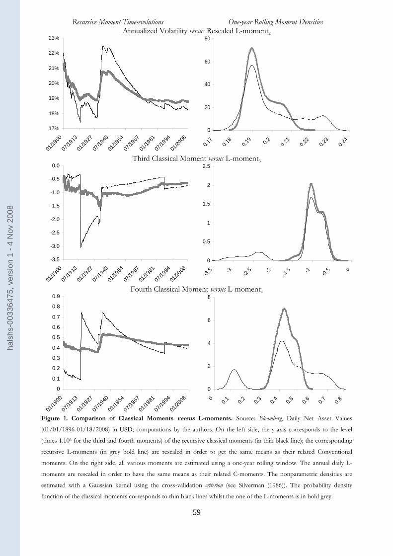
59

Recursive Moment Time-evolutions One-year Rolling Moment Densities Annualized Volatility versus Rescaled L-moment2

17%

18%

19%

20%

21%

22%

23%

01/19

00

07/19

13

01/19

27

07/19

40

01/19

54

07/19

67

01/19

81

07/19

94

01/20

080

20

40

60

80

0.17

0.18

0.19 0.2 0.2

10.2

20.2

30.2

4

Third Classical Moment versus L-moment3

-3.5

-3.0

-2.5

-2.0

-1.5

-1.0

-0.5

0.0

01/19

00

07/19

13

01/19

27

07/19

40

01/19

54

07/19

67

01/19

81

07/19

94

01/20

080

0.5

1

1.5

2

2.5

-3.5 -3 -2.5 -2 -1.5 -1 -0.5 0

Fourth Classical Moment versus L-moment4

0

0.1

0.2

0.3

0.4

0.5

0.6

0.7

0.8

0.9

01/19

00

07/19

13

01/19

27

07/19

40

01/19

54

07/19

67

01/19

81

07/19

94

01/20

08

0

2

4

6

8

0 0.1 0.2 0.3 0.4 0.5 0.6 0.7 0.8

Figure 1. Comparison of Classical Moments versus L-moments. Source: Bloomberg, Daily Net Asset Values

(01/01/1896-01/18/2008) in USD; computations by the authors. On the left side, the y-axis corresponds to the level

(times 1.106 for the third and fourth moments) of the recursive classical moments (in thin black line); the corresponding

recursive L-moments (in grey bold line) are rescaled in order to get the same means as their related Conventional

moments. On the right side, all various moments are estimated using a one-year rolling window. The annual daily L-

moments are rescaled in order to have the same means as their related C-moments. The nonparametric densities are

estimated with a Gaussian kernel using the cross-validation criterion (see Silverman (1986)). The probability density

function of the classical moments corresponds to thin black lines whilst the one of the L-moments is in bold grey.

hals

hs-0

0336

475,

ver

sion

1 -

4 N

ov 2

008

60

with Third L-moments Coloured with Fourth L-moments Coloured

Figure 2. First Four L-moment Constrained Efficient Frontier in the L1-L2 Plane. Source: Bloomberg, Weekly Net Asset

Values (06/2001-06/2006) in EUR; computations by the authors. The constrained efficient frontier is compounded with 2,610

simulated portfolios, obtained after optimization in 9,637 directions of random portfolios built with 162 European equities. Sizes of

dots and their colour shadings (from black small low levels to white large high levels) represent (respectively) the third (fourth) L-

moments on the left figure (the right figure).

with First L-moments Coloured with Fourth L-moments Coloured

Figure 3. First Four L-moment Constrained Efficient Frontier in the L2-L3 Plane. Source: Bloomberg, Weekly Net Asset

Values (06/2001-06/2006) in EUR; computations by the authors. The constrained efficient frontier is compounded with 1,932

simulated portfolios, obtained after optimization in 9,637 directions of random portfolios built with 162 European equities. Sizes

of dots and their colour shadings (from black small low levels to white large high levels) represent (respectively) the first (fourth)

L-moments on the left figure (the right figure).

hals

hs-0

0336

475,

ver

sion

1 -

4 N

ov 2

008

61

with First L-moments Coloured with Third L-moments Coloured

Figure 4. First Four L-moment Constrained Efficient Frontier in the L2-L4 Plane. Source: Bloomberg, Weekly Net Asset

Values (06/2001-06/2006) in EUR; computations by the authors. The constrained efficient frontier is compounded with 731

simulated portfolios, obtained after optimization in 9,637 directions of random portfolios built with 162 European equities. Sizes

of dots and their colour shadings (from black small low levels to white large high levels) represent (respectively) the first (third) L-

moments on the left figure (the right figure).

with Second L-moments Coloured with Third L-moments Coloured

Figure 5. First Four L-moment Constrained Efficient Frontier, in the L1-L4 Plane. Source: Bloomberg, Weekly Net Asset

Values (06/2001-06/2006) in EUR; computations by the authors. The constrained efficient frontier is compounded with 1,161

simulated portfolios, obtained after optimization in 9,637 directions of random portfolios built with 162 European equities. Sizes

of dots and their colour shadings (from black small low levels to white large high levels) represent (respectively) the second (third)

L-moments on the left figure (the right figure).

hals

hs-0

0336

475,

ver

sion

1 -

4 N

ov 2

008

62

with Second L-moments Coloured with Fourth L-moments Coloured

Figure 6. First Four L-moment Constrained Efficient Frontier in the L1-L3 Plane. Source: Bloomberg, Weekly Net Asset

Values (06/2001-06/2006) in EUR; computations by the authors. The constrained efficient frontier is compounded with 1,925

simulated portfolios, obtained after optimization in 9,637 directions of random portfolios built with 162 European equities. Sizes

of dots and their colour shadings (from black small low levels to white large high levels) represent (respectively) the second

(fourth) L-moments on the left figure (the right figure).

with First L-moments Coloured with Second L-moments Coloured

Figure 7. First Four L-moment Constrained Efficient Frontier in the L3-L4 Plane. Source: Bloomberg, Weekly Net Asset

Values (06/2001-06/2006) in EUR; computations by the authors. The constrained efficient frontier is compounded with 1,244

simulated portfolios, obtained after optimization in 9,637 directions of random portfolios built with 162 European equities. Sizes

of dots and their colour shadings (from black small low levels to white large high levels) represent (respectively) the first (second)

L-moments on the left figure (the right figure).

hals

hs-0

0336

475,

ver

sion

1 -

4 N

ov 2

008

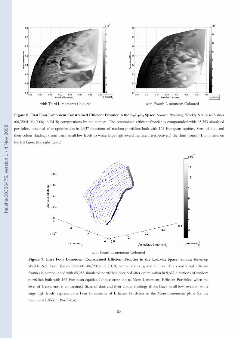
63

with Third L-moments Coloured with Fourth L-moments Coloured

Figure 8. First Four L-moment Constrained Efficient Frontier in the L1-L2-L3 Space. Source: Bloomberg, Weekly Net Asset Values

(06/2001-06/2006) in EUR; computations by the authors. The constrained efficient frontier is compounded with 65,253 simulated

portfolios, obtained after optimization in 9,637 directions of random portfolios built with 162 European equities. Sizes of dots and

their colour shadings (from black small low levels to white large high levels) represent (respectively) the third (fourth) L-moments on

the left figure (the right figure).

with Fourth L-moments Coloured

Figure 9. First Four L-moment Constrained Efficient Frontier in the L1-L2-L3 Space. Source: Bloomberg,

Weekly Net Asset Values (06/2001-06/2006) in EUR; computations by the authors. The constrained efficient

frontier is compounded with 65,253 simulated portfolios, obtained after optimization in 9,637 directions of random

portfolios built with 162 European equities. Lines correspond to Mean L-moment2 Efficient Portfolios when the

level of L-moment3 is constrained. Sizes of dots and their colour shadings (from black small low levels to white

large high levels) represent the Four L-moments of Efficient Portfolios in the Mean-L-moment2 plane (i.e. the

traditional Efficient Portfolios).

hals

hs-0

0336

475,

ver

sion

1 -

4 N

ov 2

008

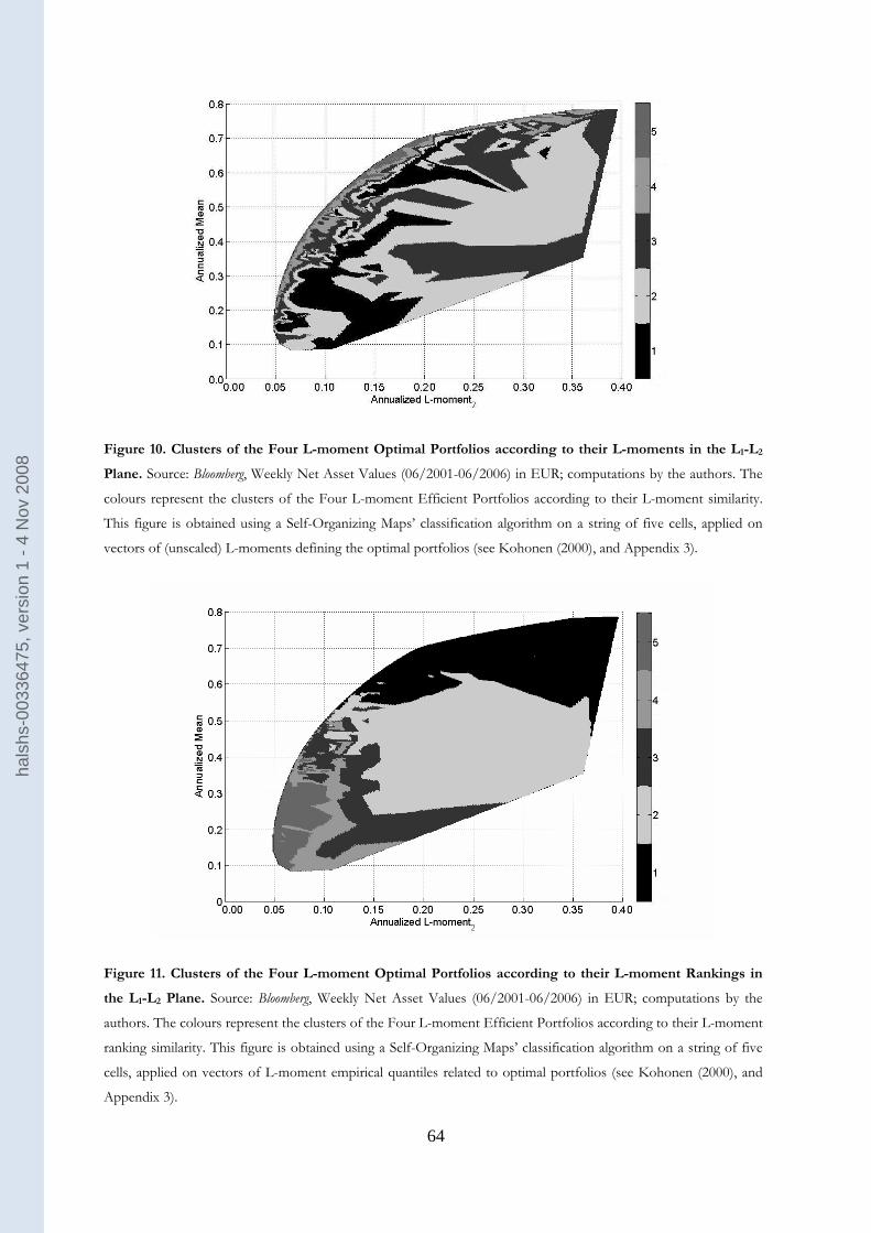
64

Figure 10. Clusters of the Four L-moment Optimal Portfolios according to their L-moments in the L1-L2

Plane. Source: Bloomberg, Weekly Net Asset Values (06/2001-06/2006) in EUR; computations by the authors. The

colours represent the clusters of the Four L-moment Efficient Portfolios according to their L-moment similarity.

This figure is obtained using a Self-Organizing Maps’ classification algorithm on a string of five cells, applied on

vectors of (unscaled) L-moments defining the optimal portfolios (see Kohonen (2000), and Appendix 3).

Figure 11. Clusters of the Four L-moment Optimal Portfolios according to their L-moment Rankings in

the L1-L2 Plane. Source: Bloomberg, Weekly Net Asset Values (06/2001-06/2006) in EUR; computations by the

authors. The colours represent the clusters of the Four L-moment Efficient Portfolios according to their L-moment

ranking similarity. This figure is obtained using a Self-Organizing Maps’ classification algorithm on a string of five

cells, applied on vectors of L-moment empirical quantiles related to optimal portfolios (see Kohonen (2000), and

Appendix 3).

hals

hs-0

0336

475,

ver

sion

1 -

4 N

ov 2

008

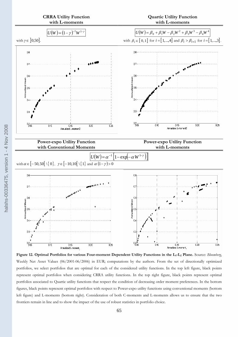
65

CRRA Utility Function with L-moments

Quartic Utility Function with L-moments

( ) ( ) γγ −−−= 111 WWU ( ) 44

33

2210 WWWWWU βββββ −+−+=

with ] ]50,0∈γ . with [ ]1,0∈iβ for [ ]4,,1 ...i = and 1+> ii ββ for [ ]3,,1 ...i = .

Power-expo Utility Function with Conventional Moments

Power-expo Utility Function with L-moments

( ) ( )[ ]γαα −− −−= 11 exp1 WWU with [ [ 0\50,50−∈α , [ [ 1\10,10 −∈γ and ( ) 01 >−γα

Figure 12. Optimal Portfolios for various Four-moment Dependent Utility Functions in the L1-L2 Plane. Source: Bloomberg,

Weekly Net Asset Values (06/2001-06/2006) in EUR; computations by the authors. From the set of directionally optimized

portfolios, we select portfolios that are optimal for each of the considered utility functions. In the top left figure, black points

represent optimal portfolios when considering CRRA utility functions. In the top right figure, black points represent optimal

portfolios associated to Quartic utility functions that respect the condition of decreasing order moment preferences. In the bottom

figures, black points represent optimal portfolios with respect to Power-expo utility functions using conventional moments (bottom

left figure) and L-moments (bottom right). Consideration of both C-moments and L-moments allows us to ensure that the two

frontiers remain in line and to show the impact of the use of robust statistics in portfolio choice.

hals

hs-0

0336

475,

ver

sion

1 -

4 N

ov 2

008

66

CRRA Utility Function with L-moments

( ) ( ) γγ −−−= 111 WWU with ] ]50,0∈γ .

with Intensified L3- (x2) and L4- (/2) moment Features with Intensified L3- (x4) and L4- (/4) moment Features

Figure 13. Efficient Frontiers for CRRA Utility Functions with Intensified Higher-order Moments. Source: Bloomberg,

Weekly Net Asset Values (06/2001-06/2006) in EUR; computations by the authors. From the set of directionally optimized

portfolios, we select those that are optimal for one of the various CRRA utility functions. On the left (right) figure, the grey bold

line represents the CRRA efficient frontier with no change (original data), whilst the thin black line represents the efficient frontier

when the third moments of underlying portfolios are multiplied by 2 (respectively by 4), the bold grey dotted line represents the

efficient frontier when the fourth moments are divided37 by 2 (by 4) and the thin black dotted line represents efficient frontier when

third moments are multiplied by 2 (by 4) and fourth moments are divided by 2 (by 4).

hals

hs-0

0336

475,

ver

sion

1 -

4 N

ov 2

008

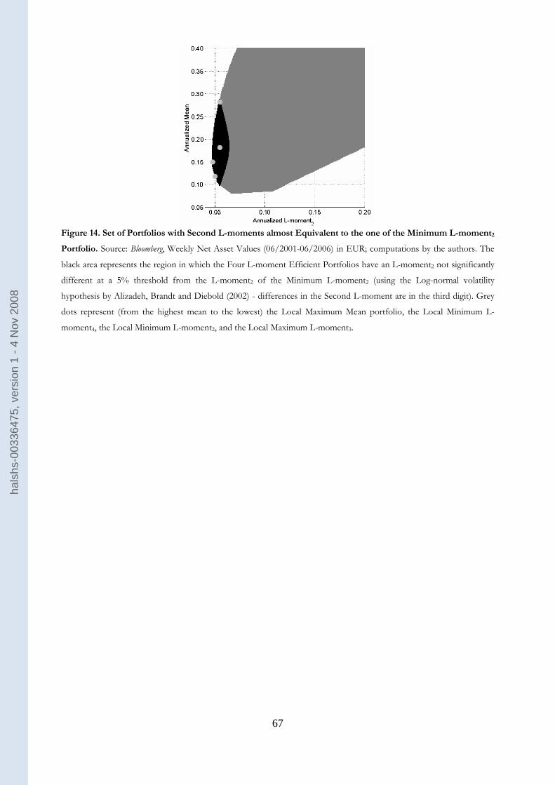
67

Figure 14. Set of Portfolios with Second L-moments almost Equivalent to the one of the Minimum L-moment2

Portfolio. Source: Bloomberg, Weekly Net Asset Values (06/2001-06/2006) in EUR; computations by the authors. The

black area represents the region in which the Four L-moment Efficient Portfolios have an L-moment2 not significantly

different at a 5% threshold from the L-moment2 of the Minimum L-moment2 (using the Log-normal volatility

hypothesis by Alizadeh, Brandt and Diebold (2002) - differences in the Second L-moment are in the third digit). Grey

dots represent (from the highest mean to the lowest) the Local Maximum Mean portfolio, the Local Minimum L-

moment4, the Local Minimum L-moment2, and the Local Maximum L-moment3.

hals

hs-0

0336

475,

ver

sion

1 -

4 N

ov 2

008

68

Table I

P-statistics of Normality Goodness-of-Fit Tests of the various Optimal Portfolio Return Series (frequencies of rejections at 1%, 5% and 10% confidence levels)

Source: Bloomberg, Weekly Net Asset Values (06/2001-06/2006) in EUR; computations by the authors. From the sets of the (162) original return series, the (65,253) general Four L-moment Efficient Portfolios (see Figure 8), the (379) Four L-moment CRRA Optimal Portfolios, the (123) Four L-moment Quartic optimal portfolio, the (92) Four C-moment Power-expo optimal portfolios, the (341) Four L-moment Power-expo Optimal Portfolios (see Figure 11), we compute the Jarque-Bera, the Kolmogorov-Smirnov, the Liliefors and the Anderson-Darling Goodness-of-Fit tests. The table reports the frequency of P-statistics below the usual probability thresholds (1% between parentheses, 5% between brackets and 10% between accolades), i.e. the relative number of (stock) portfolio series being non-normal in the sense of the usual Gaussianity tests.

Jarque- Bera

Kolmogorov-Smirnov

Liliefors

Anderson-Darling

Original European Stock Returns Series

(.91)/[.96]/.98 (.20)/[.38]/.58 (.68)/[.81]/.86 (.82)/[.90]/.94

Four L-moment General Efficient Portfolios

(.65)/[.72]/.75 (.15)/[.38]/.50 (.64)/[.82]/.89 (.78)/[.91]/.94 Four L-moment Quartic Optimal Portfolios

(.88)/[.93]/.95 (.13)/[.35]/.50 (.69)/[.80]/.84 (.74)/[.81]/.83 Four L-moment CRRA Optimal Portfolios

(.69)/[.78]/.82 (.12)/[.15]/.18 (.20)/[.26]/.45 (.46)/[.48]/.56 Four C-moment Power-expo Optimal Portfolios

(.98)/[.99]/1.00 (.10)/[.23]/.43 (.60)/[.79]/.84 (.78)/[.85]/.86 Four L-moment Power-expo Optimal Portfolios

(.83)/[.95]/1.00 (.14)/[.39]/.44 (.55)/[.60]/.63 (.65)/[.76]/.78

Table II Statistical Properties of Minimum L-moment2 Portfolio versus the Local Maximum

Mean, Local Maximum L-moment3 and Local Minimum L-moment4 Portfolios Source: Bloomberg, Weekly Net Asset Values (06/2001-06/2006) in EUR; computations by the authors. From the set of Four L-moment Efficient Portfolios with a L-moment2 that is not significantly different from the one of the Minimum L-moment2 portfolio (at a 5% threshold), we select the Local Maximum Mean, Local Maximum L-moment3 and Local Minimum L-moment4 Portfolios (see Figure 14). The table presents the first four L-moments (the two first L-moments being annualized and the two last ones being divided by 1,000), and Sharpe ratios of selected local best portfolios.

Mean L-moment2 L-moment3 L-moment4 Sharpe ratio

Minimum L-moment2

.15 .05 -.70 1.30 1.19

Local Maximum Mean

.28 .06 -.90 1.40 2.34

Local Maximum L-moment3

.11 .05 .20 1.70 .71

Local Minimum L-moment4

.17 .06 -1.10 .60 1.29

hals

hs-0

0336

475,

ver

sion

1 -

4 N

ov 2

008