université de montréal a novel approach to determine harmonic

UNIVERSITÉ DE MONTRÉAL

A NOVEL APPROACH TO DETERMINE HARMONIC DISTORTIONS IN UNBALANCED

NETWORKS AND HARMONIC FILTER PLANNING IN INDUSTRIAL SYSTEMS

AHMAD HOSSEINIMANESH

DÉPARTEMENT DE GÉNIE ÉLECTRIQUE

ÉCOLE POLYTECHNIQUE DE MONTRÉAL

MÉMOIRE PRÉSENTÉ EN VUE DE L’OBTENTION

DU DIPLÔME DE MAÎTRISE ÈS SCIENCES APPLIQUÉES

(GÉNIE ÉLECTRIQUE)

NOVEMBRE 2015

© Ahmad Hosseinimanesh, 2015.

UNIVERSITÉ DE MONTRÉAL

ÉCOLE POLYTECHNIQUE DE MONTRÉAL

Ce mémoire intitulé :

A NOVEL APPROACH TO DETERMINE HARMONIC DISTORTIONS IN UNBALANCED

NETWORKS AND HARMONIC FILTER PLANNING IN INDUSTRIAL SYSTEMS

présenté par : HOSSEINIMANESH Ahmad

en vue de l’obtention du diplôme de : Maîtrise ès sciences appliquées

a été dûment accepté par le jury d’examen constitué de :

M. KARIMI Houshang, Ph. D, président

M. KOCAR Ilhan, Ph. D, membre et directeur de recherche

M. LACROIX Jean-Sebastien, M. Sc. A, membre

iii

DEDICATION

To my beloved family Mohammad, Zahra, Hossein and Golriz

iv

ACKNOWLEDGMENTS

Firstly, I am grateful to the God for the good health and wellbeing that were necessary to

complete this thesis.

A special thanks to my family. Words cannot express how grateful I am to my mother and father

for all of the sacrifices that you have made on my behalf. I am also thankful to my brother for

supporting me spiritually throughout writing this thesis and my life in general.

My deepest gratitude is to Professor Ilhan Kocar, my Research Director, for the continuous

support of my Master study and related research, for his patience, motivation, immense

knowledge and providing me with an excellent atmosphere for doing research. His guidance

helped me in all the time of research and writing of this thesis.

My sincere thanks also goes to Jean-Sebastien Lacroix, R&D Manager at CYME International

T&D, who provided me an opportunity to join their team as intern, and who gave access to the

research facilities. Without they precious support it would not be possible to conduct this

research.

I take this opportunity to express gratitude to all of the Department faculty members for their help

and support. Special thanks to Ming Cai for commenting on my thesis and guidance. I would also

like to thank my friends in Polytechnique, particularly Thomas Kauffmann for debates and

exchange of knowledge during my graduate program, which helped enrich the experience.

I also place on record, my sense of gratitude to one and all, who directly or indirectly, have lent

their hand in this venture.

v

RÉSUMÉ

Ce mémoire présente une méthode d’analyse des harmoniques dans un réseau électrique à n

phases. Cette méthode est basée sur l’analyse nodale modifiée augmentée (abrégée MANA en

anglais). Elle peut être appliquée à des réseaux déséquilibrés avec plusieurs sources

d’harmoniques et plusieurs charges déséquilibrées. Il n’y a pas de limites quant à la taille, la

structure ou la topologie du réseau étudié.

L’algorithme développé ici peut être divisé en deux parties. Une première partie résous

l’écoulement de puissance du réseau (load-flow en anglais) pour la fréquence fondamentale. La

seconde partie est un calcul en régime permanent (basé sur la MANA) pour les différentes

fréquences des harmoniques étudiés. Cette partie permet de calculer la propagation des

harmoniques issus des éléments non-linéaires. Les éléments linéaires du réseau sont représentés

par un modèle équivalent tandis que les éléments non-linéaires sont représentés par un modèle

généralisé de l’équivalent de Norton. L’application de l’analyse nodale modifiée augmentée à

l’étude des harmoniques est réalisée ici pour la première fois.

Cette méthode est appliquée ici à l’étude des filtres passifs qui réduisent la propagation des

harmoniques. L’objectif de ces filtres est de maintenir la tension des harmoniques sous les

niveaux présentés dans le standard IEEE 519. Les différents types de filtre et la variation de la

fréquence de coupure de ceux-ci sont aussi considérés ici. De plus ce mémoire présente une

analyse sur l’emplacement de ces filtres. En raison de la forte capacité de calcul des ordinateurs

actuels ainsi que la petite taille des réseaux industriels, une méthode essai erreur est appliquée.

Dans cette méthode, toutes les barres pouvant accueillir des filtres sont identifiées puis

l’emplacement est déterminé en testant tous les cas possibles. Afin de réduire le nombre de

filtres, la méthode proposée a aussi pour objectif de minimiser les coûts d’investissement de ces

filtres.

Les principaux objectifs de cette étude sont (1) de résumer les modèles harmoniques pour les

composants de réseau dans des conditions déséquilibrées, (2) de promulguer la formulation de

MANA pour déterminer le courant / les distorsions de tension harmonique -, (3) de discuter des

stratégies pratiques afin d'améliorer la compensation réactive des systèmes électriques industriels,

tout en réduisant les problèmes de résonance et limitant les problèmes harmoniques.

vi

Les modèles et algorithmes ont été testés avec différent systèmes de distribution et industriels.

Les résultats montrent que les méthodes sont efficaces et adaptées aux ’analyses harmoniques et à

la planification des filtres passifs dans des systèmes électriques de puissance.

vii

ABSTRACT

A multiphase harmonic analysis solution technique using Modified Augmented Nodal Analysis

(MANA) formulation is presented in this thesis. The solution technique can solve unbalanced

networks with multiple unbalanced harmonic sources and unbalanced loads. There is no

limitation in terms of network size, configuration and topology.

The algorithm developed in this work consists of two steps: A fundamental frequency load flow

using the MANA formulation is carried out first. Then the second step is steady state

computation based on MANA in frequency domain to calculate the harmonic propagation due to

nonlinear devices. In this step, the linear elements of the network are represented with equivalent

models while the nonlinear devices are represented with generalized Norton equivalents. The

application of MANA for harmonic analysis is promulgated here for the first time.

A study on the application of passive harmonic filters is also presented in this thesis in relation

with IEEE 519 requirements. The application of several types of passive harmonic filters are

discussed and the tuned frequency deviation of the single tuned filter is taken into consideration

for the purpose of maintaining harmonic voltages compatible with IEEE 519 requirements. In

addition to that, a discussion on the filter planning is provided in this work. Given the

performance of present day computers and the relatively small size of industrial networks, a

simple approach based on trial and error is applied. In the proposed approach all the candidate

buses for filter placement are identified first and ideal buses are determined by simulating all

possible configurations. In order to reduce the number of filters, the proposed methodology has

an objective of minimizing the total investment cost of the designed filters.

The major objectives of this study are (1) to summarize harmonic models for network

components for unbalanced conditions, (2) to promulgate the MANA formulation to determine

the harmonic current - voltage distortions, (3) to discuss practical solution strategies in order to

improve reactive compensation of industrial power systems while reducing resonance problems

and limiting harmonic problems.

Models and algorithms are tested with different distribution and industrial systems, and the

results show that the methods are effective and suitable for harmonic analysis and planning of

passive filters in power systems.

viii

TABLE OF CONTENTS

DEDICATION ............................................................................................................................... iii

ACKNOWLEDGMENTS .............................................................................................................. iv

RÉSUMÉ ......................................................................................................................................... v

ABSTRACT .................................................................................................................................. vii

TABLE OF CONTENTS ............................................................................................................. viii

LIST OF TABLES ......................................................................................................................... xi

LIST OF FIGURES ....................................................................................................................... xii

LIST OF SYMBOLS AND ABBERVIATIONS......................................................................... xvi

LIST OF APPENDICES ............................................................................................................ xviii

CHAPTER 1 INTRODUCTION ..................................................................................................... 1

1.1 Overview .......................................................................................................................... 1

1.2 Objective .......................................................................................................................... 1

1.3 Methodology .................................................................................................................... 2

1.4 Report outline ................................................................................................................... 3

1.5 Research Contributions .................................................................................................... 3

CHAPTER 2 HARMONIC ANALYSIS IN UNBALANCED NETWORKS ............................. 4

2.1 Literature review .............................................................................................................. 4

2.2 Harmonic .......................................................................................................................... 5

2.3 Inter-harmonic .................................................................................................................. 5

2.4 Characteristics of harmonic .............................................................................................. 5

2.5 MANA formulation .......................................................................................................... 7

2.6 Impedance scan (Frequency scan) .................................................................................... 8

ix

2.7 Harmonic analysis ............................................................................................................ 9

2.7.1 Algorithm of harmonic analysis ................................................................................. 10

2.7.2 Flowchart of harmonic analysis ................................................................................. 12

2.8 Iterative harmonic analysis (IHA) .................................................................................. 12

2.9 Harmonic modeling of the network elements ................................................................ 13

2.9.1 Overhead line ............................................................................................................. 13

2.9.2 Cable ........................................................................................................................... 26

2.9.3 Voltage sources .......................................................................................................... 26

2.9.4 Transformers .............................................................................................................. 27

2.9.5 Loads .......................................................................................................................... 29

CHAPTER 3 PLANNING OF LARGE HARMONIC FILTERS IN INDUSTRIAL

NETWORKS ................................................................................................................................. 48

3.1 Literature review ............................................................................................................ 48

3.2 Harmonic filter ............................................................................................................... 49

3.2.1 Passive harmonic filters ............................................................................................. 49

3.2.2 Active harmonic filter ................................................................................................ 50

3.2.3 Hybrid harmonic filter ................................................................................................ 50

3.3 Passive filter design ........................................................................................................ 50

3.3.1 Single tuned harmonic filter ....................................................................................... 50

3.3.2 High pass harmonic filter ........................................................................................... 51

3.3.3 C-Type harmonic filter ............................................................................................... 52

3.3.4 Multiple filter banks ................................................................................................... 53

3.3.5 Resonance problem .................................................................................................... 53

3.3.6 Constraint ................................................................................................................... 54

3.3.7 Quality factor .............................................................................................................. 55

x

3.3.8 Filter detuning factor .................................................................................................. 55

3.3.9 K-Factors transformer ................................................................................................ 56

3.4 Algorithm of filter design ............................................................................................... 56

3.5 Flowchart (1).of filter design ......................................................................................... 64

3.6 Flowchart (2).of filter design ......................................................................................... 65

3.7 Harmonic filters allocation ............................................................................................. 65

3.8 Algorithm of filter allocation ......................................................................................... 66

3.9 Flowchart of filter allocation .......................................................................................... 68

CHAPTER 4 TEST CASES ......................................................................................................... 69

4.1 Validation of harmonic analysis based MANA ............................................................. 69

4.1.1 Description of the study network ............................................................................... 69

4.1.2 Results and discussions .............................................................................................. 70

4.1.3 Comparison of harmonic analysis using MANA with harmonic analysis in EMTP-

RV (v 2.6.1) ............................................................................................................................ 78

4.2 Validation of the method of passive filter design .......................................................... 79



4.3 Validation of harmonic filter allocation ......................................................................... 87



CHAPTER 5 CONCLUSION AND RECOMMENDATIONS ................................................... 94

BIBLIOGRAPHY ......................................................................................................................... 96

xi

LIST OF TABLES

Table 2-1 Line parameters data (in 60 Hz) .................................................................................... 23

Table 2-2 Typical load composition [9] ......................................................................................... 29

Table 2-3 Parameters of synchronous machine at fundamental frequency 60 Hz ......................... 45

Table 3-1 IEEE 519 voltage distortion limits ................................................................................. 54

Table 3-2 IEEE 519 current distortion limits ................................................................................. 54

Table 4-1 Harmonic source ............................................................................................................ 70

Table 4-2 Harmonic analysis in 34 bus distribution system .......................................................... 71




Table 4-6 EMTP-RV results of harmonic analysis ........................................................................ 78

Table 4-7 EMTP-RV results of harmonic analysis ........................................................................ 79

Table 4-8 Harmonic distortion of a typical 6 pulse converter PWM ............................................. 81

Table 4-9 System data .................................................................................................................... 81

Table 4-10 Parameters of harmonic filters measured by proposed method for 5 Bus industrial

system ..................................................................................................................................... 84

Table 4-12 Values required to satisfy IEEE 18 .............................................................................. 87

Table 4-13 Harmonic distortion of a typical 12 pulse converter .................................................... 88

Table 4-14 THD voltage at each bus after installation of filters (%) ............................................. 90

xii

LIST OF FIGURES

Figure 2-1Circuit in fundamental frequency .................................................................................. 11

Figure 2-2 Nonlinear devices is modelled using Norton equivalent at harmonic frequencies ...... 11

Figure 2-3 Flowchart of harmonic analysis .................................................................................... 12

Figure 2-4 Iterative Harmonic Analysis algorithm ........................................................................ 13

Figure 2-5 Phase conductors and images ....................................................................................... 14

Figure 2-6 PI model ........................................................................................................................ 18

Figure 2-7 Impedance characteristic of a PI nominal line (60Hz <f<1200 Hz) ............................. 23

Figure 2-8 Real part of a PI nominal line (60Hz <f<1200 Hz) ...................................................... 24

Figure 2-9 Imaginary part of a PI nominal line (60Hz <f<1200 Hz) ............................................. 24

Figure 2-10 Impedance characteristic of a distributed line (equivalent PI) (60Hz <f<1200 Hz) .. 25

Figure 2-11 Real part of a distributed line (equivalent PI) (60Hz <f<1200 Hz) ............................ 25

Figure 2-12 Imaginary part of a distributed line (equivalent PI) (60Hz <f<1200 Hz)................... 26

Figure 2-13 Yg yg transformer ....................................................................................................... 28

Figure 2-14 Equivalent circuit for RL series load .......................................................................... 30

Figure 2-15 Equivalent circuit of RL parallel ................................................................................ 31

Figure 2-16 RL equivalent circuit of RL parallel with skin effect ................................................. 31

Figure 2-17 Equivalent circuit of a CIGRE type C ........................................................................ 32

Figure 2-18 Y connection of spot load ........................................................................................... 33

Figure 2-19 Delta connection of spot load ..................................................................................... 33

Figure 2-20 Impedance scan of RL series load (60 Hz < f < 1200 Hz) ......................................... 34

Figure 2-21 Impedance phase of RL series load (60 Hz < f < 1200 Hz) ....................................... 35

Figure 2-22 Impedance scan of RL parallel load (60 Hz < f < 1200 Hz) ...................................... 35

Figure 2-23 Impedance phase of RL parallel load (60 Hz < f < 1200 Hz) .................................... 36

xiii

Figure 2-24 Impedance scan of RL parallel load with skin effect (60 Hz < f < 1200 Hz) ............ 36

Figure 2-25 Impedance phase of RL parallel load with skin effect (60 Hz < f < 1200 Hz) .......... 37

Figure 2-26 Impedance scan of CIGRE type C (60 Hz < f < 1200 Hz) ......................................... 37

Figure 2-27 Impedance phase of CIGRE type C (60 Hz < f < 1200 Hz) ....................................... 38

Figure 2-28 Equivalent circuit of induction motor ......................................................................... 39

Figure 2-29 Impedance scan of induction motor (60Hz < f< 1200 Hz) ......................................... 42

Figure 2-30 Phase impedance of induction motor (60Hz < f< 1200 Hz) ....................................... 42

Figure 2-31 Synchronous motor (Yg) ............................................................................................ 44

Figure 2-32 Synchronous motor (Delta or Y) ................................................................................ 44

Figure 2-33 Impedance characteristic of synchronous machine (60 Hz < f<1200 Hz) ................. 45

Figure 2-34 Phase impedance of the synchronous machine (60 Hz < f < 1200 Hz) ...................... 46

Figure 2-35 Nonlinear load ............................................................................................................ 47

Figure 2-36 Norton equivalent of a nonlinear load ........................................................................ 47

Figure 3-1 Single tuned filter ......................................................................................................... 51

Figure 3-2 Impedance Scan of single tuned harmonic filter (tuned at 420 Hz) ............................. 51

Figure 3-3 High pass harmonic filter ............................................................................................. 52

Figure 3-4 Impedance Scan of High pass harmonic filter (tuned at1020 Hz) ................................ 52

Figure 3-5 C-Type harmonic filter ................................................................................................. 53

Figure 3-6 Multiple filter bank ....................................................................................................... 53

Figure 3-7 Flowchart 1 of Passive Filter Design ............................................................................ 64

Figure 3-8 Flowchart 2 of Passive Filter Design ............................................................................ 65

Figure 3-9 Harmonic filter placement ............................................................................................ 68

Figure 4-1 IEEE 34 bus distribution system .................................................................................. 70

Figure 4-2 Voltage waveform at Bus 880a (from MATLAB code) .............................................. 72

xiv



Figure 4-5 5-Bus industrial system with multiple harmonic filters at bus 5 .................................. 80

Figure 4-6 Voltage waveform at bus 5 (from CYME Harmonic module) ..................................... 82

Figure 4-7 Current waveform at bus 5(from CYME Harmonic module) ...................................... 82

Figure 4-8 Voltage Individual Harmonic Distortions (Voltage IHD) ............................................ 82

Figure 4-9 Voltage Total Harmonic Distortions (Voltage THD) ................................................... 83

Figure 4-10 Current Total Harmonic Distortions (Current THD) .................................................. 83

Figure 4-11 Impedance characteristic waveform before filtering at bus 5 (from CYME Harmonic

module) ................................................................................................................................... 83

Figure 4-12 Voltage at bus 5 (from CYME Harmonic module) .................................................... 85

Figure 4-13 Current waveform at bus 5(from CYME Harmonic module) .................................... 85

Figure 4-14 Voltage Individual Harmonic Distortions (Voltage IHD) .......................................... 85

Figure 4-15 Voltage Total Harmonic Distortions (Voltage THD) ................................................. 86

Figure 4-16 Current Total Harmonic Distortions (Current THD) .................................................. 86

Figure 4-17 Impedance characteristic waveform after filtering at bus 5 (from CYME Harmonic

module) ................................................................................................................................... 86

Figure 4-18 13 Bus industrial system ............................................................................................. 88

Figure 4-19 Voltage THD weight of the 13 bus system (before filters placement) ....................... 89

Figure 4-20 Voltage THD weight of 13 bus system (Filter at bus 4) ............................................. 90






xv

Figure 4-26 Voltage THD weight of 13 bus system (Filter at bus 10) ........................................... 92




xvi

LIST OF SYMBOLS AND ABBERVIATIONS

(1.1) Equation 1.1

[1] Reference 1

Complex number

Dc MANA Dependency functions matrix

VN−LL Nominal line-to-line voltage

Id MANA Unknown currents in dependent voltage source vector

In MANA Nodal currents injection vector

Is MANA Unknown currents in zero impedance element vector

Iv MANA Unknown source current vector

SC MANA Adjacency matrix of zero impedance type devices

Scc−1∅ Single-phase short-circuit power

Scc−3∅ Three-phase short-circuit power

SD MANA Adjacency matrix of infinite impedance type devices

Vibe MANA Voltage sources vector

Vic MANA Voltage sources adjacency matrix

Vn MANA Unknown node voltages vector

Yn MANA Linear network admittance matrix

Z0 Complex zero sequence impedance

Z1 Complex positive sequence impedance

Z2 Complex negative sequence impedance

Z012 Complex sequence impedance

Delta Ungrounded delta connection or system

Y Wye ungrounded connection or system

Yg Wye grounded connection or system

GMR Geometrical Mean Radius

THD Total Harmonic Distortion

IHD Individual Harmonic Distortion

IEEE Institute of Electrical and Electronic Engineers

xvii

MANA Modified-Augmented-Nodal Analysis

p.u. Per-Unit

X/R Inductive per resistive ratio

PCC Point of Common Coupling

PF Power Factor

IHA Iterative Harmonic Analysis

xviii

LIST OF APPENDICES

Appendix A – DISTORTION FACTORS ................................................................................... 101

Appendix B – COMMON VOLTAGE AND REACTIVE POWER RATING BASED ON IEEE

18 .......................................................................................................................................... 102

1

CHAPTER 1 INTRODUCTION

1.1 Overview

Immediately upon, the electrical devices with nonlinear current-voltage characteristics such as

power converters came into use in the 1970s; the ability of power system to control harmonic

propagations has gained attention. However, concerns regarding the harmonic distortions were

overlooked around that time, such that the harmonics in distribution systems could cause

problems in the performance of network elements. Generally, the harmonics produced by

nonlinear devices can reduce efficiency of the power system and in some cases it can even trip

circuit breakers. In distribution networks, the end-user suffers from harmonic problems more than

the utility sector does [1]. In industrial systems, since the adjustable speed drives, and the arc

furnaces are close to each other, the problems caused by harmonic distortions are very likely to

occur. Due to these facts, the harmonic propagations in distribution and power systems,

particularly for industrial zones, should be precisely analyzed.

Since the power quality is significantly affected by propagation of harmonic distortions in power

systems, harmonic control has become a critical issue. One of the most common methods to

achieve harmonic distortion reduction is the use of harmonic filters. It should be noted that this

reduction greatly depends on the filtering system placement. There are two types of harmonic

filters commonly found in industrial systems (i) passive filters and (ii) active filters. The main

difference of these filters stand on whether they cancel harmonic distortions within specific

frequencies.

1.2 Objective

The main objective of this research project is to develop an algorithm for calculating harmonic

voltages and currents in unbalanced networks so that the result can be used for resonance

measurements and harmonic filter design. Although the proposed method is suitable for

transmission systems or other highly meshed systems, the main focus of this work is on

unbalanced distribution systems. The sub objective of this research project is to design and place

suitable harmonic filters and accordingly reduce the propagation of harmonic distortions in

industrial networks.

2

1.3 Methodology

According to the specific objective of this project, the present study includes using a

mathematical method for determining the harmonic distortions. This method involves the

modified augmented nodal analysis and is applied to steady state computations. Once all the

system elements are modified into their harmonic models respectively, the developed MANA

algorithm is employed for harmonic analysis. It should, nonetheless, be noted that the harmonic

models of system elements due to their frequency-dependent nature can be very complex and

demanding to obtain when high precision levels are targeted. Generally accepted, steady state

models are considered in this work for the harmonic modeling of components. Regarding the

metrics on the quality of power, the IEEE standard 519 is considered here as the main reference.

The purpose of IEEE 519 standard is to make sure that the utility maintains a certain quality of

power at the load terminals and that load is not subjected to high levels of harmonics [2]. Finally,

the harmonic analysis is validated by using the IEEE 34 bus distribution test system. The

validation test case demonstrates that the proposed algorithm yields precise results.

The secondary objective is related to the optimization of filter design and involves the use of two

algorithms. The first algorithm is used to determine the parameters of the passive harmonic filters

while respecting the limits set by IEEE 519 and IEEE 18. In this algorithm a systematic

procedure to design the harmonic filters is used considering the use of all the passive filters

available. It has to be mentioned that the application of passive harmonic filters is a common

practice for suppressing harmonic propagations in industrial power systems because they can

provide harmonic control and power factor correction simultaneously and also they are much

cheaper than active filters. The second algorithm presents a simple strategy to find efficient

locations of harmonic filters. A successful filter placement strategy should utilize the minimum

number of filters to achieve the greatest positive impact on power quality of the system [3]. Since

the number of buses allowing a filter installation in industrial systems is usually not exhaustive, it

is possible to determine the optimum filter location by simulating all possible configurations.

Although this is a brute force approach, given the performance of present day computers and the

size of the industrial networks, it is not demanding in terms of CPU time and it provides

guaranteed solution. The effectiveness of the algorithm, on the other hand, is demonstrated on a

test case described in chapter 4.

3

1.4 Report outline

The present thesis is organized into five chapters.

Chapter 1 provides an overview of the research project and information on the objectives and the

methodology used.

Chapter 2 presents an algorithm based on MANA for performing harmonic analysis; it also

describes and gives insight on the parameters and advanced equivalent circuit models of all

power system elements that can be encountered in typical harmonic studies.

Chapter 3 proposes an approach to design and place harmonic filters in the industrial networks.

Chapter 4 presents validation test cases used for testing the presented solution methods.

Chapter 5 is the conclusions of this work. Based on the results, some recommendations and

suggestions for future research work are presented.

1.5 Research Contributions

The major contributions of this thesis are listed as follows:

The harmonic distortions in balanced and unbalanced networks are calculated using the

state of the art MANA technique in phasor domain. The MANA approach is already

demonstrated to perform for short circuit, power flow, state estimation and fault flow

studies. Demonstrating that it can also be used for harmonic studies unifies the solver

platform for all the steady state analysis in distribution systems.

The multiphase harmonic models are presented all together so that they can be of use for

harmonic studies.

The phasor domain harmonic solutions are compared to EMTP-RV (Electromagnetic

Transient Program) simulations.

A systematic study to determine the size and type of harmonic filters in order to suppress

harmonic distortions in industrial systems is presented.

A systematic study to find efficient locations for harmonic filters in industrial power

systems is demonstrated by taking into account the standards in effect.

4

CHAPTER 2 HARMONIC ANALYSIS IN UNBALANCED NETWORKS

The algorithm presented in this section is based on MANA; the same formulation is also applied

to the study of resonant conditions. MANA was already used for unbalanced distribution systems

and proved to be efficient [4]. In this section, the harmonic models of system components are

also presented with their impedance scan with respect to frequency.

2.1 Literature review

The frequency-dependent behavior of system components plays a significant role in harmonic

analysis. A concise review on the modeling and analysis of harmonic propagation in ac networks

considering the frequency dependent behavior and along with practical considerations is

presented in [5]. It should, however, be noted that synchronous machine is modeled using single

phase units. Due to this fact, in three phase system, three single phase machines are connected;

therefore, the mutual effects are neglected. Several harmonic models and harmonic analysis are

described in [6] and [7]. The harmonic model of induction machine under balanced and

unbalanced conditions is shown in [8]. The proposed model obtains the harmonic impedance for

induction machine of all three sequences (zero, positive, and negative). The appropriate models

of synchronous generators for harmonic studies are presented in [9]. These models are developed

using detailed "dq0" representations of the synchronous machine. In [10] a synchronous machine

model is developed for three-phase harmonic load flow analysis and for initialization of the

EMTP-RV. This model can represent both the frequency conversion and the saturation effects

under various machine load flow constraints. The model is in the form of a frequency-dependent

three-phase circuit. It can therefore easily be incorporated into existing harmonic programs for

system-wide harmonic analysis. In [11], a survey on a number of models for linear loads is

demonstrated along with their impact on the harmonic impedance of the system.

In distribution systems the state of the art is to develop generic methods that can handle

unbalanced networks. In [4], an algorithm based on MANA to calculate multiphase load flow in

unbalanced distribution systems is presented. A bibliographical review of the harmonic load flow

formulation under balanced condition is provided in [12] which consist of four methods, (i)

Harmonic Penetration, which assumes no harmonic interaction between network and harmonic

sources, (ii) Iterative Harmonic Penetration (IHP), which considers harmonic influence on

5

harmonic sources, however, the fixed-point iteration technique, Gauss-Seidel (GS), used in the

IHP could present convergence problems, (iii) Simplified Harmonic Load Flow, in this method,

A fixed-point iteration of two Newton–Raphson procedures is used: one for load flow and the

other for harmonic analysis, (iv) Complete Harmonic Load Flow, this formulation is a natural

modification of the load flow where the harmonic sources’ treatment and the harmonic voltage

calculation have been included. It is based on the simultaneous resolution of power constraints,

harmonic current balance, and harmonic source equations. In [13] a multiphase harmonic load

flow technique is provided which solves the network at fundamental and harmonic frequencies.

The procedure uses an iterative analysis. In [14] and [15] as well, iterative harmonic analysis

techniques in frequency domain are presented. The use of Norton equivalent in harmonic analysis

is detailed in [16]. A time domain technique is presented in [17]. Different methods for harmonic

analysis in frequency domain and time domain are currently detailed in the literature. In [18] a

concise yet detailed revision of theoretical fundamentals and principles of classical methods for

harmonic analysis in time domain and frequency domain calculations are presented. In this paper,

frequency and time domain methods have been developed with the purpose of combining the

individual advantages of the frequency and time domain methods.

2.2 Harmonic

Harmonic is defined as a sinusoidal voltage or current that is an integer multiple of the

fundamental frequency (60 or 50 Hz). For example, a 180 Hz sine-wave signal, superposed onto

the fundamental 60 Hz mains frequency, is defined as the 3rd

harmonic (3 x 60 Hz).

2.3 Inter-harmonic

Any signal component between each harmonic order is named as inter-harmonic. In some cases,

inter harmonic may play significant role in the total harmonic distortion of a system; however in

this work, inter harmonics are not taken into account.

2.4 Characteristics of harmonic

In general, the harmonic voltage at the terminals of an element is given by:

1

1

1 2 2 3 3sin( ) sin(2 ) sin(3 ) ...cos( ) n

h n

h

V t V h t V t V t V t

(2.1)

6

Where

V t : Voltage at terminal

hV : Harmonic voltage at h harmonic order

h : Harmonic order

: Angular frequency measured in radians per second

n : Phase shift

In a balanced three phase system, the phase shift between each phase is exactly 120 degrees.

Thus, the waveform of 𝑉𝑏 and 𝑉𝑐 are 120 degrees and 240 degrees shifted from 𝑉𝑎 respectively.

The voltage at fundamental frequency is given by:

1 0cos( )aV V t (2.2)

1 0cos( 120)bV V t (2.3)

1 0cos( 120)cV V t (2.4)

Where:

1V : Voltage at fundamental frequency

aV : Voltage in phase a

bV : Voltage in phase b

cV : Voltage in phase c

Due to the symmetry, the harmonic voltage at fundamental frequency has only positive sequence

(in balanced networks).

It should be noted that if the waveform is shifted by n , its harmonics are shifted by nh (h is

harmonic order). Therefore, the second harmonic components of the three phase waveform are

given by:

2 0cos(2 2 0)aV V t (2.5)

7

2 0 2 0cos(2 2 120) cos(2 120) bV V t V t (2.6)

2 0 2 0cos(2 2 120) cos(2 240) cV V t V t (2.7)

Due to the phase shifts, the harmonic voltage at second harmonic order has only negative

sequence.

Third harmonic components are given by:

3 0cos(3 3 0)aV V t (2.8)

3 0 3 0cos(3 3 120) cos(3 0) bV V t V t (2.9)

3 0 3 0cos(3 3 120) cos(3 0) cV V t V t (2.10)

If we consider the third harmonic components, we can see that the phase shifts in all three phases

are equal to zero degree. Therefore, all three terminals are equal in potential. And, accordingly

voltage at third harmonic order has only zero sequence.

Eventually, the above reveals that fundamental, fourth, seventh and … harmonics have positive

sequence, and they are named positive sequence harmonics. The second, fifth, eighth and …

harmonics have negative sequence and they are named negative sequence harmonic. The triplen

harmonics have zero sequence and they are named zero sequence harmonic.

2.5 MANA formulation

The MANA formulation is utilized for multiphase harmonic analysis and frequency scan. The

generic formulation of MANA is given by:

A x = b (2.11)

Where:

𝐀 : System of equation

𝐛 : Known Variable of system

𝐱 : Unknown Variable of system

The detailed format is given by:

8

0 0 0

.00 0 0

00 0

h h

nn c c c n

t h

bC V

t h

C D

t h

C d S

IY V D S V

VV I

D I

S S I

(2.12)

Where:

𝒀𝒏 : Linear network admittance matrix

𝑽𝒄 : Voltage sources adjacency matrix

𝑫𝒄 : Dependency functions matrix

𝑺𝒄 : Adjacency matrix of zero impedance type devices

𝑺𝒅 : Adjacency matrix of infinite impedance type devices

𝑽𝒏 : Vector of unknown nodal

𝑰𝒗 : Vector of unknown voltage source currents

𝑰𝒅 : Vector of unknown currents in dependent branch functions

𝑰𝒔 : Vector of unknown currents in zero impedance element vector

𝑰𝒏 : Vector of nodal current injections

𝑽𝒃 : Vector of known source voltages

2.6 Impedance scan (Frequency scan)

An impedance scan, also known as frequency scan is used to identify the resonance conditions in

the system. In this approach, unit current is injected to the network then the calculated voltage

gives the driving point impedance. A plot of magnitude of driving point impedance versus

frequency provides an indication of the resonance condition. A sharp rise in the impedance

implies parallel resonance which gives the maximum impedance; on the other hand, the lowest

point of the impedance scan identifies series resonance.

9

2.7 Harmonic analysis

The harmonic analysis is the procedure used for obtaining the harmonic voltages in electric

power systems at harmonic frequencies. This procedure can be either performed using time

domain tools or frequency domain tools. The time domain tools provide higher levels of

sophistication with circuit based modeling options and higher precision [19]. However, less

computation time is required in frequency domain tools, and reasonable accuracy for practical

applications is usually achievable. Therefore frequency domain solution is widely adopted for

harmonic studies. In this work only the frequency domain solution is considered. As the

objective is to study unbalanced networks using a general and flexible approach, the MANA

method is selected to obtain the system of equations for harmonic analysis. In balanced three

phase systems, under balanced operating conditions, harmonics on each phase are related to other

phases with specific equations (refer to the characteristics of harmonics). As mentioned before,

the triple harmonics appear as zero sequence components. As such, in grounded wye

configurations, these harmonics flow in the lines and neutral/grounding circuits, while in delta or

ungrounded systems they cannot exist. Similar analysis shows that the fifth harmonic appears as

negative sequence, seventh as positive sequence, etc. therefore, the impedances and the

connection types of rotating machines, transmission lines, and transformers should be accounted

for [5]. Under unbalanced conditions, the three phase voltages at the terminals of the loads are

not symmetrical; consequently, propagation of harmonics is more complex and a general

multiphase solution technique such as MANA is required.

Generally, harmonic studies in frequency domain consist of two steps:

1- Fundamental frequency load flow

2- Harmonic frequency steady state computation in which the loads are considered as

constant impedances.

In this work both steps are performed using the MANA formulation. The MANA load flow

formulation is used in the first step and it aims to determine the voltages and currents at

fundamental frequency. The steady state MANA formulation is used in the second step and the

objective is to obtain the harmonic voltages and currents at each bus at each harmonic frequency.

10

Another method used in harmonic studies is the Iterative Harmonic Analysis (IHA). In this

method, loads are not modeled as constant impedance and, fixed point technique is performed to

determine the proper value of load impedances at each harmonic frequency. In some cases, IHA

may present convergence problem. Due to this fact, the steady state computation is

recommended.

2.7.1 Algorithm of harmonic analysis

The algorithm of harmonic analysis is as follows:

Step 1 - Initialization

Determine voltage and current at fundamental frequency using MANA load flow

formulation [4].

Step 2 – Build MANA matrix for steady state computation of network

Identify the harmonic order

Short circuit the voltage sources, and modify into the equivalent impedance

Modify nonlinear loads into the Norton equivalent load models at harmonic frequency

(refer to modeling of network component) (Figure 2.2)

Modify network elements into harmonic models at harmonic frequency (refer to modeling

of network component) (Figure 2.1)

Construct and solve the following equation (MANA steady state computation)

0 0 0

0 0

h h h

n c c n n

t h

c d

t h

c d s

Y D S V I

D I

S S I

(2.13)

Where:

h

nI : Harmonic current (harmonic source)

Step 3 – Repeat step 2 for all harmonic frequencies

Result: harmonic voltages at each bus, harmonic currents at transformers and harmonic current

through switches.

11

Figure 2-1Circuit in fundamental frequency

Figure 2-2 Nonlinear devices is modelled using Norton equivalent at harmonic frequencies

12

2.7.2 Flowchart of harmonic analysis

Figure 2-3 Flowchart of harmonic analysis

2.8 Iterative harmonic analysis (IHA)

There are various approaches to determine the harmonic distortions based on iterative

calculations. The simplest one uses the concepts of fixed point or Gauss. In this method,

harmonic influence on behavior of nonlinear devices is taken into account.

The algorithm of Iterative Harmonic Analysis (IHA) is very similar to the algorithm of harmonic

analysis (direct analysis based on MANA), however, the steady state computation of harmonic

analysis is complemented by iterative analysis.

13

Once the calculation of the voltages at fundamental frequency based on the load flow is reached,

the linear devices of the network is modified into their harmonic models and the system is

reduced to the nonlinear loads. Then afterward, at each iteration, the latest values of distorted

terminal voltages are employed to determine the harmonic current injection by solving the linear

system with Gauss – Seidel algorithm [6]. Eventually, the direct analysis (steady state

computation) is used to calculate the harmonic voltages. It should be mentioned that this method

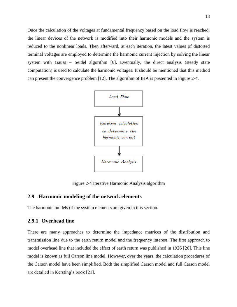
can present the convergence problem [12]. The algorithm of IHA is presented in Figure 2-4.

Figure 2-4 Iterative Harmonic Analysis algorithm

2.9 Harmonic modeling of the network elements

The harmonic models of the system elements are given in this section.

2.9.1 Overhead line

There are many approaches to determine the impedance matrices of the distribution and

transmission line due to the earth return model and the frequency interest. The first approach to

model overhead line that included the effect of earth return was published in 1926 [20]. This line

model is known as full Carson line model. However, over the years, the calculation procedures of

the Carson model have been simplified. Both the simplified Carson model and full Carson model

are detailed in Kersting’s book [21].

14

Carson line model

The calculation procedure for two conductors is presented in Figure 2-5. The self and mutual

impedance of each conductor is calculated from the conductor i and k, and their images i’ and k’.

Figure 2-5 Phase conductors and images

Due to effect of earth return, correction factor should be applied to the computation of self and

mutual impedances. This correction factor can be calculated as:

2 2 2 3 41 2 cos 3 cos4

cos cos 2 cos 2 0.6728 ln sin 28 16 16 16 15363 2 45 2

π k k k k θ πk θP k θ θ θ θ θ

k

(2.14)

Where 𝑘 and 𝜃 are defined as:

3

1.713 10

i

fk h

ρ (2.15)

0θ (2.16)

2 3 4

1 2 1 cos 2 cos 3 sin4 20.0386 ln cos (ln 1.0895)

2 64 3843 2 45 2

πk θ k θ k θ θQ k θ

k k(2.17)

Where 𝑘 and 𝜃 are defined as:

3

0.8565 10

ik

fk D

ρ (2.18)

15

1cos ( )

i k

ik

h hθ

D (2.19)

The simplified model is provided as follows:

8

π

P (2.20)

1 2

0.0386 ln2

Qk

(2.21)

As can be seen, in simplified method, the function of variable 𝜃 is ignored.

The self-resistance and self-inductive reactance of each conductor can be determined as:

4 ii c

R R ωPG (2.22)

2

2 ln( ) 4 i

ii int

i

hX X ωG ωQG

r (2.23)

where

2 ln( ) i

int

i

rX ωG

GMR (2.24)

The self and mutual impedance of the transmission line based upon Carson line model are

obtained from following equations:

ii

i

ρZ f R f f j

GMR fc

1 1( ) 0.00158836 0.00202237 1 ln 7.6786 ln

2

(2.25)

ik

ik

ρZ f f f j

D f

1 1( ) 0.00158836 0.00202237 1 ln 7.6786 ln

2

(2.26)

2 2

k

2

k

2( )

ij i iD x x y y (2.27)

where:

Zii : Self-impedance of conductor i in Ω / mile

Zik : Mutual-impedance of conductor i in Ω / mile

Ri : Resistance of conductor i in Ω / mile

f : System frequency in Hz

GMRi : Geometric Mean Radius of conductor i in ft.

16

Dik : Distance between conductors i and j in ft.

𝜌 : Resistivity of earth in Ω / meters (assume 100 Ω / meters)

𝑅𝑐 : DC resistance at 25 C in Ω

𝑥𝑖 : Horizontal distance between conductors in ft

𝑦𝑖 : Veridical distance between conductors in ft

𝐺 : Multiplying factor (0.1609347 x 10-3

ohm/mile)

𝑅𝑖𝑖 : Self-resistance of the conductors

𝑋𝑖𝑖 : Self-inductive reactance

Deri line model

Deri equations for self and mutual impedance of a distribution or transmission line are obtained

from the simplification to the full Carson line model. It should be taken into account, the

simplified Carson has some convenient approximations for limited range of frequencies and

medium frequencies are not covered. On the other hand, Deri approach results in simple formulas

which are valid throughout, from very low frequencies up to several MHz [22]. Thus, Deri line

models are employed in the harmonic studies of the lines. Deri line model is provided by using:

0

1 1( ) p σ

ρjωμ σ (2.28)

2 2

1

c

e i i

σπ r r R

(2.29)

0

1

c

c

pj ω μ σ

(2.30)

1

2

c e c

Zπ σ r p

(2.31)

1

( ) ( 2) n n nc

Z R Z n (2.32)

i

ii c

e

μ h pZ jω Z

π r

02( )

ln2

(2.33)

i k ik

ij

i k ik

h h p dμZ jω

π h h d

2 2

0

2 2

( 2 )ln

2 ( )

(2.34)

17

Where:

Zii : Self-impedance of conductor i in Ω / km

Zij : Mutual-impedance of conductor i in Ω / km

Ri : Resistance of conductor i in Ω / km

𝜔 : 2𝜋 × 𝑓

ℎ𝑖 : Heights of the conductors i above the ground in meter

ℎ𝑘 : Heights of the conductors’ k above the ground in meter

𝜇0 : 4π × 1e − 7

f : System frequency in Hz

𝑑𝑖𝑘 : Horizontal separation in meter

𝑟𝑒 : External radius in meter

𝑟𝑖 : Internal radius in meter

𝑅𝑖 : DC resistance at 25 Hz in Ω

The most difference in the line impedance matrices of the simplified Carson, full Carson and Deri

approaches is coming from difference assumptions for internal impedance of the conductors and

handling of the conductor GMR [23].

The equivalent impedance matrix of the line calculated by Carson or Deri formula is given by:

( ) ( ) ( ) ( )

( ) ( ) ( ) ( )( )

( ) ( ) ( ) ( )

( ) ( ) ( ) ( )

abcnZ f

aa ab ac an

ba bb bc bn

ca cb cc cn

na nb nc nn

Z f Z f Z f Z f

Z f Z f Z f Z f

Z f Z f Z f Z f

Z f Z f Z f Z f

(2.35)

'ij inabcabc abc

'nng ng nj nn

Z ZVV I

IV V Z Z (2.36)

After Kron’s reduction, the equation is given by:

1

abc ij in nn nj

Z Z Z Z Z (2.37)

18

( ) ( ) ( )

( ) ( ) ( ) ( )

( ) ( ) ( )

abcZ f

aa ab ac

ba bb bc

ca cb cc

Zs f Zs f Zs f

Zs f Zs f Zs f

Zs f Zs f Zs f

(2.38)

series( ) ( )

abcZ f Z f (2.39)

Several effects which are normally ignored at power frequencies have to be included at harmonic

frequencies, for instance [24]:

Frequency dependence

Long line effects

Line impedances

Line transpositions

VAR compensation plant

In this section frequency dependence, long line effects and line impedances are explained. Line

transpositions and VAR compensation plant are detailed in [24]. For calculation of transmission

line parameters in harmonic frequencies, following theories should be covered:

Evaluation of lumped parameters or PI model

Evaluation of distributed parameters or distributed model

Evaluation of Skin effect in transmission lines

1- PI (lumped parameters)

Figure 2-6 presents the equivalent circuit of PI. This model consists of series impedance and

shunt capacitance which is divided into two equal parts and placed at the two ends of the line.

The shunt capacitance of the line is computed as follows:

Figure 2-6 PI model

19

1

lˆ n ( )2

ii

ii

i

S mileP

πε RD μF (2.40)

1

ln ( )2

ˆ ij

ij

ij

S mileP

πε D μF (2.41)

i2

iiS y (2.42)

2 2

(( ) ( ) ) ij ij ii

S D S (2.43)

n n

2 2(( ) ( ) )

in i iS x x y y (2.44)

where

Pii : Self-impedance of conductor i in Ω / mile

Pij : Mutual-potential coefficients of conductor

Sii : Distance from Conductor i to its image. (ft.)

Sii : Distance from Conductor i to the image of Conductor j (ft.)

Sin : Distance from Conductor i to the image of Neutral (ft.)

RDi : Radius of Conductor i in ft.

Dij : Distance from Conductor i to Conductor j (ft.)

휀 : Permittivity of air (Assume 1.4240 × 10−2 (𝜇𝐹

𝑚𝑖𝑙𝑒) )

ˆ ˆ ˆ ˆ

ˆ ˆ ˆ ˆˆ

ˆ ˆ ˆ

ˆ ˆ ˆ ˆ

primitiveP

aa ab ac an

ba bb bc bn

ca cb cc cn

na nb nc nn

P P P P

P P P P

P P Z P

P P P P

(2.45)

in

ˆ ˆˆ

ˆ ˆ

P

ij

primitive

nj nn

PP

P P (2.46)

Kron’s reduction is applied to obtain:

1

abc ij in nn njP P P P P (2.47)

1 abc abc

C P (2.48)

20

1 2 1.609344 ( ) abc abcY C j πf l μS (2.49)

where

𝑓 : Frequency in Hz

l : Length in km

2- Equivalent PI (distributed parameters)

Due to standing wave effect on voltage and current in long line, a number of PI models (lumped

parameters) are connected in series to improve accuracy of voltage and current. According to the

power system harmonic book written by Arrilaga, three phase PI model can provide accuracy to

1.2% for quarter wavelength line (a quarter wavelength corresponds with 1500 and 1250 km at

50 and 60 Hz respectively). As frequency increase the number of nominal PI section to maintain

a particular accuracy increases proportionally. For instance, a 300 km line requires 30 nominal PI

section to maintain the 1.2% accuracy [6]. Therefore, the long line effect should be included.

And, the line parameters are distributed along the length of the line in a way to avoid lumping

them in one place. In distributed model, the equivalent PI model (distributed parameters) is

calculated from the PI model (lumped parameters) by multiplying the correction factors to the

series impedance and shunt admittance. For the single phase the correction factor is given by:

For series impedance:

` `

` `

sinh( )x Z Y

x Z Y (2.50)

For shunt admittance

` `

` `

tanh( )2

2

x Z Y

Z Yx

(2.51)

where

𝑥 : Length of the line

𝑍` : Series impedance calculated in PI nominal in Ω/km

𝑌` : Shunt admittance which is calculated in PI nominal in 𝛺−1/km

21

Since there is no direct way of computing sinh or tanh of a matrix, eigenvalues and eigenvectors

are employed for three phase line models.

abc abc

Z Yv

T eig (2.52)

abc abc

Y Zi

T eig (2.53)

1

m abcZ Z

v iT T (2.54)

1

m abcY Y

i vT T (2.55)

m m m

Γ Z Ydiag (2.56)

T T

i vT T (2.57)

1 1( ) ( ) sinh( )

series abc m m

Z f Z Γ Γi i

f T diag l T (2.58)

1 1( ) 2 h( ) ( )

2tan

shunt m m abc

Y f Γ Γ Yi i

lT diag T f (2.59)

where

𝑓 : Frequency in Hz1

𝑍𝑎𝑏𝑐 : Series impedance calculated in PI nominal in Ω/km

𝑌𝑎𝑏𝑐 : Shunt admittance which is calculated in PI nominal in 𝛺−1/km

𝑍𝑠𝑒𝑟𝑖𝑒𝑠 : Series distributed impedance in 𝛺

𝑌𝑠ℎ𝑢𝑛𝑡 : Shunt distributed impedance in 𝛺

The use of PI model (lumped parameters) at fundamental frequency can offer several advantages:

It requires lowest calculations and is easy to be implemented.

It can be used in any configuration or number of parallel circuits.

It can be used in the simulation related to transient or dynamic processes.

Moreover, PI model (lumped parameters) has some disadvantages:

There are considerable errors in the use of lumped parameter when the transmission

length is greater than 150 km at fundamental frequency (50 or 60 Hz) and 15 km at 600

Hz. Therefore, transmission lines cannot be represented with PI (lumped parameters) at

harmonic frequencies.

22

PI model does not represent frequency dependence on R and L in the case of studies

related to the frequency response or harmonics [25].

Equivalent PI (distributed parameters) must be used in any study where the frequency changes

are relevant to the results such as harmonic analysis [25].

3- Skin Effect

In transmission lines, the current flowing tends to flow on the surface of the conductor. Due to

this fact, there is an increase in the resistance and decrease in internal inductance. This effect

increases as frequency increases and it is termed the skin effect [6].

The skin effect in transmission lines is explained in [6] and [24]. The equation of skin effect is

provided as follows:

2

0 skin ll

Z R Z (2.60)

0 2 2

, ,

1

( )

ext l int l c

Rπ r r δ

(2.61)

0 2 2

, ,

1

( )

ext l int l c

Rπ r r δ

(2.62)

,

1

2

ext l c C

Zπr δ ρ

(2.63)

0

1

C

c

ρjωμ δ

(2.64)

where

𝑟𝑖𝑛𝑡,𝑙 : Internal radius of the conductor l in m

𝑟𝑖𝑛𝑡,𝑙 : External radius of the conductor l in m

𝛿𝑐 : Conductivity of the conductor in S/m

The impedance scan of a transmission line with different harmonic models are presented in

Figures 2.7 to 2.12; the line length is 300 km and Deri equation is used to calculate the series

impedance of the line. Table 2-1 shows the line parameters data at fundamental frequency.

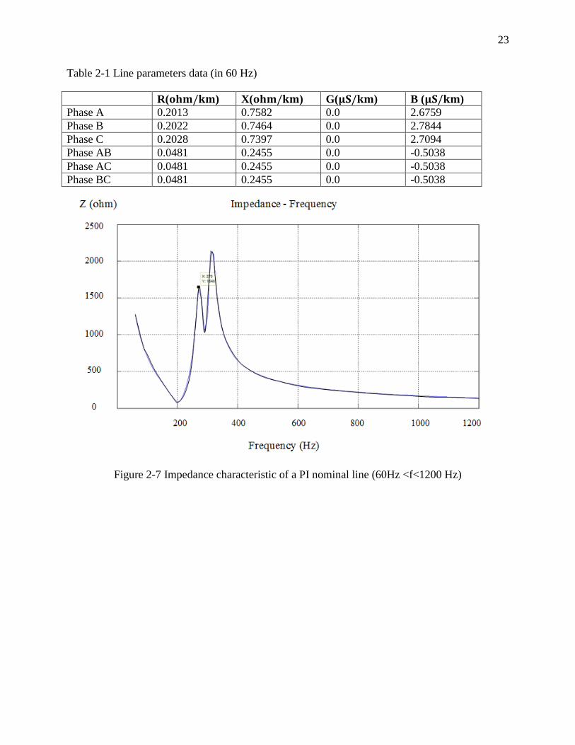
23

Table 2-1 Line parameters data (in 60 Hz)

R(𝐨𝐡𝐦/𝐤𝐦) X(𝐨𝐡𝐦/𝐤𝐦) G(𝛍𝐒/𝐤𝐦) B (𝛍𝐒/𝐤𝐦)

Phase A 0.2013 0.7582 0.0 2.6759

Phase B 0.2022 0.7464 0.0 2.7844

Phase C 0.2028 0.7397 0.0 2.7094

Phase AB 0.0481 0.2455 0.0 -0.5038

Phase AC 0.0481 0.2455 0.0 -0.5038

Phase BC 0.0481 0.2455 0.0 -0.5038

Figure 2-7 Impedance characteristic of a PI nominal line (60Hz <f<1200 Hz)

24

Figure 2-8 Real part of a PI nominal line (60Hz <f<1200 Hz)

Figure 2-9 Imaginary part of a PI nominal line (60Hz <f<1200 Hz)

25

Figure 2-10 Impedance characteristic of a distributed line (equivalent PI) (60Hz <f<1200 Hz)

Figure 2-11 Real part of a distributed line (equivalent PI) (60Hz <f<1200 Hz)

26

Figure 2-12 Imaginary part of a distributed line (equivalent PI) (60Hz <f<1200 Hz)

2.9.2 Cable

The harmonic model of cables is very similar to overhead lines. However, cables have higher

shunt capacitance than overhead lines [5]. Therefore, the equivalent PI model (distributed

parameters) can be applied for cables.

2.9.3 Voltage sources

At harmonic frequencies, the sources are grounded and represented by lumped impedance; the

equivalent admittance matrix of the source is constructed by:

R jX h h

aZ (2.65)

1[ ]

h h

source abcY Z

h h h

x y z

h h h

z x y

h h h

y z x

Y Y Y

Y Y Y

Y Y Y

(2.66)

Where

R : Resistance of source

27

X : Reactance of source

𝑍(ℎ) : Harmonic impedance of the source in ohm

ℎ : Harmonic order

𝒀𝒏 is a 2n x 2n matrix for n phase line:

h

n sourceY Y

h h h

x y z

h h h

z x y

h h h

y z x

Y Y Y

Y Y Y

Y Y Y

(2.67)

2.9.4 Transformers

The transformers at harmonic frequencies are represented with constant RL branches. The

equivalent circuit is shown in Figure 2-13. The frequency dependence is usually ignored as the

harmonic frequencies cover a small range frequency band. The nonlinear characteristics of the

magnetizing branch and winding stray capacitance tend to produce harmonic distortions (mainly

3rd

). Consequently, a harmonic source can be used to represent these distortions, although the

effect is often negligible.

The harmonic impedance of transformers is modified with following equation:

Z h R jX h (2.68)

Where

R : Resistance of transformer

X : Reactance of transformer

The admittance matrix of the transformer in general format can be computed using:

10 0

0 0

0 0

Y

Z

Z

Z

(2.69)

28

Figure 2-13 Yg yg transformer

The equivalent admittance of Ygyg transformer shown in figure 2.13 is given by:

_ 1 _ 1

_ 2

_ 3

_ 1

_ 2

_ 3

n

0 0 0 00 00

0 0 0 00 00

0 0 0 00 00

0 00

0 00

0 00

0 00

0 00

0 00

0 00 0 0 0

0 00 0 0 0

Y

a b c aab c

a

b

c

sHX mHX mHX sHXa

sHX mHXmHX mHXb

sHXmHX mHX mHXc

sHX mHX mHX sa

sHX mHXb mHX

sHXc mHX mHX

m m m nk k k

k

k

k

Y Y Y -Ym

Y YY -Ym

YY Y -Ym

-Y -Y -Y Yn

-Y -Yn -Y

-Yn -Y -Y

o

p

_ 2

_ 3

_ 1

_ 2

_ 3

0 0 0 0

0 0 0 0

0 0 0 0

0 0

0 0

0 0

0 0

0 0

0 0

00 0 0

00 0 0

b c

mHX mHX

sHX mHX

sHXmHX

HX mHX mHX

sHX mHXmHX

sHXmHX mHX

Hg

Xg

n n o p

-Y -Y

-Y -Y

-Y-Y

Y Y

Y YY

YY Y

Y

Y

(2.70)

Where

_sHX iY : Self admittance seen on the low side for unit i, i = 1, 2, 3

HgY : Grounding admittance for high side

XgY : Grounding admittance for low side

Three phase power transformer can also give a phase shift to harmonic voltages and currents. The

matrix Dc accounts for it in the MANA formulation

Dc (for Yg yg) is given by:

29

1 2 3

1

2

3

1 2 3

0 0

0 0

0 0

1 0 0

0 1 0

0 0 1

1 1 1

cD

a

b

c

a

b

c

q q q

k g

k g

k g

m

m

m

o g g g

p

(2.71)

Where

𝑔𝑖 : Turn ratio of the ideal transformer i, i = 1,2,3

2.9.5 Loads

Loads may either significant affect in damping or resonance conditions of the systems,

particularly at higher frequencies. Harmonic modeling of linear loads is related to (i) load size

(ii) composition and (iii) connection types. A typical composition of ordinary loads is presented

in Table 2-2. There are three types of loads: 1- Spot loads (Resistive) 2- Rotating loads

(inductive) 3- Nonlinear loads (harmonic sources)

Table 2-2 Typical load composition [9]

Nature Type of loads Electrical Characteristics

Domestic Incandescent lamps Spot load (Resistive)

Commercial Fluorescent lamps Nonlinear loads (harmonic

sources)

Industrial

Motors Rotating loads (inductive)

Computers Nonlinear loads (harmonic

sources)

Home electronics Nonlinear loads (harmonic

sources)

Resistive heater Spot loads (Resistive)

Air conditioning Rotating loads (inductive)

ASDs Nonlinear loads (harmonic

sources)

Pumps Rotating loads (inductive)

Arc Furnace Nonlinear

30

1- Spot loads

Four types of harmonic models are available for spot loads: (i) RL series (ii) RL parallel (iii) RL

parallel with skin effect and (iv) CIGRE/EDF. Loads at fundamental frequency are represented as

PQ loads. However, in harmonic frequencies, they are modified into equivalent admittances

which are calculated from active and reactive power at fundamental frequency. Three single

phase units are used to obtain a three phase model.

(i) RL Series

In harmonic modeling of systems, individual loads are represented with RL series. Following

schema shows the harmonic model of RL series loads at harmonic frequencies:

Figure 2-14 Equivalent circuit for RL series load

The equivalent impedance is calculated as follows:

2

2 2.

VR P

P Q (2.72)

2

2 2. .

VX h h Q

P Q (2.73)

. i i i

Z h R j X h (2.74)

Where

𝑉 : Nominal voltage in volts

𝑃 : Active power for each phase in W

𝑄 : Reactive power for each phase in VAR

(ii) RL Parallel

31

Figure 2-15 shows a RL parallel load. In harmonic modeling of systems, lumped loads are

represented with RL parallel.

Figure 2-15 Equivalent circuit of RL parallel

Equivalent impedance is calculated as follows:

2

V

RP

(2.75)

2

.V

X h h Q

(2.76)

.i i i

Z h R j X h (2.77)

(iii) RL parallel with skin effect

Figure 2-16 shows the scheme of RL parallel with skin effect. This harmonic model is best used

to represent lumped loads in the systems. In addition, it can provide frequency dependent

parameters.

Figure 2-16 RL equivalent circuit of RL parallel with skin effect

Equivalent impedance is calculated as follows:

32

2

( ).

V

R hm h P

(2.78)

2

..

V

X h h m h Q

(2.79)

0.1. 0.9 m h h (2.80)

.i i i

Z h R j X h (2.81)

Note that, whether the induction motor demand over the total demand is less than 0.1 or the linear

loads behave as constant impedance, the model (i), (ii) and (iii) can provide a good

approximation [11].

(iv) CIGRE/EDF

The CIGRE type C is best used to represents bulk loads as series and parallel RL circuit. In this

model, the resistive part of the load is calculated for the distribution transformers including a

series reactance. The inclusion of the distribution transformer reactance tends to reduce damping

at higher frequencies [11]. It should however be noticed that this approximation is not valid

for h < 5 . Figure 2-17 shows the equivalent impedance of a CIGRE type C. This harmonic

model is suggested by IEEE Power Eng. Soc. T&D Committee.

Figure 2-17 Equivalent circuit of a CIGRE type C

Equivalent impedance is calculated by:

2

V

R P

(2.82)

1

.

6.7 0.74

h RX

Q

P

(2.83)

33

20.073. .X h R (2.84)

1 2( ) ( . )

iZ h R jX j X h (2.85)

Y connection of spot load is presented in figure 2.18

Figure 2-18 Y connection of spot load

For Y connection the impedance is given by:

1

1

( ) 0 0

0 ( ) 0

0 0 ( )

kk iY Z h

a

b

c

Z h

Z h

Z h

(2.86)

Figure 2-19 Delta connection of spot load

Figure 2-19 illustrates delta connection of spot loads. Equivalent impedance is given by:

1( )

ij ij

Y h Z h (2.87)

1( )

ii ii

Y h Z h (2.88)

( ) ( ) ( ) ( )

( ) ( ) ( ) ( )

( ) ( ) ( ) ( )

kkY

ab ac ab ac

ab ab bc bc

ac bc cb ac

Y h Y h Y h Y h

Y h Y h Y h Y h

Y h Y h Y h Y h

(2.89)

Where

𝑍𝑖𝑗 : Equivalent impedance of each load (each phase) for delta connection

34

Eventually:

kkY

h h h

x y z

h h h

z x y

h h h

y z x

Y Y Y

Y Y Y

Y Y Y

(2.90)

nY

a b c

h h h

a x y z

h h h

b z x y

h h h

c y z x

k k k

k Y Y Y

k Y Y Y

k Y Y Y

(2.91)

For a load has P = 1500 kW and Q = 500 kVAR, the impedance scan of all types of harmonic

models are presented in Figures 2-20 to 2-27.

Figure 2-20 Impedance scan of RL series load (60 Hz < f < 1200 Hz)

35

Figure 2-21 Impedance phase of RL series load (60 Hz < f < 1200 Hz)

Figure 2-22 Impedance scan of RL parallel load (60 Hz < f < 1200 Hz)

36

Figure 2-23 Impedance phase of RL parallel load (60 Hz < f < 1200 Hz)

Figure 2-24 Impedance scan of RL parallel load with skin effect (60 Hz < f < 1200 Hz)

37

Figure 2-25 Impedance phase of RL parallel load with skin effect (60 Hz < f < 1200 Hz)

Figure 2-26 Impedance scan of CIGRE type C (60 Hz < f < 1200 Hz)

38

Figure 2-27 Impedance phase of CIGRE type C (60 Hz < f < 1200 Hz)

2- Rotating load

Two types of harmonic models are available for rotating loads: (i) Induction Motor (ii)

Synchronous Motor

The harmonic models present in this work are based on sequence impedance. Under unbalance

conditions or for inter-harmonic studies, it is necessary to obtain the harmonic impedance for

machines of all three sequences (zero, positive, and negative).

(i) Induction Motor

Induction machine is represented with the sequence impedances. The positive and negative

impedance of the induction machine is presented in equation 2.84 to 2.86. Figure 2.28 presents

the equivalent circuit of induction motor which is composed of stator impedance, a magnetization

branch with a core loss resistance, and slip-dependent rotor impedance. Since the type of

connection of induction machine is Delta or Y ungrounded, there is no path for zero sequence

current in a circuit; the zero sequence impedance is infinite consequently.

39

Figure 2-28 Equivalent circuit of induction motor

The harmonic slips of induction for positive sequence harmonics and negative sequence

harmonics are deference. The harmonic slips of the induction motor for each harmonic sequence

are given by:

1 1

1

h r

h

h

ω ω h s hS for h for Positive harmonic sequence

ω h h (2.92)

1

1

h

hS for h for Negative harmonic sequence

h (2.93)

where

𝜔ℎ : Synchronous frequency

𝜔𝑟 : Rotor angular frequency

𝑠 : Conventional slip at fundamental frequency

In the case of deep bar, a double – cage motor, the rotor resistance (Rr) increases significantly at

slip frequencies due to skin effect, which concentrate the rotor current in the outer edge of the

rotor bar. The rotor reactance (Xr) decreases slightly as the slip frequency decreases [5].

Therefore, the equation of rotor resistance and reactance due to skin effect are modified with

following equations:

( ) 1 r

r h

h

RR h CFR S

S (2.94)

( ) 1 r r h

X h X CFX S (2.95)

where

𝑅𝑟(ℎ) : Frequency dependent rotor resistance

40

𝐿𝑟(ℎ) : Frequency dependent rotor inductance

𝑅𝑟 : Dc rotor resistance

𝑋𝑟 : Dc rotor reactance

𝐶𝐹𝑅 : Rotor cage factors for rotor resistance

𝐶𝐹𝑋 : Rotor cage factors for rotor inductance

𝑆ℎ : is the slip at the harmonic frequency

Stator impedance:

s s s

Z h R h jX (2.96)

where

𝑅𝑠 : Stator resistance.

𝑋𝑠 : Stator reactance.

Magnetization:

2

3 1( )

4 4

m m

R h Rh h

(2.97)

( ) m m

X h h X (2.98)

( ( ) ( ))

( ( ) ( ))

m m

m

m m

R h jX hZ h

R h jX h (2.99)

where

𝑅𝑚 : Magnetization resistance.

𝑋𝑚 : Magnetization reactance.

In unbalanced three phase system, the equivalent admittance matrix of induction machine is

calculated from the sequence admittance matrix by means of Fortescue transformation.

( ) ( ) p s m p r

Z h Z h Z h Z h (2.100)

( ) ( ) n s m n r

Z h Z h Z h Z h (2.101)

41

0 0

0 0

0 0

Zinduction p

n

Z

Z

(2.102)

1

abc inductionZ A Z A (2.103)

1h

induction inductionY Z (2.104)

where

𝑍𝑛 (ℎ) : Negative sequence rotor impedance.

𝑍𝑝(ℎ) : Positive sequence rotor impedance.

Yn of induction machine is given by:

h

kk inductionY Y (2.105)

n kkY Y (2.106)

nY

a b c

h h h

a x y z

h h h

b z x y

h h h

c y z x

k k k

k Y Y Y

k Y Y Y

k Y Y Y

(2.107)

The impedance characteristic of an induction machine is shown in figures 2.28 to 2.29 for the

following induction machine parameters:

Rs = 5.0288 ohm, Xs = 20.1153 ohm, Rm = 6275.97 ohm, Xm = 704.04 ohm, Rr = 5.3479 ohm,

Xr = 20.1153 ohm, CFr = 0.0, CFx = 0.0

Note that all parameters are determined at fundamental frequency (60 Hz)

42

Figure 2-29 Impedance scan of induction motor (60Hz < f< 1200 Hz)

Figure 2-30 Phase impedance of induction motor (60Hz < f< 1200 Hz)

43

(ii) Synchronous Motor

The harmonic model of synchronous machine is represented with sequence impedance. For the

frequencies slightly greater than fundamental frequency, the sub-transient reactance multiplied

harmonic order is employed for positive and negative sequence harmonics and the zero sequence

reactance multiplied harmonic order is employed for zero sequence harmonics. Hence, the

harmonic impedance of the synchronous machine is modified with following equations:

2

'' ''

d q''X X

X (2.108)

1 ''X h h X (2.109)

2 ''X h h X (2.110)

0 0 X h h X (2.111)

where

𝑋𝑑′′ : Sub-transient reactance (d axis)

𝑋𝑞′′ : Sub-transient reactance (q axis)

𝑋0 : Zero sequence reactance

𝑋1 : Positive sequence reactance

𝑋2 : Negative sequence reactance

The resistance of the machine should be corrected due to the skin effect. The resistance at high

frequencies is modified with following equation:

(1.0 ) BR h R Ah (2.112)

where

R : Armature dc resistance

1 h

synch 012Z A Z A= (2.113)

1[ ]

h h

synch synchY Z

h h h

x y z

h h h

z x y

h h h

y z x

Y Y Y

Y Y Y

Y Y Y

(2.114)

where

44

012Z : Sequence impedance of the synchronous machine

Yn for Y grounded motor is defined by:

Figure 2-31 Synchronous motor (Yg)

h

kk synchY Y (2.115)

h

gZ

gh Z (2.116)

0

0

n

kk

YY

h

gY

(2.117)

Yn in detail format is given by:

0 0 0

0

0

0

nY

a b c

h

g

h h h

a x y z

h h h

b z x y

h h h

c y z x

g k k k

g Y

k Y Y Y

k Y Y Y

k Y Y Y

(2.118)

𝒀𝒏 for Delta connection is defined by:

Figure 2-32 Synchronous motor (Delta or Y)

n kkY Y (2.119)

45

nY

a b c

h h h

a x y z

h h h

b z x y

h h h

c y z x

k k k

k Y Y Y

k Y Y Y

k Y Y Y

(2.120)

Impedance scan of a synchronous machine is shown in Figure 2.31; the parameters of the

machine are presented in Table 2-3. As can be seen from Figure 2-32, the phase impedance of

synchronous machine is mostly 90 degree.

Table 2-3 Parameters of synchronous machine at fundamental frequency 60 Hz

R (ohm) X (ohm)

Steady state 17.62344 176.23

Transient 9.09411 115.8898

Sub transient 7.90792 100.7737

Zero sequence 2.60961 33.25

Negative sequence 7.90792 100.7737

Grounding 0.0 0.0

Figure 2-33 Impedance characteristic of synchronous machine (60 Hz < f<1200 Hz)

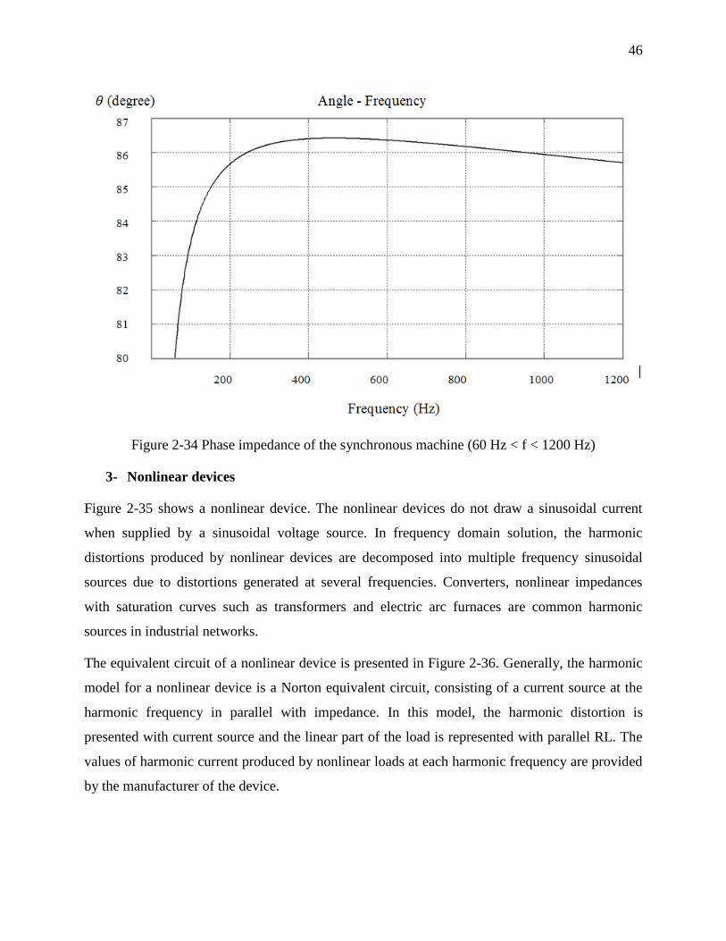
46

Figure 2-34 Phase impedance of the synchronous machine (60 Hz < f < 1200 Hz)

3- Nonlinear devices

Figure 2-35 shows a nonlinear device. The nonlinear devices do not draw a sinusoidal current

when supplied by a sinusoidal voltage source. In frequency domain solution, the harmonic

distortions produced by nonlinear devices are decomposed into multiple frequency sinusoidal

sources due to distortions generated at several frequencies. Converters, nonlinear impedances

with saturation curves such as transformers and electric arc furnaces are common harmonic

sources in industrial networks.

The equivalent circuit of a nonlinear device is presented in Figure 2-36. Generally, the harmonic

model for a nonlinear device is a Norton equivalent circuit, consisting of a current source at the

harmonic frequency in parallel with impedance. In this model, the harmonic distortion is

presented with current source and the linear part of the load is represented with parallel RL. The

values of harmonic current produced by nonlinear loads at each harmonic frequency are provided

by the manufacturer of the device.

47

Figure 2-35 Nonlinear load

Figure 2-36 Norton equivalent of a nonlinear load

The harmonic current in MANA is given by:

1

2

3

1

h

bI

h

aequ

h

bequ

h

cequ

q I

q I

q I

(2.121)

where

h

i, equI : Harmonic current at phase i (a,b,c)

48

CHAPTER 3 PLANNING OF LARGE HARMONIC FILTERS IN

INDUSTRIAL NETWORKS

In this chapter, the use of passive harmonic filters to control and limit the harmonic voltages and

currents are discussed. Different types of passive filters used to decrease harmonic distortions

within IEEE 519 requirements, are detailed.

This chapter also shows a simple methodology to place harmonic filters in a system with multiple

harmonic sources. This methodology is based on brute face search while it attempt to reduce

possible candidates and accordingly speed up the process.

3.1 Literature review

In [26] two strategies for calculating the parameters of harmonic filters are suggested: 1-

fundamental frequency reactive power compensation and 2- calculation of filter parameters using

Z-bus method. The methodology used in [27] to size harmonic filters considers: 1- reactive

compensation 2- IEEE standards for maximum harmonic distortions 3- power system variations

4- filter detuning. In [7] the filter sizing for high pass filters and single tuned filters are presented.

A systematic approach to design single tuned filter is described in [28]. The proposed method

considers the detuning effects due to temperature and frequency variations, as well as

manufacturing tolerances. In [29] a transfer function approach in the analysis and design of

passive harmonic filters is presented. The transfer function approach derives an analytical

formulation of a utility system including passive filter with a basis of Laplace transformation. In

[30] a particle swarm optimization method with nonlinear time-varying evolution is used in the

planning of passive harmonic filters for a system under multiple harmonic sources. The aim of

this optimization is to minimize the cost of filters and the filters loss.

Many efforts have been put to find the most efficient location for placing harmonic filters. A

chance constrained programming model for optimal planning of harmonic filters is presented in

[31]. Considering the randomness of the decision environment as well as the merits and

shortcomings of these two kinds of filters, a chance constrained programming model for unified

optimal allocation of active and passive filters is proposed in this paper, and a stochastic

simulation based genetic algorithm to solve the model is developed. In [32] an approach for

determining optimal or near-optimal locations and sizes of single-tuned passive harmonic filters

49

among existent capacitor busses in a power system is explained. In this paper, the constrained

problem is formulated and is solved by a genetic algorithm-based optimizer. Another approach

for filter allocation is described in [3]. The proposed strategy requires a limited knowledge of the

system impedance; in addition, it is independent of the knowledge of the harmonic current

injection locations and parameters. In [33] the harmonic filters are placed at different locations in

IEEE 13 bus industrial system and the results are compared. The genetic algorithm and simulated

annealing are common methodologies used to harmonic filter allocation. In [34] , [35] and [36],

genetic algorithm for harmonic filter allocation is discussed. However, given the small number of

nodes in industrial networks and the efficiency of frequency domain solvers, it is possible to

address straightforward techniques as will be demonstrated in this work.

3.2 Harmonic filter

The harmonic filters are one of the solutions for control of harmonic distortion. They are three

types of harmonic filters:

1- Passive harmonic filters

2- Active harmonic filters

3- Hybrid harmonic filters

3.2.1 Passive harmonic filters

Passive harmonic filters are designed to provide low impedance at tuned frequencies. There are

two configurations, use of series reactors or shunt impedances. Although the shunt impedance is

more costly than the series reactor, they successfully accomplish two purposes:

1- Control of harmonics

2- Power factor correction

Series reactors provide significant harmonic reduction at high harmonic orders (h>11), however

at low harmonic orders, the reduction is not considerable.

50

3.2.2 Active harmonic filter

Active harmonic filters inject specific current to control harmonic distortions and compensate the

reactive power. The performance of active filters depend also on its control algorithm, they can

also be used to regulate the terminal voltage simultaneously.

3.2.3 Hybrid harmonic filter

In some industrial applications, the combination of the active filters and passive filters are used

and this combination is called hybrid harmonic filter. Due to this combination, the size of active

filter is reduced. Hence, the hybrid filter can provide active filter reaction at reasonable costs.

3.3 Passive filter design

The aim in filter design is to size capacitor bank to trap certain harmonics at a certain degree by

using a tuning reactor. In some cases, an external resistance can be added for the following

reasons

1- Change the sharpness of tuning frequency

2- Control the maximum current allowed through the filter

3- Avoid the overheating of filter

As a result, the harmonic filter design involves four steps:

1- Determine the reactive compensation of the bus.

2- Size the capacitor bank of harmonic filter according to the required reactive power.

3- Tune the reactor at the harmonic frequency.

4- Size the resistance according to the quality factor of the filter.

3.3.1 Single tuned harmonic filter

The single tuned filter is the most common filter in industrial applications. They provide a very

small impedance path at the tuned frequency, and absorb the harmonic current consequently.

They can result in resonances in the system. Because of that they are not recommended to be

51

used at high frequencies. The equivalent circuit of a single tuned filter is illustrated in Figure 3-1.

And, the impedance is presented in Figure 3-2.

Figure 3-1 Single tuned filter

Figure 3-2 Impedance Scan of single tuned harmonic filter (tuned at 420 Hz)

3.3.2 High pass harmonic filter

High pass harmonic filters provide small impedance path at high harmonic orders. This type of

harmonic filters can suppress harmonic propagation over a broader range frequency and is not

sensitive only to the tuned frequency. The power loss due to the resistor is significant for this

type of filter. The equivalent circuit of a high pass harmonic filter is presented in figure 3-3. And,

the impedance scan is presented in Figure 3-4.

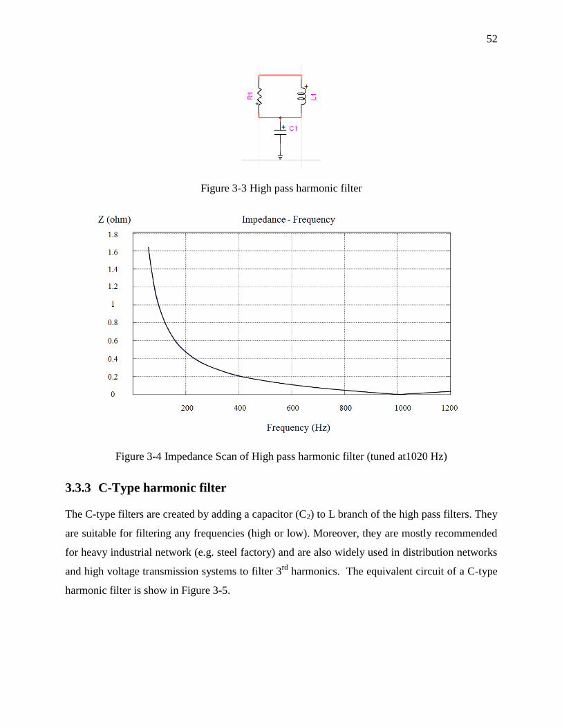
52

Figure 3-3 High pass harmonic filter

Figure 3-4 Impedance Scan of High pass harmonic filter (tuned at1020 Hz)

3.3.3 C-Type harmonic filter

The C-type filters are created by adding a capacitor (C2) to L branch of the high pass filters. They

are suitable for filtering any frequencies (high or low). Moreover, they are mostly recommended

for heavy industrial network (e.g. steel factory) and are also widely used in distribution networks

and high voltage transmission systems to filter 3rd

harmonics. The equivalent circuit of a C-type

harmonic filter is show in Figure 3-5.

53

Figure 3-5 C-Type harmonic filter

3.3.4 Multiple filter banks

When it is necessary to control harmonic distortions composed of several dominant harmonic

components, the harmonic filter should consist of several branches such that each branch

attenuates the distortion due to a specific harmonic component. One can consider a filter with

several single tuned, high pass and C- Type filters.

It is not required to tune harmonic filters for each harmonic order. Most of the time, one

harmonic filter tuned for the specific frequency can suppresses the distortions of rang of

frequencies. Figure 3.6 shows a multiple filters bank at the point of network connection.

Figure 3-6 Multiple filter bank

3.3.5 Resonance problem

The parallel resonance produced by single tuned filters can interact with the frequency response

of the system and cause a large resonance peak. At the parallel resonance frequencies, the

harmonic current can amplify voltage distortion and cause harmonic problems within the system.

The installation of several single tuned harmonic filters can provide several parallel resonances in

the system.

54

3.3.6 Constraint

In order to achieve a suitable voltage at PCC, the following constraints should be considered in

harmonic filter design:

A) Harmonic distortion limit by IEEE 519

The acceptable limits of voltage and current distortions according to IEEE 519 guideline is

presented in Table 3-1 and table 3-2. IEEE 519 set limits for harmonic current injected into PCC

as well as harmonic voltage at PCC.

Table 3-1 IEEE 519 voltage distortion limits

Voltage kV (L-L) IHD THD

> < =

0 69 3 5

69 161 1.5 2.5

161 1 1.5

Table 3-2 IEEE 519 current distortion limits

𝐈𝐡

𝐈𝐋, % − 𝐆𝐞𝐧𝐞𝐫𝐚𝐥 𝐃𝐢𝐬𝐭𝐫𝐢𝐛𝐮𝐭𝐢𝐨𝐧 𝐒𝐲𝐬𝐭𝐞𝐦 (𝟏𝟐𝟎 𝐕 − 𝟔𝟗 𝐤𝐕)

𝐈𝐡

𝐈𝐋 𝐡 < 𝟏𝟏 𝟏𝟏 ≤ 𝐡 < 𝟏𝟕 𝟏𝟕 ≤ 𝐡 < 𝟐𝟑 𝟐𝟑 ≤ 𝐡 < 𝟑𝟓 𝐡 ≥ 𝟑𝟓 𝐓𝐃𝐃 (%)

< 20 4.0 2.0 1.5 0.6 0.3 5

20 50 7.0 3.5 2.5 1.0 0.5 8

50 - 100 10 4.5 4.0 1.5 0.7 12

100 – 1000 12 5.5 5.0 2.0 1.0 15

> 1000 15 7.0 6.0 2.5 1.4 20

B) Harmonic distortion limit by IEEE 18

The filter should be designed in a way to satisfy the IEEE 18 standard requirements. According

to the IEEE 18 guideline “Capacitors shall be capable of operation under contingency system and

bank conditions provided that none of the following limitations are exceeded”:

1- 110% of rated RMS voltage.

2- 120% of rated peak voltage, i.e., peak voltage not exceeding 1.2 x √2 x rated RMS

voltage, including harmonics, but excluding transients.

3- 135% of nominal RMS current based on rated kVAR and rated voltage.

4- 135% of rated kVAR.

55

It should be noted that in section 3.4, we will discuss how to choose a suitable rated voltage for a

capacitor bank.

3.3.7 Quality factor

The ability of distributing the absorbed energy at tuned frequency is named quality factor. The

quality factor in single tuned fitters should be large enough to trap the largest amount of the

harmonic frequency; however, in high pass filters, the quality factor should be low to trap the

large amount of harmonic frequency. Typical quality factor is between 20 and 120 for single

tuned filters and between 2.5 and 5 for high pass filters.

3.3.8 Filter detuning factor

As can be seen from Figure 3-2, each single tuned filter provides series and parallel resonance in

the system. Most of the times, there are multiple dominant harmonic components in the system

and accordingly multiple single tuned filters are placed while the tuning frequencies of the filters

due to the following conditions can be changed:

1- The temperature variations can cause aging in capacitors and accordingly it would cause

decrement in capacitance value.

2- The manufacturing tolerance of the filter components can shift the tuning frequency in

any directions.

3- Removing or adding a new load or any variation in topology or configuration of the

system that changes the impedance of the system, can result in shifting of the tuning

frequency.

Shifting of series resonant point to a higher frequency point can lead the harmonic filter to

amplify the harmonic voltage distortion instead of reducing it. Therefore the harmonic filters are

typically tuned a few percent below the harmonic frequency (3% to 5% lower than the harmonic

frequency).

Detuning factor should be determined in a way to prevent interactions between the system

impedance and the resonance peak of the single tuned filter.

56

3.3.9 K-Factors transformer

K-factor addresses the problems caused by non-linear loads (harmonic sources). Sometimes the

harmonics cause overheating and subsequent insulation failure in transformer’s winding

insulation, and it is necessary to de-rate the transformer capacity. The K-Factor is given by the

following equation:

2

1

2

1

( )

h

h

h

h

I hK

I (3.1)

where

𝐼ℎ : Harmonic current at h harmonic order

𝐾 : K-Factor

For transformer with K-Factor greater than 1, the transformer should be de-rated.

3.4 Algorithm of filter design

The algorithm of harmonic filter design adopted in this work is presented as follows:


The input data required to carry out the passive filter design are detailed as follows:

Select the bus

Select the desired PF

Select the filter detuning factor (𝛿)

Select the quality factor (𝑄)

The load flow is run and following parameters at selected bus are calculated:

Determine P (active power),

Determine PF (power factor)

Determine the Thevenin equivalent impedance

The Harmonic analysis is run and following parameters at selected bus are calculated:

57

determine THDv and IHDv

Measure the voltage at each bus (at fundamental frequency and harmonic frequencies

separately)

Measure the current at each bus (at fundamental frequency and harmonic frequencies

separately)

Step 2 – Select the dominant harmonic components

According to IEEE 519, the dominant harmonic components are selected, e.g. for the nominal

voltage between 0 and 69kv, harmonic components with IHDv greater than 3% are selected.

Step 3

The harmonic voltages V(h) and harmonic currents I(h) corresponding to the selected harmonic

orders are measured.

Step 4 - Select type of filters

In this step, n numbers of harmonic orders are selected. For the first iteration n is equal to 1, and

in each iteration one filter is added (n = n+1). Then, the suitable filters for each harmonic order

are sized.

The types of harmonic filters are selected as follows:

Single tuned filter for low frequencies. (recommended for 2 < h < 17)

High pass filter for high frequencies. (recommended for h > 17 )

Step 3 - Determine the initial values of the filter components

The harmonic filters are also used to compensate the reactive power. The total reactive power

needed to correct the power factor can be determined as:

2 1(tan tan )

TotalQ P θ θ (3.2)

1 1arccosθ Pf (3.3)

1 2arccosθ Pf (3.4)

where:

𝑄𝑇𝑜𝑡𝑎𝑙 : Reactive compensation of the bus

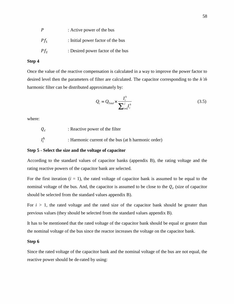
58

𝑃 : Active power of the bus

𝑃𝑓1 : Initial power factor of the bus

𝑃𝑓2 : Desired power factor of the bus

Step 4

Once the value of the reactive compensation is calculated in a way to improve the power factor to

desired level then the parameters of filter are calculated. The capacitor corresponding to the h’th

harmonic filter can be distributed approximately by:

1

h

i

c Total j h

ii

IQ Q

I (3.5)

where:

𝑄𝑐 : Reactive power of the filter

𝐼𝑖ℎ : Harmonic current of the bus (at h harmonic order)

Step 5 - Select the size and the voltage of capacitor

According to the standard values of capacitor banks (appendix B), the rating voltage and the

rating reactive powers of the capacitor bank are selected.

For the first iteration (i = 1), the rated voltage of capacitor bank is assumed to be equal to the

nominal voltage of the bus. And, the capacitor is assumed to be close to the 𝑄𝑐 (size of capacitor

should be selected from the standard values appendix B).

For i > 1, the rated voltage and the rated size of the capacitor bank should be greater than

previous values (they should be selected from the standard values appendix B).

It has to be mentioned that the rated voltage of the capacitor bank should be equal or greater than

the nominal voltage of the bus since the reactor increases the voltage on the capacitor bank.

Step 6

Since the rated voltage of the capacitor bank and the nominal voltage of the bus are not equal, the

reactive power should be de-rated by using:

59

2

2 n

c derated c

rated

VQ Q

V (3.6)

where:

𝑄𝑐 𝑑𝑒𝑟𝑎𝑡𝑒𝑑 : De-rated reactive power of the capacitor bank.

𝑉𝑛 : Nominal voltage of the bus.

𝑉𝑟𝑎𝑡𝑒𝑑 : Rated voltage of the capacitor bank.

Step 7

The equivalent reactance of the capacitor bank is calculated as:

2

c derated

c

n

QX

V (3.7)

1

c

Cω X

(3.8)

where:

𝑋𝑐 : Capacitor reactance.

𝑉𝑛 : Nominal voltage of the bus.

𝐶 : Capacitor in uf.

𝜔 : Angular frequency measured in radians per second

Step 8

The harmonic filters are tuned at their harmonic frequencies. Detuning factor should be applied to

the single tuned filter due to their sharp resonance.

The inductance of harmonic filter of single tuned filter at h’th harmonic order is calculated as:

2

1

( )

L

ω h δ C (3.9)

where:

𝐿 : Inductance of the filter.

60

𝛿 : Filter detuning factor

𝑋𝐿 : Impedance of reactor


The inductance of harmonic filter of high pass filter at h’th harmonic order is calculated as:

Lω h C 2

1

( )

(3.10)

L

X ωL (3.11)

Step 9

The resistance of the filters can be determined as:

For single tuned filters

Lh X

RQ

(3.12)

For high pass filter

L

R QR

(3.13)

where:

𝑅 : Reactive compensation of the bus

𝑋𝐿 : Impedance of reactor


𝑄 : Quality factor of the filter

Step 10 - IEEE 18

The rated voltage and the rated size of capacitor bank should satisfy the IEEE 18 requirements,

thus, the voltage and the current through the filter should be determined.

The impedance of the filter at the fundamental frequency and at the harmonic frequencies are

calculated as follows:

For single tuned filter

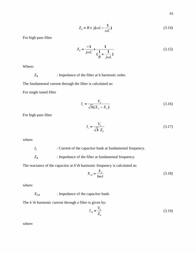
61

1

( ) h

Z R j ωL

ωC (3.14)


1 1

1 1( )

h

Z

jωC

R jωL

(3.15)

Where:

𝑍ℎ : Impedance of the filter at h harmonic order.

The fundamental current through the filter is calculated as:

For single tuned filter

3 ( )

n

c

C L

VI

X X (3.16)


3

n

c

h

VI

Z (3.17)

where:

𝐼𝑐 : Current of the capacitor bank at fundamental frequency.

𝑍ℎ : Impedance of the filter at fundamental frequency.

The reactance of the capacitor at h’th harmonic frequency is calculated as:

C

ch

XX

h δ (3.18)

where:

𝑋𝐶ℎ : Impedance of the capacitor bank.

The h’th harmonic current through a filter is given by:

h

ch

h

VI

Z (3.19)

where:

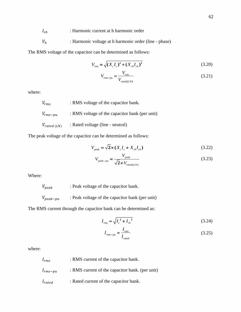
62

𝐼𝑐ℎ : Harmonic current at h harmonic order

𝑉ℎ : Harmonic voltage at h harmonic order (line - phase)

The RMS voltage of the capacitor can be determined as follows:

2 2( ) ( )

rms c c ch chV X I X I (3.20)

( )

rms

rms pu

rated LN

VV

V (3.21)

where:

𝑉𝑟𝑚𝑠 : RMS voltage of the capacitor bank.

𝑉𝑟𝑚𝑠−𝑝𝑢 : RMS voltage of the capacitor bank (per unit)

𝑉𝑟𝑎𝑡𝑒𝑑 (𝐿𝑁) : Rated voltage (line - neutral)

The peak voltage of the capacitor can be determined as follows:

2 ( ) peak c c ch ch

V X I X I (3.22)

( )2

peak

peak pu

rated LN

VV

V (3.23)

Where:

𝑉𝑝𝑒𝑎𝑘 : Peak voltage of the capacitor bank.

𝑉𝑝𝑒𝑎𝑘−𝑝𝑢 : Peak voltage of the capacitor bank (per unit)

The RMS current through the capacitor bank can be determined as:

2 2 rms c ch

I I I (3.24)

rms

rms pu

rated

II

I (3.25)

where:

𝐼𝑟𝑚𝑠 : RMS current of the capacitor bank.

𝐼𝑟𝑚𝑠−𝑝𝑢 : RMS current of the capacitor bank. (per unit)

𝐼𝑟𝑎𝑡𝑒𝑑 : Rated current of the capacitor bank.

63

The reactive power of capacitor bank can be calculated as:

newQ X I X I X h I h

c c ch ch c

2

h n

2 2(1) (1) ... ( ) ( )( ) ( ) ( ) (3.26)

new

new pu

derated

QQ

Q (3.27)

where:

𝑄𝑛𝑒𝑤 : New reactive power of the capacitor bank.

𝑄𝑛𝑒𝑤−𝑝𝑢 : New reactive power of the capacitor bank. (pu)

If any requirement is not met within the limitations of IEEE 18, the process is started over. The

rated voltage and rated reactive power of the capacitor bank should be increased (i = i+1). Then

the process is started form step 5. If all the requirements are satisfied, the process should move to

next step.

Step 11 - IEEE 519

After placing the harmonic filters, the harmonic analysis is run, then afterward, the THDv1

and

IHDv2 are determined.

If any requirement is not met within the limitations (of IEEE 519), the process is started over.

And, another filter is added (n = n+1). . Then the process is started form step 4.If all the

requirements are satisfied, the process should move to next step.

Step 12 - Check the parallel resonance

In this step, the resonance point of the system with inclusion of harmonic filter is checked.

1

2 ( )

p r

s

fπ L L C

(3.28)

where:

𝑓𝑝− 𝑟 : Parallel resonance of the filter.

1 The equations of THD (Total Harmonic Distortions) are presented in the appendix A

2 The equations of IHD (Individual Harmonic Distortions) are presented in the appendix A

64

𝐿𝑠 : Thevenin inductance of the bus.

3.5 Flowchart (1).of filter design

Figure 3-7 Flowchart 1 of Passive Filter Design

65

3.6 Flowchart (2).of filter design

Figure 3-8 Flowchart 2 of Passive Filter Design

3.7 Harmonic filters allocation

As a rule of thumb, the harmonic filters should be installed close to the harmonic sources,

however, in a system with multiple harmonic sources; this strategy may not give the best

solutions since the harmonic flow will be altered by harmonic filters. The aim is to find efficient

locations for placing the harmonic filters, the natural choices for the allocation of harmonic filter

are at the bus with the highest harmonic distortion or bus with the large nonlinear device however

as it can be seen later, the harmonic placement strongly depends on the impedance of the system

and consequently the whole system need to be analyzed [36].Moreover the installation of

harmonic filters is always costly, hence, optimization of the number of harmonic filters will result

reduction in filtering cost [24]. In the proposed algorithm in this section, all possible

configurations are simulated and the suitable configurations which can provide the maximum

reductions in harmonic distortions are selected.

66

In order to find solutions to optimal harmonic allocation, the GA (genetic algorithm) is usually

addressed [36], [35] and [37], however, it often looks like a never-ending process [38].

3.8 Algorithm of filter allocation

A simple algorithm for placing harmonic filters for medium size industrial networks is proposed

in this study.


The harmonic analysis is run (MANA harmonic analysis). THDv and IHDv are determined.

Step 2 - Identify the candidate buses

The candidate buses are identified as follows:

The buses connected to the synchronous generator are ignored (the passive filter will

decrease the power factor).

The buses with very low distortions are ignored (according to IEEE 519).

The buses required reactive power compensation are selected.

Step 3- Identify the sensitive load (optional)

The loads that need to be supplied by high quality of power is selected (optional)

Step 4 - Run proposed algorithm for sizing the suitable filters at each candidate bus

The following parameters at each simulation should be determined

THDv and IHDv at all buses

Voltages and PF at all buses

K-Factor of transformer connected to the selected bus

Step 5 – Check maximum reduction in THDv and IHDv

The buses provided maximum reduction in THDv and IHDv are selected.

Step 6 – Check overvoltage

Filter placing at some locations can provide overvoltage at other buses. These buses should be

ignored from filter allocation.

67

Step 7 – Check K-Factor

K-factor of the transformers should be checked. If filter placing at any location can cause the K-

factor of any transformer be greater than 1, this placement is not acceptable. And accordingly this

filter allocation should be ignored.

Step 8

Remaining buses are suitable locations for filters allocation.

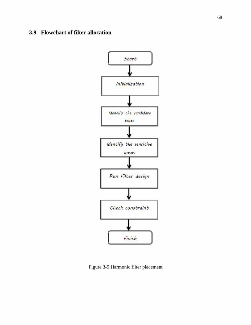
68

3.9 Flowchart of filter allocation

Figure 3-9 Harmonic filter placement

69

CHAPTER 4 TEST CASES

In this section, multiple benchmarks are tested to validate the proposed methods.

4.1 Validation of harmonic analysis based MANA

For the validation of the proposed method, a 34-bus distribution system is tested using a

MATLAB code developed specifically for the scope of this thesis. The results are validated using

EMTP-RV version 2.6.1.

4.1.1 Description of the study network

The test case is characterized by unbalanced loading of nonlinear “spot” and “distributed” loads.

In this test case, the elements of the network are modeled as follows:

Overhead lines are represented with PI harmonic model.

Transformer is represented with a series RL while R and L are not frequency dependent.

The magnetization branch is neglected. The phase shifts of voltages are automatically

considered in MANA formulation.

Spot loads and distributed loads are assumed as constant impedances. The RL parallel

harmonic model is utilized in harmonic analysis. The distributed loads are divided to two

equal loads and are placed at two ends of the lines.

Regulators are considered to be ideal.

The spot load connected to the bus #830 is assumed to be a nonlinear load. The harmonic current

produced by the nonlinear device is presented in Table 4-1. The harmonic source is defined at

different frequencies: low frequency (300Hz), medium frequency (660 Hz) and high frequency

(1260 Hz). The one line diagram of the system to be studied is illustrated in Figure 4-1.

70

Figure 4-1 IEEE 34 bus distribution system

Table 4-1 Harmonic source

Harmonic order Harmonic current (% of fundamental

current)

5 (300 Hz) 22%

11 (660 Hz) 8%

21 (1260 Hz) 5%

4.1.2 Results and discussions

The harmonic distortions of the network are determined under following conditions:

1- IEEE 34 distribution system with capacitor banks

The results of the harmonic analysis in 34 bus distribution system are presented in Table 4-2. As

can be seen from the results, the total harmonic distortion and individual harmonic distortions are

not significant at certain buses; because, the lines are long and the network is lightly loaded. In

addition to that, the capacitor bank connected to the node #844 provides filter action and

suppresses the harmonic distortions produced by the harmonic source. The figure 4-3 shows the

waveform of the voltage at Bus 800a. The voltage is sinusoidal since the large amount of the

harmonic current is absorbed by the capacitor bank (placed at Bus #844).

800

806 808 812 814

810

802 850

818

824 826

816

820

822

828 830 854 856

852

832

888 890

838

862

840836860834

842

844

846

848

864

858

71

Table 4-2 Harmonic analysis in 34 bus distribution system

Bus

h = 1 h = 5 h = 11 h = 21

THD

𝑽 𝜽 𝑽 𝜽 IHD 𝑽 𝜽 IHD 𝑽 𝜽 IHD

800a 21211.67 0.00 357.30 -71.79 1.68 77.25 -95.24 0.36 77.60 174.29 0.37 1.76

800b 21346.57 -120.02 376.22 168.26 1.76 87.08 148.33 0.41 85.08 44.60 0.40 1.85

800c 21483.67 120.01 382.22 46.63 1.78 81.95 32.89 0.38 154.85 -61.70 0.72 1.96

810b 20941.74 -120.93 376.14 168.56 1.80 86.19 149.05 0.41 81.70 46.20 0.39 1.88

822a 19348.84 -2.01 354.65 -74.63 1.83 72.13 -101.72 0.37 54.51 157.52 0.28 1.89

826b 20182.14 -122.84 370.38 170.03 1.84 75.63 152.89 0.37 46.55 60.17 0.23 1.89

838b 19824.31 -124.28 364.37 173.02 1.84 56.82 161.88 0.29 22.35 170.37 0.11 1.86

840a 19366.29 -2.75 369.11 -66.14 1.91 56.79 -77.67 0.29 23.75 -65.52 0.12 1.93

840b 19827.42 -124.27 364.40 173.05 1.84 56.82 161.92 0.29 22.33 170.46 0.11 1.86

840c 19862.34 116.54 371.98 48.87 1.87 58.12 38.32 0.29 21.72 59.24 0.11 1.90

848a 19379.10 -2.84 374.14 -66.23 1.93 60.06 -77.78 0.31 30.69 -66.21 0.16 1.96

848b 19835.92 -124.36 368.51 173.08 1.86 59.68 162.34 0.30 29.81 173.64 0.15 1.89

848c 19876.73 116.45 376.76 48.69 1.90 61.55 37.75 0.31 29.42 62.64 0.15 1.93

864a 19434.62 -2.70 369.19 -66.63 1.90 57.83 -79.36 0.30 20.44 -73.91 0.11 1.93

890a 2850.72 -4.87 51.38 -85.18 1.80 6.81 -117.61 0.24 1.34 -132.46 0.05 1.82

890b 2956.09 -126.86 52.66 151.87 1.78 7.33 119.95 0.25 1.58 80.67 0.05 1.80

890c 2931.57 114.33 52.62 28.99 1.79 6.94 -0.35 0.24 1.61 -31.29 0.05 1.81

72

Figure 4-2 Voltage waveform at Bus 880a (from MATLAB code)

2- IEEE 34 distribution system without capacitor banks

The aim of harmonic filters is to push harmonic currents in a low impedance circuit, to suppress

them from flowing in the network. The results of harmonic analysis are illustrated in Table 4-3.

The results confirm that the capacitor bank placed at Bus #844 works as a passive harmonic filter.

As can be seen from Figure 4-3, in the absence of the capacitor banks, the voltage at Bus 800a is

considerably distorted.

73


Bus

h = 1 h = 5 h = 11 h = 21

THD


800a 21211.67 0.00 856.34 -11.46 4.04 293.26 -48.76 1.38 161.13 -88.21 0.76 4.33

800b 21346.57 -120.02 895.08 -140.06 4.19 304.51 -171.87 1.43 186.96 146.44 0.88 4.51

800c 21483.67 120.01 1210.25 100.73 5.63 420.12 65.62 1.96 239.78 23.93 1.12 6.07

810b 20941.74 -120.93 895.26 -139.78 4.28 301.77 -171.20 1.44 178.84 147.87 0.85 4.59

822a 19348.84 -2.01 847.92 -14.38 4.38 271.58 -55.50 1.40 112.62 -103.13 0.58 4.64

826b 20182.14 -122.84 883.00 -138.32 4.38 266.72 -167.48 1.32 99.33 160.01 0.49 4.60

838b 19824.31 -124.28 871.37 -135.42 4.40 203.65 -158.99 1.03 44.86 -81.42 0.23 4.52

840a 19366.29 -2.75 881.61 -6.08 4.55 211.20 -32.26 1.09 55.25 33.32 0.29 4.69

840b 19827.42 -124.27 871.46 -135.40 4.40 203.63 -158.94 1.03 44.82 -81.33 0.23 4.52

840c 19862.34 116.54 1175.22 103.37 5.92 296.46 73.04 1.49 30.65 134.28 0.15 6.10

848a 19379.10 -2.84 883.14 -5.86 4.56 210.59 -31.56 1.09 57.45 35.54 0.30 4.69

848b 19835.92 -124.36 870.98 -135.18 4.39 201.83 -158.35 1.02 46.84 -78.30 0.24 4.51

848c 19876.73 116.45 1175.24 103.53 5.91 294.68 73.42 1.48 32.05 139.86 0.16 6.10

864a 19434.62 -2.70 881.54 -6.54 4.54 215.25 -33.85 1.11 48.10 25.86 0.25 4.68

890a 2850.72 -4.87 114.85 -25.04 4.03 21.26 -70.18 0.75 3.99 -15.73 0.14 4.10

890b 2956.09 -126.86 131.79 -159.18 4.46 28.61 151.53 0.97 1.81 169.80 0.06 4.56

890c 2931.57 114.33 168.79 85.99 5.76 37.47 39.61 1.28 3.75 40.92 0.13 5.90

74


3- IEEE 34 distribution system without spot loads

The results of harmonic analysis without the spot loads are presented in Table 4-4. The

distortions increase slightly due to the removal of spot loads. As the results confirm that the loads

have a damping effect on harmonic distortions. The waveform of the voltage at Bus 880a is

illustrated in Figure 4-4. The harmonic flow depends on the impedance of the system and

accordingly any modification in the impedance of the network can change the direction of

harmonic currents flowing in the network.

75


Bus

h = 1 h = 5 h = 11 h = 21

THD


800a 21211.67 0.00 361.37 -83.97 1.70 77.18 -99.44 0.36 80.46 171.58 0.38 1.78

800b 21346.57 -120.02 379.15 156.22 1.78 86.58 144.24 0.41 87.01 43.17 0.41 1.87

800c 21483.67 120.01 382.17 34.54 1.78 81.38 28.83 0.38 162.80 -63.40 0.76 1.97

810b 20941.74 -120.93 379.07 156.51 1.81 85.70 144.96 0.41 83.59 44.77 0.40 1.90

822a 19348.84 -2.01 358.69 -86.80 1.85 72.06 -105.92 0.37 56.55 154.81 0.29 1.91

826b 20182.14 -122.84 373.25 157.99 1.85 75.20 148.79 0.37 47.72 58.76 0.24 1.90

838b 19824.31 -124.28 365.53 160.64 1.84 56.00 157.12 0.28 22.37 168.69 0.11 1.87

840a 19366.29 -2.75 370.77 -78.62 1.91 55.96 -82.51 0.29 24.06 -67.29 0.12 1.94

840b 19827.42 -124.27 365.57 160.67 1.84 56.00 157.17 0.28 22.35 168.79 0.11 1.87

840c 19862.34 116.54 370.13 36.36 1.86 57.23 33.42 0.29 21.97 58.31 0.11 1.89

848a 19379.10 -2.84 375.49 -78.75 1.94 59.08 -82.70 0.30 31.07 -67.95 0.16 1.97

848b 19835.92 -124.36 369.44 160.65 1.86 58.74 157.50 0.30 29.80 171.98 0.15 1.89

848c 19876.73 116.45 374.55 36.12 1.88 60.51 32.74 0.30 29.80 61.89 0.15 1.91

864a 19434.62 -2.70 371.79 -79.00 1.91 57.29 -84.04 0.29 20.74 -75.92 0.11 1.94

890a 2850.72 -4.87 62.27 -79.35 2.18 9.78 -85.32 0.34 3.11 -85.58 0.11 2.21

890b 2956.09 -126.86 61.76 160.27 2.09 9.99 155.54 0.34 3.08 145.35 0.10 2.12

890c 2931.57 114.33 62.27 36.25 2.12 10.01 33.04 0.34 3.11 17.20 0.11 2.15

76


4- IEEE 34 distribution system with a rotating load (induction machine) connected to the

node # 888

In this test case, a synchronous motor is connected to the Bus # 888. Synchronous machine is

represented with equivalent sequence impedance. The positive and negative sequence

impedances of the Synchronous machines are presented in equations 2.92 to 2.96. The results of

harmonic analysis with a rotating load are shown in Table 4-5. As already mentioned, loads can

provide damping to the impedance of the system. Due to this fact, THD and IHD of the Bus 890

are slightly decreased.

77


Bus

h = 1 h = 5 h = 11 h = 21

THD

𝑽 𝜽 𝑽 𝜽 IHT 𝑽 𝜽 IHT 𝑽 𝜽 IHT

800a 21211.67 0.00 361.37 -83.97 1.70 77.18 -99.44 0.36 80.46 171.58 0.38 1.78

800b 21346.57 -120.02 379.15 156.22 1.78 86.58 144.24 0.41 87.01 43.17 0.41 1.87

800c 21483.67 120.01 382.17 34.54 1.78 81.38 28.83 0.38 162.80 -63.40 0.76 1.97

810b 20941.74 -120.93 379.07 156.51 1.81 85.70 144.96 0.41 83.59 44.77 0.40 1.90

822a 19348.84 -2.01 358.69 -86.80 1.85 72.06 -105.92 0.37 56.55 154.81 0.29 1.91

826b 20182.14 -122.84 373.25 157.99 1.85 75.20 148.79 0.37 47.72 58.76 0.24 1.90

838b 19824.31 -124.28 365.53 160.64 1.84 56.00 157.12 0.28 22.37 168.69 0.11 1.87

840a 19366.29 -2.75 370.77 -78.62 1.91 55.96 -82.51 0.29 24.06 -67.29 0.12 1.94

840b 19827.42 -124.27 365.57 160.67 1.84 56.00 157.17 0.28 22.35 168.79 0.11 1.87

840c 19862.34 116.54 370.13 36.36 1.86 57.23 33.42 0.29 21.97 58.31 0.11 1.89

848a 19379.10 -2.84 375.49 -78.75 1.94 59.08 -82.70 0.30 31.07 -67.95 0.16 1.97

848b 19835.92 -124.36 369.44 160.65 1.86 58.74 157.50 0.30 29.80 171.98 0.15 1.89

848c 19876.73 116.45 374.55 36.12 1.88 60.51 32.74 0.30 29.80 61.89 0.15 1.91

864a 19434.62 -2.70 371.79 -79.00 1.91 57.29 -84.04 0.29 20.74 -75.92 0.11 1.94

890a 2850.72 -4.87 62.27 -79.35 2.18 9.78 -85.32 0.34 3.11 -85.58 0.11 2.21

890b 2956.09 -126.86 61.76 160.27 2.09 9.99 155.54 0.34 3.08 145.35 0.10 2.12

890c 2931.57 114.33 62.27 36.25 2.12 10.01 33.04 0.34 3.11 17.20 0.11 2.15

78

4.1.3 Comparison of harmonic analysis using MANA with harmonic analysis

in EMTP-RV (v 2.6.1)

The results of harmonic analysis of 34 bus distribution system calculated by EMTP-RV (v 2.6.1)

are shown in Table 4-6. The comparisons of the results are presented in the column titled

“ERROR”. The validation results show that the algorithms and device MANA models provide

accurate results.

Table 4-6 EMTP-RV results of harmonic analysis

Bus

h = 5 h = 11 h = 21

EMTP-RV ERROR (%) EMTP-RV ERROR (%) EMTP-RV ERROR (%)

𝑽 𝜽 𝑽 𝜽 𝑽 𝜽 𝑽 𝜽 𝑽 𝜽 𝑽 𝜽

'832a' 370.10 -67.18 0.30 0.17 58.70 -81.19 0.08 0.46 18.03 -85.66 -0.24 2.60

'834a' 370.71 -66.15 0.34 0.09 57.30 -77.62 0.76 0.10 23.67 -65.35 -0.45 0.16

'836a' 370.34 -66.20 0.33 0.09 57.22 -77.74 0.74 0.10 23.63 -65.62 -0.51 0.16

'840a' 370.33 -66.20 0.33 0.09 57.22 -77.75 0.74 0.10 23.63 -65.63 -0.51 0.16

'842a' 370.77 -66.12 0.34 0.09 57.27 -77.50 0.78 0.09 23.85 -64.92 -0.42 0.10

'844a' 371.07 -65.95 0.35 0.08 57.15 -76.95 0.88 0.05 24.72 -62.93 -0.29 -0.20

'858a' 370.37 -66.72 0.32 0.14 58.05 -79.59 0.38 0.29 20.31 -75.03 -0.66 1.49

'862a' 370.33 -66.20 0.33 0.09 57.21 -77.74 0.74 0.10 23.63 -65.62 -0.51 0.16

'888a' 57.63 -75.33 0.32 0.15 8.24 -96.03 0.22 0.48 2.14 -101.78 0.97 2.16

The results of harmonic analysis of 34 bus distribution system with synchronous motor calculated

by EMTP-RV (vs 2.6.1) are shown in Table 4-7. The synchronous motor is connected to the Bus

#888. Since the harmonic model of synchronous machines in EMTP-RV is different, the

differences in the angle of the voltages are more significant than the previous test case.

79

Table 4-7 EMTP-RV results of harmonic analysis

Bus

h = 5 h = 11 h = 21

EMTP-RV ERROR (%) EMTP-RV ERROR (%) EMTP-RV ERROR (%)

𝑽 𝜽 𝑽 𝜽 𝑽 𝜽 𝑽 𝜽 𝑽 𝜽 𝑽 𝜽

'812a' 354.90 -69.94 -0.66 -12.16 70.37 -98.25 -3.75 -1.36 65.60 178.40 3.02 4.80

'814a' 351.05 -69.90 -0.61 -12.14 66.73 -97.99 -3.27 -1.46 50.86 175.54 3.04 3.97

'836c' 375.89 50.09 1.53 12.41 58.46 38.31 2.10 12.77 22.35 58.03 1.72 -0.50

'842b' 367.98 174.97 0.63 8.12 56.98 162.63 1.93 3.20 21.98 172.80 -2.04 1.81

'842a' 371.71 174.86 0.61 8.13 59.71 162.80 1.63 3.25 28.98 175.07 -2.82 1.76

'852a' 359.75 -64.34 0.22 -12.31 56.95 -80.44 1.22 -6.07 17.58 -85.59 -0.78 0.03

'858a' 373.93 -63.85 0.57 -12.73 58.60 -78.79 2.23 -6.66 20.37 -75.07 -1.83 -1.13

'860c' 375.90 50.10 1.53 12.40 58.45 38.34 2.10 12.77 22.34 58.08 1.71 -0.48

'888a' 375.90 50.09 1.53 12.41 58.46 38.31 2.10 12.77 22.36 58.03 1.72 -0.49

4.2 Validation of the method of passive filter design


In this section, the solution algorithm is tested on the 5-bus industrial system. This program is

written in MATLAB and the performances of the filters are tested using the commercial

harmonic analysis package CYME Harmonic module.

The system serves the small industrial plant which has an AC motor fed by a 6 pulse converter.

The figure 4.5 depicts a single diagram for this system. The industrial plant has an AC generator,

two Ygyg transformers and nonlinear loads. The details of the system data are as follows:

Synchronous Generator, P = 5000 kW, V = 13.8 kV

Transformer 1 (connected between Bus 1 and Bus 2), S = 20000 kVA, 138 kV/13.8 kV

80

Transformer 2 (connected between Bus 4 and Bus 5), S = 5000 kVA, 13.8 kV/4.2 kV

Line 1 (between Bus 3 and Bus 2), length = 0.061 km, Cable

Line 2 (between Bus 2 and Bus 4), length = 0.1528 km, Cable

Nonlinear load, P = 3500 kW, Q = 1000 kVAR,

Figure 4-5 5-Bus industrial system with multiple harmonic filters at bus 5

The harmonic currents produced by the 6 pulse converter are shown in Table 4-8; the dominant

harmonic components at drive bus are 5, 7, 11, 13 and 19. The magnitudes of the harmonic

currents are based on the full load operation (The worst case condition is taken into account).

81

Table 4-8 Harmonic distortion of a typical 6 pulse converter PWM

harmonic order current magnitude

(in % of the fundamental current magnitude)

current

magnitude

(degree)

1 96.98 -15

3 0.57 106

5 22.81 96

7 5.9 94

9 0.09 176

11 4.43 -173

13 4.0 167

15 0.06 22

17 1.75 -109

19 1.33 -107

21 0.03 179

23 0.73 -85

25 0.54 -85

The system data is presented in Table 4-9:

Table 4-9 System data

Parameters Value

Sload 3.64 MW

Isc 8252 A

IL 152 A

Isc / IL 54.23

The distorted voltage and current before the installation of harmonic filters are shown in Figures

4-6 and 4-7. The voltage IHD, voltage THD and current THD are shown in Figures 4-8, 4-9 and

4-10 respectively, and Figure 4-11 presents the impedance scan of the network seen from the bus

#5. As can be seen from the figures, the voltage THD at bus #5 is over the maximum allowable

limits. And also the 5th

order harmonic voltage at bus #5 is over the limitations. In terms of

current, current THDs at bus #2, #4 and #5 do not satisfy the standard requirements. Therefore

the harmonic filters should be connected to decrease harmonic distortion within the IEEE

requirements.

82

Figure 4-6 Voltage waveform at bus 5 (from CYME Harmonic module)

Figure 4-7 Current waveform at bus 5(from CYME Harmonic module)

Figure 4-8 Voltage Individual Harmonic Distortions (Voltage IHD)

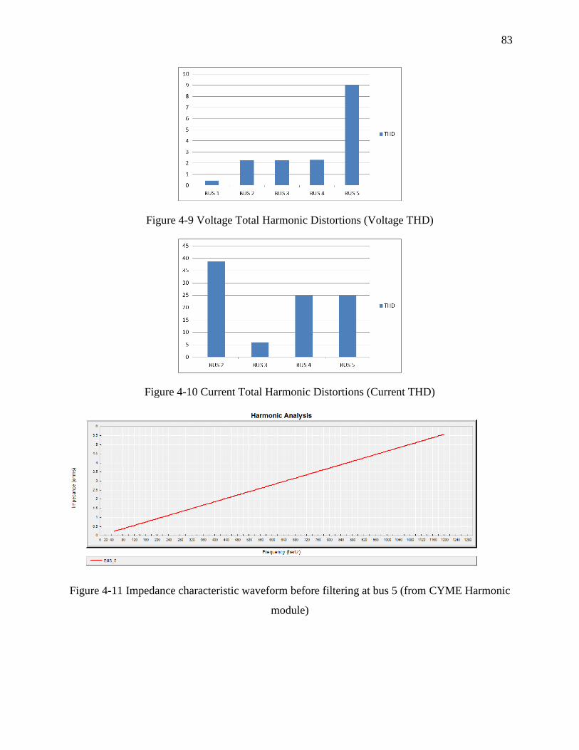
83

Figure 4-9 Voltage Total Harmonic Distortions (Voltage THD)

Figure 4-10 Current Total Harmonic Distortions (Current THD)

Figure 4-11 Impedance characteristic waveform before filtering at bus 5 (from CYME Harmonic

module)

84


The proposed algorithm is applied to determine the appropriate filters for the system. The desired

power factor is assumed to be 0.99.

From the solution of the proposed algorithm, three single tuned filters (5th

, 7th

and 11th

) are

designed. As mentioned above, in order to avoid the parallel resonance between the lower

harmonics and the filter designed for the suppression of higher order harmonic, the frequency of

the resonance points should be checked, and if they are nearby the frequencies of the dominant

harmonics, filter should be detuned. In this case, filters are tuned three percent lower than their

harmonic frequencies. These filters’ parameters are as follows:

Table 4-10 Parameters of harmonic filters measured by proposed method for 5 Bus industrial

system

Filter 1 Filter 2 Filter 3

Type Single tuned Single tuned Single tuned

Qc 900 kVar 300 kVar 300 kVar

Vc3 7200 v 7200 v 7200 v

C 0.22 uf 0.76 uf 0.76 uf

L 0.0130 H 0.0081 H 0.0080 H

R 0.24 ohm 0.52 ohm 0.33 ohm

Quality factor 100 100 100

Filter detuning factor 0.97 0.97 0.97

Filter tuned at 291 Hz 407.4 Hz 640.2 Hz

The graphs of the voltage, current, voltage THD, voltage IHD, current THD and impedance scan

at bus #5 after installation of harmonic filters are presented as follows:

3 rated voltage of the capacitor bank

85

Figure 4-12 Voltage at bus 5 (from CYME Harmonic module)

Figure 4-13 Current waveform at bus 5(from CYME Harmonic module)

Figure 4-14 Voltage Individual Harmonic Distortions (Voltage IHD)

86

Figure 4-15 Voltage Total Harmonic Distortions (Voltage THD)

Figure 4-16 Current Total Harmonic Distortions (Current THD)

Figure 4-17 Impedance characteristic waveform after filtering at bus 5 (from CYME Harmonic

module)

The filters satisfy the IEEE 18 limits. Table 4-11 presents the mathematical solutions.

87

Table 4-11 Values required to satisfy IEEE 18

Filter Type 𝒇 (𝑯𝒛) 𝑸𝒄 (𝒌𝑽𝒂𝒓) 𝑸𝒄 (𝒌𝑽𝒂𝒓) 𝑸𝒄 (𝒌𝑽𝒂𝒓) 𝑸𝒄 (𝒌𝑽𝒂𝒓) 𝑸𝒄 (𝒌𝑽𝒂𝒓) 𝑸𝒄 (𝒌𝑽𝒂𝒓)

Single

tuned filter 300 900 7200 0.61 0.99 0.63 0.77

Single

tuned filter 420 300 7200 0.71 1.18 0.61 0.74

Single

tuned filter 660 300 7200 0.41 0.72 0.58 0.62

4.3 Validation of harmonic filter allocation

In order to demonstrate the performance of the proposed methodology, the solution is tested on

the 13-bus industrial system. This program is written in MATLAB and the performances of the

filters are tested using CYME Harmonic module.


The study considers three harmonic sources connected to the BUSES bus #5, bus #9 and bus #13.

Given the harmonic current introduced by the 12 pulse converter as mentioned in Table 4-12, the

one line diagram of the system to be studied is illustrated in Figure 4.18. Figure 4.19 shows the

harmonic distortion at each bus before placing the harmonic filters. As can be seen from the

figure, bus #9 and bus #13 have the highest harmonic distortion in the system.

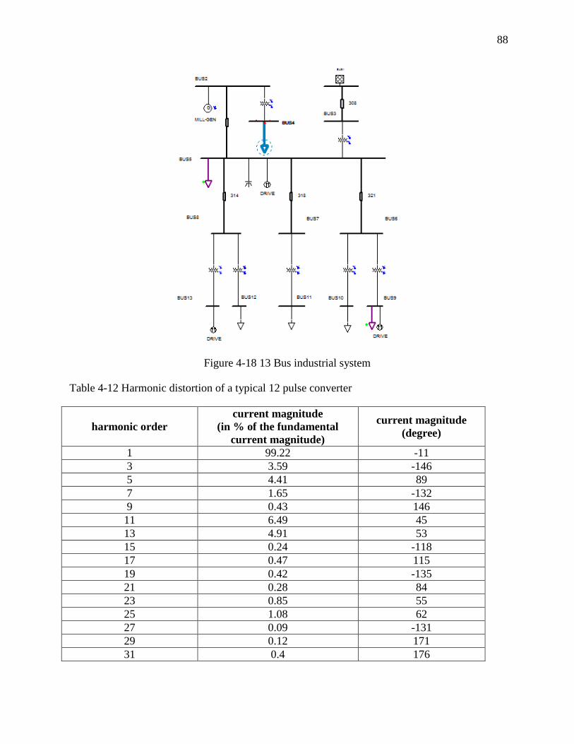
88

Figure 4-18 13 Bus industrial system

Table 4-12 Harmonic distortion of a typical 12 pulse converter

harmonic order

current magnitude

(in % of the fundamental

current magnitude)

current magnitude

(degree)

1 99.22 -11

3 3.59 -146

5 4.41 89

7 1.65 -132

9 0.43 146

11 6.49 45

13 4.91 53

15 0.24 -118

17 0.47 115

19 0.42 -135

21 0.28 84

23 0.85 55

25 1.08 62

27 0.09 -131

29 0.12 171

31 0.4 176

89

Figure 4-19 Voltage THD weight of the 13 bus system (before filters placement)


As can be seen from the one line diagram, system shows thirteen buses and hence presents

thirteen possible placements for harmonic filters. According to the proposed algorithm, all busses

except bus #1, bus #2 and bus #3 are candidates for harmonic filter placements.

According to the simulation results, from ten possible allocations for harmonic filters at this

system, two of them result in considerable reduction at harmonic distortion level (bus #6 and bus

#9). The simulation result is summarized in Table 4-13. Figures 4.20 to 4.29 illustrate the

resultant harmonic voltages when the filters are placed. In simulation of all configurations, over

voltages are taken into account and filters are design in the way to satisfy the IEEE 519 and IEEE

18 requirements.

90

Table 4-13 THD voltage at each bus after installation of filters (%)

Bus

Number

Filters placed at:

- 4 5 6 7 8 9 10 11 12 13

1 0.77 0.76 0.3 0.42 0.37 0.33 0.39 0.83 0.76 0.8 0.62

2 4.1 4.01 1.6 2.22 1.96 1.75 2.07 4.43 4.04 4.26 3.32

3 0.99 0.94 0.37 0.52 0.46 0.41 0.49 1.03 0.94 0.99 0.77

4 4.1 1.6 1.58 2.15 1.91 1.7 2.03 4.36 3.98 4.19 3.27

5 4.28 4.16 1.65 2.29 2.03 1.82 2.14 4.58 4.18 4.4 3.44

6 4.3 4.16 1.67 2.24 2.01 1.79 2.13 4.57 4.18 4.4 3.43

7 4.2 4.16 1.65 2.29 2.02 1.82 2.14 4.58 4.17 4.4 3.44

8 4.3 4.16 1.66 2.29 2.03 1.8 2.14 4.58 4.18 4.4 3.43

9 6.9 7.09 7.3 4.91 5.52 5.13 3.38 7.2 7.08 7.26 6.6

10 4.3 4.14 1.66 2.22 1.99 1.77 2.12 3.06 4.16 4.38 3.41

11 4.2 4.05 1.62 2.17 1.93 1.72 2.07 4.46 0.96 4.29 3.34

12 4.1 3.92 1.59 2.05 1.85 1.6 2.00 4.32 3.94 0.82 3.22

13 5.78 5.75 5.55 3.38 3.93 3.53 4.39 5.92 5.75 5.94 2.71

The harmonic filters installed at bus #9 require lower total power than the harmonic filters

installed at bus #6; therefore, bus #9 is suitable location for harmonic filter allocation.

Figure 4-20 Voltage THD weight of 13 bus system (Filter at bus 4)


91




92




93



94

CHAPTER 5 CONCLUSION AND RECOMMENDATIONS

This thesis presents the harmonic models of system components under balanced and unbalanced

conditions in phase frame and uses them in the MANA formulation. Certain models are obtained

from their equivalent circuits in sequence frame. In the case of multi-phase transmission lines, it

is possible to obtain the admittance matrix from different line models directly in phase frame. It

is shown that using simplified models, such as equivalent pi model, changes the frequency

response of the line.

Harmonic analysis based on the MANA formulation and which can be applied to balanced or

unbalanced electric networks is described, In addition, this methodology was implemented in a

computer program which allows the analysis of characteristic and non-characteristic of the

complex harmonic quantities. The purpose of this research work is to provide a reliable method

to determine harmonic distortion in large networks. The comparison with EMTP-RV confirms

that the method yields precise results. The difference observed between the results of EMTP-RV

and the results of the proposed method was less than three percent in magnitude of voltages,

which is due to the differences between harmonic models and detailed EMTP-RV models for

certain devices. For example, in EMTP-RV, the models used for rotating loads are based on

dynamic equations and models while in the proposed method, the steady state models are

employed for them.

The following conclusions and recommendations can be made for harmonic analysis:

MANA methodology significantly simplifies the harmonic models of transformers and

other components under unbalanced conditions.

Norton equivalent provides a straightforward solution and can speed up harmonic analysis

computations when compared to the Thevenin equivalent which requires the evaluation of

the Thevenin impedance of the bus connected to the harmonic source.

Harmonic studies and reduction of harmonic distortions using capacitor banks, as well as

harmonic filters, can be performed in a straightforward manner without addressing

heuristic methods given the complexity and size of industrial networks and due to the

simple fact that the mitigation of harmonic distortions can be achieved by placing filters

close to the harmonic sources

95

Capacitor banks can change the direction of harmonic flow in the system. Hence, in the

harmonic polluted system, the capacitor banks should be taken into account.

This thesis proposes practical solution strategies for passive filter design and filter allocation. The

objectives are to determine the parameters of harmonic filters and also to find efficient locations

for harmonic placement. The proposed methods are successfully implemented as a computer

program. The results show that the proposed method forms an efficient tool for designing and

placing harmonic filters in industrial systems. It has to be mentioned that the proposed method

for filter allocation has a limitation and it cannot be applied to large networks. The following

conclusions and recommendations can be made for harmonic filters:

In multiple filters branch, due to parallel resonance generated by single tuned filters, the

tuning frequencies of the harmonic filters should be taken into account.

The rated voltage of capacitor banks should satisfy IEEE 18 requirements. Otherwise the

harmonics can cause failure in capacitor banks (as shown with the 5 bus industrial

system).

The natural choice for the allocation of harmonic filters is at the bus with the highest

harmonic distortion or bus with the largest nonlinear device. When there are multiple

harmonic sources, this strategy may not give the optimal solution and further trials may

be required by considering the electrically close buses (as shown with the 13 bus

industrial system).

96

BIBLIOGRAPHY

[1] Roger C dugan, Mark F. Mcgranghan, Surya Santoso,H. Wayne Beaty, Electrical Power

Systems Quality, McGraw-Hill, 2004.

[2] Alexander Kusko, Marc Thompson, Power Quality in Electrical Systems, McGraw Hill

Professional, 2007.

[3] Philip E. C. Stone, Jingjiang Wang Yonge June Shin, Roger A. Dougal, "Efficient Harmonic

Filter Allocation in an Industrial Distribution System," IEEE transactions on industrial

electronics, vol. 59, no. 2, p. 740, 2012.

[4] I. Kocar, J. Mahserdedjian, U. Karragace, G. Soykan, O. Saad, "Multiphase Load Flow

Solution For Large Scale Distribuation system using MANA," IEEE TRANSACTIONS ON

POWER DELIVERY, vol. 29, no. 2, p. 908, 2014.

[5] Task Force on Harmonics Modeling and Simulation, "Modeling and Simulation of the

Propagation of Harmonics in Electric Power Networks," IEEE transaction on Power

Delivery, vol. 11, no. 1, p. 452, 1996.

[6] J. Arrillaga, D. Bradley and P. Bodger, Power System Harmonics, Jhon Wiley& Sons Ltd,

1989.

[7] G. J. Wakileh, Power Systems Harmonics, New York: Springer , 2001.

[8] J. Pedra, , L. Sainz, F. Córcoles, "Harmonic Modeling of Induction Motors," Electric Power

System Research, vol. 76, p. 936, 2004.

[9] Vikas Singhvi, Student Member, IEEE and, S. Mark Halpin, Fellow, IEEE, "Synchronous

Machine Modeling for Low-Frequency Harmonic Studies," in 39th Southeastern Symposium

on System Theory, Macon, 2007.

97

[10] Wilsun W. Xu Hermann W. Dome1 Jose R. Marti, "A SYNCHRONOUS MACHINE

MODEL FOR THREE-PHASE HARMONIC ANALYSIS AND EMTP

INITIALIZATION," Transactions on Power System, vol. 6, no. 4, p. 1530, 1991.

[11] "Impact of Aggregate Linear Load Modeling on Harmonic Analysis: A Comparison of

Common Practice and Analytical Models," IEEE TRANSACTIONS ON POWER

DELIVERY,, vol. 18, no. 2, p. 625, 2003.

[12] Sergio Herraiz, Luis Sainz, and Jordi Clua, "Review of Harmonic Load Flow Formulations,"

IEEE TRANSACTIONS ON POWER DELIVERY, vol. 18, no. 3, p. 1079, 2003.

[13] W. Xu, Jose R. Marti, Hermann W. Dommel, "A MULTIPHASE HARMONIC LOAD

FLOW SOLUTION TECHNIQUE," IEEE "axions on Power Systems, vol. 6, no. 1, p. 174,

1991.

[14] Keyhani,A. Abur, Member, S. Hao, "Evaluation of Power Flow Techniques for Personal

Computers," IEEE Transactions on Power Systems, vol. 4, no. 2, p. 817, 1989.

[15] Vinay Sharma, R.J. FleminG, Leo Niekamp, "An Iterative Approach for Analysis of

Harmonic Penetration in the Power Transmission Networks," IEEE Transmission and

Distribution Committee of the IEEE Power Engineering Society , p. 1698, 1991.

[16] E. Thunberg, L. Soder, Member, "A NORTON APPROACH DISTRIBUTION NETWORK

MODELING FOR HARMONIC STUDIES," IEEE Transactions on Power Delivery, vol.

14, no. 1, p. 272, 1999.

[17] A. A. Girgis, W. H. Quaintance III, J. Qiu, E. B. Makram, "A TIME-DOMAIN THREE-

PHASE POWER SYSTEM IMPEDANCE MODELING APPROACH FOR HARMONIC

FILTER ANALYSIS," IEEE Transactions on Power Delivery, vol. 8, no. 2, p. 504, 1993.

[18] A. Medina, J. Segundo-Ramirez, P. Ribeiro, W. Xu, K. L. Lian, G. W. Chang, V. Dinavahi,

and N. R. Watson, "Harmonic Analysis in Frequency and Time Domain," IEEE

98

TRANSACTIONS ON POWER DELIVERY, vol. 28, no. 3, p. 1813, 2013.

[19] M.A. Moreno Lope de Saa and J. Garcia, "Three Phase Harmonic Load Flow in Frequency

and Time domain," IEE Proc- Electric. Power Appl, vol. 150, no. 3, p. 295, 2003.

[20] J. R. Carson, "Wave Propagation in Overhead Wires with Ground," Bell Syst. Tech. J., vol.

5, pp. 539-554, 1926.

[21] W. H. Kersting, Distribution System Modeling and Analysis, CRC, 2012.

[22] A. Deri, G. Tevan, A. Semlyen, A. Castanheira, "The Complex Ground Return Plane a

Simplified Model for Homogeneous and Mult-Layer Earth Return," IEEE Transactions on

Power Apparatus and Systems, vol. 100, no. 8, 1981.

[23] R. Horton, W. G. Sunderman, R. F. Arritt, R. C. Dugan,, "IEEE Transactions on Power

Apparatus and Systems Earth Voltage Analysis of Multi-Grounded Distribution Feeders,"

IEEE, vol. 1, no. 1, p. 1.

[24] Enrique Acha, Manuel Madrigal, Power Systems Harmonics, Jhon WILEY and Sons, Ltd,

2001.

[25] J. M. Roldan-Fernandez, Francisco M. Gonzalez-Longatt, José Luis Rueda, H. Verdejo,

PowerFactory Applications for Power System Analysis, Springer, 2014.

[26] Elham B. makram E.V. Subramaniam Adly A.Girgis, "Harmonic Filter design usung actual

recorded data," in IEEE, 1992.

[27] Kun Ping Lin, Ming Hoon Lin, and Tung Ping Lin, "An Advanced Computer Code for

Single Tuned Harmonic Filter," IEEE Transactions on industry applications, vol. 34, no. 4,

p. 640, 1998.

[28] Kun-Ping Lin, Ming-Hoon Lin, and Tung-Ping Lin, "An Advanced Computer Code for

Single-Tuned Harmonic Filter Design," IEEE TRANSACTIONS ON INDUSTRY

99

APPLICATIONS, vol. 34, no. 4, p. 640, 1998.

[29] Young-Sik Cho, Bok-Ryul Kim, Hanju Cha, "Transfer Function Approach to a Passive

Harmonic Filter Design for Industrial Process Application," in International Conference on

Mechanics and Automation , Xi an, 2010.

[30] Chia-Nan Ko, Ying-Pin Chang, and Chia-Ju Wu, Senior Member, IEEE, "A PSO Method

With Nonlinear Time-Varying Evolution for Optimal Design of Harmonic Filters," IEEE

TRANSACTIONS ON POWER SYSTEMS,, vol. 24, no. 1, p. 437, 2009.

[31] Alexander Kusko, Marc T. Thompson, Power Quality in Electrical System, The McGraw-

Hill Companies, 2007.

[32] F. C. D. L. Rosa, Harmonic and Power System, 2006: CRC.

[33] R. Natarajan, Computer-aided Power System Analysis, New york: Marcel Dekker Inc.,

2002.

[34] Yong Zhao, Hongying Deng, Jianhua Li, Daozhi Xia, "Optimal Planning of Harmonic

Filters on Distribution System by Chance Constrained Programming," Electrical power

system research, vol. 68, p. 149, 2004.

[35] Gary W. Chang, Hung Lu Wang, and Shou Yung Cgu, "Strategic Placement and Sizing of

Passive Filters in a Power System for Controlling Voltage Distortion," IEEE transaction on

power delivery, vol. 19, no. 3, p. 1204, 2004.

[36] A.M Variz, F. M. Niquini, J.L.R Pereira, P.G. Barbosa, S. Carneiro and P.F. Rebeiro,

"Allocation of the Power Harmonic Filters using Genetic Algorithm," in IEEE international

conference on harmonic and quality of power- ICHQP 2012, 2012.

[37] GaryW. Chang, Shou-Yung Chu and Hung-LuWang, "A New Method of Passive Harmonic

Filter Planning for Controlling Voltage Distortion in a Power System," IEEE

TRANSACTIONS ON POWER DELIVERY, vol. 21, no. 1, p. 305, 2006.

100

[38] Mohammad A. S. Masoum, Marjan Ladjevardi, Akbar Jafarian, and Ewald F. Fuchs,

"Optimal Placement, Replacement and Sizing of Capacitor Banks in Distorted Distribution

Networks by Genetic Algorithms," IEEE TRANSACTIONS ON POWER DELIVERY, vol.

19, no. 4, p. 1794, 2004.

101

APPENDIX A – DISTORTION FACTORS

Total Harmonic Distortion is calculated as

2 2 2

2 3 4

1

V V VTHD

V

Individual Harmonic Distortion is given by:

1

hV

IHD V

Where

𝑉1 : Voltage at fundamental frequency

𝑉𝑖 : Voltage i harmonic order

102

APPENDIX B – COMMON VOLTAGE AND REACTIVE POWER RATING

BASED ON IEEE 18

Volt, rms

Line to line Kvar Number of phases

216 5, 7 ½, 13 1/3, 20 and 25 1 and 3

240 5, 7 ½, 13 1/3, 20, 25 and 50 1 and 3

480 5, 7 ½, 13 1/3, 20, 25, 50, 60

and 100 1 and 3

600 5, 7 ½, 13 1/3, 20, 25, 50, 60

and 100 1 and 3

2400 50, 100, 150 and 200 1

1770 50, 100, 150 and 200 1

4160 50, 100, 150 and 200 1

4800 50, 100, 150 and 200 1

6640 50, 100, 150, 200, 300 and

400 1

7200 50, 100, 150, 200, 300 and

400 1

7620 50, 100, 150, 200, 300 and

400 1

université de montréal a novel approach to determine harmonic

Documents