universitÉ du quÉbec these presentee a …constellation.uqac.ca/636/1/18326611.pdf · universitÉ...
TRANSCRIPT
UNIVERSITÉ DU QUÉBEC
THESE PRESENTEE A
L'UNIVERSITÉ DU QUÉBEC À CHICOUTIMI
COMME EXIGENCE PARTIELLE
DU DOCTORAT EN INGÉNIERIE
PAR
PING FU
MODELLING AND SIMULATION OF THE ICE ACCRETION
PROCESS ON FIXED OR ROTATING CYLINDRICAL OBJECTS BY
THE BOUNDARY ELEMENT METHOD
MODÉLISATION ET SIMULATION DES ACCRETIONS DE GLACE
ATMOSPHÉRIQUE SUR DES OBJETS CYLINDRIQUES FIXES ET
TOURNANTS PAR LA MÉTHODE DES ÉLÉMENTS FINIS DE
FRONTIÈRE.
AOÛT 2004
bibliothèquePaul-Emile-Bouletj
UIUQAC
Mise en garde/Advice
Afin de rendre accessible au plusgrand nombre le résultat destravaux de recherche menés par sesétudiants gradués et dans l'esprit desrègles qui régissent le dépôt et ladiffusion des mémoires et thèsesproduits dans cette Institution,l'Université du Québec àChicoutimi (UQAC) est fière derendre accessible une versioncomplète et gratuite de cette �uvre.
Motivated by a desire to make theresults of its graduate students'research accessible to all, and inaccordance with the rulesgoverning the acceptation anddiffusion of dissertations andtheses in this Institution, theUniversité du Québec àChicoutimi (UQAC) is proud tomake a complete version of thiswork available at no cost to thereader.
L'auteur conserve néanmoins lapropriété du droit d'auteur quiprotège ce mémoire ou cette thèse.Ni le mémoire ou la thèse ni desextraits substantiels de ceux-ci nepeuvent être imprimés ou autrementreproduits sans son autorisation.
The author retains ownership of thecopyright of this dissertation orthesis. Neither the dissertation orthesis, nor substantial extracts fromit, may be printed or otherwisereproduced without the author'spermission.
ABSTRACT
The main objective of the thesis proposed herein is to develop a new 2-D ice model
which is intended primarily for simulating the ice accretion process on transmission line
cables. In an attempt to validate this new model, a number of experimental tests were
carried out in the CIGELE icing wind tunnel, and the results obtained from these tests
were then compared with those of numerical simulation.
The theoretical work is composed of two phases. In the first phase, the ice accretion
process on a fixed cable was modelled, and model parameters, such as the Local
Collision Efficiency(LCE) and the local Heat Transfer Coefficient(HTC), were evaluated
based on time-dependent airflow and water droplet trajectory computations. For wet
accumulations, the movement of a surface water fihn was tracked for each time step so as
to obtain its direction of motion and thickness.
m the second phase, the ice accretion process on a rotating cable was specifically
studied as an extension of the newly-developed ice code or model, while both
gravitational and aerodynamic torques were considered in the rotation process. The
aerodynamic forces were derived by integrating air pressure and air shear along the
airflow boundary and were updated according to real-time airflow computations.
Subsequently, this new model was applied to analyze two types of overhead transmission
line cables under icing conditions, namely, the Bersimis cable and an overhead ground
wire, and thereby a number of observations were made.
The conditions applied in the experimental tests in the icing wind tunnel are such that
the effects of wind speed, size of test cylinder, air temperature and droplet Median
Volume Diameter (MVD) may be revealed by the ice shapes, and that, furthermore,
these ice shapes represent the range of the icing process from dry to wet accumulations,
hi particular, five sets of ice-shapes from both test results and model simulations were
illustrated and compared within this thesis so as to validate the proposed ice model. It
may be concluded from these comparisons that, in general, the ice shapes predicted by
the proposed ice model are in satisfactory agreement with the shapes obtained from
experimental tests. Nevertheless, this model tends to underestimate the ice-load to a great
extent in the event that the air temperature is high, and the wet regime becomes
dominant. In such a case, icicles form beneath the iced objects, and consequently if the
weight of the icicles is disregarded, a considerable underestimation of the overall ice-load
will occur.
In addition, this thesis examines the effects of Joule heating and water droplet size on
the icing process using the new ice model. These effects, however, proved to be difficult
to investigate with the experimental set-up currently available. By means of this new
model, moreover, it also becomes easy to demonstrate the ice density distribution within
the ice-accretion, as discussed in the latter portion of this thesis.
11
RESUME
L'objectif principal de la thèse proposée est de développer un nouveau modèle
numérique en 2D qui est destiné principalement à simuler le processus d'accumulation de
la glace atmosphérique sur les câbles de transport de l'énergie électrique. Dans une
tentative de valider ce nouveau modèle, un certain nombre d'essais expérimentaux ont été
effectués dans la soufflerie réfrigérée de la CIGELE. Les résultats obtenus de ces essais
ont été alors comparés avec ceux fournis par notre simulation numérique pour valider le
modèle.
Le travail théorique est composé de deux phases. Dans la première, le processus de
glaçage sur un câble fixe a été modélisé et les paramètres du modèle, tels 1' Efficacité de
Collision Locale (LCE) et le Coefficient de Transfert de Chaleur local (HTC), ont été
évalués. Cette évaluation est basée sur les résultats du calcul du flux d'air et de la
trajectoire des gouttelettes d'eau en fonction du temps. Pour des accumulations en régime
humide, le mouvement d'un film d'eau de surface a été suivi pour chaque pas de temps
afin d'obtenir sa direction de déplacement et son épaisseur.
Dans la deuxième phase, le processus de glaçage sur un câble tournant a été
spécifiquement étudié comme une extension du modèle nouvellement développé. Dans ce
cas les moments de torsion dus à la gravitation et aux forces aérodynamiques ont été
considérés dans le processus de rotation. Les forces aérodynamiques ont été calculées en
intégrant la pression et le cisaillement de l'air le long de la surface de glace. Les calculs
sur le flux d'air ont été mis à jour en temps réel. Par la suite, ce nouveau modèle a été
appliqué pour analyser deux types de câbles de ligne aériens dans des conditions de
givrage, le câble Bersimis et le câble de garde. Ainsi un certain nombre d'observations
ont été faites.
Les conditions appliquées dans les essais expérimentaux avec la soufflerie réfrigérée
sont telles que les effets de la vitesse du vent, la taille du cylindre d'essai, le Diamètre
m
Volumique Médian (MVD), et la température de l'air peuvent être révélés par les formes
de glace obtenues. Ces conditions appliquées permettent d'obtenir des formes de glace
en régime d'accumulation sec, humide ou mixte.
Cinq types de formes de glace obtenues à partir des simulations numériques et des
expériences ont été élaborés et comparés dans nos travaux afin de valider le modèle de
glace proposé. De ces comparaisons on peut retenir qu'en général, les formes de glace
prévues par le modèle d'accumulation proposé correspondent bien avec les formes
fournies par les essais expérimentaux. Néanmoins, ce modèle a tendance à sous-estimer
la charge de glace surtout dans le cas où la température ambiante devient élevée et le
régime humide dominant. Dans un tel cas, en soufflerie des glaçons se forment au-
dessous des objets recouverts de glace et par conséquent si leur poids est ignoré dans le
modèle numérique, une sous-estimation considérable de la charge de glace arrivera.
Notre étude examine aussi l'impact de réchauffement par effet Joule ainsi que la taille
des gouttelettes d'eau sur le processus d'accumulation de glace en utilisant un nouveau
modèle d'accumulation. Ces effets, bien que significatifs, se sont toutefois avérés
difficiles à confirmer par le procédé expérimental traditionnel. De plus, à l'aide de ce
nouveau modèle, il devient possible de montrer la distribution de la densité de glace dans
la masse accumulée.
IV
ACKNOWLEDGEMENTS
First of all, I would like to extend my sincere appreciations and gratitude to my
supervisor, Professor Masoud Farzaneh who is Chairholder of the NSERC/Hydro-
Québec/UQAC Chair on Atmospheric Icing of Power Network Equipment (CIGELE), as
well as the Canada Research Chair, Tier 1, on the Engineering of Power Network
Atmospheric Icing (INGIVRE). He displayed considerable trust and confidence in my
research potential, granting me the invaluable chance to pursue my Ph.D. study. During
past four years, he gave me a lot of advice and kept me on right track during my thesis
work. He also broadened my knowledge in the electrical aspect of the icing research.
I would like to thank the co-supervisor, Professor Gilles Bouchard who guided me and
helped me so much. I learned many things from him and he was always very kind to me.
I would also like to thank the researchers and staff at the CIGELE, who had a lot of
stimulating discussion with me and offered me technical support and suggestions. These
wonderful people include Dr. Jianhui Zhang, Dr. Anatolij Karev, Jean Talbot, Pierre
Camirand and Marc André Perron among many others. I would like to extend my thanks
to all of my peer students in the CIGELE for the pleasant time spent together. Otherwise,
my academic life would have been dull.
I am grateful to Prof. Edward Lozowski, who gave me timely advice in carrying out
the research on Local Collision Efficiency, as will be introduced in Chapter 4. I am
impressed with his deep insight and innovative ideas.
An acknowledgement is specifically extended to M. L. SinClair, for her patience and
painstaking efforts in editing my thesis.
Lastly, my profound gratitude goes to my wife, Nan Yu, for her substantial
contribution and sacrifice to our family throughout my Ph.D. study.
TABLE OF CONTENTS
ABSTRACT i
RÉSUMÉ iii
ACKNOWLEDGEMENTS v
LIST OF SYMBOLS x
LIST OF FIGURES xii
LIST OF TABLES xvi
CHAPTER 1 INTRODUCTION 1
1.1 Background 2
1.2 The Problem 4
1.3 Research Objectives 5
1.4 Methodology 7
CHAPTER2 REVIEW OF LITERATURE 10
2.1 Introduction 10
2.2 Fundamentals of Modelling the Ice Accretion process 14
2.3 Analysis of Airflow Dynamics 16
2.4 Droplet Trajectory Calculation and Local Collision Efficiency 19
2.5 Velocity and Thermal Boundary Layer 22
2.6 Thermodynamics of Ice Accretion 33
2.7 Surface Temperature of Ice Accretion 35
2.8 Ice Volume and Ice Density 35
2.9 Conclusions 39
CHAPTER3 AIRFLOW COMPUTATION 41
3.1 Introduction 41
VI
3.2 Basic Principles 43
3.3 Potential Flow 44
3.4 Airflow Boundary Layer 49
3.5 Feedback Effect in Airflow Calculation due to Boundary Layer Separation ... 55
3.6 Computation of Airflow Past an Object of Arbitrary Cross-Sectional Shape ... 56
3.7 Airflow Field Visualization 59
3.8 Conclusions 60
CHAPTER 4 DROPLET TRAJECTORY AND COLLISION
EFFICIENCY 61
4.1 Introduction 61
4.2 Basic Principles 62
4.2.1 Equations Governing the Motion of a Water Droplet 62
4.2.2 Solutions 66
4.2.3 Initial Conditions and Time Steps 66
4.2.4 Surface Collision 67
4.2.5 Evaluating Local Collision Efficiency 69
4.3 Simulation and Validation of Results 71
4.4 Conclusions 78
CHAPTER 5 THERMAL BALANCE AND SURFACE WATER
FLOW 79
5.1 Introduction 79
5.2 Solution to Thermal Boundary Layer 80
5.3 Thermal Balance Equation and Joule Heating 84
5.4 Modeling the Flow of a Water Film 87
5.5 Water-Film Calculations and Interpretation of Results 95
5.6 Conclusions 98
vu
CHAPTER 6 EXPERIMENTS AND MODEL VALIDATIONS 996.1 Experimental Set-up and Instruments 99
6.2 Measuring the LWC and MVD 105
6.3 Acquiring Ice-Shape Data 108
6.4 Comparisons of Ice Shapes from Model Simulation and Experiments 108
6.5 Conclusions 115
CHAPTER7 MODEL SIMULATION 116
7.1 Structure of Ice Model 116
7.2 Model Input Parameters 118
7.3 Model Output 121
7.4 Techniques for Implementing the Proposed Ice Model on a Computer 122
7.5 Model Simulations 126
7.6 Conclusions 140
CHAPTER 8 SIMULATION OF CABLE ROTATION 142
8.1 Introduction 142
8.2 Basic Principles 144
8.3 Description of the Calculation Procedure 146
8.3.1 Governing Equations 146
8.3.2 Evaluating the Centre of Mass 148
8.3.3 Position Change of Stagnation Point 149
8.3.3 Solution 150
8.4 Simulations and Interpretation of Results 151
8.5 Conclusions 161
CHAPTER 9 CONCLUSIONS AND RECOMMENDATIONS 163
9.1 Conclusions 163
9.2 Recommendations 167
9.2.1 Extend the 2-D Ice Model Proposed Herein to 3-D 167
vin
9.2.2 Mechanical Analysis of Iced Cable Using the New Ice Model 169
REFERENCES 170
Appendix: Runge-Kutta Algorithm 180
IX
LIST OF SYMBOLS
SYMBOL
A
cdCf
cP
Fb
Fd
Fg
g
G
H
h
hk
l
N
Nu
Pr
q
Q
R
Re
Re
St
T
Tf
Tg
TP
CONCEPT
Area of a domain under study
Drag coefficient
Skin-friction coefficient
Specific heat at constant pressure
Buoyancy force
Air drag force
Gravity
Acceleration of gravity
Shear modulus
Shape factor
Convective heat transfer coefficient
Polar moment of inertia
Thermal conductivity
Coordinate in the surface-attached system
Node for surface sectors
Nusselt number
Prandtl number
Derivative of the stream function
Heat flux
Transverse radius of curvature
Reynolds number based on the momentum thickness
Reynolds number
Stanton number
Torque
Torque generated by distributed air shear stress
Torque generated by gravity
Torque generated by distributed air pressure
DIMENSIONS
m2
m2/(s2. K)
N
N
N
m/s2
N/m2
W/(m2.K)
m4
W/(m.K)
hD/k
v/a
m/s
W/m2
m
h/Gcp
Km
Km
Km
Km
Uo Onset airflow speed m/s
Ux Free stream velocity at the outer edge of the boundary layer m/s
V Volume or water flow speed m3 or m/s
Va Free-stream velocity in the vicinity of an icing object m/s
Ve Droplet velocity in the vicinity of an icing object m/s
W Liquid water content G/m3
xa Starting point of an adverse gradient m
xm Position of minimum pressure m
xt Position where a transitional flow starts m
AT Time step for one simulation t
(x,y) Cartesian coordinates
Greek Symbols
a Molecular thermal diffusivity m2/s
P Collection coefficient
y Water density
F Free-stream (potential flow) boundary
5 Local impact angle degree
A Conduction thickness of a thermal boundary layer m
0 Boundary layer momentum thickness m
X Dimensionless pressure gradient
ja Absolute viscosity N.s/m2
v Kinematic viscosity m2/s
§ Homogeneous coordinate varying from - 1 to +1
p Density kg/m3
p a Air density kg/m3
1 Air shear stress N/m2
TW Wall shear stress N/m2
cp Stream function m2/s
§ Trial function for solving residual integral equation
XI
LIST OF FIGURES
Figure 1.1 Elementary components of the ice model under discussion 9
Figure 2.1 Local icing fraction 15
Figure 2.2 Potential flow around a circular object 17
Figure2.3 Definition of LCE 20
Figure 2.4 Velocity boundary layer 23
Figure 2.5 (a) Flow past a sphere with laminar boundary layer separation.
(b) Flow past a sphere with turbulent boundary layer separation 26
Figure 2.6 Flow past a sphere with laminar boundary layer separation 28
Figure 2.7 Local heat transfer coefficient Nu/Re1/2 on a rough circular cylinder at
various cylinder Reynolds numbers 29
Figure 2.8 Nusselt number for a rough cylinder 32
Figure 2.9 Comparison of heat flux terms in typical freezing-rain conditions 34
Figure 2.10 Relationship between ice density and Maklin number 39
Figure 3.1 Airflow computation and its role in the ice model 41
Figure 3.2 The airflow field about an object 42
Figure 3.3 Calculation procedure for airflow computation 44
Figure 3.4 Input parameters and boundary conditions for BEM calculation 48
Figure 3.5 Evolution of angular position for boundary-layer separation points
during simulation 56
Figure 3.6 Algorithm for surface smoothing 57
Figure 3.7 Airflow (a) about a plain object, and (b) about an ice-covered object... 60
Figure 4.1 Forces experienced by droplet 64
Figure 4.2 Collision points of water droplets 68
Figure 4.3 Definition of the local collision efficiency 69
Figure 4.4 Trajectories for water droplets of different diameters 71
Figure 4.5 The influence of gravity on the trajectories of water droplets 72
Figure 4.6 Comparisons based on both model simulations and test results 73
xn
Figure 4.7 Time evolution of the Ice shape and LCE for an icing object 74
Figure 4.8 Langmuir volume distribution 75
Figure 4.9 Droplet size and volume for bimodal case 76
Figure 4.10 Cumulative volume distribution for both cases 77
Figure 4.11 LCE distributions for three cases of different DSDs 77
Figure 5.1 Comparison of local HTCs obtained from present simulation and those
of earlier studies 83
Figure 5.2 Magnitude analysis for heat fluxes in the heat balance equation 87
Figure 5.3 Diagram for water-flow direction 88
Figure 5.4 Diagram of the mechanical analysis of a water film 89
Figure 5.5 Diagram for the mass conservation of a water film 90
Figure 5.6 Inclined flow between a fixed plate and moving plate 91
Figure 5.7 Diagram of the division of surface zones 93
Figure 5.8 Water-film thickness and speed on the surface of a cylinder 98
Figure 6.1 A top view of the CIGELE icing research wind tunnel 101
Figure6.2 Test section of the CAIRWT 101
Figure 6.3 Relationship between air and fan speed 102
Figure 6.4 Spray bar fitted with three nozzles 103
Figure 6.5 Control panel for air and water pressures and water flow rate 103
Figure 6.6 ( a ) Collargol coated slide
(b ) Traces of water droplets under a microscope 105
Figure 6.7 Relationship between MVD and air speed under experimental
conditions 107
Figure 6.8 Relationship between LWC and air speed under experimental
conditions 107
Figure 6.9 ( a ) An iced cylinder
( b ) Cross-sectional ice shape at midpoint of same cylinder 108
Figure 6.10 Comparison of ice shape (Air Speed 5 m/s, Air Temperature-15°C,
MVD 34 jam, Diameter 19.05 cm) 110
Figure 6.11 Comparison of ice shape (Air Speed 5 m/s, Air Temperature-15°C,
MVD 35 jam, Diameter 34.9 cm) 110
xin
Figure 6.12 Comparison of ice shapes (Air Speed 5 m/s, Air Temperature -10°C,
MVD28 um, Diameter 34.9 cm) 113
Figure 6.13 Comparison of ice shapes (Air Speed 5 m/s, Air Temperature-5°C,
MVD 26 urn, Diameter 34.9 cm) 114
Figure 6.14 Comparison of ice shapes (Air Speed 5 m/s, Air Temperature -5°C,
MVD 33 jam, Diameter 19.05 cm) 115
Figure 7.1 General structure of the proposed ice model 118
Figure 7.2 Parameter input interfaces in ice code 120
Figure 7.3 Visual display for ice accretion processes 121
Figure 7.4 Conceptual representation of the ice code under discussion 122
Figure 7.5 Hierarchical diagram for classes of ice code 125
Figure 7.6 Comparison of ice accretion shapes predicted by classical and new
methods (time step: 5min) 127
Figure 7.7 Time evolution of ice load predicted by both methods 128
Figure 7.8 Comparison of ice shapes with and without current for a dry
accumulation 130
Figure 7.9 Comparison of ice shapes with and without current for a semi-wet
accumulation 131
Figure 7.10 Comparison of ice shapes with and without current for a wet
accumulation 132
Figure 7.11 Local Collision Efficiency for cylinders of different diameters 133
Figure 7.12 Ice Shapes for cables of different diameters 134
Figure 7.13 Ice-density distribution 136
Figure 7.14 Ice accretion for droplets of 500 um in diameter 139
Figure 7.15 Ice accretion for droplets of 100 um in diameter 139
Figure 7.16 Ice accretion for droplets of 50 jam in diameter 140
Figure 7.17 Time evolution of ice mass 140
Figure 8.1 One section of cable between two towers 145
Figure 8.2 Forces experienced by an iced cable 145
Figure 8.3 Schematic diagram of forces experienced by a rotated cable 146
xiv

Figure 8.4 Parameters for an arbitrary element of ice deposit 148
Figure 8.5 Position change of stagnation point as ice accumulates 150
Figure 8.6 Comparison between ice shapes obtained from experimental and
theoretical studies 153
Figure 8.7 Time evolution of external and internal torque 156
Figure 8.8 Time evolution of cable rotation angle 157
Figure 8.9 Time evolution of weight center angle 157
Figure 8.10 Time evolution of ice mass 158
Figure 8.11 Time evolution of ice deposit 159
Figure 8.12 Torque-angle curves for wire sample 161
Figure 9.1 Icicle curtain beneath an iced cylinder 168
xv
LIST OF TABLES
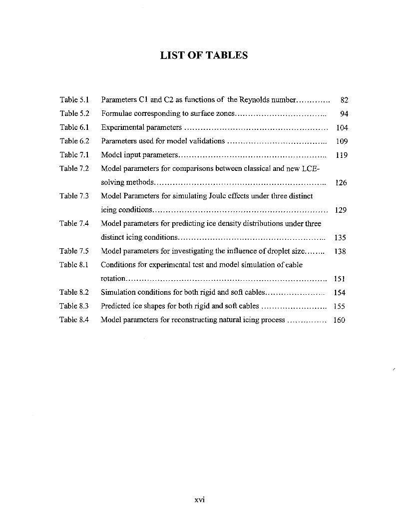
Table 5.1 Parameters C1 and C2 as functions of the Reynolds number 82
Table 5.2 Formulae corresponding to surface zones 94
Tableô.l Experimental parameters 104
Table 6.2 Parameters used for model validations 109
Table 7.1 Model input parameters 119
Table 7.2 Model parameters for comparisons between classical and new LCE-
solving methods 126
Table 7.3 Model Parameters for simulating Joule effects under three distinct
icing conditions 129
Table 7.4 Model parameters for predicting ice density distributions under three
distinct icing conditions 135
Table 7.5 Model parameters for investigating the influence of droplet size 138
Table 8.1 Conditions for experimental test and model simulation of cable
rotation 151
Table 8.2 Simulation conditions for both rigid and soft cables 154
Table 8.3 Predicted ice shapes for both rigid and soft cables 155
Table 8.4 Model parameters for reconstructing natural icing process 160
xvi
CHAPTER 1
INTRODUCTION
Atmospheric icing occurs when freezing raindrops, snow particles or supercooled
cloud droplets come into contact with exposed surfaces. It is a serious and costly natural
phenomenon which affects the operation of such services as electric power transmission
and distribution, telecommunications, and so forth. Annually, a considerably large
number of structural failures due to ice accumulation has been reported in several
countries including Canada, the United States, Japan, England, and China among others.
Approximately 140 tower-collapses as a result of ice accumulation have been reported
and confirmed since 1959 in the United States alone (Mulherin, 1996).
Icing problems may be classified into two types in terms of the meteorological
conditions that produce the ice formation, namely, precipitation icing and in-cloud icing.
Precipitation icing is the most common icing mechanism, and it can occur in any
geographical area subject to freezing rain or drizzle. The difference between the freezing
rain and drizzle is purely one of drop size rather than intensity of precipitation. Usually,
drizzle comes from sheets of low shallow cloud, whereas rain is more likely from deeper
clouds (Poots, 1996). The frozen deposit due to precipitation icing usually appears as a
clear type of glaze, and does not usually last longer than a day or two.
The second type of problem involves in-cloud icing. This type of icing condition is
caused by the impingement of supercooled water droplets in a cloud on an exposed
object. The ice formed under such conditions is mostly rime, and this process tends to
occur in mountainous areas where clouds exist above the freezing level or in a
supercooled fog at lower elevations as produced by a stable air mass with a strong
temperature inversion (Lock, 1990). Such conditions can last for days or even weeks at a
time.
In general, ice may be classified into three basic types, namely, glaze, hard rime and
soft rime(Farzaneh et al., 1992). Glaze is transparent and has a density of about 0.9
g/cm3. Hard rime is opaque and has a density of between 0.6 and 0.87 g/cm3. Soft rime
is white and opaque, with a density of less than 0.6 g/cm3. The type of ice formed is
determined by combinations of air temperature, wind speed, drop size, and liquid water
content or rainfall intensity. A detailed description will be provided in the review of the
literature.
1.1 Background
Under icing conditions, airborne icing particles come to impinge on and then adhere to
a given conductor upon which ice will grow. An ice-covered object exposed to the wind
undergoes an increase in both static and dynamic loads, the distribution of which varies
mainly according to the shape of the ice accretion.
The potential for damage incurred to transmission facilities as a result of the icing
phenomenon is considerable. Ice accumulation causes transmission-line oscillations to
damp slowly, while in the mean time causing an increase in amplitude of these
oscillations due to the non-uniform distribution of aerodynamic and gravitational loads. It
is believed that the galloping, large-amplitude oscillation of ice-covered cables at low
frequencies is responsible for around 1/3 of electric-line maintenance and operating costs
(Hinca et al. 1996). An asymmetrical accumulation also leads to the twisting of
conductors and cables as well as to an acceleration in its degree of fatigue leading to the
possibility of rupture. In extreme cases, excessive accumulations may cause serious
structural failures to overhead power lines, towers, and other related equipment.
Among the numerous power system failures caused by icing of transmission lines, the
one which occurred in southern Quebec and eastern Ontario in January of 1998 was
exceptionally disruptive in terms of both its duration and the scale of the ensuing damage
(Farzaneh, 2000). According to Statistics Canada (Lecomte et al., 1998), during this ice
storm close to 1.4 million people in Quebec and 230,000 in Ontario were subjected to
major power outages for over one week due to the fact that more than 1,000 power
transmission towers and 30,000 wooden utility poles were destroyed by excessive ice-
loads. After assessment of this tragedy, it became increasingly clear to industrial and
public concerns that there had been a significant underestimation of the ice-load effect
during the design of transmission lines for use under icing conditions.
The methods commonly used by researchers in order to investigate the icing process
are summarized as follows:
1. Mathematical modelling,
2. Experimental simulation,
3. Statistical analysis based on data from on-site observations.
Of these three methods, it is clear that the study based on data observed on-site is the
most reliable for design engineers. However, a complete set of observational data is not
always available, since the setting up of the required system is too time-consuming and
not cost-effective. Experimental simulation is a viable way of studying ice accretion since
the test conditions may be controlled to a certain extent. The experimental results,
however, are hardly comparable to observations made under natural conditions as they
tend to vary over time. Mathematical/theoretical modeling is of great value when
combined with experimental validation because of its efficiency and economy.
1.2 The Problem
A satisfactory ice model for use in establishing the critical ice load on transmission
lines under icing conditions is not yet readily available, even though extensive studies on
icing phenomena have been carried out to date by researchers in the domain. The reason
for this lack is due to the fact that scientists have always been motivated by a research
interest in the icing phenomenon alone as simulating this process requires a combination
of multi-disciplinary fields of abstract knowledge. Practical applications of such an ice
model, however, are not adequately addressed. Also, the study in itself leaves much to be
desired from the point of view of ice-model development. Newly-developed technology
and calculation methods emerging from related domains make it possible and necessary
to develop a new ice model capable of better satisfying the needs of the user in terms of
its performance and accessibility. Hence there is a genuine need for carrying the relevant
research even further.
As pointed out by Makkonen et al. (1984), there are several factors which hamper
research and investigation into the ice accretion process.
-The complexity of the ice phenomenon itself: The icing of an object involves several
feedback mechanisms and non-linear relationships between the icing rate and the
various factors affecting it.
-The difficulty in assessing the relevant input parameters: Adequate ice-modelling
requires such input parameters as the liquid water content and droplet size distribution
of the fog or cloud. There are considerable technical problems involved in measuring
these quantities accurately, even under laboratory conditions.
-The lack of experimental data: Precise quantitative verification of theoretical ice
models has been virtually impossible to date, because of the above-mentioned
difficulty in measuring the input parameters. These input parameters are highly
interrelated in the natural environment. There are also practical problems involved in
measuring the icing rate.
1.3 Research Objectives
The main objectives of this research are the following:
1. To develop a time-dependent 2D numerical ice model for simulating the ice
accretion process on a fixed cylindrical object.
2. To model and simulate the ice accretion process on a rotating cable as an
extension of the above-mentioned ice model.
3. To confirm the validity of the ice model by using experimental data obtained from
tests in the CIGELE icing wind tunnel.
The modelling of the ice accretion process may contribute to acquiring a greater in-
depth understanding of this particular phenomenon, and to provide the relevant data for
developing a feasible de-icing solution. From the model simulation, it is possible to
obtain the ice shape, ice-load, and density distribution among others.
The theoretical work consists of two phases. In the first phase, the ice accretion process
on a fixed cable is modelled and simulated, while such model parameters as the Local
Collision Efficiency (LCE) and the local Heat Transfer Coefficient (HTC) are evaluated
on the basis of time-dependent airflow and water droplet trajectory computations. In the
second phase, the ice accretion process on a rotating cable is studied specifically as an
extension of the newly-developed ice code or model, taking into account the effects of
wind and ice load.
The ultimate goal of this project is to develop an ice model intended for practical
operational use, capable of supplying the ice-load information for transmission line
design.
6
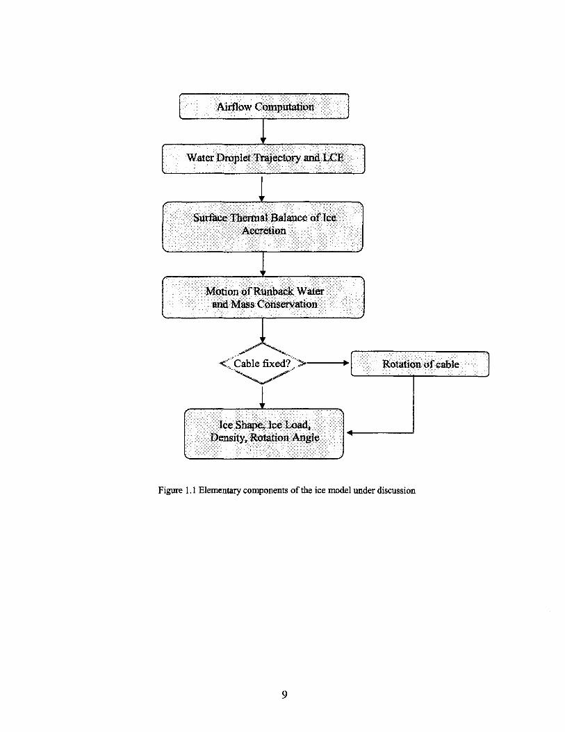
1.4 Methodology
This research project will be carried out in such a way that the theoretical modelling is
followed by the experimental investigation which will produce data for validating the
preceding modeling procedure. The mathematical model presented herein consists of a
number of elementary components, as shown in Figure 1.1.
In particular, airflow filed is solved according to the boundary layer theory, i.e.
potential flow combined with flow boundary layer. The potential flow region under
study is considered to be the superposition of a uniform flow and a disturbance flow
which may be solved using the Boundary Element Method (BEM). The fluid boundary
layer can be evaluated in terms of the velocity distribution on the common boundary as
obtained from the preceding potential flow calculation.
The motion of water droplets was modeled on the basis of the balance between
aerodynamic force, gravity, and buoyancy force. The Runge-Kutta numerical algorithm
was applied in solving the differential equations of motion so as to obtain droplet
trajectories. The local impingement efficiency was evaluated according to its original
definition (McComber, 1981).
In modelling cable rotation under icing conditions, both gravitational and aerodynamic
forces were taken into consideration. The values for the latter forces were derived from

the integration of air pressure and shear stress along the flow boundary, and were
constantly updated according to real-time airflow computations.
In view of the extensive amount of coding work involved in this project, the Object
Oriented Programming techmque (OOP) was used to organize the entire project, since
this technique makes it possible to maintain the ice code with relative ease.
Airflow Computation
Water Droplet Trajectory and LCE
ISurface Thermal Balance of Ice
Accretion
Motion of Runback Waterand Mass Conservation
Cable fixed? > -
�*>»f
Ice Shape, Ice Load,Density, Rotation Angle
Rotation of cable
Figure 1.1 Elementary components of the ice model under discussion
CHAPTER 2
REVIEW OF LITERATURE
2.1 Introduction
Nowadays, a wide variety of publications on the icing phenomenon may be found in
the literature, and certain studies may even date as far back as the 1940s. Since then, the
phenomenon has been subjected to extensive investigation prompted by the requirements
of engineering practices in a number of northern countries, including Britain, Canada,
Czech Republic, Finland, France, Germany, Hungary, Iceland, Japan, Norway, Russia,
Switzerland, and the United States. These studies were made with the aim of compiling
ice-load and wind-on-ice load databases in order to understand the various complex
forms of wet-snow and ice accretion, to develop and to confirm the validity of icing
models, and to introduce probabilistic design load approaches (Poots, 1996).
A number of the existing ice models concentrated on the global ice-load prediction
alone, as in Jones's model (1996) and Makkonen's model (1984), while others focused
on ice shape prediction so as to estimate the dynamic wind-on-ice loads together with
static ice loads. More importance was assigned to the ice shape prediction, since it is easy
to estimate the ice-load from the predicted ice shape simply by integrating the product of
ice density and the area of any element over ice accretion. Also, knowing the ice shape
makes it possible to investigate the dynamic force exerted on iced objects and in the case
of cable icing, it is possible to obtain the overall loads sustained by its supports by means
10
of carrying out integration along its span. It should be pointed out that an irregular ice
shape always aggravates the situation of the transmission line under icing conditions.
The complex nature of the icing process dictates that the quest for further
understanding its mechanism requires a multi-disciplinary approach. Evaluating such
parameters as airflow field and water droplet trajectories from a time-dependent
perspective is extremely time-consuming and requires access to vast computational
resources.
At an earlier stage of the research process, powerful computation tools were not so
easily available as they are today, and apparently this lack hampered the advancement of
studies on ice models. To date, ice model studies appear to have experienced three stages
of development, based on the increasing accessibility of computational tools, whether in
the form of hardware or software.
Stage 1: Enrichment and Collation of Basic Knowledge
By the 1970s, a number of researchers had already carried out numerous fundamental
studies either theoretically or experimentally. Langmuir and Blodgett (1946) successfully
completed trajectory calculations for droplets passing in the vicinity of a circular
cylinder. In his study on a circular cylinder, Ludlam (1951) took into account two
different ice accretion regimes, namely, the dry regime and the wet regime, and he found
that the type of regime is closely related to the water content of the non-perturbed flow at
a given temperature and speed. Fraser, Rush and Baxter (1952) discovered that, under
11
certain conditions, not all of the impinging water is removed, and that part of the water
remains in the pockets of the ice matrix resulting in the formation of spongy ice.
Messinger (1954) and List (1963) developed a heat-balance equation based on energy
conservation, in particular for a circular cylinder. This equation is formulated on the basis
of the assumption that ice accretion is a process of thermal equilibrium, and thus the sum
of all heat transfer terms should be zero.
Contemporaneously, several researchers, including Langmuir & Blodgett (1946); Imai
(1953); and Chainé and Castonguay (1974) among others, attempted to create a formula
to represent the direct relationship between the prevailing climatic conditions and ice
accretion. However, their endeavours met with partial success only.
These above-mentioned fundamental studies have had a profound influence on present-
day numerical modelling. For example, the heat balance equation mentioned above is still
widely used in modern numerical icing models, though with certain slight modifications.
As another example, the curve-fitting functions obtained from the theoretical work of
Langmuir and Blodgett (1946) is still used to evaluate the Local Collision Efficiency
(LCE) in Lozowski's model (1983).
Stage 2: Earlier Attempts at Modelling the Ice Accretion Process on Computers
In the 1980s, researchers began to write computer programs which would carry out
model simulations, and these computer models made it possible to obtain data for
12
generating ice shapes under a wide range of simulation conditions. Before that time, such
ice shapes for the purposes of research could only be obtained from experimental tests.
However, the performance of these programs was comparatively limited and the results
of simulation relied mainly on the individual interpretation of the researcher. Makkonen
(1984) put forward a model based on boundary-layer theory for predicting the local heat
transfer coefficient around a cylinder, taking into consideration the effect of roughness
characteristics. Lozowski et al. (1983) presented a model which was designed to simulate
in-flight ice accretion processes on an unheated, non-rotating cylinder where both rime
and glaze can be accounted for. The model computes the thermodynamic conditions and
the initial icing rate as a function of the angle around the upstream face of the cylinder
using the classical Messinger equation.
Stage 3: Development of Time-Dependent and All-inclusive Numerical Ice Models
Nowadays, the computer is not only an indispensable calculating tool for researchers
but it is also a communication interface between the theoretical model and its users.
Newly-developed numerical ice models tend to be more complete and inclusive, and
hence more complex. Certain time-consuming elements, such as the dynamic airflow
computation and water droplet trajectory calculation, were incorporated in the model
codes. Accordingly, the other parameters are constantly updated in response to the
changes in ice geometry and they include such parameters as the local Heat Transfer
Coefficient (HTC) which is essential in determining the ice shape of wet accretions.
Meanwhile, the models themselves were upgraded from 2D to 3D. These new
developments were more often to be found in studies on airfoil icing such as the
13
LEWICE model at the icing branch of NASA as described by Wright (1995), the one
from ONERA as described by Gent (1990) and by Hedde (1992), and the CANICE
model described by Paraschivoiu (1994). This research was so productive and successful
that these models became applicable in the investigation of ice shapes under a variety of
icing conditions, thereby producing model predictions displaying acceptable accuracy,
although no model to date is capable of encompassing all cases without exception.
The ice codes or models themselves have also been made more easily accessible to the
average layman. User-friendly graphical interfaces and vivid visualizations developed
specifically for these models facilitate the understanding of the complex mechanism of
ice accretion and draw the attention of relevant industrial concerns to the need for
obviating the potential for damage caused by the icing phenomenon.
2.2 Fundamentals of Modelling the Ice Accretion Process
Icing intensity, /, may be determined theoretically from the equation formulated by
Makkonen and Stallabrass (1984):
I = �EnUW (E2-1)
n
where E denotes the collection coefficient. Under dry icing conditions, if the bouncing
effect is disregarded, E may be replaced by the collision efficiency jS.
U and W denote the air speed and liquid water content, respectively, and
n denotes the icing fraction of the overall collected water.
14
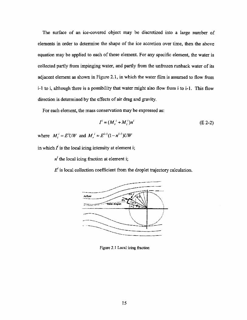
The surface of an ice-covered object may be discretized into a large number of
elements in order to determine the shape of the ice accretion over time, then the above
equation may be applied to each of these element. For any specific element, the water is
collected partly from impinging water, and partly from the unfrozen runback water of its
adjacent element as shown in Figure 2 .1 , in which the water film is assumed to flow from
i-1 to i, although there is a possibility that water might also flow from i to i -1 . This flow
direction is determined by the effects of air drag and gravity.
For each element, the mass conservation may be expressed as:
I/I1' (E 2-2)
where M! =E'UW and Mj =EM(l-ni'1)UW
in which / is the local icing intensity at element i;
ri the local icing fraction at element i;
E1 is local collection coefficient from the droplet trajectory calculation.
Figure 2.1 Local icing fraction
15
It should be noted that local airflow velocity does not appear in Eq. 2-1. The terms of
the LCE and local icing fraction, however, are closely associated with the airflow
velocity distribution, details of which will be discussed in the following section.
2.3 Analysis of Airflow Dynamics
A key problem in investigating the icing phenomenon on cylinders is obtaining
accurate flow calculations for complex geometry and high Reynolds numbers, as is
typical of many icing situations. The airflow across an iced body is compressible and
viscous, a complete solution for which, however, poses considerable mathematical
difficulty for all but the most simple flow boundary geometry.
So far, numerous studies have been carried out to find a solution to the governing
differential equations for such a flow numerically, however, limited success has hitherto
been obtained using such a procedure which has hitherto proved to be overly time-
consuming from a computational viewpoint, as pointed out by Bazeos and Beskos (1990).
hi most classical icing models, airflow computation was sidestepped due to the
difficulties described above; instead, a number of simplified calculation procedures, such
as those of Makkonen (1984) and McComber (1984), were applied. In Makkonen's
procedure, the airflow was taken as a constant free stream and the change in ice accretion
shape was disregarded. The theoretical formulae used to represent the airflow about a
circular object are as follows:
16
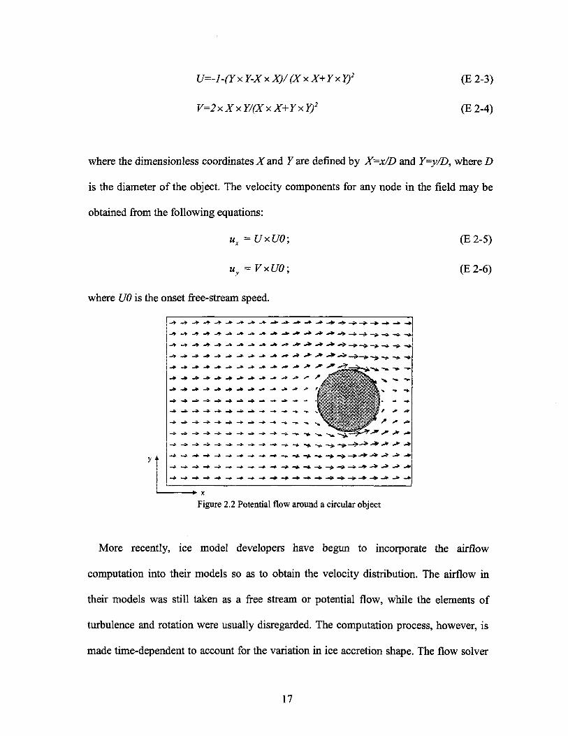
U=-l-(Yx Y-Xx X)/(X x X+Yx Y)2
V=2xXxY/(XxX+YxY)2
(E 2-3)
(E2-4)
where the dimensionless coordinates X and 7 are defined by X=x/D and Y=y/D, where D
is the diameter of the object. The velocity components for any node in the field may be
obtained from the following equations:
ux=UxU0; (E2-5)
uy =VxU0; (E2-6)
where UO is the onset free-stream speed.
- * � x
Figure 2.2 Potential flow around a circular object
More recently, ice model developers have begun to incorporate the airflow
computation into their models so as to obtain the velocity distribution. The airflow in
their models was still taken as a free stream or potential flow, while the elements of
turbulence and rotation were usually disregarded. The computation process, however, is
made time-dependent to account for the variation in ice accretion shape. The flow solver
17
used in the LEWICE code (1995) developed at Douglas, for instance, is a two-
dimensional potential flow code capable of handling up to 10 separate bodies and up to
105 panels in its modified form (Hess & Smith, 1975). According to them, the use of a
potential flow code is desirable due to its speed of execution and its ability to calculate a
flow field around the irregular geometry of the ice shapes produced during ice accretion.
The Douglas Hess-Smith code produces a flow solution by using a distribution of
sources, sinks, and/or vortices along the object geometry, hi calculating the flow field,
contributions from all the sources, sinks, and/or vortices are summed up. The body
surface itself is represented by several straight line segments called panels.
Bazeos & Beskos (1990) pointed out that the evaluation of potential flow by the
Boundary Element Method (BEM) is superior to that obtained using the Panel Method or
indirect BEM, since the physical properties of flow deal with potential and flux, rather
than sources and vortex density.
Lesnic et al. (1995) introduced a practical approach to modelling the flow past a body
with an arbitrary cross-sectional shape. The airflow field was treated as a potential flow
within the separation model and the object immersed in the fluid can be an obstacle with
an arbitrary cross-sectional shape. A tangential detachment of the flow at the edges of the
obstacle was assumed, and hence the infinite behaviour of the velocity at these positions
is removed.
18
2.4 Droplet Trajectory Calculation and Local Collision Efficiency
The Local Collision Efficiency (LCE) is a key parameter for ice accretion simulation,
since it describes the distribution of droplet impingement on the surface of an object. In
order to evaluate the LCE according to its original definition, it is necessary to obtain the
trajectories for hundreds of droplets, which further demands a thorough and all-inclusive
solution to the airflow field. Performing both these computations, however, requires a
painstaking approach to the task.
Seminal work by Taylor (1940), and Langmuir & Blodgett (1945), has laid the
foundations for studying the impact of cloud droplets on structures and, in more recent
years, for developing the theory of the inertial deposition of aerosols on objects. Consider
a stream of particles moving in a horizontal direction toward a circular cylinder placed
perpendicular to the direction of the airflow. The particles far upstream are assumed to be
moving at the free stream velocity. On approaching the cylinder, a particle undergoes a
deflecting force due to the diverging streamlines, and a resistance originating in its own
inertia. Thus the particle motion relative to the airflow decreases and the particle may fail
to reach the cylinder surface before it is swept away by the airflow. The collision
efficiency of the cylinder, E, is defined as the ratio of the mass flux of impinging particles
on the upstream side of the cylinder, to the mass flux that would be experienced by the
surface if the particles had not been deflected by the air stream. An identical definition
may be derived from the work of Taylor (1940), and Langmuir & Blodgett (1945), as
follows:
19
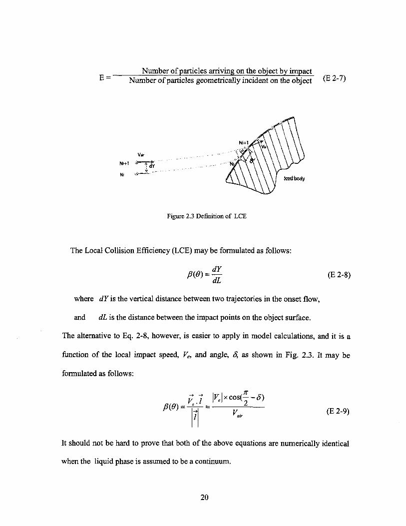
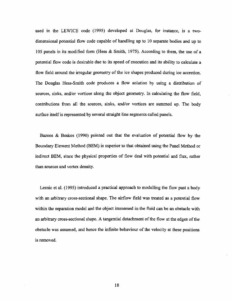
Number of particles arriving on the object by impactNumber of particles geometrically incident on the object (E2-7)
Nl+l
Ni+1
Ni
Figure 2.3 Definition of LCE
The Local Collision Efficiency (LCE) may be formulated as follows:
«»�£ (E 2-8)
where dY is the vertical distance between two trajectories in the onset flow,
and dL is the distance between the impact points on the object surface.
The alternative to Eq. 2-8, however, is easier to apply in model calculations, and it is a
function of the local impact speed, Ve, and angle, 5, as shown in Fig. 2.3. It may be
formulated as follows:
f-j rexcos(^-£)
Kir (E 2-9)
It should not be hard to prove that both of the above equations are numerically identical
when the liquid phase is assumed to be a continuum.
20
In the past, many ice model researchers preferred to use empirical approximations to
obtain the Local Collision Efficiency directly in order to avoid the complexity of field
computations. Gates et al. (1984) reported two approximate methods commonly used by
those who attempted to develop ice models. One approach, used by Ackley and
Templeton (1978), and by Makkonen (1984), assumes that the accretion retains a known
simple shape as it grows, in this case, roughly circular. The impingement coefficient can
thus be readily obtained by a function of dimensionless parameters using tabular
interpolation, or by fitting the curves plotted according to pre-computed values. An
alternative approach, formulated by Lozowski et al. (1979, 1983), assumes that the first
thin accreted layer represents a small perturbation in the shape of the accreting body,
thereby causing the airflow, droplet trajectories, and local collision efficiency to
experience small perturbations. This layer should be addressed by applying perturbation
methods to the dynamic equation for gaseous and liquid phases. In this approach, a
heuristic argument is used to estimate the perturbations.
For wire icing, Makkonen (1984) proposed an empirical correction to the total
collection efficiency. The collection efficiency, Em , based on the Median Volume
Diameter (MVD) of the droplet size distribution may thus be determined. The calculation
is again based on the Langmuir & Blodgett method for the dimensionless equation of
motion for a droplet in an airflow.
Jones (1996), however, attempted to integrate, and thus numerically solve, the
differential equation for water droplet trajectory developed by Lozowski (1983), taking
21
into account both gravitational force and air drag on freezing drizzle or precipitation-
sized droplets, as follows:.
dv
dto
4dp0v-V V~V +g (E2-10)
where v is the droplet velocity, V is the wind velocity, CD is the drag coefficient of the
�»droplets, # is the droplet diameter, and g is the acceleration of gravity. In the absence of
a solution to this equation for rain and drizzle-sized droplets, Jones assumed that the
droplets fall at their terminal velocity and move horizontally at the wind speed.
It should be noted that Eq. 2-10 is impossible to solve unless the nodal-wise airflow
�»vector, V, is available, therefore airflow computation is a prerequisite for water droplet
trajectory calculation.
2.5 Velocity and Thermal Boundary Layer
� Velocity Boundary Layer
A major practical breakthrough with regard to viscous fluid computation was made
when, according to Kays & Crawford (1993), Brandt discovered that the influence of
viscosity is confined to an extremely thin region very close to the object under
investigation, and that the remainder of the flow field can be treated approximately as
22
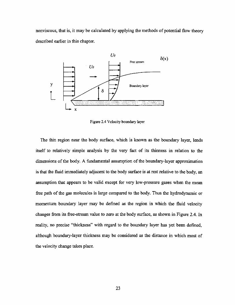
nonviscous, that is, it may be calculated by applying the methods of potential flow theory
described earlier in this chapter.
Uo
Uo
I
Free streamô(x)
Boundary layer
LFigure 2.4 Velocity boundary layer
The thin region near the body surface, which is known as the boundary layer, lends
itself to relatively simple analysis by the very fact of its thinness in relation to the
dimensions of the body. A fundamental assumption of the boundary-layer approximation
is that the fluid immediately adjacent to the body surface is at rest relative to the body, an
assumption that appears to be valid except for very low-pressure gases when the mean
free path of the gas molecules is large compared to the body. Thus the hydrodynamic or
momentum boundary layer may be defined as the region in which the fluid velocity
changes from its free-stream value to zero at the body surface, as shown in Figure 2.4. In
reality, no precise "thickness" with regard to the boundary layer has yet been defined,
although boundary-layer thickness may be considered as the distance in which most of
the velocity change takes place.
23
So far, only a few exact solutions to the equations of motion for boundary layers are
known, and these are mainly for laminar flow. When the calculation procedure becomes
overly tedious and time-consuming, it is often worthwhile to search for an approximate
approach, such as integral methods. The integral equations of the boundary layer provide
the basis for a number of approximate procedures, but are, in themselves, exact at least
within the boundary-layer approximation. The very nature of the integral solutions arises
from the manner in which they are generally employed.
� Thermal Boundary Layer
Just as a velocity boundary layer develops when there is fluid flow over a surface, a
thermal boundary layer develops concurrently, if the fluid free stream and surface
temperature differ. The region of the fluid in which these temperature gradients exist is
the thermal boundary layer, and its thickness, 8t, is typically defined as the value of y for
[ (T � T) / 1
v s y(T _ j ^ = 0.99. With increasing distance from the leading
edge, the effects of heat transfer penetrate further into the free stream and the thermal
boundary layer grows.
A number of integral equations may be applied in evaluating the Nusselt number for
the laminar boundary layer, the turbulent boundary layer, if any, and the wake section.
The free-stream velocity above the boundary layer may be determined by solving the
equations of the airflow boundary layer as described in Chapter 3, and the input
parameters may then be used for the thermal calculation of the boundary layer.
24
Once the local Nusselt number is known, the local HTC, h, may be obtained according to
the following formula:
!� = ""� K'/L (E2-11)
where, Kf is the thermal conductivity of the fluid, and L is a characteristic dimension of
the model under consideration.
2.5.1 Effect of Reynolds Number and Roughness on the Velocity Boundary Layer
Roughness or imperfections of the surface tend to provoke early transition, as does also
a high degree of turbulence in the free stream outside the boundary layer. A most
important factor, however, is the Reynolds number. If this number is measured in terms
of the distance along the surface, then for values less than about 105, the laminar
boundary layer is very stable and it is difficult to provoke transition. However, with an
increase of the Reynolds number, the stability of the laminar boundary layer decreases,
and transition is more and more easily provoked. With a Reynolds number, in terms of
distance along the surface, greater than about 2xlO6, considerable care must be taken in
keeping the surface smooth while at the same time eliminating external disturbances so as
to avoid an early transition. Surface roughness has a potential for hastening the transition
of the boundary layer as mentioned above. The small roughness elements tend to behave
like bluff bodies and eddies are cast off them which then disturb the laminar boundary
layer and induce transition to turbulent flow and in consequence the drag usually
increases. Eddies are likewise cast off the roughness elements when the boundary layer
is turbulent and then they directly increase the local drag. The larger the roughness
elements, the larger the drag increment which they cause.
25
S\
J
Tripwire toprovoketransition
V
(b)
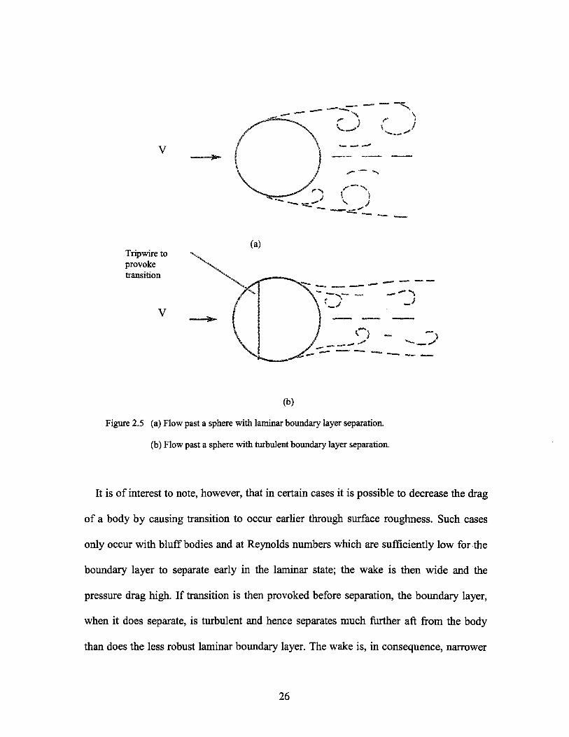
Figure 2.5 (a) Flow past a sphere with laminar boundary layer separation,
(b) Flow past a sphere with turbulent boundary layer separation.
It is of interest to note, however, that in certain cases it is possible to decrease the drag
of a body by causing transition to occur earlier through surface roughness. Such cases
only occur with bluff bodies and at Reynolds numbers which are sufficiently low for the
boundary layer to separate early in the laminar state; the wake is then wide and the
pressure drag high. If transition is then provoked before separation, the boundary layer,
when it does separate, is turbulent and hence separates much further aft from the body
than does the less robust laminar boundary layer. The wake is, in consequence, narrower
26
and the pressure drag is reduced, so that there is a marked net reduction in the total drag,
as shown in Figure 2.5 (Duncan et al , 1970). Such a process may be observed in the case
of a smooth bluff body like a sphere or cylinder as the Reynolds number increases. At
low Reynolds numbers the boundary layer is wholly laminar and separates early from the
surface causing a large eddying wake; the drag coefficient is in consequence high. With
an increase of the Reynolds number a critical value is eventually reached at which the
boundary layer goes turbulent before separation, and separation occurs later. The wake at
that stage diminishes as does the drag coefficient. The Reynolds number at which this
occurs is called the critical Reynolds number.
2.S.2 Effect of Reynolds Number and Roughness on the Thermal Boundary Layer
In general, surface roughness tends to boost the convective HTC by hastening the
boundary layer transition. As a result, in typical conditions of icing on stationary
structures, the convective Heat Transfer Coefficient (HTC ) is 2-3 times higher for a
rough cylinder than for a smooth cylinder. In typical aircraft icing conditions it may even
be 5-6 times higher (Makkonen,1984).
27
4,5
150
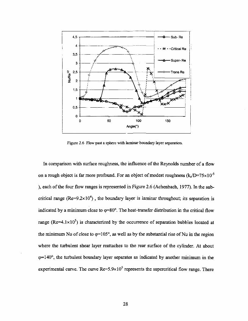
Figure 2.6 Flow past a sphere with laminar boundary layer separation.
In comparison with surface roughness, the influence of the Reynolds number of a flow
on a rough object is far more profound. For an object of modest roughness (ks/D=75xl0"5
), each of the four flow ranges is represented in Figure 2.6 (Achenbach, 1977). In the sub-
critical range (Re=9.2xlO4) , the boundary layer is laminar throughout; its separation is
indicated by a minimum close to <p=80°. The heat-transfer distribution in the critical flow
range (Re=4.1xlO5) is characterized by the occurrence of separation bubbles located at
the minimum Nu of close to <p=105°, as well as by the substantial rise of Nu in the region
where the turbulent shear layer reattaches to the rear surface of the cylinder. At about
9=140°, the turbulent boundary layer separates as indicated by another minimum in the
experimental curve. The curve Re=5.9xlO5 represents the supercritical flow range. There
28
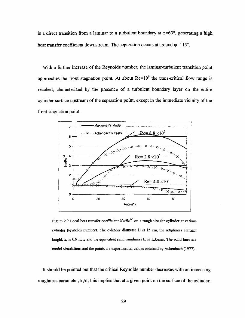
is a direct transition from a laminar to a turbulent boundary at cp=60°, generating a high
heat transfer coefficient downstream. The separation occurs at around cp=l 15°.
With a further increase of the Reynolds number, the laminar-turbulent transition point
approaches the front stagnation point. At about Re=106 the trans-critical flow range is
reached, characterized by the presence of a turbulent boundary layer on the entire
cylinder surface upstream of the separation point, except in the immediate vicinity of the
front stagnation point.
rl Makkonen's Model
- �§� - -Achenbach's Tests
80
Figure 2.7 Local heat transfer coefficient Nu/Re1''2 on a rough circular cylinder at various
cylinder Reynolds numbers. The cylinder diameter D is 15 cm, the roughness element
height, k, is 0.9 mm, and the equivalent sand roughness ks is 1.35mm. The solid lines are
model simulations and the points are experimental values obtained by Achenbach (1977).
It should be pointed out that the critical Reynolds number decreases with an increasing
roughness parameter, ks/d; this implies that at a given point on the surface of the cylinder,
29

the boundary layer undergoes transition from laminar to turbulent flow at decreasing
Reynolds numbers (Achenbach, 1971).
Makkonen (1984) put forward a mathematical model to predict the local heat transfer
coefficient along the cylinder surface, based on the integral equations of the boundary
layer. The local velocity above the boundary layer, was evaluated from the potential flow
velocity distribution around a cylinder. In particular, the local free-stream velocity above
the boundary layer was obtained with the aid of the Bernoulli equation. The model
calculation results were then compared with Achenbach's data (1977), as shown in
Figure 2.7. The solid lines are model simulations, while the points represent
experimental values obtained by Achenbach. For a small cylinder and a low Reynolds
number, Makkonen's model correctly predicted the tendency of a laminar boundary layer
to prevail at all angles on the upstream side, while no boundary layer transition occurs,
and the heat transfer coefficient decreases slowly with an increasing angle cp. An apparent
discrepancy is found downstream, at the angular position of 70°, which might arise from
the fact that the boundary layer separation was not taken into consideration in this model.
The Reynolds number in the case of cable icing lies within a range of 104 to 105, and
falls under sub-critical flow conditions. Thus, the windward side of the cable presents a
primarily laminar boundary layer upstream of the separation point.
2.5.3 Evaluating the Nusselt Number for a Rough Cylinder
� Makkonen's Correlation
30
The average convective heat transfer coefficient for a rough cylinder, as used by
Makkonen, is valid for Reynolds numbers between 7xlO4 and 9xlO5. The Reynolds
number is a function of the cylinder diameter and is evaluated at the average
temperature of the cylinder and air temperatures at the boundary layer.
N u = 0 . �
� Achenbach's Correlation
The local convective heat transfer coefficient for a rough cylinder, as measured by
Achenbach, is estimated as a function of the Reynolds Number, Re, based on the
diameter of the cylinder and the angular position, 6.
25))) (E2-13)
Eq. 2-13 was also used in Lozowski's model (1983) to estimate the heat transfer
coefficient locally.
The mean value for the Nusselt number is obtained by integrating the Nusselt
number along the effective cooling zone between -25° and 25°, and then by applying
integration to Eq. 2-13 which yields:
� Grenier's Correlation
The average convective heat transfer coefficient used by Grenier (1986) was
estimated as a function of the Reynolds number, Re, based on the diameter of the
31
cylinder and evaluated at the average temperature between the cylinder temperature
and the air boundary layer temperatures.
È
1
1000 -t �-� � -
100 -
10
0,1 -1
n n i
��� Makkonen
���� Grenier
�«s�- Achenbach
Reynolds
1000
Number
10000
1
s1O0JOOO
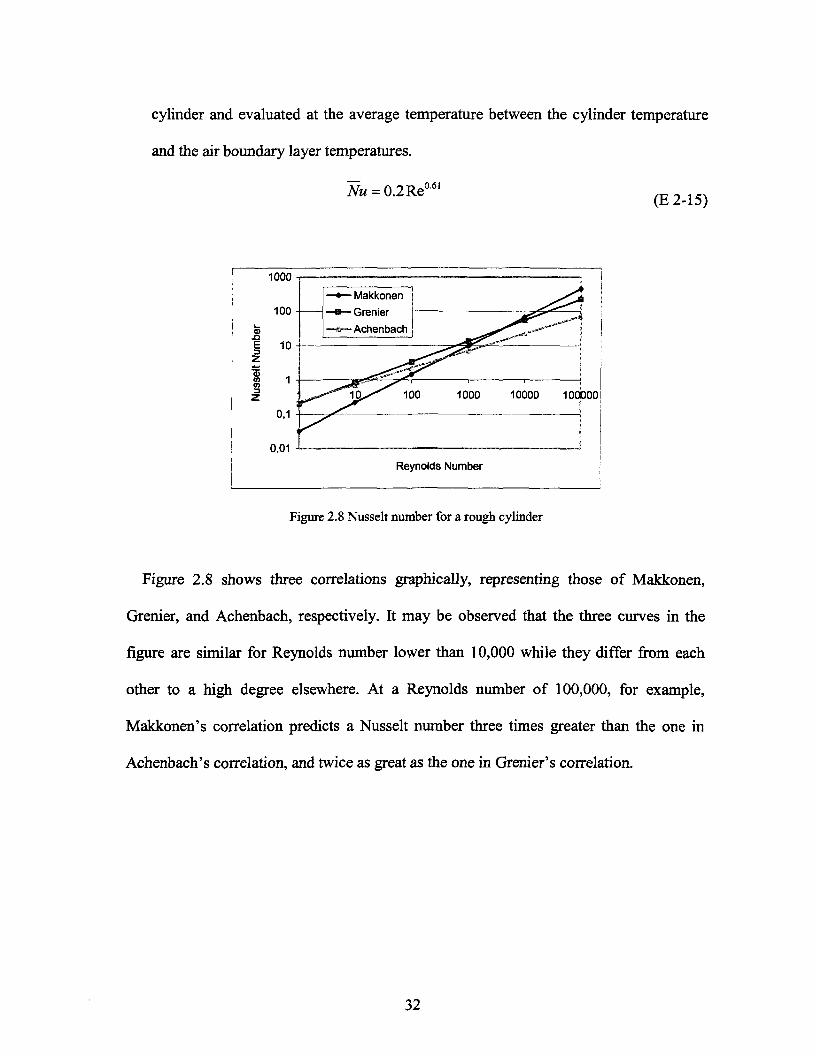
Figure 2.8 Nusselt number for a rough cylinder
Figure 2.8 shows three correlations graphically, representing those of Makkonen,
Grenier, and Achenbach, respectively. It may be observed that the three curves in the
figure are similar for Reynolds number lower than 10,000 while they differ from each
other to a high degree elsewhere. At a Reynolds number of 100,000, for example,
Makkonen's correlation predicts a Nusselt number three times greater than the one in
Achenbach's correlation, and twice as great as the one in Grenier's correlation.
32
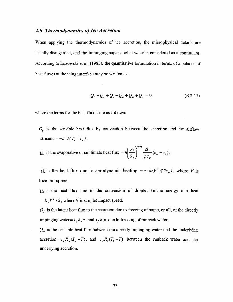
2.6 Thermodynamics of Ice Accretion
When applying the thermodynamics of ice accretion, the microphysical details are
usually disregarded, and the impinging super-cooled water is considered as a continuum.
According to Lozowski et al. (1983), the quantitative formulation in terms of a balance of
heat fluxes at the icing interface may be written as:
Qc+Qe+Qv+Qk+Qw+Qf=0
where the terms for the heat fluxes are as follows:
Qc is the sensible heat flux by convection between the accretion and the airflow
streams = -n � h(Ts -TJ.
Pr 1 d
~ (ea ~es)>
c
Qvis the heat flux due to aerodynamic heating =n-hrvV2/(2cp), where F i s
local air speed.
Qhis the heat flux due to the conversion of droplet kinetic energy into heat
= RWV212, where V is droplet impact speed.
Qf is the latent heat flux to the accretion due to freezing of some, or all, of the directly
impinging water= lfsRji, and lfiRsn due to freezing of runback water.
Qw is the sensible heat flux between the directly impinging water and the underlying
accretion = cwRw(Ta -T), and cwRs(Ts-T) between the runback water and the
underlying accretion.
33
,4
103
102
e. Relative Humidityu. Wind b. Temperature c. Pr�iplatioii d. Diameter and Solar RadiationI tv * f v k o �> I »; s I ? t u e I a s f v K c e U s i y k a e I w s f v k
. I�
�
�
-
. -
-
E
J,� IT-
-
�
-
�
�
- ]-
i i i i
-
�
'n*
�
-
�a
-
I '
�-
�E
-
�
-
m
-
m
1 1 � 1
10"
1Û"
3 | . , , , | , , , � I I | | | i l l | | �
Cooling HMtlnrj Cooling htedUng C o o i n g Haa thg Cooling Haa lhg C o d i n g " Heating
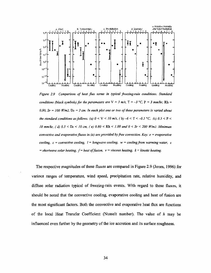
Figure 2.9 Comparison of heat flux terms in typical freezing-rain conditions. Standard
conditions (black symbols) for the parameters are V = 3 m/s, T = -3 °C, P = 3 mm/hr, Rh =
0.90, Sr = 100 W/m2, Dc = 3 cm. In each plot one or two of these parameters is varied about
the standard conditions as follows: (a)0<V < 10 m/s, (b)-6<T< -0.5 °Q (c) 0.5 < P <
10 mm/hr, (d) 0.5 < Dc < 10 cm, (e) 0.80 < Rh < 1.00 and 0 < Sr < 200 W/m2. Minimum
convective and evaporative fluxes in (a) are provided by free convection. Key: e = evaporative
cooling, c = convective cooling, I = longwave cooling, w = cooling from warming water, s
- shortwave solar heating, f= heat of fusion, v = viscous heating, k = kinetic heating.
The respective magnitudes of these fluxes are compared in Figure 2.9 (Jones, 1996) for
various ranges of temperature, wind speed, precipitation rate, relative humidity, and
diffuse solar radiation typical of freezing-rain events. With regard to these fluxes, it
should be noted that the convective cooling, evaporative cooling and heat of fusion are
the most significant factors. Both the convective and evaporative heat flux are functions
of the local Heat Transfer Coefficient (Nusselt number). The value of h may be
influenced even further by the geometry of the ice accretion and its surface roughness.
34
2.7 Surface Temperature of Ice Accretions
Knowing which ice regime prevails at any given position on the ice surface is a
prerequisite for calculating the surface temperature (Karev and Farzaneh, 2004). At the
outset, a wet regime is assumed, and the corresponding surface temperature should be at
the freezing point of water, or 0°C. The icing fraction is then calculated based on the
thermal balance equation. If the calculation result does not lie between 0 and 1, the initial
assumption is proved to be false. It may then be concluded that a dry regime has been
attained and thus, that the corresponding icing fraction should be 1. In view of the fact
that the heat balance equation is a non-linear function, a number of numerical methods
may readily be applied to it.
2.8 Ice Volume and Ice Density.
The ice volume for an arbitrary surface element / at a time step y may be obtained from
the equation as follows:
' pi (E2-16)
where mi denotes the ice mass, and pt denotes the ice density.
The type of ice obtained from the surface of an iced object is a function of atmospheric
and meteorological conditions. When ice is formed under different atmospheric and
environmental conditions, it displays totally different patterns of behaviour. Ice may be
35
classified into three basic types, namely, glaze, hard rime, and soft rime. Rime comes into
being when the conditions are such that supercooled water droplets freeze instantly at the
moment of impact. There is no unfrozen water on the surface and this absence promotes
surface roughness. Hard rime is opaque due to the presence of air bubbles which are
trapped during the rapid freezing process. Supercooled droplets may be trapped on the
surface since they do not freeze upon impact, and they tend to gather together to form
larger droplets. Usually, surface droplets are larger than impinging droplets and this fact
helps to explain why rough elements may also be observed on certain accretions of hard
rime. The presence of these rough elements on the surface leads to an increase in the rate
of heat transfer, which in turn speeds up the ice build-up process. In some extreme cases,
a protuberance composed of a mixture of rime and glaze emerges. Glaze is characterized
by a slower freezing process due to the presence of some large-sized supercooled
droplets. Of the three types of ice, glaze is of the highest density and its surface is smooth
and transparent. In general, the density of ice is a function of surface temperature. For
wet accumulations, the surface temperature may reach zero and the density may go as
high as 917kg/m3. For dry accumulations, the surface temperature is lower than 0°C and
the corresponding density varies over a wide range.
Equation 2-16 dictates that ice density may affect the predicted ice shape to such a
degree that great care should be taken when dealing with this parameter. The mass of the
frozen fraction is derived from the thermal balance equation, as described in Eq. 2-11.
The ice thickness is inversely proportional to its density. Ice density may be calculated by
using certain empirical formulae which were usually obtained from curves generated by
36
experimental data. Most of these formulae, however, are functions of the Macklin
parameter.
2.8.1 Ice Density Formula based on Macklin's Parameter
Macklin's density parameter (1962) is defined in the formulation:
R = V0dJ(2ts) (E2-17)
where dm is the median volume diameter of the droplets (jam); Vo is the impact speed of
the droplets (ms"1) at the stagnation point as obtained from droplet trajectory calculations
(Langmuir & Blodgett, 1946); and ts is the local surface temperature on the iced surface
� Macklin's Ice Density ( 1962)
The first equation for ice density was developed by Macklin and is a function of
the Macklin parameter:
Pi=Pref{~RVL5)2 (E2-17)
pref is a reference density corresponding to water density at 4°C.
� Bain and Gayet's Ice Density (1983)
This equation was defined by Bain and Gayet and is also a function of the Macklin
parameter:
p . = 0.11R076 for R<=10,
orp. =R(R+5.61)'! for 10<R<=60,
37
orp . = 0.917 for R>60. (E 2-19)
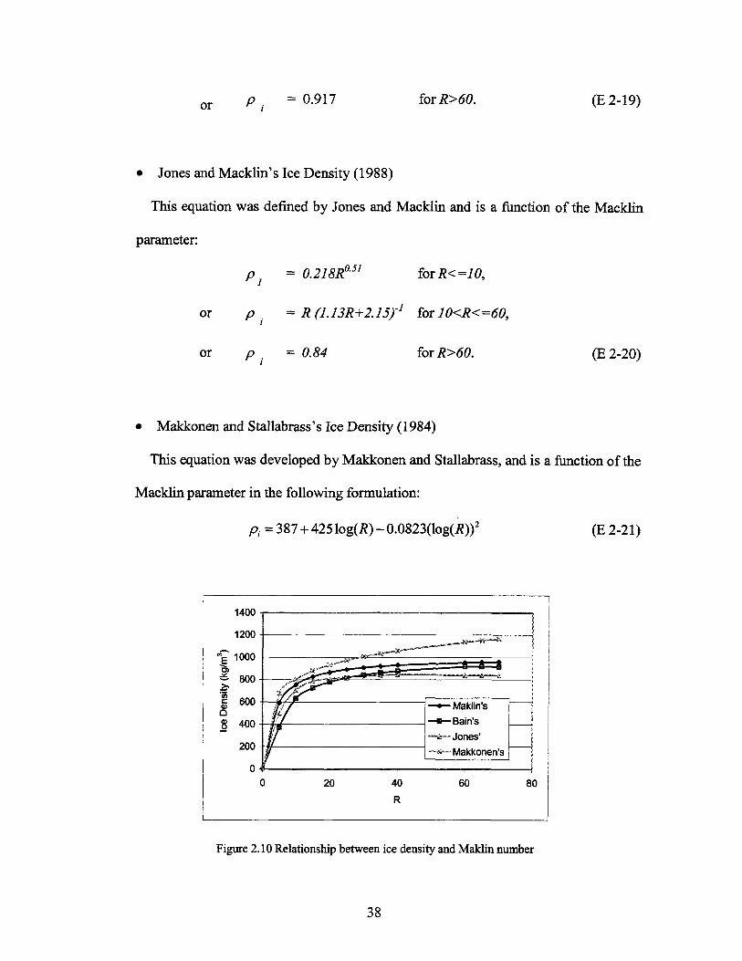
� Jones and Macklin's Ice Density (1988)
This equation was defined by Jones and Macklin and is a function of the Macklin
parameter:
= 0.218R051 for R<=10,
or p . = R(J.J3R+2.J5/1 for J0<R<=60,
or p . =0.84 forR>60. (E2-20)
� Makkonen and Stallabrass ' s Ice Density ( 1984)
This equation was developed by Makkonen and Stallabrass, and is a function of the
Macklin parameter in the following formulation:
pi = 387 + 425 \og(R) - 0.0823(log(iî))2 (E 2-21)
1400
Figure 2.10 Relationship between ice density and Maklin number
38
Figure 2.10 shows four correlations graphically, representing those of Macklin, Bain,
and Jones, and Makkonen, respectively. It may be observed that, of these four formulae,
Makkonen's correlation predicted the highest ice density over the entire Macklin-number
range while Bain's produces the lowest value over the small Macklin-number section,
and then Jones' ice density takes its place to become the lowest over the large Macklin-
number section.
2.8.2 LEWICE Ice Density
The equation developed by LEWICE is a function of the frozen fraction of supercooled
water, f, as follows:
/ (E2-22)
2.9 Conclusion
This chapter has introduced relevant aspects of modeling ice accretion processes,
including the basic principles of an ice model, the evolution of techniques used in
modeling this process as well as a number of specific researches on aspects of the ice
model.
39
CHAPTER 3
AIRFLOW COMPUTATION
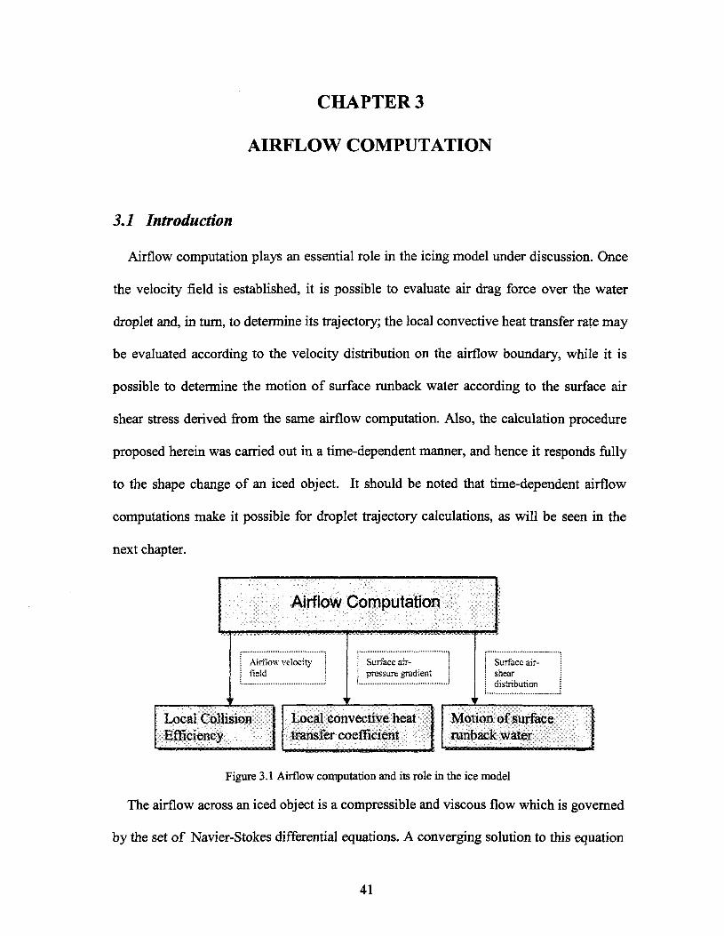
3.1 Introduction
Airflow computation plays an essential role in the icing model under discussion. Once
the velocity field is established, it is possible to evaluate air drag force over the water
droplet and, in turn, to determine its trajectory; the local convective heat transfer rate may
be evaluated according to the velocity distribution on the airflow boundary, while it is
possible to determine the motion of surface runback water according to the surface air
shear stress derived from the same airflow computation. Also, the calculation procedure
proposed herein was carried out in a time-dependent manner, and hence it responds fully
to the shape change of an iced object. It should be noted that time-dependent airflow
computations make it possible for droplet trajectory calculations, as will be seen in the
next chapter.
Airflow Computation
^
\ Airflow velocity |j Held " I
Local CollisionEfficiency
I Surface air-I pressure gradient
r
Local convective heattransfer coefficient
1
! Surface air- I! shear !! distribution !
r
Motion of surfacerunback water
Figure 3.1 Airflow computation and its role in the ice model
The airflow across an iced object is a compressible and viscous flow which is governed
by the set of Navier-Stokes differential equations. A converging solution to this equation
41
has proved to be costly and time-consuming from a computational point of view, thus
there is little purpose at present in incorporating it in the proposed ice model, hi practical
applications, a full solution to the flow field is unnecessary, since the calculation is only
required for the upstream airflow where the cylindrical object receives the major portion
of water droplet impingement.
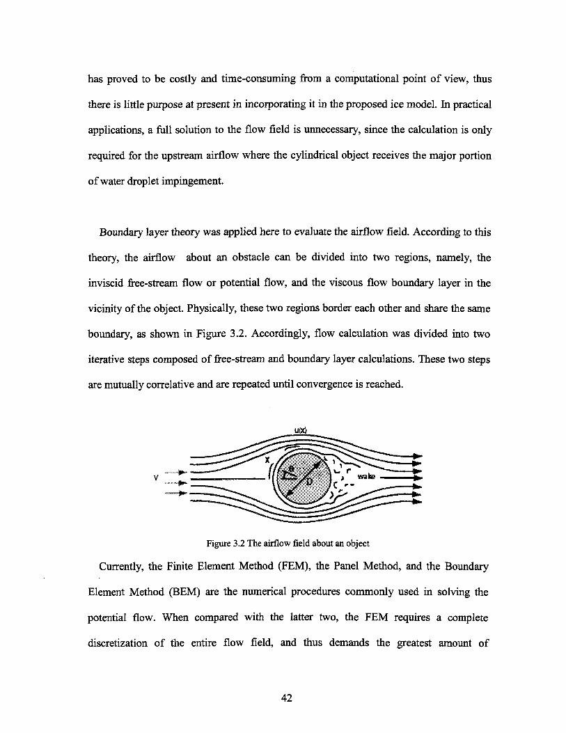
Boundary layer theory was applied here to evaluate the airflow field. According to this
theory, the airflow about an obstacle can be divided into two regions, namely, the
inviscid free-stream flow or potential flow, and the viscous flow boundary layer in the
vicinity of the object. Physically, these two regions border each other and share the same
boundary, as shown in Figure 3.2. Accordingly, flow calculation was divided into two
iterative steps composed of free-stream and boundary layer calculations. These two steps
are mutually correlative and are repeated until convergence is reached.
Figure 3.2 The airflow field about an object
Currently, the Finite Element Method (FEM), the Panel Method, and the Boundary
Element Method (BEM) are the numerical procedures commonly used in solving the
potential flow. When compared with the latter two, the FEM requires a complete
discretization of the entire flow field, and thus demands the greatest amount of
42
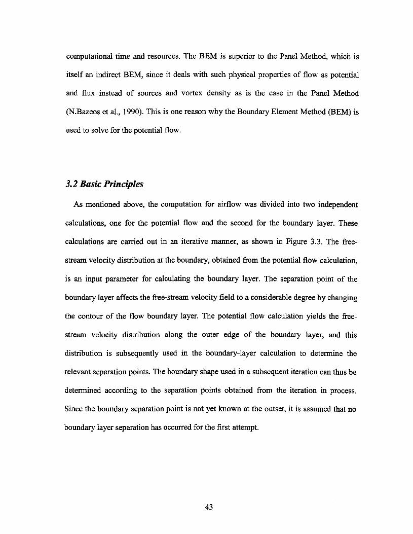
computational time and resources. The BEM is superior to the Panel Method, which is
itself an indirect BEM, since it deals with such physical properties of flow as potential
and flux instead of sources and vortex density as is the case in the Panel Method
(N.Bazeos et al., 1990). This is one reason why the Boundary Element Method (BEM) is
used to solve for the potential flow.
3.2 Basic Principles
As mentioned above, the computation for airflow was divided into two independent
calculations, one for the potential flow and the second for the boundary layer. These
calculations are carried out in an iterative manner, as shown in Figure 3.3. The free-
stream velocity distribution at the boundary, obtained from the potential flow calculation,
is an input parameter for calculating the boundary layer. The separation point of the
boundary layer affects the free-stream velocity field to a considerable degree by changing
the contour of the flow boundary layer. The potential flow calculation yields the free-
stream velocity distribution along the outer edge of the boundary layer, and this
distribution is subsequently used in the boundary-layer calculation to determine the
relevant separation points. The boundary shape used in a subsequent iteration can thus be
determined according to the separation points obtained from the iteration in process.
Since the boundary separation point is not yet known at the outset, it is assumed that no
boundary layer separation has occurred for the first attempt.
43
Ai if low Computation
Updatedboundaryshape
Potential flowcalculation(FiniteElement Method)
r
Boundary layercalculation
Figure 3.3 Calculation procedure for airflow computation
5.5 Potential Flow
As indicated earlier, potential flow is an ideal, irrotational and incompressible flow
which can be solved numerically by using the BEM. The flow around an object may be
viewed as the combination of a uniform stream and a disturbance flow according to the
theory of flow superposition. The uniform stream is of initial velocity when the border of
the body is seen as transparent, thereby allowing the stream to enter and exit freely. The
disturbance flow simulates the effect imposed by an immersed body. Accordingly, the
stream function, cp, at any position in the flow field may be expressed as a combination of
the initial stream, <pi, and the disturbance flow, q>2, as follows:
where % . V j and % - v , .
44
The equation cp, = Voy, defines the steady onset flow, and <p2 is a perturbation stream
function induced by the immersed object. Since the disturbance flow is incompressible
and irrotational, and thus of zero divergence, it may be expressed in the form of
Laplace's equation, as follows:
V2<p2=0 (E3-2)
Since the uniform stream (pi is known, it is possible to solve the variable q>j in terms of
the disturbance stream <p2-
The boundary conditions of the problem may be written asç>2=-ç>,=-V0y on F, if the
function value of the streamline on the surface of the object, F, is tentatively assumed as
zero in the formulation q> =0. For general application, cp2 will be replaced by q> when Eq.
3-2 is transformed in accordance with the BEM in the following section.
When Equation (E 3-2) is implemented with the residual integral equation according to
the Galerkin method, this equation may be written as follows:
1= j^-V2çdA = 0 (E3-3)
By applying Green's theorem and integrating the above equation by parts, Equation (E
3-3) may be written as follows:
f <p(y2cp)dA = - f cp{V2(f,)dA +\<p^-dT-\<l)^dT=Q (E 3-4)iA iA * dn f? on
The fundamental solution to the 2-D problem can be written as follows:
0 = ±]n(k (E3-5)2K r
45
According to its definition, the fundamental solution represents the field generated by a
concentrated unit charge acting at a point, i. The effect of this charge is propagated from i
to infinity without any consideration of boundary conditions.
Equation 3-5 may also be written as V2tf> + A' = 0 where A' represents a Dirac Delta
function which tends to be infinite at point i and is equal to 0 elsewhere. The integral of
A' is equal to 1 in the formulation J V2ð = 1.
Based on these considerations, Equation (E 3-4 ) can be written at point i as
(E3-6)
Applying Green's third law and integrating (E 3-6) by parts yields
;=1 h
Qwhere C, = � in which 6 is the internal angle of the corner in radians.
In
Defining q = � and replacing � with q, the equation (E 3-7) can be transformed intoon on
the following formula:
0^1 + 2, w�dl = 2,wQdl (E3-8)
When the boundary is divided into n segments or elements, the values of <p and q at any
point on an arbitrary element may be defined in terms of their nodal values and two linear
46
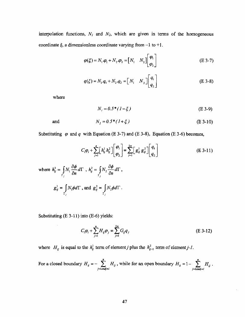
interpolation functions, Ni and N2, which are given in terms of the homogeneous
coordinate £, a dimensionless coordinate varying from -1 to +1.
(E 3-7)
(E 3-8)
= Nv<pl+N2.<p2=[Nl N2]
where
and
(E 3-9)
(E3-10)
Substituting <p and q with Equation (E 3-7) and (E 3-8), Equation (E 3-6) becomes,
j=\! '
T 2= S[«l«J]
where hy = I N ^ d T ,hiJ=\N2 � dY,� on r
J on1 j ' J
gl= $NrfdT, and gl=
(E3-11)
Substituting (E 3-11) into (E-6) yields:
(E 3-12)
where Htj is equal to the h- term of elementy plus the hl_x term of element7-/.
For a closed boundary Hu=- ^ H y , while for an open boundary Hu=l- ^ Hi}j=\andj*i j=\andj*i
Al
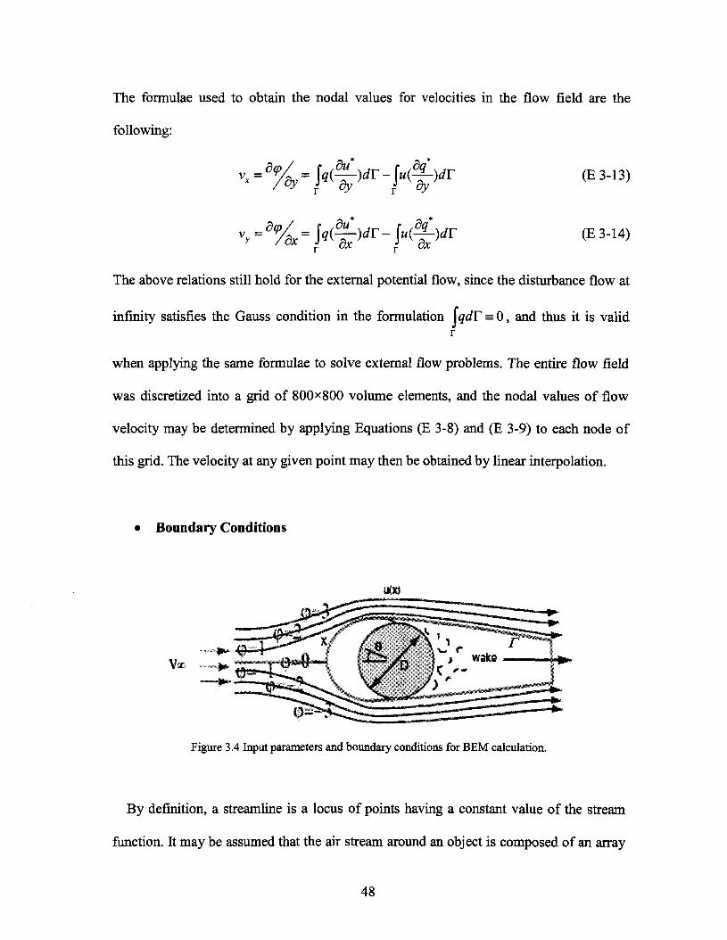
The formulae used to obtain the nodal values for velocities in the flow field are the
following:
(E3-13)
(E 3-14)
The above relations still hold for the external potential flow, since the disturbance flow at
infinity satisfies the Gauss condition in the formulation s 0, and thus it is valid
when applying the same formulae to solve external flow problems. The entire flow field
was discretized into a grid of 800x800 volume elements, and the nodal values of flow
velocity may be determined by applying Equations (E 3-8) and (E 3-9) to each node of
this grid. The velocity at any given point may then be obtained by linear interpolation.
� Boundary Conditions
Figure 3.4 Input parameters and boundary conditions for BEM calculation.
By definition, a streamline is a locus of points having a constant value of the stream
function. It may be assumed that the air stream around an object is composed of an array
48

of streamlines, the values of which may be defined in the way indicated in Figure 3.4. In
order to solve the external flow around the obstacle body, the flow boundary,/" ,was
defined in such a way as to coincide with the outer edge enclosing the object and its
resultant wake. The boundary of the wake was determined on the basis of the assumption
that the air boundary layer separates from the object surface in the tangential direction.
The value of the streamline passing along this boundary may be treated as zero in the
formulation <p = 0.
� Time-Dependent Boundary Discretization
During model simulation, the shape of the boundary, F, should be updated over time
in response to the position changes of the boundary layer separation points, as indicated
by the heavy green line in Figure 3.4. At the outset, no flow boundary separation was
assumed and the surface of the object was taken as the initial boundary for the BEM
calculation.
3.4 Airflow Boundary Layer
The fluid boundary layer may be evaluated based on the free-stream velocity
distribution on the outer edge of the flow boundary. In the empirical formulae, which will
be introduced in subsequent sections, this velocity distribution is integrated along the
surface of the object so as to determine the positions of transition points and separation
points. These formulae will also be used for the further evaluation of such parameters as
the momentum thickness and frictional coefficient for both laminar and turbulent sections.
49
3.4.1 Laminar Boundary Layer
The laminar boundary layer under a pressure gradient is governed by the integral
momentum equation as described by Duncan (1970). The direct application of this
equation proved to be impossible from a practical point of view due to the difficulty in
defining the term for the velocity profile in the presence of a pressure gradient. The
Thwaites method described in the book (Gerhart et al., 1992), however, demands no such
prerequisite, and is thus the most viable way of evaluating the laminar boundary layer.
The feasibility of this method is further confirmed by its wide use in related areas of
research. The Thwaites method (1949) may be formulated as follows:
Uxb o
where 0 is the momentum thickness;
Uo is the onset flow velocity;
Ux is the free-stream velocity on the boundary;
and xo denotes the location of the stagnation point in the surface-attached
coordinate system.
t/ois an input parameter for the ice model, and Ux may be obtained from the potential
flow calculation, as described in the preceding sections. If the integration starts from the
stagnation point, xo may be replaced by 0. Thus, Equation 3-15 may be solved for any
position in the laminar boundary layer. The calculation procedure may be carried out
according to the following steps:
50
a) Obtain U(x) from potential flow calculation, taking 0O as zero when calculation
starts from stagnation point.
b) At any x, calculate momentum thickness, 0 , from Equation 3-8.
c) Calculate dimensionless pressure gradient, X, in formulation 2 H � ( � * - ) andv dx
evaluate RQ according to RQ = .
d) Calculate air shear stress, T, according to T(Â) « (2 + 0.09)0.62
and shape factor, H, according to H(Â)2.61-3.752+ 5.24A2 (2 >0)
0.0731
0.15 + 2+ 2.088(2 <0)
e) Calculate skin-friction coefficient,Cf, using formula Cf = 2T®(AJ
f) Calculate wall shear stress, Tw, according to Tw = ��-.0
5*g) Calculate boundary thickness, ô*, according to H - � = H (A).
3.4.2 Turbulent Boundary Layer
The airflow sweeping across the iced object is characterized by a high Reynolds
number. Under the influence of surface roughness, the initial laminar boundary flow
tends to become unsteady and a flow boundary transition may thus occur earlier. There
are few satisfactory methods for solving the Reynolds-averaged equations which hold
particularly for the turbulent boundary layer (Kays and Crawford, 1993). Nevertheless, a
51
number of integral approximations are available for evaluating the turbulent boundary
layer empirically.
The approximate method developed by Spence (Duncan et al., 1970) is in use currently
and has wide application in a number of related research fields. The approximation may
be written as follows:
. ± (E3-9,
where 0 , H, x, Ux and rw bear the same definitions as those shown above, while Ç is a
dimensionless parameter. It is necessary to establish the relations between 0 , H, and Ç in
order to obtain a solution for 0 . Experimental results have shown that the velocity profile
may be viewed as a single-parameter function of H for the turbulent boundary layer
(Duncan, 1970), while Spence further suggested using the following exponential
approximate formula for the velocity profile when there is a large adverse pressure
gradient:
7T = &2 (E3-10)
where y is measured normal to the x coordinate, and penetrates into the boundary layer.
The integral equation may be solved using H=1.5, and an empirical integral equation in
terms of 0 may thus be obtained.
&6/5Ux
42 -®t6l5u;2 = 0.0106Re~1/5 [Ux*dx (E 3-11)
where xt is the coordinate at the transition point, and Ut is the free-stream velocity at the
outer edge of the boundary layer. According to Duncan (1970), the validity of applying
52
Eq. 3-11 is supported by the fact that the momentum thickness, ©, is insensitive to the
choice of the shape coefficient, H. From Ludwieg-Tillman's equation, it is possible to
obtain the friction coefficient using:
Cf = 0.246R&-26810-°678H (E 3-12)
where the dimensionless parameter R@ is the momentum thickness and may be defined as
R0=Ux0/v.
In order to evaluate the shape coefficient H with greater precision than heretofore,
Spence's equation should be used, and may be written as follows:
SV* (E3"13)
0 442where X(H) = 2.105 - , and C, =
(H-Ï)
The wall shear stress, rw, can be evaluated according to the following formula:
r-=V (E3-14)
3.4.3 Transition Points
In the preceding sections, a concentrated effort was made to develop integral formulae
for solving the velocity laminar boundary layer and turbulent boundary layer. These
formulae on their own, however, are not sufficient to complete the task of evaluating the
specific flow boundary layer under investigation. Additional work should be done in
order to determine the transitional zone where the laminar boundary flow turns into a
53
turbulent boundary flow. It should be noted that the transition is an incremental process,
rather than an abrupt one. It is still valid to assume, however, that the dimension of the
transition section is as small as a point for the flow under discussion, and may be
evaluated on the basis of the momentum thickness:
R@=l.l74[1 + 22400/Rx]Rx046 (E 3-15)
and the generally acceptable valve value for the critical Re number is
RXr=3.2xl0s (E3-16)
From Michel's expression (in Duncan, 1970), the critical Reynolds number may be
obtained in terms of the momentum thickness as follows:
R0ir=43O (E3-17)
This method provides a high degree of accuracy, since the local pressure gradient is taken
into account.
3.4.4 Separation Points
The task of determining the separation point may be carried out by using the Strafford
correlation method, whose validity has already been verified experimentally by Cebeci
(1974). By dividing the flow boundary layer into two regions, namely, the internal and
external regions, Strafford associated the separation criterion with the pressure gradient
of the external boundary layer, which may be formulated as follows:
ReJino = f(x) (E 3-18)ax
54
where Cp =l-(�/, in which Ua is the flow velocity at the starting point of thea
adverse gradient.
If a laminar section or a favorable pressure gradient develops in the boundary layer, it
is necessary to substitute x with (x-x ) , and Rx with Um(x-x)/v. The factor x
represents the distance from the imaginary stagnation point to the point of inception of
the adverse gradient. The factor x is calculated using the Spence equation as follows:
*' = *' ~ Î(TT}'>dx-943@« Rej/5(U/U ) (E 3-19)
where xm is the position of minimum pressure,
0fr is the momentum thickness at the transition point, and
Re is the non-dimensional momentum thickness at the transition point.
It is opportune, at this point, to evaluate these expressions numerically so as to obtain the
function f(x) as a criterion to be used for estimating the separation point. In formulation,
this function may be detailed as follows:
f(x) < 0.3 no separation detected;
0.3 < f(x) <0.5 separation detected at point where maximum value is found;
0.5 < f(x) separation detected at point where f(x) = 0.5.
3.5 Feedback Effect in Airflow Calculations due to Boundary Layer Separation
Since the two interactive zones, potential flow and boundary layer, cannot be evaluated
independently, iteration of calculations was made in order to determine the boundary
55
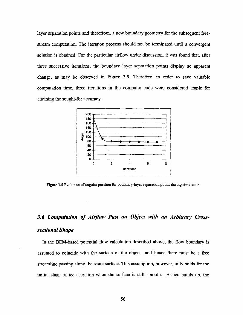
layer separation points and therefrom, a new boundary geometry for the subsequent free-
stream computation. The iteration process should not be terminated until a convergent
solution is obtained. For the particular airflow under discussion, it was found that, after
three successive iterations, the boundary layer separation points display no apparent
change, as may be observed in Figure 3.5. Therefore, in order to save valuable
computation time, three iterations in the computer code were considered ample for
attaining the sought-for accuracy.
20018016014012010080604020
VTT *�»-
4
Iterations
Figure 3.5 Evolution of angular position for boundary-layer separation points during simulation.
3.6 Computation of Airflow Past an Object with an Arbitrary Cross-
sectional Shape
In the BEM-based potential flow calculation described above, the flow boundary is
assumed to coincide with the surface of the object and hence there must be a free
streamline passing along the same surface. This assumption, however, only holds for the
initial stage of ice accretion when the surface is still smooth. As ice builds up, the
56
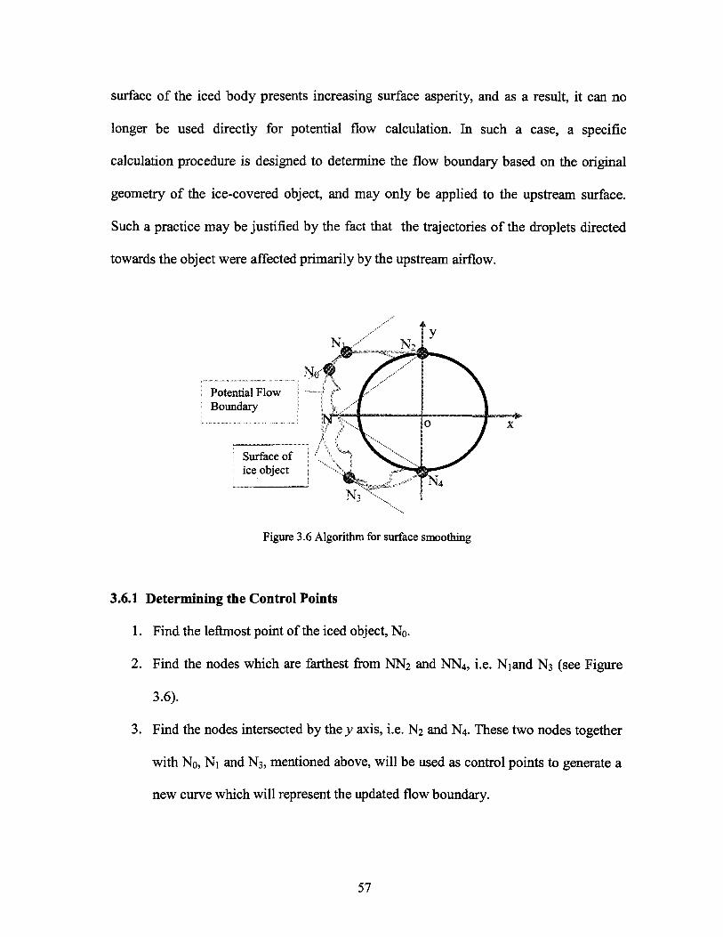
surface of the iced body presents increasing surface asperity, and as a result, it can no
longer be used directly for potential flow calculation. In such a case, a specific
calculation procedure is designed to determine the flow boundary based on the original
geometry of the ice-covered object, and may only be applied to the upstream surface.
Such a practice may be justified by the fact that the trajectories of the droplets directed
towards the object were affected primarily by the upstream airflow.
Potential FlowBoundary
Figure 3.6 Algorithm for surface smoothing
3.6.1 Determining the Control Points
1. Find the leftmost point of the iced object, No.
2. Find the nodes which are farthest from NN2 and NN4, i.e. Niand N3 (see Figure
3.6).
3. Find the nodes intersected by the y axis, i.e. N2 and N4. These two nodes together
with No, Ni and N3, mentioned above, will be used as control points to generate a
new curve which will represent the updated flow boundary.
57
3.6.2 Algorithm for Boundary Curve Based on Control Points Developed Above
A number of algorithms may be taken from among the available options, and the
curves generated by these algorithms may be totally different in shape. A number of
important curve-generating algorithms are listed below:
� The Lagrange Polynomial (LP)
The curve generated from the Lagrange polynomial will pass through all the control
points. Given the n+1 data points, the polynomial so developed is of a degree n. For large
n, such a curve would be too loose and it may also oscillate excessively, hi practice, a
tight curve is preferred. Also, the LP is unique, hi principle, there are an infinite number
of curves that pass through any set of given points, and the intended one may not happen
to be the LP. As a result, it may be concluded that a useful curve should be of a low
degree by nature and should depend on parameters that affect the shape of the curve.
� The Bézier Curve
The Bézier curve is a parametric curve P(t) which is a polynomial function of the
parameter t. The degree of the polynomial depends on the number of points used to
define the curve. The method uses control points to produce an approximating curve
which does not pass through the interior control points but is attracted by them.
� The B-Spline
The B-Spline curve overcomes the main disadvantages of the Bézier curve, namely, (i)
the degree of the Bézier curve depends on the number of control points, (ii) it provides
58
only global control, and, (iii) individual segments are easy to connect with Cl continuity,
but C2 is difficult to obtain. The B-spline curve features local control and any desired
continuity. In addition to the above-mentioned control points, the values of certain
quantities called "knots" are real numbers and may offer additional control over the shape
of the curve.
The B-Spline algorithm was adopted, particularly because the order of this parametric
function does not increase as the number of control points grows. This same algorithm
will be used later on in the research to fit a particular set of control points, thereby
generating an artificial surface which will represent the airflow boundary.
3.7 Airflow Field Visualization
Figure 3.7 shows the airflow simulation results after executing the present ice code.
The graphs in Figures 3.7 (a) and (b) represent the airflow patterns for the original non-
iced cylindrical object and the ice-covered object, respectively. For the cylinder, the
airflow is symmetrical in the windward direction, and airflow separation occurs at an
angle of about 80°, as shown in Figure 3.7 (a). According to observations made by
Duncan (1970), this separation occurs in the laminar section, rather than in the turbulent
one. The mechanism involved in this type of separation may be explained by the fact that
the Reynolds number in such a case is less than 105. Accordingly, the laminar boundary
layer remains relatively stable, making it difficult for this layer to transform itself into a
turbulent boundary layer. The pattern of airflow velocity distribution is more
sophisticated in the case of the iced object of a complex geometrical shape, as shown in
59
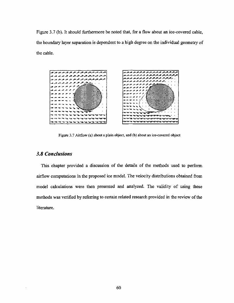
Figure 3.7 (b). It should furthermore be noted that, for a flow about an ice-covered cable,
the boundary layer separation is dependent to a high degree on the individual geometry of
the cable.
Figure 3.7 Airflow (a) about a plain object, and (b) about an ice-covered object
3.8 Conclusions
This chapter provided a discussion of the details of the methods used to perform
airflow computations in the proposed ice model. The velocity distributions obtained from
model calculations were then presented and analyzed. The validity of using these
methods was verified by referring to certain related research provided in the review of the
literature.
60
CHAPTER 4
DROPLET TRAJECTORY AND COLLISION EFFICIENCY
4.1 Introduction
Calculating local collision efficiency is of prime importance in predicting the shape of
the ice accretion, since the mass of supercooled droplets impinging on the surface of an
iced body may easily be obtained using the formula WU/3, where U and W are both
constants. For a dry accretion, the amount of water impingement collected at any given
position is proportional to its local collision efficiency.
As an a priori requirement, it is necessary to track the trajectories numerically for a
number of droplets in accordance with the original definition of Local Collision
Efficiency (LCE) as will be seen in Equation 4-13. This tracking procedure demands the
greatest amount of computational time, as well as storage resources, compared to the
time required for running any other elementary components in the model.
For a time-dependent ice model in particular, it is necessary to account for the
feedback effect of changing ice geometry. It should be noted that the changes in ice
geometry will result in the variation of such parameters as the airflow velocity field, the
motion pattern of water droplets, and the LCE.
61
Thus, the ice model under discussion takes into account the feedback effect of
changing geometry during cable icing, as well as the changed airflow velocity field. In
particular, airflow is computed on the basis of the new geometry of the iced cable, and
thereby the updated airflow velocity distributions are established. The equation of motion
is solved so as to obtain the trajectories for a number of droplets. The feedback
mechanism of the changing geometry of iced cables is accounted for by recording the
occurrence of collisions of water droplets with the iced cable surface.
4.2 Basic Principles
In the proposed model, the motion of water droplets was modeled on the basis of the
balance between the forces of air drag, gravity, and buoyancy. The Runge-Kutta
algorithm was adopted here to solve the set of differential equations of motion for
obtaining droplet trajectories. The local collision efficiency was then evaluated according
to its definition. Lastly, a third order polynomial interpolation was performed to obtain
the local collision efficiency at the relevant position. The air drag force was obtained and
updated from airflow field computations during ice accretion simulations, considering
that this force is predominant with regard to the other terms in the equation of motion for
small droplets or drizzle.
4.2.1 Equations Governing the Motion of a Water Droplet
A particular droplet in the vicinity of transmission line cables is liable, at any instant,
to undergo electric-field effects. The nature and magnitude of the influence of such
effects are dependent on the parameters of the cables as well as on the natural ambient
62
conditions. Farzaneh (2000) pointed out that several phenomena are associated with the
influences of an electric field on droplets, thus making it inappropriate to conduct an
analysis by singling out any given phenomenon from all the others. The force due to the
electrical field, Fe, is disregarded in the model presented here so as to avoid incurring
greater complexity.
The forces considered in the equation of motion are the following:
� Air Drag Force
The air drag force acting on a water droplet may be expressed as the product of the
drag coefficient, Cd , air density, frontal area of the droplet, and velocity difference
between air and droplet, in the formulation:
Fd=V2PaCdA V-v (V-v) (E4-1)
in which V is derived from the airflow computation.
In the case of a low Reynolds number, it is preferable to evaluate the Cd together with
the Reynolds number itself, according to the formulae, as described in the remaining part
of this section.
� Gravity
The classical formula for gravity is used herein, as follows:
Fg=pe~gV (E4-2)
63
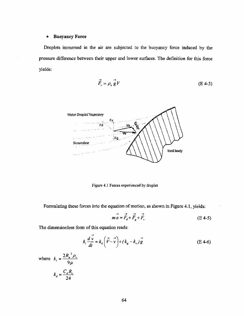
� Buoyancy Force
Droplets immersed in the air are subjected to the buoyancy force induced by the
pressure difference between their upper and lower surfaces. The definition for this force
yields:
(E4-3)
" Fd
Streamline
Figure 4.1 Forces experienced by droplet
Formulating these forces into the equation of motion, as shown in Figure 4.1, yields:
2 = Fd+Fg+Fv (E4-5)
The dimensionless form of this equation reads:
kdv_ = k1 dt ~
where k; = �2-^-£-9//
(E4-6)
64
g 9ju
k =
where v is the droplet velocity, V is the wind velocity, Cd is the drag coefficient of the
droplet, D is the drop diameter, and g is the acceleration of gravity.
In particular, kd is evaluated by combining the formulae corresponding to the
experimental studies carried out independently by Langmuir et al.(1946) and Beard et al.
(1969), as follows:
C<JR° = 1 + 0.189 x Re0632 for 21<Re<=20024
5 A = l + 0.115 x Re0 802 for 2<Re<=2124
CR = l + 0.102 x Re0 9S5 for 0.2<Re<=224
and
C R��=1+0197xReO63+2 6e-4xReus for the remaining Re numbers24
After taking components, Equation 4.6 can be reduced to a set of first-order ordinary
differential equations as follows:
kt � = kd(Vx-vx), for the*-axis, (E 4-7)dt
^ A y y ) ( k s -kb>8> f o r t h e ^
and
65
dx
dt y
The signs in the equations may vary according to the definition of directions for both x-
and y-axes.
4.2.2 Solutions
The velocities vx and vy appear on both sides of the above differential equations
thereby making them nonlinear. In view of the difficulties involved in finding a
theoretical solution, seeking numerical solutions to them is recommended. It should be
noted that these equations are a set of first-order differential formulae, to which the
Runge-Kutta algorithm may conveniently be applied. Here, a four-variable Runge-Kutta
algorithm was used to solve the equations numerically.
4.2.3 Initial Conditions and Time Steps
Initially, water droplets were located on the upstream side of the object at a horizontal
distance of 5xDcabie as shown in Figure 4.3, where the gradient of the airflow velocity
field is assumed to be 0. The initial velocity x components of water droplets may be
expressed as vx = Vo in which VQ is the onset free-stream speed.
vy = 9.32 x (1 - e-{MVDn 77)U47 ) D > 300,1» ,
or
vy = 0 D < 300/̂ m
66
where the y component is the terminal droplet speed (Best, 1950).
The time step is carefully designed to meet the requirements of computational
efficiency and accuracy. To initiate the calculation procedure, a larger time step is
adopted to account for a minor velocity change. With droplets approaching the icing
object, the time step is scaled down to compensate for a sharper velocity gradient. Also,
the time step should be proportional to the diameter of the cable, Dcabie» and inversely
proportional to the onset air speed, Vajr. In formula form, the factors may be expressed as
follows:
Dcable/Vait (E 4-12)
4.2.4 Surface Collision
In order to obtain the LCE, it is necessary to detect the location of collision points
accurately. These points are to be found at the intersection of the trajectories and the
surface of the body.
Since the surface is divided into a number of linear elements, it may be regarded as a
polygon. Thus, this problem may be converted in such a manner as to solve the
intersections between the straight line T1-T2, and the polygon, as shown in Figure 4.2.
Tl and T2 are the points on the trajectory corresponding to two sequential time steps.
The details of the procedure for determining the occurrence of collisions are provided
below:
67
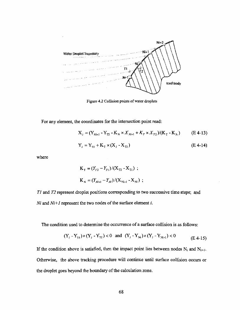
Figure 4.2 Collision points of water droplets
For any element, the coordinates for the intersection point read:
X, =(YN i + 1 -YT 2 -KNxXM + 1 +^x^ r 2 ) / (KT -KN ) (E4-13)
Y ^ Y ^ + K T X C X J - X ^ ) (E4-14)
where
KT =(YT2 -Yn)/(XT2 -XT 1) ;
77 and T2 represent droplet positions corresponding to two successive time steps; and
M and Ni+1 represent the two nodes of the surface element i.
The condition used to determine the occurrence of a surface collision is as follows:
(Y J-YT 1)x(Y J-YT 2)<0 and (Y, -YNi)x(Y, - YNi+1 ) <0 ( E 4 1 5 )
If the condition above is satisfied, then the impact point lies between nodes N, and N,+;.
Otherwise, the above tracking procedure will continue until surface collision occurs or
the droplet goes beyond the boundary of the calculation zone.
68
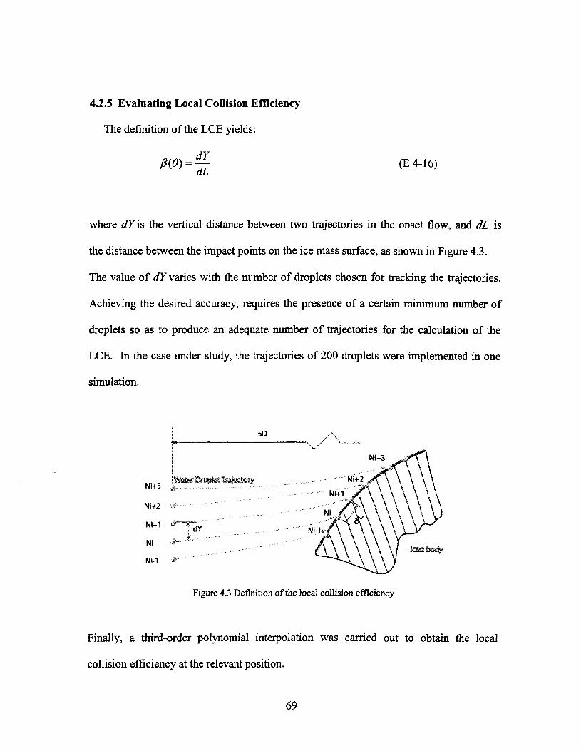
4.2.5 Evaluating Local Collision Efficiency
The definition of the LCE yields:
P(0) = % (E4-16)aL
where dY is the vertical distance between two trajectories in the onset flow, and dL is
the distance between the impact points on the ice mass surface, as shown in Figure 4.3.
The value of dY varies with the number of droplets chosen for tracking the trajectories.
Achieving the desired accuracy, requires the presence of a certain minimum number of
droplets so as to produce an adequate number of trajectories for the calculation of the
LCE. In the case under study, the trajectories of 200 droplets were implemented in one
simulation.
5D
Ni+3
Ni+2
Ni
NU
Figure 4.3 Definition of the local collision efficiency
Finally, a third-order polynomial interpolation was carried out to obtain the local
collision efficiency at the relevant position.
69
During the simulation, the Median Volume Diameter (MVD) was used to represent a
spectrum of droplets. The validity of this practice will be assessed in the next section.
70
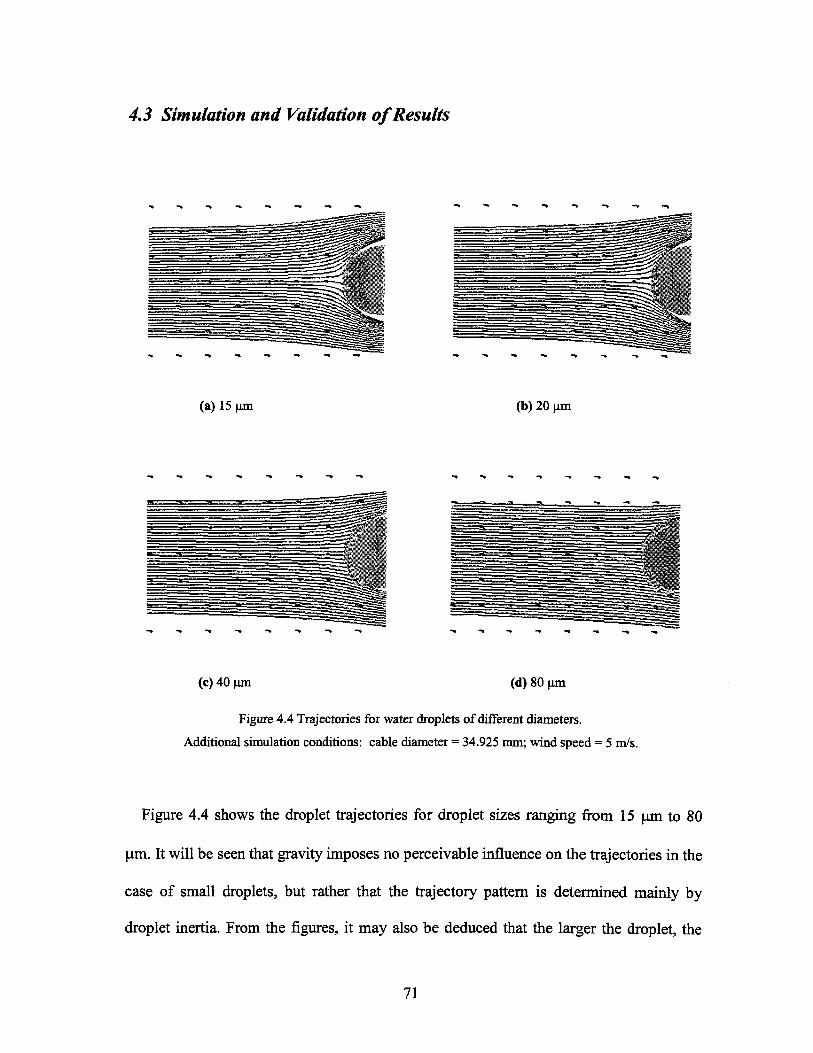
4.3 Simulation and Validation of Results
(a) 15 (b) 20 urn
(c) 40 um (d) 80 um
Figure 4.4 Trajectories for water droplets of different diameters.
Additional simulation conditions: cable diameter = 34.925 mm; wind speed = 5 m/s.
Figure 4.4 shows the droplet trajectories for droplet sizes ranging from 15 fxm to 80
|im. It will be seen that gravity imposes no perceivable influence on the trajectories in the
case of small droplets, but rather that the trajectory pattern is determined mainly by
droplet inertia. From the figures, it may also be deduced that the larger the droplet, the
71
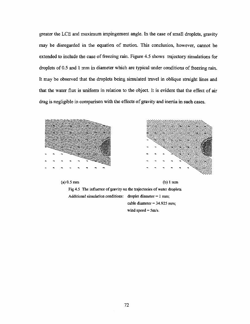
greater the LCE and maximum impingement angle. In the case of small droplets, gravity
may be disregarded in the equation of motion. This conclusion, however, cannot be
extended to include the case of freezing rain. Figure 4.5 shows trajectory simulations for
droplets of 0.5 and 1 mm in diameter which are typical under conditions of freezing rain.
It may be observed that the droplets being simulated travel in oblique straight lines and
that the water flux is uniform in relation to the object. It is evident that the effect of air
drag is negligible in comparison with the effects of gravity and inertia in such cases.
(a) 0.5 mm (b) 1 mm
Fig 4.5 The influence of gravity on the trajectories of water droplets
Additional simulation conditions: droplet diameter = 1 mm;
cable diameter = 34.925 mm;
wind speed = 5m/s.
72
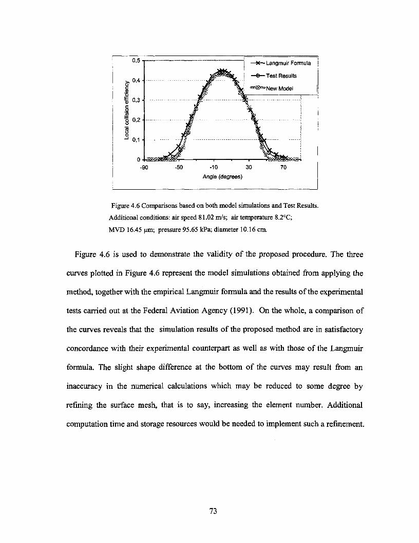
Langmuir Formula ||
Test Results
-10 30
Angle (degrees)
70
Figure 4.6 Comparisons based on both model simulations and Test Results.
Additional conditions: air speed 81.02 m/s; air temperature 8.2°C;
MVD 16.45 urn; pressure 95.65 kPa; diameter 10.16 cm.
Figure 4.6 is used to demonstrate the validity of the proposed procedure. The three
curves plotted in Figure 4.6 represent the model simulations obtained from applying the
method, together with the empirical Langmuir formula and the results of the experimental
tests carried out at the Federal Aviation Agency (1991). On the whole, a comparison of
the curves reveals that the simulation results of the proposed method are in satisfactory
concordance with their experimental counterpart as well as with those of the Langmuir
formula. The slight shape difference at the bottom of the curves may result from an
inaccuracy in the numerical calculations which may be reduced to some degree by
refining the surface mesh, that is to say, increasing the element number. Additional
computation time and storage resources would be needed to implement such a refinement.
73
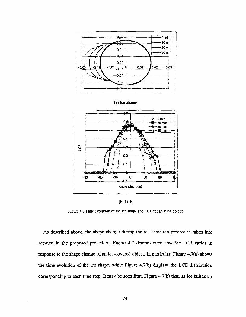
(a) Ice Shapes
O o min�B�10min�es� 20 min !
(b)LCE
Figure 4.7 Time evolution of the Ice shape and LCE for an icing object
As described above, the shape change during the ice accretion process is taken into
account in the proposed procedure. Figure 4.7 demonstrates how the LCE varies in
response to the shape change of an ice-covered object, hi particular, Figure 4.7(a) shows
the time evolution of the ice shape, while Figure 4.7(b) displays the LCE distribution
corresponding to each time step. It may be seen from Figure 4.7(b) that, as ice builds up
74
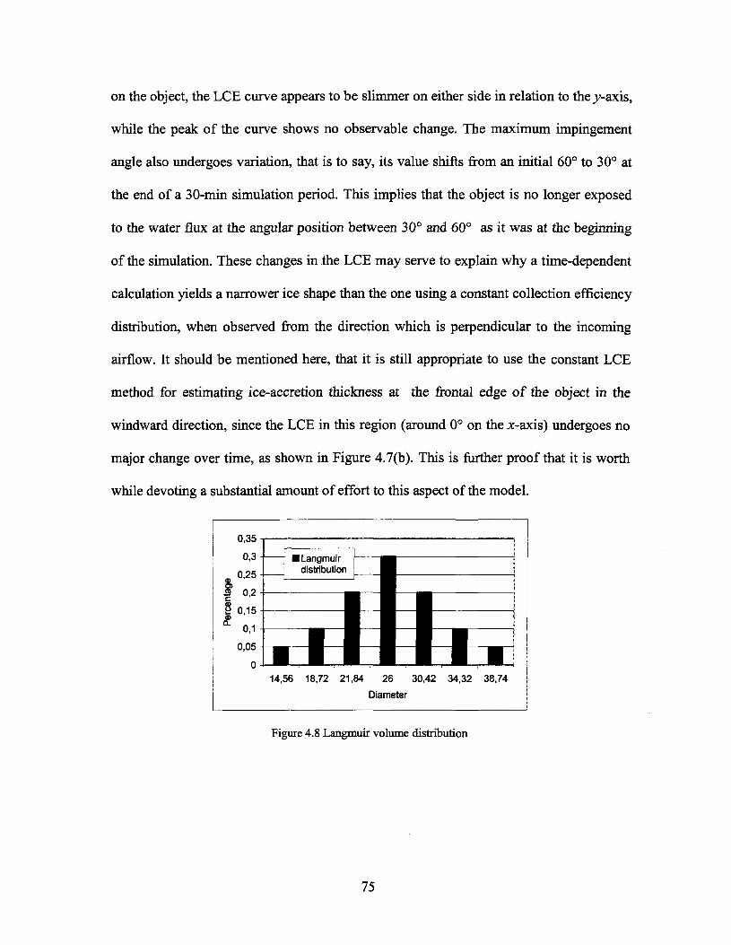
on the object, the LCE curve appears to be slimmer on either side in relation to the^-axis,
while the peak of the curve shows no observable change. The maximum impingement
angle also undergoes variation, that is to say, its value shifts from an initial 60° to 30° at
the end of a 30-min simulation period. This implies that the object is no longer exposed
to the water flux at the angular position between 30° and 60° as it was at the beginning
of the simulation. These changes in the LCE may serve to explain why a time-dependent
calculation yields a narrower ice shape than the one using a constant collection efficiency
distribution, when observed from the direction which is perpendicular to the incoming
airflow. It should be mentioned here, that it is still appropriate to use the constant LCE
method for estimating ice-accretion thickness at the frontal edge of the object in the
windward direction, since the LCE in this region (around 0° on the ;c-axis) undergoes no
major change over time, as shown in Figure 4.7(b). This is further proof that it is worth
while devoting a substantial amount of effort to this aspect of the model.
14,56 18,72 21,84 26 30,42 34,32 38,74
Diameter
Figure 4.8 Langmuir volume distribution
75
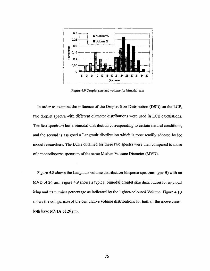
u,o -
0,25-
n o
0,15-
0,1 -
3,05 -
0-
j i1 Number % !
1 Volume % | g
2LJ1L
1 A l l '5 9 9 10 13 15 17 21 24 25 27 31 34 37 j
Diameter j
Figure 4.9 Droplet size and volume for bimodal case
In order to examine the influence of the Droplet Size Distribution (DSD) on the LCE,
two droplet spectra with different diameter distributions were used in LCE calculations.
The first spectrum has a bimodal distribution corresponding to certain natural conditions,
and the second is assigned a Langmuir distribution which is most readily adopted by ice
model researchers. The LCEs obtained for these two spectra were then compared to those
of a monodisperse spectrum of the same Median Volume Diameter (MVD).
Figure 4.8 shows the Langmuir volume distribution (disperse-spectrum type B) with an
MVD of 26 um. Figure 4.9 shows a typical bimodal droplet size distribution for in-cloud
icing and its number percentage as indicated by the lighter-coloured Volume. Figure 4.10
shows the comparison of the cumulative volume distributions for both of the above cases;
both have MVDs of 26
76
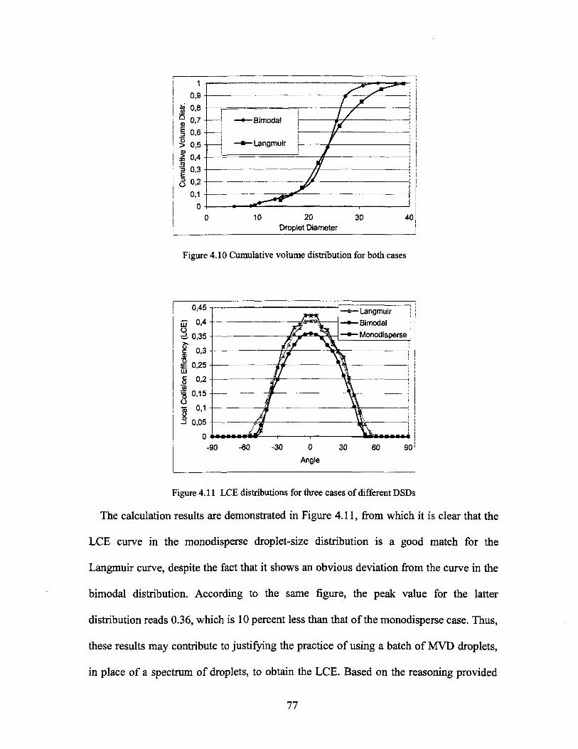
20Droplet Diameter
30 40
Figure 4.10 Cumulative volume distribution for both cases
Langmuir
Bimodal
Monodisperse
Figure 4.11 LCE distributions for three cases of different DSDs
The calculation results are demonstrated in Figure 4.11, from which it is clear that the
LCE curve in the monodisperse droplet-size distribution is a good match for the
Langmuir curve, despite the fact that it shows an obvious deviation from the curve in the
bimodal distribution. According to the same figure, the peak value for the latter
distribution reads 0.36, which is 10 percent less than that of the monodisperse case. Thus,
these results may contribute to justifying the practice of using a batch of MVD droplets,
in place of a spectrum of droplets, to obtain the LCE. Based on the reasoning provided
77
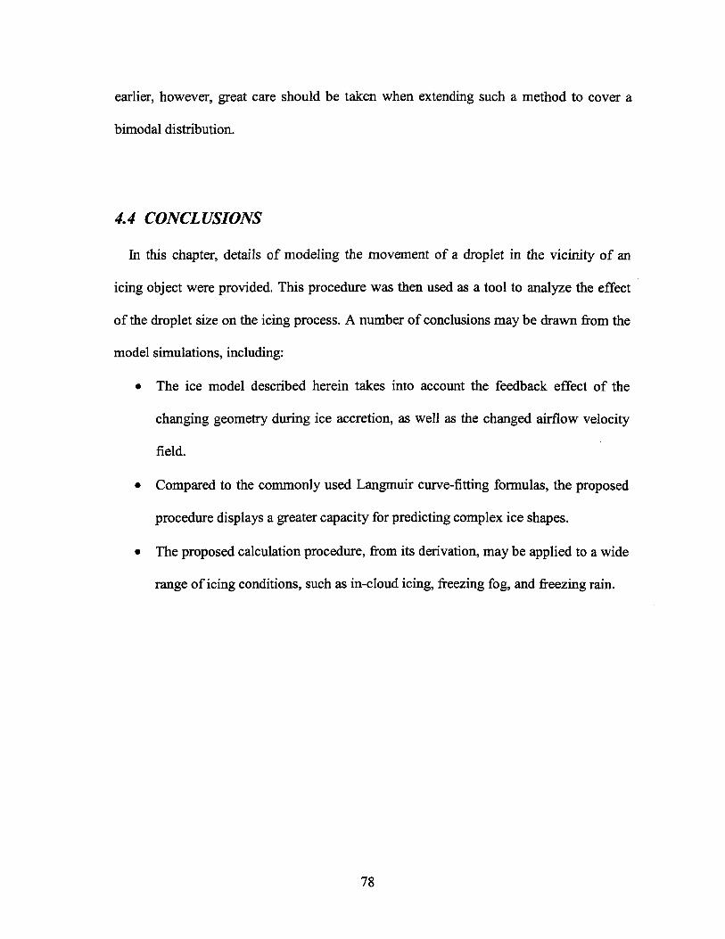
earlier, however, great care should be taken when extending such a method to cover a
bimodal distribution.
4.4 CONCLUSIONS
In this chapter, details of modeling the movement of a droplet in the vicinity of an
icing object were provided. This procedure was then used as a tool to analyze the effect
of the droplet size on the icing process. A number of conclusions may be drawn from the
model simulations, including:
� The ice model described herein takes into account the feedback effect of the
changing geometry during ice accretion, as well as the changed airflow velocity
field.
� Compared to the commonly used Langmuir curve-fitting formulas, the proposed
procedure displays a greater capacity for predicting complex ice shapes.
� The proposed calculation procedure, from its derivation, may be applied to a wide
range of icing conditions, such as in-cloud icing, freezing fog, and freezing rain.
78
CHAPTER 5
THERMAL BALANCE AND SURFACE WATER FLOW
5.7 Introduction
The solution to the thermal balance equation is used for determining the icing fraction
of the overall collected supercooled water on any given surface sector. This supercooled
water may be collected either from the incoming water flux or from the unfrozen water
on the adjacent sector. The local heat transfer coefficient is a key parameter in the
thermal balance equation for ice accretion, since two of the principal terms in this
equation, namely, the convective heat flux and the evaporative heat flux, are functions of
this heat transfer coefficient, as described in the review of the literature.
Once the icing fraction is obtained for wet accumulations, the mass of unfrozen water
may also be determined by subtracting the frozen portion from the total collected water.
The unfrozen water tends to move over the surface under the combined action of gravity
and air drag. Conventionally, the unfrozen portion is assumed to shift completely to the
adjacent surface element during each simulation step. Hence, according to this
assumption, no unfrozen water would remain on the ice-covered surface at the end of
each calculation step. It appears, however, that this is not the case in reality.
In order to estimate the amount of water retained on the surface at the end of each
simulation step, it is necessary to model the motion of the surface runback water. The
surface water film will run back along the substrate surface under the action of such
79
external forces as gravity, air drag and surface tension. One part of the water film will
move upwards while the remainder will run down. It is not necessary for the runback
water to start its motion at the stagnation point, as has been assumed by a number of
researchers. The starting point is defined as the location at which the effects of the
external forces cancel each other out, and the water-flow undergoes a change in direction.
Once the flow direction on any particular surface element is known, it is possible to
establish the calculation sequence and detennine the amount of water gained from the
preceding element together with the amount discharged to the next one.
In this chapter, the method used to detennine the local heat transfer coefficient will be
discussed, and the calculation results obtained using this method will be compared with
those of experimental tests in order to justify its applicability. The details of the thermal
balance equation will be provided further on in the chapter, and a discussion on the
modeling of the surface water film will also be included.
5.2 Solution to Thermal Boundary Layer
� The laminar boundary layer
For a body of arbitrary shape, Echert proposes an approximate solution to the
differential equations of the laminar boundary layer (Kays and Crawford, 1993), as
follows:
11.68v
80
where A denotes the conduction thickness, and U is the local free stream velocity on the
outer edge of the air boundary layer.
The local HTC may be obtained using hx = y . , where Kf is the thermal
conductivity of water.
� The turbulent boundary layer
The local HTC in the turbulent boundary layer may be evaluated in terms of the
Stanton number which is a function of the Reynolds number based on enthalpy thickness,
as follows:
R°-23Ct �t f-2S u02
St = 0.0287Pr-04 * (I° *} M (E 5-2)
[lR'-25(t0-txrGxdx\
where t0 is the surface temperature;
tx is the temperature in the free stream at the outer edge of the boundary layer;
Pr is 0.72 for the air;
R is the transverse radius of curvature of the body; and
Gx may be written in the formulation: Gx = pxUx in which px and Ux are the air
density and the free-stream velocity, respectively, on the outer edge of the boundary
layer.
Then, the local heat transfer coefficient in the turbulent boundary layer may be
evaluated in terms of the Stanton number, as follows:
81
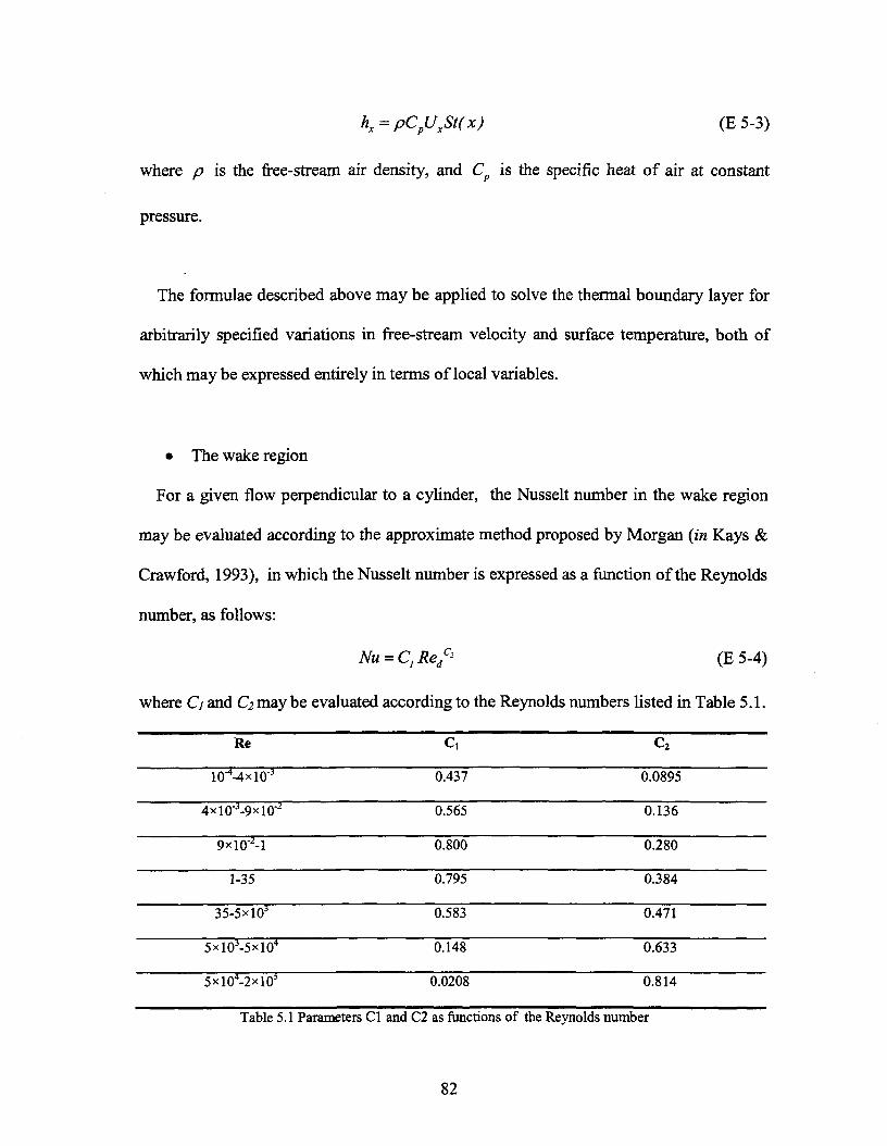
hx=pCpUxSt(x) (E5-3)
where p is the free-stream air density, and Cp is the specific heat of air at constant
pressure.
The formulae described above may be applied to solve the thermal boundary layer for
arbitrarily specified variations in free-stream velocity and surface temperature, both of
which may be expressed entirely in terms of local variables.
� The wake region
For a given flow perpendicular to a cylinder, the Nusselt number in the wake region
may be evaluated according to the approximate method proposed by Morgan (in Kays &
Crawford, 1993), in which the Nusselt number is expressed as a function of the Reynolds
number, as follows:
Nu = C1Redc- (E5-4)
where Cj and C^may be evaluated according to the Reynolds numbers listed in Table 5.1.
Re
10-MxlO-'
4xlO--9xlO-
9xlO"2-l
1-35
35-5xlO3
5xl0J-5xl04
5xl04-2xl03
c,0.437
0.565
0.800
0.795
0.583
0.148
0.0208
c2
0.0895
0.136
0.280
0.384
0.471
0.633
0.814
Table 5.1 Parameters Cl and C2 as functions of the Reynolds number
82
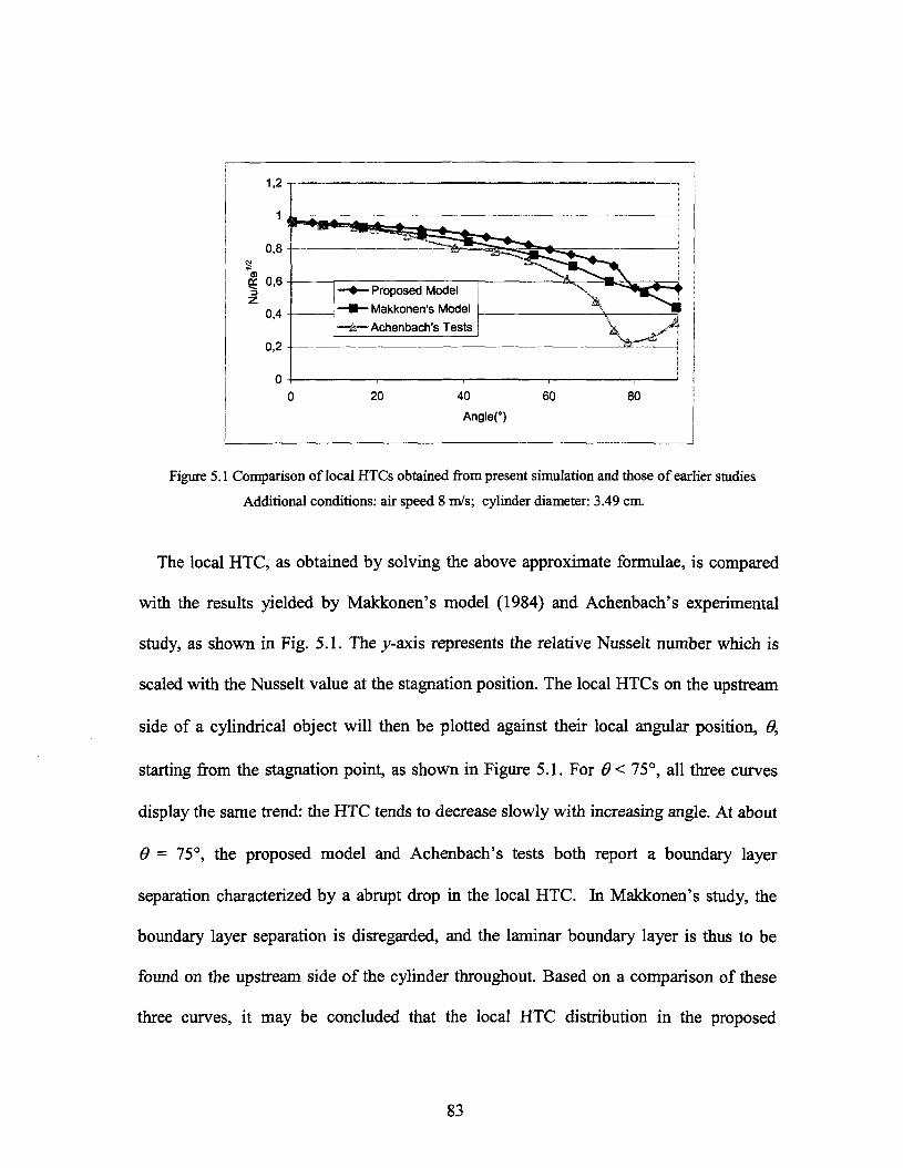
1,2
0,8 ��
I 0,6Z
0,4
0,2
0
��� Proposed Model
j ��� Makkonen's Model
i �ÊT- Achenbach's Tests
20 40
AngleC)
60 80
Figure 5.1 Comparison of local HTCs obtained from present simulation and those of earlier studies
Additional conditions: air speed 8 m/s; cylinder diameter: 3.49 cm.
The local HTC, as obtained by solving the above approximate formulae, is compared
with the results yielded by Makkonen's model (1984) and Achenbach's experimental
study, as shown in Fig. 5.1. The y-axis represents the relative Nusselt number which is
scaled with the Nusselt value at the stagnation position. The local HTCs on the upstream
side of a cylindrical object will then be plotted against their local angular position, 6,
starting from the stagnation point, as shown in Figure 5.1. For 0< 75°, all three curves
display the same trend: the HTC tends to decrease slowly with increasing angle. At about
6 = 75°, the proposed model and Achenbach's tests both report a boundary layer
separation characterized by a abrupt drop in the local HTC. In Makkonen's study, the
boundary layer separation is disregarded, and the laminar boundary layer is thus to be
found on the upstream side of the cylinder throughout. Based on a comparison of these
three curves, it may be concluded that the local HTC distribution in the proposed
83
calculation procedure reflects the actual developing process of the flow boundary layer
better than the one in Makkonen's model.
It should be pointed out that, in the case of cable icing, the Reynolds number is
primarily of order 104 to 105 , which implies a sub-critical flow condition. Thus, it may
be predicted that the windward side of the cable will present a laminar boundary layer
upstream of the separation point, throughout.
5.3 Thermal Balance Equation and Joule Heating
Provided that the incoming supercooled water is treated as a continuum, details of the
microphysics involved are usually disregarded at the time of formulating the thermal
balance equation, as has already been indicated in the review of the literature. The
quantitative formula, in terms of a balance of heat fluxes at the icing interface, may be
written as follows:
Qc +Qe +ôv +Ô* +fiw +Qf + 0 , = 0 (E 5-5)
where
Qc is the sensible heat flux between accretion and airflow by convection. In
formula: -rc.h(Ts -Ta).
[N.0.63
Scj PC
84
Qv is the heat flux due to aerodynamic heating. In formula: 7C.hrvV2 /(2Cp ) , in
which Fis local air speed, and rv is the recovery factor for viscous heating.
Qk is the heat flux due to the conversion of droplet kinetic energy into heat. In
formula:RHV212, where Fis droplet terminal speed.
Qf is the latent heat flux to the accretion due to freezing of some, or all, of the
directly impinging water, in formula: lfsRwn ; and lfsRsn for runback water.
Qw is the sensible heat flux between the liquid water and the underlying accretion.
In formula: cwRw(Ta - T), and cwRs (Ts - T) for runback water and the underlying
accretion.
Qr is the sensible heat flux from Joule heating, the details of which will be
provided later in this section.
Both of the cooling fluxes, Qc and Qe, are usually the most important heat sinks under a
wide range of conditions, and they are also both functions of the HTC. The local HTC, h,
may be obtained by following the calculation procedure described in the preceding
section.
Since the object under consideration may also be an energized cable which carries an
electric current, it is necessary to account for the heat flux, in particular from the resistive
85
or Joule heating in the heat-balance equations. The term corresponding to this portion of
heat flux may be expressed in formulation as follows:
Qr=I2RJ(7tDc) (E5-6)
where the rated current, /, may be calculated according to the following formula:
/ = (Economical Current Density) x (Conductor Cross-sectional Area)
The conductor resistance, Rc, is a function of conductor temperature, and by referring to
certain technical manuals, it is possible to obtain the resistances at both high and low
temperatures, Thigh and Tlow, respectively. Consequently, the resistance at any particular
temperature, Tc, may be obtained by using linear interpolation according to the following
equation:
"R(Thigh)-R(Tl0JT -T1 high M low
(E5-7)
The example provided below is intended for comparing resistive heat flux with a
number of other major heat fluxes, including convective heat flux, evaporative heat flux,
and so forth. The diameter of the cable under consideration is 2.63 cm. Other parameters
related to this type of cable are the rated current: / = 490 amp. and the electric resistance:
Rc=8.14*10e-5 ohms/m(0.131 ohms/mile).
The wind speed was set at 5m/s throughout the simulation. The heat fluxes obtained
are shown in Figure 5.1 in which the magnitudes are represented by vertical bars. In total,
five bars were displayed in the figure to represent convective heat flux; sublimate heat
flux; dissipated heat flux from the warming-up of newly-collected water; latent heat flux;
and resistive heat flux. It will be observed that the resistive heat flux is comparable to
86
convective heat flux and sublimate heat flux in terms of their values. The resistive heat
flux tends to warm the ice mass, while the latter two tend to cause its temperature to drop,
hi the chapter on model simulations, further details will be provided with respect to the
effect of Joule heating caused by an electric current. It should be noted that, for a totally
ice-covered cylinder, the above-mentioned method may be applied without risk of
substantial error, whereas for a partially ice-covered cylinder, this method may cause a
higher degree of inaccuracy when evaluating the effect of Joule heating, since the
resistive heat flux under such a condition tends to show a great irregularity on the surface
of the icing cylinder.
HeatfHiix
ConvectiveHeat Hux
ResistiveHeat Flux
Figure 5.2 Magnitude analysis for heat fluxes in the heat balance equation
5.4 Modelling the Flow of a Water Film
A number of assumptions were made in order to pursue the current research on
modelling the flow of a water film on the surface of an icing object, as follows:
1. The runback water is invariably treated as a thin water film.
87
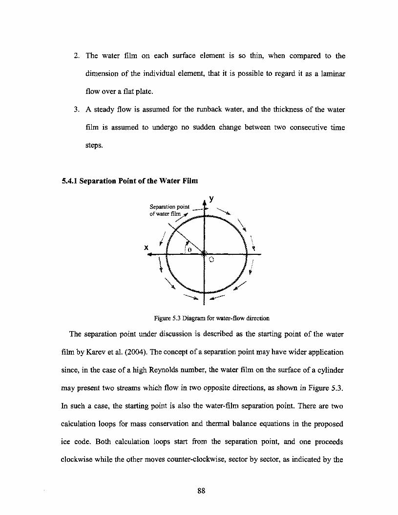
2. The water film on each surface element is so thin, when compared to the
dimension of the individual element, that it is possible to regard it as a laminar
flow over a flat plate.
3. A steady flow is assumed for the runback water, and the thickness of the water
film is assumed to undergo no sudden change between two consecutive time
steps.
5.4.1 Separation Point of the Water Film
Separation pointof water film**
Figure 5.3 Diagram for water-flow direction
The separation point under discussion is described as the starting point of the water
film by Karev et al. (2004). The concept of a separation point may have wider application
since, in the case of a high Reynolds number, the water film on the surface of a cylinder
may present two streams which flow in two opposite directions, as shown in Figure 5.3.
In such a case, the starting point is also the water-film separation point. There are two
calculation loops for mass conservation and thermal balance equations in the proposed
ice code. Both calculation loops start from the separation point, and one proceeds
clockwise while the other moves counter-clockwise, sector by sector, as indicated by the
88
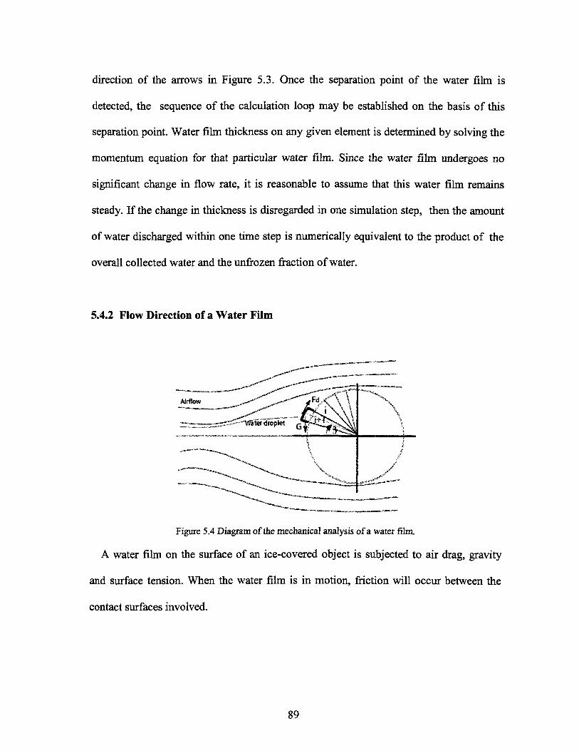
direction of the arrows in Figure 5.3. Once the separation point of the water film is
detected, the sequence of the calculation loop may be established on the basis of this
separation point. Water film thickness on any given element is determined by solving the
momentum equation for that particular water film. Since the water film undergoes no
significant change in flow rate, it is reasonable to assume that this water film remains
steady. If the change in thickness is disregarded in one simulation step, then the amount
of water discharged within one time step is numerically equivalent to the product of the
overall collected water and the unfrozen fraction of water.
5.4.2 Flow Direction of a Water Film
Figure 5.4 Diagram of the mechanical analysis of a water film.
A water film on the surface of an ice-covered object is subjected to air drag, gravity
and surface tension. When the water film is in motion, friction will occur between the
contact surfaces involved.
89
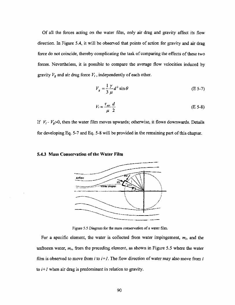
Of all the forces acting on the water film, only air drag and gravity affect its flow
direction. In Figure 5.4, it will be observed that points of action for gravity and air drag
force do not coincide, thereby complicating the task of comparing the effects of these two
forces. Nevertheless, it is possible to compare the average flow velocities induced by
gravity Vg and air drag force Vt, independently of each other.
3ju
/ air "t =
H 2
(E 5-7)
(E 5-8)
If Vt - Vg>0, then the water film moves upwards; otherwise, it flows downwards. Details
for developing Eq. 5-7 and Eq. 5-8 will be provided in the remaining part of this chapter.
5.4.3 Mass Conservation of the Water Film
Figure 5.5 Diagram for the mass conservation of a water film.
For a specific element, the water is collected from water impingement, m,, and the
unfrozen water, mr, from the preceding element, as shown in Figure 5.5 where the water
film is observed to move from i to i+1. The flow direction of water may also move from i
to i+1 when air drag is predominant in relation to gravity.
90
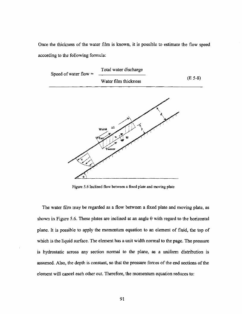
Once the thickness of the water fihn is known, it is possible to estimate the flow speed
according to the following formula:
Speed of water flow =Total water discharge
Water fihn thickness(E5-8)
Figure 5.6 Inclined flow between a fixed plate and moving plate
The water film may be regarded as a flow between a fixed plate and moving plate, as
shown in Figure 5.6. These plates are inclined at an angle 0 with regard to the horizontal
plane. It is possible to apply the momentum equation to an element of fluid, the top of
which is the liquid surface. The element has a unit width normal to the page. The pressure
is hydrostatic across any section normal to the plane, as a uniform distribution is
assumed. Also, the depth is constant, so that the pressure forces of the end sections of the
element will cancel each other out. Therefore, the momentum equation reduces to:
91
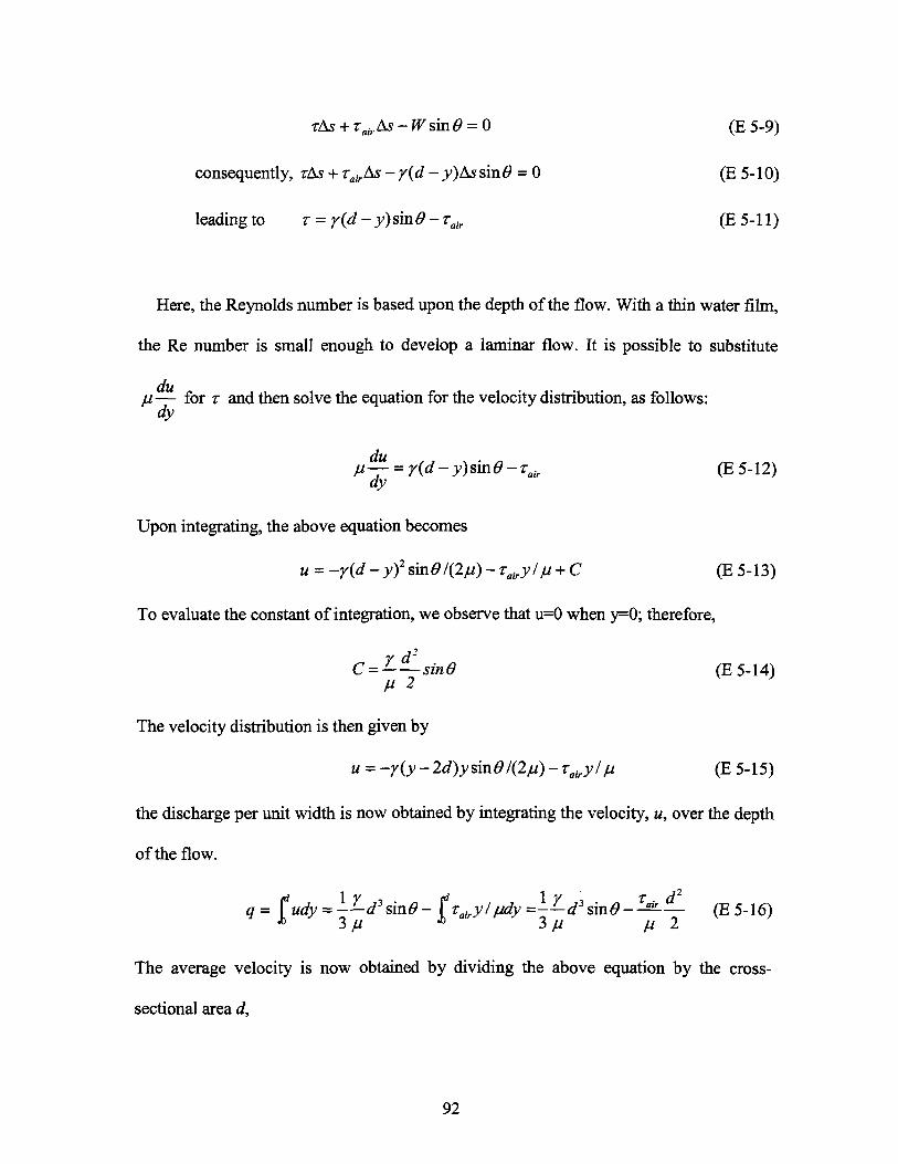
TAS + TairAs - W sin 0 = 0 (E 5-9)
consequently, TAS + tairàs - y(d - y)As sin0 = 0 (E 5-10)
leading to r = y(d - y)sin0 - rair (E 5-11 )
Here, the Reynolds number is based upon the depth of the flow. With a thin water fihn,
the Re number is small enough to develop a laminar flow. It is possible to substitute
ju� for T and then solve the equation for the velocity distribution, as follows:dy
^ y(dy)s0zair (E5-12)
dy
Upon integrating, the above equation becomes
u = -y(d-yf sm0/(2v)-Tairy/ju + C (E5-13)
To evaluate the constant of integration, we observe that u=0 when y=0; therefore,yd2
C = L�sinQ (E5-14)
The velocity distribution is then given by
u = -y(y-2d)ysM0/(2ju)-Tairy/ti (E 5-15)
the discharge per unit width is now obtained by integrating the velocity, u, over the depth
of the flow.
q= (udy = -^d3sm0-(rairy/fiidy=-^d3sm0-^� (E5-16)* 3// * 3// n 2
The average velocity is now obtained by dividing the above equation by the cross-
sectional area d,
92
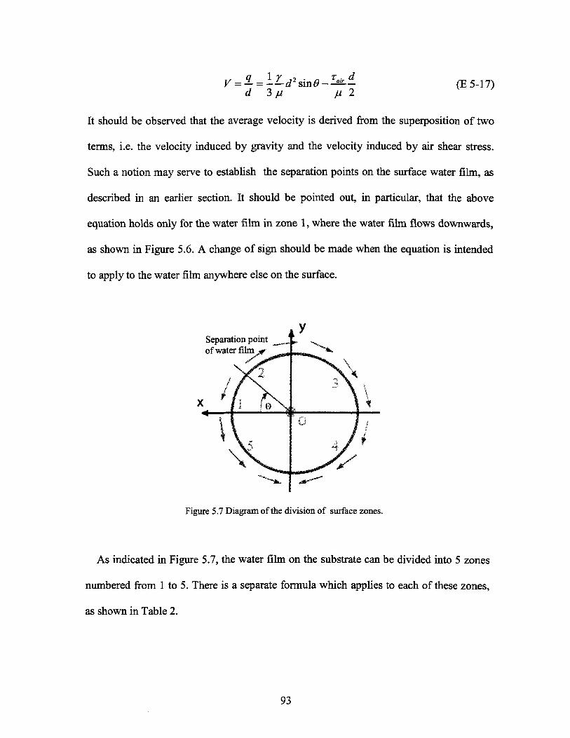
d 3 / /(E5-17)
It should be observed that the average velocity is derived from the superposition of two
terms, i.e. the velocity induced by gravity and the velocity induced by air shear stress.
Such a notion may serve to establish the separation points on the surface water fihn, as
described in an earlier section. It should be pointed out, in particular, that the above
equation holds only for the water fihn in zone 1, where the water fihn flows downwards,
as shown in Figure 5.6. A change of sign should be made when the equation is intended
to apply to the water film anywhere else on the surface.
Separation pointof water film
Figure 5.7 Diagram of the division of surface zones.
As indicated in Figure 5.7, the water fihn on the substrate can be divided into 5 zones
numbered from 1 to 5. There is a separate formula which applies to each of these zones,
as shown in Table 2.
93
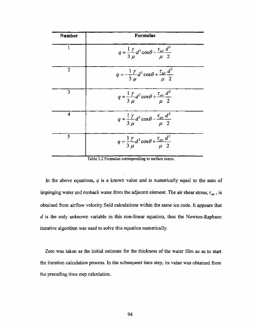
Number
1
2
3
4
5
q--
9 =
9 =
q
Formulae
1 V 3
1 1̂
3/i
3 / /
l/3
3 / /
l/3
3 / /
"
Tair
"
^"air
M
d2
2
rd2
2
d2
2
d2
2
d2
2
Table 5.2 Formulae corresponding to surface zones.
In the above equations, q is a known value and is numerically equal to the sum of
impinging water and runback water from the adjacent element. The air shear stress, tair, is
obtained from airflow velocity field calculations within the same ice code. It appears that
d is the only unknown variable in this non-linear equation, thus the Newton-Raphson
iterative algorithm was used to solve this equation numerically.
Zero was taken as the initial estimate for the thickness of the water film so as to start
the iteration calculation process. In the subsequent time step, its value was obtained from
the preceding time step calculation.
94
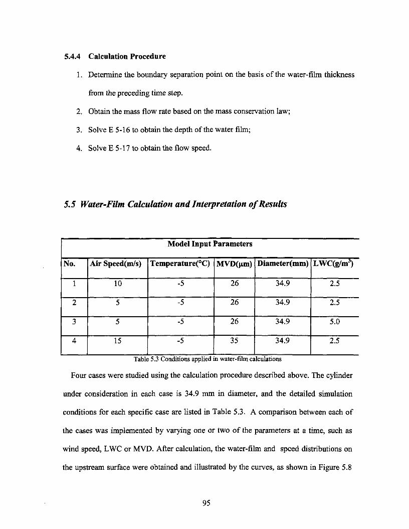
5.4.4 Calculation Procedure
1. Determine the boundary separation point on the basis of the water-film thickness
from the preceding time step.
2. Obtain the mass flow rate based on the mass conservation law;
3. Solve E 5-16 to obtain the depth of the water film;
4. Solve E 5-17 to obtain the flow speed.
5.5 Water-Film Calculation and Interpretation of Results
Model Input Parameters
No.
1
2
3
4
Air Speed(m/s)
10
5
5
15
Temperature(°C)
-5
-5
-5
-5
MVD(nm)
26
26
26
35
Diameter(mm)
34.9
34.9
34.9
34.9
LWC(g/m3)
2.5
2.5
5.0
2.5
Table 5.3 Conditions applied in water-film calculations
Four cases were studied using the calculation procedure described above. The cylinder
under consideration in each case is 34.9 mm in diameter, and the detailed simulation
conditions for each specific case are listed in Table 5.3. A comparison between each of
the cases was implemented by varying one or two of the parameters at a time, such as
wind speed, LWC or MVD. After calculation, the water-film and speed distributions on
the upstream surface were obtained and illustrated by the curves, as shown in Figure 5.8
95
The curves for water-film thickness in Cases 1, 2, and 3, in Figure 5.8(b), display the
same trend, i.e. the water-film thickness increases from an upper to a lower position
upstream of the cylinder. This trend is characterized by the ever-rising curves which
represent the water-film thickness, and may be explained by the fact that the angular
position of the water-film separation point coincides with the highest position of the
water film in all three cases, where the water film invariably flows downwards. As a
result, the sector on the lower side tends to present more water on its surface than the
preceding one, since the subsequent sector receives the unfrozen water from the adjacent
area as well as incoming water impingements. Figure 5.8( c ) reveals that the speed of the
water-film flow tends to accelerate with a decrease in the angle 9. An exception to this
trend is seen in Case 4 which presents an increase in both the wind speed and LWC
compared to the preceding three cases. In contrast with the first three cases, Case 4
undergoes an initial abrupt increase in water-film thickness, then a slight drop and lastly a
rise again, moving from the upper to the lower half of the cylinder. A sluggish growth in
thickness may be observed at the angular position of about 65°, while a change in flow
direction may be detected at the same position in Figure 5.8( c ), which may taken as an
indiction that the water-film separation occurs at this point. The occurrence of water-film
separation may cause a change in the distribution of the water-film thickness, as shown in
Figure 5.8( b ). It may also be concluded from these curves, that water-film thickness is
an essential factor in determining the speed of the surface water-film flow, and that the
thicker the water film, the faster its flow speed is.
96
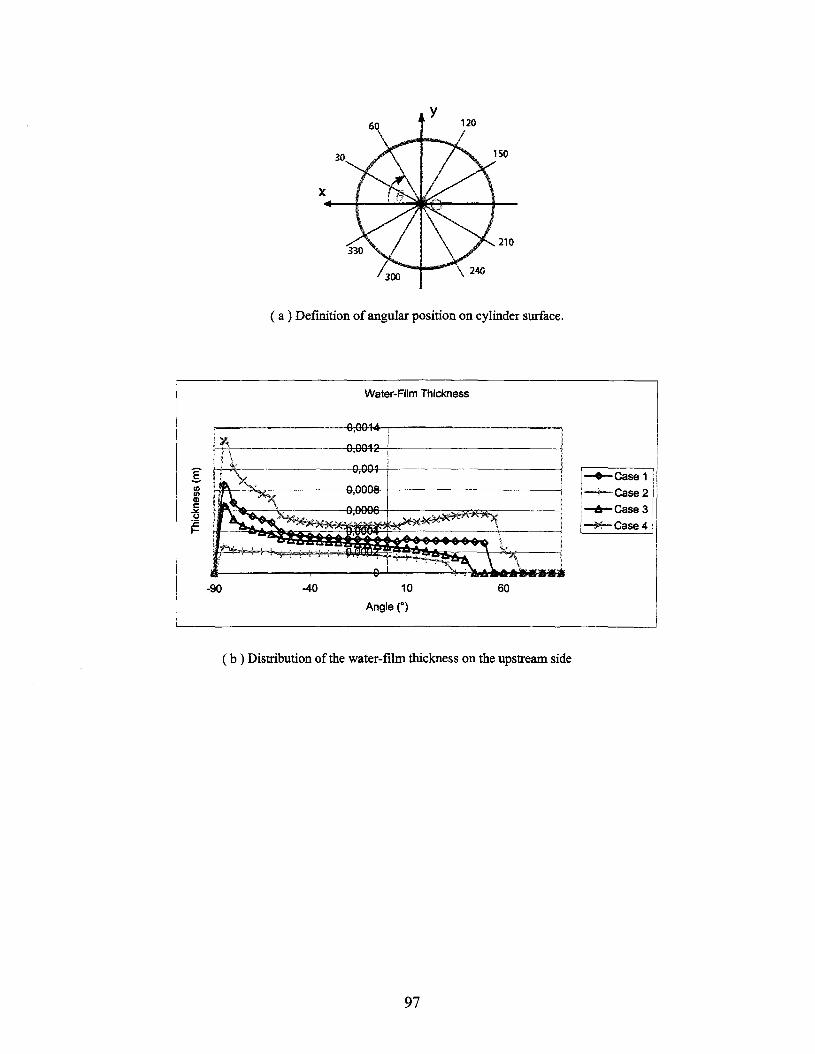
60
150
330210
\ 240
( a ) Definition of angular position on cylinder surface.
Water-Film Thickness
0,0014 ;-
��� Case 1
�-*� Case 2
�A�Case 3
�«�Case 4
( b ) Distribution of the water-film thickness on the upstream side
97
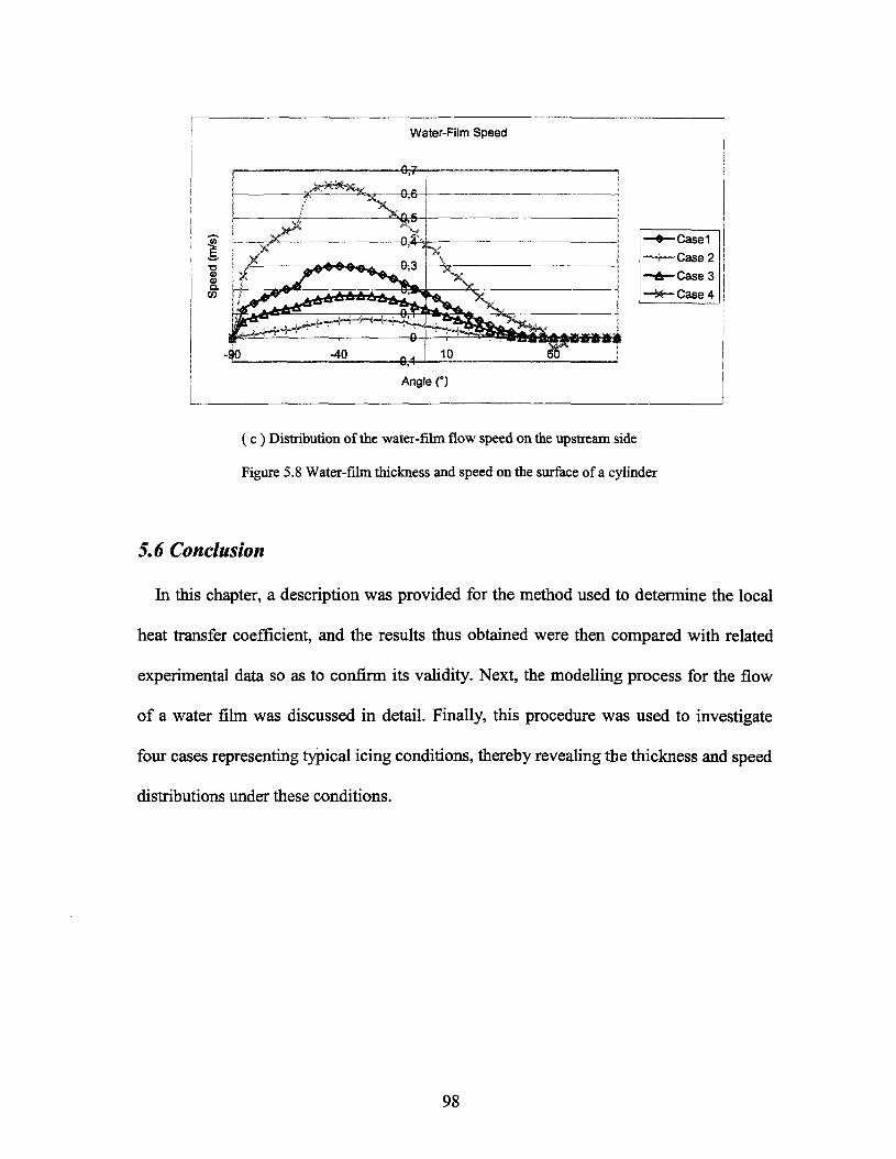
Water-Film Speed
Angle (°)
( c ) Distribution of the water-film flow speed on the upstream side
Figure 5.8 Water-film thickness and speed on the surface of a cylinder
5.6 Conclusion
In this chapter, a description was provided for the method used to determine the local
heat transfer coefficient, and the results thus obtained were then compared with related
experimental data so as to confirm its validity. Next, the modelling process for the flow
of a water fihn was discussed in detail. Finally, this procedure was used to investigate
four cases representing typical icing conditions, thereby revealing the thickness and speed
distributions under these conditions.
98
CHAPTER 6
EXPERIMENTS AND MODEL VALIDATION
An array of experimental tests was carried out in the CIGELE Atmospheric Icing
Research Wind Tunnel (CAIRWT) in order to validate the ice model discussed and
developed in the preceding chapters. The instruments in the wind tunnel should be
adjusted meticulously so that the conditions set for experimental tests are closely
representative of those observed under natural conditions. The experimental conditions
will later be used as input parameters for model simulations.
This chapter will provide an overview of the experimental set-up and the instruments
involved in the tests. Further details will contribute to clarifying the method employed to
calibrate the instruments used for creating the requisite test conditions. The latter
conditions were designed to duplicate the icing process from dry to wet accumulations,
and a specific consideration of variations in cylinder diameter was also included. The ice
shapes thus obtained will be compared with those from model simulations, and will
subsequently be discussed further on in the chapter.
6.1 Experimental Set-up and Instruments
The CIGELE Atmospheric Icing Research Wind Tunnel (CAIRWT) is located in the
CIGELE icing research pavilion which was built in 1998. It is a closed-loop atmospheric
99
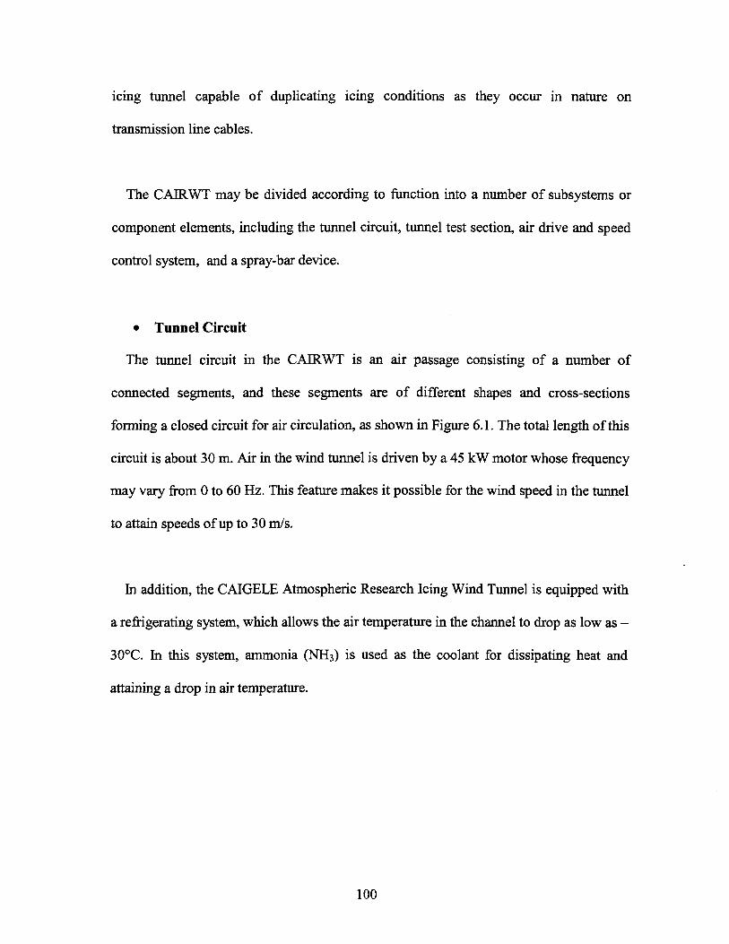
icing tunnel capable of duplicating icing conditions as they occur in nature on
transmission line cables.
The CAIRWT may be divided according to function into a number of subsystems or
component elements, including the tunnel circuit, tunnel test section, air drive and speed
control system, and a spray-bar device.
� Tunnel Circuit
The tunnel circuit in the CAIRWT is an air passage consisting of a number of
connected segments, and these segments are of different shapes and cross-sections
forming a closed circuit for air circulation, as shown in Figure 6.1. The total length of this
circuit is about 30 m. Air in the wind tunnel is driven by a 45 kW motor whose frequency
may vary from 0 to 60 Hz. This feature makes it possible for the wind speed in the tunnel
to attain speeds of up to 30 m/s.
In addition, the CAIGELE Atmospheric Research Icing Wind Tunnel is equipped with
a refrigerating system, which allows the air temperature in the channel to drop as low as -
30°C. In this system, ammonia (NH3) is used as the coolant for dissipating heat and
attaining a drop in air temperature.
100
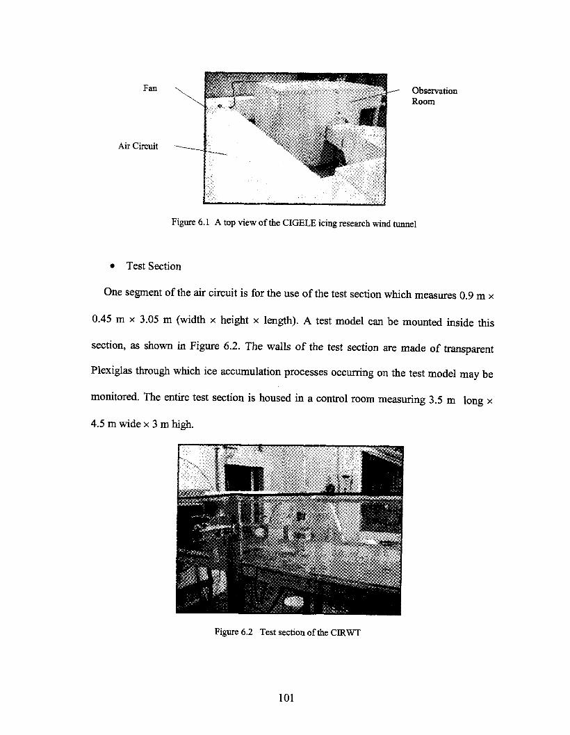
Fan
Air Circuit
ObservationRoom
Figure 6.1 A top view of the CIGELE icing research wind tunnel
� Test Section
One segment of the air circuit is for the use of the test section which measures 0.9 m x
0.45 m x 3.05 m (width x height x length). A test model can be mounted inside this
section, as shown in Figure 6.2. The walls of the test section are made of transparent
Plexiglas through which ice accumulation processes occurring on the test model may be
monitored. The entire test section is housed in a control room measuring 3.5 m long x
4.5 m wide x 3 m high.
Figure 6.2 Test section of the CIRWT
101
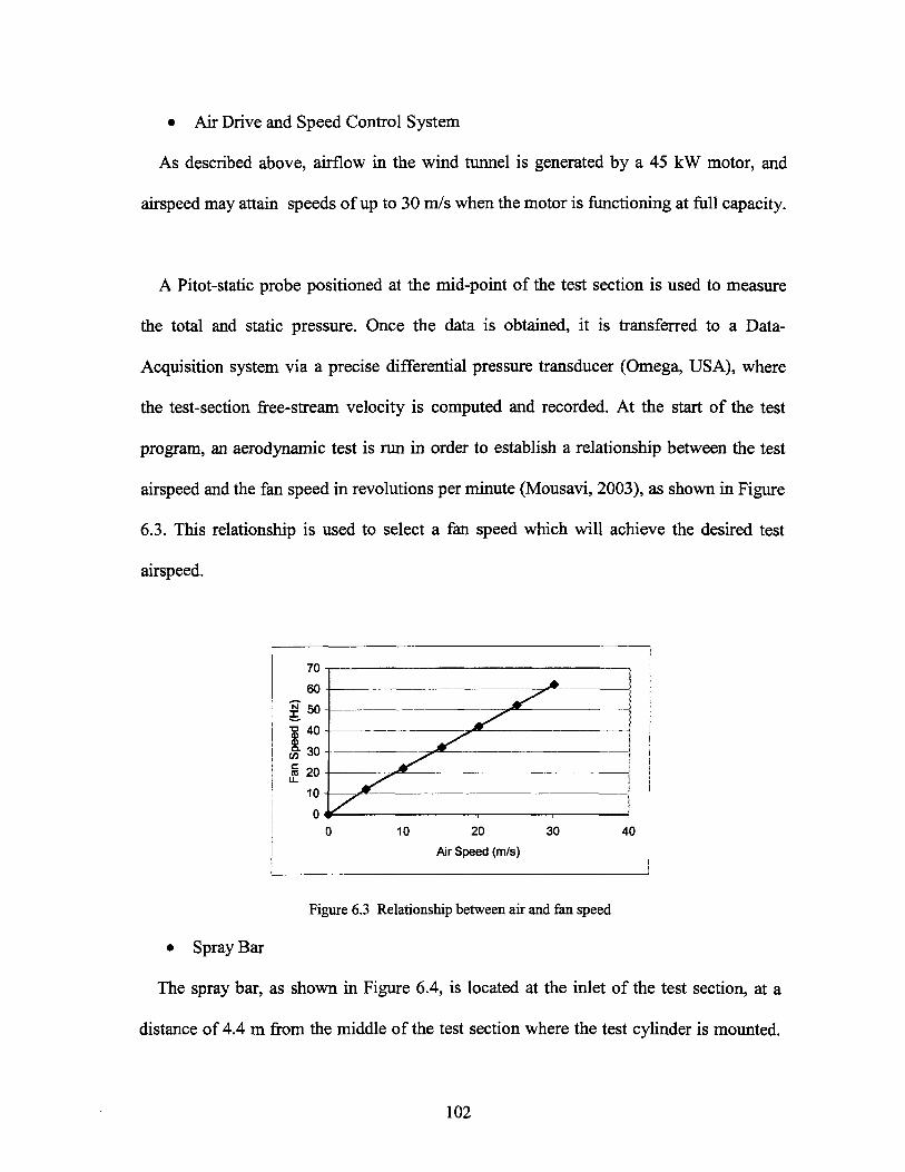
� Air Drive and Speed Control System
As described above, airflow in the wind tunnel is generated by a 45 kW motor, and
airspeed may attain speeds of up to 30 m/s when the motor is functioning at full capacity.
A Pitot-static probe positioned at the mid-point of the test section is used to measure
the total and static pressure. Once the data is obtained, it is transferred to a Data-
Acquisition system via a precise differential pressure transducer (Omega, USA), where
the test-section free-stream velocity is computed and recorded. At the start of the test
program, an aerodynamic test is run in order to establish a relationship between the test
airspeed and the fan speed in revolutions per minute (Mousavi, 2003), as shown in Figure
6.3. This relationship is used to select a fan speed which will achieve the desired test
airspeed.
70
60
£ 50I 401-30ffi 20
10
010 20 30
Air Speed (m/s)
40
Figure 6.3 Relationship between air and fan speed
� Spray Bar
The spray bar, as shown in Figure 6.4, is located at the inlet of the test section, at a
distance of 4.4 m from the middle of the test section where the test cylinder is mounted.
102
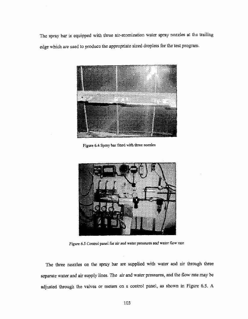
The spray bar is equipped with three air-atomization water spray nozzles at the trailing
edge which are used to produce the appropriate sized droplets for the test program.
Figure 6.4 Spray bar fitted with three nozzles
Figure 6.5 Control panel for air and water pressures and water flow rate
The three nozzles on the spray bar are supplied with water and air through three
separate water and air supply lines. The air and water pressures, and the flow rate may be
adjusted through the valves or meters on a control panel, as shown in Figure 6.5. A
103
desired Droplet-Size Distribution (DSD) at the mid-point of the test cylinder may be
obtained through controlling the water flow rate, and the water and air pressures, among
other parameters (Karev et al., 2002).
The existing experimental set-up in the CAIRWT provides facility in setting the values
for most of the major parameters, including air speed and air temperature. Other
parameters such as the Liquid Water Content (LWC) and the Median Volume Diameter
(MWD), however, cannot be accurately estimated until a specific test is under way. These
parameters may be divided into two groups on the basis of the means applied to
determine their values, as shown in Table 6.1. The parameters in the first group may be
set with ease simply by adjusting the controls or valves, while for those appearing in the
second group, the values can only be accurately determined by measurement. The
measuring process proved overly time-consuming, thus substantiating the merits of
modelling and simulating the ice accretion process numerically.
Group no.
1
(to be set)
2
(to be measured)
Parameters
Wind Speed, Air Temperature, Diameter of test cylinder, Pressures
for both water and air pipelines, Type of nozzle
LWC, Droplet Size Distribution (or MVD)
Table 6.1 Experimental parameters
104
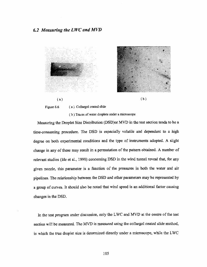
6.2 Measuring the L WC and MVD
( a ) ( b )
Figure 6.6 ( a ) Coîlargol coated slide
( b ) Traces of water droplets under a microscope
Measuring the Droplet Size Distribution (DSD)or MVD in the test section tends to be a
time-consuming procedure. The DSD is especially volatile and dependent to a high
degree on both experimental conditions and the type of instruments adopted. A slight
change in any of these may result in a permutation of the pattern obtained. A number of
relevant studies (Ide et al., 1990) concerning DSD in the wind tunnel reveal that, for any
given nozzle, this parameter is a function of the pressures in both the water and air
pipelines. The relationship between the DSD and other parameters may be represented by
a group of curves. It should also be noted that wind speed is an additional factor causing
changes in the DSD.
In the test program under discussion, only the LWC and MVD at the centre of the test
section will be measured. The MVD is measured using the collargoî coated slide method,
in which the true droplet size is determined directly under a microscope, while the LWC
105
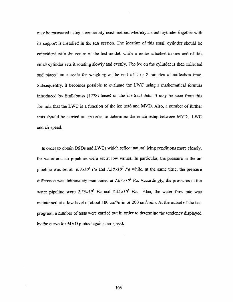
may be measured using a commonly-used method whereby a small cylinder together with
its support is installed in the test section. The location of this small cylinder should be
coincident with the centre of the test model, while a motor attached to one end of this
small cylinder sets it rotating slowly and evenly. The ice on the cylinder is then collected
and placed on a scale for weighing at the end of 1 or 2 minutes of collection time.
Subsequently, it becomes possible to evaluate the LWC using a mathematical formula
introduced by Staîlabrass (Î978) based on the ice-load data. It may be seen from this
formula that the LWC is a function of the ice load and MVD. Also, a number of further
tests should be carried out in order to determine the relationship between MVD, LWC
and air speed.
In order to obtain DSDs and LWCs which reflect natural icing conditions more closely,
the water and air pipelines were set at low values. In particular, the pressure in the air
pipeline was set at 6.9xl(f Pa and 1.38xl(f Pa while, at the same time, the pressure
difference was deliberately maintained at 2.07x10s Pa. Accordingly, the pressures in the
water pipeline were 2.76x10⁵ Pa and 3.45xl(f Pa. Also, the water flow rate was
maintained at a low level of about 100 cm3/min or 200 cm3/min. At the outset of the test
program, a number of tests were carried out in order to determine the tendency displayed
by the curve for MVD plotted against air speed.
106
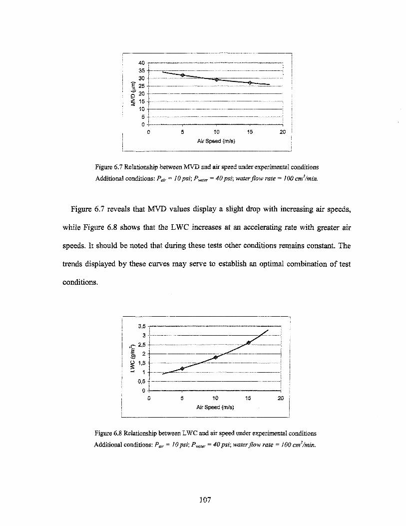
10
Air Speed (m/s)
15 20
Figure 6.7 Relationship between MVD and air speed under experimental conditions
Additional conditions: P^, - lOpsi; PHUWT = 40psi; water flow rate = 100 cm3/min.
Figure 6.7 reveals that MVD values display a slight drop with increasing air speeds,
while Figure 6.8 shows that the LWC increases at an accelerating rate with greater air
speeds. It should be noted that during these tests other conditions remains constant. The
trends displayed by these curves may serve to establish an optimal combination of test
conditions.
5 10 15Air Speed (m/s)
20
Figure 6.8 Relationship between LWC and air speed under experimental conditions
Additional conditions: Pair = lOpsi; PVMter = 40psi; water flow rate = 100 cm3/min.
107
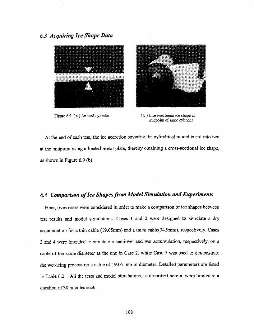
6.3 Acquiring Ice Shape Data
Figure 6.9 ( a ) Am iced cylinder ( b ) Cross-sectional ice shape atmidpoint of same cylinder
At the end of each test, the ice accretion covering the cylindrical model is cut into two
at the midpoint using a heated metal plate, thereby obtaining a cross-sectional ice shape,
as shown in Figure 6.9 (b).
6.4 Comparison of Ice Shapes from Model Simulation and Experiments
Here, fives cases were considered in order to make a comparison of ice shapes between
test results and model simulations. Cases 1 and 2 were designed to simulate a dry
accumulation for a thin cable (19.05mm) and a thick cable(34.9mm), respectively. Cases
3 and 4 were intended to simulate a semi-wet and wet accumulation, respectively, on a
cable of the same diameter as the one in Case 2, while Case 5 was used to demonstrate
the wet-icing process on a cable of 19.05 mm in diameter. Detailed parameters are listed
in Table 6.2. All the tests and model simulations, as described herein, were limited to a
duration of 30 minutes each.
108
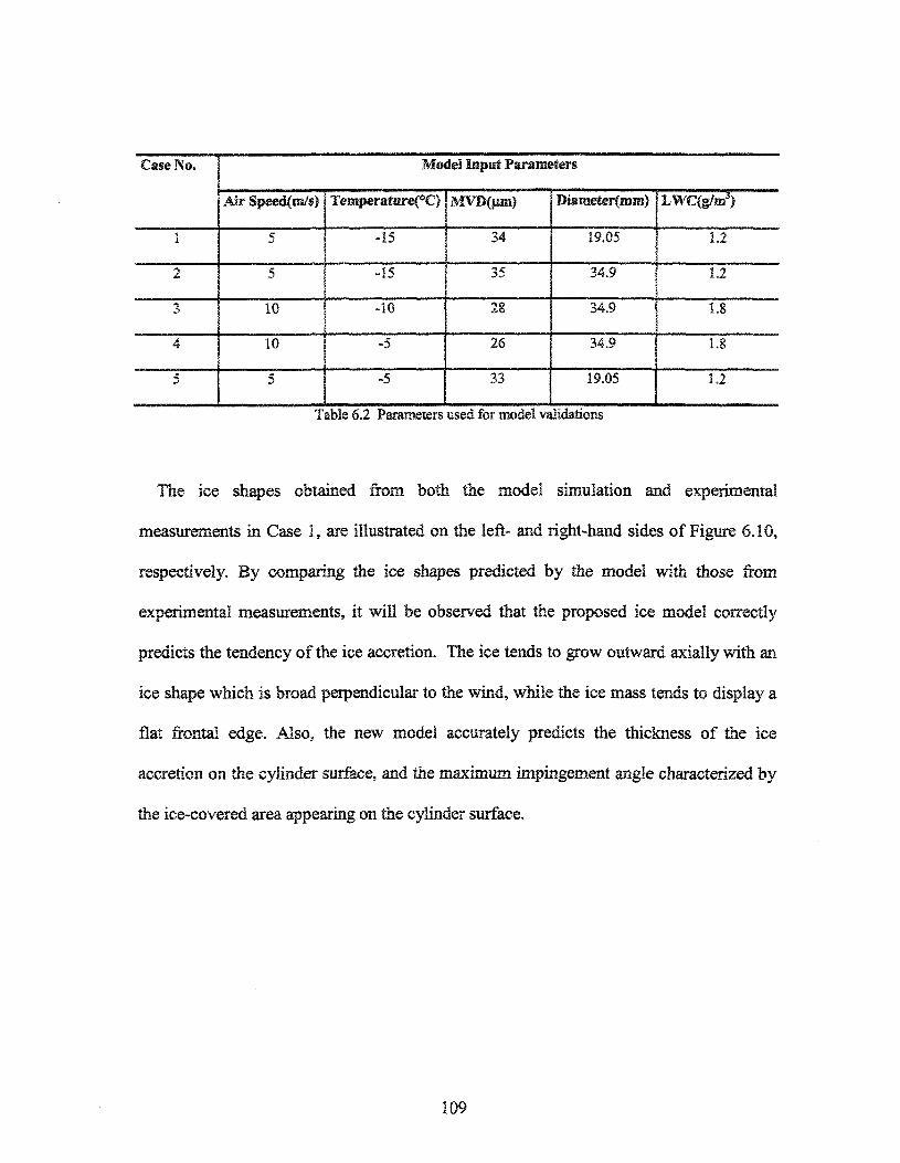
Case No.
1
2
3
4
5
Medel Input Parameters
Air Speed(ia/s)
5
5
10
10
5
TeinperaftireCoC) 1 MVD(fun)Î
-15
-15
-10
-5
-5
34
35
28
26
33
DisineteF(mm)
19.05
34.9
34.9
34.9
19.05
LWCfe/m3)
1.2
1.2
1.8
1.8
1.2
Table 6.2 Parameters used for model validations
The ice shapes obtained from both the model simulation and experimental
measurements in Case 1, are illustrated on the left- and right-hand sides of Figure 6.10,
respectively. By comparing the ice shapes predicted by the model with those from
experimental measurements, it will be observed that the proposed ice model correctly
predicts the tendency of the ice accretion. The ice tends to grow outward axially with an
ice shape which is broad perpendicular to the wind, while the ice mass tends to display a
flat frontal edge. Also, the new model accurately predicts the thickness of the ice
accretion on the cylinder surface, and the maximum impingement angle characterized by
the ice-covered area appearing on the cylinder surface.
109
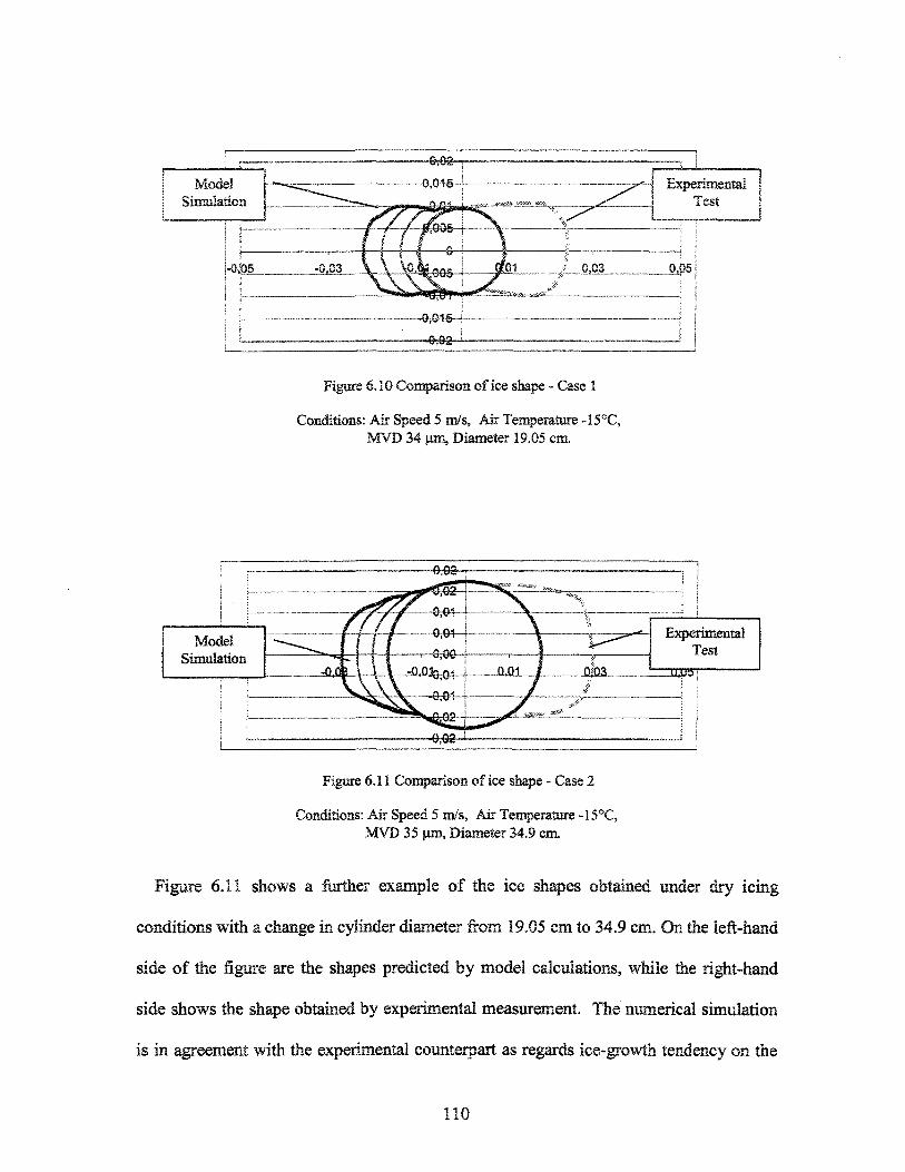
Figure 6.10 Comparison of ice shape - Case 1
Conditions: Air Speed 5 m/s, Air Temperature-15CC,MVD 34 \xm, Diameter 19.05 cm.
Figure 6.11 Comparison of ice shape - Case 2
Conditions: Air Speed 5 m/s, Air Temperature -15°C,MVD 35 |im, Diameter 34.9 cm.
Figure 6.11 shows a further example of the ice shapes obtained under dry icing
conditions with a change in cylinder diameter from 19.05 cm to 34.9 cm. On the ieft-hand
side of the figure are the shapes predicted by model calculations, while the right-hand
side shows the shape obtained by experimental measurement. The numerical simulation
is in agreement with the experimental counterpart as regards ice-growth tendency on the
110
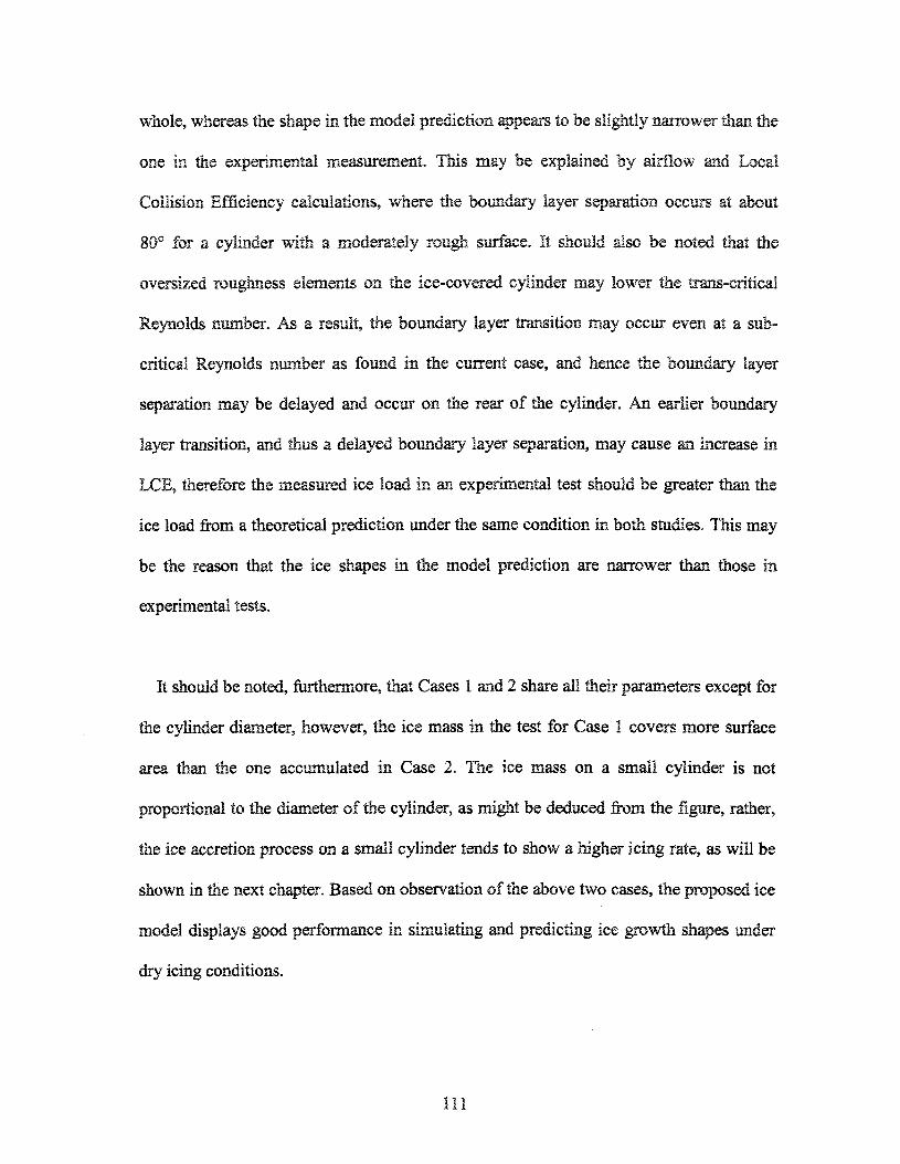
whole, whereas the shape in the mode! prediction appears to be slightly narrower than the
one in the experimental measurement. This may be explained by airflow and Local
Collision Efficiency calculations, where the boundary layer separation occurs at about
80° for a cylinder with a moderately rough surface. It should also be noted that the
oversized roughness elements on the ice-covered cylinder may lower the trans-critical
Reynolds number. As a result, the boundary layer transition may occur even at a sub-
critical Reynolds number as found in the current case, and hence the boundary layer
separation may be delayed and occur on the rear of the cylinder. An earlier boundary
layer transition, and thus a delayed boundary layer separation, may cause an increase in
LCE, therefore the measured ice load in an experimental test should be greater than the
ice load from a theoretical prediction under the same condition in both studies. This may
be the reason that the ice shapes in the model prediction are narrower than those in
experimental tests.
It should be noted, furthermore, that Cases 1 and 2 share all their parameters except for
the cylinder diameter, however, the ice mass in the test for Case 1 covers more surface
area than the one accumulated in Case 2. The ice mass on a small cylinder is not
proportional to the diameter of the cylinder, as might be deduced from the figure, rather,
the ice accretion process on a small cylinder tends to show a higher icing rate, as will be
shown in the next chapter. Based on observation of the above two cases, the proposed ice
model displays good performance in simulating and predicting ice growth shapes under
dry icing conditions.
I l l
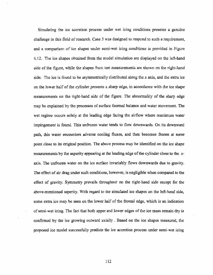
Simulating the ice accretion process under wet icing conditions presents a genuine
challenge in this field of research. Case 3 was designed to respond to such a requirement,
and a comparison of ice shapes under semi-wet icing conditions is provided in Figure
6.12. The ice shapes obtained from the model simulation are displayed on the left-hand
side of the figure, while the shapes from test measurements are shown on the right-hand
side. The ice is found to be asymmetrically distributed along the JC axis, and the extra ice
on the lower half of the cylinder presents a sharp edge, in accordance with the ice shape
measurements on the right-hand side of the figure. The abnormality of the sharp edge
may be explained by the processes of surface thermal balance and water movement. The
wet regime occurs solely at the leading edge facing the airflow where maximum water
impingement is found. This unfrozen water tends to flow downwards. On its downward
path, this water encounters adverse cooling fluxes, and then becomes frozen at some
point close to its original position. The above process may be identified on the ice shape
measurements by the asperity appearing at the leading edge of the cylinder close to the x-
axis. The unfrozen water on the ice surface invariably flows downwards due to gravity.
The effect of air drag under such conditions, however, is negligible when compared to the
effect of gravity. Symmetry prevails throughout on the right-hand side except for the
above-mentioned asperity. With regard to the simulated ice shapes on the left-hand side,
some extra ice may be seen on the lower half of the frontal edge, which is an indication
of semi-wet icing. The fact that both upper and lower edges of the ice mass remain dry is
confirmed by the ice growing outward axially . Based on the ice shapes measured, the
proposed ice model successfully predicts the ice accretion process under semi-wet icing
112
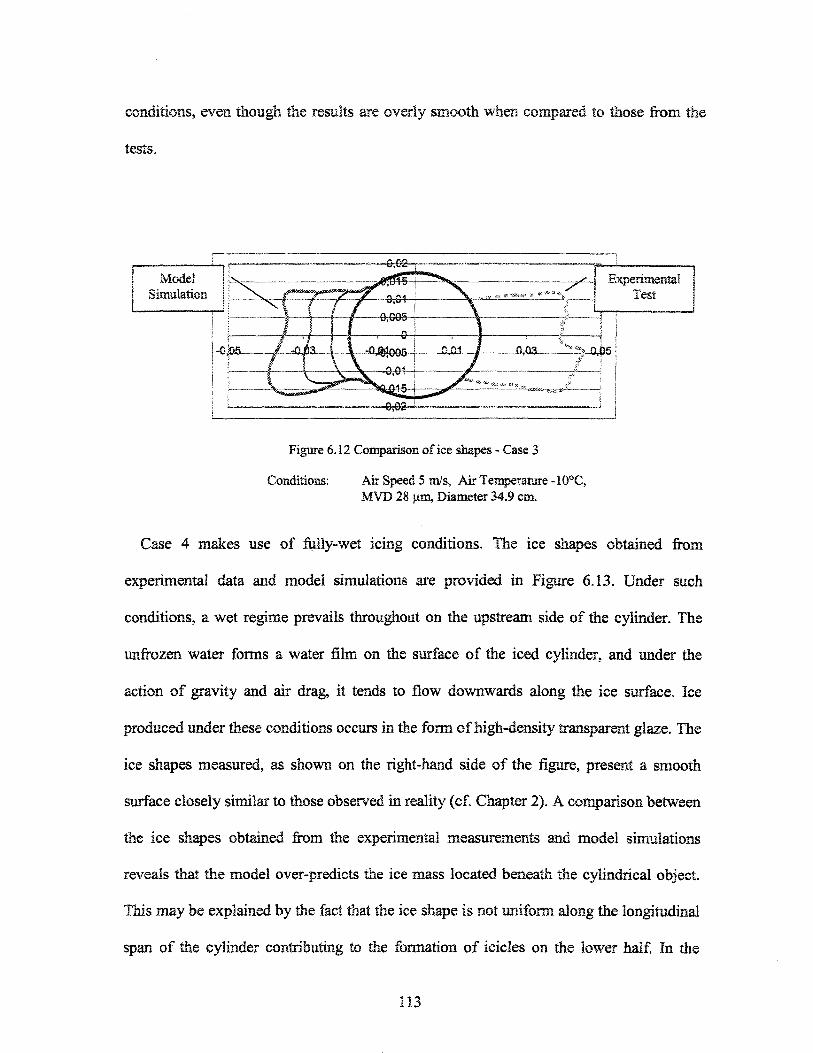
conditions, even though the results are overly smooth when compared to those from the
tests.
ExperimentalTest
5-ÛJ5
Figure 6.12 Comparison of ice shapes - Case 3
Conditions: Air Speed 5 m/s, Air Temperature -10°C,MVD 28 Mm, Diameter 34.9 cm.
Case 4 makes use of fully-wet icing conditions. The ice shapes obtained from
experimental data and model simulations are provided in Figure 6.13. Under such
conditions, a wet regime prevails throughout on the upstream side of the cylinder. The
unfrozen water forms a water film on the surface of the iced cylinder, and under the
action of gravity and air drag, it tends to flow downwards along the ice surface. Ice
produced under these conditions occurs in the form of high-density transparent glaze. The
ice shapes measured, as shown on the right-hand side of the figure, present a smooth
surface closely similar to those observed in reality (cf. Chapter 2). A comparison between
the ice shapes obtained from the experimental measurements and model simulations
reveals that the model over-predicts the ice mass located beneath the cylindrical object.
This may be explained by the fact that the ice shape is not uniform along the longitudinal
span of the cylinder contributing to the formation of icicles on the lower half. In the
113
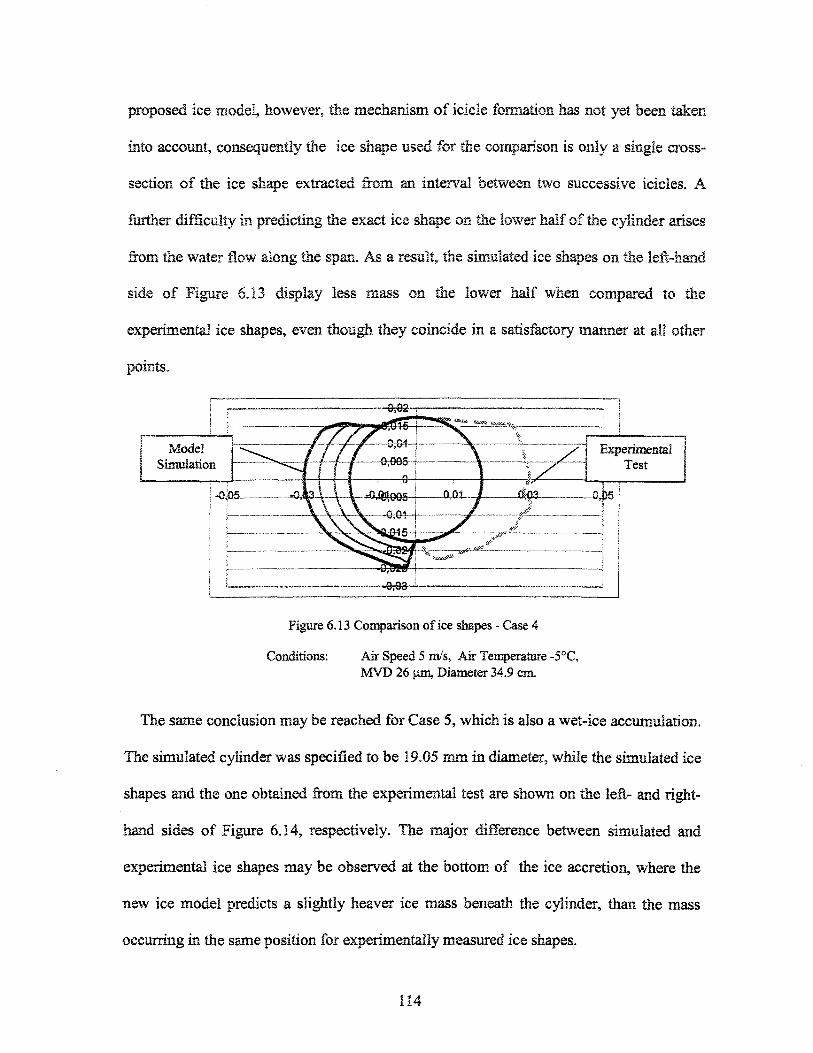
proposed ice model, however, the mechanism of icicle formation has not yet been taken
into account, consequently the ice shape used for the comparison is only a single cross-
section of the ice shape extracted from an interval between two successive icicles. A
former difficulty in predicting the exact ice shape on the lower half of the cylinder arises
from the water flow along the span. As a result, the simulated ice shapes on the left-hand
side of Figure 6.13 display less mass on the lower half when compared to the
experimental ice shapes, even though they coincide in a satisfactory manner at all other
points.
Figure 6.Î3 Comparison of ice shapes - Case 4
Conditions: Air Speed 5 m/s, Air Temperature -5°C,MVD 26 jim, Diameter 34.9 cm.
The same conclusion may be reached for Case 5, which is also a wet-ice accumulation.
The simulated cylinder was specified to be Î9.05 mm in diameter, while the simulated ice
shapes and the one obtained from the experimental test are shown on the left- and right-
hand sides of Figure 6.14, respectively. The major difference between simulated and
experimental ice shapes may be observed at the bottom of the ice accretion, where the
new ice model predicts a slightly heaver ice mass beneath the cylinder, than the mass
occurring in the same position for experimentally measured ice shapes.
114
ExperimentalTest
Figure 6.14 Comparison of ice shapes - Case 5
Conditions: Air Speed 5 m/s, Air Temperature -5°C,
MVD 33 pn, Diameter 19.05 cm.
45 Conclusion
This chapter provided a description of the experimental set-up and procedures involved
in the current test program. The ice shapes obtained from these tests were then compared
with those obtained by simulating the ice model under discussion. It may be concluded
that, on the whole, the proposed ice model displays good performance capacity for
simulating and predicting ice-growth shapes under dry- and wet- icing conditions.
115
MODEL SIMULATION
The basic components of the proposed icing model have been introduced in the
preceding chapters. In this chapter, a discussion of the model will be provided as an
overview; it will include the way in which the components work together to simulate the
ice accretion process on a cylindrical object which may be either current-carrying or not.
The techniques used to implement the proposed ice model into a computer code will also
be described briefly. Lastly, the new ice model will be used as a tool for examining the
effects of several factors on the ice load and shape as they occur on transmission line
cables. These factors include Joule heating, the Median Volume Diameter (MVD), and
cable size, among others.
7.1 Structure of Ice Model
Figure 7.1 is used to demonstrate the general structure of the icing model under
discussion, and the parameters transferred from one to another. The role of airflow
computation is pivotal in the model, since the output of this calculation provides the basic
parameters for subsequent components. Thus, the calculation for airflow past the iced
body should be carried out at the outset of the model calculation. Then, it becomes
possible to track the trajectories for an array of water droplets according to the velocity
distribution so obtained, and thereby to determine the Local Collision Efficiency (LCE).
Subsequently, the local Heat Transfer Coefficient (HTC) may be evaluated according to
116
the regularly updated velocity distribution on the boundary, and based on the same
velocity distribution, the thermal-balance equation may be solved so as to estimate the
icing fraction of the water collected on each surface element. This stage is followed by a
simulation of surface water-film flow to determine the water-film thickness and water
flow speed. Lastly, after each simulation step, the ice shape, ice density distribution, ice
load and rotational angle may be obtained.
117
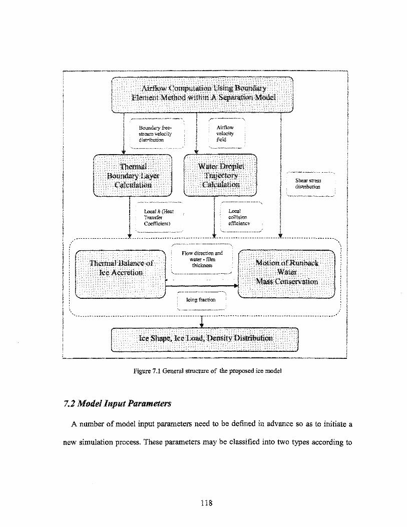
ir
Airflow Computation Using BoundaryBlemenl Method within A Separation Model
Boundary free-steam velocitydistribution
Airflowvelocityfield
I ThermalI Boundary Layer
Calculation
Water DropielTrajectoryCalculai ion
Local h (HeatTransferCoefficient)
Localcollisionefficiency
Shear stressdistribution
Thermal Balance ofi.ee Accretion
Flow direction andwater - filmthickness Motion of Kanback
WaterMass Consen'ation
Icing fractionj
TIce Shape, Ice Load, Density Distribution
Figure 7.1 General structure of the proposed ice mode!
7.2 Model Input Parameters
A number of model input parameters need to be defined in advance so as to initiate a
new simuiation process. These parameters may be classified into two types according to
118
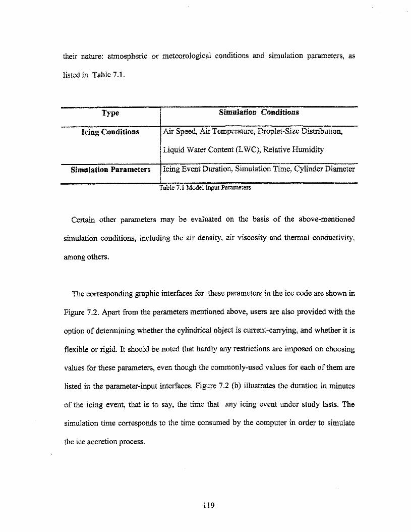
their nature: atmospheric or meteorological conditions and simulation parameters, as
listed in Table 7.1.
Type
Icing Conditions
Simulation Parameters
Simulation Conditions
Air Speed, Air Temperature, Droplet-Size Distribution,
Liquid Water Content (LWC), Relative Humidity
Icing Event Duration, Simulation Time, Cylinder Diameter
Table 7.1 Model Input Parameters
Certain other parameters may be evaluated on. the basis of the above-mentioned
simulation conditions, including the air density, air viscosity and thermal conductivity,
among others.
The corresponding graphic interfaces for these parameters in the ice code are shown in
Figure 7.2. Apart from the parameters mentioned above, users are also provided with the
option of determining whether the cylindrical object is current-carrying, and whether it is
flexible or rigid. It should be noted that hardly any restrictions are imposed on choosing
values for these parameters, even though the commonly-used values for each of them are
listed in the parameter-input interfaces. Figure 7.2 (b) illustrates the duration in minutes
of the icing event, that is to say, the time that any icing event under study lasts. The
simulation time corresponds to the time consumed by the computer in order to simulate
the ice accretion process.
119
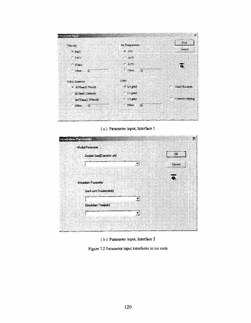
' ïv *-'
( a ) Parameter iuput, Inîerfece 1
( b ) Parameter input, Interface 2
Figure 7.2 Parameter input interfaces in ice code
120
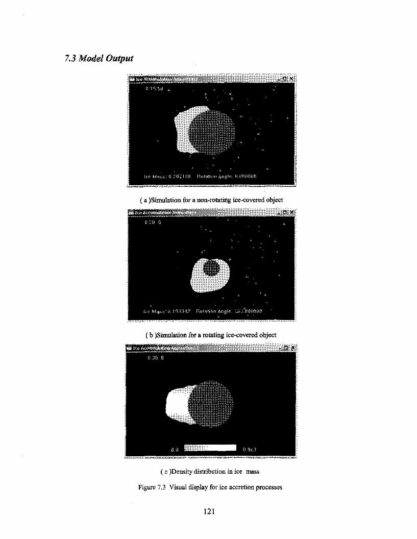
7.3 Model Output
( a )Sirauktion for a non-rotating ice-covered object
( b )Simulation for a rotating ice-covered object
( c )Density distribution in ice mass
Figure 7.3 Visual display for ice accretion processes
121
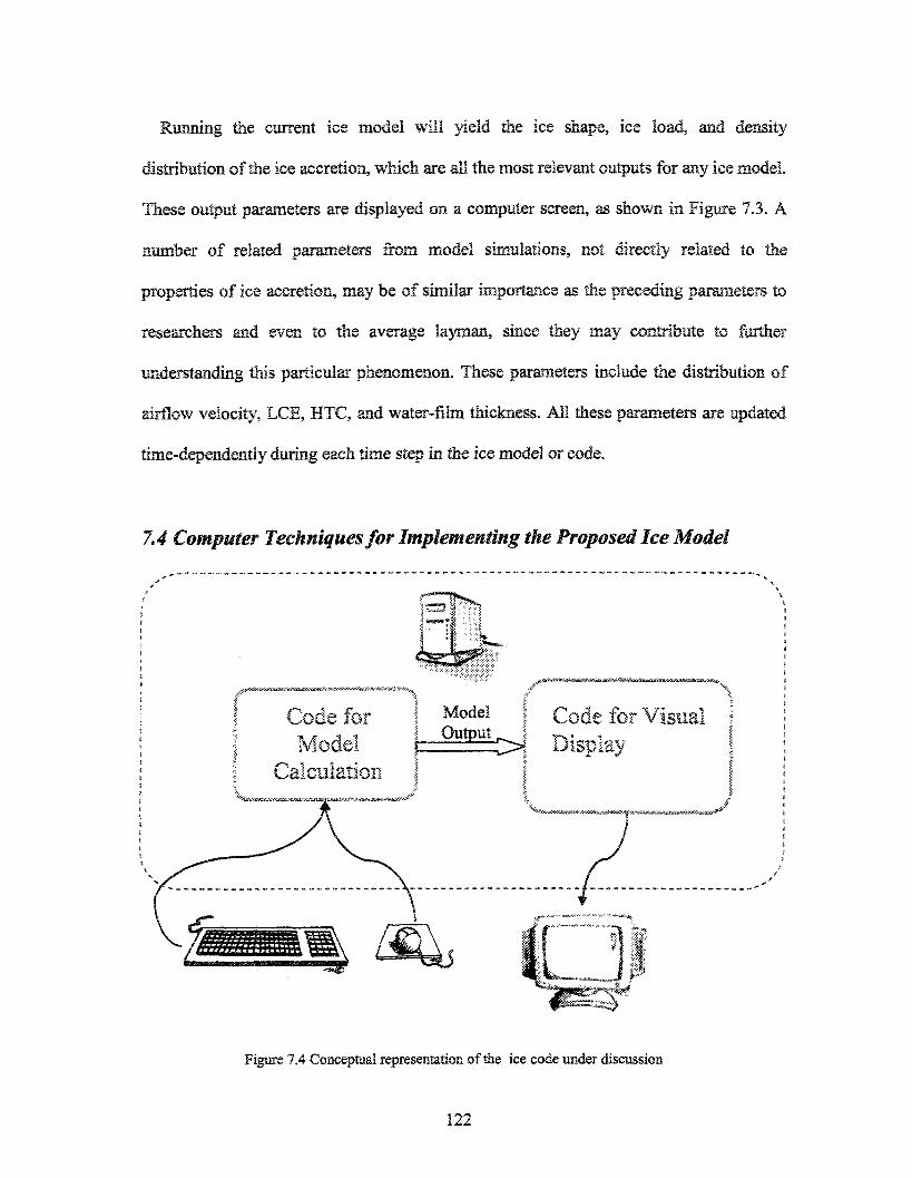
Running the current ice model will yield the ice shape, ice load, and density
distribution of the ice accretion, which are all the most relevant outputs for any ice model.
These output parameters are displayed on a computer screen, as shown in Figure 7.3. A
number of related parameters from model simulations, not directly related to the
properties of ice accretion, may be of similar importance as the preceding parameters to
researchers and even to the average layman, since they may contribute to further
understanding this particular phenomenon. These parameters include the distribution of
airflow velocity, LCE, HTC, and water-film thickness. All these parameters are updated
time-dependently during each time step in the ice model or code.
7.4 Computer Techniques for Implementing the Proposed Ice Model
ModelOutput
Code for Visual
Figure 7.4 Conceptual representation of the ice code under discussion
122
As shown in Figure 7.4S the programs for model calculation and for the visual display
of the icing process were mutually independent in terms of their fonctions and coding
phases even though they co-exist within the same code. As a result, any modification to
the ice model or code will not affect the program for the visual display. It should be noted
that the computer language used to implement model calculations need not necessarily be
C++, as was used here. The language could also be Fortran, as preferred by a large
majority of researchers. If the developing process of an ice code is divided into two
phases: code-developing and code-linking, then no major change will be observed in the
code-developing phase during which the model calculation code may be developed and
debugged independently. The code for model calculations will be linked to the visual
display code in the code-running phase, so that the calculation results can be animated by
the same display code presented earlier.
The computer code initiates mode! calculations upon receiving the model simulation
parameters designated by the user. At each simulation step, the subroutine for model
calculations sends a new set of calculation results to the visualization subroutine so as to
update the ice image on the screen in real time. The user may control and intervene in the
simulation process either by changing computer simulation time or by modifying the
display mode. The user also has the option of observing the time evolution of a number of
parameters such as the airflow past the iced cylinder or the local LCE , all of which
present great interest for research.
123
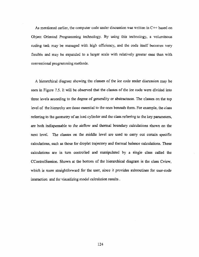
As mentioned earlier, the computer code under discussion was written in C++ based on
Object Oriented Programming technology. By «sing this technology, a voluminous
coding task may be managed with high efficiency, and the code itself becomes very
flexible and may be expanded to a larger scale with relatively greater ease than with
conventional programming methods.
A hierarchical diagram showing the classes of the ice code under discussion may be
seen in Figure 7.5. It will be observed that the classes of the ice code were divided into
three levels according to the degree of generality or abstractaess. The classes on the top
level of the hierarchy are those essential to the ones beneath them. For example, the class
referring to the geometry of an iced cylinder and the class referring to the key parameters,
are both indispensable to the airflow and thermal boundary calculations shown on the
next level. The classes on the middle level are used to carry out certain specific
calculations, such as those for droplet trajectory and thermal balance calculations. These
calculations are in turn controlled and manipulated by a single class called the
CControlSession. Shown at the bottom of the hierarchical diagram is the class Cview,
which is more straightforward for the user, since it provides subroutines for user-code
interaction and for visualizing model calculation results.
124
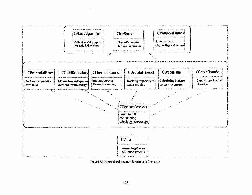
I CNumÂfgorithml{ Collection of all-purposei Numerical Algorithms
CIceBody
Shape ParameterAirflow Parameter
CPhysicalParam
Subroutines to| obtain Physical Param
CControISession
V
. I Controling &' coordinating| calculation procedure
CPotentialFiow
Airflow computationwith BEM
CFIuiclBoundary
Momentum integratiorover airflow Boundary
j CThermalBound
f integration owrj Thermal Boundary
CDropIetTraject
Tracking trajectory ofwater droplet
CWaterRIm
Calculating Surfacewater movement
CCableRotation
Simylation of cableRotation
CVIew
Animating the IceAccretion Process
Figure 7.5 Hierarchical diagram for classes of ice code
125
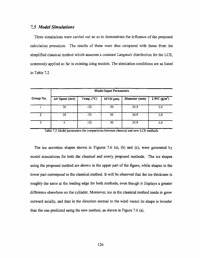
7.5 Model Simulations
Three simulations were carried out so as to demonstrate the influence of the proposed
calculation procedure. The results of these were then compared with those from the
simplified classical method which assumes a constant Langmuir distribution for the LCE,
commonly applied so far in existing icing models. The simulation conditions are as listed
in Table 7.2
Greap No.
1
2
3
Model lapai Parameters
Air Speed {mis)
10
10
5
Temp.f�)
-12
-12
-12
MVD (§»w)
20
30
30
Diameter (sum)
34.9
34.9
34.9
LWC (g/ia3)
1.0
Î.0
1.0
Table 7.2 Model parameters for comparisons between classical and new LCE methods
The ice accretion shapes shown in Figures 7.6 (a), (b) and (c), were generated by
model simulations for both the classical and newly proposed methods. The ice shapes
using the proposed method are shown in the upper part of the figure, while shapes in the
lower part correspond to the classical method. It will be observed that the ice thickness is
roughly the same at the leading edge for both methods, even though it displays a greater
difference elsewhere on the cylinder. Moreover, ice in the classical method tends to grow
outward axially, and thus in the direction normal to the wind vector its shape is broader
than the one predicted using the new method, as shown in Figure 7.6 (a).
126
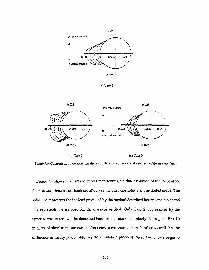
0,025
proposed method
-0,0;
classical method
0,025 i
-0,025 J
proposed method0,025
fi -0,035
ciassical method
-0,025
(b) Case 2 (c) Case 3
Figure 7.6 Comparison of ice accretion shapes predicted by ciassical and new methods(time step: 5min)
Figure 7.7 shows three sets of curves representing the time evolution of the ice load for
the previous three cases. Each set of curves includes one solid and one dotted curve. The
solid line represents the ice load predicted by the method described herein, and the dotted
line represents the ice load for the classical method. Only Case 2, represented by the
upper curves in red, will be discussed here for the sake of simplicity. During the first 10
minutes of simulation, the two ice-load curves coincide with each other so well that the
difference is hardly perceivable. As the simulation proceeds, these two curves begin to
127
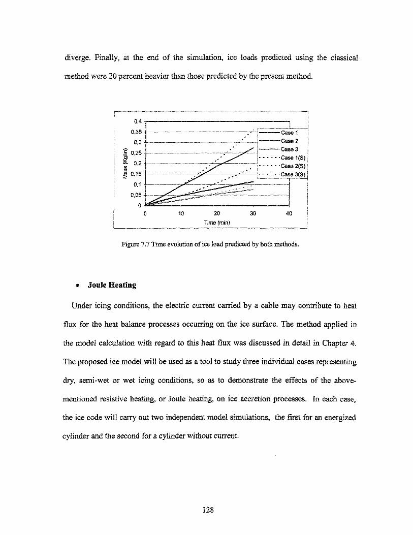
diverge. Finally, at the end of the simulation, ice loads predicted using the classical
method were 20 percent heavier than those predicted by the present method.
CaseiCase 2CaseSCase 1{S)Case 2(S)Case 3(S)
20
Time (min)
Figure 7.7 Time evolution of ice load predicted by both methods.
« Joule Heating
Under icing conditions, the electric current carried by a cable may contribute to heat
flux for the heat balance processes occurring on the ice surface. The method applied in
the model calculation with regard to this heat flux was discussed in detail in Chapter 4.
The proposed ice model will be used as a tool to study three individual cases representing
dry, semi-wet or wet icing conditions, so as to demonstrate the effects of the above-
mentioned resistive heating, or Joule heating, on ice accretion processes. In each case,
the ice code will carry out two independent model simulations, the first for an energized
cylinder and the second for a cylinder without current.
128
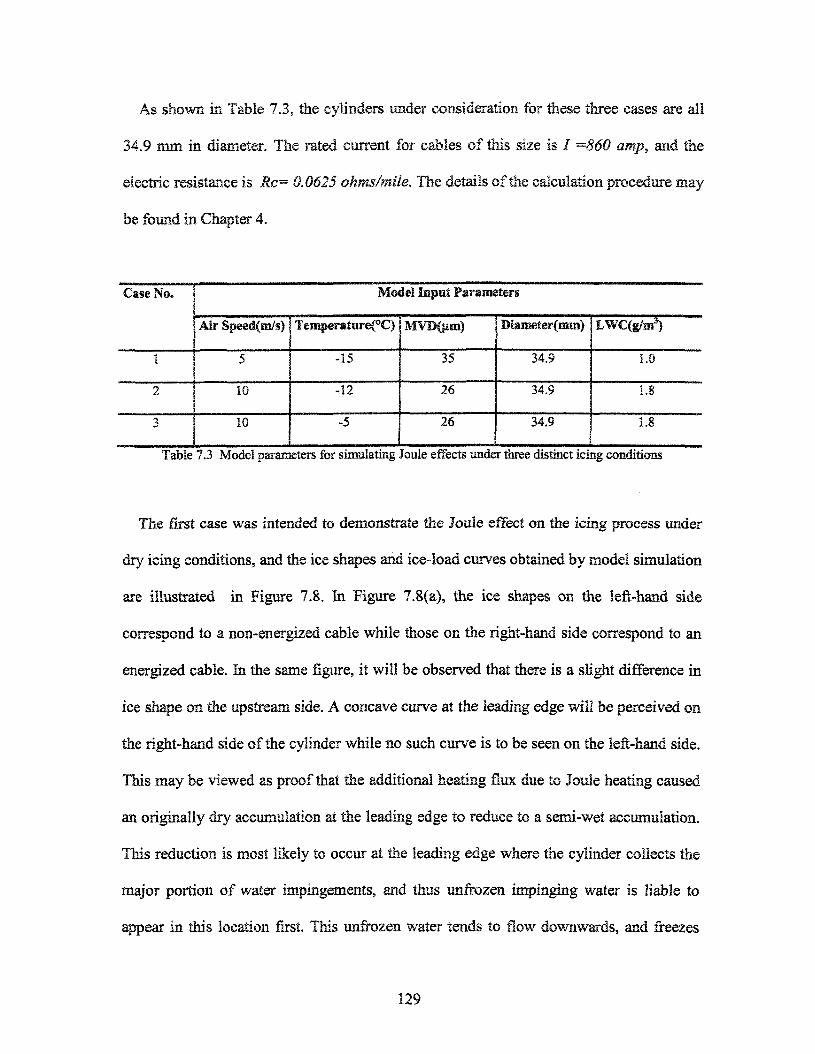
As shown in Table 7.3, the cylinders under consideration for these three cases are all
34.9 mm in diameter. The rated current for cables of this size is / �860 amp, and the
electric resistance is Rc= 0.0625 ohms/mile. The details of the calculation procedure may
be found in Chapter 4.
Case No.
1
2
3
Model Input Parameters
Air Speed(m/s)
5
10
id
TemperaturefC)
-15
-Î2
-5
MVD(fim)
35
26
26
Diameter(mra)
34.9
34.9
34.9
LWCd/m3)
1.0
1.8
1.8
Table 7.3 Model parameters for simulating Joule effects under three distinct icing conditions
The first case was intended to demonstrate the Joule effect on the icing process under
dry icing conditions, and the ice shapes and ice-load curves obtained by model simulation
are illustrated in Figure 7.8. In Figure 7.8(a), the ice shapes on the left-hand side
correspond to a non-energized cable while those on the right-hand side correspond to an
energized cable. In the same figure, it will be observed that there is a slight difference in
ice shape on the upstream side. A concave curve at the leading edge will be perceived on
the right-hand side of the cylinder while no such curve is to be seen on the left-hand side.
This may be viewed as proof that the additional heating flux due to Joule heating caused
an originally dry accumulation at the leading edge to reduce to a semi-wet accumulation.
This reduction is most likely to occur at the leading edge where the cylinder collects the
major portion of water impingements, and thus unfrozen impinging water is liable to
appear in this location Irst. This unfrozen water tends to flow downwards, and freezes
129
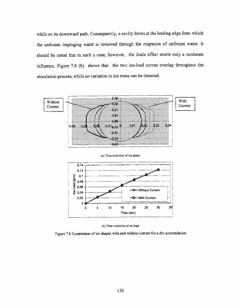
while on its downward path. Consequently, a cavity forms at the leading edge from which
the unfrozen impinging water is removed through the migration of unfrozen water. It
should be noted that in such a case, however, the Jouîe effect exerts only a moderate
influence. Figure 7.8 (b) shows that the two ice-load curves overlap throughout the
simulation process, while no variation in ice mass can be detected.
(a) Time evolution of ice shape
0.14 - j �
0,12
0,08 4
0,06
0,04�^�Without Current
�B� With Current
10 15 20
Time (min)
25 30 35!
(b) Time evolution of ice load
Figure 7.8 Comparison of ice shapes with and without carrent for a dry accumulation
130
{ a ) Time evolution of ice shape
With CurrentWithout Current
10 15 20
Time (min)
( b ) Time evolution of ice load
Figure 7,9 Comparison of ice shapes with and without current for a semi-wet accumulation
The second case was designed for semi-wet conditions, and its simulation results are
plotted in Figures 7.9 (a) and (b) which show that, on the whole, no major difference in
ice shape may be observed between these two sets of ice shapes. The simulation for an
energized cylinder still yields a semi-wet ice accretion, while even more ice is predicted
at the bottom of the ice accretion, as shown on the right-hand side of the same figure.
This may be explained by the fact that the extra heat flux from the electric current, in the
case of the energized cylinder, contributes to the formation of more unfrozen water which
131
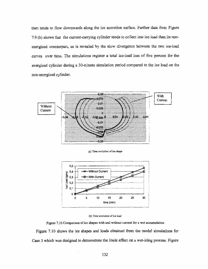
then tends to flow downwards along the ice accretion surface. Further data from Figure
7.9 (b) shows that the carrent-cairying cyMnder tends to collect less ice load than its non-
energized counterpart, as is revealed by the slow divergence between the two ice-load
curves over time. The simulations register a total ice-load loss of five percent for the
energized cylinder during a 30-minute simulation period compared to the ice load on the
non-energized cylinder.
(a) Time evolution of ice shape
0,5
0 4 __) �«-withoutCurrent
10 15 20
time (min)
(b) Time evolution of ice load
Figure 7.10 Comparison of ice shapes with and without current for a wet accumulation
Figure 7.10 shows the ice shapes and loads obtained from the model simulations for
Case 3 which was designed to demonstrate the Joule effect on a wet-icing process. Figure
Î32
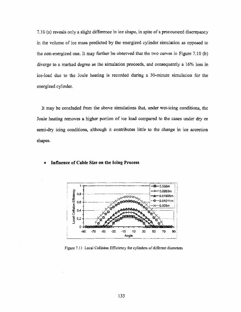
7.10 (a) reveals only a slight difference in ice shape, in spite of a pronounced discrepancy
in the volume of ice mass predicted by the energized cylinder simulation as opposed to
the non-energized one. It may further be observed that the two curves in Figure 7.10 (b)
diverge to a marked degree as the simulation proceeds, and consequently a 16% loss in
ice-load due to the Joule heating is recorded during a 30-minute simulation for the
energized cylinder.
It may be concluded from the above simulations that, under wet-icing conditions, the
Joule heating removes a higher portion of ice load compared to the cases under dry or
semi-dry icing conditions, although it contributes little to the change in ice accretion
shapes.
« Influence of Cable Size on the Icing Process
B�0.035m0.0263m0.01905m
-90 -70 -50 -30 -10 10 30 50Angle
Figure 7.11 Local Collision Efficiency for cylinders of different diameters
133
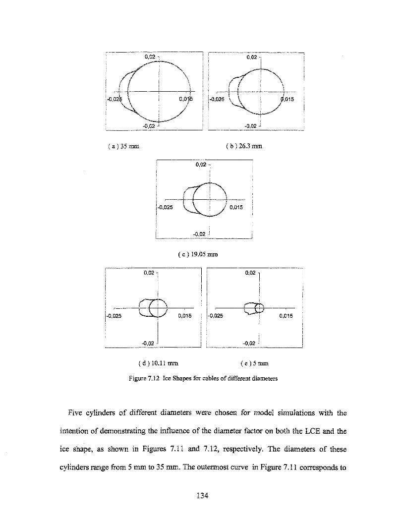
0,02 -
i-0,02!
-0,02 J
0,02 -
-0,025 I \
-0,02 -
"A0,015
( a ) 35 mm ( b ) 26.3 mm
0.02-
-0,025
-0,02 J
' c ) 19.05 mm
0,02
-0,025
-0,02
0,015
( d ) 10.11 mm (e)5mm
Figure 7.12 Ice Shapes for cables of different diameters
Five cylinders of different diameters were chosen for model simulations with the
intention of demonstrating the influence of the diameter factor on both the LCE and the
ice shape, as shown in Figures 7.11 and 7.12, respectively. The diameters of these
cylinders range from 5 mm to 35 mm. The outermost curve in Figure 7.11 corresponds to
134
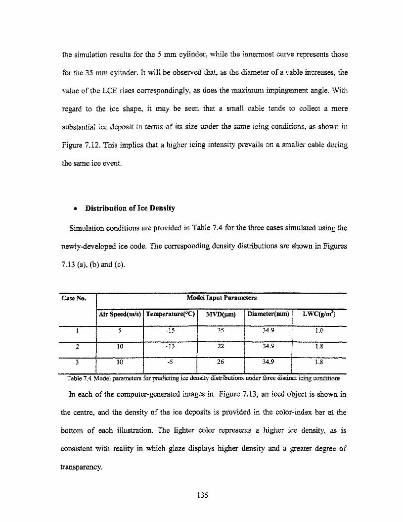
the simulation results for the 5 mm cylinder, while the innermost curve represents those
for the 35 mm cylinder. It will be observed that, as the diameter of a cable increases, the
value of the LCE rises correspondingly, as does the maximum impingement angle. With
regard to the ice shape, it may be seen that a small cable tends to collect a more
substantial ice deposit in terms of its size under the same icing conditions, as shown in
Figure 7.12. This implies that a higher icing intensity prevails on a smaller cable during
the same ice event.
� Distribution of Ice Density
Simulation conditions are provided in Table 7.4 for the three cases simulated using the
newly-developed ice code. The corresponding density distributions are shown in Figures
7.13 (a), (b) and (c).
Case No.
1
2
3
Model Input Parameters
Air Speed(m/s)
5
10
10
TemperaturefC)
-15
-13
-5
MYDQun)
35
22
26
Diameter(mm)
34.9
34.9
34.9
LWCCg/m3)
1.0
1.8
1.8
Table 7.4 Model parameters for predicting ice density distributions under three distinct icing conditions
In each of the computer-generated images in Figure 7.13, an iced object is shown in
the centre, and the density of the ice deposits is provided in the color-index bar at the
bottom of each illustration. The lighter color represents a higher ice density, as is
consistent with reality in which glaze displays higher density and a greater degree of
transparency.
135
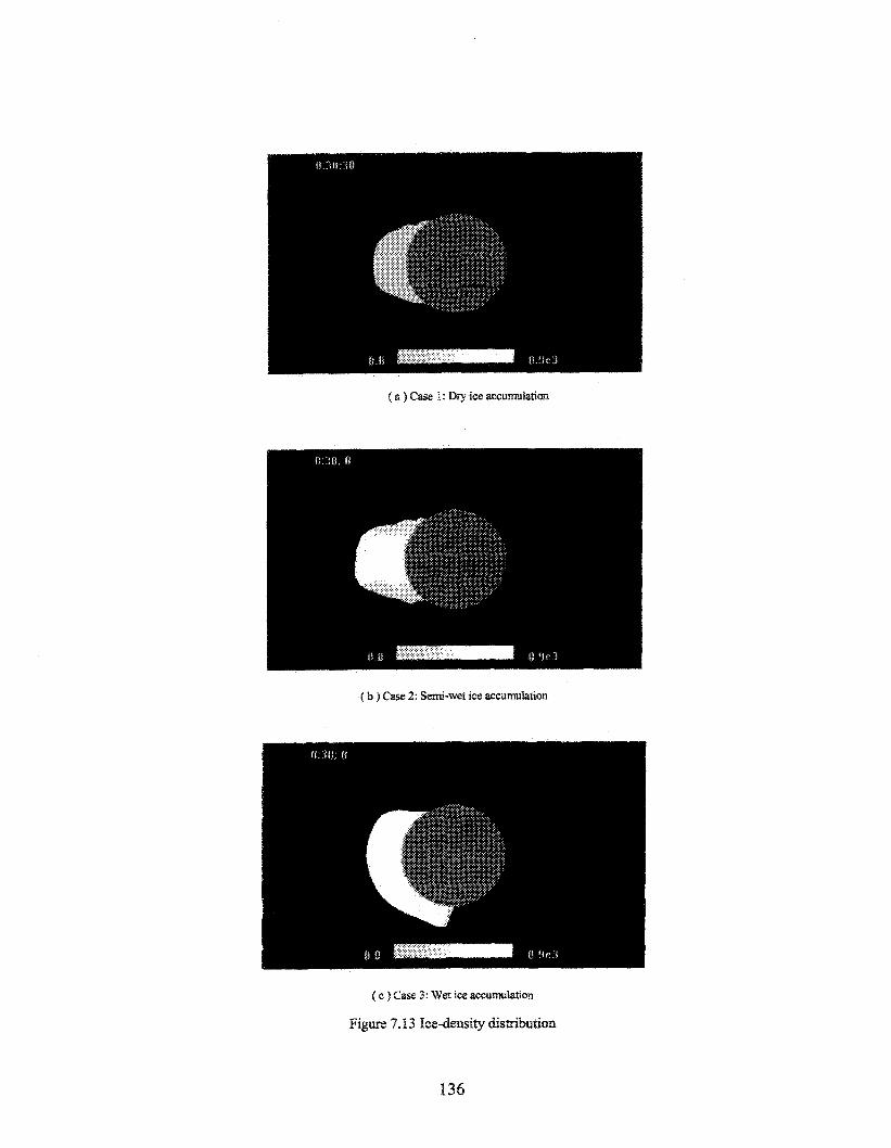
( a ) Case 1 : Dry ice accumulation
( b ) Case 2: Semi-wet ice accumulation
( c ) Case 3: Wet ice accumulation
Figure 7.13 Ice-density distribution
136
Since Case 1 represents a typical dry accumulation at -15°C, its density is less than
400kg/m3, and thus the ice shape was rendered with a darker color.
Case 2 represents a semi-wet ice accumulation. In the centre, a high-density wet
regime may be seen, and thus a light color was used to render the shape in this position.
On each of the upper and lower edges of the ice mass, dry ice of a low density
accumulates, and is thus represented by a darker color. Also, Figure 7.13 (b) reveals a
tendency of the ice to be drier at the initial stage, becoming wetter as the icing process
advances.
Case 3 represents a wet accumulation where it is clear that the wet regime prevails
throughout, thus a light color was used to render the ice shape.
� Influence of Droplet Size on the Icing Process
A convenient feature of this newly-developed icing model is that it accepts user-
defined MVD values yet it imposes no particular restrictions. This new feature makes it
possible to investigate the influence of droplet size on icing processes. Different MVDs
are used in the present study as model input parameters for three separate cases, while all
other parameters are kept unchanged. A detailed list of the simulation conditions are
provided in Table 7.5. It should be noted that these MVDs are intended to represent three
separate batches of small-, intermediate- and large-sized droplets.
137
Case No.
1
2
3
Air Speed{m/s)
5
Mai
TenxperaturefC)
-5
-5
-5
lei Input Params
MVD(jtin)
50
100
500
stars
Diameter(mni)
34.9
34.9
34.9
LWCCg/m3)
2.5
2.5
2.5
Table 7.5 Mode! parameters for investigatiag the influence of droplet size
Figure 7.14 shows the time evolution of the ice mass in Case 1, where the MVD of the
droplets is set at 500 jjm. A wet regime prevails on the surface of the ice mass, since this
surface is smooth with a low surface icing rate. The ice mass is found not only on the
windward side, but also on the leeward side, which may be explained by the fact that the
rear surface receives direct water impingement from the incoming water flux which
precipitates obliquely rather than horizontally in relation to the icing object. Also, part of
the unfrozen water will flow in a clockwise direction, pushing its own pathway even
further back. Then, under adverse cooling conditions, ice freezes somewhere on its way
downwards on the rear surface. As a result, it may be predicted that the ice mass will
cover an increasingly greater part of the rear surface of a cylindrical object with a
corresponding increase in the MVD.
When reducing the MVD of droplets to 100 pm, an apparent drop in ice mass is
observed on the leeward side of the icing object, as shown in Figure 7.15. Further
decreasing the size of water droplets implies that the trajectories of these droplets become
horizontal to a greater extent, as in Case 3. Under such conditions water impingement
collides solely with the windward-side surface, and also air drag is not strong enough to
138
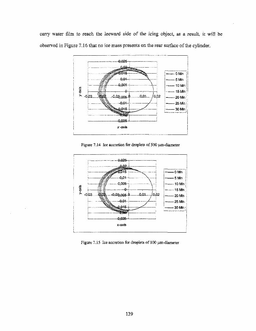
carry water film to reach the îeewarf side of the icing object, as a result» it will
observed 1B Figure 7.16 that no ice mass presents on the rear surface of the cylinder.
: IdaMt
� ^ ^ t e
OC�6-066-
ft
EE|ffi_=0..tthnnKJ
x-axis
\ \
� OMn I
� 10Mn|
20Wn|25Mn|
-30Mn|
Figure 7.14 Ice accretion for droplete of 500 jun-diameter
-OMn-5Mn
-15Mhi-20Mnj-25Mn!-30Mn|
x-axs
Figure 7.15 Ice accretion for droplets of 100 pin-diameter
139
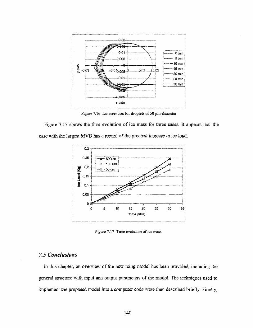
- 0 min 1
- 5 min \
�10 min j
-15 min :
-20 min !
-25 min j
-30 min j
x-axis
Figure 7.16 Ice accretion for droplets of 50 jim-diameter
Figure 7.17 shows the time evolution of ice mass for three cases. It appears that the
case with the largest MVD has a record of the greatest increase in ice load.
15 20
Time (Min)
25 30 35j
Figure 7.1? Time evolution of ice mass
7.5 Conclusions
In this chapter, an overview of the new icing model has been provided, including the
general structure with input and output parameters of the model. The techniques used to
implement the proposed model into a computer code were then described briefly. Finally,
140

the new Ice model was used as a tool to examine the effects of several factors on the ice
load and shape as they occur on transmission line cables.
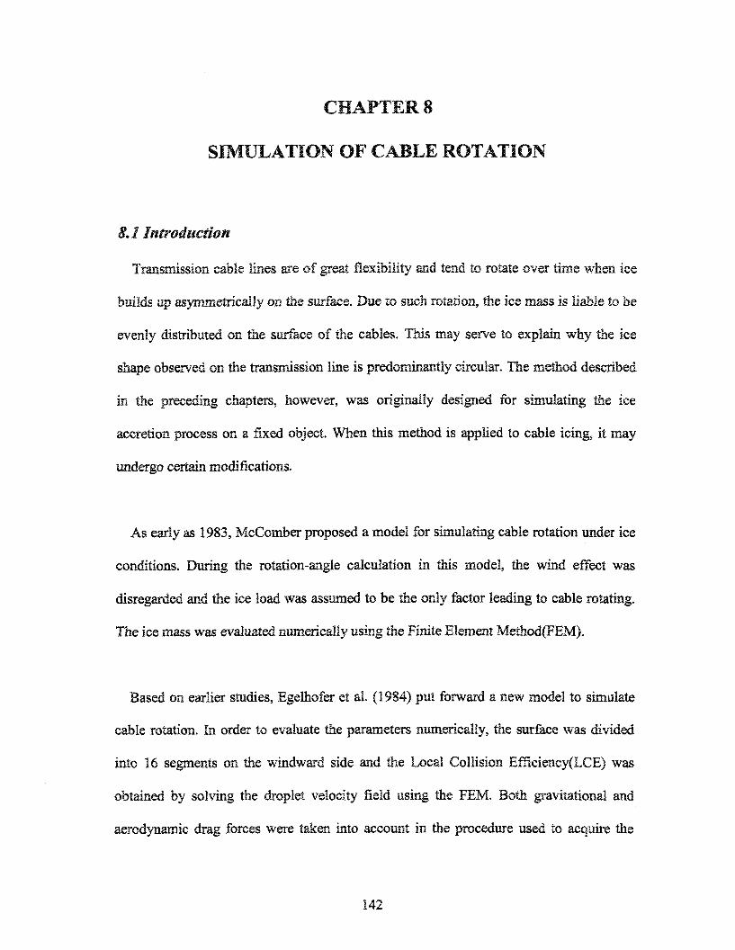
Transmission cable lines are of great flexibility and tend to rotate over time when ice
builds up asymmetrically on the surface. Due to such rotation, the ice mass is liable to be
evenly distributed on the surface of the cables. TMs may serve to explain why the ice
shape observed on the transmission line is predominantly circular. The method described
in the preceding chapters, however, was originally designed for simulating the ice
accretion process on a fixed object. When this method is applied to cable icing, it may
undergo certain modifications.
As early as 1983, McComber proposed a model for simulating cable rotation under ice
conditions. During the rotation-angîe calculation in this model, the wind effect was
disregarded and the ice load was assumed to be the only factor leading to cable rotating.
The ice mass was evaluated numerically using the Finite Element Method(FEM).
Based on earlier studies, Egelhofer et al. (1984) put forward a new model to simulate
cable rotation, in order to evaluate the parameters numerically, the surface was divided
into 16 segments on the windward side and the Local Collision Efficiency(LCE) was
obtained by solving the droplet velocity field using the FEM. Both gravitational and
aerodynamic drag forces were taken into account in the procedure used to acquire the
142
rotating angle on the iced object. From a theoretical point of view, their model was
rendered more satisfactory than previously with the inclusion of these supplementary
characteristics.
Further work is necessary, however, to make it possible for an ice model to perform
simulations over a more extended period of time, since both the aforementioned models
were designed only for simulations at the preliminary stages of cable rotation. Also, these
models assumed that the ice deposit would retain an initial simple shape throughout the
entire accretion process, making it practically impossible for the simulation of an icing
event of long-duration. The method, which will be described below, evaluates the airflow
velocity field and thus the LCE on a real-time basis using the potential flow calculation
in the context of the boundary-layer separation theory. Such a procedure then makes it
possible to carry out precise and reliable model simulations over a long period. By using
this model, the ice shapes will be obtained at rotational angles of 90°, 180°, 270° or
greater.
Unfortunately, the existing body of experimental studies pertaining to this problem is
so far limited due in part to the difficulty inherent in designing a viable experimental
setup to simulate cable twisting. It is, nevertheless, encouraging to find a published
experimental study concerning the formation of ice on test wires in an instrumented wind
tunnel, as performed under natural conditions by Personne and Gayet (1988). The
torsional rotation resulting from gravitational and aerodynamic torques under natural
conditions was simulated by wires set in conical bearings and attached to a helical
143
spring. The data from these tests will contribute to validating the theoretical study
presented herein.
It is worth mentioning that the influence of cable rotation on transmission facilities is
not necessarily a negative one. The rotation causes the ice to be more evenly distributed
on the cable surface in a roughly circular shape. From the point of view of mechanical
analysis, such a change will improve the performance of transmission lines by lessening
the potential for galloping, which is one of the adverse effects of ice accretion.
Meanwhile, it will also minimize the cross-sectional area for a given mass.
8.2 Basic Principles
In view of the complexity of this problem, a number of assumptions were made as
follows:
� the torques from aerodynamic forces and ice load were assumed to be evenly
distributed over the length of the transmission line as shown in Figure 8.1.
� the ice deposit over the cable surface creates no resistance to cable rotation.
� the cable rotates at so low a speed that its inertia! effect may be disregarded.
Hence, at any given position, the cable may be seen as being at rest, and the net
external torque is balanced by that of the internal resistance.
Figure 8.1 shows one section of the transmission line where both ends, A and B, are
fixed. Its length is 60.97 meters. A plane cut, o-o, is applied at point C where the
144
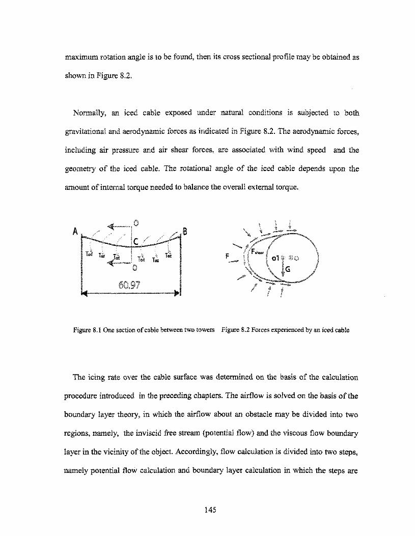
maximum rotation angle is to be found, then its cross sectional profile may be obtained as
shown in Figure 8.2,
Normally, an iced cable exposed under natural conditions is subjected to both
gravitational and aerodynamic forces as indicated in Figure 8.2. The aerodynamic forces,
including air pressure and air shear forces, are associated with wind speed and the
geometry of the iced cable. The rotational angle of the iced cable depends upon the
amount of internai torque needed to balance the overall external torque.
Figure 8.1 One section of cable between two towers Figure 8.2 Forces experienced by an iced cable
The icing rate over the cable surface was determined on the basis of the calculation
procedure introduced in the preceding chapters. The airflow is solved on the basis of the
boundary layer theory, in which the airflow about an obstacle may be divided into two
regions, namely, the inviscid free stream (potential flow) and the viscous flow boundary
layer in the vicinity of the object. Accordingly, flow calculation is divided into two steps,
namely potential flow calculation and boundary layer calculation in which the steps are
145
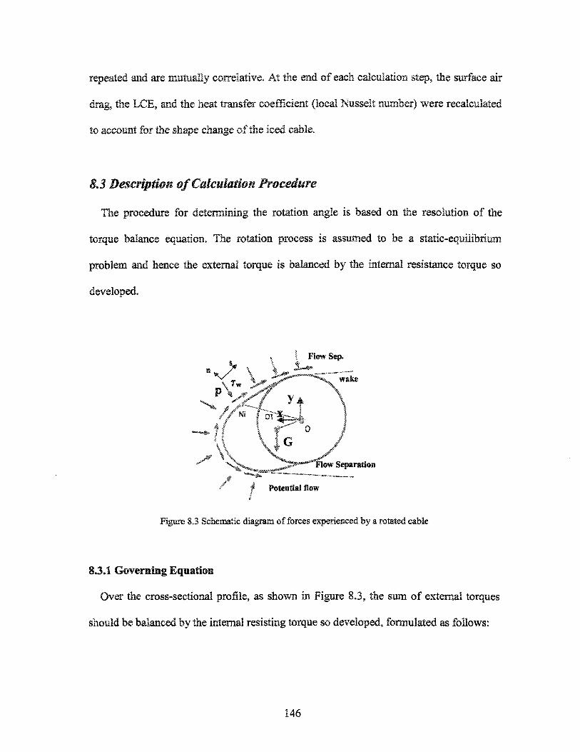
repeated and are mutually correlative. At the end of each calculation step, the surface air
drag, the LCE, and the heat transfer coefficient (local Nusselt number) were recalculated
to account for the shape change of the iced cable.
8.3 Description ofCalculaaon Pr&cedure
The procedure for determining the rotation angle is based on the resolution of the
torque balance equation. The rotation process is assumed to be a static-equilibrium
problem and hence the external torque is balanced by the internal resistance torque so
developed.
| Flow Sep.
wake
Flow Separation
Potential flow
Figure 8.3 Schematic diagram efforces experienced by a rotated cable
8.3.1 Governing Equation
Over the cross-sectional profile, as shown in Figure 8.3, the sum of external torques
should be balanced by the internal resisting torque so developed, formulated as follows:
146
* External ~ ^Internal (E 8-1)
In formulaic presentation, TEaerml denotes the sum of external torques, which includes the
torque from air pressure, Tp, air shear force, Tf, and gravity, Tg, as follows
(E8-2)
where:
Tp+Tf= ^QxTp+7wxTf)ds (E 8-3)
in which p = p0 +�CppV02, whereCp is derived from the potential flow calculation
defined by Cp = 1 - (F� / F0)2 , in which Vo and FM represent the onset free-stream speed
and free-stream speed on the outer edge of the flow boundary layer, respectively; and
tw = �CfpV02, where Cf is obtained from the momentum calculation of the boundary
layer.
Also, r g = G x ^ î (E8-4)
where G = L/2xw in which L is the cable span between two transmission towers; the
definition of oo\ may be found in Fig. 8.3; and
(E8-5)
147
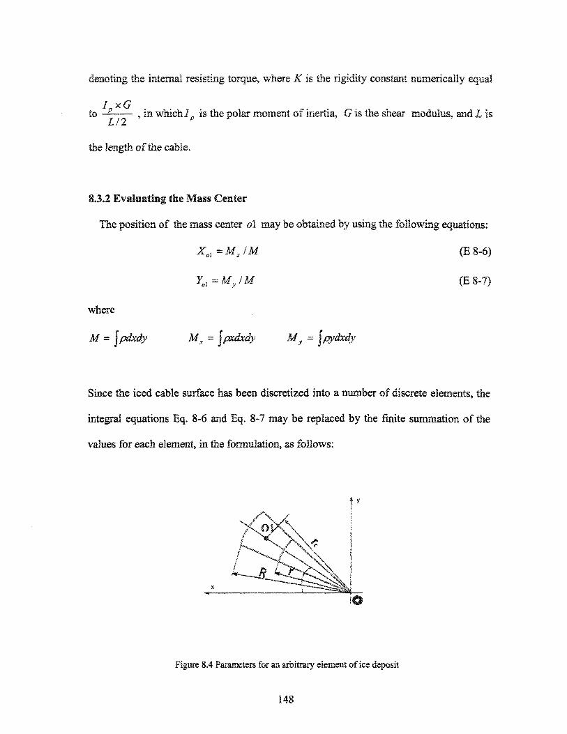
denoting the internal resisting torque» where K is the rigidity constant numericaily equal
I.xGl0 _£ 5 ^ which 1 p is the polar moment of inertia, G is the shear modulus, and L is
the length of the cable.
8.3.2 Evaluating the Mass Center
The position of the mass center ol may be obtained by using the following equations:
(E8-6)Xoi =MX/M
(E8-7)
where
M = Ipdxdy Mx = îpxdxdy My = îpydxdy
Since the iced cable surface has been discretized into a number of discrete elements, the
integral equations Eq. 8-6 and Eq. 8-7 may be replaced by the finite summation of the
values for each element, in the formulation, as follows:
Figure 8.4 Parameters for an arbitrary element of ice deposit
148
mc (E 8-8)
Mx = p J (R,2 - r2 )&f> 12 x rd x cos # (E 8-9)
£/ x sin # (E 8-10)
. 2s in#( i? 2+i?r + r2) . - .^ - .. - t ^ r ^ -where r . = -1 �- ; definitions of these symbols may be found m
3 # R + rFigure 8.4 which shows the parameters for any given element, i.
8.3.3 Position Change of Stagnation Point
The stagnation point is defined as the position where the airflow comes to rest. In
calculating the airflow boundary layer, the fluid momentum integration used for
determining the separation points always starts from the stagnation point, therefore this
calculation should be carried out meticulously in order to diminish the possibility of any
inaccuracies arising.
When the cable starts to rotate, a distinct location change of the stagnation point may
be observed, as shown in Figure 8.5, where the stagnation point shifts from si to s2, and
an obvious shift in the distribution of shear stress also occurs. Within the newly-
developed ice code, an algorithm was specifically designed for detecting the new position
of the stagnation point at each time step, thus ensuring a constantly updated position for
subsequent calculations.
149
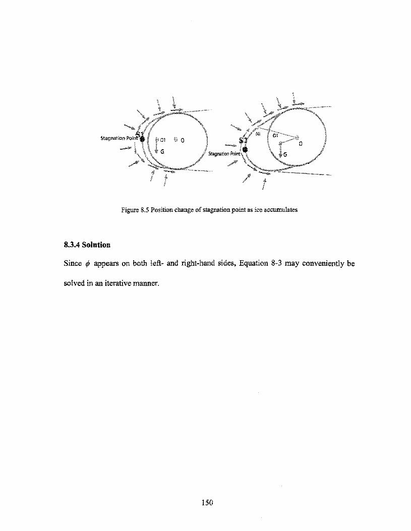
*«««**-�^^^C
lé
Figure 8.5 Position change of stagnation point as ice accumuktes
S.3.4 Solution
Since ^ appears on both left- and right-hand sides, Equation 8-3 may conveniently be
solved in an iterative manner.
150
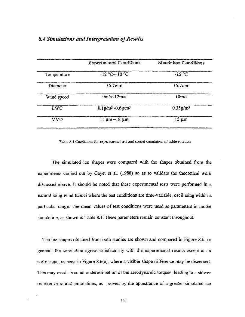
8.4 Simulations and Imterpreiaîi&m of Results
Temperature
Diameter
Wind speed
LWC
MVD
Experimental Conditions
-12 °O-18 °C
15.7mm
9m/s~12m/s
0.1g/m3~0.6g/m3
11 jim~18 jim
SiinulatioB Conditions
-15 °C
15.7mm
lOm/s
0.35g/m3
15 jim
Table 8.1 Conditions for experimental test and model simulation of cable rotation
The simulated ice shapes were compared with the shapes obtained from the
experiments carried out by Gayet et al. (1988) so as to validate the theoretical work
discussed above. It should be noted that these experimental tests were performed in a
natural icing wind tunnel where the test conditions are time-variable, oscillating within a
particular range. The mean values of test conditions were used as parameters in model
simulation, as shown in Table 8.1. These parameters remain constant throughout.
The ice shapes obtained from both studies are shown and compared in Figure 8.6. In
general, the simulation agrees satisfactorily with the experimental results except at an
early stage, as seen in Figure 8.6(a), where a visible shape difference may be discerned.
This may result from an underestimation of the aerodynamic torques, leading to a slower
rotation in model simulations, as proved by the appearance of a greater simulated ice
151
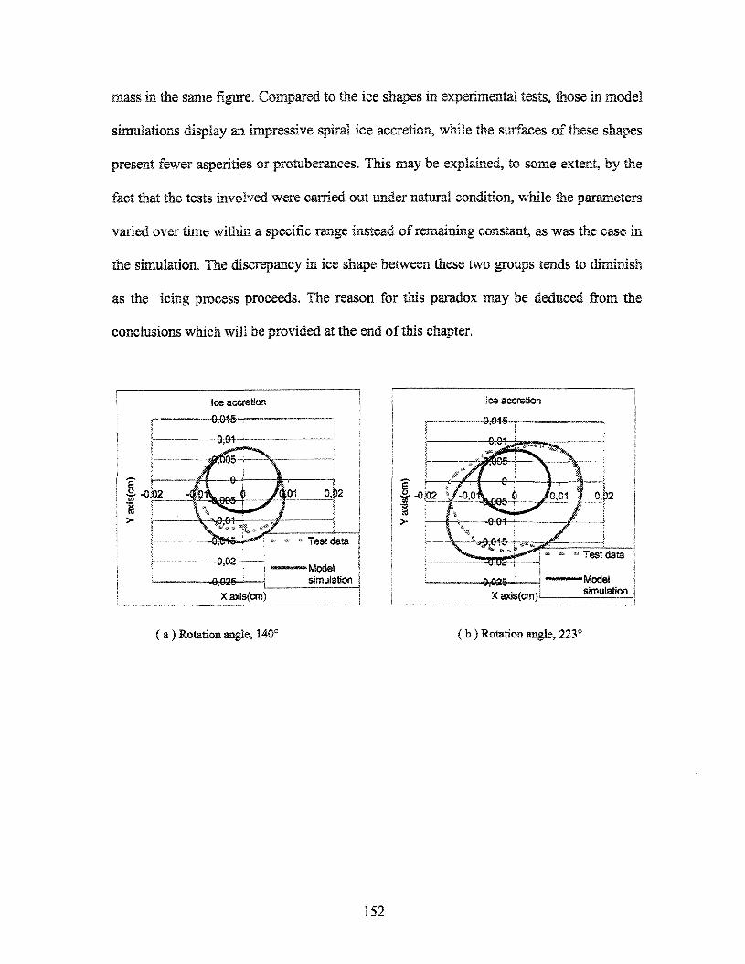
mass in the same figure. Compared to the ice shapes in experimental tests, those in model
simulations display an impressive spiral ice accretion, while the surfaces of these shapes
present fewer asperities or protuberances. This may be explained, to some extent, by the
fact that the tests involved were carried out under natural condition, while the parameters
varied over time within a specific range instead of remaining constant, as was the case in
the simulation. The discrepancy in ice shape between these two groups tends to diminish
as the icing process proceeds. The reason for this paradox may be deduced from the
conclusions which will be provided at the end of this chapter.
lee accretion
X axis(cm)
( a ) Rotation angle, 140° ( b ) Rotation angle, 223°
152
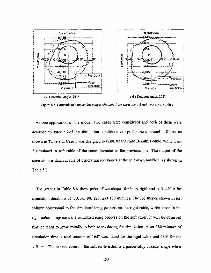
Ice accretion
X axisCcmj
( c ) Rotation angle, 263C {d ) Rotation angle, 29 ic
Figure 8.6 Comparison between ice shapes obtained from experimental and theoretical studies
As one application of the model, two cases were considered and both of them were
designed to share all of the simulation conditions except for the torsional stiffness, as
shown in Table 8.2. Case 1 was designed to simulate the rigid Bersimis cable, while Case
2 simulated a soft cable of the same diameter as the previous one. The output of the
simulation is data capable of generating ice shapes at the mid-span position, as shown in
Table 8.3.
The graphs in Table 8.4 show pairs of ice shapes for both rigid and soft cables for
simulation durations of 30, 50, 80, 120, and 180 minutes. The ice shapes shown in left
column correspond to the simulated icing process on the rigid cable, while those in the
right column represent the simulated icing process on the soft cable. It will be observed
that ice tends to grow spirally in both cases during the simulation. After 180 minutes of
simulation time, a total rotation of 164° was found for the rigid cable and 280° for the
soft one. The ice accretion on the soft cable exhibits a perceivably circular shape while
153
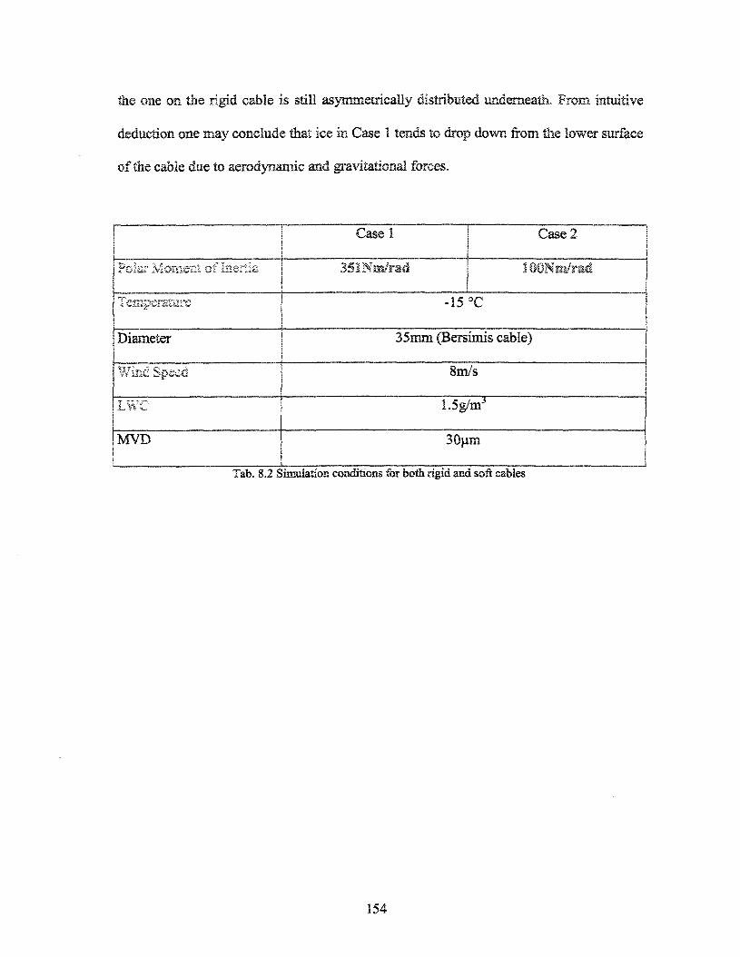
the one on the rigid cable is still asymmetrically distributed underneath. From intuitive
déduction one may conclude that ice in Case ! tends to drop down from the lower surface
of the cable due to aerodynamic and gravitational forces.
Polar Moment of inertia
Temperature
Diameter
Wind Speed
T XT:-I*.»""-JLi W V-
MVD
Case 1
SSlNm/rad
Case 2
ÎQQEmimé
-15 °C
35mm (Bersimis cable)
8m/s
1.5g/mJ
3Qpm
Tab. 8.2 Simulation conditions for both rigid and soft cables
154
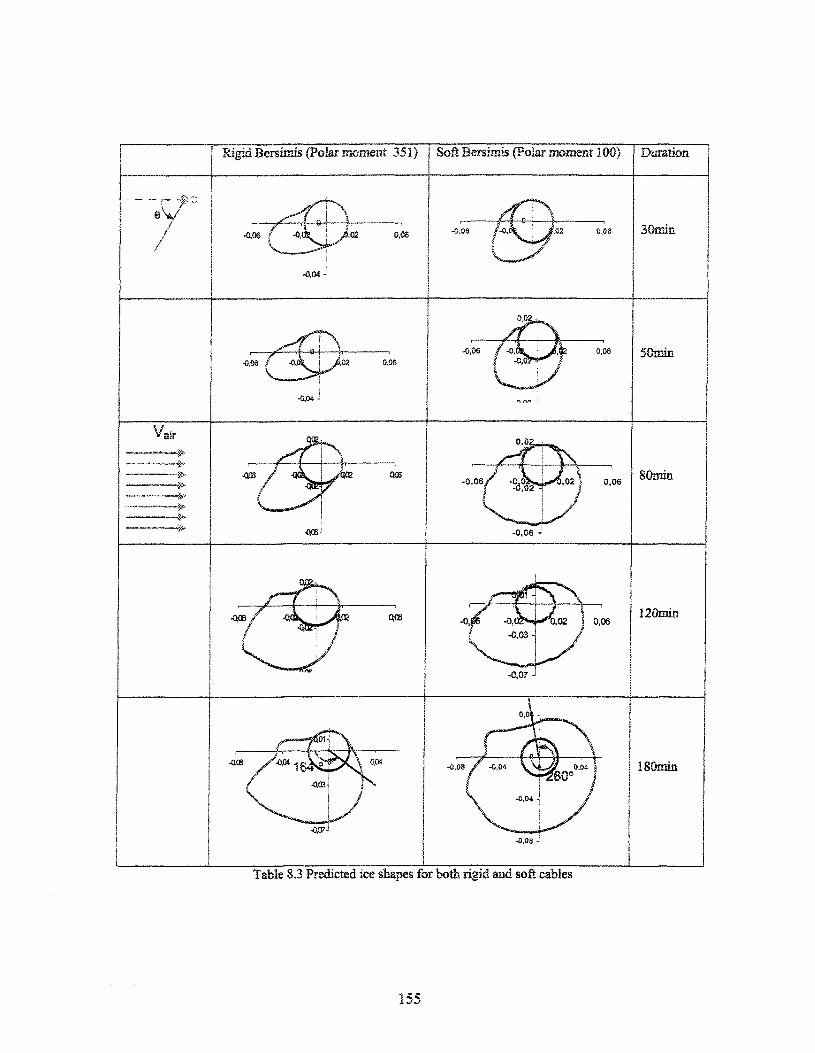
Rigid Bersimis (Polar moment 35 Î ) Soft Bersimis (Polar moment 100) Duration
-0,06 0,06
-0,04
0,08 30am
-0,06-0,06 0,08 50min
'air
�m -0,06 0,0680mia
-0,06 J
-Q05 0,06i20min
-0,07
-0,08 / -0,04 180min
-0,08 -
Table 8.3 Predicted ice shapes for both rigid and soft cables
155
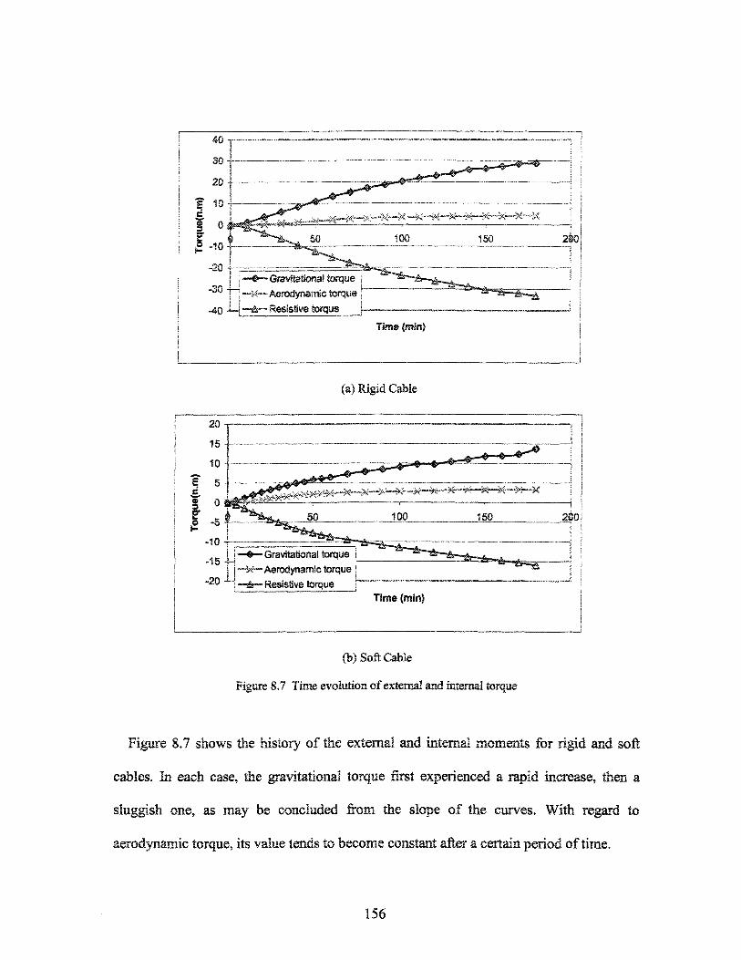
-20-
-30+-Gravitattonal torque
34-"» Aerodynamic torque
-40 i- j �èr~ Resistive toque [�
Time (min)
(a) Rigid Cable
j | Aerodynamic torque-20 -H�^�Resistive torque
Time (min)
(b) Soft Cable
Figure 8.7 Time evolution of external and internal torque
Figure 8.7 shows the history of the external and internal moments for rigid and soft
cables. In each case, the gravitational torque first experienced a rapid increase, then a
sluggish one, as may be concluded from the slope of the curves. With regard to
aerodynamic torque, its value tends to become constant after a certain period of time.
156
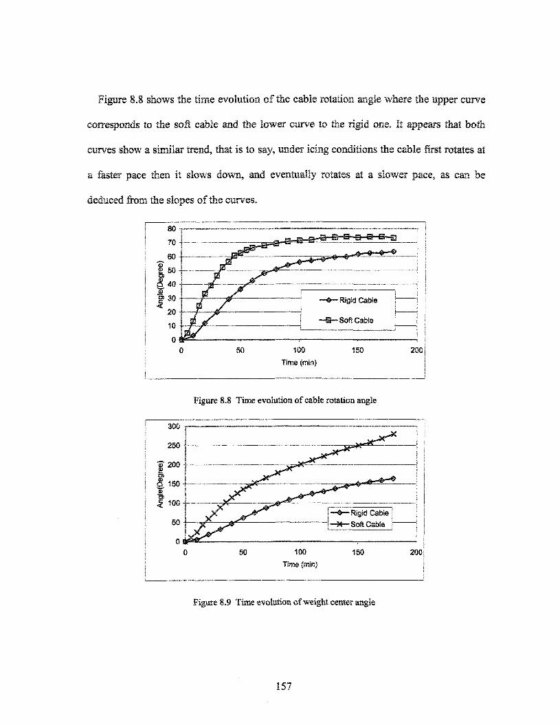
Figure 8.8 shows the time evolution of the cable rotation angle where the Epper curve
corresponds to the soft cable and the lower curve to the rigid one. It appears that both
curves show a similar tread, that is to say, under icing conditions the cable first rotates at
a faster pace then it slows down, and eventually rotates at a slower pace, as can be
deduced from the slopes of the curves.
�«� Rigid Cabte
�S�Sot Cable
100
Time (min)
150
300
150Time {min)
200
Figure 8.8 Time evolution of cable rotation angle
(�©�Rigid Cable!
I�H�Soft Cable i
200
Figure 8.9 Time evolution of weight center angle
157
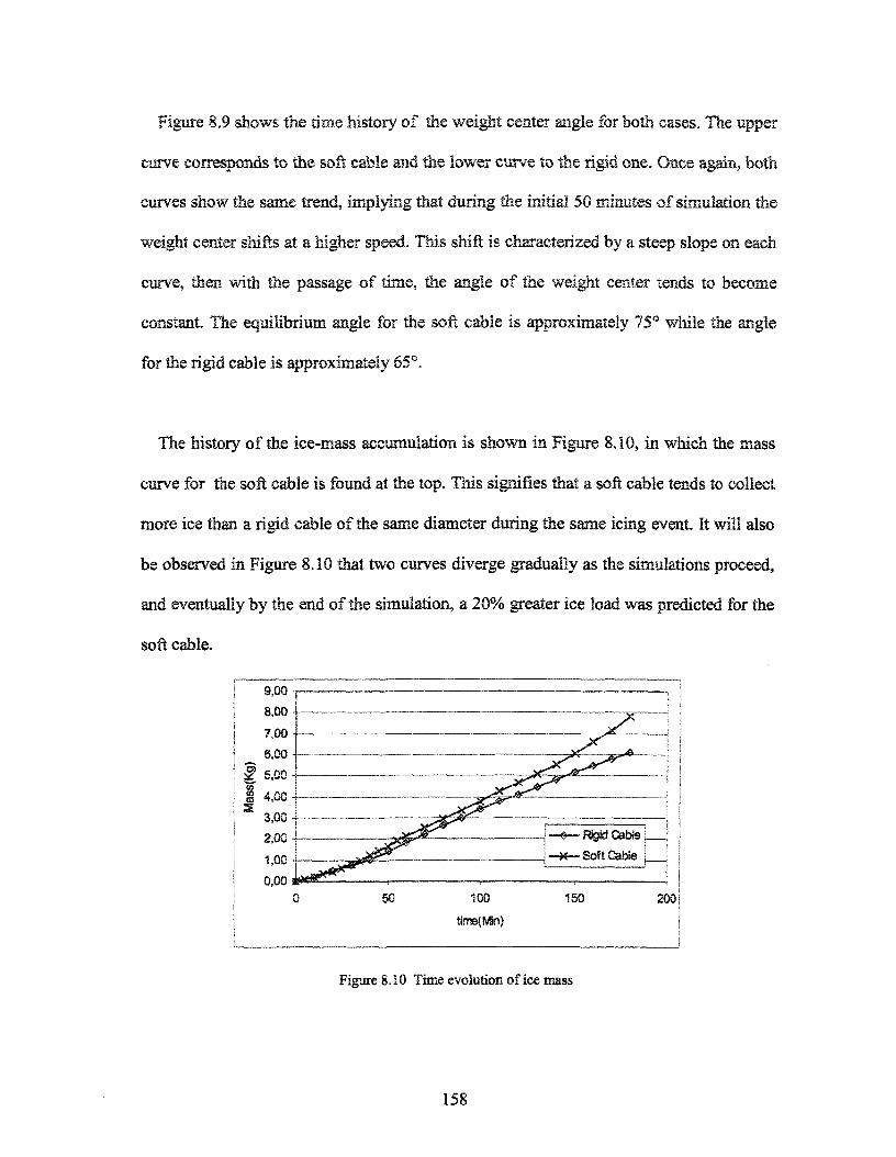
Figure 8.9 shows the time history of the weight center angle for both cases. The upper
curve corresponds to the soft cable and the lower curve to the rigid one. Once again, both
curves show the same trend, implying that during the initial 50 minutes of simulation the
weight center shifts at a higher speed. This shift is characterized by a steep slope on each
curve, then with the passage of time, the angle of the weight center tends to become
constant. The equilibrium angle for the soft cable is approximately 75° while the angle
for the rigid cable is approximately 65°.
The history of the ice-mass accumulation is shown in Figure 8.10, in which the mass
curve for the soft cable is found at the top. This signifies that a soft cable tends to collect
more ice than a rigid cable of the same diameter during the same icing event. It will also
be observed in Figure 8.10 that two curves diverge gradually as the simulations proceed,
and eventually by the end of the simulation, a 20% greater ice load was predicted for the
soft cable.
100
time(fcSn)150 200 j
Figure 8.10 Time evolution of ice mass
158
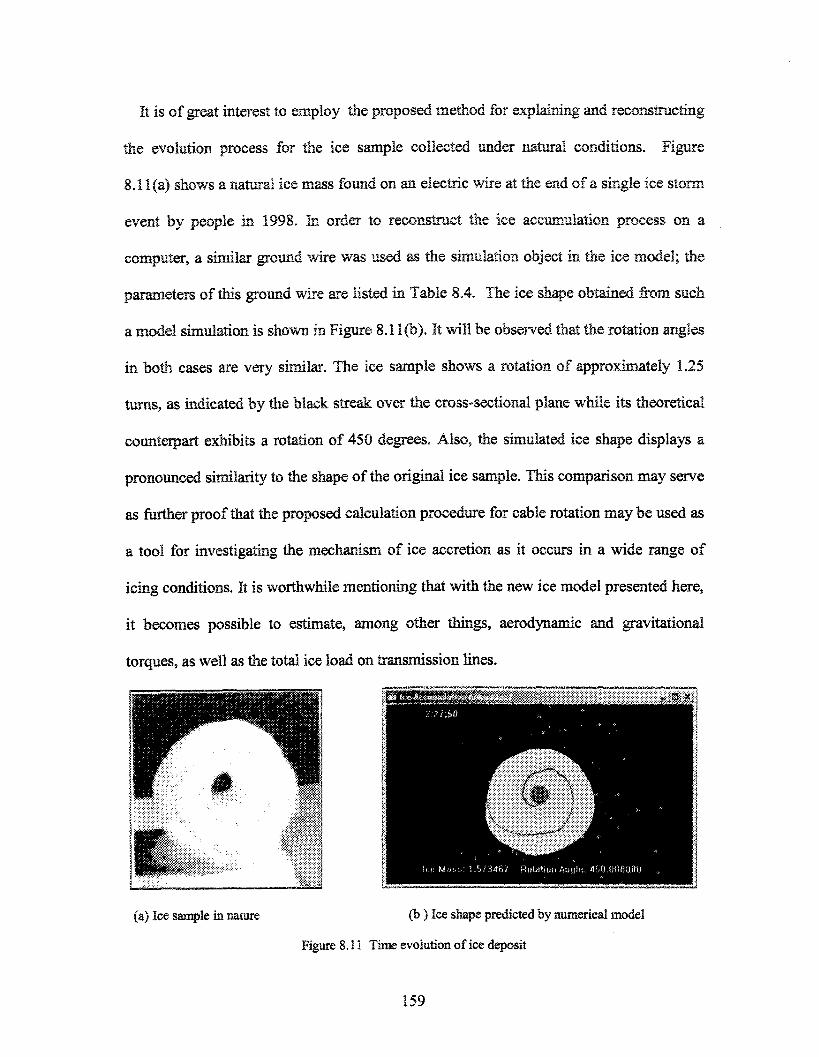
It is of great interest to employ the proposed method for explaining and reconstructing
the evolution process for the ice sample collected under natural conditions. Figure
8.11 (a) shows a natural ice mass found on an electric wire at the end of a single ice storm
event by people in 1998. In order to reconstruct the ice accumulation process on a
computer, a similar ground wire was used as the simulation object in the ice model; the
parameters of this ground wire are listed in Table 8.4. The ice shape obtained from such
a model simulation is shown in Figure 8.1 l(b). It will be observed that the rotation angles
in both cases are very similar. The ice sample shows a rotation of approximately 1.25
turns, as indicated by the black streak over the cross-sectional plane while its theoretical
counterpart exhibits a rotation of 450 degrees. Also, the simulated ice shape displays a
pronounced similarity to the shape of the original ice sample. This comparison may serve
as further proof that the proposed calculation procedure for cable rotation may be used as
a tool for investigating the mechanism of ice accretion as it occurs in a wide range of
icing conditions. It is worthwhile mentioning that with the new ice model presented here,
it becomes possible to estimate, among other things, aerodynamic and gravitational
torques, as well as the total ice load on transmission lines.
(a) Ice sample in nature (b ) Ice shape predicted by numerical model
Figure 8.11 Time evolution of ice deposit
159
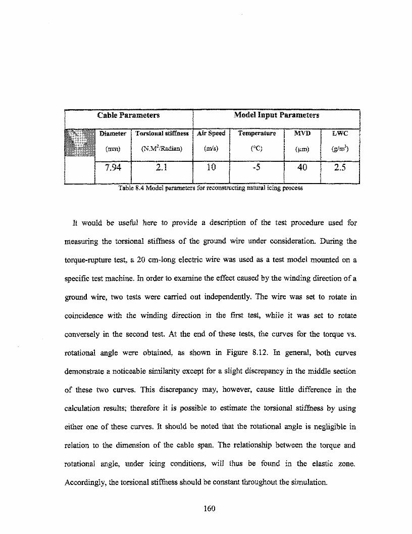
Cable Parameters
Diameter
(mm)
7.94
Torsiona! stiffness
(N.M2/Radian)
2.1
Model Input Parameters j
AirSpeed
(m/s)
10
Temperature S MVD
(°C) (mn)
-5 401
LWC
Cg/m3) ;
2.5
Table 8.4 Model parameters for reconstructing natural icing process
It would be useful here to provide a description of the test procedure used for
measuring the torsional stiffness of the ground wire under consideration. During the
torque-rupture test, a 20 cm-long electric wire was used as a test model mounted on a
specific test machine. In order to examine the effect caused by the winding direction of a
ground wire, two tests were carried out independently. The wire was set to rotate in
coincidence with the winding direction in the first test, while it was set to rotate
conversely in the second test. At the end of these tests, the curves for the torque vs.
rotational angle were obtained, as shown in Figure 8.12. In general, both curves
demonstrate a noticeable similarity except for a slight discrepancy in the middle section
of these two curves. This discrepancy may, however, cause little difference in the
calculation results; therefore it is possible to estimate the torsional stiffness by using
either one of these curves. It should be noted that the rotational angle is negligible in
relation to the dimension of the cable span. The relationship between the torque and
rotational angle, under icing conditions, will thus be found in the elastic zone.
Accordingly, the torsional stiffness should be constant throughout the simulation.
160
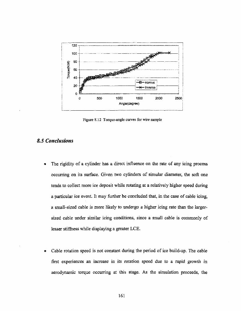
500 1000 1500 2000 2500
Figure 8.12 Torque-angle curves for wire sample
8,5 Conclusions
The rigidity of a cylinder has a direct influence on the rate of any icing process
occurring on its surface. Given two cylinders of simular diameter, the soft one
tends to collect more ice deposit while rotating at a relatively higher speed during
a particular ice event. It may further be concluded that, in the case of cable icing,
a small-sized cable is more likely to undergo a higher icing rate than the larger-
sized cable under similar icing conditions, since a small cable is commonly of
lesser stiffness while displaying a greater LCE.
Cable rotation speed is not constant during the period of ice build-up. The cable
first experiences an increase in its rotation speed due to a rapid growth in
aerodynamic torque occurring at this stage. As the simulation proceeds, the
161
rotation speed begins to decrease, and gradually the torque from the ice load
becomes the main drive for maintaining cable rotation.
® The contribution of aerodynamic torque to the cable-rotation process varies over
time under icing conditions. In general, aerodynamic torque exerts a significant
influence at an early stage, which diminishes over time, however, as opposed to
the influence of gravitational torque.
162
CHAPTER 9
CONCLUSIONS AND RECOMMENDATIONS
A new numerical ice model and code designed specifically for simulating the ice
accretion process on transmission line cables has been successfully developed. The
research involved in the design of this model is the first attempt of its kind using real-
time airflow computation to account for the relationships between the airflow field and its
related aspects in the same accretion process. These aspects include the movement of a
droplet in the vicinity of an ice-covered cylinder, convective heat transfer in the thermal
boundary layer, flow of a water film on the icing surface, and rotation of an ice-covered
cable. Although an electric wire was treated as a cylindrical object in the ice model, it is
possible, nevertheless, to apply the same model to simulate the icing process on an object
of an arbitrary cross-sectional shape, since a cylindrical ice shape is not specifically
assumed during the modelling. The validity and reliability of this code has been
confirmed by comparing the simulation results to those obtained from experimental
measurements. This is further supported by the fact that the simulated ice shape on a
flexible wire shows a striking similarity to an ice sample collected during one major ice
event which occurred in Québec in 1998.
9.1 Conclusions
1. Time-dependent field calculations, such as airflow computation and droplet
trajectory calculations, have been incorporated into the model described above. It
163
may be concluded that these efforts are well worth while since the proposed
procedure displays a greater capacity for predicting complex ice shapes than the
commonly-used procedure based on the Langmuir curve-fitting formulae. The
new calculation procedure alone may be applied in the simulation of the icing
process on either a cylindrical or an object of arbitrary shape.
2. The Boundary Element Method (BEM) combined with the Finite Volume Method
(FVM) was used to the compute the free-stream field. It was found that this
calculation procedure is easy to implement on a computer, that only moderate
calculation time is required, and that calculation results display satisfactory
accuracy. However, since a large quantity of finite volume elements are required
to store field velocity information, a minimum of 256 MB RAM may be needed
to run the proposed ice code.
3. The Runge-Kutta method is an appropriate numerical algorithm chosen for
tracking and simulating water droplet trajectories in the vicinity of an ice-covered
object since, when using this method, a convergent solution to a set of differential
equations may be achieved with a moderate number of time steps.
4. Surface runback water is assumed to exist in the form of a water film in the
proposed ice model. This assumption holds true for wet accumulations
characterized by abundant unfrozen water on an icing surface. Surface runback
water can also exist on the ice surface in the form of drops or rivulets, which tend
164
to promote elements of surface roughness. By disregarding such a factor, the
proposed ice model may predict an overly smooth ice shape.
5. The proposed model may be used to simulate ice accretion processes for both dry
and wet accumulations, and the cylindrical object used for model calculations
may be either a rigid or flexible cable. It should be noted that icicles may form
suspended beneath the iced object when a wet regime is dominant on the icing
surface. In such a case, this model may underestimate the ice-load to a high
degree due to the neglect of such icicle formation.
6. When compared to its non-energized counterpart, an energized cylinder under
icing conditions may present a wetter ice surface, consequently collecting less ice
deposit on its surface. However, no apparent change in ice shape is to observed in
the same comparison.
7. As the diameter of a cable decreases, the value of the LCE rises correspondingly,
as does the maximum impingement angle. It may be further observed that a small
cable tends to collect a more substantial ice deposit in terms of its size under the
same icing conditions. This implies that a higher icing intensity prevails on a
smaller cable during the same ice event.
165
8. For an ice accretion under semi-wet icing conditions, ice is found to be drier
initially while becoming wetter as the icing process advances. Meanwhile, dry ice
of low density is observed on each of the upper and lower edges of the ice mass.
9. Ice mass will be found more on the rear surface of a cylindrical object with a
increase in the MVD alone. In wet-icing conditions, a heavier ice load will be
observed on an icing cylinder when larger-sized droplets are involved.
10. The rigidity of a cylinder has a direct influence on the rate of the icing process
occurring on its surface. For two cylinders of similar diameter, the softer one
tends to collect more ice deposit while rotating at a relatively higher speed during
a particular icing event. It may further be concluded that, in the case of cable
icing, a cable of smaller size is more likely to undergo a higher icing rate than the
cable of larger size under the same icing conditions, since a small cable is
commonly less rigid while at the same time displaying a greater LCE.
11. The cable rotation speed is not constant. The cable first experiences an increase in
its rotation speed due to a rapid growth in aerodynamic torque at this stage. With
time elapsing, the rotation speed then begins to decrease, and eventually it is the
torque from the ice load which maintains cable rotation.
12. Under icing conditions, the contribution of the aerodynamic torque to the cable-
rotation process varies with time. In general, the aerodynamic torque exerts a
166
significant effect at an early stage, although, this effect diminishes over time
compared to the gravitational torque.
A 2-D icing model assumes that model parameters such as the hCE, HTC, and so
forth, are evenly distributed along the span of a cylindrical object, and thus a uniform ice
distribution along this span may be taken for granted. As a result, the cross-sectional cut
for the purpose of study may be applied at any position along the span. This assumption,
however, fails to take into account such factors as the velocity components of airflow and
water flow along the same span, among others. Therefore, extending the proposed ice
model to 3-D appears to be of particular significance so as to account adequately for the
above-mentioned factors.
9.2 Recommendations for Future Research Directions
9.2.1 Extend the 2-D ice model proposed herein to a 3-D ice model
A study on a new 3-D model should be assigned priority among all other necessary
updating projects, since it may serve to overcome the main drawbacks of a 2-D icing
model based on the reasons provided earlier. It is recommended that the 3-D model under
consideration be developed on the basis of knowledge acquired thus far, and also that it
should be an extension of the present 2-D ice model.
A single icicle comes into being in icing conditions due to the flow of unfrozen water
under the combined action of gravity , air drag and water surface tension. Makkonen's
icicle model (1995) takes into account gravity and surface tension involved in the process
167
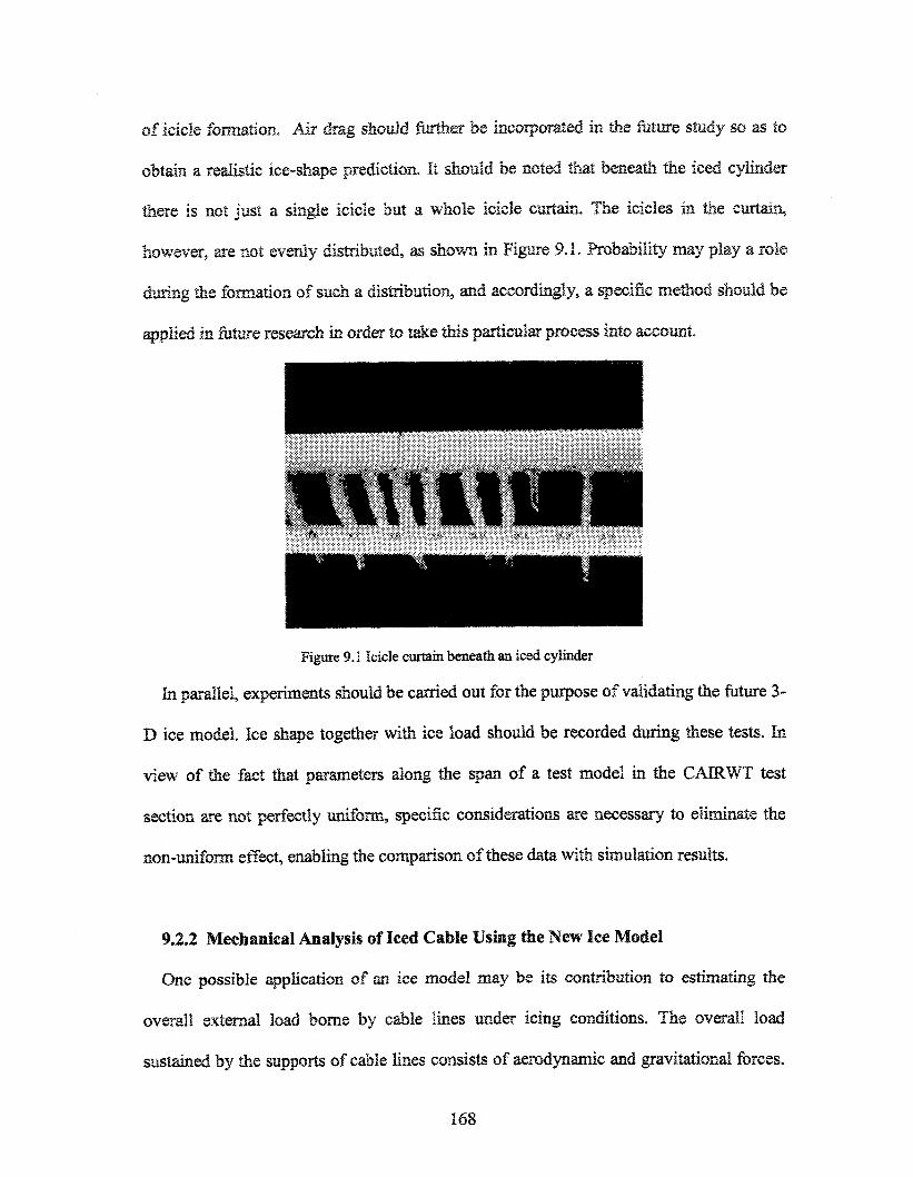
of icicle formation. Air drag should further be incorporated in the future study so as to
obtain a realistic ice-shape prediction. It should be noted that beneath the iced cylinder
there is not just a single icicle but a whole icicle curtain. The icicles in the curtain,
however, are not evenly distributed, as shown in Figure 9.L Probability may play a role
during the formation of such a distribution, and accordingly, a specific method should be
applied in future research in order to take this particular process into account.
Figure 9.1 Icicle curtain beneath an iced cylinder
In parallel, experiments should be carried out for the purpose of validating the future 3-
D ice model. Ice shape together with ice load should be recorded during these tests. In
view of the fact that parameters along the span of a test model in the CAIRWT test
section are not perfectly uniform, specific considerations are necessary to eliminate the
non-uniform effect, enabling the comparison of these data with simulation results.
9.2.2 Mechanical Analysis of Iced Cable Using the New Ice Model
One possible application of an ice model may be its contribution to estimating the
overall external load borne by cable lines under icing conditions. The overall load
sustained by the supports of cable lines consists of aerodynamic and gravitational forces.
168
Both forces are known parameters in the new ice model, in order to evaluate the
aerodynamic force, it is necessary to solve the 3-D airflow field numerically and thereby
obtain the air shear and pressure distribution on the ice surface. Commercial
computational software may play and important role in carrying out the field calculations.
From the outset, this commercial software must be able to access geometric data
produced by model calculations after running icing code. The load thus obtained may
serve as a reference for design engineers to determine the ultimate ice load for design
purposes.
169
REFERENCES
[1] Âchenbach, E., " Heat transfer from smooth and rough surfaced circularcylinders in a cross flow", Proceedings of the 5* International Heat TransferConference, Tokyo, pp. 229-233,1974,
[2] Ackley, S. F. and Templeton, M. K., "Numerical simulation of atmospheric iceaccretion ", The 2nd International Symposium on Snow Removal and IceControl Research, Hanover, N. H., USA, pp. 27,1978.
[3] Bazeos, N. and Beskos, D. E., "Numerical Determination of Wind Pressures on2-D Structures," Boundary Elements in Mechanical and Electrical Engineering,Computational Mechanics Publications, Springer-Verlag, 1990.
[4] Best, A.C., "The size distribution of raindrops," Quart. J. Roy. Met. Soc, Vol.76, pp. 418-428,1950.
[5] Bouamoul, A., Farzaneh, M., and G. McClure, "Boundary Element MethodApplication to Ice Shedding from Overhead Power Line Conductors by MeltingProcess", The Proceedings of the 10th International Workshop on AtmosphericIcing of Structures, IWAIS 2002, BRNO, Czech Republic, June 17-20, 2002, 8-7.
[6] Bouamoul, A., "Processus de délestage naturel des câbles et conducteurs detransport d'énergie électrique", Ph.D. in Engineering, UQAC, 2002.
[7] Brebbia, C. A., Telles, J. C. F., and Wrobei, L. C , "Boundary ElementTechniques", Springer-Verlag, 1984.
Bukowska, B. B., and Kreja, L, " Fixed Finite Element Model of Heat Transferwith Phase Change- Part I: Theoretical Formulation and Numerical Algorithm",International Journal of Offshore and Polar Engineering, Vol. 7, No. 2, June1997.
[9] Castellano, N. £., Nasello, O. B., and Levi, L., "Study of hail densityparameterisations", Proceedings of the 13th Int. Conf. on Clouds and
170
Precipitation, Reno, Nevada, USA, Vol. 2, pp. 1081-1084, August 2000.
[10] Cebeci, T., and Smith A. M. O., "Analysis of turbulent boundary layers",Academic Press, New York, 1974.
[11] Chaîné, P. M. and Castonguay, G., "New Approach to Radial Ice ThicknessConcept Applied to Bundle-Like Conductors", Industrial Meteorology-Study,Environment Canada, Toronto, pp. 11,1974.
[12] Chen, H. C. and Ettema, R., "Atmospheric-ice loading of power transmissioncables: laboratory experiments ", Proceedings of the 6* International Workshopon Atmospheric Icing of Structures, pp. 12,1993.
[13] Chen, Y., Farzaneh, M., Lozowski, E.P., and Szilder, K., "Modeling of IceAccretion on Transmission Line Conductors", Proceedings of the 9*International Workshop on Atmospheric Icing of Structures, Chester, UnitedKingdom, June 2000, Session 7a.
[14] Chen, Y., "A 2-D Random Walk Model for Predicting Ice Accretion on aCylindrical Conductor", Master's Degree Thesis, UQAC, 2001.
[15] Draez, J., Louchez, S., and McComber, P., "Ice shedding from cables", ColdRegions Science and Technology, Vol. 23, pp. 377-388,1995.
[16] Draez, J., McComber, P., and Farzaneh, M., "Atmospheric Icing on a TestPower Line", Transactions of the Canadian Society for Mechanical Engineering,C.S.M.E., Vol. 24, No. 2, pp. 359-374,2000.
[17] Duncan, W. J., Thorn A. S., and Young. A. D., "Mechanics of Fluids". EdwardArnold Ltd., London, 1970.
[18] Du N.-D., "Études des méthodes par impact et à l'huile utilisées pour déterminerle diamètre des gouttelettes dans les brouillards naturels et artificiels" , M. Se.Thesis, Université du Québec à Chicoutimi, Canada, 1987.
[19] Engene L. Lecomte, Alan W. Pang and James W. Russell, "ICE STORM' 98",Institue for Catastrophic Loss Reduction, Canada, 1998
171
[20] Egeîhofer, K. Z., Ackley, S. F., and Lynch, D, R., "Computer modeling ofatmospheric Ice accretion and aerodynamic loading of transmission lines",Proceedings of the 2nd International Workshop on Atmospheric Icing ofStructures, pp. 103,1984.
[21] FAA Technical Center, "Aircraft Icing handbook," Federal AviationAdministration, Vol. 1 of 3, March 1991.
[22] FARZANEH, M , "Ice Accretion on H.V. Conductors and Insulators and RelatedPhenomena," Invited article, Philosophical Transactions, The Royal Society,London, No. 358, pp. 1-35,2000.
Farzaneh, M., Kiernicki, J., and Drapeau, J.-F., "Ice Accretion on Energized Line
Insulators," International Journal of Offshore and Polar Engineering (DOPE),
Vol. 2, No. 3, Sept. 1992.
[24] Fikiin, K. A., "Generalized numerical modeling of unsteady heat transfer duringcooling and freezing using an improved enthalpy method and quasi-one-dimensional formulation", Int. J. Refrig. Vol. 19, No. 2, pp. 132-140,1996.
[25] Fraser, D., Rush, C. K. and Baxter, D., 'Thermodynamic limitations of iceaccretion instruments", NRC NAE Laboratory Report LR-32,1952.
[26] Fu, P., Bouchard, G., and Farzaneh, M., "Simulation of Ice Accumulation onTransmission Line Cables Based on Time-Dependent Airflow and Water DropletTrajectory Calculations", Proceedings of the 23rd International Conference onOffshore Mechanics and Arctic Engineering, Vancouver, Canada, 2004.
[27] Gates E. M., Lozowski E. P., Finstad K. J., "An approximate method for time-dependent modelling of rime ice accretion", Proceedings of the 2nd InternationalWorkshop on Atmospheric Icing of Structures, pp 111,1984.
[28] Gent, R.W., "TRAJICE2 - A Combined Water Droplet Trajectory and Ice AccretionPrediction Program for Aerofoil," DRA Technical Report TR90054, Nov. 1990.
[29] Gent, R.W., "Ice Accretion Prediction on Aerofoils," Proceedings of the FirstBombardier International Workshop on Aircraft Icing and Boundary-LayerStability and Transition, Montréal, Canada, Sept. 20-21,1993, pp. 113-138.
172
[30] Gerhait P. M., Gross R. J., and Hochstein J. L, "Fundamentals of FluidMechanics", Addison-Wesley Publishing Company, 1992.
[31] Godard, S., " Mesure des gouttelettes de nuage avec un film de collargoî",Bulletin de l'Observatoire du P»y de Dome, No.2,41-45,1960.
[32] Goodwin, E, J. et al. "Predicting ice and snow loads for transmission linedesign", Proceedings of the 1st International Workshop on Atmospheric Icing ofStructures, N. H., USA, PP. 267-273,1983.
[33] Grenier, J. C , Admirât, P., and Maccagnan, M., "Theoretical Study of the HeatBalance During the Growth of Wet Snow Sleeves on Electrical Conductor",Proceedings of the 3rd International Workshop on Atmospheric Icing ofStructures, May 1986.
[34] Hedde, T., "Modélisation tridimensionnelle des dépôts de givre sur les voiluresd'aéronefs," Thèse/doctorat, Université Blaise Pascal, Clermont-Ferrand H,France, No. D.U. 462, Dec. 1992.
[35] Hedde, T. and Guffond, D., "Improvement of the ONERA 3D Icing Code,Comparison with 3D Experimental Shapes," AIAA Paper 93-0169,1993.
[36] Hedde, T. and Guffond, D., "ONERA Three-Dimensional Icing Model", AIAAJournal, Vol. 33, No. 6, June 1995.
[37] Hess, J.L., and Smith, A.M.O., "Calculation of Potential Flow About ArbitraryBodies," Progress in Aeronautics Sciences, Vol. 8, pp. 1-138,1967.
[38] Hess, J.L., Review of integral-equation techniques for solving potential flowproblems with emphasis on the surface-source method, Computer Methods inApplied Mechanics and Engineering, 5,145,1975.
[39] Ide, R. F., "Liquid water content and droplet size calibration of the NASALEWIS Icing Research Tunnel", NASA, USA, TM-102447,1990.
[40] Imai, I , "Studies on Ice Accretion", Research on Snow and Ice, No. 1, pp. 34-44,1953.
173
[41] Jones, K. F., "A Simple Model for Freezing Rain Ice Loads", Proceedings of the7th International Workshop on Atmospheric Icing of Structures, Chieoutimi, QC5
Canada, pp. 412-416,1996
[42] Jones, K. F., "The Density of natural ice accretions", Fourth internationalconference on atmospheric icing of Structures, E. D. F., Volume 77, #1, pp. 114-118, Paris, September 1988.
[43] Karev, A. R. and Farzaneh, M., "Evolution of Droplet Size Distribution in anIcing Wind Tunnel", Proceedings of the 10th Intemational Workshop onAtmospheric Icing of Structures, BRNO, Czech Republic, 2002.
Karev, A.R., Farzaneh, M.5 and Mousavi, M., "Influence of non-uniformity ofdroplet size distribution on an ice accretion ", Proceedings of the 10thIntemational Workshop on Atmospheric Icing of Structures, BRNO, CzechRepublic, 2002.
[45] Karev, A.R., Farzaneh, M., Kollar, L. & Vaslon, S., "Freezing Water in an OpenChannel Flow with a Constant Bottom Temperature under Supercooled AmbientConditions ", 17* Annual Symposium on Ice, St. Petersburg, Russia, June 2004,pp. 379-384
[46] Kays, W. M., and Crawford, M. E., "Convective Heat and Mass Transfer".McGraw-Hill, pp. 601,1993.
[47] Kuroiwa, D., "Icing and Snow Accretion on Electric Wires", U. S. ArmyMateriel Command, January 1965.
[48] Langmuir, I. P. and Blodgett, K. B., "Mathematical Investigation of WaterDroplet Trajectories", Program Press 196, Vol. 10, Report No. RL-224,1945.
[49] Langmuir, I. P. and Blodgett, K. B., " A mathematical investigation of waterdrop trajectories", AAF Technical Report No. 5418, pp. 47,1946.
[50] Larouche, E., Bouchard, G., Rouat, J.3 and Farzaneh, M., "Exploration ofStandard and Time Dependent Neural Network Techniques for the Prediction ofIce Accretion on Overhead Line Conductors", Proceedings of the 9th
Intemational Workshop on Atmospheric Icing of Structures, Chester, United
174
Kingdom, June 2000, Session 2.
[51] Lesnic, D., Elliott, L. & Ingham, D.B., "Effect of sharp comers on Potential fluidflows past blunt bodies", BE Applications in Fluid Mechanics, 1-29,1995.
[52] List, R., 1963: General heat and mass exchange of spherical hailstones. J. Atmos.Sci. 20,189-197.
[53] List, R., "Ice Accretion on Structures", J. GlacioL, 19,451 -465,1977.
[54] Llinca, A., Llinca, F., and Ignat, L., "Numerical Study of Iced ConductorsAerodynamics", Proceedings of the 7th International Workshop on AtmosphericIcing of Structures. 3-7 June, 1996.
[55] Lock, G. S. H. "The growth and decay of ice", Cambridge University Press, NewYork, 1990.
[56] Lozowski, E. P. et a l , "The icing of an unheated, non-rotating cylinder in liquidWater droplet-ice crystal clouds", National Research Council of Canada ReportLTR-LT-96,61 pp., 1979.
[57] Lozowski, E. P., Stallabrass, J. R., and Hearty, P. F., "The Icing of an Unheated,Non-rotating Cylinder, Part I: A Simulation Model", Journal of Climate andApplied Meteorology, Vol. 22, pp. 2053-2062,1983.
[58] Ludlam, F. EL, "The heat economy of a rimed cylinder", Q. Jl R. Met. Soc. 77,663-666,1951.
[59] Macklin W.C., "The density and structure of ice formed by accretion," QuarterlyJournal of the Royal Meteorological Society, pp. 30-50,1962.
[60] Macklin, W.C, and Payne, G. S., " A theoretical study of the ice accretionprocess ", Quarterly Journal of the Royal Meteorological Society, pp. 195-213,1967.
[61] Makkonen, L., Stallabrass, J. R., "ICE ACCRETION ON CYLINDERS ANDWIRES," National Research Council of Canada, Low Temperature Laboratory,
175
Report TR-LT-005,1984.
[62] Makkonen, L., "Modelling of Ice Accretion on Wires," Journal of Climate andApplied Meteorology, Vol. 23, No. 6, pp. 929-939,1984.
[63] Makkonen, L., " Heat transfer and icing of a rough cylinder", Cold RegionsScience and Technology, Vol. 10, pp. 105-116,1984.
[64] Makkonen L.5 "Atmospheric Accretion of Ice Loads", Department ofMeteorology University of Helsinki, Report No. 25,1985.
[65] - Makkonen, L., "The effect of conductor diameter on ice load as determined by anumerical model," Proceedings of the 3rd
Atmospheric Icing of Structures, pp. 81-89,1986.numerical model," Proceedings of the 3rd International Workshop on
[66] Makkonen, L., and Fujji, Y., "Spacing of icicles", Cold Regions Sciences andTechnology, Vol. 21, pp. 317-322,1993.
[67] Makkonen, L., "Modelling Power Line Icing in Freezing Precipitation",Proceedings of the 7th International Workshop on Atmospheric Icing ofStructures, Chicoutimi, QC, pp. 195-200,1996.
[68] Makkonen, L., "Models for the growth of rime, glaze, icicles and wet snow onstructures", Philosophical transactions: mathematical, physical & engineeringsciences, 2000.
[69] McComber, P. and Touzot, G., "Calculation of the Impingement of CloudDroplets in a Cylinder by the Finite-Element Method", Journal of theAtmospheric Sciences, Vol. 38, May 1981.
[70] McComber, P., "Numerical Simulation of Cable Twisting Due to Icing", ColdRegions Science and Technology, pp. 253-259,1984.
[71] McComber, P. and Bouchard, G., "The Numerical Calculation of the Wind ForceCoefficients on Two Dimensional Iced Structures", Proceedings of the 3rdInternational Workshop on Atmospheric Icing of Structures, May 1986.
176
[72] Mousavi, M., "Experimental and Theoretical Verification of Two Icing Codes",Master's Degree thesis, UQAC, 2003.
[73] Messinger, B. L., " Equilibrium temperature of an unheated icing surface as afonction of airspeed", Journal of the Aeronautical Sciences, Vol. 20, pp. 195-200,1953.
[74] Mulherin, N. D., "Atmospheric Icing and Tower Collapse in the United States",Proceedings of the 7th International Workshop on Atmospheric Icing ofStructures, June 1996.
[75] Paraschivoiu, I., Tran, P., and Brahimi, M.T., "Prediction of Ice Accretion withViscous Effects on Aircraft Wings," AIAA Journal of Aircraft, Vol. 31, No. 4,pp. 855-861, July-Aug. 1994, (also AIAA Paper 93-0027).
[76] Paraschivoiu, I , Gouttebroze, S., and Saeed, F., "CANICE�Capabilities andCurrent Status," NATO/RTO Workshop, Assessment of Icing Code PredictionCapabilities, at CIRA in Capua, Italy, Dec. 6-7,2000.
[77] Pellet, J. L. and Dennis A. S., "Effects of heat storage in hailstones", Preprints ofthe Conference on Cloud Physics, Tucson, pp. 63-66,1974.
[78] Personne, P. and Gayet J.-F., "Ice Accretion on Wires and Anti-Icing Induced byJoule Effect", Journal of Applied Meteorology, V.27, pp.101-115,1988.
[79] Foots, G., "Ice and Snow Accretion on Structures," Research Studies PressLTD, 1996.
[80] Porcu, F., Smargjassi, E., and Prodi, F, "2D and 3D Modelling of Ice Accretionon Wires", Proceedings of the 6th International Workshop on Atmospheric Icingof Structures, PP: 53-55,1993.
Rae, W. H. and Pope, A., " Low-speed tunnel testing", J. Wiley and Sons, 2nd
edition, New York, N.Y., USA, pp. 534,1984.
[82] Rudzinski, W J., Lozowski, E. P., and Farzaneh, M., "2-D Numerical Modelingof the Icing of a Non-Energized Station Post Insulator Under Freezing RainConditions", Proceedings of the 10th International Workshop on Atmospheric
177
Icing of Structures, IWAIS 2002, BRNO, Czech Republic, June 17-20, 2002, 6-2.
[83] Savadjiev, K., and Farzaneh, M., " Study of icing and related meteorologicalparameter distributions during atmosphere icing events ", Proceedings of the11th International and Polar Engineering Conference, Stavanger, Norway, Vol.1, pp. 52-54,2001.
[84] Semyonov Yu, V., and Smoroding, A. Z., "Characteristic Features of ConvectiveHeat Transfer at a Liquid-Solid Body Phase Interface", Journal of EngineeringPhysics and Thermophysics, Vol. 64, No. 5,1993.
[85] Skelton, P. L. L, and Foots, G., "Approximate predictions of ice accretion on anoverhead transmission line which rotates with constant angular velocity". IMAJournal of Applied Mathematics, Vol. 40, pp. 23-45, 1998.
[86] Stallabrass, J. R., "An appraisal of the single rotating cylinder method of liquidwater content measurement", National Research Council of Canada, Division ofMechanical Engineering, Report LTR-LT-92, Nov., 1978.
[87] Szilder, K., Lozowski, E. P., and Gates, E. M., "Modelling Ice Accretion onNon-Rotating Cylinders -The Incorporation of Time Dependence and InternalHeat Conduction ", Cold Regions Science and Technology, Vol. 13, pp. 177-191,1987.
Szilder, K., Lozowski, E. P., and Gates, E. M., "Some Applications of a NewTime-Dependent Cylinder Ice Accretion Model", Atmospheric Research, V.22,pp. 41-59,1988.
[89] Szilder, K., and Lozowski, E. P., "Simulation of Icicle Growth Using a Three-Dimensional Random Walk Model," Atmospheric Research, Vol. 36, No. 1, pp.243-249,1995.
[90] Szilder, K., and Lozowski, E. P., "Three-Dimensional Modelling of IceAccretion Micro Structure", Proceedings oAtmospheric Icing of Structures, June 1996.Accretion Micro Structure", Proceedings of the 7th International Workshop on
[91] Szilder, K., and Lozowski, EP., "Morphogenetic Modelling of Wet IceAccretions on Transmission Lines as a Result of Freezing Rain", Proceedings ofthe 11th International and Polar Engineering Conference, ISOPE, Brest, Vol. 2,
178
pp. 616-621,1999.
[92] Sziîder, K., Farzaneh, M., and Lozowski, EP., "Analysis of Water Film Flow onan Icing Surface", Proceedings of the 9th International Workshop onAtmospheric Icing of Structures, Chester, United Kingdom, June 2000, session
[93] Szilder, K., Lozowski, EP., and Farzaneh, M., "Morphogenetic Modeling of WetIce Accretions on Transmission Lines as a Result of Freezing Rain",International Journal of Offshore and Polar Engineering, Vol. 11, No. 1, pp. 16-22, March 2001.
[94] Taylor, G.I., "Notes on Possible Equipment and Technique for Experiments onIcing on Aircraft," British Aeronautical Research Council, R&G, No. 2024, Jan.1940.
[95] Thwaites, B., "Approximate Calculation of the Laminar Boundary Layer,"Aeronautical Quarterly, 1,1949.
[96] Vick, D. and Nelson, D. J., "The Boundary Element Method Applied to Freezingand Melting Problems," Numerical Heat Transfer, part B, Vol. 24, pp. 263-277,1993.
Wright, W.B., "Advancement in the LEWICE Ice Accretion Model," AIAAPaper 93-0171,1993.
[98] Zukauskas, A., "Heat Transfer from tubes in cross-flow", Advances in HeatTransfer, Vol. 8, pp. 93-160,1972.
The Runge-Kutta algorithm makes it possible to solve a differential equation numerically
(i.e. approximately). Consider the single variable problem
x' =f(t,x)
with initial condition x(0)=x0. Suppose that xn is the value of the variable at time tn. The
Runge-Kutta formula takes xn and tn and calculates an approximation for xn at a brief
time later, tn+h. It uses a weighted average of approximated values of f(t,x) at several
time points within the interval (tmtn+h). The formula is given by
xn+J =xn+ (h/6)(kt + 2k2 + 2h + k4)
where
h =f(tn, Xn)
h =f(tn + h/2, xn + (h/2)ki)
k3=f(tn + h/2,xn + (h/2)k2)
k4 =f(tn + h,xn + h k3)
To run the simulation, we simply start with xg and find x\ using the formula above. Then
we plug in xj to find x? and so on.
The Runge-Kutta algorithm is known to be very accurate and Mfills the requirements
for a wide range of problems. For further information on why this is such a satisfactory
method, or where it can be expected to fail, consult pertinent references in the field.
Î80
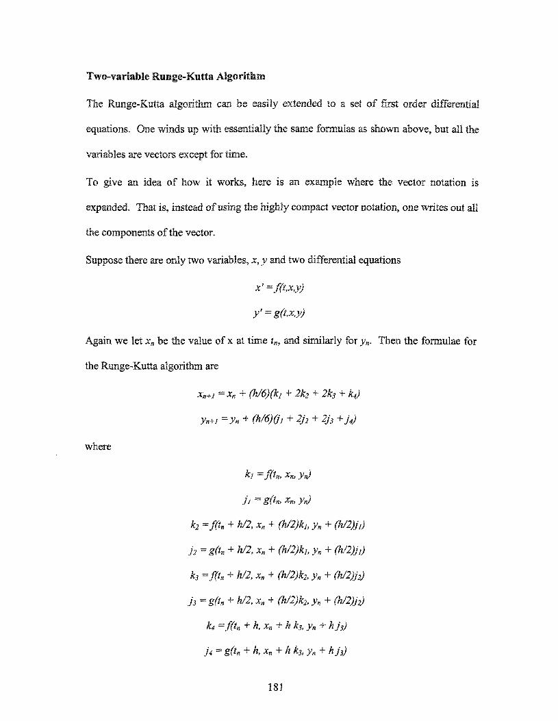
The Runge-Kutta algorithm can be easily extended to a set of first order differential
equations. One winds up with essentially the same formulas as shown above, but all the
variables are vectors except for time.
To give an idea of how it works, here is an example where the vector notation is
expanded. That is, instead of using the highly compact vector notation, one writes out all
the components of the vector.
Suppose there are only two variables, x, y and two differential equations
x' =f(t,x,y)
y' = g(t,x,y)
Again we let xn be the value of x at time tm and similarly for yn. Then the formulae for
the Runge-Kutta algorithm are
xn+j =x* + (h/6)(k} + 2k2 + 2k3 + k4)
yn+} =yn + (h/6)(ji + 2j2 + 2j3 +j4)
where
ki =f(tn, xm yj
ji = g(tn, Xn, Vn)
k2 =f(tn + h/2, xn + (h/2)kh yn
h = g(U + h/2, xn + (h/2)kh yn
k3 =f(tn + h/2, xn + (h/2)k2> yn + (h/2)j2)
js = g(tn + h/2, xn + (h/2)k2, yn + (h/2)h)
k4 =f(tn +h,xn+h k3, yn + hj3)
j 4 = gftn + h,xn + h k3, yn + hj3)
18!
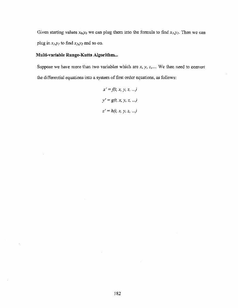
Given starting values xo,yo we can plug them into the formula to find X},yj. Then we can
plug in xj,yi to find X2&2 and- so on.
Multi-variable Rmige-Kiitta Algorithm...
Suppose we have more than two variables which are x, y, z,.... We then need to convert
the differential equations into a system of first order equations, as follows:
x' �f(t, x, y, z,...)
y' = g(i, x, y, z,...)
z' = h(t, x, y, z,...)
182