unclassified eco/wkp(2000)21 - economics · unclassified eco/wkp(2000)21 organisation de...
TRANSCRIPT
Unclassified ECO/WKP(2000)21 Organisation de Coopération et de Développement Economiques OLIS : 19-Jun-2000 Organisation for Economic Co-operation and Development Dist. : 26-Jun-2000 __________________________________________________________________________________________ English text only ECONOMICS DEPARTMENT
ECONOMIC GROWTH IN THE OECD AREA: RECENT TRENDS AT THE AGGREGATE AND SECTORAL LEVEL ECONOMICS DEPARTMENT WORKING PAPERS NO. 248
by Stefano Scarpetta, Andrea Bassanini, Dirk Pilat and Paul Schreyer
Unclassified
EC
O/W
KP(2000)21
English text only
Most Economics Department Working Papers beginning with No. 144 are now available through OECD's Internet Web site at http://www.oecd.org/eco/eco.
92819 Document complet disponible sur OLIS dans son format d'origine Complete document available on OLIS in its original format
ECO/WKP(2000)21
2
ABSTRACT/RÉSUMÉ
This paper discusses growth performance in the OECD countries over the past two decades. Special attention is given to developments in labour productivity, allowing for human capital accumulation, and multifactor productivity (MFP), allowing for changes in the composition and quality of physical capital. The paper suggests wide (and growing) disparities in GDP per capita growth, while differences in labour productivity have remained broadly stable. These patterns are explained by different employment growth rates across countries. In the most recent years, a rise in MFP growth in ICT-related industries has boosted aggregate growth in some countries (e.g. the United States). JEL classification: N10, O47 Keywords: Economic growth, productivity, human capital, investment
*****
Cette étude examine les performances en matière de croissance dans les pays de l’OCDE durant les deux dernières décennies. Une attention est tout particulièrement donnée à la productivité du travail, en tenant compte de l’accroissement du capital humain, et de la productivité multifactorielle (PMF), en tenant compte des changements dans la composition et la qualité du capital physique. L’étude suggère des disparités importantes (et en augmentation) dans les taux de croissance du PIB par habitant, alors que les différences dans les taux de croissance de la productivité du travail sont demeurées généralement stables. Des taux d’accroissement de l’emploi très variés sont à la base de ces différences. Durant ces dernières années, une hausse du taux d’accroissement de la productivité multifactorielle dans les industries liées aux technologies de l’information et des communications a accru la croissance globale dans certains pays (ex. les États-Unis). Classification JEL :N10, O47. Mots-Clés : Croissance économique, productivité, capital humain, investissement.
Copyright: OECD, 2000 Applications for permission to reproduce or translate all, or part of, this material should be made to: Head of Publications Service, OECD, 2 rue André-Pascal, 75775 PARIS CEDEX 16, France.
ECO/WKP(2000)21
3
TABLE OF CONTENTS
ECONOMIC GROWTH IN THE OECD AREA: RECENT TRENDS AT THE AGGREGATE AND SECTORAL LEVEL.......................................................................................................................................5
SUMMARY AND CONCLUSIONS..............................................................................................................5
Introduction..................................................................................................................................................7 1. Cross-country growth patterns..............................................................................................................8
1.1 Measurement issues.....................................................................................................................8 1.2 Trend growth in output .............................................................................................................10 1.3 Labour utilisation and productivity ...........................................................................................13 1.4 Capital deepening and capital productivity ...............................................................................24 1.5 Multi-factor productivity ...........................................................................................................30
2. Income and productivity levels: what is the scope for further catch-up? ...........................................39 2.1 The evolution of income and productivity levels over time ......................................................39 2.2 Current disparities in income and productivity levels ...............................................................41
Summing up findings from the analysis of aggregate data ........................................................................44 3. Growth performance at the sectoral level ...........................................................................................48
3.1 The breakdown of growth and labour productivity change by sector .......................................48 3.2 The determinants of labour productivity growth .......................................................................50 3.3 Structural changes and labour productivity growth...................................................................55 3.4 Productivity levels in manufacturing.........................................................................................59
Summing up findings from the sectoral analysis .......................................................................................61
BIBLIOGRAPHY .........................................................................................................................................62
STATISTICAL ANNEX...............................................................................................................................70
ANNEX 2. MEASUREMENT ISSUES AND DATA SOURCES...............................................................85
A2.1 Measuring inputs and output for the purpose of international comparisons ...................................85 A2.1.1 Independence of input and output statistics...........................................................................85 A2.1.2 Chained and fixed-weighted index numbers .........................................................................86 A2.1.3 Price indices for rapidly changing products ..........................................................................89
A2.2 The impact of SNA revisions on productivity level estimates and time series ...............................92 A2.2.1 The impact on levels of GDP and productivity .....................................................................93 A2.2.2 The impact on growth rates ...................................................................................................93 A2.2.3 The impact on capital stock ...................................................................................................94
A2.3 Estimates of purchasing power parities...........................................................................................95 A2.3.1 The choice of aggregation method ........................................................................................95 A2.3.2 The choice of benchmark year...............................................................................................96
ECO/WKP(2000)21
4
A2.4 Data sources and link with national sources ...................................................................................99 A2.4.1 Hours worked ......................................................................................................................101 A2.4.2 United States........................................................................................................................101 A2.4.3 Canada .................................................................................................................................103 A2.4.4 United Kingdom ..................................................................................................................105
ANNEX 3. METHODOLOGICAL NOTES...............................................................................................106
A3.1 Measurement of labour and capital inputs ....................................................................................106 A3.1.1 Productivity growth measures without adjustment for different types of factor input ........106 A3.1.2 Productivity growth measures with adjustment for different types of factor input .............107 A3.1.3 Labour input ........................................................................................................................108 A3.1.4 Capital input ........................................................................................................................108
A3.2 Sensitivity analysis of multi-factor productivity...........................................................................110 A3.2.1 Trend vs. actual time series .................................................................................................110 A3.2.2 Estimates of partial output elasticities .................................................................................115
A3.3 Estimates of trend output and trend labour productivity...............................................................122 A3.3.1 The Hodrick-Prescott filter and the Extended Hodrick-Prescott filter ................................122 A3.3.2 The Multivariate filter .........................................................................................................123 A3.3.3 Empirical implementation ...................................................................................................125 A3.3.4 Comparison of results..........................................................................................................127
Boxes 1. Estimates of trend output: the extended Hodrick-Prescott and multivariate filter 2. US productivity performance: the contribution of information and communication technology 3. Measures of multi-factor productivity (MFP) 4. Features of US growth performance in the 1990s
ECO/WKP(2000)21
5
ECONOMIC GROWTH IN THE OECD AREA: RECENT TRENDS AT THE AGGREGATE AND SECTORAL LEVEL
Stefano Scarpetta, Andrea Bassanini, Dirk Pilat and Paul Schreyer1
SUMMARY AND CONCLUSIONS
1. The aim of this paper is to ascertain how OECD countries' growth performance has evolved in recent years, whether disparities are indeed widening, and which factors are immediately responsible. It describes which countries have done particularly well or badly in terms of output and productivity growth over recent years; which sectors in the economy are the main contributors to economic growth; and which factors support growth.
2. It should be stressed at the outset that, despite major efforts by national statistical offices and international organisations, data problems still limit the possibility of comparing growth performances across countries and sectors, as well as over time. Comparability problems have always affected international analyses of growth performances but are particularly relevant at present because of the different pace and comprehensiveness with which different countries have adopted new measurement techniques in their national accounts. In addition, the growing emphasis on growth in quality instead of growth in quantity and the large share of hard-to-measure services in total output are some of the factors adding to these measurement problems. For this reason, the paper is supported by a methodological annex (Annex 2) that discusses data comparability across the different dimensions, as well as the adjustments made to the original sources to improve the results of cross-country time-series analyses. In any event, actual growth rates may hide significant differences in the cyclical position of countries, especially in the 1990s. Thus, this paper largely relies on cyclically adjusted series.
3. Bearing these caveats in mind, the following conclusions can be drawn from the paper:
− In the OECD area as a whole, trend GDP growth was somewhat lower in the 1990s than in the previous decade. This general picture hides significant and widening differences across regions and individual countries.
1. This paper reflects the joint work of the OECD Economics Department and the Directorate for Science,
Technology and Industry. A previous version of this paper was presented at the spring 2000 meeting of Working Party No. 1 of the Economic Policy Committee and the November 1999 meeting of the Statistical Working Party of the Industry Committee. The authors are indebted to Thomas Andersson, Jørgen Elmeskov, Mike Feiner, Philip Hemmings, Nicholas Vanston, Ignazio Visco and Andrew Wickoff for helpful discussions and comments on previous drafts. The views expressed are those of the authors and do not necessarily reflect those of the OECD or its Member countries.
ECO/WKP(2000)21
6
− Given generally modest demographic changes, widening disparities in trend GDP growth rates have also resulted in more diverse trend growth rates of GDP per capita, an (imperfect and partial) indicator of economic welfare. These differences can only partially be explained by the catching up of some countries (Ireland, Korea, Portugal, Turkey) to higher income levels. They are more the results of markedly higher growth rates in some relatively affluent countries, such as the United States, Australia, the Netherlands and Norway and lower growth rates in Continental Europe, Japan and Korea.
− Growing disparities in growth rates of per capita GDP have been accompanied by much smaller variations (over time and across countries) in labour productivity growth rates, especially when the latter are measured as output per hour worked.
− The proximate explanation of these seemingly conflicting developments is the diversity in the trends of labour utilisation. Countries with higher per capita growth rates maintained or even increased employment over the 1990s, while employment has stagnated or even fallen in those experiencing a GDP growth slow-down. Average hours worked have generally declined in the OECD countries. In this respect, part of the continued convergence of labour productivity levels was caused by labour shedding in countries with weak employment growth.
− Changes in labour productivity growth rates are in some cases (e.g. the United States, Australia, Denmark, Norway) related to significant technological changes as estimated by the growth rates of multifactor productivity (MFP). In some of the countries where high or rising labour productivity was associated with sluggish or falling employment, MFP growth did not show any significant improvement, or even fell in the 1990s as compared with the previous decade.
− Available data suggest a significant degree of convergence in the sectoral sources of aggregate productivity growth amongst the OECD countries, i.e. the same industries provide the strongest contributions to aggregate productivity growth, especially amongst the G7 economies. Productivity performance at the industry level tends to be associated with the effort to innovate (proxied by R&D intensity) as well as by up-skilling of the workforce. In the manufacturing sector of many Continental European countries, the latter process has been associated with employment losses amongst low-skilled workers. This has been partially compensated by employment growth in service sectors with relatively slow productivity growth, reinforcing the negative correlation between productivity growth and employment in the total economy.
− Reflecting the growth patterns described above, the United States began to pull away from most other countries in terms of GDP per capita levels over the 1990s. This happened despite some continued, albeit slight, convergence in levels of productivity. Differences in productivity levels at the industry level remain important. In manufacturing, the process of convergence of labour productivity to the US level which took place in previous decades but was reversed in the 1990s because of a speedup in US industries.
4. The growth performance of some OECD countries deserves a closer look. Thus, growth patterns in the United States, especially in the most recent years, include higher growth rates of GDP per capita, employment, labour and MFP as well as further capital deepening. These patterns are not uncommon amongst successfully catching-up countries, but unusual for a country that is already at the world productivity frontier in many industries. Some of these trends are likely to continue and tentatively suggest the move towards relatively high potential growth rates for some time to come. Productivity improvements
ECO/WKP(2000)21
7
in the information and communication technology industry itself provided a strong contribution to the speed-up of aggregate labour productivity in the 1990s. Available estimates also suggest that the shift in capital composition due to the spread of information technology in other industries made a contribution to aggregate output and productivity growth, with a rising trend in the most recent years. Moreover, in some sectors increases in productivity may have gone unmeasured.
5. Differences in growth performance in the other countries can partly be related to different labour market conditions and policy reforms. Thus, the strong employment content of GDP growth in Australia, Canada, Ireland and the Netherlands went hand-in-hand with major structural reform efforts there,2 and in Norway growth was related to persistently favourable labour market conditions over the 1990s. It is also interesting to note that significant growth in MFP has occurred in most of the countries with a record of reforms and a higher employment content of growth than in the past. In other words, structural changes seem to have led to higher utilisation of labour in a context of more productive use of factor inputs (or greater factor productivity if quality changes in factor inputs are taken into account). On the other side of the spectrum, stagnant employment conditions are often associated with insufficient structural reforms in countries with persistently high unemployment rates (e.g. several countries in Continental Europe) or with economic stagnation - and consequent labour shedding (e.g. Japan).
Introduction
6. This paper examines several concepts of economic growth: real GDP (the usual summary measure of economic activity); GDP per capita (an indicator of the average economic welfare of the population); labour and capital productivity; and multifactor productivity (a pointer to, among other things, technological progress). Productivity measures also attempt to account for changes in the quality of production factors as well as their quantities. Where relevant, trends by sector are examined, as well as economy-wide concepts. The paper also examines levels of these variables, where possible. Low levels of output per head may indicate opportunities for catch-up, and the breakdown into proximate causes may give hints as to the underlying factors behind below-average performance. Some of these may be susceptible to policy influence.
7. The first section examines cross-country patterns of growth of output and factor inputs across the OECD area, bearing in mind several key measurement issues that affect comparisons across countries and over time. The section also examines less-easily-measurable trends in the quality of inputs of labour and capital and their impact on productivity. The second section looks at the levels of GDP per capita and productivity across countries to shed light on relative positions of countries as well as to assess the role of economic convergence. The third section looks at sectoral performances and the role of structural shifts and productivity increases within sectors in explaining performance at the macro level.
2. These countries have all a high record of structural reforms as measured by follow-through of the
recommendations of the Jobs Strategy (see OECD, 1999a). Moreover, they have all experienced significant improvements in labour market conditions over the 1990s.
ECO/WKP(2000)21
8
1. Cross-country growth patterns
1.1 Measurement issues
8. It has to be emphasised at the outset that the coverage and depth of analysis in this paper is necessarily constrained by the availability, accuracy and international comparability of economic statistics. Economic statistics are regularly revised to reflect underlying shifts in the structures of economies, to incorporate improved methodologies to quantify economic developments and to take into account new sources. National authorities and international organisations have recently taken important steps to improve the quality of time series of outputs, inputs and productivity as well as to facilitate international comparability. Nevertheless, a number of measurement issues still arise at the aggregate and especially at the disaggregated levels. The three most pertinent issues in output measurement are: i) the independence of output from input measures; ii) the use of chain and fixed-weighted indices; and iii) the treatment of price indices of information technology products, in particular computers. For example, for industries that mainly comprise non-market producers (such as health or education), output volume series are often based on the extrapolation of input measures, which is likely to generate a downward bias within each country.3 Moreover, annual chain-weighted indices are used in a small number of OECD countries instead of fixed base years for the construction of time series of outputs, inputs and productivity. Annual chain-weighted indices minimise the substitution bias implicit in fixed-weight price and volume indices that occurs in periods of rapid change of relative prices and quantities or over long time periods. Finally, the method to construct price indices of computers and peripheral equipment varies between OECD countries. The use of hedonic methods in the deflation of computers tends to produce much more rapid price declines than other methods. Hence, the growth rate of volume output of those countries that do not use hedonic methods will be lower, ceteris paribus, than those that do. Annex 2 provides a more comprehensive discussion of these points.
9. These measurement issues are particularly relevant at the time of writing because of the ongoing implementation of revised methodology and use of new statistical definitions for compiling national accounts (i.e. the implementation of the 1993 System of National Accounts, SNA). Given the large scale of the revision, its implementation has been gradual, with progress from the old to the new methods uneven across countries, across series within a country, and over different time horizons. This paper uses data provided by the national authorities and included in the Analytical Data Base (ADB) of the OECD which takes into account changes known to date to the new SNA. Adjustments were necessary to improve international comparability and details are given in Annex 2. Notwithstanding the efforts made, statements about relative growth performance, in particular at the sectoral level, have to be read with these caveats in mind, and results should be interpreted with the necessary care.
10. Another complication inherent in international comparisons of growth performance in the short to medium term is that cross-country differences in output growth rates and levels may reflect differences in cyclical positions as well as underlying differences in performance. This problem was particularly relevant in the 1990s when business cycles were largely unsynchronised across OECD countries.4 In order to account for differences in the cyclical position of countries, the trend series reported in this paper were calculated using an extended version of the Hodrick-Prescott (HP) filter. Given the aim of this paper to
3. The extent of the underestimation is difficult to determine, although BLS suggests that the order of
magnitude is unlikely to be very large (Dean, 1999).
4. OECD estimates suggest that most European countries experienced the trough of the business cycle in 1993. The United States and Australia bottomed out in 1991, Canada and New Zealand in 1992, Portugal in 1994, and Japan in 1995 (OECD, 1999a). However, since then the strength of recoveries has been very uneven across countries.
ECO/WKP(2000)21
9
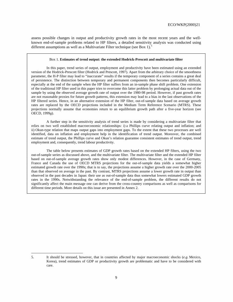
assess possible changes in output and productivity growth rates in the most recent years and the well-known end-of-sample problems related to HP filters, a detailed sensitivity analysis was conducted using different assumptions as well as a Multivariate Filter technique (see Box 1).5
Box 1. Estimates of trend output: the extended Hodrick-Prescott and multivariate filter
In this paper, trend series of output, employment and productivity have been estimated using an extended version of the Hodrick-Prescott filter (Hodrick and Prescott, 1997). Apart from the arbitrary choice of the smoothness parameter, the H-P filter may lead to “inaccurate” results if the temporary component of a series contains a great deal of persistence. The distinction between temporary and permanent components then becomes particularly difficult, especially at the end of the sample when the HP filter suffers from an in-sample phase shift problem. One extension of the traditional HP filter used in this paper tries to overcome this latter problem by prolonging actual data out of the sample by using the observed average growth rate of output over the 1980-98 period. However, if past growth rates are not reasonable proxies for future growth patterns, this extension may lead to a bias in the last observations of the HP filtered series. Hence, in an alternative extension of the HP filter, out-of-sample data based on average growth rates are replaced by the OECD projections included in the Medium Term Reference Scenario (MTRS). These projections normally assume that economies return to an equilibrium growth path after a five-year horizon (see OECD, 1999g).
A further step in the sensitivity analysis of trend series is made by considering a multivariate filter that relies on two well established macroeconomic relationships: i) a Phillips curve relating output and inflation; and ii) Okun-type relation that maps output gaps into employment gaps. To the extent that these two processes are well identified, data on inflation and employment help in the identification of trend output. Moreover, the combined estimate of trend output, the Phillips curve and Okun’s relation guarantee consistent estimates of trend output, trend employment and, consequently, trend labour productivity.
The table below presents estimates of GDP growth rates based on the extended HP filters, using the two out-of-sample series as discussed above, and the multivariate filter. The multivariate filter and the extended HP filter based on out-of-sample average growth rates show only modest differences. However, in the case of Germany, France and Canada the use of OECD MTRS projections for the out-of-sample data yields a somewhat higher estimated growth rate over the 1990s; that is to say, the projections assume a higher growth rate over the 2000-2005 than that observed on average in the past. By contrast, MTRS projections assume a lower growth rate in output than observed in the past decades in Japan: their use as out-of-sample data thus somewhat lowers estimated GDP growth rates in the 1990s. Notwithstanding the relevance of the end-of-sample problem, the different results do not significantly affect the main message one can derive from the cross-country comparisons as well as comparisons for different time periods. More details on this issue are presented in Annex 2.
5. It should be stressed, however, that in countries affected by major macroeconomic shocks (e.g. Mexico,
Korea), trend estimates of GDP or productivity growth are problematic and have to be considered with care.
ECO/WKP(2000)21
10
Box 1. Estimates of trend output: the extended Hodrick-Prescott and multivariate filter (continued)
1 9 7 0 -9 8 1 9 7 0 -7 9 1 9 8 0 -8 9 1 9 9 0 -9 8 3 1 9 9 5 -9 8U n ited S ta te s A c tu a l 3 .1 3 .5 3 .1 3 .1 4 .2
M V filte r 3 .0 3 .0 2 .9 3 .1 3 .5
E H P filte r1 2 .9 2 .9 2 .9 3 .1 3 .5
E H P filte r2 2 .9 2 .9 2 .9 3 .1 3 .5
Jap a n A ctu a l 3 .4 4 .6 3 .9 1 .3 1 .2M V filte r 3 .5 4 .3 3 .9 1 .9 1 .4
E H P filte r1 3 .6 4 .9 3 .8 1 .9 1 .4
E H P filte r2 3 .6 4 .9 3 .9 1 .8 1 .2G erm an y A ctu a l 2 .6 2 .9 1 .9 1 .2 1 .5
M V filte r 2 .6 2 .6 2 .0 1 .1 1 .4
E H P filte r1 2 .6 2 .8 2 .1 1 .3 1 .4
E H P filte r2 2 .6 2 .8 2 .1 1 .4 1 .6F ran ce A c tu a l 2 .4 3 .5 2 .3 1 .4 2 .2
M V filte r .. .. 2 .2 1 .7 1 .8
E H P filte r1 2 .4 3 .4 2 .1 1 .6 1 .7
E H P filte r2 2 .5 3 .4 2 .2 1 .8 2 .0Ita ly A c tu a l 2 .4 3 .6 2 .2 1 .3 1 .2
M V filte r 2 .5 3 .7 2 .4 1 .4 1 .3
E H P filte r1 2 .5 3 .6 2 .4 1 .4 1 .4
E H P filte r2 2 .5 3 .6 2 .4 1 .5 1 .5
U n ited K in g d o m A ctu a l 2 .2 2 .4 2 .9 2 .0 2 .8M V filte r .. .. 2 .4 2 .2 2 .4
E H P filte r1 2 .2 1 .9 2 .5 2 .2 2 .5
E H P filte r2 2 .2 1 .9 2 .5 2 .2 2 .5
C a n a d a A ctu a l 3 .2 4 .6 3 .1 2 .2 2 .9M V filte r 3 .1 4 .2 2 .9 2 .3 2 .6
E H P filte r1 3 .1 4 .1 2 .8 2 .3 2 .7
E H P filte r2 3 .1 4 .1 2 .8 2 .4 2 .9
E H P : ex ten d ed H o d ric k -P resc o tt filte r , M V :m u ltiv a ria te filte r .1 . H o d rick -P resco tt filte r w ith o u t-o f-sam p le g ro w th ra te re s tr ic tio n .2 . H o d rick -P resco tt filte r u s in g O E C D p ro je c tio n s to ex te n d tim e-se rie s o u t o f sam p le .3 . 1 9 9 2 -9 8 fo r G e rm a n y .
T ab le . C o m p a r in g d ifferen t e stim a tes o f tren d s in G D P in th e G 7 co u n tr ie s(T o ta l eco n o m y, p e rcen tag e ch an g es a t an n u a l ra te s)
1.2 Trend growth in output6
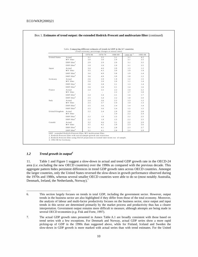
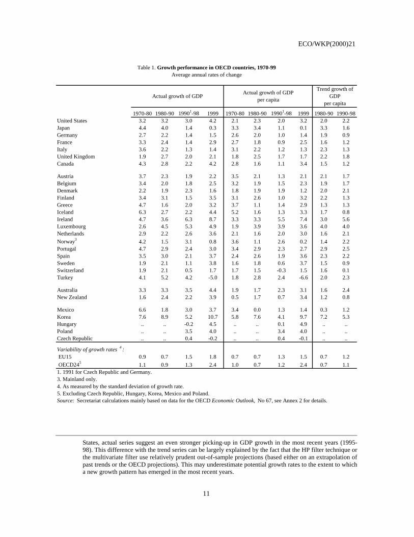
11. Table 1 and Figure 1 suggest a slow-down in actual and trend GDP growth rate in the OECD-24 area (i.e. excluding the new OECD countries) over the 1990s as compared with the previous decade. This aggregate pattern hides persistent differences in trend GDP growth rates across OECD countries. Amongst the larger countries, only the United States reversed the slow-down in growth performance observed during the 1970s and 1980s, whereas several smaller OECD countries were able to do so (most notably Australia, Denmark, Ireland, the Netherlands, Norway).7
6. This section largely focuses on trends in total GDP, including the government sector. However, output
trends in the business sector are also highlighted if they differ from those of the total economy. Moreover, the analysis of labour and multi-factor productivity focuses on the business sector, since output and input trends in this sector are determined primarily by the market process and productivity thus has a clearer interpretation. Government output remains more difficult to measure, although attempts are being made in several OECD economies (e.g. Fisk and Forte, 1997).
7. The actual GDP growth rates presented in Annex Table A.1 are broadly consistent with those based on trend series with a few exceptions. For Denmark and Norway, actual GDP series show a more rapid picking-up of GDP in the 1990s than suggested above, while for Finland, Iceland and Sweden the slow-down in GDP growth is more marked with actual series than with trend estimates. For the United
ECO/WKP(2000)21
11
1970-80 1980-90 19901-98 1999 1970-80 1980-90 19901-98 1999 1980-90 1990-98United States 3.2 3.2 3.0 4.2 2.1 2.3 2.0 3.2 2.0 2.2Japan 4.4 4.0 1.4 0.3 3.3 3.4 1.1 0.1 3.3 1.6Germany 2.7 2.2 1.4 1.5 2.6 2.0 1.0 1.4 1.9 0.9France 3.3 2.4 1.4 2.9 2.7 1.8 0.9 2.5 1.6 1.2Italy 3.6 2.2 1.3 1.4 3.1 2.2 1.2 1.3 2.3 1.3United Kingdom 1.9 2.7 2.0 2.1 1.8 2.5 1.7 1.7 2.2 1.8Canada 4.3 2.8 2.2 4.2 2.8 1.6 1.1 3.4 1.5 1.2
Austria 3.7 2.3 1.9 2.2 3.5 2.1 1.3 2.1 2.1 1.7Belgium 3.4 2.0 1.8 2.5 3.2 1.9 1.5 2.3 1.9 1.7Denmark 2.2 1.9 2.3 1.6 1.8 1.9 1.9 1.2 2.0 2.1Finland 3.4 3.1 1.5 3.5 3.1 2.6 1.0 3.2 2.2 1.3Greece 4.7 1.6 2.0 3.2 3.7 1.1 1.4 2.9 1.3 1.3Iceland 6.3 2.7 2.2 4.4 5.2 1.6 1.3 3.3 1.7 0.8Ireland 4.7 3.6 6.3 8.7 3.3 3.3 5.5 7.4 3.0 5.6Luxembourg 2.6 4.5 5.3 4.9 1.9 3.9 3.9 3.6 4.0 4.0Netherlands 2.9 2.2 2.6 3.6 2.1 1.6 2.0 3.0 1.6 2.1Norway3 4.2 1.5 3.1 0.8 3.6 1.1 2.6 0.2 1.4 2.2Portugal 4.7 2.9 2.4 3.0 3.4 2.9 2.3 2.7 2.9 2.5Spain 3.5 3.0 2.1 3.7 2.4 2.6 1.9 3.6 2.3 2.2Sweden 1.9 2.1 1.1 3.8 1.6 1.8 0.6 3.7 1.5 0.9Switzerland 1.9 2.1 0.5 1.7 1.7 1.5 -0.3 1.5 1.6 0.1Turkey 4.1 5.2 4.2 -5.0 1.8 2.8 2.4 -6.6 2.0 2.3
Australia 3.3 3.3 3.5 4.4 1.9 1.7 2.3 3.1 1.6 2.4New Zealand 1.6 2.4 2.2 3.9 0.5 1.7 0.7 3.4 1.2 0.8
Mexico 6.6 1.8 3.0 3.7 3.4 0.0 1.3 1.4 0.3 1.2Korea 7.6 8.9 5.2 10.7 5.8 7.6 4.1 9.7 7.2 5.3Hungary .. .. -0.2 4.5 .. .. 0.1 4.9 .. ..Poland .. .. 3.5 4.0 .. .. 3.4 4.0 .. ..Czech Republic .. .. 0.4 -0.2 .. .. 0.4 -0.1 .. ..
Variability of growth rates 4 : EU15 0.9 0.7 1.5 1.8 0.7 0.7 1.3 1.5 0.7 1.2 OECD245 1.1 0.9 1.3 2.4 1.0 0.7 1.2 2.4 0.7 1.11. 1991 for Czech Republic and Germany.3. Mainland only.4. As measured by the standard deviation of growth rate.5. Excluding Czech Republic, Hungary, Korea, Mexico and Poland. Source: Secretariat calculations mainly based on data for the OECD Economic Outlook, No 67, see Annex 2 for details.
Trend growth of GDP
per capita
Actual growth of GDPper capitaActual growth of GDP
Table 1. Growth performance in OECD countries, 1970-99Average annual rates of change
States, actual series suggest an even stronger picking-up in GDP growth in the most recent years (1995-98). This difference with the trend series can be largely explained by the fact that the HP filter technique or the multivariate filter use relatively prudent out-of-sample projections (based either on an extrapolation of past trends or the OECD projections). This may underestimate potential growth rates to the extent to which a new growth pattern has emerged in the most recent years.
ECO/WKP(2000)21
12
1980-90 1990-98Coefficient of variation OECD total 6 0.47 0.54Coefficient of variation EU15 0.28 0.58Coefficient of variation OECD 24 4 0.28 0.51
1. 1990-97 for Iceland and Portugal, 1991-98 for Germany.2. Mainland only.3. Growth rate for OECD 24 is computed as a weighted average of country growth rates, using country GDP levels expressed in 1993 EKS PPPs as weights, see Annex 2.4. Excluding Czech Republic, Hungary, Korea, Mexico and Poland. 5. Western Germany for 1980-90.6. Excluding Czech Republic, Hungary and Poland. Source: Secretariat calculations based on data for the OECD Economic Outlook, No 66, see Annexes 2 and 3 for details.
Figure 1. Trend GDP growth in the OECD area, 1980-90 and 1990-98(Total economy, percentage change at annual rate)
0 1 2 3 4 5 6 7 8 9
Switzerland
Sweden
Germany (5)
Italy
France
Iceland
Finland
Greece
Japan
Belgium
United Kingdom
Austria
New Zealand
Canada
Spain
OECD 24 (3,4)
Denmark
Portugal
Norway (2)
Netherlands
Mexico
United States
Australia
Turkey
Luxembourg
Ireland
Korea
%
1980-90 1990-98 (1)
ECO/WKP(2000)21
13
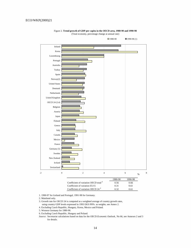
12. From a national living standard perspective, trends in per-capita GDP growth are more relevant than aggregate GDP growth.8 These are presented in Figure 2. Since demographic changes are generally slow the same broad evolution is evident: only the United States registered a significant acceleration amongst the larger countries, whereas several of the smaller economies improved their performance in the 1990s as compared to the previous decade. In particular, Australia, Ireland, the Netherlands and Norway recorded markedly higher growth rates of GDP per capita in the 1990s than in the 1980s. Whereas disparities in overall GDP growth increased only marginally in the 1990s relative to the 1980s, those in GDP per capita increased markedly.9 In particular, disparities in trend GDP per capita growth rates in the European Union have doubled in the past decade.
1.3 Labour utilisation and productivity
13. This sub-section explores how growth in per-capita output can be “explained” by changes in labour input and its productivity. Growth in GDP per capita can be decomposed into five elements:
− Changes in the ratio of persons of working-age (15–64 years) to the total population;
− Changes in the ratio of those in the labour force to the working-age population, i.e. the labour force participation rate;
− Changes in the ratio of those employed to the labour force, i.e. (1 - the unemployment rate);
− Changes in the number of working hours per person employed;
− Changes in GDP per hour worked.
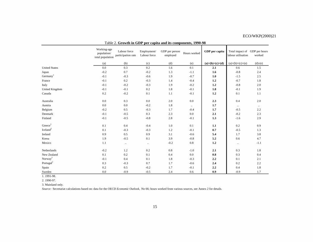
14. With a different intensity, all these factors are affected by macroeconomic, structural, educational and immigration policies, either directly or indirectly given the close interactions between demographic trends, macroeconomic conditions and decisions affecting labour demand and labour supply. The first element in the breakdown reflects the age-structure of the population. It may have an important impact on GDP per-capita growth in the future since most OECD economies are about to undergo a rapid ageing of their population.10 Changes in the next three ratios are more important in an economic and policy sense, since they reflect how an economy uses its potential workforce (those of working age). The final ratio reflects changes in labour productivity. Table 2 presents a breakdown of growth of GDP per capita in these five components for most OECD countries over the period 1990-98.
8. Strictly speaking, per capita GNP growth would be an even better measure, but in practice there is little
difference between the two concepts in trend growth rates terms. There are, however, a few exceptions, including Switzerland and Ireland: for the former actual annual growth rate of GNP was 0.2 percentage points higher than the GDP growth rate (0.5 per cent); for Ireland, it was 0.6 percentage points lower than the GDP annual growth rate (6.3 per cent).
9. The variability of growth performance is generally expressed in this paper on the basis of the unweighted coefficient of variation: the standard deviation divided by the average.
10. The ageing process implies that the ratio of those of working-age to the total population will decline significantly in the next few decades. At current participation rates and productivity levels, this will inevitably have a depressing impact on growth of GDP per capita (OECD, 1998b).
ECO/WKP(2000)21
14
1980-90 1990-98Coefficient of variation OECD total 6 0.56 0.66Coefficient of variation EU15 0.31 0.61Coefficient of variation OECD 24 4 0.32 0.61
1. 1990-97 for Iceland and Portugal, 1991-98 for Germany.2. Mainland only.3. Growth rate for OECD 24 is computed as a weighted average of country growth rates, using country GDP levels expressed in 1993 EKS PPPs as weights, see Annex 2.4. Excluding Czech Republic, Hungary, Korea, Mexico and Poland. 5. Western Germany for 1980-90.6. Excluding Czech Republic, Hungary and Poland. Source: Secretariat calculations based on data for the OECD Economic Outlook, No 66, see Annexes 2 and 3 for details.
Figure 2. Trend growth of GDP per capita in the OECD area, 1980-90 and 1990-98(Total economy, percentage change at annual rate)
-2 0 2 4 6 8
Switzerland
Iceland
New Zealand
Sweden
Germany (5)
France
Mexico
Canada
Italy
Greece
Finland
Japan
Austria
Belgium
OECD 24 (3,4)
United Kingdom
Netherlands
Denmark
United States
Norway(2)
Spain
Turkey
Australia
Portugal
Luxembourg
Korea
Ireland
%
1980-90 1990-98 (1)
ECO/WKP(2000)21
15
Working-age population/
total population
Labour force participation rate
Employment/Labour force
GDP per person employed
Hours worked GDP per capita Total impact of labour utilisation
GDP per hours worked
(a) (b) (c) (d) (e) (a)+(b)+(c)+(d) (a)+(b)+(c)+(e) (d)-(e)United States 0.0 0.3 0.2 1.6 0.1 2.1 0.6 1.5Japan -0.2 0.7 -0.2 1.3 -1.1 1.6 -0.8 2.4Germany1 -0.1 -0.3 -0.6 1.9 -0.7 1.0 -1.5 2.5France -0.1 0.2 -0.3 1.4 -0.4 1.2 -0.7 1.8Italy -0.1 -0.2 -0.3 1.9 -0.2 1.2 -0.8 2.0United Kingdom -0.1 -0.1 0.2 1.8 -0.1 1.8 -0.1 1.9Canada 0.2 -0.2 0.1 1.1 -0.1 1.2 0.1 1.1
Australia 0.0 0.3 0.0 2.0 0.0 2.3 0.4 2.0Austria 0.0 0.0 -0.2 1.8 .. 1.7 .. ..Belgium -0.2 0.5 -0.3 1.7 -0.4 1.7 -0.5 2.2Denmark -0.1 -0.5 0.3 2.3 0.0 2.1 -0.2 2.3Finland -0.1 -0.5 -0.8 2.8 -0.1 1.3 -1.6 2.9
Greece2 0.1 0.4 -0.4 1.0 0.1 1.1 0.2 0.9Iceland2 0.1 -0.3 -0.3 1.2 -0.1 0.7 -0.5 1.3Ireland 0.9 0.5 0.9 3.1 -0.6 5.4 1.7 3.8Korea 1.9 -0.5 0.1 3.9 -0.8 5.2 0.6 4.7Mexico 1.1 .. .. -0.2 0.8 1.2 .. -1.1
Netherlands -0.2 1.2 0.2 0.8 -1.0 2.1 0.3 1.8New Zealand 0.1 0.2 0.1 0.4 0.0 0.8 0.3 0.4Norway3 -0.1 0.4 0.1 1.8 -0.3 2.2 0.1 2.1Portugal2 0.3 -0.3 0.7 1.7 -0.6 2.4 0.2 2.2Spain 0.2 0.5 -0.2 1.7 -0.1 2.2 0.4 1.8Sweden 0.0 -0.9 -0.5 2.4 0.6 0.9 -0.9 1.71. 1991-98.2. 1990-97.3. Mainland only.Source: Secretariat calculations based on: data for the OECD Economic Outlook, No 66; hours worked from various sources, see Annex 2 for details.
Table 2. Growth in GDP per capita and its components, 1990-98
ECO/WKP(2000)21
16
15. As the period considered is quite short, the impact of changes in demographic structure is limited. For most countries, the share of the working-age population in the total population changed only marginally over the 1990s. However, the slight decline in a number of old OECD countries reversed the post-war trend and mechanically reduced the growth of GDP per capita. Countries with significant changes are those with a rapidly evolving age structure due to strong population growth (Korea) and changes in migration flows (e.g. Ireland).
16. Participation rates for the OECD countries as a whole have been rather stable over the recent past, with rising prime-age female participation rates largely compensated by falling participation rates among older workers and youths. In a few countries, the rise in part-time work (most notably in the Netherlands) has been associated with increasing participation rates, especially, amongst women (see OECD, 1999a). In the other countries, participation rates made more modest contributions to growth or even fell in some of those with high levels (notably in most of the Nordic countries).
17. Changes in employment with respect to the labour force or, equivalently, in the unemployment rate have strongly influenced the evolution of GDP per capita. Amongst the major economies, the United States and the United Kingdom and Canada all recorded falls in trend unemployment over the 1990s, while the other G7 countries had either persistently high unemployment rates or significantly rising rates. A significant easing of labour market conditions was also observed in some smaller countries.11
18. Average hours worked vary considerably across the OECD countries (see next section) and there have been major differences in their evolution over time. Over the 1990s, hours worked fell in most countries, and particularly so in continental Europe, thus lowering the growth rate of GDP per capita. In part this reflects differing rates of decline in statutory (collectively agreed) working weeks, but in a number of countries (especially in Europe) it also reflects a substantial increase in part-time working.12 The association between changes in hours worked and changes in participation rates across countries supports the view that the spread of part-time work has encouraged people to enter the labour force rather than oblige those who prefer to work full time to accept part-time jobs.13
19. The overall net effect of these changes in labour utilisation on GDP per capita can be considerable, and has provided a significant boost to annual growth in some countries (e.g. the United States, Ireland). Greater labour utilisation can thus make an important contribution to growth over the short and medium run, but its potential is not unlimited. Even so, there are large differences in the degree of labour utilisation and the potential for higher levels is far from exhausted, especially in Continental Europe where employment rates are low, especially amongst youths, prime-age women and older workers.14 Moreover, policy may affect migration flows and thus the size of the working age population, especially in the context of the ageing of population in most OECD countries.
11. More details on the evolution of trend unemployment rates are in OECD (1999a).
12. In the Netherlands almost half of the growth in employment in the 1993-97 period was in the form of part-time employment and almost two-third of women are currently employed part-time. In Germany, the increase in part-time employment partly compensated fall in full time employment. See OECD (1999a).
13. The 1999 Jobs Strategy report (OECD, 1999a) suggests that part-time is largely voluntary in most countries, although significant involuntary part-time was observed in the 1990s in countries with high and persistent unemployment where it was a second-best choice for a number of workers seeking employment in the absence of full time jobs.
14. In 1998, employment rates range from about 50 per cent (i.e. one person of working age in two is employed) in Italy and Spain to more than 70 per cent in the United Kingdom, Sweden, the United States, Denmark and Norway (OECD, 1999a).
ECO/WKP(2000)21
17
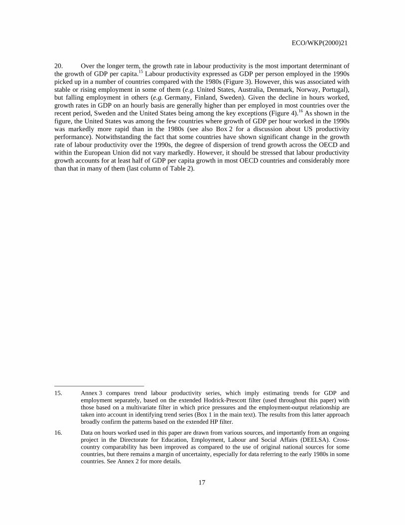
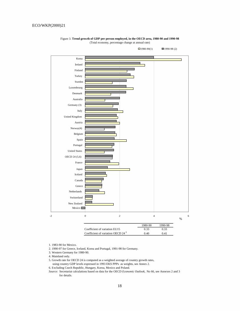
20. Over the longer term, the growth rate in labour productivity is the most important determinant of the growth of GDP per capita.15 Labour productivity expressed as GDP per person employed in the 1990s picked up in a number of countries compared with the 1980s (Figure 3). However, this was associated with stable or rising employment in some of them (e.g. United States, Australia, Denmark, Norway, Portugal), but falling employment in others (e.g. Germany, Finland, Sweden). Given the decline in hours worked, growth rates in GDP on an hourly basis are generally higher than per employed in most countries over the recent period, Sweden and the United States being among the key exceptions (Figure 4).16 As shown in the figure, the United States was among the few countries where growth of GDP per hour worked in the 1990s was markedly more rapid than in the 1980s (see also Box 2 for a discussion about US productivity performance). Notwithstanding the fact that some countries have shown significant change in the growth rate of labour productivity over the 1990s, the degree of dispersion of trend growth across the OECD and within the European Union did not vary markedly. However, it should be stressed that labour productivity growth accounts for at least half of GDP per capita growth in most OECD countries and considerably more than that in many of them (last column of Table 2).
15. Annex 3 compares trend labour productivity series, which imply estimating trends for GDP and
employment separately, based on the extended Hodrick-Prescott filter (used throughout this paper) with those based on a multivariate filter in which price pressures and the employment-output relationship are taken into account in identifying trend series (Box 1 in the main text). The results from this latter approach broadly confirm the patterns based on the extended HP filter.
16. Data on hours worked used in this paper are drawn from various sources, and importantly from an ongoing project in the Directorate for Education, Employment, Labour and Social Affairs (DEELSA). Cross-country comparability has been improved as compared to the use of original national sources for some countries, but there remains a margin of uncertainty, especially for data referring to the early 1980s in some countries. See Annex 2 for more details.
ECO/WKP(2000)21
18
1980-90 1990-98Coefficient of variation EU15 0.33 0.33Coefficient of variation OECD 24 6 0.40 0.41
1. 1983-90 for Mexico.2. 1990-97 for Greece, Iceland, Korea and Portugal, 1991-98 for Germany. 3. Western Germany for 1980-90.4. Mainland only.5. Growth rate for OECD 24 is computed as a weighted average of country growth rates, using country GDP levels expressed in 1993 EKS PPPs as weights, see Annex 2.6. Excluding Czech Republic, Hungary, Korea, Mexico and Poland. Source: Secretariat calculations based on data for the OECD Economic Outlook, No 66, see Annexes 2 and 3 for details.
Figure 3. Trend growth of GDP per person employed, in the OECD area, 1980-90 and 1990-98 (Total economy, percentage change at annual rate)
Mexico
New Zealand
Switzerland
Netherlands
Greece
Canada
Iceland
Japan
France
OECD 24 (5,6)
United States
Portugal
Spain
Belgium
Norway(4)
Austria
United Kingdom
Italy
Germany (3)
Australia
Denmark
Luxembourg
Sweden
Turkey
Finland
Ireland
Korea
-2 0 2 4 6%
1980-90(1) 1990-98 (2)
ECO/WKP(2000)21
19
1980-90 1990-98Coefficient of variation EU15 6 0.28 0.32Coefficient of variation OECD 24 5 0.35 0.40
1. 1990-97 for Greece, Iceland, Korea and Portugal, 1991-98 for Germany. 2. Western Germany for 1980-90.3. Mainland only.4. Growth rate for OECD 24 is computed as a weighted average of country growth rates, using country GDP levels expressed in 1993 EKS PPPs as weights, see Annex 2.5. Excluding Austria, Czech Republic, Hungary, Korea, Luxembourg, Mexico, Poland and Turkey.6. Excluding Austria and Luxembourg.Source: Secretariat calculations based on data for the OECD Economic Outlook, No 66; hours worked from various sources, for details see Annexes 2 and 3.
Figure 4. Trend growth of GDP per hours worked, in the OECD area, 1980-90 and 1990-98 (Total economy, percentage change at annual rate)
-2 0 2 4 6
New Zealand
Switzerland
Greece
Canada
Iceland
United States
Sweden
Netherlands
Spain
France
OECD 24 (4,5)
United Kingdom
Australia
Italy
Norway(3)
Belgium
Portugal
Denmark
Japan
Germany (2)
Finland
Ireland
Korea
%
1980-90 1990-98 (1)
ECO/WKP(2000)21
20
Box 2. US productivity performance: the contribution of information and communication technology
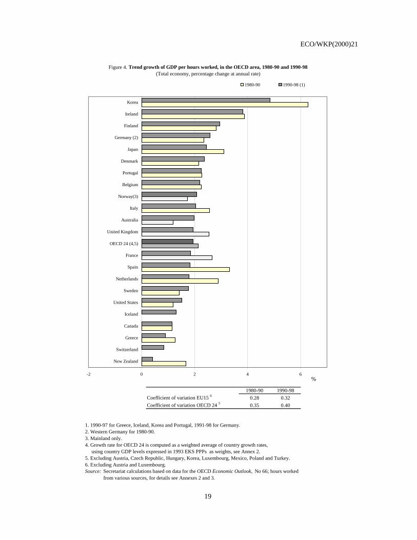
The causes and implications of recent productivity performance in the US economy have been a source of heated debate over the past few years. The official productivity data, from the Bureau of Labor Statistics, suggest that labour productivity growth has been very strong in the past decade and especially in the most recent years. Output per hour in the private non-farm business sector grew at 2 per cent annually over the entire decade and at 2.9 per cent in the 1995-99 period, almost double the average growth rate of the period 1973-95.
The long expansion in the United States economy has been accompanied by a surge in investment in information and communication technology (ICT) assets. In particular, the acceleration of US output in the second half of the 1990s coincided with a rise in the growth rate of hardware and communication equipment and the question has been raised as to the role of the information and communication technology in the improved productivity performance at the macro level. There are at least three, complementary approaches to assess the role of ICT in output growth, and all three angles have been covered in different studies of the US economy:
ICT industries. One way to grasp the economic importance of ITCs is to look at the importance of ICT production in the economy. Although value-added shares of ICT industries are relatively modest when measured in current prices, the contribution to real output growth can be significant if ICT industries grow much faster than other parts of the economy.
ICT as a capital input. A second avenue by which ICT can affect output and labour productivity growth is via its role as a capital good. ICT investment takes place in all parts of the economy and thereby provides capital services. These are part of the overall contribution of ICT to output and labour productivity growth. Studies that assess the importance of ICT as a capital input include Oliner and Sichel (2000), Whelan (2000) and OECD (2000) (see below for an international comparison). These studies treat ICT capital goods like other types of capital goods – in particular, it is assumed that firms who own ICT assets are able to reap most or all benefits that accrue from using new technologies. Only in this case is it possible to observe market income accruing to ICT capital and make inferences about its overall growth contribution. If there are other, unobserved benefits or income, this contribution would be under-estimated. This leads to the point about ICT as a special input.
Spillovers from ICT usage. A final avenue by which to trace effects of ICT is based on the claim that ICTs produce benefits that go beyond those accruing to investors and owners, for example through network externalities. Where such spillovers exist, they would raise overall MFP growth. As such, they are similar to advances in knowledge as well as the appearance of new blueprints and formulae or organisational innovations that potentially benefit all market participants. Studies at the firm level (for example Brynjolfsson and Kemerer, 1996; Gandal, et al., 1999) do indeed point to spillovers from ICT capital, but it is difficult to transpose these results to the aggregate level.
Notwithstanding measurement issues, there is growing consensus about a strong overall impact of ICT on observed output and productivity performance in the United States. Gordon (1999) finds that most of the rise in overall labour productivity growth is due to productivity advances in computer-producing industries (see also below for an international comparison). The result is obtained by combining the effects of capital deepening and MFP growth in the computer industry on labour productivity. The latest Economic Report of the President (2000) singles out the contribution of multifactor productivity in the computer sector to aggregate productivity and suggests that only a fraction of the post-1995 acceleration of labour productivity growth is accounted for by the acceleration of MFP in the computer sector. Two additional studies (Whelan, 2000; Oliner and Sichel, 2000) also relate the growing utilisation of computer hardware and software to faster aggregate productivity growth in the United States. Their estimates suggest an almost doubling in labour productivity growth in the 1996-99 period as compared with the first part of the decade: the use of information technology and the production of computers accounted for about two-thirds of this acceleration. More generally, it should also be stressed that the use of different deflators may affect the way in which the overall impact on productivity is split between the ICT-producing industry and the ICT using industries. For example, the rapid fall in the hedonic ICT deflator in the US tends to assign a stronger role to the ICT-producing industry (see footnote 58 below).
ECO/WKP(2000)21
21
Growth in human capital and its impact on labour productivity
21. Workers differ significantly in their characteristics and this has an important bearing on workers’ contribution to output, as implicitly shown by the variability in wage rates.17 Accordingly, workers with different characteristics should ideally be treated as separate and distinct inputs in the measurement of output and productivity changes. This paper attempts to do this by calculating labour input as a weighted sum of different groups of workers with different levels of education, each weighted by their relative wage.18 Moreover, since wage rates of men and women differ markedly, the decomposition is applied separately to each of them. To the extent wages are a reasonable proxy for differences in productivity19, the measured labour input control for changes in the ‘quality’ of the workforce over time.20 Compared with other proxies available in the literature (largely for the United States) this decomposition is rather crude, but it does shed some light on the role of compositional changes in labour input consistently for a range of OECD countries, thereby permitting cross-country comparisons.21
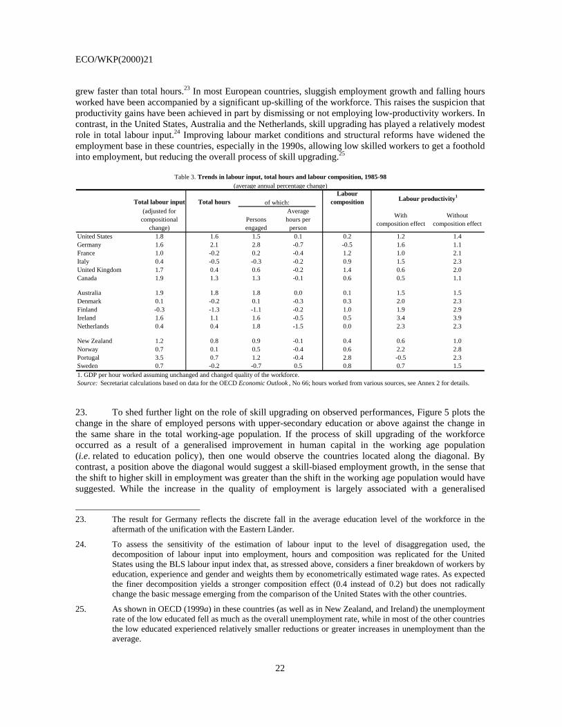
22. Table 3 decomposes changes in total labour input into a component that reflects unweighted changes in total hours and a second component reflecting the changing educational composition of labour, as well as changes in the relative wages earned by different workers. Given data availability, the decomposition covers only a selected number of OECD countries and the 1985-96 period.22 The labour composition effect is positive in all but one country, implying that quality-adjusted hourly labour input
17. From the seminal contributions of Becker (1975) and Mincer (1974), a wealth of studies have focused on
the effects of education and experience on earnings. For a survey, see Psacharopoulos (1994).
18. It is not suggested here that there is a perfect association between wage rates by education and relative productivity. Another OECD study (OECD, 1998f) looks at labour composition effects at the industry level using occupational data. At the aggregate level, however, the availability of data on employment by educational attainment offers a better grasp of compositional effects since education is often a prerequisite for entrance in an occupation and because education enhances performance in many occupations (see BLS, 1993 and especially Denison, 1985).
19. This is a strong assumption that is however common in the literature. It implies that firms operate under constant returns to scale in competitive input and product markets. Moreover, firms are assumed to maximise their profits by equating compensation with each worker’s contribution to output. BLS (1993) discusses how deviations from these hypotheses affect the relationship between the contribution to output and compensation.
20. As stressed by Barro (1998), although groupings on the basis of education or occupations do not remove workers heterogeneity, any finer grouping than simple head-counts delivers a better measure of labour input and thus productivity.
21. A number of studies on growth accounting for the OECD and non-OECD countries use the Barro-Lee database on population of working age by levels of educational attainment (Barro and Lee, 1993, 1996). Labour input is obtained by weighting years of education with wages rates obtained by applying a constant rate of return to education. This latter hypothesis is quite restrictive and is removed in some recent studies on the US economy. A study by the Bureau of Labour Statistics (BLS, 1993) proxies skills by education and experience of men and women separately. Moreover, wage rates for each category are based on econometrically estimated hourly earnings functions instead of sample estimates of average hourly earnings. Jorgenson, Gollop and Fraumeni (1987) and Ho and Jorgenson (1999) estimated labour input using a very large number of categories of workers representing cross-classification of five characteristics [age, education, class of workers, occupation (not in Ho and Jorgenson) and gender]. The average shares obtained from cross-classified labour compensation data give the weights.
22. The period and countries covered reflect data availability on education and relative wages. Moreover, a somewhat longer time period was chosen with respect to most of the analysis in this paper (1985 onwards instead of 1990-98) to better grasp the contribution to labour input stemming from the increase in the educational attainment of the workforce.
ECO/WKP(2000)21
22
grew faster than total hours.23 In most European countries, sluggish employment growth and falling hours worked have been accompanied by a significant up-skilling of the workforce. This raises the suspicion that productivity gains have been achieved in part by dismissing or not employing low-productivity workers. In contrast, in the United States, Australia and the Netherlands, skill upgrading has played a relatively modest role in total labour input.24 Improving labour market conditions and structural reforms have widened the employment base in these countries, especially in the 1990s, allowing low skilled workers to get a foothold into employment, but reducing the overall process of skill upgrading.25
Total labour input Total hoursLabour
composition(adjusted for
compositional change)
Persons engaged
Average hours per
person
With composition effect
Without composition effect
United States 1.8 1.6 1.5 0.1 0.2 1.2 1.4Germany 1.6 2.1 2.8 -0.7 -0.5 1.6 1.1France 1.0 -0.2 0.2 -0.4 1.2 1.0 2.1Italy 0.4 -0.5 -0.3 -0.2 0.9 1.5 2.3United Kingdom 1.7 0.4 0.6 -0.2 1.4 0.6 2.0Canada 1.9 1.3 1.3 -0.1 0.6 0.5 1.1
Australia 1.9 1.8 1.8 0.0 0.1 1.5 1.5Denmark 0.1 -0.2 0.1 -0.3 0.3 2.0 2.3Finland -0.3 -1.3 -1.1 -0.2 1.0 1.9 2.9Ireland 1.6 1.1 1.6 -0.5 0.5 3.4 3.9Netherlands 0.4 0.4 1.8 -1.5 0.0 2.3 2.3
New Zealand 1.2 0.8 0.9 -0.1 0.4 0.6 1.0Norway 0.7 0.1 0.5 -0.4 0.6 2.2 2.8Portugal 3.5 0.7 1.2 -0.4 2.8 -0.5 2.3Sweden 0.7 -0.2 -0.7 0.5 0.8 0.7 1.51. GDP per hour worked assuming unchanged and changed quality of the workforce. Source: Secretariat calculations based on data for the OECD Economic Outlook , No 66; hours worked from various sources, see Annex 2 for details.
of which: Labour productivity1
Table 3. Trends in labour input, total hours and labour composition, 1985-98 (average annual percentage change)
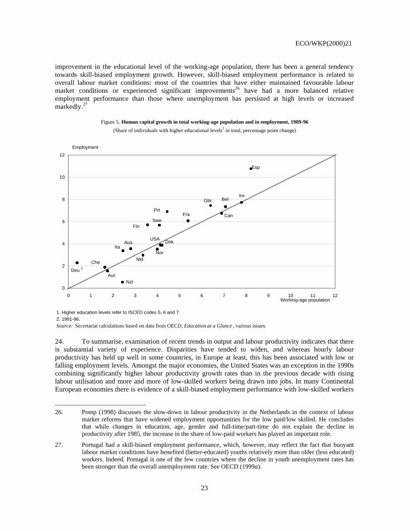
23. To shed further light on the role of skill upgrading on observed performances, Figure 5 plots the change in the share of employed persons with upper-secondary education or above against the change in the same share in the total working-age population. If the process of skill upgrading of the workforce occurred as a result of a generalised improvement in human capital in the working age population (i.e. related to education policy), then one would observe the countries located along the diagonal. By contrast, a position above the diagonal would suggest a skill-biased employment growth, in the sense that the shift to higher skill in employment was greater than the shift in the working age population would have suggested. While the increase in the quality of employment is largely associated with a generalised
23. The result for Germany reflects the discrete fall in the average education level of the workforce in the
aftermath of the unification with the Eastern Länder.
24. To assess the sensitivity of the estimation of labour input to the level of disaggregation used, the decomposition of labour input into employment, hours and composition was replicated for the United States using the BLS labour input index that, as stressed above, considers a finer breakdown of workers by education, experience and gender and weights them by econometrically estimated wage rates. As expected the finer decomposition yields a stronger composition effect (0.4 instead of 0.2) but does not radically change the basic message emerging from the comparison of the United States with the other countries.
25. As shown in OECD (1999a) in these countries (as well as in New Zealand, and Ireland) the unemployment rate of the low educated fell as much as the overall unemployment rate, while in most of the other countries the low educated experienced relatively smaller reductions or greater increases in unemployment than the average.
ECO/WKP(2000)21
23
improvement in the educational level of the working-age population, there has been a general tendency towards skill-biased employment growth. However, skill-biased employment performance is related to overall labour market conditions: most of the countries that have either maintained favourable labour market conditions or experienced significant improvements26 have had a more balanced relative employment performance than those where unemployment has persisted at high levels or increased markedly.27
1. Higher education levels refer to ISCED codes 5, 6 and 7.2. 1991-96.Source: Secretariat calculations based on data from OECD, Education at a Glance , various issues.
Figure 5. Human capital growth in total working-age population and in employment, 1989-96(Share of individuals with higher educational levels1 in total, percentage point change)
Deu 2
USA
Gbr
Che
Swe
Esp
Prt
Nor
Nzl
Nld
Ita
Ire
Fra
Fin
Dnk
Can
Bel
Aut
Aus
0
2
4
6
8
10
12
0 1 2 3 4 5 6 7 8 9 10 11 12Working-age population
Employment
24. To summarise, examination of recent trends in output and labour productivity indicates that there is substantial variety of experience. Disparities have tended to widen, and whereas hourly labour productivity has held up well in some countries, in Europe at least, this has been associated with low or falling employment levels. Amongst the major economies, the United States was an exception in the 1990s combining significantly higher labour productivity growth rates than in the previous decade with rising labour utilisation and more and more of low-skilled workers being drawn into jobs. In many Continental European economies there is evidence of a skill-biased employment performance with low-skilled workers
26. Pomp (1998) discusses the slow-down in labour productivity in the Netherlands in the context of labour
market reforms that have widened employment opportunities for the low paid/low skilled. He concludes that while changes in education, age, gender and full-time/part-time do not explain the decline in productivity after 1985, the increase in the share of low-paid workers has played an important role.
27. Portugal had a skill-biased employment performance, which, however, may reflect the fact that buoyant labour market conditions have benefited (better-educated) youths relatively more than older (less educated) workers. Indeed, Portugal is one of the few countries where the decline in youth unemployment rates has been stronger than the overall unemployment rate. See OECD (1999a).
ECO/WKP(2000)21
24
been trapped into unemployment or inactivity. The next section examines how labour productivity may have been influenced by changes in the quality of labour inputs, while Sections 1.4 and 1.5 look at trend growth of capital and multifactor productivity.
1.4 Capital deepening and capital productivity
25. Labour productivity growth provides only partial insights into overall economic efficiency. First of all, changes in labour productivity growth rates may occur because of changes in the capital/labour ratio, which in turn depends upon the rate of growth in fixed capital formation and/or changes in employment. Output growth also depends on the productivity of physical capital, which measures how physical capital is used in providing goods and services: changes therein indicate to what extent output growth can be achieved with lower welfare costs in the form of foregone consumption.
26. Yet, the accurate measurement of capital input is inherently difficult and comparisons across countries are particularly so. From the viewpoint of economic theory, the objective is to measure the flow of capital services, akin to the flow of effective hours worked (i.e. in equivalent quality terms, see above). Two important assumptions are often made in the empirical literature:
− The flow of capital services is often assumed to be a constant proportion of an estimated measure of the capital stock. This has the practical advantage that the assumed rate of change of capital services over time coincides with the rate of change of the capital stock as estimated by cumulating measurable investment according to assumptions about asset life-times, etc. However, this choice may lead to an over-estimation of the flow of capital services in times of low capital utilisation and vice versa.
− A second and equally important assumption is that the aggregate capital stock is made up of one homogenous type of asset, or alternatively, that different assets generate the same marginal revenues in production. Stocks of individual assets can be computed, given information on investment flows, on the service life and on the profile of wear and tear of an asset. To obtain a measure of the service flow from all assets, the services from each asset would then have to be aggregated with user cost weights, designed to take into account the likely differences in the service flows of assets of different types (see OECD (1999f) for a detailed treatment of capital measurement).28
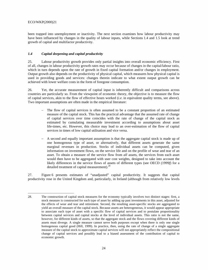
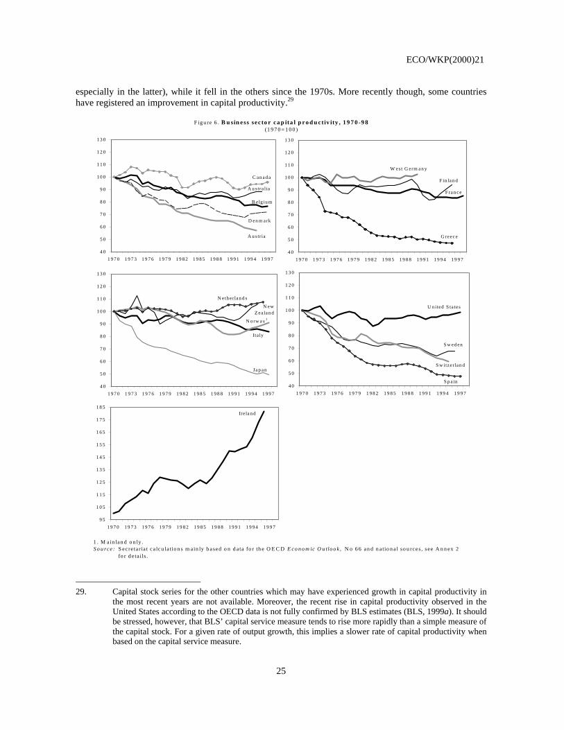
27. Figure 6 presents estimates of “unadjusted” capital productivity. It suggests that capital productivity rose in the United Kingdom and, particularly, in Ireland (although from relatively low levels
28. The construction of capital stock measures for the economy typically involves two distinct stages: first, a
stock measure is constructed for each type of asset by adding up past investments in this asset, adjusted for the effects of wear and tear and retirement. Second, the resulting asset-specific stocks are aggregated to yield an overall measure of the capital stock. Because assets are heterogeneous, it would appear appropriate to associate each type of asset with a specific flow of capital services and to postulate proportionality between capital services and capital stocks at the level of individual assets. This ratio is not the same, however, for different kinds of assets, so that the aggregate stock and the flows covering different kinds of assets must diverge. A single measure cannot serve both purposes except when there is only one single homogenous capital good (Hill, 1999). In practice, then, using the rate of change of a single aggregate measure of the capital stock to approximate capital services will not appropriately reflect the compositional change of capital services and possibly lead to a biased assessment of the contribution of capital to economic growth.
ECO/WKP(2000)21
25
especially in the latter), while it fell in the others since the 1970s. More recently though, some countries have registered an improvement in capital productivity.29
1 . M ain lan d o n ly .S o u rce : S ec re ta ria t c a lcu la tio n s m ain ly b ased o n d a ta fo r th e O E C D E co n o m ic O u tlo o k , N o 6 6 an d n a tio n a l so u rces , see A n n ex 2 fo r d e ta ils .
F ig u re 6 . B u sin ess sec to r ca p ita l p r o d u ctiv ity , 1 9 7 0 -9 8(1 9 7 0 = 1 0 0 )
4 0
5 0
6 0
7 0
8 0
9 0
1 0 0
1 1 0
1 2 0
1 3 0
1 9 7 0 1 9 7 3 1 9 7 6 1 9 7 9 1 9 8 2 1 9 8 5 1 9 8 8 1 9 9 1 1 9 9 4 1 9 9 7
A u stria
B elg iu m
C an a d a
A u stra lia
D en m ark
4 0
5 0
6 0
7 0
8 0
9 0
1 0 0
1 1 0
1 2 0
1 3 0
1 9 7 0 1 9 7 3 1 9 7 6 1 9 7 9 1 9 8 2 1 9 8 5 1 9 8 8 1 9 9 1 1 9 9 4 1 9 9 7
F in la n d
W est G erm a n y
G reec e
F ran ce
4 0
5 0
6 0
7 0
8 0
9 0
1 0 0
1 1 0
1 2 0
1 3 0
1 9 7 0 1 9 7 3 1 9 7 6 1 9 7 9 1 9 8 2 1 9 8 5 1 9 8 8 1 9 9 1 1 9 9 4 1 9 9 7
Ita ly
Ja p a n
N orw ay 1
N ew Z ea lan d
N eth erlan d s
4 0
5 0
6 0
7 0
8 0
9 0
1 0 0
1 1 0
1 2 0
1 3 0
1 9 7 0 1 9 7 3 1 9 7 6 1 9 7 9 1 9 8 2 1 9 8 5 1 9 8 8 1 9 9 1 1 9 9 4 1 9 9 7
S p a in
S w itzerlan d
S w ed en
U n ited S ta tes
9 5
1 0 5
1 1 5
1 2 5
1 3 5
1 4 5
1 5 5
1 6 5
1 7 5
1 8 5
1 9 7 0 1 9 7 3 1 9 7 6 1 9 7 9 1 9 8 2 1 9 8 5 1 9 8 8 1 9 9 1 1 9 9 4 1 9 9 7
Ire la n d
29. Capital stock series for the other countries which may have experienced growth in capital productivity in
the most recent years are not available. Moreover, the recent rise in capital productivity observed in the United States according to the OECD data is not fully confirmed by BLS estimates (BLS, 1999a). It should be stressed, however, that BLS’ capital service measure tends to rise more rapidly than a simple measure of the capital stock. For a given rate of output growth, this implies a slower rate of capital productivity when based on the capital service measure.

ECO/WKP(2000)21
26
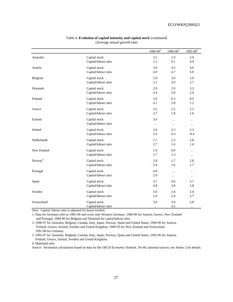
28. Several factors lie behind observed growth rates in capital productivity (Parham, 1999), notably changes in the capital/labour ratio. Indeed, in a neoclassical framework, the increase in this ratio implies that each unit of capital has less labour to work with, contributing to diminishing returns. Over the past decade, the rate of growth of the capital/labour ratio fell in most countries (Table 4). There are a few notable exceptions to this pattern which, however, have to be seen in conjunction with employment patterns. In some continental European countries (e.g. Germany, Italy) the growth rate of capital intensity increased in the 1990s compared with the 1980s, but this was mainly driven by losses in employment rather than an acceleration of investment. A significant picking-up in the growth rate of capital was also observed in some other countries (e.g. the United States, Australia, Ireland the Netherlands, and Norway) in the second half of the 1990s, but this was in conjunction with strong employment growth.
1980-901 1990-982 1995-983
United States Capital stock 3.0 2.6 3.3Capital/labour ratio 1.1 0.6 1.0
Japan Capital stock 5.7 4.2 3.6Capital/labour ratio 4.9 4.7 4.4
Germany Capital stock 2.6 2.6 2.3Capital/labour ratio 2.9 3.7 3.1
France Capital stock 2.0 2.0 2.0Capital/labour ratio 2.3 2.3 2.3
Italy Capital stock 2.8 2.7 2.7Capital/labour ratio 2.7 3.5 3.4
United Kingdom Capital stock 1.8 1.6 1.6Capital/labour ratio 1.8 1.2 1.0
Canada Capital stock 3.5 2.2 2.7Capital/labour ratio 1.8 0.9 1.4
Table 4. Evolution of capital intensity and capital stock(Average annual growth rate)
ECO/WKP(2000)21
27
1980-901 1990-982 1995-983
Australia Capital stock 3.5 1.9 2.9Capital/labour ratio 1.5 0.1 0.9
Austria Capital stock 3.9 4.3 4.0Capital/labour ratio 4.0 4.7 5.0
Belgium Capital stock 2.9 3.0 2.9Capital/labour ratio 3.1 3.0 2.7
Denmark Capital stock 2.9 2.9 3.3Capital/labour ratio 3.4 2.8 2.6
Finland Capital stock 3.0 0.3 0.5Capital/labour ratio 4.1 2.8 1.2
Greece Capital stock 3.5 2.5 2.5Capital/labour ratio 2.7 1.8 1.6
Iceland Capital stock 3.0 .. ..Capital/labour ratio .. .. ..
Ireland Capital stock 2.6 2.3 3.3Capital/labour ratio 2.4 -0.1 -0.4
Netherlands Capital stock 1.7 2.3 2.8Capital/labour ratio 2.7 1.6 1.6
New Zealand Capital stock 1.9 0.9 ..Capital/labour ratio 1.7 -1.1 ..
Norway4 Capital stock 2.8 1.7 2.8Capital/labour ratio 3.4 1.6 1.7
Portugal Capital stock 4.0 .. ..Capital/labour ratio 2.9 .. ..
Spain Capital stock 3.7 4.0 3.7Capital/labour ratio 4.8 3.8 2.8
Sweden Capital stock 3.0 1.8 2.4Capital/labour ratio 2.6 2.4 2.7
Switzerland Capital stock 3.6 3.0 2.8Capital/labour ratio .. 3.5 ..
Note: Capital /labour ratio is adjusted for hours worked.1. Data for Germany refer to 1981-90 and cover only Western Germany, 1986-90 for Austria, Greece, New Zealand and Portugal, 1984-90 for Belgium and Denmark for capital/labour ratio.2. 1990-97 for Australia, Belgium, Canada, Italy, Japan, Norway, Spain and United States, 1990-96 for Austria, Finland, Greece, Ireland, Sweden and United Kingdom, 1990-95 for New Zealand and Switzerland, 1991-98 for Germany.3. 1995-97 for Australia, Belgium, Canada, Italy, Japan, Norway, Spain and United States, 1995-96 for Austria, Finland, Greece, Ireland, Sweden and United Kingdom.4. Mainland only.Source: Secretariat calculations based on data for the OECD Economic Outlook , No 66; national sources, see Annex 2 for details.
Table 4. Evolution of capital intensity and capital stock (continued)(Average annual growth rate)
ECO/WKP(2000)21
28
29. Technological change might be a counterbalancing factor to diminishing returns to capital, although apparently not sufficiently so in most countries.30 Greater X-efficiency (defined as the distance of the observed production mix from the production possibility frontier), for instance in the form of better organisational and management practices, would result in higher growth of multi-factor productivity (see below), which would, in its turn, increase capital productivity.31
30. Changes in capital productivity may also arise from compositional shifts, for example if new investments are allocated towards more productive uses, or if the new investment is primarily geared towards more productive types of capital goods. To shed light on this issue, Table 5 presents estimates of the latter type of composition effects for the G-7 countries. These are based on comparing inputs of different types of capital weighted together either by acquisition prices or the relevant user costs. Several caveats are called for before interpreting these effects. First, the size of the composition effect depends on the level of detail at which aggregation with user costs or with acquisition prices is available. The present results are based on an aggregation across six types of capital goods - given the great heterogeneity of physical capital assets, this is still a fairly high level of aggregation32 and so probably under-estimates the compositional effect. Second, a number of assumptions have to be made in the course of computing capital stocks by asset, in deriving user costs expressions and in aggregating across assets. Accordingly, the resulting time series of capital inputs and capital stocks may vary from those available from other sources, including national statistical offices. For example, in the study underlying Table 5, particular effort was made to derive a set of internationally harmonised price indices (based on hedonic adjustments) for investment in the asset type ‘information and communication technology’ (Schreyer, 2000).
31. Two main observations can be made regarding the results in Table 5:
− For all seven countries, and over both time periods shown, the compositional effect is positive, i.e. capital services grew at a more rapid pace than the capital stock.33 The positive
30. For instance, the use of hedonic price indexes for investment in computer equipment implies the
embodiment of technological change in measures of capital stock (see OECD, 1999g).
31. Simple algebra suggests that, in the presence of static constant returns to scale, capital productivity declines when the capital-labour ratio increases and improves when multifactor productivity increases.
32. As a matter of comparison, a similar study by Dean et al. (1996), starting at a much lower level of aggregation for the United States, yields a rate of change of capital services of 4.0 per cent over the period 1979-90 and of 2.0 per cent over the period 1990-94. The capital stock measure changes by 3.1 per cent and 1.6 per cent, respectively. This gives rise to a rate of compositional change of 0.9 per cent over the years 1979-90 and of 0.4 per cent over the years 1990-94. Ho et al. (1999), base their analysis for the United States on 69 different types of assets and derive a rate of compositional change of 0.31 per cent (the difference between the growth of capital services of 2.05 per cent and the growth of the capital stock of 1.74 per cent) over the period 1990-96. Such comparisons remain approximate, however, because these studies differ not only in their level of dis-aggregation of assets but also in other methodological aspects. For example, the work by Ho et al. (1999) uses a geometrically declining age-efficiency function which tends to produce slower rates of growth of the capital stock than the hyperbolic age-efficiency functions applied in the present study or by Dean et al.
33. This reflects a situation where the more rapidly growing assets command a higher share in total user costs than they do in the total capital stock, valued at acquisition prices. This happens when relative acquisition prices between assets are not equal to relative user costs. One important factor that drives a wedge between relative user costs and relative acquisition prices is depreciation: short-lived assets exhibit higher costs of depreciation and user costs than longer-lived assets. Thus, if investment in short-lived assets is more rapid than investment in other assets, an index based on relative user costs will attach more weight to these short-lived assets than an index based on acquisition prices. The higher user cost weights for short-lived assets are appropriate because they approximate more accurately the higher marginal productivity of short-lived assets.
ECO/WKP(2000)21
29
composition effect observed here reflects the rapid investment in information and communication technology assets in G-7 countries - they are relatively short lived and, on the assumptions adopted, their marginal productivity in each of the few periods of their service life has to be high enough to finance depreciation and capital losses. Available evidence suggests that the capital composition effect in the United States is likely to have increased significantly in the past few years due to a marked boost in ICT investment (especially in hardware and communication equipment) (see Oliner and Sichel, 2000). This increase in ICT investment is linked to the rapid decline in ICT prices, which has led to a substitution of ICT goods for other capital goods.
− A positive composition effect implies that the measured contribution of capital to output growth is higher after controlling for quality changes in the capital stock (at the same time, measured multi-factor productivity growth will decline by the same amount, see below). In other words, the measurement of capital services shifts some of the growth effects from exogenous productivity growth to capital, or to a source of growth that is associated with return to private investors. The quantitative importance of this should not be exaggerated: the impact of the compositional change of the capital measure on the contribution of capital to output growth is the product of the overall cost share of capital times the compositional effect. As the overall cost share is about 0.3, the impact on the measured contribution to output growth amounts to about one third of the composition effect. For example, the changing composition of capital input contributed 0.1 percentage points (one third of 0.3) to US business-sector output growth in the period 1990-96.
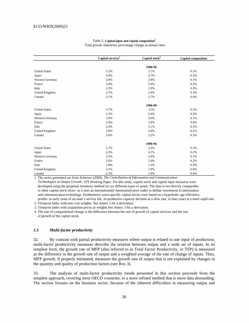
ECO/WKP(2000)21
30
Capital services2 Capital stock3 Capital composition
United States 3.3% 3.1% 0.2%Japan 4.9% 4.7% 0.3%Western Germany 2.8% 2.8% 0.1%France 3.4% 3.0% 0.3%Italy 2.2% 1.9% 0.3%United Kingdom 2.7% 2.4% 0.3%Canada 3.1% 2.7% 0.4%
United States 3.7% 3.5% 0.2%Japan 5.3% 5.0% 0.3%Western Germany 3.0% 3.0% 0.1%France 3.9% 3.4% 0.4%Italy 2.4% 2.1% 0.3%United Kingdom 2.8% 2.6% 0.2%Canada 3.6% 3.2% 0.3%
United States 2.7% 2.4% 0.3%Japan 4.3% 4.1% 0.2%Western Germany 2.5% 2.4% 0.1%France 2.6% 2.4% 0.2%Italy 1.8% 1.5% 0.3%United Kingdom 2.5% 1.9% 0.6%Canada 2.3% 1.9% 0.4%1. The series presented are from Schreyer (2000), The Contribution of Information and Communication Technologies to Output Growth ; STI Working Paper. For this study, capital stock and capital input measures were developed using the perpetual inventory method for six different types of assets. The data is not directly comparable to other capital stock series as it uses an internationally harmonised price index to deflate investment in information and communication technology. Furthermore, asset-specific capital stocks were based on a hyperbolic age-efficiency profile: in early years of an asset’s service life, its productive capacity declines at a slow rate, in later years at a more rapid rate.2. Törnqvist index with user cost weights. See Annex 3 for a derivation.3. Törnqvist index with acquisition prices as weights See Annex 3 for a derivation.4. The rate of compositional change is the difference between the rate of growth of capital services and the rate of growth of the capital stock.
1990-96
Table 5. Capital input and capital composition1
Total private industries, percentage change at annual rates
1980-96
1980-90
1.5 Multi-factor productivity
32. By contrast with partial productivity measures where output is related to one input of production, multi-factor productivity measures describe the relation between output and a wide set of inputs. In its simplest form, the growth rate of MFP (also referred to as Total Factor Productivity, or TFP) is measured as the difference in the growth rate of output and a weighted average of the rate of change of inputs. Thus, MFP growth, if properly estimated, measures the growth rate of output that is not explained by changes in the quantity and quality of production factors (see Box 3).
33. The analysis of multi-factor productivity trends presented in this section proceeds from the simplest approach, covering most OECD countries, to a more refined method that is more data demanding. The section focuses on the business sector, because of the inherent difficulties in measuring output and
ECO/WKP(2000)21
31
capital stock for the government sector, and on trend series to avoid picking up idiosyncratic movements in output and inputs.
34. Table 6 reports MFP growth rates in the business sector in a large sample of countries computed using employment and gross capital stock as factor inputs (i.e. neither adjusted for hours worked nor for changes in the quality and composition of labour and capital inputs). This is the broadest measure of productivity growth that incorporates the effects of progress in human capital as well as embodied (in physical capital) and disembodied technological progress.34 For partial output elasticities, three different approaches are compared: average factor shares, time-varying factor shares and econometrically estimated output elasticities with a production function expressed in levels (see Annex 3 for the method of estimation). As it can be seen, only minor differences arise between the three methods.35 These findings, which appear to be robust across a large number of countries, imply that the results from the use of more sophisticated measures of factor inputs will not be vitiated by using the comparatively simple “factor share” measures of partial output elasticities, reported in the next paragraphs.
34. For countries that use hedonic (or similar) price indices for certain investment goods (e.g. ICT), this
measure of MFP growth rate does not incorporate technological progress embodied in them (as the capital stock is augmented by the improvements in quality of ICT goods). Bassanini et al. (2000) try to identify this component of broad MFP growth by considering the differences in growth rates of hedonic and non-hedonic price indexes of ICT. For the United States, the embodied part of MFP growth would be about 0.2 percentage point in the 1980-90 period and about 0.3 percentage point in the 1990-96 period.
35. See also Annex Tables A3.1 and A3.2.
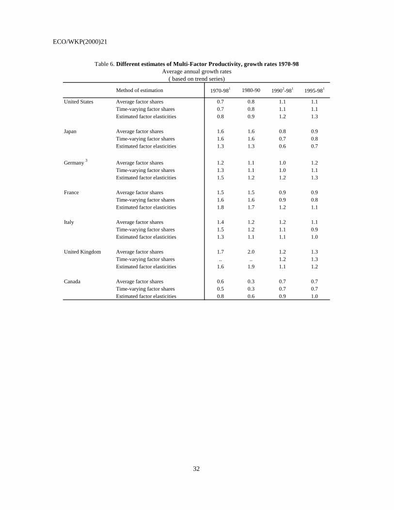
ECO/WKP(2000)21
32
Method of estimation 1970-981 1980-90 19902-981 1995-981
United States Average factor shares 0.7 0.8 1.1 1.1Time-varying factor shares 0.7 0.8 1.1 1.1Estimated factor elasticities 0.8 0.9 1.2 1.3
Japan Average factor shares 1.6 1.6 0.8 0.9Time-varying factor shares 1.6 1.6 0.7 0.8Estimated factor elasticities 1.3 1.3 0.6 0.7
Germany 3 Average factor shares 1.2 1.1 1.0 1.2Time-varying factor shares 1.3 1.1 1.0 1.1Estimated factor elasticities 1.5 1.2 1.2 1.3
France Average factor shares 1.5 1.5 0.9 0.9Time-varying factor shares 1.6 1.6 0.9 0.8Estimated factor elasticities 1.8 1.7 1.2 1.1
Italy Average factor shares 1.4 1.2 1.2 1.1Time-varying factor shares 1.5 1.2 1.1 0.9Estimated factor elasticities 1.3 1.1 1.1 1.0
United Kingdom Average factor shares 1.7 2.0 1.2 1.3Time-varying factor shares .. .. 1.2 1.3Estimated factor elasticities 1.6 1.9 1.1 1.2
Canada Average factor shares 0.6 0.3 0.7 0.7Time-varying factor shares 0.5 0.3 0.7 0.7Estimated factor elasticities 0.8 0.6 0.9 1.0
Table 6. Different estimates of Multi-Factor Productivity, growth rates 1970-98
( based on trend series)Average annual growth rates
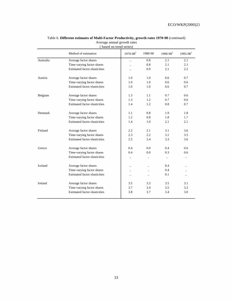
ECO/WKP(2000)21
33
Method of estimation 1970-981 1980-90 1990-981 1995-981
Australia Average factor shares .. 0.8 2.1 2.1Time-varying factor shares .. 0.8 2.1 2.1Estimated factor elasticities .. 0.9 2.1 2.2
Austria Average factor shares 1.0 1.0 0.6 0.7Time-varying factor shares 1.0 1.0 0.6 0.6Estimated factor elasticities 1.0 1.0 0.6 0.7
Belgium Average factor shares 1.3 1.1 0.7 0.6Time-varying factor shares 1.3 1.2 0.7 0.6Estimated factor elasticities 1.4 1.2 0.8 0.7
Denmark Average factor shares 1.1 0.8 1.9 1.8Time-varying factor shares 1.2 0.8 1.8 1.7Estimated factor elasticities 1.4 1.0 2.1 2.1
Finland Average factor shares 2.2 2.1 3.1 3.6Time-varying factor shares 2.3 2.2 3.1 3.5Estimated factor elasticities 2.5 2.4 3.3 3.6
Greece Average factor shares 0.4 0.0 0.4 0.6Time-varying factor shares 0.4 0.0 0.3 0.6Estimated factor elasticities .. .. .. ..
Iceland Average factor shares .. .. 0.4 ..Time-varying factor shares .. .. 0.4 ..Estimated factor elasticities .. .. 0.1 ..
Ireland Average factor shares 3.5 3.3 3.5 3.1Time-varying factor shares 3.7 3.4 3.5 3.2Estimated factor elasticities 3.8 3.7 3.4 3.0
Average annual growth rates( based on trend series)
Table 6. Different estimates of Multi-Factor Productivity, growth rates 1970-98 (continued)
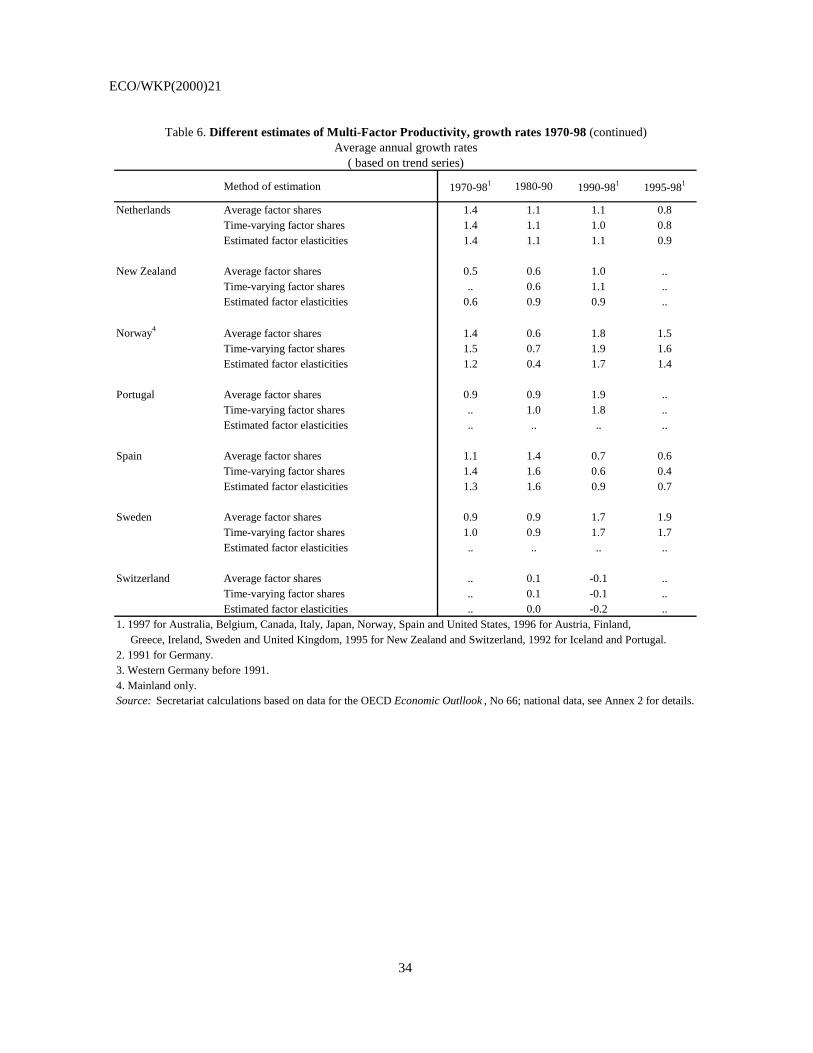
ECO/WKP(2000)21
34
Method of estimation 1970-981 1980-90 1990-981 1995-981
Netherlands Average factor shares 1.4 1.1 1.1 0.8Time-varying factor shares 1.4 1.1 1.0 0.8Estimated factor elasticities 1.4 1.1 1.1 0.9
New Zealand Average factor shares 0.5 0.6 1.0 ..Time-varying factor shares .. 0.6 1.1 ..Estimated factor elasticities 0.6 0.9 0.9 ..
Norway4 Average factor shares 1.4 0.6 1.8 1.5Time-varying factor shares 1.5 0.7 1.9 1.6Estimated factor elasticities 1.2 0.4 1.7 1.4
Portugal Average factor shares 0.9 0.9 1.9 ..Time-varying factor shares .. 1.0 1.8 ..Estimated factor elasticities .. .. .. ..
Spain Average factor shares 1.1 1.4 0.7 0.6Time-varying factor shares 1.4 1.6 0.6 0.4Estimated factor elasticities 1.3 1.6 0.9 0.7
Sweden Average factor shares 0.9 0.9 1.7 1.9Time-varying factor shares 1.0 0.9 1.7 1.7Estimated factor elasticities .. .. .. ..
Switzerland Average factor shares .. 0.1 -0.1 ..Time-varying factor shares .. 0.1 -0.1 ..Estimated factor elasticities .. 0.0 -0.2 ..
1. 1997 for Australia, Belgium, Canada, Italy, Japan, Norway, Spain and United States, 1996 for Austria, Finland, Greece, Ireland, Sweden and United Kingdom, 1995 for New Zealand and Switzerland, 1992 for Iceland and Portugal. 2. 1991 for Germany.3. Western Germany before 1991.4. Mainland only.Source: Secretariat calculations based on data for the OECD Economic Outllook , No 66; national data, see Annex 2 for details.
( based on trend series)
Table 6. Different estimates of Multi-Factor Productivity, growth rates 1970-98 (continued)Average annual growth rates
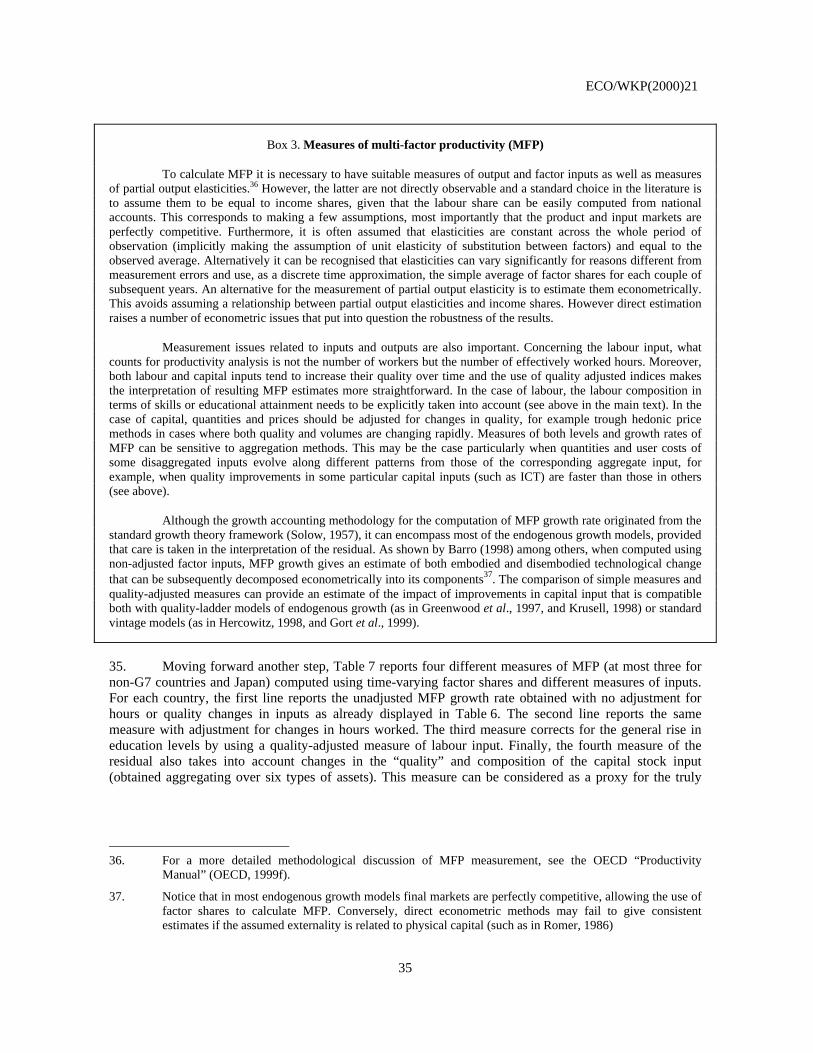
ECO/WKP(2000)21
35
Box 3. Measures of multi-factor productivity (MFP)
To calculate MFP it is necessary to have suitable measures of output and factor inputs as well as measures of partial output elasticities.36 However, the latter are not directly observable and a standard choice in the literature is to assume them to be equal to income shares, given that the labour share can be easily computed from national accounts. This corresponds to making a few assumptions, most importantly that the product and input markets are perfectly competitive. Furthermore, it is often assumed that elasticities are constant across the whole period of observation (implicitly making the assumption of unit elasticity of substitution between factors) and equal to the observed average. Alternatively it can be recognised that elasticities can vary significantly for reasons different from measurement errors and use, as a discrete time approximation, the simple average of factor shares for each couple of subsequent years. An alternative for the measurement of partial output elasticity is to estimate them econometrically. This avoids assuming a relationship between partial output elasticities and income shares. However direct estimation raises a number of econometric issues that put into question the robustness of the results.
Measurement issues related to inputs and outputs are also important. Concerning the labour input, what counts for productivity analysis is not the number of workers but the number of effectively worked hours. Moreover, both labour and capital inputs tend to increase their quality over time and the use of quality adjusted indices makes the interpretation of resulting MFP estimates more straightforward. In the case of labour, the labour composition in terms of skills or educational attainment needs to be explicitly taken into account (see above in the main text). In the case of capital, quantities and prices should be adjusted for changes in quality, for example trough hedonic price methods in cases where both quality and volumes are changing rapidly. Measures of both levels and growth rates of MFP can be sensitive to aggregation methods. This may be the case particularly when quantities and user costs of some disaggregated inputs evolve along different patterns from those of the corresponding aggregate input, for example, when quality improvements in some particular capital inputs (such as ICT) are faster than those in others (see above).
Although the growth accounting methodology for the computation of MFP growth rate originated from the standard growth theory framework (Solow, 1957), it can encompass most of the endogenous growth models, provided that care is taken in the interpretation of the residual. As shown by Barro (1998) among others, when computed using non-adjusted factor inputs, MFP growth gives an estimate of both embodied and disembodied technological change that can be subsequently decomposed econometrically into its components37. The comparison of simple measures and quality-adjusted measures can provide an estimate of the impact of improvements in capital input that is compatible both with quality-ladder models of endogenous growth (as in Greenwood et al., 1997, and Krusell, 1998) or standard vintage models (as in Hercowitz, 1998, and Gort et al., 1999).
35. Moving forward another step, Table 7 reports four different measures of MFP (at most three for non-G7 countries and Japan) computed using time-varying factor shares and different measures of inputs. For each country, the first line reports the unadjusted MFP growth rate obtained with no adjustment for hours or quality changes in inputs as already displayed in Table 6. The second line reports the same measure with adjustment for changes in hours worked. The third measure corrects for the general rise in education levels by using a quality-adjusted measure of labour input. Finally, the fourth measure of the residual also takes into account changes in the “quality” and composition of the capital stock input (obtained aggregating over six types of assets). This measure can be considered as a proxy for the truly
36. For a more detailed methodological discussion of MFP measurement, see the OECD “Productivity
Manual” (OECD, 1999f).
37. Notice that in most endogenous growth models final markets are perfectly competitive, allowing the use of factor shares to calculate MFP. Conversely, direct econometric methods may fail to give consistent estimates if the assumed externality is related to physical capital (such as in Romer, 1986)
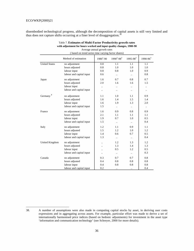
ECO/WKP(2000)21
36
disembodied technological progress, although the decomposition of capital assets is still very limited and thus does not capture shifts occurring at a finer level of disaggregation.38
Table 7. Estimates of Multi-Factor Productivity growth rates with adjustment for hours worked and input quality changes, 1980-98
Average annual growth rates( based on trend series time varying factor shares)
Method of estimation 19801-90 19902-983 1995-983 1990-963
United States no adjustment 0.8 1.1 1.1 1.1 hours adjusted 0.8 1.0 1.0 1.0 labour input 0.8 0.8 1.0 0.9 labour and capital input 0.6 .. .. 0.8
Japan no adjustment 1.6 0.7 0.8 0.7 hours adjusted 2.0 1.6 1.6 1.5 labour input .. .. .. .. labour and capital input .. .. .. ..
Germany 4 no adjustment 1.1 1.0 1.1 0.9 hours adjusted 1.6 1.4 1.5 1.4 labour input 1.6 1.9 1.3 2.0 labour and capital input 1.5 .. .. ..
France no adjustment 1.6 0.9 0.8 0.9 hours adjusted 2.1 1.1 1.1 1.1 labour input 1.9 0.7 1.0 0.5 labour and capital input 1.5 .. .. 0.4
Italy no adjustment 1.2 1.1 0.9 1.1 hours adjusted 1.5 1.2 1.0 1.2 labour input 1.4 0.6 0.7 0.5 labour and capital input 1.3 .. .. 0.4
United Kingdom no adjustment .. 1.2 1.3 1.2 hours adjusted .. 1.3 1.4 1.3 labour input .. 0.5 1.2 0.5 labour and capital input .. .. .. 0.3
Canada no adjustment 0.3 0.7 0.7 0.8 hours adjusted 0.4 0.8 0.8 0.8 labour input 0.4 0.8 0.8 0.8 labour and capital input 0.2 .. .. 0.4
38. A number of assumptions were also made in computing capital stocks by asset, in deriving user costs
expressions and in aggregating across assets. For example, particular effort was made to derive a set of internationally harmonised price indices (based on hedonic adjustments) for investment in the asset type ‘information and communication technology’ (see Schreyer, 2000 for more details).
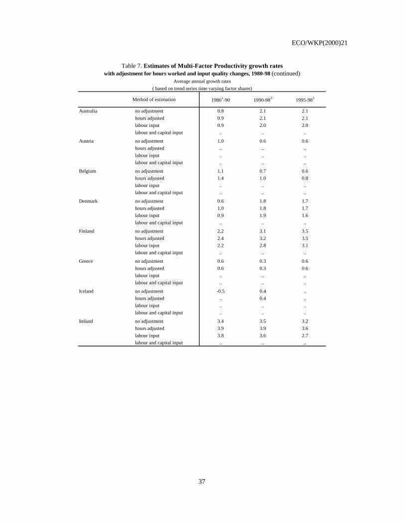
ECO/WKP(2000)21
37
Method of estimation 19801-90 1990-983 1995-983
Australia no adjustment 0.8 2.1 2.1 hours adjusted 0.9 2.1 2.1 labour input 0.9 2.0 2.0 labour and capital input .. .. ..
Austria no adjustment 1.0 0.6 0.6 hours adjusted .. .. .. labour input .. .. .. labour and capital input .. .. ..
Belgium no adjustment 1.1 0.7 0.6 hours adjusted 1.4 1.0 0.8 labour input .. .. .. labour and capital input .. .. ..
Denmark no adjustment 0.6 1.8 1.7 hours adjusted 1.0 1.8 1.7 labour input 0.9 1.9 1.6 labour and capital input .. .. ..
Finland no adjustment 2.2 3.1 3.5 hours adjusted 2.4 3.2 3.5 labour input 2.2 2.8 3.1 labour and capital input .. .. ..
Greece no adjustment 0.6 0.3 0.6 hours adjusted 0.6 0.3 0.6 labour input .. .. .. labour and capital input .. .. ..
Iceland no adjustment -0.5 0.4 .. hours adjusted .. 0.4 .. labour input .. .. .. labour and capital input .. .. ..
Ireland no adjustment 3.4 3.5 3.2 hours adjusted 3.9 3.9 3.6 labour input 3.8 3.6 2.7 labour and capital input .. .. ..
Table 7. Estimates of Multi-Factor Productivity growth rates
Average annual growth rates( based on trend series time varying factor shares)
with adjustment for hours worked and input quality changes, 1980-98 (continued)
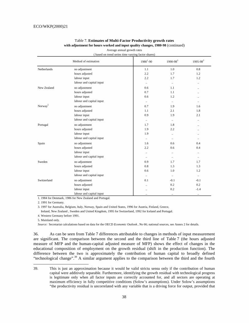
ECO/WKP(2000)21
38
Method of estimation 19801-90 1990-983 1995-983
Netherlands no adjustment 1.1 1.0 0.8 hours adjusted 2.2 1.7 1.2 labour input 2.2 1.7 1.2 labour and capital input .. .. ..
New Zealand no adjustment 0.6 1.1 .. hours adjusted 0.7 1.1 .. labour input 0.6 1.2 .. labour and capital input .. .. ..
Norway5 no adjustment 0.7 1.9 1.6 hours adjusted 1.1 2.1 1.8 labour input 0.9 1.9 2.1 labour and capital input .. .. ..
Portugal no adjustment 1.7 1.8 .. hours adjusted 1.9 2.2 .. labour input 1.9 .. .. labour and capital input .. .. ..
Spain no adjustment 1.6 0.6 0.4 hours adjusted 2.2 0.6 0.4 labour input .. .. .. labour and capital input .. .. ..
Sweden no adjustment 0.9 1.7 1.7 hours adjusted 0.8 1.3 1.3 labour input 0.6 1.0 1.2 labour and capital input .. .. ..
Switzerland no adjustment 0.1 -0.1 -0.1 hours adjusted .. 0.2 0.2 labour input .. 0.2 -1.4 labour and capital input .. .. ..
1. 1984 for Denmark, 1986 for New Zealand and Portugal.2. 1991 for Germany.3. 1997 for Australia, Belgium, Italy, Norway, Spain and United States, 1996 for Austria, Finland, Greece, Ireland, New Zealand , Sweden and United Kingdom, 1995 for Switzerland, 1992 for Iceland and Portugal. 4. Western Germany before 1991.5. Mainland only.Source: Secretariat calculations based on data for the OECD Economic Outlook , No 66; national sources, see Annex 2 for details.
Table 7. Estimates of Multi-Factor Productivity growth rates with adjustment for hours worked and input quality changes, 1980-98 (continued)
Average annual growth rates( based on trend series time varying factor shares)
36. As can be seen from Table 7 differences attributable to changes in methods of input measurement are significant. The comparison between the second and the third line of Table 7 (the hours adjusted measure of MFP and the human-capital adjusted measure of MFP) shows the effect of changes in the educational composition of employment on the growth residual (shift in the production function). The difference between the two is approximately the contribution of human capital to broadly defined “technological change”.39 A similar argument applies to the comparison between the third and the fourth 39. This is just an approximation because it would be valid strictu sensu only if the contribution of human
capital were additively separable. Furthermore, identifying the growth residual with technological progress is legitimate only when all factor inputs are correctly accounted for, and all sectors are operating at maximum efficiency in fully competitive conditions (Solow’s assumptions). Under Solow’s assumptions “the productivity residual is uncorrelated with any variable that is a driving force for output, provided that
ECO/WKP(2000)21
39
line of Table 7 with respect to the adjustment for changes in the composition of the capital stock (see also Hercowitz, 1998).
37. Comparisons of the different MFP estimates in Table 7 indicate significant variation amongst the G-7 countries. The United States and Canada recorded a recovery in MFP growth that reversed a longstanding downward trend.40 Conversely, all measures of MFP growth rates decreased significantly in France and Italy. The correction for changes in the composition of labour and capital inputs tends to reduce measured MFP insofar as part of the productivity growth is assigned to improvements in the quality of factors used in the production process (i.e. embodied in inputs). Only in a few smaller countries did MFP growth unambiguously and significantly increase in the 1990s compared with the previous decade. Thus, Australia, Denmark, Finland, New Zealand, Norway and Sweden all experienced increases in average growth rates of MFP of at least 0.5 percentage point (in most cases from relatively low rates in the 1980s).
38. It should be stressed that trend series as estimated in this chapter could underestimate the potential pick-up in output and productivity that might have occurred in the most recent years. According to a very recent study (Jorgenson and Stiroh, 2000), the acceleration of MFP in the ICT industry in the second half of the 1990s was sufficiently strong to positively affect the economy-wide MFP growth rate in the United States. Two additional studies (Whelan, 2000; Oliner and Sichel, 2000) also relate the growing utilisation of computer hardware and software to faster aggregate MFP growth in the United States.
2. Income and productivity levels: what is the scope for further catch-up?
2.1 The evolution of income and productivity levels over time
39. From a policy point of view, differences in income levels between countries are also of interest as markedly high or low levels of GDP per capita (and especially productivity) give some indication of how much - or little - extra output can be generated via reforms and policies that lead countries (or sectors) towards “best practice”. Put it in another way, comparing output and productivity levels is related to studying the “catch-up” or “convergence” phenomenon, whereby countries with low GDP per capita can be expected to grow faster than high per capita ones, ceteris paribus. At least amongst the “old” OECD countries, inter-country differences in GDP per-capita levels are not very large at present relative to
the variable is not one that shifts the production function” (Hall, 1990). However, at least at the industry level the invariance property fails to hold. Hall offers three main explanations for this: 1) monopolistic competition; 2) measurement errors (e.g. lack of account for changes in work effort over the cycle); and 3) thick market externalities in expansions. There is not clear-cut evidence on the impact of these factors for the estimates of MFP (e.g. Morrison, 1992). In the case of mark-ups of prices over marginal costs, Oliveira Martins and Scarpetta (1999) suggest that the presence of positive and counter-cyclical price margins has only a marginal impact on estimates of MFP growth rates. Another - perhaps more important - reason of failure of the invariance property consists in aggregation biases: from a fully rigorous perspective, the possibility of estimating an aggregate production function is conditional to the fact that the structure of the economy does not change over time (see e.g. Pasinetti, 1993). The analysis in Section 3 shows that this assumption fails to hold. However, little economic research has been conducted to understand the direction and size of aggregation biases, let aside how to overcome them (see e.g. Forni and Lippi, 1997).
40. Germany also had somewhat higher MFP growth rates based on labour quality adjusted measures in the 1990s compared with the 1980s, although reversion to the mean can be observed in the most recent years. It should be stressed, however, that quality adjusted measures for Germany are somewhat less reliable because reunification implied a slump in input quality at the beginning of the 1990s that was subsequently recovered, without changes of equal magnitude on output.
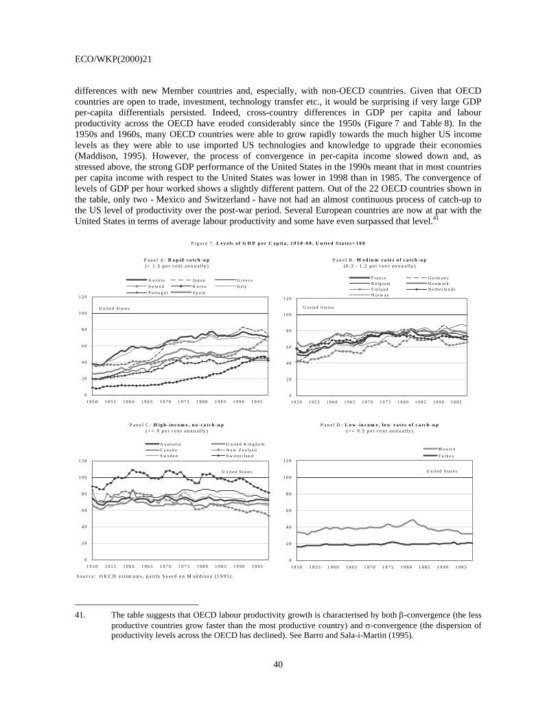
ECO/WKP(2000)21
40
differences with new Member countries and, especially, with non-OECD countries. Given that OECD countries are open to trade, investment, technology transfer etc., it would be surprising if very large GDP per-capita differentials persisted. Indeed, cross-country differences in GDP per capita and labour productivity across the OECD have eroded considerably since the 1950s (Figure 7 and Table 8). In the 1950s and 1960s, many OECD countries were able to grow rapidly towards the much higher US income levels as they were able to use imported US technologies and knowledge to upgrade their economies (Maddison, 1995). However, the process of convergence in per-capita income slowed down and, as stressed above, the strong GDP performance of the United States in the 1990s meant that in most countries per capita income with respect to the United States was lower in 1998 than in 1985. The convergence of levels of GDP per hour worked shows a slightly different pattern. Out of the 22 OECD countries shown in the table, only two - Mexico and Switzerland - have not had an almost continuous process of catch-up to the US level of productivity over the post-war period. Several European countries are now at par with the United States in terms of average labour productivity and some have even surpassed that level.41
S o u r c e : O E C D e s t im a te s , p a r t ly b a s e d o n M a d d is o n (1 9 9 5 ) .
F ig u r e 7 . L e v e ls o f G D P p e r C a p ita , 1 9 5 0 -9 8 , U n it e d S t a te s = 1 0 0
P a n e l B : M e d iu m r a te s o f c a tc h - u p( 0 .3 - 1 .2 p e r c e n t a n n u a l ly )
P a n e l A : R a p id c a tc h -u p( > 1 .3 p e r c e n t a n n u a l ly )
P a n e l C : H ig h - in c o m e , n o -c a tc h - u p( < = 0 p e r c e n t a n n u a l ly )
P a n e l D : L o w - in c o m e , lo w r a t e s o f c a tc h -u p(< = 0 .5 p e r c e n t a n n u a l ly )
0
2 0
4 0
6 0
8 0
1 0 0
1 2 0
1 9 5 0 1 9 5 5 1 9 6 0 1 9 6 5 1 9 7 0 1 9 7 5 1 9 8 0 1 9 8 5 1 9 9 0 1 9 9 5
A u s tr a l i a U n ite d K in g d o mC a n a d a N e w Z e a la n dS w e d e n S w i tz e r la n d
U n i te d S ta te s
0
2 0
4 0
6 0
8 0
1 0 0
1 2 0
1 9 5 0 1 9 5 5 1 9 6 0 1 9 6 5 1 9 7 0 1 9 7 5 1 9 8 0 1 9 8 5 1 9 9 0 1 9 9 5
M e x ic o
T u r k e y
U n i te d S ta te s
0
2 0
4 0
6 0
8 0
1 0 0
1 2 0
1 9 5 0 1 9 5 5 1 9 6 0 1 9 6 5 1 9 7 0 1 9 7 5 1 9 8 0 1 9 8 5 1 9 9 0 1 9 9 5
F ra n c e G e r m a n yB e lg iu m D e n m a rkF in la n d N e th e r la n d sN o r w a y
U n i te d S ta te s
0
2 0
4 0
6 0
8 0
1 0 0
1 2 0
1 9 5 0 1 9 5 5 1 9 6 0 1 9 6 5 1 9 7 0 1 9 7 5 1 9 8 0 1 9 8 5 1 9 9 0 1 9 9 5
A u s t r i a J a p a n G r e e c eI r e la n d K o r e a I ta lyP o r tu g a l S p a in
U n i te d S ta te s
41. The table suggests that OECD labour productivity growth is characterised by both β-convergence (the less
productive countries grow faster than the most productive country) and σ-convergence (the dispersion of productivity levels across the OECD has declined). See Barro and Sala-i-Martin (1995).
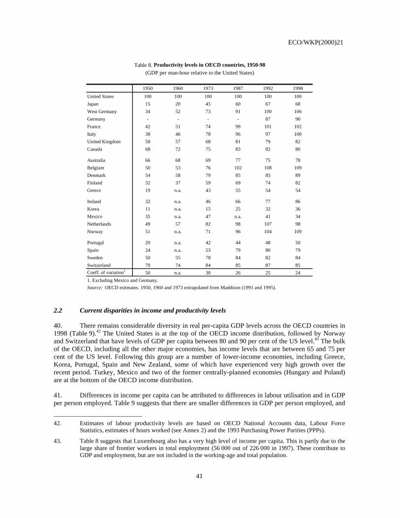
ECO/WKP(2000)21
41
Table 8. Productivity levels in OECD countries, 1950-98(GDP per man-hour relative to the United States)
1950 1960 1973 1987 1992 1998
United States 100 100 100 100 100 100Japan 15 20 45 60 67 68West Germany 34 52 73 91 100 106Germany - - - - 87 90France 42 51 74 99 101 102Italy 38 46 78 96 97 100United Kingdom 58 57 68 81 79 82Canada 68 72 75 83 82 80
Australia 66 68 69 77 75 78Belgium 50 53 76 102 108 109Denmark 54 58 79 85 85 89Finland 32 37 59 69 74 82Greece 19 n.a. 43 55 54 54
Ireland 32 n.a. 46 66 77 86Korea 11 n.a. 15 25 32 36Mexico 35 n.a. 47 n.a. 41 34Netherlands 49 57 82 98 107 98Norway 51 n.a. 71 96 104 109
Portugal 20 n.a. 42 44 48 50Spain 24 n.a. 53 79 80 79Sweden 50 55 78 84 82 84Switzerland 70 74 84 85 87 85Coeff. of variation1 50 n.a. 30 26 25 241. Excluding Mexico and Germany.Source: OECD estimates. 1950, 1960 and 1973 extrapolated from Maddison (1991 and 1995).
2.2 Current disparities in income and productivity levels
40. There remains considerable diversity in real per-capita GDP levels across the OECD countries in 1998 (Table 9).42 The United States is at the top of the OECD income distribution, followed by Norway and Switzerland that have levels of GDP per capita between 80 and 90 per cent of the US level.43 The bulk of the OECD, including all the other major economies, has income levels that are between 65 and 75 per cent of the US level. Following this group are a number of lower-income economies, including Greece, Korea, Portugal, Spain and New Zealand, some of which have experienced very high growth over the recent period. Turkey, Mexico and two of the former centrally-planned economies (Hungary and Poland) are at the bottom of the OECD income distribution.
41. Differences in income per capita can be attributed to differences in labour utilisation and in GDP per person employed. Table 9 suggests that there are smaller differences in GDP per person employed, and
42. Estimates of labour productivity levels are based on OECD National Accounts data, Labour Force
Statistics, estimates of hours worked (see Annex 2) and the 1993 Purchasing Power Parities (PPPs).
43. Table 8 suggests that Luxembourg also has a very high level of income per capita. This is partly due to the large share of frontier workers in total employment (56 000 out of 226 000 in 1997). These contribute to GDP and employment, but are not included in the working-age and total population.
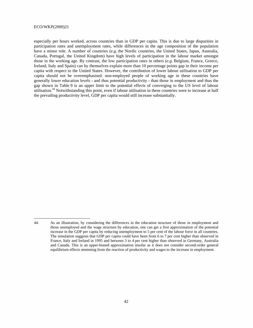
ECO/WKP(2000)21
42
especially per hours worked, across countries than in GDP per capita. This is due to large disparities in participation rates and unemployment rates, while differences in the age composition of the population have a minor role. A number of countries (e.g. the Nordic countries, the United States, Japan, Australia, Canada, Portugal, the United Kingdom) have high levels of participation in the labour market amongst those in the working age. By contrast, the low participation rates in others (e.g. Belgium, France, Greece, Ireland, Italy and Spain) can by themselves explain more than 10 percentage points gap in their income per capita with respect to the United States. However, the contribution of lower labour utilisation to GDP per capita should not be overemphasised: non-employed people of working age in these countries have generally lower education levels - and thus potential productivity - than those in employment and thus the gap shown in Table 9 is an upper limit to the potential effects of converging to the US level of labour utilisation.44 Notwithstanding this point, even if labour utilisation in these countries were to increase at half the prevailing productivity level, GDP per capita would still increase substantially.
44. As an illustration, by considering the differences in the education structure of those in employment and
those unemployed and the wage structure by education, one can get a first approximation of the potential increase in the GDP per capita by reducing unemployment to 5 per cent of the labour force in all countries. The simulation suggests that GDP per capita could have been from 6 to 7 per cent higher than observed in France, Italy and Ireland in 1995 and between 3 to 4 per cent higher than observed in Germany, Australia and Canada. This is an upper-biased approximation insofar as it does not consider second-order general equilibrium effects stemming from the reaction of productivity and wages to the increase in employment.
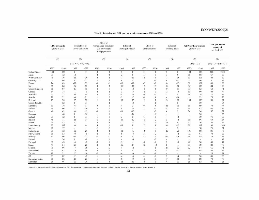
ECO/WKP(2000)21
43
1985 1998 1985 1998 1985 1998 1985 1998 1985 1998 1985 1998 1985 1998 1985 1998
United States 100 100 0 0 0 0 0 0 0 0 0 0 100 100 100 100Japan 71 72 13 4 2 3 -2 0 5 1 9 0 58 68 67 69West Germany 79 76 -11 -30 4 2 -7 -11 -1 -6 -7 -16 90 106 84 90Germany - 68 0 -21 - 2 - -7 - -4 - -12 - 90 - 77France 74 69 -22 -33 -1 -1 -10 -12 -3 -8 -8 -13 96 102 88 89Italy 68 66 -24 -35 3 3 -16 -18 -3 -9 -8 -10 92 100 84 90United Kingdom 66 67 -13 -15 -1 -1 0 -2 -3 -1 -9 -11 79 82 69 71Canada 84 74 -1 -6 2 2 0 -3 -2 -3 -2 -3 85 80 83 77Australia 73 72 -6 -6 0 1 -4 -3 0 -2 -1 -1 78 78 77 77Austria 72 71 -4 -21 1 2 -9 -7 4 0 - -16 - 92 76 76Belgium 75 74 -25 -35 1 0 -15 -15 -6 -7 -5 -12 100 109 95 97Czech Republic - 52 0 2 - 2 - -3 - -1 - 5 - 50 - 54Denmark 80 78 -6 -11 0 1 7 3 0 0 -13 -15 86 89 73 74Finland 69 66 2 -16 2 1 3 -3 2 -7 -4 -7 66 82 62 75Greece 46 42 -8 -12 -1 1 -11 -13 1 -3 4 3 54 54 57 57Hungary - 40 0 -16 - 1 - -14 - -2 - -1 - 56 - 55Iceland 79 72 8 2 -3 -1 5 5 6 1 - -3 - 70 71 67Ireland 48 71 -18 -14 -5 1 -10 -12 -6 -2 3 -2 66 86 69 84Korea 26 42 4 7 0 3 -7 -7 2 1 10 9 22 36 32 45Luxembourg 87 117 -8 0 4 1 -13 8 7 3 -6 -12 96 117 90 105Mexico 20 17 .. .. -9 -3 .. .. .. .. - 3 - 18 26 21Netherlands 71 73 -30 -26 2 3 -18 -5 -4 1 -10 -25 101 98 91 73New Zealand 66 53 -8 -8 -1 0 -9 -4 3 -2 -1 -2 75 61 73 59Norway 83 86 -14 -23 -3 -2 4 4 4 1 -19 -26 96 109 78 83Poland - 34 0 -8 - 1 - -6 - -3 - - - - - 42Portugal 38 45 -4 -5 -1 1 -3 -1 -1 -2 0 -3 42 50 43 47Spain 49 54 -29 -25 -1 2 -16 -14 -13 -12 1 -1 79 79 80 78Sweden 76 66 -7 -19 -2 -3 7 -2 4 -1 -17 -13 82 84 66 71Switzerland 99 81 12 -4 3 1 2 4 8 2 - -12 - 85 86 74Turkey 19 21 -7 -10 -3 -1 -4 -9 0 -1 - - - - 26 31G7 83 82 -2 -8 1 1 -4 -4 0 -2 0 -4 86 90 86 86European Union 68 66 -18 -23 1 1 -9 -9 -3 -5 -7 -10 85 89 79 78Euro area 68 66 -20 -26 1 2 -12 -11 -4 -6 -6 -11 88 92 82 81
Sources : Secretariat calculations based on data for the OECD Economic Outlook No 66, Labour Force Statistics , hours worked from Annex 2.
Table 9 . Breakdown of GDP per capita in its components, 1985 and 1998
GDP per capita(as % of US)
Effect of working age population
(15-64 years) to total population
Effect of participation rate
Effect of unemployment
GDP per person employed
(as % of US)
Effect of working hours
GDP per hour worked(as % of US)
[ (3) + (4) + (5) + (6) ]
Total effect of labour utilisation
(1) (2) (3) (5)(4)
[ (1) - (3) - (4) - (5) ][ (1) - (2) ]
(8)(6) (7)
ECO/WKP(2000)21
44
Summing up findings from the analysis of aggregate data
42. The analysis of aggregate indicators of economic growth suggest rising disparities across the OECD countries in the 1990s compared with the previous decade as well as persistent differences in per-capita GDP levels. Table 10 focuses on growth dynamics. Amongst the major countries, the United States experienced improving growth performances in the 1990s, in a context of continuously favourable product and labour market conditions. Especially in the most recent years, a combination of positive trends characterises the US economy, including higher growth rates of GDP per capita, employment, labour and, to some extent, multi-factor productivity as well as further capital deepening. These patterns are not uncommon amongst successfully catching-up countries, but unusual for a country that is already at the world productivity frontier in many sectors (see below). Although it is perhaps too early to fully assess structural shifts in growth patterns, these trends may suggest the move towards higher potential growth rates. Box 4 discusses some of the policy factors behind US growth performance.
Box 4. Features of US growth performance in the 1990s
An important reason in OECD countries for the renewed interest in economic growth and policies to sustain it, has been the recent growth record of the United States. GDP growth there has exceeded that in the European Union in all but three of the last twenty years, and in Japan in all but three of the last ten years. As a result, U.S. per capita income is now moving even further above that in other OECD countries. The upswing is the longest (although not the strongest) since records began in 1850, and has been accompanied by low inflation rates, falling unemployment, and improving public finances. With the benefit of hindsight, it is clear that the innovation and the extensive spread of new technologies in the fields of information and communication have been a key factor in giving the upswing a new lease of life in recent years, and possibly moving the economy to a new higher potential growth path. These developments are discussed in another box above. But other factors may also have played a role in permitting output and employment to rise smoothly in a sustained fashion for nearly a decade.
Upswings generally peter out, or go into reverse, when the economy comes up against capacity limits, or when investment proves to have been based on too-optimistic demand projections. Thus it was not expected that the US economy would be able to generate substantial increases in employment every year since 1992 without putting strong upward pressure on wages, real and nominal. In the event, employment growth has averaged around 2 per cent annually, similar to the growth in earlier upswings despite slower population growth, since more people were drawn into the labour market (thanks, in part, to welfare reform). Moreover, unemployment has fallen below levels which most analysts would argue are consistent with stable inflation in the medium term. And in fact both nominal and real wages have accelerated in the past few years, but labour productivity has recently accelerated even more, bringing an improvement in profitability and allowing core inflation to remain in a range consistent with price stability objectives, helped by favourable movements in import prices.
ECO/WKP(2000)21
45
Box 4. Features of US growth performance in the 1990s (cont.)
This combination of elastic supply response and stable macro conditions raises the question as to what sorts of policies and framework conditions have contributed to bringing it about, and whether strains are building up. Among the factors to consider are the relative importance and roles of:
• strong work incentives in contributing to the rising mobilisation of labour;
• high job-market flexibility in accommodating the considerable changes in the structure of demand for labour, which have not provoked major shortages;
• leaving resource allocation issues in product and financial markets to be handled by the private sector, subject to policies that reduce distortions and spur competition in these markets;
• a legal framework for bankruptcy, competition and securities markets, and low effective marginal tax rates on corporate earnings, in encouraging a strong entrepreneurial tradition;
• monetary and fiscal policies that have allowed the private sector to operate at high capacity, without strains, while maintaining confidence that macro conditions were likely to remain stable.
The challenge for policy currently is to engineer a transition to a more sustainable rate of growth that ensures inflation remains under control while avoiding recession. The continuing large external deficits and build-up of external debt, combined with low household (though not national) savings rates will complicate this task.
43. In some other OECD countries (including Australia, Ireland and the Netherlands and Norway, as well as Canada in most recent years) growth rates of trend GDP per capita, employment and multi-factor productivity have generally accelerated in the 1990s as compared with the previous decade. It is noticeable that these are also the countries that made substantial reforms in their labour and product markets over the past two decades.45
45. These countries have all a high record of structural reforms as measured by follow-through of the
recommendations of the Jobs Strategy (see OECD, 1999g). Moreover, they have all experienced significant improvements in labour market conditions over the 1990s.
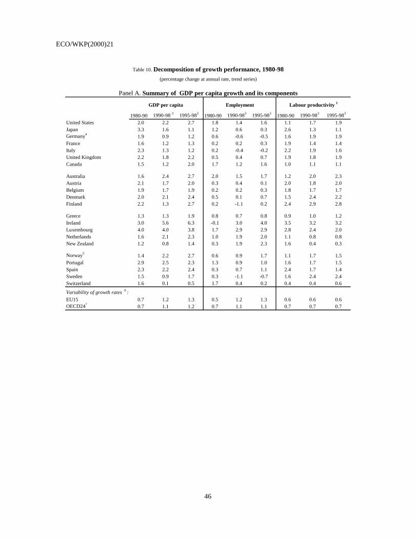
ECO/WKP(2000)21
46
1980-90 1990-98 2 1995-982 1980-90 1990-983 1995-983 1980-90 1990-983 1995-983
United States 2.0 2.2 2.7 1.8 1.4 1.6 1.1 1.7 1.9Japan 3.3 1.6 1.1 1.2 0.6 0.3 2.6 1.3 1.1Germany4 1.9 0.9 1.2 0.6 -0.6 -0.5 1.6 1.9 1.9France 1.6 1.2 1.3 0.2 0.2 0.3 1.9 1.4 1.4Italy 2.3 1.3 1.2 0.2 -0.4 -0.2 2.2 1.9 1.6United Kingdom 2.2 1.8 2.2 0.5 0.4 0.7 1.9 1.8 1.9Canada 1.5 1.2 2.0 1.7 1.2 1.6 1.0 1.1 1.1
Australia 1.6 2.4 2.7 2.0 1.5 1.7 1.2 2.0 2.3Austria 2.1 1.7 2.0 0.3 0.4 0.1 2.0 1.8 2.0Belgium 1.9 1.7 1.9 0.2 0.2 0.3 1.8 1.7 1.7Denmark 2.0 2.1 2.4 0.5 0.1 0.7 1.5 2.4 2.2Finland 2.2 1.3 2.7 0.2 -1.1 0.2 2.4 2.9 2.8
Greece 1.3 1.3 1.9 0.8 0.7 0.8 0.9 1.0 1.2Ireland 3.0 5.6 6.3 -0.1 3.0 4.0 3.5 3.2 3.2Luxembourg 4.0 4.0 3.8 1.7 2.9 2.9 2.8 2.4 2.0Netherlands 1.6 2.1 2.3 1.0 1.9 2.0 1.1 0.8 0.8New Zealand 1.2 0.8 1.4 0.3 1.9 2.3 1.6 0.4 0.3
Norway5 1.4 2.2 2.7 0.6 0.9 1.7 1.1 1.7 1.5Portugal 2.9 2.5 2.3 1.3 0.9 1.0 1.6 1.7 1.5Spain 2.3 2.2 2.4 0.3 0.7 1.1 2.4 1.7 1.4Sweden 1.5 0.9 1.7 0.3 -1.1 -0.7 1.6 2.4 2.4Switzerland 1.6 0.1 0.5 1.7 0.4 0.2 0.4 0.4 0.6
Variability of growth rates 6 :EU15 0.7 1.2 1.3 0.5 1.2 1.3 0.6 0.6 0.6OECD247 0.7 1.1 1.2 0.7 1.1 1.1 0.7 0.7 0.7
Table 10. Decomposition of growth performance, 1980-98(percentage change at annual rate, trend series)
GDP per capita Employment Labour productivity 1
Panel A. Summary of GDP per capita growth and its components
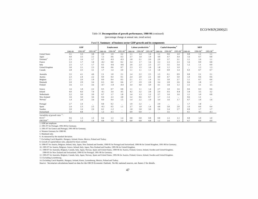
ECO/WKP(2000)21
47
1980-90 1990-989 1995-9810 1980-90 1990-989 1995-9810 1980-90 1990-989 1995-9810 1980-90 1990-9811 1995-9812 1980-90 1990-9811 1995-9812
United States 3.1 3.3 3.8 2.0 1.9 2.2 1.1 1.4 1.6 1.1 0.6 1.0 0.8 1.1 1.1Japan 4.0 2.5 2.2 1.3 0.6 0.3 2.7 1.8 1.9 4.9 4.7 4.4 1.6 0.7 0.8Germany4 2.3 1.6 1.7 0.5 -0.5 -0.3 1.8 2.1 2.0 2.9 3.7 3.1 1.1 1.0 1.1France 2.3 1.7 1.8 -0.2 0.0 0.2 2.4 1.7 1.6 2.3 2.3 2.3 1.6 0.9 0.8Italy 2.5 1.7 1.7 0.5 -0.6 -0.6 2.0 2.3 2.3 2.7 3.5 3.4 1.2 1.1 0.9United Kingdom 3.0 2.1 2.3 0.6 0.6 0.7 2.3 1.5 1.6 1.8 1.2 1.0 .. 1.2 1.3Canada 2.8 2.5 3.1 1.7 1.4 2.0 1.1 1.1 1.1 1.8 0.9 1.4 0.3 0.7 0.7
Australia 3.5 4.1 4.6 2.1 1.8 2.1 1.4 2.2 2.5 1.5 0.1 0.9 0.8 2.1 2.1Austria 2.3 2.4 2.2 0.0 0.4 0.1 2.4 2.0 2.1 4.0 4.7 5.0 1.0 0.6 0.6Belgium 2.1 2.0 1.9 0.0 0.4 0.5 2.1 1.5 1.4 3.1 3.0 2.7 1.1 0.7 0.6Denmark 2.0 2.9 3.4 0.3 0.0 0.6 1.7 2.9 2.8 3.4 2.8 2.6 0.6 1.8 1.7Finland 2.6 2.1 3.6 -0.7 -1.9 -0.4 3.4 4.0 3.9 4.1 2.8 1.2 2.2 3.1 3.5
Greece 1.6 1.8 2.2 0.5 0.7 0.8 1.1 1.1 1.4 2.7 1.8 1.6 0.6 0.3 0.6Ireland 4.0 6.6 7.4 -0.1 3.4 4.5 4.2 3.2 2.8 2.4 -0.1 -0.4 3.4 3.5 3.2Netherlands 2.2 3.0 3.0 0.7 1.7 1.8 1.4 1.3 1.2 2.7 1.6 1.6 1.1 1.0 0.8New Zealand 1.6 3.0 3.6 0.4 2.3 2.8 1.2 0.6 0.7 1.7 -1.1 .. 0.6 1.1 ..Norway5 1.4 2.6 3.4 0.0 0.4 1.5 1.4 2.2 1.9 3.4 1.6 1.7 0.7 1.9 1.6
Portugal 2.7 2.4 .. 0.8 0.2 .. 1.9 2.2 .. 2.9 .. .. 1.7 1.8 ..Spain 2.4 2.3 2.5 -0.3 0.5 1.1 2.7 1.8 1.4 4.8 3.8 2.8 1.6 0.6 0.4Sweden 2.0 1.6 2.0 0.2 -1.2 .. 1.8 2.8 3.0 2.6 2.4 2.7 0.9 1.7 1.7Switzerland 2.2 0.8 .. 1.3 -0.1 .. 0.9 0.9 .. .. 3.5 .. 0.1 -0.1 -0.1
Variability of growth rates 6 :EU1513 0.6 1.3 1.5 0.4 1.3 1.4 0.8 0.8 0.8 0.8 1.3 1.3 0.8 1.0 1.0OECD2414 0.7 1.2 1.4 0.8 1.2 1.3 0.8 0.8 0.8 1.1 1.6 1.3 0.7 0.9 0.91. GDP per employee. 2. 1991-97 for Portugal, 1991-98 for Germany.3. 1991-97 for Greece and Portugal, 1991-98 for Germany. 4. Western Germany for 1980-90.5. Mainland only.6. As measured by the standard deviation.7. Excluding Czech Republic, Hungary, Iceland, Korea, Mexico, Poland and Turkey.8. Growth of capital/labour ratio, adjusted for hours worked.9. 1990-97 for Austria, Belgium, Ireland, Italy, Japan, New Zealand and Sweden, 1990-95 for Portugal and Switzerland, 1990-96 for United Kingdom, 1991-98 for Germany.10. 1995-97 for Austria, Belgium, Greece, Ireland, Italy, Japan, New Zealand and Sweden, 1995-96 for United Kingdom.11. 1990-97 for Australia, Belgium, Canada, Italy, Japan, Norway, Spain and United States, 1990-96 for Austria, Finland, Greece, Ireland, Sweden and United Kingdom, 1990-95 for New Zealand and Switzerland, 1990-92 for Portugal, 1991-98 for Germany.12. 1995-97 for Australia, Belgium, Canada, Italy, Japan, Norway, Spain and United States, 1995-96 for Austria, Finland, Greece, Ireland, Sweden and United Kingdom.13. Excluding Luxembourg.14. Excluding Czech Republic, Hungary, Iceland, Korea, Luxembourg, Mexico, Poland and Turkey.Source: Secretariat calculations based on data for the OECD Economic Outlook, No 66; national sources, see Annex 2 for details.
Table 10. Decomposition of growth performance, 1980-98 (continued)(percentage change at annual rate, trend series)
Panel B. Summary of business sector GDP growth and its components
GDP Employment Labour productivity 1 Capital deepening 8 MFP
ECO/WKP(2000)21
48
44. In the other countries, growth performance did not change significantly in the 1990s, and in some cases deteriorated. Amongst those with low per-capita income levels, Portugal and Turkey continued to grow at relatively high (and stable) rates and Greece maintained relatively low growth rates. In most Continental Europe, growth rates of per-capita GDP did not improve either because of clear slow down in productivity or, more often, because of sluggish employment developments. In these countries, the up-skilling of the workforce has accounted for most of the changes in labour input and thus for most of the contribution of labour to output growth, while the skill upgrading has gone hand in hand with growth in employment in other countries. The significant slow-down in the growth rate of GDP per capita in Japan has been accompanied by relatively smaller employment adjustments leading to declines in labour productivity growth rates.
3. Growth performance at the sectoral level
45. The aggregate analysis of growth performance may hide significant differences in growth trends across sectors and firms (see, amongst others, Bernard and Jones, 1996a, 1996b). The investigation of sectoral trends helps to throw further light on the growth process and the factors that drive it, and may also be important in the assessment of policies that can support growth (amongst others, see Haltiwanger, 1997). In particular, it allows assessing whether differences in the link between GDP growth, labour productivity and employment across countries are the result of aggregation of different sectoral patterns within each country or rather similar patterns across sectors. Differences in growth patterns at the sector level may also point to variations in the extent to which countries are benefiting from broader economic changes or the potential offered by technological change (Stoneman and Diederen, 1994). For example, technological change has enabled rapid productivity growth in telecommunications over recent years, but there are considerable variations in the degree to which countries have benefited from this potential. Detailed information on differences in sectoral productivity performances across countries also helps understanding the role of competition policies and privatisation in a variety of industries (e.g. telecommunication, airline, electricity, etc.) (see OECD, 1997).
46. The analysis of sectoral performances and their contribution to aggregate growth patterns is organised as follows. After a brief discussion of growth patterns across broad sectors of the economy, this section analyses within-industry productivity performance to shed light on the driving forces of recent growth patterns at the aggregate levels. This is followed by the assessment of structural shifts and their role to overall productivity patterns. Although significant changes have occurred both within and between industries over the past decade, aggregate performances are also affected by persistent differences across countries in industry productivity levels. These are discussed in the final part of this section.
3.1 The breakdown of growth and labour productivity change by sector
47. Productivity measurement at the sector level is constrained by the degree of detail and by measurement problems, in particular in services.46 The productivity analysis below focuses on the non-farm business sector (i.e. excluding agriculture and community, social and personal services). Moreover, the sectoral decomposition of productivity does not take into account sectoral interactions due to the role that goods and services of some sectors play in the production process of other sectors and vice versa. Bearing these caveats in mind, a sectoral decomposition of labour productivity growth indicates that
46. As stressed in Annex 2, industry data used in this paper are from the OECD International Sectoral Data
Base (ISDB) and the OECD STAN Database for Industrial Analysis. Industry disaggregation is available for the service sector at 2 digits (or even 1 digit for some services in some countries) which significantly affect the analysis of structural changes.
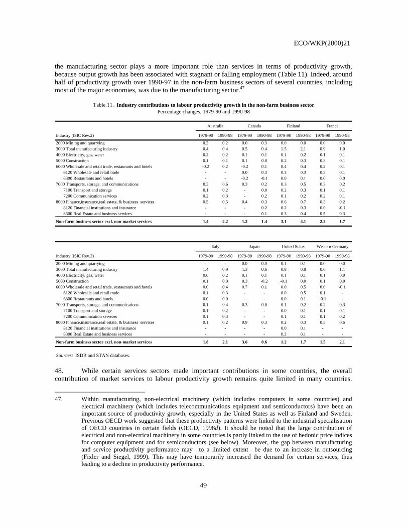
ECO/WKP(2000)21
49
the manufacturing sector plays a more important role than services in terms of productivity growth, because output growth has been associated with stagnant or falling employment (Table 11). Indeed, around half of productivity growth over 1990-97 in the non-farm business sectors of several countries, including most of the major economies, was due to the manufacturing sector.47
Australia Canada Finland France
Industry (ISIC Rev.2) 1979-90 1990-98 1979-90 1990-98 1979-90 1990-98 1979-90 1990-98
2000 Mining and quarrying 0.2 0.2 0.0 0.3 0.0 0.0 0.0 0.03000 Total manufacturing industry 0.4 0.4 0.5 0.4 1.5 2.1 0.9 1.04000 Electricity, gas, water 0.2 0.2 0.1 0.1 0.1 0.2 0.1 0.15000 Construction 0.1 0.1 0.1 0.0 0.2 0.3 0.3 0.16000 Wholesale and retail trade, restaurants and hotels -0.2 0.2 -0.2 0.1 0.4 0.4 0.2 0.1
6120 Wholesale and retail trade - - 0.0 0.3 0.3 0.3 0.3 0.16300 Restaurants and hotels - - -0.2 -0.1 0.0 0.1 0.0 0.0
7000 Transports, storage, and communications 0.3 0.6 0.3 0.2 0.3 0.5 0.3 0.27100 Transport and storage 0.1 0.2 - 0.0 0.2 0.3 0.1 0.17200 Communication services 0.2 0.3 - 0.2 0.1 0.2 0.2 0.1
8000 Finance,insurance,real estate, & business services 0.5 0.5 0.4 0.3 0.6 0.7 0.5 0.28120 Financial institutions and insurance - - - 0.2 0.2 0.3 0.0 -0.18300 Real Estate and business services - - - 0.1 0.3 0.4 0.5 0.3
Non-farm business sector excl. non-market services 1.4 2.2 1.2 1.4 3.1 4.1 2.2 1.7
Italy Japan United States Western Germany
Industry (ISIC Rev.2) 1979-90 1990-98 1979-90 1990-98 1979-90 1990-98 1979-90 1990-98
2000 Mining and quarrying - - 0.0 0.0 0.1 0.1 0.0 0.03000 Total manufacturing industry 1.4 0.9 1.3 0.6 0.8 0.8 0.6 1.14000 Electricity, gas, water 0.0 0.2 0.1 0.1 0.1 0.1 0.1 0.05000 Construction 0.1 0.0 0.3 -0.2 -0.1 0.0 0.1 0.06000 Wholesale and retail trade, restaurants and hotels 0.0 0.4 0.7 0.1 0.0 0.5 0.0 -0.1
6120 Wholesale and retail trade 0.1 0.3 - - 0.0 0.5 0.1 -6300 Restaurants and hotels 0.0 0.0 - - 0.0 0.1 -0.1 -
7000 Transports, storage, and communications 0.1 0.4 0.3 0.0 0.1 0.2 0.2 0.37100 Transport and storage 0.1 0.2 - - 0.0 0.1 0.1 0.17200 Communication services 0.1 0.3 - - 0.1 0.1 0.1 0.2
8000 Finance,insurance,real estate, & business services 0.1 0.2 0.9 0.3 0.2 0.3 0.5 0.68120 Financial institutions and insurance - - - - 0.0 0.1 - -8300 Real Estate and business services - - - - 0.2 0.1 - -
Non-farm business sector excl. non-market services 1.8 2.1 3.6 0.6 1.2 1.7 1.5 2.1
Sources: ISDB and STAN databases.
Table 11. Industry contributions to labour productivity growth in the non-farm business sectorPercentage changes, 1979-90 and 1990-98
48. While certain services sectors made important contributions in some countries, the overall contribution of market services to labour productivity growth remains quite limited in many countries.
47. Within manufacturing, non-electrical machinery (which includes computers in some countries) and
electrical machinery (which includes telecommunications equipment and semiconductors) have been an important source of productivity growth, especially in the United States as well as Finland and Sweden. Previous OECD work suggested that these productivity patterns were linked to the industrial specialisation of OECD countries in certain fields (OECD, 1998d). It should be noted that the large contribution of electrical and non-electrical machinery in some countries is partly linked to the use of hedonic price indices for computer equipment and for semiconductors (see below). Moreover, the gap between manufacturing and service productivity performance may - to a limited extent - be due to an increase in outsourcing (Fixler and Siegel, 1999). This may have temporarily increased the demand for certain services, thus leading to a decline in productivity performance.
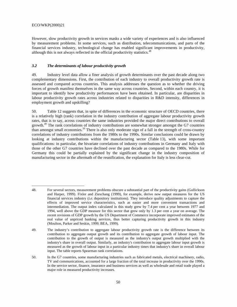
ECO/WKP(2000)21
50
However, slow productivity growth in services masks a wide variety of experiences and is also influenced by measurement problems. In some services, such as distribution, telecommunications, and parts of the financial services industry, technological change has enabled significant improvements in productivity, although this is not always reflected in the official productivity statistics.48
3.2 The determinants of labour productivity growth
49. Industry level data allow a finer analysis of growth determinants over the past decade along two complementary dimensions. First, the contribution of each industry to overall productivity growth rate is assessed and compared across countries. This analysis addresses the question as to whether the driving forces of growth manifest themselves in the same way across countries. Second, within each country, it is important to identify how productivity performances have been obtained. In particular, are disparities in labour productivity growth rates across industries related to disparities in R&D intensity, differences in employment growth and upskilling?
50. Table 12 suggests that, in spite of differences in the economic structure of OECD countries, there is a relatively high (rank) correlation in the industry contribution of aggregate labour productivity growth rates, that is to say, across countries the same industries provided the major direct contributions to overall growth.49 The rank correlations of industry contributions are somewhat stronger amongst the G7 countries than amongst small economies.50 There is also only moderate sign of a fall in the strength of cross-country correlations of industry contributions from the 1980s to the 1990s. Similar conclusions could be drawn by looking at industry contributions within the manufacturing sector (Table 13), with some important qualifications: in particular, the bivariate correlations of industry contributions in Germany and Italy with those of the other G7 countries have declined over the past decade as compared to the 1980s. While for Germany this could be partially explained by the significant change in the industry composition of manufacturing sector in the aftermath of the reunification, the explanation for Italy is less clear-cut.
48. For several sectors, measurement problems obscure a substantial part of the productivity gains (Gullickson
and Harper, 1999). Fixler and Zieschang (1999), for example, derive new output measures for the US financial services industry (i.e. depository institutions). They introduce quality adjustments to capture the effects of improved service characteristics, such as easier and more convenient transactions and intermediation. The output index calculated in this study grew by 7.4 per cent a year between 1977 and 1994, well above the GDP measure for this sector that grew only by 1.3 per cent a year on average. The recent revisions of GDP growth by the US Department of Commerce incorporate improved estimates of the real value of unpriced banking services, thus better capturing productivity growth in this industry (Moulton, Parker and Seskin, 1999; BEA, 1999).
49. The industry’s contribution to aggregate labour productivity growth rate is the difference between its contribution to aggregate output growth and its contribution to aggregate growth of labour input. The contribution to the growth of output is measured as the industry's output growth multiplied with the industry's share in overall output. Similarly, an industry's contribution to aggregate labour input growth is measured as the growth of labour input in a particular industry times that industry's share in overall labour input. The table reports Spearman rank correlations.
50. In the G7 countries, some manufacturing industries such as fabricated metals, electrical machinery, radio, TV and communications, accounted for a large fraction of the total increase in productivity over the 1990s. In the service sector, finance, insurance and business services as well as wholesale and retail trade played a major role in measured productivity increases.
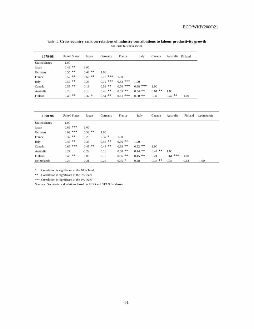
ECO/WKP(2000)21
51
1979-98 Finland
United States 1.00Japan 0.42 ** 1.00Germany 0.55 ** 0.48 ** 1.00France 0.52 ** 0.60 ** 0.78 *** 1.00Italy 0.59 ** 0.29 0.72 *** 0.82 *** 1.00Canada 0.55 ** 0.16 0.58 ** 0.70 *** 0.68 *** 1.00Australia 0.23 0.13 0.46 ** 0.55 ** 0.54 ** 0.61 ** 1.00Finland 0.46 ** 0.37 * 0.54 ** 0.61 *** 0.60 ** 0.32 0.42 ** 1.00
1990-98 Netherlands
United States 1.00Japan 0.69 *** 1.00Germany 0.62 *** 0.59 ** 1.00France 0.37 ** 0.23 0.37 * 1.00Italy 0.45 ** 0.33 0.48 ** 0.56 ** 1.00Canada 0.66 *** 0.45 ** 0.48 ** 0.39 ** 0.52 ** 1.00Australia 0.27 -0.22 0.18 0.50 ** 0.44 ** 0.47 ** 1.00Finland 0.45 ** 0.03 0.15 0.56 ** 0.45 ** 0.24 0.64 *** 1.00Netherlands 0.24 0.21 0.22 0.35 * 0.28 0.38 ** 0.33 0.13 1.00
* Correlation is significant at the 10% level.** Correlation is significant at the 5% level.*** Correlation is significant at the 1% level.Sources : Secretariat calculations based on ISDB and STAN databases.
Germany France Finland
Germany
Italy Canada Australia
Table 12. Cross-country rank correlations of industry contributions to labour productivity growthnon-farm business sector.
United States Japan
France Australia ItalyUnited States Japan Canada
ECO/WKP(2000)21
52
1979-98
United States 1.00Japan 0.54 ** 1.00Germany 0.70 *** 0.42 * 1.00France 0.62 ** 0.50 ** 0.77 *** 1.00Italy 0.37 0.36 0.72 *** 0.87 *** 1.00United Kingdom 0.43 * 0.33 0.62 ** 0.82 *** 0.60 ** 1.00Canada 0.51 ** 0.15 0.72 *** 0.66 ** 0.55 ** 0.57 ** 1.00Australia 0.04 0.02 0.38 * 0.36 0.49 ** 0.50 ** 0.40 * 1.00Finland 0.43 ** 0.28 0.44 ** 0.61 ** 0.59 ** 0.41 * 0.26 0.30 1.00Netherlands 0.24 -0.15 0.25 0.38 * 0.47 ** 0.39 * 0.32 0.24 0.53 ** 1.00Norway 0.33 0.13 0.41 * 0.45 ** 0.35 0.28 0.30 0.17 0.69 *** 0.51 ** 1.00Sweden 0.52 ** 0.44 * 0.65 ** 0.80 *** 0.76 *** 0.63 ** 0.54 ** 0.48 ** 0.80 *** 0.45 ** 0.56 ** 1.00
1990-98
United States 1.00Japan 0.71 *** 1.00Germany 0.61 ** 0.62 ** 1.00France 0.46 ** 0.33 0.39 * 1.00Italy 0.12 0.13 0.32 0.50 ** 1.00United Kingdom 0.46 ** 0.38 * 0.21 0.65 ** 0.29 1.00Canada 0.48 ** 0.46 ** 0.39 * 0.42 * 0.26 0.63 ** 1.00Australia 0.01 -0.21 0.06 0.34 0.30 0.23 0.38 * 1.00Finland 0.32 0.06 0.14 0.51 ** 0.48 ** 0.20 0.14 0.59 ** 1.00Netherlands 0.29 0.13 0.03 0.35 0.20 0.59 ** 0.39 * 0.16 0.29 1.00Norway 0.23 0.23 0.14 0.50 ** 0.21 0.22 0.11 0.20 0.49 ** 0.03 1.00Sweden 0.48 ** 0.25 0.45 ** 0.73 *** 0.36 0.48 ** 0.37 * 0.62 ** 0.73 *** 0.23 0.48 ** 1.00
* Correlation is significant at the 10% level.** Correlation is significant at the 5% level.*** Correlation is significant at the 1% level.Sources : Secretariat calculations based on ISDB and STAN databases.
Table 13. Cross-country rank correlations of industry contributions to labour productivity growthmanufacturing.
Sweden
Sweden
United States Japan Germany France Italy United Kingdom
Canada Australia Finland
United States Japan Germany France Italy United Kingdom
Canada
Netherlands Norway
Australia Finland Netherlands Norway
51. The high correlation in industry contribution (especially in manufacturing) seems to point to some communality in the sources of growth amongst the OECD countries. The somewhat weaker correlations amongst small economies reflect their narrower specialisation, especially in manufacturing (Pilat, 1996). However, rank correlations of industry contributions to labour productivity growth in different countries may hide significant differences in the dynamics of specific industries.51 This seems to be the case for the information and communication technology industry. For example the aggregate industry comprising the office and computing machinery industry (ISIC 3825) plus the Radio, TV & communication equipment industry (ISIC 3823)52 enjoyed a productivity growth above 10 per cent on average in the United States in 1990-97 period (as compared with 2.3 per cent on average in the manufacturing sector) and accounted for about 40 per cent of total manufacturing productivity growth. International comparisons of the contribution of ICT industry to manufacturing productivity growth is somewhat limited by the fact that some countries, including the United States, use hedonic price deflators for computers and others do not and this is likely to have a significant impact on measured productivity in 51. In particular, the variability of labour productivity growth rates across industries has increased markedly in
the United States, driven by sharp increase in productivity in the ICT industry, but remained fairly constant in most other OECD countries, and even fell in some countries, including Japan, Italy and the United Kingdom. See below for further detail.
52. The OECD definition of the ICT industry includes “those industries which facilitate, by electronic means, the processing, transmission and display of information. See http://www.oecd.org/dsti/sti/it/stats/defin.htm.
ECO/WKP(2000)21
53
the industry.53 Available data suggest that, although generally higher than the manufacturing average, labour productivity growth rates of ICT industry have been smaller in most of the other OECD countries as compared with the United States, and particularly so in some of the countries with low productivity growth in the whole manufacturing sector, such as Italy.
52. Within each country, there is evidence that labour productivity growth rates have been associated with various experiences concerning labour utilisation, changes in quality of inputs, capital deepening and the growth rate of technological change (see above). At the industry level, three indicators are available to shed further light on productivity differences within countries; i) R&D intensity (expressed as the ratio of R&D expenditure to output); ii) employment adjustments; and iii) skill up-grading. These three factors are closely related. R&D intensity in manufacturing provides an - albeit limited - indicator of the capacity of firms to discover and implement new ideas and production technologies as well as of their effort towards technological improvement54, while employment and up-skilling characterise changes in labour input.
53. Table 14 presents weighted correlation coefficients of changes in labour productivity growth rates with these three factors, in turn.55 It points to a generally positive correlation between R&D intensity and labour productivity growth at the industry level in almost all OECD countries. This relationship has a limited statistical significance for contemporaneous R&D intensity, but it is more significant when a lagged indicator of R&D intensity is used.56 This is suggestive of an impact from R&D in particular, and technological change in general, on labour productivity growth as would be expected.
53. The use of hedonic price deflators tends to boost the contribution of the ICT industry in two ways: i) it
raises its value added compared with that of other industries; and ii) lowers the value added in industries which use ICT products (e.g. semiconductors) as intermediate inputs. As a thought experiment, real value added in the US computer-producing industry (Office and computing machineries; ISIC 3825) was re-calculated using conventional “matched model” deflators approximated by means of a price index for Germany that does not employ hedonic techniques. This provides only a very rough indication of the effects of hedonic techniques for two main reasons: 1) the product composition of the computer industry can be quite different between the United States and Germany; and 2) the true price can differ, because of differences in market structures and other factors. Bearing in mind these limitations, the results of the simulation suggest a significantly smaller contribution of the computer-producing industry to manufacturing value added and labour productivity when quality changes (as measured by the hedonic method) in computers and semiconductors are not taken into account.
54. Many studies find that research and development expenditures provide a positive contribution to productivity growth. However, technology diffusion from other industries is also a major source of productivity gains (these two components are mutually interdependent and, in practice, their independent contribution cannot be fully disentangled, see Cohen and Levinthal, 1989; Cockburn and Henderson, 1998; Mowery and Oxley, 1995). Likewise, importing modern technologies from abroad is increasingly driving productivity growth. See, amongst others, OECD (1996c).
55. As compared with simple correlations, weighted correlations allow to consider differences in industry size and thus provide information that is representative of aggregate phenomena. Employment shares were used as weights.
56. The rationale of using lagged indicators of R&D intensity is that most R&D expenditure represents a long-run investment deemed to produce results in the far future in terms of productivity changes.
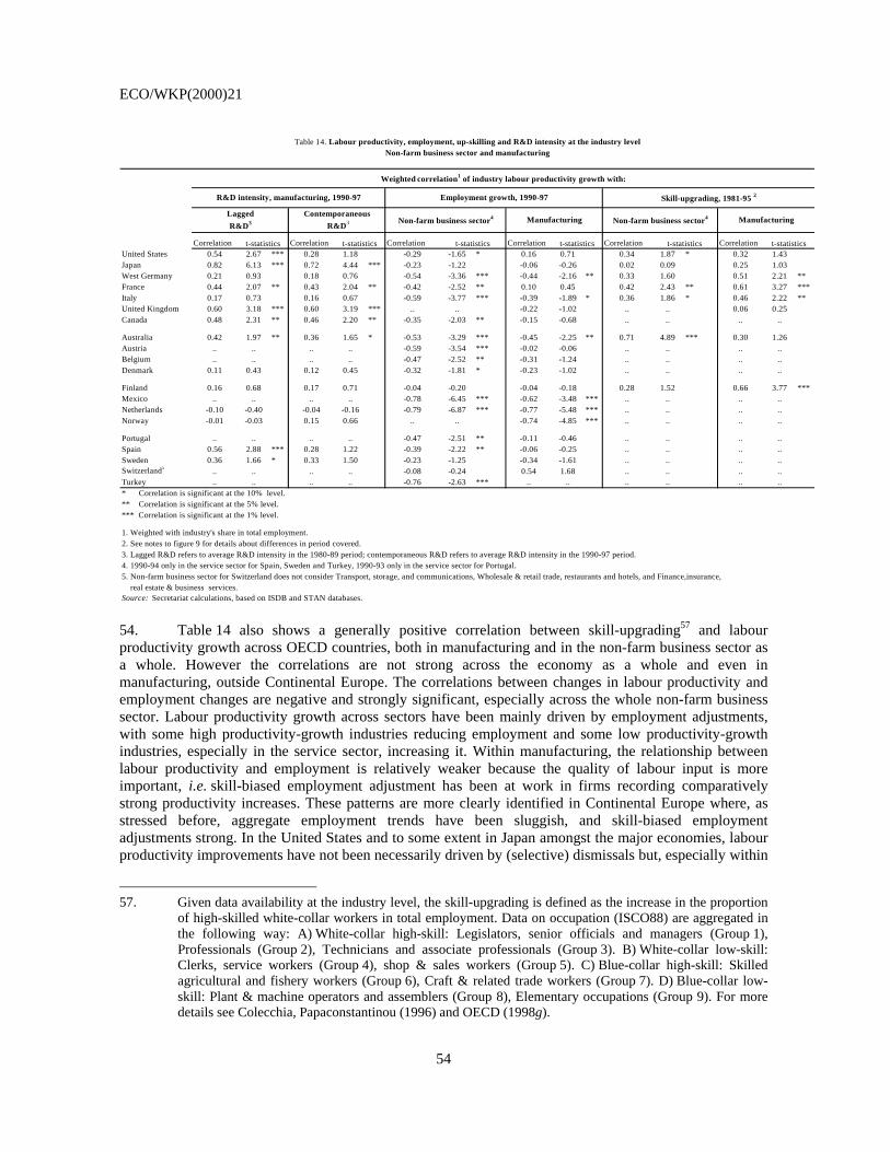
ECO/WKP(2000)21
54
Correlation Correlation Correlation Correlation Correlation CorrelationUnited States 0.54 2.67 *** 0.28 1.18 -0.29 -1.65 * 0.16 0.71 0.34 1.87 * 0.32 1.43 Japan 0.82 6.13 *** 0.72 4.44 *** -0.23 -1.22 -0.06 -0.26 0.02 0.09 0.25 1.03 West Germany 0.21 0.93 0.18 0.76 -0.54 -3.36 *** -0.44 -2.16 ** 0.33 1.60 0.51 2.21 **France 0.44 2.07 ** 0.43 2.04 ** -0.42 -2.52 ** 0.10 0.45 0.42 2.43 ** 0.61 3.27 ***Italy 0.17 0.73 0.16 0.67 -0.59 -3.77 *** -0.39 -1.89 * 0.36 1.86 * 0.46 2.22 **United Kingdom 0.60 3.18 *** 0.60 3.19 *** .. .. -0.22 -1.02 .. .. 0.06 0.25 Canada 0.48 2.31 ** 0.46 2.20 ** -0.35 -2.03 ** -0.15 -0.68 .. .. .. ..
Australia 0.42 1.97 ** 0.36 1.65 * -0.53 -3.29 *** -0.45 -2.25 ** 0.71 4.89 *** 0.30 1.26 Austria .. .. .. .. -0.59 -3.54 *** -0.02 -0.06 .. .. .. .. Belgium .. .. .. .. -0.47 -2.52 ** -0.31 -1.24 .. .. .. .. Denmark 0.11 0.43 0.12 0.45 -0.32 -1.81 * -0.23 -1.02 .. .. .. ..
Finland 0.16 0.68 0.17 0.71 -0.04 -0.20 -0.04 -0.18 0.28 1.52 0.66 3.77 ***Mexico .. .. .. .. -0.78 -6.45 *** -0.62 -3.48 *** .. .. .. .. Netherlands -0.10 -0.40 -0.04 -0.16 -0.79 -6.87 *** -0.77 -5.48 *** .. .. .. .. Norway -0.01 -0.03 0.15 0.66 .. .. -0.74 -4.85 *** .. .. .. ..
Portugal .. .. .. .. -0.47 -2.51 ** -0.11 -0.46 .. .. .. .. Spain 0.56 2.88 *** 0.28 1.22 -0.39 -2.22 ** -0.06 -0.25 .. .. .. .. Sweden 0.36 1.66 * 0.33 1.50 -0.23 -1.25 -0.34 -1.61 .. .. .. .. Switzerland5 .. .. .. .. -0.08 -0.24 0.54 1.68 .. .. .. .. Turkey .. .. .. .. -0.76 -2.63 *** .. .. .. .. .. .. * Correlation is significant at the 10% level.** Correlation is significant at the 5% level.*** Correlation is significant at the 1% level.
1. Weighted with industry's share in total employment.2. See notes to figure 9 for details about differences in period covered.3. Lagged R&D refers to average R&D intensity in the 1980-89 period; contemporaneous R&D refers to average R&D intensity in the 1990-97 period.4. 1990-94 only in the service sector for Spain, Sweden and Turkey, 1990-93 only in the service sector for Portugal. 5. Non-farm business sector for Switzerland does not consider Transport, storage, and communications, Wholesale & retail trade, restaurants and hotels, and Finance,insurance, real estate & business services.Source: Secretariat calculations, based on ISDB and STAN databases.
Table 14. Labour productivity, employment, up-skilling and R&D intensity at the industry level Non-farm business sector and manufacturing
Employment growth, 1990-97 Skill-upgrading, 1981-95 2R&D intensity, manufacturing, 1990-97
Weighted correlation1 of industry labour productivity growth with:
Non-farm business sector4 Manufacturing
t-statistics t-statisticst-statistics t-statistics
Lagged R&D3
Contemporaneous R&D3
t-statistics t-statistics
Non-farm business sector4 Manufacturing
54. Table 14 also shows a generally positive correlation between skill-upgrading57 and labour productivity growth across OECD countries, both in manufacturing and in the non-farm business sector as a whole. However the correlations are not strong across the economy as a whole and even in manufacturing, outside Continental Europe. The correlations between changes in labour productivity and employment changes are negative and strongly significant, especially across the whole non-farm business sector. Labour productivity growth across sectors have been mainly driven by employment adjustments, with some high productivity-growth industries reducing employment and some low productivity-growth industries, especially in the service sector, increasing it. Within manufacturing, the relationship between labour productivity and employment is relatively weaker because the quality of labour input is more important, i.e. skill-biased employment adjustment has been at work in firms recording comparatively strong productivity increases. These patterns are more clearly identified in Continental Europe where, as stressed before, aggregate employment trends have been sluggish, and skill-biased employment adjustments strong. In the United States and to some extent in Japan amongst the major economies, labour productivity improvements have not been necessarily driven by (selective) dismissals but, especially within
57. Given data availability at the industry level, the skill-upgrading is defined as the increase in the proportion
of high-skilled white-collar workers in total employment. Data on occupation (ISCO88) are aggregated in the following way: A) White-collar high-skill: Legislators, senior officials and managers (Group 1), Professionals (Group 2), Technicians and associate professionals (Group 3). B) White-collar low-skill: Clerks, service workers (Group 4), shop & sales workers (Group 5). C) Blue-collar high-skill: Skilled agricultural and fishery workers (Group 6), Craft & related trade workers (Group 7). D) Blue-collar low-skill: Plant & machine operators and assemblers (Group 8), Elementary occupations (Group 9). For more details see Colecchia, Papaconstantinou (1996) and OECD (1998g).
ECO/WKP(2000)21
55
manufacturing, by strong technological innovation and have sometimes been accompanied by positive employment changes.
3.3 Structural changes and labour productivity growth
55. Aggregate productivity growth patterns depend on within industry productivity performance as well as shifts of resources across industries. Historically, structural shifts were an important factor, as resources moved from a low-productive agricultural sector to a more productive manufacturing sector. More recently, the evidence from aggregate data seems to suggest that a large contribution to overall productivity growth patterns comes from productivity changes within industries rather than as a result of significant shifts of employment across industries (van Ark, 1996). Evidence from firm-level data partly confirm this finding of a strong within-firm effect, but also point to churning (entry and exit of firms) as an important component of productivity growth at the industry and possibly at the aggregate level (for a survey, see Foster et al., 1998).58 For the purpose of an international comparison, Figure 8 presents a decomposition of labour productivity growth in the business sector in three factors using the maximum industry decomposition available in ISDB-STAN (2-digit ISIC for services and a 3-4 digit ISIC for manufacturing):59
− An “intra-sectoral effect”, that measures productivity growth within industries;
− A “net-shift effect”, that measures the impact on productivity of the shift in employment between industries;
− And a residual third effect, the “interaction effect”. This effect is positive when sectors with growing productivity have a growing employment share or when industries with falling relative productivity decline in size. It is negative when industries with growing relative productivity decline in size or when industries with falling productivity grow in size.
58. Evidence from firm-level data also suggests that changes in market shares of individual firms within a
given industry and other competitive effects can make an important contribution to growth at the industry level (OECD, 1998a). For US manufacturing, such competitive effects explained over 40 per cent of total factor productivity growth between 1977 and 1987 (Haltiwanger, 1997). A future paper in the OECD work on economic growth will look specifically at firm-level patterns. This will build on previous work on longitudinal databases (OECD, 1998a).
59. The shift-share analysis presented has limitations other than the lack of detail for services (Timmer and Szirmai, 1999). First, it focuses on labour productivity, and not on multi-factor productivity. Second, it assumes that marginal productivity of factor inputs moving in or out an industry is the same as average productivity. Finally, if output growth is positively related to productivity growth (the Verdoorn effect), the impact of structural change may be underestimated, since part of the shift to rapid-growth sectors will be counted in the within-effect.
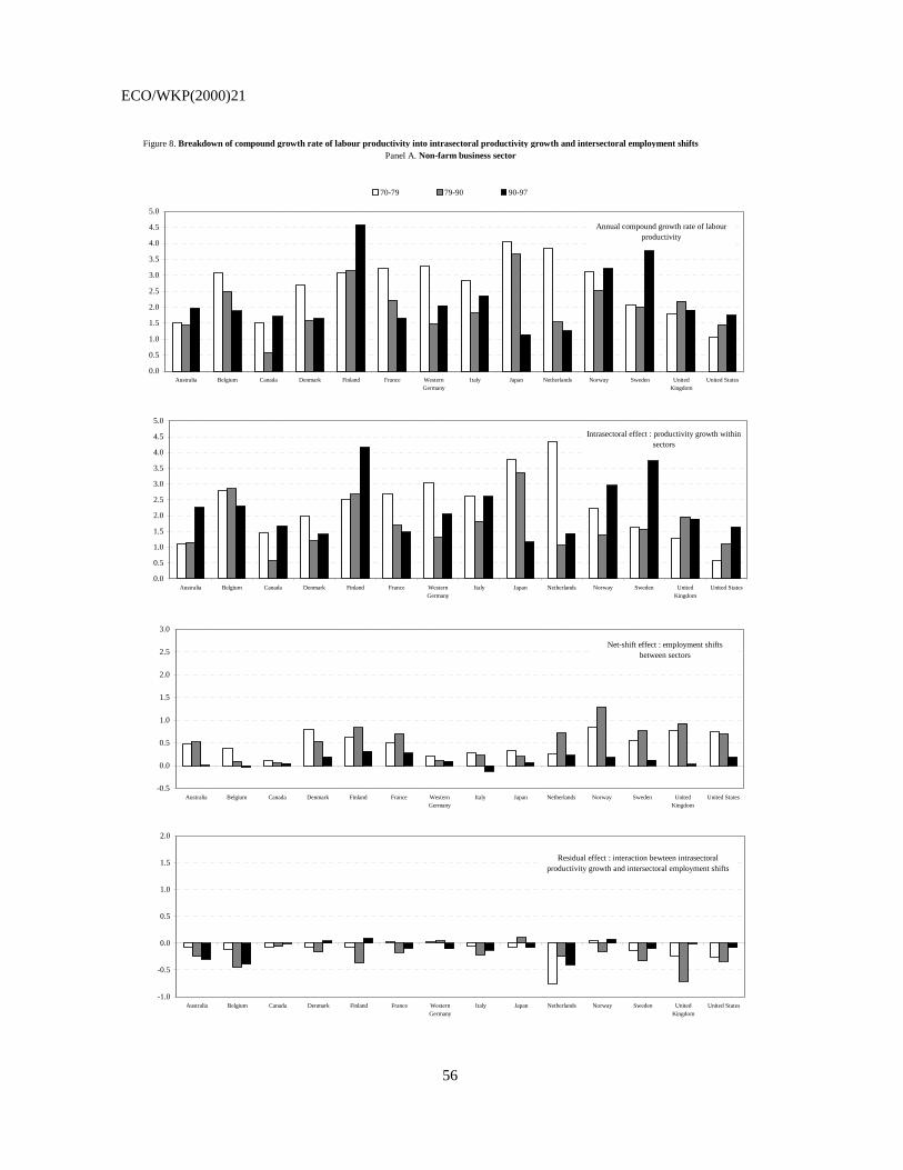
ECO/WKP(2000)21
56
Figure 8. Breakdown of compound growth rate of labour productivity into intrasectoral productivity growth and intersectoral employment shiftsPanel A. Non-farm business sector
0.0
0.5
1.0
1.5
2.0
2.5
3.0
3.5
4.0
4.5
5.0
Australia Belgium Canada Denmark Finland France WesternGermany
Italy Japan Netherlands Norway Sweden UnitedKingdom
United States
70-79 79-90 90-97
Annual compound growth rate of labour productivity
0.0
0.5
1.0
1.5
2.0
2.5
3.0
3.5
4.0
4.5
5.0
Australia Belgium Canada Denmark Finland France WesternGermany
Italy Japan Netherlands Norway Sweden UnitedKingdom
United States
Intrasectoral effect : productivity growth within sectors
-0.5
0.0
0.5
1.0
1.5
2.0
2.5
3.0
Australia Belgium Canada Denmark Finland France WesternGermany
Italy Japan Netherlands Norway Sweden UnitedKingdom
United States
Net-shift effect : employment shifts between sectors
-1.0
-0.5
0.0
0.5
1.0
1.5
2.0
Australia Belgium Canada Denmark Finland France WesternGermany
Italy Japan Netherlands Norway Sweden UnitedKingdom
United States
Residual effect : interaction bewteen intrasectoral productivity growth and intersectoral employment shifts
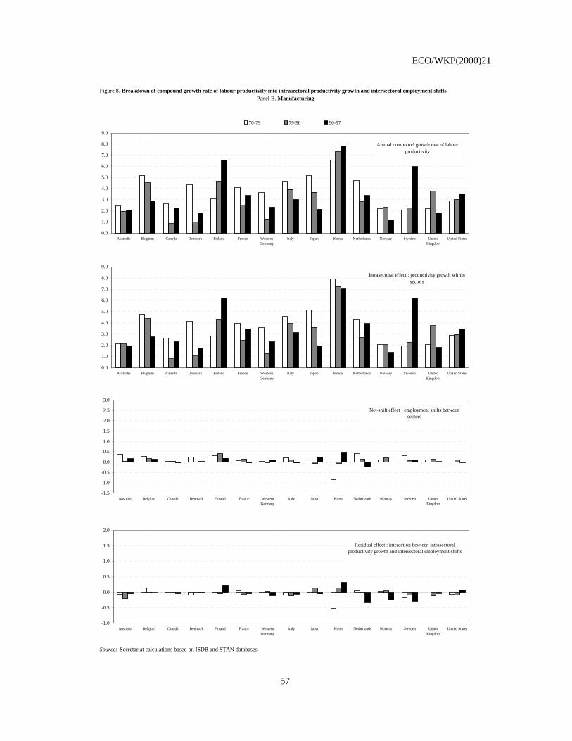
ECO/WKP(2000)21
57
Figure 8. Breakdown of compound growth rate of labour productivity into intrasectoral productivity growth and intersectoral employment shifts
Source: Secretariat calculations based on ISDB and STAN databases.
Panel B. Manufacturing
0.0
1.0
2.0
3.0
4.0
5.0
6.0
7.0
8.0
9.0
Australia Belgium Canada Denmark Finland France WesternGermany
Italy Japan Korea Netherlands Norway Sweden UnitedKingdom
United States
70-79 79-90 90-97
Annual compound growth rate of labour productivity
0.0
1.0
2.0
3.0
4.0
5.0
6.0
7.0
8.0
9.0
Australia Belgium Canada Denmark Finland France WesternGermany
Italy Japan Korea Netherlands Norway Sweden UnitedKingdom
United States
Intrasectoral effect : productivity growth within sectors
-1.5
-1.0
-0.5
0.0
0.5
1.0
1.5
2.0
2.5
3.0
Australia Belgium Canada Denmark Finland France WesternGermany
Italy Japan Korea Netherlands Norway Sweden UnitedKingdom
United States
Net-shift effect : employment shifts between sectors
-1.0
-0.5
0.0
0.5
1.0
1.5
2.0
Australia Belgium Canada Denmark Finland France WesternGermany
Italy Japan Korea Netherlands Norway Sweden UnitedKingdom
United States
Residual effect : interaction bewteen intrasectoral productivity growth and intersectoral employment shifts
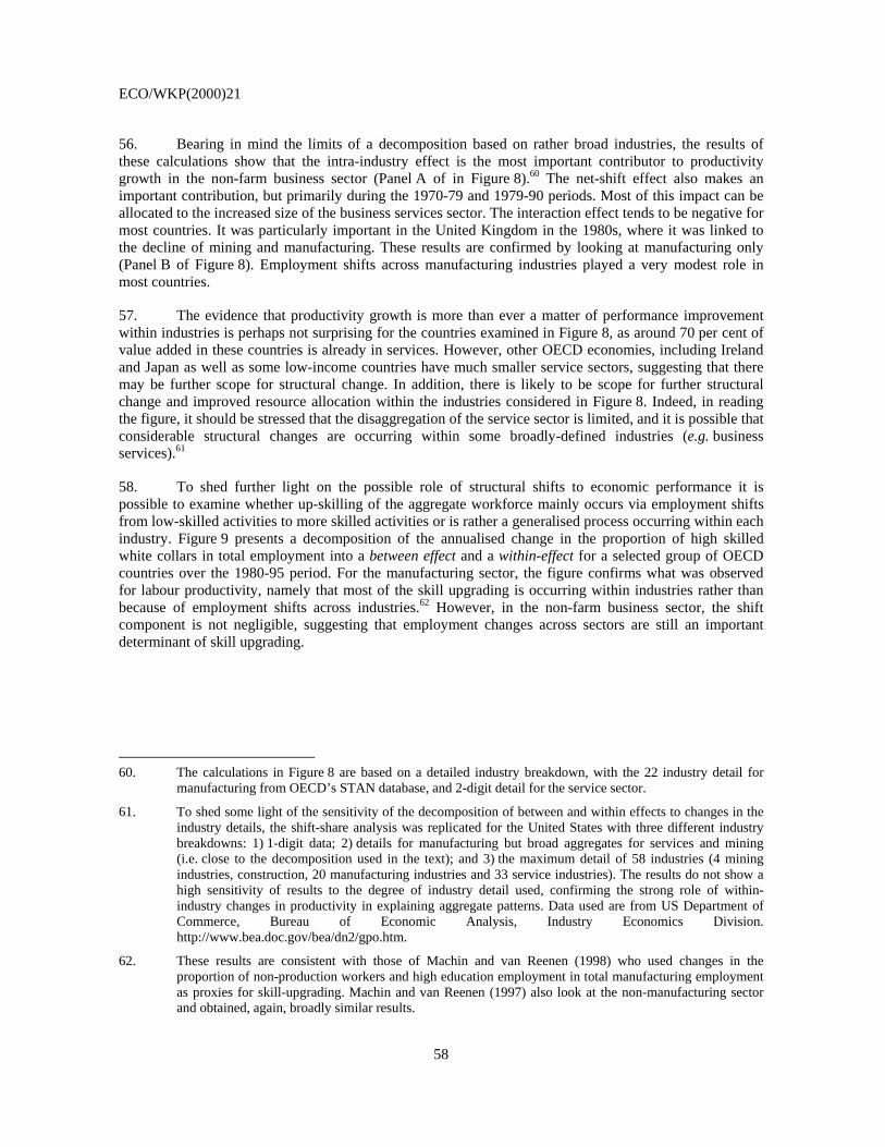
ECO/WKP(2000)21
58
56. Bearing in mind the limits of a decomposition based on rather broad industries, the results of these calculations show that the intra-industry effect is the most important contributor to productivity growth in the non-farm business sector (Panel A of in Figure 8).60 The net-shift effect also makes an important contribution, but primarily during the 1970-79 and 1979-90 periods. Most of this impact can be allocated to the increased size of the business services sector. The interaction effect tends to be negative for most countries. It was particularly important in the United Kingdom in the 1980s, where it was linked to the decline of mining and manufacturing. These results are confirmed by looking at manufacturing only (Panel B of Figure 8). Employment shifts across manufacturing industries played a very modest role in most countries.
57. The evidence that productivity growth is more than ever a matter of performance improvement within industries is perhaps not surprising for the countries examined in Figure 8, as around 70 per cent of value added in these countries is already in services. However, other OECD economies, including Ireland and Japan as well as some low-income countries have much smaller service sectors, suggesting that there may be further scope for structural change. In addition, there is likely to be scope for further structural change and improved resource allocation within the industries considered in Figure 8. Indeed, in reading the figure, it should be stressed that the disaggregation of the service sector is limited, and it is possible that considerable structural changes are occurring within some broadly-defined industries (e.g. business services).61
58. To shed further light on the possible role of structural shifts to economic performance it is possible to examine whether up-skilling of the aggregate workforce mainly occurs via employment shifts from low-skilled activities to more skilled activities or is rather a generalised process occurring within each industry. Figure 9 presents a decomposition of the annualised change in the proportion of high skilled white collars in total employment into a between effect and a within-effect for a selected group of OECD countries over the 1980-95 period. For the manufacturing sector, the figure confirms what was observed for labour productivity, namely that most of the skill upgrading is occurring within industries rather than because of employment shifts across industries.62 However, in the non-farm business sector, the shift component is not negligible, suggesting that employment changes across sectors are still an important determinant of skill upgrading.
60. The calculations in Figure 8 are based on a detailed industry breakdown, with the 22 industry detail for
manufacturing from OECD’s STAN database, and 2-digit detail for the service sector.
61. To shed some light of the sensitivity of the decomposition of between and within effects to changes in the industry details, the shift-share analysis was replicated for the United States with three different industry breakdowns: 1) 1-digit data; 2) details for manufacturing but broad aggregates for services and mining (i.e. close to the decomposition used in the text); and 3) the maximum detail of 58 industries (4 mining industries, construction, 20 manufacturing industries and 33 service industries). The results do not show a high sensitivity of results to the degree of industry detail used, confirming the strong role of within-industry changes in productivity in explaining aggregate patterns. Data used are from US Department of Commerce, Bureau of Economic Analysis, Industry Economics Division. http://www.bea.doc.gov/bea/dn2/gpo.htm.
62. These results are consistent with those of Machin and van Reenen (1998) who used changes in the proportion of non-production workers and high education employment in total manufacturing employment as proxies for skill-upgrading. Machin and van Reenen (1997) also look at the non-manufacturing sector and obtained, again, broadly similar results.
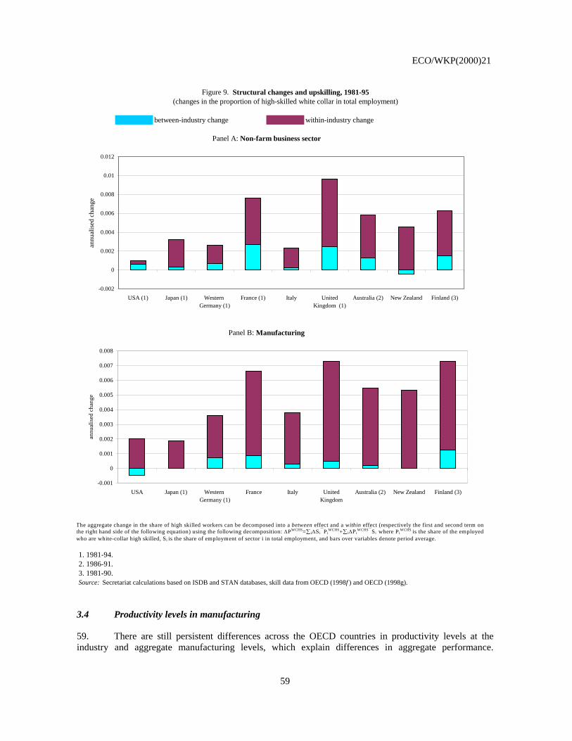
ECO/WKP(2000)21
59
between-industry change within-industry change
1. 1981-94.2. 1986-91.3. 1981-90.Source: Secretariat calculations based on ISDB and STAN databases, skill data from OECD (1998f ) and OECD (1998g).
Figure 9. Structural changes and upskilling, 1981-95(changes in the proportion of high-skilled white collar in total employment)
Panel A: Non-farm business sector
Panel B: Manufacturing
-0.002
0
0.002
0.004
0.006
0.008
0.01
0.012
USA (1) Japan (1) Western Germany (1)
France (1) Italy UnitedKingdom (1)
Australia (2) New Zealand Finland (3)
annu
alis
ed c
hang
e
-0.001
0
0.001
0.002
0.003
0.004
0.005
0.006
0.007
0.008
USA Japan (1) Western Germany (1)
France Italy UnitedKingdom
Australia (2) New Zealand Finland (3)
annu
alis
ed c
hang
e
The aggregate change in the share of high skilled workers can be decomposed into a between effect and a within effect (respectively the first and second term onthe right hand side of the following equation) using the following decomposition: ΔPWCHS=∑ iΔSi⎯Pi
WCHS+∑ iΔΡiWCHS⎯Si where Pi
WCHS is the share of the employedwho are white-collar high skilled, Si is the share of employment of sector i in total employment, and bars over variables denote period average.
3.4 Productivity levels in manufacturing
59. There are still persistent differences across the OECD countries in productivity levels at the industry and aggregate manufacturing levels, which explain differences in aggregate performance.
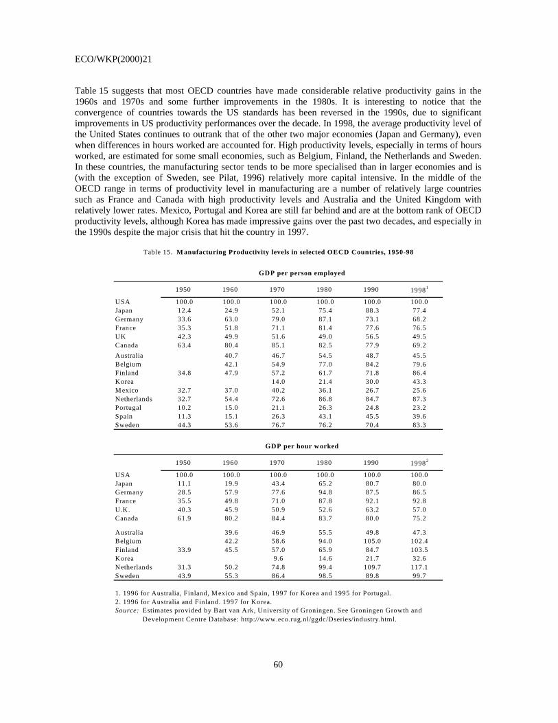
ECO/WKP(2000)21
60
Table 15 suggests that most OECD countries have made considerable relative productivity gains in the 1960s and 1970s and some further improvements in the 1980s. It is interesting to notice that the convergence of countries towards the US standards has been reversed in the 1990s, due to significant improvements in US productivity performances over the decade. In 1998, the average productivity level of the United States continues to outrank that of the other two major economies (Japan and Germany), even when differences in hours worked are accounted for. High productivity levels, especially in terms of hours worked, are estimated for some small economies, such as Belgium, Finland, the Netherlands and Sweden. In these countries, the manufacturing sector tends to be more specialised than in larger economies and is (with the exception of Sweden, see Pilat, 1996) relatively more capital intensive. In the middle of the OECD range in terms of productivity level in manufacturing are a number of relatively large countries such as France and Canada with high productivity levels and Australia and the United Kingdom with relatively lower rates. Mexico, Portugal and Korea are still far behind and are at the bottom rank of OECD productivity levels, although Korea has made impressive gains over the past two decades, and especially in the 1990s despite the major crisis that hit the country in 1997.
1950 1960 1970 1980 1990 19981
USA 100.0 100.0 100.0 100.0 100.0 100.0Japan 12.4 24.9 52.1 75.4 88.3 77.4Germany 33.6 63.0 79.0 87.1 73.1 68.2France 35.3 51.8 71.1 81.4 77.6 76.5UK 42.3 49.9 51.6 49.0 56.5 49.5Canada 63.4 80.4 85.1 82.5 77.9 69.2Australia 40.7 46.7 54.5 48.7 45.5Belgium 42.1 54.9 77.0 84.2 79.6Finland 34.8 47.9 57.2 61.7 71.8 86.4Korea 14.0 21.4 30.0 43.3M exico 32.7 37.0 40.2 36.1 26.7 25.6Netherlands 32.7 54.4 72.6 86.8 84.7 87.3Portugal 10.2 15.0 21.1 26.3 24.8 23.2Spain 11.3 15.1 26.3 43.1 45.5 39.6Sweden 44.3 53.6 76.7 76.2 70.4 83.3
1950 1960 1970 1980 1990 19982
USA 100.0 100.0 100.0 100.0 100.0 100.0Japan 11.1 19.9 43.4 65.2 80.7 80.0Germany 28.5 57.9 77.6 94.8 87.5 86.5France 35.5 49.8 71.0 87.8 92.1 92.8U.K. 40.3 45.9 50.9 52.6 63.2 57.0Canada 61.9 80.2 84.4 83.7 80.0 75.2
Australia 39.6 46.9 55.5 49.8 47.3Belgium 42.2 58.6 94.0 105.0 102.4Finland 33.9 45.5 57.0 65.9 84.7 103.5Korea 9.6 14.6 21.7 32.6Netherlands 31.3 50.2 74.8 99.4 109.7 117.1Sweden 43.9 55.3 86.4 98.5 89.8 99.7
1. 1996 for Australia, Finland, M exico and Spain, 1997 for Korea and 1995 for Portugal.2. 1996 for Australia and Finland. 1997 for Korea.Source: Estimates provided by Bart van Ark, University of Groningen. See Groningen Growth and Development Centre Database: http://www.eco.rug.nl/ggdc/Dseries/industry.html.
GDP per person employed
GDP per hour w orked
Table 15. M anufacturing Productivity levels in selected OECD Countries, 1950-98

ECO/WKP(2000)21
61
Summing up findings from the sectoral analysis
60. Differences in aggregate productivity performances can be explained by differences in both the economic structure of the OECD countries and in the productivity performances of individual industries. Available data suggest a significant degree of convergence in the sources of productivity growth amongst the OECD countries, i.e. the same industries provide the strongest contributions to aggregate productivity patterns, especially amongst the G7 economies. However, the ICT industry, at least so far, may have played a much stronger role in driving productivity performance in the United States than in most of the other countries. While productivity performance at the industry level tend to be associated with the effort to innovate (proxied by R&D intensity) in most countries, the relationship of productivity with both employment and human capital varies a great deal across the board, somewhat confirming differences observed at the aggregate level. Manufacturing data point to a strong role of skill-biased employment adjustment, which however has been associated with net employment losses in Continental Europe.63 This has been partially compensated by employment growth in - relatively less productive - service sectors reinforcing the negative correlation between productivity and employment at the aggregate level. While at the firm level, the association of labour productivity with changes in employment depends upon demand conditions, return to scale and technological innovation64, it is more difficult to use these concepts to explain observed country patterns at the aggregate and manufacturing levels. Relative wage rigidities, regulatory constraints and product market competition conditions are more likely to be behind poor employment performance in a number of European countries.65
61. Notwithstanding growth patterns in the past decade, there remains significant differences in the economic structure and individual sector productivity levels across the OECD countries. Structural shifts provide only a limited explanation of aggregate productivity patterns in most countries. This holds in particular for the manufacturing sector where a fine disaggregation of industries is available. For services the lack of evidence of a significant contribution of structural shifts to productivity performance in most countries has to be discounted for the lack of industry details which does not allow to identify shifts across detailed industries. Differences in productivity levels at the industry level remain important and may suggest that there is still scope for catching up to best practice in a number of countries. In manufacturing, the process of convergence of labour productivity to the US level has somewhat slowed down in the past decade over time and has even been reversed in the 1990s because of a speedup in US industries.
63. These results seem to be consistent with patterns observed at the firm levels. According to OECD (1998a),
productivity growth is almost equally due to successful upsizers (i.e. increasing labour productivity combined with rising employment) and successful downsizers (i.e. increasing labour productivity combined with falling employment) in the United States, Japan and the Netherlands but not in France where successful downsizers dominated in explaining increases in labour productivity in manufacturing.
64. The combination of increased employment and labour productivity can be explained by increased product demand combined with increasing return to scale, or technological innovation that allows firms to lower the price of output in the face of elastic product demand. By contrast, labour productivity growth with downsizing may indicate technological innovation combined with falling or inelastic demand (see Bartelsman et al., 1995; Baily et al., 1996).
65. The effects of rigidities in the product and labour markets on employment performances are extensively reviewed in the Jobs Strategy publications of the OECD. See in particular (OECD, 1999g) for a detailed overview of policy reforms and employment performance: the study suggests that there has been a close correlation between the effort of reform along the lines of the OECD Jobs Strategy and employment performances in the business sector.
ECO/WKP(2000)21
62
BIBLIOGRAPHY
ABRAMOVITZ, M. (1989), Thinking About Growth, Cambridge University Press, Cambridge.
APEL, M. and P. JANSSON (1999), “A Theory-Consistent Approach for Estimating Potential Output and the NAIRU”, Economics Letters, Vol. 64, 271-75.
ARK, B. VAN (1996), “Issues in Measurement and International Comparison of Productivity - An Overview”, in OECD (1996), Industry Productivity - International Comparison and Measurement Issues, Paris, pp. 19-47.
ARK, B. VAN (1996), “Sectoral Growth Accounting and Structural Change in Post-War Europe”, in: B. Van Ark and N.F.R. Crafts, eds., Quantitative Aspects of Post-War European Economic Growth, CEPR/Cambridge University Press, pp. 84-164.
ARK, B. VAN and R.H. McGUCKIN (1999), “International Comparisons of Labor Productivity and per Capita Income”, Monthly Labor Review, July 1999, pp. 33-41.
AUSTRALIAN BUREAU OF STATISTICS (1997), “Development of Annually Re-weighted Chain Volume Indexes in Australia’s National Accounts”, paper presented at the 1997 OECD/Eurostat meeting of National Accountants, mimeo.
AUSTRALIAN BUREAU OF STATISTICS (1999), Australian System of National Accounts 1997-98, ABS Catalogue 5204.0, April 23, Canberra.
BAILY, M.N. and H. GERBASCH (1995), “Efficiency in Manufacturing and the Need for Global Competition, Brookings Papers on Economic Activities; Microeconomics, pp. 307-358.
BAILY, M.N., E.J. BARTELSMAN and J. HALTIWANGER (1996), “Downsizing and Productivity Growth: Myth or Reality”, Small Business Economics. Vol. 8, No. 4, August, pp. 259-278.
BANERJEE, A., J. DOLADO, J.W. GALBRAITH and D.F. HENDRY (1993), Co-Integration, Error-Correction and the Econometric Analysis of Non-Stationary Data, Oxford University Press, Oxford.
BANERJEE, A., J.W. GALBRAITH and J. DOLADO (1990), “Dynamic Specification with the General Error Correction Form”, Oxford Bulletin of Economics and Statistics, Vol. 52, pp. 225-55.
BARRO, R.J. and J.W. LEE (1993), “International Comparisons of Edicational Attainment”, Journal of Monetary Economics, December, 32(3), pp. 363-394.
BARRO, R.J. and J.W. LEE (1996), “International Measures of Schooling Years and Schooling Quality”, American Economic Review, Papers and Proceedings, Vol. 86, No. 2, pp. 218-223.
BARRO, R.J. and X. SALA-I-MARTIN (1995), Economic Growth, MIT Press.
ECO/WKP(2000)21
63
BARRO, R.J. (1998), “Notes on Growth Accounting”, NBER Working Paper 6654, Cambridge, MA.
BÅRSDEN, G. (1989), “The Estimation of Long-Run Coefficients from Error-Correction Models”, Oxford Bulletin of Economics and Statistics, Vol. 51, pp. 345-50.
BARTELSMAN, E., G. van LEEUWEN and H.R. NIEUWENHUIJSEN (1995), “Downsizing and Productivity Growth: Myth and Reality, Netherlands Official Statistics, Autumn, pp. 23-28.
BAUMOL, W.J., S.A.B. BLACKMAN and E.N. WOLFF (1989), Productivity and American Leadership: The Long View, MIT Press, Cambridge, MA.
BECKER, G. (1975) “Human Capital”, Columbia University Press.
BERNARD, A.B. and C.I. JONES (1996a), “Comparing Apples to Oranges: Productivity Convergence and Measurement Across Industries and Countries”, American Economic Review, Vol. 86, No. 5, pp. 1216-1238. December.
BERNARD, A.B. and C.I. JONES (1996b), “Productivity across Industries and Countries: Time Series Theory and Evidence”, Review of Economics and Statistics.
BLISS, C. (1999), “Galton's Fallacy and Economic Convergence”, Oxford Economic Papers, 51(1), January, pp. 4-14.
BOONE, L. (2000), “Specifying the Hodrick-Prescott Multivariate Filter as an Unobserved Component Model”, OECD Economics Department Working Paper, forthcoming.
BRINJOLFSSON, E. and C. KEMERER (1996), “Network Externalities in Microcomputer Software: An Econometric Analysis of the Spreadsheet Market”, Management Science, Vol. 42, pp. 1627-1647.
BRINJOLFSSON, E. and L. HITT (1994), “Computers and Economic Growth: Firm Level Evidence”, MIT Sloan School of Management Working Paper No 3714.
BUREAU OF ECONOMIC ANALYSIS (1999), “Gross Domestic Product: Third Quarter 1999 (Advance) - Revised Estimates 1959-99”, October 28, Washington, D.C.
BUREAU OF LABOR STATISTICS (1993), “Labor Composition and U.S. Productivity Growth, 1948-90”, U.S. Department of Labor, Bureau of Labor Statistics, Bulletin 2426. December.
BUREAU OF LABOR STATISTICS (1999a), Multifactor Productivity Trends 1997, February 11.
BUREAU OF LABOR STATISTICS (1999b), Productivity and Costs, Revised Second-Quarter Measures, September 2.
BUTLER, L. (1996), “A Semi-Structural Approach to Estimate Potential Output: Combining Economic Theory with A Time-Series Filter”, Bank of Canada Technical Report No. 76, Ottawa.
CAMERON, G. (1998), “Catch-Up and Leapfrog between the USA and Japan”, Nuffield College, Oxford, mimeo.
COCKBURN, I.M and R.M. HENDERSON (1998) “Absorptive Capacity, Coauthoring Behavior, and the Organization of Research in Drug Discovery”, Journal of Industrial Economics, Vol. 46, pp. 157-82.
ECO/WKP(2000)21
64
COHEN, W. and D. LEVINTHAL (1989), Innovation and Learning: The Two Faces of R&D”, The Economic Journal, Vol. 99, pp. 569-596.
COLECCHIA, A., and G. PAPACONSTATINOU (1996), “The Evolution of Skills in OECD Countries and the Role of Technology”, OECD STI Working Papers, 1996/8.
CONFERENCE BOARD (1997), “Understanding Differences in Economic Performance”, Perspectives on a Global Economy, Report No. 1187-97-RR, Summer, New York.
CONWAY, P. and B. HUNT (1997), “Estimating Potential Output: A Semi-Structural Approach”, Bank of New Zealand Discussion Paper G97/9, Wellington.
COUNCIL OF ECONOMIC ADVISORS (2000), “Economic Report of the President - 2000”, February.
DE BOER, S, J. VAN DALEN and P. VERBIEST (1997), “The Use of Chain Indices in the Netherlands”, paper presented at the 1997 OECD/Eurostat meeting of National Accountants, Statistics Netherlands, mimeo.
DEAN, E.R. (1999), “The Accuracy of the BLS Productivity Measures”, Monthly Labor Review, February, pp. 24-34.
DEAN, E.R., M.J. HARPER and M.S. SHERWOOD (1996), “Productivity Measurement with Changing-Weight Indices of Outputs and Inputs”, in OECD (1996), Industry Productivity: International Comparison and Measurement Issues, Paris.
DENISON, E. (1985), “Trends in American Economic Growth: 1929-1982”, Brookings Institutions, Washington D.C.
DURAND, R. (1999), “Productivity Growth and Structural Changes in the Canadian Business Sector”, paper presented at the Pacific Economic Outlook Structure Specialists Meeting, Statistics Canada, September, mimeo.
ELDRIDGE, L.P. (1999), “How Price Indexes affect BLS Productivity Measures”, Monthly Labor Review, February, pp. 35-46.
ELTETO, O. and P. KOVES (1964), “On an Index Computation Problem in International Comparisons” (in Hungarian), Statistztikai Szemle, Vol. 42, 507-518.
ENGLANDER, S. and A. GURNEY (1994), “Medium-Term Determinants of OECD Productivity”, OECD Economic Studies, No. 22, Spring, pp. 49-109.
EUROSTAT (1997), Report of Eurostat Taskforce on Volume Measures, paper presented at the 1997 OECD/Eurostat meeting of National Accountants.
FISK, D. and D. FORTE (1997), “The Federal Productivity Measurement Program: Final Results”, Monthly Labor Review, May, pp. 19-28.
FIXLER, D. and D. SIEGEL (1999), “Outsourcing and Productivity Growth in Services”, Structural Change and Economic Dynamics, Vol. 10, pp. 177-194.

ECO/WKP(2000)21
65
FIXLER, D. and K. ZIESCHANG (1999), “The Productivity of the Banking Sector: Integrating Approaches to Measuring Financial Service Output”, Canadian Journal of Economics, Vol. 32, No. 2, pp. 547-569.
FORNI, M., and M. LIPPI (1997), Aggregation and the Microfoundations of Dynamic Macroeconomics, Oxford: Oxford University Press.
FOSTER, L, J. HALTIWANGER and C.J. KRIZAN (1998), “Aggregate Productivity Growth: Lessons from Microeconomic Evidence”, NBER Working Paper Series, No. 6803, November.
GANDAL, N., S. GREENSTEIN and D. SALANT (1999), “Adoptions and Orphans in the Early Microcomputer Market, Journal of Industrial Economics, Vol. 47, pp. 97-116.
GORDON, R.J. (1997), “The Time-Varying NAIRU and Its Implications for Economic Policy, Journal of Economic Perspectives, Vol. 11, 11-32.
GORDON, R.J. (1999), “Has the “New Economy” Rendered the Productivity Slowdown Obsolete?”, Northwestern University and NBER, mimeo.
GORT, M., S. JAFAREY and P. RUPERT (1999), “Defining Capital in Growth Models”, Federal Reserve Bank of Cleveland Economic Review, Vol. 32, n.2, pp. 19-23.
GREENWOOD, J., Z. HERCOWITZ and P. KRUSELL (1997), “Long-Run Implications of Investment-Specific Technological Change”, American Economic Review, Vol. 87, pp. 342-362.
GULLICKSON, W. and M.J. HARPER (1999), “Possible Measurement Bias in Aggregate Productivity Growth”, Monthly Labor Review, February, pp. 47-67.
HALL, R.E. (1990), “Invariance Properties of Solow‘s Productivity Residual”, in P. Diamond (ed.) “Growth, Productivity Unemployment”, The MIT Press, Cambridge Mass.
HALTIWANGER, J.C. (1997), “Measuring and Analyzing Aggregate Fluctuations: The Importance of Building from Microeconomic Evidence”, Federal Reserve Bank of St. Louis Review, May/June, pp. 55-77.
HARVEY, A.C. and A. JAEGER (1993), “Detrending, Stylized Facts and the Business Cycle”, Journal of Applied Econometrics, Vol. 8, 231-47.
HERCOWITZ, Z. (1998), “The “Embodiment” Controversy: A Review Essay”, Journal of Monetary Economics, Vol. 41, pp. 217-224.
HILL (1999); “The productive capital stock and the quantity index for flows of capital services”; Note to the OECD Expert Group on Capital Measurement, Washington D.C. meeting.
HO, M.S. and D.W. JORGENSON (1999), “The Quality of the U.S. Work Force, 1948-95”, Kennedy School of Government, Harvard Univ., mimeo.
HO, M.S., D.W. JORGENSON and K.J. STIROH (1999), “U.S. High-Tech Investment and the Pervasive Slowdown in the Growth of Capital Services”, mimeo.
HODRICK, R. and E. PRESCOTT (1997), “Post-war US Business Cycles: An Empirical Investigation”, Journal of Money, Credit and Banking, Vol. 29, 1-16.
ECO/WKP(2000)21
66
HOSTLAND, D. and D. COTÉ (1993), “Measuring Potential Output and the NAIRU as Unobserved Variables in a Systems Framework”, in Bank of Canada, Economic Behaviour and Policy Choice Under Price Stability, Ottawa.
JORGENSON, D.W. and Z. GRILICHES (1967), “The Explanation of Productivity Change”, Review of Economic Studies, Vol. 34, No. 3, July.
JORGENSON, D.W. (1963), “Capital Theory and Investment Behaviour”, American Economic Review; Vol. 53, No. 2, May.
JORGENSON, D.W., F.M. GOLLOP and B.M. FRAUMENI (1987), Productivity and U.S. Economic Growth, Amsterdam: North-Holland.
KRAVIS, I.B., A. HESTON and R. SUMMERS (1982), World Product and Income, Johns Hopkins University Press, Baltimore.
KRUSELL, P. (1998), “Investment-specific R&D and the Decline in the Relative Price of Capital”, Journal of Economic Growth, Vol. 3, pp. 131-141.
LANDEFELD, J.S. and R.P. PARKER (1997), “BEA’s Chain Indexes, Time Series, Measures of Long-Term Economic Growth”, Survey of Current Business, May, pp. 58-68.
LAXTON, D. and R. TETLOW (1992), “A Simple Multivariate Filter for the Measurement of Potential Output”, Bank of Canada, Technical Report, No. 59.
MACHIN, S. and J. van REENEN (1997), “Technology and Changes in Skill Structure: Evidence from Seven Countries”, Labour Market Consequences of Technical and Structural Changes Discussion Paper No. 24.
MACHIN, S. and J. van REENEN (1998), “Technology and Changes in Skill Structure: Evidence from Seven Countries”, Quarterly Journal of Economics, November.
MADDISON, A. (1991), Dynamic Forces in Capitalist Development, Oxford University Press, Oxford.
MADDISON, A. (1995), Monitoring the World Economy, 1980-1992, OECD Development Centre, Paris.
MINCER (1974), “Schooling, Experience and Earnings”, New York, Columbia University Press.
MOOSA, I.A. (1997), “A Cross-country Comparison of Okun’s Coefficient, Journal of Comparative Economics, Vol. 24, 335-56.
MORRISON, C.J. (1992), “Unraveling the Productivity Growth Slowdown in the United States, Canada, and Japan: The Effects of Subequilibrium, Scale Economies and Markups”, Review of Economics and Statistics, Vol. 74, pp. 381-393.
MOULTON, B.R., R.P. PARKER and E.P. SESKIN (1999), “A Preview of the 1999 Comprehensive Revision of the National Income and Product Accounts - Definitional and Classificational Changes”, Survey of Current Business, August, pp. 7-20, Bureau of Economic Analysis.
MOWERY, D.C. and J. OXLEY (1995) “Inward Technology Transfer and Competitiveness: The Role of National Innovation Systems”, Cambridge Journal of Economics; Vol. 19 pp. 67-93.

ECO/WKP(2000)21
67
OECD (1996), Industry Productivity - International Comparison and Measurement Issues, OECD, Paris.
OECD (1996a), Services: Measuring Real Value Added, Paris.
OECD (1996b), Industry Productivity - International Comparison and Measurement Issues, OECD, Paris.
OECD (1996c), Technology and Industrial Performance, OECD, Paris.
OECD (1997), “Review of the OECD-Eurostat PPP Program”, STD/PPP(97)5, Paris.
OECD (1997), OECD Report on Regulatory Reform - Volume II: Thematic Studies, Paris.
OECD (1998a), Science, Technology and Industry Outlook 1998, Paris.
OECD (1998b), Maintaining Prosperity in an Ageing Society, Paris.
OECD (1998c), Performance and Regulation Patterns in OECD Countries, ECO/CPE/WP1(98)15, Paris.
OECD (1998d), “Medium-Term Productivity Developments in OECD Countries: Determinants and Industry Contributions”, DSTI/EAS/IND/SWP(98)2, Paris.
OECD (1998e), OECD Economic Outlook, No. 64, December, Paris.
OECD (1998f), “Labour Input and Labour Composition measures by Industry: An Exploratory Analysis for the G7 Countries”, DSTI/EAS/IND/SWP(98)1, Paris.
OECD (1998g), “OECD Data on Skills, Employment by Industry and Occupation”, STI Working Paper 1998/4.
OECD (1999a), “Problems Related to the Overhaul of the National Accounts in OECD Countries and Other Statistical Issues”, ECO/CPE/STEP(99)8, Paris.
OECD (1999b), “OECD Manual on Productivity Measurement: A Guide to the Measurement of Industry-Level and Aggregate Productivity Growth”, DSTI/EAS/IND/SWP(99)2, Paris.
OECD (1999c), Implementing the OECD Jobs Strategy: Assessing Performance and Policy, Paris.
OECD (1999d), OECD Employment Outlook 1999, Paris.
OECD (1999e), OECD Science, Technology and Industry Scoreboard 1999, Paris.
OECD (1999f), National Accounts - Main Aggregates 1960-97, Paris.
OECD (1999g), OECD Economic Outlook, No. 66, December, Paris.
OECD (1999h), “High-Growth Firms and Employment”, DSTI/IND/PME(99)6, Paris.
OECD (1999i), Strategic Business Services, Paris.
OECD (2000a), “The Concept, Policy Use and Measurement of Structural Unemployment: Annex 2. Estimating a Time-Varying NAIRU Across 21 OECD Countries”, ECO/CPE/WP1(2000)2/ANN2, Paris.
ECO/WKP(2000)21
68
OECD (2000b), Purchasing Power Parities and Real Expenditures - 1996 Results, 1996 Edition, Paris.
OLINER, S.D. and D.E. SICHEL (2000), “The Resurgence of Growth in the Late 1990s: Are Computers the Story?”, forthcoming, Journal of Economic Perspectives.
OLIVEIRA MARTINS, J. and S. SCARPETTA (1999), “The Levels and Cyclical Behaviour of Mark-ups across Countries and Market Structures, OECD Economics Department Working Papers, No. 213.
PARHAM, D (1999), The New Economy? A New Look at Australia’s Productivity Performance, Productivity Commission Staff Research Paper, AusInfo, Canberra, May.
PASINETTI, L.L. (1993), Structural Economic Dynamics, Cambridge: Cambridge University Press.
PHILLIPS, P.C.B. and B. HANSEN (1990), “Statistical Inference in Instrumental Variable Regression with I(1) Processes”, Review of Economic Studies, Vol. 57, pp. 99-125.
PILAT, D. (1996), “Labour Productivity Levels in OECD Countries: Estimates for Manufacturing and Selected Service Sectors”, OECD Economics Department Working Papers, No. 169.
PILAT, D. (1997), “Competition, Productivity and Efficiency”, OECD Economic Studies, No. 27, 1996/II, pp. 107-145, OECD, Paris.
POMP, M. (1998), “Labour Productivity Growth and Low-Paid Work”, CPB Report, 98/1, the Netherlands.
PRODUCTIVITY COMMISSION (1999), Microeconomic Reform and Australian Productivity: Exploring the Links, forthcoming, November.
PSACHAROPOULOS, G. (1994), “Returns to Investment in Education: A Global Update”, World Development, Vol. 22, No. 9, pp. 1325-1343.
ROMER, P.M. (1986), “Increasing Returns and Long-Run Growth”, Journal of Political Economy, Vol. 94, pp. 1002-1034.
SAIKKONEN, P. (1991), “Asymptotically Efficient Estimation of Cointegration Regressions”, Econometric Theory, Vol. 7, pp. 1-21.
SCHREYER, P. (2000), “The Impact of Information and Communication Technology on Output Growth”; OECD STI Working Paper, 2000/2.
SENHADJI, A. (1999), “Sources of Economic Growth: An Extensive Growth Accounting Exercise”, IMF Working Paper, WP/99/77, Washington, D.C.
SESKIN, E.P. (1999), “Improved Estimates of the National Income and Product Accounts for 1959-98 - Results of the Comprehensive Revision”, Survey of Current Business, Vol. 79, December, pp. 15-43.
SHIN, Y. (1994), “A Residual-Based Test of the Null of Cointegration Against the Alternative of No Cointegration”, Econometric Theory, Vol. 10, pp. 91-115.
SOLOW, R.M. (1957), “Technical Change and the Aggregate Production Function”, Review of Economics and Statistics, Vol. 39, pp. 312-320.

ECO/WKP(2000)21
69
STATISTICS CANADA (1999), “Multifactor Productivity 1997”, The Daily, March 23.
STONEMAN, P. and P. DIEDEREN (1994), “Technology Diffusion and Public Policy”, Economic Journal, Vol. 104, July, pp. 918-30.
SZULC, B. (1964), “Index Numbers of Multilateral Regional Comparisons” (in Polish), Przeglad Statysticzny, Vol. 3, 239-254.
TIMMER, M.P. and A. SZIRMAI (1999), “Productivity Growth in Asian Manufacturing: The Unimportance of Structural Change”, Conference on Economic Growth, Trade and Technology, Eindhoven, October, mimeo.
UNITED NATIONS (1993), System of National Account 1993, New York.
WHELAN, K. (2000), “Computers, Obsolescence and Productivity”, Federal Reserve Board, February, mimeo.

ECO/WKP(2000)21
70
STATISTICAL ANNEX
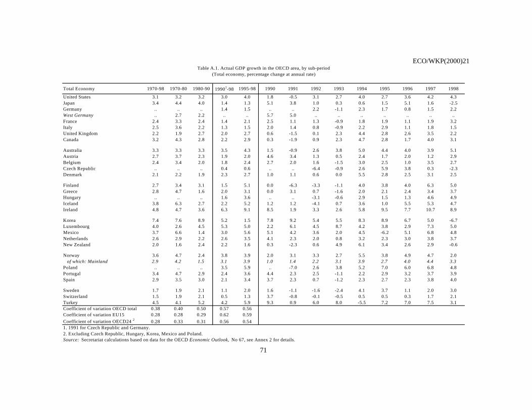
ECO/WKP(2000)21
71
Total Economy 1970-98 1970-80 1980-90 19901-98 1995-98 1990 1991 1992 1993 1994 1995 1996 1997 1998
United States 3.1 3.2 3.2 3.0 4.0 1.8 -0.5 3.1 2.7 4.0 2.7 3.6 4.2 4.3Japan 3.4 4.4 4.0 1.4 1.3 5.1 3.8 1.0 0.3 0.6 1.5 5.1 1.6 -2.5Germany .. .. .. 1.4 1.5 .. .. 2.2 -1.1 2.3 1.7 0.8 1.5 2.2West Germany .. 2.7 2.2 .. .. 5.7 5.0 .. .. .. .. .. .. ..France 2.4 3.3 2.4 1.4 2.1 2.5 1.1 1.3 -0.9 1.8 1.9 1.1 1.9 3.2Italy 2.5 3.6 2.2 1.3 1.5 2.0 1.4 0.8 -0.9 2.2 2.9 1.1 1.8 1.5United Kingdom 2.2 1.9 2.7 2.0 2.7 0.6 -1.5 0.1 2.3 4.4 2.8 2.6 3.5 2.2Canada 3.2 4.3 2.8 2.2 2.9 0.3 -1.9 0.9 2.3 4.7 2.8 1.7 4.0 3.1
Australia 3.3 3.3 3.3 3.5 4.3 1.5 -0.9 2.6 3.8 5.0 4.4 4.0 3.9 5.1Austria 2.7 3.7 2.3 1.9 2.0 4.6 3.4 1.3 0.5 2.4 1.7 2.0 1.2 2.9Belgium 2.4 3.4 2.0 1.8 2.4 2.7 2.0 1.6 -1.5 3.0 2.5 1.0 3.5 2.7Czech Republic .. .. .. 0.4 0.6 .. .. -6.4 -0.9 2.6 5.9 3.8 0.3 -2.3Denmark 2.1 2.2 1.9 2.3 2.7 1.0 1.1 0.6 0.0 5.5 2.8 2.5 3.1 2.5
Finland 2.7 3.4 3.1 1.5 5.1 0.0 -6.3 -3.3 -1.1 4.0 3.8 4.0 6.3 5.0Greece 2.8 4.7 1.6 2.0 3.1 0.0 3.1 0.7 -1.6 2.0 2.1 2.4 3.4 3.7Hungary .. .. .. 1.6 3.6 .. .. -3.1 -0.6 2.9 1.5 1.3 4.6 4.9Iceland 3.8 6.3 2.7 2.2 5.2 1.2 1.2 -4.1 0.7 3.6 1.0 5.5 5.3 4.7Ireland 4.8 4.7 3.6 6.3 9.1 8.5 1.9 3.3 2.6 5.8 9.5 7.7 10.7 8.9
Korea 7.4 7.6 8.9 5.2 1.5 7.8 9.2 5.4 5.5 8.3 8.9 6.7 5.0 -6.7Luxembourg 4.0 2.6 4.5 5.3 5.0 2.2 6.1 4.5 8.7 4.2 3.8 2.9 7.3 5.0Mexico 3.7 6.6 1.4 3.0 5.6 5.1 4.2 3.6 2.0 4.5 -6.2 5.1 6.8 4.8Netherlands 2.6 2.9 2.2 2.6 3.5 4.1 2.3 2.0 0.8 3.2 2.3 3.0 3.8 3.7New Zealand 2.0 1.6 2.4 2.2 1.6 0.3 -2.3 0.6 4.9 6.1 3.4 2.6 2.9 -0.6
Norway 3.6 4.7 2.4 3.8 3.9 2.0 3.1 3.3 2.7 5.5 3.8 4.9 4.7 2.0 of which: Mainland 2.9 4.2 1.5 3.1 3.9 1.0 1.4 2.2 3.1 3.9 2.7 4.0 4.4 3.3Poland .. .. .. 3.5 5.9 .. -7.0 2.6 3.8 5.2 7.0 6.0 6.8 4.8Portugal 3.4 4.7 2.9 2.4 3.6 4.4 2.3 2.5 -1.1 2.2 2.9 3.2 3.7 3.9Spain 2.9 3.5 3.0 2.1 3.4 3.7 2.3 0.7 -1.2 2.3 2.7 2.3 3.8 4.0
Sweden 1.7 1.9 2.1 1.1 2.0 1.6 -1.1 -1.6 -2.4 4.1 3.7 1.1 2.0 3.0Switzerland 1.5 1.9 2.1 0.5 1.3 3.7 -0.8 -0.1 -0.5 0.5 0.5 0.3 1.7 2.1Turkey 4.5 4.1 5.2 4.2 5.9 9.3 0.9 6.0 8.0 -5.5 7.2 7.0 7.5 3.1Coefficient of variation OECD total 0.38 0.40 0.50 0.57 0.56Coefficient of variation EU15 0.28 0.28 0.29 0.62 0.59Coefficient of variation OECD24 2 0.28 0.33 0.31 0.56 0.541. 1991 for Czech Republic and Germany.2. Excluding Czech Republic, Hungary, Korea, Mexico and Poland. Source: Secretariat calculations based on data for the OECD Economic Outlook, No 67, see Annex 2 for details.
Table A.1. Actual GDP growth in the OECD area, by sub-period(Total economy, percentage change at annual rate)
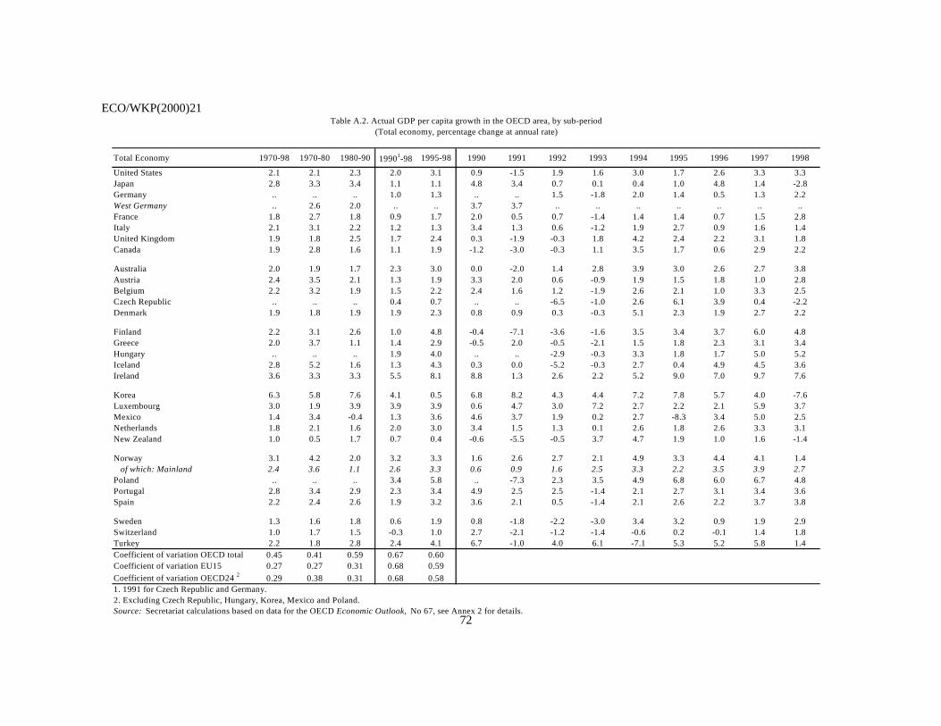
ECO/WKP(2000)21
72
Total Economy 1970-98 1970-80 1980-90 19901-98 1995-98 1990 1991 1992 1993 1994 1995 1996 1997 1998
United States 2.1 2.1 2.3 2.0 3.1 0.9 -1.5 1.9 1.6 3.0 1.7 2.6 3.3 3.3Japan 2.8 3.3 3.4 1.1 1.1 4.8 3.4 0.7 0.1 0.4 1.0 4.8 1.4 -2.8Germany .. .. .. 1.0 1.3 .. .. 1.5 -1.8 2.0 1.4 0.5 1.3 2.2West Germany .. 2.6 2.0 .. .. 3.7 3.7 .. .. .. .. .. .. ..France 1.8 2.7 1.8 0.9 1.7 2.0 0.5 0.7 -1.4 1.4 1.4 0.7 1.5 2.8Italy 2.1 3.1 2.2 1.2 1.3 3.4 1.3 0.6 -1.2 1.9 2.7 0.9 1.6 1.4United Kingdom 1.9 1.8 2.5 1.7 2.4 0.3 -1.9 -0.3 1.8 4.2 2.4 2.2 3.1 1.8Canada 1.9 2.8 1.6 1.1 1.9 -1.2 -3.0 -0.3 1.1 3.5 1.7 0.6 2.9 2.2
Australia 2.0 1.9 1.7 2.3 3.0 0.0 -2.0 1.4 2.8 3.9 3.0 2.6 2.7 3.8Austria 2.4 3.5 2.1 1.3 1.9 3.3 2.0 0.6 -0.9 1.9 1.5 1.8 1.0 2.8Belgium 2.2 3.2 1.9 1.5 2.2 2.4 1.6 1.2 -1.9 2.6 2.1 1.0 3.3 2.5Czech Republic .. .. .. 0.4 0.7 .. .. -6.5 -1.0 2.6 6.1 3.9 0.4 -2.2Denmark 1.9 1.8 1.9 1.9 2.3 0.8 0.9 0.3 -0.3 5.1 2.3 1.9 2.7 2.2
Finland 2.2 3.1 2.6 1.0 4.8 -0.4 -7.1 -3.6 -1.6 3.5 3.4 3.7 6.0 4.8Greece 2.0 3.7 1.1 1.4 2.9 -0.5 2.0 -0.5 -2.1 1.5 1.8 2.3 3.1 3.4Hungary .. .. .. 1.9 4.0 .. .. -2.9 -0.3 3.3 1.8 1.7 5.0 5.2Iceland 2.8 5.2 1.6 1.3 4.3 0.3 0.0 -5.2 -0.3 2.7 0.4 4.9 4.5 3.6Ireland 3.6 3.3 3.3 5.5 8.1 8.8 1.3 2.6 2.2 5.2 9.0 7.0 9.7 7.6
Korea 6.3 5.8 7.6 4.1 0.5 6.8 8.2 4.3 4.4 7.2 7.8 5.7 4.0 -7.6Luxembourg 3.0 1.9 3.9 3.9 3.9 0.6 4.7 3.0 7.2 2.7 2.2 2.1 5.9 3.7Mexico 1.4 3.4 -0.4 1.3 3.6 4.6 3.7 1.9 0.2 2.7 -8.3 3.4 5.0 2.5Netherlands 1.8 2.1 1.6 2.0 3.0 3.4 1.5 1.3 0.1 2.6 1.8 2.6 3.3 3.1New Zealand 1.0 0.5 1.7 0.7 0.4 -0.6 -5.5 -0.5 3.7 4.7 1.9 1.0 1.6 -1.4
Norway 3.1 4.2 2.0 3.2 3.3 1.6 2.6 2.7 2.1 4.9 3.3 4.4 4.1 1.4 of which: Mainland 2.4 3.6 1.1 2.6 3.3 0.6 0.9 1.6 2.5 3.3 2.2 3.5 3.9 2.7Poland .. .. .. 3.4 5.8 .. -7.3 2.3 3.5 4.9 6.8 6.0 6.7 4.8Portugal 2.8 3.4 2.9 2.3 3.4 4.9 2.5 2.5 -1.4 2.1 2.7 3.1 3.4 3.6Spain 2.2 2.4 2.6 1.9 3.2 3.6 2.1 0.5 -1.4 2.1 2.6 2.2 3.7 3.8
Sweden 1.3 1.6 1.8 0.6 1.9 0.8 -1.8 -2.2 -3.0 3.4 3.2 0.9 1.9 2.9Switzerland 1.0 1.7 1.5 -0.3 1.0 2.7 -2.1 -1.2 -1.4 -0.6 0.2 -0.1 1.4 1.8Turkey 2.2 1.8 2.8 2.4 4.1 6.7 -1.0 4.0 6.1 -7.1 5.3 5.2 5.8 1.4Coefficient of variation OECD total 0.45 0.41 0.59 0.67 0.60Coefficient of variation EU15 0.27 0.27 0.31 0.68 0.59Coefficient of variation OECD24 2 0.29 0.38 0.31 0.68 0.581. 1991 for Czech Republic and Germany.2. Excluding Czech Republic, Hungary, Korea, Mexico and Poland. Source: Secretariat calculations based on data for the OECD Economic Outlook, No 67, see Annex 2 for details.
Table A.2. Actual GDP per capita growth in the OECD area, by sub-period(Total economy, percentage change at annual rate)
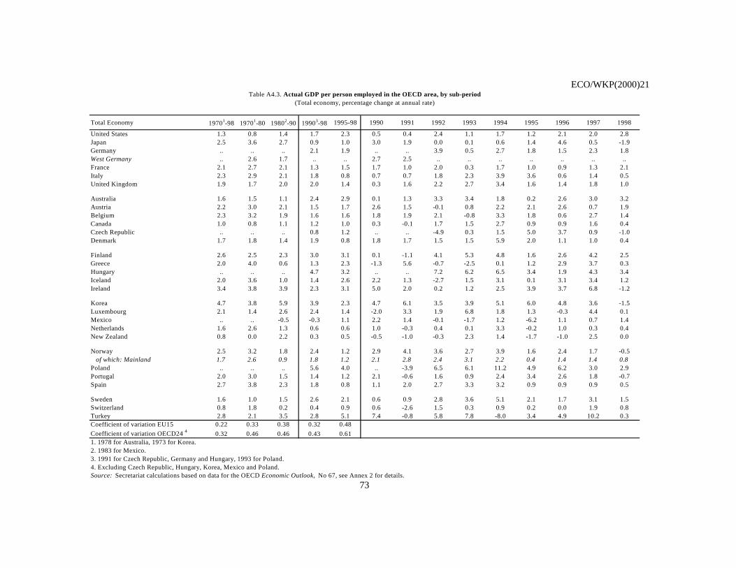
ECO/WKP(2000)21
73
Total Economy 19701-98 19701-80 19802-90 19903-98 1995-98 1990 1991 1992 1993 1994 1995 1996 1997 1998
United States 1.3 0.8 1.4 1.7 2.3 0.5 0.4 2.4 1.1 1.7 1.2 2.1 2.0 2.8Japan 2.5 3.6 2.7 0.9 1.0 3.0 1.9 0.0 0.1 0.6 1.4 4.6 0.5 -1.9Germany .. .. .. 2.1 1.9 .. .. 3.9 0.5 2.7 1.8 1.5 2.3 1.8West Germany .. 2.6 1.7 .. .. 2.7 2.5 .. .. .. .. .. .. ..France 2.1 2.7 2.1 1.3 1.5 1.7 1.0 2.0 0.3 1.7 1.0 0.9 1.3 2.1Italy 2.3 2.9 2.1 1.8 0.8 0.7 0.7 1.8 2.3 3.9 3.6 0.6 1.4 0.5United Kingdom 1.9 1.7 2.0 2.0 1.4 0.3 1.6 2.2 2.7 3.4 1.6 1.4 1.8 1.0
Australia 1.6 1.5 1.1 2.4 2.9 0.1 1.3 3.3 3.4 1.8 0.2 2.6 3.0 3.2Austria 2.2 3.0 2.1 1.5 1.7 2.6 1.5 -0.1 0.8 2.2 2.1 2.6 0.7 1.9Belgium 2.3 3.2 1.9 1.6 1.6 1.8 1.9 2.1 -0.8 3.3 1.8 0.6 2.7 1.4Canada 1.0 0.8 1.1 1.2 1.0 0.3 -0.1 1.7 1.5 2.7 0.9 0.9 1.6 0.4Czech Republic .. .. .. 0.8 1.2 .. .. -4.9 0.3 1.5 5.0 3.7 0.9 -1.0Denmark 1.7 1.8 1.4 1.9 0.8 1.8 1.7 1.5 1.5 5.9 2.0 1.1 1.0 0.4
Finland 2.6 2.5 2.3 3.0 3.1 0.1 -1.1 4.1 5.3 4.8 1.6 2.6 4.2 2.5Greece 2.0 4.0 0.6 1.3 2.3 -1.3 5.6 -0.7 -2.5 0.1 1.2 2.9 3.7 0.3Hungary .. .. .. 4.7 3.2 .. .. 7.2 6.2 6.5 3.4 1.9 4.3 3.4Iceland 2.0 3.6 1.0 1.4 2.6 2.2 1.3 -2.7 1.5 3.1 0.1 3.1 3.4 1.2Ireland 3.4 3.8 3.9 2.3 3.1 5.0 2.0 0.2 1.2 2.5 3.9 3.7 6.8 -1.2
Korea 4.7 3.8 5.9 3.9 2.3 4.7 6.1 3.5 3.9 5.1 6.0 4.8 3.6 -1.5Luxembourg 2.1 1.4 2.6 2.4 1.4 -2.0 3.3 1.9 6.8 1.8 1.3 -0.3 4.4 0.1Mexico .. .. -0.5 -0.3 1.1 2.2 1.4 -0.1 -1.7 1.2 -6.2 1.1 0.7 1.4Netherlands 1.6 2.6 1.3 0.6 0.6 1.0 -0.3 0.4 0.1 3.3 -0.2 1.0 0.3 0.4New Zealand 0.8 0.0 2.2 0.3 0.5 -0.5 -1.0 -0.3 2.3 1.4 -1.7 -1.0 2.5 0.0
Norway 2.5 3.2 1.8 2.4 1.2 2.9 4.1 3.6 2.7 3.9 1.6 2.4 1.7 -0.5 of which: Mainland 1.7 2.6 0.9 1.8 1.2 2.1 2.8 2.4 3.1 2.2 0.4 1.4 1.4 0.8Poland .. .. .. 5.6 4.0 .. -3.9 6.5 6.1 11.2 4.9 6.2 3.0 2.9Portugal 2.0 3.0 1.5 1.4 1.2 2.1 -0.6 1.6 0.9 2.4 3.4 2.6 1.8 -0.7Spain 2.7 3.8 2.3 1.8 0.8 1.1 2.0 2.7 3.3 3.2 0.9 0.9 0.9 0.5
Sweden 1.6 1.0 1.5 2.6 2.1 0.6 0.9 2.8 3.6 5.1 2.1 1.7 3.1 1.5Switzerland 0.8 1.8 0.2 0.4 0.9 0.6 -2.6 1.5 0.3 0.9 0.2 0.0 1.9 0.8Turkey 2.8 2.1 3.5 2.8 5.1 7.4 -0.8 5.8 7.8 -8.0 3.4 4.9 10.2 0.3Coefficient of variation EU15 0.22 0.33 0.38 0.32 0.48Coefficient of variation OECD24 4 0.32 0.46 0.46 0.43 0.611. 1978 for Australia, 1973 for Korea.2. 1983 for Mexico.3. 1991 for Czech Republic, Germany and Hungary, 1993 for Poland.4. Excluding Czech Republic, Hungary, Korea, Mexico and Poland. Source: Secretariat calculations based on data for the OECD Economic Outlook, No 67, see Annex 2 for details.
Table A4.3. Actual GDP per person employed in the OECD area, by sub-period(Total economy, percentage change at annual rate)
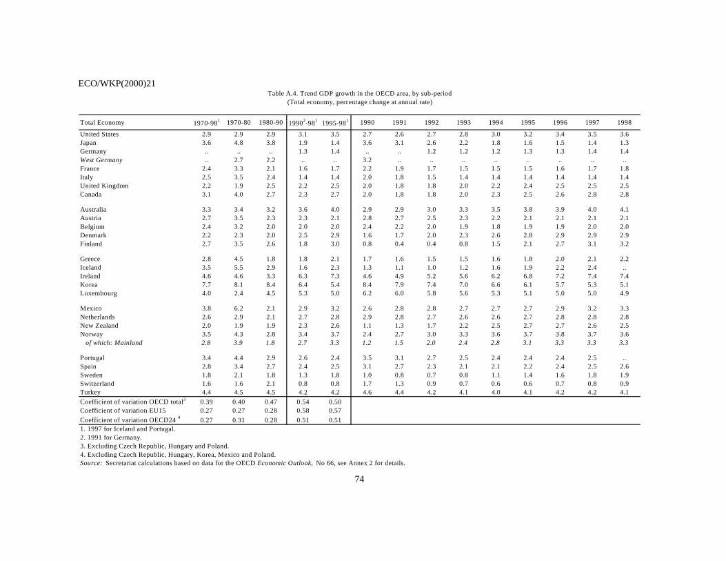
ECO/WKP(2000)21
74
Total Economy 1970-981 1970-80 1980-90 19902-981 1995-981 1990 1991 1992 1993 1994 1995 1996 1997 1998
United States 2.9 2.9 2.9 3.1 3.5 2.7 2.6 2.7 2.8 3.0 3.2 3.4 3.5 3.6Japan 3.6 4.8 3.8 1.9 1.4 3.6 3.1 2.6 2.2 1.8 1.6 1.5 1.4 1.3Germany .. .. .. 1.3 1.4 .. .. 1.2 1.2 1.2 1.3 1.3 1.4 1.4West Germany .. 2.7 2.2 .. .. 3.2 .. .. .. .. .. .. .. ..France 2.4 3.3 2.1 1.6 1.7 2.2 1.9 1.7 1.5 1.5 1.5 1.6 1.7 1.8Italy 2.5 3.5 2.4 1.4 1.4 2.0 1.8 1.5 1.4 1.4 1.4 1.4 1.4 1.4United Kingdom 2.2 1.9 2.5 2.2 2.5 2.0 1.8 1.8 2.0 2.2 2.4 2.5 2.5 2.5Canada 3.1 4.0 2.7 2.3 2.7 2.0 1.8 1.8 2.0 2.3 2.5 2.6 2.8 2.8
Australia 3.3 3.4 3.2 3.6 4.0 2.9 2.9 3.0 3.3 3.5 3.8 3.9 4.0 4.1Austria 2.7 3.5 2.3 2.3 2.1 2.8 2.7 2.5 2.3 2.2 2.1 2.1 2.1 2.1Belgium 2.4 3.2 2.0 2.0 2.0 2.4 2.2 2.0 1.9 1.8 1.9 1.9 2.0 2.0Denmark 2.2 2.3 2.0 2.5 2.9 1.6 1.7 2.0 2.3 2.6 2.8 2.9 2.9 2.9Finland 2.7 3.5 2.6 1.8 3.0 0.8 0.4 0.4 0.8 1.5 2.1 2.7 3.1 3.2
Greece 2.8 4.5 1.8 1.8 2.1 1.7 1.6 1.5 1.5 1.6 1.8 2.0 2.1 2.2Iceland 3.5 5.5 2.9 1.6 2.3 1.3 1.1 1.0 1.2 1.6 1.9 2.2 2.4 ..Ireland 4.6 4.6 3.3 6.3 7.3 4.6 4.9 5.2 5.6 6.2 6.8 7.2 7.4 7.4Korea 7.7 8.1 8.4 6.4 5.4 8.4 7.9 7.4 7.0 6.6 6.1 5.7 5.3 5.1Luxembourg 4.0 2.4 4.5 5.3 5.0 6.2 6.0 5.8 5.6 5.3 5.1 5.0 5.0 4.9
Mexico 3.8 6.2 2.1 2.9 3.2 2.6 2.8 2.8 2.7 2.7 2.7 2.9 3.2 3.3Netherlands 2.6 2.9 2.1 2.7 2.8 2.9 2.8 2.7 2.6 2.6 2.7 2.8 2.8 2.8New Zealand 2.0 1.9 1.9 2.3 2.6 1.1 1.3 1.7 2.2 2.5 2.7 2.7 2.6 2.5Norway 3.5 4.3 2.8 3.4 3.7 2.4 2.7 3.0 3.3 3.6 3.7 3.8 3.7 3.6 of which: Mainland 2.8 3.9 1.8 2.7 3.3 1.2 1.5 2.0 2.4 2.8 3.1 3.3 3.3 3.3
Portugal 3.4 4.4 2.9 2.6 2.4 3.5 3.1 2.7 2.5 2.4 2.4 2.4 2.5 ..Spain 2.8 3.4 2.7 2.4 2.5 3.1 2.7 2.3 2.1 2.1 2.2 2.4 2.5 2.6Sweden 1.8 2.1 1.8 1.3 1.8 1.0 0.8 0.7 0.8 1.1 1.4 1.6 1.8 1.9Switzerland 1.6 1.6 2.1 0.8 0.8 1.7 1.3 0.9 0.7 0.6 0.6 0.7 0.8 0.9Turkey 4.4 4.5 4.5 4.2 4.2 4.6 4.4 4.2 4.1 4.0 4.1 4.2 4.2 4.1Coefficient of variation OECD total3 0.39 0.40 0.47 0.54 0.50Coefficient of variation EU15 0.27 0.27 0.28 0.58 0.57Coefficient of variation OECD24 4 0.27 0.31 0.28 0.51 0.511. 1997 for Iceland and Portugal.2. 1991 for Germany.3. Excluding Czech Republic, Hungary and Poland.4. Excluding Czech Republic, Hungary, Korea, Mexico and Poland. Source: Secretariat calculations based on data for the OECD Economic Outlook, No 66, see Annex 2 for details.
Table A.4. Trend GDP growth in the OECD area, by sub-period(Total economy, percentage change at annual rate)
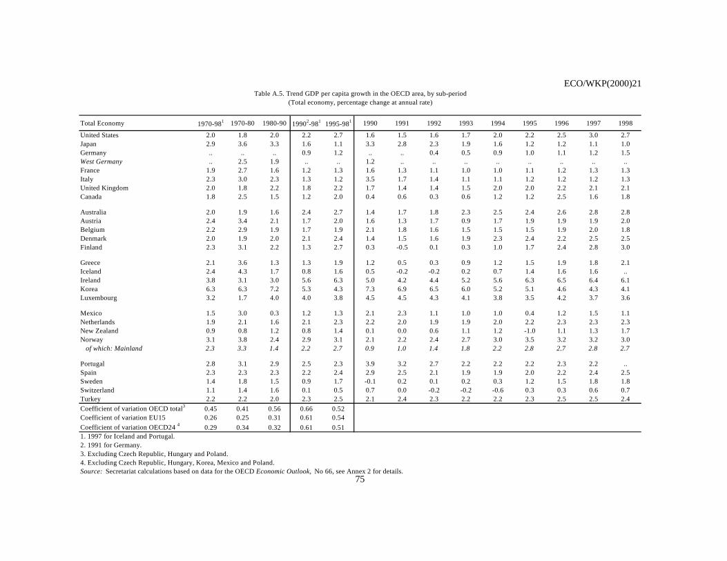
ECO/WKP(2000)21
75
Total Economy 1970-981 1970-80 1980-90 19902-981 1995-981 1990 1991 1992 1993 1994 1995 1996 1997 1998
United States 2.0 1.8 2.0 2.2 2.7 1.6 1.5 1.6 1.7 2.0 2.2 2.5 3.0 2.7Japan 2.9 3.6 3.3 1.6 1.1 3.3 2.8 2.3 1.9 1.6 1.2 1.2 1.1 1.0Germany .. .. .. 0.9 1.2 .. .. 0.4 0.5 0.9 1.0 1.1 1.2 1.5West Germany .. 2.5 1.9 .. .. 1.2 .. .. .. .. .. .. .. ..France 1.9 2.7 1.6 1.2 1.3 1.6 1.3 1.1 1.0 1.0 1.1 1.2 1.3 1.3Italy 2.3 3.0 2.3 1.3 1.2 3.5 1.7 1.4 1.1 1.1 1.2 1.2 1.2 1.3United Kingdom 2.0 1.8 2.2 1.8 2.2 1.7 1.4 1.4 1.5 2.0 2.0 2.2 2.1 2.1Canada 1.8 2.5 1.5 1.2 2.0 0.4 0.6 0.3 0.6 1.2 1.2 2.5 1.6 1.8
Australia 2.0 1.9 1.6 2.4 2.7 1.4 1.7 1.8 2.3 2.5 2.4 2.6 2.8 2.8Austria 2.4 3.4 2.1 1.7 2.0 1.6 1.3 1.7 0.9 1.7 1.9 1.9 1.9 2.0Belgium 2.2 2.9 1.9 1.7 1.9 2.1 1.8 1.6 1.5 1.5 1.5 1.9 2.0 1.8Denmark 2.0 1.9 2.0 2.1 2.4 1.4 1.5 1.6 1.9 2.3 2.4 2.2 2.5 2.5Finland 2.3 3.1 2.2 1.3 2.7 0.3 -0.5 0.1 0.3 1.0 1.7 2.4 2.8 3.0
Greece 2.1 3.6 1.3 1.3 1.9 1.2 0.5 0.3 0.9 1.2 1.5 1.9 1.8 2.1Iceland 2.4 4.3 1.7 0.8 1.6 0.5 -0.2 -0.2 0.2 0.7 1.4 1.6 1.6 ..Ireland 3.8 3.1 3.0 5.6 6.3 5.0 4.2 4.4 5.2 5.6 6.3 6.5 6.4 6.1Korea 6.3 6.3 7.2 5.3 4.3 7.3 6.9 6.5 6.0 5.2 5.1 4.6 4.3 4.1Luxembourg 3.2 1.7 4.0 4.0 3.8 4.5 4.5 4.3 4.1 3.8 3.5 4.2 3.7 3.6
Mexico 1.5 3.0 0.3 1.2 1.3 2.1 2.3 1.1 1.0 1.0 0.4 1.2 1.5 1.1Netherlands 1.9 2.1 1.6 2.1 2.3 2.2 2.0 1.9 1.9 2.0 2.2 2.3 2.3 2.3New Zealand 0.9 0.8 1.2 0.8 1.4 0.1 0.0 0.6 1.1 1.2 -1.0 1.1 1.3 1.7Norway 3.1 3.8 2.4 2.9 3.1 2.1 2.2 2.4 2.7 3.0 3.5 3.2 3.2 3.0 of which: Mainland 2.3 3.3 1.4 2.2 2.7 0.9 1.0 1.4 1.8 2.2 2.8 2.7 2.8 2.7
Portugal 2.8 3.1 2.9 2.5 2.3 3.9 3.2 2.7 2.2 2.2 2.2 2.3 2.2 ..Spain 2.3 2.3 2.3 2.2 2.4 2.9 2.5 2.1 1.9 1.9 2.0 2.2 2.4 2.5Sweden 1.4 1.8 1.5 0.9 1.7 -0.1 0.2 0.1 0.2 0.3 1.2 1.5 1.8 1.8Switzerland 1.1 1.4 1.6 0.1 0.5 0.7 0.0 -0.2 -0.2 -0.6 0.3 0.3 0.6 0.7Turkey 2.2 2.2 2.0 2.3 2.5 2.1 2.4 2.3 2.2 2.2 2.3 2.5 2.5 2.4Coefficient of variation OECD total3 0.45 0.41 0.56 0.66 0.52Coefficient of variation EU15 0.26 0.25 0.31 0.61 0.54Coefficient of variation OECD24 4 0.29 0.34 0.32 0.61 0.511. 1997 for Iceland and Portugal.2. 1991 for Germany.3. Excluding Czech Republic, Hungary and Poland.4. Excluding Czech Republic, Hungary, Korea, Mexico and Poland. Source: Secretariat calculations based on data for the OECD Economic Outlook, No 66, see Annex 2 for details.
Table A.5. Trend GDP per capita growth in the OECD area, by sub-period(Total economy, percentage change at annual rate)
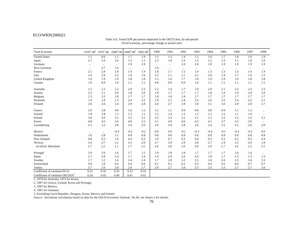
ECO/WKP(2000)21
76
Total Economy 19701-982 19701-80 19803-90 19904-982 1995-982 1990 1991 1992 1993 1994 1995 1996 1997 1998
United States 1.1 0.6 1.1 1.7 1.9 1.3 1.3 1.4 1.5 1.6 1.7 1.8 1.9 1.9Japan 2.7 3.9 2.6 1.3 1.1 2.3 1.9 1.6 1.3 1.2 1.2 1.1 1.0 1.0Germany .. .. .. 1.9 1.9 .. .. 2.0 2.0 2.0 1.9 1.9 1.9 1.9West Germany .. 2.7 1.6 .. .. 1.9 .. .. .. .. .. .. .. ..France 2.1 2.8 1.9 1.4 1.4 1.8 1.7 1.5 1.4 1.3 1.3 1.3 1.4 1.4Italy 2.4 2.9 2.2 1.9 1.6 2.2 2.1 2.1 2.1 2.0 1.9 1.7 1.6 1.5United Kingdom 1.9 1.9 1.9 1.8 1.9 1.5 1.6 1.7 1.9 1.9 1.9 1.9 1.8 1.8Canada 1.0 0.9 1.0 1.1 1.1 0.8 0.9 0.9 1.0 1.1 1.1 1.1 1.1 1.1
Australia 1.5 1.3 1.2 2.0 2.3 1.2 1.4 1.7 1.9 2.0 2.1 2.2 2.3 2.3Austria 2.3 3.1 2.0 1.8 2.0 1.8 1.7 1.7 1.7 1.8 1.9 1.9 2.0 2.0Belgium 2.3 3.2 1.8 1.7 1.7 1.8 1.8 1.8 1.7 1.7 1.7 1.7 1.7 1.7Denmark 1.9 1.8 1.5 2.4 2.2 1.9 2.1 2.4 2.6 2.6 2.5 2.4 2.2 2.1Finland 2.6 2.6 2.4 2.9 2.8 2.6 2.7 2.8 3.0 3.1 3.0 2.9 2.8 2.7
Greece 2.0 3.8 0.9 1.0 1.2 1.2 1.1 0.9 0.8 0.8 0.9 1.1 1.3 ..Iceland 1.8 2.8 1.3 1.2 1.1 1.5 1.4 1.3 1.2 1.2 1.2 1.1 1.0 ..Ireland 3.6 4.0 3.5 3.2 3.2 3.5 3.3 3.2 3.1 3.1 3.2 3.2 3.2 3.1Korea 4.8 4.5 5.6 4.0 3.2 5.1 4.9 4.6 4.3 4.1 3.7 3.3 3.0 ..Luxembourg 2.1 1.2 2.8 2.4 2.0 3.0 2.9 2.8 2.6 2.4 2.2 2.1 2.0 2.0
Mexico .. .. -0.4 -0.2 -0.2 0.0 0.0 -0.1 -0.3 -0.4 -0.5 -0.3 -0.2 0.0Netherlands 1.6 2.8 1.1 0.8 0.8 0.8 0.8 0.8 0.8 0.8 0.8 0.8 0.8 0.8New Zealand 0.8 0.2 1.6 0.4 0.3 1.0 0.7 0.5 0.4 0.3 0.2 0.2 0.3 0.4Norway 2.4 2.7 2.1 2.5 2.0 2.7 2.9 2.9 2.8 2.7 2.4 2.2 2.0 1.8 of which: Mainland 1.7 2.2 1.1 1.7 1.5 1.6 1.8 1.9 2.0 1.9 1.7 1.6 1.5 1.5
Portugal 2.0 2.6 1.6 1.7 1.5 1.9 1.8 1.8 1.7 1.7 1.7 1.6 1.4 ..Spain 2.7 3.8 2.4 1.7 1.4 1.9 2.0 2.0 2.0 1.8 1.7 1.5 1.3 1.3Sweden 1.7 1.2 1.6 2.4 2.4 1.7 2.0 2.2 2.5 2.6 2.6 2.5 2.4 2.3Switzerland 0.8 1.6 0.4 0.4 0.6 0.1 0.1 0.2 0.3 0.4 0.5 0.6 0.7 0.7Turkey 2.7 2.6 2.8 2.6 2.7 2.8 2.7 2.6 2.5 2.5 2.5 2.7 2.7 2.6Coefficient of variation EU15 0.22 0.32 0.33 0.33 0.33Coefficient of variation OECD245 0.34 0.45 0.40 0.41 0.411. 1978 for Australia, 1973 for Korea.2. 1997 for Greece, Iceland, Korea and Portugal.3. 1983 for Mexico.4. 1991 for Germany.5. Excluding Czech Republic, Hungary, Korea, Mexico and Poland. Source: Secretariat calculations based on data for the OECD Economic Outlook, No 66, see Annex 2 for details.
Table A.6. Trend GDP per person employed in the OECD area, by sub-period(Total economy, percentage change at annual rate)
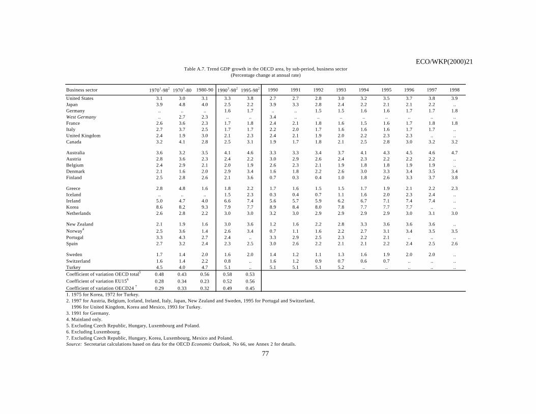
ECO/WKP(2000)21
77
Business sector 19701-982 19701-80 1980-90 19903-982 1995-982 1990 1991 1992 1993 1994 1995 1996 1997 1998
United States 3.1 3.0 3.1 3.3 3.8 2.7 2.7 2.8 3.0 3.2 3.5 3.7 3.8 3.9Japan 3.9 4.8 4.0 2.5 2.2 3.9 3.3 2.8 2.4 2.2 2.1 2.1 2.2 ..Germany .. .. .. 1.6 1.7 .. .. 1.5 1.5 1.6 1.6 1.7 1.7 1.8West Germany .. 2.7 2.3 .. .. 3.4 .. .. .. .. .. .. .. ..France 2.6 3.6 2.3 1.7 1.8 2.4 2.1 1.8 1.6 1.5 1.6 1.7 1.8 1.8Italy 2.7 3.7 2.5 1.7 1.7 2.2 2.0 1.7 1.6 1.6 1.6 1.7 1.7 ..United Kingdom 2.4 1.9 3.0 2.1 2.3 2.4 2.1 1.9 2.0 2.2 2.3 2.3 .. ..Canada 3.2 4.1 2.8 2.5 3.1 1.9 1.7 1.8 2.1 2.5 2.8 3.0 3.2 3.2
Australia 3.6 3.2 3.5 4.1 4.6 3.3 3.3 3.4 3.7 4.1 4.3 4.5 4.6 4.7Austria 2.8 3.6 2.3 2.4 2.2 3.0 2.9 2.6 2.4 2.3 2.2 2.2 2.2 ..Belgium 2.4 2.9 2.1 2.0 1.9 2.6 2.3 2.1 1.9 1.8 1.8 1.9 1.9 ..Denmark 2.1 1.6 2.0 2.9 3.4 1.6 1.8 2.2 2.6 3.0 3.3 3.4 3.5 3.4Finland 2.5 2.8 2.6 2.1 3.6 0.7 0.3 0.4 1.0 1.8 2.6 3.3 3.7 3.8
Greece 2.8 4.8 1.6 1.8 2.2 1.7 1.6 1.5 1.5 1.7 1.9 2.1 2.2 2.3Iceland .. .. .. 1.5 2.3 0.3 0.4 0.7 1.1 1.6 2.0 2.3 2.4 ..Ireland 5.0 4.7 4.0 6.6 7.4 5.6 5.7 5.9 6.2 6.7 7.1 7.4 7.4 ..Korea 8.6 8.2 9.3 7.9 7.7 8.9 8.4 8.0 7.8 7.7 7.7 7.7 .. ..Netherlands 2.6 2.8 2.2 3.0 3.0 3.2 3.0 2.9 2.9 2.9 2.9 3.0 3.1 3.0
New Zealand 2.1 1.9 1.6 3.0 3.6 1.2 1.6 2.2 2.8 3.3 3.6 3.6 3.6 ..Norway4 2.5 3.6 1.4 2.6 3.4 0.7 1.1 1.6 2.2 2.7 3.1 3.4 3.5 3.5Portugal 3.3 4.3 2.7 2.4 .. 3.3 2.9 2.5 2.3 2.2 2.1 .. .. ..Spain 2.7 3.2 2.4 2.3 2.5 3.0 2.6 2.2 2.1 2.1 2.2 2.4 2.5 2.6
Sweden 1.7 1.4 2.0 1.6 2.0 1.4 1.2 1.1 1.3 1.6 1.9 2.0 2.0 ..Switzerland 1.6 1.4 2.2 0.8 .. 1.6 1.2 0.9 0.7 0.6 0.7 .. .. ..Turkey 4.5 4.0 4.7 5.1 .. 5.1 5.1 5.1 5.2 .. .. .. .. ..Coefficient of variation OECD total5 0.48 0.43 0.56 0.58 0.53Coefficient of variation EU156 0.28 0.34 0.23 0.52 0.56Coefficient of variation OECD24 7 0.29 0.33 0.32 0.49 0.451. 1975 for Korea, 1972 for Turkey.2. 1997 for Austria, Belgium, Iceland, Ireland, Italy, Japan, New Zealand and Sweden, 1995 for Portugal and Switzerland, 1996 for United Kingdom, Korea and Mexico, 1993 for Turkey.3. 1991 for Germany.4. Mainland only.5. Excluding Czech Republic, Hungary, Luxembourg and Poland.6. Excluding Luxembourg.7. Excluding Czech Republic, Hungary, Korea, Luxembourg, Mexico and Poland. Source: Secretariat calculations based on data for the OECD Economic Outlook, No 66, see Annex 2 for details.
Table A.7. Trend GDP growth in the OECD area, by sub-period, business sector(Percentage change at annual rate)
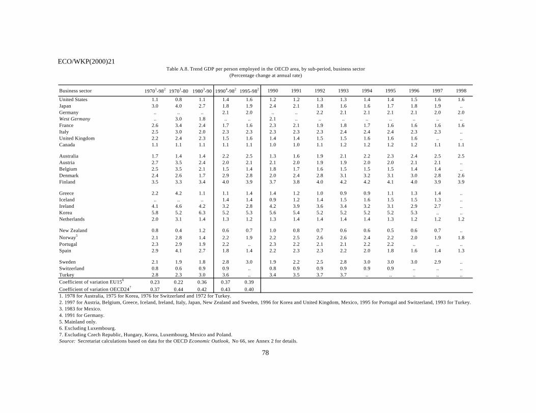
ECO/WKP(2000)21
78
Business sector 19701-982 19701-80 19803-90 19904-982 1995-982 1990 1991 1992 1993 1994 1995 1996 1997 1998
United States 1.1 0.8 1.1 1.4 1.6 1.2 1.2 1.3 1.3 1.4 1.4 1.5 1.6 1.6Japan 3.0 4.0 2.7 1.8 1.9 2.4 2.1 1.8 1.6 1.6 1.7 1.8 1.9 ..Germany .. .. .. 2.1 2.0 .. .. 2.2 2.1 2.1 2.1 2.1 2.0 2.0West Germany .. 3.0 1.8 .. .. 2.1 .. .. .. .. .. .. .. ..France 2.6 3.4 2.4 1.7 1.6 2.3 2.1 1.9 1.8 1.7 1.6 1.6 1.6 1.6Italy 2.5 3.0 2.0 2.3 2.3 2.3 2.3 2.3 2.4 2.4 2.4 2.3 2.3 ..United Kingdom 2.2 2.4 2.3 1.5 1.6 1.4 1.4 1.5 1.5 1.6 1.6 1.6 .. ..Canada 1.1 1.1 1.1 1.1 1.1 1.0 1.0 1.1 1.2 1.2 1.2 1.2 1.1 1.1
Australia 1.7 1.4 1.4 2.2 2.5 1.3 1.6 1.9 2.1 2.2 2.3 2.4 2.5 2.5Austria 2.7 3.5 2.4 2.0 2.1 2.1 2.0 1.9 1.9 2.0 2.0 2.1 2.1 ..Belgium 2.5 3.5 2.1 1.5 1.4 1.8 1.7 1.6 1.5 1.5 1.5 1.4 1.4 ..Denmark 2.4 2.6 1.7 2.9 2.8 2.0 2.4 2.8 3.1 3.2 3.1 3.0 2.8 2.6Finland 3.5 3.3 3.4 4.0 3.9 3.7 3.8 4.0 4.2 4.2 4.1 4.0 3.9 3.9
Greece 2.2 4.2 1.1 1.1 1.4 1.4 1.2 1.0 0.9 0.9 1.1 1.3 1.4 ..Iceland .. .. .. 1.4 1.4 0.9 1.2 1.4 1.5 1.6 1.5 1.5 1.3 ..Ireland 4.1 4.6 4.2 3.2 2.8 4.2 3.9 3.6 3.4 3.2 3.1 2.9 2.7 ..Korea 5.8 5.2 6.3 5.2 5.3 5.6 5.4 5.2 5.2 5.2 5.2 5.3 .. ..Netherlands 2.0 3.1 1.4 1.3 1.2 1.3 1.4 1.4 1.4 1.4 1.3 1.2 1.2 1.2
New Zealand 0.8 0.4 1.2 0.6 0.7 1.0 0.8 0.7 0.6 0.6 0.5 0.6 0.7 ..Norway5 2.1 2.8 1.4 2.2 1.9 2.2 2.5 2.6 2.6 2.4 2.2 2.0 1.9 1.8Portugal 2.3 2.9 1.9 2.2 .. 2.3 2.2 2.1 2.1 2.2 2.2 .. .. ..Spain 2.9 4.1 2.7 1.8 1.4 2.2 2.3 2.3 2.2 2.0 1.8 1.6 1.4 1.3
Sweden 2.1 1.9 1.8 2.8 3.0 1.9 2.2 2.5 2.8 3.0 3.0 3.0 2.9 ..Switzerland 0.8 0.6 0.9 0.9 .. 0.8 0.9 0.9 0.9 0.9 0.9 .. .. ..Turkey 2.8 2.3 3.0 3.6 .. 3.4 3.5 3.7 3.7 .. .. .. .. ..Coefficient of variation EU156 0.23 0.22 0.36 0.37 0.39Coefficient of variation OECD247 0.37 0.44 0.42 0.43 0.401. 1978 for Australia, 1975 for Korea, 1976 for Switzerland and 1972 for Turkey.2. 1997 for Austria, Belgium, Greece, Iceland, Ireland, Italy, Japan, New Zealand and Sweden, 1996 for Korea and United Kingdom, Mexico, 1995 for Portugal and Switzerland, 1993 for Turkey. 3. 1983 for Mexico.4. 1991 for Germany. 5. Mainland only.6. Excluding Luxembourg.7. Excluding Czech Republic, Hungary, Korea, Luxembourg, Mexico and Poland. Source: Secretariat calculations based on data for the OECD Economic Outlook, No 66, see Annex 2 for details.
Table A.8. Trend GDP per person employed in the OECD area, by sub-period, business sector(Percentage change at annual rate)
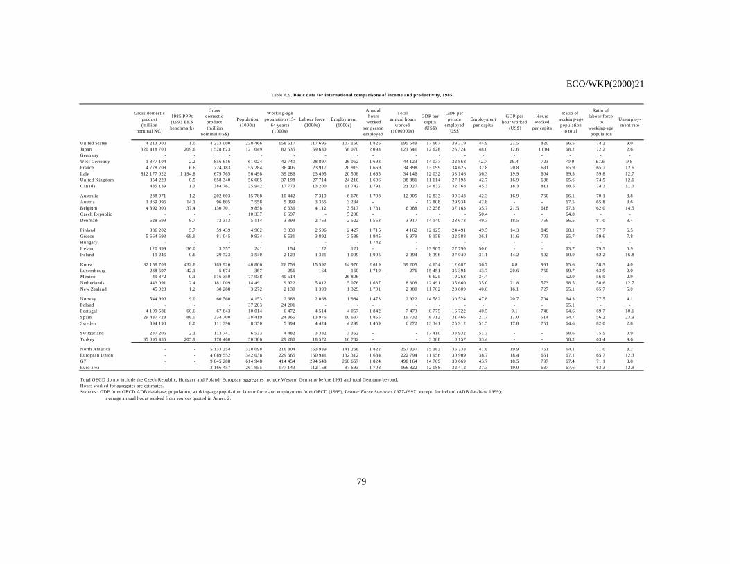
ECO/WKP(2000)21
79
Gross domesticproduct (million
nominal NC)
1985 PPPs (1993 EKS benchmark)
Gross domestic product (million
nominal US$)
Population (1000s)
Working-age population (15-
64 years) (1000s)
Labour force (1000s)
Employment (1000s)
Annual hours
worked per person employed
Total annual hours
worked (1000000s)
GDP per capita (US$)
GDP per person
employed (US$)
Employment per capita
GDP per hour worked
(US$)
Hours worked
per capita
Ratio of working-age population
to total
Ratio of labour force
to working-age population
Unemploy-ment rate
United States 4 213 000 1.0 4 213 000 238 466 158 517 117 695 107 150 1 825 195 549 17 667 39 319 44.9 21.5 820 66.5 74.2 9.0Japan 320 418 700 209.6 1 528 623 121 049 82 535 59 630 58 070 2 093 121 541 12 628 26 324 48.0 12.6 1 004 68.2 72.2 2.6Germany - - - - - - - - - - - - - - - - -West Germany 1 877 104 2.2 856 616 61 024 42 740 28 897 26 062 1 693 44 123 14 037 32 868 42.7 19.4 723 70.0 67.6 9.8France 4 778 709 6.6 724 183 55 284 36 405 23 917 20 915 1 669 34 898 13 099 34 625 37.8 20.8 631 65.9 65.7 12.6Italy 812 177 022 1 194.8 679 765 56 498 39 286 23 495 20 508 1 665 34 146 12 032 33 146 36.3 19.9 604 69.5 59.8 12.7United Kingdom 354 229 0.5 658 340 56 685 37 198 27 714 24 210 1 606 38 881 11 614 27 193 42.7 16.9 686 65.6 74.5 12.6Canada 485 139 1.3 384 761 25 942 17 773 13 200 11 742 1 791 21 027 14 832 32 768 45.3 18.3 811 68.5 74.3 11.0
Australia 238 071 1.2 202 603 15 788 10 442 7 319 6 676 1 798 12 005 12 833 30 348 42.3 16.9 760 66.1 70.1 8.8Austria 1 369 095 14.1 96 805 7 558 5 099 3 355 3 234 - - 12 808 29 934 42.8 - - 67.5 65.8 3.6Belgium 4 892 000 37.4 130 701 9 858 6 636 4 112 3 517 1 731 6 088 13 258 37 163 35.7 21.5 618 67.3 62.0 14.5Czech Republic - - - 10 337 6 697 - 5 208 - - - - 50.4 - - 64.8 - -Denmark 628 699 8.7 72 313 5 114 3 399 2 753 2 522 1 553 3 917 14 140 28 673 49.3 18.5 766 66.5 81.0 8.4
Finland 336 202 5.7 59 439 4 902 3 339 2 596 2 427 1 715 4 162 12 125 24 491 49.5 14.3 849 68.1 77.7 6.5Greece 5 664 693 69.9 81 045 9 934 6 531 3 892 3 588 1 945 6 979 8 158 22 588 36.1 11.6 703 65.7 59.6 7.8Hungary - - - - - - - 1 742 - - - - - - - - -Iceland 120 899 36.0 3 357 241 154 122 121 - - 13 907 27 790 50.0 - - 63.7 79.3 0.9Ireland 19 245 0.6 29 723 3 540 2 123 1 321 1 099 1 905 2 094 8 396 27 040 31.1 14.2 592 60.0 62.2 16.8
Korea 82 158 708 432.6 189 926 40 806 26 759 15 592 14 970 2 619 39 205 4 654 12 687 36.7 4.8 961 65.6 58.3 4.0Luxembourg 238 597 42.1 5 674 367 256 164 160 1 719 276 15 451 35 394 43.7 20.6 750 69.7 63.9 2.0Mexico 49 872 0.1 516 350 77 938 40 514 - 26 806 - - 6 625 19 263 34.4 - - 52.0 56.9 2.9Netherlands 443 091 2.4 181 009 14 491 9 922 5 812 5 076 1 637 8 309 12 491 35 660 35.0 21.8 573 68.5 58.6 12.7New Zealand 45 023 1.2 38 288 3 272 2 130 1 399 1 329 1 791 2 380 11 702 28 809 40.6 16.1 727 65.1 65.7 5.0
Norway 544 990 9.0 60 560 4 153 2 669 2 068 1 984 1 473 2 922 14 582 30 524 47.8 20.7 704 64.3 77.5 4.1Poland - - - 37 203 24 201 - - - - - - - - - 65.1 - -Portugal 4 109 581 60.6 67 843 10 014 6 472 4 514 4 057 1 842 7 473 6 775 16 722 40.5 9.1 746 64.6 69.7 10.1Spain 29 437 728 88.0 334 700 38 419 24 865 13 976 10 637 1 855 19 732 8 712 31 466 27.7 17.0 514 64.7 56.2 23.9Sweden 894 190 8.0 111 396 8 350 5 394 4 424 4 299 1 459 6 272 13 341 25 912 51.5 17.8 751 64.6 82.0 2.8
Switzerland 237 206 2.1 113 741 6 533 4 482 3 382 3 352 - - 17 410 33 932 51.3 - - 68.6 75.5 0.9Turkey 35 095 435 205.9 170 460 50 306 29 280 18 572 16 782 - - 3 388 10 157 33.4 - - 58.2 63.4 9.6
North America - - 5 133 354 338 098 216 804 153 939 141 268 1 822 257 337 15 183 36 338 41.8 19.9 761 64.1 71.0 8.2European Union - - 4 089 552 342 038 229 665 150 941 132 312 1 684 222 794 11 956 30 909 38.7 18.4 651 67.1 65.7 12.3G7 - - 9 045 288 614 948 414 454 294 548 268 657 1 824 490 164 14 709 33 669 43.7 18.5 797 67.4 71.1 8.8Euro area - - 3 166 457 261 955 177 143 112 158 97 693 1 708 166 822 12 088 32 412 37.3 19.0 637 67.6 63.3 12.9
Total OECD do not include the Czech Republic, Hungary and Poland. European aggregates include Western Germany before 1991 and total Germany beyond.Hours worked for agregates are estimates.Sources: GDP from OECD ADB database; population, working-age population, labour force and employment from OECD (1999), Labour Force Statistics 1977-1997 , except for Ireland (ADB database 1999);
average annual hours worked from sources quoted in Annex 2.
Table A.9. Basic data for international comparisons of income and productivity, 1985
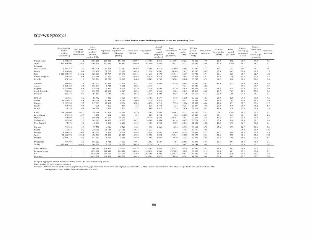
ECO/WKP(2000)21
80
Gross domesticproduct (million
nominal NC)
1990 PPPs (1993 EKS benchmark)
Gross domestic product (million
nominal US$)
Population (1000s)
Working-age population (15-
64 years) (1000s)
Labour force (1000s)
Employment (1000s)
Annual hours
worked per person employed
Total annual hours
worked (1000000s)
GDP per capita (US$)
GDP per person
employed (US$)
Employment per capita
GDP per hour worked
(US$)
Hours worked
per capita
Ratio of working-age population
to total
Ratio of labour force
to working-age population
Unemploy-ment rate
United States 5 803 250 1.0 5 803 250 249 911 164 577 128 007 118 793 1 819 216 084 23 221 48 852 47.5 26.9 865 65.9 77.8 7.2Japan 430 039 900 189.9 2 264 979 123 611 86 140 63 840 62 490 2 031 126 917 18 323 36 245 50.6 17.8 1 027 69.7 74.1 2.1Germany - - - - - - - - - - - - - - - - -West Germany 2 497 753 2.1 1 194 526 63 254 43 947 30 369 27 988 1 611 45 080 18 885 42 680 44.2 26.5 713 69.5 69.1 7.8France 6 619 068 6.6 999 498 56 735 37 381 24 853 22 098 1 652 36 506 17 617 45 230 38.9 27.4 643 65.9 66.5 11.1Italy 1 320 833 300 1 423.2 928 053 56 737 39 076 24 515 21 215 1 674 35 514 16 357 43 745 37.4 26.1 626 68.9 62.7 13.5United Kingdom 554 486 0.6 915 618 57 561 37 603 28 498 26 639 1 613 42 969 15 907 34 371 46.3 21.3 746 65.3 75.8 6.5Canada 678 135 1.3 523 794 27 791 18 910 14 408 13 165 1 790 23 562 18 848 39 787 47.4 22.2 848 68.0 76.2 8.6
Australia 393 662 1.4 283 757 17 085 11 438 8 551 7 870 1 809 14 236 16 609 36 055 46.1 19.9 833 66.9 74.8 8.0Austria 1 813 482 13.5 133 841 7 718 5 206 3 526 3 412 - - 17 341 39 226 44.2 - - 67.5 67.7 3.2Belgium 6 577 000 36.6 179 696 9 967 6 674 4 179 3 726 1 699 6 330 18 029 48 228 37.4 28.4 635 67.0 62.6 10.8Czech Republic 703 362 5.1 136 930 10 363 6 843 5 034 4 995 1 999 9 983 13 213 27 413 48.2 13.7 963 66.0 73.6 0.8Denmark 825 310 9.1 91 194 5 141 3 463 2 912 2 638 1 492 3 936 17 739 34 569 51.3 23.2 766 67.4 84.1 9.4
Finland 521 021 6.3 82 462 4 986 3 356 2 576 2 457 1 677 4 119 16 539 33 562 49.3 20.0 826 67.3 76.8 4.6Greece 13 315 043 126.8 105 039 10 089 6 761 4 000 3 719 1 912 7 111 10 411 28 244 36.9 14.8 705 67.0 59.2 7.0Hungary 2 282 398 19.5 117 061 10 390 6 934 4 783 4 196 1 710 7 176 11 266 27 897 40.4 16.3 691 66.7 69.0 12.3Iceland 364 402 78.6 4 638 255 164 128 126 1 772 223 18 201 36 807 49.5 20.8 876 64.4 78.2 1.8Ireland 28 524 0.6 44 206 3 503 2 151 1 332 1 160 1 922 2 229 12 620 38 119 33.1 19.8 636 61.4 61.9 12.9
Korea 178 796 800 501.7 356 386 42 869 29 648 18 539 18 085 2 433 44 002 8 313 19 706 42.2 8.1 1 026 69.2 62.5 2.4Luxembourg 372 618 40.7 9 158 384 266 192 189 1 724 326 23 825 48 483 49.1 28.1 847 69.1 72.2 1.5Mexico 738 898 1.1 658 488 83 657 46 234 - 29 710 1 625 48 281 7 871 22 164 35.5 13.6 577 55.3 52.0 2.7Netherlands 537 850 2.2 249 302 14 951 10 305 6 872 6 268 1 454 9 114 16 675 39 774 41.9 27.4 610 68.9 66.7 8.8New Zealand 72 776 1.6 46 861 3 363 2 209 1 616 1 481 1 762 2 609 13 934 31 642 44.0 18.0 776 65.7 73.2 8.4
Norway 722 705 9.3 77 752 4 241 2 746 2 142 1 992 1 432 2 853 18 333 39 032 47.0 27.3 673 64.7 78.0 7.0Poland 56 027 0.2 270 790 38 119 24 711 17 637 15 233 - - 7 104 17 776 40.0 - - 64.8 71.4 13.6Portugal 9 855 074 96.4 102 272 9 873 6 556 4 948 4 658 1 882 8 766 10 359 21 956 47.2 11.7 888 66.4 75.5 5.9Spain 52 345 374 106.2 492 741 38 851 25 849 15 333 12 578 1 824 22 941 12 683 39 175 32.4 21.5 590 66.5 59.3 18.0Sweden 1 403 172 9.5 147 381 8 590 5 516 4 540 4 465 1 480 6 610 17 157 33 008 52.0 22.3 769 64.2 82.3 1.7
Switzerland 317 303 2.1 153 592 6 712 4 593 3 581 3 563 1 627 5 797 22 883 43 108 53.1 26.5 864 68.4 78.0 0.5Turkey 393 060 171 1 488.9 264 000 56 203 34 022 20 650 18 538 - - 4 697 14 241 33.0 - - 60.5 60.7 10.2
North America - - 7 006 210 358 952 229 721 166 478 155 361 1 853 287 927 19 519 45 096 43.3 24.3 802 64.0 72.5 6.7European Union - - 5 674 988 348 340 234 110 158 645 143 210 1 656 237 202 16 292 39 627 41.1 23.9 681 67.2 67.8 9.7G7 - - 12 629 718 635 600 427 634 314 490 292 388 1 801 526 633 19 871 43 195 46.0 24.0 829 67.3 73.5 7.0Euro area - - 4 415 756 266 959 180 767 118 695 105 749 1 670 176 624 16 541 41 757 39.6 25.0 662 67.7 65.7 10.9
European aggregates include Western Germany before 1991 and total Germany beyond.Hours worked for agreggates are estimates.Sources: GDP from OECD ADB database; population, working-age population, labour force and employment from OECD (1999), Labour Force Statistics 1977-1997 , except for Ireland (ADB database 1999);
average annual hours worked from sources quoted in Annex 2.
Table A.10. Basic data for international comparisons of income and productivity, 1990
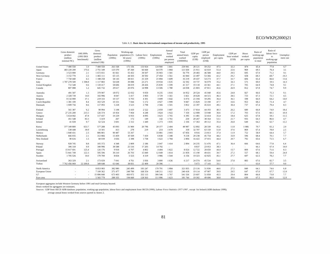
ECO/WKP(2000)21
81
Gross domesticproduct (million
nominal NC)
1995 PPPs (1993 EKS benchmark)
Gross domestic product (million
nominal US$)
Population (1000s)
Working-age population (15-
64 years) (1000s)
Labour force (1000s)
Employment (1000s)
Annual hours
worked per person employed
Total annual hours
worked (1000000s)
GDP per capita (US$)
GDP per person
employed (US$)
Employment per capita
GDP per hour worked
(US$)
Hours worked
per capita
Ratio of working-age population
to total
Ratio of labour force
to working-age population
Unemploy-ment rate
United States 7 400 550 1.0 7 400 550 263 168 172 156 133 924 124 900 1 841 229 941 28 121 59 252 47.5 32.2 874 65.4 77.8 6.7Japan 483 220 200 175.6 2 751 349 125 570 87 260 66 660 64 570 1 884 121 650 21 911 42 610 51.4 22.6 969 69.5 76.4 3.1Germany 3 523 000 2.1 1 672 651 81 661 55 452 39 507 35 903 1 581 56 770 20 483 46 588 44.0 29.5 695 67.9 71.2 9.1West Germany 3 152 770 2.2 1 465 111 65 125 44 503 30 592 27 454 1 561 42 844 22 497 53 366 42.2 34.2 658 68.3 68.7 10.3France 7 750 440 6.5 1 188 258 58 143 38 021 25 329 21 894 1 609 35 219 20 437 54 273 37.7 33.7 606 65.4 66.6 13.6Italy 1 787 278 500 1 598.8 1 117 883 56 638 39 088 23 271 19 934 1 635 32 592 19 737 56 079 35.2 34.3 575 69.0 59.5 14.3United Kingdom 712 548 0.6 1 120 417 58 606 38 019 28 426 25 839 1 599 41 317 19 118 43 361 44.1 27.1 705 64.9 74.8 9.1Canada 807 088 1.2 645 732 29 617 20 076 14 998 13 506 1 780 24 038 21 803 47 811 45.6 26.9 812 67.8 74.7 9.9
Australia 491 587 1.3 370 907 18 072 12 032 9 059 8 235 1 816 14 952 20 524 45 040 45.6 24.8 827 66.6 75.3 9.1Austria 2 328 739 14.0 165 996 8 047 5 417 3 903 3 729 1 561 5 821 20 628 44 515 46.3 28.5 723 67.3 72.1 4.5Belgium 8 132 000 37.1 219 333 10 157 6 703 4 301 3 699 1 642 6 074 21 594 59 295 36.4 36.1 598 66.0 64.2 14.0Czech Republic 1 381 100 8.4 163 529 10 331 7 044 5 172 4 927 1 999 9 847 15 829 33 190 47.7 16.6 953 68.2 73.4 4.7Denmark 1 009 756 8.6 117 093 5 228 3 523 2 798 2 566 1 501 3 852 22 397 45 633 49.1 30.4 737 67.4 79.4 8.3
Finland 561 387 6.2 90 994 5 108 3 410 2 522 2 059 1 687 3 473 17 814 44 193 40.3 26.2 680 66.8 74.0 18.4Greece 27 235 200 215.5 126 374 10 454 7 064 4 248 3 824 1 922 7 350 12 089 33 048 36.6 17.2 703 67.6 60.1 10.0Hungary 5 614 042 47.8 117 437 10 229 6 933 4 095 3 623 1 765 6 395 11 481 32 414 35.4 18.4 625 67.8 59.1 11.5Iceland 451 548 83.3 5 419 267 172 149 142 1 761 250 20 267 38 164 53.1 21.7 935 64.3 86.6 4.7Ireland 41 028 0.7 62 524 3 601 2 312 1 449 1 273 1 835 2 336 17 363 49 112 35.4 26.8 649 64.2 62.7 12.2
Korea 377 349 800 653.7 577 288 45 093 31 900 20 796 20 377 2 404 48 987 12 802 28 330 45.2 11.8 1 086 70.7 65.2 2.0Luxembourg 538 448 39.9 13 501 413 278 219 214 1 678 359 32 707 63 150 51.8 37.6 869 67.4 78.8 2.5Mexico 1 840 431 2.3 806 801 90 487 53 267 - 33 881 2 003 67 856 8 916 23 813 37.4 11.9 752 58.9 64.4 5.7Netherlands 666 035 2.1 312 866 15 459 10 569 7 410 6 838 1 348 9 218 20 238 45 754 44.2 33.9 596 68.4 70.1 7.7New Zealand 90 616 1.5 60 039 3 656 2 398 1 738 1 622 1 784 2 894 16 422 37 015 44.4 20.7 792 65.6 72.5 6.7
Norway 928 745 8.8 105 372 4 348 2 809 2 186 2 047 1 414 2 894 24 235 51 476 47.1 36.4 666 64.6 77.8 6.4Poland 306 318 0.9 340 996 38 588 25 516 17 205 14 792 - - 8 837 23 053 38.3 - - 66.1 67.4 14.0Portugal 15 817 691 125.4 126 176 9 918 6 707 4 802 4 404 1 822 8 024 12 722 28 650 44.4 15.7 809 67.6 71.6 8.3Spain 72 841 749 122.3 595 596 39 210 26 703 15 849 12 049 1 814 21 859 15 190 49 431 30.7 27.2 557 68.1 59.4 24.0Sweden 1 705 526 10.0 170 700 8 834 5 523 4 319 3 986 1 544 6 156 19 323 42 825 45.1 27.7 697 62.5 78.2 7.7
Switzerland 363 329 2.1 173 029 7 041 4 761 3 936 3 800 1 636 6 217 24 574 45 534 54.0 27.8 883 67.6 82.7 3.5Turkey 7 762 456 069 22 200.8 349 648 61 646 38 831 22 409 20 396 - - 5 672 17 143 33.1 - - 63.0 57.7 9.0
North America - - 8 853 083 382 980 245 499 183 247 170 791 1 884 321 835 23 116 51 836 44.6 27.5 840 64.1 74.6 6.8European Union - - 7 100 362 371 477 248 789 168 354 148 211 1 622 240 418 19 114 47 907 39.9 29.5 647 67.0 67.7 12.0G7 - - 15 896 840 673 403 450 072 332 115 306 546 1 767 541 526 23 607 51 858 45.5 29.4 804 66.8 73.8 7.7Euro area - - 5 565 779 288 355 194 660 128 563 111 996 1 623 181 744 19 302 49 696 38.8 30.6 630 67.5 66.0 12.9
European aggregates include Western Germany before 1991 and total Germany beyond.Hours worked for agreggates are estimates.Sources: GDP from OECD ADB database; population, working-age population, labour force and employment from OECD (1999), Labour Force Statistics 1977-1997 , except for Ireland (ADB database 1999);
average annual hours worked from sources quoted in Annex 2.
Table A.11. Basic data for international comparisons of income and productivity, 1995
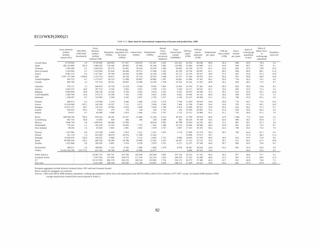
ECO/WKP(2000)21
82
Gross domesticproduct (million
nominal NC)
1995 PPPs (1993 EKS benchmark)
Gross domestic product (million
nominal US$)
Population (1000s)
Working-age population (15-
64 years) (1000s)
Labour force (1000s)
Employment (1000s)
Annual hours
worked per person employed
Total annual hours
worked (1000000s)
GDP per capita (US$)
GDP per person
employed (US$)
Employment per capita
GDP per hour worked
(US$)
Hours worked
per capita
Ratio of working-age population
to total
Ratio of labour force
to working-age population
Unemploy-ment rate
United States 8 759 950 1.0 8 759 950 269 092 177 207 138 935 131 457 1 833 241 022 32 554 66 638 48.9 36.3 896 65.9 78.4 5.4Japan 495 210 800 165.9 2 984 202 126 449 86 892 67 928 65 144 1 842 119 995 23 600 45 809 51.5 24.9 949 68.7 78.2 4.1Germany 3 784 200 2.1 1 829 636 82 272 55 841 39 534 35 478 1 580 56 065 22 239 51 571 43.1 32.6 681 67.9 70.8 10.3West Germany 3 429 683 2.1 1 623 664 65 636 44 648 30 572 27 040 1 562 42 239 24 738 60 047 41.2 38.4 644 68.0 68.5 11.6France 8 582 113 6.5 1 327 307 58 799 38 426 25 858 22 339 1 599 35 717 22 574 59 417 38.0 37.2 607 65.4 67.3 13.6Italy 2 057 731 300 1 694.0 1 214 753 56 871 39 158 23 714 20 253 1 648 33 377 21 360 59 979 35.6 36.4 587 68.9 60.6 14.6United Kingdom 843 725 0.7 1 273 937 58 154 37 908 28 867 26 882 1 587 42 661 21 906 47 391 46.2 29.9 734 65.2 76.1 6.9Canada 895 704 1.2 737 310 30 541 20 803 15 699 14 330 1 768 25 333 24 142 51 452 46.9 29.1 829 68.1 75.5 8.7
Australia 579 111 1.3 440 970 18 730 12 518 9 364 8 585 1 801 15 463 23 543 51 362 45.8 28.5 826 66.8 74.8 8.3Austria 2 622 572 14.0 187 723 8 120 5 493 3 912 3 709 1 515 5 619 23 117 50 615 45.7 33.4 692 67.6 71.2 5.2Belgium 9 064 000 36.8 246 158 10 224 6 709 4 365 3 814 1 635 6 235 24 076 64 549 37.3 39.5 610 65.6 65.1 12.6Czech Republic 1 820 700 10.4 174 275 10 290 7 105 5 205 4 823 2 003 9 662 16 936 36 132 46.9 18.0 939 69.0 73.3 7.3Denmark 1 168 307 8.7 133 605 5 294 3 545 2 875 2 705 1 527 4 130 25 237 49 398 51.1 32.3 780 67.0 81.1 5.9
Finland 686 013 6.2 110 600 5 154 3 440 2 586 2 216 1 674 3 708 21 459 49 919 43.0 29.8 719 66.7 75.2 14.3Greece 35 910 600 247.2 145 260 10 527 7 111 4 271 3 836 1 930 7 404 13 799 37 863 36.4 19.6 703 67.6 60.1 10.2Hungary 10 672 137 80.7 132 219 10 094 6 876 3 940 3 620 1 788 6 473 13 099 36 521 35.9 20.4 641 68.1 57.3 8.1Iceland 550 027 85.5 6 432 276 178 150 145 1 747 253 23 328 44 402 52.5 25.4 918 64.6 84.2 3.4Ireland 59 637 0.7 85 096 3 666 2 453 1 646 1 521 1 797 2 732 23 211 55 966 41.5 31.1 745 66.9 67.1 7.6
Korea 449 508 700 704.2 638 355 46 391 33 167 21 884 21 336 2 313 49 359 13 760 29 919 46.0 12.9 1 064 71.5 66.0 2.5Luxembourg 665 735 40.6 16 392 429 286 240 234 1 648 385 38 229 70 169 54.5 42.6 898 66.7 83.9 2.7Mexico 3 846 739 3.8 1 009 033 96 068 57 699 - 38 618 2 092 80 798 10 503 26 129 40.2 12.5 841 60.1 67.3 3.0Netherlands 776 161 2.1 363 343 15 353 10 605 7 791 7 423 1 368 10 155 23 666 48 946 48.4 35.8 661 69.1 73.5 4.7New Zealand 98 204 1.5 65 820 3 801 2 491 1 822 1 679 1 767 2 967 17 315 39 195 44.2 22.2 780 65.5 73.2 7.9
Norway 1 107 082 9.0 123 298 4 418 2 853 2 331 2 227 1 401 3 119 27 909 55 374 50.4 39.5 706 64.6 81.7 4.5Poland 551 110 1.3 425 095 38 679 26 074 17 298 15 362 - - 10 990 27 671 39.7 - - 67.4 66.3 11.2Portugal 19 020 678 130.6 145 655 9 946 6 757 5 123 4 665 1 732 8 080 14 645 31 220 46.9 18.0 812 67.9 75.8 8.9Spain 86 968 544 126.2 689 258 39 360 26 788 16 480 13 201 1 821 24 037 17 512 52 212 33.5 28.7 611 68.1 61.5 19.9Sweden 1 872 849 9.9 189 195 8 867 5 554 4 256 3 979 1 551 6 171 21 337 47 549 44.9 30.7 696 62.6 76.6 6.5
Switzerland 380 011 2.0 188 695 7 135 4 782 3 968 3 849 1 579 6 078 26 447 49 018 54.0 31.0 852 67.0 83.0 3.0Turkey 51 625 142 598 119 173.5 433 193 64 749 41 600 22 996 21 077 - - 6 690 20 553 32.6 - - 64.2 55.3 8.3
North America - - 10 491 722 395 701 255 708 193 449 183 449 1 892 347 154 26 514 57 191 46.4 30.2 877 64.6 75.7 5.2European Union - - 7 957 916 373 036 250 073 171 518 152 253 1 619 246 478 21 333 52 268 40.8 32.3 661 67.0 68.6 11.2G7 - - 18 127 095 682 178 456 235 340 534 315 882 1 754 554 172 26 572 57 386 46.3 32.7 812 66.9 74.6 7.2Euro area - - 6 215 920 290 194 195 956 131 249 114 851 1 620 186 111 21 420 54 121 39.6 33.4 641 67.5 67.0 12.5
European aggregates include Western Germany before 1991 and total Germany beyond.Hours worked for agreggates are estimates.Sources: GDP from OECD ADB database; population, working-age population, labour force and employment from OECD (1999), Labour Force Statistics 1977-1997 , except for Ireland (ADB database 1999);
average annual hours worked from sources quoted in Annex 2.
Table A.12. Basic data for international comparisons of income and productivity, 1998
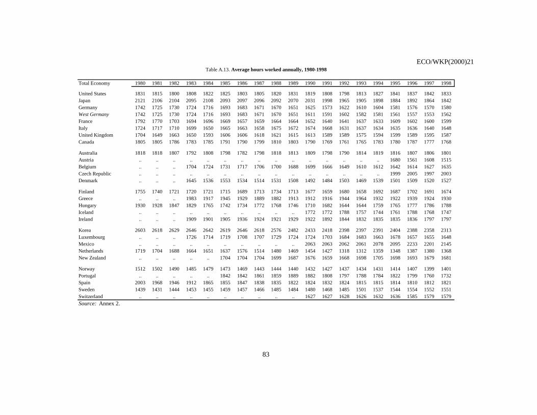
ECO/WKP(2000)21
83
Total Economy 1980 1981 1982 1983 1984 1985 1986 1987 1988 1989 1990 1991 1992 1993 1994 1995 1996 1997 1998
United States 1831 1815 1800 1808 1822 1825 1803 1805 1820 1831 1819 1808 1798 1813 1827 1841 1837 1842 1833Japan 2121 2106 2104 2095 2108 2093 2097 2096 2092 2070 2031 1998 1965 1905 1898 1884 1892 1864 1842Germany 1742 1725 1730 1724 1716 1693 1683 1671 1670 1651 1625 1573 1622 1610 1604 1581 1576 1570 1580West Germany 1742 1725 1730 1724 1716 1693 1683 1671 1670 1651 1611 1591 1602 1582 1581 1561 1557 1553 1562France 1792 1770 1703 1694 1696 1669 1657 1659 1664 1664 1652 1640 1641 1637 1633 1609 1602 1600 1599Italy 1724 1717 1710 1699 1650 1665 1663 1658 1675 1672 1674 1668 1631 1637 1634 1635 1636 1640 1648United Kingdom 1704 1649 1663 1650 1593 1606 1606 1618 1621 1615 1613 1589 1589 1575 1594 1599 1589 1595 1587Canada 1805 1805 1786 1783 1785 1791 1790 1799 1810 1803 1790 1769 1761 1765 1783 1780 1787 1777 1768
Australia 1818 1818 1807 1792 1808 1798 1782 1798 1818 1813 1809 1798 1790 1814 1819 1816 1807 1806 1801Austria .. .. .. .. .. .. .. .. .. .. .. .. .. .. .. 1680 1561 1608 1515Belgium .. .. .. 1704 1724 1731 1717 1706 1700 1688 1699 1666 1649 1610 1612 1642 1614 1627 1635Czech Republic .. .. .. .. .. .. .. .. .. .. .. .. .. .. .. 1999 2005 1997 2003Denmark .. .. .. 1645 1536 1553 1534 1514 1531 1508 1492 1484 1503 1469 1539 1501 1509 1520 1527
Finland 1755 1740 1721 1720 1721 1715 1689 1713 1734 1713 1677 1659 1680 1658 1692 1687 1702 1691 1674Greece .. .. .. 1983 1917 1945 1929 1889 1882 1913 1912 1916 1944 1964 1932 1922 1939 1924 1930Hungary 1930 1928 1847 1829 1765 1742 1734 1772 1768 1746 1710 1682 1644 1644 1759 1765 1777 1786 1788Iceland .. .. .. .. .. .. .. .. .. .. 1772 1772 1788 1757 1744 1761 1788 1768 1747Ireland .. .. .. 1909 1901 1905 1936 1924 1921 1929 1922 1892 1844 1832 1835 1835 1836 1797 1797
Korea 2603 2618 2629 2646 2642 2619 2646 2618 2576 2482 2433 2418 2398 2397 2391 2404 2388 2358 2313Luxembourg .. .. .. 1726 1714 1719 1708 1707 1729 1724 1724 1703 1684 1683 1663 1678 1657 1655 1648Mexico .. .. .. .. .. .. .. .. .. .. 2063 2063 2062 2061 2078 2095 2233 2201 2145Netherlands 1719 1704 1688 1664 1651 1637 1576 1514 1480 1469 1454 1427 1318 1312 1359 1348 1387 1380 1368New Zealand .. .. .. .. .. 1704 1704 1704 1699 1687 1676 1659 1668 1698 1705 1698 1693 1679 1681
Norway 1512 1502 1490 1485 1479 1473 1469 1443 1444 1440 1432 1427 1437 1434 1431 1414 1407 1399 1401Portugal .. .. .. .. .. 1842 1842 1861 1859 1889 1882 1808 1797 1788 1784 1822 1799 1760 1732Spain 2003 1968 1946 1912 1865 1855 1847 1838 1835 1822 1824 1832 1824 1815 1815 1814 1810 1812 1821Sweden 1439 1431 1444 1453 1455 1459 1457 1466 1485 1484 1480 1468 1485 1501 1537 1544 1554 1552 1551Switzerland .. .. .. .. .. .. .. .. .. .. 1627 1627 1628 1626 1632 1636 1585 1579 1579Source: Annex 2.
Table A.13. Average hours worked annually, 1980-1998
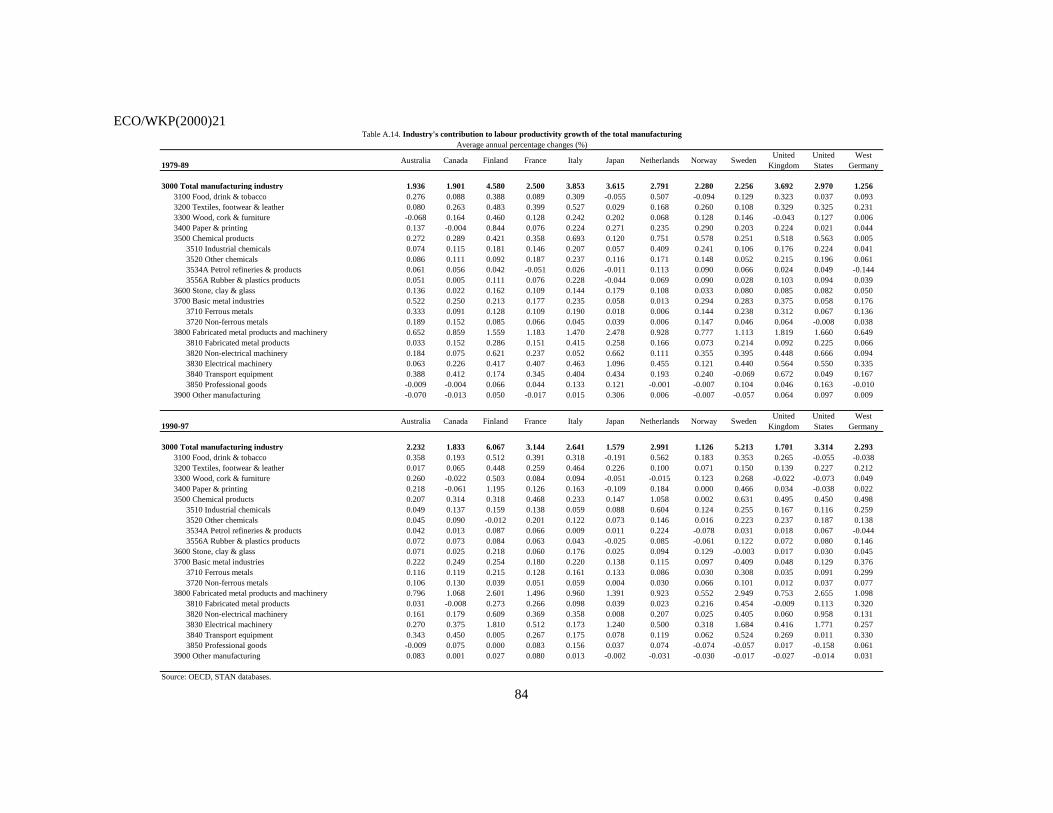
ECO/WKP(2000)21
84
1979-89 Australia Canada Finland France Italy Japan Netherlands Norway Sweden United Kingdom
United States
West Germany
3000 Total manufacturing industry 1.936 1.901 4.580 2.500 3.853 3.615 2.791 2.280 2.256 3.692 2.970 1.2563100 Food, drink & tobacco 0.276 0.088 0.388 0.089 0.309 -0.055 0.507 -0.094 0.129 0.323 0.037 0.0933200 Textiles, footwear & leather 0.080 0.263 0.483 0.399 0.527 0.029 0.168 0.260 0.108 0.329 0.325 0.2313300 Wood, cork & furniture -0.068 0.164 0.460 0.128 0.242 0.202 0.068 0.128 0.146 -0.043 0.127 0.0063400 Paper & printing 0.137 -0.004 0.844 0.076 0.224 0.271 0.235 0.290 0.203 0.224 0.021 0.0443500 Chemical products 0.272 0.289 0.421 0.358 0.693 0.120 0.751 0.578 0.251 0.518 0.563 0.005
3510 Industrial chemicals 0.074 0.115 0.181 0.146 0.207 0.057 0.409 0.241 0.106 0.176 0.224 0.0413520 Other chemicals 0.086 0.111 0.092 0.187 0.237 0.116 0.171 0.148 0.052 0.215 0.196 0.0613534A Petrol refineries & products 0.061 0.056 0.042 -0.051 0.026 -0.011 0.113 0.090 0.066 0.024 0.049 -0.1443556A Rubber & plastics products 0.051 0.005 0.111 0.076 0.228 -0.044 0.069 0.090 0.028 0.103 0.094 0.039
3600 Stone, clay & glass 0.136 0.022 0.162 0.109 0.144 0.179 0.108 0.033 0.080 0.085 0.082 0.0503700 Basic metal industries 0.522 0.250 0.213 0.177 0.235 0.058 0.013 0.294 0.283 0.375 0.058 0.176
3710 Ferrous metals 0.333 0.091 0.128 0.109 0.190 0.018 0.006 0.144 0.238 0.312 0.067 0.1363720 Non-ferrous metals 0.189 0.152 0.085 0.066 0.045 0.039 0.006 0.147 0.046 0.064 -0.008 0.038
3800 Fabricated metal products and machinery 0.652 0.859 1.559 1.183 1.470 2.478 0.928 0.777 1.113 1.819 1.660 0.6493810 Fabricated metal products 0.033 0.152 0.286 0.151 0.415 0.258 0.166 0.073 0.214 0.092 0.225 0.0663820 Non-electrical machinery 0.184 0.075 0.621 0.237 0.052 0.662 0.111 0.355 0.395 0.448 0.666 0.0943830 Electrical machinery 0.063 0.226 0.417 0.407 0.463 1.096 0.455 0.121 0.440 0.564 0.550 0.3353840 Transport equipment 0.388 0.412 0.174 0.345 0.404 0.434 0.193 0.240 -0.069 0.672 0.049 0.1673850 Professional goods -0.009 -0.004 0.066 0.044 0.133 0.121 -0.001 -0.007 0.104 0.046 0.163 -0.010
3900 Other manufacturing -0.070 -0.013 0.050 -0.017 0.015 0.306 0.006 -0.007 -0.057 0.064 0.097 0.009
1990-97 Australia Canada Finland France Italy Japan Netherlands Norway Sweden United Kingdom
United States
West Germany
3000 Total manufacturing industry 2.232 1.833 6.067 3.144 2.641 1.579 2.991 1.126 5.213 1.701 3.314 2.2933100 Food, drink & tobacco 0.358 0.193 0.512 0.391 0.318 -0.191 0.562 0.183 0.353 0.265 -0.055 -0.0383200 Textiles, footwear & leather 0.017 0.065 0.448 0.259 0.464 0.226 0.100 0.071 0.150 0.139 0.227 0.2123300 Wood, cork & furniture 0.260 -0.022 0.503 0.084 0.094 -0.051 -0.015 0.123 0.268 -0.022 -0.073 0.0493400 Paper & printing 0.218 -0.061 1.195 0.126 0.163 -0.109 0.184 0.000 0.466 0.034 -0.038 0.0223500 Chemical products 0.207 0.314 0.318 0.468 0.233 0.147 1.058 0.002 0.631 0.495 0.450 0.498
3510 Industrial chemicals 0.049 0.137 0.159 0.138 0.059 0.088 0.604 0.124 0.255 0.167 0.116 0.2593520 Other chemicals 0.045 0.090 -0.012 0.201 0.122 0.073 0.146 0.016 0.223 0.237 0.187 0.1383534A Petrol refineries & products 0.042 0.013 0.087 0.066 0.009 0.011 0.224 -0.078 0.031 0.018 0.067 -0.0443556A Rubber & plastics products 0.072 0.073 0.084 0.063 0.043 -0.025 0.085 -0.061 0.122 0.072 0.080 0.146
3600 Stone, clay & glass 0.071 0.025 0.218 0.060 0.176 0.025 0.094 0.129 -0.003 0.017 0.030 0.0453700 Basic metal industries 0.222 0.249 0.254 0.180 0.220 0.138 0.115 0.097 0.409 0.048 0.129 0.376
3710 Ferrous metals 0.116 0.119 0.215 0.128 0.161 0.133 0.086 0.030 0.308 0.035 0.091 0.2993720 Non-ferrous metals 0.106 0.130 0.039 0.051 0.059 0.004 0.030 0.066 0.101 0.012 0.037 0.077
3800 Fabricated metal products and machinery 0.796 1.068 2.601 1.496 0.960 1.391 0.923 0.552 2.949 0.753 2.655 1.0983810 Fabricated metal products 0.031 -0.008 0.273 0.266 0.098 0.039 0.023 0.216 0.454 -0.009 0.113 0.3203820 Non-electrical machinery 0.161 0.179 0.609 0.369 0.358 0.008 0.207 0.025 0.405 0.060 0.958 0.1313830 Electrical machinery 0.270 0.375 1.810 0.512 0.173 1.240 0.500 0.318 1.684 0.416 1.771 0.2573840 Transport equipment 0.343 0.450 0.005 0.267 0.175 0.078 0.119 0.062 0.524 0.269 0.011 0.3303850 Professional goods -0.009 0.075 0.000 0.083 0.156 0.037 0.074 -0.074 -0.057 0.017 -0.158 0.061
3900 Other manufacturing 0.083 0.001 0.027 0.080 0.013 -0.002 -0.031 -0.030 -0.017 -0.027 -0.014 0.031
Source: OECD, STAN databases.
Table A.14. Industry's contribution to labour productivity growth of the total manufacturingAverage annual percentage changes (%)
ECO/WKP(2000)21
85
ANNEX 2. MEASUREMENT ISSUES AND DATA SOURCES
62. Several measurement issues arise when time series of inputs, outputs and productivity are constructed and compared at the international level. The three most important points are: a) conceptual independence of output quantity measures from input quantity measures; b) chained and fixed-weighted indices; c) methodology to derive price and quantity measures for products that are rapidly changing in terms of type and quality, in particular computers and semiconductors. These issues are discussed in the first section of this annex.
63. In recent years, international comparisons have also been affected by the different timing and scope of the transition of National Accounts from the 1968 system (SNA68) to the new 1993 system (SNA93). The implications of the shift of National accounts to the new system are discussed in the second section of the annex.
64. International comparisons of income per capita and productivity have to take into account international price differences that affect the purchasing power of the same dollar in different countries. Purchasing Power Parity indexes are discussed in the third section of the annex.
65. While the main data sources used in this paper come from the OECD Analytical Data Base (ADB), for aggregate data, and the OECD International Sectoral Data Base (ISDB) as well as the OECD STAN Database for Industrial Analysis, for sectoral data, some adjustments have been made to enhance cross-country comparability. The fourth section of this annex documents sources of data used for the purpose of this study, provides methodological details of the adjustment that has been made and compares adjusted series with time-series available from national sources.
A2.1 Measuring inputs and output for the purpose of international comparisons
A2.1.1 Independence of input and output statistics
66. A vital point for the validity of productivity measures is that price and volume indices of output are constructed independently of price and volume indices of inputs. Dependence occurs, for example, when output volume series are based on extrapolation of input measures. Extrapolation implies that quantity indicators of inputs, frequently employment, are used to carry forward and backward real output series. Input-based extrapolation is more frequent in the service industries than in other parts of the economy. However, extrapolation of base-year value added can also be based on physical output indicators or on volume measures obtained by deflating outputs. This may be a good first approximation for certain sectors (transport, for instance).
67. From the perspective of productivity measurement, the independence of statistics on inputs and outputs is key. Input-based indicators that are used to deflate output series generate an obvious bias in productivity measures: (labour) productivity growth will either be zero by construction or will reflect any assumption about productivity growth made by statisticians. Occurrences of input-based extrapolation are concentrated mainly in non-market activities where output prices are difficult to observe. This creates a

ECO/WKP(2000)21
86
case for restricting productivity measurement to the market sector of the economy and thereby partially avoiding potential biases from output measurement.
68. In 1996, OECD published a report on the different methods to construct constant-price series of value-added in Member countries. The study focused on service industries as the part of the economy where output tends to be more difficult to measure than elsewhere. It suggests that direct extrapolation of base year value-added is the most important approach, followed by double deflation and single deflation. Extrapolation of base-year value-added using employment or hours worked turns out to be a popular technique for service activities where output is difficult to define such as public administration and defence or where output is difficult to measure such as financial and insurance services. It should be noted, though that many countries have changed compilation methodologies in conjunction with implementing SNA 93.
A2.1.2 Chained and fixed-weighted index numbers
69. Whenever price or quantity indices of two non-adjacent periods have to be compared, the question arises of which period should be chosen as a basis of comparison. One option is to choose the first or last observations as the base (“fixed-weight” or “fixed-base” Laspeyres or Paasche indexes respectively)66 - another is to use the chain principle. In principle, chain indices can use the Laspeyres, Paasche or Fisher formulas. They are obtained by linking either price or volume indices for consecutive periods. The period-to-period movements are calculated using weighting patterns appropriate to the periods concerned.
70. In a time-series context, i.e. for the measurement of the rates of change of outputs, inputs and productivity, there is a strong presumption in the literature in favour of chained indices. This is because they are much less prone to a substitution bias than fixed-weight indices. The difference between fixed and chain-weighted indices became highly visible with the rising importance of information technology products, in particular computers (see below). Computer prices have fallen very rapidly relative to other goods and their quantities have increased relatively more rapidly. Fixed-weight volume series tend to be biased upwards after the base year and downwards prior to the base year (see Table A2.1). One disadvantage of chained indices of output is that they lack additive consistency over time.
66. Use of Fisher ideal index is a further option.
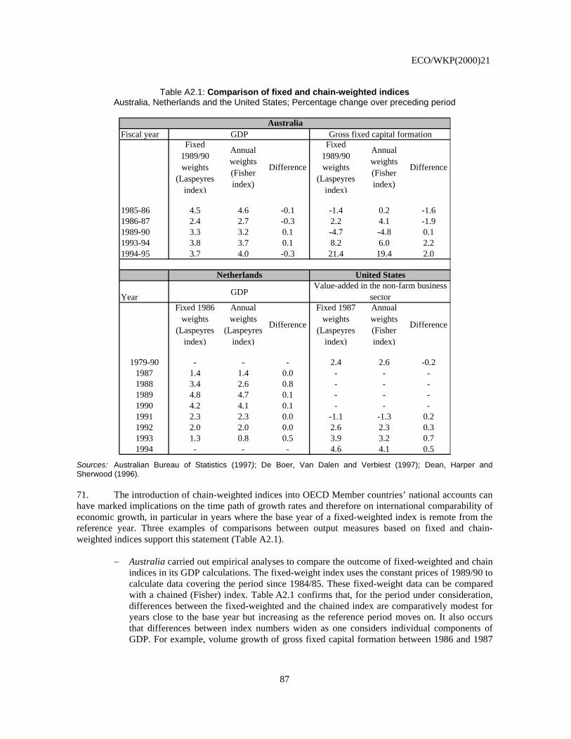
ECO/WKP(2000)21
87
Table A2.1: Comparison of fixed and chain-weighted indices Australia, Netherlands and the United States; Percentage change over preceding period
AustraliaFiscal year GDP Gross fixed capital formation
Fixed 1989/90 weights
(Laspeyres index)
Annual weights (Fisher index)
Difference
Fixed 1989/90 weights
(Laspeyres index)
Annual weights (Fisher index)
Difference
1985-86 4.5 4.6 -0.1 -1.4 0.2 -1.61986-87 2.4 2.7 -0.3 2.2 4.1 -1.91989-90 3.3 3.2 0.1 -4.7 -4.8 0.11993-94 3.8 3.7 0.1 8.2 6.0 2.21994-95 3.7 4.0 -0.3 21.4 19.4 2.0
Netherlands United States
Year GDPValue-added in the non-farm business
sectorFixed 1986
weights (Laspeyres
index)
Annual weights
(Laspeyres index)
Difference
Fixed 1987 weights
(Laspeyres index)
Annual weights (Fisher index)
Difference
1979-90 - - - 2.4 2.6 -0.21987 1.4 1.4 0.0 - - -1988 3.4 2.6 0.8 - - -1989 4.8 4.7 0.1 - - -1990 4.2 4.1 0.1 - - -1991 2.3 2.3 0.0 -1.1 -1.3 0.21992 2.0 2.0 0.0 2.6 2.3 0.31993 1.3 0.8 0.5 3.9 3.2 0.71994 - - - 4.6 4.1 0.5
Sources: Australian Bureau of Statistics (1997); De Boer, Van Dalen and Verbiest (1997); Dean, Harper and Sherwood (1996).
71. The introduction of chain-weighted indices into OECD Member countries’ national accounts can have marked implications on the time path of growth rates and therefore on international comparability of economic growth, in particular in years where the base year of a fixed-weighted index is remote from the reference year. Three examples of comparisons between output measures based on fixed and chain-weighted indices support this statement (Table A2.1).
− Australia carried out empirical analyses to compare the outcome of fixed-weighted and chain indices in its GDP calculations. The fixed-weight index uses the constant prices of 1989/90 to calculate data covering the period since 1984/85. These fixed-weight data can be compared with a chained (Fisher) index. Table A2.1 confirms that, for the period under consideration, differences between the fixed-weighted and the chained index are comparatively modest for years close to the base year but increasing as the reference period moves on. It also occurs that differences between index numbers widen as one considers individual components of GDP. For example, volume growth of gross fixed capital formation between 1986 and 1987
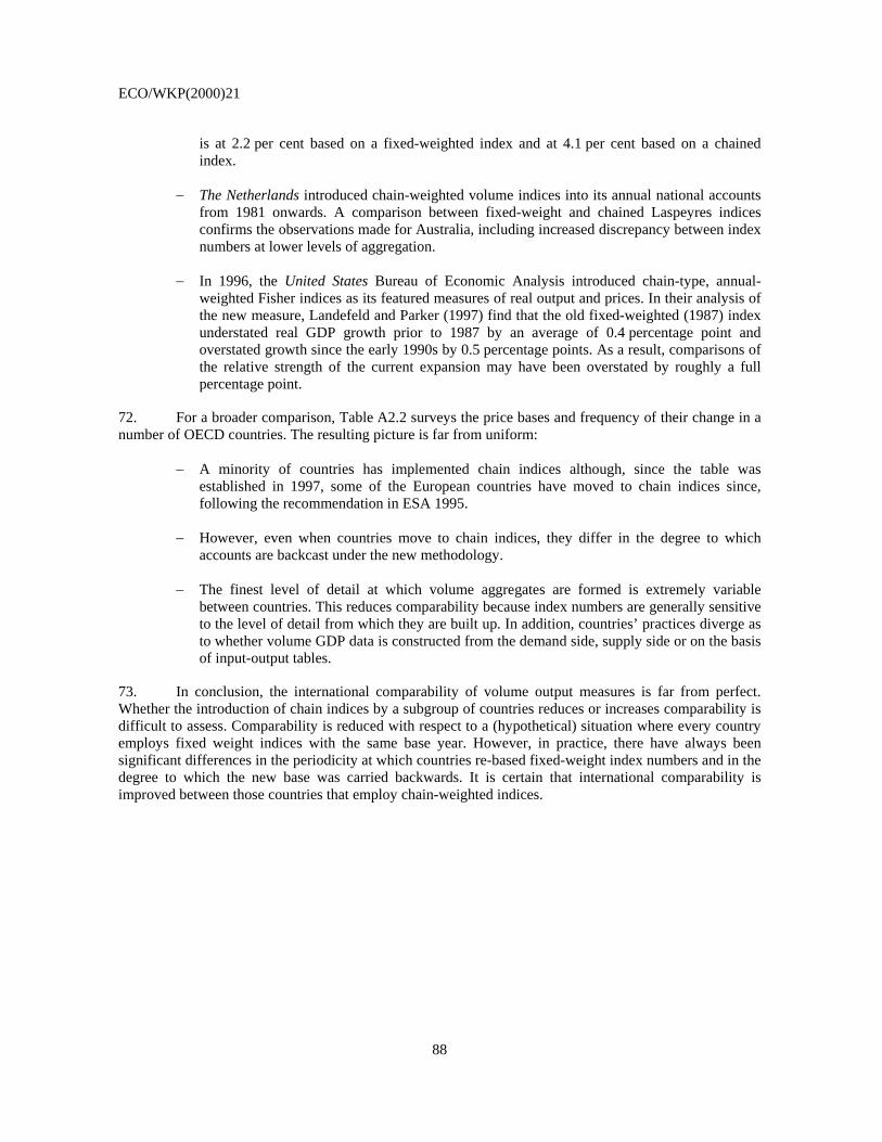
ECO/WKP(2000)21
88
is at 2.2 per cent based on a fixed-weighted index and at 4.1 per cent based on a chained index.
− The Netherlands introduced chain-weighted volume indices into its annual national accounts from 1981 onwards. A comparison between fixed-weight and chained Laspeyres indices confirms the observations made for Australia, including increased discrepancy between index numbers at lower levels of aggregation.
− In 1996, the United States Bureau of Economic Analysis introduced chain-type, annual-weighted Fisher indices as its featured measures of real output and prices. In their analysis of the new measure, Landefeld and Parker (1997) find that the old fixed-weighted (1987) index understated real GDP growth prior to 1987 by an average of 0.4 percentage point and overstated growth since the early 1990s by 0.5 percentage points. As a result, comparisons of the relative strength of the current expansion may have been overstated by roughly a full percentage point.
72. For a broader comparison, Table A2.2 surveys the price bases and frequency of their change in a number of OECD countries. The resulting picture is far from uniform:
− A minority of countries has implemented chain indices although, since the table was established in 1997, some of the European countries have moved to chain indices since, following the recommendation in ESA 1995.
− However, even when countries move to chain indices, they differ in the degree to which accounts are backcast under the new methodology.
− The finest level of detail at which volume aggregates are formed is extremely variable between countries. This reduces comparability because index numbers are generally sensitive to the level of detail from which they are built up. In addition, countries’ practices diverge as to whether volume GDP data is constructed from the demand side, supply side or on the basis of input-output tables.
73. In conclusion, the international comparability of volume output measures is far from perfect. Whether the introduction of chain indices by a subgroup of countries reduces or increases comparability is difficult to assess. Comparability is reduced with respect to a (hypothetical) situation where every country employs fixed weight indices with the same base year. However, in practice, there have always been significant differences in the periodicity at which countries re-based fixed-weight index numbers and in the degree to which the new base was carried backwards. It is certain that international comparability is improved between those countries that employ chain-weighted indices.
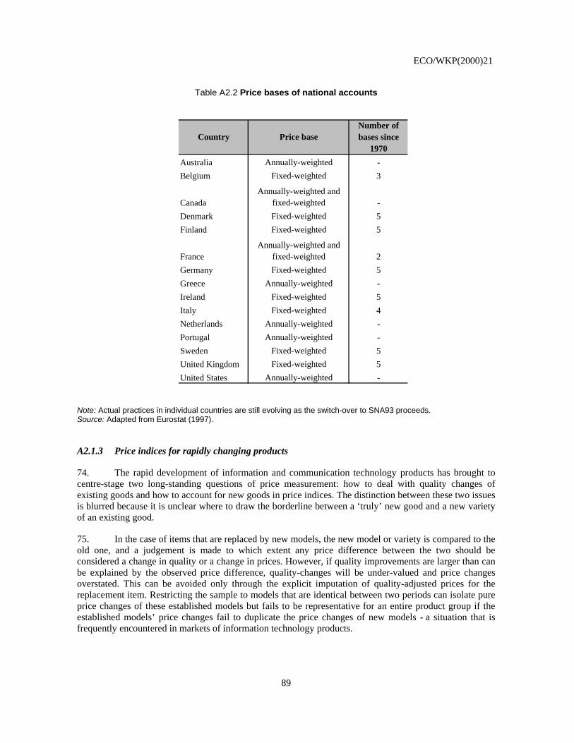
ECO/WKP(2000)21
89
Table A2.2 Price bases of national accounts
Country Price baseNumber of bases since
1970Australia Annually-weighted -Belgium Fixed-weighted 3
CanadaAnnually-weighted and
fixed-weighted -Denmark Fixed-weighted 5Finland Fixed-weighted 5
FranceAnnually-weighted and
fixed-weighted 2Germany Fixed-weighted 5Greece Annually-weighted -Ireland Fixed-weighted 5Italy Fixed-weighted 4Netherlands Annually-weighted -Portugal Annually-weighted -Sweden Fixed-weighted 5United Kingdom Fixed-weighted 5United States Annually-weighted -
Note: Actual practices in individual countries are still evolving as the switch-over to SNA93 proceeds. Source: Adapted from Eurostat (1997).
A2.1.3 Price indices for rapidly changing products
74. The rapid development of information and communication technology products has brought to centre-stage two long-standing questions of price measurement: how to deal with quality changes of existing goods and how to account for new goods in price indices. The distinction between these two issues is blurred because it is unclear where to draw the borderline between a ‘truly’ new good and a new variety of an existing good.
75. In the case of items that are replaced by new models, the new model or variety is compared to the old one, and a judgement is made to which extent any price difference between the two should be considered a change in quality or a change in prices. However, if quality improvements are larger than can be explained by the observed price difference, quality-changes will be under-valued and price changes overstated. This can be avoided only through the explicit imputation of quality-adjusted prices for the replacement item. Restricting the sample to models that are identical between two periods can isolate pure price changes of these established models but fails to be representative for an entire product group if the established models’ price changes fail to duplicate the price changes of new models - a situation that is frequently encountered in markets of information technology products.
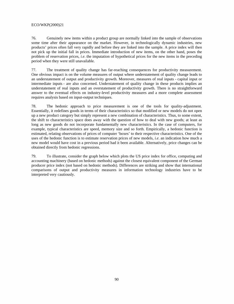
ECO/WKP(2000)21
90
76. Genuinely new items within a product group are normally linked into the sample of observations some time after their appearance on the market. However, in technologically dynamic industries, new products’ prices often fall very rapidly and before they are linked into the sample. A price index will then not pick up the initial fall in prices. Immediate introduction of new items, on the other hand, poses the problem of reservation prices, i.e. the imputation of hypothetical prices for the new items in the preceding period when they were still unavailable.
77. The treatment of quality change has far-reaching consequences for productivity measurement. One obvious impact is on the volume measures of output where understatement of quality change leads to an understatement of output and productivity growth. Moreover, measures of real inputs - capital input or intermediate inputs - are also concerned. Understatement of quality change in these products implies an understatement of real inputs and an overstatement of productivity growth. There is no straightforward answer to the eventual effects on industry-level productivity measures and a more complete assessment requires analysis based on input-output techniques.
78. The hedonic approach to price measurement is one of the tools for quality-adjustment. Essentially, it redefines goods in terms of their characteristics so that modified or new models do not open up a new product category but simply represent a new combination of characteristics. Thus, to some extent, the shift to characteristics space does away with the question of how to deal with new goods; at least as long as new goods do not incorporate fundamentally new characteristics. In the case of computers, for example, typical characteristics are speed, memory size and so forth. Empirically, a hedonic function is estimated, relating observations of prices of computer ‘boxes’ to their respective characteristics. One of the uses of the hedonic function is to estimate reservation prices of new models, i.e. an indication how much a new model would have cost in a previous period had it been available. Alternatively, price changes can be obtained directly from hedonic regressions.
79. To illustrate, consider the graph below which plots the US price index for office, computing and accounting machinery (based on hedonic methods) against the closest equivalent component of the German producer price index (not based on hedonic methods). Differences are striking and show that international comparisons of output and productivity measures in information technology industries have to be interpreted very cautiously.
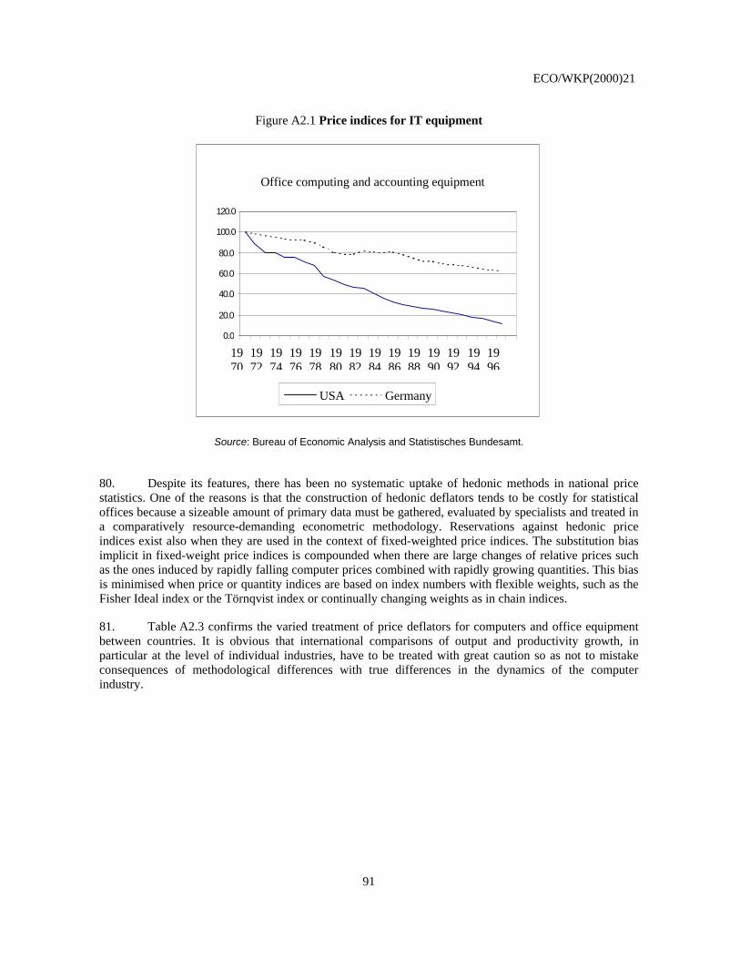
ECO/WKP(2000)21
91
Figure A2.1 Price indices for IT equipment
Office computing and accounting equipment
0.0
20.0
40.0
60.0
80.0
100.0
120.0
1970
1972
1974
1976
1978
1980
1982
1984
1986
1988
1990
1992
1994
1996
USA Germany
Source: Bureau of Economic Analysis and Statistisches Bundesamt.
80. Despite its features, there has been no systematic uptake of hedonic methods in national price statistics. One of the reasons is that the construction of hedonic deflators tends to be costly for statistical offices because a sizeable amount of primary data must be gathered, evaluated by specialists and treated in a comparatively resource-demanding econometric methodology. Reservations against hedonic price indices exist also when they are used in the context of fixed-weighted price indices. The substitution bias implicit in fixed-weight price indices is compounded when there are large changes of relative prices such as the ones induced by rapidly falling computer prices combined with rapidly growing quantities. This bias is minimised when price or quantity indices are based on index numbers with flexible weights, such as the Fisher Ideal index or the Törnqvist index or continually changing weights as in chain indices.
81. Table A2.3 confirms the varied treatment of price deflators for computers and office equipment between countries. It is obvious that international comparisons of output and productivity growth, in particular at the level of individual industries, have to be treated with great caution so as not to mistake consequences of methodological differences with true differences in the dynamics of the computer industry.
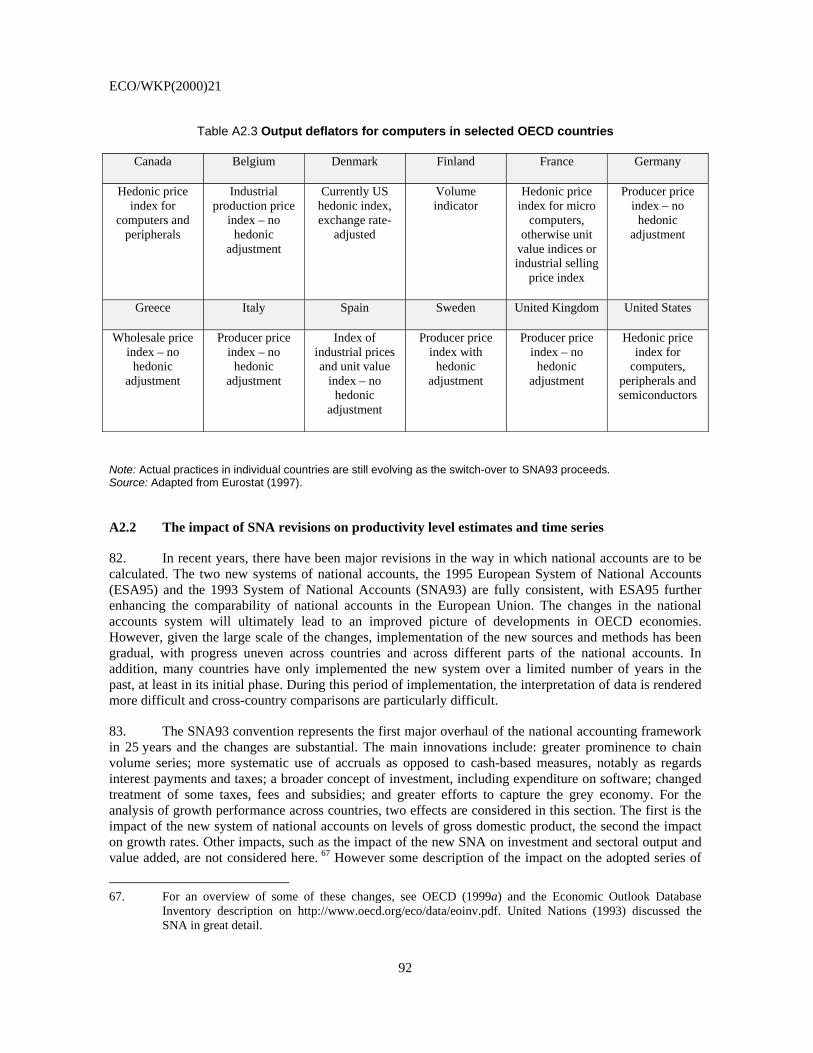
ECO/WKP(2000)21
92
Table A2.3 Output deflators for computers in selected OECD countries
Canada Belgium Denmark Finland France Germany
Hedonic price index for
computers and peripherals
Industrial production price
index – no hedonic
adjustment
Currently US hedonic index, exchange rate-
adjusted
Volume indicator
Hedonic price index for micro
computers, otherwise unit
value indices or industrial selling
price index
Producer price index – no
hedonic adjustment
Greece Italy Spain Sweden United Kingdom United States
Wholesale price index – no
hedonic adjustment
Producer price index – no
hedonic adjustment
Index of industrial prices and unit value
index – no hedonic
adjustment
Producer price index with
hedonic adjustment
Producer price index – no
hedonic adjustment
Hedonic price index for
computers, peripherals and semiconductors
Note: Actual practices in individual countries are still evolving as the switch-over to SNA93 proceeds. Source: Adapted from Eurostat (1997).
A2.2 The impact of SNA revisions on productivity level estimates and time series
82. In recent years, there have been major revisions in the way in which national accounts are to be calculated. The two new systems of national accounts, the 1995 European System of National Accounts (ESA95) and the 1993 System of National Accounts (SNA93) are fully consistent, with ESA95 further enhancing the comparability of national accounts in the European Union. The changes in the national accounts system will ultimately lead to an improved picture of developments in OECD economies. However, given the large scale of the changes, implementation of the new sources and methods has been gradual, with progress uneven across countries and across different parts of the national accounts. In addition, many countries have only implemented the new system over a limited number of years in the past, at least in its initial phase. During this period of implementation, the interpretation of data is rendered more difficult and cross-country comparisons are particularly difficult.
83. The SNA93 convention represents the first major overhaul of the national accounting framework in 25 years and the changes are substantial. The main innovations include: greater prominence to chain volume series; more systematic use of accruals as opposed to cash-based measures, notably as regards interest payments and taxes; a broader concept of investment, including expenditure on software; changed treatment of some taxes, fees and subsidies; and greater efforts to capture the grey economy. For the analysis of growth performance across countries, two effects are considered in this section. The first is the impact of the new system of national accounts on levels of gross domestic product, the second the impact on growth rates. Other impacts, such as the impact of the new SNA on investment and sectoral output and value added, are not considered here. 67 However some description of the impact on the adopted series of
67. For an overview of some of these changes, see OECD (1999a) and the Economic Outlook Database
Inventory description on http://www.oecd.org/eco/data/eoinv.pdf. United Nations (1993) discussed the SNA in great detail.
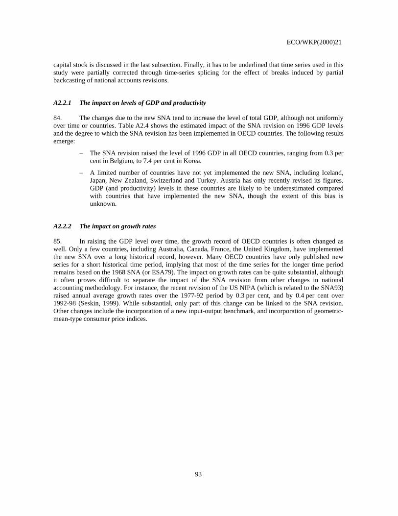
ECO/WKP(2000)21
93
capital stock is discussed in the last subsection. Finally, it has to be underlined that time series used in this study were partially corrected through time-series splicing for the effect of breaks induced by partial backcasting of national accounts revisions.
A2.2.1 The impact on levels of GDP and productivity
84. The changes due to the new SNA tend to increase the level of total GDP, although not uniformly over time or countries. Table A2.4 shows the estimated impact of the SNA revision on 1996 GDP levels and the degree to which the SNA revision has been implemented in OECD countries. The following results emerge:
− The SNA revision raised the level of 1996 GDP in all OECD countries, ranging from 0.3 per cent in Belgium, to 7.4 per cent in Korea.
− A limited number of countries have not yet implemented the new SNA, including Iceland, Japan, New Zealand, Switzerland and Turkey. Austria has only recently revised its figures. GDP (and productivity) levels in these countries are likely to be underestimated compared with countries that have implemented the new SNA, though the extent of this bias is unknown.
A2.2.2 The impact on growth rates
85. In raising the GDP level over time, the growth record of OECD countries is often changed as well. Only a few countries, including Australia, Canada, France, the United Kingdom, have implemented the new SNA over a long historical record, however. Many OECD countries have only published new series for a short historical time period, implying that most of the time series for the longer time period remains based on the 1968 SNA (or ESA79). The impact on growth rates can be quite substantial, although it often proves difficult to separate the impact of the SNA revision from other changes in national accounting methodology. For instance, the recent revision of the US NIPA (which is related to the SNA93) raised annual average growth rates over the 1977-92 period by 0.3 per cent, and by 0.4 per cent over 1992-98 (Seskin, 1999). While substantial, only part of this change can be linked to the SNA revision. Other changes include the incorporation of a new input-output benchmark, and incorporation of geometric-mean-type consumer price indices.
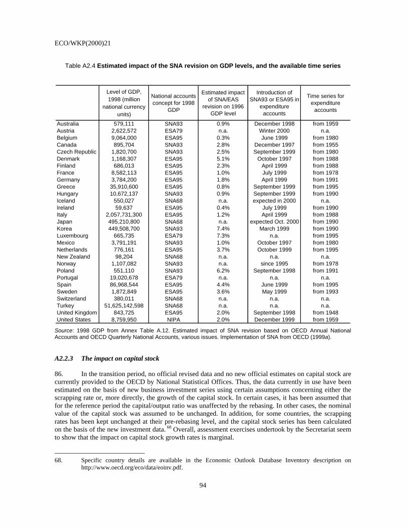
ECO/WKP(2000)21
94
Table A2.4 Estimated impact of the SNA revision on GDP levels, and the available time series
Level of GDP,1998 (million
national currencyunits)
National accountsconcept for 1998
GDP
Estimated impactof SNA/EAS
revision on 1996GDP level
Introduction ofSNA93 or ESA95 in
expenditureaccounts
Time series forexpenditure
accounts
Australia 579,111 SNA93 0.9% December 1998 from 1959Austria 2,622,572 ESA79 n.a. Winter 2000 n.a.Belgium 9,064,000 ESA95 0.3% June 1999 from 1980Canada 895,704 SNA93 2.8% December 1997 from 1955Czech Republic 1,820,700 SNA93 2.5% September 1999 from 1980Denmark 1,168,307 ESA95 5.1% October 1997 from 1988Finland 686,013 ESA95 2.3% April 1999 from 1988France 8,582,113 ESA95 1.0% July 1999 from 1978Germany 3,784,200 ESA95 1.8% April 1999 from 1991Greece 35,910,600 ESA95 0.8% September 1999 from 1995Hungary 10,672,137 SNA93 0.9% September 1999 from 1990Iceland 550,027 SNA68 n.a. expected in 2000 n.a.Ireland 59,637 ESA95 0.4% July 1999 from 1990Italy 2,057,731,300 ESA95 1.2% April 1999 from 1988Japan 495,210,800 SNA68 n.a. expected Oct. 2000 from 1990Korea 449,508,700 SNA93 7.4% March 1999 from 1990Luxembourg 665,735 ESA79 7.3% n.a. from 1995Mexico 3,791,191 SNA93 1.0% October 1997 from 1980Netherlands 776,161 ESA95 3.7% October 1999 from 1995New Zealand 98,204 SNA68 n.a. n.a. n.a.Norway 1,107,082 SNA93 n.a. since 1995 from 1978Poland 551,110 SNA93 6.2% September 1998 from 1991Portugal 19,020,678 ESA79 n.a. n.a. n.a.Spain 86,968,544 ESA95 4.4% June 1999 from 1995Sweden 1,872,849 ESA95 3.6% May 1999 from 1993Switzerland 380,011 SNA68 n.a. n.a. n.a.Turkey 51,625,142,598 SNA68 n.a. n.a. n.a.United Kingdom 843,725 ESA95 2.0% September 1998 from 1948United States 8,759,950 NIPA 2.0% December 1999 from 1959
Source: 1998 GDP from Annex Table A.12. Estimated impact of SNA revision based on OECD Annual National Accounts and OECD Quarterly National Accounts, various issues. Implementation of SNA from OECD (1999a).
A2.2.3 The impact on capital stock
86. In the transition period, no official revised data and no new official estimates on capital stock are currently provided to the OECD by National Statistical Offices. Thus, the data currently in use have been estimated on the basis of new business investment series using certain assumptions concerning either the scrapping rate or, more directly, the growth of the capital stock. In certain cases, it has been assumed that for the reference period the capital/output ratio was unaffected by the rebasing. In other cases, the nominal value of the capital stock was assumed to be unchanged. In addition, for some countries, the scrapping rates has been kept unchanged at their pre-rebasing level, and the capital stock series has been calculated on the basis of the new investment data. 68 Overall, assessment exercises undertook by the Secretariat seem to show that the impact on capital stock growth rates is marginal.
68. Specific country details are available in the Economic Outlook Database Inventory description on
http://www.oecd.org/eco/data/eoinv.pdf.

ECO/WKP(2000)21
95
A2.3 Estimates of purchasing power parities
87. A key requirement in comparing income and productivity across countries is a purchasing power parity (PPP). A PPP is needed to convert expenditure and total GDP in the currency of each individual country to a common currency, customarily the US dollar. Market exchange rates are not suitable for this purpose, since they do not properly reflect international price differences, and because they are heavily influenced by short-term fluctuations. Over the past two decades, the OECD has regularly published estimates of PPPs, derived from its joint programme with Eurostat. Benchmark estimates of PPPs are currently available for 1980, 1985, 1990, 1993 and 1996, and work is underway for a new benchmark comparison for 1999.69 In using PPP estimates for international comparisons of income and productivity, two issues must be addressed, namely the choice of aggregation method and the choice of benchmark year.
A2.3.1 The choice of aggregation method
88. The choice of aggregation method for international comparisons has been a source of debate over the past two decades. Initial work on international comparisons, such as the seminal study by Kravis, Heston and Summers (1982), provided a wide range of aggregation methods. The latest benchmark comparisons offer only two alternatives, namely those based on the Geary-Khamis method, and those based on the EKS method.70 Aggregation takes place after price ratios for individual goods and services have been averaged to obtain unweighted parities for small groups of homogeneous commodities. It involves weighting and summing the unweighted commodity group parities to arrive at PPPs and real values for each category of expenditure up to the level of total GDP.
89. The EKS method treats countries as a set of independent units with each country being assigned equal weight. The EKS prices are obtained by minimising the differences between multilateral binary PPPs and bilateral binary PPPs. The EKS PPPs are thus close to the PPPs that would have been obtained if each pair of countries had been compared separately. The Geary-Khamis method treats countries as members of a group. Each country is weighted according to its share in GDP and the prices that are calculated are characteristic of the group overall. Both methods have a number of advantages and disadvantages:
− For countries with price structures that are very different from the average, the Geary-Khamis approach leads to higher estimates of volumes (and GDP per capita) than if more characteristic prices had been used. This effect is known as the Gerschenkron effect, and is particular important when comparing countries with great differences in income levels. The GK approach leads to results that are additively consistent, however, which implies that the real value of aggregates is the sum of the real value of its components. This is an advantage for national accounts and permits comparisons of price and volume structures across countries.
69. The internet site of the OECD Statistics Department provides an overview of some of the key issues related
to the construction of purchasing power parities, see http://www.oecd.org/std/ppps.htm. An evaluation of the PPP programme was prepared by the former chief statistician of the Australian Bureau of Statistics, Ian Castles, in 1997 (OECD, 1997), and has led to a range of improvements in the construction of PPPs. The recently published benchmark study for 1996 also contains an extensive discussion of many of the issues related to the OECD/Eurostat work on PPPs (OECD, 2000b).
70. See Elteto and Coves (1964) and Szulc (1964). More elaborate descriptions of these methods and the differences between them are available in OECD (2000b). See also Van Ark (1996), Pilat (1997) and OECD (1998b) for a discussion of the use of PPPs for international comparisons of productivity.
ECO/WKP(2000)21
96
− The EKS method leads to results that are more characteristic of each country’s own prices, and does not suffer from the Gerschenkron effect. Its results are not additive, however.
90. For OECD countries, the differences between the two methods are relatively small, since relative prices differ only little between countries (Table A2.5). The comparisons of income and productivity in the main paper utilise the EKS results, however, since these do not suffer from the Gerschenkron effect and are more closely aligned with index number theory.71 The EKS method is also the method officially accepted by Eurostat for administrative purposes.
A2.3.2 The choice of benchmark year
91. For several OECD countries, the OECD/Eurostat estimates of PPPs are currently available for 5 benchmark years. This raises a problem of which benchmark to choose for international comparisons. In principle, it seems appropriate to use the most recent benchmark, i.e. 1996, since this is most likely to reflect current price differences in the OECD area. To indicate the sensitivity of comparisons of income and productivity to the choice of benchmark, Table A2.5 and 6 provide an overview of comparative estimates of GDP per capita for 1996, based on alternative benchmark results.72 A number of results emerge:
− There is a wide variation in results between the different benchmark years.
− The 1985 benchmark provides the lowest estimate of GDP per capita relative to the United States for almost all OECD countries.
− The most recent benchmark results, for 1996, provide the highest level of GDP per capita relative to the United States for almost all OECD Member countries. This is even the case when the estimate is based on the EKS index, which is likely to lead to the lowest estimate of the two alternative aggregation methods.
− The estimates for 1990 and 1993 are quite close for most countries.
92. The 1996 benchmark results, even if they are the most recent, thus lead to estimates of relative income and productivity that are substantially higher than previously published results. The 1996 PPPs lead to estimates of comparative productivity that suggest that the United States has been surpassed by a considerable number of countries in Western Europe (Table A2.6). This is at odds with most other evidence on this point. In addition, the 1993 estimates have recently been used for several international comparisons of productivity (OECD, 1999b; Van Ark and McGuckin, 1999). For these reasons, the main paper applies the 1993 EKS benchmark PPPs.73
71. The EKS method is closely related to superlative index numbers, such as the Theil-Tornqvist index.
72. An alternative approach is to compare PPP estimates for 1996, based on the different benchmarks. This approach leads to the same results as those shown in Table A2.6, since both approaches use time series of GDP in current and constant prices to update the estimates to non-benchmark years.
73. For the Czech Republic, Hungary, Mexico and Poland, 1996 EKS PPPs are used since no other estimates are available. For Western Germany, 1990 EKS PPPs were used since no recent estimates are available. Korea is based on official OECD estimates, published in the OECD National Accounts.
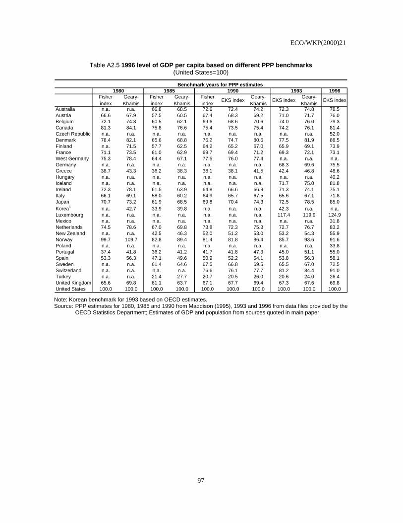
ECO/WKP(2000)21
97
Table A2.5 1996 level of GDP per capita based on different PPP benchmarks (United States=100)
Benchmark years for PPP estimates1980 1985 1990 1993 1996
Fisher index
Geary-Khamis
Fisher index
Geary-Khamis
Fisher index
EKS indexGeary-Khamis
EKS indexGeary-Khamis
EKS index
Australia n.a. n.a. 66.8 68.5 72.6 72.4 74.2 72.3 74.8 78.5Austria 66.6 67.9 57.5 60.5 67.4 68.3 69.2 71.0 71.7 76.0Belgium 72.1 74.3 60.5 62.1 69.6 68.6 70.6 74.0 76.0 79.3Canada 81.3 84.1 75.8 76.6 75.4 73.5 75.4 74.2 76.1 81.4Czech Republic n.a. n.a. n.a. n.a. n.a. n.a. n.a. n.a. n.a. 52.0Denmark 78.4 82.1 65.6 68.8 76.2 74.7 80.6 77.5 81.9 88.5Finland n.a. 71.5 57.7 62.5 64.2 65.2 67.0 65.9 69.1 73.9France 71.1 73.5 61.0 62.9 69.7 69.4 71.2 69.3 72.1 73.1West Germany 75.3 78.4 64.4 67.1 77.5 76.0 77.4 n.a. n.a. n.a.Germany n.a. n.a. n.a. n.a. n.a. n.a. n.a. 68.3 69.6 75.5Greece 38.7 43.3 36.2 38.3 38.1 38.1 41.5 42.4 46.8 48.6Hungary n.a. n.a. n.a. n.a. n.a. n.a. n.a. n.a. n.a. 40.2Iceland n.a. n.a. n.a. n.a. n.a. n.a. n.a. 71.7 75.0 81.8Ireland 72.3 78.1 61.5 63.9 64.8 66.6 66.9 71.3 74.1 75.1Italy 66.1 69.1 58.0 60.2 64.9 65.7 67.5 65.6 67.1 71.8Japan 70.7 73.2 61.9 68.5 69.8 70.4 74.3 72.5 78.5 85.0Korea1 n.a. 42.7 33.9 39.8 n.a. n.a. n.a. 42.3 n.a. n.a.Luxembourg n.a. n.a. n.a. n.a. n.a. n.a. n.a. 117.4 119.9 124.9Mexico n.a. n.a. n.a. n.a. n.a. n.a. n.a. n.a. n.a. 31.8Netherlands 74.5 78.6 67.0 69.8 73.8 72.3 75.3 72.7 76.7 83.2New Zealand n.a. n.a. 42.5 46.3 52.0 51.2 53.0 53.2 54.3 55.9Norway 99.7 109.7 82.8 89.4 81.4 81.8 86.4 85.7 93.6 91.6Poland n.a. n.a. n.a. n.a. n.a. n.a. n.a. n.a. n.a. 33.8Portugal 37.4 41.8 36.2 41.2 41.7 41.8 47.3 45.0 51.1 55.0Spain 53.3 56.3 47.1 49.6 50.9 52.2 54.1 53.8 56.3 58.1Sweden n.a. n.a. 61.4 64.6 67.5 66.8 69.5 65.5 67.0 72.5Switzerland n.a. n.a. n.a. n.a. 76.6 76.1 77.7 81.2 84.4 91.0Turkey n.a. n.a. 21.4 27.7 20.7 20.5 26.0 20.6 24.0 26.4United Kingdom 65.6 69.8 61.1 63.7 67.1 67.7 69.4 67.3 67.6 69.8United States 100.0 100.0 100.0 100.0 100.0 100.0 100.0 100.0 100.0 100.0
Note: Korean benchmark for 1993 based on OECD estimates. Source: PPP estimates for 1980, 1985 and 1990 from Maddison (1995), 1993 and 1996 from data files provided by the
OECD Statistics Department; Estimates of GDP and population from sources quoted in main paper.
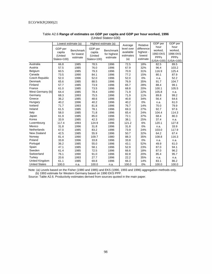
ECO/WKP(2000)21
98
Table A2.6 Range of estimates on GDP per capita and GDP per hour worked, 1996 (United States=100)
Lowest estimate (a) Highest estimate (a)
GDP per capita
(United States=100)
Benchmark for lowest estimate
GDP per capita
(United States=100)
Benchmark for highest estimate
Australia 66.8 1985 78.5 1996 72.5 18% 82.5 89.5Austria 57.5 1985 76.0 1996 67.9 32% 96.4 103.2Belgium 60.5 1985 79.3 1996 70.9 31% 116.9 125.4Canada 73.5 1990 84.1 1996 77.2 15% 80.1 87.9Czech Republic 52.0 1996 52.0 1996 52.0 0% n.a. 52.2Denmark 65.6 1985 88.5 1996 76.9 35% 91.7 104.7Finland 57.7 1985 73.9 1996 65.7 28% 88.4 99.1France 61.0 1985 73.5 1996 68.8 20% 100.1 105.5West Germany (b) 64.4 1985 78.4 1990 71.9 22% 105.8 n.a.Germany 68.3 1993 75.5 1996 71.9 11% 89.8 99.2Greece 36.2 1985 48.6 1996 40.8 34% 56.4 64.6Hungary 40.2 1996 40.2 1996 40.2 0% n.a. 61.0Iceland 71.7 1993 81.8 1996 76.7 14% 70.0 79.9Ireland 61.5 1985 78.1 1996 69.3 27% 92.7 97.6Italy 58.0 1985 71.8 1996 65.4 24% 104.4 114.3Japan 61.9 1985 85.0 1996 72.1 37% 68.4 80.3Korea 33.9 1985 42.3 1993 38.1 25% 37.4 n.a.Luxembourg 117.4 1993 124.9 1996 121.2 6% 120.1 127.8Mexico 31.8 1996 31.8 1996 31.8 0% n.a. 33.9Netherlands 67.0 1985 83.2 1996 73.9 24% 103.0 117.9New Zealand 42.5 1985 55.9 1996 50.7 32% 64.2 67.4Norway 81.4 1990 109.7 1980 88.3 35% 108.8 116.3Poland 33.8 1996 33.8 1996 33.8 0% n.a. n.a.Portugal 36.2 1985 55.0 1996 43.1 52% 49.9 61.0Spain 47.1 1985 58.1 1996 52.9 23% 87.0 94.1Sweden 61.4 1985 72.5 1996 66.6 18% 87.0 96.2Switzerland 76.1 1990 91.0 1996 82.8 20% 85.4 95.7Turkey 20.6 1993 27.7 1996 22.2 35% n.a. n.a.United Kingdom 61.1 1985 69.8 1996 66.3 14% 83.1 86.2United States 100.0 n.a. 100.0 n.a. 100.0 0% 100.0 100.0
GDP per hour
worked, 1996 EKS
PPPs (USA=100)
GDP per hour
worked, 1993 EKS
PPPs (USA=100)
Average level over available estimates
(a)
Relative difference highest -lowest
estimate
Note: (a) Levels based on the Fisher (1980 and 1985) and EKS (1990, 1993 and 1996) aggregation methods only. (b) 1993 estimate for Western Germany based on 1990 EKS PPP. Source: Table A2.6. Productivity estimates derived from sources quoted in the main paper.
ECO/WKP(2000)21
99
A2.4 Data sources and link with national sources
93. As a rule, two OECD databases were used in this study:
− the Analytical Data Base (ADB) for indicators at the level of the entire economy or at the level of the total business sector;
− the Structural Analysis (STAN/ISDB) database at the level of individual industries or sectors (see Table A2.7).
94. In consultation with the OECD Directorate for Employment, Labour and Social Affairs, several specific adjustments were made to data on hours worked. These are discussed in a subsection. Also, in some cases, the latest (1999) edition of the STAN database does not reflect the latest data available from national sources and where updates were available, they have been used in this study.
95. For some analytical parts, information is drawn from additional sources. These include recent work by DSTI (Schreyer, 2000) which is the source for information on the compositional change of the capital stock and on the flow of capital services in the G-7 countries. Similarly, the data needed to differentiate labour input by type of worker comes from OECD Education at a Glance, OECD Database, 1999.
96. In individual cases, a decision was taken to use alternative sources or to construct specific estimates in order to enhance time-series and cross-country comparability in the derived growth rates. Specific adjustments have been made for three countries: United Kingdom, Canada and United States. In a specific subsection for each country, these adjustments are discussed and compared with national sources. Among the most important adjustments are those concerning capital stock series for the United States and Canada. These adjustments reflect efforts to use a gross capital stock measure for basic productivity calculations, so as to be in line with the majority of data available for other countries.
97. Furthermore, three OECD countries (the United States, Canada and Australia) have undertaken specific statistical programmes to develop national series on multi-factor productivity growth. Because of somewhat different methodologies, these national indicators may not coincide with those developed by OECD in the present study. It is therefore useful to reconcile national and international results so as to maximise transparency about possible differences. The subsections on data sources for the United States and Canada accomplish this task as well. In the comparison with national sources, measures used for this study will be termed as OECD measure for simplicity.

ECO/WKP(2000)21
100
Table A2.7 Industry breakdown (ISDB, STAN databases)
ISIC 2 classification3000 Total manufacturing industry3100 Food, drink & tobacco3200 Textiles, footwear & leather3300 Wood, cork & furniture3400 Paper & printing3500 Chemical products3510 Industrial chemicals3520 Other chemicals3512X Chemicals excl. drugs3522 Drugs and medicines3534A Petrol refineries & products3556A Rubber & plastics products3600 Stone, clay & glass3700 Basic metal industries3710 Ferrous metals3720 Non-ferrous metals3800 Fabricated metal products and machinery3810 Fabricated metal products3820 Non-electrical machinery382X Machinery & equipment, nec3825 Office machinery & computers3830 Electrical machinery383X Electrical machinery excl. comm. equipment3832 Radio, TV & communication equipment3840 Transport equipment3841 Shipbuilding3843 Motor vehicles3845 Aircraft3842A Other transport equipment3850 Professional goods3900 Other manufacturing1000 Agriculture2000 Mining and quarrying4000 Electricity, gas, water5000 Construction6000 Wholesale & retail trade, restaurants and hotels6120 Wholesale and retail trade6300 Restaurants and hotels7000 Transports, storage, and communications7100 Transport and storage7200 Communication services8000 Finance,insurance,real estate, & business services8120 Finance and insurance8300 Real estate and business services9000 Community, social, and personal services9100 Public administration and defence9200 Sanitary and similar services9300 Social and related community services9400 Recreational and cultural services9500 Personal and household services9600 International services
ECO/WKP(2000)21
101
A2.4.1 Hours worked
98. Estimates of hours worked come mainly from two national or EU sources:
− For Austria, Belgium, Denmark, Greece, Ireland, Italy, Luxembourg, Netherlands, Portugal, and the United Kingdom, a country-specific adjustment has been applied to data from the European Labour Force Survey (EULFS). This adjustment factor varies by year and is obtained as the ratio of adjusted versus non-adjusted estimates of hours worked based on the EULFS under the assumption that there is a 50 per cent underestimation for time lost due to illness and maternity. The average adjustment factor for the countries reported above is 0.97.
− For Finland and Iceland, an average adjustment factor derived from the EULFS has been applied to national Labour Force Survey (LFS) estimates due to the limited length of EULFS series.
− For Australia, Czech Republic, Korea, and New Zealand, data come from LFS, adjusted with the average adjustment factor of 0.97.
− For Canada, France, Germany, Hungary, Japan, Norway, Spain, Sweden, and Switzerland, data are national estimates (either from LFS, or from national accounts/enterprise surveys). For the United States data are the BLS estimate of total hours worked on the basis of the Current Population Survey, the Current Employment Statistics, and the Hours at Work Survey, divided by the average number of employed persons.
− For Mexico hours worked are based on a level estimate from Maddison (1995) for 1992 and a time series from the National Survey of Employment (see OECD, 1999d, for more detailed information on national sources).
Where possible, estimates has also been extended backwards through splicing with the estimates from Maddison (1995).
A2.4.2 United States
99. In the United States, BLS provides official series on labour and multi-factor productivity. In what follows, comparisons are made with BLS’s annual multifactor statistics for the United States business sector. The table below compares average annual rates of change of output and different input measures for the period 1980-97. The following observations can be made:
Output
100. Small differences occur, because OECD (ADB) business sector data is based on national income and product accounts data, reflecting revisions as of 28 Oct. 1999 which have not yet been incorporated into the BLS series. Also, the BLS business sector output measures exclude government enterprises to be fully consistent with its capital input series. The OECD series does not make this adjustment and therefore
ECO/WKP(2000)21
102
includes government enterprises. Also, the ADB adjustment to move from an aggregate for the total economy to the value-added of the business sector is not identical to national procedures.74
Labour
101. The number of persons in the OECD series is taken from employment data as published in the United States’ National Income and Product Accounts. It reflects persons employed in production, i.e. the number of employees plus self-employed. Hours worked per person were derived separately, as discussed above. BLS, in its multi-factor productivity series, uses an index of labour input. Conceptually, the measure of labour input is similar to OECD’s labour input measure as described in Annex 3 (Section A3.1): it reflects total hours worked, adjusted for changes in the composition of the quality of labour. Although BLS is able to use a much finer level of differentiation between types of labour, the two labour input measures differ only by 0.2 percentage points over the period under consideration. While this difference would appear small, it may be the result of compensating differences or simply due to the specific period chosen for comparison.
Capital
102. As pointed out earlier, for its basic MFP series, OECD uses an estimated measure of the gross capital stock75, while available data in ADB refer to a concept of net capital stock as published by BEA. BLS, akin to its labour input measure, uses a measure of capital services that reflects both the quantity and the changing composition of capital input. The underlying concept is briefly described in Annex 3 (Section A3.1) as well as in the body of the text, and more fully in OECD (1999a). As would be expected, the gross capital stock measure grows by much less (at an average 2.8 per cent) than BLS’ capital service measure (at an average of 3.2 per cent). However, there is significant similarity between OECD’s capital service series and that of BLS. The construction of the OECD capital service data is described above in Annex 3 (Section A3.1).
MFP measures
103. Depending on the ingredients, different MFP measures are constructed: a simple MFP term based on unadjusted labour and capital data, grows by 1.0 per cent per year over the period 1980-97. It falls to 0.8 per cent when labour input is adjusted for compositional change and falls further to 0.6 per cent when adjusted capital input is used. The latter measure is the one closest comparable to BLS’ MFP index, and the resulting 0.2 percentage point difference would appear within the bounds of comparability.
74. More specific information is available from the Economic Outlook data base description on
http://www.oecd.org/eco/data/eoinv.pdf.
75. The estimate of the gross stock uses BEA’s former gross stock measure up to 1993, the last available update. More recent estimates were obtained as follows: the historical series of gross stock were regressed against BEA’s net stock series and BLS’ capital services series. For years after 1993, the gross stock was then estimated as the predicted value from this regression, using recent observations on the net stock and on capital services.

ECO/WKP(2000)21
103
Table A2.8 Comparison between productivity measures by OECD and by the Bureau of Labour Statistics*
MeasureOECD Difference
Output 3.1% 3.2% -0.1%
Labour 1.8%0.0%2.0% 2.2% -0.1%
Capital 1980-97 2.8% 3.2% -0.4%
1980-96 b) Capital services** 3.2% 3.2%
c) Memorandum item:1980-97 Wealth capital stock (US Bureau of Economic Analysis) 2.5%
Results:MFP, based on hours worked and capital stock 1.0%MFP, based on labour input and capital stock 0.8%MFP, based on labour input and capital services 1980-97 0.5%MFP, based on labour input and capital services 1980-96 0.6% 0.4% 0.2%
* BLS Annual multifactor productivity statistics** See text for explanations.
a) Number of persons
Labour input**b) Labour input**
1980-97 Average annual rate of change
Methodology/definitionOECD BLS BLS
Value-added of business sector
Capital services**
Hours per person
a) Gross capital stock Capital services**
A2.4.3 Canada
104. In Canada, labour and MFP statistics are published annually by Statistics Canada. In what follows, comparisons are made with Statistics Canada’s data for the business sector, and based on a value-added concept. The table below compares average annual rates of change of output and different input measures for the period 1980-97. The following observations can be made:
Output
105. There are only minor differences between OECD business sector series and the ones published by Statistics Canada, due to differences in the definition of the business sector.
Labour
106. The number of persons in the OECD series is taken from employment data as published by Statistics Canada’s Input-Output Division. Series on both the number of persons and on total hours are available. Statistics Canada, in its multi-factor productivity series, uses an index of labour input. Conceptually, this labour input measure is not as elaborate as the one used by BLS but is more developed than a simple sum of all hours. Differentiation takes place by industry, because each industry’s contribution to the economy’s labour input is weighted by the share that a given industry occupies in the economy’s total labour compensation. If average wages in an industry exceed those of other sectors, an
ECO/WKP(2000)21
104
implicit weighting of hours by industry takes place. However, there is no explicit differentiation by educational attainment or the skills of workers. As it turns out, over the period 1980-97 presented here, there is only a minor difference between total hours and the labour input series. However, and not surprisingly, the comparison with OECD’s labour input series (which reflects an attempt to explicitly differentiate between types of workers) shows a more important difference: the former grows by 1.4 per cent, the latter by 1.7 per cent.
Capital
107. As pointed out earlier, for its basic MFP series, OECD uses an estimated measure of the gross capital stock. For Canada, gross capital stock is the Statistics Canada capital stock series that is constructed on a one-hoss shay age-efficiency pattern. Statistics Canada’s own MFP calculations use as input another of their capital stock series, one based on a geometric age-efficiency pattern. A second difference lies in the aggregation procedure: Statistics Canada uses a Fisher index number formula to aggregate capital input across industries. The gross capital stock measure used by OECD is based on a Laspeyres-type aggregation formula. Again, the final outcome does not differ by much, although this reflects the combined, and partly offsetting, effects of a different age-efficiency pattern and a different index number formula. Finally, the table shows OECD’s capital services measure which aims at capturing the changing composition of capital input. The underlying concept is briefly described in Annex 3 as well as in the body of the text.
MFP measures
108. Depending on the ingredients, different MFP measures are constructed: a simple MFP term based on unadjusted labour and capital data, grows by 0.6 per cent per year over the period 1980-97. This compares with a 0.7 per cent change in Statistics Canada’s data. The OECD MFP measure falls to 0.4 per cent when labour input is adjusted for compositional change and falls further to 0.2 per cent when adjusted capital input is used.

ECO/WKP(2000)21
105
Table A2.9 Comparison between productivity measures by OECD and by Statistics Canada
MeasureOECD Difference
Output2.5% 2.6% 0.0%
Labour 1.5%-0.1% 1.4% 0.1%1.7%
Capital a )1980-97 2.9% 2.7% 0.1%
b )1980-96 3.1%
MFP, based on hours worked and capital stock 1980-97 0.6% 0.7% -0.1%MFP, based on labour input and capital stock 1980-97 0.4%MFP, based on labour input and capital services 1980-96 0.2%
* Statistics Canada's Multifactor Productivity Measures based on value-added (as of December 1999)** See text for explanations.
Capital services**
Value added of business sector
a) Number of personsHours per person
b) Labour input**Labour input**
Gross capital stock Capital input**
1980-97 Average annual rate of change
Methodology/definitionOECD Statistics Canada Statistics Canada
A2.4.4 United Kingdom
109. In the United Kingdom, time series for business sector GDP and employment have been corrected to take into account the fact that the National Health Service (NHS) Trust, created in 1991, is not accounted for in the government sector. Conversely all public health services were accounted for in the government sector before 1991. For comparability reasons both employment and GDP of NHS Trust have been subtracted from business sector series. The method of calculation of GDP of NHS Trust is as follows: First on the basis of United Kingdom Abstract of Statistics, 1998, a productivity level at current prices of NHS Staff was computed on the basis of Total Current Expenditure on the NHS (item KJQJ) and Total Employment of NHS (items KDBC+KDBO+KWUH). Then a real (at 1995 prices) productivity was computed through the implicit deflator of Health and Social Work sector (Sector N in the National Accounts - National Accounts, 1998 - Blue Book). Then this productivity was applied to data on NHS Trust staff.
ECO/WKP(2000)21
106
ANNEX 3. METHODOLOGICAL NOTES
A3.1 Measurement of labour and capital inputs
110. Measures of factor use for the purpose of productivity analysis should be constructed so as to reflect the role that each factor plays as input in the production process. In the case of labour input, the simple count of hours worked is only a crude approximation to the correct measure of labour input insofar as workers show great differences in education, experience, sector of activity and other attributes that greatly affect their marginal productivity. In particular, different types of labour should be weighted by their marginal contribution to the production activity in which they are employed. Since these productivity measures are generally not observable, information on relative wages by characteristics is used to derive the required weights to aggregate different types of labour. The resulting measure of labour input can be quite different from a simple aggregate of total hours or total persons (Dean et al., 1996). The difference between the weighted and unweighted series yields an index for the compositional change of labour input, or its quality.
111. Jorgenson (1963) and Jorgenson and Griliches (1967) were the first to develop aggregate capital input measures that took the heterogeneity of assets into account: they defined the flow of quantities of capital services individually for each type of asset, and then applied asset-specific user costs as weights to aggregate across services from the different types of assets. User costs are prices for capital services and, under competitive markets and equilibrium conditions, these prices reflect marginal productivities of the different assets. User cost weights are thus a means to effectively incorporate differences in the productive contribution of heterogeneous investments as the composition of investment and capital changes. Changes in aggregate capital input therefore have two distinct sources – changes in the quantity of capital of a given type, and changes in the composition of the various types of assets with different marginal products and user costs (Ho et al., 1999). Computationally, the comparison of an aggregate capital stock with a measure of capital services based on user costs weights, yields a measure of the compositional change of capital input.
A3.1.1 Productivity growth measures without adjustment for different types of factor input
112. The following notation is used to discuss factor productivity with and without control for quality effects:
Y Current price value-added;
P Price index of value-added;
N Total number of persons engaged;
H Average hours worked per person;
N*H Total hours worked;
Κ Aggregate gross capital stock.
ECO/WKP(2000)21
107
113. Letting lower case letters represent logarithms and Δ the first difference operator, Δx approximates the (instantaneous) growth rate of any variable x. The standard measure of factor productivity growth rates, dπL and dπK are given by:
ΔπL=Δy - Δp - (Δn + Δh) Labour productivity
ΔπK=Δy - Δp - Δk Capital productivity
114. This standard specification does not differentiate between different types of inputs: it attaches the same weight to each hour worked, and it does not differentiate between assets even though their marginal contribution to output may be quite different. Such differentiation can be introduced when there is information on quantities and prices of the different types of factor inputs. In the case of labour, prices will represent the skill-specific wage rate, in the case of capital the asset specific rental price or user cost of capital. In what follows different types of labour and capital will be distinguished by the subscript j.
A3.1.2 Productivity growth measures with adjustment for different types of factor input
115. Given a set of observations on different types of labour or capital and given a set of corresponding prices, t,jw it is possible to construct an aggregate variable F that combines quantities of different types of inputs to a measure of total, quality-adjusted labour or capital input. In this regard, productivity studies often use the Törnqvist index and this practice is followed here. A Törnqvist index of factor input F is given by the expression below, where t,jv stands for the share of the component j in total costs of the factor. This is a conceptually correct measure for the flow of the total quantity of labour or capital services:
( ) .21)(
,,
,,,1,,,,, ∑∑ =+=Δ⋅=Δ −
ititi
tjtjtjtjtjtj
jtjtjt Fw
Fwvandvvvwherefvadjf [A3.1]
116. Thus, the growth rate of total factor input Δf, using the Törnqvist index, is a weighted average of the growth rates of different components. Weights correspond to the current price share in the overall cost for each factor. Subtracting the unadjusted measure of factor input from the one adjusted for compositional changes yields an expression Δcf for the effects of changing factor quality on total factor input services:
Δcl = Δl(adj) - (Δn + Δh). [A3.2]
Δck = Δk(adj) - Δk. [A3.3]
117. Equations [A3.2] and [A3.3] can be rearranged to yield a decomposition of the overall growth in factor input:
Δl(adj) = Δcl + Δn + Δh
Δk(adj) = Δck + Δk
ECO/WKP(2000)21
108
A3.1.3 Labour input
118. In order to consider changes in the composition of labour input, six different types of labour were considered, based on gender and three different educational levels: below upper secondary education; upper secondary education and tertiary education. Thus, if Lj indicates the labour input jth with j=1,2,..6 and each type of labour is remunerated with wage rate w,j , the following observation concerning calculations should be made:
− First, it is assumed that the rate change in average weekly or yearly hours is identical between education and gender groups, i.e. Δh,j=Δh for all j. This simplification can be used, in conjunction with the relation Δl,j=Δn,j + Δh,j.
− Second, data on relative wage rates by education attainment and gender are only available for the 1990s, and thus relative wage rates were assumed to be constant over the period considered in the analysis. More specifically, for the six available categories of education and
gender, the wage spread was computed as 6,5,4,3,2,,
=jw
w
USM
j as each education category’s
wage rate relative to wages of male workers with upper-secondary education (wM,,US).
− The weights vj,c from equation [A3.1] for country c can be rewritten in terms of relative wages:
∑∑==
== 6
1,
,,
,
,,,
,
6
1,,
,,,
ici
cUSM
ci
cjcUSM
cj
icici
cjcjcj
Nw
w
Nw
w
Nw
Nwv .
119. Data on the level of education attainment of employment and relative wages are from the OECD Education at a Glance and refers to the ISCED classification. Available data have been re-grouped into three education groups, for both men and women: 1) below upper secondary education (ISCED 0 to ISCED 2); 2) upper secondary education (ISCED 3); and 3) tertiary education (ISCED 5 to ISCED 7). The level of education attainment for male and female workers is available for the early 1980s and 1996 for the following countries: Denmark, Finland, France, New Zealand, Norway, Spain and Sweden. For the other countries, the first available data in the OECD database is 1989. To estimate changes in the composition of employment from the 1980s to the 1990s, the OECD data have been complemented with information from the Barro and Lee (1996) database. In particular, growth rates of employment by different level of education were used to estimate missing observations for the early 1980s. For Austria, Belgium, Czech Republic, Greece, Hungary, Korea, Mexico, Poland, Spain, Switzerland and Turkey the calculation of labour input was not possible due to the unavailability of either the education composition of employment or relative wages by education level.
A3.1.4 Capital input76
120. In the case of capital, it is assumed that capital services from asset type j, t,jK , are in constant proportion to the productive stock77 of capital asset j, P
t,jK :
76. For a fuller description, see Schreyer (2000).

ECO/WKP(2000)21
109
.6,...2,1jKK Pt,jjt,j == ρ
121. Six types of assets were used as a basis for calculation: non-residential structures, transport equipment, information technology equipment, communication equipment, other producer durable equipment and other capital goods. For each asset, a productive capital stock is constructed by aggregating across different vintages of investment and by allowing for losses of productive efficiency over an asset’s service life.
122. Because countries employ different methodologies to construct deflators for information and communication technology assets, a harmonised deflator was used to measure real investment expenditure in these products.
123. Associated with the quantity flow of capital services (such as ton-kilometres provided by a freight truck or cubic feet of storage space provided by a warehouse) comes a price component, the user cost or rental price of capital. Capital services are sometimes traded between asset owners and the producers who need to use them. However, most capital services are produced for own consumption within producers’ establishments and cannot be observed in the marketplace. Jorgenson (1963) and Jorgenson and Griliches (1967) demonstrated how user cost expressions can be computed. They are composed of i) the opportunity costs of investing money in the bank rather than in a capital good; ii) of the costs of depreciation, i.e. the loss in value of the capital asset as it ages; and iii) of capital gains or losses, or the change in value of the asset that is unrelated to ageing.78 These three components are reflected in the user cost expression jμ for asset j below, where qj is the asset’s acquisition price, r is the internal rate of return (equal across all assets), and dj is the asset-specific rate of depreciation.
1,,,,
1,,,, )( +
+ Δ−+=⎟⎟⎠
⎞⎜⎜⎝
⎛ Δ−+= tjtjttj
tj
tjtjttjtj qdrq
drqμ
77. There are different ways how the loss in productive efficiency can be modelled, including at a constant rate
(geometric age-efficiency profile), by a constant amount (linear declining balance), in a single step at the end of the service life (‘one hoss shay), or at a changing rate that accelerates over an asset’s service life (hyperbolic pattern). The choice of a particular age-efficiency profile is an empirical one – and a matter of plausibility. For the present exposition, a hyperbolic profile underlies the calculation but other results can be tested.
78. Taxes and depreciation allowances are further elements that should enter user cost expressions. For a more comprehensive treatment of the measurement of user costs, see OECD (1999a).
ECO/WKP(2000)21
110
124. Given the time series on Pt,jK and t,jμ , asset specific weights t,jv as in equation [A3.1] are given
by:
∑=
= 6
1,,
,,,
i
Ptiti
Ptjtj
tj
K
Kv
μ
μ
A3.2 Sensitivity analysis of multi-factor productivity
125. Table 6 and Table 7 in the main text report various measures of MFP growth. Using trend series for output and labour, Table 6 shows the effect of different measures of partial output elasticities (namely average labour shares, time-varying labour shares and estimated elasticities). Table 7 shows how the measure of MFP growth rates is affected by changes in the way inputs are measured (namely accounting for hours worked and quality changes). Results and consequent interpretation of different MFP measures are discussed in the main text and are not repeated here. This section expands further the sensitivity analysis by reporting measures of MFP growth based on actual series. Furthermore, in a separate subsection, it gives details on the estimation of partial output elasticities.
A3.2.1 Trend vs. actual time series
126. All the analysis on growth rates of MFP developed in the main text considers trend series of real GDP and employment in the business sector. In principle, it can be expected that the use of trend rather than actual time series makes little difference for average growth rates over a long period (e.g. 10 years). Conversely, over a shorter period, averages of trend growth rates of MFP can be rather different from averages of actual growth rates, due to the fact that the latter incorporate short-run dynamics due to partial adjustment, cyclical phenomena and the effect of transitory shocks. Table A3.1 reports MFP growth rates based on actual time-series (The table has the same structure of Table 6 in the main text). As expected, differences between MFP growth rates based on actual and trend series are small except for the period 1995-98 for few countries.79 A similar conclusion can be drawn for MFP growth rates adjusted for hours worked, reported in Table A3.2.
79. Somewhat significant differences can be observed for Japan also the period 1990-97.
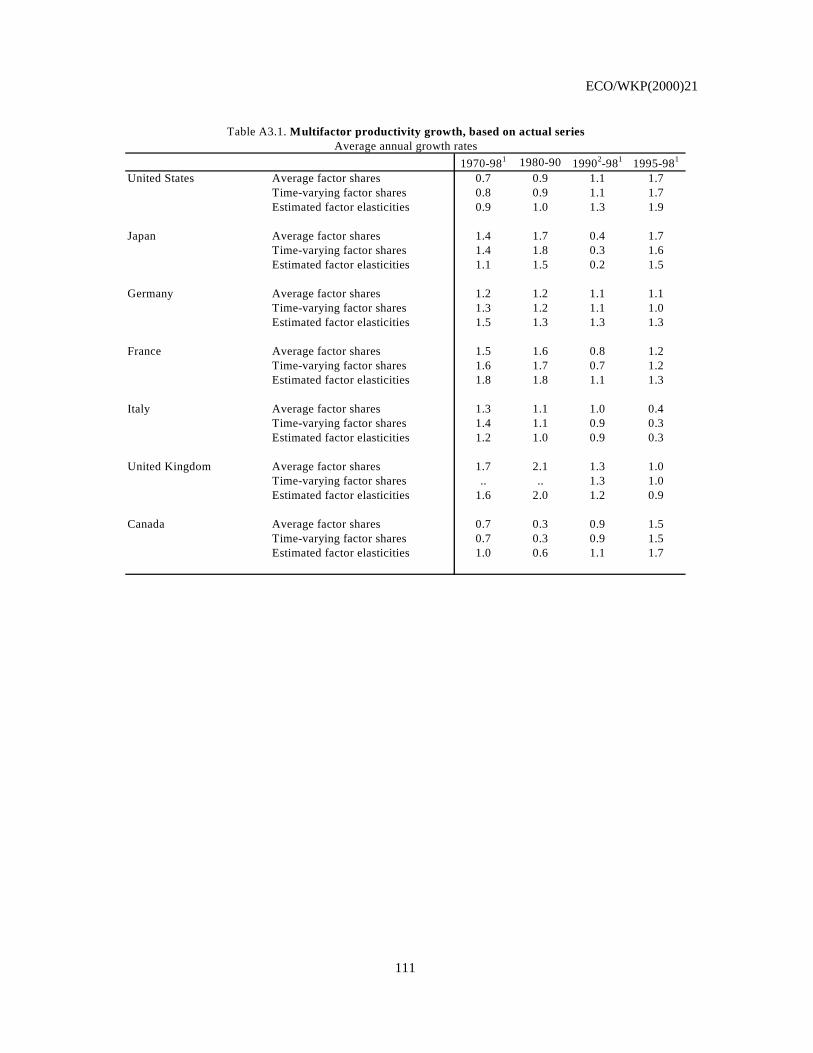
ECO/WKP(2000)21
111
1970-981 1980-90 19902-981 1995-981
United States Average factor shares 0.7 0.9 1.1 1.7Time-varying factor shares 0.8 0.9 1.1 1.7Estimated factor elasticities 0.9 1.0 1.3 1.9
Japan Average factor shares 1.4 1.7 0.4 1.7Time-varying factor shares 1.4 1.8 0.3 1.6Estimated factor elasticities 1.1 1.5 0.2 1.5
Germany Average factor shares 1.2 1.2 1.1 1.1Time-varying factor shares 1.3 1.2 1.1 1.0Estimated factor elasticities 1.5 1.3 1.3 1.3
France Average factor shares 1.5 1.6 0.8 1.2Time-varying factor shares 1.6 1.7 0.7 1.2Estimated factor elasticities 1.8 1.8 1.1 1.3
Italy Average factor shares 1.3 1.1 1.0 0.4Time-varying factor shares 1.4 1.1 0.9 0.3Estimated factor elasticities 1.2 1.0 0.9 0.3
United Kingdom Average factor shares 1.7 2.1 1.3 1.0Time-varying factor shares .. .. 1.3 1.0Estimated factor elasticities 1.6 2.0 1.2 0.9
Canada Average factor shares 0.7 0.3 0.9 1.5Time-varying factor shares 0.7 0.3 0.9 1.5Estimated factor elasticities 1.0 0.6 1.1 1.7
Table A3.1. Multifactor productivity growth, based on actual seriesAverage annual growth rates
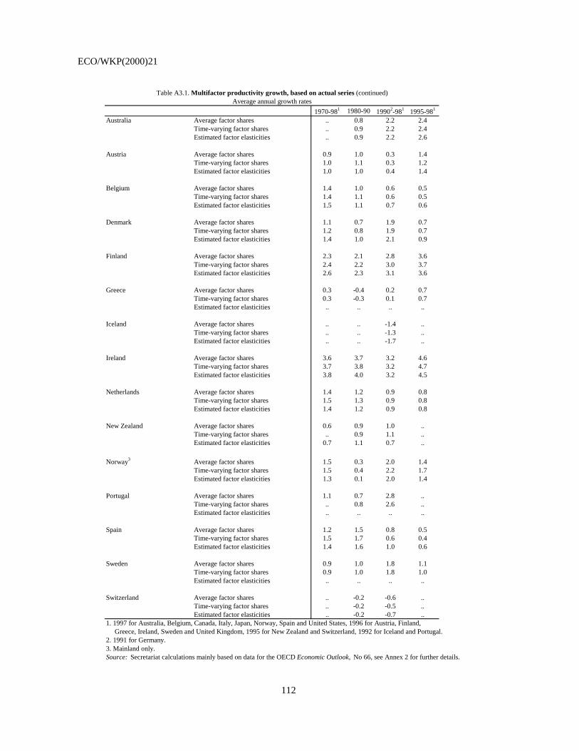
ECO/WKP(2000)21
112
1970-981 1980-90 19902-981 1995-981
Australia Average factor shares .. 0.8 2.2 2.4Time-varying factor shares .. 0.9 2.2 2.4Estimated factor elasticities .. 0.9 2.2 2.6
Austria Average factor shares 0.9 1.0 0.3 1.4Time-varying factor shares 1.0 1.1 0.3 1.2Estimated factor elasticities 1.0 1.0 0.4 1.4
Belgium Average factor shares 1.4 1.0 0.6 0.5Time-varying factor shares 1.4 1.1 0.6 0.5Estimated factor elasticities 1.5 1.1 0.7 0.6
Denmark Average factor shares 1.1 0.7 1.9 0.7Time-varying factor shares 1.2 0.8 1.9 0.7Estimated factor elasticities 1.4 1.0 2.1 0.9
Finland Average factor shares 2.3 2.1 2.8 3.6Time-varying factor shares 2.4 2.2 3.0 3.7Estimated factor elasticities 2.6 2.3 3.1 3.6
Greece Average factor shares 0.3 -0.4 0.2 0.7Time-varying factor shares 0.3 -0.3 0.1 0.7Estimated factor elasticities .. .. .. ..
Iceland Average factor shares .. .. -1.4 ..Time-varying factor shares .. .. -1.3 ..Estimated factor elasticities .. .. -1.7 ..
Ireland Average factor shares 3.6 3.7 3.2 4.6Time-varying factor shares 3.7 3.8 3.2 4.7Estimated factor elasticities 3.8 4.0 3.2 4.5
Netherlands Average factor shares 1.4 1.2 0.9 0.8Time-varying factor shares 1.5 1.3 0.9 0.8Estimated factor elasticities 1.4 1.2 0.9 0.8
New Zealand Average factor shares 0.6 0.9 1.0 ..Time-varying factor shares .. 0.9 1.1 ..Estimated factor elasticities 0.7 1.1 0.7 ..
Norway3 Average factor shares 1.5 0.3 2.0 1.4Time-varying factor shares 1.5 0.4 2.2 1.7Estimated factor elasticities 1.3 0.1 2.0 1.4
Portugal Average factor shares 1.1 0.7 2.8 ..Time-varying factor shares .. 0.8 2.6 ..Estimated factor elasticities .. .. .. ..
Spain Average factor shares 1.2 1.5 0.8 0.5Time-varying factor shares 1.5 1.7 0.6 0.4Estimated factor elasticities 1.4 1.6 1.0 0.6
Sweden Average factor shares 0.9 1.0 1.8 1.1Time-varying factor shares 0.9 1.0 1.8 1.0Estimated factor elasticities .. .. .. ..
Switzerland Average factor shares .. -0.2 -0.6 ..Time-varying factor shares .. -0.2 -0.5 ..Estimated factor elasticities .. -0.2 -0.7 ..
1. 1997 for Australia, Belgium, Canada, Italy, Japan, Norway, Spain and United States, 1996 for Austria, Finland, Greece, Ireland, Sweden and United Kingdom, 1995 for New Zealand and Switzerland, 1992 for Iceland and Portugal. 2. 1991 for Germany.3. Mainland only.Source: Secretariat calculations mainly based on data for the OECD Economic Outlook, No 66, see Annex 2 for further details.
Table A3.1. Multifactor productivity growth, based on actual series (continued)Average annual growth rates
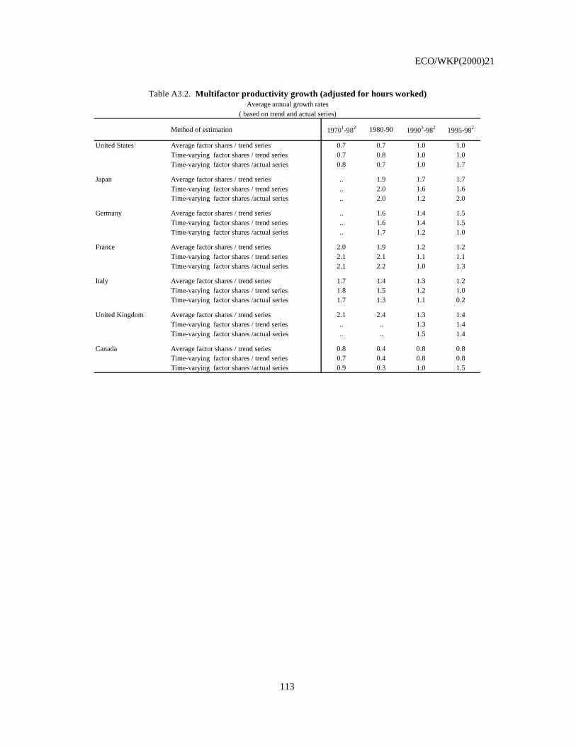
ECO/WKP(2000)21
113
Method of estimation 19701-982 1980-90 19903-982 1995-982
United States Average factor shares / trend series 0.7 0.7 1.0 1.0Time-varying factor shares / trend series 0.7 0.8 1.0 1.0Time-varying factor shares /actual series 0.8 0.7 1.0 1.7
Japan Average factor shares / trend series .. 1.9 1.7 1.7Time-varying factor shares / trend series .. 2.0 1.6 1.6Time-varying factor shares /actual series .. 2.0 1.2 2.0
Germany Average factor shares / trend series .. 1.6 1.4 1.5Time-varying factor shares / trend series .. 1.6 1.4 1.5Time-varying factor shares /actual series .. 1.7 1.2 1.0
France Average factor shares / trend series 2.0 1.9 1.2 1.2Time-varying factor shares / trend series 2.1 2.1 1.1 1.1Time-varying factor shares /actual series 2.1 2.2 1.0 1.3
Italy Average factor shares / trend series 1.7 1.4 1.3 1.2Time-varying factor shares / trend series 1.8 1.5 1.2 1.0Time-varying factor shares /actual series 1.7 1.3 1.1 0.2
United Kingdom Average factor shares / trend series 2.1 2.4 1.3 1.4Time-varying factor shares / trend series .. .. 1.3 1.4Time-varying factor shares /actual series .. .. 1.5 1.4
Canada Average factor shares / trend series 0.8 0.4 0.8 0.8Time-varying factor shares / trend series 0.7 0.4 0.8 0.8Time-varying factor shares /actual series 0.9 0.3 1.0 1.5
Table A3.2. Multifactor productivity growth (adjusted for hours worked)
( based on trend and actual series)Average annual growth rates
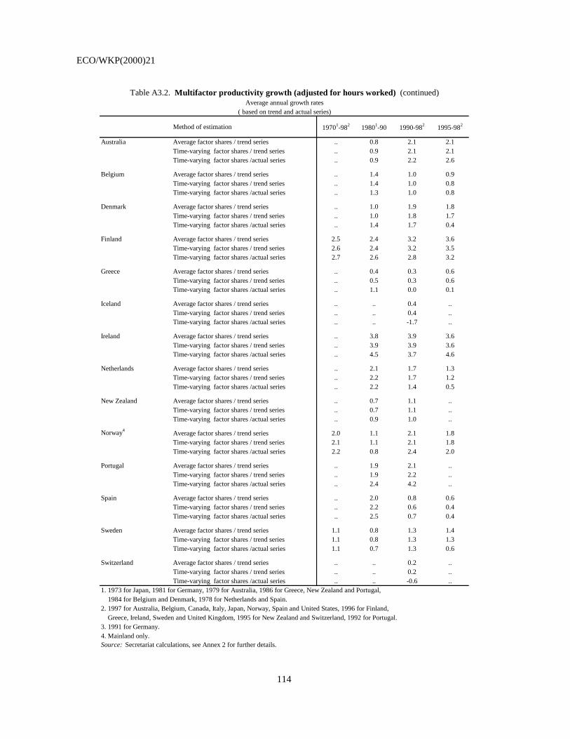
ECO/WKP(2000)21
114
Method of estimation 19701-982 19801-90 1990-982 1995-982
Australia Average factor shares / trend series .. 0.8 2.1 2.1Time-varying factor shares / trend series .. 0.9 2.1 2.1Time-varying factor shares /actual series .. 0.9 2.2 2.6
Belgium Average factor shares / trend series .. 1.4 1.0 0.9Time-varying factor shares / trend series .. 1.4 1.0 0.8Time-varying factor shares /actual series .. 1.3 1.0 0.8
Denmark Average factor shares / trend series .. 1.0 1.9 1.8Time-varying factor shares / trend series .. 1.0 1.8 1.7Time-varying factor shares /actual series .. 1.4 1.7 0.4
Finland Average factor shares / trend series 2.5 2.4 3.2 3.6Time-varying factor shares / trend series 2.6 2.4 3.2 3.5Time-varying factor shares /actual series 2.7 2.6 2.8 3.2
Greece Average factor shares / trend series .. 0.4 0.3 0.6Time-varying factor shares / trend series .. 0.5 0.3 0.6Time-varying factor shares /actual series .. 1.1 0.0 0.1
Iceland Average factor shares / trend series .. .. 0.4 ..Time-varying factor shares / trend series .. .. 0.4 ..Time-varying factor shares /actual series .. .. -1.7 ..
Ireland Average factor shares / trend series .. 3.8 3.9 3.6Time-varying factor shares / trend series .. 3.9 3.9 3.6Time-varying factor shares /actual series .. 4.5 3.7 4.6
Netherlands Average factor shares / trend series .. 2.1 1.7 1.3Time-varying factor shares / trend series .. 2.2 1.7 1.2Time-varying factor shares /actual series .. 2.2 1.4 0.5
New Zealand Average factor shares / trend series .. 0.7 1.1 ..Time-varying factor shares / trend series .. 0.7 1.1 ..Time-varying factor shares /actual series .. 0.9 1.0 ..
Norway4 Average factor shares / trend series 2.0 1.1 2.1 1.8Time-varying factor shares / trend series 2.1 1.1 2.1 1.8Time-varying factor shares /actual series 2.2 0.8 2.4 2.0
Portugal Average factor shares / trend series .. 1.9 2.1 ..Time-varying factor shares / trend series .. 1.9 2.2 ..Time-varying factor shares /actual series .. 2.4 4.2 ..
Spain Average factor shares / trend series .. 2.0 0.8 0.6Time-varying factor shares / trend series .. 2.2 0.6 0.4Time-varying factor shares /actual series .. 2.5 0.7 0.4
Sweden Average factor shares / trend series 1.1 0.8 1.3 1.4Time-varying factor shares / trend series 1.1 0.8 1.3 1.3Time-varying factor shares /actual series 1.1 0.7 1.3 0.6
Switzerland Average factor shares / trend series .. .. 0.2 ..Time-varying factor shares / trend series .. .. 0.2 ..Time-varying factor shares /actual series .. .. -0.6 ..
1. 1973 for Japan, 1981 for Germany, 1979 for Australia, 1986 for Greece, New Zealand and Portugal, 1984 for Belgium and Denmark, 1978 for Netherlands and Spain. 2. 1997 for Australia, Belgium, Canada, Italy, Japan, Norway, Spain and United States, 1996 for Finland, Greece, Ireland, Sweden and United Kingdom, 1995 for New Zealand and Switzerland, 1992 for Portugal. 3. 1991 for Germany.4. Mainland only.Source: Secretariat calculations, see Annex 2 for further details.
Average annual growth rates( based on trend and actual series)
Table A3.2. Multifactor productivity growth (adjusted for hours worked) (continued)
ECO/WKP(2000)21
115
A3.2.2 Estimates of partial output elasticities
127. In the context of the sensitivity analysis of estimates of MFP growth rate, partial output elasticities were also estimated directly using a production function (see Table 6 in the main text and Table A3.1 for estimates based on actual series). The rationale for this is to avoid postulating a relationship between partial output elasticities and income shares. 80
128. Estimating partial output elasticities involves direct estimation the production function using actual time series:
),( KLFQ =
and deriving partial elasticities for labour as:
),(),(
KLFL
LKLFa
∂∂
=
where Q is output, L is labour and K is capital stock.
129. The analysis can also be undertaken in intensive form by imposing constant returns to scale and dividing output and one of the factors by the other. Generally the choice of imposing rather than testing constant returns to scale depends on availability of data, given that sufficiently long time series are required for testing the assumption. In the analysis of this study constant returns to scale has been imposed, together with the assumption of unit elasticity of substitution between labour and capital (Cobb-Douglas production function) and Hicks- or Harrod-neutral technological progress. The latter assumption deserves some attention. Hicks/Harrod-neutral technological progress means that, in a Cobb-Douglas production function expressed in logarithms, the effect of technological change is additively separable. This allows testing trend-stationarity of technological change. Trend-stationarity is necessary to estimate the full relationship in levels. In fact, expressed in logarithms, the full relationship in labour-intensive form to be estimated is:
ulktlq ql +−++=− )(γβα [A3.4]
with γ̂1ˆ −=a , or in capital-intensive form,
ukltkq qk +−++=− )(δβα [A3.5]
with δ̂ˆ =a ;
α, β, and γ are the parameters to be estimated, t is time (semester or year), and u is a stationary random disturbance. If technological progress utMFP ++= βα were not trend-stationary, the relationships would
80. The methods based on income shares can be sensitive to measurement errors in inputs and outputs. For
instance, even under the assumption of perfect competition and thus when inputs are paid their (correctly measured) marginal productivity, the labour share corresponds to the coefficient of the labour input only if human capital has been included in the measure of labour input. Conversely, it can be different from the coefficient when the labour input is approximated with employment.
ECO/WKP(2000)21
116
not be cointegrated, and output elasticities could not be estimated directly from the foregoing equations using standard techniques.81
130. There are important issues related to the direct econometric estimation of equations [A3.4] and [A3.5] which relate to sample size and unreliability of measures of capital stock. The latter problem has often been partially solved in the literature by relying on estimation in first differences rather than in levels. However, first differences capture only short-run relationships and can provide very imprecise approximations of long-run relationships. Furthermore estimation in first differences gives up the convenient property of superconsistency of estimators in the case of cointegrated relationships between non-stationary variables, that is often the case with production functions. Senhadji (1999) compares estimates in first differences and estimates in levels based on cointegration techniques for 88 countries to conclude that reliability of level estimates is greater.
131. Estimation of equation [A3.4] or [A3.5] in levels involves several steps. First, unit root tests has to be carried out to select pairs of variables in intensive terms - (q-l,k-l) or (q-k,l-k) - that are either difference-stationary (presence of a unit root) or trend-stationary (absence of a unit root). Second, if the selected pair contain a unit root, the existence of a cointegration vector has to be tested. Third, if the test shows evidence of cointegration, or if the variables of the selected pair are trend-stationary, the corresponding equation can be estimated using an appropriate technique.
132. Table A3.3 reports standard Augmented Dickey-Fuller (ADF) unit root tests for the logarithm of output, employment and capital stock, as well as for variables in intensive form. The null hypothesis is that the tested time series contains a unit root, the alternative hypothesis is absence of unit roots. The number of lags in the equation depends on the significance of the coefficient of the maximum lag amongst those specifications that do not suffer from autocorrelation, according to a Box-Pierce test with appropriate choice of lags (see Banerjee et al., 1993). When autocorrelation is present in all models up to four lags, then the model with the lowest autocorrelation is chosen. The model always contains a deterministic time trend.
133. For each country reported in Table A3.3, it is possible to find at least a couple of variables in intensive terms - (q-l,k-l) or (q-k,l-k) - for which the tests show evidence of one unit root, with the only exception of Greece and Portugal, where the logarithm of the capital/labour ratio appears trend-stationary but the output in either labour or capital intensive form is only difference-stationary.82
81. Although they could be estimated in first differences.
82. Greece and Portugal were then eliminated from the analysis. Furthermore, for completeness, Table A3.3 and A3.4 report results for Iceland, although the number of observations is too short to have large confidence in estimates.
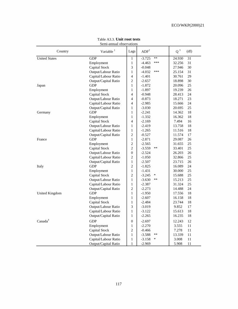
ECO/WKP(2000)21
117
Country Variable 1 Lags ADF2 Q 3 (df)
United States GDP 1 -3.725 ** 24.930 31Employment 1 -4.463 *** 32.256 31Capital Stock 3 -0.048 27.946 30Output/Labour Ratio 1 -4.032 *** 25.154 31Capital/Labour Ratio 4 -1.401 30.761 29Output/Capital Ratio 2 -2.657 18.898 30
Japan GDP 1 -1.872 20.096 25Employment 1 -1.897 19.239 26Capital Stock 4 -0.948 28.413 24Output/Labour Ratio 4 -0.873 18.271 23Capital/Labour Ratio 4 -2.985 15.666 24Output/Capital Ratio 1 -3.030 20.695 25
Germany GDP 1 -2.241 14.362 18Employment 1 -1.332 16.362 18Capital Stock 4 -2.169 7.494 16Output/Labour Ratio 1 -2.419 13.758 18Capital/Labour Ratio 1 -1.265 11.516 18Output/Capital Ratio 2 -0.527 11.574 17
France GDP 1 -2.871 29.087 26Employment 2 -2.565 31.655 25Capital Stock 2 -3.559 ** 33.401 25Output/Labour Ratio 0 -2.524 26.203 26Capital/Labour Ratio 2 -1.050 32.866 25Output/Capital Ratio 1 -2.507 23.715 26
Italy GDP 2 -1.825 16.089 24Employment 1 -1.431 30.000 25Capital Stock 2 -3.245 * 15.688 25Output/Labour Ratio 1 -3.630 ** 15.213 25Capital/Labour Ratio 1 -2.387 31.324 25Output/Capital Ratio 2 -2.273 14.488 24
United Kingdom GDP 1 -1.950 17.556 18Employment 1 -2.607 16.158 18Capital Stock 1 -2.484 23.744 18Output/Labour Ratio 3 -3.019 9.852 17Capital/Labour Ratio 1 -3.122 15.613 18Output/Capital Ratio 1 -2.265 16.235 18
Canada4 GDP 0 -2.697 12.243 12Employment 1 -2.270 3.555 11Capital Stock 2 -0.466 7.278 11Output/Labour Ratio 1 -3.588 ** 13.339 11Capital/Labour Ratio 1 -3.158 * 3.008 11Output/Capital Ratio 1 -2.969 5.908 11
Table A3.3. Unit root testsSemi-annual observations
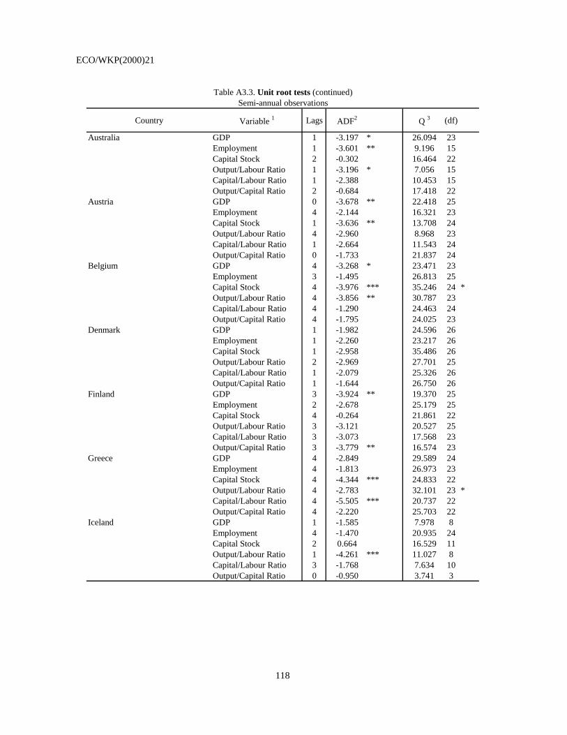
ECO/WKP(2000)21
118
Country Variable 1 Lags ADF2 Q 3 (df)
Australia GDP 1 -3.197 * 26.094 23Employment 1 -3.601 ** 9.196 15Capital Stock 2 -0.302 16.464 22Output/Labour Ratio 1 -3.196 * 7.056 15Capital/Labour Ratio 1 -2.388 10.453 15Output/Capital Ratio 2 -0.684 17.418 22
Austria GDP 0 -3.678 ** 22.418 25Employment 4 -2.144 16.321 23Capital Stock 1 -3.636 ** 13.708 24Output/Labour Ratio 4 -2.960 8.968 23Capital/Labour Ratio 1 -2.664 11.543 24Output/Capital Ratio 0 -1.733 21.837 24
Belgium GDP 4 -3.268 * 23.471 23Employment 3 -1.495 26.813 25Capital Stock 4 -3.976 *** 35.246 24 *Output/Labour Ratio 4 -3.856 ** 30.787 23Capital/Labour Ratio 4 -1.290 24.463 24Output/Capital Ratio 4 -1.795 24.025 23
Denmark GDP 1 -1.982 24.596 26Employment 1 -2.260 23.217 26Capital Stock 1 -2.958 35.486 26Output/Labour Ratio 2 -2.969 27.701 25Capital/Labour Ratio 1 -2.079 25.326 26Output/Capital Ratio 1 -1.644 26.750 26
Finland GDP 3 -3.924 ** 19.370 25Employment 2 -2.678 25.179 25Capital Stock 4 -0.264 21.861 22Output/Labour Ratio 3 -3.121 20.527 25Capital/Labour Ratio 3 -3.073 17.568 23Output/Capital Ratio 3 -3.779 ** 16.574 23
Greece GDP 4 -2.849 29.589 24Employment 4 -1.813 26.973 23Capital Stock 4 -4.344 *** 24.833 22Output/Labour Ratio 4 -2.783 32.101 23 *Capital/Labour Ratio 4 -5.505 *** 20.737 22Output/Capital Ratio 4 -2.220 25.703 22
Iceland GDP 1 -1.585 7.978 8Employment 4 -1.470 20.935 24Capital Stock 2 0.664 16.529 11Output/Labour Ratio 1 -4.261 *** 11.027 8Capital/Labour Ratio 3 -1.768 7.634 10Output/Capital Ratio 0 -0.950 3.741 3
Table A3.3. Unit root tests (continued)Semi-annual observations
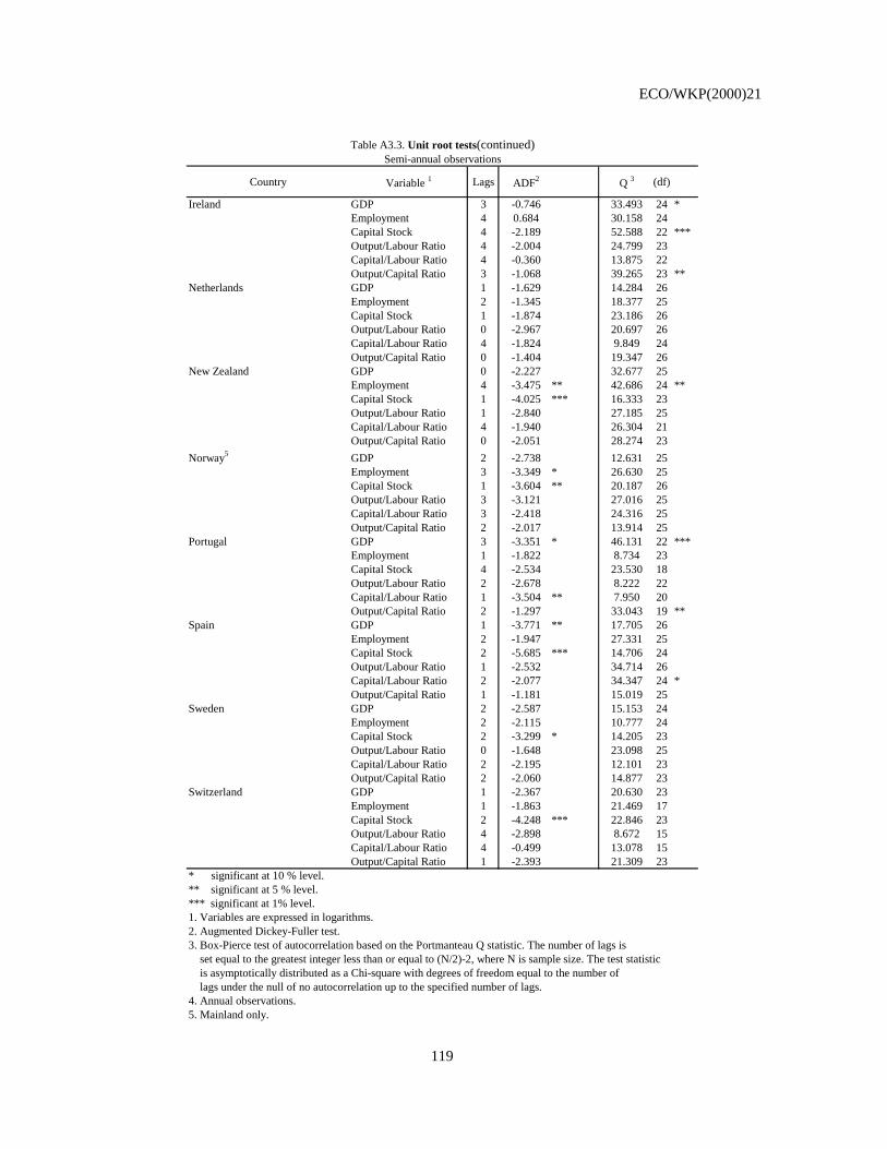
ECO/WKP(2000)21
119
Country Variable 1 Lags ADF2 Q 3 (df)
Ireland GDP 3 -0.746 33.493 24 *Employment 4 0.684 30.158 24Capital Stock 4 -2.189 52.588 22 ***Output/Labour Ratio 4 -2.004 24.799 23Capital/Labour Ratio 4 -0.360 13.875 22Output/Capital Ratio 3 -1.068 39.265 23 **
Netherlands GDP 1 -1.629 14.284 26Employment 2 -1.345 18.377 25Capital Stock 1 -1.874 23.186 26Output/Labour Ratio 0 -2.967 20.697 26Capital/Labour Ratio 4 -1.824 9.849 24Output/Capital Ratio 0 -1.404 19.347 26
New Zealand GDP 0 -2.227 32.677 25Employment 4 -3.475 ** 42.686 24 **Capital Stock 1 -4.025 *** 16.333 23Output/Labour Ratio 1 -2.840 27.185 25Capital/Labour Ratio 4 -1.940 26.304 21Output/Capital Ratio 0 -2.051 28.274 23
Norway5 GDP 2 -2.738 12.631 25Employment 3 -3.349 * 26.630 25Capital Stock 1 -3.604 ** 20.187 26Output/Labour Ratio 3 -3.121 27.016 25Capital/Labour Ratio 3 -2.418 24.316 25Output/Capital Ratio 2 -2.017 13.914 25
Portugal GDP 3 -3.351 * 46.131 22 ***Employment 1 -1.822 8.734 23Capital Stock 4 -2.534 23.530 18Output/Labour Ratio 2 -2.678 8.222 22Capital/Labour Ratio 1 -3.504 ** 7.950 20Output/Capital Ratio 2 -1.297 33.043 19 **
Spain GDP 1 -3.771 ** 17.705 26Employment 2 -1.947 27.331 25Capital Stock 2 -5.685 *** 14.706 24Output/Labour Ratio 1 -2.532 34.714 26Capital/Labour Ratio 2 -2.077 34.347 24 *Output/Capital Ratio 1 -1.181 15.019 25
Sweden GDP 2 -2.587 15.153 24Employment 2 -2.115 10.777 24Capital Stock 2 -3.299 * 14.205 23Output/Labour Ratio 0 -1.648 23.098 25Capital/Labour Ratio 2 -2.195 12.101 23Output/Capital Ratio 2 -2.060 14.877 23
Switzerland GDP 1 -2.367 20.630 23Employment 1 -1.863 21.469 17Capital Stock 2 -4.248 *** 22.846 23Output/Labour Ratio 4 -2.898 8.672 15Capital/Labour Ratio 4 -0.499 13.078 15Output/Capital Ratio 1 -2.393 21.309 23
* significant at 10 % level.** significant at 5 % level.*** significant at 1% level.1. Variables are expressed in logarithms.2. Augmented Dickey-Fuller test.3. Box-Pierce test of autocorrelation based on the Portmanteau Q statistic. The number of lags is set equal to the greatest integer less than or equal to (N/2)-2, where N is sample size. The test statistic is asymptotically distributed as a Chi-square with degrees of freedom equal to the number of lags under the null of no autocorrelation up to the specified number of lags. 4. Annual observations.5. Mainland only.
Semi-annual observationsTable A3.3. Unit root tests(continued)
ECO/WKP(2000)21
120
134. The labour intensive form of the production function (that is, eq. [A3.4]) is chosen whenever the output-labour ratio has a unit root83; otherwise the capital-intensive form (eq. [A3.5]) is considered. Cointegration is checked through Shin’s test (Shin, 1994) that, contrary to most single-equation cointegration tests, takes the hypothesis of cointegration as the null and that of no cointegration as the alternative, consistently with standard ways of testing the presence of unit roots. Given the strong theoretical ground for the existence of a stable relationship such as [A3.4] or [A3.5] (existence of a stable production function with constant returns to scale), a test that assumes cointegration as the null hypothesis seems more appropriate.84 Shin’s test is constructed on the basis of the residuals of the selected equation, estimated using dynamic estimators involving backward and forward lags for the first differences of the dependent variable (Saikkonen, 1991). Its critical values have been tabulated for large samples. As shown in Table A3.4, the test cannot reject the null of cointegration at 1 per cent confidence level for any country, although it leads to evidence of no-cointegration at 5 per cent confidence level for three countries (Australia, Iceland and Switzerland). However, these are the countries for which the period of observation is the shortest. Keeping into account that the behaviour of the test is not known in small samples, production functions were estimated for these three countries as well.
135. Production functions are estimated using standard dynamic estimators, to correct for small-sample biases of static estimators in cointegrated regressions. In other words, equation [A3.4] and [A3.5] are rewritten as:
t
K
iiti
K
iititttt uxyxxyty +Δ+Δ++−++=Δ ∑∑
=−
=−−−−
01111 )( ϕφδγβα
where x and y are the independent and the dependent variables respectively, K is the chosen number of lags and greek letters indicate parameters to be estimated, that can be estimated by Ordinary Least Squares (see Bårsden, 1989, Banerjee et al., 1990, and Banerjee et al., 1993). Long-run partial output elasticity of y to x can be obtained as 1-(δ /γ).85 Lags in the dynamic specification were chosen with the same criteria used for unit root tests.
83. However the analysis was replicated in capital-intensive terms for both cointegration testing and
production function estimation without finding any significant difference.
84. Other cointegration tests based on the null of no-cointegration applied to production function relationship usually lead to overwhelming amount of no-cointegration results due to the relatively low power of the tests (see Senhadji, 1999).
85. In many cases dynamic estimators of this type perform equally good as Fully Modified estimators (Phillips and Hansen, 1990), although the formers can be more easily implemented (see Banerjee et al., 1993).

ECO/WKP(2000)21
121
CountryOutput/Labour
elasticity Lags Observations2 Dependent variableQ 3 (df)
United States 0.796 2 68 22.84 31 0.81 0.101 * Output/Capital RatioJapan 0.696 1 56 24.68 25 5.12 * 0.061 Output/Labour RatioGermany6 0.735 3 42 20.26 17 2.04 0.097 Output/Labour RatioFrance 0.757 1 58 25.05 26 12.15 *** 0.087 Output/Labour RatioItaly 0.623 2 56 23.62 25 1.02 0.051 Output/Capital RatioUnited Kingdom 0.605 1 42 14.46 18 2.47 0.103 * Output/Labour RatioCanada 0.876 1 28 6.53 11 16.15 *** 0.076 Output/Capital Ratio
Australia 0.704 3 36 8.39 14 1.25 0.123 ** Output/Capital RatioAustria 0.656 1 54 18.84 24 4.54 0.060 Output/Labour RatioBelgium 0.716 6 56 36.78 23 *** 0.53 0.067 Output/Capital RatioDenmark 0.743 1 58 29.49 26 0.17 0.120 * Output/Labour RatioFinland 0.743 1 54 23.02 24 0.13 0.120 * Output/Labour RatioIceland 0.563 3 12 3.73 2 0.14 0.141 ** Output/Capital RatioIreland 0.848 3 54 33.39 23 *** 1.20 0.069 Output/Labour RatioNetherlands 0.669 2 58 14.31 26 0.63 0.072 Output/Labour RatioNew Zealand 0.800 2 52 24.69 23 * 11.33 *** 0.106 * Output/Labour RatioNorway7 0.638 1 58 30.36 26 1.70 0.090 Output/Labour RatioSpain 0.717 6 56 21.97 23 1.98 0.065 Output/Labour RatioSweden 1.078 1 54 19.67 24 1.62 0.080 Output/Labour RatioSwitzerland 0.646 6 40 11.50 15 ** 8.51 ** 0.131 ** Output/Labour Ratio* significant at 10 % level.** significant at 5 % level.*** significant at 1% level.
1. Production functions are estimated in levels using a specification in logarithms and dynamic estimators (with a consistent criterion for the choice of lags). Constant returns to scale are imposed. The choice of the dependent variable follows from unit-root tests.2. Semiannual observations except for Canada.3. Box-Pierce test of autocorrelation based on the Portmanteau Q statistic. The number of lags is set equal to the greatest integer less than or equal to (N/2)-2, where N is sample size. The test statistic is asymptotically distributed as a Chi-square with degrees of freedom equal to the number of lags under the null of no autocorrelation up to the specified number of lags. 4. Jarque-Bera test of normality of the residuals (asymptotically distributed as a Chi-square with 2 degrees of freedom under the null of normality of the residuals).5. Shin’s test of cointegration (with the null of cointegration).6. Western Germany.7. Mainland only.
Table A3.4. Production functions estimation 1
Statistical tests
Jarque-Bera4 Shin 5
136. Estimation results are reported in Table A3.4. To make estimated equations for different countries comparable, only derived long-run partial elasticities of output to labour are reported. However, the retained functional form is also reported in the table. Furthermore, for the sake of comparison, the table presents observed average labour share as a memo item. The table shows implausible results for Sweden (negative partial elasticity of output with respect to capital), due probably to the fact that in this country employment has shown a strong downward trend over the whole period of analysis. Overall, however, only few countries (namely United States, Canada, Iceland, Ireland, and New Zealand, as well as Sweden) display estimated elasticities that differs more than 0.1 from average observed factor shares, but this turns out to have only limited importance in the computation of MFP growth rate. 86 Given the small sample size for input quality and hours worked or production functions were not re-estimated with hours worked and input quality.
86. See Table 6 and Table A3.1. MFP growth rates are not computed with elasticity estimates for Sweden,
because of the estimate implausibility mentioned above.
ECO/WKP(2000)21
122
A3.3 Estimates of trend output and trend labour productivity
137. This section describes the methods used to estimate trend time series in this paper: i) the Hodrick-Prescott filter (Hodrick and Prescott, 1997); ii) a univariate extension of the Hodrick-Prescott filter; and iii) a semi-structural approach based on the Multivariate filter (Laxton and Tetlow, 1992; Hostland and Côté, 1993). The latter has only been applied to the G-7 countries.
A3.3.1 The Hodrick-Prescott filter and the Extended Hodrick-Prescott filter
138. The Hodrick-Prescott (H-P) filter belongs to a family of stochastic approaches that treats the cyclical component of observed output as a stochastic phenomenon. The cyclical component (demand shocks) is separated from the permanent component (supply shocks) under the assumption that the former has only a temporary effect, while the latter persists. The H-P filter is derived by minimising the sum of squared deviations of log output (y) from the estimated trend τy, subject to a smoothness constraint that penalises squared variations in the growth of the estimated trend series. Thus, H-P trend values are those that minimise:
( ) ( ) ( )[ ]∑∑ −+ −−−+−= 21,,,1,
2,)( tytytytytytyHP ττττλτλ
139. Estimated trend output τy is a function of λ and both past and future values of y. Higher values of λ imply a large weight on smoothness in the estimated trend series (for very large values the estimated trend series will converge to a linear time trend). Apart from the arbitrary choice of the λ parameter (set to the standard value of 400 for semi-annual time series), the H-P filter may lead to “inaccurate” results if the temporary component contains a great deal of persistence. The distinction between temporary and permanent components then becomes particularly difficult, especially at the end of the sample when the H-P filter suffers from an in-sample phase shift problem.
140. In order to reduce the end-of-sample problem various alternatives can be explored. One of them consists in modifying the H-P filter to take into account the information carried by the average historical growth rate (Butler, 1996, Conway and Hunt, 1997). Thus, trend values obtained through the growth rate restricted Extended Hodrick-Prescott filter (EHP) would be those that minimise:
( ) ( ) ( ) ( )[ ]∑∑∑ −+ −−−+−Δ+−= 21,,,1,
2,,,2
2,121 21
),,( tytytytyTTytytyt gwywwwEHP ττττλττλ
where the two w parameter vectors are the vectors of weights attached to the gap terms, Δτy is the growth rate of estimated trend output and g is the historical growth rate between dates T1 and T2. The choice of weights determines the importance of the two gaps in the minimisation problem. In the actual estimation w1 is set equal to 1 in the sample period and to 0 afterwards, w2 is set equal to 0 in the sample period and to 1 afterwards. Given the objective of estimating recent growth patterns, this way to solve the end-point problem can be considered as a prudent approach. In fact it underestimates sharp deviations from the historical pattern in the neighbourhood of the end of the sample. On the other hand, its estimates can be considered as a lower bound in the case of acceleration of the growth rate in the most recent years (or vice versa in the case of deceleration). Another alternative consists in extending the time series of log output by means of the OECD Medium Term Reference Scenario (MTRS, see OECD, 1999g). The two solutions can be applied together as well.
141. The end-point problem is not the only severe theoretical pitfall of the H-P filter. When the supply-side components are subject to temporary stochastic shocks with greater variance than that of the demand-side component, or when the demand-side component has a significant degree of persistence, the
ECO/WKP(2000)21
123
decomposition of cycle and trend estimated by an H-P filter turns out to be inaccurate (see e.g. Harvey and Jaeger, 1993, and Conway and Hunt, 1997). The Multivariate filter described in the next subsection is one of the attempts to solve this problem. It exploits additional economic information while keeping a simple estimation algorithm (for more details on alternative methods used by the Secretariat see OECD, 2000a).
A3.3.2 The Multivariate filter
142. The Multivariate (MV) filter is a more complicate alternative that generalises the EHP filter by taking into account some of the theoretical critiques to the H-P filter. In order to better disentangle demand from supply disturbances, the multivariate filter used in this paper relies on two well established macroeconomic relationships: i) a Phillips curve relating output and inflation; and ii) an Okun-type relationship, which maps output gaps into employment gaps.
Phillips curve: πεγτβπαπ ++−+Δ=Δ z)()()( LyL y
Okun’s curve: ( ) EyyEELEE ετφδ +−+−=− )(*)(*
where: )NAIRU1** ttt - ( LFS E = [A3.6]
and π is the CPI inflation rate, y is log of output, U is the unemployment rate, E* is trend employment, LFS* is the H-P series of the labour force, NAIRU is the non-accelerating inflation rate of unemployment, τy is the trend value of the variable y, X(L) terms are polynomial lag operators, and z is a vector of temporary supply shocks affecting inflation over and above the effects stemming from the labour market. The NAIRU is derived through a separate multivariate filtering procedure based on a Phillips curve specified in a similar way as above (see OECD, 2000). The problem of the multivariate filter is to minimise:
( ) ( ) ( ) ( )[ ]∑∑∑∑∑ −+ −−−+++−Δ+−
=2
1,,,1,2
,42
,32
,,,22
,1
4321
21
),, ,,(
tytytytytUtTTytytyt wwgwyw
wwwwEMV
ττττλεεττ
λ
π
The four w parameter vectors correspond to the weights attached to the gap terms. In the actual estimation, w1 and w2 are set in the same way as for the EHP filter87; w3 and w4 are set to be the same for all countries and are chosen in such a way to give equal importance to all the gap terms in the minimisation process. The first and the last terms in the equation are the usual H-P filter terms.
143. The MV filtered series are estimated through a recursive procedure: a first estimate of τy is obtained applying the standard H-P filter. Second, this provisional estimate of τy is then used to estimate a Phillips curve and an Okun’s curve. Third, the revised estimate of τy is obtained by using the H-P filter augmented by the residuals from the estimated Phillips curve and the Okun’s curve. Finally, with the new τy estimate obtained from the third step, the whole procedure is repeated starting with the second step until convergence in the parameters is obtained.
87. This means that w1 is set equal to 1 in the sample period and to 0 afterwards, w2 is set equal to 0 in the
sample period and to 1 afterwards.

ECO/WKP(2000)21
124
144. With the MV filter, information about the output-inflation process and the employment-output process is thus included in the optimisation problem.88 To the extent that these two processes are well identified, data on inflation and employment help in the identification of trend output. The combined estimation of trend output, the Phillips curve and the Okun’s curve guarantee consistent estimation of trend output and trend employment. Moreover, the ratio of the two series yields a consistent measure of trend labour productivity. Trend labour productivity can be estimated consistently by dividing trend output by trend employment as expressed by [A3.6].
145. The H-P filter and the MV filter can be rationalised as optimal estimators of the trend component of different unobserved component models of the data generating process. Spelling out these models explicitly allows a better understanding of the relationships between the two procedures as well as it helps defining an unambiguous choice of the w weights to be used for the residuals of the Phillips and the Okun’s curve (for more details see OECD, 2000a).
146. Consider the following data generating process:
1, ttyt ey += τ with ),0(~ 2
11 σNet [A3.7]
11,, −− += ttyty μττ [A3.8]
21 ttt e+= −μμ with ),0(~ 2
22 σNet [A3.9]
where μ stands for the non-stationary growth rate of the unobserved trend component τy and all disturbances are assumed to be uncorrelated. Equations [A3.8] and [A3.9] can be combined to give:
21,, ttyty e+Δ=Δ −ττ .
147. The H-P filter can be rationalised as the optimal estimator of the trend component in the model made by the equations [A3.7], [A3.8] and [A3.9], provided that variances of disturbances are calibrated
rather than estimated, and the parameter λ is set equal to 22
21
σσ (see Harvey and Jaeger, 1993, and the
literature quoted there). For example, 25.021 =σ and 000625.02
2 =σ justifies the standard H-P filter with smoothing parameter λ of 400.
148. The same intuition can be extended to the MV filter (see also Boone, 2000). Abstracting from growth rate restrictions in the out-of-sample period (setting w2=0 always), the issue here is only to extend the model composed of equations [A3.7], [A3.8], [A3.9] by adding the Phillips curve and/or the Okun’s curve:
3, )()()( tttyttt eLyL ++−+Δ=Δ zγτβπαπ with ),0(~ 2
33 σNet
( ) 4, )(*)(* ttyttt eyEELEE +−+−=− τφδ with ),0(~ 2
44 σNet
88. The use of both is not frequent in the literature: The Phillips curve has been used more widely
(e.g. Gordon, 1997, and OECD, 1999c, 2000a), however the Okun’s law has been used by Moosa (1997). Laxton and Tetlow (1992), Conway and Hunt (1997) and Apel and Jansson (1999) use both.
ECO/WKP(2000)21
125
149. The argument used before for the H-P filter can be extended to the calibration of weights in the MV filter. Putting it another way, w3 and w4 has to be calibrated on variances in such a way that:
23
21
3 σσ
=w and 24
21
4 σσ
=w .
A3.3.3 Empirical implementation
150. Measures of trend that are used in all the tables and figures of the main text are based on the EHP filter, if not differently specified. However, a sensitivity analysis with the MV filter and an H-P filter has been carried over. Comparative results are discussed in the next subsection.
151. EHP filter-based trend estimates of derived variables (such as GDP per employee or GDP per hour) are computed from EHP filters applied to source variables (that is GDP and employment for what concerns GDP per employee and GDP, employment and hours per employee). Initial and final dates (T1 and T2 respectively) for the computation of the average historical growth rate (g) are set to be equal to 1980:1 or earlier available semi-annual observation and 1999:1 or later available semi-annual observation. The out-of-sample period starts from 1999:2 or after the last observed value and ends in 2009.
152. The MV filter has been implemented in a similar way to the EHP filter. Initial and final dates for the computation of the historical growth rate are set to be equal to 1980:1 or earlier available semi-annual observation and 1999:1 or later available semi-annual observation while the end date of the out-of-sample period is set to 2009. All w parameters except w2 are set equal to 0 out of sample. Conversely, w2 is set equal to 0 in the sample period. In the sample period the weights of the residuals from the Phillips curve (w3) is calibrated to 16. This is motivated by the fact that on an annual basis an average output gap (y-τy) close to 1-2 percent is considered to be the norm among most OECD countries, suggesting that a gap well above or below 2 percent should probably be seen as exceptional. On semi-annual data, Phillips curve errors of 0.5 percent are typical (see OECD, 2000a for more details). Similarly, this argument can be extended to the determination of the weights given to the residuals from the Okun’s curve (w4). Simple regressions between an output gap estimated with an H-P filter and the employment gap (E-E*)89 give an average error of 0.4 per cent, that leads to a weight of about 24. This can be considered as a cautious calibration, given that it can be expected a priori that residuals from the Okun’s curve could turn out smaller once the latter is estimated with the MV filter using the full recursive procedure.90
153. The choice of temporary supply shock variables in the Phillips curve has largely been governed by which variables are most often statistically significant across a number of country specifications of the Phillips curve expressed in terms of unemployment (and used in the estimation of the NAIRU, see OECD, 2000). In particular the variables included in the empirical regressions include the change in real import price inflation (weighted by the degree of openness of the economy), the change in real oil price inflation (weighted by a measure of the degree of oil intensity in production), as well as the difference between these inflations and the CPI inflation. Dummies have been kept to a minimum and constrained to reflect well-identified specific historical episodes. Tables A3.5 and A3.6 report final estimates of the Phillips and Okun’s curve obtained with MV filtering recursive procedure. Overall equations turn out to be sufficiently good in terms of autocorrelation and explanatory power, taking into account that the minimisation of the sum of the square errors from four relationships reduces the ex ante expected explanatory power of each
89. As said in the previous section, trend employment is based on the MV filter estimate of NAIRU (see
OECD, 2000a) and an extended H-P filter applied to the labour market participation rate.
90. A posteriori, this has been confirmed by the results. See the last two rows of Table A3.6.
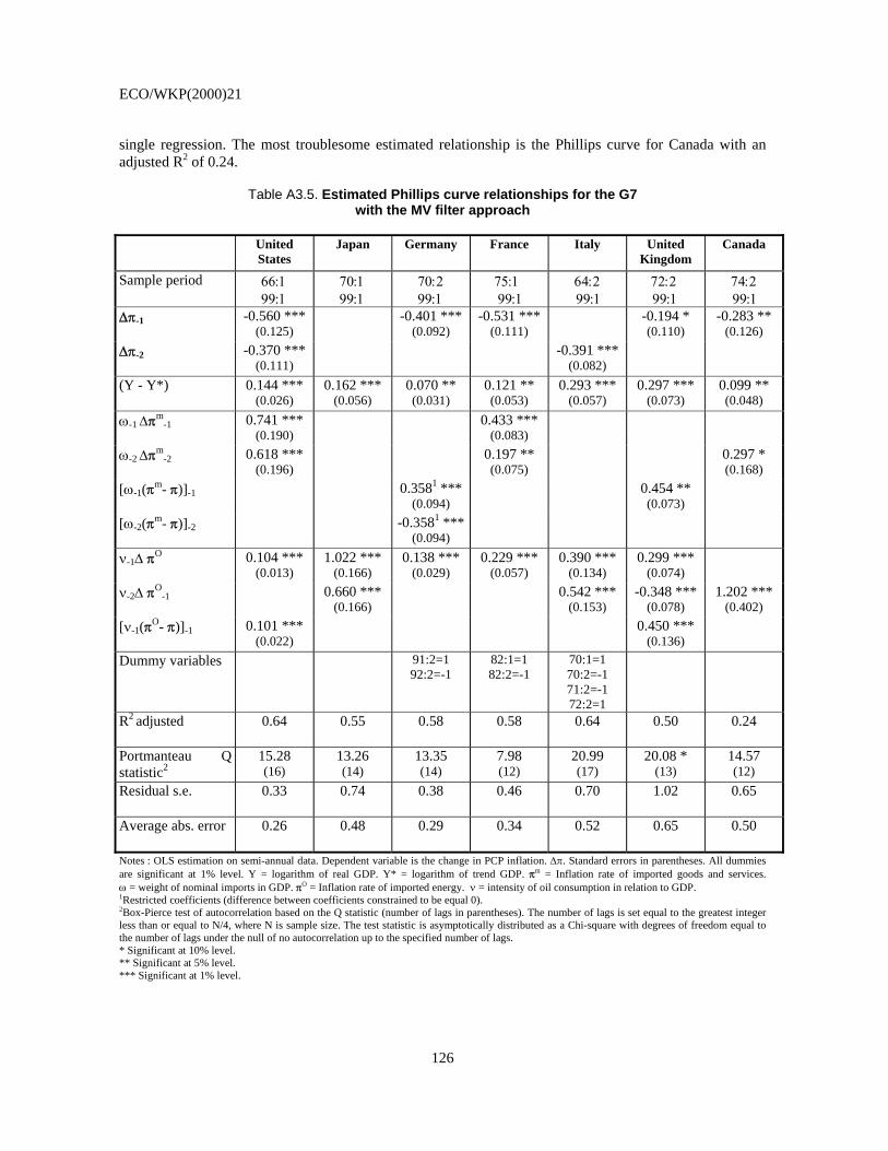
ECO/WKP(2000)21
126
single regression. The most troublesome estimated relationship is the Phillips curve for Canada with an adjusted R2 of 0.24.
Table A3.5. Estimated Phillips curve relationships for the G7 with the MV filter approach
United
States Japan
Germany France Italy United
Kingdom Canada
Sample period 66:1 99:1
70:1 99:1
70:2 99:1
75:1 99:1
64:2 99:1
72:2 99:1
74:2 99:1
Δπ-1
-0.560 *** (0.125)
-0.401 *** (0.092)
-0.531 *** (0.111)
-0.194 * (0.110)
-0.283 ** (0.126)
Δπ-2
-0.370 *** (0.111)
-0.391 *** (0.082)
(Y - Y*)
0.144 ***
(0.026) 0.162 ***
(0.056) 0.070 ** (0.031)
0.121 ** (0.053)
0.293 *** (0.057)
0.297 *** (0.073)
0.099 ** (0.048)
ω-1 Δπm-1 0.741 ***
(0.190) 0.433 ***
(0.083)
ω-2 Δπm-2 0.618 ***
(0.196) 0.197 **
(0.075) 0.297 *
(0.168) [ω-1(πm- π)]-1
0.3581 *** (0.094)
0.454 ** (0.073)
[ω-2(πm- π)]-2
-0.3581 ***(0.094)
ν-1Δ πO
0.104 *** (0.013)
1.022 *** (0.166)
0.138 *** (0.029)
0.229 *** (0.057)
0.390 *** (0.134)
0.299 *** (0.074)
ν-2Δ πO-1
0.660 ***
(0.166) 0.542 ***
(0.153) -0.348 ***
(0.078) 1.202 ***
(0.402) [ν-1(πO- π)]-1
0.101 *** (0.022)
0.450 *** (0.136)
Dummy variables
91:2=1 92:2=-1
82:1=1 82:2=-1
70:1=1 70:2=-1 71:2=-1 72:2=1
R2 adjusted 0.64 0.55 0.58 0.58 0.64 0.50 0.24
Portmanteau Q statistic2
15.28 (16)
13.26 (14)
13.35 (14)
7.98 (12)
20.99 (17)
20.08 * (13)
14.57 (12)
Residual s.e. 0.33 0.74 0.38 0.46 0.70 1.02 0.65
Average abs. error 0.26 0.48 0.29 0.34 0.52 0.65 0.50
Notes : OLS estimation on semi-annual data. Dependent variable is the change in PCP inflation. Δπ. Standard errors in parentheses. All dummies are significant at 1% level. Y = logarithm of real GDP. Y* = logarithm of trend GDP. πm = Inflation rate of imported goods and services. ω = weight of nominal imports in GDP. πO = Inflation rate of imported energy. ν = intensity of oil consumption in relation to GDP. 1Restricted coefficients (difference between coefficients constrained to be equal 0). 2Box-Pierce test of autocorrelation based on the Q statistic (number of lags in parentheses). The number of lags is set equal to the greatest integer less than or equal to N/4, where N is sample size. The test statistic is asymptotically distributed as a Chi-square with degrees of freedom equal to the number of lags under the null of no autocorrelation up to the specified number of lags. * Significant at 10% level. ** Significant at 5% level. *** Significant at 1% level.
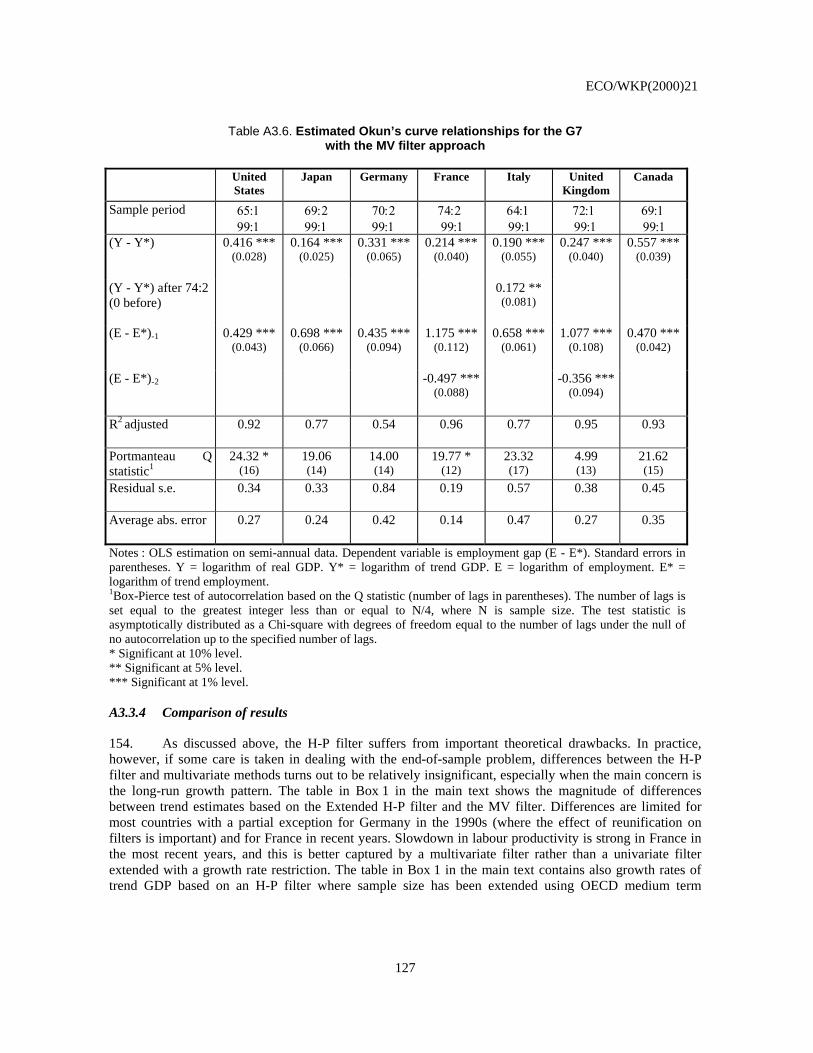
ECO/WKP(2000)21
127
Table A3.6. Estimated Okun’s curve relationships for the G7 with the MV filter approach
United
States Japan
Germany France Italy United
Kingdom Canada
Sample period 65:1 99:1
69:2 99:1
70:2 99:1
74:2 99:1
64:1 99:1
72:1 99:1
69:1 99:1
(Y - Y*)
0.416 *** (0.028)
0.164 *** (0.025)
0.331 *** (0.065)
0.214 *** (0.040)
0.190 *** (0.055)
0.247 *** (0.040)
0.557 *** (0.039)
(Y - Y*) after 74:2 (0 before)
0.172 ** (0.081)
(E - E*)-1
0.429 *** (0.043)
0.698 *** (0.066)
0.435 *** (0.094)
1.175 *** (0.112)
0.658 *** (0.061)
1.077 *** (0.108)
0.470 *** (0.042)
(E - E*)-2
-0.497 ***(0.088)
-0.356 *** (0.094)
R2 adjusted 0.92 0.77 0.54 0.96 0.77 0.95 0.93
Portmanteau Q statistic1
24.32 * (16)
19.06 (14)
14.00 (14)
19.77 * (12)
23.32 (17)
4.99 (13)
21.62 (15)
Residual s.e. 0.34 0.33 0.84 0.19 0.57 0.38 0.45
Average abs. error 0.27 0.24 0.42 0.14 0.47 0.27 0.35
Notes : OLS estimation on semi-annual data. Dependent variable is employment gap (E - E*). Standard errors in parentheses. Y = logarithm of real GDP. Y* = logarithm of trend GDP. E = logarithm of employment. E* = logarithm of trend employment. 1Box-Pierce test of autocorrelation based on the Q statistic (number of lags in parentheses). The number of lags is set equal to the greatest integer less than or equal to N/4, where N is sample size. The test statistic is asymptotically distributed as a Chi-square with degrees of freedom equal to the number of lags under the null of no autocorrelation up to the specified number of lags. * Significant at 10% level. ** Significant at 5% level. *** Significant at 1% level.
A3.3.4 Comparison of results
154. As discussed above, the H-P filter suffers from important theoretical drawbacks. In practice, however, if some care is taken in dealing with the end-of-sample problem, differences between the H-P filter and multivariate methods turns out to be relatively insignificant, especially when the main concern is the long-run growth pattern. The table in Box 1 in the main text shows the magnitude of differences between trend estimates based on the Extended H-P filter and the MV filter. Differences are limited for most countries with a partial exception for Germany in the 1990s (where the effect of reunification on filters is important) and for France in recent years. Slowdown in labour productivity is strong in France in the most recent years, and this is better captured by a multivariate filter rather than a univariate filter extended with a growth rate restriction. The table in Box 1 in the main text contains also growth rates of trend GDP based on an H-P filter where sample size has been extended using OECD medium term
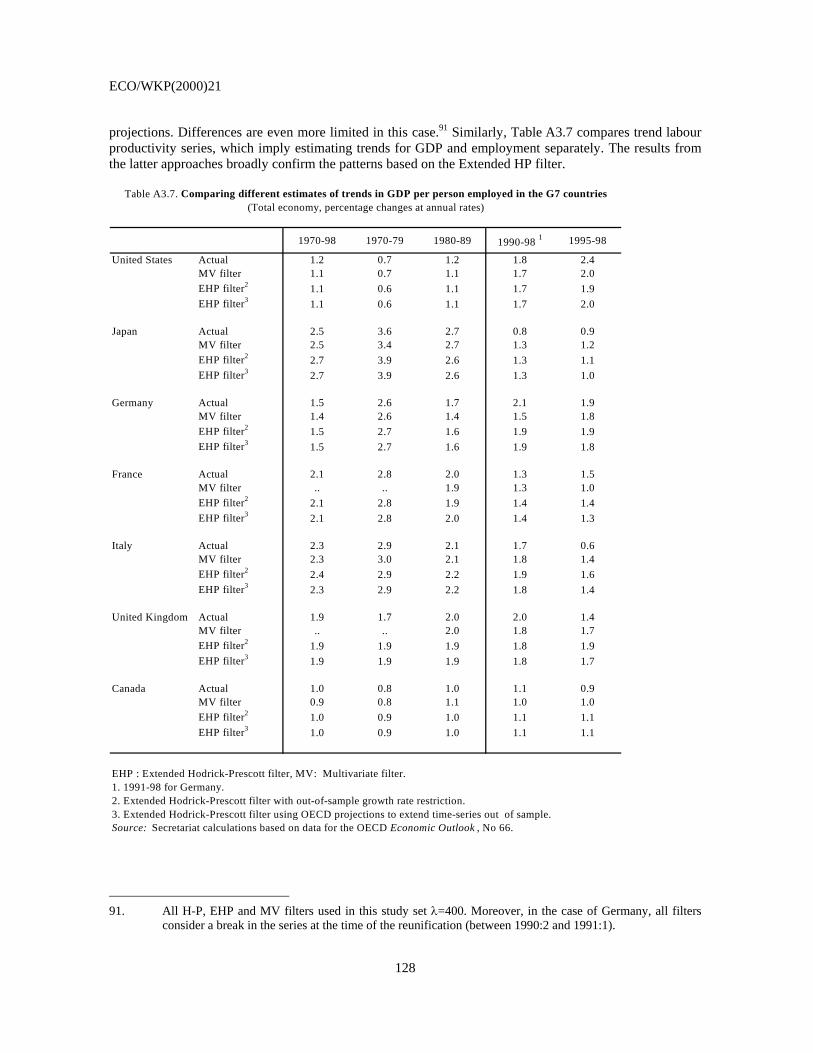
ECO/WKP(2000)21
128
projections. Differences are even more limited in this case.91 Similarly, Table A3.7 compares trend labour productivity series, which imply estimating trends for GDP and employment separately. The results from the latter approaches broadly confirm the patterns based on the Extended HP filter.
1970-98 1970-79 1980-89 1990-98 1 1995-98
United States Actual 1.2 0.7 1.2 1.8 2.4MV filter 1.1 0.7 1.1 1.7 2.0EHP filter2 1.1 0.6 1.1 1.7 1.9EHP filter3 1.1 0.6 1.1 1.7 2.0
Japan Actual 2.5 3.6 2.7 0.8 0.9MV filter 2.5 3.4 2.7 1.3 1.2EHP filter2 2.7 3.9 2.6 1.3 1.1EHP filter3 2.7 3.9 2.6 1.3 1.0
Germany Actual 1.5 2.6 1.7 2.1 1.9MV filter 1.4 2.6 1.4 1.5 1.8EHP filter2 1.5 2.7 1.6 1.9 1.9EHP filter3 1.5 2.7 1.6 1.9 1.8
France Actual 2.1 2.8 2.0 1.3 1.5MV filter .. .. 1.9 1.3 1.0EHP filter2 2.1 2.8 1.9 1.4 1.4EHP filter3 2.1 2.8 2.0 1.4 1.3
Italy Actual 2.3 2.9 2.1 1.7 0.6MV filter 2.3 3.0 2.1 1.8 1.4EHP filter2 2.4 2.9 2.2 1.9 1.6EHP filter3 2.3 2.9 2.2 1.8 1.4
United Kingdom Actual 1.9 1.7 2.0 2.0 1.4MV filter .. .. 2.0 1.8 1.7EHP filter2 1.9 1.9 1.9 1.8 1.9EHP filter3 1.9 1.9 1.9 1.8 1.7
Canada Actual 1.0 0.8 1.0 1.1 0.9MV filter 0.9 0.8 1.1 1.0 1.0EHP filter2 1.0 0.9 1.0 1.1 1.1EHP filter3 1.0 0.9 1.0 1.1 1.1
EHP : Extended Hodrick-Prescott filter, MV: Multivariate filter.1. 1991-98 for Germany.2. Extended Hodrick-Prescott filter with out-of-sample growth rate restriction.3. Extended Hodrick-Prescott filter using OECD projections to extend time-series out of sample.Source: Secretariat calculations based on data for the OECD Economic Outlook , No 66.
Table A3.7. Comparing different estimates of trends in GDP per person employed in the G7 countries(Total economy, percentage changes at annual rates)
91. All H-P, EHP and MV filters used in this study set λ=400. Moreover, in the case of Germany, all filters
consider a break in the series at the time of the reunification (between 1990:2 and 1991:1).
ECO/WKP(2000)21
129
ECONOMICS DEPARTMENT
WORKING PAPERS
247. Economic Effects on the 1999 Turkish Earthquakes: an Interim Report (June 2000) Alexandra Bibbee, Rauf Gonenc, Scott Jacobs, Josef Konvitz and Robert Price 246. Policy Influences on Economic Growth in OECD Countries: an Evaluation of the Evidence (June 2000) Sanghoon Ahn and Philip Hemmings 245. The Tax System in the Czech Republic (May 2000) Chiara Bronchi and Andrew Burns 244. The Tax System in Norway: Past Reforms and Future Challenges (May 2000) Paul van den Noord 243. A Changing Financial Environment and the Implications for Monetary Policy (May 2000) Paul Mylonas, Sebastian Schich, Gert Wehinger 242. Carbon Emission Leakages: a General Equilibrium View (May 2000) Jean-Marc Burniaux and Joaquim Oliveira Martins 241. The Healthcare System in Hungary (April 2000) Eva Orosz and Andrew Burns 240. Comparing Semi-Structural Methods to Estimate Unobserved Variables: the HPMV and Kalman Filters
Approaches (April 2000) Laurence Boone 239. New Issues in Public Debt Management: Government Surpluses in Several OECD Countries, the Common
Currency in Europe and Rapidly Rising Debt in Japan (April 2000) Paul Mylonas, Sebastian Schich, Thorsteinn Thorgeirsson and Gert Wehinger 238. Regulation, Industry Structure and Performance in the Electricity Supply Industry (April 2000) Faye Steiner 237. Regulation, Market Structure and Performance in Telecommunications (April 2000) Olivier Boylaud and Giuseppe Nicoletti 236. Predicting the Evolution and Effects of the Asia Crisis from the OECD Perspective (April 2000) Pete Richardson, Ignazio Visco and Claude Giorno 235. Modelling Manufacturing Export Volumes Equations A System Estimation Approach (April 2000) Keiko Murata, Dave Turner, Dave Rae and Laurence Le Fouler 234. The Polish Tax Reform (March 2000) Patrick Lenain and Leszek Bartoszuk 233. The Tax System in Mexico: a Need for Strengthening the Revenue Raising Capacity (March 2000) Thomas Dalsgaard 232. EMU, the Euro and the European Policy Mix (February 2000) Jonathan Coppel, Martine Durand and Ignazio Visco
ECO/WKP(2000)21
130
231. The Tax System in Japan: a Need for Comprehensive Reform (February 2000) Thomas Dalsgaard and Masaaki Kawagoe 230. The Size and Role of Automatic Fiscal Stabilisers in the 1990s and Beyond (January 2000) Paul van den Noord 229. Enhancing Environmentally Sustainable Growth in Finland (January 2000) Ann Vourc’h and Miguel Jimenez 228. Finance and Growth: Some Theoretical Considerations, and a Review of the Empirical Literature (January 2000) Kotaro Tsuru 227. What the Yield Curves Say about Inflation: Does It Change over Time? (December 1999) Sebastian Schich 226. Summary Indicators of Product Market Regulation with an Extension to Employment Protection Legislation (December 1999) Giuseppe Nicoletti, Stefano Scarpetta and Olivier Boylaud 225. Some Issues Related to the Equity-Efficiency Trade-Off in the Swedish Tax and Transfer System (November 1999) Henning Strand 224. The Economic Effects of Employment-Conditional Income Support Schemes for the Low-Paid: An Illustration
from a CGE Model Applied to Four OECD Countries (October 1999) Andrea Bassanini, Jørn Henrik Rasmussen and Stefano Scarpetta 223. The Use of Financial Market Indicators by Monetary Authorities (September 1999) Paul Mylonas and Sebastian Schich 222. Tax Reform in Switzerland (August 1999) David Carey, Kathryn Gordon and Philippe Thalman 221. Trends in Market Openness (August 1999) Jonathan Coppel and Martine Durand 220. Technology Upgrading with Learning Cost: A Solution for Two “Productivity Puzzles” (July 1999) Sanghoon Ahn 219. Testing for a Common OECD Phillips Curve (July 1999) Dave Turner and Elena Seghezza 218. Sustainable Economic Growth: Natural Resources and the Environment (July 1999) Paul van den Noord and Ann Vourc’h 217. Coping with Population Ageing in Australia (July 1999) David Carey 216. Estimating Prudent Budgetary Margins for 11 EU Countries: A Simulated SVAR Model Approach (July 1999) Thomas Dalsgaard and Alain de Serres