telecom multimedia vision application - ecofac2010.irisa.frecofac2010.irisa.fr/cours-david.pdf ·...
TRANSCRIPT
26/03/2010
1
Gestion de l’alimentation dans les systèmes multiprocesseurs sur silicium
Contact : Raphaël DAVID
Plan
• Introduction aux architecture multicœurs
• Gestion de la consommation dans les architectures multicoeurs
• Architectures multicœurs sur puce
• Cas de l’architecture SCMP
• Les nouveaux Challenges
2
26/03/2010
2
LIST –DTSI –
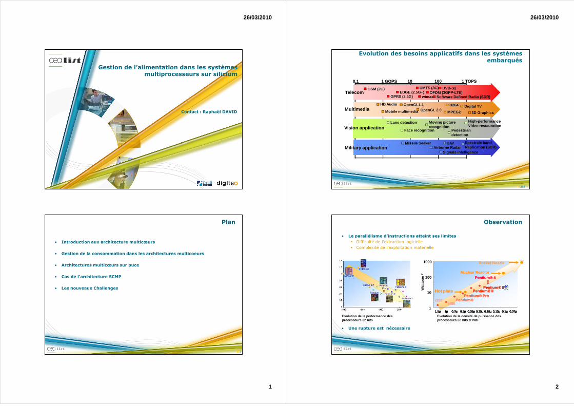
Evolution des besoins applicatifs dans les systèmes embarqués
1 GOPS0.1 10 100 1 TOPS
HD AudioMultimedia
OpenGL1.1OpenGL 2.0
H264 Digital TVMobile multimedia MPEG2 3D Graphics
Vision applicationLane detection High-performance
Video restaurationFace recognition
Moving picturerecognition
Pedestrian detection
Missile SeekerAirborne Radar
UAV
Signals intelligence
Spectrale band Replication (SBR)Military application
UMTS (3G)EDGE (2.5G+)
GPRS (2.5G)
GSM (2G)
wimaxOFDM (3GPP-LTE)
Software Defined Radio (SDR)Telecom
DVB-S2
Observation
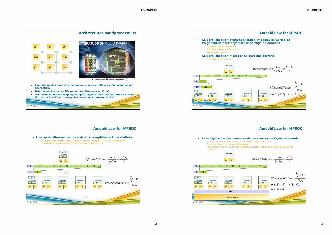
• Le parallélisme d’instructions atteint ses limites
� Difficulté de l’extraction logicielle
� Complexité de l’exploitation matérielle
• Une rupture est nécessaire
Evolution de la performance des processeurs 32 bits
Wat
ts/c
m2
1
10
100
1000
1.5µ1.5µ1.5µ1.5µ 1µ1µ1µ1µ 0.7µ0.7µ0.7µ0.7µ 0.5µ0.5µ0.5µ0.5µ 0.35µ0.35µ0.35µ0.35µ 0.25µ0.25µ0.25µ0.25µ 0.18µ0.18µ0.18µ0.18µ 0.13µ0.13µ0.13µ0.13µ 0.1µ0.1µ0.1µ0.1µ 0.07µ0.07µ0.07µ0.07µ
i386i386i486i486
Pentium®Pentium®Pentium® ProPentium® Pro
Pentium® IIPentium® IIPentium® IIIPentium® III
Hot plateHot plate
Nuclear ReactorNuclear ReactorPentium® 4Pentium® 4
Evolution de la densité de puissance des processeurs 32 bits d’Intel
Rocket Nozzle
26/03/2010
3
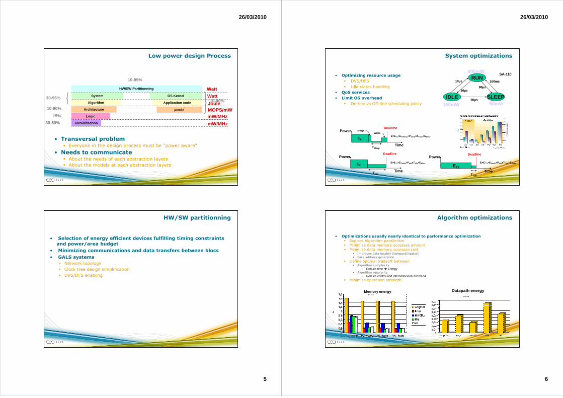
Architectures multiprocesseurs
• Exploitation de cœurs de processeurs simples et efficaces d’un point de vue énergétique
• Interconnexion de ces PEs par un Noc (Network on Chip)
• Ordonnancement et mapping statique d’applications parallélisées au niveau tâches sur les PEs et routage des communications sur le NoC
µP µP µP
DSP $ DSP
$ µP DSP
Architecture multicoeurs Intel[ISSCC’07]
Amdahl Law for MPSOC
N
PS
Accel+
= 1
• Une application ne peut jamais être complètement parallélisée� Le calcul intensif côtoie toujours des activités de contrôle, au minimum pour
l’initialisation et la mise en forme des données produites
Ts Tp
Ts Tp
P1 P2 P3 P4 P5S
A
TT
Surface
TexeSiliciumEfficacité SP +==
AN
TN
T
SiliciumEfficacitéS
P
.
+=
Procsseur
$D $I
Procsseur
$D $I
Procsseur
$D $I
Procsseur
$D $I
Procsseur
$D $I
S
P1 P2 P3 P4 P5
Procsseur
$D $I
S
P1
26/03/2010
4
Amdahl Law for MPSOC
• La parallélisation d’une application implique la reprise de l’algorithmie pour organiser le partage de données� Fonctions de synchronisation
� Fonctions de gestion de tâche
� Allocation mémoire
• La parallélisation n’est par ailleurs pas parfaite � Dépendances aux données
Ts Tp
Ts Tp
P1 P2 P3 P4 P5S
A
TT
Surface
TexeSiliciumEfficacité SP +==
SS
SP
TTetTAN
TN
T
SiliciumEfficacité
>>
+=
'PP'
''
T avec
.
Procsseur
$D $I
Procsseur
$D $I
Procsseur
$D $I
Procsseur
$D $I
Procsseur
$D $I
S
P1 P2 P3 P4 P5
Procsseur
$D $I
Ts’ Tp’
Amdahl Law for MPSOC
• La multiplication des ressources de calcul nécessite l’ajout de matériel � Pour la communication entre tâches (mémoires, réseaux sur puce)
� Pour la gestion de la cohérence des données
� Pour l’optimisation éventuelle des fonctions de synchronisation de tâches et de gestion de ressources
Ts Tp
Ts Tp
Procsseur
$D $I
Procsseur
$D $I
Procsseur
$D $I
Procsseur
$D $I
Procsseur
$D $I
Procsseur
$D $I
P1 P2 P3 P4 P5S
S
P1 P2 P3 P4 P5
A
SP
Surface
TexeSiliciumEfficacité
+==
AA' avec
TT avec
'.
SS'PP'
'
>>>
+=
TetTAN
TN
T
SiliciumEfficacitéS
P
NoCNoC
L2 Mem (+ snoop)
26/03/2010
5
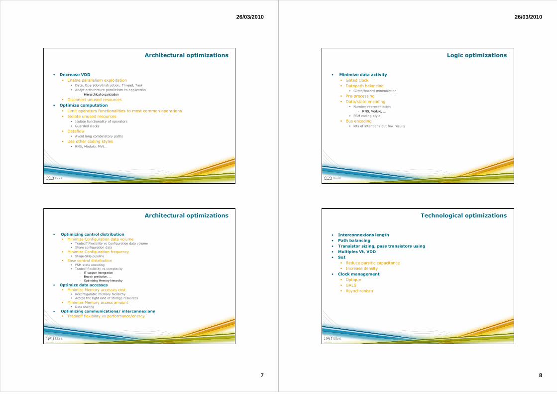
Low power design Process
• Transversal problem� Everyone in the design process must be "power aware"
• Needs to communicate� About the needs of each abstraction layers
� About the models at each abstraction layers
Circuit/technoCircuit/techno
10-80%30-95%
10-90%
15%
30-50%
10-95%
LogicLogic
Architecture µcodeArchitecture µcode
Algorithm Application codeAlgorithm Application code
System OS KernelSystem OS Kernel
HW/SW PartitionningHW/SW Partitionning WattWatt
JouleMOPS/mWmW/MHz
mW/MHz
HW/SW partitionning
• Selection of energy efficient devices fulfilling timing constraints and power/area budget
• Minimizing communications and data transfers between blocs
• GALS systems
� Network topology
� Clock tree design simplification
� DVS/DFS enabling
26/03/2010
6
System optimizations
• Optimizing resource usage
� DVS/DFS
� Idle states handling
• QoS services
• Limit OS overhead
� On-line vs Off-line scheduling policy
RUN
SLEEPIDLE
400mW
160mW 50mW
10µs
10µs
160ms
90µs
90µs
SA-110
ET1
DeadlinePower
Time
E=E'T1+EToIdle+PIdlexT' Idle+EWake
DeadlinePower
Time
E=ET1+EToIdle+PIdlexT Idle+EWakeET1
ET1
Deadlinesleep
wakePower
Time
E=ET1+EToSleep+PSleepxTSleep+EWake
TSleep
TIdle T'Idle
Algorithm optimizations
• Optimizations usually nearly identical to performance optimization� Explore Algorithm parallelism� Minimize data memory accesses amount� Minimize data memory accesses cost
� Improves data locality (temporal/spatial)� Ease address generation
� Define optimal tradeoff between� Algorithm complexity
- Reduce time � Energy� Algorithm regularity
- Reduce control and interconnexion overhead� Minimize operation strength
J
Datapath energy
J
Memory energy
26/03/2010
7
Architectural optimizations
• Decrease VDD
� Enable parallelism exploitation� Data, Operation/Instruction, Thread, Task
� Adapt architecture parallelism to application
- Hierarchical organization
� Disconect unused resources
• Optimize computation
� Limit operators functionalities to most common operations
� Isolate unused resources� Isolate functionality of operators
� Guarded clocks
� Dataflow � Avoid long combinatory paths
� Use other coding styles� RNS, Modulo, MVL…
Architectural optimizations
• Optimizing control distribution
� Minimize Configuration data volume� Tradeoff Flexibility vs Configuration data volume
� Share configuration data
� Minimize Configuration frequency� Stage-Skip pipeline
� Ease control distribution� FSM-state encoding
� Tradeof flexibility vs complexity
- IT support intergration- Branch prediction, …- Optimizing Memory hierarchy
• Optimize data accesses
� Minimize Memory accesses cost� Reconfigurable memory hierarchy
� Access the right kind of storage resources
� Minimize Memory access amount� Data sharing
• Optimizing communications/ interconnexions
� Tradeoff flexibility vs performance/energy
26/03/2010
8
Logic optimizations
• Minimize data activity
� Gated clock
� Datapath balancing� Glitch/hazard minimization
� Pre-processing
� Data/state encoding� Number representation
- RNS, Modulo, …
� FSM coding style
� Bus encoding � lots of intentions but few results
Technological optimizations
• Interconnexions length
• Path balancing
• Transistor sizing, pass transistors using
• Multiples Vt, VDD
• SoI
� Reduce parsitic capacitance
� Increase density
• Clock management
� Optique
� GALS
� Asynchronism
26/03/2010
9
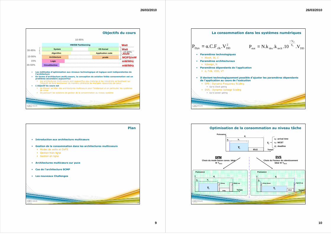
Objectifs du cours
• Les méthodes d’optimisation aux niveaux technologique et logique sont indépendantes de l’architecture
• En terme d’architecture multi-coeurs, la conception de solution faible consommation est un problème secondaire aujourd’hui
� Les architectures multi-coeurs sont aujourd’hui peu matures et les industriels se focalisent sur l’objectif de faire fonctionner de manière cohérente de mutliples ressources de calcul
• L’objectif du cours est
� de dresser un bilan des architectures multicoeurs pour l’embarqué et en particulier les systèmes de vision
� De parcourir les solutions de gestion de la consommation au niveau système
Circuit/technoCircuit/techno
10-80%30-95%
10-90%
15%
30-50%
10-95%
LogicLogic
Architecture µcodeArchitecture µcode
Algorithm Application codeAlgorithm Application code
System OS KernelSystem OS Kernel
HW/SW PartitionningHW/SW Partitionning WattWatt
JouleMOPS/mWmW/MHz
mW/MHz
Plan
• Introduction aux architecture multicœurs
• Gestion de la consommation dans les architectures multicoeurs
� Modes de veille et DVFS
� Gestion hors ligne
� Gestion en ligne
• Architectures multicœurs sur puce
• Cas de l’architecture SCMP
• Les nouveaux Challenges
18
26/03/2010
10
La consommation dans les systèmes numériques
• Paramètres technologiques
� Ktech, St, C
• Paramètres architecturaux
� Kdesign, N
• Paramètres dépendants de l’application
� α, Fclk, VDD, VT
• Il devient technologiquement possible d’ajuster les paramètres dépendants de l’application au cours de l’exécution
� DFS : Dynamic Frequency Scaling� Up to Clock gating
� DVS : Dynamic Voltage Scaling� Up to power gating
2DDclkDyn .Vα.C.FP = DD
S
V
techdesstat .V.10.kN.kP t
T−
=
Optimisation de la consommation au niveau tâche
TTii
ai : arrival time
s i : WCET
d i : deadline
s i
d i
ai
TTii
Temps
Puissance
Choix du mode basse conso. Idéal ���� TIDLE
Choix du Facteur de ralentissement Idéal ���� TIDLE
TTii
s i
d i
ai
Temps
Puissance
IDLE
TTii
d i
ai
Temps
Puissance
IDLEPSMi
Speed upSlow downSleep Wake up
DPMDPM DVSDVS
26/03/2010
11
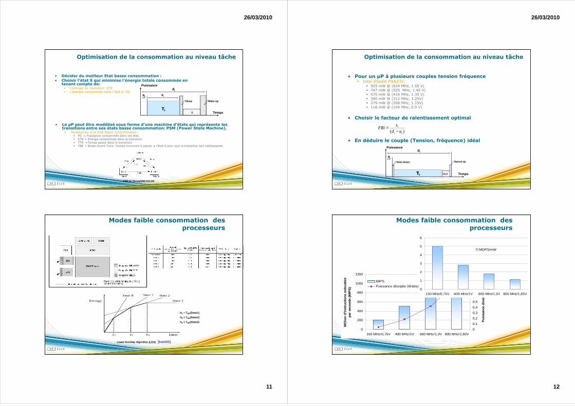
Optimisation de la consommation au niveau tâche
• Décider du meilleur Etat basse consommation :• Choisir l’état S qui minimise l’énergie totale consommée en
tenant compte de:� L’énergie de transition: ETR� L’énergie consommée dans l’état S: ES
• Le µP peut être modélisé sous forme d’une machine d’états qui représente les transitions entre ses états basse consommation: PSM (Power State Machine).� Paramètres d’un état basse consommation:
� PS = Puissance consommée dans cet état.� ETR = Energie consommée dans la transition � TTR =Temps passé dans la transition� TBE = Break-Event Time: Temps minimum à passer à l’état S pour que la transition soit intéressante.
PSM du StrongARM SA1100
TTii
s i
d i
ai
Temps
Puissance
S
Sleep Wake up
Modes faible consommation des processeurs
Lower Envelop Algorithm (LEA) [Irani03]
- b1 = TBE(State1)
- b2 = TBE(State2)
- b3 = TBE(State3)
26/03/2010
12
TTii
d i
ai
Temps
Puissance
Speed upSlow down
IDLE
Optimisation de la consommation au niveau tâche
)( ii
i
ad
sFRi
−=
• Pour un µP à plusieurs couples tension fréquence � Intel XScale PXA27x:
� 925 mW @ (624 MHz, 1.55 V)� 747 mW @ (520 MHz, 1.45 V)� 570 mW @ (416 MHz, 1.35 V)� 390 mW @ (312 MHz, 1.25V)� 279 mW @ (208 MHz, 1.15V)� 116 mW @ (104 MHz, 0.9 V)
• Choisir le facteur de ralentissement optimal
• En déduire le couple (Tension, fréquence) idéal
Modes faible consommation des processeurs
0
200
400
600
800
1000
1200
150 MHz/0,75V 400 MHz/1V 600 MHz/1,3V 800 MHz/1,65V
Mill
ion
d'in
stru
ctio
ns e
xécu
tées
pa
r se
cond
e (M
IPS
)
0
0,1
0,2
0,3
0,4
0,5
0,6
0,7
0,8
0,9
1
Pui
ssan
ce d
issi
pée
(Wat
ts)
MIPS
Puissance dissipée (Watts)0
1
2
3
4
5
6
150 MHz/0,75V 400 MHz/1V 600 MHz/1,3V 800 MHz/1,65V
MOPS/mW
26/03/2010
13
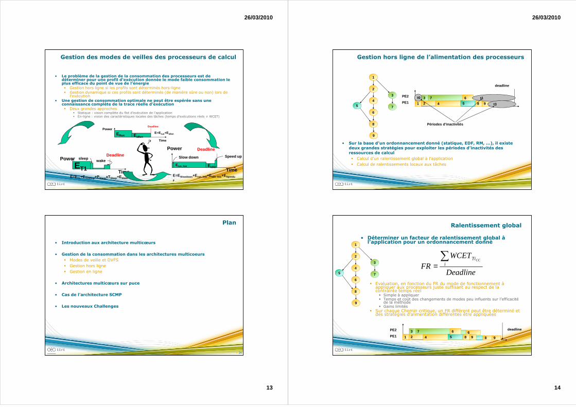
Gestion des modes de veilles des processeurs de calcul
• Le problème de la gestion de la consommation des processeurs est de déterminer pour une profil d’exécution donnée le mode faible consommation le plus efficace du point de vue de l’énergie� Gestion hors ligne si les profils sont déterminés hors-ligne� Gestion dynamique si ces profils sont déterminés (de manière sûre ou non) lors de
l’exécution • Une gestion de consommation optimale ne peut être espérée sans une
connaissance complète de la trace réelle d’exécution� Deux grandes approches
� Statique : vision complète du flot d’exécution de l’application� En-ligne : vision des caractéristiques locales des tâches (temps d’exécutions réels ≠ WCET)
ERun
DeadlinePower
Time
E=Erun+EidlenEIdlen
ET1
Deadlinesleep
wakePower
TimeE=ET1+EToSleep+PSleepxTSleep+EWake
Erun_low
Deadline
Slow down Speed up
TimeEIdlel
E=ESlowdown +Erun_low +EIdle_low +ESpeedup
Power
Plan
• Introduction aux architecture multicœurs
• Gestion de la consommation dans les architectures multicoeurs
� Modes de veille et DVFS
� Gestion hors ligne
� Gestion en ligne
• Architectures multicœurs sur puce
• Cas de l’architecture SCMP
• Les nouveaux Challenges
26
26/03/2010
14
Gestion hors ligne de l’alimentation des processeurs
• Sur la base d’un ordonnancement donné (statique, EDF, RM, ...), il existe deux grandes stratégies pour exploiter les périodes d’inactivités des ressources de calcul
� Calcul d’un ralentissement global à l’application
� Calcul de ralentissements locaux aux tâches
1
2
4
6
8
5
3
7
9
1PE1
PE2
2
3 7
4 5
6
8 9
deadline
t0 t1
t3
Périodes d’inactivités
Ralentissement global
• Déterminer un facteur de ralentissement global à l’application pour un ordonnancement donné
� Evaluation, en fonction du FR du mode de fonctionnement à appliquer aux processeurs juste suffisant au respect de la contrainte temps réel� Simple à appliquer� Temps et coût des changements de modes peu influents sur l’efficacité
de la méthode� Gains limités
� Sur chaque Chemin critique, un FR différent peut être déterminé et des stratégies d’alimentation différentes être appliquées
Deadline
WCETFR i
TiCC∑=
1
2
4
6
8
5
3
7
9
PE1
PE23 7 6
1 2 4 5 8 9
deadline
1 2
3 7
4 5
6
8 9
26/03/2010
15
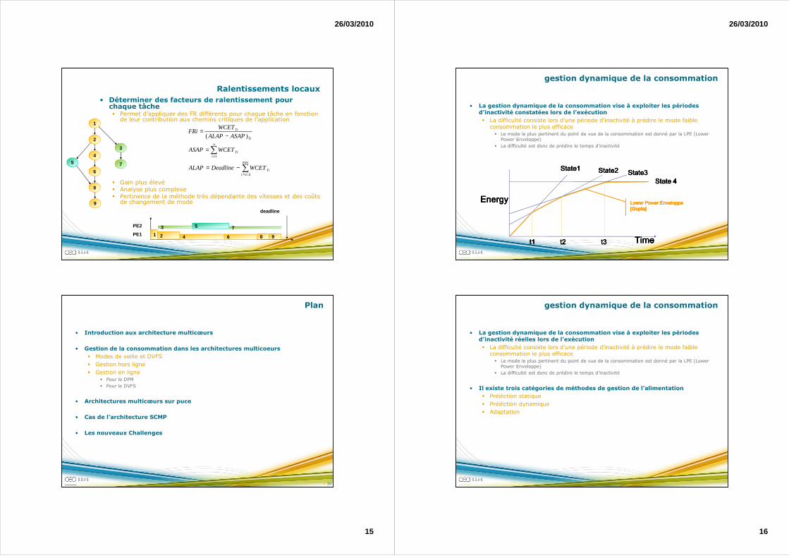
Ralentissements locaux
• Déterminer des facteurs de ralentissement pour chaque tâche� Permet d’appliquer des FR différents pour chaque tâche en fonction
de leur contribution aux chemins critiques de l’application
� Gain plus élevé� Analyse plus complexe� Pertinence de la méthode très dépendante des vitesses et des coûts
de changement de mode
∑
∑
+=
=
−=
=
−=
max
1
1
)(
niTi
n
iTi
Ti
Ti
WCETDeadlineALAP
WCETASAP
ASAPALAP
WCETFRi
PE1
PE2
1 2
3 7
4
5
6 8 9
deadline
1
2
4
6
8
5
3
7
9
Plan
• Introduction aux architecture multicœurs
• Gestion de la consommation dans les architectures multicoeurs
� Modes de veille et DVFS
� Gestion hors ligne
� Gestion en ligne� Pour le DPM
� Pour le DVFS
• Architectures multicœurs sur puce
• Cas de l’architecture SCMP
• Les nouveaux Challenges
30
26/03/2010
16
gestion dynamique de la consommation
• La gestion dynamique de la consommation vise à exploiter les périodes d’inactivité constatées lors de l’exécution
� La difficulté consiste lors d’une période d’inactivité à prédire le mode faible consommation le plus efficace
� Le mode le plus pertinent du point de vue de la consommation est donné par la LPE (Lower Power Enveloppe)
� La difficulté est donc de prédire le temps d’inactivité
EnergyEnergyEnergyEnergy
TimeTimeTimeTime
State 4State 4State 4State 4
State1State1State1State1 State2State2State2State2 State3State3State3State3
t1t1t1t1 t2t2t2t2 t3t3t3t3
Lower Power Enveloppe Lower Power Enveloppe Lower Power Enveloppe Lower Power Enveloppe [Gupta][Gupta][Gupta][Gupta]
gestion dynamique de la consommation
• La gestion dynamique de la consommation vise à exploiter les périodes d’inactivité réelles lors de l’exécution
� La difficulté consiste lors d’une période d’inactivité à prédire le mode faible consommation le plus efficace
� Le mode le plus pertinent du point de vue de la consommation est donné par la LPE (Lower Power Enveloppe)
� La difficulté est donc de prédire le temps d’inactivité
• Il existe trois catégories de méthodes de gestion de l’alimentation
� Prédiction statique
� Prédiction dynamique
� Adaptation
26/03/2010
17
Prédiction statique
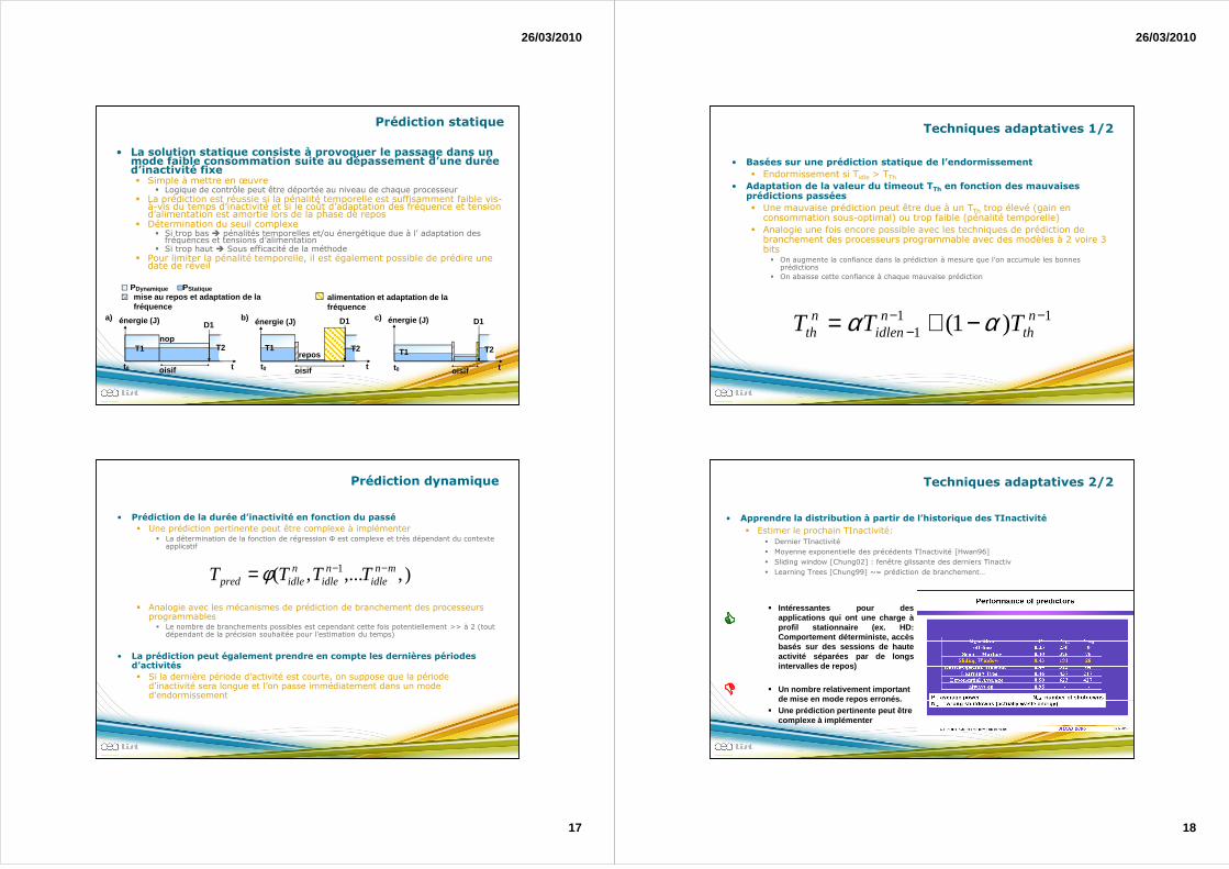
• La solution statique consiste à provoquer le passage dans un mode faible consommation suite au dépassement d’une durée d’inactivité fixe� Simple à mettre en œuvre
� Logique de contrôle peut être déportée au niveau de chaque processeur� La prédiction est réussie si la pénalité temporelle est suffisamment faible vis-
à-vis du temps d’inactivité et si le coût d’adaptation des fréquence et tension d’alimentation est amortie lors de la phase de repos
� Détermination du seuil complexe� Si trop bas � pénalités temporelles et/ou énergétique due à l’ adaptation des
fréquences et tensions d’alimentation� Si trop haut � Sous efficacité de la méthode
� Pour limiter la pénalité temporelle, il est également possible de prédire une date de réveil
alimentation et adaptation de la fréquence
repos
oisif t
nopT1 T2 T1 T2 T1 T2
D1
t0 tt0
D1énergie (J) énergie (J)
tt0
énergie (J) D1
oisif oisif
PDynamique PStatique
a) b) c)
mise au repos et adaptation de la fréquence
Prédiction dynamique
• Prédiction de la durée d’inactivité en fonction du passé
� Une prédiction pertinente peut être complexe à implémenter � La détermination de la fonction de régression Φ est complexe et très dépendant du contexte
applicatif
� Analogie avec les mécanismes de prédiction de branchement des processeurs programmables
� Le nombre de branchements possibles est cependant cette fois potentiellement >> à 2 (tout dépendant de la précision souhaitée pour l’estimation du temps)
• La prédiction peut également prendre en compte les dernières périodes d’activités
� Si la dernière période d’activité est courte, on suppose que la période d’inactivité sera longue et l’on passe immédiatement dans un mode d’endormissement
),,...,( 1 mnidle
nidle
nidlepred TTTT −−= φ
26/03/2010
18
Techniques adaptatives 1/2
• Basées sur une prédiction statique de l’endormissement
� Endormissement si Tidle > TTh• Adaptation de la valeur du timeout TTh en fonction des mauvaises
prédictions passées
� Une mauvaise prédiction peut être due à un TTh trop élevé (gain en consommation sous-optimal) ou trop faible (pénalité temporelle)
� Analogie une fois encore possible avec les techniques de prédiction de branchement des processeurs programmable avec des modèles à 2 voire 3 bits
� On augmente la confiance dans la prédiction à mesure que l’on accumule les bonnes prédictions
� On abaisse cette confiance à chaque mauvaise prédiction
111 )1( −−
− −+= nth
nidlen
nth TTT αα
Techniques adaptatives 2/2
• Apprendre la distribution à partir de l’historique des TInactivité
� Estimer le prochain TInactivité:� Dernier TInactivité
� Moyenne exponentielle des précédents TInactivité [Hwan96]
� Sliding window [Chung02] : fenêtre glissante des derniers Tinactiv
� Learning Trees [Chung99] ~= prédiction de branchement…
� Intéressantes pour desapplications qui ont une charge àprofil stationnaire (ex. HD:Comportement déterministe, accèsbasés sur des sessions de hauteactivité séparées par de longsintervalles de repos)
� Un nombre relativement important de mise en mode repos erronés.
� Une prédiction pertinente peut être complexe à implémenter
����
����
26/03/2010
19
Plan
• Introduction aux architecture multicœurs
• Gestion de la consommation dans les architectures multicoeurs
� Modes de veille et DVFS
� Gestion hors ligne
� Gestion en ligne� Pour le DPM
� Pour le DVFS
• Architectures multicœurs sur puce
• Cas de l’architecture SCMP
• Les nouveaux Challenges
37
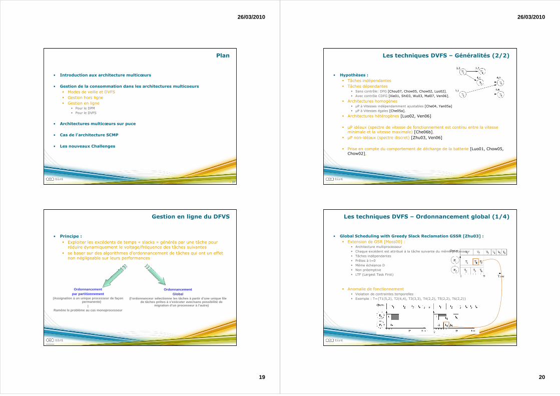
Ordonnancement par partitionnement
(Assignation à un unique processeur de façon permanente)
|Ramène le problème au cas monoprocesseur
Ordonnancement Global
(l’ordonnanceur sélectionne les tâches à partir d’une un ique file de tâches prêtes à s’exécuter avec/sans possibilité de
migration d’un processeur à l’autre)
Gestion en ligne du DFVS
• Principe :
� Exploiter les excédents de temps « slacks » générés par une tâche pour réduire dynamiquement le voltage/fréquence des tâches suivantes
� se baser sur des algorithmes d’ordonnancement de tâches qui ont un effet non négligeable sur leurs performances
26/03/2010
20
Les techniques DVFS – Généralités (2/2)
• Hypothèses :
� Tâches indépendantes
� Tâches dépendantes � Sans contrôle: DFG [Chou07, Chow05, Chow02, Luo02],
� Avec contrôle CDFG [Xie01, Shi03, Wu03, Mal07, Ven06],
� Architectures homogènes� µP à Vitesses indépendamment ajustables [Che04, Yan05a]
� µP à Vitesses égales [Che05a],
� Architectures hétérogènes [Luo02, Ven06]
� µP idéaux (spectre de vitesse de fonctionnement est continu entre la vitesse minimale et la vitesse maximale) [Che06b],
� µP non-idéaux (spectre discret) [Zhu03, Ven06]
� Prise en compte du comportement de décharge de la batterie [Luo01, Chow05, Chow02],
Les techniques DVFS – Ordonnancement global (1/4)
• Global Scheduling with Greedy Slack Reclamation GSSR [Zhu03] :
� Extension de GSR [Moss00] :� Architecture multiprocesseur
� Chaque excédent est attribué à la tâche suivante du même processeur
� Tâches indépendantes
� Prêtes à t=0
� Même échéance D
� Non préemptive
� LTF (Largest Task First)
� Anomalie de fonctionnement� Violation de contraintes temporelles
� Exemple : T={T1(5,2), T2(4,4), T3(3,3), T4(2,2), T5(2,2), T6(2,2)}
26/03/2010
21
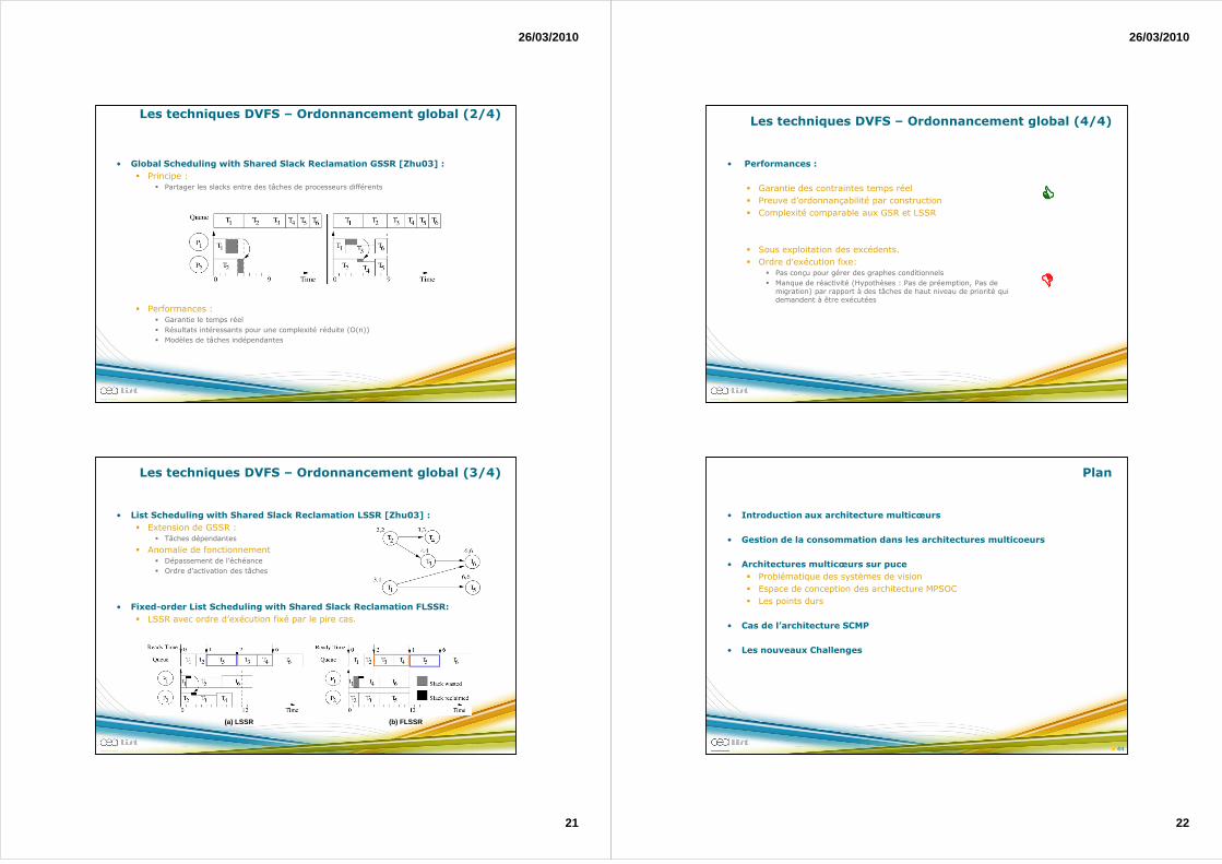
Les techniques DVFS – Ordonnancement global (2/4)
• Global Scheduling with Shared Slack Reclamation GSSR [Zhu03] :
� Principe :� Partager les slacks entre des tâches de processeurs différents
� Performances :� Garantie le temps réel
� Résultats intéressants pour une complexité réduite (O(n))
� Modèles de tâches indépendantes
• List Scheduling with Shared Slack Reclamation LSSR [Zhu03] :
� Extension de GSSR :� Tâches dépendantes
� Anomalie de fonctionnement� Dépassement de l’échéance
� Ordre d’activation des tâches
• Fixed-order List Scheduling with Shared Slack Reclamation FLSSR:
� LSSR avec ordre d’exécution fixé par le pire cas.
(a) LSSR (b) FLSSR
Les techniques DVFS – Ordonnancement global (3/4)
26/03/2010
22
����
����
Les techniques DVFS – Ordonnancement global (4/4)
• Performances :
� Garantie des contraintes temps réel
� Preuve d’ordonnançabilité par construction
� Complexité comparable aux GSR et LSSR
� Sous exploitation des excédents.
� Ordre d’exécution fixe: � Pas conçu pour gérer des graphes conditionnels
� Manque de réactivité (Hypothèses : Pas de préemption, Pas de migration) par rapport à des tâches de haut niveau de priorité qui demandent à être exécutées
Plan
• Introduction aux architecture multicœurs
• Gestion de la consommation dans les architectures multicoeurs
• Architectures multicœurs sur puce
� Problématique des systèmes de vision
� Espace de conception des architecture MPSOC
� Les points durs
• Cas de l’architecture SCMP
• Les nouveaux Challenges
44
26/03/2010
23
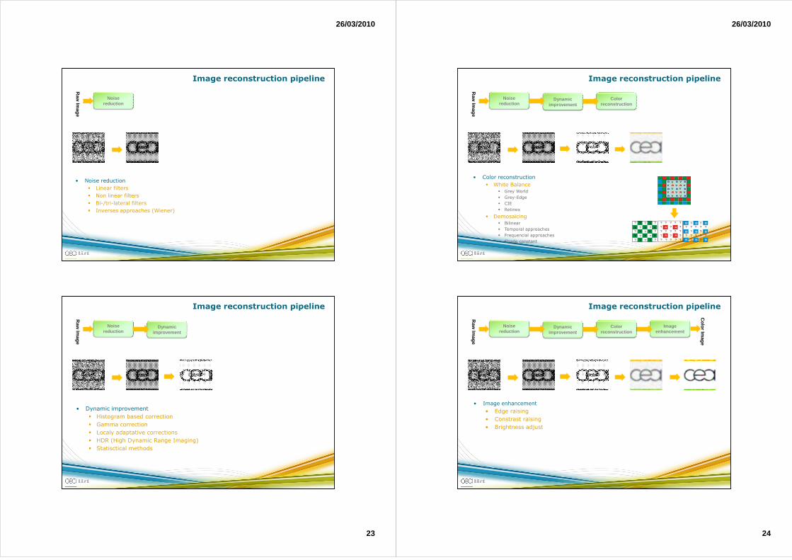
Image reconstruction pipeline
• Noise reduction
� Linear filters
� Non linear filters
� Bi-/tri-lateral filters
� Inverses approaches (Wiener)
Raw
Image
Noise reduction
Image reconstruction pipeline
Raw
Image
Noise reduction
Dynamicimprovement
• Dynamic improvement
� Histogram based correction
� Gamma correction
� Localy adaptative corrections
� HDR (High Dynamic Range Imaging)
� Statisctical methods
26/03/2010
24
Image reconstruction pipeline
Raw
Image
Noise reduction
Dynamicimprovement
Color reconstruction
V
V
VV
V V
V V
V
V
V
V
R
R
R
RB
B
B
B
B
B
B
B
B
?
? ?
?
? ?
?
? ?
?
?
?
?
?
?
?
?
? ?
?
?
?
?
?
? ???
?
?? ? ?
?
?
??
?
?
?
? ? ???B
V
V
VV
V V
V V
V
V
V
V
B
B
B
B
B
B
B
B
R
R
R
R
?
?
?
?
?
• Color reconstruction
� White Balance� Grey World
� Grey-Edge
� CIE
� Retinex
� Demosaïcing� Bilinear
� Temporal approaches
� Frequencial approaches
� Shade constant
Image reconstruction pipelineR
aw Im
age
Noise reduction
Dynamicimprovement
Image enhancement
Color Im
age
Color reconstruction
• Image enhancement
• Edge raising
• Constrast raising
• Brightness adjust
26/03/2010
25
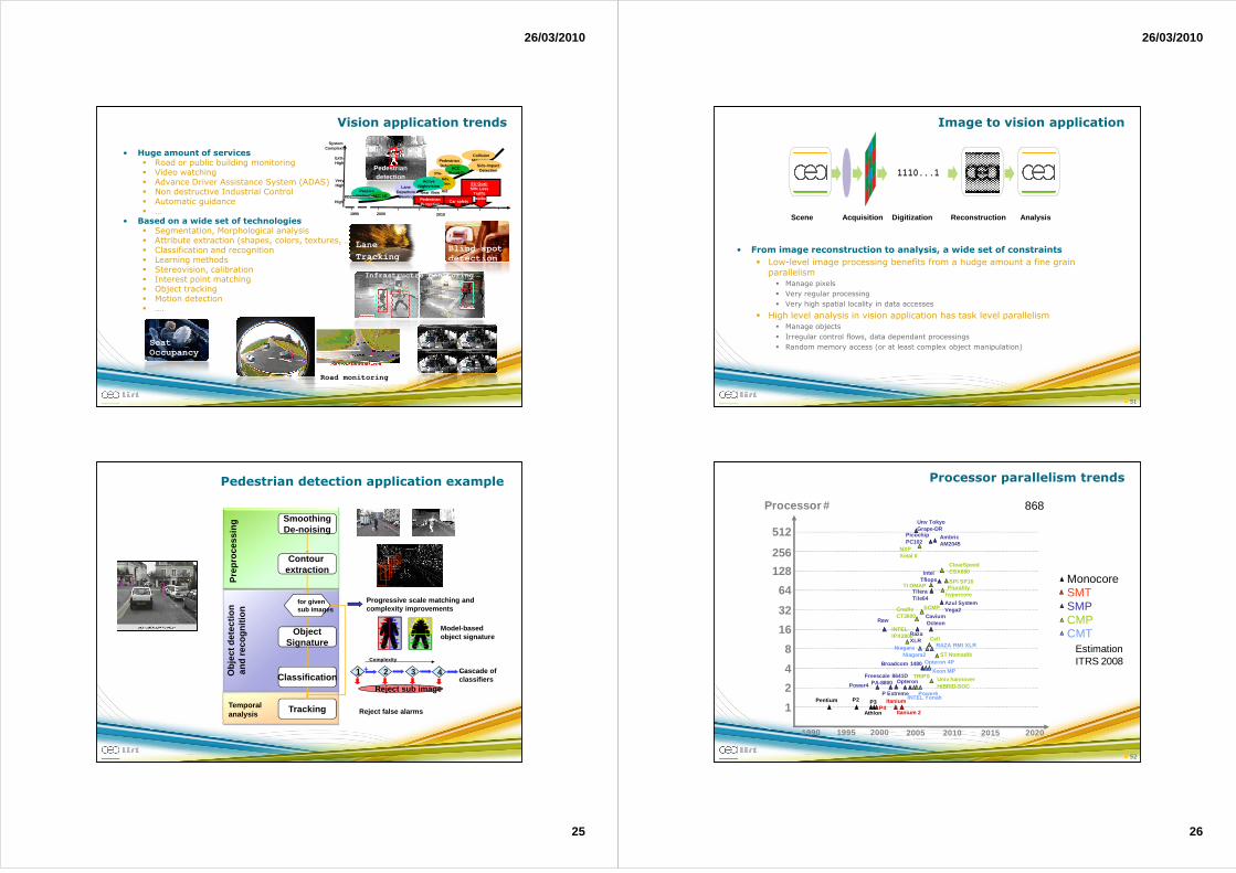
Vision application trends
• Huge amount of services� Road or public building monitoring � Video watching� Advance Driver Assistance System (ADAS)� Non destructive Industrial Control� Automatic guidance� …
• Based on a wide set of technologies � Segmentation, Morphological analysis� Attribute extraction (shapes, colors, textures, …) � Classification and recognition� Learning methods� Stereovision, calibration� Interest point matching� Object tracking� Motion detection� ….
Seat Occupancy
Blind spot detection
Lane
Tracking
Pedestrian detection
Rear ViewCamera
PassiveNightvision
Pre-Crash
1990
Extr.High
VeryHigh
2000
PedestrianDetection
2010
Lane DepartureWarning
CollisionMitigation
Side-ImpactDetection
EU Goal:50% Less
Traffic Deaths
Car safety ACC 1G
High
ACCStop&Go
Pedestrian Protection
Adv. Parking
Aid
ActiveNightvision
SystemComplexity
Road monitoring
Infrastructre monitoring
Pedestrian detection application example
SmoothingDe-noising
Contour extraction
ObjectSignature
Classification
for given sub images
Pre
proc
essi
ngO
bjec
t det
ectio
n an
d re
cogn
ition
Progressive scale matching and complexity improvements
Model-based object signature
1 2 3 4
Reject sub image
+-
Cascade of classifiers
Complexity
TrackingTemporal analysis Reject false alarms
26/03/2010
26
Image to vision application
• From image reconstruction to analysis, a wide set of constraints
� Low-level image processing benefits from a hudge amount a fine grain parallelism
� Manage pixels
� Very regular processing
� Very high spatial locality in data accesses
� High level analysis in vision application has task level parallelism� Manage objects
� Irregular control flows, data dependant processings
� Random memory access (or at least complex object manipulation)
51
Scène
1110...1
ReconstructionCapture UtilisationCAN & lectureScene Acquisition Digitization digitisationReconstruction Analysis
Processor parallelism trends
52
1990 1995 2000 2005 2010
Processor #
1
2
4
8
16
32
64
128
256
512
Pentium P2 P3P4
Itanium
Itanium 2Athlon
Power4Opteron
P Extreme
PA-8800
Broadcom 1480
Freescale 8641D
Raw
IntelTflops
CaviumOcteon
RazaXLR
PicochipPC102
AmbricAM2045
TileraTile64
Unv TokyoGrape-DR
Azul SystemVega2
Power6
Niagara
INTEL Yonah
Opteron 4P
Xeon MP
Niagara2
RAZA RMI XLR
MonocoreSMTSMPCMPCMT
2015 2020
Estimation ITRS 2008
868
NXPXetal II
ClearSpeedCSX600
SPI SP16
Cell
Pluralityhypercore
TRIPS
Cradle CT3600
INTEL IPX2800
Univ hannoverHiBRID-SOC
ST Nomadik
TI OMAP
SCMP
26/03/2010
27
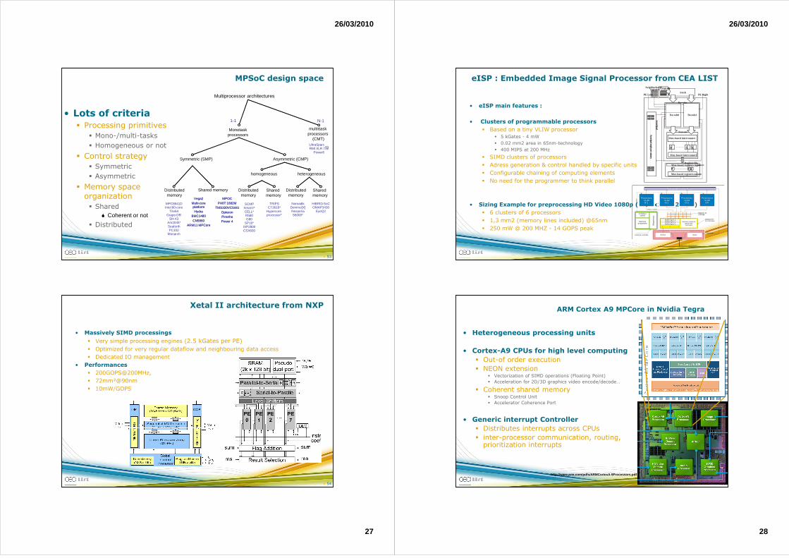
MPSoC design space
• Lots of criteria� Processing primitives
� Mono-/multi-tasks
� Homogeneous or not
� Control strategy
� Symmetric
� Asymmetric
� Memory space organization
� Shared� Coherent or not
� Distributed
53
Multiprocessor architectures
Monotaskprocessors
multittaskprocessors
(CMT)UltraSparc
T2RMI XLR 732Power6
1-1 N-1
Symmetric (SMP)
homogeneous heterogeneous
Distributedmemory
MPC8641DIntel 80-core
Tile64Grape-DR
SH-X3Am2045*SeaforthPC102
Monarch
Asymmetric (CMP)
SCMPXetal-II*CELL*R580G80
SP16*IXP2800CSX600
TRIPSCT3616*
Hypercore processor*
NomadikDomino[X]NexperiaS6000*
HiBRID-SoCOMAP3430
EyeQ2
MPOC PA6T 1682M
TMS320VC5441OpteronPiranhaPower 4
Vega2Multi-coreplatformHydra
BMC1480CN5860
ARM11 MPCore
Shared memory
MPOC PA6T 1682M
TMS320VC5441OpteronPiranhaPower 4
Vega2Multi-coreplatformHydra
BMC1480CN5860
ARM11 MPCore
Distributedmemory
Distributedmemory
Shared memory
Shared memory
Xetal II architecture from NXP
• Massively SIMD processings
� Very simple processing engines (2.5 kGates per PE)
� Optimized for very regular dataflow and neighbouring data access
� Dedicated IO management
• Performances
� 200GOPS@200MHz,
� 72mm²@90nm
� 10mW/GOPS
54
26/03/2010
28
eISP : Embedded Image Signal Processor from CEA LIST
• eISP main features :
• Clusters of programmable processors
� Based on a tiny VLIW processor� 5 kGates - 4 mW
� 0.02 mm2 area in 65nm-technology
� 400 MIPS at 200 MHz
� SIMD clusters of processors
� Adress generation & control handled by specific units
� Configurable chaining of computing elements
� No need for the programmer to think parallel
• Sizing Example for preprocessing HD Video 1080p (1920x1080 25FPS)
� 6 clusters of 6 processors
� 1,3 mm2 (memory lines included) @65nm
� 250 mW @ 200 MHZ - 14 GOPS peak
Sérialiseur (des résultats)
Entrée Sortie
Inst
ruct
ions
Pixel 1 + voisins
Résultats
Canal de transmission
Processeur VLIWN° 1
Processeur VLIWN° 2
Processeur VLIWN° 3
Processeur VLIWN°4
Mémoire programme
Compteur ordinal
Séq
uenc
eur
Buffer ligne 1Buffer ligne 2Buffer ligne 3
Machine à états de gestion des voisinages
Gestionnairede voisinages
Unité de contrôle
Module de gestion du flux
Op0
Op 1
Mux-based interconnect
Mux-based interconnect
Mux-based RF input interconnect
Scratchpads ingleportmem
ory
R0R1Rr
Mux-based registers input
Mux-based registers output
Decode1Decode0
Programmemory
Opp
Neighborhoodregisters
Register file
Execute
Decoder
Fetch
Scratchpa d
PE Left PE Right
56
ARM Cortex A9 MPCore in Nvidia Tegra
• Heterogeneous processing units
• Cortex-A9 CPUs for high level computing
� Out-of order execution
� NEON extension� Vectorization of SIMD operations (Floating Point)
� Acceleration for 2D/3D graphics video encode/decode…
� Coherent shared memory � Snoop Control Unit
� Accelerator Coherence Port
• Generic interrupt Controller
� Distributes interrupts across CPUs
� inter-processor communication, routing, prioritization interrupts
http://www.arm.com/pdfs/ARMCortexA-9Processors.pdf
26/03/2010
29
Scène
1110...1
ReconstructionCapture UtilisationCAN & lectureScene Acquisition Digitization digitisationReconstruction Analysis
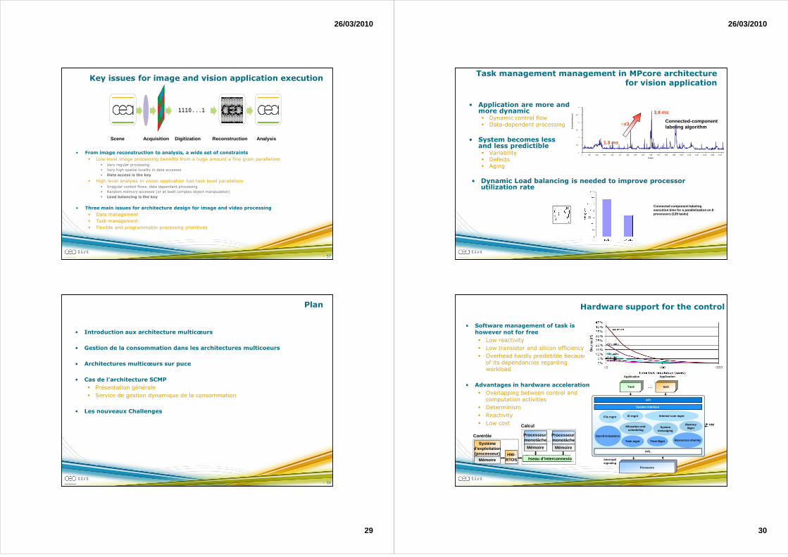
Key issues for image and vision application execution
• From image reconstruction to analysis, a wide set of constraints
� Low-level image processing benefits from a huge amount a fine grain parallelism� Very regular processing
� Very high spatial locality in data accesses
� Data access is the key
� High level analysis in vision application has task level parallelism� Irregular control flows, data dependant processing
� Random memory accesses (or at least complex object manipulation)
� Load balancing is the key
• Three main issues for architecture design for image and video processing
� Data management
� Task management
� Flexible and programmable processing primitives
57
Plan
• Introduction aux architecture multicœurs
• Gestion de la consommation dans les architectures multicoeurs
• Architectures multicœurs sur puce
• Cas de l’architecture SCMP
� Présentation générale
� Service de gestion dynamique de la consommation
• Les nouveaux Challenges
58
26/03/2010
30
Task management management in MPcore architecture for vision application
• Application are more and more dynamic� Dynamic control flow� Data-dependent processing
• System becomes lessand less predictible� Variability� Defects� Aging
• Dynamic Load balancing is needed to improve processor utilization rate
Connected-component labeling algorithm
3.8 ms
1.3 ms
~x3
1
1,5
2
2,5
3
3,5
4
1 83 165 247 329 411 493 575 657 739 821 903 985 1067 1149 1231 1313 1395 1477
Images
Exe
cutio
n tim
e (m
s)
Connected component labeling execution time for a parallelization on 8 processors (128 tasks)
• Software management of task is however not for free
� Low reactivity
� Low transistor and silicon efficiency
� Overhead hardly predictible becausee of its dependancies regarding workload
• Advantages in hardware acceleration
� Overlapping between control and computation activities
� Determinism
� Reactivity
� Low cost
Hardware support for the control
The Scheduler and the time tick processing overheads in MicroC/OS-II on a PowerPC, A Configurable Scheduler for Real-Time Systems – ERSA03
TâcheTâcheTâche
System interface
Processeur
API
Task
Application
Interrupt/ signaling
HMI
TâcheTâcheTâchetask
Application
ProcesseurProcesseurProcesors
Allocation and scheduling
Synchronizations
MemoryMgnt
File mgnt
Systemmessaging
Task mgnt Time Mgnt
IO mgnt Internal com mgnt
Resources sharing
HAL
Réseau d’interconnexion
Mémoire
Processeur monotâche
Mémoire
Processeur monotâche
Contrôle
Mémoire
Systèmed’exploitation(processeur)
Calcul
HW-RTOS
26/03/2010
31
Hardware support for task management
• Full Hardware solution� For asymmetric approaches
� May need several 100kgate but support very aggressive real time scheduling approaches
• Shared accelerator� For SMP systems
� Less than 100kgate � Not so smart but allow secured sharing
of system information and a centralized signalization scheme
• Mix approach � For multi-purpose asymmetric approaches� Based on a small RISC processor with optimized coprocessor interface
61
PE and MemoryAllocation
Selection
Control Interface / CPL (CI)
Task Exec. and Synch.
CPU Mgnt
Scheduling
PECtrl
Fault-toleranceMgr
L1
Interconnect
Core
L1
Core
L1
Memory Interface
On/O
ff control
Clustermonitors
Core
Cluster monitors
Event/InterruptManager
It MgrC/S Regs
Fault-ToleranceC/S Registers
PowerMgt
Internal Registers
Prog. NotifierC/S Registers
ProgrammableNotifier
SynchronizationC/S Registers
Synchro RegsUpdater
PowerC/S regs
Mem
ory
(L2,
L3,
Ext
ern)
Data Management
• Image and vision applications manage huge amount of data• Particular attention must be paid on memory subsystem• Try to avoid know problems of traditional approaches
� Caches� Power consumption� Silicon density � Predictability� Low spatial locality in multi-dimensional data
� Scratchpads � Performance overhead due to SW memory management (Allocation, data fetching)� Not User friendly
� In both case there is no overlapping between data fetching and computations• Basic principles of an efficient memory subsystem
� Use simple memory primitives � Add hardware support for memory management with efficient synchronization schemes� Use this potential parallelism to forecast data fetching (don’t wait for a cache miss to fetch
a data !) and ease application software pipelining
LOAD
EXE
STORE
LOAD
EXE
STORE
LOAD
EXE
STORE
N
Prolog
Epilog
26/03/2010
32
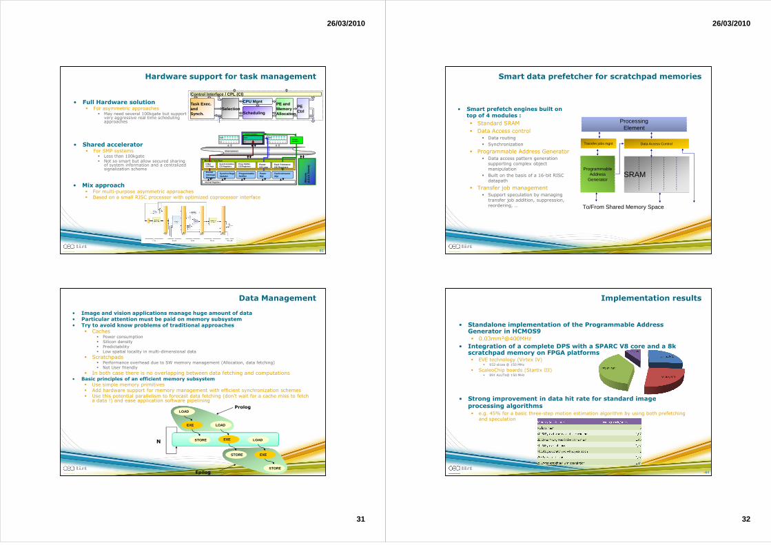
Smart data prefetcher for scratchpad memories
• Smart prefetch engines built on top of 4 modules :
� Standard SRAM
� Data Access control� Data routing
� Synchronization
� Programmable Address Generator� Data access pattern generation
supporting complex object manipulation
� Built on the basis of a 16-bit RISC datapath
� Transfer job management� Support speculation by managing
transfer job addition, suppression, reordering, …
ProcessingElement
ProcessingElement
Data Access ControlData Access Control
SRAMSRAM
To/From Shared Memory Space
Programmable Address
Generator
Programmable Address
Generator
Transfer jobs mgntTransfer jobs mgnt
Implementation results
• Standalone implementation of the Programmable Address Generator in HCMOS9� 0.03mm²@400MHz
• Integration of a complete DPS with a SPARC V8 core and a 8k scratchpad memory on FPGA platforms� EVE technology (Virtex IV)
� 932 slices @ 150 MHz
� ScaleoChip boards (Startix III)� 891 ALUTs@ 150 MHz
• Strong improvement in data hit rate for standard image processing algorithms � e.g. 45% for a basic three-step motion estimation algorithm by using both prefetching
and speculation
64
54%
25%
13%8%
AG Core
Request Ctrl
Transfer Ctrl
Job control
26/03/2010
33
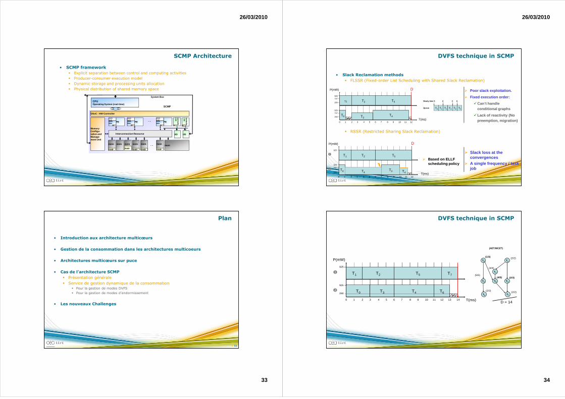
SCMP Architecture
• SCMP framework
� Explicit separation between control and computing activities
� Producer-consumer execution model
� Dynamic storage and processing units allocation
� Physical distribution of shared memory space
CPUOperating System (real-time)
SCMP
System Bus
Interconnection Resource
PE
meminstrmem data
PE
meminstrmemdata
mem
controller I/O
I/O
mem mem mem
PE
meminstrmemdata
mem mem mem
instr instr instr instr instr
Memory Configu-ration and Manage-ment Unit
GA GA GA GA
controller I/O
GA
I/O
OSoC : HW Controller
Plan
• Introduction aux architecture multicœurs
• Gestion de la consommation dans les architectures multicoeurs
• Architectures multicœurs sur puce
• Cas de l’architecture SCMP
� Présentation générale
� Service de gestion dynamique de la consommation� Pour la gestion de modes DVFS
� Pour la gestion de modes d’endormissement
• Les nouveaux Challenges
66
26/03/2010
34
• Slack Reclamation methods
� FLSSR (Fixed-order List Scheduling with Shared Slack Reclamation)
� RSSR (Restricted Sharing Slack Reclamation)
DVFS technique in SCMP
0 1 2 3 4 5 6 7 8 9 10 11 12
T0
925747
260IDLE
T3T4
IDLE
T1 T2 T5
925747
260
P(mW)
T(ms)
D
T0 T1 T2 T3 T4 T5
Ready time 0 2 3 6
Queue
0 1 2 3 4 5 6 7 8 9 10 11 12
T0
925747
222T3
T1 T2 T5
925
P(mW)
T(ms)T4
IDLE
D
T4
�
�
� Poor slack exploitation.
� Fixed execution order:
�Can’t handle conditional graphs
� Lack of reactivity (No preemption, migration)
� Slack loss at the convergences
� A single frequency / task job
� Based on ELLF scheduling policy
DVFS technique in SCMP
T0 T1
T2
T3T5T4
(1/3) (2/2)
(5/5)(4/6) (2/3)
(4/4)
T6 T7
(2/2)(2/2)
0 1 2 3 4 5 6 7 8 9 10 11 12 13 14
T0
925
260
T1 T2
T4
925
P(mW)
T(ms)
T3 T6
T7T5
D = 14
-a- -b-
IDLE
�
�
(AET/WCET)
26/03/2010
35
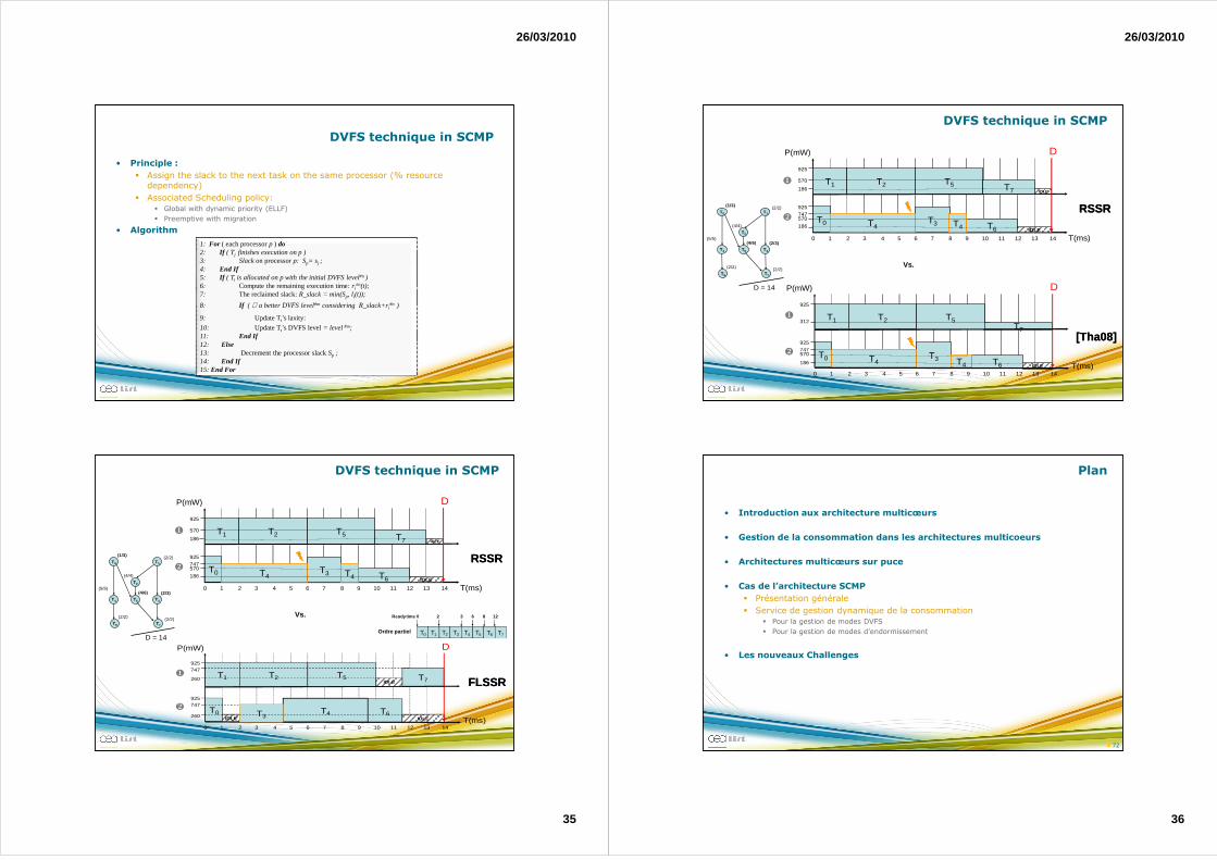
DVFS technique in SCMP
• Principle :
� Assign the slack to the next task on the same processor (% resource dependency)
� Associated Scheduling policy:� Global with dynamic priority (ELLF)
� Preemptive with migration
• Algorithm
1: For ( each processorp ) do2: If ( Tj finishes execution on p )3: Slackon processorp: Sp= sj ;4: End If5: If ( Ti is allocated on p with the initial DVFS level#n)6: Compute the remaining execution time:r i
#n(t);7: The reclaimed slack:R_slack = min(Sp, li(t));
8: If ( ∃ a better DVFS level#m considering R_slack+ri#n )
9: Update Ti’s laxity:
10: Update Ti’s DVFS level= level#m;11: End If12: Else13: Decrement the processor slackSp ;14: End If15: End For
DVFS technique in SCMP
T0
925747570
186
T5T1 T2
T3
925
570
186
P(mW)
T(ms)
D
T4 T6T4
T7
0 1 2 3 4 5 6 7 8 9 10 11 12 13 14
IDLE
IDLE
�
�T0 T1
T2
T3T5T4
(1/3) (2/2)
(5/5)(4/6) (2/3)
(4/4)
T6 T7
(2/2) (2/2)
D = 14
Vs.
RSSRRSSR
FLSSRFLSSR
T0 T1 T2 T3 T4 T5
Readytime 0 2 3 6 8 12
Queue T6 T7
T0
925747
260
T1 T2
925747
260
P(mW) D
T4 T6
T7
0 1 2 3 4 5 6 7 8 9 10 11 12 13 14
IDLE
�
�
T5
T(ms)IDLET3
IDLE
Ordre partiel
26/03/2010
36
DVFS technique in SCMP
T0
925747570
186
T5T1 T2
T3
925
570
186
P(mW)
T(ms)
D
T4 T6T4
T7
0 1 2 3 4 5 6 7 8 9 10 11 12 13 14
IDLE
IDLE
�
�
T0
925747570
186
T1 T2
T3
925
312
P(mW) D
T4 T6T4
T7
0 1 2 3 4 5 6 7 8 9 10 11 12 13 14
IDLE
�
�
T5
T(ms)
T0 T1
T2
T3T5T4
(1/3) (2/2)
(5/5)(4/6) (2/3)
(4/4)
T6 T7
(2/2) (2/2)
D = 14
Vs.
RSSRRSSR
[Tha08] [Tha08]
Plan
• Introduction aux architecture multicœurs
• Gestion de la consommation dans les architectures multicoeurs
• Architectures multicœurs sur puce
• Cas de l’architecture SCMP
� Présentation générale
� Service de gestion dynamique de la consommation� Pour la gestion de modes DVFS
� Pour la gestion de modes d’endormissement
• Les nouveaux Challenges
72
26/03/2010
37
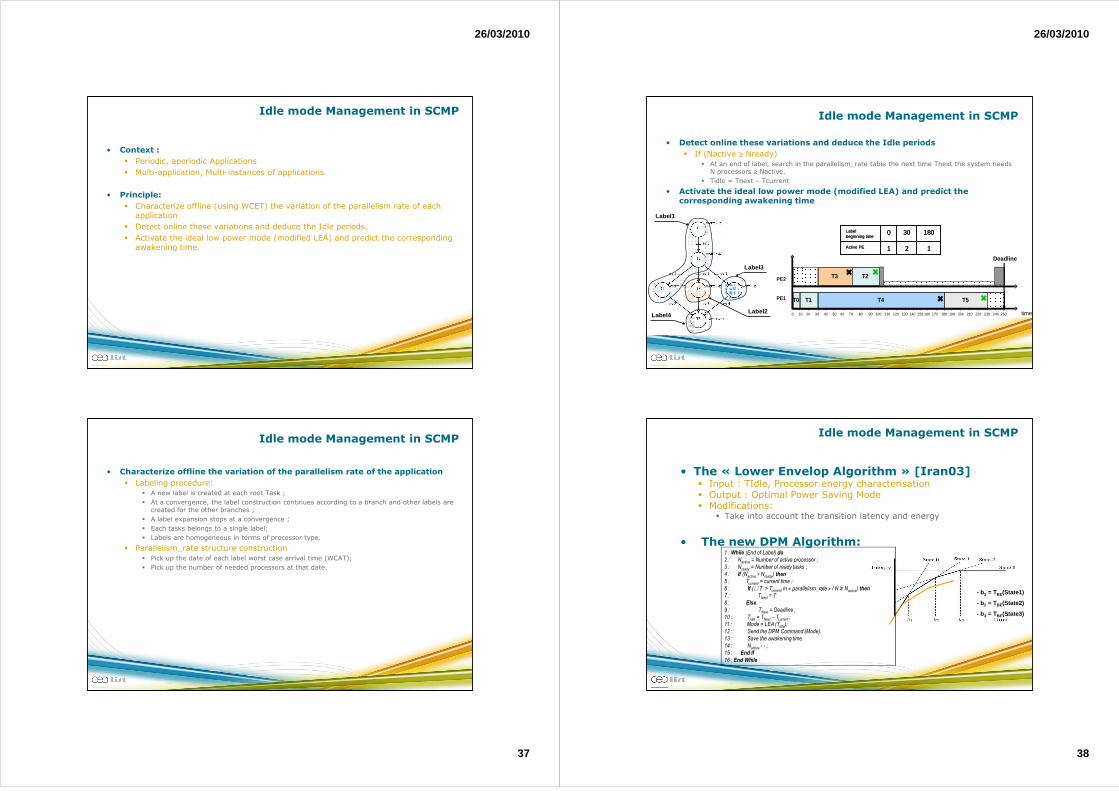
Idle mode Management in SCMP
• Context :
� Periodic, aperiodic Applications
� Multi-application, Multi-instances of applications
• Principle:
� Characterize offline (using WCET) the variation of the parallelism rate of each application
� Detect online these variations and deduce the Idle periods.
� Activate the ideal low power mode (modified LEA) and predict the corresponding awakening time.
Idle mode Management in SCMP
• Characterize offline the variation of the parallelism rate of the application
� Labeling procedure:� A new label is created at each root Task ;
� At a convergence, the label construction continues according to a branch and other labels are created for the other branches ;
� A label expansion stops at a convergence ;
� Each tasks belongs to a single label;
� Labels are homogeneous in terms of processor type.
� Parallelism_rate structure construction� Pick up the date of each label worst case arrival time (WCAT);
� Pick up the number of needed processors at that date.
26/03/2010
38
Idle mode Management in SCMP
• Detect online these variations and deduce the Idle periods
� If (Nactive ≥ Nready)� At an end of label, search in the parallelism_rate table the next time Tnext the system needs
N processors ≥ Nactive.
� Tidle = Tnext – Tcurrent
• Activate the ideal low power mode (modified LEA) and predict the corresponding awakening time
Label1
Label4
Label3
Label2 0 10 20 30 40 50 60 70 80 90 100 110 120 130 140 150 160 170 180 190 200 210 220 230 240 250
T0 T1 T4
T3 T2
T5
Deadline
time
PE1
PE2
121Active PE
180300Label beginning time
121Active PE
180300Label beginning time
�
�
�
�
- b1 = TBE(State1)
- b2 = TBE(State2)
- b3 = TBE(State3)
Idle mode Management in SCMP
1 : While (End of Label) do
2 : Nactive = Number of active processor ;
3 : Nready = Number of ready tasks ;
4 : If (Nactive > Nready) then
5 : Tcurrent = current time ;
6 : If (∃ T > Tcurrent in « parallelism_rate » / N ≥ Nactive) then
7 : TNext = T
8 : Else
9 : TNext = Deadline ;
10 : Tidle = TNext – Tcurrent ;
11 : Mode = LEA (Tidle);
12 : Send the DPM Command (Mode).
13 : Save the awakening time.
14 : Nactive - - ;
15 : End If
16 : End While
• The « Lower Envelop Algorithm » [Iran03] � Input : TIdle, Processor energy characterisation� Output : Optimal Power Saving Mode� Modifications:
� Take into account the transition latency and energy
• The new DPM Algorithm:
26/03/2010
39
0 10 20 30 40 50 60 70 80 90 100 110 120 130 140 150 160 170 180 190 200 210 220 230 240 250
T0 T1 T4
T3 T2PE2
PE1
Deadline
T5 T0 T1 T4
T3 T2
T5
time
Period
T0 T1
260 270 280 290 300 310 320 330 340 350 360 370 380 390 400 410 420 430 440 450 460 470 480 490 500 510 520
121Active PE
180300Label beginning time
121Active PE
180300Label beginning time
121
430280250
121
430280250
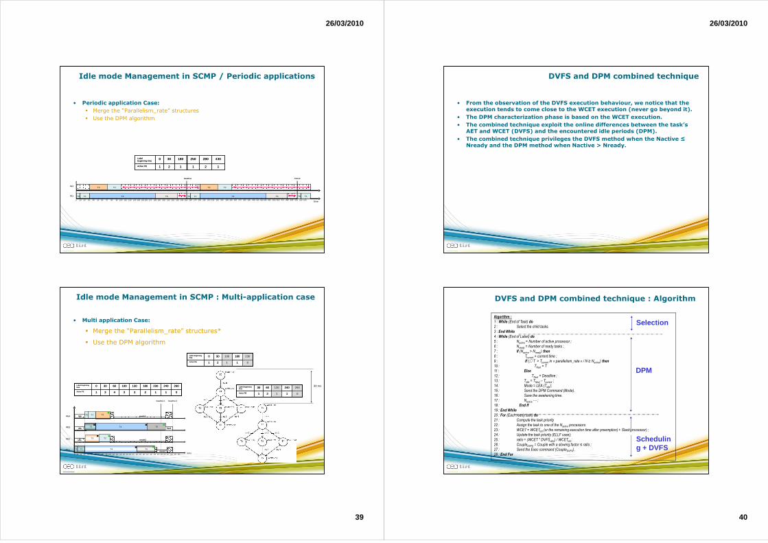
Idle mode Management in SCMP / Periodic applications
• Periodic application Case:
� Merge the “Parallelism_rate” structures
� Use the DPM algorithm
Idle mode Management in SCMP : Multi-application case
• Multi application Case:
� Merge the “Parallelism_rate” structures*
� Use the DPM algorithm
01121Active PE
230180100300Label beginning time
01121Active PE
230180100300Label beginning time
01121Active PE
2602401306030Label beginning time
01121Active PE
2602401306030Label beginning time
30 ms
0 10 20 30 40 50 60 70 80 90 100 110 120 130 140 150 160 170 180 190 200 210 220 230 240 250
T0 T1 T4
PE4
PE1
Deadline 1
T5
T3PE2
PE3
T0 T1
T4
Deadline 2
time260 270 280 290 300
T2
T2
T5
mode1
mode2
Idle
Idle
Idle
2
130
2
180
1
230
1
240
03431Active PE
26010060300Label beginning time
2
130
2
180
1
230
1
240
03431Active PE
26010060300Label beginning time
mode2T3
Idle
�
��
�
�
�
�
�
26/03/2010
40
DVFS and DPM combined technique
• From the observation of the DVFS execution behaviour, we notice that the execution tends to come close to the WCET execution (never go beyond it).
• The DPM characterization phase is based on the WCET execution.
• The combined technique exploit the online differences between the task’s AET and WCET (DVFS) and the encountered idle periods (DPM).
• The combined technique privileges the DVFS method when the Nactive ≤ Nready and the DPM method when Nactive > Nready.
Algorithm :
1 : While (End of Task) do
2 : Select the child tasks.
3 : End While
4 : While (End of Label) do
5 : Nactive = Number of active processor ;
6 : Nready = Number of ready tasks ;
7 : If (Nactive > Nready) then
8 : Tcurrent = current time ;
9 : If (∃ T > Tcurrent in « parallelism_rate » / N ≥ Nactive) then
10 : TNext = T
11 : Else
12 : TNext = Deadline ;
13 : Tidle = TNext – Tcurrent ;
14 : Mode = LEA (Tidle);
15 : Send the DPM Command (Mode).
16 : Save the awakening time.
17 : Nactive - - ;
18 : End If
19 : End While
20 : For (Each ready task) do
21 : Compute the task priority
22 : Assign the task to one of the Nactive processors
23 : WCET = WCETold (or the remaining execution time after preemption) + Slack(processor) ;
24 : Update the task priority (ELLF case);
25 : ratio = (WCET * DVFSratio) / WCETold ;
26 : CoupleDVFS = Couple with a slowing factor ≤ ratio ;
27 : Send the Exec command (CoupleDVFS).
28 : End For
Selection
DPM
Scheduling + DVFS
DVFS and DPM combined technique : Algorithm
26/03/2010
41
Simulation Results
• SystemC simulation of an image labeling application parallelized on 12 sub-images.
T0 CHARGEMENT
T1 DECOUPAGE
T2 T3 T4
T5
DISPATCH1
T6
END
INIT
DISPATCH0 DISPATCH2
T7 T8 T9 T10 T11 T12 T13 T14 T15 T16
T17 T18 T19CORRESP_FUSION_HCORRESP_FUSION_H-S CORRESP_FUSION_H-N
LABELLISATION
T20 T21 T22CORRESP_V1CORRESP_V0 CORRESP_V2 T23 CORRESP_V3
T24 FUSION_CORRESP_V
T25 FUSION_V_RECONST
ev0
ev1 ev1ev1
ev2 ev2 ev2 ev2 ev3 ev3 ev3 ev3 ev4 ev4 ev4 ev4
ev5 ev6 ev7 ev8 ev9 ev10 ev11 ev12 ev13 ev14 ev15 ev16
ev17 ev17 ev17 ev17
ev20ev21 ev22
ev18ev18 ev18 ev18
ev19ev19 ev19 ev19
ev23
ev24
0 1 2 3
4 5 6 7
8 9 10 11
117
33
34
3549
236
0
100
200
300
400
500
1 0,8 0,75 0,6 0,5
AET/WCET
Mea
n P
ow
er (m
W)
0
10
20
30
40
50
60
Gain
(%)
No Optimization with DVFS with DVFS and DPM Gain(DVFS + DPM)
0
100
200
300
400
500
600
700
800
900
1000
1 0,8 0,75 0,6 0,5
AET/WCET
Mea
n P
ow
er (m
W)
0
10
20
30
40
50
Gai
n (%
)
No Optimization with DVFS with DVFS and DPM Gain(DVFS + DPM)
4 PE (PPC 405) 8 PE (PPC 405)
Simulation Results
• SystemC simulation of an image labeling application parallelized on 12 sub-images.
26/03/2010
42
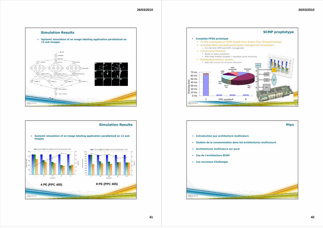
SCMP proptotype
• Complete FPGA prototype
� 75 MHz prototypes on FCM4 boards from Scaleo Chip (StratixIII based)
� Including OSoC and additionnal power management accelerators� For real time DPM and DVFS management
� 4 Processing Elements� Based on sparc processors
� With Data Prefetch Engines + standard cache memories
� Multibanked memory system� With HW support for dynamic allocation
83
A
H
B
PE0
PE1
PE2
PE3
Selection
$D
$D
$D
$D
$D
$D
RAMDPS
TLB
DPS
TLB
DPS
TLB
DPS
TLB
GPTimer
UARTDebug
Host
M
U
L
T
I
-
B
U
S
$I
$I
$I
$I
ITMP
UGM
0 ms10 ms20 ms30 ms40 ms50 ms60 ms70 ms
1 2 4 8
Run
ning
tim
e
PE number
schedulingwait for datarunning labelling
Ctrl IT5%
DPS18%
UGM10%
basic peripherals
10%
Scheduler11%
PEs 46%
Plan
• Introduction aux architecture multicœurs
• Gestion de la consommation dans les architectures multicoeurs
• Architectures multicœurs sur puce
• Cas de l’architecture SCMP
• Les nouveaux Challenges
84