Simulation and modeling of pressure pulse

propagation in fluids inside drill strings

To the Faculty of Geosciences, Geoengineering and Mining

of the Technische Universität Bergakademie Freiberg

approved

THESIS

to attain the academic degree of

Doktor-Ingenieur

(Dr.-Ing.)

submitted

by M.Sc. Mohammed Ali Namuq

born on the 1. July 1980 in Salahuddin, Iraq

Reviewers: Prof. Dr.-Ing. Matthias Reich, Freiberg

Prof. Dr.-Ing. Gerhard Thonhauser, Leoben

Prof. Dr.-Ing. Joachim Oppelt, Clausthal

Date of the award: 20.02.2013

ii

Declaration I hereby declare that I completed this work without any improper help from a third party

and without using any aids other than those cited. All ideas derived directly or indirectly

from other sources are identified as such.

In the selection and in the use of materials and in the writing of the manuscript I received

support from the following person:

Prof. Dr.-Ing. Matthias Reich

Persons other than that above did not contribute to the writing of this thesis. I did not seek

the help of a professional doctorate-consultant. Only persons identified as having done so

received any financial payment from me for any work done for me.

This thesis has not previously been submitted to another examination authority in the

same or similar form in Germany or abroad.

Freiberg, 20.02.2013 Mohammed Ali Namuq

iii

Namuq, Mohammed Ali

Simulation and modeling of pressure pulse propagation in fluids inside drill strings

Dissertation 2013; 114 Pages; 64 Figures; 6 Tables; 3 Appendices

TU Bergakademie Freiberg, Faculty of Geosciences, Geoengineering and Mining,

Institute of Drilling Engineering and Fluid Mining

Abstract Modern bottom-hole assemblies are equipped with various sensors which measure the

geological and directional information of the borehole while drilling. It is very crucial to

get the measured downhole information to the surface in real time in order to be able to

monitor, steer and optimize the drilling process while drilling. The transmission of the

information to the surface is most commonly carried out by coded pressure pulses (the

technology called mud pulse telemetry) which propagate through the drilling mud inside

the drill string towards the surface. However, hardly any specific experimental research

on the hydraulic data transmission can be found in the literature. Moreover, it is essential

to use a reliable model/simulation tool which can more accurately simulate the pressure

pulse propagation in fluids inside drill strings under various drilling operation conditions

in order to improve the performance of the data transmission process. The aims of this

study are to develop and test a laboratory experimental setup, a simulation model and a

novel method for detecting and decoding of measurement while drilling pressure pulse

propagation in fluids inside drill strings.

This thesis presents a laboratory experimental setup for investigating the process of data

transmission in boreholes by mud pulse telemetry. The test facility includes a flow loop, a

centrifugal pump, a positive mud pulser or alternatively a mud siren, pressure transducers

at four different locations along the flow loop and a data collection system. Moreover, it

includes an “actuator system” for the simulation of typical noise patterns created by the

common duplex or triplex mud pumps. This laboratory setup with great capabilities

opens the way for testing and developing new concepts for data transmission.

A theoretical model using ANSYS CFX11 (Computational Fluid Dynamics (CFD)

commercial code) was successfully developed to simulate dynamic pressure pulse

iv

transmission behavior in the fluid inside the flow loop. The collected laboratory data

which simulate various data transmission processes in boreholes were used to verify and

calibrate the theoretical method. A pretty good agreement is achieved between the

predicted and measured pressure pulses at different locations along the flow loop for

positive pulses with various durations using different flow rates and for continuous

pressure pulses using different carrier frequencies.

A novel approach (continuous wavelet transformation) for detecting and decoding the

received continuous pressure pulses in a noisy environment was applied to various

simulated drilling operation conditions for data transmission in boreholes in the

laboratory. The concept was registered at the German Patent and Trade Mark Office

(DPMA) for a patent in 2011. The results indicate that the continuous wavelet

transformation can be used to clearly identify and better detect the continuous pressure

pulse periods, frequencies and discontinuity positions in the time domain compared to the

conventional method (Fourier transformation). This method will contribute to the

possibility of transmitting the data at higher rates and over longer distances.

A concept for developing an innovative pulser using electrical discharge or acoustic

sources for inducing pulses keeping the drill strings fully open (eliminating the problem

of plugging the pulser by pumped lost circulation materials) and without any mechanical

moving parts (eliminating the failure related to the pulser moving parts) was also

registered at the German Patent and Trade Mark Office (DPMA) for a patent in 2012.

With this pulser, it is expected that it would be possible to transmit the data over longer

distances and at higher rates. Realizing the concept of the new pulser and using

continuous wavelet transformation for detecting and decoding the pulser signal are

recommended for future work.

v

Acknowledgements I would like to thank my doctoral supervisor, Prof. Dr.-Ing. Matthias Reich, for his

support, encouragement, guidance and patience throughout the course of this work. I

would like also to thank him for his support and encouragement to participate in national

and international conferences, writing scientific articles and preparing patents which

helped me finish my work.

I would like to acknowledge the support and encouragement from Prof. Dr. Steffen

Wagner and Prof. Dr.-Ing. Moh’d M. Amro. I gratefully acknowledge the time and

assistance of Dipl.-Ing. Silke Röntzsch in setting up the laboratory experiment. I thank

PD Dr. Swanhild Bernstein for her cooperation and advisement regarding the application

of wavelet transformation in data transmission process by mud pulse telemetry. Thanks to

Dipl.-Ing. Andreas Schramm, engineer Uwe Wohrow, Mr. Jens Richter and Mr. Philipp

Wella for their help during set up of the laboratory experiment. I thank Mr. Julian Corwin

and Mr. Melvin Kome for reading my dissertation. I would like also to thank other staff

members of the institute of Drilling Engineering and Fluid Mining for their help and

supports.

I deeply appreciate the scholarship provided by DAAD (German Academic Exchange

Service) and financial support provided by Dr. Erich Krüger Research Foundation

(Freiberg High-Pressure Research Centre (FHP)) during this work.

Finally, I want also to express my deepest gratitude to my wife and parents for their

support and encouragement and to my son, Adam, for his love and patience. This thesis is

dedicated to them.

vi

Table of contents

Declaration .......................................................................................................................... ii

Abstract .............................................................................................................................. iii

Acknowledgements ............................................................................................................. v

Table of contents ................................................................................................................ vi

List of abbreviations and symbols ..................................................................................... ix

Chapter 1: Introduction ................................................................................................. 12

1.1 Research motivation.................................................................................................... 12

1.2 Objectives ................................................................................................................... 15

1.3 Methods and materials ................................................................................................ 16

1.4 Organization of the dissertation .................................................................................. 17

Chapter 2: Fundamentals of measurement while drilling pressure pulses ............... 18

2.1 Historical background and state of the art .................................................................. 18

2.2 Types of mud pulse telemetry ..................................................................................... 21 2.2.1 Positive mud pulse telemetry ........................................................................... 21 2.2.2 Negative mud pulse telemetry ......................................................................... 22 2.2.3 Continuous wave (mud siren) telemetry .......................................................... 22

2.3 Data transmission modulations ................................................................................... 24 2.3.1 Baseband transmission ..................................................................................... 25

2.3.1.1 Return-to-zero (RZ) .................................................................................. 26 2.3.1.2 Non return-to-zero (NRZ) ......................................................................... 26 2.3.1.3 Manchester (or Split-Phase) ...................................................................... 26

2.3.2 Passband transmission ..................................................................................... 26 2.3.2.1 Phase shift keying (PSK) .......................................................................... 27 2.3.2.2 Frequency shift keying (FSK) ................................................................... 27 2.3.2.3 Amplitude shift keying (ASK) .................................................................. 27

2.4 Characteristics of drilling mud channels ..................................................................... 28 2.4.1 Attenuation ....................................................................................................... 28 2.4.2 Noise ................................................................................................................ 29

2.5 Pressure pulse (wave) propagation ............................................................................. 31 2.5.1 Pressure pulse (wave) speed ............................................................................ 31 2.5.2 Transmission and reflection ............................................................................. 32

2.6 Transformation methods for mud pulse detection and decoding ................................ 34 2.6.1 Fourier transformation ..................................................................................... 34 2.6.2 Short time Fourier transformation ................................................................... 36 2.6.3 Continuous wavelet transformation ................................................................. 36 2.6.4 Comparison of transformation methods ........................................................... 39

Chapter 3: Laboratory experiment ............................................................................... 42

vii

3.1 Laboratory experimental setup ................................................................................... 42 3.1.1 Laboratory positive mud pulser ....................................................................... 44 3.1.2 Laboratory mud siren pulser ............................................................................ 45 3.1.3 Actuator system ............................................................................................... 47 3.1.4 Data collection and experiment operation conditioning system ...................... 49

3.2 Laboratory positive pulser and mud siren pulser performance ................................... 50

3.3 Actuator system performance ..................................................................................... 52

3.4 Pressure fluctuations effect on positive and mud siren pulser signals identification . 53

3.5 Carrier frequency selection ......................................................................................... 56

3.6 Noise cancellation ....................................................................................................... 58

3.7 Application of transformation methods to experimental cases ................................... 60 3.7.1 Amplitude shift keying modulation ................................................................. 60 3.7.2 Frequency shift keying modulation ................................................................. 62

3.8 Pressure pulse (wave) speed measurement ................................................................. 64

3.9 High speed photography for measuring the laboratory positive pulser movement .... 67

Chapter 4: Numerical simulation and modeling of positive pressure pulse propagation ...................................................................................................................... 69

4.1 Mathematical model .................................................................................................... 69

4.2 Fluid compressibility .................................................................................................. 71

4.3 Hydrostatic pressure modeling ................................................................................... 71

4.4 Geometry and mesh generation .................................................................................. 72

4.5 Boundary conditions ................................................................................................... 73 4.5.1 Inlet boundary condition .................................................................................. 74 4.5.2 Outlet boundary condition ............................................................................... 74 4.5.3 Modeling of pump effect (time dependent boundary conditions) ................... 74

4.6 Modeling mesh movement .......................................................................................... 76

4.7 Initializations............................................................................................................... 77

4.8 Convergence criteria ................................................................................................... 77

4.9 Mesh sensitivity study................................................................................................. 78

4.10 Validation .................................................................................................................. 79

Chapter 5: Numerical simulation and modeling of continuous pressure pulse propagation ...................................................................................................................... 86

5.1 Mathematical model .................................................................................................... 86

5.2 Geometry and mesh generation .................................................................................. 86

5.3 Boundary conditions ................................................................................................... 86 5.3.1 Inlet boundary condition .................................................................................. 87

viii

5.3.2 Outlet boundary condition ............................................................................... 87

5.4 Modeling of rotor plate rotation .................................................................................. 87

5.5 Initializations............................................................................................................... 88

5.6 Convergence criteria ................................................................................................... 88

5.7 Mesh sensitivity study................................................................................................. 89

5.8 Validation .................................................................................................................... 90

Chapter 6: Conclusions and future works .................................................................... 95

6.1 Conclusions ................................................................................................................. 95

6.2 Future works ............................................................................................................... 98

References ...................................................................................................................... 100

List of Figures ................................................................................................................. 104

List of Tables .................................................................................................................. 108

List of publications ........................................................................................................ 109

Appendix 1 ..................................................................................................................... 112

Appendix 2 ..................................................................................................................... 113

Appendix 3 ..................................................................................................................... 114

ix

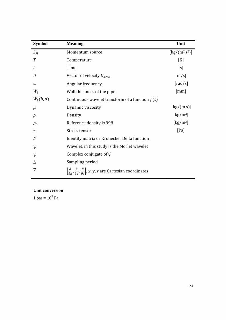
List of abbreviations and symbols

Symbol Meaning Unit

1, 2,

3, 4

1

2

| |

Scale  dilation  parameter of the wavelet transform 

Amplitude shift keying

Translation  shifting   parameter  of  the  wavelet 

transform 

Bottom‐hole assembly 

Speed of wave  

Computational Fluid Dynamics 

Calculated  pressure  signal  by  ANSYS  CFX11  of 

monitor points 1, 2, 3 and 4  

Continuous wavelet transformation 

Discrete Fourier transformation 

Modulus of elasticity of the pipe material  

Electromagnetic  valve  frequency  of  the  actuator 

system 

Bulk modulus of elasticity of the medium  

First mud siren frequency  dominant frequency   

Second mud siren frequency 

Pseudo frequency corresponding to scale 

Center frequency of a wavelet, for Morlet wavelet 

is 0.8125 

Fast Fourier transformation 

Absolute value of the FFT for data 

Time averaged value of flow rate  

Field programmable gate array 

Frequency shift keying 

A time domain function, real valued function 

Spectrum of  , a complex valued function

 

 

 

 

 

m/s  

 

 

bar  

 

 

N/m2  

 

Hz  

N/m2  

Hz  

Hz  

Hz  

 

Hz  

 

 

m3/hr  

 

 

 

 

x

Symbol Meaning Unit

1, 2, 3, 4

1 , 2 ,

3 , 4

1 , 3

 

 

 

 

Inner diameter of pipe

Inverse Fast Fourier transformation

√ 1 

Lost circulation materials 

Logging while drilling 

Main valve revolution of the actuator system 

measured from the open position 

Measurement while drilling 

Non return‐to‐zero 

Outer diameter  

Static pressure  

Absolute pressure 

Reference pressure, absolute value is 105  

Pressure signal of transmitters 1, 2, 3 and 4  

Time averaged value of pressure signal for 

transmitters 1, 2, 3 and 4  

Pressure signal of transmitters 1 and 3 respectively 

after noise is cancelled 

Pressure difference, calculated and measured 

unsteady state pressure signals minus steady state 

and time averaged pressure values for open flow 

area case for each monitor point and transmitter 

respectively  

Phase shift keying 

Polyvinyl Chloride pipe 

Rotation per minute 

Return‐to‐zero 

Short time Fourier transformation

mm  

 

 

 

 

revolution  

or  R  

 

 

mm  

Pa  

Pa  

Pa  

bar  

 

bar  

 

bar  

 

 

 

 

bar  

 

 

 

 

xi

Symbol Meaning Unit

,

 

∆

Momentum source

Temperature 

Time 

Vector of velocity  , ,  

Angular frequency 

Wall thickness of the pipe  

Continuous wavelet transform of a function   

Dynamic viscosity  

Density  

Reference density is 998  

Stress tensor  

Identity matrix or Kronecker Delta function  

Wavelet, in this study is the Morlet wavelet   

Complex conjugate of 

Sampling period  

, , ,  , , are Cartesian coordinates

kg/ m2 s2

K  

s  

m/s  

  rad/s  

mm  

 

  kg/ m s  

kg/m3  

kg/m3  

Pa  

 

 

 

 

Unit conversion

1 bar = 105 Pa

12

Chapter 1: Introduction

1.1 Research motivation The information gathered by the sensors of the bottom-hole assembly can be transmitted

to the surface while drilling by several means. These include mud pulses, wired pipe,

acoustic waves and electromagnetic waves. Some of them are in use on a commercial

basis, other are still under development. The most commonly used method is called the

mud pulse telemetry. Figure 1.1 shows a typical mud pulse telemetry system.

Fig. 1.1: Typical mud pulse telemetry (redrawn and modified) (Klotzb et al., 2008; Tennent and Fitzgerald, 1997)

Mud pulse telemetry systems use positive, negative or continuous wave pulsers to

generate controlled pressure fluctuations which carry the data to the surface through the

drilling mud inside the drill string (Hutin et al., 2001; Tubel et al., 1992). The measured

13

downhole sensors signals are converted to a binary code, consisting of a series of ones

and zeros, which is used to actuate the pulser. Depending on the individual design the

pulser will restrict, vent or continuously restrict and release the circulating drilling mud

inside the drill pipe in certain patterns. Subsequently, the pressure of the drilling mud

column will vary accordingly. The coded pressure waves will propagate through the

drilling mud to the surface where they are detected and read out by a pressure transducer.

A computer in the surface unit decodes the information and displays the data on the rig

floor to be used for monitoring, steering and optimizing the drilling process while

drilling. Consequently, this enables the industry to drill more complex well paths, make

drilling in general much safer and maximize production.

Although mud pulse telemetry can be considered as the global standard and common

state of the art for transmitting data in real time, details about the process of pressure

wave propagation in drill strings are still not understood in all details and hardly any

specific laboratory setup for evaluating the mechanisms of data transmission by mud

pulses can be found in the literature. Furthermore, the process of pulse transmission may

sound simple, propagation, reflection and attenuation of pressure waves (pulses) in fluids

inside pipes are, in reality, rather complex. The need exists for development of a reliable

method which can simulate dynamic pressure pulse transmission behavior in fluids inside

drill strings under various drilling operation conditions found in practice. This method

would lead to considerable improvement of the performance of the existing mud pulse

telemetry systems and the development of an innovative pulse telemetry system before

attempting time and cost consuming measurements in a real case.

In the present work a facility consisting of a centrifugal pump, a positive or alternatively

a mud siren pulser, four pressure transducers and a data collection system was designed

and constructed for the laboratory experiment to study the process of data transmission in

boreholes. Furthermore, typical noise patterns created by the drilling mud pumps were

simulated by building a special system named “actuator system”. The unsteady flow

behavior was simulated and modeled with the Computational Fluid Dynamics (CFD)

code (ANSYS CFX11). The laboratory experimental results were used to evaluate the

effectiveness of the numerical model. The agreement between the lab results and the

numerically computed values was quite encouraging.

14

The pressure waves are attenuated and contaminated by hydraulic noise on their way to

the surface. Thus the signal reception becomes a difficult task. The main and most

powerful sources of noise in the data transmission channel are the mud pumps which

severely disturb the identification of the mud pulses (Brandon et al., 1999; Tennent and

Fitzgerald, 1997). The pressure signal measured by a sensor attached to the standpipe will

contain both, the information signals and the hydraulic noise. Based on experimental

tests, the effect of the pressure fluctuation associated with the work of mud pumps on the

pressure pulses produced by a positive pulser and a mud siren pulser was examined. The

experimental results demonstrate that the hydraulic noise overlaps with the positive

pulser signal and makes its detection on the receiver more difficult. Depending on the

data, the positive pulser generates coded pressure pulses with varied durations; often their

frequency overlaps with hydraulic noise frequencies. In contrast, with the mud siren data

can be transmitted using carrier frequencies which do not overlap with hydraulic noise

frequencies. In practice however, it has to be considered that high carrier frequencies for

data transmission are not always an option, as high frequency signals suffer significant

attenuation on their way to the surface through the pipe system (Hutin et al., 2001). Thus

the detection of the generated mud siren signals and the extraction of their characteristics

(starts, durations and frequencies) in a noisy pressure signal measured in the mud column

at the standpipe are very essential for obtaining the correct information while drilling.

The most commonly used method for analyzing signals is the Fourier transformation

which provides information about the average strength of the frequency components in

the time signal. It is however not possible to obtain information about the moment when a

particular event in the time signal takes place. The information transmitted by the mud

pulse telemetry using a mud siren is of non-stationary characteristics as there are abrupt

changes at the beginnings and ends of the coded continuous pressure pulses in a fixed

time period to represent binary values. These characteristics and the frequency of the

carriers are the most important parameters of the transmitted information signals. As

opposed to the Fourier transformation, the wavelet techniques are relatively new and well

suited to analyze such characteristics of signals. The ability of the wavelet for identifying

carrier frequencies and extracting their characteristics has not been explored yet.

15

In the present study, experiments were carried out using a flow loop equipped with a mud

siren pulser and a special “actuator system”. Continuous pressure pulses of various

frequencies were produced by the mud siren using different data transmission

modulations. At the same time, hydraulic noise with various amplitudes and frequencies

was induced to the flow loop by the actuator system to simulate typical noise patterns

created by the common duplex or triplex mud pumps. The hydraulic noise was overlaid

to the continuous pressure pulses, resulting in complex time signals for the pressure in the

flow loop. For all experimental runs the noise amplitudes induced by the actuator system

were greater than the continuous pressure pulse amplitudes generated by the mud siren.

The wavelet toolbox in the MATLAB software was then successfully utilized to separate

the hydraulic noise from the pressure pulses again and to extract the continuous pressure

pulse characterization.

1.2 Objectives The main objectives of this thesis were the following:

a. Design and build up a flow loop and experimental setup in the laboratory

simulating all significant observations associated with the process of hydraulic

data transmission in boreholes using the state of the art mud pulse telemetry.

b. Carry out laboratory experimental tests, study and clarify the mechanisms of

pressure pulse propagation in fluids inside drill strings generated by both positive

and mud siren pulsers.

c. Develop a novel detection and decoding method and verify it’s effectiveness by

applying it to detect and identify the starts, periods and frequencies of continuous

pressure pulses generated by the mud siren for various transmission modulations.

d. Develop a theoretical model for pressure pulse propagation in fluids generated by

both pulsers (positive and mud siren).

e. Validate the theoretical method capability of modeling realistic pressure pulses

transmission by comparing the predicted results against the laboratory

experimental results.

16

1.3 Methods and materials The following approaches were used in the present thesis:

a. Literature review: A comprehensive review of the real time data transmission

systems in boreholes using mud pulse telemetry was made. This includes

technical descriptions of the state of the art systems, coding and modulation

techniques, and an overview on attenuation and noise problems in the

transmission channel (flowing drilling fluid inside a drill pipe).

b. Laboratory experimental setup: A flow loop equipped with a pressure pulse

generator (positive or mud siren pulser) and a special noise generator (actuator

system) to study the process of data transmission in boreholes in laboratory was

built up. In addition, it includes a data acquisition system to observe pressure

signals at 4 different locations along the flow loop, inlet flow rate and pulser

position, and a high speed camera.

c. Data collection: Data were gathered from the laboratory experiments. Tests were

carried out with different pulsers individually and in combination with the

actuator system for inducing noise with varied amplitudes and frequencies in the

flow loop, simulating a variety of drilling operation conditions for data

transmission in boreholes.

d. Wavelet transformation and Fourier transformation: Continuous Wavelet and

Fourier transformations were studied for analysis and detection of non-stationary

carrier frequencies characteristics. A computer program written in MATLAB was

developed to analyze and identify the continuous pressure pulses characteristics

using Fourier transformation, Short Time Fourier transformation and continuous

Morlet Wavelet transformation. Furthermore, a program was written in MATLAB

to filter noise using a Fast Fourier Transformation. The collected experimental

data and a synthetic case were used to compare and confirm the effectiveness of

the transformation methods.

e. ANSYS CFX11: A three dimensional numerical simulation model was developed

with the aid of ANSYS CFX11 (Computational Fluid Dynamics (CFD)

commercial code) to simulate the pressure pulse transmission in the flow loop

17

generated by the both positive and mud siren pulsers. Modeling of geometry and

meshing were done using ANSYS ICEM CFD.

f. Validation of model: The validation of the model was performed by comparing

the predicted results with the gathered laboratory experimental results which

simulate a wide range of data transmission processes in boreholes (positive pulses

with various durations and for different flow rates, and continuous pressure pulses

of the mud siren for different frequencies).

1.4 Organization of the dissertation Chapter 1: Introduction.

Chapter 2: Description of the state of the art of mud pulse telemetry systems, coding and

modulation types and characteristics of transmission channels. Furthermore, it presents,

discusses and compares the Fourier and wavelet transformation techniques.

Chapter 3: Laboratory experimental setup and results.

Chapter 4: Computational Fluid Dynamics (CFD) code (ANSYS CFX11) and results of

the numerical simulation and modeling of positive pressure pulses propagation in the

flow loop.

Chapter 5: Results of the numerical simulation and modeling of continuous pressure

pulses (mud siren signal) propagation in the flow loop.

Chapter 6: Conclusions and proposed ideas for the future works.

18

Chapter 2: Fundamentals of measurement while drilling pressure pulses

2.1 Historical background and state of the art The need for real time information at the surface while drilling for monitoring and

steering the drill bit through the formation has created the concept of measurement while

drilling (MWD). An early mud pulse telemetry system with data rates of less than 1 bit/s

using a plunger valve for generating discrete mud pulses was described by Arps and Arps

in 1964 (Hutin et al., 2001). A real time (inclination-only) MWD system was introduced

by B. J. Hughes in 1970 (Tubel et al., 1992). Patton et al., in 1977 described a Mobile

MWD system that used a rotating valve mechanism (also known as a mud siren) to

generate continuous waves using phase shift keying modulation. Data rates of up 3 bits/s

were claimed in the article (Hutin et al., 2001). In September 1978 Teleco Oilfield

Services began the commercial service of a wireless MWD system using mud pulse

telemetry in the Gulf of Mexico and shortly after provided service in over 400 wells in

the Gulf area alone. The Teleco Company expanded its service to the North Sea,

California, Alaska, West Africa and the Middle East making this the first and most

extensively used wireless MWD system for directional work in the world (Roberts,

1982). Ongoing developments made positive, negative and continuous mud pulse

telemetry systems available for sending information to the surface while drilling. Mud

pulse telemetry is the current industry standard for transmission of data from MWD and

LWD tools to surface and typically functions at 3 to 6 bits/s, rising to 12 bits/s under

ideal conditions (Reeves et al., 2005). The mud pulse carrier frequency is typically below

100 Hz, this limits data rate (Gao et al., 2006).

In the course of this development many types of coding systems and transmission

techniques were also developed. Monroe (1990) applied digital data encoding techniques

to mud pulse telemetry and showed improvement in data transmission rates. Tubel et al.,

(1992) described a positive pulse system with a transmission rate of two pulses per

second. Martin et al., (1994) described a mud siren pulser with downlink features (known

also as PowerPulse MWD tool) to meet the reliability demand. Communication from the

surface to the downhole tool is achieved by varying the mud flow rate at the surface

19

through a predefined sequence. A downhole microprocessor is programmed to recognize

specific patterns of flow variations detected from changes in the speed of the downhole

turbine. This enables the tool to cycle through a predefined “menu” of transmission

frequencies and telemetry frames. The downlink feature of the PowerPulse system made

it possible to optimize the use of the real time transmission system depending on the

application and drilling environment. Data transmission rates of 3 bits/s were achieved in

a deep water well (greater than 6100 m measured depth) in the Gulf of Mexico by using

mud siren telemetry (PowerPulse) (Hutin et al., 2001). Klotza et al., (2008) introduced a

mud siren telemetry system using an oscillating valve instead of a rotating valve. In this

article faster data rates compared to conventional mud pulse telemetry systems (normally

3 bits/s) were claimed to be achievable.

In the course of the development of the mud pulse telemetry systems, there were also

efforts to develop a model to reproduce and simulate the pulse transmission in the drill

strings. Patton et al., 1977 attempted to develop a model for MWD pulse transmission.

Due to the complexity of the variables which include pipe size, mud viscosity, drilling

depth, etc., the conclusion was empirical, creating substantial inaccuracy (Chen and

Aumann, 1985). A numerical simulation was introduced by Chen and Aumann in 1985

for predicting the pressure pulse transmission of a MWD system. The surface and

downhole equipment were modeled mathematically as the boundary conditions. The

calculation of pulse height is improved in comparison with the Patton et al model;

however it was concluded that due to the wide variation in drilling parameters the

discrepancy between prediction and experiment values is inevitable (Chen and Aumann,

1985). Carter (1986) tested a fluidic type valve (fluidic mud pulser) on 2883 m length

drill pipe for generating pressure pulses at frequencies as high as 25 Hz at the Louisiana

State University. The fluidic pulser employs centrifugal forces to create a vortex flow

which in turn causes an increase pressure drop. The pulse attenuation was also calculated

using the Lamb’s attenuation equations and compared with the measured data. The

attenuation data showed scattering as the fluid viscosity was increased. Lea and

Kyllingstad (1996) presented a coupling effect model between pressure waves

propagating inside and outside the drill string in a borehole. The system was modeled by

using three distinct wave propagation modes, differentiating between the propagation in

20

the mud inside the drill string, in the drill string, and the mud in the annulus and

formation. At a discontinuity in the formation stiffness or in the wellbore diameter, the

produced pressure pulses from a downhole telemetry tool could be partially reflected and

converted to other modes. Many assumptions were made to simplify the application of

this theory, which are not often satisfied in real wells such as an open wellbore with no

casing, isotropic and impermeable formation, uniform layers and no damping (Lea and

Kyllingstad, 1996). Xiu-Shan et al., (2007) proposed a multiphase flow formula to

calculate the mud pulse velocity.

The pressure pulses are attenuated and severely disturbed by noise in the drilling mud

channel as they propagate towards the surface. The mud pumps usually are the dominant

source of noise. The pressure signal measured by a sensor attached to the standpipe at any

point inevitably will contain both, the information signals and the hydraulic noise.

Tennent and Fitzgerald (1997) showed that the digital information transmitted by means

of pressure waves can be treated in much the same way as telephone or radio modem

signals using methods commonly used in telephone modems and cellular telephones.

Brandon et al., (1999) suggested two methods (nonlinear amplification and signal

averaging) for real time adaptive compensation of mud pump noise in MWD signals.

Those methods require signals from two channels, a primary signal (containing data and

noise) and a reference signal (containing noise). A typical example of two channels is the

use of two pressure sensors. The success of cancelling the noise component in the

primary channel by both methods depends on the complexity of the noise signal. It is

very common to install two pressure transducers on the stand pipe at a suitable distance

between them to cancel the pump noise from the signal (Martin et al., 1994). The most

commonly used transformation method for analyzing and detecting mud pulse signals,

particularly for the mud siren signals, is the Fourier transformation which does not

provide information about the time events. But the capability of the continuous wavelet

transformation which is more suitable for analyzing non-stationary signals like mud siren

signals has not been explored yet. In addition, a laboratory experiment for studying and

clarifying the mechanisms of data transmission in boreholes by a positive pulser and a

mud siren pulser can hardly be found in the literature. Moreover, a reliable and proved

model to describe the pressure pulses transmission in the drilling mud inside the drill

21

string generated by both pulsers (positive and mud siren) is desired to improve the data

transmission process.

2.2 Types of mud pulse telemetry Mud pulse telemetry systems are using positive, negative or continuous wave pulsers

(called mud sirens). They are very sensitive to underbalanced drilling. Pulser tolerance in

lost circulation material applications is a critical aspect for all available mud pulse

telemetry systems (Klotzb et al., 2008). They can be plugged by injected lost circulation

materials. Moreover, one of the contributors to downhole tool failures is the mechanical

moving components associated with mud pulse telemetry (Reeves et al., 2005).

2.2.1 Positive mud pulse telemetry

Positive pressure pulses are created in the mud column by momentarily and partially

restricting the open flow area for the drilling mud by a valve. Consequently, this causes

increased mud pressure which travels in the drilling mud inside the drill string to the

surface. When the mud flow area is opened again, the mud pressure returns back to its

original state. Thus the information is encoded and transmitted in a binary format using

discrete pulse type data transmission. The presence of a positive pulse (increased

pressure) is considered a binary 1 and the absence of a positive pulse (original state) is

considered a binary 0, vice versa is also applicable, see figure 2.1.

Fig. 2.1: Positive pulser and generated coded positive pressure pulses (redrawn and modified) (Hutin et al., 2001; Bone et al., 2005; Reich et al., 2003)

22

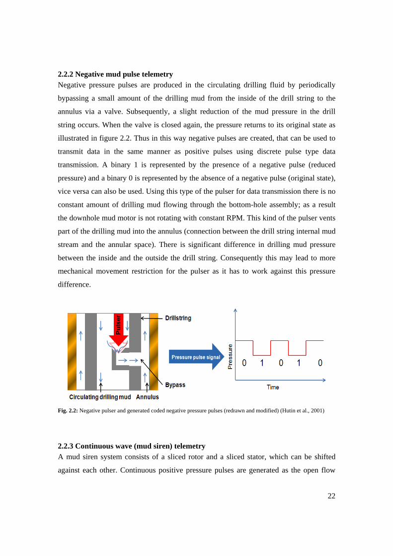
2.2.2 Negative mud pulse telemetry Negative pressure pulses are produced in the circulating drilling fluid by periodically

bypassing a small amount of the drilling mud from the inside of the drill string to the

annulus via a valve. Subsequently, a slight reduction of the mud pressure in the drill

string occurs. When the valve is closed again, the pressure returns to its original state as

illustrated in figure 2.2. Thus in this way negative pulses are created, that can be used to

transmit data in the same manner as positive pulses using discrete pulse type data

transmission. A binary 1 is represented by the presence of a negative pulse (reduced

pressure) and a binary 0 is represented by the absence of a negative pulse (original state),

vice versa can also be used. Using this type of the pulser for data transmission there is no

constant amount of drilling mud flowing through the bottom-hole assembly; as a result

the downhole mud motor is not rotating with constant RPM. This kind of the pulser vents

part of the drilling mud into the annulus (connection between the drill string internal mud

stream and the annular space). There is significant difference in drilling mud pressure

between the inside and the outside the drill string. Consequently this may lead to more

mechanical movement restriction for the pulser as it has to work against this pressure

difference.

Fig. 2.2: Negative pulser and generated coded negative pressure pulses (redrawn and modified) (Hutin et al., 2001)

2.2.3 Continuous wave (mud siren) telemetry

A mud siren system consists of a sliced rotor and a sliced stator, which can be shifted

against each other. Continuous positive pressure pulses are generated as the open flow

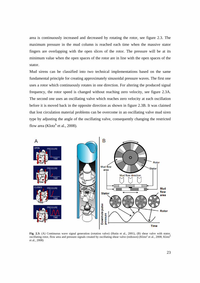
23

area is continuously increased and decreased by rotating the rotor, see figure 2.3. The

maximum pressure in the mud column is reached each time when the massive stator

fingers are overlapping with the open slices of the rotor. The pressure will be at its

minimum value when the open spaces of the rotor are in line with the open spaces of the

stator.

Mud sirens can be classified into two technical implementations based on the same

fundamental principle for creating approximately sinusoidal pressure waves. The first one

uses a rotor which continuously rotates in one direction. For altering the produced signal

frequency, the rotor speed is changed without reaching zero velocity, see figure 2.3A.

The second one uses an oscillating valve which reaches zero velocity at each oscillation

before it is moved back in the opposite direction as shown in figure 2.3B. It was claimed

that lost circulation material problems can be overcome in an oscillating valve mud siren

type by adjusting the angle of the oscillating valve, consequently changing the restricted

flow area (Klotzb et al., 2008).

Fig. 2.3: (A) Continuous wave signal generation (rotation valve) (Hutin et al., 2001), (B) shear valve with stator, oscillating rotor, flow area and pressure signals created by oscillating shear valve (redrawn) (Klotza et al., 2008; Klotzb et al., 2008)

24

In both cases the number of stator/rotor lobes and the operation revolutions or oscillations

per minute determines the frequency of the generated wave. Thus by using a mud siren

the data are modeled onto a continuous pressure wave with specific frequency (called

carrier frequency) which is shifted with different binary values (0 or 1) representing

different data values. For example, a higher carrier frequency can be used to represent a

binary 1 and a lower carrier frequency can be used to represent a binary 0 or vice versa.

In the same way the amplitude or the phase shifting of the generated continuous pressure

waves can be used to represent binary values (0 or 1). With a mud siren, different carrier

frequencies may easily be selected to place the telemetry signal in a part of the frequency

spectrum with the lowest noise. However, it should be considered that a carrier with a

higher frequency for data transmission will suffer a significant attenuation (shorter reach)

on its way through the drilling mud to the surface compared to carrier with a low

frequency (Hutin 2001).

2.3 Data transmission modulations Downhole measurement while drilling systems contain three primary subsystems: (1) a

downhole sensor package, (2) a method of sending information from the sensor package

to the surface while drilling proceeds and (3) surface equipment to receive this

information and convert it into usable information (Chen and Aumann, 1985). The

downhole sensor signals are converted to binary words consisting of ones and zeroes.

They are used to actuate a pulser, which in turn transmits coded information by pressure

waves in the mud column inside the drill pipe. These pressure waves propagate to the

surface. At the surface, the opposite process takes place. A pressure transducer attached

to the standpipe is used to measure and register the pressure fluctuations. To clear the

electrical signals of the transducer from background noise, they are run through special

filters. Then they are passed to a pulse recognition circuit in order to identify genuine

pulses from spurious ones. Moreover, they are passed to a decoder which decodes the

information and displays the data on the rig floor (Chen and Aumann, 1985).

Figure 2.4 shows an example of a mud siren telemetry data frame using phase shift

keying modulation and data rates of 6 bit/s. Each bit has a fixed time width (called bit

period), in phase shift keying modulation a continuous pressure wave (carrier frequency)

25

is sent in this time period to represent a binary 0. For altering the binary value to 1, the

rotor speed is slowed down to shift the phase of the continuous pressure wave. In this

example the updating time for each downhole variable parameter is not the same for

instance 10 bits are required to transmit the resistivity value which is updated every 8

seconds. Moreover, the data frames are identified by synchronization (or control bits)

(Martin et al., 1994). Some of the code modulations which are used in telecommunication

science are utilized by mud pulse telemetry systems to transmit downhole information to

surface. The transmission of data can be divided into two main categories, baseband

transmission and passband transmission.

Fig. 2.4: Example of a mud siren telemetry data frame using phase shift keying modulation (redrawn) (Martin et al., 1994)

2.3.1 Baseband transmission

The data are transmitted using discrete pressure pulses instead of using continuous

pressure pulses with specific frequencies (carrier frequencies). The positive, negative and

even mud siren pulsers can be used to transmit the data in such way. Various code

modulations were developed and are now available for baseband transmission of

information. There is no “ideal” one but each one has advantages and disadvantages. In

this thesis some of them are listed (Foster, 1965).

26

2.3.1.1 Return-to-zero (RZ)

The presence of a pulse at a bit period indicates a binary 1 and the absence of a pulse

represents a binary 0. Alteration happens at the beginning and midpoint of a bit period,

see figure 2.5.

2.3.1.2 Non return-to-zero (NRZ)

An initial one must be identified. Thereafter, every change in pulse level indicates a

change from the previous bit. Thus if the last bit is a one and the input data indicate a

pulse level change, the next bit will be a zero. The system will continue to interpret the

incoming data as a succession of zeros until another pulse level change is received,

whereupon the data will be interpreted as a sequence of ones, see figure 2.5.

2.3.1.3 Manchester (or Split-Phase)

Transition of a pulse level occurs in the midpoint of a bit period. Increasing stands for a

binary 0 and decreasing is for a binary 1. Opposite modulation is also possible, see figure

2.5.

Fig. 2.5: Different code modulations for baseband transmission of information (Foster, 1965)

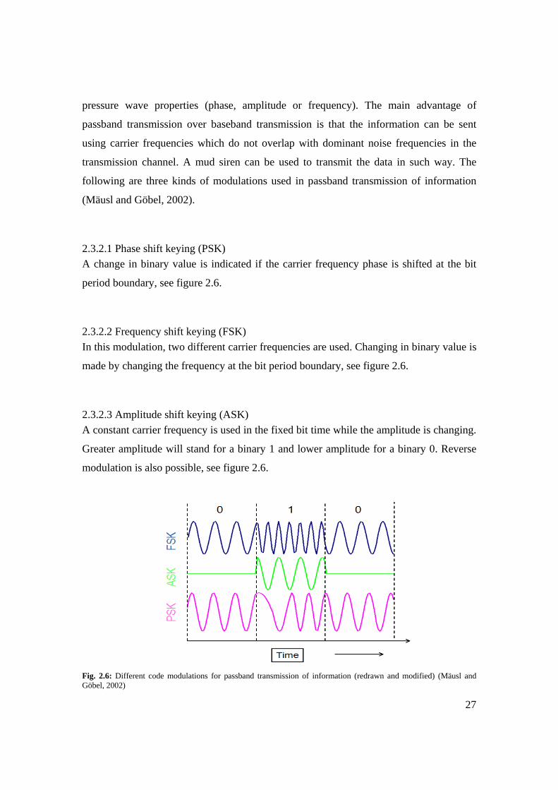
2.3.2 Passband transmission

The data are transmitted using continuous pressure waves with specific frequencies

(carrier frequencies). The binary 1 and 0 are represented by changing the continuous

27

pressure wave properties (phase, amplitude or frequency). The main advantage of

passband transmission over baseband transmission is that the information can be sent

using carrier frequencies which do not overlap with dominant noise frequencies in the

transmission channel. A mud siren can be used to transmit the data in such way. The

following are three kinds of modulations used in passband transmission of information

(Mäusl and Göbel, 2002).

2.3.2.1 Phase shift keying (PSK)

A change in binary value is indicated if the carrier frequency phase is shifted at the bit

period boundary, see figure 2.6.

2.3.2.2 Frequency shift keying (FSK)

In this modulation, two different carrier frequencies are used. Changing in binary value is

made by changing the frequency at the bit period boundary, see figure 2.6.

2.3.2.3 Amplitude shift keying (ASK)

A constant carrier frequency is used in the fixed bit time while the amplitude is changing.

Greater amplitude will stand for a binary 1 and lower amplitude for a binary 0. Reverse

modulation is also possible, see figure 2.6.

Fig. 2.6: Different code modulations for passband transmission of information (redrawn and modified) (Mäusl and Göbel, 2002)

28

2.4 Characteristics of drilling mud channels

2.4.1 Attenuation

The amplitude of downhole coded pressure pulses is dissipated as they travel thousands

of meters through the mud inside the pipe towards the receiver. The attenuation of mud

pulses is related to the properties of the drilling mud and the travelled distance (Hutin et

al., 2001). For instance the sharp rectangle pulses which are produced by a positive or

negative pulser downhole will be rounded, flattened and diminished in amplitude on their

way to the surface. Thus the detection and decoding of the pulses at the surface will

become more difficult. Consequently, this limits the mud pulse telemetry systems to

transmit the data at higher rates and over longer distances.

Field tests showed that about half the signal’s amplitude was lost for every 450 to 900 m

of depth (Gravley, 1983). The signal attenuation increases with smaller pipe diameter,

greater compressibility, higher viscosity and higher signal frequencies (Hutin et al.,

2001). Xiu-Shan et al., (2007) concluded from their work that the mud pulse attenuation

mainly increases with well depth, mud viscosity and signal frequency. Any air or gas in

the mud, caused by factors such as malfunctioning pumps or incomplete removal of gas

that flows into the mud stream from the formation, will increase the compressibility of

the mud and as a result significantly reduces the amplitude of the pressure pulses on their

way towards the surface (Hutin et al., 2001). Based on the experimental and simulation

results of an upward flowing air-water bubbly flow, Wang et al., (2000) showed that the

wave decay mainly depends on the distance travelled, the wave frequency and the air

void fraction. Huang et al., (2005) showed based on their experimental tests that the

attenuation coefficient of pressure wave propagation increases with the increase of the air

void fraction in air-water bubbly flow.

In very deep wells and viscous drilling mud, it is not easy to transmit the data at higher

rates because of significant attenuation of the signals at higher frequency. Therefore the

only opportunity is to transmit the data at lowest possible frequency so that an adequate

pulse amplitude can be seen at the surface. Figure 2.7 shows an example of signal

attenuation versus depth. It can be noticed that at 12 Hz the signal amplitude drops off

significantly with increasing depth while at 1 Hz the attenuation versus depth is much

29

less severe (Hutin et al., 2001). It can be said that the parameters which affect the pulse

attenuation, are either uncontrollable or very important for other reasons related to the

drilling process, except the carrier frequencies and may be also the air or gas content in

the mud. However, the selection of carrier frequencies for data transmission is also

restricted by the noise frequencies in the mud channel.

Fig. 2.7: Signal attenuation vs. depth and frequency (Hutin et al., 2001)

2.4.2 Noise

In the previous section it has been stated that carrier frequencies are one of the

parameters which affect the pressure pulse attenuation; however it is desirable for the

mud pulse telemetry to operate in the cleanest or least noisy frequency spectrum. The

interference of noise with the pressure pulses can be destructive or constructive

depending on their relative phase relationships. Thus the received pressure pulses at the

surface are severely distorted, phase shifted and masked by background noise as

illustrated by an example in figure 2.8. The main effects of noise on the data transmission

include:

30

Making pressure pulse detection very difficult or even in worse cases impossible.

Wrong decoding.

Sometimes prohibit using carrier frequencies which have low attenuation for data

transmission in order to have good pulse amplitude at the surface.

Fig. 2.8: Example explaining the effect of noise in the transmission channel on positive pulse detection and decoding

Anything which generates unwanted pressure fluctuations in the drilling mud column is

considered as hydraulic noise. Some of the noise is induced from downhole tools and will

travel to the surface in the same direction as the mud pulse signals. Others are generated

by surface equipment (for instance mud pumps) and will travel down the drill string in

the opposite propagation direction of the generated pulser signals. There are many

sources of noise in the drilling mud channel. Their frequencies are variable and

distributed over a wide range of the frequency spectrum, see figure 2.9. Even a frequency

of the same noise source could change from time to time during the course of the drilling

operation. Among them, the mud pulse signals are most severely disturbed by the noise

from the mud pumps. The mud pulse telemetry systems normally work at frequencies

below 100 Hz (Gao et al., 2006). Main noise sources include:

Drilling mud pumps

Bit interaction with the formation

Stick/slip phenomena

Drill string interaction with borehole

walls

Turbine of MWD supply

Stalling of mud motor

Positive displacement downhole motors

Balling of gumbo shale around bit teeth

31

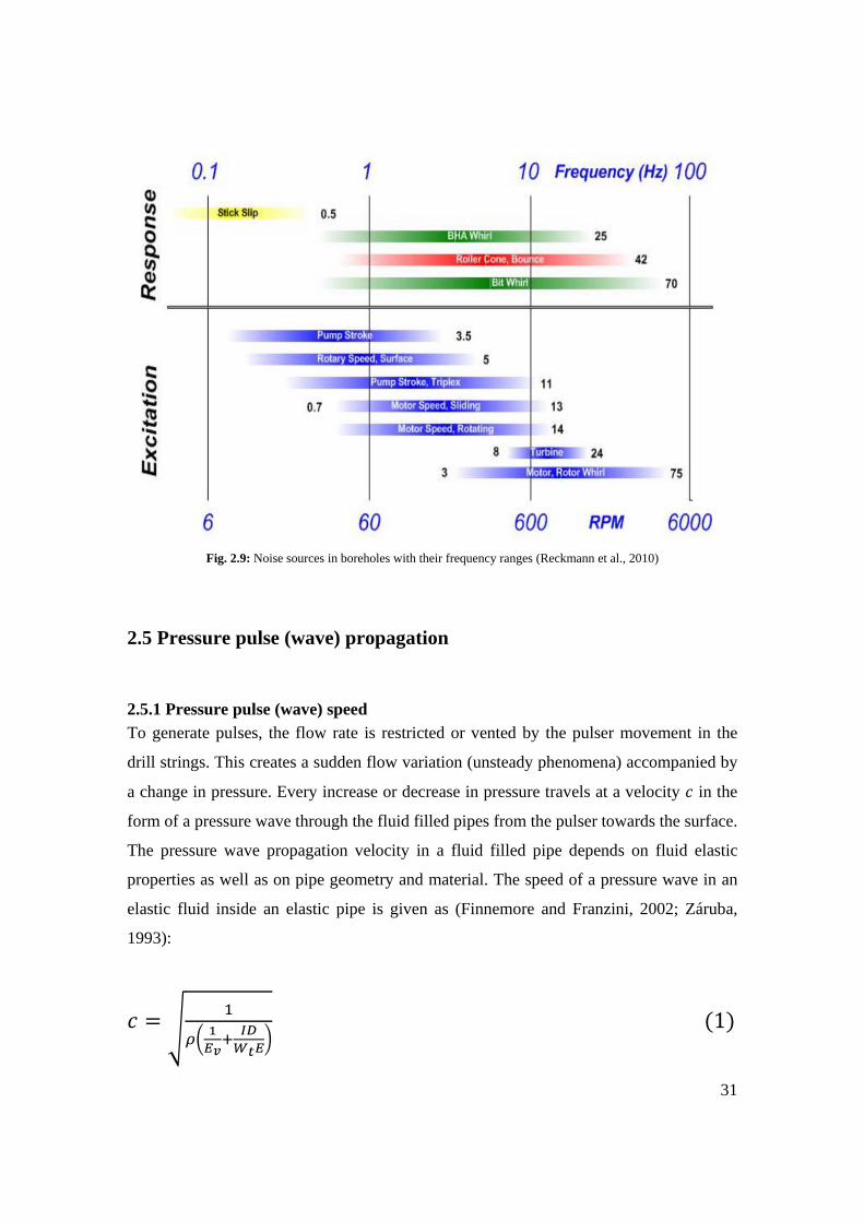
Fig. 2.9: Noise sources in boreholes with their frequency ranges (Reckmann et al., 2010)

2.5 Pressure pulse (wave) propagation

2.5.1 Pressure pulse (wave) speed

To generate pulses, the flow rate is restricted or vented by the pulser movement in the

drill strings. This creates a sudden flow variation (unsteady phenomena) accompanied by

a change in pressure. Every increase or decrease in pressure travels at a velocity in the

form of a pressure wave through the fluid filled pipes from the pulser towards the surface.

The pressure wave propagation velocity in a fluid filled pipe depends on fluid elastic

properties as well as on pipe geometry and material. The speed of a pressure wave in an

elastic fluid inside an elastic pipe is given as (Finnemore and Franzini, 2002; Záruba,

1993):

                                                                                       1

32

Thus the generated pulses downhole will reach the surface after a delay in time equal to

the mud pulse travel time in drilling mud column inside the drill string.

2.5.2 Transmission and reflection

The generated pressure waves travel at the speed through the fluid inside the pipes. At

each change in cross section and division of the pipes, the waves are partially reflected

back towards the source while partially continuing to travel in the original direction

(Záruba, 1993). The reflected waves can be again reflected and once again progress

towards the original direction, this process continues till they completely diminish. When

a pressure wave reaches the separating surface between two different mediums, part of it

is reflected while the rest penetrates into the second medium (Semat and Katz, 1958).

In the data transmission process various devices which form part of a drilling mud and

drill string systems for example mud pumps, pulsation dampeners, swivel, surface pipes,

etc; act like reflectors (Hutin et al., 2001). In addition to mud pulse telemetry signal,

several pressure waves originating from different noise sources can propagate

simultaneously in the drilling mud inside the drill string. Those waves are also partially

reflected and transmitted when for instance they encounter change in the cross sectional

area of the pipes. The waves including reflection waves superimpose on each other in the

drilling mud inside the drill string when they arrive at a particular location at the exact

same instant. Constructive or destructive superimposition of these waves takes place

depending on their relative phase relationships (Hutin et al., 2001). Thus in addition to

the noise in the data transmission channel, several reflected and multi-reflected waves

can contribute to the process of the induced pressure pulses by the mud pulse telemetry

with a large number of reflectors. As a result, a complex pressure signal will be formed.

Figure 2.10 shows the effect of change in the internal diameter of the drill pipe on the

received signal at the surface due to the reflection of the main wave. The reflected wave

from the change in the cross sectional area of the drill pipe travels back towards the

bottom where it is once more reflected and again propagates towards the surface. The

individual pressure waves are added and a complex variation in pressure develops

throughout the drill string. The main wave reaches the surface and then echoes arrive at

some later time (Hutin et al., 2001).

33

Fig. 2.10: Effect of signal waves reflecting off a change in the internal diameter of the drill string (Hutin et al., 2001)

When a wave strikes a reflecting surface normally (at zero angle of incidence), the wave

is reflected back at the same angle and consequently along the same line. If a continuous

wave is propagated in this medium, the incident and reflected waves will interfere with

each other. If the two waves traveling in opposite directions through the medium have the

same wavelength and the same amplitude, their effect is to set up steady vibrations called

standing waves. The amplitude of vibration varies from place to place on the line. At

positions separated by half a wavelength, the amplitude of the vibration is zero. Points of

zero vibration are called nodes. Midway between two nodes the vibration shows a

maximum at points called antinodes. The two successive nodes are separated by a

distance of half a wavelength (Semat and Katz, 1958). This could happen in the data

transmission process by the mud siren telemetry which uses continuous pressure waves

(pulses) for data transmission in boreholes.

34

2.6 Transformation methods for mud pulse detection and decoding The pulse or wave amplitude varies largely according to depth, frequency, mud type and

pulse generator device. A typical mud surface pulse amplitude is 1 bar. In a sine wave

transmission the surface amplitude may go as low as 0.1 bar (Lyons and Plisga, 2006).

Therefore noise filtration and transformation methods are used in order to detect the mud

pulses and decode the received information at the surface.

The positive mud pulse telemetry does not use a specific frequency for data transmission.

The pure presence and absence of the positive pulses is the characteristic which is used

for their detection and decoding. The noise is filtered and the detection and decoding of

the information will be made based on the amplitude of the positive pulses and their

presence and absence in the bit period.

As opposed to the positive and the negative pulsers, the mud siren uses continuous

pressure waves with specific frequencies (carrier frequencies) for data transmission. The

noise filtration methods can also be used with the mud siren telemetry. The detection of a

mud siren signal will be based on the continuous wave frequency and decoding will be

based on shifting of the continuous wave frequency characteristic (phase, amplitude and

frequency) in the bit period. The most commonly used method (conventional) for

processing the mud siren signals is the Fourier transformation.

2.6.1 Fourier transformation

The main advantage of transforming a signal is to reveal hidden information. The Fourier

transformation is the most common transformation technique used in signal analysis

(Ortiz et al., 2009; Soliman et al., 2001). The mathematical expression for the Fourier

transformation pair is given by the following equations (Goswami and Chan, 1999):

                                                                     2

12

                                                                 3

35

Equation [2] is called the Fourier transformation which transforms the function from

a time domain function into a frequency domain function  by breaking up a signal in

sine and cosine waves of different frequencies. Equation [3] is known as the inverse

Fourier transformation which transforms the function from a frequency domain into a

time domain. Figure 2.11 shows the Fourier transformation and the decomposition of a

Fourier signal.

Fig. 2.11: The Fourier transformation and decomposition of a Fourier signal (redrawn) (Guan et al., 2004)

In the data transmission by mud pulse telemetry the pressure values are a function of

time. Representing them as a function of frequency using the Fourier transformation

provides information about the frequency content in the signal. This is of great

importance for the data transmission process with regards to finding the cleanest or less

noisy frequency ranges in order to be used by the carriers.

Fourier coefficients only provide a kind of average information on the signal as a whole;

they are unable to reveal the non-stationary characteristics of the signal. The Fourier

coefficients for a certain frequency provide the average strength of that frequency in the

full signal (Guan et al., 2004). A mud siren generates continuous pressure wave which

varies its characteristics (frequency, amplitude or phase) in time to represent ones or

zeroes which are used to carry the data as a binary code to surface. These non-stationary

characteristics of the pressure waves are the most important part of the transmitted

information signals but they cannot be regarded by the Fourier transformation.

36

In general, most signals in real life are sampled signals; the discrete Fourier

transformation is computable directly to produce a spectrum of the original signal. For

this study the available Fast Fourier Transformation (FFT) algorithm in MATLAB is

utilized to compute the discrete Fourier transformation (DFT) of the signal. The

difference between the FFT and the DFT is that the FFT reduces the number of

computations required to compute the DFT (Weaver, 1989).

2.6.2 Short time Fourier transformation

In an attempt to reveal the time events in the Fourier transformation of the signal from the

time domain to the frequency domain, the Fourier transformation was adapted to analyze

only a small section of the signal at a time. This adaptation is called short time Fourier

transformation (STFT) which maps a signal into a two dimensional function of time and

frequency (Guan et al., 2004), see figure 2.12. The precision of the STFT is dependent on

the size of the window. Once the window is chosen, the time-frequency resolution is

fixed throughout the processing of the signals analysis (Goswami and Chan, 1999). Thus

the STFT represents a sort of compromise between the time and frequency based view of

signal (Guan et al., 2004). The available Fast Fourier Transformation (FFT) algorithm in

MATLAB is used for this study.

Fig. 2.12: Theory of the short time Fourier transformation (redrawn) (Guan et al., 2004)

2.6.3 Continuous wavelet transformation

The wavelet transformation is an advanced technique compared to the Fourier

transformation. It has found its application in different sciences including petroleum

37

engineering, particularly the area of reservoir characterization, geological model up

scaling and analyzing seismic signals (Guan et al., 2004). The integral (or continuous)

wavelet transformation of a function with respect to some analyzing wavelet is

defined as (Goswami and Chan, 1999):

,1

√

∞

∞,           0                           4

The continuous wavelet transformation (CWT) uses a window technique with different

sizes to separate out the frequency components of a signal keeping its time dependency

by breaking it up into shifted and scaled versions of the original (or mother) wavelet. The

CWT permits the use of long time windows where low frequency information is needed,

and shorter time windows where high frequency information is needed (Ortiz et al., 2009;

Soliman et al., 2001). At any scale ( ), the wavelet coefficients are obtained by

convolving and a dilated and translated version of the wavelet. The higher

coefficient values indicate the position where a particular event has taken place. The

graphical representation of the wavelet coefficients for a range of scales as a function of

local domain is the scalegram. At higher scale lower frequencies will be analyzed while

at lower scale higher frequencies will be analyzed. Figure 2.13 shows the wavelet

transformation and decomposition of a wavelet signal.

Fig. 2.13: The wavelet transformation and decomposition of a wavelet signal (Redrawn) (Guan et al., 2004)

38

The CWT produces time-scale analysis; however proper scale to frequency

transformation allows an analysis that is very close to a time-frequency analysis

(Goswami and Chan, 1999). The Morlet wavelet which is shown in figure 2.14 is selected

for performing the CWT of the signals in this study. The Morlet wavelets maintain the

same shape whether they are compressed or dilated (Guan et al., 2004).

Fig. 2.14: Morlet wavelet (Guan et al., 2004)

A wavelet is a waveform of effectively limited duration and it has an average value of

zero. A wavelet basis consists of a father wavelet that represents the smooth baseline

trend and a mother wavelet that is dilated and shifted to construct different levels of

details (Guan et al., 2004). The conversion from scale to frequency (called pseudo

frequency) is (www.mathworks.com, 2010):

∆                                                                                                5

Wavelets are well suited to reveal non-stationary characteristics of a signal (Guan et al.,

2004). This property makes it be an appropriate transformation technique for the

detection and decoding of transmitted data by a mud siren which transmits the

information using carrier frequencies. The characteristic of carrier frequencies is changed

in the bit period to represent the binary 1 and 0. For this study the wavelet algorithm in

MATLAB is utilized to perform the continuous wavelet transformations of the signals.

39

2.6.4 Comparison of transformation methods

To compare those methods, two examples will be considered as shown in figure 2.15a.

The first one (called stationary signal, left) is composed of two superimposed continuous

sinusoidal waves (4 and 20 Hz) for three seconds. For instance 20 Hz sinusoidal waves

simulate the carrier frequency of a mud siren telemetry while 4 Hz sinusoidal simulates a

pump noise. The second example (called non-stationary signal, right) is also composed of

two sinusoidal waves (4 and 20 Hz) but the 20 Hz sine waves (carrier frequency) appear

in the periods 0.5-1 s and 1.5-2 s. This example simulates the case of transmitting the

binary code (010100) by a mud siren telemetry using amplitude shift keying modulation.

Furthermore, both sine waves have the same amplitude. A MATLAB based algorithm

was written to perform FFT, continuous wavelet transformation and short time Fourier

transformation of the signal (see the provided DVD for more details).

A plot of absolute Fourier coefficients of both examples shows two high peaks at 4 and

20 Hz representing two superimposed sinusoidal wave frequencies; see figure 2.15e. The

Fourier analysis gives no information about the discontinuity of the 20 Hz sine waves in

the time domain. The only difference that could be noticed from the Fourier analysis of

both examples is that the amplitude of the 20 Hz sine waves in the non-stationary case is

smaller than in the stationary case. In contrast, the scalegram or the plot of absolute

continuous Morlet wavelet transformation coefficients for the range of scales clearly

provides more details and identifies the appearance durations of the 20 Hz sine waves in

the time domain and the exact locations of the discontinuity of the 20 Hz sine waves at

0.5, 1, 1.5 and 2 s for the non-stationary case as shown in figure 2.15b. The higher

coefficient values indicate the position where a particular frequency has taken place.

The corresponding scales of frequencies 4 and 20 Hz are 203 and 40 respectively which

are calculated based on the equation [5] using sample rate equal to 1000 Hz. The plots of

the CWT coefficients of the signals at both scales (203 and 40) versus time are shown in

figure 2.15c and 2.15d respectively. Thus the wavelet coefficients of the signal at the

scale corresponding to the carrier frequency can be used for reconstruction and decoding

processes of a mud siren telemetry signal. From those coefficients discontinuity

positions, frequency and durations of each sine wave forming the signal can simply be

determined.

40

Fig. 2.15: Transformation of the synthetic signals using FFT and CWT, (a) the synthetic signals, (b) Absolute continuous Morlet wavelet transformation of the signals (scalegram), (c) Morlet wavelet coefficients at the scale 203 (4 Hz), (d) Morlet wavelet coefficients at the scale 40 (20 Hz), (e) Fourier analysis of the signals

The short time Fourier transformation for the same non-stationary signal was performed

for different time window sizes (0.3, 0.5, 0.75 and 1 s) as shown in the figure 2.16b, c, d,

e respectively. With the 0.3 window size, ten windows were generated to analyze the

signal. The first window includes only the 4 Hz sine waves while the second window

includes the 4 and 20 Hz sine waves for 0.3 and 0.1 s durations respectively. Therefore

the starting point of the 20 Hz sine waves at 0.5 s cannot be properly identified. However,

the location of the window number 6 starts with the appearance of the 20 Hz sine waves

at 1.5 s; therefore the starting position of the 20 Hz sine waves is well captured.

When window sizes of 0.75 and 1 s are used, both frequency contents in the signal are

well distinguished as shown in figure 2.16d, e respectively but the discontinuity positions

and durations of the 20 Hz sine waves in the time domain are not resolvable at all.

41

Fig. 2.16: Transformation of the synthetic signals using STFT (a) The synthetic signals, (b) Window size 0.3 s, (c) Window size 0.5 s, (d) Window size 0.75 s, (e) Window size 1 s

The short time Fourier transformation with a window size of 0.5 s provides accurate

information about the appearance of the 20 Hz sine waves in the time domain, see figure

2.16c. The window size and window locations along the time axis fit properly with the

durations and beginnings and ends of the 20 Hz sine waves. Thus the identification of the

discontinuity positions and durations of the carrier frequencies can only be obtained with

the STFT when an appropriate window size and window locations along the time axis of

the signal are used.

42

Chapter 3: Laboratory experiment

3.1 Laboratory experimental setup The flow loop which is schematically shown in figure 3.1 was built up to study the

effects of pressure wave propagation in drill strings in the laboratory.

Fig. 3.1: Scheme of the laboratory flow loop

The total length of the flow loop from the discharge of the pump back to the water tank is

82.5 m. The pulser diameter is bigger than the flow loop diameter which has an ID of 57

mm. Therefore it was necessary to have an adapter. This was achieved by increasing the

diameter of the connection pipe of 4.6 m length ahead of the pulser section (length 0.6 m)

slightly and gradually. Coming from the centrifugal pump, the flow moves through the

actuator system vertically by 3.6 m, runs through an elbow and then through a long

horizontal section towards the pulser. The pipe behind the pulser leads back to the water

tank, simulating the annulus in the borehole. The experimental facilities in the workshop

43

hall are shown in figure 3.2, see appendix 1 for more details about the layout of the flow

loop (top view) with dimensions in the workshop hall. The pipe used for the setup is

made of PVC (Polyvinyl Chloride). It’s maximum operating pressure is 10 bars. The

open water tank has a volume of one cubic meter. Real drilling rigs use piston pumps in

the mud system. With those pumps the flow rate is dependent on the number of strokes

per minute. However for the flow loop in the laboratory, it was necessary to be able to

adjust the flow rate and the strokes per minute individually. This was achieved by

installing a centrifugal pump to provide a constant base flow rate and adding the variable

“actuator system” to overlay the typical pressure fluctuations of piston pumps.

Fig. 3.2: Experimental facilities in the workshop hall

The centrifugal pump allows a maximum flow rate of 40 m3/hr. Next to the discharge of

the pump, the actuator system is mounted vertically; thereafter an electromagnetic flow

meter is used to measure the flow rate. Either the positive mud pulser or the mud siren

pulser is connected to the flow loop at a distance of 38.86 m from the pump. The pressure

in the pipe is measured at four different locations by using pressure sensors (called P1,

44

P2, P3 and P4) which are attached to the pipe at 4.5, 19.5, 38.51 and 39.89 m distance

from the pump’s discharge respectively. The measuring range of the pressure transmitters

is 0-6 bar. They work according to the piezoresistivity measurement principle. The

measuring tools, both pulsers and the actuator system are hard wired to the data

collection system. The operating variables for the experiment can be controlled either

manually or automatically from the computer.

3.1.1 Laboratory positive mud pulser

The positive mud pulser consists of a double acting pneumatic cylinder with a continuous

piston rod which is actuated by air pressure and controlled by a 5/2 directional control

valve with a prompt (push button). A moving part of the pulser which has a diameter of

80 mm is connected to one end of the piston rod, see figure 3.3.

Fig. 3.3: Laboratory positive pulser

The pulser is fixed in the middle of the transparent pipe by a metallic double O-ring. The

inner metal O-ring holds the pneumatic cylinder in place while the outer metal O-ring

aligns the pulser along the centerline of the pipe. The pulser has a length of 275 mm. It is

placed inside a double transparent pipe (with a length of 0.6 m and the inner transparent

pipe ID of 93 mm) with thread connections at both ends to facilitate joining within the

45

flow loop. The OD of the outer metal O-ring fits perfectly with the ID of the outer

transparent pipe. Furthermore, it is pressed from both sides by the inner transparent pipes

which have the same diameter as the outer metal O-ring. Moreover, there is a transparent

restriction ring (ID = 81 mm) which is part of the inner transparent pipes in front of the

moving part of the pulser, see appendix 2 for more details about the dimensions of the

positive pulser.

An O-ring washer is used to make up a tight connection with the flow loop. A maximum

air pressure of 10 bars can be used to move the pulser by 5 mm into the restriction ring

(as shown in figure 3.3B) and back to its original position (as shown in figure 3.3A) to

partially restrict and release the open flow area of the ring. The pulser position is

measured on the computer. The values of 1 indicate that the flow area is restricted (pulses

are induced) while the values of zero indicate that the flow area is not restricted. With

each restriction of the open flow area, the pressure in the pipe ahead of the pulser

increases and propagates through the system towards the pump side. The pulser

movement and pulse duration can be controlled by hand via the push button or

automatically via the computer.

3.1.2 Laboratory mud siren pulser

The mud siren pulser is also known as continuous wave pulser. It consists of a stator plate

and a rotor plate, each having 4 lobes as illustrated in figure 3.4. The total length of the

mud siren pulser is 269.5 mm. Again, it is placed inside a double transparent pipe which

has the same dimensions as those used for the positive mud pulser. The stator plate has a

holder in the middle of each massive stator finger. The diameter of the stator from holder

to holder is equal to the ID of the outside transparent pipe. The motor flange also has four

corresponding holders which are connected together with the stator holders via four rods

which are screwed to the thread boxes in the holders. Those rods are used to adjust the

distance between the stator and rotor plates. The distance is fixed to 1 mm to avoid

friction between the two plates, see appendix 3 for more details about the dimensions of

the mud siren pulser. The inner transparent pipe is also used to press the holders and fix

the pulser in the center of the pipe.

The rotor plate is connected to an electrical motor shaft. A 12 V battery is used to provide

46

the power to the electrical motor which rotates the rotor versus the stator. The frequency

of the generated wave is determined by the number of stator/rotor lobes and the operation

revolutions per minute. The maximum frequency that can be generated by this mud siren

is 60 Hz. Continuous positive pressure pulses are produced as the rotor closes and opens

the open spaces in the stator. The maximum pressure in the flow loop ahead of the pulser

is reached each time the massive rotor fingers completely close the open spaces of the

stator as shown in figure 3.4C. In contrast, the pressure will be at its minimum value

when the open spaces of the rotor are in line with the open spaces of the stator as

illustrated in figure 3.4A.

Fig. 3.4: Laboratory mud siren pulser

The regulator system is used to specify two different operational frequencies for the mud

siren. One of them is the dominant frequency (called F1) and the second one (called F2)

is initiated either by hand via a prompt (push button) or automatically via a computer.

With the regulator system the rotor position is measured by an inductive proximity sensor

47

which is attached to the pipe as shown in figure 3.5. On the computer, the values of 1

indicate that the rotor fingers pass by the inductive sensor while values of zero indicate

that the open spaces of the rotor pass by the inductive sensor. In addition, the exact

induced wave frequency can be read on the small screen of the regulator system as shown

in figure 3.5.

Fig. 3.5: Regulator system components and the measured rotor position of induced 60 Hz continuous waves by the laboratory mud siren

3.1.3 Actuator system

In the lab water is pumped into the pipe by a centrifugal pump which provides a constant

flow rate and pressure while in reality on the rig site triplex or duplex pumps are used.

The reciprocating action of the drilling pumps induces hydraulic noise which dominates

in the data transmission channel used by mud pulse telemetry and severely disturbs the

identification of the mud pulses. This noise often has larger amplitude than the telemetry

signals that have to travel thousands of meters from the bottom of a well to a receiver at

the surface.

48

In order to take this effect into consideration, an actuator system which simulates the

hydraulic noise of drilling mud pumps was designed and built into the flow loop. This

system allows the adjustment of the noise amplitude and frequency independently from

each other. This is not possible on real drilling mud pumps as here the flow rate, the

pressure pattern created by the pistons and the resulting noise frequency are dependent on

each other and cannot be adjusted individually. The actuator system consists of the main

pipe (ID = 50 mm) with the main valve for restricting the flow (controlling the signal

amplitude) and the bypass pipe (ID = 17 mm) with an electromagnetic valve for

completely closing and opening the flow area in the bypass pipe (controlling the signal

frequency), see figure 3.6. The total system length is 0.74 m and it is installed directly at

the discharge of the pump. Both pipes are connected to each other at an angle of 45° at

the lower and upper part.

Fig. 3.6: Actuator system

The electromagnetic valve is actuated from the computer. Without current it is fully

closed and with current it is fully opened. The maximum frequency that can be generated

49

by this system is set to 5 Hz. The noise amplitude is controlled by the main valve in the

main pipe. If the main valve is opened wide, only a very small portion of the flow will

move through the bypass pipe, resulting in low amplitude of the generated noise signal. If

the flow area of the main valve is reduced, a greater amount of flow moves through the

bypass pipe, resulting in greater noise signal amplitude. Experience showed that the

generated noise amplitude is very small for the first 10 revolutions from the open position

while closing the main valve. The flow area in the main pipe is completely closed after

14.5 revolutions of the main valve from the open position.

3.1.4 Data collection and experiment operation conditioning system

The data collection system consists of a measuring cabin (Integrated CompactRIO

systems with a reconfigurable FPGA chassis and embedded real-time controller) and a

computer with a LabVIEW real time module as illustrated in figure 3.7.

Fig. 3.7: Data collection and experiment operation conditioning system

All measured data (such as the pressure signals measured at the four positions along the

flow loop, the flow rate and the positive pulser position or the rotor position of the mud

50

siren pulser) are transmitted by wires to the computer where they are recorded, stored and

displayed graphically. A maximum sampling rate of 2000 Hz can be used. The measured

pressure signals are simultaneously converted from the time domain to the frequency

domain using Fourier transformation. Both charts are continuously displayed on the

screen. The operating parameters for the experimental work can be controlled either

manually or automatically from the computer. Parameters include flow rate, frequency of

the electromagnetic valve, durations and sequence of the positive pulses, operating

frequencies of the mud siren and durations of produced carrier frequencies.

3.2 Laboratory positive pulser and mud siren pulser performance In order to evaluate the performance of the developed flow loop, laboratory

investigations were performed with both individual pulsers in place. The sampling rate

for all experimental runs in the whole research work was kept constant at 1000 Hz. An air

pressure of 9 bars was used for the positive pulser to guarantee a quick and complete

pulser stroke of 5 mm. This air pressure was also kept constant for all experimental tests

in the whole research work. The main valve was fully opened and the electromagnetic

valve frequency was set to zero Hz (bypass valve closed). The flow rate was set to 35

m3/hr. The pressure signals of the four pressure sensors, the flow rate and the pulser

position or rotor position were measured and stored in the data acquisition system.

For the first experimental run, the positive mud pulser was installed in the flow loop. A

sequence of four pulses with durations of 0.5 s was programmed on the computer. The

resulting pulser position, the flow rate and the measured pressure pulses at the four

pressure gauges along the pipeline are presented in figure 3.8. The measured pressure

pulses at P3, which is close to the pulser, have approximately sharp rectangular shape.

But they are rounded, flattened and reduced in amplitude as they propagate towards P1

which is close to the pump. It was found that the flow rate was slightly decreased, each

time the flow area was restricted by the positive pulser for inducing positive pulses. It can

be also noticed that the measured signals are noisy.

For the second experimental run, the positive pulser was replaced by the mud siren. The

dominant frequency (F1) of the mud siren was set to 60 Hz and it was activated from the

computer for permanent rotation. Figure 3.9 shows the generated continuous pressure

51

pulses by the mud siren, the flow rate and the measured rotor position by the inductive

proximity sensor.

Fig. 3.8: Generated positive pulses by the laboratory positive pulser (flow rate = 35 m3/hr, EMVF = 0 Hz, MVR = 0 revolution)

Fig. 3.9: Generated 60 Hz continuous pressure pulses by the laboratory mud siren pulser (flow rate = 35 m3/hr, EMVF = 0 Hz, MVR = 0 revolution)

52

It can be seen that the mud siren pulser approximately generates sinusoidal pulse shape.

As opposed to the positive pulser, there was no decreasing of the flow rate while the

continuous pressure pulses were induced by the mud siren. The constant flow rate during

generation of continuous pressure pulses by the laboratory mud siren is given for all

carrier frequencies (maximum frequency = 60 Hz) which can be produced by this mud

siren. But here only the 60 Hz continuous pressure wave is presented as shown in figure

3.9.

3.3 Actuator system performance In the next step the actuator system was tested. Each time the open flow area at the main

valve of the actuator system was reduced in order to induce a greater hydraulic noise

amplitude, the flow rate decreased. Therefore, regardless of the main valve rotation from

the open position, the flow rate was kept constant at 35 m3/hr for the electromagnetic

valve frequency set to zero. Then the frequency of the electromagnetic valve in the

bypass was set and controlled from the computer for inducing hydraulic noise with a

specific frequency. For the function test it was set to 2 and 3 Hz while the main valve

rotation was set to 10 and 11 revolutions (measured from the open position). The

measured pressure signals at the transmitter P1 are shown in figure 3.10. It can clearly be

observed that at a fixed frequency of the bypass valve the generated noise amplitude

increases with decreasing open flow area at the main valve of the actuator system. It can

also be observed that there is noise in the measured signals in addition to the generated

hydraulic noise by the actuator system.

Figure 3.11 presents the pressure signal measured at the transmitter P1 as a function of

the frequency of the electromagnetic valve. The frequency was modified between 1 and 4

Hz with an interval of 1 Hz while the flow area was restricted by setting the main valve to

a fixed value of 11 revolutions (measured from the open position).

Thus using this special “actuator system” and a centrifugal pump in the flow loop it is

possible to adjust a specific flow rate and overlay typical pulsation effects. The artificial

hydraulic noise can be modified and adjusted with regard to amplitude and frequency by

changing the open flow area in the main pipe and activating a pulsating bypass flow.

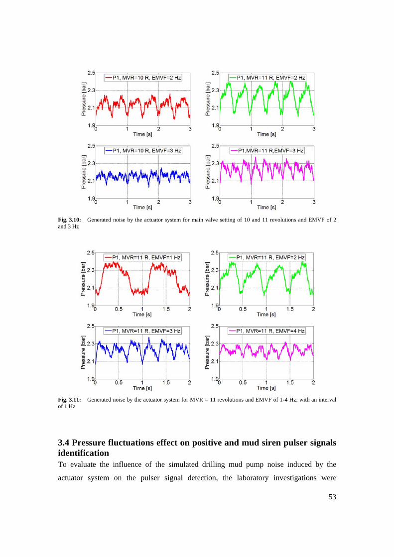
53

Fig. 3.10: Generated noise by the actuator system for main valve setting of 10 and 11 revolutions and EMVF of 2 and 3 Hz

Fig. 3.11: Generated noise by the actuator system for MVR = 11 revolutions and EMVF of 1-4 Hz, with an interval of 1 Hz

3.4 Pressure fluctuations effect on positive and mud siren pulser signals identification To evaluate the influence of the simulated drilling mud pump noise induced by the

actuator system on the pulser signal detection, the laboratory investigations were

54

performed for combinations of the actuator system with each pulser separately in the flow

loop. The positive pulser was installed to the flow loop. The flow rate of 35 m3/hr was

kept constant for the electromagnetic valve frequency set to zero regardless of the main

valve rotation from the open position. The positive pulser was programmed on the

computer to generate one pulse with 0.5 s duration, followed by two pulses with 2 and 3 s

duration. A second test was carried out but this time with the mud siren pulser in place.

The dominant frequency (F1) was set to 15 Hz and the mud siren was activated from the

computer. Hydraulic noise was not induced by the actuator system for both tests. The

Fast Fourier Transformation algorithm in MATLAB was used to transform the measured

signals from the time domain into the frequency domain. The measured pressure signals

at P1 are shown in figure 3.12 for both tests in both time and frequency domains. The

positive pulser signal can be clearly identified from the measured time domain signals

while the peak at 15 Hz in the frequency domain represents the mud siren signal.

Fig. 3.12: Three positive pulses with different durations and 15 Hz mud siren signal measured at P1 in both time and frequency domains

The experiments were repeated with the positive and mud siren pulser keeping their

induced signal the same but this time hydraulic noise with various amplitudes and

55

frequencies were induced to the flow loop by the actuator system. In the first series of

tests the noise frequency (electromagnetic valve frequency (EMVF)) was varied from 1

to 3 Hz while the noise amplitude was maintained constant. Figure 3.13 presents the

measured pressure signals at P1 in the time and frequency domain. The hydraulic noise

makes the detection of the positive pulser signal difficult, particularly the pulse with short

duration (0.5 s). The positive pulse with long duration, for instance 3 s, can still be

recognized as shown in figure 3.13.

Fig. 3.13: Influence of the actuator system noise with various frequencies (EMVF = 1 and 3 Hz) and constant amplitude on the laboratory positive and mud siren pulser signals

The positive pulser does not generate pulses with a specific frequency for carrying out the

information to the surface. Transforming the positive pulser signal from the time domain

into the frequency domain using FFT reveals only the actuator system noise. The peaks at

specified actuator system frequencies and their harmonics can be only seen in the

frequency domain. As opposed to the results of the positive pulser, the produced

continuous pulses by the mud siren can still be identified in the frequency domain as

peaks at 15 Hz even if the noise is induced in the flow loop, see figure 3.13.

The same experiments were repeated but this time the noise frequency was maintained

56

constant at 2Hz while its amplitude was increased. Figure 3.14 presents the measured

pressure signals at the pressure transducer P1 in the time and frequency domain. The

pulses produced by the mud siren can be identified even if the noise is induced in the

flow loop. This is because there is a clear difference between the continuous pressure

pulse frequency and the induced noise frequency. In practice however, high carrier

frequencies suffer significant attenuation on their way towards the surface (Hutin et al.,

2001). In contrast, interference with partial cancellation of the positive pulses occurred

with the presence of the noise. Thus the detection of the pulses generated by the positive

pulser becomes complex, especially when the noise amplitude increases and the noise

frequency gets closer to the pulse frequency.

Fig. 3.14: Influence of the actuator system noise with constant frequency (EMVF = 2 Hz) and various amplitudes on the laboratory positive and mud siren pulser signals

3.5 Carrier frequency selection In the previous section it has been depicted that with the mud siren, data can be

transmitted by shifting the carrier frequency to the less noisy frequency spectrum in order

to avoid interference with dominant noise frequencies in the transmission channel. Now

the question is whether all carrier frequencies which are not overlapping with noise

57

frequencies are suitable to be used and selected for delivering the data or not. This

question will be answered in this section. In the lab, it was observed that the continuous

pressure pulse amplitude measured at a fixed point was subjected to variation by

changing the carrier frequency of the mud siren. Figure 3.15 illustrates an example of the

mud siren signal measured at P1 for three different carrier frequencies 39, 51 and 60 Hz

in time domain (left).

Fig. 3.15: Measured pressure signals at P1 for different continuous pressure pulse frequencies (39, 51 and 60 Hz) generated by the laboratory mud siren pulser (left) in time domain for 0.5 s (right) in frequency domain for 10 s

The amplitudes of the continuous pressure pulses can clearly be seen in the time domain

for the carrier frequency 39 Hz but they get diminished when the carrier frequency is

shifted to 51 Hz. The amplitudes of the continuous pressure pulses appear again by

modifying the carrier frequency to 60 Hz. The measured time domain signals for those

three carrier frequencies were transformed by FFT into a frequency domain as shown in

figure 3.15 (right). The three peaks at 39, 51 and 60 Hz represent the three carrier

frequencies of the mud siren. The highest amplitude is at 39 Hz, it decreases at 51 Hz and

increases again at 60 Hz. This is because the continuous pressure waves generated by the

mud siren are reflected as they propagate in the entire setup of the flow loop at the

58

boundaries and the devices which are forming the flow loop. The main pressure wave

superimposes with its own reflections when they arrive at a particular location at the

exact same time. As a result, the wave amplitudes increase or decrease depending on the

relative phase interferences. The 39 and 60 Hz carrier frequencies can be considered as

good channel frequencies for the flow loop.

In practice, the pressure signals are measured at fixed points by a pressure transducer

attached to the standpipe at the surface. Selecting an optimum carrier frequency during

drilling operation for data transmission can be achieved by programming the downhole

mud siren pulser to generate continuous pressure pulses and increase the carrier

frequency gradually and step by step. On the surface, amplitude versus frequency

diagram can be generated from the measured pressure signal. Those carrier frequencies

(channel frequencies) which provide the clearest amplitude at the sensor and do not

overlap with the dominant noise frequencies in the drilling mud channel are

recommended to be selected for data transmission. However, it should be considered that

the drilling operation conditions for data transmission will vary with time. Thus the

process of selecting the optimum carrier frequency should be repeated each time the

continuous pressure pulse detection becomes difficult again. Thus an optimization of the

data transmission process during drilling operation can be achieved.

3.6 Noise cancellation It was noticed in the laboratory that in addition to the artificial hydraulic noise induced by

the actuator system, there is further “natural” noise included in the measured signal. The

uncertainty between the time averaged values and measured values of the pressure signal

is ±0.05 bar for all transducers and for the flow rate it is ±0.5 m3/hr. The noise can be

caused for instance by the pump, electronic devices, valves, turbulent flow, etc. Among

them, only the hydraulic noise generated by the centrifugal pump has a specific frequency

for each specific work condition. A MATLAB based algorithm was written and used to

perform the noise cancellation process (see the provided DVD). Figure 3.16 shows the

noise cancellation process of the measured pressure signals at P1 and P3 for an example

of the laboratory experiment using the mud siren. The individual steps of the process of

noise cancellation are:

59

(a) Use time domain pressure signals as measured in the laboratory at the transmitters

P1 and P3. In this example the mud siren is used to generate a constant carrier

frequency of 15 Hz.

(b) Transform time domain signals into frequency domain using a Fast Fourier

Transformation (FFT). The frequency range is shown up to 55 Hz. The peak at 15

Hz represents the mud siren carrier frequency.

(c) The amplitudes of the frequency bands of main interest (tolerance of ±1 Hz of the

specified actuator system frequency and ±2 Hz of the specified mud siren carrier

frequency) are retained the same while the amplitudes of all other frequency

bands are set to zero. These tolerances are fixed for all noise cancellation

processes in the whole research work.

(d) Apply the inverse Fast Fourier Transformation (IFFT) to the filtered signals in

order to transform them back into time domain.

Fig. 3.16: Noise cancellation process with the laboratory experimental example

60

It can be seen that the measured carrier frequency at P1 and P3 is extracted from the

surroundings noise and is made visible after the cancellation of the noise as shown in

figure 3.16d.

3.7 Application of transformation methods to experimental cases To evaluate the performance of the transformation methods for detection of the

continuous pressure pulses (carrier frequencies) and extraction of their characteristics,

series of experiments were carried out for combinations of the actuator system with the

mud siren pulser using amplitude and frequency shift keying modulations. The flow rate

was kept constant at 35 m3/hr for the main valve rotation 10.5 revolutions from the open

position and the electromagnetic valve frequency zero Hz (bypass valve closed). The Fast

Fourier Transformation (conventional method) and the continuous Morlet wavelet

transformation were applied to the measured pressure signals at P1.

3.7.1 Amplitude shift keying modulation

In this step a non-stationary signal was created by the mud siren pulser using amplitude

shift keying modulation (ASK). In this modulation a constant carrier frequency is used in

the fixed bit time while the amplitude is changed. Larger amplitude stands for a binary 1

and lower amplitude stands for a binary 0. A reverse definition is also possible. For the

laboratory experiments the dominant frequency (F1) was set to 40 Hz while the second

frequency (F2) was set to zero. The carrier frequency (F2) duration (length) was set to 1

s. Two tests were performed, one with the electromagnetic valve frequency set to 1 Hz

and other one set to 2 Hz. For each test F2 was initiated by the computer. Figure 3.17

shows the FFT of the measured pressure signals at P1 for 3 s for both tests. The peak at

40 Hz represents the mud siren signal and the peaks at 1 and 2 Hz represent the actuator

system frequencies. From figure 3.17 the duration and the discontinuity locations of the

carrier frequency cannot be determined. It is noticeable that the noise amplitude is many

times greater than that one of the continuous pressure pulses. The rotor position and the

pressure values at P1 after passing through the noise cancellation algorithm are shown in

figure 3.18 for 1 Hz induced noise by the actuator system and 40 Hz carrier frequency.

61

The corresponding scales to 1 and 40 Hz are 812 and 20 respectively. Although there is a

greater difference between the amplitude of the created hydraulic noise and the mud siren

pulses, the scalegram clearly illustrates the frequency components of the signal (the noise

plus the pulses), the durations of F1 and F2 and the discontinuity positions of the overlaid

40 Hz pressure waves created by the mud siren, see figure 3.18.

Fig. 3.17: FFT of 3 s measured pressure signal at P1 for the mud siren frequency = 40 Hz and EMVF equal to (a) 1 Hz (b) 2 Hz (flow rate =35 m3/hr, MVR=10.5 revolutions)

Fig. 3.18: Rotor position and the pressure signal at P1 after passing through the noise cancellation algorithm, the absolute CWT coefficients (scalegram) and the wavelet coefficients at the scales 812 and 20 (corresponding to 1 and 40 Hz respectively) (flow rate =35 m3/hr and MVR=10.5 revolutions)

The CWT coefficients of the signal at the scales 812 and 20 provide information about

the occurrence of the both frequencies (the noise and the pulses) in the time signal. It can

be seen from the scalegram and also from the coefficients at the scale 20 that there is a

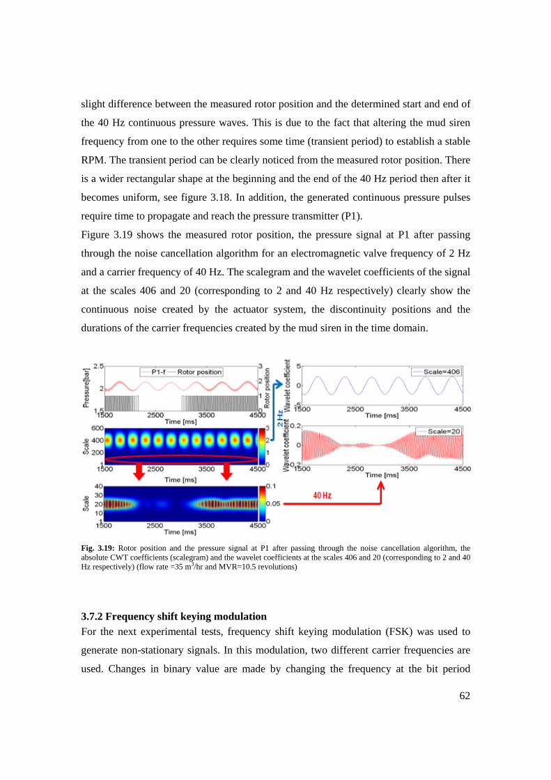
62

slight difference between the measured rotor position and the determined start and end of

the 40 Hz continuous pressure waves. This is due to the fact that altering the mud siren

frequency from one to the other requires some time (transient period) to establish a stable

RPM. The transient period can be clearly noticed from the measured rotor position. There

is a wider rectangular shape at the beginning and the end of the 40 Hz period then after it

becomes uniform, see figure 3.18. In addition, the generated continuous pressure pulses

require time to propagate and reach the pressure transmitter (P1).

Figure 3.19 shows the measured rotor position, the pressure signal at P1 after passing

through the noise cancellation algorithm for an electromagnetic valve frequency of 2 Hz

and a carrier frequency of 40 Hz. The scalegram and the wavelet coefficients of the signal

at the scales 406 and 20 (corresponding to 2 and 40 Hz respectively) clearly show the

continuous noise created by the actuator system, the discontinuity positions and the

durations of the carrier frequencies created by the mud siren in the time domain.

Fig. 3.19: Rotor position and the pressure signal at P1 after passing through the noise cancellation algorithm, the absolute CWT coefficients (scalegram) and the wavelet coefficients at the scales 406 and 20 (corresponding to 2 and 40 Hz respectively) (flow rate =35 m3/hr and MVR=10.5 revolutions)

3.7.2 Frequency shift keying modulation

For the next experimental tests, frequency shift keying modulation (FSK) was used to

generate non-stationary signals. In this modulation, two different carrier frequencies are

used. Changes in binary value are made by changing the frequency at the bit period

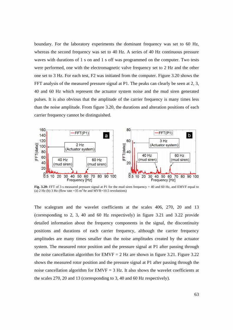
63

boundary. For the laboratory experiments the dominant frequency was set to 60 Hz,

whereas the second frequency was set to 40 Hz. A series of 40 Hz continuous pressure

waves with durations of 1 s on and 1 s off was programmed on the computer. Two tests

were performed, one with the electromagnetic valve frequency set to 2 Hz and the other

one set to 3 Hz. For each test, F2 was initiated from the computer. Figure 3.20 shows the

FFT analysis of the measured pressure signal at P1. The peaks can clearly be seen at 2, 3,

40 and 60 Hz which represent the actuator system noise and the mud siren generated

pulses. It is also obvious that the amplitude of the carrier frequency is many times less

than the noise amplitude. From figure 3.20, the durations and alteration positions of each

carrier frequency cannot be distinguished.

Fig. 3.20: FFT of 3 s measured pressure signal at P1 for the mud siren frequency = 40 and 60 Hz, and EMVF equal to (a) 2 Hz (b) 3 Hz (flow rate =35 m3/hr and MVR=10.5 revolutions)

The scalegram and the wavelet coefficients at the scales 406, 270, 20 and 13

(corresponding to 2, 3, 40 and 60 Hz respectively) in figure 3.21 and 3.22 provide

detailed information about the frequency components in the signal, the discontinuity

positions and durations of each carrier frequency, although the carrier frequency

amplitudes are many times smaller than the noise amplitudes created by the actuator

system. The measured rotor position and the pressure signal at P1 after passing through

the noise cancellation algorithm for EMVF = 2 Hz are shown in figure 3.21. Figure 3.22

shows the measured rotor position and the pressure signal at P1 after passing through the

noise cancellation algorithm for EMVF = 3 Hz. It also shows the wavelet coefficients at

the scales 270, 20 and 13 (corresponding to 3, 40 and 60 Hz respectively).

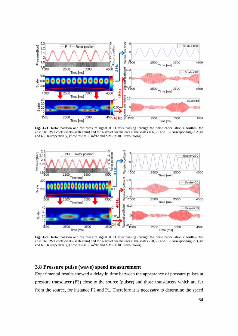
64

Fig. 3.21: Rotor position and the pressure signal at P1 after passing through the noise cancellation algorithm, the absolute CWT coefficients (scalegram) and the wavelet coefficients at the scales 406, 20 and 13 (corresponding to 2, 40 and 60 Hz respectively) (flow rate = 35 m3/hr and MVR = 10.5 revolutions)

Fig. 3.22: Rotor position and the pressure signal at P1 after passing through the noise cancellation algorithm, the absolute CWT coefficients (scalegram) and the wavelet coefficients at the scales 270, 20 and 13 (corresponding to 3, 40 and 60 Hz respectively) (flow rate = 35 m3/hr and MVR = 10.5 revolutions)

3.8 Pressure pulse (wave) speed measurement Experimental results showed a delay in time between the appearance of pressure pulses at

pressure transducer (P3) close to the source (pulser) and those transducers which are far

from the source, for instance P2 and P1. Therefore it is necessary to determine the speed

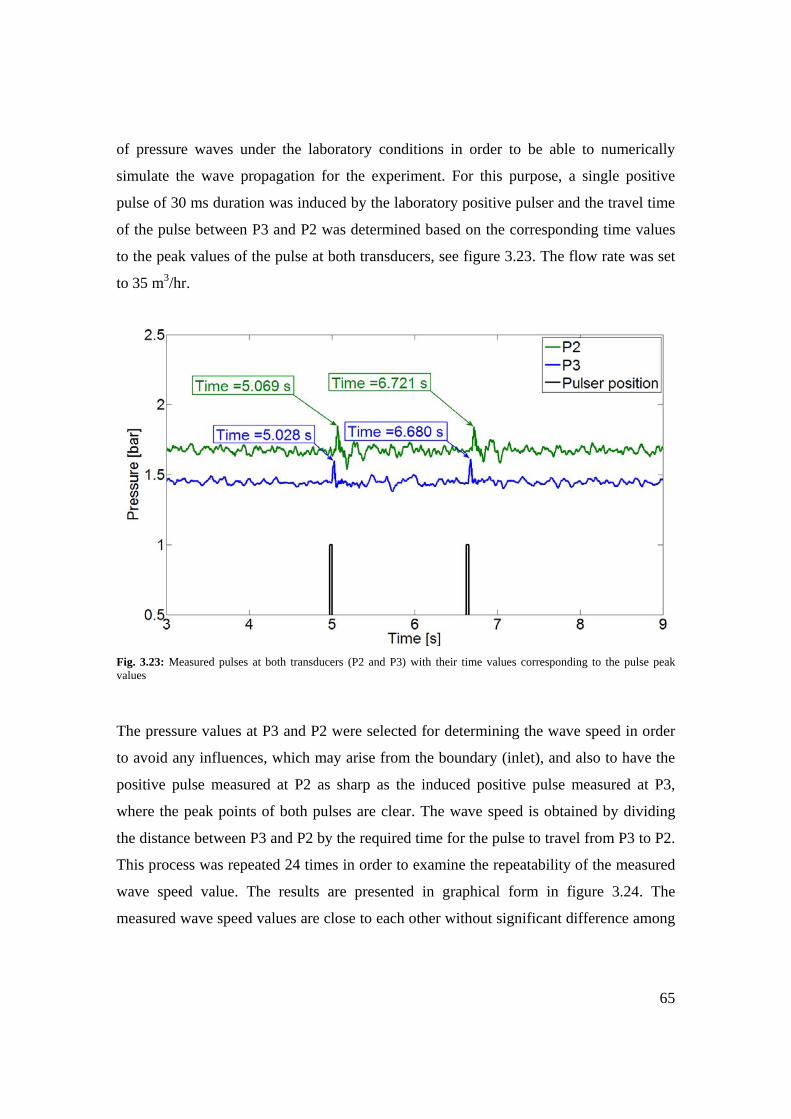
65

of pressure waves under the laboratory conditions in order to be able to numerically

simulate the wave propagation for the experiment. For this purpose, a single positive

pulse of 30 ms duration was induced by the laboratory positive pulser and the travel time

of the pulse between P3 and P2 was determined based on the corresponding time values

to the peak values of the pulse at both transducers, see figure 3.23. The flow rate was set

to 35 m3/hr.

Fig. 3.23: Measured pulses at both transducers (P2 and P3) with their time values corresponding to the pulse peak values

The pressure values at P3 and P2 were selected for determining the wave speed in order

to avoid any influences, which may arise from the boundary (inlet), and also to have the

positive pulse measured at P2 as sharp as the induced positive pulse measured at P3,

where the peak points of both pulses are clear. The wave speed is obtained by dividing

the distance between P3 and P2 by the required time for the pulse to travel from P3 to P2.

This process was repeated 24 times in order to examine the repeatability of the measured

wave speed value. The results are presented in graphical form in figure 3.24. The

measured wave speed values are close to each other without significant difference among

66

them. The standard deviation of the measured wave speed values is 10.778 m/s.

Therefore an average wave speed value, 462 m/s, was used in all numerical simulations.

Fig. 3.24: Measured wave (pulse) speed values

The theoretical value for the wave speed was also calculated from Equation [1] using the

parameters in Table 3.1. It results in a speed of 437 m/s.

Table 3.1: PVC pipe and water properties for calculating theoretically wave speed

Bulk

modulus of

elasticity

(water)**

[N/m2]

Inner pipe

diameter

[mm]

Wall

thickness

(pipe)

[mm]

Elasticity

Modulus

(PVC pipe)***

[N/m2]

Water

density**

[kg/m3]

Speed of

wave

[m/s]

2.03*109 57 3 4*109 998 437

** (Záruba, 1993), *** (Askeland, 1996)

The difference between the measured and calculated wave speed is not significant. This

leads to the conclusion of negligible influences of air bubbles in the water during the

67

experiments. The presence of air in the system significantly reduces the wave speed

because of its higher compressibility compared relative to water.

If the difference between the measured sound speeds under different system pressure or

difference between the measured and the theoretic sound speed is significant, it is

presumed that the fluid line contained air bubbles (Chatoorgoon and Li, 2009).

3.9 High speed photography for measuring the laboratory positive pulser movement The measured laboratory positive pulser movement as a function of time is required for

the numerical simulation and modeling of the pulser. Therefore a high speed camera was

employed to obtain a detailed movement of the laboratory positive pulser and to

determine the total required time for forward and backward movement of the pulser. For

this purpose, a high speed camera was used with a frame rate of 1000 frames/s. The

measurement process in the laboratory is illustrated in figure 3.25.

Fig. 3.25: The measurement process of the laboratory positive pulser movement using high speed camera

A single short pulse was induced using compressed air pressure of 9 bars for moving the

positive pulser and the images were recorded and saved on the computer. The starts and

68

ends of the pulser movement for forward and backward movement were determined by

displaying the images. The start time of the pulser movement for both forward and

backward strokes was considered as 0 s. Then the total movement of the pulser was

determined each time by displaying the next images till the complete stroke length of the

pulser was reached. Figure 3.26 shows the total laboratory positive pulser movement

versus time for two different flow rates for forward movement (figure 3.26a) and

backward movement (figure 3.26b). The measured total pulser movement as a function of

time is used in the numerical simulation of the laboratory positive pulser. The total time

required for the positive pulser to move 5 mm forward is 0.016 and 0.014 s for 35 and 30

m3/hr water flow rate respectively, while for the backward movement is 0.011 s for the

both flow rates.

Fig. 3.26: Total laboratory positive pulser movement versus time measured by a high speed camera for different flow rates using constant air pressure of 9 bars (a) Forward, (b) Backward

69

Chapter 4: Numerical simulation and modeling of positive pressure pulse propagation

4.1 Mathematical model A numerical simulation and modeling based on ANSYS CFX11 software was developed

to simulate the pressure wave propagation for the both laboratory pulsers (positive and

mud siren). ANSYS CFX11 is a computational fluid dynamics (CFD) program for

simulating the behavior of systems involving fluid flow, heat transfer and other related

physical processes. The set of equations which describe the processes of momentum, heat

and mass transfer are known as the Navier-Stockes equations. The set of equations solved

by ANSYS CFX11 are the unsteady Navier-Stockes equations in their conservation form.

The entire flow region of interest is divided into many small regions, called control

volumes. The equations are discretized and solved for each control volume. The solver is

based on the finite volume method.

The modeled system in the whole research work was considered isothermal, so the

energy equation does not need to be solved. The instantaneous equations of mass and

momentum conservation can be written in a stationary frame (manual ANSYS CFX11) as

follows

The continuity equation:

  · 0                                                                                  6

The momentum equations:

  . .                                            7

Where the stress tensor is related to the strain rate by

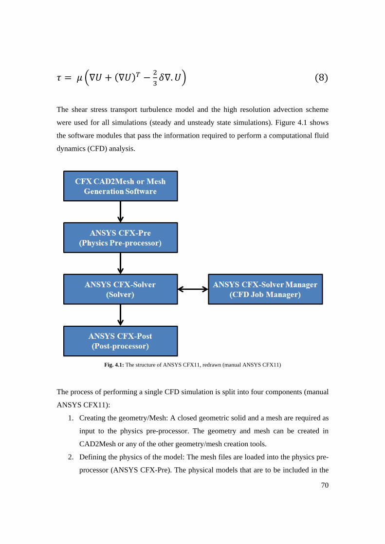
70

  .                                                           8

The shear stress transport turbulence model and the high resolution advection scheme

were used for all simulations (steady and unsteady state simulations). Figure 4.1 shows

the software modules that pass the information required to perform a computational fluid

dynamics (CFD) analysis.

Fig. 4.1: The structure of ANSYS CFX11, redrawn (manual ANSYS CFX11)

The process of performing a single CFD simulation is split into four components (manual

ANSYS CFX11):

1. Creating the geometry/Mesh: A closed geometric solid and a mesh are required as

input to the physics pre-processor. The geometry and mesh can be created in

CAD2Mesh or any of the other geometry/mesh creation tools.

2. Defining the physics of the model: The mesh files are loaded into the physics pre-

processor (ANSYS CFX-Pre). The physical models that are to be included in the

71

simulation are selected. Flow physics, boundary conditions, initial values and

solver parameters are specified.

3. Solving the CFD problem: The component that solves the CFD problem is called

the solver (ANSYS CFX-Solver). It solves all the solution variables for the

simulation for the problem specification generated in ANSYS CFX-Pre and

produces the required results in a non-interactive process.

4. Visualizing the results in the post processor: The post-processor (ANSYS CFX-

Post) is the component used to analyze, visualize and present the results

interactively.

4.2 Fluid compressibility The fluid used in the lab is water. For some applications the water compressibility may

not play an important role; therefore it may be ignored. But for wave propagation

phenomena in water it is necessary to include the compressibility in the calculation.

Hydraulic compressibility effects can properly be taken into account by the compressible

CFD based on Navier-Stokes equations for weakly compressible fluids, incorporating the

equation of state for water for defining the density (Ismaier and Schlücker, 2009; Yan et

al., 2008).

                                                                                9

The measured average wave speed value (462 m/s) was used in the above equation for all

numerical simulations.

4.3 Hydrostatic pressure modeling In order to include the hydrostatic pressure of the vertical section of the laboratory

experiment in the calculations it was necessary to turn on the gravitational acceleration

and define it in magnitude and direction. The gravity magnitude in the x and y-axes was

72

defined as zero while in z axis it was defined as 9.8 m/s2. The hydrostatic pressure

contribution will be included in the variable called absolute pressure.

4.4 Geometry and mesh generation The computational geometry and the grid generation were prepared using ANSYS ICEM

CFD. The geometry of the modeled domain was defined to be from the discharge of the

pump to the pressure transducer P4. A structured hexahedral 3D mesh was used. The total

number of elements for the modeled domain is 425,853. This is named fine mesh case in

the mesh sensitivity analysis section. The modeled domain was divided into two parts,

the flow loop section domain and the positive pulser section domain (the same

dimensions as the pulser section including the laboratory positive pulser which has been

previously described). The laboratory positive pulser was modeled as an empty domain.

Figure 4.2 shows the cross section and mesh of the modeled positive pulser section

domain including the laboratory positive pulser.

Fig. 4.2: Cross section of the modeled positive pulser section domain including the positive pulser by ANSYS CFX11

The extension of the flow loop in three axes and their lengths, elbows and different pipe

sections ahead of the pulser section with their diameters were treated similarly to that in

the experiment as shown in figure 4.3. In regions where the flow circulates or experiences

large gradients, a finer grid was used. These regions include the joints, elbows, pipe

73

walls, boundaries and the close area around the pulser. Figure 4.4 shows the mesh close

to the pipe wall for different pipe diameters used in the flow loop.

Fig. 4.3: (a) Modeled two different pipe diameters a head of the pulser section by ANSYS CFX11, (b) modeled elbow by ANSYS CFX11

Fig. 4.4: Cross section of the flow loop section domain shows mesh close to the pipe wall for different diameters modeled by ANSYS CFX11

4.5 Boundary conditions A no slip boundary condition was used at the pipe walls. The positive pulser wall

(including the moving parts and the double acting pneumatic cylinder wall) was also

defined as a no slip wall condition. The moving part wall velocity of the pulser was

74

realized as a velocity relative to the mesh motion. The pulser section domain is connected

to the flow loop section domain via a general connection interface model, see figure 4.5.

Fig. 4.5: Modeled positive pulser section domain in 3D with boundary conditions by ANSYS CFX11

4.5.1 Inlet boundary condition

In steady state simulations, the inlet boundary condition was specified as a constant mass

rate, which was taken as a time averaged value of the measured flow rate, while it was

turned to a time dependent total pressure in unsteady state simulations. Moreover, the

acoustic reflectivity was activated for all simulations.

4.5.2 Outlet boundary condition

In steady state simulations, the outlet boundary condition was specified as opening

constant pressure, which was taken as time averaged value of the measured pressure at

P4, whereas it was defined as a time dependent opening pressure boundary condition for

unsteady state simulations. Moreover, the acoustic reflectivity was activated for all

simulations.

4.5.3 Modeling of pump effect (time dependent boundary conditions)

In the laboratory, a centrifugal pump is used. The characteristics of a centrifugal pump

together with a pipe system are shown in figure 4.6 for an open and a restricted flow area

(represented by points 1 and 2 respectively). Accordingly they represent both cases where

75

the flow area is not restricted and restricted by the laboratory positive pulser respectively.

The increased pressure (pulse induced, point 2) by shifting of the system curve will be

accompanied by a decrease in the flow rate. Point 1 is reached again when the pulser is

moved back to its original position (pulse is not induced). In order to take this inevitable

pump effect in the numerical simulation and modeling of positive pressure pulse

propagation into account, two steady state simulations were carried out prior to unsteady

state simulations for two cases (open and restricted flow area). Furthermore, the total

inlet pressure values were calculated. In the unsteady state simulations the inlet boundary

condition values were shifted between the two calculated total pressure values in steady

state simulations, each time when the pulser was moved, taken into account the travel

time for the pulse to propagate from the pulser to the pump. Such a boundary condition is

called a time dependent boundary condition. The total time required for the inlet

boundary condition to shift between those two values for forward and backward

movement of the pulser equals to the measured total time required for the positive pulser

to move 5 mm forward and backward respectively.

Fig. 4.6: Pump and system curves for open and restricted flow area by a valve (inlet boundary condition characteristic)

In unsteady state simulations, the outlet boundary condition values were also shifted

between the two measured time averaged pressure values at P4 for the two cases (open

76

and restricted flow area), taking the transient periods after the pulser movement into

consideration. The transient periods were determined to last from the starting time of the

pulser movement till reaching the time averaged value for P4. The measured pressure

values in the laboratory were used for the transient periods.

4.6 Modeling mesh movement The positive pulser section domain was also divided into two domains, a positive pulser

section stationary domain and a positive pulser section rotating domain. The angular

velocity for the rotating domain was set to zero radian/s for all simulations. A frozen

Rotor-Stator interface was used between the rotating and stationary domains for steady

state simulations while a transient Rotor-Stator interface was used for unsteady

simulations, see figure 4.7.

Fig. 4.7: Modeled positive pulser section rotating domain with defined interfaces, mesh deformation and subdomains by ANSYS CFX11

The rotating domain was also divided into three subdomains named front, middle and

back subdomain. The rotating domain is 1 mm larger in diameter than the moving part of

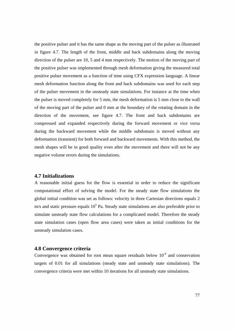
77

the positive pulser and it has the same shape as the moving part of the pulser as illustrated

in figure 4.7. The length of the front, middle and back subdomains along the moving

direction of the pulser are 10, 5 and 4 mm respectively. The motion of the moving part of

the positive pulser was implemented through mesh deformation giving the measured total

positive pulser movement as a function of time using CFX expression language. A linear

mesh deformation function along the front and back subdomains was used for each step

of the pulser movement in the unsteady state simulations. For instance at the time when

the pulser is moved completely for 5 mm, the mesh deformation is 5 mm close to the wall

of the moving part of the pulser and 0 mm at the boundary of the rotating domain in the

direction of the movement, see figure 4.7. The front and back subdomains are

compressed and expanded respectively during the forward movement or vice versa

during the backward movement while the middle subdomain is moved without any

deformation (transient) for both forward and backward movements. With this method, the

mesh shapes will be in good quality even after the movement and there will not be any

negative volume errors during the simulations.

4.7 Initializations A reasonable initial guess for the flow is essential in order to reduce the significant

computational effort of solving the model. For the steady state flow simulations the

global initial condition was set as follows: velocity in three Cartesian directions equals 2

m/s and static pressure equals 105 Pa. Steady state simulations are also preferable prior to

simulate unsteady state flow calculations for a complicated model. Therefore the steady

state simulation cases (open flow area cases) were taken as initial conditions for the

unsteady simulation cases.

4.8 Convergence criteria Convergence was obtained for root mean square residuals below 10-4 and conservation

targets of 0.01 for all simulations (steady state and unsteady state simulations). The

convergence criteria were met within 10 iterations for all unsteady state simulations.

78

4.9 Mesh sensitivity study The density of elements plays an important role in numerical simulations. Therefore the

total number of elements in the computational domain was increased using four different

mesh sizes, named coarse, medium, fine and very fine mesh in order to ensure that the

obtained results are mesh independent. The total number of elements for each case is

tabulated in Table 4.1. The percentage of the increased total number of elements with

respect to the previous case is greater than 30% for each step. For the two steady state

simulations, the inlet flow rates were set to 35 and 33.434 m3/hr for the open and

restricted flow area respectively. Accordingly, the outlet pressure values were set to

1.123 and 1.019 bar.

Table 4.1: Total number of elements for different cases (mesh sizes) used for mesh sensitivity study for the positive pulser

Cases (mesh size) Coarse Medium Fine Very fine

Total number of elements 211149 289989 425853 571167

In unsteady state simulations, two pulses with durations of 0.8 s were numerically

generated. The time step size for all unsteady state simulations was fixed to 0.001 s

which is equal to the laboratory experiments time step size. The pressure values at four

monitor points (corresponding to the four pressure transducer locations) and the inlet

flow rate values were computed and compared with each other. The predicted positive

pressure pulses are presented graphically in figure 4.8 for the four different mesh sizes.

Furthermore, figure 4.8 includes the predicted total mesh displacement (corresponds to

the total positive pulser movements) at the adjacent element to the moving part of the

pulser. The mesh and the model for different cases are available in the provided DVD.

The differences between the predicted pulses at the four different locations and the inlet

flow rates for different cases (mesh sizes) are not significant, particularly fine and very

fine meshes do not present major differences. Therefore the fine mesh case was selected

for the rest of the numerical simulations and for the validation with the laboratory

experimental results.

79

Fig. 4.8: Comparison of predicted positive pressure pulses and the inlet flow rate values by the model for different mesh sizes

4.10 Validation For the validation purpose, three examples were considered, positive pressure pulses with

constant durations for two different flow rates and positive pressure pulses with various

durations. The laboratory positive pulser was combined with the flow loop. The flow rate

was set to 35 m3/hr (open flow area case). The experiments were conducted for the two

steady state cases (open and restricted flow area), and the flow rate and pressure values

were measured. The sampling rate was 1000 Hz for all the experimental runs. Both cases

were also numerically simulated using ANSYS CFX11 and the pressure values at four

80

monitor points (correspond to the four pressure transducer locations) and the flow rate

values at the inlet boundary were computed. The results are tabulated in Table 4.2.

Table 4.2: The calculated and measured pressure and flow rate values for both steady state cases (open and restricted flow area) for the positive pulser (flow rate = 35 m3/hr)

Lab

[m3/hr]

Total pressure

inlet

[bar]

[bar]

[bar]

[bar]

[bar]

Open flow

area

35

-

2.106

1.705

1.457

1.123

Restricted

flow area

33.434

-

2.263

1.895

1.665

1.019

ANSYS

CFX11

Flow

rate

[m3/hr]

CFX total

pressure inlet

[bar]

CFXP1

[bar]

CFXP2

[bar]

CFXP3

[bar]

CFXP4

[bar]

Open flow

area

35

2.233

2

1.65

1.397

1.123

Restricted

flow area

33.434

2.355

2.141

1.822

1.59

1.019

In the next step, a series of three pulses with constant duration of 0.8 s was programmed

on the computer in the laboratory and the experiment was carried out. The first pulse

started after 0.8 s. This process was also numerically simulated. A time step size of 0.001

s which is equal to that one used in the laboratory was set for all unsteady state

simulations. In order to compare the pressure fluctuations generated by the positive

pulser movement, the measured and computed steady state pressure values for the open

flow area case, as provided in table 4.2, were subtracted from the measured and

calculated time history unsteady state pressure values for each pressure transmitter and

monitor point respectively. This procedure is named PD. The pressure values in unsteady

81

simulations were computed at the four monitor points and compared with pressure signals

measured at the four transducers in the laboratory. The results are presented in figure 4.9.

Furthermore, figure 4.9 includes the predicted and measured flow rate values at the inlet.

The total pulser movement was also predicted by calculating the total mesh displacement

at an adjacent element to the moving part of the pulser, see figure 4.9. Good agreement

can be seen between the measured and the predicted results for the pressure pulses at the

different locations and also for the flow rate values at the inlet boundary. The possible

reasons for the slight differences between the measured and numerically obtained results

are the noise in the system, the accuracy of the measurement tools (which is ±0.25%), the

model and used grid.

Fig. 4.9: Comparison of the model (ANSYS CFX11) results with the measured positive pressure pulses (flow rate = 35 m3/hr, constant pulse durations)

82

Figure 4.10 illustrates the total mesh displacement magnitude (left) and the mesh

deformation (right) on a plane before the pulser movement at time equal to 0.8 s (upper)

and after the complete 5 mm movement of the pulser at time equal to 0.816 s (lower). It

can be seen that even after the complete 5 mm movement of the pulser, the mesh shapes

are still in good quality.

Fig. 4.10: Total mesh displacement magnitude on a plane (left), mesh shapes and distribution (right), (a) before the movement of the positive pulser (time = 0.8 s), (b) after complete 5 mm movement of the positive pulser (time = 0.816 s), (flow rate = 35 m3/hr, constant pulses durations)

Figure 4.11 shows the pressure magnitude on a plane with the positive pulser for two

cases where the flow area is not restricted (time = 0.8 s) and restricted (time = 1.59 s) by

the pulser. Clearly, it can be observed that the pressure increases when the pulser moves

and restricts the flow area. The second experiment was performed keeping the flow rate

of 35 m3/hr for the open flow area case while the induced positive pulses durations were

changed. Three pulses with durations of 0.5, 1, 1.5 s were generated. The first pulse

started after 0.8 s. Figure 4.12 shows the predicted time histories values of the inlet flow

rate, the total mesh displacement and the pressure at the four monitor points of the

simulated positive pressure pulses. In addition, it shows the measured pressure signals at

the four transducers and the flow rate values.

83

Fig. 4.11: Pressure magnitude on a plane when the flow area is not restricted (a) and restricted (b) by the positive pulser (flow rate = 35 m3/hr, constant pulses durations)

Fig. 4.12: Comparison of the model (ANSYS CFX11) results with the measured positive pressure pulses (flow rate = 35 m3/hr, various pulse durations)

84

The third experiment was carried out by changing the flow rate this time to 30 m3/hr for

the open flow area case. Table 4.3 shows the experimental and numerical results for two

steady state cases (open and restricted flow area).

Table 4.3: Calculated and measured pressure and flow rate values for both steady state cases (open and restricted flow area) for the positive pulser (flow rate = 30 m3/hr)

Lab

[m3/hr]

Total pressure

inlet

[bar]

[bar]

[bar]

[bar]

[bar]

Open flow

area

29.907

-

1.523

1.223

1.035

0.792

Restricted

flow area

28.602

-

1.635

1.36

1.186

0.713

ANSYS

CFX11

Flow

rate

[m3/hr]

CFX total

pressure inlet

[bar]

CFXP1

[bar]

CFXP2

[bar]

CFXP3

[bar]

CFXP4

[bar]

Open flow

area

29.907

1.616

1.444

1.184

0.992

0.792

Restricted

flow area

28.602

1.706

1.547

1.308

1.13

0.713

The experiment was conducted for generating a series of three pulses with constant

durations of 0.8 s. This unsteady state process was also simulated using ANSYS CFX11

and the pressure, the flow rate and the total mesh displacement values were calculated.

Figure 4.13 presents the time history of the experimental and numerical results including

the pressure values at four different locations along the flow loop, the flow rate values

and the predicted total pulser movement values. This good accordance between the

measured and calculated results confirms the CFD model capability to model realistic

pressure pulses.

85

Fig. 4.13: Comparison of the model (ANSYS CFX11) results with the measured positive pressure pulses (flow rate = 30 m3/hr, constant pulse durations)

86

Chapter 5: Numerical simulation and modeling of continuous pressure pulse propagation

5.1 Mathematical model The same mathematical model which has been previously described for the laboratory

positive pulser is also valid for the numerical simulation and modeling of continuous

pressure pulses propagation generated by the laboratory mud siren pulser. Moreover, the

shear stress transport turbulence model, the high resolution advection scheme, fluid

compressibility and hydrostatic pressure modeling were also maintained the same for all

simulations (steady and unsteady state simulations) of continuous pressure pulse

propagation.

5.2 Geometry and mesh generation The only difference with the previous computational geometry which has been presented

for the laboratory positive pulser is the pulser section domain. The modeled domain was

divided into two parts, the flow loop section domain and the pulser section domain (the

same dimensions as the laboratory mud siren pulser section including the mud siren

pulser which has been previously described).

The mud siren pulser was modeled as an empty domain. ANSYS ICEM CFD was used to

prepare the computational geometry and to generate a structured hexahedral 3D mesh.

The total number of elements for the modeled domain is 416,088 (named fine mesh case

in the mesh sensitivity study).

5.3 Boundary conditions The pipeline wall and the mud siren pulser components including the stator and the rotor

plates and the electrical motor were defined as a no slip wall condition. The pulser

section domain is connected to the flow loop section domain via a general connection

interface model, see figure 5.1.

87

Fig. 5.1: Modeled mud siren pulser section domain in 3D with boundary conditions by ANSYS CFX11

5.3.1 Inlet boundary condition

The inlet boundary condition was specified as a constant mass rate in steady state

simulations while it was turned to constant total pressure in unsteady state simulations.

Moreover, the acoustic reflectivity was activated for the inlet boundary for all

simulations. The time averaged value of the measured flow rate was set for the inlet

boundary condition for all steady state simulations.

5.3.2 Outlet boundary condition

The outlet boundary condition was specified as an opening constant pressure in steady

state simulations; whereas it was defined as an opening constant Cartesian velocity

components boundary condition for unsteady state simulations. The acoustic reflectivity

was activated for the outlet boundary for all simulations. The time averaged value of the

measured pressure P4 was set for the outlet boundary condition for all steady state

simulations.

5.4 Modeling of rotor plate rotation The modeled mud siren pulser section domain was also divided into two domains, a mud

siren pulser stationary domain (including the mud siren stator plate) and a mud siren

pulser rotating domain (including the mud siren rotor plate). An interface between the

two domains is needed. All steady state simulations were performed using a frozen

88

Rotor-Stator interface between the two domains and zero radian/s angular velocity for the

rotating domain while a transient Rotor-Stator interface was used between them for

unsteady state simulations, see figure 5.2. The angular velocity for the rotating domain in

each unsteady state simulation was set to a specific value based on the modeled mud

siren carrier frequency.

Fig. 5.2: Modeled mud siren pulser rotating and stationary domains with defined interfaces

5.5 Initializations For the steady state flow simulations, the same global initial conditions as that one used

for the steady state simulations and modeling of the positive pulser were set. For instance

velocity in three Cartesian directions equals 2 m/s and static pressure equals 105 Pa. The

steady state simulations with a frozen Rotor-Stator interface between the mud siren pulser

stationary and rotating domains were taken as initial conditions for the unsteady state

simulations.

5.6 Convergence criteria For the numerical simulations and modeling of continuous pressure pulse propagation,

convergence was obtained for root mean square residuals below 10-4 and conservation

targets of 0.01 for all simulations. The convergence criteria were met within 10 iterations

for all unsteady state simulations.

89

5.7 Mesh sensitivity study Although the mesh sensitivity study was previously made for the simulation and

modeling of the positive pulse propagation, here the study is repeated for the mud siren

signal propagation in order to ensure further that the results are grid independent. The

mesh sensitivity results are shown in figure 5.3 in the frequency domain for different

mesh sizes named coarse, medium and fine. The total number of elements for each mesh

size is provided in Table 5.1. Continuous pressure pulses (carrier frequency of 39 Hz)

were considered for the mesh sensitivity study.

Table 5.1: Total number of elements for different cases (mesh sizes) used for mesh sensitivity study for the mud siren pulser

Cases (mesh size) Coarse Medium Fine

Total number of elements 231732 280080 416088

Fig. 5.3: Predicted continuous pressure pulses (39 Hz carrier frequency) for different mesh sizes in frequency domain for 1.5 s time signal

The inlet flow rate was set to 35.513 m3/hr and the outlet pressure was set to 1.122 bars

for steady state simulations. The same time step size (0.001 s) of the laboratory

experiment was used for all unsteady state simulations. The calculated time history

pressure signals at four monitor points (corresponding to the four pressure transmitter

90

locations) for different mesh sizes were analyzed in the frequency domain using the Fast

Fourier Transformation code in MATLAB and compared against each other, see figure

5.3. Although the results of different mesh sizes do not show great changes, the rest of

the simulations was performed using the fine mesh case. The mesh and the model for

different cases can be found in the provided DVD.

5.8 Validation A model validation was performed by comparing the experimental pressure

measurements at the four different locations along the flow loop with the results obtained

from the numerical simulations for three different rotor rotational speeds (three different

carrier frequencies). The measured time averaged flow rate value was 35.513 m3/hr. The

computed and measured pressure and flow rate values for the steady state case are

tabulated in Table 5.2.

Table 5.2: The calculated and measured pressure and flow rate values for steady state case for the mud siren pulser

Case

[m3/hr]

Total pressure

inlet

[bar]

[bar]

[bar]

[bar]

[bar]

Lab 35.513 - 1.952 1.528 1.293 1.122

Flow rate

[m3/hr]

CFX total

pressure inlet

[bar]

CFXP1

[bar]

CFXP2

[bar]

CFXP3

[bar]

CFXP4

[bar]

ANSYS

CFX11

35.513

2.115

1.878

1.522

1.264

1.122

The computed Cartesian velocity components (u, v, w) values at the outlet boundary

condition in the steady state simulation are 0, 3.88, and 0 m/s respectively. Those values

were set at the outlet boundary condition in all unsteady state simulations.

For unsteady state simulation cases, the same time step (0.001 s) as the one in the lab was

used. The total simulated time was set to 3 s corresponding to approximately 18 round

91

trips for the pressure wave propagation from the mud siren pulser side to the pump and

back again. A MATLAB code was developed for the frequency analysis of the pressure

signals obtained from the simulations and measured from the experiments. The pressure

values of the last 1.5 s were used to plot time histories and to perform Fast Fourier

Transformations of the computed time domain continuous pressure pulses. Figure 5.4

shows the pressure magnitude on a plane with the modeled mud siren pulser for three

different rotor plate positions, (a) the pressure value ahead of the pulser is at its minimum

value (the rotor and stator open spaces are on the same line), (b) the open spaces of the

stator plate are partially closed by the massive part of the rotor plate and (c) the pressure

value ahead of the pulser is at its maximum value (the massive part of the rotor plate

closes completely the open spaces of the stator plate). It can clearly be observed that the

pressure increases ahead of the pulser when the open spaces of the stator plate are closed

by the massive part of the rotor plate.

Fig. 5.4: Pressure magnitude on a plane with the modeled mud siren pulser when the open spaces of the stator plate is (a) completely open (b) partially closed and (c) completely closed

The PD values were also computed by subtracting the steady state pressure values from

the measured and the calculated time history unsteady state pressure values for each

pressure transmitter and monitor point respectively in order to compare the pressure

fluctuations generated by the mud siren. For the lab the time averaged pressure values

were taken to be the steady state pressure values while for numerical simulations the

pressure values of the steady state simulation were used as provided in Table 5.2. Figure

5.5 shows the measured and ANSYS CFX11 predicted results of pressure values for 60

Hz carrier frequency at four different locations along the flow loop in the time domain.

92

The simulation results are also analyzed in the frequency domain and compared against

the lab results, see figure 5.6.

Fig. 5.5: The model results and the measured continuous pressure pulses for 60 Hz carrier frequency

Fig. 5.6: The model results and the measured continuous pressure pulses for 60 Hz carrier frequency in frequency domain for 1.5 s time signal

93

Good agreement is achieved between the measured and predicted values for all four

pressure transducers. Furthermore, the harmonic frequency at 120 Hz can also be

captured in a good way as shown in figure 5.6. The measured and estimated continuous

pressure waves for carrier frequencies of 51 and 39 Hz at four different locations are

shown in figure 5.7 and figure 5.8 respectively. For both 60 and 39 Hz carrier frequencies

clear pressure pulse amplitudes can be observed at P1 for both measured and obtained

model results. Both carrier frequencies can be considered as good channel frequencies for

data transmission in the flow loop. In contrast, the 51 Hz carrier frequency is not a

suitable channel frequency for data transmission in the flow loop because the pulse

amplitudes do not clearly appear at P1. This happens because the reflected continuous

pressure waves from the boundary sides overlap with the main continuous waves coming

from the mud siren when they arrive at a particular location at the same instant.

Depending on the relative phase relationship constructive or destructive interferences will

take place. This will lead to a clear continuous pressure pulse amplitude appearance at

some specific locations in the flow loop while smaller or may be even no pulse

amplitudes will be found at some other locations depending on the carrier frequency.

With altering the carrier frequency the locations of clear continuous pressure pulse

amplitudes will change.

The presented results confirm the suitability of the numerical model to provide a good

estimation of the mud siren pulser signal propagation along the pipeline at any desired

position. Moreover, the presented simulations highlight the practicability of employing

this model to improve the available mud pulse telemetry by studying any design

modifications or studying the effect of any parameter in opposition to the lengthy and

costly alternative of assembling and running real test. The slight discrepancies between

the measured and the numerically obtained results can be related to the noise in the

system, the measurement accuracy of the pressure sensors (which is ±0.25%), inconstant

rotation of the rotor (tolerance of ±1 Hz) of the set mud siren frequency in the

experiments, the model and the used grid. Furthermore, the inconstant rotation of the mud

siren rotor also leads to slight deviations in phase between the predicted continuous

pressure waves by the ANSYS CFX11 and the experimental observations.

94

Fig. 5.7: The model results and the measured continuous pressure pulses for 51 Hz carrier frequency

Fig. 5.8: The model results and the measured continuous pressure pulses for 39 Hz carrier frequency

95

Chapter 6: Conclusions and future works

6.1 Conclusions Data transmission from downhole to the surface in boreholes while drilling is a very

important issue, directly related to the formation evaluation, the ability to drill more

complex well paths and the drilling optimization and safety. The most commonly used

method for data transmission is by means of coded hydraulic pressure pulses. But till

2008, data transmission was not practically included in the lectures at the TU

Bergakademie Freiberg and even hardly any specific laboratory setup for studying and

clarifying the mechanisms of hydraulic data transmission in boreholes could be found in

the literature.

In frame of this thesis, a laboratory experimental setup was successfully designed and

built up to investigate the process of data transmission in boreholes by using mud pulse

telemetry. A positive mud pulser and a mud siren pulser are used to generate different

kinds of common mud pulses. These pulses were observed as they travelled through the

pipe system. Adjustable induced hydraulic noise with regard to amplitude and frequency

(typical piston pump pressure characteristics) was induced from a special “actuator

system” to simulate a wide range of operating conditions for the data transmission.

Moreover, a theoretical model using ANSYS CFX11 (computational fluid dynamic

(CFD) commercial code) was successfully developed to simulate all effects observed on

the flow loop. Furthermore, a novel approach which uses a continuous Morlet wavelet

transformation was developed and tested to detect the carrier frequencies generated by

the mud siren and to identify their characteristics in the time domain for a better

decoding. The laboratory experimental data were used to calibrate the developed

numerical model and to prove the effectiveness of the continuous wavelet method.

According to the available literature, a similar experimental setup including a positive

and a mud siren pulser with variable noise patterns for studying the data transmission

process has not been used anywhere else in research facilities. In addition, this laboratory

experiment with great capabilities of simulating all relevant aspects of hydraulic data

transmission offers the opportunity to be used for testing and evaluating new data

transmission concepts in order to develop an innovative data transmission system.

96

Since 2008 this flow loop supports the teaching work at the institute. TU Bergakademie

Freiberg is now the only university which offers students practical work on data

transmission in boreholes by mud pulse telemetry systems. In addition, from 2008 to

2012 several research works in form of student, project and diploma were made on the

flow loop with tasks including designing and building up a mud siren and a noise inducer,

making the measured pressure signals audible, and designing and constructing of a novel

pulser which is also recommend for future work.

Laboratory experimental tests were carried out and the mechanisms of pressure pulse

propagation in the flowing fluid inside pipes, generated by both positive and mud siren

pulsers, were studied and clarified in details. The experimental results confirmed that

unlike the positive pulser in the presence of the induced noise, the signals of the mud

siren can be detected best by shifting the signal energy in a part of the frequency

spectrum with the lowest hydraulic noise. Nevertheless it was found that not all generated

mud siren carrier frequencies which are not overlapping with the noise frequencies can be

considered as good channel frequencies (or optimum carrier frequencies) for data

transmission in the flow loop, as in the flow loop, there are carrier frequencies which do

not clearly appear at the receiver end. However, it should be considered that this clear

appearance and disappearance of certain carrier frequencies which have been presented in

this thesis are only valid for this particular flow loop. This finding suggests that for real

drilling operations those carrier frequencies which provide sufficient amplitude at the

receiver and do not overlap with noise frequencies existing in the transmission channel

can be considered as optimum carrier frequencies and can be selected and used for a safer

and an optimum data transmission process in the system. In practice the data transmission

channel conditions are variable; therefore the process of selecting optimum carrier

frequencies should be repeated each time when the continuous pressure pulses are no

longer obvious at the receiver.

A method utilizing the continuous wavelet transformation (CWT) was devised to detect

and decode the carrier frequencies generated by the mud siren. A MATLAB program was

developed to perform the process of wavelet transformation. The collected laboratory

data which simulate various drilling operation conditions for data transmission in

boreholes were used to verify the effectiveness of the method. The results showed that

97

the carrier frequencies and their characteristics (discontinuity positions and durations) for

commonly used data transmission modulations by the mud siren telemetry can

successfully be identified and determined by the continuous Morlet wavelet

transformation, although the continuous pressure pulses were contaminated by the noise

of the actuator system and their amplitudes were smaller than the induced noise

amplitudes. A good agreement is obtained between the laboratory measurement and the

CWT determination of the carrier frequency durations and discontinuity positions. Thus

with the CWT, the received continuous pressure pulses can be better decoded compared

to the conventional method (Fourier transformation). Furthermore, the wavelet

transformation offers a smart graphical presentation of the continuous mud pulse signal in

two dimensions (time-scale or time-frequency) for visual inspection. This method can

contribute to the possibility of transmitting data at higher rates and over longer distances.

Based on the literature study, it can be assumed that the developed model utilizing

ANSYS CFX11 is a new approach for simulating and modeling the mud pulse telemetry

signal propagation. The comparison of the model predictions against the experimental

results for positive pressure pulse propagation in the fluid inside the flow loop with

various flow rates and pulse durations showed the capability of the simulation algorithms

to model realistic positive pressure pulses.

A numerical simulation and modeling of continuous pressure pulses propagation

generated by the mud siren pulser using ANSYS CFX11 was also presented and

compared with the experimental observations of the laboratory mud siren signal at four

different locations along the pipeline. The measured and obtained signals were analyzed

and compared in both time and frequency domains. A MATLAB program was developed

to transform the signal from the time domain into the frequency domain. The

Computational Fluid Dynamic code also proved to be an appropriate platform to

successfully model the mud siren signal propagation as expressed by the reasonably good

agreement found between the numerical and the experimental results for different carrier

frequencies. The harmonic and channel frequencies were also very well predicted by the

model.

The significance of this model is that it can be used to study any pulser design

modifications and operational conditions in order to improve the existing mud pulse

98

telemetry systems and develop and design novel mud pulse telemetry systems for

transmitting data at higher rates and over longer distances before attempting time and

cost consuming measurements in a real scenario. With this computational model, the

dynamic transmission behavior of positive and continuous pressure pulses can easily be

examined at any desired position along the flow loop. Furthermore, the model is flexible

in terms of type of fluids and allows simulating various drilling tool operation functions

as input in order to study their generated pressure fluctuations (noise) effects on the

pulses at any desired locations.

6.2 Future works This research work can be extended upon interest in several directions. The following

recommendations are made for future works:

Mud pulsers are the most critical components of the BHA with regards to

plugging by lost circulation materials. Therefore increasing the tolerance of all

available mud pulse telemetry systems for lost circulation material (LCM)

applications is desired. The plugging of the pulser by the lost circulation materials

leads to blind drilling (no data transmission), thereby necessitating a trip out of

drill string, consequently increasing the cost of the well. Furthermore, all mud

pulse telemetry systems use mechanically moving parts to restrict the flow area.

Those parts can get damaged; consequently, this leads to the same previously

mentioned problems. In deep wells where pressure pulses are significantly

attenuated on their way to the surface, higher pulse amplitudes can only be

generated in all available mud pulse telemetry systems by further restricting the

flow area. This however leads to further restrictions using lost circulation

materials. The concept for developing a new mud pulser (named LCM-pulser)

was registered at the German Patent and Trade Mark Office (DPMA) for a patent

in 2012. The idea of the LCM-pulser is to use electrical discharges or acoustic

sources in order to produce pressure pulses in a flowing fluid keeping the drill

pipe fully open (without restricting flow area) for pumping any kind of lost

circulation materials. In addition the LCM-pulser eliminates the need for the

moving components for inducing pressure pulses. With the new pulser, it is

99

expected that it would be possible to safely transmit the data to the surface at

higher rates and over longer distances. As here with the LCM-pulser it would be

possible to induce pressure pulses with higher amplitude in very short bit periods.

For deep wells and whenever it becomes necessary, greater pressure pulse

amplitudes can easily be induced with the LCM-pulser by changing the discharge

energy in order to have clear pressure pulses at the receiver at the surface. The

pulse frequency can be altered by changing the time of discharge. The continuous

wavelet transformation technique can be used to detect and decode the transmitted

information by the LCM-pulser. This new method for inducing pressure pulses is

recommended to be assessed both experimentally and using the numerical

simulation (ANSYS CFX) and be further extended to field tests and applications.

The concept of using two mud siren pulsers in line or a mud siren pulser plus a

positive pulser in the drill string, which could increase the data transmission rates,

could not be found in any literature. The presented model in this thesis can be

used to study these ideas and optimize them in terms of generated carrier

frequencies, positions with respect to each other, etc. These ideas can also be

realized and assessed experimentally and be extended to the field applications.

100

References Askeland 1996 Askeland, D. R.: The Science and Engineering of Materials. 3. S. I.

edition, London, Chapman & Hall, 1996. ISBN 0-412-53910-1

Bone 2005 Bone, G.; Janwadkar, S.; John, W.; Isbell M.: Mature field benefits from

application of high end technology. SPE/IADC 92624, presented at the SPE/IADC

Drilling Conference held in Amsterdam, The Netherlands, (23-25 February 2005)

Brandon 1999 Brandon, T. L.; Mintchev, M. P.; Tabler, H.: Adaptive compensation of

the mud pump noise in a measurement-while-drilling system. SPE 56852-PA, SPE

Journal, 4 (June 1999), Nr. 2, P. 128-133

Carter 1986 Carter, J. A.: Experimental and theoretical study of mud pulse propagation.

Master thesis submitted to the Louisiana State University, Baton Rouge, USA, May 1986

Chatoorgoon 2009 Chatoorgoon, V.; Li, Q.: A study of acoustic wave damping in water-

filled pipes with zero flow and turbulent flow. Elsevier, Journal of Nuclear Engineering

and Design, 239 (November 2009), Nr. 11, P. 2326-2332

Chen 1985 Chen, S. J.; Aumann, J. T.: Numerical simulation of MWD pressure pulse

transmission. SPE 14324, presented at the 60th Annual Technical Conference and

Exhibition of the Society of Petroleum Engineers held in Las Vegas, NV, (22-25

September 1985)

Finnemore 2002 Finnemore, E. J.; Franzini, J. B.: Fluid mechanics with engineering

applications. 10 editions, Boston, McGraw-Hill, 2002. ISBN 0-07-243202-0; 0-07-

112196-X

Foster 1965 Foster, L. E.: Telemetry system. New York, Wiley, 1965

Gao 2006 Gao, L.; Finley, D.; Gardner, W.; Robbins, C.; Linyaev, E.; Moore, J.;

Memarzadeh, M; Johnson, D.: Acoustic telemetry can deliver more real-time downhole

data in underbalanced drilling operations. IADC/SPE 98948, presented at the IADC/SPE

Drilling Conference held in Miami, Florida, U.S.A., (21-23 February 2006)

Goswami 1999 Goswami, J. C.; Chan, A. K.: Fundamentals of wavelets: theory,

algorithms, and applications. New York, Wiley, 1999. ISBN 0-471-19748-3

Gravley 1983 Gravley, W.: Review of downhole measurement-while-drilling systems.

SPE 10036-PA, Journal of Petroleum Technology, 35 (August 1983), Nr. 8, P. 1439-1445

101

Guan 2004 Guan, L.; Du, Y.; Li, L.: Wavelets in petroleum industry: past, present and

future. SPE 89952, presented at the SPE Annual Technical Conference and Exhibition

held in Houston, Texas, U. S. A., (26-29 September 2004)

Huang 2005 Huang, F.; Takahashi, M.; Guo, L.: Pressure wave propagation in air-water

bubbly and slug flow. Elsevier, Journal of Progress in Nuclear Energy, 47 (2005), Nr. 1-

4, P. 648-655

Hutin 2001 Hutin, R.; Tennent, R. W.; Kashikar, S. V.: New mud pulse telemetry

techniques for deepwater applications and improved real-time data capabilities.

SPE/IADC 67762, presented at the SPE/IADC Drilling Conference held in Amsterdam,

the Netherlands, (27 February – 1 March 2001)

Ismaier 2009 Ismaier, A.; Schlücker, E.: Fluid dynamic interaction between water

hammer and centrifugal pumps. Elsevier, Journal of Nuclear Engineering and Design,

239 (December 2009), Nr. 12, P. 3151-3154

Klotza 2008 Klotz, C.; Bond, P.; Wasserman, I.; Priegnitz, S.: A new mud pulse

telemetry system for enhanced MWD/LWD applications. IADC/SPE 112683, presented

at the IADC/SPE Drilling Conference held in Orlando, Florida, U.S:A., (4-6 March 2008)

Klotzb 2008 Klotz, C.; Wasserman, I.; Hahn, D.: Highly flexible mud-pulse telemetry: A

new system. SPE 113258, presented at the Indian Oil and Gas Technical Conference and

Exhibition held in Mumbai, India, (4-6 March 2008)

Lea 1996 Lea, S-H.; Kyllingstad A.: Propagation of coupled waves in Borehole with drill

string. SPE 37156, presented at the international Conference on Horizontal Well

Technology held in Calgary, Canada, (18-21 November 1996)

Lyons 2006 Lyons, W. C.; Plisga G. J.: Standard handbook of Petroleum & natural Gas

Engineering. 2 edition, Burlington, MA/Oxford, UK, Gulf Professional Pub, 2006. ISBN

0-7506-7785-6

Mäusl 2002 Mäusl, R.; Göbel, J.: Analoge und digitale modulationsverfahren, Basisband

und Trägermodulation. Heidelberg, Hüthig, 2002. ISBN 3-7785-2886-6

Manual ANSYS CFX11

Martin 1994 Martin, C. A.; Philo, R. M.; Decker, D. P.; Burgess, T. M.: Innovative

advances in MWD. IADC/SPE 27516, presented at the IADC/SPE Drilling Conference

held in Dallas, Texas, (16-18 February 1994)

102

Monroe 1990 Monroe, S. P.: Applying digital data-encoding techniques to mud pulse

telemetry. SPE 20326, presented at the Fifth SPE Petroleum Computer Conference held

in Denver, Colorado, (25-28 June 1990)

Ortiz 2009 Ortiz, C. E. P.; Aguiar, R. B.; Pires, A. P.: Wavelet filtering of permanent

downhole gauge data. SPE 123028, presented at the Latin American and Caribbean

Petroleum Engineering Conference held in Cartagena, Colombia, (31 May-3 June 2009)

Reckmann 2010 Reckmann, H.; Jogi, P.; Kpetehoto, F.; Chandrasekaran, S.;

Macpherson, J.: MWD failure rates due to drilling dynamics. IADC/SPE 127413,

presented at the IADC/SPE Drilling Conference and Exhibition held in New Orleans,

Louisiana, USA, (2-4 February 2010)

Reeves 2005 Reeves, M. E.; Payne, M. L.; Ismayilov, A. G.; Jellison, M. J.: Intelligent

drill string field trials demonstrate technology functionality. SPE/IADC 92477, presented

at the IADC/SPE Drilling Conference held in Amsterdam, the Netherlands, (25-25

February 2005)

Reich 2003 Reich, M.; Oesterberg, M.; Montes, H.; Treviranus, J.: Straight down to

success: Performance review of a vertical drilling system. SPE 84451, presented at the

SPE Annual Technical Conference and Exhibition held in Denver, Colorado, USA, (5-8

October 2003)

Roberts 1982 Roberts, A.; Newton, R.; Stone, F.: MWD field use and results in the Gulf

of Mexico. SPE 11226, presented at the 57th Annual Fall Technical Conference and

Exhibition of the Society of Petroleum Engineers of AIME held in New Orleans, LA,

(26-29 September 1982)

Semat 1958 Semat, H.; Katz, R.: Physics, mechanics, heat, wave motion & sound. Vol.

1, New York, Rinehart, 1958

Soliman 2001 Soliman, M. Y.; Ansah, J.; Stephenson, S.; Mandal, B.: Application of

wavelet transform to analysis of pressure transient data. SPE 71571, presented at the SPE

Annual Technical Conference and Exhibition, New Orleans, LA, (30 September-3

October 2001)

Tennent 1997 Tennent, R. W.; Fitzgerald, W. J.: Passband complex fractionally-spaced

equalization of MSK signals over the mud pulse telemetry channel. The 1st IEEE Signal

103

Processing Workshop on Signal Processing Advances in Wireless Communications

(SPAWC ’97) held in Paris, France, (16-18 April 1997), P. 5-8

Tubel 1992 Tubel, P.; Bergeron, C.; Bell, S.: Mud pulser telemetry system for downhole

measurement-While-Drilling. The 9th IEEE Instrumentation and Measurement

Technology Conference (IMTC), (12-14 May 1992), P. 219-223

Wang 2000 Wang, H.; Priestman, G. H.; Beck, S. B. M.; Boucher, R. F.: Measurement

and simulation of pressure wave attenuation in upward air-water bubbly flow. Elsevier,

International Journal of Heat and Fluid Flow, 21 (February 2000), Nr. 1, P. 104-111

Weaver 1989 Weaver, H. J.: Theory of discrete and continuous Fourier analysis. New

York, Wiley, 1989. ISBN 0-471-62872-7

www.mathworks.com/help/toolbox/wavelet/ref/scal2frq.html (downloaded on

23.11.2010), MATLAB version 7.11.0.584 (R2010b)

Xiu-Shan 2007 Xiu-shan, L.; Bo, L.; Yu-quan, Y.: Transmission behavior of mud

pressure pulse along well bore. Elsevier, Journal of Hydrodynamics, Ser. B, 19 (April

2007), Nr. 2, P. 236-240

Yan 2008 Yan, J.; Koutnik, J.; Seidel, U.; Hübner, B.: Compressible simulation of rotor-

stator interaction in pump-turbines. IOP Conference Series: Earth and Environment

Science, 12 (2008), Nr.1.

http://iopscience.iop.org/1755-1315/12/1/012008, (downloaded on 11.05.2011)

Záruba 1993 Záruba, J.: Water hammer in pipe-line systems. Vol. 43, Amsterdam,

Elsevier, 1993. ISBN 0-444-98722-3

104

List of Figures Fig. 1.1: Typical mud pulse telemetry (redrawn and modified) (Klotzb et al., 2008; Tennent and Fitzgerald, 1997) .......................................................................................... 12 Fig. 2.1: Positive pulser and generated coded positive pressure pulses (redrawn and modified) (Hutin et al., 2001; Bone et al., 2005; Reich et al., 2003) ................................ 21 Fig. 2.2: Negative pulser and generated coded negative pressure pulses (redrawn and modified) (Hutin et al., 2001) ........................................................................................... 22 Fig. 2.3: (A) Continuous wave signal generation (rotation valve) (Hutin et al., 2001), (B) shear valve with stator, oscillating rotor, flow area and pressure signals created by oscillating shear valve (redrawn) (Klotza et al., 2008; Klotzb et al., 2008) ...................... 23 Fig. 2.4: Example of a mud siren telemetry data frame using phase shift keying modulation (redrawn) (Martin et al., 1994) ...................................................................... 25 Fig. 2.5: Different code modulations for baseband transmission of information (Foster, 1965) ................................................................................................................................. 26 Fig. 2.6: Different code modulations for passband transmission of information (redrawn and modified) (Mäusl and Göbel, 2002) ........................................................................... 27 Fig. 2.7: Signal attenuation vs. depth and frequency (Hutin et al., 2001) ........................ 29 Fig. 2.8: Example explaining the effect of noise in the transmission channel on positive pulse detection and decoding ............................................................................................ 30 Fig. 2.9: Noise sources in boreholes with their frequency ranges (Reckmann et al., 2010)........................................................................................................................................... 31 Fig. 2.10: Effect of signal waves reflecting off a change in the internal diameter of the drill string (Hutin et al., 2001) .......................................................................................... 33 Fig. 2.11: The Fourier transformation and decomposition of a Fourier signal (redrawn) (Guan et al., 2004) ............................................................................................................ 35 Fig. 2.12: Theory of the short time Fourier transformation (redrawn) (Guan et al., 2004)........................................................................................................................................... 36 Fig. 2.13: The wavelet transformation and decomposition of a wavelet signal (Redrawn) (Guan et al., 2004) ............................................................................................................ 37 Fig. 2.14: Morlet wavelet (Guan et al., 2004) ................................................................... 38 Fig. 2.15: Transformation of the synthetic signals using FFT and CWT, (a) the synthetic signals, (b) Absolute continuous Morlet wavelet transformation of the signals (scalegram), (c) Morlet wavelet coefficients at the scale 203 (4 Hz), (d) Morlet wavelet coefficients at the scale 40 (20 Hz), (e) Fourier analysis of the signals ........................... 40 Fig. 2.16: Transformation of the synthetic signals using STFT (a) The synthetic signals, (b) Window size 0.3 s, (c) Window size 0.5 s, (d) Window size 0.75 s, (e) Window size 1 s ......................................................................................................................................... 41 Fig. 3.1: Scheme of the laboratory flow loop ................................................................... 42 Fig. 3.2: Experimental facilities in the workshop hall ...................................................... 43 Fig. 3.3: Laboratory positive pulser .................................................................................. 44 Fig. 3.4: Laboratory mud siren pulser ............................................................................... 46 Fig. 3.5: Regulator system components and the measured rotor position of induced 60 Hz continuous waves by the laboratory mud siren ................................................................. 47 Fig. 3.6: Actuator system .................................................................................................. 48 Fig. 3.7: Data collection and experiment operation conditioning system ......................... 49

105

Fig. 3.8: Generated positive pulses by the laboratory positive pulser (flow rate = 35 m3/hr, EMVF = 0 Hz, MVR = 0 revolution) .................................................................... 51 Fig. 3.9: Generated 60 Hz continuous pressure pulses by the laboratory mud siren pulser (flow rate = 35 m3/hr, EMVF = 0 Hz, MVR = 0 revolution)............................................ 51 Fig. 3.10: Generated noise by the actuator system for main valve setting of 10 and 11 revolutions and EMVF of 2 and 3 Hz ............................................................................... 53 Fig. 3.11: Generated noise by the actuator system for MVR = 11 revolutions and EMVF of 1-4 Hz, with an interval of 1 Hz ....................................................................... 53 Fig. 3.12: Three positive pulses with different durations and 15 Hz mud siren signal measured at P1 in both time and frequency domains ....................................................... 54 Fig. 3.13: Influence of the actuator system noise with various frequencies (EMVF = 1 and 3 Hz) and constant amplitude on the laboratory positive and mud siren pulser signals ... 55 Fig. 3.14: Influence of the actuator system noise with constant frequency (EMVF = 2 Hz) and various amplitudes on the laboratory positive and mud siren pulser signals ............. 56 Fig. 3.15: Measured pressure signals at P1 for different continuous pressure pulse frequencies (39, 51 and 60 Hz) generated by the laboratory mud siren pulser (left) in time domain for 0.5 s (right) in frequency domain for 10 s ...................................................... 57 Fig. 3.16: Noise cancellation process with the laboratory experimental example ............ 59 Fig. 3.17: FFT of 3 s measured pressure signal at P1 for the mud siren frequency = 40 Hz and EMVF equal to (a) 1 Hz (b) 2 Hz (flow rate =35 m3/hr, MVR=10.5 revolutions) .... 61 Fig. 3.18: Rotor position and the pressure signal at P1 after passing through the noise cancellation algorithm, the absolute CWT coefficients (scalegram) and the wavelet coefficients at the scales 812 and 20 (corresponding to 1 and 40 Hz respectively) (flow rate =35 m3/hr and MVR=10.5 revolutions) ..................................................................... 61 Fig. 3.19: Rotor position and the pressure signal at P1 after passing through the noise cancellation algorithm, the absolute CWT coefficients (scalegram) and the wavelet coefficients at the scales 406 and 20 (corresponding to 2 and 40 Hz respectively) (flow rate =35 m3/hr and MVR=10.5 revolutions) ..................................................................... 62 Fig. 3.20: FFT of 3 s measured pressure signal at P1 for the mud siren frequency = 40 and 60 Hz, and EMVF equal to (a) 2 Hz (b) 3 Hz (flow rate =35 m3/hr and MVR=10.5 revolutions) ....................................................................................................................... 63 Fig. 3.21: Rotor position and the pressure signal at P1 after passing through the noise cancellation algorithm, the absolute CWT coefficients (scalegram) and the wavelet coefficients at the scales 406, 20 and 13 (corresponding to 2, 40 and 60 Hz respectively) (flow rate = 35 m3/hr and MVR = 10.5 revolutions) ........................................................ 64 Fig. 3.22: Rotor position and the pressure signal at P1 after passing through the noise cancellation algorithm, the absolute CWT coefficients (scalegram) and the wavelet coefficients at the scales 270, 20 and 13 (corresponding to 3, 40 and 60 Hz respectively) (flow rate = 35 m3/hr and MVR = 10.5 revolutions) ........................................................ 64 Fig. 3.23: Measured pulses at both transducers (P2 and P3) with their time values corresponding to the pulse peak values ............................................................................ 65 Fig. 3.24: Measured wave (pulse) speed values ............................................................... 66 Fig. 3.25: The measurement process of the laboratory positive pulser movement using high speed camera ............................................................................................................. 67

106

Fig. 3.26: Total laboratory positive pulser movement versus time measured by a high speed camera for different flow rates using constant air pressure of 9 bars (a) Forward, (b) Backward ..................................................................................................................... 68 Fig. 4.1: The structure of ANSYS CFX11, redrawn (manual ANSYS CFX11) .............. 70 Fig. 4.2: Cross section of the modeled positive pulser section domain including the positive pulser by ANSYS CFX11 ................................................................................... 72 Fig. 4.3: (a) Modeled two different pipe diameters a head of the pulser section by ANSYS CFX11, (b) modeled elbow by ANSYS CFX11................................................. 73 Fig. 4.4: Cross section of the flow loop section domain shows mesh close to the pipe wall for different diameters modeled by ANSYS CFX11 ........................................................ 73 Fig. 4.5: Modeled positive pulser section domain in 3D with boundary conditions by ANSYS CFX11 ................................................................................................................. 74 Fig. 4.6: Pump and system curves for open and restricted flow area by a valve (inlet boundary condition characteristic) .................................................................................... 75 Fig. 4.7: Modeled positive pulser section rotating domain with defined interfaces, mesh deformation and subdomains by ANSYS CFX11 ............................................................ 76 Fig. 4.8: Comparison of predicted positive pressure pulses and the inlet flow rate values by the model for different mesh sizes ............................................................................... 79 Fig. 4.9: Comparison of the model (ANSYS CFX11) results with the measured positive pressure pulses (flow rate = 35 m3/hr, constant pulse durations) ..................................... 81 Fig. 4.10: Total mesh displacement magnitude on a plane (left), mesh shapes and distribution (right), (a) before the movement of the positive pulser (time = 0.8 s), (b) after complete 5 mm movement of the positive pulser (time = 0.816 s), (flow rate = 35 m3/hr, constant pulses durations) ................................................................................................. 82 Fig. 4.11: Pressure magnitude on a plane when the flow area is not restricted (a) and restricted (b) by the positive pulser (flow rate = 35 m3/hr, constant pulses durations) .... 83 Fig. 4.12: Comparison of the model (ANSYS CFX11) results with the measured positive pressure pulses (flow rate = 35 m3/hr, various pulse durations) ....................................... 83 Fig. 4.13: Comparison of the model (ANSYS CFX11) results with the measured positive pressure pulses (flow rate = 30 m3/hr, constant pulse durations) ..................................... 85 Fig. 5.1: Modeled mud siren pulser section domain in 3D with boundary conditions by ANSYS CFX11 ................................................................................................................. 87 Fig. 5.2: Modeled mud siren pulser rotating and stationary domains with defined interfaces ........................................................................................................................... 88 Fig. 5.3: Predicted continuous pressure pulses (39 Hz carrier frequency) for different mesh sizes in frequency domain for 1.5 s time signal ...................................................... 89 Fig. 5.4: Pressure magnitude on a plane with the modeled mud siren pulser when the open spaces of the stator plate is (a) completely open (b) partially closed and (c) completely closed.............................................................................................................. 91 Fig. 5.5: The model results and the measured continuous pressure pulses for 60 Hz carrier frequency ........................................................................................................................... 92 Fig. 5.6: The model results and the measured continuous pressure pulses for 60 Hz carrier frequency in frequency domain for 1.5 s time signal ........................................................ 92 Fig. 5.7: The model results and the measured continuous pressure pulses for 51 Hz carrier frequency ........................................................................................................................... 94

107

Fig. 5.8: The model results and the measured continuous pressure pulses for 39 Hz carrier frequency ........................................................................................................................... 94

108

List of Tables Table 3.1: PVC pipe and water properties for calculating theoretically wave speed ....... 66 Table 4.1: Total number of elements for different cases (mesh sizes) used for mesh sensitivity study for the positive pulser ............................................................................ 78 Table 4.2: The calculated and measured pressure and flow rate values for both steady state cases (open and restricted flow area) for the positive pulser (flow rate = 35 m3/hr) 80 Table 4.3: Calculated and measured pressure and flow rate values for both steady state cases (open and restricted flow area) for the positive pulser (flow rate = 30 m3/hr) ........ 84 Table 5.1: Total number of elements for different cases (mesh sizes) used for mesh sensitivity study for the mud siren pulser ......................................................................... 89 Table 5.2: The calculated and measured pressure and flow rate values for steady state case for the mud siren pulser ............................................................................................ 90 

109

List of publications

Articles

1. Namuq 2012 Namuq, M. A.; Reich, M.; Al-Zoubi, A.: Numerical simulation and

modeling of a laboratory MWD mud siren pressure pulse propagation in fluid

filled pipe. Oil Gas European Magazine, vol. 38, 3/2012, pp. OG 125 – OG 130,

September 2012.

2. Reich 2012 Reich, M.; Namuq, M.; Fischer, N.: Sounds aus dem Rohr – Effekte

der hydraulischen Datenübertragung in Bohrlöchern hörbar gemacht.

DGMK/ÖGEW-Frühjahrstagung 2012 (Presentation and Manuscript),

Fachbereich Aufsuchung und Gewinnung, Celle, Germany, 19 - 20 April 2012.

ISBN 978-3-941721-25-8

3. Namuq 2011 Namuq, M. A.; Reich, M.: Effect of pressure fluctuations of mud

pumps on data transmission with mud pulse telemetry. Young Scientist

conference (Presentation and Manuscript), St. Petersburg, Russia, 20 - 22 April,

2011. (First place winner)

4. Namuq 2010 Namuq, M. A.; Reich, M.: Laboratory experiments on pressure

wave propagation in drill strings (mud pulse telemetry). Oil Gas European

Magazine, vol. 36, 3/2010, pp. OG 119 – OG 125, September 2010.

5. Namuq 2010 Namuq, M. A.; Reich, M.: Review of real time data transmission

systems for boreholes using mud pulse telemetry (MPT). DGMK/ÖGEW-

Frühjahrstagung 2010-1 (Poster and Manuscript), Fachbereich Aufsuchung und

Gewinnung, Celle, Germany, 12 -13 April, 2010. ISBN 978-3-941721-05-0

6. Namuq 2010 Namuq, M. A.; Reich, M.: Laboratory experiments on real time

data transmission in boreholes by mud pulse telemetry (MPT). Young Scientist

conference (Manuscript), St. Petersburg, Russia, 21 - 23 April, 2010.

7. Hou 2008 Hou, M. Z.; Namiq, M. A.; Zhou, L.; Gou, Y.: Analytical and

numerical simulations of a hydraulic fracturing experiment. DGMK/ÖGEW-

Frühjahrstagung 2008-1 (Presentation and Manuscript), Fachbereich Aufsuchung

und Gewinnung, Celle, Germany, 10 - 11 April, 2008. ISBN 978-3-936418-79-8

110

Patents

1. Reich, M.; Namuq, M. A.; Kirsten, U.; Sohmer, M.; Müller, T.; Eisert, S.;

Gelfond, L.: Druckwellengeneratoren und Verfahren zum Steuern eines

Druckwellengenerators „english: Pressure wave generators and procedure for

driving a pressure wave generator“. Registered at German Patent and Trade Mark

Office (DPMA) for a patent in 2012.

2. Namuq, M. A.; Reich, M.; Bernstein, S.: Empfangseinrichtung und Verfahren

zum Empfangen von Informationen „english: Receiver and procedure to receive

information“. Registered at German Patent and Trade Mark Office (DPMA) for a

patent in 2011.

Conferences

1. Namuq 2012 Namuq, M. A.; Reich, M.; Kirsten, U.; Lehmann, F.: "Plasma

explosions: Innovative method for inducing a high pressure pulse for data

transmission in boreholes”. Presented (Poster) at the Freiberg High Pressure

Symposium held in Freiberg, Germany (8 - 10 October 2012).

2. Namuq 2012 Namuq, M. A.; Reich, M.; Bernstein, S.: Using Transformation

Techniques to Improve Data Transmission Process in Boreholes. Presented at the

Freiberg Research Forum (Mathematics in Engineering Science), the 63rd Forum

of Mining and Metallurgy held in Freiberg, Germany (13 - 15 June 2012).

3. Sohmer 2012 Sohmer, M.; Namuq, M. A.: Looking ahead the bit while drilling –

an introduction to latest research work at the Institute for Drilling Engineering and

Fluid Mining. Presented at the Freiberg Research Forum (Heading for

Unconventional Reservoirs), the 63rd Forum of Mining and Metallurgy held in

Freiberg, Germany (14 June 2012).

4. Namuq 2011 Namuq, M. A.; Reich, M.: Application of transformation techniques

in data transmission process by mud pulse telemetry. Presented at the Third

International Scientific and Practical Conference “Oil and Gas Horizons” held in

Gubkin Russian State University of Oil and Gas, Moscow, Russian Federation (14

- 15 November 2011). (Second prize winner)

111

5. Namuq 2011 Namuq, M. A.; Reich, M.: Improving Mud Siren (continuous wave)

Telemetry Performance. Presented at the SPE Offshore Europe Oil & Gas

Conference & Exhibition “European Regional Student Paper Contest” held in

Aberdeen, UK (6 - 8 September 2011).

6. Namuq 2010 Namuq, M. A.; Reich, M.: Mud pulse telemetry: Laboratory

experiments. Presented (Poster) at the GSSPE Student Technical Conference held

in Wietze, Germany (7 - 8 October 2010).

Submitted articles and abstracts

1. Namuq, M. A.; Reich, M.; Bernstein, S.: Continuous wavelet transformation: a

novel approach for better detection of mud pulses. Article has been submitted to

Elsevier, Journal of Petroleum Science and Engineering (status: under

Reviewer(s)).

2. Namuq, M. A.; Reich, M.; Kirsten, U.; Sohmer, M.; Lehmann, F.: Concept and

Laboratory Experiments for a new Lost Circulation Material Pulser (LCM-Pulser)

for Real Time Data Transmission in Boreholes. Abstract has been submitted to

the SPE Offshore Technology Conference (OTC-2013) held in Houston, Texas,

USA (6 – 9 May 2013), (status: under Reviewer(s)).

112

Appendix 1 The figure shows the layout of the laboratory flow loop (top view) in the workshop hall

with details about the dimensions.

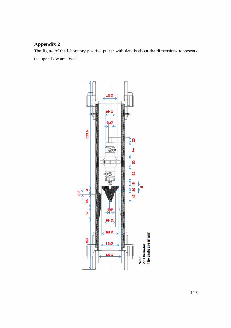
113

Appendix 2 The figure of the laboratory positive pulser with details about the dimensions represents

the open flow area case.

114

Appendix 3 The following figure shows the laboratory mud siren pulser with details about the

dimensions.