Effective Langevin equations for constrained stochastic processes

Satya N. Majumdar

Laboratoire de Physique Théorique et Modèles Statistiques (UMR 8626 du CNRS),

Université Paris-Sud, Bâtiment 100, 91405 Orsay Cedex, France

Henri Orland

Institut de Physique Théorique, CEA, IPhT

CNRS, URA2306,

F-91191 Gif-sur-Yvette, France

and

Beijing Computational Science Research Center

No.3 HeQing Road, Haidian District

Beijing, 100084, China ∗

AbstractWe propose a novel stochastic method to exactly generate Brownian paths conditioned to start at

an initial point and end at a given final point during a fixed time tf . These paths are weighted with a

probability given by the overdamped Langevin dynamics. We show how these paths can be exactly

generated by a local stochastic differential equation. The method is illustrated on the generation of

Brownian bridges, Brownian meanders, Brownian excursions and constrained Ornstein-Uehlenbeck

processes. In addition, we show how to solve this equation in the case of a general force acting on

the particle. As an example, we show how to generate constrained path joining the two minima of a

double-well. Our method allows to generate statistically independent paths, and is computationally

very efficient.

∗ satya.majumdar@u-psud.fr, henri.orland@cea.fr

1

arX

iv:1

503.

0263

9v2

[co

nd-m

at.s

tat-

mec

h] 1

3 M

ay 2

015

I. INTRODUCTION

Even after more than hundred years since its introduction, Brownian motion has remained

a fundamental cornerstone of classical physics [1]. Simple Brownian motion and its variants

have found numerous applications not just in natural sciences such as physics, chemistry,

biology etc., but also in man made subjects such as finance, economics, queueing theory,

search processes, and computer science amongst others (for reviews on the subject see [2–

6]). Some of these applications led to the studies of the statistical properties of simple

variants of Brownian motion, generally referred to as ‘constrained Brownian motion’, i.e,

a free Brownian motion conditioned to satisfy certain prescribed global constraints (see

below for examples). More generally, one would also like to study other stochastic processes

(thus going beyond the simple Brownian motion) in presence of one or more such global

constraints. An interesting and challenging problem is to find simple and efficient algorithms

that generate these constrained paths, for Brownian motion and other stochastic processes,

with the correct statistical weight. Many of the concepts presented in this article through a

physical presentation, can be found in the mathematical literature, for example in [7].

As a simple example, let us first start with a free Brownian motion B(t) in one dimension,

starting from the origin B(0) = 0. The time evolution of B(t) is governed by the simple

Langevin equationdB

dt= η(t) , (1)

where η(t) is a Gaussian white noise with zero mean 〈η(t)〉 = 0 and the correlator,

〈η(t)η(t′)〉 = 2D δ(t − t′) (D being the diffusion constant). It is easy to generate a trajec-

tory of this process numerically, simply by simulating the time-discretized version of the

Langevin equation

B(t+ ∆t) = B(t) +√

2D∆t ξt , (2)

where the noise ξt ≡ N (0, 1) is a standard normally distributed random variable with zero

mean and unit variance, drawn independently at each discrete time step. Three globally

constrained variants (amongst others) of this simple 1-d Brownian motion that have been

widely studied in the literature are the so called (i) Brownian bridge (ii) Brownian excursion

and (iii) Brownian meander that we discuss next.

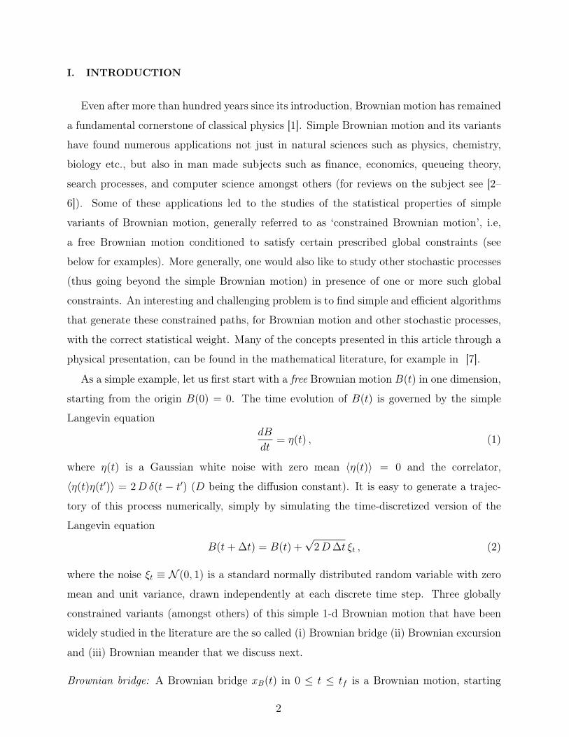
Brownian bridge: A Brownian bridge xB(t) in 0 ≤ t ≤ tf is a Brownian motion, starting

2

x

t

tf

0

x

t

t

x0

f

xf

0

Figure 1. (a) Two configurations of a Brownian bridge, starting at xB(t) = 0, and returning to

xB(tf ) = 0 at time tf (b) two configurations of a generalised Brownian bridge starting at xB(0) = x0

and ending at the final position xB(tf ) = xf at time tf (xf fixed, but not necessarily zero).

at xB(0) = 0, that is constrained to come back to its starting point at a final time tf ,

i.e., xB(tf ) = 0 (see Fig. (1 a)). A generalised Brownian bridge corresponds to those

configurations of Brownian motions that start at xB(0) = x0 and end at xB(tf ) = xf (with

xf fixed, not necessarily the same as the starting position x0) at time tf (see Fig. (1 b)).

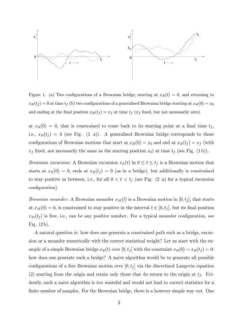
Brownian excursion: A Brownian excursion xE(t) in 0 ≤ t ≤ tf is a Brownian motion that

starts at xE(0) = 0, ends at xE(tf ) = 0 (as in a bridge), but additionally is constrained

to stay positive in between, i.e., for all 0 < t < tf (see Fig. (2 a) for a typical excursion

configuration).

Brownian meander: A Brownian meander xM(t) is a Brownian motion in [0, tf ], that starts

at xM(0) = 0, is constrained to stay positive in the interval t ∈ [0, tf ], but its final position

xM(tf ) is free, i.e., can be any positive number. For a typical meander configuration, see

Fig. (2 b).

A natural question is: how does one generate a constrained path such as a bridge, excur-

sion or a meander numerically with the correct statistical weight? Let us start with the ex-

ample of a simple Brownian bridge xB(t) over [0, tf ] with the constraint xB(0) = xB(tf ) = 0:

how does one generate such a bridge? A naive algorithm would be to generate all possible

configurations of a free Brownian motion over [0, tf ] via the discretized Langevin equation

(2) starting from the origin and retain only those that do return to the origin at tf . Evi-

dently, such a naive algorithm is too wasteful and would not lead to correct statistics for a

finite number of samples. For the Brownian bridge, there is a however simple way out. One

3

x

t

0tf

x

t

0

ft

Figure 2. (a) A typical configuration (schematic) of a Brownian excursion in the time interval [0, tf ],

that starts at xE(0) = 0, ends at xE(tf ) = 0, and stays positive in the whole interval t ∈ [0, tf ]

and (b) A typical configuration (schematic) of a Brownian meander in the time interval [0, tf ], that

starts at xM (0) = 0, stays positive in the time period [0, tf ], but its final position xM (tf ) can be

any positive number.

first generates a free Brownian path B(t) via (2) starting from B(0) = 0 and from this path,

one constructs a new path xB(t) via the following simple construction

xB(t) = B(t)− t

tfB(tf ) t ∈ [0, tf ] . (3)

By construction xB(t) in (3) satisfies the bridge condition xB(0) = xB(tf ) = 0. In addition,

by computing the propagator for the constructed process xB(t), it is easy to show that

indeed xB(t) has the correct statistical weight of a Brownian bridge.

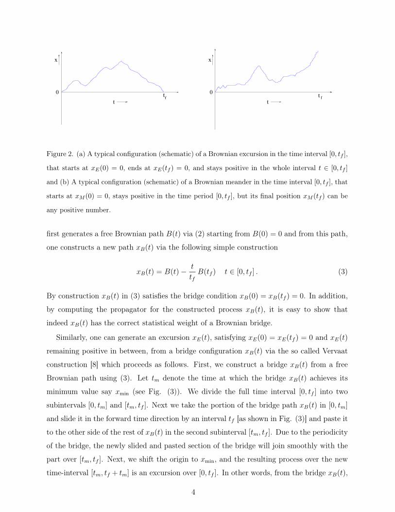
Similarly, one can generate an excursion xE(t), satisfying xE(0) = xE(tf ) = 0 and xE(t)

remaining positive in between, from a bridge configuration xB(t) via the so called Vervaat

construction [8] which proceeds as follows. First, we construct a bridge xB(t) from a free

Brownian path using (3). Let tm denote the time at which the bridge xB(t) achieves its

minimum value say xmin (see Fig. (3)). We divide the full time interval [0, tf ] into two

subintervals [0, tm] and [tm, tf ]. Next we take the portion of the bridge path xB(t) in [0, tm]

and slide it in the forward time direction by an interval tf [as shown in Fig. (3)] and paste it

to the other side of the rest of xB(t) in the second subinterval [tm, tf ]. Due to the periodicity

of the bridge, the newly slided and pasted section of the bridge will join smoothly with the

part over [tm, tf ]. Next, we shift the origin to xmin, and the resulting process over the new

time-interval [tm, tf + tm] is an excursion over [0, tf ]. In other words, from the bridge xB(t),

4

0 tf

tf

tm tf_ tm t

f_ tm tm

xB(t)

0

xE(t)

BRIDGE EXCURSION

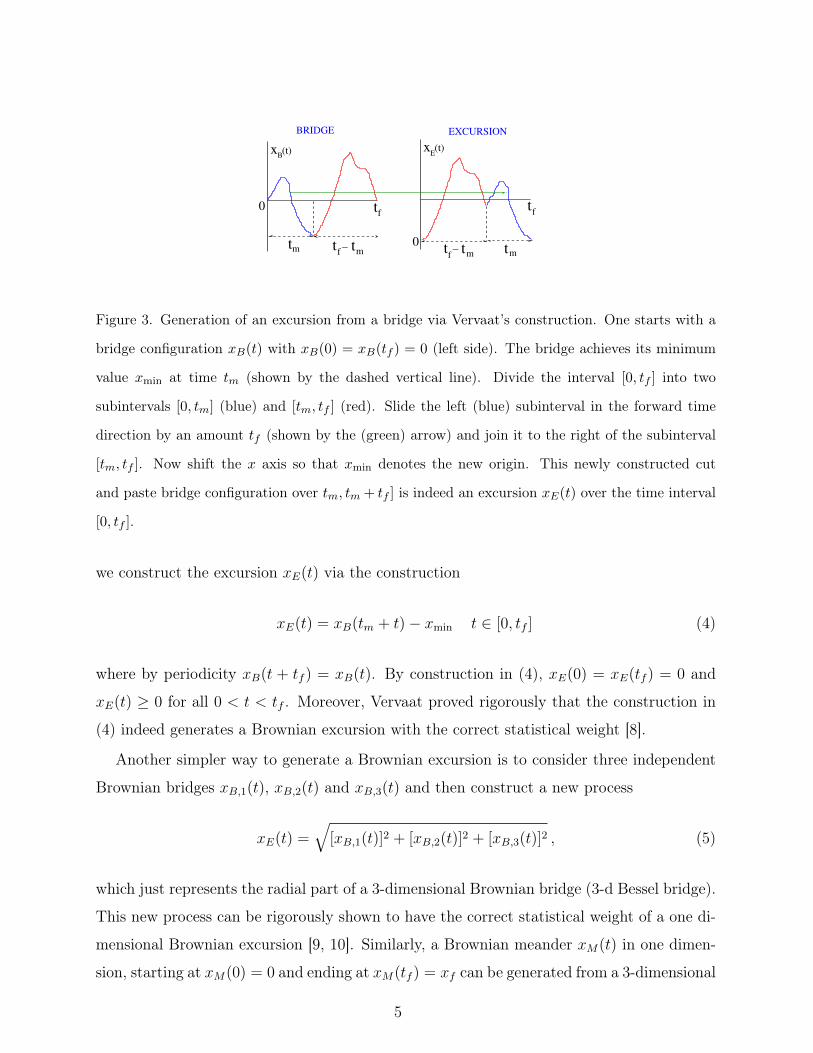
Figure 3. Generation of an excursion from a bridge via Vervaat’s construction. One starts with a

bridge configuration xB(t) with xB(0) = xB(tf ) = 0 (left side). The bridge achieves its minimum

value xmin at time tm (shown by the dashed vertical line). Divide the interval [0, tf ] into two

subintervals [0, tm] (blue) and [tm, tf ] (red). Slide the left (blue) subinterval in the forward time

direction by an amount tf (shown by the (green) arrow) and join it to the right of the subinterval

[tm, tf ]. Now shift the x axis so that xmin denotes the new origin. This newly constructed cut

and paste bridge configuration over tm, tm + tf ] is indeed an excursion xE(t) over the time interval

[0, tf ].

we construct the excursion xE(t) via the construction

xE(t) = xB(tm + t)− xmin t ∈ [0, tf ] (4)

where by periodicity xB(t + tf ) = xB(t). By construction in (4), xE(0) = xE(tf ) = 0 and

xE(t) ≥ 0 for all 0 < t < tf . Moreover, Vervaat proved rigorously that the construction in

(4) indeed generates a Brownian excursion with the correct statistical weight [8].

Another simpler way to generate a Brownian excursion is to consider three independent

Brownian bridges xB,1(t), xB,2(t) and xB,3(t) and then construct a new process

xE(t) =√

[xB,1(t)]2 + [xB,2(t)]2 + [xB,3(t)]2 , (5)

which just represents the radial part of a 3-dimensional Brownian bridge (3-d Bessel bridge).

This new process can be rigorously shown to have the correct statistical weight of a one di-

mensional Brownian excursion [9, 10]. Similarly, a Brownian meander xM(t) in one dimen-

sion, starting at xM(0) = 0 and ending at xM(tf ) = xf can be generated from a 3-dimensional

5

Bessel bridge by the following construction [9, 10]

xM(t) =

√[xB,1(t)]2 + [xB,2(t)]2 + [xB,3(t) +

t

tfxf ]2 . (6)

For a nice review on the connection between bridges, excursions and meanders, see [11, 12]

and for recent applications of such constrained paths, see [6, 13–19].

These clever transformations connecting bridges, excursions and meanders to free Brow-

nian motion are, of course, very efficient to generate them numerically. However, these

transformations rely on the specific properties of a free Brownian motion and will, in gen-

eral, not hold for a more general process such as a particle diffusing in an external potential.

Moreover, one may want to generate paths which are not simply bridges, excursions or me-

anders, but constrained in some other way. For example, in many applications in computer

science, one needs to generate, say a Brownian excursion xE(t) over t ∈ [0, tf ] with a fixed

area under the excursion A =´ tf

0xE(t) dt [6, 13–17, 20–22]. Hence, it would be much more

desirable to build a recipe to construct an effective Langevin equation like (2) which (i) will

automatically take into account the global constraints and (ii) will hold for more general

stochastic processes such as a particle diffusing in an external potential. Once we have such

a recipe for an effective Langevin equation, it can subsequently be easily time-discretized

leading to an efficient method to generate constrained paths. The purpose of this paper is

to provide precisely such a recipe and demonstrate it with several examples. Some of the re-

sults to be discussed in this paper were probably known, at least partially, in the probability

literature but in a language perhaps not easily accessible to physicists. One of the purposes

of this paper is to unveil the recipe for an effective Langevin equation in a physicist friendly

language. For a recent review on some aspects of constrained stochastic processes, namely,

constraints on large deviations of a stochastic variable, see [23].

The rest of the paper is organized as follows: we first derive the effective Langevin

equation which satisfies the boundary constraint. We then illustrate the method on four

analytically soluble cases, namely the Brownian bridges, Brownian meanders, Brownian

excursions and the Ornstein-Uhlenbeck process. We then show how this equation can be

solved exactly numerically in the case of any landscape potential U(x).

6

II. DERIVATION OF EFFECTIVE LANGEVIN EQUATION

From now on, we assume that the system is driven by a force F (x, t) and is subject to

stochastic dynamics in the form of an overdamped Langevin equation.

For the sake of simplicity, we illustrate the method on a one-dimensional system, the

generalization to higher dimensions or larger number of degrees of freedom being straight-

forward. We follow closely the presentation given in Ref. [24].

The over damped Langevin equation reads

dx

dt=

1

γF (x(t), t) + η(t) (7)

where x(t) is the position of the particle at time t, driven by the force F (x, t), γ is the friction

coefficient, related to the diffusion constant D through the Einstein relation D = kBT/γ,

where kB is the Boltzmann constant and T the temperature of the thermostat. In addition,

η(t) is a Gaussian white noise with moments given by

< η(t) >= 0 (8)

< η(t)η(t′) >=2kBT

γδ(t− t′) (9)

The probability distribution P (x, t) for the particle to be at point x at time t satisfies a

Fokker-Planck equation [26]

∂P

∂t= D

∂

∂x

(∂P

∂x− βFP

)(10)

where β = 1/kBT is the inverse temperature. This equation is to be supplemented by the

initial condition P (x, 0) = δ(x−x0), where the particle is assumed to be at x0 at time t = 0.

To emphasize this initial condition, we will often use the notation P (x, t) = P (x, t|x0, 0).

We now study the probability over all paths starting at x0 at time 0 and conditioned to

end at a given point xf at time tf , to find the particle at point x at time t ∈ [0, tf ]. This is

the generalized bridge. This probability can be written as

P(x, t) =1

P (xf , tf |x0, 0)Q(x, t)P (x, t)

where we use the notation

P (x, t) = P (x, t|x0, 0)

7

Q(x, t) = P (xf , tf |x, t)

Indeed, the probability for a path starting from (x0, 0) and ending at (xf , tf ) to go through

x at time t is the product of the probability P (x, t|x0, 0) to start at (x0, 0) and to end at

(x, t) by the probability P (xf , tf |x, t) to start at (x, t) and to end at (xf , tf ).

The equation satisfied by P is the Fokker-Planck equation mentioned above (10), whereas

that for Q is the so-called reverse or adjoint Fokker-Planck equation [26] given by

∂Q

∂t= −D∂

2Q

∂x2−DβF ∂Q

∂x(11)

It can be easily checked that the conditional probability P(x, t) satisfies a new Fokker-

Planck equation

∂P∂t

= D∂

∂x

(∂P∂x−(βF + 2

∂ lnQ

∂x

)P)

Comparing this equation with the initial Fokker-Planck (10) and Langevin (7) equations,

one sees that it can be obtained from a Langevin equation with an additional potential force

dx

dt= DβF + 2D

∂ lnQ

∂x+ η(t) (12)

This equation has been originally obtained by Doob [27] in the probability literature and

is known as the Doob transform of the Langevin equation (7). It was also presented in

the physics literature in the context of barrier crossing [24]. It provides a simple recipe to

construct a generalized bridge. It generates Brownian paths, starting at (xi, 0) conditioned

to end at (xf , tf ), with unbiased statistics. It is the additional term 2D ∂ lnQ∂x

in the Langevin

equation that guarantees that the trajectories starting at (x0, 0) and ending at (xf , tf ) are

statistically unbiased. Note that this additional term is a priori time dependent, and thus

the effective force which conditions the paths is space and time dependent.

In the following, we will specialize to the case where the force F is derived from a potential

U(x). The bridge equation becomes

dx

dt= − D

kBT

∂U

∂x+ 2D

∂ lnQ

∂x+ η(t) (13)

In that case, the Fokker-Planck equation can be recast into an imaginary time Schrödinger

equation [26], and the probability distribution function P can be written as

Q(x, t) = P (xf , tf |x, t) = e−β/2(U(xf )−U(x)) < xf |e−H(tf−t)|x > (14)

8

where the "quantum Hamiltonian" H is defined by

H = −D ∂2

∂x2+DV (x) (15)

and the potential V by

V =

(β

2

∂U

∂x

)2

− β

2

∂2U

∂x2(16)

We denote by M the matrix element of the Euclidian Schrödinger evolution operator

M(x, t) =< xf |e−H(tf−t)|x >

Using eq.(14) for Q, one can write equation (13) as

dx

dt= 2

kBT

γ

∂

∂xln < xf |e−(tf−t)H |x > +η(t) (17)

We see on the above form that when t → tf , the matrix element M(x, t) converges to

δ(xf −x), and it is this singular attractive potential which drives all the paths to xf at time

tf .

Note that for large time tf , M(x, t) is dominated by the ground state of H, namely

< xf |e−(tf−t)H |x >∼ e−E0(tf−t)Ψ0(xf )Ψ0(x) (18)

It is well known that the ground state wave function of H is Ψ0(x) = 1N e−βU(x)/2 where

N is the normalization constant. Indeed, it is easily checked that H|Ψ0〉 = 0 which implies

that Ψ0 is an eigenstate of H with ground state energy E0 = 0. Inserting these relations in

eq.(17), one recovers, as expected, the original unconditioned Langevin equation for large

time tf . Note that although relation (18) holds only for a normalizable ground state wave

function Ψ0(x), it still yields the correct Langevin equation (7) for non-normalizable cases

(such as the free Brownian motion U(x)=0, for which E0 = 0 and Ψ0 = 1/√V where V is

the volume).

In order to build a representative sample of paths starting at (x0, 0) and ending at (xf , tf ),

one must simply solve equation (13) for many different realizations of the random noise. Only

the initial boundary condition is to be imposed, as the singular term in the equation imposes

the correct final boundary condition. An important point to note is that all the trajectories

generated by this procedure are statistically independent.

9

At this stage, we see that all the difficulty lies in calculating either the Green’s function

Q(x, t) or the matrix element M(x, t). In general, this is not possible analytically except

for a few special cases. In ref.[24], a short time approximation to compute M(x, t) was

presented, but in the following, we specialize on a few exactly analytically solvable cases.

III. THE FREE BROWNIAN BRIDGE

The simplest case is the case of a free particle in unrestricted space. In that case, the

Green’s function Q(x, t) can be easily computed and yields

Q(x, t) =1√

4πD(tf − t)e−

(xf−x)2

4D(tf−t)

The corresponding conditioned Langevin equation becomes

dx

dt=xf − xtf − t

+ η(t) (19)

This equation (19) can be found in [7, 23]. It is completely universal as the drift term

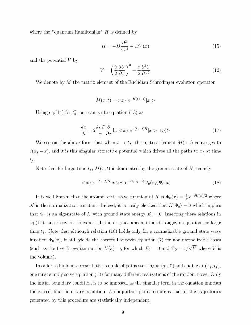
does not depend on the diffusion constant D. We show in Fig.(4) a set of 500 trajectories

starting at x0 = −1 at time 0 and ending at xf = +1 at time tf = 1, obtained for different

noise histories. The time step used in the discretization is dt = 0.001. All these trajectories

are statistically independent. The thick black curve is the mean trajectory. As can be seen

from eq.(19), it is a straight line.

IV. THE BROWNIAN MEANDER AND EXCURSION

The Brownian meander is a Brownian path of a free particle in a half-space. In other

words, the Brownian particle cannot penetrate in one of the half-planes. In 1d, if we define

the half-space as x > 0, the particle cannot go into the x < 0 subspace. Here the meander

xM(t) starts, say at the origin xM(t = 0) = x0 > 0, ends at xM(tf ) = xf > 0, while staying

positive in t ∈ [0, tf ]. For the special case where both the initial and the final position tend

to zero, the meander is called an excursion xE(t). These constrained Brownian paths have

been shown to be relevant to the anomalous diffusion of cold atoms in optical lattices [25].

In the case of a general meander, the Green’s functionQ(x, t) is that of a particle restricted

to a half space. This Green’s function is well known and can be calculated by using the

10

x

tf

Figure 4. A sample of 500 Brownian bridges

method of images. In the case when the end point is fixed at xf at time tf we obtain

Q(x, t) =1√

4πD(tf − t)

(e− 1

4D

(xf−x)2

tf−t − e−1

4D

(xf+x)2

tf−t

)If the end point xf at tf can be anywhere in the 1/2 plane xf > 0, the Green’s function

above has to be further integrated for xf ∈ [0,+∞] to obtain

QM(x, t) =

ˆ ∞0

dxf Q(x, t)

= erf

(x√

4D(tf − t)

)(20)

where erf(x) = 2√π

´ x0e−u

2du. The corresponding Langevin equation for the meander then

reads

dx

dt=

2√4πD(tf − t)

exp(− x2

4D(tf−t)

)erf( x√

4D(tf−t))

+ η(t) (21)

The case of a Brownian excursion, where the extremity xf is fixed, is generated by the

Langevin equation

dx

dt=

(xf−xtf−t

)e− 1

4D

(xf−x)2

tf−t +(xf+x

tf−t

)e− 1

4D

(xf+x)2

tf−t

e− 1

4D

(xf−x)2

tf−t − e−1

4D

(xf+x)2

tf−t

+ η(t) (22)

11

tf

x

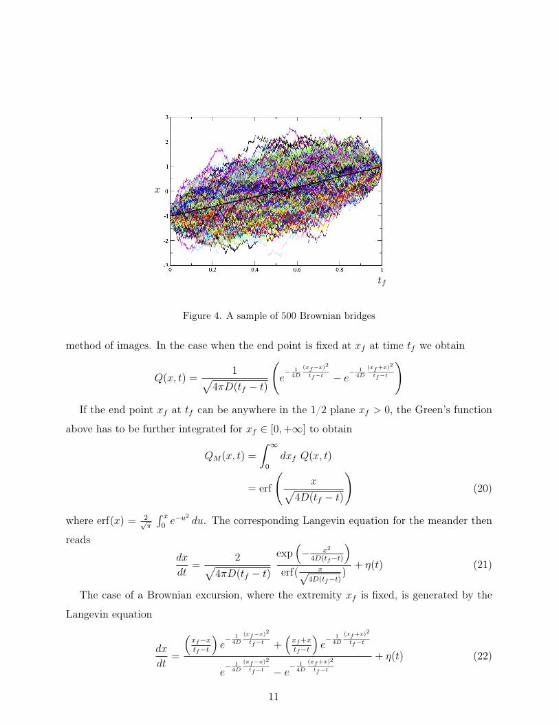
Figure 5. A sample of 500 meanders

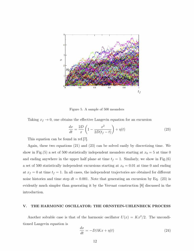
Taking xf → 0, one obtains the effective Langevin equation for an excursion

dx

dt=

2D

x

(1− x2

2D(tf − t)

)+ η(t) (23)

This equation can be found in ref.[7].

Again, these two equations (21) and (23) can be solved easily by discretizing time. We

show in Fig.(5) a set of 500 statistically independent meanders starting at x0 = 5 at time 0

and ending anywhere in the upper half plane at time tf = 1. Similarly, we show in Fig.(6)

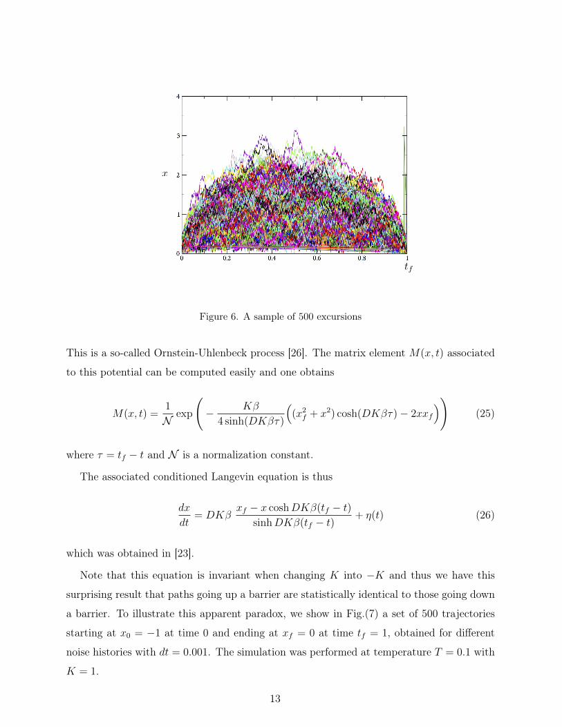
a set of 500 statistically independent excursions starting at x0 = 0.01 at time 0 and ending

at xf = 0 at time tf = 1. In all cases, the independent trajectories are obtained for different

noise histories and time step dt = 0.001. Note that generating an excursion by Eq. (23) is

evidently much simpler than generating it by the Vervaat construction [8] discussed in the

introduction.

V. THE HARMONIC OSCILLATOR: THE ORNSTEIN-UHLENBECK PROCESS

Another solvable case is that of the harmonic oscillator U(x) = Kx2/2. The uncondi-

tioned Langevin equation isdx

dt= −DβKx+ η(t) (24)

12

x

tf

Figure 6. A sample of 500 excursions

This is a so-called Ornstein-Uhlenbeck process [26]. The matrix element M(x, t) associated

to this potential can be computed easily and one obtains

M(x, t) =1

Nexp

(− Kβ

4 sinh(DKβτ)

((x2

f + x2) cosh(DKβτ)− 2xxf

))(25)

where τ = tf − t and N is a normalization constant.

The associated conditioned Langevin equation is thus

dx

dt= DKβ

xf − x coshDKβ(tf − t)sinhDKβ(tf − t)

+ η(t) (26)

which was obtained in [23].

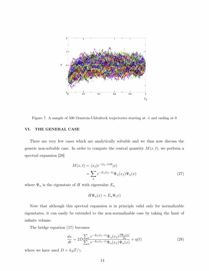
Note that this equation is invariant when changing K into −K and thus we have this

surprising result that paths going up a barrier are statistically identical to those going down

a barrier. To illustrate this apparent paradox, we show in Fig.(7) a set of 500 trajectories

starting at x0 = −1 at time 0 and ending at xf = 0 at time tf = 1, obtained for different

noise histories with dt = 0.001. The simulation was performed at temperature T = 0.1 with

K = 1.

13

tf

x

Figure 7. A sample of 500 Ornstein-Uhlenbeck trajectories starting at -1 and ending at 0

VI. THE GENERAL CASE

There are very few cases which are analytically solvable and we thus now discuss the

generic non-solvable case. In order to compute the central quantity M(x, t), we perform a

spectral expansion [28]

M(x, t) = 〈xf |e−(tf−t)H |x〉

=∑α

e−Eα(tf−t)Ψα(xf )Ψα(x) (27)

where Ψα is the eigenstate of H with eigenvalue Eα

HΨα(x) = EαΨ(x)

Note that although this spectral expansion is in principle valid only for normalizable

eigenstates, it can easily be extended to the non-normalizable case by taking the limit of

infinite volume.

The bridge equation (17) becomes

dx

dt= 2D

∑α e−Eα(tf−t)Ψα(xf )

∂Ψα(x)∂x∑

α e−Eα(tf−t)Ψα(xf )Ψα(x)

+ η(t) (28)

where we have used D = kBT/γ.

14

In order to be able to solve this equation numerically (by discretization for instance),

one has to compute the eigenstates Ψα and eigenvalues Eα of the Hamiltonian H. In the

case of low-dimensional system, this can be done very easily by diagonalizing the discretized

Hamiltonian H which turns out to be a tridiagonal operator.

VII. THE QUARTIC DOUBLE-WELL

We illustrate the above method on the example of barrier crossing in 1d (quartic poten-

tial).

U(x) =1

4(x2 − 1)2

This potential has two minima at x = ±1, separated by a barrier of height 1/4. Note

that V (x) = (βU ′/2)2 − βU ′′/2 is much steeper than U(x) and thus more confining around

its minima. At low temperature, the potential V (x) has two minima at points close to ±1

and one minimum at x = 0.

The ground state of the Hamiltonian is Ψ0(x) ∼ exp(−βU(x)/2. The Hamiltonian is

diagonalized by discretizing space and writing it in the form of a tridiagonal matrix. The

diagonalization is performed using programs specific to tridiagonal matrices. All the exam-

ples were performed at low temperature T = 0.05, where the barrier height is equal to 5 in

units of kBT and the Kramers relaxation time, given by the inverse of the smallest non-zero

eigenvalue of H, is equal to τK = 362.934 .

On fig.8, we present a long trajectory (tf = 1000) obtained by solving the unconditioned

Langevin eq.(7) for a particle starting at x0 = −1 at time 0 .

The general pattern is that of the particle staying in one of the wells for a long time,

then crossing very rapidly into the other well and back and forth. If one is interested more

precisely in the transition region, our method allows to perform the simulation of the rare

crossing events between the two wells and generate a large sample of statistically independent

paths in this transition region.

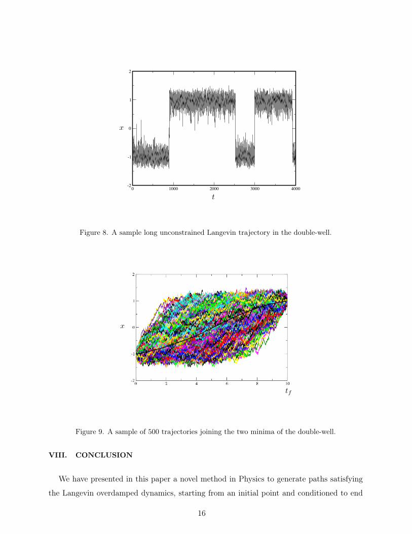
In fig.9, we show a set of 500 trajectories starting at x0 = −1 at time 0 and ending at

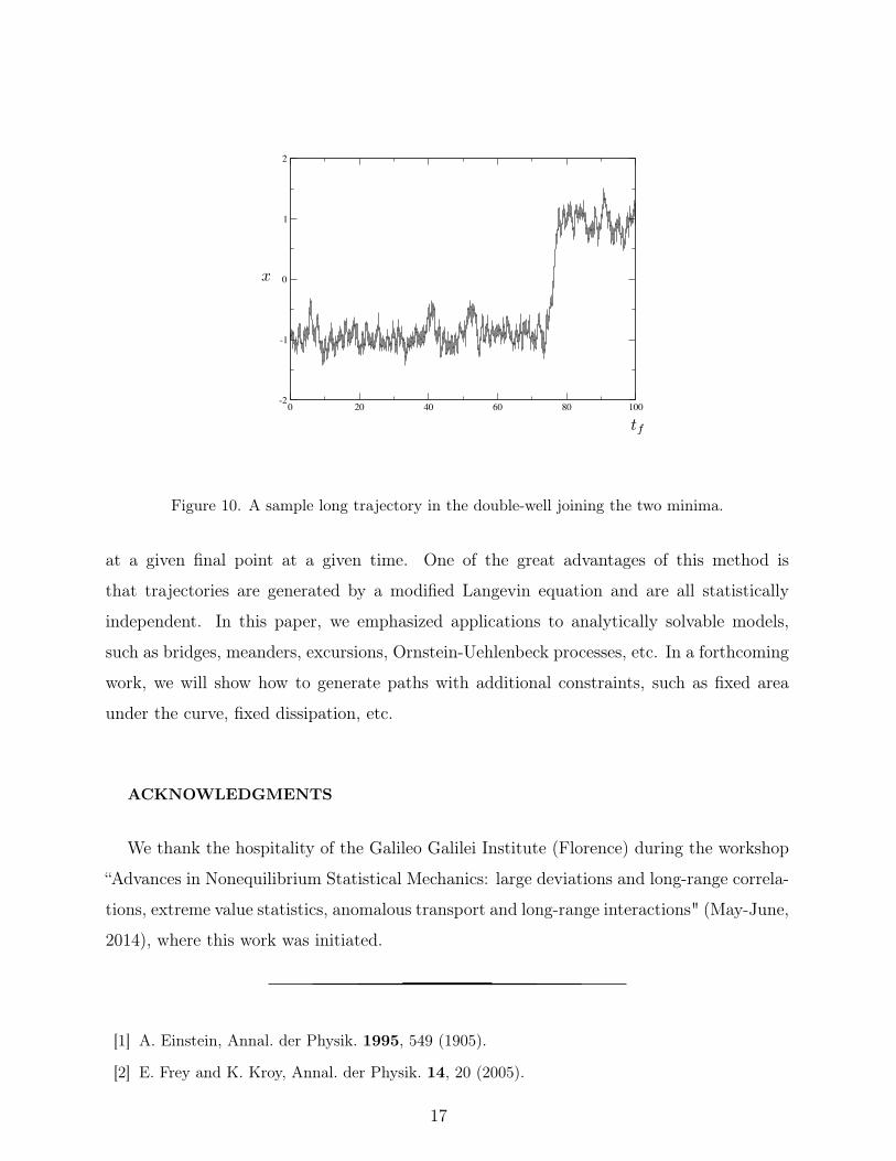
xf = +1 at time tf = 10, obtained for different noise histories with dt = 0.001. In fig.10,

we show a longer trajectory starting at x0 = −1 at time 0 and ending at xf = +1 at time

tf = 100 with dt = 0.001.

15

0 1000 2000 3000 4000-2

-1

0

1

2

x

t

Figure 8. A sample long unconstrained Langevin trajectory in the double-well.

x

tf

Figure 9. A sample of 500 trajectories joining the two minima of the double-well.

VIII. CONCLUSION

We have presented in this paper a novel method in Physics to generate paths satisfying

the Langevin overdamped dynamics, starting from an initial point and conditioned to end

16

0 20 40 60 80 100-2

-1

0

1

2

tf

x

Figure 10. A sample long trajectory in the double-well joining the two minima.

at a given final point at a given time. One of the great advantages of this method is

that trajectories are generated by a modified Langevin equation and are all statistically

independent. In this paper, we emphasized applications to analytically solvable models,

such as bridges, meanders, excursions, Ornstein-Uehlenbeck processes, etc. In a forthcoming

work, we will show how to generate paths with additional constraints, such as fixed area

under the curve, fixed dissipation, etc.

ACKNOWLEDGMENTS

We thank the hospitality of the Galileo Galilei Institute (Florence) during the workshop

“Advances in Nonequilibrium Statistical Mechanics: large deviations and long-range correla-

tions, extreme value statistics, anomalous transport and long-range interactions" (May-June,

2014), where this work was initiated.

[1] A. Einstein, Annal. der Physik. 1995, 549 (1905).

[2] E. Frey and K. Kroy, Annal. der Physik. 14, 20 (2005).

17

[3] B. Duplantier, Séminaire Poincare, 1, 155 (2005);

[4] M. Yor, Some aspects of Brownian motion, Lectures in Mathematics (ETH Zurich, Birkhausser,

1992).

[5] A. Comtet, J. Desbois, and C. Texier, J. Phys. A: Math. Gen. 38, R341 (2005).

[6] S. N. Majumdar, Curr. Sci. 89, 2076 (2005).

[7] L. C. G. Rogers and D. Williams, Diffusions, Markov Processes and Martingales (Cambridge

University Press, Cambridge, 2000)

[8] W. Vervaat, Ann. of Probab. 7, 143 (1979).

[9] D. Williams, B. Am. Math. Soc. 76, 871 (1970).

[10] J. P. Imhof, J. Appl. Probab. 21, 500 (1984).

[11] J. Bertoin and J. Pitman, Bulletin des sciences mathematiques, 118, 147 (1994).

[12] P. Biane, J. Pitman, and M. Yor, Bull. Amer. Math. Soc. 38, 435 (2001).

[13] S. N. Majumdar and A. Comtet, Phys. Rev. Lett. 92, 225501 (2004); J. Stat. Phys. 119, 777

(2005).

[14] M. J. Kearney and S. N. Majumdar, J. Phys. A: Math. Gen. 38, 4097 (2005).

[15] S. Janson, Probability Surveys 4 80 (2007).

[16] M. J. Kearney and S. N. Majumdar J. Phys. A: Math. Gen. 47, 465001 (2014).

[17] M. J. Kearney, S. N. Majumdar and R. J. Martin, J. Phys. A: Math. Theor. 40, F863 (2007).

[18] A. Perret, A. Comtet, S. N. Majumdar and G. Schehr, arXiv: 1502.01218

[19] F. Font-Clos, G. Pruessner, A. Deluca, and N. R. Moloney, arXiv: 1410.6048

[20] D. A. Darling, Ann. Probab. 11, 803 (1983).

[21] G. Louchard, Comp. Math. Appl. 10, 413 (1984).

[22] P. Flajolet, P. Poblete, and A. Viola, Algorithmica, 22, 490 (1998).

[23] R. Chetrite and H. Touchette, arXiv: 1405.5157; see also Phys. Rev. Lett. 111, 120601 (2013).

[24] H. Orland, J. Chem. Phys. 134, 174114 (2011).

[25] E. Barkai, E. Aghion, and D. A. Kessler, Phys. Rev. X 4, 021036 (2014).

[26] N.G. Van Kampen, Stochastic Processes in Physics and Chemistry (North-Holland Personal

Edition, 1992); R. Zwanzig, Nonequilibrium Statistical Mechanics (Oxford University Press,

2001).

[27] J. L. Doob, Bull. Soc. Math. France 85 (1957), 431-458; P. Fitzsimmons, J. Pitman and M.

Yor, Seminar on Stochastic Processes: " Markovian bridges: construction, Palm interpretation,

18

and splicing" (1992) 101-134.

[28] M. Reed and B. Simon, Methods of Mathematical Physics, vols I-IV, Academic Press 1972;

R.P. Feynman and A.R. Hibbs, Quantum Mechanics and Path Integrals (McGraw-Hill,1965)

19